GRAPHICS GEMS
IV
Edited by Paul S. Heckbert
Computer Science Department
Carnegie Mellon University
Pittsburgh, Pennsylvania
Morgan Kaufmann is an imprint of Academic Press
A Harcourt Science and Technology Company
San Diego San Francisco New York Boston
London Sydney Tokyo

ACADEMIC PRESS
A Harcourt Science and Technology Company
525 B Street. Suite 1900. San Diego. CA 92101-4495 USA
http://www.academicpress.com
Academic Press
24-28 Oval Road. London ^rwl 7DX United Kingdom
http://www.hbuk/ap/
Morgan Kaufmann
340 Pine Street. Sixth Floor. San Francisco, CA 94104-3205
http://mkp.com
This book is printed on acid-free paper (^
Copyright © 1994 by Academic Press, Inc.
All rights reserved.
No part of this publication may be reproduced or
transmitted in any form or by any means, electronic ^ , .—, , __ /^
or mechanical, including photocopy, recording, or 2 /, j ~j^_ fj\- £l O O 3
any information storage and retrieval system, without "^
permission in writing from the publisher , -"^^^—---^
All brand names and product names mentioned in this book i f" |~f J3
are trademarks or registered trademarks of their respective companies, j .
Ko!n
l<m K 35/1
Library of Congress Cataloging-in-Publication Data
Graphics Gems IV / edited by Paul S. Heckbert.
p. cm. -(The Graphics Gems Series)
Includes bibliographicsl references and index.
ISBN 0-12-336156-7 (with Macintosh disk). —ISBN 0-12-336155-9
(with IBM disk).
I. Computer graphics. 1. Heckbert, Paul S., 1958-
II. Title; Graphics Gems 4. 111. Title; Graphics Gems four.
IV. Series.
T385.G6974 1994
006.6'6-dc20 93-46995
CIP
Printed in the United States of America
99 00 01 02 03 MB 9 8 7 6 5 4

0
Contents
Author Index ix
Foreword by Andrew Glassner xi
Preface xv
About the Cover xvii
I. Polygons and Polyhedra 1
1.1. Centroid of a Polygon by Gerard Bashein and Paul R. Detmer 3
1.2. Testing the Convexity of a Polygon by Peter Schorn and Frederick Fisher 7
1.3. An Incremental Angle Point in Polygon Test by Kevin Weiler 16
1.4. Point in Polygon Strategies by Eric Haines 24
1.5. Incremental Delaunay Triangulation by Dani Lischinsl<i 47
1.6. Building Vertex Normals from an Unstructured Polygon List by
Andrew Glassner 60
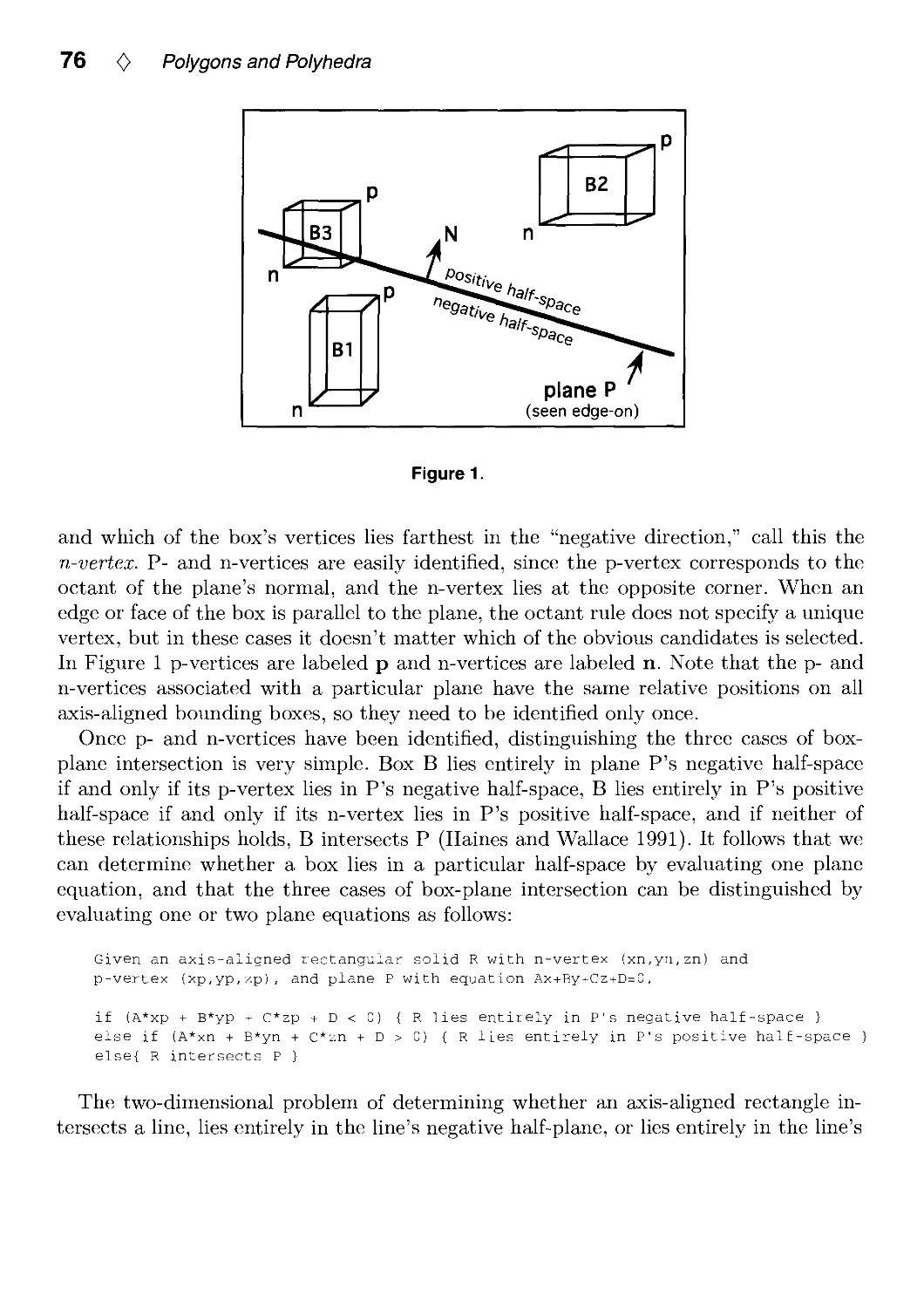
1.7. Detecting Intersection of a Rectangular Solid and a Convex Polyhedron by
Ned Greene 74
1.8. Fast Collision Detection of Moving Convex Polyhedra by Rich Rabbitz 83
II. Geometry Ill
11.1. Distance to an Ellipsoid by John C. Hart 113
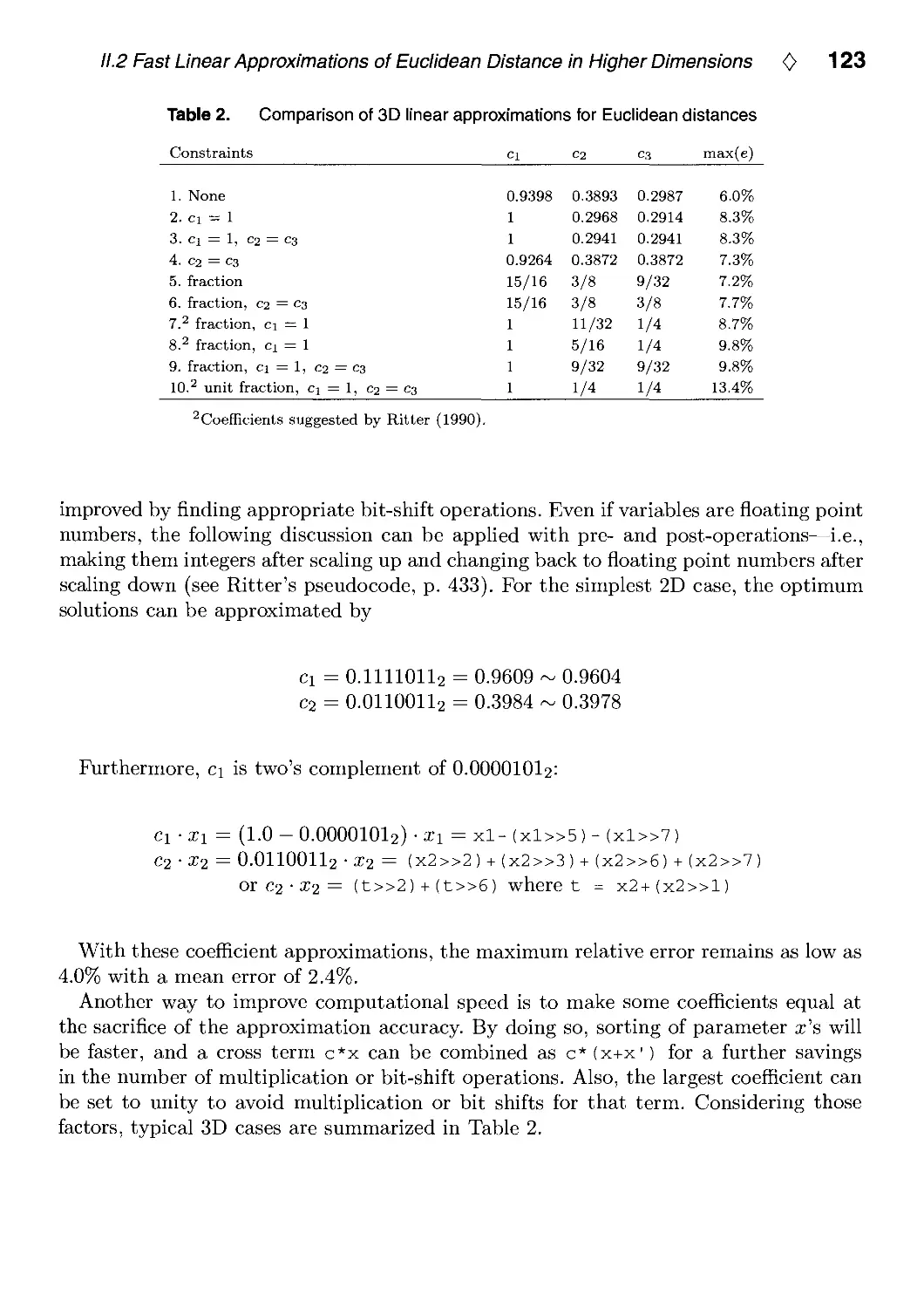
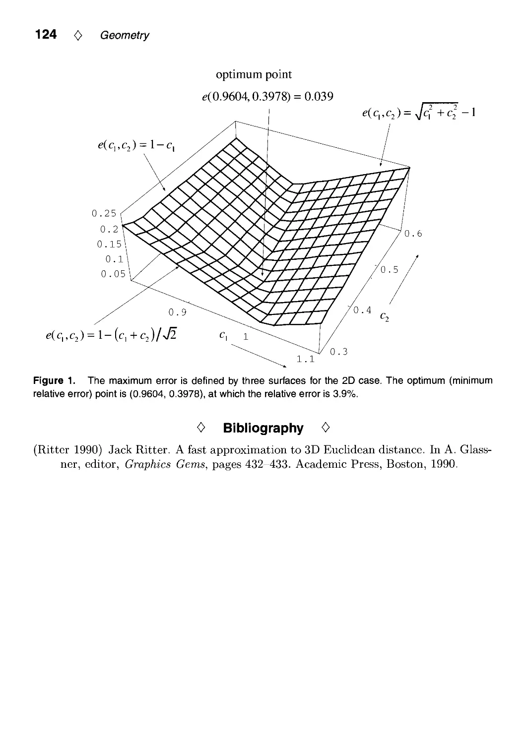
11.2. Fast Linear Approximations of Euclidean Distance in Higher Dimensions
by Yoshikazu Ohashi 120
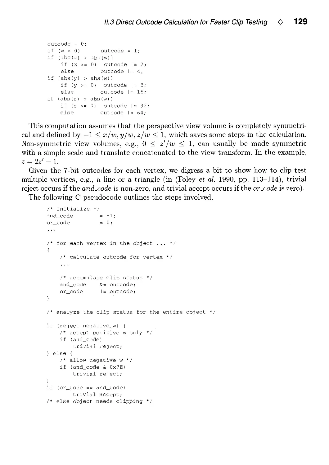
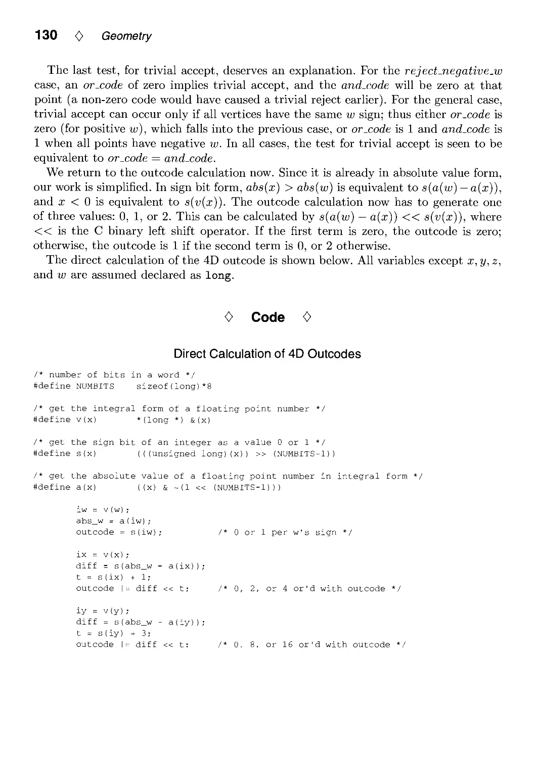
11.3. Direct Outcode Calculation for Faster Clip Testing by Walt Donovan and
Tim Van Hook 125
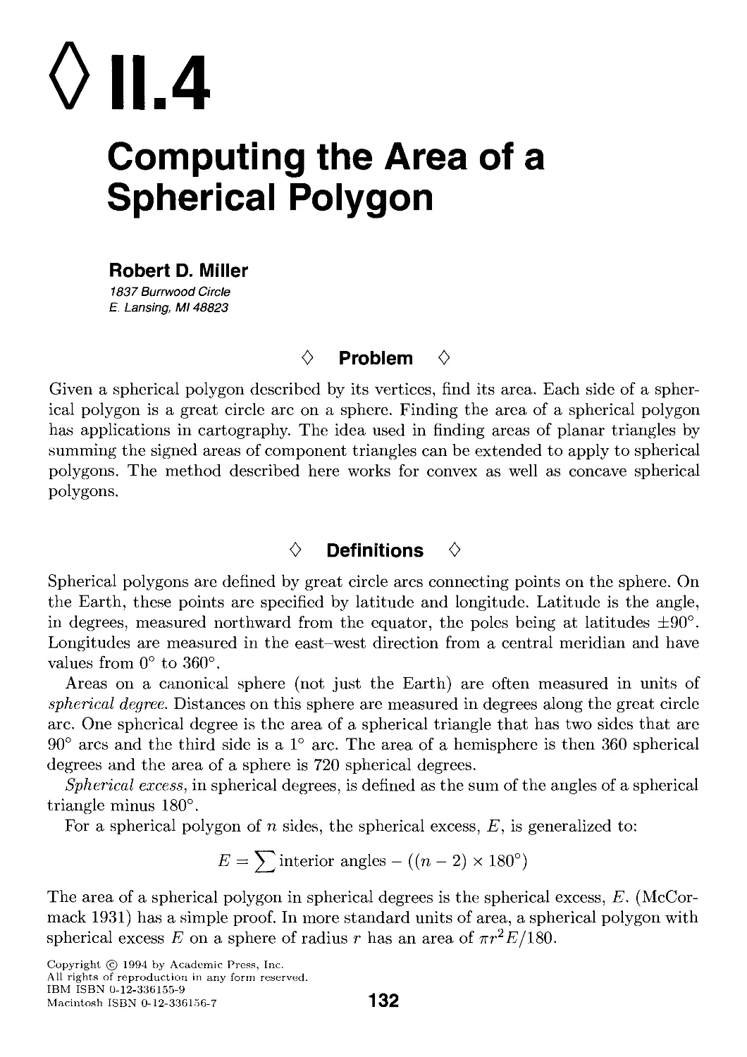
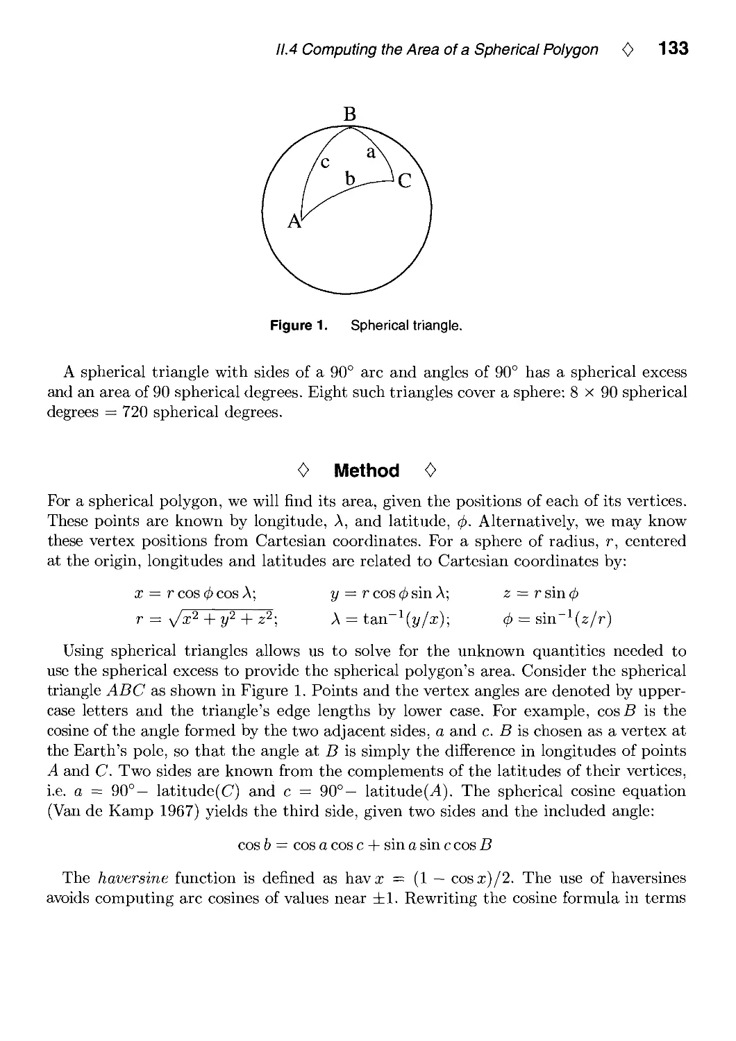
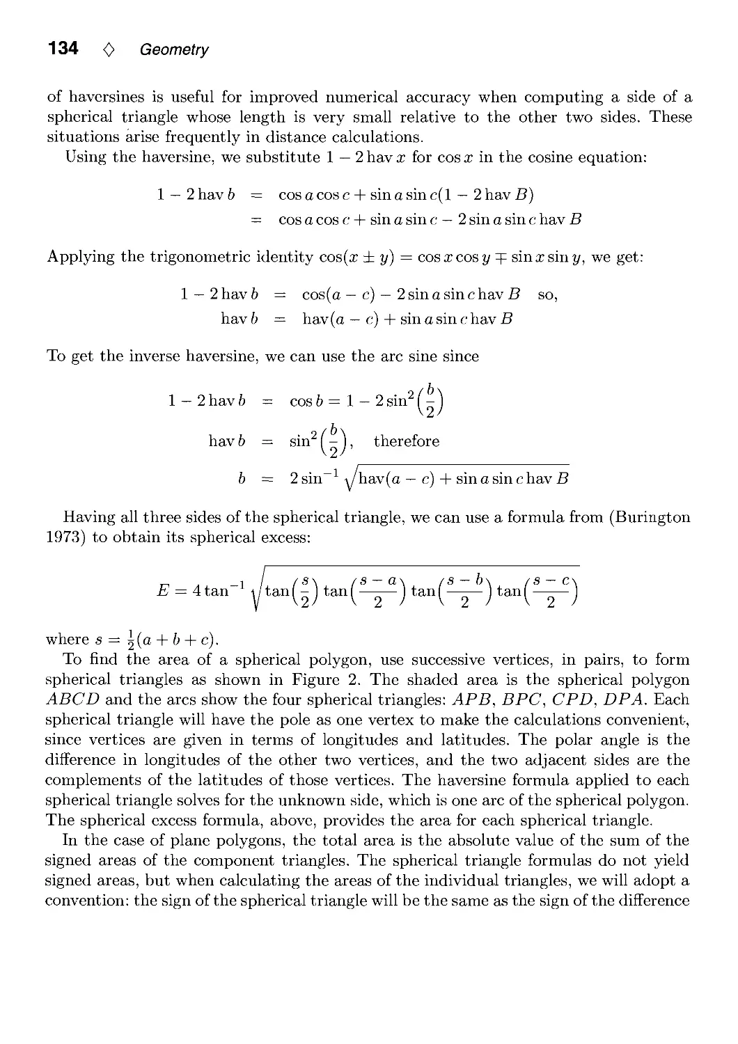
11.4. Computing the Area of a Spherical Polygon by Robert D. Miller 132
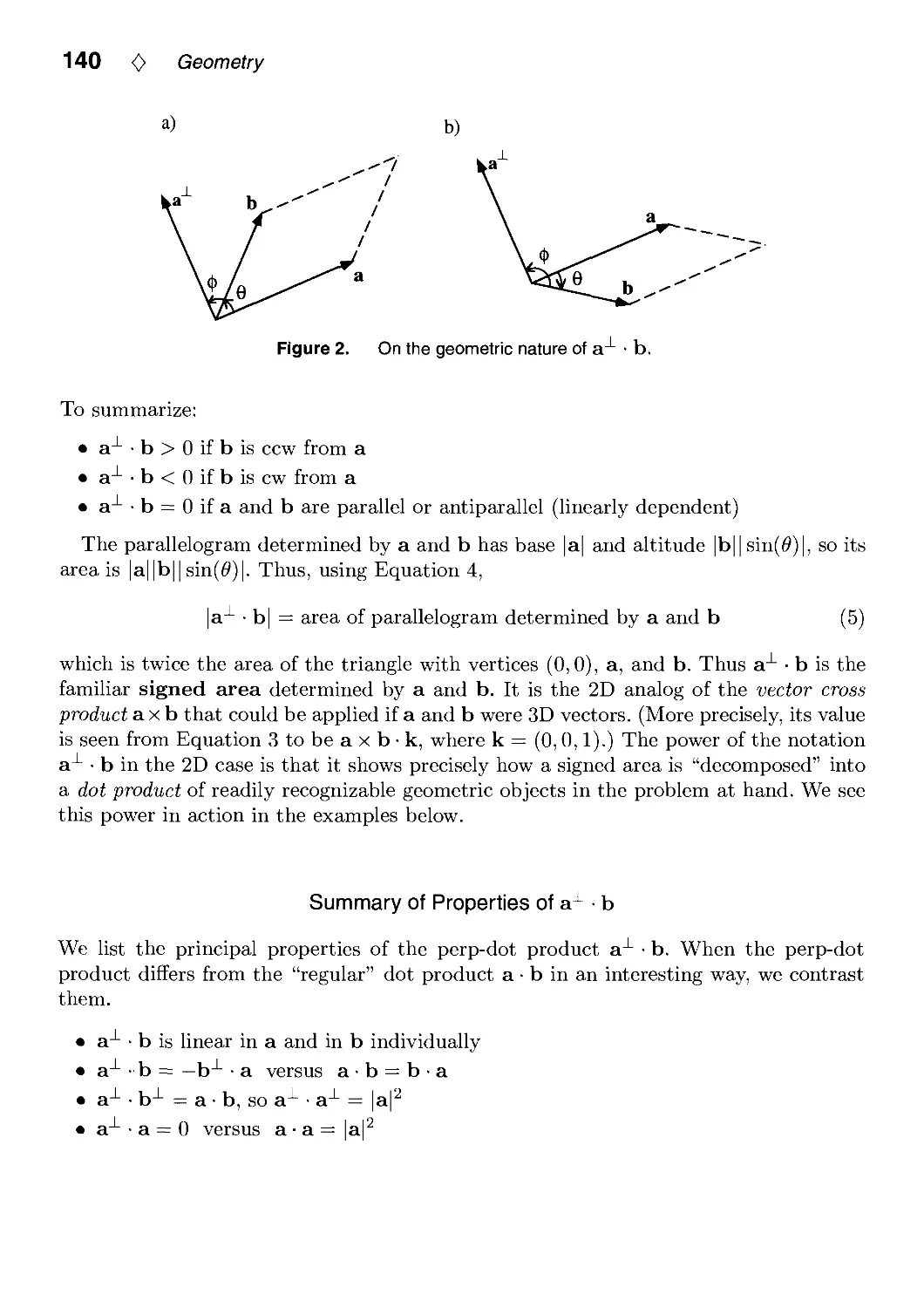
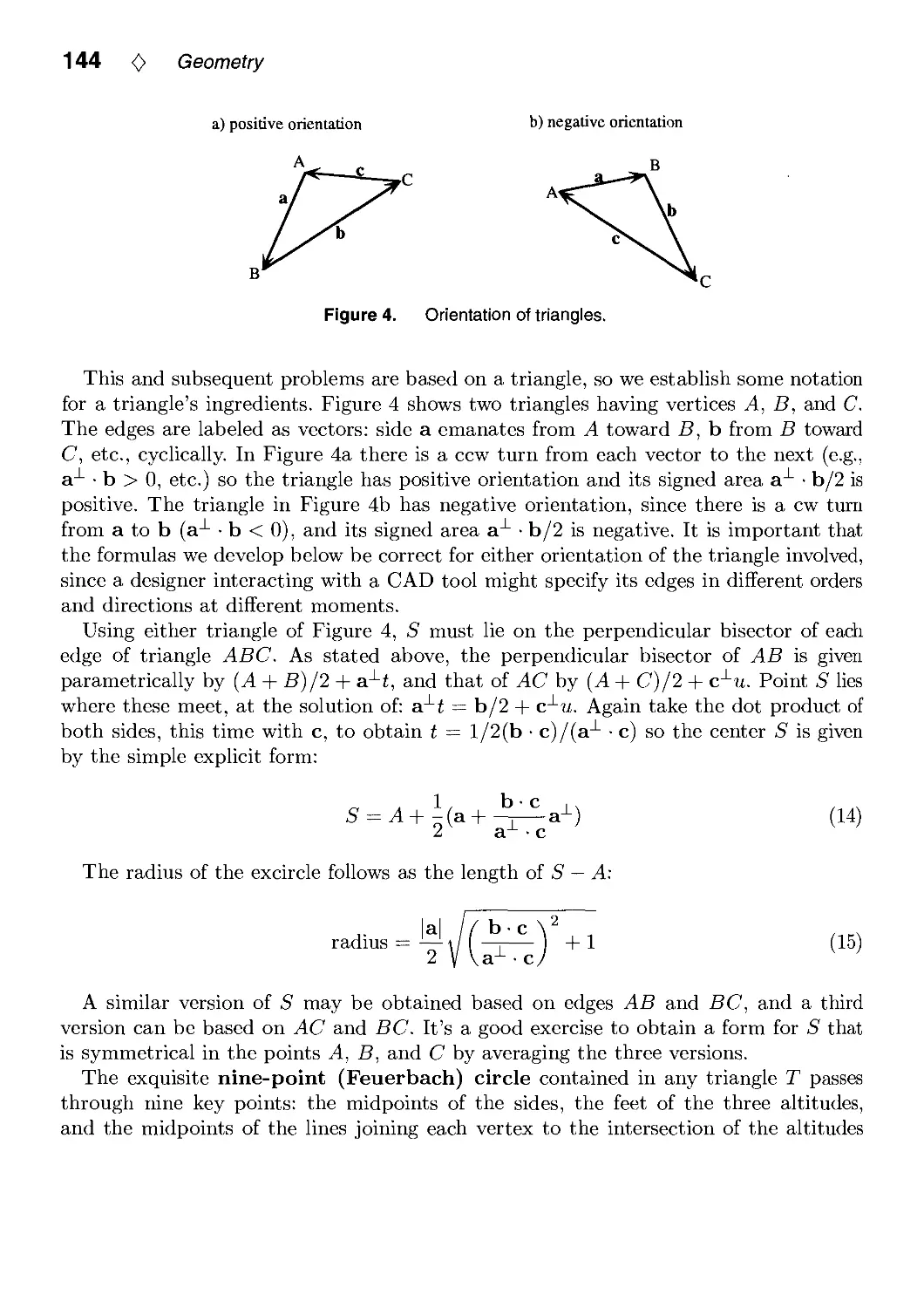
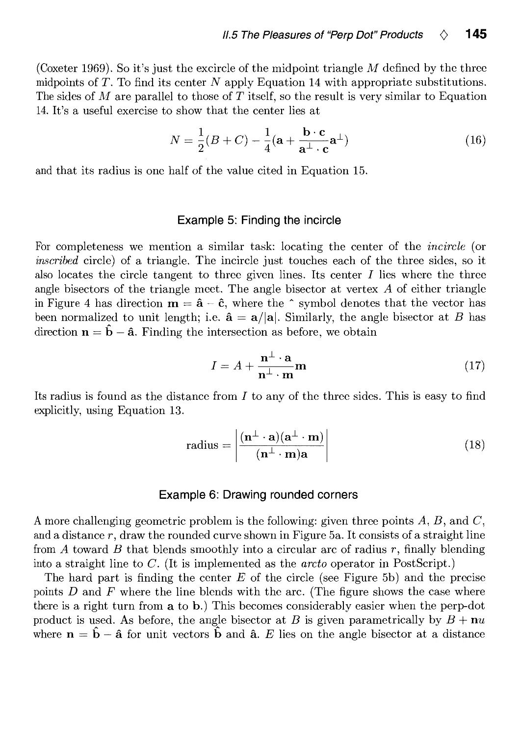
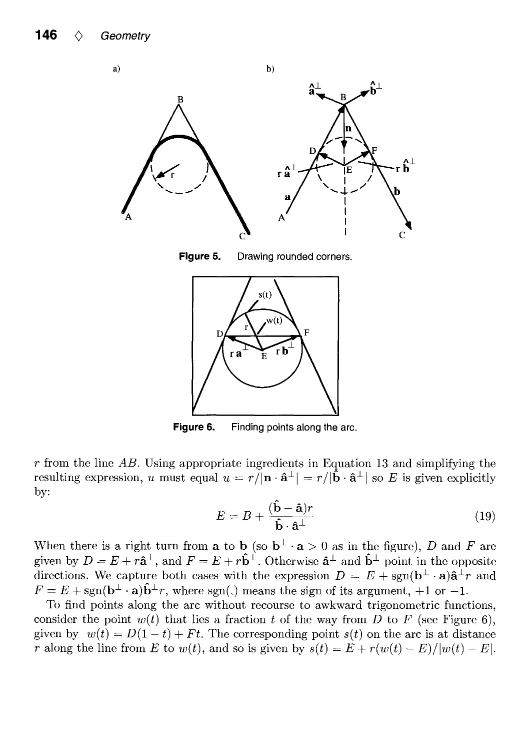
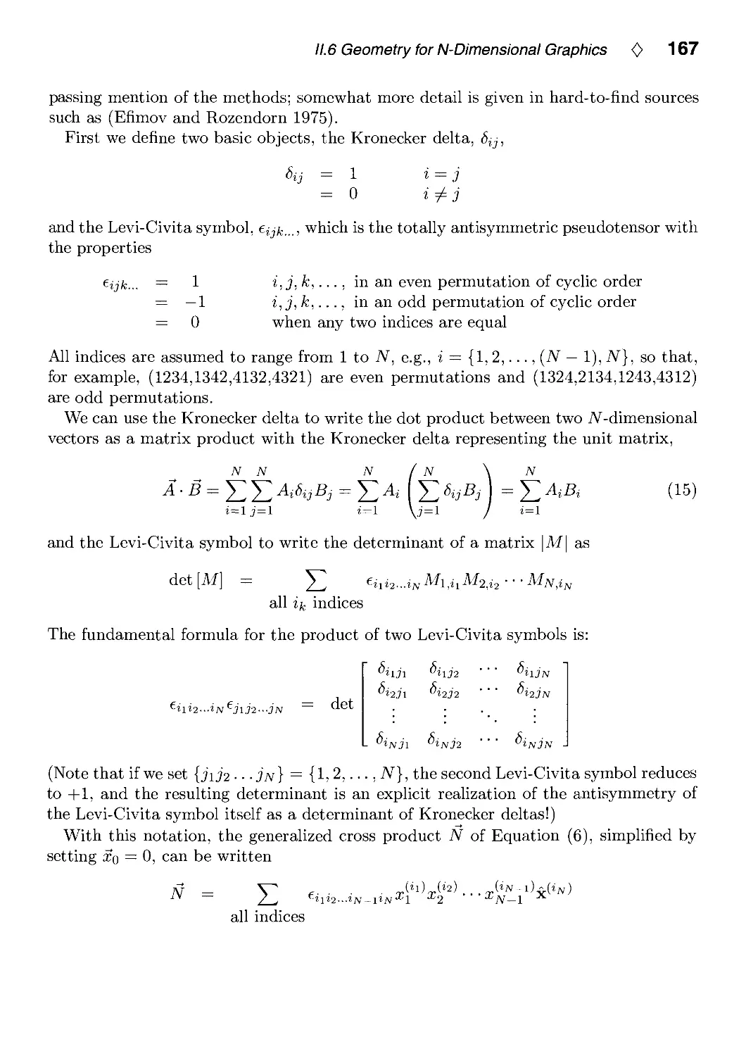
11.5. The Pleasures of "Perp Dot" Products by F S. Hill, Jr 138
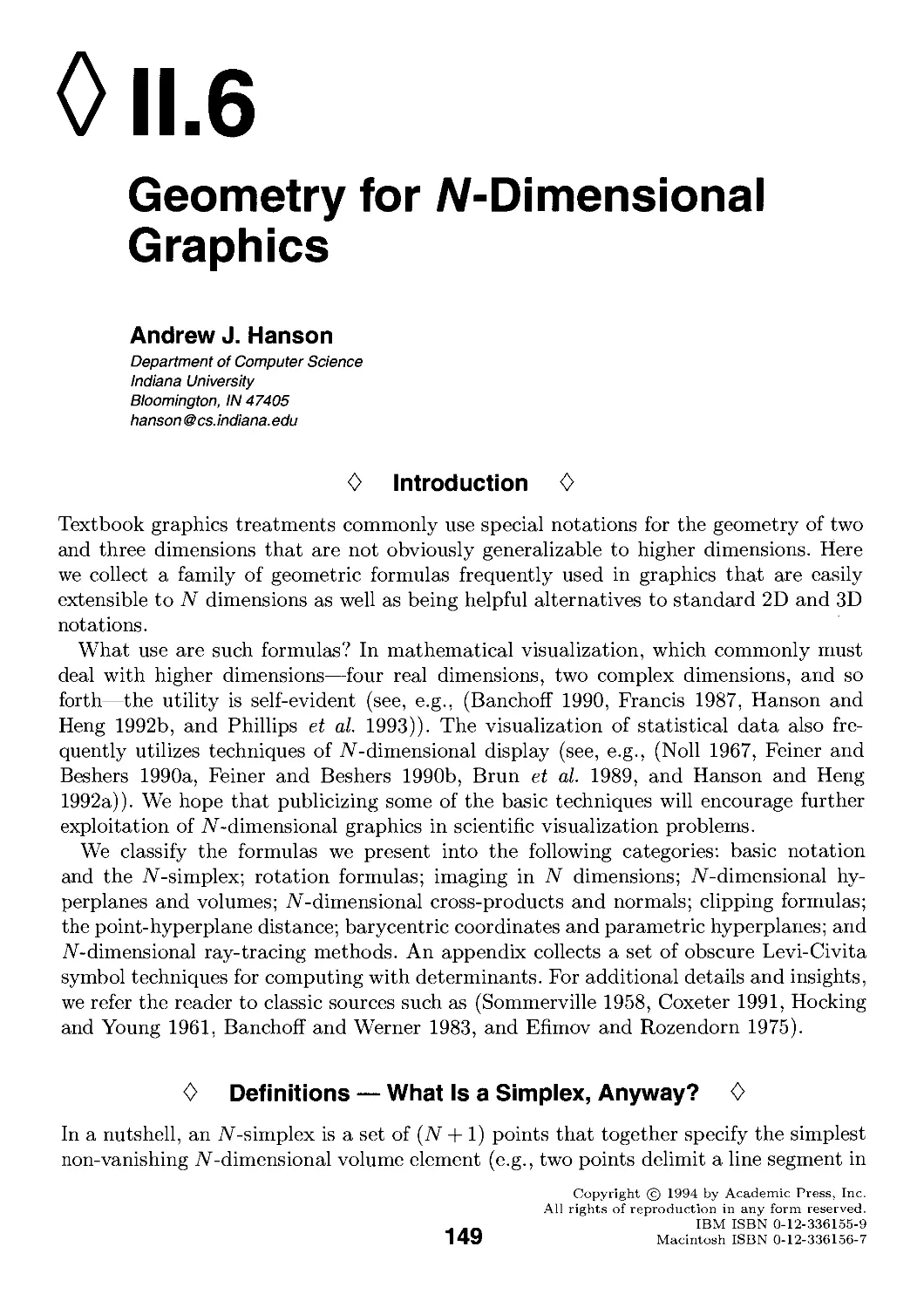
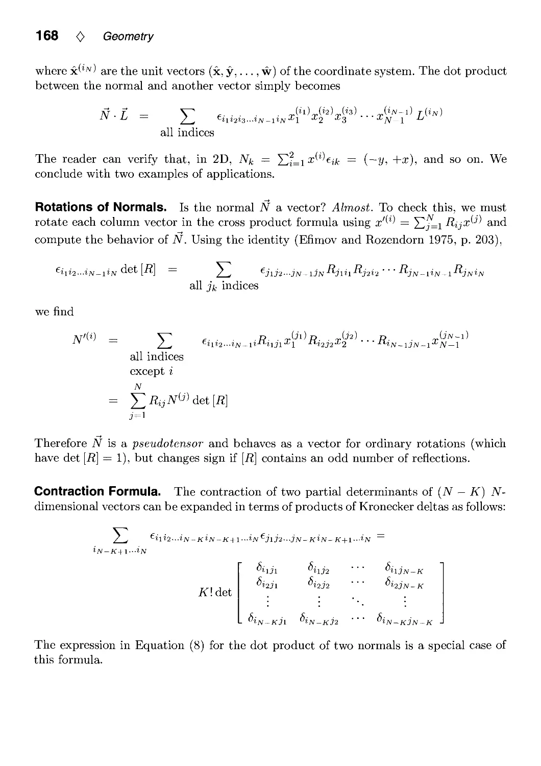
11.6. Geometry for A/-Dimensional Graphics by Andrew J. Hanson 149
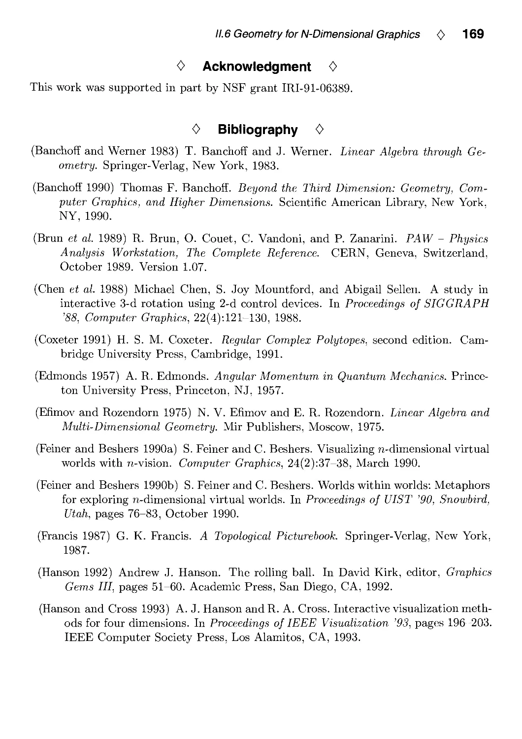
III. Transformations 173
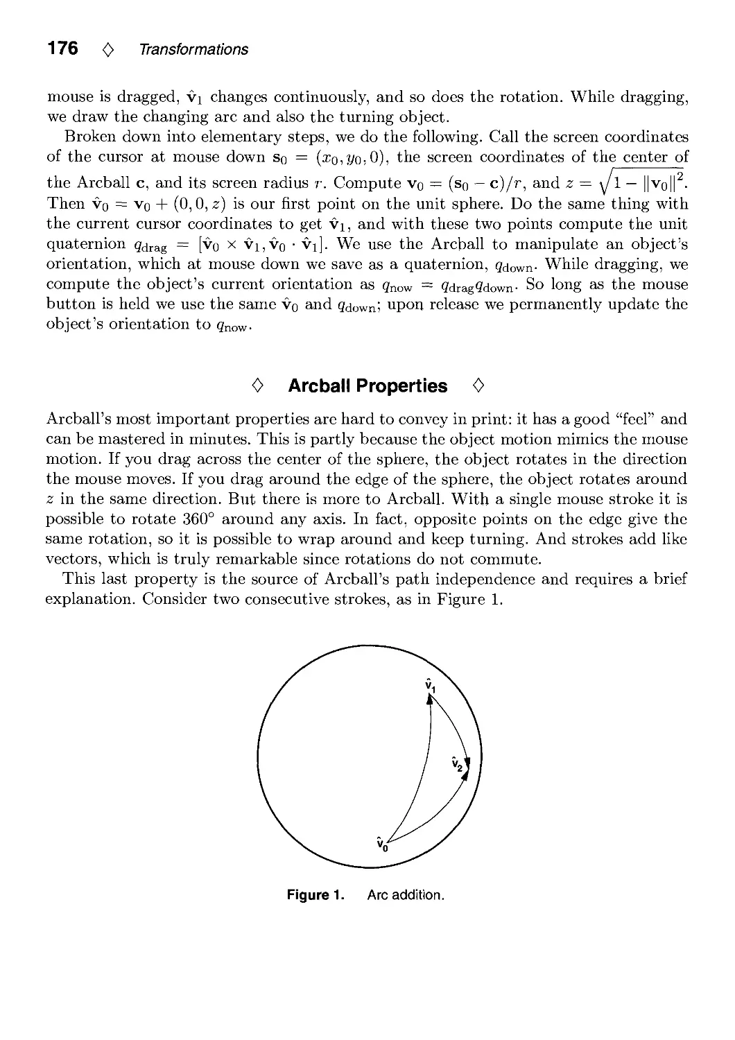
111.1. Arcball Rotation Control by Ken Shoemake 175
111.2. Efficient Eigenvalues for Visualization by Robert L. Cromwell 193

vi 0 Contents
111.3. Fast Inversion of Length- and Angle-Preserving Matrices by Kevin Wu 199
111.4. Polar Matrix Decomposition by Ken Shoemake 207
111.5. Euler Angle Conversion by Ken Shoemake 222
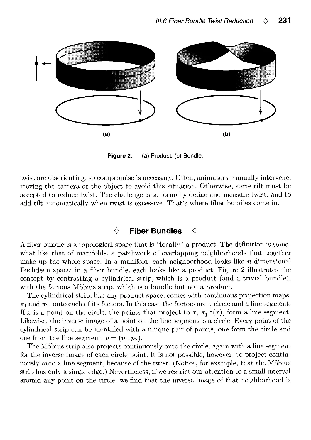
111.6. Fiber Bundle Twist Reduction by Ken Shoemake 230
IV. Curves and Surfaces 239
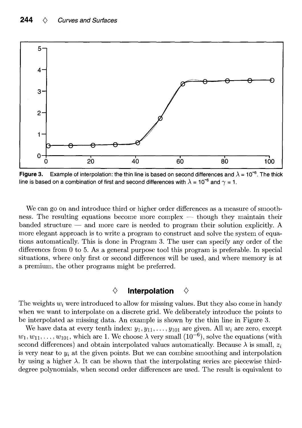
IV.1. Smoothing and Interpolation with Finite Differences by Paul H. C. Eilers 241
IV.2. Knot Insertion Using Forward Differences by Phillip Barry and
Ron Goldman 251
IV.3. Converting a Rational Curve to a Standard Rational Bernstein-Bezier
Representation by Chandrajit Bajaj and Guoliang Xu 256
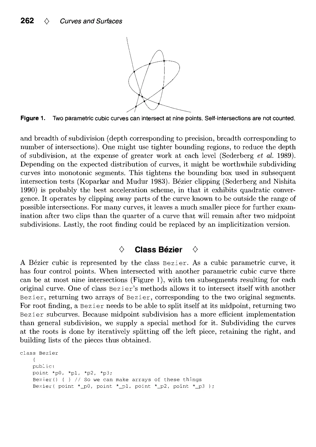
IV.4. Intersecting Parametric Cubic Curves by Midpoint Subdivision by
R. Victor Klassen 261
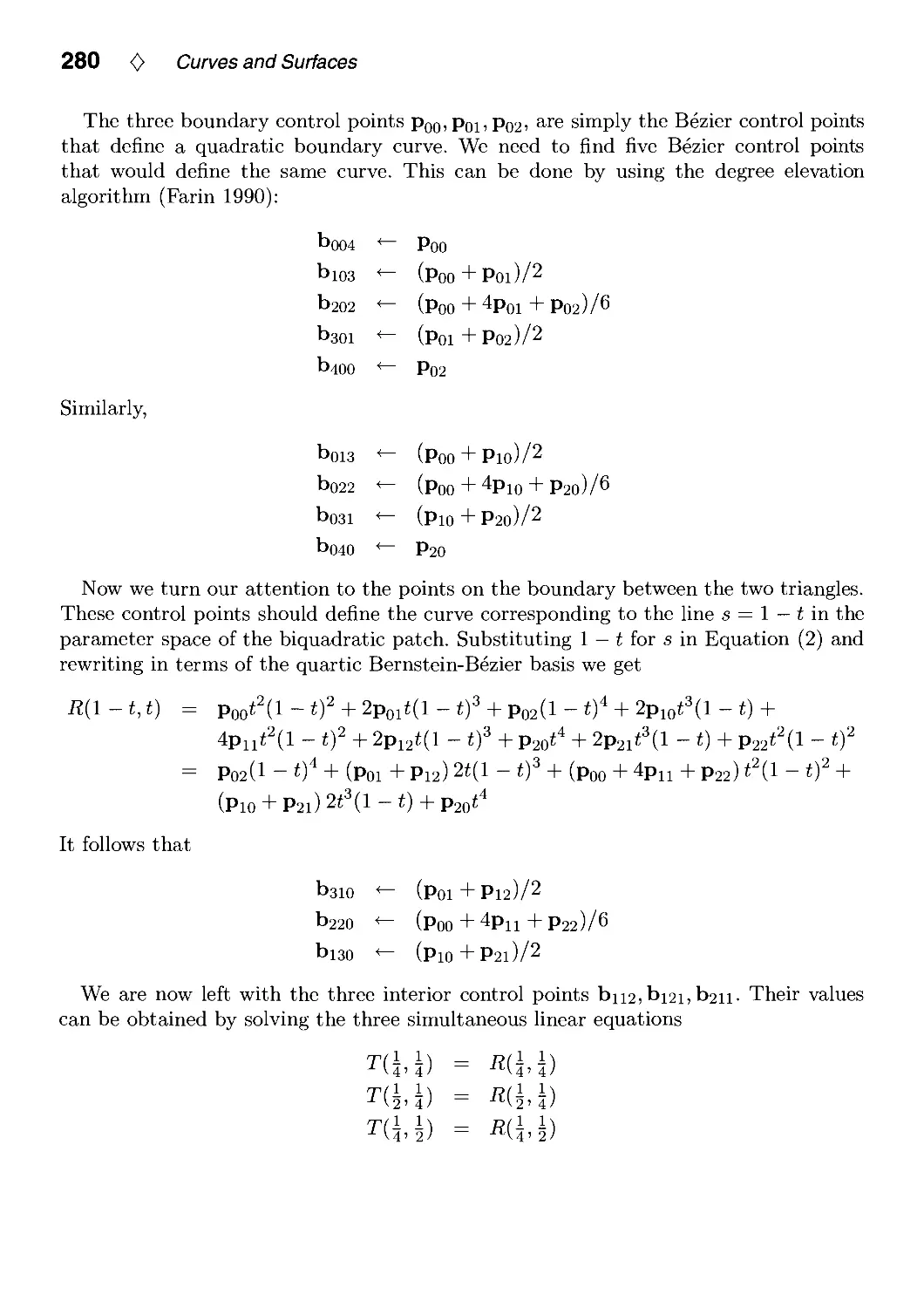
IV.5. Converting Rectangular Patches into Bezier Triangles by Dani Lischinski 278
IV.6. Tessellation of NURB Surfaces by John W. Peterson 286
IV.7. Equations of Cylinders and Cones by Ching-Kuang Shene 321
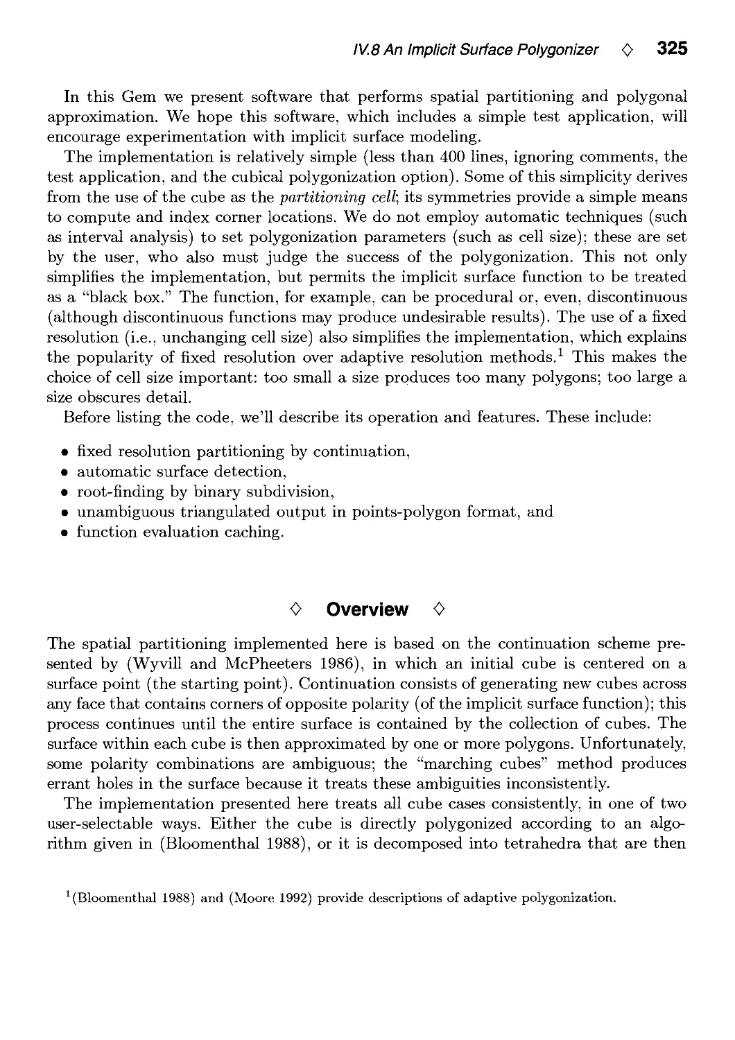
IV.8. An Implicit Surface Polygonizer by Jules Bloomenthal 324
V. Ray Tracing 351
V.1. Computing the Intersection of a Line and a Cylinder by
Ching-Kuang Shene 353
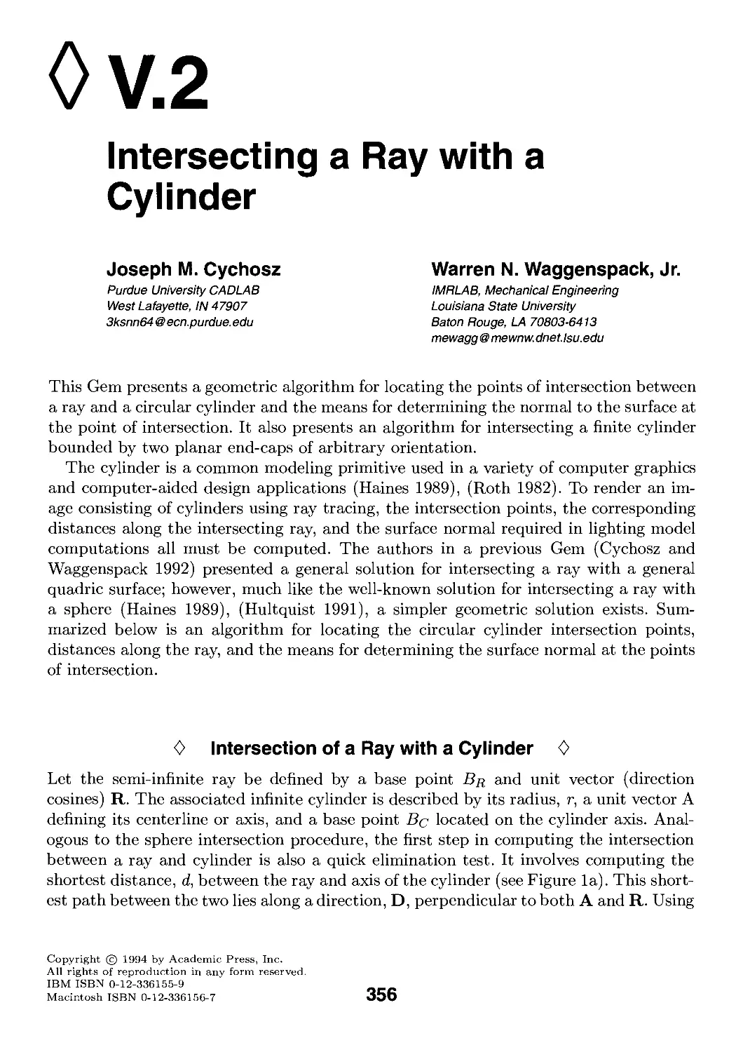
V.2. Intersecting a Ray with a Cylinder by Joseph M. Cychosz and
Warren N. Waggenspack, Jr 356
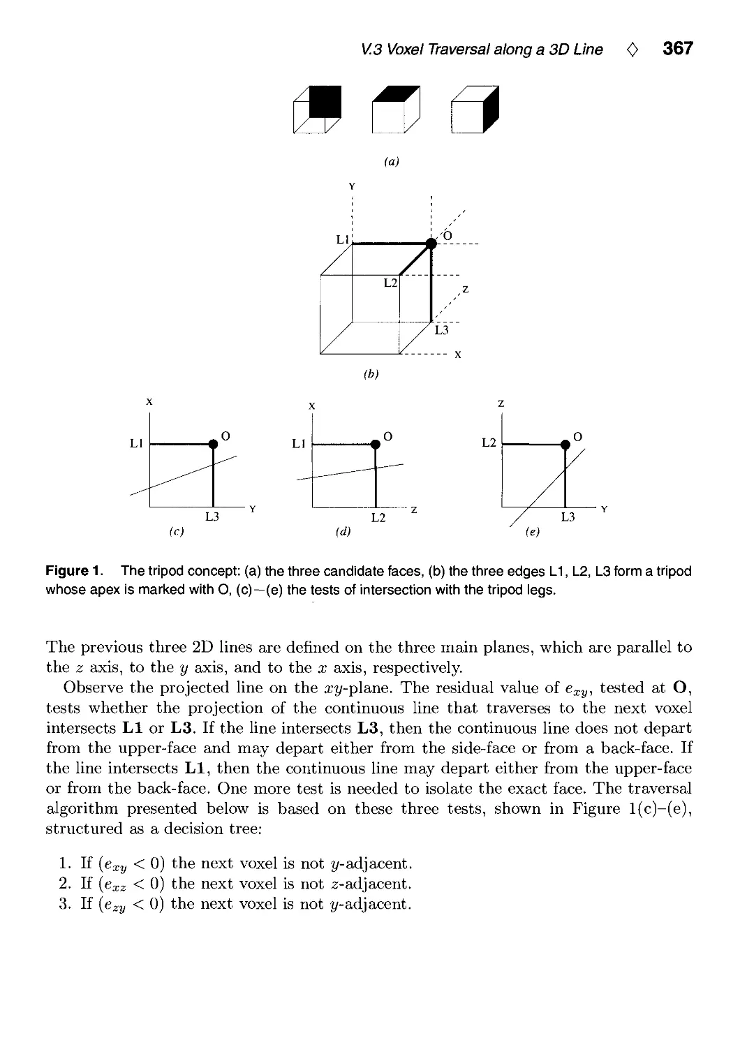
V.3. Voxel Traversal along a 3D Line by Daniel Cohen 366
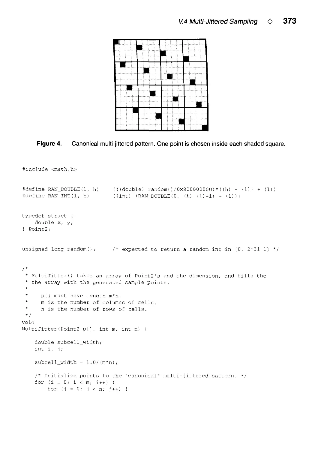
V.4. Multi-Jittered Sampling by Kenneth Chiu, Peter Shirley and
Changyaw Wang 370
V.5. A Minimal Ray Tracer by Paul S. Heckbert 375
VI. Shading 383
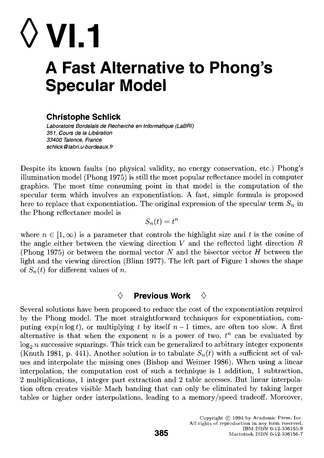
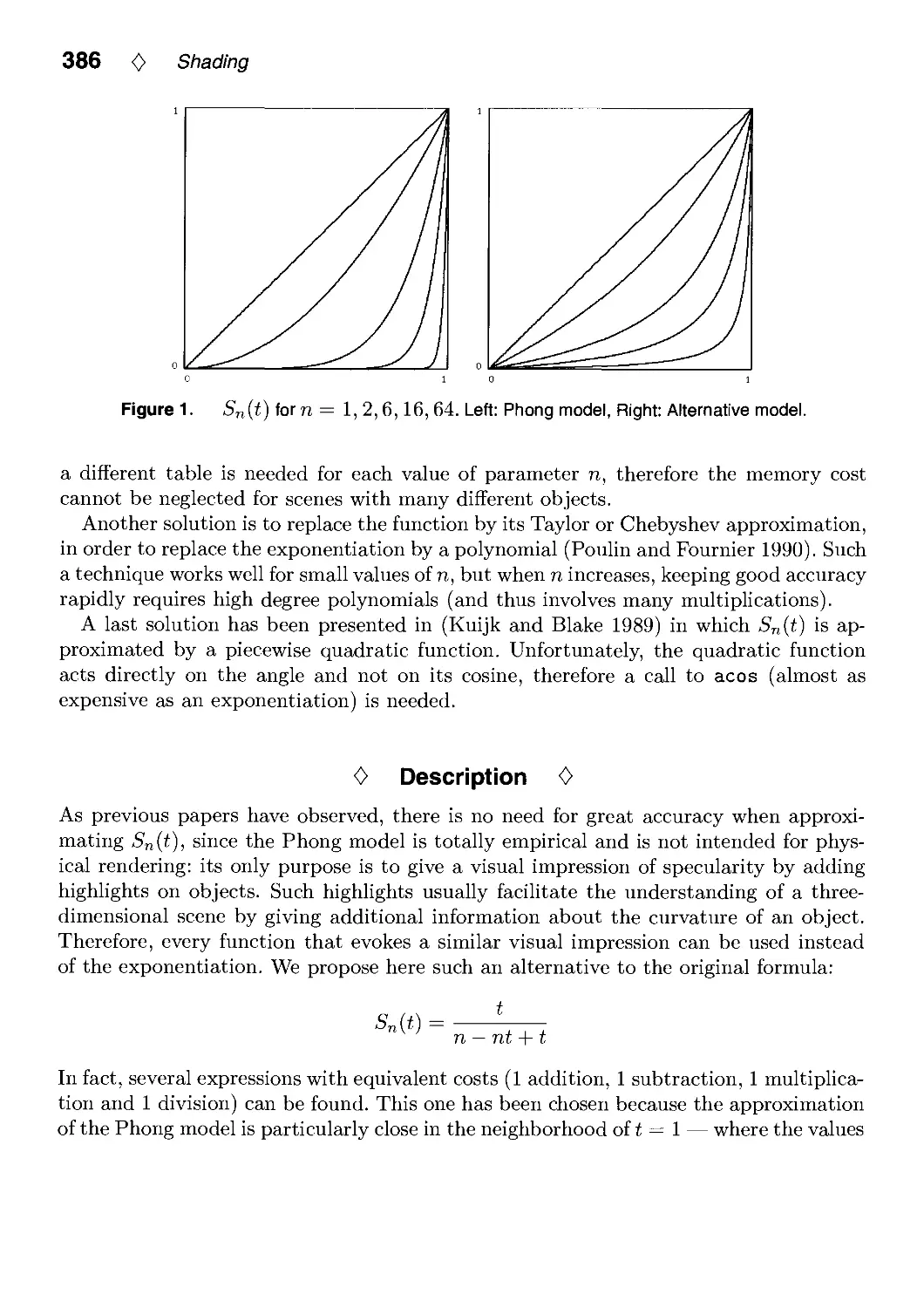
VI.1. A Fast Alternative to Phong's Specular Model by Christophe Schlick 385
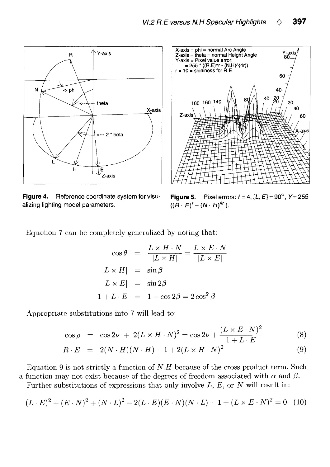
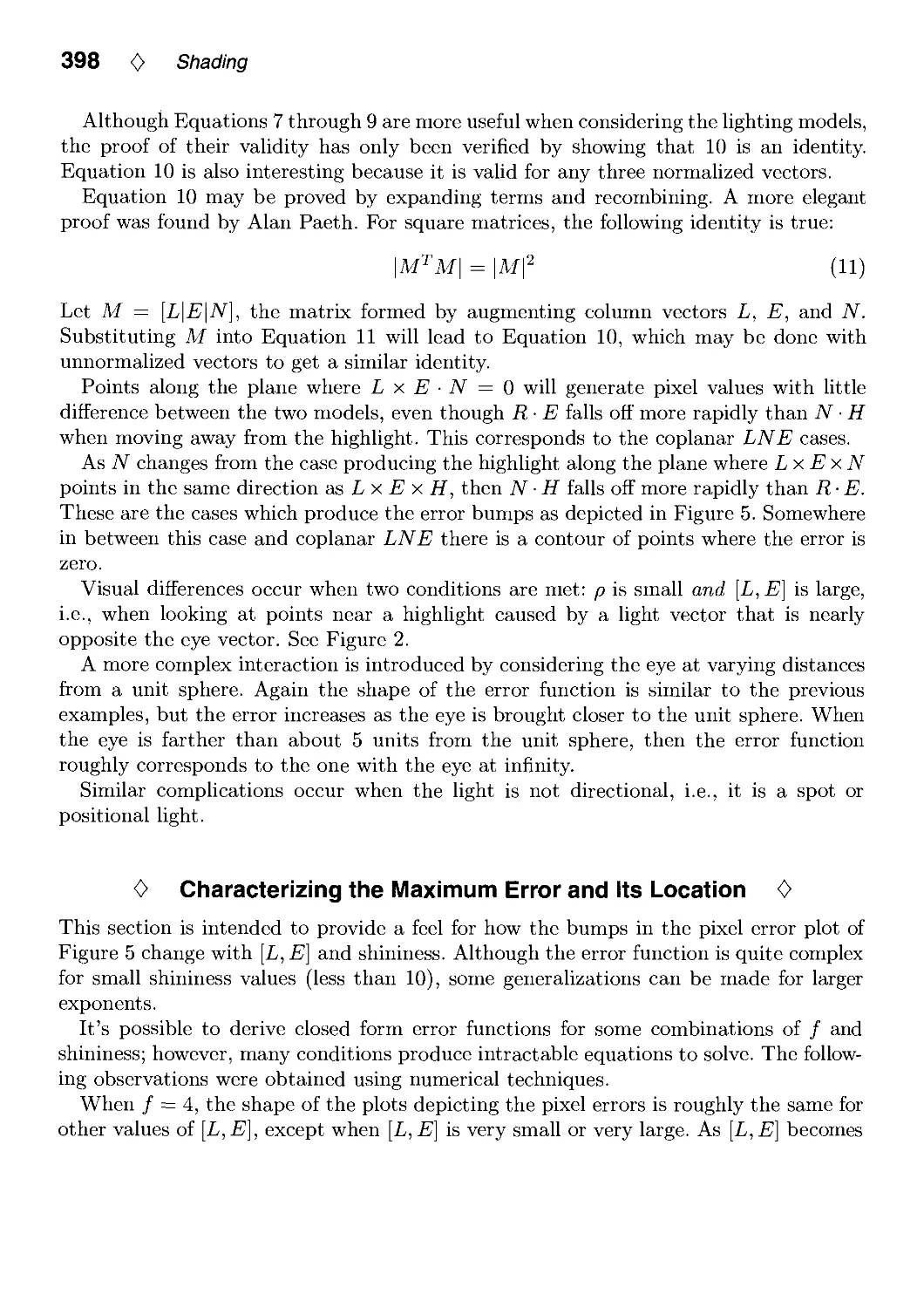
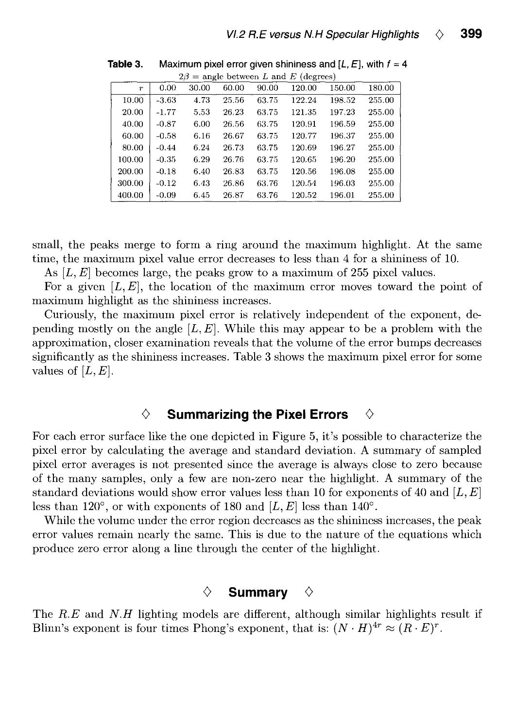
VI.2. R.E versus N.H Specular Highlights by Frederick Fisher and Andrew Woo.. .388
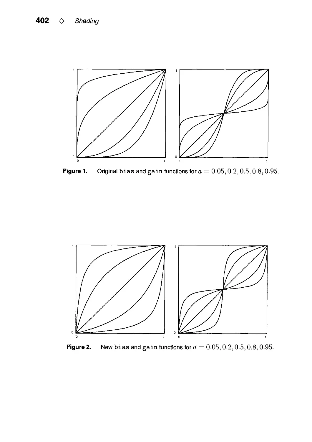
VI.3. Fast Alternatives to Perlin's Bias and Gain Functions by Christophe Schlick. .401
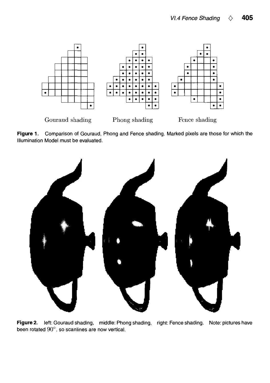
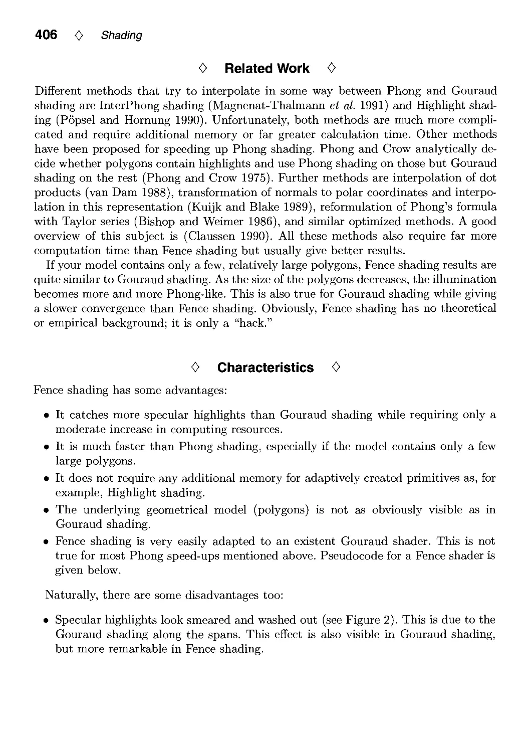
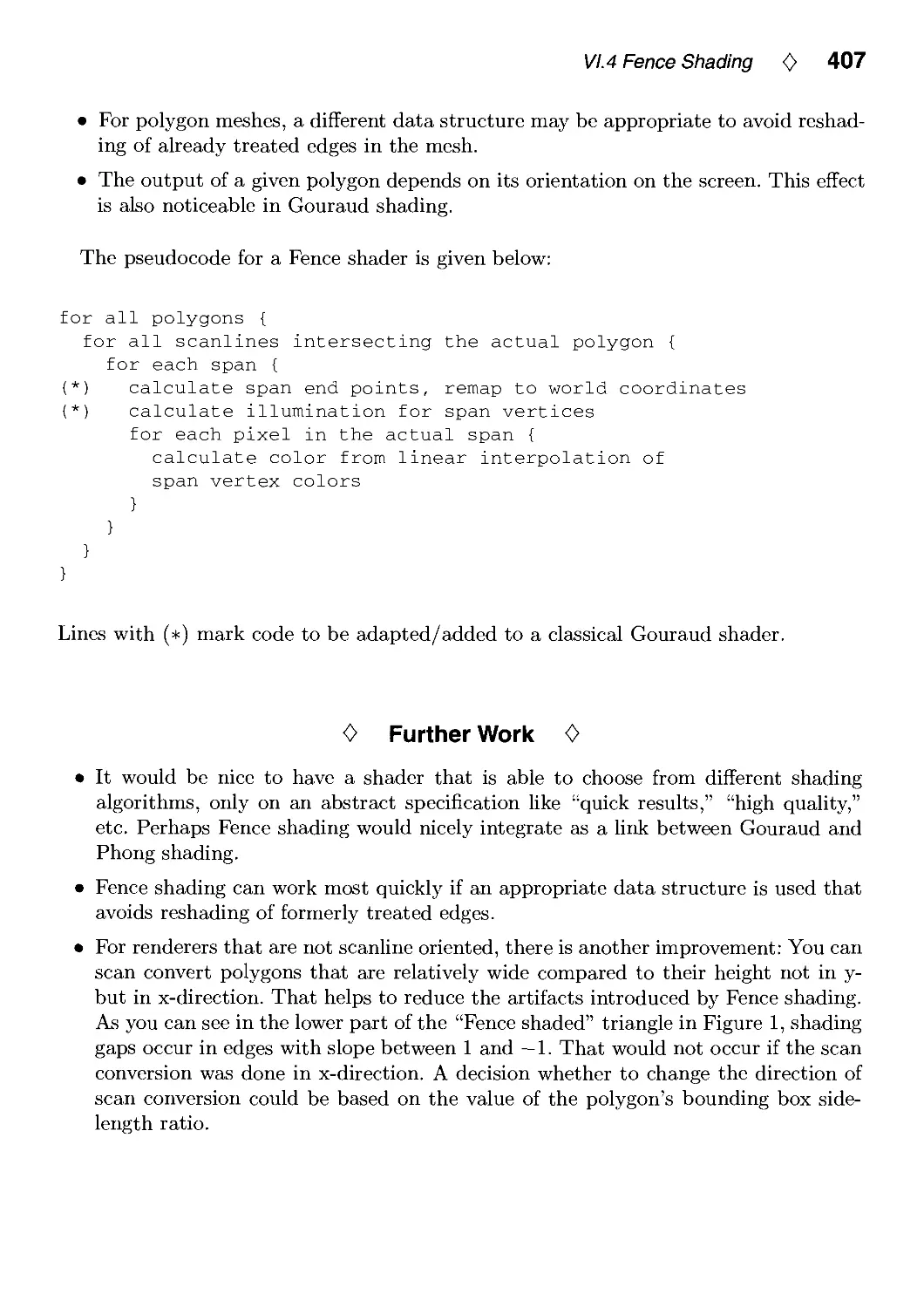
VI.4. Fence Shading by Uwe Behrens 404

Contents 0 vii
VII. Frame Buffer Techniques 411
VII.1. XOR-Drawing with Guaranteed Contrast by Manfred Kopp and
Michael Gervautz 413
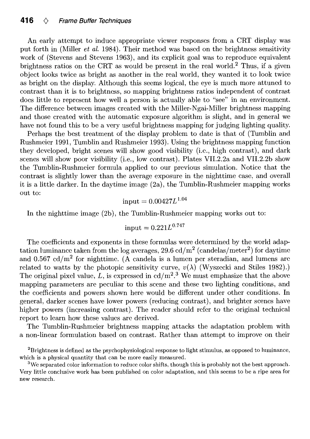
VII.2. A Contrast-Based Scalefactor for Luminance Display by Greg Ward 415
VII.3. Higli Dynamic Range Pixels by Christophe Schlick 422
VIM. Image Processing 431
VIII.1. Fast Embossing Effects on Raster Image Data by John Schlag 433
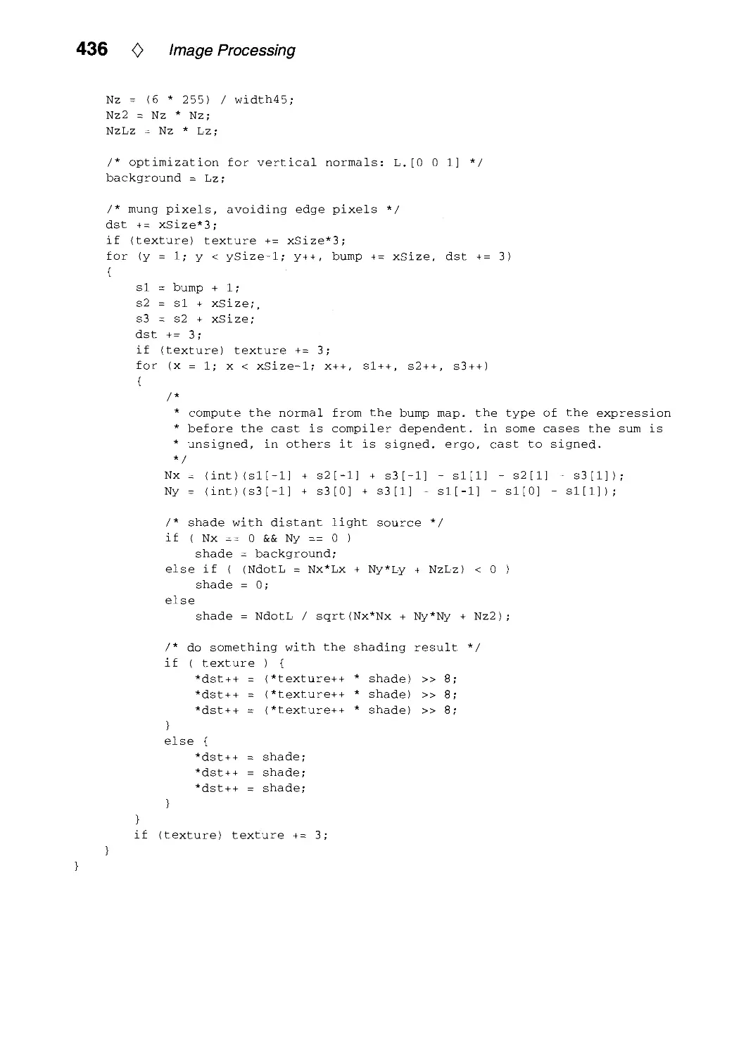
VIII.2. Bilinear Coons Patch Image Warping by Paul S. Heckbert 438
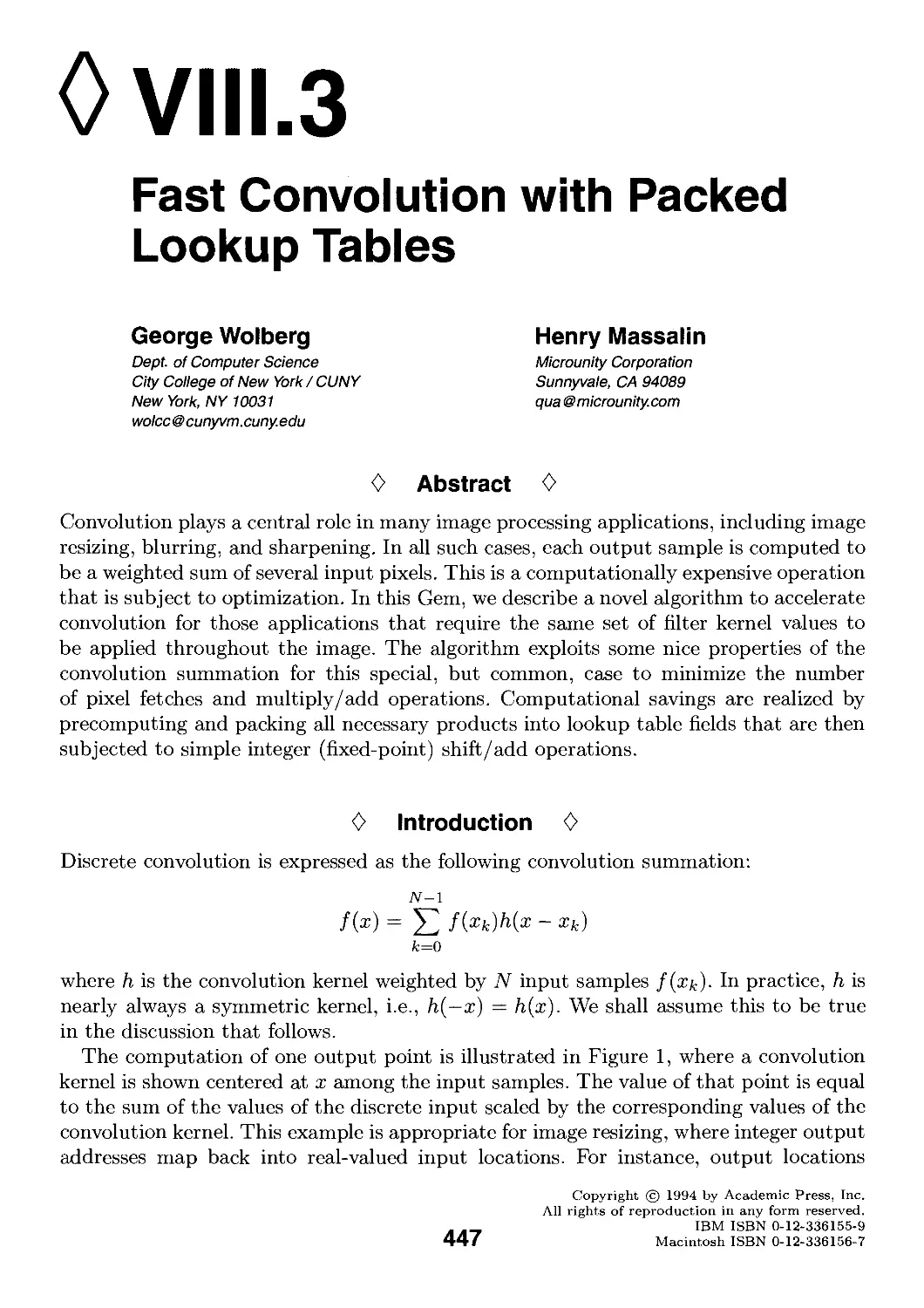
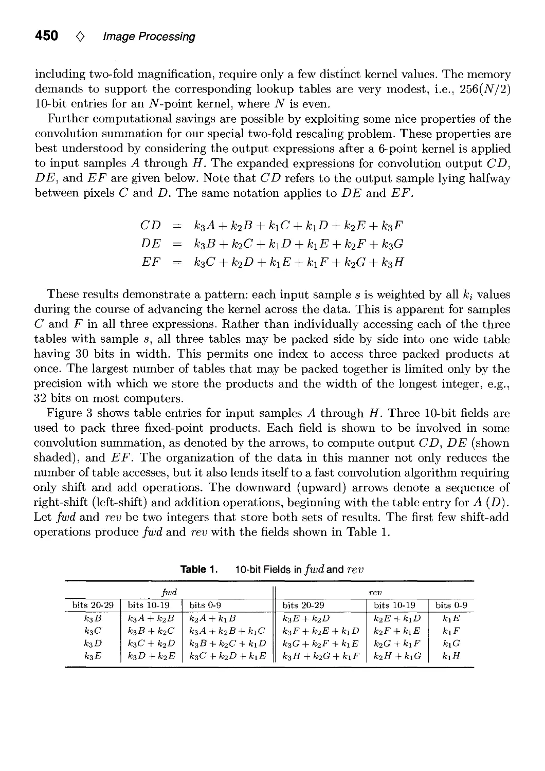
VIII.3. Fast Convolution with Packed Lookup Tables by George Wolberg
and Henry Massalin 447
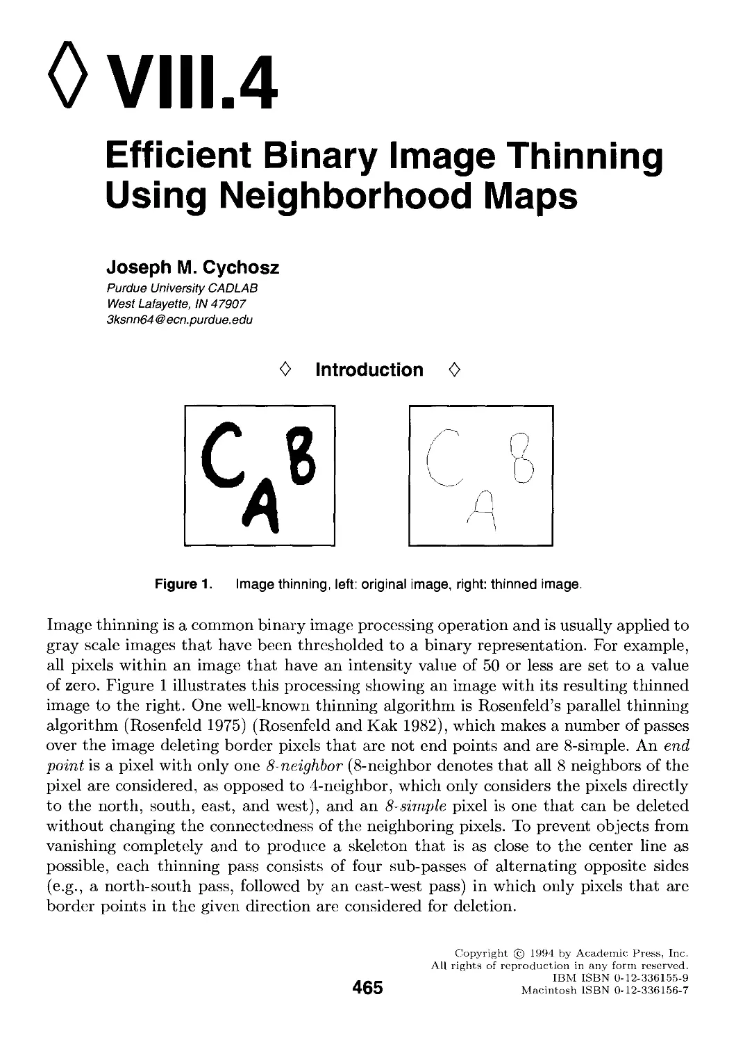
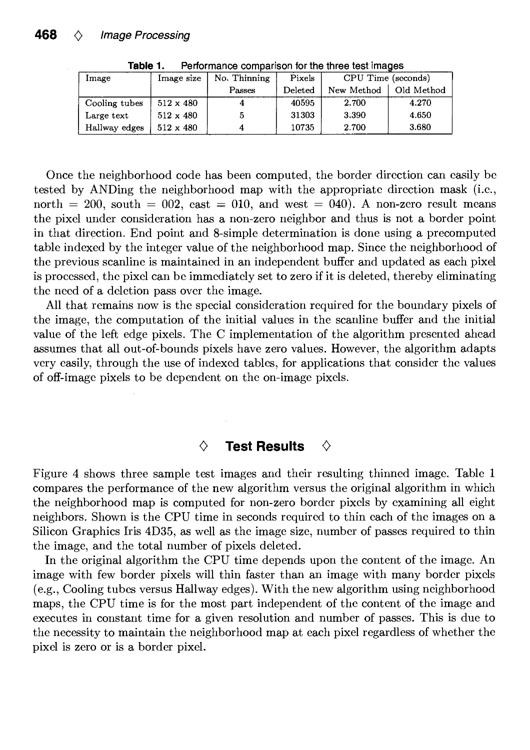
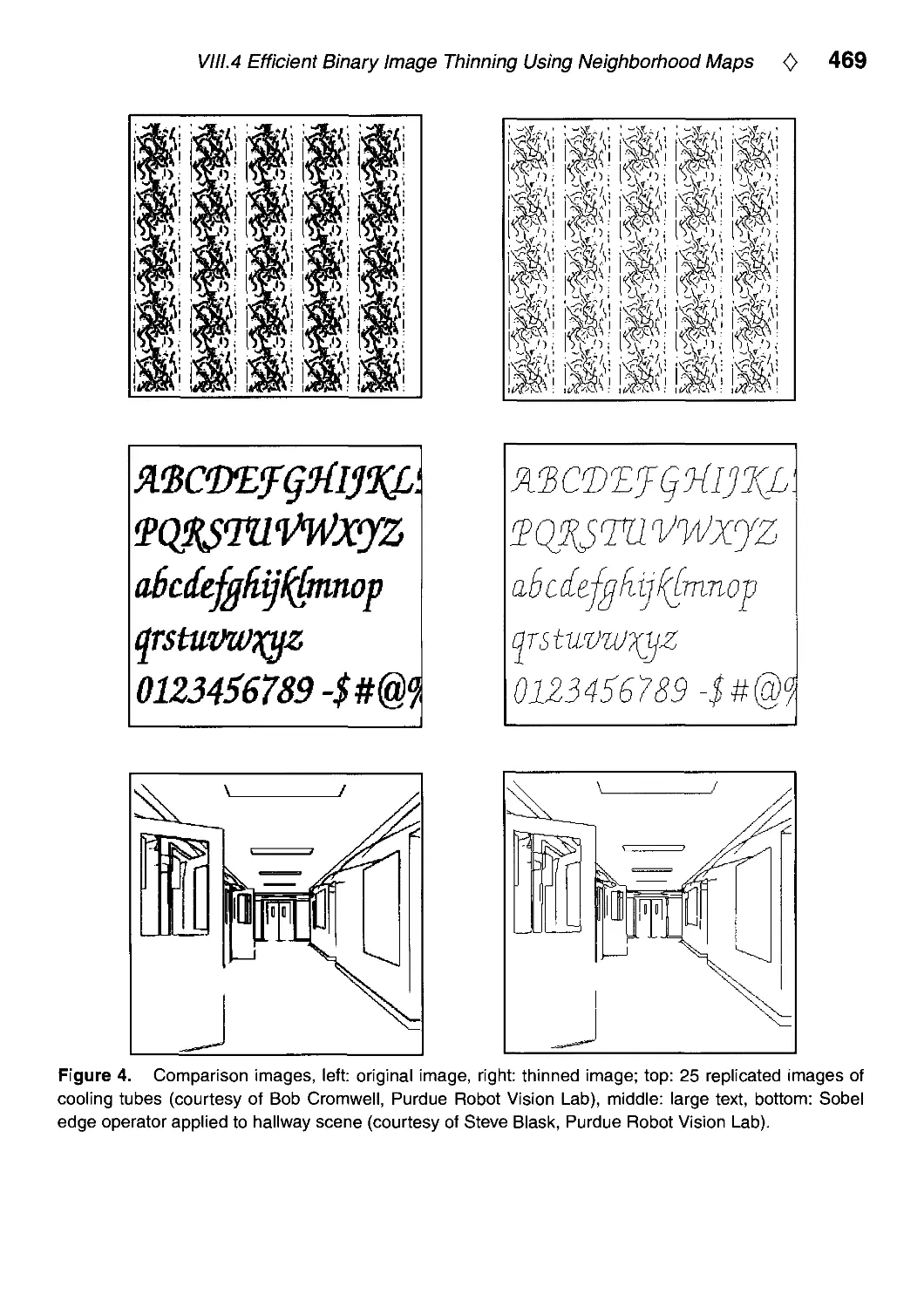
VIII.4. Efficient Binary Image Thinning Using Neighborhood Maps by
Joseph M. Cychosz 465
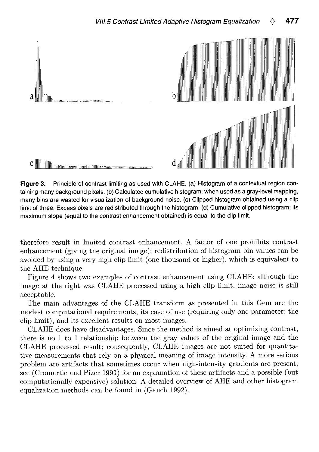
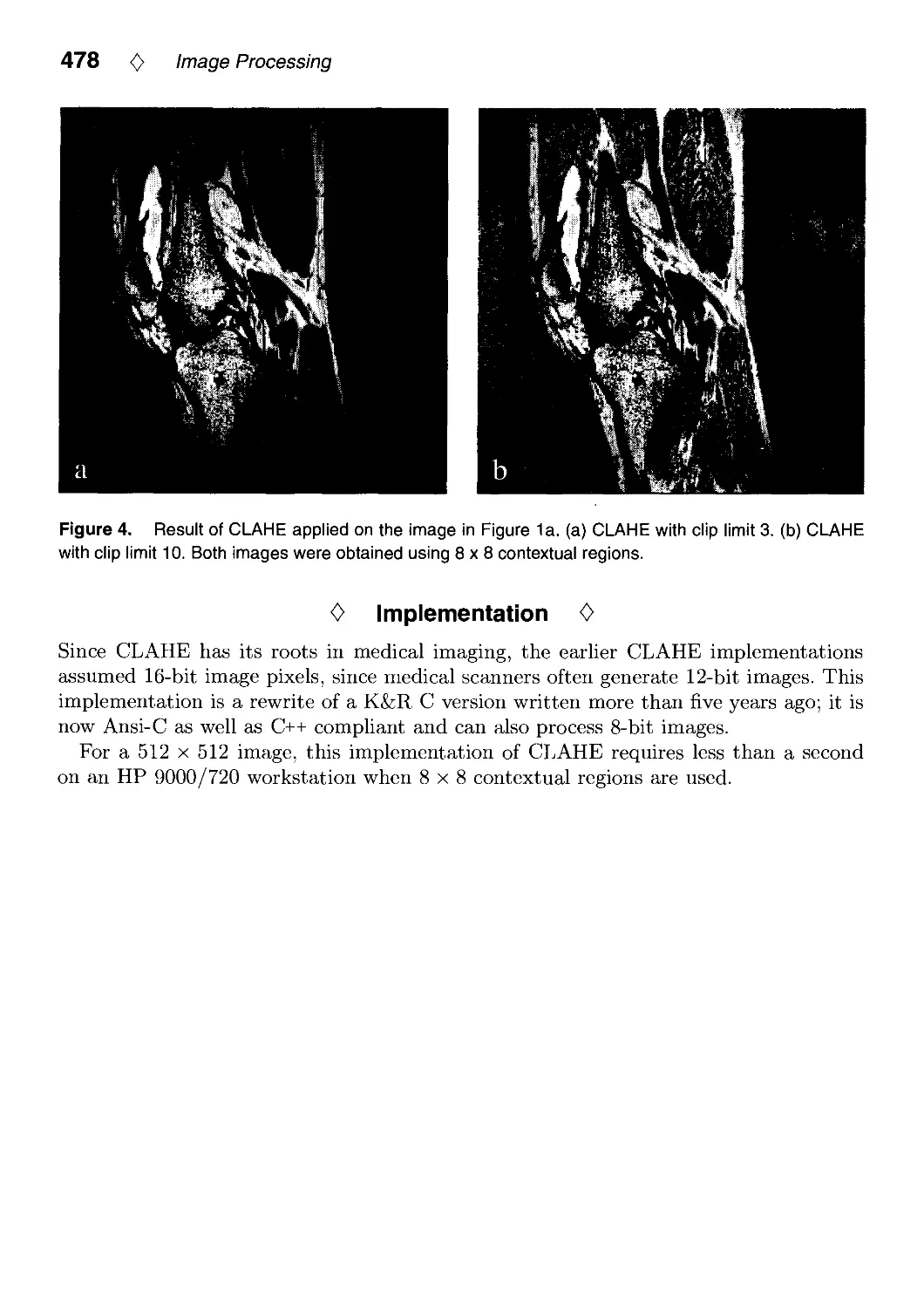
VIII.5. Contrast Limited Adaptive Histogram Equalization by Karel Zuiderveld 474
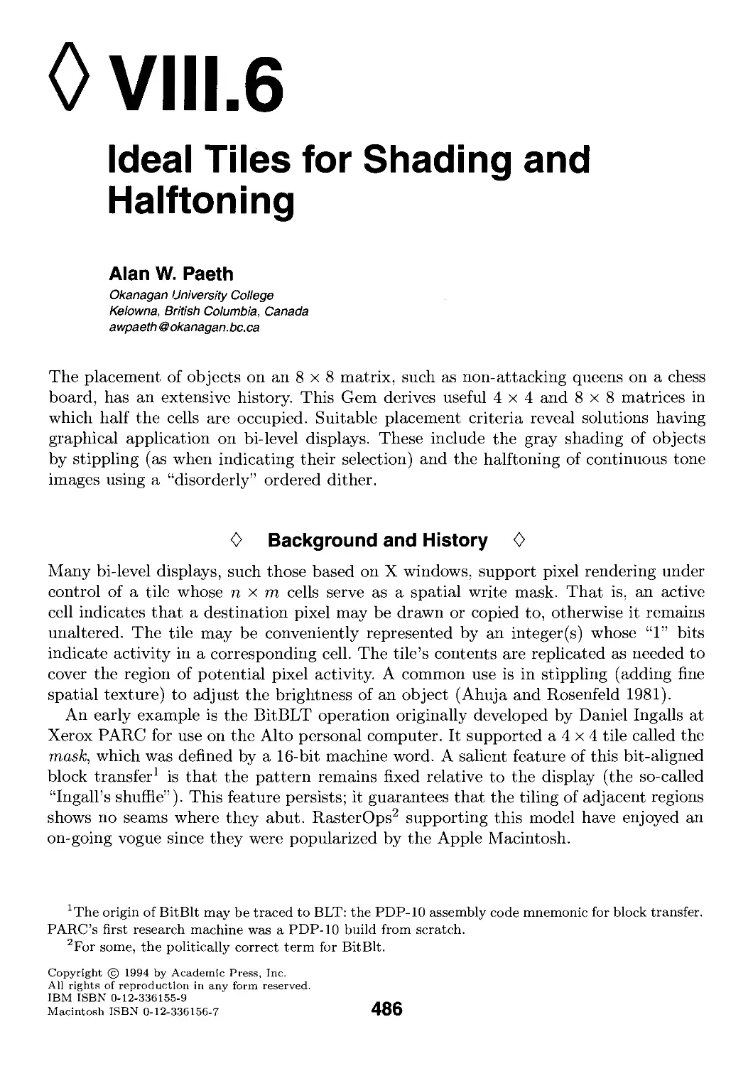
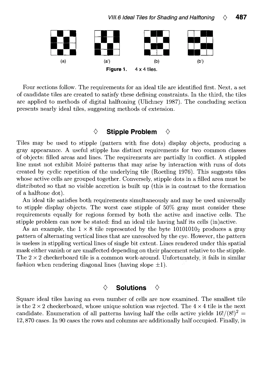
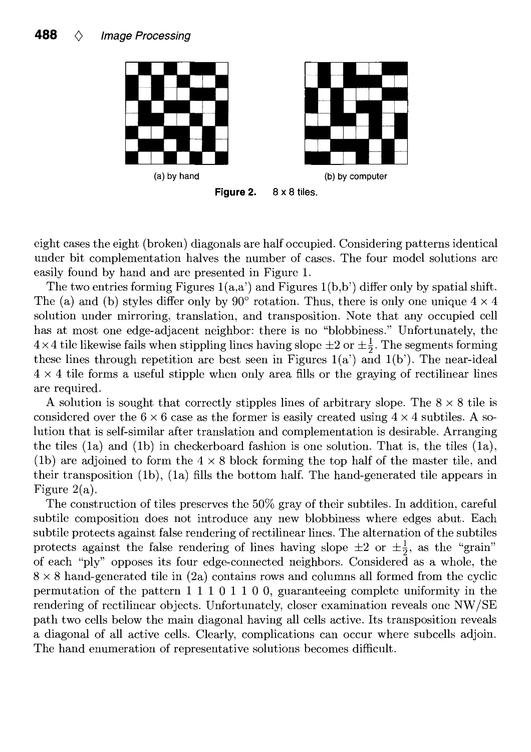
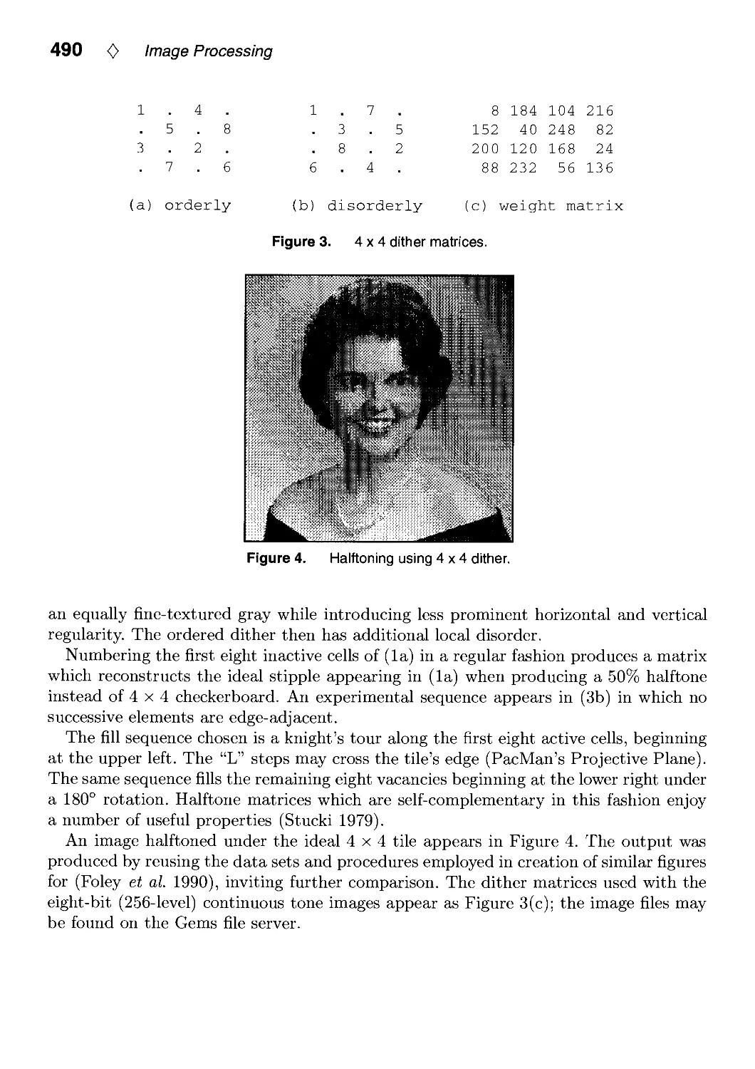
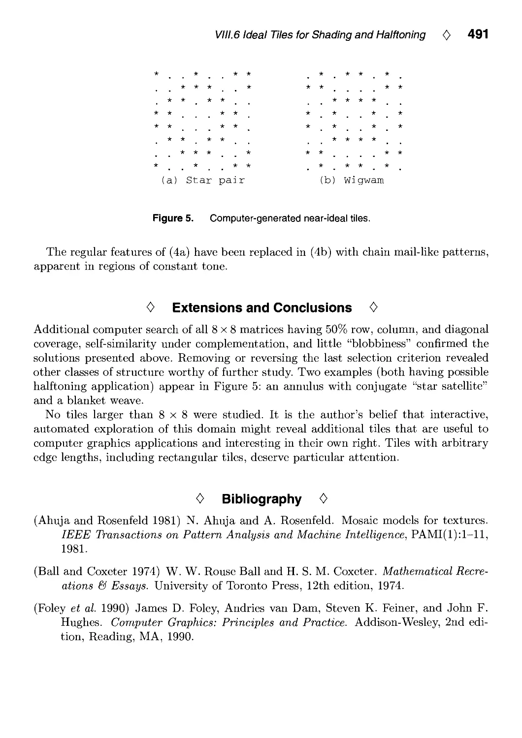
VIII.6. Ideal Tiles for Shading and Halftoning by Alan W. Paeth 486
IX. Graphic Design 495
IX.1. Placing Text Labels on Maps and Diagrams by Jon Christensen, Joe Marks,
and Stuart Shieber 497
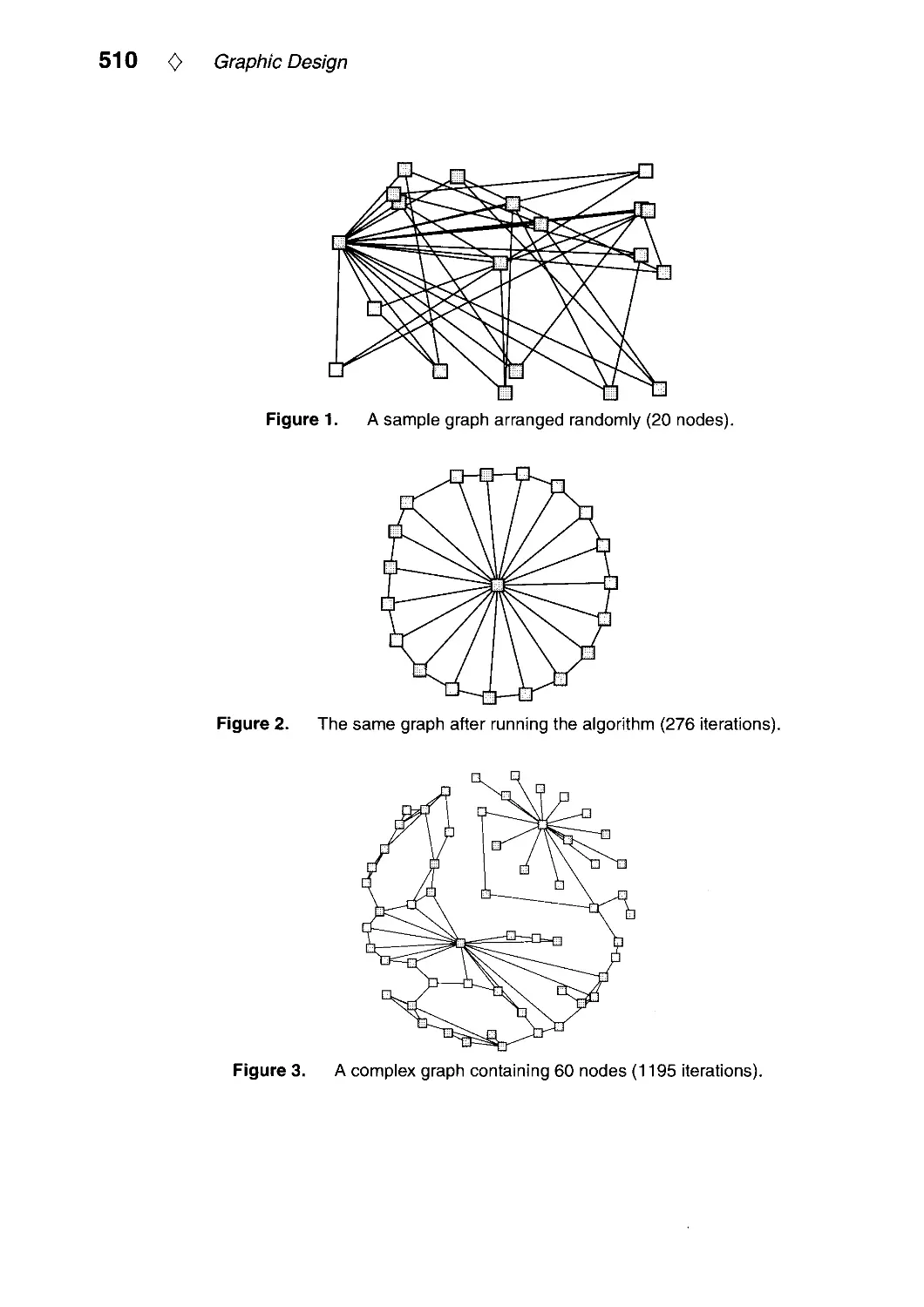
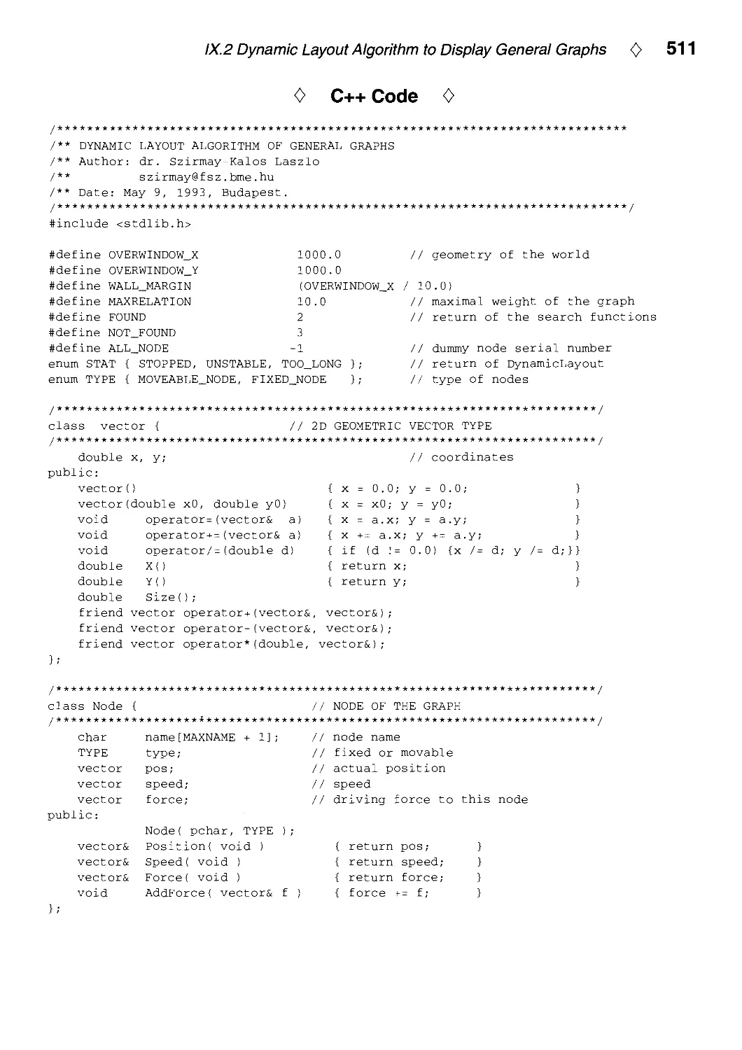
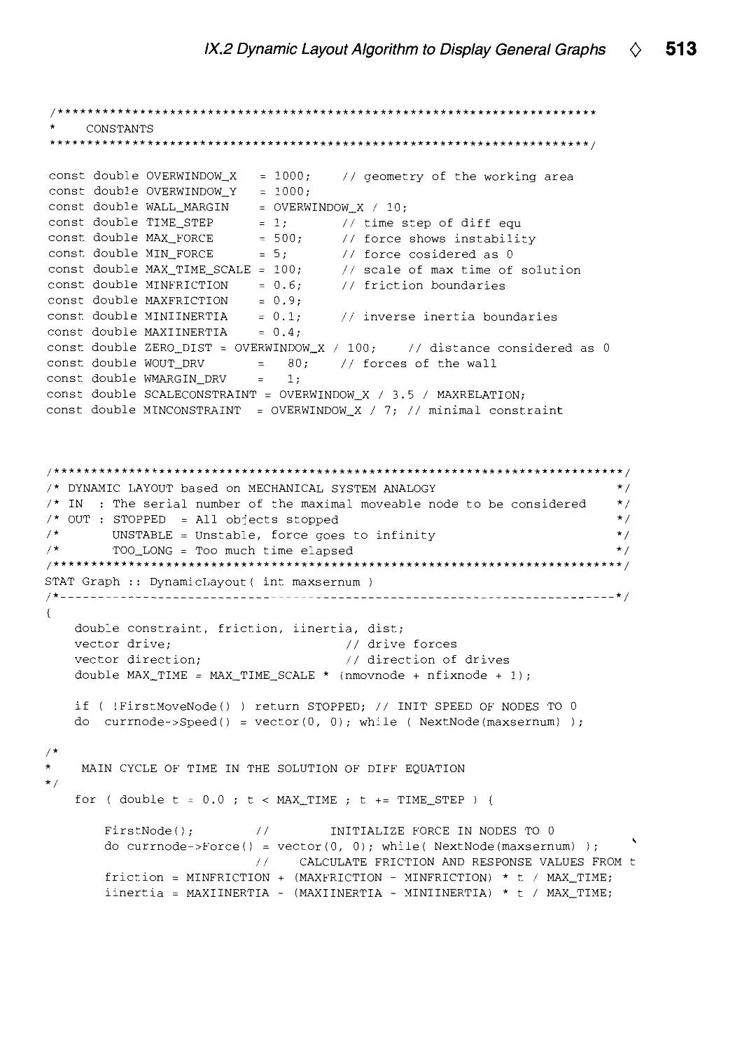
IX.2. Dynamic Layout Algorithm to Display General Graphs by
Laszlo Szirmay-Kalos 505
X. Utilities 519
X.1. Tri-linear Interpolation by Steve Hill 521
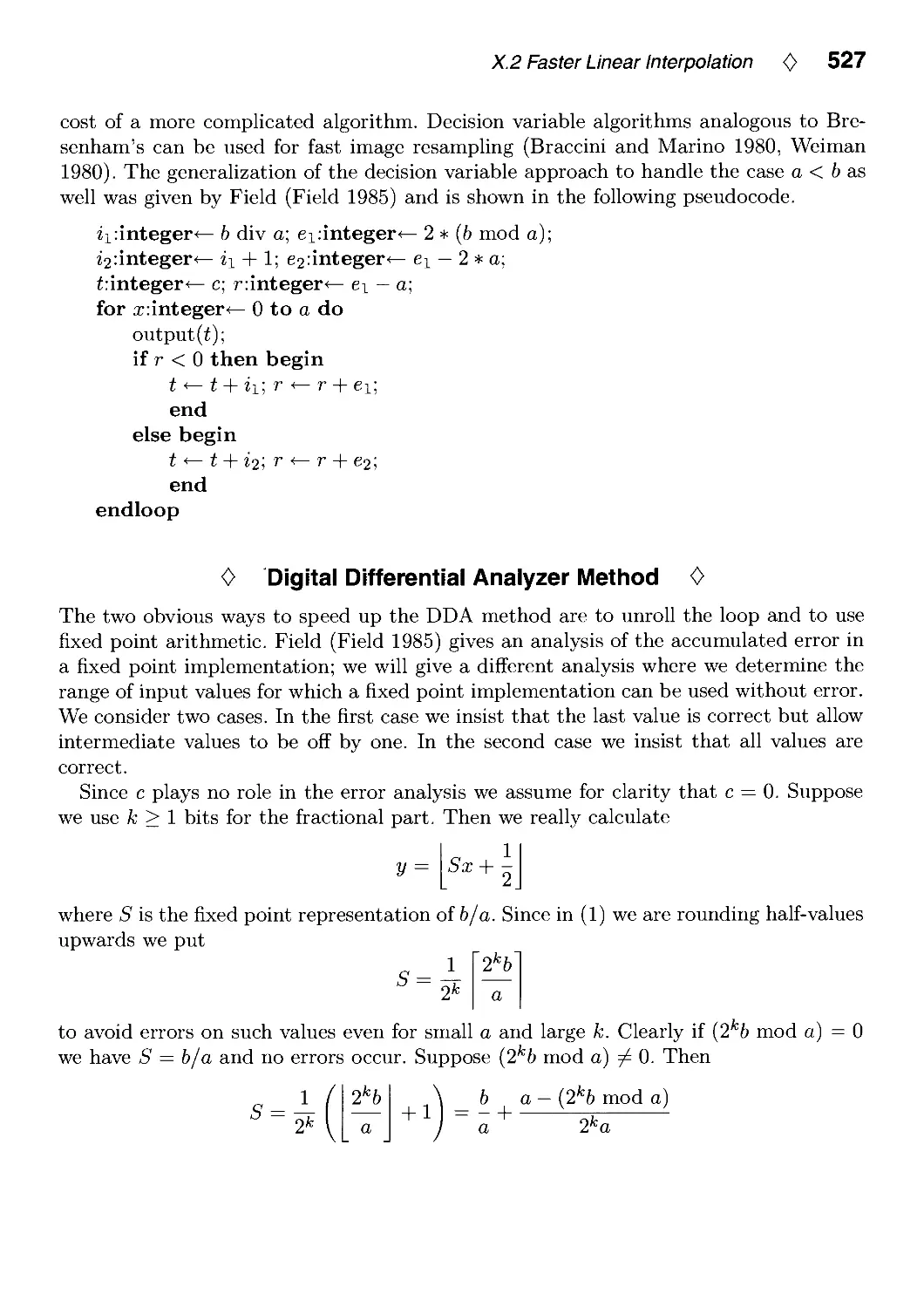
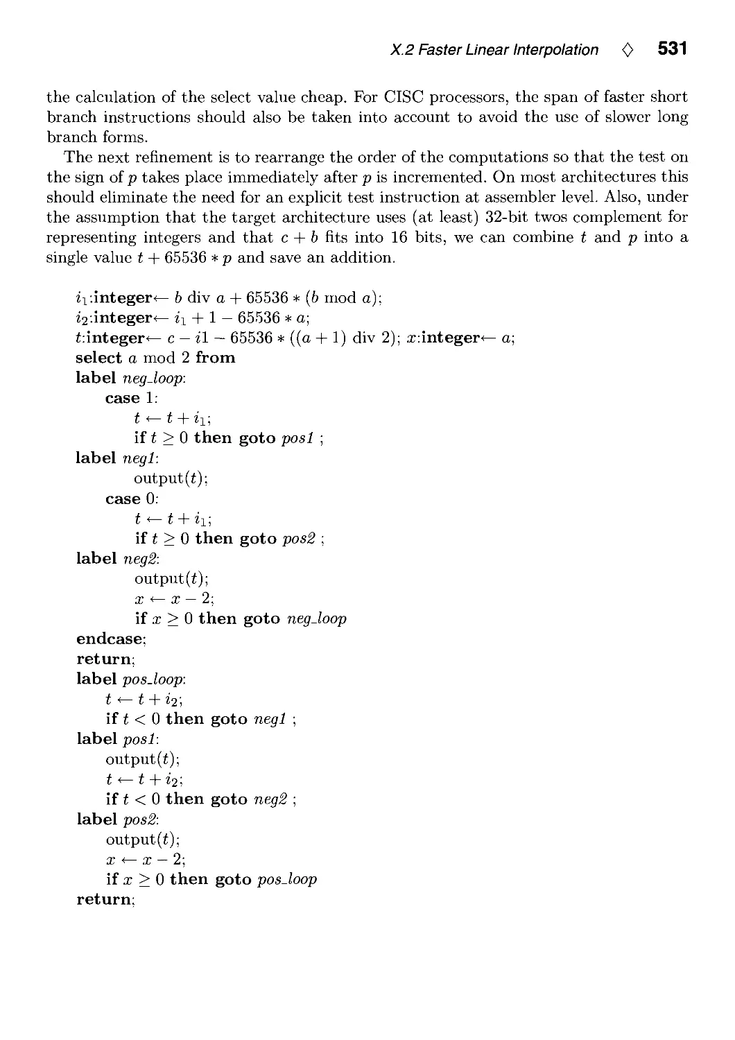
X.2. Faster Linear Interpolation by Steven Eker 526
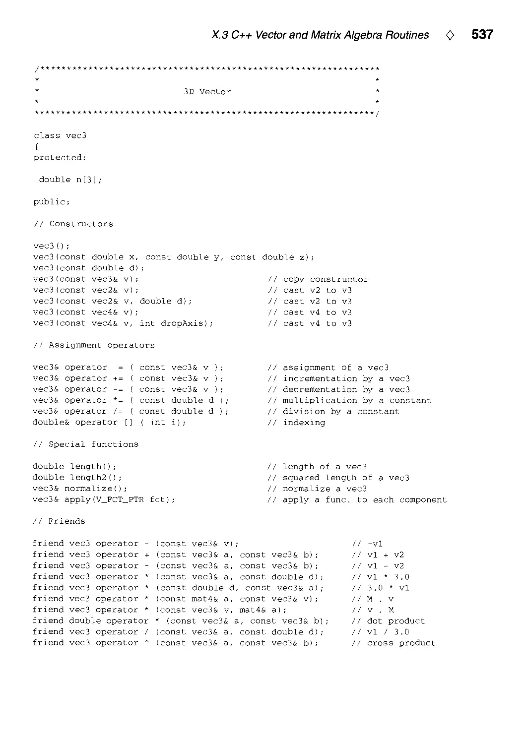
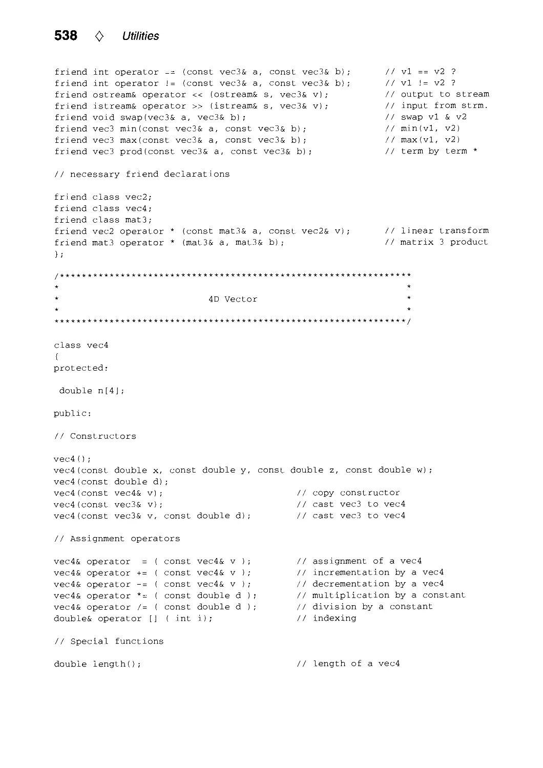
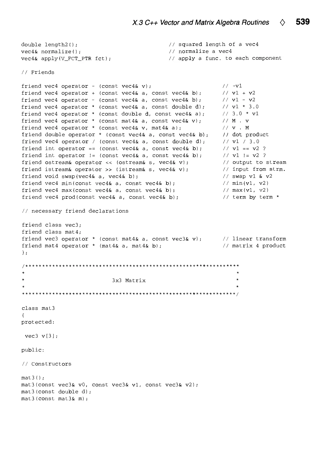
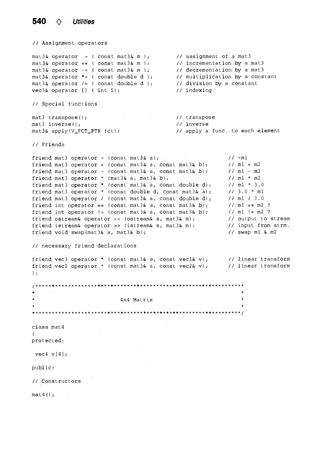
X.3. C++ Vector and Matrix Algebra Routines by Jean-Frangois Doue 534
X.4. C Header File and Vector Library by Andrew Glassner and Eric Haines 558
Index 571

0
Author Index
Format: author, institution, chapter number: p. start page.
Author's full address is listed on the first page of each chapter.
Chandrajit Bajaj, Purdue University, West Lafayette, IN, USA, IV.3: p. 256.
Phillip Barry, University of Minnesota, Minneapolis, MN, USA, IV.2: p. 251.
Gerard Bashein, University of Washington, Seattle, WA, USA, I.l: p. 3.
Uwe Behrens, Bremen, Germany, VI.4: p. 404.
Jules Bloomenthal, George Mason University, Fairfax, VA, USA, IV.8: p. 324.
Kenneth Chiu, Indiana University, Bloomington, IN, USA, V.4: p. 370.
Jon Christensen, Harvard University, Cambridge, MA, USA, IX. 1: p. 497.
Daniel Cohen, Ben Gurion University, Beer-Sheva, Israel, V.3: p. 366.
Robert L Cromwell, Purdue University, West Lafayette, IN, USA, III.2: p. 193.
Joseph M. Cychosz, Purdue University, West Lafayette, IN, USA, V.2: p. 356,
VIII.4: p. 465.
Paul R. Detmer, University of Washington, Seattle, WA, USA, I.l: p. 3.
Walt Donovan, Sun Microsystems, Mountain View, CA, USA, II.3: p. 125.
Jean-Frangois Doue, HEC, Paris, France, X.3: p. 534.
Paul H. C Eilers, DCMR Milieudienst Rijnmond, Schiedam, The Netherlands,
IV.l: p. 241.
Steven Eker, City University, London, UK, X.2: p. 526.
Frederick Fisher, Kubota Pacific Computer, Inc., Santa Clara, CA, USA, 1.2: p. 7
VI.2: p. 388.
Michael GervautZ, Technical University of Vienna, Vienna, Austria, VII.1: p. 413.
Andrew Glassner, Xerox PARC, Palo Alto, CA, USA, 1.6: p. 60, X.4: p. 558.
Ron Goldman, Rice University, Houston, TX, USA, IV.2: p. 251.
Ned Greene, Apple Computer, Cupertino, CA, USA, 1.7: p. 74.
Eric Haines, 3D/Eye Inc., Ithaca, NY, USA, 1.4: p. 24, X.4: p. 558.
Andrew J. Hanson, Indiana University, Bloomington, IN, USA, II.6: p. 149.
John C Hart, Washington State University, Pullman, WA, USA, II. 1: p. 113.
Pauls. Heckbert, Carnegie Mellon University, Pittsburgh, PA, USA, V.5: p. 375,
Vin.2: p. 438.
F S. Hill, Jr, University of Massachusetts, Amherst, MA, USA, II.5: p. 138.
IX

X 0 Author Index
Steve Hill, University of Kent, Canterbury, UK, X.l: p. 521.
R. Victor Klassen, Xerox Webster Research Center, Webster, NY, USA, IV.4: p. 261
Manfred Kopp, Technical University of Vienna, Vienna, Austria, VII.1: p. 413.
Dani Lischinski, Cornell University, Ithaca, NY, USA, 1.5: p. 47, IV.5: p. 278.
Joe Marks, Digital Equipment Corporation, Cambridge, MA, USA, IX.l: p. 497.
Henry Massalin, Microunity Corporation, Sunnyvale, CA, USA, VIII.3: p. 447.
Robert D. Miller, E. Lansing, MI, USA II.4: p. 132.
Yoshikazu Ohashi, Cognex, Needham, MA, USA, II.2: p. 120.
Alan W. Paeth, Okanagan University College, Kelowna, British Columbia, Canada,
VIII.6: p. 486.
John W. Peterson, Taligent, Inc., Cupertino, CA, USA, IV.6: p. 286.
Rich RabbitZ, Martin Marietta, Moorestown, NJ, USA, 1.8: p. 83.
John Schlag, Industrial Light and Magic, San Rafael, CA, USA, VIII.l: p. 433.
Christophe Schlick, Laboratoire Bordelais de Recherche en Informatique, Talence,
France, VI.l: p. 385, VI.3: p. 401, VII.3: p. 422.
Peter Schorn, ETH, Ziirich, Switzerland, 1.2: p. 7.
Ching-Kuang Shene, Northern Michigan University, Marquette, MI, USA,
IV.7: p. 321, V.l: p. 353.
Stuart Shieber, Harvard University, Cambridge, MA, USA, IX.l: p. 497.
Peter Shirley, Indiana University, Bloomington, IN, USA, V.4: p. 370.
Ken Shoemake, University of Pennsylvania, Philadelphia, PA, USA, III.l: p. 175,
III.4: p. 207, III.5: p. 222, III.6: p. 230.
Laszio Szirmay-Kalos, Technical University of Budapest, Budapest, Hungary,
IX.2: p. 505.
Tim Van Hook, Silicon Graphics, Mountain View, CA, USA, II.3: p. 125.
Warren N. Waggenspack, Jr, Louisiana State University, Baton Rouge, LA, USA,
V.2: p. 356.
Changyaw Wang, Indiana University, Bloomington, IN, USA, V.4: p. 370.
Greg Ward, Lawrence Berkeley Laboratory, Berkeley, CA, USA, VII.2: p. 415.
Kevin Weiler, Autodesk Inc., Sausalito, CA, USA, 1.3: p. 16.
George Wolberg, City College of New York/CUNY, New York, NY, USA,
Vin.3: p. 447.
Andrew Woo, Alias Research, Inc., Toronto, Ontario, Canada, VI.2: p. 388.
Kevin Wu, SunSoft, Mountain View, CA, USA, III.3: p. 199.
GuoliangXu, Purdue University, West Lafayette, IN, USA, IV.3: p. 256.
Karel Zuiderveld, Utrecht University, Utrecht, The Netherlands, VIII.5: p. 474.

0
Foreword
Andrew S. Glassner
We make images to communicate. The ultimate measure of the quality of our images
is how well they communicate information and ideas from the creator's mind to the
perceiver's mind. The efficiency of this communication, and the quality of our image,
depends on both what we want to say and to whom we intend to say it.
I believe that computer-generated images are used today in two distinct ways,
characterized by whether the intended receiver of the work is a person or machine. Images
in these two categories have quite different reasons for creation, and need to satisfy
different criteria in order to be successful.
Consider first an image made for a machine. For example, an architect planning
a garden next to a house may wish to know how much light the garden will typically
receive per day during the summer months. To determine this illumination, the architect
might build a 3D model of the house and garden, and then use computer graphics to
simulate the illumination on the ground at different times of day in a variety of seasons.
The images generated by the rendering program would be a by-product, and perhaps
never even looked at; they were only generated in order to compute illumination. The
only criterion for judgment for such images is an appropriate measure of accuracy.
Nobody will pass judgment on the aesthetics of these pictures, since no person with
an aesthetic sense will ever see them. Accuracy does not require beauty. For example,
a simulation may not produce images that are individually correct, but instead average
to the correct answer. The light emitted by the sun may be modeled as small, discrete
chunks, causing irregular blobs of illumination on the garden. When these blobs are
averaged together over many hours and days, the estimates approach the correct value
for the received sunlight. No one of these pictures is accurate individually, and probably
none of them would be very attractive.
When we make images for people, we have a different set of demands. We almost
always require that our images be attractive in some way. In this context, attractive
does not necessarily mean beautiful, but it means that there must be an aesthetic
component influenced by composition, color, weight, and so on. Even when we intend
to act as analytic and dispassionate observers, humans have an innate sense of beauty
that cannot be denied. This is the source of all ornament in art, music, and literature:
we always desire something beyond the purely functional. Even the most utilitarian
objects, such as hammers and pencils, are designed to provide grace and beauty to
our eyes and offer comfort to our hands. When we weave together beauty and utility,
we create elegance. People are more interested in beautiful things than neutral things,
because they stimulate our senses and our feelings.
XI

xii 0 Foreword
So even the most utilitarian image intended to communicate something to another
person must be designed with that person in mind: the picture must be composed so
that it is balanced in terms of form and space, the colors must harmonize, the shapes
must not jar. It is by occasionally violating these principles that we can make one part
of the image stand out with respect to the background; ignoring them produces images
that have no focus and no balance, and thus do not capture and hold our interest.
Their ability to communicate is reduced. Every successful creator of business charts,
wallpaper designs, and scientific visualizations knows these rules and works with them.
So images intended for people must be attractive. Only then can we further address
the idea of accuracy. What does it mean for an image intended for a person to be
"accurate" ?
Sometimes "accuracy" is interpreted to mean that the energy of the visible light
calculated to form the image exactly matches the energy that would be measured if the
modeled scene (including light sources) really existed, and were photographed; this idea
is described in computer graphics by the term photorealism. This would certainly be
desirable, under some circumstances, if the image were intended for a machine's analysis,
but the human perceptual apparatus responds differently than a flatbed scanner. People
are not very good at determining absolute levels of light, and we are easily fooled into
thinking that the brightest and least chromatic part of an image is "white."
Again we return to the question of what we're trying to communicate. If the point of
an image is that a garden is well-lit and that there is uniform illumination over its entire
surface, then we do not care about the radiometric accuracy of the image as much as
the fact that it conveys that information; the whole picture could be too bright or too
dark by some constant factor and this message will still be carried without distortion.
In the garden image, we expect a certain variation due to the variety of soil, rocks,
plants, and other geometry in the scene. Very few people could spot the error in a
good but imprecise approximation of such seemingly random fluctuation. In this type
of situation, if you can't see the error, you don't care about it. So not only can the
illumination be off by a constant factor, it can vary from the "true" value quite a bit
from point to point and we won't notice, or if we do notice, we won't mind.
If we want to convey the sense of a scene viewed at night, then we need to take
into account the entire observer of a night scene. The human visual system adapts to
different light levels, which changes how it perceives different ranges of light. If we look
at a room lit by a single 25-watt light bulb, and then look at it again when we use
a 1000-watt bulb, the overall illumination has changed by a constant factor, but our
perception of the room changes in a non-linear way. The room lit by the 25-watt bulb
appears dark and shadowy, while the room lit by the 1000-watt bulb is stark and bright.
If we display both on a CRT using the same intensity range, even though the underlying
radiance values were computed with precision, both images will appear the same. Is this
either accurate or photorealisticl
Sometimes some parts of an image intended for a person must be accurate, depending

Foreword <> x\\\
on what that image is intended to communicate. If the picture shows a new object
intended for possible manufacture, the precise shape may be important, or the way
it reflects light may be critical. In these applications we are treating the person as a
machine; we are inviting the person to analyze one or more characteristics of the image
as a predictor of a real object or scene. When we are making an image of a smooth and
glossy object prior to manufacture in order to evaluate its appearance, the shading must
match that of the final object as accurately as possible. If we are only rendering the
shape in order to make sure it will fit into some packing material, the shading only needs
to give us information about the shape of the object; this shading may be arbitrarily
inaccurate as long as we still get the right perception of shape. A silver candlestick
might be rendered as though it were made of concrete, for example, if including the
highlights and caustics would interfere with judging its shape. In this case our definition
of "accuracy" involves our ability to judge the structure of shapes from their images,
and does not include the optical properties of the shape.
My point is that images made for machines should be judged by very different criteria
than images made for people. This can help us evaluate the applicability of different
types of images with different objective accuracies. Consider the picture generated for
an architect's client, with the purpose of getting an early opinion from the client
regarding whether there are enough trees in the yard. The accuracy of this image doesn't
matter as long as it looks good and is roughly correct in terms of geometry and shading.
Too much precision in every part of the image may lead to too much distraction;
because of its perceived realism and implied finality, the client may start thinking about
whether a small shed in the image is placed just right, when it hasn't even been
decided that there will be a shed at all. Precision implies a statement; vagueness implies
a suggestion.
Consider the situation where someone is evaluating a new design for a crystal drinking
glass; the precision of the geometry and the rendering will matter a great deal, since
the reflections and sparkling colors are very important in this situation. But still, the
numerical accuracy of the energy simulation need not be right, as long as the relative
accuracy of the image is correct. Then there's the image made as a simulation for
analysis by a machine. In this case the image must be accurate with respect to whatever
criteria will be measured and whatever choice of measurement is used.
Images are for communication, and the success of an image should be measured only
by how well it communicates. Sometimes too little objective accuracy can distort the
message; sometimes too much accuracy can detract from the message. The reason for
making a picture is to communicate something that must be said; the image should
support that message and not dominate it. The medium must be chosen to fit the
message.
To make effective images we need effective tools, and that is what this book is intended
to provide. Every profession has its rules of thumb and tricks of the trade; in computer
graphics, these bits of wisdom are described in words, equations, and programs. The

xiv 0 Foreword
Graphics Gems series is like a general store; it's fun to drop in every once in a while
and browse, uncovering unusual items with which you were unfamiliar, and seeing new
applications for old ideas. When you're faced with a sticky problem, you may remember
seeing just the right tool on display. Happily, our stock is in limitless supply, and as
near as your bookshelf or library.

0
Preface
This book is a cookbook for computer graphics programmers, a kind of "Numerical
Recipes" for graphics. It contains practical techniques that can help you do 2D and 3D
modeling, animation, rendering, and image processing. The 52 articles, written by 54
authors worldwide, have been selected for their usefulness, novelty, and simplicity. Each
article, or "Gem," presents a technique in words and formulas, and also, for most of
the articles, in C or C++ code as well. The code is available in electronic form on the
IBM or Macintosh floppy disk in the back pocket of the book, and is available on the
Internet via FTP (see address below). The floppy disk also contains all of the code from
the previous volumes: Graphics Gems I, II, and ///. You are free to use and modify this
code in any way you like.
A few of the Gems in this book deserve special mention because they provide
implementations of particularly useful, but non-trivial algorithms. Gems IV.6 and IV.8 give
very general, modular code to polygonize parametric and implicit surfaces, respectively.
With these two and a polygon renderer, you could probably display 95% of all
computer graphics models! Gem 1.5 finds 2D Voronoi diagrams or Delaunay triangulations.
These data structures are very widely used for mesh generation and other geometric
operations. In the area of interaction, Gem III.l provides code for control of orientation
in 3D. This could be used in interactive 3D modelers. Finally, Gem 1.8 gives code to find
collisions of polyhedra, an important task in physically based modeling and animation.
This book, like the previous three volumes in the Graphics Gems series, lies
somewhere between the media of textbook, journal, and computer bulletin board. Textbooks
explain algorithms very well, but if you are doing computer graphics programming, then
they may not provide what you need: an implementation. Similarly, technical
journals seldom present implementations, and they are often much more theoretical than
a programmer cares for. The third alternative, computer bulletin boards such as the
USENET news group comp.graphics.algorithms, occasionally contains good code, but
because most bulletin boards are unmoderated and unedited, they are so flooded with
queries that it is tedious to find useful information. The Graphics Gems series is an
attempt at a middle ground, where programmers worldwide can contribute graphics
techniques that they have found useful, and the best of these get published. Most of the
articles are written by the inventors of the techniques, so you will learn their
motivations and see their programming techniques firsthand. Also, the implementations have
been selected for their portability; they are not limited to UNIX, IBM, or Macintosh
systems. Most of them will compile and run, perhaps with minor modifications, on any
computer with a C or C++ compiler.
XV

XVI 0 Preface
Assembling this book has been a collaborative process involving many people. In the
Spring of 1993, a call for contributions was distributed worldwide via electronic mail
and word of mouth. Submissions arrived in the Summer of 1993. These were read by
me and many were also read by one or more of my outside reviewers: Eric Haines,
Andrew Glassner, Chandrajit Bajaj, Tom Duff, Ron Goldman, Tom Sederberg, David
Baraff, Jules Bloomenthal, Ken Shoemake, Mike Kass, Don Mitchell, and Greg Ward.
Of the 155 articles submitted, 52 were accepted for publication. These were revised
and, in most cases, formatted into I^TgX by the authors. Coordinating the project
at Academic Press in Cambridge, Massachusetts, were Jenifer Niles and Brian Miller.
Book composition was done by Rena Wells at Rosenlaui Publishing Services in Houston,
Texas, and the cover image was made by Eben Ostby of Pixar, in Richmond, California.
I am very thankful to all of these people and to the others who worked on this book
for helping to make it a reality. Great thanks also to the Graphics Gems series editor,
Andrew Glassner, for inviting me to be editor for this volume, and to my wife, Bridget
Johnson-Heckbert, for her patience.
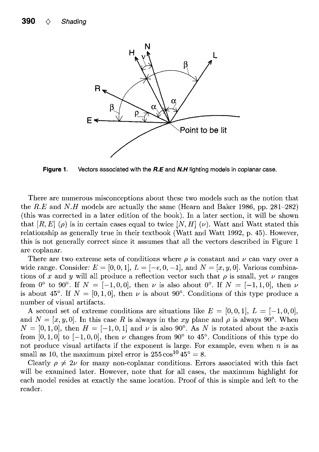
There are a few differences between this book and the previous volumes of the series.
Organizationally, the code and bibliographies are not collected at the back of the book,
but appear with the text of the corresponding article. These changes make each Gem
more self-contained. The book also differs in emphasis. Relative to the previous volumes,
I have probably stressed novelty more, and simplicity less, preferring an implementation
of a complex computer graphics algorithm over formulas from analytic geometry, for
example.
In addition to the Graphics Gems series, there are several other good sources for
practical computer graphics techniques. One of these is the column "Jim Blinn's
Corner" that appears in the journal IEEE Computer Graphics and Applications. Another is
the book A Programmer's Geometry, by Adrian Bowyer and John Woodwark (Butter-
worth's, London, 1983), which is full of analytic geometry formulas. A mix of analytic
geometry and basic computer graphics formulas is contained in the book Computer
Graphics Handbook: Geometry and Mathematics by Michael E. Mortensen (Industrial
Press, New York, 1990). Another excellent source is, of course, graphics textbooks.
Code in this book is available on the Internet by anonymous FTP from princeton.edu
(128.112.128.1) in the directory pub/Graphics/GraphicsGems/GemsIV. The code for
other Graphics Gems books is also available nearby. Bug reports should be submitted
as described in the README file there.
Paul Heckbert, March 1994

0
About the Cover
The cover: "Washday Miracle" by Eben Ostby. Copyright © 1994 Pixar.
When series editor Andrew Glassner called me to ask if I could help with a cover image
for Graphics Gems IV, there were four requirements: the image needed to tell a story; it
needed to have gems in it; it should be a computer-generated image; and it should look
good. To these parameters, I added one of my own: it should tell a story that is different
from the previous covers. Those stories were usually mystical or magical; accordingly, I
decided to take the mundane as my inspiration.
The image was created using a variety of tools, including Alias Studio; Menv, our own
internal animation system; and Photorealistic RenderMan. The appliances, table, and
basket were built in Alias. The gems were placed by a stochastic "gem-placer" running
under Menv. The house set was built in Menv. Surface descriptions were written in the
RenderMan shading language and include both procedural and painted textures.
For the number-conscious, this image was rendered at a resolution of 2048 by 2695
and contains the following:
16 lights
643 gems
30,529 lines or 2,389,896 bytes of model information
4 cycles: regular, delicate, Perma-Press, and Air Fluff
Galyn Susman did the lighting design. Andrew Glassner reviewed and critiqued, and
made the image far better as a result. Matt Martin made prepress proofs. Pixar (in
corpora Karen Robert Jackson and Ralph Guggenheim) permitted me time to do this.
Eben Ostby
Pixar
XVII

Polygons and Polyhedra
This part of the book contains five Gems on polygons and three on polyhedra. Polygons
and polyhedra are the most basic and popular geometric building blocks in computer
graphics.
1.1. Centroid of a Polygon, by Gerard Bashein and Paul R. Detmer
Gives formulas and code to find the centroid (center of mass) of a polygon. This is
useful when simulating Newtonian dynamics. Page 3.
1.2. Testing the Convexity of a Polygon, by Peter Schorn and Frederick Fisher
Gives an algorithm and code to determine if a polygon is convex, non-convex (concave
but not convex), or non-simple (self-intersecting). For many polygon operations, faster
algorithms can be used if the polygon is known to be convex. This is true when scan
converting a polygon and when determining if a point is inside a polygon, for instance.
Page 7.
1.3. An Incremental Angle Point in Polygon Test, by Kevin Weiler
1.4. Point in Polygon Strategies, by Eric Haines.
Provide algorithms for testing if a point is inside a polygon, a task known as point
inclusion testing in computational geometry. Point-in-polygon testing is a basic task
when ray tracing polygonal models, so these methods are useful for 3D as well as
2D graphics. Weiler presents a single algorithm for testing if a point lies in a concave
polygon, while Haines surveys a number of algorithms for point inclusion testing in both
convex and concave polygons, with empirical speed tests and practical optimizations.
Pages 16 and 24.

2 0 Polygons and Polyhedra
1.5. Incremental Delaunay Triangulation, by Dani Lischinski.
Gives some code to solve a very important problem: finding Delaunay triangulations
and Voronoi diagrams in 2D. These two geometric constructions are useful for
triangular mesh generation and for nearest neighbor finding, respectively. Triangular mesh
generation comes up when doing interpolation of surfaces from scattered data points,
and in finite element simulations of all kinds, such as radiosity. Voronoi diagrams are
used in many computational geometry algorithms. Page 47.
The final three Gems of this part of the book concern polyhedra: polygonal models that
are intrinsically three-dimensional.
1.6. Building Vertex Normals from an Unstructured Polygon List, by Andrew Glassner.
Solves a fairly common rendering problem: if one is given a set of polygons in raw form,
with no topological (adjacency) information, and asked to do smooth shading (Gouraud
or Phong shading) of them, one must infer topology and compute vertex normals.
Page 60.
1.7. Detecting Intersection of a Rectangular Solid and a Convex Polyhedron, by
Ned Greene.
Presents an optimized technique to test for intersection between a convex polyhedron
and a box. This is useful when comparing bounding boxes against a viewing frustum in
a rendering program, for instance. Page 74.
1.8. Fast Collision Detection of Moving Convex Polyhedra, by Rich Rabbitz.
A turn-key piece of software that solves a difficult but basic problem in physically based
animation and interactive modeling. Page 83.

01.1
Centroid of a Polygon
Gerard Bashein^ Paul R. Detmer^
Department of Anesthesiology and Department of Surgery and
Center for Bioengineering, RN-10 Center for Bioengineering, RF-25
University of Wastiington University of Washington
Seattle, WA 98195 Seattle, WA 98195
gb @locl<e. hs. Washington, edu pdetmer® u. Washington, edu
This Gem gives a rapid and accurate method to calculate the area and the coordinates
of the center of mass of a simple polygon.
Determination of the center of mass of a polygonal object may be required in the
simulation of planar mechanical systems and in some types of graphical data analysis.
When the density of an object is uniform, the center of mass is called the centroid. The
naive way of calculating the centroid, taking the mean of the x and y coordinates of
the vertices, gives incorrect results except in a few simple situations, because it actually
finds the center of mass of a massless polygon with equal point masses at its vertices. As
an example of how the naive method would fail, consider a simple polygon composed
of many small line segments (and closely spaced vertices) along one side and only a
few vertices along the other sides. The means of the vertex coordinates would then be
skewed toward the side having many vertices.
Basic mechanics texts show that the coordinates {x,y) of the centroid of a closed
planar region R are given by
JJj^ X dx dy _ fj^
A - A ^^'
^_ IlRydxdy _ ^iy
y~ A ~ A ^^'
where A is the area of R, and /U^ and iiy are the first moments of R along the x- and
^/-coordinates, respectively.
In the case where i? is a polygon given by the points {xi,yi), i = 0, ..., n, with
xo = Xn and yo = Vn, (Roberts 1965) and later (Rokne 1991), (Goldman 1991), and
others have shown a rapid method for calculating its area based upon Green's theorem
in a plane.
^Supported by grants HL42270 and HL41464 from the National Institutes of Health, Bethesda, MD.
Copyright (c) 1994 by Academic Press, Inc.
All rights of reproduction in any form reserved.
IBM ISBN 0-12-336155-9
3 Macintosh ISBN 0-12-336156-7

4 0 Polygons and Polyhedra
-• n—1
A= 'Y^ai, where o, = Xiyi+i - Xi+iyi
Janicki et al. have also shown that the first moments /Ux and jiy of a polygon can also
be found by Green's theorem (Janicki et al. 1981), which states that given continuous
functions M{x,y) and N{x,y) having continuous partial derivatives over a region R,
which is enclosed by a contour C,
c
{Mdx + Ndy) = jj^i^--^)dxdy
(3)
To evaluate the numerator of (1), let M = 0 and A^ = ^x^. Then the right side of (3)
equals /i^, and the first moment can be calculated as
Then, representing the line segments between each vertex parametrically and summing
the integrals over each line segment yields
-. n—1
Similarly, to evaluate the numerator of (2), let M = — 2^^ ^'^^ N = 0, and evaluate
the left side of (3). The result becomes
-I lb— i_
i=0
The form of the equations given above is particularly suited for numerical
computation, because it takes advantage of a common factor in the area and moments, and
because it eliminates one subtraction (and the consequent loss of accuracy) from each
term of the summation for the moments. The loss of numerical accuracy due to the
remaining subtraction can be reduced if, before calculating the centroid, the coordinate
system is translated to place its origin somewhere close to the polygon.
The techniques used above can be generalized to find volumes, centroids, and
moments of inertia of polyhedra (Lien and Kajiya 1984).
The following C code will calculate the x- and y-coordinates of the centroid and the
area of any simple (non-self-intersecting) convex or concave polygon. The algebraic
signs of both the area (output by the function) and first moments (internal variables
only) will be positive when the vertices are ordered in a counterclockwise direction in
the x-y plane, and negative otherwise. The coordinates of the centroid will have the

/. 1 Centroid of a Polygon 0 5
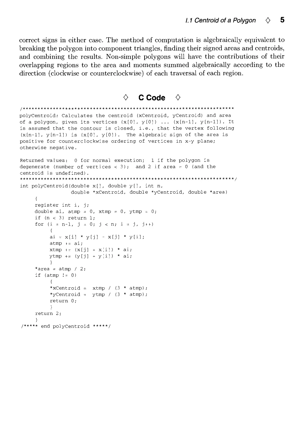
correct signs in either case. The method of computation is algebraically equivalent to
breaking the polygon into component triangles, finding their signed areas and centroids,
and combining the results. Non-simple polygons will have the contributions of their
overlapping regions to the area and moments summed algebraically according to the
direction (clockwise or counterclockwise) of each traversal of each region.
0 C Code 0
polyCentroid: Calculates the centroid (xCentroid, yCentroid) and area
of a polygon, given its vertices (x[0], y[0]) ... {x[n-l], y[n-l]). It
is assumed that the contour is closed, i.e., that the vertex following
(x[n-l], y[n-l]) is (x[0], y[0]). The algebraic sign of the area is
positive for counterclockwise ordering of vertices in x-y plane;
otherwise negative.
Returned values: 0 for normal execution; 1 if the polygon is
degenerate (number of vertices < 3); and 2 if area = 0 (and the
centroid is undefined).
int polyCentroid(double x[], double y[l, int n,
double *xCentroid, double *yCentroid, double *area)
{
register int i, j;
double ai, atmp = 0, xtmp = 0, ytmp = 0;
if (n < 3) return 1;
for (i = n-1, j = 0; j <n; i = j, j++)
{
ai = x[i] * y[j] - x[j] * y[il;
atmp += ai;
xtmp += {x[j] + x[i]) * ai;
ytmp += {y[j] + y[il) * ai;
}
*area = atmp / 2;
if (atmp != 0)
{
*xCentroid = xtmp / (3 * atmp);
*yCentroid = ytmp / (3 * atmp);
return 0;
}
return 2;
}
/***** end polyCentroid *****/

6 0 Polygons and Polyhedra
0 Bibliography 0
(Goldman 1991) Ronald N. Goldman. Area of planar polygons and volume of
polyhedra. In James Arvo, ed., Graphics Gems II, pages 170-171. Academic Press,
Boston, MA, 1991.
(Janicki et al. 1981) Joseph S. Janicki et al. Three-dimensional myocardial and
ventricular shape: A surface representation. Am. J. Physiol, 241:H1-Hll, 1981.
(Lien and Kajiya 1984) S. Lien and J. T. Kajiya. A symbolic method for calculating the
integral properties of arbitrary nonconvex polyhedra. IEEE Com,puter Graphics
& Applications, 4(10):35-41, 1984.
(Roberts 1965) L. G. Roberts. Machine perception of three-dimensional solids. In
J. P. Tippet et al., eds.. Optical and Electro-Optical Information Processing. MIT
Press, Cambridge, MA, 1965.
(Rokne 1991) Jon Rokne. The area of a simple polygon. In James Arvo, ed., Graphics
Gems II, pages 5-6. Academic Press, Boston, MA, 1991.

01.2
Testing the Convexity of a
Polygon
Peter Schorn Frederick Fisher
Institut fur Theoretische Informatik 2630 Walsh Avenue
ETH, CH-8092 Zurich, Switzerland Kubota Pacific Computer, Inc.
schorn@inf.ethz.ch Santa Clara, CA
fred@lipc.com
0 Abstract 0
This article presents an algorithm that determines whether a polygon given by the
sequence of its vertices is convex. The algorithm is implemented in C, runs in time
proportional to the number of vertices, needs constant storage space, and handles all
degenerate cases, including non-simple (self-intersecting) polygons.
Results of a polygon convexity test are useful to select between various algorithms that
perform a given operation on a polygon. For example, polygon classification could be
used to choose between point-in-polygon algorithms in a ray tracer, to choose an output
rasterization routine, or to select an algorithm for line-polygon clipping or polygon-
polygon clipping. Generally, an algorithm that can assume a specific polygon shape can
be optimized to run much faster than a general routine.
Another application would be to use this classification scheme as part of a filter
program that processes input data, such as from a tablet. Results of the filter could
eliminate complex polygons so that following routines may assume convex polygons.
0 Issues in Solving the Problem 0
The problem whose solution this article describes started out as a posting on the
USENET bulletin board 'comp.graphics' which asked for a program that could decide
whether a polygon is convex. Answering this question turned into a contest, managed
by Kenneth Sloan, which aimed at the construction of a correct and efficient program.
The most important issues discussed were:
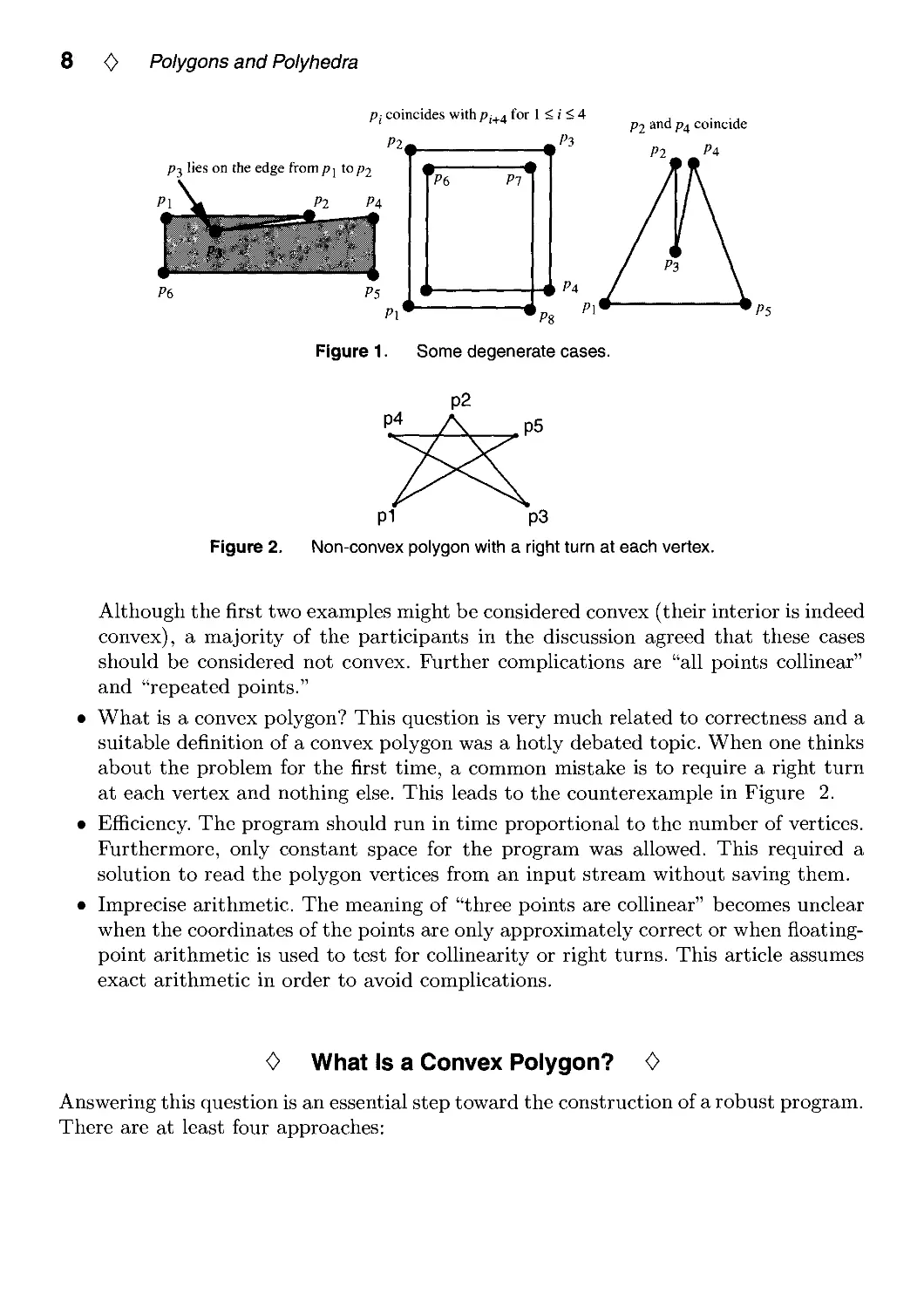
• Correctness, especially in degenerate cases. Many people quickly succeeded in
writing a program which could handle almost all cases. The challenge was a program
which works in all, even degenerate, cases. Some degenerate examples are depicted
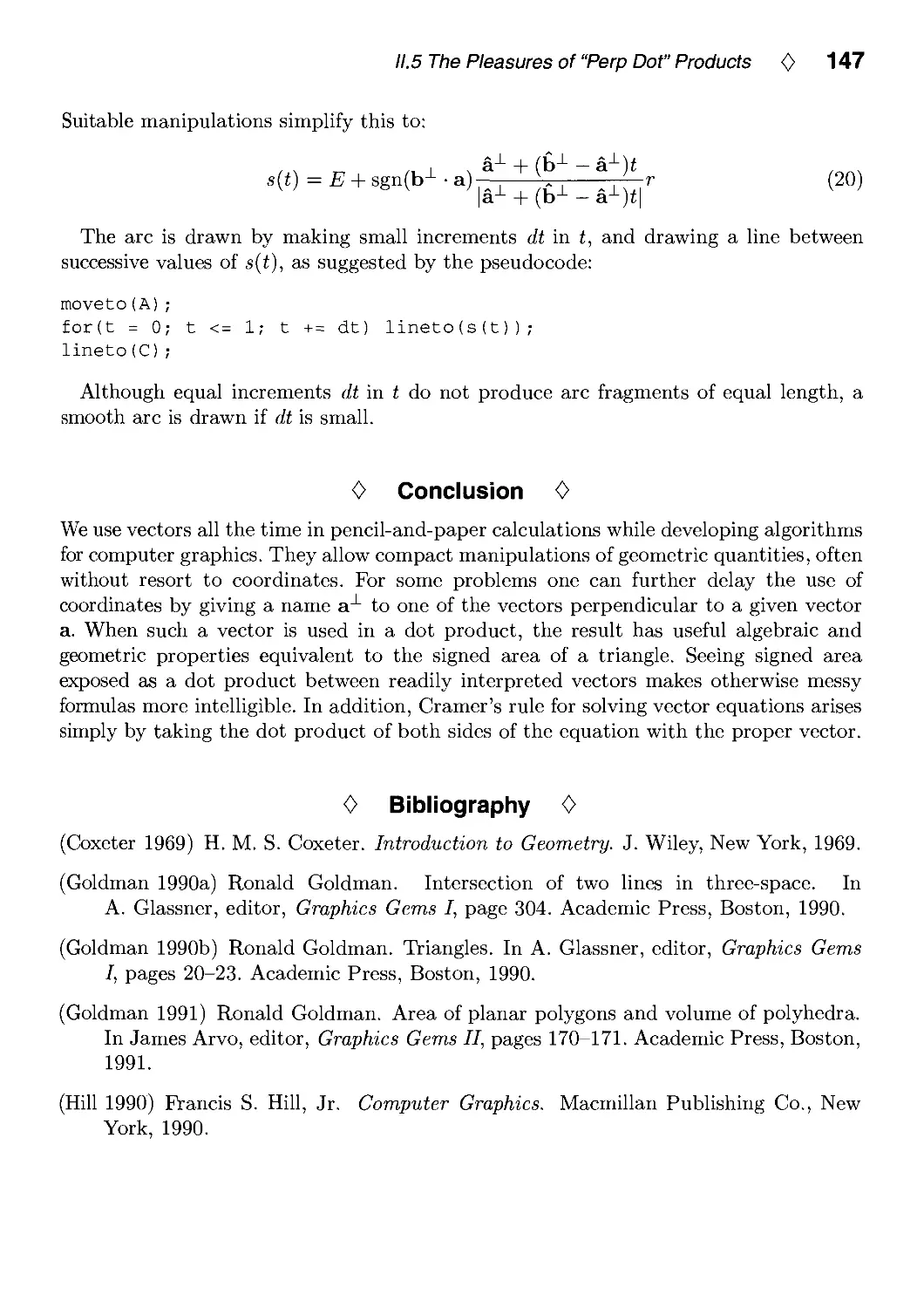
in Figure 1.
Copyright © 1994 by Academic Press, Inc.
All rights of reproduction in any form reserved.
IBM ISBN 0-12-336155-9
7 Macintosh ISBN 0-12-336156-7

8 0 Polygons and Polyhedra
P(, Pi
Pi coincides withPj.a for 1 < ( < 4 , ■ ■ .
' '^^ po and Pi coincide
Pit. ^Pi
P3 lies on the edge from p j to P2
Pi Pa
4 Pa
Figure 1. Some degenerate cases.
Figure 2.
pi p3
Non-convex polygon with a right turn at each vertex.
Although the first two examples might be considered convex (their interior is indeed
convex), a majority of the participants in the discussion agreed that these cases
should be considered not convex. Further complications are "all points coUinear"
and "repeated points."
What is a convex polygon? This question is very much related to correctness and a
suitable definition of a convex polygon was a hotly debated topic. When one thinks
about the problem for the first time, a common mistake is to require a right turn
at each vertex and nothing else. This leads to the counterexample in Figure 2.
Efficiency. The program should run in time proportional to the number of vertices.
Furthermore, only constant space for the program was allowed. This required a
solution to read the polygon vertices from an input stream without saving them.
Imprecise arithmetic. The meaning of "three points are coUinear" becomes unclear
when the coordinates of the points are only approximately correct or when
floatingpoint arithmetic is used to test for coUinearity or right turns. This article assumes
exact arithmetic in order to avoid complications.
0 What Is a Convex Polygon? 0
Answering this question is an essential step toward the construction of a robust program.
There are at least four approaches:

1.2 Testing the Convexity of a Polygon 0 9
p6
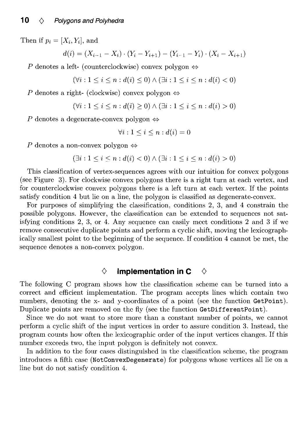
Figure 3. An undisputed convex polygon.
• The cavalier attitude: I know what a convex polygon is when I see one. For example
the polygon in Figure 3 is clearly convex.
• The "what works for me" approach: A polygon P is convex if my triangulation
routine (renderer, etc.) which expects convex polygons as input can handle P.
• The "algorithm as definition" approach: A polygon is convex if my convexity testing
program declares it as such.
• A more abstract, mathematical approach starting with the definition of a convex
set: A set S of points is convex ^
{p e S) A {q e S) ^ y\ : 0 < X < 1 : X ■ p + {1 - X) ■ q e S
This roughly means that a set of points S is convex iff for any Une drawn between
two points in the set S, then all points on the line segment are also in the set.
In the following we propose a different, formal approach, which has the following
advantages:
• It captures the intuition about a convex polygon.
• It gives a reasonable answer in degenerate cases.
• It distinguishes between clockwise- and counterclockwise orientations.
• It leads to a correct and efficient algorithm.
Classification: Given a sequence P = pi,p2, • • • ,Pn of points in the plane such that
1. n is an integer and (n > 0).
2. Consecutive vertices are different, pi j^ p^+i for 1 < i < n (we assume pn+i = pi).
3. We restrict consideration to sequences where pi is lexicographically the smallest,
i.e., pi<piior2<i<n where p < q <^ {px < qx) ^ (ipx = Qx) A (py < qy)).
4. All convex polygons are monotone polygons, that is the x-coordinate of the points
increases monotonically and then decreases monotonically. pj is the "rightmost
vertex."
3j : 1 < j < n : Pi < pi+i for 1 < i < j and pj+i < Pi ior j < i < n

10 0 Polygons and Polyhedra
Then if pi = [X^, Yj], and
d{i) = (X,_i - Xi) ■ (Y, - F,+i) - (F,_i - Yi) ■ {X, - X,+i)
P denotes a left- (counterclockwise) convex polygon <^
(Vi : 1 < i < n : d{i) < 0) A (3i : 1 < i < n : d{i) < 0)
P denotes a right- (clockwise) convex polygon <^
(Vi : 1 < i < n : d{i) > 0) A (3i : 1 < i < n : d{i) > 0)
P denotes a degenerate-convex polygon ^
yi:l<i<n: d(i) = 0
P denotes a non-convex polygon ^
{3i:l<i<n: d{i) < 0) A (3i : 1 < i < n : d{i) > 0)
This classification of vertex-sequences agrees with our intuition for convex polygons
(see Figure 3). For clockwise convex polygons there is a right turn at each vertex, and
for counterclockwise convex polygons there is a left turn at each vertex. If the points
satisfy condition 4 but lie on a line, the polygon is classified as degenerate-convex.
For purposes of simplifying the classification, conditions 2, 3, and 4 constrain the
possible polygons. However, the classification can be extended to sequences not
satisfying conditions 2, 3, or 4. Any sequence can easily meet conditions 2 and 3 if we
remove consecutive duplicate points and perform a cyclic shift, moving the
lexicographically smallest point to the beginning of the sequence. If condition 4 cannot be met, the
sequence denotes a non-convex polygon.
0 Implementation in C 0
The following C program shows how the classification scheme can be turned into a
correct and efficient implementation. The program accepts lines which contain two
numbers, denoting the x- and y-coordinates of a point (see the function GetPoint).
Duplicate points are removed on the fly (see the function GetDifferentPoint).
Since we do not want to store more than a constant number of points, we cannot
perform a cyclic shift of the input vertices in order to assure condition 3. Instead, the
program counts how often the lexicographic order of the input vertices changes. If this
number exceeds two, the input polygon is definitely not convex.
In addition to the four cases distinguished in the classification scheme, the program
introduces a fifth case (NotConvexDegenerate) for polygons whose vertices all lie on a
line but do not satisfy condition 4.

1.2 Testing the Convexity of a Polygon <> 11
<> Program to Classify a Polygon's Shape 0
#lnclude <stdlo.h>
typedef enum { NotConvex, NotConvexDegenerate,
ConvexDegenerate, ConvexCCW, ConvexCW } PolygonClass;
typedef struct { double x, y; } Polnt2d;
Int WhichSide(p, q, r)
Point2d p, q, r;
/* Given a directed line pq, determine */
/* whether qr turns CW or CCW. */
double result;
result = (p.x - q.x) * (q.y - r.y) - (p.y - q.y) * (q.x - r.x);
If (result < 0) return -1; /* q lies to the left (qr turns CW).
if (result > 0) return 1; /* q lies to the right (qr turns CCW).
return 0;
/* q lies on the line from p to r.
int Compare(p, q)
Point2d p, q;
/* Lexicographic comparison of p and q
if (p.x < q.x) return -1
if (p.x > q.x) return 1
if (p.y < q.y) return -1
if (p.y > q.y) return 1
return 0;
}
int GetPoint(f, p)
FILE *f;
Point2d *p;
{
/* p is less than q.
/* p is greater than q.
/* p is less than q.
/* p is greater than q.
/* p is equal to q.
return !feof(f) && (2
/* Read p's X- and y-coordinates from f */
/* and return true, iff successful. */
fscanf(f, "%lf%lf, &(p->x), &(p->y)));
}
int GetDifferentPoint(f, previous, next)
FILE *f; /* Read next point into 'next' until it */
Point2d previous, *next; /* is different from 'previous' and */
{ /* return true iff successful. */
int eof;
while((eof = GetPoint(f, next)) && (Compare(previous, *next) == 0));
return eof;
}
/* CheckTriple tests three consecutive points for change of direction
* and for orientation.
*/
#define CheckTriple \
if ( (thisDir = Compare(second, third)) == -curDir ) \
++dirChanges; \
CurDir = thisDir; \
if ( thisSign = WhichSide(first, second, third) ) { \

12 <> Polygons and Polyhedra
if ( angleSign == -thisSign )
return NotConvex;
angleSign = thisSign;
}
first = second; second = third;
/* Classify the polygon vertices on file 'f' according to: 'NotConvex' */
/* 'NotConvexDegenerate', 'ConvexDegenerate', 'ConvexCCW, 'ConvexCW. */
PolygonClass ClassifyPolygon(f)
FILE *f;
{
int curDir, thisDir, thisSign, angleSign = 0, dirChanges = 0;
PolygonClass result;
Point2d first, second, third, saveFirst, saveSecond;
if ( !GetPoint(f, &first) II !GetDif f erentPoint (f, first, Scsecond) )
return ConvexDegenerate;
saveFirst = first; saveSecond = second;
curDir = Compare(first, second);
while( GetDifferentPoint(f, second, &third) ) {
CheckTriple;
}
/* Must check that end of list continues back to start properly. */
if ( Compare(second, saveFirst) ) {
third = saveFirst; CheckTriple;
}
third = saveSecond; CheckTriple;
if ( dirChanges > 2 ) return angleSign ? NotConvex : NotConvexDegenerate;
if ( angleSign > 0 ) return ConvexCCW;
if ( angleSign < 0 ) return ConvexCW;
return ConvexDegenerate;
mt main()
{
switch ( ClassifyPolygon(stdin) ) {
case NotConvex: fprintf( stderr,"Not ConvexXn"),
exit(-1)
case NotConvexDegenerate: fprintf(
exit(-1)
case ConvexDegenerate: fprintf(
exit( 0)
fprintf(
exit( 0)
fprintf(
exit( 0)
case ConvexCCW:
case ConvexCW:
break;
stderr, "Not Convex DegenerateXn") ;
break;
stderr,"Convex DegenerateXn");
break;
stderr,"Convex Counter-ClockwiseXn") ,
break;
stderr,"Convex ClockwiseXn");
break;

1.2 Testing the Convexity of a Polygon <> 13
0 Optimizations <>
The previous code was chosen for its conciseness and readabiUty. Other versions of the
code were written which accept a vertex count and pointer to an array of vertices. Given
this interface, it is possible to obtain good performance measurements by timing a large
number of calls to the polygon classification routine.
Variations of the code presented have resulted in a two to four times performance
increase, depending on the polygon shape. Optimizations for a particular machine or
programming language will undoubtedly produce different results. Some considerations
are:
• Convert each of the routines to macro definitions.
• Instead of keeping track of the first, second, and third points, keep track of the
previous delta (second — first), and a current delta (third — second). This will
speed up parts of the algorithm: The macro Compare needs only compare two
numbers with zero, instead of four numbers with each other; the routine for getting
a different point calculates the delta as it determines if the new point is different;
the cross product calculation uses the deltas directly instead of subtracting vertices
each time; the comparison for the WhichSide routine may be moved up to the
CheckTriple routine to save a comparison at the expense of a little more code;
and preparing to examine the next point requires three moves instead of four.
• Checking for less than three vertices is possible, but generally slows down the other
cases.
• Every time the variable dirChanges is incremented, it would be possible to check
if the number is now greater than two. This will slow down the convex cases, but
makes it possible to exit early for polygons which violate classification condition
4. If it is important to distinguish between NotConvex and NotConvexDegenerate,
this optimization may not be used.
<> Reasonably Optimized Routine to Classify a Polygon's Shape <>
/*
. . . code omitted which reads polygon, stores in an array, and calls
classifyPolygon2()
*/
typedef double Number; /* float or double */
#define ConvexCompare(delta) \
( (delta[0] > 0) ? -1 : /* x coord diff, second pt > first pt */\

14 <> Polygons and Polyhedra
(delta[0] < 0) ? 1
(delta[l] > 0) ? -1
(delta[l] < 0) ? 1
0 )
/* X coord diff, second pt < first pt */\
/* X coord same, second pt > first pt */\
/* X coord same, second pt > first pt */\
/* second pt equals first point */
#define ConvexGetPointDelta(delta, pprev, pcur )
/* Given a previous point 'pprev', read a new point into
/* and return delta in 'delta'.
pcur = pVert[iread++];
delta[0] = pcur[0] - pprev[0];
delta[l] = pcur[l] - pprev[l];
'pcur'
/
/
\
\
\
\
\
#define ConvexCross(p, q) p[0] * q[l] - p[l]
q[0]
#define ConvexCheckTriple
if ( (thisDir = ConvexCompare(dcur))
++dirChanges;
-curDir ) {
The following line will optimize for polygons that are
not convex because of classification condition 4,
otherwise, this will only slow down the classification,
if ( dirChanges > 2 ) return NotConvex;
curDir
thisDir;
cross = ConvexCross(dprev, dcur);
if ( cross
0 )
else if (cross <
{ if ( angleSign ==
angleSign = 1;
}
0) { if (angleSign
angleSign =
-1 ) return NotConvex;
1) return NotConvex;
}
pSecond -
dprev[0]
dprev[1]
pThird;
= dcur[0]
= dcur[l]
Remember ptr to current point.
Remember current delta.
'/ \
\
\
\
\
\
\
\
\
\
\
\
\
classifyPolygon2( nvert, pVert )
int nvert;
Number pVert[][2];
/* Determine polygon type, return one of:
* NotConvex, NotConvexDegenerate,
* ConvexCCW, ConvexCW, ConvexDegenerate
V
{
int curDir, thisDir, dirChanges = 0,
angleSign = 0, iread, endOfData;
Number *pSecond, *pThird, *pSaveSecond, dprev[2], dcur[2], cross;
/* if ( nvert <= 0 ) return error;
if you care */
/* Get different point, return if less than 3 diff points. */
if ( nvert < 3 ) return ConvexDegenerate;
iread = 1;
while ( 1 ) {
ConvexGetPointDelta( dprev, pVert[0], pSecond );

1.2 Testing the Convexity of a Polygon <> 15
if ( dprev[0] I I dprev[l] ) break;
/* Check if out of points. Check here to avoid slowing down cases
* without repeated points.
*/
if ( iread >= nvert ) return ConvexDegenerate;
}
pSaveSecond = pSecond;
curDir = ConvexCompare(dprev); /* Find initial direction */
while ( iread < nvert ) {
/* Get different point, break if no more points */
ConvexGetPointDelta(dcur, pSecond, pThird );
if ( dcur[0] == 0.0 && dcur[l] == 0.0 ) continue;
ConvexCheckTriple; /* Check current three points */
}
/* Must check for direction changes from last vertex back to first */
pThird = pVert[0]; /* Prepare for 'ConvexCheckTriple' ^
dcur[0] = pThird[0] - pSecond[0];
dcur[l] = pThird[l] - pSecond[l];
if ( ConvexCompare(dcur) ) {
ConvexCheckTriple;
}
/* and check for direction changes back to second vertex */
dcur[0] = pSaveSecond[0] - pSecond[0];
dcur[l] = pSaveSecond[1] - pSecond[1];
ConvexCheckTriple; /* Don't care about 'pThird' now */
/* Decide on polygon type given accumulated status */
if ( dirChanges > 2 )
return angleSign ? NotConvex ; NotConvexDegenerate;
if ( angleSign > 0 ) return ConvexCCW;
if ( angleSign < 0 ) return ConvexCW;
return ConvexDegenerate;
0 Acknowledgments <>
We are grateful to the participants of the electronic mail discussion: Gavin Bell, Wayne
Boucher, Laurence James Edwards, Eric A. Haines, Paul Heckbert, Steve Hollasch, Tor-
ben jEgidius Mogensen, Joseph O'Rourke, Kenneth Sloan, Tom Wright, and Benjamin
Zhu.

01.3
An Incremental Angle Point in
Polygon Test
Kevin Weiler
Autodesk Inc.
2320 Marinship Way
Sausalito, CA 94965
kjw @ autodesk. com
This algorithm can determine whether a given test point is inside of, or outside of,
a given polygon boundary composed of straight line segments. The algorithm is not
sensitive to whether the polygon is concave or convex or whether the polygon's vertices
are presented in a clockwise or counterclockwise order. Extensions allow the algorithm
to handle polygons with holes and non-simple polygons. Only four bits of precision are
required for all of the incremental angle calculations.
<> Introduction <>
There are two commonly used algorithms for determining whether a given test point is
inside or outside of a polygon.
The first, the semi-infinite line technique, extends a semi-infinite line from the test
point outward, and counts the number of intersections of the edges of the polygon
boundary with the semi-infinite line. An odd number of intersections indicates the
point is inside the polygon, while an even number (including zero) indicates the point
is outside the polygon.
The second, the incremental angle technique, uses the angle of the vertices of the
polygon relative to the point being tested, where there is a total angle of 360 degrees
all the way around the point. For each vertex of the polygon, the difference angle (the
incremental angle) between the angle of that vertex of the polygon and the angle of the
next vertex of the polygon, as viewed from the test point, is added to a running sum.
If the final sum of the incremental angles is plus or minus 360 degrees, the polygon
surrounds the test point and the point is inside of the polygon. If the sum is 0 degrees,
the point is outside of the polygon.
What is less commonly known about the incremental angle technique is that only
four bits of precision are required for all of the incremental angle calculations, greatly
simplifying the necessary calculations. The angle value itself requires only two bits of
precision, lending itself to a quadrant technique where the quadrants are numbered
Copyright © 1994 by Academic Press, Inc.
All rights of reproduction in any form reserved.
IBM ISBN 0-12-336155-9
Macintosh ISBN 0-12-336156-7 1 6

1.3 An Incremental Angle Point in Polygon Test <> 17
from 0 to 3. The incremental or delta angle requires an additional sign bit to indicate
clockwise or counterclockwise direction, for a total of three bits to represent the
incremental angle itself. The accumulated angle requires four bits total: three to represent
the magnitude, ranging from 0 to 4, plus a sign bit.
The following algorithm describes a four-bit precision incremental angle point in
polygon test. Extensions for polygons with holes and for degenerate polygons are also described.
The algorithm described was inspired by the incremental angle surrounder test
sometimes used for the Warnock hidden surface removal algorithm. That surrounder
algorithm determines if a polygon surrounds rectangular screen areas by partitioning the
space around the rectangular window using an eight neighbor partitioning technique
(Newman and Sproull 1973, pp. 520-521, 526-527), (Rogers 1985, pp. 249-251). If one
shrinks the central rectangular window of that partitioning scheme down to a point
(shrinking the rectangular partitions directly above and below and to the left and right
of the window down to lines), the partitioning becomes a quadrant style division of the
space around the point. This reduces the precision of angle calculations needed and
simplifies the algorithm to the point in polygon test presented here.
Further discussion and comparisons of point in polygon techniques can be found in
Eric Haines' article in this volume (Haines 1994).
<> Preliminaries 0
For sake of completeness, before describing the algorithm, simple type definitions used
in the following code as well as a typical definition for a polygon representation are
given below.
/* type for quadrant id's, incremental angles, accumulated angle values */
typedef short quadrant_type;
/* type for result value from point in polygon test */
typedef enum pt_poly_relation {INSIDE, OUTSIDE} pt_poly_relation;
/* polygon vertex definition */
typedef struct vertex_struct {
double x,y; /* coordinate values */
struct vertex_struct *next; /* circular singly linked list from poly */
} vertex, *vertex_ptr;
/* polygon definition */
typedef struct polygon_struct {
vertex_ptr last; /* pointer to end of circular vertex list */
} polygon, *polygon_ptr;
/* polygon vertex access */
#define polygon_get_vertex(poly, vertex) \
((vertex == NULL) ? poly->last->next : vertex->next)
The quadrant and return result types are self-explanatory.

18 <> Polygons and Polyhedra
Polygon vertices are regarded as structures that allow direct access of the X and Y
coordinate values in C via vertex->x and vertex->y structure member dereferencing.
Polygons are treated here as objects that have a single access routine:
polygon_get_vertex(poly, vertex), where poly specifies a pointer to the polygon. If
vertex is NULL, the function will return a pointer to an arbitrary vertex of the polygon.
Otherwise, if vertex is a pointer to a given vertex of the polygon, the function will return
a pointer to the next vertex in the ordered circular list of vertices of the polygon. Given
the list representation of the polygons as described here, polygon vertices are regarded
as unique even if their coordinate values are not.
0 The Algorithm 0
The basic idea of the algorithm, as previously stated, is to accumulate the sum of the
incremental angles between the vertices of the polygon as viewed from the test point,
and then see if the angles add up to the logical equivalent of a full 360 degrees, meaning
the point is surrounded by the polygon.
The algorithm is presented here in four small pieces. First, a macro to determine
the quadrant angle of a polygon vertex is presented. Second, a macro to determine
x-intercepts of polygon edges is presented. Third, a macro to adjust the angle delta is
presented. Fourth, the main point in polygon test routine is presented.
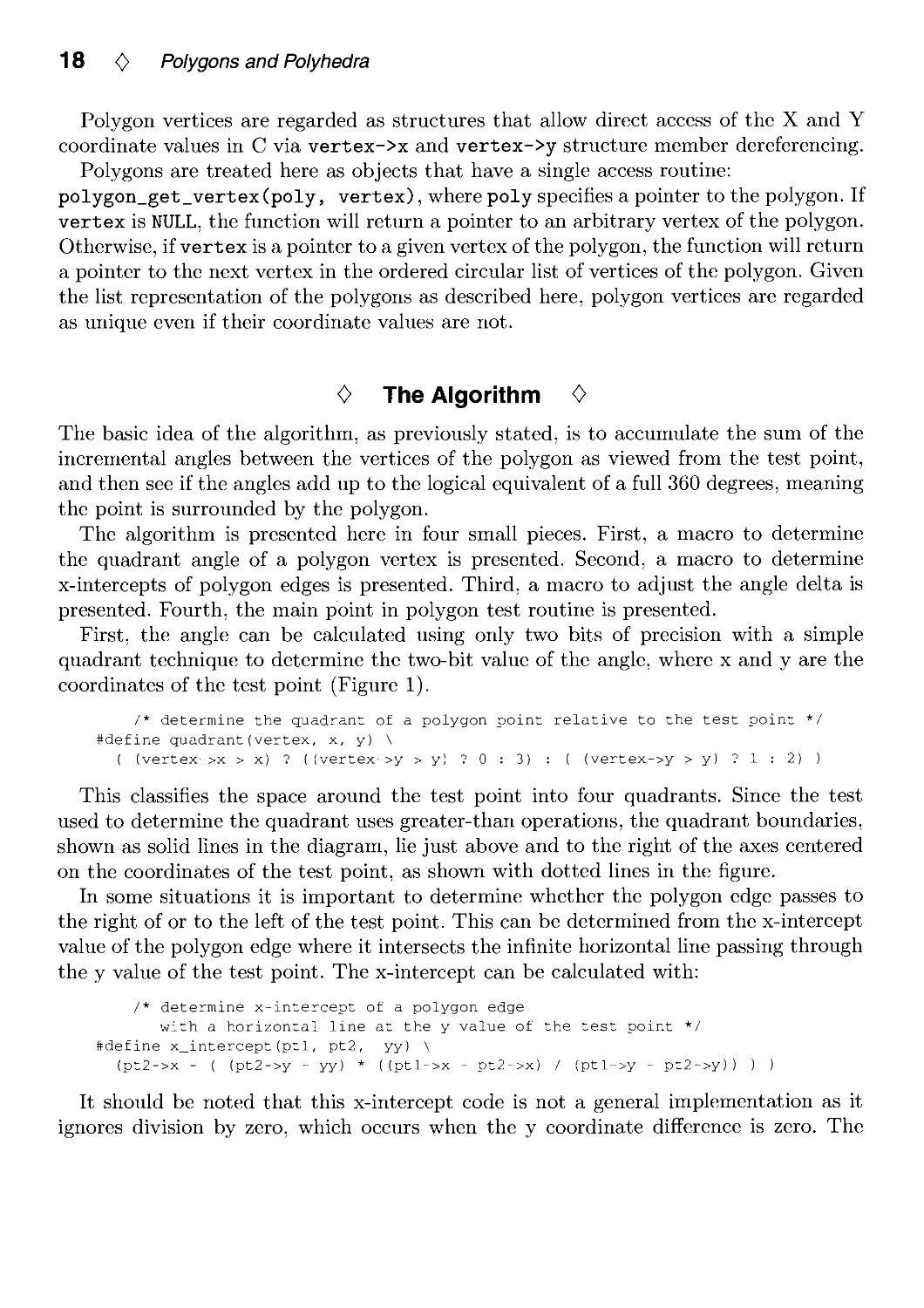
First, the angle can be calculated using only two bits of precision with a simple
quadrant technique to determine the two-bit value of the angle, where x and y are the
coordinates of the test point (Figure 1).
/* determine the quadrant of a polygon point relative to the test point */
#define quadrant(vertex, x, y) \
( (vertex->x > x) ? ((vertex->y > y) ? 0 : 3) : ( (vertex->y > y) ? 1 : 2) )
This classifies the space around the test point into four quadrants. Since the test
used to determine the quadrant uses greater-than operations, the quadrant boundaries,
shown as solid lines in the diagram, lie just above and to the right of the axes centered
on the coordinates of the test point, as shown with dotted lines in the figure.
In some situations it is important to determine whether the polygon edge passes to
the right of or to the left of the test point. This can be determined from the x-intercept
value of the polygon edge where it intersects the infinite horizontal line passing through
the y value of the test point. The x-intercept can be calculated with:
/* determine x-intercept of a polygon edge
with a horizontal line at the y value of the test point */
#define x_intercept(ptl, pt2, yy) \
(pt2->x - ( (pt2->y - yy) * ((ptl->x - pt2->x) / (ptl->y - pt2->y)) ) )
It should be noted that this x-intercept code is not a general implementation as it
ignores division by zero, which occurs when the y coordinate difference is zero. The

1.3 An Incremental Angle Point in Polygon Test <> 19
quadrant 1
quadrant 0
test point
quadrant 2
quadrant 3
Figure 1. Quadrants.
implementation is adequate for our purposes here, however, as it will never be called
under this condition.
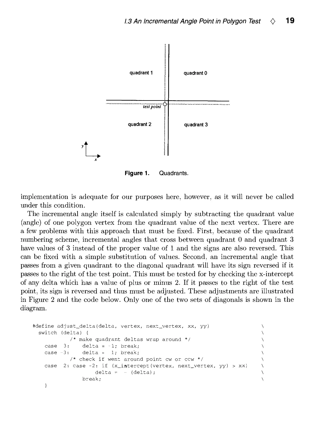
The incremental angle itself is calculated simply by subtracting the quadrant value
(angle) of one polygon vertex from the quadrant value of the next vertex. There are
a few problems with this approach that must be fixed. First, because of the quadrant
numbering scheme, incremental angles that cross between quadrant 0 and quadrant 3
have values of 3 instead of the proper value of 1 and the signs are also reversed. This
can be fixed with a simple substitution of values. Second, an incremental angle that
passes from a given quadrant to the diagonal quadrant will have its sign reversed if it
passes to the right of the test point. This must be tested for by checking the x-intercept
of any delta which has a value of plus or minus 2. If it passes to the right of the test
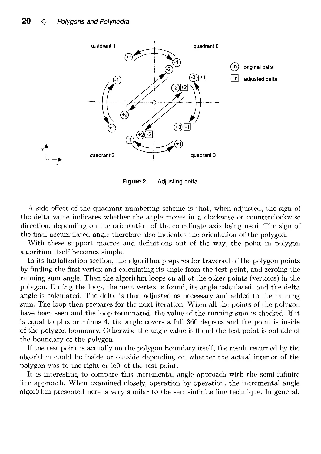
point, its sign is reversed and thus must be adjusted. These adjustments are illustrated
in Figure 2 and the code below. Only one of the two sets of diagonals is shown in the
diagram.
#define adjust_delta(delta, vertex, next_vertex, xx, yy)
switch (delta) {
/* make quadrant deltas wrap around */
case 3: delta = -1; break;
case -3: delta = 1; break;
/* check if went around point cw or ccw */
case 2: case -2: if (x_intercept(vertex, next_vertex,
delta = - (delta);
break;
}
yy) > xx)

20 <> Polygons and Polyhedra
quadrant 1
quadrant 0
quadrant 2
(^t) original delta
r"l adjusted delta
quadrant 3
Figure 2. Adjusting delta.
A side effect of the quadrant numbering scheme is that, when adjusted, the sign of
the delta value indicates whether the angle moves in a clockwise or counterclockwise
direction, depending on the orientation of the coordinate axis being used. The sign of
the final accumulated angle therefore also indicates the orientation of the polygon.
With these support macros and definitions out of the way, the point in polygon
algorithm itself becomes simple.
In its initialization section, the algorithm prepares for traversal of the polygon points
by finding the first vertex and calculating its angle from the test point, and zeroing the
running sum angle. Then the algorithm loops on all of the other points (vertices) in the
polygon. During the loop, the next vertex is found, its angle calculated, and the delta
angle is calculated. The delta is then adjusted as necessary and added to the running
sum. The loop then prepares for the next iteration. When all the points of the polygon
have been seen and the loop terminated, the value of the running sum is checked. If it
is equal to plus or minus 4, the angle covers a full 360 degrees and the point is inside
of the polygon boundary. Otherwise the angle value is 0 and the test point is outside of
the boundary of the polygon.
If the test point is actually on the polygon boundary itself, the result returned by the
algorithm could be inside or outside depending on whether the actual interior of the
polygon was to the right or left of the test point.
It is interesting to compare this incremental angle approach with the semi-infinite
line approach. When examined closely, operation by operation, the incremental angle
algorithm presented here is very similar to the semi-infinite line technique. In general,

1.3 An Incremental Angle Point in Polygon Test <> 21
the incremental angle method takes a constant amount of time per vertex regardless of
axis crossings of the polygon edges (the exception is when the vertices of the polygon
edge are in diagonal quadrants, which takes the same amount of time for both
approaches). The semi-infinite line technique performs more operations when its preferred
axis is crossed, and fewer operations when the other axis is crossed. To put it a
different way, the semi-infinite line technique has both deeper and shallower code branch
alternatives than the incremental angle technique presented depending on whether its
preferred axis is crossed or not. Because of this variable behavior, worst case scenarios
can be constructed to make either algorithm perform better than the other.
Performance comparisons done by Haines (Haines 1994) give statistics that show the
incremental angle technique presented here to be slower than the semi-infinite line
technique. Some of this performance difference will be reduced if the C compiler performs
case statement optimizations which utilize indexed jump tables.
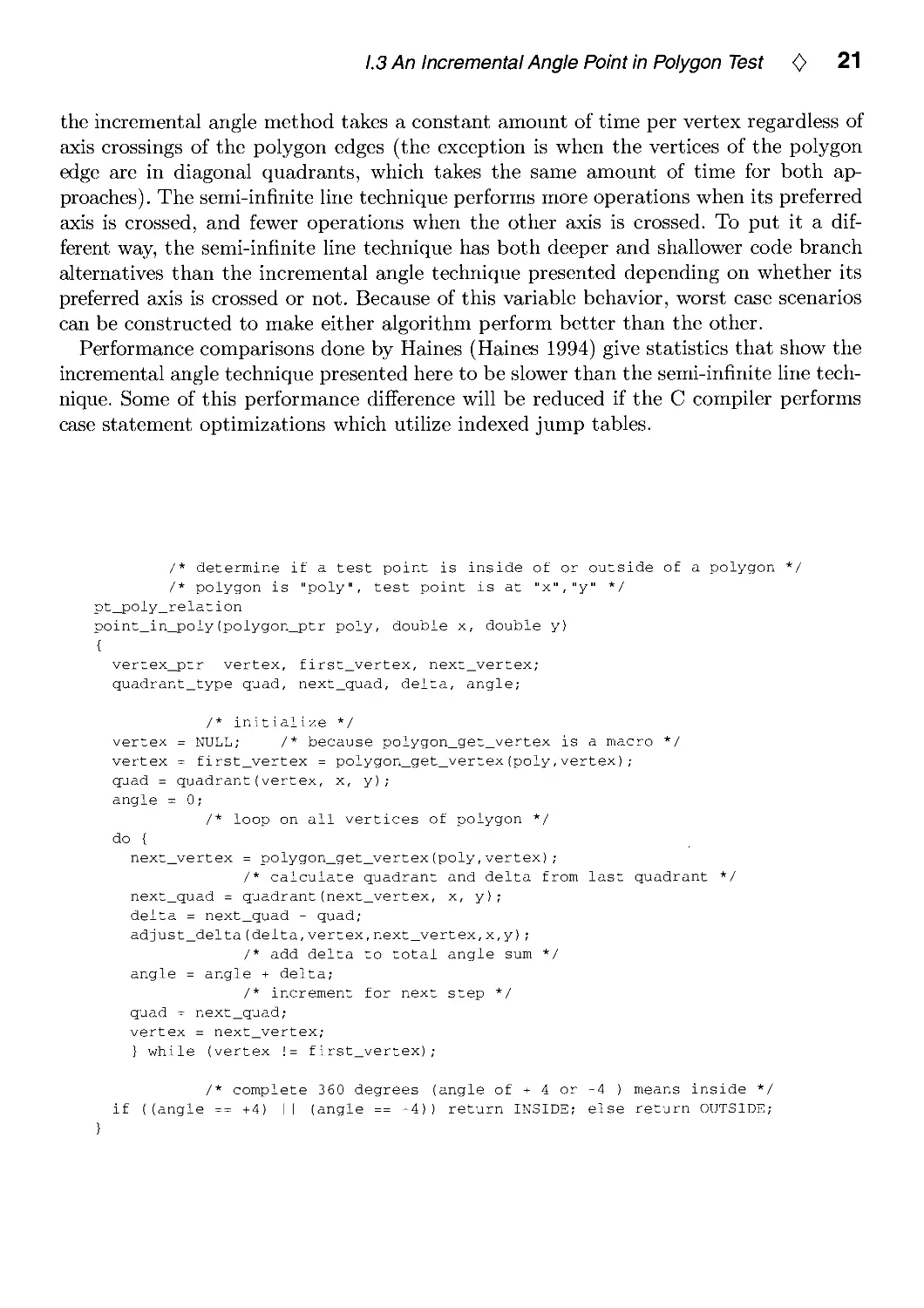
/* determine if a test point is inside of or outside of a polygon */
/* polygon is "poly", test point is at "x","y" */
pt_poly_relation
point_in_poly(polygon_ptr poly, double x, double y)
{
vertex_ptr vertex, first_vertex, next_vertex;
quadrant_type quad, next_quad, delta, angle;
/* initialize */
vertex = NULL; /* because polygon_get_vertex is a macro */
vertex = first_vertex = polygon_get_vertex(poly,vertex);
quad = quadrant(vertex, x, y);
angle = 0;
/* loop on all vertices of polygon */
do {
next_vertex = polygon_get_vertex(poly,vertex);
/* calculate quadrant and delta from last quadrant */
next_quad = quadrant(next_vertex, x, y);
delta = next_quad - quad;
adjust_delta(delta,vertex,next_vertex,x,y);
/* add delta to total angle sum */
angle = angle + delta;
/* increment for next step */
quad = next_quad;
vertex = next_vertex;
} while (vertex != first_vertex);
/* complete 360 degrees (angle of + 4 or -4 ) means inside */
if ((angle == +4) I I (angle == -4)) return INSIDE; else return OUTSIDE;
}

22 <> Polygons and Polyhedra
<> Extension for Polygons with Holes 0
In order to determine whether a test point is inside of or outside of a polygon which has
holes, the point in polygon test needs to be applied separately to each of the polygon's
boundaries. It is preferable to start with the outermost boundary of the polygon, since
the polygon's area is in most applications likely to be smaller than the total area in which
the test point might lie. If the test point is outside of this polygon boundary, then it is
outside of the entire polygon. If it is inside, then each hole boundary needs to be checked.
If the test point is inside any of the hole boundaries, then the test point is outside of the
entire polygon and checking can stop immediately. If the test point is outside of every
hole boundary (as well as being inside the outermost boundary), then the point is inside
of the polygon. Note that because the point in polygon test presented is insensitive to
whether the polygon boundaries are clockwise or counterclockwise, both the outermost
polygon boundary and the hole boundaries may be of any orientation. For polygons
with holes, however, the algorithm must be told which boundary is the outermost
boundary (some polygon representations encode this information in the orientation of
the boundaries).
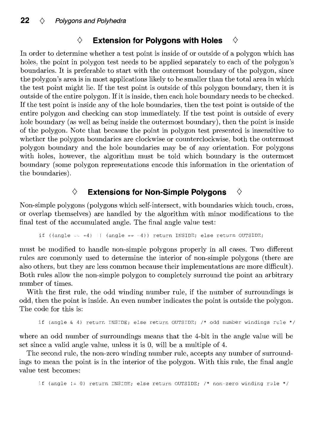
0 Extensions for Non-Simple Polygons 0
Non-simple polygons (polygons which self-intersect, with boundaries which touch, cross,
or overlap themselves) are handled by the algorithm with minor modifications to the
final test of the accumulated angle. The final angle value test:
if ((angle == +4) I I (angle == -4)) return INSIDE; else return OUTSIDE;
must be modified to handle non-simple polygons properly in all cases. Two different
rules are commonly used to determine the interior of non-simple polygons (there are
also others, but they are less common because their implementations are more difficult).
Both rules allow the non-simple polygon to completely surround the point an arbitrary
number of times.
With the first rule, the odd winding number rule, if the number of surroundings is
odd, then the point is inside. An even number indicates the point is outside the polygon.
The code for this is:
if (angle & 4) return INSIDE; else return OUTSIDE; /* odd number windings rule */
where an odd number of surroundings means that the 4-bit in the angle value will be
set since a valid angle value, unless it is 0, will be a multiple of 4.
The second rule, the non-zero winding number rule, accepts any number of
surroundings to mean the point is in the interior of the polygon. With this rule, the final angle
value test becomes:
if (angle != 0) return INSIDE; else return OUTSIDE; /* non-zero winding rule */

1.3 An Incremental Angle Point in Polygon Test <> 23
Of course, the accumulated angle value can no longer be contained within a four-bit
number under these conditions, but this characteristic is probably little more than a
curiosity anyway, except for its original effect of reducing angle calculations to simple
quadrant testing.
<> Bibliography <>
(Haines 1994) Eric Haines. Point in Polygon Strategies. In Paul Heckbert, editor,
Graphics Gems IV, 24-46. Academic Press, Boston, 1994.
(Newman and Sproull 1973) William Newman and Robert Sproull. Principles of
Interactive Computer Graphics, 1st edition. McGraw-Hill, New York, 1973.
(Rogers 1985) David Rogers. Procedural Elements for Computer Graphics. McGraw-
Hill, New York, 1985.

01.4
Point in Polygon Strategies
Eric Haines
3D/Eye Inc.
1050 Craft Road
Ithaca, NY 14850
erich@eye.com
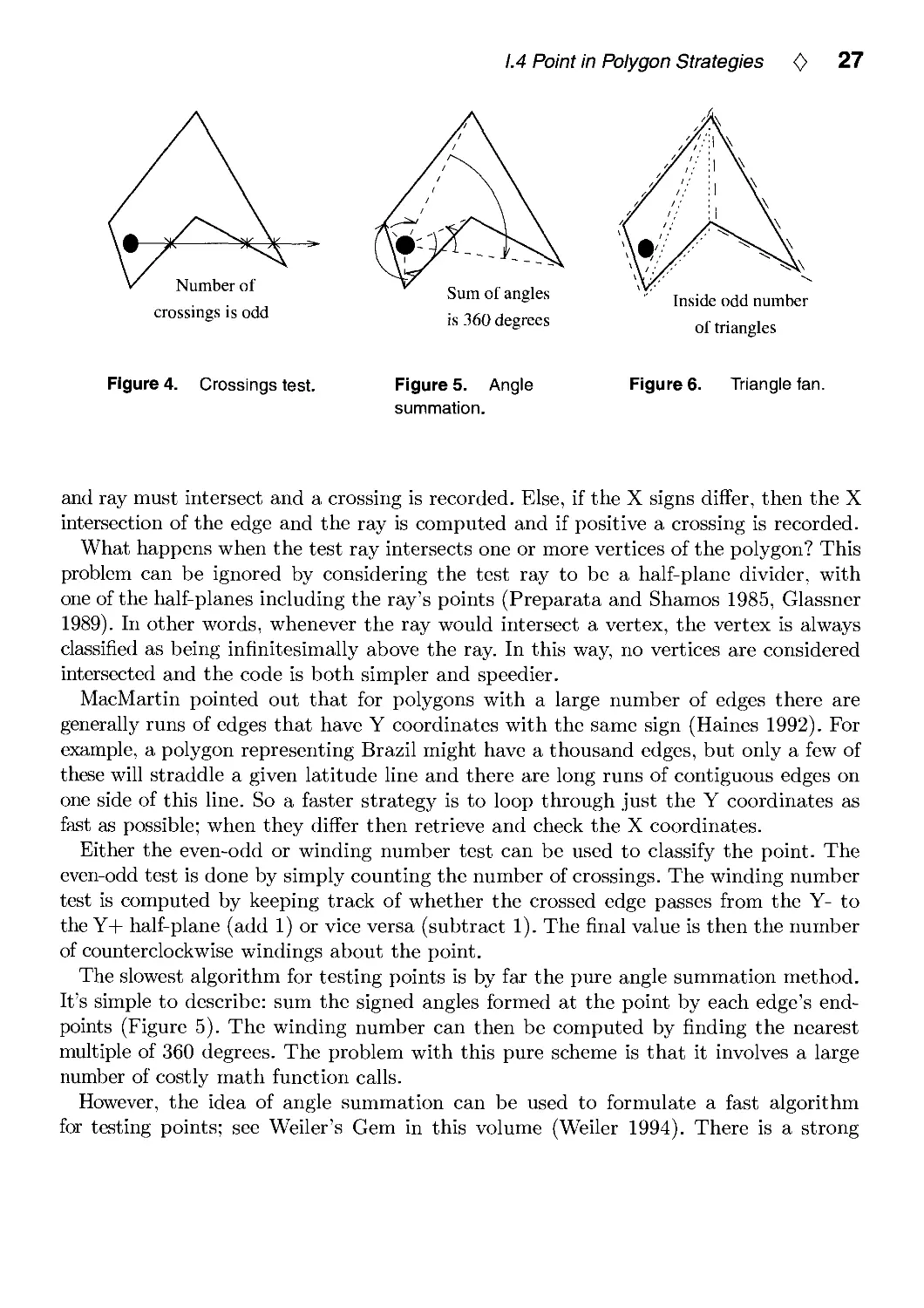
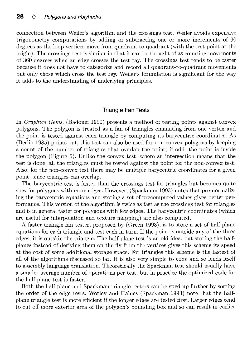
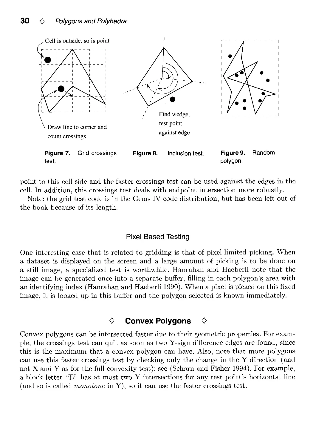
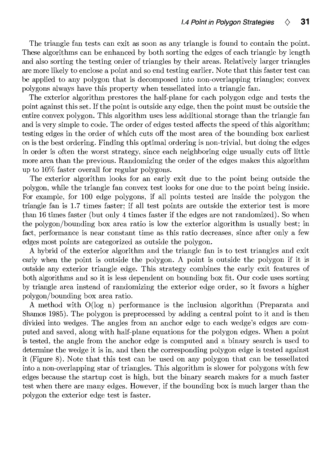
Testing whether a point is inside a polygon is a basic operation in computer graphics.
This Gem presents a variety of efficient algorithms. No single algorithm is the best in
all categories, so the capabilities of the better algorithms are compared and contrasted.
The variables examined are the different types of polygons, the amount of memory
used, and the preprocessing costs. Code is included in this article for several of the best
algorithms; the Gems IV distribution includes code for all the algorithms discussed.
0 Introduction 0
The motivation behind this Gem is to provide practical algorithms that are simple to
implement and are fast for typical polygons. In applied computer graphics we usually
want to check a point against a large number of triangles and quadrilaterals and
occasionally test complex polygons. When dealing with floating-point operations on these
polygons we do not care if a test point exactly on an edge is classified as being inside
or outside, since these cases are normally extremely rare.
In contrast, the field of computational geometry has a strong focus on the order of
complexity of an algorithm for all polygons, including pathological cases that are rarely
encountered in real applications. The order of complexity for an algorithm in
computational geometry may be low, but there is usually a large constant of proportionality
or the algorithm itself is difficult to implement. Either of these conditions makes the
algorithm unfit for use. Nonetheless, some insights from computational geometry can be
applied to the testing of various sorts of polygons and can also shed light on connections
among seemingly different algorithms.
Readers that are only interested in the results should skip to the "Conclusions"
section.
Copyright © 1994 by Academic Press, Inc.
All rights of reproduction in any form reserved.
IBM ISBN 0-12-336155-9
Macintosh ISBN 0-12-336156-7 24

1.4 Point in Polygon Strategies <> 25
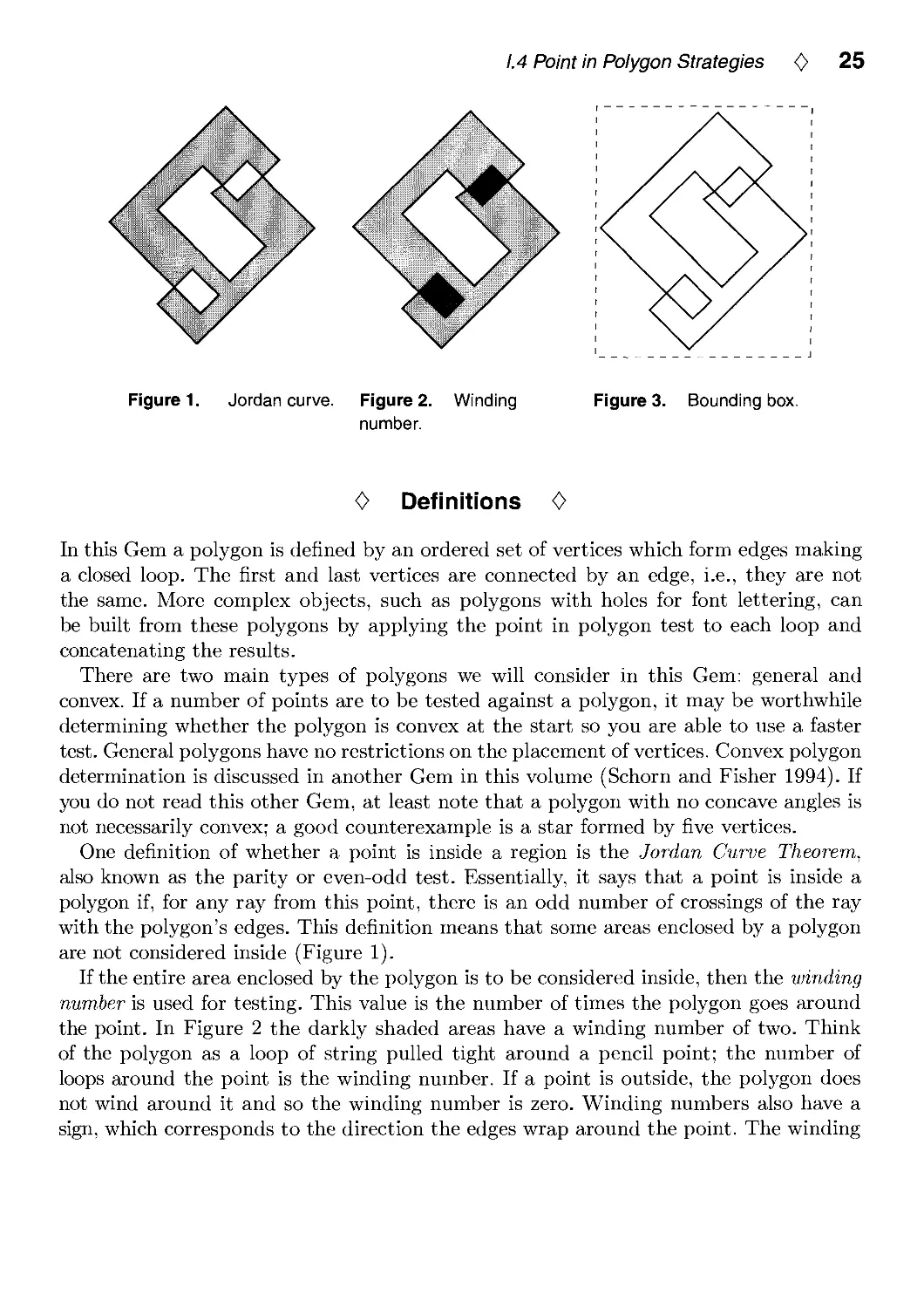
Figure 1. Jordan curve.
Figure 2. Winding
number.
Figure 3. Bounding box.
0 Definitions 0
In this Gem a polygon is defined by an ordered set of vertices which form edges making
a closed loop. The first and last vertices are connected by an edge, i.e., they are not
the same. More complex objects, such as polygons with holes for font lettering, can
be built from these polygons by applying the point in polygon test to each loop and
concatenating the results.
There are two main types of polygons we will consider in this Gem: general and
convex. If a number of points are to be tested against a polygon, it may be worthwhile
determining whether the polygon is convex at the start so you are able to use a faster
test. General polygons have no restrictions on the placement of vertices. Convex polygon
determination is discussed in another Gem in this volume (Schorn and Fisher 1994). If
you do not read this other Gem, at least note that a polygon with no concave angles is
not necessarily convex; a good counterexample is a star formed by five vertices.
One definition of whether a point is inside a region is the Jordan Curve Theorem,
also known as the parity or even-odd test. Essentially, it says that a point is inside a
polygon if, for any ray from this point, there is an odd number of crossings of the ray
with the polygon's edges. This definition means that some areas enclosed by a polygon
are not considered inside (Figure 1).
If the entire area enclosed by the polygon is to be considered inside, then the winding
number is used for testing. This value is the number of times the polygon goes around
the point. In Figure 2 the darkly shaded areas have a winding number of two. Think
of the polygon as a loop of string pulled tight around a pencil point; the number of
loops around the point is the winding number. If a point is outside, the polygon does
not wind around it and so the winding number is zero. Winding numbers also have a
sign, which corresponds to the direction the edges wrap around the point. The winding

26 <C> Polygons and Polyhedra
number test can be converted to the parity test; an odd winding number is equivalent
to the parity test's inside condition.
In ray tracing and other applications the original polygon is three-dimensional. To
simplify computation it is worthwhile to project the polygon and test point into two
dimensions. One way to do this is simply to ignore one coordinate. The best coordinate
to drop is the one that yields the largest area for the 2D polygon formed. This is easily
done by taking the absolute value of each coordinate of the polygon plane's normal
and finding the largest; the corresponding coordinates are ignored (Glassner 1989).
Precomputing some or all of this information once for a polygon uses more memory but
increases the speed of the intersection test itself.
Point in polygon algorithms often benefit from having a bounding box around
polygons with many edges. The point is first tested against this box before the full polygon
test is performed; if the box is missed, so is the polygon (Figure 3). Most statistics
generated in this Gem assume this bounding box test was already passed successfully.
In ray tracing, (Worley and Haines 1993) points out that the polygon's 3D bounding
box can be treated like a 2D bounding box by throwing away one coordinate, as done
above for polygons. By analysis of the operations involved, it can be shown to be more
profitable in general to first intersect the polygon's plane and then test whether the
point is inside the 2D bounding box, rather than first testing the 3D bounding box and
then the plane. Other bounding box variants can be found in (Woo 1992).
0 General Algorithms 0
This section discusses the fastest algorithms for testing points against general polygons.
Three classes of algorithms are compared: those which use the vertex list as their only
data structure, those which do preprocessing and create an alternate form of the
polygon, and those which create additional efficiency structures. The advantages of a vertex
list algorithm is that no additional information or preprocessing is needed. However,
the other two types of algorithms offer faster testing times in many cases.
Crossings Test
The fastest algorithm without any preprocessing is the crossings test. The earliest
presentation of this algorithm is (Shimrat 1962), though it has a bug in it, corrected by
(Hacker 1962). A ray is shot from the test point along an axis (-I-X is commonly used),
and the number of crossings is computed for the even-odd test (Figure 4). One way to
think about this algorithm is to consider the test point to be at the origin and to check
the edges against this point. If the Y coordinates of a polygon edge differ in sign, then
the edge can cross the test ray. In this case, if both X coordinates are positive, the edge

1.4 Point in Polygon Strategies <0> 27
Number of
crossings is odd
Sum of angles
is 360 degrees
Inside odd number
of triangles
Figure 4. Crossings test.
Figure 5. Angle
summation.
Figure 6. Triangle fan.
and ray must intersect and a crossing is recorded. Else, if the X signs differ, then the X
intersection of the edge and the ray is computed and if positive a crossing is recorded.
What happens when the test ray intersects one or more vertices of the polygon? This
problem can be ignored by considering the test ray to be a half-plane divider, with
one of the half-planes including the ray's points (Preparata and Shamos 1985, Glassner
1989). In other words, whenever the ray would intersect a vertex, the vertex is always
classified as being infinitesimally above the ray. In this way, no vertices are considered
intersected and the code is both simpler and speedier.
MacMartin pointed out that for polygons with a large number of edges there are
generally runs of edges that have Y coordinates with the same sign (Haines 1992). For
example, a polygon representing Brazil might have a thousand edges, but only a few of
these will straddle a given latitude line and there are long runs of contiguous edges on
one side of this line. So a faster strategy is to loop through just the Y coordinates as
fast as possible; when they differ then retrieve and check the X coordinates.
Either the even-odd or winding number test can be used to classify the point. The
even-odd test is done by simply counting the number of crossings. The winding number
test is computed by keeping track of whether the crossed edge passes from the Y- to
the Y-|- half-plane (add 1) or vice versa (subtract 1). The final value is then the number
of counterclockwise windings about the point.
The slowest algorithm for testing points is by far the pure angle summation method.
It's simple to describe: sum the signed angles formed at the point by each edge's end-
points (Figure 5). The winding number can then be computed by finding the nearest
multiple of 360 degrees. The problem with this pure scheme is that it involves a large
number of costly math function calls.
However, the idea of angle summation can be used to formulate a fast algorithm
for testing points; see Weiler's Gem in this volume (Weiler 1994). There is a strong

28 <C> Polygons and Polyhedra
connection between Weiler's algorithm and the crossings test. Weiler avoids expensive
trigonometry computations by adding or subtracting one or more increments of 90
degrees as the loop vertices move from quadrant to quadrant (with the test point at the
origin). The crossings test is similar in that it can be thought of as counting movements
of 360 degrees when an edge crosses the test ray. The crossings test tends to be faster
because it does not have to categorize and record all quadrant-to-quadrant movements
but only those which cross the test ray. Weiler's formulation is significant for the way
it adds to the understanding of underlying principles.
Triangle Fan Tests
In Graphics Gems, (Badouei 1990) presents a method of testing points against convex
polygons. The polygon is treated as a fan of triangles emanating from one vertex and
the point is tested against each triangle by computing its barycentric coordinates. As
(Berlin 1985) points out, this test can also be used for non-convex polygons by keeping
a count of the number of triangles that overlap the point; if odd, the point is inside
the polygon (Figure 6). Unlike the convex test, where an intersection means that the
test is done, all the triangles must be tested against the point for the non-convex test.
Also, for the non-convex test there may be multiple barycentric coordinates for a given
point, since triangles can overlap.
The barycentric test is faster than the crossings test for triangles but becomes quite
slow for polygons with more edges. However, (Spackman 1993) notes that pre-normaliz-
ing the barycentric equations and storing a set of precomputed values gives better
performance. This version of the algorithm is twice as fast as the crossings test for triangles
and is in general faster for polygons with few edges. The barycentric coordinates (which
are useful for interpolation and texture mapping) are also computed.
A faster triangle fan tester, proposed by (Green 1993), is to store a set of half-plane
equations for each triangle and test each in turn. If the point is outside any of the three
edges, it is outside the triangle. The half-plane test is an old idea, but storing the half-
planes instead of deriving them on the fly from the vertices gives this scheme its speed
at the cost of some additional storage space. For triangles this scheme is the fastest of
all of the algorithms discussed so far. It is also very simple to code and so lends itself
to assembly language translation. Theoretically the Spackman test should usually have
a smaller average number of operations per test, but in practice the optimized code for
the half-plane test is faster.
Both the half-plane and Spackman triangle testers can be sped up further by sorting
the order of the edge tests. Worley and Haines (Spackman 1993) note that the half-
plane triangle test is more efficient if the longer edges are tested first. Larger edges tend
to cut off more exterior area of the polygon's bounding box and so can result in earlier

1.4 Point in Polygon Strategies <0> 29
exit from testing a given triangle. Sorting in this way makes the test up to 1.7 times
faster, rising quickly with the number of edges in the polygon. However, polygons with
a large number of edges tend to bog down the sorted edge triangle algorithm, with the
crossings test being faster above around 10 edges.
A problem occurs in general triangle fan algorithms when the code assumes that a
point that lies on a triangle edge is always inside that triangle. For example, a
quadrilateral is treated as two triangles. If a point is exactly on the edge between the two
triangles it will be classified as being inside both triangles and so will be classified as
being outside the polygon (this problem does not happen with the convex test).
The code presented for these algorithms does not fully address this problem. In reality,
a random point tested against a polygon has an infinitesimal chance of landing exactly
on any edge. For rendering purposes this problem can be ignored, with the result being
one misshaded pixel once in a great while. A more robust solution (which will slow
down the test) is to note whether an edge is to include the points exactly on it or not.
Also, an option which has not been explored is to test shared interior edges only once
against the point and share the results between the adjacent triangles.
Grid Method
An even faster, and more memory intensive, method of testing for points inside a
polygon is lookup grids. The idea is to impose a grid inside the bounding box containing
the polygon. Each grid cell is categorized as being fully inside, fully outside, or
indeterminate. The indeterminate cells also have a list of edges that overlap the cell, and also
one corner (or more) is determined to be inside or outside.
To test a point against this structure is extremely quick in most cases. For a reasonable
polygon many of the cells are either inside or outside, so testing consists of a simple
look-up. If the cell contains edges, then a line segment is formed from the test point to
the cell corner and is tested against all edges in the list (Antonio 1992). Since the state
of the corner is known, the state of the test point can be found from the number of
intersections (Figure 7). Salesin and Stolfi suggest an algorithm similar to this as part
of their ray tracing acceleration technique (Salesin and Stolfi 1989).
Care must be taken when a polygon edge exactly (or even nearly exactly) crosses a
grid corner, as this corner is then unclassifiable. Rather than coping with the topological
and numerical precision problems involved, one simple solution is to just start generating
the grid from scratch again, giving slightly different dimensions to the bounding box.
Also, when testing the line segment against the edges in a list, exact intersections of an
edge endpoint must be counted only once.
One additional enhancement partially solves this problem. Each grid cell has four
sides. If no polygon edges cross a side, then that side will be fully inside or outside the
polygon. A horizontal or vertical test line segment can then be generated from the test

30 <C> Polygons and Polyhedra
,Cell is outside, so is point
I 1 7\ 1 1
'• i A i i
I \L-I I I I
Draw line to comer and
count crossings
Find wedge,
test point
against edge
Figure 7. Grid crossings Figure 8. Inclusion test,
test.
Figure 9. Random
polygon.
point to this cell side and the faster crossings test can be used against the edges in the
cell. In addition, this crossings test deals with endpoint intersection more robustly.
Note: the grid test code is in the Gems IV code distribution, but has been left out of
the book because of its length.
Pixel Based Testing
One interesting case that is related to gridding is that of pixel-limited picking. When
a dataset is displayed on the screen and a large amount of picking is to be done on
a still image, a specialized test is worthwhile. Hanrahan and Haeberli note that the
image can be generated once into a separate buffer, filling in each polygon's area with
an identifying index (Hanrahan and Haeberli 1990). When a pixel is picked on this fixed
image, it is looked up in this buffer and the polygon selected is known immediately.
<> Convex Polygons 0
Convex polygons can be intersected faster due to their geometric properties. For
example, the crossings test can quit as soon as two Y-sign difference edges are found, since
this is the maximum that a convex polygon can have. Also, note that more polygons
can use this faster crossings test by checking only the change in the Y direction (and
not X and Y as for the full convexity test); see (Schorn and Fisher 1994). For example,
a block letter "E" has at most two Y intersections for any test point's horizontal line
(and so is called monotone in Y), so it can use the faster crossings test.

1.4 Point in Polygon Strategies <C> 31
The triangle fan tests can exit as soon as any triangle is found to contain the point.
These algorithms can be enhanced by both sorting the edges of each triangle by length
and also sorting the testing order of triangles by their areas. Relatively larger triangles
are more likely to enclose a point and so end testing earlier. Note that this faster test can
be applied to any polygon that is decomposed into non-overlapping triangles; convex
polygons always have this property when tessellated into a triangle fan.
The exterior algorithm prestores the half-plane for each polygon edge and tests the
point against this set. If the point is outside any edge, then the point must be outside the
entire convex polygon. This algorithm uses less additional storage than the triangle fan
and is very simple to code. The order of edges tested affects the speed of this algorithm;
testing edges in the order of which cuts off the most area of the bounding box earliest
on is the best ordering. Finding this optimal ordering is non-trivial, but doing the edges
in order is often the worst strategy, since each neighboring edge usually cuts off little
more area than the previous. Randomizing the order of the edges makes this algorithm
up to 10% faster overall for regular polygons.
The exterior algorithm looks for an early exit due to the point being outside the
polygon, while the triangle fan convex test looks for one due to the point being inside.
For example, for 100 edge polygons, if all points tested are inside the polygon the
triangle fan is 1.7 times faster; if all test points are outside the exterior test is more
than 16 times faster (but only 4 times faster if the edges are not randomized). So when
the polygon/bounding box area ratio is low the exterior algorithm is usually best; in
fact, performance is near constant time as this ratio decreases, since after only a few
edges most points are categorized as outside the polygon.
A hybrid of the exterior algorithm and the triangle fan is to test triangles and exit
early when the point is outside the polygon. A point is outside the polygon if it is
outside any exterior triangle edge. This strategy combines the early exit features of
both algorithms and so it is less dependent on bounding box fit. Our code uses sorting
by triangle area instead of randomizing the exterior edge order, so it favors a higher
polygon/bounding box area ratio.
A method with 0(log n) performance is the inclusion algorithm (Preparata and
Shamos 1985). The polygon is preprocessed by adding a central point to it and is then
divided into wedges. The angles from an anchor edge to each wedge's edges are
computed and saved, along with half-plane equations for the polygon edges. When a point
is tested, the angle from the anchor edge is computed and a binary search is used to
determine the wedge it is in, and then the corresponding polygon edge is tested against
it (Figure 8). Note that this test can be used on any polygon that can be tessellated
into a non-overlapping star of triangles. This algorithm is slower for polygons with few
edges because the startup cost is high, but the binary search makes for a much faster
test when there are many edges. However, if the bounding box is much larger than the
polygon the exterior edge test is faster.

32 <0> Polygons and Polyhedra
0 statistics 0
The timings given in Tables 1-3 were produced on an HP 720 RISC workstation; timings
had similar performance ratios on an IBM PC 386 with no FPU. The general non-convex
algorithms were tested using two sorts of polygons: those generated with random points
and regular (i.e., equal length sides and vertex angles) polygons with a random rotation
applied. Random polygons tend to be somewhat unlikely (no one ever uses 1000-edge
random polygons for anything except testing), while regular polygons are more orderly
than a "typical" polygon; normal behavior tends to be somewhere in between. Test
points were generated inside the bounding box for the polygon. Figure 9 shows a typical
10-sided random polygon and some test points. Convex algorithms were tested with only
regular polygons, and so have a certain bias to them.
Test points were generated inside the box bounding the polygon; looser fitting boxes
yield different results. Timings are in microseconds per polygon. They are given to two
significant figures, since their accuracy is roughly ±10%. However, the best way to get
useful timings is to run the code on the target machine; there is a testbed program
provided in the Gems IV code distribution which can be used to try new algorithms
and generate timings under various test conditions. Also, of course, hacking the code
for a particular machine and compiler can make a significant difference.
<> Discussion <>
The crossings test is generally useful, but we can do better. Testing triangles using
either sorted triangle fan algorithm is more than twice as fast, though for polygons
with many edges the crossings test is still faster.
Given enough resolution (and enough memory!), gridding gives near constant time
performance for most normal polygons, though it performs a bit slower when entirely
random polygons are tested. Interestingly, even for polygons with just a few edges the
gridding algorithm outperforms most of the other tests.
Testing times can be noticeably decreased by using an algorithm optimized for convex
testing when possible. For example, the convex sorted half-plane test is 1.4 times faster
for 10-sided polygons than its general case counterpart. For convex polygons with many
edges the inclusion test is extremely efficient because of its 0(log n) behavior.
Other algorithms remain to be discovered and tested; for example, a practical general
polygon algorithm with better than 0(n) performance and low storage costs would fill
a useful niche.

1.4 Point in Polygon Strategies <0> 33
Table 1. General Algorithms, Random Polygons
Algorithm
Crossings
Half Plane w/edge sort
Half Plane, no sort
Spackman w/edge sort
Spackman, no sort
Barycentric
Weiler angle
Trigonometric angle
Grid (100x100)
Grid (20x20)
Number of edges per polygon
3 4 10 20 50 100 1000
2.8
1.1
1.2
1.3
1.4
2.4
3.7
42
1.8
2.0
3.1
1.7
2.0
2.1
2.2
4.0
4.3
51
1.9
2.0
5.7
5.7
6.3
6.0
6.4
13
8.7
110
1.9
2.2
10
12
14
13
14
29
16
210
1.9
2.5
25
32
36
32
35
76
39
520
2.2
3.6
48
65
72
66
70
150
77
1030
2.5
5.5
470
650
740
670
720
1600
760
10300
9.2
38
Table 2. General Algorithms, Regular Polygons
Algorithm
Crossings
Half Plane w/edge sort
Half Plane, no sort
Spackman w/edge sort
Spackman, no sort
Barycentric
Weiler angle
Trigonometric angle
Grid (100x100)
Grid (20x20)
Number of edges per polygon
3 4 10 20 50 100 1000
2.6
1.3
1.3
1.5
1.5
2.5
3.5
39
1.8
2.0
2.7
1.8
2.1
2.1
2.3
4.2
4.0
51
1.8
2.0
4.3
4.6
6.7
5.4
5.8
13
7.9
120
1.8
2.0
7.2
9.2
14
10
11
26
15
230
1.8
2.0
16
23
37
26
28
68
35
560
1.8
2.0
32
45
74
51
55
140
70
1200
1.8
2.1
300
460
760
510
550
1400
690
11100
1.9
2.8
Table 3. Convex Algorithms, Regular Polygons
Algorithm
Inclusion
Hybrid Sorted Half Plane
Sorted Half Plane
Unsorted Half Plane
Random Exterior Edges
Ordered Exterior Edges
Convex Crossings
Number of edges per polygon
3 4 10 20 50 100 1000
5.5
1.3
1.2
1.2
1.3
1.3
2.5
5.7
1.6
1.6
1.9
1.7
1.7
2.5
6.3
3.3
3.4
5.7
3.8
3.8
3.6
6.6
6.1
6.2
12
7.1
7.3
5.6
7.1
14
15
30
17
18
12
7.6
28
29
61
33
35
22
9.9
280
280
620
320
350
220

34 <0> Polygons and Polyhedra
0 Conclusions 0
• If no preprocessing nor extra storage is available, use the Crossings test.
• If a little preprocessing and extra storage is available:
— For general polygons
* with few sides, use the Half-Plane or Spackman test.
* with many sides, use the Crossings test.
— For convex polygons
* with few sides, use the Hybrid Half-Plane test.
* with many sides, use the Inclusion test.
* But if the bounding box/polygon area ratio is high, use the Exterior
Edges test.
• If preprocessing and extra storage is available in abundance, use the Grid Test
(except for perhaps triangles).
Of course, some of these conclusions may vary with machine architecture and compiler
optimization.
0 C Code 0
ptinpoly.h
/* ptinpoly.h - point in polygon inside/outside algorithms header file.
*/
/* Define CONVEX to compile for testing only convex polygons (when possible,
* this is faster). */
/* #define CONVEX */
/* Define HYBRID to compile triangle fan test for CONVEX with exterior edges
* meaning an early exit (faster - recommended).
*/
/* #define HYBRID */
/* Define DISPLAY to display test triangle and test points on screen. */
/* #define DISPLAY */
/* Define RANDOM to randomize order of edges for exterior test (faster -
* recommended). */
/* #define RANDOM */
/* Define SORT to sort triangle edges and areas for half-plane and Spackman

1.4 Point in Polygon Strategies <C> 35
* tests (faster - recommended). */
/* #define SORT */
/* Define WINDING if a non-zero winding number should be used as the criterion
* for being inside the polygon. Only used by the general crossings test and
* Weiler test. The winding number computed for each is the number of
* counterclockwise loops the polygon makes around the point.
*/
/* #define WINDING */
/* =========================== System Related ============================= */
/* Define your own random number generator; change as needed. */
/* SRAN initializes random number generator, if needed. */
#define SRANO srand48(l)
/* RANOl returns a double from [0..1) */
#define RANOl () drand48()
double drand48() ;
/* =========== Half-Plane stuff =========================================== */
typedef struct {
double vx, vy, c ; /* edge equation vx*X + vy*Y + c = 0 */
#ifdef CONVEX
#ifdef HYBRID
int ext_flag ; /* TRUE == exterior edge of polygon */
#endif
#endif
} PlaneSet, *pPlaneSet ;
#ifdef CONVEX
#ifdef SORT
/* Size sorting structure for half-planes */
typedef struct {
double size ;
pPlaneSet pps ;
} SizePlanePair, *pSizePlanePair ;
#endif
#endif
#ifdef CONVEX
pPlaneSet ExteriorSetup()
void ExteriorCleanup () ;
#ifdef SORT
int CompareSizePlanePairs()
#endif
#endif
pPlaneSet PlaneSetupO ;
void PlaneCleanup () ;

36 <0> Polygons and Polyhedra
ptinpoly.c
/* ptinpoly.c - point in polygon inside/outside code.
by Eric Haines, 3D/Eye Inc, erich@eye.com
This code contains the following algorithms:
crossings - count the crossing made by a ray from the test point
half-plane testing - test triangle fan using half-space planes
exterior test - for convex polygons, check exterior of polygon
*/
#include <stdio.h>
#include <stdlib.h>
#include <math.h>
♦include "ptinpoly.h"
#define X 0
#define Y 1
#define TRUE 1
#ifndef HUGE
#define HUGE 1.79769313486232e+308
#endif
#define MALLOC_CHECK( a ) if ( !(a) ) { \
fprintf( stderr, "out of memory\n" ) ; \
exit(l) ; \
}
/* ======= Crossings algorithm ============================================ */
/* Shoot a test ray along +X axis. The strategy, from MacMartin, is to
* compare vertex Y values to the testing point's Y and quickly discard
* edges which are entirely to one side of the test ray.
*
* Input 2D polygon _pgon_ with _numverts_ number of vertices and test point
* _point_, returns 1 if inside, 0 if outside. WINDING and CONVEX can be
* defined for this test.
*/
int CrossingsTest( pgon, numverts, point )
double pgon[][2] ;
int numverts ;
double point[2] ;
{
#ifdef WINDING
register int crossings ;
#endif
register int j, yflagO, yflagl, inside_flag, xflagO ;
register double ty, tx, *vtxO, *vtxl ;
#ifdef CONVEX

1.4 Point in Polygon Strategies <} 37
register int line_flag ;
#endif
tx = point[X] ;
ty = point[Y] ;
vtxO = pgon[numverts-1] ;
/* get test bit for above/below X axis */
yflagO = ( vtxO[Y] >= ty ) ;
vtxl = pgon[0] ;
#ifdef WINDING
crossings = 0 ;
#else
inside_flag = 0 ;
#endif
#ifdef CONVEX
line_flag = 0 ;
#endif
for ( j = numverts+1 ; --j ; ) {
yflagl = ( vtxl[Y] >= ty ) ;
/* check if endpoints straddle (are on opposite sides) of X axis
* (i.e., the Y's differ); if so, +X ray could intersect this edge.
*/
if ( yflagO != yflagl ) {
xflagO = ( vtxO[X] >= tx ) ;
/* check if endpoints are on same side of the Y axis (i.e., X's
* are the same); if so, it's easy to test if edge hits or misses.
*/
if ( xflagO == ( vtxl[X] >= tx ) ) {
/* if edge's X values both right of the point, must hit */
#ifdef WINDING
if ( xflagO ) crossings += ( yflagO ? -1 : 1 ) ;
telse
if ( xflagO ) inside_flag = !inside_flag ;
#endif
} else {
/* compute intersection of pgon segment with +X ray, note
* if >= point's X; if so, the ray hits it.
*/
if ( (vtxl[X] - (vtxl[Y]-ty)*
( VtxO[X]-vtxl[X])/(vtxO[Y]-vtxl[Y])) >= tx ) {
#ifdef WINDING
crossings += ( yflagO ? -1 : 1 ) ;
#else
inside_flag = !inside_flag ;
#endif
}
}
#ifdef CONVEX
/* if this is second edge hit, then done testing */

38 0 Polygons and Polyhedra
if ( line_flag ) goto Exit ,-
/* Note that one edge has been hit by the ray's line. */
line_flag = TRUE ;
#endif
}
/* Move to next pair of vertices, retaining info as possible. */
yflagO = yflagl ;
vtxO = vtxl ;
vtxl += 2 ;
}
#ifdef CONVEX
Exit: ;
#endif
#ifdef WINDING
/* Test if crossings is not zero. */
inside_flag = (crossings != 0) ;
#endif
return( inside_flag ) ;
}
Triangle half-plane algorithm ================================== */
/* Split the polygon into a fan of triangles and for each triangle test if
* the point is inside of the three half-planes formed by the triangle's edges
*
* Call setup with 2D polygon _pgon_ with _numverts_ number of vertices,
* which returns a pointer to a plane set array.
* Call testing procedure with a pointer to this array, _numverts_, and
* test point _point_, returns 1 if inside, 0 if outside.
* Call cleanup with pointer to plane set array to free space.
*
* SORT and CONVEX can be defined for this test.
*/
/* Split polygons along set of x axes - call preprocess once. */
pPlaneSet PlaneSetup( pgon, numverts )
double pgon[][2] ;
int numverts ;
{
int i, pi, p2 ;
double tx, ty, vxO, vyO ;
pPlaneSet pps, pps_return ;
#ifdef SORT
double len[3], len_temp ;
int j ;
PlaneSet ps_temp ;
#ifdef CONVEX
pPlaneSet pps_new ;
pSizePlanePair p_size_pair ;

#endlf
#endif
1.4 Point in Polygon Strategies 0 39
pps = pps_return =
(pPlaneSet)malloc( 3
MALLOC_CHECK( pps ) ;
#ifdef CONVEX
#ifdef SORT
p_size_palr =
(pSizePlanePair)malloc( (numverts-2)
MALLOC_CHECK( p_size_pair ) ;
#endif
#endif
(numverts-2) * slzeof( PlaneSet
slzeof( SlzePlanePair
vxO = pgon[0][X]
vyO = pgon[0][Y]
for
#ifdef
#ifdef
#ifdef
#endif
#endif
#endif
#ifdef
#endif
#ifdef
#ifdef
#endif
#endif
( pi = 1, p2 = 2 ; p2 < numverts
pps->vx = vyO - pgon[pl][Y] ;
pps->vy = pgon[pl][X] - vxO ;
pps->c = pps->vx * vxO + pps->vy
SORT
len[0]
CONVEX
HYBRID
pps->ext
pl+
vyO
p2 4
) {
= pps->vx
pps->vx + pps->vy
pps->vy
.flag = ( pi == 1 )
/* Sort triangles by areas, so compute (twice) the area here. */
p_size_pair[pl-1].pps = pps ;
p_size_pair[pl-1].size =
Y]
( pgon[0][X]
( pgon[pl] [X]
( pgon[p2] [X]
( pgon[pl][X]
( pgon[p2][X]
( pgon[0][X]
* pgon[pi][Y
* pgon[p2] [■
* pgon[0] [Y
* pgon[0] [Y
* pgon [pi] [■
* pgon[p2] [Y
PPS++ ;
pps->vx = pgon[pi][Y] - pgon[p2][Y] ;
pps->vy = pgon[p2][X] - pgon[pl][X] ;
pps->c = pps->vx * pgon[pl][X] + pps->vy * pgon[pl][Y]
SORT
len[l] = pps->vx * pps->vx + pps->vy * pps->vy ;
CONVEX
HYBRID
pps->ext_flag = TRUE ;
PPS++ ;
pps->vx = pgon[p2][Y] - vyO
pps->vy = vxO - pgon[p2][X]

40 <0> Polygons and Polyhedra
pps->c = pps->vx * pgon[p2][X] + pps->vy * pgon[p2][Y] ;
#ifdef SORT
len[2] = pps->vx * pps->vx + pps->vy * pps->vy ;
#endif
#ifdef CONVEX
#ifdef HYBRID
pps->ext_flag = ( p2 == numverts-1 ) ;
#endif
#endif
/* Find an average point that must be inside of the triangle. */
tx = ( vxO + pgon[pl][X] + pgon[p2][x] ) / 3.0 ;
ty = ( vyO + pgon[pl][Y] + pgon[p2][Y] ) / 3.0 ;
/* Check sense and reverse if test point is not thought to be inside
* first triangle.
*/
if ( pps->vx * tx + pps->vy * ty >= pps->c ) {
/* back up to start of plane set */
pps -= 2 ;
/* Point is thought to be outside, so reverse sense of edge
* normals so that it is correctly considered inside.
*/
for ( i = 0 ; i < 3 ; i++ ) {
pps->vx = -pps->vx ;
pps->vy = -pps->vy ;
pps->c = -pps->c ;
PPS++ ;
}
} else {
PPS++ ;
}
#ifdef SORT
/* Sort the planes based on the edge lengths. */
pps -= 3 ;
for ( i = 0 ; i < 2 ; i++ ) {
for ( j = i+1 ; j < 3 ; j++ ) {
if ( len[i] < len[j] ) {
ps_temp = pps[i] ;
pps[i] = pps[j] ;
pps[j] = ps_temp ;
len_temp = len[i] ;
len[i] = len[j] ;
len[j] = len_temp ;
}
}
}
pps += 3 ;
#endif
}
#ifdef CONVEX

1.4 Point in Polygon Strategies <0> 41
#ifdef SORT
/* Sort the triangles based on their areas. */
qsort( p_size_pair, numverts-2,
sizeof( SizePlanePair ), CompareSizePlanePairs
/* Make the plane sets match the sorted order. */
for ( i = 0, pps = pps_return
; i < numverts-2
; i++ ) {
pps_new = p_size_pair[i].pps ;
for ( j = 0 ; j < 3 ; j++, pps++, pps_new++ ) {
ps_temp = *pps ;
*pps = *pps_new ;
*PPS_new = ps_temp ;
}
}
free( p_size_pair ) ;
#endif
#endif
return( pps_return ) ;
}
#ifdef CONVEX
#ifdef SORT
int CompareSizePlanePairs( p_spO, p_spl )
pSizePlanePair p_spO, p_spl ;
{
if ( p_spO->size == p_spl->size ) {
return ( 0 ) ,-
} else {
return( p_spO->size > p_spl->size ? -1 : 1 ) ;
}
}
#endif
#endif
/* Check point for inside of three "planes" formed by triangle edges. */
int PlaneTest ( p_plane_set, numverts, point )
pPlaneSet p_plane_set ;
int numverts ;
double point [2] ;
{
register pPlaneSet ps ;
register int p2 ;
#ifndef CONVEX
register int inside_flag ;
#endif
register double tx, ty ;
tx = point[X] ;

42 <0> Polygons and Polyhedra
ty = point [Y] ,•
#ifndef CONVEX
lnside_flag = 0 ;
#endif
for ( ps = p_plane_set, p2 = numverts-1
'P2 ; ) {
if ( ps->vx * tx + ps->vy * ty < ps->c ) {
ps + + ;
if ( ps->vx * tx + ps->vy * ty < ps->c ) {
ps + + ;
/* Note: we make the third edge have a slightly different
* equality condition, since this third edge is in fact
* the next triangle's first edge. Not fool-proof, but
* it doesn't hurt (better would be to keep track of the
* triangle's area sign so we would know which kind of
* triangle this is). Note that edge sorting nullifies
* this special inequality, too.
*/
if ( ps->vx * tx + ps->vy * ty <= ps->c ) {
/* point is inside polygon */
#ifdef CONVEX
telse
#endif
return( 1 ) ;
inside_flag = !inside_flag ;
#ifdef CONVEX
#ifdef HYBRID
/* check if outside exterior edge */
else if ( ps->ext_flag ) return( 0 )
#endif
#endif
ps + + ;
} else {
#ifdef CONVEX
#ifdef HYBRID
/* check if outside exterior edge */
if ( ps->ext_flag ) return( 0 ) ;
#endif
#endif
/* get past last two plane tests */
ps += 2 ;
}
} else {
#ifdef CONVEX
#ifdef HYBRID
/* check if outside exterior edge */
if ( ps->ext_flag ) return( 0 ) ;
#endif
#endif
/* get past all three plane tests */

1.4 Point in Polygon Strategies <0> 43
ps += 3 ;
}
}
#ifdef CONVEX
/* for convex, if we make it to here, all triangles were missed */
return( 0 ) ;
#else
return( inside_flag ) ;
#endif
}
void PlaneCleanup( p_plane_set )
pPlaneSet p_plane_set ;
{
free( p_plane_set ) ;
}
Exterior (convex only) algorithm
/* Test the edges of the convex polygon against the point. If the point is
* outside any edge, the point is outside the polygon.
*
* Call setup with 2D polygon _pgon_ with _numverts_ number of vertices,
* which returns a pointer to a plane set array.
* Call testing procedure with a pointer to this array, _numverts_, and
* test point _point_, returns 1 if inside, 0 if outside.
* Call cleanup with pointer to plane set array to free space.
*
* RANDOM can be defined for this test.
* CONVEX must be defined for this test; it is not usable for general polygons.
*/
#ifdef CONVEX
/* make exterior plane set */
pPlaneSet ExteriorSetup( pgon, numverts )
double pgon[][2] ;
int numverts ;
{
int pi, p2, flip_edge ;
pPlaneSet pps, pps_return ;
#ifdef RANDOM
int i, ind ;
PlaneSet ps_temp ;
#endif
pps = pps_return =
(pPlaneSet) malloc ( numverts * sizeof( PlaneSet )) ;
MALLOC_CHECK( pps ) ;
/* take cross product of vertex to find handedness */
flip_edge = (pgon[0][X] - pgon[l][X]) * (pgon[l][Y] - pgon[2][Y] ) >

44 <0> Polygons and Polyhedra
(pgon[0][Y] -pgon[l][Y]) * (pgon[l][X] -pgon[2][x] ) ;
/* Generate half-plane boundary equations now for faster testing later.
* vx Sc vy are the edge's normal, c is the offset from the origin.
*/
for ( pi = numverts-1, p2 = 0 ; p2 < numverts ; pi = p2, p2++, pps++ ) {
pps->vx = pgon[pl][Y] - pgon[p2][Y] ;
pps->vy = pgon[p2][X] - pgon[pl][X] ;
pps->c = pps->vx * pgon[pl][X] + pps->vy * pgon[pl][Y] ;
/* check sense and reverse plane edge if need be */
if ( flip_edge ) {
pps->vx = -pps->vx ;
pps->vy = -pps->vy ;
pps->c = -pps->c ;
}
}
#ifdef RANDOM
/* Randomize the order of the edges to improve chance of early out. */
/* There are better orders, but the default order is the worst. */
for (1=0, pps = pps_return
; 1 < numverts
; i++ ) {
ind = (int)(RANOIO * numverts ) ;
if ( ( ind < 0 ) II ( ind >= numverts ) ) {
fprintf( stderr,
"Yikes, the random number generator is returning values\n" )
fprintf( stderr,
"outside the range [0.0,1.0), so please fix the code!\n" ) ;
ind = 0 ;
}
/* swap edges */
ps_temp = *pps ;
*pps = pps_return[ind] ;
pps_return[ind] = ps_temp ;
}
#endif
return( pps_return ) ;
}
/* Check point for outside of all planes. */
/* Note that we don't need "pgon", since it's been processed into
* its corresponding PlaneSet.
*/
int ExteriorTest( p_ext_set, numverts, point )
pPlaneSet p_ext_set ;
int numverts ;
double point[2] ;
{
register PlaneSet *pps ;

1.4 Point in Polygon Strategies <0> 45
register int pO ;
register double tx, ty ;
int inside_flag ;
tx = point[X] ;
ty = point[Y] ;
for ( pO = numverts+1, pps = p_ext_set ; --pO ; pps++ ) {
/* Test if the point is outside this edge. */
if ( pps->vx * tx + pps->vy * ty > pps->c ) {
return( 0 ) ;
}
}
/* If we make it to here, we were inside all edges. */
return( 1 ) ;
}
void ExteriorCleanup( p_ext_set )
pPlaneSet p_ext_set ;
{
free( p_ext_set ) ;
}
#endif
<> Bibliography <>
(Antonio 1992) Franklin Antonio. Faster line segment intersection. In David Kirk,
editor, Graphics Gems III, pages 199-202. Academic Press, Boston, 1992.
(Badouel 1990) Didier Badouel. An efficient ray-polygon intersection. In Andrew Glass-
ner, editor, Graphics Gems, pages 390-393. Academic Press, Boston, 1990.
(Berlin 1985) Jr. Edwin P. Berlin. Efficiency considerations in image synthesis. In
SIGGRAPH '85 State of the Art in Image Synthesis seminar notes, July 1985.
(Glassner 1989) A. Glassner, editor. An Introduction to Ray Tracing. Academic Press,
London,1989.
(Green 1993) Chris Green. Simple, fast triangle intersection. Ray Tracing News 6(1),
E-mail edition, anonymous ftp from princeton.edu:/pub/Graphics/RTNews, 1993.
(Hacker 1962) R. Hacker. Certification of algorithm 112: position of point relative to
polygon. Communications of the ACM, 5:606, 1962.
(Haines 1992) Eric Haines, editor. Fastest point in polygon test. Ray Tracing News
5(3), E-mail edition, anonymous ftp from princeton.edu:/pub/Graphics/RTNews,
1992.

46 <0> Polygons and Polyhedra
(Hanrahan and Haeberli 1990) Pat Hanrahan and Paul Haeberli. Direct WYSIWYG
painting and texturing on 3d shapes. Computer Graphics (SIGGRAPH '90
Proceedings), 24(4):215-223, August 1990.
(Preparata and Shamos 1985) F. P. Preparata and M. I. Shamos. Computational
Geometry: An Introduction. Springer-Verlag, New York, NY, 1985.
(Salesin and Stolfi 1989) David Salesin and Jorge Stolfi. The ZZ-buffer: A simple and
efficient rendering algorithm with reliable antialiasing. In Proc. 2nd Intl. Conf. on
Computer Graphics (PIXIM '89), pages 451-465, Paris, France, 1989.
(Schorn and Fisher 1994) Peter Schorn and Frederick Fisher. Testing the convexity of
a polygon. In Paul Heckbert, editor, Graphics Gems IV, 7-15. Academic Press,
Boston, 1994.
(Shimrat 1962) M. Shimrat. Algorithm 112: position of point relative to polygon. Com,-
munications of the ACM, 5:434, 1962.
(Spackman 1993) John Spackman. Simple, fast triangle intersection, part ii.
Ray Tracing News 6(2), E-mail edition, anonymous ftp from prince-
ton.edu:/pub/Graphics/RTNews, 1993.
(Weiler 1994) Kevin Weiler. An incremental angle point in polygon test. In Paul
Heckbert, editor, Graphics Gems IV, 16-23. Academic Press, Boston, 1994.
(Woo 1992) Andrew Woo. Ray tracing polygons using spatial subdivision. In
Proceedings of Graphics Interface '92, pages 184-191, May 1992.
(Worley and Haines 1993) Steve Worley and Eric Haines. Bounding areas for
ray/polygon intersection. Ray Tracing News 6(1), E-mail edition, anonymous ftp
from princeton.edu:/pub/Graphics/RTNews, 1993.

01.5
Incremental Delaunay
Triangulatlon
Dani Lischinski
580 ETC Building
Cornell University
Ithaca, NY 14853
danix @ graphics. Cornell, edu
0 Introduction 0
This Gem gives a simple algorithm for the incremental construction of the Delaunay
triangulatlon (DT) and the Voronoi diagram (VD) of a set of points in the plane.
A triangulatlon is called Delaunay if it satisfies the empty circumcircle property: the
circumcircle of a triangle in the triangulatlon does not contain any input points in its
interior. DT is the straight-line dual of the Voronoi diagram of a point set, which is a
partition of the plane into polygonal cells, one for each point in the set, so that the cell
for point p consists of the region of the plane closer to p than to any other input point
(Preparata and Shamos 1985, Fortune 1992).
Delaunay triangulations and Voronoi diagrams, which can be constructed from
them, are a useful tool for efficiently solving many problems in computational
geometry (Preparata and Shamos 1985). DT is optimal in several respects. For example, it
maximizes the minimum angle and minimizes the maximum circumcircle over all
possible triangulations of the same point set (Fortune 1992). Thus, DT is an important
tool for high-quality mesh generation for finite elements (Bern and Eppstein 1992). It
should be noted, however, that standard DT doesn't allow edges that must appear in
the triangulatlon to be specified in the input. Thus, in order to mesh general
polygonal regions the more complicated constrained DT should be used (Bern and Eppstein
1992).
The incremental DT algorithm given in this Gem was originally presented by Green
and Sibson (Green and Sibson 1978), but the implementation is based entirely on the
quad-edge data structure and the pseudocode from the excellent paper by Guibas and
Stolfi (Guibas and Stolfi 1985). I will briefly describe the data structures and the
algorithm, but the reader is referred to Guibas and Stolfi for more details.
Copyright (c) 1994 by Academic Press, Inc.
All rights of reproduction in any form reserved.
IBM ISBN 0-12-336155-9
47 Macintosh ISBN 0-12-336156-7

48 <0> Polygons and Polyhedra
e[2]
o
L _
' e[3]
e[l]
o
e[0]
(a)
(b)
(c)
Figure 1. The quad-edge data structure.
<> The Quad-Edge Data Structure <>
The quad-edge data structure (Guibas and Stolfi 1985) was designed for representing
general subdivisions of orientable manifolds. It is similar to the winged-edge data
structure (Baumgart 1975), but it simultaneously represents both the subdivision and its
dual. Each quad-edge record groups together four directed edges corresponding to a
single undirected edge in the subdivision and to its dual edge (Figure la). Each
directed edge has two pointers: a next pointer to the next counterclockwise edge around
its origin, and a data pointer to geometrical and other nontopological information (such
as the coordinates of its origin.)
Figures lb and Ic illustrate how three edges incident on the same vertex are
represented using the quad-edge data structure: the vertex itself corresponds to the inner
cycle of pointers in Figure Ic. The remaining three cycles correspond to the three faces
meeting at the vertex.
Aside from a primitive to create an edge (MakeEdge), a single topological operator
Splice is defined that can be used to link disjoint edges together as well as to break
two linked edges apart. This operator is its own inverse and together with MakeEdge it
can be used to construct any subdivision.
<> The Incremental Algorithm <>
The incremental DT algorithm starts with a triangle large enough to contain all of the
points in the input. Points are added into the triangulation one by one, maintaining
the invariant that the triangulation is Delaunay. Figure 2 illustrates the point insertion
process. First, the triangle containing the new point p is located (2a). New edges are
created to connect p to the vertices of the containing triangle (2b). The old edges of the
triangle are inspected to verify that they still satisfy the empty circumcircle condition.

1.5 Incremental Delaunay Triangulation <0> 49
Figure 2. Inserting a point into the triangulation. Dashed lines indicate edges that need to be inspected
by the algorithm.

50 <0> Polygons and Polyhedra
Figure 3. The DT (left) and the VD (right) of 250 random points uniformly distributed in the unit square.
If the condition is satisfied (2c) the edge remains unchanged. If it is violated (2d) the
offending edge is flipped, that is, replaced by the other diagonal of the surrounding
quadrilateral. In this case two more edges become candidates for inspection (edges a
and b in Figure 2e.) The process continues until no more candidates remain, resulting
in the triangulation shown in Figure 2f.
In the worst case the insertion of a point can require 0{n) edges to be flipped.
However, in practice the average number of edges tested per insertion is small (< 9).
Guibas, Knuth, and Sharir have shown that if the insertion order is randomized, the
expected time is 0(1) per insertion (Guibas et al. 1990).
Locating the containing triangle can be done in an optimal O(logn) time, but this
requires maintaining complicated data structures. Alternatively, the triangle can be
located by starting from an arbitrary place in the triangulation and moving in the
direction of p until the containing triangle is reached. This requires 0{n) time, but if
the inserted points are uniformly distributed, the expected number of operations to
locate a point is only 0(n^'^). A simple improvement is always to resume the search
from the triangle that was found last: in this way, when the points to be located are
near each other, the containing triangles are determined quickly.
Figure 3 shows the DT and the corresponding VD produced by this algorithm from
250 random points in the unit square. Note that because the quad-edge data structure
represents both the triangulation and its dual, the topology of the Voronoi diagram is
readily available from the DT constructed by the algorithm. To have a complete VD
one only needs to compute the circumcenters of all the triangles (i.e., the locations of
the Voronoi vertices).

1.5 Incremental Delaunay Triangulation 0 51
<> Robustness <>
In order to produce a practical implementation of a geometric algorithm, one typically
needs to address two problems: geometric degeneracies and numerical errors. For DT,
four or more cocircular points in the input constitute a geometric degeneracy, and the
resulting DT is not unique. In such a case this algorithm will produce one of the possible
triangulations as output.
Dealing with numerical errors is more difficult. Various applications in which the need
for DT or VD arises differ in the nature of their input and in their output accuracy
requirements. Therefore, it is very difficult to come up with a single efficient solution
to the problem. Karasick, Lieber, and Nackman suggest a solution that uses rational
arithmetic as well as survey other approaches (Karasick et al. 1991).
In this implementation all the computations are performed using standard
floatingpoint arithmetic. Epsilon tolerances are used to determine whether two points coincide
and whether a point falls on an edge. No other special measures to ensure
robustness were taken. Nevertheless, largely because of the simplicity of the algorithm, the
implementation has proven to be very robust.
0 C++ Code 0
The code listed below is the C-|—I- implementation of the quad-edge data structure and
the incremental Delaunay triangulation algorithm. In addition, the disk that comes
with this book contains code for 2D vectors, points, and lines, and a test program. This
program constructs and displays a triangulation, allowing the user to add more points
into the triangulation interactively by clicking a mouse button at the place of insertion.
The code should compile and execute on SGI graphics workstations.
#include <geom2d.h>
class QuadEdge;
class Edge {
friend QuadEdge;
friend void Splice(Edge*, Edge*);
private:
int num;
Edge *next;
Point2d *data;
public:
Edge() { data = 0; }
Edge* Rot();
Edge* invRot () ;
Edge* Sym();
Edge* Onext() ;
Edge* Oprev();

52 0 Polygons and Polyhedra
Edge* Dnext();
Edge* Dprev();
Edge* Lnext();
Edge* Lprev();
Edge* Rnext();
Edge* Rprev();
Point2d* Org();
Point2d* Dest();
const Point2d& Org2d() const;
const Point2d& Dest2d() const;
void EndPoints(Point2d*, Point2d*);
QuadEdge* Qedge() { return (QuadEdge *)(this - num); }
};
class QuadEdge {
friend Edge *MakeEdge();
private:
Edge e[4] ;
public:
QuadEdge() ;
};
class Subdivision {
private:
Edge *startingEdge;
Edge *Locate(const Point2d&);
public:
Subdivision(const Point2d&, const Point2d&, const Point2d&);
void InsertSite(const Point2d&);
void Draw();
};
inline QuadEdge::QuadEdge()
{
e[0].num = 0, e[l].num = 1, e[2].num = 2, e[3].num = 3;
e[0].next = &(e[0]); e[l].next = &(e[3]);
e[2].next = &(e[2]); e[3].next = &(e[l]);
/*************************
Edge Algebra
*************************************/
inline Edge* Edge::Rot()
// Return the dual of the current edge, directed from its right to its left.
return (num < 3) ? this
1 : this
3;
inline Edge* Edge::invRot()
// Return the dual of the current edge, directed from its left to its right.
return (num > 0) ? this - 1 : this + 3;

1.5 Incremental Delaunay Triangulation 0 53
inline Edge* Edge::Sym()
// Return the edge from the destination to the origin of the current edge.
{
return (num < 2) ? this + 2 : this - 2;
}
inline Edge* Edge::Onext ()
// Return the next ccw edge around (from) the origin of the current edge.
{
return next;
}
inline Edge* Edge::Oprev()
// Return the next cw edge around (from) the origin of the current edge.
{
return Rot()->Onext()->Rot();
}
inline Edge* Edge::Dnext ()
// Return the next ccw edge around (into) the destination of the current edge.
{
return Sym()->Onext()->Sym();
}
inline Edge* Edge::Dprev()
// Return the next cw edge around (into) the destination of the current edge.
{
return invRot()->Onext()->invRot();
}
inline Edge* Edge::Lnext()
// Return the ccw edge around the left face following the current edge.
{
return invRot()->Onext()->Rot();
}
inline Edge* Edge::Lprev()
// Return the ccw edge around the left face before the current edge.
{
return Onext()->Sym() ;
}
inline Edge* Edge::Rnext()
// Return the edge around the right face ccw following the current edge.
{
return Rot()->Onext()->invRot();
)
inline Edge* Edge::Rprev()
// Return the edge around the right face ccw before the current edge.
{
return Sym()->Onext();
}

54 0 Polygons and Polyhedra
/************** Access to Data Pointers *************************************/
inline Point2d* Edge::Org()
{
return data;
}
inline Point2d* Edge::Dest()
{
return Sym()->data;
}
inline const Point2d& Edge:-.Org2d () const
{
return *data;
}
inline const Point2d& Edge::Dest2d() const
{
return (num < 2) ? *((this + 2)->data) : *((this - 2)->data);
}
inline void Edge::EndPoints(Point2d* or, Point2d* de)
{
data = or;
Sym()->data = de;
}
/*********************** Basic TODOloaical ODerators ************************/
Edge* MakeEdge()
{
QuadEdge *ql = new QuadEdge;
return ql->e;
}
void Splice(Edge* a, Edge* b)
// This operator affects the two edge rings around the origins of a and b
// and, independently, the two edge rings around the left faces of a and b.
// In each case, (i) if the two rings are distinct. Splice will combine
// them into one; (ii) if the two are the same ring, Splice will break it
// into two separate pieces.
// Thus, Splice can be used both to attach the two edges together and
// to break them apart. See Guibas and Stolfi (1985, p. 96) for more details
// and illustrations.
{
Edge* alpha = a->Onext()->Rot();
Edge* beta = b->Onext()->Rot();
Edge* tl = b->Onext();
Edge* t2 = a->Onext();
Edge* t3 = beta->Onext();
Edge* t4 = alpha->Onext();

1.5 Incremental Delaunay Triangulation 0 55
a->next = tl;
b->next = t2;
alpha->next = t3;
beta->next = t4;
void DeleteEdge(Edge* e)
Splice(e, e->Oprev());
Splice(e->Sym(), e->Sym()->Oprev());
delete e->Qedge();
^************* Topological Operations for Delaunay Diagrams *
****************/
Subdivision::Subdivision(const Point2d& a, const Point2d& b, const Point2d& c)
// Initialize a subdivision to the triangle defined by the points a, b, c.
{
Point2d *da, *db, *dc;
da = new Point2d(a), db = new Point2d(b), dc = new Point2d(c);
Edge* ea = MakeEdge()
ea->EndPoints(da, db)
Edge* eb = MakeEdge()
Splice(ea->Sym(), eb)
eb->EndPoints(db, dc)
Edge* ec = MakeEdge()
Splice(eb->Sym(), ec)
ec->EndPoints(dc, da)
Splice(ec->Sym(), ea)
startingEdge = ea;
}
Edge* Connect(Edge* a. Edge* b)
// Add a new edge e connecting the destination of a to the
// origin of b, in such a way that all three have the same
// left face after the connection is complete.
// Additionally, the data pointers of the new edge are set.
Edge* e - MakeEdge();
Splice(e, a->Lnext());
Splice(e->Sym(), b);
e->EndPoints(a->Dest()
return e;
b->Org() ) ;
}
void Swap(Edge* e)
// Essentially turns edge e counterclockwise inside its enclosing
// quadrilateral. The data pointers are modified accordingly.
Edge* a = e->Oprev();
Edge* b = e->Sym()->Oprev();
Splice(e, a) ;

56 0 Polygons and Polyhedra
Splice(e->Sym(), b);
Splice(e, a->Lnext());
Splice(e->Sym0, b->Lnext());
e->EndPoints(a->Dest(), b->Dest());
}
/*************** Geometric Predicates for Delaunay Diagrams *****************/
inline Real TriArea(const Point2d& a, const Point2d& b, const Point2d& c)
// Returns twice the area of the oriented triangle (a, b, c), i.e., the
// area is positive if the triangle is oriented counterclockwise.
{
return (b.x - a.x)*(c.y - a.y) - (b.y - a.y)*(c.x - a.x);
}
int InCircle(const Point2d& a, const Point2d& b,
const Point2d& c, const Point2d& d)
// Returns TRUE if the point d is inside the circle defined by the
// points a, b, c. See Guibas and Stolfi (1985) p.107.
{
return (a.x*a.x + a.y*a.y) * TriArea(b, c, d) -
(b.x*b.x + b.y*b.y) * TriArea(a, c, d) +
(c.x*c.x + c.y*c.y) * TriArea(a, b, d) -
(d.x*d.x + d.y*d.y) * TriArea(a, b, c) > 0;
}
int ccw(const Polnt2d& a, const Point2d& b, const Polnt2d& c)
// Returns TRUE if the points a, b, c are in a counterclockwise order
{
return (TrlArea(a, b, c) > 0);
}
int RightOf(const Point2d& x. Edge* e)
{
return ccw(x, e->Dest2d(), e->0rg2d());
}
int LeftOf(const Point2d& x. Edge* e)
{
return ccw(x, e->0rg2d(), e->Dest2d());
}
int OnEdge(const Point2d& x. Edge* e)
// A predicate that determines if the point x is on the edge e.
// The point is considered on if it is in the EPS-neighborhood
// of the edge.
{
Real tl, t2, t3;
tl = (x - e->0rg2d() ) .norm() ;
t2 = (x - e->Dest2d() ) .normO ;
if (tl < EPS I I t2 < EPS)
return TRUE;
t3 = (e->0rg2d() - e->Dest2d()).norm();

1.5 Incremental Delaunay Triangulation 0 57
if (tl > t3 II t2 > t3)
return FALSE;
Line line(e->0rg2d( ) , e--.Dest2d ( ) ) ;
return (tabs(line.eval(x)) < EPS);
}
/************* ^n Incremental Algorithm for the Construction of *************/
/************************ Delaunav Diaarams *********************************/
Edge* Subdivision:iLocate(const Point2d& x)
// Returns an edge e, such that either x is on e, or e is an edge of
// a triangle containing x. The search starts from startingEdge
// and proceeds in the general direction of x. Based on the
// pseudocode in Guibas and Stolfi (1985, p. 121).
{
Edge* e = startingEdge;
while (TRUE) {
if (x == e->0rg2d() I I x == e->Dest2d())
return e;
else if (RightOf(x, e) )
e = e->Sym();
else if (!RightOf(x, e->Onext()))
e = e->Onext();
else if (!RightOf(x, e->Dprev()))
e = e->Dprev();
else
return e;
}
}
void Subdivision::InsertSlte(const Point2d& x)
// Inserts a new point into a subdivision representing a Delaunay
// triangulation, and fixes the affected edges so that the result
// is still a Delaunay triangulation. This is based on the
// pseudocode from Guibas and Stolfi (1985, p. 120), with slight
// modifications and a bug fix.
{
Edge* e = Locate(x);
if ((X == e->0rg2d()) II (x == e->Dest2d())) // point is already in
return;
else if (OnEdge(x, e)) {
e = e->Oprev ( ) ;
DeleteEdge(e->Onext());
}
// Connect the new point to the vertices of the containing
// triangle (or quadrilateral, if the new point fell on an
// existing edge).
Edge* base = MakeEdge();
base->EndPoints(e->Org(), new Point2d(x));
Splice(base, e);
StartingEdge = base;

58 0 Polygons and Polyhedra
do {
base = Connect(e, base->Sym());
e = base->Oprev();
} while (e->Lnext() != startIngEdge);
// Examine suspect edges to ensure that the Delaunay condition
// Is satisfied,
do {
Edge* t = e->Oprev();
if (RightOf(t->Dest2d() , e) &&
InClrcle(e->0rg2d(), t->Dest2d(), e->Dest2d(), x)) {
Swap(e);
e = e->Oprev();
}
else If (e->Onext() == startIngEdge) // no more suspect edges
return;
else // pop a suspect edge
e = e->Onext()->Lprev();
} while (TRUE);
/*****************************************************************************,
<> Bibliography <>
(Baumgart 1975) B. G. Baumgart. A polyhedron representation for computer vision. In
1975 National Computer Conference, volume 44 of AFIPS Conference Proceedings,
pages 589-596. AFIPS Press, Arlington, VA, 1975.
(Bern and Eppstein 1992) Marshall Bern and David Eppstein. Mesh generation and
optimal triangulation. In F. K. Hwang and D.-Z. Du, editors. Computing in
Euclidean Geometry, pages 23-90. World Scientific, Singapore, 1992.
(Fortune 1992) Steven Fortune. Voronoi diagrams and Delaunay triangulations. In
F. K. Hwang and D.-Z. Du, editors. Computing in Euclidean Geometry, pages
193-233. World Scientific, Singapore, 1992.
(Green and Sibson 1978) P. J. Green and R. Sibson. Computing Dirichlet tessellations
in the plane. Computer Journal, 21(2):168-173, 1978.
(Guibas and Stolfi 1985) Leonidas Guibas and Jorge Stolfi. Primitives for the
manipulation of general subdivisions and the computation of Voronoi diagrams. ACM
Transactions on Graphics, 4(2):74-123, 1985.
(Guibas et al. 1990) L. J. Guibas, D. E. Knuth, and M. Sharir. Randomized
incremental construction of Delaunay and Voronoi diagrams. In Proc. 17th Int. Colloq. —
Automata, Languages, and Programming, volume 443 of Springer-Verlag LNCS,
pages 414-431. Springer-Verlag, Berlin, 1990.

1.5 Incremental Delaunay Triangulation 0 59
(Karasick et al. 1991) Michael Karasick, Derek Lieber, and Lee R. Nackman. Efficient
Delaunay triangulation using rational arithmetic. ACM Transactions on Graphics.,
10(1):71-91, 1991.
(Preparata and Shamos 1985) Franco P. Preparata and Michael Ian Shamos.
Computational Geometry. Springer-Verlag, New York, 1985.

01.6
Building Vertex Normals from an
Unstructured Polygon List
Andrew Glassner
Xerox PARC
3333 Coyote Hill Road
Palo Alto, CA 94304
glassner@parc.xerox.com
0 Abstract 0
Many polygonal models are used as piecewise-flat approximations of curved models,
and are thus "smooth-shaded" when displayed. To apply Gouraud or Phong shading
to a model one needs to compute a surface normal at every vertex; often this simply
involves averaging the surface normal of each polygon sharing that vertex.
This Gem provides a general-purpose procedure that computes vertex normals from
any list of polygons. I assume that the polygons describe a simple manifold in 3D space,
so that every local neighborhood is a flat sheet. I also assume that the structure is a
mesh] that is, there are no "T" vertices, isolated vertices, or dangling edges. Except for
the addition of normals at the vertices, the input model is unchanged.
I infer the topology of the model by building a data structure that allows quick access
to all the polygons that have a vertex in the same region of space. To find the normal
for a selected vertex, one needs only search the region surrounding the vertex and then
average the normals for all polygons that share that vertex.
0 Overview 0
Polygons continue to be a popular primitive for approximating curved surfaces. To make
polygonal models look smooth we can use Gouraud or Phong shading, often supported
by hardware. Both of these techniques require a normal at each vertex of each polygon.
Typically a vertex normal is computed by combining the normals of all the
polygons that share that vertex. A number of different strategies for this computation are
presented in (Glassner 1990), but they all require that the polygons be identified first.
When the polygons are generated in a mesh, it is easy to find all the polygons that
share a vertex.
Some shape-generation programs are not so cooperative and instead generate
polygons according to a less organized scheme. The result is a big list of polygons, each
Copyright (c) 1994 by Academic Press, Inc.
All rights of reproduction in any form reserved.
IBM ISBN 0-12-336155-9
Macintosh ISBN 0-12-336156-7 60

1.6 Building Vertex Normals from an Unstructured Polygon List 0 61
identified by a list of explicit vertices. The trick then becomes finding which vertices
are held in common by which polygons.
This Gem presents a piece of code that will run through all the polygons, identify
shared vertices to infer the topology of the model, and average together the appropriate
polygons to build vertex normals. Two vertices are labeled identical if they have very
similar coordinates, to within a small tolerance.
I found it useful to provide a simple form of edge preservation for meshes, an idea
originally introduced by Gouraud (Foley et al. 1990). If two adjacent polygons are
sufficiently far from flat, then they are not averaged together at a common vertex.
The use of edge preservation and its tolerance are selectable by the client (the calling
routine).
The general idea is first to initialize the package, and then feed in a sequence of
polygons in any order. When all the polygons are in, call a routine to compute all the
normals. You then use the normals somehow (perhaps writing the resulting, augmented
polygons to a file), and then free up the memory the package allocated.
0 The Algorithm 0
The algorithm used here is very simple. A few data structures guide the way.
First is the Polygon, which contains explicit storage for each vertex and its normal,
and some bookkeeping information such as the polygon's own normal, its number of
vertices, and so on.
The central organization comes from a hash table, which is made up of a linked list
of HashNode structures. Each of these structures represents one vertex; it points to the
polygon containing the vertex, identifies it by number, and provides its status, which
is one of waiting, working, or done (explained ahead).
Polygons are entered one by one into the database. The client passes in a pointer to
a list of vertices (an array of Points structures), which is then copied, so the client can
free or re-use that memory. When a polygon is entered, its normal is computed using
Newell's method (Sutherland et al. 1974) (Tampieri 1992), and its vertices are inserted
into the hash table. Each vertex is marked as waiting.
To compute normals, the system scans the list stored at each entry of the hash table
and identifies all the polygons that have a particular vertex in common (to within the
fuzz tolerance). The normals of all the participating polygons are averaged together and
stored with the associated vertices.
The test for equality uses a parameter called fuzz, to accomodate floating-point errors
when the model is made. If the Manhattan distance between two vertices doesn't exceed
fuzz, then they are considered the same.
Note that if we identify (i.e., merge) two vertices that are nearby to be the same
then we might be tempted to use just one piece of storage to hold the vertex and its

62 0 Polygons and Polyhedra
normal, rather than replicate that vertex at each polygon. The reason I don't do this is
to support edge preservation. This is a technique where two adjacent polygons are not
averaged together if they diverge from coplanarity by more than a given criterion. For
example, if a number of polygons all come together at the tip of a narrow cone, then
we probably don't want to smooth the vertex at the tip, though we want to smooth the
other vertices of the cone. So the vertex at the tip will have a different normal for each
constituent polygon. Edge preservation is disabled by default; you can enable it (and
supply its comparison threshold) with a function call.
Note that as with any hashing scheme, two spatially distinct vertices can hash to the
same table entry, so we may need to pass through each hash-table list multiple times
to pick up each vertex.
The general flow of the algorithm is a pair of small loops in a larger loop. The outer
loop scans all the hash buckets. If the entry is NULL then it moves to the next; if it
is non-NULL then it is processed. Processing starts up a loop that continues as long as
there are any vertices in the list at this entry that are marked as waiting (I simply scan
the list and look for any such vertex). The first vertex found that is waiting is set to
working; this becomes the vertex for which we want to compute a normal. We initialize
a new vertex normal with the normal of the polygon containing this vertex.
We now continue scanning the list. If we find another vertex that is acceptably close
to this one spatially, then we examine it. If edge preservation is disabled, we mark
that vertex also as working and add its polygon's normal in to the accumulating vertex
normal. If edge preservation is enabled, we check the angle between the new polygon
and the original one and mark it working and add in the new polygon's normal only if
the angle is sufficiently large.
When we reach the end of the list, we normalize the vertex normal. We then pass
through the list again, searching for nodes with the status working. For each such node,
we copy the vertex normal into the normal pointer for that vertex for that polygon,
and set the node to done.
When we reach the end of the list, we return to scan for any more vertices that are
still waiting. If every node in the list is done, we move on to the next hash-table entry.
0 Use 0
You supply input to the package by filling up data structures of type Polygon, which
the package augments with vertex normals.
A simple demonstration program is supplied with the code; it makes a mesh of
quadrilaterals and triangles and writes them to the standard output with vertex normals. The
main routine initializes the package, inserts polygons, enables edge preservation, builds
normals, saves the polygons, and frees the package's memory. The mesh is a function
z = y\l~2x\ over the unit square; so at y = 0 it's flat, and at y = 1 it's a sharp crease. In

1.6 Building Vertex Normals from an Unstructured Polygon List 0 63
the driver I turn on edge preservation with a minimum dot value of 0.0 (corresponding
to 90°), so the crease is smooth up to y = 0.5, when it becomes crisp.
To use the package, call initAllTables, which returns a pointer to a data structure
of type Smooth.
To insert polygons, fill in an array of Point3 structures with the vertex locations,
and pass this array, the vertex count, and the smooth pointer to includePolygon. This
routine also allows you to attach a user pointer of arbitrary type to the polygon. I have
found this useful for keeping color and texture information with the polygon.
To enable edge preservation, you can call enableEdgePreservation at any time after
initialization and before computing normals. Pass it the sm.ooth pointer and the value
of the smallest dot product (i.e., the cosine of the largest angle) which you are willing
to call "flat." If you later want to turn off this option, call disableEdgePreservation.
The fuzz tolerance for comparisons is set by a call to setFuzzFraction.
When all your polygons are in, call makeVertexNormals, passing in the sm,ooth
pointer. The result is that Sm.ooth field polygonTable now points to a copy of your
polygon list, only each polygon now contains its own surface normal (stored in norm,al)
and an array of normals (stored in normals as an array of VectorS structures)
corresponding to each vertex. The next field points to the next polygon so you can read them
all back by following this link. The polygons are stored in this list in the same order in
which you included them.. When you're done with all the polygons, call freeAll with
the pointer to sm,ooth to release the storage used by the system.
You may want to play with the hashing function; I used a very simple one. First I
round each vertex to three digits of precision (this is controlled by the QSIZE constant).
I then scale the three coordinates by three different small primes. You can try any hash
function you like, but it must always return a non-negative value. The size of the hash
table is given by the HASH„TABLE„SIZE constant.
0 Discussion 0
This algorithm can be sensitive to small variations in the input. For example, if two
adjacent polygons share a vertex, but one stores the X coordinate of that vertex as
3.999999 and the other stores it as 4.0, then the two vertices might fall into different
buckets. This could be fixed by multiple hashing: use two different, overlapping
hashing functions, and run through both hash tables for each vertex (being careful not to
duplicate included polygons).
The algorithm could be improved by making QSIZE also dependent on the overall
bounding box of the model.
Some applications may find it useful to access the internal data structure which
contains the inferred topology of the model before returning that memory to the operating
system.

64 0 Polygons and Polyhedra
<> C Code 0
Header File
/* smooth.h */
/* header file for polygon smoothing */
/* Andrew S. Glassner / Xerox PARC */
#include <stdio.h>
#include <math.h>
#ifdef STANDALONE_TEST
#define NEWTYPE(x) (x *)malloc((unsigned)(sizeof(x)))
typedef struct PointSStruct {
double X, y, z;
} point 3;
typedef Points Vectors,■
typedef int boolean;
#define TRUE 1
#define FALSE 0
Vectors *V3Normalize(Vectors *v);
Vectors *VSAdd(Vectors *a, Vectors *b, Vectors *c);
double VSDot(Vectors *a, Vectors *b);
#else
♦include "GraphicsGems.h"
#endif
/********* MACROS and CONSTANTS *********/
/* new array creator */
#define NEWA(x, num) (x *)malloc((unsigned)((num) * sizeof(x)))
#define MARKWAITING 0
#define MARKWORKING 1
#define MARKDONE 2
/* fuzzy comparison macro */
#define FUZZEQ(x,y) (fabs((x)-(y))<(smooth->fuzz))
/* hash table size; related to HASH */
#define HASH_TABLE_SIZE 1000
/* quantization increment */
#define QSIZE 1000.0
#define QUANT(x) (((int)((x)*QSIZE))/QSIZE)
#define ABSQUANT(x) (((int)((fabs(x))*QSIZE))/QSIZE)
#define HASH(pt) ( \
(int)(((S*ABSQUANT(pt->x)) + \

1.6 Building Vertex Normals from an Unstructured Polygon List 0 65
(5*ABSQUANT(pt->y)) + \
(7*ABSQUANT(pt->z))) * \
HASH_TABLE_SIZE)) % HASH_TABLE_SIZE
/********* STRUCTS AND TYPES *********/
typedef struct Polygonstruct {
Points
Vectors
Vectors
int
void
struct
} Polygon,
_di
typedef Polygon.
♦vertices; /
♦normals; /
normal; /
numVerts; /
*user; /
Polygonstruct
Bf;
_def *Polygon;
polygon vertices */
normal at each vertex
normal for polygon */
number of vertices */
user information */
*next;
typedef struct HashNodestruct {
Polygon polygon; /* polygon for this vertex */
int vertexNum; /* which vertex this is */
int marked; /* vertex status */
struct HashNodestruct *next;
} HashNode_def;
typedef HashNode_def *HashNode;
typedef struct SmoothStruct {
HashNode hashTable[HASH_TABLE_SIZE];
Polygon polygonTable;
Polygon polyTail;
double fuzz; /* distance for vertex equality */
double fuzzFraction; /* fraction of model size for fuzz */
boolean edgeTest; /* apply edging test using minDot */
float minDot; /* if > this, make sharp edge; see above */
} Smooth_def;
typedef Smooth_def *Smooth;
/********* public procs ************/
Smooth initAllTables();
void includePolygon(int numVerts, Points *verts. Smooth smooth, void *user)
void makeVertexNormals(Smooth smooth);
/********* public option contorl procs ************/
void setFuzzFraction(Smooth smooth, float fuzzFraction);
void enableEdgePreservation(Smooth smooth, float minDot);
void disableEdgePreservation(Smooth smooth);
Smoothing Code
/* smooth.c - Compute vertex normals for polygons.
Andrew S. Glassner / Xerox PARC

66 0 Polygons and Polyhedra
The general idea is to 1) initialize the tables, 2) add polygons one by one,
3) optionally enable edge preservation, 4) optionally set the fuzz factor,
5) compute the normals, 6) do something with the new normals, then 7) free
the new storage. The calls to do this are:
1) smooth = initAllTables();
2) includePolygon(int numVerts, Points *verts. Smooth smooth);
3) (optional) enableEdgePreservation(Smooth smooth, float minDot);
4) (optional) setFuzzFraction(smooth Smooth, float fuzzFraction);
5) makeVertexNormals(smooth);
6) YOUR CODE
7) freeSmooth(smooth);
Edge preservation is used to retain sharp creases in the model. If it is
enabled, then the dot product of each pair of polygons sharing a vertex
is computed. If this value is below the value of 'minDot' (that is,
the two polygons are a certain distance away from flatness), then the
polygons are not averaged together for the vertex normal.
If you want to re-compute the results without edge preservation, call
disableEdgePreservation(smooth);
The general flow of the algorithm is:
1. currentHash = scan hashTable
2. while (any unmarked) {
3. firstVertex = first unmarked vertex. set to MARKWORKING
4. normal = firstVertex->polygon->normal
5. scan currentHash. If vertex = firstVertex
6. normal += vertex->polygon->normal
7. set vertex to MARKWORKING
(end of scan)
8. set normal to unit length
9. scan currentHash. If vertex set to MARKWORKING
10. set vertex->normal = normal
11. set to MARKDONE
(end of scan)
(end while)
The HASH macro must always return a non-negative value, even for negative inputs.
The size of the hash table can be adjusted to taste.
The fuzz for comparison needs to be matched to the resolution of the model.
*/
#include "smooth.h"
void addVertexToTable(Point3 *pt. Polygon polygon, int vNum, Smooth smooth);
void makePolyNormal(Polygon polygon);
void writeSmooth(FILE *fp, int numPolys);
HashNode getFirstWaitingNode(HashNode node);
void processHashNode(HashNode headNode, HashNode firstNode, Smooth smooth);
int hashPolys(boolean phase);
void writeGeom(int numPolys);
void freeSmooth(Smooth smooth);

1.6 Building Vertex Normals from an Unstructured Polygon List <} 67
boolean compareVerts(Points *vO, Points *vl, Smooth smooth);
void computeFuzz(Smooth smooth);
/********* ENTRY PROCS *********/
/* add this polygon to the tables */
void includePolygon(int numVerts, Points *verts, Smooth smooth, void *user) {
int i ;
Points *vp, *ovp;
Polygon polygon = NEWTYPE(Polygon_def);
polygon->next = NULL;
if (smooth->polyTail != NULL) {
smooth->polyTail->next = polygon;
} else {
smooth->polygonTable = polygon;
};
smooth->polyTail = polygon;
polygon->vertices = NEWA(struct PointSStruct, numVerts);
polygon->normals = NEWA(struct PointSStruct, numVerts);
polygon->user = user;
vp = polygon->vertices;
ovp = verts;
polygon->numVerts = numVerts;
for (i=0; i<numVerts; i++) {
vp->x = ovp->x;
vp->y = ovp->y;
vp->z = ovp->z;
addVertexToTable(vp, polygon, i, smooth);
vp++;
ovp++;
};
makePolyNormal(polygon);
}
void enableEdgePreservation(Smooth smooth, float minDot) {
smooth->edgeTest = TRUE;
smooth->minDot = minDot;
}
void disableEdgePreservation(Smooth smooth) {
smooth->edgeTest = FALSE;
}
void setFuzzFraction(Smooth smooth, float fuzzFraction) {
smooth->fuzzFraction = fuzzFraction;
}
/******** PROCEDURES ********/
/* set all the hash-table linked lists to NULL */
Smooth initAllTables() {
int i;

68 0 Polygons and Polyhedra
Smooth smooth = NEWTYPE(Smooth_def);
for (i=0; i<HASH_TABLE_SIZE; i++) smooth->hashTable[i] = NULL;
smooth->polygonTable = NULL;
smooth->polyTail = NULL;
smooth->edgeTest = FALSE;
smooth->minDot = 0.2;
smooth->fuzzFraction = 0.001;
smooth->fuzz = 0.001;
return(smooth);
}
/* hash this vertex and add it into the linked list */
void addVertexToTable(Points *pt, Polygon polygon, int vNum, Smooth smooth) {
int hash = HASH(pt);
HashNode newNode = NEWTYPE(HashNode_def);
newNode->next = smooth->hashTable[hash];
smooth->hashTable[hash] = newNode;
newNode->polygon = polygon;
newNode->vertexNum = vNum;
newNode->marked - MARKWAITING;
}
/* compute the normal for this polygon using Newell's method */
/* (see Tampieri, Gems III, p. 517) */
void makePolyNormal(Polygon polygon) {
Points *vp, *pO, *pl;
int i;
polygon->normal.X = 0.0; polygon->normal.y = 0.0; polygon->normal.z = 0.0;
vp = polygon->vertices;
for (1=0; i<polygon->numVerts; i++) {
pO = vp++;
pi = vp;
if (i == polygon->numVerts-l) pi = polygon->vertices;
polygon->normal.X += (pl->y - pO->y) * (pl->z + pO->z)
polygon->normal.y += (pl->z - pO->z) * (pl->x + pO->x)
polygon->normal.z += (pl->x - pO->x) * (pl->y + pO->y)
};
(void) V3Normalize(&(polygon->normal));
}
/* scan each list at each hash table entry until all nodes are marked */
void makeVertexNormals(Smooth smooth) {
HashNode currentHashNode;
HashNode firstNode;
int i;
computeFuzz(smooth);
for (i=0; i<HASH_TABLE_SIZE; i++) {
CurrentHashNode = smooth->hashTable[i];
do {
firstNode = getFirstWaitingNode(currentHashNode);
if (firstNode != NULL) {
processHashNode(currentHashNode, firstNode, smooth);
};

1.6 Building Vertex Normals from an Unstructured Polygon List <} 69
} while (firstNode 1= NULL),
};
}
void computeFuzz(Smooth smooth) {
Points min, max;
double od, d;
Points *v;
int i;
Polygon poly = smooth->polygonTable;
min.x = max.x = poly->vertices->x;
min.y = max.y = poly->vertices->y;
min.z = max.z = poly->vertices->z;
while (poly 1= NULL) {
V = poly->vertices;
for
if
if
if
if
if
if
V+-f
};
poly
};
d = fat
i=0; i<poly->numVerts
(v->x < min.x)
(v->y < min.y)
(v->z < min.z)
(v->x > max.x)
(v->y > max.y)
(v->z > max.z)
= poly->next;
s(max.x - min.
od = fabs(max.y - min
od = fabs(max.z - min
smooth-
}
min.x
min .y
min. z
max.x
max.y
max. z
X) ;
.y) ; i
. z) ; i
>fuzz = od * smooth->
;
=
=
=
=
=
=
f
f
i + + ) {
V- >x ;
V- >y ;
v->z ;
v->x;
v->y ;
v->z ;
(od > d)
(od > d)
d =
d =
fuzzFraction;
= od;
= od;
/* get first node in this list that isn't marked as done */
HashNode getPirstWaitingNode(HashNode node) {
while (node != NULL) {
if (node->marked != MARKDONE) return(node);
node = node->next;
};
return(NULL);
}
/* are these two vertices the same to with the tolerance? */
boolean compareVerts(Points *vO, Points *vl. Smooth smooth) {
float qO, ql;
qO = QUANT(vO->x); ql = QUANT(vl->x); if (!FUZZEQ(qO, ql)) return(FALSE)
qO = QUANT(vO->y); ql = QUANT(vl->y); if (!FUZZEQ(qO, ql)) return(FALSE)
qO = QUANT(vO->z); ql = QUANT(vl->z); if (!FUZZEQ(qO, ql)) return(FALSE)
return(TRUE);
}
/* compute the normal for an unmarked vertex */
void processHashNode(HashNode headNode, HashNode firstNode, Smooth smooth) {
HashNode scanNode = firstNode->next;

70 0 Polygons and Polyhedra
Points *firstVert = Sc ( f irstNode->polygon->vertices [ f irstNode->vertexNum] )
Points *headNorm = Sc (f irstNode->polygon->normal) ;
Points *testVert, *testNorm,-
Points normal;
float ndot;
firstNode->marked = MARKWORKING;
normal.X = firstNode->polygon->normal.x;
normal.y = firstNode->polygon->normal.y;
normal.z = firstNode->polygon->normal.z;
while (scanNode != NULL) {
testVert = Sc (scanNode->polygon->vertices [scanNode->vertexNum] ) ;
if (compareVerts(testVert, firstVert, smooth)) {
testNorm = Sc (scanNode->polygon->normal) ;
ndot = VSDot(testNorm, headNorm);
if ((!(smooth->edgeTest)) || (ndot > smooth->minDot)) {
VSAdd (Scnormal, testNorm, Scnormal);
scanNode->marked = MARKWORKING;
};
};
scanNode = scanNode->next;
};
VSNormalize (Scnormal) ,■
scanNode = firstNode;
while (scanNode != NULL) {
if (scanNode->marked == MARKWORKING) {
testNorm = Sc (scanNode->polygon->normals [scanNode->vertexNum] ) ;
testNorm->x = normal.x;
testNorm->y = normal.y,■
testNorm->z = normal.z,■
scanNode->marked = MARKDONE;
testVert = Sc (scanNode->polygon->vertices [scanNode->vertexNum] ) ;
};
scanNode = scanNode->next;
};
}
/* free up all the memory */
void freeSmooth(Smooth smooth) {
HashNode headNode;
HashNode nextNode;
Polygon poly;
Polygon nextPoly;
int i;
for (i=0; i<HASH_TABLE_SIZE; i++) {
headNode = smooth->hashTable[i];
while (headNode != NULL) {
nextNode = headNode->next;
free(headNode);

1.6 Building Vertex Normals from an Unstructured Polygon List <} 71
headNode = nextNode;
};
};
poly = smooth->polygonTable;
while (poly != NULL) {
nextPoly = poly->next;
freePoly(poly);
poly = nextPoly;
};
smooth->polygonTable = NULL;
free(smooth);
}
freePoly(polygon) Polygon polygon; {
if (polygon->vertices != NULL) free(polygon->vertices)
if (polygon->normals != NULL) free(polygon->normal3);
polygon->next = NULL;
free(polygon);
}
Sample Driver
/* test.c - sample driver for polygon smoother */
/* makes a mesh height field of quadrilaterals and triangles */
/* Andrew S. Glassner / Xerox PARC */
#include "smooth.h"
#ifdef STANDALONE_TEST
/* from Graphics Gems library ; for standalone compile */
/* normalizes the input vector and returns it */
Vectors *V3Normalize(Vectors *v) {
double len = sqrt(V3Dot(v, v));
if (len != 0.0) { v->x /= len; v->y /= len; v->z /= len; }
return(v) ;
}
/* return vector sum c = a+b */
Vectors *V3Add(Vector3 *a, Vector3 *b, Vector3 *c) {
c->x = a->x+b->x; c->y = a->y+b->y; c->z = a->z+b->z;
return(c);
}
/* return the dot product of vectors a and b */
double V3Dot(Vector3 *a, Vector3 *b) {
return((a->x*b->x)+(a->y*b->y)+(a->z*b->z));
}
#endif

72 0 Polygons and Polyhedra
/* make a square height field of quadrilaterals and triangles
main(int ac, char *av[]) {
int xres, yres;
Smooth smooth;
if (ac < 3) { printf("use: test x y\n"); exit(-l)
xres = atoi(*++av);
yres = atoi(*++av);
smooth = initAllTables 0; /*
buildMesh(smooth, xres, yres); /'
enableEdgePreservation(smooth, 0.0); /'
makeVertexNormals(smooth); /'
savePolys(smooth); /'
freeSmooth(smooth); /*
}; /* abrupt, I know */
initialize */
build the mesh (calls includePolygon) */
90 degree folds or more stay crisp */
build the normals */
save the result in a file */
take only normals, leave only footprints */
}
/* z=f(x,y) */
double fofxy(double x, double y)
double h;
h=2.0*(0.5-x);if(h<
return(h);
h = -h; h
}
buildMesh(Smooth smooth, int xres, int yres) {
int X, y;
Points *vlist;
double dx, dy, Ix, ly, hx, hy;
vlist = NEWA(struct Point3Struct, 4);
dx = 1.0/((double)(xres));
dy = 1.0/((double)(yres));
for (y=0; y<yres; y++) {
ly = y * dy;
hy = (y+1) * dy;
for (x=0; x<xres; x++) {
Ix = X * dx;
hx = (x+1) * dx;
if ((x+y)%2 == 0) addTriangles(Ix, ly, hx, hy, vlist, smooth);
else addQuadrilateral(Ix, ly, hx, hy, vlist, smooth)
};
};
free(vlist);
}
addTriangles(double Ix, double ly, double hx, double hy,
points *vlist. Smooth smooth) {
Points *p = vlist;
/* make the first triangle */
p->x = Ix;
p - >x = hx;
p->x = Ix;
p->y
p->y
p->y
ly
ly
hy
p->z
p->z
p->z
= fofxy(p->x
= fofxy(p->x
= fofxy(p->x
NULL
includePolygon(3, vlist, smooth, NULL); /
/* make the other triangle */
p = vlist;
p->x = hx; p->y = ly; p->z = fofxy(p->x.
p->yj
p->y!
p->y!
' add
p->y)
P++;
P++;
P++;
the polygon */

1.6 Building Vertex Normals from an Unstructured Polygon List <) 73
p->x = hx; p->y = hy; p->z = fofxy(p->x, p->y); p++;
p->x = Ix; p->y = hy; p->2 = fofxy(p->x, p->y); p++;
includePolygon(3, vlist, smooth, NULL); /* add the polygon */
}
addQuadrilateral(double Ix, double ly, double hx, double hy.
Points *vlist. Smooth smooth) {
Points *p = vlist;
p->x = Ix; p->y = ly; p->z = fofxy(p->x, p->y); p++;
p->x = hx; p->y = ly; p->2 = fofxy(p->x, p->y); p++;
p->x = hx; p->y = hy; p->z = fofxy(p->x, p->y); p++;
p->x = Ix; p->y = hy; p-->z = fofxy(p->x, p->y) ; p + +;
includePolygon(4, vlist, smooth, NULL); /* add the polygon */
}
savePolys(Smooth smooth) {
Polygon poly = smooth->polygonTable;
int i, k;
Points *v, *n;
printf("NQUAD\n"); /* header for point/normal format */
while (poly 1= NULL) {
for (i=0; i<4; i++) {
k = i; /* we always write 4 points so double 3rd triangle vertex */
if (i >= poly->numVerts) k = poly->numVerts-l;
V = Sc (poly->vertices [k] ) ;
n = Sc (poly->normals [k] ) ;
printf("%f %f %f %f %f %f\n", v->x, v->y, v->2, n->x, n->y, n->z);
};
printf("\n");
poly = poly->next;
};
}
0 Bibliography 0
(Foley et al. 1990) James Foley, Andries van Dam, Steven Feiner, and John Hughes.
Computer Graphics Principles and Practice, second edition. Addison-Wesley,
Reading, 1990.
(Glassner 1990) Andrew S. Glassner. Computing surface normals for 3d models. In
Andrew S. Glassner, editor, Graphics Gems, chapter 10.12. Academic Press, Boston,
1990.
(Sutherland et al. 1974) I. E. Sutherland, R. F. Sproull, and R. A. Schumacker. A
characterization often hidden-surface algorithms. AMC Com,puting Surveys, 6(1) :1 55,
1974.
(Tampieri 1992) Filippo Tampieri. Newell's method for computing the plane equation
of a polygon. In David Kirk, editor, Graphics Gems III, chapter V.5. Academic
Press, Boston, 1992.

01.7
Detecting Intersection of a
Rectangular Solid and a Convex
Polyhedron
Ned Greene
Apple Computer and University of California at Santa Cruz
One Infinite Loop, MS 301-3J
Cupertino, CA 95014
greene @ apple, com
This Gem presents a fast method for determining whether a rectangular solid intersects
a convex polyhedron. Our algorithm is based on the observation that a rectangular solid
R intersects a convex polyhedron P if and only if (a) the projections of R and P intersect
in all three axis-aligned orthographic views (i.e., front, side, and top views), and (b) R
does not lie entirely "outside" the plane of any face of P. After finding the equations
of certain lines and planes associated with P, we can determine whether these criteria
are satisfied by simply evaluating inequalities. The method is well suited to culling
a geometric model organized in an octree to a viewing frustum. For this application,
determining whether a bounding box intersects a viewing frustum requires evaluating
between one and thirty inequalities. The method can also be applied to detecting the
intersection of a rectangular solid and a 3D planar polygon.
<? Introduction 0
Beginning with some definitions, we will refer to a convex polyhedron simply as a
polyhedron and to an axis-aligned rectangular solid simply as a box. The term "bounding
box" will specifically refer to a "tight," axis-aligned rectangle in 2D or rectangular
solid in 3D. Axis-aligned orthographic views, the familiar front, side, and top views of
engineering drawings, will be referred to simply as orthographic views.
Various computer graphics techniques associate bounding boxes in the shape of
rectangular solids with clusters of geometric primitives to enhance efficiency, the idea being
that performing a single operation on a bounding box often eliminates the need to
process primitives inside the box individually. When culling a geometric model to a
viewing frustum, for example, if a bounding box lies outside the frustum, the primitives
it contains also lie outside and need not be considered individually. This observation
underlies simple, fast procedures for culling models represented in spatial hierarchies.
Copyright (c) 1994 by Academic Press, Inc.
All riglits of reproduction in any form reserved.
IBM ISBN 0-12-336155-9
Macintosh ISBN 0-12-336156-7 74

/. 7 Detecting Intersection of a Rectangular Solid and a Convex Polyhedron <) 75
For example, if geometric primitives are organized in an octree of bounding boxes, parts
of the model which lie entirely outside a viewing frustum can be efficiently culled by
testing for box-frustum intersection during recursive subdivision of the octree (Garlick
et al. 1990).
Since box-polyhedron intersection tests may be performed hundreds or thousands
of times in the course of producing a single image of a scene, devising an efficient
intersection algorithm is worthwhile. One intuitive approach to the problem combines
a test for intersecting bounding boxes, tests to see if a vertex of one solid lies inside the
other, and tests to see if an edge of one solid intersects a face of the other. While this
method is very straightforward, the expense of finding geometric intersections makes
it quite costly. Alternatively, we could employ algorithms for detecting intersection
of convex polyhedra that are described in the computational geometry literature, for
example, the method of Chazelle and Dobkin (Chazelle and Dobkin 1987). However,
such methods are typically complicated, designed with asymptotic performance in mind,
and poorly suited to simple problems like deciding whether a box intersects a viewing
frustum.
Our approach is both simple and efficient. It does not require finding geometric
intersections, but rather, after finding the equations of certain lines and planes associated
with a polyhedron, box-polyhedron intersection can be determined by simply
comparing bounding boxes and evaluating inequalities. The algorithm performs most efficiently
when comparing numerous bounding boxes to the same polyhedron, but even when
performing a single intersection test, efficiency compares favorably to other methods.
We precede OTir analysis of box-polyhedron intersection with a discussion of primitive
operations that our algorithm performs — determining whether a box intersects a plane,
whether a rectangle intersects a line, and whether a rectangle intersects a polygon.
0 Box-Plane and Rectangle-Line Intersection <>
One of the fundamental operations performed by our box-polyhedron intersection
algorithm is determining whether a box intersects a plane, and if not, which side of the
plane the box lies on. The problem is illustrated in Figure 1, an orthographic
projection in which the viewpoint has been chosen so that plane P is perpendicular to the
screen. Vector N is normal to P, pointing into P's positive half-space.^ Box Bl lies in
P's negative half-space, box B2 lies in P's positive half-space, and box B3 intersects P.
These are the three cases that we wish to distinguish in general.
The first step in distinguishing these cases is to establish which of a box's vertices lies
farthest in the "positive direction" (the direction of normal N), call this the p-vertex,
^Recall that a plane defined by equation Ax+By+Cz+D=0 has normal (A,B7C) and divides space
into a positive half-space satisfying the equation Ax+By+Cz+D>0 and a negative half-space satisfying
the equation Ax+By+Cz+D<0.

76 0 Polygons and Polyhedra
Figure 1.
and which of the box's vertices Ues farthest in the "negative direction," call this the
n-vertex. P- and n-vertices are easily identified, since the p-vertex corresponds to the
octant of the plane's normal, and the n-vertex lies at the opposite corner. When an
edge or face of the box is parallel to the plane, the octant rule does not specify a unique
vertex, but in these cases it doesn't matter which of the obvious candidates is selected.
In Figure 1 p-vertices are labeled p and n-vertices are labeled n. Note that the p- and
n-vertices associated with a particular plane have the same relative positions on all
axis-aligned bounding boxes, so they need to be identified only once.
Once p- and n-vertices have been identified, distinguishing the three cases of box-
plane intersection is very simple. Box B lies entirely in plane P's negative half-space
if and only if its p-vertex lies in P's negative half-space, B lies entirely in P's positive
half-space if and only if its n-vertex lies in P's positive half-space, and if neither of
these relationships holds, B intersects P (Haines and Wallace 1991). It follows that we
can determine whether a box lies in a particular half-space by evaluating one plane
equation, and that the three cases of box-plane intersection can be distinguished by
evaluating one or two plane equations as follows:
Given an axis-aligned rectangular solid R with n-vertex (xn,yn,zn) and
p-vertex (xp,yp,zp), and plane P with equation Ax+By+Cz+D=0,
if (A*xp + B*yp + C*zp + D <
else if (A*xn + B*yn + C*2n +
else{ R intersects P }
]) { R lies entirely in P's negative half-space }
D > 0) { R lies entirely in P's positive half-space }
The two-dimensional problem of determining whether an axis-aligned rectangle
intersects a line, lies entirely in the line's negative half-plane, or lies entirely in the line's

/. 7 Detecting Intersection of a Rectangular Solid and a Convex Polyhedron <} 77
positive half-plane is entirely analogous, requiring the evaluation of one or two line
equations.
Given an axis-aligned rectangle R with n-vertex (xn.yn) and p-vertex (xp.yp),
and line L with equation Ax+By+C=0,
if (A*xp + B*yp + C < 0) { R lies entirely in L's negative half-plane }
else if (A*xn + B*yn + C > 0) { R lies entirely in L's positive half-plane }
else{ R intersects L }
0 Rectangle-Polygon Intersection 0
We now consider another subproblem, determining whether an axis-aligned rectangle
R and a convex polygon P, both lying in the same plane, intersect. It can easily be
shown that R intersects P if and only if (a) R intersects P's bounding box and (b) R
does not lie entirely "outside"^ any of the infinite lines defined by P's edges, which we
will refer to as edge-lines. The problem is illustrated in Figure 2 where P's bounding
box B is drawn in dashed lines and P's edge-lines are drawn in dotted lines (e.g., E).
Applying the intersection criteria to rectangles Rl, R2, and R3 of Figure 2, Rl is found
not to intersect P because it does not intersect P's bounding box, R2 is found not to
intersect P because it lies outside of edge-line E, and R3 is found to intersect P because
it satisfies both intersection criteria.
The rectangle-line intersection method described in the preceding section is an
efficient way to evaluate criterion (b). Using this method we can determine whether a
rectangle lies outside an edge-line by substituting the coordinates of the rectangle's n-
vertex into the edge-line's equation. For example, to show that R2 lies outside edge-line
E we would substitute the coordinates of R2's lower left vertex (the n-vertex for E) into
the line equation for E.
The rectangle-polygon intersection problem is germane because our algorithm looks
for box-polyhedron intersection in orthographic views,^ and in these views a box always
projects to an axis-aligned rectangle and the silhouette of a convex polyhedron is always
a convex polygon. These conditions apply, for example, in Figure 3 where the panels
labeled "front," "side," and "top" are orthographic views of a box and a polyhedron in
the shape of a viewing frustum. Once the polygonal silhouette of the polyhedron has
been identified in an orthographic view,^ determining whether box-polyhedron
intersection occurs in that view reduces to the rectangle-polygon intersection problem described
above. Incidentally, Figure 3 illustrates that intersection of a box and a polyhedron in
By "outside" we mean on the side opposite polygon P.
^Remember that axis-aligned is implied in this term.
Finding a convex polyhedron's silhouette edges is particularly straightforward in an orthographic
view. In a view down an axis, call it the u-axis, if the u components of the outward-pointing normals
of two adjacent faces have opposite signs, their common edge is a silhouette edge.

78 0 Polygons and Polyhedra
■
r '— -,.—'-•V
--.-■"1 ■/""""" \
'. 1/
/I
,' 1
/ 1
.' L
;'
_R3 >
fl2-
1
V 1
\ 1
^/^ 1
' 4
B •
• .
R1
- - - ■
,-'
Figure 2. Testing for intersection between a polygon P and various rectangles Rj.
all three orthographic views does not guarantee intersection in 3D, as is apparent in
the upper right panel.
It follows from the rules for rectangle-polygon intersection that the projections of a
box B and a polyhedron P intersect in all three orthographic views if and only if (1) B
intersects P's bounding box and (2) the projection of B does not lie outside any of the
edge-lines of P's silhouette in any of the three orthographic views. Our box-polyhedron
intersection algorithm uses this formulation to establish intersection in orthographic
views, as elaborated in the following section.
0 Box-Polyhedron Intersection 0
Our box-polyhedron intersection algorithm is based on the observation that for any two
convex polyhedra A and B which do not intersect, there exists a separating plane lying
between them that is (1) parallel to a face of A, (2) parallel to a face of B, or (3) parallel
to an edge of A and an edge of B.^
Applying this observation to a rectangular solid R and a convex polyhedron P, we
will say that a separating plane which is parallel to a face of R is of type 1, a separating
plane which is parallel to a face of P is of type 2, and a separating plane which is parallel
to an edge of R and an edge of P is of type 3. If a separating plane of type 1, 2, or 3
exists, R and P do not intersect; otherwise they do.
^My thanks to an anonymous reviewer for pointing this out and suggesting the ensuing line of
exposition. As a starting point for a proof, consider two non-interpenetrating convex polyhedra whose
surfaces are in contact, e.g., a vertex touches a face, an edge touches an edge, an edge touches a face,
etc. For any possible configuration, a plane of type 1, 2, or 3 separates the polyhedra except for the
point, line segment, or polygon of contact.

/. 7 Detecting Intersection of a Rectangular Solid and a Convex Polyhedron <) 79
front
side
Figure 3. Four views of a rectangular solid and a polyhedron in the shape of a viewing frustum. The
front, side, and top views are axis-aligned orthographic views.
We can easily see whether a type 1 plane exists by determining whether P's bounding
box intersects R. If so, a type 1 plane does not exist; if not, a type 1 plane does exist,
demonstrating that R and P do not intersect, and we are done.
We can see whether a type 2 plane exists by comparing each face-plane of P with the
corresponding n-vertex of R using the method presented in the section on box-plane
intersection. If any of these n-vertices is outside of its respective face-plane, there exists
a type 2 separating plane demonstrating that R and P do not intersect and we are done.
The remaining problem is to determine whether a separating plane of type 3 exists.
Since a type 3 plane is parallel to an edge of R, it projects to a "separating line" lying
between the projections of R and P in one of the orthographic views. It follows that
a type 3 plane exists if and only if the projections of R and P do not intersect in at
least one of the three orthographic views. Combining this observation with intersection
criterion (2) from the preceding section, the existence of a type 3 plane can be decided
by determining whether the projection of R lies outside an edge-line of P in at least
one orthographic view.^ If so, a type 3 plane exists, establishing that R and P do not
intersect; if not, a type 3 plane does not exist and we conclude that R and P intersect
because no type 1, 2, or 3 separating plane exists.
Note that we have already established that R intersects P's bounding box, satisfying intersection
criterion (1) from the preceding section.

80 <> Polygons and Polyhedra
Incidentally, the conditions for box-polyhedron intersection can be stated very
concisely as follows: Box R intersects polyhedron P if and only if (a) the projections of R
and P intersect in all three orthographic views, and (b) R does not lie entirely outside
the plane of any face of P. In this formulation the requirement that R intersects P's
bounding box is subsumed by condition (a). The analogous intersection conditions for
a box R and a 3D planar polygon P are as follows: R and P intersect if and only if the
projections of R and P intersect in all three orthographic views and R intersects the
plane of P.
<> Summary of the Algorithm <>
Let's reiterate the algorithm as it is applied in practice with efficient execution in mind.
Assuming for the moment that polyhedron P will be compared to numerous boxes,
we begin with the following preliminary steps: 1) for each face of P we find the plane
equation and identify which box corner is the n-vertex; 2) for each silhouette edge of P
in the three orthographic views we find the line equation and identify which box corner
is the n-vertex;^ and 3) we find P's bounding box. If P will be compared to only a small
number of boxes, lazy evaluation of this information may be more efficient.
Now box-polyhedron intersection testing proceeds as follows. If box R does not
intersect P's bounding box, we conclude that R does not intersect P and we are done.
Next we consider P's face-planes one by one, seeing if R lies entirely outside any of
these planes. If so, we conclude that R does not intersect P and we are done. Finally,
we consider P's edge-lines^ one by one, seeing if R's projection lies entirely outside any
of these lines in the appropriate orthographic view. If so, we conclude that R does not
intersect P and we are done. Otherwise, it has been established that intersection does
occur.
To estimate the computational expense of the algorithm we examine the cost of the
primitive operations. We can determine whether two 3D bounding boxes intersect by
evaluating between one and six simple inequalities of the form "is a < b?" Determining
whether a box lies entirely outside a face-plane requires evaluating one plane
equation. Determining whether a box's projection lies entirely outside an edge-line requires
evaluating one line equation. So when comparing a box to a polyhedron with F faces
and E silhouette edges in orthographic views, each box-polyhedron intersection test
requires evaluating between one and six simple inequalities, evaluating between zero
and F plane equations, and evaluating between zero and E line equations. Summing
up, between 1 and 6 + E + F inequalities must be evaluated to show that B and P do
not intersect, and all 6 + E + F inequalities must be evaluated to show that B and
^Pick either of the two vertices which coincide in the orthographic view.
®I.e., the lines defined by P's silhouette edges in the three orthographic views.

/. 7 Detecting Intersection of a Rectangular Solid and a Convex Polyhedron <> 81
P do intersect. For a viewing frustum, E is at most 18 and F is 6, so the maximum
number of inequalities which must be evaluated to decide box-frustum intersection is
30. Our cost estimate should also amortize the cost of finding line and plane equations
and identifying n-vertices over the number of intersection tests performed.
There are many variations on this basic algorithm. To avoid evaluating all 6 + E + F
inequalities whenever intersection occurs, a test can be added to see if the polyhedron
lies entirely inside the box or vice versa. When culling geometry to a viewing frustum
it may be useful to know which of the frustum's face-planes a box intersects, because
they correspond to clipping planes. These refinements are included in the procedure
outlined in the following section which we use to cull an octree to a viewing frustum.
<> Pseudocode <>
Given a collection of axis-aligned rectangular solids and a convex polyhedron P, the
following procedure classifies each rectangular solid R as entirely outside, entirely inside,
or partially inside P, and in the latter case reports which face-planes of P are intersected
by R. The procedure can be streamlined for applications which only need to detect
intersection.
/* Routine for Detecting Box-Polyhedron Intersection */
/* Preliminary Step */
Determine P's bounding box.
Find the plane equation of each face of P (these are face-planes) .
Determine which vertex of an axis-aligned rectangular solid is the "n-vertex"
and which is the "p-vertex" for each face-plane of P.
Determine the silhouette edges of P's projection in the three orthographic
views, and find the line equation of each of these edges (these are edge-lines) .
Determine which vertex of an axis-aligned rectangular solid is the "n-vertex"
for each edge-line of P.
For each rectangular solid R {
/* Bounding Box Tests */
if R does not intersect P's bounding box, R is entirely outside P, done with R
if P's bounding box is entirely inside R, R is partially inside P and R
intersects all face-planes, done with R
/* Face-Plane Tests */
for each face-plane F |
if R is entirely outside F, R is entirely outside P, done with R
if R is entirely inside F, set a flag indicating that R does not intersect F
else R Intersects F, set a flag indicating that R intersects F
}
if R was entirely inside all face-planes, R is entirely inside P, done with R

82 <> Polygons and Polyhedra
I* Edge-Line Tests */
for each edge-line E
if the projection of R is entirely outside E (in the appropriate
orthographic projection), R is entirely outside P, done with R
R is partially inside P and it is known which face-planes R intersects
<> Bibliography <>
(Chazelle and Dobkin 1987) B. Chazelle and D. Dobkin. Intersection of convex objects
in two and three dimensions. Journal of the ACM, 34(l):l-27, Jan. 1987.
(Garlick et al. 1990) B. Garlick, D. Baum, and J. Winget. Interactive viewing of large
geometric data bases using multiprocessor graphics workstations. Siggraph '90,
Course Notes, Vol. 28 (Parallel Algorithms and Architectures for 3D Image
Generation), pp. 239-245.
(Haines and Wallace 1991) E. Haines and J. Wallace. Shaft culling for efficient ray-
traced radiosity. SIGGRAPH '91, Course Notes, Vol. 12 (Frontiers in Rendering),
pp. 2.1-2.28.

01.8
Fast Collision Detection of
Moving Convex Polyhedra
Rich Rabbitz
Martin Marietta, 138-202
Moorestown, NJ 08057
rrabbitz%pgn138fs@serling.motown.ge.com
<> Introduction <>
Traditional animation systems do not consider the possibility of two objects colliding.
Two objects crossing the same path are simply allowed to move through each other,
creating an unrealistic effect. A more realistic approach would be to detect when two
objects collide and apply the laws of physics to compute an impulse. As a minimum
capability, an animation system should allow the animator to visualize when two objects
collide. This would allow the empirical simulation of an impulse.
This Gem combines ideas from (Baraff 1990) and (Gilbert et al. 1988) to form an
efficient algorithm for collision detection in an environment where the basic modeling
primitives are represented as convex polyhedra. The main collision detection algorithm
calls a distance algorithm that can be tailored to compute efficiently the minimum
distance between two convex polyhedra in R^, or between two convex polygons in R^.
C code is provided. Readers not interested in a summary of the algorithm can skip
straight to the code.
<> Bacl<ground <>
This section reviews some necessary equations and definitions from convex analysis. For
completeness a brief summary is given of the results presented in (Gilbert et al. 1988)
and (Rockafellar 1970), where more detailed discussions can be obtained.
All geometry will be defined in Euclidean space. The inner product of points W,Q &
IT- is denoted by {W, Q) = ELi WiQi. The Euclidean norm is denoted ||H^|| = ^{W,W).
An object can be represented by the space it occupies with a compact set S C -R". Then,
the minimum distance between two objects is defined by
d{Si,S2) = m.m\\W-Q\\, W ^ Su Q & S2 (1)
In i?" a set of points S is convex if any two points W,Q & S form a line segment
that is entirely contained in S. It is a closed convex set if it is finitely bounded. For our
Copyright © 1994 by Academic Press, Inc.
All rights of reproduction in any form reserved.
IBM ISBN 0-12-336155-9
83 Macintosh ISBN 0-12-336156-7

84 <> Polygons and Polyhedra
purposes all convex sets are assumed to be closed. The afRne and convex hulls of a set
of points S G i?" are defined by
{r r '\
J2 ^iQu where $] A^ = 1, Qi^S, \ ^ r\ (2)
i=i i=i J
{r r "j
^AjQj, where ^Ai = 1, Ai > 0, Qi^S, Xi ^ r\ (3)
i=l j=l J
In RP' a point VF is linearly dependent on a set of points 5 = {Qi,..., Qm} if there
exist some real scalar numbers Ai,..., Am such that W = XiQi + • • • + XmQm- If we
impose the additional condition that Ai + • • ■ + Xra = 1, then W is affinely dependent on
S. If we add the constraint that all Ai > 0, then W is convexly dependent on S. A set
of points 5 = {Qi,..., Qm] is affinely independent if no single point Qi of S is affinely
dependent on all the other members of S. If F is a finite set of points, the convex hull
of V is called a convex polytope. For the sake of brevity, when we refer to polytope,
it implies convex polytope.
In i?" a hyperplane H is defined by {Q G i?" : {Q, A) = /?}, where A / 0 is normal to
H. H is an affine subspace of i?" of dimension n—l.H divides i?" into two half-spaces.
These half-spaces can be open or closed. The two closed half-spaces corresponding to
H are defined as H- = {Q e R"" : {Q, A) < /3}, and H+ = {Q € R"" : {Q, A) > /?}.
If 5 is a compact convex set, S H H / 0, and S is contained in one of the closed
half-spaces determined by H, then if is a supporting hyperplane of S. The supporting
function Hs : -R" i-^ -R of 5 is defined by
Hs{A) = max{(Q, A) : Q G 5}, A G i?" (4)
We denote the contact function Cs{A) : i?" i-^ 5 as a solution to (4) where Cs{A.)
satisfies
Hs{A) = {Cs{A),A), Cs{A)eS (5)
for all A in i?". Cs{A) defines a point farthest in S in the direction of A. If {Qi,..., Qr}^
where Qi G F is a finite set of points in i?" the support and contact functions for the
conv(y) are similarly defined by
^conv(y)(A) = max{(Qi,A), i = l,...,r}, A G i?" (6)
and
Cconv(y)(A) = Qj, j = mm{i : (A, Q^) = ifconv(y)(A), I < i < r} (7)
A result of Equations (4), (5), (6), and (7) is that compact convex sets and polytopes
can be described in terms of their support properties. This result is particularly useful

1.8 Fast Collision Detection of Moving Convex Polyhedra <> 85
when dealing with functions such as the sum or difference of two sets. For example, we
can describe the set difference S = Si — S2 in terms of its support and contact functions
by
Hs = HsM) + HsA-A.) (8)
Cs = CsM)-Cs,{-A) (9)
Let ^i and S2 be non-empty sets in i?". Then ^i and S2 are said to be separated
if there exists a hyperplane H such that ^i and S2 belong to opposing half-spaces. If
we add the constraint that ^i and S2 are not both contained in H, then ^i and S2 are
properly separated. If S3, S^ G i?" are convex sets, it can be shown that the necessary
and sufficient condition for the existence of a hyperplane separating S3 and S^ properly
is that they have no common points. See (Rockafellar 1970) for proof. Therefore, from
(1) we can make the observation that if the minimum distance between S3 and S4 is not
0, then a hyperplane exists that properly separates S3 and S4. Since one of the convex
sets can be contained in H, this implies that S3 and S4 can be properly separated by
H, where if is a support hyperplane of one of the sets as defined in (4).
Basic 3D modeling primitives such as spheres, boxes, cylinders, cones, etc., can all
be approximated by simple convex polyhedra. These basic primitives can be combined
to create more complex objects. A polyhedron PH consists of a set of vertices V G R^
and a set of simple planar polygons (faces) F. The planes of the faces divide R^ into
two disjoint sets: the polyhedron interior and its exterior. Each vertex is represented
by an xyz cartesian coordinate. Each face is represented by a directed graph G{V, £"),
where V is the set of vertices defined above and £" is a set of edges tracing out the face.
Each edge £" of a polyhedron is a member of exactly two faces. It is convex if its interior
is a convex set. It is simple if no pair of non-adjacent faces shares a vertex and no two
faces have exactly the same vertex set. In all further references to polyhedra it will be
assumed that they are simple and convex.
0 Problem 0
Given a pair of polyhedra PHi and PH2 with mi and m2 vertices and transformation
matrices Mi and M2, respectively, detect if PHi and PH2 collide as Mi and M2 vary
over time.
The goal of a collision detection algorithm is to quickly determine if two polyhedra
intersect. If they do intersect it is not necessary to compute the intersection. All we need
is a yes or no answer to the intersection question. This question must be answered
repeatedly as Ml and M2 vary over time. Therefore, we want to exploit spatial coherence
when we can to solve a series of collision detection problems efficiently. It is important
to incorporate these concepts into the design of the collision detection algorithm.

86 0 Polygons and Polyhedra
0 Main Algorithm 0
If PHi and PH2 are a pair of polyhedra in R^, we know that if they have no points in
common then a plane exists that separates them properly. Therefore, we can answer the
question of whether PHi and PH2 intersect by determining if there exists a plane that
separates PHi and PH2 properly. If such a plane exists, PHi and PH2 are disjoint;
otherwise they intersect.
Now that we know how to answer the intersection question at time ti, we want to
use information from this solution to speed up the computation at time ij+i. The way
we do this is by caching witnesses from one time step to another (Baraff 1990). In this
Gem the witness is the plane H, which properly separates PHi and PH2 at time tt.
Suppose at time t^ PHi and PH2 are properly separated by the plane H. Let H also
be a supporting plane of the polyhedron with the maximum number of vertices, say
PHi. Then we can say i7 is a witness to PHi and PH2 being properly separated at
time ti. In most animations the spatial relationship between a pair of polyhedra remains
relatively the same during a time step. Using this fact we can cache the separation
witness from time ti and use it as a prospective separation witness at time ii+i. Since
H \s a, supporting plane of the polyhedron with the maximum number of vertices, the
test to check if it is a proper separating plane at time ti+i can be performed with at
most min(mi,m2) inner products, where mi and m2 are the number of vertices in PHi
and PH2, respectively. When a cached witness fails to be a proper separating plane, an
attempt is made to compute another proper separating plane, if one exists. The first
step in computing a new proper separating plane is to find the two nearest points Qi
and Q2 on the boundaries of the two polyhedra. An efficient algorithm to do this is
given in the next section. Once Qi and Q2 have been computed the separating plane is
then constructed by defining the plane normal as the difference Q2 — Qi- Then, let Qi
be a point on the plane. It should be noted that this separating plane construction is
different from the one described in (Baraff 1990). The main collision detection algorithm
is now defined.
Input : A pair of polyhedra PHi and PH2 with mi and 7712 vertices,
respectively (mi > m.2), and a prospective proper separating
plane H that is also a support plane of PHi.
Output : Whether or not the pair of polyhedra intersect.
begin
for i = 0 to m2 — 1 do
d = (Qj, A) where Qi C PH2 and A is normal to H.
ifd<0
test for new proper separating plane
if no proper separating plane exists

1.8 Fast Collision Detection of Moving Convex Polyhedra 0 87
return intersection = TRUE
else
return intersection = FALSE
endelse
endif
endfor
return intersection = FALSE
end;
0 Determining a Proper Separating Plane 0
The problem of finding a proper separating plane between two convex polyhedra PHi
and PH2 is equivalent to the problem of finding two points W and Q, W C conv(Pi7i),
Q C conv(Pi72), that satisfy Equation (1), i.e., the two points in conv(Pi7i) and
couv{PH2) nearest each other. An iterative algorithm due to (Gilbert et al. 1988) that
solves Equation (1) for convex sets and terminates after a finite number of steps if the
sets are polytopes (convex hulls of the polyhedra) will be presented.
Equation (1) requires the computation of the minimum norm of a set difference.
We can avoid dealing directly with this set difference by defining the polytopes in
terms of their support properties by using Equations (8) and (9). The problem of
solving Equation (1) for two polytopes Pi and P2 can now be reduced to the problem
of finding the minimum norm of a single polytope P = Pi — P2- This is done by
generating a sequence of elementary polytopes contained in P that converge to the
polytype containing the point in P closest to the origin and is denoted by
V{P)eP, ||F(P)||=min{||t/|| :t/GP} (10)
When the algorithm terminates, the solution is expressed as
r r
V{P) = J2>^^U^ = W-~Q, A, >0, 5^A, = 1, U^eP (11)
where
r r
W = J2KWr, W.ePu Q = J2^^Q^^ Qi^P2 (12)
The points W and Q in (12) represent the near points in Pi and P2.
0 Distance Algorithm 0
The distance algorithm is based on the following theorem;

88 0 Polygons and Polyhedra
Theorem 1 Let S C R^ be compact and convex and define Gs ■ R^ ^^ R by
Gs{A.) = \\Af + Hs{-A) (13)
Suppose A G 5. Then (1) if Gs{A.) > 0 there is a point U in the line segment conv
{A, Csi-A)} satisfying \\U\\ < \\A\\; (2) A = V{S) if and only if GsiA) = 0; (3)
\\A-V{S)\\^<GsiA).
Proof: See (Gilbert et al. 1988). □
Input : A polytope P in i?", and an initial set of points {Qi,. .., Qm) C P,
where 1 <m <n + 1.
Output ; V{P), such that V{P) is the point in P closest to the origin.
begin
set Pq = {Qi,..., Qm}, and A; = 0 /* first elementary polytope */
loop forever
Vfc = y{Pk) = sub-distance(Pfc)
compute Hp{ — Vk) /* support function w.r.t. —Vfc */
compute Cp{—Vk) /* contact function w.r.t. —Vfc */
GpiVk) = llFfcf + Hpi-Vk) r Eq. (13) */
ifGp{Vk) = 0
return V{P) = Vk
else
set Pfc+i = Pfc U {Cp(—Vfc)} /* next elementary polytope */
endif
continue
end;
The above algorithm is guaranteed to converge to a solution in a finite number of
steps. The algorithm generates a sequence of elementary polytopes P^, until V{Pk) =
V{P). For each elementary polytope the function sub-distance computes V{Pk), the
point in P^ of minimum norm, sub-distance computes V{Pk) explicitly and is designed
to be computationally efficient for lower dimension polytopes.
It is a simple process to generalize the distance algorithm to solve Equation (1) when
the sets are polytopes. It has already been shown how to compute the support and
contact functions of a set difference using Equations (8) and (9). The only issue that
remains is the choice of the initial points {Qi, ■ ■ ■, Qm} C P as input. In practice any
single point initialization scheme works. One method would be to choose randomly a
vertex from each polytope and use the vector difference. In (Gilbert et al. 1988) it is
suggested to use Cp{U2-~Ui), where Ui and U2 are the centroids of the input polytopes.

1.8 Fast Collision Detection of Moving Convex Polyhedra 0 89
For problems which require the distance algorithm to be computed repeatedly for a
pair of moving polytopes over time (i.e., collision detection) we can use spatial coherence
to converge to a solution quickly. In most cases the convergence occurs in one iteration
of the distance algorithm. For example, if we computed the t/^'s of (11) at time ti,
we can use these t/^'s to initialize the algorithm at time tt^i. In most animations the
time step is small and the vertices of the polytopes will remain relatively unchanged.
In this case the distance algorithm will only need to compute a new set of A's for (11)
regardless of the size of the polytopes' vertex sets.
Upon termination of the distance algorithm the proper separating plane can be
constructed using the points from (12). Choose one of them to be a point on the plane,
and form the plane normal vector by subtracting one point from the other.
0 Sub-Distance Algorithm 0
The sub-distance algorithm originated by (Johnson 1987) finds the point in a polytope
P closest to the origin where P = {Wi,.. ., Wm}, VVj G -R", 1 < m < n + 1. It computes
Vfc in each iteration of the distance algorithm previously given. It is specifically designed
to be efficient when the number of points in P is small and when the solution set is
afSnely independent. When the algorithm terminates, the solution is expressed as
vip) = E ^^^* (14)
where
Ai>0, ^ Ai = 1, ieIsC{l,...,m}
and the set Ps = {Wi : i & Is} C P is affinely independent.
S represents a particular member from the collection of all non-empty subsets of P.
Since m is small the algorithm examines each of these subsets until a solution to (14)
is found.
Let us first consider solving the problem V{aii{Ps)), where Ps C P. Let {Qi,..., Qr}
be any ordering of Pg- Also, assume r 7^ 1, since this would be a trivial solution. Then
V{aS{Ps)) = AiQi + ■ ■ ■ + XrQr- The Aj result from the minimization of/(Ai,.. ., A^) =
llAiQi + ■ ■ ■ + ArQriP with the constraint that Ai + ■ ■ ■ + A^ — 1 = 0. This type of
minimization can be solved by applying the method of Lagrange multipliers, which
yields the linear system of equations A A = B, where
{Q2~QiVQi ■■■ {Q2~QlVQr
V (Qr - QlfQl ■■■ iQr~ QlVQr J
B
(15)
Vo/

90 0 Polygons and Polyhedra
We can solve such a system using Cramer's method. Let us define the cofactors of
Ao,. Denote the cofactor of Aqj by Ai{Ps), i G Is, where j satisfies Qj = Wj. Since
Aq, contains all I's, the determinant of A is defined by
A{Ps) = Y. MPs) (16)
If A{Ps) > 0, then the solution to V{aS{Ps)) is
F(afr(P5)) = E [\{Ps)/AiPs)]W^ (17)
ieis
A solution exists whenever Ps is afRnely independent.
Suppose we want to compute V{a,S{Ps)) for each non-empty subset Ps G P. We
could compute the Ai{Ps) and A(P5) for each Ps; however, there is a more efficient
technique. Suppose we recursively compute Ai{Ps) in order of increasing cardinality of
S. The idea is to append a row and column to A using Wj, where j G Ig, and 7^ is
the complement of Is- Then
Aj{Ps U {Wj}) = Yl \{Ps)Wl{Wk - Wj), j G 7f, k = mm{i G Is}
ieis (18)
Ai{{W,}) = l, ie{l,...,m}
We can now define the sub-distance algorithm, which is based on the following
theorem.
Theorem 2 Given P and a non-empty subset Ps G P, VfcoiwfP)) can be expressed
as in (14) if and only if (1) A{Ps) > 0, (2) Ai{Ps) > 0, for each i G Is, and (3)
Aj{Ps U {VFj-}) < 0 for each j G I^. Furthermore, the Aj in (14) are given by X-i =
AiiPs)/A{Ps).
Proof: See (Johnson 1987). □
Input : A polytope P = {Wi,..., Wm} G i?"
where 1 < m < n + 1.
Output : V{P), such that V{P) is the point in P closest to the origin.
begin
choose an ordering Ps, s = 1,..., cr of all subsets of P.
for s = 1 to cr do
if all conditions in Theorem 2 are met
return V(conv(P)) as computed in (14).
endloop
end;

1.8 Fast Collision Detection of Moving Convex Polyhedra 0 91
On rare occasions the sub-distance algorithm will not find a Ps that satisfies the
three conditions in Theorem 2. This is due to numerical roundoff error. In (Gilbert
et al. 1988) a back-up method is described which solves (14) when this situation occurs
by choosing the numerically best Ps- This method has been implemented in the source
code.
0 C Code 0
#include <math.h>
typedef long
Boolean;
#define FUZZ
#define TRUE
#define FALSE
#define MAX_VERTS
(0.00001)
(1)
(0)
(1026)
#define ABS(x)
#define EQZ(x)
( (x) > 0 •
( ABS((x))
(X) :
FUZZ
(x) )
TRUE : FALSE )
#define D0T3(u,v) ( u[0]*v[0] + u[l]*v[l] + u[2]*v[2])
#define VECADD3 (r,u,v) { r [0] =u [0]+v [0] ; r [1] =u [ 1]+v [ 1] ; r [2] =u [2]+v [2] ; }
#deflne VECADDS3(r,a,u,v){r[0]=a*u[0]+v[0]; r[1]=a*u[1]+v[1]; r[2]=a*u[2]+v[2];}
#define VECSMULT3(a,u) { u[0]= a * u[0]; u[l]= a * u[l]; u[2]= a * u[2]; }
#define VECSUB3 (r,u,v) { r [0] =u [0]-v [0] ; r [1] =u [1]-v [1] ; r [2 ] =u [2 ]-v [2 ] ; }
#define CPVECT0R3 (u, v) { u[0]=v[0]; u[l]=v[l]; u[2]=v[2]; }
#define VECNEGATE3(u) { u[0]=(-u [0] ) ; u[1] = (-u[1]) ; u[2] = (-u[2] ) ; }
tdefine GET(u,i,j,s) (*(u+i*s+j))
#define GET3(u,i,j,k,s) (*(u+1*(s*2)+(j*2)+k))
The structure polyhedron is used to store the geometry of the primitives
used in this collision detection example. Since the collision detection
algorithm only needs to operate on the vertex set of a polyhedron, and
no rendering is done in this example, the faces and- edges of a
polyhedron are not stored. Adding faces and edges to the structure for
rendering purposes should be straightforward and will have no effect on
the collision detection computations.
V
typedef struct polyhedron {
double verts[MAX_VERTS][3]; /*
int m; /*
double trn[3]; /'
double itrn[3]; /'
} * Polyhedron;
3D vertices of polyhedron. */
number of 3D vertices. */
translational position in world coords. */
inverse of translational position. */

92 0 Polygons and Polyhedra
The structure couple is used to store the information required to
repeatedly test a pair of polyhedra for collision. This information
includes a reference to each polyhedron, a flag indicating if there
is a cached prospective proper separating plane, two points for
constructing the proper separating plane, and possibly a cached set
of points from each polyhedron for speeding up the distance algorithm.
typedef struct couple {
Polyhedron
Polyhedron
Boolean
double
double
int
int
Couple;
polyhdrnl;
polyhdrn2;
plane_exists;
pln_pntl [3] ;
pln_pnt2[3];
vert_indx[4][2];
n;
/
/
/
/
/
/
/
First polyhedron of collision test. */
Second polyhedron of collision test. */
prospective separating plane flag. */
1st point used to form separating plane.
2nd point used to form separating plane,
cached points for distance algorithm. */
number of cached points, if any. */
/*** Arrays for vertex sets of three primitives ***/
double box[24];
double cyl[108];
double sphere[1026];
/*** RJR 08/20/93 *****************************************************
* Function to create vertex set of a polyhedron used to represent a
* box primitive.
* On Entry:
* box_verts - an empty array of type double of size 24 or more.
On Exit:
box_verts - vertices of a polyhedron representing a box with
dimensions length = 5.0, width = 5.0, and height
5.0.
Function Return : none.
void malc_box (box_verts)
double box_verts[];
{
int i ;
static double verts[24] =
{-5.0, 5.0, 5.0, -5.0, 5.0, -5.0, 5.0, 5.0, -5.0,
5.0, 5.0, 5.0, -5.0, -5.0, 5.0, -5.0, -5.0, -5.0,
5.0, -5.0, -5.0, 5.0, -5.0, 5.0}:

1.8 Fast Collision Detection of Moving Convex Polyhedra 0 93
for (i = 0; i < 24; i++)
box_verts[i] = verts [i]
}
/*** RJR 08/20/93
Function to create vertex set of a polyhedron used to approximate
a cylinder primitive.
On Entry:
cyl_verts - an empty array of type double of size 108 or more.
On Exit:
cyl_verts - vertices of a polyhedron, approximating a cylinder with
a base radius = 5.0, and height = 5.0.
Function Return : none.
void mak_cyl(cyl_verts)
double cyl_verts [] ;
{
int i;
double *pD_l, *pD_2, rads, stp, radius;
pD_l = cyl_verts; pD_2 = cyl_verts + 54;
stp = 0.34906585; rads = 0.0; radius = 5.0;
for (i = 0; i < 18; i++) {
pD_l[0] = pD_2[0] = radius * cos(rads); /* X for top and bot. */
pD_l[l] =5.0; /* Y for top */
pD_2[l] =0.0; /* Y for bot. */
pD_l[2] = pD_2[2] = -(radius * sin(rads)); /* Z for top and bot. */
rads += stp; pD_l += 3; pD_2 += 3;
}
}
* Function to create vertex set of a polyhedron used to approximate
* a sphere primitive.
* On Entry:
* sph_verts - an empty array of type double of size 1026 or more.
* On Exit:
* sph_verts - vertices of a polyhedron approximating a sphere with
* a radius = 5.25.
* Function Return : none.

94 0 Polygons and Polyhedra
void mak_sph(sph_verts)
double sph_verts[];
{
int i, j;
double rads_l, rads_2, stp_l, stp_2, *pD_l, *pD_2, radius;
rads_l = 1.570796327; stp_l = 0.174532935;
rads_2 = 0.0; stp_2 = 0.34906585;
pD_l = sph_verts; radius = 5.25;
for (i = 0; i < 19; i++) {
pD_l[0] = radius * cos(rads_l); pD_l[l] = radius * sin(rads_l);
pD_l[2] = 0.0;
if (EQZ(pD_l[0]))
pD_l[0] = 0.01;
rads_2 = 0.0; stp_2 = 0.34906585;
for (j = 0; j < 18; j+ + ) {
pD_2 = pD_l + j * 3;
pD_2[0] = pD_l[0] * cos(rads_2) - pD_l[2] * sin(rads_2); /* X */
pD_2[1] = pD_l[1]; /* Y */
pD_2[2] = -(pD_l[0] * sin(rads_2) + pD_l[2] * COS(rads_2)); /* Z */
rads_2 += stp_2;
}
pD_l += 54; rads_l -= stp_l;
}
* Function to evaluate the support and contact functions at A for a given
* polytope. See Equations (6) & (7).
* On Entry:
* P - table of 3-element points containing polytope vertices.
* r - number of points in table.
* A - vector at which support and contact functions will be evaluated
* Cp - empty 3-element array.
* P_i - pointer to an int.
* On Exit:
* Cp - contact point of P w.r.t. A.
* P_i - index into P of contact point.
* Function Return :
* the result of the evaluation of Eq. (6) for P and A.
double Hp(P, r, A, Cp, P_i)
double P[] [3] , A[] , Cp [ ] ;

1.8 Fast Collision Detection of Moving Convex Polyhedra 0 95
int
{
mt
double
r, * P_i;
max_val, val;
max_val = DOT3(P[0], A);
for (i = 1; i < r; i++) {
val = D0T3(P[i], A);
if (val > max_va1) {
* P_i = i ;
max_va1 = val;
}
}
CPVECT0R3(Cp, P[*P_i]);
return max_val;
Function to evaluate the support and contact functions at A for the
set difference of two polytopes. See Equations (8) & (9).
On Entry:
PI - table of 3-element points containing first polytope's vertices.
ml - number of points in PI.
P2 - table of 3-element points containing second polytope's vertices.
m2 - number of points in P2 .
A - vector at which to evaluate support and contact functions.
Cs - an empty array of size 3.
Pl_i - a pointer to an int.
P2_i - a pointer to an int.
On Exit:
Cs - solution to Equation (9).
Pl_i - index into PI for solution to Equation (9).
P2_i - index into P2 for solution to Equation (9).
Function Return :
the result of the evaluation of Eq.
for Pi and P2 at A.
double Hs(Pl, ml, P2, m2, A, Cs, Pl_i, P2_i)
double Pl[][3], P2[][3], A[], Cs[];
int ml, m2, *Pl_i, *P2_i;
{
double Cp_l[3], Cp_2[3], neg_A[3], Hp_l, Hp_2;
Hp_l = Hp(Pl, ml, A, Cp_l, Pl_i);

96 0 Polygons and Polyhedra
CPVECT0R3(neg_A, A);
VECNEGATE3(neg_A);
Hp_2 = Hp(P2, m2, neg_A, Cp_2, P2_i);
VECSUB3(Cs ,Cp_l, Cp_2);
return (Hp_l + Hp_2);
}
/*** RJR 05/26/93 ********************************************************
* Alternate function to compute the point in a polytope closest to the
* origin in 3-space. The polytope size m is restricted to 1 < m <= 4.
* This function is called only when comp_sub_dist fails.
* On Entry:
* stop_index - number of sets to test.
* D_P - array of determinants for each set.
* Di_P - cofactors for each set.
* Is - indices for each set.
* c2 - row size offset.
* On Exit:
* Function Return :
* the index of the set that is numerically closest to Eq. (14) .
int sub_dist_back(P, stop_index, D_P, Di_P, Is, c2)
double P[][3], Di_P[][4], *D_P;
int stop_index, *Is, c2;
{
Boolean first, pass;
int i, k, s, is, best_s;
float sum, v_aff, best_v_aff;
first = TRUE; best_s = -1;
for (s = 0; s < stop_index; s++) {
pass = TRUE;
if (D_P[s] > 0.0) {
for (i = 1; i <= GET(Is,s,0,c2); i++) {
is = GET(Is,s,i,c2);
if (Di_P[s][is] <= 0.0)
pass = FALSE;
}
}
else
pass = FALSE;
if (pass) {
/*** Compute Equation (33) in Gilbert ***/

1.8 Fast Collision Detection of Moving Convex Polyhedra 0 97
k = GET(Is,s,l,c2) ;
sum = 0;
for (i = 1; i <= GET(Is, s, 0, c2); i++) {
is = GET(Is,s,i,c2);
sum += Di_P[s][i3] * D0T3(P[is],P[k]);
}
v_aff = sqrt(sum / D_P[s]);
if (first) {
best_s = s;
best_v_aff = v_aff;
first = FALSE;
}
else {
if (v^aff < best_v_aff) {
best_s = s;
best_v_aff = v_aff;
}
}
}
}
if (best_s == -1) {
printf("backup failedXn");
exit(0);
}
return best_s;
}
/*** RJR 05/26/93 ********************************************************
* Function to compute the point in a polytope closest to the origin in
* 3-space. The polytope size m is restricted to 1 < m <= 4.
* On Entry:
* P - table of 3-element points containing polytope's vertices.
* m - number of points in P.
* jo - table of indices for storing Dj_P cofactors in Di_P.
* Is - indices into P for all sets of subsets of P.
* IsC - indices into P for complement sets of Is.
* near_pnt - an empty array of size 3.
* near_indx - an empty array of size 4.
* lambda - an empty array of size 4.
* On Exit :
* near_pnt - the point in P closest to the origin.
* near_indx - indices for a subset of P which is affinely independent.
* See Eq. (14) .
* lambda - the lambda as in Eq. (14).
* Function Return :
* the number of entries in near_indx and lambda.

98 0 Polygons and Polyhedra
int comp_sub_dist(P, m, jo, Is, IsC, near_pnt, near_indx, lambda)
double P[][3], near_pnt[], lambda[];
int m, *jo, *Is, *IsC, near_lndx[];
{
Boolean pass, fail;
int i, j, k, isp, is, s, row, col, stop_index, cl, c2;
double D_P[15], x[3], Dj_P, Di_P[15][4];
static int combinations[5] = {0,0,3,7,15};
stop_index = combinations[m]; /** how many subsets in P **/
cl = m; c2 = m + 1; /** row offsets for IsC and Is **/
/** Initialize Di_P for singletons **/
Di_P[0][0] = Di_P[l][1] =Di_P[2][2] =Di_P[3][3] =1.0;
S = 0; pass = FALSE;
while ((s < stop_index) && (Ipass)) { /* loop through each subset */
D_P[S] = 0.0; fail = FALSE;
for (i = 1; i <= GET(Is,s,0,c2); i++) { /** loop through all Is **/
is = GET(Is,s,i,c2);
if (Di_P[s][is] > 0.0) /** Condition 2, Theorem 2 **/
D_P[s] += Di_P[s][is]; /** sum from Eq. (16) **/
else
fail = TRUE;
}
for (j = 1; j <= GETdsC, s, 0,cl) ; j + +) { /** loop through all IsC **/
Dj_P =0; k = GET(Is,s,l,c2);
isp = GETdsC, s, j ,cl) ;
for (i = 1; i <= GET(Is,s,0,c2); i++) {
is = GET(Is,s,i,c2);
VECSUB3 (X, P[l<], P[isp]); /** Wl< - Wj Eq. (18) **/
Dj_P += Di_P[s][is] * D0T3(P[is], x); /** sum fromEq. (18) **/
}
row = GET3(jo,s,isp,0,cl);
col = GET3(jo,s,isp,1,cl);
Di_P[row][col] = Dj_P; /** add new cofactors **/
if (Dj_P > 0.00001) /** Condition 3, Theorem 2 **/
fail = TRUE;
}
if ((Ifail) && (D_P[s] > 0.0)) /** Conditions 2 && 3 && 1, Theorem 2 **
pass = TRUE;
else
S + +;
}
if (!pa s s) {
printf("*** using backup procedure in sub_dist\n");
s = sub_dist_back(P, stop_index, D_P, Di_P, Is, c2);
}

1.8 Fast Collision Detection of Moving Convex Polyhedra 0 99
near_pnt[0] = near_pnt[l] = near_pnt[2] = 0.0;
j = 0;
for (1 = 1; i <= GETds.s, 0, c2) ; i + + ) { /** loop through all Is **/
is = GET(Is,s,i,c2);
near_indx[j] = is;
lambda[j] = Di_P[s][ls] / D_P[s]; /** Eq. (17) **/
VECADDS3(near_pnt, lambda[j], P[ls], near_pnt); /** Eq. (17) **/
j + +;
}
return (j-l) ;
}
/*** RJR 05/26/93 ***********************************************************
* Function to compute the point in a polytope closest to the origin in
* 3-space. The polytope size m is restricted to 1 < m <= 4.
*
* On Entry:
* P - table of 3-element points containing polytope's vertices.
* m - number of points in P.
* near_pnt - an empty array of size 3.
* near_indx - an empty array of size 4.
* lambda - an empty array of size 4.
* On Exit:
* near_pnt - the point in P closest to the origin.
* near_indx - indices for a subset of P which is affinely independent.
* See Eq. (14).
* lambda - the lambda as in Eq. (14) .
* Function Return :
* the number of entries in near_indx and lambda.
int sub_dist(P, m, near_pnt, near_indx, lambda)
double P[][3], near_pnt[], lambda[];
int near_indx[], m;
{
int size;
/*
* Tables to index the Di_p cofactor table in comp_sub_dist. The s,i
* entry indicates where to store the cofactors computed with Is_C.
*/
static int jo_2[2][2][2] = { {{0,0}, {2,1}},
{{2,0}, {0,0}}};

100 0 Polygons and Polyhedra
static mt
joJ[6] [3] [2]
static mt
jo_4[14][4][2] = { {
{{0
{{3
{{4
{{0
{{0
{{6
{ {0
{ {4
{ {5
{ {6
{ {0
{ {0
{ {0
{{10
{{11
{{12
{ {0
{ {0
{ {0
{{14
0}
0}
0}
0}
0}
0}
0}
0}
0}
0}
0}
0}
0}
0}
0}
0}
0}
0}
0}
0}
, {3
, {0
, {5
, {0
, {6
, {0
, {4
, {0
, {7
, (8
, {0
,{10
, {11
, {0
, {0
, {13
, {0
, {0
,{14
, {0
1},
0},
1},
0},
1},
0},
1},
0},
1},
1},
0},
1},
1},
0},
0},
1},
0},
0},
1},
0},
{4,
{5,
{0,
{6,
{0,
{0,
2}}
2}}
0}}
2}}
0}}
0}}}
{5,2}
{7,2}
{0,0}
{9,2}
{10,2}
{0,0}
{12,2}
{0,0},{1
{13,2}, {
{0,0}, {
{0,0},{1
{14,2}, {
{0,0}, {
{0,0}, {
.3}}
.3}}
,3}}
,0}}
,3}}
,3}}
0}}
3}}
.0}}
0}}
.3}}
0}}
0}}
0}}}
These tables represent each Is. The first column of each row indicates
the size of the set.
static int Is_2[3][3] = { {1,0,0}, {1,1,0}, {2,0,1}};
static int Is_3[7][4] = { {1,0,0,0}, {1,1,0,0}, {1,2,0,0}, {2,0,1,0},
{2,0,2,0}, {2,1,2,0}, {3,0,1,2}};
static int
{1
{1
{2
{2
{3
0
3
0
2
0
0
0
3
3
2
0
0
0
0
3
0} ,
0} ,
0} ,
0} ,
0} ,
{1
{2
{2
{3
{3
1
0
1
0
1
0
1
2
1
2
0
0
0
2
3
0}
0}
0}
0}
0}
{1
{2
{2
{3
{4
2
0
1
0
0
0
2
3
1
1
0
0
0
3
2
0},
0},
0},
0},
3}};
These tables represent each Is complement. The first column of each row
indicates the size of the set.
static mt
IsC_2[3][2] = { {1,1}, {1,0}, {0,0}};
static int IsC_3[7][3] = { {2,1,2}, {2,0,2}, {2,0,1}, {1,2,0}, {1,1,0},
{1,0,0}, {0,0,0}};
static int IsC_4[15][4] = { {3,1,2,3}, {3,0,2,3}, {3,0,1,3}, {3,0,1,2},
{2,2,3,0}, {2,1,3,0}, {2,1,2,0}, {2,0,3,0},
{2,0,2,0}, {2,0,1,0}, {1,3,0,0}, {1,2,0,0},
{1,1,0,0}, {1,0,0,0}, {0,0,0,0}};

1.8 Fast Collision Detection of Moving Convex Polyhedra 0 101
}
/** Call comp_sub_dist with appropriate tables according to size of P **/
swi t ch (m) {
case 2 :
size = comp_sub_dist (P, m, jo_2, Is_2, IsC_2, near_pnt,
near_indx, lambda);
break;
case 3:
size = comp_sub_dist(P, m, jo_3, Is_3, IsC_3, near_pnt,
near_indx, lambda);
break;
case 4:
size = comp_sub_dist(P, m, jo_4, Is_4, IsC_4, near_pnt,
near_indx, lambda);
break;
}
return size;
Function to compute the minimum distance between two convex polytopes in
3-space.
On Entry;
PI - table of 3-element points containing first polytope's vertices,
ml - number of points in PI.
P2 - table of 3-element points containing second polytope's vertices.
m2 - number of points in P2.
VP - an empty array of size 3.
near_indx - a 4x2 matrix possibly containing indices of initialization
points. The first column contains indices into Pi, and the second
column contains indices into P2.
lambda - an empty array of size 4.
m3 - a pointer to an int, which indicates how many initial points
to extract from near_indx. If 0, near_indx is ignored.
On Exit:
Vp - vector difference of the two near points in Pi and P2.
The length of this vector is the minimum distance between PI
and P2.
near_indx - updated indices into PI and P2 which indicate the affinely
independent point sets from each polytope which can be used
to compute along with lambda the near points in PI and P2
as in Eq. (12). These indices can be used to re-initialize
dist3d in the next iteration,
lambda - the lambda as in Eqs. (11) & (12).
m3 - the updated number of indices for Pi and P2 in near_indx.

102 0 Polygons and Polyhedra
Function Return ; none.
void dist3d(Pl, ml, P2, m2, VP, near_indx, lambda, m3)
double Pl[][3], P2[][3], VP [ ] , lambda [];
int ml, m2, near_indx[][2], *m3;
{
Boolean pass;
int set_size, I [4], i, j, i_tab[4], j_tab[4], Pl_i, P2_i, k;
double HsO, Pk[4][3], Pk_subset [4] [3 ] , Vk[3], neg_Vk[3], Cp[3],
Gp;
if ((*m3) == 0) { /** if *m3 == 0 use single-point initialization **/
set_size = 1;
VECSUB3(Pk[0], P1[0], P2[0]); /** first elementary polytope **/
i_tab[0] = j_tab[0] = 0;
}
else { /** else use indices from near_indx **/
for (k = 0; k < (*m3); k++) {
i = i_tab[k] = near_indx[k][0];
j = j_tab[k] = near_indx[k][1];
VECSUB3(Pk[k], Pl[i], P2[j]); /** first elementary polytope **/
}
set_size = *m3;
}
pass = FALSE;
while (Ipass) {
/** compute Vk **/
if (set_size == 1) {
CPVECT0R3(Vk, Pk[0]);
I[0] = 0;
}
else
set_size = sub_dist(Pk, set_size, Vk, I, lambda);
/** eq. (13) **/
CPVECT0R3(neg_Vk, Vk); VECNEGATE3(neg_Vk);
Gp = D0T3(Vk, Vk) + Hs(Pl, ml, P2, m2, neg_Vk, Cp, &Pl_i, &P2_i);
/** keep track of indices for PI and P2 **/
for (i =0; i < set_size; i++) {
j = I[i];
i_tab[i] = i_tab[j]; /** j is value from member of some Is **/
j_tab[i] = j_tab[j]; /** j is value from member of some Is **/
}
if (EQZ(Gp)) /** Do we have a solution set? **/

1.8 Fast Collision Detection of Moving Convex Polyhedra 0 103
pass = TRUE;
else {
for (i = 0; i < set_size; i++) {
j = I[i] ;
CPVECT0R3(Pk_subset[i], Pk[j]); /** extract affine subset of Pk **/
}
for (i = 0; 1 < set_size; i++)
CPVECT0R3(Pk[i], Pk_subset[i]) ; /** load into Pk+1 **/
CPVECT0R3(Pk[i], Cp); /** Union of Pk+1 with Cp **/
i_tab[i] = Pl_i; j_tab[i] = P2_i;
set_size++;
}
}
CPVECT0R3(VP, Vk); /** load VP **/
*m3 = set_size;
for(i = 0; i < set_size; i++) {
near_indx[i][0] = i_tab[i]; /** set indices of near pnt. in PI **/
near_indx[i][1] = j_tab[i]; /** set indices of near pnt. in P2 **/
}
}
/*** RJR 05/26/93 ***********************************************************
* Function to compute a proper separating plane between a pair of
* polytopes. The plane will be a support plane for polytope 1.
* On Entry:
* couple - couple structure for a pair of polytopes.
* On Exit:
* couple - containing new proper separating plane, if one was
* found.
* Function Return :
* result of whether or not a separating plane exists.
Boolean get_new_plane(couple)
Couple couple;
{
Polyhedron polyhedronl, polyhedron2;
Boolean plane_exists;
double pntsl[MAX_VERTS][3], pnts2[MAX_VERTS][3], dist,
u[3], v[3], lambda[4], VP[3];
int i, k, ml, m2;
plane_exists = FALSE;
polyhedronl = couple->polyhdrnl; polyhedron2 = couple->polyhdrn2;

104 0 Polygons and Polyhedra
/** Apply Ml to vertices of polytope 1 **/
ml = polyhedronl->m;
for (i = 0; i < ml; i++) {
CPVECT0R3(pntsl[i], polyhedronl->verts[i]);
VECADD3(pntsl[1], pntsl[1], polyhedronl->trn);
}
/** Apply M2 to vertices of polytope 1 **/
m2 = polyhedron2->m;
for (i =0; i < m2; i++) {
CPVECT0R3(pnts2[i], polyhedron2->verts[i]);
VECADD3(pnts2[i], pnts2[i], polyhedron2->trn) ;
}
/** solve Eq. (1) for two polytopes **/
dist3d(pntsl, ml, pnts2, m2, VP, couple->vert_indx, lambda, &couple->n)
dist = sqrt(D0T3(VP,VP)); /** distance between polytopes **/
if (!EQZ(dist)) { /** Does a separating plane exist? **/
plane_exists = TRUE;
u[0] = u[l] = u[2] = v[0] = v[l] = v[2] = 0.0;
for (i = 0; i < couple->n; i++) {
k = couple->vert_indx[i][0];
VECADDS3(u, lambda[i], pntsl[k], u); /** point in PI **/
k = couple->vert_indx[i][1];
VECADDS3(v, lambda[i], pnts2[k], v); /** point in P2 **/
}
/** Store separating plane in Pi's local coordinates **/
VECADD3(u, u, polyhedronl->itrn) ;
VECADD3(v, V, polyhedronl->itrn);
/** Place separating plane in couple data structure **/
CPVECT0R3(couple->pln_pntl, u);
CPVECT0R3(couple->pln_pnt2, v);
}
return plane_exists;
}
/*** RJR 05/26/93 ********************************************************'
*
* Function to detect if two polyhedra are intersecting.
*
* On Entry:
* couple - couple structure for a pair of polytopes.
*
* On Exit:

1.8 Fast Collision Detection of Moving Convex Polyhedra 0 105
Function Return :
result of whether polyhedra are intersecting or not.
Boolean Collision(couple)
Couple couple;
{
Polyhedron polyhedronl, polyhedron2;
Boolean collide, loop;
double u[3], v[3], norm[3], d;
int i, m;
polyhedronl = couple->polyhdrnl; polyhedron2 = couple->polyhdrn2;
collide = FALSE;
if (couple->plane_exists) {
/** Transform proper separating plane to P2 local coordinates. **/
/** This avoids the computational cost of applying the **/
/** transformation matrix to all the vertices of P2. **/
CPVECT0R3(u, couple->pln_pntl); CPVECT0R3(v, couple->pln_pnt2);
VECADD3(u, u, polyhedronl->trn); VECADD3(v, v, polyhedronl->trn);
VECADD3(u, u, polyhedron2->itrn); VECADD3(v, v, polyhedron2->itrn);
VECSUB3(norm, v, u);
m = polyhedron2->m; i = 0; loop = TRUE;
while ((i < m) && (loop)) {
/** Evaluate plane equation **/
VECSUB3(v, polyhedron2->verts[i], u);
d = D0T3(v, norm);
if (d <= 0.0) { /** is P2 in opposite half-space **/
loop = FALSE;
if (!get_new_plane(couple)) {
collide = TRUE; /** Collision **/
couple->plane_exists = FALSE;
}
}
i + +;
}
}
else
if (get_new__plane (couple) ) {
couple->plane_exists = TRUE; /** No collision **/
}
else
collide = TRUE; /** Collision **/

106 0 Polygons and Polyhedra
return collide;
}
RJR 05/26/93 **********************************^
Function to initialize a polyhedron.
On Entry:
polyhedron - pointer to a polyhedron structure.
verts - verts to load.
m - number of verts.
tx - X translation.
ty - y translation.
tE - z translation.
On Exit:
polyhedron - an initialized polyhedron.
Function Return : none.
void init_polyhedron(polyhedron, verts, m, tx, ty, tz)
Polyhedron polyhedron;
double *verts, tx, ty, tz;
int m;
{
int i;
double *p;
polyhedron->trn[0] = tx; polyhedron->trn[1] = ty;
polyhedron->trn[2] = tz;
polyhedron->itrn[0] = -tx; polyhedron->itrn[1] = -ty;
polyhedron->itrn[2] = -tz;
polyhedron->m = m;
p = verts;
for (i = 0; i < m; i++) {
CPVECT0R3(polyhedron->verts[i], p);
P += 3;
}
}
/*** RJR 05/26/93 ***********************************************************
* Function to move a polyhedron.
* On Entry:
* polyhedron - pointer to a polyhedron.
* tx - X translation.

1.8 Fast Collision Detection of Moving Convex Polyhedra 0 107
ty - y translation,
tz - z translation.
On Exit:
polyhedron - an updated polyhedron.
Function Return : none.
void move_polyhedron(polyhedron, tx, ty, tz)
Polyhedron polyhedron;
double tx, ty, tz;
{
polyhedron->trn[0] += tx; polyhedron->trn[1] += ty;
polyhedron->trn[2] += tz;
polyhedron->itrn[0] -= tx; polyhedron->itrn[1] -= ty;
polyhedron->ltrn[2] -= tz;
}
/*** RJR 05/26/93 ***********************************************************
* This is the Main Program for the Collision Detection example. This test
* program creates the vertices of three polyhedra: a sphere, a box, and a
* cylinder. The three polyhedra oscillate back and forth along the x-axis.
* A collision test is done after each movement on each pair of polyhedra.
* This test program was run on an SGI Onyx/4 and an SGI 4D/80. A total of
* 30,000 collision detection tests was performed. There were 3,160
* collisions detected. The dist3d function was called in 14% of the
* collision tests. The average number of iterations in dist3d was 1.7.
* The above functions are designed to compute accurate solutions when
* the polyhedra are simple and convex. The functions will work on
* concave polyhedra, but the solutions are computed using the convex hulls
* of the concave polyhedra. In this case when the algorithm returns a
* disjoint result, it is exact, but when it returns an intersection result
* it is approximate.
>/
main()
{
Polyhedron Polyhedronl, Polyhedron2, Polyhedron3;
Couple Couplel, Couple2, Couple3;
double xstpl, xstp2, xstp3;
int i, steps;
long hits = 0;
/*** Initialize the 3~test polyhedra ***/
mak_box(box);
mak_cyl(cyl);
mak_sph(sphere);

108 0 Polygons and Polyhedra
Polyhedronl = (Polyhedronjmalloc(sizeof(struct polyhedron));
init_polyhedron(Polyhedronl, sphere, 342, 0.0, 0.0, 0.0);
Polyhedron2 = (Polyhedron)malloc(sizeof(struct polyhedron));
init_polyhedron(Polyhedron2, box, 8, 50.0, 0.0, 0.0);
Polyhedrons = (Polyhedron)malloc(sizeof(struct polyhedron));
init_polyhedron(Polyhedron3, cyl, 36, -50.0, 0.0, 0.0);
Couplel = (Couple)malloc(sizeof(struct couple));
Couplel->polyhdrnl = Polyhedronl; Couplel->polyhdrn2 = Polyhedron2;
Couplel->n = 0;
Couplel->plane_exists = FALSE;
Couple2 = (Couple)malloc(sizeof(struct couple));
Couple2->polyhdrnl = Polyhedronl; Couple2->polyhdrn2 = Polyhedron3;
Couple2->n = 0;
Couple2->plane_exists = FALSE;
Couple3 = (Couple)malloc(sizeof(struct couple));
Couple3->polyhdrnl = Polyhedron3; Couple3->polyhdrn2 = Polyhedron2;
Couple3->n = 0;
Couple3->plane_exists = FALSE;
/** Perform Collision Tests **/
xstpl = 1.0; xstp2 = 5.0; xstp3 = 10.0; steps = 10000;
for (i = 0; i < steps; i++) {
move_polyhedron(Polyhedronl, xstpl, 0.0, 0.0)
move_polyhedron(Polyhedron2, xstp2, 0.0, 0.0)
move_polyhedron(Polyhedron3, xstp3, 0.0, 0.0)
if (Collision(Couplel))
hits++;
if (Collision(Couple2))
hits++;
if (Collision(Couple3))
hits++;
if (ABS(Polyhedronl->trn[0]) > 100.0)
xstpl = -xstpl;
if (ABS(Polyhedron2->trn[0]) > 100.0)
xstp2 = -xstp2;
if (ABS(Polyhedron3->trn[0]) > 100.0)
xstp3 = -xstp3;
}
printf("number of tests = %d\n",(steps * 3));
printf("number of hits = %ld\n", hits);

1.8 Fast Collision Detection of Moving Convex Polyhedra 0 109
0 Bibliography 0
(Baraff 1990) David Baraff. Curved surfaces and coherence for non-penetrating rigid
body simulation. Computer Graphics, 24(4): 19-28, 1990.
(Gilbert et al. 1988) E. G. Gilbert, D. W. Johnson, and S. S. Keerthi. A fast procedure
for computing the distance between complex object in three-dimensional space.
IEEE Journal of Robotics and Automation, 4(2):193-203, 1988.
(Johnson 1987) Daniel Johnson. The Optimization of Robot Motion in the Presence of
Obstacles. University of Michigan, Ph. D. Dissertation, 1987.
(Rockafellar 1970) R. T. Rockafellar. Convex Analysis. Princeton University Press,
1970.

Geometry
This part of the book contains a mix of formulas, optimized algorithms, and tutorial
information on the geometry of 2D, 3D, and n-D space.
11.1. Distance to an Ellipsoid, by John C. Hart.
Gives the formulas necessary to find the distance from a point to an ellipsoid, or from
a point to an ellipse. These formulas can be useful for geometric modeling or for ray
tracing. Page 113.
11.2. Fast Linear Approximations of Euclidean Distance in Higher Dimensions, by
Yoshikazu Ohashi.
Provides optimized formulas for approximating Euclidean distance in two or more
dimensions without square roots. Page 120.
11.3. Direct Outcode Calculation for Faster Clip Testing, by Walt Donovan and
Tim Van Hook.
A very clever optimization of clip testing that exploits the properties of IEEE
floating point format. Techniques are described to compute the "outcodes" needed for line
clipping using only integer arithmetic. Page 125.
11.4. Computing the Area of a Spherical Polygon, by Robert D. Miller
Gives the formulas needed to find the area of a polygon on a sphere that is bounded by
great circle arcs. This is useful in cartography. Page 132.
Ill

112 0 Geometry
11.5. The Pleasures of "Perp Dot" Products, by F. S. Hill, Jr.
A tutorial on the "perp dot product," which is the dot product, in 2D, of one vector
and the vector perpendicular to another. Page 138.
11.6. Geometry for /V-Dimensional Graphics, by Andrew J. Hanson.
A tutorial on n-dimensional geometry. Hanson generalizes a number of familiar concepts,
such as plane equations, clipping, volume, and rotation, to n-D. Page 149.

011.1
Distance to an Ellipsoid
John C. Hart
School of Electrical Engineering and Computer Science
Washington State University
Pullman, WA 99164-2752
hart® eecs. wsu. edu
<> Introduction <>
The following Gem derives a formula for the distance from a point to an ellipsoid.
The problem came to the author's attention when developing a method for rendering
surfaces implicitly defined by functions that return the distance to the surface (Hart
1993).
Without loss of generality, the ellipsoid E is centered at the origin with principal axes
parallel to the coordinate axes. This canonical state is within an isometry of any
particular case. The distance c?(xo, E) is the length of the shortest line segment connecting
xo to any point x on the ellipsoid. This segment will be normal to the ellipsoid at x, as
are all such points x that satisfy the equation
Xo — X = Q;n(x) (1)
where n(x) is the (not necessarily unit length) surface normal at x pointing outside the
ellipsoid. The distance to an ellipsoid is hence given by the formula
d(xo,£') = amaxllnll (2)
where ccmax is the greatest solution to (1) and n is the normal of the closest point on
the ellipsoid.
<> Implicit Form <>
The function
implicitly defines an ellipsoid with principal axes of radius a, b, and c. The normal to
an implicit surface at x is defined by the gradient
n(x) = V/(x) = (^- ^> ^ j = 2 (^, p, ^ j (4)
Copyright © 1994 by Academic Press, Inc.
All rights of reproduction in any form reserved.
IBM ISBN 0-12-336155-9
113 Macintosh ISBN 0-12-336156-7

114 <> Geometry
Since we are only interested in the normal direction, we will drop the factor of two in
the following derivations.
Substituting (4) into (1) produces the system of equations
Xo -
2/0-
zo -
- X
-y
- z
=
=
=
X
y
z
which yields an expression for x given a as
O^Xq
a + a?
b'yo
a+ 62
C^ZQ
a + c'^
Plugging this expression into (3) constrains x to the ellipsoid, producing
(a + a2)2 (a+ 62)2 (a + c2)2
which has the same solutions as
a^a + 62)2(a + c2)2x2 + (a + a2)262(a + c2)2y2 + (c, + a2)2(a + 62)202^2
= (a + a2)2(a + 62)2(a + c2)2 ^^^
<> Parametric Form <>
The same formula results from the parametric derivation. A parametric function for an
ellipsoid is
x{u,v) = {aCvCu,bCvSu,cSv)
where Cy = cosv,Sv = sinf, and likewise for u. Then, by the normal transformation
rule (Barr 1984), we have
n{u, v) = ( -CyCu, -CySu, -Sv ] (6)
\a 0 c J

//. 1 Distance to an Ellipsoid 0 115
Expanding (1) parametrically produces the system of equations
a
Xq (XLyvLyu
2/0 - bCvSu
a
a
1
a
c
(7)
(8)
(9)
The substitution Sy = ^1 — C'^ gives the following solution for Cy from (9),
\
1
ZQ
C +
Similarly, (7) and (8) give the competing expressions for C„
Xo
t>u
t>u
(a + f)a
2/0
respectively. Setting (11) and (12) equal to each other (squaring both) yields
(10)
(11)
(12)
C?,
vl
(13)
and substituting Cy from (10) produces the first pleasing equation in this derivation:
-^0 .I Vo _|_ ^0
(«+f)' ip+%y (c+?)^
(14)
As pleasing as it is, (14) doesn't handle the case where xq is the origin. Removing
the denominators returns
h +
a\'^ /. a^ ^
f\\^+fj -l+i-+-^\^+-X ^+{-+-,) (^+i) ^i
a +
in^^in<^
which can easily be manipulated to yield (5) again.

116 <> Geometry
<> Observations <>
Solving (1) requires finding the roots of the sixth-degree polynomial^ (5). Many
numerical methods exist for finding the roots of such polynomials (Press et al. 1988). However,
a few observations suggest a simple solution.
The first observation explains the six roots. For xq outside the ellipsoid, there is only
one point on the ellipsoid whose normal points toward xq. However, there can be as
many as five other points whose surface normals point directly away from xq. This is
most easily demonstrated by reducing the problem to two dimensions, setting c = a
and zq = 0.
Consider the parameters a = 1,6 = 2, and the point xq = (5/4,1/4). Figure 1
illustrates the resulting ellipse and some of its surface normals. The four surface normals
intersecting xq are highlighted. The shaded region in the center indicates all points
intersecting four ellipse normals. Its boundary, called the evolute of the ellipse because
it is tangent everywhere to an ellipse normal (Millman and Parker 1977), indicates
points intersecting three ellipse normals. Points outside the evolute intersect two ellipse
normals.
For an ellipse, the evolute is the pinched superellipse
\ax
in implicit form, or
cos"* 0, sm"* 0
\ a b )
in parametric form (Spain 1957, p. 44). For an ellipsoid, the six intersecting surface
normals lie on a quadric cone (Spain 1960, §40), and its evolute is most likely a pinched
superellipsoid (Barr 1981).
The second observation simplifies the numerical solution. Figure 2 plots (5) as a
function of a. As this figure demonstrates, the solution graph is strictly decreasing with
decreasing slope beyond the largest root. Hence, Newton's method, given a sufficiently
large initial point, will converge to the desired solution and swiftly compute the distance
to the ellipsoid.
The third observation finds an appropriate initial point for Newton's method.
Overestimating the distance and surface normal magnitude produces a value greater than
the maximum root. If xq is on or inside the ellipsoid, then the maximum root will be
zero or negative and an initial value of ccq = 0 suffices.
^One might assume that the gradient at xo points directly away from the closest point on the implicit
surface, which yields a quadratic solution (Lorensen 1993). While this is true for the sphere and other
natural quadrics, it does not generalize to their stretched versions. In particular, it is not true for
ellipsoids.

//. 1 Distance to an Ellipsoid <> 117
\
\
\
^K^
Sk
%>
;^"^
Figure 1. Ellipse and evolute. Dotted lines indicate extended normals to the ellipsoid, enveloping the
shaded evolute interior. The solid line segment indicates the only positive solution to (5), whereas the
dashed line segments indicate three negative solutions.

118 <> Geometry
Figure 2. The function in (5) as a function of a. The rightmost root is the root of interest. There is a
double root at -1.
Otherwise xq is outside the ellipsoid and the initial point needs to satisfy
ao >
n
Certainly ||xo||, the distance to the origin, overestimates the distance to the ellipsoid.
Since the equation for the distance to an ellipsoid (5) is the same for both implicit and
parametric representations, consider the parametric surface normal (6). That function
for the normal is the same as the parametric function for an ellipsoid with principal
axes of radius 1/a, 1/6, and 1/c! Therefore, ||n|| > min{l/a, 1/6,1/c}, and a starting
value of
ao = I |xo 11 max{a, 6, c}
suffices.
This Gem originated with 10 sheets of hotel stationery from a conversation with Al
Barr and Jim Kajiya at SIGGRAPH '92. As editor, Paul Heckbert originated Figure 1,
which forced the author to learn more analytic and differential geometry than he had
originally intended.
<> Bibliography <>
(Barr 1981) Alan H. Barr. Superquadrics and angle-preserving transformations. IEEE
Computer Graphics and Applications, l(l):ll-23, 1981.

//. 1 Distance to an Ellipsoid <> 119
(Barr 1984) Alan H. Barr. Global and local deformations of solid primitives. Computer
Graphics, 18(3):21-30, July 1984.
(Hart 1993) John C. Hart. Sphere tracing: Simple robust antialiased rendering of
distance-based implicit surfaces. Technical Report EECS-93-015, School of EECS,
Washington State University, Jan. 1993. Appears in Jules Bloomenthal and Brian
Wyvill, Eds., SIGGRAPH '93 Course Notes #25, "Modeling, Visualizing and
Animating Implicit Surfaces."
(Lorensen 1993) William E. Lorensen. Geometric clipping using boolean textures. In
Proceedings of Visualization '93, pages 268-274. IEEE Computer Society Press,
Los Alamitos, CA, 1993.
(Millman and Parker 1977) Richard S. Millman and George D. Parker. Elements of
Differential Geometry. Prentice Hall, Englewood Cliffs, NJ, 1977.
(Press et al. 1988) William H. Press, Brian P. Flannery, Saul A. Teukolsky, and
William T. Vetterling. Numerical Recipes in C. Cambridge University Press,
New York, 1988.
(Spain 1957) Barry Spain. Analytical Conies. Pergamon Press, New York, 1957.
(Spain 1960) Barry Spain. Analytical Quadrics. Pergamon Press, New York, 1960.

011.2
Fast Linear Approximations of
Euclidean Distance in Higher
Dimensions
Yoshikazu Ohashi^
Cognex
Needham, MA
yoshi @ cognex. com
<> Distance Measures <>
In the n-dimensional Euclidean space, the general distance metric Lm between two
points p = {xip, X2p, ■.., Xnp} and q = {xig, X2q,. •., Xnq} is defined by
The two most frequently used metrics are the city block or Manhattan distance (for
m = 1), and the Euclidean distance (m = 2), which is given by
L,
i
Y^ Axf where Ax, = \xip
X.
iq\
In many cases in computer graphics and machine vision applications, this distance
measure has to be evaluated repetitively and, moreover, accuracy is not required.
Because the square root function takes a double type argument, a further speedup is
possible by avoiding a type conversion in the case of an integer argument such as pixel
(or voxel) positions.
In a previous article, Ritter discussed a fast linear approximation for 3D cases (Ritter
1990). This Gem is its extension to higher dimensions to find optimum coefficients,
Ci{i = 1, 2,..., n), of the following linear approximation to the Euclidean distance,
n
Lapprox = Cl ■ Axi + C2 " Ax2 -\ h C„ ■ Ax„ = ^ Q • Axi
i
^Formerly at ARCO Research Center, Piano, Texas, where a part of this work Wcis conducted.
Copyright (c) 1994 by Academic Press, Inc.
All rights of reproduction in any form reserved.
IBM ISBN 0-12-336155-9
Macintosh ISBN 0-12-336156-7 120

11.2 Fast Linear Approximations of Euclidean Distance in Higher Dimensions 0 121
where the variables are sorted in descending order such that
Axi > Ax2 > • ■ ■ Ax„ > 0
Without ordering, the error of the approximation is much larger. Sorting is 0(n log n),
and this approach is useful for a small n. The relative error of this approximation is
given by
e =
Y^ Ci ■ Axi
i
-1
E^^f
E
Ci ■ Ui
where Ui = Ax,/wX]" Ax^ is the ith axis component of a unit vector parallel to Ax.
<> Optimum Approximations <>
Our goal is to find a set of coefficients Ci(i = 1, 2,..., n) such that
mm
max
'^Ci-Ui-l
under the conditions
1 > ^1 > ^2 > ■ ■ ■ > ^n > 0
The summation X]" c^ ■ ix^, which is a dot product of two vectors c = {ci, C2,..., c„}
and u = {ixi, 1X2,..., «„}, is maximized when the two vectors are parallel and the
maximum value is the length of the vector \c\ -
X]"cf- (Note that the antiparallel case
will not occur because L and Lapprox are non-negative.) The maximum can also occur
at the boundaries of the region bounded by 1 > ixi > 1x2 >■••>«„> 0, i.e..
IXl = 1
Ui—U2 = l/\/2
Ui= U2 = Uz= l/\/3
and 1X2 = M3 = W4 = • ■ ■ = ix„ = 0
and 1x3 = U4 = • ■ ■ = ix„ = 0
and 1x4 = ■ • ■ = ix„ = 0
ui= U2 = ■ ■■ = Un^i = l/vn-l
Ui =U2 = ■■■ = Un^l =Un = l/\/n
and
ix„ = 0
Considering these (n + 1) cases—one from the function maximum and n from
boundary conditions—we can explicitly express the relative error as
e(ci,C2,... ,c„) = max{|eo|, |ei|,..., |e„|}

122 <> Geometry
Table 1. Optimum coefficients in linear approximation for Euclidean distance
Dimensions
max(e)
ci
C2
C3
C4
eg
C6
C7
C8
2
3.9%
0.9604
0.3978
3
6.0%
0.9398
0.3893
0.2987
4
7.4%
0.9262
0.3836
0.2943
0.2482
5
8.4%
0.9161
0.3794
0.2912
0.2455
0.2162
6
9.2%
0.9081
0.3762
0.2887
0.2433
0.2144
0.1938
7
9.8%
0.9016
0.3734
0.2866
0.2416
0.2128
0.1924
0.1769
8
10.4%
0.8961
0.3712
0.2848
0.2401
0.2115
0.1912
0.1759
0.1637
where
eo
\
i:=?-i
ei = ci - 1
62 --
J2ci/V2]-1
i=i J
1
Note that an error can be negative or positive and that there are (n + l) error equations
for the n-dimensional cases. For example, in 2D and 3D these errors are
2D
3D
eo
ei
62
1
ci-l
{Ci+C2)/V2-1
1
eo = ycf + cl + c1
ei = ci - 1
62 = (Ci+C2)/V2-1
63 = (Cl + C2 + C2)/\/3 - 1
The optimum set of coefficients can be found as solutions for n simultaneous equations
l^ol = I fill = 1621 = ■■■ = |en|- (There are only n relationships among n + 1 error
equations.) The error surface for 2D is shown in Figure 1. The optimum solutions
through the eighth dimension are listed in Table 1.
<> Computing Speed Enhancement <>
In the original form of this linear approximation, floating point multiplication operations
are still required. Especially when variables are integers, the performance can be further

11.2 Fast Linear Approximations of Euclidean Distance in Higher Dimensions 0 123
Table 2. Comparison of 3D linear approximations for Euclidean distances
Constraints ci C2 cs max(e)
1. None
2. ci = 1
3. ci = 1, C2 = C3
4. C2 = C3
5. fraction
6. fraction, C2 = 03
1 ?■ fraction, ci = 1
8.^ fraction, ci = 1
9. fraction, ci = 1, C2 = C3
10.^ unit fraction, Cj = 1, C2 = C3
0.9398
0.9264
15/16
15/16
0.3893
0.2968
0.2941
0.3872
3/8
3/8
11/32
5/16
9/32
1/4
0.2987
0.2914
0.2941
0.3872
9/32
3/8
1/4
1/4
9/32
1/4
6.0%
8.3%
8.3%
7.3%
7.2%
7.7%
8.7%
9.8%
9.8%
13.4%
^Coefficients suggested by Ritter (1990).
improved by finding appropriate bit-shift operations. Even if variables are floating point
numbers, the following discussion can be applied with pre- and post-operations—i.e.,
making them integers after scaling up and changing back to floating point numbers after
scaling down (see Ritter's pseudocode, p. 433). For the simplest 2D case, the optimum
solutions can be approximated by
ci = O.IIIIOII2 = 0.9609 ~ 0.9604
C2 = O.OIIOOII2 = 0.3984 ~ 0.3978
Furthermore, c\ is two's complement of O.OOOOIOI2:
C\-X\ = (1.0 - O.OOOOIOI2) -Xi = xl- (xl»5 ) - (xl»7 )
C2-X2 = O.OIIOOII2 • X2 = (x2»2) + (x2»3) + (x2»6) + (x2»7)
or C2 • ^2 = (t>>2) + (t>>6) where t = x2+(x2>>l)
With these coefficient approximations, the maximum relative error remains as low as
4.0% with a mean error of 2.4%.
Another way to improve computational speed is to make some coefficients equal at
the sacrifice of the approximation accuracy. By doing so, sorting of parameter x's will
be faster, and a cross term c*x can be combined as c* (x+x' ) for a further savings
in the number of multiplication or bit-shift operations. Also, the largest coefficient can
be set to unity to avoid multiplication or bit shifts for that term. Considering those
factors, typical 3D cases are summarized in Table 2.

124 <> Geometry
optimum point
e(0.9604,0.3978) = 0.039
e{c^,c^) = ^^ + cl -1
0.6
e{c^,c^) = \-[c^ + Cj)IJ2
1.1
0.3
Figure 1. The maximum error is defined by tliree surfaces for tlie 2D case. Tlie optimum (minimum
relative error) point is (0.9604, 0.3978), at which the relative error is 3.9%.
<> Bibliography <>
(Ritter 1990) Jack Ritter. A fast approximation to 3D Euclidean distance. In A. Glass-
ner, editor, Graphics Gems, pages 432-433. Academic Press, Boston, 1990.

011.3
Direct Outcode Calculation for
Faster Clip Testing
Walt Donovan
Sun Microsystems, Mail Stop 17-10
1505 Salado Avenue
Mountain View, CA 94043
donovan @ eng. sun.com
Tim Van Hook
Silicon Graphics
2011 N. Shoreline Blvd.
Mountain View, CA 94043-1389
tvh@sgi.com
<> Introduction <>
This gem describes a method for calculating clip region outcodes directly from the
IEEE-standard floating point representation of the 2D or 4D vertex. This method uses
integer and logical operations and no conditional branches, and can be used as an
alternative to the obvious method when optimizing a software implementation of the
graphics pipeline.
The basic idea is to treat an IEEE floating point value as a two's complement integer.
Since the IEEE representation is a sign-magnitude one, an absolute value is calculated
by zeroing the sign bit, and a condition code is calculated by subtracting the magnitudes.
Multiple condition codes are then assembled into an outcode.
This direct method performs more operations than the obvious method. However, the
overall performance of a software implementation of a graphics pipeline on superscalar
RISC processors is improved using the direct method. The lack of branches permits
more code to be correctly prefetched, and the integer-only nature of the direct method
permits the floating point unit to be used for other calculations. On one superscalar
RISC processor, for example, the time it takes to transform, clip check, and project a
4D vertex is reduced from about 80 clocks to about 50 clocks.
<> IEEE Floating Point Review <>
An IEEE floating point number (ANS 1985) consists of three fields: the sign bit s, the
exponent e, and the fraction /. Single-precision numbers use 8 bits to store e and 23
bits to store /; double-precision numbers use 11 and 52 bits, respectively. The sign bit s
is stored in the most significant bit, then the next most significant bit is the high-order
bit of e, and then the least significant bits store /, high order to low order. This is
illustrated in the following figure.
125
Copyright © 1994 by Academic Press, Inc.
All rights of reproduction in any form reserved.
IBM ISBN 0-12-336155-9
Macintosh ISBN 0-12-336156-7

126 <> Geometry
single precision
double precision
msb
1
msb
23
Isb
11
52
Isb
Figure 1. IEEE single- and double-precision floating point formats, msb means most significant bit; Isb
least significant bit.
A single-precision number has a value determined by the following rules:
1. If e = 255 and f y^ 0, then the value is NaN (not a number) regardless of s.
2. If e = 255 and / = 0, then the value is (—l)*oo.
3. If 0 < e < 255, then the value is (-1)^2^-127(1./).
4. If e = 0 and / 7^ 0, then the value is (-1)^2-^26(0./).
5. If e = 0 and / = 0, then the value is (-1)^0 (zero).
For double precision, the rules are:
If e = 2047 and f j^ 0, then the value is NaN (not a number) regardless of s.
If e = 2047 and / = 0, then the value is (-l)^oo.
If 0 < e < 2047, then the value is (-l)^2^-i°23(i./).
If e = 0 and / 7^ 0, then the value is (-1)^2-^022(g./).
If e = 0 and / = 0, then the value is (-1)^0 (zero).
Let a(x) be the number formed by concatenating the e and / fields of the non-NaN
floating point number x; e.g., a{x) = 2^^e + / for single precision. Let v{x) be the
integral value of the floating point number x; e.g., v{x) = 2^^s + 2'^^e + f for single
precision. Let s{i) be the sign bit of some integral value i; e.g., s(—1) = 1 and s(l) = 0.
First, if X < 0, then s{v{x)) = 1, and if x > 0, s{v{x)) = 0, by definition.
It is easy to see by induction that |x| < \y\ if and only if a{x) < a{y), with equality
implying equality. Thus, sign(x — y) = sign(a(x) — a{y)) for x,y > 0. The other cases
are of less interest to us; e.g., sign(x — y) = —1 for x < 0, y > 0 as long as a{x) + a{y)
doesn't overflow into the sign bit. (The problem is that detecting the overflow case takes
more code than is worth doing.)
In the C language code that follows, we assume that single-precision floating point
(float) is used on 32-bit processors, where sizeof(long) = sizeof(float) = 4 8-bit

11.3 Direct Outcode Calculation for Faster Clip Testing <> 127
bytes. We also assume that double-precision floating point is used on 64-bit processors,
and that sizeof (long) = sizeof (double) = 8 bytes there. Then the C code for direct
outcode calculation will work properly on either 32 and 64 bit processors.
<> 2D Outcode Calculation <>
The standard outcode calculation in C for the 2D vertex (x, y) against the clip window
with corners at {xmin,ymin) and {xmax,ymax) is (Foley et al. 1990, p. 116, function
CompOutCode)
outcode = 0;
if (x < xmln) outcode 1= 1
if (x > xmax) outcode I= 2
if (y < ymin) outcode 1= 4
if (y > ymax) outcode 1= 8
where we use explicit constants to make the following clearer. We assume that
0 < xmin < xmax and 0 < ymin < ymax, since negative clip windows are
atypical of 2D graphics pipelines. Let us rewrite the first if test above
if (x < xmin)
as
if ( (x < 0 ScSc X < xmin) I I (x >= 0 && x < xmin) )
which is clearly equivalent. Now, since xmin > 0, we can simplify the above test to
if ( (X < 0) II (x >= 0 && X < xmin))
because x < 0 implies that x < xmin. Finally, we introduce the absolute value and
simplify further to
if ( (X < 0) II (abs(x) < xmin) )
A similar sequence of steps for the x > xmax expression gives
if ( (x >= 0) && (abs(x) > xmax) )
as an equivalent calculation. We substitute y for x to get the equivalent expressions for
the ymin and ymax if tests. The outcode calculation then becomes
outcode = 0;
if ( (x < 0) II (abs(x) < xmin) ) outcode 1= 1
if ( (x >= 0) && (abs(x) > xmax) ) outcode 1= 2
if ( (y < 0) II (abs(y) < ymin) ) outcode 1= 4
if ( (y >= 0) && (abs(y) > ymax) ) outcode 1= 8;
We are now ready to translate the above to sign bit form, x < 0 is equivalent to
s{v{x)). X > 0 is equivalent to s{^v{x)), where -■ is the Boolean negation operator.
abs{x) < xmin is equivalent to s{a{x) — v{xmin)). abs{x) > xmax is equivalent to
s{v{xmax) — a(x)). Putting that all together, we get the following direct outcode
calculation. All variables except x and y are assumed declared as long.

128 <> Geometry
<> Code 0
Direct Calculation of 2D Outcodes
/* number of bits in a word */
#define NUMBITS sizeof(long)*8
/* get the integral form of a floating point number */
#define v(x) *(long *) &(x)
/* get the sign bit of an integer as a value 0 or 1 */
#define s(x) (((unsigned long)(x)) >> (NUMBITS-1))
/* get the absolute value of a floating point number in integral form */
#define a(x) ((x) & ~(1 << (NUMBITS-1)))
/* these values typically would be calculated once and cached */
ixmin = v(xmin),
ixmax = v(xmax)
iymin = v(ymin)
iymax = v(ymax)
/* get the bits and absolute value */
ix = v(x); ax = a(ix);
/* put the sign bit in bit 0 */
outcode = s(ix I (ax - ixmin));
/* put the sign bit in bit 1 */
outcode 1= s(~ix & (ixmax - ax)) << 1;
/* do the same for y */
iy = v(y) ;
ay = a(iy);
outcode 1= s(iy I (ay - iymin)) << 2;
outcode 1= s(~iy & (iymax -ay)) << 3;
In a software 2D pipeline implementation, one would overlap the direct outcode
calculation with transforming the next 2D vertex.
<> 4D (Homogeneous) Outcode Calculation <>
In the most general form of homogeneous clipping, we accept points with negative as
well as positive w (see (Foley et al. 1990, pp. 271-278), which only discusses a 6-bit
outcode, but the extension to 7 bits is obvious). Other times, we accept points with
positive w only. The following algorithm uses a 7-bit outcode for the homogeneous
vertex (x, y, z, w) to implement both cases.
First, we show the computation of the 7-bit outcode.

11.3 Direct Outcode Calculation for Faster Clip Testing 0 129
outcode = 0;
if (w < 0) outcode = 1;
if (abs(x) > abs(w))
if (x >= 0) outcode 1=2;
else outcode 1= 4;
if (abs(y) > abs(w))
if (y >= 0) outcode 1= 8;
else outcode 1= 16;
if (abs(z) > abs(w))
if (z >= 0) outcode 1= 32;
else outcode 1= 64;
This computation assumes that the perspective view volume is completely
symmetrical and defined by —1 < x/w, y/w, z/w < 1, which saves some steps in the calculation.
Non-symmetric view volumes, e.g., 0 < z'/w < 1, can usually be made symmetric
with a simple scale and translate concatenated to the view transform. In the example,
z = 2z' - 1.
Given the 7-bit outcodes for each vertex, we digress a bit to show how to clip test
multiple vertices, e.g., a line or a triangle (in (Foley et al. 1990, pp. 113-114), trivial
reject occurs if the and.code is non-zero, and trivial accept occurs if the or .code is zero).
The following C pseudocode outlines the steps involved.
/* initialize */
and_code = -1;
or_code = 0;
/* for each vertex in the object ... */
{
/* calculate outcode for vertex */
/* accumulate clip status */
and_code &= outcode;
or_code 1= outcode;
}
/* analyze the clip status for the entire object */
if (reject_negative_w) {
/* accept positive w only */
if (and_code)
trivial reject;
} else {
/* allow negative w */
if (and_code & 0x7E)
trivial reject;
}
if (or_code == and_code)
trivial accept;
/* else object needs clipping */

130 <> Geometry
The last test, for trivial accept, deserves an explanation. For the reject-negative.w
case, an or-code of zero implies trivial accept, and the and-code will be zero at that
point (a non-zero code would have caused a trivial reject earlier). For the general case,
trivial accept can occur only if all vertices have the same w sign; thus either or.code is
zero (for positive w), which falls into the previous case, or or.code is 1 and and.code is
1 when all points have negative w. In all cases, the test for trivial accept is seen to be
equivalent to or.code = and-code.
We return to the outcode calculation now. Since it is already in absolute value form,
our work is simplified. In sign bit form, abs{x) > abs{iu) is equivalent to s{a{w) — a(x)),
and X < 0 is equivalent to s{v{x)). The outcode calculation now has to generate one
of three values: 0, 1, or 2. This can be calculated by s{a{iu) — a{x)) « s{v{x)), where
<< is the C binary left shift operator. If the first term is zero, the outcode is zero;
otherwise, the outcode is 1 if the second term is 0, or 2 otherwise.
The direct calculation of the 4D outcode is shown below. All variables except x, y, z,
and w are assumed declared as long.
<> Code <>
Direct Calculation of 4D Outcodes
/* number of bits in a word */
#define NUMBITS sizeof(long)*8
/* get the integral form of a floating point number */
#define v(x) *(long *) &(x)
/* get the sign bit of an integer as a value 0 or 1 */
#define s(x) (((unsigned long)(x)) » (NUMBITS-1))
/* get the absolute value of a floating point number in integral form */
#define a(x) ((x) & ~(1 « (NUMBITS-1)))
iw = V (w) ;
abs_w = a(iw);
outcode = s(iw); /* 0 or 1 per w's sign */
ix = V (x) ;
diff = s(abs_w - a(ix));
t = s(ix) + 1;
outcode 1= diff << t; /* 0, 2, or 4 or'd with outcode */
iy = v(y) ;
diff = s(abs_w - ady));
t = s(iy) + 3;
outcode 1= diff « t: /* 0, 8. or 16 or'd with outcode */

11.3 Direct Outcode Calculation for Faster Clip Testing <> 131
Iz = V (z) ;
diff = s(abs_w - a(iz));
t = s(iz) + 5;
outcode 1= diff « t; /* 0, 32, or 64 or'd with outcode */
In a software implementation of a 3D pipeline, one would interleave the preceding
outcode calculation with the transformation from projective coordinates to device
coordinates.
Note that the direct calculation above accepts the invalid homogeneous point
(0,0,0,0). One can avoid generating that value by disallowing degenerate projection
matrices. Alternatively, one could trap for an invalid operation exception in the device
coordinates transformation step and correct the outcode.
<> Bibliography <>
(ANS 1985) IEEE standard for binary floating-point arithmetic. ANSI/IEEE Standard
754-1985, IEEE, New York, 1985.
(Foley et al. 1990) James D. Foley, Andries van Dam, Steven K. Feiner, and John F.
Hughes. Computer Graphics Principles and Practice, second edition. Addison-
Wesley, Reading, MA, 1990.

011.4
Computing the Area of a
Spherical Polygon
Robert D. Miller
1837 Burrwood Circle
E. Lansing, Ml 48823
0 Problem 0
Given a spherical polygon described by its vertices, find its area. Each side of a
spherical polygon is a great circle arc on a sphere. Finding the area of a spherical polygon
has applications in cartography. The idea used in finding areas of planar triangles by
summing the signed areas of component triangles can be extended to apply to spherical
polygons. The method described here works for convex as well as concave spherical
polygons.
<> Definitions <>
Spherical polygons are defined by great circle arcs connecting points on the sphere. On
the Earth, these points are specified by latitude and longitude. Latitude is the angle,
in degrees, measured northward from the equator, the poles being at latitudes ±90°.
Longitudes are measured in the east-west direction from a central meridian and have
values from 0° to 360°.
Areas on a canonical sphere (not just the Earth) are often measured in units of
spherical degree. Distances on this sphere are measured in degrees along the great circle
arc. One spherical degree is the area of a spherical triangle that has two sides that are
90° arcs and the third side is a 1° arc. The area of a hemisphere is then 360 spherical
degrees and the area of a sphere is 720 spherical degrees.
Spherical excess, in spherical degrees, is defined as the sum of the angles of a spherical
triangle minus 180°.
For a spherical polygon of n sides, the spherical excess, E, is generalized to:
E = ^interior angles - ((n - 2) x 180°)
The area of a spherical polygon in spherical degrees is the spherical excess, E. (McCor-
mack 1931) has a simple proof. In more standard units of area, a spherical polygon with
spherical excess E on a sphere of radius r has an area of 7rr^£'/180.
Copyright © 1994 by Academic Press, Inc.
All rights of reproduction in any form reserved.
IBM ISBN 0-12-336155-9
Macintosh ISBN 0-12-336156-7 132

11.4 Computing the Area of a Spherical Polygon <> 133
Figure 1. Spherical triangle.
A spherical triangle with sides of a 90° arc and angles of 90° has a spherical excess
and an area of 90 spherical degrees. Eight such triangles cover a sphere: 8 x 90 spherical
degrees = 720 spherical degrees.
<> Method 0
For a spherical polygon, we will find its area, given the positions of each of its vertices.
These points are known by longitude. A, and latitude, (f). Alternatively, we may know
these vertex positions from Cartesian coordinates. For a sphere of radius, r, centered
at the origin, longitudes and latitudes are related to Cartesian coordinates by:
X = r cosi^cos A; y = r cos (f) sin X; z = rsm(f)
r = \/x2 + y'^ + z^] A = tan~^(y/x); (f) = sm~^{z/r)
Using spherical triangles allows us to solve for the unknown quantities needed to
use the spherical excess to provide the spherical polygon's area. Consider the spherical
triangle ABC as shown in Figure 1. Points and the vertex angles are denoted by
uppercase letters and the triangle's edge lengths by lower case. For example, cosB is the
cosine of the angle formed by the two adjacent sides, a and c. B is chosen as a vertex at
the Earth's pole, so that the angle at B is simply the difference in longitudes of points
A and C. Two sides are known from the complements of the latitudes of their vertices,
i.e. a = 90°— latitude(C) and c = 90°— latitude(^). The spherical cosine equation
(Van de Kamp 1967) yields the third side, given two sides and the included angle:
cos b = cos a cos c + sin a sin c cos B
The haversine function is defined as havx = (1 — cosx)/2. The use of haversines
avoids computing arc cosines of values near ±1. Rewriting the cosine formula in terms

134 <> Geometry
of haversines is useful for improved numerical accuracy when computing a side of a
spherical triangle whose length is very small relative to the other two sides. These
situations arise frequently in distance calculations.
Using the haversine, we substitute 1 — 2 hav x for cos x in the cosine equation:
1 —2hav6 = cosacosc + sinasinc(l — 2havi?)
= cos a cos c + sin a sin c — 2 sin a sin c hav B
Applying the trigonometric identity cos(x ± y) = cosxcosy =f sinxsiny, we get:
1 — 2 hav 6 = cos(a — c) — 2sinasinchavi? so,
hav 6 = hav (a — c) + sin a sine hav i?
To get the inverse haversine, we can use the arc sine since
l-2hav6 = cos6= 1 - 2sin^('-'
hav b = sin^ (~) > therefore
b = 2sin ^ A/hav(a — c) + sinasinchavB
Having all three sides of the spherical triangle, we can use a formula from (Burington
1973) to obtain its spherical excess:
-1 / /*\ /'S — a\ /s — b\ /s — c
h = 4 tan Wtan - tan —-— tan —-— tan
2J \ 2 J \ 2 J V 2
where s = ^{a + b + c).
To find the area of a spherical polygon, use successive vertices, in pairs, to form
spherical triangles as shown in Figure 2. The shaded area is the spherical polygon
ABCD and the arcs show the four spherical triangles: APE, BPC, CPD, DP A. Each
spherical triangle will have the pole as one vertex to make the calculations convenient,
since vertices are given in terms of longitudes and latitudes. The polar angle is the
difference in longitudes of the other two vertices, and the two adjacent sides are the
complements of the latitudes of those vertices. The haversine formula applied to each
spherical triangle solves for the unknown side, which is one arc of the spherical polygon.
The spherical excess formula, above, provides the area for each spherical triangle.
In the case of plane polygons, the total area is the absolute value of the sum of the
signed areas of the component triangles. The spherical triangle formulas do not yield
signed areas, but when calculating the areas of the individual triangles, we will adopt a
convention: the sign of the spherical triangle will be the same as the sign of the difference

11.4 Computing the Area of a Spherical Polygon <> 135
Figure 2. Spherical polygon.
of the longitudes of a pair of adjacent vertices. The area of the spherical polygon is the
absolute value of the sum of spherical excesses of each of the spherical triangles. The
area of a spherical polygon with many vertices may be found using this method. There is
one provision: in forming the spherical triangles, one must enumerate the vertex points
by traversing the polygon in a consistent direction, e.g., counterclockwise.
<> Geographic Particulars <>
If the sphere of interest is the Earth, we can use the mean radius r w 3956.5466 miles,
r'^ = 15,654,261 miles'^, and the spherical excess, E, so the area S = E x 273,218.4
square miles, or S = E x 707,632.4 square kilometers.
When finding the area of a relatively small spherical polygon on the Earth, we should
take its slightly oblate shape into account. A better value for the Earth's radius near
the latitudes of interest is the radius of the ellipsoid, r, at latitude (f):
r(^) =
1 — e^ sin^ (
where a is the Earth's equatorial radius, w 3963.1905 miles, and e is the eccentricity
of the Earth's ellipsoid. For Clarke's Ellipsoid of 1866,
1987).
0.006768658. See (Snyder
<> C Code <>
♦include <math.h>
static const double
HalfPi= 1.5707963267948966192313,
Degree= 57.29 5779513 08232087 6798;
/* degrees per radian */

136 <> Geometry
double Hav(double X)
/* Haversine function: hav(x)= (l-cos(x))/2. */
{
return (1.0 -cos(X))/2.0;
}
double SphericalPolyArea(double *Lat, double *Lon, int N)
/* Returns the area of a spherical polygon in spherical degrees,
given the latitudes and longitudes in Lat and Lon, respectively.
The N data points have indices which range from 0 to N-1. */
{
int J, K;
double
Laml, Lam2, Betal, Beta2,
CosBl, CosB2, HavA,
T, A, B, C, S, Sum, Excess;
Sum=
for
{
0;
(J=
0; J <= N; J++)
K= J+1;
if (J == 0)
{
Laml= Lon[J];
Lam2= Lon[J + 1] ;
CosBl= cos(Betal)
}
else
{
K= (J+1)
Laml= Lam2;
Lam2= Lon[K];
CosBl= CosB2;
(N+1),
Betal= Lat [J] ,-
Beta2= Lat[J+1];
CosB2= cos(Beta2)
Betal= Beta2;
Beta2= Lat[K];
CosB2= cos(Beta2)
}
if (Laml != Lam2)
{
HavA= Hav(Beta2-Betal
A= 2*asin(sqrt(HavA));
B= HalfPi -Beta2;
C= HalfPi -Betal;
S= 0.5*(A+B+C);
T= tan(S/2) * tan((S-A)/2)
+CosBl*CosB2 *Hav(Lam2-Laml)
tan((S-B)/2)
tan((S-C)/2) ,
Excess= fabs(4*atan(sqrt(fabs(T))
if (Lam2 < Laml) Excess= -Excess;
*Degree;
Sum= Sum + Excess;
return fabs(Sum);
} /* SphericalPolyArea. */

11.4 Computing the Area of a Spherical Polygon <> 137
<> Bibliography <>
(Burington 1973) Richard Stevens Burington. Handbook of Mathematical Formulas and
Tables. McGraw-Hill, New York, NY, 1973.
(McCormack 1931) Joseph P. McCormack. Solid Geometry. D. Appleton-Century, New
York, NY, 1931.
(Snyder 1987) John P. Snyder. Map Projections, A Working Manual. U.S. Geological
Survey, Washington, D.C., 1987.
(Van de Kamp 1967) Peter Van de Kamp. Principles of Astrometry. W. H. Freeman,
San Francisco, 1967.

011.5
The Pleasures of "Perp Dot"
Products
F. S. Hill, Jr.
Dept. of Electrical and Computer Engineering
University of Massachusetts
Amherst, MA 01003
hill @ ecs. umass. edu
<> Introduction <>
While developing code to perform certain geometric tasks in computer graphics, we do
a lot of pencil-and-paper calculations to work out the relationships among the various
quantities involved. This often requires intricate manipulations involving individual
components of points and vectors, which can be both confusing and error-prone. It's
a boon, therefore, when a concise and expressive notational device is developed to
"expose" key geometric quantities lurking beneath the surface of many problems. This
Gem presents two such geometric objects and develops some algebraic tools for working
with them. It then applies them to obtain compact explicit formulas for finding incircles,
excircles, corner rounding, and other well-known, messy problems.
We work in 2D and make explicit a notation for a vector that lies perpendicular to
a given vector. Figure 1 shows vector a = (ax, ay). There are two vectors that have the
same length as a and are perpendicular to it; we give the name a-*- (read as a perp) to
the one that is rotated 90° counterclockwise (ccw). It is easy to see that its coordinates
are
= a
( _1 0 ) " i-(^x,ay)
(1)
formed by interchanging the components of a and negating the first. The "perp" symbol
_L may be viewed as the "rotate 90° ccw" operator applied to any vector a, whereupon
Figure 1. Vector a and its "perp."
Copyright © 1994 by Academic Press, Inc.
All rights of reproduction in any form reserved.
IBM ISBN 0-12-336155-9
Macintosh ISBN 0-12-336156-7
138

//. 5 The Pleasures of "Perp Dot" Products <> 139
it enjoys the following easily proved properties:
Some Properties of a^
• Linearity: (a + b)-*- = a-*- + b"*- and (^a)-*- = ^a^ for any scalar A
Length of a : |a| = |a |
Applying _L twice: a-*-*- = (a
= —a
(If we view a vector as a point in the complex plane, the perp operator is equivalent to
multiplying by i = \/—T, which makes these algebraic properties immediately apparent.)
As a simple example, we find the perpendicular bisector of the segment between
points A and B, which arises in such studies as fractal curves and finding the circle
through three points. The perpendicular bisector is the line that passes through the
midpoint between A and B (given by {A + B)/2) and is perpendicular to the vector
B — A. So using parameter t gives the compact parametric representation:
p(t) = \{A + B) + iB-A)H (2)
By itself the perp notation is merely congenial. Its power emerges when we use it in
conjunction with a second vector. Given 2D vectors a and b, what is the nature of the
dot product between a-*- and b? Just work out the usual component form to obtain
• b = axby - aybx =
(3)
CLx CLy
bx by
which shows that it is the determinant of the matrix with first row a and second row b.
We call a-*- • b the perp-dot product of vectors a and b. Some of its evident properties
are
a-L . b = -b-L -a, a-L • b-L = a ■ b, a-^ • a = 0, and a-^ • a-^ = ja-^p = |ap
(Aside: Pursuing the analogy with complex numbers, a ■ b corresponds to the real part
of a*6 where a* is the complex conjugate of a, and a-*- • b corresponds to the imaginary
part of a*6. These correspondences also make the above properties readily apparent.)
From well-known properties of the dot product we see in Figure 2a that a-*- • b has
the value |a-'-||b| cos((^), where (f) is the angle between a-*- and b. Calling 9 the angle
from a to b (measured positive ccw), then cos{(f)) equals sin(0), so:
a^-b= |a||b|sin(0) (4)
This dot product is positive if a-*- is less than 90° away from b (that is, if there is a left
turn from a to b), and is negative otherwise, as seen in Figure 2b. Thus it gives the
sense of the turn from the direction of a to that of b, which is a key ingredient in many
geometric algorithms. If a-*- • b = 0, there is no turn, and a is parallel to b.

140 <> Geometry
a)
b)
Figure 2. On the geometric nature of a-*- • b.
To summarize:
• a-*- • b > 0 if b is ccw from a
• a-*- ■ b < 0 if b is cw from a
• a-*- • b = 0 if a and b are parallel or antiparallel (linearly dependent)
The parallelogram determined by a and b has base |a| and altitude |b|| sin(0)|, so its
area is |a||b|| sin(0)|. Thus, using Equation 4,
|a^ • b| = area of parallelogram determined by a and b
(5)
which is twice the area of the triangle with vertices (0,0), a, and b. Thus a ■ b is the
familiar signed area determined by a and b. It is the 2D analog of the vector cross
product a X b that could be applied if a and b were 3D vectors. (More precisely, its value
is seen from Equation 3 to be a x b • k, where k = (0,0,1).) The power of the notation
a • b in the 2D case is that it shows precisely how a signed area is "decomposed" into
a dot product of readily recognizable geometric objects in the problem at hand. We see
this power in action in the examples below.
Summary of Properties of a^ • b
We list the principal properties of the perp-dot product a-*- • b. When the perp-dot
product differs from the "regular" dot product a • b in an interesting way, we contrast
them.
• a-*- • b is linear in a and in b individually
• a-*- • b = —b-*- • a versus a • b = b • a
• a-*- • b-*- = a • b, so a^ • a-*- = |ap
• a-*- • a = 0 versus a ■ a = lap

11.5 The Pleasures of "Perp Dot" Products <> 141
• a-*" • b = |a||b| sin(0) versus a • b = |a||b| cos(0)
. (a^-b)2 + (a-b)2 = |a|2|b|2
• la-*- • b| is the area of the parallelogram defined by a and b
• a-*- • b is positive if and only if there is a ccw turn from a to b
<> Example Applications of the Perp-Dot Product <>
The first example reiterates some classic uses of signed area and just casts them in
terms of perp-dot products. For the subsequent examples, however, the perp-dot product
appears in more surprising ways and leads to compact, explicit expressions for a number
of geometric results. We present brief derivations of some of the formulas in order to
show how the perp-dot product can be manipulated and its properties exploited.
Example 1: Convexity and area of polygons
Consider the simple polygon P with vertices Pj and edge vectors Vj = Pj+i — Pi, for
i = 1,..., A'^ (where P/v+i is understood to equal Pi). This polygon is convex if and
only if all turns from one edge vector to the next have the same sense. This rule is easily
stated in terms of the perp-dot product as:
P is convex iff all vj-*- • v;.,.! > 0 , or all v;-*" ■ 'V[_^_i < 0
(Note: A more efficient convexity test is known that doesn't require a priori knowledge
that P is simple; see e.g. (Moret and Shapiro 1991). It is also based on signed areas.)
Further, it is well known (e.g. (Goldman 1991, Hill 1990)) that to find the area of P
just add up the A^ signed areas of its "component triangles" (with vertices (0,0), Pj+i,
and Pi) and take the magnitude. In terms of perp-dot products:
1
area = -
2
N
(area of polygon P) (6)
(Note that points appear in this expression where really only vectors should reside.
Consider Pj as shorthand for the vector from (0,0) to Pj, and similarly for Pj"^!.)
Example 2: Find the Intersection of two lines
The task of finding the intersection of two lines arises often in clipping and hidden line
removal algorithms. Let the first line have parametric representation A + at, so that
it passes through point A with direction a. Similarly, the second line passes through

142 <> Geometry
b)
A^ a
Figure 3. Finding the perpendicular projection of c onto a.
point B in direction b, and so has parametric representation B + hu. We seek values
of the parameters t and u that make these points coincide: A + at = B + hu. CaUing
B — A = c, -we must solve
at = c + hu (7)
which gives a set of two equations in the two unknowns t and u. At this point one
usually writes out the two equations in terms of components such as bx and ay, and
invokes Cramer's rule. But the perp-dot product provides a much more direct route.
Just form the dot product of both sides of the equation with b"*-. Since b-*- ■ b = 0, this
eliminates the hu term and yields (b-*- ■ a)t = b"*- • c, whereupon
b^ ■ c
t=^ (8)
b ■ a
as long as b-*- • a 7^ 0; i.e., as long as b and a are not parallel. Hence the point of
intersection is given explicitly by
b^ • c
A -\ j a (point of intersection) (9)
b-^ ■ a
(Note: For lines in 3D space the explicit expression for t is more complex (Goldman
1990a): i = (c x b) • (a x b)/|a x bp.)
Example 3: Resolving a vector and orthogonal projections
The previous example is actually a special case of a more general problem: that of
resolving a vector into the proper linear combination of two other vectors. (For instance,
find "weights" R and S such that (12, 9) = i?(4, -6) + 5(2, 7).) In general, given three
2D vectors a, b, and c as shown in Figure 3a, where a and b are not parallel (a-*- • b 7^ 0),
we seek R and S that solve c = Ra + 5b.

//. 5 The Pleasures of "Perp Dot" Products 0 143
First take dot products of both sides with b"*- to obtain R, and then with a-*- to obtain
S.
c = —j a H j b (c resolved into a and b) (10)
b-^ • a a-^ • b
This resolves c explicitly into the required portion "along" a and the required portion
"along" b. It's just Cramer's rule, of course, but written in a form that avoids dealing
with individual components of the vectors involved. Note that it can be written in the
symmetrical form:
(a^ • b)c+ (b-*- • c)a+ (c-*- • a)b = 0 (relation between any three 2D vectors) (11)
which is true for any three 2D vectors a, b, and c, even when some are parallel or even
0. This form is easily memorized, since each term involves a, b, and c in cyclic order,
■••b —> c —> a —> b---, and the three combinations appear once each. The truth of
Equation 11 is obvious by dotting it with your choice of a-*-, b-*-, or C"*-.
As a special case of resolving one vector into two others, we often want the
orthogonal projection of a vector c onto a given vector a, as pictured in Figure 3b. But this
is equivalent to resolving c into a portion along a and a portion perpendicular to a, so
just set b = a-*- in Equation 10, and use some of the properties summarized above to
obtain
c = -j——a -\—I—7^-^'^ (c resolved into a and a-*-) (12)
a a
The first term is the desired projection, and the second term gives the error term
explicitly and compactly. This also immediately yields a formula for the distance from a
point to a line. In Figure 3b the relevant point is C, and the line is A + at. The distance
d is just the length of the second term in Equation 12:
d =
4?;:^a^
■(C-A)
(distance from C to the line A + at) (13)
which has an appealing simplicity in terms of the unit vector in the direction of a-'
Example 4: Finding the excircle (and nine-point circle)
It is often of interest to locate the center S of the unique circle (called the excircle or
circumcircle) that passes through three given points. Previous Gems (Goldman 1990b,
Lopez-Lopez 1992) have offered closed forms for S. We derive a very simple one below,
making ample use of the perp-dot product.

144 <> Geometry
This and subsequent problems are based on a triangle, so we establish some notation
for a triangle's ingredients. Figure 4 shows two triangles having vertices A, B, and C.
The edges are labeled as vectors: side a emanates from A toward B, b from B toward
C, etc., cyclically. In Figure 4a there is a ccw turn from each vector to the next (e.g.,
a-*- • b > 0, etc.) so the triangle has positive orientation and its signed area a-*- • b/2 is
positive. The triangle in Figure 4b has negative orientation, since there is a cw turn
from a to b (a-*- • b < 0), and its signed area a-*- • b/2 is negative. It is important that
the formulas we develop below be correct for either orientation of the triangle involved,
since a designer interacting with a CAD tool might specify its edges in different orders
and directions at different moments.
Using either triangle of Figure 4, S must lie on the perpendicular bisector of each
edge of triangle ABC. As stated above, the perpendicular bisector of AB is given
parametrically by (A + B)/2 + a^i, and that of AC by (A + C)/2 + c-^u. Point S lies
where these meet, at the solution of: a-^t = b/2 + c-^u. Again take the dot product of
both sides, this time with c, to obtain t = l/2(b • c)/(a-'- • c) so the center S is given
by the simple explicit form:
S = A+lia+^a^) (14)
z a • c
The radius of the excircle follows as the length of 5 — A:
radius = J-^W^ +1 (15)
A similar version of S may be obtained based on edges AB and BC, and a third
version can be based on AC and BC. It's a good exercise to obtain a form for S that
is symmetrical in the points A, B, and C by averaging the three versions.
The exquisite nine-point (Feuerbach) circle contained in any triangle T passes
through nine key points: the midpoints of the sides, the feet of the three altitudes,
and the midpoints of the lines joining each vertex to the intersection of the altitudes

11.5 The Pleasures of "Perp Dot" Products <> 145
(Coxeter 1969). So it's just the excircle of the midpoint triangle M defined by the three
midpoints of T. To find its center A^ apply Equation 14 with appropriate substitutions.
The sides of M are parallel to those of T itself, so the result is very similar to Equation
14. It's a useful exercise to show that the center lies at
iV=:i(i? + C)-i(a+-^a^) (16)
2 4 a-^ • c
and that its radius is one half of the value cited in Equation 15.
Example 5: Finding the incircle
For completeness we mention a similar task: locating the center of the incircle (or
inscribed circle) of a triangle. The incircle just touches each of the three sides, so it
also locates the circle tangent to three given lines. Its center / lies where the three
angle bisectors of the triangle meet. The angle bisector at vertex A of either triangle
in Figure 4 has direction m = a — c, where the " symbol denotes that the vector has
been normalized to unit length; i.e. a = a/|a|. Similarly, the angle bisector at B has
direction n = b — a. Finding the intersection as before, we obtain
I = A + ^'—^m (17)
n • m
Its radius is found as the distance from / to any of the three sides. This is easy to find
explicitly, using Equation 13.
radius
(n-*- • a) (a-*- • m)
(n-*- • m)a
(18)
Example 6: Drawing rounded corners
A more challenging geometric problem is the following: given three points A, B, and C,
and a distance r, draw the rounded curve shown in Figure 5a. It consists of a straight line
from A toward B that blends smoothly into a circular arc of radius r, finally blending
into a straight line to C. (It is implemented as the arcto operator in PostScript.)
The hard part is finding the center E of the circle (see Figure 5b) and the precise
points D and F where the line blends with the arc. (The figure shows the case where
there is a right turn from a to b.) This becomes considerably easier when the perp-dot
product is used. As before, the angle bisector at B is given parametrically by i? + nit
where n = b — a for unit vectors b and a. E lies on the angle bisector at a distance

146 0 Geometry
a)
b)
Figure 5. Drawing rounded corners.
Figure 6. Finding points along the arc.
r from the line AB. Using appropriate ingredients in Equation 13 and simplifying the
resulting expression, u must equal u = r/\n- a-^\ = r/|b • a-*-] so i? is given explicitly
by:
(b — a)r
E = B +
b a^
(19)
When there is a right turn from a to b (so b"*- ■ a > 0 as in the figure), D and F are
given hy D = E + ra.-^, and F = E + rh^. Otherwise a-*- and b-*- point in the opposite
directions. We capture both cases with the expression D = E + sgn(b-'- ■ a)a-'-r and
F = E + sgn(b-'- ■ a)b r, where sgn(.) means the sign of its argument, +1 or —1.
To find points along the arc without recourse to awkward trigonometric functions,
consider the point w{t) that lies a fraction t of the way from D to F (see Figure 6),
given by w{t) = D{1 — t) + Ft. The corresponding point s{t) on the arc is at distance
r along the line from E to w{t), and so is given by s{t) = E + r{w{t) — E)/\w{t) — E\.

11.5 The Pleasures of "Perp Dot" Products <) 147
Suitable manipulations simplify this to:
s{t) = E + sgn(b^ ■ a)^^±i^^^l^r (20)
The arc is drawn by making small increments dt in t, and drawing a line between
successive values of s{t), as suggested by the pseudocode:
moveto(A)
for(t = 0
lineto(C)
t <= 1; t += dt) lineto(s(t));
Although equal increments dt in t do not produce arc fragments of equal length, a
smooth arc is drawn if dt is small.
<> Conclusion 0
We use vectors all the time in pencil-and-paper calculations while developing algorithms
for computer graphics. They allow compact manipulations of geometric quantities, often
without resort to coordinates. For some problems one can further delay the use of
coordinates by giving a name a-*- to one of the vectors perpendicular to a given vector
a. When such a vector is used in a dot product, the result has useful algebraic and
geometric properties equivalent to the signed area of a triangle. Seeing signed area
exposed as a dot product between readily interpreted vectors makes otherwise messy
formulas more intelligible. In addition, Cramer's rule for solving vector equations arises
simply by taking the dot product of both sides of the equation with the proper vector.
0 Bibliography 0
(Coxeter 1969) H. M. S. Coxeter. Introduction to Geometry. J. Wiley, New York, 1969.
(Goldman 1990a) Ronald Goldman. Intersection of two lines in three-space. In
A. Glassner, editor, Graphics Gems I, page 304. Academic Press, Boston, 1990.
(Goldman 1990b) Ronald Goldman. Triangles. In A. Glassner, editor, Graphics Gem,s
I, pages 20-23. Academic Press, Boston, 1990.
(Goldman 1991) Ronald Goldman. Area of planar polygons and volume of polyhedra.
In James Arvo, editor, Graphics Gems II, pages 170-171. Academic Press, Boston,
1991.
(Hill 1990) Francis S. Hill, Jr. Computer Graphics. Macmillan Publishing Co., New
York, 1990.

148 0 Geometry
(Lopez-Lopez 1992) F. J. Lopez-Lopez. Triangles revisited. In D. Kirk, editor, Graphics
Gems III, pages 215-218. Academic Press, Boston, 1992.
(Moret and Shapiro 1991) B. Moret and H. Shapiro. Algorithms from P to NP.
Benjamin Cummings, Reading, MA, 1991.

011.6
Geometry for A/-Dimensional
Graphics
Andrew J. Hanson
Department of Computer Science
Indiana University
Bloomington, IN 47405
hanson @ cs. Indiana, edu
0 Introduction 0
Textbook graphics treatments commonly use special notations for the geometry of two
and three dimensions that are not obviously generalizable to higher dimensions. Here
we collect a family of geometric formulas frequently used in graphics that are easily
extensible to A^ dimensions as well as being helpful alternatives to standard 2D and 3D
notations.
What use are such formulas? In mathematical visualization, which commonly must
deal with higher dimensions—four real dimensions, two complex dimensions, and so
forth—the utility is self-evident (see, e.g., (Banchoff 1990, Francis 1987, Hanson and
Heng 1992b, and Phillips et al. 1993)). The visualization of statistical data also
frequently utilizes techniques of A^-dimensional display (see, e.g., (Noll 1967, Feiner and
Beshers 1990a, Feiner and Beshers 1990b, Brun et al. 1989, and Hanson and Heng
1992a)). We hope that publicizing some of the basic techniques will encourage further
exploitation of A^-dimensional graphics in scientific visualization problems.
We classify the formulas we present into the following categories: basic notation
and the A^-simplex; rotation formulas; imaging in A^ dimensions; A^-dimensional hy-
perplanes and volumes; A^-dimensional cross-products and normals; clipping formulas;
the point-hyperplane distance; barycentric coordinates and parametric hyperplanes; and
A^-dimensional ray-tracing methods. An appendix collects a set of obscure Levi-Civita
symbol techniques for computing with determinants. For additional details and insights,
we refer the reader to classic sources such as (Sommerville 1958, Coxeter 1991, Hocking
and Young 1961, Banchoff and Werner 1983, and Efimov and Rozendorn 1975).
0 Definitions — What Is a Simplex, Anyway? 0
In a nutshell, an A^-simplex is a set of (A^ + 1) points that together specify the simplest
non-vanishing A^-dimensional volume element (e.g., two points delimit a line segment in
Copyright (c) 1994 by Academic Press, Inc.
All rights of reproduction in any form reserved.
IBM ISBN 0-12-336155-9
149 Macintosh ISBN 0-12-336156-7

150 <} Geometry
Figure 1. 2D projections of simplexes with dimensions 1-4. An /V-simplex is defined by (/V+ 1) linearly
independent points and generalizes the concept of a line segment or a triangular surface patch.
ID, 3 points a triangle in 2D, 4 points a tetrahedron in 3D, etc.). From a mathematical
point of view, there are lots of different /^-dimensional spaces: here we will restrict
ourselves to ordinary flat, real Euclidean spaces of A^ dimensions with global orthogonal
coordinates that we can write as
x = {x,y,z,...,w)
or more pedantically as
„■__ (M) ™(2) ™(3) (Af)x
We will use the first, less cumbersome, notation whenever it seems clearer.
Our first type of object in A^ dimensions, the 0-dimensional point x, may be thought
of as a vector from the origin to the designated set of coordinate values. The next type
of object is the 1-dimensional line, which is determined by giving two points (xqi^^i);
the line segment from xq to xi is called a 1-simplex. If we now take three noncollinear
points (a:o,a?i,3^2)5 these uniquely specify a plane; the triangular area delineated by
these points is a 2-simplex. A 3-simplex is a solid tetrahedron formed by a set of four
noncoplanar points, and so on. In Figure 1, we show schematic diagrams of the first few
simplexes projected to 2D.
Starting with the (A^ + 1) points {xo,xi,X2, ■. ■ ,X]y) defining a simplex, one then
connects all possible pairs of points to form edges, all possible triples to form faces,
and so on, resulting in the structure of component "parts" given in Table 1. The next
higher object uses its predecessor as a building block: a triangular face is built from
three edges, a tetrahedron is built from four triangular faces, a 4-simplex is built from
five tetrahedra.
The general idea should now be clear: (A'^ + 1) linearly independent points define
a hyperplane of dimension A^ and specify the boundaries of an A^-dimensional
coordinate patch comprising an N-simplex (Hocking and Young 1961). Just as the surfaces
modeling a 3D object may be broken up (or tessellated) into triangular patches, A^-
dimensional objects may be tessellated into (A^ — 1)-dimensional simplexes that define
their geometry.

//. 6 Geometry for N-Dimensional Graphics 0 151
Table 1. Numbers of component structures making up an /V-simplex. For example, in 2D, the basic
simplex is the triangle with three points, three edges, and one 2D face
Type of Simplex
Points (OD)
Edges (ID simplex)
Faces (2D simplex)
Volumes (3D simplex)
{N - 2)D simplex
{N - 1)D simplex
A^D simplex
Dimension of Space
N = 1
2
1
0
Af = 2
3
3
1
0
Af = 3
4
6
4
1
N = 4
5
10
10
5
1
N
i-v)^
( N + 1
/ A' + 1
/ A' + 1
( N + l
\^ Af- 1
(";")^
{:i\)
N + 1
)
)
)
)
N + l
= 1
0 Rotations 0
In N Euclidean dimensions, there are ( 9 ) = N{N — l)/2 degrees of rotational
freedom corresponding to the free parameters of the group SO{N). In 2D, that means
we only have one rotational degree of freedom given by the angle used to mix the x and y
coordinates. In 3D, there are three parameters, which can be thought of as corresponding
either to three Euler angles or to the three independent quaternion coordinates that
remain when we represent rotations in terms of unit quaternions. In 4D, there are six
degrees of freedom, and the familiar 3D picture of "rotating about an axis" is no longer
valid; each rotation leaves an entire plane fixed, not just one axis.
General rotations in A^ dimensions may be viewed as a sequence of elementary
rotations. Each elementary rotation acts in the plane of a particular pair, say (i, j), of
coordinates, leaving an (A^ — 2)-dimensional subspace unchanged; we may write any
such rotation in the form
X
'{i) -
r'U) -
Ak) _
x^^^cos/
=Fx^*^ sin(
±x
{3)
smf
+ x^^' cos/
= xW {k^i^j)

152 0 Geometry
"(N) _^
Origin
Figure 2. Schematic view of the projection process for an /V-dimensional pinhole camera.
It is important to remember that order matters when doing a sequence of nested
rotations; for example, two sequences of small 3D rotations, one consisting of a (2,3)-plane
rotation followed by a (3, l)-plane rotation, and the other with the order reversed, will
differ by a rotation in the (l,2)-plane. (See any standard reference such as (Edmonds
1957).)
We then have a number of options for controlling rotations in A^-dimensional
Euclidean space. Among these are the following:
• {i,j)-space pairs. A brute-force choice would be just to pick a sequence of {i,j)
planes in which to rotate using a series of matrix multiplications.
• {i, j, k)-space triples. A more interesting choice for an interactive system is to
provide the user with a family of {i,j, k) triples having a 2D controller like a mouse
coupled to two of the degrees of freedom, and having the third degree of freedom
accessible in some other way—with a different button, from context using the "virtual
sphere" algorithm of (Chen et al. 1988), or implicitly using a context-free method
like the "rolling-ball" algorithm (Hanson 1992). The simplest example is (1,2,3)
in 3D, with the mouse coupled to rotations about the x-axis (2,3) and the y-axis
(3,1), giving z-axis (1,2) rotations as a side effect. In 4D, one would have four
copies of such a controller, (1,2,3), (2,3,4), (3,1,4), and (1,2,4), or two copies
exploiting the decomposition of 50(4) infinitesimal rotations into two independent
/ N \
copies of ordinary 3D rotations. In A^ dimensions, ( „ j sets of these controllers
(far too many when A^ is large!) could in principle be used.
<> A^-DimensJonal Imaging <>
(1) r(2)
.(A')^
The general concept of an "image" is a projection of a point x = {x^ ',x
from dimension A^ to a point u of dimension (A^ — 1) along a line. That is, the image of

11.6 Geometry for N-Dimensional Graphics 0 153
far
near
near
near
Figure 3. Qualitative results of perspective projection of a wire-frame square, a cube, and a hypercube
in 2D, 3D, and 4D, respectively.
a 2D world is a projection to ID film, 3D worlds project to 2D film, 4D worlds project
to 3D film, and so on. Since we can rotate our coordinate system as we please, we
lose no generality if we assume this projection is along the A^th coordinate axis. An
orthographic or parallel projection results if we simply throw out the A^th coordinate
x^^' of each point. A pinhole camera perspective projection (see Figure 2) results when,
in addition, we scale the first (A^ — 1) coordinates by dividing by {d^ — x^^^)//^, where
c?jv is the distance along the positive A^th axis to the camera focal point and fjy is the
focal length. One may need to project this first image to successively lower dimensions
to make it displayable on a 2D graphics screen; thus a hierarchy of up to (A^ — 2)
parameter sets {(/at, diy), ■ ■ ■, (/s, c^s)} may be introduced if desired.
In the familiar 3D case, we replace a vertex (x, y, z) of an object by the 2D coordinates
{xf/{d — z),yf/(d ~ z)), so that more distant objects (in the negative z direction) are
shrunk in the 2D image. In 4D, entire solid objects are shrunk, thus giving rise to
the familiar wire-frame hypercube shown in Figure 3 that has the more distant cubic
hyperfaces actually lying inside the projection of the nearest cube.
As we will see later when we discuss normals and cross products, the usual shading
approaches allow only (A^ — l)-manifolds to interact uniquely with a light ray. That is,
the generalization of a viewable "object" to A^ dimensions is a manifold of dimension
{N — 1) that bounds an A^-dimensional volume; only this boundary is visible in the
projected image if the object is opaque. For example, curves in 2D reflect light toward
the focal point to form images on a "film line"; surface patches in 3D form area images
on a 2D film plane; volume patches in 4D form volume images in the 3D film volume,
and so on. The image of this (A^ — l)-dimensional patch may be ray traced or scan
converted. Objects are typically represented as tessellations that consist of a collection
of (A^—l)-dimensional simplexes; for example, triangular surface patches form models of
the visible parts of 3D objects, while tetrahedral volumes form models of the visible parts
of 4D objects. (An interesting side issue is how to display meaningful illuminated images
of lower-dimensional manifolds—lines in 3D, surfaces and lines in 4D, for example; see
(Hanson and Heng 1992b) for further discussion.)

154 0 Geometry
Origin
Figure 4. The line from xq to xi whose points obey the equation n ■ (x — xq) = 0. The constant c is
just n • xq.
<0> Hyperplanes and Volume Formulas <>
Implicit Equation of a Hyperplane. In 2D, a special role is played by the single linear
equation defining a line; in 3D, the analogous single linear equation defines a plane. In
A^-dimensions, the following implicit linear equation describes a set of points belonging
to an (A^ — l)-dimensional hyperplane:
n
{x - xo) = 0
(1)
Here xq is any point on the hyperplane, and conventionally ii ■ n = 1. The geometric
interpretation of this equation in 2D is the ID line shown in Figure 4. In general, ii
is a normalized unit vector that is perpendicular to the hyperplane, and n ■ xq = c is
simply the (signed) distance from the origin to the hyperplane. The point Xc = ch is
the point on the hyperplane closest to the origin; the point closest to some other point
P is Xc = P + n{n ■ (xq - P)}.
Simplex Volumes and Subvolumes. The volume (by which we always mean the
A^-dimensional hypervolume) of an A^-simplex is determined in a natural way by a
determinant of its (A^ + 1) defining points (Sommerville 1958):
Vn
m
det
Xl
yi
Wl
1
X2 ■
y2 ■
W2 ■
1 •
• XN
■ VN
■ WN
■ 1
Xo
yo
Wo
1
(2)
The bottom row of I's in Equation (2) corresponds to the familiar homogeneous
coordinate used with 4x4 projection matrices in 3D graphics. We will attempt to convince
the reader in a moment that disastrous sign inconsistencies result unless the global
origin xq of the A^-simplex's coordinate system is in the last column as shown.

11.6 Geometry for N-Dimensional Graphics 0 155
The expression for the volume in Equation (2) is signed, which means that it impHc-
itly defines the A^-dimensional generalization of the right-hand rule typically adopted
to determine triangle orientation in 3D geometry. For example, we observe that if
xo = (0,0,..., 0) is the origin and we choose xi = (1, 0,..., 0), X2 = (0) Ij Oj ■ • ■ j 0),
and so on, the value of the determinant is +1. If we had put xq in the first row in
Equation (2), the sign would alternate from dimension to dimension! We will exploit
this signed determinant shortly to define A^-dimensional normal vectors, and again later
to formulate A^-dimensional clipping.
First, we use the standard column-subtraction identity for determinants to reduce
the dimension of the determinant in Equation (2) by one, expressing it in a form that
is manifestly translation-invariant:
V,
N
m
det
N\
det
(Xi - Xo) (X2 - Xo)
(yi - yo) (y2 - yo)
{Wi — Wo) iw2 - Wo)
0 0
(Xi - xo) (X2 - Xo)
(yi - yo) (y2 - yo)
. {Wi - Wo) iw2 - Wo)
(xat - Xo) Xo
ivN - yo) yo
{wn - Wo) Wo
0 1
(XAT - Xo)
ivN - yo)
{WN - Wo)
(3)
These formulas for Vn can be intuitively understood as generalizations of the familiar
3D triple scalar product
[(Xi - xo) X (X2 " Xo)] ■ (X3 - Xo)
which gives the volume of the parallelepiped with sides ((xi — xo), {x2 — xo), (xs — xo))-
The corresponding tetrahedron with vertices at the points {xo,xi,X2,xs) has one-sixth
the volume of the parallelepiped. The analogous observation in A^ dimensions is that
the factor of 1/A^! in Equation (3) is the proportionality factor between the volume
of the A^-simplex and the volume of the parallelepiped whose edges are given by the
matrix columns.
Invariance. The volume determinant is invariant under rotations. To see this
explicitly, let |X| be the matrix in Equation (3) and let \R\ be any orthonormal rotation
matrix (i.e., one whose columns are of unit length and are mutually perpendicular, with
unit determinant); then, letting |X'| = \R\ ■ \X\, we find
det |X'| = det(|i?| • |X|) = det \R\ det |X| = det |X| = N\ Vn

156 0 Geometry
since the determinant of a product is the product of the determinants.
A manifestly translation and rotation invariant form for the square of the volume
element is
(Vn)
^)'det|X^X|
vi2,l)
1 \\
t;(l,2)
t;(2,2)
.v{N,l) v{N,2)
v{l,N)
v{2,N)
v{N,N)
(4)
where v{i,j) = (xj - xq) ■ {xj - fo)-
This invariant form is not presented as an idle observation; we now exploit it to show
how to construct volume forms for subspaces of A^-dimensional spaces, for which the
defining vertices of the desired simplex cannot form square matrices!
The trick here is to note that while V^, for K < A^, is not expressible in terms of a
square matrix of coordinate differences the way Vjy is, we may write Vpc as the determinant
of a square matrix in one particular coordinate frame, and multiply this matrix by its
transpose to get a form such as Equation (4), which does not depend on the frame. Since
the form is invariant, we can transform back to an arbitrary frame to find the following
expression for Vk in terms of its K basis vectors {xk — xo) of dimension A^:
(Vi
K)
1 \\
Xl
X2
Xq
Xq
1
lo.
det
XK -Xo
t;(2,l)
■ [ f 1 - f 0 ^2-^0
XK - XQ
t;(2,2)
.v{K,l) v{K,2)
vil,K)
v{2,K)
v{K,K)
(5)
That is, to compute a volume of dimension K m N dimensions, find the K independent
basis vectors spanning the subspace, and form a square K x K matrix of dot products
related to V^ by multiplying the N x K matrix of column vectors by its transpose on
the left. When K = 1, we see that we have simply the squared Euclidean distance in A^
dimensions, w(l, 1) = (xi — xq) ■ {xi — xq).
<> Normals and the Cross Product 0
A frequently asked question in A^-dimensional geometry concerns how to define a normal
vector as a cross product of edges for use in geometry and shading calculations. To begin

11.6 Geometry for N-Dimensional Graphics 0 157
with, you must have an (A^ — l)-manifold (a hne in 2D, a surface in 3D, a volume in
4D) in order to have a well-defined normal vector; otherwise, you may have a normal
space (a plane, a volume, etc.). Suppose you have an ordered set of (A^ — 1) edge vectors
{xk — xq) tangent to this (A^ — l)-manifold at a point xq; typically these vectors are
the edges of one of the (A^ — l)-simplexes in the tessellation. Then the normal N at the
point is a generalized cross product whose components are cofactors of the last column
in the following (notationally abusive!) determinant:
N
N^k + Nyf + N^z + --- + N^\v
det
(Xi - Xq) {x2 - Xo)
(yi - yo) (y2 - yo)
{Zi - Zo) {Z2 - 2:0)
{Wi - Wo) {W2 - Wo)
{xn-1 - xo)
ivN-i - yo)
{zn-1 - Zo)
X
y
z
(wn-
Wo)
w
(6)
As usual, we can normalize using ||iV||, the square root of the sum of the squares of the
cofactors, to form the normalized normal n = iV/||iV||. A quick check shows that if the
vectors {xk — xo) are assigned to the first (A'^ — 1) coordinate axes in order, this normal
vector points in the direction of the positive A^th axis. For example, in 2D, we want
the normal to the vector (xi — xo, yi — yo) to be iV = (—(yi — yo), {xi — xo)) so that
a vector purely in the x direction has a normal in the positive y direction; placing the
column of unit vectors (x, y, z,..., w) in the first column fails this test. The 3D case
can be done either way because an even number of columns are crossed! It is tempting
to move the column of unit vectors to the first column instead of the last, but one must
resist: the choice given here is the one to use for consistent behavior across different
dimensions!
The qualitative interpretation of Equation (6) can now be summarized as follows:
• 2D: Given two points (xo,xi) determining a line in 2D, the cross product of a
single vector is the normal to the line.
• 3D: Given three points defining a plane in 3D, the cross product of the two 3D
vectors outlining the resulting triangle is the familiar formula (xi — xo) x (x2 — xo)
for the normal N to the plane.
• 4D: In four dimensions, we use four points to construct the three vectors (xi —
Xo), {x2 — Xo), (x3 — Xo); the cross product of these vectors is a four-vector that
is perpendicular to each vector and thus is interpretable as the normal to the
tetrahedron specified by the original four points.
From this point on, the relationship to standard graphics computations should be
evident: If, in A^-dimensional space, the (A^ — l)-manifold to be rendered is tessellated into
(N — l)-simplexes, use Equation (6) to compute the normal of each simplex for flat

158 0 Geometry
shading. For interpolated shading, compute the normal at each vertex (e.g., by averaging
the normals of all neighboring simplexes and normalizing, or by computing the gradient
of an implicit function specifying the vertex). Compute the intensity at a point for
which you know the normal by taking the dot product of the appropriate illumination
vector with the normal (e.g., by plugging it into the last column of Equation (6)).
If appropriate, set the dot product to zero if it is negative (pointing away from the
light). Back face culling, to avoid rendering simplexes pointing away from the camera,
is accomplished in exactly the same way: plug the camera view vector into the last
column of Equation (6) and discard the simplex if the result is negative.
Dot Products of Cross Products. We conclude this section with the remark that
sometimes computing the dot product between a normal and a simple vector is not
enough; if we need to know the relative orientation of two face normals (e.g., to
determine whether a finer tessellation is required), we must compute the dot products of
normals. In principle, this can be done by brute force directly from Equation (6). Here
we note an alternative formulation that is the A^-dimensional generalization of the 3D
formula for the decomposition of the dot product of two cross products; in the 3D case,
if one normal is given by the cross product X = A x B and the other hy Y = C x D,
we can write
X-Y = {AxB)-{CxD) = {A- C){B ■D)-{A-D){B- C) (7)
We note that the degenerate case for the square of a cross product is
{AxB)-{AxB) = {A- A){B ■ B) - {A ■ Bf
which, if 9 is the angle between A and B, reduces to the identity ||^p||Bpsin^ 0 =
\\Af\\Bf - \\Af\\Bf cos'' e.
The generalization of this expression to A^ dimensions can be derived from the product
of two Levi-Ciyita symbols (see the Appendix). If X and Y are two cross products
formed from the sets of vectors xi, X2,..., xj^^i and yi,y2,..., yW-i, then
X-Y :
(8)
E -
(»l)„(»2)
1^2 . .
all indices
det
^iljl
Oi2Ji
- "iN-ljl
:a, 6ij, is defined as
6ij = 1
= 0
JiN-l) ijl)
ViiJ2
di2J2
"iN^lh ' '
i = j
i +3
2/2 ■■■Vn-i
Oiiji^_l
^i2JN-\
■ ^iN^lJN-l -

//. 6 Geometry for N-Dimensional Graphics 0 159
It is easy to verify that for A^ = 3 this reduces to Equation (7).
More remarkable, however, is the fact that this formula shows that the square
magnitude of the normal iV of a hyperplane given in Equation (6) is the subvolume of
the corresponding parallelepiped specified by Equation (5). That is, not only does the
direction of Equation (6) have an important geometric meaning with respect to the
{N — l)-simplex specifying the hyperplane, but so does its magnitude] We find
N -N = dei
t;(2,l)
t;(l,2)
t;(2,2)
.w(iV-l,l) w(iV-l,2)
w(l,iV
v{2,N
v{N -l,N -I)
{{N-1)\Vn-i]
<> Clipping Tests in A^ Dimensions <>
Now we can exploit the properties of the volume formula to define clipping ("which
side") tests in any dimension. If we replace {xn — xq) by (x — xq), Equation (3) becomes
a function V)v(x). Furthermore, this function has the remarkable property that it is an
alternative form for the hyperplane equation, Equation (1), when Vn{x) = 0.
We can furthermore determine on which side of the (A^ — l)-dimensional hyperplane
determined by {xo,xi,..., xat-i) an arbitrary point x lies simply by checking the sign
of Vn{x). That is,
• Vn{x) = 0 ^ the point x lies on a hyperplane and solves an equation of the form
Equation (1).
• Vn{x) > 0 ^ the point x lies above the hyperplane.
• Vn{x) < 0 ^ the point x lies below the hyperplane.
Note: The special case Vn = 0 is of course just the general criterion for discovering
linear dependence among a set of (A^ + 1) vector variables. This has the following
elegant geometric interpretation: in 2D, we use the formula to compute the area of the
triangle formed by three points (xo,xi,x); if the area vanishes, the three points lie on a
single line. In 3D, if the volume of the tetrahedron formed by four points (xq, a?i, a?2, x)
vanishes, all four points are coplanar, and so on. Vanishing A^-volume means the points
lie in a hyperplane of dimension no greater than (A^ — !)■
These relationships between the sign of Vn{x) and the relative position of x are
precisely those we are accustomed to examining when we clip vectors (e.g., edges of
a triangle) to lie on one side of a plane in a viewing frustum or within a projected
viewing rectangle. For example, a 2D clipping line defined by the vector xi — xq =
(xi —xo, yi —yo) has a right-handed (unnormalized) normal N = {—{yi—yo), {xi —xq)).

160 0 Geometry
Writing the 2D volume as the area A, Equation (3) becomes
A{x) = - det
(xi - xo) (x - xq)
(yi - yo) (y - yo)
1
N -[x-xq]
for some arbitrary point x, and so we recover the form of Equation (1) as
n ■ (x - Xo) =
xi -xol
where n = iV/|| A^||; the relationship of x to the clipping line is determined by the sign.
In 3D, when clipping a line against a plane, everything reduces to the traditional
form, namely the dot product between a 3D cross product and a vector from a point
Xo in the clipping plane to the point x being clipped. The normal to the plane through
(xo,Xi,X2) is
iV = (xi
= f+det
Xo) X (X2 - xo)
(yi - yo) (y2 - yo) "
{Zi - Zq) {z2 - Zq)
(Xi - Xo) (X2 - Xo
. {zr - zo) {Z2 - zo]
det
and we again find the same general form
n • (x—
Xo) =
+ det
6V
(Xi - xo) (X2 - Xo)
(yi - yo) (y2 - yo)
(9)
\N\
whose sign determines where x falls. Figure 5 summarizes the relationship of the signed
volume to the clipping task in 2D and 3D.
Hyperplanes for clipping applications in any dimension are therefore easily defined
and checked by choosing xa^ to be the test point x and checking the sign of Equation (3).
If N and a point xo are easy to determine directly, then the procedure reduces to
checking the sign of the left hand side of Equation (1).
The final step is to find the desired point on the truncated, clipped line. Since the
clipped form of a triangle, tetrahedron, etc., can be determined from the clipped forms
of the component lines, we need only consider the point at which a line straddling
the clipping hyperplane intersects this hyperplane. If the line to be clipped is given
parametrically as x{t) = Xa + t{xb — Xq), where Xa and X(, are on opposite sides of the
clipping hyperplane so 0 < i < 1, then we simply plug x{t) into V{x) = 0 and solve
for t:
det [ xi - Xo X2 - Xo • • • Xq - Xo ] _ n • (xg - xo)
det [ xi - Xo X2 - a:o • • • Xa - Xb ] n • (xq - Xb)
Here n is of course just the normal to the clipping hyperplane, discussed in detail above.

11.6 Geometry for N-Dimensional Graphics 0 161
Figure 5. In 2D, the line through xq to xi defined by n • (x — xq) = 0 partitions the plane into two
regions, one where this expression is positive (e.g., for x-i-) and another where it is negative (e.g., for a:_).
In 3D, the analogous procedure uses the plane defined by {xo,xi,X2) to divide 3-space into two half
spaces. The same pictures serve to show how the distance h from a point to a hyperplane is computable
from the ratio of the simplex volume to the lower-dimensional volume of its base, i.e., 2A/L or 3V/A.
0 Point-Hyperplane Distance 0
The general formula for the volume of a parallelepiped is the product of the base and
the height, W = Bh. In A^ dimensions, if we take Wn = A^! Vn to be the volume of the
parallelepiped with edges (xi — xq), (x2 — xq), ..., (xat-i — xq), (x — xq), this generalizes
to
Wn = hWN-l ,
where h is the perpendicular distance from the point x to the (A^ — l)-dimensional
parallelepiped with volume Wn^\ = (A^—1)! Vat-i and edges (xi — xq), (x2 —xq), • • •, (^^Af-i —
xo)- We may thus immediately compute the distance h from a point to a hyperplane as
h =
Wn _ NWn _ NVn
Wn-1 " (Ar-l)!VOv_i " VV^
(11)
Note! Here one must use the trick of Equation (4) to express Wjy^i in terms of the
square root of a square determinant given by the product of two non-square matrices.
Thus in 2D, the area of a triangle {xo,xi,x) is
A = V2 = ^W2 = ^det
(xi
. (yi
Xo) (X - Xo)
yo) (y - yo)
and the length-squared of the base is L^ = (xi — xo) • (xi — xo) so, with A = {l/2)hL,
the height becomes h = 2A/L = W2/L = W2/W1. In 3D, the volume of the tetrahedron

162 0 Geometry
(a:o,x'i,a:2,a:) is ^ = V3 = {1/6)W3 and the area A = {1/2)W2 of the triangular base
may be written
i2Af = {W2f = det
(fi - fo) • (^1 - ^0) {xi - So) ■ {x2 - So)
{X2 - So) ■ {Si - So) {S2 - So) ■ (X2 - fo)
We know V = {l/3)hA, and so h = W/A = Wl2A = Wj,/W2. (See Figure 5.) We note
for reference that, as we showed earlier, the base (A^ — l)-volume is related to its normal
Here we also typically need to answer one last question, namely where is the point p
on the base hyperplane closest to the point S whose distance h we just computed? This
can be found by parameterizing the line from S to the base hyperplane along the normal
n to the hyperplane as S{t) = S + th, writing the implicit equation for the hyperplane
as n • {S{t) — So) = 0, and solving for the mutual solution tp = h ■ {So — S) = —h. Thus
p = S + n(n • (fo - S))
= S ~ hh
0 Barycentric Coordinates 0
Barycentric coordinates (see, e.g., (Hocking and Young 1961, chapter 5)) are a practical
way to parameterize lines, surfaces, etc., for applications that must compute where
various geometric objects intersect. In practice, the barycentric coordinate method reduces
to specifying two points {So,Si) on a line, three points {So,Si,S2) on a plane, four
points {So,Si,S2,Ss) in a volume, and so on, and parameterizing the line segment, the
enclosed triangular area, the enclosed tetrahedral volume, and so forth, respectively, by
S{t) = So + t{Si~So) (12)
S{ti,t2) = So + ti{Si - So) + t2{S2 - So) (13)
S{tl,t2,t3) = So + ti{Si - So) + t2{S2 - So) + t3{S3 - So) (14)
The line and plane geometries are shown in Figure 6. The interpolated point then lies
within the A^-simplex defined by the specified points provided that the fs obey
0<i< 1
0 < ii < 1, 0 < i2 < 1, 0 < (1 - ii - ^2) < 1
0 < ii < 1, 0 < i2 < 1, 0 < is < 1, 0<{l-ti-t2-t3)<l

//. 6 Geometry for N-Dimensional Graphics 0 163
Figure 6. Barycentric coordinates in A/dimensions.
Center of What? However, this is really only half the story of barycentric coordinates.
For the other half, we seek a geometric interpretation of the parameters U when we are
given the value of x.
First let us look at the simple case when x lies on the line segment between xq and
xi. Solving Equation (12) for t directly gives
_ _0^- xo) ■ {xi - xo)
(fi - xo) ■ (xi
xo)
That is, t is the fraction of the distance that x has traveled along the line, the ratio
between the length from xo to x and the total length. But, since xi —xq = xi —x+x —xo,
we easily see that an alternative parameterization would be to take ti = t and
to
(xi - x) • (xi - Xo)
(xi - Xo) • (xi - Xo)
so that 1 = to + ti and Equation (12) for x becomes
^(*0,*l) = *0^0 + tiXi
If to = 1, then the entire fraction of the distance from xi to x is assigned to to and
X = Xo. If ti = 1, then the entire fraction of the distance from xo to x is assigned to ti
and X = xi.
Next, suppose we know x in a plane and wish to compute its barycentric coordinates
by solving Equation (13) for (ii, t2)- Once we realize that (xi — xo) and (x2 — xo) form
the basis for an affine coordinate system for the plane specified by (xo,3:i,X2) in any
dimension, we see that we may measure the relative barycentric coordinates by taking
the dot product with each basis vector:
(x - Xo) • (xi - Xo)
(x - Xo) • (X2 - Xo)
= ^l||xi-Xo|| + t2(x2 - Xo) • (Xi - Xo)
= ti(xi - Xo) • (X2 - Xo) + t2||x2 - Xoll^

164 0 Geometry
Extending the previously introduced abbreviation to the form v{x,j) = {x-'Xo)-{xj—xo)
and solving this pair of equations by Cramer's rule, we get
det
v{x,l)
v{x,2)
vil,2)
vi2,2)
det
det
t2 =
vil,l) t;(l,2)
t;(2,l) t;(2,2)
t;(l,l) v{x,l)
w(l,2) v{x,2)
det
t;(l,l)
t;(2,l)
t;(l,2)
t;(2,2)
The denominator is clearly proportional to the square of the area of the triangle
(0:0,3^1,3^2)1 and the numerators have the form of squared areas as well. In A^
dimensions, the numerators reduce to determinants of products of non-square matrices and
so may not be expressed as two separate determinants! However, if we transform to a
coordinate system that contains the triangle within the plane of two coordinate axes, or
if A^ = 2, an effectively square matrix is recovered; one factor of area in the denominator
then cancels out, giving the intuitively expected result that the barycentric coordinates
are ratios of two areas: ii = A{x,xo,xi)/A{xo,xi,X2), ^2 = A{x,X2,xo)/A{xo,xi,X2)-
This leads us to introduce the generalized version of to for the line, namely.
to = 1 — ti — t2
det
_ A{XI,X2,X)
A{xo,Xi,X2)
Xo) ■ {Xi ~ X) (f 1 - Xo) ■ ix2 - X)
(fl
{X2 - Xo) ■ (Xi - X) {X2 - Xo) ■ (X2 - x)
det
vil,l) vil,2)
t;(2,2) t;(2,2)
Here we used the squaring argument given above to extend to from its special-coordinate-
system interpretation as the fraction of the area contributed by the triangle {x,xi,X2)
to the invariant form. This form obviously has the desired property that to = I when
X = Xo, and we finally have the sought equation (with 1 = to + ti + ^2)
^(*0, tl,t2) = toXo + hXl + ^2^2 ■
It is amusing to note that the determinant identity 1 = to+ti+t2 and its higher analogs,
which are nontrivial to derive, generalize the simple identity xi — xq = xi — x + x — xo
that we used in the ID case.
Thus we can construct barycentric coordinates in any dimension which intuitively
correspond to fractions of hypervolumes; each barycentric coordinate is the hypervolume

11.6 Geometry for N-Dimensional Graphics 0 165
Figure 7. Schematic diagram comparing an ordinary camera ray and a planar "thick ray" used in N-
dimensional ray-tracing methods.
of an A^-simplex defined by the point x and all but one of the other simplex-defining
points divided by the volume of the whole simplex. The actual computation, however,
is best done using the squared-volume form because only that form is independent of
the chosen coordinate system.
Note: The volumes are signed; even if x lies outside the A^-simpIex volume, the ratios
remain correct due to the cancellation between the larger volumes and the negative
volumes. We also remark that the generalized formulas for ti in any dimension, with
1 = X^j=o*«i give an elegant geometric interpretation of Cramer's rule as ratios of
simplex volumes.
0 Ray Tracing 0
It is often useful to compute the intersection of a ray passing through two points
(typically the camera focal point C and an image point P) with a geometrical object. In A^
dimensions, this object will typically be an (A^ — l)-simplex defining an oriented visible
"face" with a normal vector computable as described above. We need to do several
things: compute the intersection of the ray with the hyperplane containing the "face,"
check to see whether the point lies within the simplex's boundaries (observe that this
is a clipping problem), and see whether the normal vector points in the direction of the
ray (making it visible).
We formulate this procedure by first writing
X{t) = C + t{P~C)
for the position of a point on the camera ray, as illustrated in Figure 7. Then we consider
a single (A^ — l)-simplex of the tessellation to be described either by a known normal or
by using the set of A'^ points giving its vertices to define its normal via Equation (6); in
either case, we can write the equation of any other point x lying within the simplex as
n • (x — xo) = 0

166 0 Geometry
Plugging in the parametric ray equation, we solve for the point X{t) in the simplex
that lies on the ray:
t =
n.(P-C)
A useful generalization of ray tracing to A^ dimensions follows from the observation
that a "thick ray" is cast into space by an open-ended simplex that is essentially a
barycentric coordinate form with the restriction 0< (1 — ti — t2 — ■ ■ ■) < 1 relaxed (see,
e.g., (Hanson and Cross 1993)). A planar ray such as that shown in Figure 7 then has
two parameters,
X{h,t2) = C + ti{Pi-C) + t2{P2 - C)
with obvious generalizations to M-parameter ray-like M-volumes. Intersecting such a
planar ray with an (A^ — 2)-dimensional manifold (describable using {N — 2) barycentric
parameters) results in A^ equations with A^ unknown parameters, and thus a unique
point is determined as the mutual solution. In 3D a plane intersects a line in one point,
while in 4D two planes intersect in a single point, and in 5D a plane intersects a volume
in a point. Other generalizations, including rays that intersect particular geometries in
lines and surfaces, can easily be constructed. For example, the intersection of a planar
ray with the single hyperplane equation for a 3-manifold in 4D leaves one undetermined
parameter, and is therefore a line.
0 Conclusion 0
Geometry is an essential tool employed in the creation of computer graphics images of
everyday objects. Statistical data analysis, mathematics, and science, on the other hand,
provide many problems where A^-dimensional generalizations of the familiar 2D and 3D
formulas are required. The A^-dimensional formulas and insights into the nature of
geometry that we have presented here provide a practical guide for extending computer
graphics into these higher-dimensional domains.
0 Appendix: Determinants and the Levi-Civita Symbol 0
One of the unifying features that has permitted us throughout this treatment to extend
formulas to arbitrary dimensions has been the use of determinants. But what if you
encounter an expression involving determinants that has not been given here and you
wish to work out its algebraic properties for yourself? In this appendix, we outline a
useful mathematical tool for treating determinants: the Levi-Civita symbol. References
for this are hard to locate; the author learned these techniques by apprenticeship while
studying general relativity, but even classic texts like M0ller (M0ller 1972) contain only

11.6 Geometry for N-Dimensional Graphics 0 167
passing mention of the methods; somewhat more detail is given in hard-to-find sources
such as (Efimov and Rozendorn 1975).
First we define two basic objects, the Kronecker delta, 6ij,
Sij = 1
= 0
t = J
i+2
and the Levi-Civita symbol, Cijk..., which is the totally antisymmetric pseudotensor with
the properties
^ijk... = 1 hj, k,..., in an even permutation of cyclic order
= —1 i,j,k,..., in an odd permutation of cyclic order
= 0 when any two indices are equal
All indices are assumed to range from 1 to A^, e.g., i = {1, 2,..., (A^ — 1), A^}, so that,
for example, (1234,1342,4132,4321) are even permutations and (1324,2134,1243,4312)
are odd permutations.
We can use the Kronecker delta to write the dot product between two A^-dimensional
vectors as a matrix product with the Kronecker delta representing the unit matrix.
N N N / N \ ^
and the Levi-Civita symbol to write the determinant of a matrix |M| as
det[M] = ^ e»ii2,.,»^Mi,iiM2,i2---Mjv,i^
all ifc indices
The fundamental formula for the product of two Levi-Civita symbols is:
(15)
^ili2---iN^jlJ2---JN ^ "^^t
-'nji
-'1231
^«2J2
^«NJ1 ^*NJ2
^*2JN
-'iNjN
(Note that if we set {jiJ2 ■ ■ -Jn} = {1, 2,..., A^}, the second Levi-Civita symbol reduces
to +1, and the resulting determinant is an explicit realization of the antisymmetry of
the Levi-Civita symbol itself as a determinant of Kronecker deltas!)
With this notation, the generalized cross product N of Equation (6), simplified by
setting xq = 0, can be written
A — 2_^ ^«li2---«N~l*N'^l
all indices
(«l)^(«2)
X-i X
^(»N~l)-(i;v)
'Af-1
X^

168 0 Geometry
where x^*'^) are the unit vectors (x, y,..., w) of the coordinate system. The dot product
between the normal and another vector simply becomes
J-^ ■ J-i — 2_^ ^n*2«3---«N-l«N*^l
all indices
^(«i)^(«2)^(»3)... ^(.I'v-i) r(*N)
'^jv'-i" -^
The reader can verify that, in 2D, A^^ = Yji=iX^^^^ik = (—y, +x), and so on. We
conclude with two examples of applications.
Rotations of Normals. Is the normal N a vector? Almost. To check this, we must
rotate each column vector in the cross product formula using x'^*^ = Ef=i Rtjx^'^ and
compute the behavior of N. Using the identity (Efimov and Rozendorn 1975, p. 203),
all jk indices
we find
N'ii) =
E
Ah)
.(32)
Un~i)
^1112...IN-
all indices
except i
N
= ^i?»jiV(^')det[i?]
i=i
Therefore A^ is a pseudotensor and behaves as a vector for ordinary rotations (which
have det [R] = 1), but changes sign if [R] contains an odd number of reflections.
Contraction Formula. The contraction of two partial determinants of {N - K) N-
dimensional vectors can be expanded in terms of products of Kronecker deltas as follows:
iN-K+l-'-lN
K\det
Oi2Ji
^1132
^«2J2
1 ^i
L '^IN^KJI "IN~KJ2
^i2JN-K
■ 6
^N-KJN-K
The expression in Equation (8) for the dot product of two normals is a special case of
this formula.

//. 6 Geometry for N-Dimensional Graphics 0 169
0 Acknowledgment 0
This work was supported in part by NSF grant IRI-91-06389.
0 Bibliography 0
(Banchoff and Werner 1983) T. Banchoff and J. Werner. Linear Algebra through
Geometry. Springer-Verlag, New York, 1983.
(Banchoff 1990) Thomas F. Banchoff. Beyond the Third Dimension: Geometry,
Computer Graphics, and Higher Dimensions. Scientific American Library, New York,
NY, 1990.
(Brun et al. 1989) R. Brun, O. Couet, C. Vandoni, and P. Zanarini. PAW - Physics
Analysis Workstation, The Complete Reference. CERN, Geneva, Switzerland,
October 1989. Version 1.07.
(Chen et al. 1988) Michael Chen, S. Joy Mountford, and Abigail Selleii. A study in
interactive 3-d rotation using 2-d control devices. In Proceedings of SIGGRAPH
'88, Computer Graphics, 22(4):121-130, 1988.
(Coxeter 1991) H. S. M. Coxeter. Regular Complex Polytopes, second edition.
Cambridge University Press, Cambridge, 1991.
(Edmonds 1957) A. R. Edmonds. Angular Momentum in Quantum Mechanics.
Princeton University Press, Princeton, NJ, 1957.
(Efimov and Rozendorn 1975) N. V. Efimov and E. R. Rozendorn. Linear Algebra and
Multi-Dimensional Geometry. Mir Publishers, Moscow, 1975.
(Feiner and Beshers 1990a) S. Feiner and C. Beshers. Visualizing n-dimensional virtual
worlds with n-vision. Computer Graphics, 24(2):37-38, March 1990.
(Feiner and Beshers 1990b) S. Feiner and C. Beshers. Worlds within worlds: Metaphors
for exploring n-dimensional virtual worlds. In Proceedings of UIST '90, Snowbird,
Utah, pages 76-83, October 1990.
(Francis 1987) G. K. Francis. A Topological Picturebook. Springer-Verlag, New York,
1987.
(Hanson 1992) Andrew J. Hanson. The rolling ball. In David Kirk, editor, Graphics
Gems III, pages 51-60. Academic Press, San Diego, CA, 1992.
(Hanson and Cross 1993) A. J. Hanson and R. A. Cross. Interactive visualization
methods for four dimensions. In Proceedings of IEEE Visualization '93, pages 196 203.
IEEE Computer Society Press, Los Alamitos, CA, 1993.

170 0 Geometry
(Hanson and Heng 1992a) Andrew J. Hanson and Pheng A. Heng. Four-dimensional
views of 3-D scalar fields. In Proceedings of Visualization '92, pages 84-91. IEEE
Computer Society Press, Los Alamitos, CA, October 1992.
(Hanson and Heng 1992b) Andrew J. Hanson and Pheng A. Heng. Illuminating the
fourth dimension. IEEE Computer Graphics and Applications, 12(4):54-62, July
1992.
(Hocking and Young 1961) John G. Hocking and Gail S. Young. Topology. Addison-
Wesley, Reading, MA, 1961.
(M0ller 1972) C. M0ller. The Theory of Relativity. Oxford University Press, London,
1972.
(Noll 1967) Michael A. Noll. A computer technique for displaying n-dimensional hy-
perobjects. Communications of the ACM, 10(8)-.469-473, August 1967.
(Phillips et al. 1993) Mark Phillips, Silvio Levy, and Tamara Munzner. Geomview: An
interactive geometry viewer. In the Computers and Mathematics column of the
Notices of the Amer. Math. Soc, 40(8):985-988 (October 1993).
(Sommerville 1958) D. M. Y. Sommerville. An Introduction to the Geometry of N
Dimensions. Reprinted by Dover Press, 1958.

0 III 0
Transformations
This part of the book contains six Gems on the subject of 3D transformations. The title
of this part is "Transformations," but it could also be "Shoemake et al.,''^ since most of
them were written by Ken Shoemake!
111.1. Arcball Rotation Control, by Ken Shoemake.
Asks the question: how does one control the three degrees of freedom of rotation in 3D,
using a 2D input device such as a mouse? Shoemake's answer: use a pair of points to
designate a relative rotation, and use quaternions to make the rotation axis specification
intuitive and consistent. Page 175.
111.2. Efficient Eigenvalues for Visualization, by Robert L. Cromwell.
Answers the question: if I have a set of points in 3D, from what direction should I
view them to get the best view (minimizing bunching in the projection)? Solving this
involves the eigenvalues of a 3 x 3 matrix. Optimized formulas are given for computing
the eigenvalues. Page 193.
111.3. Fast Inversion of Length- and Angle-Preserving Matrices, by Kevin Wu.
Presents optimized formulas and code to compute the inverse of a 4 x 4 matrix that is
known to be length- and angle-preserving (consisting of only rotation, translation, and
uniform scaling). Page 199.
111.4. Polar Matrix Decomposition, by Ken Shoemake.
Describes a method for decomposing an affine 3D transformation into translation,
scaling, and rotation transformations in a physically meaningful way. This can be useful
for keyframe animation. Page 207.
173

174 0 Transformations
111.5. Euler Angle Conversion, by Ken Shoemake.
Gives code to convert a rotation expressed by one triple of axes into another triple.
Rotations in 3D are often described in terms of Euler angles: rotations about x, y,
and z in some order. The order of rotations is significant, but not standardized. These
routines are useful for doing such conversions. Page 222.
111.6. Fiber Bundle Twist Reduction, by Ken Shoemake.
Applies some advanced concepts from topology to the problem of minimizing twist
(rotation about the z axis of screen space) in animation. Page 230.

0III.1
Arcball Rotation Control
Ken Shoemake
University of Pennsylvania
Philadelphia, PA
shoemake @ graphics, cis. upenn. edu
0 Introduction 0
Previous Gems have explained how to manipulate rotations in 3D with a virtual
trackball (Hultquist 1990), and in both 3D and 4D with a rolling ball (Hanson 1992). Both
methods are essentially the virtual sphere of a recent survey (Chen et al. 1988), and
simulate some physical action. In so doing, however, they exhibit hysteresis, or path
dependence. That is, when you drag the mouse from point A to point B, the end result
will change depending on the path you follow. Hanson uses this effect as a way to rotate
around the axis perpendicular to the screen (which I will call z), but usually it is just a
counterintuitive nuisance. This Gem presents C code for the Arcball rotation controller
(Shoemake 1992), which is path independent. It is cheaper to implement than the other
methods, but better behaved and more versatile. One special feature of Arcball is its
ability to handle with equal ease both free rotation and constrained rotation about any
axis. The simplest implementation uses quaternions (Shoemake 1985).
0 Arcs to Rotations 0
Recall that a unit quaternion q = [{x,y,z),w] = [vsin^, cos0] represents a rotation
by 29 around the axis given by the unit vector v, and that the quaternion product
qp represents the rotation p followed by q. Now suppose we have two points on a unit
sphere in 3-space, vq and vi, considered as unit quaternions [vo,0] and [vi,0]. Their
"ratio" viV(7^ converts the arc between them to a rotation.^ What rotation do we get?
Because the points give us pure vector quaternions, we have viV(7 = [vq x vi, vq " vi].
Thus the axis of rotation is perpendicular to the plane containing the two vectors, and
the angle of rotation is twice the angle between them.
The Arcball controller displays this sphere on the screen (cheaply, as the circle of its
silhouette), and uses the mouse down and drag positions on the sphere as the end points
of an arc generating a rotation. The user clicks down at vq and drags to vi. As the
'Be careful not to confuse the unit quaternion hypersphere, where a single point represents a rotation,
with this ordinary sphere, where a pair of points is required.
Copyright (c) 1994 by Academic Press, Inc.
All rights of reproduction in any form reserved.
IBM ISBN 0-12-336155-9
175 Macintosh ISBN 0-12-336156-7

176 0 Transformations
mouse is dragged, vi changes continuously, and so does the rotation. While dragging,
we draw the changing arc and also the turning object.
Broken down into elementary steps, we do the following. Call the screen coordinates
of the cursor at mouse down sq = {xo,yo,0), the screen coordinates of the center of
the Arcball c, and its screen radius r. Compute vq = (sq — c)/r, and z = yl — ||vo|| .
Then vq = vq + (0,0, z) is our first point on the unit sphere. Do the same thing with
the current cursor coordinates to get vi, and with these two points compute the unit
quaternion Qdrag = [vo x vi,vo " vi]. We use the Arcball to manipulate an object's
orientation, which at mouse down we save as a quaternion, Qdown- While dragging, we
compute the object's current orientation as Qnow = QdragQdown- So long as the mouse
button is held we use the same vq and Qdown! upon release we permanently update the
object's orientation to Qnow
0 Arcball Properties 0
Arcball's most important properties are hard to convey in print: it has a good "feel" and
can be mastered in minutes. This is partly because the object motion mimics the mouse
motion. If you drag across the center of the sphere, the object rotates in the direction
the mouse moves. If you drag around the edge of the sphere, the object rotates around
z in the same direction. But there is more to Arcball. With a single mouse stroke it is
possible to rotate 360° around any axis. In fact, opposite points on the edge give the
same rotation, so it is possible to wrap around and keep turning. And strokes add like
vectors, which is truly remarkable since rotations do not commute.
This last property is the source of Arcball's path independence and requires a brief
explanation. Consider two consecutive strokes, as in Figure 1.
Figure 1. Arc addition.

///. 1 Arcball Rotation Control 0 177
(a) 1 (b)
Figure 2. (a) Constraint implementation, (b) Constraint selection.
A stroke from Vq to Vi followed by a stroke from vi to V2 gives the same
effect as a direct stroke from vq to V2- That's because the composite quaternion is
(v2V^ )(viv^ ) = V2V^ ■ The benefit is a more forgiving interface with a solid feel.
Once you start dragging, where the mouse is positioned matters, but not how you got
there. There is no permanent penalty for losing a mouse sample, which is often hard to
avoid; the behavior is like lossless incremental accumulation. Path independence also
makes displaying an arc meaningful, since it really does show you the cumulative effect
of your drag.
Like Hanson, we can also use a pair of controllers to turn objects in 4D. The
complexity of rotations grows with the square of the dimension, giving in 4D 6 degrees of
freedom. We can use an arbitrary quaternion, p, to describe a point, and a pair of unit
quaternions, u and v, to describe a rotation. In 3D, we use the formula upu^^; a 4D
version is uvpu~^. Adjust u with one Arcball, and v with the other.
<> Adding Constraints 0
We can now rotate with full freedom, but sometimes we want less. Fortunately, Arcball
can easily be augmented with axis constraints.^ (See Figure 2a.) To implement this, take
your original Arcball points, subtract their components parallel to your chosen axis, and
renormalize onto the sphere. Call the unit axis vector a; then compute Vq = vq —(vo-a)a,
and Vq = Vo/||vo||. Do the same for vi. If either Vg or v'^ ends up with negative z, negate
^Where you get an axis is up to you. It could be a coordinate axis, a surface normal, a body principal
axis of inertia, a light reflection direction, or whatever.

178 0 Transformations
that vector to its opposite on the front hemisphere. Using these new points instead of
the originals to compute q'drag, your rotation is now constrained.
Here's an easy way to pick one axis from a small set of choices. Signal constraint mode
by holding down, say, the [shift] key. Have the controller pop up arcs superimposed on
the Arcball, one for each of your axes. As you move the mouse around before clicking,
the closest arc should be highlighted. (See Figure 2b.) When you click down with the
mouse, you are constrained to the axis for the closest arc, and the other arcs disappear.
There is both a visual clue (seeing pop-up arcs) and a kinesthetic clue (holding down
the [shift] key) that you are in constraint mode. When you release only the mouse
button, you stay in constraint mode and are again shown all the arc choices. When you
release the [shift] key, you return to free mode, signaled by having the constraint arcs
disappear. If you have different axis sets (object axes, camera axes, et cetera), you can
hold down different keys to signal constraint mode.
0 Code 0
/***** BallMath.h - Essential routines for Arcball. *****/
#ifndef _H_BallMath
#define _H_BallMath
#include "BallAux.h"
HVect MouseOnSphere(HVect mouse, HVect ballCenter, double ballRadius);
HVect ConstrainToAxis(HVect loose, HVect axis);
int NearestConstraintAxis(HVect loose, HVect *axes, int nAxes);
Quat Qt_FromBallPoints(HVect from, HVect to);
void Qt_ToBallPoints(Quat q, HVect *arcFrom, HVect *arcTo) ;
#endif
/***** EOF *****/
/***** BallAux.h - Vector and quaternion routines for Arcball. *****/
#ifndef _H_BallAux
#define _H_BallAux
typedef int Bool;
typedef struct {float x, y, z, w;} Quat;
enum QuatPart {X, Y, Z, W, QuatLen};
typedef Quat HVect;
typedef float HMatrix[QuatLen][QuatLen];
extern Quat qOne;
HMatrix *Qt_ToMatrix(Quat q, HMatrix out);
Quat Qt_Conj(Quat q);
Quat Qt_Mul(Quat qL, Quat qR) ;
HVect V3_(float x, float y, float z);
float V3_Norm(HVect v);
HVect V3_Unit(HVect v);
HVect V3_Scale(HVect v, float s);
HVect V3_Negate(HVect v);

///. 1 Arcball Rotation Control <0> 179
HVect V3_Sub(HVect vl, HVect v2);
float V3_Dot(HVect vl, HVect v2);
HVect V3_Cross(HVect vl, HVect v2);
HVect V3_Bisect(HVect vO, HVect vl);
#endif
/***** EOF *****/
/***** Rail h *****/
#ifndef _H_Ball
#define _H_Ball
#include "BallAux.h"
typedef enum AxisSet{NoAxes, CameraAxes, BodyAxes, OtherAxes, NSets} AxisSet;
typedef float *ConstraintSet;
typedef struct {
HVect center;
double radius;
Quat qNow, qDown, qDrag;
HVect vNow, vDown, vFrom, vTo, vrFrom, vrTo;
HMatrix mNow, mDown;
Bool showResult, dragging;
ConstraintSet sets[NSets];
int setSizes[NSets];
AxisSet axisSet;
int axis Index;
} BallData;
/* Public routines */
void Ball_Init(BallData *ball);
void Ball_Place(BallData *ball, HVect center, double radius);
void Ball_Mouse(BallData *ball, HVect vNow);
void Ball_UseSet(BallData *ball, AxisSet axisSet);
void Ball_ShowResult(BallData *ball);
void Ball_HideResult(BallData *ball);
void Ball_Update(BallData *ball);
void Ball_Value(BallData *ball, HMatrix mNow);
void Ball_BeginDrag(BallData *ball);
void Ball_EndDrag(BallData *ball);
void Ball_Draw(BallData *ball);
/* Private routines */
void DrawAnyArc(HVect vFrom, HVect vTo);
void DrawHalfArc(HVect n);
void Ball_DrawConstraints(BallData *ball);
void Ball_DrawDragArc(BallData *ball);
void Ball_DrawResultArc(BallData *ball);
#endif
/***** EOF *****/
/**** Body.h ****/
#ifndef _H_Body
#define _H_Body
#include <gl/gl.h>
void drawbody(Matrix Rot);
#endif
/***** EOF *****/

180 0 Transformations
/**** BallMath.c - Essential routines for ArcBall. ****/
#include <math.h>
#include "BallMath.h"
#include "BallAux.h"
/* Convert window coordinates to sphere coordinates. */
HVect MouseOnSphere(HVect mouse, HVect ballCenter, double ballRadius)
{
HVect ballMouse;
register double mag;
ballMouse.X = (mouse.x - ballCenter.x) / ballRadius;
ballMouse.y = (mouse.y - ballCenter.y) / ballRadius;
mag = ballMouse.x*ballMouse.x + ballMouse.y*ballMouse.y;
if (mag > 1.0) {
register double scale = 1.0/sqrt(mag);
ballMouse.X *= scale; ballMouse.y *= scale;
ballMouse.z = 0.0;
} else {
ballMouse. z = sqrtd - mag);
}
ballMouse.w = 0.0;
return (ballMouse);
}
/* Construct a unit quaternion from two points on unit spliere */
Quat Qt_FromBallPoints(HVect from, HVect to)
{
Quat qu;
qu.x = from.y*to.z - from.z*to.y;
qu.y = from.z*to.x - from.x*to.z;
qu.z = from.x*to.y - from.y*to.x;
qu.w = from.x*to.x + from.y*to.y + from.z*to.z;
return (qu) ;
}
/* Convert a unit quaternion to two points on unit sphere */
void Qt_ToBallPoints(Quat q, HVect *arcFrom, HVect *arcTo)
{
double s;
s = sqrt(q.x*q.x + q.y*q.y);
if (s == 0.0) {
*arcFrom = V3_(0.0, 1.0, 0.0);
} else {
*arcFrom = V3_(-q.y/s, q.x/s, 0.0);
}
arcTo->x = q.w*arcFrom->x - q.z*arcFrom->y;
arcTo->y = q.w*arcFrom->y + q.z*arcFrom->x;
arcTo->z = q.x*arcFrom->y - q.y*arcFrom->x;
if (q.w < 0.0) *arcFrom = V3_(-arcFrom->x, -arcFrom->y, 0.0),
}

///. 1 Arcball Rotation Control <> 181
/* Force sphere point to be perpendicular to axis. */
HVect ConstrainToAxis(HVect loose, HVect axis)
{
HVect onPlane;
register float norm;
onPlane = V3_Sub(loose, v3_Scale(axis, v3_Dot(axis, loose)))
norm = V3_Norm(onPlane);
if (norm > 0.0) {
if (onPlane.z < 0.0) onPlane = V3_Negate(onPlane);
return ( V3_Scale(onPlane, 1/sqrt(norm)) );
} /* else drop through */
if (axis.z == 1) {
onPlane = V3_(1.0, 0.0, 0.0);
} else {
onPlane = V3_Unit(V3_(-axis.y, axis.x, 0.0));
}
return (onPlane);
/* Find the index of nearest arc of axis set. */
int NearestConstraintAxis(HVect loose, HVect *axes, int nAxes)
{
HVect onPlane;
register float max, dot;
register int i, nearest;
max = -1; nearest = 0;
for (i=0; i<nAxes; i++) {
onPlane - ConstrainToAxis(loose, axes[i]);
dot = V3_Dot(onPlane, loose);
if (dot>max) {
max = dot; nearest = i;
}
}
return (nearest);
}
/***** EOF *****/
/***** BallAux.c *****/
#include <math.h>
#include "BallAux.h"
Quat qOne = {0, 0, 0, 1};
/* Return quaternion product qL * qR. Note: order is important!
* To combine rotations, use the product Mul(qSecond, qFirst),
* which gives the effect of rotating by qFirst then qSecond. */
Quat Qt_Mul(Quat qL, Quat qR)
{
Quat qq;
qq.w = qL.w*qR.w - qL.x*qR.x - qL.y*qR.y - qL.z*qR.z;
qq.x = qL.w*qR.x + qL.x*qR.w + qL.y*qR.z - qL.z*qR.y;
qq.y = qL.w*qR.y + qL.y*qR.w + qL.z*qR.x - qL.x*qR.z;
qq.z = qL.w*qR.z + qL.z*qR.w + qL.x*qR.y ~ qL.y*qR.x;
return (qq);
}

182 0 Transformations
I* Construct rotation matrix from (possibly non-unit) quaternion.
* Assumes matrix is used to multiply column vector on the left:
* vnew = mat void. Works correctly for right-handed coordinate system
* and right-handed rotations. */
HMatrix *Qt_ToMatrix(Quat q, HMatrix out)
{
double Nq =
double s =
double xs =
double wx =
double XX =
double yy =
out[X][X] =
out[X] [Y] =
out[X] [Z] =
out [X] [W] =
out[W][W] =
q.x*q.x + q.y*q.y + q.z*q.z + q.w*q.w;
(Nq > 0.0) ? (2.0 / Nq) : 0.0;
q.x*s, ys = q.y*s, zs = q.z*s;
q.w*xs, wy = q.w*ys, wz = q.w*zs;
q.x*xs, xy = q.x*ys, xz = q.x*zs;
q.y*ys, yz = q.y*zs, zz = q.z*zs;
1.0 - (yy + zz) ; out [Y] [X] = xy + wz; out [Z] [X]
xy - wz; out [Y][Y] = 1.0 - (xx + zz); out [Z] [Y]
xz + wy; out [Y] [z] = yz - wx; out [Z] [Z] = 1.0 -
out[Y][W] = out[Z][W] = out [W] [X] = out[W][Y] =
1.0;
return ((HMatrix *)&out);
- xz - wy
- yz + wx
(XX + yy)
out[W] [Z]
0.0;
}
/* Return conjugate of quaternion. */
Quat Qt_Conj(Quat q)
{
Quat qq;
qq.x = -q.x; qq.y = -q.y; qq.z = -q.z; qq.w = q.w;
return (qq);
}
/* Return vector formed from components */
HVect V3_(float x, float y, float z)
{
HVect v;
v.x = x; v.y = y; v.z = z; v.w = 0;
return (v);
}
/* Return norm of v, defined as sum of squares of components */
float V3_Norm(HVect v)
{
return ( v.x*v.x + v.y*v.y + v.z*v.z );
}
/* Return unit magnitude vector in direction of v */
HVect V3_Unit(HVect v)
{
static HVect u = {0, 0, 0, 0};
float vlen = sqrt(V3_Norm(v));
if (vlen != 0.0) {
u.x = v.x/vlen; u.y = v.y/vlen; u.z = v.z/vlen;
}
return (u);
}

///. 1 Arcball Rotation Control <0> 183
/* Return version of v scaled by s */
HVect V3_Scale(HVect v, float s)
{
HVect u;
u.x = s*v.x; u.y = s*v.y; u.z = s*v.z; u.w = v.w;
return (u);
}
/* Return negative of v */
HVect V3_Negate(HVect v)
{
static HVect u = {0, 0, 0, 0};
u.x = -v.x; u.y = -v.y; u.z = -v.z;
return (u) ;
}
/* Return sum of vl and v2 */
HVect V3_Add(HVect vl, HVect v2)
{
static HVect v= {0, 0, 0, 0};
v.x = vl.x+v2.x; v.y - vl.y+v2.y; v.z = vl.z+v2.z;
return (v);
}
/* Return difference of vl minus v2 */
HVect V3_Sub(HVect vl, HVect v2)
{
static HVect v = {0, 0, 0, 0};
v.x = vl.x-v2.x; v.y = vl.y-v2.y; v.z = vl.z~v2.z;
return (v);
}
/* Halve arc between unit vectors vO and vl. */
HVect V3_Bisect(HVect vO, HVect vl)
{
HVect v= {0, 0, 0, 0};
float Nv;
V = V3_Add(vO, vl);
Nv = V3_Norm(v);
if (Nv < l.Oe-5) {
V = V3_(0, 0, 1);
} else {
V = V3_Scale(v, 1/sqrt(Nv));
}
return (v);
}
/* Return dot product of vl and v2 */
float V3_Dot(HVect vl, HVect v2)
{
return (vl.x*v2.x + vl.y*v2.y + vl.z*v2.z);
}

184 0 Transformations
RGBcolor(255,
RGBcolor(195,
RGBcolor(255,
RGBcolor(127,
RGBcolor(195,
255,
127,
255,
255,
31,
255
31)
63)
255
31)
/* Return cross product, vl x v2 */
HVect V3_Cross(HVect vl, HVect v2)
{
static HVect v = {0, 0, 0, 0};
v.x = vl.y*v2.z-vl.z*v2.y;
v.y = vl.z*v2.x-vl.x*v2.z;
v.z = vl.x*v2.y-vl.y*v2.X;
return (v);
}
/***** EOF *****/
/* Ken Shoemake, 1993 */
#include <gl/gl.h>
#include "Ball.h"
#include "BallMath.h"
#define LG_NSEGS 4
#define NSEGS (1«LG_NSEGS)
#define RIMCOLORO
#define FARCOLOR()
#define NEARCOLOR(:
#define DRAGCOLORC
#define RESCOLORO
HMatrix mid = {{1,0,0,0},{0,1,0,0},{0,0,1,0},{0,0,0,1}};
float otherAxis[][4] = {{-0.48, 0.80, 0.36, 1}};
/* Establish reasonable initial values for controller. */
void Ball_Init(BallData *ball)
{
int i;
ball->center = qOne;
ball->radius = 1.0;
ball->vDown = ball->vNow = qOne;
ball->qDown = ball->qNow = qOne;
for (i=15; i>=0; i--)
((float *)ball->mNow)[i] = ((float *)ball->mDown)[i] = ((float *)mld)[i]
ball->showResult = ball->dragging = FALSE;
ball->axisSet = NoAxes;
ball->sets[CameraAxes] = mId[X]; ball->setsizes[CameraAxes] = 3;
ball->sets[BodyAxes] = ball->mDown[X]; ball->setSizes[BodyAxes] = 3;
ball->sets[OtherAxes] = otherAxis[X]; ball->setSizes[OtherAxes] = 1;
}
/* Set the center and size of the controller. */
void Ball_Place(BallData *ball, HVect center, double radius)
{
ball->center = center;
ball->radius = radius;
}

///. 1 Arcball Rotation Control <0> 185
/* Incorporate new mouse position. */
void Ball_Mouse(BallData *ball, HVect vNow)
{
ball->vNow = vNow;
}
/* Choose a constraint set, or none. */
void Ball_UseSet(BallData *ball, AxisSet axisSet)
{
if (!ball->dragging) ball->axisSet = axisSet;
}
/* Begin drawing arc for all drags combined. */
void Ball_ShowResult(BallData *ball)
{
ball->showResult = TRUE;
}
/* Stop drawing arc for all drags combined. */
void Ball_HideResult(BallData *ball)
{
ball->showResult = FALSE;
}
/* Using vDown, vNow, dragging, and axisSet, compute rotation etc. */
void Ball_Update(BallData *ball)
{
int i, setsize = ball->setsizes[ball->axisSet];
HVect *set = (HVect *)(ball->sets[ball->axisSet]);
ball->vFrom = MouseOnSphere(ball->vDown, ball->center, ball->radius);
ball->vTo = MouseOnSphere(ball->vNow, ball->center, ball->radius);
if (ball->dragging) {
if (ball->axisSet!=NoAxes) {
ball->vFrom = ConstrainToAxis(ball->vFrom, set[ball->axislndex]);
ball->vTo = ConstrainToAxis(ball->vTo, set[ball->axislndex]);
}
ball->qDrag = Qt_FromBallPoints(ball->vFrom, ball->vTo);
ball->qNow = Qt_Mul(ball->qDrag, ball->qDown);
} else {
if (ball->axisSet!=NoAxes) {
ball->axislndex = NearestConstraintAxis(ball->vTo, set, setSize);
}
}
Qt_ToBallPoints(ball->qDown, &ball->vrFrom, &ball->vrTo);
Qt_ToMatrix(Qt_Conj(ball->qNow), ball->mNow); /* Gives transpose for GL. */
}
/* Return rotation matrix defined by controller use. */
void Ball_Value(BallData *ball, HMatrix mNow)
{
int i;
for (i=15; i>=0; i--) ((float *)mNow)[i] = ((float *)ball->mNow)[i];
}

186 0 Transformations
/* Begin drag sequence. */
void Ball_BeginDrag(BallData *ball)
{
ball->dragging = TRUE;
ball->vDown = ball->vNow;
}
/* Stop drag sequence. */
void Ball_EndDrag(BallData *ball)
{
i nt i;
ball->dragging = FALSE;
ball->qDown = ball->qNow;
for {i=15; i>=0; i--)
((float *)ball->mDown)[i] = ((float *)ball->mNow)[i];
}
/* Draw the controller with all its arcs. */
void Ball_Draw(BallData *ball)
{
float r = ball->radius;
pushmatrix();
loadmatrix(mid);
ortho2(-1.0, 1.0, -1.0, 1.0);
RIMCOLOR();
scale(r, r, r);
circ(0.0, 0.0, 1.0);
Ball_DrawResultArc(ball);
Ball_DrawConstraints(ball);
Ball_DrawDragArc(ball);
popmatrix();
}
/* Draw an arc defined by its ends. */
void DrawAnyArc(HVect vFrom, HVect vTo)
{
int i;
HVect pts[NSEGS+l];
double dot;
pts[0] = vFrom;
pts[l] = pts[NSEGS] = vTo;
for (i=0; i<LG_NSEGS; i++) pts[l] = V3_Bisect(pts[0], pts[l]:
dot = 2.0*V3_Dot(pts[0], pts[l]);
for (i=2; i<NSEGS; i++) {
pts[i] = V3_Sub(V3_Scale(pts[i-l], dot), pts[i-2]);
}
bgnline();
for (i=0; i<=NSEGS; i++)
v3f((float *)&pts[i]);
endline();
}

///. 1 Arcball Rotation Control <0> 187
/* Draw the arc of a semicircle defined by its axis. */
void DrawHalfArc{HVect n)
{
HVect p, m;
p.z = 0;
if {n.z != 1.0) {
p.x = n.y; p.y = -n.x;
p = V3_Unit(p);
} else {
p.x = 0; p.y = 1;
}
m = V3_Cross{p, n) ,■
DrawAnyArc {p, m) ;
DrawAnyArc(m, V3_Negate(p));
}
/* Draw all constraint arcs. */
void Ball_DrawConstraints{BallData *ball)
{
ConstraintSet set;
HVect axis;
int j, axisi, setSize = ball->setSizes[ball->axisSet];
if {ball->axisSet==NoAxes) return;
set = ball->sets[ball->axisSet];
for {axisl=0; axisI<setSize; axisl++) {
if {ball->axislndex!=axisl) {
if {ball->dragging) continue;
FARCOLOR{);
} else NEARCOLORO ;
axis = *{HVect *)&set[4*axisl];
if (axis.z==1.0) {
circ{0.0, 0.0, 1.0);
} else {
DrawHalfArc(axis);
}
}
}
/* Draw "rubber band" arc during dragging. */
void Ball_DrawDragArc(BallData *ball)
{
DRAGCOLORO ;
if (ball->dragging) DrawAnyArc(ball->vFrom, ball->vTo);
}
/* Draw arc for result of all drags. */
void Ball_DrawResultArc(BallData *ball)
{
RESCOLOR();
if (ball->showResult) DrawAnyArc(ball->vrFrom, ball->vrTo);
}
/***** EOF *****/

188 0 Transformations
/***** Body.c *****/
#include <gl/gl.h>
#include "Body.h"
enum QuatPart {X, Y, Z,
int bodyNPoints = 8;
int bodyNFaces = 7;
W} ;
float theBodyRadius = 3
float thePo
{ 3.0,
{-1.0,
{-1.0,
{-0.75,
{ 1.0,
{-0.75,
{-0.5,
{-0.5,
1. .
ints[] [4] =
0.0,
1
-1
0
0
0
~0
0
0,
0,
0,
0,
0,
125,
125,
int theFaceVertices[][4
{3, 0,
{3, 4,
{3, 4,
(3, 5,
{3, 0,
{3, 0,
{3, 1,
1, 2},
5, 6},
7, 5},
7,6},
2, 3},
3, 1},
3, 2
,
0
{
0
0
0
-0
0
0
0
0
=
0,
0,
0,
25,
0,
75,
0,
0,
= {
1}
1}
1}
1}
1}
1}
1}
1}
};
float theFaceNormals[][4] =
{0., 0., 1., 0} ,
{0.08152896377 97 9659767,
{0.08152896377979659767,
{-0.948 683298050513 7996,
{0.06428243465332250222,
{0.0 642 8243465332250222,
{-0.7071067811865475244,
};
short theFaceColors[
(102, 204, 255},
[3]
0
0
204
51
51
102
153,
153,
51,
102,
102,
102,
204} ,
204} ,
157} ,
157} ,
157} ,
172} ,
-0.978347565357559172, 0.19023424881952 53946, 0},
0.978347565357559172, 0.19023424881952 53 946, 0},
0., -0.3162277660168379332, 0},
-0.2571297386132900089, -0.96423651979 98375334, 0},
0.2571297386132900089, -0.96423 651979983753 34, 0},
0., -0.7071067811865475244, 0},
};

///. 1 Arcball Rotation Control 0 189
/* Transform body normals, draw front */
void drawbody(Matrix Rot)
{
double bodyScale = 1.0/theBodyRadius;
register int i, j, k, n;
pushmatrix();
scale(bodyScale, bodyScale, bodyScale);
for (j=0; j<bodyNFaces; j++) {
double dot = Rot[X][Z]*theFaceNormals[j][X]
+Rot[Y][Z]*theFaceNormals[j][Y]
+Rot[Z] [Z]*theFaceNormals[j] [Z];
if (dot>0.0) { /* Front-facing polygon, so draw it */
short shadedColor[3];
dot += 0.4; if (dot>1.0) dot = 1.0;
ShadedColor[0] = dot*theFaceColors[j][0]
ShadedColor[1] = dot*theFaceColors[j][1]
ShadedColor[2] = dot*theFaceColors[j] [2] ,
n = theFaceVertices[j] [0] ;
RGBcolor(shadedColor[0] , shadedColor[1] , shadedColor[2]
bgnpolygon();
for (k=l; k<=n; k++) {
i = theFaceVertices[j][k];
v4f(thePoints [i]) ;
}
endpolygon();
}
}
popmatrix();
}
y * * * * * EOF *****/
>***** Dpttio c *****/
/* Ken Shoemake, 1993 */
#include <gl/gl.h>
#include <gl/device.h>
#include "BallAux.h"
#include "Body.h"
#include "Ball.h"
typedef
#define
#define
#define
struct {1
RADIUS
CNTRLDN
SHIFTDN
void main(void)
r
int
gid;
short active;
Device dev;
short val;
Place winsize
ong
(0
1
2
X, y;} Place;
75)
/* TRUE if wi
, winorig;
Place mouseNow, mouseDown;

190 0 Transformations
int keysDown;
HVect vNow;
BallData ball;
keepaspect(1, 1) ;
prefposition(50, 950, 50, 950);
gid = winopen("Arcball Demo");
doublebuffer () ;
RGBmode();
gconfig();
qdevlce(MOUSEX); qdevice(MOUSEY); qdevice(LEFTMOUSE);
qdevice(LEFTCTRLKEY); qdevice(RIGHTCTRLKEY);
qdevice(LEFTSHIFTKEY); qdevice(RIGHTSHIFTKEY);
qdevice(CAPSLOCKKEY); qdevice(WINSHUT);
/* perspective(400, 1.0, 0.001, 100000.0); */
ortho(-1.0, 1.0, -1.0, 1.0, 0.001, 100000.0);
translate(0.0, 0.0, -3.0);
active = 0;
getsize(&winsize.X, &winsize.y);
getorigin(&winorig.X, &winorig.y);
keysDown = 0;
Ball_Init(&ball) ;
Ball_Place(&ball, qOne, RADIUS);
while (TRUE) {
while (qtest()) { /* process queued events */
dev = qread(&val);
switch (dev) {
case WINSHUT: /* exit program */
gexit();
exit(0);
break;
case INPUTCHANGE:
active = val;
break;
case REDRAW:
reshapeviewport();
getsize (Scwinsize .X, &winsize.y) ;
getorigin(&winorig.X, &winorig.y);
break;
case MOUSEX:
mouseNow.x = val;
vNow.x = 2.0*(mouseNow.x - winorig.x)/winsize.x - 1.0;
break;
case MOUSEY:
mouseNow.y = val;
vNow.y = 2.0*(mouseNow.y - winorig.y)/winsize.y - 1.0;
break;
case LEFTMOUSE:
if (val) Ball_BeginDrag(&ball);
else Ball_EndDrag(&ball) ;
break;

///. 1 Arcball Rotation Control 0 191
CNTRLDN
case LEFTCTRLKEY: case RIGHTCTRLKEY:
keysDown = (keysDown&~CNTRLDN) I (val:
break;
case LEFTSHIFTKEY: case RIGHTSHIFTKEY:
keysDown = (keysDown&~SHIFTDN)I(val? SHIFTDN
break;
case CAPSLOCKKEY:
if (val) Ball_ShowResult(&ball);
else Ball_HideResult(&ball);
break;
default:
break;
} /* end of switch */
Ball_Mouse(&ball, vNow);
switch (keysDown) {
case CNTRLDN+SHIFTDN: Hall_UseSet(&bal1,
case CNTRLDN: Ball_UseSet(&bal1,
case SHIFTDN: Ball_UseSet(&bal1,
default:
OtherAxes);
BodyAxes);
CameraAxes)
NoAxes);
}
}
Ball_Update(&ball);
scene_Draw(&ball);
swapbuffers();
}
/* NOT REACHED */
Ball_UseSet(&ball
end of while on qtest */
draw into the back buffer */
and show it in the front buffer
break
break
break
break
}
/* Draw whole window, including controller. */
void scene_Draw(BallData *ball)
{
RGBcolor(0, 0, 0);
clear();
body_Draw(ball);
Ball_Draw(ball);
}
/* Draw the object being controlled. */
void body_Draw(BallData *ball)
{
HMatrix mNow;
Ball_Value(ball, mNow);
pushmatrix();
multmatrix(mNow);
scale(RADIUS, RADIUS, RADIUS);
drawbody(mNow);
popmatrix();
EOF
V

192 0 Transformations
0 Bibliography 0
(Chen et al. 1988) Michael Chen, Joy S. Mountford, and Abigail Sellen. A study in
interactive 3-d rotation using 2-d control devices. Computer Graphics, 22(4):121-
129, August 1988. Proceedings of SIGGRAPH '88.
(Hanson 1992) Andrew J. Hanson. The rolling ball. In David Kirk, editor, Graphics
Gems III, pages 51-60. Academic Press, Boston, 1992.
(Hultquist 1990) Jeff Hultquist. A virtual trackball. In Andrew Glassner, editor,
Graphics Gems, page 462. Academic Press, Boston, 1990.
(Shoemake 1985) Ken Shoemake. Animating rotation with quaternion curves.
Computer Graphics, 19(3):245-254, July 1985. Proceedings of SIGGRAPH '85.
(Shoemake 1992) Ken Shoemake. Arcball: A user interface for specifying three-
dimensional orientation using a mouse. In Proceedings of Graphics Interface '92,
pages 151-156, 1992.

0III.2
Efficient Eigenvalues for
Visualization
Robert L. Cromwell
School of Electrical Engineering
1285 Electrical Engineering Building
Purdue University
West Lafayette, IN 47907-1285
cromwell@ecn.purdue.edu
There are many applications for the efficient visualization of a cloud of independently
moving points or small objects flowing through 3D space in a fashion similar to a
virtual swarm of bees or school of fish. For instance, in gas or particle dynamics it is
important that the user clearly see the overall motions of such a cloud. In biochemistry
or molecular biology, the viewer of a simulated reaction or biological process wants to
clearly see complex interactions within a constantly flowing cloud of molecules. As a
general rule of thumb, the "best" viewpoint is one from which the swarm of points
is most spread out—a viewpoint from which the distribution is of minimal thickness.
What's more, the alignment of the individual objects or swarm with respect to a world
coordinate system is generally of no concern. In other words, there is no "up" at the
scale of molecular biology. For these reasons, the most effective visualization tool might
be one in which the viewpoint automatically changes from frame to frame, constantly
tracking a path of optimal viewpoints.
Treating the swarm of objects as a 3D distribution of points, this optimal view
direction is defined by an eigenvector of the matrix of central moments; specifically, the
eigenvector associated with the eigenvalue of smallest magnitude. One might informally
say that the direction of that eigenvector is the direction along which the distribution
exhibits minimal thickness, and so a desirable viewpoint lies along a line parallel to that
eigenvector and passing through the distribution's centroid. Therefore, it is crucial to
update the eigenvalues, and thus the eigenvectors, of the distribution with each frame.
It follows that eigensystem analysis of a 3 x 3 matrix must be done efficiently. Once
the eigenvalues have been found, it is a simple matter to find the eigenvectors through
Gaussian elimination. The difficulty lies in efficiently determining the eigenvalues.
Figure 1 shows a 2D view of two interacting clusters of methane molecules. In the
interest of simplicity, let's assume that a visualization system must select a viewpoint
within this 2D plane, so that it can produce a useful ID projection of the 2D
distribution. This allows us to present an unambiguous example on the written page, and the
Copyright © 1994 by Academic Press, Inc.
All rights of reproduction in any form reKcrved.
IBM ISBN 0-12-336155-9
193 Macintosh ISBN 0-12-336156-7

194 0 Transformations
^
Figure 1. A distribution of particles with eigenvectors and a selected viewpoint.
extension to producing a 2D view of a 3D distribution is a simple one. The eigenvectors
of the distribution are shown as solid arrows, and the line along which the selected
viewpoint should lie is shown as a dotted line.
The standard approaches use an iterative approach; e.g., the algorithms described in
Numerical Recipes in C (Press et al. 1988). However, if the problem is constrained as
in the application described here, such that one knows that the eigenvalues will be real,
then it is possible to use a bit of algebra and trigonometry to express the eigenvalues
as explicit functions of the terms of the matrix of central moments, allowing the direct
computation of the eigenvalues. Recall that A, the matrix of central moments for a
collection of n 3D points [xi,yj,2i]^, with centroid [x,y, 2]^, is defined as:
an ai2 ai3
a2i a22 a23
031 a32 a33
n n n
^{xi - x){xi - x) ^{xi ~ x){yi - y) ^{xi - x){zi - z)
j=i
1=1
j=i
X!(y»~y)(^i ~^) Y^ivi ~ y){yi ^ y) Y^{yi - y){zi - z)
i=l j=l i=l
n n n
^{z, - z){xi - x) Y^{zi - z){yi - y) Y^{z^ - z){zi - z)
i=l
i=l
i=l
(1)
(2)

III.2 Efficient Eigenvalues for Visualization 0 195
E
(Xi - x)
{Vi - V)
{zi - z)
[{xi -x),{yi~y),{zi - z)]
(3)
In short, our method explicitly computes the eigenvalues of the 3x3 matrix A
directly from the terms of that matrix. It offers a 5:1 increase in computational speed
over the usual approach, and it is much simpler to implement. To find the eigenvalues of
100,000 3x3 matrices and then calculate the eigenvectors by Gaussian elimination, our
method required 10.2 CPU seconds on a Sun 4/50MX-16; iterative algorithms (Press
et al. 1988) required 51.3 CPU seconds. For those uninterested in the mathematical
details, we suggest skipping to the final paragraph, which summarizes the equations
to be implemented. For those interested in the details, we derive our method in the
following paragraphs.
The eigenvalues of a square matrix A are the roots of the equation det{Xi. — A) = 0.
The first step in our direct computation method is to evaluate the explicit form of the
determinant. This yields a cubic equation, which can be solved by a simple
trigonometric method. The final result is a set of trigonometric expressions directly yielding the
eigenvalues of a 3 x 3 matrix. In the method described here, we point out some
simplifications that can be made in the computation of the terms of the determinant expansion
and in the trigonometric analysis, yielding increased computational efficiency.
The first step is the expansion of the determinant:
det{\\ ~ A)
A - an
-a2i
-0131
-ai2
A — a22
-a32
-ai3
-an
A-a33
(4)
Multiplying through, and gathering terms of the same degree of A, we find that:
det[\\ - A) = \^ + [-an - 022 - 033] A^
+ [0.110.22 + aiiflss + 022033 - 023032 - 012O21 - 013031] A
+ [-011O22O33 + 011O23O32 + 012O21O33 - 012O23O31 (5)
-013O21O32 + 013022031]
= \^+p\^+q\ + r (6)
To make the calculations of the terms p, q, and r more efficient, one should first note
that A, the matrix of central moments, is symmetric, and so the three matrix terms 021,
031, and 032 need not be calculated. Second, note that q and r share some products. In
the actual implementation, one would first calculate the following intermediate terms: .
C = 011022
d = 023032
(7)
(8)

196 0 Transformations
e = ai2a2i (9)
/ = otiaaai (10)
Now q and r may be calculated much more efficiently:
p = -ail - 0.22 - a33 (11)
q = c+(an+ 022)033-(f-e-/ (12)
r = (e - c)a33 + (fan - 2(012023031)+ /a22 (13)
Explicit calculation of the three terms p, q, and r, as in Equation 5, would have required
18 multiplications and 12 additions. The method of Equations 7-13 requires only 11
multiplications and 11 additions.
Given p, q, and r, we must simply solve a cubic equation in A. As described in (Beyer
1978), we first reduce the cubic equation to:
x-^ + ax + b = 0 (14)
by the substitutions
X = A + p/3 (15)
a = q-p'^/3 (16)
b = 2p^/27-pq/3 + r (17)
To solve for the roots by the trigonometric method, we calculate 6 as
9=\cos-'(^) (18)
o \amj
where
m = 2^-a/3 (19)
Note that |36/am| < 1 and a < 0 because A is a matrix of central moments. We could
solve for the three roots
(20)
(21)
(22)
Resubstituting the values found in Equations 20-22 into Equation 15 would then yield
the desired eigenvalues.
(23)
(24)
(25)
Xl =
X2 --
xz =
= m cos(cyj
= m cos(6' + 27r/3)
= m cos(6' + 47r/3)
Ai =
A2 =
A3 =
= m cos(0) — p/3
= m cos(6' + 27r/3) -
= m cos(6' + 47r/3) -
-p/3
-p/3

III.2 Efficient Eigenvalues for Visualization 0 197
As it is formulated here, in a form equivalent to that in (Schwarze 1990), the
calculation of the three eigenvalues requires the calculation of one square root, in Equation 19,
and the calculation of four trigonometric functions, in Equations 18, 23, 24, and 25.
However, this can be made more computationally efficient. We know that
cos(a + /3) = cos(q;) cos(/3) — sin(a) sin(/3)
(26)
The P terms in Equations 24 and 25 are known constants, 2n/3 and 47r/3, so their
trigonometric functions are themselves constants which can be pre-computed. An
optimized algorithm would first calculate cg and sg:
(27)
(28)
(29)
(30)
(31)
Assuming that the \/3 terms in Equations 30 and 31 are pre-computed and stored
as constants, we now must calculate only one square root, in Equation 19, and three
trigonometric functions, in Equations 18, 27, and 28. If one uses the C function
sincosi) to simultaneously calculate both co and sg, then only two trigonometric
function calls are needed.
To summarize our method for explicit eigenvalue computation. Equations 7-13 are
used to calculate efficiently the terms p, q, and r. Those values are then used to find
a, b, and m, and thus 6, cg, and sg, as in Equations 16-19, 27, and 28. Then, the
eigenvalues Ai are directly computed from m, cg, sg, and p as in Equations 29-31. Given
the eigenvalues, the desired eigenvector is then easily found by Gaussian elimination.
C0
= cos(0)
S0 = sm{6)
can now reformulate the eigenvalues more efficiently as:
Ai
A2
As
=
=
=
P
mc0 - -
m
m
C0 + \/3s0
2
C0 - \/3s0
2
P
3
P
3
0 Bibliography 0
(Beyer 1978) William H. Beyer. CRC Standard Mathematical Tables. CRC Press, West
Palm Beach, FL, 1978.
(Press et al. 1988) William H. Press, Brian P. Flannery, Saul A. Teukolsky, and
William T. Vetterling. Numerical Recipes in C, The Art of Scientific
Computing. Cambridge University Press, Cambridge, England, 1988.

198 0 Transformations
(Schwarze 1990) Jochen Schwarze. Cubic and quartic roots. In Andrew S. Glassner
editor, Graphics Gems, pages 404-407. Academic Press, Boston, 1990.

0III.3
Fast Inversion of Length- and
Angle-Preserving Matrices
Kevin Wu
SunSoft
2550 Garcia Avenue
Mail Stop UMTV10-115
Mountain View, CA 94043-1100
kevin. wu @ eng. sun. com
This Gem describes methods for quickly inverting 4x4 matrices that preserve lengths
and angles. Matrices of these types frequently arise in 3D computer graphics. The
distance between two points is invariant after transformation by a length-preserving
matrix; likewise for the angle between two vectors and an angle-preserving matrix.
Programmers can use these methods within the fast matrix inversion framework described
in a previous Gem (Wu 1991), or simply in situations where a program handles matrices
without perspective and anisotropic scaling.
0 Properties and l\/latrix Forms 0
Methods for quickly inverting length- and angle-preserving matrices are immediately
apparent once their forms are explicitly known. Unlike the previous Gem (Wu 1991),
we adopt the convention of representing points with column vectors to conform with a
well-known graphics textbook (Foley et al. 1990). The two conventions are related by
matrix transposition.
The Length-Preserving Matrix Group Vi
Theorem 1 A 4 x 4 homogeneous matrix M preserves lengths if and only if it has the
block matrix form
A C
0 1
M =
where A is the 3x3 upper left submatrix, C is the 3x1 upper right submatrix, 0 is
the 1x3 lower left submatrix of zeros, and A is orthogonal: A^^ = A^.
Copyright (c) 1994 by Academic Press, Inc.
All rights of reproduction in any form reserved.
IBM ISBN 0-12-336155-9
1 99 Macintosh ISBN 0-12-336156-7

200 0 Transformations
Xi
yi
Zl
P2 =
X2
2/2
. 22
Proof 1 Let pi and p2 be two points
Pi
The square of the distance between the two points is given by the inner product of the
difference with itself.
r^ = (P2-pi)'^(P2-Pl) (1)
A matrix with perspective does not preserve lengths in general. Consider a general 4x4
homogeneous matrix
A C
B D
M
where B is the 1x3 lower left submatrix and D is the 1x1 lower right submatrix,
which is a scalar. After transforming pi and p2 by this matrix and dividing by the
homogeneous coordinate, the length-preserving condition requires that
Ap2 + C
Bp2 + D
Api + C\^/Ap2 + C
Bpi+Dj
Api + C
Bp2 + D Bpi + D
which is the square of the distance between the two transformed points. In general, this
condition cannot be satisfied by two arbitrary points pi and P2 when B 7^ 0; hence, the
length-preserving condition requires that B = 0. D is a nonzero scaling factor because
all points are transformed to infinity if D = 0. We can simply divide the matrix by D
without changing the effective geometric mapping because D scales the w component of
transformed points, and we eventually divide the other components by that component.
This means that D can always be set to 1. Therefore M is affine, and it can be written
M
A C
0 1
Given that M preserves lengths, we must show that A is orthogonal. M preserves
lengths so the distance between the points after transformation is the same as before.
((Ap2 + C) - (Api + C)f ((Ap2 + C) ^ (Api + C))
(A(p2-pi)f(A(p2-pi))
(P2-Pi)'^A'^A(p2-pi)
(2)
(3)
(4)
Given that M preserves lengths. Equations 1 and 4 are equal for all pi and p2. This
condition can be satisfied only when A^A = I or A~^ = A^.
The converse (given a matrix with the form shown above implies that the matrix
preserves lengths) is straightforward to prove, so this part of the proof is not included
here for brevitv-

II1.3 Fast Inversion of Length- and Angle-Preserving Matrices 0 201
The basic matrices that are members of the length-preserving matrix group include
translations, rotations, and reflections. We can write this as follows:
{T(i,, ty, t,),R, S(±l, ±1, ±1)} C Vl
where T(ia., i^, tz) is a translation matrix, R is a rotation matrix in (x, y, z) coordinate
space, and S{sx, Sy,Sz) is a scale matrix. Any matrix composed of the concatenation
of any combination of only these matrices for translations, rotations, and reflections
preserves lengths.
A program can identify length-preserving matrices in a number of ways, including
the following examples:
• A priori: A program knows in advance that a particular matrix is the concatenation
of only translation, rotation, and reflection matrices.
• Groups: A program keeps track of each matrix by maintaining an associated record
of memberships to matrix groups (Wu 1991).
• Form: A program checks that a particular matrix has the form stated in Theorem 1.
The matrix must be affine, which can be confirmed by checking the last row. Then
the program calculates the product A^ A and checks that it is the identity matrix I.
In practice, provision should be made for roundoff errors arising from floating-point
calculations.
• Eigenvalues: A program checks the eigenvalues of A after confirming that the matrix
is affine. A is an orthogonal matrix, or more generally, a unitary matrix. A property
of unitary matrices is that the modulus of every eigenvalue A is one: |A| = 1; in other
words, all eigenvalues lie on the unit circle in the complex plane (Strang 1988). For
example, the eigenvalues of a 2D rotation matrix are e*^ and e~*^, where i = \/^
and 6 is the angle of rotation in radians. In practice, this method of identification is
likely to be slower than any of the examples above. Calculation of the eigenvalues of
A requires the solution to the cubic characteristic equation, which involves square
and cubic roots (Spiegel 1968). In general, one eigenvalue is 1 or —1 and the other
two are either complex conjugates or both 1 or —1.
The Angle-Preserving Matrix Group Va
Theorem 2 A 4 x 4 homogeneous matrix M preserves angles if and only if it has the
block matrix form
A C
0 1
M
where A is the 3x3 upper left submatrix, C is the 3x1 upper right submatrix, 0 is
the 1x3 lower left submatrix of zeros, A = sQ, s / 0 is a scalar, and Q is orthogonal:

202 0 Transformations
Proof 2 Let vi and V2 be two nonzero direction vectors
Vl = [ XI yi 21 ] V2 = [ X2 y2 Z2 ]
The cosine of the angle between the two vectors is given by the inner product of the
normalized vectors. t
COSU = -J :- (5)
llvill IIV2II
(viVl'^)(V2V2'^)
It is intuitive and straightforward to prove that a matrix with perspective does not
preserve angles in general. (This part of the proof is slightly more involved than the
length-preserving case, but it is similar so it is not included here for brevity.) Therefore
M is affine, and it can be written
M
A C
0 1
Since Vi and V2 are direction vectors, only the submatrix A applies to them for
transformation (Turkowski 1990).
Given that M preserves angles, we must show that A = sQ where s is a nonzero
scalar and Q is orthogonal. M preserves angles so the angle between the vectors after
transformation is the same as before.
(viA) (V2A)'^
viAA^V2^ (8)
(viAA^vi^)(v2AA^V2^)
Given that M preserves angles. Equations 6 and 8 are equal for all vi and V2. This
condition can be satisfied when AA^ = I or A^^ = A^. However, this restriction is more
confining than necessary because a nonzero scalar can be introduced without affecting
equality since the constant cancels in the numerator and denominator of Equation 8.
So we take as our restriction A = sQ where s is a nonzero scalar and Q~^ = Q^.
The converse (given a matrix with the form shown above implies that the matrix
preserves angles) is straightforward to prove, so this part of the proof is not included
here for brevity.
The basic matrices that are members of the angle-preserving matrix group include
translations, rotations, and isotropic scalings (possibly with reflections). We can write
this as follows:
{T{t:,,ty,t,),R,S{±s,±s,±s)\s ^0} cVa

111.3 Fast Inversion of Length- and Angle-Preserving Matrices 0 203
Any matrix composed of the concatenation of any combination of only matrices for
translations, rotations, and isotropic scalings preserves angles. The length-preserving
matrix group with scale factor s = 1 is a subgroup of the angle-preserving matrix group;
a matrix that preserves lengths also preserves angles.
Methods of identifying angle-preserving matrices are similar to those for length-
preserving matrices.
• A priori: A program knows in advance that a particular matrix is the concatenation
of only translation, rotation, and isotropic scale matrices.
• Groups: A program keeps track of each matrix by maintaining an associated record
of memberships to matrix groups.
• Form: A program checks that a particular matrix is affine and the product of A
with its transpose is a scalar times the identity matrix: AA
'I.
Eigenvalues: A program checks that a particular matrix is affine and that the moduli
of all eigenvalues of A equal the same constant: |A| = s.
0 Fast Inversion Techniques 0
The block matrix forms for length- and angle-preserving matrices are important for
deriving fast inversion techniques. Inverses of block matrices often arise in the theory of
linear systems (Kailath 1980). The following form is applicable to 3D affine matrices:
M
A
0
c
B
A-i
0
A iCB
B 1
1 1
This holds for any square submatrices A and B as long as their inverses exist. For our
affine matrices, we let A be the 3x3 upper left submatrix of M and B be 1. Then this
result simplifies to
M"
A
0
c
1
-1
A-1
0
-A-iC
1
For an angle-preserving matrix, A is the product of a nonzero scalar with an
orthogonal matrix: A = sQ. The inverse of A can be written as
A-i = (sQ)-i = s-iQ-i = s-^Q^ = s
The inverse of an angle-preserving matrix is given by
-(«Q)
-2
M
-1
.T
0
2A^C
1
The isotropic scale factor of A is s. Within the framework of the previous Gem for
fast matrix inversion (Wu 1991), a program can keep track of the isotropic scale factor.

204 0 Transformations
which changes only when the program concatenates an isotropic scale matrix or when
it inverts the matrix. Alternatively, if M is known to preserve angles, the isotropic scale
factor can be calculated as the length of any row or column of A since the length of
any row or column of an orthogonal matrix is 1.
A length-preserving matrix also preserves angles, and the isotropic scale factor is
always s = 1. Therefore, the inverse of a length-preserving matrix is given by
M
A^ -A^C
0 1
The fast inversion method for 4 x 4 affine matrices (Wu 1991) requires 48
multiplications and 2 divisions; it is applicable to affine matrices with anisotropic scaling.
The method for angle-preserving matrices can be performed with 19 multiplications
and 1 division provided that the isotropic scale factor is known; otherwise, an
additional 2 multiplications are needed. The method for length-preserving matrices takes 9
multiplications.
If the purpose of inverting a 4 x 4 matrix belonging to the affine, angle-preserving,
or length-preserving matrix groups is to transform normal or direction vectors, then a
program only needs to compute the inverse of the 3x3 upper left submatrix A. This
requires nine fewer multiplications in each of the operation counts stated above.
nclude "GraphlcsGems.h"
nclude <stdio.h>
0 C Code 0
angle_preserving_matrix4_inverse
Computes the inverse of a 3D angle-preserving matrix.
This procedure treats the 4 by 4 angle-preserving matrix as a block
matrix and calculates the inverse of one submatrix for a significant
performance improvement over a general procedure that can invert any
nonsingular matrix:
0 1
-1
-2 T ~2 T
S A -SAC
* where M is a 4 by 4 angle-preserving matrix,
* A is the 3 by 3 upper left submatrix of M,
* C is the 3 by 1 upper right submatrix of M.

III.3 Fast Inversion of Length- and Angle-Preserving Matrices 0 205
* Input:
* in - 3D angle-preserving matrix
*
* Output:
* out - inverse of 3D angle-preserving matrix
*
* Returned value:
* TRUE if input matrix is nonsingular
* FALSE otherwise
*
* * * /
boolean
angle_preserving_matrix4_inverse (Matrix4 *in, Matrix4 *out)
{
double scale;
/* Calculate the square of the isotropic scale factor */
scale = in->element[0][0] * in->element[0][0] +
in->element[0][1] * in->element[0][1] +
in->element[0] [2] * in->element[0] [2] ;
/* Is the submatrix A singular? */
if (scale == 0.0) {
/* Matrix M has no inverse */
fprintf (stderr, "angle_preserving_matrix4_inverse: singular matrix\n"
return FALSE;
/* Calculate the inverse of the square of the isotropic scale factor */
scale = 1.0 / scale;
/* Transpose and scale the 3
out->element[0][0] = scale *
out->element[1][0] = scale *
out->element[2][0] = scale *
out->element[0][1] = scale *
out->element[1][1] = scale *
out->element[2][1] = scale *
out->element[0][2] = scale *
out->element[1][2] = scale *
out->element[2][2] = scale *
by 3 upper left submatrix */
in->element[0][0]
in->element[0][1]
in->element[0][2]
in->element[1][0]
in->element[1][1]
in->element[1][2]
in->element[2][0]
in->element[2][1]
in->element[2][2]
/* Calculate -(transpose(A) / s*s) C */
out->element[0][3]
out->element[1][3]
out->element[2][3]
( out->element[0][0]
out->element[0][1]
out->element[0][2]
( out->element[1][0]
out->element[1][1]
out->element[1][2]
( out->element[2][0]
in->element[0][3]
in->element[1][3]
in->element[2][3]
in->element[0][3]
in->element[1][3]
in->element[2][3]
in->element[0][3]

206 0 Transformations
out->element[2][1] * in->element[1][3] +
out->element[2][2] * in->element[2][3] );
/* Fill in last row */
out->element[3][0] = out->element[3][1] = out->element[3][2] = 0.0;
out->element[3][3] = 1.0;
return TRUE;
}
0 Bibliography 0
(Foley et al. 1990) James D. Foley, Andries van Dam, Steven K. Feiner, and John F.
Hughes. Computer Graphics: Principles and Practice, second edition. Addison-
Wesley, Reading, MA, 1990.
(Kailath 1980) Thomas Kailath. Linear Systems. Prentice Hall, Englewood Cliffs, NJ,
1980.
(Spiegel 1968) Murray R. Spiegel. Mathematical Handbook of Formulas and Tables.
Schaum's Outline Series in Mathematics. McGraw-Hill, New York, NY, 1968.
(Strang 1988) Gilbert Strang. Linear Algebra and Its Applications, third edition. Har-
court Brace Jovanovich, San Diego, CA, 1988.
(Turkowski 1990) Ken Turkowski. Properties of surface-normal transformations. In
Andrew S. Glassner, editor, Graphics Gems, pages 539-547. Academic Press, Boston,
MA, 1990.
(Wu 1991) Kevin Wu. Fast matrix inversion. In James Arvo, editor, Graphics Gems
II, pages 342-350. Academic Press, Boston, MA, 1991.

0 III.4
Polar Matrix Decomposition
Ken Shoemake
University of Pennsylvania
Philadelphia, PA
shoemake @graphics.cis. upenn.edu
0 Introduction 0
Extracting meaning from matrices is a compelling challenge, judging by the number
of previous Gems on the subject. Affine matrices are especially awkward to dissect
(Thomas 1991, Goldman 1992). A combination of rotating, scaling, shearing, and
translating will generate any affine transform. Yet while a rotation, say, has a simple
geometric meaning by itself, the rotation chosen by these previous Gems generally does
not—as a factor. Since it is entirely dependent on the basis chosen to express the
transformation as a matrix, the decomposition forfeits any claim of being geometrically
meaningful. There is, however, an alternative: a physical, intuitive way to decompose
an affine matrix. It is based on the linear algebra polar decomposition. The text of this
Gem sketches the theory and benefits of polar decomposition,^ and the code gives a
sample implementation.
Why does it matter if a decomposition is geometric, and what does it mean? It may
not matter if, for example, you simply need to recreate the effect of a given matrix
using a graphics library with a limited choice of primitives. But if a human being
is going to try to interpret the results, or if an animation program is going to try
to interpolate the results, it matters a great deal. A good decomposition will give
interpretations and interpolations that correspond to our perceptually based intuitions.
Physics and psychology suggest two important criteria: coordinate independence and
rigidity preservation. The first of these is the minimum needed for decomposition to
have true geometric meaning.
Coordinate independence is an elaborate name for a simple observation. So far as we
can tell, the universe has no built-in coordinate system. There is no special direction to
call X or y, no self-evident unit of distance, no designated origin. The implication for
matrix decomposition is that the results should not depend on the particular coordinate
basis used, so long as the axes are perpendicular and scaled the same in all directions.
In mathematical terms this has the following consequence. Suppose M is a linear
transformation in one such basis, and M' is the same transformation expressed in another,
'See (Shoemake and Duff 1992) for a longer discussion.
Copyright © 1994 by Academic Press, Inc.
All rights of reproduction in any form reserved.
IBM ISBN 0-12-336155-9
207 Macintosh ISBN 0-12-336156-7

208 0 Transformations
so that M' = BMB"^ Now suppose M and M' decompose as, say, M = QS and
M' = Q'S'. Then we should find that Q' = BQE"^ and S' = BSB^^ The Thomas
and Goldman decompositions fail this test.
The second test, rigidity preservation, is more subtle and less certain, but important
nevertheless. A variety of experiments in psychology give compelling evidence that the
human visual system will interpret motion as rigid motion if possible. All rigid motion
consists of rotations and translations, so this is a stringent demand, and not always
possible. We can only say that, to the extent we can decompose a transform rigidly, we
should do so. The Thomas and Goldman decompositions also fail this test.
0 Polar Decomposition 0
The polar form of a non-zero complex number z = re*^ consists of two factors: a
positive scaling r, and a rotation e*^. The polar decomposition of a non-singular matrix
M = QS also consists of a positive scaling S, and a rotation Q, with two quibbles. The
first quibble is that the S factor is a little more general than the usual scale matrix, since
it need not be diagonal. Formally, it is a symmetric positive semi-definite matrix, which
means it is only diagonal in some orthonormal basis, and has positive (or zero if M is
singular) scale factors that can differ from each other. There is no standard computer
graphics name for such a matrix, but I call it a stretch matrix, since it reminds me of
cartoon animation's squash and stretch. The second quibble is that the Q factor is not
necessarily a rotation. It is a more general orthogonal matrix (which can reflect as well
as rotate), having a determinant of the same sign as M. Quibbles aside, the motivation
for the name should be clear.
Polar decomposition is ideally suited for our purposes, for three reasons. First, it is
coordinate independent, so it tells us about the transformation in physically meaningful
terms. Second, any non-singular matrix M has a unique polar decomposition, and Q is
as close to M as possible,^ equaling M if M is orthogonal. Thus, to the extent possible,
rigidity is preserved. Third, it is simple to calculate. The Q factor can be obtained
by setting Qo = M, then iterating Qi+i = (Qi + {Q^'^)'^)/2 until there is negligible
change. An earlier Gem (Raible 1990) gives another application and a fast approximate
calculation method, though polar decomposition is not explicitly mentioned.
0 Decomposing an Affine Transformation 0
We know that any 3D affine transformation can be factored as a 3D linear
transformation followed by a translation. To find the translation, transform the zero vector.
Assuming the transformation is given as a homogeneous matrix that acts on column
Closeness can be measured using the sum of the squares of the element differences.

III.4 Polar Matrix Decomposition 0 209
vectors, this step is trivial: strip off the last column of the matrix. This is the
factorization A == TM. Then find the polar decomposition of M, so we have A = TQS.
We could stop here, but more often we will want to further decompose the Q and S
factors. If Q is not a rotation, it must be the negative of one (since 3 is an odd number
of dimensions). Thus we can factor Q = FR, where R is a rotation and F (for flip) is
±1 . If Q is a rotation, det(Q) = +1, otherwise det(Q) = —1, so this factorization is
easy to compute. Since a rotation matrix can easily be described with a quaternion or
an axis and angle, we will not decompose it further.
As noted above, the S factor is symmetric positive semi-definite. Thus it has a spectral
decomposition S = UKU , where U is a rotation and K (for scale) is diagonal with
positive or zero entries. The scaling is usually non-uniform, i.e., different along each
coordinate axis.'^ For human comprehension and simpler primitives, it will be helpful
to include this extra step.
Be aware, however, that the spectral decomposition is not unique. Although S as a
whole has geometric significance, its U and K factors are more ambiguous. Changing the
labels and reversing the directions of the axes along which S is diagonalized^ changes U
and K, but not the product UKU^. I suggest picking the U with the smallest rotation
angle; but consult (Shoemake and Duff 1992) for a more extended discussion of polar
and spectral decomposition in the context of animation.
We now have a complete decomposition, M = TQS = TFRUKU^. As a reality
check, let's count degrees of freedom. The original matrix. A, has 12 freely chosen
entries, and so 12 degrees of freedom. The flip F is only a sign choice, so it contributes
no degrees of freedom. The rotations R and U each have three degrees of freedom, as
do the scaling K and the translation T. (We count U only once, though it's used twice.)
Thus we exactly match the needed degrees of freedom.
0 Implementation 0
Complete TFRUKU factoring requires computing polar and spectral decompositions.
If you already have a singular value decomposition routine, you can use its results to
do both. The SVD of M has the form VKU^, directly giving U and K, and indirectly
giving Q = VU^. (It may be necessary to negate U and V to ensure that U is a
rotation.) Though SVD routines are complicated, they are also reliable.
But you don't need SVD code. If you have a symmetric eigenvalue routine (another
name for spectral decomposition), you can use it instead. Decompose M^M as UDU^,
where D is diagonal, and compute K from D by taking the positive square root of each
entry. Then if M is non-singular, Q can be computed as MUK^^U^. This approach
The scale factors are the eigenvalues of S and the singular values of M.
The axis directions are the eigenvectors of S.

210 0 Transformations
should be used with caution, for K has no inverse if M is singular, and some accuracy
will always be lost.
As mentioned earlier, however, the simplest approach is to set Qo = M, then iter-
atively compute Qi+i = (Qi + (Qj"^)^)/2 until the difference between the entries of
Qi and Qj+i is nearly zero. (By definition an orthogonal matrix satisfies Q Q = I,
so Q = (Q^^)^-) When M is already nearly orthogonal, this iteration will converge
quadratically, but the code given below includes a trick (Higham and Schreiber 1988)
to accelerate convergence when there are large scale factors.
A singular M need only be a nuisance for this code, not an impenetrable barrier; but
a spectral decomposition will still be needed after computing S = Q^M. Since S has
a characteristic polynomial which is only cubic, its roots (the diagonal of K) can be
found in closed form. But accuracy requires care, and U must still be found; so instead,
try the method of Jacobi. A series of plane rotations Uj will force S to converge to
diagonal form: U^ - - - Uju7SUiU2 ■ ■ ■ U„ = K; then U = U1U2 ■ ■ ■ U„.
0 Decomposing the Inverse 0
If A has been factored as TFRUKU , it is cheap to compute its inverse. The derivation
begins by distributing inversion to each of the factors:
(TFRUKU^)"^ = (U^)-^K-^U"^R"^F-^T-^.
Since U and R are orthogonal and F is its own inverse, this simplifies to
UK"^U^R^FT ^
These matrices are easy. The inverse of K = Scale{kx,ky,kz) is Scale(A;J^, A;^^, A;J^).
The inverse of T = Translate(tx, ty, t^) is Translate(—tx, —ty, —tz)- In the event we have
stored the rotations as quaternions, we simply conjugate them.
If we only need the inverse as a matrix, we multiply everything and quit. But if we
want it in the form A"-"^ = T'F'R'U'K'(U') , we must manipulate our terms into the
correct order. First, premultiply by R^R, which is the identity, and regroup to obtain
R^(RU)K-^(RU)^FT-\
Now F commutes with everything, so we can move it to the front and identify the terms
F' = F, R' = RT, U' = RU, and K' = K ^
This gives us the form M'T"^, but what we really want is T'M'. To order the
translation correctly, we take T' = Translate(—M'T), where T = Translate(r).

III.4 Polar Matrix Decomposition 0 211
HVect
Quat
Quat
HVect
float
t
q
u
k
f
/
/
/
/
/
0 Code 0
/**** Decompose.h - Basic declarations ****/
#ifndef _H_Decompose
#define _H_Decompose
typedef struct {float x, y, z, w;} Quat; /* Quaternion */
enum QuatPart {X, Y, Z, W};
typedef Quat HVect; /* Homogeneous 3D vector */
typedef float HMatrix[4][4]; /* Right-handed, for column vectors */
typedef struct {
Translation components */
Essential rotation */
Stretch rotation */
Stretch factors */
Sign of determinant */
} AffineParts;
float polar_decomp(HMatrix M, HMatrix Q, HMatrix S);
HVect spect_decomp(HMatrix S, HMatrix U);
Quat snuggle(Quat q, HVect *k);
void decomp_affine(HMatrix A, AffineParts *parts);
void invert_affine(AffineParts *parts, AffineParts *inverse);
#endif
/**** EOF ****/
/**** Decompose.c ****/
/* Ken Shoemake, 1993 */
#include <math.h>
#include "Decompose.h"
/******* Matrix Preliminaries *******/
/** Fill out 3x3 matrix to 4x4 **/
#define mat_pad(A) (A[W] [X]=A[X] [W]=A[W] [Y]=A[Y] [W]=A[W] [Z]=A[Z] [W]=0,A[W] [W]=1)
/** Copy nxn matrix A to C using "gets" for assignment **/
#define mat_copy(C,gets,A,n) {int i,j; for(i=0;i<n;i++) for(j=0;j<n;j++)\
C[i] [j] gets (A[i] [j]);}
/** Copy transpose of nxn matrix A to C using "gets" for assignment **/
#define mat_tpose(AT,gets,A,n) {int i,j; for(i=0;i<n;i++) for(j=0;j<n;j++)\
AT[i] [j] gets (A[j] [i]);}
/** Assign nxn matrix C the element-wise combination of A and B using "op" **/
#define mat_binop(C,gets,A,op,B,n) {int i,j; for(i=0;i<n;i++) for(j=0;j<n;j++)\
C[i][j] gets (A[i][j]) op (B[i][j]);}
/** Multiply the upper left 3x3 parts of A and B to get AB **/
void mat_mult(HMatrix A, HMatrix B, HMatrix AB)
{
int i, j;
for (i=0; i<3; i++) for (j=0; j<3; j++)
AB[i][j] = A[i] [0]*B[0] [j] + A[i] [1]*B[1] [j] + A [ i] [ 2 ] *B [2 ] [ j ] ;
}

212 0 Transformations
/** Return dot product of length 3 vectors va and vb **/
float vdot(float *va, float *vb)
{
return (va[0]*vb[0] +va[l]*vb[l] + va[2]*vb[2]);
}
/** Set V to cross product of length 3 vectors va and vb **/
void vcross(float *va, float *vb, float *v)
{
v[0] = va[l]*vb[2] - va[2]*vb[l]
v[l] = va[2]*vb[0] - va[0]*vb[2];
v[2] = va[0]*vb[l] - va[l]*vb[0]
}
/** Set MadjT to transpose of inverse of M times determinant of M **/
void adjoint_transpose(HMatrix M, HMatrix MadjT)
{
vcross(M[l], M[2], MadjT[0]),
vcross(M[2], M[0], MadjT[l])
vcross(M[0], M[1], MadjT[2])
/*
Quaternion Preliminaries **
V
/* Construct a (possibly non-unit) quaternion from real components */
Quat Qt_(float x, float y, float z, float w)
{
Quat qq;
qq.x = X; qq.y = y; qq.z = z; qq.w = w;
return (qq);
}
/* Return conjugate of quaternion */
Quat Qt_Conj(Quat q)
{
Quat qq;
qq.x = -q.x; qq.y = -q.y; qq.z =
return (qq);
}
-q.z; qq.w = q.w;
/* Return quaternion product qL * qR. Note: order is important!
* To combine rotations, use the product Mul(qSecond, qFirst),
* which gives the effect of rotating by qFirst then qSecond. */
Quat Qt_Mul(Quat qL, Quat qR)
{
Quat qq;
qq.w = qL.w*qR.w - qL.x*qR.x - qL.y*qR.y - qL.z*qR.z;
qq.x = qL.w*qR.x + qL.x*qR.w + qL.y*qR.z - qL.z*qR.y;
qq.y = qL.w*qR.y + qL.y*qR.w + qL.z*qR.x - qL.x*qR.z;
qq.z = qL.w*qR.z + qL.z*qR.w + qL.x*qR.y - qL.y*qR.x;
return (qq);
}

III.4 Polar Matrix Decomposition 0 213
/* Return product of quaternion q by scalar w */
Quat Qt_Scale(Quat q, float w)
{
Quat qq;
qq.w = q.w*w; qq.x = q.x*w; qq.y = q.y*w; qq.z = q.z*w;
return (qq);
}
/* Construct a unit quaternion from rotation matrix. Assumes matrix is
* used to multiply column vector on the left: vnew = mat void. Works
* correctly for right-handed coordinate system and right-handed rotations.
* Translation and perspective components ignored. */
Quat Qt_FromMatrix(HMatrix mat)
{
/* This algorithm avoids near-zero divides by looking for a large component
* -- first w, then x, y, or z. When the trace is greater than zero,
* Iwl is greater than 1/2, which is as small as a largest component can be.
* Otherwise, the largest diagonal entry corresponds to the largest of Ixl,
* lyl, or Izl, one of which must be larger than Iwl, and at least 1/2. */
Quat qu;
register double tr, s;
tr = mat [X] [X] + mat [Y] [Y] + mat [Z] [Z] ;
if (tr >= 0.0) {
s = sqrt(tr + mat[W][W]);
qu . w = s * 0 . 5 ;
s = 0.5 / s;
qu.x = (mat [Z] [Y] - mat [Y] [Z] ) * s ;
qu.y = (mat[X][Z] - mat[Z][X]) * s;
qu.z = (mat[Y][X] - mat[X][Y]) * s;
} else {
int h = X;
if (mat[Y][Y] > mat[X][X]) h = Y;
if (mat [Z] [Z] > mat [h] [h] ) h = Z;
switch (h) {
#define caseMacro(i,j,k,I,J,K) \
case I:\
s = sqrt( (mat[I][I]
qu . i = s * 0.5;\
s = 0.5 / s;\
qu.j = (mat[I][J]
qu.k = (mat[K][I]
qu.w = (mat[K][J]
break
caseMacro(x,y,z,X,Y,Z)
caseMacro(y,z,x,Y,Z,X)
caseMacro(z,x,y,Z,X,Y)
(mat[J][J]+mat[K][K])) + mat[W][W] );\
+ mat[J][I];
+ mat[I] [K] :
- mat[J][K]:
s;\
s;\
s;\
}
if (mat[W][W]
return (qu);
1.0) qu = Qt_Scale(qu, 1/sqrt(mat[W][W]

214 0 Transformations
/******* Decomp Auxiliaries *******/
static HMatrix mat_id = {{1,0,0,0},{0,1,0,0},{0,0,1,0},{0,0,0,1}};
/** Compute either the 1 or the infinity norm of M, depending on tpose **/
float mat_norm(HMatrix M, int tpose)
{
int i ;
float sum, max;
max = 0.0;
for (1=0; i<3; 1++) {
if (tpose) sum = fabs(M[0][i])+fabs(M[1][i])+fabs(M[2][1]);
else sum = fabs(M[i] [0])+fabs(M[i] [1])+fabs(M[i] [2]) ;
if (max<sum) max = sum;
}
return max;
}
float norm_inf(HMatrix M) {mat_norm(M, 0);}
float norm_one(HMatrix M) {mat_norm(M, 1);}
/** Return index of column of M containing maximum abs entry, or -1 if M=0 **/
int find_max_col(HMatrix M)
{
float abs, max;
int i, j, col;
max = 0.0; col = -1;
for (i=0; i<3; i++) for (j=0; j<3; j++) {
abs = M[i][j]; if (abs<0.0) abs = -abs;
if (abs>max) {max = abs; col = j;}
}
return col;
}
/** Make u for Householder reflection to zero all v components but first **/
void make_reflector(float *v, float *u)
{
float s = sqrt(vdot(v, v));
u[0] = v[0] ; u[l] = v[l] ;
u[2] = v[2] + ((v[2]<0.0) ? -s : s);
s = sqrt(2.0/vdot(u, u));
u[0] = u[0]*s; u[l] = u[l]*s; u[2] = u[2]*s;
}
/** Apply Householder reflection represented by u to column vectors of M **/
void reflect_cols(HMatrix M, float *u)
{
int i, j;
for (i=0; i<3; i++) {
float s = u[0]*M[0][i] + u[l]*M[l][i] + u [2 ] *M [2 ] [i] ;
for (j = 0; j<3; j++) M[j][i] -= u[j]*s;
}
}

III.4 Polar Matrix Decomposition 0 215
/** Apply Householder reflection represented by u to row vectors of M **/
void reflect_rows(HMatrix M, float *u)
{
int i, j ;
for (i=0; i<3; i++) {
float s = vdot(u, M[i]);
for (j = 0; j<3,- j++) M[i][j] -= u[j]*s;
}
}
/** Find orthogonal factor Q of rank 1 (or less) M **/
void do_rankl(HMatrix M, HMatrix Q)
{
float vl[3], v2[3], s;
int col;
inat_copy (Q, = , mat_id, 4) ;
/* If rank(M) is 1, we should find a non-zero column in M */
col = find_max_col(M);
if (col<0) return; /* Rank is 0 */
vl[0] = M[0] [col] ; vl[l] = M[1] [col] ; vl[2] = M[2] [col] ;
inake_ref lector (vl, vl); ref lect_cols (M, vl) ;
v2[0] = M[2] [0] ; v2 [1] = M[2] [1] ; v2 [2] = M[2] [2] ;
make_reflector(v2, v2); reflect_rows(M, v2);
s = M[2] [2] ;
if (s<0.0) Q[2][2] = -1.0;
reflect_cols(Q, vl) ; reflect_rows(Q, v2 ) ;
}
/** Find orthogonal factor Q of rank 2 (or less) M using adjoint transpose **/
void do_rank2(HMatrix M, HMatrix MadjT, HMatrix Q)
{
float vl[3], v2[3] ;
float w, X, y, z, c, s, d;
int i, j, col;
/* If rank(M) is 2, we should find a non-zero column in MadjT */
col = find_max_col(MadjT);
if (col<0) {do_rankl(M, Q); return;} /* Rank<2 */
vl[0] = MadjT[0] [col] ; vl[l] = MadjT[1] [col] ; vl[2] = MadjT[2] [col] ;
make_reflector(vl, vl)
vcross(M[0], M[l], v2)
make_reflector(v2, v2)
reflect_cols(M, vl);
reflect_rows(M, v2);
w = M[0][0]; X = M[0][1]; y = M[1][0]; z = M[l][l];
if (w*z>x*y) {
c = z+w; s = y-x; d = sqrt(c*c+s*s); c = c/d; s = s/d;
Q[0][0] = Q[l][l] = c; Q[0][1] = -(Q[1][0] = s);
} else {
c = z-w; s - y+x; d = sqrt(c*c+s*s); c = c/d; s = s/d;
Q[0][0] = -(Q[l][l] = c); Q[0][1] = Q[1][0] = s;
}
Q[0][2] = Q[2][0] = Q[l][2] = Q[2][l] = 0.0; Q[2][2] = 1.0;
reflect_cols(Q, vl); reflect_rows(Q, v2);
}

216 0 Transformations
/******* Polar Decomposition *******/
/* Polar Decomposition of 3x3 matrix in 4x4,
* M = QS. See Nicholas Higham and Robert S. Schreiber,
* Fast Polar Decomposition of an Arbitrary Matrix,
* Technical Report 88-942, October 1988,
* Department of Computer Science, Cornell University.
*/
float polar_decomp(HMatrix M, HMatrix Q, HMatrix S)
{
#define TOL l.Oe-6
HMatrix Mk, MadjTk, Ek;
float det, M_one, M_inf, MadjT_one, MadjT_inf, E_one, gamma, tl, t2, gl, g2;
int i, j;
mat_tpose(Mk,=,M,3);
M_one = norm_one(Mk); M_inf = norm_inf(Mk);
do {
adjoint_transpose(Mk, MadjTk);
det = vdot(Mk[0], MadjTk[0]);
if (det==0.0) {do_rank2 (Mk, MadjTk, Mk) ; break,-}
MadjT_one = norm_one(MadjTk); MadjT_inf = norm_inf(MadjTk);
gamma = sqrt(sqrt((MadjT_one*MadjT_inf)/(M_one*M_inf))/fabs(det));
g1 = gamma * 0.5;
g2 = 0.5/(gamma*det);
mat_copy(Ek,=,Mk,3);
mat_binop(Mk,=,gl*Mk,+,g2*MadjTk,3);
mat_copy(Ek,-=,Mk,3)
M_inf = norm_inf(Mk)
E_one = norm_one(Ek)
M_one = norm_one(Mk)
} while (E_one>(M_one*TOL));
mat_tpose(Q,=,Mk,3); mat_pad(Q);
mat_mult(Mk, M, S); mat_pad(S);
for (i = 0; i<3; i + +) for (j = i,- j<3; j++)
S[i][j] = S[j][i] = 0.5*(S[i] [j]+S[j] [ii:
return (det);

III.4 Polar Matrix Decomposition 0 217
/******* Spectral Decomposition *******/
/* Compute the spectral decomposition of symmetric positive semi-definite S.
* Returns rotation in U and scale factors in result, so that if K is a diagonal
* matrix of the scale factors, then S = U K (U transpose). Uses Jacobi method.
* See Gene H. Golub and Charles F. Van Loan, Matrix Computations, Hopkins 1983.
*/
HVect spect_decomp(HMatrix S, HMatrix U)
{
HVect kv;
double Diag[3],0ffD[3]; /* OffD is off-diag (by omitted index) */
double g,h, fabsh, fabsOf fDi, t, theta, c,s,tau,ta,OffDq,a,b,-
static char nxt[] = {Y,Z,X};
int sweep, i, j;
mat_copy(U,=,mat_id,4);
Diag[X] = S[X][X]; Diag[Y] = S[Y][Y]; Diag[Z] = S[Z][Z];
OffD[X] = S[Y][Z]; OffD[Y] = S[Z](X]; OffD[Z] = S[X][Y],-
for (sweep=2 0; sweep>0; sweep—) {
float sm = fabs(OffD[X])+fabs(OffD[Y])+fabs(OffD[Z]);
if (sm==0.0) break;
for (i=Z; i>=X; i—) {
int p = nxt[i]; int q = nxt[p];
fabsOffDi = fabs(OffD[i]);
g = 100.0*fabsOffDi;
if (fabsOffDi>0.0) {
h = Diag[q] - Diag[p];
fabsh = fabs(h);
if (fabsh+g==fabsh) {
t = OffD[i]/h;
} else {
theta = 0.5*h/OffD[i];
t = 1.0/(fabs(theta)+sqrt(theta*theta + 1.0) ) ;
if (theta<0.0) t = -t;
}
c = 1.0/sqrt(t*t+l.0); s = t*c;
tau = s/(c+1.0);
ta = t*OffD[i]; OffD[i] = 0.0;
Diag[p] -= ta; Diag[q] += ta;
OffDq = OffD[q];
OffD[q] -= s*(OffD[p] + tau*OffD[q]);
OffD[p] += s*(OffDq - tau*OffD[p]);
for (j=Z; j>=X; j--) {
a = U[j] [p]; b = U[j] [q]
U[j][p] -= s*(b + tau*a)
U[j] [q] += s* (a - tau*b)
}
}
}
}
kv.x = Diag[X]; kv.y = Diag[Y]; kv.z = Diag[Z]; kv.w = 1.0;
return (kv);

218 0 Transformations
Spectral Axis Adjustment
W
Given a unit quaternion, q, and a scale vector, k, find a unit quaternion, p,
which permutes the axes and turns freely in the plane of duplicate scale
factors, such that q p has the largest possible w component, i.e., the
smallest possible angle. Permutes k's components to go with q p instead of q.
See Ken Shoemake and Tom Duff, Matrix Animation and Polar Decomposition,
Proceedings of Graphics Interface 1992. Details on pp. 262-263.
*/
Quat snuggle(Quat q,
{
#define SQRTHALF (0
#define sgn(n,v)
#define swap(a,i,j)
#define cycle(a,p)
HVect *k)
7071067811865475244)
((n)?-(v):(V))
{a[3]=a[i]; a[i]=a[j]; a[j]=a[3]
if (p) {a[3]=a[0]; a[0]=a[l];
else {a[3]=a[2] ; a[2]=a[l] ,-
a[l]=a[2] ; a[2]=a[3] ; } \
a[l]=a[0]; a[0]=a[3] ; }
Quat p;
float ka[4] ;
int i, turn = -1;
ka[X] = k->x; ka[Y] =
if (ka[X]==ka[Y]) {if
else {if (ka[X]==ka[Z
if (turn>=0) {
Quat qtoz, qp;
unsigned neg[3], win
double mag[3], c, s,
static Quat qxtoz =
static Quat qytoz =
static Quat qppmm =
static Quat qpppp =
static Quat qmpmm =
static Quat qpppm =
static Quat qOOOl =
static Quat qlOOO =
switch (turn) {
default: return (Qt_i
q = Qt_Mul(q
q = Qt_Mul(q
qtoz = qOOOl; break
k->y; ka[Z] = k->z;
(ka[X]==ka[Z]) turn = W;
) turn = Y; else if (kaj
else turn = Z;}
Y]==ka[Z]) turn =
X;}
case
case
case
}
q = Qt_Conj(q);
mag[0] = (double)q.z*q
mag[l] = (double)q.x*q
mag[2] = (double)q.y*q
for (i=0; i<3,- i++) if (neg[i]
{0,SQRTHALF,0,SQRTHALF};
{SQRTHALF,0,0,SQRTHALF};
{ 0.5, 0.5,-0.5,-0.5}
{ 0.5, 0.5, 0.5, 0.5}
{-0.5, 0.5,-0.5,-0.5}
{ 0.5, 0.5, 0.5,-0.5}
{ 0.0, 0.0, 0.0, 1.0}
{ 1.0, 0.0, 0.0, 0.0}
Conj(q));
, qtoz = qxtoz); swap(ka,X,Z) break;
, qtoz = qytoz); swap
ka,Y,Z) break;
z+(double)q.
z-(double)q.
if (mag[0]>mag[l]) {if
{if
else
switch
case 0
case 1
case 2
}
w*q.w-0.5;
y*q.w;
z+(double)q.x*q.w;
(mag[i]<0.0))
(mag[0]>mag[2]) win = 0;
(mag[1]>mag[2]) win = 1;
mag 11J = ■
else win
else win
^mag 11J
= 2;}
= 2;}
(win) {
if (neg[0])
if (neg[l])
if (neg[2])
qlOOO;
qppmm;
qmpmm;
else p
else p
else p
qOOOl;
qpppp;
qpppm;
break;
cycle(ka,0)
cycle(ka,1)
break;
break;

III.4 Polar Matrix Decomposition 0 219
qp = Qt_Mul(q, p);
t = sqrt(mag[win]+0.5);
P = Qt_Mul(p, Qt_(0.0,0.0,-qp.z/t,qp.w/t));
p = Qt_Mul(qtoz, Qt_Conj(p));
} else {
float qa[4], pa[4];
unsigned lo, hi, neg[4], par = 0;
double all, big, two;
qa[0] = q.x; qa[l] = q.y; qa[2] = q.z; qa[3] = q.w;
for (i=0,- i<4; i++) {
pa[i] = 0.0;
if (neg[i] = (qa[i]<0.0)) qa[i] = -qa[i];
par ^= neg[i];
}
/* Find two largest components, indices in hi and lo */
if (qa[0]>qa[l] ) lo = 0; else lo = 1;
if (qa[2]>qa[3]) hi = 2; else hi = 3;
if (qa[lo]>qa[hi]) {
if (qa[lo-"l]>qa[hi] ) {hi = lo; lo ^= 1;}
else {hi ^= lo; lo •^= hi; hi ^= lo;}
} else {if (qa[hi"l]>qa[lo]) lo = hi"l;}
all = (qa[0]+qa[l]+qa[2]+qa[3])*0.5;
two = (qa[hi]+qa[lo])*SQRTHALF;
big = qa[hi];
if (all>two) {
if (all>big) {/*all*/
{int i; for (i=0; i<4; i++) pa[i] = sgn(neg[i], 0.5);}
cycle (l<a,par)
} else {/*big*/ pa[hi] = sgn(neg[hi],1.0); }
} else {
if (two>big) {/*two*/
pa[hi] = sgn(neg[hi],SQRTHALF); pa[lo] = sgn(neg[lo], SQRTHALF),
if (lo>hi) {hi -"= lo; lo "= hi; hi -"= lo; }
if (hi==W) {hi = "\001\002\000"[lo]; lo = 3-hi-lo;}
swap (l<a,hi, lo)
} else {/*big*/ pa[hi] = sgn(neg[hi],1.0);}
}
p.x = -pa[0]; p.y = -pa[l]; p.z = -pa[2]; p.w = pa[3];
}
l<->x = l<a[X]; l<->y = l<a[Y]; l<->z = l<a[Z];
return (p);

220 0 Transformations
Decompose Affine Matrix
V
/* Decompose 4x4 affine matrix A as TFRUK(U transpose), where t contains the
* translation components, q contains the rotation R, u contains U, k contains
* scale factors, and f contains the sign of the determinant.
* Assumes A transforms column vectors in right-handed coordinates.
* See Ken Shoemake and Tom Duff, Matrix Animation and Polar Decomposition,
* Proceedings of Graphics Interface 1992.
*/
void decomp_affine(HMatrix A, AffineParts *parts)
{
HMatrix Q, S, U;
Quat p;
float det;
parts->t = Qt_(A[X][W], A[Y][W], A[Z][W], 0);
det = polar_decomp(A, Q, S);
if (det<0.0) {
mat_copy(Q,=,-Q,3);
parts->f = -1;
} else parts->f = 1;
parts->q = Qt_FromMatrix(Q);
parts->k = spect_decomp(S, U);
parts->u = Qt_FromMatrix(U);
p = snuggle(parts->u, &parts->k);
parts->u = Qt_Mul(parts->u, p);
/'
Invert Affine Decomposition *******/
/*
*/
voi
{
Compute inverse of affine decomposition.
d invert_affine(AffineParts *parts, AffineParts *inverse)
Quat t, p;
inverse->f = parts->f;
inverse->q = Qt_Conj(parts->q);
inverse->u = Qt_Mul(parts->q, parts->u);
inverse->k.x - (parts->k.x==0.0) ? 0.0
inverse->k.y = (parts->k.y==0.0) ? 0.0
inverse->k.z = (parts->k.z==0.0) ? 0.0
inverse->k.w = parts->k.w;
t = Qt_(-parts->t.X, -parts->t.y, -parts->t.z, 0);
t = Qt_Mul(Qt_Conj(inverse->u), Qt_Mul(t, inverse->u))
t = Qt_(inverse->k.x*t.X, inverse->k.y*t.y, inverse->k
p = Qt_Mul(inverse->q, inverse->u);
t = Qt_Mul(p, Qt_Mul(t, Qt_Conj(p)));
inverse->t - (inverse->f>0.0) ? t : Qt_(-t.x, -t.y, -t
1.0/parts->k.x;
1.0/parts->k.y;
1.0/parts->k.z;
*t.z, 0);
0) ;
}
** EOF **
V

III.4 Polar Matrix Decomposition 0 221
0 Bibliography 0
(Goldman 1992) Ronald N. Goldman. Decomposing linear and affine transformations.
In David Kirk, editor, Graphics Gems III, pages 108-116. Academic Press, Boston,
1992.
(Golub and Van Loan 1989) Gene H. Golub and Charles F. Van Loan. Matrix
Computations, second edition. Johns Hopkins University Press, Baltimore, 1989.
(Higham and Schreiber 1988) Nicholas Higham and Robert S. Schreiber. Fast polar
decomposition of an arbitrary matrix. Technical Report 88-942, Department of
Computer Science, Cornell University, October 1988.
(Raible 1990) Eric Raible. Decomposing a matrix into simple transformations. In
Andrew Glassner, editor, Graphics Gems, page 464. Academic Press, Boston, 1990.
(Shoemake and Duff 1992) Ken Shoemake and Tom Duff. Matrix animation and polar
decomposition. In Proceedings of Graphics Interface '92, pages 258-264, 1992.
(Thomas 1991) Spencer W. Thomas. Decomposing a matrix into simple
transformations. In James Arvo, editor, Graphics Gems II, pages 320-323. Academic Press,
Boston, 1991.

0III.5
Euler Angle Conversion
Ken Shoemake
University of Pennsylvania
Philadelphia, PA
shoemal<e@graphics.cis.upenn.edu
0 Introduction 0
All modern computer graphics systems use homogeneous matrices internally, and most
use quaternions (Foley et al. 1990). Many, however, retain a text-based interface using
Euler angles and need to convert to and from their internal representations. But to
exchange data with other systems, an interface may need to handle all of the 24 different
ways of specifying rotations with a triple of angles (Craig 1989, Appendix B). The
purpose of this Gem is to show how a few lines of code can convert any of these varieties
of Euler angles to and from matrices and quaternions, with the choice of variety given
as a parameter.
Recall that a triple of Euler angles [^1,^2)^3] describes how a coordinate frame r
rotates with respect to a static frame s. The triple is interpreted as a rotation by 61
around an axis Ai, then a rotation by 62 around an axis A2, and finally a rotation by
^3 around an axis A3, with A2 different from both Ai and A3. The axes are restricted
to the coordinate axes, X, Y, and Z, giving 12 possibilities: XYZ, XYX, YZX, YZY,
ZXY, ZXZ, XZY, XZX, YXZ, YXY, ZYX, ZYZ. The jump to 24 comes from the
choice of using axes from either the static frame s or the rotating frame r. Equivalently,
the rotations can be listed right to left or left to right.^
0 Combinatorial Collapse 0
It will be helpful to designate a convention with a 4-tuple: inner axis, parity, repetition,
and frame. The inner axis will be the axis of the first standard matrix to multiply a
vector. Since we are assuming column vectors, the inner axis is the axis of the rightmost
matrix. Parity is even if the inner axis X is followed by the middle axis y, or y is
followed by Z, or Z is followed by X; otherwise parity is odd. Repetition means whether
the first and last axes are the same or different. Frame refers to the choice of either the
static or the rotating frame, and applies to all three axes. With static frame axes the
See (Craig 1989, Section 2.8) for a more leisurely discussion.
Copyright © 1994 by Academic Press, Inc.
All rights of reproduction in any form reserved.
IBM ISBN 0-12-336155-9
Macintosh ISBN 0-12-336156-7 222

III.5 Euler Angle Conversion 0 223
inner axis is the first axis, while with rotating frame axes the inner axis is the last axis.
Define the standard rotation matrices Rx(^), Ry(^), and Ilzi&) as
1
0
0
0
cos^
sin^
0 "
sin —9
cos 6
cos^
0
sin—^
0-
1
0
sin
0
cos
cos^
sin^
0
sin —0
cos 9
0
0
0
1
Then Rx(^3)Rj/(^2)rix(^i) is [X,Even,Same,S-frame], which we can abbreviate as XESS,
while Kz{6i)'Rx{&2)'^y{d3) is [Y,Odd,Diff,R-frame], which we can abbreviate as YODR.
Since each of the last three choices in the tuple can be encoded in a single bit, the
whole tuple compactly encodes as an integer between 0 and 23. From a human factors
perspective, the tuple notation makes it impossible to refer to nonsense conventions like
XYY, and the integer values can be given meaningful names (see the code).
From a programming perspective, the tuple helps us collapse 24 cases to 2. Suppose
we have code to convert a rotation matrix to XEDS angles, R = R2(^3)Ry(^2)Rx(^i)-
If we are asked to extract XEDR angles, R = R^(6'i)Ry(6'2)Rx(6'3), we use our code as
is, and simply swap 6i and ^3 afterwards.
We can also accomodate YEDS angles, R = Kx{63)'Rz{62)'Ry{di), by first changing
the basis of R by a permutation matrix P which converts (Y,Z,X) to {X,Y,Z). Now
applying our old XEDS code to PRP^ extracts the YEDS angles we want from R. In
fact, we can extract any permutation we like by a suitable choice of P, with one caveat.
When the permutation is odd (XODS), we are switching to a left-handed coordinate
frame, and the sense of rotation is reversed. The fix is simple: negate the angles.
No permutation, however, can turn {X,Y,Z) into {X,Y,X); we need new code for
XESS angles. But the XEDS and XESS archetypes, coupled with permuting, negating,
and swapping, are all we need. For efficiency, we can permute as we access the matrix
entries during extraction. And while the discussion so far has focused on matrix-to-
angle extraction, angle-to-matrix conversion permits the same economies. A little more
thought shows quaternion conversions can also be collapsed.
0 Archetypes 0
Now we need archetypes for the conversions. The XEDS and XESS choices list fixed
axis rotations in the order they are applied, and yield the matrices
R
■xyz
and
ti'xyx —
C2C3
C2S3
. -•52
C2
S2S3
-S2C3
S2S1C3 - C1S3
S2S1S3 + C1C3
C2S1
S2S1
-C2S1S3 + C1C3
C2S1C3 + C1S3
•S2C1C3 + S1S3
•S2C1S3 - S1C3
C2C1
S2C1
-C2C1S3 - S1C3
C2C1C3 - S1S3

224 0 Transformations
where C2 is cos ^2, si is sin^i, and so on. The corresponding quaternions are
Qxyz = [C2S1C3 - S2C1S3, C2S1S3 + S2C1C3, C2C1S3 - S2'SlC3, C2C1C3 + S2S1S3]
and
Qxyx = [C2(C1S3 + S1C3), 82(0103 + S1S3), S2(ciS3 " •S1C3), C2(ciC3 - S1S3)]
Note that the quaternion w component is given last, not first.
Conversion from Euler angles to quaternions or matrices can take advantage of
common subexpressions, but is otherwise obvious. Converting a quaternion to Euler angles
is easiest if we first convert to a matrix. Matrix conversion extracts sine and cosine of
62, then divides by the results to obtain sine and cosine of 6i and ^3. When sin^2 = 0
(XESS) or cos ^2 = 0 (XEDS), an alternate strategy must be used to avoid dividing by
zero. In any scheme of Euler angles there are many triples that can describe the same
matrix, which is a particularly bad problem when the alternate strategy is needed. The
conversion routine cannot avoid this problem, but makes a conservative choice. In
either situation atan2 is used to compute each angle from its sine and cosine to obtain
quadrant information and good accuracy.
The HMatrix data type in the code represents 4-by-4 homogeneous transforms for
right-handed rotations in right-handed coordinates applied to column vectors. If you
are using row transforms (such as the Silicon Graphics GL library's Matrix type), you
will need to transpose the matrix accesses. Free storage management is much easier
if common data types are (multiples of) the same size, so I have chosen to use the
Quat data type to hold Euler angles as well. A variety of construction and extraction
macros are defined, but most users will only need the constants encoding order, such as
EulOrdXYZs. For example, the following program reads 0, 6, and ip and converts them
to a matrix using the quantum mechanics convention R^(0)Ry(^)Rx('?/') (Goldstein
1980, Appendix B). It then converts the matrix to roll, pitch, and yaw angles, and
prints them.
/* EulerSample.c - Read angles as quantum mechanics, write as aerospace */
#include <stdio.h>
#include "EulerAngles.h"
void main(void)
{
EulerAngles outAngs, inAngs = {0,0,0,EulOrdXYXr};
HMatrix R;
printf("Phi Theta Psi (radians): ");
scanf("%f %f %f",&inAngs.X,&inAngs.y,&inAngs.z);
Eul_ToHMatrix(inAngs, R) ;
outAngs = Eul_FromHMatrix(R, EulOrdXYZs);
printf(" Roll Pitch Yaw (radians)\n");
printf("%6.3f %6.3f %6.3f\n", outAngs.x, outAngs.y, outAngs.z);
}

III.5 Euler Angle Conversion 0 225
0 Code 0
Headers
/**** QuatTypes.h - Basic type declarations
#ifndef _H_QuatTypes
#define _H_QuatTypes
/*** Definitions ***/
typedef struct {float x, y,
enum QuatPart {X, Y, Z, W};
typedef float HMatrix[4][4]
typedef Quat EulerAngles;
#endif
/**** EOF ****/
z, w; } Quat; /* Quaternion */
Right-handed, for column vectors */
(x,y,z)=ang 1,2,3, w=order code */
/**** EulerAngles.h - Support for 24 angle schemes
/* Ken Shoemake, 1993 */
#ifndef _H_EulerAngles
#define _H__EulerAngles
#include "QuatTypes.h"
/*
Order type constants, constructors.
extractors ***/
designated by:
There are 24 possible conventions,
o EulAxI = axis used initially
o EulPar = parity of axis permutation
o EulRep = repetition of initial axis as last
o EulFrm = frame from which axes are taken
Axes I,J,K will be a permutation of X,Y,Z.
Axis H will be either I or K, depending on EulRep.
Frame S takes axes from initial static frame.
If ord = (AxI=X, Par=Even, Rep=No,
{a,b,c,ord} means Rz(c)Ry(b)Rx(a),
rotates v around Z by c radians.
#define EulFrmS 0
#define EulFrmR 1
Frm=S), then
where Rz(c)v
#define EulFrm(ord)
#define EulRepNo
#define EulRepYes
#define EulRep(ord)
#define EulParEven
#define EulParOdd
#define EulPar(ord)
#define EulSafe
#define EulNext
#define EulAxI(ord)
#define EulAxJ(ord)
#define EulAxK(ord)
#define EulAxH(ord)
((unsigned)(ord)&l)
1
(((unsigned)(ord)>>1)&1)
1
(((unsigned)(ord)>>2)&1)
"\000\001\002\000"
"\001\002\000\001"
((int)(EulSafe[(((unsigned)(ord)>>3)&3)]))
((int)(EulNext[EulAxI(ord)+(EulPar(ord)==EulParOdd)]))
((int)(EulNext[EulAxI(ord)+(EulPar(ord) UEulParOdd)]))
((EulRep(ord)==EulRepNo)?EulAxK(ord):EulAxI(ord))
/* EulGetOrd unpacks all useful information about order simultaneously. */
#define EulGetOrd(ord,i,j,k,h,n,s,f) {unsigned o=ord;f=o&l;o>>=l;s=o&l;o>>=l;\
n=o&l;o>>=l;i=EulSafe[o&3];j=EulNext[i+n];k=EulNext[i+l-n];h=s?k:i;}
/* EulOrd creates an order value between 0 and 23 from 4-tuple choices. */
#define EulOrd ( i,p, r, f) (((((( (i ) «1) + (p) ) <<1) + (r) ) <<1)+ ( f ) )

226 0 Transformations
I* static axes */
#define EulOrdXYZs EulOrd(X,
#define EulOrdXYXs EulOrd(X,
#define EulOrdXZYs EulOrd(X,
#define EulOrdXZXs EulOrd(X,
#define EulOrdYZXs EulOrd(Y,
#define EulOrdYZYs EulOrd(Y,
#define EulOrdYXZs EulOrd(Y,
#define EulOrdYXYs EulOrd(Y,
#define EulOrdZXYs EulOrd(Z,
#define EulOrdZXZs EulOrd(Z,
#define EulOrdZYXs EulOrd(Z,
#define EulOrdZYZs EulOrd(Z,
/* Rotating axes */
#define EulOrdZYXr EulOrd(X,
#define EulOrdXYXr EulOrd(X,
#define EulOrdYZXr EulOrd(X,
#define EulOrdXZXr EulOrd(X,
#define EulOrdXZYr EulOrd(Y,
#define EulOrdYZYr EulOrd(Y,
#define EulOrdZXYr EulOrd(Y,
#define EulOrdYXYr EulOrd(Y,
#define EulOrdYXZr EulOrd(Z,
#define EulOrdZXZr EulOrd(Z,
#define EulOrdXYZr EulOrd(Z,
#define EulOrdZYZr EulOrd(Z,
EulParEven,EulRepNo,EulFrmS)
EulParEven,EulRepYes,EulFrmS)
EulParOdd,EulRepNo,EulFrmS)
EulParOdd,EulRepYes,EulFrmS)
EulParEven,EulRepNo,EulFrmS)
EulParEven,EulRepYes,EulFrmS)
EulParOdd,EulRepNo,EulFrmS)
EulParOdd,EulRepYes,EulFrmS)
EulParEven,EulRepNo,EulFrmS)
EulParEven,EulRepYes,EulFrmS)
EulParOdd,EulRepNo,EulFrmS)
EulParOdd,EulRepYes,EulFrmS)
EulParEven,EulRepNo,EulFrmR)
EulParEven,EulRepYes,EulFrmR)
EulParOdd,EulRepNo,EulFrmR)
EulParOdd,EulRepYes,EulFrmR)
EulParEven,EulRepNo,EulFrmR)
EulParEven,EulRepYes,EulFrmR)
Eul Par Odd, Eu 1 RepNo, Eul FrmR)
EulParOdd,EulRepYes,EulFrmR)
EulParEven,EulRepNo,EulFrmR)
EulParEven,EulRepYes,EulFrmR)
EulParOdd,EulRepNo,EulFrmR)
EulParOdd,EulRepYes,EulFrmR)
EulerAngles Eul_(float ai, float aj, float ah, int order);
Quat Eul_ToQuat(EulerAngles ea);
void Eul_ToHMatrix(EulerAngles ea, HMatrix M);
EulerAngles Eul_FromHMatrix(HMatrix M, int order);
EulerAngles Eul_FromQuat(Quat q, int order);
#endif
/**** EOF ****/
Routines
/**** EulerAngles.c - Convert Euler angles to/from matrix or quat
/* Ken Shoemake, 1993 */
#include <math.h>
#include <float.h>
#include "EulerAngles.h"
EulerAngles Eul_(float ai, float aj, float ah, int order)
EulerAngles ea;
ea.x = ai; ea.y = aj; ea.z = ah;
ea.w = order;
return (ea);

III.5 Euler Angle Conversion 0 227
/* Construct quaternion from Euler angles (in radians)
Quat Eul_ToQuat(EulerAngles ea)
th, ci, cj, ch, si, sj, sh.
Quat qu;
double a[3], ti, tj
int i,j,k,h,n,s,f;
EulGetOrd(ea.w,i,j,k,h,n,s,f);
if (f==EulFrmR) {float t = ea.x; ea.x = ea.:
if (n==EulParOdd) ea.y = -ea.y;
ti = ea.x*0.5; tj = ea.y*0.5; th = ea.z*0.5;
ci = cos(ti); cj = cos(tj); ch = cos(th);
si = sin(ti); sj = sin(tj); sh = sin(th);
cc = ci*ch; cs = ci*sh; sc = si*ch; ss = si'
if (s==EulRepYes) {
t;}
sh;
a[i]
a[j]
a[k]
qu.w
else {
a[i]
a[j]
a[k]
qu.w
CD'
sj'
sj'
cj'
cj'
cj*
cj'
cj*
■ (cs
■ {cc
■ (cs
■ {cc
■sc -
ss +
cs -
cc +
sc)
ss)
sc)
ss)
/* Could speed up with
/* trig identities. */
SD'
sj'
sj'
sj'
cs;
cc;
sc;
ss;
}
if (n==EulParOdd)
qu. X = a [ X ] ; qu . y
return (qu);
a[j] =
= a[Y]
-a[j];
qu. z
a[Z];
}
/* Construct matrix from Euler
void Eul_ToHMatrix(EulerAngles
{
double ti, tj, th, ci, cj,
int i,j,k,h,n,s,f;
EulGetOrd(ea.w,i,j,k,h,n,s,
if (f==EulFrmR) {float t =
if (n==EulParOdd) {ea.x = -
ti = ea.x; tj = ea.y;
ci = cos(ti); cj = cos(tj);
si = sin(ti); sj = sin(tj);
cc = ci*ch; cs = ci*sh; sc
if (s==EulRepYes) {
M[i] [i]
M[j] [i]
angles (in radians)
ea, HMatrix M)
ch, si, sj, sh, cc,
f);
ea. x;
ea.x;
th =
ch =
sh =
= si*
ea.x =
ea.y =
ea. z;
cos(th)
sin(th)
ch; ss =
ea. z;
-ea.y;
ea. z
ea.
t;}
-ea.z;}
M[k] [i]
else {
M[i] [i]
M[j] [i]
M[k][i]
CD;
sj *sh;
-sj *ch;
M[i] [j]
M[j] [j]
M[k] [j]
SD
^cj
cj
si*sh;
M[i]
[k]
*ss+cc; M[j][k]
*sc+cs; M[k][k]
cj*ch;
cj *sh;
-sj ;
M[i] [j]
M[j] [j]
M[k] [j]
SD
sj
cj
*sc-cs ; M [i] [k]
*ss + cc; M [ j] [k]
*si; M[k] [k]
SD'
sj'
cj'
s D c 1;
-cj *cs-sc;
cj *cc-ss;
cc+ss;
cs-sc;
ci;
}
M[W] [X]=M[W] [Y]=M[W] [Z]=M[X] [W]=M[Y] [W]=M[Z] [W]=0.0; M [W] [W]=1.0;

228 0 Transformations
/* Convert matrix to Euler angles (in radians). *
EulerAngles Eul_FromHMatrix(HMatrix M, int order)
{
EulerAngles ea;
int i,j,k,h,n,s,f;
EulGetOrd((
3rde:
if (s ==EulRepY.
double
if (sy
ea
ea
ea
} else
ea
ea
ea
}
} else {
double
if (cy
ea,
ea.
ea.
} else
ea.
ea.
ea.
sy
r,i,j,k,h,n,s,:
es) {
= sqrt(M[i] [j]^
> 16*FLT_EPSIL0N)
.X =
• y =
. z =
{
.X =
• y =
. z =
cy :
atan2(M[i][j],
atan2(sy, M[i:
atan2 (M[j] [i]
atan2 (-M[j] [k:
atan2 (sy, M[i!
0;
= sqrt(M[i][i]'
> 16*FLT_EPSIL0N)
.X =
■ y =
. z -
{
x =
y =
. z =
atan2 (M[k] [j] ,
atan2 (-M[k] [i]
atan2 (M[j] [i] ,
atan2 (-M[j] [k:
atan2 (-M[k] [i:
0;
f);
*M[i] [j]
{
, M[i] [k
1 [i]) ;
, -M[k] [
1. M[j] [.
1 [i] ) ;
*M[i] [i]
{
. M[k] [k
, cy);
M[i] [i:
, M[j] [;
, cy);
M[i] [k]*M[i] [k] ) :
j]).
M[j] [i]*M[j] [i])
}
}
if (n==EulParOdd) {ea.x = -ea.x; ea.y = - ea.y; ea.z = -ea.z;
if (f==EulFrmR) {float t = ea.x; ea.x = ea.z; ea.z = t;}
ea.w = order;
return (ea);
}
/* Convert quaternion to Euler angles (in radians)
EulerAngles Eul_FromQuat(Quat q, int order)
{
HMatrix M;
double Nq = q.x*q.x+q.y*q.y+q.z*q.z+q.w*q.w;
}
double s = (Nq > 0.0) ? (2.0 / Nq) :
double xs = q.x*s, ys = q.y*s.
double wx = q.w*xs, wy = q.w*ys.
double XX = q.x*xs, xy = q.x*ys.
double yy = q.y*ys, yz = q.y*zs,
M[X][X] = 1.0 - (yy + zz); M[X][Y] =
M[Y][X] = xy + wz; M[Y][Y] = 1.0 - (
M[Z] [X] = xz - wy; M[Z] [Y] = yz + wx
0.0;
z s = q . z * s ;
wz = q.w*zs;
xz = q.x*zs;
zz = q.z*zs;
xy - wz; M[X] [Z] = xz + wy;
XX + zz) ; M[Y] [Z] = yz - wx;
; M[Z][Z] = 1.0 - (XX + yy);
M[W] [X]=M[W] [Y]=M[W] [Z]=M[X] [W]=M[Y] [W]=M[Z] [W]=0.0; M[W] [W]=1.0
return (Eul_FromHMatrix(M, order));
"** EOF ****/

III.SEuler Angle Conversion <} 229
0 Bibliography 0
(Craig 1989) John J. Craig. Introduction to Robotics: Mechanics and Control, 2nd
edition. Addison-Wesley, Reading, MA, 1989.
(Foley et al. 1990) James D. Foley, Andries van Dam, Steven K. Feiner, and John F.
Hughes. Computer Graphics: Principles and Practice, 2nd edition. Addison-
Wesley, Reading, MA, 1990.
(Goldstein 1980) Herbert Goldstein. Classical Mechanics, 2nd edition. Addison-Wesley,
Reading, MA, 1980.

0III.6
Fiber Bundle Twist Reduction
Ken Shoemake
University of Pennsylvania
Philadelphia, PA
shoemake@graphics.cis.upenn.edu
0 Introduction 0
Mathematicians are clever at recycling. When an old concept proves inadequate for a
new situation, often a little fudging makes it fit. Fiber bundles are such a success story.
Computer graphics can use a famous bundle, the Hopf fibration of the quaternion unit
sphere, for a little fudging of its own: reducing twist in camera tracking. This Gem
provides a brief introduction to fiber bundles, explains the Hopf fibration, and shows
how to use it to measure and reduce twist. Don't worry if the mathematical details take
a while to sink in. The concepts are subtle, but the calculations are simple.
Patrons of a play sit still, viewing action on the stage in front of them. Early cin-
ematographers did the same, using a static, constantly recording camera. Over time,
zooming, panning, trucking, and cutting became accepted practice. Yet, even today,
there are conventional limits on camera use.^ Computer graphics ignores many viewer-
friendly conventions, but does respect one: cameras rarely tilt. (See Figure la.)
(a)
(b)
(c)
(d)
Figure 1. (a) Tilted, (b) Untilted. (c) Path with rapid twist, from top. (d) Path with slow twist, from side.
When a camera tracks an object passing directly overhead, or nearly so, avoiding tilt
requires a large change in orientation for even a small change in gaze. (See Figure Ic.)
This manifests itself as rapid turning, or twist, around the gaze direction. Both tilt and
^You might notice, for example, that a train ride from San Francisco to Chicago is filmed with the
train moving from left to right in every scene, to give a sense of progress.
Copyright © 1994 by Academic Press, Inc.
All riglits of reproduction in any form reserved.
IBM ISBN 0-12-336155-9
Macintosh ISBN 0-12-336156-7
230

III.6 Fiber Bundle Twist Reduction 0 231
(a)
(b)
Figure 2. (a) Product, (b) Bundle.
twist are disorienting, so compromise is necessary. Often, animators manually intervene,
moving the camera or the object to avoid this situation. Otherwise, some tilt must be
accepted to reduce twist. The challenge is to formally define and measure twist, and to
add tilt automatically when twist is excessive. That's where fiber bundles come in.
0 Fiber Bundles 0
A fiber bundle is a topological space that is "locally" a product. The definition is
somewhat like that of manifolds, a patchwork of overlapping neighborhoods that together
make up the whole space. In a manifold, each neighborhood looks like n-dimensional
Euclidean space; in a fiber bundle, each looks like a product. Figure 2 illustrates the
concept by contrasting a cylindrical strip, which is a product (and a trivial bundle),
with the famous Mobius strip, which is a bundle but not a product.
The cylindrical strip, like any product space, comes with continuous projection maps,
TTi and 7r2, onto each of its factors. In this case the factors are a circle and a line segment.
If X is a point on the circle, the points that project to x, vrf ^(x), form a line segment.
Likewise, the inverse image of a point on the line segment is a circle. Every point of the
cylindrical strip can be identified with a unique pair of points, one from the circle and
one from the line segment: p = {pi,p2)-
The Mobius strip also projects continuously onto the circle, again with a line segment
for the inverse image of each circle point. It is not possible, however, to project
continuously onto a line segment, because of the twist. (Notice, for example, that the Mobius
strip has only a single edge.) Nevertheless, if we restrict our attention to a small interval
around any point on the circle, we find that the inverse image of that neighborhood is

232 <> Transformations
a product of the neighborhood with a line segment. Segments of the Mobius strip look
just like segments of the cylindrical strip.
Every fiber bundle shares these features of the Mobius strip (Steenrod 1951). There
is a total space, here the strip, which is a bundle over the base space, here a circle.
There is a continuous projection, vr, from the total space to the base space. The inverse
image, it~^{x), of a point x in the base space is called the fiber over x, and each fiber
is topologically the same as (homeomorphic to) the fiber space, here a line segment.
Every point of the base space has some open neighborhood whose inverse image is
(homeomorphic to) the product of that neighborhood with the fiber space. Notice that
for a product space both factor spaces have equal status, while for a fiber bundle the
single projection introduces an asymmetry between the base space and the fiber space.
Here are a few examples to give the definitions more meaning. Every differentiable n-
dimensional manifold M comes with a 2n-dimensional bundle which is also a manifold:
the tangent bundle, TM. (It also has a cotangent bundle, T*M.) The fiber over a point
of M is the space of tangent vectors there. For example, at each point of a sphere there
is a tangent plane, which we take as a fiber. The bundle of all these tangent planes,
however, is certainly not the product of a sphere and a plane. If it were, we could easily
define a smooth non-vanishing field of tangent vectors, which the famous "hairy ball"
theorem says is impossible (Milnor 1965). We can throw away the lengths of the tangent
vectors to get the contact bundle, CM (Burke 1985). In the next section we will see
that unit quaternions and 3D rotations are also bundles over a sphere. We can view a
sphere itself as a bundle over 2D projective space; fibers are antipodal points.
<? Hopf Fibration <?
Heinz Hopf discovered the unexpected fiber bundle we are going to use. He showed that
S^, the unit sphere in 4D space, was a fiber bundle over S"^, the unit sphere in 3D space,
with fiber space S^, the unit sphere in 2D space. (The exponent gives the dimension
of the sphere, which is one less than the space it is embedded in. So S^ is a circle, S"^
is an ordinary sphere, and S^ is a hypersphere.) This dissection is known as the Hopf
fibration. It is not terribly complicated, and it is just what we need to limit twist. See
the visualization in color plate III.6.1.
Unit quaternions (Shoemake 1985) will serve as our points on S^. Remember that a
quaternion q acts as a rotation Rq on a 3D point p via the formula Rq{p) = qpq~^, and
that Rq{Rr{p)) = Rqr{p). A Unit quaternion q = [{x,y,z),w] = [vsin^, cos^] acts as a
rotation by 29 around the axis v. Let z = [(0,0,1), 0] be a unit vector in the z direction.
We choose the projection 7r(g) of a unit quaternion q to be Rq{^)- Since rotating a unit
vector gives a unit vector, this formula clearly produces a point on S"^ (at the tip of
the vector). As q varies we will get different points, so 7r(g) really does map points on
S^ (the unit quaternions, q) to points on S"^ (the position of the rotated z tip). From

III.6 Fiber Bundle Twist Reduction 0 233
our knowledge of quaternions and their relationship to rotations we can verify that this
map is a well-defined and continuous projection.
So far we have 5^, S"^, and a projection map vr from one to the other; now we need
to find fibers that look like S^, i.e., circles. The fiber over a point p of S"^ is supposed
to be all the quaternions q that project to p. Suppose q is [(0,0,0),1], so that Rq is
no rotation at all and z stays where it is. This q is one point that projects to p = z;
what others are there? That is, what other rotations leave z where it is? The answer
is simply any rotation around the z axis. These are given by quaternions r of the form
r = [(0,0, sin9), cos9]. We could hardly hope for a more obvious circle! A little thought
shows the fiber over any point p is a circle, since if 7r(g) = p, then also 7r((/r) = p for
all r of the form just given. Finally, the product-in-a-neighborhood property can also
be verified, so S^ is indeed a fiber bundle over S"^ with fiber space S^.
We are going to use an obvious^ consequence of the discussion so far: The rotations
in 3D (collectively called SO(3)) also form a fiber bundle over 5^, with fiber space the
rotations in 2D (called S0{2)). After all, the projection we just described only depended
on the behavior of unit quaternions acting as rotations.^
0 Measuring Twist 0
By a lucky coincidence, the projection just described maps a rotation (or a quaternion)
to the direction it points a camera. For a given base point—now thought of as a gaze
direction—the fiber gives all the possible tilts for that direction.
Animation uses a sequence of frames, each of which aims and tilts the camera. Looking
through the lens, the horizontal camera axis is Xc, the vertical axis is yc, and the
perpendicular to the screen is Zc- At each frame i, the camera axes are rotated with
respect to the world axes by quaternion g^. Let's assume the vertical direction in the
world is called y«,. If the camera is untilted, then Xc • y«, = 0. With a static gaze, the
twist from one frame to the next is just the difference in tilt; but this trivial case is not
what motivates us. Remember, cameras rarely tilt.
Usually the gaze follows some path along the sphere of possible directions, as in
Figure 1, so the gaze direction is constantly changing. Measuring the twist between
frames with different gaze directions is challenging because the fibers are different.
Each fiber is a circle, but how do the points in one match up with the points in the
other? For a product space, matching fiber points is easy: Two points match if they
map to the same point using the other projection, (li p = {pi,P2) and p' = iPi,P2)^
then p matches p' when p2 = p'^-) But since we only have a bundle, we don't have that
other projection. What to do?
■^Well, maybe not.
■^In fact, for any positive dimension n, SO(n + 1) is a bundle over 5" with fiber space SO{n).

234 <> Transformations
Figure 3. Parallel transport from pi_^_i to pi.
As you have probably guessed, we are going to exploit local product structures. In
fact, we will "lift" a gaze path on S"^ to a quaternion path on S^, or to a full rotation
path (gaze plus tilt) on S0{3). Begin with g^ on S^ and pi = ix{qi) on S"^. Now if
Pi+i on S"^ is close enough to pi, any product structure around piS fiber selects a
point in Pi+i's fiber "next to" qi. We can even match directions around the circles
(so we don't go clockwise around one and counterclockwise around the other). Thus
we can align fibers over a base path, which is enough to let us measure the twists we
want. But we must choose which product structure is used at each point. Every point is
overlapped by many product neighborhoods, and different product choices give different
twist amounts.
There is one choice that is both natural and easy to compute. To understand it, we
rephrase our problem as follows. The tilt at a gaze direction can be given by choosing a
camera y vector perpendicular to that direction—in effect, a tangent to that point oi S^.
This reinterprets our problem in terms of the tangent bundle of S"^. The natural choice
will parallel transport (Burke 1985) a unit tangent vector of S"^ from pj+i directly to pi.
To do that, we rotate a copy of the sphere and its tangent planes as little as possible
to bring pi+i to pi. (See Figure 3.)
We would prefer to sample gaze direction rather coarsely by topology standards—at
frame intervals. Fortunately, the local product structures of the Hopf fibration extend
over large neighborhoods. In fact, unless the gaze direction actually reverses from one
frame to the next, we will have no problem with parallel transport. (If gaze direction
does reverse, twist hardly matters!)

III.6 Fiber Bundle Twist Reduction 0 235
0 Twist Calculations 0
All this mathematics cooks down to a few simple calculations. Remember that the gaze
direction (from the Hopf projection) is
7r(g) = gzg"^
Let
Pi = 7r(gj)
and let A^ be the quaternion that turns pi to pj+i around their common perpendicular.
Treating pi and pi^i as quaternions, we can compute Aj as
Pi+m ^
The Arcball Gem in this volume (Shoemake 1994) may help explain the part inside
the square root. The square root itself is used to correct the amount of rotation. Let
p = pi-^-ip~^ have components p = [{x, y, z),w]. Then to find the square root of p, take
p' = [(x,y,z),w + I], and compute
A-^
'" Wp'W
We use Ai for parallel transport, computing
^=2tan~i —
Then the twist angle is
0 Limiting Twist 0
Now that we can measure the twist from one animation frame to the next, we can
decide if the change is too great, and if so, correct it. There are a number of possible
strategies. A goal of any strategy is to alter as few twists as possible, to introduce as
little tilt as possible.
One simple but effective strategy can be termed "react slowly." When excessive twist
is detected between qi and (/i+i, reduce the twist to the maximum we will tolerate by
altering (/i+i. Note that this may propagate effects forward, since a previously small
change can now be larger. For example, suppose the twist is 80° between frames 1
and 2, 5° between 2 and 3, and that we will accept twists of no more than 15°. Then
changing frame 2 to limit the first twist will probably increase the second twist. Thus
frame 3, which was fine before, may now need adjustment.

236 <> Transformations
To change the twist of g^+i with respect to qi by A0, we construct a quaternion
and then set
r = [(0,0,sm—),cos—J
g-+i = Qi+ir'
A second strategy is "prepare slowly." This is just the react strategy with time
reversed. That is, scan the frames from last to first, instead of first to last. Even better, use
a dual strategy that is a mix of these two. First scan backward with a loose tolerance,
then scan forward with the desired tight tolerance.
These simple strategies can cause sudden accelerations (second-derivative
discontinuities) in the twist, so it may be desirable to limit the change in twist rate as well.
Though other strategies are possible, these are easy to implement and they limit the
twist tampering to as few frames as possible.
Notice that none of these calculations refers to tilt. The twist angles are an intrinsic
property of the rotation sequence and can be used in situations that have nothing to do
with untilted cameras. For example, when a cross section is swept along a curve to give
a surface, it must rotate to follow the shape of the curve while remaining perpendicular
to it. The preceding twist calculations make sense for these rotations, too.
0 Bibliography 0
(Burke 1985) William L. Burke. Applied Differential Geometry. Cambridge University
Press, Cambridge, U.K., 1985.
(Milnor 1965) John W. Milnor. Topology from the Differentiable Viewpoint. The
University Press of Virginia, Charlottesville, 1965. 6th printing, page 30.
(Shoemake 1985) Ken Shoemake. Animating rotation with quaternion curves.
Computer Graphics, 19(3):245 254, July 1985. Proceedings of SIGGRAPH '85.
(Shoemake 1994) Ken Shoemake. Arcball rotation control. In Paul Heckbert, editor,
Graphics Gems IV, 175-192. Academic Press, Boston, 1994.
(Steenrod 1951) Norman Steenrod. The Topology of Fibre Bundles. Princeton
University Press, Princeton, NJ, 1951.

Curves and Surfaces
This part of the book contains four Gems on curves and four Gems on surfaces. Most
of these deal with parametric curves and surfaces, but the last two discuss implicit
surfaces (those of the form F{x, y, z) = 0).
IV.1. Smoothing and Interpolation with Finite Differences, by Paul H. C. Eilers.
Gives simple techniques for smoothing a set of uniformly spaced samples. This can be
used to remove noise from input data. Page 241.
IV.2. Knot Insertion Using Forward Differences, by Phillip Barry and Ron Goldman.
Describes a fast technique for subdivision of B-spline curves and surfaces. Subdivision
is a fundamental operation in modeling and rendering. Page 251.
IV.3. Converting a Rational Curve to a Standard Rational Bernstein-Bezier
Representation, by Chandrajit Bajaj and Guoliang Xu.
Discusses a low-level operation on curves: conversion of a rational piecewise polynomial
curve into rational Bernstein-Bezier form, a commonly used type of non-uniform rational
B-spline (NURB). Rational splines are useful because they allow conic curves to be
represented exactly, whereas standard (polynomial) splines do not. Page 256.
IV.4. Intersecting Parametric Cubic Curves by Midpoint Subdivision, by
R. Victor Klassen.
Provides code to find the intersection points of planar cubic curves. Page 261.
IV.5. Converting Rectangular Patches into Bezier Triangles, by Dani Lischinski.
A parametric surface conversion routine. Page 278.
239

240 <> Curves and Surfaces
IV.6. Tessellation of NURB Surfaces, by John W. Peterson.
Gives code for polygonizing a very general class of parametric surfaces: NURBs. Poly-
gonization of parametric surfaces is useful both for rendering and for modeling. Page
286.
IV.7. Equations of Cylinders and Cones, by Ching-Kuang Shene.
Derives the implicit equations of cylinders and cones. Page 321.
IV.8. An Implicit Surface Polygonizer, by Jules Bloomenthal.
Gives code to polygonize an arbitrary implicit surface. Polygonization is a common
approach to implicit surface rendering and volume rendering. If the trilinear interpolation
code of Gem X.2 is combined with that given here, a program for polygonizing volume
data can easily be constructed. The resulting polygonizations will be superior to those
generated by the "Marching Cubes" algorithm, in many cases. Page 324.

Oiv.1
Smoothing and Interpolation
with Finite Differences
Paul H. C. Eilers
DCMR Milieudienst Rijnmond
's-Gravelandseweg 565
3119 XT Schiedam, The Netherlands
paul@dcmr.nl
0 Smoothness and Differences 0
Splines are very popular these days for constructing smooth curves. But did you know
that in 1923 E. T. Whittaker published an algorithm, based on finite differences, that
is very well suited to discrete smoothing and interpolation (Whittaker 1923)? He was
concerned with the "graduation" of life-tables, but we can take advantage of his method
for present-day computer graphics.
Let a series of m points yi be sampled at equal intervals. We wish to construct a
smooth series z that is not too different from the series y. The fit of the two series can
be expressed by the following sum of squares of differences:
m
Si = Y.iy^ - ^if
i=l
The smoothness of z can be expressed in terms of the first differences Azj = Zi — Zi-i:
S2 = X;(Az,
i=2
A combined measure of fit and smoothness is
m m
i=l i=2
where A is a parameter by which we can trade smoothness of z against fit to the data y.
Some of the datapoints yi may be missing, therefore we introduce weights Wi.
Normally Wi = 1, but when yi is missing, the corresponding Wi = Q and we can give any
value we like to yi. The expression for S is changed as follows:
m m
S = Y,Wi{yi - zif + A53(A2i)2
i=\ i=2
Copyright © 1994 by Academic Press, Inc.
All rights of reproduction in any form reserved.
IBM ISBN 0-12-336155-9
241 Macintosh ISBN 0-12-336156-7

242 <> Curves and Surfaces
Figure 1. An example of smoothing with first differences: A = 1 (thinnest line), A = 10 (medium line) and
A = 100 (thicl<est line).
To minimize 5, we set the partial derivatives dS/dzi equal to zero and arrive at the
following system of equations:
{wi + X)zi - Xz2
-Xzi-i + {wi + 2X)zi - Azj+i
-XZjn~l + {Wm + X)Zni
wiyi
WiZ,
WrnVn
, m — 1
(1)
(2)
(3)
The number of equations is m. It might seem that for long series we have to solve a
large system of equations. However, the structure of the equations is very simple. They
have a tridiagonal form, which means that the work to solve them is proportional to m.
We store the diagonal and one subdiagonal of the matrix of coefficients in two linear
arrays; see the C implementation. A simple adaptation of the Cholesky decomposition
(Golub and Van Loan 1989) gives a fast and compact algorithm.
Figure 1 shows an application. The data are simulated as a parabolic curve with
added noise. Several values of A are used. Note that a very high value of A would give
a horizontal line, because the second term of S is then dominant. The smoothest z
possible has Azi = Zi ~- 2j_i = 0 for all i > 1. But this means that all Zi are equal. In
fact they have to be equal to the average of the series y, to minimize the first term of S.
In Figure 1 we see that increasing A increases the smoothness of z, but there remains
some wiggliness for moderate A. We also see, especially at the ends of the interval, that

IV. 1 Smoothing and Interpolation with Finite Differences 0 243
5-
4-
3-
2-
1-
0
0
0
0^
d^
10 20
^
«>_^. °.o
"°°5^^
30
%*
40
0
50
Figure 2. An example of smoothing with second differences: A = 1 (thinnest line), A = 10 (medium line)
and A = 100 (thickest line).
the smooth curve tends to move toward the average of the data points. We can improve
results by using second, instead of first, differences to express the smoothness:
where b^Zi = A(A2j)
5 = E^i(yi-^^)' + ^E(^'^»)'
Zi — 2zi-i + Zi-2- The resulting equations are
{wi + X)zi - 2Xz2 + Xzs = wiyi
wiyi
W2y2
WiTJi, f = 3, . .
Wm-lVm-l
^mym
. ,m -
(4)
(5)
-2 (6)
(7)
(8)
—2Xzi + {w2 + 5X)z2 — 4:Xz3 + Xz4
Xzi-2 - "iXzi-i + {wi + 6X)zi - AXzi+i + Xzi+2 ■
XZjn-3 - 4:XZjn-2 + {Wm-l + 5A)
XZm-2 — 2XZm-l + {Wm + X)Zm
Again we have a banded structure, but now five adjacent elements of z are involved
in each equation. The strategy for storing the coefficients and solving the equations
remains the same. We need three linear arrays for working storage; see program 2. The
amount of computation is again proportional to m.
Figure 2 shows results for the same data as in Figure 1. We see that smoother results
are obtained. For high values of A, the linear regression line is approached; this follows
from the fact that second differences of a linear sequence are zero.

244 0 Curves and Surfaces
Figure 3. Example of interpolation: the thin line is based on second differences and A = 10 . The thick
line is based on a combination of first and second differences with A = 10'® and 7 = 1.
We can go on and introduce third or higher order differences as a measure of
smoothness. The resulting equations become more complex — though they maintain their
banded structure — and more care is needed to program their solution explicitly. A
more elegant approach is to write a program to construct and solve the system of
equations automatically. This is done in Program 3. The user can specify any order of the
differences from 0 to 5. As a general purpose tool this program is preferable. In special
situations, where only first or second differences will be used, and where memory is at
a premium, the other programs might be preferred.
0 Interpolation 0
The weights Wi were introduced to allow for missing values. But they also come in handy
when we want to interpolate on a discrete grid. We deliberately introduce the points to
be interpolated as missing data. An example is shown by the thin line in Figure 3.
We have data at every tenth index: yi, yu,..., yioi are given. All Wi are zero, except
wi,wu, ■ ■ ■, wioi, which are 1. We choose A very small (10~^), solve the equations (with
second differences) and obtain interpolated values automatically. Because A is small, zi
is very near to yi at the given points. But we can combine smoothing and interpolation
by using a higher A. It can be shown that the interpolating series are piecewise third-
degree polynomials, when second order differences are used. The result is equivalent to

IV. 1 Smoothing and Interpolation with Finite Differences 0 245
the use of smoothing splines (Reinsch 1967). With first order differences we get piecewise
linear interpolation.
In some cases the interpolated curve might be too flexible, for instance when mono-
tonicity is wanted. The thin line in Figure 3 is an example: it shows some under- and
overshoot near the jump in the data. We can stiffen the interpolated curve by using a
weighted combination of first and second differences (Eilers 1987):
m m
With 7 = 1, we get the thicker line in Figure 3.
0 General Difference Equations 0
From the last problem we can see that in general we combine a measure of fit, the first
term of 5, with the weighted square of a linear difference equation of order n in z:
m m n
S = ^Wi{yi-Zif+ \ ^ (^ajZi-jf
j=l i=n+l j=0
The function asmooth in Program 3 is designed this way. It accepts a vector A with
the coefficients aj. With first differences we have ^i = [1 -1] , with second differences
A2 — [1 -2 1], with third differences A3 =[1-3 3 -1], and so on. Note that the
elements of Aj come from row j + 1 of Pascal's triangle, but that they have alternating
signs. The function pascalrow in Program 3 constructs An for a given order n of the
differences. When first and second differences are combined, as in the last example, we
work with a vector A = A2 + 7^1.
A note on the precision of the calculations: when working with first and second
differences, single precision is sufficient; with higher orders and strong smoothing, it is
advisable to use double precision.
0 A Comparison with Other Smoothers 0
It is instructive to compare the finite difference smoother to other methods. Of course
this is not the place for an in-depth treatment: only the most characteristic differences
will be noted.
The finite difference penalty suggests connections with methods for processing
discrete signals. The recursive filter is similar. In its first order form this filter computes a
smooth series z from data y by the formula
Zi = azi-i + (1 — a)2/i, with 0 < a < 1

246 0 Curves and Surfaces
As a starting value (zq), yi or 0 might be used. This type of filter is known as exponential
smoother (Thomopoulos 1980), because z can be written as a sum of exponentially
weighted values of y:
Zi = {l- a){yi + ayi_i + a^yi-2 + a^yt-s + •••)•
This filter is extremely easy to implement. But is has many drawbacks: the series z lags
behind y, the more so when strong smoothing (high a) is applied; missing data are not
handled easily; and you cannot use the filter for interpolation.
Another type of smoother uses (weighted) running means or regression lines. The
weighting function generally has a bell shape and is known as the "kernel," hence the
name kernel smoother (Hardle 1990). You can use this smoother for interpolation and
it can handle missing data and irregularly spaced data, if the "holes" are not too large.
For strong smoothing, the kernel has to have a broad span. Then the computations
become proportional to the square of the number of data points. Also, strong boundary
effects can occur: at the ends of the interval the smoothed curve is drawn toward zero.
It was already mentioned that there is a strong resemblance between the finite
difference smoother and smoothing splines (Reinsch 1967). The latter have many good
properties: they can handle missing data and interpolation, there is no boundary effect,
and they can be computed efficiently. For discrete smoothing problems there is some
overkill, as you compute a continuous (piecewise cubic) function. Smoothing splines of
higher degree than three (corresponding to second order differences) are seldom used.
As far as I know, there exist no mechanical procedures for working with smoothing
splines of arbitrary degree.
Finally we have regression splines (Eubank 1988) and B-splines (Dierckx 1993) where
pieces of a smooth curve connect at a relatively small number of joining points, the
knots. This type of smoother can handle missing data and interpolation, and no
boundary effects occur. Computation is efficient: a regression problem of small size has to be
solved. The main problem is the choice of the number and positions of the knots, as
these determine the amount of smoothing.
A very detailed and not too technical account of a number of smoothing methods is
given in (Buja et al. 1989).
It seems fair to conclude that the finite difference smoother compares well to other
methods. It is easily implemented and should have a place in your graphics toolbox.
Whittaker's pioneering work deserves to live on.
0 Programs 0
The first program fragment presents the function for smoothing with first differences.
/* Program 1. Smoothing and interpolation with first differences. */

IV.1 Smoothing and Interpolation with Finite Differences 0 247
#define MMAX 101 /* choose the right length for your application */
typedef float vec[MMAX+l];
void smoothl(vec w, vec y, vec z, float lambda, int m)
/* Smoothing and interpolation with first differences.
Input: weights (w), data (y): vector from 1 to m.
Input: smoothing parameter (lambda), length (m).
Output: smoothed vector (z): vector from 1 to m. */
{
int i, il;
vec c, d;
d[l] = w[l] + lambda;
c[l] = -lambda / d[l] ;
z[l] = w[l] * y[l] ;
for (i = 2; i < m; i++) {
il = i - 1;
d[i]= w[i] + 2 * lambda - c[il] * c[il] * d[il];
c[i] = -lambda / d[i];
z[i] = w[i] * y[i] - c[il] * z[il];
}
d [m] = w[m] + lambda -c[m-l] *c[m-l] *d[m-l];
z [m] = (w[m] * y [m] - c [m - 1] * z [m - 1] ) / d [m] ;
for (i = m - 1; 1 <= i; i--) z[i] = z[i] / d[i] - c[i] * z[i + 1];
}
The second program fragment presents the function for smoothing with second
differences.
/* Program 2. Smoothing and interpolation with second differences. */
#define MMAX 101 /* choose the right length for your application */
typedef float vec[MMAX+1];
void smooth2(vec w, vec y, vec z, float lambda, int m)
/* Smoothing and Interpolation with second differences.
Input: weights (w), data (y): vector from 1 to m.
Input: smoothing parameter (lambda), length (m).
Output: smoothed vector (z): vector from 1 to m. */
{
int i, il, 12;
vec c, d, e;
d[l] = w[l] + lambda;
c[l] = -2 * lambda / d[l];
e[l] = lambda /d[l];
z[l] = w[l] * y[l] ;
d[2] = w[2] + 5 * lambda - d[l] * c[l] * c[l];
c[2] = (-4 * lambda - d[l] * c[l] * e[l]) / d[2];
e[2] = lambda / d[2];
z[2] = w[2] * y[2] - c[l] * z[l] ;

248 0 Curves and Surfaces
for (i =3; i < m-1; 1++) {
il = i - 1; 12 = i - 2;
d[i]= w[i] + 6 * lambda - c[il] * c[il] * d[ll] - e[i2] * e[i2] * d[i2];
c[l] = (-4 * lambda -d[ll] * c[il] * e[il])/ d[i];
e [ i] = 1ambda / d[i ] ;
z[i] = w[l] * y[i] - c[ll] * z[il] - e[i2] * z[i2];
};
ll=m-2; i2=m-3;
d[m - 1] = w[m - 1] + 5 * lambda -c[il] * c[il] * d[il] - e[i2] * e[i2] * d[i2];
c[m - 1] = (-2 * lambda - d[il] * c[il] * e[il]) / d[m - 1] ;
z[m - 1] = w[m - 1] * y[m - 1] - c[il] * z[il] - e[i2] * z[12];
11 = m - 1; 12 = m - 2;
d[m] = w[m] + lambda -c[il] * c[il] * d[il] - e[i2] * e[i2] * d[i2];
z [m] = (w[m] * y[m] - c[il] * z[il] - e[i2] * z[12]) / d[m];
z[m-l] = z[m-l] / d[m-l] - c[m-l] * z [m] ;
for (i = m - 2; 1<= i; 1--)
z[i] = z[i] / d[l] - c[i] * z[i + 1] - e[l] * z[i + 2];
};
A function for smoothing with any order of the differences, up to 5, is presented in
program 3.
/* Program 3. Smoothing and Interpolation with any difference equation. */
#define MMAX 101 /* choose the right length for your application */
typedef float vec[MMAX + 1];
typedef float vecn[6];
void asmooth(vec w, vec y, vec z, vecn a, float lambda, int m, int n)
/* Smoothing and interpolation with any difference equation of order <=5.
Input: weights (w), data (y): vector from 1 to m.
Input: smoothing parameter (lambda), length (m).
Input: coefficients (a) and order of difference equation (n).
Output: smoothed vector (z): vector from 1 to m. */
{
static float b[MMAX + 1][6];
static int v[MMAX + 1];
int i, j, jl, j2, k, kl;
float s;
for (i =1; i <= m + n; i++) {
v[i] = 1; if ((i <= n) II (i >m)) v[i] = 0;
};
/* construct band matrix */
for (i = 1; i <= m; i++) {
j2 = m - i; if (j2 > n) j2 = n;
for (j = 0; j <= j2; j++) {
s = 0.0; if (j ==0) s = w[i] / lambda;
for (k = j; k <= n; k++) s = s + v[i + k] * a[k] * a[k - j];
b[i] [j] = s;
};
};

IV. 1 Smoothing and Interpolation with Finite Differences 0 249
/* compute Cholesky decomposition */
for (i = 1; 1 <= m; i++) {
s = b[i][0];
jl = i - n; if (jl < 1) jl = 1;
for (j = jl; j <= i - 1; j++) s = s - b[j][0] * b[j][i - j] * b[j][i - j ] ;
b[i] [0] = (s) ;
j2 = i + n; if (j2 > m) j2 = m;
for (j = i + 1; j <= j2; j++) {
s = b[i] [j - i] ;
kl = j - n; if (kl < 1) kl = 1;
for (k = kl; k <= i - 1; k++) s = s - b[k] [0] * b[k] [i - k] * b[k] [j - k] ;
b[i] [j - i] = s / b[i] [0];
};
};
/* solve triangular systems */
for (i = 1; i <= m; i++) {
s = w[i] *y[i] / lambda;
jl = i - n; if (jl < 1) jl = 1;
for (j = jl; j <= i - 1; j++) s = s - z[j] * b[j][i - j];
z [ i ] = s;
};
for (i = m; i >= 1; i--) {
s = z[i] / b[i] [0];
j2 = i + n; if (j2 >m) j2 =m;
for (j = i + 1; j <= j2; j++) s = s - z[j] * b[i][j - i];
z [ i ] = s;
};
};
void pascalrow(vecn a, int n)
/* Construct row n of Pascal's triangle in a */
{
int i, j;
for (j = 0; j <= n; j++) a[j] = 0;
a[0] = 1;
for (j = 1; j <= n; j++) for (i = n; i >= 1; i--) a[i] = a[i] - a[i - 1];
};
void gensmooth(vec w, vec y, vec z, float lambda, int m, int n)
/* Smoothing and interpolation with differences of order <=5.
Input: weights (w), data (y): vector from 1 to m.
Input: smoothing parameter (lambda), length (m).
Input: order of differences (n) .
Output: smoothed vector (z): vector from 1 to m. */
{
vecn a;
int i;
pascalrow(a, n);
asmooth(y, w, z, a, lambda, m, n);
};

250 0 Curves and Surfaces
0 Bibliography 0
(Buja et al. 1989) A. Buja, T. Hastie, and R. Tibishirani. Linear smoothers and
additive models (with discussion). Ann. Statist., 80:453-555, 1989.
(Dierckx 1993) P. Dierckx. Curve and Surface Fitting with Splines. The Clarendon
Press, Oxford, U.K., 1993.
(Eilers 1987) P. H. C. Eilers. A uniform algorithm for discrete smoothing and
interpolation (in Dutch). Kwantitatieve Methoden, 24:115-126, 1987.
(Eubank 1988) R. L. Eubank. Spline Smoothing and Nonparametric Regression. Marcel
Dekker, New York, 1988.
(Golub and Van Loan 1989) G. H. Golub and C. F. Van Loan. Matrix Computations.
The Johns Hopkins University Press, Baltimore, MD, 1989.
(Hardle 1990) W. Hardle. Applied Nonparametric Regression. Cambridge University
Press, Cambridge, U.K., 1990.
(Reinsch 1967) C. Reinsch. Smoothing by spline functions. Num,erische Mathem,atik,
10:177-183, 1967.
(Thomopoulos 1980) N. T. Thomopoulos. Applied Forecasting Methods. Prentice Hall,
Englewood Cliffs, NJ, 1980.
(Whittaker 1923) E. T. Whittaker. On a new method of graduation. Proceedings of
the Edinburgh Mathem,atical Society, 41:63-75, 1923.

OlV.2
Knot Insertion Using Forward
Differences
Phillip Barry Ron Goldman
Computer Science Department Rice University
University oi Minnesota Houston, TX
4-192 EE/CSci BIdg. rng@cs.rice.edu
200 Union St SE
Minneapolis, MN 55455
barry @ cs.umn.edu
Forward differencing is a well-known and commonly used technique for evaluating
polynomial curves. This technique is popular because, after an initial start-up step, points
on the curve can be found using no multiplications and only a small number of
additions. The purpose of this note is to observe that a similar technique applies to inserting
knots into B-spline curves.
Let's first recall the key observations about evaluation using forward differences. The
forward differences of a sequence {cj} are given by
A°Ci := c,
A'-q := A'-Iq+i - A'-Iq, r>0 (1)
Suppose we wish to evaluate a degree n polynomial / at domain values 0, h, 2h,.... For
any i, once we have A°/(i/i),..., A"/(z/i) we can find A°/((i + l)h),..., A"/((i + l)h)
by using the fact that the nth forward difference is a constant independent of i, and
thus
A^f{{i + l)h) = A^f{zh) (2)
and by rearranging Equation (1) to get
A'-V((i + m = A'fiih) + A'-'f{ih), r = 1,..., n (3)
In particular, this yields A°((i + l)h), which is /((i + l)/i). So once we find the
starting values A°/(0),..., A"/(0) we can repeatedly use these observations to find
f{h),f{2h),....
Copyright (c) 1994 by Academic Press, Inc.
All rights of reproduction in any form reserved.
IBM ISBN 0-12-336155-9
251 Macintosh ISBN 0-12-336156-7

252 0 Curves and Surfaces
For a cubic polynomial written in the form f{t) = 03^^ + a2t^ + ait + ao, the starting
values are given by
A°/(0) = ao
AV(0) = ash^ + a2h^ + aih
AV(0) = 603/1^ + 202/1^
A3/(0) = 6a3h^
See, e.g., (Wallis 1990, Foley et al. 1990, Bartels et al. 1987, and de Boor 1978) for
further details.
A similar technique holds for knot insertion of B-spline curves. That is, if we insert
enough equally spaced knots into any interval of the curve, then most of the new control
points can be found, after a start-up step, using only additions.
Admittedly, this situation will occur less often than evaluation, but it still is
interesting because knot insertion is such a powerful operation for B-spline curves.
Let / be a degree n (order n + 1) B-spline curve with original knots {ti\ and control
points {Vi}. Suppose we insert p equally spaced knots into the interval [tq, iq+i]. Denote
the refined knot vector (i.e., the knot vector after insertion of the new knots) by {ui\.
Then the new knots and old knots are related by
i < q
-q)h q<i<q + p (4)
q +p < i
Note Ui+i — Ui = h for q < i < q + p. The knot insertion process finds new control
points {Wi} expressing / over {ui}.
Evaluation using forward differences works with points on the curve; knot
insertion works with control points, so we will consider forward differences of the control
point sequence {Wi}. We need the control points and differences involved to depend
only on the equally spaced knots Ug,... ,Up+q+i; thus we consider the control points
Wq-i,..., Wq+p-n+i and the differences A'^Wi,..., A'^Wi for i = g —1,..., q+p — 2n+l,
and A^Wi,..., A^+P'^'+'^-'Wi iov i = q + p-2n + 2,... ,q + p-n + l. Two observations
similar to those for evaluation using forward differences apply to these differences. First,
A'^Wi is a constant independent of i for i = q — 1,..., q + p — 2n + I, so
Second,
A"H^i+i = A"H^i, i = q-l,...,q+p-2n (5)
A'-^Wi+i = A'Wi + A'-^Wi (6)
for r = 1,..., n, when q — 1 < i < q+p — 2n + l, and forr= I,... ,q+p — n+l—i, when
q+p — 2n+2 < i < q+p—n. Therefore once we know the values A°VFi,..., A^Wt for any

IV.2 Knot Insertion Using Fonvard Differences 0 253
i such that q — l<i<q + p — 2n then we can find the values A° VFj+i,..., A" VFi+i. Or
once we know A°VFi,..., A''+P~"+^~*VFi for any i such that q+p — 2n + l <i< q+p—n,
then we can find the values A°VFi+i,..., A''+p~"~*Wj+i. By repeatedly using these
observations, we can start with A^Wq-i,..., A"Wq_i, and use only additions to find
-n+1-
When i > q + p — 2n, Equations (5) and (6) no longer hold for all difTerences. This
is because we are approaching the right endpoint of the curve segment over [tq,tg^i].
If we were applying evaluation using forward difTerences to a segment of a piecewise
polynomial curve, a similar situation would occur. To avoid checking if we are computing
invalid differences, we can simply use Equations (5) and (6) for all r = l,...,n and
i = q — l,... ,q + p — n. This will not afTect the output of the algorithm since the invalid
values are not used in the computation of the control points Wg,..., Wg+p-n+i anyway.
Of course, one should not use the invalid values in subsequent computations.
So while the indices make knot insertion using forward difTerences appear more
complicated than in the evaluation case, the process is essentially the same: obtain the
starting values, and then apply Equations (5) and (6) repeatedly.
We still need to find the starting values. Moreover, since the procedure above applies
only to the new control points VF^^i,..., Wp_i_q_„_i_i, we also need to find the other
new control points. We have Wi = Vi for i < q — n, and Wt = Vt-p for i > q + p
since these points are not afTected by the new knots. The points Wg-n+i, • • •, ^,7-2 and
Wg+p-n+2, • • •, Wq+p-1 are afTected by both new knots and old knots. These point are
found by the following procedure, which also finds A^W^^i = Wq-i-
1. For i = 0,..., n set P° = Vg-n+i-
2. For j = 1,..., n — 1, for z = 0,..., n — 1 - j, set
pj __ {tg+jh-tg^n+i+j)Pi+l + {iq+l+i -tq- j^)?!'^
I
^q+l+i ^q—n+i+j
Then Wg-n+j = Pq for j = 1,... ,n - 1.
3. For j = 1,..., n — 2, for i = 2,..., n — j, set
{tg+l - jh - tg^n+i+j)Pi+l + {iq+l+i - k+l + Jh)Pi~^
Pi
tq+l+i tq—n+i+j
Then Wg+p-n+j = -Pf -^ for j = 2,..., n - 1.
Then the remainder of the start-up difTerences are found by starting with the values
P° from Step 1 of the procedure above, and then performing the following steps:
4. For j = 1,..., n, for i = 0,..., n — j, set
pt} - pr'
Pi
i+l
tq+l+i tg—n+i+j

254 0 Curves and Surfaces
5. For i = 1,... ,n set
6. For J = 1,..., n — 1, for i = 1,..., n — J, set
Qi = {tg + {n- j)h - tg^n+i+j)QUl + Ql'-
Then AW,_i =n---{n-j + l)h^Q'^~^ for j = 1,..., n.
Note that for the cubic case these steps simpUfy considerably.
If additional knots are to be inserted into the B-spline curve, one then proceeds using
the new knot vector {ui} and the new control points {VFi}.
There are a number of perspectives on why this algorithm works. For example, one
can show that the new control points Wg+t for i = —1, 0,... ,p—n+l can be expressed as
a degree n polynomial in i, and therefore applying evaluation using forward differences
to this polynomial yields these control points.
The value p must be large enough that the number of points computed by this
technique outweighs the startup cost. At the same time, evaluation by forward differencing
is known to have problems with error propagation, and knot insertion using forward
differences may share some of this behavior so caution should be exercised (see, e.g.,
(Bartels et al. 1987) for a discussion of evaluation using forward differencing and error
propagation).
Some other observations about evaluation using forward differences will also apply
to knot insertion using forward differences. In particular, integer implementations or
special hardware for evaluation using forward differencing may well be applicable to
knot insertion as well.
Knot insertion using forward differences is a specialization of a knot insertion
technique which has been called "factored knot insertion" or "high speed refinement," and
studied in (Barry and Goldman 1993a, Barry and Goldman 1993b, Silbermann et al.
1991). The first and third of these works discuss this more general technique in
detail. The second work is a survey which explores the relation among a number of knot
insertion techniques, one of which is factored knot insertion.
0 Bibliography 0
(Barry and Goldman 1993a) P. J. Barry and R. N. Goldman. Factored knot insertion.
In Ronald N. Goldman and Tom Lyche, editors. Knot Insertion and Deletion
Algorithms for B-spline Curves and Surfaces, pages 65-88. SIAM, Philadelphia,
1993.
(Barry and Goldman 1993b) P. J. Barry and R. N. Goldman. Knot insertion
algorithms. In Ronald N. Goldman and Tom Lyche, editors. Knot Insertion and

IV.2 Knot Insertion Using Fonvard Differences 0 255
Deletion Algorithms for B-spline Curves and Surfaces, pages 89-133. SIAM,
Philadelphia, 1993.
(Bartels et al. 1987) R. H. Bartels, J. C. Beatty, and B. A. Barsky. An Introduction to
Splines for Use in Computer Graphics and Geom,etric Modeling. Morgan Kauf-
mann Publishers, Palo Alto, California, 1987.
(de Boor 1978) C. de Boor. A Practical Guide to Splines. Springer-Verlag, New York,
1978.
(Foley et al. 1990) J. D. Foley, A. van Dam, S. K. Feiner, and J. F. Hughes. Com,puter
Graphics: Principles and Practices. Addison-Wesley, Reading, Massachusetts,
1990.
(Silbermann et al. 1991) M. J. Silbermann, S. Y. Wang, and L. A Ferrari. Efficient
computation of multiple knot nonuniform spline functions. In P. J. Laurent,
A. Le Mehaute, and L. L. Schumaker, editors. Curves and Surfaces, pages 449^452.
Academic Press, Boston, 1991.
(Wallis 1990) Bob Wallis. Tutorial on forward differencing. In Andrew Glassner, editor,
Graphics Gems, pages 594-603. Academic Press, Boston, 1990.

OlV.3
Converting a Rational Curve to a
Standard Rational
Bernstein-Bezier Representation
Chandrajit Bajaj Guoliang Xu
Department of Computer Science Department of Computer Science
1398 Computer Science BIdg Purdue University
Purdue University West Lafayette, IN 47907-1398
West Lafayette, IN 47907-1398 xuguo@cs.purdue.edu
bajaj @ cs.purdue. edu
0 Introduction 0
Quite often geometric designers and engineers using an RBB (Rational Bernstein-
Bezier) curve like to have it in a standard form, where the denominator polynomial
has only positive coefficients (Tiller 1983). This assumption is quite strong, but rids the
curve of real poles (roots of the denominator polynomial) and gives the RBB curve its
convex hull property. In this gem, we show how to convert a smooth rational curve with
no poles in the interval [a, h\ into a finite number of C°° standard RBB curve segments.
We also show that for a degree n smooth rational curve, the number of converted RBB
curve segments is bounded above by " ^ • We use this conversion algorithm as a final
step in our NURBS approximation of algebraic plane and space curves (Bajaj and Xu
1992), (Bajaj and Xu 1994).
0 standard RBB Representation 0
Without loss of generality, we assume that the given rational curve has no poles in
the interval [a,b], since it is straightforward to break the curve first at the poles. An
essential step is to transform the rational curve into Bernstein-Bezier (BB) form. Let
R{s) = [x(s), y{s), z{s)]^lw{s)
be a space rational curve on the interval [a, 6], where x(s), y{s), z{s) and w{s) are
polynomials of degree n. Since
J=
c\
Copyright © 1994 by Academic Press, Inc.
All rights of reproduction in any form reserved.
IBM ISBN 0-12-336155-9 OCC
Macintosh ISBN 0-12-336156-7 256

IV.3 Converting a Rational Curve to a Standard Rational Bernstein-Bezier Representation 0
where
i\{n — i)\
we have, for any polynomial P{s) of degree n,
P{s) = J2c.f = J2(t %j)Bm = JZb[B-{t)
i=o i=o i=o i i=o
where 6^ = 13j=o c^^j- Therefore R{s) can be expressed as an RBB curve over [a,b]
R{s) = J2w,hB^{t)/J2w,B^{t)
where wi ^ M, 6i G iR^ are Bezier weights and points, respectively.
The remaining step now is to transform the RBB curve into the standard RBB
representation, where the denominator polynomial, say P{t), has only positive coefficients.
n
We now show how the denominator polynomial P{t) = ^ WiBf{t), t G [0,1]
i=o
is divided over subintervals, say, 0 = ^o < ^i < • • • < ti+i = 1, such that the BB
form of P{t) on each of the subintervals -P(OI[«,«j+il ~ Pi{^) ~ Pi{U + (^i+i — ti)s) =
Pi{s) = 2Z^j-Sf(s) has positive coefficients. We assume P{t) > 0 over [0,1] since the
RBB has no poles in [0,1]. Compute the first breakpoint ^i = c as explained below.
The remaining breakpoints can be computed in a similar fashion. By the subdivision
formula, Bf{ct) = J21=o Bi{c)B'l{t). We have in [0,c], {s = ct; t€ [0,1])
P{s) = P{ct) = Y.^^Bf{ct)
i=0
n
= J2^^J2 Bl{c)BJ{t)
i=0 j=0
= J2qAc)B^{t)
i=o
where qj{c) = Y?i=QWiBl{c) is a degree j polynomial in BB form.
Note that the limc^o qj{c) = wq, since B^(0) = 1, -B-'(O) = 0, i > 0. But P(0) = wq,
and since P{t) > 0 for i G [0,1] we know that wq > 0. Take c < min{all roots of qj{c) in
[0,1]} and c > 0. This c will guarantee that all qj{c) are positive.
Example 1.0.1 Figure 1 shows an example of this conversion for the denominator
polynomial (1 — x)^ — x{l — x)^ + 2x'^(l — x)^ + x^(l — x)'^ — x^(l — x) + 0.5x^.

258 0 Curves and Surfaces
• Old control point
O New control point
■ Breakpoint
Figure 1. Denominator polynomial with positive Bezier coefficients.
The initial quintic Bezier coefficients over [0,1] are
bb[0] = 1.000000 bb[l] = -0.200000 bb[2] = 0.200000
bb[3]
— ±.\j\j\j\j\j\j uu\±\ — —w.^wwwww uu\^\ — yj. ^yjyjyjyjyj
= 0.100000 bb[4] = -0.200000 bb[5] = 0.500000
of which two coefficients are negative. The control points are plotted in Figure 1 with
dark colored dots. The above conversion yields two pieces in standard BB form over
[0,1] with 0.640072 as the breakpoint. The new coefficients of the two quintic BB pieces
are
bb[0] = 1.000000 bb[l] = 0.231913 bb[2] = 0.119335
bb[3] = 0.111575 66[4] = 0.060781 bb[5] = 0.060781
and
bb[0] = 0.060781 bb[l] = 0.060781 bb[2] = 0.076842
bb[3] = 0.125649 66[4] = 0.248051 bb[5] = 0.500000
The new control points are plotted in Figure 1 with circles. The curve itself is, of course,
the same.
0 Upper Bound 0
We give an upper bound for the total number of RBB pieces required for a degree n
rational curve.

IV.3 Converting a Rational Curve to a Standard Rational Bernstein-Bezier Representation 0
Theorem. Let p{x) — Xir=o'"^«-^t"(^)'deg(p) = n, and p{x) > 0 on [0,1]. Then there
exists
0 = xo < xi < xi < ... xg < x^+i = 1 (1)
with
l<"^ (2)
such that the BB form of p{x) on [xi,Xj-|_i] has positive and monotonic coefficients.
Proof. Let Z = U"r/ {x : p^^^x) = 0}. Then the cardinality of Z < ^^^i^. Take
distinct xi in Zf]{0,l) and arrange them in increasing order, to obtain (1) and (2).
Next subdivide the interval [0,1] into subintervals (xj,Xi+i) for (i = 0,1,..., £), such
thatp*--''(x) has no zero in (xi,Xi+i) for j = 0,1,... ,n—1. Let qi{t) := p(xj(l—t)+Xi+ii).
Then J^'j ' = J^j {xi+i—Xiy. Hence Qi {t) has no zero in (0,1) for j = 0,1,... ,n —1.
Further, q\ '{t) has no zero on [0,1] by the earlier assumption.
Now we prove that the BB form qi{t) = YL^=oWj B'^{t),i = 0,1,... ,£ has positive
and monotonic coefficients. In fact we prove a more general conclusion.
Lemma. If q(t) is a polynomial of degree n, and q^^'{t) has no zero in the open interval
(0,1) for j = 0,1,... ,n, then the coefficients of the BB form representation q^^'{t) =
Yh=o "^i ^?~''i^) ^"f"^ monotonic and have the same sign for any fixed j.
Proof. We prove this fact by induction. For j = n, q^^\t) is a nonzero constant and the
required conclusion is obviously true. In general, suppose the lemma is true for j + 1,
then for j we have since q^^'{t) = Yl^=o '^i ^7~'' i^)
= ^Y^Aw<f^Br'-'{t)
i=0
where Awl — ""^i+i ~ ""^i ' ^•^•' ""^i+i ~ ''^i ~ '^i • Since vof does not change
sign, hence w^ is monotonic. But Wq = q'^^\Q) and w^_, = (l^^\^) have the same
sign. Hence w\ has the same sign and the induction is complete.
Back to the proof of the theorem. We know from the above lemma that the coefficients
w^ of qi(t) are monotonic for fixed i. Hence they are positive since Wq and W are
positive.
It should be noted that the partition given in the theorem guarantees not only positiv-
ity but also monotonicity of coefficients. This is often important because this stronger
condition on the coefficients prevents the standard RBB representation from having
very small positive denominator coefficients.

260 0 Curves and Surfaces
0 Pseudocode of the Algorithm 0
The algorithm in pseudocode for converting a polynomial into positive coefficients BB
form is as follows:
k<— 0, to<— 0,
Transform P{s) to BB form E^"f ^^i" on [0,1]
while {tk <1)
begin
if (all wf ^ > 0)
begin
tk+i <— 1,
l<— k,
hi— A: + 1,
end
else
begin
compute the first breakpoint c of '^w\ Bf, that is, take
0 < c < min{ all roots of Ei=o^"f ^^i" i" \^M }•
tk+l < ^fc + (1 - tk)c,
Transform Y.wf^Bf on [tk+i, 1] to BB form Y.wf'^^Bf on [0,1]
/c <— A: + 1,
endelse
endif
endwhile
vetuvn{l,to,...,tij^i)
0 Bibliography 0
(Bajaj and Xu 1992) C. Bajaj and G. L. Xu. Piecewise rational approximation of real
algebraic curves. Technical Report CAPO 92-19, Computer Science Department,
Purdue University, 1992.
(Bajaj and Xu 1994) C. Bajaj and G. L. Xu. Nurbs approximation of surface/surface
intersection curves. Advances in Computational Mathematics, 2(1):1-21, 1994.
(Tiller 1983) W. Tiller. Rational b-splines for curve and surface representation. IEEE
Com,puter Graphics and Applications, 3(6):61-69, 1983.

OlV.4
Intersecting Parametric Cubic
Curves by IVIidpoint Subdivision
R. Victor Klassen
Xerox Webster Research Center
Webster, NY
klassen.wbst128@xerox.com
0 Background 0
This Gem describes a C++ implementation of the methods for intersecting Bezier
curves embodied in the theorems of (Lane and Riesenfeld 1980) and (Wang 1984). It
also clarifies some of the subtleties involved in manipulating Bezier curves. Because
cubics are in such common use, and fixing the degree allows for some efficiency, only
cubics are used in this Gem. The theorems in the original papers are not restricted in
this way.
There are several competing methods for intersecting splines. They differ in the root
finding approach: how the parameter values corresonding to intersections are found.
The preferred approach depends on the application. The two dominant classes are im-
plicitization and subdivision. For applications requiring eight decimal digits of precision
(typical of CAD), implicitization has been recommended as fastest for degree up to four
(Sederberg and Parry 1986). This has been extended to as high as ten without loss of
accuracy; however, the running time grows much faster with degree than for
subdivision (Manocha and Demmel 1992). The running time of implicitization is relatively
insensitive to the degree of accuracy required and to the number of intersections. For
many graphics applications, typical curves are short, relative to the degree of accuracy
required: eight to twelve bits (not digits) of accuracy is sufficient for root finding. And
the most common case is zero intersections. Where curves are short, and relatively
unlikely to intersect and with only moderate precision required if they do, subdivision is
as fast as implicitization. Recursive subdivision is also conceptually simple.
The process is summarized as follows: find the roots (parameter values at intersection
points), sort them, and subdivide the curves at the roots. Root finding is done by
recursive subdivision, conceptually the simplest method. Accuracy and consistency are
guaranteed in the sense that where a root is detected the separation of the curves is
less than e, and at ambiguous points near tangency, either zero or two roots are found.
There are a number of acceleration schemes that could be applied using the code in
this Gem as a base. Which are worthwhile would depend on the expected average depth
Copyright @ 1994 by Academic Press, Inc.
All rights of reproduction in any form reserved.
IBM ISBN 0-12-336155-9
261 Macintosh ISBN 0-12-336156-7

262 0 Curves and Surfaces
Figure 1. Two parametric cubic curves can intersect at nine points. Self-intersections are not counted.
and breadth of subdivision (depth corresponding to precision, breadth corresponding to
number of intersections). One might use tighter bounding regions, to reduce the depth
of subdivision, at the expense of greater work at each level (Sederberg et al. 1989).
Depending on the expected distribution of curves, it might be worthwhile subdividing
curves into monotonic segments. This tightens the bounding box used in subsequent
intersection tests (Koparkar and Mudur 1983). Bezier clipping (Sederberg and Nishita
1990) is probably the best acceleration scheme, in that it exhibits quadratic
convergence. It operates by clipping away parts of the curve known to be outside the range of
possible intersections. For many curves, it leaves a much smaller piece for further
examination after two clips than the quarter of a curve that will remain after two midpoint
subdivisions. Lastly, the root finding could be replaced by an implicitization version.
<> Class Bezier <>
A Bezier cubic is represented by the class Bezier. As a cubic parametric curve, it
has four control points. When intersected with another parametric cubic curve there
can be at most nine intersections (Figure 1), with ten subsegments resulting for each
original curve. One of class Bezier's methods allows it to intersect itself with another
Bezier, returning two arrays of Bezier, corresponding to the two original segments.
For root finding, a Bezier needs to be able to split itself at its midpoint, returning two
Bezier subcurves. Because midpoint subdivision has a more efficient implementation
than general subdivision, we supply a special method for it. Subdividing the curves
at the roots is done by iteratively splitting off the left piece, retaining the right, and
building lists of the pieces thus obtained.
class Bezier
{
public:
point *pO, *pl, *p2, *p3;
Bezier() { } // So we can make arrays of these things
Bezier( point *_pO, point *_pl, point *_p2, point *_p3 );

IV.4 Intersecting Parametric Cubic Curves by Midpoint Subdivision <> 263
l = r
3 0
1 r
2 1
< V < V
/ \ / \
1 temp r
< V < V < V
/ \ / \ / \
V = 1 V V V = r
0 0 1 2 3 3
Figure 2. Bezier subdivision. The bottom row contains input control points. The left subcurve's control
points can be read off the left edge of the pyramid (^o, 'i, '2, '3); the right subcurve's control points can be
read off the right edge (ro, Ti,r2, r^). Arrows are directed from points to be averaged to their averages.
Thus, for example, ^i = {vq + f i)/2.
Bezier * Split( );
void ParameterSplitLeft( double t, Bezier &result )
Bezier **Intersect( Bezier B ) const;
-Bezier() ;
}
<> Subdivision and Reparametrization <>
To subdivide a Bezier at its parametric midpoint, we build a pyramid, with the control
points at the bottom. To form a new row of the pyramid, average adjacent points in the
previous row. The resulting control points can be read off of the sides of the pyramid,
as in Figure 2. (I learned this way of describing subdivision from Ron Goldman. I don't
know where he learned it, or where it first appears.) Splitting off the left piece is similar,
so it is not shown here. The principal difference comes from taking weighted averages.
With a little care, one can avoid the temporary variable, re-using right .pi.
#define left r[0]
♦define right r[l]
Bezier *Bezier::Split() const
{
Bezier *r = new Bezier[2];
(left.pO = pO)->refcount++;
(right.p3 = p3)->refcount++;
left.pl = new point( pO, pi, 1);
right.p2 = new point( p2, p3, 1);
right.pl = new point( pi, p2, 1); // temporary holding spot
left.p2 = new point ( left.pl, right.pl, 1);
*right.pl = mid( right.pl, right.p2 ); // Real value this time
left.pB = right.pO = new point( left.p2, right.pl, 2 );
return r;
}

264 <> Curves and Surfaces
(Supplying a third argument to point: : point explicitly sets the reference count: points
have reference counts to help keep C++ from overzealous garbage collection.)
The remaining method from Bezier is Intersect. When a curve is split, it is
implicitly reparametrized — t runs from 0 to 1 in the original, and for each subsegment
t' runs from 0 to 1. The calculated roots are in the original parametrization, so as each
curve is processed from left to right, the parameters at which to split (after the first)
are given by tspiu = {U - ti^i)/{1.0 - U-i).
Bezier **Bezier::Intersect( Bezier B )
{
Bezier **rvalue;
double **t = Findlntersections( *this, B );
if ( t[0] [0] > -0.5 )
{
ParameterSplitLeft( t[0][0], rvalue[0][0] );
B.ParameterSplltLeft( t[l][0], rvalue[l][0] );
index++;
while( t[0][index] > -0.5 )
{
double
splitT = (t[0][index]-t[0][index-1])/(1.0-t[0][index-1]);
ParameterSplitLeft( splitT, rvalue[0][index] );
splitT = (t[1] [index]-t[1] [index-1])/(1.0-t[1] [index-1]);
B.ParameterSplitLeft( splitT, rvalue[1][index] );
index++;
}
}
rvalue [0] [index] = *tliis;
rvalue[1][index] = B;
return rvalue;
}
<> Finding Intersections <>
What remains is to find the roots. If the bounding boxes do not overlap, the curves
cannot intersect. Otherwise the process is by recursive subdivision. Maximum
subdivision depth is computed from an a priori bound. If we compute three vectors from the
differences of adjacent control points, and then take differences of adjacent vectors, the
resulting two vectors are proportional to the curvature vectors at the start and end of
the segment. Let ^o be the magnitude of the largest component of the two vectors thus
computed. If the curve is approximated by subdividing to depth r = \log^{3\/2lo/{4e))~\,
and the ends of the subsegments are joined by straight lines, the approximation will
always be within e of the curve (Wang 1984).

IV.4 Intersecting Parametric Cubic Curves by Midpoint Subdivision <> 265
double ** Findlntersections( Bezier a, Bezier b )
{
double **parameters = new double *[2];
parameters[0] = new double[10];
parameters[1] = new double[10];
int Index = 0;
if( IntersectBB( a, b ) )
{
// Compute ra and rb, tlie recursive intersection deptlis
// for tlie two curves
Recursivelylntersect( a, 0, 1, ra, b, 0, 1, rb,
parameters, index );
}
if( index < 9 ) // Flag tlie last entry
{
parameters[0][index] = parameters[1][index] = -1.0;
}
Sort( parameters[0], index );
Sort( parameters [1] , index );
return parameters;
}
Recursivelylntersect takes as arguments two (sub)curves, the global parameters
corresponding to their starts and ends, their respective remaining subdivision depths,
an array into which to put solution points, and the index of the next available slot in
the array. If it finds a root, it stores it in the array and increments the index. If either
or both of the curves has subdivisions left to be applied, it is subdivided, and each
resulting pair of (sub)curves is tested for overlap, and possibly intersected recursively.
Recursion stops when either the bounding boxes are distinct, or both curves are fully
subdivided, in which case the lines connecting their end control points are intersected as
far as finding the parameter corresponding to the intersection point. Line intersection
follows the method described by Bowyer and Woodwark (Bowyer and Woodwark 1983).
void
Recursivelylntersect ( Bezier a, double tO, double tl, int deptlia,
Bezier b, double uO, double ul, int deptlib,
double **parameters, int &index )
{
if{ deptlia > 0 )
{
Bezier *A = a.Split();
double tmid = (t0+tl)*0.5;
deptlia--;
if ( deptlib > 0 )
{
Bezier *B = b.SplitO;
double umid = (u0+ul)*0.5;
deptlib--;
if( IntersectBB( A[0], B[0] )

266 <C> Curves and Surfaces
Recursivelylntersect( A[0], tO, tmid, deptha,
B[0], uO, umld, depthb,
parameters, index );
// ... test and possibly intersect
// the other three combinations...
}
else // depthb == 0
{
// ... handle the two remaining cases
}
}
else // deptha == 0
{
if( depthb > 0 )
{
//
}
else // Both are fully subdivided; now do line segments
{
// ... compute xnm, ylk, etc
// from differences of endpoints ...
double det = xnm * ylk - ynm * xlk;
if( 1.0 + det == 1.0 )
return;
else
{
double detinv =1.0 / det;
double s = ( xnm * ymk - ynm *xmk ) * detinv;
double t = ( xlk * ymk - ylk * xmk ) * detinv;
if((s<0.0) II (s>1.0)
II (t<0.0) II (t>1.0) )
return;
parameters[0][index] = tO + s * ( tl - tO );
parameters[1][index] = uO + t * ( ul - uO );
index++;
The full implementation is listed below.
<> vector, h <>
// Floating point vector library
#ifndef VECTORS_INCLUDED
♦include <math.h>
class point
{
private:
int refcount;

IV.4 Intersecting Parametric Cubic Curves by Midpoint Subdivision <> 267
public:
double X, y;
point()
{
refcount = 0;
}
point( const double _x, const double _y )
{
X = _x, y = _y;
refcount = 1;
}
point( const point &p )
{
X = p.x, y = p.y; refcount = 1;
}
point( const point &p, const int count )
{
X = p.x, y = p.y; refcount = count;
}
point( const point *a, const point *b, const int count ) // midpoint
{
X = ( a->x + b->x ) * 0.5;
y = ( a->y + b->y ) * 0.5;
refcount = count;
}
friend class Bezier;
};
class vector
{
public:
double X, y;
vector()
{
}
vector( const vector &v )
{
X = v.x, y = v.y;
}
vector( const double _x, const double _y )
{
X = _x, y = ^^;
}
}
inline vector operator-(const point a, const point b ) // p - p = v
{
return vector( a.x - b.x, a.y - b.y );
}
inline vector operator-(const vector a, const vector b ) // v - v = v

268 <> Curves and Surfaces
{
return vector( a.x - b.x, a.y - b.y );
}
Inline point operator+(const point *a, const vector b ) // p + v = p
{
return point( a->x + b.x, a->y + b.y );
}
inline point operator+(const point a, const vector b ) // p + v = p
{
return point( a.x + b.x, a.y + b.y );
}
inline vector operator+(const vector a, const vector b ) // v + v = v
{
return vector( a.x + b.x, a.y + b.y );
}
inline vector operator*(const double s, const vector v ) // sv = v
{
return vector( s * v.x, s * v.y );
}
inline vector operator*(const vector v, const double s) // v s = v
{
return vector( s * v.x, s * v.y );
}
inline double operator*(const vector a, const vector b) // v * v = s (dot product)
{
return a.x * b.x + a.y * b.y;
}
inline point mld( const point *a, const point *b )
{
return point( ( a->x + b->x ) * 0.5, ( a->y + b->y ) * 0.5 );
}
inline vector vabs( const vector a )
{
return vector( fabs( a.x ), fabs( a.y ) );
}
♦define VECTORS_INCLUDED
#endif
<> Bezler.h <>
♦include "vector.h"
#lfndef _BEZIER_INCLUDED_

IV.4 Intersecting Parametric Cubic Curves by Midpoint Subdivision <> 269
class Bezier
{
public;
point *pO, *pl, *p2, *p3;
Bezier()
{
pO = 0; pi = 0; p2 = 0; p3 = 0;
}
Bezier( point *_pO, point *_pl, point *_p2, point *_p3 )
{
pO = _pO; pi = _pl; p2 = _p2; p3 = _p3;
}
Bezier * Split( );
void ParameterSplitLeft( double t, Bezier &result );
// Intersect with another curve. Return two 10-elt arrays. Array 0
// contains fragments of self. Array 1 contains fragments of other curve.
// Fragments continue until one with nil pointers pointing at point data.
Bezier **Intersect( Bezier B );
-Bezier()
{
if( --pO->refcount <= 0 ) delete pO;
if( --pl->refcount <= 0 ) delete pi;
if( --p2->refcount <= 0 ) delete p2;
if( --p3->refcount <= 0 ) delete p3;
}
}
♦define _BEZIER_INCLUDED_
#endif
<> Bezier.cc <>
♦include <sys/stdtypes.h> // for size_t
♦include "vector.h"
♦include "Bezier.h"
♦include <math.h>
♦define INV_EPS (1L<<14) // close enough for most applications
extern "C" void
qsort( char *base, int nel, size_t width, int (*compar)(void *, void
int compare_doubles( void *a, void *b )
{
register double *A = (double *)a, *B = (double *)b;
return( *A > *B )?1:(*A < *B ? -1 : 0 );
}
void Sort( double *array, int length )
{
qsort( (char *)array, length, sizeof( double ), compare_doubles )

270 <C> Curves and Surfaces
* Split the curve at the midpoint, returning an array with the two parts.
* Temporary storage Is minimized by using part of the storage for the result
* to hold an intermediate value until it is no longer needed.
*/
#define left r[0]
♦define right r[l]
Bezier *Bezier::Split()
{
Bezier *r
(left.pO
(right.p3
left.pl =
right.p2
= new Bezier [2] ;
= pO)->refcount++;
= p3)->refcount++;
new point( pO, pi,
: new point( p2, p3,
rlght.pl = new point( pi, p2,
left.p2 = new point ( left.pl
*rlght.pi
left.pB =
return r;
}
#undef left
#undef right
// temporary holding spot
right.pi, 1);
= mid( right.pl, right.p2 ); // Real value this t:
right.pO = new point( left.p2, right.pl, 2 );
* Test the bounding boxes of two Bezier curves for interference.
* Several observations:
* First, it is cheaper to compute the bounding box of the second curve
* and test its bounding box for interference than to use a more direct
* approach of comparing all control points of the second curve with
* the various edges of the bounding box of the first curve to test
* for interference.
* Second, after a few subdivisions it is highly probable that two corners
* of the bounding box of a given Bezier curve are the first and last
* control points. Once this happens once, it happens for all subsequent
* subcurves. It might be worth putting in a test and then short-circuit
* code for further subdivision levels.
* Third, in the final comparison (the interference test) the comparisons
* should both permit equality. We want to find Intersections even if they
* occur at the ends of segments.
* Finally, there are tighter bounding boxes that can be derived. It isn't
* clear whether the higher probability of rejection (and hence fewer
* subdivisions and tests) is worth the extra work.
*/
Int IntersectBB( Bezier a, Bezier b )
{
// Compute bounding box for a
double mlnax, maxax, minay, maxay;
if( a.pO->x > a.p3->x ) // These are the most likely to be extremal
minax = a.p3->x, maxax = a.pO->x;
else

IV.4 Intersecting Parametric Cubic Curves by Midpoint Subdivision <> 271
minax = a.pO->x, maxax = a.p3->x;
lf( a.p2->x < minax )
minax = a.p2->x;
else if( a.p2->x > maxax )
maxax = a.p2->x;
if( a.pl->x < minax )
minax = a.pl->x;
else if( a.pl->x > maxax )
maxax =
if( a.pO->y
minay =
else
minay =
if( a.p2->y
minay =
a
>
a
a
<
a
. pl->x,■
a.p3->y )
. p3->y, maxay =
.pO->y, maxay =
minay )
.p2->y ;
: a . p 0 - >y ;
: a.p3->y;
else if( a.p2->y > maxay )
maxay = a.p2->y;
if( a.pl->y < minay )
minay = a.pl->y;
else if( a.pl->y > maxay )
maxay = a.pl->y;
// Compute bounding box for b
double minbx, maxbx, minby, maxby;
if( b.pO->x > b.p3->x )
minbx = b.p3->x, maxbx = b.pO->x;
else
minbx = b.pO->x, maxbx = b.p3->x;
if( b.p2->x < minbx )
minbx = b.p2->x;
else if( b.p2->x > maxbx )
maxbx = b.p2->x;
if( b.pl->x < minbx )
minbx = b.pl->x;
else if( b.pl->x > maxbx )
maxbx = b.pl->x;
if( b.pO->y > b.p3->y )
minby = b.p3->y, maxby = b.pO->y;
else
minby = b.pO->y, maxby = b.p3->y;
if( b.p2->y < minby )
minby = b.p2->y;
else if( b.p2->y > maxby )
maxby = b.p2->y;
if( b.pl->y < minby )
minby = b.pl->y;
else if( b.pl->y > maxby )
maxby = b.p1->y;
// Test bounding box of b against bounding box of a
if( ( minax > maxbx ) I I ( minay > maxby ) // Not >= ; need boundary case
i i ( minbx > maxax ) !I ( minby > maxay ) )
return 0; // they don't intersect
else
return 1; // they intersect

272 <C> Curves and Surfaces
* Recursively Intersect two curves keeping track of their real parameters
* and depths of Intersection.
* The results are returned In a 2D array of doubles indicating the parameters
* for which Intersections are found. The parameters are In the order the
* Intersections were found, which Is probably not in sorted order.
* When an Intersection Is found, the parameter value for each of the two
* is stored In the index elements array, and the index is Incremented.
* If either of the curves has subdivisions left before it is straight
* (depth > 0)
* that curve (possibly both) is (are) subdivided at its (their) midpoint(s).
* The depth(s) is (are) decremented, and the parameter value(s) corresponding
* to the midpoint(s) is (are) computed.
* Then each of the subcurves of one curve is Intersected with each of the
* subcurves of the other curve, first by testing the bounding boxes for
* Interference. If there is any bounding box Interference, the corresponding
* subcurves are recursively Intersected.
* If neither curve has subdivisions left, the line segments from the first
* to last control point of each segment are intersected. (Actually
* only the parameter value corresponding to the intersection point is found.)
* The a priori flatness test is probably more efficient than testing at each
* level of recursion, although a test after three or four levels would
* probably be worthwhile, since many curves become flat faster than their
* asymptotic rate for the first few levels of recursion.
* The bounding box test falls much more frequently than it succeeds, providing
* substantial pruning of the search space.
* Each (sub)curve is subdivided only once, hence it is not possible that for
* one final line intersection test the subdivision was at one level, while
* for another final line intersection test the subdivision (of the same curve)
* was at another. Since the line segments share endpoints, the intersection
* is robust: a near-tangential intersection will yield zero or two
* intersections.
*/
void Recurslvelylntersect( Bezier a, double tO, double tl, int deptha,
Bezler b, double uO, double ul, int depthb,
double **parameters, int &index )
{
if( deptha > 0 )
{
Bezler *A = a.Split();
double tmld = (tO+tl)*0.5;
deptha--;
if( depthb > 0 )
{
Bezler *B = b.Split();
double umld = (uO+ul)*0.5;

IV.4 Intersecting Parametric Cubic Curves by Midpoint Subdivision <> 273
depthb--;
lf( IntersectBB( A[0], B[0] ) )
Recursivelylntersect( A[0], tO, tmld, deptha,
B[0], uO, umid, depthb,
parameters, index );
if( IntersectBB( A[l], B[0] ) )
Recursivelylntersect( A[l], tmid, tl, deptha,
B[0], uO, umid, depthb,
parameters, index );
if( IntersectBB( A[0], B[l] ) )
Recursivelylntersect( A[0], tO, tmid, deptha,
B[l], umid, ul, depthb,
parameters, index );
if( IntersectBB( A[l], B[l] ) )
Recursivelylntersect( A[l], tmid, tl, deptha,
B[l], umid, ul, depthb,
parameters, index );
}
else
{
if( IntersectBB( A[0], b ) )
Recursivelylntersect( A[0], tO, tmid, deptha,
b, uO, ul, depthb,
parameters, index );
if( IntersectBB( A[l], b ) )
Recursivelylntersect( A[l], tmid, tl, deptha,
b, uO, ul, depthb,
parameters, index );
}
}
else
if( depthb > 0 )
{
Bezier *B = b.Split();
double umid = (uO + ul)*0.5;
depthb--;
if( IntersectBB( a, B[0] ) )
Recursivelylntersect( a, tO, tl, deptha,
B[0], uO, umid, depthb,
parameters, index );
if( IntersectBB( a, B[l] ) )
Recursivelylntersect( a, tO, tl, deptha,
B[0], umid, ul, depthb,
parameters, index );
}
else // Both segments are fully subdivided; now do line segments
{
double xlk = a.p3->x - a.pO->x;
double ylk = a.p3->y - a.pO->y;
double xnm = b.p3->x - b.pO->x;
double ynm = b.p3->y - b.pO->y;
double xmk = b.pO->x - a.pO->x;
double ymk = b.pO->y - a.pO->y;

274 <C> Curves and Surfaces
double det = xnm * ylk - ynm * xlk;
if( 1.0 + det == 1.0 )
return;
else
{
double detlnv = 1.0 / det;
double s = ( xnm * ymk - ynm '
double t = ( xlk * ymk - ylk '
lf( (s<0.0) II (s>1.0;
return;
parameters[0][index] = tO + s
parameters[1][index] = uO + t
index++;
xmk
) *
xmk )
1 1
* (
* (
( t
tl
ul
detinv;
* detinv
< 0.0 )
-to ) ;
- uO ) ;
II ( t
1.0 ) )
inline double log4( double x ) { return 0.5 * log2( x ); }
^ Wang's tlieorem is used to estimate tlie level of subdivision required,
•■ but only if the bounding boxes interfere at the top level.
^ Assuming there is a possible intersection, Recursivelylntersect is
* used to find all the parameters corresponding to intersection points.
'' These are then sorted and returned in an array.
V
Findlntersections( Bezier a, Bezier b
double
{
double **parameters = new double
parameters[0] = new double[9];
parameters[1] = new double[9];
int index = 0;
if( IntersectBB( a, b ) )
{
■[2]
vector lal :
vector la2 :
vector la;
= vabs(
= vabs(
( *(a.p2) ■
( *(a.p3) ■
- *(a.pl) ) ■
- *(a.p2) ) ■
- ( *(a.pl) ■
- ( *(a.p2) ■
- *(a.pO
- *(a.pl
if ( lal.x > la2.x )
if( lal.y > la2.y )
vector Ibl = vabs(
vector lb2 = vabs(
vector lb;
if( Ibl.x > lb2.x )
if( Ibl.y > lb2.y )
double 10;
la.x = lal.x; else la.x = la2.x;
la.y = lal.y; else la.y = la2.y;
(
(
*(b.p2) - *(b.pl)
*(b.p3) - *(b.p2)
Ib.x = Ibl.x; else
Ib.y = Ibl.y; else
) - (
) - (
Ib.x
Ib.y
*(b.pl) ■
*(b.p2) ■
= lb2.x;
= lb2.y;
- *(b.pO
- *(b.pl
if (
else
int
if (
la.
10
10
ra;
10
ra
> la.
la.x;
la.y;
0.75
0;
M_SQRT2
1.0 == 1.0 )

IV.4 Intersecting Parametric Cubic Curves by Midpoint Subdivision <> 275
else
ra = (lnt)ceil( log4( M_SQRT2 * 6.0 / 8.0 * INV_EPS * 10 ) );
if( Ib.x > Ib.y )
10 = Ib.x;
else
10 = Ib.y;
Int rb;
if( 10 * 0.75 * M_SQRT2 + 1.0 == 1.0 )
rb = 0;
else
rb = (int)ceil(log4( M_SQRT2 * 6.0 / 8.0 * INV_EPS * 10 ) );
Recursivelylntersect( a, 0., 1., ra, b, 0., 1., rb, parameters, index )
}
if( index < 9 )
parameters[0][index] = parameters[1][index] = -1.0;
Sort( parameters[0], index );
Sort( parameters[1], index );
return parameters;
}
void
Bezier::ParameterSplitLeft( double t, Bezier &left )
{
left.pO = pO;
left.pl = new point( *pO + t * ( *pl - *pO ) );
left.p2 = new point ( *pl + t * ( *p2 - *pl ) ); // temporary liolding spot
p2->refcount--;
p2 = new point( *p2 + t * ( *p3 - *p2 ) );
pi->refcount--;
pi = new point( *(left.p2) + t * ( *p2 - *(left.p2) ) );
*(left.p2) = ( *(left.pl) + t * ( *(left.p2) - *(left.pl) ) );
(left.p3 = pO = new point(*(left.p2) + t * (*(pi)-*(left.p2))))->refcount+^
left.pO->refcount++; left.pi->refcount++;
left.p2->refcount++; left.p3->refcount++;
}
/'
Intersect two curves, returning an array of two arrays of curves.
* Tlie first array of curves corresponds to ~tliis' curve, tlie second
* corresponds to curve B, passed in.
* Tlie intersection parameter values are computed by Findlntersections,
* and tliey come bacl< in tlie range 0..1, using tlie original parametrlzation.
* Once one segment lias been removed, i.e., tlie curve is split at splltT, tlie
* parametrlzation of tlie second lialf is from 0..1, so tlie parameter for
* tlie next split point, if any, must be adjusted.
* If we split at t[i], tlie split point at t[i + l] is
* ( t[i + l] - t [i] ) / ( 1 - t [i] ) of tlie way to tlie end from tlie new
* start point.
*/
Bezier **Bezier::Intersect( Bezier B )
{
// The return from Findlntersections will decrement all refcounts.

276 <C> Curves and Surfaces
II (a c++-ism)
B.pO->refcount++; B.pl->refcount++; B.p2->refcount++; B.p3->refcount++;
Bezier **rvalue = new Bezier *[2];
rvalue[0] = new Bezier[9];
rvalue[1] = new Bezier[9];
double **t;
t = Findlntersections( *this, B );
int index = 0;
if( t[0][0] > -0.5 )
{
ParameterSplitLeft ( t[0][0], rvalue[0][0] );
B.ParameterSplitLeft( t[l][0], rvalue[l][0] );
index++;
while( t[0][index] > -0.5 && index < 9 )
{
double splitT = (t[0][index] - t[0][index-1])/(1.0 - t[0][index-1])
ParameterSplitLeft( splitT, rvalue[0][index] );
splitT = (t[l][index] - t[1][index-1])/(1.0 - t[1][index-1]);
B.ParameterSplitLeft( splitT, rvalue[1][index] );
index++;
}
}
rvalue [0 ] [index] = *tliis;
rvalue[1][index] = B;
return rvalue;
}
<> Bibliography <>
(Bowyer and Woodwark 1983) A. Bowyer and J. R. Woodwark. A Programmer's
Geometry. Butterworths, London, 1983.
(Koparkar and Mudur 1983) P. A. Koparkar and S. P. Mudur. A new class of
algorithms for the processing of parametric curves. Computer-Aided Design, 15(1) :41-
45, 1983.
(Lane and Riesenfeld 1980) J. Lane and R. Riesenfeld. A theoretical development for
the computer generation and display of piecewise polynomial surfaces. IEEE
Transactions on Pattern Analysis and Machine Intelligence, PAMI-2(l):35-46,
January 1980.
(Manocha and Demmel 1992) D. Manocha and J. Demmel. Algorithms for intersecting
parametric and algebraic curves. In Proc. Graphics Interface 92, pages 232-241,
1992.
(Sederberg and Nishita 1990) T. Sederberg and T. Nishita. Curve intersection using
Bezier clipping. Computer-Aided Design, 22(9):538-549, November 1990.

IV.4 Intersecting Parametric Cubic Curves by Midpoint Subdivision <> 277
(Sederberg and Parry 1986) T. W. Sederberg and S. R. Parry. A comparison of three
curve intersection algorithms. Computer-Aided Design, 18(l):58-63, 1986.
(Sederberg et al. 1989) T. W. Sederberg, S. White, and A. Zundel. Fat arcs: A
bounding region with cubic convergence. Computer Aided Geometric Design, 6:205-218,
1989.
(Wang 1984) G. Wang. The subdivision method for finding the intersection between
two Bezier curves or surfaces. Zhejiang University Journal, special issue on
Computational Geometry (in Chinese), 1984.

OlV.5
Converting Rectangular Patches
into Bezier Triangles
Dani Lischinski
580 ETC Building
Cornell University
Ithaca, NY 14853
danix@graphics.cornell.edu
0 Introduction <>
In the third volume of Graphics Gems I described a method of converting Bezier
triangles into rectangular Bezier patches (Lischinski 1992). This Gem addresses the "inverse"
problem of representing a rectangular Bezier patch with Bezier triangles.
I will describe how to convert a biquadratic patch into two quartic triangles. The
same technique can be used to derive a conversion for patches of higher order. For
completeness I will briefly repeat the definitions for rectangular and triangular Bezier
patches; Farin's excellent book (Farin 1990) is recommended as a more comprehensive
reference.
<> Bezier Rectangles and Triangles <>
A rectangular Bezier patch is a mapping R{s, t) from a unit square [0,1] x [0,1] into
E^, defined by a set of control points p^j e E^ as
m n II
Ris,t) = EEp.--,.-,,^r;M;._,M^^^^(i - ^r-'i^ - *)""'' (1)
l = Uj
%^^^'H\3\{m~i)\{n-3)\
where vn and n are the degrees of the patch in s and i, respectively. In the biquadratic
case, for example, this simplifies to
^(5,*) = (Poo(l-5)' + 2Poi5(l-5) + Po25')(l-*)'
+ (pio(l - sf + 2pn5 (1 - 5) + P1252) 2t{\ - t)
+ (P20(l - sf + 2p2i5 (1 - 5) + P225') t^ (2)
Copyright (c) 1994 by Academic Press, Inc.
All rights of reproduction in any form reserved.
IBM ISBN 0-12-336155-9
Macintosh ISBN 0-12-336156-7 278

IV.5 Converting Rectangular Patches into Bezier Triangles <> 279
040
o
031
o
022
013
<h-
•-
b|3^
^121
^112
♦-
•-
•
"220^
Kn
•-
b
-•—
•
•
310\
-•
—u
0
4»
0
"004 103 202 "301 "400
Figure 1. Control points defining a biquadratic Bezier patch (left) and two quartic Bezier triangles (right).
A Bezier triangle of degree n is essentially a mapping T{u, v) from a unit triangle
((0,0), (1,0), (0,1)) into E^. It is defined by a set of control points byfc e E^ as
(3)
where w = \ — u — v, and the summation is over all i,j, k > 0 such that i + j + k = n.
In the quartic case, for example, this simplifies to
T{u,v) = boo4t'^ + 4:hi03uw + 6h202U w + Ah^oiu w
2„,2
+ 4b3iow^-i; + Gho22v'^w'^ + I2hi2iuv'^w + 6b22o«^'*^
(4)
As can be seen from Equation (1), each of the control points Pjj of a Bezier rectangle
is weighted by a basis function that is a bivariate polynomial of total degree m + n.
Thus, Bezier triangles of order m + n are required in order to represent exactly the
same surface. For example, a bilinear patch can be converted to quadratic triangles, a
biquadratic patch to quartic triangles, and a bicubic patch to sixth degree triangles. We
need two triangles to tile a square; hence, two Bezier triangles are needed to represent
a single rectangular patch.
<> Converting Biquadratic Patches <>
Given the nine control points Pj^ that define the biquadratic patch R{s,t), we need to
find fifteen control points for each of the two quartic triangles (see Figure 1). In this
section we derive the values of the control points for the lower left triangle. The points
for the upper right triangle are defined symmetrically.

280 <> Curves and Surfaces
The three boundary control points Pgo, Poii Po2) ^^^ simply the Bezier control points
that define a quadratic boundary curve. We need to find five Bezier control points
that would define the same curve. This can be done by using the degree elevation
algorithm (Farin 1990):
Similarly,
boo4 ^
bl03 ^
b202 ^
baoi ^
b400 ^
boi3 ^
bo22 ^
bo31 ^
bo40 ^
- Poo
- (Poo + Poi)/2
- (Poo + 4Poi + Po2)/6
- (Poi+Po2)/2
- P02
- (Poo + Pio)/2
- (Poo + 4Pio + P2o)/6
- (Pio + P2o)/2
- P20
Now we turn our attention to the points on the boundary between the two triangles.
These control points should define the curve corresponding to the line s = I — t in the
parameter space of the biquadratic patch. Substituting 1 — i for s in Equation (2) and
rewriting in terms of the quartic Bernstein-Bezier basis we get
Ril-t,t) = p^^t\l~tf + 2po,til-tf + Po^il-t)^ + 2p,ot\l-t) +
4piit2(l - t)^ + 2pi2*(l - tf + P2ot^ + 2p2it^(l -t) + P22i^(l - tf
= Po2(l - *)' + (Poi + P12) 2*(1 - tf + (poo + 4pn + P22) *'(1 - tf +
(Pl0 + P2l)2i'(l-*) + P20*'
follows that
baio ^
b220 ^
bl30 ^
- (Poi+Pi2)/2
- (Poo + 4Pii+P22)/6
- (Pio + P2i)/2
We are now left with the three interior control points bii2,bi2i, b2ii. Their values
can be obtained by solving the three simultaneous linear equations
^(4'4) = -^(4'4)
^(4'2) = -^(4'2)

IV.5 Converting Rectangular Patches into Bezier Triangles <> 281
which yields the solution
bii2 ^ (2Poo + Poi + Pio + 2pii)/6
bi2i ^ (Poo + 2Pio + 2pii+P2i)/6
b2ii ^ (Poo + 2Poi + 2pii + Pi2)/6
<> C++ Code <>
Given here are skeletal class definitions for the control point (ControlPoint) class,
definitions and code for quadratic and quartic Bezier triangle classes (BezierTri2 and
BezierTri4, respectively), and for the bilinear and biquadratic Bezier rectangular patch
classes (BezierRectl and BezierRect2.) The conversion described in the Gem takes
place in the Convert member functions of the BezierRectl and BezierRect2 classes,
which each take references to two Bezier triangles (of appropriate degree) as an
argument.
Note that control points do not have to be {x,y,z) triplets. For instance, they can
be scalars, RGB triplets, etc., as long as the operators +, *, /, and = (assignment)
are provided. If you have a class that you wish to use instead of the one given in the
code, all you have to do is to remove the definitions of the ControlPoint class and its
operators, and insert instead something like:
#include <iny_class.h>
typedef MyClass ControlPoint;
/***** It ******* Control Point Class ********^*******************************/
class ControlPoint {
public:
ControlPoint operator+(const ControlPoint&);
friend ControlPoint operator*(float, const ControlPoint&);
friend ControlPoint operator/(const ControlPoint&, float);
private:
float X, y, z;
};
/************* Quadratic Bezier Trianqle Class ****************************/
class BezierTri2 {
private:
ControlPoint cp[6] ;
public:
ControlPoint& b(int, int, int);
ControlPoint operator()(float, float);
};

282 <> Curves and Surfaces
ControlPoint& BezierTri2::b(int i, int j, int /* k */)
// Returns the (i,j,k) control point.
{
static int row_start[3] = {0, 3, 5};
return cp[row_start[j] + i];
}
ControlPoint BezierTri2::operator()(float u, float v)
// Evaluates the Bezier triangle at (u,v).
{
float w = 1 - u - v;
float u2 = u * u;
float v2 = V * v;
float w2 = w * w;
return (w2*b(0,0,2) + (2*u*w)*b(1,0,1) + u2*b(2,0,0) +
(2*v*w)*b(0,l,1) + (2*u*v)*b(l,1,0) +v2*b(0,2,0)
}
/************* Ouartic Bezier Triangle Class ******************************/
class BezierTri4 {
private:
ControlPoint cp[15];
public:
ControlPoint& b(int, int, int);
ControlPoint operator()(float, float);
};
ControlPoint& BezierTri4::b(int i, int j, int /* k */)
// Returns the (i,j,k) control point.
{
static int row_start[5] = {0, 5, 9, 12, 14};
return cp[row_start[j] + i];
}
ControlPoint BezierTri4::operator()(float u, float v)
// Evaluates the Bezier triangle at (u,v).
{
float w = 1 - u - v;
float u2 = u * u, u3 = u2 * u, u4 = u3 * u;
float v2 = V * V, v3 = v2 * V, v4 = v3 * v;
float w2 = w * w, w3 = w2 * w, w4 = w3 * w;
return (w4*b(0,0,4) + (4*u*w3)*b(1,0,3) + (6*u2*w2)*b(2,0,2) +
(4*u3*w) *b(3, 0, 1) +u4*b(4,0,0) + (4*v*w3 ) *b (0 ,1, 3 ) +
(12*u*v*w2) *b(l,l,2) + (12*u2*v*w) *b(2, 1, 1) + (4*u3*v) *b (3 , 1, 0 ) -i
(6*v2*w2)*b(0,2,2) + (12*u*v2*w)*b(1,2,1) + (6*u2*v2)*b(2,2,0) +
(4*v3*w)*b(0,3,1) + (4*u*v3)*b(l,3,0) + v4*b(0,4,0));
}

IV.5 Converting Rectangular Patches into Bezier Triangles <> 283
/************* Bilinear Bezier Rectangle Class
It****************************/
class BezierRectl {
private:
ControlPoint cp[2][2];
public:
ControlPoint& p(int i, int j) { return cp[i][j]; }
ControlPoint operator()(float, float);
void Convert(BezierTri2&, BezlerTri2&);
};
ControlPoint BezierRectl::operator()(float s, float t)
// Evaluates the Bezier rectangle at (s,t).
{
float si = 1 - s;
return ((1-t) * (sl*p(0,0) + s*p(0,l)) +
t * (sl*p(l,0) + s*p(l,l) ) ) ;
void BezierRectl::Convert(BezierTri2& tl, BezierTri2& t2)
// Converts a bilinear Bezier rectangle into two quadratic Bezier
// triangles tl and t2, such that the value of the bilinear
// at (s,t) is equal to tl(s,t) if (s + t <= 1), and t2(l-t,l-s)
// otherwise.
{
// lower left triangle:
tl.b(0,0,2) = p(0,0);
tl.b(l,0,l) = 0.5 * (p(0,0) + p(0,l));
tl.b(2,0,0) = p(0,l);
tl.b(0,l,l) = 0.5 * (p(0,0) +p(l,0));
tl.b(l,l,0) = 0.5 * (p(0,0) + p(l,l));
tl.b(0,2,0) = p(l,0);
// upper right triangle:
t2.b(0,0,2) = p(l,l);
t2.b(l,0,l) = 0.5 * (p(l,l) + p(0,l));
t2.b(2,0,0) = p(0,l);
t2.b(0,l,l) = 0.5 * (p(l,l) + p(l,0));
t2.b(l,l,0) = 0.5 * (p(0,0) + p(l,l));
t2.b(0,2,0) = p(l,0);

284 <C> Curves and Surfaces
/************* Bicfusdirstic Bszisir Rsctsncils Clsss **************************/
class BezierRect2 {
private:
ControlPoint cp[3][3];
public:
ControlPoint& p(int i, int j) { return cp[i][j]; }
ControlPoint operator()(float, float);
void Convert(BezierTri4&, BezierTri4&);
};
ControlPoint BezierRect2::operator()(float s, float t)
// Evaluates the Bezier rectangle at (s,t).
{
float si = 1 - s, ssl = 2*s*sl, s2 = s*s, sl2 = sl*sl;
float tl = 1 - t, ttl = 2*t*tl, t2 = t*t, tl2 = tl*tl;
return (tl2 * (sl2*p(0,0) + ssl*p(0,l) + s2*p(0,2)) +
ttl * (sl2*p(l,0) + ssl*p(l,l) + s2*p(l,2)) +
t2 * (sl2*p(2,0) + ssl*p(2,l) + s2*p(2,2) ) ) ;
}
void BezierRect2::Convert(BezierTri4& tl, BezierTri4& t2)
// Converts a biquadratic Bezier rectangle into two quartic Bezier
// triangles tl and t2, such that the value of the biquadratic
// at (s,t) is equal to tl(s,t) if (s + t <= 1), and t2(l-t,l-s)
// otherwise.
{
// lower left triangle:
tl.b(0,0,4) = p(0,0);
tl.b(l,0,3) = 0.5 * (p(0,0) + p(0,l));
tl.b(2,0,2) = (p(0,0) + 4 * p(0,l) + p(0,2)) / 6;
tl.b(3,0,l) = 0.5 * (p(0,l) + p(0,2));
tl.b(4,0,0) = p(0,2);
tl.b(0,l,3) = 0.5 * (p(0,0) + p(l,0));
tl.b(l,l,2) = (p(0,0) + p(l,l)) / 3 + (p(0,l) + P(1,0)) / 6;
tl.b(2,l,l) = (p(0,0) + p(l,2)) / 6 + (p(0,l) + P(1,1)) / 3;
tl.b(3,l,0) = 0.5 * (p(0,l) + p(l,2));
tl.b(0,2,2)
tl.b(l,2,l)
tl.b(2,2,0)
tl.b(0,3,l)
tl.b(l,3,0)
tl.b(0,4,0) = p(2,0);
// upper right triangle:
t2.b(0,0,4) = p(2,2);
t2.b(l,0,3) = 0.5 * (p(2,2) + p(l,2));
t2.b(2,0,2) = (p(2,2) + 4 * p(l,2) + p(0,2)) / 6;
(p(0,0) + 4 *
(p(0,0) + p(2
(p(0,0) + 4 *
0.5 * (p(l,0)
0.5 * (p(l,0)
p(l,0) + p(2,0) ) / 6;
,1) ) / 6 + (p(l,0) + p(l,l) ) / 3
p(l,l) + p(2,2) ) / 6;
+ P(2,0) ) ;
+ P(2,l) ) ;

IV.5 Converting Rectangular Patches into Bezier Triangles <> 285
t2.b(3,0,l) = 0.5 * (p(l,2) + p(0,2));
t2.b(4,0,0) = p(0,2);
t2.b(0,l,3) = 0.5 * (p(2,2) + p(2,l));
t2.b(l,l,2) = (p(2,2) + p(l,l)) / 3 + (p(l,2) + p(2,l)) / 6;
t2.b(2,l,l) = (p(2,2) + p(0,l)) / 6 + (p(l,2) + p(l,l)) / 3;
t2.b(3,l,0) = 0.5 * (p(0,l) + p(l,2));
t2.b(0,2,2) = (p(2,2) + 4 * p(2,l) + p(2,0)) / 6 ;
t2.b(l,2,l) = (p(2,2) + p(l,0)) / 6 + (p(2,l) + p(l,l)) / 3;
t2.b(2,2,0) = (p(2,2) + 4 * p(l,l) + p(0,0)) / 6;
t2.b(0,3,l) = 0.5 * (p(2,l) + p(2,0));
t2.b(l,3,0) = 0.5 * (p(l,0) + p(2,l));
t2.b(0,4,0) = p(2,0);
<> Bibliography <>
(Farin 1990) Gerald E. Farin. Curves and Surfaces for Computer Aided Geometric
Design: A Practical Guide, 2nd edition. Academic Press, Boston, 1990.
(Lischinski 1992) Dani Lischinski. Converting Bezier triangles into rectangular patches.
In David Kirk, editor, Graphics Gems III, pages 256-261. Academic Press, Boston,
1992.

OlV.6
Tessellation of NURB Surfaces
John W. Peterson
Taligent, Inc.
10201 N. DeAnza Blvd.
Cupertino, CA 95014-2233
jp@taligent.com
<> Introduction <>
NURB (Non-uniform rational B-spline) surfaces are commonly used to represent curved
or smooth objects in computer graphics. Despite their popularity, many people
experimenting with 3D graphics don't support NURBs (or curved surfaces) because of their
perceived complexity. However, with a few basic techniques, like those provided here,
it's straightforward to add curved surfaces to your 3D rendering package. Doing so
greatly increases the variety of objects you can model and render.
The goal of this Gem is to provide a worked example of how to triangulate a NURB
surface. It is relatively light on the underlying derivation of the mathematics, as this is
covered in detail in the textbooks on the subject. (See the bibliography at the end.)
Rendering NURB surfaces directly from the spline representation is generally
prohibitive. It requires evaluating the surface in the inner pixel rendering loop (which is
very slow) and root-finding or other awkward methods to find silhouette edges. In order
to render surfaces quickly, a better method is to convert the surface into much simpler
primitives (like triangles) that existing rendering code handles easily. Tessellation refers
to the process of breaking a curved surface into flat pieces approximating the surface
well enough that artifacts (shading problems, faceted edges) aren't visible.
This Gem presents two techniques for tessellation: a simple surface evaluation scheme
and a more elaborate adaptive subdivision method. These operatate on NURB surfaces
of arbitrary order (> 2) using any valid knot sequence. The implementation for these
is provided in portable C code, listed at the end.
<> Surface Evaluation <>
The formula for a point Q{u,v) on a NURB surface is:
Q{u,v)
ETJoET~oBr,kMBj,kAv)^.
'..J
Copyright © 1994 by Academic Press, Inc.
All rights of reproduction in any form reserved.
IBM ISBN 0-12-336155-9 ooe
Macintosh ISBN 0-12-336156-7 286

IV.6 Tessellation of NURB Surfaces <> 287
where:
u, V are the parameters of the surface,
Bi^k{u) are the B-Sphne basis functions,
ku,kv are the orders in the u and v directions, respectively,
Vij is a mesh of control points, of size i = 0... m.u, j = 0 ... vriv,
Wi,j is the "rational" component of the control points,
(the weights). They should be > 0.
A surface also has two knot vectors, {wOiSo^'^'" a^iid {^i}S)^ "j used by the basis
functions for controlling the continuity of the surface. The basis functions are for general
B-splines, defined by:
B^,l{u)
1 Ui < U < -Uj-i-l
0 otherwise
U Ui ,^ ^ ^ ti^+r — ^
Bi,riu) = Bi^r-liu) -\ Bi+i^r-liu)
r=2,3,...fc
The tangents of the surface in the u and v directions at Q(u,v) are determined by
taking two partial derivatives,
d d
— Q{u,v) and —Q{u,v)
to find the tangents to the surface in the u and v directions. Note that performing
these derivatives requires the quotient rule to handle the rational denominator properly.
Taking the cross product of these two tangent vectors produces the normal to the
surface.
With a routine for evaluating the surface at a particular u, v, a simple tessellation
scheme is simply to step across in u and down in v, generating a grid of points. These
are easily broken into triangles for use with a polygon rendering package.
<> Adaptive Subdivision <>
A second technique for tessellation is "adaptive subdivision." This method is more
complex to implement, but has a number of nice properties — it reduces the number
of triangles, it avoids cracks between them, and the hierarchical nature of subdivision
is useful for some rendering methods, like generating hierarchical bounding volumes for
ray tracing. It also makes use of the object size and surface curvature to determine
how many triangles to generate; if a surface is relatively flat, subdivision generates
few triangles. If an object is scaled up to appear larger on the screen, the subdivision
code can automatically generate more triangles to prevent facets from appearing (see
Figure 1).

288 <C> Curves and Surfaces
Figure 1. A surface tessellated with adaptive subdivision.
The subdivision process works according to the following recursive algorithm:
Subdiv( surf )
if IsFlat( surf ) then
EmitTriangles( surf )
else
SplitSurf( surf , leftSurf, rightSurf )
Subdiv( leftSurf )
Subdiv( rightSurf )
Let's look at each of the components of this algorithm.
Flatness Testing
To see if the control mesh for the surface (or more often, a subdivided piece of a surface)
is flat enough to triangulate, the flatness testing checks the mesh of control points in
the following ways:
• Are the edges straight?
• Is each row straight?
• Is each column straight?
• Do all four corners of the surface lie in the same plane (i.e., not twisted)?
These tests are not exact, but employ a tolerance to determine when the
approximation is acceptable. To test if an edge, row, or column of control points is straight, the
following algorithm is used:

IV.6 Tessellation of NURB Surfaces 0 289
/* Test if points V, for i = 1 to n are collinear within Tolerance */
StraightnessTest( V, n, Tolerance )
if the row has only two control points (i.e., linear), then
return TRUE;
Select a point Vo
for i = n to 1 step —1
while ||Vi - Vol I < e, next i
if i < 0 then
return TRUE /* row is degenerate to a point */
T ^ V, - Vo
for i = n to 1 step —1
if ||(Vi - Vo) X T|| > Tolerance then
return FALSE
return TRUE
This algorithm finds a line between two of the points that are greater than e apart
and then tests the distance between each remaining point and the line to see if it's
greater than the specified tolerance for the subdivision.
To see if the surface is twisted, we take the cross product of two adjacent edges and
use this to form a plane equation Ax + By + Cz + D = 0. The opposing corner is tested
with this equation to see if it is more than the acceptable distance from the plane.
An important optimization for flatness testing is to propagate the known flatnesses
from the parent surface to its children. If we find that a surface is flat in a particular
direction, then its children are also. For example, consider a cylinder. Since it's flat along
its length, the test only needs to be done once. All subsequent tests and subdivisions
only occur about its circumference. Six flags are used to cache the flatness tests: one
for the row direction, another for the column direction, and four more for each edge.
The edge flags are also used for crack prevention (discussed below).
If the surface isn't flat in either direction, the subdivision code alternates the direction
(in u or in v) the surface is split. If the surface is flat in only one direction, the subdivision
is performed only in the other direction.
Splitting the Surface
To split the surface, adaptive subdivision uses refinement, a process that adds additional
control points to a surface without changing its shape. This process is implemented with
the Oslo algorithm (Bartels et al. 1987). The Oslo algorithm takes a new knot vector
with additional knots, and adds control points corresponding to the new knots. For
splitting a curve or surface, subdivision uses the following property of refinement: If
we insert a number of knots at the same parametric value, where the number added is
equal to the order of the curve (e.g., cubic = 4), then two new curves are generated
with the same shape as the original unrefined curve. The two new curves together have

290 <C> Curves and Surfaces
i ' i i i i
Figure 2. Splitting a curve.
exactly the same shape as the old curve, and they each have a control point on the
curve where they join, as shown in Figure 2.
For surfaces, splitting the control mesh looks something like Figure 3.
Once the surface is split, the four corners of the parent surface are copied to the
respective corners of the children. New normals are computed for the four new corners
between the children.
The next step is to propagate the cache of "straightness" flags mentioned above.
The two flags for all rows and all columns straight are passed directly (e.g., the cylinder
example mentioned above). All of the edge straightness flags are passed from the parent
to the children except for the new edges created along the seam between the two halves.
These must be re-tested. Once the two child surfaces are complete, the storage for the
parent is deleted.
The Corners
Each surface contains four corner data structures. The corners contain a copy of the
control point at the corner, and the surface normal. The normals are computed from
the control mesh. This is trivial for Bezier surfaces, by taking cross products of vectors
formed from the corners of the control mesh.^ For example, in the mesh shown in Figure
4, the frontmost normal is computed as shown.
The corner structure must also store its own copy of the control point at the corner
of the mesh (e.g., Co,o)- This is used for crack prevention, explained below.
In effect, the subdivision process breaks the original B-spline surface into a series of piecewise Bezier
patches.

IV.6 Tessellation of NURB Surfaces 0 291
Figure 3. Splitting a surface.
N = (Co,i - Co,o) X (Ci,o - Co,o)
C0,0
Figure 4. Finding ttie normal.

292 <C> Curves and Surfaces
Not Straight
Figure 5. "Crack" in the triangulation.
Figure 6. Fixed cracl<.
Crack Prevention
Each time the surface is split, checks must be made to avoid cracks. Cracks occur when
one subsurface receives more subdivision than an adjacent one. Consider the example
shown in Figure 5.
In this example, when the right half of the original surface is created, the flatness
test finds its left edge "straight" (to within the tolerance specified) but its right edge
is still curved, so it is split. The left half of the original is found to be flat, so it is
turned directly into triangles. Because the right half is subdivided more than the left if
the subdivision is done naively, a crack forms between the two. However, because the
splitting procedure knows that the left edge of the right half was a straight line, it can
project the points stored in the corners onto the line, eliminating the crack, as shown
in Figure 6.

IV.6 Tessellation of NURB Surfaces <> 293
It's important that the points stored in the corner structure are moved to prevent
the crack, not points stored in the control mesh of the surface. If the surface control
points are moved, then subsequent normal computations give erroneous results.
Emitting the Triangles
If a surface passes all of the straightness tests, the final step is to emit the triangles.
The vertices of the triangles (and their normals) are simply taken from the corner data
structures. Some care needs to be taken with the normals before they are emitted — in
some cases they may be degenerate, causing shading errors. To help avoid this problem,
check the length of each normal. If it's collapsed to near zero, a reasonable approach is
to take the value of a neighboring normal. If all the triangle's normals are degenerate,
then the plane equation of the triangle should be used.
<> Further Reading <>
There are a large number of books and papers on curves and surfaces. Two of the most
popular are (Bartels et al. 1987) and (Farin 1988). Bartels et al. provides a detailed
mathematical background along with several useful algorithms for rendering and
evaluating splines (the implementation of the basis functions and the Oslo algorithm
presented here are based on this book). Farin's book provides a more geometric treatment
of curves and surfaces, and provides an overview of how rational curves and surfaces
work. (Rogers and Adams 1990) and (Foley et al. 1990) also cover NURB surfaces.
<> Implementation <>
The implementation consists of six files:
nurbs.h Basic structure and constant definitions
drawing.h External routines called by the tessellation package
NurbEval. c Evaluation and simple tessellation scheme
NurbUtils.c Allocating, deleting, and copying surfaces
NurbRef ine. c Refine a surface using the Oslo algorithm
NurbSubdiv. c Subdivision implementation
Main.c Simple test program using the above routines
The code employs some types and routines defined in GraphicsGems.h and GGVecLib.c,
which were published in previous Gems volumes.
To use the package, you need to create a NurbSurf ace structure with the data for
your surface. Calling DrawEvaluation tessellates it into a grid of triangles. The size of
the grid is determined by the value Granularity in DrawEvaluation.

294 <C> Curves and Surfaces
For tessellating with subdivision, call DrawSubdivision. This calls the routine
ScreenProject to convert a point from 4D world space {x,y,z,w) to 3D screen space
(x, y, z). The subdivision code uses the global SubdivTolerance to determine how far to
subdivide the surface. This value must be in the same units as the points returned from
ScreenProject. As discussed above in the section on flatness testing, SubdivTolerance
specifies the allowed distance from the ideal curve. In practice this is usually kept to the
size of a few pixels, to avoid facets from appearing on the edges of the curved surface.
Both routines generate triangles as output. The vertices are defined by the Surf Sample
struct, and contain the point on the surface, the normal, and the values of u and v
(for texture mapping). To render a triangle, the tessellation package calls the
function pointed to by DrawTriangle. This should be a function taking three Surf Sample
pointers as arguments (like the prototypes for FastTriangle and SlowTriangle given
in drawing.h). Paul Heckbert's generic polygon scan converter in Graphics Gems I is an
excellent source for a triangle renderer to use with this tessellation package (Heckbert
1990).
Some of the routines used internally by the tessellation package may be useful in
other applications besides tessellation, for example CalcPoint, which returns a point
and two tangents on a surface at a given u and v; and RefineSurface, which adds
control points to a surface using the Oslo algorithm.
<> nurbs.h <>
/*
* Nurbs.h Nurb surface processing code.
*
* John Peterson
*/
ttinclude "GraphicsGems.h"
ttifndef THINK_C
typedef unsigned char Boolean;
#endif
/* Rational (homogeneous) point */
typedef struct Point4Struct {
double X, y, z, w;
} Polnt4;
typedef Point4 Vector4;
/*
* Sampled point on a surface. This contains the point, normal and
* surface coordinates (u,v). This structure is passed to the rendering

IV.6 Tessellation of NURB Surfaces <> 295
* code for shading, etc.
*/
typedef struct SurfSample {
Points point, normal; /* Point on surface, normal at that point */
double normLen; /* Used for normalizing normals */
double u, v; /* Parameters, e.g., used for texture mapping. */
/* Note the parameter's range is determined by the surface's knot vector,
* i.e., u goes from kvU[orderU-1] to kvU[numU], and likewise for v */
} SurfSample;
ttdefine MAXORDER 20 /* Maximum order allowed (for local array sizes) */
typedef struct NurbSurface {
/* Number of Points in the U and V directions, respectivly */
long numU, numV;
/* Order of the surface in U and V (must be >= 2, < MAXORDER) */
long orderU, orderV;
/* Knot vectors, indexed as [0..numU+orderU-1] and [0..numV+orderV-1] */
double * kvU, * kvV;
/* Control points, indexed as points[0..numV-1][0..numU-1] */
/* Note the w values are *premultiplied* with the x, y and z values */
Point4 ** points;
/* These fields are added to support subdivision */
Boolean strVO, strVn, /* Edge straightness flags for subdivision */
strUO, strUn;
Boolean flatv, flatU; /* Surface flatness flags for subdivision */
SurfSample cOO, cOn,
cnO, cnn; /* Corner data structures for subdivision */
} NurbSurface;
extern double SubdivTolerance; /* Screen space tolerance for subdivision */
ttdefine CHECK( n ) \
{ if (!(n)) { fprintf( stderr, "Ran out of memoryXn" ); exit(-l); } }
ttdefine DIVW( rpt, pt ) \
{ (pt)->x = (rpt)->x / (rpt)->w; \
(pt)->y = (rpt)->y / (rpt)->w; \
(pt)->z = (rpt)->z / (rpt)->w; }
/* Function prototypes */
extern void DrawSubdivision( NurbSurface * );
extern void DrawEvaluation( NurbSurface * );
extern long FindBreakPoint( double u, double * kv, long m, long k );
extern void AllocNurb( NurbSurface *, double *, double * );
extern void CloneNurb( NurbSurface *, NurbSurface * );
extern void FreeNurb( NurbSurface * );
extern void RefineSurface( NurbSurface *, NurbSurface *, Boolean );
extern void CalcPoint( double, double, NurbSurface *, Point3 *, Polnt3 *, Point3 * );

296 <> Curves and Surfaces
<> drawing.h <>
/*
* These routines need to be provided by your rendering package.
*/
extern void FastTrlangle( SurfSample *, SurfSample *, SurfSample * );
extern void SlowTrlangle( SurfSample *, SurfSample *, SurfSample * );
extern void (*DrawTriangle)( SurfSample *, SurfSample *, SurfSample * ),
extern void ScreenProject( Point4 *, Point3 * );
<> NurbEval.c <>
/*
* NurbEval.c - Code for evaluating NURB surfaces.
*
* John Peterson
*/
ttinclude <stdlib.h>
ttinclude <stdlo.h>
ttinclude <math.h>
ttinclude "nurbs.h"
ttinclude "drawing.h"
/*
* Return the current knot the parameter u is less than or equal to.
* Find this "breakpoint" allows the evaluation routines to concentrate on
* only those control points actually affecting the curve around u.
*
* m is the number of points on the curve (or surface direction)
* k is the order of the curve (or surface direction)
* kv is the knot vector ([0..m+k-l]) to find the break point in
*/
long
FindBreakPoint( double u, double * kv, long m, long k )
{
long i;
if (u == kv[m+l]) /* Special case for closed interval */
return m;
i = m + k;
while ((u < kv[i]) && (i > 0))
i"";
return( i );

IV.6 Tessellation of NURB Surfaces 0 297
}
/*
* Compute Bi,k(u), for i = 0..k.
* u is the parameter of the spline to find the basis functions for
* brkPoint is the start of the knot interval ("segment")
* kv is the knot vector
* k is the order of the curve
* bvals is the array of returned basis values
*
* (From Bartels, Beatty & Barsky, p. 387)
*/
static void
BasisFunctions( double u, long brkPoint, double * kv, long k, double * bvals )
{
register long r, s, i;
register double omega;
bvals[0] = 1.0;
for (r = 2; r <= k; r++)
{
i = brkPoint - r + 1;
bvals[r - 1] = 0.0;
for (s = r-2; s >= 0; s--)
{
i + +;
if (i < 0)
omega = 0;
else
omega = (u - kv[i]) / (kv[i + r - 1] - kv[i]);
bvals[s + 1] = bvals[s + 1] + (1 - omega) * bvals[s];
bvals[s] = omega * bvals[s];
}
/*
* Compute derivatives of the basis functions Bi,k(u)'
*/
static void
BasisDerivatives( double u, long brkPoint, double * kv, long k, double * dvals )
{
register long s, 1;
register double omega, knotScale;
BasisFunctions( u, brkPoint, kv, k - 1, dvals );
dvals[k-l] = 0.0; /* BasisFunctions misses this */
knotScale = kv[brkPoint + IL] - kv[brkPoint];
1 = brkPoint - k + IL;

298 <> Curves and Surfaces
for (s = k - 2L; s >= OL; s--)
{
i + +;
omega = knotScale * ((double)(k-lL)) / (kv[i+k-lL] - kv[i]);
dvals[s + IL] += -omega * dvals[s];
dvals[s] *= omega;
}
}
/*
* Calculate a point p on NurbSurface n at a specific u, v using the tensor product.
* If utan and vtan are not nil, compute the u and v tangents as well.
*
* Note the valid parameter range for u and v is
* (kvU[orderU] <= u < kvU[numU), (kvV[orderV] <= v < kvV[numV])
*/
void
CalcPoint(double u, double v, NurbSurface * n,
Points * p, Points * utan, Point3 * vtan)
{
register long i, j, rl, rj;
register Polnt4 * cp;
register double tmp;
register double wsqrdiv;
long ubrkPoint, ufirst;
double bu[MAXORDER], buprime[MAXORDER];
long vbrkPoint, vfirst;
double bv[MAXORDER], bvprime[MAXORDER];
Point4 r, rutan, rvtan;
r.x = 0.0;
r.y = 0.0;
r.z = 0.0;
r.w - 0.0;
rutan = r;
rvtan - r;
/* Evaluate non-uniform basis functions (and derivatives) */
ubrkPoint = FindBreakPoint( u, n->kvU, n->numU-l, n->orderU );
ufirst - ubrkPoint - n->orderU + 1;
BasisFunctions( u, ubrkPoint, n->kvU, n->orderU, bu );
if (utan)
BasisDerivatives( u, ubrkPoint, n->kvU, n->orderU, buprime );
vbrkPoint = FindBreakPoint( v, n->kvV, n->numV-l, n->orderV );
vfirst = vbrkPoint - n->orderV + 1;
BasisFunctions( v, vbrkPoint, n->kvV, n->orderV, bv );
if (vtan)
BasisDerivatives( v, vbrkPoint, n->kvV, n->orderV, bvprime );

IV.6 Tessellation of NURB Surfaces 0 299
/* Weigh control points against the basis functions */
for (i = 0; i < n->orderV; i++)
for (j = 0; j < n->orderU; j++)
{
rl = n->orderV - IL - i;
rj = n->orderU - IL - j;
tmp = bu[rj] * bv[ri];
cp = &( n->polnts[1+vfirst][j+ufirst] );
r.x += cp->x * tmp;
r.y += cp->y * tmp;
r.z += cp->z * tmp;
r.w += cp->w * tmp;
if (utan)
{
}
if
{
tmp =
rutan
rutan
rutan
rutan
(vtan)
tmp =
rvtan
rvtan
rvtan
rvtan
buprime[rj] * bv[ri
.X += cp->x * tmp;
.y += cp->y * tmp;
. z += cp->z * tmp;
.w += cp->w * tmp;
bu[rj] * bvprime[ri
.X += cp->x * tmp;
.y += cp->y * tmp;
.z += cp->z * tmp;
.w += cp->w * tmp;
/* Project tangents, using the quotient rule for differentiation */
wsq
if
{
}
if
{
rdiv = 1.
(utan)
utan->x
utan->y
utan->z
(vtan)
vtan->x
vtan->y
vtan->z
0
=
=
=
=
=
=
/
(r
(r
(r
(r
(r
(r
(r.
.w
.w
.w
.w
.w
.w
w
*
*
*
*
*
*
* r.w)
rutan.
rutan.
rutan.
rvtan.
rvtan.
rvtan.
} ;
.X -
■ y -
, z -
.X
• y -
. z •
- rutan.
- rutan.
- rutan.
- rvtan.
- rvtan.
- rvtan
.w
.w
.w
.w
.w
.w
*
*
*
*
*
*
r
r
r
r
r
r
.X)
• y)
.z)
.X)
■ y)
.z)
*
*
*
*
*
*
wsqrdiv;
wsqrdiv;
wsqrdiv;
wsqrdiv;
wsqrdiv;
wsqrdiv;
}
p->x = r.x / r.w;
p->y = r.y / r.w;
p->z = r.z / r.w;
}

300 <C> Curves and Surfaces
/*
* Draw a mesh of points by evaluating the surface at evenly spaced
* points.
*/
void
DrawEvaluation( NurbSurface * n )
{
Points p, utan, vtan;
register long i, j;
register double u, v, d;
SurfSample ** pts, *sptr;
long Granularity =10; /* Controls the number of steps in u and v */
/* Allocate storage for the grid of points generated */
CHECK( pts = (SurfSample**) malloc( (Granularity+lL) * sizeof( SurfSample* );
CHECK( pts[0] = (SurfSample*) malloc( (Granularity+lL)*(Granularity+lL)
* sizeof( SurfSample )));
for (i = 1; i <= Granularity; i++)
pts[i] = &(pts[0][(Granularity+lL) * i]);
sptr = pts[0];
/* Compute points on curve */
for (1=0; i <= Granularity; i++)
{
V = ((double) i / (double) Granularity)
* (n->kvV[n->numV] - n->kvV[n->orderV-l])
+ n->kvV[n->orderV-l];
for (j = 0; j <= Granularity; j++)
{
u = ((double) j / (double) Granularity)
* (n->kvU[n->numU] - n->kvU[n->orderU-l])
+ n->kvU[n->orderU-l];
CalcPoint( u, v, n, &(pts[i][j].point), &utan, &vtan );
(void) V3Cross( &utan, &vtan, &p );
d = V3Length( &p ) ;
if (d != 0.0)
{
p. X / = d;
p.y /= d;
p. z /= d;
}
else
{
p.x = 0;
p.y = 0
p. z = 0

IV.6 Tessellation of NURB Surfaces <} 301
pts[i][j].normLen = d;
pts[i][j].normal = p;
pts [i] [j] .u = u;
pts[i][j].V = v;
}
}
/* Draw the grid */
for (i = 0; 1 < Granularity; i++)
for (j = 0; j < Granularity; j++)
{
(*DrawTriangle) ( &pts[i][j], &pts [i + 1] [j + 1] , &pts[i + l][j] );
(*DrawTriangle) ( &pts[i][j], &pts[i] [j+1], &pts[i + 1] [j+ 1] )
}
free( pts [0] ) ;
free( pts );
<> NurbUtils.c <>
/*
* NurbUtils.c - Code for Allocating, freeing, and copying NURB surfaces.
*
* John Peterson
*/
ttinclude <stdlib.h>
ttinclude <stdio.h>
ttinclude <math.h>
#include "nurbs.h"
/*
* Allocate memory for a NURB (assumes numU, numV, orderU
* and orderV have been set). If ukv or vkv are not NIL, they
* are assumed to be pointers to valid knot vectors.
*/
void
AllocNurb( NurbSurface * n, double * ukv, double * vkv )
{
long i;
if (! ukv)
CHECK( n->kvU = (double *) malloc( (n->numU + n->orderU) * sizeof( double ) ) )
else
n->kvU = ukv;
if (! vkv)

302 <> Curves and Surfaces
CHECK( n->kvV = (double *) malloc( (n->numV + n->orderV) * sizeof( double ) )
else
n->kvV = vkv;
CHECK( n->points = (Point4 **) malloc( (long) n->numV
* (long) sizeof( Point4 * ) ) );
for (i = 0; i < n->numV; i++)
CHECK( n->points[i] = (Point4 *) malloc( (long) n->numU
* (long) sizeof( Point4 )) );
}
/*
* Release storage for a patch
*/
void
FreeNurb( NurbSurface * n )
{
long i;
if (n->kvU) free ( n->kvU );
n->kvU = NULL;
if (n->kvV) free( n->kvV );
n->kvV = NULL;
for (i = 0; i < n->numV; i++)
free( n->points[i] );
free( n->points );
}
/*
* Clone a nurb (deep copy)
*/
void
CloneNurb( NurbSurface * src, NurbSurface * dst )
{
long i, j ;
double * srcp, *dstp;
*dst = *src; /* Copy fields that don't change */
dst->kvU = NULL;
dst->kvV = NULL; /* So they get allocated */
dst->points =NULL;
AllocNurb( dst, NULL, NULL );
/* Copy kv's */
srcp = src->kvU;
dstp = dst->kvU;
for (i = 0; i < src->numU + src->orderU; i++)
*dstp++ = *srcp++;
srcp = src->kvV;

IV.6 Tessellation of NURB Surfaces 0 303
dstp = dst->kvV;
for (i = 0; i < src->numV + src->orderV; i++)
*dstp++ = *srcp++;
/* Copy control points */
for (i = 0; i < src->numV; i++)
for (j = 0; j < src->numU; j++)
dst->points[i][j] = src->points[i][j]
}
<> NurbRefine.c <>
* NurbRefine.c - Given a refined knot vector, add control points to a surface.
+
* John Peterson
*/
ttinclude <stdlib.h>
ttinclude <stdio.h>
ttinclude <math.h>
ttinclude "nurbs.h"
/*
* Given the original knot vector ukv, and a new knot vector vkv, compute
* the "alpha matrix" used to generate the corresponding new control points.
* This routines allocates the alpha matrix if it isn't allocated already.
* This is from Bartels, Beatty & Barsky, p. 407
*/
static void
CalcAlpha( double * ukv, double * wkv, long m, long n, long k, double *** alpha )
{
register long i, j;
long brkPoint, r, rml, last, s;
double omega;
double aval[MAXORDER];
if (! *alpha) /* Must allocate alpha */
{
CHECK( *alpha = (double **) malloc( (long) ((k+1) * sizeof( double * ))) !
for (i = 0; i <= k; i++)
CHECK( (*alpha)[i] = (double *) malloc( (long) ((m + n + 1)
* sizeof( double ))) );
}
for (j =0; j <= m + n; j++)
{
brkPoint = FindBreakPoint( wkv[j], ukv, m, k );
aval[0] = 1.0;

304 <C> Curves and Surfaces
for (r = 2; r <= k; r++)
{
rml = r - 1;
last = MIN( rml, brkPoint );
i = brkPoint - last;
if (last < rml)
aval[last] = aval[last] * (wkv[j + r - 1] - ukv[i])
/ (ukv[i + r - 1] - ukv[i]);
else
aval[last] = 0.0;
for (s = last - 1; s >= 0; s-- )
{
i + +;
omega = (wkv[j + r - 1] - ukv[i]) / (ukv[i + r - 1] - ukv[i]);
aval[s + 1] = aval[s+l] + (1 - omega) * aval[s];
aval[s] = omega * aval[s];
}
}
last = MIN( k - 1, brkPoint );
for (1=0; i <= k; i++)
(*alpha)[i][j] = 0.0;
for (s = 0; s <= last; s++)
(*alpha)[last - s][j] = aval[s];
}
}
/*
* Apply the alpha matrix computed above to the rows (or columns)
* of the surface. If dirflag is true do the U's (row), else do V's (col).
*/
void
RefineSurface( NurbSurface * src, NurbSurface * dest, Boolean dirflag )
{
register long i, j, out;
register Point4 * dp, * sp;
long 11, brkPoint, maxj, maxout;
register double tmp;
double ** alpha = NULL;
/* Compute the alpha matrix and indexing variables for the requested direction */
if (dirflag)
{
CalcAlpha( src->kvU, dest->kvU, src->numU - 1, dest->numU - src->numU,
src->orderU, &alpha );
maxj = dest->numU;
maxout = src->numV;
}
else
{
CalcAlpha( src->kvV, dest->kvV, src->numV - 1, dest->numV - src->numV,
src->orderV, &alpha );

IV.6 Tessellation of NURB Surfaces 0 305
maxj = dest->numV;
maxout = dest->numU;
/* Apply the alpha matrix to the original control points, generating new ones */
for (out = 0; out < maxout; out++)
for (j = 0; j < maxj; j++)
{
if (dirflag)
{
dp = &(dest->points[out][j]);
brkPoint = FindBreakPoint( dest->kvU[j], src->kvU,
src->numU-l, src->orderU );
il = MAX( brkPoint - src->orderU +1, 0 );
sp = &(src->points[out][il]);
} else {
dp = &(dest->points[j][out]);
brkPoint = FindBreakPoint( dest->kvV[j], src->kvV,
src->numV-l, src->orderV );
il = MAX( brkPoint - src->orderV +1, 0 );
sp = &(src->points[il][out]);
}
dp->x =0.0
dp->y =0.0
dp->z = 0.0
dp->w = 0.0
for (i = 11;
{
tmp = alpha [i - il][j];
sp = (dirflag ? &(src->points[out][1]) : &(src->points[i][out]
dp->x += tmp * sp->x;
dp->y += tmp * sp->y;
dp->z += tmp * sp->z;
dp->w += tmp * sp->w;
}
i <= brkPoint; i++)
}
/* Free up the alpha matrix */
for (i = 0; i <= (dirflag 7 src->orderU : src->orderV); i++)
free( alpha[i] );
free( alpha ) ;
<> NurbSubdiv.c <>
/*
* NurbSubdiv.c - Perform adaptive subdivision on a NURB surface.
*
* John Peterson

306 <C> Curves and Surfaces
* /
ttinclude <stdlib.h>
ttinclude <stdio.h>
ttinclude <math.h>
ttinclude "nurbs.h"
ttinclude "drawing.h"
ttdefine EPSILON 0.0000001 /* Used to determine when things are too small. */
ttdefine DIVPT( p, dn ) { ((p).x) /= (dn); ((p).y) /= (dn); ((p).z) /= (dn); }
double SubdivTolerance; /* Size, in pixels of facets produced */
ttdefine maxV(surf) ((surf)->numV-lL)
ttdefine maxU(surf) ((surf)->numU-IL)
/*
* Split a knot vector at the center, by adding multiplicity k knots near
* the middle of the parameter range. Tries to start with an existing knot,
* but will add a new knot value if there's nothing in "the middle" (e.g.,
* a Bezier curve).
*/
static long
SplitKV( double * srckv,
double ** destkv,
long * splitPt, /* Where the knot interval is split */
long m, long k )
long i, last;
long middex, extra, same; /* "middex" ==> "middle index" */
double midval;
extra = OL;
last = (m + k);
middex = last / 2;
midVal = srckv[middex];
/* Search forward and backward to see if multiple knot is already there */
i = middex+lL;
same = IL;
while ((i < last) && (srckv[i] == midVal)) {
i++;
same++;
}
i = middex-IL;
while ((i > OL) && (srckv[i] == midVal)) {
i-- ;
middex--; /* middex is start of multiple knot */
same++;
{

IV.6 Tessellation of NURB Surfaces 0 307
}
if (i <= OL) /* No knot in middle, must create it */
{
midVal = (srckv[OL] + srckv[last]) / 2.0;
middex = last / 2L;
while (srckv[middex + IL] < mldVal)
middex++;
same = OL;
}
extra = k - same;
CHECK( *destkv = (double *) malloc( (long) (sizeof( double )
* (m+k+extra+lL) ) ) );
if (same < k) /* Must add knots */
{
for (i = OL; i <= middex; i++)
(*destkv)[l] = srckv[i];
for (i = middex+lL; i <= middex+extra; i++)
(*destkv)[i] = midVal;
for (i = middex + k - same + IL; 1 <= m + k + extra; i++)
(*destkv)[i] = srckv[i - extra];
}
else
{
for (i = OL; i <= m + k; i++)
(*destkv)[i] = srckv[i];
}
*splltPt = (extra < k) ? middex - IL : middex;
return( extra );
}
/*
* Given a line defined by firstPt and lastPt, project mldPt onto
* that line. Used for fixing "cracks".
*/
static void
ProjectToLine( Point3 * firstPt, Point3 * lastPt, Point3 * midPt )
{
Points base, vO, vm;
double fraction, denom;
base = *firstPt;
(void) V3Sub( lastPt, &base, &vO );
(void) V3Sub( midPt, &base, &vm );
denom = V3SquaredLength( &vO );
fraction = (denom == 0.0) ? 0.0 : (V3Dot( &vO, &vm ) / denom);

308 <> Curves and Surfaces
midPt->x = base.x + fraction * vO.x;
midPt->y = base.y + fraction * vO.y;
midPt->z = base.z + fraction * vO.z;
}
/*
* If a normal has collapsed to zero (normLen == 0.0) then try
* and fix it by looking at its neighbors. If all the neighbors
* are sick, then re-compute them from the plane they form.
* If that fails too, then we give up...
*/
static void
FixNormals( SurfSample * sO, SurfSample * si, SurfSample * s2 )
{
Boolean goodnorm;
long i, j, ok;
double dist;
SurfSample * V[3];
Points norm;
V[0] = sO; V[l] = si; V[2] = s2;
/* Find a reasonable normal */
for (ok = 0, goodnorm = FALSE;
(ok < 3L) && !(goodnorm = (V[ok]->normLen > 0.0)); ok++);
if (! goodnorm) /* All provided normals are zilch, try and invent one */
{
norm.x = 0.0; norm.y = 0.0; norm.z = 0.0;
for (i = 0; i < 3L; i++)
{
j = (i + IL) % 3L;
norm.x += (V[i]->point.y - V[j]->point.y) * (V[l]->point.z + V[j]->point.z)
norm.y += (V[i]->point.z - V[j]->point.z) * (V[i]->point.x + V[j]->point.x)
norm.z += (V[i]->point.x - V[j]->point.x) * (V[i]->point.y + V[j]->point .y)
}
dist = V3Length( &norm );
if (dist == 0.0)
return; /* This sucker's hopeless... */
DIVPT( norm, dist );
for (i = 0; i < 3; i++)
{
V[i]->normal = norm;
V[i]->normLen = dist;
}
}
else /* Replace a sick normal with a healthy one nearby */
{
for (i = 0; i < 3; i++)

IV.6 Tessellation of NURB Surfaces 0 309
if ((i != ok) && (V[i]->normLen == 0.0))
V[i]->normal = V[ok]->normal;
}
return;
}
/*
* Normalize the normal in a sample. If it's degenerate,
* flag it as such by setting the normLen to 0.0
*/
static void
AdjustNormal( SurfSample * samp )
{
/* If it's not degenerate, do the normalization now */
samp->normLen = V3Length( &(samp->normal) );
if (samp->normLen < EPSILON)
samp->normLen = 0.0;
else
DIVPT( (samp->normal), samp->normLen );
}
/*
* Compute the normal of a corner point of a mesh. The
* base is the value of the point at the corner, indU and indv
* are the mesh indices of that point (either 0 or numUtnumV).
*/
static void
GetNormal( NurbSurface * n, long indV, long indU )
{
Points tmpL, tmpR; /* "Left" and "Right" of the base point */
SurfSample * crnr;
if ( (indU && indv) II ((! indU) && (lindV)) )
{
if (indU)
crnr = &(n->cnn);
else
crnr = &(n->cOO);
DIVW( &(n->polnts[indV] [(indU ? (indU-lL) : IL)] ) , &tmpL );
DIVW( &(n->points[(indv ? (indV-lL) : IL)][indU]), &tmpR );
}
else
{
if (indU)
crnr = &(n->cOn);
else
crnr = &(n->cnO);
DIVW( &(n->points[indv][(IndU ? (indU-lL) : IL)]), &tmpR );
DIVW( &(n->points[(indV ? (indV-lL) : lL)][indU]), &tmpL );
}
(void) V3Sub( &tmpL, &(crnr->point), &tmpL );

310 <C> Curves and Surfaces
(void) V3Sub( &tmpR, &(crnr->point), &tmpR );
(void) V3Cross( &tmpL, &tmpR, &(crnr->normal) );
AdjustNormal( crnr );
}
/*
* Build the new corners in the two new surfaces, computing both
* point on the surface along with the normal. Prevent cracks that may occur.
*/
static void
MakeNewCorners( NurbSurface * parent,
NurbSurface * kidO,
NurbSurface * kidl.
Boolean dirflag )
{
DIVW( &(kidO->points[maxV(kidO)][maxU(kidO)]), &(kidO->cnn.point) );
GetNormal( kidO, maxV(kidO), maxU(kidO) ) ;
if (dirflag)
{
kidO->strUn = FALSE; /* Must re-test new edge straightness */
DIVW( &(kidO->points[OL][maxU(kidO)]), &(kidO->cOn.point) );
GetNormal( kidO, OL, maxU(kidO) );
/*
* Normals must be re-calculated for kidl in case the surface
* was split at a cl (or cO!) discontinuity
*/
kidl->cOO.point = kidO->cOn.point;
GetNormal( kidl, OL, OL );
kidl->cnO.point = kidO->cnn.point;
GetNormaK kidl, maxV(kidl), OL );
/*
* Prevent cracks from forming by forcing the points on the seam to
* lie along any straight edges. (Must do this BEFORE finding normals)
*/
if (parent->strVO)
ProjectToLine( &(parent->cOO.point),
&(parent->cOn.point),
&(kidO->cOn.point) );
if (parent->strVn)
ProjectToLine( &(parent->cnO.point),
&(parent->cnn.point),
&(kidO->cnn.point) );
kidl->cOO.point = kidO->cOn.point;
kidl->cnO.point = kidO->cnn.point;
kidl->strUO = FALSE;
}
else
{
kidO->strVn = FALSE;

IV.6 Tessellation of NURB Surfaces 0 311
DIVW( &(kidO->points[maxV(kldO)][0]), &(kidO->cnO.point) );
GetNormal( kidO, maxV(kidO), OL ) ;
kidl->cOO.point = kidO->cnO.point;
GetNormal( kidl, OL, OL );
kidl->cOn.point = kidO->cnn.point;
GetNormal( kidl, OL, maxU(kidl) );
if (parent->strUO)
ProjectToLine( &(parent->c00.point),
&(parent->cnO.point),
&(kidO->cnO.point) );
if (parent->strUn)
ProjectToLine( &(parent->cOn.point),
&(parent->cnn.point),
&(kidO->cnn.point) );
kidl->cOO.point = kidO->cnO.point;
kidl->cOn.point = kidO->cnn.point;
kidl->strVO = FALSE;
}
}
/*
* Split a surface into two halves. First inserts multiplicity k knots
* in the center of the parametric range. After refinement, the two
* resulting surfaces are copied into separate data structures. If the
* parent surface had straight edges, the points of the children are
* projected onto those edges.
*/
static void
SplitSurface( NurbSurface * parent,
NurbSurface * kidO, NurbSurface * kidl.
Boolean dirflag ) /* If true subdivided in U, else in V */
{
NurbSurface tmp;
double * newkv;
long i, j, splitPt;
/*
* Add a multiplicty k knot to the knot vector in the direction
* specified by dirflag, and refine the surface. This creates two
* adjacent surfaces with cO discontinuity at the seam.
*/
tmp = *parent; /* Copy order, # of points, etc. */
if (dirflag)
{
tmp.numU = parent->numU + SplitKV( parent->kvU,
&newkv,
&splitPt,
maxU(parent),
parent->orderU );

ned
312 <C> Curves and Surfaces
AllocNurb( &tmp, newkv, NULL );
for (i = OL; i < tmp.numV + tmp.orderV; i++)
tmp.kvV[i] = parent->kvV[i];
}
else
{
tmp.numV = parent->numV + SplitKV( parent->kvV,
&newkv,
&splitPt,
maxV(parent),
parent->orderV );
AllocNurb( &tmp, NULL, newkv );
for (i = OL; i < tmp.numU + tmp.orderU; i++)
tmp.kvU[i] = parent->kvU[i];
}
RefineSurface( parent, &tmp, dirflag );
/*
* Build the two child surfaces, and copy the data from the refi
* version of the parent (tmp) into the two children
*/
/* First half */
*kidO = *parent; /* copy various edge flags and orders */
kidO->numU = dirflag ? splitPt+lL : parent->numU;
kidO->numV = dirflag ? parent->numV : splitPt+lL;
kidO->kvU = kidO->kvV = NULL;
kidO->points = NULL;
AllocNurb( kidO, NULL, NULL );
for (i = OL; i < kidO->numV; i++) /* Copy the point and kv data */
for (j = OL; j < kidO->numU; j++)
kidO->points[i][j] = tmp.points[i][j];
for (i = OL; i < kidO->orderU + kidO->numU; i++)
kidO->kvU[i] = tmp.kvU[i];
for (i = OL; i < kidO->orderV + kidO->numV; i++)
kidO->kvV[i] = tmp.kvV[i];
/* Second half */
splitPt++;
*kidl = *parent;
kidl->numU = dirflag ? tmp.numU - splitPt : parent->numU;
kidl->numV = dirflag ? parent->numV : tmp.numV - splitPt;
kidl->kvU = kidl->kvV = NULL;
kidl->points = NULL;
AllocNurb( kidl, NULL, NULL );
for (i = OL; i < kidl->numV; i++) /* Copy the point and kv data */
for (j = OL; j < kidl->numU; j++)

IV.6 Tessellation of NURB Surfaces 0 313
kidl->points[i] [j]
= tmp.points[dirflag ? i: (i + splitPt) ][dirflag ? (j + splitPt) : j];
for (i = OL; i < kidl->orderU + kidl->numU; i++)
kidl->kvU[i] = tmp.kvU[dirflag ? (i + splitPt) : i];
for (i = OL; i < kidl->orderV + kidl->numV; i++)
kidl->kvV[i] = tmp.kvV[dirflag ? i : (i + splitPt)];
/* Construct new corners on the boundary between the two kids */
MakeNewCorners( parent, kidO, kidl, dirflag );
FreeNurb( &tmp ); /* Get rid of refined parent */
}
/*
* Test if a particular row or column of control points in a mesh
* is "straight" with respect to a particular tolerance. Returns true
* if it is.
*/
ttdefine GETPT( i ) (( dirflag ? &(n->points[crvind][i]) : &(n->points[i][crvind]) ))
static Boolean
IsCurveStraight( NurbSurface * n,
double tolerance,
long crvind.
Boolean dirflag ) /* If true, test in U direction, else test in V */
{
Points p, vec, prod;
Points cp, eO;
long i, last;
double linelen, dist;
/* Special case: lines are automatically straight. */
if ((dirflag ? n->numU : n->numV) == 2L)
return( TRUE );
last = (dirflag ? n->numU : n->numV) - IL;
ScreenProject( GETPT( OL ), &eO );
/* Form an initial line to test the other points against (skipping degen lines) */
linelen = 0.0;
for (i = last; (i > OL) && (linelen < EPSILON); i--)
{
ScreenProject( GETPT( i ), &cp );
(void) V3Sub( &cp, &eO, &vec );
linelen = sqrt( V3SquaredLength( &vec ) );
}
DIVPT( vec, linelen );
if (linelen > EPSILON) /* If no non-degenerate lines found, it's all degen */

314 <> Curves and Surfaces
for (i = IL; i <= last; i++)
{
/* The cross product of the vector defining the
* initial line with the vector of the current point
* gives the distance to the line. */
ScreenProject( GETPT( i ), &cp );
(void) V3Sub( &cp,&eO,&p );
(void) V3Cross( &p, &vec, &prod );
dist = V3Length( &prod );
if (dist > tolerance)
return( FALSE );
}
return( TRUE );
}
/*
* Check to see if a surface is flat. Tests are only performed on edges and
* directions that aren't already straight. If an edge is flagged as straight
* (from the parent surface) it is assumed it will stay that way.
*/
static Boolean
TestFlat( NurbSurface * n, double tolerance )
{
long i;
Boolean straight;
Points cpOO, cpOn, cpnO, cpnn, planeEqn;
double dist.d ;
/* Check edge straightness */
if (! n->strUO)
n->strUO = IsCurveStraight( n, tolerance, OL, FALSE );
if (! n->strUn)
n->strUn = IsCurveStraight( n, tolerance, maxU(n), FALSE );
if (! n->strVO)
n->strVO = IsCurveStraight( n, tolerance, OL, TRUE );
if (! n->strVn)
n->strVn = IsCurveStraight( n, tolerance, maxV(n), TRUE );
/* Test to make sure control points are straight in U and V */
straight = TRUE;
if ( (1 n->flatU) && (n->strVO) && (n->strVn) )
for (i = IL;
(i < maxV(n)) && (straight = IsCurveStraight( n, tolerance, i, TRUE
i + +) ;
if (straight && n->strVO && n->strVn)
n->flatU = TRUE;

IV.6 Tessellation of NURB Surfaces <} 315
straight = TRUE;
if ( (1 n->flatV) && (n->strUO) && (n->strUn) )
for (i = IL;
(i < maxU(n)) && (straight = IsCurveStraight( n, tolerance, i, FALSE ));
i + +) ;
if (straight && n->strUO && n->strUn)
n->flatV = TRUE;
if ( (! n->flatV)
return( FALSE
(1 n->flatU)
/* The surface can pass the above tests but still be twisted.
ScreenProject( &(n->points[OL][OL]), &cpOO )
ScreenProject( &(n->points[OL][maxU(n)]), &cpOn )
ScreenProject( &(n->points[maxV(n)][OL]), &cpnO )
ScreenProject( &(n->points[maxV(n)][maxU(n)]), &cpnn )
(void) V3Sub( &cpOn, &cpOO, &cpOn );
(void) V3Sub( &cpnO, &cpOO, &cpnO );
/* MaJce edges into vectors */
/*
* Compute the plane equation from two adjacent sides, and
* measure the distance from the far point to the plane. If it's
* larger than tolerance, the surface is twisted.
*/
(void) V3Cross( &cpnO, &cpOn, &planeEqn );
(void) V3Normalize( &planeEqn ); /* Normalize to Jceep adds in sync w/ mults */
d = V3Dot( &planeEqn, &cpOO );
dist = fabs( V3Dot( &planeEqn, &cpnn ) - d );
if ( dist > tolerance ) /* Surface is twisted */
return( FALSE );
else
return( TRUE ) ;
Turn a sufficiently flat surface into triangles.
*/
static void
EmitTriangles( NurbSurface * n )
Point3 vecnn, vecOn;
double len2nn, len20n;
double uO, un, vO, vn;
/* Diagonal vectors */
/* Diagonal lengths squared */
/* Texture coords;
/'

316 <> Curves and Surfaces
* Measure the distance along the two diagonals to decide the best
* way to cut the rectangle into triangles.
*/
(void) V3Sub( &n->cOO.point, &n->cnn.point, &vecnn );
(void) V3Sub( &n->cOn.point, &n->cnO.point, &vecOn );
len2nn = V3SquaredLength( &vecnn ); /* Use these to reject triangles */
len20n = VBSquaredLength( &vecOn ); /* that are too small to render */
if (MAX(len2nn, len20n) < EPSILON)
return; /* Triangles are too small to render */
/*
* Assign the texture coordinates
*/
uO = n->kvU[n->orderU-lL];
un = n->kvU[n->numU];
vO = n->kvV[n->orderV-lL];
vn = n->kvV[n->numV];
n->cOO.u = uO; n->cOO.v = vO;
n->cOn.u = un; n->cOn.v = vO;
n->cn0.u = uO; n->cn0.v = vn;
n->cnn.u = un; n->cnn.v = vn;
/*
* If any normals are sick, fix them now.
*/
if ((n->cOO.normLen == 0.0) II (n->cnn.normLen == 0.0) II (n->cnO.normLen == 0.0)
FixNormals( &(n->cOO), &(n->cnn), &(n->cnO) );
if (n->cOn.normLen == 0.0)
FixNormals( &(n->cOO), &(n->cOn), &(n->cnn) );
if ( len2nn < len20n )
{
(*DrawTriangle)( &n->cOO, &n->cnn, &n->cnO );
(*DrawTriangle)( &n->cOO, &n->cOn, &n->cnn );
}
else
{
(*DrawTriangle)( &n->cOn, &n->cnn, &n->cnO );
(*DrawTriangle)( &n->cOn, &n->cnO, &n->cOO );
}
}
/*
* The recursive subdivision algorithm. Test if the surface is flat.
* If so, split it into triangles. Otherwise, split it into two halves,
* and invoke the procedure on each half.
*/
static void
DoSubdivision( NurbSurface * n, double tolerance, Boolean dirflag, long level )
{

IV.6 Tessellation of NURB Surfaces <> 317
NurbSurface left, right; /* ...or top or bottom. Whatever spins your wheels. */
if (TestFlat( n, tolerance ))
{
EmitTriangles( n );
}
else
{
if ( ((! n->flatV) && (! n->flatU)) II ((n->flatV) && (n->flatU)) )
dirflag = ! dirflag; /* If twisted or curved in both directions, */
else /* then alternate subdivision direction */
{
if (n->flatU) /* Only split in directions that aren't flat */
dirflag = FALSE;
else
dirflag = TRUE;
}
SplitSurface( n, &left, &right, dirflag );
DoSubdivision( &left, tolerance, dirflag, level + IL );
DoSubdivision( &right, tolerance, dirflag, level + IL );
FreeNurb( &left );
FreeNurb( &right ); /* Deallocate surfaces made by SplitSurface */
}
}
/*
* Main entry point for subdivision */
void
DrawSubdivision( NurbSurface * surf )
{
surf->flatV = FALSE;
surf->flatU = FALSE;
surf->strUO = FALSE;
surf->strUn = FALSE;
surf->strVO = FALSE;
surf->strVn = FALSE;
/*
* Initialize the projected corners of the surface
* and the normals.
*/
DIVW( &(surf->points[OL][OL]), &surf->cOO.point )
DIVW( &(surf->points[OL][surf->numU-lL]), &surf->cOn.point )
DIVW( &(surf->points[surf->numV-lL][OL]), &surf->cnO.point )
DIVW( &(surf->points[surf->numV-lL][surf->numU-IL]), &surf->cnn.point )
GetNormal( surf, OL, OL );
GetNormal( surf, OL, maxU(surf) );
GetNormal( surf, maxV(surf), OL );
GetNormal( surf, maxV(surf), maxU(surf) );
DoSubdivision( surf, SubdivTolerance, TRUE, OL );
/* Note surf is deallocated by the subdivision process */
}

318 <C> Curves and Surfaces
<> Main.c <>
ttinclude <stdio.h>
ttinclude <stdlib.h>
ttinclude <math.h>
ttinclude "nurbs.h"
ttinclude "drawing.h"
extern void MakeWindow( void ); /* External system routine to create a window */
void (*DrawTriangle)(); /* Pointer to triangle drawing function */
/* This generates the NURB surface for a torus, centered about the origin */
static NurbSurface *
generateTorus(double majorRadius, double minorRadius)
{
/* These define the shape of a unit torus centered about the origin. */
double xvalues[] = { 0.0, -1.0, -1.0, -1.0, 0.0, 1.0, 1.0, 1.0, 0.0 };
double yvalues[] = { 1.0, 1.0, 0.0, -1.0, -1.0, -1.0, 0.0, 1.0, 1.0 };
double zvalues[] = { 0.0, 1.0, 1.0, 1.0, 0.0, -1.0, -1.0, -1.0, 0.0 };
double offsets[] = { -1.0, -1.0, 0.0, 1.0, 1.0, 1.0, 0.0, -1.0, -1.0 } ;
/* Piecewise Bezier knot vector for a quadratic curve with four segments */
long knots[] ={0,0,0,1,1,2,2,3,3,4,4,4};
long i, j;
double r2over2 = sqrt( 2.0 ) / 2.0;
double weight;
NurbSurface * torus = (NurbSurface *) malloc ( sizeof(NurbSurface) );
CHECK( torus );
/* Set up the dimension and orders of the surface */
torus->numU = 9; /* A circle is formed from nine points */
torus->numV = 9;
torus->orderU =3; /* Quadratic in both directions */
torus->orderV = 3;
/* After the dimension and orders are set, AllocNurb creates the dynamic
* storage for the control points and the knot vectors */
AllocNurb( torus, NULL, NULL );
for (i = 0; i < 9; i++)
{
for (j = 0; j < 9; j++)
{
weight = ((j & 1) ? r2over2 : 1.0) * ((i & 1) ? r2over2 : 1.0);
/* Notice how the weights are pre-multiplied with the x, y and z values */
torus->points[i] [j] .X = xvalues[j]

IV.6 Tessellation of NURB Surfaces 0 319
* (majorRadius + offsets[i] * minorRadius) * weight
torus->points[i][j].y = yvalues[j]
* (majorRadius + offsets[i] * minorRadius) * weight
torus->points[i][j].z = (zvalues[i] * minorRadius) * weight;
torus->points[i][j].w = weight;
}
}
/* The knot vectors define piecewise Bezier segments (the same in both U and V). */
for (i = 0; i < torus->numU + torus->orderU; i++)
torus->kvU[i] = torus->kvV[i] = (double) knots[i];
return torus;
}
/* These drawing routines assume a window of around 400x400 pixels */
void
ScreenProject( Point4 * worldPt, Point3 * screenPt )
{
screenPt->x = worldPt->x / worldPt->w * 100 + 200
screenPt->y = worldPt->y / worldPt->w * 100 + 200
screenPt->z = worldPt->z / worldPt->w * 100 + 200
}
static void
LineTriangle( SurfSample * vO, SurfSample * vl, SurfSample * v2 )
{
MoveTo( (short) (vO->point.x * 100 + 200), (short) (vO->point.y * 100 + 200) )
LineTo( (short) (vl->point.x * 100 + 200), (short) (vl->point.y * 100 + 200) )
LineTo( (short) (v2->point.x * 100 + 200), (short) (v2->point.y * 100 + 200) )
LineTo( (short) (vO->point.x * 100 + 200), (short) (vO->point.y * 100 + 200) )
}
main ()
{
NurbSurface * torus;
MakeWindow(); /* Create a window on the screen */
/* Set up the subdivision tolerance (facets span about two pixels) */
SubdivTolerance = 2.0;
DrawTriangle = LineTriangle;
torus = generateTorus( 1.3, 0.3 );
DrawSubdivision( torus );
/* DrawEvaluation( torus ); */ /* Alternate drawing method */
}

320 <> Curves and Surfaces
<> Bibliography <>
(Bartels et al. 1987) Richard Bartels, John Beatty, and Brian Barsky. An
Introduction to Splines for Use in Computer Graphics and Geometric Modeling. Morgan
Kaufmann, Los Altos, CA, 1987.
(Farin 1988) Gerald Farin. Curves and Surfaces for Computer Aided Geometric Design.
Academic Press, Boston, MA, 1988.
(Foley et al. 1990) James Foley, Andries van Dam, Steve Feiner, and John Hughes.
Computer Graphics: Principles and Practice, 2nd ed. Addison-Wesley, Reading,
MA, 1990.
(Heckbert 1990) Paul Heckbert. Generic convex polygon scan conversion and
clipping. In Andrew Glassner, editor, Graphics Gems, pages 84-86, 667-680. Academic
Press, Boston, MA, 1990.
(Rogers and Adams 1990) David F. Rogers and J. Alan Adams. Mathematical
Elements for Computer Graphics, 2nd ed. McGraw-Hill, New York, 1990.

OlV.7
Equations of Cylinders and
Cones
Ching-Kuang Shene
Department of Mathematics and Computer Science
Northern Michigan University
Marquette, Ml 49855-5340
facs@nmumus.bitnet
Although spheres, cylinders and cones are frequently represented with vector notation,
in some cases, we may want to use their equations. Since these are quadric surfaces,
their equations share a common form, x-^Qx = 0, where Q is a 4 x 4 symmetric matrix
and x-^ = [xi,X2,X3,l] (Dresden 1967, Spain 1960). In this Gem, we shall compute Q
for spheres, cylinders, and cones. Since Q is symmetric, only its upper triangular part
will be shown.
Consider a sphere with center O = [01,02,03]-^ and radius r. Since its equation is
(Xi - 01)^ + (X2 - 02f + {X3 - 03)^ -
0, we have
Q
0
1
-01
-02
-03
IOP-:
Now consider the cylinder case. Let X be any point on the cylinder with axis A + tu
and radius r, where A = [01,02,03] , u= [ui,U2,U3] , and \u\ = 1. Since the distance
from X to the axis of the cylinder is r, we have
\X - A\'^ - [{X - A) ■ u\'^ = r^
(1)
The first term |X — ^p has the following form
1
0
1
0 -ai
0 -a2
1 -03
lip
321
Copyright © 1994 by Academic Press, Inc.
All rights of reproduction in any form reserved.
IBM ISBN 0-12-336155-9
Macintosh ISBN 0-12-336156-7

322 <} Curves and Surfaces
while the symmetric matrix of the second term, [{X — A) ■ u]'^, is the following:
Ui U1U2 UlUz
U2U3
ul
U3
— {A • u)ui
-{A ■u)u2
-{A-U)U3
(A-u)^
Combining these two matrices and the constant term, we have our final result:
" 1
-uj
-UIU2
l-ul
-UIU3
—U2U3
1-4
—ai + {A • u)ui
-a2 + {A ■ u)u2
-as + {A ■ u)u3
|1P- (1.^)2-,
Q =
Finally, consider a cone with vertex V = [f 1, ^2, vs]^, axis direction u = [ui,U2, Us]^,
\u\ = 1, and cone angle a. For any point X on the cone that is not the vertex, the
vector X — V and the axis direction u make an angle of a or tt — a. Therefore, we have
X -V
\x -v\
u = ± cos a
(2)
Squaring and rearranging gives
{X -u-V -u)^ - cos^a{X -V)-{X -V) = 0
The same technique as above delivers the following matrix:
Q =
uf — cos^a
U1U3 vicos'^a — {u ■V)ui
u% — cos^a U2U3 V2 cos^a — {u ■ V)u2
U3 — cos^a V3 cos^a — {u ■ V)u3
U1U2
.1 - ^^^^^
Equations (1) and (2) give us a simple way to perform point classification (i.e.,
determine if a point lies inside, on, or outside a surface). For a cylinder, if \X — ^p —
[{X — A) ■ {(]2 is greater than {resp., equal to or less than) r^, point X lies outside {resp.,
on, or inside) the cylinder. For a cone, ii X ~ V and u make an angle that is smaller
than a or greater than tt — a, then X lies inside the cone. Hence, if ( .^~-. ■ u] is
greater than (resp., equal to or less than) cos^a, then X lies inside (resp., on or outside)
the cone.

/K7 Equations of Cylinders and Cones <} 323
<> Bibliography <>
(Dresden 1967) Arnold Dresden. Solid Analytical Geometry and Determinants. Dover,
New York, 1967.
(Spain 1960) Barry Spain. Analytical Quadrics. Pergamon Press, New York, 1960.

OlV.8
An Implicit Surface Polygonizer
Jules Bloomenthal
Visual Information Technologies
C200 College Hall
George Mason University
Fairfax, VA 22030-4444, USA
jbloom@beauty.gmu.edu
This Gem describes an algorithm for the polygonization of implicit surfaces, and
provides an implementation in C. The discussion reviews implicit surface polygonization
and compares various methods.
0 Introduction 0
Some shapes are more readily defined by implicit, rather than parametric, techniques.
For example, consider a sphere centered at C with radius r. It can be described para-
metrically as {-P}, where:
{Px,Py,Pz) = {Cx,Cy,Cz) + (rcos/3cosa, rcos/3sina,rsin/3),
ae[0,27r), /3e[-7r/2,7r/2]
The implicit definition for the same sphere is more compact:
(Px - C,)' + {Py - Cyf + (P, - C,)2 -r^=0
Because an implicit representation does not produce points by substitution, root-
finding must be employed to render its surface. One such method is ray tracing, which
can generate excellent images of implicit surfaces. Alternatively, an image of the function
(not surface) can be created with volume rendering.
Polygonization is a method whereby a polygonal (i.e., parametric) approximation
to the implicit surface is created from the implicit surface function. This allows the
surface to be rendered with conventional polygon renderers; it also permits non-imaging
operations, such as positioning an object on the surface. Polygonization consists of
two principal steps. First, space is partitioned into adjacent cells at whose corners the
implicit surface function is evaluated; negative values are considered inside the surface,
positive values outside. Second, within each cell, the intersections of cell edges with the
implicit surface are connected to form one or more polygons.
Copyright © 1994 by Academic Press, Inc.
All rights of reproduction in any form reserved.
IBM ISBN 0-12-336155-9
Macintosh ISBN 0-12-336156-7 324

IV.SAn Implicit Surface Polygonizer 0 325
In this Gem we present software that performs spatial partitioning and polygonal
approximation. We hope this software, which includes a simple test application, will
encourage experimentation with implicit surface modeling.
The implementation is relatively simple (less than 400 lines, ignoring comments, the
test application, and the cubical polygonization option). Some of this simplicity derives
from the use of the cube as the partitioning cell; its symmetries provide a simple means
to compute and index corner locations. We do not employ automatic techniques (such
as interval analysis) to set polygonization parameters (such as cell size); these are set
by the user, who also must judge the success of the polygonization. This not only
simplifies the implementation, but permits the implicit surface function to be treated
as a "black box." The function, for example, can be procedural or, even, discontinuous
(although discontinuous functions may produce undesirable results). The use of a fixed
resolution (i.e., unchanging cell size) also simplifies the implementation, which explains
the popularity of fixed resolution over adaptive resolution methods.^ This makes the
choice of cell size important: too small a size produces too many polygons; too large a
size obscures detail.
Before listing the code, we'll describe its operation and features. These include:
• fixed resolution partitioning by continuation,
• automatic surface detection,
• root-finding by binary subdivision,
• unambiguous triangulated output in points-polygon format, and
• function evaluation caching.
0 Overview 0
The spatial partitioning implemented here is based on the continuation scheme
presented by (Wyvill and McPheeters 1986), in which an initial cube is centered on a
surface point (the starting point). Continuation consists of generating new cubes across
any face that contains corners of opposite polarity (of the implicit surface function); this
process continues until the entire surface is contained by the collection of cubes. The
surface within each cube is then approximated by one or more polygons. Unfortunately,
some polarity combinations are ambiguous; the "marching cubes" method produces
errant holes in the surface because it treats these ambiguities inconsistently.
The implementation presented here treats all cube cases consistently, in one of two
user-selectable ways. Either the cube is directly polygonized according to an
algorithm given in (Bloomenthal 1988), or it is decomposed into tetrahedra that are then
' (Bloomenthal 1988) and (Moore 1992) provide descriptions of adaptive polygonization.

326 0 Curves and Surfaces
continuation (side view)
decomposition
polygonization
Figure 1. Overview of the polygonizer.
polygonized, as suggested by (Payne and Toga 1990). Thus, either a cube or a
tetrahedron serves as the polygonizing cell. Each edge of the polygonizing cell that connects
corners of differing polarity is intersected with the surface; we call these surface/edge
intersections surface vertices. When connected together, they form polygons.
The continuation, decomposition, and polygonization steps are illustrated in Figure 1.
0 Continuation versus Exhaustive Search 0
Continuation methods require O(n^) function evaluations, where n is some measure of
the size of the object (thus, n^ corresponds to the object's surface area). Methods that
employ exhaustive search through a given volume require O(n^) function evaluations.
We know of only one other published polygonization implementation, which is given in
(Watt and Watt 1993); it employs a marching cubes exhaustive search.
One benefit of exhaustive search is its detection of all pieces of a set of disjoint
surfaces. This is not guaranteed with continuation methods, which require a starting
point for each disjoint surface. With the implementation provided here, a surface is
automatically detected by random search; thus, only a single object is detected and
polygonized. If, however, the client provides a starting point for the partitioning, random
search is not performed and disjoint objects may be polygonized by repeated calls to
the polygonizer, each with a different starting point.
0 Root-Finding 0
Most exhaustive search methods were designed to process three-dimensional arrays (i.e.,
discrete samples such as produced by CAT or MRI scans); the present polygonizer,
however, was designed for objects defined by a continuous, real-valued function. Such

IV.S An Implicit Surface Polygonizer 0 327
Figure 2. Surface vertex computation: accurate (left) and interpolated (right).
functions allow the location of a surface vertex to be computed accurately, rather than
approximated by linear interpolation as is commonly employed with discrete arrays.
The effects of interpolation can be seen in Figure 2.
Binary subdivision is a reliable and simple method to compute accurately the surface
vertex location; given one point inside the surface and one outside, the subdivision
converges to a point on the surface. Binary subdivision can, at times, be more efficient
than other convergence methods, such as regula falsi. In our implementation, the number
of iterations is fixed (at 10); the client can modify this constant or pass it to the program
as a variable.
In our implementation, the number of function evaluations is held to a minimum.
The location of a surface vertex is computed only once; it is cached and subsequently
indexed according to the coordinates of its edge endpoints, using a hashing technique
reported in (Wyvill and McPheeters 1986). Function values at cube corners are cached
similarly. The overhead in storing function values may exceed the cost of additional
evaluations for very simple functions; for complex functions, however, the elimination
of redundant evaluation is a significant advantage.
Although designed for continuous functions, the polygonizer can process
three-dimensional arrays if the cube size is set to the sampling resolution of the array and the
real-valued coordinates are converted to indices into the array. In this case, binary
subdivision isn't possible, and linear interpolation must be used to estimate the surface
vertex locations. Alternatively, the implicit surface function can provide a tri-linear
interpolation of the discrete samples in the neighborhood of the query point (i.e., the
argument to the function). This will work well for functions that are locally linear. The
following pseudocode produces an interpolated value given a three-dimensional array of
evenly spaced values and a query point P within the range Min, Max of the array. The
array resolution in three dimensions is given by Res.

328 0 Curves and Surfaces
ValueFromDiscreteArray (values, P, Min, Max, Res
if P not in {Min..Max)
then error(OutOfRange)
else begin
(Px - Minx
{Px - Miny
x: real
y: real
z: real
(Resx -1 > / (Maxx - Minx > ;
(Resjy -1) / (Maxy - Miny) ;
(Pz -Minz ) * (Res2 -1 > / (Max^ -Min^ ) ;
vOOO: real •<— values[[xj] [[?/]][ [2;J] ;
vOOl: real <— values[[xJ][[2/J][[2;] + 1] ;
vOlO: real •<- values[[xjjffyj +l][L-2j];
vOll: real •<- values[[xJ][[2/J + l][[z\ + 1] ;
wiOO: real •<— values[[xj + 1][L2/J][ W]''
);iOi: real •<- values[[xj + l][[2/J][L-2j + 1] ;
vllO: real •<- values[[xj + l][[y\ + l][L-2j];
);iii: real -(- values[[xj + 1][[2/J + l][L-2j + 1]
vOO: real •<— wOOO+f rac(2;)* (wOOi-wOOO) ;
wOi: real •<— wOiO+frac(2;)* (wOii-wOiO) ;
wiO: real •<— vlOO+frac{z)* (vlOl-vlOO) ;
vll: real •<— wiiO+frac(2;)* (wiii-wiiO) ;
vO: real •<— wOO+frac(2/)* (wOi-wOO) ;
wi: real •<— wiO+frac(2/)* (wii-wiO) ;
return [);0+frac(x)* (vl-vO) ] ;
end;
(first of eight comer values)
(last of 8 values)
(interpolate along xOyO edge)
(interpolate along xOyl edge)
(interpolate along xlyO edge)
(interpolate along Xlyl edge)
(interpolate along xO face)
(interpolate along XL face)
(tri-linearly interpolated value)
0 Polygonization 0
Polygonization of an individual cell is performed using a table that contains one entry
for each of the possible configurations of the cell vertex polarities. For the tetrahedron,
this is a 16-entry table; for the cube, it is a 256-entry table.
The tetrahedral configurations are shown in Figure 3; each configuration produces
either nothing, a triangle, or a quadrilateral (i.e., two triangles). In the figure, the
elements of the set (denoted by braces) represent the edges of the tetrahedron that
contain a surface vertex.
Although the tetrahedral table may be generated by inspection, the greater number
of configurations for the cube motivates an algorithmic generation, which is illustrated
in Figure 4. For each of the possible 256 polarity configurations, a surface vertex is
presumed to exist on those edges connecting differently signed vertices. The surface
vertices are ordered by proceeding from one surface vertex to the next, around a face in
clockwise order; upon arriving at a new vertex, the face across the vertex's edge from
the current face becomes the new current face.
Because the tetrahedral edges include the diagonals of the cube faces, the tetrahedral
decomposition yields a greater number of surface vertices per surface area than does

IV. 8 An Implicit Surface Polygonizer 0 329
case 0000
{}
case 0100
{ab, be, bd}
case 1000
{ab, ad, ac}
case 1100
{ad, ac, be, bd}
case 0001
{bd, cd, ad}
case 0101
{ad, ab, be, cd}
case 1001
{ab, bd, cd, ac}
case 1101
{cd, ac, be}
case 0010
{ac, cd, be}
case 0110
{ab, ac, cd, bd}
ease 1010
{ab, ad, cd, be}
case 1110
{bd, ad, cd}
16 table entries
case 0011
{ad, bd, be, ac}
ease 0111
{ab, ac, ad}
ease 1011
{ab, bd, be}
ease 1111
{}
• negative function
O positive function
• surface vertex
producing a triangle
or quadrilateraf
Figure 3. Tetrahedral polygonization.
Figure 4. Cubical polygonization. (Appeared in CAGD, '88. Reprinted by permission.

330 0 Curves and Surfaces
Figure 5. Polygonization with tetrahedral decomposition (left) and without (right).
cubical polygonization, as shown in Figure 4. Cubical polygonization requires less
computation than does tetrahedral decomposition and polygonization, but requires a more
complex implementation.
Some implementations produce surface vertices on a per polygon basis, duplicating a
vertex every time it appears in an adjoining polygon. A more efficient format, known as
"points/polygons," is to list the vertices separately and to define each polygon as a set of
indices into the vertex list. This format often is more convenient for polygon renderers.
Our implementation supports this format, producing polygons first, then vertices.
0 Client Use 0
The client of this software calls the procedure polygonizeO, passing an arbitrary
implicit surface function (in the test application provided, the function torus () is used);
polygonizeO will produce a set of triangles that approximates the implicit surface. In
our test application, a triangleProc updates a pointer to the (ever-growing) array of
vertices, and copies the indices for the triangle onto an (ever-growing) array of triangles.
The triangleProc can also be used to indicate a user-specified abort and to provide a
graphical display of the polygonization progress. The polygonizer computes the normal
at each surface vertex as an approximation to the function gradient. Presently, each
vertex is a structure containing the position and normal of the vertex; the client may
wish to add other fields, such as color.
The client may wish to experiment with reversing the normal direction and/or the
triangle orientation, in order to suit a particular modeling or rendering environment.
As presently implemented, triangles are produced (in a left-handed coordinate system)
with vertices in counterclockwise order when viewed from the out (positive) side of the
object; surface normals will point outwards. Inverting the sign of the implicit surface
function will reverse the normals and triangle orientation. If these are incorrect with
respect to the rendering system, then algorithms that rely on back-facing polygon tests

IV.S An Implicit Surface Polygonizer 0 331
Figure 6. Correctly and incorrectly oriented polygons.
will fail. For example, reversing the polygon orientation for the torus shown on the
left in Figure 6 causes the inside polygons to be displayed, resulting in the improbable
looking torus on the right.
0 Function Considerations 0
Many implicitly defined objects, such as the tori in Figure 7, are bounded. The tori are
both of the form (x^ + y^ + z^ + i?^ — r^)^ — 4i?^(x^ + y^), where R and r are the major
and minor radii (in this example, r = i?/4). To achieve a rotation and offset, the lower
torus is defined by (x^ + (y + R)'^ + z'^ + R'^ - r^f - AR^{{y + Rf + z'^). The right
side of the figure depicts an equi-potential surface, i.e., those points for which the torus
functions are equal. This surface is not bounded and demonstrates the need to limit the
polygonizer during propagation. In our implementation, the client sets the parameter
hounds, which restricts the propagation in all six (left, right, above, below, near, and
far) directions from the starting cube. For the equi-potential surface below, hounds is
seven.
There is no limit to the complexity of the implicit surface function. For example, the
object in Figure 8, which resembles a piece used in the game of jacks, is defined by:
(l/(xV9 + 4y2 + 4^2)4 + l/(y2/9 + 4x2 ^ 4^2)4 + 1/(^2/9 + 4y2 ^ 4^2)4
+ l/((4x/3 - 4)2 + 16y2/9 + 16z2/9)4 + l/((4x/3 + Af + 16y2/9 + 16zV9)^
+ l/((4y/3 - 4)2 + 16x2/9 + 16^2/9)4 + l/((4y/3 + 4)2 + 16x2/9 + 16z2/9)4)-i/4 _ i
Although its complexity is unrestricted, the implicit surface function should be C^
continuous; otherwise the object that results may be incomplete, have truncated edges,
or contain small jutting pieces. This latter artifact is demonstrated by the "wiffle cube,"

332 0 Curves and Surfaces
Figure 7. Torus r us: two tori and their equi-potential surface
Figure 8. A jack.

IV.S An Implicit Surface Polygonizer 0 333
Figure 9. The wiffle cube.
a rounded cube with a sphere removed (see Figure 9); it is defined by: 1 — (ax +a y +
(j2^2y6 _ ^^8^8 ^ ^8y8 ^ 58_j,8^6^ ^-^j^ ^ ^ ^^2.3 and 6 = 1/2. A sharply edged wedge
occurs along each circular opening of the cuboid.
Here the disadvantage of a fixed grid resolution is evident; higher resolution is
desirable along the sharp edges. The jutting pieces visible along the circular openings are
due to the chance occurrence that a polygonizing cell edge intersects the wedge close
to its center. A surface vertex calculated for this edge will lie very close to the center
of the wedge; it will appear shifted with respect to neighboring vertices, which will lie
along a wider part of the wedge.
Despite this difficulty (which is due to the inherently numerical nature of polygo-
nizers), we believe the expanded range of modeling afforded by implicit surfaces holds
great promise, and that polygonization is an important tool for implicit design. Happy
modeling!
0 Acknowledgments 0
Many thanks to Paul Haeberli, Paul Heckbert, and Mark Hammel for assistance while
at C; to Stewart Dickson for his comments; to Mark Ganter (ganter@u.washington.edu),
who provided the jack, equi-potential tori, and wiffle cube functions; and, especially, to
the editor, who carefully catalogued numerous facets in need of polishing.

334 0 Curves and Surfaces
0 implicith 0
#ifndef IMPLICIT_HDR
#define IMPLICIT_HDR
#define TET 0 /* use tetrahedral decomposition */
#define NOTET 1 /* no tetrahedral decomposition */
typedef struct { /* a three-dimensional point */
float X, y, z; /* its coordinates */
} POINT;
typedef struct { /* surface vertex */
POINT position, normal; /* position and surface normal */
} VERTEX;
typedef struct { /* list of vertices in polygonization */
int count, max; /* # vertices, max # allowed */
VERTEX *ptr; /* dynamically allocated */
} VERTICES;
#ifdef cplusplus
extern "C" {
#endif
char *polygonize (
float (*function)(float x, float y, float z),
float size,
int bounds,
float X, float y, float z,
int (*triproc)(int il, int i2, int i3, VERTICES vertices),
int mode);
/* see implicit.c for explanation of arguments */
#ifdef cplusplus
}
#endif
#endif
0 implicit.c 0
/* implicit.c
* an implicit surface polygonizer, translated from Mesa to ANSI C
* applications should call polygonize()
*
* to compile a test program for ASCII output:
* cc implicit.c -o implicit -Im
* to compile a test program for display on an SGI workstation:
* cc -DSGIGFX implicit.c -o implicit -lgl_s -Im
* to compile for subroutine use without main:
* cc -DNOMAIN -c implicit.c
*
* Authored by Jules Bloomenthal, Xerox PARC.
* Copyright (c) Xerox Corporation, 1991. All rights reserved.
* Permission is granted to reproduce, use and distribute this code for
* any and all purposes, provided that this notice appears in all copies.

IV.8An Implicit Surface PolygonIzer 0 335
* Last modified 11 Jan 95 by Jules Bloomenthal and Paul Heckbert
* Fixed memory leaks, cleaned up. Use TET mode, since NOTET may have bugs.
*/
#include <math.h>
#include <malloc.h>
#include <stdio.h>
#include <sys/types.h>
#include "implicit.h"
#define RES
10 /* # converge iterations
#define
#define
#define
#define
#define
#define
#define
#define
#define
#define
#define
#define
#define
#define
L
R
B
T
N
F
LBN
LBF
LTN
LTF
RBN
RBF
RTN
RTF
0
1
2
3
4
5
0
1
2
3
4
5
6
7
/*
/*
/*
/*
/*
/*
/*
/*
/*
/*
/*
/*
/*
/*
left direction: -x, -i
right direction; +x, +i
bottom direction; -y, -j
top direction: +y, +j
near direction: -z, -k
far direction: +z, +k:
left bottom near corner
left bottom far corner
left top near corner
left top far corner
right bottom near corner
right bottom far corner
right top near corner
right top far corner
*/
*/
*/
*/
*/
*/
*/
*/
*/
*/
*/
*/
*/
*/
/* the LBN corner of cube (i, j, k), corresponds with location
* (start.x+(i-.5)*size, start.y+(j-.5)*size, start.z+(k-.5)*size) */
#define RAND()
#define HASHBIT
#define HASHSIZE
#define MASK
#define HASH(i,j,k)
#define BIT(i, bit)
#define FLIP(i,bit)
( (rand()Sc32767) 732767. ) /* random number, 0 and 1 */
(5)
(size_t) (1«(3*HASHBIT) ) /* hash table size (32768) */
( (1«HASHBIT) -1)
( ( ( ( ( (i)ScMASK)«HASHBIT) I ( (j)ScMASK) )«HASHBIT) I ( (k)ScMASK) )
( ( (i)»(bit) )Scl)
( (i) "1« (bit) ) /* flip the given bit of i */
typedef struct {
POINT p;
float value;
int ok;
} TEST;
/* test the function for a signed value */
/* location of test */
/* function value at p */
/* if value is of correct sign */
typedef struct cornerlist {
int i, j, k;
float value;
struct cornerlist *next;
} CORNERLIST;
/* list of corners */
/* corner id */
/* corner value */
/* remaining elements */
typedef struct {
int i, j, k;
CORNERLIST *corners[8];
} CUBE;
/* partitioning cell (cube) */
/* lattice location of cube */
/* eight corners */
typedef struct cubes {
CUBE cube;
struct cubes *next;
} CUBES;
/* linked list of cubes acting as stack */
/* a single cube */
/* remaining elements */

336 0 Curves and Surfaces
typedef struct centerlist {
int i, j, k;
struct centerlist *next;
} CENTERLIST;
typedef struct edgelist {
int il, jl, kl, i2, j2, k2;
int vid;
struct edgelist *next;
} EDGELIST;
typedef struct intlist {
int i;
struct intlist *next;
} INTLIST;
typedef struct intlists {
INTLIST *list;
struct intlists *next;
} INTLISTS;
typedef struct process {
float (*function)
(float X, float y, float z);
int (*triproc)(int il, int i2,
int 13, VERTICES vertices);
float size, delta;
int bounds;
POINT start;
CUBES *cubes;
VERTICES vertices;
CENTERLIST **centers;
CORNERLIST **corners;
EDGELIST **edges;
} PROCESS;
/* list of cube locations */
/* cube location */
/* remaining elements */
/* list of edges */
/* edge corner ids */
/* vertex id */
/* remaining elements */
/* list of integers */
/* an integer */
/* remaining elements */
/* list of list of integers */
/* a list of integers */
/* remaining elements */
/* parameters, function, storage */
/* implicit surface function */
triangle output function */
cube size, normal delta */
/* cube range within lattice */
/* start point on surface */
/* active cubes */
/* surface vertices */
/* cube center hash table */
/* corner value hash table */
/* edge and vertex id hash table */
char *mycalloc (int nitems, int nbytes);
CORNERLIST *setcorner (PROCESS *p, int i, int j, int k);
int converge (
POINT *pl, POINT *p2, float V,
float ('function)(float x, float y, float z),
POINT *p);
TEST find (int sign, PROCESS *p, float x, float y, float z);
#ifndef NOMAIN
/**** A Test Program ****/
/* torus: a torus with major, minor radii = 0.5, 0.1, try size
float torus (float x, float y, float z) {
float x2 = x*x, y2 = y*y, z2 = z*z;
float a = x2+y2+z2+(0.5*0.5)-(0.1*0.1);
return a*a-4.0*(0.5*0.5)*(y2+z2);
}
/* sphere: an inverse square function (always positive) */

IV.8 An Implicit Surface Polygonizer 0 337
float sphere (float x, float y, float z) {
float rsq = x*x+y*y+z*2;
return 1.0/(rsq < 0.00001? 0.00001 : rsq);
}
/* blob: a three-pole blend function, try size = .1 */
float blob (float x, float y, float z) {
return 4.0-sphere(x+.5,y-.5,z-.5)-sphere(x-.5,y+.5,z-.5)-sphere(x-.5,y-.5,z+.5)
}
#ifdef SGIGFX /**************************************************************/
#include "gl.h"
#include "gl/device.h"
int shadepolys = 1, nvertices = 0, ntriangles = 0;
/* triangler called by polygonizeO for each triangle; set SGI lines */
int triangle (int il, int 12, int 13, VERTICES vertices) {
int i, ids[3];
ids[0] = 13i
ids [ 1 ] = 12 ;
ids[2] = il;
if (shadepolys) bgnpolygon(); else bgnclosedline();
for (i = 0; i < 3; i++) {
VERTEX *vv - Scvertices.ptr [ids [i] ] ;
if (shadepolys) n3f (&vv->normal.x):
v3f (&vv->position.x);
}
if (shadepolys) endpolygon(); else endclosedline();
ntriangles++:
nvertices = vertices.count;
return 1;
}
/* main: call polygonize() with blob function, display on SGI */
main (int ac, char *av[]) {
char *err;
int sp = shadepolys = ac < 2 II strcmp(av[1], "-lines");
float size = shadepolys? 0.2 : 0.1;
keepaspect(1, 1);
winopen("implicit");
doublebuffer 0 ;
if (shadepolys) {
Matrix identity = {1, 0, 0, 0, 0, 1, 0, 0, 0, 0, 1, 0, 0, 0, 0, 1);
static float material[] = {
AMBIENT, .05, .05, .05,
DIFFUSE, 1., 1., 1.,
SPECULAR, .5, .5, .5,
SHININESS, 10,
LMNULL,
};
static float lightModel[] = {

338 0 Curves and Surfaces
AMBIENT, .05, .05,
LOCALVIEWER, 1.,
LMNULL,
};
static float light[] =
LCOLOR, 1., 1., 1.,
POSITION,
LMNULL,
};
.05,
0. , 0.
RGBmode ();
gconfig ();
mmode (MVIEWING) ;
loadmatrix (identity);
Isetdepth (getgdesc (GD_ZMIN), getgdesc (GD_ZMAX)
zbuffer (TRUE);
backface (TRUE);
czclear(0x404040, getgdesc (GD_ZMAX));
Imdef (DEFMATERIAL, 1, 0, material);
Imdef (DEFLIGHT, 1, 0, light);
Imdef (DEFLMODEL, 1, 0, lightModel);
Imbind (MATERIAL, 1);
Imbind (LMODEL, 1);
Imbind (LIGHTO, 1);
}
else {
gconfig();
color(7);
clear();
}
swapbuffers();
perspective(450, 1.
translate(0.0, 0.0,
0/1.0, 0.1, 10.0);
-3.0) ;
makeobj(1);
if (shadepolys) {
RGBcolor (0, 2 55, 0);
Imcolor (LMC_DIFFUSE);
}
if ((err = polygonize(blob, size, 20, 0.,0.,0., triangle, TET)
fprintf(stderr, "%s\n", err);
exit(1);
}
closeobj();
printf ("%d vertices, %d triangles\n", nvertices, ntriangles);
NULL) {
pushmatrix();
for (;;) { /* spin the object */
reshapeviewport();
if (shadepolys) {
czclear(0x404040, getgdesc (GD_ZMAX)
Imcolor(LMC_DIFFUSE);
}
else {color(7); clearO; color(lOO);}
rot(0.8, 'X');
rot(0.3, 'y')
rot(0.1, 'z')
callobj(1);
swapbuffers()
#else /***********************************************************************/

IV.8 An Implicit Surface Polygonizer 0 339
int gntris; /* global needed by application */
VERTICES gvertices; /* global needed by application */
/* triangle: called by polygonizeO for each triangle; write to stdout */
int triangle (int il, int i2, int i3, VERTICES vertices) {
gvertices = vertices;
gntris++;
fprintf(stdout, "%d %d %d\n", il, i2, i3);
return 1;
}
/* main: call polygonize() with blob function
* write points-polygon formatted data to stdout */
main {) {
int i;
char *err;
gntris = 0;
fprintf(stdout, "triangles\n\n");
if ((err = polygonize(blob, .1, 20, 0.,0.,0., triangle, TET)) != NULL) {
fprintf(stdout, "%s\n", err);
exit(1);
}
fprintf(stdout, "\n%d triangles, %d vertices\n", gntris, gvertices.count);
fprintf(stdout, "\nvertices\n\n");
for (i = 0; i < gvertices.count; i++) {
VERTEX v;
V = gvertices.ptr[i];
fprintf(stdout, "%f %f %f\t%f %f %f\n",
v.position.x, v.position.y, v.position.z,
V.normal.x, v.normal.y, v.normal.z);
}
fprintf(stderr, "%d triangles, %d vertices\n", gntris, gvertices.count);
exit(0);
#endif /*********** endif for SGIGFX *****************************************/
#endif /*********** endif for NOMAIN *****************************************/
/**** An Implicit Surface Polygonizer ****/
/* polygonize: polygonize the implicit surface function
* arguments are:
* float function (float x, float y, float z)
* the implicit surface function given an arbitrary point
* return negative for inside, positive for outside
* float size
* width of the partitioning cube
* int bounds
* max. range of cubes (+/- on the three axes) from first cube
* float X, y, z
* coordinates of a starting point on or near the surface
* may be defaulted to 0., 0., 0.
* int triproc (il, i2, i3, vertices)
* int il, i2, i3 (indices into the vertex array)

340 0 Curves and Surfaces
VERTICES vertices (the vertex array, indexed from 0)
called for each triangle
the triangle coordinates are (for i = il, i2, 13):
vertices.ptr[i].position.X, .y, and .z
vertices are ccw when viewed from the out (positive) side
in a left-handed coordinate system
vertex normals point outwards
return 1 to continue, 0 to abort
int mode
TET: decompose cube and polygonize six tetrahedra
NOTET: polygonize cube directly
returns error or NULL
V
char *polygonize (
float (*functicn)(float x, float y, float z),
float size,
int bounds,
float X, float y, float z,
int (*triproc)(int il, int i2, int i3, VERTICES vertices),
int mode)
{
PROCESS p; .
int n, noabort;
TEST in, out;
p.function = function;
p.triproc = triproc;
p. si2e = size;
p.bounds = bounds;
p.delta = size/(float)(RES*RES);
/* allocate hash tables: */
p.centers = (CENTERLIST **) mycalloc(HASHSIZE, sizeof(CENTERLIST *));
p.corners = (CORNERLIST **) mycalloc(HASHSIZE, sizeof(CORNERLIST *));
p.edges = (EDGELIST **) mycalloc(2*HASHSIZE, sizeof(EDGELIST *));
p.vertices.count = p.vertices.max = 0; /* no vertices yet */
p.vertices.ptr = NULL;
mak:ecubetable() ; /* build cube polygon table */
/* find point on surface, beginning search at (x, y, z): */
srand(l);
in = findd, &p, x, y, z);
out = find(0, &p, X, y, z);
if (lin.ok I I lout.ok) {
freeprocess(&p);
if (lin.ok) printf ("in not ok\n");
if (lout.ok) printf ("out not ok\n");
return "can't find starting point";
}
converge(&in.p, &out.p, in.value, p.function, &p.start);
/* push initial cube on stack: */
p.cubes = (CUBES *) mycallocd, sizeof (CUBES) ) ; /* list of 1 */
p.cubes->cube.i = p.cubes'>cube.j = p.cubes->cube.k = 0;
p.cubes->next = NULL;
/* set corners of initial cube: */
for (n = 0; n < 8; n++)
p.cubes->cube.corners[n] = setcorner(&p, BIT(n,2), BIT(n,l), BIT(n,0))j

IV.S An Implicit Surface Polygonizer 0 341
}
setcenter(p.centers, 0, 0, 0);
while (p.cubes != NULL) { /* process active cubes till none left */
CUBE c;
CUBES *temp = p.cubes;
c = p.cubes->cube;
noabort = mode == TET?
/* either decompose into tetrahedra and polygonize; */
dotet(ScC, LBN, LTN, RBN, LBF, Sep) ScSc
dotet(ScC, RTN, LTN, LBF, RBN, Sep) ScSc
dotet(ScC, RTN, LTN, LTF, LBF, Sep) ScSc
dotet(ScC, RTN, RBN, LBF, RBF, Sep) ScSc
dotet(ScC, RTN, LBF, LTF, RBF, Sep) ScSc
dotet(ScC, RTN, LTF, RTF, RBF, Sep)
/* or polygonize the cube directly: */
docube(ScC, Sep) ;
if (! noabort) {
freeprocess (Sep) ;
return "aborted";
}
/* pop current cube from stack */
p. cubes = p. cubes->next ;
free((char *) temp);
/* test six face directions, maybe add to stack: */
testface(c.i-l, c.j, c.k, &c, L, LBN, LBF, LTN, LTF, Sep) ;
testface (c.i + 1, c.j, c.k, SiC, R, RBN, RBF, RTN, RTF, Sep) ;
testface(c.i, c.j-1, c.k, &c, B, LBN, LBF, RBN, RBF, Sep) ;
testface(c.i, c.j+1, c.k, &c, T, LTN, LTF, RTN, RTF, Sep) ;
testface(c.i, c.j, c.k-1, &c, N, LBN, LTN, RBN, RTN, Sep) ;
testface(c.i, c.j, c.k+1, SiC, F, LBF, LTF, RBF, RTF, Sep) ;
}
freeprocess (Sep) ;
return NULL;
/* freeprocess: free all allocated memory except
cubetable, which may be re-used during repeated calls on polygonize */
int freeprocess (PROCESS *p) {
int index;
CORNERLIST *1, *lnext;
CENTERLIST *cl, *clnext;
EDGELIST *edge, *edgenext;
for (index = 0; index < HASHSIZE; index++)
for (1 = p->corners[index]; 1; 1 = Inext) {
Inext = l->next;
free((char *) 1); /* free CORNERLIST */
}
for (index - 0; index < HASHSIZE; index++)
for (cl = p->centers[index]; cl; cl = clnext) {
clnext = cl->next;
free((char *) cl); /* free CENTERLIST */
}
for (index = 0; index < 2*HASHSIZE; index++)
for (edge = p->edges[index]; edge; edge = edgenext) {
edgenext = edge->next;

342 0 Curves and Surfaces
}
free((char *) edge);
}
free({char *) p->edges);
free{(char *) p->corners);
free((char *) p->centers);
if (p'>vertices.ptr)
free((char *) p->vertices.ptr);
/* free EDGELIST */
/* free array of EDGELIST pointers */
/* free array of CORNERLIST pointers */
/* free array of CENTERLIST pointers */
/* free VERTEX array */
/* testface: given cube at lattice (i, j, k), and four corners of face,
* if surface crosses face, compute other four corners of adjacent cube
* and add new cube to cube stack */
testface (
int i, int j, int k,
CUBE *old,
int face, int cl, int c2, int c3, int c4,
PROCESS *p)
{
CUBE new;
CUBES *oldcubes = p->cubes;
static int facebit[6] = {2, 2, 1, 1, 0, 0);
int n, pos = old->corners[cl]->value > 0.0 1
0, bit = facebit[face]
/*
if
if
test if no surface crossing, cube out of bounds, or already visited: */
((old->corners[c2]->value > 0) == pos &&
(old->corners[c3]->value > 0) == pos &&
(old->corners[c4]->value > 0) == pos) return;
(abs(i) > p->bounds I I abs(j) > p->bounds I I abs(k) > p->bounds) return;
if (setcenter(p->centers.
j, k)) return;
/* create new cube: */
new.i = i;
new.j = j;
new. k = k;
for (n = 0; n < 8; n++)
new.corners[n] = NULL;
new.corners[FLIP(cl, bit)
new.corners[FLIP(c2, bit)
new.corners[FLIP(c3, bit)
new.corners[FLIP(c4, bit)
for (n = 0; n < 8; n++)
if (new.corners[n] ==
new.corners[n] =
] = old->corners[cl];
] = old->corners[c2];
] = old->corners[c3];
] = old->corners[c4];
NULL)
setcorner(p, i+BIT(n,2),
j+BIT(n,l), k+BIT(n,0);
}
/*add cube to top of stack: */
p->cubes = (CUBES *) mycallocd, sizeof (CUBES)
p->cubes->cube = new;
p->cubes->next = oldcubes;
/* setpoint: set point location given lattice location */
setpoint (POINT *pt, int i, int j, int k, PROCESS *p) {
pt->x = p->start.x+{(float)i-0.5)*p->size;
pt->y = p->start.y+((float)j-0.5)*p->size;
pt->z = p->start.z+((float)k-0.5)*p->size;
}
/* setcorner: return corner with the given lattice location
set (and cache) its function value */

IV. 8 An Implicit Surface Polygonizer 0 343
CORNERLIST *setcorner (PROCESS *p, int i, int j, int k) {
/* for speed, do corner value caching here */
int index - HASH(i, j, k);
CORNERLIST *1 - p->corners[index];
POINT pt;
for (; 1 != NULL;
if (l->i == i
l->next)
l->j == j ScSc l->k
k) return 1;
setpoint (Scpt, i, j, k, p) ;
1 = (CORNERLIST *) mycalloc(l, sizeof(CORNERLIST));
l->i = i; l->j = j; l->k = k;
l->value = p->function(pt.X, pt,y, pt.z);
l->next = p->corners[index];
p->corners[index] = 1;
return 1;
/* find: search for point with value of given sign (0: neg, 1: pos)
TEST find (int sign, PROCESS *p, float x, float y, float z)
{
int i;
TEST test;
float range = p->size;
test.ok = 1;
for (i = 0; i < 10000; i++) {
test.p.X = x+range*(RAND()
test.p.y = y+range*(RAND()
test.p.z = z+range*(RAND()
-0
-0
-0
5
5
5
test.value = p->function(test.p.x, test.p.y, test.p.z);
if (sign == (test.value > 0.0)) return test;
range = range*l.0005; /* slowly expand search outwards */
}
test.ok = 0;
return test;
/**** Tetrahedral Polygon!zation ****/
/* dotet: triangulate the tetrahedron
* b, c, d should appear clockwise when viewed from a
* return 0 if client aborts, 1 otherwise */
int dotet (CUBE *cube, int cl, int c2, int c3, int c4, PROCESS *p) {
CORNERLIST *a = cube->corners[cl];
CORNERLIST *b = cube->corners[c2];
CORNERLIST *c = cube->corners[c3];
CORNERLIST *d = cube->corners[c4];
int index = 0, apos, bpos, epos, dpos, el, e2, e3, e4, e5, e6;
if (apos = (a->value > 0.0)) index += 8
if (bpos = {b->value > 0.0)) index += 4
(epos = {c->value > 0.0)) index += 2
(dpos = {d->value > 0.0)) index += 1
index is now 4-bit number representing one of the 16 possible cases */
(apos
(apos
if (apos
bpos)
epos)
dpos)
el
e2
e3
vertid(a,
vertid(a,
vertid(a.
b, p);
c, p) ;
d, p) ;

344 0 Curves and Surfaces
if (bpos 1= epos)
if (bpos i= dpos)
if (epos 1= dpos)
/* 14 produetive te
switeh (index) {
case 1: return
ease 2: return
ease 3: return
ease 4:
ease 5:
return
return
ease 6: return
case 7
ease 8
ease 9
return
return
return
case 10: return
ease 11: return
ease 12: return
ease 13: return
case 14: return
4 = vertid(b, e,
5 = vertid(b, d,
6 = vertid(e, d,
trahedral eases
p->triproc(e5,
p->triproe(e2,
p->triproe(e3,
p->triproc(e3,
p->triproe(el,
p->triproe(e3,
p->triproc(e3,
p->triproc(el,
p->triproc(el,
p->triproe(el,
p->triproc(el,
p->triproe(el,
p->triproe(el,
p->triproe(el,
p->triproe(el,
p->triproe(el,
p->triproc(e3,
p->triproe(e3,
p->triproe(e6,
p->triproe(e5.
P);
P);
P);
(00 00 and
e6,
e6.
e3, p
e4, p
e5, e4, p
e4, e2, p
e4, e5, p
el, e4, p
e4, e6, p
e2, e6, p
e5, p-
e3, p-
e2 , p-
e6, p-
e2 , p
e6, p-
e4, p-
e5, e4, p-
e2, e4, p
e5, p-
e4.
e2, e4,
e3, e6.
1111 do not yield polygons */
->vertices);
->vertiees);
->vertiees) &&
->vertices);
->vertices);
->vertiees) &&
->vertiees);
->vertices) &&
■>vertiees);
■>vertiees);
■>vertiees);
■>vertiees) &&
->vertices);
■>vertiees) &&
■>vertiees);
■>vertices) ;
->vertices) &&
■>vertices);
■>vertiees);
■>vertices);
return 1;
/* * * * Cubical Polygoni zat ion {opt ional) * * * */
#define LB
#define LT
#define LN
frdefine LF
#define RB
#define RT
#define RN
#define RF
#define BN
#define BF
#define TN
#define TF
0 /* left bottom edge */
1 /* left top edge */
2 /* left near edge */
3 /* left far edge */
4 /* right bottom edge */
5 /* right top edge */
6 /* right near edge */
7 /* right far edge */
8 /* bottom near edge */
9 /* bottom far edge */
10 /* top near edge */
11 /* top far edge */
static INTLISTS *eubetable[256]
static int eubetablemade = 0;
/*
static int cornerl[12]
static int eorner2[12]
static int leftfaee[12]
static int rightface[12]
edge: LB, LT, LN, LF, RB, RT, RN, RF, BN, BF, TN, TF */
= {LBN,LTN,LBN,LBF,RBN,RTN,RBN,RBF,LBN,LBF,LTN,LTF);
= {LBF,LTF,LTN,LTF,RBF,RTF,RTN,RTF,RBN,RBF,RTN,RTF};
= {B, L, L, F, R, T, N, R, N, B, T, F);
/* face on left when going eornerl to corner2 */
{L, T, N, L, B, R, R, F, B, F, N, T} ;
/* face on right when going eornerl to eorner2 */
/* doeube: triangulate the cube directly, without decomposition */
int doeube (CUBE *eube, PROCESS *p) {
INTLISTS *polys;

IV.SAn Implicit Surface Polygonizer 0 345
int i, index = 0;
for (i = 0; i < 8; i++) if (cube->corners[i]->value > 0.0) index += {l<<i);
for (polys = cubetable[index]; polys; polys = polys->next) {
INTLIST *edges;
int verts[12], nverts = 0;
for (edges = polys->list; edges; edges = edges->next) {
CORNERLIST *cl = cube->corners[cornerl[edges->i]];
CORNERLIST *c2 = cube->corners[corner2[edges->i]];
verts[nverts++] = vertid(cl, c2, p);
}
if
(nverts < 6) /* naive triangulation: */
for (i = 1; i < nverts-1; i++)
if (I p->triproc(verts[0], verts[i+l], verts[i]
return 0;
else { /* centroid triangulation, IEEE CG&A, Nov. 1993,
VERTEX c;
int cid;
float X - 0.0, y = 0.0, z = 0.0;
p->vertices)
p. 40 */
for (i = 0; i < nverts; i++) {
POINT *pos = &p->vertices.ptr[verts[i]
X += pos->x;
y += pos->y;
z += pos->z;
}
c.position.X = x / nverts;
c.position.y = y / nverts;
c.position.z = z / nverts;
vnormal(&c.position, p, &c.normal);
cid = addtovertices(&p->vertices, c);
for (i = 0; i < nverts; i++) {
int ii = (i+1) % nverts;
if (1 p->triproc(cid, verts[i]
return 0;
}
.position;
verts[ii], p->vertices)
}
return 1;
/* nextcwedge: return next cloclcwise edge from given edge around given face */
int nextcwedge (int edge
switch (edge) {
case LB: return
case LT: return
case LN: return
case LF: return
case RB: return
case RT: return
case RN: return
case RF: return
case BN: return
case BF,: return
case TN: return
case TF: return
int face) {
(face
(face
(face
(face
(face
(face
(face
(face
(face
(face
(face
(face
L)?
L)?
L)?
L)?
R) ?
R) ?
R) ?
R)?
B)?
B)?
T) ?
T) ?
LF
LN
LB
LT
RN
RF
RT
RB
RB
LB
LT
RT
BN;
TF;
TN;
BF;
BF;
TN;
BN;
TF;
LN;
RF;
RN;
LF;
}
}
/* otherface: return face adjoining edge that is not the given face */

346 0 Curves and Surfaces
int otherface (int edge, int face) {
int other = leftface[edge];
return face == other? rightface[edge] : other;
}
/* makecubetable: create the 256 entry table for cubical polygonization */
makecubetable () {
int i, e, c, done[12], pos[8];
if (cubetablemade) return;
cubetablemade = 1;
for (i = 0; i < 256; i++) {
for (e = 0; e < 12; e++) done[e] = 0;
for (c = 0; c < 8; C++) pos[c] = BIT(i, c);
for (e = 0; e < 12; e++)
if (I done[e] && (pos[corner1[e]] 1= pos[corner2[e]])) {
INTLIST *ints = 0;
INTLISTS *lists = (INTLISTS *) mycalloc{l, sizeof(INTLISTS));
int start = e, edge = e;
/* get face that is to right of edge from pos to neg corner: */
int face = pos[cornerl[e]]? rightface[e] : leftface[e];
for (;;) {
edge = nextcwedge(edge, face);
done[edge] = 1;
if (pos[cornerl[edge]] != pos[corner2[edge]]) {
INTLIST *tmp = ints;
ints = (INTLIST *) mycallocd, sizeof (INTLIST) ) ;
intS'>i = edge;
/* add edge to list head (affects poly orientation): */
ints->next = tmp;
if (edge == start) break;
face = otherface(edge, face);
}
}
lists->list = ints; /* add ints to head of table entry */
lists->next = cubetable[i];
cubetable[i] = lists;
/* freecubetable: called after all calls to polygonize() */
freecubetable() {
int i;
INTLISTS *lists, *listsnext;
INTLIST *ints, *intsnext;
for (i = 0; i < 256; i++) { /* free the cube table */
for (lists=cubetable[i]; lists; lists=listsnext) {
listsnext = lists->next;
for (ints = lists->list; ints; ints = intsnext) {
intsnext = ints->next;
free((char *) ints); /* free INTLIST */
}
free((char *) lists); /* free INTLISTS */
}

IV. 8 An Implicit Surface Polygonizer 0 347
cubetable[i] = 0;
}
cubetablemade = 0;
}
/**** storage
/* mycalloc: return successful calloc or exit program */
char *mycalloc (int nitems, int nbytes) {
char *ptr = (char *) calloc(nitems, nbytes);
if (ptr 1= NULL) return ptr;
fprintf(stderr, "can't calloc %d bytesXn", nitems*nbytes)
exi t (1) ;
}
/* setcenter: set (i,j,k) entry of table!]
* return 1 if already set; otherwise, set and return 0 */
int setcenter(CENTERLIST *table[], int i, int j, int k) {
int index - HASH(i, j, k);
CENTERLIST *new, *1, *q = table[index];
for (1 = q; 1 != NULL; 1 = l->next)
if (l->i == i Sc£i l->j == j ScSc l->k -= k) return 1;
new = (CENTERLIST *) mycallocd, sizeof (CENTERLIST) ) ;
new->i = i; new->j = j; new->k = k; new->next = q;
table[index] = new;
return 0;
}
/* setedge: set vertex id for edge */
setedge (
EDGELIST *table[],
int il, int jl, int kl, int i2, int j2, int k2, int vid)
{
unsigned int index;
EDGELIST *new;
if (il>i2 II (il==i2 && (jl>j2 II (jl==j2 && kl>k2)))) {
int t=il; il=i2; i2=t; t=jl; jl=j2; j2=t; t=kl; kl=k2; k2=t;
}
index = HASH(il, jl, kl) + HASH(12, j2, k2);
new = (EDGELIST *) mycalloc(1, sizeof(EDGELIST));
new->il = il; new->jl = jl; new->kl = kl;
new->i2 = 12; new->j2 = j2; new->k2 = k2;
new->vid = vid;
new'>next = table[index];
table[index] = new;
}
/* getedge: return vertex id for edge; return -1 if not set */
int getedge (EDGELIST *table[], int il, int jl, int kl, int i2, int j2, int k2)
{
EDGELIST *q;
if (il>i2 II (il==i2 && (jl>j2 II (jl==j2 && kl>k2)))) {
int t=il; il=i2; i2=t; t=jl; jl=j2; j2=t; t=kl; kl=k2; k2=t;

348 0 Curves and Surfaces
}
q = table[HASH{il, jl, kl)+HASH{i2, j2, k2)];
for (; q != NULL; q = q'>next)
if {q->il == il && q'>jl == jl && q'>kl == kl &&
q->i2 == i2 && q->j2 == j2 && q->k2 == k2)
return q->vid;
return -1;
/**** vertices ****/
/* vertid: return index for vertex on edge:
* cl->value and c2->value are presumed of different sign
* return saved index if any; else compute vertex and save */
int vertid (CORNERLIST *cl, CORNERLIST *c2, PROCESS *p) {
VERTEX v;
POINT a, b;
int vid = getedge(p->edges, cl->i, cl->j, cl->k, c2'>i, c2->j, c2->k);
if (vid != -1) return vid; /* previously computed
setpoint (&a, cl->i, cl->j, cl->k, p);
setpoint (&b, c2->i, c2->j, c2->k, p);
converge(&a, &b, cl->value, p->function, &v.position); /* position */
vnormal(&v.position, p, &v.normal); /* normal */
vid = addtovertices(&p->vertices, v); /* save vertex */
setedge(p->edges, cl->i, cl->j, cl->k, c2->i, c2->j, c2->k, vid);
return vid;
}
/* addtovertices: add v to sequence of vertices and return its id */
int addtovertices (VERTICES *vertices, VERTEX v) {
if (vertices->count == vertices->max) {
int i;
VERTEX *new;
vertices->max = vertices->count == 0 ? 10 : 2*vertices->count;
new = (VERTEX *) mycalloc((unsigned) vertices'>max, sizeof(VERTEX));
for (i = 0; i < vertices'>count; i++) new[i] = vertices->ptr[i];
if (vertices->ptr 1= NULL) free((char *) vertices'>ptr);
vertices->ptr = new;
}
vertices->ptr[vertices->count++] = v;
return (vertices-->count-l) ;
/* vnormal: compute unit length surface normal at point */
vnormal (POINT *point, PROCESS *p, POINT *v) {
float f = p->function(point->x, point->y, point->z);
v->x = p->function(point->x+p->delta, point->y, point->z)-f
v->y = p->function(point->x, point->y+p->delta, point->z)-f
v->z = p->function(point->x, point->y, point->z+p->delta)-f
f = sqrt(v->x*v->x + v->y*v->y + v->z*v->z);
if (f != 0.0) {V'>x /= f; v->y /= f; v->z /= f;}
}
/* converge: from two points of differing sign, converge to zero crossing */

IV.8 An Implicit Surface Polygonizer 0 349
converge (
POINT *pl, POINT *p2, float V,
float (*function)(float x, float y, float z),
POINT *p)
{
int i = 0;
POINT pos, neg;
if (V < 0) {
pos.x = p2->x; pos.y = p2->y; pos.z = p2->z;
neg.x = pl->x; neg.y = pl->y; neg.z = pl->z;
}
else {
pos.x = pl->x; pos.y = pl->y; pos.z = pl->z;
neg.x = p2->x; neg.y = p2->y; neg.z = p2->z;
}
for (;;) {
p->x = 0.5*(pos.x + neg.x);
p->y = 0.5*(pos.y + neg.y);
p->z = 0.5*(pos.z + neg.z);
if (i++ == RES) return;
if ((function(p->x, p->y, p->z)) > 0.0)
{pos.x = p->x; pos.y = p->y; pos.z = p->z;}
else {neg.x = p->x; neg.y = p->y; neg.z = p->z;}
}
0 Bibliography 0
(Bloomenthal 1988) J. Bloomenthal. Polygonization of implicit surfaces. Computer
Aided Geometric Design, 5(4):53-60, Nov. 1988.
(Moore 1992) D. Moore. Simplicial Mesh Generation with Applications. PhD thesis,
Computer Science, Cornell University, 1992.
(Payne and Toga 1990) B. Payne and A. Toga. Surface mapping brain function on 3d
models. IEEE Computer Graphics and Applications, September 1990.
(Watt and Watt 1993) A. Watt and M. Watt. Advanced Animation and Rendering
Techniques. Addison-Wesley, Reading, Mass., 1993.
(Wyvill and McPheeters 1986) G. Wyvill and C. McPheeters. Data structure for soft
objects. The Visual Computer, 2(4), August 1986.

Ray Tracing
This part of the book contains five Gems on ray tracing.
V.1. Computing the Intersection of a Line and a Cylinder, by Ching-Kuang Shene.
V.2. Intersecting a Ray with a Cylinder, by Joseph M. Cychosz and
Warren N. Waggenspack, Jr
Two geometric methods for intersecting a ray with a cylinder. Pages 353 and 356.
V.3. Voxel Traversal along a 3D Line, by Daniel Cohen.
Visits all the voxels along a 3D line segment with integer endpoints, something like a 3D
Bresenham's algorithm. This code could be modified to take endpoints with fixed point
coordinates. Then the algorithm could be very useful for ray tracing, when a uniform
grid is being used as a spatial data structure for optimization, or for volume rendering
of grid data. Page 366.
V.4. Multi-Jittered Sampling, by Kenneth Chiu, Peter Shirley and Changyaw Wang.
Presents a new technique for high quality stochastic sampling. This is useful for
antialiasing. Page 370.
V.5. A Minimal Ray Tracer, by Paul S. Heckbert.
Answers the question: how short can a ray tracer be? Page 375.
351

Ov.1
Computing the Intersection of a
Line and a Cylinder
Ching-Kuang Shene
Department of Mathematics and Computer Science
Northern Michigan University
Marquette, Ml 49855-5340
facs@nmumus.bitnet
Computing the intersection of a line and a surface is a common operation in
graphics applications. Traditional methods usually assume that the surface is given by an
implicit equation and reduce the intersection problem to solving a single-variable
equation. However, in many graphics applications, a cylinder or a cone is represented by
some geometric form like the one used in this Gem. Although a geometric form can be
transformed to an implicit equation (Shene 1994) so that traditional methods could be
applied, a direct geometric method would be more efficient and robust. In this Gem,
we shall present a simple geometric technique to compute the intersection of a line and
a circular cylinder. The following notations will be used throughout this Gem:
• Upper- {resp., lower-) case vectors are position {resp., direction) vectors. Position
vectors are sometimes referred to as points. Therefore, P and P are equivalent. All
direction vectors are of unit length. \U\ is the length of vector U.
• PQ and PQ are the line and the segment, respectively, determined by points P
and Q.
• u X V denotes the cross product of vectors u and v.
• u iSi V is the normalized u x v. That is, u iSi v = u x v/\u x v\.
• 1{A, it) is the line defined by base point A and direction u.
• C{A,u,r) is the circular cylinder with axis £{A,u) and radius r.
Let £{A,u) and C{B,v,r) be a line and a circular cylinder. If u and v are parallel,
then we have two cases to consider based on the distance from B to L If this distance
is not equal to r, £ does not intersect C; otherwise, £ lies on C.
Suppose £ and the axis of C are not parallel. Let 6 be the acute angle between u
and V. Thus, cos^ = |« ■ C?|. Let OP be the common perpendicular of £ and the axis of
the cylinder, where O is on the cylinder's axis and P is on £. Let \d\ be the length of
the segment OP. Then, the plane containing £{A, u) and OP cuts C in an ellipse with
Copyright (c) 1994 by Academic Press, Inc.
All rights of reproduction in any form reserved.
IBM ISBN 0-12-336155-9
353 Macintosh ISBN 0-12-336156-7

354 0 Ray Tracing
Figure 1. Computing the intersection point of a line and a circular cylinder.
semi-major axis length a = |M — 0| = r/sin6 = r/y/l — {u • v)'^ and semi-minor axis
length r, where M is the intersection point of C and the line through O and parallel to
£ (see Figure 1). If OM and OP are chosen to be the x- and the y-axes, respectively,
2 2 —*
and O the origin, the intersection ellipse has equation % + ^ = 1. Since l{A,u) is
parallel to the x-axis at a distance of \d\, its intersection points with the ellipse can be
determined by computing the x-coordinates corresponding to y = \d\. Hence, we have
If r < |d|, ^ intersects C at two points,
P±
1 — (« • v)'^
If r = \d\, ^ is tangent to C at P; otherwise, £ does not intersect C.
Remark. P and \d\ are not difficult to compute. Since the common perpendicular of
£ and the cylinder's axis has direction w = «(8) i?, we have
A + ru + dw = B + sv
(1)
for some appropriate r and s. Since both u and v are perpendicular to w, computing
the inner product of Equation (1) with w gives d = {B ~ A) ■ w. Computing the cross

v. 1 Computing the Intersection of a Line and a Cylinder <> 355
product of Equation (1) with v gives {B ~ A — dw) x v = r{u x v). Computing the
inner product of this result with uxv delivers r = [{B — A — dw) x v\ ■ {u x v)/\u x -up.
Therefore, P = A + ru is determined. □
Using some results from classic theory of conic sections (Drew 1875, Macaulay 1895),
we can apply the same technique to compute the intersection of a line and a cone;
however, the resulting formulae are more involved. The interested reader should refer
to (Johnston and Shene 1992) for the details.
See also the other article on ray-cylinder intersection in this volume (Cychosz and
Waggenspack 1994).
<C> Bibliography <C>
(Cychosz and Waggenspack 1994) J. M. Cychosz and W. N. Waggenspack, Jr.
Intersecting a ray with a cylinder. In Paul Heckbert, editor, Graphics Gems IV, pages
356-365. Academic Press, Boston, 1994.
(Drew 1875) William H. Drew. A Geometric Treatise on Conic Sections, fifth edition.
Macmillan and Co., London, UK, 1875.
(Johnstone and Shene 1992) John K. Johnstone and Ching-Kuang Shene.
Computing the intersection of a plane and a natural quadric. Computers & Graphics,
16(2):179~186, 1992.
(Macaulay 1895) Francis S. Macaulay. Geometric Conies. Cambridge University Press,
Cambridge, UK, 1895.
(Shene 1994) Ching-Kuang Shene. Equations of cylinders and cones. In Paul Heckbert,
editor, Graphics Gems IV, pages 321-323. Academic Press, Boston, 1994.

OV.2
Intersecting a Ray with a
Cylinder
Joseph M. Cychosz Warren N. Waggenspack, Jr.
Purdue University CADLAB IMRLAB, Mechanical Engineering
West Lafayette, IN 47907 Louisiana State University
3ksnn64@ecn.purdue.edu Baton Rouge, LA 70803-6413
mewagg@mewnw.dnet.lsu.edu
This Gem presents a geometric algorithm for locating the points of intersection between
a ray and a circular cylinder and the means for determining the normal to the surface at
the point of intersection. It also presents an algorithm for intersecting a finite cylinder
bounded by two planar end-caps of arbitrary orientation.
The cylinder is a common modeling primitive used in a variety of computer graphics
and computer-aided design applications (Haines 1989), (Roth 1982). To render an
image consisting of cylinders using ray tracing, the intersection points, the corresponding
distances along the intersecting ray, and the surface normal required in lighting model
computations all must be computed. The authors in a previous Gem (Cychosz and
Waggenspack 1992) presented a general solution for intersecting a ray with a general
quadric surface; however, much like the well-known solution for intersecting a ray with
a sphere (Haines 1989), (Hultquist 1991), a simpler geometric solution exists.
Summarized below is an algorithm for locating the circular cylinder intersection points,
distances along the ray, and the means for determining the surface normal at the points
of intersection.
<C> Intersection of a Ray with a Cylinder <C>
Let the semi-infinite ray be defined by a base point Br and unit vector (direction
cosines) R. The associated infinite cylinder is described by its radius, r, a unit vector A
defining its centerline or axis, and a base point Be located on the cylinder axis.
Analogous to the sphere intersection procedure, the first step in computing the intersection
between a ray and cylinder is also a quick elimination test. It involves computing the
shortest distance, d, between the ray and axis of the cylinder (see Figure la). This
shortest path between the two lies along a direction, D, perpendicular to both A and R. Using
Copyright (c) 1994 by Academic Press, Inc.
All rights of reproduction in any form reserved.
IBM ISBN 0-12-336155-9
Macintosh ISBN 0-12-336156-7 356

K2 Intersecting a Ray with a Cylinder <> 357
PT A= C,
(a) (b)
Figure 1. Geometric presentation of tlie ray-cylinder intersection problem.
a combination of vector and scalar products it can be shown that the direction D and
the distance d are computed as follows.
D
Rx A
Rx A
d=\{BR-Bc)--D\
If d is greater than r, then the ray misses the cylinder and no further processing is
necessary. Otherwise the ray intersects the cylinder in two points, Hi and H2, located
symmetrically about the point P where the ray passes closest to the axis of the cylinder.
The distance t along the ray from the base point to the point P is determined by.
^_{{Br~Bc)xA}.-D {{Br~Bc)xA}-KxA
Rx A
Rx A
From the symmetry formed about the midpoint P, a set of right triangles can be
assembled where k"^ + d'^ = r^ (see Figure lb). The distance s, along the ray between
the intersections and the midpoint P, can now be computed by defining the unit vector
orthogonal to both A and D
D X A
O
D X A
and noting that
sK-0 = ±k

358 <> Ray Tracing
thus
k
R O
^r
d^
R O
The intersection distances, Un and tout, and the corresponding points of intersection,
Hin and Hout are then simply:
tout ^ t -\- S
with
Hin = Br + tinR.
Hout = Br + tout^
/-^R
A
Figure 2. Geometric description for parallel ray and cylinder.
For the special case where the ray is parallel to the axis of the cylinder (i.e.,
R X A = 0), the distance, d, between the ray base point and the axis of the cylinder
dictates if the ray travels inside or outside of the cylinder. The alternate formulation
for d is shown below and, again, if d is greater than r, then the ray falls outside the
cylinder and no further computation is required. (See Figure 2.)
RC = Br~Bc = RC^a + R-C||A = dN + (RC • A)A
dN = RC-(RC-A)A
d = IRC^aI = I RC - (RC • A)A I
Should the ray travel inside the cylinder {d < r), the entering and exiting distances,
tin and tout are set to negative and positive infinity, respectively. As detailed in a
section to follow, these results are used in determining the appropriate bounded cylinder
intersections.
A different derivation of the intersection of a ray with an infinite cylinder is contained
in another article in this volume (Shene 1994).

K2 Intersecting a Ray with a Cylinder <> 359
<C> Determining the Surface Normal <C>
Much like determining the normal on the surface of a sphere, where the normal is defined
as the vector originating from the center of the sphere and passing through the point on
the surface, a simple geometric solution exists for the cylinder also. The normal, N, at
a given location H on the surface of the cylinder is simply the vector perpendicular to
the cylinder's axis that passes through H {see Figure 1). It can be formulated in terms
of the unit vector parallel to the component of HB = H — Be that is perpendicular
to A.
HB
rN
N
H -Bc = HB^A + HB||A = rN + (HB A)A
HB - (HB A)A
HB - (HB A) A
<C> Intersecting a Ray with a Finite Cylinder <C>
Rarely are infinite cylinders used as modeling primitives; instead the cylinder is often
bounded by two planar end-caps. In addition to testing the infinite cylinder, a
comparison must be made with the planar end-caps to determine if the ray does indeed
intersect the bounded portion of the cylinder, one of the planar end-caps, or misses the
finite surfaces altogether.
N
ray
cap
R»N>0
(a)
R»N<0
(b)
R»N = 0
(c)
Figure 3. Determination of intersecting surfaces for a cylinder bounded by two end-cap planes.
Each end-cap plane is described with an outward pointing unit normal N, and an
offset d defining an oriented, shortest distance from the plane to the origin. A point lies
on the plane iff (P • N -I- d = 0). A positive d indicates the origin lies above the plane

360 <> Ray Tracing
or on the outside in terms of bounding the cylinder. The distance along the ray to the
intersection point on a planar end-cap can be computed as:
_ Bn-N + d
R-N
Once computed, the intersection distances to the end-caps are compared with those
from the infinite cylinder {tin and tout)- If the ray points in the same direction as
the corresponding end-plane normal (R-N > 0), then it potentially exits the finite
cylinder volume there. This intersection is thus compared with the exiting distance
of the cylinder, tout- The minimum of these two distances dictates which of the two
surfaces defines the true intersection (see Figure 3a). Where the ray direction opposes
that of the corresponding end-plane normal (R • N > 0), it may be that it enters the
finite cylinder volume there. The resulting intersection distance is therefore compared
to tin and the maximum of the two indicates which of the two surface intersections is
actually where the ray enters the bounded volume (see Figure 3b). Upon integrating
the results from the two end-caps, a quick comparison-of the intersection distances will
indicate if the ray completely misses the bounded cylinder (i.e., tout < tin)-
Special attention must be given where the ray is determined to be parallel to an
end-cap plane (R • N = 0). In this instance, the location of the ray base point
relative to the cap plane is enough to establish where the ray passes with respect to the
bounded volume. If the numerator in the ray-plane intersection computation is positive,
{Bn-'N+d > 0), then the ray misses the cylinder (see Figure 3c). Otherwise, the current
tin and tout remain valid intersection distances.
The object clipping presented here can be used for any object with one pair of
intersection points such as the family of quadric surfaces presented in (Cychosz and
Waggenspack 1992). An analogous intersection procedure can also be derived for other
quadrics such as the cone from the plane-quadric intersection procedures described in
(Johnston and Shene 1992). For the simplified case of a right circular cylinder where the
end-cap planes are parallel and the normals are aligned with the axis of the cylinder,
the computation of the intersection distances to the end-caps is greatly simplified and
all that must be determined when the ray is parallel to the end-cap planes is whether
the ray lies between the two planes.
<C> Summary <C>
A benefit of this geometric approach to the ray-cylinder intersection is that it deals
directly in object space coordinates. This avoids the overhead of transforming either the
rays and/or the bounded cylinder into a canonical form for testing. This is especially
true for instances when the cylinder is in motion (i.e., rendering a cylinder that is
changing either size or position with motion blur), which would require re-computation

y.2 Intersecting a Ray with a Cylinder <> 361
of the transfrom at each instance. For stationary cylinders, the approach presented
here basically requires the computation of 3 cross products (each cross product requires
6 multiplies and 3 additions), whereas the approaches that perform a transformation
require the computation of 1 cross product and 1 vector-matrix multiplication (a vector-
matrix multiplication that ignores perspective requires 12 multiplies and 9 additions).
In the context of this problem, there are going to be times where transforming an object
in a canonical space may be faster, but one still can't handle the arbitrary end-caps
in a "canonical" fashion. It would require non-linear transformations to normalize the
end-caps while not distorting the cylinder!
<C> C Implementation <C>
The following code calls vector arithmetic routines defined in Chapter X.4.
#include "GraphicsGems.h"
#include <math.h>
/* intcyl - Intersect a ray with a cylinder. */
/* */
/* */
/* Description: */
/* Intcyl determines the intersection of a ray with a */
/* cylinder. */
/* */
/* On entry: */
/* raybase = The base point of the intersecting ray. */
/* raycos = The direction cosines of the above ray. (unit) */
/* base = The base location of the cylinder. */
/* axis = The axis of symmetry for the cylinder. (unit) */
/* radius = The radius of the cylinder. */
/* */
/* On return: */
/* in = The entering distance of the intersection. */
/* out = The leaving distance of the intersection. */
/* */
/* Returns: True if the ray intersects the cylinder. */
/* */
/* Note: In and/or out may be negative indicating the */
/* cylinder is located behind the origin of the ray. */
/* */
/* */
#define HUGE 1.0e21 /* Huge value */

362 <C> Ray Tracing
boolean intcyl (raybase,raycos,base,axis,radius,in,out)
Points
Vectors
Points
Vectors
double
double
double
*raybase;
*raycos,•
*base;
*axis;
radius;
*in;
*out ;
/
/
/
/
/
/
/
Base of the intersection ray */
Direction cosines of the ray */
Base of the cylinder */
Axis of the cylinder */
Radius of the cylinder */
Entering distance */
Leaving distance */
const
boolean
Vectors
double
double
Vectors
double
double
hit;
RC;
d;
t, s;
n, D,
In;
pinf
0;
= HUGE
/* True if ray intersects cyl
/* Ray base to cylinder base
/* Shortest distance between
/* the ray and the cylinder
/* Distances along the ray
/* Positive infinity
RC.x = raybase->x - base->x;
RC.y = raybase->y - base->y;
RC.z = raybase->z - base->z;
VSCross (raycos,axis,&n);
if ( (In = VSLength (&n)) == 0. ) {
d = VSDot (&RC,axis);
D.x = RC.x - d*axis->x;
D.y = RC.y - d*axis->y;
D.z = RC.z - d*axis->z;
d = VSLength (&D);
*in = -pinf;
*out = pinf;
return (d <= radius);
}
/* ray parallel to cyl
/* true if ray is in cyl*/
VSNormalize (&n);
d = fabs (VSDot (&RC,&n));
hit = (d <= radius);
/* shortest distance
if (hit) {
VSCross (&RC,axis,&0);
t = - VSDot (&0,&n) / In;
VSCross (&n,axis,&0);
VSNormalize (&0);
s = fabs (sqrt(radius*radius
* in = t - s;
*out = t + s;
/* if ray hits cylinder */
d*d) / VSDot (raycos,&0));
/* entering distance */
/* exiting distance */
return (hit);

y.2 Intersecting a Ray with a Cylinder <> 363
clipobj - Clip object with plane pair.
Description:
Clipobj clips the supplied infinite object with two
(a top and a bottom) bounding planes.
On entry:
raybase = The base point of the intersecting ray.
raycos = The direction cosines of the above ray. (unit)
bot = The normal and perpendicular distance of the
bottom plane,
top = The normal and perpendicular distance of the
top plane,
objin = The entering distance of the intersection with
the object,
objout = The exiting distance of the intersection with
the object.
On return:
obj in
objout
surfin
surfout
= The entering distance of the intersection.
= The exiting distance of the intersection.
= The identifier for the entering surface.
= The identifier for the leaving surface.
Returns: True if the ray intersects the bounded object.
#define
#define
#define
SIDE 0
BOT 1
TOP 2
/* Object surface
/* Bottom end-cap surface
/* Top end-cap surface
typedef struct {
double a ,b ,c, d;
} Plane;
/* Plane: ax+by+cz+d=0
boolean clipobj
(raybase,raycos,bot,top,objin,objout,surfin,surfout)
Points
Vectors
Plane
Plane
double
double
int
int
raybase;
raycos;
bot;
top;
objin;
objout;
surfin;
surfout;
/
/
/
/
/
/
/
/
Base of the intersection ray */
Direction cosines of the ray */
Bottom end-cap plane */
Top end-cap plane */
Entering distance */
Exiting distance */
Entering surface identifier */
Exiting surface identifier */
boolean hit;
double dc, dw, t;
double in, out;
/* Object intersection dists.

364 0 Ray Tracing
*surfin = *surfout = SIDE;
in = *objin;
out = *objout;
Intersect the ray with the bottom end-cap plane. */
dc = bot->a*raycos->x + bot->b*raycos->y + bot->c*raycos->z;
dw = bot->a*raybase->x + bot->b*raybase->y + bot->c*raybase->z + bot->d;
if ( dc == 0.0 ) { /* If parallel to bottom plane */
if ( dw >= 0. ) return (FALSE);
} else {
t = - dw / dc;
if ( dc >= 0.0 ) { /* If far plane */
if ( t > in && t < out ) { out = t; * surfout = BOT; }
if ( t < in ) return (FALSE);
} else { /* If near plane */
if ( t > in && t < out ) { in = t; *surfin = BOT; }
if ( t > out ) return (FALSE);
}
}
Intersect the ray with the top end-cap plane. */
dc = top->a*raycos->x + top->b*raycos->y + top->c*raycos->z;
dw = top->a*raybase->x + top->b*raybase->y + top->c*raybase->z + top->d;
if ( dc == 0.0 ) { /* If parallel to top plane */
if ( dw >= 0. ) return (FALSE);
} else {
t = - dw / dc;
if ( dc >= 0.0 ) { /* If far plane */
if ( t > in && t < out ) { out = t; *surfout = TOP; }
if ( t < in ) return (FALSE);
} else { /* If near plane */
if ( t > in && t < out ) { in = t; *surfin = TOP; }
if ( t > out ) return (FALSE);
}
}
*objin = in;
*objout = out;
return (in < out);

y.Z Intersecting a Ray with a Cylinder <> 365
0 Bibliography 0
(Cychosz and Waggenspack 1992) J. M. Cychosz and W. N. Waggenspack, Jr.
Intersecting a ray with a quadric surface. In David Kirk, editor, Graphics Gems III,
pages 275-283. Academic Press, Boston, 1992.
(Haines 1989) Eric Haines. Essential ray tracing algorithms. In A. Glassner, editor, An
Introduction to Ray Tracing, pages 33-77. Academic Press, London, 1989.
(Hultquist 1991) Jeflf Hultquist. Intersection of a ray with a sphere. In A. Glassner,
editor, Graphics Gems, pages 275-283. Academic Press, Boston, 1991.
(Johnston and Shene 1992) John K. Johnston and Ching-Kuang Shene. Computing the
intersection of a plane and a natural quadric. Computers and Graphics, 16(2): 179-
186, 1992.
(Roth 1982) S. Roth. Ray casting for modeling solids. Computer Graphics and Image
Processing, 18:109-144, 1982.
(Shene 1994) Ching-Kuang Shene. Computing the intersection of a line and a cylinder.
In Paul Heckbert, editor, Graphics Gems IV, 353-355. Academic Press, Boston,
1994.

OV.3
Voxel Traversal along a 3D Line
Daniel Cohen
Department of Math and Computer Science
Ben Gurion University, Beer-Sheva 84105, Israel
danny@ cs. bgu. ac. il
This algorithm generates the sequence of all the voxels visited by a 3D line with end-
points on an integer grid. Unlike other algorithms (Amanatides and Woo 1987, Cleary
and Wyvill 1988, Fujimoto et al. 1986), this algorithm (Cohen and Kaufman 1991)
uses only integers and no trigonometric functions for its initialization. In many senses
it can be regarded as an extension of the 2D line rasterization algorithms (Bresenham
1965, Aken and Novak 1985) to 3D (Kaufman and Shimony 1986, Cohen and Kaufman
1990), but here the algorithm guarantees to visit exactly all the voxels pierced by the
3D continuous line.
Each voxel along the 3D line is face-adjacent to its predecessor. That is, the next
voxel can be determined by the face which the continuous line pierces when it leaves
the voxels. Three faces are the candidates for the pierced face. Assume the line direction
is positive in all three coordinates, then the continuous line departs from a voxel either
through a side-face, an upper-face, or a back-face. The three faces, shown in Figure 1(a),
share a vertex marked by O in Figure 1(b). The three edges emanating from O connect
adjacent faces. The face from which the continuous line departs can be detected by
testing the relation between the three edges LI, L2, L3 (Figure 1(c)) and the continuous
line. The midpoint technique (Aken and Novak 1985) is used to accomplish these tests
in order to get the pierced face.
The projection of the 3D line on the xy plane introduces a line from {xQ,yo) to
(xo -I- Ax, yo + Ay) with an implicit equation:
e^i^y = yAx - xAy - c^y = Q (1)
Similarly, the projection of the 3D line on the xz plane is a line from {xo,zq) to {xq +
Ax, zq + Az) with an implicit equation:
Cxz = z/\x — xlS.Z — Cxz = 0 (2)
and on the zy plane we get
e^y = yAz - zAy - c^y = 0 (3)
Copyright (c) 1994 by Academic Press, Inc.
All rights of reproduction in any form reserved.
IBM ISBN 0-12-336155-9
Macintosh ISBN 0-12-336156-7 366

V.3 Voxel Traversal along a 3D Line 0 367
m^&
LI
(a)
L2
.'O
L3
(b)
Figure 1. The tripod concept: (a) the three candidate faces, (b) the three edges L1, L2, L3 form a tripod
whose apex is marked with O, (c)—(e) the tests of intersection with the tripod legs.
The previous three 2D lines are defined on the three main planes, which are parallel to
the z axis, to the y axis, and to the x axis, respectively.
Observe the projected line on the xy-plane. The residual value of exy, tested at O,
tests whether the projection of the continuous line that traverses to the next voxel
intersects LI or L3. If the line intersects L3, then the continuous line does not depart
from the upper-face and may depart either from the side-face or from a back-face. If
the line intersects LI, then the continuous line may depart either from the upper-face
or from the back-face. One more test is needed to isolate the exact face. The traversal
algorithm presented below is based on these three tests, shown in Figure l(c)-(e),
structured as a decision tree:
1. If {cxy < 0) the next voxel is not y-adjacent.
2. If {cxz < 0) the next voxel is not z-adjacent.
3. If {ezy < 0) the next voxel is not y-adjacent.

368 0 Ray Tracing
The evaluation of the decision variables is similar to the midpoint mechanism. The
midpoint location is at an equidistant point from the two candidates at the corner of
the pixel, such that its sign determines whether the line intersects a side-edge or an
upper-edge.
<C> The Integer Base Incremental Traversal <>
I* The following C subroutine visits all voxels along the line
segment from (x, y, z) and (x + dx, y + dy, z + dz) */
Line ( X, y, z, dx, dy, dz )
int X, y, z, dx, dy, dz;
{
int n, sx, sy, sz, exy, exz, ezy, ax, ay, az, bx, by, bz;
sx = sgn(dx); sy = sgn(dy); sz = sgn(dz);
ax = abs(dx); ay = abs(dy); az = abs(dz);
bx = 2*ax; by = 2*ay; bz = 2*az;
Gxy = ay-ax; exz = az-ax; ezy = ay-az;
n = ax+ay+az;
while ( n-- ) {
VisitVoxel ( x, y, z ) ;
if ( exy < 0 ) {
if ( exz < 0 ) {
X + = sx;
exy += by; exz += bz;
}
else {
z + = s z;
exz -= bx; ezy += by;
}
}
else {
if ( ezy < 0 ) {
z + = s z;
exz -= bx; ezy + = by;
}
else {
y += sy;
exy -= bx; ezy -= bz;
}
}
}

V.3 Voxel Traversal along a 3D Line 0 369
<C> Bibliography <C>
(Aken and Novak 1985) J. R. Van Aken and M. Novak. Curve-drawing algorithms for
raster displays. ACM Transactions on Graphics, 4(2):147~169, April 1985.
(Amanatides and Woo 1987) John Amanatides and Andrew Woo. A fast voxel traversal
algorithm for ray tracing. In G. Marechal, editor, Proceedings of EUROGRAPH-
ICS'87, pages 3-9, North-Holland, 1987. Elsevier Science Publishers B.V.
(Bresenham 1965) J. E. Bresenham. Algorithm for computer control of a digital plotter.
IBM Systems Journal, 4(1):25~30, 1965.
(Cleary and Wyvill 1988) John G. Cleary and Geoff Wyvill. Analysis of an algorithm
for fast ray tracing using uniform space subdivision. The Visual Computer, 4:65-
83, July 1988.
(Gohen and Kaufman 1990) D. Cohen and A. Kaufman. Scan-conversion algorithms
for linear and quadratic objects. In A. Kaufman, editor, Volume Visualization,
pages 280-301. IEEE Computer Society Press, Los Alamitos, CA, 1990.
(Cohen and Kaufman 1991) D. Cohen and A. Kaufman. 3D discrete lines: Voxelization
algorithms and connectivity control. TR 91.05.09, Computer Science, SUNY at
Stony Brook, May 1991. Submitted for publication.
(Fujimoto et al. 1986) Akira Fujimoto, Takayu Tanaka, and Kansei Iwata. ARTS:
Accelerated ray-tracing system. IEEE Computer Graphics and Applications, 6(4):16-
26, April 1986.
(Kaufman and Shimony 1986) A. Kaufman and E. Shimony. 3d scan-conversion
algorithms for voxel-based graphics. In Proceedings of the 1986 Workshop on
Interactive 3D Graphics, pages 45-75, Chapel Hill, NC, 1986. ACM, New York.

OV.4
Multi-Jittered Sampling
Kenneth Chiu Peter Shirley
215 Lindley Hall Computer Science Department
Indiana University Lindley Hall
Bloomington, IN 47405 Indiana University
chiuk@cs.indiana.edu Bloomington, IN 47405
Shirley @ iuvax. cs. Indiana, edu
Changyaw Wang
Indiana University
Bloomington, IN 47405
wangc@ iuvax. cs. Indiana, edu
♦ Abstract 0
Jittered sampling patterns perform better than random sampling patterns because they
limit the degree of clumping that can occur. Clumping can still be present in one-
dimensional projections of jittered patterns, however. We present a simple method to
reduce the clumping of the X-axis and Y-axis projections by imposing an additional
A'^-rooks constraint on the jittered sampling pattern. The resulting sampling pattern
can reduce the number of rays necessary for a satisfactory image when ray-tracing.
<C> Introduction <C>
Monte-Carlo integration is often used to compute pixel values. For every pixel, a set
of sample points is generated. The radiances of each point are then computed and
averaged. To avoid aliasing, the sample points must be generated randomly such that
every point is equally likely to be selected. However, a sampling pattern that is "too
random" can overemphasize some parts of the pixel, resulting in excessive noise unless
the number of samples is very large.
This variance can be reduced by selecting a sampling pattern that is well distributed.
Intuitively, by "well distributed" we mean uniform and without clumping. Determining
exactly what kinds of uniformity are important is difficult, though, especially since some
patterns work well on some classes of image functions but not others.
The usual sampling pattern in computer graphics is jittered (Figure 1) (Cook et al.
1984). The pixel is divided into an n x n rectangular grid of cells. One sample point
is randomly selected from within each cell, yielding N = n? samples. This method
performs well in practice. Some clumping can occur, but the severity is limited.
Copyright © 1994 by Academic Press, Inc.
All rights of reproduction in any form reserved.
IBM ISBN 0-12-336155-9 o-»n
Macintosh ISBN 0-12-336156-7 370

V.4 Multi-Jittered Sampling <> 371
Figure 1. Jittered sampling for n = 3, W = 9.
Figure 2. /V-rooks sampling for W = 9.
The jittered sampling pattern is well distributed in two dimensions. When projected
onto the X-axis or Y-axis, however, the clumping can be greatly increased. For an n x n
grid, up to 2n sample points may project to essentially the same point on the X-axis.
The poor quality of the projection is not important for some images, but for something
like a vertical edge, the variance will increase.
To improve the distribution of the projected sampling pattern, Shirley (Shirley 1991)
suggested an N-rooks pattern (Figure 2). The pixel is divided into a,n N x N rectangular
grid of cells. N cells are then randomly selected with the constraint that no two selected
cells may be in the same row or column. Within each selected cell, a sample point is
randomly selected.
This method really amounts to jittering separately in each dimension and is well
distributed in one dimension when projected to the X-axis or Y-axis, but not in the
two dimensions combined. Consequently, it works better than jittering for horizontal
and vertical edges, but for other images it usually performs no better when the number
of samples is small, and considerably worse than jittering when the number of samples
is large (Mitchell 1992).

372 <> Ray Tracing
(a) (b)
Figure 3. (a) Multi-jittered sampling for n = 3, A/= 9. (b) Multi-jittered sampling for m = 4, n = 3, A/= 12.
0 Multi-Jittering 0
To minimize the two-dimensional variations, yet still preserve the projected distribution,
we can combine the two methods (Figure 3a). The new pattern appears jittered when
viewed separately in each one-dimensional projection, and also when viewed in two
dimensions. For N = 'n? samples, an n x n grid of cells is superimposed over an N x N
subgrid of subcells. So each cell is an n x n array of subcells. One sample point is
then selected from each cell as in jittered sampling, but simultaneously the A'^-rooks
condition is also satisfied on the subgrid. The resulting sampling pattern is a jittered
pattern relative to the nxn grid, and an A'^-rooks pattern relative to the N x N subgrid.
It is well distributed in the one-dimensional projections and in two dimensions.
If the number of samples per pixel is not a perfect square, this method can still be
used, as long as two acceptable factors can be found (Figure 3b). For N = mn samples,
an m X n grid of cells is superimposed over an N x N subgrid of subcells. So each cell
is an n X m array of subcells. One sample point is again selected from each cell while
simultaneously observing the A'^-rooks condition on the subgrid.
This method has performed better than either jittering or A'^-rooks on our test
images regardless of feature orientation. This is probably because imposing the A^-rooks
condition on the jittered pattern improves not only the one-dimensional projected
distributions, but also the two-dimensional distribution.
<> C Code <>
The code below fills a [0,1] x [0,1] square with an m x n multi-jittered pattern. The
points are placed into an array that is passed in as an argument. The "canonical"
multi-jittered pattern mentioned in the comment is shown in Figure 4.

VA Multi-Jittered Sampling 0 373
' [■ 1, 1
1
Figure 4. Canonical multi-jittered pattern. One point is chosen inside each shaded square.
#include <math.h>
#define RAN_DOUBLE(1, h)
# define RAN_INT (1, h)
(((double) random()/OxSOOOOOOOU)*((h) - (1)) + (1))
((int) (RAN_DOUBLE(0, {h)-(l)+l) + (1)))
typedef struct {
double X, y;
} Point2;
unsigned long random(); /* expected to return a random int in [0, 2^31-1] */
* MultiJitter() takes an array of Point2's and the dimension, and fills the
* the array with the generated sample points.
* p[] must have length m*n.
* m is the number of columns of cells.
* n is the number of rows of cells.
*/
void
MultiJitter(Point2 p[], int m, int n) {
double subcell_width;
int i, j;
subcell_width = 1.0/(m*n);
/* Initialize points to the "canonical" multi-jittered pattern. */
for (i = 0; i < m; i++) {
for (j = 0; j < n; j++) {

374 0 Ray Tracing
p(i*n + j].x = i*n*subcell_width + j*subcell_width
+ RAN_DOUBLE(0, subcell_width);
p(i*n + j].y = j*m*subcell_width + i*subcell_width
+ RAN_DOUBLE(0, subcell_width);
}
}
/* Shuffle X coordinates within each column of cells. */
for (i = 0; i < m; i++) {
for (j = 0; j < n; j++) {
double t;
int k;
k = RAN_INT(j, n - 1);
t = p(i*n + j].x;
p(i*n + j].x = p(i*n + k].x;
p(i*n + k].x = t;
}
}
/* Shuffle y coordinates within each row of cells. */
for (i = 0; i <n; i++) {
for (j = 0; j < m; j++) {
double t;
int k;
k = RAN_INT(j , m - 1) ;
t = p(j*n + i] .y;
p(j*n + i] .y = p(k*n + i].y;
p(k*n + i].y = t;
0 Bibliography 0
(Cook et al. 1984) Robert L. Cook, Thomas Porter, and Loren Carpenter. Distributed
ray tracing. Computer Graphics, 18(3):137-145, 1984.
(Mitchell 1992) Don Mitchell. Ray tracing and irregularities of distribution. In
Proceedings of Third Eurographics Workshop on Rendering, pages 61-69, 1992.
(Shirley 1991) Peter Shirley. Discrepancy as a quality measure for sampling
distributions. In Eurographics '91, pages 183-193, September 1991.

OV.5
A Minimal Ray Tracer
Paul S. Heckbert
Computer Science Department
Carnegie Mellon University
5000 Forbes Ave.
Pittsburgh, PA 15213-3891
ph@cs.cmu.edu
In the Spring of 1987 I ran a "minimal ray tracer programming contest" over the
Internet on the USENET group comp.graphics, challenging people to write the shortest
Whitted-style ray tracing program in C. This Gem^summarizes the contest and lists
an ultra-minimal hybrid of the winning entries. In 21 lines of C code, this program ray
traces a scene consisting of spheres, recursing for specular reflected and transmitted
rays, and simulating shadows and colored lights.
First, the contest rules are briefly summarized, then the announcement of winners is
given, and finally, C code is listed. The text here is a condensed version of the e-mail
messages from comp.graphics. For full listings, see the Gems IV distribution on floppy
or by FTP.
0 Contest Rules 0
The goal: write the shortest Whitted-style ray tracing program in C (Whitted 1980).
Countless people have written basic sphere ray tracers and made pictures of glass and
chrome balls, so isn't it time we found out just how short such a program can be?
An entry in the contest was considered valid if it met the following conditions:
• it consisted of a single C source file, which compiled into an executable with no
warnings,
• it ray traced spheres using Whitted's recursive shading model, simulating shadows
and colored lights (more precisely, the pixel values output had to agree within ±10
with a solution computed using a specified shading formula),
• the scene description was compiled into the program from a header file,
• it used a specified perspective camera model,
• a color picture was output in a specified ascii format.
Not required were: antialiasing, any geometric primitives besides spheres, CSG, Jell-0,
any distribution ray tracing effects, lint-free code, or speed.
Copyright (c) 1994 by Academic Press, Inc.
All rights of reproduction in any form reserved.
IBM ISBN 0-12-336155-9
375 Macintosh ISBN 0-12-336156-7

376 0 Ray Tracing
The winner was the valid entry with the minimum number of tokens after running
the source through the C preprocessor. (This is a better measure of program length
than number of lines or object code size, since it is machine-independent and more
hacker-resistant.) Code to count tokens was provided to the entrants.
The contest was announced on 4 May 1987 and the winners were announced on 20
June 1987.
0 Contest Winners 0
I received entries from five people. The entries I received all passed my validation tests
and they were all quite clever. Joe Cychosz of Purdue won first place with an incredibly
short program of just 916 tokens.
PLACE #TOKENS AUTHOR NOTES
1
la
2
3
4
916
932
956
981
1003
GENUINE ENTRIES
Joe Cychosz, Purdue
Joe Cychosz, Purdue
Darwyn Peachey, Saskatchewan
Michel Burgess, Montreal
Greg Ward, Berkeley
compiler-dependent
portable
portable
portable
portable
HONORABLE MENTIONS
cl 10 Tony Apodaca, Pixar cheater
c2 66 Greg Ward, Berkeley cheater
Interestingly, the entries had nearly identical modularization into six subroutines:
main, trace, intersect-sphere, vector-normalize, vector-add, and dot-product. One
person, Greg Ward, cleverly exploited a loophole in my rules which allowed arbitrarily long
character strings to count as a single token, and submitted a program which writes a
source file, compiles it, and runs it! Tony Apodaca used a different cheat: hiding the real
program in an unused part of the source file and compiling and running that program
with a single call to systemO. His program is about as minimal as you can get: 10
tokens.
What did we learn from all this? The first thing I learned is that there aren't many real
hackers in comp.graphics. Various people offered explanations for the sparse turnout:
"The unwcished might think that the task is too difficult and the cognoscenti might think 'I
know I could do it, but it's too much trouble just for a contest'. "
"We're all busy with previous hacking commitments."
"If you had a 'Get a job at Pixar Ray Tracer Contest', I might be motivated to enter."'^
'Actually, Darwyn Peachey did get a job at Pixar shortly after this contest, but it's not clear if there
Wcis a connection.

V.5 A Minimal Ray Tracer 0 377
Those who entered the contest also learned some repulsive C coding tricks:
• color = point: struct {float r, g, b;} => struct {float x, y, z;}
• pass structures (not just pointers to structs) to allow vector expressions
• use global variables for return values
• no optimizations: trace specular and transmitted rays even if coeff=0!
• reuse variables!
• for (i=0; i<n; i++) => i = n; while (i—)
• merge x and y loops into one
• assume statics are initialized to 0
• &sph[i] => sph+i
• choose just the right set of utility routines
• creative use of commas, e.g.: if (a) {b;c;} => if (a) b,c;
• move assignments into expressions: b = vdot(D, U = vcoinb(-l., P, s->cen))
Cheats (non-portable C):
• eliminate semicolons in struct def: struct {int a;} => struct {int a}
• assume right-to-left argument evaluation order
Winner of the most shocking cheat award, a little gem by Joe Cychosz:
• printf("°/,f %f %f\n", pt.x, pt.y, pt.z); ^printf("°/.f 7,f %f\n", pt);
Since Joe Cychosz said this was only his second C program (!), I asked him how he
managed to do so well. He responded:
"My primary program language is FORTRAN and COMPASS (CDC assembly) for the CYBER
205 and tlie CYBER 800s. ... Tliis is an interesting way to learn C. I spent the weekend looking
through Kernighan & Ritchie trying to determine if what I wanted to do was legal C. Finally,
Kirk Smith found 12 tokens while we were sitting in a bar."
But if you were expecting a useful ray tracing program out of this, a warning: as one
would expect of any "minimal" program, the winning program is cryptic, inefficient,
unmaintainable, and nearly useless except as a source of C coding tricks. If you want a
good ray tracer, look elsewhere!
0 C Code 0
After the contest, I took some of the tricks from Darwyn Peachey's and Joe Cychosz's
programs and combined them with some of my own to create an ultra-minimal hybrid
program. Two versions are reproduced below: a compacted version, minray.card.c
that fits nicely on a business card or on an old-fashioned 24 x 80 terminal screen, and
a "readable" version, minray.c.

378 0 Ray Tracing
minray.card.c
typedef struct{double x,y,z}vec;vec U,black,amb={.02,.02,.02};struct sphere{
vec cen,color;double rad,kd,ks,kt,kl,ir}*s,*best,sph(]={0.,6.,.5,1.,1.,1.,.9,
.05, .2, .85,0.,1.7,-1.,8.,-.5,1., .5, .2,1., .7, .3,0., .05,1.2,1.,8.,-.5, .1, .8, .8,
l.,.3,.7,0.,0.,1.2,3.,-6.,15.,l.,.8,l.,7.,0.,0.,0.,.6,1.5,-3.,-3.,12.,.8,l.,
1. ,5 . ,0 . ,0 . ,0 . , .5,1.5,};yx;double u,b,tmin,sqrt() ,tan();double vdot(A,B)vec A
,B;{return A.x*B.x+A.y*B.y+A.z*B.z;}vec vcomb(a,A,B)double a;vec A,B;{B.x+=a*
A.x;B.y+=a*A.y;B.z+=a*A.z;return B;}vec vunit(A)vec A;{return vcomb(1./sqrt(
vdot(A,A)),A,black);}struct sphere*intersect(P,D)vec P,D;{best=0;tmin=le30;s=
sph+5;while(s-->sph)b=vdot(D,U=vcomb(-l.,P,s->cen)),u=b*b-vdot(U,U)+s->rad*s
->rad, u=u>0?sqrt (u) ;le31,u=b-u>le-7 7b~u ;b+u, tmin=u>=le-7ScScU<tmin?best = s , u:
tmin;return best;}vec trace(level,P,D)vec P,D;{double d,eta,e;vec N,color;
struct sphere*s,*1;if(!level--)return black;if(s=intersect(P,D));else return
amb;color=amb;eta=s->ir;d= -vdot(D,N=vunit(vcomb(-1.,P=vcomb(tmin,D,P),s->cen
)));if(d<0)N=vcomb(-l.,N,black),eta=l/eta,d= -d;l=sph+5;while(l-->sph)if((e=l
->kl*vdot (N,U=vunit (vcomb ( -1. , P, l->cen) ) ) ) >OScSc inter sect ( P, U) = = 1) col or=vcomb (e
,l->color,color);U=s->color;color.x*=U.x;color.y*=U.y;color.z*=U.z;e=l-eta*
eta*(l-d*d);return vcomb(s->kt,e>0?trace(level,P,vcomb(eta,D,vcomb(eta*d-sqrt
(e),N,black))):black,vcomb(s->ks,trace(level,P,vcomb(2*d,N,D)),vcomb(s->kd,
color, vcomb (s->kl,U, black) ) ) ) ; }main() {printf (■'%d %d\n",32,32) ; while (yx<32* 32 )
U.x=yx%32-32/2,U.z=32/2-yx++/32,U.y=32/2/tan(25/114.5915590261),U=vcomb(2 55.,
trace(3,black,vunit(U)),black),printf("%.0f %.0f %.0f\n",U);}/*minray!*/
ray.h
/* ray.h for testl, first test scene */
#define DEPTH 3 /* max ray tree depth */
#define SIZE 32 /* resolution of picture in x and y */
#define AOV 25 /* total angle of view in degrees */
#define NSPHERE 5 /* number of spheres */
AMBIENT
{ .02,
.02,
.02};
/* ambient light color */
/* sphere: x y z r g b rad kd ks kt kl ir */
SPHERE = {
0., 6. , .5, 1. , 1. , 1. , .9
};
-1.
1.
3.
-3.
-.5,
-.5,
, 15. ,
, 12. ,
1.
.1
1.
.05, .2
.7, .3,
.3, .7,
0., 0.,
0., 0.,
,
0
0
0
0
85, 0. ,
, .05,
, 0. ,
, .6,
, .5,
1.7
1.2
1.2
1.5
1.5

V.5 A Minimal Ray Tracer 0 379
minray.c
/* minimal ray tracer, hybrid version ~ 888 tokens
* Paul Heckbert, Darwyn Peachey, and Joe Cychosz 13 Jun 87 */
#define TOL le-7
#define AMBIENT vec U, black, amb
#define SPHERE struct sphere {vec cen, color; double rad, kd, ks, kt, kl, ir} \
*s, *best, sph[]
typedef struct {double x, y, z} vec;
#include "ray.h"
yx;
double u, b, tmin, sqrt(), tan();
double vdot(A, B)
vec A, B;
{ return A.x*B.x + A.y*B.y + A.z*B.2; }
vec vcomb(a, A, B) /* aA+B */
double a;
vec A, B;
{
B.X += a*A.x;
B.y += a*A.y;
B.z += a*A.z;
return B;
}
vec vunit(A)
vec A;
{ return vcomb(1./sqrt(vdot(A, A)), A, black); }
struct sphere *intersect(P, D)
vec P, D;
{
best = 0;
tmin = le3 0;
s = sph+NSPHERE;
while (s-->sph)
b = vdot(D, U = vcomb(-1., P, s->cen)),
u = b*b-vdot(U, U)+s->rad*s->rad,
u = u>0 ? sqrt(u) : le31,
u = b-u>TOL ? b-u ; b+u,
tmin = u>=TOL && u<tmin ?
best = s, u : tmin;
return best;
}
vec tracedevel, P, D)
vec P, D;
{
double d, eta, e;
vec N, color;
struct sphere *s, *1;

380 0 Ray Tracing
if (!level--) return black;
if (s = intersect(P, D));
else return amb;
color = amb;
eta = s->ir;
d = -vdot(D, N = vunit(vcomb(-1., P = vcomb(tmin, D, P), s->cen)));
if (d<0)
N = vcomb(-1., N, black),
eta = 1/eta,
d = -d;
1 = sph+NSPHERE;
while (l-->sph)
if ((e = l->kl*vdot(N, U = vunit(vcomb(-1., P, l->cen)))) > 0 &&
intersect(P, u)==l)
color = vcomb(e, l->color, color);
U = s->color;
color.X *= U.x;
color.y *= U.y;
color.z *= U.z;
e = l-eta*eta*(l-d*d);
/* the following is non-portable; we assume right to left arg evaluation.
* (use U before call to trace, which modifies U) */
return vcomb(s->kt,
e>0 ? trace(level, P, vcomb(eta, D, vcomb(eta*d-sqrt(e), N, black)))
; black,
vcomb(s->ks, tracedevel, P, vcomb(2*d, N, D) ) ,
vcomb(s->kd, color, vcomb(s->kl, U, black))));
main()
{
printf("%d %d\n", SIZE, SIZE);
while (yx<SIZE*SIZE)
U.x = yx%SIZE-SIZE/2,
U.z = SIZE/2-yx++/SIZE,
U.y = SIZE/2/tan(AOV/114.5915590261), /* 360/PI~=114 */
U = vcomb(255., trace(DEPTH, black, vunit(U)), black),
printf("%.Of %.0f %.Of\n", U) ; /* yowsa! non-portable! */
0 Acknowledgments 0
I'd like to thank everyone who participated in the contest, especially Darwyn Peachey,
who helped me debug the rules, and Paul Haeberli, who hatched the idea for the contest
with me. A Postscript version of the minimal ray tracer was written by John Hartman
of U.C. Berkeley. It runs on most printers.

V.5 A Minimal Ray Tracer 0 381
0 Bibliography 0
(Whitted 1980) Turner Whitted. An improved illumination model for shaded display
CACM, 23(6):343-349, June 1980.

Shading
This part of the book contains four Gems on shading 3D models.
VI.1. A Fast Alternative to Phong's Specular Model, by Christophe Schlick.
Describes a simple approximation to Phong's specular reflection formula that does not
require exponentiation or table lookup. Page 385.
VI.2. R.E versus N.H Specular Highlights, by Frederick Fisher and Andrew Woo.
Compares two common variants of Phong's specular reflection formula and derives a
surprising relationship between them. Page 388.
VI.3. Fast Alternatives to Perlin's Bias and Gain Functions, by Christophe Schlick.
Gives a simple approximation to some formulas that are commonly used in procedural
texture synthesis and volume synthesis. Page 401.
VI.4. Fence Shading, by Uwe Behrens.
Proposes an approach halfway between Gouraud shading and Phong shading: shade
along the edges of the polygon, but interpolate across the interior. Page 404.
383

Ovi.1
A Fast Alternative to Phong's
Specular Model
Christophe Schlick
Laboratoire Bordelais de Recherche en Informatique (LaBRI)
351, Cours de la Liberation
33400 faience, France
schlick @ labri. u-bordeaux. fr
Despite its known faults (no physical validity, no energy conservation, etc.) Phong's
illumination model (Phong 1975) is still the most popular reflectance model in computer
graphics. The most time consuming point in that model is the computation of the
specular term which involves an exponentiation. A fast, simple formula is proposed
here to replace that exponentiation. The original expression of the specular term Sn in
the Phong reflectance model is
Sn{t) = e
where n G [l,oo) is a parameter that controls the highlight size and t is the cosine of
the angle either between the viewing direction V and the reflected light direction R
(Phong 1975) or between the normal vector N and the bisector vector H between the
light and the viewing direction (Blinn 1977). The left part of Figure 1 shows the shape
of Sn{t) for different values of n.
0 Previous Work 0
Several solutions have been proposed to reduce the cost of the exponentiation required
by the Phong model. The most straightforward techniques for exponentiation,
computing exp(nlogi), or multiplying t by itself n —1 times, are often too slow. A first
alternative is that when the exponent n is a power of two, i" can be evaluated by
log2 n successive squarings. This trick can be generalized to arbitrary integer exponents
(Knuth 1981, p. 441). Another solution is to tabulate Sn{t) with a sufficient set of
values and interpolate the missing ones (Bishop and Weimer 1986). When using a linear
interpolation, the computation cost of such a technique is 1 addition, 1 subtraction,
2 multiplications, 1 integer part extraction and 2 table accesses. But linear
interpolation often creates visible Mach banding that can only be eliminated by taking larger
tables or higher order interpolations, leading to a memory/speed tradeoff. Moreover,
Copyright (c) 1994 by Academic Press, Inc.
All rights of reproduction in any form reserved.
IBM ISBN 0-12-336155-9
385 Macintosh ISBN 0-12-336156-7

386 0 Shading
Figure 1. Sn{t) for n = 1, 2,6,16, 64. Left: Phong model, Right: Alternative model.
a different table is needed for each value of parameter n, therefore the memory cost
cannot be neglected for scenes with many different objects.
Another solution is to replace the function by its Taylor or Chebyshev approximation,
in order to replace the exponentiation by a polynomial (Poulin and Fournier 1990). Such
a technique works well for small values of n, but when n increases, keeping good accuracy
rapidly requires high degree polynomials (and thus involves many multiplications).
A last solution has been presented in (Kuijk and Blake 1989) in which Sn{t) is
approximated by a piecewise quadratic function. Unfortunately, the quadratic function
acts directly on the angle and not on its cosine, therefore a call to acos (almost as
expensive as an exponentiation) is needed.
0 Description 0
As previous papers have observed, there is no need for great accuracy when
approximating Sn{t), since the Phong model is totally empirical and is not intended for
physical rendering: its only purpose is to give a visual impression of specularity by adding
highlights on objects. Such highlights usually facilitate the understanding of a three-
dimensional scene by giving additional information about the curvature of an object.
Therefore, every function that evokes a similar visual impression can be used instead
of the exponentiation. We propose here such an alternative to the original formula:
Suit)
n
nt + t
In fact, several expressions with equivalent costs (1 addition, 1 subtraction, 1
multiplication and 1 division) can be found. This one has been chosen because the approximation
of the Phong model is particularly close in the neighborhood of t = 1 — where the values

VI. 1 A Fast Alternative to Phong's Specular Model 0 387
of Sn{t) are high — instead of the neighborhood of t = 0 as with classical approximation
techniques.
The new formulation compares favorably with previous work. Compared to an
implementation using Taylor or Chebyshev approximation, both the memory and the
computation costs are lower. According to the architecture, the speed is more or less
equivalent to look-up tables with linear interpolations (it depends on the cost of the
division compared to the cost of the multiplication for the given architecture). But
compared to look-up tables, the new implementation is not prone to Mach banding (all
derivatives of the function are continuous) and does not require memory at all (only n
has to be stored). Therefore, the formulation is particularly well adapted for hardware
implementations.
The right part of Figure 1 shows the shape of Sn{t) for different values of n. Compared
to the left part, one can see that the decrease of the function starting from S'n(l) = 1
is slower as t decreases. Visually, it means that the main difference between the two
models appears that the highlight frontiers are broader with the new model than with
the original one.
0 Bibliography 0
(Bishop and Weimer 1986) G. F. Bishop and D. M. Weimer. Fast phong shading.
Computer Graphics, 20(4): 103-106, 1986.
(Blinn 1977) J. F. Blinn. Models of light reflection for computer synthesized pictures.
Computer Graphics, 11(4):192-198, 1977.
(Knuth 1981) D. E. Knuth. The Art of Computer Programming, vol. 2, Seminum,erical
Algorithms, 2nd ed. Addison-Wesley, Reading, MA, 1981.
(Kuijk and Blake 1989) A. A. Kuijk and E. H. Blake. Faster phong shading via angular
interpolation. Computer Graphics Forum, 8(4):315-324, 1989.
(Phong 1975) B. T. Phong. Illumination for computer generated pictures.
Communications of the ACM, 18(8):311-317, 1975.
(Poulin and Fournier 1990) P. Poulin and A. Fournier. A model for anisotropic
reflection. Computer Graphics, 19(3):15-21, 1990.

OVI.2
R.E versus N.H Specular
Highlights
Frederick Fisher Andrew Woo
2630 Walsh Avenue Alias Research, Inc.
Kubota Pacific Computer, Inc. 110 Richmond Street East
Santa Clara, CA Toronto, Ontario, M5C 1P1, Canada
fred@kpc.com awoo@alias.com
0 Abstract <>
Phong's illumination model is one popular method for calculating the specular
contribution from a light source, which involves taking the dot product of the light's reflection
vector R and the eye vector E (Phong 1975). Another method involves finding the
vector halfway between the eye and the light vector (call this H), and taking the dot
product of H and the surface normal vector A^ (Blinn 1977). In either case, the
resulting dot product is raised to an exponent to control the shininess of the specular
contribution. This Gem will discuss some commonalities and misconceptions regarding
the two models and show that similar highlights result if Blinn's exponent is four times
Phong's exponent, that is: {N ■ Hf'' » {R ■ Ef.
0 Organization and Definitions 0
This Gem is organized as follows:
• Definitions for each lighting model are presented along with some history about the
origins of each model, and some common misconceptions.
• Motivation for using the N.H model and why it is faster in some situations.
• Relationships between the two models are derived for the cases where L, A^, and E
are coplanar. Associated errors are examined.
• Images relating the two lighting models.
• Pixel errors when A^ is not coplanar with L and E.
• A general relationship between the two lighting models.
• Characterizing the maximum error and its location.
• Summarizing the pixel errors.
• Summary.
Copyright (c) 1994 by Academic Press, Inc.
All rights of reproduction in any form reserved.
IBM ISBN 0-12-336155-9
Macintosh ISBN 0-12-336156-7 388

VI.2 R.E versus N.H Specular Highlights 0 389
For the following, refer to Figure 1. All vectors are normalized and anchored at
the point to be lit. For convenience, some vector examples may be specified in their
unnormalized form, such as [—1,1,0] instead of [—^/2,^/2,0]. This paper uses a right-
handed coordinate system.
L = Vector from point to light
A^ = Surface normal at the point
E = Vector from point to eye
R = Reflected light vector = 2(L • N)N - L
M = Reflected eye vector = 2{E ■ N)N - E
H = Half angle vector = Normalize{L + E) = {L + £')/sqrt(2 + 2(L • E))
Let a be the angle between L and A^,
which is the same as between A^ and R
Let f3 be the angle between L and H,
which is the same as between H and E
Let R.E be the name of the lighting model which uses the dot
product of R and E to calculate the specular contribution
Let N.H be the name of the lighting model which uses the dot
product of H and A^ to calculate the specular contribution
Let p be the angle from R to E (rho for reflection); cos p = R • E
Let 1/ be the angle from N to H (nu for normal); cos u = N ■ H
Let r be the shininess exponent for the R.E model
Let n be the shininess exponent for the N.H model
Let / be the factor required to make the following true:
cos'' p = cos-^'' v, n = fr
LNR refers to the plane containing the vectors L, A^, and R
LHE refers to the plane containing the vectors L, H, and E
[a, b] means the angle between vector a and b
In this Gem, all pixel errors are represented on a scale from —255 to 255. These
represent the maximum error in typical images, because the peak pixel value (radiance)
of a highlight is usually chosen to be 255 or less for frame buffers with 8 bits per channel.
0 Some History 0
Bui-Tuong Phong was the first to propose a model for specular reflections (Phong
1975). This model basically evaluates the highlight intensity at {R • Ey (see Figure 1).
Blinn later proposed a variation of this highlight evaluation: (A^ • .ff)", where H =
(L + E)/\L + £"1 (Blinn 1977). Both models have often been referred to as Phong's
illumination model (not to be confused with Phong shading).

390 0 Shading
Point to be lit
Figure 1. Vectors associated with the R.E and N.H lighting models in coplanar case.
There are numerous misconceptions about these two models such as the notion that
the R.E and N.H models are actually the same (Hearn and Baker 1986, pp. 281-282)
(this was corrected in a later edition of the book). In a later section, it will be shown
that [R, E] (p) is in certain cases equal to twice [N,H] (i^). Watt and Watt stated this
relationship as generally true in their textbook (Watt and Watt 1992, p. 45). However,
this is not generally correct since it assumes that all the vectors described in Figure 1
are coplanar.
There are two extreme sets of conditions where p is constant and i^ can vary over a
wide range. Consider: E = [0, 0,1], L = [—e, 0, —1], and A^ = [x, y, 0]. Various
combinations of X and y will all produce a reflection vector such that p is small, yet i/ ranges
from 0° to 90°. li N = [-1,0,0], then i^ is also about 0°. li N = [-1,1,0], then i/
is about 45°. If A^ = [0,1,0], then v is about 90°. Conditions of this type produce a
number of visual artifacts.
A second set of extreme conditions are situations like E = [0,0,1], L = [—1,0,0],
and A^ = [x, y, 0]. In this case R is always in the xy plane and p is always 90°. When
A^ = [0,1,0], then H = [—1,0,1] and v is also 90°. As A^ is rotated about the z-axis
from [0,1,0] to [—1,0,0], then v changes from 90° to 45°. Conditions of this type do
not produce visual artifacts if the exponent is large. For example, even when n is as
small as 10, the maximum pixel error is 255cos^°45° = 8.
Clearly p ^ 2v for many non-coplanar conditions. Errors associated with this fact
will be examined later. However, note that for all cases, the maximum highlight for
each model resides at exactly the same location. Proof of this is simple and left to the
reader.

VI.2 R. E versus N. H Specular Highlights 0 391
Other references on this topic can be found, though lightly discussed, in textbooks
(Foley et al. 1990, pp. 738-739, 813), (Hall 1989, pp. 76-78, 87). Also, Max mentioned
that p ^ 2u and the use of n = 4r for some limited conditions (Max 1988, p. 39).
0 Motivations for Using the N.H l\/lodel 0
It can be argued that the N.H evaluation is computationally faster than R.E. If we
have a directional light with a constant viewing vector (perhaps an orthographic view
or the eye at infinity for lighting), then the H vector is constant for the entire rendered
scene. Thus the N.H evaluation only requires finding H when the light vectors change.
If H is not constant, then N ■ H am be evaluated a.s{N -L + N ■ £')/sqrt(2 + 2(L ■ E)).
Generally, N ■ L is already calculated for the diffuse component, while N ■ E is constant
for all lights being considered with A^.
When using the R.E model, it's not necessary to compute R for every light. By
computing the eye's reflection vector (M), then the value of i? ■ £" is equivalent to L ■ M.
Therefore, only one reflection calculation is required for each normal. This implies that
M is constant for each shading pass (computed only once per shading pass), and can
be reused as the mirror reflection ray during ray tracing as well. As a result, it can be
seen that for different assumptions, the R.E model is faster than the N.H model.
We also need to consider which of the two models is more physically based. Hall
plotted and compared the distribution functions oi R ■ E and A^ ■ H (Hall 1989). Hall
showed that the N-H distribution matched the more physically based Torrance-Sparrow
model much more closely than R- E. In addition, renderings were done by the authors
that supported the conclusions of these function plots, in which A^ ■ H highlights were
much more similar in shape to the Torrance-Sparrow model than the R ■ E highlights.
Understanding the relationship between these two lighting models is helpful in
matching software between an Application Programming Interface (API) that uses the R.E
model (such as PEX) and ones that use the N.H lighting model (such as Silicon
Graphics' GL).
0 Coplanar L, N, and E 0
When L, A^, and E are coplanar, it can be shown that:
p = 2i/, 0° < p < 180° (1)
p + 2a =
p + 2a =
P =
= 2/3; and P = i' + a
= 2{u + a) = 2v + 2a
= 2u
Although this relationship is valid as long as N ■ H > 0, keep in mind that this is
only meaningful for p < 90°, otherwise the R.E lighting model implies that the specular

392 0 Shading
contribution should be zero while the N.H specular contribution may exist until p is
almost 180°. This difference can often be ignored because the specular contribution
from the N.H lighting model becomes negligible for typical exponents with p > 90°.
One way to simulate R.E lighting with the N.H model would be to calculate N-H and
convert it to R-E before raising the value to the exponent. Using standard trigonometric
identities produces:
cos p = cos 2iy = 2 cos v — I (2)
So, ii N ■ H is available, it could be converted to R ■ E with:
R-E = 2{N-H){N-H)-l (3)
The drawback of this approach is that it requires modifying the internals of whatever
is calculating A^ ■ H and raising it to the power of r.
Alternatively, what is the value of / that would satisfy the following?
{R ■ EY = {N ■ hY'' (4)
In other words, given that the specular contribution will be calculated using A^ ■ H
raised to some power, how should the exponent for the R.E model be modified such
that (4) is true.
To solve for /, start by taking the rth root of both sides of Equation (4):
{R-E) = {N ■ ny
Substitute {R ■ E) = 2{N ■ Hf - I
2{N -ny -i = {N -ny
Take the log of both sides
log(2(Ar. H){N ■H)-l) = f \og{N ■ H)
And solve for /
f = \og{2{N-H){N-H)-l) I \og{N-H) (5)
Thus, we see that the / is independent of the exponent, depending solely on the N-H
result. Table 1 shows some substitutions oi N ■ H into (5).
From this we hypothesize that using a constant / of 4 might provide an acceptable
approximation. Comparing the Taylor series expansion of cos'' 2v and cos'*'' v shows that
this is quite accurate for small p, and p ^ 2v.
and {l+xY = l+px + 0{x^)
By definition, cos(a) = 1 -
so for small v
cos'' 2i/ w (1 - 21/2)'- ;
cos4''i/w(l-^)4'-R
thus cos'' 2v K, cos'*'' v
- f + 0{a^
» 1 - 2ri/2
i 1 - 2ri/2

VI.2 R. E versus N. H Specular Highlights 0 393
Table 1. Required f for p given any exponent, coplanar LNE
p (degrees)
Required /
5
4.0038
20.0
4.06
40.0
4.28
60.0
4.82
80.0
6.57
85.0
8.01
87.00
9.19
89.00
11.98
89.50
13.85
89.90
18.37
Given p = 2u, this table shows the value of / required to make the following true: cos'' p = cos-'^'^ u.
Table 2. Pixel value errors for r from 5 to 45, coplanar LNE
p (deg.)
10.00
20.00
30.00
40.00
50.00
60.00
70.00
80.00
85.00
5.00
0.069
0.906
3.252
6.227
7.668
6.391
3.525
1.195
0.573
10.00
0.128
1.330
3.210
3.437
1.913
0.560
0.082
0.006
0.001
Shininess exponent
15.00
0.179
1.466
2.376
1.424
0.360
0.038
0.002
0.000
0.000
20.00
0.221
1.435
1.564
0.525
0.060
0.002
0.000
0.000
0.000
25.00
0.255
1.318
0.965
0.181
0.010
0.000
0.000
0.000
0.000
r
30.00
0.284
1.161
0.571
0.060
0.001
0.000
0.000
0.000
0.000
35.00
0.307
0.995
0.329
0.019
0.000
0.000
0.000
0.000
0.000
40.00
0.325
0.835
0.186
0.006
0.000
0.000
0.000
0.000
0.000
45.00
0.339
0.690
0.103
0.002
0.000
0.000
0.000
0.000
0.000
Given p = 2u, and pixel values that range from 0 to 255, this table shows the error associated with calculating
the specular contribution using: cos*'' u instead of cos'' p.
Specifically, table value = 255(cos*'' i/ — cos'' p).
As p increases beyond 90°, the R.E result would be less than zero, but N • H is still
greater than zero because the A^ • H curve does not fall off as rapidly as R • E. This
means that for large angles from the eye to the reflection vector, the error increases
without bounds. Fortunately, when the value of (A^ • H)^^ is calculated, and combined
with the pixel range of [0,255], the maximum pixel value error is limited. We measure
the absolute error using the following definition:
pixel error = 255 (cos ^ u — cos'^ p)
(6)
For exponents from 5 to 45, Table 2 shows the error in pixel values. Note that using
/ = 4 produces very little error. Although the required / from Table 1 increases with
p, the final pixel values are smaller, and the overall effect is very little pixel value errors
even when using a constant / of 4. For exponents greater than 45 (which are typical
values), the error remains less than one pixel value. When the exponent is less than 5
(not typical), and p approaches 90°, the maximum pixel error may be from 10 to greater
than 60.
0 Images Relating the Two Lighting Models 0
In order to test the notion of using / = 4 in the general case, we rendered some
spheres under varying conditions. Figure 2 was rendered with the values of £" = [0,0,1],
L=[Lx,0,Lz], and N = [Nx, Ny, Nz].

394 0 Shading
§sM= 0 45 90 139 tfiO
9L£m
NJ](t>
iiiJI|li6|
NJi(32)
NJiW
Figure 2. Normalized images comparing R.E and A/.H specular highlights.

y\.2 R. E versus N. H Specular Highlights <} 395
R.E (4J,16«32)
N.H (1632^,128)
Figure 3. Some quadric surfaces comparing R.E and N.H specular liigliiiglits.
Columns of images from left to right correspond to [L,E] of: 0°, 45°, 90°, 135°, and
160°. From top to bottom, each row of spheres was rendered with: R.E model, N.H
model with / = 1,2,4, and 6. Note that for [L,E] < 45°, the R.E model and N.H
model with / = 4 exhibit almost identical highlights. However, for [L,E] > 45°, their
highlights look noticeably different. This is when p is small and [L, E] becomes large.
Even more interesting are the general shapes of the differing highlights: the N.H model
appears to generate more circular highlights regardless of the geometry, whereas the
R.E model produces highlights that appear to wrap around the geometry. The N.H
highlight effect more closely corresponds to the physically based lighting effects observed
in nature.
Figure 3 shows three distinct geometry types (bottle cap, cylinder, sphere) lit by a
single directional light source.
Geometries exhibit different patterns of highlight (from different surface normal
orientations). The left image was produced with the R.E model, using cosine exponents
of 4, 8, 16 and 32. The right image was produced with the N.H model, with the
exponent values multiplied by / = 4. The highlights look to be very similar, and hardly
distinguishable from each other, except for the left-most cylinders in each image.
A final note: it is possible to generate results where both models will exhibit a sharp
discontinuity in highlights, as can be seen in Figure 2 when [A'^, i7]'s exponent is 8,
and [L, E] = 135°. This occurs when N.L < 0, but the highlight dot products {R.E or
N.H) are still positive. In most rendering software, the N ■ L < 0 check determines if
any diffuse or specular light is received. Thus, this is a common flaw in both models.

396 <} Shading
<> Pixel Errors When N Is Not Coplanar with L and E 0
Unfortunately, when E is not coplanar with L and A'^, the relationship of p = 21/ can
only be an approximation. However, the associated errors are minimized by using /
equal to four.
In order to visualize the errors, note that L, N, R are always coplanar, and L, H, E are
also coplanar. Given any system of L, A'^, and E, it's possible to transform the original
coordinates to a normalized right-handed reference coordinate system such that:
• The eye vector is pointing along the +z axis. E = [0, 0,1].
• The LHE plane is transformed such that L, H, and E lie in the —x half space, on
the xz plane.
• The L vector is in the xz plane where x < 0. L = [Lx, 0, Lz], Lx^ + Lz^ = 1.
• The normal can be anywhere in the +z halfspace. This implies that the reflection
vector may be anywhere. To characterize the position of the normal, we define the
angles (f> and 9. See Figure 4. (f> is measured from the —x axis. 9 is measured from the
+y axis. Both these angles range from 0° to 180°. Definitions for the normal angles
were chosen such that plots and tables enumerating information have roughly the
same orientation.
A'' = [— sin 9 cos (f), cos 9, sin 9 sin (p]
• All possible normal positions are representable with: 0° < ^ < 180° and 0° < ^ <
180°.
This scenario corresponds to looking at the specular highlight on a unit sphere, using
directional lights with the eye at infinity (constant angle between L and E). These
assumptions leave three degrees of freedom: two for the direction of the normal and one
for the angle between the light and eye.
Figure 5 shows the pixel errors for different A'^ vectors, given [L, E] = 90°, / = 4, and
r = 10.
0 A General Relationship between the Two Lighting Models <>
It was possible to derive the following generalization which relates p and v.
cos p = COS 2i/ + 2 sin /3 cos 9 (7)
The coplanar cases correspond to ^ = 90°. Note the error increases as P increases
or the normal moves from the coplanar cases. Equation 7 was perceived by a stroke of
intuition, preceded by hours of looking at function plots of various sub-terms associated
with N.H and R.E.

VI.2 R. E versus N. H Specular Highlights 0 397
Figure 4. Reference coordinate system for visu- Figures. Pixelerrors: f = 4, [L, E] = 90°, y=255
alizing lighting model parameters. ((R ■ Ey-{N ■ H)^').
Equation 7 can be completely generalized by noting that:
LxH N LxE-N
cos 9
\LxH\
\LxE\
1 + L-E
\L xE\
\LxH\
sin/3
sin 2/3
1 + cos 2/3 = 2 cos^ /3
Appropriate substitutions into 7 will lead to:
cosp = 008 2^ + 2{L X H ■ N)'^ = 008 2^ +
RE = 2{N ■H){N-H)~l + 2{LxH-Nf
{LxE- Nf
1 + L-E
(8)
(9)
Equation 9 is not strictly a function of N.H because of the cross product term. Such
a function may not exist because of the degrees of freedom associated with a and /3.
Further substitutions of expressions that only involve L, E, or A'^ will result in:
(L • E)^ + {E ■ N)^ + {N ■ Lf - 2{L ■ E){E ■ N){N ■ L) ~ 1 +{L x E ■ Nf = Q (10)

398 <0> Shading
Although Equations 7 through 9 are more useful when considering the lighting models,
the proof of their validity has only been verified by showing that 10 is an identity.
Equation 10 is also interesting because it is valid for any three normalized vectors.
Equation 10 may be proved by expanding terms and recombining. A more elegant
proof was found by Alan Paeth. For square matrices, the following identity is true:
|M^M| = |Mp (11)
Let M = [Ll^^lA'^], the matrix formed by augmenting column vectors L, E, and A'^.
Substituting M into Equation 11 will lead to Equation 10, which may be done with
unnormalized vectors to get a similar identity.
Points along the plane where L x E ■ N = 0 will generate pixel values with little
difference between the two models, even though R ■ E falls off more rapidly than N ■ H
when moving away from the highlight. This corresponds to the coplanar LNE cases.
As A'^ changes from the case producing the highlight along the plane where Lx Ex N
points in the same direction as L x E x H, then N ■ H falls off more rapidly than R ■ E.
These are the cases which produce the error bumps as depicted in Figure 5. Somewhere
in between this case and coplanar LNE there is a contour of points where the error is
zero.
Visual differences occur when two conditions are met: p is small and [L,E] is large,
i.e., when looking at points near a highlight caused by a light vector that is nearly
opposite the eye vector. See Figure 2.
A more complex interaction is introduced by considering the eye at varying distances
from a unit sphere. Again the shape of the error function is similar to the previous
examples, but the error increases as the eye is brought closer to the unit sphere. When
the eye is farther than about 5 units from the unit sphere, then the error function
roughly corresponds to the one with the eye at infinity.
Similar complications occur when the light is not directional, i.e., it is a spot or
positional light.
<0> Characterizing the Maximum Error and Its Location <0>
This section is intended to provide a feel for how the bumps in the pixel error plot of
Figure 5 change with [L, E] and shininess. Although the error function is quite complex
for small shininess values (less than 10), some generalizations can be made for larger
exponents.
It's possible to derive closed form error functions for some combinations of / and
shininess; however, many conditions produce intractable equations to solve. The
following observations were obtained using numerical techniques.
When / = 4, the shape of the plots depicting the pixel errors is roughly the same for
other values of [L, E], except when [L, E] is very small or very large. As [L, E] becomes

VI.2 R.E versus N.H Specular Highlights 0 399
Table 3. Maximum pixel error given shininess and [L, E], with f = 4
2/3 = angle between L and E (degrees)
r
10.00
20.00
40.00
60.00
80.00
100.00
200.00
300.00
400.00
0.00
-3.63
-1.77
-0.87
-0.58
-0.44
-0.35
-0.18
-0.12
-0.09
30.00
4.73
5.53
6.00
6.16
6.24
6.29
6.40
6.43
6.45
60.00
25.56
26.23
26.56
26.67
26.73
26.76
26.83
26.86
26.87
90.00
63.75
63.75
63.75
63.75
63.75
63.75
63.75
63.76
63.76
120.00
122.24
121.35
120.91
120.77
120.69
120.65
120.56
120.54
120.52
150.00
198.52
197.23
196.59
196.37
196.27
196.20
196.08
196.03
196.01
180.00
255.00
255.00
255.00
255.00
255.00
255.00
255.00
255.00
255.00
small, the peaks merge to form a ring around the maximum highlight. At the same
time, the maximum pixel value error decreases to less than 4 for a shininess of 10.
As [L, E] becomes large, the peaks grow to a maximum of 255 pixel values.
For a given [L,E], the location of the maximum error moves toward the point of
maximum highlight as the shininess increases.
Curiously, the maximum pixel error is relatively independent of the exponent,
depending mostly on the angle [L,E]. While this may appear to be a problem with the
approximation, closer examination reveals that the volume of the error bumps decreases
significantly as the shininess increases. Table 3 shows the maximum pixel error for some
values of [L,E].
<0> Summarizing the Pixel Errors <0>
For each error surface like the one depicted in Figure 5, it's possible to characterize the
pixel error by calculating the average and standard deviation. A summary of sampled
pixel error averages is not presented since the average is always close to zero because
of the many samples, only a few are non-zero near the highlight. A summary of the
standard deviations would show error values less than 10 for exponents of 40 and [L, E]
less than 120°, or with exponents of 180 and [L,E] less than 140°.
While the volume under the error region decreases as the shininess increases, the peak
error values remain nearly the same. This is due to the nature of the equations which
produce zero error along a line through the center of the highlight.
<0> Summary <0>
The R.E and N.H lighting models are different, although similar highlights result if
Blinn's exponent is four times Phong's exponent, that is: (A'^ • H)'^'^ ^ {R ■ EY.

400 <0> Shading
Visual differences occur when two conditions are met: p is small and [L, E] is large,
i.e., when looking at points near a highlight caused by a light vector that is nearly
opposite the eye vector.
An identity was derived which relates angles involved in the R.E and N.H lighting
models:
(LxE-N)^
cos p = cos 2zy +-!^ -^ (12)
1 + L- E
Demonstrating the validity of Equation 12 resulted in proving an interesting identity
that is valid for any three normalized vectors, L, E, and A'^:
(L • E)'^ + {E ■ N)'^ + (A^ • L)2 - 2(L • E){E ■ N){N ■ L) - I + {L x E ■ N)'^ = 0 (13)
<0> Acknowledgments <0>
Fred would like to thank Mike Toelle for getting him started on this by showing that
p = 2u for coplanar LNE, and Karen Melchior for her support and encouragement
during the post inspiration phase of this paper. Both Andrew and Fred would like to
thank Paul Heckbert for his insight and suggestions, and Alan Paeth for the elegant
proof of the vector identity.
<0> Bibliography <0>
(Blinn 1977) J. Blinn. Models of light reflection for computer synthesized pictures.
Computer Graphics, 11(2): 192-198, July 1977.
(Foley et al. 1990) J. Foley, A. Van Dam, S. Feiner, and J. Hughes. Computer Graphics:
Principles and Practice. Addison-Wesley, Reading, MA, 1990.
(Hall 1989) R. Hall. Illumination and Color in Computer Generated Imagery. Springer-
Verlag, New York, 1989.
(Hearn and Baker 1986) B. Hearn and M. Baker. Computer Graphics. Prentice-Hall,
Englewood Cliffs, NJ, 1986.
(Max 1988) N. Max. Shading algorithms, 1988. Tutorial notes on Image Synthesis,
ACM SIGGRAPH '88, August 1988, Chapter 7.
(Phong 1975) Bui-Tuong Phong. Illumination for computer generated pictures.
Communications of the ACM, 18(6):311-317, June 1975.
(Watt and Watt 1992) A. Watt and M. Watt. Advanced Animation and Rendering
Techniques, Theory and Practice. Addison-Wesley, Reading, MA, 1992.

OVI.3
Fast Alternatives to Perlin's Bias
and Gain Functions
Christophe Schlick
Laboratoire Bordelais de Recherche en Informatique (LaBRI)
351, Cours de la Liberation
33400 Talence, France
schlick @ labri. u-bordeaux, fr
In (Perlin and HofFert 1989), the authors presented two basic functions bias and gain.
Initially proposed to modify density distributions in the so-called hypertexture
technique, bias and gain have become very general tools, almost as famous as the noise
function from the same author (Perlin 1985). We propose here alternate formulas for
the two functions which require less computation time.
Applications for bias and gain can be found at every step of the rendering pipeline,
including geometrical modeling by implicit surfaces, procedural textures, goniometric
distributions of light sources, colormap manipulation, and image filtering.
The purpose of bias is to alter the result of a given function, in order to favor either
its low or its high values.^ The purpose of gain is to increase or decrease the gradient
of a function at a given point. The original functions proposed in (Perlin and Hoffert
1989) were the following:
Bias : Vie [0,1] /3a(i) = r^
Gain : Vi G [0,1] if i < ^ then ja{t) = ^ 0a{2t) else 7a(i) = 1 - ^ /3a(2-2i)
where a e (0,1) is a parameter that defines the strength of the deformation applied
to the function — note that /3i(i) = 7i(i) = t. Figure 1 shows bias and gain with
2 2
different values for a.
In scenes of medium or high complexity (including many procedural textures, for
instance) a heavy use of bias and gain is usually made (one hundred times per antialiased
pixel is common), therefore a fast implementation for the two functions is desirable.
A first possibility is to create look-up tables for them. Such a solution works well when
variables are discrete with few different values (like an 8-bit colormap), but it becomes
Note that the bias function is essentially the same as the "gamma function" that has been used
for years for gamma correction of pictures. The contribution of Perlin and Hoffert was mainly to give
the function a name and to propose some innovative ways to extend its applicability.
Copyright (c) 1994 by Academic Press, Inc.
All rights of reproduction in any form reserved.
IBM ISBN 0-12-336155-9
401 Macintosh ISBN 0-12-336156-7

402 <0> Shading
Figure 1. Original bias and gain functions for a = 0.05,0.2, 0.5,0.8,0.95.
Figure 2. New bias and gain functions for a = 0.05,0.2,0.5,0.8,0.95.

VI.3 Fast Alternatives to Periln's Bias and Gain Functions 0 403
less efficient wlien tlie number of discrete values increases. Wlien continuous variables
are considered, it is even less efficient because an interpolation sclieme between different
look-up values is required (and usually simple linear interpolation is not sufficient due
to tlie visible Macli banding effects it creates). But tlie main drawback of look-up tables
for tlie implementation of bias and gain is tliat a different table is needed for eacli
different value of parameter a. Tlierefore tlie memory cost can become troublesome for
complex scenes witli many procedural textures, for instance.
A second possibility is to use a simpler matliematical function to replace tlie
exponentiation. We propose liere sucli an alternative (see Figure 2):^
Bias : /3„(i) = -—; — ^
^"^ ' (l/a-2)(l-i) + l
^ . T 1 1 / N t , / ^ (l/a-2)(l -2i) -i
Gam : if i < - tlien ^Jt) = ^-, r: ^ e se ^Jt) = M tt z
2 ^"^ ' (l/a-2)(l-2i) + l ^"^ ^ (l/a-2)(l-2i)-l
In an efficient implementation (by precomputing one or two values), tlie cost of bias
can be reduced to 1 addition, 1 multiplication and 1 division, and the cost of gain
to 1 comparison, 3 additions, 1 multiplication and 1 division. Compared to an
implementation using a look-up table with linear interpolations, the computation of the new
formulation is almost equivalent, but of course, it is not prone to Mach banding and only
requires the storage of one or two precomputed values for each parameter a. Therefore,
the formulation is particularly well adapted for hardware implementations.
In addition to speed, this Gem presents two other advantages over the original
formulas. First, the curves are symmetric across the second diagonal (that is, /3a(l —/3a(i)) =
1 — i): it means that low and high values are treated similarly. Second, by
replacing a by 1 — a, symmetric curves across to the first diagonal are obtained (that is,
/3i_a(/3a(i)) = t): it means that the effect of the functions can be reversed by giving a
symmetric value to parameter a.
<0> Bibliography <0>
(Perlin 1985) K. Perlin. An image synthesizer. Computer Graphics, 19(3): 183-190,
1985.
(Perlin and Hoffert 1989) K. Perlin and E. Hoffert. Hypertexture. Computer Graphics,
23(3):287-296, 1989.
(Schlick 1994) C. Schlick. Rational fraction approximation: A basic tool for computer
graphics. Technical Report, 94/795, LaBRI, 1994.
How the formulas have been found is out of the scope of this Gem. The interested reader is invited
to refer to (Schlick 1994) or to contact the author for a full explanation of the approximiation process.

OVI.4
Fence Shading
Uwe Behrens
Am Neuen Markt21
28199 Bremen, Germany
I11h@zfn. uni-bremen. de
<0> Introduction <0>
A nice and easily implemented way to enhance the quality of Gouraud shading is to use
Fence shading instead. Remember: Gouraud shading first calculates the illumination
model at the vertices of a convex polygon. Afterwards, it linearly interpolates between
these colors along the edges of the polygon and then between edges along each scan
line (Gouraud 1971). A method that results in reduced Mach banding and better
image quality is Phong shading. Instead of interpolating the colors of the vertices over
the entire polygon, Phong interpolated the normals of the surface at the vertices and
calculated the illumination model at each pixel, using the interpolated normals (Phong
1975). As a link between these algorithms we propose Fence shading. Here, illumination
is computed along polygon edges, but interpolated across scan lines.
<0> Fence Shading <0>
Fence shading is a mixture of Phong and Gouraud shading. In Fence shading, normals
are interpolated along the edges of the polygon and then used to calculate the
illumination at the end points of each span. These colors are then linearly interpolated along
the scan line, resulting in the color for each pixel. Using this method, you get a "fence"
of Phong shaded pixels at the boundary of the polygon surrounding a set of Gouraud
shaded spans. See Figure 1 for a comparison of the three methods. For Gouraud shading,
the number of pixels that have to be illuminated is constant for a given polygon. Doing
Phong shading, the number of pixels to be illuminated equals the number of pixels in
the polygon, which increases with the square of the polygon's diameter in pixels. For
Fence shading, only two pixels per scan line must be illuminated. Consequently, the
sum of pixels that have to be illuminated grows linearly with the polygon's diameter.
It it is clear that Fence shading drastically reduces the time for illuminating a polygon,
compared to Phong shading, when the polygon is large.
Copyright (c) 1994 by Academic Press, Inc.
All rights of reproduction in any form reserved.
IBM ISBN 0-12-336155-9
Macintosh ISBN 0-12-336156-7 404

VIA Fence Shading <0> 405
Gouraud shading Phong shading Fence shading
Figure 1. Comparison of Gouraud, Phong and Fence shading. Marl<ed pixels are those for which the
Illumination Model must be evaluated.
Figure 2. left: Gouraud shading, middle: Phong shading, right: Fence shading. Note: pictures have
been rotated 90°. so scanlines are now vertical.

406 <0> Shading
0 Related Work 0
DiflFerent methods that try to interpolate in some way between Phong and Gouraud
shading are InterPhong shading (Magnenat-Thalmann et al. 1991) and Highhght
shading (Popsel and Hornung 1990). Unfortunately, both methods are much more
complicated and require additional memory or far greater calculation time. Other methods
have been proposed for speeding up Phong shading. Phong and Crow analytically
decide whether polygons contain highlights and use Phong shading on those but Gouraud
shading on the rest (Phong and Crow 1975). Further methods are interpolation of dot
products (van Dam 1988), transformation of normals to polar coordinates and
interpolation in this representation (Kuijk and Blake 1989), reformulation of Phong's formula
with Taylor series (Bishop and Weimer 1986), and similar optimized methods. A good
overview of this subject is (Claussen 1990). All these methods also require far more
computation time than Fence shading but usually give better results.
If your model contains only a few, relatively large polygons. Fence shading results are
quite similar to Gouraud shading. As the size of the polygons decreases, the illumination
becomes more and more Phong-like. This is also true for Gouraud shading while giving
a slower convergence than Fence shading. Obviously, Fence shading has no theoretical
or empirical background; it is only a "hack."
<0> Characteristics <0>
Fence shading has some advantages:
• It catches more specular highlights than Gouraud shading while requiring only a
moderate increase in computing resources.
• It is much faster than Phong shading, especially if the model contains only a few
large polygons.
• It does not require any additional memory for adaptively created primitives as, for
example. Highlight shading.
• The underlying geometrical model (polygons) is not as obviously visible as in
Gouraud shading.
• Fence shading is very easily adapted to an existent Gouraud shader. This is not
true for most Phong speed-ups mentioned above. Pseudocode for a Fence shader is
given below.
Naturally, there are some disadvantages too:
• Specular highlights look smeared and washed out (see Figure 2). This is due to the
Gouraud shading along the spans. This eflFect is also visible in Gouraud shading,
but more remarkable in Fence shading.

VIA Fence Shading <0> 407
• For polygon meshes, a diflFerent data structure may be appropriate to avoid reshad-
ing of already treated edges in the mesh.
• The output of a given polygon depends on its orientation on the screen. This eflFect
is also noticeable in Gouraud shading.
The pseudocode for a Fence shader is given below:
for all polygons {
for all scanlines intersecting the actual polygon {
for each span {
(*) calculate span end points, remap to world coordinates
(*) calculate illumination for span vertices
for each pixel in the actual span {
calculate color from linear interpolation of
span vertex colors
}
}
}
}
Lines with (*) mark code to be adapted/added to a classical Gouraud shader.
0 Further Work 0
It would be nice to have a shader that is able to choose from diflFerent shading
algorithms, only on an abstract specification like "quick results," "high quality,"
etc. Perhaps Fence shading would nicely integrate as a link between Gouraud and
Phong shading.
Fence shading can work most quickly if an appropriate data structure is used that
avoids reshading of formerly treated edges.
For renderers that are not scanline oriented, there is another improvement: You can
scan convert polygons that are relatively wide compared to their height not in y-
but in x-direction. That helps to reduce the artifacts introduced by Fence shading.
As you can see in the lower part of the "Fence shaded" triangle in Figure 1, shading
gaps occur in edges with slope between 1 and —1. That would not occur if the scan
conversion was done in x-direction. A decision whether to change the direction of
scan conversion could be based on the value of the polygon's bounding box side-
length ratio.

408 <0> Shading
<0> Comparison <0>
Figure 3 and the table below compare the ability to catch highlights on a polygon for
several locations between Gouraud, Phong, and Fence shading.
(a)
(b)
(c)
(d)
Figure 3. Various locations for liigliliglits on a triangle; see table below for a comparison of Gouraud vs.
Phong vs. Fence shading.
Method/Location
(a)
(b)
(c)
(d)
Gouraud
Phong
Fence
hit
hit
hit
miss
hit
hit/miss^
miss
hit
hit
miss
hit
miss
<0> Acknowledgments <0>
Many thanks go to Ute Claussen for her aid in editing and translating this paper. Stefan
Hahn and Thomas Dunkhase made the production of the screenshots possible.
<0> Bibliography <0>
(Bishop and Weimer 1986) G. Bishop and D. M. Weimer. Fast phong shading.
Computer Graphics (SIGGRAPH '86 Proceedings), 20(4):103-106, August 1986.
(Claussen 1990) Ute Claussen. On reducing the phong shading method. Computers
and Graphics, 14(1):73-81, 1990.
(Gouraud 1971) H. Gouraud. Continuous shading of curved surfaces. IEEE
Transactions on Computers, C-20(6):623-629, June 1971.
(Kuijk and Blake 1989) A. A. M. Kuijk and E. H. Blake. Faster phong shading via
angular interpolation. Computer Graphics Forum, 8(4):315-324, December 1989.
'if scan conversion was done in x-direction, this highlight will be visible; otherwise, it won't.

VIA Fence Shading 0 409
(Magnenat-Thalmann et al. 1991) Nadia Magnenat-Thalmann, Daniel Thalmann, and
Hong Tong Minh. InterPhong shading. In James Arvo, editor, Graphics Gems II,
pages 232-241. Academic Press, Boston, 1991.
(Phong 1975) Bui-T. Phong. Illumination for computer generated pictures.
Communications of the ACM, 18(6):311-317, June 1975.
(Phong and Crow 1975) Bui-T. Phong and F. C. Crow. Improved rendition of
polygonal models of curved surfaces. In Proceedings of the 2nd USA-Japan Computer
Conference, 1975.
(Popsel and Hornung 1990) J. Popsel and Ch. Hornung. Highlight shading: Lighting
and shading in a PHIGS+/PEX-environment. Computers and Graphics, 14(1):55-
64, 1990.
(van Dam 1988) Andries van Dam. PHIGS+ functional description Revision 3.0.
Computer Graphics, 22(3):125-218, July 1988.

Vll.
Frame Buffer
Techniques
This part of the book contains one Gem on interactive raster graphics and two on high
fidehty image display and storage. They apply to both grayscale and color images.
VII.1. XOR-Drawing with Guaranteed Contrast, by Manfred Kopp and
Michael Gervautz.
Gives simple guidelines for the choice of write mask when drawing cursors and other
graphics with exclusive-OR on multi-bit frame buflFers. Page 413.
VII.2. A Contrast-Based Scalefactor for Luminance Display, by Greg Ward.
Presents a simple technique for displaying pictures that have a dynamic range (ratio of
brightest to dimmest pixel) beyond that of the display. Page 415.
VII.3. High Dynamic Range Pixels, by Christophe Schlick.
Proposes a pixel encoding technique that allows color images with high dynamic range
to be stored using only 24 bits per pixel. Page 422.
411

Ovii.1
XOR-Drawing with Guaranteed
Contrast
Manfred Kopp Michael Gervautz
Technical University of Vienna Technical University of Vienna
Vienna, Austria Vienna, Austria
kopp @ eigvs4. una. ac.at gervautz @ eigvsA. una.ac.at
Cursors, rubber band lines, and other graphics often must be drawn very quickly during
interaction. Using an XOR operation to draw such graphics is very fast, since it can be
undone with another XOR. Other techniques such as double buflFering, or saving and
restoring a window around the graphic element, are much slower. Consequently XOR's
are the most commonly used technique for fast, reversible graphics. This Gem describes
the best XOR masks to use for guaranteed color contrast of graphics with background.
Frame buflFers with 8 or fewer bits per pixel are typically used either with a smooth
colormap that ramps smoothly from black to white (sometimes linear, sometimes a
"gamma" power curve), or otherwise with a less regular colormap. Frame buflFers with
more than 8 bits per pixel usually have their bits segregated into red bits, green bits,
and blue bits by the hardware. Common configurations are 15 bits per pixel and 24 bits
per pixel, with 5 and 8 bits per component, respectively. Such frame buflFers sometimes
have colormaps and sometimes not. When colormaps are available, they are almost
always set to a smooth black-to-white ramp. Like in the case of the grayscale, these
colormaps typically use either a linear or a gamma power curve.
For the purpose of XOR graphics, there are really only two cases to consider: frame
buflFers with a smooth colormap (no colormap is like an identity colormap), and frame
buflFers with a "non-smooth" colormap. When XOR-ing all bits in a frame buflFer with a
smooth colormap, colors near mid-gray are hardly changed (Figure 1). If the colormap is
an identity, then the crossover point is at 50% gray. In frame buflFers with a non-smooth
colormap, the results are, regardless of the XOR-mask, very colormap-dependent.
Let us examine the color 50% gray. The greatest color diflFerence relative to gray is
50% in each color component red, green, and blue. The appropriate colors are black,
white, red, green, blue, yellow, magenta, and cyan. So the minimum over all colors of
the maximal color diflFerence for any arbitrary color is 50% in each color component.
The only XOR-mask that fulfills this constraint is the color where the most significant
bit of each color component is set to 1 and all others set to 0. The eflFect of such an
Copyright {£) 1994 by Academic Press, Inc.
All rights of reproduction in any form reserved.
IBM ISBN 0-12-336155-9
413 Macintosh ISBN 0-12-336156-7

414 0 Frame Buffer Techniques
displayed
Intensity
mcK- - 4^
displayed
Intensity
mcK
original
pixel value
max
original
pixel value
Figure 1. XOR all bits.
Figure 2.
max
XOR highest bit.
XOR-mask is that the most significant bit of every color component is inverted, causing
a color difference of about 50% in every color component (Figure 2). The exact color
diflference depends on the colormap: In the case of an identity or a linear grayscale from
black to white, the color diflference is about 50%. In the other case of a gamma power
curve, this gamma curve represents the real intensity curve of the monitor, thus the
real color diflFerence observed on the screen is again about 50%, even though the color
values may suggest a lower or higher diflFerence.
<> Conclusions <>
Inverting all bits of the pixel is not a good solution when using a frame buflFer with
no colormap, or a smooth colormap, because drawings near mid-gray are hardly
recognizable. A better solution is an XOR-mask where only the most significant bit of each
color component is inverted, because it gains a good color contrast for every color to its
inversion. So appropriate XOR-masks on frame buffers with a smooth or no colormap
are, in hexadecimal:
80 on an 8-bit frame buflFer with a grayscale colormap,
4210 on a 15-bit frame buflFer,
808080 on a 24-bit frame buflFer.

OVII.2
A Contrast-Based Scalefactor
for Luminance Display
Greg Ward
Lawrence Berkeley Laboratory
1 Cyclotron Rd., 90-3111
Berkeley CA 94720
gjward@lbl.gov
Global illumination methods allow us to calculate physical values such as radiance and
luminance at each pixel, but they do not tell us how to display these values. If we attempt
to fully reproduce the world luminance levels on a computer monitor, slide, or print, the
results are usually disappointing, for a couple of reasons. First, contemporary display
media fall short of the real world's dynamic range by a few orders of magnitude. It isn't
possible to reproduce the luminances in bright and dark regions accurately. Second,
the "adaptation luminance," or light level to which the viewer is accustomed, is almost
always diflFerent under the real-world and computer display viewing conditions, and this
aflFects visual response dramatically.
A common solution to this problem is that of an automatic exposure camera:
determine the average luminance value on the image and compute a scalefactor that takes
this level to a reasonable value for display, perhaps one half the maximum display
brightness (i.e., input = 0.5).^ This solution has the eflFect of making visible on the
display values that are close to the average world luminance in the image. Values much
higher or lower are clipped to the maximum and minimum display values, respectively.
Bright areas appear as white and dark areas appear as black. Color plate VII.2.la shows
a simulation of a daylit cabin space. A scalefactor for the display values was computed
from a logarithmic average of the image luminance at each pixel. Plate VII.2.lb shows
a simulation of the same cabin space at night with electric lighting. Since we are scaling
the nighttime image to the same average display value as the daytime scene, the second
image does not properly convey that there is in fact less light and decreased visibility
under nighttime conditions.
'in this Gem, we assume that monitor gamma response and other such non-linear effects have been
corrected, so we have a linear relationship between input pixel value and output display luminance. We
further assume that the minimum display luminance corresponds to an input of 0 and the maximum
luminance corresponds to an input of 1.
Copyright {£) 1994 by Academic Press, Inc.
All rights of reproduction in any form reserved.
IBM ISBN 0-12-336155-9
415 Macintosh ISBN 0-12-336156-7

416 0 Frame Buffer Techniques
An early attempt to induce appropriate viewer responses from a CRT display was
put forth in (Miller et al. 1984). Their method was based on the brightness sensitivity
work of (Stevens and Stevens 1963), and its explicit goal was to reproduce equivalent
brightness ratios on the CRT as would be present in the real world.^ Thus, if a given
object looks twice as bright as another in the real world, they wanted it to look twice
as bright on the display. Although this seems logical, the eye is much more attuned to
contrast than it is to brightness, so mapping brightness ratios independent of contrast
does little to represent how well a person is actually able to "see" in an environment.
The diflFerence between images created with the Miller-Ngai-Miller brightness mapping
and those created with the automatic exposure algorithm is slight, and in general we
have not found this to be a very useful brightness mapping for judging lighting quality.
Perhaps the best treatment of the display problem to date is that of (Tumblin and
Rushmeier 1991, Tumblin and Rushmeier 1993). Using the brightness mapping function
they developed, bright scenes will show good visibility (i.e., high contrast), and dark
scenes will show poor visibility (i.e., low contrast). Plates VII.2.2a and VII.2.2b show
the Tumblin-Rushmeier formula applied to our previous simulation. Notice that the
contrast is slightly lower than the average exposure in the nighttime case, and overall
it is a little darker. In the daytime image (2a), the Tumblin-Rushmeier mapping works
out to:
input = 0.00427Li°^
In the nighttime image (2b), the Tumblin-Rushmeier mapping works out to:
input = 0.221L°-^'*^
The coefficients and exponents in these formulas were determined by the world
adaptation luminance taken from the log averages, 29.6 cd/m'^ (candelas/meter'^) for daytime
and 0.567 cd/m for nighttime. (A candela is a lumen per steradian, and lumens are
related to watts by the photopic sensitivity curve, v{X) (Wyszecki and Stiles 1982).)
The original pixel value, L, is expressed in cd/m^.^ We must emphasize that the above
mapping parameters are peculiar to this scene and these two lighting conditions, and
the coefficients and powers shown here would be diflFerent under other conditions. In
general, darker scenes have lower powers (reducing contrast), and brighter scenes have
higher powers (increasing contrast). The reader should refer to the original technical
report to learn how these values are derived.
The Tumblin-Rushmeier brightness mapping attacks the adaptation problem with
a non-linear formulation based on contrast. Rather than attempt to improve on their
■^Brightness is defined as the psychophysiological response to light stimulus, as opposed to luminance,
which is a physical quantity that can be more easily measured.
^We separated color information to reduce color shifts, though this is probably not the best approach.
Very little conclusive work has been published on color adaptation, and this seems to be a ripe area for
new research.

VII.2 A Contrast-Based Scalefactor for Luminance Display 0 417
formula by adding terms, we want to derive a simpler, linear function that has some of
the same advantages. A linear function also has the potential advantage of representing
a darker scene with a darker display, which may be more natural than a display with a
similar mean value but reduced contrast.
<0> Derivation <0>
Our goal is simple: find a constant of proportionality between display luminance and
world luminance that yields a display with roughly the same contrast visibility as the
actual scene. We base our scalefactor on the subject studies conducted in the early
1970s by Blackwell (CIE 1981). Using a briefly flashed dot on a uniform background,
Blackwell established the following relationship between adaptation luminance (L^) and
minimum discernible diflFerence in luminance:
AL{La) = 0.0594(1.219 + L°-^)^-^
(Luminances in this formula are expressed in SI units of cd/m^.) This formula tells
us what is visible at a given luminance level. That is, La ± AL is discernible on a
background of La, but L^ ±e for e < AL is not. We can exploit this relationship simply
by linking display adaptation and visibility to world adaptation and visibility.
We want a linear formula, so we seek a multiplier m such that:
Ld = mLu,
where:
Ld = display luminance at an image point
Lw = world luminance at an image point
Thus, the displayed image will be some factor more or less luminous than the real
scene. The contrast visibility can be made the same simply because a darker display
has reduced contrast visibility and a brighter display has increased contrast visibility.
Using AL{La), we can correlate visible luminance diflFerences on the display to
luminance diflFerences in the scene:
AL{Lda) = m AL{L^
where:
AL{Lda) = minimum discernible luminance change at Lda
Lda = display adaptation luminance
Lwa = world adaptation luminance
This equation is really the key assumption that allows us to calculate m, so let's try
to understand what it means. On the left side, we have AL{Lda), which is the minimum

418 0 Frame Buffer Techniques
visible luminance diflFerence at the display adaptation level. On the right side, we have
mAL{Lwa), which is our multiplier, m, times the minimum visible luminance diflFerence
at the world adaptation level. That is, when we apply our multiplier to the calculated
luminance values and display the result, the diflFerences that are just visible in the real
world should be just visible on our display. Solving for m, we arrive at our multiplier:
n2.5
m =
1-219 + ^1^
1.219+ L0;4
Remember that this multiplier converts from world luminance to display luminance.
To get a scalefactor that computes display input in the range 0 to 1, we need to know
the maximum display luminance, Ldmax-'^ We also need to know the display adaptation
luminance of the viewer, L^^. Assuming nominal viewing conditions, i.e., the display is
in surroundings that are not very much brighter or darker than the display itself, we
can relate adaptation luminance to maximum display luminance. We have found that
Lda = -^dmax/2 is closc enough for most applications. The final scalefactor to get from
world luminance to display input is then:
»/= '
Ldn
1.219+ (Ldinax/2)°-^''-'
1-219+ L0;4
The two unknowns in the equation are the maximum display luminance, Ldmax,
and the world adaptation luminance, L^a- The maximum display luminance can be
measured with a luminance meter. A typical value for a modern color CRT display is
100 cd/m^. Under good indoor lighting, a photograph has a maximum luminance close
to this value at around 120 cd/m^. The world adaptation level can be determined a
couple of ways. One way is to take a log average of the image as was done by Tumblin
and Rushmeier, possibly excluding light sources not in direct line of sight. This approach
assumes that since we cannot determine the true viewer adaptation, which changes as
a function of fixation, a global average is the best guess. Another approach is to assume
that an imaginary person in the scene has fixated on a certain point, and use that area
of the image to set the adaptation level. We can then interpret the result as telling us
how well a person would see in an environment while looking at this point.
0 Results 0
Plate VII.2.3a shows our daylit scene with a scalefactor of 0.0145 computed from a
log average approximation of the world adaptation luminance. Plate VII.2.3b shows
For simplicity, we assume that the minimum display luminance is zero. As long as it is small
in relation to the maximum value, it has little effect on visible contrast and is therefore a minor
consideration.

VII.2 A Contrast-Based Scalefactor for Luminance Display 0 419
our nighttime scene with its corresponding scalefactor of 0.147. Since the computed
luminances in Plate VII.2.3b were much smaller than under daylight conditions, the
final image is darker despite the larger scalefactor.
Because our scalefactors were derived from contrast visibility predictions, we can
argue that these two pictures give a reasonable impression of how well a person could
see under the two lighting conditions. Furthermore, it is obvious which scene is darker.
Continuing our exploration of contrast visibility, we may produce images using a local
viewer adaptation instead of a global adaptation. For example, let's say a person is only
looking at the cabin window and is adapted to the luminance of that local area. Under
daylight conditions, that would mean an adaptation luminance of about 918 cd/m^.
We calculate a corresponding scalefactor of 0.000765, which produces Plate VII.2.4a.
Note that we can now see what is outside the window quite clearly, though our new
adaptation means we cannot see the interior as well. However, when we adjust our
adaptation in the nighttime scene for looking at the cabin window {L^ja = 0.34 cd/m^,
sf = 0.457), the resulting image (Plate VII.2.4b) shows little local improvement in
visibility. This tells us that we cannot see such dark areas at this low light level.
Plate VII.2.5a shows the lower deck of a naval vessel under standard lighting
conditions. Plate VII.2.5b shows the same deck under emergency lighting conditions. Scale-
factors were computed from a linear average of non-source luminances, which we think
is more appropriate for scenes with small light sources. Images like these together with
walk-through animations have been used to evaluate alternatives for shipboard lighting.
Without some tie to visibility, there would be no basis for such comparisons.
<0> Conclusion <0>
We have presented the calculation of a linear scalefactor for display of global illumination
results. The calculation is based on contrast sensitivity studies conducted by Blackwell
in the early 1970s. The net result is a display that represents visibility under known
lighting and viewing conditions, showing bright lighting conditions as a bright display
and dark lighting conditions as a dark display. It is easy to dismiss this as too obvious,
but the scalefactor is not the same for all scenes; it adjusts to maintain the same
visibility level on the display as would be present in the real world. Thus, the subjective
reaction of the viewer under real and simulated conditions should be similar, and the
display is that much more meaningful. If an object is discernible on the display, then it
would be discernible in the actual space. If it is too dark to see on the display, then it
would be too dark to see in real life.
We wish to emphasize that our approach is not necessarily better or worse than
other approaches. In fact, it uses a much simpler viewer model than that of Tumblin
and Rushmeier. The main advantage is the convenience of a global linear scalefactor,
which preserves color and image contrast, making dark scenes really appear dark.

420 0 Frame Buffer Techniques
0 Related Work 0
Early investigation of subjective image processing was done by Thomas Stockham
(Stockham 1972), who recommended (among other things) a logarithmic pixel encoding
to preserve dynamic range.
Interested readers should also look up the recent paper on spatially nonuniform
brightness mappings (Chiu et al. 1993). Their paper addresses some of the problems in
representing images with wide dynamic ranges and oflFers an interesting solution.
The Radiance Synthetic Imaging System was used to render and process the images
presented in this article. This software is available from anonymous ftp at hobbes.lbl.gov
(128.3.12.38). This type of image processing almost demands a floating-point image
format. Such a format is used in Radiance, and described in (Ward 1991).
<0> Acknowledgments <>
Robert Clear provided much of the background that led to this formulation, which was
inspired by some comments from Sam Berman. Thanks also to Jack Tumblin and Holly
Rushmeier, who helped us to understand and apply their mapping function. Cindy
Larson created the cabin model. Saba Rofchaei developed much of the ship model, which
was funded under contract N6153392F0854 by the U.S. Department of Navy, Carde-
rock Division, Naval Surface Warfare Center, to improve energy-efficiency of shipboard
lighting. This work was supported by the Assistant Secretary for Conservation and
Renewable Energy, Office of Building Technologies, Buildings Equipment Division of the
U.S. Department of Energy under Contract No. DE-AC03-76SF00098.
<0> Bibliography <0>
(Chiu et al. 1993) K. Chiu, M. Herf, P. Shirley, S. Swamy, C. Wang, and K.
Zimmerman. Spatially nonuniform scaling functions for high contrast images. In
Proceedings of Graphics Interface '93, June 1993.
(CIE 1981) An analytic model for describing the influence of lighting parameters upon
visual performance, vol 1. Technical foundations. CIE 19/2.1, Technical
Committee 3.1, 1981.
(Miller et al. 1984) Naomi Johnson Miller, Peter Y. Ngai, and David D. Miller. The
application of computer graphics in lighting design. Journal of the Illuminating
Engineering Society, 14(1), October 1984.
(Stevens and Stevens 1963) S. S. Stevens and J. C. Stevens. Brightness function: EflFects
of adaptation. Journal of the Optical Society of America, 53(3), March 1963.

VII.2 A Contrast-Based Scalefactor for Luminance Display 0 421
(Stockham 1972) Thomas G. Stockham, Jr. Image processing in the context of a visual
model. Proceedings of the IEEE, July 1972.
(Tumblin and Rushmeier 1991) Jack Tumblin and Holly Rushmeier. Tone
reproduction for realistic computer generated images. Technical Report GIT-GVU-91-13,
Graphics, Visualization & Usability Center, College of Computing, Georgia
Institute of Technology, Atlanta, GA 30332-0280, 1991.
(Tumblin and Rushmeier 1993) Jack Tumblin and Holly E. Rushmeier. Tone
reproduction for realistic images. Computer Graphics and Applications, pages 42-48, Nov.
1993.
(Ward 1991) Greg Ward. Real pixels. In James Arvo, editor, Graphics Gems II.
Academic Press, Boston, 1991.
(Wyszecki and Stiles 1982) Gunter Wyszecki and W. S. Stiles. Color Science: Concepts
and Methods, Quantitative Data and Formulae, 2nd ed. Wiley, New York, 1982.

OVII.3
High Dynamic Range Pixels
Christophe Schlick
Laboratoire Bordelais de Recherche en Informatique (LaBRI)
351, Cours de la Liberation
33400 Talence, France
schlicl<@ labri.u-bordeaux.fr
This Gem presents a picture encoding technique for RGB color images that uses non-
hnear quantization of pixel values to achieve a much higher dynamic range than the
usual 256 values per primary color. The encoding uses only 24 bits per pixel.
<0> Introduction <0>
Global illumination algorithms (radiosity, Monte Carlo ray tracing) usually generate
pictures with much higher dynamic ranges than direct illumination ones: a factor of
2000 between the highest and the lowest intensity values is common and a factor of
30,000 is sometimes reached with special illumination cases (Chiu et al. 1993). Therefore
traditional 24-bit picture representations with a dynamic range of 256 are inadequate.
Moreover, when applying gamma correction, even pure 24-bit pictures can create color
banding for low values (Hall 1989) showing that a greater dynamic range is needed.
Ward has proposed a technique (Ward 1991) in which pixel values are coded with a
floating-point format. Four bytes per pixel are used (one byte for a common exponent
and one byte for the mantissa of each primary color), which provides a huge dynamic
range of 2^^^, more than enough for rendering purposes.
Nevertheless, that method has several weak points. First, the memory cost is increased
by a third. Second, the coding/decoding routines make heavy use of the math routines
f rexp and Idexp, which are typically slow (though more efficient implementations can
be found). Third, using a common exponent for R, G, and B favors the dominant color
and can lead to color shifts (only the dominant component uses a full 8-bit mantissa,
the two others can have several leading zeros in their mantissa in order to compensate
for the inadequate common exponent).
Moreover, floating-point pixels only solve half the problem: if they enable storage and
manipulation of high dynamic range pictures, mapping these pictures to the 256 values
allowed by the typical frame buflFer is still unclear.
Logarithmic quantization has been proposed as a remedy to these problems (an
overview as well as some implementation issues can be found in (Blinn 1989)). The
Copyright {£) 1994 by Academic Press, Inc.
All rights of reproduction in any form reserved.
IBM ISBN 0-12-336155-9
Macintosh ISBN 0-12-336156-7 422

VII.3 High Dynamic Range Pixels <0> 423
technique is based on the observation that when quantizing pixel intensities, one should
pay more attention when encoding low values than high ones. There are at least two
main reasons for doing so. First, the human visual system is much more sensitive to
small diflFerences between low values than between high values. Second, if low
intensities are not stored with enough precision, gamma correction will create gaps between
consecutive values, leading to visible color bandings in dark parts of the picture.
Logarithmic quantization has often been recommended but rarely implemented,
certainly because finding a good quantization function for a given picture is not trivial.
The present Gem proposes a fast, simple way to convert any dynamic range of pixel
intensities into 256-integer values, thus enabling the storage of high dynamic range
pictures using only 24 bits per pixel.
<0> Description <0>
Let's suppose that we have rendered a picture in which the intensity values range from
0 to 1000 (whatever the units). In order to compute the dynamic range, we have to find
the lowest nonzero value; let's say that it is 0.25. So the dynamic range of the picture is
1000/0.25 = 4000, which means that we need at least 4000 quantized values to account
correctly for the smallest intensity increment.
A linear quantization of the intensity values to the 256 values accepted by the
visualization device will create regular gaps throughout the range (the 256 quantization steps
will map to the following intensity values: 0.0, 3.9, 7.8, 11.7, ..., 992.2, 996.1, 1000.0).
The idea behind logarithmic quantization is to enlarge gaps for high values in order
to reduce them for low values where human vision is uncompromising (this time, the
mapping will be: 0.0, 1.0, 3.0, 4.0, 5.1, ..., 980.2, 990.1, 1000.0).
Rather than using a logarithmic function, we propose to transform the values (linearly
scaled to [0,1]) with a function similar to the bias function described elsewhere in
the present book (see Fast Alternatives to Perlin's Bias and Gain Functions, (Schlick
1994b)). The function we use here is identical to one we proposed for shading (see A
Fast Alternative to Phong's Specular Model, (Schlick 1994a)):
we [0,1] MO-^37^7
where r G (0,1] controls the strength of the deformation applied to the incoming range;
r = 1 yields the identity.
The function has two interesting properties for our quantization scheme. First, its
inverse is a function of the same class: (i.e., /i/r(/r(i)) = t), therefore encoding and
decoding will be similar processes, simply by changing r into 1/r. Second, there is an
optimal value for parameter r that minimizes round-oflF errors after an encoding/decoding
sequence. That optimal value is simply the ratio between the outcoming and the
incoming ranges (in our example r = 256/4000 for the encoding and r = 4000/256
for the decoding).

424 0 Frame Buffer Techniques
0 Implementation <0>
The implementation that we propose here uses one look-up table, two functions and
one macro, both for the encoding and the decoding steps.
The function init_HDP_encode creates the encoding LUT and it takes three
parameters: LoVal (the lowest nonzero intensity of the picture), HiVal (the highest intensity
of the picture), and NbVal (the number of entries for the look-up table). As each entry
uses one byte, NbVal is also the memory size needed for storing the table. When the
allocation of the table fails, init.HDP_encode returns zero.
The function init_HDP_decode creates the decoding LUT, which has 256 entries, each
of them being a floating-point value (that is one kilobyte for single precision and two
kilobytes for double precision). The function takes three parameters: LoVal and HiVal,
which have the same meaning as in init_HDP_encode, and Bright, which allows one
to alter the brightness during the decoding operation. When Bright lies in (-1,0) the
picture is darkened, when Bright lies in (0,1) the picture is lightened, and when Bright
is 0, the decoded picture is the same as the initial one (except for round-oflF errors, of
course). It should be noted that even when lightened or darkened, the picture intensities
still lie in [0, HiVal] — only the ratio of bright versus dark pixels changes.
The macro functions HDP_ENCODE and HDP_DECODE convert between RealColor (an
array of three float values in the range [0,HiVal]) and ByteColor (an array of three
char values in the range [0,255]). Finally, exit_HDP_encode and exit_HDP_decode are
called to deallocate the look-up tables.
The encoding/decoding package proposed here can be used in two diflFerent ways.
A first solution is to use it as a post-processing stage for a rendering program that
uses a floating-point coding for picture storage (either with true floating-point variables
or with Ward's common exponent technique). The result of that post-processing will
be a 24-bit picture which can be directly displayed or converted into standard picture
formats for file exchanges.
The package can also be directly included in the rendering program. In that case,
there is an additional complication: one has to set LoVal and HiVal before the picture
is computed. But a good guess is quite easy to find: HiVal is usually the intensity of the
brightest light source, and almost every rendering program includes an epsilon value —
beneath which intensities are considered as negligible — that gives a perfect LoVal.
<0> Acknowledgments <0>
I wish to thank Paul Heckbert and Greg Ward for their constructive reviews of an earlier
version of this article. Thanks to their comments and suggestions, the two versions are
so diflFerent that even a mother would not recognize this one as her own child!

VII.3 High Dynamic Range Pixels <0> 425
0 C Code 0
hdp.h
/*
** HDP.H : Encoding and Decoding of High Dynamic Range Pixels
*/
/*
** Encoding and Decoding Types
*/
typedef unsigned char byte;
typedef float real; /* change to "double" if you work with double precision */
typedef byte bytecolor[3];
typedef real realcolor[3 ] ;
/*
** Encoding and Decoding Tables
*/
extern byte *EncodeLut;
extern real *DecodeLut;
extern real LutScale;
/*
** Encoding and Decoding Functions
*/
extern int init_HDP_encode {real,real,int);
extern int init_HDP_decode {real,real,real);
extern void exit_HDP_encode {void);
extern void exit_HDP_decode {void);
/*
** Encoding and Decoding Macros
*/
#define HDP_ENCODE{RealColor,ByteColor) { \
ByteColor[0] = EncodeLut [{int) {RealColor[0] * LutScale + 0.5)], \
ByteColor[l] = EncodeLut [{int) {RealColor[1] * LutScale + 0.5)], \
ByteColor[2] = EncodeLut [{int) {RealColor[2] * LutScale + 0.5)])
#define HDP_DECODE{ByteColor,RealColor) { \
RealColor[0] = DecodeLut [ByteColor[0]], \
RealColor[l] = DecodeLut [ByteColor[1]], \
RealColor[2] = DecodeLut [ByteColor[2]])

426 0 Frame Buffer Techniques
hdp.c
/*
** HDP.C : Encoding and Decoding of High Dynamic Range Pixels
*/
#include <stdio.h>
void *malloc(unsigned int);
#include "hdp.h"
/*
** Encoding and Decoding Look-Up Tables
*/
byte *EncodeLut;
real *DecodeLut;
real LutScale;
/*
** Construction of the Encoding Look-Up Table
* *
** Input :
** LoVal = Less significant {i.e., lowest non-zero) value of the incoming range
** HiVal = Most significant {i.e., highest) value of the incoming range
** NbVal = Number of elements in the encoding LUT
* *
** Output ;
** The function returns 0 if the allocation failed
*/
int init_HDP_encode (real LoVal, real HiVal, int NbVal)
{
real t, r;
int n;
EncodeLut = (byte *) malloc (NbVal * sizeof (byte));
if (! EncodeLut) return (NULL);
NbVal--;
/* Scaling factor = ratio between the encoding LUT and the incoming range */
LutScale = NbVal / HiVal;
/* Bias factor = ratio between the outcoming and the incoming range */
r = 2 5 6.0 * LoVal / HiVal;
for (n = 0; n <= NbVal; n++) {
t = (float) n / NbVal;
EncodeLut[n] = 255.0 * t / (t-r*t+r) + 0.5;
}
return (! NULL);
}

VII.3 High Dynamic Range Pixels <0> 427
/*
** Destruction of the Encoding Look-Up Table
*/
void exit_HDP_encode (void)
{
free (EncodeLut);
}
/*
** Construction of the Decoding Look-Up Table
* *
** Input :
** LoVal = Less significant {i.e., lowest non-zero) value of the incoming range
** HiVal = Most significant {i.e., highest) value of the incoming range
** Bright = Brightness factor in the range {-1,1)
** {Bright < 0 : Image is darkened. Bright > 0 : Image is lightened)
* *
** Output :
** The function returns 0 if the allocation failed
*/
int init_HDP_decode {real LoVal, real HiVal, real Bright)
{
float t, r;
int n;
DecodeLut = {real *) malloc {256 * sizeof {real));
if {! DecodeLut) return {NULL);
/* Change Bright from {-1,1) into a scaling coefficient {0,infinity) */
Bright = Bright < 0.0 7 Bright+1.0 : 1.0 / {1.0-Bright);
/* Bias factor = ratio of incoming and outcoming range * brightness factor */
r = Bright * HiVal / LoVal / 2 5 6.0;
for (n = 0; n <= 256; n++) {
t = {float) n / 255.0;
DecodeLut[n] = t / {t-t*r+r) * HiVal;
}
return (! NULL);
}
/*
** Destruction of the Decoding Look-Up Table
*/
void exit_HDP_decode {void)
{
free (DecodeLut);
}

428 0 Frame Buffer Techniques
test^hdp.c
/*
** TEST_HDP.C : Simple testing program for the HDP routines
*/
#include "hdp.h"
void main (void)
{
realcolor RealColor;
bytecolor ByteColor;
real LoVal, HiVal, Bright;
int Index, NbTst, NbVal;
/* Dynamic range of 4000 {try also larger or smaller values) */
LoVal = 0.25;
HiVal = 1000.0;
/* Memory for encoding LUT = 8 Kbytes */
NbVal = 8192;
/* Construction of the encoding LUT */
init_HDP_encode {LoVal, HlVal, NbVal);
/* No brightness modification {try also negative and positive values) */
Bright = 0.0;
/* Construction of the decoding LUT */
init_HDP_decode {LoVal, HiVal, Bright);
/*
Test NbTst sample values (ranging from 0 to HiVal)
before and after a coding/decoding sequence
*/
NbTst = HiVal / LoVal;
for (Index = 0; Index <= NbTst; Index++) {
RealColor[0] = RealColor[l] = RealColor[2] = Index * HiVal / NbTst;
printf ("Before = %.2f\t", RealColor[0]);
HDP_ENCODE (RealColor, ByteColor);
printf ("Coded value = %d\t", ByteColor[0]);
HDP_DECODE (ByteColor, RealColor);
printf ("After = %.2f\n", RealColor[0]);
}
/* Destruction of the look-up tables */
exit_HDP_encode ();
exit_HDP_decode ();
}

VII.3 High Dynamic Range Pixels <0> 429
<0> Bibliography <0>
(Blinn 1989) J. F. Blinn. Dirty pixels. IEEE Computer Graphics and Applications,
9(3):100-105, 1989.
(Chiu et al. 1993) K. Chiu, M. Herf, P. Shirley, S. Swamy, C. Wang, and K.
Zimmerman. Spatially nonuniform scaling functions for high contrast images. In
Proceedings of Graphics Interface 93, pages 182-191, 1993.
(Hall 1989) R. Hall. Illumination and color in computer generated imagery. Springer
Verlag, New York, 1989.
(Schlick 1994a) C. Schlick. A fast alternative to Phong's specular model. In Paul
Heckbert, editor, Graphics Gems IV, pages 385-387. Academic Press, Boston,
1994.
(Schlick 1994b) C. Schlick. Fast alternatives to PerHn's bias and gain functions. In
Paul Heckbert, editor, Graphics Gems IV, pages 401-403. Academic Press, Boston,
1994.
(Ward 1991) G. Ward. Real pixels. In James Arvo, editor, Graphics Gems II. Academic
Press, Boston, 1991.

. VIII.
Image Processing
This part of the book contains six Gems on image processing.
VIII.1. Fast Embossing Effects on Raster Image Data, by John Schlag.
Presents a simple, fast technique that interprets an image as a height field or bump
map, and then shades it, yielding an embossing effect. Page 433.
VIII.2, Bilinear Coons Patch Image Warping, by Paul S. Heckbert.
Presents a fast technique to warp an image according to four boundary curves. This
can be used to correct distortions in images, or to introduce them, for special effects
purposes. Page 438.
VIII.3. Fast Convolution with Packed Lookup Tables, by George Wolberg and
Henry Massalin.
Gives optimized code for convolution of discrete signals. This is useful for image
resampling and filtering. Page 447.
VIII.4. Efficient Binary Image Thinning Using Neighborhood Maps, by
Joseph M. Cychosz.
Provides fast code to thin a bitmap image and find its "skeleton." Image thinning is
used for pattern recognition. Page 465.
VIII.5. Contrast Limited Adaptive Histogram Equalization, by Karel Zuiderveld.
Presents a contrast enhancement technique that overcomes some of the flaws of simple
histogram equalization, such as noise amplification and suppression of local contrast.
Page 474.
431

432 0 Image Processing
VIII.6. Ideal Tiles for Shading and Halftoning, by Alan W. Paeth.
Discusses heuristics and design techniques for top-quahty dither and stipple patterns
Page 486.

Oviii.1
Fast Embossing Effects on
Raster Image Data
John Schlag
Computer Graphics Group
Industrial Light and Magic
PO Box 2459
San Rafael, CA 94912
By viewing an image as a 3D surface over a regular grid, one can apply standard 3D
shading techniques to it to good eflFect. This is a useful tool to have in a paint system.
The shading can be considerably optimized due to the constrained nature of the surface.
This note concentrates on embossing — better known in 3D rendering circles as bump
mapping (Blinn 1978) — although once a surface position and normal are available,
many of the standard 3D shading techniques can be applied. Input images can be
obtained from a variety of sources, including paint work, scanned logos, text (from
outline fonts), or even z-buffers.
Consider a bump map image as a 3D surface p{u,v) = [u v i{u,v)]. This interprets
black pixels (0)
normal is then
as low, and white (25
N{P) =Pu^Pv~
5) as high.
1 0 iu
0 1 i„
X y z
With i
= [-h
di/du, etc., the surface
1]
10 1'
1 0 1
1 0 1
iv{p) «
' 1
0
-1
1
0
-1
1
0
The partial derivatives i„ and i„ at a point p can be estimated from the image by
convolving with the following masks;
iu{p)
Edge conditions for evaluating these masks are left to the reader. Note that since the
masks are 3 by 3 pixels, this will blur the bump map image a bit, lending some
antialiasing to sharp edges.
The normal thus obtained must be corrected for the response of the masks. It is also
useful to be able to control the "bump height." Both of these aims can be accomplished
by scaling i{u,v), or, equivalently, by scaling A^^. The latter is preferable since Nz is a
constant. (Note that [—aiu — ai^ 1] is the same normal as [—i„ — i„ 1/a].) If the bump
433
Copyright © 1994 by Academic Press, Inc.
All rights of reproduction in any form reserved.
IBM ISBN 0-12-336155-9
Macintosh ISBN 0-12-336156-7

434 0 Image Processing
^ not
;! II \ t hiii'i,. I
show \\ll;)l
Figure 1. A bump map.
Figure 2. Embossed image lit from above riglit.
map is obtained from a decal or logo of some sort, as is often the case, the size of the
transition region, or "bevel" — and, hence, the apparent depth of the effect — can be
modulated by blurring the map image. In this case, a useful control is the edge transition
width w that corresponds to a 45° angle for A'^ (i.e., the diameter of the blurring filter).
Consider the image function i{u,v) = au. The convolution will produce an estimate
iu = 3(a(« + 2)) — ?>au = 6a. The slope is a = 255/w, so we set A^^ = 6 * 255/w.
By restricting ourselves to a single distant light source, we can get cheap but
pleasing results from the Lambertian shading formula A'^ • L/dA'^llLj). The multiplications
necessary to scale the shading result to a pixel value can be avoided by scaling L to
length 256. The calculations can be further optimized by noting that often many of the
bump map pixels are black. This results in vertical normals, all of which yield the same
pixel value. This value can be computed ahead of time and is simply [0 01] • L or L^. In
these cases, we can skip the calculation of A'^ (especially the normalization). When the
length of N must be computed, there are other optimizations that apply (Ritter 1990).
Figure 1 shows a bump map and Figure 2 the result of shading.
The shading result can be used directly as a monochrome pixel value, put through
a color map to produce a color value, or multiplied by another texture image. When
using a texture image, most of the texture pixels get darkened by a factor of L^. If this
is undesirable, shading results larger than Lz can be used to lighten pixels, and shades
less than Lz to darken pixels. Color plate VIII.1.1 shows an embossed, textured image.
One interesting psychophysical note on embossing is that people typically perceive
the result of this process as embossing if the light is coming from the top of the image,
and as engraving if the light is coming from the lower half.

VIII. 1 Fast Embossing Effects on Raster Image Data 0 435
Although not as heavily optimizable as embossing, other eflFects such as reflection
and refraction can be applied by choosing an eyepoint somewhere above the image. The
view vector from the eyepoint to each pixel can then be reflected into an environment
map, or refracted into a background texture. For highest quality results, however, some
technique for both texture and highlight antialising must be applied, as in 3D (Williams
1983, Crow 1984).
<0> Source Code <0>
/*
* Emboss - shade 24-bit pixels using a single distant light source.
* Normals are obtained by differentiating a monochrome 'bump' image.
* The unary case ('texture' == NULL) uses the shading result as output.
* The binary case multiples the optional 'texture' image by the shade.
* Images are in row major order with interleaved color components (rgbrgb...).
* E.g., component c of pixel x,y of 'dst' is dst[3*(y*xSize + x) + c].
*/
#include <math.h>
#include <sys/types.h>
void
Emboss{
double azimuth, double elevation, /* light source direction */
u_short width45, /* filter width */
u_char *bump, /* monochrome bump image */
u_char *texture, u_char *dst, /* texture & output images */
u_short xSize, u_short ySize /* image size */
)
{
long Nx, Ny, Nz, Lx, Ly, Lz, Nz2, NzLz, NdotL;
register u_char *sl, *s2, *s3, shade, background;
register u_short x, y;
#define pixelScale 255.9
/*
* compute the light vector from the input parameters.
* normalize the length to pixelScale for fast shading calculation.
*/
Lx = cos(azimuth) * cos(elevation) * pixelScale;
Ly = sin(azimuth) * cos(elevation) * pixelScale;
Lz = sin(elevation) * pixelScale;
/*
* constant z component of image surface normal - this depends on the
* image slope we wish to associate with an angle of 45 degrees, which
* depends on the width of the filter used to produce the source image.
*/

436 0 Image Processing
Nz = {6 * 255) / width45;
Nz2 = Nz * Nz;
NzLz = Nz * Lz;
/* optimization for vertical normals: L.[0 0 1] */
background = Lz;
/* mung pixels, avoiding edge pixels */
dst += xSize*3;
if (texture) texture += xSize*3;
for {y = 1; y < ySize-1; y++, bump += xSize, dst += 3)
{
si = bump + 1;
s2 = si + xSize;,
s3 = s2 + xSize;
dst += 3;
if (texture) texture += 3;
for (X = 1; X < xSize-1; x++, sl++, s2++, s3++)
{
/*
* compute the normal from the bump map. the type of the expression
* before the cast is compiler dependent, in some cases the sum is
* unsigned, in others it is signed, ergo, cast to signed.
*/
Nx = (int)(sl[-l] + s2[-l] + s3[-l] - sl[l] - s2[l] - s3[l]);
Ny = (int)(s3[-l] + s3[0] + s3[l] - sl[-l] - sl[0] - sl[l]);
/* shade with distant light source */
if ( Nx == 0 && Ny == 0 )
shade = background;
else if ( (NdotL = Nx*Lx + Ny*Ly + NzLz) < 0 )
shade = 0;
else
shade = NdotL / sqrt(Nx*Nx + Ny*Ny + Nz2);
/* do something with the shading result */
if ( texture ) {
*dst++ = (*texture++ * shade) >>
*dst++ = (*texture++ * shade) >>
*dst++ = (*texture++ * shade) >>
}
else {
*dst++ = shade;
*dst++ = shade;
*dst++ = shade;
}
}
if (texture) texture += 3;
}

VIII. 1 Fast Embossing Effects on Raster Image Data 0 437
<0> Bibliography <0>
(Blinn 1978) James Blinn. Simulation of wrinkled surfaces. Computer Graphics, 12(3),
1978.
(Crow 1984) Franklin C. Crow. Summed-area tables for texture mapping. Computer
Graphics, 18(3):207-212, 1984.
(Ritter 1990) Jack Ritter. A fast approximation to 3D Euclidean distance. In Andrew S.
Glassner, editor, Graphics Gems, pages 432-433. Academic Press, Boston, 1990.
(Williams 1983) Lance Williams. Pyramidal parametrics. Computer Graphics, 17(3),
1983.

OVIII.2
Bilinear Coons Patch Image
Warping
Paul S. Heckbert
Computer Science Department
Carnegie Mellon University
5000 Forbes Ave.
Pittsburgh, PA 15213-3891
ph@cs.cmu.eclu
This Gem describes how the bihnear Coons patch, a bivariate parametric function, can
be used to warp a region of one raster image bounded by four arbitrary curves to a
rectangular region in another image. C code is given which performs this warp very
quickly using only integer adds, shifts, and table lookups in its inner loop.
<0> Bilinear Coons Patch <0>
In the 1960s, Steve Coons developed a family of parametric surfaces that we today call
Coons patches (Coons 1967, Forrest 1972, Bohm et al. 1984), (Rogers and Adams 1990,
pp. 422-425). They are defined by boundary curves around the perimeter of the patch
and blending functions that are used to interpolate a surface between the boundary
curves. Coons patches are very general; they are a superset of the more widely used
tensor product surfaces.
The bilinear Coons patch is the class of Coons patches obtained when there are four
boundary curves and the blending functions are linear. Suppose that we want to create
a surface p(«, v) over the unit square that interpolates the four boundary curves Puq{u),
Pui{u), poi;(w), and Pit;(w), which correspond to the bottom, top, left, and right of the
•""'t^^pilli^
/ V
JL—"^ ^—
Poo P„o(m)
-,Pii
/PlvM
PlO
Figure 1. Boundary curve notation,
Copyright (c) 1994 by Academic Press, Inc.
All rights of reproduction in any form reserved.
IBM ISBN 0-12-336155-9
Macintosh ISBN 0-12-336156-7 438

VIII.2 Bilinear Coons Patch Image Warping <0> 439
Figure 2. The sum of a surface lofted in tlie v direction between tlie bottom and top curves (a), plus a
surface lofted in the u direction between the left and right curves (b), minus a bilinear surface through the
four corner points (c), yields a bilinear Coons patch (d). This is a plot of x as a function of {u, v); y and
z are similar.
square, respectively (Figure 1). That is, we want Puo{u) = p(«,0), Pui{u) = p(«, 1),
POv{v) = p(0, v), and piv{v) = p(l, u) for all u and v. For surface modeling applications,
p will typically be a 3-vector: p{u,v) = {px{u,v),py{u,v),pz{u,v)), but the Coons patch
can be generalized to arbitrary dimensions.
We can easily construct a surface that interpolates the bottom and top boundary
curves by lofting: linear interpolation in v between corresponding points of the two
curves yields the surface (1 — v)puo{u)+vpui{u), shown in Figure 2(a). We can likewise
create a surface that interpolates the left and right boundary curves: (1 — u)poy{v) +
upiv{v), seen in Figure 2(b). Can these two be combined to yield a surface that
interpolates all four curves? Coons observed that if we add these two surfaces, then subtract a
bilinear surface through the four corner points, the resulting surface does just that! The
bilinear surface, shown in Figure 2(c), is defined by (1 — «)(! — w)poo + ^^(1 — ''^)Pio +
(1 -u)vpoi +uvpu-
The only condition on the boundary curves to guarantee interpolation is that end-
points of the corner curves are coincident, that is, poo = Puo(O) = POi;(0), Pio =
P«o(l) = Pii;(0), poi = Pui(O) = Poi;(l), and pn = p^i(l) = Pit;(l). Other than this
restriction, the boundary curves can take any shape whatsoever.
If the endpoints of the corner curves are not coincident, then the surface will not
interpolate them, in general, but a useful surface can still be constructed by taking
the corner points to be the midpoints of the corresponding endpoints: poo = (Puo(O) +
Po^;(0))/2, etc.
The formula for a bilinear Coons patch is thus:
P{U,V) = {l - v)Puo{u) + VPul{u)
+(1 - u)pQv{v) + upiy{v)
-(1 -«)(!- ■(;)poo - u{l - ■(;)pio - (1 - u)vpoi - uvpu
(1)

440 0 Image Processing
0 Bilinear Coons Image Warp <0>
In the late 1970s, Lance Williams at the New York Institute of Technology (NYIT)
Computer Graphics Lab employed the biHnear Coons patch for image warping. In image
warping, we are given a source image and a 2D-to-2D mapping between the source image
space and the destination image space, and we wish to compute the destination image.
The most straightforward warping algorithm simply loops over each destination pixel,
computes the corresponding source pixel, and copies it to the destination image. The
mapping between source and destination spaces can be specified by either the forward
mapping from source space to destination space or its inverse. The straightforward
warping algorithm requires the inverse mapping.
The bilinear Coons patch, as defined above, is a mapping from 2D to an arbitrary
number, n, of dimensions. For image warping, we take the special case n = 2. Since the
biHnear Coons patch defines a mapping that is very difficult to invert, in general, we
will use it directly as the inverse mapping from destination space to source space. For
that reason, we use coordinates (x, y) for the source image and {u, v) for the destination
image. ^
Williams's idea was to allow a user to draw four boundary curves on the source image
with a tablet, mouse, or other input device and use the bilinear Coons patch to warp
the region bounded by those curves into a rectangle. If the rectangle has corner («0, vO),
width nu + 1, and height nv + 1, then the warp is performed by scanning the destination
image like so:
for iv ■>— 0 to nv
for iu ^ 0 to nu
(x,y) <— p{iu/nu,iv/nv)
dest[«0 + iu,vO + iv] *— source[x, y]
If higher quality results are desired, filtering can be used instead of simply copying
the nearest pixel.
The bilinear Coons patch image warp, or bilinear Coons warp for short, is a very
flexible transformation. The boundary curves are arbitrary; they can be linear or higher
degree polynomial; they can be defined by one function or piecewise; they can cross
themselves; they can be roughly arc-length parameterized (constant speed) or not; and
they can be defined by an array of points. Most transformations that are used for
image warping, including piecewise affine, bilinear, biquadratic, or bicubic mappings
(Wolberg 1990), are defined by a much smaller number of control points, giving the
user less control over the shape of the boundary. On the other hand, the bilinear Coons
^The opposite convention is common in texture mapping; we use this one here in keeping with
standard Coons patch notation.

VIII.2 Bilinear Coons Patch Image Warping <0> 441
Figure 3. Bilinear Coons patclies in source space witli u and v isoparametric curves: (a) a bilinear
patch, (b) a quadrilateral with non-arc-length-parameterized boundary curves, (c) a circle, (d) a concave
region, (e) a wiggly region exhibiting fold-over. The four boundary curves are shown in bold, and corners
are shown as white dots.
warp does not allow the user direct control over the interior of the patch, as does a
bicubic tensor product patch, for instance.
Figure 3 shows examples of the deformations that are possible with the bilinear Coons
warp.
<0> Implementation <0>
In an implementation, the boundary curves are best stored as arrays; this allows
arbitrary curves to be accommodated quickly and easily. The bottom and top curves p„o
and pui should be resampled to create arrays whose length is the width of the
destination image, nu + 1, and the left and right curves pot; and pii; should be resampled
to create arrays whose length is the height, nv + 1. The following code implements arc-
length-parameterized curve resampling, that is, successive points of the output curve are
(approximately) equispaced. Arc-length-parameterized boundary curves yield smoother
warps.
typedef struct {
float X, y;
} Point2f;
/* 2D POINT OR VECTOR */
typedef struct {
int npt;
Point2f *pt;
} Curve;
/* A CURVE DEFINED BY A SEQUENCE OF POINTS */
/* number of points */
/* array of npt points */
#include <assert.h>
#define ALLOC{ptr, type, n) assert{ptr = {type *)malloc{(n)*sizeof{type)
static double len{double x, double y) {return sqrt{x*x+y*y);}
/* resample: resample curve a to create curve b, with n points
* allocates b->pt to have length n */

442 <C> Image Processing
static void resample(Curve *a, Curve *b, int n) {
int i;
double step, 1, d;
Point2f *ap, *bp;
assert(a->npt>=2) ;
for (step=0., ap=a->pt, i=a->npt-l; i>0; i--, ap++)
step += len(ap[l].x-ap[0].X, ap[1].y-ap[0].y);
step /= n-1; /* length of each output segment (ideally) */
ALLOC(b->pt, Point2f, n);
b->npt = n;
d = .0001; /* = 0 + tolerance for round-off error */
for (ap=a->pt, bp=b->pt, i=a->npt-l; i>0; i--, ap++) {
1 = len(ap[l].x-ap[0].X, ap[1].y-ap[0].y);
d += 1;
/* d is the remaining length of the line segment from ap[0] to ap[l]
* that needs to be subdivided into segments of length step */
while (d>0.) {
bp->x = ap[l].x - d/1*(ap[l].x-ap[0].X);
bp->y = ap[l].y - d/1* (ap [1] .y-ap [0] .y) ,■
bp++,■
d -= step;
}
}
assert(bp-b->pt == n); /* check that we made requested no. of pts. */
}
With the boundary curves stored in arrays, the Coons warp, if implemented directly
from Equation (1), requires 24 multiplications and 8 table lookups per destination pixel
(remember that p is a 2-vector). These counts do not include the cost of copying or
filtering pixels.
These formulas can be optimized substantially, however. We can use forward
differencing to incrementalize the terms that are linear in u, pulling six of the eight curve
and corner references out of the inner loop into the variable q:
for iu *— 0 to nv
V <— iv/nv
q ^ PQv[iv] - (1 - w)poo - wpoi
dq ^ [piv[iv] - pov[iv] - (1 - w)(pio - Poo) - v(jpn - poi)j/nu
for i« <— 0 to nu
{x, y) ^p ^ Puoiiu] + v{pui[iu] - Puo[iu]) + q
dest[«0 -|- iu, vO + iv] <— source[x, y]
q^q + dq
This leaves 2 multiplications and 4 array references per destination pixel.
Eliminating the last two multiplications (without precomputing everything) seems
impossible until we observe that the sum of the first two terms of p, which we denote as

VIII.2 Bilinear Coons Patch Image Warping <C> 443
pu[i«] = {l—v)puo['i'U\ +vpui[iu], changes by a constant increment within any column of
the destination image. If we precompute the array Apu[i«] = [Puiiiul—Puoiiu]) / nv then
pu can be updated from scan hne to scan hne by incrementing it by Apu. In addition
to these optimizations, we can switch from floating-point to integer arithmetic. The
resulting inner loop computes the warp with just six adds, two shifts, and six indirect
memory references.
An implementation in C is listed below. This code uses the previous formulas with
one change: the comments refer to p^o as "top" and p„i as "bottom," since most frame
buffers have their y-coordinate pointing down. For maximum portability, the code calls
generic routines pixel_read and pixel_write.
#define SHIFT 20 /^
#define SCALE (1«SHIFT)
number of fractional bits in fixed point coords */
typedef struct {
int px, py;
int dx, dy;
} Ipoint;
/
/
/
INTEGER POINT AND VECTOR */
position */
incremental displacement */
coons_warp: warps the picture in source image into a rectangular
destination image according to four boundary curves, using a
bilinear Coons patch.
bound[0] through bound[3] are the top, right,' bottom, and left
boundary curves, respectively, clockwise from upper left.
(These comments are written assuming that y points down on your
frame buffer. Otherwise, bound should proceed CCW from lower left.)
The lengths of bound[0] and bound[2] are assumed to be the width of
the destination rectangle, and the lengths of bound[l] and bound[3]
are assumed to be the height of the rectangle.
The upper left corner of the destination rectangle is (uO,vO).
Paul Heckbert
25 Feb 82, 15 Oct 93
V
void coons_warp(Pic *source
register Ipoint *pu;
register int u, x, y,
int nu, nv, v, count;
float du, dv, fv;
Point2f pOO, pOl, plO
Ipoint *pua;
Pic *dest. Curve *bound,
qx, qy, dqx, dqy;
int uO, int vO) {
pll, *puO, *pul, *pOv, *plv;
nu = bound[0].npt-1;
nv = bound[1].npt-1;
assert(bound[2].npt==nu+l);
assert(bound[3] .npt==nv+l) ,
/* nu = dest_width-l */
/* nv = dest_height-l */
puO = &bound[0].pt[0];
plv = &bound[l].pt[0];
/* top boundary curve */
/* right */

444 <C> Image Processing
pul = &bound[2].pt[nu]; /* bottom */
pOv = &bound[3].pt[nv]; /* left */
/* arrays pul and pOv are in the reverse of the desired order,
running from right to left and bottom to top, resp., so we
index them with negative subscripts from their ends (yeeeha!) */
pOO
pOO
plO
plO
pll
pll
pOl
pOl
du -
dv =
ALLC
for
X -
y =
X -
y =
X -
y =
X =
y =
= 1.
= 1.
(pOv[ 0]
(pOv[ 0]
(pu 0[nu]
(pu 0[nu]
(plv[nv]
(plv[nv]
(pul[ 0]
(pul[ 0]
/nu;
/nv;
. X
• y
. X
• y
. X
y
X
y
3C(pua, Ipoint,
(pu
=pua, u=0
+
+
+
+
+
+
+
+
puO[
puO[
plv[
plv[
pul[
pul[
pOv[
pOv[
nu+1);
u<-
0]
0]
0]
0]
-nu]
-nu]
-nv]
-nv]
=nu; U++,
.x)/2
.y)/2
.x)/2
.y)/2
.x)/2
.y)/2
.x)/2
.y)/2
pu+ +
/* upper left patch corner */
/* upper right */
/* lower right */
/* lower left */
) {
pu->dx = (pul[-u].x - puO[u].x)*dv*SCALE
pu->dy = (pul[-u].y - puO[u].y)*dv*SCALE
pu->px = puO[u].x*SCALE + .5;
pu->py = puO[u].y*SCALE + .5;
.5;
.5;
count
0;
for (fv=0., v=0; v<=nv; v
qx = (pOv[-v].X - (1.
gy = (pOv[-v] .y -
dqx = (plv[v].x -
*du*SCALE
dqy = (plv[v].y -
*du*SCALE
for (pu=pua, u=0;
X = pu->px+qx
y = pu->py+qy
pixel_write(dest,
qx += dqx;
qy += dqy;
pu->px += pu->dx;
pu->py += pu->dy;
+, fv+=dv)
fv)*pOO.x
(l.-fv)*pOO.y
pOv[-v].X
+ .5;
pOv[-v].y
+ .5;
u<=nu; u+
>>
>>
{
(1.
(1.
PU4
fv*p01.x + .5)*SCALE + .5;
fv*p01.y + .5)*SCALE + .5;
-fv)*(plO.x-pOO.x) - fv*(pll.x-pOl.x))
-fv)*(plO.y-pOO.y)
^) {
SHIFT;
SHIFT;
uO+u, vO+v, pixel_read(source.
fv*(pll.y-pOl.y))
y));
free(pua);
On a Silicon Graphics workstation with a MIPS R4000 processor, the code above
warps a 512 x 486 image in .25 seconds. The speedup relative to the unoptimized
algorithm on this machine is a factor of 4; on other machines with relatively slower
multipliers or slower floating point, the speedup would be greater.

VIII.2 Bilinear Coons Patch Image Warping <} 445
^^^'
/°-:-<::'.""y
V
a. ■•■•'
°v••••••.. .■:
..'■:...,. ■■'^•...
I
5-....'-i's.
Figure 4. Boundary curves for color plates VIII.2.2-4. Each warp Is controlled by four boundary curves.
The region of the source image bounded by the four curves is warped into the rectangular destination
image.
This code can be modified to do filtering. As it is written, blockiness (rastering)
results where the warp locally scales up the image; this could easily be improved using
a bilinear reconstruction filter (Hill 1994). Eliminating aliasing where the warp locally
scales down is more difficult.
Color plates VIII.2.1-4 show several examples of images created using the bilinear
Coons warp. The boundary curves that generated them are shown in figure 4.
0 Acknowledgments and History 0
This work could not have been done without Lance Williams, who was the first to
apply the Coons patch to image warping. Also instrumental in this work was another
colleague at the NYIT Computer Graphics Lab, Tom Brigham, who in 1982 bet me
a cheeseburger that I couldn't double the speed of our Coons warp program. Before
these optimizations, our program took two minutes to warp a 486-line image on a PDP
11/34. Afterward, it took 20 seconds. Settlement was made at the Landmark Diner.
Tom Brigham went on to use the program described here as a building block in his
pioneering "morphing" work around 1983. In his approach, two images are decomposed
into a mosaic of potentially overlapping regions bounded by closed curves, and a pair-
wise correspondence is established from regions of one image to regions of the other.
The regions and correspondence are specified interactively by the user/animator. To
metamorphose a fraction a from one image to the other, Brigham warped the shapes
and cross-dissolved the colors of each of the regions by this fraction a, drawing them one
by one into a frame buffer. Individual regions were warped by interpolating between
Coons patches. The most difficult step in this process is inversion of a Coons warp;
Brigham accomplished this with a large two-dimensional lookup table.
In more recent work, Pete Litwinowicz at Apple has employed meshes of Coons
patches to animate textured regions as part of a keyframe animation system
(Litwinowicz 1991).

446 <C> Image Processing
<> Bibliography <>
(Bohm et al. 1984) Wolfgang Bohm, Gerald Farin, and Jurgen Kahmann. A survey of
curve and surface methods in CAGD. Computer Aided Geometric Design, 1:1-60,
1984.
(Coons 1967) Steven A. Coons. Surfaces for computer-aided design of space forms.
Technical Report MAC-TR-41, Project MAC, MIT, June 1967.
(Forrest 1972) A. Robin Forrest. On Coons and other methods for the representation
of curved surfaces. Computer Graphics and Image Processing, 1:341-359, 1972.
(Hill 1994) Steve Hill. Tri-linear interpolation. In Paul Heckbert, editor, Graphics
Gems IV, pages 521-525. Academic Press, Boston, 1994.
(Litwinowicz 1991) Peter C. Litwinowicz. Inkwell: A 2 1/2-D animation system. Com,-
puter Graphics (SIGGRAPH '91 Proceedings), 25(4):113-121, July 1991.
(Rogers and Adams 1990) David F. Rogers and J. Alan Adams. Mathem,atical
Elements for Computer Graphics, 2nd ed. McGraw-Hill, New York, 1990.
(Wolberg 1990) George Wolberg. Digital Image Warping. IEEE Computer Society
Press, Los Alamitos, CA, 1990.

OVIII.3
Fast Convolution with Packed
Lookup Tables
George Wolberg Henry Massalin
Dept. of Computer Science Microunity Corporation
City College of New York / CUNY Sunnyvale, CA 94089
New York, NY 10031 qua@microunity.com
wolcc @ cunyvm.cuny edu
<> Abstract 0
Convolution plays a central role in many image processing applications, including image
resizing, blurring, and sharpening. In all such cases, each output sample is computed to
be a weighted sum of several input pixels. This is a computationally expensive operation
that is subject to optimization. In this Gem, we describe a novel algorithm to accelerate
convolution for those applications that require the same set of filter kernel values to
be applied throughout the image. The algorithm exploits some nice properties of the
convolution summation for this special, but common, case to minimize the number
of pixel fetches and multiply/add operations. Computational savings are realized by
precomputing and packing all necessary products into lookup table fields that are then
subjected to simple integer (fixed-point) shift/add operations.
<> Introduction <>
Discrete convolution is expressed as the following convolution summation:
N-l
/(^) = 51 f(^k)h{x - Xk)
k=0
where h is the convolution kernel weighted by A^ input samples f{xk). In practice, h is
nearly always a symmetric kernel, i.e., h{—x) = h{x). We shall assume this to be true
in the discussion that follows.
The computation of one output point is illustrated in Figure 1, where a convolution
kernel is shown centered at x among the input samples. The value of that point is equal
to the sum of the values of the discrete input scaled by the corresponding values of the
convolution kernel. This example is appropriate for image resizing, where integer output
addresses map back into real-valued input locations. For instance, output locations
Copyright © 1994 by Academic Press, Inc.
All rights of reproduction in any form reserved.
IBM ISBN 0-12-336155-9
447 Macintosh ISBN 0-12-336156-7

448 <C> Image Processing
h(x)
f(Xk)
-^ X
X]^ X
Resampled
Point ^^^ y
Interpolation
Function
-^ X
Figure 1. Convolution.
0,1, 2, 3,..., correspond to input locations 0, .5,1,1.5,..., upon two-fold magnification.
In other applications, such as blurring, the image dimensions remain the same after
convolution, and the convolution kernel is always centered on an input sample.
There are two time-consuming phases in convolution: computing the convolution
kernel weights h{x — Xk) to be used, and the actual multiply/add core operations. The first
problem is apparent if we consider what happens when the kernel in Figure 1 is moved
slightly. A new set of kernel values must now be applied to the input. Several researchers
have looked at ways of speeding up this computation. In (Ward and Cok 1989, Wolberg
1990), a technique using coefficient bins is described that places constraints on where
the kernel may be centered. By limiting the kernel to be placed at any one of, say, 64
subpixel positions, the kernel weights may be precomputed and stored in a table before
the actual multiply/add operations begin. As the kernel makes its way across the input
image, it must be recentered to the closest subpixel position. In (Schumacher 1992), a
scaling algorithm is given which stores the computed kernel values after processing an
input row, and reuses those weights for all subsequent scanlines.
This Gem describes an efficient means for implementing fast convolution using lookup
table operations. It assumes one important constraint: the same set of kernel values are
applied throughout the image. This is appropriate for low-pass filtering (blurring), for
instance, where the kernel is always centered directly on an input sample, and the
same set of weights are applied to the neighbors. It is also appropriate for two-fold
magnification or minification where, again, only a single set of kernel values is needed
(Wolberg and Massalin 1993).

VI11.3 Fast Convolution with Packed Lookup Tables 0 449
h(x)
/f.
-3 -2
1
\
-1
1
(
'
k
)
.1
Y
1 2 3
•
^2 ^2
Figure 2. Six-point l<ernel samples.
0 A Fast Convolver for Two-fold Magnification 0
In order to place this presentation on firm ground, we will first describe this approach
in the context of two-fold image magnification. We will later demonstrate how these
results are generalized to fast convolution with filter kernels of arbitrary length. This
is relevant to any linear filtering operation, such as image blurring, sharpening, and
edge detection. It is important to note that the algorithm is developed for the ID case,
where only rows or columns may be processed. In 2D, the image is processed separably.
That is, each input row is filtered to produce an intermediate image /. Image / is then
convolved along its columns to produce the final output image. For convenience, our
discussion will assume that we are convolving 8-bit data with a 6-point kernel for the
purpose of image magnification.
Due to symmetry, a 6-point kernel has only three unique kernel values: ki, ^2, and
^3 (see Figure 2). The seventh kernel value, fco, in Figure 2 is unused here since it sits
between the input samples. It will be necessary later when we consider general linear
filtering.
Since each kernel value ki can be applied to an integer in the range [0, 255], we may
precompute their products and store them in three lookup tables tabi, for 1 < i < 3. The
product of data sample s with weight ki now reduces to a simple lookup table access, e.g.,
tabi[s]. This makes it possible to implement a 6-point convolver without multiplication;
only lookup table and addition operations are necessary. In order to retain numerical
accuracy during partial evaluations, we designate each 256-entry lookup table to be
10-bits wide. This accommodates 8-bit unsigned integers with 2-bit fractions.
The use of lookup tables to eliminate multiplication becomes unfeasible when a
large number of distinct kernel values are required in the convolution summation. This
is particularly true of general convolution. Fortunately, many filtering applications.

450 0 Image Processing
including twofold magnification, require only a few distinct kernel values. The memory
demands to support the corresponding lookup tables are very modest, i.e., 256{N/2)
10-bit entries for an A'^-point kernel, where N is even.
Further computational savings are possible by exploiting some nice properties of the
convolution summation for our special two-fold rescaling problem. These properties are
best understood by considering the output expressions after a 6-point kernel is applied
to input samples A through H. The expanded expressions for convolution output CD,
DE, and EF are given below. Note that CD refers to the output sample lying halfway
between pixels C and D. The same notation applies to DE and EF.
CD = ksA + k2B + kiC + k^D + k2E + k3F
DE = k^B + k2C + kiD + kiE + k2F + kaG
EF = ksC + k2D + kiE + kiF + k2G + k^H
These results demonstrate a pattern: each input sample s is weighted by all ki values
during the course of advancing the kernel across the data. This is apparent for samples
C and F in all three expressions. Rather than individually accessing each of the three
tables with sample s, all three tables may be packed side by side into one wide table
having 30 bits in width. This permits one index to access three packed products at
once. The largest number of tables that may be packed together is limited only by the
precision with which we store the products and the width of the longest integer, e.g.,
32 bits on most computers.
Figure 3 shows table entries for input samples A through H. Three 10-bit fields are
used to pack three fixed-point products. Each field is shown to be involved in some
convolution summation, as denoted by the arrows, to compute output CD, DE (shown
shaded), and EF. The organization of the data in this manner not only reduces the
number of table accesses, but it also lends itself to a fast convolution algorithm requiring
only shift and add operations. The downward (upward) arrows denote a sequence of
right-shift (left-shift) and addition operations, beginning with the table entry for A (D).
Let fwd and rev be two integers that store both sets of results. The first few shift-add
operations produce fwd and rev with the fields shown in Table 1.
Table 1. 10-bit Fields in fwd and rev
bits 20-29
fcsB
ksD
kiE
fwd
bits 10-19
k^A + k2B
ksB + k2C
k3C+k2D
k3D + k2E
bits 0-9
k2A + kiB
k3A + k2B + kiC
ksB + k2C + kiD
k^C + k2D + kiE
bits 20-29
k3E + k2D
ksF + k2E + kiD
ksG + k2F + kiE
ksH + k2G + kiF
rev
bits 10-19
k2E + kiD
k2F + kiE
k2G + kiF
k2H + kiG
bits 0-9
kiE
kiF
kiG
kiH

VII1.3 Fast Convolution with Packed Lookup Tables 0 451
k3*A
k2*A
kl*A
k3*G
k2*G
kl*G
k3*H
k2*H
kl*H
Figure 3. A fast convolver.
Notice that the low-order 10-bit fields of fwd contain half of the convolution
summation necessary to compute the output. The other half is contained in the high-order
10-bit fields of rev. Simply adding both fields together generates the output values.
This scheme is hampered by one complication: addition may cause one field to spill
into the next, thereby corrupting its value. This will happen if a field value exceeds the
range [0, 2^ — 1]. Note that although we use 10-bit fields, the integer part is 8 bits wide.
We now consider the two range limits on field value v = k^A + ^2-6 + kiC.
We may guard against negative values by simply adding a bias to the field of all
negative kernel values hi. After rescaling the bias to a 10-bit quantity, it is simply
1024fcj. Simultaneously, we must guarantee that the sum of the three kernel values and
the biases is less than unity to ensure that the upper limit is satisfied. Note that the
bias is removed from the computation when we add the low-order 10-bit field oi fwd to
the high-order 10-bit field of rev.
The following fragment of C code demonstrates the initialization of the packed lookup
table lut, consisting of 256 32-bit integers.

452 0 Image Processing
ttdefine MASK 0x3FF
#define ROUND 1
ttdefine PACK(A,B,C) (((A)«20) + ((B)«10) + (C)
ttdefine INT(A) ((int) ((A)*262144+32768) » 16)
bl = b2 = b3 = 0;
if(kl < 0) bl = -kl * 1024
if(k2 < 0) b2 = -k2 * 1024
if(k3 < 0) b3 = -k3 * 1024
bias = 2 * (bl + b2 + b3);
for(i=0; i<256; i++)
lut[i] = PACK( INT(i*k3)+b3, INT(i*k2)+b2+R0UND, INT(i*kl)+bl );
The INT macro converts the real-valued kernel samples into 10-bit fixed-point
quantities. Notice that since the macro argument A has an 8-bit magnitude, we form an
intermediate 26-bit result by multiplying ^ by 1<<18. Round-off is achieved by adding
1<<15 (or .5) before right-shifting by 16 bits to obtain the final 10-bit number. A bias
is added to each field to prevent negative numbers and the undesirable sign extension
that would corrupt its neighbors. ROUND is necessary to avoid round-off error when
adding the fwd and rev terms together to compute the output. Adding ROUND directly
in lut spares us from having to explicitly add it at every output computation.
Once lut is initialized, it is used in the following code to realize fast convolution.
The variable I en refers to the number of input samples, and ip and op are input and
output pointers that reference the padded working buffer buf. We assume that the input
samples have already been copied into the even addresses of buf in order to trivially
compute half of the two-fold magnification output. Since we are now using a 6-point
kernel, the left padding occupies positions 0 and 2, the first input sample lies in position
4, and the first output sample will lie in position 5.
/* clamp definition: clamp A into the range [L,H] */
ttdefine CLAMP(A,L,H) ((A)<=(L) ? (L) : (A)<=(H) ? (A) : (H))
/* initialize input and output pointers, ip and op, respectively */
ip = &buf[0];
op = &bu f[5];
fwd = (lut[ip[0]] » 10) + lut[ip[2]];
rev = (lut[ip[6]] « 10) + lut[ip[8]];
ip += 4;
while(len--) {
fwd = (fwd » 10) + lut[ip[0]];

VIII.3 Fast Convolution with Packed Lookup Tables 0 453
& MASK) - bias) » 2;
rev = (rev << 10) +
val = ((fwd & MASK)
*op = CLAMP(val, 0,
/* input and output
ip += 2;
op += 2 ;
lut[ip[6]];
+ ((rev >> 2 0
255) ;
strides are 2
}
The bias terms find their way into the low-order and high-order fields of fwd and rev
through the sequence of shift-add operations. Since these two fields are used to compute
val, we must subtract twice the sum of the bias terms from val to restore its proper
value. Recall that bias was defined in the previous code fragment. We then discard the
fractional part of val by a two-bit right shift, leaving us with an 8-bit integer. Since val
may now be negative, it is necessary to clamp it into the range [0, 255].
Operating with symmetric kernels has already been shown to reduce the number of
arithmetic operations: N/2 multiplies and A^ — 1 for an A^-point kernel, where A^ is even.
This algorithm, however, does far better. It requires no multiplication (other than that
needed to initialize lut), and a total of four adds per output sample, for a 6-point kernel.
Furthermore, no distinction is made between 2-, 4-, and 6-point kernels because they
are all packed into the same integer. That is, a 4-point kernel is actually implemented
as a 6-point kernel with ^3 = 0. Since there is no additional penalty for using a 6-point
kernel, we are induced to use a superior (6-point) filter at low cost. Larger kernels can
be assembled by cascading additional 6-point kernel stages together (see the supplied
code).
0 General Convolution 0
The C code provided with this Gem demonstrates the use of the fast convolver for
general linear filtering. This is essentially the same technique as for the two-fold
magnifier shown earlier. There is one important difference though: the A^-point kernels are
centered on input samples and so N must be odd. The extra kernel value corresponds
to the center pixel, that must now be weighted by Icq. Although this can be explicitly
added to the weighted sum of the neighboring six pixels, the number of addition
operations to compute an output pixel would rise by one. For instance, the following C
statement could be used:
val = ((fwd & MASK) + ((rev » 20) & MASK) - bias + lutO[*ip]) » 2;
where ip points to the center pixel that is used to index lutO, a lookup table storing the
product of the pixel with kernel sample ko. Note that a total of 5 additions are needed
to compute a 7-point kernel: 1 each for fwd and rev, and 3 for val. We will refer to this

454 0 Image Processing
Table 2. Comparison of Operation Counts
N
3
5
7
9
11
13
15
Method 1
5
5
5
9
9
9
13
Method 2
4
4
8
8
8
12
12
approach as Method 1. In order to reduce one addition, we can embed that weighting
directly in the packed lookup tables by halving ko and permitting it to be applied on the
center pixel in both fwd and rev for the purpose of adding the contribution of that pixel
(Method 2). This, however, reduces the extent of the kernel by one. Table 2 compares
the number of additions needed to compute an output value using the two methods for
various values of A'^ in an A'^-point kernel.
It is important to note that multiple instances of fwd and rev are needed when they
are cascaded to realize wider kernels. This explains why the number of additions above
rises by increments of four: two to compute a new pair of fwd and rev terms, and two
to add them to val. Method 2 is generally more efficient than Method 1, except in
instances when the overhead cost of adding an additional fwd and rev pair sets in. The
supplied code implements Method 2.
0 Summary and Conclusions 0
In summary, this Gem has focused on optimizing the evaluation of the convolution
summation. We achieve large performance gains by packing all weighted instances of
an input sample into one 32-bit integer and then using these integers in a series of
shift-add operations to compute the output. The algorithm benefits from a technique
well known in the folklore of assembler programmers and microcoders: multiple integers
can be added in parallel in a single word if their bit fields do not overlap. This alone,
however, is not the basis of the algorithm. Rather, the novelty of the algorithm lies
in identifying a particularly efficient structure for the fast convolver that can exploit
this straightforward technique for parallel addition and apply it to kernels of arbitrary
length. An additional feature of the fast convolver is that it requires each pixel to be
fetched only once, even though it is used in the computation of several output pixels.
The sequence of shift-add operations essentially mimics a pipelined vector processor
on a general 32-bit computer. This approach will likely find increased use with the
forthcoming generation of 64-bit computers. The additional bits will permit us to handle
wider kernels at finer precision.

VI11.3 Fast Convolution with Packed Lookup Tables 0 455
0 Acknowledgments 0
This work was supported in part by the NSF (PYI Award IRI-9157260), PSC-CUNY
(RF-664314), and the Xerox Foundation.
0 C Code 0
The following C code implements the fast convolution algorithm. The program takes
three arguments: filenames for the input image, kernel, and output image. Utility
functions are provided to read and write 8-bit grayscale images. The image format used
is simple: two integers specifying the width and height followed by a stream of 8-bit
unsigned pixel data. The kernel is stored in an ASCII file containing one kernel value
per row beginning with ko. For instance, the following kernel file contains a 7-point
low-pass filter:
.33333333333333333333
.23958333333333333333
.08333333333333333333
.01041666666666666666
The program handles up to 17-point kernels. Extending this to handle larger kernels
is a simple matter of accommodating additional stages in the lutS data structure and
fastconvQ function.
Execution time on a SUN 4/50 (IPX) workstation was measured on the repeated
calls to fastconv{) in function convolve{). Convolution of a 256 x 256 image with a
7-point and 17-point kernel took .75 seconds and .85 seconds, respectively. The same
convolution took 1.75 seconds and 3.96 seconds, respectively, when implemented with
standard multiply/add operations. Due to the separable implementation, execution time
grows linearly with filter width.
Fast Convolution with Packed Lookup Tables
by George Wolberg and Henry Massalin
Compile: cc convolve.c -o convolve
Execute: convolve in.bw kernel out.bw
#include <stdio.h>
#include <stdlib.h>
typedef unsigned char uchar;

456 0 Image Processing
typedef struct {
int width;
int height;
uchar * image;
} images, *imageP;
/* image data structure */
/* image width {# cols) */
/* image height {# rows) */
/* pointer to image data */
typedef struct {
int lut0[256]
int lutl[256]
int lut2[256]
int bias;
int stages;
} lutS, *lutP;
/* packed lut structure */
/* stage 0 for 5-pt kernel */
/* stage 1 for 11-pt kernel */
/* stage 2 for 17-pt kernel */
/* accumulated stage biases */
/* # of stages used: 1,2,3 */
/* definitions */
#define MASK
#define ROUNDD
#define PACK{A,B,C)
#define INT(A)
#define CLAMP{A,L,H)
#define ABS(A)
0x3FF
1
{ { {A)«20)
{(int) {(A)
{{A)<={L) ?
{ (A) >= 0 ?
- {{B)«10) + (O)
►262144+32768) »
(L) : {A)<={H) ?
(A) : -(A))
16)
(A)
(H)
/* declarations for convolution functions */
void convolve{);
void initPackedLuts{);
void fastconv{);
/* declarations for image utility functions */
imageP alloclmage{);
imageP readlmage{);
int savelmage{);
void freelmage{);
/^
Main function to collect input Image and kernel values.
Pass them to convolve{) and save result in output file.
main
int
char
{
argc, argv)
argc;
**argv;
int n;
imageP 11, 12;
float kernel [9
char buf[80];
FILE *fp;
/* make sure the user invokes this program properly */
if{argc 1= 4) {
fprintf(stderr, "Usage: convolve in.bw kernel out.bwXn"
exit(1);

VI11.3 Fast Convolution with Packed Lookup Tables 0 457
}
/* read input image */
if{{Il=readlmage{argv[l])) == NULL) {
fprintf(stderr, "Can't read input file %s\n", argv[l]);
exit(1);
}
/* read kernel: n lines in file specify a {2n-l)-point kernel
* Don't exceed 9 kernel values {17-point symmetric kernel is limit)
*/
if{{fp=fopen{argv[2], "r")) == NULL) {
fprintf(stderr, "Can't read kernel file %s\n", argv[2]);
exit(1);
}
for{n=0; n<9 && fgets{buf, 80, fp); n++) kernel[n] = atof{buf);
/* convolve input II with fast convolver */
12 = alloclmage{Il->width, Il->height);
convolvedl, kernel, n, 12);
/* save output to a file */
if{savelmage{12, argv[3]) == NULL) {
fprintf(stderr, "Can't save output file %s\n", argv[3]);
exit(1);
}
f
convolve:
* Convolve input image II with kernel, a {2n-l)-point symmetric filter
* kernel containing n entries: h[i] = kernel[ lil ] for -n < i < n.
* Output is stored in 12.
*/
void
convolvedl, kernel, n, 12)
imageP II, 12;
float *kernel;
int n;
{
int X, y, w, h;
uchar *src, *dst;
imageP II;
lutS luts;
w = Il->width; /* image width */
h = Il->height; /* image height */
II = alloclmage(w, h); /* reserve tmp image */
initPackedLuts(kernel, n, &luts); /* init packed luts */

458 0 Image Processing
for{y=0; y<h; y++) { /* process all rows */
src = Il->image + y*w; /* ptr to input row */
dst = II->image + y*w; /* ptr to output row */
fastconv(src, w, 1, &luts, dst);/* w pixels; stride=l */
}
for{x=0; x<w; x++) {
src = II->image
dst = 12->image
fastconv(src, h
+ x;
+ x;
w, &luts,
dst)
/
/
/
;/
process all columns */
ptr to input column */
ptr to output column */
h pixels; stride=w */
freelmage{II)
/* free temporary image */
/*
initPackedLuts:
Initialize scaled and packed lookup tables in lut.
Permit up to 3 cascaded stages for the following kernel sizes:
stage 0
stage 1
stage 2
lut->lutO <=
lut->lutl <=
5-point kernel
11-point kernel
17-point kernel
packed entries {i*k2,
packed entries {i*k5,
kl,
k4,
k7,
.5*i*k0),
i*k3),
i*k6),
for i in [0,
for i in [0,
for i in [0,
255
255
255
lut->lut2 <== packed entries {i*k8,
where k0,...k8 are taken in sequence from kernel[].
Note that in lutO, kO is halved since it corresponds to the center
pixel's kernel value and it appears in both fwdO and revO (see text)
*/
static void
initPackedLuts(kernel,
n, luts)
float
int
lutP
{
*kernel
n;
luts;
int
int
float
float
i / k, s
bl, b2,
kl, k2.
sum;
*lut;
b3;
k3;
/* enforce flat-field response constraint: sum of kernel values - 1 */
sum = kernel[0];
for{i=l; i<n; i++) sum += 2*kernel[i]; /* account for symmetry */
if{ABS{sum - 1) > .001)
fprintf(stderr, "Warning: filter sum != 1 {=%f)\n", sum);
/* init bias added to fields to avoid negative numbers (underflow) */
luts->bias = 0;

VIII.3 Fast Convolution with Packed Lookup Tables 0 459
/* set up lut stages, 3 kernel values at a time */
for{k=s=0; k<n; s++) { /* init lut (stage s) */
kl = (k < n) ? kernel[k++]
k2 = (k < n) ? kernel[k++]
k3 = (k < n) ? kernel[k++]
if{k <= 3) kl *= .5;
/* kernel[0]: halve kO */
/* select proper array in lut structure based on stage s */
switch{s) {
case 0: lut = luts->lutO; break;
case 1: lut = luts->lutl; break;
case 2: lut = luts->lut2; break;
}
/* check kl,k2,k3 to avoid overflow in 10-bit fields */
if{ABS{kl) + ABS{k2) + ABS{k3) > 1) {
fprintf(stderr, "I%fI+I%fI+I%fI > l\n", kl, k2, k3);
exit(1);
}
/* compute bias for each field to avoid underflow */
bl = b2 = b3 = 0;
if{kl < 0) bl = -kl * 1024;
if{k2 < 0) b2 = -k2 * 1024
if{k3 < 0) b3 = -k3 * 1024
/* luts->bias will be subtracted in convolve() after adding
* stages; multiply by 2 because of combined effect of fwd
* and rev terms
*/
luts->bias += 2*{bl + b2 + b3);
/* scale and pack kernel values in lut */
for{i=0; i<256; i++) {
INT{A) forms fixed point field:
(A*{1<<18)+{1<<15)) » 16
*/
lut[i] = PACK{ INT{i*k3) + b3,
INT{i*k2) + b2 -
INT{i*kl) + bl ;
ROUNDD,
}
luts->stages
fastconv:
Fast ID convolver.

460 0 Image Processing
* Convolve len input samples in src with a symmetric kernel packed in luts,
* a lookup table that is created by initPackedLuts{) from kernel values.
* The output goes into dst.
*/
static void
fastconv(src, len, offst, luts, dst)
int len, offst;
uchar *src, *dst;
lutP luts;
{
int X, padlen, val, bias;
int fwdO, fwdl, fwd2;
int revO, revl, rev2;
int *lutO, *lutl, *lut2;
uchar *pl, *p2, *ip, *op;
uchar buf[1024];
/* copy and pad src into buf with padlen elements on each end */
padlen = 3*{luts->stages) - 1;
pi = src; /* pointer to row (or column) of input */
p2 = buf; /* pointer to row of padded buffer */
for{x=0; x<padlen; x++) /* pad left side: replicate first pixel */
*p2++ = *pl;
for{x=0; x<len; x++) { /* copy input row (or column) */
*p2++ = *pl;
pi += offst;
}
pi -= offst; /* point to last valid input pixel */
for{x=0; x<padlen; x++) /* pad right side: replicate last pixel */
*p2++ = *pl;
/* initialize input and output pointers, ip and op, respectively */
ip = buf;
op = dst;
/* bias was added to lut entries to deal with negative kernel values */
bias = luts->bias;
switch{luts->stages) {
case 1: /* 5-pt kernel */
lutO = luts->lutO;
ip += 2; /* ip[0] is center pixel */
fwdO = {lut0[ip[-2]] >> 10) + lutO[ip[-l]];
revO = {lutO[ip[ 0]] << 10) + lutO[ip[ 1]];
while(len--) {
fwdO = (fwdO » 10) + lutO[ip[0]];
revO = (revO << 10) + lut0[ip[2]];
val = {{fwdO & MASK) + {{revO » 20) & MASK) - bias)
» 2;
*op = CLAMP{val, 0, 255);

VIII.3 Fast Convolution with Packed Lookup Tables 0 461
case 2:
}
break;
lutO
lutl
ip++;
op += offst;
/* 11-pt kernel */
luts->lutO;
luts->lutl;
ip += 5; /* ip[0] is center pixel */
fwdO = {lut0[ip[-2]] » 10) + lutO[ip[-l]];
revO = {lutO[ip[ 0]] << 10) + lutO[ip[ 1]];
fwdl = {lutl[ip[-5]] » 10) + lutl[ip[-4]];
revl = {lutl[ip[ 3]] << 10) + lutl[ip[ 4]];
whileden--) {
fwdO = (fwdO » 10) + lutO[ip[0]];
revO = (revO << 10) + lutO[ip[2]];
fwdl = (fwdl » 10)
revl = (revl << 10)
+ lutl[ip[-3]
+ lutl[ip[ 5]
val = {(fwdO & MASK) +
+{fwdl & MASK) +
» 2;
*op = CLAMP{val, 0, 255)
{(revO » 20) & MASK)
{(revl >> 20) & MASK)
bias)
case 3
}
break;
lutO =
lutl =
lut2 =
ip + =
fwdO =
revO =
fwdl =
revl =
fwd2 =
rev2 =
ip++;
op += offst;
/* 17-pt kernel
luts->lutO;
luts->lutl;
luts->lut2;
8; /* ip[0
{lut0[ip[-2]]
{lutO[ip[ 0]]
{lutl[ip[-5]]
{lutl[ip[ 3]]
{lut2[ip[-8]]
{lut2[ip[ 6]]
whileden--) {
fwdO = (fwdO
revO = (revO
fwdl = (fwdl
revl = (revl
>>
<<
>>
<<
>>
<<
>>
<<
>>
<<
*/
is
10)
10)
10)
10)
10)
10)
10)
10)
10)
10)
center pixel */
+
+
+
+
+
+
+
+
+
+
lutO[ip[-l] ] ;
lutO[ip[ 1]];
lutl[ip[-4]];
lutl[ip[ 4] ] ;
lut2[ip[-7]];
lut2[ip[ 7]];
lutO[ip[0]];
lut0[ip[2]];
lutl[ip[-3]] ;
lutl[ip[ 5]] ;

462 0 Image Processing
fwd2 = {fwd2 » 10) + lut2[ip[-6]];
rev2 = {rev2 << 10) + lut2[ip[ 8]];
val = {{fwdO & MASK) + {(revO » 20) & MASK)
+{fwdl & MASK) + {(revl » 20) & MASK)
+{fwd2 & MASK) + {{rev2 >> 20) & MASK) - bias)
>> 2;
*op = CLAMP{val, 0, 255);
ip++;
op += offst;
}
break;
/*
* readlmage:
* Read an image from file.
* Format: two integers to specify width and height, followed by uchar data.
* Return image structure pointer.
*/
imageP
readlmage(file)
char *file;
{
int
FILE
imageP
s z [ 2 ] ;
*fp;
I = NULL
/* open file for reading */
if{{fp = fopen{file, "r")) != NULL) { /* open file for read */
fread{sz, sizeof{int), 2, fp); /* read image dimensions*/
I = allocImage{ sz[0],sz [1]); /* init image structure */
fread{I->image, sz[0],sz[1],fp);/* read data into I */
fclose{fp); /* close image file */
}
returnd); /* return image pointer */
/*
* savelmage:
* Save image I into file.
* Return NULL for failure, 1 for success.
*/
int
savelmaged, file)

VII1.3 Fast Convolution with Packed Lookup Tables 0 463
imageP I;
char *file;
{
int sz[2], status = NULL;
FILE *fp;
if{{fp = fopen{file, "w")) != NULL) { /* open file for save */
sz[0] = I->width;
sz[l] = I->height;
fwrite{sz, sizeof(int), 2, fp); /* write dimensions */
fwrite{I->image,sz[0],sz[1],fp);/* write image data */
fclose{fp); /* close image file */
status = 1; /* register success */
}
return{status);
/'
alloclmage:
* Allocate space for an uchar image of width w and height h.
* Return image structure pointer.
*/
imageP
alloclmage(w, h)
int w, h;
{
imageP I;
/* allocate memory for image data structure */
if{(I = (imageP) malloc(sizeof(images))) != NULL) {
I->width = w; /* init width */
I->helght = h; /* init height */
I->image =(uchar*) malloc(w*h);/* init data pointer */
}
return(I); /* return image pointer */
}
/■>
freelmage:
* Free image memory.
*/
void
freelmage(I)
imageP I;
{
free((char *) I->image)
free((char *) I);
}

464 0 Image Processing
0 Bibliography 0
(Schumacher 1992) Dale Schumacher. General filtered image rescaling. In David Kirk,
editor, Graphics Gems III. Academic Press, Boston, 1992.
(Ward and Cok 1989) Joseph Ward and David R. Cok. Resampling algorithms for
image resizing and rotation. In Proc. SPIE Digital Image Processing Applications,
volume 1075, pages 260-269, 1989.
(Wolberg 1990) George Wolberg. Digital Image Warping. IEEE Computer Society
Press, Los Alamitos, CA, 1990.
(Wolberg and Massalin 1993) George Wolberg and Henry Massalin. A fast algorithm
for digital image scaling. In Proc. Computer Graphics International, 1993.

OVIII.4
Efficient Binary Image Tliinning
Using Neigliborliood IVIaps
Joseph M. Cychosz
Purdue University CADLAB
West Lafayette, IN 47907
3l<snn64 @ ecn.purdue. edu
0 Introduction 0
Figure 1. Image thinning, left: original image, rigiit: tiiinned image.
Image thinning is a common binary image processing operation and is usually applied to
gray scale images that have been thresholded to a binary representation. For example,
all pixels within an image that have an intensity value of 50 or less are set to a value
of zero. Figure 1 illustrates this processing showing an image with its resulting thinned
image to the right. One well-known thinning algorithm is Rosenfeld's parallel thinning
algorithm (Rosenfeld 1975) (Rosenfeld and Kak 1982), which makes a number of passes
over the image deleting border pixels that are not end points and are 8-simple. An end
point is a pixel with only one S-neighbor (8-neighbor denotes that all 8 neighbors of the
pixel are considered, as opposed to 4-neighbor, which only considers the pixels directly
to the north, south, east, and west), and an S-simple pixel is one that can be deleted
without changing the connectedness of the neighboring pixels. To prevent objects from
vanishing completely and to produce a skeleton that is as close to the center line as
possible, each thinning pass consists of four sub-passes of alternating opposite sides
(e.g., a north-south pass, followed by an east-west pass) in which only pixels that are
border points in the given direction are considered for deletion.
465
Copyright (c) 1994 by Academic Press, Inc.
All rights of reproduction in any form reserved.
IBM ISBN 0-12-336155-9
Macintosh ISBN 0-12-336156-7

466 0 Image Processing
A summary of Rosenfeld's algorithm follows:
pixel.deleted: boolean := true;
while ( pixel.deleted ) do
pixel-deleted := false;
for ( each direction d :=N, S, E, w ) do
for (each pixel i^^y with neighbor pixel id ) do
if ( i^^y = 0 ) loop;
if ( id ^ Q ) loop;
if ( ix,y is an end point ) loop;
if ( ix^y is not S-simple ) loop;
mark pixel ix^y for deletion;
pixel.deleted := true;
endloop
delete marked pixels;
endloop
endloop
0 Thinning Using Neighborhood IVIaps 0
The previous algorithm requires a minimum of two accesses to the image, one to
examine the pixel being considered and another to examine the neighbor pixel in the
given boarder direction to determine if the pixel is a border point in that direction. If
the considered pixel passes these two initial tests, the other neighbors must then be
examined to determine if the pixel is either an end point or is not 8-simple.
The thinning process can be made more efficient by maintaining a bitmap of the
neighborhood (i.e., non-zero neighbors have a bit value of 1, while zero neighbors have
a bit value of 0) of each pixel as it is processed. Assuming a top-down, left-right scan
of the image, this approach would still essentially require two accesses to the image to
maintain the right edge of the neighborhood. One access is to the lower right pixel in the
image, and the other is to a scanline buffer containing the neighborhood map codes for
the previous scanline. Given the bit assignment and thus the encoding scheme, for the
neighborhood shown in Figure 1, the neighborhood for a given pixel {p') is determined
by masking, left shifting, and ORing together the previous pixel's neighborhood (p),
the neighborhood of the pixel directly above (g), and the condition of the lower right
neighbor {i). This process is illustrated in Figure 2 and computed with the equation
(constants are in octal):
p' = or{and(lshift(j9,1),666), and(lshift(g, 3), lio), notequal(i[2;+l,y+l], o) }

VIII.4 Efficient Binary Image Thiinning Using Neighibortiood Maps 0 467
a b c
d e f
g h i
neighborhood map = abc def ghi
1
0
0
0
0
0
0
0
0
0
1
1
0
1
0
1
1
0
0
1
1
0
1
1
0
1
1
100 oil oil -> 433
not an end point
not 8-simple
000 oil 001 -> 031
not an end point
8-simple
010 Oil 001 -> 231
not an end point
8-simple
Figure 2. Bit assignments for neighborhood map encoding with example pixel neighborhoods and their
corresponding encodings (codes are shown in octal).
<?d
%
<?h
I
V
<?f
Pd
Pb
Ph
Pf
->
Pd
Pb
=g Ph
P'
<?f
Figure 3. Neighborhood map computation.

468 0 Image Processing
Table 1. Performance comparison for the three test images
Image
Image size
No. Thinning
Pixels
Deleted
CPU Time (seconds)
New Method Old Method
Cooling tubes
Large text
Hallway edges
512 X 480
512 X 480
512 X 480
40595
31303
10735
2.700
3.390
2.700
4.270
4.650
3.680
Once the neighborhood code has been computed, the border direction can easily be
tested by ANDing the neighborhood map with the appropriate direction mask (i.e.,
north = 200, south = 002, east = 010, and west = 040). A non-zero result means
the pixel under consideration has a non-zero neighbor and thus is not a border point
in that direction. End point and 8-simple determination is done using a precomputed
table indexed by the integer value of the neighborhood map. Since the neighborhood of
the previous scanline is maintained in an independent buffer and updated as each pixel
is processed, the pixel can be immediately set to zero if it is deleted, thereby eliminating
the need of a deletion pass over the image.
All that remains now is the special consideration required for the boundary pixels of
the image, the computation of the initial values in the scanline buffer and the initial
value of the left edge pixels. The C implementation of the algorithm presented ahead
assumes that all out-of-bounds pixels have zero values. However, the algorithm adapts
very easily, through the use of indexed tables, for applications that consider the values
of off-image pixels to be dependent on the on-image pixels.
0 Test Results 0
Figure 4 shows three sample test images and their resulting thinned image. Table 1
compares the performance of the new algorithm versus the original algorithm in which
the neighborhood map is computed for non-zero border pixels by examining all eight
neighbors. Shown is the CPU time in seconds required to thin each of the images on a
Silicon Graphics Iris 4D35, as well as the image size, number of passes required to thin
the image, and the total number of pixels deleted.
In the original algorithm the CPU time depends upon the content of the image. An
image with few border pixels will thin faster than an image with many border pixels
(e.g.. Cooling tubes versus Hallway edges). With the new algorithm using neighborhood
maps, the CPU time is for the most part independent of the content of the image and
executes in constant time for a given resolution and number of passes. This is due to
the necessity to maintain the neighborhood map at each pixel regardless of whether the
pixel is zero or is a border pixel.

VI11.4 Efficient Binary Image Thinning Using Neighborhood Maps 0 469
m m'yi \m'M
.-'5;
.0;
m m
issii miv i*ii
I
K'li
|v,Vt^. i^Ji i^^i
i^^^:
m
■■ss?.c I
it
9(i$3m9Wxyz
a6c(kfjfiijl(fmnop
(pStUVWTQjZ
01Z3456789 -^#@9
a6 c (ltfgfitj(([irinov
01234^6789-$^®'/
Figure 4. Comparison images, left: original image, right: thinned image; top: 25 replicated images of
cooling tubes (courtesy of Bob Cromwell, Purdue Robot Vision Lab), middle: large text, bottom: Sobel
edge operator applied to hallway scene (courtesy of Steve Blasl<, Purdue Robot Vision Lab).

470 <> Image Processing
#include <stdio.h>
typedef unsigned char Pixel;
typedef struct {
short Hres;
short Vres;
int Size;
Pixel *i;
Pixel *p[l];
} Image;
0 C Code 0
I* Pixel data type */
/* Image control structure */
/* Horizontal resolution (x) */
/* Vertical resolution (y) */
/* Image size (bytes) */
/* Image array */
/* Scanline pointer array */
/* Pixel {x,y) is given by */
/* image->p(y][x] */
/* Thinlmage - Thin binary image.
/*
/*
/*
/*
/*
/*
/*
/*
/* -
Description:
Thins the supplied binary image using Rosenfeld's parallel
thinning algorithm.
On Entry:
image = Image to thin.
static int
masks[]
/* Direction masks:
/* N S W E
= { 0200, 0002, 0040, 0010 };
0
0
0
0
0
0
0
0
0
0
0
0
0
0
0
0
0
0
0
0
0
1
0
0
0
0
0
0
1
0
1
0
0
0
0
0
0
0
0
1
0
0
0
0
0
0
0
0
0
0
0
0
0
0
0
1
0
1
0
0
0
0
0
0
1
0
1
0
0
0
0
0
0
0
0
0
0
1
0
0
0
0
1
0
0
0
1
0
0
0
0
1
0
1
0
1
0
1
0
0
1
0
1
0
1
0
1
0
0
0
0
0
0
0
0
0
0
0
0
0
0
0
0
0
0
0
0,
1,
0,
1,
0,
1,
0,
1,
0,
0
1,
0
1,
0,
1,
0,
1,
0,
/* True if pixel neighbor map indicates the pixel is 8-simple and */
/* not an end point and thus can be deleted. The neighborhood */
/* map is defined as an integer of bits abcdefghi with a non-zero */
/* bit representing a non-zero pixel. The bit assignment for the */
/* neighborhood is: */
/* */
/* a b c */
/* d e f */
/* g h i */
static unsigned char delete[512] = {

VI 11.4 Efficient Binary Image Thinning Using Neighborhood Maps <> 471
0
0
1
0
1
0
1
0
0
0
1
0
0
0
0
0
1
0
1
0
1
0
1
0
0
0
0
0
0
0
0
0
0
0
0
0
0
0
0
0
0
0
0
0
0
- 0
0
0
1
0
0
0
1
0
0
0
1
0
0
0
0
0
0
0
1
0
0
0
1
0
0
1
0
0
0
1
0
0
0
1
0
0
0
0
0
0
0
1
0
0
0
1
0
0
1
0
0
0
1
0
0
0
1
0
0
0
0
0
0
0
1
0
0
0
1
0
0
0
0
0
0
0
0
0
0
0
0
0
0
0
0
0
0
0
0
0
0
0
0
0
1
0
0
0
1
0
0
0
1
0
0
0
0
0
0
0
1
0
0
0
1
0
0
1
0
0
0
1
0
0
0
1
0
0
0
0
0
0
0
1
0
0
0
1
1
0
1
0
1
0
1
0
0
0
0
0
0
0
0
0
1
0
1
0
1
0
1
1,
0,
1,
0,
1,
0,
1,
0,
0,
0,
0,
0,
0,
0,
0,
0,
1,
0,
1,
0,
1,
0,
1,
1,
0,
1,
0,
1,
0,
1,
0,
0,
0,
1,
0,
0,
0,
1,
0,
1,
0,
1,
0,
1,
0,
1,
1
0
1
0
1
0
1
0
0
0
1
0
0
0
1
0
1
0
1
0
1
0
1
0
0
1
0
0
0
1
0
0
0
0
0
0
0
0
0
0
0
1
0
0
0
1
0
0
1
0
0
0
1
0
0
0
0
0
0
0
0
0
0
0
1
0
0
0
1
1,
0,
1,
0,
1,
0,
1,
0,
0,
0,
1,
0,
0,
0,
1,
0,
1,
0,
1,
0,
1,
0,
1,
1,
0,
1,
0,
1,
0,
1,
0,
0,
0,
1,
0,
0
0
1
0,
1,
0,
1,
0,
1,
0,
1}
void
Thinlmage
Image
int
int
int
int
int
int
Pixel
int
(image)
* image;
xsize,
X, y;
i ;
pc
count
p, q;
*qb;
m;
ysize;
= 0;
= 1;
/
/
/
/
/
/
/
/
/
/
/
/* Image control structure
/* Image resolution
Pixel location
Pass index
Pass count
Deleted pixel count
Neighborhood maps of adjacent*/
cells */
Neighborhood maps of previous*/
scanline */
Deletion direction mask */
xsize = image->Hres;
ysize = image->Vres;
qb = (Pixel *) malloc (xsize*sizeof(Pixel));
qb[xsize-l] = 0; /* Used for lower right pixel */
while ( count ) {
pc++;
count = 0;
/* Scan image while deletions */
for ( i = 0 ; i < 4 ; i++ ) {
m = masks[i];

472 <> Image Processing
I* Build initial previous scan buffer.
p = image->p[0][0] != 0;
for ( X = 0 ; X < xsize-1 ; x++ )
qb[x] = p = ((p«l)&0006) I {image->p[0] [x+1] != 0);
/* Scan image for pixel deletion candidates. =
for { y = 0 ; y < ysize-1 ; y++ ) {
q = qb[0];
p = {(q«3)&0110) I {image->p[y+l] [0] != 0);
for { X = 0 ; X < xsize-1 ; x++ ) {
q = qb[X];
p = {{p«l)&0666) I {{q«3)&0110) I
{image->p[y+1][x+1] != 0);
qb[x] = p;
if { {(p&m) == 0) && delete[p] ) {
count++;
image->p[y][x] = 0;
}
}
/* Process right edge pixel. '
p = {p<<l)&0666;
if ! (p&m) == 0 && delete[p] ) {
count++;
image->p[y] [xsize-1] = 0;
}
}
/* Process bottom scan line. '
for ( X = 0 ; X < xsize ; x++ ) {
q = qb [ X ] ;
p = {{p«l)&0666) I ( {q«3)&0110) ;
if { (p&m) == 0 && delete[p] ) {
count++;
image->p[ysize-1][x] = 0;
}
}
}
printf ("Thinlmage: pass %d, %d pixels deletedXn", pc, count)
}
free (qb)

VI11.4 Efficient Binary Image Thinning Using Neighborhood Maps <> 473
0 Bibliography 0
(Rosenfeld 1975) A. Rosenfeld. A characterization of parallel thinning algorithms.
Information Control, 29:286-291, 1975.
(Rosenfeld and Kak 1982) Azriel Rosenfeld and Avinash C. Kak. Digital Picture
Processing, Volume 2, 2nd edition. Academic Press, Orlando, FL, 1982.

OVIII.5
Contrast Limited Adaptive
Histogram Equalization
Karel Zuiderveld
Computer Vision Research Group
Utrecht University
Utrecht, The Netherlands
l<arel@cv.ruu.nl
This Gem describes a contrast enhancement technique called adaptive histogram
equalization, AHE for short, and an improved version of AHE, named contrast limited
adaptive histogram, equalization, CLAHE, that both overcome the limitations of standard
histogram equalization. CLAHE was originally developed for medical imaging and
has proven to be successful for enhancement of low-contrast images such as portal
films (Rosenman et al. 1993).
<> Introduction <>
Probably the most used image processing function is contrast enhancement with a
lookup table, a 1-to-l pixel transform as described in (Jain 1989). When an image has
poor contrast, the use of an appropriate mapping function (usually a linear ramp) often
results in an improved image.
The mapping function can also be non-linear; a well-known example is gamma
correction. Another non-linear technique is histogram equalization; it is based on the
assumption that a good gray-level assignment scheme should depend on the frequency
distribution (histogram) of image gray levels. As the number of pixels in a certain class
of gray levels increases, one likes to assign a larger part of the available output gray
ranges to the corresponding pixels. This condition is met when cumulative histograms
are used as a gray-level transform as is shown in Figure 1.
The histogram of the resulting image is approximately flat, which suggests an optimal
distribution of the gray values. However, Figure 1 shows that histogram equalization in
its basic form can give a result that is worse than the original image. Large peaks in
the histogram can also be caused by uninteresting areas (especially background noise);
in this case, histogram equalization mainly leads to an improved visibility of image
noise. The technique does also not adapt to local contrast requirements; minor contrast
differences can be entirely missed when the number of pixels falling in a particular gray
range is small.
Copyright (c) 1994 by Academic Press, Inc.
All rights of reproduction in any form reserved.
IBM ISBN 0-12-336155-9
Macintosh ISBN 0-12-336156-7 474

VIII.5 Contrast Limited Adaptive Histogram Equalization <> 475
Figure 1. Example of contrast enhancement using histogram equalization, (a) The original image, an
image of a human knee obtained with Magnetic Resonance Imaging, (b) Result of histogram equalization.
<> Adaptive Histogram Equalization (AHE) <>
Since our eyes adapt to the local context of images to evaluate their contents, it makes
sense to optimize local image contrast (Pizer et al. 1987). To accomplish this, the image
is divided in a grid of rectangular contextual regions in which the optimal contrast must
be calculated. The optimal number of contextual regions depends on the type of input
image, and its determination requires some experimentation. Division of the image into
8x8 contextual regions usually gives good results; this implies 64 contextual regions
of size 64 x 64 when AHE is performed on a 512 x 512 image.
For each of these contextual regions, the histogram of the contained pixels is
calculated. Calculation of the corresponding cumulative histograms results in a gray-level
assignment table that optimizes contrast in each of the contextual regions, essentially
a histogram equalization based on local image data.
To avoid visibility of region boundaries, a bilinear interpolation scheme is used (see
Figure 2).
Applying adaptive histogram equalization on the image in Figure la results in the
image that can be found in Figure 2b. Although the contrast of the relevant structures
in the knee is largely improved, the most striking feature of the image is the
background noise that has become visible. Although one can argue that AHE does what it
is supposed to do — optimal presentation of information present in the image — noise
present in AHE images turns out to be a major drawback of the method.

476 <> Image Processing
a
i-y
^**—♦
B
-O
D
Figure 2. Subdivision and interpolation scheme used with adaptive histogram equalization and a
typical result of AHE. (a) The gray-level assignment at the sample position, indicated by a white dot, is
derived from the gray-value distributions in the surrounding contextual regions. The points A, B, C,
and D form the center of the relevant contextual regions; region-specific gray-level mappings (5/i(s),
9b{s)' 9c{s) and gois)) are based on the histogram of the pixels contained. Assuming that the
original pixel intensity at the sample point is s, its new gray value is calculated by bilinear
interpolation of the gray-level mappings that were calculated for each of the surrounding contextual regions:
s' = (1 — J/)((1 — x)gA{s) + xgsis)) + J/((1 — x)gc{s) + xgois)) where x and y are
normalized distances with respect to the point A. At edges and corners, a slightly different interpolation scheme
is used, (b) Result of AHE using 8x8 contextual regions applied on the image in Figure 1a. Although
structures in the knee can be better distinguished, the overall appearance of the image suffers due to
noise enhancement.
<> Contrast Limited Adaptive Histogram Equalization (CLAHE) <>
The noise problem associated with AHE can be reduced by hmiting contrast
enhancement specifically in homogeneous areas. These areas can be characterized by a high peak
in the histogram associated with the contextual regions since many pixels fall inside the
same gray range. With CLAHE, the slope associated with the gray-level assignment
scheme is limited; this can be accomplished by allowing only a maximum number of
pixels in each of the bins associated with local histograms. After clipping the histogram,
the pixels that were clipped are equally redistributed over the whole histogram to keep
the total histogram count identical (see Figure 3).
The clip limit (or contrast factor) is defined as a multiple of the average histogram
contents. With a low factor, the maximum slope of local histograms will be low and

VIII.5 Contrast Limited Adaptive Histogram Equalization <> 477
Figure 3. Principle of contrast limiting as used with CLAHE. (a) Histogram of a contextual region
containing many background pixels, (b) Calculated cumulative histogram; when used as a gray-level mapping,
many bins are wasted for visualization of background noise, (c) Clipped histogram obtained using a clip
limit of three. Excess pixels are redistributed through the histogram, (d) Cumulative clipped histogram; its
maximum slope (equal to the contrast enhancement obtained) is equal to the clip limit.
therefore result in limited contrast enhancement. A factor of one prohibits contrast
enhancement (giving the original image); redistribution of histogram bin values can be
avoided by using a very high clip limit (one thousand or higher), which is equivalent to
the AHE technique.
Figure 4 shows two examples of contrast enhancement using CLAHE; although the
image at the right was CLAHE processed using a high clip limit, image noise is still
acceptable.
The main advantages of the CLAHE transform as presented in this Gem are the
modest computational requirements, its ease of use (requiring only one parameter: the
clip limit), and its excellent results on most images.
CLAHE does have disadvantages. Since the method is aimed at optimizing contrast,
there is no 1 to 1 relationship between the gray values of the original image and the
CLAHE processed result; consequently, CLAHE images are not suited for
quantitative measurements that rely on a physical meaning of image intensity. A more serious
problem are artifacts that sometimes occur when high-intensity gradients are present;
see (Cromartie and Pizer 1991) for an explanation of these artifacts and a possible (but
computationally expensive) solution. A detailed overview of AHE and other histogram
equalization methods can be found in (Gauch 1992).

478 <> Image Processing
Figure 4. Result of CLAHE applied on the image in Figure 1a. (a) CLAHE with clip limit 3. (b) CLAHE
with clip limit 10. Both images were obtained using 8x8 contextual regions.
<> Implementation <>
Since CLAHE has its roots in medical imaging, the earher CLAHE implementations
assumed 16-bit image pixels, since medical scanners often generate 12-bit images. This
implementation is a rewrite of a K&R C version written more than five years ago; it is
now Ansi-C as well as C++ compliant and can also process 8-bit images.
For a 512 x 512 image, this implementation of CLAHE requires less than a second
on an HP 9000/720 workstation when 8x8 contextual regions are used.

VIII.5 Contrast Limited Adaptive Histogram Equalization 0 479
/*
* These functions implement contrast limited adaptive histogram equalization.
* The main routine (CLAHE) expects an input image that is stored contiguously in
* memory; the CLAHE output image overwrites the original input image and has the
* same minimum and maximum values (which must be provided by the user).
* This implementation assumes that the X- and Y image resolutions are an integer
* multiple of the X- and Y sizes of the contextual regions. A check on various other
* error conditions is performed.
*
* #defi,ne the symbol BYTE.IMAGE to make this implementation suitable for
* 8-bit images. The maximum number of contextual regions can be redefined
* by changing uiMAX-REG-X and/or uiMAX-REG.Y; the use of more than 256
* contextual regions is not recommended.
*
* The code is ANSI-C and is also C++ compliant.
*
* Author: Karel Zuiderveld, Computer Vision Research Group,
* Utrecht, The Netherlands (karel@cv.mu.nl)
*/
#ifdef BYTE_IMAGE
typedef unsigned char kz_pixel_t; /* for 8 bit-per-pixel images */
#define uiNR_OF_GREY (256)
#else
typedef unsigned short kz_pixel_t; /* for 12 bit-per-pixel images (default) */
# define uiNR_OF_GREY (4096)
#endif
/******^* Prototype of CLAHE function. Put this in a separate include file. *****/
int CLAHE(kz_pixel_t* pimage, unsigned int uiXRes, unsigned int uiYRes, kz_pixel_t Min,
kz_pixel_t Max, unsigned int uiNrX, unsigned int uiNrY,
unsigned int uiNrBins, float fCliplimit);
/*********************** Local prototypes ************************/
static void ClipHistogram (unsigned long*, unsigned int, unsigned long);
static void MakeHistogram (kz_pixel_t*, unsigned int, unsigned int, unsigned int,
unsigned long*, unsigned int, kz_pixel_t*);
static void MapHistogram (unsigned long*, kz_pixel_t, kz_pixel_t,
unsigned int, unsigned long);
static void MakeLut (kz_pixel_t*, kz_pixel_t, kz_pixel_t, unsigned int);
static void Interpolate (kz_pixel_t*, int, unsigned long*, unsigned long*,
unsigned long*, unsigned long*, unsigned int, unsigned int, kz_pixel_t*);
/************** Start of actual code **************/
#include <stdlib.h> /* To get prototypes of malloc() and free() */
const unsigned int uiMAX_REG_X = 16; /* max. # contextual regions in x-direction */
const unsigned int uiMAX_REG_Y = 16; /* max. # contextual regions in y-direction */

480 0 Image Processing
/************************** main function CLAHE ******************/
Int CLAHE (kz_pixel_t* pimage, unsigned Int uiXRes, unsigned int uiYRes,
kz_plxel_t Min, kz_pixel_t Max, unsigned Int ulNrX, unsigned Int ulNrY,
unsigned Int ulNrBlns, float fCllpllmlt)
/* pimage - Pointer to the input/output image
* uiXRes - Image resolution in the X direction
* uiYRes - Image resolution in the Y direction
* Min - Minimum gray-value of input image (also becomes minimum of output image)
* Max - Maximum gray-value of input image (also becomes maximum of output image)
* uiNrX - Number of contextial regions in the X direction (min 2, max uiMAX-REG.X)
* uiNrY - Number of contextial regions in the Y direction (min 2, max uiMAX-REG-Y)
* uiNrBins - Number of gray bins for histogram ("dynamic range")
* float fCliplimit - Normalized clip limit (higher values give more contrast)
* The number of "effective" gray levels in the output image is set by uiNrBins; selecting
* a small value (eg. 128) speeds up processing and still produce an output image of
* good quality. The output image will have the same minimum and maximum value as the input
* image. A clip limit smaller than 1 results in standard (non-contrast-limited) A HE.
*/
{
unsigned IntulX.ulY; /* counters */
unsigned Int ulXSlze, ulYSlze, ulSubX, ulSubY; /* size of context, reg. and subimages */
unsigned Int ulXL, ulXR, ulYU, ulYB; /* auxiliary variables interpolation routine */
unsigned long ulCllpLlmlt, ulNrPlxels;/* clip limit and region pixel count */
kz_plxel_t* pImPolnter; /* pointer to image */
kz_plxel_t aLUT [ulNR_OF_GREY] ; /* lookup table used for scaling of input image */
unsigned long* pulHlst, *pulMapArray; /* pointer to histogram and mappings*/
unsigned long* pulLU, *pulLB, *pulRU, *pulRB; /* auxiliary pointers interpolation */
If (ulNrX > ulMAX_REG_X) return -1; /* # of regions x-direction too large */
If (ulNrY > ulMAX_REG_Y) return -2; /* # of regions y-direction too large */
If (ulXRes % ulNrX) return -3; /* x-resolution no multiple of uiNrX */
If (ulYRes & ulNrY) return -4; /* y-resolution no multiple of uiNrY */
If (Max >= ulNR_OF_GREY) return -5; /* maximum too large */
If (Min >= Max) return -6; /* minimum equal or larger than maximum */
If (ulNrX < 2 I I ulNrY < 2) return -7;/* at least 4 contextual regions required */
If (fCllpllmlt == 1.0) return 0; /* is OK, immediately returns original image. */
If (ulNrBlns == 0) ulNrBlns = 128; /* default value when not specified */
pulMapArray=(unsigned long *)malloc(slzeof(unsigned long)*ulNrX*ulNrY*ulNrBlns);
If (pulMapArray == 0) return -8; /* Not enough memory! (try reducing uiNrBins) */
ulXSize = ulXRes/ulNrX; ulYSlze = ulYRes/ulNrY; /* Actual size of contextual regions */
ulNrPlxels = (unsigned long)ulXSlze * (unsigned long)ulYSlze;
If (fCllpllmlt > 0.0) { /* Calculate actual cliplimit */
UlCllpLlmlt = (unsigned long) (fCllpllmlt * (ulXSlze * ulYSlze) / ulNrBlns);
ulCllpLlmlt = (ulCllpLlmlt < lUL) ? lUL : ulCllpLlmlt;
}
else ulCllpLlmlt = 1UL<<14; /* Large value, do not clip (AHE) */

VIII.5 Contrast Limited Adaptive Histogram Equalization 0 481
MakeLut (aLUT, Mln, Max, uiNrBlns); /* Make lookup table for mapping of gray values */
/* Calculate gray-level mappings for each contextual region */
for (uiY = 0, pImPolnter = pimage; uiY < uiNrY; uiY++) {
for (uiX = 0; uiX < uiNrX; uiX++, pImPointer += uiXSize) {
pulHlst = &pulMapArray[uiNrBins * (uiY * uiNrX + uiX)];
MakeHlstogram(pImPointer,uiXRes,uiXSize,uiYSlze,pulHist,uiNrBins,aLUT);
CllpHistogram(pulHist, uiNrBins, ulClipLimit);
MapHistogram(pulHist, Min, Max, uiNrBins, ulNrPixels);
}
pImPointer += (uiYSize - 1) * uiXRes; /* skip lines, set pointer */
}
/* Interpolate gray-level mappings to get CLAHE image */
for (pImPointer = pimage, uiY = 0; uiY <= uiNrY; uiY++) {
if(uiY==0){ /* special case: top row */
uiSubY = uiYSize >> 1; uiYU = 0; uiYB = 0;
}
else {
if (uiY == uiNrY) { /* special case: bottom row */
uiSubY = uiYSize >> 1; uiYU = uiNrY-1; uiYB = uiYU;
}
else { /* default values */
uiSubY = uiYSize; uiYU = uiY - 1; uiYB = uiYU + 1;
}
}
for (uiX = 0; uiX <= uiNrX; uiX++) {
if(uix==0){ /* special case: left column */
uiSubX = uiXSize >> 1; uiXL = 0; uiXR = 0;
}
else {
if (uiX == uiNrX) { /* special case: right column */
uiSubX = uiXSize » 1; uiXL = uiNrX - 1; uiXR = uiXL;
}
else { /* default values */
uiSubX = uiXSize; uiXL = uiX - 1; uiXR = uiXL + 1;
}
}
pulLU = &pulMapArray[uiNrBins * (uiYU * uiNrX + uiXL)]
pulRU = &pulMapArray[uiNrBins * (uiYU * uiNrX + uiXR)]
pulLB = &pulMapArray[uiNrBins * (uiYB * uiNrX + uiXL)]
pulRB = &pulMapArray[uiNrBins * (uiYB * uiNrX + uiXR);
Interpolate(pImPointer,uiXRes,pulLU,pulRU.pulLB,pulRB,uiSubX,uiSubY,aLUT);
pImPointer += uiSubX; /* set pointer on next matrix */
}
pImPointer += (uiSubY - 1) * uiXRes;
}
f ree (pulMapArray) ; /* free space for histograms */
return 0; /* return status OK */

482 0 Image Processing
void ClipHistogram (unsigned long* pulHlstogram, unsigned Int
ulNrGreylevels, unsigned long ulCllpLlmlt)
/* This function performs clipping of the histogram and redistribution of bins.
* The histogram is clipped and the number of excess pixels is counted. Afterwards
* the excess pixels are equally redistributed across the whole histogram (providing
* the bin count is smaller than the clip limit).
*/
{
unsigned long* pulBlnPolnter, *pulEndPolnter, *pulHlsto;
unsigned long ulNrExcess, ulUpper, ulBlnlncr, ulStepSlze, 1;
long IBlnExcess;
ulNrExcess = 0; pulBlnPolnter = pulHlstogram;
for (1 = 0; 1 < ulNrGreylevels; 1 + +) { /* calculate total number of excess pixels */
IBlnExcess = (long) pulBlnPolnter[1] - (long) ulCllpLlmlt;
If (IBlnExcess > 0) ulNrExcess += IBlnExcess; /* excess in current bin */
};
/* Second part: clip histogram and redistribute excess pixels in each bin */
ulBlnlncr = ulNrExcess / ulNrGreylevels; /* average bin increment */
ulUpper = UlCllpLlmlt - ulBlnlncr; /* Bins larger than ulUpper set to clip limit */
for (1=0; 1 < UlNrGreylevels; 1++) {
If (pulHlstogram[i] > ulCllpLlmlt) pulHlstogram[ 1] = ulCllpLlmlt; /* clip bin */
else {
If (pulHlstogram[l ] > ulUpper) { /* high bin count */
UlNrExcess -= pulHlstogram[l] - ulUpper; pulHlstogram[1]=ulCllpLlmlt;
}
else { /* low bin count */
UlNrExcess -- ulBlnlncr; pulHlstogram[l] += ulBlnlncr;
}
}
}
while (ulNrExcess) { /* Redistribute remaining excess */
pulEndPolnter = &pulHlstogram[uiNrGreylevels]; pulHlsto = pulHlstogram;
while (ulNrExcess && pulHlsto < pulEndPolnter) {
ulStepSlze = ulNrGreylevels / ulNrExcess;
if (ulStepSlze < 1) ulStepSlze = 1; /* stepsize at least 1 */
for (pulBlnPolnter=pulHlsto; pulBlnPolnter < pulEndPolnter && ulNrExcess;
pulBlnPolnter += ulStepSlze) {
If (*pulBlnPolnter < ulCllpLlmlt) {
(*pulBlnPolnter)++; ulNrExcess--; /* reduce excess */
}
}
pulHlsto++; /* restart redistributing on other bin location */
}

VIII.5 Contrast Limited Adaptive Histogram Equalization 0 483
void MakeHistogram {kz_pixel_t* pimage, unsigned int uiXRes,
unsigned int uiSizeX, unsigned int uiSizeY,
unsigned long* pulHistogram,
unsigned int uiNrGreylevels, kz_pixel_t* pLookupTable)
/ * This function classifies the gray-levels present in the array image into
* a grey-level histogram. The pLookupTable specifies the relationship
* between the gray-value of the pixel (typically between 0 and 4095) and
* the corresponding bin in the histogram (usually containing only 128 bins).
*/
(
kz_pixel_t* pImagePointer;
unsigned int i;
for (i = 0; i < uiNrGreylevels; i + +) pulHistogram[i] = OL; /* clear histogram */
for (i - 0; i < uiSizeY; i++) {
pImagePointer = &plmage[uiSizeX];
while (pimage < pImagePointer) pulHistogram[pLookupTable[*plmage++]]++;
pImagePointer += uiXRes;
pimage = &pImagePointer[-uiSizeX];
}
}
void MapHistogram (unsigned long* pulHistogram, kz_pixel_t Min, kz_pixel_t Max,
unsigned int uiNrGreylevels, unsigned long ulNrOfPixels)
/* This function calculates the equalized lookup table (mapping) by
* cumulating the input histogram. Note: lookup table is rescaled in range [Min..Max].
*/
{
unsigned int i; unsigned long ulSum = 0;
const float fScale = ((float)(Max - Min)) / ulNrOfPixels;
const unsigned long ulMin - (unsigned long) Min;
for (i = 0; i <: uiNrGreylevels; i + +) {
ulSum += pulHistogram[i]; pulHistogram[i]=(unsigned long)(ulMin+ulSum*fScale);
if (pulHistogram[i] > Max) pulHistogram[i] = Max;
}
}
void MakeLut (kz_pixel_t * pLUT, kz_pixel_t Min, kz_pixel_t Max, unsigned int uiNrBins)
/* To speed up histogram clipping, the input image [Min,Max] is scaled down to
* [0,uiNrBins-1]. This function calculates the LUT.
*/
{
int i;
const kz_pixel_t BinSize = (kz_pixel_t) (1 + (Max - Min) / uiNrBins);
for (i = Min; i <= Max; i + + ) pLUT[i] =r (i - Min) / BinSize;
}

484 0 Image Processing
void Interpolate (kz_pixel_t * pimage, int uiXRes, unsigned long * pulMapLU,
unsigned long * pulMapRU, unsigned long * pulMapLB, unsigned long * pulMapRB,
unsigned int uiXSize, unsigned int uiYSize, kz_pixel_t * pLUT)
/* pimage - pointer to input/output image
* uiXRes - resolution of image in x-direction
* pulMap^ - mappings of gray-levels from histograms
* uiXSize - uiXSize of image submatrix
* uiYSize - uiYSize of image submatrix
* pLUT - lookup table containing mapping gray values to bins
* This function calculates the new gray-level assignments of pixels within a submatrix
* of the image with size uiXSize and uiYSize. This is done by a bilinear interpolation
* between four different mappings in order to eliminate boundary artifacts.
* It uses a division; since division is often an expensive operation, I added code to
* perform a logical shift instead when feasible.
*/
{
const kz_pixel_t Max = (kz_pixel_t) uiNR_OF_GREY - 1 ;
const unsigned int uilncr = uiXRes-uiXSize; /* Pointer increment after processing row */
kz_pixel_t GreyValue; unsigned int uiNum = uiXSize*uiYSize; /* Normalization factor */
unsigned int uiXCoef, uiYCoef, uiXInvCoef, uiYInvCoef, uiShift = 0;
if (uiNum & (uiNum - 1) ) /^ If uiNum is not a power of two, use division */
for (uiYCoef = 0, uiYInvCoef = uiYSize; uiYCoef < uiYSize;
uiYCoef++, uiYInvCoef--,plmage+=uilncr) {
for (uiXCoef = 0, uiXInvCoef = uiXSize; uiXCoef < uiXSize;
uiXCoef++, uiXInvCoef--) {
GreyValue = pLUT [*plmage] ; /* get histogram bin value */
*plmage++ = (kz_pixel_t ) ((uiYInvCoef * (uiXInvCoef*pulMapLU[GreyValue]
+ uiXCoef * pulMapRU[GreyValue])
+ uiYCoef * (uiXInvCoef * pulMapLB[GreyValue]
+ uiXCoef * pulMapRB[GreyValue])) / uiNum);
}
}
else { /* avoid the division and use a right shift instead */
while (uiNum >>= 1) uiShift + +; /* Calculate 2log of uiNum */
for (uiYCoef = 0, uiYInvCoef = uiYSize; uiYCoef < uiYSize;
uiYCoef++, uiYInvCoef--,plmage+=uilncr) {
for (uiXCoef = 0, uiXInvCoef = uiXSize; uiXCoef < uiXSize;
uiXCoef++, uiXInvCoef--) {
GreyValue = pLUT [*plmage] ; /* get histogram bin value */
*plmage++ = (kz_pixel_t) ( (uiYInvCoef* (uiXInvCoef * pulMapLU[GreyValue]
+ uiXCoef * pulMapRU[GreyValue])
+ uiYCoef * (uiXInvCoef * pulMapLB[GreyValue]
+ uiXCoef * pulMapRB[GreyValue])) » uiShift);
}

VI11.5 Contrast Limited Adaptive Histogram Equalization 0 485
<> Bibliography <>
(Cromartie and Pizer 1991) R. Cromartie and S.M. Pizer. Edge-affected context for
adaptive contrast enhancement. In A. C. S. Colchester and D. J. Hawkes, editors,
Proceedings of the Xllth International Meeting on Information Processing in
Medical Imaging: Lecture Notes in Computer Science, pages 474-485, Springer-Verlag,
Berlin, 1991.
(Gauch 1992) J. M. Gauch. Investigations of image contrast space defined by
variations on histogram equalization. CVGIP: Graphical Models and Image Processing,
54(4):269-280, July 1992.
(Jain 1989) A. K. Jain. Fundam,entals of digital image processing. Prentice Hall, En-
glewood Cliffs, NJ, 1989.
(Pizer et al. 1987) S. M. Pizer, E. P. Amburn, J. D. Austin, R. Cromartie,
A. Geselowitz, B. ter Haar Romeny, J. B. Zimmerman, and K. Zuiderveld.
Adaptive histogram equalization and its variations. Com,puter Vision, Graphics, and
Image Processing, 39:355-368, 1987.
(Rosenman et al. 1993) J. Rosenman, C. A. Roe, R. Cromartie, K. E. Muller, and S. M.
Pizer. Portal film enhancement: Technique and clinical utility. Int. J. Radiat.
Oncol. Biol. Physics, pages 333-338, 1993.

OVIII.6
Ideal Tiles for Shading and
Halftoning
Alan W. Paeth
Okanagan University College
Kelowna, British Columbia, Canada
awpaeth @okanagan.bc.ca
The placement of objects on an 8 x 8 matrix, such as non-attacking queens on a chess
board, has an extensive history. This Gem derives useful 4x4 and 8x8 matrices in
which half the cells are occupied. Suitable placement criteria reveal solutions having
graphical application on bi-level displays. These include the gray shading of objects
by stippling (as when indicating their selection) and the halftoning of continuous tone
images using a "disorderly" ordered dither.
<> Background and History <>
Many bi-level displays, such those based on X windows, support pixel rendering under
control of a tile whose n x m cells serve as a spatial write mask. That is, an active
cell indicates that a destination pixel may be drawn or copied to, otherwise it remains
unaltered. The tile may be conveniently represented by an integer(s) whose "1" bits
indicate activity in a corresponding cell. The tile's contents are replicated as needed to
cover the region of potential pixel activity. A common use is in stippling (adding fine
spatial texture) to adjust the brightness of an object (Ahuja and Rosenfeld 1981).
An early example is the BitBLT operation originally developed by Daniel Ingalls at
Xerox PARC for use on the Alto personal computer. It supported a 4 x 4 tile called the
mask, which was defined by a 16-bit machine word. A salient feature of this bit-aligned
block transfer^ is that the pattern remains fixed relative to the display (the so-called
"Ingall's shuffle"). This feature persists; it guarantees that the tiling of adjacent regions
shows no seams where they abut. RasterOps'^ supporting this model have enjoyed an
on-going vogue since they were popularized by the Apple Macintosh.
^The origin of BitBlt may be traced to BLT: the PDP-10 assembly code mnemonic for block transfer.
PARC's first research machine was a PDP-10 build from scratch.
^For some, the politically correct term for BitBlt.
Copyright (c) 1994 by Academic Press, Inc.
All rights of reproduction in any form reserved.
IBM ISBN 0-12-336155-9
Macintosh ISBN 0-12-336156-7 486

VIII. 6 Ideal Tiles for Shading and Halftoning <> 487
tl
ffi ^
(a) (a') (b) (b')
4x4 tiles.
Four sections follow. The requirements for an ideal tile are identified first. Next, a set
of candidate tiles are created to satisfy these defining constraints. In the third, the tiles
are applied to methods of digital halftoning (Ulichney 1987). The concluding section
presents nearly ideal tiles, suggesting methods of extension.
<> Stipple Problem <>
Tiles may be used to stipple (pattern with fine dots) display objects, producing a
gray appearance. A useful stipple has distinct requirements for two common classes
of objects: filled areas and lines. The requirements are partially in conflict. A stippled
line must not exhibit Moire patterns that may arise by interaction with runs of dots
created by cyclic repetition of the underlying tile (Roetling 1976). This suggests tiles
whose active cells are grouped together. Conversely, stipple dots in a filled area must be
distributed so that no visible accretion is built up (this is in contrast to the formation
of a halftone dot).
An ideal tile satisfies both requirements simultaneously and may be used universally
to stipple display objects. The worst case stipple of 50% gray must consider these
requirements equally for regions formed by both the active and inactive cells. The
stipple problem can now be stated: find an ideal tile having half its cells (in)active.
As an example, the 1x8 tile represented by the byte IOIOIOIO2 produces a gray
pattern of alternating vertical lines that are unresolved by the eye. However, the pattern
is useless in stippling vertical lines of single bit extent. Lines rendered under this spatial
mask either vanish or are unaffected depending on their placement relative to the stipple.
The 2x2 checkerboard tile is a common work-around. Unfortunately, it fails in similar
fashion when rendering diagonal lines (having slope ±1).
<> Solutions <>
Square ideal tiles having an even number of cells are now examined. The smallest tile
is the 2x2 checkerboard, whose unique solution was rejected. The 4x4 tile is the next
candidate. Enumeration of all patterns having half the cells active yields 16!/(8!)'^ =
12, 870 cases. In 90 cases the rows and columns are additionally half occupied. Finally, in

488 0 Image Processing
(a) by hand (b) by computer
Figure 2. 8x8 tiles.
eight cases the eight (broken) diagonals are half occupied. Considering patterns identical
under bit complementation halves the number of cases. The four model solutions are
easily found by hand and are presented in Figure 1.
The two entries forming Figures l(a,a') and Figures l(b,b') differ only by spatial shift.
The (a) and (b) styles differ only by 90° rotation. Thus, there is only one unique 4x4
solution under mirroring, translation, and transposition. Note that any occupied cell
has at most one edge-adjacent neighbor: there is no "blobbiness." Unfortunately, the
4x4 tile likewise fails when stippling lines having slope ±2 or ± ^. The segments forming
these lines through repetition are best seen in Figures l(a') and l(b'). The near-ideal
4x4 tile forms a useful stipple when only area fills or the graying of rectilinear lines
are required.
A solution is sought that correctly stipples lines of arbitrary slope. The 8x8 tile is
considered over the 6x6 case as the former is easily created using 4x4 subfiles. A
solution that is self-similar after translation and complementation is desirable. Arranging
the tiles (la) and (lb) in checkerboard fashion is one solution. That is, the tiles (la),
(lb) are adjoined to form the 4x8 block forming the top half of the master tile, and
their transposition (lb), (la) fills the bottom half. The hand-generated tile appears in
Figure 2(a).
The construction of tiles preserves the 50% gray of their subfiles. In addition, careful
subtile composition does not introduce any new blobbiness where edges abut. Each
subtile protects against false rendering of rectilinear lines. The alternation of the subfiles
protects against the false rendering of lines having slope ±2 or ±^, as the "grain"
of each "ply" opposes its four edge-connected neighbors. Considered as a whole, the
8x8 hand-generated tile in (2a) contains rows and columns all formed from the cyclic
permutation of the pattern 1110110 0, guaranteeing complete uniformity in the
rendering of rectilinear objects. Unfortunately, closer examination reveals one NW/SE
path two cells below the main diagonal having all cells active. Its transposition reveals
a diagonal of all active cells. Clearly, complications can occur where subcells adjoin.
The hand enumeration of representative solutions becomes difficult.

VIII. 6 Ideal Tiles for Shading and Halftoning <> 489
Closer study reveals one valid solution (proved unique by the computer). It is the
checkerboard tiling of patterns (la') and (lb') appearing as (2b). This ideal 8x8 tile is
symmetric under central inversion: identical after 180° rotation and hence by x and y
mirroring, but not by either taken alone. (Instead, each 90° turn is equivalent to a bit
complementation.) Rows and columns are not similar: some show runs of three, leading
to slightly increased blobbiness. No lone cells (those having no edge neighbors) appear.
Conceptually, the computer solution is a pattern of interlocking active and inactive L's
at all eight possible orientations.
Related Work
The solutions (2a) and (2b) may be considered a tiling of the plane with n-polyominoes
(Golomb 1966) where 2 < n < 4 and in which regular shapes such as the 2x2 box
or 4 X 1 strip are omitted. Tiles having half the cells of any row or column filled are
called anallagmatic pavements by (Ball and Coxeter 1974) on pages 107-109. Solution
of the related queen's placement problem using matrix determinants appears on pages
166-171. An automated enumeration of tiles is a straightforward programming
exercise. Less simple are the definition and identification of local features which may arise
through cyclic patterning, as seen above. Candidate tiles may be selected based on the
number of active adjacent neighbors of each cell, considered cyclically. This suggests
using the cellular automaton rules of Conway's "LIFE" (Gardner 1970) as a density
test. Remarkably, an arbitrarily large area patterned by (2b) is stable, save for erosion
along the pattern's boundary, a consequence of the repeated interlocking pattern. (The
tile itself persists for 302 generations, ending in still life.)
<> Digital Halftoning <>
Digital halftoning of continuous tone images requires the creation of a weight matrix
whose entries are a sequence of integers. These indicate the placement of ink for tones of
increasing density. Halftoning for print media employs a sequence forming a contiguous
region, building up an ink dot which achieves dot gain (Schreiber 1986). The opposite
is true when halftoning for bi-level displays. The sequence of elements is not adjacent,
thus introducing dither, a form of local noise (Roberts 1962). Ordered dither matrices
(Jarvis et al. 1976) based on a recursive tiling of 2 x 2 blocks are a familiar example. The
similar construction methods used for stipple patterns above suggest that they could
be helpful for dithering.
When the 4x4 ordered dither is used to halftone an image, a visually distracting
(Hamey 1992) grid may appear. The 25% gray tone is pronounced, as a l-in-4 dot
pattern is created (Figure 3(a)). In printing parlance, the screen angle is zero, a condition
normally avoided. A set of weights based on the ideal 4 x 4 or 8 x 8 tiles allows for

490 0 Image Processing
1
3
(a)
. 4 .
5 . 8
. 2 .
7 . 6
orderly
1
7
3
8 184 104 216
152 40 248 82
200 120 168 24
88 232 56 136
6.4.
(b) disorderly (c) weight matrix
Figure 3. 4x4 dither matrices.
Figure 4. Halftoning using 4x4 ditlier.
an equally fine-textured gray while introducing less prominent horizontal and vertical
regularity. The ordered dither then has additional local disorder.
Numbering the first eight inactive cells of (la) in a regular fashion produces a matrix
which reconstructs the ideal stipple appearing in (la) when producing a 50% halftone
instead of 4 x 4 checkerboard. An experimental sequence appears in (3b) in which no
successive elements are edge-adjacent.
The fill sequence chosen is a knight's tour along the first eight active cells, beginning
at the upper left. The "L" steps may cross the tile's edge (PacMan's Projective Plane).
The same sequence fills the remaining eight vacancies beginning at the lower right under
a 180° rotation. Halftone matrices which are self-complementary in this fashion enjoy
a number of useful properties (Stucki 1979).
An image halftoned under the ideal 4x4 tile appears in Figure 4. The output was
produced by reusing the data sets and procedures employed in creation of similar figures
for (Foley et al. 1990), inviting further comparison. The dither matrices used with the
eight-bit (256-level) continuous tone images appear as Figure 3(c); the image files may
be found on the Gems file server.

VIII. 6 Ideal Tiles for Shading and Halftoning 0 491
* * * *
* * * *
* * * *
* * * *
* * * *
* * * *
* * * *
* * * *
(a) Star pair
* * * *
* * * *
* * * *
* * * *
* * * *
* * * *
(b) Wigwam
Figure 5. Computer-generated near-ideal tiles.
The regular features of (4a) have been replaced in (4b) with chain mail-like patterns,
apparent in regions of constant tone.
0 Extensions and Conclusions 0
Additional computer search of all 8 x 8 matrices having 50% row, column, and diagonal
coverage, self-similarity under complementation, and little "blobbiness" confirmed the
solutions presented above. Removing or reversing the last selection criterion revealed
other classes of structure worthy of further study. Two examples (both having possible
halftoning application) appear in Figure 5: an annulus with conjugate "star satelhte"
and a blanket weave.
No tiles larger than 8x8 were studied. It is the author's belief that interactive,
automated exploration of this domain might reveal additional tiles that are useful to
computer graphics applications and interesting in their own right. Tiles with arbitrary
edge lengths, including rectangular tiles, deserve particular attention.
0 Bibliography 0
(Ahuja and Rosenfeld 1981) N. Ahuja and A. Rosenfeld. Mosaic models for textures.
IEEE Transactions on Pattern Analysis and Machine Intelligence, PAMI(1):1-11,
1981.
(Ball and Coxeter 1974) W. W. Rouse Ball and H. S. M. Coxeter. Mathematical
Recreations & Essays. University of Toronto Press, 12th edition, 1974.
(Foley et al. 1990) James D. Foley, Andries van Dam, Steven K. Feiner, and John F.
Hughes. Computer Graphics: Principles and Practice. Addison-Wesley, 2nd
edition, Reading, MA, 1990.

492 <> Image Processing
(Gardner 1970) Martin Gardner. The game of LIFE. Scientific American, October
1970.
(Golomb 1966) Solomon Wolf Golomb. Polyominoes. Allen &: Unwin, London, 1966.
(Hamey 1992) L. G. C. Hamey. On human perception of regular repetitive textures.
Technical Report 92-0094C, School of MPCE, Macquarie University, Australia,
1992.
(Jarvis et al. 1976) J. F. Jarvis, N. Judice, and W. H. Ninke. A survey of techniques
for the display of continuous tone pictures on bilevel displays. Computer Graphics
and Image Processing, 5(l):13-40, March 1976.
(Roberts 1962) L. G. Roberts. Picture coding using pseudo-random noise. IRE Trans.
Info. Theory, B1T-8:145, February 1962.
(Roetling 1976) Paul G. Roetling. Halftone method with edge enhancement and moire
suppression. Jour. Opt. Soc. Amer., 66(10):985-989, October 1976.
(Schreiber 1986) William F. Schreiber. Fundam,entals of Electronic Imaging Systems.
Springer Verlag, Berlin, 1986.
(Stucki 1979) Peter Stucki. Digital screening of continuous tone image data for
bilevel display. In Peter Stucki, editor. Symposium on Advances in Digital Im,age
Processing, Plenum Press, New York, 1979.
(Ulichney 1987) Robert Ulichney. Digital Halftoning. MIT Press, Cambridge, MA,
1987.

♦ IX ♦
Graphic Design
This part of the book contains two Gems on algorithms for graphical layout.
IX.1. Placing Text Labels on Maps and Diagrams, by Jon Christensen, Joe Marks, and
Stuart Shieber
Presents an algorithm to arrange text labels in a way that avoids overlap. This is useful
in cartography. Page 497.
IX.2. Dynamic Layout Algorithm to Display General Graphs, byLaszIo Szirmay-Kalos.
Gives code that finds aesthetic arrangements for a graph. This could be used to
graphically display data structures. Page 505.
495

Oix.1
Placing Text Labels on Maps
and Diagrams
Jon Christensen Joe Marks
Harvard University Digital Equipment Corporation
Cambridge, MA Cambridge Research Lab
christen@das.harvard.edu Cambridge, MA
marks @ das. harvard, edu
Stuart Shieber
Harvard University
Cambridge, MA
shieber@das.harvard.edu
0 Introduction <^
Tagging graphical objects with text labels is a fundamental task in the design of many
types of informational graphics. This problem is seen in its most essential form in
cartography, but it also arises frequently in the production of other informational graphics
such as scatterplots. The quality of a labeling is determined essentially by the degree to
which labels obscure other labels or features of the underlying graphic. The goal is to
choose positions for the labels that do not give rise to label overlaps and that minimize
obscuration of features. Construction of a good labeling is thus a combinatorial
optimization problem, which has been shown to be NP-hard (Formann and Wagner 1991,
Marks and Shieber 1991). In this Gem, we describe a method for heuristically solving
this optimization problem using simulated annealing (Kirkpatrick et al. 1983, Cerny
1985). Extensive empirical testing has shown that the simulated-annealing approach to
the label-placement problem produces higher quality labelings than other previously
published algorithms and is competitive with respect to efficiency (Christensen et al.
1992).
<^ Iterative Local Improvement <^
As an example, suppose one is given a set of point features (perhaps a set of city
locations on a map or point locations on a scatterplot), each of which may be labeled
in one of eight positions, as shown in Figure 1. As a hypothetical baseline algorithm,
randomly choosing positions for each label, as in Figure 2, is likely to generate a poor
labeling. The apparent poor quality of the labeling can be quantified using a metric
Copyright (c) 1994 by Academic Press, Inc.
All rights of reproduction in any form reserved.
IBM ISBN 0-12-336155-9
497 Macintosh ISBN 0-12-336156-7

498 <^ Graphic Design
2
1
\7
4 3
Figure 1. A set of potential label positions and their relative desirability.
that counts the number of conflicted labels, i.e., those that obscure point features or
other labels. Using this metric, this labeling has a score of 86.
One might attempt to improve the labeling by an iterative local improvement method,
adjusting a label position if it leads to a better overall score. Such a local method is
prone to ending up in unacceptable local optima. Repeatedly performing the best local
improvements (i.e., the local improvements that give the greatest decrease in the number
of conflicted labels at each step) on the example of Figure 2 generates the locally optimal
labeling in Figure 3, which, though better than the original random labeling, can still
be greatly improved upon.
<^ Simulated Annealing <^
In order to escape from local optima in the search space, we use simulated annealing
(Kirkpatrick et al. 1983, Cerny 1985, van Laarhoven and Aarts 1987) to allow occasional
label adjustments that make the overall score worse. Of course, such anarchic behavior
cannot be tolerated uniformly. Rather, the ability of the algorithm to degrade the
solution is controlled by a parameter T, called the temperature, that decreases over
time according to an annealing schedule. At zero temperature, such backwards steps are
disallowed completely, so that the algorithm reduces to a local optimization method. At
higher temperatures, however, a wider range of the search space can be explored, so that
regions surrounding better local optima (and perhaps even the global optimum) may
be visited. The following outline describes the essential characteristics of a simulated-
annealing algorithm for the label-placement problem:
1. For each point feature, place its label randomly in any of the available potential
positions.
2. Initialize the temperature T to Tq.
3. Repeat until the rate of improvement falls below a given threshold:
(a) Decrease the temperature, T, according to the annealing schedule.
(b) Pick a label at random and move it to a new position at random.
(c) Compute I\E, the change in the score caused by repositioning the label.

IX. 1 Placing Text Labels on Maps and Diagrams (} 499
(d) If the new labeling is worse, undo the label repositioning with probability
P = 1.0 - e-A£Vr
A geometric annealing schedule is recommended, where the temperature remains
constant for a given number of iterations, and then is decreased by a constant factor. We
have used the following particular annealing schedule with success. The initial
temperature To is set so that P = 1/3 when AE = 1. This gives a value for To of about 2.5. The
temperature is decreased by 10 percent every 50n iterations through loop (3), where n
is the number of point features. If more than lOn successful configuration changes are
made at any temperature, the temperature is immediately decreased. This process is
repeated for at most 50 temperature stages. However, if we stay at a particular
temperature for the full 50n steps without accepting a single label repositioning, and if the
cost is the lowest seen so far, then the algorithm stops with the current labeling as the
final solution. In limited experimentation we found the particular choice of annealing
schedule to have a relatively minor effect on the performance of the algorithm. This
schedule was chosen primarily to provide reasonable execution times; longer annealing
schedules result in moderately improved solutions.
Figure 4 shows the labeling generated by this algorithm for the same point data used
in Figure 2. This labeling was generated in under a second on a DEC 3000 Model 400
AXP workstation.
<^ Augmentations and Comparisons <^
To make the algorithm practical, care must be taken in the computation of AE.
Cartographic practice requires that provision be made for a priori preferences among label
positions and the ability to delete labels in congested areas (Yoeli 1972). In this section,
we discuss these issues and conclude with an informal comparison along several
dimensions of the simulated annealing approach and other previously proposed approaches to
label placement.
Computation of AE
Because simulated annealing is a statistical method that relies on a large number of
evaluations for its success, the best scoring functions are those for which AE can be
computed easily. The most straightforward scoring function simply counts the number
of pairwise overlaps. In practice, however, it is often preferable to have a single label
with three overplots (four labels conflicted) instead of three distinct pairwise overplots
(six labels conflicted). Therefore, the scoring function we choose counts the number of
labels obstructed by at least one other label or graphical object.

500 <^ Graphic Design
Cambridgeport, .Fort Winthrop
Newton .°'=«Bi'5BKfi«fe Fort6awes
g-cte. „ Woodland ^ .„ Fort Warren
axoftville GrantviUe . •
ThoBabson^Hric „ , „ .Fojt Andrews
Natick 'Welllsley Fora^pifi"d Hull
Ashland -FrS^Jifegfcfehfck 'NeedhanBe^levue .Milton Hill
Morseville* , ...^ Forbes Wharf
Sherborn • nc<*Ui»,*i^ Milton*
GoSetefiilgifeo'rn '^°^" ""^^ISilWhcroft QuiiB«M»*' ^ Fort'nill
East Holhston. , ffiuJiodee vVeynWhBraintree
hers
Norwood
Braggville EastWaJpole , . , Pine Crove
.Rocky Hill ^^""^ ^^^.„ ^fevSat" -^^-^-Hatherly
Caryvnie. We^W^^^^™ -^^ ^aZ ^l' . ^Rockland
ValleyWjShfersfield . SBtoughton '''^°" Brookxftfegton.
Forest Htefti^gha^^^j^i;^ Sharon Heights .West Abi^gton
.. ,'Scott Hill Acres Wrentham ' °Wes4'Foxboro 'Brocktoi\^KftM^ ., , „
Maple RicTge. » EastB«*K»t n, Beava.' •^°''* """"^
Wadsworth 'T**^^ M°"i>* %Bff,'Corner NsfeWifle
'WKHtevei^iWkeville 'Sheldonville E^Watefjelflj (^ ^^ 'West M®5J«eiteVville
Purdy Corner. " •WgS^SlHSer. ^ .Elmwood
Plainville Stanley
Figure 2. Initial random labeling of a set of 120 points in Massachusetts (86 labels conflicted).
Cambridgeport, ,P§Pt(Winthrop
Nobscot . *Newton .Beaconsfield * Fort 6awes
•Cochitjiate Woodland Brookline Fort VVarren
GrantvillethoBatwon^Hric Fort Andrews .
Framin^h.m Natick 'TVelSiTey Forest Hills- Hull
rrainingnain, * »,,■,. i* Raiia,;^..^
Ashland. SoJVy|!jpKf*fck Needham Highland pXIwharf^Milton Hill
Morseville* .,.,, ^ . ,, ,
,A -Sherborn 'Dover Dedbaaffle* Milton* Qumcy Neck. Fort^Hill
EastHoniTton- ^ 'South Sherborn ^ ; ""^enfo°dge "^'WeySaribBraintree
HoUiston- H;ftkdfield Westwood Ellis Ponkapoag . "Tuttleville
Braeeville*Metcalf ^ ,„ ,N°™°°'' Lovell Corners
^ Millis '^"^''^^nlfows. Randolph. P'?^ ^'r'^'^Hatherlv
.Rocky Hill ^-l" Canton- 'springdale *"°'''™°'' """^"'^
Valley View. 'Caryvi.le J;^7'^'>P°''^*-^fc"d" • ^East^ShaJ Avon* • 'R-^land
Wethersfield Norfolk* "-edar ^ SBtoughton '^'^™ Brookville Abington
Forest Park.; p^^^j^,;^^ .PondviUe 'Sha™n Heights ^^^^^^^^^ .West Abi^gton
A, , „-J • %<iittStePAcres Wrentham .West Foxboro wKnMy^
Maple Ridge • * Fast K«rv±u»«i<, »/ r- „"". North Hanson
ia; J ,.1 * ^ »?»!SBK) Morse Corner M^BeaMOt.
Wadsworth , Morris Corner.' NsfflWlfle ggst^jUg
Crooks Corner ^„ , .„ 'Sheldonville Foxvale _. ^__ ___^ .West Meadow ' Qirtisville
...„ .„ •• -Rakeville GmtjftliWBffiafibM Aleers Corner ,<-urtisvme
Millerville , ^veX!OTners .Aigers Lorner .gjj^j^ggj
Plainville Purdy Corner Stanley
Figure 3. Random labeling improved by iterative local improvement (42 labels conflicted).

IX. 1 Placing Text Labels on Maps and Diagrams <) 501
Cambridgeport. .Boston^ Fort Dawes
Nobscot SaxonviUe Woodland. .Newton .Beaconsfield Fort Winthrop '
,' • Grantville Thompsonville Brookline .Fort Warren
Cochituate ^^^jj^^j^^^ • ^Babson Park .Forest Hills Fort Andrews. .Hull
Framineham Wesifffla-tiqk .Needham , »Bellevue
Ashland. Mors'eville. ^outh Natick "'S"""'' Forbes^Wharf^Milton Hill
Whitneys. .Sherborn .Dover De^taa^e. ^^^^j.^^^' °"' Quincy Neck. .Fort Hill
Gooch Corners* .South Sherborn Islington. _ • East Braintree. .Weymouth
East Holliston* Harding. Westwood* '„.. Greenlodge Braintree .
Metcalf. 'Holliston * .Medfield . ^ 'Ponkapoag Lovell Corners' "■""'"'"'
Brap-p-villp Millis Wins ows oiiMpoag
RockyHill'^' • East Walpole: Canton. ^Sp,i„gdale •■^""1°""' .Pme Grove
CaryviUe West Wapole. Cedar Hill .East Sharon Avon "°"',™°!' ""therly
Valley View. ' Norfolk ' . . . * .Brookville »Rockland
Fnrp.tP,rl, 'wethersfield ' Cedar . Sharon Stoughton .Abington
^ Bellingham Franklin .Pondville Sharon Heights West Abington. Rye Hill
Maple Ridge. Wrentham .West Foxboro Brockton' Whitman* '
Scott Hill Acres' . ' Fox^oro. .East Foxboro ^,"™rner ^"*^''"^- .North Hanson
Wadsworth .Foxvale Morris Corner.' 'Beaver Eastville
Crooks Corner. .Rakeville 'gheldonville East Mansfield Easton. .Five'Corners 'West Meadow ' Curtisville
-MiUerville .PlainviUe . 'Ginty Corner .^'g-^ Corner '
Purdy Corner ' Stanley Elmwood
Figure 4. Labeling of the same set of points generated by the simulated-annealing algorithm (4 labels
conflicted).
Cambridgeport .Boston ^ . „
" ^ • • . Fort Dawes
Nobscot SaxonviUe Woodland. .Newton .Beaconsfield Fort Winthrop
Grantville Thompsonville Brookline .Fort Warren
Cochituate ^^^^^^1^^^ • ^Babson Park .Forest Hills Fort Andrews. .Hull
Framingham. West Natick * .Needham 'Bellevue
Ashland. Mors'eville. 'South Natick "'S*^'""' Fo^besWharf^Milton Hill
Whitneys. .Sherborn .Dover Oakdale. ^^^^^.^j^' °"» Quincy Neck. .Fort Hill
Gooch Corners* .South Sherborn Islington. _• East Braintree. .Weymouth
East Holliston* Hardine Westwood* '^,,. Greenlodge Braintree ,
• t.ins Tuttleville
Metcalf. Holliston .Medfield 'N^^^^d 'ponkapoag Lovell Corners'
Brap-p-villp Millis Winslows uiukaputig
Rocky Hill.'^^^ • EastWalpole: Canton. ^sp,.„gdale '"'""''.'''P'^ .r™ ^"^'^
CaryviUe West Wapole. Cedar Hill .East Sharon Avon u"^^r°^ Hatherly
Valley View. ' Norfolk ' . . ^ « m. ^Brookville 'Rockland
Fnrp.fP,>.t Wethersfield ' Cedar . Sharon Stoughton .Abington
Forest I ark..g^jj.^^j^^^ Franklin •P™,^"'^^ , Sharon Heights West Abington. , Hill
Maple Ridge. •,,, ., West Foxboro „ , , • Whitman*
Scott HiU Acres' . ^""*''"- Fox^'-. , '^^^'°^'-" M^cTrner ^"''^""'^. .North Hanson
Wadsworth .Foxvale Morris Corner.' 'Beaver Eastville
Crooks Corner. .Rakeville 'gheldonville East Mansfield Easton. .Five'corners 'West Meadow ' Curtisville
•Millerville .Plainville .^^^^^ ^^Ginty Corner '---— •,,_,
Figure 5. A labeling of the same set of points with point deletion (2 points deleted).

502 <^ Graphic Design
Initialization of the algorithm involves the following five steps:
1. Precompute all intersections between potential label positions, recording for each
label position a list of which points and label positions overlap it.
2. Generate an initial random labeling.
3. For each point, store a counter of the number of pairwise overlaps between its
current label position and those of the other points.
4. Calculate an initial score, the number of points with non-zero counters.
Calculation of AE at each step can now be done with reasonable efficiency. Given
a single label repositioning for a source point p, the change in the score is simply the
number of newly conflicted labels minus the number of newly cleared labels. To count
the number of newly cleared labels, each point q that potentially conflicts with the
old label position is examined, using the table set up in step (1). If the current label
position of g is in a conflicting position with the old label position of p (as precomputed
in step (1)), the conflict counter for q (initialized in step (3)) is decremented. If the
conflict counter of q reaches zero, the number of cleared labels is incremented. The
calculation of newly created conflicts is analogous: The algorithm examines the list of
points that potentially conflict with the new position. If a point switches from zero
pairwise conflicts to one or more, then the candidate repositioning has created a new
label conflict. Finally, the algorithm notes whether the source point p itself has switched
from unconflicted to conflicted, or vice-versa, and adjusts the score accordingly.
Placement Preferences
Typically, not all of the potential label positions for a given point are equally desirable.
It is standard in cartography applications, for instance, to give highest preference to
the upper right label position, all else being equal (Yoeli 1972). Although this
additional consideration makes the labeling problem more difficult, the simulated-annealing
algorithm handles preferences easily by adding a penalty to the scoring function for
each point feature that reflects the relative undesirability of its label position. Given a
ranking of the positions such as that given by the numbers in Figure 1, a penalty of
(r — i)/N is associated with the rth ranked of A'' positions. In the example, the upper
right position is therefore given a penalty of 0, the upper left a penalty of 1/8, and so
forth. Placement preferences were incorporated in the runs of the simulated-annealing
algorithm that produced Figures 4 and 5.
Deletion of Labels
In many applications, especially automated cartography, an alternative to placing a
label in a highly congested area is to delete the label and often its associated point

IX. 1 Placing Text Labels on Maps and Diagrams <) 503
feature. This strategy can be incorporated into the algorithm by modifying the scoring
function to be the number of conflicted labels plus the number of deleted labels. This is
equivalent to maximizing the number of labels displayed without conflicts and ensures
that an optimal map will have no conflicted labels. Optionally, deletion terms may be
weighted to discourage deletion of important features, such as capital cities.
Figure 5 shows the result of allowing point deletion for the set of point features used
in Figure 2.
Comparison with Other Algorithms
A wide variety of approaches — greedy heuristics (Doerschler and Freeman 1992, Jones
1989), physical models (Hirsch 1982), and reductions to integer programming (Zoraster
1990), among others — have been pursued to solve the label-placement problem. (A
more complete bibliography is provided by Christensen et al. (1992).) Empirical
testing of a wide variety of algorithms, including essentially all practical published
algorithms, has shown that the simulated-annealing method finds better solutions at
all label densities (Christensen et al. 1992, 1993). The simulated-annealing algorithm
is also competitive with its alternatives in terms of efficiency, falling roughly in the
mid-range of running times. In practice, the algorithm requires only a few seconds on
a modern workstation for page-sized maps at typical cartographic labeling densities.
The simulated-annealing algorithm may be the easiest algorithm to implement beyond
random placement or iterative local improvement. Finally, the simulated-annealing
approach has the advantage of generality. Although the discussion here has used labeling
of point features to exemplify the algorithm, simulated annealing can be used to solve
the labeling problem for any features — points, lines, areas — for which alternative
label positions can be generated and quality of labeling can be quantified.
<^ Acknowledgments <^
The research reported in this article was supported in part by a contract with U S WEST
Advanced Technologies, by grant IRI-9157996 from the National Science Foundation,
and by a matching grant from Digital Equipment Corporation.
<^ Bibliography <^
(Cerny 1985) V. Cerny. A thermodynamical approach to the travelling salesman
problem: An efficient simulation algorithm. Journal of Optimization Theory
Applications, 45:41-51, 1985.

504 <^ Graphic Design
(Christensen et al. 1992) Jon Christensen, Joe Marks, and Stuart Shieber. Labeling
point features on maps and diagrams. Technical Report TR-25-92, Harvard
University, November 1992.
(Christensen et al. 1993) Jon Christensen, Joe Marks, and Stuart Shieber. Algorithms
for cartographic label placement. In Proceedings of the American Congress on
Surveying and Mapping '93, Vol. 1, pages 75-89, New Orleans, Louisiana, February
15-18, 1993.
(Doerschler and Freeman 1992) Jeffrey S. Doerschler and Herbert Freeman. A rule-
based system for dense-map name placement. Communications of the Association
of Computing Machinery, 35(l):68-79, January 1992.
(Formann and Wagner 1991) Michael Formann and Frank Wagner. A packing problem
with applications to lettering of maps. In Proceedings of the Seventh Annual
Symposium on Computational Geometry, pages 281-288, North Conway, New
Hampshire, July 1991. ACM.
(Hirscli 1982) Stephen A. Hirsch. An algorithm for automatic name placement around
point data. The American Cartographer, 9(1):5-17, 1982.
(Jones 1989) Christopher Jones. Cartographic name placement with Prolog. IEEE
Computer Graphics and Applications, 9(5):36-47, September 1989.
(Kirkpatrick et al. 1983) S. Kirkpatrick, C. D. Gelatt Jr., and M. P. Vecchi.
Optimization by simulated annealing. Science, 220:671-680, 1983.
(Marks and Shieber 1991) J. Marks and S. Shieber. The computational complexity of
cartographic label placement. Technical Report TR-05-91, Harvard University,
March 1991.
(van Laarhoven and Aarts 1987) P. J. M. van Laarhoven and E. H. L. Aarts. Simulated
Annealing: Theory and Applications. D. Reidel, Dordrecht, Holland, 1987.
(Yoeli 1972) P. Yoeli. The logic of automated map lettering. The Cartographic Journal,
9(2):99-108, December 1972.
(Zoraster 1990) Steven Zoraster. The solution of large 0-1 integer programming
problems encountered in automated cartography. Operations Research, 38(5):752-759,
September-October 1990.

OlX.2
Dynamic Layout Algorithm to
Display General Graphs
Laszio Szirmay-Kalos
Department of Process Control
Technical University of Budapest
Budapest, Muegyetem rkp. 11, H-1111, Hungary
szirmay @ fsz. bme.tiu
This Gem proposes a simple and effective algorithm for the display of graphs. The
algorithm is based on physical simulation of an analogous mechanical system and also
on heuristics to increase its speed and to introduce useful features not provided by the
simulation.
<^ Introduction <^
Many programs designed for interactive applications, scientific visualization, multimedia
etc., should display graphs on the computer screen. The emphasis is usually on the
topological relationships, the exact position of the nodes is not important (just for a
few of them), but the picture of the graph should be easy to understand by human
observers. An easy-to-interpret or "nice looking" graph is expected to:
• be in the center of the screen (or in a given part the world coordinate system if
ZOOM/PAN operations are allowed), and expand loosely over the available area.
• contain straight line edges crossing each other as little as possible and nodes having
enough room around them to provide some textual information.
• place strongly coupled node groups in a compact manner and put nodes which have
large topological distance far away.
• have a "natural" arrangement (similar to those human observers are used to).
These subjective criteria, however, are almost impossible to be formulated by
mathematical means that could serve as the basis for the definition of an optimality condition
or a computer algorithm for finding it. In these poorly defined problems we can rely on
heuristics and also on analogies of systems that behave somehow similarly but allow a
more rigorous analysis (Tamassia et al. 1988) (Hofman et al. 1991).
Copyright (c) 1994 by Academic Press, Inc.
All rights of reproduction in any form reserved.
IBM ISBN 0-12-336155-9
505 Macintosh ISBN 0-12-336156-7

506 <^ Graphic Design
This Gem is based on a combined effort to deal witfi this problem:
1. It uses an analogous approach, applying mechanical system theory (X. Pintado
1991) providing solution for the "natural" arrangement problem.
2. It takes advantage of heuristic methods to drive the analogous solution, to add
those features that are not reflected by the behavior of mechanical systems, and
also to reduce the response time of the algorithm.
<^ Mechanical Simulation <^
The idea of using a mechanical or physical analogy comes from the fact that the graph
is supposed to be arranged "naturally," since this approach makes sure that the layout
of the graph will be similar to everyday systems. Since physical systems are driven to
their energy minimum, in the analogous approach the energy minimum, or the stable
state of the graph model, is to be found.
Let's model the graph as a mechanical system, where the nodes correspond to
particles, while edges, or absence of edges, correspond to driving forces among these particles.
Let the force be attractive between those pairs of particles which are not very close to
each other, and let it be repulsive otherwise. Since objects (or particles in the analogy)
are expected to be near if they have an edge between them and far away otherwise, the
threshold distance of repulsion is defined differently if the two objects are connected by
an edge. For connected edges this threshold distance (or constraint) is set to exceed the
required minimum radius around an object to hold space for some text, and to provide
a loose picture, where the graph expands uniformly over the screen. For unconnected
objects it should be much greater depending on the screen size (or on the size of the
world coordinate system) and the number of objects. This binary classification can be
further refined for weighted graphs, where the constraint can be proportional to the
value of the weight:
If A and B are arbitrary objects:
constraint(A, B) = constraint^nm + {weightma.^ — weight{A, B)) ■ constraint scale
We define the repulsing and attracting forces to be proportional to the difference of
the actual distance of the objects and the constraint. The force on A due to B is:
force{A, B) = {constraint{A, B) — distance{A, B))/distance{A, B) ■ {pos{A) —pos{B))
where pos{A) is the position vector of object A.
In order to keep the objects inside the working area, forces of the walls of the area
boundaries are also taken into account. Let's define the force of a wall to be zero if the

IX.2 Dynamic Layout Algorithm to Display General Graphs 0 507
object is far, proportional to the distance from the wall if it is close (in some margin)
but still inside, and proportional with some greater value if it is outside. The direction
of this force always points inward and is perpendicular to the wall.
If A is inside the working area, but not in the margin:
force^^niA) = 0
If A is in the margin:
force^g^yi{A) = [margin^Q^x — distance{A, wall)) ■ margin.drive^g^ii
If A is outside:
force^^\\[A) = distance{A, wall) ■ out^drive^ow + margin^an ' margin.drive^g^]^
The particles (or nodes) of the graph can be fixed to some location or can be moveable,
in which case they are placed by the algorithm. Responding to the resultant force, each
moveable particle will move until the system reaches equilibrium, where the resultant
driving force and the speed of all particles are zero. In order to guarantee convergence,
friction proportional to speed is introduced.
Since the energy is minimized in the stable state, attracting particles (related objects)
can be expected to be placed close to each other and repelling (unrelated) objects placed
far away. The total system will be located somewhere in the middle of the working area.
The stable state can be found by discrete time simulation using the following formulas:
Let the resultant driving force of a given particle be D, the mass m, the coefficient
of the friction //, the current speed v[t) and the current position r[t) in time t.
The resultant force is
F = D- v{t) ■ n
Applying Newton's law the approximate speed and position in time t + dt can be
calculated:
{v{t + dt) - v{t))/dt = F/m
{f{t + dt) - f{t))/dt = {v{t) + v{t + dt))/2
Using the previous definitions, v{t + dt) and f{t + dt) can be expressed:
v{t + dt) = [l-f)-v{t) + I-D
r{t + dt) = r{t) + {v{t) + v{t + dt))- dt/2

508 0 Graphic Design
where / is the friction parameter:
/ = fi/m ■ dt
and I is the inverse inertia describing how quickly a node reacts to forces:
I = dt/m
If the friction parameter is small and the inverse inertia is large, the system will react
to the forces very quickly, which is an advantage in the beginning of the simulation
but can result in excessive transients and oscillation around the stability point. To
overcome this problem, I and / are also time-dependent allowing quick stabilization
without excessive transients and oscillation:
f{t) = frictioumm + {frictionm!,y. - frictioTimm) ■ t/timemax
I{t) = iinertia^i^x — {iinertiamax — iinertia^in) ' t/tim.e^g.x
where timemax is the maximum response time allowed in an interactive environment.
The simulation keeps going until
1. a stable state has been found {D is zero for all the objects)
2. the transient becomes too big [D > force^g^^) (hopefully this never happens)
3. too much time has elapsed without finding a stable state.
<> Initial Positions <>
The initial arrangement of the simulation is also critical because the simulation does not
always converge to the global minimum energy, there are many possible stable states
giving better or worse arrangement, and the necessary simulation time also depends on
the careful selection of the initial positions.
In order to find appropriate initial positions, a heuristic method is proposed which
guarantees that related objects are close while unrelated objects are distant, and also
that the initial positions are not too far from mechanical stability. The heuristic
algorithm places the fixed objects first, then introduces the moveable objects step by step,
calculating the center of gravity of the nodes that have an edge to the new node and
the center of gravity of unrelated objects. The new node is placed at the reflection of
the center of gravity of unrelated objects about the center of gravity of related objects.
Having placed a new object, its position is perturbed randomly to avoid solutions
corresponding to locally extremal energy when, for example, all the objects are on a single

IX.2 Dynamic Layout Algorithm to Display General Graphs 0 509
line. The amplitude of the perturbation decreases as the number of already placed nodes
increases. Finally, the node is moved inside the working area if it falls outside, and the
mechanical simulation is applied to find a nearly stable state before introducing the
next object.
In the sample program the InitialPlacement function is responsible for this initial
placement of nodes, while the mechanical simulation routine is called DynamicLayout.
<> Conclusions and Applications <>
The implementation of the proposed algorithm was successful in many applications,
including modeling of human relationships and information flow in a company, software
engineering support for object-oriented development, etc. Although the algorithm does
not take any explicit steps to eliminate the edge crossings, it is quite effective in doing
so since it minimizes the length of edges and keeps objects far from unrelated parts.
In interactive systems, where the user supplies and deletes nodes and edges, only
the DynamicLayout algorithm is used to refine the arrangement while sustaining the
general outline specified by the user. In other cases when the graph should be built
from scratch, the InitialPlacement function has to be called.
Concerning possible enhancements to the algorithm, in many applications the edges
are also labeled, which makes it necessary to repel other nodes from the midpoints of
the edges. This can be achieved if the edge midpoints also have some repulsive force.
Global control of the layout can be introduced by simulating field forces. A simple
example of the application of the field force is the display of the hierarchical relationships
in an office, where the boss is expected to be on the top of the screen, and the employees
are supposed to be located below him according to their level in the hierarchy. In order
to generate this kind of picture, the boss should be fixed to the top of the screen, and a
global force should be introduced to attract other employees toward the bottom of the
screen.
The computational time required by the algorithm depends on many factors,
including the number of nodes, edges, and loops in the graph, and the used tolerance of
equilibrium. This tolerance has resulted the slight asymmetry in Figure 2. Having made
running time experiments with wheel-like graphs of Figure 2, in the range of 10 to 100
nodes, I concluded that the number of total iterations is a sublinear function of the size
of the graph, but the probability of finding the global optimum decreases as the number
of nodes increases. Since the required computation in a single iteration is proportional
to the square of number of nodes, the complexity of the algorithm is between O(n^)
and 0{n'^). Since the mechanical simulation algorithm goes from the initial position
toward the "optimal" arrangement, even if it is stopped before the stabilization due
to the response time constraints, a quasi-optimal picture can be expected. This allows
graphs containing more than 50 vertices to be rendered interactively.

510 <> Graphic Design
Figure 1. A sample graph arranged randomly (20 nodes).
Figure 2. The same graph after running the algorithm (276 iterations).
Figure 3. A complex graph containing 60 nodes (1195 iterations).

IX.2 Dynamic Layout Algorithm to Display General Graphs 0 511
0 C++ Code 0
/** DYNAMIC LAYOUT ALGORITHM OF GENERAL GRAPHS
/** Author: dr. Szirmay-Kalos Laszlo
/** szirmay@fsz.bme.hu
/** Date: May 9, 1993, Budapest.
/••••••••••••••••••••••••••••••••••••••••••••••••••••••••••••••••••••••••••••/
#include <stdlib.h>
#define OVERWINDOW_X 1000.0 // geometry of the world
#define OVERWINDOW_Y 1000.0
#define WALL_MARGIN (OVERWINDOW_X / 10.0)
#define MAXRELATION 10.0 // maximal weight of the graph
#define FOUND 2 // return of the search functions
#define NOT_FOUND 3
#define ALL_NODE -1 // dummy node serial number
enum STAT { STOPPED, UNSTABLE, TOO_LONG }; // return of DynamicLayout
enum TYPE { MOVEABLE_NODE, FIXED_NODE }; // type of nodes
/••••••••••••••••••••••••••••••••••••••••••••••••••••••••••••••••••••••••/
class vector { // 2D GEOMETRIC VECTOR TYPE
double X, y; // coordinates
public;
vector 0 { x = 0.0; y = 0.0;
vector(double xO, double yO) { x = xO; y = yO;
void operator=(vector& a) { x = a.x; y = a.y;
void operator+=(vector& a) { x += a.x; y += a.y;
void operator/=(double d) { if (d != 0.0) {x /= d; y /= d;}
double X() { return x;
double Y() { return y;
double Size();
friend vector operator+(vector&, vector&);
friend vector operator-(vector&, vector&);
friend vector operator*(double, vector&);
};
class Node { // NODE OF THE GRAPH
char name[MAXNAME +1]; // node name
TYPE type; // fixed or movable
vector pos; // actual position
vector speed; // speed
vector force; // driving force to this node
public:
Node( pchar, TYPE ) ;
vector& Position( void ) { return pos; }
vector& Speed( void ) { return speed; }
vector& Force( void ) { return force; }
void AddForce( vector& f ) { force += f; }
};

512 0 Graphic Design
/••••••••••••••••••••••••••••••••••••••••••••••••••••••••••••••••••••••••/
class Relation { // EDGE OF THE GRAPH
char name[MAXNAME + 1]; // relation name
double intensity; // relation intensity
Node * relation_to; // related node
public:
Relation( pchar , Node *, double );
double GetRelation( void ) { return intensity; }
Node * GetOtherNode( void ) { return relation_to; }
};
/•••••••••••*••••••••••••••••••••••••••••••••••••••••••••••••••••••••••••/
class RelationElem : public Relation { // EDGE ITEM IN DYNAMIC DATA STRUCT
RelationElem * next_relatlon; // next on the list
public:
RelationElem( pchar name, Node * p, double r );
};
/••••••••••••••••••••••••••••••••••••••••••••••••••••••••••••••••••••••••/
class NodeElem : public Node { // NODE ITEM IN DYNAMIC DATA STRUCT.
int ser_num; // serial number in list
NodeElem * next_node; // pointer to next node
RelationElem * relation; // first relation of this node
public:
NodeElem(pchar, TYPE);
void SetRelation( RelationElem * p ) { relation = p;
void SetSerNum( int sernum ) { ser_num = sernum;
NodeElem * GetNext( void ) { return next_node;
RelationElem * GetRelation( void ) { return relation;
int GetSerNum( void ) { return ser_num;
};
/•••••••••••••••••••••••••••••••••••••••••••••*••••••••••••••••••••••••••/
class Graph { // GRAPH IS AN ORTHOGONAL LIST OF NODES AND EDGES
int
int
NodeElem
NodeElem
RelationElem
public:
BOOL
void
BOOL
STAT
void
STAT
BOOL
BOOL
BOOL
nfixnode; // number of fixed nodes
nmovnode; // number of moveable nodes
currnode; // current node
relatenode; // actual relation of curr
currelation; // relation of nodes list
AddNode( pchar, TYPE ); // add new node to the graph (INPUT)
AddRelation( pchar, double ); // add new relation (INPUT)
SearchRelation( void );
InitialPlacement( void
RandomArrange( void );
DynamicLayout( int );
FirstNode( void );
FirstMoveNode( void );
// relation currnode and relatenode
;// place nodes step-by-step
// arrange nodes randomly
// mechanical system analogy
// select first node on the list
// select first moveable node
NextNode( int max = ALL_NODES ); // select next to currnode
};

IX.2 Dynamic Layout Algorithm to Display General Graphs 0 513
// scale of max time of solution
// friction boundaries
// inverse inertia boundaries
* CONSTANTS
const double OVERWINDOW_X = 1000; // geometry of the working area
const double OVERWINDOW_Y = 1000;
const double WALL_MARGIN = OVERWINDOW_X / 10;
const double TIME_STEP =1; // time step of diff equ
const double MAX_FORCE = 500; // force shows instability
const double MIN_F0RCE =5; // force cosidered as 0
const double MAX_TIME_SCALE = 100;
const double MINFRICTION = 0.6;
const double MAXFRICTION = 0.9;
const double MINIINERTIA = 0.1;
const double MAXIINERTIA = 0.4;
const double ZERO_DIST = OVERWINDOW_X / 100; // distance considered as 0
const double WOUT_DRV = 80; // forces of the wall
const double WMARGIN_DRV = 1;
const double SCALECONSTRAINT = OVERWINDOW_X 7 3.5/ MAXRELATION;
const double MINCONSTRAINT = OVERWINDOW_X / 7; // minimal constraint
/* DYNAMIC LAYOUT based on MECHANICAL SYSTEM ANALOGY */
/* IN : The serial number of the maximal moveable node to be considered */
/* OUT : STOPPED = All objects stopped */
/* UNSTABLE = Unstable, force goes to infinity */
/* TOO_LONG = Too much time elapsed */
STAT Graph :: DynamicLayout( int maxsernum )
/* */
{
double constraint, friction, iinertia, dist;
vector drive; // drive forces
vector direction; // direction of drives
double MAX_TIME = MAX_TIME_SCALE * (nmovnode + nfixnode +1);
if ( IFirstMoveNode() ) return STOPPED; // INIT SPEED OF NODES TO 0
do currnode->Speed() = vector(0, 0); while ( NextNode(maxsernum) );
/*
*/
MAIN CYCLE OF TIME IN THE SOLUTION OF DIFF EQUATION
for ( double t = 0.0 ; t < MAX_TIME ; t += TIME_STEP ) {
FirstNodeO; // INITIALIZE FORCE IN NODES TO 0
do currnode->Force() = vector(0, 0); while( NextNode(maxsernum) );
// CALCULATE FRICTION AND RESPONSE VALUES FROM t
friction = MINFRICTION + (MAXFRICTION - MINFRICTION) * t / MAX_TIME;
iinertia = MAXIINERTIA - (MAXIINERTIA - MINIINERTIA) * t / MAX_TIME;

514 0 Graphic Design
/*
* CALCULATE DRIVE FORCE BETWEEN EACH PAIR OF NODES
*/
FirstNode() ;
do {
relatenode = currnode->GetNext();
while( relatenode 1= NULL && relatenode->GetSerNum() <= maxsernum ) {
direction = currnode->Position() - relatenode->Position();
dist = direction.Size();
if ( dist < ZERO_DIST ) dist = ZERO_DIST;
switch( SearchRelation() ) { // CALCULATE FORCE FROM THEIR RELATION
case NOT_FOUND:
constraint = MINCONSTRAINT + MAXRELATION * SCALECONSTRAINT;
break;
case FOUND:
constraint = MINCONSTRAINT +
(MAXRELATION - currelation->GetRelation()) * SCALECONSTRAINT;
break;
}
drive = (constraint - dist) / dist * direction; // SET FORCE
drive /= (double)(maxsernum + nfixnode);
currnode->AddForce(drive);
relatenode->AddForce(-drive);
relatenode = relatenode->GetNext();
}
} while ( NextNode( maxsernum ) );
/*
ADD FORCES OF THE WALLS AND DETERMINE MAXIMAL FORCE
double max_force = 0.0;
FirstMoveNode();
do {
dist = currnode->Position().X();
if (dist < 0) { // OUT LEFT
drive = vector(-dist * WOUT_DRV + WALL_MARGIN * WMARGIN_DRV, 0);
currnode->AddForce(drive);
} else if (dist < WALL_MARGIN) { // IN LEFT MARGIN
drive = vector((WALL_MARGIN - dist) * WMARGIN_DRV, 0);
currnode->AddForce(drive);
}
dist = currnode->Position().X() - OVERWIND0W_X;
if (dist > 0) { // OUT RIGHT
drive = vector(-dist * WOUT_DRV + WALL_MARGIN * WMARGIN_DRV, 0);
currnode->AddForce(drive);
} else if (-dist < WALL_MARGIN) { // IN RIGHT MARGIN
drive = vector((-WALL_MARGIN - dist) * WMARGIN_DRV, 0);
currnode->AddForce(drive);
}
dist = currnode->Position().Y();
if (dist < 0) { // OUT BOTTOM
drive = vector(0, -dist * WOUT_DRV + WALL_MARGIN * WMARGIN_DRV);

IX.2 Dynamic Layout Algorithm to Display General Graphs 0 515
currnode->AddForce(drive);
} else if (dist < WALL_MARGIN) { //IN BOTTOM MARGIN
drive = vector(0, (WALL_MARGIN - dist) * WMARGIN_DRV);
currnode->AddForce(drive);
}
dist = currnode->Position().Y() - OVERWINDOW_Y;
if (dist > 0) { // OUT TOP -> FORCE OF TOP WALL
drive = vector(0, -dist * WOUT_DRV + WALL_MARGIN * WMARGIN_DRV);
currnode->AddForce(drive);
} else if (-dist < WALL_MARGIN) { // IN TOP MARGIN
drive = vector(0, (-WALL_MARGIN - dist) * WMARGIN_DRV);
currnode->AddForce(drive);
}
•^ NEWTON'S LAW -> STEP TO t + dt
V
vector old_speed = currnode->Speed( );
currnode->Speed() =
(1 - friction) * old_speed + iinertia * currnode->Force();
currnode->Position() +=
0.5 * TIME_STEP * (old_spGed + currnode->Speed() );
double abs_force = currnode->Force().Size( ); // CALC. MAX FORCE
if ( abs_force > max_force) max_force = abs_force;
} while ( NextNode( maxsernum ) );
/'
/*
■k
*/
STOP CALCULATION IF
if ( max_force < MIN_FORCE ) return STOPPED; // All objects stopped
if ( max_force > MAX_FORCE ) return UNSTABLE; // Too big transient
}
return TOO_LONG; // Too much time elapsed
}
/•••••••••*••••••••••••••••••••••••••••••••••••••••••••••••••••••••••••••/
/* INITIAL PLACEMENT ALGORITHM */
/* OUT : STOPPED = All objects stopped */
/* UNSTABLE = Unstable, force goes to infinity */
/* TOO_LONG = Too much time elapsed */
STAT Graph :: InitialPlacement( )
/"
vector candidate; // candidate position
vector relate_cent; // center of related nodes
vector notrel_cent; // center of not related nodes
vector center(OVERWINDOW_X / 2, OVERWINDOW_Y / 2); // center point
int nrel; // number of related nodes
int nnotrel; // number of not related nodes
double perturb_x = OVERWINDOW_X / (double)RAND_MAX ;
double perturb_y = OVERWINDOW_Y / (double)RAND_MAX ;

516 <> Graphic Design
I*
■k
*/
/*
■k
*/
/*
■k
*/
* I
I*
■k
*/
if ( IFirstMoveNodeO ) return STOPPED; // SKIP FIXED NODES
MAIN CYCLE OF INTRODUCING MOVEABLE NODES STEP-BY-STEP
CALCULATE THE CENTER OF GRAVITY OF ALREADY INTRODUCED NODES
relate_cent IS FOR RELATED NODES
notrel_cent IS FOR NON_RELATED NODES
for( int inode =1; ; inode++ ) {
relate_cent = notrel_cent = vector (0, 0) ,-
nrel = nnotrel =0; // displayed nodes
relatenode = currnode;
for( FirstNode(); currnode != relatenode; NextNode() ) {
switch ( SearchRelation() ) {
case NOT_FOUND: notrel_cent += currnode->Position();
nnotrel++;
break;
case FOUND; relate_cent += currnode->Position() ;
nrel++;
break;
}
}
if ( nrel 1= 0 ) relate_cent /= (double)nrel;
if ( nnotrel != 0 ) notrel_cent /= (double)nnotrel;
IF THIS IS THE FIRST POINT->PUT TO THE MIDDLE
if (nrel == 0 && nnotrel == 0) candidate = center;
else
IF NO NOT_RELATED NODE -> PUT TO THE CENTER OF GRAVITY OF RELATED NODES
if ( nnotrel == 0 ) candidate = relate_cent;
else
IF NO RELATED NODE->PUT TO THE MIRROR OF THE nrel_cent ON THE CENTER
if ( nrel == 0 ) candidate = 2.0 * center - notrel_cent;
else
BOTH TYPE OF NODES EXIST ->
CALCULATE THE CANDIDATE POINT AS THE MIRROR OF notrel_cent TO relate_cent
candidate =2.0 * relate_cent - notrel_cent;
PERTURBATE RANDOMLY
candidate += vector( perturb_x / (double)(nfixnode + inode +5) *
(double)( randO - RAND_MAX / 2),
perturb_y / (double)(nfixnode + inode +5) *
(double)( randO - RAND_MAX / 2 ));

I*
V
IX.2 Dynamic Layout Algorithm to Display General Graphs 0 517
DECIDE IF IT IS OUTSIDE->FIND THE NEAREST INSIDE POINT
if ( candidate.X() < WALL_MARGIN)
candidate = vector( 2 * WALL_MARGIN, candidate.Y() );
if ( candidate.X() > OVERWINDOW_X - WALL_MARGIN)
candidate = vector(OVERWINDOW_X - 2 * WALL_MARGIN, candidate.Y());
if ( candidate.Y() < WALL_MARGIN)
candidate = vector( candidate.X0, 2 * WALL_MARGIN );
if ( candidate.YO > OVERWINDOW_Y - WALL_MARGIN)
candidate = vector(candidate.X(), OVERWINDOW_Y - 2 * WALL_MARGIN );
relatenode->Position( ) = candidate; // SET POSITION OF THE NEW NODE
ARRANGE ALREADY DEFINED NODES BY DYNAMIC LAYOUT
NodeElem * oldcurrnode = currnode;
int ret = DynamicLayout( inode );
currnode = oldcurrnode;
if ( ret != STOPPED I I !NextNode() ) return ret;
<> Bibliography <>
(Hofman et al. 1991) M. Hofman, H. Langendoerfer, K. Laue, and E. Luebben. The
principle of locality used for hypertext navigation. Technical Report 1991, TU
University of Braunschweig, 1991.
(Tamassia et al. 1988) Roberto Tamassia, Giuseppe Battista, and Carlo Batini.
Automatic graph drawing and readibility of diagrams. Transactions of Systems, Man,
and Cybernetics, 18(l):61-79, 1988.
(X. Pintado 1991) D. Tsichritzis and X. Pintado. Fuzzy relationships and affinity links.
In Dennis Tsichritzis, editor. Object Composition, pages 273-285. Universite de
Geneve, Geneva, 1991.

X
Utilities
This part of the book contains two Gems on basic interpolation methods, and two Gems
providing subroutine libraries for vector and matrix algebra.
X.I. Tri-linear Interpolation, by Steve Hill.
Gives optimized code for performing linear interpolation in a 3D grid. Trilinear
interpolation is useful for volume rendering, and its 2D variant, bilinear interpolation, is a
very common operation in image processing. Page 521.
X.2. Faster Linear Interpolation, by Steven Eker.
Gives optimized code for generic linear interpolation. This is most useful for
assembler language programming of graphics operations such as Gouraud shading and image
scaling. Page 526.
X.3. C++ Vector and Matrix Algebra Routines, by Jean-Frangois Doue.
A C-|—I- subroutine library for 2D, 3D, and 4D vector and matrix operations. Page 534.
X.4. C Header File and Vector Library, by Andrew Glassner and Eric Haines.
Revised version of the "Graphics Gems" subroutine library, used in several other Gems
in this book. Page 558.
519

Ox.i
Tri-linear Interpolation
Steve Hill
Computing Laboratory
University of Kent
Canterbury, UK
sali@ul<c.ac.ul<
When rendering volume data and when magnifying raster images, it is usually necessary
to interpolate between data points. According to circumstance we may need to
interpolate in one, two, three, or more dimensions. The most common forms of interpolation
are linear and cubic. Thus, for image processing purposes we often require bi-linear and
bi-cubic interpolation (Andrews and Patterson 1976). For a more detailed account of
digital filtering in general; see (Hamming 1989).
In this Gem we describe linear interpolation for one, two, and three dimensions, and
provide an implementation of tri-linear interpolation. The code should prove useful as
an off-the-shelf routine for anyone implementing a volume renderer.
<> Linear Interpolation 0
Interpolating between two data points in one dimension is simple. If we have two
sampled values vq and vi, a linear interpolation between these points is:
Vx = (1 - fx)vO + fxVl
where 0 < fx < 1 and represents the fractional position between the data points. For
the purposes of computation it is better to formulate this as:
Vx = Vo + fx{vi -Vo)
which saves us one multiplication. See the macro LERP defined in the Graphics Gems
header file.
In two dimensions, we interpolate between four data points vqq, vqi, viq, and Vu. The
interpolation can be formulated directly thus:
Vxy = (1 - /x)(l - fy)voo +
(1 - fx) fy Vol +
fx (1 - fy)vw +
fx fy Vn
Copyrigtit (c) 1994 by Academic Press, Inc.
All rights of reproduction in any form reserved.
IBM ISBN 0-12-336155-9
521 Macintosh ISBN 0-12-336156-7

522 0 Utilities
This method involves eight multipUcations. A more efficient formulation can be achieved
by cascading three one-dimensional interpolations. We proceed by interpolating between
?;oo and t;io to obtain Vxo and can calculate Vxi similarly. The interpolation then proceeds
between Vxo and Vxi as for the one-dimensional case.
VxO = ■yOO + /a;(l'lO -■Woo)
Vxl = VOl + fx{vu - Vol)
Vxy = VxO + fy{Vxl - Vxo)
This involves just three multiplications, so it is considerably more efficient.
Adopting this approach for three dimensions requires seven interpolations, and hence
seven multiplications, thus:
I'xOO = ■"000+ /a;(l'lOO - ■WOOO)
I'xoi = ■"001 + fx{vmi - ■"001)
I'xlO = ■"OlO + /a;(l'llO - ■"Oio)
Vxu = ■"Oil + fxivin - ■"on)
VxyO = VxOO + fyiVxlO — VxOo)
Vxyl = ■"xOl + fyiVxU - VxOl)
Vxyz = VxyO + fziVxyl — Vxyo)
The direct formulation would require twenty-four multiplications. In general, for an
n-dimensional interpolation, the direct method would perform n2" multiplications,
whereas the cascaded method requires just 2" — 1.
<> The Implementation <>
The implementation provides a function trilinear () which computes the interpolated
value of a point within a cube ranging from (0,0,0) to (xsize-1, ysize-1, zsize-
1). The parameters are as follows:
• p — the point of interest — note that it is not required to lie within the cube.
• d — a three-dimensional array of density values implemented as a contiguous array
of double. An element (ix, iy, iz) is stored at &d[ix+xsize* (iy+ysize*iz) ],
that is with the x coordinate varying fastest.
• xsize, ysize, zsize — the dimensions of the array.
def — a default density value for points which lie outside the cube.
•
The implementation is complicated by the need to check for points outside the cube.
This is necessary, in part, because data points that lie at the edge of the volume have

X. 1 Tri-linear Interpolation 0 523
influence that extends beyond its boundary. We expect that most points of interest will
fall within the volume, so test for this eventuality first. For these points, we use pointer
arithmetic to speed access to the array. There is some scope for optimization (with loss
of clarity) in the case of points that lie outside. The final part of the routine performs
the seven interpolations using the LERP macro.
0 C Code 0
#include "GraphicsGems.h"
double
trilinear(p, d, xsize, ysize, zsize, def)
Points *p;
double *d;
int xsize, ysize, zsize;
double def;
{
#
define DENS(X, Y, Z) d[(X)+xsize*( (Y)+ysize* ( Z) )]
int xO, yO
xl, yl
double *dp.
fx, fy
dOOO,
dlOO,
dxOO,
dxyO,
xO = FLOOR(p->x);
yO = FLOOR(p->y);
zO = FLOOR(p->z);
xl = xO + 1;
yl = yO + 1;
zl = zO + 1;
if (xO >= 0 ScSc xl
yO >= 0 ScSc yl
zO >= 0 ScSc zl
{
dp = ScDENS(xO
dOOO = dp[0];
dlOO = dp[l];
, zO,
, zl;
, fz.
dOOl,
dlOl,
dxOl,
dxyl,
fx =
fy =
fz =
dOlO,
dllO,
dxlO,
dxy z ;
p->x
p->y -
p->z -
< xsize ScSc
< ysize ScSc
< zsize)
, yO,
zO) ;
dOll
dill
dxll
- xO;
- yO;
- zO;

524 0 Utilities
dp + =
dOlO
dllO
dp + =
dOll
dill
dp - =
dOOl
dlOl
}
else
r
: xsize;
= dp[0] ;
= dp [ 1] ;
: xsize*ysize
= dp [ 0] ;
= dp[1] ;
xsize;
= dp[0] ;
= dp[1] ;
1
define INRANGE(X,
dOOO
dOOl
dOlO
dOll
dlOO
dlOl
dllO
dill
}
((X) >=
(Y) >=
(Z) > =
= INRANGE(xO
= INRANGE(xO
= INRANGE(xO
= INRANGE(xO
= INRANGE(xl
= INRANGE(xl
= INRANGE(xl
= INRANGE(xl
dxOO = LERP(fx, dOOO,
dxOl = LERP(fx, dOOl,
dxlO = LERP(fx, dOlO,
dxll = LERP(fx, dOll,
Y, Z)
0 ScSc
0 ScSc
0 ScSc
yo, :
yO, :
yi, :
yi, :
yO,
yO,
yi, :
\
(X
(Y
(Z
20
2l
20
2l
20
2l
20
yi, zi
dlOO)
dlOl)
dllO)
dill)
<
<
<
7
7
7
7
7
7
7
7
xsize ScSc
ysize ScSc
zsize)
DENS(xO,
DENS(xO,
DENS(xO,
DENS(xO,
DENS(xl,
DENS(xl,
DENS(xl,
DENS(xl,
\
\
yO,
yO,
yl,
yi.
yO,
yO,
yl,
yl.
zO)
zl)
zO)
zl)
zO)
zl)
zO)
zl)
def ;
def ;
def ;
def ;
def ;
def ;
def ;
def;
dxyO = LERP(fy, dxOO, dxlO)
dxyl = LERP(fy, dxOl, dxll)
dxyz = LERP(fz, dxyO, dxyl)
return dxyz;

X. 1 Tri-linear Interpolation 0 525
0 Bibliography 0
(Andrews and Patterson 1976) Harry C. Andrews and Claude L. Patterson, III. Digital
interpolation of discrete images. IEEE Transactions on Computers, 25 (2): 196-202,
February 1976.
(Hamming 1989) R. W. Hamming. Digital Filters, 3rd edition. Signal Processing Series.
Prentice-Hall, Englewood Cliffs, NJ, 1989.

OX.2
Faster Linear Interpolation
Steven Eker
Department of Computer Science
City University
Norttiampton Square
London EC1V0HB, UK
steve@cs.city.ac.ul<
<> Introduction <>
Linear interpolation is one of the fundamental procedures in computer graphics and
has many applications including line drawing, computing polygon edges, approximate
texture mapping, image scaling, and Gouraud shading. Since linear interpolation is often
used at the lowest level in a graphics driver it needs to be done as rapidly as possible and
thus it is often implemented in assembler. We examine some coding tricks that can be
expressed in a higher level notation but whose advantage is best seen at assembler level.
In particular, we give an improved error analysis of the integer digital differential analyzer
method and develop an "unrolled" implementation of the decision variable method.
Given integers a, b, c with a > 0, 6 > 0 the problem is to compute a sequence of a + 1
integer values starting at c, ending at c + 6, and spaced as evenly as possible over the
interval. More formally we wish to compute a sequence of values
y = c +
b 1
a 2
(1)
for X = 0,. .. ,a.
The digital differential analyzer (DDA) approach is shown below.
/:real ^— b/a;
s:real ^ c + 0.5;
for X : integers 0 to a do
output ([s\);
s ^ s + f;
endloop
This has the disadvantage of requiring floating-point arithmetic and giving only
approximate results due to the accumulation of truncation error. The decision variable
approach was developed by Bresenham (Bresenham 1965) in the case where a > b. A
number of improvements have been proposed (Wu and Rokne 1987, Wyvill 1990) which
reduce the number of additions and comparisons required to compute each value at the
Copyrigtit (c) 1994 by Academic Press, Inc.
All rights of reproduction in any form reserved.
IBM ISBN 0-12-.336155-9
Macintosh ISBN 0-12-336156-7 526

X.2 Faster Linear Interpolation 0 527
cost of a more complicated algorithm. Decision variable algorithms analogous to Bre-
senham's can be used for fast image resampling (Braccini and Marino 1980, Weiman
1980). The generalization of the decision variable approach to handle the case a < 6 as
well was given by Field (Field 1985) and is shown in the following pseudocode.
ii:integer^ b div a; ei:integer^ 2 * (6 mod a);
i2:integer<— ii + 1; e2:integer<— ei — 2 * a;
t:integer<— c; r:integer<— ei — a;
for xanteger^ 0 to a do
output (t);
if r < 0 then begin
t ^ t + ii; r ^ r + ei;
end
else begin
t ^ t + i2; r
end
endloop
r+ 62;
0 Digital Differential Analyzer Method 0
The two obvious ways to speed up the DDA method are to unroll the loop and to use
fixed point arithmetic. Field (Field 1985) gives an analysis of the accumulated error in
a fixed point implementation; we will give a different analysis where we determine the
range of input values for which a fixed point implementation can be used without error.
We consider two cases. In the first case we insist that the last value is correct but allow
intermediate values to be off by one. In the second case we insist that all values are
correct.
Since c plays no role in the error analysis we assume for clarity that c = 0. Suppose
we use A; > 1 bits for the fractional part. Then we really calculate
1
y
Sx +
where S is the fixed point representation oib/a. Since in (1) we are rounding half-values
upwards we put
S
1
2^
2'^6
to avoid errors on such values even for small a and large k. Clearly if (2 6 mod a)
we have S = b/a and no errors occur. Suppose (2 6 mod a) 7^ 0. Then
S
2%
+ 1
6 a — {2^b mod a)
+
2^a

528 0 utilities
Consider the last value, where x = a. We have
y =
a — I2^b mod a) 1
Now in the worst case a — {2^b mod a) = a — 1 (since {2^b mod a) 7^ 0), and thus as
long as (a — l)/2'^ < 1/2 or equivalently a < 2^^"^ we will have the last value correctly
calculated as y = b and clearly intermediate values will be off by at most one. Typically
we might have k = 16, in which case we require a < 32768.
We now consider intermediate values which are computed as
y
b 1
-x+-+e
a 2
where
a — {2^b mod a)
2Fa ■
(2)
is the accumulated error. The possibility of an off by one error in the value of y occurs
when the fractional part of {b/a)x lies between 0 and 1/2, so that adding e gives a
fractional part greater or equal to 1/2. The fractional part of {b/a)x can be written as
a
bx
a
bx mod a
If a is even, the worst case occurs when {bx mod a) = a/2 — 1, giving / = 1/2 — 1/a. If
a is odd the worst case occurs when {bx mod a) = {a — l)/2, giving / = 1/2 — l/(2a).
These worst cases actually occur if a and b are relatively prime. To avoid an error we
require that f + e < 1/2 or equivalently e < l/(2a). Now from (2) we know
£<
2''a
so to avoid an error we require
2f'a 2a
or a < ^2^^-1 + 1. A gain taking A; = 16 we require a < 182.
A practical problem with fixed point arithmetic is the need to extract the integer
part of the result; making a copy of the fixed point value and doing a right shift is
usually too expensive. Some processors allow the top 16 bits of a 32-bit register to be
stored/moved separately, so on these processors it is natural to have 16 bits for both
integer and fraction parts. On other processors which allow the bottom 16 bits of a
32-bit register to be stored/moved separately but not the top 16 bits, it is possible to
store the integer part in the bottom 16 bits and the fractional part in the top 16 bits

X.2 Faster Linear Interpolation 0 529
and use add-with-carry instructions. In this case a register holds the integer part of one
value and the fractional part of the next value. Finally, it is possible to keep fractional
and integer parts in different registers. This then requires two add instructions per value
but with fc = 32 we only require a < 46341 for complete accuracy. In all cases we end
up with a piece of linear code consisting of register-to-register add instructions together
with instructions to use/store the calculated values. We avoid branches; this may be an
advantage on heavily pipelined architectures.
<? Decision Variable l\/lethod <?
In the decision variable algorithm given previously, the decision variable r ranges
between 2(6 mod a)~2a and 2(6 mod a) —1. At worst we know that r G {—2a,..., 2a —3}.
We can reduce the range to {—a,... ,a — 2} by dividing the decision variable and its
increments by two. Although the increments are always even, r may start off as even
or odd. Let p = [r/2j be the new decision variable. Clearly
r >0<^p> 0
Thus we want to initialize r with ((6 mod a) — fa/2]). Note that the alternative of
putting p = fr/2] would cause an error at r = — 1 because p > 0. This gives us the
following algorithm.
ii:integer<— 6 div a; ei:integer<— 6 mod a;
Z2:integer^ ^l + 1; e2:integer^ e\ — a;
t:integer^ c; printeger^ ei — (a + 1) div 2;
for a;:integer<— 0 to a do
output(t);
if p < 0 then begin
t -^ t + h; p ^ p + ei;
end
else begin
t -^ t + 12; p ^ p + €2;
end
endloop
This trick may allow faster 8- or 16-bit arithmetic to be used for the error term on low
performance processors. On many processors ei — (a + 1) div 2 can be evaluated by a
right shift (of a) followed by a subtract-with-carry (from Ci).
Typically the decision variable method requires a test, a branch, and two add
instructions plus the overhead of the loop for each iteration. We now reduce this to a
branch and one add together with some fraction of the loop overhead. We first unroll
the loop into a pair of loops. Here for conciseness we will calculate two interpolated

530 0 Utilities
values within each loop; in practice eight or sixteen would be more realistic. Since a + 1
in general will not be a multiple of this number we enter the first loop using a "Duff's
device" type construction, which can easily be coded in C or assembler but is not so
easy to code in higher level languages.
zi:integer<— b div a; ei:integer<— b mod a;
Z2:integers ^l + 1; 62:integer^ ei — a;
t.integer^- c; p:integer^ Ci — (a + 1) div 2;
x:integers a;
select a mod 2 from
label negJoop:
case 1:
output (t);
if p > 0 then goto posl ;
label negl:
t ^ t + ii; p ^ p + ei;
case 0:
output (t);
if p > 0 then goto pos2 ;
label neg2:
t ^ t + ii; p ^ p + ei;
if x > 0 then goto negJoop
endcase;
return;
label posJoop:
output (t);
if p < 0 then goto negl ;
label posl:
t ^t + i2;p^p + e2;
output (t);
if p < 0 then goto neg2 ;
label pos2:
t -^ t + 12] p ^ p + 62;
X <— X — 2;
if x > 0 then goto posJoop
return;
Since we compute two values for each iteration the loop overhead is reduced by a factor
of two. Also, since we count down rather than up, on most processors an explicit test
for x > 0 is unnecessary. The optimum number of values per iteration for a given
processor will depend chiefly on cache size, but will typically be a power of two to make

X.2 Faster Linear Interpolation 0 531
the calculation of the select value cheap. For CISC processors, the span of faster short
branch instructions should also be taken into account to avoid the use of slower long
branch forms.
The next refinement is to rearrange the order of the computations so that the test on
the sign of p takes place immediately after p is incremented. On most architectures this
should eliminate the need for an explicit test instruction at assembler level. Also, under
the assumption that the target architecture uses (at least) 32-bit twos complement for
representing integers and that c + b fits into 16 bits, we can combine t and p into a
single value t + 65536 * p and save an addition.
iiiinteger^ b div a + 65536 * (6 mod a);
i2:integer^ ii + 1 — 65536 * a;
t integer^- c — il ~ 65536 * ((a + 1) div 2); xiinteger^ a;
select a mod 2 from
label negJoop:
case 1.
t ^ t + ii;
if t > 0 then goto posl ;
label negl:
output (t);
case 0;
t ^ t + ii;
if t >0 then goto pos2 ;
label neg2:
output (t);
X ^ X — 2;
if x > 0 then goto negJoop
endcase;
return;
label posJoop:
t ^ t + i2;
if t < 0 then goto negl ;
label posl:
output (t);
t ^ t + i2;
if t <0 then goto neg2 ;
label pos2:
output (t);
x <— x — 2;
if x > 0 then goto posJoop
return;

532 0 Utilities
In our C implementation we test for a > b and avoid the division and modulo
computation if so. The division, modulo, and multiplication by powers of 2 is done with shifts
and bitwise ands. The interpolated values are stored on the array o. Using the GNU
C compiler (with optimization flag) the calculation and storage of each value requires
three MC68020 instructions (an add and a branch to compute the value and a move to
store it in the array) and four SPARC instructions (an add and a branch to compute
the value and a store and an add to store it in the array) together with one quarter of
the loop overhead.
0 C Implementation of the Unrolled Decision Variable Method <>
/*
Compute o[x] = c + floor(b*x/a + 0.5) for x = 0 to a
We assume that int is 32 bits, short is 16 bits, and int to short
conversion produces the least significant 16 bits of the int
with respect to twos complement representation.
*/
linear(a, b, c, o)
int a, b, c;
short *o;
{
int t, il, 12;
if(a > b){
t = 0; 11 = b;
}
else{
t = b / a; 11 = b % a;
}
11 = (11 « 16) + t;
12 = 12 - (a « 16) - 1;
t = c - t - ( ( (a + 1) » 1) « 16) ;
switch(a & 3) {
do{
case 3 :
if((t += 11) >= 0) goto posl;
negl:
*o++ = t;
case 2 :
if((t += 11) >= 0) goto pos2;
neg2 :
*o++ = t;
case 1:
if((t += 11) >= 0) goto pos3;
neg3 :
*o++ = t;
case 0:

X.2 Faster Linear Interpolation 0 533
if((t += il) >= 0) goto pos4;
neg4 :
*o++ = t;
}while((a -= 4) >= 0) ;
}
return;
do{
if((t += 12) < 0) goto negl;
posl:
*o++ = t;
if((t += 12) < 0) goto neg2;
pos2 :
*o++ = t;
if((t += 12) < 0) goto neg3;
pos3 :
*o++ = t;
lf((t += 12) < 0) goto neg4;
pos4 :
*o++ = t;
}whlle((a -= 4) >= 0) ;
}
<> Bibliography <>
(Braccini and Marino 1980) Carlo Braccini and Giuseppe Marino. Fast geometrical
manipulations of digital images. Computer Graphics and Image Processing, 13:127-
141, 1980.
(Bresenham 1965) J. E. Bresenham. Algorithm for the control of a digital plotter. IBM
Systems Journal, 4(1):106-111, May 1965.
(Field 1985) Dan Field. Incremental linear interpolation. ACM Transactions on
Graphics, 4(1):1-11, January 1985.
(Weiman 1980) Carl F. R. Weiman. Continuous anti-aliased rotation and zoom of raster
images. Computer Graphics (SIGGRAPH '80 Proceedings), 14(3):286-293, July
1980.
(Wu and Rokne 1987) Xiaolin Wu and Jon G. Rokne. Double-step incremental
generation of lines and circles. Computer Vision, Graphics and Image Processing,
37:331-344, 1987.
(Wyvill 1990) Brian Wyvill. Symmetric double step line algorithm. In A. Glassner,
editor, Graphics Gems, pages 101-104. Academic Press, Boston, 1990.

OX.3
C++ Vector and Matrix Algebra
Routines
Jean-Fran9ois Doue
HEC, Paris, France
h058@frhec1.hec.fr
This gem consists of a collection of C++ routines written to make the programming
of computer graphics applications easier. The library takes care of many low-level
operations on vectors and matrices, both in 2D and 3D, and also supplies the most basic
2D and 3D transformations, such as rotation around an arbitrary axis or scaling. The
library is composed of five different classes:
• three vector classes (2D, 3D, and 4D vectors)
• two matrix classes (3x3 and 4x4)
The library makes code shorter and easier to read. I have used it to rewrite a ray-
tracing program and have reduced the number of code lines by at least 30% relative to
a traditional C implementation.^ The library also helps when debugging applications.
Implementation. The 2D vector class and the 3x3 matrix class work together to
provide 2D graphics, while the 3D vector class and 4x4 matrix class do the same for
3D graphics. The 3D vector class together with the 3x3 matrix class are useful for color
transforms. The 4D vector class serves a variety of purposes. It is used internally to
implement the 4x4 matrix class. It can also be used to store 3D vectors in homogeneous
coordinates and is helpful when working with planes or cubic splines.
Casting. The vector types can be cast back and forth between each other. When one
casts a type to a higher dimension, one can either supply the coordinate in the higher
dimension, or let the cast function automatically add 1.0 as the coordinate in the new
dimension. When one casts a type to a lower dimension, there are two choices as well:
either let the routine get rid of the last dimension (in which case the coordinates of the
remaining dimensions are divided by the coordinates of the removed dimension); or use
a constructor which specifies the dimension to drop (in which case no division is made).
^The code for this program, which does ray casting (non-recursive ray tracing) of spheres and concave
polyhedra, is included in the Gems IV software distribution on floppy disk or by FTP.
Copyright (c) 1994 by Acadeinic Press, Inc.
All rights of reproduction in any form reserved.
IBM ISI3N 0-12-336155-9
Macintosh ISBN 0-12-336156-7 534

X.3 C++ Vector and Matrix Algebra Routines 0 535
0 C++ Code 0
algebraS.H
* *
* C++ Vector and Matrix Algebra routines *
* Author: Jean-Francois DOUE *
* Version 3.1 October 1993 *
* *
#include <stream.h>
#include <stdlib.h>
// this line defines a new type: pointer to a function which returns a
// double and takes as argument a double
typedef double (*V_FCT_PTR)(double);
// min-max macros
#define MIN(A,B) ((A) < (B) ? (A) : (B))
#define MAX(A,B) ((A) > (B) ? (A) : (B))
// error handling macro
#define V_ERROR(E) { cerr << E; exit(l); }
class vec2;
class vec3;
class vec4;
class mat3;
class mat4;
enum {VX, VY, VZ, VW}; // axes
enum {PA, PB, PC, PD}; // planes
enum {RED, GREEN, BLUE}; // colors
enum {KA, KD, KS, ES}; // phong coefficients
* *
* 2D Vector *
* *
class vec2
{
protected:
double n[2];
public:
// Constructors

536 0 Utilities
vec2 ( ) ;
vec2(const double x, const double y)
vec2(const double d) ;
vec2(const vec2& v);
vec2(const vec3& v);
vec2(const vec3& v, int dropAxis);
// copy constructor
// cast v3 to v2
// cast v3 to v2
// Assignment operators
vec2& operator -
vec2& operator +=
vec2& operator -=
vec2& operator *=
vec2& operator /=
( const vec2& v )
( const vec2& v )
( const vec2& v )
( const double d
( const double d
doubles operator [] ( int i)
// assignment of a vec2
// incrementation by a vec2
// decrementation by a vec2
// multiplication by a constant
// division by a constant
// indexing
// Special functions
double length();
double length2();
vec2& normalize();
vec2& apply(V_FCT_PTR fct)
// length of a vec2
// squared length of a vec2
// normalize a vec2
// apply a func. to each component
// Friends
friend
friend
friend
friend
friend
friend
friend
friend
friend
friend
friend
friend
friend
friend
friend
friend
friend
friend
vec2 operator - (const vec2& v);
vec2 operator + (const vec2& a, const vec2& b);
vec2 operator - (const vec2& a, const vec2& b);
(const vec2& a, const double d);
(const double d, const vec2& a);
(const mat3& a, const vec2& v);
(const vec2& v, mat3& a);
* (const vec2& a, const vec2& b)
vec2 operator *
vec2 operator *
vec2 operator *
vec2 operator *
double operator
vec2 operator / (const vec2& a, const double d)
vec3 operator ^ (const vec2& a, const vec2& b);
int operator == (const vec2& a, const vec2& b);
int operator != (const vec2& a, const vec2& b);
ostreamSi operator << (ostream& s, vec2& v) ;
istreamSc operator >> (istream& s, vec2& v) ;
void swap(vec2& a, vec2& b);
vec2 min(const vec2& a, const vec2& b);
vec2 max(const vec2& a, const vec2& b);
vec2 prod(const vec2& a, const vec2& b);
// -vl
// vl + v2
// vl - v2
vl * 3.0
3.0 * vl
M . V
V . M
// dot product
// vl / 3.0
cross product
= = v2 ?
!= v2 7
// output to stream
// input from strm.
// swap vl & v2
// min(vl, v2)
// max(vl, v2)
// term by term *
//
//
//
//
//
// vl
// vl
// necessary friend declarations
friend class vec3,'

X.3 C++ Vector and Matrix Algebra Routines 0 537
* *
* 3D Vector *
* *
class vec3
{
protected:
double n[3] ;
public;
// Constructors
vec3() ;
vec3(const double x,
vec3(const double d)
vec3(const vec3& v);
vec3(const vec2& v);
vec3(const vec2& v,
vec3(const vec4& v);
vec3(const vec4& v,
const double y, const double z)
double d);
int dropAxis)
// copy constructor
// cast v2 to v3
// cast v2 to v3
// cast v4 to v3
// cast v4 to v3
// Assignment operators
vec3& operator
vec3& operator +=
vec3& operator -=
vec3& operator *=
vec3& operator /-
( const vec3& v );
( const vec3& v );
( const vec3& v );
( const double d )
( const double d ),
doubles operator [] ( int i)
// Special functions
double length();
double length2();
vec3& normalize() ;
vec3& apply(V_FCT_PTR fct);
// assignment of a vec3
// incrementation by a vec3
// decrementation by a vec3
// multiplication by a constant
// division by a constant
// indexing
// length of a vec3
// squared length of a vec3
// normalize a vec3
// apply a func. to each component
// Friends
friend
friend
friend
friend
friend
friend
friend
friend
friend
friend
vec3
vec3
vec3
vec3
vec3
vec3
vec3
operator
operator
operator
operator
operator
operator
operator
double operate
vec3
vec3
operator
operator
-
+
-
*
*
*
*
)r
/
^
(const vec3& v);
(const vec3& a,
(const vec3& a,
(const vec3& a,
(const double d,
(const mat4& a,
(const vec3& v,
const vec3& b);
const vec3& b);
const double d);
const vec3& a) ,
const vec3& v);
mat4& a) ;
* (const vec3& a, const vec3& b)
(const vec3& a, const double d);
(const vec3& a, const vec3& b);
//
//
//
//
//
//
//
//
//
//
-vl
vl + v2
vl - v2
vl * 3.0
3.0 * vl
M . V
V . M
dot product
vl / 3.0
cross product

538 <> Utilities
friend int operator == (const vec3& a, const vec3&
friend int operator i= (const vec3& a, const vec3&
friend ostream& operator << (ostream& s, vec3& v);
friend istream& operator >> (istream& s, vec3& v);
friend void swap(vec3& a, vec3& b);
friend vec3 min(const vec3& a, const vec3& b);
friend vec3 max(const vec3& a, const vec3& b);
friend vec3 prod(const vec3& a, const vec3& b);
// vl == v2 ?
// vl != v2 ?
// output to stream
// input from strm.
// swap vl & v2
// min(vl, v2)
// max(vl, v2)
// term by term *
// necessary friend declarations
friend class vec2;
friend class vec4;
friend class mat3;
friend vec2 operator
friend mat3 operator
};
(const mat3& a,
(mat3& a, mat3&
const vec2& v)
b) ;
// linear transform
// matrix 3 product
/*
* 4D Vector *
* *
class vec4
{
protected:
double n[4] ;
public:
// Constructors
vec4();
vec4(const double x, const double y, const double z, const double w)
vec4(const double d);
vec4(const vec4& v); // copy constructor
vec4(const vec3& v); // cast vec3 to vec4
vec4(const vec3& v, const double d); // cast vec3 to vec4
// Assignment operators
vec4& operator =
vec4& operator +=
vec4& operator -=
vec4& operator *=
vec4& operator /=
( const vec4& v )
( const vec4& v )
( const vec4& v )
( const double d
( const double d
doubles operator [] ( int i)
// assignment of a vec4
// incrementation by a vec4
// decrementation by a vec4
// multiplication by a constant
// division by a constant
// indexing
// Special functions
double length();
// length of a vec4

X.3 C++ Vector and Matrix Algebra Routines 0 539
double length2();
vec4& normalize();
vec4& apply(V_FCT_PTR fct)
// Friends
// squared length of a vec4
// normalize a vec4
// apply a func. to each component
friend
friend
friend
friend
friend
friend
friend
friend
friend
friend
friend
friend
friend
friend
friend
friend
friend
vec4 operator -
vec4 operator +
vec4 operator -
vec4 operator *
vec4 operator *
vec4 operator *
vec4 operator *
double operator
vec4 operator /
int operator ==
int operator !=
(const vec4& v);
(const vec4& a,
(const vec4& a,
(const vec4& a,
(const double d,
(const mat4& a,
(const vec4& v,
const vec4& b);
const vec4& b);
const double d);
const vec4& a);
const vec4& v);
mat4& a);
* (const vec4& a, const vec4& b)
(const vec4& a, const double d);
const vec4& b);
const vec4& b);
(const vec4& a
(const vec4& a
ostream& operator << (ostream& s, vec4& v
istream& operator >> (istream& s, vec4& v
void swap(vec4& a, vec4& b);
vec4 min(const vec4& a, const vec4& b);
vec4 max(const vec4& a, const vec4& b);
vec4 prod(const vec4& a, const vec4& b);
// -vl
// vl + v2
// vl - v2
// vl * 3.0
// 3.0 * vl
// M . V
// V . M
// dot product
// vl / 3.0
// vl == v2 ?
// vl ]= v2 ?
// output to stream
// input from strm.
// swap vl & v2
// min(vl, v2)
// max(vl, v2)
// term by term *
// necessary friend declarations
friend class vec3;
friend class mat4;
friend vec3 operator * (const mat4& a, const vec3& v)
friend mat4 operator * (mat4& a, mat4& b);
};
// linear transform
// matrix 4 product
* *
* 3x3 Matrix *
* *
class mat3
{
protected:
vec3 V [3 ] ;
public:
// Constructors
mat3 0 ;
mat3(const vec3& vO, const vec3& vl, const vec3& v2);
mat3(const double d);
mat3(const mat3& m);

540 0 Utilities
II Assignment operators
mat3& operator
mat3& operator +=
mat3& operator -=
mat3& operator *=
mat3& operator /=
vec3& operator []
( const mat3& m )
( const mat3& m )
( const mat3& m )
( const double d
( const double d
( int i);
// Special functions
mat3 transpose();
mat3 inverse();
mat3& apply(V_FCT_PTR fct);
// assignment of a mat3
// incrementation by a mat3
// decrementation by a mat3
// multiplication by a constant
// division by a constant
// indexing
// transpose
// inverse
// apply a func.
to each element
// Friends
friend mat3 operator - (const mat3& a);
friend mat3 operator + (const mat3& a, cons
friend mat3 operator - (const mat3& a, cons
friend mat3 operator * (mat3& a, mat3& b);
friend mat3 operator * (const mat3& a, cons
friend mat3 operator * (const double d, con
friend mat3 operator / (const mat3& a, cons
friend int operator == (const mat3& a, cons
friend int operator != (const mat3& a, cons
friend ostream& operator << (ostream& s, ma
friend istream& operator >> (istream& s, ma
friend void swap(mat3& a, mat3& b);
t mat3&
t mat3&
t doubl
St mat3
t doubl
t mat3&
t mat3&
t3& m);
t3& m);
b) ;
b) ;
e d)
& a)
e d)
b) ;
b) ;
// necessary friend declarations
friend vec3 operator * (const mat3& a, const vec3& v)
friend vec2 operator * (const mat3& a, const vec2& v)
// -ml
// ml + m2
// ml - m2
//ml * m2
// ml * 3.0
// 3.0 * ml
//ml / 3.0
// ml == m2 ?
//ml 1= m2 ?
// output to stream
// input from strm.
// swap ml & m2
// linear transform
// linear transform
* *
* 4x4 Matrix *
* *
class mat4
{
protected:
vec4 v[4];
public:
// Constructors
mat4 0 ;

X.3 C++Vector and Matrix Algebra Routines <} 541
mat4(const vec4& vO, const vec4& vl, const vec4& v2, const vec4& v3)
mat4(const double d);
mat4(const mat4& m);
// Assignment operators
mat4& operator
mat4& operator
mat4& operator
mat4& operator
mat4& operator
vec4& operator
= ( const mat4& m )
+= ( const mat4& m )
-= ( const mat4& m )
*= ( const double d
/= ( const double d
[] ( int i) ;
// assignment of a mat4
// incrementation by a mat4
// decrementation by a mat4
// multiplication by a constant
// division by a constant
// indexing
// Special functions
mat4 transpose();
mat4 inverse();
mat4& apply(V_FCT_PTR fct);
// transpose
// inverse
// apply a func.
to each element
// Friends
friend mat4 operator -
friend mat4 operator +
friend mat4 operator -
friend mat4 operator *
friend mat4 operator *
friend mat4 operator *
friend mat4 operator /
friend int operator ==
friend int operator !=
friend ostream& operator <<
friend istream& operator >>
friend void swap(mat4& a, mat4& b)
(const
(const
(const
(mat4&
(const
(const
(const
(const
(const
mat4& a)
mat4& a,
mat4& a,
a, mat4&
mat4& a,
double d
mat4& a,
mat4& a.
mat4& a,
const mat4& b);
const mat4& b);
b) ;
const double d)
const mat4& a)
const double d)
const mat4& b);
const mat4& b);
(ostreamSi s, mat4& m) ;
(istreamSc s, mat4& m) ;
// -ml
// ml + m2
//ml - m2
// ml * m2
// ml * 4.0
// 4.0 * ml
// ml / 3.0
// ml == m2 7
//ml != m2 ?
// output to stream
// input from strm.
// swap ml & m2
// necessary friend declarations
friend vec4 operator * (const mat4& a, const vec4& v)
friend vec3 operator * (const mat4& a, const vec3& v)
// linear transform
// linear transform
****************************************************************
* 2D functions and 3D functions *
* *
****************************************************************/
mat3 identity2D();
mat3 translation2D(vec2& v);
mat3 rotation2D(vec2& Center, const double angleDeg)
mat3 scaling2D(vec2& scaleVector);
mat4 identity3D();
mat4 translation3D(vec3& v);
mat4 rotation3D(vec3& Axis, const double angleDeg);
// identity 2D
// translation 2D
// rotation 2D
// scaling 2D
// identity 3d
// translation 3D
// rotation 3D

542 0 Utilities
mat4 scaling3D(vec3& scaleVector);
mat4 perspective3D(const double d);
// scaling 3D
// perspective 3D
algebraS.C
#include "algebra3.H"
#include <ctype.h>
* *
* vec2 member functions *
* *
// Constructors
vec2: :vec2() {}
vec2::vec2(const double x, const double y)
{ n[VX] = X; n[VY] = y; ]
vec2 : ■.vec2 (const double d)
{ n[VX] = n[VY] = d; }
vec2::vec2(const vec2& v)
{ n[VX] = v.n[VX]; n[VY] = v.n[VY]; }
vec2::vec2(const vec3& v) //it is up to caller to avoid divide-by-zero
{ n[VX] = v.n[VX]/v.n[VZ]; n[VY] = v.n[VY]/v.n[VZ]; };
vec2::vec2(const vec3& v, int dropAxis) {
switch (dropAxis) {
case VX
case VY
default
n[VX] = v.n[VY]
n[VX] = v.n[VX]
n[VX] = v.n[VX]
n[VY] = v.n[VZ]
n[VY] = v.n[VZ]
n[VY] = v.n[VY]
break
break
break
// Assignment operators
vec2& vec2:;operator = (const vec2& v)
{ n[VX] = v.n[VX]; n[VY] = v.n[VY]; return *this; }
vec2& vec2::operator += ( const vec2& v )
{ n[VX] += v.n[VX]; n[VY] += v.n[VY]; return *this; }
vec2& vec2::operator -= ( const vec2& v )
{ n[VX] -= v.n[VX]; n[VY] -= v.n[VY]; return *this; }
vec2& vec2::operator *= ( const double d )
{ n[VX] *= d; n[VY] *= d; return *this; }

X.3 C++ Vector and Matrix Algebra Routines <} 543
vec2& vec2::operator /= ( const double d )
{ double d_inv = l./d; n[VX] *= d_inv; n[VY] *= d_inv; return *this; }
doubles vec2: .-operator [] ( int i) {
if (i < VX II i > VY)
V_ERROR("vec2 [] operator: illegal access; index = " << i << '\n'
return n[i];
// Special functions
double vec2::length()
{ return sqrt(length2()); }
double vec2::length2()
{ return n[VX]*n[VX] + n[VY]*n[VY]; }
vec2& vec2::normalize() // it is up to caller to avoid divide-by-zero
{ *this /= length 0; return *this; }
vec2& vec2::apply(V_FCT_PTR fct)
{ n[VX] = (*fct)(n[VX]); n[VY] = (*fct)(n[VY]); return *this; }
// Friends
vec2 operator - (const vec2& a)
{ return vec2(-a.n[VX],-a.n[VY]); }
vec2 operator + (const vec2& a, const vec2& b)
{ return vec2(a.n[VX]+ b.n[VX], a.n[VY] + b.n[VY]); }
vec2 operator - (const vec2& a, const vec2& b)
{ return vec2(a.n[VX]-b.n[VX], a.n[VY]-b.n[VY]); }
vec2 operator * (const vec2& a, const double d)
{ return vec2(d*a.n[VX], d*a.n[VY]); }
vec2 operator * (const double d, const vec2& a)
{ return a*d; }
vec2 operator * (const mat3& a, const vec2& v) {
vec3 av;
av.n[VX] = a.v[0].n[VX]*v.n[VX] + a.v[0].n[VY]*v.n[VY] + a.v[0].n[VZ]
av.n[VY] = a.v[l].n[VX]*v.n[VX] + a.v[1].n[VY]*v.n[VY] + a.v[l].n[VZ]
av.n[VZ] = a.v[2].n[VX]*v.n[VX] + a.v[2].n[VY]*v.n[VY] + a.v[2].n[VZ]
return av;
vec2 operator * (const vec2& v, mat3& a)
{ return a.transpose() * v; }

544 0 Utilities
double operator * (const vec2& a, const vec2& b)
{ return (a.n[VX]*b.n[VX] + a.n[VY]*b.n[VY]); }
vec2 operator / (const vec2& a, const double d)
{ double d_inv = l./d; return vec2(a.n[VX]*d_inv, a.n[VY]*d_inv)
vec3 operator "^ (const vec2& a, const vec2& b)
{ return vec3(0.0, 0.0, a.n[VX] * b.n[VY] - b.n[VX] * a.n[VY]);
int operator == (const vec2& a, const vec2& b)
{ return (a.n[VX] == b.n[VX]) && (a.n[VY] == b.n[VY]); }
int operator != (const vec2& a, const vec2& b)
{ return !(a == b); }
ostreamSi operator « (ostream& s, vec2& v)
{ return s « "I " << v.n[VX] << ' ' << v.n[VY] « " I"; }
istreamSi operator >> (istream& s, vec2& v) {
vec2 v_tmp;
char c = ' ';
while (isspace(c))
S >> c ;
// The vectors can be formatted either as x y or as I x y I
if (c == 'I') {
s >> v_tmp[VX] >> v_tmp[VY];
while (s >> c && isspace(c)) ;
if (c != ■I■)
s.set(_bad);
}
else {
s.putback(c);
s >> v_tmp[VX] >> v_tmp[VY];
}
if (s)
V = V_tmp;
return s;
void swap(vec2& a, vec2& b)
{ vec2 tmp(a); a = b; b = tmp; }
vec2 min(const vec2& a, const vec2& b)
{ return vec2(MIN(a.n[VX], b.n[VX]), MIN(a.n[VY], b.n[VY])); }
vec2 max(const vec2& a, const vec2& b)
{ return vec2(MAX(a.n[VX], b.n[VX]), MAX(a.n[VY], b.n[VY])); }
vec2 prod(const vec2& a, const vec2& b)
{ return vec2(a.n[VX] * b.n[VX], a.n[VY] * b.n[VY]); }

X.3 C++Vector and Matrix Algebra Routines 0 545
/•••••••••••••••••••••••••••••••••••••••••**••••*••••••••••••••••
* vec3 member functions *
// Constructors
vec3::vec3() {}
vec3::vec3(const double x, const double y, const double z)
{ n[VX] = x; n[VY] = y; n[VZ] = z; }
vec3::vec3(const double d)
{ n[VX] = n[VY] = n[VZ] = d; }
vec3::vec3(const vec3& v)
{ n[VX] = v.n[VX]; n[VY] = v.n[VY]; n[VZ] = v.n[VZ]; }
vec3::vec3(const vec2& v)
{ n[VX] = v.n[VX]; n[VY] = v.n[VY]; n[VZ] = 1.0; }
vec3::vec3(const vec2& v, double d)
{ n[VX] = v.n[VX]; n[VY] = v.n[VY]; n[VZ] = d; }
vec3::vec3(const vec4& v) // it is up to caller to avoid divide-by-zero
{ n[VX] = v.n[VX] / v.n[VW]; n[VY] = v.n[VY] / v.n[VW];
n[VZ] = v.n[VZ] / v.n[VW]; }
vec3::vec3(const vec4& v, int dropAxis) {
switch (dropAxis) {
case VX: n[VX] = v.n[VY]; n[VY] = v.n[VZ]; n[VZ] = v.n[VW]; break;
case VY: n[VX] = v.n[VX]; n[VY] = v.n[VZ]; n[VZ] = v.n[VW]; break;
case VZ: n[VX] = v.n[VX]; n[VY] = v.n[VY]; n[VZ] = v.n[VW]; break;
default: n[VX] = v.n[VX]; n[VY] = v.n[VY]; n[VZ] = v.n[VZ]; break;
// Assignment operators
vec3& vec3::operator = (const vec3& v)
{ n[VX] = v.n[VX]; n[VY] = v.n[VY]; n[VZ] = v.n[VZ]; return *this; }
vec3& vec3::operator += ( const vec3& v )
{ n[VX] += v.n[VX]; n[VY] += v.n[VY]; n[VZ] += v.n[VZ]; return *this;
vec3& vec3::operator -= ( const vec3& v )
{ n[VX] -= v.n[VX]; n[VY] -= v.n[VY]; n[VZ] -= v.n[VZ]; return *this;
vec3& vec3::operator *= ( const double d )
{ n[VX] *= d; n[VY] *= d; n[VZ] *= d; return *this; }

546 0 utilities
vec3& vec3::operator /= ( const double d )
{ double d_inv = l./d; n[VX] *= d_inv; n[VY] *= d_inv; n[VZ] *= d_inv;
return *this; }
doubles vec3::operator [] ( int i) {
if (i < VX I I i > VZ)
V_ERROR("vec3 [] operator: illegal access; index = " << i << '\n')
return n[i];
// Special functions
double vec3::length()
{ return sqrt(length2()); }
double vec3::length2()
{ return n[VX]*n[VX] + n[VY]*n[VY] + n[VZ]*n[VZ]; }
vec3& vec3::normalize() // it is up to caller to avoid divide-by-zero
{ *this /= length(); return *this; }
vec3& vec3::apply(V_FCT_PTR fct)
{ n[VX] = (*fct)(n[VX]); n[VY] = (*fct)(n[VY]); n[VZ] = (*fct)(n[VZ]);
return *this; }
// Friends
vec3 operator - (const vec3& a)
{ return vec3(-a.n[VX],-a.n[VY],-a.n[VZ]); }
vec3 operator + (const vec3& a, const vec3& b)
{ return vec3(a.n[VX]+ b.n[VX], a.n[VY] + b.n[VY], a.n[VZ] + b.n[VZ]
vec3 operator - (const vec3& a, const vec3& b)
{ return vec3(a.n[VX]-b.n[VX], a.n[VY]-b.n[VY], a.n[VZ]-b.n[VZ]); }
vec3 operator * (const vec3& a, const double d)
{ return vec3(d*a.n[VX], d*a.n[VY], d*a.n[VZ]); }
vec3 operator * (const double d, const vec3& a)
{ return a*d; }
vec3 operator * (const mat4& a, const vec3& v)
{ return a * vec4(v); }
vec3 operator * (const vec3& v, mat4& a)
{ return a.transpose() * v; }
double operator * (const vec3& a, const vec3& b)
{ return (a.n[VX]*b.n[VX] + a.n[VY]*b.n[VY] + a.n[VZ]*b.n[VZ]); }

X.3 C++Vector and Matrix Algebra Routines <C> 547
vec3 operator / (const vec3& a, const double d)
{ double d_inv = l./d; return vec3(a.n[VX]*d_inv, a.n[VY]*d_inv,
a.n[VZ]*d_inv); }
vec3 operator ^ (const vec3& a, const vec3& b) {
return vec3(a.n[VY]*b.n[VZ] - a.n[VZ]*b.n[VY],
a.n[VZ]*b.n[VX] - a.n[VX]*b.n[VZ],
a.n[VX]*b.n[VY] - a.n[VY]*b.n[VX]);
int operator == (const vec3& a, const vec3& b)
{ return (a.n[VX] == b.n[VX]) && (a.n[VY] == b.n[VY]) && (a.n[VZ] == b.n[VZ]
int operator != (const vec3& a, const vec3& b)
{ return ](a == b); }
ostreamSi operator « (ostream& s, vec3& v)
{ return s << "I " << v.n[VX] << ' ' << v.n[VY] <<■'<< v.n[VZ] << " I";
istreamSi operator >> (istream& s, vec3& v) {
vec3 v_tmp;
char c = ' ' ;
while (isspace(c))
S >> C ;
// The vectors can be formatted either as x y z or as I x y z I
if (c == ■ I ■) {
s » v_tmp[VX] » v_tmp[VY] >> v_tmp[VZ];
while (s >> c && isspace(c)) ;
if (c != ' I ' )
s.set(_bad);
}
else {
s.putback(c);
s >> v_tmp[VX] >> v_tmp[VY] >> v_tmp[vz];
}
if (s)
V = v_tmp;
return s;
void swap(vec3& a, vec3& b)
{ vec3 tmp(a); a = b; b = tmp; }
vec3 min(const vec3& a, const vec3& b)
{ return vec3(MIN(a.n[VX], b.n[VX]), MIN(a.n[VY], b.n[VY]), MIN(a.n[VZ],
b.n[VZ])); }
vec3 max(const vec3& a, const vec3& b)
{ return vec3(MAX(a.n[VX], b.n[VX]), MAX(a.n[VY], b.n[VY]), MAX(a.n[VZ],
b.n[VZ])); }

548 0 utilities
vec3 prod(const vec3& a, const vec3& b)
{ return vec3(a.n[VX] * b.n[VX], a.n[VY] * b.n[VY], a.n[VZ] * b.n[VZ]); }
* *
* vec4 member functions *
* *
// Constructors
vec4::vec4() {}
vec4::vec4(const double x, const double y, const double z, const double w)
{ n[VX] = x; n[VY] = y; n[VZ] = z; n[VW] = w; }
vec4::vec4(const double d)
{ n[VX] = n[VY] = n[VZ] = n[VW] = d; }
vec4::vec4(const vec4& v)
{ n[VX] = v.n[VX]; n[VY] = v.n[VY]; n[VZ] = v.n[VZ]; n[VW] = v.n[VW]; }
vec4::vec4(const vec3& v)
{ n[VX] = v.n[VX]; n[VY] = v.n[VY]; n[VZ] = v.n[VZ]; n[VW] = 1.0; }
vec4::vec4(const vec3& v, const double d)
{ n[VX] = v.n[VX]; n[VY] = v.n[VY]; n[VZ] = v.n[VZ]; n[VW] = d; }
// Assignment operators
vec4& vec4:-.operator = (const vec4& v)
{ n[VX] = v.n[VX]; n[VY] = v.n[VY]; n[VZ] = v.n[VZ]; n[VW] = v.n[VW];
return *this; }
vec4& vec4::operator += ( const vec4& v )
{ n[VX] += v.n[VX]; n[VY] += v.n[VY]; n[VZl += v.n[VZ]; n[VW] += v.n[VW];
return *this; }
vec4& vec4::operator -= ( const vec4& v )
{ n[VX] -= v.n[VX]; n[VY] -= v.n[VY]; n[VZ] -= v.n[VZ]; n[VW] -= v.n[VW];
return *this; }
vec4& vec4::operator *= ( const double d )
{ n[VX] *= d; n[VY] *= d; n[VZ] *= d; n[VW] *= d; return *this; }
vec4& vec4::operator /= ( const double d )
{ double d_inv = l./d; n[VX] *= d_inv; n[VY] *= d_inv; n[VZ] *= d_inv;
n[VW] *= d_inv; return *this; }
doubles vec4::operator [] ( int i) {
if (i < VX I I i > VW)
V_ERROR("vec4 [] operator: illegal access; index = " « i << '\n')
return n[i];

X.3 C++Vector and Matrix Algebra Routines 0 549
// Special functions
double vec4::length()
{ return sqrt(length2()); }
double vec4::length2()
{ return n[VX]*n[VX] + n[VY]*n[VY] + n[VZ]*n[VZ] + n[VW]*n[VW]; }
vec4& vec4::normalize() // it is up to caller to avoid divide-by-zero
{ *this /= length(); return *this; }
vec4& vec4::apply(V_FCT_PTR fct)
{ n[VX] = (*fct)(n[VX]); n[VY] = (*fct)(n[VY]); n[VZ] = (*fct)(n[VZ]);
n[VW] = (*fct)(n[VW]); return *this; }
// Friends
vec4 operator - (const vec4& a)
{ return vec4(-a.n[VX],-a.n[VY],-a.n[VZ],-a.n[VW]); }
vec4 operator + (const vec4& a, const vec4& b)
{ return vec4(a.n[VX] + b.n[VX], a.n[VY] + b.n[VY], a.n[VZ] + b.n[VZ],
a.n[VW] + b.n[VW]); }
vec4 operator - (const vec4& a, const vec4& b)
{ return vec4(a.n[VX] - b.n[VX], a.n[VY] - b.n[VY], a.n[VZ] - b.n[VZ],
a.n[VW] - b.n[VW]); }
vec4 operator * (const vec4& a, const double d)
{ return vec4(d*a.n[VX], d*a.n[VY], d*a.n[VZ], d*a.n[VW] ); }
vec4 operator * (const double d, const vec4& a)
{ return a*d; }
vec4 operator * (const mat4& a, const vec4& v) {
#define ROWCOL(i) a.v[i].n[0]*v.n[VX] + a.v[i].n[1]*v.n[VY] \
+ a.v[i].n[2]*v.n[VZ] + a.v[i].n[3]*v.n[VW]
return vec4(ROWCOL(O), ROWCOL(l), R0WC0L(2), R0WC0L(3));
#undef ROWCOL(i)
vec4 operator * (const vec4& v, mat4& a)
{ return a.transpose() * v; }
double operator * (const vec4& a, const vec4& b)
{ return (a.n[VX]*b.n[VX] + a.n[VY]*b.n[VY] + a.n[VZ]*b.n[VZ] +
a.n[VW]*b.n[VW]); }
vec4 operator / (const vec4& a, const double d)
{ double d_inv = l./d; return vec4(a.n[VX]*d_inv, a.n[VY]*d_inv, a.n[VZ]*d_inv,
a.n[VW]*d_inv); }

550 0 Utilities
int operator == (const vec4& a, const vec4& b)
{ return (a.n[VXl == b.n[VX]) && (a.n[VY] == b.n[VY]) && (a.n[VZ] == b.n[VZ]:
&& (a.n[VW] == b.n[VW]); }
int operator != (const vec4& a, const vec4& b)
{ return ! (a == b) ; }
ostreamSc operator « (ostream& s, vec4& v)
{ return s << "I " << v.n[VX] << ' ' << v.n[VY] << ' ' << v.n[VZ] << ' '
<< v.n[VW] << " I"; }
istreamSi operator >> (istream& s, vec4& v) {
vec4 v_tmp;
char c = ' ' ;
while (isspace(c))
s >> c;
// The vectors can be formatted either as x y z w or as I x y z w
if (c == 'I') {
s >> v_tmp[VX] >> v_tmp[VY] >> v_tmp[VZ] >> v_tmp[VW];
while (s >> c && isspace(c)) ;
if (c ]= 'I')
s.set(_bad);
}
else {
s.putback(c);
s >> v_tmp[VX] >> v_tmp[VY] >> v_tmp[VZ] >> v_tmp[VW];
}
if (s)
V = v_tmp;
return s;
void swap(vec4& a, vec4& b)
{ vec4 tmp(a); a = b; b = tmp; }
vec4 min(const vec4& a, const vec4& b)
{ return vec4(MIN(a.n[VX], b.n[VX]), MIN(a.n[VY], b.n[VY]), MIN(a.n[VZ],
b.n[vz]), MIN(a.n[VW], b.n[VW])); }
vec4 max(const vec4& a, const vec4& b)
{ return vec4 (MAX (a.n [VX] , b.n[VX]), MAX(a.n[VY], b.n[VY])', MAX(a.n[VZ],
b.n[VZ]), MAX(a.n[VW], b.n[VW])); }
vec4 prod(const vec4& a, const vec4& b)
{ return vec4(a.n[VX] * b.n[VX], a.n[VY] * b.n[VY], a.n[VZ] * b.n[VZ],
a.n[VW] * b.n[VW] ) ; }

X.3 C++Vector and Matrix Algebra Routines <> 551
/**********************************************^
* mat3 member functions *
// Constructors
mat3::mat3() {}
mat3::mat3(const vec3& vO, const vec3& vl, const vec3& v2)
{ v[0] = vO; v[l] = vl; v[2] = v2; }
mat3::mat3(const double d)
{ v[0] = v[l] = v[2] = vec3 (d) ; }
mat3::mat3(const mat3& m)
{ v[0] = m.v[0]; v[l] = m.v[l]; v[2] = m.v[2]; }
// Assignment operators
mat3& mat3::operator = ( const mat3& m )
{ v[0] = m.v[0]; v[l] = m.v[l]; v[2] = m.v[2]; return *this; }
mat3& mat3::operator +- ( const mat3& m )
{ v[0] += m.v[0]; v[l] += m.v[l]; v[2] += m.v[2]; return *this; }
mat3& mat3::operator -= ( const mat3& m )
{ v[0] -= m.v[0]; v[l] -= m.v[l]; v[2] -= m.v[2]; return *this; }
mat3& mat3::operator *= ( const double d )
{ v[0] *= d; v[l] *= d; v[2] *= d; return *this; }
mat3& mat3::operator /= ( const double d >
{ v[0] /= d; v[l] /:= d; v[2] /= d; return *this; }
vec3& mat3::operator [] ( int i) {
if (i < VX I I i > VZ)
V_ERROR("mat3 [] operator: illegal access; index = " << i << '\n')
return v[i];
}
// Special functions
mat3 mat3::transpose() {
return mat3(vec3(v[0][0], v[l][0], v[2][0]),
vec3(v[0] [1] , v[l] [1] , v[2] [1] ) ,
vec3 (v[0] [2] , v[l] [2] , v[2] [2] ) ) ;
}
mat3 mat3::inverse() // Gauss-Jordan elimination with partial pivoting
{
mat3 a(*this), // As a evolves from original mat into identity

552 <> Utilities
b(identity2D()); // b evolves from identity into inverse(a)
int i, j, il;
// Loop over cols of a from left to right, eliminating above and below diag
for (j=0; j<3; j++) { // Find largest pivot in column j among rows j..2
il = j; // Row with largest pivot candidate
for (i=j+l; i<3; i++)
if (fabs(a.v[i].n[j]) > fabs(a.v[il].n[j]))
il = i;
// Swap rows il and j in a and b to put pivot on diagonal
swap (a.v[il], a.v[j]);
swap (b. v[il] , b.v[j]);
// Scale row j to have a unit diagonal
if (a.v[j] .n[j]= = 0.)
V_ERROR("mat3::inverse: singular matrix; can't invertXn")
b.v[j] /= a.v[j].n[j];
a . V [ j ] / = a. V [ j ] . n [ j ] ;
// Eliminate off-diagonal elems in col j of a, doing identical ops to b
for (i=0; i<3; i++)
if (il=j) {
b.v[i] -= a.v[i] .n[j]*b.v[j] ;
a.v[i] -= a.v[i] .n[j] *a.v[j] ;
}
}
return b;
}
mat3& mat3 :: apply (V_FCT._PTR fct) {
v[VX].apply(fct),
v[VY].apply(fct)
v[VZ] .apply (fct) ,
return *this;
}
// Friends
mat3 operator - (const mat3& a)
{ return mat3(-a.v[0], -a.v[l], -a.v[2]); }
mat3 operator + (const mat3& a, const mat3& b)
{ return mat3(a.v[0] + b.v[0], a.v[l] + b.v[l], a.v[2] + b.v[2]); }
mat3 operator - (const mat3& a, const mat3& b)
{ return mat3(a.v[0] - b.v[0], a.v[l] - b.v[l], a.v[2] - b.v[2]); }
mat3 operator * (mat3& a, mat3& b) {
#define ROWCOLd, j) \
a.v[i] .n[0]*b.v[0] [j] + a . v [i] . n [1] *b. v [ 1] [ j ] + a . v [i] .n [2] *b. v [2 ] [ j ]
return mat3(vec3(ROWCOL(0,0), ROWCOL(0,1), ROWCOL(0,2)),

X.3 C++Vector and Matrix Algebra Routines <> 553
vec3 (ROWCOLd, 0) , ROWCOL (1, 1) , ROWCOL (1, 2 ) ) ,
vec3(R0WC0L(2,0), ROWCOL(2,1), ROWCOL(2,2)));
#undef ROWCOL(i, j)
}
mat3 operator * (const mat3& a, const double d)
{ return mat3(a.v[0] * d, a.v[l] * d, a.v[2] * d) ; }
mat3 operator * (const double d, const mat3& a)
{ return a*d; }
mat3 operator / (const mat3& a, const double d)
{ return mat3(a.v[0] / d, a.v[l] / d, a.v[2] / d) ; }
int operator == (const mat3& a, const mat3& b)
{ return (a.v[0] == b.v[0]) && (a.v[l] == b.v[l]) && (a.v[2] == b.v[2]); }
int operator != (const mat3& a, const mat3& b)
{ return !(a == b); }
ostreamSc operator << (ostream& s, mat3& m)
{ return s << m.v[VX] << '\n' << m.v[VY] << '\n' << m.v[VZ]; }
istreamSc operator >> (istream& s, mat3& m) {
mat3 m_tmp;
s >> m_tmp[VX] >> m_tmp[VY] >> m_tmp[VZ];
if (s)
m = m_tmp;
return s;
}
void swap(mat3& a, mat3& b)
{ mat3 tmp(a); a = b; b = tmp; }
/****************************************************************
* mat4 member functions *
* *
// Constructors
mat4: :mat4() {}
mat4::mat4(const vec4& vO, const vec4& vl, const vec4& v2, const vec4& v3)
{ v[0] = vO; v[l] = vl; v[2] = v2; v[3] = v3; }
mat4::mat4(const double d)
{ v[0] = v[l] = v[2] = v[3] = vec4(d); }
mat4::mat4(const mat4& m)

554 <> Utilities
{ v[0] = m.v[0]; v[l] = m.v[l]; v[2] = m.v[2]; v[3] = m.v[3]; }
// Assignment operators
mat4& mat4: .-operator = ( const mat4& m )
{ v[0] = m.v[0]; v[l] = m.v[l]; v[2] = m.v[2]; v[3] = m.v[3];
return *this; }
mat4& mat4::operator += ( const mat4& m )
{ v[0] += m.v[0]; v[l] += m.v[l]; v[2] += m.v[2]; v[3] += m.v[3];
return *this; }
mat4& mat4::operator -= ( const mat4& m )
{ v[0] -= m.v[0]; v[l] -= m.v[l]; v[2] -= m.v[2]; v[3] -= m.v[3];
return *this; }
mat4& mat4::operator *= ( const double d )
{ v[0] *= d; v[l] *= d; v[2] *= d; v[3] *= d; return *this; }
mat4& mat4::operator /= ( const double d )
{ v[0] /= d; v[l] /= d; v[2] /= d; v[3] /= d; return *this; }
vec4& mat4:-.operator [] ( int i) {
if (i < VX I I i > VW)
V_ERROR("mat4 [] operator: illegal access; index ="<<!<< '\n')
return v[i];
}
// Special functions;
mat4 mat4::transpose() {
return mat4(vec4(v[0][0], v[l][0], v[2][0], v[3][0]),
vec4(v[0] [1] , v[l][l], v[2][l], v[3][l]),
vec4(v[0] [2] , v[l][2], v[2][2], v[3][2]),
vec4(v[0] [3] , v[l][3], v[2][3], v[3][3]));
}
mat4 mat4::inverse() // Gauss-Jordan elimination with partial pivoting
{
mat4 a(*this), // As a evolves from original mat into identity
b(identity3D()); // b evolves from identity into inverse(a)
int i, j, il;
// Loop over cols of a from left to right, eliminating above and below diag
for (j=0; j<4; j-^ + ) { // Find largest pivot in column j among rows J..3
il = j; // Row with largest pivot candidate
for (i=j+l; i<4; i++)
if (fabs(a.v[i] .n[j] ) > f abs (a . v [il] .n [ j ] ) )
il = i;
// Swap rows il and j in a and b to put pivot on diagonal
swap(a.V[il], a.v[j]);

X.3 C++Vector and Matrix Algebra Routines <> 555
swap (b.v [il] , b.v[j]);
// Scale row j to have a unit diagonal
if (a.v[j] .n[j]= = 0.)
V_ERROR("mat4::inverse: singular matrix; can't invert\n");
b.v[j] /= a.v[j].n[j];
a.v[j] /= a.v[j] .n[j] ;
// Eliminate off-diagonal elems in col j of a, doing identical ops to b
for (i=0; i<4; i++)
if (i!=j) {
b.v[i] -= a.v[i] .n[j]*b.v[j] ;
a.v[i] -= a.v[i] .n[j] *a.v[j] ;
}
}
return b;
}
mat4& mat4::apply(V_FCT_PTR fct)
{ v[VX].apply(fct); v[VY].apply(fct); v[VZ].apply(fct); v[VW].apply(fct),
return *this; }
// Friends
mat4 operator - (const mat4& a)
{ return mat4(-a.v[0], -a.v[l], -a.v[2], -a.v[3]); }
mat4 operator + (const mat4& a, const mat4& b)
{ return mat4(a.v[0] + b.v[0], a.v[l] + b.v[l], a.v[2] + b.v[2],
a.v[3] +b.v[3]);
}
mat4 operator - (const mat4& a, const mat4& b)
{ return mat4(a.v[0] - b.v[0], a.v[l] - b.v[l], a.v[2] - b.v[2], a.v[3] - b.v[3]); }
mat4 operator * (mat4& a, mat4& b) {
#define ROWCOL(i, j) a.V[i].n[0]*b.v[0][j] + a.v[i].n[1]*b.v[1][j] + \
a.v[i] .n[2]*b.v[2] [j] + a . v [i] . n [3 ] *b. v [3 ] [ j ]
return mat4(
vec4(ROWCOL(0,0), ROWCOL(0,1), ROWCOL(0,2), ROWCOL(0,3)),
vec4(ROWCOL(1,0), ROWCOL(1,1), ROWCOL(1,2), ROWCOL(1,3)),
vec4(ROWCOL(2,0), ROWCOL(2,1), ROWCOL(2,2), ROWCOL(2,3)),
vec4(ROWCOL(3,0), ROWCOL(3,1), ROWCOL(3,2), ROWCOL(3,3))
> ;
}
mat4 operator * (const mat4& a, const double d)
{ return mat4(a.v[0] * d, a.v[l] * d, a.v[2] * d, a.v[3] * d); }
mat4 operator * (const double d, const mat4& a)
{ return a*d; }

556 <> Utilities
mat4 operator / (const mat4& a, const double d)
{ return mat4(a.v[0] / d, a.v[l] / d, a.v[2] / d, a.v[3] / d) ; }
int operator == (const mat4& a, const mat4& b)
{ return ((a.v[0] == b.v[0]) && (a.v[l] == b.v[l]) && (a.v[2] == b.v[2]) &&
(a.v[3] =:= b.v[3] ) ) ; }
int operator != (const mat4& a, const mat4& b)
{ return ](a == b); }
ostreamSc operator << (ostream& s, mat4& m)
{ return s << m.v[VX] << '\n' << m.v[VY] << '\n' << m.v[VZ] << '\n' << m.v[VW]; }
istreamSc operator » (istream& s, mat4& m)
{
mat4 m_Lmp;
s >> m_tmp[VX] >> m_tmp[VY] >> m_tmp[VZ] >> m_tmp[VW];
if (s)
m = m_tmp;
return s;
}
void swap(mat4& a, mat4& b)
{ mat4 tmp(a); a = b; b = tmp; }
* *
* 2D functions and 3D functions *
* *
mat3 identity2D()
{ return mat3(vec3(1.0, 0.0, 0.0),
vec3(0.0, 1.0, 0.0),
vec3(0.0, 0.0, 1.0)); }
mat3 translation2D(vec2& v)
{ return mat3(vec3(1.0, 0.0, v[VX]),
vec3(0.0, 1.0, v[VY]),
vec3(0.0, 0.0, 1.0)); }
mat3 rotation2D(vec2& Center, const double angleDeg) {
double angleRad = angleDeg * M_PI / 180.0,
c - cos(angleRad),
s = sin(angleRad);
return mat3(vec3(c, -s. Center[VX] * (1.0-c) + Center[VY] * s)
vec3(s, c. Center[VY] * (1.0-c) - Center[VX] * s),
vec3(0.0, 0.0, 1.0));
}

X.3 C++Vector and Matrix Algebra Routines <> 557
mat3 scaling2D(vec2& scaleVector)
{ return mat3(vec3(scaleVector[VX], 0.0, 0.0),
vec3(0.0, scaleVector[VY], 0.0),
vec3(0.0, 0.0, 1.0)); }
mat4 identity3D()
{ return mat4(vec4(1.0, 0.0, 0.0, 0.0),
vec4(0.0, 1.0, 0.0, 0.0),
vec4(0.0, 0.0, 1.0, 0.0),
vec4(0.0, 0.0, 0.0, 1.0)); }
mat4 translation3D(vec3& v)
{ return mat4(vec4(1.0, 0.0, 0.0, v[VX]),
vec4(0.0, 1.0, 0.0, v[VY]),
vec4(0.0, 0.0, 1.0, v[VZ]),
vec4(0.0, 0.0, 0.0, 1.0)); }
mat4 rotation3D(vec3& Axis, const double angleDeg) {
double angleRad = angleDeg * M_PI / 180.0,
c = cos(angleRad),
s = sin(angleRad),
t = 1.0 - c;
Axis.normalize();
return mat4(vec4(t * Axis[VX] * Axis[VX] + c,
t * Axis[VX] * Axis[VY] - s * Axis[VZ]
t * Axis[VX] * Axis[VZ] + s * Axis[VY]
0.0) ,
vec4(t * Axis[VX] * Axis[VY] + s * Axis[VZ]
t * Axis[VY] * Axis[VY] + c,
t * Axis[VY] * Axis[VZ] - s * Axis[VX]
0.0) ,
vec4(t * Axis[VX] * Axis[VZ] - s * Axis[VY]
t * Axis[VY] * Axis[VZ] + s * Axis[VX]
t * Axis[VZ] * Axis[VZ] + c,
0.0) ,
vec4(0.0, 0.0, 0.0, 1.0));
}
mat4 scaling3D(vec3& scaleVector)
{ return mat4(vec4(scaleVector[VX], 0.0, 0.0, 0.0),
vec4(0.0, scaleVector[VY], 0.0, 0.0),
vec4(0.0, 0.0, scaleVector[VZ], 0.0),
vec4(0.0, 0.0, 0.0, 1.0)); }
mat4 perspective3D(const double d)
{ return mat4(vec4(1.0, 0.0, 0.0, 0.0),
vec4(0.0, 1.0, 0.0, 0.0),
vec4(0.0, 0.0, 1.0, 0.0),
vec4(0.0, 0.0, 1.0/d, 0.0)); }

OX.4
C Header File and Vector Library
Andrew Glassner Eric Haines
Xerox PARC 3D/Eye Inc.
3333 Coyote Hill Road 2359 N. Triphammer Road
Palo Alto, CA 94304 Ithaca, NY 14850
glassner@parc.xerox.com erich @eye.com
The following are C definitions and subroutines that are useful for graphics, particularly
for manipulating 2-vectors, 3-vectors, and for root-finding.^
<> GraphicsGems.h <>
/*
* GraphicsGems.h
* Version 1.0 - Andrew Glassner
* from "Graphics Gems", Academic Press, 1990
*/
#ifndef GG_H
#define GG_H 1
/* 2d geometry types */
typedef struct Point2Struct { /* 2d point */
double X, y;
} Point2;
typedef Point2 Vector2;
typedef struct IntPoint2Struct { /* 2d integer point */
int X, y;
} IntPoint2;
typedef struct Matrix3Struct { /* 3-by-3 matrix */
double element[3][3];
} Matrix3;
typedef struct Box2dStruct { /* 2d box */
'Earlier versions of these routines, written by Andrew Glassner, appeared in Graphics Gems I-III.
Eric Haines collected the corrections that appear here.
Copyright (c) 1994 by Academic Press, Inc.
All rights of reproduction in any form reserved.
IBM ISBN 0-12-336155-9
Macintosh ISBN 0-12-336156-7 558

X.4C Header File and Vector Library <> 559
Point2 min, max;
} Box2;
/* 3d geometry types */
typedef struct Point3Struct { /* 3d point */
double X, y, z;
} Point3;
typedef Point3 Vector3;
typedef struct IntPoint3Struct { /* 3d integer point */
int X, y, z;
} IntPoint3;
typedef struct Matrix4Struct { /* 4-by-4 matrix */
double element[4] [4];
} Matrix4;
typedef struct Box3dStruct { /* 3d box */
Point3 min, max;
} Box3;
/* one-argument macros */
/* absolute value of a */
#define ABS{a) ({{a)<0) ? -(a) : (a))
/* round a to nearest int */
#define ROUND(a) floor((a)+0.5)
/* take sign of a, either -1, 0, or 1 */
#define ZSGN{a) ({{a)<0) ? -1 : (a)>0 ? 1 : 0)
/* take binary sign of a, either -1, or 1 if >= 0 */
#define SGN{a) (((a)<0) ? -1 : 1)
/* shout if something that should be true isn't */
#define ASSERT(x) \
if (!(x)) fprintf(stderr," Assert failed: x\n");
/* square a */
#define SQR(a) ((a)*(a))

560 O utilities
/* two-argument macros */
/* find minimum of a and b */
#define MIN(a,b) {((a)<(b))?(a):(b))
/* find maximum of a and b */
#define MAX(a,b) (((a)>(b))?(a):(b))
/* swap a and b (see Gem by Wyvill) */
#define SWAP(a,b) { a"=b; b"=a; a'"=b; }
/* linear interpolation from 1 (when a=0) to h (when a=l)*/
/* (equal to (a*h)+((1-a)*1) */
#define LERP(a,l,h) ((1)+(((h)-(1))*(a)))
/* clamp the input to the specified range */
#define CLAMP(v,l,h) ((v)<(l) ? (1) : (v) > (h) ? (h) : v)
/* memory allocation macros */
/* create a new instance of a structure (see Gem by Hultquist) */
#define NEWSTRUCT(x) (struct x *)(malloc((unsigned)sizeof(struct x)
/* create a new instance of a type */
#define NEWTYPE(x) (x *)(malloc((unsigned)sizeof(x)))
/* useful constants */
#def ine
#define
#define
#def ine
#define
#define
#def ine
#define
#def ine
PI
PITIMES2
PI0VER2
E
SQRT2
SQRT3
GOLDEN
DTOR
RTOD
3 .141592
6.283185
1.570796
2.718282
1.414214
1.732051
1.618034
0.017453
57.29578
/
/
/
/
/
/
/
/
/
the venerable pi */
2 * pi */
pi / 2 */
the venerable e */
sqrt(2) */
sqrt(3) */
the golden ratio */
convert degrees to radians */
convert radians to degrees */
/* booleans */
#define TRUE 1
#define FALSE 0
#define ON 1

X.4 C Header File and Vector Library <> 561
#define OFF 0
typedef int boolean; /* boolean data type */
typedef boolean flag; /* flag data type */
extern double V2SquaredLength(), V2Length();
extern double V2Dot{>, V2DistanceBetween2Points();
extern Vector2 *V2Negate(), *V2Normalize(), *V2Scale(), *V2Add(), *V2Sub(;
extern Vector2 *V2Lerp(), *V2Combine(), *V2Mul(), *V2MakePerpendicular();
extern Vector2 *V2New(), *V2Duplicate();
extern Point2 *v2MulPointByProjMatrix();
extern Matrix3 *V2MatMul(), *TransposeMatrix3();
extern double V3SquaredLength{), V3Length();
extern double V3Dot(), V3DistanceBetween2Points();
extern Vector3 *V3Normalize(), *V3Scale{), *V3Add(), *V3Sub();
extern Vector3 *V3Lerp(), *V3Combine(), *V3Mul(), *V3Cross();
extern Vector3 *V3New{), *V3Duplicate();
extern Point3 *V3MulPointByMatrix(), *V3MulPointByProjMatrix();
extern Matrix4 *V3MatMul();
extern double RegulaFalsi(), NewtonRaphson(), findroot();
#endif

562 <> Utilities
<> GraphicsGems.c <>
/*
2d and 3d Vector C Library
by Andrew Glassner
from "Graphics Gems", Academic Press, 1990
*/
#include <math.h>
#include "GraphicsGems.h"
/* 2d Library */
/******************/
/* returns squared length of input vector */
double V2SquaredLength(a)
Vector2 *a;
{ return((a->x * a->x)+(a->y * a->y));
}
/* returns length of input vector */
double V2Length(a)
Vector2 *a;
{
return(sqrt(v2SquaredLength(a)));
}
/* negates the input vector and returns it */
Vector2 *v2Negate(v)
Vector2 *v;
{
v->x = -v->x; v->y = -v->y;
return(v);
}
/* normalizes the input vector and returns it */
Vector2 *v2Normalize(v)
Vector2 *v;
{
double len = V2Length(v);
if (len != 0.0) { v->x /= len; v->y /= len; }
return(v);
}
/* scales the input vector to the new length and returns it */
Vector2 *V2Scale(v, newlen)
Vector2 *v;
double newlen;
{
double len = V2Length(v);
if (len ]= 0.0) { v->x *= newlen/len; v->y *= newlen/len; }

X.4 C Header File and Vector Library 0 563
return(v);
}
/* return vector sum c = a+b */
Vector2 *v2Add(a, b, c)
Vector2 *a, *b, *c;
{
c->x = a->x+b->x; c->y = a->y+b->y;
return(c);
}
/* return vector difference c = a-b */
Vector2 *V2Sub(a, b, c)
Vector2 *a, *b, *c;
{
c->x = a->x-b->x; c->y = a->y-b->y;
return(c);
}
/* return the dot product of vectors a and b */
double V2Dot(a, b)
Vector2 *a, *b;
{
return((a->x*b->x)+(a->y*b->y));
}
/* linearly interpolate between vectors by an amount alpha */
/* and return the resulting vector. */
/* When alpha=0, result=lo. When alpha=l, result=hi. */
Vector2 *v2Lerp(lo, hi, alpha, result)
Vector2 *lo, *hi, *result;
double alpha;
{
result->x = LERP(alpha, lo->x, hi->x);
result->y = LERP(alpha, lo->y, hi->y) ,-
return(result);
}
/* make a linear combination of two vectors and return the result. */
/* result = (a * ascl) + (b * bscl) */
Vector2 *V2Combine (a, b, result, ascl, bscl)
Vector2 *a, *b, *result;
double ascl, bscl;
{
result->x = (ascl * a->x) + (bscl * b->x);
result->y = (ascl * a->y) + (bscl * b->y);
return(result);
}
/* multiply two vectors together component-wise */
Vector2 *V2Mul (a, b, result)
Vector2 *a, *b, *result;

564 <> Utilities
{
result->x = a->x * b->x;
result->y - a->y * b->y;
return(result);
}
/* return the distance between two points */
double V2DistanceBetween2Points(a, b)
Point2 *a, *b;
{
double dx = a->x - b->x;
double dy = a->y - b->y;
return(sqrt((dx*dx)+(dy*dy)));
}
/* return the vector perpendicular to the input vector a */
Vector2 *V2MakePerpendicular(a, ap)
Vector2 *a, *ap;
{
ap->x = -a->y;
ap->y = a->x;
return(ap);
}
/* create, initialize, and return a new vector */
Vector2 *V2New(x, y)
double X, y;
{
Vector2 *v = NEWTYPE(Vector2);
v->x = x; v->y = y;
return(v);
}
/* create, initialize, and return a duplicate vector */
Vector2 *V2Duplicate(a)
Vector2 *a;
{
Vector2 *v = NEWTYPE (Vector2 ) ,■
v->x = a->x; v->y = a->y;
return(v);
}
/* multiply a point by a projective matrix and return the transformed point */
Point2 *V2MulPointByProjMatrix(pin, m, pout)
Point2 *pin, *pout;
Matrix3 *m;
{
double w;
pout->x = (pin->x * m->element[0][0]) +
(pin->y * m->element[1][0]) + m->element[2][0];
pout->y = (pin->x * m->element[0][1]) +
(pin->y * m->element[1][1]) + m->element[2][1];

X.4C Header File and Vector Library <} 565
w = (pin->x * m->element[0][2]) +
(pin->y * m->element[1][2]) + m->element[2][2];
if (w ]= 0.0) { pout->x /= w; pout->y /= w; }
return(pout);
}
/* multiply together matrices c = ab */
/* note that c must not point to either of the input matrices */
Matrix3 *V2MatMul(a, b, c)
Matrix3 *a, *b, *c;
{
int i, j, k;
for (i=0; i<3; i++) {
for (j=0; j<3; j++) {
c->element[i][j] = 0;
for (k=0; k<3; k++) c->element[i][j] +=
a->element[i][k] * b->element[k][j]
}
}
return(c);
}
/* transpose matrix a, return b */
Matrix3 *TransposeMatrix3(a, b)
Matrix3 *a, *b;
{
int i, j;
for (i=0; i<3; i++) {
for (j=0; j<3; j++)
b->element[i][j] = a->element[j][i];
}
return(b);
}
/* 3d Library */
/******************/
/* returns squared length of input vector */
double V3SquaredLength(a)
Vector3 *a;
{
return((a->x * a->x)+(a->y * a->y>+(a->z * a->z)
}
/* returns length of input vector */
double V3Length{a)
Vector3 *a;
{
return(sqrt{V3SquaredLength(a)) ) ;

566 <> Utilities
}
/* negates the input vector and returns it */
Vectors *V3Negate(v)
Vectors *v;
{
v->x - -v->x; v->y = -v->y; v->z = -v->z;
return(v);
}
/* normalizes the input vector and returns it */
Vectors *V3Normalize(v)
Vectors *v;
{
double len = V3Length(v);
if (len != 0.0) { v->x /= len; v->y /= len; v->z /= len; }
return(v);
}
/* scales the input vector to the new length and returns it */
Vectors *V3Scale(v, newlen)
Vectors *v;
double newlen;
{
double len = V3Length(v);
if (len != 0.0) {
v->x *= newlen/len; v->y *= newlen/len; v->z *= newlen/len;
}
return(v);
}
/* return vector sum c = a+b */
Vectors *V3Add(a, b, c)
Vectors *a, *b, *c;
{
c->x ' a->x+b->x; c->y = a->y+b->y; c->z ~ a->z+b->z;
return(c);
}
/* return vector difference c = a-b */
Vectors *VSSub(a, b, c)
Vectors *a, *b, *c;
{
c->x = a->x-b->x; c->y = a->y-b->y; c->z = a->z-b->z;
return(c);
}
/* return the dot product of vectors a and b */
double vSDot(a, b)
Vectors *a, *b;
{
return((a->x*b->x)+(a->y*b->y)+(a->z*b->z));

X.4 C Header File and Vector Library <> 567
lo->x.
lo->y,
lo->z,
hi
hi
hi
->x) ;
->y);
->z) ;
}
/* linearly interpolate between vectors by an amount alpha */
/* and return the resulting vector. */
/* When alpha=0, result=lo. When alpha=l, result=hi. */
Vectors *V3Lerp(lo, hi, alpha, result)
Vectors *lo, *hi, *result;
double alpha;
{
result->x = LERP(alpha,
result->y = LERP(alpha,
result->z = LERP(alpha,
return(result);
}
/* make a linear combination of two vectors and return the result. */
/* result = (a * ascl) + (b * bscl) */
Vectors *V3Combine (a, b, result, ascl, bscl)
Vectors *a, *b, *result;
double ascl, bscl;
{
result->x = (ascl * a->x) + (bscl * b->x)
result->y = (ascl * a->y) + (bscl * b->y)
result->z = (ascl * a->z) + (bscl * b->z)
return(result) ;
}
/* multiply two vectors together component-wise and return the result */
Vectors *V3Mul (a, b, result)
Vectors *a, *b, *result;
{
result->x = a->x * b->x;
result->y = a->y * b->y;
result->z - a->z * b->z;
return(result);
}
/* return the distance between two points */
double V3DistanceBetween2Points(a, b)
Points *a, *b;
{
double dx = a->x - b->x;
double dy = a->y - b->y;
double dz = a->z - b->z;
return(sqrt((dx*dx)+(dy*dy)+(dz*dz)));
}
/* return the cross product c = a cross b */
Vectors *VSCross(a, b, c)
Vectors *a, *b, *c;
{
c->x := (a->y*b->z) - (a->z*b->y) ;

568 <> Utilities
c->Y - (a->z*b->x) - (a->x*b->z);
c->z = (a->x*b->y) - (a->y*b->x) ,-
return(c);
}
/* create, initialize, and return a new vector */
Vectors *V3New(x, y, z)
double X, y, z;
{
Vectors *v = NEWTYPE(Vectors);
v->x = x; v->y = y; v->z - z;
return(v);
}
/* create, initialize, and return a duplicate vector */
Vectors *V3Duplicate(a)
Vectors *a;
{
Vectors *v = NEWTYPE(Vectors);
v->x - a->x; v->y = a->y; v->z - a->z;
return(v);
}
/* multiply a point by'a matrix and return the transformed point */
Points *VSMulPointByMatrix(pin, m, pout)
Points *pin, *pout;
MatrixS *m;
{
pout->x = (pin->x * m->element[0][0]) + (pin->y * m->element[1][0])
(pin->z * m->element[2][0]);
pout->y = (pin->x * m->element[0][1]) + (pin->y * m->element[1][1])
(pin->z * m->element[2][1]);
pout->z = (pin->x * m->element[0][2]) + (pin->y * m->element[1][2])
(pin->z * m->element[2][2]);
return(pout);
}
/* multiply a point by a projective matrix and return the transformed point
Points *VSMulPointByProjMatrix(pin, m, pout)
Points *pin, *pout;
Matrix4 *m;
{
double w;
pout->x = (pin->x * m->element[0][0]) + (pin->y * m->element[1][0])
(pin->z * m->element [2] [0]) + m->element[S] [0];
pout->y = (pin->x * m->element[0][1]) + (pin->y * m->element[1][1])
(pin->z * m->element[2][1]) + m->element[S][1];
pout->z = (pin->x * m->element[0][2]) + (pin->y * m->element[1][2])
(pin->z * m->element[2][2]) + m->element[S][2];
w = (pin->x * m->element[0][3]) + (pin->y * m->element[1][3]) +
(pin->z * m->element[2][3]) + m->element[3][3];
if (w != 0.0) { pout->x /= w; pout->y /= w; pout->z /= w; }

X.4 C Header File and Vector Library <} 569
return(pout);
}
/* multiply together matrices c - ab */
/* note that c must not point to either of the input matrices */
Matrix4 *V3MatMul(a, b, c)
Matrix4 *a, *b, *c;
{
int i, j , k;
for (i=0; i<4; i++) {
for (j=0; j<4; j++) {
c->element[i][j] = 0;
for (k=0; k<4; k++) c->element[i][j] +=
a->element[i][k] * b->element[k][j];
}
}
return(c);
}
/* binary greatest common divisor by Silver and Terzian. See Knuth */
/* both inputs must be >= 0 */
gcd(u, V)
int u, V;
{
int t, f;
if ((u<0) II (v<0)) return(l); /* error if u<0 or v<0 */
f = 1;
while ((0 == (u%2)) && (0 == (v%2))) {
U>> = 1; V>>=:1, f*=2;
}
if (u&Ol) { t = -v; goto B4; } else { t = u; }
B3 : if (t > 0) { t »= 1; } else { t = -((-t) » 1); }
B4: if (0 == (t%2)) goto B3 ,■
if (t > 0) u = t; else v = -t;
if (0 != (t = u - V)) goto B3;
return(u*f);
}
/* Useful Routines */
/***********************/
/* return roots of ax^2+bx+c */
/* stable algebra derived from Numerical Recipes by Press et al.*/
int quadraticRoots(a, b, c, roots)
double a, b, c, *roots;
{
double d, q;
int count = 0;
d = (b*b) -(4*a*c) ,-
if (d < 0.0) { *roots = *{roots+l) = 0.0; return(O); }
q = -0.5 * (b + (SGN{b)*sqrt(d)));

570 <> Utilities
if (a ]= 0.0) { *roots++ = q/a; count + +,- }
if (q ]= 0.0) { *roots++ = c/q; count++; }
return(count);
}
/* generic Id regula-falsi step. f is function to evaluate */
/* interval known to contain root is given in left, right */
/* returns new estimate */
double RegulaFalsi(f, left, right)
double (*f)(), left, right;
{
double d = (*f)(right) - (*f)(left);
if (d ]= 0.0) return (right
return ( (left+right) /2.0) ,-
- (*f)(right)*(right-left)/d)
}
/* generic Id Newton-Raphson step, f is function, df is derivative */
/* X is current best guess for root location. Returns new estimate */
double NewtonRaphson(f, df, x)
double
{
double
(*f
d =
0
(*df) 0, x;
(*df)(X);
if (d != 0.0)
return(x-1.0)
}
return (x-((*f)(x)/d));
/* hybrid Id Newton-Raphson/Regula Falsi root finder. */
/* input function f and its derivative df, an interval */
/* left, right known to contain the root, and an error tolerance */
/* Based on Blinn */
double findroot(left, right, tolerance, f, df)
double left, right, tolerance;
double (*f) 0, (*df) 0;
{
double newx =
while
left;
(ABS((*f)(newx)) > tolerance) {
newx = NewtonRaphson(f, df, newx);
if (newx < left I I newx > right)
newx = RegulaFalsi(f, left, right);
if ((*f)(newx) * (*f)(left) <= 0.0) right = newx;
else left = newx;
}
return(newx),
}

0
Index
Adaptive subdivision, of surface, 287
Afiine transformation, see Transformation
Algebra, see Vector and Matrix
Animation
camera control, 230
collision detection, 83
morphing, 445
Antialiasing, 370, 445
Approximation, 241
Arcball, 175
Area
of planar polygon, 3, 141
of spherical polygon, 132
of triangle, 140, 161
Arithmetic
complex, 139
exponentiation, 385, 403
floating point, 125, 422
integer, 123, 449, 526
B
B-spline, see Curve, B-spline and Surface,
parametric
Barycentric coordinates, 162
Bezier, see Curve, Bezier and Surface, parametric
Bias function, 401
Bilinear interpolation, see Interpolation
BitBlt, 486
Bitmap, 466, 486
Blobby model, 324
Blur, see Image, Filter
Bounding box, 26, 74
Bresenham's algorithm, see Line, drawing
Brightness mapping, 415
Bump mapping, 433
Camera transformation, 230
Cartography
area of spherical polygon, 132
label placement, 497
Centroid of a polygon, 3
Circle
circumscribing a triangle, 47, 143
inscribing a triangle, 145
Circumcircle, 47, 143
CLAHE (contrast limited adaptive histogram
equalization), 476
Clipping, line
n-dimensional, 159
in 2D and 4D, 125
Collision detection, 83
Color
image display, 415
quantization, 422
subroutines useful for RGB images, 534
Colormap, 401, 413
Complex number, 139
Concave polygon, testing for, 7
Cone
equation for, 321
intersection of ray with, 355
Constraints for interactive rotation, 177
Contrast
cursor, 413
display of high, 415
enhancement, 401, 474
Convex
polygon, see Polygon, convexity testing
polyhedron, collision detection, 83
Convolution, 447
Corner rounding, 145
Crack prevention, 292
Cramer's rule, 90, 142, 164
Cross product
identity, 158, 397
n-dimensional, 156, 167
in 2D, 140
Cursor, 413
Curve
B-spline, 252
Bezier, 256, 261
intersection of cubic, 261
knot insertion, 252
rational, 256
reparametrization, 263, 441
smoothing, 241
subdivision, 251
Cylinder
equation for, 321
intersection of ray with, 353, 356
normal vector, 359
571

572 <> Index
Data smoothing, 241
Data structure, see Grid and Octree
DDA, see Line, drawing
Decimation, see Resampling
Delauncy triangulation, 47
Determinant, see Matrix, determinant
Diagram layout, 497, 505
Difference equation, 245
Display, see Image, display
Distance
between two polyhedra, 83
to an ellipsoid, 113
to a hyperplanc, 161
to a line, 143
n-dimensional, 120
Dither, 489
Dot product
n-dimensional, 158
in 2D, 140
Dynamic range of image, 415, 422
Dynamic simulation, mass and spring model, 506
Earth, ellipsoidal approximation, 135
Edge preservation, 61
Eigenvalues, see Matrix, eigenvalues
Ellipsoid, 113
Embossing, 433
Euclidean distance, see Distance
Euler angle, 222
Evolute, 116
Excircle, 47, 143
Exponentiation, see Arithmetic, exponentiation
Fence shading, 404
Feiierbach circle, 144
Fiber bundle, 230
Fillet, 145
Filter, see Image, filter
Finite difference, 241
Floating point arithmetic, see Arithmetic, floating
point
Forward difference, 251
Frame buffer, see Image
Free-form surface, see Surface, parametric
Gain fimction, 401
Gamrna correction. 401. 423
Geometry
n-dimensional, 83, 149
2D, 138
Gouraud shading, see Shading, Gouraud
Graph, display of, 505
Graphic design, 497, 505
Great circle, 132
arc, code to draw, 178
Grid
for fast point search, 61
for faster point-in-polygon testing, 29
interpolating in a, 521
iso-surface of grid data, 326
traversing a 3D, 366
H
Halftoning, 489
Hashing, for point search, 61
High dimensional, see A^-dimensional
Highlight, see Specular reflection
Histogram equalization, 474
Homogeneous coordinates
clipping linos using, 128
n-dimensional, 154
subroutine library for 2D and 3D, 534
Hopf fibration, 232
Hyperplane, parametric formiila, 162
Hyperspace, see N-diniensional
Hypertexture procedural volume model, 401
I
IEEE floating point, 125
Illumination, Phong model, 385, 388
Image
display, high fidelity, 415
enhancement, 474
filter
bilinear/trilinear reconstruction, 445, 521
convolution, 447
embossing, 433
quantization, 422
resampling, 440, 449, 527
thinning, 465
warping, 440
Implicit siirfacc, see Surface, implicit
Incircle, 145
Inclusion testing, see Polygon, point in polygon
testing
Integer arithmetic, see Arithmetic, integer
Interactive
camera control, 230
cursor display, 413
image warp control, 440
orientation control, 175

Index 0 573
Interpolation
bilinear interpolation in 2D array, 445, 475, 521
linear, fast, 526
of image, see Image, filter
of ID data, 241
trilinear interpolation in 3D array, 328, 521
Intersection
of a box and a polyhedron, 78
of cubic curves, 261
of ray with cone, 355
of ray with cylinder, 353, 356
of ray with hyperplane, 165
of ray with implicit surface, 113
of ray with polygon, 26
of ray with voxel grid, 366
of a rectangle and a polygon, 77
of two lines in 2D, 141
of two polyhedra, 83
Inverse of a matrix, see Matrix, inverse
Iso-surface, 324
Jell-O, 375
Jittered sampling, 370
K
Knot insertion, 252
Kronecker delta function, 158, 167
Label placement on maps, 497
Layout, see Graphic design
Levi-Civita symbol, 158, 167
Lighting, see Illumination
Line
clipping, see Clipping, line
drawing
for fast linear interpolation, 526
for 3D voxel traversal, 366
intersection, see Intersection, of two lines
Linear interpolation, see Interpolation
Lookup table, 424, 449, 468
M
Magnification of image
Map-making, 497
Marching cubes, 325
Matrix
of central moments,
decomposition, 207
determinant, 154, 167
449
194
eigenvalues
of 3 X 3 matrix, 195
of 4 X 4 matrix, 201, 209
inverse, 199, 534
subroutine library for 3 X 3 and 4x4, 534
Mechanical simulation, mass and spring model, 506
Medical imaging, contrast enhancement, 474
volume data, see Volume rendering
Mesh
computing normals for 3D mesh, 60
generation for 2D region, 47
Modeling, see Curve and Surface and Polygon
Molecular graphics, 193
Monte Carlo
label placement, 498
sampling, 370
Morphing, 445
N
A^-dimensional
distance, 120
geometry, 149
Nine-point circle, 143
Normal vector
of cylinder, 359
of ellipsoid, 113, 114
interpolation of, 404
n-dimcnsional, 156
rotation of, 168
in 2D, 138
vertex, 60
NURB (nonuniform rational B-spline), 256, 286
Octree, 74
Orientation
of triangle, 144
Orientation control, 175
Orthogonal projection, in 2D, 142
Paint program, 433
Parallelepiped, 155, 161
Parallelogram, 140
Parametric surface, see Surface, parametric
Patch, see Surface, parametric
Perception
of brightness, 416
of texture patterns, 487
Perp-dot product, 139
Perpendicular bisector, 139
Perpendicular vector, see Normal vector
Perspective, n-dimensional, 153

574 <> Index
Phong illumination (specular formula), see
Illumination, Phong
Phong shading (normal vector interpolaton), see
Shading, Phong
Physically based methods, for graph layout, 506
Pixel value, dynamic range, 415, 422
Planar subdivision, 47
Point in polygon, see Polygon, point in polygon
testing
Polar decomposition of matrix, 207
Polygon, see also Polyhedron
area, 3, 141
area of spherical, 132
centroid, 3
convexity testing, 7, 25, 141
point in polygon testing, 16, 24
scan conversion, 404
shading, 404
triangulation, 47
Polygonization
of implicit surface, 324
of parametric surface, 287
of planar region, 47
Polyhedron, see also Polygon
collision detection, 78, 83
inferring the topology of, 61
normal vector, 60
Polytope, 84, 149
PostScript language, 145, 380
Projection
n-dimensional, 152
onto vector in 2D, 142
Quad-edge data structure, 48
Quadric surface, see Surface, implicit
Quantization, logarithmic, 420, 422
Quaternion, 151, 175, 209, 222, 232
Rasterizing, see Scan conversion
Ray tracing
code for, 420, 534
intersection testing, see Intersection
minimal, 375
sampling, 370
Reconstruction of continuous function from discrete
samples, 521
Reflectance, see Illumination
Relaxation, 498, 506
Rendering, see Shading and Illumination and Ray
Tracing
Resampling
curve, 441
image, 440, 449
Root-finding
for polygonization, 326
in ray tracing, see Intersection
subroutines for, 558
Rotation, see Transformation, rotation
Rounded corners, 145
Sampling, stochastic, 370
Scan conversion
of hues in 3D, 366
of polygons, 404
Scatterplot, 193, 497
Shading
Fence, 404
Gouraud, 60, 404, 526
Phong, 60, 404
from z-buffer, 433
Simplex
n-dimensional, 149
polygonization with tetrahedra, 326
Simulated annealing, 498
Singular value decomposition, 209
Skeleton, image, 465
Smooth shading, see Shading, Gouraud and
Shading, Phong
Smoothing of data, 241
Software engineering, 377
Spatial data structure, see Grid and Octree and
Bounding box
Spectral decomposition of matrix, 209
Specular reflection, 385, 388, 404
Spherical
arc, 132
arc, code to draw, 178
excess, 132
polygon, area of, 132
Spline, see Curve and Surface
Statistics, visualizing 3D data, 193
Stipple, 487
Stochastic sampling, see Sampling
Subdivision
of parametric curve, 251, 263
of parametric surface, 287
triangulation, 47
Surface, see also Curve
implicit
blob, 324
cone, 321, 355
cylinder, 321, 353, 356
ellipsoid, 113
hyperplane, 154
polygonization of, 324

parametric
B-spline, 286
Bezier, 278, 290
bilinear Coons patch, 438
biquadratic rectangular, 278
ellipsoid, 114
hyperplane, 162
NURB (nonuniform rational B-spline), 286
polygonization, 287
quartic triangular, 278
rational, 286
reparametrization, 278
subdivision, 287
polyhedron, see Polyhedron
SVD, see Singular value decomposition
Tessellation, see Polygonization
Text, placement on maps, 497
Texture
bump mapping, 433
environment mapping, 435
synthesis, 401
Thinning, image, 465
Topology
of polygon data, 61
of rotation space, 230
Transformation
angle-preserving, 199
length-preserving, 199
matrix, see Matrix
rotation
Euler angle, 222
interactive 3D, 175
n-dimensional, 151
quaternion, see Quaternion
twist control, 230
subroutines for, 534, 558
for visualization, 193
Index <} 575
Triangulation, see also Polygonization
of planar region, 47
Trilinear interpolation, see Interpolation
Triple scalar product, 155
Twist reduction in animation, 230
Vector
cross product, see Cross product
dot product, see Dot product
norm, 120
subroutine library for 2D, 3D, and 4D, 534, 558
Vertex normal, see Normal vector, vertex
Visualization
of graph, 505
of n-dimensional data, 149
of 3D point data, 193
Volume
of n-dimensional parallelepiped, 155, 161
of n-dimensional simplex, 154
of tetrahedron, 162
Volume model, procedural "hypertexture", 401
Volume rendering, 324, 366, 521
Voronoi diagram, 47
Voxel traversal, 366
W
Warp, see Image, warping
Winding number, 22, 25
Winged-edge data structure, 48
XOR cursor, 413
Z-buffer, shading from, 433

Graphics Gems IV is the newest volume in the Graphics Gems series providing creative solutions to
graphics problems. With over 50 contributors in the latest edition, editor Paul S. Heckbert has put
together an innovative collection of gems that are immediately accessible and useful in formulating
clean, fast, and elegant programs. The C programming language has been used for most of the
program listings, although several of the gems have C++ implementations. A disk containing all of the
code from all Four volumes is included.
• Includes all NEW gems
• Written by practicing programmers and professionals
• Contains practical solutions for graphics problems
using the latest techniques in the field
Topics covered include; Polygons, Polyhedra, Geometry, Transformations, Curves, Surfaces, Ray
Tracing, Shading, Frame Buffer Techniques, Image Processing, Graphic Design, Utilities.
/ I
I
Contributors to
GRAPHICS GEMS IV
Chandrajit Bajaj
Phillip Barry
Gerard Bashein
Uwe Behrens
Jules Bloomenthal
Kenneth Chiu
Jon Christensen
Daniel Cohen
Robert L. Cromwell
Joseph M. Cychosz
Paul R. Detmer
Walt Donovan
Jean-Fran?ols Doue
Paul H. C. Eilers
Steven Eker
Frederick Fisher
Michael Gervautz
Andrew Glassner
Ron Goldman
Ned Greene
Eric Haines
Andrew J. Hanson
John C. Hart
Paul S. Heckbert
F S. Hill, Jr.
Steve Hill
R. Victor Klassen
Manfred Kopp
Dani Lischinski
Joe Marks
Henry Massalin
Robert D. Miller
Yoshikazu Ohashi
Alan W. Paeth
Y^ System Requirements:
^^ 286 or higher IBM PC or compatible,
Morgan
Kaufmann
DOS 4.0 Of higher.
Cover images copyright ©1994 Pixar.
John W. Peterson
Rich Rabbitz
John Schlag
Christophe Schlick
Peter Schorn
Ching-Kuang Shene
Stuart Shieber
Peter Shirley
Ken Shoemoke
Laszio Szirmay-Kalos
Tim Van Hook
Warren N. Waggenspack, Jr.
Changyaw Wang
Greg Ward
Kevin Weiler
George Wolberg
Andrew Woo
Kevin Wu
Guoliong Xu
Korei Zuiderveld
ISBN D-15-33blSS-1
7
sn-
■>T.
7/;i
R";/.
90C
190