Learn C Programming

Second Edition

A beginner's guide to learning the most powerful and
general-purpose programming language with ease

Jeff Szuhay

BIRMINGHAM—MUMBAI

Learn C Programming
Second Edition
Copyright © 2022 Packt Publishing
All rights reserved. No part of this book may be reproduced, stored in a retrieval system, or transmitted
in any form or by any means, without the prior written permission of the publisher, except in the case
of brief quotations embedded in critical articles or reviews.
Every effort has been made in the preparation of this book to ensure the accuracy of the information
presented. However, the information contained in this book is sold without warranty, either express
or implied. Neither the author, nor Packt Publishing or its dealers and distributors, will be held liable
for any damages caused or alleged to have been caused directly or indirectly by this book.
Packt Publishing has endeavored to provide trademark information about all of the companies and
products mentioned in this book by the appropriate use of capitals. However, Packt Publishing cannot
guarantee the accuracy of this information.
Associate Group Product Manager: Gebin George
Senior Editor: Rohit Singh
Content Development Editor: Kinnari Chohan
Technical Editor: Pradeep Sahu
Copy Editor: Safis Editing
Project Coordinator: Manisha Singh
Proofreader: Safis Editing
Indexer: Hemangini Bari
Production Designer: Alishon Mendonca
Marketing Coordinator: Sonakshi Bubbar
First edition: June 2020
Second edition: August 2022
Production reference: 2110822
Published by Packt Publishing Ltd.
Livery Place
35 Livery Street
Birmingham
B3 2PB, UK.
ISBN 978-1-80107-845-0

www.packt.com

To Jaimie, my daughter and "inload manager," this book is for you.

Contributors
About the author
Jeff Szuhay is the principal developer at QuarterTil2, which specializes in graphics-rich software
chronographs for desktop environments. In his software career of over 35 years, he has engaged in a full
range of development activities from systems analysis and systems performance tuning to application
design, from initial development through full testing and final delivery.
Throughout that time, he has taught computer applications and programming languages at various
educational levels from elementary school students to university students, as well as developing and
presenting professional, on-site training.
I would like to thank, first of all, my teachers who instructed, cajoled, and inspired me. Notable
among these are George Novacky Ph.D. and Alan Rose Ph.D. I would also like to thank the following
colleagues who had the courage to help me see where I went awry: Dave Kipp, Tim Snyder, Sam
Caruso, Mark Dalrymple, Tony McNamara, Bill Geraci, and particularly Jonathan Leffler. Lastly, my
wife, Linda, who listened patiently through all of it, to whom I am forever grateful.

About the reviewers
Alexey Bokov is an experienced cloud architect. He has previously worked for Microsoft as an Azure
technical evangelist and enterprise architect, currently leading cloud strategy at Splunk. His core focus
is on new markets and scenarios, helping to enhance security capabilities for top enterprise customers
all around the world. He's a long-time contributor as coauthor and reviewer for many Google and
Azure books and an active speaker at technical conferences.

I'd like to thank my family, my beautiful wife Yana and amazing son Kostya,
who supported my efforts to help the author and publishers of this book.
Shyamal Chandra is a freelance software developer based in Pittsburg, Kansas. He has diverse and deep
interests in AI, machine learning, and deep learning. He has coauthored nine publications (including
one that has won a Best Paper award), published one eBook on Bayesian networks, and coauthored
one patent, along with being a program committee member for SIGCSE 2020. He has participated
in the ACM Regional, CS Games, and Carnegie Mellon programming contest. His hobbies include
singing, songwriting, acting, dancing, drawing, photography, filmmaking, editing, piano, ultimate
frisbee, basketball, table tennis, volleyball, tennis, chess, and eSports. He also has created two podcasts
available on iTunes titled Long Tail News and Techno Kungfu.
Nibedit Dey is a software engineer turned serial entrepreneur with over a decade of experience in building
complex software-based products with amazing user interfaces. Before starting his entrepreneurial
journey, he worked for Larsen & Toubro and Tektronix in different R&D roles. He holds a bachelor's
degree in biomedical engineering and a master's degree in digital design and embedded systems.
Specializing in Qt and embedded technologies, his current role involves end-to-end ownership of
products right from architecture to delivery. Currently, he leads two technology-driven product startups named ibrum technologies and AIDIA Health. He is a tech-savvy developer who is passionate
about embracing new technologies.
Nemanja Boric has more than a decade's experience in building large-scale systems in C, C++, and D.
For the past several years, he's been working as the senior software engineer at Amazon Redshift, and
is experienced in distributed systems and database engines. Since 2019, he has represented Amazon
on the ISO C++ committee.

Table of Contents
Preface

Part 1: C Fundamentals

1
Running Hello, World!
Technical requirements
Writing your first C program

4
4

Hello, world!

5

Understanding the program
development cycle

6

Edit6
Compile7
Run11
Verify12
Repeat12

Creating, typing, and saving your
first C program
Compiling your first C program
Running your first C program
Writing comments to clarify the
program later

14
15
15
16

Some guidelines on commenting code
18
Adding comments to the Hello, world! program 19

Learning to experiment with code
21
Summary22

2
Understanding Program Structure
Technical requirements
Introducing statements and blocks

24
24

Introducing functions
Understanding function definitions

35
36

Experimenting with statements and blocks
Understanding delimiters
Understanding whitespace
Introducing statements

25
28
30
33

Exploring function identifiers
Exploring the function block
Exploring function return values
Passing in values with function parameters

37
38
39
41

viii

Table of Contents

Order of execution
47
Understanding function declarations 49

Summary52
Questions52

3
Working with Basic Data Types
Technical requirements
Understanding data types
Bytes and chunks of data
Representing whole numbers

54
54
57
59

Representing positive and negative whole
numbers60
Specifying different sizes of integers
60

Representing numbers with fractions 62

Representing single characters
64
Representing Boolean true/false
65
Understanding the sizes of data types 65
The sizeof() operator
Ranges of values

66
69

Summary71
Questions72

4
Using Variables and Assignments
Technical requirements
74
Understanding data types and values 74
Introducing variables
74

Explicitly typed constants
Naming constant variables

82
83

Using types and assignments

83

Naming variables
Introducing explicit types of variables
Using explicit typing with initialization

75
76
77

Exploring constants

78

Using explicit assignment – the simplest
statement84
Assigning values by passing function parameters84
Assignment by the function return value
86

Literal constants
Defined values

79
81

Summary87
Questions88

5
Exploring Operators and Expressions
Technical requirements
90
Understanding expressions and
operations90

Introducing operations on numbers

92

Considering the special issues resulting from
operations on numbers

96

Table of Contents

Exploring type conversion

100

Understanding implicit type conversion and
values100
Using explicit type conversion – casting
104

Introducing operations on characters 106
Logical operators
Relational operators
Bitwise operators

108
112
113

The conditional operator
The sequence operator
Compound assignment operators
Incremental operators

114
116
117
118

Order of operations and grouping
121
Summary122
Questions122

6
Exploring Conditional Program Flow
Technical requirements
124
Understanding conditional
expressions124
Introducing the if()… else… complex
statement125
Using a switch()… complex statement129

Introducing multiple if()… statements134
Using nested if()… else… statements 138
The dangling else problem

139

Summary142
Questions142

7
Exploring Loops and Iterations
Technical requirements
144
Understanding repetition
144
Understanding brute-force repetition 146
Introducing the while()… statement 149
Introducing the for()… statement
151
Introducing the do … while()
statement153
Understanding loop equivalency
156

Understanding unconditional
branching – the dos and (mostly)
don'ts of goto
158
Further controlling loops with break
and continue
162
Understanding infinite loops
166
Summary168
Questions168

ix

x

Table of Contents

8
Creating and Using Enumerations
Technical requirements
Introducing enumerations
Defining enumerations
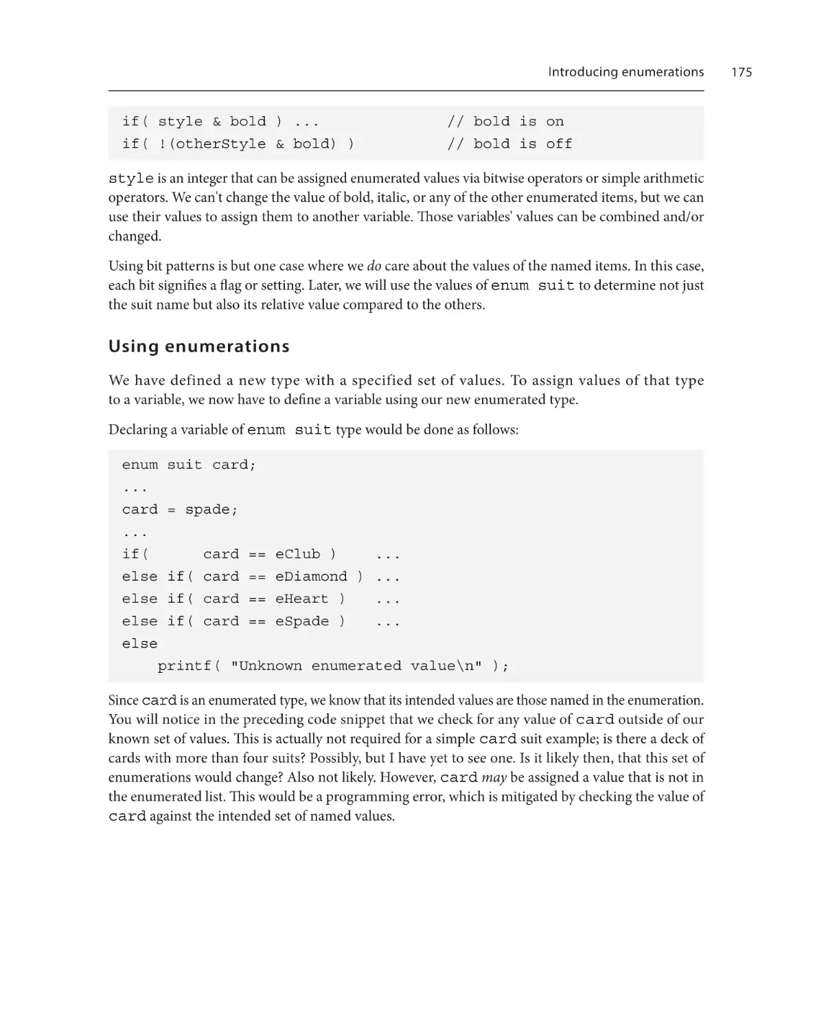
Using enumerations

The switch()… statement revisited

170
170
171
175

Using enumerated item values as
literal integer constants
184
Summary185
Questions185

179

Part 2: Complex Data Types

9
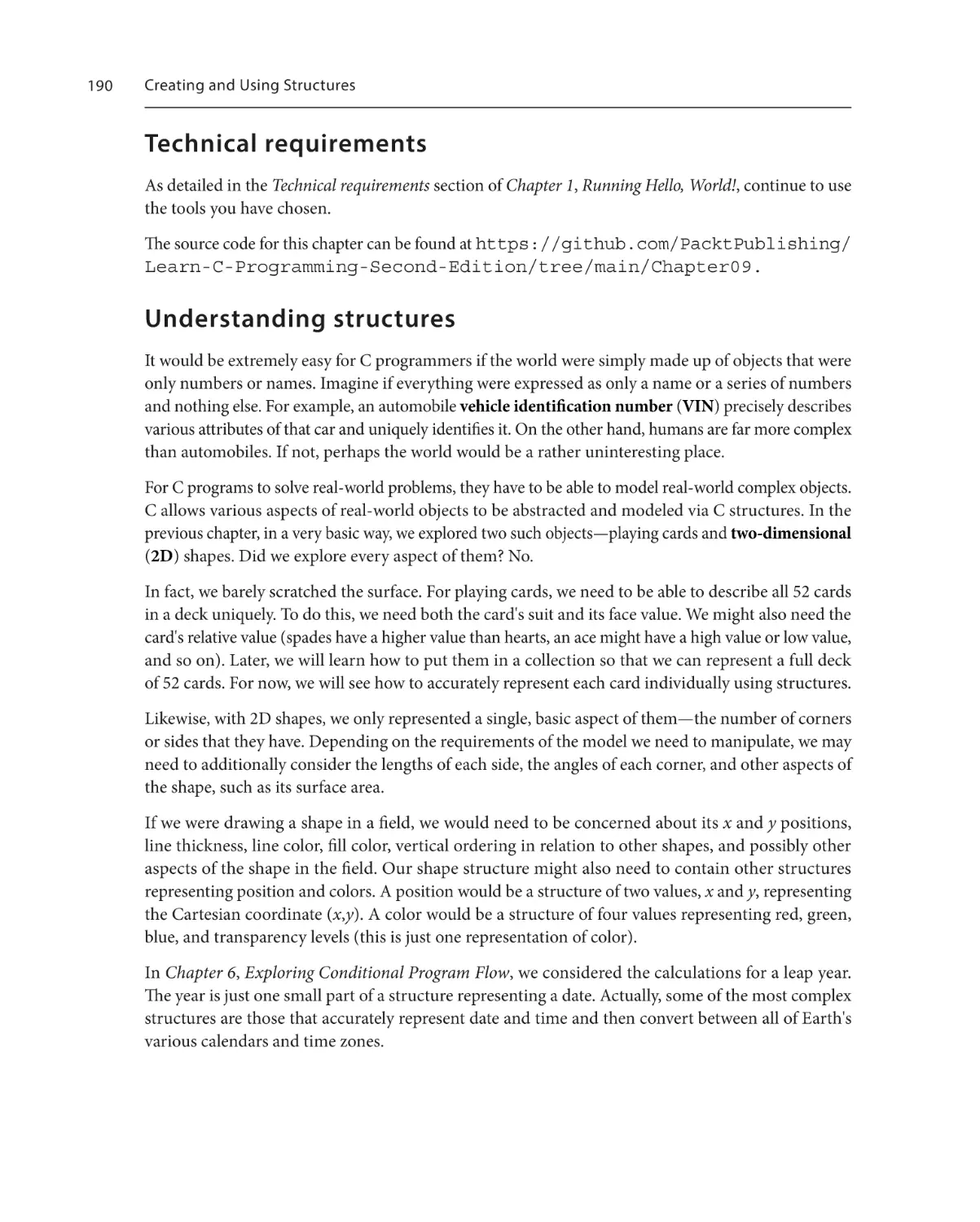
Creating and Using Structures
Technical requirements
Understanding structures

190
190

Declaring structures
191
Initializing structures and accessing structure
elements195

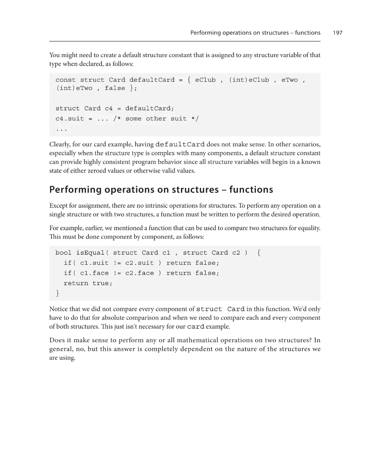
Performing operations on structures
– functions
197

Structures of structures

200

Initializing structures with functions
202
Printing a structure of structures – reusing
functions204

The stepping stone to OOP
208
Summary208
Questions209

10
Creating Custom Data Types with typedef
Technical requirements
211
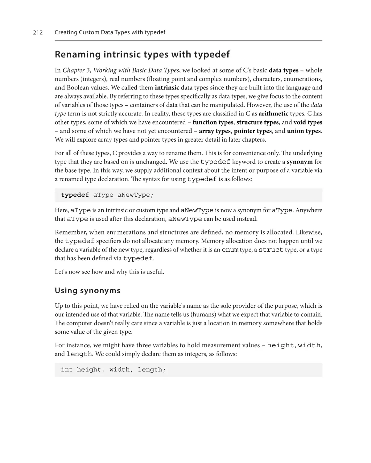
Renaming intrinsic types with typedef212
Using synonyms

212

Simplifying the use of enum types
with typedef215
Simplifying the use of struct types
with typedef
217
Other uses of typedef

220

Exploring some more useful
compiler options
220
Using a header file for custom types
and the typedef specifiers
222
Summary225
Questions226

Table of Contents

11
Working with Arrays
Technical requirements
Declaring and initializing arrays
Initializing arrays

227
228
230

Understanding variable-length arrays 231
Accessing array elements
234

Assigning values to array elements

237

Operating on arrays with loops
237
Using functions that operate on arrays238
Summary243
Questions243

12
Working with Multi-Dimensional Arrays
Technical requirements
Going beyond 1D arrays to multidimensional arrays
Revisiting 1D arrays
Moving on to 2D arrays
Moving on to 3D arrays
Considering N-dimensional arrays

245

Declaring and initializing arrays of N
dimensions253

246

Accessing elements of multidimensional arrays of various
dimensions253
Manipulating multi-dimensional
arrays using loops within loops
255

246
247
248
250

Declaring and initializing multidimensional arrays of various
dimensions250
Declaring arrays of two dimensions
Initializing arrays of two dimensions
Declaring arrays of three dimensions
Initializing arrays of three dimensions

251
251
252
252

Using nested loops to traverse a 2D array
Using nested loops to traverse a 3D array

255
255

Using multi-dimensional arrays in
functions256
Summary261
Questions262

13
Using Pointers
Technical requirements
Addressing pointers – the
boogeyman of C programming
Why use pointers at all?

264
264
265

Introducing pointers

266

Understanding direct addressing and indirect
addressing266
Understanding memory and memory
addressing267

xi

xii

Table of Contents
Managing and accessing memory
Exploring some analogies in the real world

268
268

Declaring the pointer type, naming
pointers, and assigning addresses

271

Declaring the pointer type
Naming pointers
Assigning pointer values (addresses)

Operations with pointers
Assigning pointer values
Differentiating between the NULL pointer
and void*
Accessing pointer targets
Understanding the void* type
Pointer arithmetic

271
272
272

273
273
274
274
278
281

Comparing pointers

281

Verbalizing pointer operations
Variable function arguments

283
284

Passing values by reference
Passing addresses to functions without
pointer variables 
Pointers to pointers

286

Using pointers to structures

289
290

291

Accessing structures and their elements via
pointers292
Using pointers to structures in functions
293

Summary295
Questions295

14
Understanding Arrays and Pointers
Technical requirements
297
Understanding array names and
pointers298
Understanding array elements and
pointers300
Accessing array elements via pointers

301

Operations on arrays using pointers 302

Using pointer arithmetic
302
Passing arrays as function pointers revisited 307
Interchangeability of array names and pointers 307

Introducing an array of pointers to
arrays 310
Summary318
Questions318

15
Working with Strings
Technical requirements
320
Characters – the building blocks of
strings320
The char type and ASCII
Beyond ASCII – UTF-8 and Unicode
Operations on characters
Getting information about characters

321
324
325
328

Manipulating characters

331

Exploring C strings

337

An array with a terminator
Strengths of C strings
Weaknesses of C strings

Declaring and initializing a string

337
337
338

338

Table of Contents
String declarations
Initializing strings
Passing a string to a function
Empty strings versus null strings
Hello, World! revisited

338
339
342
343
344

Creating and using an array of strings346

Common operations on strings – the
standard library
352
Common functions
Safer string operations

352
353

Summary356
Questions357

16
Creating and Using More Complex Structures
Technical requirements
Introducing the need for complex
structures 
Revisiting card4.h
Understanding an array of structures

360

Using a structure with arrays

360
361
370

Understanding randomness and random
number generators
390
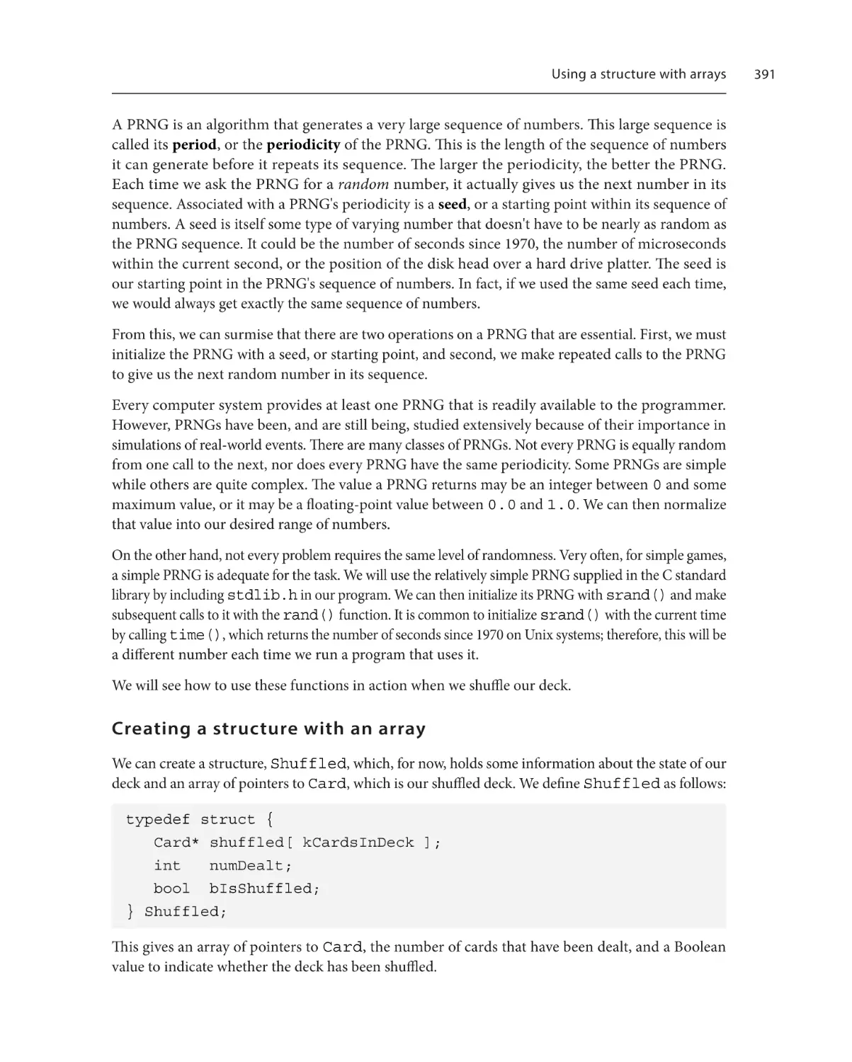
Creating a structure with an array
391
Accessing array elements within a structure
392
Manipulating array elements within a structure392

Creating an array of structures
370
Accessing structure elements within an array 371
Manipulating an array of structures
374

Using a structure with other
structures379
Creating a structure consisting of other
structures380
Accessing structure elements within the
structure380
Manipulating a structure consisting of other
structures382

390

Using a structure with an array of
structures396
Creating a structure with an array of structures396
Accessing individual structure elements of
the array within a structure
397
Manipulating a structure with an array of
structures398
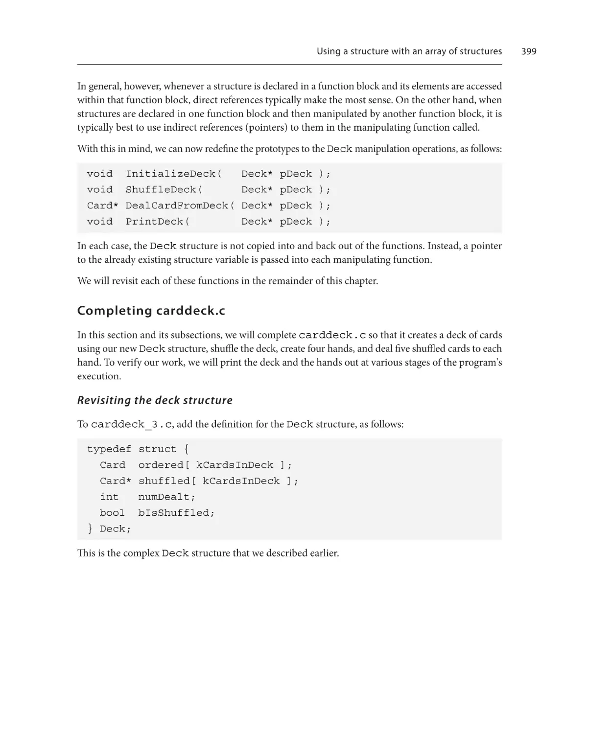
Completing carddeck.c
399

Summary407
Questions408

Part 3: Memory Manipulation

17
Understanding Memory Allocation and Lifetime
Technical requirements
Defining storage classes

412
412

Understanding automatic versus
dynamic storage classes
Automatic storage

412
413

xiii

xiv

Table of Contents
Dynamic storage

Understanding internal versus
external storage classes
Internal or local storage classes
External or global storage classes
The lifetime of automatic storage

413

413
414
415
416

Exploring the static storage class
Internal static storage
External static storage
The lifetime of static storage

416
417
419
421

Summary421
Questions421

18
Using Dynamic Memory Allocation
Technical requirements
Introducing dynamic memory
A brief tour of C's memory layout

424
424
424

Allocating and releasing dynamic
memory426
Allocating dynamic memory
Releasing dynamic memory
Accessing dynamic memory
The lifetime of dynamic memory

426
428
428
429

Special considerations for dynamic
allocation430

Heap memory management

430

The linked list dynamic data structure433
Linked list structures
Declaring operations on a linked list

Pointers to functions
More complex operations on a linked list
A program to test our linked list structure

434
435

445
446
447

Other dynamic data structures
452
Summary453
Questions454

Part 4: Input and Output

19
Exploring Formatted Output
Technical requirements
Revisiting printf()

458
458

Understanding the general format specifier
form458

Using format specifiers for unsigned
integers460
Using unsigned integers in different bases

460

Considering negative numbers as unsigned
integers461
Exploring the powers of 2 and 9 in different
bases462
Printing pointer values
463

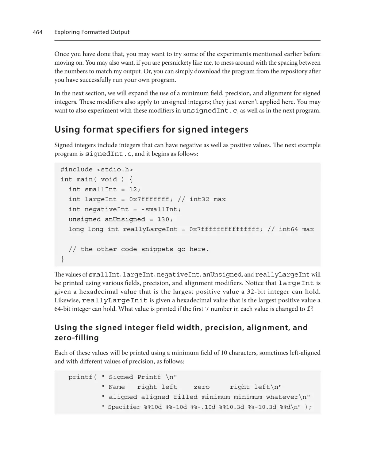
Using format specifiers for signed
integers464

Table of Contents
Using the signed integer field width,
precision, alignment, and zero-filling
Formatting long-long integers
Powers of 2 and 9 with different modifiers

464
465
465

Using format specifiers for floats and
doubles467
Using the floating-point field width,
precision, alignment, and zero-filling
Printing doubles in hexadecimal format

467
469

Printing optimal field widths for doubles

469

Using format specifiers for strings
and characters

471

Using the string field width, precision,
alignment, and zero-filling
Exploring the substring output
Using single character formatting

471
472
472

Summary473
Questions474

20
Getting Input from the Command Line
Technical requirements
Revisiting the main() function
The special features of main()
The two forms of main()

Using argc and argv

475
475
476
476

477

Simple use of argc and argv
478
Command-line switches and command-line
processors480

Summary485
Questions485

21
Exploring Formatted Input
Technical requirements
Introducing streams
Understanding the standard output stream
Understanding the standard input stream
Revisiting the console output with printf()
and fprintf()
Exploring the console input with scanf()

488
488
490
492
492
493

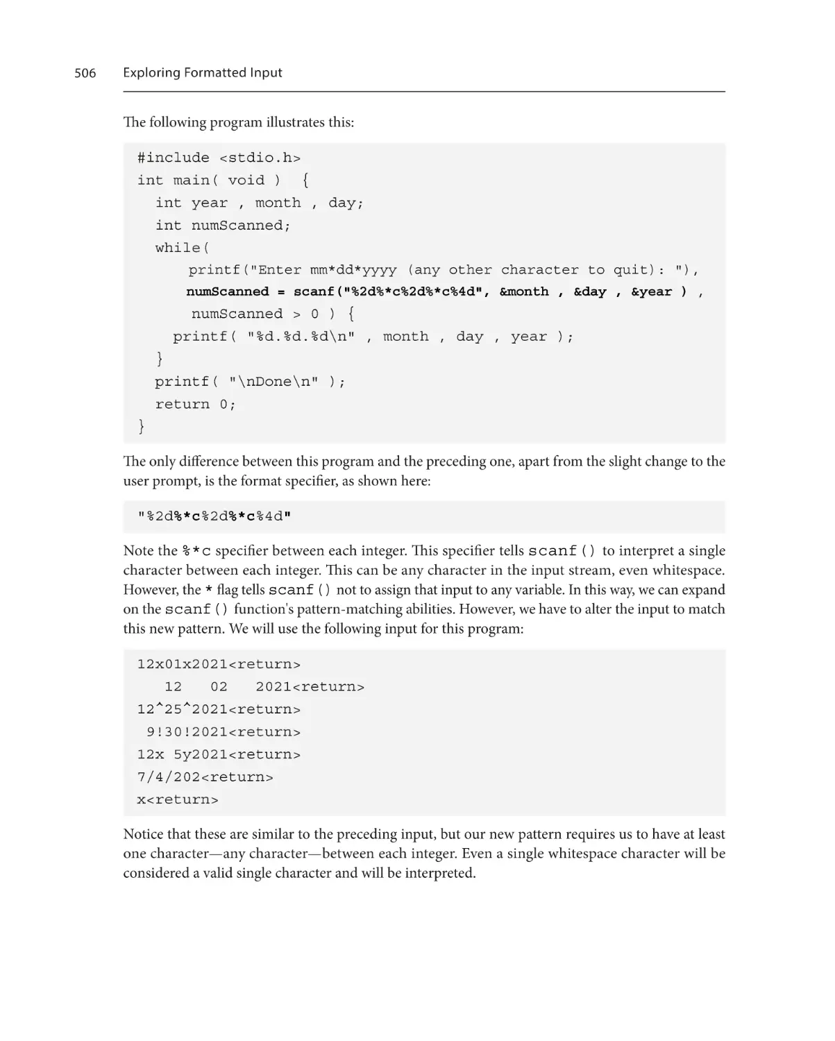
Reading formatted input with scanf() 494
Reading numerical input with scanf()
494
Reading string and character input with scanf()499
Using a scan set to limit possible input
characters502
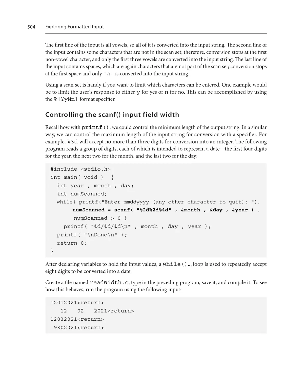
Controlling the scanf() input field width 
504

Using internal data conversion
Using sscanf() and sprintf() to convert values
into and from strings
Converting strings into numbers with atoi()
and atod()

Exploring unformatted I/O
Getting the string I/O to/from the console
Using the simple I/O of strings with gets()
and puts()
Creating a sorted list of names with fgets()
and fputs()

507
508
510

511
511
512
515

Summary520
Questions520

xv

xvi

Table of Contents

22
Working with Files
Technical requirements
Understanding basic file concepts

522
522

Revisiting file streams
522
Understanding the properties of FILE streams 523
Opening and closing a file
524
Understanding file operations for each type of
stream525

Getting acquainted with the filesystem

527

Opening files for reading and writing 528
Getting filenames from within a program
Getting filenames from the command line 

531
534

Summary536
Questions536

Introducing the filesystem essentials 526

23
Using File Input and File Output
Technical requirements
File processing

537
538

Processing filenames from the command line 538

Creating a file of unsorted names
Trimming the input string from fgets()
Reading names and writing names

544
544
546

them
for output
Using a linked list to sort names
Writing names in sorted order

551
552
558

Summary560
Questions560

Reading unsorted names and sorting

Part 5: Building Blocks for Larger Programs

24
Working with Multi-File Programs
Technical requirements
Understanding multi-file programs
Using header files for declarations
and source files for definitions
Creating source files

564
564
565
565

Thinking about multiple source files
Creating header files

Revisiting the preprocessor
Introducing preprocessor directives

566
566

568
568

Table of Contents
Understanding the limits and dangers of the
preprocessor569
Using the preprocessor effectively
569
Debugging with the preprocessor
571

Creating a multi-file program
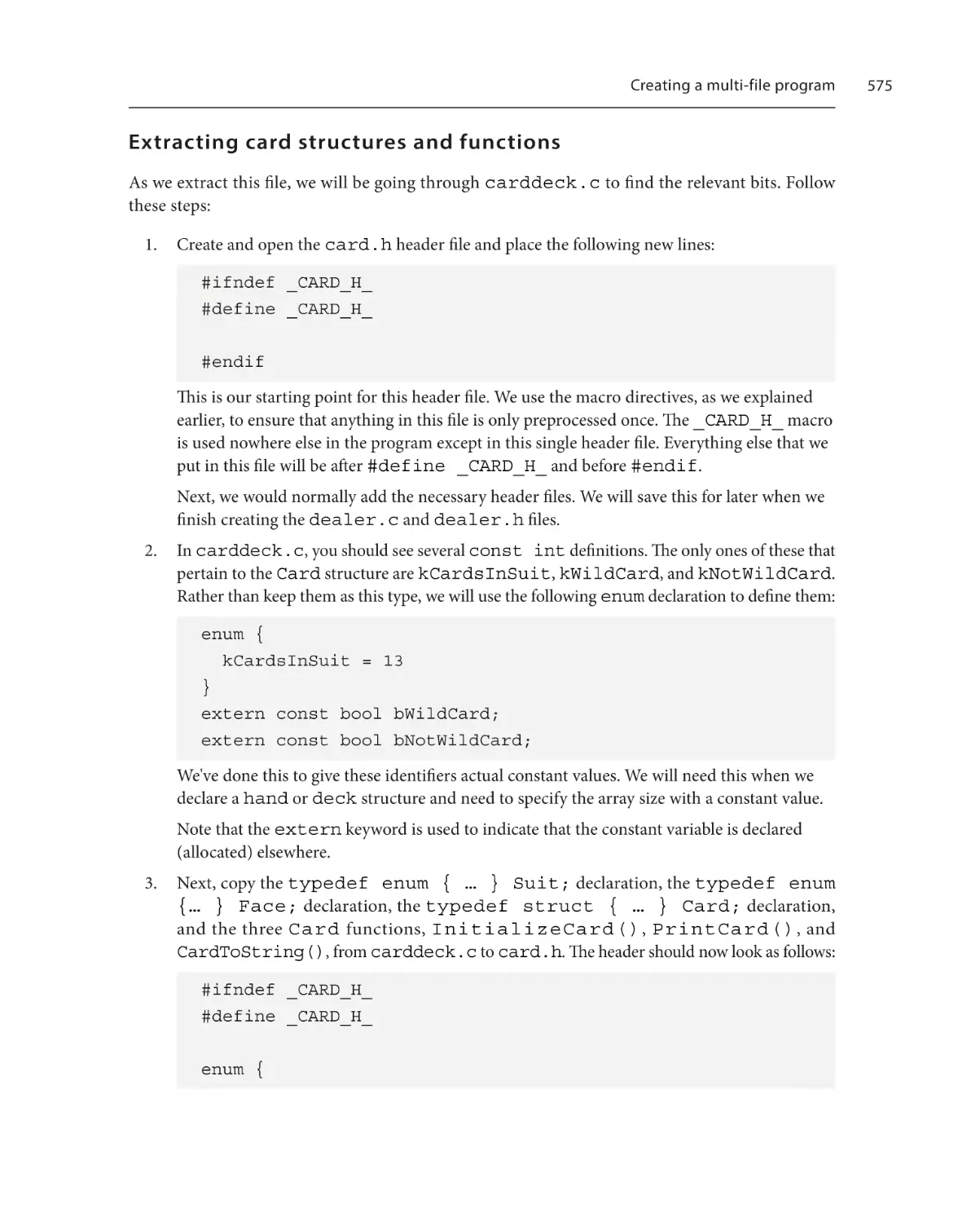
Extracting card structures and functions

574
575

Extracting hand structures and functions
Extracting deck structures and functions
Finishing the dealer.c program

578
580
582

Building a multi-file program
584
Summary586
Questions587

25
Understanding Scope
Technical requirements
Defining scope – visibility, extent,
and linkage

590

variables593

590

Understanding function parameter scope
Understanding file scope
Understanding global scope

597
597
598

Understanding scope for functions

599

Exploring visibility
590
Exploring extent
591
Exploring linkage
592
Putting visibility, extent, and linkage all
together593

Exploring variable scope
Understanding the block scope of

593

Understanding scope and information hiding 599
Using the static specifier for functions
601

Summary605
Questions606

26
Building Multi-File Programs with Make
Technical requirements
Preparing dealer.c for make
Introducing the make utility
Using macros
Using special macros

Creating rules – targets,
dependencies, and actions
Creating useful rules that have only actions
Pattern rules and %

608
608
611
612
613

614
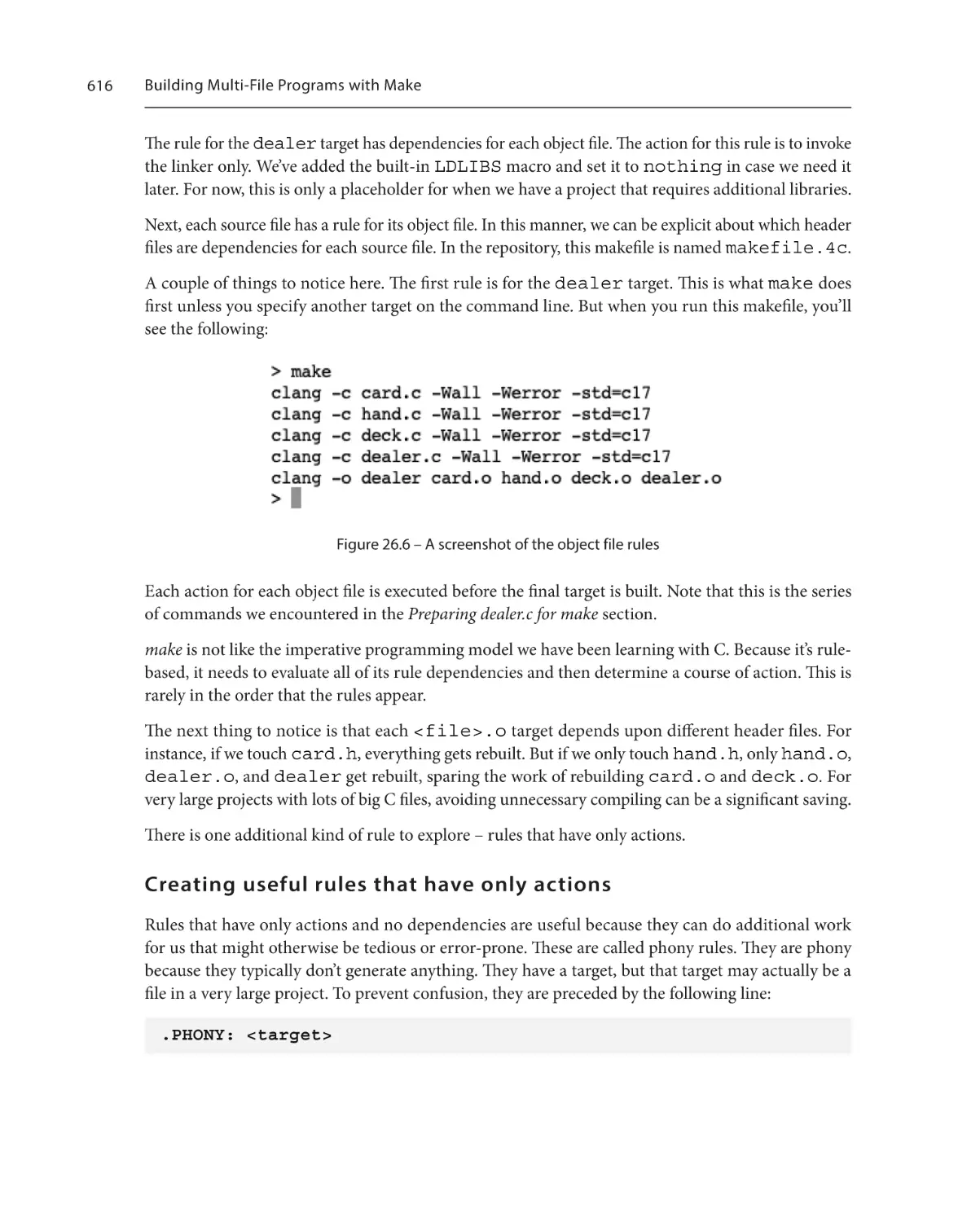
616
617

Built-in functions
Caveman debugging in your makefile

618
618

A general makefile for simple projects619
Going further with make
621
Summary621
Questions621

xvii

xviii

Table of Contents

27
Creating Two Card Programs
Technical requirements
Game one – Blackjack

624
624

Introducing Blackjack624
Determining which structures and functions
will be needed
625
Considering user interaction and the limits of
a console interface
626
Preparing source files for Blackjack
627
Implementing Blackjack
627
Considering ways Blackjack could be extended 640

Game two – One-Handed Solitaire

Introducing One-Handed Solitaire
640
Determining which structures and functions
will be needed
641
Considering user interactions and the limits
of a console interface
641
Preparing source files for One-Handed Solitaire642
Implementing One-Handed Solitaire
648
Considering ways One-Handed Solitaire
could be extended
658

Summary658

640

Appendix
C definition and keywords
659
C keywords
659
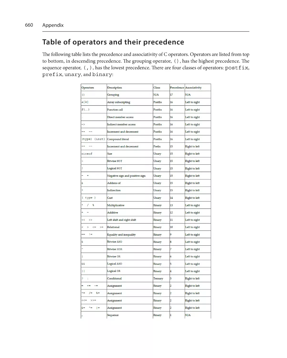
Table of operators and their
precedence660
Summary of useful GCC and Clang
compiler options
661
ASCII character set
661
The Better String Library (Bstrlib)
662
A quick introduction to Bstrlib
663
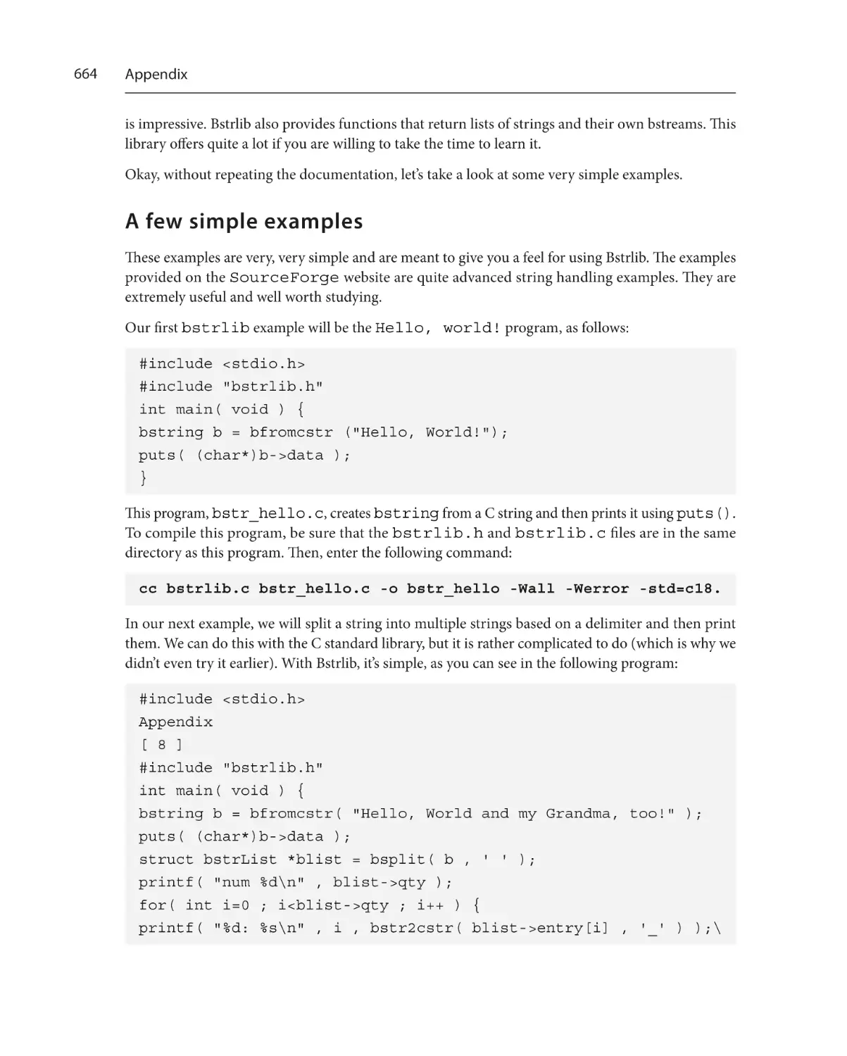
A few simple examples
664

Unicode and UTF-8
A brief history
Where we are today
Moving from ASCII to UTF-8

A UTF to Unicode example
The C standard library
Method 1
Method 2
Method 3

668
668
668
668

669
670
671
672
672

Epilogue
Taking the next steps

675

Assessments
Chapter 2 – Understanding Program
Structure679
Chapter 3 – Working with Basic Data
Types679

Chapter 4 – Using Variables and
Assignments679
Chapter 5 – Exploring Operators
and Expressions
680

Table of Contents

Chapter 6 – Exploring Conditional
Program Flow
680
Chapter 7 – Exploring Loops and
Iteration680
Chapter 8 – Creating and Using
Enumerations681
Chapter 9 – Creating and Using
Structures681
Chapter 10 – Creating Custom Data
Types with typedef
681
Chapter 11 – Working with Arrays 682
Chapter 12 – Working with MultiDimensional Arrays
682
Chapter 13 – Using Pointers
682
Chapter 14 – Understanding Arrays
and Pointers
683
Chapter 15 – Working with Strings 683

Index
Other Books You May Enjoy

Chapter 16 – Creating and Using
More Complex Structures
684
Chapter 17 – Understanding Memory
Allocation and Lifetime
684
Chapter 18 – Using Dynamic
Memory Allocation
684
Chapter 19 – Exploring Formatted
Output685
Chapter 20 – Getting Input from the
Command Line
685
Chapter 21 – Exploring Formatted
Input685
Chapter 22 – Working with Files
686
Chapter 23 – Using File Input and
File Output
686
Chapter 24 – Working with MultiFile Programs
686
Chapter 25 – Understanding Scope 687

xix

Preface
Preface to the Second Edition
In the Preface to the First Edition, I stated that "you will find a particular way to make C work for
you." I must admit that I myself was a victim of this trap. It turns out that because I had learned C
before 1990, I was not as familiar with important C99 features as I should have been. I was guilty of
thinking with my older C version habits. This outdated thinking was reflected largely in the chapter
on enumerations and especially in the chapter introducing arrays, where Variable-Length Arrays
(VLAs) – a major feature of C99 – were poorly covered. Both of these chapters have been completely
rewritten to accurately represent the C standard.
I especially want to thank readers who pointed out the various text and source code typos. I understand
how frustrating it can be when the code you use from the book just won't work. For this reason, extra
attention has been given to the source code in the book and the example programs in the repository.
This edition corrects those typographical errors both in the text and in the sample code. It also corrects
some conceptual errors that were either poorly described or just plain wrong. I offer my sincerest
apologies to the readers of that edition. Any errors that remain are purely my responsibility.
This edition, as much as possible, provides some hints as to what is to come in the next version of
the C standard – C23. These are added refinements that do not change the core of C but extend the
clarity and usefulness of C.
Another addition to this version is the questions at the end of each chapter to reinforce
the key concepts of that chapter. These should prove to be especially useful to programming beginners.
Finally, Chapter 27 has been added, which implements two complete yet simple card games. These
demonstrate how to use pre-built structures and functions as well as how to employ a library, in this
case. our own linked list library, for added functionality.

Preface to the First Edition
Learning to program is the process of learning to solve problems with a computer. Your journey in
gaining this knowledge will be long and arduous with unexpected twists and turns, yet the rewards
of this journey, both small and large, are manyfold. Initial satisfaction comes when you get your
program to work and give the correct results. Satisfaction grows as you are able to solve larger and
more complex problems than you ever thought possible.

xxii

Preface

The beginning of your journey is learning a programming language. This book primarily addresses
that beginning: learning a programming language – in this case, C. The first step in learning a
programming language is to learn its syntax. This means understanding and memorizing important
keywords, punctuation, and the basic building blocks of program structure.
The approach taken in Learn C Programming is intended to give you the tools, methods, and practices you
need to help you minimize the frustrations you will encounter. Every program provided is a complete,
working program using modern C syntax. The expected output for each program is also provided.
Learning to program is especially frustrating because there are so many moving parts. By this, I mean
that every aspect of the programming process has changed over time and will continue to change in
the future. Computer hardware and operating systems will evolve to meet new uses and challenges.
Computer languages will also evolve and change to remove old language deficiencies and also adapt
to solve new problems. The programming practices and methods used today will change as languages
evolve. The kinds of problems that need to be solved will also change as people use computers for
different uses. And lastly, you will change. As you use a programming language, it will change the way
you think about problems. As problems and solutions change, so does our thinking about what will
become possible. This leads to changes in computer language. It's a never-ending cycle.
C has evolved considerably from the language first developed by Dennis Ritchie in the early 1970s.
It was extremely simple yet powerful enough to develop early versions of the Unix operating system
at Bell Labs. Those early versions of C were not for novice programmers. Those versions required
advanced knowledge and programming skills in order to make programs robust and stable. Over the
years, as C compilers became much more widely available, there have been several efforts to rein in
unrestricted and sometimes dangerous language features. The first was ANSI C, codified in 1989. The
next major refinement came with C99, codified in 1999; it included significant language additions
and clarified many C behaviors. Since then, two additional revisions have been made, C11 and C17,
both of which have focused on minor language additions and internal corrections to the language.
C today is much more constrained and complex than the early versions of C. Yet it retains its power,
performance, and suitability for a wide range of computing problems. This book strives to present
the most current syntax and concepts as specified in C99, C11, and C17. Each program has been
compiled and run using the C11 standard. As time goes on, C17 compliance will be much more
widespread than today. I would expect, however, that all of these programs will compile and run as
intended using the C17 standard.
There will always be more to learn, even without the parts moving. After reading Learn C Programming,
you will find a particular way to make C work for you. As you gain experience in solving problems
with C, you will discover new things – features, uses, and limitations – about C that you didn't see
before. So, we can say that learning to program is as much about learning how to learn as it is about
solving problems with programs.
Along the way, you will learn about other programming concepts not directly tied to C. The general
development cycle will not only be discussed but also illustrated in the development of a card-dealing

Who this book is for

program. While you may not be interested in cards, pay particular attention to the process of how
this program is developed. Throughout, the basic practices of experimentation and validation will
be illustrated.

Who this book is for
When this book was conceived, it was intended for two very diverse audiences, the absolute programming
beginner and the experienced programmer who wants to learn C. Each of these audiences has very
different needs.
For the programming beginner, I have written this book as if I were sitting beside you, explaining
the most important concepts and practices you need to know to become a successful C programmer.
I have tried to explain every concept thoroughly and have reinforced each concept with a working
program. The beginner should be familiar with the general operation of their computer; no other
knowledge is assumed.
For the experienced programmer, I have presented the full range of C syntax as well as common C
idioms. You may skim the explanations and focus primarily on the source code provided. The programs
are intended to provide a reference to C syntax.
For both, there are over 100 working programs that demonstrate both the syntax of C as well as the
flavor of C programming idioms – things that are common in C but not found in other languages. I
have sprinkled in programming practices and techniques that have served me well in my nearly 35
years of experience.

What this book covers
Part 1, C Fundamentals, introduces the very basic concepts of C syntax and program structure.
Chapter 1, Running Hello, World!, introduces the program development cycle and the tools you'll need
for the rest of the book. Those tools are used to create, build, and run your first C program, a "Hello,
world!" program. The concepts of commenting code and experimenting with code are also introduced.
Chapter 2, Understanding Program Structure, introduces statements and blocks. It also describes
function definitions and function declarations, also known as function prototypes. How functions
are called and their order of execution is illustrated. Statements, blocks, and functions define the
structure of C programs.
Chapter 3, Working with Basic Data Types, explores how C represents values in various ways through the
use of data types. Each data type has a size and possible range of values that C uses to interpret a value.
Chapter 4, Using Variables and Assignments, introduces variables and constants, which are used to
contain values. For a variable to receive a value, that value must be assigned to it; several types of
assignment are explained.

xxiii

xxiv

Preface

Chapter 5, Exploring Operators and Expressions, introduces and demonstrates operations – ways to
manipulate values – on each of the various data types.
Chapter 6, Exploring Conditional Program Flow, introduces the flow of control statements, which
execute one group of statements or another, depending on the result of an expression.
Chapter 7, Exploring Loops and Iterations, introduces each of the looping statements. It also describes
the proper and improper use of goto. Additional means of controller loop iterations are explained.
Chapter 8, Creating and Using Enumerations, explains named constants, enumerations, and how to
use them.
Part 2, Complex Data Types, extends your understanding of the concepts of basic, or intrinsic, data
types to more complex types.
Chapter 9, Creating and Using Structures, explores how to represent complex objects with groups
of variables, called structures. Operations on structures are explored. How structures are related to
object-oriented programming is described.
Chapter 10, Creating Custom Data Types with typedef, describes how to rename enum and struct
declarations. Compiler options and header files are explored.
Chapter 11, Working with Arrays, illustrates how to define, initialize, and access simple arrays. Using
loops to traverse arrays is explored. Operating on arrays via functions is demonstrated.
Chapter 12, Working with Multi-Dimensional Arrays, extends your understanding of the concept of
one-dimensional arrays to two-, three-, and n-dimensional ones. Declaring, initializing, and accessing
these multi-dimensional arrays in loops and functions are demonstrated.
Chapter 13, Using Pointers, explores direct and indirect addressing with pointers. Operations with
pointers are demonstrated. How to think and talk about pointers is described. Using pointers in
functions and using pointers to structures is demonstrated.
Chapter 14, Understanding Arrays and Pointers, explores the similarities and differences between
pointers and arrays.
Chapter 15, Working with Strings, introduces the ASCII character set and C strings, which are arrays
with two special properties. A program to print the ASCII character set in a table is developed. The
C standard library string operations are introduced.
Chapter 16, Creating and Using More Complex Structures, builds upon the concepts of structures and
arrays to explore how to create various combinations of complex structures. Throughout the chapter,
each complex structure is demonstrated through the development of a complete card-dealing program.
This chapter provides the most comprehensive example of the method of stepwise, iterative program
development.
Part 3, Memory Manipulation, explores how memory is allocated and deallocated in a variety of ways.

What this book covers

Chapter 17, Understanding Memory Allocation and Lifetime, introduces the concepts of automatic
versus dynamic memory storage classes as well as internal versus external storage classes. The static
storage class is demonstrated.
Chapter 18, Using Dynamic Memory Allocation, introduces the use of dynamic memory and describes
various operations on dynamic memory. A dynamic linked-list program is demonstrated. An overview
of other dynamic structures is provided.
Part 4, Input and Output, explores a wide variety of topics related to the reading (input) and writing
(output) of values.
Chapter 19, Exploring Formatted Output, goes into thorough detail about the various format specifiers
of printf() for each of the intrinsic data types: signed and unsigned integers, floats and doubles,
and strings and characters.
Chapter 20, Getting Input from the Command Line, demonstrates how to usethe argc and argv
parameters of main() to get values from the command line.
Chapter 21, Exploring Formatted Input, demonstrates how to read values from an input stream using
scanf(). It clarifies how the format specifiers for printf() and scanf(), while similar, are
really very different. Internal data conversion and unformatted input and output are also demonstrated.
Chapter 22, Working with Files, is a largely conceptual chapter that introduces basic file concepts. It
demonstrates how to open and close files from within a program and from the command line.
Chapter 23, Using File Input and File Output, demonstrates how to use command-line switches with
getopt() to read and write files. The basic program is then expanded to read names from input,
sort them via a linked list, and then write them out in sorted order.
Part 5, Building Blocks for Larger Programs, details how to create and manage programs that consist
of multiple files.
Chapter 24, Working with Multi-File Programs, demonstrates how to take the single source file program
that was developed in Chapter 16, Creating and Using More Complex Structures, and separate it into
multiple source files. Each of the source files has functions that are logically grouped by the structures
they manipulate. Effective and safe uses for the preprocessor are described.
Chapter 25, Understanding Scope, defines various components of scope and how they relate to singleand multi-file programs. Details of variable scope and function scope are described.
Chapter 26, Building Multi-File Programs with make, introduces basic features of the make utility. make
is then used to build a multi-file program. A general-purpose makefile is developed.
Chapter 27, Creating Two Card Programs, starts with the dealer program developed in Chapter 16,
Creating and Using More Complex Structures, to create two different yet complete and playable card
games: Blackjack, or 21, and One-Handed Solitaire. The user interface is limited to the command-line
entry of characters.

xxv

xxvi

Preface

The Epilogue outlines some useful next steps to take in learning both C and programming.
The Appendix provides a number of useful reference guides. These include C keywords, operator
precedence, a summary of some useful GCC and Clang options, ASCII characters, using Bstrlib,
a brief overview of Unicode, an annotated history of C versions, and an itemization of the C standard
library.

To get the most out of this book
To use this book, you will need a basic text editor, a terminal or console application, and a compiler.
Descriptions of each of these and how to download and use them are provided in Chapter 1, Running
Hello, World!. Here are the technical requirements for this book:

All of the software given in the table are either built into the operating system or are free to download.
To install GCC on certain Linux OSs, follow these steps:
• If you are running an RPM-based Linux, such as Red Hat, Fedora, or CentOS, on the command
line in Terminal, enter the following:
$ sudo yum group install development-tools
If you are running Debian Linux, on the command line in Terminal, enter the following:
$ sudo apt-get install build-essential

To get the most out of this book

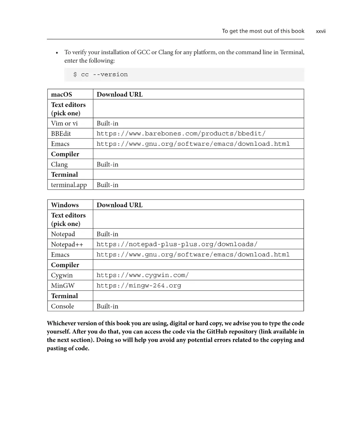
• To verify your installation of GCC or Clang for any platform, on the command line in Terminal,
enter the following:
$ cc --version

Whichever version of this book you are using, digital or hard copy, we advise you to type the code
yourself. After you do that, you can access the code via the GitHub repository (link available in
the next section). Doing so will help you avoid any potential errors related to the copying and
pasting of code.

xxvii

xxviii

Preface

If you are an absolute beginner, once you have the necessary development tools, you will need to learn
how to read a programming book. If you have taken an algebra course or a calculus course in school,
then you will need to approach learning from a programming book in a similar fashion:
1.

Read through the chapter to get an overview of the concepts being presented.

2.

Begin the chapter again, this time typing in each program as you encounter it. Make sure you
get the expected output before moving on. If you don't get the expected output, try to figure
out what is different in your program from the one given. Learning to program is a lot like
learning math – you must do the exercises and get the programs to work. You cannot learn
to program just by looking at programs; to learn to program, you must program. There is no
way around that.

3.

Focus on memorizing keywords and syntax. This will greatly speed up your learning time.

4.

Be aware that you will need to sharpen the precision of your thinking. The syntax of computer
language is extremely precise, and you will need to pay extra attention to it. You will also have
to think much more precisely and in sometimes excruciating detail about the steps needed to
solve a particular problem.

5.

Review both the concepts and example programs. Make a note of anything you don't understand.

If you are an experienced programmer who is new to C, I still strongly advise you to first skim the
text and examples. Then, enter the programs and get them to work on your system. This will help you
to learn C syntax and its idioms more quickly.
I have found that it is important to understand what kind of book you are reading so that you can use
it most appropriately. There are several kinds of computer programming books:
• Conceptual books, which deal with the underlying ideas and motivation for the topics they
present. Kernighan and Ritchie's The C Programming Language and Effective C: An Introduction
to Professional C Programming, by Seacord, are two such books.
• Textbooks, which go through every major area of the language, sometimes in gory detail and
usually with a lot of code snippets. Deitel and Deitel's books, as well as C Programming: A
Modern Approach, by K. N. King, are examples of these. They are often best used in a formal
programming course.
• Reference books, which describe the specifics of each syntax element. C: A Reference Manual,
by Harbison and Steele, is one such book.
• Cookbooks, which present specific solutions to specific problems in a given language. Advanced
C Programming by Example, by Perry, Expert C Programming: Deep Secrets, by Van Der Linden,
and Algorithms in C, by Sedgewick, are examples of these.
• Topical books, which delve deeply into one or more aspects of a programing language. Pointers
in C, by Reek, is one example.

Download the example code files

• Practice books, which deal with how to address programming with C generally. C Interfaces
and Implementations, by Hanson, and 21st Century C: C Tips from the New School, by Klemens,
are two examples of these.
There are different ways to use these books. For instance, read a conceptual book once, but keep a
reference book around and use it often. Try to find cookbooks that offer the kinds of programs you
are likely to need and use them as needed.
I think of this book as a combination of a C cookbook, a C reference book, and a C practice book.
This is not intended to be a textbook. All of the programs are working examples that can be used to
verify how your compiler behaves on your system. Enough of the C language has been included that
it may also be used as a first-approximation reference. Throughout, my intent has been to show good
programming practice with C.
I expect that Learn C Programming will not be your last book on C. When you consider other C books,
be sure that they pertain to C99 at a minimum; ideally, they should include C11, C17, or C23. Most
C code before C99 is definitely old-school; more effective programming practices and methods have
been developed since C99 and before.

Download the example code files
You can download the example code files for this book from GitHub at https://github.com/
PacktPublishing/Learn-C-Programming-Second-Edition. If there's an update
to the code, it will be updated in the GitHub repository.
We also have other code bundles from our rich catalog of books and videos available at https://
github.com/PacktPublishing/. Check them out!

Download the color images
We also provide a PDF file that has color images of the screenshots and diagrams used in this book.
You can download it here: https://packt.link/uDSeu

Conventions used
There are a number of text conventions used throughout this book.

Code in text: Indicates code words in text, database table names, folder names, filenames, file
extensions, pathnames, dummy URLs, user input, and Twitter handles. Here is an example: "Mount
the downloaded WebStorm-10*.dmg disk image file as another disk in your system."

xxix

xxx

Preface

A block of code is set as follows:
html, body, #map {
height: 100%;
margin: 0;
padding: 0
}
When we wish to draw your attention to a particular part of a code block, the relevant lines or items
are set in bold:
[default]
exten => s,1,Dial(Zap/1|30)
exten => s,2,Voicemail(u100)
exten => s,102,Voicemail(b100)
exten => i,1,Voicemail(s0)
Any command-line input or output is written as follows:
$ mkdir css
$ cd css
Tips or Important Notes
Appear like this.

Get in touch
Feedback from our readers is always welcome.
General feedback: If you have questions about any aspect of this book, email us at customercare@
packtpub.com and mention the book title in the subject of your message.
Errata: Although we have taken every care to ensure the accuracy of our content, mistakes do happen.
If you have found a mistake in this book, we would be grateful if you would report this to us. Please
visit www.packtpub.com/support/errata and fill in the form.
Piracy: If you come across any illegal copies of our works in any form on the internet, we would
be grateful if you would provide us with the location address or website name. Please contact us at
copyright@packt.com with a link to the material.
If you are interested in becoming an author: If there is a topic that you have expertise in and you
are interested in either writing or contributing to a book, please visit authors.packtpub.com.

Share Your Thoughts

Share Your Thoughts
Once you’ve read Learn C Programming, we’d love to hear your thoughts! Please click here to
go straight to the Amazon review page for this book and share your feedback.
Your review is important to us and the tech community and will help us make sure we’re delivering
excellent quality content.

xxxi

Par t 1:
C Fundamentals

We are going to start right away writing simple programs as we explore the fundamentals of not only
C but also general programming.
This part contains the following chapters:
• Chapter 1, Running Hello, World
• Chapter 2, Understanding Program Structure
• Chapter 3, Working with Basic Data Types
• Chapter 4, Using Variables and Assignments
• Chapter 5, Exploring Operators and Expressions
• Chapter 6, Exploring Conditional Program Flow
• Chapter 7, Exploring Loops and Iterations
• Chapter 8, Creating and Using Enumerations

1
R u n n i n g H e l l o, Wo r l d !
Computer programming is about learning how to solve problems with a computer – it's about how to
get a computer to do all the tedious work for you. The basic development cycle, or process of writing
a computer program, is to determine the steps that are necessary to solve the problem at hand and
then tell the computer to perform those steps. Our first problem, as we begin exploring this process,
is to learn how to write, build, run, and verify a minimal C program.
In this chapter, we will cover the following topics:
• Writing your first C program
• Understanding the program development cycle
• Creating, typing into a text editor, and saving your C program
• Compiling your first C program
• Running your program, verifying its result, and, if necessary, fixing it
• Exploring different commenting styles and using them
• Employing guided chaos, followed by careful observation for deeper learning
The knowledge gained with these topics will be essential for further progress. So, let's get started!

4

Running Hello, World!

Technical requirements
To complete this chapter and the rest of this book, you will need a running computer that has the
following capabilities:
• A basic text editor that can save unformatted plain text
• A Terminal window where commands can be entered via the command line
• A compiler to build your C programs with
Each of these will be explained in more detail as we encounter them in this chapter.
The source code for this chapter can be found at https://github.com/PacktPublishing/
Learn-C-Programming-Second-Edition. However, please make every effort to type the
source code in yourself. Even if you find this frustrating at first, you will learn far more and learn far
more quickly if you do all the code entry yourself.

Writing your first C program
We will begin with one of the simplest, most useful programs that can be created in C. This program
was first used to introduce C by its creators, Brian W. Kernighan and Dennis M. Ritchie, in their
now-classic work, The C Programming Language, which was published in 1978. The program prints
a single line of output – the greeting Hello, world! – on the computer screen.
This simple program is important for several reasons. First, it gives us a flavor of what a C program
is like, but more importantly, it proves that the necessary pieces of the development environment –
the Operating System (OS), text editor, command-line interface, and compiler – are installed and
working correctly on your computer system. Finally, it gives us a first taste of the basic programming
development cycle. In the process of learning to program and, later, actually solving real problems
with programming, you will repeat this cycle often. It is essential that you become both familiar and
comfortable with this cycle.
This program is useful because it prints something out to the Terminal, also known as the console,
telling us that it actually did something – it displays a message to us. We could write shorter programs
in C, but they would not be of much use. Although we would be able to build and run them, we
would have very little evidence that anything actually happened. So, here is your first C program.
Throughout this book, and during the entirety of your programming experience, obtaining evidence
of what actually happened is essential.

Writing your first C program

Since Kernighan and Ritchie introduced the Hello, world! program over 40 years ago, this simple
program has been reused to introduce many programming languages and has been used in various
settings. You can find variations of this program in Java, C++, Objective-C, Python, Ruby, and more.
GitHub, an online source code repository, even introduces its website and its functions with a Hello
World beginner's guide.

Hello, world!
Without further ado, here is the Hello, world! C program. It performs no calculations, nor does it
accept any input. It only displays a short greeting and then ends, as follows:
#include <stdio.h>
int main()
{
printf( "Hello, world!\n" );
return 0;
}
Some minor details of this program have changed since it was first introduced. What is presented here
will build and run with all C compilers that have been created in the last 30 years.
Before we get into the details of what each part of this program does, see whether you can identify
which line of the program prints our greeting. You might find the punctuation peculiar; we will explain
this in the next chapter. Additionally, notice how some punctuation marks come in pairs, while others
do not. There are five paired and five unpaired punctuation marks in total. Can you identify them?
(Note that we are not counting the punctuation, that is, the comma and exclamation point, in the
Hello, world! message.)
There is another pairing in this simple program that is not so obvious at this time but one that we will
explore further in the next chapter. As a hint, this pairing involves the int main() and return
0; lines.
Before we jump into creating, compiling, and running this program, we need to get an overview of
the whole development process and the tools we'll be using.
Tip
If you are eager to begin creating your first program, you can jump ahead to the next section.
If you do, please come back to the Understanding the program development cycle section to
complete your understanding.

5

6

Running Hello, World!

Understanding the program development cycle
There are two main types of development environments:
• Interpreted: In an interpreted environment such as Python or Ruby, the program can be
entered, line by line, and run at any point. Each line is evaluated and executed as it's entered,
and the results are immediately returned to the console. Interpreted environments are dynamic
because they provide immediate feedback and are useful for the rapid exploration of algorithms
and program features. Programs entered here tend to require the interpreting environment to
be running as well.
• Compiled: In a compiled environment, such as C, C++, C#, or Objective-C, programs are entered
into one or more files, then compiled all at once, and if no errors are found, the program can
be run as a whole. Each of these phases is distinct, with separate programs used for each phase.
Compiled programs tend to execute faster since there is a separate, full compilation phase that
can be run independently of the interpreting environment.
As with shampoo, where we are accustomed to wet hair, lather, rinse, and repeat, we will do the same
with C – we will become familiar with the edit, compile, run, verify, and repeat cycle.

Edit
Programs are generated from text files whose filenames use predefined file extensions. These are known
as source files or source code files. For C, the .c file extension indicates a C source code file. A .h
extension (which is present in our Hello, world! program) indicates a C header file. The compiler looks
for .c and .h files as it encounters them, and because each has a different purpose, it also treats each
of them differently. Other languages have their own file extensions; the contents of a source code file
should match the language that the compiler expects.
To create and modify C files, you will need a plain text editor. This is a program that allows you to
open, modify, and save plain text without any formatting such as font size, font family, and font style.
For instance, on Windows, Notepad is a plain text editor while Word is not. The plain text editor
should have the following capabilities:
• File manipulation: This allows you to open a file, edit a file, save the file and any changes that
have been made to it, and, finally, save the file with another name.
• The ability to navigate the file: This allows you to move up, down, left, or right to the beginning
of the line, end of the line, beginning of the file, end of the file, and more.
• Text manipulation: This allows you to insert text, delete text, insert a line, delete a line, selection,
cut, copy, paste, undo/redo, and more.
• Search and replace: This allows you to find text, replace text, and more.

Understanding the program development cycle

The following capabilities are handy but not essential:
• Automatic indentation
• Syntax coloring for the specific programming language
• Automatic periodic saving
Almost any plain text editor will do. Do not get too caught up in the features of any given text editor.
Some are better than others; some are free, while others are costly and might not immediately be
worth the expense (perhaps later, one or more might be worthwhile but not at this time), and none
will do 100% of what you might want them to do.
Here are some free plain text editors that are worth installing on your computer and trying out:
• Everywhere: Nano, which runs in a Terminal window; it has a moderate learning curve.
• Linux/Unix: This consists of the following:
a. Vim or vi: This runs in a Terminal window; it has a moderate learning curve. It is on every
Linux/Unix system, so it's worth learning how to use its basic features.
b. gedit: This is a powerful general-purpose editor.
c. Emacs: This is an everything and the kitchen sink editor; it has a very large learning curve.
• Windows: This consists of the following:
a. Notepad: This is very simple – sometimes too simple for programming – but included in
every Windows system.
b. Notepad++: This is a better version of Notepad with many features for programming.
• macOS only: This runs BBEdit (the free version), which is a full-featured GUI programming
text editor.
There are many text editors, each with its own strengths and weaknesses. Pick a text editor and get
used to it. Over time, as you use it more and more, it will become second nature.

Compile
The compiler is a program that takes input source code files – in our case, the .c and .h files – translates
the textual source code found there into machine language, and links together all the predefined parts
required to enable the program to run on our specific computer hardware and OS. It generates an
executable file that consists of machine language.

7

8

Running Hello, World!

Machine language is a series of instructions and data that a specific Central Processing Unit (CPU)
knows how to fetch from the program execution stream and execute on the computer one by one. Each
CPU has its own machine language or instruction set. By programming in a common language, such
as C, the programmer is shielded from the details of machine language; that knowledge is embodied
in the compiler.
Sometimes, assembler language is called machine language, but that is not quite accurate since
assembler language still contains text and symbols, whereas machine language only consists of binary
numbers. Today, very few people have the skills to read machine language directly; at one time, many
more programmers were able to do it. Times have changed!
When we compile our programs, we invoke the compiler to process one or more source files. The
result of this invocation is either a success and an executable file is generated, or it will identify the
programming errors it found during compilation. Programming errors can range from a simple
misspelling of names or omitted punctuation to more complex syntax errors. Typically, the compiler
tries to make sense of any errors it finds; it attempts to provide useful information for the problem it
has found. Note that try and attempts are merely goals; in reality, the compiler might spew many lines
of error messages that originate from a single error. Furthermore, the compiler will process the entire
source code when invoked. You might find many different errors in different parts of the program for
each compiler invocation.
A complete, runnable program consists of our compiled source code – the code we write – and
predefined compiled routines that come with the OS, that is, code written by the authors of the OS.
The predefined program code is sometimes called the runtime library. It consists of a set of callable
routines that know how to interact, in detail, with the various parts of the computer. For example, in
Hello, world!, we don't have to know the detailed instructions to send characters to the computer's
screen – we can simply call a predefined function, printf();, to do it for us. printf() is part
of the C runtime library, along with many other routines, as we will discover later. In the next chapter,
we will explore the role of functions. How text is sent to the console is likely to be different for each
OS, even if those OSes run on the same hardware. So, the programmers are shielded not only from
the minutiae of the machine language, but they are also shielded from the varying implementation
details of the computer itself.
It follows from this that for each OS, there is a compiler and a runtime library specific to it. A compiler
designed for one OS will most likely not work on a different OS. If, by chance, a compiler from one OS
just happens to or even appears to run on a different OS, the resulting programs and their executions
would be highly unpredictable. Mayhem is likely.

Many C compilers for every OS
You can learn C on many computer platforms. Common compilers in use on Unix and Linux OS are
either the GNU Compiler Collection (GCC) or the LLVM compiler project, Clang. For Windows, GCC
is available via the Cygwin project or the MinGW project. You could even learn C using a Raspberry
Pi or Arduino, but this is not ideal because of the special considerations required for these minimal

Understanding the program development cycle

computer systems. It is recommended that you use a desktop computer since many more computer
resources (such as memory, hard drive space, CPU capability, and more) are available on any such
computer that can run a web browser.
Important Note
You should be aware that there are many variants of C. Typically, these are created by hardware
vendors for the specific needs of their customers or by other groups who wish to retain extended
features not approved in the standard specification.
Also, be aware that there are areas of the C specification that are undefined; that is, the standards
committees have left those implementation details up to the creators of a given compiler for
a given hardware system.
In this book, we will describe and focus strictly upon what the C standard provides. However,
our approach will be such that we will emphasize how to verify program behavior so that we will
always know when our program behaves differently. Because compilers are written by humans
and not autogenerated from a specification, we subscribe to the guidance: trust but verify.

A note about Integrated Development Environments
On many OSes, the compiler is installed as a part of an Integrated Development Environment
(IDE) for that OS. An IDE consists of a set of programs needed to create, build, and test programs
for that OS. It manages one or more files associated with a program, has its own integrated text editor,
can invoke the compiler and present its results, and can execute the compiled program. Typically,
the programmer never leaves this environment while developing. Often, the IDE streamlines the
production of a standalone working program.
There are many such IDEs – Microsoft's Windows-only Visual Studio, Microsoft's multiplatform Visual
Studio Code, Apple's Xcode for macOS and other Apple hardware platforms, Eclipse Foundation's
Eclipse, and Oracle's Netbeans, to name a few. Each of these IDEs can develop programs in a variety
of languages. Nearly all of the programs used in this book were developed using a simple IDE named
CodeRunner for macOS.
We will not use an IDE to learn C. In fact, at this stage of your learning, it is not advised for several
reasons. To begin, learning and using an IDE can be a daunting learning task in and of itself. This
task can and should be put off until you have more experience with each of the individual parts of the
program development cycle. IDEs, while they have common functions, are sometimes implemented
in vastly different ways with far too many different features to explore. Learn C first; then, you can
learn an IDE for your desired environment later.

9

10

Running Hello, World!

Installing a compiler on Linux, macOS, or Windows
Here are the steps to follow to install a C compiler on the major desktop computer environments –
Linux, macOS, and Windows. For other platforms, you'll have to do some investigation to find the
compiler you need. However, since those platforms want you to use them, they'll likely make those
instructions easy to find and follow:
• For Linux, perform the following steps:
1. If you are running a Red Hat Package Manager (RPM)-based Linux, such as Red Hat,
Fedora, or CentOS, enter the following command on the command line:
$ sudo yum group install development-tools
2. If you are running Debian Linux, open a Terminal window and enter the following
command from the command line:
$ sudo apt-get install build-essential
3. Verify your installation by entering the following command on the command line:
$ cc --version
From the preceding command, you will observe that you likely have GCC or Clang. Either
one is fine. You are now ready to compile C programs on your version of Linux.
• For macOS, perform the following steps:
1. Open Terminal.app and enter the following on the command line:
$ cc --version
2. If the development tools have not been installed yet, simply invoking the preceding
command will guide you through their installation.
3. Once the installation is complete, close the Terminal window, open a new one, and enter
the following:
$ cc --version
You are now ready to compile C programs on your version of macOS.
• For Windows, perform the following steps:
1. Install either Cygwin (http://www.cygwin.com) or MinGW (http://mingww64.org/) from their respective websites. Either one will work well. If you choose to
install Cygwin, be sure to also install the extra package for the GCC. This will install a
number of other necessary compilers and debugging programs with GCC.
2. Once the installation is complete, open Command Prompt and enter the following:
$ cc --version
You are now ready to compile C programs on your version of Windows.

Understanding the program development cycle

Note that compilation is a two-part process – compiling and linking. Compiling involves syntax
checking and converting source code into nearly complete executable code. In the linking phase, the
nearly complete machine code is merged with the runtime library and becomes complete. Typically,
when we invoke the compiler, the linker is also invoked. If the compiler phase succeeds (that is, with
no errors), the linking phase is automatically invoked. Later, we will discover that we can get error
messages from the compiler either at compile time – the compiling phase – or at link time – the linking
phase – when all of the program's pieces are linked together.
We will learn how to invoke the compiler later when we compile our first program.
Throughout this book, once you have a working program, you will be directed to purposely break
it – causing the compilation of your program to fail. This is so that you can start learning about the
correlation of various program errors with compiler errors, so you will not be afraid of breaking your
program. You will simply undo the change and success will be yours once more.

Run
Once compilation has been completed successfully, an executable file will be generated. This executable
file, unless we provide an explicit name for it, will be named a.out. Typically, the executable file
will be created in the same directory the compiler was invoked from. For the most part, we will make
sure our current working directory has the same location as the source files.
Running an executable file is performed by invoking it from the command line. When invoked, the
executable is loaded into the computer's memory and then becomes the CPU's program execution
stream. Once loaded into memory, the CPU begins at the special reserved word, known as main(),
and continues until either return; or a closing } character is encountered. The program stops and
the executable is then unloaded from memory.
To run an executable, open Command Prompt (on Windows) or a Terminal window (on Linux and
Mac), navigate with cd to the directory of the executable file, and simply enter the executable's name
(for example, a.out or whatever you've specified).
Note
If you successfully navigate to the same location as the executable and you have verified it exists,
but you get an error message from the command interpreter, you likely have a problem with
your command interpreter's built-in PATH variable. To quickly work around this, enter the $
./a.out command to run it. This instructs the command interpreter to look in the current
directory for the file named a.out.
As the program runs, any output will be directed to the Terminal or console window. When the program
has ended, the command interpreter will present you with a new command prompt.

11

12

Running Hello, World!

Verify
At this point in the cycle, you might feel that simply getting your program to compile without errors
and running it without crashing your computer means you are done. However, you are not. You must
verify that what you think your program was supposed to do is what it actually did do. Did your
program solve the problem it was intended to? Is the result correct?
So, you have to return to writing your original program and then compare that to the output your
program gives. If your intended result matches, your program is correct; only then are you done.
As we get further into writing more complex programs, we will discover that a proper or good program
exhibits each of the following qualities:
• Correct: The program does what it's supposed to do.
• Complete: The program does everything it's supposed to do.
• Concise: The program does no more than it's supposed to do and it does so as efficiently as
possible.
• Clear: The program is easily understandable to those who use it and to those who must maintain it.
For most of this book, we will concern ourselves largely with correctness, completeness, and clarity.
Currently, hello1.c is not complete, nor clear, and we will understand why shortly.

Repeat
Unlike our shampoo metaphor that we mentioned earlier, which was wet hair, lather, rinse, and repeat,
instead of repeating the instructions just once, you will repeat this cycle multiple times.
Rarely will you be able to go through the program development cycle with only one iteration. Most
likely, you have to will repeat parts of it many more times. For example, you might edit the source
code, compile it, and find that the compiler failed. In this scenario, you will have to go back to edit
the source code and compile it, each time figuring out what went wrong and then fixing it. Once it
compiles successfully, you will move on to running and verifying it. If the output is not correct or the
program crashes, you will have to figure out what went wrong and start editing the source code again.
Does this sound frustrating? It can be – especially when you don't know why something went wrong
or you can't figure out what the compiler or computer is saying is wrong.

Understanding the program development cycle

Many years ago, when compilers were simpler and not as forgiving as they are today (actually, compilers
are still not very forgiving – they've just gotten better at figuring out what we humans might have done
wrong with our programs and communicating it to us in better ways!), the very first time I attempted to
compile my Hello, world! program on a Digital Equipment Virtual Address Extension (VAX) Virtual
Memory System (VMS) C compiler, the compiler gave me 23 thousand error messages. It turns out
that I had overlooked a single ; character somewhere. One character. Sheesh!
The point of that story is to reassure you that you will make mistakes, mostly missing or erroneous
punctuation or misspelled variables, and you will get frustrated. Part of learning to program is learning
how to deal with your frustration and how to become a sleuth to track down the picayune errors that
will crop up.
When that happens, get up and take a break from the computer. Take a walk. Have a laugh. Then, get
back to work. Don't omit the first parts (that is, laughing and walking around a bit).

A note about debugging
As you go through the program development cycle, and as you get more familiar with the development
language, the development tools, and yourself (yes, you are learning about yourself while you program),
this will all become second nature to you, as it should. When you make a typing error, or when you
get an obviously incorrect result, these are not bugs – they are just mistakes. Bugs are far more subtle.
There is a deeper trap that is very difficult for most beginner programmers to see; that is, their
assumptions about what should happen without any evidence of what did happen. Most of the most
difficult bugs that I introduced in my code were those that I assumed the program would work on in
a certain way, but I did not verify that. When I finally went back to my assumptions and proved them
in code, I was able to get beyond my self-imposed bugs.
So, can you avoid this trap?
Yes. Throughout this book, we will attempt to mitigate this subtle problem with a method we will use to
develop programs. As we proceed, we will use trial and error, guided discovery, and evidence through
observation. Sometimes, we will purposefully break our programs to see what happens. Additionally,
we will try to prove each concept so that the expected behavior matches the actual behavior.
This is not to say that even with such an approach, bugs won't creep in. They will. But with careful
attention to your assumptions, observed behavior, and the collection of evidence that you have gathered
to prove any assumption, most bugs can be avoided.
Now that we have introduced the program development cycles, you are now ready to write your first
program. As you progress through this book, you will become very familiar with these cycles.

13

14

Running Hello, World!

Creating, typing, and saving your first C program
Let's begin creating our Hello, world! program.
Before we begin creating files, create a directory on your computer where you will save all of the work
for this book. Perhaps you can create it in your $HOME directory or your Documents folder. My
advice is to put it somewhere inside a user directory of your choice. Let's go ahead with our program:
1.

Open Command Prompt, a Terminal window, or a console (depending on your OS).

2.

Navigate to $HOME or ./Documents, or wherever you chose to work from, and create a
directory for the programs that you'll write in this book. Do this with the following command:
$ mkdir PacktLearnC

3.

Make that directory your current working directory using the following command:
$ cd PacktLearnC

4.

Make a new directory for this chapter using the following command:
$ mkdir Chapter1_HelloWorld

5.

Make that directory your current working directory with the following command:
$ cd Chapter1_HelloWorld

6.

Picking the text editor of your choice – any will do – open the text editor either from the
command line or the GUI (depending on both your OS and your preference of which one
you wish to use).
From the command line, you might enter $ myEditor hello1.c, or just $
myEditor, and later, you will have to save the file as hello1.c in the current working
directory.

7.

Enter the following program text exactly, all while paying attention to spacing, {} versus ()
versus "" (these double quotation marks are the keys next to the ; and : keys) versus <>,
with particular attention being paid to #, \, ., and ;:
#include <stdio.h>
int main()
{
printf( "Hello, world!\n" );
return 0;
}

Compiling your first C program

8.

Save your work and exit the editor.

9.

Verify that hello1.c exists by listing the directory and verifying that its file size is not zero.

Congratulations! You have completed your first editing phase of the program development cycle.

Compiling your first C program
Having successfully entered and saved your hello1.c file, it is now time to compile it:
1.

In a Terminal, command-line, or console window (depending on your OS), with the current
working directory the same as your hello1.c file, enter $ cc hello1.c.

2.

Once this is done and you have a new command-line prompt, verify that you have a file named
a.out.

You have completed your first compiling phase of the program development cycle.

Running your first C program
Your hello1.c program has been successfully compiled, and you now have an a.out file in the
same directory. It's time to run it! Let's get started:
1.

In a Terminal, command-line, or console window (depending on your OS), navigate to the
directory that holds a.out.

2.

At the command prompt, usually indicated by a > character in the first column, enter ./a.out.

3.

You should see Hello, world!.

4.

If you see that, we can now verify the output of your program.

5.

Note that the command prompt, $, is not on the same line as Hello, world!. This means
you correctly entered \n in the output stream. If not, you need to re-edit hello1.c and
make sure \n occurs immediately preceding the second ", recompile it, and rerun a.out.

6.

If Hello, world! is on a line by itself with a command prompt before and after it –
woo-hoo! You did it!

If everything works as it should, you should see the following output in your Terminal:

Figure 1.1 – A successful compilation and execution of hello1.c

15

16

Running Hello, World!

In the screenshot of our Terminal session, > is the prompt the Terminal gives to indicate that it is
ready to take input from us. After the first prompt, we have entered cc hello1.c followed by
<return>. The fact that the very next thing we see is another prompt means that the compilation
was successful, and we can now run the compiled program. We then enter a.out followed by
<return> to execute hello1.c. We should see our desired message, Hello, world!,
followed by a prompt awaiting Figure 1.1 – further input.
If the compiler spews out any error messages, read what the compiler is telling you and try to understand
what error it is telling you to fix. Always focus on the very first error message, to begin with; later error
messages are usually the result of the very first error. Then, go back to the editing phase and examine
where your entered program is different from what has been shown here. The two must match exactly.
Then, come back to this phase; hopefully, your program will compile successfully (that is, there will
be no error messages).
It's always important to remember to do a little dance, and make a little joy, get down tonight! when
you've successfully completed something. Programming can be very frustrating, so remembering to
celebrate even your small successes will make your life a little bit more joyful through all the frustration.
Too many programmers forget this incremental and regular step of celebrating with joy!
As we progress through this book, we'll add more compiler options to the cc command to make our
life easier.
Tip
If you skipped over the Understanding the program development cycle section of this chapter,
now would be a good time to read it before moving on.

Writing comments to clarify the program later
A lot about writing good code is writing code in a consistent manner. Consistency makes it somewhat
easier for the reader (or you) to comprehend at a later time. Consistency is very often a good thing.
However, there might be times where we need to step out of that consistency, and for some good reason,
when we write code, that code becomes particularly twisted or obtuse and difficult to understand. Or,
we might write code a certain way that might not be obvious or might not be expected, again for good
reason. It is in these circumstances that we should comment on our code – not for the compiler, but
for ourselves and others who might be reading our code later, often much later, scratching our/their
foreheads and thinking, What? What did I/they intend to do here?
Code comments are a way to explain why a particular piece of code is written in a certain way. Let's
explore some of the different ways we can write code comments in C.

Writing comments to clarify the program later

Comments in code, when done correctly, are ignored by the compiler. They are only for human
edification. Consider the following code comments:
/* (1) A single-line C-style comment. */
/* (2) A multi-line
C-style comment. */
/*
* (3) A very common way to
* format a multi-line
* C-Style comment.
*/
/* (4) C-style comments can appear almost anywhere. */
/*(5)*/ printf( /* Say hello. */ "Hello, world!\n" );
/*(6)*/ printf( "Hello, world!\n" ); /* Yay! */
// (7) A C++ style comment (terminated by End-of-Line).
printf( "Hello, world!\n" ); // (8) Say hello; yay!
//
// (9) A more common way
// of commenting with multi-line
// C++ style comments
//
// (10) anything can appear after //, even /* ... */ and
// even more // after the first // but they will be
// ignored because they are all in the comment.
The comments illustrated in the preceding code are not particularly useful comments, but they show
various ways in which comments in C can be employed.

17

18

Running Hello, World!

Comments with tags (1)–(6) are old-style C comments. The rules for these are simple – when /*
is encountered, it is a comment until */ is subsequently encountered, whether it appears on the same
line or several lines later. / * (with a space between them) and * / (with a space between them)
are not valid comment indicators.
C comments that have been adopted from C++ are shown from tags (7) to (10). When // is
encountered, it is a comment until an End Of Line (EOL) is encountered. Therefore, these comments
cannot appear anywhere like C comments can. Likewise, / / (with a space between them) is not a
valid comment indicator.
C comments are more flexible, while C++-style comments are more obvious. Both styles are useful.
We'll use both throughout this book.
Now that we know the various ways we can format comments, let's consider some effective ways for
using them.

Some guidelines on commenting code
One of the best guidelines for commenting in code is the same guideline to follow in life. This is
sometimes called the Goldilocks Principle, also known as the Three Bears Principle, named after the
children's fairy tale, Goldilocks and the Three Bears. The essence of this guideline is not too much; not
too little; just right. However, just right is subjective, it depends on several factors, and will be different
for each situation. Your own judgment and experience must be your guide to your Goldilock's moment.
Here is a list of essential guidelines to follow when commenting on your code:
• Assume the reader already knows the language: You are not teaching your reader how to
code. Do not explain the obvious features of the language. You are explaining the non-obvious
aspects of your code.
• Write in full sentences with proper capitalization and punctuation: Comments are not code.
They are the words you are writing to yourself or other readers of your code. Your comments
will be much less cryptic and more easily understood if you follow this guideline.
• Comment on unusual uses of the language: Every language has oddities and idiosyncrasies
that might not be used often or might be used in unexpected ways. These should be clarified
and highlighted.
• Try to comment in a way that is resilient to code changes: Very often, as code changes,
comments are not necessarily updated to match those changes. One way to mitigate this issue
is to put comments in globs at the beginning of functions or to precede blocks of code rather
than them being interspersed within code blocks. This is so that if those code blocks change,
the comments are still valid. You will see examples of how to do this throughout this book.

Writing comments to clarify the program later

• Comment at a high level: Describe the intent of the code and the way it attempts to solve a
problem. This guideline goes hand in hand with the first guideline we mentioned. The higher
the level the comments are describing, the less likely they will need to be changed as the code
changes.
• Convey your intent: With your comments, strive to convey the intent of the code you are
writing, why the code is needed, and what the code is trying to accomplish. What the code is
actually doing should come from the code itself.
I am often surprised when I revisit a piece of code I wrote 6 months ago. Too often, I find that I am
scratching my head asking why did I do this? or what was I thinking here? (both are cases of too little
commenting). I also find that when I change code, I have to delete numerous comments that are no
longer necessary (a case of too much commenting). I rarely find that I have commented too much
when I have focused on the intent of the code (what was I trying to do here).
At one point in my career, I came across a programmer whose comments were completely divorced
from the code that was there. I concluded that this programmer initially intended their algorithm to
work one way, but then modified the code so significantly that the comments no longer matched the
actual code at all. When I saw that programmer's name in subsequent code, after careful inspection, I
simply deleted the code comments because I found them to be irrelevant. Please do not do this unless
you are absolutely certain you understand the code and that the comments do not match the code.
Learning how to effectively comment on code is a lifelong challenge. I do not suppose you will learn
this quickly. You will learn this after years of examining your code and making your code clearer to
yourself, let alone making your code clearer to others. As we work through various C example programs,
I intend to demonstrate a variety of useful and resilient commenting techniques.

Adding comments to the Hello, world! program
Now that we have explored the various ways we can comment on code and commenting styles, let's
copy hello1.c to hello2.c and add appropriate comments.
You can either copy hello1.c to hello2.c with your command interpreter or, in your editor,
open hello1.c and immediately save it as hello2.c. Regardless of how you do this, you should
have both hello1.c and hello2.c in your Chapter1_HelloWorld directory.
In your editor, modify hello2.c so that it appears as follows:
/*
* hello2.c
* My first C program with comments.
* by <your name>
* created yyyy/mm/dd
*/

19

20

Running Hello, World!

#include <stdio.h>
int main()
{
printf( "Hello, world!\n" );
return 0;
}
/* eof */
Note how the * character at the beginning of each line providing a comment makes it clear that there
are several lines of comments in a group; the group begins with /* and eventually ends with */.
Compile, run, and verify this program. Make sure you haven't introduced an accidental character
here or there, which is always possible and should always be verified.
This is now a complete program. We know from the evidence from hello1.c that the program is
correct – it displays our intended message in the way we desire. The first six lines of comments provide
minimal information about the program's author and the date it was written. This program's heading
information can be simple or it can be more comprehensive. For now, we will keep such heading
information simple.
The program itself is so simple that anyone who understands C would know that a simple message is
printed. No further commenting is required here.
Finally, we mark the end of the file with a comment; the only benefit to such a marking is when there
are multiple editor windows open and/or programs get very long. This simple demarcation lets us
know we're at the EOF. This final EOF indicator is entirely optional and becomes more of a stylistic
preference than a practice with rigorous rationale.
I have found that in every programming language I have used, my commenting style has adapted to
the simplicity or obtuseness of the given language. When I programmed in assembler language at
university or later in an early version of Fortran 4, I commented on almost every line. However, for
C++ or Objective-C, I found I commented only sparsely or in globs – large sections of comments that
explain a concept or programming solution.
Furthermore, even within a given language, when the problem being solved is unusual or I am using
a novel approach to its solution, more comments are required.
In the remainder of this book, depending on the code sample, we'll explore various useful commenting
practices that are effective, even when the code is subject to change.

Learning to experiment with code

Learning to experiment with code
Now that we have gotten our basic program to work (woo-hoo!), we can turn our attention to learning
how to intentionally break it (ouch!). This is so that we can learn more about what the compiler is
trying to tell us. What it is telling us isn't always clear, especially while we are learning.
Once you have mastered the language, there would be little need to do this (yay!). However, while
we are learning the language, becoming familiar with the various kinds of compiler error messages
is essential and, ultimately, will save us many hours/weeks of debugging, which might have been
prevented early on in the iterative program development cycle. Please do not skip this essential step
as you learn C as it will save you many hours/weeks.
So, using the full program development cycle outlined earlier, inject the following errors into your
source file. When you see the error messages, try to correlate them with what you just did to cause
them. After each one, correct the error and recompile it to verify the fix:
• Remove { from hello2.c. Save it and compile it. What errors does the compiler give?
• Put { back in its appropriate place and remove }. What errors does the compiler give?
• There are three other paired punctuation marks: <> and (), which occur twice, and "". What
errors does the compiler give when you remove the opening of the pair and the closing of the
pair? Put them back after each experiment.
• Remove ; from either line. What error messages does the compiler give?
• Comment out the return 0; line. What error messages does the compiler give?
• Change int main() to int MAIN(). What does the compiler tell you?
• Similarly, change printf( to printout(. With this error, you should be able to see what
linker messages look like.
• Now, comment out #include <stdio.h>. You should also see linker errors telling you
they can't find the printf() function.
• Return hello2.c to its original state. Compile, run, and verify the program is both correct
and complete.
If you get more than 23,000 lines of error messages from the compiler, I would really like to know.
Please email me with the details of your experiments.

21

22

Running Hello, World!

Summary
Whew!
In this chapter, you've learned an enormous amount about the program development cycle and how
to set up your C development environment. Getting Hello, world! to compile and run is a far larger
accomplishment for beginners than they might imagine. You have a working text editor, a working
compiler, and you've begun manipulating programs in a command-line interpreter. You have probably
experienced frustration to an extent you've rarely experienced before. I, like many programmers
before you, feel your pain. We have all lived that pain. And with luck, I'm here to help take some of
that pain away. In the rest of this book, we'll explore various ways to optimize this whole experience.
You have begun to learn that programming is about solving problems. While we haven't solved many
interesting programming problems yet, you are just beginning your journey from simple programs and
problems to far more complex programs and problems. We'll encounter a few of these in later chapters.
Furthermore, you are now aware of ways to make your programs clearer to both yourself – especially
months after you've written the code – and to others who might later be tasked with modifying your
code for new demands.
To be sure, getting a C++, C#, Objective-C, or JavaScript environment up and running would be
similar yet subtly different.
In the next chapter, we will go into much more detail about how Hello, world! works and then modify
it in some interesting ways to learn about statements, blocks, and functions – the building blocks of
larger and more interesting programs.
Woo-hoo! You did it! Isn't programming fun?

2
Understanding Program
Structure
A C program, as in most programming languages, consists of a sequence of small, individual pieces
of computational work called statements, which can form larger building blocks called functions,
which are then compiled into a single program.
In the previous chapter, we learned about the basic development process. While understanding the
process is fundamental, programming is principally about solving problems. This chapter will introduce
one of the most important aspects of solving problems in any programming language: the ability to
break a problem into smaller parts and then focus on solving each smaller problem. You can then use
those parts as necessary to combine them into a complete program/solution. This is done by creating
and using functions. As we examine these programming elements throughout this chapter, we will
expand on the main() function, which we encountered in the previous chapter.
The following topics will be covered in this chapter:
• Introducing statements and blocks
• Introducing functions
• Understanding function definitions
• Order of execution
• Understanding function declarations
By the end of this chapter, you will have a solid foundation to create and use function statements.
NOTE:
When you type in the program and get compilation errors (likely due to inappropriate line
wrapping in the text), refer to the source code in the repository for proper use of line breaks.

24

Understanding Program Structure

Technical requirements
Throughout the rest of this book, unless otherwise mentioned, you will continue to use your computer
with the following:
• A plaintext editor of your choice
• A console, terminal, or command-line window (depending on your OS)
• A compiler – either the GNU Compiler Collection (GCC) or Clang (clang) for your
particular OS
For consistency, it is best if you use the same computer and programming tools for all of the exercises.
By doing so, you can focus more closely on the details of C.
The source code for this chapter can be found at https://github.com/PacktPublishing/
Learn-C-Programming-Second-Edition/tree/main/Chapter02. Continue to
type in the source code yourself and get your versions of the programs to run correctly.

Introducing statements and blocks
Before we begin to explore the details of statements, let's return to the various uses of punctuation
that we encountered in our Hello, world! program. Here is the program for reference; comments have
been removed so that we can concentrate on the details of the code:
#include<stdio.h>
int main() {
printf( "Hello, world!\n" );
return 0;
}
First, I'd like to draw your attention to the paired punctuation – the punctuation that occurs with a
beginning mark and an ending mark. Going through it line by line, we can see the following pairs
– < and >, ( and ) (which occur on two lines), { and }, and " and ". We can also see some other
punctuation that may or not be familiar to you. These are #, ., ;, \, <space>, and <newline>.
These punctuation marks are significant in the C language.
When we look closely at our "Hello, world!\n" greeting, we can see the beginning " character
and the ending " character. Everything between them is part of what will be printed on the console.
Therefore, there are two punctuation marks that we can ignore – , and !. We can ignore the comma
and the exclamation mark contained between " and " because, as we have already seen, these are
printed to the screen as part of our greeting. The characters between " and " represent a sequence of
characters, or a string, to be displayed on the console. However, \ is a punctuation mark that has
special significance when it's part of a string.

Introducing statements and blocks

Note that, on your keyboard, the location of two different punctuation marks – /, or the forward slash,
and \, or the backward slash (also known as backslash). As you read from left to right, the forward
slash falls forward while the backslash falls backward; hence their names. They have different uses
in C. As we have seen with C++-style comments, two // characters constitute the beginning of a
comment, terminated by the <newline> character. We'll come back to <newline> in a moment.
However, if any other character occurs between //, then we do not have a C++-style comment; we
have something else. A digraph in C is a two-character sequence, which means something more than
either of the characters alone. Care must be exercised to ensure the digraph of two / characters is
preserved; otherwise, the compiler will interpret this as something other than a C++-style comment.
In our greeting string, we can see the \n digraph, which represents the <newline> character to be
output to the console. We must distinguish the <newline> character, \n, from the <carriage
return> character, \r. We'll learn about many more of these digraphs when we explore output
formatting in Chapter 19, Exploring Formatted Output, and input formatting in Chapter 21, Exploring
Formatted Input. On some computer systems, to get a new line – that is, to advance one line down
and return to the beginning of the line – \n is used (on Linux, Unix, and macOS). On others, \r is
used (on some versions of Unix and other OSes). Yet, on others, both \r and \n are used together
(on Windows).
These digraphs reflect the operation of antiquated manual typewriters. Manual typewriters have a
carriage with a rotating platter and a return lever. Paper is fed into and wrapped around the platter.
As characters are struck, the platter moves, positioning the paper for the next character. When the
paper moves to its left most position (the end of the line), the page must be repositioned, or returned,
to the beginning of the next line. This is done by manipulating the return lever. When the return
lever is manipulated, it rotates the platter, giving a line feed or a new line to the next line. Then, the
lever is forcibly pushed to the right and the carriage is returned to its beginning position – hence,
a carriage return. Often, these two actions are combined into one swift and firm movement – new
line and carriage return. The physical action of the manual typewriter is mirrored by the \n and \r
diagraphs, as well as others.

Experimenting with statements and blocks
What happens to your system when you replace \n with \r? The most likely result is that it will appear as
if no greeting was printed at all. If that is the case, what happened is that the text's printing focus went
back to the beginning of the line, but the line was not advanced; the console prompt wrote over it,
wiping out our greeting. If you want to advance to the next line without returning to the beginning of
the line, try the <linefeed> character, or \v. This is the equivalent of rotating the platter without
returning it to its beginning position.

25

26

Understanding Program Structure

Digraphs that appear in strings are also called escape sequences because they escape from the normal
meaning of every single character. They all begin with the backslash (\) character. The following table
shows the legal C digraphs:

Even though escape sequences appear in our program as two characters, they are single, non-visible
characters. We will explore these in much greater detail in Chapter 15, Working with Strings. Here
are some examples:
"Hello, world without a new line"
"Hello, world with a new line\n"
"A string with \"quoted text\" inside of it"
"Tabbed\tColumn\tHeadings"
"A line of text that\nspans three lines\nand completes the
line\n"
To see how this works, create a file called printingExcapeSequences.c and edit/type
the following program:
#include <stdio.h>
int main(
printf(
printf(
printf(

void ) {
"Hello, world without a new line" );
"Hello, world with a new line\n" );
"A string with \"quoted text\" inside of it\n\n" );

Introducing statements and blocks

printf(
printf(
printf(
printf(

"Tabbed\tColumn\tHeadings\n" );
"The\tquick\tbrown\n" );
"fox\tjumps\tover\n" );
"the\tlazy\tdog.\n\n" );

printf( "A line of text that\nspans three lines\nand completes the

line\n\n" );
return 0;
}
This program is a series of printf() statements that each writes a string to the console. Note the
use of the <newline> character, \n, which typically appears at the end of a string but can appear
anywhere in it or not at all. In the third string, an escape sequence, \", is used to print the " character
in the output string. Notice how tabs, \t, can be embedded into any string.
Once you have typed in this program, save it. Compile and run it in a console window using the
following commands:
cc printingEscapeSequences.c <return>
./a.out<return>
You should see the following output:

Figure 2.1 – Screenshot of the compilation and execution of printingEscapeSequences.c

As you examine the output, see whether you can correlate the printf() strings to what you
can see in the console. Notice what happens when there is no \n character in an output string, the
quotation marks within an output string, and what \n\n looks like. Finally, notice how \t can be
used to align columns of text.

27

28

Understanding Program Structure

We use the printf() function extensively to output strings to the console. In Chapter 20, Getting
Input from the Command Line, we will use a variant of printf() to output strings to a file for
permanent storage.

Understanding delimiters
Delimiters are characters that are used to separate smaller parts of the program from one another.
These smaller parts are called tokens. A token is the smallest complete C language element. A token
is either a single character or a sequence of characters predefined by the C language, such as int or
return, or a sequence of characters/words defined by us, which we will learn about later. When a
token is predefined by C, it cannot be used except in a prescribed way. These tokens are called keywords.
Three keywords we have already encountered are include, int, and return. We will encounter
many others throughout this chapter.
What about main()? Is it a keyword? No, it is not. Every C program must have a single function
named main(), which is the starting point for the execution of the program. This is sometimes
called the program's entry point; the main() function is called by the system when we run the
program from the command line. We will learn more about function names later in the Exploring
function identifiers section.
Again, here is the Hello, world! program for reference:
#include<stdio.h>
int main() {
printf( "Hello, world!\n" );
return 0;
}
There are three types of delimiters that we will explore here:
• Single delimiters: ; and <space>
• Paired, symmetric delimiters: <>, (), {}, and ""
• Asymmetric delimiters that begin with one character and end with another: # and <newline>
and // and <newline>
Each of these delimiters has a specific use. Most of them have unique and unambiguous uses. That
is, when you see them, they can mean one thing and only one thing. Others have slightly different
meanings when they appear in different contexts.

Introducing statements and blocks

In our Hello, world! program, there are only two required <space> characters that are delimiters.
We can see a delimiting space here, between int and main():
int main()
We can also see a delimiting space here, between return and the value being returned – in this case, 0:
return 0;
In these cases, the <space> character is used to separate one keyword or token from another.
A keyword is a predefined word that has a special meaning. It is reserved because it cannot be used
elsewhere for some other meaning or purpose. int and return are keywords and tokens. main()
is a function identifier and a token. 0 and ; are tokens; one is a literal value, while the other is
a delimiter. The compiler identifies and translates tokens into machine language as appropriate.
Delimiters, including <space>, facilitate interpreting text in the program compilation stream
into tokens. Otherwise, when spaces are not needed to separate tokens, they are optional and are
considered whitespace.
You can see the paired symmetric delimiters from the list of types of delimiters. One always begins a
particular sequence, while the other always ends it. <> is used for a specific type of filename, which
tells the compiler how to search for the given file. () indicates that the token is associated with a
function name; we'll explore this more soon. {} indicates a block that groups one or more statements
into a single unit; we will explore statements later. Finally, "" indicates the beginning and end of a
sequence of characters, also referred to as a string.
Lastly, we'll consider the first line, which begins with # and ends with <newline>. This is an
asymmetric delimiter pair. This particular line is a preprocessor directive. The preprocessor is the very
first part of the compiler phase where directives are interpreted. In this case, the file named stdio.h is
searched for and inserted into the program compilation stream, or included, just as if the file had been
typed into our program. To direct the compiler to insert it, we only need to specify its filename; the
compiler has a predefined set of locations to look for it. The compiler finds it and opens and reads it
into the stream. If it cannot find it, an error is reported.
This #include mechanism allows a single file to be used instead of manually copying the contents
of this file into every source file that needs it. If the stdio.h file changes, all the programs that use
it can simply be recompiled to pick up the new changes. Otherwise, any changes to any version of
the copied text of stdio.h would have to also be made in every file that also copied its contents
directly. We will encounter many of these files – those that are part of the Standard Library and those
we create – as we begin to make our programs more complex and useful.

29

30

Understanding Program Structure

Now that we understand delimiters, we can remove all the extraneous spaces, tabs, and newlines. We
can pair it down to just keywords, tokens, and delimiters. Our program, hello_nowhitespace.c,
would look like this:
#include<stdio.h>
int main(){printf("Hello, world!\n");return 0;}
Create a new file called hello_nowhitespace.c, type this in, save it, compile it, run it, and
verify that its output is as it was previously. Note that we do not remove the space in our string message;
that part of the program is intended for humans.
Is this good programming practice? In a word – never.
You might think that a practice like this would somehow save space on your computer's hard drive/
SSD; in reality, this space-saving is insignificant, especially compared to the added human time needed
to understand and modify such a program.
It is a basic fact of programming that programs are read many tens of times more often than they are
created or modified. In reality, every line of code is read at least 20 times over its lifetime. You may
find that you re-read your programs several times before you consider changing them or reusing
them. Others will read your programs with or without your knowledge. Therefore, while we must pay
attention to the rules of the compiler and strive to write complete and correct programs, we must also
strive to write clear programs for other humans to understand. This not only means using comments
effectively but also using whitespace effectively.

Understanding whitespace
When a <space> or <newline> character is not required to delimit a portion of C code, it is
considered whitespace. Whitespace can also be <tab>, <carriage return>, or some other
obscure character. However, the use of tabs in C source files is discouraged since the program listing
may look different on someone else's computer or when the source code is printed, thereby diminishing
clarity and obfuscating your original intent.
Because we cannot predict how tabs are configured or where tabs are used, always use spaces instead
of tabs in your source code files.
We write <newline> to mean the start of a new line, which has the same effect as hitting Enter on
your keyboard. Similarly, <space> is the same as hitting the spacebar at the bottom of your keyboard.
Many programmers have different opinions on how to effectively use whitespace. Some programmers
feel strongly about using two spaces to indent a line, while others are vehement about using four
spaces. Others don't care one way or the other. In reality, there is no one correct way to do it. As you
write more of your programs and read those of others, you should pay attention to whitespace styles
to try to get a sense of what is effective and what you might prefer.

Introducing statements and blocks

Similar to whitespace, the placement of { and } to open and close a code block engenders various
opinions. In one use, the opening { is placed at the end of the line of code where the block begins.
Here is the Hello, world! program using this practice:
int main() {
printf( "Hello, world!\n" );
return 0;
}
In a second use, the open { is placed on a line by itself. This tends to emphasize the beginning and
end of the block. Here is the Hello, world! program using this practice:
int main()
{
printf( "Hello, world!\n" );
return 0;
}
In both cases, the closing } is on a line alone by itself. Some even prefer to place the closing } at the
end of the last line of the block.
Throughout this book, we will employ the former method primarily because it is a bit more condensed.
We will also place the closing } on a line by itself since it emphasizes the closing of the block.
Also, note how the lines of code within the block are indented with two spaces.
Consistency in code formatting, including whitespace and { placement, is more important than you
might think. Consistent code helps set the code reader's expectations, making the code easier to read,
and hence to comprehend. Inconsistent whitespace formatting can make the code harder to read and,
consequently, introduce coding errors and bugs.
Here is an example of the inconsistent and inappropriate use of whitespace. It is from our Hello,
world! program but with excessive and nonsensical whitespace added:
#

include

int
main
(
)
{
printf

<stdio.h>

31

32

Understanding Program Structure

(
"Hello, world!\n"
)
;
return
0
;
}
Note that this is still a valid C program. It will compile and run and provide the same output as before.
The C compiler ignores whitespace.
Because this is an example of bad practice, you do not have to type this in yourself. In the remaining
programs in this book, all the source code will be presented with both consistent whitespace usage
as well as consistent commenting style. You don't have to adopt these stylistic guidelines, but you
should pay attention to them and compare them to other styles. Whatever style you choose, apply it
consistently in your code.
When you are paid to create or modify programs for another individual or a company, they may
have a set of style guides for you to follow. Strive to follow them. More than likely, however, they will
not have a set of style guides; the coding style guidelines will be embodied in their existing repository
of programs. Here, again, strive to follow the coding styles in the existing code you are modifying.
This consistency makes the programs easier to read and faster to comprehend for later programmers.
Some programming teams employ source code pretty-printers, where each programmer runs their
source code through a special program that reads their source file, reformats it according to preset
formatting rules, and writes it out in the new format; the language functionality is unchanged. In
this manner, all source code looks the same, regardless of who wrote it, since the style guidelines are
enforced through the program's single set of rules. Every programmer can then read the formatted
source code as if anyone had written it. They can focus on the code itself and not be distracted by
various coding styles.
Here is a table of the delimiters that we have already encountered in our simple program:

Introducing statements and blocks

Later, we will see that some of these punctuation marks have different meanings when used in different
contexts. When they're not being used as delimiters, their alternate meaning will be clear from the
context. For instance, < is the less than logical operator and will occur alone when it has that meaning.
For completeness, we have included the delimiters to indicate an array, which is square brackets; we
will encounter them later in this book.
We are now ready to explore how these delimiters are used in various types of C statements.

Introducing statements
Statements in C are the basic building blocks of programs; each statement forms a complete unit of
computational logic. There are many types of statements and they are made up of a wide variety of
elements. We have already encountered several types of statements in our simple "Hello, World" program:
• Simple statements: End with ;. return 0; is a simple statement.

33

34

Understanding Program Structure

• Block statements: Begin with { and end with }. They contain and group other statements.
Here, we represent them as { … }, where … represents one or more statements of any type
of valid statement.
• Complex statements: They consist of a keyword, a parenthetical expression, and one or more
block statements. main(){…} is a complex statement; it has the main function identifier and
other pre-defined elements, including a block statement. Complex statements include functions
(which will be covered in this chapter), control statements (covered in Chapter 6, Exploring
Conditional Program Flow), and looping statements (covered in Chapter 7, Exploring Loops
and Iterations).
• Compound statements: These are made up of simple statements and/or complex statements
that consist of multiple statements. The body of our program is a compound block statement
that consists of two statements – a call to printf(); and a return 0; statement.
In our Hello, world! program, the following are other kinds of statements we have already encountered:
• Preprocessor directive: This begins with # and ends with <newline>. It isn't a C statement
that performs computation; instead, it is a command to the compiler to process our C file in
a specified way. Preprocessor directives do not follow C syntax and formatting but they are
included in the language; we can think of them as outside of C syntax. They direct the compiler
to do extra, preparatory stuff before the compiler gets down to the actual work of compiling
the program.
• Function definition statement: The main() function is a function definition. A function
definition is a complex statement that consists of several parts. We will explore this in detail in
the next section. Every executable C program must have one – and only one – main() function
defined. The main() function is a pre-defined name for a more general function statement.
By adding statements to main(), we complete the function definition. We will also define
our own function definition statements – or, put simply, our own functions.
A function definition alone does nothing. To execute the function – that is, to perform the
statements within a function definition – the function must be called or invoked. main()
is called by the system when we run a program. We will define our own functions and then
call them.
• Function call statement: This is a simple statement. Just as main() is called by the system to
be executed, we can call functions that have already been defined or that we have defined in our
program. In this case, we call the pre-defined printf() function to do some of the work for
us. When we call a function, the execution of the current statement of the current function is
suspended; here, the execution jumps into the called function and continues in that function.
• Return statement: This is a simple statement that causes execution in the current function to end;
execution then returns to the caller. In the main() function, when return is encountered,
our program ends, and control returns to the system.

Introducing functions

• Block statement: A block statement is a compound statement that consists of one or
more statements enclosed in { }. Block statements are required for function definition
statements and control statements – we will call these named blocks – and have a well-defined
structure. However, we can also group statements into unnamed blocks to organize multiple
statements into related units of computation. Unnamed blocks have a simple structure and can
appear anywhere that a statement can appear. We'll explore this in greater depth in Chapter
25, Understanding Scope. Until then, our use of blocks will be both simple and intuitively obvious.
For completeness, here are the other statement types we will encounter later:
• Control statements: These include if() {…} else {…}, goto, break, and continue.
The return statement is also a control statement. Like a call statement function, these change
the order of the execution of statements within a function. Each has a well-defined structure.
We'll explore these further in Chapter 6, Exploring Conditional Program Flow.
• Looping statements: These include while(){…}, do(){…}while, and for(){…}. They
are similar to control statements, but their primary purpose is to iterate; that is, to perform a
statement 0 or more times. We'll explore these further in Chapter 7, Exploring Loops and Iterations.
• Expression statements: These are simple statements that evaluate expressions and return some
kind of result or value. We'll examine these in Chapter 5, Exploring Operators and Expressions.
Except for control, looping, and the wide variety of simple expression statements available, we have
already encountered the essential C program statements that make up the bulk of our C programs.
Now, we will explore functions, function definitions, function return values, function parameters,
and function calls further.

Introducing functions
Functions are callable segments of program code that perform one or more statements of related
computational work. Functions group statements into a cohesive set of instructions that perform a
specific, complex task. This may comprise a single statement, only a few statements, or many statements.
Functions can also call other functions. Functions made up of one or more statements, are the next,
higher-up, more complex units of program composition. Statements make functions; functions make
programs. main() is a function made of statements and other functions.
The process of writing programs – or rather, solving a given problem – with a computer program is
primarily the task of breaking the problem down into smaller pieces – into functions – and focusing
on the work to be done in each smaller piece. When we break a problem down into smaller parts, we
can easily see the essence of the problem. We can focus our attention either on aspects of the larger
problem or on the fine details of the subdivided problem pieces.

35

36

Understanding Program Structure

We may be able to reuse a single problem piece – or function – so that we don't have to copy and paste
it throughout the program whenever it is needed again. Anytime a function changes, we change it in
only one place. If we discover that a function does not cover all the cases we originally expected, we
can either expand its functionality, add a similar function to provide a slightly different solution, or
break the function down into smaller functions.
This approach is preferable to writing one large program without any functions. In many cases, writing
large, monolithic programs without functions can and has been done. However, each time, a program
like this would require modification; the monolithic program would have to be understood in toto,
so that even a small change might require the entire program to be considered. When a problem can
be expressed so that we can see its major and minor parts, as implemented with functions, it is often
easier to understand it generally and look at each of its components, which makes it easier to modify.
So, a major part of solving problems in C is breaking the problem into smaller, functional parts and
writing functions to resolve each of the smaller problems.

Understanding function definitions
Functions are an essential part of any C program. Each function that you will create has the following
parts:
• Function identifier: This is the name of the function. The name of the function should match
what it does closely.
• Function result type or return value type: Functions can return a value to the caller; the
caller may ignore the result. If a return value type is specified, the function must return a value
of that type to the caller.
• Function block: A block that's directly associated with the function name and parameter list
where additional statements are added to perform the work of the function.
• Return statement: The primary mechanism to return a value of the specified type from the
called function to its caller.
• Function parameter list: This is an optional list of values that are passed into the function,
which it may use as part of its calculation.
Let's examine each of these in turn. The goal is for you to begin to recognize, understand, and create the
function statement pattern for yourself. We'll use the absolute minimum C program with main() as
our example function and highlight each essential part.
The function type, function identifier, and function parameter list comprise a function signature.
In a C program, each function identifier must be unique. In other languages, the complete function
signature is considered, but not in C. When a function is called, only its function identifier is considered.

Understanding function definitions

Each part of a function is illustrated in the following diagram:

Figure 2.2 – Parts of a function definition

Once a function has been defined with a function identifier, that function identifier cannot be redefined
with a different function result type or function parameter list. Each function identifier in C must
be unique.
Note that function signatures are not used in C to uniquely identify a function. Therefore, two functions
with the same identifier but with different parameter lists or result types will cause a compilation to fail.

Exploring function identifiers
So, main() is a function just like any other function. However, it does have some significant
differences – the main function identifier is pre-defined. The signature for it is also pre-defined in
two specific ways. You cannot name any other function in your main program. Your program should
never call main itself; main can be called by your program code but this is an unwise practice and
should be avoided.
Function identifiers should be descriptive of their purpose. You would expect the
printGreeting() function to print a greeting, as its name implies. Likewise, you would expect
the printWord() function to print a single word. Naming functions to match their purpose is a good
programming practice. Naming functions any other way – say, Moe(), Larry(), and Curly() –
gives no real indication of what they do, even if, somehow in your conception, these three functions
are related; this would be considered very bad programming practice.
Function identifiers are case-sensitive. This means that main, MAIN, Main, and maiN are all different
function names. It is never a good idea to write function names all in uppercase since the shape of
the word is lost. All uppercase text is extremely difficult to read and should, therefore, be avoided if
possible. Every identifier in C is case-sensitive. So, this guideline applies to every other C identifier, too.

37

38

Understanding Program Structure

An exception to using all uppercase names is for names used in preprocessor directives. Here, by
convention, preprocessor directive names tend to take all uppercase letters separated by underscores.
This is a historical convention. It is best to avoid all uppercase identifiers in your C code and to leave
this convention to the domain of the preprocessor. Separating uppercase/preprocessor names from
lowercase/program identifiers makes it clearer to the reader of the program which identifiers are
handled by the preprocessor and which are actual C program identifiers.
When two functions have a similar purpose but are slightly different, do not rely on differences in
the upper or lowercase of their names to differentiate them. It is far better to make them slightly
different in length or use different modifiers in their name. For instance, if we had three functions
to change the color of some text to three different shades of green, a poor naming choice would
be makegreen(), makeGreen(), and makeGREEN() (where the capitalization here seems
to imply the intensity of the color green). A better choice that explicitly conveys their purpose would
be makeLightGreen(), makeGreen(), and makeDarkGreen(), respectively.
Two common methods to make function names descriptive yet easy to read are camel case and underscoreseparated, also known as snake case. Camel case names have the beginning characters of words within
the name capitalized. In underscore-separated names, _ is used between words:
• All uppercase: MAKELIGHTGREEN(), MAKEMEDIUMGREEN(), and MAKEDARKGREEN()
• All lowercase: makelightgreen(), makemediumgreen(), and makedarkgreen()
• Camel case: makeLightGreen(), makeMediumGreen(), and makeDarkGreen()
• Snake case (or underscore-separated): make_light_green(), make_medium_
green(), and make_dark_green()
As you can see, the all-lowercase names are somewhat difficult to read. However, these are not nearly
as difficult to read as all-uppercase names. The other two ways are quite a bit easier to read. Therefore,
it is better to use either of the last two.
If you choose one identifier naming convention, stick to it throughout your program. Do not mix
different identifier naming schemes as this makes remembering the exact name of function identifiers,
as well as other identifiers, much more difficult and error-prone.

Exploring the function block
The function block is where the function does its work. The function block defines what the function
does. The function block is also known as the function body.

Understanding function definitions

Within the function block, there are one or more statements. In our Hello, world! main() function,
there are only two statements. In the following program, main.c, there is only one – the return
0; statement:
int main() {
return 0;
}
While there is no ideal size, large or small, for the number of statements in a function block, typically,
functions that are no longer than either the number of lines in a terminal, 25 lines, or a printed page
– say, 60 lines – are preferable to much longer functions. The Goldilocks target – given multiple
options, the one Goldilocks in the fairy tale Goldilocks and the Three Bears would have chosen – in
this case, would be somewhere between 25 and 50 lines. Shorter functions are often preferred over
much longer ones.
In some cases, however, longer functions are warranted. Rarely, if ever, are they considered good
programming practice. The objective is to break the problem into meaningful subproblems and solve
each one independently of the larger problem. By keeping functions small, the subproblem can be
quickly grasped and solved.

Exploring function return values
A function statement can return a value to its caller. It does so from within its function block. The caller
is not required to use the returned value and can ignore it. In Hello, world!, the printf() function
call returns a value but we ignore it.
When a function statement is specified with a return type, it must return a value of that type. Such a
specification consists of two parts:
• The return type of the function, given before the name of the function
• The return value, which is of the same type as the return type
In main.c, int – short for integer or whole number – is the type that's specified that the main()
function must return to its caller. Immediately before the closing brace, we find the return 0;
statement, which returns the 0 integer value. In most OS system calls (such as Unix, Linux, macOS,
and Windows), a return value of 0, by convention, typically means no error is encountered.
If the return type of a function is void instead of int or some other type, there is no return value.
The return statement is optional. Consider the following two functions:
void printComma()
...
return;

{

39

40

Understanding Program Structure

}
int main() {
...
return 0;
}
Note
The ellipsis, ..., indicates that one or more other statements would appear here; it is not a valid
C statement or expression. It is used to draw attention to simpler, uncluttered program syntax.
We have defined the printComma() function with a void return type. A void return type, in
this context, means no return value, or that nothing is to be returned. In the function body, there
is an explicit return statement. However, this return statement is optional; it is implied when the
closing brace of the function body is encountered and execution returns to the caller. Note that the
printComma() function has a return type of void; therefore, the return; statement provides
no value in it.
In the following hello2.c program, return is expressed explicitly:
#include <stdio.h>
void printComma()
printf( ", " );
return;
}

{

int main() {
printf( "Hello" );
printComma();
printf( "world!\n" );
return 0;
}
In the hello2.c program, we have a function whose purpose is only to print a comma and space to
the console. Type out this program. Compile, run, and verify it. Verification should be familiar to you
by now since we are creating the same output. Clearly, by itself, this is not a particularly useful function.

Understanding function definitions

We intend to focus on moving from a single statement in our original Hello, world! program to a
program that employs several functions to do the same thing. In each case, the output will be the same.
In this chapter, we will focus on the mechanism of the function, not the actual utility of the function
just yet. As we expand our knowledge of C, our functions will become more useful and more relevant.
Historical Note
In C99, the return 0; statement in the main() function is optional. If there is no return
or return 0; statement, then the value of 0 is assumed to be returned by main(). This,
by convention, means that everything is executed normally and all is well. With this in mind,
the modern, minimal main() function now becomes the following:

int main()

{

}
The previous main() function becomes the following:

int main()

{

printf( "Hello" );
printComma();
printf( "world!\n" );}
Note that this was done for C++ compatibility. This rule, however, only applies to the main()
function and no other. Therefore, for consistency, we will not follow this convention in any of
our programs.
For functions that do return result codes, it is good programming practice to capture them and act on
them if an error does occur. We will see how to do this in Chapter 4, Using Variables and Assignments,
and Chapter 6, Exploring Conditional Program Flow.

Passing in values with function parameters
A function can be given values as input to the function. It can then use them within its body. When
the function is defined, the type and number of parameters that can be passed in or received by the
functions are specified. When that function with parameters is called, the values of the parameters must
be given. The function call parameters must match the type and number of parameters specified. In
other words, the function signature must match both the caller of the function and the called function.
We have already encountered a function that takes a parameter – the printf( "Hello,
world!\n" ); function call. Here, the single parameter is a string with a value of "Hello,
world!\n". It could be almost any string, so long as it is delimited by "".

41

42

Understanding Program Structure

Function parameters are specified in the function definition between the ( … ) delimiters. The
ellipsis indicates that there can be zero or more function parameters in the parameter list, separated by
commas (a C token we haven't encountered yet). When there are no parameters, the definition looks
like ( void ) or, as shorthand, just (). (void) and () are equivalent empty parameter lists.
Throughout this book, we will be explicit and use ( void ) when we declare an empty parameter
list. However, it is very common to see the () shorthand for an empty parameter list. However, to
call a function with an empty parameter list, we should only use ().
Each parameter consists of two parts: a data type and an identifier. The data type specifies what kind
of value is being used – a whole number, a decimal number, a string, and so on. The identifier is the
name that's used to access the value. Multiple parameters are separated by a comma. We will explore
data types fully in the next chapter. A value identifier is very similar to a function identifier; where
a function name can be called from somewhere, the parameter identifier is the name by which the
passed in value can be accessed within the function body. Let's look at what parameter lists look like
with zero, one, and two parameters:
void printComma( void )
...
}

{

void printAGreeting( char* aGreeting )
...
}

{

void printSalutation( char* aGreeting , char* who )
...
}

{

Take as given, for the moment, that the C type of a string that's passed into a function is char*. This
will be introduced in Chapter 3, Working With Basic Data Types. We'll explore this in much greater
detail in Chapter 15, Working With Strings. In each of these function parameters, the focus is on each
parameter and then on each part of each parameter.
Within the function body, the parameter value can not only be accessed but can also be manipulated.
Any such manipulations on the parameter value are only valid within the function body. Once the
function body ends, the parameter values are discarded.
In the following program, we can see how to use the parameter values within the function body:
#include <stdio.h>
void printComma( void )

{

Understanding function definitions

printf( ", " );
}
void printWord( char* word )
printf( "%s" , word );
}

{

int main( void ) {
printWord( "Hello" );
printComma();
printWord( "world" );
printf( "!\n" );
return 0;
}
In the two functions defined, because the return type is void, the return; statement is, therefore,
optional and omitted. In the first function, there are no function parameters, so the parameter list is
void. In the second function, the parameter identifier is word. The parameter type is char*, which
we'll take to mean a string. To use word as a string in the printf() function call, we must specify
a different kind of escape sequence, %s, that's specific to the printf() function, which is called
a format specifier. This specifier says to take the string value given in the next function parameter
– in this case, word – and print it at this location in the string. We will casually introduce format
specifiers as we encounter them; they will be examined in exhaustive detail in Chapter 19, Exploring
Formatted Output. Notice how the definition for printComma() uses void to indicate an empty
parameter list but that the call to printComma() in the main() function does not use void.
As we did previously, type in this program, then compile, run, and verify its output. The output should
be Hello, world!.
Now, with these two functions, we can use them to build a more general greeting function that takes a
greeting and an addressee. We could then call this function with two values: one value for the greeting
and the other for who is being greeted. To see how this works, create a new file named hello4.c and
enter the following program:
#include <stdio.h>
void printComma( void )
printf( ", " );
}

{

43

44

Understanding Program Structure

void printWord( char* word )
printf( "%s" , word );
}

{

void printGreeting( char* greeting , char* addressee )
printWord( greeting );
printComma();
printWord( addressee );
printf( "!\n" );
}
int main( void )
printGreeting(
printGreeting(
printGreeting(
printGreeting(
return 0;
}

{

{
"Hello" , "world" );
"Good day" , "Your Royal Highness" );
"Howdy" , "John Q. and Jane P. Doe" );
"Hey" , "Moe, Larry, and Curly" );

Again, for now, take as given that the char* parameter type specifies that a string is being used; this
will be explained later. In hello4.c, we have moved the statements from the body of main into
a newly declared function, printGreeting(), which takes two parameters of a string type.
Now, we have a function that can be called with different values, which we saw in the main body.
printGreeting() is called four times, each time with two different string parameters. Note
how each string parameter is delimited by "". Also, note how only one printf() function prints
<newline>. Save this program. Compile it and run it. You should see the following output:

Figure 2.3 – Screenshot of compiling and running hello4.c

Considering our functions and how they work, we may find that we don't need printComma()
and printWord(), but we still want to provide a general printGreeting() function. We
will combine printComma() and printWord() into a single printf() statement with two

Understanding function definitions

format specifiers. To do that, copy hello4.c into a file named hello5.c. Modify hello5.c so
that it looks as follows:
#include <stdio.h>
void printGreeting( char* greeting , char* who )
printf( "%s, %s!\n" , greeting , who );
}
int main( void )
printGreeting(
printGreeting(
printGreeting(
printGreeting(
return 0;
}

{

{
"Hello" , "world" );
"Greetings" , "Your Royal Highness" );
"Howdy" , "John Q. and Jane R. Doe" );
"Hey" , "Moe, Larry, and Curly" );

This program is simpler than it was previously; it only defines one function instead of three. However,
it still provides a general way to print various greetings via function parameters. Save this file. Compile
and run it. Your output should be identical to that of hello4.c.
On the other hand, we may find that we need to break printGreeting() into even smaller
functions. So, let's do this. Copy hello5.c into a file named hello6.c and modify it so that it
looks as follows:
#include <stdio.h>
void printAGreeting( char* greeting )
printf( "%s" , greeting );
}
void printAComma( void )
printf( ", " );
}

{

{

void printAnAddressee( char* aName )
printf( "%s" , aName );
}

{

45

46

Understanding Program Structure

void printANewLine( void )
printf( "\n" );
}

{

void printGreeting( char* aGreeting , char* aName )
printAGreeting( aGreeting );
printAComma();
printAnAddressee( aName );
printANewLine();
}

{

int main( void ) {
printGreeting( "Hi" , "Bub" );
return 0;
}
In hello6.c, there are more, smaller functions we can use to print a greeting. The advantage of
doing is this is to be able to reuse our functions without having to copy one or more statements.
For instance, we could expand our program to not just print a greeting but also print a variety of
sentences, a question, a normal sentence, and so on. An approach such as this might be appropriate
for a program that processes language and generates text. Compile hello6.c and run it. You should
see the following output:

Figure 2.4 – Screenshot of compiling and running hello6.c

This might seem like a lot of functions just to print two words. However, as you can see, we can
organize our program in many ways with functions. We can create fewer, possibly larger, or more
general functions or decide to use more, possibly smaller, more specific functions. We can break
functions into one or more other functions and call them as needed. All of these approaches will
depend on the problem to be solved. So, while there are many different ways to organize a program,
there is rarely a single way to do so.
You may be wondering why we define our functions with specific numbers of parameters, and yet the
printf() function can take multiple parameters. This is called a variadic function. C provides
a mechanism to do this. We will not explore this here; we will, however, touch on it briefly in the
Appendix section with the stdarg.h header file.

Order of execution

In our explanations, to differentiate a function from some other program element, we will refer
to a function containing name() (the parentheses after the identifier to indicate it is a function,
where name is the function identifier).
As a means to express the relationship between functions clearly, consider the following:
• Functions are called and have a caller, which is the function that calls them. printComma() is
called by printGreeting(). printGreeting() is the caller of printComma().
• The called function, or callee, returns to its caller. printComma() returns to printGreeting(). printGreeting() returns to main().
• A function calls another function, the callee, which is the function that is called. main() calls
printGreeting(). printGreeting() calls printAddressee().
Historical Note
In K&R C (1978), function return types were assumed to be int unless otherwise specified.
Also, function parameter information was specified somewhat differently. ANSI C (C90)
added function prototypes, void function return types, and enhanced return types. Function
definitions and prototypes have remained largely unchanged since C90. We will explore some
additional enhancements when we encounter functions and arrays in Chapter 14, Understanding
Arrays and Pointers.
Now that we have created a few functions – some simple, some comprised of other functions – let's
take a closer look at how program execution proceeds from the caller to the callee and back to the
caller. This is known as the order of execution.

Order of execution
When a program executes, it finds main() and begins executing statements in the main() function
block. Whenever a function call statement is encountered, several actions occur:
1.

If there are function parameters, the actual values that are found in the function call statement
are assigned to the function parameter names.

2.

Program execution jumps to that function and begins executing statements in that function block.

3.

Execution continues until either a return statement is encountered or the end of the block is
encountered (the closing }).

4.

Execution jumps back, or returns, to the calling function and resumes from that point.

If, in Step 2, execution encounters another function call statement, the steps are repeated from Step 1.

47

48

Understanding Program Structure

The following diagram illustrates the call/return order of execution when function calls are encountered.
Notice that in every case, the called function returns to the location of the callee. There is only one
entry point to a function block – at its beginning – and typically only one exit point from a function
block – at its end. This is generally known as structured programming. C largely enforces structured
programming. In most cases, there is only one return statement in a program; C allows multiple return
statements to be used within a function:
Historical Note
Before structured programming, some early programming languages permitted the use of an
unrestricted goto statement, where the program flow could jump almost anywhere in the
program. Extensive use of goto resulted in what was known as spaghetti code, where the flow
of execution through the program was akin to following strands of spaghetti in a bowl. Such
code was extremely difficult to understand and maintain.
.

Figure 2.5 – Order of execution

The following steps are executed:
1.

The program is called by the system and begins execution at main().

2.

main() calls printGreeting(). Execution jumps to its function block.

3.

printGreeting() calls printAGreeting(). Execution jumps to its function block.

Understanding function declarations

4.

printAGreeting() completes its function block and returns to printGreeting().

5.

printGreeting() then calls printAComma(). Execution jumps to its function block.

6.

printAComma() completes its function block and returns to printGreeting().

7.

printGreeting() then calls printAnAddressee(). Execution jumps to its
function block.

8.

printAnAddressee() completes its function block and returns to printGreeting().

9.

printGreeting() then calls printANewline(). Execution jumps to its function block.

10. printANewline() completes and returns to printGreeting().
11. printGreeting() has completed its function block, so it returns to main().
12. main() must return an integer, so the next statement that's processed is return 0;, which
causes main() to complete its execution and return to the system.
In each case, when a function returns, it picks up immediately from where it left off in the calling
function.
If there were any statements after return 0; or return;, they would never be executed.
You may have noticed that all the functions that we have used have been defined before they were called.
What if we wanted to call them in any order? To do that, we need to understand function declarations.

Understanding function declarations
For the compiler to recognize a function call when it sees it, it must already know about the function.
In other words, it must process the function statement's definition before it can process the call to
that function. We have seen this behavior in all of our programs up to this point. In each program,
we have defined the function and then, later in our program, called it.
This behavior is somewhat limiting since we may want to call a function from anywhere in our
program. We don't want to get caught up in its relative position in the program and have to reshuffle
the definitions of the functions just to make the compiler happy. The compiler is supposed to work
for us, not the other way around.
C provides a way to declare a function so that the compiler knows just enough about the function
to be able to process a call to the function before it processes the function definition. These are
called function declarations. They tell the compiler the function's name, the return type, and the
parameter list. They have no function body. Note that instead of the function body, they end with ;.
We saw this earlier as the function signature. Elsewhere, the function definition must exist not only
with the same function name, return type, and parameter list, but also to define the function block. In
other words, the function signature in a function's declaration must match the function's definition, as
well as the function when it is called. When function declarations differ from the function definitions,
a compiler error occurs. This is a frequent cause of frustration.

49

50

Understanding Program Structure

Function declarations are also called function prototypes. In many ways, using the term function prototypes
is less confusing than using the term function declarations; however, using either phrase is fine. We
prefer to use function prototypes since that term is less similar to a function definition and so causes
less confusion. In the hello7.c program, function prototypes are specified at the beginning of
the program, as follows:
#include <stdio.h>
// function prototypes
void printGreeting(
char* aGreeting , char* aName );
void printAGreeting(
char* greeting );
void printAnAddressee( char* aName );
void printAComma( void );
void printANewLine( void );
int main( void ) {
printGreeting( "Hi" , "Bub" );
return 0;
}
void printGreeting( char* aGreeting , char* aName )
printAGreeting( aGreeting );
printAComma();
printAnAddressee( aName );
printANewLine();
}
void printAGreeting( char* greeting )
printf( "%s" , greeting );
}
void printAnAddressee( char* aName )
printf( "%s" , aName );
}
void printAComma( void )
printf( ", " );

{

{

{

{

Understanding function declarations

}
void printANewLine( void )
printf( "\n" );
}

{

In hello7.c, we have rearranged the order of the function definitions. Here, functions are
defined in the order that they are called. An ordering such as this is sometimes called top-down
implementation since the functions that are called first also appear first in the program file. main()
is called first so that the function definition is at the top. Those that are called later appear later in the
file. printANewLine() is called last, so it shows up as the last function that's defined in the source
file. This approach closely matches the process of starting with a whole problem and breaking it down
into smaller parts. Our previous programs were ordered in a bottom-up implementation, where we
start reading the code from the bottom, as it were. In those programs, main() appeared as the last
function defined in the source file. It does not matter if you take a top-down or bottom-up approach.
For the compiler to be able to process functions in a top-down manner, function prototypes are
required. Note that while any function prototype must appear before the function is called, the order
they appear in is unimportant.
Before you add the function prototypes, you may want to copy hello6.c to hello7.c and
rearrange the functions instead of typing in the program again. However, either method is fine. Try
to compile the program. You may notice that you get the same kind of errors as when we removed
the #include <stdio.h> line.
Note that the order of execution has not changed. Even though the order of the functions in hello7.c has
changed in the source file, at execution time, each function is called in the same order as in hello6.c,
and the graph of the order of execution, which was shown in the previous section, is also the same.
Once the functions are in the preceding order and main() is the first function, add the function
prototypes, then compile, run, and verify that the output of hello7.c is identical to that of hello6.c.
It is good practice to put all the function prototypes together at the beginning of the file. This is not
a requirement, however.
Function prototypes do not have to appear in the same order as the function definitions themselves.
However, to do so, while tedious, makes it somewhat easier to find function definitions (function_C() is
defined after function_B() and before function_D() and function_E(), for instance),
especially when there are many function definitions. Then, we can use the order of the function
prototypes as a kind of index of where to find the function definition in our source file.
You can now write programs consisting of the main() function and zero or more functions you
define. The function definitions can appear in any order and can be called from anywhere within
the program.

51

52

Understanding Program Structure

Summary
In this chapter, we began with a very simple C program and explored C statements. We expanded and
changed our program through the use of functions. We saw how to define functions, call them, and
declare function prototypes. Lastly, we saw how we can structure our programs using a top-down or
bottom-up approach when implementing our programs.
Thinking about solving a problem in terms of breaking it down into smaller pieces, and then solving each
via functions, is an essential skill to be able to solve complex problems in any programming language.
As we explore the remainder of the C syntax, we will demonstrate each feature through functions.
We will explore how we can change functions to make our programs either more appropriate to our
problem or to make it easier to understand how the problem is being solved.
In the next chapter, we will begin to develop an understanding of data types. Data types determine
how to interpret values and what kind of manipulation can be done to those values.

Questions
Answer the following questions to test your knowledge of this chapter:
1.

Can you name the five types of statements we have already encountered?

2.

Can you name the three types of statements we have not encountered yet?

3.

Can you name the five parts of a function definition?

4.

What is another name for a function declaration?

5.

What is the difference between the function declaration and the function definition?

6.

Is a return statement always required? If not, why not?

3
Wo r k i n g w i t h B a s i c
D a t a Ty p e s
Everything in a computer is a sequence of binary digits. C's basic data types enable the compiler to
tell the computer how to interpret binary sequences of data. Intrinsic data types are predefined and
built into the language.
A binary sequence plus a data type results in a meaningful value. The data type not only leads to a
meaningful value, but it also helps you determine what kind of operations on that value make sense.
Operations involve manipulating values along with converting or casting a value from one data type
into a related data type.
In this chapter, we will cover the following topics:
• Understanding bytes and chunks of data
• Working with whole numbers
• Representing numbers with fractions
• Representing single characters
• Understanding false (or zero) versus true (or anything not exactly zero)
• Understanding how types are implemented on your computer with sizeof()
• Discovering the minimum and maximum values for each type on your computer
Once we have explored C's intrinsic data types in this chapter, we can then use them as building
blocks for more complex data representations. This chapter will be the basis for the more complex data
representations that we will encounter from Chapter 8, Creating and Using Enumerations, to Chapter
16, Creating and Using More Complex Structures.

54

Working with Basic Data Types

Technical requirements
For the remainder of this book, unless otherwise stated, you will continue to use your computer with
the following:
• A plain text editor of your choice
• A console, Terminal, or command-line window (depending on your OS)
• The compiler, either GCC or Clang, for your particular OS
For the sake of consistency, it is best if you use the same computer and programming tools. By doing
so, you can focus more closely on the details of C on your computer.
The source code for this chapter can be found at https://github.com/PacktPublishing/
Learn-C-Programming-Second-Edition/tree/main/Chapter03.

Understanding data types
Everything in a computer is a sequence of binary digits (or bits). A single bit is either off (0) or on (1).
Eight bits are strung together to form a byte. A byte is the basic unit of data. Bytes are treated singly,
as pairs called 16-bit words, as quadruples to form 32-bit words, or as octets to form 64-bit words.
These combinations of sizes of bytes are used in the following ways:
• As instructions for the CPU
• As addresses for the locations of all things in the computer
• As data values
The compiler generates binary instructions from our C statements; therefore, we don't need to deal
with these binary instructions since we are writing proper C syntax.
Additionally, we interact with various parts of the computer via the address of that part. Typically, we
don't do this directly. For instance, we've discussed how printf() knows how to fetch the data from
a function call we make and then move it to the part of the computer that spits it out to the console.
We are not, nor should we be, concerned with these addresses, as they could change from computer
to computer and from version to version of our operating system.
We will deal with the addresses of some, but not all, things in the computer in Chapter 13, Using
Pointers. Again, for the most part, the compiler handles these issues for us.
Both instructions and addresses deal with data. Instructions manipulate data and move it around.
Addresses are required for the instructions to be able to fetch the data and then store the data. In
between fetching and storing, instructions manipulate it.
Before we get to manipulating data, we need to understand how data is represented and the various
considerations for each type of data.

Understanding data types

Here is the basic problem. We have a pattern of black and white bits, but what does it mean?

Figure 3.1 – A pattern of black and white bits

To illustrate how a pattern alone might not provide enough information for proper interpretation,
let's consider the following sequence. What does 13 mean in this context?

Figure 3.2 – The pattern in the context of numbers

Okay, I know what you are thinking. But wait! Look again. Now, what does 13 mean in this context?

Figure 3.3 – The pattern in the context of letters

Combining both aspects, we can now observe the full spectrum of the problem:

Figure 3.4 – An ambiguous interpretation of the pattern

55

56

Working with Basic Data Types

The central picture is just a two-dimensional pattern of black and white pixels. In one context, the
central picture makes sense as the number 13; in another context, the central picture makes more
sense as the letter B. We can only resolve the ambiguity of the pixel pattern from its context with other
pixel patterns. So, how we interpret the patterns of black and white pixels is entirely dependent upon
the context in which we view them.
This is very much like the byte sequences the compiler generates, which the CPU processes. Internally,
commands, addresses, and data in the computer are nothing more than sequences of 1s and 0s of
various sizes. So, how the computer interprets the patterns of 1s and 0s is entirely dependent upon
the context given to them by the computer language and the programmer.
We, as programmers, must provide the guidelines to the compiler, and consequently to the CPU, on
how to interpret the sequence. We do this in C by explicitly assigning a data type to the data we want
to manipulate. The data type of a value provides the context to correctly interpret a sequence of bits.
C is a strongly typed language. That is, every value must have a type associated with it. It should be noted
that some languages infer the type of a piece of data by how it is used. They will also make assumptions
about how to convert one data type into another. These are called loosely typed languages. C also
does automatic, or implicit, conversions from one type into another, but the rules are fairly specific
compared to other programming languages. We can also perform manual, or explicit, conversions
with type casting. Type casting is an operation that we might need to do to a value; it will be covered
in greater detail in Chapter 5, Exploring Operators and Expressions.
In C, as in most programming languages, there are five basic, and intrinsic, data types. The five basic
types are as follows:
• Whole numbers: These numbers can represent a positive-only range of values or a range that
includes both positive and negative values.
• Numbers with fractions or decimal numbers: These are all of the numbers between whole
numbers, such as ½, ¾, 0.79, and 1.125, as well as other numbers that aren't easily represented
using fractions. One such common number is 3.14159, which is a very approximate value for
π, or even 3.1415926535897932384626433 – an even more precise but still approximate value
for π. Decimal numbers can always include negative values.
• Characters: These are the basis of C strings. Some languages have a separate string type. In C,
strings are a special case of arrays of characters – they are not a data type but a special arrangement
of contiguous character values. We will begin our encounter with arrays in Chapter 11, Working
with Arrays, and then look at strings specifically in Chapter 15, Working with Strings.

Bytes and chunks of data

• Boolean values: These represent the conditions of YES or NO, or more precisely, TRUE or
FALSE. These can be of any size depending on the preference of the compiler and the machine's
preferred whole number size.
• Addresses: These are the location of bytes in a computer's memory. C offers the direct addressing
of values in memory. Many languages do not allow direct addressing. Pointers will be covered,
in full, in Chapter 13, Using Pointers.
Within each of these five types, there are different sizes of types to represent different ranges of values.
C has very specific rules about how to convert a given data type into another type. Some are valid,
while others make no sense. We will explore all of this in Chapter 4, Using Variables and Assignments.
For now, we need to understand the basic types and the different sizes of values they might represent.

Bytes and chunks of data
The smallest data value in C is a bit. However, bit operations tend to be very expensive and not all
that common for most computer problems. In this book, we will not go into bit operations. If you
find you need to delve deeper into bit operations in C, please refer to the annotated bibliography in
the Appendix for texts that treat this subject more fully.
The basic data value in C is a byte or a sequence of 8 bits. The set of values a byte can represent is 256
or 28 values. These values range from 0 to 255 or 28–1. 0 is a value that must be represented in the
set of 256 values; we can't leave that value out. A byte can either represent a positive integer ranging
from 0 to 255, or 28–1, or a negative integer ranging from -128 to 127. In either case, there are only
256 unique combinations of 1s and 0s.
While, in our daily routine, most humans don't ordinarily count this high, for a computer, this is a
very narrow range of values. A byte is the smallest of the chunks of data since each byte in memory
can be addressed directly. Also, a byte is commonly used for alphanumeric characters (similar to those
you are now reading) but is not large enough for Unicode characters. American Standard Code for
Information Interchange (ASCII) characters, UTF-8, and Unicode characters will be explained in
greater detail in Chapter 15, Working with Strings.

57

58

Working with Basic Data Types

Chunks, or bytes, increase in multiples of 2 from 1 byte, 2 bytes, 4 bytes, 8 bytes, and 16 bytes. The
following table shows how these could be used:

In the history of computing, there have been various byte ranges for basic computation. The earliest
and simplest CPUs used 1-byte integers. These very rapidly developed into 16-bit computers whose
address space and largest integer value could be expressed in 2 bytes. As the range of integers increased
from 2 to 4, to 8, so too did the range of possible memory addresses and the ranges of floating-point
numbers. As the problems that were addressed by computers further expanded, computers themselves
expanded. This resulted in more powerful computers with a 4-byte address range and 4-byte integer
values. These machines were prevalent from the 1990s to the early part of the 21st century.
Today, most desktop computers are 64-bit computing devices that can address incredibly large
numbers of memory and model problems, accounting for all of the atoms in the universe! For
problems that require the processing of values that are 128 bytes and higher, very specialized
computers have been developed.

Representing whole numbers

You will seldom, if ever, need to consider those astronomically large numbers, but they are necessary
to solve mind-bendingly large and complex problems. Nonetheless, what you can do with very small
chunks and relatively small ranges of values, you can also do with large ones. It is more important for
you to learn how different types are represented and used, regardless of their size.
Notice, in the preceding table, the correlation between the number of bits in a chunk and the exponent
in the binary form. Also, notice that the number of bytes is a power of 2: 20, 21, 22, 23, and 24. There
are no 3-byte, 5-byte, or 7-byte chunks. They are just not needed.
Additionally, you can observe from the table that the typical use of a chunk is directly related to its
size. In C, the machine's preferred whole number size is typically the same as an address. That is, the
machine's natural integer size is the count of the largest number of bytes that the machine can address.
This is not a hard rule, but it is a common guideline.
Byte allocations and ranges could vary from machine to machine. Embedded computers, tablets, and
phones will likely have different sizes for each type than desktop computers or even supercomputers.
Historical Note
Not all computers use this specific combination of bytes. You might encounter some computer
systems that employ 24, 36, or even 96 bytes for various representations within their hardware.
The C compiler for that computer system will have been adapted for those bit sequences.
Later in this chapter, we'll create the sizes_ranges.c program to confirm and verify the sizes and
ranges of integers on your machine. This program will be handy to run whenever you are presented
with a new system on which to develop C programs.

Representing whole numbers
The basic whole number type is an integer or just int. Integers can either be positive only, called
unsigned, or they can be negative and positive, called signed. As you might expect, the natural
use for integers is to count things. You must specify unsigned if you know you will not require
negative values.
To be explicit, the default type is signed int, where the signed keyword is optional.
An unsigned integer has 0 as its lowest value; its highest value is when all bits are set to 1. For instance,
a single byte value has a possible 256 values, but their range is 0 to 255. This is sometimes called the
one-off problem where the starting value for counting is 0 and not 1, as we were taught when we
first learned to count. This is a problem because it takes some time for new programmers to adjust
their thinking. Until you are comfortable about thinking in this way, the one-off problem will be a
common source of confusion and possibly the cause of bugs in your code. We will revisit the need for
this kind of thinking when we explore loops (Chapter 7, Exploring Loops and Iterations) and when we
work with arrays (Chapter 11, Working with Arrays, and Chapter 12, Working with Multi-Dimensional
Arrays) and strings (Chapter 15, Working with Strings).

59

60

Working with Basic Data Types

Representing positive and negative whole numbers
When negative numbers are needed, that is, whole numbers smaller than 0, we specify them with the
signed keyword. So, a signed integer will be specified as signed int. The natural use for signed
integers is when we want to express a direction relative to zero, either larger or smaller. By default,
and without any extra specifiers, integers are signed.
A signed integer uses one of the bits to indicate whether the remaining bits represent a positive
or negative number. Typically, this is the most significant bit; the least significant bit is that which
represents the value of 1. As with positive whole numbers, a signed integer has the same number of
values, but the range is shifted so that half of the values are below 0, or, algebraically speaking, to the
left of 0. For instance, a single signed byte has 256 possible values, but their range is from -128 to 127.
Remember to count 0 as one of the possible values – hence, the apparent asymmetric range of values
(again, there's that pesky one-off problem).

Specifying different sizes of integers
Integers can be specified to have various sizes for their data chunk. The smallest chunk is a single byte.
This is called a char type. It is so named for historical reasons. Before Unicode and UTF-8 came
along, the full set of English characters, uppercase, lowercase, numbers, punctuation, and certain
special characters, could be represented with 256 values. In some languages, a byte is actually called
a byte; unfortunately, this is not the case in C.
Here is a list of the basic integer types:

Representing whole numbers

Here are some notes to bear in mind:
• When a signed or unsigned type is specified, the type is guaranteed to be of the specified
positive/negative or positive-only ranges. When not specified, the default might be signed.
• The short type is guaranteed to be at least 2 bytes but might be longer depending upon
the machine.
• The int, unsigned, long, and unsigned long types are guaranteed to be at least 4
bytes but might be longer depending on the machine.
• The long long and unsigned long long types are guaranteed to be at least 8 bytes
but might be longer depending on the machine.

61

62

Working with Basic Data Types

In any implementation, the size of various integer types is left up to the implementor to, essentially,
mirror the capabilities of the target CPU. Therefore, the sizes given in the preceding table might not
be accurate for every implementation. This makes the portability of C programs unpredictable. To
remedy this, C99 added integer types that specify the exact width, the fastest width, and the minimum
width of integer values. The basic set of these are of the following forms:
• The int<n>_t or uint<n>_t forms for exact width integer types
• The Int_least<n>_t or uint_least<n>_t forms for the smallest width of an integer
(this might be larger)
• The Int_fast<n>_t or uint_fast<n>_t forms for the fastest width for an integer
in that implementation
Here, <n> is either 8, 16, 32, or 64.
The values of these types are exactly, or at the very least, that number of bits. There is also intmax_t
for the largest possible integer. Such type specifications allow much greater predictability when porting
a program from one computer system to a different one with a different possible CPU and operating
system. Along with the width of each integer type, there are corresponding minimum and maximum
values defined for each type. These types are defined in the somewhat redundant standard library files
of stdint.h and inttypes.h.
Do not be too concerned with all of these variations at first. For the most part, you can safely use int
until you begin developing programs on a wider variety of hardware where portability is a bigger concern.
While int types represent whole numbers, they are a relatively small set of numbers. The set of
numbers between whole numbers – numbers with fractions or decimal numbers – is a much larger
set of numbers that requires its own type.

Representing numbers with fractions
Not everything in the world is a whole number. For that, we have numbers with fractions or rational
numbers. Rational numbers, represented as p/q where p is the numerator and q is the denominator,
are most naturally used to measure things.
A rational number is represented on the computer with the following form:
significand x baseexponent
Here, both the significand and the exponent are signed integers, and the base depends upon the
floating-point implementation. The size of each depends on the number of bytes for a given rational
number type. There are no unsigned components. This provides a very large range of numbers, from
positive to negative, as well as very small fractional values:

Representing numbers with fractions

Typically, when real numbers are used, either very precise values are desired or the calculations tend
to have incredibly large ranges.
Historical Note
Before C23, the floating-point library was implemented with a base 2 significand and the
exponent. This is called a binary floating-point system. However, such an implementation
might not represent all sets of very small or very large numbers evenly or completely. For this
reason, C23 adds the decimal floating-point type where the base for each part is in base 10. This
provides a different representation for very small numbers, very large numbers, and numerical
distribution. These types are as follows:

For completeness, rational numbers are just one part of the set of real numbers. Real numbers include
all rational numbers, irrational numbers, transcendental numbers, such as π, and integers. float,
double, and long double represent real numbers with varying ranges and accuracies. The types
with larger sizes have greater ranges and precision.
Real numbers exist on a number line. These are contrasted with imaginary numbers, sometimes
called complex numbers. They have an imaginary component, which is -11/2, the square root of -1.
C99 added the option to manipulate complex numbers by including the Standard Library header,
complex.h. These types are as follows:

63

64

Working with Basic Data Types

Because these types are used for very specific kinds of computations, both complex and imaginary
types are optional features of the C standard.
Historical Note
In 2008, the C Standards Committee specified a common set of extensions to the C language,
known as Embedded C, to address the special needs of embedded systems. Typically, embedded
systems are much simpler CPUs, or microprocessors, with very limited memory and I/O designed
to perform a single, very limited set of tasks. Embedded C provides consistent program behavior
across various embedded environments by specifying fixed-point arithmetic, the management
of multiple distinct memory banks, and basic I/O operations. This set of extensions is not
addressed in this book.
While we have identified a rather diverse set of representations of numbers with fractions, it is
worthwhile noting that float, double, and long double form the most frequently used data
types of this group.
Another use for values is to represent alphabetical characters.

Representing single characters
To specify a single character, use char. Typically, the signed char and unsigned char
types are not used for single characters but to represent small integer values. C was developed in the
time before Unicode and UTF-8. The character set they decided to use was ASCII. All of the necessary
characters for printing control, device control, and printable characters and punctuation could be
represented in 7 bits.
One reason ASCII was chosen was because of its somewhat logical ordering of uppercase and lowercase
letters. An uppercase A and lowercase a are different by only 1 bit. This makes it relatively easy to
convert from uppercase into lowercase and vice versa. There is an ASCII table provided for your
reference in the Appendix; we also develop a program to print a complete ASCII table in Chapter 15,
Working with Strings.
To summarize ASCII's organization, please refer to the following table:

Representing Boolean true/false

As Unicode, and later UTF-8, were developed and have become standardized, they use 2-byte or 4-byte
encodings for the many character sets of the world's languages. 7-bit ASCII codes were incorporated
into the lowest 7 bits for backward compatibility with the original ASCII. However, Unicode is not
implemented uniformly across all operating systems, whereas UTF-8 is.
Like the set of numbers with fractions, there is a much wider set of character types to reflect the
development and use of much larger character sets than just ASCII. As Unicode, and later, UTF-8,
were implemented, character types to represent them are available but not presented here. Unicode
and UTF-8, both beyond the scope of this book, are briefly explored in the Appendix.
There is another integer value that is very widely used and that has such a specific meaning, it has
been given its own type. That is the Boolean type. Another reason it is a unique type is that it can be
implemented in many different ways on different systems. We'll discuss this in greater detail next.

Representing Boolean true/false
A Boolean value is one that evaluates to true or false. On some systems, YES and yes are
equivalent to true, while NO and no are equivalent to false. For instance, Is today Wednesday?
evaluates to true only 1 out of 7 days. On the other 6 days, it evaluates to false.
Before C99, there was no explicit type for a Boolean. A value of any type that is 0 (exactly 0) is
considered as also evaluating to a Boolean false. Any value other than exactly 0 (a bit pattern of
only 0s) will evaluate to a Boolean value of true. Real numbers rarely, if ever, evaluate exactly to
0, especially after any kind of operation on them. Therefore, these data types would almost always
evaluate to true and, hence, would be poor choices as a Boolean substitute.
Since C99, a _Bool type was added, which, when evaluated, will always evaluate to only 0 or 1.
When we include the stdbool.h file, we are able to use the bool type as well; this is a bit cleaner
than using the cumbersome _Bool type. Also, in stdbool.h, true and false are defined.
Any value of the _Bool type will only ever have a value of either 1 (true) or 0 (false) regardless of
the value from which it is assigned.
As a general rule, it is always more reliable to test for zero-ness, or false, than to rely on the compiler's
implementation for interpreting Boolean true values from other types.
We will delay our discussion of pointer types until Chapter 13, Using Pointers. Now that we know about
the other four intrinsic data types, we can explore their sizes and ranges of values.

Understanding the sizes of data types
As discussed earlier, the number of bytes that a type uses is directly related to the range of values
it can hold. Up to this point, this has all been necessarily theoretical. Now, let's write a program to
demonstrate what we've been exploring.

65

66

Working with Basic Data Types

While we are focusing exclusively on the C standard, we need to be aware that the standard allows
for quite a bit of discretion on the part of any compiler implementor. This is necessary because not all
CPUs have the same architecture, nor do they all have the same capabilities. Nor should they. Also,
compilers are implemented by humans trying to interpret complex standards documents. Humans,
despite our best intentions, might not perfectly conform to the standard.
In this light, it is critical to understand the behavior of your compiler on your system. Here and
throughout the book, we emphasize the trust but verify principle so that we are not surprised when
things do not work as we expect. Many of the programs we present should become a part of your
"testing toolbox" when you are given a new system (hardware or compiler) to work with.
C provides a way for programmers to ascertain the sizes of each of the data types on a given system
with the sizeof() operator.

The sizeof() operator
The sizeof() operator is a built-in function that takes a C data type as its parameter and returns
the number of bytes for that data type. Any programmer needs to know the sizes of the data types on
a given system to ensure the data type used will appropriately hold the range of values they expect to
encounter. Let's write a program to discover how sizeof() works.
In the first part, we'll set up the necessary include files, declare the function prototypes, and create
our main() function. Even though we show this program in two parts, it is really just a single file.
The following program, sizes_ranges1.c, shows the first part of our program:
#include <stdio.h>
#include <stdint.h>
#include <stdbool.h>
// function prototypes
void printSizes( void );
int main( void )
{
printSizes();
}
Here, the header file, stdio.h, is included, as are two new header files: stdint.h and stdbool.h.
Recall that stdio.h declares, among other things, the function prototype for printf(). stdint.h
declares the sizes, in bytes, of each of the intrinsic data types. stdbool.h defines the bool data
type and the true and false values. These are part of the C Standard Library. We will encounter
several other C Standard Library files, but not all of them. All of them are listed, along with a brief

Understanding the sizes of data types

description of their purpose, in the Appendix. We will learn a great deal more about header files in
Chapter 24, Working with Multi-File Programs.
As you can see, we call a function that has been declared, or prototyped, but has not yet been defined.
Let's define it in the next section of the program:
// function to print the # of bytes for each of C11's data types

void printSizes( void )
{
printf( "Size of C data types\n\n" );
printf( "Type
Bytes\n\n" );
printf( "char
%lu\n" , sizeof( char ) );
printf( "int8_t
%lu\n" , sizeof( int8_t ) );
printf( "unsigned char

%lu\n" , sizeof( unsigned char ) );

printf(
printf(
printf(
printf(
printf(
printf(
printf(
printf(
printf(
printf(
printf(
printf(

%lu\n"
%lu\n"
%lu\n"
%lu\n"
%lu\n"
%lu\n"
%lu\n"
%lu\n"
%lu\n"
%lu\n"
%lu\n"
%lu\n"

"uint8_t
"short
"int16_t
"uint16_t
"int
"unsigned
"long
"unsigned long
"int32_t
"uint32_t
"long long
"int64_t

printf( "unsigned long long

printf(
printf(
printf(
printf(
printf(
printf(
printf(
printf(
printf(
}

"uint64_t
"\n" );
"float
"double
"long double
"\n" );
"bool
"_Bool
"\n" );

,
,
,
,
,
,
,
,
,
,
,
,

sizeof(
sizeof(
sizeof(
sizeof(
sizeof(
sizeof(
sizeof(
sizeof(
sizeof(
sizeof(
sizeof(
sizeof(

uint8_t ) );
short ) );
int16_t ) );
uint16_t ) );
int ) );
unsigned ) );
long ) );
unsigned long ) );
int32_t ) );
uint32_t ) );
long long ) );
int64_t ) );

%lu\n" , sizeof( unsigned long long ));

%lu\n" , sizeof( uint64_t ) );
%lu\n" , sizeof( float ) );
%lu\n" , sizeof( double ) );
%lu\n" , sizeof( long double ) );
%lu\n" , sizeof( bool ) );
%lu\n" , sizeof( _Bool ) );

67

68

Working with Basic Data Types

In this program, we need to include the header file, <stdint.h>, which defines the fixed-width
integer types. If you omit this include, you'll get a few errors. Try doing that – comment out the
include line and see what happens.
To get the new bool definition, we also have to include <stdbool.h>. But what happens if you
omit that file?
The return type of sizeof() on my system is size_t; this is analogous to an unsigned long
type. (We will learn how this is done in Chapter 10, Creating Custom Data Types with typedef.) To
print this value properly, we use the format specifier of %lu to properly print out a value of that type.
On my system, I get the following output:

Figure 3.5 – Output from printSizes()

Understanding the sizes of data types

On my 64-bit operating system, a pointer is 8 bytes (64 bits). So, too, are the long and unsigned
long types.
So, how do the values reported by your system differ from these?
For a given computer system, not only do the sizes of data types need to be provided, but also the
range of possible values for each data type. These ranges are defined by the compiler maker in other
header files.

Ranges of values
Let's extend this program to provide the ranges for each data type. While we could compute these
values ourselves, they are defined in two header files: limits.h for integer limits and float.h for
real number limits. To implement this, we add another function prototype, add a call to that function
from within main(), and then define the function to print out the ranges. In the printRanges()
function, we use the fixed-width types to avoid variations from system to system.
Let's add another function. In the following code, the additional include directives and function
prototype are highlighted:
#include
#include
#include
#include
#include

<stdio.h>
<stdint.h>
<stdbool.h>
<limits.h>
<float.h>

// function prototypes
void printSizes( void );
void printRanges( void );
int main( void )
printSizes();
printRanges();
}

{

Now that we have the printRanges() prototype, let's add its definition. The printSizes()
function is unchanged:
void printRanges( void ) {
printf( "Ranges for integer data types in C\n\n" );
printf( "int8_t %20d %20d\n" , SCHAR_MIN , SCHAR_MAX );

69

70

Working with Basic Data Types

printf(
printf(
printf(
printf(
printf(
printf(
printf(
printf(
printf(
printf(
printf(

"int16_t %20d %20d\n" , SHRT_MIN , SHRT_MAX );
"int32_t %20d %20d\n" , INT_MIN , INT_MAX );
"int64_t %20lld %20lld\n" , LLONG_MIN , LLONG_MAX );
"uint8_t %20d %20d\n" , 0 , UCHAR_MAX );
"uint16_t %20d %20d\n" , 0 , USHRT_MAX );
"uint32_t %20d %20u\n" , 0 , UINT_MAX );
"uint64_t %20d %20llu\n" , 0 , ULLONG_MAX );
"\n" );
"Ranges for real number data types in C\n\n" );
"float %14.7g %14.7g\n" , FLT_MIN , FLT_MAX );
"double %14.7g %14.7g\n" , DBL_MIN , DBL_MAX );

printf( "long double %14.7Lg %14.7Lg\n" , LDBL_MIN , LDBL_MAX );

printf( "\n" );
}
Some of the numbers that appear after % in the format specifier string might appear mysterious. These
will be explained in exhaustive detail in Chapter 19, Exploring Formatted Output. The result of the
added function should appear as follows, in addition to what we had before:

Figure 3.6 – Output from printRanges()

So, how do the values from your system compare?

Summary

Source code formatting guidelines used in this book:
These are guidelines, not hard and fast rules. They are intended to make the code easy to read
and understand.
• 2 spaces for each indentation level.
• No space between complex statements—if( for(, while(, do(-- and opening(.
• Single space after opening ( and before closing ) in complex statements.
• Single space before and after each , of function parameters (if line is not too long; these
can be removed).
• No space before ; (end of statement).
• Vertical alignment of comments on multiple lines.
• Vertical alignment of variable names in multiple declarations.
• If function parameters exceed a single line, generally, the 2nd line of the function parameter
is indented to 1st parameter on preceding line, otherwise, it is indented 2 spaces from
function identifier.
• As much as possible, printf() format specifiers are on a single line (see previous guide).
• L
 ong printf() format specifiers can be broken into shorter lines with " ending one line,
and " beginning again on the next line (with indentation).
• Opening { are at the end of the line while closing } on a line by themselves.
• Other formatting options are described in the text as they occur.
Be aware that there may be line breaks in the source code text that may cause your code to not
compile. Refer to the source code in the repository for proper line breaks, in that case.

Summary
Again, whew!
In this chapter, there were a lot of details about data types, chunk sizes, and value ranges. The key
idea from this chapter is to remember that there are only really five data types: integers, real numbers,
characters, Booleans, and pointers. Additionally, characters and Booleans can be considered special
cases of integers. The fifth type, the pointer, is really just another special case of an integer, but with
some specialized operations and implicit behavior.
In the next chapter, we will explore how to use these different types of values when we create and
assign values.

71

72

Working with Basic Data Types

Questions
1.

Identify the four intrinsic types we have encountered (ignore the fifth type, pointers, for now).

2.

For each of the four intrinsic types, identify each sub-type.

3.

Why is the size of a data type important?

4
U s i n g Va r i a b l e s
and Assignments
Programs manipulate data values. Whether a program performs a single calculation, such as, say,
converting a temperature value from Fahrenheit into Celsius, reads data only to display it, or performs
much more complex calculations and interactions, the values a program manipulates must be both
accessible and assignable. Accessible means that a value must reside somewhere in computer memory
and should be retrievable. Assignable means that a given value, or the result of a calculation, must
be stored somewhere in computer memory to be retrieved and/or changed later. Each value that can
be accessed and assigned has a data type and a named location where it is stored. These can either be
variables or constants.
Variables, or non-constant variables, hold values that are accessible and assignable. Their values may
change during the execution of the program. Constant variables are variables that don't change their
value once they are given a value. Variables, whether constant or variable, receive their values
via assignment. Assignment is a simple expression. Literal values, or literals, are values that
are encoded in the program and can never change.
The following topics will be covered in this chapter:
• Understanding data types and values
• Introducing variables
• Exploring constants
• Using types and assignments
Understanding variables and constants is essential to learning how to manipulate values. We will
see that as values are manipulated, changed, and stored in variables, we can compose both simple
and complex manipulations on values via variables. This makes variables become the doorway to
meaningful calculations.

74

Using Variables and Assignments

Technical requirements
For this chapter, you will need the following:
• A plaintext editor of your choice
• A console, terminal, or command-line window (depending on your OS)
• A compiler – either GCC or clang – for your particular OS
The source code for this chapter can be found at https://github.com/PacktPublishing/
Learn-C-Programming-Second-Edition/tree/main/Chapter04.

Understanding data types and values
Every value in a computer program has an associated type. The type of a value can be inferred by
how it is expressed in the program code and how it is coded. Alternatively, the type of a value can be
explicitly determined by you. A value in C always has a type. So, a value can have either an inferred
or implicit type or an explicit type.
There are also inferred types from literal values. A literal value is a sequence of digits in the program
code whose value is implicitly determined by the compiler at compile time, which is when the program
is compiled. The value of a literal can never change; it is baked into the program code.
When a value is given an explicit type, the compiler assigns a type to that value. A value of one type can
also be converted into another type, either implicitly by how it is used or explicitly with typecasting.
So, we should always think of the value/type pair. They are closely intertwined. The type determines
not only how the value is interpreted but also what possible valid ranges of values it can have.
If we have a value, then we should always ask what is its type? If we have a type, then we should always
ask what values can it have? and what value is it now? This kind of thinking will be critical when we
look at looping and arrays.

Introducing variables
A variable is a location in memory that holds a value of a specified type that can vary over the life of
the variable, identified by its name. When the variable is defined with both a type and an identifier,
its life begins. It can hold the same value throughout its life, or it can be modified or overwritten
with a new value of that type. The variable's life ends – that is, the memory it identifies is deallocated
– when the block that it was declared in ends. We'll talk more about variable lifetimes in Chapter
25, Understanding Scope.

Introducing variables

So, a variable is a memory location with an identifier (name) associated with a type that contains a
value. The following three components are essential:
• A unique identifier or name
• A type
• A value
A variable is created by declaring it; this is also called defining a variable. When we declare a variable,
we specify the data type to be stored in the variable and the name, or identifier, of the variable. This
identifier is the location of the value in memory. When we declare a variable with just a data type and
identifier, it does not have a known value yet.
The variable should always have some known starting value, even if it is 0. The first value that's given
to a variable is called initialization. Initialization can occur when the value is created or any time
before we access the variable for use. If we don't give the variable an initial value, we can never be
sure what value it might have from one access to the next. When function blocks and programs are
deallocated, the values that are occupied by their memory are left behind. So, it is up to us to ensure
that we initialize the memory we use to known good values.
A variable is initialized and overwritten using an assignment operation, where a value is assigned to
the memory location identified by the variable. Once a constant variable is given a value, that value
can never change.
Before we explore values and assignment, we need to understand explicit typing when we create variables.

Naming variables
Every variable has an identifier or a name. A variable name is an identifier; function names are identifiers.
We will encounter other kinds of identifiers that are used in many different contexts.
An identifier, or name, in C is a sequence of capital letters (A..Z) and small letters (a..z), digits
(0..9), and the underscore (_) character. An identifier may not begin with a digit. Upper and
lowercase letters are different from each other, so achar, aChar, AChar, and ACHAR would
identify different variables. An identifier may not have the same spelling as a C keyword. A list of C
keywords can be found in the Appendix section of this book.
As with function identifiers, relying on the casing of letters to differentiate variables is not good
programming practice. The most essential guideline is that variable names should closely match the
kinds of values they hold. Use variables names that reflect their purpose – for example, inch, foot,
yard, and mile.

75

76

Using Variables and Assignments

There are many conventions for naming variables. Two common methods for making variable
names descriptive yet easy to read are camel case and underscore-separated, also known as snake
case. Camel case names have the beginning characters of words within the name capitalized. In
underscore-separated names, _ is used between words:
• All lowercase: inchesperminute, feetpersecond, and milesperhour
• Camel case: inchesPerMinute, feetPerSecond, and milesPerHour
• Snake case (or underscore-separated): inches_per_minute, feet_per_second,
and miles_per_hour
As you can see, all lowercase names are somewhat difficult to read. However, these are not nearly as
difficult to read as all-uppercase names. The other two ways are quite a bit easier to read. Therefore,
we prefer to use either of the last two. We will use camel case identifiers throughout this book.
If you choose one identifier naming convention, stick to it throughout your program. Do not mix
different identifier naming schemes as this makes remembering the exact name of a thing, function
identifiers, and other identifiers much more difficult and error-prone.
We can now explore explicit types of variables.

Introducing explicit types of variables
The format of a variable declaration is as follows:
type identifier;
Alternatively, it can be as follows:
type identifier1, identifiers, ... ;.
Here, type is one of the data types that we encountered earlier and identifier is the name of the
variable we are declaring. In the first example, a single variable was declared. In the second example,
multiple variables were declared, each having the same type, separated by commas. Note that each is a
C statement because it concludes with ;. Consider the following variable declarations:

/* stdbool.h allows us to use: bool, true, false */
#include <stdbool.h>
int
long
long long
float

aNumber;
aBigNumber;
aReallyBigNumber;
inches;

Introducing variables

float
float
double
bool

feed;
yards;
length, width, height;
isItRaining;

Each variable is declared with a data type and an identifier. None of them have any known values yet.
In each of these declarations, we use spacing to make the type and name of each variable easier to
read. Unfortunately, these declarations are not necessarily the best we could use. The values of the
variables do not have any value yet, only a data type and identifier. They have not been initialized yet.
Let's learn how to declare and initialize variables in one statement.

Using explicit typing with initialization
A better format for a variable declaration is one where the variable is initialized or given a starting
value when it is declared, such as the following:
type
type

identifier1 = value1;
identifier2 = value2;

The following is an alternative:
type identifier1 = value1 , identifier2 = value2 , ... ;.
Here, value is a literal constant or an already-declared variable. Note that in the second form of
variable declaration, each variable must have an initializing value. These are often accidentally omitted.
Therefore, the first form is preferred. Consider the following declarations with initialization:
#include <stdbool.h>

/* So we can use: bool, true, false */

int
aNumber
= 10;
long
aBigNumber
= 3211145;
long long aReallyBigNumber = 425632238789;
float
float
float

inches
feet
yards

= 33.0;
= 2.5;
= 1780;

double

length = 1 , width = 2 , height = 10;

bool

isItRaining

= false;

77

78

Using Variables and Assignments

Here, arbitrary spacing is used to vertically align variable names, as well as to align their initial values.
This is only done for readability. This sort of practice is not required but is generally considered
good practice.
Initialization is a form of assignment; we are assigning a starting value to each variable. This is indicated
by the = sign.
Note that because the type of the variable is explicit in its declaration, the assigned values – in this
case, literal constants – are converted values of that type. So, while the following is correct, it may
mislead an already tired or overworked programmer reading it:
double length = 1 , width = 2 , height = 10;
Note how a comma (,) is used to separate variable identifiers and the initialization. This declaration
is still a single statement since it ends with a semi-colon (;). We will explore this further in Chapter
5, Exploring Operators and Expressions.
It is almost always better, although not required, to be explicit. A slightly better version of the preceding
code would be as follows:
double length = 1.0;
double width = 2.0;
double height = 10.0;
Here, each type, identifier, and initial value is on a single line:
int myCounter = 0;
int aDifferentCounter = myCounter;
In these two declarations, myCounter has been initialized to 0 and aDifferentCounter has
been initialized to the current value of myCounter.
Having examined variables whose values can change, we can now turn our attention to constant
variables (yes, that sounds odd to me as well) and literal constants.

Exploring constants
We use variables to hold values that are computed or can change over their lifetime, such as counters.
However, we often have values that we don't ever want to change during their lifetimes. These are
constants and can be defined in several ways for different uses.

Exploring constants

Literal constants
Consider the following literal character sequences:
65
'A'
8.0f
131072.0
Each of these has an internal byte stream of 0100 0001. However, because of the punctuation surrounding
these values, the compiler can infer what types they have from their context:
65 --> int
'A' --> unsigned char
8.0f --> float
131072.0 --> double
These values are typed into our source code and their types are determined by how they are written,
or by how punctuation around them specifies the context for their data type.
The internal value for each is constant; it is that same bit pattern. The literal 65 value will always be
interpreted as an integer with that value. The literal 'A' value will always be interpreted as a single
character. The literal 8.0 value may be interpreted as a float; if it is interpreted as a double, it will have
a slightly different internal bit pattern. When we append f to 8.0, we are telling the compiler that
this literal should be treated as a float. The literal 131072.0 value may also be interpreted as a
float or a double. When it is interpreted as a double, it will also have the same bit pattern as the others.
To prove the similarity of bit patterns, the following output was produced by the
bitpattern_0x41.c program:

Figure 4.1 – Possible interpretations of bitpattern_0x41.c

79

80

Using Variables and Assignments

In the first column, the data type is shown; in the second column, the natural representation of that
value is shown; and in the third column, the hexadecimal value 0x41 is shown. As you can see, all of
these data types have either 0x00 or 0x41 somewhere in their sequence. You may want to return to
this chapter to study how this program works after Chapter 19, Exploring Formatted Output; at that
time, you will have explored all of the concepts that are being used in this program.
Here are some examples to expand on each of these explanations:
• Integer constants: 65, 1024, -17 , 163758 , 0, and -1
• Double constants: 3.5, -0.7, 1748.3753, 0.0, -0.0000007, 15e4, and -58.1e-4
• Character constants: 'A', 'a', '6', '0', '>', '.', and '\n'
Notice that while the 0 value is present in each case, because they are all typed differently, they will
have different internal bitstreams. Integer 0 and double 0.0 are patterns of all zeros. However,
the '0' character will have a different value, which we will see in Chapter 15, Working with Strings.
You may have also noticed the strange notation for the 15e4 and -58.1e-4 doubles. These values
are expressed in scientific notation, where the first value evaluates to 15 x 10^4, or 150,000,
and the second evaluates to -58.1 x 10-^4, or -0.000581. This is a shorthand notation for
values that are either too large or too small to easily express with common decimal notation.
When a constant integer value is too large to fit into the valid ranges of the default type, the type is
altered to hold the larger value. Therefore, an int value may become long int or long long
int, depending on the value given and the machine architecture. This is implicit typecasting. The
compiler does not want to lose any part of a value by stuffing it into a type with a smaller range, so it
picks a type that will fit the value.
There is the same issue regarding implicit conversion of floats and doubles – when a literal value is
interpreted, the compiler will pick the most appropriately sized data type, depending on both the
value and how that literal value is used.
The preceding literal constants are the most common ones and are evaluated using the base-10 or
decimal numbering system. In base-10, there are 10 symbols, 0 through 9, to represent 10 values.
Every value in a base-10 number system can be represented as a power of 10. The value 2,573 is
really 2,000 + 500 + 70 + 3, or, using exponents of base-10, it is 2*10^3 + 5*10^2 +
7*10^1 + 3*10^0.
Sometimes, we may want to express a constant value in base-8, known as octal, or base-16, known
as hexadecimal. In C, octal constants begin with the digit 0 and subsequent digits must be in the range of
valid octal digits, 0 through 7. Hexadecimal constants begin with ox or 0X (0 followed by the letter x) and
the following characters may be the valid hexadecimal digits, 0 through 9 and a through f or A through F.
Without going into greater detail about octal and hexadecimal, here are some examples:
• Octal integers: 07, 011, and 036104

Exploring constants

• Unsigned octal: 07u, 011u, and 036104u
• Long octal: 07L, 011L, and 036104L
• Hexadecimal integers: 0x4, 0Xaf, 0x106a2, and ox7Ca6d
• Unsigned hexadecimal: 0x4u, 0Xafu, 0x106a2u, and ox7Ca6du
• Long hexadecimal: 0x4L, 0XafL, 0x106a2L, and ox7Ca6dL
Just remember that base-10, base-8, and base-16 are just different ways to represent values.
Additionally, if you want to guarantee that a decimal number will be a smaller float type than a
double, you can follow it with f or F. If you want it to be a much larger long double, you can
follow it with l or L. L is preferred over using l so as not to confuse the number 1 with the letter l.
Here are some examples:
• Float literals: 0.5f, -12E5f, and 3.45e-5F
• Double literals: 0.5, -12E5, and 3.45e-5
• Long-double literals: 0.5L, -12E5fL, and 3.45e-5FL
By using a suffix, you can explicitly type a literal value instead of letting the compiler implicitly pick
a type.
Literal constants are interpreted by the compiler and embedded into our program.
Typically, we use these kinds of constants when we initialize our variables, as we saw in the previous
section, or when we want to perform some known calculation on a variable, such as the following:
feet = inches / 12.0;
yards = feet / 3.0;
In these calculations, both denominators are decimal numbers. Therefore, they determine the contexts
of the resultant calculation. Regardless of what type inches is, the result will be a decimal number.
Then, that result will be implicitly converted into whatever type feet is upon assignment. Likewise,
the result of feet / 3.0 will be a decimal number (float or double); upon assignment, that result
will be converted into the yards type.

Defined values
Another way to define constants is to use the #define preprocessor directive. This takes the form
of #define symbol text, where symbol is an identifier and text is a literal constant or a
previously defined symbol. Symbol names are typically all in uppercase and underscores are used to
distinguish them from variable names.

81

82

Using Variables and Assignments

An example would be to define the number of inches in a foot or the number of feet in a yard:
#define INCHES_PER_FOOT 12
#define FEET_PER_YARD
3
feet = inches / INCHES_PER_FOOT;
yards = feet / FEET_PER_YARD;
When the preprocessing phase of compilation encounters a definition such as this, it carries out a textual
substitution. It simply replaces the symbol with text. There is no type associated with the symbol and
there is no way to verify that the actual use of a symbol matches its intended use. For this reason, the
use of these kinds of constants is discouraged. We only included them here for completeness since
many older C programs may make extensive use of this mechanism.
Because #define enables textual substitution, there are many other ways it can be and is used. This
feature is so powerful that it must be used with extreme caution; that is, if it is used at all. Many of
the original reasons for relying on the preprocessor are no longer valid. The best place to explore the
preprocessor would be in a much more advanced programming course.

Explicitly typed constants
C provides a safer means of declaring named constants, other than by using the preprocessor. This
is done by adding the const keyword to a variable declaration. This sort of declaration must be of
the const type identifier = value; form, where type, identifier, and value are
the same as in our preceding variable declaration form – except here, the initializing value is not
optional. The constant variable loses its ability to change after the statement is evaluated. If we don't
give it a value when we declare it, we cannot do so later. Such a declaration without an initializing
value is, therefore, useless.
When we declare a constant in this manner, it is named; it has a type, and it has a value that may not
be changed. So, our previous example becomes as follows:
const float kInchesPerFoot = 12.0;
const float kFeetPerYard
= 3.0;
feet = inches / kInchesPerFoot;
yards = feet / kFeetPerYard;
This is considered safer because the constant's type is known and any incorrect use of this type or
invalid conversion from this type to some other type will be flagged by the compiler.

Using types and assignments

It is an arbitrary convention to begin constant names with theletter k;it is not mandatory to do so. We
could have also named these constants inchesPerFootConst and feetPerYardConst,
or, simply, inchesPerFoot and feetPerYard . Any attempt to change their values
would result in a compiler error.

Naming constant variables
C makes no distinction between a variable identifier and a constant variable identifier. However, it is
often useful to know whether the identifier you are using is a constant.
As with functions and variables, several conventions are commonly used for naming constants. The
following conventions are relatively common to arbitrarily differentiate constants from variables:
• Prefix a constant name with k or k_ – for example, kInchesPerFoot or k_inches_
per_foot.
• Suffix a name with const or _const – for example, inchesPerFootConst or inches_
per_foot_const.
• Use snake case with all capitals – for example, THIS_IS_A_CONSTANT. All uppercase is
quite unreadable. This is typically used for the #define symbols to show that they are not
just a constant – for example, INCHES_PER_FOOT.
• Non e . C d o e s n ot d i s t i ng u i s h b e t we e n c ons t ant s – for e x amp l e , i n t
inchesPerFoot versus const int inchesPerFoot. It should be obvious that
the number of inches per foot never changes. Therefore, there is no real need to distinguish
its name as a constant.
As with other naming conventions, any convention for constant variables, if one exists, should be
clearly defined and consistently used throughout a program or set of program files. I tend to use either
the first or the last conventions in my programs.

Using types and assignments
So, we have variables to hold values of a specified type that we can retrieve and manipulate by their
identifiers. What can we do with them? Essentially, believe it or not, we can just copy them from one
place to another. Values in variables or constants can only be changed through assignment. When we
use them, their value is copied as part of the evaluation, but the value remains unchanged. A variable's
value can be used in many ways over its lifetime, but that value will not change except for when a new
value is copied over it. We will now explore the various ways that variables are copied:
• Explicit assignment using the = operator
• Function parameter assignment

83

84

Using Variables and Assignments

• Function return assignment
• Implicit assignment (this will be covered when we look at expressions in the next chapter)
Let's look at the first three ways of copying variables in the subsequent sections.

Using explicit assignment – the simplest statement
We have already seen explicit assignment being used when we initialized variables and constants. Once
we have declared a variable, we can change it by using the = assignment operator. An assignment
statement is of the form identifier = value;, where identifier is our already-declared
variable and the value can be a constant, another variable, the result of a calculation, or the returned
value from a function. Later, we will see how all of these expressions are evaluated and provide a result.
Here is an example of assignment statements:
float feet;
float yards;
feet = 24.75;
The 24.75 literal constant is evaluated as a value of float, in this case, and is assigned to the feet variable:
feet = yards/3.0 ;
The value of yards is obtained and then divided by the 3.0 literal constant. The result of the
evaluation is assigned to the feet variable. The value of yards is unchanged.

Assigning values by passing function parameters
When we declare a function prototype that takes parameters, we also declare those parameters as formal
parameters. Formal parameters have no value – only a type and, optionally, a name. However, when
we call the function, we supply the actual parameters, which are the values that are copied into those
placeholder parameters.
Consider the printDistance() function declaration and definition in the following program:
#include <stdio.h>
void printDistance( double );
int main( void )
{
double feet = 5280.0;

Using types and assignments

printf( "feet = %5.4g\n\n" , feet );
printDistance( feet );
return 0;
}
// Given feet, print the
void printDistance( double
{
printf( "The distance in
f = f / 3.0 ;
printf( "The distance in
}

distance in feet and yards.
f )
feet is %5.3g\n" , f );
yards is %5.3g\n" , f );

In this function, we focus on the assignment that occurs between the function call and the execution
of the function (at its definition).
The function prototype says that the function takes a single parameter of the double type. Its name
is not given since it is optional. Even if we did give it a name, it is not required to match the parameter
name given in the function definition. In the function definition, the parameter is named f. For the
function, the f variable is created as a double with the value given in the function call. It is as if we
had assigned the value of the feet variable to the f function variable. This is exactly how we do
that. We can manipulate f because it is assigned a copy of the value of feet at the time the function
is called. What this example shows is that the value of the f variable is divided by 3.0 and assigned
back to the f variable, and then printed to the console. The f variable has a lifetime of the block of
the function and the changed value in f does not change the value in the feet variable.
Because we want to use good coding practices that make our intentions clear rather than obtuse, a
better version of this function would be as follows:
// Given feet, print the distance in feet and yards.
void printDistance( double feet ) {
double yards = feet / 3.0 ;
printf( "The distance in feet is %5.3g\n" , feet );
printf( "The distance in yards is %5.3g\n" , yards );
}

85

86

Using Variables and Assignments

This is clearer because of the following:
• We declare the actual parameter, feet, which tells the reader what is being passed into
the function.
• We are explicitly declaring the yards variable and assigning it a value that is the number of
feet, or feet, divided by 3.0.
The lifetime of the feet actual parameter and the yards declared variable begins with the start
of the execution of the function block and ends with the end of the function block, the return
statement, or a closing bracket, }.

Assignment by the function return value
A function is a statement that can return the result of its execution to its caller. When the function
has a data type that is not void, the function is replaced with its returned value, which can then be
assigned to a variable of a compatible type.
The returned value may be explicitly assigned to a variable, or it may be implicitly used within a
statement and discarded once the statement has been completed.
Consider the inchesToFeet() function declaration and definition:
#include <stdio.h>
double inchesToFeet( double );
int main( void ) {
double inches = 1024.0;
double feet = 0.0;
feet = inchesToFeet( inches );
printf( "%12.3g inches is equal to %12.3g feet\n" , inches , feet );

return 0;
}
// Given inches, convert this to feet
double inchesToFeet( double someInches )
double someFeet = someInches / 12.0;
return someFeet;
}

{

Summary

In this function, we are focusing on the assignment that occurs at the return statement in the
function block and the caller.
In this function, inches – known to the function as the i variable – is converted via a simple
calculation into feet and that value is assigned to the f variable in the function. The function returns
the value of f to the caller. Essentially, the function call is replaced with the value that it returns. That
value is then assigned (copied) to the feet variable in the main() function.
First, we have the following two lines:
double feet = 0.0;
feet = inchesToFeet( inches );
Those two lines could be replaced with the following single line:
double feet = inchesToFeet( inches );
This statement declares feet as a double and initializes it via the return value from the function call.

Summary
Variables are how we store values and their associated types. Variables are identified by a given name.
Variable declarations allocate memory for the lifetime of the variable. This depends on where the
variable is declared. Variables that are declared within a block, between { and }, only exist while that
block is executing. There are variables whose values can change while the program executes, constant
variables whose values do not change once they are given a value, and literal values that never change.
Variables are declared with explicit types. However, the type of a value can be implicitly inferred by
how it is used. Literal values are constants whose type is inferred both by how they appear and how
they are used.
The only way to change the value of a variable is by assigning a value to it. Initialization is the means
of giving a variable or constant a value when it is declared. Otherwise, the values of the variables
can only change through direct assignment, which is done as the result of a function return value.
Functions receive values via their function parameters when the function is called; these values are
copies of the values when called and are discarded when the function returns.
Now, you might be wondering, how do we manipulate variables, not just copy them? Variables are
changed by assigning the resulting value from an evaluation. C has a rich set of operators to perform
evaluations; we will explore these in the next chapter.

87

88

Using Variables and Assignments

Questions
Answer the following questions to test your knowledge of this chapter:
1.

What are the three components of a variable?

2.

What are the various types of constant values?

3.

Why do we initialize variables?

4.

How do we give a variable a value?

5
Exploring Operators and
Expressions
So far, we have seen how values are stored to and from variables. Simply storing and retrieving
values to and from variables, while important, is only a small part of handling values. What is far
more important is the ability to manipulate values in useful ways, which corresponds to the ways we
manipulate real-world values, such as adding up our restaurant bill or calculating how much further
we have to go to get to grandma's house and how much longer that might take.
The kinds of manipulations that are reasonable to perform on one or more values depend entirely on
what kinds of values they are, that is, their data types. What makes sense for one data type may not
make sense for another. In this chapter, we will explore the myriad ways that values can be manipulated.
The following topics will be covered in this chapter:
• Understanding expressions and operations
• Exploring operations on numbers and understanding the special considerations regarding
numbers
• Understanding how to convert values from one type to another – type conversion and casting
• Exploring character operations
• Exploring various ways to compare values
• Writing a program to print out truth tables
• Examining a snippet that performs simple bitwise operations
• Exploring the conditional operator
• Examining the sequence operator
• Exploring compound assignment operators
• Examining multiple assignment statements

90

Exploring Operators and Expressions

• Exploring increment and decrement operators
• Writing a program to illustrate grouping
• Understanding operator precedence and why to avoid relying upon it (there is an easier way)

Technical requirements
As detailed in the Technical requirements section of Chapter 1, Running Hello, World!, continue to use
the tools you have chosen.
The source code for this chapter can be found at https://github.com/PacktPublishing/
Learn-C-Programming-Second-Edition/tree/main/Chapter05.

Understanding expressions and operations
What are expressions? Well, in simple terms, an expression is a way of computing a value. We've seen
how to do this with functions and return values. We will now turn to C's basic set of arithmetic operators
for addition, subtraction, multiplication, and division, which are common in most programming
languages. C adds to this a large number of operations that includes incrementation/decrementation,
relational operators, logical operators, and bitwise manipulation. C further extends assignment
operations in useful ways. Finally, C includes some unusual operators that are not commonly found
in other languages, such as conditional and sequence operators.
The expressions we will explore in this chapter consist of one or more values as variables or constants
combined with the help of operators. Expressions can be complete statements; however, just as often,
expressions are components of complex statements. Operators work on one or more expressions,
where an expression can be simple or complex, as shown in the following examples:
• 5 is a literal expression that evaluates to the value of 5.
• 5 + 8 is an arithmetic expression of two simple expressions (literal constants), which, with
the addition operator, evaluates to 13.
• A more complex expression, 5 + 8 - 10, is really two binary arithmetical operations where
5 and 8 are first evaluated to produce an intermediate result, and then 10 is subtracted from it.
• 5; is an expression statement that evaluates to 5 and then moves on to the next statement. A
more useful version of this would be aValue = 5;, which is really two expressions – the
evaluation of 5 and then the assignment of that value to the aValue variable.
Each value of an expression can be one of the following:
• A literal constant
• A variable or constant variable
• The returned value from a function call

Understanding expressions and operations

An example expression using all of these would be as follows:
5 + aValue + feetToInches( 3.5 )
Consider the following statement:
aLength = 5 + aValue + feetToInches( 3.5 );
The preceding statement is, in reality, five distinct operations in one statement:
• The retrieval of the value from the aValue variable
• The function call to feetToInches()
• The addition of the literal 5 value, with the value of aValue giving an intermediate result
• The addition of the function call result to the intermediate result
• The assignment of the intermediate result to the aLength variable
An alternative way in which to calculate the same result can involve three simple statements instead
of one complex statement, as follows:
aLength = 5;
aLength = aLength + aValue;
aLength = aLength + feetToInches( 3.5 );
In this way, the different values are evaluated and added to the aLength variable. Instead of one
assignment, there are three. Instead of a temporary intermediate result, the results of the additions are
accumulated explicitly in the aLength variable as a result of each statement.
A simple program, calcLength.c, that applies each method of using simple and complex
expressions is as follows:
#include <stdio.h>
int feetToInches( double feet ) {
int inches = feet * 12;
return inches;
}
int main( void ) {
int aValue
= 8;
int aLength = 0;

91

92

Exploring Operators and Expressions

aLength = 5 + aValue + feetToInches( 3.5 );
printf( "Calculated length = %d\n" , aLength );
aLength = 5;
aLength = aLength + aValue;
aLength = aLength + feetToInches( 3.5 );
printf( "Calculated length = %d\n" , aLength );
return 0;
}
This program calculates aLength from the sum of a literal value, which, in this case, is 5, an
aValue variable, and the result of the feetToInches() function. It then prints out the result
to the terminal. The program itself is not very useful – we have no idea what we are calculating, nor
do we know why the values that were chosen are significant. For now, however, let's just focus on
the expression of aLength. This is a value calculated by adding three other values together in one
complex statement and again with three simple statements.
Now, create the calcLength.c file, type in the program, and then save the file. Compile the
program and run it. You should see the following output:

Figure 5.1 – Screenshot of calcLength.c output

As you can see, the single statement for calculating aLength is far less verbose than using the three
statements to do so. However, neither approach is incorrect, nor is one method always preferred
over the other. When calculations are relatively simple, the first method might be clearer and more
appropriate. On the other hand, when calculations become much more complex, the second method
might make each step of the computation clearer and more appropriate. Choosing which method to
employ can be a challenge, as you are trying to find a balance between brevity and clarity. Whenever
you have to choose one over the other, always choose clarity.

Introducing operations on numbers
The basic arithmetic operators on numbers are addition (+), subtraction (-), multiplication (*), and
division (/). They are binary operations, as they work on one pair of expressions at a time. They work
largely as you would expect them to for both integers (whole numbers) and real numbers (numbers
with fractions). Division of two real numbers results in a real number. Division of two whole numbers
results in a whole number; any possible fraction part is discarded from the result. There is also the
modulo operator (%) that will provide the integer remainder of the division of two integers.

Introducing operations on numbers

For example, 12.0 / 5.0 (two real numbers) evaluates to 2.5, whereas 12 / 5 (two integers) evaluates
to 2. If we were working only with integers and we needed the remainder of 12 / 5, we would use the
remainder operator, %. Thus, 12 % 5 evaluates to another integer, 2.
Many languages have an exponent operator. C does not. To raise an expression to a power, standard
C provides the pow( x , y) library function. The prototype for this function is double pow(
double x , double y );, which raises the value of x to the power of value y and yields
double as its result. To use this function in your program, include the <math.h> header file
wherever the prototype is declared.
Let's create a new file, convertTemperature.c, where we will create two useful functions,
celsiusToFahrenheit() and fahrenheitToCelsius(), as follows:
// Given a Celsius temperature, convert it to Fahrenheit.
double celsiusToFahrenheit( double degreesC ) {
double degreesF = (degreesC * 9.0 / 5.0 ) + 32;
return degreesF;
}
// Given a Fahrenheit temperature, convert it to Celsius.
double fahrenheitToCelsius( double degreesF ) {
double degreesC = (degreesF - 32 ) * 5.0 / 9.0 ;
return degreesC;
}
Each function takes a double value type as an input parameter and returns the converted value as
double.
There are a couple of things to take note of regarding these functions.
First, we could have made them single-line functions by combining the two statements in each function
body into one, as follows:
return (degreesC * 9.0

/ 5.0 ) + 32;

Here is another example:
return (degreesF - 32 ) * 5.0 / 9.0;

93

94

Exploring Operators and Expressions

Many programmers would do this. However, as your programming skills advance, this actually
becomes a needless practice – it doesn't really save much of anything, and it makes debugging with
a debugger (an advanced topic) far more difficult and time-consuming.
Many programmers are further tempted to turn these functions into #define macro symbols
(another advanced topic), as follows:
#define celsiusToFahrenheit( x )
#define fahrenheitToCelsius( x )

(((x) * 9.0 / 5.0 ) + 32)
(((x) - 32 ) * 5.0 / 9.0)

Using macros can be dangerous because we could lose type information or the operations in such a
macro might not be appropriate for the type of value given. Furthermore, we would have to be extremely
careful about how we craft such preprocessor symbols to avoid unexpected results. Note that in this
example, there is an extra set of () around each x; this is to avoid misinterpretation of any value of
x, for instance, x being given as aValue + 5. For the few characters of typing saved, neither the
single-line complex return statement nor the macro definitions are worth the potential hassle.
Second, we use the grouping operator, ( and ), to ensure our calculations are performed in the correct
order. For now, just know that anything inside ( and ) is evaluated first. We will discuss this in more
detail later on in this chapter.
A Note About the Use of the Preprocessor
There are many temptations to use the preprocessor as much as possible – that is, to overuse
the preprocessor. There lies the road to perdition! Instead, if you find yourself being pulled by
such temptations for whatever reason, take a look at the Using preprocessor effectively section
from Chapter 24, Working With Multi-File Programs. We will revisit the above macros and why
the additional parentheses are needed in Chapter 25, Understanding Scope.
We can now finish the program that uses the two functions we created. Add the following to
convertTemperature.c before the two function definitions:
#include <stdio.h>
double celsiusToFahrenheit( double degreesC );
double fahrenheitToCelsius( double degreesF );
int main(
int c =
int f =
printf(

void ) {
0;
32;
"%4d Celsius
is %4d Fahrenheit\n" ,
c , (int)celsiusToFahrenheit( c ) );

Introducing operations on numbers

printf( "%4d Fahrenheit is %4d Celsius\n\n" ,
f , (int)fahrenheitToCelsius( f ) );
c = 100;
f = 212;
printf( "%4d Celsius
is %4d Fahrenheit\n" ,
c , (int)celsiusToFahrenheit( c ) );
printf( "%4d Fahrenheit is %4d Celsius\n\n" ,
f , (int)fahrenheitToCelsius( f ) );
c = f = 50;
printf( "%4d Celsius
is %4d Fahrenheit\n" ,
c , (int)celsiusToFahrenheit( c ) );
printf( "%4d Fahrenheit is %4d Celsius\n\n" ,
f , (int)fahrenheitToCelsius( f ) );
return 0;
}
// function definitions here...
With all of the parts in place, save the file, compile it, and then run it. You should see the following
output:

Figure 5.2 – Screenshot of convertTemperature.c output

Note how we exercised our functions with known values to verify that they are correct. First, freezing
values for each scale were converted to the other scale. Then, boiling values for each scale were converted
to the other scale. We then tried a simple middle value to see the results.
You may be wondering how to perform the conversions if we pass values other than doubles into the
function. You might even be inclined to create several functions whose only difference is the type of
variables. Take a look at the convertTemperature_NoNo.c program. Try to compile it for

95

96

Exploring Operators and Expressions

yourself and see what kind of errors you get. You will find that, in C, we cannot overload function
names, that is, use the same function name but with different parameter and return types. This is
possible with other languages but not with C.
In C, each function is simply called by its name; nothing else is used to differentiate one function
call from another. A function having one name with a given type and two parameters cannot be
distinguished from another function of the same name with a different type and no parameter.
We c o u l d t r y t o e m b e d t h e t y p e n a m e s i nt o t h e f u n c t i o n n a m e s , s u c h a s
fahrenheithDblToCelsiusInt() and celsiusIntToCelsiusDbl(), but this
would be extremely tedious to declare and define for all data types. Additionally, it would be extremely
difficult to use in our programs. Compiler errors, due to mistyping the function names and even
mistyping the calling parameters, would be highly likely and time-consuming to work through in a
large or complicated program. So, how does C deal with this?
Don't fret! We will consider this very topic in the next section, along with a complete program showing
how to use these functions.

Considering the special issues resulting from operations on
numbers
When performing calculations with any numbers, the possible ranges of both the inputs and outputs
must be considered. For each type of number, there is a limit to both its maximum values and minimum
values. These are defined on each system in the C standard library for that system in the header file,
limits.h.
As the programmer, you must ensure that the results of any arithmetic operation are within the
limits of the range for the data type specified or your program must check for valid inputs, thereby
preventing invalid outputs. There are four types of invalid outputs – Not a Number (NaN), Infinity
(Inf), underflow, and overflow.

Understanding NaN and Inf
NaN and Inf outputs can occur as a result of expressions upon floating-point numbers. There are two
NaN types, one that is quiet and allows computations to continue, and one that signals an exception.
What happens when such an exception occurs depends upon the C implementation; it may continue,
halt the program, or perform some other behavior.
A NaN result occurs when the result of an operation is an undefined or unrepresentable number.
An Inf result occurs when the result of an operation is an inexpressibly large number or infinity.
Consider this equation – y = 1 / x. What is the value of y as x approaches zero from the positive side?
It will become an infinitely large positive value. This results in a positive Inf result. What then is
the value of y as x approaches zero from the negative side? It will become an infinitely large negative
value and result in a negative Inf output.

Introducing operations on numbers

A NaN result also occurs when the data types are real but the result of the computation is a complex
number, for example, the square root of a negative number or the logarithm of a negative number. A
NaN result can also occur where discontinuities appear in inverse trigonometric functions.
Consider the following program, Inf_Nan.c:
#include <stdio.h>
#include <math.h>
int main( void ) {
double y = 1 / 0.0;
printf( " 1 / 0.0 = %f\n" , y );
y = -1/0.0;
printf( "-1 / 0.0 = %f\n" , y );
y = log( 0 );
printf( "log( 0 ) = %f\n" , y );
y = sqrt( -1 );
printf( "Square root of -1 = %f\n" , y );
return 0;
}
This program will generate a positive Inf output and two negative Inf outputs, as well as a NaN.
We need to include <math.h>, a standard library file that will enable us to call the log() and
sqrt() functions.
When you enter, save, compile, and run this program, you will see the following output:

Figure 5.3 – Screenshot of Inf_Nan.c output

Understanding underflow
Underflow occurs when the result of an arithmetic operation is smaller than the smallest value that
can be represented by the type specified.

97

98

Exploring Operators and Expressions

For integers, this would mean either a number less than 0 if the integer is unsigned or a very large
negative number if the integer is signed (for instance, -2 is smaller than -1).
For real numbers, this would be a number very, very close to zero (that is, an extremely small
fractional part), resulting from the division of an extremely small number by a very large number, or
the multiplication of two extremely small numbers.

Understanding overflow
Overflow occurs when the result of an arithmetic operation is greater than the greatest value that can
be represented for the type specified.
This would occur with both the addition and multiplication of two extremely large numbers or the
division of a very large number by an extremely small number.
In the following program, Overflow_Underflow.c, we can see how overflow and underflow
can occur:
#include <stdio.h>
#include <inttypes.h>
#include <float.h>
int main( void ) {
uint16_t biggest = UINT16_MAX;
uint16_t overflow = biggest + 1;
printf( "Biggest=%d and overflow=%d\n" ,
biggest , overflow );
int16_t smallest = INT16_MIN;
int16_t underflow = smallest - 1;
printf( "Biggest=%d and underflow=%d\n" ,
smallest , underflow );
float
fBiggest = FLT_MAX;
float
fOverflow = fBiggest * 2;
printf( "FloatBiggest = %g FloatOverflow (FloatBiggest * 2) =
%g\n" , fBiggest , fOverflow );
float
fSmallest = FLT_MIN;
float
fUnderflow = fBiggest / fSmallest;
printf( "FloatSmallest = %g FloatUnderflow (FloatBiggest/
FloatSmallest) = %g\n", fSmallest , fUnderflow );

Introducing operations on numbers

return 0;
}
We need to include inttypes.h and float.h, both C standard library headers, to declare
variables of known size regardless of your system or C implementation. uint16_t is an unsigned
16-bit integer and int16_t is a signed 16-bit integer. Overflow occurs when we add 1 to the largest
possible 16-bit unsigned integer. Underflow occurs when we subtract 1 from the smallest 16-bit signed
integer; note how the value became positive. We then demonstrate overflow and underflow with floats
(floats and doubles already have an implementation-independent size).
Note that these are not the only expressions that may cause overflow and underflow.
If you create, save, compile, and run Overflow_Underflow.c, you will see the following output:

Figure 5.4 – Screenshot of Overflow_Underflow.c output

For integers, we can see that when we add 1 to the largest 16-bit unsigned integer, we don't get 65536,
but instead get 0 because 65537 cannot be represented in 16 bits. Likewise, when we subtract 1
from the smallest 16-bit signed integer, we don't get –32769 but instead get 32767 (the sign bit
becomes 0 instead of 1 and we get a very large number as a result).
Likewise, for floating-point numbers, when we multiply the largest float by 2, we get an overflow
value that becomes inf. When we divide the largest float by the smallest float, we should get
a very large number. But it cannot be represented in a float, so we get an inf result.
When we reach these overflow/underflow conditions, unpredictable results can happen. One way to
mitigate this problem is to assign the results of one size computation (two 16-bit ints or two floats)
to a larger data type (32-bit int or double, respectively).

Considering precision
When performing calculations with real numbers, we need to be concerned with the exponential
difference between the two of them. When one exponent is very large (positive) and the other very
small (negative), we will likely produce either insignificant results or a NaN output. This happens
when the calculated result will either represent an insignificant change to the largest exponent value
via addition and subtraction – therefore, precision will be lost – or be outside the possible range of
values via multiplication and division – therefore, a NaN or Inf output will result. Adding a very,
very small value to a very, very large value may not give any significant change in the resulting value
– again, precision in the result will be lost.

99

100

Exploring Operators and Expressions

It is only when the exponents are relatively close, and the calculated result is within a reasonable range,
that we can be sure of the accuracy of our result.
With 64-bit integer values and up to 128-bit real values, the ranges of values are vast, even beyond
ordinary human conception. More often, however, our programs will use data types that do not
provide the extreme limits of possible values. In those cases, the results of operations should always
be given some consideration.

Exploring type conversion
C provides mechanisms that allow you to convert one type of value into another type of the same
value. When there is no loss of precision – in other words, when the conversion of values results in
the same value – C operates without complaining. However, when there is a possible loss of precision,
or if the resulting value is not identical to the original value, then the C compiler does not provide
any such warning.

Understanding implicit type conversion and values
So, what happens when expressions are performed with operands of different types, for example, the
multiplication of an int with a float, or the subtraction of a double from a short?
To answer that, let's revisit our sizes_ranges2.c program from Chapter 3, Working with Basic
Data Types. There, we saw how different data types took different numbers of bytes; some are 1 byte,
some are 2 bytes, some are 4 bytes, and most values are 8 bytes.
When C encounters an expression of mixed types, it first performs an implicit conversion of the
smallest data type (in bytes) to match the number of bytes in the largest data type size (in bytes). The
conversion occurs in such a way that the value with the narrow range would be converted into the
other with a wider range of values.
Consider the following calculation:
int
feet = 11;
double yards = 0.0;
yards = feet / 3;
In this calculation, both the feet variables and 3 are integer values. The resulting value of the expression
is an integer. However, the integer result is implicitly converted into a double upon assignment. The
feet integer divided by the 3 integer is not 3.2 but 3 because an integer cannot have a fractional
part. The value of yards is then 3.0 (3 converted to a double is 3.0), which is clearly incorrect.
This error can be corrected by either type casting feet or by using a decimal literal, as follows:
yards = (double)feet / 3; // type casting
yards = feet / 3.0;
// forcing proper type with a
// float literal

Exploring type conversion

The first statement casts feet to double and then performs the division; the result is double.
The second statement specifies a decimal literal, which is interpreted as double and performs
the division; the result is double. In both statements, because the result is double, there is no
conversion needed upon assignment to yards; that now has the correct value of 3.66667.
Implicit conversion also occurs when the type of the actual parameter value is different from the
defined parameter type.
A simple conversion is when a smaller type is converted into a larger type. This would include short
integers being converted into long integers or float being converted into double.
Consider the following function declaration and the statement that calls it:
long int add( long int i1 , long int i2 )
return i1 + i2;
}

{

int main( void ) {
unsigned char b1 = 254;
unsigned char b2 = 253;
long int r1;
r1 = add( b1 , b2 );
printf( "%d + %d = %ld\n" , b1 , b2 , r1 );
return 0;
}
The add() function has two parameters, which are both long integers of 8 bytes each. Later, add()
is called with two variables that are 1 byte each. The single-byte values of 254 and 253 are implicitly
converted into the wider long int when they are copied into the function parameters. The result
of the addition is 507, which is correct.
The output of this program, bytelong.c, is as follows:

Figure 5.5 – Screenshot of bytelong.c output

101

102

Exploring Operators and Expressions

Most integers can easily be converted into a float or double. In the multiplication of an int
(4 bytes) with a float (4 bytes), an implicit conversion will happen – int will be converted into a
float. The implicit result of the expression would be a float.
In the subtraction of a double (8 bytes) from a short (2 bytes), one conversion happens on the
short – it is converted into a double (8 bytes). The implicit result of the expression would be
a double. Depending on what happens next in the compound expression, the implicit result may
be further converted. If the next operation involves an explicit type, then the implicit result will be
converted into that type, if necessary. Otherwise, it may again be converted into the widest possible
implicit type for the next operation.
However, when we assign an implicit or explicit result type to a narrower type in the assignment, a
loss of precision is likely. For integers, loss involves the high-order bits (or the bits with the largest
binary values). A value of 32,000,000 assigned to a char (signed or unsigned) will always
be 0. For real numbers, truncation and rounding occur. Conversion from a double to a float
will cause rounding or truncation, depending upon the compiler implementation. Conversion from
a float to an int will cause the fractional part of the value to be lost.
Consider the following statements:
long int add( long int i1 , long int i2 )
return i1 + i2;
}

{

int main( void ) {
unsigned char b1 = 254;
unsigned char b2 = 253;
unsigned char r1;
r1 = add( b1 , b2 );
printf( "%d + %d = %d\n" , b1 , b2 , r1 );
return 0;
}

Exploring type conversion

The only change in these statements is the type of the r1 variable; it is now a single byte. So, while
b1 and b2 are widened to long int, add() returns a long int, but this 8-byte return value
must be truncated into a single byte. The value assigned to r1 is incorrect; it becomes 251. Note that
we also changed the format specifier from %ld to just %d.
When we create, edit, save, compile, and run this program, longbyte.c , we will see the
following output:

Figure 5.6 – Screenshot of longbyte.c output

As you can see, 254 + 253 is clearly not 251. This shows the result of incorrect results from having
to narrow a value from a long int to a single byte (unsigned char).
When performing complicated expressions that require a high degree of precision in the result, it
is always best to perform the calculations in the widest possible data type and only at the very end
convert the result into a narrower data type.
Let's test this with a simple program. In truncRounding.c, we have two functions – one that
takes a double as a parameter and prints it, and one that takes a long int as a parameter and
prints it. The following program illustrates implicit type conversion, in which the parameter values
are assigned to actual values:
#include <stdio.h>
void doubleFunc( double
dbl );
void longintFunc( long int li );
int main( void ) {
float floatValue
= 58.73;
short int intValue = 13;
longintFunc( intValue );
longintFunc( floatValue ); // possible truncation
doubleFunc( floatValue );
doubleFunc( intValue );
return 0;
}

103

104

Exploring Operators and Expressions

void doublFunc( double dbl ) {
printf( "doubleFunc %.2f\n" , dbl );
}
void longintFunc( long int li ) {
printf( "longintFunc %ld\n" , li );
}
We have not yet explored the ways in which printf() can format values. For now, simply take for
granted that %.2f will print a double value with two decimal places, and that %ld will print out
a long int. This will be explained fully in Chapter 19, Exploring Formatted Output.
Enter, compile, and run truncRounding.c. You should see the following output:

Figure 5.7 – Screenshot of truncRounding.c output

Note that no rounding occurs when 58.73 is converted into a long int. However, we do lose the
fractional part; this is called truncation, where the fractional part of the value is cut off. A short
int is properly converted into a double just as a float is properly converted into a double.
Also, note that when you compiled and ran truncRounding.c, no compiler error nor runtime
warning was given when the float was converted into a long int, resulting in the loss of precision.

Using explicit type conversion – casting
If we rely on implicit casting, our results may go awry or we may get unexpected results. To avoid this,
we can cause an explicit, yet temporary, type change. We do this by casting. When we explicitly cast
a variable to another type, its value is temporarily converted into the desired type and then used. The
type of the variable and its value does not change.
Any expression can be prefixed by (type) to change its explicit type to the indicated type for the
lifetime of the expression. This lifetime is only a single statement. The explicit type is never changed,
nor is the value stored in that explicitly typed variable. An example of this is given in the following
program, casting.c:
#include <stdio.h>
int main( void ) {

Exploring type conversion

int numerator
= 33;
int denominator =
5;
double result
= 0.0;
result = numerator / denominator;
printf( "Truncation: %d / %d = %.2g\n" ,
numerator , denominator , result );
result = (double) numerator / denominator;
printf( "No truncation: %.2f / %d = %.2f\n" ,
(double)numerator , denominator , result );
result = numerator / (double)denominator;
printf( "
%d / %.2f = %.2f\n" ,
numerator , (double)denominator , result );
return 0;
}
Enter, compile, and run casting .c. You should see the following output:

Figure 5.8 – Screenshot of casting.c output

In casting.c, we can see, in the first division expression, that there is no casting and no implicit
conversion. Therefore, the result is an int output and the fractional part is truncated. When the int
result is assigned to a double, the fractional part has already been lost. In the second and third
division statements, we guarantee that the operation is done on double values by casting either
one of them to double. The other value is then implicitly converted to double. The result is a
double, so when it is assigned to a double, there is no truncation.
The types of numerators and denominators are not changed permanently but only within the context
of the expression where casting occurs.

105

106

Exploring Operators and Expressions

Introducing operations on characters
The integer value of the letter 'a' is 97. When we treat that value as a char, the 97 value becomes
'a'. Since characters are internally represented as integers, any of the integer operations can be
applied to them too. However, only a couple of operations make sense to apply to characters – the
additive operators (that is, addition and subtraction). While multiplying and dividing characters are
legal, those operations never produce any practical or useful results:
• char - char yields int. The result represents the distance between characters.
• char + int yields char. This yields the character that is the specified distance from the
original character.
• char - int yields char. This also yields the character that is the specified distance from
the original character.
So, 'a' + 5 is 'f'; that is, 97 + 5 is 102, which as a character is 'f'. 'M' - 10 is 'C';
that is, 77 – 10 is 67, which as a character is 'C'. And finally, 'a' - 'A' is 32; that is, 97
– 65 is 32, the distance between a and A.
Remember that a char is only one unsigned byte, so any addition or subtraction outside of the range
of 0..255 will yield unexpected results due to the truncation of high-order bits.
A common use of the addition and subtraction of characters is the conversion of a given ASCII character
to uppercase or lowercase. If the character is uppercase, then simply adding 32 to it will give you its
lowercase version. If the character is lowercase, then simply subtracting 32 from it will give you its
uppercase version. An example of this is given in the following program, convertUpperLower.c:
#include <stdio.h>
int main( void ) {
char lowerChar = 'b';
char upperChar = 'M';
char anUpper = lowerChar - 32;
char aLower = upperChar + 32;
printf( "Lower case '%c' can be changed to upper case '%c'\n" ,
lowerChar , anUpper );
printf( "Upper case '%c' can be changed to lower case '%c'\n" ,
upperChar , aLower );
return 0;
}

Introducing operations on characters

Given a lowercase 'e', we convert it into uppercase by subtracting 32 from it. Given an uppercase
'S', we convert it into lowercase by adding 32 to it. We will explore characters much more thoroughly
in Chapter 15, Working with Strings.
In your editor, create a new file and enter the convertUpperLower.c program. Compile and
run it in a terminal window. You should see the following output:

Figure 5.9 – Screenshot of convertUpperLower.c output

Another common use of operations on characters is to convert the character of a digit ('0' to '9')
into its actual numerical value. The value of '0' is not 0 but some other value that represents that
character. To convert a character digit into its numerical value, we simply subtract the '0' character
from it. An example of this is given in the following program, convertDigitToInt.c:
int main( void ) {
char digit5 = '5';
char digit8 = '8';

int sumDigits = digit5 + digit8;
printf( "digit5 + digit8 = '5' + '8' = %d (oh, dear!)\n" ,
sumDigits );

char value5 = digit5 - '0';
char value8 = digit8 - '0';

//
//
//
//

get the numerical value
of '5'
get the numerical value
of '8'

sumDigits = value5 + value8;
printf( "value5 + value8 = 5 + 8 = %d\n" ,
sumDigits );
return 0;
}

107

108

Exploring Operators and Expressions

When we simply add characters together, unexpected results are likely to occur. What we really need
to do is to convert each digit character into its corresponding numerical value and then add those
values. The results of that addition are what we want.
In your editor, create a new file and enter the convertDigitToInt.c program. Compile and
run it in a terminal window. You should see the following output:

Figure 5.10 – Screenshot of convertDigitToInt.c output

In order to understand the difference between a character and its value, we will explore characters in
much greater depth in Chapter 15, Working with Strings.

Logical operators
A Boolean value is one that has either the value of true or false and no other value. Early versions
of C did not have explicit Boolean (true and false) data types. To handle boolean values, C
implicitly converts any zero value into the Boolean false value and implicitly converts any non-zero
value into the Boolean true value. This implicit conversion comes in handy very often but must be
used with care.
However, when we use #include <stdbool.h>, the official bool types and true and
false values are available to us. We will explore later how we might choose to define our own
Boolean values with enumerations (Chapter 9, Creating and Using Structures) or with custom types
(Chapter 11, Working with Arrays).
There are three Boolean operators:
• ||: The binary logical OR operator
• &&: The binary logical AND operator
• ^: The binary logical XOR operator
• !: The unary logical NOT operator
These are logical operators whose results are always Boolean true (non-zero) or false (exactly
zero). They are so named in order to differentiate them from bitwise operators whose results involve
a different bit pattern, which we shall learn about shortly.
The first two logical operators evaluate the results of two expressions:
expressionA boolean-operator expressionB

Introducing operations on characters

The result of logical AND is TRUE only if both expressionA and expressionB are TRUE; it
is FALSE if either or both are FALSE.
The result of logical OR is FALSE only if both expressionA and expressionB are FALSE;
it is TRUE if either or both are TRUE.
In this Boolean expression, it would seem that both expressionA and expressionB are both
always evaluated. This is not the case; we must consider what is known as short-circuit evaluation
or minimal evaluation of Boolean expressions. When there are two or more Boolean expressions,
only those expressions are evaluated with results that satisfy the Boolean comparison. Once satisfied,
the rest of the expression is ignored.
When the operator is logical AND (&&), and if expressionA evaluates to false, then expressionB
is not evaluated. It does not need to be since regardless of what the second result is, the AND condition
will still be false. However, when expressionA is true, expressionB must then be evaluated.
When the operator is logical OR (||), if expressionA evaluates to true, then expressionB
is not evaluated. It does not need to be since regardless of what the second result is, the OR condition
will still be true. However, when expressionA is false, expressionB must then be evaluated.
The unary logical NOT (!) operator is employed, therefore, as !expressionC.
It takes the result of expressionC, implicitly converting it into a Boolean result and evaluating it
with its opposite Boolean result. Therefore, !true becomes false, and !false becomes true.
In the logical.c program, three tables are printed to show how the logical operators work. They
are known as truth tables. The values are printed as either 1 or 0 decimals, but they are really Boolean
values. The first truth table is produced with the printLogicalAND() function, as follows:
void printLogicalAND( bool z, bool o )
bool zero_zero = z && z ;
bool zero_one = z && o ;
bool one_zero = o && z ;
bool one_one
= o && o ;

{

printf( "AND | %1d | %1d\n"
, z , o );
printf( " %1d | %1d | %1d \n"
, z , zero_zero ,
zero_one );
printf( " %1d | %1d | %1d \n\n" , o , zero_one ,
one_one );
}

109

110

Exploring Operators and Expressions

The next truth table is produced with the printLogicalOR() function, as follows:
void printLogicalOR(
bool zero_zero = z
bool zero_one = z
bool one_zero = o
bool one_one
= o

bool
|| z
|| o
|| z
|| o

z, bool o )
;
;
;
;

{

printf( "OR | %1d | %1d\n"
, z , o );
printf( " %1d | %1d | %1d \n"
, z , zero_zero ,
zero_one );
printf( " %1d | %1d | %1d \n\n" , o , zero_one ,
one_one );
}
The next truth table is produced with the printLogicalXOR() function, as follows:
void printLogicalXOR( bool z, bool o )
bool zero_zero = z ^ z ;
bool zero_one = z ^ o ;
bool one_zero = o ^ z ;
bool one_one
= o ^ o ;

{

printf( "XOR | %1d | %1d\n"
, z , o );
printf( " %1d | %1d | %1d\n"
, z, zero_zero ,
zero_one );
printf( " %1d | %1d | %1d\n\n" , o , one_zero ,
one_one );
printf( "\n" );
}

Introducing operations on characters

Finally, the printLogicalNOT() function prints the NOT truth table, as follows:
void printLogicalNOT( bool z, bool o )
bool not_zero = !z ;
bool not_one = !o ;

{

printf( "NOT \n" );
printf( " %1d | %1d \n"
, z , not_zero );
printf( " %1d | %1d \n\n" , o , not_one );
}
Create the logicals.c file and enter the three truth table functions. Then, add the following
program code to complete logicals.c:
#include <stdio.h>
#include <stdbool.h>
void
void
void
void

printLogicalAND(
printLogicalOR(
printLogicalXOR(
printLogicalNOT(

int main( void )
bool one = 1;
bool zero = 0;

bool
bool
bool
bool

z , bool o );
z , bool o );
z , bool o );
z , bool o );

{

printLogicalAND( zero , one );
printLogicalOR( zero , one );
PrintLogicalXOR( zero , one );
printLogicalNOT( zero , one );
return 0;
}

111

112

Exploring Operators and Expressions

Save, compile, and run logicals.c. You should see the following output:

Figure 5.11 – Screenshot of logicals.c output

These are known as truth tables. When you perform the AND, OR, XOR, or NOT operations on a value
in the top row and a value in the left column, the intersecting cell is the result. So, 1 AND 1 yields
1, 1 OR 0 yields 1, and NOT 0 yields 1.
Not all operations can be simply expressed as strictly Boolean values. In these cases, there are the
relational operators that produce results that are convenient to regard as true and false. Statements
such as if and while, as we shall learn, test those results.

Relational operators
Relational operators involve the comparison of the result of one expression with the result of a second
expression. They have the same form as the binary logical operators shown previously. Each of them
gives a Boolean result. They are as follows:
• > (greater than operator): true if expressionA is greater than expressionB
• >= (greater than or equal operator): true if expressionA is greater than or equal to

expressionB

Introducing operations on characters

• < (less than operator): true if expressionA is less than expressionB
• <= (less than or equal operator): true if expressionA is less than or equal to

expressionB
• == (equal operator (note that this is different from the = assignment operator)): true if
expressionA is equal to expressionB
• != (not equal operator): true if expressionA is not equal to expressionB
We will defer exploring these operators in depth until we get to the if, for, and while statements
in upcoming chapters.

Bitwise operators
Bitwise operators manipulate bit patterns in useful ways. The bitwise AND (&), OR (|), and XOR (^)
operators compare the two operands bit by bit. The bitwise shifting operators shift all of the bits of
the first operand left or right. The bitwise complement changes each bit in a bit pattern to its opposite
bit value.
Each bit in a bit field (8, 16, or 32 bits) could be used as if it was a switch, or flag, determining whether
some feature or characteristic of the program was off (0) or on (1). The main drawback of using bit
fields in this manner is that the meaning of the bit positions can only be known by reading the source
code, assuming that the proper source code is both available and well commented!
Bitwise operations are less valuable today, not only because memory and CPU registers are cheap and
plentiful but because they are now expensive operations computationally. They do, occasionally, find
a useful place in some programs but not often.
The bitwise operators are as follows:
• &: Bitwise AND – for example, 1 if both bits are 1.
• |: Bitwise OR – for example, 1 if either bit is 1.
• ^: Bitwise XOR – for example, 1 if either but not both are 1.
• <<: Bitwise shift left. Each bit is moved over to the left (the larger bit position). It is equivalent
to value * 2 – for example, 0010 becomes 0100.
• >>: Bitwise shift right. Each bit is moved over to the right (the smaller bit position). It is
equivalent to value / 2 – for example, 0010 becomes 0001.
• ~: Bitwise complement. Change each bit to its other – for example, 1 to 0, and 0 to 1.
The following is an example of bitwise operators and flags:
/* flag name */
const unsigned char lowercase 1;

/* bit pattern */
/* 0000 0001 */

113

114

Exploring Operators and Expressions

const unsigned char bold 2;
const unsigned char italic 4;
const unsigned char underline 8;

/* 0000 0010 */
/* 0000 0100 */
/* 0000 1000 */

unsigned char flags = 0;
flags = flags | bold; /* switch on bold */
flags = flags & ~italic; /* switch off italic; */
if((flags & underline) == underline) ... /* test for underline
bit 1/on? */
if( flags & underline ) ... /* test for underline */
Instead of using bitwise fields, custom data types called enumerations and more explicit data structures,
such as hash tables, are often preferred.

The conditional operator
This is also known as the ternary operator. This operator has three expressions – testExpression,
ifTrueExpression, and ifFalseExpression. It looks like this:
testExpression ? ifTrueExpression : ifFalseExpression
In this expression, testExpression is evaluated. If the testExpression result is true, or
non-zero, then ifTrueExpression is evaluated and its result becomes the expression result. If the
testExpression result is false, or exactly zero, then ifFalseExpression is evaluated and
its result becomes the expression result. Either ifTrueExpression or ifFalseExpression
is evaluated – never both.
This operator is useful in odd places, such as setting switches, building string values, and printing
out various messages. In the following example, we'll use it to add pluralization to a word if it makes
sense in the text string:
printf( "Length = %d meter%c\n" , len, len == 1 ? '' : 's' );
Or, we can use it to print out whole words:
printf( "Length = %d %s\n" , len, len == 1 ? "foot" : "feet" );

Introducing operations on characters

The following program uses these statements:
#include <stdio.h>
const double inchesPerFoot = 12.0;
const double inchesPerMeter = 39.67;
void printLength( double meters );
int main( void
printLength(
printLength(
printLength(
printLength(

) {
0.0 );
1.0 );
inchesPerFoot / inchesPerMeter );
2.5 );

return 0;
}
void printLength( double meters ) {
double feet = meters * inchesPerMeter / inchesPerFoot;
printf( "Length = %f meter%c\n" ,
meters,
meters == 1.0 ? ' ' : 's' );
printf( "Length = %f %s\n\n" ,
feet,
0.99995 < feet && feet < 1.00005 ? "foot" : "feet" );
}
In the preceding program, you might be wondering why the statement for determining "foot" or
"feet" has become so much more complex. The reason is that the feet variable is a computed
value. Furthermore, because of the precision of the double data type, it is extremely unlikely that
any computation will be exactly 1.0000…, especially when division is involved. Therefore, we need
to consider values of feet that are reasonably close to zero but might never be exactly zero. For our
simple example, four significant digits will suffice.

115

116

Exploring Operators and Expressions

When you type in the printLength.c program, save it, compile it, and run it, you should see
the following output:

Figure 5.12 – Screenshot of printLength.c output

Be careful, however, not to overuse the ternary operator for anything other than simple value
replacements. In the next chapter, we'll explore how more explicit solutions are commonly used for
general conditional executions.

The sequence operator
Sometimes, it makes sense to perform a sequence of expressions as though they were a single statement.
This would rarely be used or make sense in a normal statement.
We can string multiple expressions together in sequence using the , operator. Each expression is
evaluated from left to right in the order they appear. The value of the entire expression is the resultant
value of the rightmost expression.
For instance, consider the following:
int
...
...
x =
...
...
x =
...
...
x =

x = 0, y = 0, z = 0;

3 , y = 4 , z = 5;

4; y = 3; z = 5;

5;

// declare and initialize.

Introducing operations on characters

y = 12;
z = 13;
The single line assigning all three variables is perfectly valid. However, in this case, there is little value
in doing it. The three variables are either loosely related or not related at all from what we can tell in
this snippet. Note that this use of the comma is not a sequence operator but is used to declare a list of
variables. Furthermore, commas in function parameter lists are also not sequence operators.
The next line shows the comma as a sequence operator. It makes each assignment its own expression
and condenses the code from three lines to one. While it is also valid, there is seldom a need for this.
The sequence operator, however, does make sense in the context of iterative statements, such as
while() …, for() …, and do … while(). They will be explored in Chapter 7, Exploring
Loops and Iterations.

Compound assignment operators
As we have already seen, expressions can be combined in many ways to form compound expressions.
There are some compound expressions that recur so often that C has a set of operators that make
them shorter. In each case, the result is formed by taking the variable on the left of the operator,
performing the operation on it with the value of the expression on the right, and assigning it back to
the variable on the left.
Compound operations are of the variable operator= expression form.
The most common of these is incrementation with an assignment:
counter = counter + 1;
With the += compound operator, this just becomes the following:
counter += 1 ;
The full set of compound operators is as follows:
• +=: assignment with addition to a variable
• -=: assignment with subtraction to a variable
• *=: assignment with multiplication to a variable
• /=: assignment with division (integer or real) to a variable
• %=: assignment with an integer remaindering to a variable
• <<=: assignment with bitwise shift left
• >>=: assignment with bitwise shift right

117

118

Exploring Operators and Expressions

• &=: assignment with bitwise AND
• ^=: assignment with bitwise XOR (exclusive OR)
• |=: assignment with bitwise OR
These operators help to make your computations a bit more condensed and somewhat clearer.

Multiple assignments in a single expression
We have learned how to combine expressions to make compound expressions. We can also do this
with assignments. For example, we could initialize variables, as follows:
int height, width, length;
height = width = length = 0;
The expressions are evaluated from right to left, and the final result of the expression is the value of
the last assignment. Each variable is assigned a value of 0.
Another way to put multiple assignments in a single statement is to use the , sequence operator. We could
write a simple swap statement in one line with three variables, as follows:
int first, second, temp;
// Swap first & second variables.
temp = first, first = second, second = temp;
The sequence of three assignments is performed from left to right. This would be equivalent to the
following three statements:
temp = first;
first = second;
second = temp;
Either way is correct. Some might argue that the three assignments are logically associated because of
their commonality to being swapped, so the first way is preferred. Ultimately, which method you choose
is a matter of taste and appropriateness in the given context. Always choose clarity over obfuscation.

Incremental operators
C provides even shorter shorthand (shortest shorthand?) operators that make the code even smaller
and clearer. These are the autoincrement and autodecrement operators.
Writing the counter = counter + 1; statement is equivalent to a shorter version, counter
+= 1;, as we have already learned. However, this simple expression happens so often, especially
when incrementing or decrementing a counter or index, that there is an even shorter shorthand way
to do it. For this, there is the unary increment operator of counter++; or ++counter;.

Introducing operations on characters

In each case, the result of the statement is that the value of the counter has been incremented by one.
Here are the unary operators:
• ++: autoincrement by 1, prefix or postfix
• --: autodecrement by 1, prefix or postfix

Postfix versus prefix incrementation
There are subtle differences between how that value of the counter is incremented when it is prefixed
(++ comes before the expression is evaluated) or postfixed (++ comes after the expression).
In prefix notation, ++ is applied to the result of the expression before its value is considered. In postfix
notations, the result of the expression is applied to any other evaluation and then the ++ operation
is performed.
Here, an example will be useful.
In this example, we set a value and then print that value using both the prefix and postfix notations.
Finally, the program shows a more predictable method, that is, perform either method of incrementation
as a single statement. The result will always be what we expect:
int main( void ) {
int aValue = 5;
// Demonstrate prefix incrementation.
printf( "Initial: %d\n" , aValue );
printf( " Prefix: %d\n" , ++aValue );

printf( "
aValue = 5;

Final: %\n"

// Prefix incrementation.

, aValue );

// Reset aValue.

// Demonstrate postfix incrementation.
printf( "Initial: %d\n" , aValue );
printf( " Prefix: %d\n" , aValue++ );

printf( "

Final: %\n"

// Postfix incrementation.

, aValue );

// A more predictable result: increment in isolation.
aValue = 5;
++aValue;
printf( "++aValue (alone) == %d\n" , aValue );

119

120

Exploring Operators and Expressions

aValue = 5;
aValue++;
printf( "aValue++ (alone) == %d\n" , aValue );
return 0;
}
Enter, compile, and run prefixpostfix.c. You should see the following output:

Figure 5.13 – Screenshot of prefixPostfix.c output

In the output, you can see how the prefix and postfix notations affect (or not) the value passed to
printf(). In prefix autoincrement, the value is first incremented and then passed to printf().
In postfix autoincrement, the value is passed to printf() as is, and after printf() is evaluated,
the value is then incremented. Additionally, note that when these are single, simple statements, both
results are identical.
Some C programmers relish jamming together as many expressions and operators as possible. There
is really no good reason to do this. I often go cross-eyed when looking at such code. In fact, because
of the subtle differences in compilers and the possible confusion if and when such expressions need
to be modified, this practice is discouraged. Therefore, to avoid the possible side effects of the prefix
or postfix incrementations, a better practice is to put the incrementation on a line by itself, when
possible, and use grouping (we will discuss this in the next section).

Order of operations and grouping

Order of operations and grouping
When an expression contains two or more operators, it is essential to know which operation will be
performed first, next, and so on. This is known as the order of evaluation. Not all operations are
evaluated from left to right.
Consider 3 + 4 * 5. Does this evaluate to 35 – 3 + 4 = 7 * 5 = 35? Or does this evaluate to 23 – 4 * 5
= 20 + 3 = 23?
If, on the other hand, we explicitly group these operations in the manner desired, we remove all doubt.
Either 3 + (4 * 5) or (3 + 4) * 5 is what we actually intend.
C has built-in precedence and associativity of operations that determine how and in what order
operations are performed. Precedence determines which operations have a higher priority and are,
therefore, performed before those with a lower priority. Associativity refers to how operators of the
same precedence are evaluated – from left to right or from right to left.
The following table shows all the operators we have already encountered along with some that we will
encounter in later chapters (such as postfix [] . -> and unary * &). The highest precedence is the
postfix group at the top and the lowest precedence is the sequence operator at the bottom:

Table 5.1 – Operator precedence table

What is most interesting here is that (1) grouping happens first, and (2) assignment typically happens
last in a statement. Well, this is not quite true. Sequencing happens after everything else. Typically,
though, sequencing is not often used in a single statement. It can, however, be quite useful as a part
of the for complex statement, as we shall learn in Chapter 7, Exploring Loops and Iterations.

121

122

Exploring Operators and Expressions

While it is important to know precedence and associativity, I would encourage you to be very explicit in
your expressions and use grouping to make your intentions clear and unambiguous. As we encounter
additional operators in subsequent chapters, we will revisit this operator precedence table.

Summary
Expressions provide a way of computing a value. Expressions are often constructed from constants,
variables, or function results combined together by operators.
We have explored C's rich set of operators. We have seen how arithmetic operators (such as addition,
subtraction, multiplication, division, and remainders) can apply to different data types – integers, real
numbers, and characters. We touched on character operations; we will learn much more about these
in Chapter 15, Working with Strings. We have learned about implicit and explicit type conversions. We
learned about C Boolean values, created truth tables for logical operators, and learned how relational
operations evaluate to Boolean values.
We have explored C's shorthand operators when used with assignments and explored C's shortest
shorthand operators for autoincrement and autodecrement. Finally, we learned about C's operator
precedence and how to avoid reliance on it with the grouping operator. Throughout the chapter, we
have written programs to demonstrate how these operators work. Expressions and operators are the
core building blocks of computational statements. Everything we have learned in this chapter will be
an essential part of any programs we create going forward.
In the next two chapters, Chapter 6, Exploring Conditional Program Flow, and Chapter 7, Exploring
Loops and Iterations, not only will we use these expressions for computations, but we will also learn
how expressions are essential parts of other complex C statements (if()… else…, for()…,
while()…, and do…while()). Our programs can then become more interesting and more useful.

Questions
1.

Are all operations available for all data types? Why or why not?

2.

What are the arithmetic operators?

3.

What are the logical operators?

4.

Why might you need to use type casting?

5.

Should we rely on built-in operator precedence? How can we ensure proper order of evaluation?

6
Exploring Conditional
Program Flow
Not only do the values of variables change when a program runs but the flow of execution can also
change through a program. The order of statement execution can be altered depending upon the
results of conditional expressions. In a conditional program flow, there is one mandatory branch and
one optional branch. If the condition is met, the first branch, or path, will be taken; if not, the second
path will be taken.
We can illustrate such a branching with the following simple example:
Is today Saturday?
If so, do the laundry.
Else, go for a walk.
In this conditional statement, we are instructed to do the laundry if today is Saturday.
For the remaining days that are not Saturday, we are instructed to go for a walk.
This is a simple conditional statement; it has a single conditional expression, a single mandatory
branch, and a single optional branch.
The following topics will be covered in this chapter:
• Understanding various conditional expressions
• Using if()… else… to determine whether a value is even or odd
• Using a switch()… statement to give a message based on a single letter
• Determining ranges of values using if()… else if()… else if()… else…
• Exploring nesting if()… else… statements
• Understanding the pitfalls of nesting if()… else… statements

124

Exploring Conditional Program Flow

In this chapter, we will explore conditional statements that evaluate multiple conditions. We will also
explore conditional statements where multiple branches may be taken.

Technical requirements
As detailed in the Technical requirements section of Chapter 1, Running Hello, World!, continue to use
the tools you have chosen.
The source code for this chapter can be found at https://github.com/PacktPublishing/
Learn-C-Programming-Second-Edition/tree/main/Chapter06.

Understanding conditional expressions
We have seen how execution progresses from one statement to the next with simple statements. We
have also seen how program execution can be diverted or redirected via a function call; after executing
the function body, it returns to the place of the function call and continues execution. We are now
going to see how the flow of execution can change and how statements can be executed or skipped
with some of C's complex statements.
Execution flow will be determined by the result of evaluating conditional expressions, which we
learned about in the previous chapter. Conditional expressions can be either simple or complex.
Complex conditional statements should be clear and unambiguous. If they cannot be made clear and
unambiguous, they should be reworked to be less complex. However, when reworking their results in
more awkward code, the complex conditional expression should be thoroughly commented. Careful
consideration should be given to the valid inputs and expected results of the conditional expression.
Conditional expressions appear in very specific places within a complex statement. In every case, the
conditional expression appears enclosed between ( and ) in the complex statement. The result will
always be evaluated as true or false, regardless of the expression's complexity.
Some conditional expressions are given as follows:

( bResult == true )
( bResult )
( status != 0 )
( status )

/* A compact alternative. */

/* A compact alternative where status is */
/* only ever false when it is 0
*/

( count < 3 )
( count > 0 && count <= maxCount )

Introducing the if()… else… complex statement

/* Both must be true for the */
/* overall expression to be true. */

In each case, the result is one of two possible outcomes. In this manner, we can use the result to
perform one pathway, or branch, or the other branch.

Introducing the if()… else… complex statement
if()… else… is a complex statement that can have two forms – a simple form where the if()…
part is present, and a complete form where both the if()… and else… parts are present.
In the if()… else… complex statement, either the true path or the false path will be executed.
The path that is not taken will be ignored. In the simplest if()… statement where there is no false
path, the true path is executed only if the conditional expression is true.
The statement has two syntactical forms, as follows:
• The simplest form (no false path), as illustrated in the following code snippet:
if( expression )
statement1
statement3

/* next statement to be executed */

• The complete form (both the true path and the false path), as illustrated in the following
code snippet:
if( expression )
statement1
else
statement2
statement3

/* next statement to be executed */

In both the if()… (simple) and if()… else… (complete) statements, expression is evaluated.
If the result is true, statement1 is executed. In the complete form, if the expression result is
false, statement2 is executed. In either case, the execution continues with the next statement,
statement3.

125

126

Exploring Conditional Program Flow

Note that the statements do not indicate whether there is a semicolon or not. This is because
statement1 or statement2 may either be simple statements (which are terminated with a ;)
or they may be compound statements, enclosed between { and }. In the latter case, each statement
with the statement block will be terminated by ; but not the overall block itself.
A simple use of this statement would be determining whether an integer value is even or odd. This
is a good opportunity to put the % modulo operator into action. A function that does this using the
simple form is illustrated in the following code block:
bool isEven( int num )
bool isEven = false;

{
// Initialize with assumption that
// it's not false.

if( (num % 2) == 0 )
isEven = true;
return isEven;
}
In the preceding function, we first assume the value is not even, and then test it with a simple if
statement and return the result. Notice that the if()… branch is a single statement that is only
executed if num % 2 is 0. We had to use a relational operator in the condition because when num
is even, num % 2 evaluates to 0, which would then be converted to the Boolean as false, which
would not be the correct result. If the condition is false, the if branch is not executed and we
return the value of isEven.
This function could also be written in a slightly condensed form using multiple return statements
instead of the num local variable, as follows:
bool isEven ( int num)
if( num % 2 )
return false;
return true;
}

{

In the preceding function, we use a very simple conditional that will be non-zero only if num is odd;
therefore, we must return false for the function to be correct. This function has two exit points,
one that will be executed if the test condition is true and one that will be executed when the if
branch is not executed. When num is even, the second return statement will never be executed.

Introducing the if()… else… complex statement

The most condensed version of this function would be as follows:
bool isEven ( int num)
return !(num % 2 )
}

{

When num is even, num % 2 gives 0 (false), and so we have to apply NOT to return the correct
result.
A function that uses the complete form of this complex statement would be as follows:
bool isOdd ( int num) {
bool isOdd;
if( num % 2 ) isOdd = true;
else
isOdd = false;
return isOdd;
}
In the preceding function, isOdd is not initialized. We must, therefore, ensure that whatever value
is given as input to the isOdd function is assigned either true or false. As in the preceding
examples, each branch of the complex statement is a single statement assigning a value to isOdd.
To explore various uses of this complex statement, let's begin exploring a function that calculates leap
years. Leap years in Western civilization first appeared in 45 BC when the Julian calendar (named
after Julius Caesar) added a day in February every 4 years. To mirror this reality, we use a modulo of 4
operations. So, in our first approximation of calculating leap years, our function would look like this:
bool isLeapYear( int year ) {
if( (year % 4) == 0 ) return true;
return false;
}
In this function block, each time we know whether the given year is a leap year or not,
we return from the function block with that result using return logic to stop the execution of
statements within the function. Note that there are several ways in which we could have
written the second conditional expression, some of which are shown in the following
code block:
if( (year % 4) == 0 ) …
if( (year % 4) < 1 ) …
if( !(year % 4) ) …

127

128

Exploring Conditional Program Flow

Of these, the first way is the most explicit, while the last is the most compact. All are correct.
The remainder of this program looks like this:
#include <stdio.h>
#include <stdbool.h>
bool isLeapYear( int );
int main( void )
int year;

{

printf( "Determine if a year is a leap year or not.\n\n" );
printf( "Enter year: ");
scanf( "%d" , &year );
// A simple version of printing the result.
if( isLeapYear( year ) )
printf( "%d year is a leap year\n" , year );
else
printf( "%d year is not a leap year\n" , year );
// A more C-like version to print the result.
printf( "%d year is%sa leap year\n" , year ,
isLeapYear( year ) ? " " : " not " );
return 0;
}
In the main() code block, we use both an if()… else… statement to print out the result and a
more idiomatic C-like printf() statement, which uses the ternary (conditional) operator. Either
method is fine. In the C-like version, %s represents a string (a sequence of characters enclosed in
"…") to be filled in the output string.
Create a new file named leapyear1.c and add the code. Compile the program and run it. You
should see the following output:

Using a switch()… complex statement

Figure 6.1 – Screenshot of the output of leapyear1.c

We test this program by testing each path through the program; that is, we test our programming
using a year we know is not a leap year and one we know is a leap year. But is this program correct?
No, it is not, because of leap centuries. The year 2000 is a leap year but 1900 is not. It turns out that
the solar year is slightly less than 365.25 days; it is actually approximately 365.2425 days (365 + 1/4
- 1/100 + 1/400). In 1582, Pope Gregory XIII changed the calendar to account for leap centuries. In
many countries, this new calendar system was adopted quickly; however, Britain and its colonies
did not adopt it until 1752. Note that we'll have to account for 1/100 (every 100 years) and 1/400
(every 400 years). Our function will have to get a bit more complicated when we revisit it after the
next section.

Using a switch()… complex statement
With the if()… else… statement, the conditional expression evaluates to only one of two values
– true or false. But what if we had a single result that could have multiple values, with each value
requiring a different bit of code execution?
For this, we have the switch()… statement. This statement evaluates an expression to a single
result and selects a pathway where the result matches the known values that we care about.
The syntax of the switch()… statement is as follows:
switch( expression )
case constant-1 :

{
statement-1

129

130

Exploring Conditional Program Flow

case constant-2 :
…
case constant-n :
default :

statement-2
statement-n
statement-default

}
Here, the expression evaluates a single result. The next part of the statement is called the case-statement
block, which contains one or more case clauses and an optional default: clause. In the casestatement block, the result is compared to each of the constant values in each case clause. When
they are equal, the code pathway for that case clause is evaluated. These are indicated by the case
<value>: clauses. When none of the specified constants matches the result, the default pathway is
executed, as indicated by the default: clause.
Even though the default: clause is optional, it is always a good idea to have one, even if only to
print an error message. By doing so, you can ensure that your switch() statement is being used
as intended and that you haven't forgotten to account for a changed or new value being considered
in the switch statement.
As before, each statement could be a simple statement or a compound statement.
We could rewrite our leap year calculation to use the switch statement, as follows:
switch( year % 4 )
case 0 :
return true;
case 1 :
case 2 :
case 3 :
default :
return false;
}

{

Note that for case 1, case 2, and case 3, there is no statement at all. The evaluation of the
result of the expression continues to the next case. It falls through each case evaluation into the default
case and returns false.
We can simplify this to the only value we really care about, which is 0, as follows:
switch( year % 4 )
case 0 :
return true;
default :

{

Using a switch()… complex statement

return false;
}
In the context of the isLeapYear() function, the return statements exit the switch()
statement and also the function block.
However, there are many times when we need to perform some actions for a given pathway and then
perform no further case comparisons. The match was found, and we are done with the switch
statement. In such an instance, we don't want to fall through. We need a way to exit the pathway as
well as the case-statement block. For that, there is the break statement.
The break statement causes the execution to jump out, to the end of the statement block, where it
is encountered.
To see this in action, we'll write a calc() function that takes two values and a single-character
operator. It will return the result of the operation on the two values, as follows:
double calc( double operand1 , double operand2 , char operator
) {
double result = 0.0;
printf( "%g %c %g = " , operand1 , operator , operand2 );
switch( operator ) {
case '+':
result = operand1 + operand2;
break;
case '-':
result = operand1 - operand2;
break;
case '*':
result = operand1 * operand2;
break;
case '/':
if( operand2 == 0.0 ) {
printf( "*** ERROR *** division by %g is undefined.\n" ,
operand2 );
return result;
}
else {
result = operand1 / operand2;
}
break;
case '%':

131

132

Exploring Conditional Program Flow

// Remaindering: assume operations on integers (cast first).

result = (int) operand1 % (int) operand2;
break;
default:
printf( "*** ERROR *** unknown operator;
operator must be + - * / or %%\n" );
return result;
break;
}
/* break brings us to here */
printf( "%g\n" , result );
return result;
}
In this function, double data types are used for each operand so that we can calculate whatever
is given to us. Through implicit type conversion, int and float will be converted to the wider
double type. We can cast the result to the desired type after we make the function call because it is
at the function call, where we will know the data types being given to the function.
For each of the five characters-as-operators that we care about, there is a case clause where we
perform the desired operation, assigning a result. In the case of /, we do a further check to verify
that division by zero is not being done.
Experiment
Comment out this if statement and divide without the check to see what happens.
In the case of %, we cast each of the operands to int since % is an integer-only operator.
Experiment
Remove the casting and add some calls to calc() with various real numbers to see what
happens.
Also, notice the benefit of having a default: clause that handles the case when our calc program
is called with an invalid operator. This kind of built-in error checking becomes invaluable over the life
of a program that may change many times at the hands of many different programmers.

Using a switch()… complex statement

To complete our calc.c program, the rest of the program is as follows:
#include <stdio.h>
#include <stdbool.h>
double calc( double operand1, double operand2 , char operator );
int main( void
calc( 1.0 ,
calc( 10.0 ,
calc( 4.0 ,
calc( 5.0 ,
calc( 5.0 ,
calc( 1.0 ,

) {
2.0 ,
7.0 ,
2.3 ,
0.0 ,
2.0 ,
2.0 ,

'+'
'-'
'*'
'/'
'%'
'?'

);
);
);
);
);
);

return 0;
}
In this program, we call calc() with all of the valid operators as well as an invalid operator. In
the fourth call to calc(), we also attempt a division by zero. Save and compile this program. You
should see the following output:

Figure 6.2 – Screenshot of the output of calc.c

In each case, the correct result is given for both valid and invalid operations. Don't forget to try the
experiments mentioned.
The switch()… statement is ideal when a single variable is being tested for multiple values. Next,
we'll see a more flexible version of the switch()… statement.

133

134

Exploring Conditional Program Flow

Introducing multiple if()… statements
The switch statement tests a single value. Could we have done this another way? Yes – with the
if()… else if()… else if()… else… construct. We could have written the calc()
function using multiple if()… else… statements, in this way:
double calc( double operand1 , double operand2 , char operator
) {
double result = 0.0;
printf( "%g %c %g = " , operand1 , operator , operand2 );
if( operator == '+' )
result = operand1 + operand2;
else if( operator == '-' )
result = operand1 - operand2;
else if( operator == '*' )
result = operand1 * operand2;
else if( operator == '/'
if( operand2 == 0.0 ) {
printf( "*** ERROR *** division by %g is undefined.\n",
operand2 );
return result;
} else {
result = operand1 / operand2;
}
else if( operator == '%') {
// Remaindering: assume operations on integers (cast first).

result = (int) operand1 % (int) operand2;
}
else {
printf( "*** ERROR *** unknown operator;
operator must be + - * / or %%\n" );
return result;
}
printf( "%g\n" , result );
return result;
}

Introducing multiple if()… statements

This solution, while perfectly fine, introduces a number of concepts that need to be clarified, as follows:
• The first if()… statement and each else if()… statement correlate directly to each
case : clause of the switch()… statement. The final else… clause corresponds to the
default: clause of the switch statement.
• In the first three if()… statements, the true path is a single simple statement.
• In the fourth if()… statement, even though there are multiple lines, the if()… else…
statement is itself a single complex statement. Therefore, it is also a single statement.
This if()… statement is slightly different than the other statements; it uses a conditional
expression for a different variable, and it occurs in the else if()… branch as a complex
statement. This is called a nested if()… statement.
• Again, in the last two pathways, each branch has multiple simple statements. To combine them
into a single statement, we must make them a part of a compound statement by enclosing
them in { and }.
Experiment
Remove { and } from the last two pathways to see what happens.
• You might argue that, for this case, the switch()… statement is clearer and thus preferred,
or you may not think so.
In this code sample, we are comparing a single value to a set of constants. There are instances where
a switch statement is not only unusable but cannot be used. One such instance is when we want to
simplify ranges of values into one or more single values. Consider the describeTemp() function,
which, when given a temperature, provides a relevant description of that temperature. This function is
illustrated in the following code block:
void describeTemp( double degreesF )
char * message;
if(

degreesF >= 100.0 )

else if( degreesF
swimming.";
else if( degreesF
else if( degreesF
else if( degreesF
skiing weather.";
else

{

message = "hot! Stay in the shade.";

>=

80.0 )

message = "perfect weather for

>=
>=
>=

60.0 )
40.0 )
20.0 )

message = "very comfortable.";
message = "chilly.";
message = "freezing, but good
message = "way too cold to do

135

136

Exploring Conditional Program Flow

much of anything!" ;
printf( "%g°F is %s\n" , degreesF , message );
}
In this function, a temperature is given as a double type, representing °F. Based on this value, a series
of if()… else… statements select the appropriate range and then print a message describing that
temperature. The switch()… statement could not be used for this.
We could also have written describeTemp() using the && logical operator, as follows:
void describeTemp( double degreesF ) {
char* message;
if( degreesF >= 100.0 )
message = "hot! Stay in the shade.";
if( degreesF < 100.0 && degreesF >= 80.0 )
message = "perfect weather for swimming.";
if( degreesF < 80.0 && defgredegreesF >= 60.0 )
message = "very comfortable.";
if( degreesF < 60.0 && degreesF >= 40.0 )
message = "chilly.";
if( degreesF < 40.0 degreesF >= 20.0 )
message = "freezing, but good skiing weather.";
if( degreesF < 20.0 )
message= "way too cold to do much of anything!" ;
printf( "%g°F is %s\n" , degreesF , message );
}
In this version of describeTemp(), each if()… statement checks for a range of degreesF
values. Most of the conditional expressions test an upper limit and a lower limit. Note that there is no
else()… clause for any of these. Also, note that for any given value of degreesF, one – and only
one – if()… statement will be satisfied. It is important that all ranges of possible values are covered
by this kind of logic. This is called fall-through logic, where executions fall through each if()…
statement to the very end. We will see further examples of fall-through logic in the next section.
The full program, which also exercises the various temperature ranges, is found in temp.c. When
you compile and run this program, you see the following output:

Introducing multiple if()… statements

Figure 6.3 – Screenshot of the output of temp.c

We can now return to our leapYear.c program and add the proper logic for leap centuries. Copy
the leapYear1.c program to leapYear2.c, which we will modify. We keep some parts from
the preceding function, but this time, our logic includes both leap centuries (every 400 years) and
non-leap centuries (every 100 years), as follows:
// isLeapYear logic conforms to algorithm given in
// https://en.wikipedia.org/wiki/Leap_year.
//
bool isLeapYear( int year ) {
bool isLeap = false;
// Gregorian calendar leap year calculation.
// Cannot use years before 1 using BC or BCE year notation.
if( year
isLeap
else if(
isLeap
else if(
isLeap
else

% 4 ) != 0 )
// Year is not a multiple of 4.
= false;
( year % 400 ) == 0 ) // Year is a multiple of 400.
= true;
(year % 100) == 0 )
// Year is multiple of 100.
= false;

isLeap = true; // Year is a multiple of 4 (other conditions 400
// years, 100 years) have already been considered.

return isLeap;
}

137

138

Exploring Conditional Program Flow

This underlying logic we are trying to mimic lends itself naturally to a series of if()…else…
statements. We now handle 100-year and 400-year leap years properly. Save leapYear2.c, compile
it, and run it. You should see the following output:

Figure 6.4 – Output of if()… else… statements

We are again using a sequence of if()… else if()… else… statements to turn a year value
into a simple Boolean result. However, in this function, instead of returning when the result is known,
we assign that result to a local variable, isLeap, and only return it at the very end of the function
block. This method is sometimes preferable to having multiple return statements in a function,
especially when the function becomes long or contains particularly complicated logic.
Note that it correctly determines that 2000 is a leap year and that 1900 is not.

Using nested if()… else… statements
Sometimes, we can make the logic of if()… else… statements clearer by nesting if()… else…
statements within either one or both clauses of the if()… else… statements.
In our isLeap() example, someone new to the intricacies of Gregorian calendar development and
the subtleties of a century leap year calculation might have to pause and wonder a bit about our if/else
fall-through logic. Actually, this case is pretty simple; much more tangled examples of such logic can
be found. Nonetheless, we can make our logic a bit clearer by nesting an if()… else … statement
within one of the if()… else… clauses.
Copy leapYear2.c to leapYear3.c, which we will now modify. Our isLeap() function
now looks like this:
bool isLeapYear( int year )
bool isLeap = false;

{

Using nested if()… else… statements

// Gregorian calendar leap year calculation.
// Cannot use years before 1 using BC or BCE year notation.
//
if( (year % 4 ) != 0 ) // Year is not a multiple of 4.
isLeap = false;
else {
// Year is a multiple of 4.
if( (year % 400 ) == 0 )
isLeap = true;
else if( (year % 100 ) == 0 )
isLeap = false;
else
isLeap = true;
}
return isLeap;
}
Again, we use a local variable, isLeap. In the last else clause, we know at that point that a year is
divisible by four. So, now, we nest another if()… else… series of statements to account for leap
centuries. Again, you might argue that this is clearer than before, or you might not.
Note, however, that we enclosed – nested – the last series of if()… else… statements in a statement
block. This was done not only to make its purpose clearer to other programmers but also to avoid
the dangling else problem.

The dangling else problem
When multiple statements are written in if()… else… statements where a single statement is
expected, surprising results may occur. This is sometimes called the dangling else problem and is
illustrated in the following code snippet:
if( x == 0 ) if( y == 0 ) printf( "y equals 0\n" );
else printf( "what does not equal 0\n" );
To which if()… does the else… belong – the first one or the second one? To correct this possible
ambiguity, it is best to always use compound statements in if()… and else… clauses to make your
intention unambiguous. Many compilers will give an error such as the following: warning: add
explicit braces to avoid dangling else [-Wdangling-else].

139

140

Exploring Conditional Program Flow

On the other hand, some do not. The best way to remove doubt is to use brackets to associate the
else… clause with the proper if()… clause. The following code snippet will remove both ambiguity
and the compiler warning:

if( x == 0 ) {
if( y == 0 ) printf( "y equals 0\n" );
}
else printf( "x does not equal 0\n" );
In the usage shown in the preceding code block, the else… clause is now clearly associated with the
first if()…, and we see x does not equal 0 in our output.
In the following code block, the else… clause is now clearly associated with the second if()…
clause, and we'll see y does not equal 0 in our output. The first if()… statement has no
else… clause, as can be seen here:

if( x == 0 ) {
if( y == 0 ) printf( "y equals 0\n" );
else printf( "y does not equal 0\n" );
}
Notice how the if( y == 0 ) statement is nested within the if( x == 0 ) statement.
In my own programming experience, whenever I have begun writing an if()… else… statement,
rarely has each clause been limited to a single statement. More often, as I add more logic to the if()…
else… statement, I have to go back and turn them into compound statements with { and }. As a
consequence, I now always begin writing each clause as a compound statement to avoid having to go
back and add them in. Before I begin adding the conditional expression and statements in either of
the compound statements, my initial entry looks like this:
if( ) {
// blah blah blahblah
} else {
// gabba gabba gab gab
}

Using nested if()… else… statements

You may find that the } else { line is better when broken into three separate lines. The choice is
a matter of personal style. This is illustrated in the following code snippet:
if( ) {
// blah blah blahblah
}
else
{
// gabba gabba gab gab
}
In the first code example, the else… closing block and the if() opening block are combined on
one line. In the second code example, each is on a line by itself. The former is a bit more compact,
while the latter is less so. Either form is acceptable, and their use will depend upon the length and
complexity of the code in the enclosed blocks.
Stylistically, we could also begin each of the if blocks with an opening { on its own line, as follows:
if( )
{
// blah blah blahblah
} else {
// gabba gabba gab gab
}
Alternatively, we could do this:
if( ) {
// blah, blah blah blah.
}
else
{
// gabba gabba, gab gab.
}
Some people prefer the block opening { on its own line, while others prefer the block opening at
the end of the conditional statement. Again, either way is correct. Which way is used depends on
both personal preference and the necessity of following the conventions of the existing code base –
consistency is paramount.

141

142

Exploring Conditional Program Flow

Summary
From this chapter, we learned that we can not only alter program flow with function calls but also
execute or omit program statements through the use of conditional statements. The if()… else…
statement has a much wider variety of forms and uses. The switch()… statement operates on a single
value, comparing it to the desired set of possible constant values and executing the pathway that matches
the constant value. if()… else… statements can be chained into longer sequences to mimic the
switch()… statement and to provide a richer set of conditions than possible with switch()….
Also, if()… else… statements can be nested in one or both clauses to either make the purpose of
that branch clear or the condition for each pathway less complex.
In these conditional statements, execution remains straightforward, from top to bottom, where only
specific parts of the statement are executed. In the next chapter, we'll see how to perform multiple
iterations of the same code path, with various forms of looping and the somewhat stigmatized
goto statement.

Questions
1.

Are both statements of an if()… else... statement executed?

2.

Can you replace every if()… statement with a switch()… statement?

3.

Can you replace every switch()… statement with a complex if()… statement?

4.

How do you avoid the dangling else problem?

7
Exploring Loops
and Iterations
Some operations need to be repeated one or more times before their result is completely
evaluated. The code to be repeated could be copied the required number of times, but
this would be cumbersome. Instead, for this, there are loops – for()… , while()… , and
do … while() loops. Loops are for statements that must be evaluated multiple times.
In this chapter, we will explore C loops. After considering loops, we'll move on to the much-maligned
goto statement.
The following topics will be covered in this chapter:
• Understanding brute-force repetition and why it might be bad
• Exploring looping with the while()… statement
• Exploring looping with the for()… statement
• Exploring looping with the do … while() statement
• Understanding when you would use each of these looping statements
• Understanding how loops could be interchanged, if necessary
• Exploring the good, the bad, and the ugly of using goto
• Exploring safe alternatives to goto – continue and break
• Understanding the appropriate use of loops that never end

144

Exploring Loops and Iterations

Technical requirements
As detailed in the Technical requirements section of Chapter 1, Running Hello, World!, continue to use
the tools you have chosen.
The source code for this chapter can be found at https://github.com/PacktPublishing/
Learn-C-Programming-Second-Edition/tree/main/Chapter07.

Understanding repetition
Very often, we need to perform a series of statements repeatedly. We might want to perform a calculation
on each member of a set of values, or we might want to perform a calculation using all of the members
in a set of values. Given a collection of values, we also might want to iterate over the whole collection
to find the desired value, to count all the values, to perform some kind of calculation on them, or to
manipulate the set in some way – say, to sort it.
There are a number of ways to do this. The simplest, yet most restrictive way is the brute-force method.
This can be done regardless of the language being used. A more dynamic and flexible method is to
iterate or repeatedly loop. C provides three interrelated looping statements – while()… , for()…,
and do … while(). Each of them has a control or continuation expression, and a loop body.
The most general form of these is the while()… loop. Lastly, there is the archaic goto label
method of looping. Unlike other languages, there is no repeat … until() statement; such a
statement can easily be constructed from any of the others.
Each looping statement consists of the following two basic parts:
• The loop continuation expression
• The body of the loop
When the loop continuation expression evaluates to t r u e , the body of the loop is
executed. The execution then returns to the continuation expression, evaluates it, and, if
true , the body of the loop is again executed. This cycle repeats until the continuation
expression evaluates to false ; the loop ends, and the execution commences after the
end of the loop body.
There are two general types of continuation expressions used for looping statements,
as follows:
• Counter-controlled looping, where the number of iterations is dependent upon a count
of some kind. The desired number of iterations is known beforehand. The counter may be
increasing or decreasing.
• Condition- or sentinel-controlled looping, where the number of iterations is dependent
upon some condition to remain true for the loop to continue. The actual number of iterations
is not known. A sentinel is a value that must attain a certain state before the loop completes.

Understanding repetition

We will explore counter-controlled looping in this chapter and return to sentinel-controlled looping
in later chapters when we get input from the console and read input from files.
C also provides some additional looping control mechanisms, such as break, which we saw in the
switch()… statement in Chapter 6, Exploring Conditional Program Flow, and continue. These
provide even greater looping control when simple counters or sentinel values aren't enough to meet
our needs in special circumstances.
To boost our motivation for iteration and repetition, let's visit a problem that was presented to the
young, brilliant mathematician Carl Friedrich Gauss in the 17th century. When Gauss was in elementary
school, to fill time before a recess, the teacher assigned the task of adding numbers 1 to 100 (or some
such range). While all the other students were busily performing the tedious task of adding each
number one by one (brute-force), young Gauss came up with a simple yet elegant equation to perform
the task nearly instantly. His general solution was the following equation:
sum(n) = n * (n+1) / 2
Here, n is the highest number in a sequence of natural numbers (integers) beginning at 1.
So, throughout this chapter, we will explore the problem presented to the young Gauss – starting with
his insightful equation and then moving on to various programmatic solutions – first, using bruteforce addition, which Gauss cleverly avoided, and then, performing the task using each of the looping
constructs C provides, and, finally, looping with the dreaded goto statement.
The following code snippet shows Gauss's equation in a sumNviaGauss() C function:
int sumNviaGauss( int N )
int sum = 0;
sum = N * ( N+1 ) / 2;
return sum;
}

{

The input parameter is N. The result is the sum of 1 .. N integer values. This function is a part of the
gauss_bruteforce.c program, and there are links in that program for delightful explanations
of this equation, along with the variations of it, which we need not go into here. The curious reader
can download gauss_bruteforce.c and explore the links given there.
Note that the N * ( N+1 ) / 2 equation requires ( ) because * and / have higher precedence
than +. ( ) has higher precedence than all the operators here and thus gives us the desired result.
What is the point of providing this solution here? As C programmers, we have all of these wonderful
C statements that we can use to construct complex calculations for solving a complex mathematical
problem. However, we must remember that there may be an equation or algorithm that exists already that
is much simpler and more generalized than anything that we may hope to concoct. For this reason, every
programmer should be familiar with the Numerical Recipes in X books that provide complex mathematical

145

146

Exploring Loops and Iterations

solutions in the X language, where X is either C, Fortran, or C++, to some of the most demanding and
challenging math problems that have vexed mathematicians, scientists, engineers, computer scientists,
and operations researchers alike. Ignore such works at your peril!
Important Note
As an aside, I should mention that some of the most interesting and useful algorithms I've
ever encountered as a computer scientist have come from the operations research guys. They
seem to be always attempting to solve some really difficult yet important problems. But that is
a topic out of scope for this book.
While young Gauss abhorred the use of brute force to solve the problem he was given, sometimes
brute force may be the only way or even the best way, but not often. We examine that next.

Understanding brute-force repetition
In brute-force repetition, a statement or series of statements to be repeated is simply copied over and
over the required number of times. This is the most restrictive form of repetition because the number
of repeats is hardcoded in and can't be changed at runtime.
There are several other downsides to this type of repetition. First, what if you had to change one or
more of the statements that have been copied over and over? Tedious would be the word to describe
the work required to either change all of them (error-prone) or to delete, correct, and recopy the lines
(also error-prone). Another downside is that it makes the code unnecessarily bulky. Copying 10 lines
is one thing, but 100 or 1,000 is another thing altogether.
However, there are also times when copying a single statement multiple times is actually necessary.
The situation where this occurs is in an advanced topic involving loop unrolling, which we will not
cover in this book. If you are still interested after you have finished this chapter, you can perform your
own internet search to find out more. It is, as a reminder, an advanced topic related to specialized
high-performance situations. You will have many other fish to fry before – if ever – you need to master
that topic.
The sum100viaBruteForce() function is a brute-force function to perform our desired task,
and is shown in the following code block:
int sum100bruteForce( void )
int sum = 0;
sum = 1;
sum += 2;
sum += 3;
…

{

Understanding brute-force repetition

…
sum += 99;
sum += 100;
return sum;
}
Note that we do not include every single line of this over-100-lines function. It is very tedious and
dull. Yet, in fact, it correctly calculates the sum of 1 .. 100. This function only works for this
sequence and no other. You'd need a different brute-force method to calculate 1 .. 10 or 1 ..
50. Yawn. Even more tedium.
Here is a second version, a bit more general, using some useful C operators – the
sum100viaBruteForce2() function, illustrated in the following code block:
int sum100bruteForce2( void )
int sum = 0;
int num = 1;
sum
sum
sum
sum
…
…
sum
sum

{

=
num;
+= ++num;
+= ++num;
+= ++num;

+= ++num;
+= ++num; // 100

return sum;
}
Note, again, that we do not include every single tedious line of this over-100-lines function.
While this approach removes the need to actually type in each value from 1 to 100, it is
equally tedious. I found that it was actually more difficult to create than the first version
(that is, sum100viaBruteForce() ) because it was hard to keep track of how many
sum += ++num; lines I had copied. You'll see in the gauss_bruteforce.c
file that I added comments to help keep things straightforward and simple.
Each of these functions is over 100 lines long. That's like over 100 miles of dry, dusty, dull road to
drive across on a hot, arid, boring day with no rest stops and no ice water. The compiler might not
care but those who will later have to read/update your code will.

147

148

Exploring Loops and Iterations

When you enter these functions yourself, it is acceptable in this case to use copy and paste to help
overcome the tedium.
The main() function for gauss_bruteforce.c is as follows:
#include <stdio.h>
#include <stdbool.h>
int sum100bruteForce( void );
int sum100bruteForce2( void );
int sumNviaGauss( int N );
int main( void ) {
int n = 100;
printf( "The sum of 1..100 = %d (via brute force)\n" ,
sum100bruteForce() );
printf( "The sum of 1..100 = %d (via brute force2)\n" ,
sum100bruteForce2() );
printf( "The sum of 1..%d = %d (via Gaussian insight)\n" ,
n , sumNviaGauss( n ) );
return 0;
}
Create the gauss_bruteforce.c file, and then enter the main() function and the three sum
functions. Compile the program with the cc gauss_bruteforce.c -o gauss_bruteforce
command. The -o command option followed by a name generates an executable file with that name
instead of a.out (the default executable name that we have been using before now). Run the program.
You should see the following output from gauss_bruteforce:

Figure 7.1 – Screenshot of gauss_bruteforce.c output

In the preceding screenshot, you can see that each of the three methods to calculate the sum of 1…100
gives us the same result.

Introducing the while()… statement

Thankfully, there are better ways (well, still not as good as Gauss's original solution, but better from a
C programming perspective) to solve this problem and – happily for us – to illustrate looping.
As we examine the various forms of repetitive methods, we will solve Gauss's problem each time.
This approach affords a couple of advantages. As you work with loop iteration counters, any starting
or stopping errors made in the loop counter condition will result in a different sum; so, by using the
same problem that we have already solved, we can verify our code. Also, since we've already solved
the problem in two ways, it will not be new and will even become familiar. Therefore, we can focus
more on the variations in the syntax of each looping method.

Introducing the while()… statement
The while()… statement has the following syntax:
while( continuation_expression ) statement_body
It consists of a continuation_expression and a loop body. At each iteration of the while loop,
the continuation_expression is evaluated. If its result is true, statement_body is
executed and continuation_expression is evaluated again. When the continuation_
expression evaluates to false, the loop ends; the execution resumes after statement_body.
If continuation_expression initially evaluates to false, the statement_body loop
is never executed.

statement_body is – or may be – a single statement, or even the null statement (a single ;
without an expression), but most often, it is a compound statement. Note that there is no semicolon
specified as a part of the while()… statement. A semicolon would appear as a part of a single
statement in statement_body, or would be absent in the case of statement_body consisting
of a { … } compound statement.
Also note that within statement_body, there must be some means to change the value(s) used
in the continuation_expression. If not, the loop will either never execute, or it will never
terminate once begun. The latter condition is also known as an infinite loop. Therefore, in countercontrolled looping, the counter must be changed somewhere in the body of the loop.
Returning to Gauss's problem, we'll use a while()… loop in a function that takes N as a parameter,
which is the highest value of the sequence to sum, and returns that sum of 1 to N. We need a variable
to store the sum that is initialized to 0. We'll also need a counter to keep track of our iterations, also
initialized to 0. The counter will have a range of 0 to (N-1). Our loop condition is, is the counter less
than N? When the counter reaches the value of N, our loop condition will be false (N is not less
than N) and our loop will stop. So, in the body of our loop, we accumulate the sum and increment
our counter. When looping is complete, the sum is returned.

149

150

Exploring Loops and Iterations

The sumNviaWhile() function is shown in the gauss_loops.c program, as follows:
int sumNviaWhile( int N ) {
int sum = 0;
int num = 0;
while( num < N ) { // num: 0..99 (100 is not less than
// 100)
sum += (num+1);
// Off-by-one: shift 0..99 to 1..100.
num++;
}
return sum;
}
There is a bit of a wrinkle; this wrinkle is known as the off-by-one problem. This problem has many
forms in other programming languages and not just in C. Note that our counter starts at 0 and
goes to N-1, to give us N iterations. We could start at 1 and check whether the counter is less than
N+1. Or, we could also start at 0 and test whether the counter is less than or equal to N. This second
approach would give a correct answer for this problem but would give us N+1 iterations instead of
just N iterations. Starting at 0 and going to, say 10, would altogether be 11 iterations.
There is a valid reason we have chosen to start our counter at zero. It has more to do with C array
indexes, which we will encounter in Chapter 11, Working with Arrays. This may seem confusing now,
yet zero-based counting/indexing is a very consistent principle in C. Getting accustomed to it now
will save many more headaches when working with array indexing and pointer addition later.
To help mitigate any possible confusion with counter ranges, I have found it is always helpful to
indicate the expected range of values (that the counter or index will take) in comments. In that way,
necessary adjustments, as done previously, can be made to any other calculations that use that counter.
On the other hand, there is another way. (There is always another way in C, as in most programming
languages!) In this second way of implementing the while()… loop, instead of counting up, we'll
count down. Furthermore, we'll use the N input parameter value as the counter so that we don't need
a separate counting variable. Remember that the function parameters are copied from the caller and
also that they then become local variables within the function. We'll use N as a local variable to be our
counter. Instead of incrementing our counter, we'll decrement it. The valid range will thus be from N down
to 1. In this way, we'll let 0 be the stopping condition because it also evaluates to false.
Our continuation_expression is simply evaluating whether N is non-zero to continue.
We could have also used while( N > 0 ), which would be only slightly more explicit, even if
redundant. In addition, we get some minor benefits of not having to deal with the off-by-one problem.
Then, our counter is also an accurate representation of the value that we want to add.

Introducing the for()… statement

The revised sumNviaWhile2() function in the gauss_loops2.c program is shown in the
following code block:
int sumNviaWhile2( int N ) {
int sum = 0;
while( N>0 ) {
// N: N down to 1 (stops at 0).
sum += N;
N--;
}
return sum;
}
Is one approach better than the other? Not really. And certainly not in these examples, because our
problem is rather simple. When statement_body becomes more complex, one approach may
be better in terms of clarity and readability than the other. The point here is to show how thinking
about the problem in a slightly different way can make the code clearer sometimes. In this instance,
the difference is in how the count is performed.

Introducing the for()… statement
The for()… statement has the following syntax:

for( counter_initialization ; continuation_expression ; counter_
increment ) statement_body
The for()… statement consists of a three-part control expression and a statement body. The control
expression is made up of a counter_initialization expression, continuation_
expression, and a counter_increment expression, where a semicolon separates each
part of an expression. Each one has a well-defined purpose. Their positions cannot be interchanged.
Upon executing the for()… statement, the counter_initialization expression is
evaluated. This is performed only once. Then, continuation_expression is evaluated. If
its result is true, the statement_body is executed. At the end of statement_body, the
counter_increment expression is evaluated. Then, the process repeats, with the evaluation of
continuation_expression. When continuation_expression evaluates to false, the
loop ends; the execution resumes after statement_body. If the continuation_expression
initially evaluates to false, the statement_body loop is never executed.

statement_body may be a single statement or even a null statement (a single ; without an
expression) but, most often, it is a compound statement. Note that there is no semicolon specified
as a part of the for()… statement. A semicolon would appear as part of a single statement in
statement_body or would be absent in the case of statement_body consisting of the { …
} compound statement.

151

152

Exploring Loops and Iterations

In the for()… statement, all of the control elements are present at the beginning of the loop. This
design was intentional so as to keep all of the control elements together. This construct is particularly
useful when statement_body is either complex or overly long. There is no possibility of losing
track of the control elements since they are all together at the beginning.
The counter_increment expression may be any expression that increments, decrements, or
otherwise alters the counter. Also, when the counter is both declared and initialized within a for
loop, it may not be used outside of that for loop's statement_body, much like the function
parameters that are local to the function body. We will explore this concept in greater detail in Chapter
25, Understanding Scope.
Returning to Gauss's problem, we'll use a for()… loop in a function that takes as a parameter N, the
highest value of the sequence to sum, and returns that sum of 1 to N. We need a variable to store the
sum, initialized to 0. The counter we'll need will be both declared and initialized to 0 in the first part
of the for()… statement. The counter will have the range of 0 to (N-1); when it reaches N, our is
the counter less than N? loop condition will be false (N is not less than N) and our loop will stop. So,
in the body of our loop, we need to only accumulate the sum. When looping has been completed, the
sum is returned.
The sumNviaFor() function in the gauss_loop.c program is shown in the following code block:
int sumNviaFor( int N ) {
int sum = 0;
for( int num = 0 ; num < N ; num++ ) {
// num: 0..99 (it's a C thing)
sum += (num+1);
// Off-by-one: shift 0..99 to
// 1..100.
}
return sum;
}
As we saw with the while()... loop, we have encountered and had to deal with the off-byone problem. But also, as before, there is a second way to perform this loop. In this second way of
implementing the for()… loop, instead of counting up, we'll count down. Again, we'll use the input
parameter value (N) as the counter, so we don't need a separate counting variable. Remember that
function parameters are copied from the caller, and also that they then become local variables within
the function. We'll use N as a local variable to be our counter. Instead of incrementing our counter,
we'll decrement it and let 0 be the stopping condition (as well as evaluate it to false).
As before, we get the somewhat minor benefit of not having to deal with the off-by-one problem.
Then, our counter is also an accurate representation of the value we want to add.

Introducing the do … while() statement

The revised sumNviaFor2() function in the gauss_loop2.c program is shown
as follows:
int sumNviaFor2( int N ) {
int sum = 0;
for( int i = N ; // range: 100..1
i > 0 ;
// stops at 1.
i-) {
sum += i;
// No off-by-one.
}
return sum;
}
One final thing to notice in sumNviaFor2() is that the parts of the control expression are
formatted such that each part is now on its own line. Doing this allows for more complex expressions
and comments for each part.
For example, let's assume we want to simultaneously count up and down, using two counters. We can
initialize more than one counter in the counter_initialization expression by using the ,
sequence operator. We can also increment more than one counter in the counter_increment
expression, again by using the , operator. Our for()… condition might look like this:
for( int i = 0 , int j = maxLen ;
(i < maxLen ) && (j > 0 ) ;
i++ , j-- ) {
...
}
However, the indentation should be used to keep the control expression clearly identifiable from the
loop body. In this simple example, such code formatting is unnecessary and should only be used where
the control expression becomes more complex.

Introducing the do … while() statement
The do…while() statement has the following syntax:
do statement_body while( continuation_expression );

153

154

Exploring Loops and Iterations

The only difference between this statement and the while()_ statement is that in the do…
while() statement, statement_body is executed before continuation_expression
is evaluated. If the continuation_expression result is true, the loop repeats. When
continuation_expression evaluates to false, the loop ends. Note also the terminating
semicolon. If continuation_expression initially evaluates to false, the statement_
body loop is executed once and only once.
Returning again to Gauss's problem, the similarities to the while()_ statement are clear. In fact, for
this problem, there is very little difference between the while()_ and do…while() statements.
The sumNviaDoWhile() function in the gauss_loop.c program can be seen in the following
code block:
int sumNviaDoWhile( int N )
int sum = 0;
int num = 0;
do {
sum += (num+1);
//
//
num++;
} while ( num < N );
//
//
return sum;
}

{

Off-by-one: shift 0..99 to
1..100.
num: 0..99 (100 is not less
than 100).

Note that because the statement_body consists of more than one statement, a statement block
is required; otherwise, a compiler error would result.
And, as we have already seen before, we can rework this function to use N as our counter and decrement it.
The sumNviaDoWhile2() function in the gauss_loop2.c program can be seen in the
following code block:
int sumNviaDoWhile2( int N ) {
int sum = 0;
do {
sum += N;
N--;
} while ( N );
// range: N down to 1 (stops at 0).
return sum;
}

Introducing the do … while() statement

Before going any further, it's time to create not one but two programs, gauss_loop.c, and
gauss_loop2.c.
The main() function of the gauss_loop.c program can be seen in the following
code block:
#include <stdio.h>
#include <stdbool.h>
int sumNviaFor(
int n );
int sumNviaWhile(
int n );
int sumNviaDoWhile( int n );
int main( void ) {
int n = 100;
printf( "The sum of 1..%d = %d (via while() ...
loop)\n" , n , sumNviaWhile( n ) );
printf( "The sum of 1..%d = %d (via for() ...
loop)\n"
, n , sumNviaFor( n ) );
printf( "The sum of 1..%d = %d (via do...while() loop)\n"
, n , sumNviaDoWhile( n ) );
return 0;
}
Create the gauss_loops.c file, and enter the main() function and the three sum functions.
Compile the program with the cc gauss_loops.c -o gauss_loops command. Run the
program. You should see the following output from gauss_loops:

Figure 7.2 – Screenshot of the gauss_loops.c output

In the preceding screenshot, you can see that each of the three looping methods to calculate the
sum of 1..100 gives us the same result as well as the identical result as gauss_bruteforce.

155

156

Exploring Loops and Iterations

The main body of gauss_loop2.c is as follows:
#include <stdio.h>
#include <stdbool.h>
int sumNviaFor2(
int N );
int sumNviaWhile2(
int N );
int sumNviaDoWhile2( int N );
int main( void ) {
int n = 100;
printf("The sum of 1..%d = %d (via while() ... loop 2)\n" ,
n , sumNviaWhile2(n) );
printf("The sum of 1..%d = %d (via for() ... loop 2)\n" ,
n , sumNviaFor2(n) );
printf("The sum of 1..%d = %d (via do...while() 2)\n" ,
n , sumNviaDoWhile2(n) );
return 0;
}
Create the gauss_loops2.c file, enter the main() function, and the three sum functions.
Compile the program with the cc gauss_loops2.c -o gauss_loops2 command. Run
the program. You should see the following output:

Figure 7.3 – Screenshot of gauss_loops2.c output

In the preceding screenshot, you can see that each of the alternate three looping methods to calculate
the sum of 1..100 gives us the same result as we have seen before.

Understanding loop equivalency
After having typed in both versions of each loop and run them, you may have begun to see some
similarities between each of the looping statements. In fact, for counter-controlled looping, each of
them is readily interchangeable.

Understanding loop equivalency

To illustrate, let's examine each counter-controlled loop by comparing each of its
essential parts.
The counter-controlled while()… loop has the following syntax:
counter_initialization;
while( continuation_expression )
statement_body
counter_increment;
}

{

Note that both counter initialization and counter increments have been added to the basic syntax of
the while()… loop and that they are somewhat scattered about.
The counter-controlled for()… loop has the following syntax:
for( counter_initialization ; continuation_expression ;
counter_increment )
statement_body
It would be perfectly logical to assume that the for()… loop is really just a special case of the
while()… loop.
The counter-controlled do…while() loop has the following syntax:
counter_initialization;
do {
statement_body
counter_increment;
} while( continuation_expression );
Note that, as with the while()… loop, the counter-control expressions have been added
to the basic syntax of the do…while() loop and are also somewhat scattered about
the loop.
For counter-controlled looping, the for()… loop is a natural first choice over the other two.
Nonetheless, any of these may be used. However, when we look at sentinel-controlled loops, these
equivalencies begin to break down. We will see that the while()… loop provides far more general
use in many cases, especially when looking for a sentinel value to end continuation.

157

158

Exploring Loops and Iterations

Understanding unconditional branching – the dos and
(mostly) don'ts of goto
The goto statement is an immediate and unconditional transfer of program execution to the specified
label within a function block. goto causes execution to jump to the label. In current C, unlike the
bad old days, goto may not jump out of a function block, and so it may neither jump out of one
function into the middle of another nor out of one program into another program (neither were
uncommon in those days).
The goto statement consists of two parts. First, there must be a label declared either as a standalone
statement, as follows – label_identifier : – or as a prefix to any other statement, like so –
label_identifier : statement.
And secondly, there must be a goto statement to that label_identifier statement. The syntax
for the goto statement is as follows:
goto label_identifier;
The reason for the goto statement being shunned comes from the bad old days before structured
programming. The main tenet of structured programming was one entry point, one exit point. We don't
hear much about this anymore because, well, programmers have been trained better and languages
– starting with C – have become more disciplined, so goto is not really needed. The main aim of
the structured programming movement was to counter the spaghetti code of earlier programs, where
goto ruled because a more disciplined mechanism did not exist, and the use of goto in some cases
had got completely out of control. Programs jumped from here to there, and to anywhere, and code
became extremely difficult to understand or modify (because the goto statement made it impossible
to know all the possible flows of control). Often, the answer to the questions, How did we end up here?
and What was the code path that got us to this point? was not easily discernible, if it was discernible at all.
Thanks to C, and subsequent derivative languages of C, the undisciplined use of goto was reined in.
The creators of C felt there was occasionally, albeit rarely, a need for goto, and so they left it in the
language. In C, goto is highly constrained in terms of where it can – ahem – go to. Unlike the bad
old days, you cannot use goto in a label inside another function. You cannot use goto out of the
current function. You cannot use goto in another program, nor can you use goto somewhere
in the runtime library or into system code. All these things were often done for expediency, only
without regard to the long-term maintainability of the code. Mayhem ruled. But no longer, at least
with respect to goto.
Today, in C, the g o t o statement can only jump to a label within the same function.
goto is extremely handy in the case of deeply nested if… else… statements or deeply
nested looping statements when you just need to get out and move on. While this is
sometimes necessary, it should be considered rarely necessary. It is also handy at times
in high-performance computing. So, for those reasons alone, we consider it here.

Understanding unconditional branching – the dos and (mostly) don'ts of goto

Besides, C provides two other extremely useful and disciplined statements that rein in
the undisciplined and chaotic use of goto, as we will see in the next section.
For the remainder of this section, we'll look at structured uses of g o t o and how to
implement the looping statements we've already seen using goto . In each case, there is
a pair of labels identifying the beginning and end of what in other statements would be the loop block.
In our first example, the end-of-loop label is not needed; it is there for clarity, as shown in the following
example of the sumNviaGoto_Do() function of the gauss_goto.c program:
int sumNviaGoto_Do( int N ) {
int sum = 0;
int num = 0;
begin_loop:
sum += (num+1);
num++;
if( num < N ) goto begin_loop; // loop!
// else fall-through out of loop.
end_loop:
return sum;
}

In the sumNviaGoto_Do() function, we find all the elements of the preceding looping statements.
There is the loop block beginning at the begin_loop: label. There is the loop block ending at the
end_loop: label, and, in this example, the body of the loop block is executed exactly once before
the loop condition is evaluated. This, then, is the goto equivalent of a do … while() loop.
So, you might now be wondering what a goto-equivalent while() … loop might look like. Here it
is, in the sumNviaGoto_While() function of the gauss_goto.c program:
int sumNviaGoto_While( int N ) {
int sum = 0;
int num = 0;
begin_loop:
if( !(num < N) ) goto end_loop;
sum += (num+1);
num++;
goto begin_loop;

159

160

Exploring Loops and Iterations

end_loop:
return sum;
}
Note how the loop condition had to be slightly modified. Also, note that when that loop
condition is true , we go to the label that is after the goto begin_loop statement.
This is the only way we get out of the loop, just as in the while() … statement.
Finally, we can implement a for() … loop with goto, as shown here in the sumNviaGoto_
For() function of the gauss_goto.c program:
int sumNviaGoto_For( int N) {
int sum = 0;
int num = 0;
int i = 0;
begin_loop:
if( !(i < N) ) goto end_loop;
sum += (num+1);
num++;
i++;
goto begin_loop;
end_loop:
return sum;
}

// initialize counter
// test condition

// counter increment

To do this, we had to add a local counter variable, i, initialize it to 0, test that its value was not less
than N, and, finally, increment it before we unconditionally branch to the top of our loop. You should
be able to see how each of these statements corresponds to those in the for() … statement.
In assembler language – a nearly direct translation to machine language – there is no for() … ,
while() … , or do … while() loops. There is only goto. These goto looping constructs
could very well be translated directly into either assembler language or directly to machine language.
But we are programming C, so the point of demonstrating these constructs is to show the equivalence
between the various looping mechanisms.
The main() function of the gauss_goto.c program is given as follows:
#include <stdio.h>
#include <stdbool.h>
int sumNviaGoto_While( int N );

Understanding unconditional branching – the dos and (mostly) don'ts of goto

int sumNviaGoto_Do( int N );
int sumNviaGoto_For( int N );
int main( void ) {
int n = 100;
printf( "The sum of 1..%d = %d (via do-like goto loop)\n" ,
n , sumNviaGoto_Do( n ) );
printf( "The sum of 1..%d = %d (via while-like goto loop)\n" ,
n , sumNviaGoto_While( n ) );
printf( "The sum of 1..%d = %d (via for-like goto loop)\n" ,
n , sumNviaGoto_For( n ) );
return 0;
}
Create the gauss_goto.c file, and enter the main() function and the three sum functions.
Compile the program with the cc gauss_goto.c -o gauss_goto command. Run the
program. You should see the following output:

Figure 7.4 – Screenshot of the gauss_goto.c output

In the preceding screenshot, you can see that each of the alternate three looping methods to calculate
the sum of 1...100 gives us the same result as we have seen before.
So, now, the question before us is, We can loop with goto, but should we?
The answer is quite resoundingly, No! We don't need to, at all. We use for()… , while()…, or
do … while() instead!
These complex looping statements exist to make our code clearer as well as to obviate the need for
goto. Let the compiler generate the goto statement for us. So, for general-purpose computing, goto
should rarely be used, if ever. However, in certain high-performance computing situations, goto may
be necessary.
Remember, the overuse and/or improper use of g o t o is a way to perdition!
Use goto wisely.

161

162

Exploring Loops and Iterations

Further controlling loops with break and continue
Rather than relying on g o t o to get out of sticky situations inside of deeply nested
statements, the creators of C provided two very controlled g o t o -like mechanisms.
These are break and continue.

break jumps out of and to the end of the enclosing statement block, whereas continue is used
for looping, which goes immediately to the next iteration of the looping statement, skipping any
statements that would otherwise be executed in the loop after the continue mechanism.
We have previously encountered the use of break in the switch statement in the preceding chapter,
where break caused the execution to resume immediately after the switch statement block. break
can also be used to jump to the end of the enclosing statement_body loop.
In the following isPrime() function, break is used to get out of a loop that determines whether
the given number is divisible by the counter value; if so, the number is not prime.
The isPrime() function of the primes.c program can be seen in the following
code block:
bool isPrime( int num ) {
if( num < 2 )
return false;
if( num == 2 ) return true;
bool isPrime = true;

// Make initial assumption that
// num is prime.
for( int i = 2 ; i < num ; i++ ) {
if( (num % i) == 0 ) { // We found a divisor of num;
// num is not prime.
isPrime = false;
break;
// No need to keep checking; leave
// the loop.
}
}
return isPrime;
}
Here, we are demonstrating break in a rather simple example. In this case, you may recall, we could
also have simply used return false instead, but where's the fun in that? Because break is not
in a switch statement but is in a loop, break takes the execution out of the loop to the very next
statement after the closing loop } bracket.

Further controlling loops with break and continue

The continue statement only works within an enclosing statement_body. When encountered,
the execution jumps to immediately before the closing loop } bracket, thereby commencing on the
next continuation_expression loop and possible loop iteration (only if the continuation
evaluates to true).
Let's say we want to calculate a sum for all prime numbers between 1 and N as well as all non-prime
numbers in the same range. We can use the isPrime() function within a loop. If the candidate
number is not prime, do no more processing of this iteration and begin the next one. Our function that
adds only prime numbers would look like this sumPrimes() function of the primes.c program:
int sumPrimes( int num ) {
int sum = 0;
for( int i = 1 ; i < (num+1) ; i++ )
if( !isPrime( i ) ) continue;

{

printf( "%d " , i);
sum += i;
}
printf("\n");
return sum;
}
Similarly, a function that adds only non-prime numbers would look like this sumNonPrimes()
function of the primes.c program:
int sumNonPrimes( int num ) {
int sum = 0;
for( int i = 1 ; i < (num+1) ; i++ )
if( isPrime( i ) ) continue;

{

printf( "%d " , i);
sum += i;
}
printf("\n");
return sum;
}
Care must be exercised when using the continue statement to ensure that the loop counter update
is performed and not bypassed with the continue statement. Such oversight would result in an
infinite loop.

163

164

Exploring Loops and Iterations

The main() function of primes.c, which illustrates break and continue, does three things.
First, it does a simple validation of our isPrime() function using a for()… loop. Then, it calls
sumPrimes() via a printf() function, and, finally, it calls sumNonPrimes() again via a
printf() function. If the program logic is correct, the sum of both prime and non-prime numbers
should be the same as our preceding summing functions; that is how we will verify the correctness of
the program. The main() function of the primes.c program is given as follows:
#include <stdio.h>
#include <stdbool.h>
bool isPrime( int num );
int
int

sumPrimes(
int num );
sumNonPrimes( int num );

int main( void ) {
for( int i = 1 ; i < 8 ; i++ )
printf( "%d => %sprime\n", i , isPrime( i ) ? "" :
"not " );
printf("\n");
printf( "Sum of prime numbers 1..100
= %d\n" ,
sumPrimes( 100 ) );
printf( "Sum of non-prime numbers 1..100 = %d\n" ,
sumNonPrimes( 100 ) );
return 0;
}
Create and type in the primes.c program. Compile, run, and verify its results.
Create the primes.c file, and enter the main() function, the isprime() function, and the two
sumPrime functions. Compile the program with the cc primes.c -o primes command.
Run the program. You should see the following output:

Further controlling loops with break and continue

Figure 7.5 – Screenshot of primes.c output

In the preceding screenshot, you can see that for each function, we first validate that the isPrime()
function properly determines the primeness of one through seven. Not only can you see the sum of
prime numbers and non-prime numbers but you can also see the numbers in each set, for further
verification. Note that 1060 + 3990 = 5050 is the expected correct result.
For a complete comparison of break, continue, return, and goto, consider the following
code outline:
int aFunction( ... ) {
...
for( ... ) { /* outer loop */
for( ... ) { /* inner loop */
...
if( ... ) break;
/* Get out of inner loop. */
...
if( ... ) continue;
/* Next iteration of inner loop. */
...
if( ... ) goto ERROR;
/* Get out of ALL loops. */
...
/* Next statement after continue; */
/* Also next iteration of inner-loop. */
}

165

166

Exploring Loops and Iterations

/* Next statement after break; still in outer-loop. */
...
}
return 0;

/* normal function exit */

ERROR:
/* Error recovery */
...
return -1; /* abnormal function exit */
}
In this outline, there is an inner for() … loop nested within an outer for() … loop. break
will only go to the end of its immediate enclosing statement_body. In this case, it goes to the
end of the inner loop block and executes statements in the outer loop block. continue goes to the
point immediately before the end of the enclosing statement_body to repeat the loop iteration.
goto ERROR immediately jumps to the ERROR: label at the end of the function body and handles
the error condition before returning from the function. In the statement before the ERROR: label,
there is a return 0 that returns from the function, thus preventing the execution of the error
recovery statements.

Understanding infinite loops
So far, we have considered loops that have an actual end. In most cases, this is both intended and
desirable. When loops never end, either unintentionally because we goofed up somewhere or
intentionally, they are called an infinite loop. There are a few special cases where an infinite loop is
actually intentional. The cases are as follows:
• When the user interacts with the program until they choose to quit the program.
• When there is input with no known end, as in networking, where data can come
at any time.
• Operating system event loop processing. This begins upon boot-up and waits (loops) for events
to happen until the system is shut down.
When you start a program that accepts user input – keyboard strokes, mouse movements,
and so on – it goes into an infinite loop to process each input. We would then need to use
a break , goto , or return statement in the statement-body of our infinite loop
to end it.

Understanding infinite loops

A simplified version using for()… might look something like the following:
void get_user_input( void )
{
...
for( ; ; )
{
...
if( ... ) goto exit;
...
if( cmd == 'q' || cmd == 'Q' ) break;
...
}
exit:
... // Do exit stuff, like clean up, then end.
}
When continuation_expression is null, it is evaluated to true. The other parts of the
control expression are optional.
The computer's main routine, after it loads all of its program parts, might look something like this:
void system_loop( void ) {
...
while( 1 )
{
...
getNextEvent();
handleEvent();
...
if( system_shutdown_event ) goto shutdown;
...
}
shutdown:
... // Perform orderly shut-down activities, then power off.
}
This is an extremely oversimplified version of what actually goes on. However, it shows that somewhere
in your computer, an infinite loop is running and processing events.

167

168

Exploring Loops and Iterations

Summary
We have encountered various repetitious looping techniques, from the ridiculous (brute-force iteration)
to the sublime (various loop statements with break, continue, and goto). You can use loops
for a wide variety of purposes: to evaluate all the elements of an array, to traverse lists, trees, and other
data structures, to get multiple inputs from the user, and so on. We will encounter these different uses
of loops in later chapters. We have explored the use of goto in a variety of ways; in reality, goto
should be used sparingly and with great restraint.
With functions, conditional expressions, and – now – looping statements, we conclude our journey
through C flow-of-control statements. Nearly all of these concepts can be easily translated into other
programming languages.
In the bulk of the remainder of the book, we'll broaden our understanding and ability to manipulate
data well beyond the simple forms we have so far encountered. In the next chapter, we will explore
custom-named values called enumerations.

Questions
1.

What are the four types of looping statements in C?

2.

What is the difference between a counter-controlled loop and a sentinel-controlled loop?

3.

What is the minimum number of times a while()… loop will be executed? What is the
maximum number?

4.

What is the minimum number of times a do … while() loop will be executed? What is
the maximum number?

5.

Which looping statement(s) are best for counter-controlled looping? Which are best for
sentinel-controlled looping?

6.

True or false – you should never consider using goto.

8
Creating and Using
Enumerations
The real world is complicated – far more complicated than just whole numbers, numbers with fractions,
Boolean values, and characters. In order to model it, C provides various mechanisms for custom and
complex data types. For the next eight chapters, we are going to explore various ways that our intrinsic
data types can be extended and combined to more closely match the real world.
The first of these extensible data types is enumerated types. These are named values that are grouped
because of some conceptual relationship we want to give them; we don't really care about their values
– we differentiate each item in the group by its name. There is a value corresponding to each name,
but usually, although not always, that value is irrelevant to us; the significance lies in its unique name
within the group of enumerated items. However, a specific value for each item in the group can be
specified by us otherwise it will be automatically assigned by the compiler. We can then use the names
instead of values – the compiler replaces the name with their value – or we can convert the name to
its value. The switch statement is particularly handy when dealing with enumerated items, also
simply called enumerations. Finally, we can name values that are loosely related or not at all related
by using a special kind of enumeration; doing so allows us to use these named values in places where
const variables cannot be used.
By using enumerated types, we can express conceptual relationships between different
values via their enumerated names. Enumeration also allows us to give a name to a
meaningful value; we can then use that name instead of the value. Both of these make
the intent of our code clear and, ideally, less error-prone.
The following topics will be covered in this chapter:
• Understanding how enumerations limit values to a specified range
• Declaring various enumerations
• Writing a function to use the enumerations declared

170

Creating and Using Enumerations

• Using the switch statement to select an enumeration to perform actions specific to it
• Using enumerated item values as literal integer constants

Technical requirements
As detailed in the Technical requirements section of Chapter 1, Running Hello, World!, continue to use
the tools you have chosen.
The source code for this chapter can be found at https://github.com/PacktPublishing/
Learn-C-Programming-Second-Edition/tree/main/Chapter08.

Introducing enumerations
There are times when we want a program or function variable to take an integer value that is from a set
of related values. For convenience, and to make the relationship between each value clear, each value in
the set of values is given a name. We can think of this set as a grouping of conceptually related values.
Let's say we want a variable to represent the suits of a deck of cards. Naturally, we know
each suit by its name – spades, hearts, clubs, and diamonds. But C doesn't know about
card names or card suits. If we wanted to represent each of these suits with a value, we could
pick any value for each, say, 4 for spades, 3 for hearts, 2 for diamonds, and 1 for clubs.
Our program, using this simple scheme, might look as follows:
int card;
...
card = 3; // Heart.
But we would have to do the work of remembering the conceptual relationship. We would
have to do the work remembering which value corresponds to which suit. This is an
error-prone way of solving this problem.
We could, however, improve that solution by either using the preprocessor or by using constants, as
follows:
#define
#define
#define
#define

SPADE
HEART
DIAMOND
CLUB

4
3
2
1

int card = heart;

Introducing enumerations

This gives each value a name but relies upon the preprocessor. It also does not really convey any
conceptual relationship between them.
Or, even better, we could do it by using constants for each value, as follows:
const
const
const
const

int
int
int
int

kSpade
kHeart
kDiamond
kClub

=
=
=
=

4;
3;
2;
1;

int card = heart;
Again, this gives each value a name but, as we will see in Chapter 11, Working with Arrays, does not
allow us to use these names as we might like.
While each of these values accurately represents the four suits, they are still unrelated.
Rather, they are only related by our intention. The data type of the c a r d variable is
an integer; this tells us nothing about the valid values for card . Furthermore, card
could be assigned with a value that is not one of the four and therefore would make
no sense.
C provides a way to group values by name so that their conceptual relationship is clear.

Defining enumerations
The enumeration type allows us to specify a set, or group, of values a variable is intended to have.
These values are constant and may not be changed. Note, however, that a variable of an enumerated
type may still be given a value not in the list of enumerated items. The advantage of the enumeration
is that we make our intention of the relationship between the enumerated items explicit.
There are two kinds of enumerations, named and unnamed, or anonymous. For each kind of enumeration,
the item specified by it is always named. The syntax for defining a named enumerated type is as follows:
enum name { enumerationItem1,enumerationItem2, …
,enumerationItemN };
The type consists of two words, enum, and name. The group of enumerated items is contained within
{ and }. Each named item in the group of enumerated items is separated by , and the definition is
concluded with ;. Each enumerated item represents a constant integer value. So, the definition of our
enumerated type named suit would be as follows:
enum suit { eSpade , eHeart , eDiamond , eClub };

171

172

Creating and Using Enumerations

Or, we might want to make each item appear on its own line, as follows:
enum suit {
eSpade ,
eHeart ,
eDiamond ,
eClub
};
We have just created a new data type – enum suit. We will see later, in Chapter 10, Creating Custom
Data Types with typedef, that with typedef, we can abbreviate this type even further.
Any variable of the enum suit type may take one of those four possible enumerated constant values.
In this definition, we don't know what the values actually are; the values are hidden by their item names.
The convenience of this new type is that we no longer have to remember what each numerical value
means; the enumerated item name tells us that.
When we define an enumerated type as we have done previously, the compiler automatically assigns
values to each enumerated item.
What if we wanted each enumerated item to have a specific constant value? We could be completely
explicit and assign each named item a value, as follows:
enum suit {
eSpade
=
eHeart
=
eDiamond =
eClub
=
};

4,
3,
2,
1

Here, the 4 value is named eSpade, the value 3 value is named eHeart, and so on. These could
be any values. However, we assign these values intentionally to give each suit a specific value, which
we will use in later chapters. This models the fact that in most card games, spades have a higher value
than hearts, hearts have a higher value than diamonds, and clubs have the lowest suit value.

Introducing enumerations

Experiment One
Use the following program as your "test bed":

#include <stdio.h>
enum suit {
eSpade
= 4,
eHeart
= 3,
eDiamond = 2,
eClub
= 1
};
int main( void ) {
enum suit s = eClub;
printf( "%d\n" , s);
return 0;
}
Create this file, giving it any name you like, say, testenum.c. Save it and be certain it
successfully compiles. Now, change the value of each enumerated constant to the same value;
it could be any value you choose. Does this test program still compile? It should. This tells us
that while item names must be unique within an enumeration list, the values themselves do
not have to be unique.
We will use this file for the next experiment in a moment.
In Chapter 5, Exploring Operators and Expressions, we briefly examined bitwise operators using
constants to declare single-bit flags. We can do this more clearly with enumeration. However, when
we use enumeration in this manner, we actually do care about the value of each enumerated item. An
enumerated definition for textStyles would be as follows:
/* flag name
binary value */
enum textStyle {
lowercase
= 0b00000001,
bold
= 0b00000010,
italic
= 0b00000100,
underline
= 0b00001000
}

173

174

Creating and Using Enumerations

We set each item in the enumeration to be a specific bit pattern for its value or, put another way, a
specific bit in its bit field. 0b00000001 is the binary value for 1. Knowing this, we could have
alternatively defined enum textStyle as follows:
/* flag name binary value */
enum textStyle {
lowercase
= 1,
bold
= 2,
italic
= 4,
underline
= 8
}
You need to be careful when doing this, because the importance of the bit pattern may not be obvious
in the second example, and an unsuspecting programmer may add an additional item with a clashing
bit pattern, such as the following:
strikethrough = 5;
In our original intended scheme, the added item would be 4 (italic) + 1 (lowercase) and might
later give unpredictable results at runtime since tests for italic or lowercase would evaluate to
true if strikethrough was intended. To properly add the strikethrough item, it should
be defined as having a power of 2 so as not to clash with the other enumerated values, as follows:
enum textStyle {
lowercase
bold
italic
underline
strikethrough
}

= 1,
= 2,
= 4,
= 8,
= 16,

Using enumerations in this way is possible and sometimes necessary. By carefully assigning values
to each name, we can then combine these textStyle enums in an integer variable and extract
them, as follows:
int style

= bold | italic;

// Style has bold and
// italic turned on.
int otherStyle = italic + underline; // OtherStyle has
// italic and underline turned on.

Introducing enumerations

if( style & bold ) ...
if( !(otherStyle & bold) )

// bold is on
// bold is off

style is an integer that can be assigned enumerated values via bitwise operators or simple arithmetic
operators. We can't change the value of bold, italic, or any of the other enumerated items, but we can
use their values to assign them to another variable. Those variables' values can be combined and/or
changed.
Using bit patterns is but one case where we do care about the values of the named items. In this case,
each bit signifies a flag or setting. Later, we will use the values of enum suit to determine not just
the suit name but also its relative value compared to the others.

Using enumerations
We have defined a new type with a specified set of values. To assign values of that type
to a variable, we now have to define a variable using our new enumerated type.
Declaring a variable of enum suit type would be done as follows:
enum
...
card
...
if(
else
else
else
else

suit card;
= spade;
card
if( card
if( card
if( card

==
==
==
==

eClub )
...
eDiamond ) ...
eHeart )
...
eSpade )
...

printf( "Unknown enumerated value\n" );
Since card is an enumerated type, we know that its intended values are those named in the enumeration.
You will notice in the preceding code snippet that we check for any value of card outside of our
known set of values. This is actually not required for a simple card suit example; is there a deck of
cards with more than four suits? Possibly, but I have yet to see one. Is it likely then, that this set of
enumerations would change? Also not likely. However, card may be assigned a value that is not in
the enumerated list. This would be a programming error, which is mitigated by checking the value of
card against the intended set of named values.

175

176

Creating and Using Enumerations

Experiment Two
Keeping the enumerated items as before (all having the same value), change the main()
function to the following:

int main( void )

{

card = spade;
if(

card == eClub )

printf( "club\n" );

else if( card == eDiamond ) printf( "diamond\n" );
else if( card == eHeart )

printf( "heart\n" );

else if( card == eSpade )

printf( "spade\n" );

else
printf( "Unknown enumerated value\n" );
return 0;
}
Save, compile, and run your test program. Does your program print spade? No, because the eClub
named value has the same actual value as the eSpade named value and the first if()... condition
evaluates to TRUE. This means that when we need to compare enumerated items, their values should
be unique.
Experiment Three
Now change the value of each enumerated item in enum suit so that each are unique. Save,
compile, and run the program. Does your program now print spade? It should do.
Now assign other named values (enumerated items) as well as bogus values to card. Recompile
each time and run. The program should run as expected for each value of card.
The practice of checking for unknown enumerated items is recommended because the number of items
could expand or even just the names of the items could change at some later time. Such a simple check
will ensure that the new values are properly handled (or not), but the program behavior will not be
unexpected, thereby avoiding possible mayhem. When an unhandled or unknown enumeration appears,
it means we either have a new enumeration that we are not checking or that the new enumeration is
not properly handled in our program. We will see this later. Imagine if, in the initial version of the
program, the enum shape enumerated type was the following:
enum shape { triangle, rectangle , circle };

Introducing enumerations

Later, it may be found that enum shape needs to be extended to deal with more shapes, as follows:
enum shape { triangle, square, rectangle, trapezoid, pentagon,
hexagon, octagon, decagon, circle );
All of the existing code that checks for triangle, square, and circle will work as before.
However, as we have added new enumerated values, we must also add code to handle each one. It
may not be obvious at all whether we remembered to change every place in our program that uses
these new types. The unknown type check is a fail-safe plan to help us root out all instances where
the handling of new enumerated items may have been missed.
As we saw at the end of the preceding chapter, if our program was large and involved many files, we
might even want to perform error processing and exit gracefully, as follows:
int shapeFunc( enum shape )
{
...
if(
shape == triangle ) ...
else if( shape == rectangle ) ...
else if( shape == circle ) ...
else
goto error:
}
...
return 0; // Normal end.
error:
...

// Error: unhandled enumerated type.
// Clean up, alert user, exit.
return -1; // Some error value.

}
In the preceding code block, we may have been pressed for time and have forgotten to handle our
new enumerated values – trapezoid, pentagon, hexagon, and octagon. Or, as more often
happens, we may have failed to have updated code for just one or two of them. By including a check
as shown, while we may not completely eliminate unexpected runtime behavior, we can limit the
possible negative effects of not handling one of the added enumerated values.
In the next section, we will see how to replace this if()… else if()… else… code with a
switch()… statement, thereby eliminating the need for a goto statement.

177

178

Creating and Using Enumerations

Indeed, we could even make our return type an enumerated type and let the caller handle the error,
as follows:
enum result_code
{
noError = 0,
unHandledEnumeration,
...
unknownError
};
Here, n o E r r o r is specifically assigned the 0 value. Any subsequent items are
automatically assigned unique values for that enumerated group by the compiler.
Then, our function would become as follows:
enum result_code shapeFunc( enum shape )
...
if( shape == triangle ) ...
else if( shape == square ) ...
else if( shape == circle ) ...
else
return unHandledEnumeration;
}
...
return noError;
}

{

In this code block, we have removed the g o t o : section. By removing the "clean-up"
processing, responsibility is then placed on the caller of shapeFunc() . The caller of
this function should then do a check and handle result_code, as follows:
enum result_code result;
enum shape
aShape;
...
result = shapeFunc( aShape );
if( noError != result ) {
... // An error condition occurred; do error processing.
}
...

The switch()… statement revisited

In the preceding i f condition, as it is evaluated, a call is made to s h a p e F u n c ( )
and e n u m _ r e s u l t is returned. Note that the enumerated value, which is constant
and immutable, is placed first. In this way, we can avoid the somewhat common error
of assigning a function result to one element of a conditional expression. Let's explore
this a bit further.
In the following code, the variable is given first:
if( result == noError ) ...

// continue.

This could be mistakenly written (or later altered) as follows:
if( result = noError ) ...

// continue.

In the latter case, noError is assigned to the result variable. Its value is actually 0 by definition,
which would then be interpreted as false. The code would behave as if an error condition had
occurred when, in fact, no error was encountered.
The preceding code illustrates a defensive coding tactic – in a conditional expression, strive to put
the invariant conditional first. In the preceding example, the value of noError cannot be changed
by definition, whereas result can. Therefore, it is safer to put noError first in the conditional
expression, to avoid any confusion between comparison (==) and assignment (=) operators.
A more concise version of the call and error check would be as follows:
if( noError != shapeFunc( aShape ) ) {
... // An error condition occurred; do error processing.
}
The returned function value is used immediately. This approach has some advantages and disadvantages.
While we avoid the use of the result variable, what if, in the error processing code, we want to test
for several error conditions and process each differently? This concise method does not allow us to do
that. We would have to reintroduce our result variable and then use it to check for various values.
The next section will show how we can avoid this possibility even further with
enumerated types.

The switch()… statement revisited
The switch()… statement is best used when we have a single value that can only have a specified
set of values. Doesn't that sound like an enumerated type? It should and, happily, it does.

179

180

Creating and Using Enumerations

Using the switch()… statement to evaluate an enumerated type simplifies the intent of our code
and helps to prevent some troublesome situations. Here is the shapeFunc() function revisited
using the switch()… statement:
enum result_code shapeFunc( enum shape aShape) {
...
switch( aShape )
{
case triangle:
...
break;
case rectangle:
...
break;
case circle:
...
break;
default:
...
// Error: unhandled enumerated type. Clean
// up, alert user, return.
return unHandledEnumeration;
break;
}
...
return noError; // Normal end.
}
By using the switch()… statement, it is clear we are considering only the value of shape. Recall
that using if()…else… is more general; other conditions may be introduced into the processing,
which would make the intent of processing the value of shape less straightforward. The switch()…
statement also allows us to remove the need for goto and handle the unknown shape enumerated
type in the default: branch of the switch()… statement. Note that even though our default:
branch has a return statement, we also add the break statement as a matter of safety. As a rule,
any default: branch should always include a break statement because other case: branches
may occur after the default: branch.

The switch()… statement revisited

Let's put this very function into a working program. In sides.c, we define an enumerated list of
shapes and then call PrintShapeInfo() to tell us how many sides each shape has. We'll also
demonstrate fall-through logic in the switch()… statement. The PrintShapeInfo() function
is as follows:
void PrintShapeInfo( enum shape aShape) {
int nSides = 0;
switch( aShape ) {
case triangle:
nSides = 3;
break;
case square:
case rectangle:
case trapezoid:
nSides = 4;
break;
// missing something?
case hexagon:
nSides = 6;
break;
case octagon:
nSides = 8;
break;
// missing something?
case circle:
printf( "A circle has an infinite number of sides\n" );
return;
break;
default:
printf( "UNKNOWN SHAPE TYPE: %s\n" ,
GetShapeName( aShape ) );
return;
break;
}
printf( "A %s has %d sides\n" , GetShapeName( aShape) ,
nSides );
}

181

182

Creating and Using Enumerations

The purpose of the function is to determine and print the number of sides of a given shape.
Notice that square , rectangle , and trapezoid all have four sides. When one of
them is encountered, the logic is the same – assign 4 to the number of sides. For a circle,
no number is possible to represent infinity; in that case, we simply print that and return
from the function. For all the other cases, we call another function, getShapeName() ,
to return the name of the shape.
Note that, in this switch()… statement, we have forgotten to handle some of our shapes. The
function handles this gracefully. We do not need to return a function result status because we are
simply printing out the name and number of sides of a given shape.
The getShapeName() function is as follows:
const char* GetShapeName( enum shape aShape) {
const char* name = nameUnknown;
switch( aShape ) {
case triangle: name = nameTriangle; break;
case square:
name = nameSquare;
break;
case rectangle: name = nameRectangle; break;
case trapezoid: name = nameTrapezoid; break;
case pentagon: name = namePentagon; break;
case hexagon:
name = nameHexagon;
break;
case octagon:
name = nameOctagon;
break;
case circle:
name = nameCircle;
break;
// missing something?
default:
name = nameUnknown;
break;
}
return name;
}
This function takes a shape enumerated type and returns the name of that shape. Here, we put each
branch of the switch()… statement on a single line consisting of case:, an assignment, and a
break statement. But where do these names come from? We will explore strings in Chapter 15,
Working with Strings. For now, let's just take these as given. To use them in our function, we must
define them as global constants. We cannot define them in the function itself because they will be
destroyed in the function block when the function returns. So, by the time the caller needs those values,
they are gone! By making them global constants, they exist for the life of the program, and they do
not change (they don't need to change). We will explore this concept in greater detail in Chapter 25,
Understanding Scope. The shape names must be defined in our program, as follows:
#include <stdio.h>

The switch()… statement revisited

const
const
const
const
const
const
const
const
const
const

char*
char*
char*
char*
char*
char*
char*
char*
char*
char*

nameTriangle
nameSquare
nameRectangle
nameTrapezoid
namePentagon
nameHexagon
nameOctagon
nameDecagon
nameCircle
nameUnknown

=
=
=
=
=
=
=
=
=
=

"triangle";
"square";
"rectangle";
"trapezoid";
"pentagon";
"hexagon";
"octagon";
"decagon";
"circle";
"unknown_name";

enum shape {
triangle,
square,
rectangle,
trapezoid,
pentagon,
hexagon,
octagon,
decagon,
circle
};
void
PrintShapeInfo( enum shape aShape );
const char* GetShapeName(
enum shape aShape );
int main( void )
PrintShapeInfo(
PrintShapeInfo(
PrintShapeInfo(
PrintShapeInfo(
PrintShapeInfo(
PrintShapeInfo(
PrintShapeInfo(
PrintShapeInfo(

{
triangle );
square );
rectangle );
trapezoid );
pentagon );
hexagon );
octagon );
decagon );

183

184

Creating and Using Enumerations

PrintShapeInfo( circle );
return 0;
}
Unfortunately, in C, we cannot use an enumerated type to define string values. We define them as
constants because we do not want the names to change.
Create the shapes.c file, enter the main function and the two functions, and save your program.
Compile and run the program. You should see the following output:

Figure 8.1 – Screenshot of shapes.c output

Note that there are two unknown shape types. Perhaps we forgot to handle them somewhere in our
program. Edit the program so that all the shape types are handled. Also, note that there is an unknown
shape name. Perhaps we forgot to add that name to our list of shapes. You can find the source code
in the GitHub repository for shapes.c and the completed version, shapes2.c, which handles
all of the enumerated items.
We may not always have values that are closely related, yet we might want to still give them names.
To do that, we use the second kind of enumerated type.

Using enumerated item values as literal integer constants
There is one other form of enumerated types. It is when we want to give an identifier to a literal constant
value and we want to avoid the use of #define. Early versions of C relied upon the preprocessor
heavily – later versions, much less so. The pros and cons of using the preprocessor will be discussed
in Chapter 24, Working with Multi-File Programs.

Summary

Instead of using #define, we can declare an anonymous enumerated type that contains enumerated
items that act identically to literal constants, as follows:
enum {
inchesPerFoot
FeetPerYard
feetPerMile
yardsPerMile
...
}

=
=
=
=

12,
3,
5280,
1760,

Note that there is no name associated with the enum type; this is what makes it anonymous. Each of
these enumerated values can be used wherever we need that value; we simply use its name. This will
become important when we want to declare arrays with predefined sizes. Because enumerated item
values are integers, this method cannot completely replace the need for #define preprocessors or
for non-integer values; in those cases, the use of const is preferred.

Summary
An enumerated type is a set of conceptually related named values. An enumerated item in an enumerated
type is a way to give a name to a literal value. The value of an enumerated item is constant. Most of
the time, the values are not significant, but items that are in the set themselves add meaning to the
type. We can use enumerated types to create natural collections or groups of values, as we have seen
with card suits and shapes. The switch()… statement is ideally suited to select and process items
within an enumerated type. We can also use an anonymous enumerated type to name unrelated literal
integer values instead of using #define for them.
An enumerated type, unfortunately, doesn't provide everything we might need to model the real world.
For instance, in a deck of cards, each card has both a suit and a face value, two different enumerations.
To combine them into a single card object that represents reality more closely, we need another custom
data type – structures. We will explore them in the next chapter.

Questions
1.

Why might you want to use an enumerated type?

2.

Do you have to give each enumerated constant a value?

3.

Do enumerated constants have to be unique with a group?

4.

Do the values of each case: condition in a switch()… statement have to be unique?

5.

Enumerated constants are limited to which intrinsic data type?

185

Par t 2:
C o m p l e x D a t a Ty p e s

The real world is complicated. In order to model it, C provides a mechanism for complex data types.
This part contains the following chapters:
• Chapter 9, Creating and Using Structures
• Chapter 10, Creating Custom Data Types with typedef
• Chapter 11, Working with Arrays
• Chapter 12, Working with Multi-Dimensional Arrays
• Chapter 13, Using Pointers
• Chapter 14, Understanding Arrays and Pointers
• Chapter 15, Working with Strings
• Chapter 16, Creating and Using More Complex Structures

9
Creating and
Using Structures
When a number of different kinds of values all pertain to a single thing, we can keep them organized
with structures. A structure is a user-defined type. There may be multiple values in a structure and
they may be of the same type or different types. A structure, then, is a collection of information
representing a complex object.
With structures, not only can we represent complex objects more realistically, but we can also create
functions that manipulate the structure in relevant ways. Just as data within a structure is grouped
together in a meaningful manner, we can also group functions that manipulate the structure together
in meaningful ways.
C is not an object-oriented programming (OOP) language. However, OOP has been a primary focus
of programming languages and programming since the early 1990s. It is extremely likely that after
you learn C, you will, at the very least, be exposed to OOP concepts. Therefore, after we learn about C
structures and the operations we can use on them, we will learn how C structures are a logical transition
to OOP. Thinking about C in a special manner then becomes a stepping stone to learning OOP.
The following topics will be covered in this chapter:
• Understanding structures
• Performing operations on structures – functions
• Structures of structures
• Understanding how C structures and functions are similar to and different from objects in
other OOP languages
Let's get started!

190

Creating and Using Structures

Technical requirements
As detailed in the Technical requirements section of Chapter 1, Running Hello, World!, continue to use
the tools you have chosen.
The source code for this chapter can be found at https://github.com/PacktPublishing/

Learn-C-Programming-Second-Edition/tree/main/Chapter09.

Understanding structures
It would be extremely easy for C programmers if the world were simply made up of objects that were
only numbers or names. Imagine if everything were expressed as only a name or a series of numbers
and nothing else. For example, an automobile vehicle identification number (VIN) precisely describes
various attributes of that car and uniquely identifies it. On the other hand, humans are far more complex
than automobiles. If not, perhaps the world would be a rather uninteresting place.
For C programs to solve real-world problems, they have to be able to model real-world complex objects.
C allows various aspects of real-world objects to be abstracted and modeled via C structures. In the
previous chapter, in a very basic way, we explored two such objects—playing cards and two-dimensional
(2D) shapes. Did we explore every aspect of them? No.
In fact, we barely scratched the surface. For playing cards, we need to be able to describe all 52 cards
in a deck uniquely. To do this, we need both the card's suit and its face value. We might also need the
card's relative value (spades have a higher value than hearts, an ace might have a high value or low value,
and so on). Later, we will learn how to put them in a collection so that we can represent a full deck
of 52 cards. For now, we will see how to accurately represent each card individually using structures.
Likewise, with 2D shapes, we only represented a single, basic aspect of them—the number of corners
or sides that they have. Depending on the requirements of the model we need to manipulate, we may
need to additionally consider the lengths of each side, the angles of each corner, and other aspects of
the shape, such as its surface area.
If we were drawing a shape in a field, we would need to be concerned about its x and y positions,
line thickness, line color, fill color, vertical ordering in relation to other shapes, and possibly other
aspects of the shape in the field. Our shape structure might also need to contain other structures
representing position and colors. A position would be a structure of two values, x and y, representing
the Cartesian coordinate (x,y). A color would be a structure of four values representing red, green,
blue, and transparency levels (this is just one representation of color).
In Chapter 6, Exploring Conditional Program Flow, we considered the calculations for a leap year.
The year is just one small part of a structure representing a date. Actually, some of the most complex
structures are those that accurately represent date and time and then convert between all of Earth's
various calendars and time zones.

Understanding structures

Lastly, when we consider a structure consisting of multiple aspects, we must also consider the
operations we can perform on that structure. This is similar to our basic data types and the operations
we perform on those data types. However, because structures are custom to our specific program
and problem domain, we must realize that we have to also fashion the necessary operations on those
structures—how to set and get information within them; how to compare one to another; and which
other operations might be possible, such as adding a duration to time or blending two colors. Later,
when we have collections of structures, we might want to order them, find a specific structure in a
collection of structures, and perform other operations on them.

Declaring structures
The structure type allows us to specify a group of related variables, each representing an aspect, or
component, of the thing being modeled. There may be just a few components in the modeled thing;
more often than not, there are many components. Each component can be of any intrinsic C data type
(integer, real, Boolean, char, complex, and so on) or any previously defined custom type (a structure
within a structure). The components in a structure do not have to be of the same type. Therein lies
the power of a structure—it allows us to group various aspects of the thing we are modeling into a
single custom data type; in this case, a C structure. We can then use that data type much like we use
any other data type.
The syntax for defining a structured type is shown here:
struct
type
type
… ;
type
};

name {
componentName1;
componentName2;
componentNameN;

The type consists of two words, struct and name. The components of the structure are contained
within { and }. Each named component in the structure is separated by ;, and the definition of the
structure is concluded with ;. Unlike intrinsic data types, components can't be initialized within a
structure when the structure is defined. The initialization of components is done when a variable of
that structure type is declared.
So, the definition of our enumerated type of card would look like this:
enum Suit {
eClub
= 1,
eDiamond,
eHeart,
eSpade

191

192

Creating and Using Structures

};
enum Face {
eOne
= 1,
eTwo,
eThree,
eFour,
eFive,
eSix,
eSeven,
eEight,
eNine,
eTen,
eJack,
eQueen,
eKing,
eAce
};
struct Card {
enum Suit suit;
int
suitValue;
enum Face face;
int
faceValue;
bool
isWild;
};
struct Card card;
Notice that we must define enumerations of enum Suit and enum Face before using them in
our structure. Also, note that enum Suit and enum Face (custom types) are similarly named but
are still different from the suit and face variables. Remember that uppercase letters are different
from lowercase letters in identifiers (IDs)/variable names. We are adopting an arbitrary convention
here that custom data types begin with an uppercase letter and variables of that type begin with a
lowercase letter of the same name.
Our struct Card enumeration now has enough information to accurately reflect a playing card's
suit and face. We have added integer variables to hold the card's relative suit and face value. We might

Understanding structures

have chosen to use the values contained within enum Suit and enum Face, but that might cause
issues later on, so we have a separate component for each. In some card games, the ace is either high
or low. In most card games, the suits have an ordered value, with spades being the highest and clubs
being the lowest. For instance, in the card game Blackjack, suit value doesn't matter and aces are the
highest-value card, whereas in some poker games, suit value does matter and the ace may be high or
low. Our struct Card enumeration is general enough that it can be used for each of these scenarios.
Finally, we declare a card variable of struct Card, again using the convention that the custom
data type name has an uppercase name while an instance of that type has a lowercase name.
The card variable is the overall name for a variable of five components—suit, suitValue, face,
faceValue, and isWild. When the card variable is declared, enough space must be allocated
to hold all the values of the components within it. If we assume that the enum types are 4 bytes and
bool is 1 byte, then the result of sizeof( card ) would be 17. So, each time a variable of the
struct Card type is declared, 17 bytes would be allocated for it.
Note that, here, we assume that enum types are the same size as int and that a bool is 1 byte. The
compiler actually determines the size of each enum type based on the range of values it contains.
Therefore, in reality, we cannot always rely on our assumptions. We can verify this, of course, with
the following code:
printf( " enum Suit is
enum Suit ) );
printf( " enum Face is
enum Face ) );
printf( "
int is
printf( "
bool is

%lu bytes\n" , sizeof(
%lu bytes\n" , sizeof(
%lu bytes\n" , sizeof( int ) );
%lu bytes\n" , sizeof( bool ) );

Note that we use the type as the parameter of sizeof(). The return type of sizeof() is size_t,
which is equivalent to unsigned long. To print the result of size(), we need to specify %lu in
print(). This will be thoroughly explained in Chapter 19, Exploring Formatted Output. We could
have also used any declared variable, as follows:
printf( "struct Card is %lu bytes\n" , sizeof(
struct Card ) );
printf( "
card is %lu bytes\n" , sizeof( card ) );
Let's verify our assertions about the size of struct card with the following code:
// add necessary includes
// add definitions for enum Suit, enum Face, and struct
// Card

193

194

Creating and Using Structures

int main( void ) {
struct Card card;
printf( " enum Suit is %lu bytes\n" , sizeof(
enum Suit ) );
printf( " enum Face is %lu bytes\n" , sizeof(
enum Face ) );
printf( " int is %lu bytes\n" , sizeof( int ) );
printf( " bool is %lu bytes\n" , sizeof( bool ) );
printf( "struct Card is %lu bytes\n" , sizeof(
struct Card ) );
printf( " card is %lu bytes\n" , sizeof( card ) );
return 0;
}
Create a card.c file and enter the preceding code, adding the necessary header file(s) and enum
and struct definitions. Save the file, compile it, and run it. You might see the following output:

Figure 9.1 – card.c output

We previously calculated that struct Card would be 17 bytes, but our test program shows that
it is 20 bytes. What's going on?
It turns out that something else is going on behind the scenes. That something is called structure
alignment, where a given structure is padded with enough space so that it contains an even multiple
of the size of its largest component. In the case of struct Card, it is padded with 3 bytes so
that it will occupy an even multiple of 4, with 4 bytes being the largest size of any component in
struct Card.

Understanding structures

Let's try two different tests.
Experiment 1
First, add another bool variable to struct Card. Run the program again. Notice that
the structure takes the same number of bytes—20. The 1-byte bool reduced the amount of
padding needed, but the structure is still 20 bytes.

Experiment 2
Now, add a double variable to struct Card and run the program. Notice that the size
of struct Card is now 32, or an even multiple of 8, which is the size of a double.
Padding within a structure can occur at the end or even in between components. Holes may appear
between two consecutive components or after the last component. For the most part, we don't need
to and shouldn't concern ourselves with how padding occurs within a structure.
However, because of the padding that's used to align structures, we cannot compare two structures
as whole entities for comparison. If padding is present in a structure, the contents of that padding
may be undefined, depending on how it is initialized. Therefore, even if two structures have identical
component values, the values in the padding are highly unlikely to be equal.
Instead, if an equality test is required, a function must be written to compare two structures component
by component. We'll look at this in more detail later in the Performing operations on structures –
functions section.

Initializing structures and accessing structure elements
Once a structure is defined, we can declare variables of that type. The variables of that structure type
must be initialized before use. C gives us a number of ways to do this, depending on the needs of the
situation.
Given the definition of struct Card, we can initialize a variable of that type in one of three ways,
as outlined here:
• At the time of declaration: The first way of initializing a structure variable is at declaration
time, as follows:
struct Card c1 = { eHeart , (int) eHeart , eKing, (int)
eKing , false };

195

196

Creating and Using Structures

The structure component values are enclosed between { and }, separated by commas. The order is
significant. c1 is a card of the eHeart suit with suitValue of the eHeart enumeration and
face of eKing with faceValue of the eKing enumeration, which is not a wildcard. In this
form of initialization, we must be careful to get the order exactly correct within the definition of
struct Card.
If we wanted a completely zero initial state, we could initialize all bytes in the structure with
the following code:
struct Card card3 = {0};

// Entire structure is zero-d.

Zeroing the structure in this manner can only be done at the same time the variable is
declared.
• After declaration, the entire structure, in toto: The second way of initializing a structure
variable is by assigning it the values of another structure variable in toto, or a complete and
whole copy. This can be done as follows:
struct Card card2 = card1;
As card2 is being declared, every component of card1 is assigned to the corresponding
component of card2. Care must be taken that these structures are of the same type,
otherwise unpredictable results/assignments may occur. This is because it is a bitwise
assignment that assumes all of the components of each structure are identically positioned
(with padding) with the structure type.
• After declaration, component by component: Lastly, a structure variable can have its components
assigned explicitly, component by component. When doing this, it is a good idea to first nullify,
or zero, the entire structure at its definition. Each component is accessed using . notation,
which specifies a given component of the structure. This initialization would look like this:
struct Card card3 = {0}; // Entire structure is
// zero-d.
card3.suit = eSpade;
card3.suitValue = (int)eSpade;
card3.face = eAce;
card3.faceValue = (int)eAce;
card3.isWile = true;
In this way, each component is accessed directly. The components do not have to be assigned
in the same order that they are defined in the structure, but it is a good practice to do so.
This type of initialization is done via component initialization. While tedious, it is often the
most error-free approach since the structure can change; as long as the component names
are the same, the code will not fail. When using this approach, it is also a good idea to
initialize to some default state, which can either be all zeros or a default value.

Performing operations on structures – functions

You might need to create a default structure constant that is assigned to any structure variable of that
type when declared, as follows:
const struct Card defaultCard = { eClub , (int)eClub , eTwo ,
(int)eTwo , false };
struct Card c4 = defaultCard;
c4.suit = ... /* some other suit */
...
Clearly, for our card example, having defaultCard does not make sense. In other scenarios,
especially when the structure type is complex with many components, a default structure constant
can provide highly consistent program behavior since all structure variables will begin in a known
state of either zeroed values or otherwise valid values.

Performing operations on structures – functions
Except for assignment, there are no intrinsic operations for structures. To perform any operation on a
single structure or with two structures, a function must be written to perform the desired operation.
For example, earlier, we mentioned a function that can be used to compare two structures for equality.
This must be done component by component, as follows:
bool isEqual( struct Card c1 , struct Card c2 )
if( c1.suit != c2.suit ) return false;
if( c1.face != c2.face ) return false;
return true;
}

{

Notice that we did not compare every component of struct Card in this function. We'd only
have to do that for absolute comparison and when we need to compare each and every component
of both structures. This just isn't necessary for our card example.
Does it make sense to perform any or all mathematical operations on two structures? In
general, no, but this answer is completely dependent on the nature of the structures we
are using.

197

198

Creating and Using Structures

For the card game Blackjack, we need to add up the face values of our hand. First, we'd have to set up our
faceValue component with the proper values for Blackjack. Then, we need to create an operation
to add faceValue for two cards. We could do this in a couple of ways. The first way would be to
simply add the faceValue component of each card, accessing that component directly, as follows:
int handValue = card1.faceValue + card2.faceValue;
if( handValue > 21 ) {
// you lose
} else {
// decide if you want another card
}
Alternatively, we could write a function that adds two cards, as follows:
int sumCards( struct Card c1 , struct Card c2 )
int faceValue = c1.faceFalue + c2.faceValue;
return faceValue;
}

{

Then, we can get the sum of two cards with the following code:
int cardsValue = sumCards( card1 , card2 );
if( cardsValue > 21 ) ...
Given these two approaches, is one preferred over the other? It really depends on a number of factors.
First, if we need to add the faceValue component of cards in just one or possibly two places in
our program, the former approach is acceptable. If, however, we must add faceValue in many
places, it is better to consolidate that operation into a single function. Any changes or enhancements
that must be made to the operation can then be made in a single place—the one function. All calls to
that function would remain unchanged. Each call would reflect the new changes to the function and
consistent results would be provided.
For example, what if aces could have either a high value—say, 14—or a low value say, 1? If we used
the former approach, we'd have to be certain our ace faceValue component was properly set
before performing the addition. If the ace value could change or be either value, depending on the
situation, then we'd have to add code to take that into consideration in every place where we added
faceValue components. In the latter approach, we would have to take the ace's value into account
in only one place: the add function.
Notice in the preceding function that the faceValue variable is different than both c1.faceValue
and c2.faceValue. You might think that these variable names conflict because they have the
ID name, but they don't. faceValue is a local variable to the sumCards() function, while

Performing operations on structures – functions

c1.faceValue is a component of c1, and c2.faceValue is a component of c2. Each of them
is actually a different location in memory capable of holding different values.
Now, let's put these concepts into a simplified yet working program.
Copy the card.c file to card2.c. Add the isEqual() and sumCards() functions to it, along
with their function prototypes. Delete the body of main() and replace it with the following code:

int main( void ) {
struct Card card1 = { eHeart , (int)eHeart , eKing,
(int)eKing , false };
struct Card card2 = card1; // card 2 is now identical
// to card 1
struct Card card3
card3.suit
=
card3.suitValue =
card3.face
=
card3.faceValue =
card3.isWild
=

= {0};
eSpade;
(int)eSpade;
eAce;
(int)eAce;
true;

bool cardsEqual = isEqual( card1 , card2 );
printf( "card1 is%s equal to card2\n" ,
cardsEqual? "" : " not" );
cardsEqual = isEqual( card2 , card3 );
printf( "card2 is%s equal to card3\n" ,
cardsEqual? "" : " not" );
printf( "The combined faceValue of card2(%d) + card3(%d) is
%d\n" , card2.faceValue , card3.faceValue , sumCards( card2 ,
card3 ) );
return 0;
}

199

200

Creating and Using Structures

Save your work. Compile and run cards2.c. You should see the following output:

Figure 9.2 – card2.c output

After initializing three cards with enum and int values, we then use the function we wrote to compare
two structures for equality. We also use the sumCards() function to add up the face value of two
cards. Note that while we can copy one structure to another with the = operator, for any other types
of comparisons or operations on structures, we need to create and call our own functions.
So far, we have created a structure that is composed of intrinsic types (int), as well as custom types
(enum). We can also compose a structure out of other structures.

Structures of structures
A structure can contain components of any type, even other structures.
Let's say we want to represent a hand of five cards. We'll define a structure that contains five struct
Card components, as follows:
struct Hand {
int cardsDealt;
struct Card c1;
struct Card c2;
struct Card c3;
struct Card c4;
struct Card c5;
}
We could have just as easily written this as follows:
struct Hand {
int cardsDealt;
struct Card c1, c2, c3, c4, c5;
];

Structures of structures

Both definitions are functionally identical. Do you see how this is similar to how variables of the same
type were declared in Chapter 4, Using Variables and Assignments? As you work with C more and more,
you will begin to see patterns being used repeatedly throughout the language. These repeated patterns
make the language concise, consistent (for the most part), and easier to understand.
As we will see in Chapter 16, Creating and Using More Complex Structures, there is a somewhat more
appropriate way to express our hand of cards; that is, by using a structure that contains an array of
cards. For now, we'll stick with our current method.
In the struct Hand structure, we use a counter, cardsDealt, to store how many cards are
currently in our hand.
Given the structure definition we have seen, each component would be accessed as before, like this:
struct Hand h = {0};
In the preceding code snippet, struct Hand h is initialized to 0 for all its components and
subcomponents.
Then, we can access each of the card components directly, as follows:
h.c1.suit
=
h.c1.suitValue =
h.c1.face
=
h.c1.faceValue =
h.c1.isWild
=
h.cardsDealt++;

eSpade;
(int)eSpade;
eTwo;
(int)eTwo;
false;

The preceding code is equivalent to adding a card to our hand. Writing these lines out is tedious. A
common way to do this without things getting cumbersome is to use the following code:
struct Card c1 = { eSpade
, (int)eSpade
,
eTen
, (int)eTen
, false };
struct Card c2 = { eHeart
, (int)eHeart
,
eQueen
, (int)eQueen , false };
struct Card c3 = { eDiamond , (int)eDiamond ,
eFive
, (int)eFive
, false };
struct Card c4 = { eClub
, (int)eClub
,
eAce
, (int)eAce
, false };
struct Card c5 = { eHeart
, (int)eHeart
,
eJack
, (int)eJack , false };

201

202

Creating and Using Structures

struct Card c6 = { eClub
eTwo

, (int)eClub
, (int)eTwo

,
, false };

While somewhat tedious, it is less tedious than the preceding method and enables us to see the patterns
of the values that have been assigned to each card.

Initializing structures with functions
Another way to initialize our hand is with a function. When given a card as an input parameter to an
addCard() function, we need to make sure we put it in the correct place in our hand. The function
is shown here:
struct Hand addCard( struct Hand oldHand , struct Card card
) {
struct Hand newHand = oldHand;
switch( newHand.cardsDealt ) {
case 0:
newHand.c1 = card; newHand.cardsDealt++; break;
case 1:
newHand.c2 = card; newHand.cardsDealt++; break;
case 2:
hewHand.c3 = card; newHand.cardsDealt++; break;
case 3:
hewHand.c4 = card; newHand.cardsDealt++; break;
case 4:
hewHand.c5 = card; newHand.cardsDealt++; break;
default:
// Hand is full, what to do now?
// ERROR --> Ignore new card.
newHand = oldHand;
break;
}
return newHand;
}
Note that in this switch()... statement, three statements are placed on one line instead of three
lines. This method is sometimes preferable as it highlights both similarities and differences in each
case clause. In this function, addCard(), oldHand, and card are inputs to the function.
Remember that variables, including structures, are passed by copy (a copy of them is made). Therefore,

Structures of structures

we have to give the function our struct Hand structure in its current or old state, add a card to
it, and then return an updated or a new version of it back to the caller, again via a copy. The call to
this function would, therefore, look like this:
struct
struct
...
aCard
myHand
...

Card aCard;
Hand myHand;
= getCard( ... );
= addCard( myHand , aCard );

We have not defined getCard() yet and will defer that until Chapter 16, Creating and Using More
Complex Structures.
In this function, rather than copy each struct Card subcomponent of hand, we simply assign
one struct Card component in toto to the hand's appropriate card component.
Also, in this function, we pass in a copy of our current hand, create a new hand based on the current
hand, modify it, and then return the modified version. This is not necessarily the best way to perform
this operation, but it is a common function pattern—that is, copy in the structure, modify a copy of
it in the function, and then overwrite the original with the modified structure. In Chapter 13, Using
Pointers, we will look at an alternate way of doing this that avoids all of the structure copying.
Notice that, in the function, we have not considered what to do if the hand is already full. Do we
expect our function to handle it or perhaps handle it with another function, discardCard(),
before calling addCard()? The code to do that would look like this:
...
card = getCard();
if( myHand.cardsDealt >= 5 )

{

// should never be
// greater than 5
myHand = discardCard( myHand, ... );

}
myHand = addCard( myHand, card );
...
To keep things simple, for now, we will assume that more than 5 cards is a programming mistake and
that our addCard() function handles the card presented to it by simply ignoring it.

203

204

Creating and Using Structures

Printing a structure of structures – reusing functions
Let's create a function to print the contents of the hand. This function will use a function that we will create
to print the structures it contains. In this way, the minimum amount of code is used since printing an
individual card exists in only one function. The following function takes our struct Hand structure
as an input parameter, determines which card we are dealing with, and calls printCard() with that
card as a parameter, as follows:
void printHand( struct Hand h ) {
for( int i = 1; i < h.cardsDealt+1 ; i++ )
struct Card c;
switch( i ) {
case 1: c = h.c1; break;
case 2: c = h.c2; break;
case 3: c = h.c3; break;
case 4: c = h.c4; break;
case 5: c = h.c5; break;
default: return; break;
}
printCard( c );
}
}

{

// 1..5

In this function, printHand(), we iterate over the number of cards in our hand. At each iteration,
we figure out which card we are looking at and copy it to a temporary variable so that all subsequent
accesses are to the temporary structure variable. We can then call printCard() for each card
(shown in the following code snippet), which deals with the face and suit of the given card,
even though it is a copy of a different card at each iteration. Alternatively, we could have written a
printHand() function, as follows:
void printHand2( struct Hand h
int dealt = h.cardsDealt;
if( d == 0 ) return;
printCard( h.c1 ); if( dealt
printCard( h.c2 ); if( dealt
printCard( h.c3 ); if( dealt
printCard( h.c4 ); if( dealt
printCard( h.c5 ); return;
}

)

{

==
==
==
==

1
2
3
4

)
)
)
)

return;
return;
return;
return;

Structures of structures

In the preceding function, we use fall-through logic to print the cards in our hand.
The printHand() function contains two switch statements to print an individual card—one
to print the face and one to print the suit, as follows:
void printCard( struct Card c ) {
switch( c.face ) {
case eTwo:
printf( "
2 " ); break;
case eThree: printf( "
3 " ); break;
case eFour: printf( "
4 " ); break;
case eFive: printf( "
5 " ); break;
case eSix:
printf( "
6 " ); break;
case eSeven: printf( "
7 " ); break;
case eEight: printf( "
8 " ); break;
case eNine: printf( "
9 " ); break;
case eTen:
printf( "
10 " ); break;
case eJack: printf( " Jack " ); break;
case eQueen: printf( "Queen " ); break;
case eKing: printf( " King " ); break;
case eAce:
printf( " Ace " ); break;
default:
printf( " ??? " ); break;
}
switch( c.suit ) {
case eSpade:
printf( "of Spades\n");
break;
case eHeart:
printf( "of Hearts\n");
break;
case eDiamond: printf( "of Diamonds\n"); break;
case eClub:
printf( "of Clubs\n");
break;
default:
printf( "of ???s\n");
break;
}
}
Let's put these concepts into a simplified yet working program.
Copy card2.c to card3.c and remove the function prototypes and functions from card3.c.
Add the addCard(), printHand(), printHand2(), and printCard() functions and
their prototypes. Then, replace main() with the following code:
int main( void ) {
struct Hand h = {0};

205

206

Creating and Using Structures

struct Card c1 = { eSpade
eTen
struct Card c2 = { eHeart
eQueen
struct Card c3 = { eDiamond
eFive
struct Card c4 = { eClub
eAce
struct Card c5 = { eHeart
eJack
struct Card c6 = { eClub
eTwo
h
h
h
h
h
h

=
=
=
=
=
=

addCard(
addCard(
addCard(
addCard(
addCard(
addCard(

h
h
h
h
h
h

,
,
,
,
,
,

c1
c2
c3
c4
c5
c6

,
,
,
,
,
,
,
,
,
,
,
,

(int)eSpade
,
(int)eTen
, false };
(int)eJeart
,
(int)eQueen , false };
(int)eDiamond ,
(int)eFive
, false };
(int)eClub
,
(int)eAce
, false };
(int)eHeart
,
(int)eJack , false };
(int)eClub
,
(int)eTwo
, false };

);
);
);
);
);
);

printHand( h );
printf("\n");
printHand2( h );
return 0;
}
Compile card3.c and run it. You should see the following output:

Structures of structures

Figure 9.3 – card3.c output

Here, you can see that both printHand() functions match our card initializations.
Lastly, we must mention that a structure may not contain a component that is its own type. For
example, a struct Hand structure may not contain a component of struct Hand. A structure
may contain a pointer reference to a component that is its own type. For example, take a look at the
following code:
struct Hand {
int cardCount
struct Hand myHand;
};

/* NOT VALID */

This code is not valid because a structure cannot contain a component that is itself. Now, take a look
at the following code:
struct Hand {
int cardCount;
struct Hand * myHand;
}

/* OK */

This is valid because the component is a pointer reference to the same type of structure. The type of
myHand is struct Hand *, which points to a different variable of the struct Hand type. We
will explore this feature in more detail in Chapter 13, Using Pointers.
Now that we have seen some simple uses of C structures and functions that manipulate them, we can
look at how these facilities give us a preview of OOP.

207

208

Creating and Using Structures

The stepping stone to OOP
OOP has been defined in many ways. At the core of all OO languages are objects. Objects are collections
of data, much like C structures, and also operations on that data that are specific to that object, similar
to C functions that operate on a structure. So, an object contains both its data and the set of operations
that can be performed on it. Sometimes, the internals of the object are completely hidden to the outside
program and its components are only available through functions with access to them, called accessors.
This is a more self-contained version of C where functions are somewhat independent of the data or
structures they operate on and must be passed the data that they manipulate. In C, a function—or a
manipulator of data—is loosely tied or coupled to the data it manipulates.
In this chapter, we have used a set of data structures and enumerations to represent real-world
cards. We also made functions specific to that data, such as addCard(), printCard(), and
printHand(), which are meant to manipulate those data structures.
So, data structures and functions that manipulate them become the basis for OOP. Data and operations
being used on that data, when combined into a self-contained cohesive unit, are called a class. A data
object may be a derivative of a more general classification of objects, much like a square is a derivative
of the more general shape classification. In this case, the square class derives certain general properties
from the shape class. Such a derivation is called inheritance and is also common to all OOP languages.
Methods, also called member functions, are functions that only operate on the data contained within
the class, also called member data.
Later, in Chapter 24, Working with Multi-File Programs, we will see that we can approximate OO
thinking in C where a single file would contain a set of data structures and constants, as well as a set
of functions that are meaningful for those data structures. Such a single C file data and functions
approach would be a stepping stone to how you might make the transition from C, a function-oriented
programming language, to an OOP language.

Summary
In this chapter, we learned about user-defined C structures. This is one of the most powerful ways of
representing real-world objects in a cohesive and clear manner. First, we learned how to declare structures
of our basic intrinsic types and custom types (enum). Then, we explored how to directly access and
manipulate the components of C structures. The only simple operation that we can perform on structures
in toto is the assignment operator.
We also explored how to manipulate structures via functions that access structure components and
manipulate either the individual components, the entire structure, or multiple structures at the same
time. We then expanded on the concept of what can be in a structure by defining structures of other
structures. Finally, we learned that while C is not an OO language, we saw how C structures are the
stepping stone to languages that are OO.

Questions

You may have found that, while using enums and structs, having to remember to add those keywords is
somewhat cumbersome. In the next chapter, we will learn how to make using enums and structs a
bit less cumbersome with the typedef type specifier. This will allow us to make the names of our data
types more expressive, in a similar way to how we make variable IDs express their intended purpose.

Questions
1.

How do you initialize a variable of struct someName to zero?

2.

How do you do a bitwise copy of one structure variable to another?

3.

What are the advantages of initializing the components of a structure variable at the time
of declaration?

4.

What are the disadvantages of initializing the components of a structure variable at the time
of declaration?

5.

Which data types may make up the components of a structure?

209

10
C r e a t i n g C u s t o m D a t a Ty p e s
with typedef
As we saw in the last two chapters, C allows you to define your own types from enumerations (enum
types) and structures (struct types). C also allows you to redefine types for the convenience of
naming and to provide clarity about how to use the redefined type. The redefined type becomes
a synonym for the original type. The purpose of this chapter is to create a synonym of one type from
another, which is extremely useful to express the purpose of variables, not only through their names
but also through their redefined types.
The following topics will be covered in this chapter:
• Creating custom named types from intrinsic types
• Creating new synonyms from other custom named types
• Simplifying the use of enumerations
• Simplifying the use of structures
• Exploring some important compiler options
• Using header files for custom types and the typedef specifiers

Technical requirements
Continue to use the tools you chose from the Technical requirements section of Chapter 1, Running
Hello, World!.
The source code for this chapter can be found at https://github.com/PacktPublishing/
Learn-C-Programming-Second-Edition/tree/main/Chapter10.

212

Creating Custom Data Types with typedef

Renaming intrinsic types with typedef
In Chapter 3, Working with Basic Data Types, we looked at some of C's basic data types – whole
numbers (integers), real numbers (floating point and complex numbers), characters, enumerations,
and Boolean values. We called them intrinsic data types since they are built into the language and
are always available. By referring to these types specifically as data types, we give focus to the content
of variables of those types – containers of data that can be manipulated. However, the use of the data
type term is not strictly accurate. In reality, these types are classified in C as arithmetic types. C has
other types, some of which we have encountered – function types, structure types, and void types
– and some of which we have not yet encountered – array types, pointer types, and union types.
We will explore array types and pointer types in greater detail in later chapters.
For all of these types, C provides a way to rename them. This is for convenience only. The underlying
type that they are based on is unchanged. We use the typedef keyword to create a synonym for
the base type. In this way, we supply additional context about the intent or purpose of a variable via
a renamed type declaration. The syntax for using typedef is as follows:
typedef aType aNewType;
Here, aType is an intrinsic or custom type and aNewType is now a synonym for aType. Anywhere
that aType is used after this declaration, aNewType can be used instead.
Remember, when enumerations and structures are defined, no memory is allocated. Likewise,
the typedef specifiers do not allocate any memory. Memory allocation does not happen until we
declare a variable of the new type, regardless of whether it is an enum type, a struct type, or a type
that has been defined via typedef.
Let's now see how and why this is useful.

Using synonyms
Up to this point, we have relied on the variable's name as the sole provider of the purpose, which is
our intended use of that variable. The name tells us (humans) what we expect that variable to contain.
The computer doesn't really care since a variable is just a location in memory somewhere that holds
some value of the given type.
For instance, we might have three variables to hold measurement values – height, width,
and length. We could simply declare them as integers, as follows:
int height, width, length;

Renaming intrinsic types with typedef

Their use as measurements is fairly obvious, but what are the intended units of measurement? We
cannot tell this from the int type. However, by using typedef, we can add more useful context,
as follows:
typedef int meters;
meters height, width, length;
height = 4;
width = height * 2;
length = 100;

meters has been defined as a synonym of the int type. Anywhere we use these, either as standalone
variables or as arguments to functions, they are now known as values of meters and not simply as
integers. We have added the context of units of measure via the synonym. We can assign integers to
them and perform integer operations on them. If we assign real numbers to them, truncation will
occur in the type conversion to integers.
There is another benefit to using synonyms for types. It is when we may need to change the underlying
base type. When we declare variables using intrinsic or custom types, their type is set to and constrained
to that type. In the preceding example (before typedef), all the variables are of the int type. However,
what if we needed to change their type either to long long for a much larger range of whole numbers
or to double to add greater fractional accuracy? Without using typedef, we'd have to find every
declaration of those variables and functions that use them and change their type to the new type, which
is tedious and error-prone. With typedef, we would need to change only one line, as follows:
typedef double meters;
After making the change in the typedef specifier, any variable of the meters type has an underlying
type of double. Using typedef in this way allows us some flexibility to easily modify our program.
Note that creating a synonym with typedef is largely done as a matter of convenience. Doing so
doesn't limit operations on the newly defined type; any operations that are valid on the underlying
type are also valid on the synonym type.
Nevertheless, this is extremely useful and very convenient. For instance, in some situations, such as
dealing with data to and from a network connection, is it not only useful but also essential to have a
clear understanding of the sizes of the various data types and variables that are being used. One way
to provide this clarity is through the use of typedef, as follows:
typedef
char
typedef unsigned char
typedef unsigned short

byte;
ubyte;
ushort;

// 7-bits + 1 signed bit
// 8-bits
// 16 bits

213

214

Creating Custom Data Types with typedef

typedef unsigned long
ulong;
typedef long long llong;
typedef unsigned long long ullong;

// 32 bits
// 63 bits + 1 signed bit
// 64 bits

In a program that uses these redefined types, every time a variable of ubyte is declared, we
know that we are dealing with 1 byte (8 bits) and that any value is positive only (unsigned).
The ubyte synonym exactly matches the definition of the computer's byte unit, which is 8 bits. As
an added benefit, ubyte uses far fewer keystrokes than unsigned char.
As stated earlier, anywhere where unsigned char would be used, ubyte can be used instead.
This applies to additional typedef specifiers, too. We can redeclare a synonym type to be yet another
synonym type, as follows:
typedef ubyte Month;
typedef ubyte Day;
typedef ulong Year;
struct Date {
Month m;
Day
d;
Year y;
};
In struct Date, each component is itself a typedef type based on ubyte (which is based
on unsigned char). We have created a new custom type based on a synonym we have already created.
In the preceding example, this makes sense because both Month and Day will never exceed a value
in the range provided by unsigned char (0..256). For most practical purposes, Year could
be represented as ushort, but here it is as ulong.
Use typedef to make the intended usage of the variables you declare clearer and to avoid ambiguity.
You can also use typedef when you are uncertain about whether the chosen type is the final, correct
type. Furthermore, you may develop for yourself a standard set of typedef specifiers that you use
frequently and consistently in the programs you write. We will see, later in this chapter, that we can
put them in a file so that they don't have to be repeatedly edited in our programs.

Simplifying the use of enum types with typedef

Simplifying the use of enum types with typedef
Before we examine the use of typedef with enum types, we must first complete the picture of using
enum types. Remember that defining a new type does not require memory allocation. Only when
we declare variables of a given type is memory allocated to the variables. In the last two chapters, we
used enum types by first defining them and then separately declaring variables of that type, as follows:
// First define some enumerated types.
enum Face { eOne , eTwo , eThree , ... };
enum Suit { eSpade , eHeart, ... };
// Then declare variables of those types.
enum Face f1 , f2;
enum Suit s1 , s2;
In the preceding code fragment, we have defined two types – enum Face and enum Suit. Later,
in separate statements, two variables of each type are declared – f1, f2, s1, and s2.
Another way to achieve the same result is to both define the enumerated type and to declare variables
of that type in one statement, as follows:
// Defining an enumeration and declaring variables of
// that type at same time.
enum Face { eOne , eTwo , eThree , ... } f1, f2;
enum Suit { eSpade , eHeart , ... }
s1 , s2;
In this code fragment, instead of four statements, we only have two. In each statement, a type is defined
and then variables of that type are declared. This second method is handy if the enumerated type is
only going to be used in a single function or within a single file. Otherwise, its use is somewhat limited
and the previous method of two-step definition and declaration is preferred. We will see why when
we put our custom type definitions in a header file later in this chapter.
The situation is quite different, however, when typedef is thrown into the mix. The syntax for
using typedef in enumerations has three forms. The first form is a two-part definition where, in
the first part, the enumeration is defined, and in the second part, the typedef specifier creates a
synonym for it, as follows:
enum name { enumeration1, enumeration2, … , enumerationN };
typedef enum name synonym_name;

215

216

Creating Custom Data Types with typedef

enum name is our custom type. We use that type, just as we did with intrinsic types, to create a new
synonym. An example we have seen is as follows:
enum Face { eOne , eTwo , eThree , ... };
enum Suit { eSpade, eHeart , ... };
typedef enum Face Face;
typedef enum Suit Suit;
We now have two custom types – enum Face and enum Suit – and convenient short-form
synonyms for them – Face and Suit. Anywhere that we need, say, to use enum Suit, we can
now simply use Suit.
The second form defines both the enumeration and synonyms for it in one statement,
as follows:
typedef enum name { enumeration1, enumeration2, … ,
enumerationN } synonym1, synonym2, …;
The custom type is enum name, with one or more synonyms in the same statement – synonym1,
synonym2 ,. This is very different from what we saw earlier when an enum and variables were
declared in the same statement. In this case, there is no allocation of memory and no variables are
created. Using this form for Face and Suit would work as follows:
typedef enum Face { eOne , eTwo , eThree , ... } Face;
typedef enum Suit { eSpade , eHeart , ... }
Suit;
In each of the two statements, a custom type is defined and a synonym for it is created. While this
is similar to the preceding statement where a custom type is defined and variables of that type are
allocated, here, typedef makes all the difference.
There is an even shorter form, the third form, where name is omitted and we only have the
synonyms for our unnamed or anonymous custom type. The following code block shows this:

typedef enum { eOne , eTwo , eThree , ... } Face;
typedef enum { eSpade , eHeart , ... }
Suit;
We have created two anonymous enumerations that are now only known as a type by their synonyms –
Face and Suit. Regardless of which method we use to create synonyms for enum Face and enum
Suit, we can now declare variables using our new synonyms, as follows:
Face face;
Suit suit;

Simplifying the use of struct types with typedef

We have declared two variables – face and suit – using a convention where the custom type
identifier has the first letter in its name in uppercase and the variables are all lowercase identifiers.
Of the three ways given to create typedef enumerations, the last method is most common. Once
the synonyms for a custom type are defined, there is rarely a need to use the enum name custom
type; this, however, is not a strict rule, and all three forms can be used depending on what best fits
the situation.

Simplifying the use of struct types with typedef
All of the considerations we explored for enumerations equally apply to structures. We will go through each
of them as they apply to structures.
Before we examine the use of typedef with structures, we must first complete the picture of using
structures. In the previous chapter, we used structures by first defining them and then separately
declaring variables of that type, as follows:
// First define a structured type.
struct Card { Face face; Suit suit; ... };
// Then declare variables of that type.
struct Card c1 , c2 , c3 , c4 , c5;
In the preceding code fragment, we have defined one type, struct Card. In a separate statement,
five variables of that type are declared – c1, c2, c3, c4, and c5.
Another way to achieve the same result is to both define the structured type and declare variables of
that type in one statement, as follows:
// Defining an structure and declaring variables of that
// type at the same time
struct Card { Face face; Suit suit; ... } c1 , c2 , c3 , c4 ,
c5;
In this code fragment, instead of two statements, we have only one. In that statement, a type is defined
and then variables of that type are declared. This second method is handy if the structured type is only
going to be used in a single function or within a single file. Otherwise, its use is somewhat limited,
and the previous method of two-step definition and declaration is preferred. We will see why when
we put our custom type definitions in a header file later in this chapter.

217

218

Creating Custom Data Types with typedef

The situation is quite different, however, when typedef is thrown into the mix. The syntax for
using typedef in structure definitions has three forms. The first form is a two-part definition, where
first the structure is defined and then the typedef specifier creates a synonym for it, as follows:
struct name { type component1; type component2; … ; type
componentN }; typedef struct name synonym_name;

struct name is our custom type. We use that type, just as we did with intrinsic types, to create a
new synonym. An example we have seen is as follows:
struct Card { Face face; Suit suit; ... };
typedef struct Card Card;
We now have one custom type, struct Card, and a convenient short-form synonym for it, Card.
Anywhere that we need, say, to use struct Card, we can now simply use Card.
The second form defines both the structure and synonyms for it in one statement, as follows:
typedef struct name {
type component1;
type component2;
… ;
type componentN;
} synonym1, synonym2, …;

The custom type is struct name, with one or more synonyms in the same statement – synonym1,
synonym2,. This is very different from what we saw earlier when a struct and variables were declared in
the same statement. In this case, there is no allocation of memory and no variables are created. Using
this form for Card is as follows:
typedef struct Card { Face face; Suit suit; ... } Card;
In this statement, a custom type is defined and a synonym for it is created. While this is similar to
the preceding statement, where a custom type is defined and variables of that type are allocated,
here, typedef makes all the difference.
There is an even shorter form where name is omitted and we only have the synonyms for
our unnamed or anonymous custom type. The following code snippet shows this:
typedef struct { Face face; Suit suit; ... } Card;

Simplifying the use of struct types with typedef

We have created an anonymous struct that is now only known as a type by its synonym, Card.
Regardless of which method we use to create synonyms for struct Card, we can now declare
variables using our new synonyms, as follows:
Card c1 , c2 , c3, c4, c5;
We have declared five variables – c1, c2, c3, c4, and c5 – using a convention where the custom
type identifier begins with an uppercase letter and the variables are all lowercase identifiers.
Of the three ways given to create structs defined via typedef, the last method is the most common. Once
the synonyms for a custom type are defined, there is rarely a need to use the struct name custom
type; this, however, is not a strict rule, and all three forms can be used depending on what best fits
the situation.
Reading this section, did you feel as if you had read this before? If so, that is not coincidental. The
considerations for using typedef for enumerations and structures are identical.
Let's put all of this into use with a working program. Let's alter the card3.c program from the
previous chapter, making use of our knowledge of typedef. We'll modify a copy of this program to
use enumerations (defined via typedef) and structures. Copy card3.c to card4.c and make
the following changes in card4.c:
• Use typedef for the enumerations for Suit and Face.
• Use typedef for the structures for Card and Hand.
• In the structs that use enum Suit and enum Face, replace these with their synonyms.
• Replace each occurrence of struct Card and struct Hand with their synonyms wherever
they are found (hint – with other structs, function prototypes, function parameters, and so on).
Save, compile, and run card4.c. You should see the following output:

Figure 10.1 – Screenshot of card4.c output

219

220

Creating Custom Data Types with typedef

Finally, compare your edits on your local card4.c program to the card4.c program provided
in the source repository for this chapter. You should have eliminated all but two enum keywords
and all but two struct keywords in card4.c , and the output should be identical to that
of card3.c from the preceding chapter.
What we just did – that is, refactor a program to use more expressive C features – is a quite common
programming skill. Note that we had a working program, modified it to use new language features,
and then verified the program by using the program output. This is a skill we will reinforce throughout
the rest of this book.
Before we move on to other C features in this chapter, let's preview some of the other uses of typedef.

Other uses of typedef
We began this chapter by discussing C's various types beyond arithmetic types and custom types. It
should come as no surprise, then, that typedef can apply to more than just the types we have explored
in this chapter. typedef can be applied to the following types:
• Arrays (explored in the next chapter)
• Pointer types (explored in Chapter 13, Using Pointers)
• Functions
• Pointers to functions
We mention these here as a matter of completeness only. When we explore pointers, we will touch on
using typedef on variables of pointer types. However, the use of typedef for the other types is
somewhat advanced conceptually and beyond the scope of this book – nevertheless, we will touch on
them with some simple examples in later chapters.

Exploring some more useful compiler options
Up until now, we have been compiling our programs with just the -o output_file option.
Your compiler, whether gcc, clang, or icc, probably unbeknownst to you before this point, has
a bewildering array of options.
If you are curious, type cc -help into your command shell and see what spews out. Tread lightly!
If you do this, just understand that you will never need the vast majority of those options. Some of
these options are for the compiler only; others are passed on to the linker only. They are there for both
very specialized system software configurations and for the compiler and linker writers.
If you are using a Unix or Unix-like system, type man cc in the command shell to see a more
reasonable list of options and their usage.

Exploring some more useful compiler options

The most important of these options, and the one we will use from now on, is -std=c17 or -std=c11.
The -std switch tells the compiler which version of the C standard to use. Some compilers default
to older versions of the C standard, such as C89 or C99, for backward compatibility. Nearly all
compilers now support the newest standard, C17, and even the next standard, C23. On the rather
old system that I am using to write this, C17 is not supported. However, on another updated system
I have, -std=c17 is supported; on that system, I will use that switch.
Another very important compiler switch is -Wall. The -W switch allows you to enable an individual
warning or all warnings that the compiler encounters. Without that switch, the compiler may only
report the most serious warnings. More often, especially when learning, we want to see all of them.
It is also a very good idea to treat all warnings as errors with the -Werror switch. Any warning
conditions encountered by the compiler will then prevent further processing (the linker will not be
invoked) and no executable output file will be created.
There are many reasons why using -Wall with -Werror is always the best practice. As you
encounter more C programs and more books about C, you will find that many rely on and are steeped
in older versions of C with slightly different behaviors. Some older behaviors are good, while others
are not as good. Newer compilers may or may not continue to allow or support those behaviors;
without -Wall and -Werror, the compiler might issue warnings when they are encountered. In a
worst-case scenario, no error or warning will be given but your program will behave in unexpected ways
or will crash. Another reason is that you may be using C in a way that is not quite as it was intended to
be used, according to Hoyle, and the compiler will provide warnings when that happens. When you get
a warning, it is then important to do the following:
• Understand why the warning was presented (what caused it or what did you do to cause it?).
• Fix and remove the cause of the warning.
• Repeat until there are no errors or warnings.
Compilers are notorious for spewing cryptic warnings. Thankfully, we now have the internet to help
us out. When you get an error or warning you don't understand, copy it from your command shell
and paste it into the search field of your favorite web browser.
Given these considerations, our standard command line for compilation will be as follows:
cc source.c -std=c17 -Wall -Werror -o source
Here, source is the name of the C program to be compiled. Use c11 if your system does not
support c17 (or consider upgrading your compiler/system). You will get tired of typing these switches.
For now, I want you to do this manually.

221

222

Creating Custom Data Types with typedef

Using a header file for custom types and the typedef
specifiers
Because we have explored custom types (enumerations, structures, and the typedef specifiers), it is
now appropriate to explore how to collect these custom types into our own header file and include them
in our program.
We have seen the following statements:
#include <stdio.h>
#include <stdbool.h>
These are predefined header files that provide standard library function prototypes –
the typedef specifiers, enumerations, and structures – related to those function prototypes. When
a header file is enclosed in < and >, the compiler looks in a predefined list of places for those files. It
then opens them and inserts them into the source file just as if they had been copied and pasted into
the source file.
We can now create our own header file, say card.h, and use it in our program. But where do we
put it? We could find the location of the predefined header files and save ours there. That, however,
is not a good idea since we may end up writing many, many programs; editing, saving, and updating
program files in many locations is tedious and error-prone. Fortunately, there is a solution.
When we enclose a header file in " and ", the compiler first looks in the same directory as the source .c file
before it starts looking elsewhere for a given file. So, we would create and save our card.h file in the
same directory location as, say, card5.c. We would then direct the compiler to use it as follows:
#include "card.h"
When you create header files for your programs, they will nearly always reside in the same directory location
as the source files. We can then rely on this simple convention of using " and " to locate local header
files. Local header files are those in the same directory as our source file(s).
For the time being, we will associate one header file with one source file. This is an extremely simple
use of header files. As you might already expect, the usefulness of using a header file goes far beyond
its inclusion in a single source file. We will explore the common uses of header files in multiple files
and special considerations when doing so in Chapter 24, Working with Multi-File Programs, in the
Using the preprocessor effectively section.
We must now consider what belongs in header files and what doesn't belong there.

Using a header file for custom types and the typedef specifiers

As a general convention, each C source file has an associated header file. In that file are the function
prototypes and any custom types used within the source file that are specific to it. We will explore this
simplified use of a header file in this section. Here are the basic guidelines:
• Put anything in a header that does not allocate memory (variables) and does not define functions.
• Put anything into the source file that allocates memory or defines functions.
To be clear, anything that could go into a header file doesn't have to go into a header file; as we have
already seen, it can be put into the source file where it is used. Whether to put something in a header or
not is a topic covered in Chapter 24, Working with Multi-File Programs, and Chapter 25, Understanding
Scope. Complications arise when we use a header file in more than one place, and we will see how to
do that in Chapter 24, Working with Multi-File Programs. For now, we will use a single header file for
our single C source file as a means to declutter the source file.
Let's begin reworking card4.c into card.h and card5.c, which will use card.h but will
otherwise remain unchanged. Depending on the editor you are using, copying and pasting between
files may be easy or difficult. The approach we will take will avoid using the editor's copy and paste
abilities. Our approach is as follows:
1.

Copy card4.c to card.h.

2.

Copy card4.c to card5.c.

3.

Then, pare down each of those two new files into what we want.

Open card.h and remove the #include statements, the main() function definition, and any
other function definitions. You should be left with the following:
typedef enum {
eClub = 1 , eDiamond , eHeart , eSpade
} Suit;
typedef enum {
eOne = 1, eTwo, eThree, eFour, eFive, eSix, eSeven,
eEight, eNine, eTen, eJack, eQueen, eKing, eAce
} Face;
typedef struct {
Suit suit;
int suitValue;
Face face;
int faceValue;

223

224

Creating Custom Data Types with typedef

bool isWild;
} Card;
typedef struct {
int cardsDealt;
Card c1, c2, c3, c4, c5;
} Hand;
Hand
void
void
void

addCard(
printHand(
printHand2(
printCard(

Hand
Hand
Hand
Card

oldHand , Card card );
h );
h );
c );

Now, open card5.c and delete the typedef enumerations, the typedef structures, and
the function prototypes. Replace them all with a single line, as follows:
#include "card.h"
Your card5.c file should now look like the following:
#include <stdio.h>
#include <stdbool.h>
#include "card.h"
int main( void)
...
...
}

{

// and all the rest of the function definitions.
...
...
What we have done is essentially split card4.c into two files – card.h and card5.c .
Compile card5.c (with our new switches) and run it. You should see the following output (it
should be the same as for card4.c):

Summary

Figure 10.2 – Screenshot of card5.c output

Once again, we modified our program to use a C feature, a header file, and then verified that it gave
the same output as before our modifications.
This header file as it is can only ever be included in a single C file. However, header files are most
commonly used in multiple-file programs and included in two or more C source files. We will see
how to properly use a header file in multiple C files in Chapter 24, Working with Multi-File Programs,
in the Using the preprocessor effectively section.
Stop and consider this file organization – a source file with main() and function definitions, along with
its header file, containing enumerations, structures, the typedef specifiers, and function prototypes.
This is a core pattern of C source files. For now, this is a simple introduction to creating and using
our own header files. Henceforth, you'll see custom header files being created and used. These will be
simple header files and will typically consist of only a single header that we create. We will explore more
complex header files, as well as multiple header files, in Chapter 24, Working with Multi-File Programs.

Summary
We have seen how to create alternative names, or synonyms, for intrinsic types and custom types
declared with enumerations and structures. Using typedef, we have explored convenient ways to
create synonyms for intrinsic types and how the typedef specifiers simplify the use of enumerations
and structures. We have also seen how synonyms make your code clearer and provide added context
for the intended use of variables of that synonym type.
We have seen how it is somewhat cumbersome to declare and manipulate multiple instances of
structured data of the same type without a synonym for that type, especially when there are many
instances of a single structure type, such as a deck of cards.

225

226

Creating Custom Data Types with typedef

In the next chapter, we will see how to group, access, and manipulate collections of data types that are
identical in type but differ only in values. These are called arrays. Arrays help us to further model and
manipulate, for instance, a deck of cards consisting of 52 cards.

Questions
1.

What does the typedef keyword provide for intrinsic types?

2.

What does the typedef keyword provide for enumeration and structure types?

3.

How is using typedef for enumerations different from using typedef for structures?

4.

What are two compiler switches that help us prevent undefined program behavior?

5.

What goes into a header file? What does not go into a header file?

11
Wo r k i n g w i t h A r r a y s
We have already seen how a structure is a grouping of one or more components that can each be
of different data types. Often, we need a grouping that consists of the same type; this is called an
array. An array is a collection of multiple occurrences of the same data type grouped together
under a single name. Each element of the array is accessed via its base name and an offset of that
base. Arrays have many uses, from organizing homogenous data types to providing the basis for
strings, or arrays of characters.
Before we can learn about some of the wide uses of arrays, we need to explore the basics of declaring
and manipulating arrays.
The following topics will be covered in this chapter:
• Declaring an array of values
• Initializing an array in several ways
• Understanding variable-length arrays
• Accessing each element of an array
• Understanding zero-based array indexing
• Assigning and manipulating elements of an array
• Using looping statements to access all elements of an array
• Using array references as function parameters

Technical requirements
Continue to use the tools chosen from the Technical requirements section of Chapter 1, Running
Hello, World!.
The source code for this chapter can be found at https://github.com/PacktPublishing/
Learn-C-Programming-Second-Edition/tree/main/Chapter11.

228

Working with Arrays

Declaring and initializing arrays
An array is a collection of two or more values, all of which have the same type and share a single
common base name. It makes no sense to have an array of just one value; that would simply be
a variable. An array definition has the following syntax: dataType arrayIdentifier[
numberOfElements ]; Here, dataType is any intrinsic or custom type, arrayIdentifier
is the base name of the array, and numberOfElements specifies how many values of dataType
are in the array. numberOfElements, for whatever type and values are given, is a literal constant or
expression that will be converted to an integer. Most commonly, numberOfElements is an integer
constant expression. An array whose size is defined by a constant expression we call a constant-length
array. All the elements of the array are contiguous (or side by side) so that the size of the array is the
size of each element multiplied by the number of elements in the array. Once an array is declared, its
size is fixed and cannot be changed.
To declare an integer array of 10 elements, we use the following statement:

int anArray[10];
anArray is the base name of our array of 10 integers. This declaration creates 10 variables, each
accessed via a single name, anArray, and an offset to each element within the range of 0..9.
We could also declare the size of the array using a preprocessor symbol, an enumeration constant, a
variable, a variable constant, the result of a function call, or an expression.
In the following code sample, a preprocessor symbol is used to define the array size:
#define ARRAY_SIZE 10
int secondArray[ ARRAY_SIZE ];
In the following code sample, an enumeration constant is used to define the array size,
as follows:
enum {
eArraySize = 10
}
int thirdArray[ eArraySize ];
Note that for these three arrays, anArray , secondArray , and thirdArray , the
numberOfElements component of the array definition can be determined and is known at compile
time. Each of them has 10 elements whose offsets are in the 0..9 range. These are constant-length
array definitions. The next array declarations declare variable-length arrays. Their size is determined
by the value of a variable, an expression, or the result of a function call.

Declaring and initializing arrays

In the following code sample, we use a variable constant:
const int kArraySize = 10;
int fourthArray[ kArraySize ];

kArraySize is an integer whose value does not change. Here, we use a convention where constant
values have k as their prefix. This is convenient because we can use kArraySize later when we
want to access all the elements of the array.
Note that the const int data type is a variable type whose value is assigned at runtime and cannot
be changed. The C compiler does not see any difference between a variable and constant variable they
have been declared.
In the following code sample, a variable is used to define the array size:
int arraySize = 10;
int fifthArray[ arraySize ];
When we use a variable, we must understand that even if that value changes, the size of the array does
not. The array size is set by the value of the variable at the time of its definition; the array size is fixed
and cannot be changed after the array is defined, even though the variable value may later change.
In the following code sample, an expression is used to define the array size:
int someVariable = 5;
int sixthArray[ 2 * someVariable ];
As with a variable, when the array size can only be determined by evaluating an expression at runtime
(that is, the expression contains one or more variables), the array size is set by the value of the expression
at that time. Once the array has been allocated, its size is fixed and cannot change.
Let's say we wanted to keep track of the air pressure and tread depth for the wheels of various vehicles.
If we had a getNumberOfWheels( enum VehicleKind ) function that returned an
integer, we might want to declare our arrays for each of the wheels of a given vehicle using that
function, as follows:
double tireTread[ getNumberOfWheels( tricycle ) ];
double tirePressure[ getNumberOfWheels( tricycle ) ];

getNumberOfWheels( tricycle ) would return 3. So, we would have declared two arrays
of three double elements – one to hold values for each wheel's tireTread property and another
to hold values for each wheel's tirePressure property. If, on the other hand, we needed to do
this for an automobile, our use of the function to declare the arrays might look as follows:
double tireTread[ getNumberOfWheels( automobile ) ];
double tirePressure[ getNumberOfWheels( automobile ) ];

229

230

Working with Arrays

In the preceding code fragment, getNumberOfWheels( automobile ) would return 4. So,
we would have declared two arrays of four double elements – one to hold values for each wheel's
tireTread property and another to hold values for each wheel's tirePressure property.
Note that a function call is also an expression that can result in different values when the function
is called.
Also, note that just as we cannot redefine the same name of a variable in the same function, we cannot
use the same array names in the same function, even though they are of different sizes. The preceding
declarations would have to occur in different places in our program or would have to have different
names if they were in the same function.
Before going into further details, pay special attention to the difference between the definitions
of anArray, secondArray, and thirdArray from the definitions of fourthArray,
fifthArray, sixthArray, tireTread, and tirePressure. In the former set, the array
sizes are constants that can be determined at compile time, whereas in the latter set, the array sizes
cannot be determined at compile time and can only be evaluated when the program is running, at
runtime. This is especially important when initializing each set of arrays. This is the essential difference
between constant-length arrays and variable-length arrays.

Initializing arrays
As with all variables, it is important to initialize array elements to some known value before using
them. Just as with structures, as we saw in Chapter 9, Creating and Using Structures, we can initialize
an array in several different ways. We can initialize constant-length arrays differently than variablelength arrays. After initialization, these two types of arrays are otherwise identical.
The most basic way to initialize a constant-length array is to set all of its values to the same value at
the time of definition. We set all the array elements to the same value, as follows:
int anArray[10] = {0};
int secondArray[ ARRAY_SIZE ] = {2};
int thirdArray[ eArraySize ] = {100};

All the values of each array are set to the same value given within { and }. All 10 values of anArray
are set to 0, all 10 values of secondArray are set to 2, and all 10 values of thirdArray are set
to 100. We can change the value of each element as needed later.
Note that we cannot initialize the variable-length arrays in this manner. We will see why in the
Understanding variable-length arrays section.

Understanding variable-length arrays

To set each element to different values during initialization, each element's value can be specified
between { and }, separated by commas, as follows:
int anArray[10] = { 2 , 4 , 6 , 8 , 10 , 12 , 14 , 16 , 18 , 20 };

anArray has set each element to an even number.
However, dynamically assigning an array size is possible if we don't first specify the number of elements.
Even though the array size is not given (the array is temporarily an incomplete type), the compiler can
determine the size from the values given. However, once the size is set in this manner, it cannot be
changed. We can do this and let the number of given values determine the size of the array, as follows:
float lengthArray[] = { 1.0 , 2.0 , 3.0 , 4.0 , 3.0 , 2.0 , 1.0 };

In this definition, lengthArray contains seven floating-point values. Each of these values can
later change, but the size of lengthArray will now always be seven values of the float type.
We will see, in Chapter 15, Working with Strings, how this feature is essential to defining arrays of
characters (strings).
Note that we cannot initialize the variable-length arrays in this manner, either. We will see why in the
next section, Understanding variable length arrays.
Let's now see why we did not initialize the variable-length arrays declared earlier.

Understanding variable-length arrays
A Variable-Length Array (VLA) is an array whose size is not known until runtime. The first set of arrays
declared earlier have fixed length declarations. The second set of arrays are VLA declarations. A VLA
declaration is like a fixed-length declaration, except that the array size is specified by a non-constant
expression. Here, non-constant refers to a non-literal variable value.
Remember that a const type is a variable whose value is determined at runtime, so even though it cannot
be changed once initialized, it is still considered a variable and not a literal constant. When a VLA
declaration is encountered, the size expression is evaluated and the array is created with the resultant
length. This length must be a positive integer. Once created, the size of a VLA is fixed and cannot change,
just as with constant-length arrays.
So, note that the variable in a VLA means that the array size is defined by some variable value and
not that the size of the array may vary. C does not support arrays whose size may change after they
are defined.
The main restriction for VLAs is that they may not be initialized when they are declared as constantlength arrays can be. We will see how to do this before we leave this chapter. The main benefit of VLAs
is that they enable functions to operate on arrays much more flexibly.

231

232

Working with Arrays

Historical Note 1
VLAs were added to C99 and were a major feature of that version. While VLAs cannot be
initialized as fixed-length arrays can, they are extremely useful when used within function
parameters.

Historical Note 2
In C99, VLAs were a mandatory feature of the language. However, VLAs could not be reliably
implemented due to memory constraints in certain environments. This, therefore, limited the
adoption of C99. To remedy this, C11 made VLAs an optional feature of the language. Any
implementation that does not support VLAs sets the __STDC_NO_VLA__ symbol to 1.
This can then be tested by the programmer at runtime and handled appropriately, as follows:

#if __STDC_NO_VLA__
… Code that does not use VLAs.
#else
… Code that uses VLAs.
#endif
We can then determine the size of the array (if we know the data type of its elements) with the
following program:
int main( void ) {
int
anArray[10]

= {0}; // Initialize the whole thing
// to 0.

short typeSize
= sizeof( short );
short arraySize = sizeof( anArray );
short elementNum = arraySize / typeSize;
printf( "
printf( "
printf( "

sizeof(short) = %2d bytes\n" , typeSize );
sizeof(anArray) = %2d bytes\n" , arraySize );
anArray[] has %2d elements\n\n" , elementNum );

// Dynamically allocate array size via initialization.

Understanding variable-length arrays

float lengthArray[] = { 1.0 , 2.0 , 3.0 , 4.0 , 3.0 , 2.0
, 1.0 };
typeSize
= sizeof( float );
arraySize = sizeof( lengthArray );
elementNum = arraySize / typeSize;
printf( "
sizeof(float) = %2d bytes\n" , typeSize );
printf( "sizeof(lengthArray) = %2d bytes\n" , arraySize );
printf( "

lengthArray[] has %2d elements\n\n" , elementNum);

// Allocate a VLA
const int kVLASize = 12;

long

vlArray[ kVLASize ];

typeSize = sizeof( long );
arraySize = sizeof( vlArray );
elementNum = arraySize / typeSize;
printf( "
printf( "
printf( "

return 0;
}

sizeof(long) = %2d bytes\n" , typeSize );
sizeof(vlArray) = %2d bytes\n" , arraySize );
vlArray has %2d elements\n\n" , elementNum );

233

234

Working with Arrays

With your editor, create an array1.c file and type in the preceding program. Compile it using the
compiler options from the previous chapter and run it. You should see the following output:

Figure 11.1 – Screenshot of array1.c output

anArray has a known size that was specified at its definition, initialized to 0. lengthArray
has a dynamic size specified by the number of values given at its definition/initialization. By using
sizeof() at runtime, the actual size of an array can be determined when the program runs.
There is another way to initialize any array – constant-length or variable-length – that is, element by
element. Before we can do this, we must understand how to access each element. We will do this in
the Accessing array elements section and the Operations on arrays with loops section when we will use
a loop to access all elements of an array.

Accessing array elements
Each element of an array is accessed via its base name and an index into the array. An index is also
known as a subscript. Each element is accessed using the following form:
arrayName[ index ]
Here, index is a value between 0 and the (array size minus 1). We can access any element of an
array using this form. Just as with defining an array, the index may be a literal value, a variable, the
result of a function call, or the result of an expression, as follows:
float anArray[10] = {2.0};
int
counter = 9;
float aFloat = 0.0;

Accessing array elements

aFloat = anArray[ 9 ];
aFloat = anArray[ counter ];

// Access last element.
// Access last element
// via value of counter.
aFloat = anArray[ exp( 3 , 2 ) ]; // Access element at
// result of function.
aFloat = anArray[ (sizeof(anArray)/sizeof(float) - 1 ];
// Access last element via expression.
Each of these statements accesses the last element of the array and assigns the value of that element
to the aFloat variable. Note how the index is evaluated in several ways using a literal, a variable, a
function result, and an expression. All of them evaluate to 9, the index of the last element of the array.
Now, it may seem odd that even though we declared an array of 10 elements, the index of the last
element is not 10 but 9. To fully understand array indexing, it is critical to understand that the index
is really an offset from the base name. We will henceforth use the array offset term whenever an index
is intended. The first element of an array, therefore, has an offset of 0.
For example, we can declare an array of 4 integers, as follows:
int arr[4] = {0};

// 4 elements

Then, we can initialize each element of this array one by one, as follows:
arr[0]
arr[1]
arr[2]
arr[3]

=
=
=
=

1;
2;
3;
4;

arr[4] = 5;

//
//
//
//

0th
1st
2nd
3rd

offset,
offset,
offset,
offset,

1st
2nd
3rd
4th

element
element
element
element (last one)

// ERROR! there is no 5th element.

First, we can see how we can initialize an array element by element. For an array whose size is 4
elements, the valid range of offsets is 0 .. 3. This is called zero-based indexing, where the first
element's index is 0. It is also sometimes referred to as the off-by-one problem, and it requires careful
consideration since it can be a great source of programmer frustration. We originally encountered this
in Chapter 7, Exploring Loops and Iterations, when examining the for()… loop. It is not actually a
problem; some programmers might even consider it an intended design feature of C. It is really only
a problem when we misunderstand it.
However, when we instead think of the index as an offset – the first element has no offset or a 0
offset – confusion is dispelled, and therein lies the difference. We will see in a bit how this off-by-one
problem can actually work to our advantage when we loop through the whole array.

235

236

Working with Arrays

Note that it is up to the programmer to ensure that the array index is properly within the range of
the array's dimension. The compiler may provide a warning if an array index is out of bounds, but it
doesn't always do so.
Let's see when we can rely on the compiler and when we cannot with an example program. Copy
array1.c into array2.c, delete main(), and then replace it with the following:
int main( void ) {
int
anArray[10]
int x, y , z;
x = 11;
y = 12;
z = 13;

= {0}; // Initialize the whole thing to 0.

anArray[ 11 ] = 7; // Compiler error!
anArray[ x ] = 0; // No compiler error, but runtime error!;
return 0;
}
Compile array2.c and run array2. You should see something like the following output:

Figure 11.2 – Screenshot of compiler error for array2.c

The compiler sees that anArray[11] is out of array bounds and generates an error. Now, comment
out the second-to-last line (anArray[11] ...). Again, compile and run array2. You should
see something like the following output:

Figure 11.3 – Screenshot of runtime error for array2.c

Operating on arrays with loops

Here, anArray[x] does not cause a compiler error but does cause a runtime error, which is displayed
as Abort trap: 6. The compiler cannot tell that the value of x holds a value that is out of bounds
for the array at compile time. At runtime, however, an abort trap is generated.
This demonstrates that the compiler does not always detect array out-of-bounds errors. Therefore,
we cannot rely on the compiler to always do so.

Assigning values to array elements
Once you can identify an element of an array, you can retrieve values from it or assign values to it,
just as you would with any other variable.
To change the value of an array element, we can similarly use the following access forms to assign a
value to it:
float anArray[10] = {0.0};
int
counter = 9;
float aFloat = 2.5;
anArray[
anArray[
anArray[
anArray[

9 ]
= aFloat;
counter ]
= getQuarterOf( 10.0 );
pow( 3 , 2 ) ]
= 5.0 / 2.0;
(sizeof(anArray)/sizeof(float) - 1 ] = 2.5;

Each of these array-assignment statements assigns a value (evaluated in various ways) to the last array
element, whose index is evaluated in various ways. In each case, the index is evaluated to 9, the index of
the last element of the array. The pow() function raises the first parameter to the power of the second
parameter, which in this case is 32 or 9. In each case, the value assigned to that array element is 2.5.
To summarize, each element of an array is a variable that we can get values from or assign values to
via the array's name and its index.

Operating on arrays with loops
When an array is present, a common operation is to iterate over all of its elements. For this, we
typically use the for()… loop. We could also use any of the other looping statements described
in Chapter 7, Exploring Loops and Iterations. However, because, more often than not, we know the
loop's size, it is easier and more reliable to use a counter-controlled for()… loop. When we explore
arrays of characters (or strings) in Chapter 15, Working with Strings, we will begin our exploration of
sentinel-controlled loops.

237

238

Working with Arrays

To iterate over the array, the index counter is initialized to 0 (to match the zeroth offset), the continuation
expression specifies that the index counter remains fewer than the number of elements, and the index
counter is incremented at each iteration. The loop is as follows:
const int kArraySize = 25;
int anArray[ kArraySize ];
for( int i=0 ; i < kArraySize ; i++ )
// i: 0..24 (kArraySize-1)
anArray[ i ] = i;
}

{

anArray has 25 elements. The offsets range for each element in anArray goes from 0 to 24. In
the loop statement, each element of the array is initialized to the value of its own offset. Note that we've
made a note about the expected range of the value of the index counter, i, in that line's comment.
For historical reasons that predate C and have more to do with another, older language, FORTRAN
(now referred to as Fortran), the variable names – i, j, and k – are typically used as index counter
variables. So, we often see these used as a common index-counting convention in C.
Note that the continuation expression, i < kArraySize, is rather concise. Here, the zero-based
indices work together with the single less-than operator (<) to enable such compactness. There are
other ways that this loop could have been expressed, but none are as compact as this. It is a common
C idiom that had a valid design rationale when Central Processor Units (CPUs) were slower and
simpler; this rationale is seldom valid today. Yet, it lives on. Indeed, this idiom characterizes the innate
terseness of C.

Using functions that operate on arrays
An array is a collection of variables bound together by a common base name and an offset from that
base. In nearly every respect, we can treat an individual element of an array just as we would any
other variable. Even with function parameters, array elements can be passed into them as with regular
variables, as follows:
#include <math.h>
int anArray[10] = {0};
anArray[3] = 5;
anArray[3] = pow( anArray[3] , 2 );

Using functions that operate on arrays

The fourth element of the array is assigned a value of 5. The function declared in math.h, pow(), is
called with the value found in the fourth element of the array and is raised to the power of 2 (squared)
and assigned back to the fourth element of the array, which now has a value of 25.
We could write a function that operations on anArray, as follows:

int find10Min( int anArray[10] );
This function prototype specifies that the function definition will only take arrays of size 10 and no
other. This is perfectly fine if that is all we wanted to do. In fact, before C99, other mechanisms were
used to create functions to operate on arrays of varying sizes; C99 made this easier.
We want to create functions that operate on all elements of an array, regardless of its size. But how
do we use arrays of unknown sizes as parameters to functions? We can do this; arrays of unknown
sizes can be passed as arguments to functions. We are specifying a VLA to do this. To pass an array of
unknown size as a function parameter, we must declare that the function parameter is a VLA, as follows:
int findMin( int size, int anArray[] );
int findMax( int size, int anArray[] );
double findMean(
int size , int anArray[*] );
double findStdDev( int size , int anArray[*] );
In the last two function prototypes, [*] is equivalent to [] but explicitly states that the size of the
array given is a VLA and will be known at runtime. The [*] syntax can only be used in function
prototypes, not in function definitions.
C does not store the size of an array. We, as programmers, must keep track of that in order to ensure
that we do not access memory beyond the bounds of the array. So, for the function declared previously,
we pass the size of the array we are going to provide as one of the parameters. By doing this, the
function can operate on a valid array of any size. This means that we don't have to write a function that
operates on an array of 10 elements and another function to operate on an array of, say, 12 elements.
Next, we provide the type of each element – in this case, int – with the array name – in this case,
anArray – and [] to indicate that the anArray identifier is actually an array. The size of the
array is not relevant.
We have also provided two other function declarations previously that we will soon explore. In all
of these declarations, an array is passed in whose size won't be known until run time, except by the
passed-in size value.

239

240

Working with Arrays

Now, it might be assumed that C will copy the entire array into the called function as it does with other
variables; however, it does not. Since that is not the case, arrays as parameters might appear to violate
the rules of passing function parameters by copy, but they do not. How this mechanism works will
become clear in Chapter 14, Understanding Arrays and Pointers. For now, we will take as given the fact
that the array name is a named reference to a memory location and that the named reference is being
copied into the function. Again, we will see, in Chapter 14, Understanding Arrays and Pointers, how the
array name (a named reference to a memory location) and an offset from that location can become an
individual array element. We will define the two functions given previously as follows:

int findMin( int size , int a[] ) {
int min = a[0];
for( int i = 1 ; i < size ; i++ )
if( a[i] < min )
min = a[i];
return min;
}
int findMax( int size , int a[] ) {
int max = a[0];
for( int i = 1 ; i < size ; i++ )
if( a[i] > max ) max = a[i];
return max;
}

In both functions, we set the min or max parameters to be the value of the first element (the zeroth
offset element) and then compare every subsequent value to min or max. When a newly encountered
value is greater than or less than the current min or max values, we update min or max. You might look
at this and see that we are comparing a[0] to min or max, which has already been set to a[0], and
think, "That's redundant." It is, but it also only requires an extremely small cost of computation. If you
choose, you could modify these properties to start the loop from the first offset instead of the zeroth offset.
Finding the minimum and maximum values for an array is sometimes useful. So, too, is finding the mean
and standard deviation for a set of values. Mean is the average value and is computed by finding the sum
of all values and dividing it by the number of values. A loop that iterates over the array is indicated. The
standard deviation is a value that shows how far from the mean the overall set of numbers is. A set with
a small standard deviation has values that are mostly the same. A set with a large standard deviation has
values that are all over the place. We would define those two functions as follows:

double findMean( int size , int a[] )
double sum = 0.0;

{

Using functions that operate on arrays

for( int i = 0 ; i < size ; i++ )
sum += a[i];
}
double mean = sum / size;
return mean;

{

}
double findStdDev( int size , int a[] ) {
// Compute variance.
double mean
= findMean( size , a );
double sum
= 0.0;
double variance = 0.0;
for( int i = 0; i < size ; i++ ) {
sum += pow( (a[i] - mean) , 2 );
}
variance = sum / size;
// Compute standard deviation from variance.
double stdDev = sqrt( variance );
return stdDev;
}

There are a few things to take note of in findMean() and findStdDev(). First, notice that the
VLA indication is [] and not [*]. Next, notice that variables are declared as they are needed and
are not necessarily all declared at the beginning of the function block. Next, notice that the pow()
and sqrt() functions are math functions declared in math.h and are available in the C standard
runtime library. We will have to use #include <math.h> to be able to compile our program.
Lastly, recall that the names of function parameters in function prototypes are optional. The names
of parameters that are actually used are found in the parameter list of the function definition.
To use these functions, create an array3.h file and add the function declarations there. Then, create
an array3.c file and add the following main() portion of the program:
#include <stdio.h>
#include <math.h>
#include "array3.h"
int main( void ) {
int array1[] = { 3 , 4 , 6 , 8, 13 , 17 , 18 , 19 };
int array2[] = { 34 , 88 , 32 , 12 , 10 };

241

242

Working with Arrays

int size = sizeof( array1 ) / sizeof( int );
printf( "array1: range, mean, & standard deviation\n" );
printf( "
range = [%d..%d]\n" ,
findMin( size , array1 ) ,
findMax( size , array1 ) );
printf( "
mean = %g\n" , findMean( size , array1 ) );
printf( " std dev = %g\n\n", findStdDev( size , array1 ) );
size = sizeof( array2 ) / sizeof( int );
printf( "array2: range, mean, & standard deviation\n" );
printf( "
range = [%d..%d]\n" ,
findMin( size , array2 ) ,
findMax( size , array2 ) );
printf( "
mean = %g\n" , findMean( size , array2 ) );
printf( " std dev = %g\n\n", findStdDev( size , array2 ) );
return 0;
}
In this program, two arrays – array1 and array2 – are dynamically defined and initialized. Note
that when the functions that expect an array argument are called, only the array name is given. The
details of the array are provided in the function prototype. Then, information about each of them is
calculated and printed. Compile and run this program. You should see the following output:

Figure 11.4 – Screenshot of array3.c output

Summary

In one case, we calculated the range, mean, and standard deviation of an integer array with eight
dynamically assigned elements, and in another, we did the same calculations for a dynamically
assigned integer array of five elements. Passing VLAs to these functions would be identical to how
constant-length arrays are passed to them.

Summary
In this chapter, we learned how arrays are homogenous groupings of data types, unlike structures.
We then learned how to declare arrays, as well as how to initialize them in various ways, depending
on how they were declared. We learned the differences between constant-length arrays and VLAs
for initialization and how they are identical in every other way. We saw that we don't always have
to specify the size of an array if we initialize it with values when it is declared. Once an array has
been declared, its size is fixed and cannot change. We learned how to access array elements via the
element's offset, also known as the index or subscript. We further saw how to manipulate the simplest
kind of array – a one-dimensional array – directly via the for()… loop, as well as by using arrays
as function parameters.
This chapter is a prerequisite to Chapter 12, Working with Multi-Dimensional Arrays, through to Chapter
16, Creating and Using More Complex Structures, where various aspects of arrays will be explored with
greater complexity. In Chapter 12, Working with Multi-Dimensional Arrays, we will examine how
to declare, initialize, and manipulate arrays of two, three, and more dimensions. Chapter 13, Using
Pointers, while not directly about arrays, is essential to understanding the relationship between arrays
and pointers, which are explored in Chapter 14, Understanding Arrays and Pointers, which becomes
the basis for Chapter 15, Working with Strings. In Chapter 16, Creating and Using More Complex
Structures, we will complete our exploration of arrays with various kinds of arrays of structures and
structures containing arrays.

Questions
1.

What are the three components of an array definition?

2.

What is a constant-length array definition?

3.

What is a variable-length array definition?

4.

Can you initialize a constant-length array when it is defined? Can you initialize a VLA when
it is defined?

5.

Why are VLAs useful as function parameters?

243

12
Wo r k i n g w i t h
Multi-Dimensional Arrays
Chapter 11, Working with Arrays, is essential for understanding the concepts presented in this chapter.
Please read through and ensure you understand that chapter before reading this one.
In Chapter 11, Working with Arrays, we explored a one-dimensional (1D) array, where an array is a
contiguous group of the same data type accessed via a base name and an index. In this chapter, we will
extend the concept of arrays from one dimension to many dimensions. Multi-dimensional arrays occur
in a myriad of objects that we deal with in daily life—from a simple checkers board or chessboard, a
multiplication table, or the pixels on a screen to more complex three-dimensional (3D) objects, such
as volumetric spaces. We will see that these are simple extensions of 1D arrays.
The following topics will be covered in this chapter:
• Going beyond 1D arrays to multi-dimensional arrays
• Declaring and initializing multi-dimensional arrays of various dimensions
• Accessing elements of multi-dimensional arrays of various dimensions
• Manipulating multi-dimensional arrays using loops within loops
• Using multi-dimensional arrays in functions

Technical requirements
Continue to use the tools you chose from the Technical requirements section of Chapter 1, Running
Hello, World!.
The source code for this chapter can be found at https://github.com/PacktPublishing/
Learn-C-Programming-Second-Edition/tree/main/Chapter12.

246

Working with Multi-Dimensional Arrays

Going beyond 1D arrays to multi-dimensional arrays
It is common to present a two-dimensional (2D) array as an array of a 1D array. Likewise, a 3D array
can be thought of as an array of 2D arrays. Furthermore, an N-dimensional array can be thought of
as an array of (N – 1)-dimensional arrays.
This approach, while mathematically correct, may not provide a useful, working framework for
multi-dimensional arrays. Therefore, before we can address the C syntax for declaring, initializing,
and accessing multi-dimensional arrays, a proper conceptual framework must be developed. With
that firmly understood, we can then delve into C's syntax for multi-dimensional arrays.

Revisiting 1D arrays
An array of one dimension is a block, or contiguous grouping, of a specified data type accessed via a
base name; each element is then accessed via an offset from that base name. That offset is also called
the index.
A 1D array may be called a vector in some domains, while in others, it may be referred to as a linear
array. To review what we covered in the last chapter, we will use a 1D array as the basis for our
discussion, as follows:
int array1D[5] = { 1 , 2 , 3 , 4 , 5 };
Here, array1D has five integers, initialized to the values of 1 through 5 for the values at the zeroth
through fourth offsets. array1D is a block of five integers; they are contiguous (or side by side) so
that the block takes up 5 * sizeof(int) bytes of memory. The array has five elements, with
offsets from the base to each element in the range of 0..4. This linear array can be represented
vertically, as follows:

Figure 12.1 – Vertical representation of a 1D array

Alternatively, it can be represented horizontally, as follows:

Figure 12.2 – Horizontal representation of a 1D array

Going beyond 1D arrays to multi-dimensional arrays

Both of these diagrams represent a 1D array of five elements. In either case, incrementing the array's
index provides access to the very next element of the array. This is an essential property of C arrays
to keep in mind as we move on to more dimensions.
Of the two graphical representations, the former is more technically accurate with respect to how
the computer allocates and accesses the array. We will revisit this representation in Chapter 13, Using
Pointers, and Chapter 14, Understanding Arrays and Pointers. However, for our conceptual framework,
the latter is a better representation as a block of linear elements. Looking at array1D in this way
will help us make a logical transition to 2D arrays and beyond.

Moving on to 2D arrays
A 2D array can be conceptualized either as an array of arrays (1D) or as a matrix consisting of rows
and columns. For our discussion, we'll consider a 2D array, named array2D, either as an array of
four arrays of five 1D elements or as a matrix of four rows and five columns. Both conceptualizations
are equivalent.
In terms of the real world, there are many examples of 2D arrays—hotel mail slots, windows on
the side of a modern skyscraper, any video display that has a matrix of pixels, the periodic table of
elements, a spreadsheet of multiple rows and columns, a selection of snacks in a vending machine,
and a baseball innings scoreboard, to name just a few. A 2D array in C, therefore, is a useful tool for
modeling many real-world matrices or grids.
If we consider array2D as an array of arrays, we have an array of four groups of a defined type.
Here, the defined type happens to be a 1D array of five elements. Each element in the 1D array is
an integer, so each of the four groups has a single array consisting of five integers. So, we have four
elements of a five-integer array for a total of 20 integers in the 2D array. A graphical representation
of this is shown here:

Figure 12.3 – 2D array made up of 1D arrays

247

248

Working with Multi-Dimensional Arrays

If we consider array2D as a matrix, we have a table (or grid) of five columns and four rows. Here,
we have 20 integers in our 2D array (five columns by four rows). A graphical representation of this
would be similar to the previous array of arrays, except that we think of it only in terms of rows and
columns. It would look like this:

Figure 12.4 – 2D array as a matrix of columns and rows

In both cases, array2D is a contiguous block of 20 integers, regardless of how we conceptualize it.
Note that the base name always takes the leftmost and uppermost location in our block. It is always
the very first element in an array.
Having crossed this conceptual chasm from one to two dimensions, we will again apply this concept
to 3D arrays.

Moving on to 3D arrays
A 3D array can be conceptualized either as an array of arrays of arrays (2D arrays of 1D arrays) or as a
3D volume consisting of X, Y, and Z dimensions, where the Y and X dimensions are rows and columns,
respectively. For our discussion, we'll consider a 3D array, named array3D, either as a collection of
three arrays, each consisting of 20 2D arrays, or as a volume of three layers (the Z dimension), four
rows (the Y dimension), and five columns (the X dimension). Both conceptualizations are equivalent.
Layers is an arbitrary name for the arrays in the Z dimension.
As you will soon see, the order of array dimensions in C is significant. The natural way to think of 3D
space is as an x axis, a y axis, and a z axis. In C, we should think of the higher dimensions first—so,
that means the z axis, the y axis, and then the x axis. Hold that thought; it will be reflected in C syntax
in the next section.
In terms of the real world, there are many examples of 3D arrays—offices in a building with many
floors, the 3D space that we live and move around in (useful, for instance, for games), and spatial
dimensions for modeling objects, to name just a few. A 3D array in C, therefore, is a useful tool for
modeling many real-world volumes and 3D spaces.
When we consider array3D as an array of arrays, we have an array of three groups of a defined type.
Here, the defined type happens to be a 2D array of four elements; each element in the 2D array is a
1D array of integers. Therefore, each of the three groups has a single array consisting of 20 integers.

Going beyond 1D arrays to multi-dimensional arrays

So, we have three elements—each of a 20-integer array—for a total of 60 integers in the 3D array. A
graphical representation of this is shown here:

Figure 12.5 – A 3D array of 1D and 2D arrays

When we consider array3D as a volume, we have a grid of three layers of five columns and four
rows. In this case, we have 60 integers in our 3D array (3 layers x 5 columns x 4 rows). A graphical
representation of this is similar to the array of arrays, except that we think of it only in terms of layers,
rows, and columns. It would look like this:

Figure 12.6 – 3D array as a matrix of layers

In both cases, array3D is a contiguous block of 60 integers (5 columns x 4 rows x 3 layers), regardless
of how we conceptualize it. Note that the base name always takes the leftmost and uppermost location
in our block. It is always the very first element in any array.

249

250

Working with Multi-Dimensional Arrays

This ends our visual conceptualization of multi-dimensional arrays—firstly, because graphically
representing more than three dimensions is difficult, and secondly because while we can conceptualize
four or more dimensions, for many of us, the visualization of more than three dimensions is difficult.
Lastly, just as we have applied the approach of going from one to two to three dimensions, we can
likewise extend this same thinking to more dimensions without requiring a graphical representation.

Considering N-dimensional arrays
As we move from three dimensions to four, five, or more, we can continue to conceptualize an array
of N dimensions either as an array of (N-1) dimensions or as a contiguous block of basic elements
whose size is the multiplicative result of each dimension. Say we wanted a four-dimensional (4D)
array that has 7 x 3 x 4 x 5 for each dimension. This 4D array, named array4D, can be
conceptualized as an array of seven arrays of array3D or as a block whose size is 420 elements, or
420 = 5 x 4 x 3 x 7.
Here, 5 is the number of first-dimension elements, 4 is the number of second-dimension elements,
3 is the number of third-dimension elements, and 7 is the number of fourth-dimension elements.
C, as specified, allows an unlimited number of array dimensions. The actual limit depends on the
limits of the compiler used. In general practice, however, it is unwieldy, both in terms of human
conceptualization and in terms of machine memory allocation, to have an array greater than—say—
three or four dimensions. This does not rule out arrays of a higher number of dimensions, but as we
will see in Chapter 16, Creating and Using More Complex Structures, we will be able to combine arrays
and structures in various ways to make complex collections of data that closely match their real-world
representations, as well as provide conceptual clarity and conciseness.

Declaring and initializing multi-dimensional arrays of
various dimensions
With a firm, conceptual grasp of multi-dimensional arrays, we can now explore the C syntax for
declaring them. As we move from two to more dimensions, we will continue to use array1D,
array2D, array3D, and array4D to match the previous section. As each array is declared, pay
particular attention to the order in which the array indices appear in each definition. In general, the
highest-order dimension appears at the leftmost side and the lowest-order dimension (in our example,
array1D) appears in the rightmost position.
Before we begin, we'll define some size constants, as follows:
enum {
size1D = 5,
size2D = 4,
size3D = 3,

Declaring and initializing multi-dimensional arrays of various dimensions

size4D = 7
};
In each of our declarations, we could simply use literal numbers to specify each dimension's size.
Instead, we'll use the size1D, size2D, size3D, and size4D constants, not just in this section
but for the remainder of this chapter, to firmly fix the relationship of a dimension's position as we
declare, initialize, and access multi-dimensional array elements.

Declaring arrays of two dimensions
Just as in declaring a 1D array, [ and ] are used to specify each dimension. array2D is declared
using numeric literals for its two dimensions, as follows:
int array2D[4][5];
Using the enumeration constants that we already defined, we would declare array2D as follows:
int array2D[size2D][size1D];
We could also use variables, like this:
int rows = 4;
int cols = 5;
int array2D[rows][cols];
This is a 2D variable-length array (VLA) definition. As with any array declaration using variables, the
value of the variables may later change, but the array size is fixed and unchangeable after it is declared.

Initializing arrays of two dimensions
We can initialize array2D at the declaration stage in several ways, as follows:
int array2D[4][5] = {0};

array2D is initialized with all of its elements set to 0. Note that we can initialize this array because
it is a constant-length array (CLA) definition.
For a CLA, we can also initialize each element to a different value at the definition stage, as follows:
int array2D[size2D][size1D] = { {11
{21
{31
{41

,
,
,
,

12
22
32
42

,
,
,
,

13
23
33
43

,
,
,
,

14
24
34
44

,
,
,
,

15
25
35
45

}
}
}
)

,
,
,
};

251

252

Working with Multi-Dimensional Arrays

In this declaration, the first row of elements is given the values 11..15, and the second row is given
the values 21..25. Notice how the initialization of the array in this manner closely matches our
conceptualization of a 2D array earlier in this chapter.

Declaring arrays of three dimensions
Moving on to three dimensions, we would declare array3D using numeric literals, as follows:
int array3D[3][4][5];
Using the enumeration constants already defined, we would declare array3D like this:
int array3D[size3D][size2D][size1D];
We could also use variables, like this:
int x = 5;
int y = 4;
int z = 3;
int array3D[z][y][x];
Again, this is a VLA definition. Note how the z dimension (the highest order) comes first and the x
dimension (the lowest order) comes last in the declaration.

Initializing arrays of three dimensions
We can initialize array3D at the declaration stage in several ways. For CLAs, we can initialize it
like this:
int array3D[3][4][5] = {0};

array3D is initialized with all of its elements set to 0.
To give each element a different value at the declaration stage, we would initialize this CLA like this:
int array3D[size3D][size2D][size1D] =
{ { {111 , 112
{121 , 122
{ {211 , 212
{221 , 222
{ {311 , 312
{321 , 322

,
,
,
,
,
,

113
123
213
223
313
323

,
,
,
,
,
,

114
124
214
224
314
324

,
,
,
,
,
,

115
125
215
225
315
325

},
} },
},
} },
},
} } };

Accessing elements of multi-dimensional arrays of various dimensions

In this declaration, the first Z layer of elements is given the values 111..115 and 121..125.
The second Z layer of elements is given the values 211..215 and 221..225. The third Z layer
of values is given the values 311..315 and 321..325. Again, notice how the initialization of
the array in this manner closely matches our conceptualization of a 3D array earlier in this chapter.

Declaring and initializing arrays of N dimensions
We can declare array4D as follows:
int array4D[size4D][size3D][size2D][size1D] = {0};
Note how the size4D dimension (the highest order) comes first and the size1D dimension (the
lowest order) comes last in the declaration. array4D is declared, and all of its elements are initialized
to 0. Initializing arrays with many dimensions or large arrays (arrays with a large number of elements
in each dimension) at declaration time becomes tedious. Later in this chapter, we'll initialize arrays
with loops.

Accessing elements of multi-dimensional arrays of
various dimensions
To access an array element using array notation, we must be consistent in using both the dimensions
of the array and a valid range of offsets for each dimension.
To access an element of an array, we would use the [ and ] notation for each of its offsets in each
dimension. Remember that C indices are zero-based. It is better to think of them as offsets from the
array base—for example, the column offset for the first element in a 1D array is [0]; the row offset
for the first row of a 2D array is [0][x]; the layer offset for the first layer of a 3D array is [0][y]
[x]. Putting this knowledge to work, let's access the third element of our various arrays, as follows:
int third;
first = array1D[2];
// third element.
first = array2D[0][2];
// third element of 1st row.
first = array3D[0][0][2]; // third element of 1st layer and
// 1st row.
first = array4D[0][0][0][2]; // third element of 1st
// volume, 1st layer,
// and 1st row.

253

254

Working with Multi-Dimensional Arrays

Using numeric literals as indices for the last element of each dimension, we can get the last element
of each of our arrays, as follows:
int last;
last = array1D[4];
last = array2D[3][4];
last = array3D[2][3][4];

//
//
//
//
last = array4D[6][2][3][4]; //
//

last element.
last element of
last element of
of last row.
last element of
last layer, and

last row.
last layer
last volume,
last row.

Getting the last element is a bit more cumbersome but less error-prone when we know the size of
the dimension. Using the enumeration constants defined earlier in this chapter, we can get the last
element of each array, as follows:
int last;
last = array1D[size1D-1];
last = array2D[size2D-1][size1D-1];

// last element.
// last element of
// last row.
last = array3D[size3D-1][size2D-1][size1D-1]; // last
// element of last
// layer of last row.
last = array4D[size4D-1][size3D-1][size2D-1][size1D-1];
In each case, the last dimension is that dimension's size minus 1; this is consistent with zero-based
indexing or zero-based offsets. This method is less error-prone if and when using VLAs and the size of
the given arrays may be different. By using a constant and simple calculation, the last elements always
correct themselves for the given dimension size (assuming that the size constant is used throughout).
Note that we can both retrieve values from the array elements or assign values to them with array
notation. This is to say that anywhere we can have a variable, we can also use an array element using
its notation, as illustrated in the following code snippet:
last = INT_MAX;
array1D[size1D-1] = last;
array2D[size2D-1][size1D-1] = last;
array3D[size3D-1][size2D-1][size1D-1] = last;
array4D[size4D-1][size3D-1][size2D-1][size1D-1] = last;
In each case, the very last element of the array is assigned the value of last, which is the predefined
INT_MAX constant. Any value other than that could have been used.

Manipulating multi-dimensional arrays using loops within loops

Manipulating multi-dimensional arrays using loops
within loops
There are many ways in which to use loops to access elements within multi-dimensional arrays. The
best way, however, is to use nested for()… loops. In a nested loop, the outermost loop contains one
or more loops within it, nested such that the outer loop completely contains the inner loop. When
using nested loops, the outermost loop manipulates the index of the highest-order dimension, while
the innermost loop manipulates the index of the lowest-order dimension. We will explore 2D and
3D looping. It is then simple to extend the nested loops to as many as are needed for an array with
more than three dimensions.
When nesting loops, it is a common convention to use variables named i, j, k, and so on to hold
the values of the array offsets, with i being the first-order dimensional offset, j being the secondorder dimensional offset, k being the third-order dimensional offset, and so on. This convention is
optional. For 2D arrays, col and row might be more descriptive offset variables, and for 3D arrays,
x, y, and z might be more descriptive. Use whichever best fits the situation and/or appropriately
describes what the array represents.

Using nested loops to traverse a 2D array
To traverse a 2D array, we use a loop within a loop. The outer loop controls the row offset (the Y
dimension) and the inner loop controls the column offset (the X dimension). Our nested loop structure
looks like this:
for( j = 0; j < size2D ; j++ ) {
for( i = 0; i < size1D ; i++ ) {
array2D[j][i] = (10*j) + i ;
}
}

// j : 0..(size2D-1)
// i : 0..(size1D-1)

Each element of array2D is assigned a value computed from i and j.
Note that for each loop counter variable, we show the range of valid values as a comment. This is only
a reminder for us; the goal is to help us keep our offsets within the proper range.

Using nested loops to traverse a 3D array
To traverse a 3D array, we use a 2D loop within a loop. The outer loop controls the layer offset, and
the inner loops control the row and column offsets. Our nested loop structure looks like this:
for( k = 0 ; k < size3D ; k++ ) {
for( j = 0 ; j < size2D ; j++ ) {

// k : 0..(size3D-1)
// j : 0..(size2D-1)

255

256

Working with Multi-Dimensional Arrays

for( i = 0 ; i < size1D ; i++ ) { // i : 0..(size1D-1)
array2D[k][j][i] = (k*100) + (j*10) + i ;
}
}
}
Each element of array3D is assigned a value based on the offset values of i, j, and k. What if we
wanted to assign all the values of array2D to the last layer of array3D? Again, we would use
nested loops, as follows:
for( j = 0; j < size2D ; j++ ) {
for( i = 0; i < size1D ; i++ ) {
array3D[(size3D-1)][j][i] = array2D[j][i] +
(100*(size3D-1));
}
}

(size3D-1) is the offset of the last layer of the 3D array. This offset doesn't change in the nested
loops, whereas the other two offsets do change in the nested loops.

Using multi-dimensional arrays in functions
Now that we can declare, initialize, and access arrays of many dimensions, we are ready to create
functions to manipulate them. We'll proceed as follows:
1.

First, let's create a function to initialize a 2D array and a function to initialize a 3D array,
as follows:
void initialize2DArray( int col, int row,
[col] ){
for( int j = 0 ; j < row ; j++ ) {// j
for( int i = 0 ; i < col ; i++ ) {//
//
array[j][i] = (10*(j+1)) + (i+1);
}
}
}

int array[row]
: 0..(row-1)
i : 0..
(col-1)

void intialize3DArray( int x, int y, int z, int array[z]
[y][x] ){

Using multi-dimensional arrays in functions

for( int k = 0 ; k <
for( int j = 0 ; j
for( int i = 0 ;
array[k][j][i]
(i+1);
}
}
}

z
<
i
=

; k++ ) {
// k : 0..(z-1)
y ; j++ ) { // j : 0..(y-1)
< x ; i++ ) {// i : 0..(x-1)
(100*(k+1)) + (10*(j+1)) +

}
In each function, nested loops are used to iterate over the entire array, initializing each
element to a value based on their indices.
2.

Next, let's create functions to sum the elements of each array, as follows:
int sum2DArray( int col, int row, int array[row][col]){
int sum = 0;
for( int j = 0 ; j < row ; j++ ) {
// j :
//0..(row-1)
for( int i = 0 ; i < col ; i++ ) {
// i :
//0..(col-1)
sum += array[j][i];
}
}
return sum;
}
int sum3DArray( int x, int y, int z, int array[z][y][x] )
{
int sum = 0;
for( int k = 0 ; k < z ; k++ ) {
// k : 0..(z-1)
for( int j = 0 ; j < y ; j++ ) { // j : 0..(y-1)
for( int i = 0 ; i < x ; i++ ) {// i : 0..(x-1)
sum += array[k][j][i];
}
}
}
return sum;
}

257

258

Working with Multi-Dimensional Arrays

Each function iterates over the entire 2D or 3D array and totals the values of each element in
the array.
3.

Next, let's create functions to print the contents of each array, as follows:
void print2DArray( int col, int row, int array[row][col]
){
for( int j = 0 ; j < row ; j++ ) {
// j :
//0..(row-1)
for( int i = 0 ; i < col ; i++ ) {
// i :
//0..(col-1)
printf("%4d" , array[j][i]);
}
printf("\n");
}
printf("\n");
}
void print3DArray( int
[x] ){
for( int k = 0 ; k <
for( int j = 0 ; j
for( int i = 0 ;
printf("%4d" ,
}
printf("\n");
}
printf("\n");
}
}

4.

x, int y, int z, int array[z][y]
z ; k++ ) {
// k : 0..(z-1)
< y ; j++ ) { // j : 0..(y-1)
i < x ; i++ ) {// i : 0..(x-1)
array[k][j][i]);

Finally, we create a main() function to prove our work, as follows:
#include <stdio.h>
#include <stdbool.h>
enum {
size1D = 5,
size2D = 4,

/* x-axis */
/* y-axis */

Using multi-dimensional arrays in functions

size3D = 3

/* z-axis */

};
int main( void ) {
//
// This variable determines whether arrays are
// printed with or without row and column
// headings.
bool pretty = true;
int array2D[size2D][size1D]
= {0};
int array3D[size3D][size2D][size1D] = {0};
int total = 0;
// 2D array
initialize2DArray(

size1D , size2D , array2D );

if( !pretty ) print2DArray(
size1D , size2D ,
array2D );
else
prettyPrint2DArray( size1D , size2D ,
array2D );
total = sum2DArray( size1D , size2D , array2D );
printf( "Total for array2D is %d\n\n" , total );
// 3D array
initialize3DArray(
array3D );

size1D , size2D , size3D ,

if( !pretty)
print3DArray(
size1D , size2D , size3D ,
array3D );
else
prettyPrint3DArray( size1D , size2D , size3D ,

259

260

Working with Multi-Dimensional Arrays

array3D );
total = sum3DArray( size1D , size2D , size3D ,
array3D );
printf( "Total for array3D is %d\n\n" , total );
return 0;
}
In this program, we declare some enumerated constant sizes and a 2D and 3D array and then call
functions to manipulate them, first to initialize each array, then to print its contents, and finally to
compute the sum of all elements in the array.
It is now time—if you have not done so already—to create a program yourself. This program is named
arraysND.c (for N-dimensional arrays). Create a new file in your favorite editor and add main()
and the other functions. Remember to put the function prototypes into arraysND.h and save
that file. Compile arraysND.c. At this point, you may find that any number of typos somehow
creep in, so you may have to go through several iterations of editing, saving, and compiling until your
compilation succeeds. Then, run the program. You should see the following output:

Figure 12.7 – Output of arraysND.c

Summary

As a challenge, if you are up to it, modify the print2DArray() and print3DArray()
functions to also print out the column and row headings for the x, y, and z headings. Printing is
fussy; prepare to be at least a little frustrated. I am certain you will have to iterate many times, as well
as edit, compile, and run until your output looks something like this:

Figure 12.8 – arraysND.c with pretty-printing

While I was creating this output, I had to edit, compile, run, and verify the output about a dozen times
until I got all the little tricky bits just the way that I wanted. But persistence pays off.
In case you get frustrated and give up (please don't give up!), the source code provided on the
GitHub repository provides both a basic print function and a pretty-print function for each array.
Compare your efforts to the code given but do so only after you have successfully made your own
pretty-print functions.

Summary
In this chapter, we have taken the basic idea of a 1D array from Chapter 11, Working with Arrays, and
extended it to 2D, 3D, and even N-dimensional arrays. A conceptual basis for multi-dimensional
arrays has been developed. Then, we have seen how to declare, initialize, access, and iterate over

261

262

Working with Multi-Dimensional Arrays

multi-dimensional arrays using C syntax. Emphasis was placed on zero-based array indices (more
appropriately known as offsets) and on the somewhat peculiar order in which indices are specified—left
to right from the highest-order dimension to the lowest-order dimension. This order, however, lends
itself somewhat elegantly to nested looping to iterate over multi-dimensional arrays. This chapter may
have seemed long; the intent was to demonstrate how consistently the same concepts can be applied
from 1D arrays to N-dimensional arrays.
In this chapter, we have not spent too much time delving into what the base of an array is. Before we
can get a greater understanding of array base names, we must first visit another essential and unique
feature of C—pointers. In Chapter 13, Using Pointers, we will explore pointer concepts, basic memory
concepts, and elemental pointer arithmetic. Chapter 13, Using Pointers, is essential to understanding
the chapter that follows, Chapter 14, Understanding Arrays and Pointers, where we'll delve further
into array base names and explore some alternate ways to both access and iterate over array elements
using pointers.

Questions
1.

What is another name for a 1D array?

2.

What is another name for a 2D array?

3.

What are some possible real-life representations of a 3D array?

4.

In a 2D or 3D array, which index represents the x axis or column number?

5.

Is it more desirable to use CLA or VLA definitions for multi-dimensional arrays?

13
Using Pointers
A pointer is a variable that holds a value; that value is the location (or memory address) of another
value. The pointer data type has two important roles. First, it identifies the variable identifier as a
pointer. Second, it specifies the kind of value that will be accessed at the location held by the pointer.
It is essential to learn how to verbally differentiate the address of notation (a pointer value) and the
target of notation (the value found at the address that the pointer points to). In this chapter, we will
strive to demystify C pointers.
Learning how to properly use pointers expands both the expressiveness of C programs, as well as the
range of problems that can be solved.
The following topics will be covered in this chapter:
• Dispelling some myths and addressing some truths about C pointers
• Understanding where values are stored and how they are accessed
• Declaring pointers and naming them appropriately
• Using pointer arithmetic
• Accessing pointers and their targets
• Understanding the NULL pointer and void*
• Comparing pointers
• Talking and thinking about pointers correctly
• Using pointers in function parameters
• Accessing structures via pointers

264

Using Pointers

Technical requirements
Continue to use the tools you chose from the Technical requirements section of Chapter 1, Running
Hello, World!.
The source code for this chapter can be found at https://github.com/PacktPublishing/
Learn-C-Programming-Second-Edition/tree/main/Chapter13.

Addressing pointers – the boogeyman of C programming
Before we begin our understanding of declaring, initializing, and using pointers, we must address
some common misconceptions and unavoidable truths about C pointers.
C pointers are often considered one of the most troublesome concepts in C, so much so that many
modern languages claim to have improved on C by removing pointers altogether. This is unfortunate.
In many cases, this limits the language's power and expressiveness. Other languages still have
pointers but severely restrict how they may be used.
Pointers in C are one of its most powerful features. With great power comes great responsibility. That
responsibility is nothing more than knowing how to correctly and appropriately use the power that is
given. This responsibility also involves knowing when not to use that power and understanding its limits.
Untested and unverified programs that incorrectly or haphazardly employ pointers may appear to
behave in a random fashion. Programs that once worked reliably but have been modified without
understanding or proper testing become unpredictable. The program flow and, consequently, program
behavior becomes erratic and difficult to grasp. Improper use of pointers can wreak real havoc. This
is often exacerbated by an overly complex and obfuscated syntax, both with and without pointers.
Pointers, in and of themselves, are not the cause of these symptoms.
It is my point of view that full knowledge of C pointers greatly enhances a programmer's understanding
of how programs and computers work. Furthermore, most – if not all – programming errors that
use pointers arise from untested assumptions, improper conceptualization, and poor programming
practices. Therefore, they should be avoided. We will focus on proper conceptualization, methods of
testing assumptions, and good programming practices.
In the preceding chapters, we emphasized a test and verify approach to programming behavior. This
is not only a good approach in general but is also especially important when using pointers. This
approach, hopefully, is now somewhat ingrained in your thinking about developing programs. With
experience – based on practical experiments and proof by example (both of which we covered in
earlier chapters) – your knowledge and understanding of pointers are reinforced so that they can be
mastered quickly and used safely with confidence.

Addressing pointers – the boogeyman of C programming

Important Note
The importance of a test and verify approach cannot be overstated for many reasons. First,
implementations of C vary over time. As the C standard evolves, features are added, removed
(rarely), and refined. What may have worked on an older standard version may no longer work,
work slightly differently, or cause defined behavior. Second, any C compiler is implemented
by humans. This means that not everyone has perfect knowledge or every implementation is
perfectly implemented according to a C standard. Lastly, the C Standards Committee purposely
left many implementation details of the language up to the compiler writers for any given
environment. Not all CPUs have the same capabilities, and not all environments have the same
hardware resources. This is called "undefined behavior" of the C standard, but I prefer to think
of it as "unspecified behavior" in that the implementors get to specify the final behavior for
their target environment. Knowing all of this, the programmer must verify program behaviors
for any environment they write their programs for.
So, the programming task is not only to write the program but also to write test programs that verify
behaviors of critical parts of it. The test programs aid the verification process when a program is moved
from one environment to another. To be a complete programmer, thorough knowledge and practice
of various testing methods must be mastered, along with programming itself.

Why use pointers at all?
If pointers are so problematic, why use them at all? First and foremost, pointers are not the problem;
misuse of pointers is the problem.
Nonetheless, there are four main uses for pointers:
• To overcome the call-by-value restriction in function parameters: Pointers expand the
flexibility of function calls by allowing variable function parameters.
• As an alternative to array subscripting: Pointers allow access to array elements without
subscripting.
• To manage C strings: Pointers allow easy (ahem, easier) allocation and manipulation of C strings.
• For dynamic data structures: Pointers allow memory to be allocated at runtime for useful
dynamic structures, such as linked lists, trees, and dynamically sized arrays.
We will deal with the first point, the mechanics of pointers and variable function parameters, in this
chapter. The second point will be explored in Chapter 14, Understanding Arrays and Pointers. The third
point will be explored in Chapter 15, Working with Strings. Finally, the fourth point will be explored
in Chapter 18, Using Dynamic Memory Allocation.
Pointers allow our programs to model real-world objects that are dynamic – that is, their size or
the number of elements is not known when the program is written, and their size or the number of
elements will change as the program runs. One such real-world example is a grocery list. Imagine

265

266

Using Pointers

your list could only ever hold, say, six items; what do you do if you needed seven items? Also, what if
when you got to the store, you remembered three more items to add to your list?
Because pointers give us an alternative means to access structures, arrays, and function parameters,
their use enables our programs to be more flexible. Pointers, then, become another mechanism for
accessing values from which we can choose the best fit for the needs of our program.

Introducing pointers
A pointer is a variable whose value is the location (or memory address) of some
other variable. This concept is so basic yet so essential to understanding pointers that it bears elaboration.
A variable identifies a value stored at a fixed location. It consists of a type and an identifier. Implicit in the
definition is its location. This location is fixed and cannot be changed. The value is stored at that location. The
location is primarily determined by where a variable is declared in a program. The variable identifier, then,
is our assigned name for the location of that value; it is a named location to store a value of a given type. We
rarely, if ever, care about the specific value of that location – in fact, we never do. So, we never care about
the specific address of a variable. We only care about the name of the location or our variable identifier.
A pointer variable, like any other variable, also identifies a value stored at a fixed location. It also
consists of a type and an identifier. The value it holds, however, is the location of another variable or
named location. We don't specifically care about the value of the pointer variable itself, except that it
contains the location of another variable whose value we do care about.
So, while a variable's location cannot change, its contents can. For pointer variables, this means that a
pointer's value can be initialized to one named location (address) and then later reassigned to another
named location (address). Two or more pointers can even have the same-named location; they can
point to the same address.
To highlight the difference between a variable that is named and contains a value and a pointer variable
that is also named but whose value is an address, we first need to understand the concept of the direct
addressing and indirect addressing of values.

Understanding direct addressing and indirect addressing
When we use a non-pointer variable, we are, in fact, accessing the value directly through the variable's
identifier (its named location). This is called direct addressing.
When we use a pointer variable to access a value at its assigned, named location (a variable in a
different location), we are accessing that value through the pointer variable. Here, we access the
variable indirectly through the pointer. In essence, from the pointer value, we get the address of the
location that holds the value we want, and then we go to that address or location to get the actual value.
Before going further, we need to understand some background concepts – memory and memory
addressing.

Introducing pointers

Understanding memory and memory addressing
First, it is essential to understand that everything that runs on a computer is in memory. When we run
a program, it is read from the disk, loaded into memory, and becomes the execution stream. When we
read from a file on a disk, CD, or flash drive, it is first read into memory and accessed from there, not
from its original location (this is an oversimplification since there is a bit more that goes on). All of
the functions we call and execute are in memory. All of the variables, structures, and arrays we declare
are given their own locations in memory. Finally, all of the parts of the computer that we can read
from or write to are accessible through some predefined memory location. How the OS handles all of
the system devices, system resources (memory), and the filesystem is beyond the scope of this book.
Second, once we understand that everything is in memory, we must know that each byte of memory
is addressable. The memory address is the starting location of a value, a function, or even a device. To
a running program, memory is seen as a continuous block of bytes, each having its own address
from 1 to the largest unsigned int value available on that computer. The 0 address has a special
meaning, which we will see later on in this chapter. An address, then, is the nth byte in the range of
all possibly addressable bytes on the computer.
If a computer uses 4 bytes for an unsigned int value, then the address space of that computer's
memory is from 1 .. 4,294,967,295, just over 4 billion bytes or 4 gigabytes (GB). This is
known as a 32-bit address space. It may seem like a large number, but most computers today come
with at least this much memory, some with 16 GB, 64 GB, 256 GB, or even more GB of memory
(RAM). Because of this, a 4 GB address space is insufficient and leaves most of the other memory
unaddressable, and so inaccessible.
If a computer uses 8 bytes for an unsigned int value, then the address space of that computer's
memory is from 1 .. 18,446,744,073,709,551,615 bytes, or over 18 quintillion bytes.
This is known as a 64-bit address space and holds many orders of magnitude more memory than any
computer can hold today or in the foreseeable future.
The actual physical memory (which is physically present on the machine) may be far smaller than
the amount of memory that is virtually addressable. A 64-bit computer can address memory of over
18 quintillion bytes, but computers of any size rarely have anything even close to that much physical
memory. The OS provides mechanisms to map the virtual address space into a much smaller physical
address space and manage that mapping as needed.
A 64-bit address space provides a very large working address space available to a program. Programs
that model subatomic reactions, perform finite-element analysis on extremely large structures (such
as very long bridges), simulate jet engine performance, or simulate astronomical models of our galaxy
require enormous address spaces.
Lucky for us, dealing with the need for such large address spaces is not a problem for us today, nor
is it a problem for us tomorrow. We can have a much simpler working concept of an address space
while basking in the knowledge that we will not have to worry about the limits of our programs in a
64-bit address space anytime soon.

267

268

Using Pointers

Managing and accessing memory
C provides ways for a program to allocate, release, and access virtual memory in our physical address
space; it is then up to the OS to manage the physical memory. The OS swaps virtual memory in and
out of the physical memory as needed. In this way, our program is only concerned with the virtual
memory address space.
C also provides some limits on what memory can be accessed and how it can be manipulated. In
Chapter 17, Understanding Memory Allocation and Lifetime, and Chapter 18, Using Dynamic Memory
Allocation, we will explore some of the ways that C gives us limited control of our program's memory.
In Chapter 20, Getting Input from the Command Line, and Chapter 23, Using File Input and File Output,
we will explore how C allows us to get data dynamically from a user via the command line, as well as
read and write data files. In each of these chapters, we will expand our conceptualization of memory
and how it is used by our programs.
C was written before Graphical User Interfaces (GUIs) were developed; therefore, there is no concept
of pixels and colorspaces, audio ports, or network interfaces. To C, these are all just Input/Output (I/O)
streams that are tied to a device accessed through memory that we can read from or write to via an
intermediary program or library.
Lastly, every time we run our program, the memory addresses within it will likely
change. This is why we are concerned with named locations and never specific
memory addresses.
So, to summarize, we now know the following:
• Memory is seen as one large contiguous block.
• Everything in a computer is stored somewhere in memory or is accessible via a memory location.
• Every byte in a computer's memory has an address.
• Named locations (variables) are fixed addresses in memory.

Exploring some analogies in the real world
Real-life analogies for pointers are abundant. We'll explore two analogies to help provide some clarity
about them.
In our first analogy, John, Mary, Tom, and Sally each own a different thing that they will give to us when
we ask them for it. John owns a book, Mary owns a cat, Tom owns a song, and Sally owns a bicycle.
If you want, say, a song, you ask Tom. If you want a bicycle, you ask Sally. If we want something, we
go directly to the owner of it. That is direct addressing.

Introducing pointers

Now, say that we don't know who each of them is or what they own. Instead, there is someone else
we know – say, Sophia – who knows each person and what they own. To get something that we want,
we have to go to Sophia, who then goes to the proper person, gets what they own, and gives it to us.
Now, to get a book, we go to Sophia, who then goes to John to get the book and gives it to us. To get a
cat, we again go to Sophia, who then goes to Mary to get the cat and gives it to us. We still don't know
anyone but Sophia, but we don't care because we can still get everything indirectly through Sophia.
This is indirect addressing.
John, Mary, Tom, and Sally are similar to variables. When we want the things they hold, we go directly to
them. Sophia is similar to a pointer variable. We don't know where each thing we want is held, so
we go to the pointer, which then goes to where the thing we want is held. We go to the things we
want indirectly through the pointer.
Our second analogy involves a mailman and the mailboxes where we receive our mail. In a neighborhood
or city, each building has a street name and number, as well as a city, state, or province and a postal
code. All of these together uniquely identify a building's address. The building could be a home, a
farm, an office, a factory, and so on. In front of or attached to the buildings are mailboxes, each one
associated with a specific building. The mailboxes could stand alone or be grouped together. In the
mailboxes, envelopes, parcels, magazines, and so on are delivered. Anyone can place something in
any mailbox and the addressee (the resident of the building) can remove the content.
We can think of the mailboxes as variable names (fixed locations) and the content placed in those
mailboxes as the values we assign to variables. Furthermore, each mailbox has a unique address,
comprising several parts, just as variables have a unique address, comprising just a single number – its
byte address. Just like a mailbox, a value can be assigned to a variable, and the value can be accessed
from that variable.
If we want to send a parcel to an address, we, in essence, give it to the mailman (a named identifier)
to deliver it for us. The mailman travels to the address indicated and places the parcel in the mailbox
for that address.
We can think of the mailman as the pointer that takes an address, travels to it, and takes or leaves a
value at that address.
Analogies, however, are rarely perfect. The preceding two analogies, in the end, are not as accurate as
we might like. So, let's look at a diagram of memory with some variables and a pointer variable that
points to one of the variable's locations:

269

270

Using Pointers

Figure 13.1 – A memory diagram of three integer variables and a pointer variable

Here, memory is seen as a linear stream of bytes. In this diagram, we are not concerned with the
actual byte addresses and so they are not shown. We see three named integer locations (variables)
– length, width, and height. Because these are int values, they each take up 4 bytes.
We also see a pointer variable, pDimension, which takes up 8 bytes and points to the location
named height. The value of pDimension is the address of the height named location. We
never need to be concerned about the actual value of a pointer. Instead, we should be concerned about
the named location it points to.
Note that there are some bytes that are neither named nor used. These are the padding bytes that the
compiler uses to align variables of different sizes. We saw this before with structures in Chapter 9,
Creating and Using Structures. While we need to be aware that padding bytes exist, we should also
be aware that we cannot predict their presence or absence, nor can we control them. Therefore, we
should not be overly concerned about them.
We will come back to this diagram once we have more details about declaring and assigning pointers,
which we'll be looking at in the next section.

Declaring the pointer type, naming pointers, and assigning addresses

Declaring the pointer type, naming pointers, and
assigning addresses
The following are the most basic aspects of pointers:
• We can declare a variable of the pointer type.
• We can assign an already-declared named location to it.
• We can perform a limited number of operations on pointers.
So, while a pointer is a variable and can change, we do not assign values to it willy-nilly. A pointer
should only be assigned a value that is an already-declared and named location. This means that a
pointer must point to something that already exists in memory.
Because pointers give us values somewhat differently than simple variables, we also need to consider
some naming conventions that set them apart from regular variables. These are conventions only and
are intended to make the purpose of the variable as a pointer clear.

Declaring the pointer type
A pointer is a variable. Therefore, it has a type and an identifying name. It is distinguished as a pointer
at declaration with the * notation.
The syntax for a pointer is type * identifier;, where type is either an intrinsic type or a
custom type, * indicates a pointer to the given type, and identifier is the name of the pointer
variable. The actual type of a pointer variable is not just type but also type*. This is what distinguishes
a direct variable from an indirect variable.
A pointer must have a type for the thing it points to. A pointer type can be any intrinsic type
(such as int, long, double, char, and byte) or any already-defined custom type (such as
an array, struct, and typedef). The pointer's value (an address) can be any named location (the
variable identifier) that has that type. We will see why this is essential when we access the value at
the pointer's address.
An example of an integer pointer is the following:
int height;
int width;
int length;
int* pDimension;

271

272

Using Pointers

Here, we can see three integer variables – height, width, and length – and a single pointer
variable, pDimension, which can hold the address of any integer variable. pDimension cannot
hold the address of a variable of the float, double, or char types (to name just three) – only int.
The type of pDimension is int*.
In this code fragment, none of the variables, nor the pointer, have been assigned a value.

Naming pointers
Because pointers hold addresses of values and not the desired values themselves, it is a good idea to
differentiate between them by naming the pointers slightly differently than the direct variables. There
are several naming conventions that are more or less in widespread use. This includes prefixing or
suffixing ptr or p to the name of the variable identifier. So, our identifiers may appear as follows:
int anInteger;
int*
int*
int*
int*

ptrAnInteger;
pAnInteger;
anIntegerPtr;
anIntegerP;

//
//
//
//

prefix
prefix
suffix
suffix

ptrp- (shorthand)
-Ptr
-P (shorthand)

The general advice is to pick one of these conventions and use it consistently throughout your code.
Of the four shown, the p- shorthand prefix is probably the most common and easiest to both type
(with your keyboard) and read. This convention will be used for the remainder of this book. So, when
we see, say, pDimension, we know immediately that it is a variable that is a pointer. This will help
us to correctly assign and access it.

Assigning pointer values (addresses)
As with all other variables, a pointer has no meaningful value until one is assigned to it. Any variable
declaration merely states what value the variable is capable of holding. We must assign a meaningful
value to the pointer.
A pointer variable holds the address of another named location. This is the target of the pointer. A
pointer points to another variable's location. That variable's value is its target. The way to assign an
address value to a pointer is to use the & operator and the variable identifier, as follows:
int height;
int* pDimension;
pDimension = &height;

Operations with pointers

This assigns the address of the height named location to the pDimension pointer variable.
As previously mentioned, we don't care about the specific value of &height. But now, we know
that pDimension points to the same memory location as height. Another way to express this
is that height is the current target of pDimension.
We'll explore how to use this a bit more in the next section.

Operations with pointers
At this point, the only operations that work reasonably with pointers are the following:
• Assignment
• Accessing pointer targets
• Limited pointer arithmetic
• The comparison of pointers
We will explore each of these in turn. As we do, we must also consider the NULL special pointer
value (the zeroth address), or a null pointer, and the void* special, unspecified pointer type, or a
void pointer type.

Assigning pointer values
We have just seen how to assign an address to a pointer variable by using another variable's named
location, as follows:
int height;
int width;
int length
int* pDimension;
pDimension = &height;
A diagram of the memory layout for these declarations is given in the Accessing pointer targets section.
We can later reassign pDimension, as follows:
pDimension = &width;
This assigns the address of width to the pDimension variable. width and *pDimension are
now at the same memory address. The target of pDimension is now width.

273

274

Using Pointers

Each time we assign an address to pDimension, it is the address of an already-defined variable
identifier, as follows:
pDimension = &height;
// Do something.
pDimension = &width;
// Do something else.
pDimension = &length;
// Do something more.
pDimension = &height;
First, we make height the target of pDimension, then width, and then length. Finally, we
set height to again be the target of pDimension.

Differentiating between the NULL pointer and void*
A pointer variable should always have an assigned value. Its value should never be
unknown. However, there are times when a proper address cannot be assigned or the
desired address is currently unknown. For these instances, there is a constant N U L L
pointer. This value is defined in stddef.h and represents a value of 0 . It is defined
as follows:
#define NULL ((void*)0)
Here, (void*) specifies a pointer to the void type. The void type represents no type – a type
that is unknown or a non-existent value. You cannot assign a variable to have the void type, but a
function can return void (nothing). As we have already seen, functions with the void return type
don't return anything.
So, when we declare a pointer variable but do not yet have a target for it, it is best to assign the value of
NULL to the pointer variable. In this way, we can test for NULL and know that the pointer variable is
not in use. If we don't initialize a pointer variable to null, it may have a random value that we cannot
differentiate from a valid memory address. The NULL pointer is the way to be certain.

Accessing pointer targets
A pointer must know the type of the value that it points to so that it can correctly get the correct
number of bytes for that value. Without an associated type, pointer access will not know how many
bytes to use when returning a value. For example, an int value is 4 bytes. An integer pointer variable
(8 bytes) will then use its value as an address to go there and get 4 bytes to return an int value in
the correct range. It does not matter that a pointer variable is 8 bytes. It does matter that the correct
number of bytes is interpreted at the target.

Operations with pointers

To access a value indirectly via a pointer variable, we must dereference the pointer – that is to say, we
must use the address stored in the pointer variable to go and get the value it points to, or we go to its
target. To assign a value to the pointer's target, we use the * operator, as follows:
int height;
...
int* pDimension = &height;
...
height = 10;
...
*pDimension = 15;

height is assigned a value of 10 directly through that variable identifier. In the next statement, 15 is
assigned to the target of pDimension. Because pDimension points to height, that now has a
value of 15 via *pDimension. Referenced in two different ways, height and *pDimension are
the same memory location.
Note that the * operator is used in both the pointer declaration and in pointer dereferencing.
Pointer dereferencing can also be used to access values, as follows:
pDimension = &height;
int aMeasure;
...
aMeasure = height;
...
aMeasure = *pDimension;
Here, the value at the height direct variable and the pDimension indirect variable is accessed
(retrieved) in two identical ways. In the first method, aMeasure is assigned the value directly
from height, or, more precisely, the following occurs:
1.

height evaluates to the value at its fixed location.

2.

The value is assigned to aMeasure.

In the second method, because pDimension points to height – in other words, height is the
target of pDimension – the following occurs:
1.

*pDimension evaluates its target – in this case, height.

2.

The target (height) evaluates to the value of that target.

3.

The value is assigned to aMeasure.

Let's illustrate direct and indirect access using pointers with a simple program.

275

276

Using Pointers

In order to print out the addresses and target values that pDimension will hold, we use the %p
format specifier for pointers:
#include <stdio.h>
int main( void ) {
int height = 10;
int width = 20;
int length = 40;
int* pDimension = NULL;
printf( "\nValues:\n\n");
printf( " sizeof(int) = %2lu\n" , sizeof(int) );
printf( " sizeof(int*) = %2lu\n" , sizeof(int*) );
printf( " [height, width, length] = [%2d,%2d,%2d]\n\n" ,
height , width , length );
printf( " address of pDimension = %p\n" , &pDimension );
printf( "\nUsing address of each named variables...\n\n");
pDimension = &height;
printf( " address of height = %p, value at address = %2d\n" ,
pDimension , *pDimension );
pDimension = &width;
printf( " address of width = %p, value at address = %2d\n" ,
pDimension , *pDimension );
pDimension = &length;
printf( " address of length = %p, value at address = %2d\n" ,
pDimension , *pDimension );
return 0;
}
Using your program editor, create a new file called pointers1.c and type in the preceding program.
Pay particular attention to the printf() format specifiers.
In this program, the %2lu format specifier prints out two digits of an unsigned long value since
that is the type of value that sizeof() returns. To print an address in hexadecimal format, we use
the %p format specifier, which prints a long hexadecimal value prepended with 0x to indicate that
it's a hex value.

Operations with pointers

Compile and run this program. You should see something like the following output:

Figure 13.2 – A screenshot of the pointers1.c output

Each of the addresses printed is an 8-byte hexadecimal value. When you run this on
your system, your addresses will certainly be different. If you look very closely at the
addresses of the variables themselves, you may see something a bit unusual. The variables
in our program have been defined in one order in our program but have been allocated
in a different order in memory by the compiler. A diagram of memory looks something like this:

Figure 13.3 – A detailed memory diagram of three integer variables and a pointer variable with values

277

278

Using Pointers

In the preceding diagram, the memory addresses do not match the output given previously because
the picture was created at a different time with a different run of the program. Also, the addresses
shown are 32-bit hexadecimal values. My computer is a 64-bit computer, so the addresses should
include twice as many hex numbers for each address. For brevity, I've omitted the high 32-bit values.
As you study this, pay attention to the relative positions of the variables in memory. Your compiler
may not order the variables in memory as mine has. Here, even though pDimension was declared
last, it appears as the lowest memory address. Likewise, height, which was declared first, appears
at a higher memory address. This is an important consideration – we cannot foresee exactly how the
compiler will order variables in memory. It is for this reason that we must always use named memory
locations (variables). Even though we declare variables in one way, we cannot guarantee the compiler
will honor that order.
As an experiment, see what happens when you use %d everywhere in place of %2lu and %#lx when
you compile your experiment (copy the program to another file first, and then experiment on the copy).

Understanding the void* type
There are times when the type of a pointer is not known. This occurs primarily in C library functions.
For this reason, the void* pointer type represents a generic, as yet unspecified pointer – in other
words, a pointer whose type is not known at declaration. Any pointer type can be assigned to a pointer
variable of the void* type. However, before that pointer variable can be accessed, the type of the
data being accessed must be specified through the use of a casting operation:
void* aPtr = NULL;
...
aPtr = &height;

// we don't yet know what it points to.
// it has the address of height, but no
// type yet.

...
int h = *(int*)aPtr; // with casting, we can now go to that
// address and fetch an integer value.
In the first statement of the preceding code block, we can see how aPtr is declared as a pointer,
but we don't yet know its type or what it points to. In the next statement, aPtr is given the address
of height, but we still don't know the type of the object that aPtr points to. You might think that
the type could be inferred from the named variable, but C is not that smart – in other words, the
compiler does not keep that kind of information about variables around for use at runtime. In the last
statement, there is quite a bit going on. First, we must cast void* aPtr to int* aPtr. Having
done that, we can then get the target of the integer pointer to get the value of height, which is the
correct number of bytes for int. Casting tells the compiler exactly how many bytes to fetch and
exactly how to interpret those bytes.

Operations with pointers

A more explicit way to express the same operation is through the use of an added ( ) ,
as follows:

int h = *( (int*)aPtr );
Now, we can see that h is being assigned *(...) (dereferencing the pointer within (...)) and that
an integer pointer is determined by (int*)aPtr, which casts the aPtr void pointer to a pointer
and then to an integer. Once aPtr is cast to a type, it can be dereferenced.
Let's explore this with a simple program. The following code section uses a void pointer to point to
an integer type:
int main( void) {
int height = 10;
void* aPtr = NULL;
aPtr
= &height;]
int h =
printf(
printf(
printf(
printf(
printf(

*(int*)aPtr;
"
height
"
*(int*)aPtr
"
h
"
sizeof( height )
"sizeof(*(int*)aPtr) =

= [%d]\n" , height );
= [%d]\n" , *(int*)aPtr );
= [%d]\n" , h );
= %lu\n" , sizeof( height ) );
%lu\n" , sizeof( *(int*)aPtr ) );

*(int*)aPtr = 3;
printf( "
*(int*)aPtr = [%d]\n" , *(int*)aPtr );
printf( "
height = [%d]\n\n" , height );
return 0;
}
First, a height integer variable is declared and initialized. Then, a void pointer, aPtr, is declared
and given the address of height, which is now the target of aPtr. At this point, aPtr has a value
but does not fully have a type. In the next line, aPtr is cast as a pointer to an integer and dereferenced
so that the value at the target of aPtr is then assigned to the h integer. We use this same notation
to print out the values of height, *aPtr, and h, as well as the size of each of these targets. The
targets are one and the same, but we access them both directly and indirectly. The next line shows
how to use the same syntax to set the value of the target to 3, and we show that target's value both
directly and indirectly.

279

280

Using Pointers

Create a voidPointerCasting.c filename and enter the preceding code segment. Remember
to include stdio.h so that printf() is available to be called. Compile and run the program. An
expanded version of this program can be found in the repository, which also uses aPtr for double
and char. It gives the following output:

Figure 13.4 – A screenshot of the voidPointerCasting.c output

You might want to try copying the preceding code segment two more times in your program and then
modify each copied segment, one for double and the other for char.
Coming back to NULL, we can see that 0 – by default, interpreted as an integer – is cast to the generic
pointer type. So, the 0 integer is cast as a pointer to the 0 byte address and is named NULL. There is
no value at the 0 address, ever. So, NULL becomes a useful way to set a pointer to a known value but
an inconsequential and unusable target.
We can then assign NULL to any pointer, as follows:
int* pDimension = NULL;
...
pDimension = &height;
...
pDimenion = NULL;

Operations with pointers

First, pDimension is both declared as a pointer to an integer and initialized to NULL .
Then, pDimension is given the address of height . Finally, pDimension is reset
to NULL.
The reason for doing this will become obvious when we explore the comparison of pointer values.

Pointer arithmetic
Even though pointers are integers, only certain arithmetic operations are possible. Be aware that adding
values to pointers is not quite the same as adding values to integers. So, adding 1 to an integer value
gives us the next integer value – for example, 9 + 1 = 10. However, adding 1 to a pointer increases
the pointer value by the value multiplied by the size of bytes of the pointer's target type. Using the
preceding diagram, adding 1 to pDimension actually adds 4 to the address of pDimension because
4 equals sizeof(int). So, if pDimension = 0x328d2720, then pDimension + 1 =
0x328d2724.
Pointer arithmetic actually only makes sense in the context of arrays. We will discuss pointer arithmetic
in greater detail in Chapter 14, Understanding Arrays and Pointers.

Comparing pointers
As we stated earlier, we never concern ourselves about the specific value of a pointer. However, we
can carry out comparison operations on pointers for the following:
• Is a pointer equal or not equal to NULL?
• Is a pointer equal to or not equal to a named location?
• Is one pointer equal or not equal to another pointer?
In each case, we can either check for equality (==) or inequality (!=). Because we can never be certain
of the variable ordering in memory, it makes no sense whatsoever to test whether one pointer is greater
than (>) or less than (<) another pointer.
If we consistently apply the guideline to always assign a value to a pointer, even if that value is NULL,
we can then make the following comparisons:
if( pDimension == NULL ) printf("pDimension points to
nothing!\n");
if( pDimension != NULL ) printf("pDimension points to
something!\n");

281

282

Using Pointers

The first comparison checks whether pDimension points to NULL, which implies it has not
yet been given a valid address or that it has been reset to NULL. The second comparison checks
whether pDimension has any other value than NULL. Note that this does not necessarily
that mean pDimension has a valid address; it only means that it is not NULL. If we've been
consistent in always initializing or resetting our pointer to NULL, then we can be a bit more certain
that pDimension does have a valid address.
Both of the preceding comparisons can be shortened to the following:
if( !pDimension ) printf( "pDimension points to nothing!\n" );
if( pDimension ) printf( "pDimension points to something!\n" );
If pDimension has a non NULL value alone in a comparison expression, it will evaluate to TRUE.
If pDimension has a NULL value in a comparison expression, it will evaluate to FALSE. This is
not what we want in the first comparison, since NULL will evaluate to 0 or FALSE, so we have to
apply the not operator (!) to switch the comparison evaluation to match the condition we want.
Both comparison methods are commonly used. I prefer the more explicit form given in the first example
because the intention is very clear. In the second example, ! may be overlooked or even misconstrued.
The comparisons of a pointer to a named location will look as follows:
if( pDimension == &height )
printf( "pDimension points to height.\n" );
if( pDimension != &height )
printf( "pDimension does not point to height!\n" );
The first comparison will evaluate to TRUE if pDimension points exactly to the address
of height. If pDimension has any other value, even NULL, it will evaluate to FALSE. The
second comparison will evaluate to FALSE if pDimension points exactly to the address of height;
otherwise, if pDimension has any other value, even NULL, it will evaluate to TRUE.
The comparisons of one pointer to another will look as follows:
int* pDim1 = NULL;
int* pDim2 = NULL;
...
pDim1 = &height;
pDim1 = pDim2;
...
pDim2 = & weight;

Verbalizing pointer operations

...
if( pDim1 == pDim2 )
printf( "pDim1 points to the same location as pDim2.\n" );
...
if( pDim != pDim2 )
printf( "pDim1 and pDim2 are different locations.\n" );
We have now declared two pointers – pDim1 and pDim2 – initializing them to NULL. Later on, we
make height the target of pDim1. Then, we give pDim2 the same target as pDim1. At this point,
both pointers have the same target.
Later, we assign weight as the target of pDim2 . The first comparison will succeed if
both pDim1 and pDim2 have exactly the same target, or if both are NULL. The second comparison
will fail if both pDim1 and pDim2 have exactly the same target, or if both are NULL.
As an aside, when two pointers have the same target – in this case, height – we can assign or access
the value of height directly with height by dereferencing pDim1 or by dereferencing pDim2.
Each method changes the value at the height named location.
It is one thing to see C pointer syntax in code, but it is quite another to have a clear mental vision of
pointer operations in your mind's eye. With explicit verbalization, we can verbally differentiate one
pointer operation from another. So, let's explore how we talk about pointer syntax.

Verbalizing pointer operations
In this chapter, we have seen a variety of ways to describe pointers, what they point to, and how they
are used. We will now turn our attention to how to verbalize various aspects of pointers. If we can
consistently and clearly talk about pointers to ourselves, then we'll have a firmer grasp on how they
operate and what we're actually doing with them.
Important Note
Talking correctly leads to thinking clearly.
The following table shows some actions that we might carry out with pointers, the C syntax for each
action (what we see in code), and, lastly, how to mentally verbalize that action:

283

284

Using Pointers

Verbalizing each of these in this manner may take some practice or simply consistent repetition.
So, we have now covered the most basic mechanics of pointers – declaring them, assigning them,
accessing them, comparing them, and even talking about them. The examples given have focused on
these basic mechanics. You may have already come to the conclusion that you would never need to use
pointers in the manner that they have been shown. You would be correct in drawing that conclusion.
However, having covered these basic mechanics, we are now ready to put pointers to good use.
For the remainder of this chapter, we'll look at how to use pointers as function parameters and,
subsequently, in the function body. After that, we'll expand on pointers to variables to include pointers
to structures and then use them in function parameters.

Variable function arguments
As we saw in Chapter 2, Understanding Program Structure, function parameters in C are call by value. In
other words, when a function is defined to take parameters, the values that the function body receives
through them are copies of the values given at the function call. The following code copies the values
of two values into function parameters so that the function can use those values in its function body:
double RectPerimeter( double h , double w )
h += 10.0;

{

Variable function arguments

w += 10.0;
return 2*(w + h) ;
}
int main( void ) {
double height = 15.0;
double width = 22.5;
double perimeter = RectPerimeter( height , width );
}
In this simple example, the RectPerimeter() function takes two parameters – h and w – and returns
a value that is based on both of them – the perimeter of the rectangle. When RectPerimeter() is
called, the h and w function variables are created, and the values of height and width are
assigned to them so that h has a copy of the value of height and w has a copy of the value
of width. In the function body, the values of h and w are modified and then used to calculate the
return value. When the function returns, h and w are deallocated (or thrown away), but the values
of height and width remain unchanged.
This is how call by value works. One advantage of call by value is that we can modify the copies of
values passed into the function and the original values remain unchanged. One disadvantage of call
by value is that for parameters that are very large arrays or structures, this copying is significantly
inefficient and may even cause the program to crash.
But what if we wanted to change the values in the original variables?
We could contrive a structure to hold all three values, as well as copying in and then copying back
that structure. This will involve the following code:
typedef struct _RectDimensions
double height;
double width;
double perimeter;
} RectDimensions;

{

RectDimensions RectPerimeter( RectDimensions rd )
rd.height += 10.0;
rd.width += 10.0;
rd.perimeter = 2*(rd.height*rd.width);
return rd ;
}

{

285

286

Using Pointers

int main( void ) {
RectDimensions rd;
rd.height = 15.0;
rd.width = 22.5;
rd = RectPerimeter( rd );
}
However, that is quite cumbersome. It is also unnecessary. There is a better way of doing this with
pointers, which we will explore in the last section of this chapter, Using pointers to structures.

Passing values by reference
If we wanted to change the values of parameters so that they are also changed after the function
returns, we can use pointers to do so. We will assign the address of the values that we want to modify
to pointer variables and then pass the pointer variables into the function. The addresses (which can't
change anyway) will be copied into the function body, and we can dereference them to get the values
we want. This is called passing by reference. We will modify our program as follows:
double RectPerimeter( double* pH , double *pW )
*pH += 10.0;
*pW += 10.0;
return 2*( *pW + *pH ) ;
}

{

int main( void ) {
double height = 15.0;
double width = 22.5;
double* pHeight = &height;
double* pWidth = &width;
double perimeter = RectPerimeter( pHeight , pWidth );
}
The RectPerimeter() function now takes two pointers – pH and pW. When the function is
called, pH and pW are created, and the values of pHeight and pWidth are assigned to each. pH has
the same target as pHeight, while pW has the same target as pWidth. To use the desired values,
pointers are dereferenced and 10.0 is added to each. Here is an example where the *pH +=
10.0; shorthand comes in handy; recall that it is equivalent to *pH = *pH + 10.0;.

Variable function arguments

When the function call is complete, height now has the 25.0 value and width has the
32.5 value. You might want to verify this yourself with a similar program, but one that prints out
the values of height and width both before and after the function call in main().
Any function that modifies values that exist outside of its function body is said to have side effects. In
this case, these side effects were intended. However, in many cases, side effects may cause unanticipated
consequences and so should be employed with careful intention and caution.
Let's return to the earlier program that we looked at in this chapter that dealt with height, width,
and length. As you examine it, you might think that the printing part of the program is quite messy,
and there might be a way to create a cleaner solution. We can create a function that takes two pointer
parameters but does not have any side effects (the pointer targets are not modified in the function body).
Copy the pointers1.c file into pointers2.c and modify it as follows:
1.

Add the following two functions (after #include <stdio.h> and before int main()):
void showInfo( int height, int width , int length ) {
printf( " sizeof(int) = %2lu\n" , sizeof(int) );
printf( " sizeof(int*) = %2lu\n" , sizeof(int*) );
printf( " [height, width, length] = [%2d,%2d,%2d]\n\n" ,
height , width , length );
}
void showVariable( char* pId , int* pDim ) {
printf( "
address of %s = %#lx, value at address =
%2d\n" , pId, (unsigned long)pDim , *pDim );
}

2.

The body of our main() function should now look as follows:
int height = 10;
int width = 20;
int length = 40;
int* pDimension = NULL;
char* pIdentifier = NULL;
printf( "\nValues:\n\n");
showInfo( height , width , length );
printf( " address of pDimension = %#lx\n" ,
(unsigned long)&pDimension );
printf( "\nUsing address of each named variables...\n\n");

287

288

Using Pointers

pIdentifier = "height";
pDimension = &height;
showVariable( pIdentifier , pDimension );
pIdentifier = "width ";
pDimension = &width;
showVariable( pIdentifier , pDimension );
pIdentifier = "length";
pDimension = &length;
showVariable( pIdentifier , pDimension );
So, we move the messy bits of printf() into showInfo() and showVariable().
The showInfo() function simply uses call by value for each of the variables we want to show.
This is what we did before.
The interesting part is making the two parameters to the showVariable() pointers – one a pointer
to char (the target of this will be a string name of the variable's identifier) and the other a pointer
to int (the target of this will be the value of the variable itself). At each call to showVariable(),
we provide a pointer to the variable's identifier and a pointer to the variable's location. We will explore
the relationship between pointers and strings in Chapter 15, Working with Strings.
Save, compile, and run this program. Your output should be exactly like that given before:

Figure 13.5 – A screenshot of the pointers2.c output

We can see both the sizes of int and a pointer to int, as well as the values stored at the height, width,
and length named locations. Next, we can see both the addresses of each variable and, to confirm
the correctness of our pointers, the values stored at those addresses. They correctly correlate to the
values in our named variables. Note how each address is offset by 4 bytes; this, by no coincidence, is
the size of int.

Variable function arguments

Passing addresses to functions without pointer variables
We can actually go one step further and remove the pointer variables in main() and then pass
the desired addresses directly in each function call. We'll still need the pointer variables as function
parameters in the function definition, just not in the main() function body.
Copy pointers2.c to pointers3.c and modify only the body of main(), as follows:
int height = 10;
int width = 20;
int length = 40;
printf( "\nValues:\n\n");
showInfo( height , width , length );
printf( "\nUsing address
showVariable( "height" ,
showVariable( "width " ,
showVariable( "length" ,

of each named variables...\n\n");
&height );
&width );
&length );

The showInfo() and showVariables() functions do not change. You'll also
have to remove the printf() statement that prints info about pDimension. Save, compile, and
run the program. As before, the output should be similar to earlier versions of this program, except
we no longer see information about pDimension since it now doesn't exist:

Figure 13.6 – A screenshot of the pointers3.c output

289

290

Using Pointers

You may notice that the variable addresses have changed since we removed pDimension. In this
case, as you can see, they have not changed.

Pointers to pointers
If we can have a pointer that points to a variable, it should come as no surprise that we can have a
pointer that points to another pointer, which then points to our desired variable. This is called double
indirection. When using a pointer to a pointer to a variable, we must doubly dereference our starting
pointer to get to the desired value. Why might we need to do that?
Consider the following snippet in pointers2.c:
printf( "

address of pDimension = %#lx\n" ,
(unsigned long)&pDimension );

Now, you might have observed that we didn't move this code snippet into the showInfo() function.
This is because if we passed pDimension into the function as a parameter, a new temporary variable
will be created and the value of pDimension will be copied into it. We will thus see the address of
the function variable, which will be different from the location of pDimension. We can move it
into showInfo(), but we will need to use a bit more trickery with pointers.
To show the value of the pointer itself when we pass it into a function, we have to create
a pointer to the pointer. This is a pointer to a pointer to a named location, or, more
precisely, it is a pointer variable that points to another pointer variable that points to
a variable.
Since this is a somewhat advanced topic, rather than going into more detail, we'll see how this is done
with an example. Copy pointers2.c into pointers4.c and make the following modifications:
1.

Change the showInfo() function definition. Your modifications to showInfo() should
look as follows:
{
printf( " sizeof(int) = %2lu\n" ,
printf( " sizeof(int) = %2lu\n" ,
printf( " [height, width, length]
height , width , length );
printf( " address of pDimension =
(unsigned long)ppDim );

sizeof(int) );
sizeof(int) );
= [%2d,%2d,%2d]\n\n" ,
%#lx\n" ,

}
2.

Change how showInfo() is called from the main() function.

Using pointers to structures

3.

Remove the printf() statement for pDimension in the main() function after the call
to showInfo(). The modifications to the main() function should look as follows:
int* pDimension = NULL;
int** ppDimension = &pDimension;
char* pIdentifier = NULL;
printf( "\nValues:\n\n");
showInfo( height , width , length , ppDimension );

Save, compile, and run pointers4.c. Your output should look identical to that of pointers2.c:

Figure 13.7 – A screenshot of the pointers4.c output

If this makes your head spin, don't worry. It has done the same to many C programmers, just as it did
to me. Double indirection is an advanced topic and is only included here for future reference. We will
only use double indirection sparingly in upcoming programs, if at all.

Using pointers to structures
Before we finish with pointers, we need to expand the concept of a pointer pointing to a variable of an
intrinsic type to that of a pointer pointing to a structure. We can then also expand the typedef specifiers
to structures to include the typedef-defined pointers to structures.
Recall that a pointer points to the first byte of a target data type. We explored pointers to intrinsic
types in Chapter 3, Working with Basic Data Types. Also, recall that a structure is a named location
that holds a collection of named values. The structure as a whole is named, as are each of the member
elements of that structure.

291

292

Using Pointers

Once the structure type is defined, variables may be declared that are of that type. When a variable
of any type is declared, the appropriate number of bytes is allocated in memory to store the values
of that type. We can then access the member's structure elements directly via the structure variable's
name and the . notation.
Declaring a pointer to a structure variable is no different than declaring a pointer to any other variable.
The variable must already have been declared (that is, allocated). The pointer address is the first byte
allocated to the structure, just as for any other variable.
For this exploration, we'll use a Date structure type, representing the numerical day, month, and
year. It is defined as follows:
typedef struct {
int day;
int month;
int year;
} Date;
We can then declare variables of that type, as follows:
Date anniversary;
We can then assign values to anniversary, as follows:
anniversary.month = 8;
anniversary.day
= 18;
anniversary.year = 1990;
Now, we can declare a pointer to this structure variable, as follows:
Date* pAnniversary = &anniversary;
At this point, pAnniversary points to the structure variable as a whole, very much like other
variables. Unlike intrinsic variables, we are not just interested in the structure as a whole; we are more
interested in each of the structure variable's elements.

Accessing structures and their elements via pointers
We access the structure as a whole as we did with intrinsic variables so that *pAnniversary and
anniversary refer to the same memory location.

Using pointers to structures

To access one of the anniversary elements via the pointer, we might consider using
*pAnniversary.month. However, because the. operator has higher precedence than the * operator,
the element reference will fail evaluation and will be inaccessible. We can change the evaluation order
with parentheses, as follows:
(*pAnniversary).day
(*pAnniversary).month
(*pAnniversary).year

<-<-<--

anniversary.day;
anniversary.month;
anniversary.year;

Because accessing structure elements via pointers is quite common, an alternative syntax to access
structure elements via pointers is available. This is done using the --> operator and appears as follows:
pAnniversary->day
pAnniversary->month
pAnniversary->year

<-<-<--

(*pAnniversary).day;
(*pAnniversary).month;
(*pAnniversary).year;

The alternative syntax uses two fewer characters, which is a slight improvement. Whether you find
one method easier to read than the other, the general advice is to pick one and use it consistently.

Using pointers to structures in functions
Now that we can use an indirect reference (a pointer) to a structure variable as easily as we can with
a direct reference (a variable identifier) to a structure variable, we can use the indirect reference in
function parameters to avoid the unnecessary copying of structures to temporary function variables.
We can use the structure pointer in function parameters, as follows:
void printDate( Date* pDate );
We declare the pointer to the structure type in the function declaration. We then define the function,
accessing each element, as follows:
void printDate( Date* pDate ) {
int m, d , y;
m = pDate->month;
d = pDate->day;
y = pDate->year;
printf( "%4d-%2d-%2d\n" , y , m , d );
// or
printf( %4d-%2d-%2d\n" , pDate->year , pDate->month ,

293

294

Using Pointers

pDate->day );
}
In the definition of printDate(), we can create local variables and assign the dereferenced pointer
values to them, or we can just use the dereferenced pointer values without creating and assigning
temporary variables.
We will then call printDate(), as follows:
Date anniversary = { 18 , 8 , 1990 };
Date* pAnniversary = &anniversary;
printDate( pAnniversary );
// or
printDate( &anniversary );
As we saw earlier, we can call printDate() using a pointer variable, pAnniversary, or by
using the &anniversary variable reference, without using a pointer variable.
Returning to the RectDimension structure shown in an earlier section of this chapter, we can
eliminate the need to copy the structure into the function and copy it back as a return value by using
a pointer, as follows:
typedef struct _RectDimensions
double height;
double width;
double perimeter;
} RectDimensions;

{

void CalculateRectPerimeter( RectDimensions* pRD )
pRD->height += 10.0;
pRD->width += 10.0;
pRD->perimeter = 2*(pRD->height * pRD->width);
}
int main( void ) {
RectDimensions rd;
rd.height = 15.0;

{

Summary

rd.width = 22.5;
CalculateRectPerimeter( &rd );
}
In the main() function, rd is declared (allocated) and given initial values. A pointer to this structure is
then passed into the CalculateRectPerimeter() function, thereby making a copy of the
pointer value, not the structure, to be used in the function body. The pointer value is then used to
access and manipulate the structure referenced by the pointer.

Summary
In this chapter, we learned how a pointer is a variable that points to or references a value at a named
location. To use a pointer, we have learned that we must know, either through definition or through
casting, the type of the pointer's target, as well as the address of the target. Pointers should always
be initialized to a named location or set to NULL. We have explored the relatively few operations on
pointers – assignment, access (dereference), and comparison. We will later explore pointer arithmetic.
We have also extended the idea of pointers to variables to include pointers to structures and their
elements. We have also seen how we can use pointers to provide greater flexibility in passing and
manipulating function parameters.
This chapter is essential to understanding the next chapter, Chapter 14, Understanding Arrays and
Pointers, where we will extend our concepts of using pointers to arrays. We will see how to access and
traverse arrays with pointers. Remember that an array is also a named location that holds a collection
of unnamed values, all of the same type. The array as a whole has an identifier, but each of its elements
is unnamed; they are relative to the array's name plus an offset. As we will see, these array concepts
dovetail nicely with and extend our existing concepts of pointers.

Questions
1.

Does a pointer variable have a value? If so, what is that value?

2.

Does a pointer have a type?

3.

What is the target of a pointer?

4.

When a variable is passed via a function parameter, what is copied? When a pointer is passed
via a function parameter, what is copied?

5.

What is dereferencing a pointer?

6.

What is addressable via a pointer? What is not?

295

14
Understanding Arrays
and Pointers
C pointers and arrays are closely related; so closely, in fact, that they are often interchangeable! However,
this does not mean pointers and arrays are identical. We will explore this relationship and why we
might want to use either array notation or pointer notation to access array elements. Most often, we
will need to understand this relationship when we pass arrays to functions. So, understanding the
interchangeability of arrays and pointers will be essential to making any function that manipulates
arrays more flexible and expressive.
Having read two previous chapters, Chapter 11, Working with Arrays, and Chapter 13, Using Pointers,
is essential to understanding the concepts presented here. Please do not skip those chapters before
reading this one.
The following topics will be covered in this chapter:
• Reviewing the memory layout of arrays
• Understanding the relationship between array names and pointers
• Using pointers in various ways to access and traverse arrays
• Expanding the use of pointer arithmetic, specifically for array elements
• Creating an array of pointers to arrays and a two-dimensional (2D) array to highlight their
differences

Technical requirements
Continue to use the tools you chose from the Technical requirements section of Chapter 1, Running
Hello, World!.
The source code for this chapter can be found at https://github.com/PacktPublishing/
Learn-C-Programming-Second-Edition/tree/main/Chapter14.

298

Understanding Arrays and Pointers

Understanding array names and pointers
As we have seen, elements of arrays can always be accessed via indices and traversed by means of
an integer offset from the zeroth element. Sometimes, however, it is more convenient to access array
elements via a pointer equivalent.
Let's begin by declaring an array and two pointers, as follows:
const int arraySize = 5;
int
array[5] = { 1 , 2 , 3 , 4 , 5 };
int*
pArray1 = NULL;
int*
pArray2 = NULL;
We have declared a contiguous block of arraySize, or 5, which are elements that are integers. We
don't use arraySize in the array declaration because that would make the array a variable-length
array (VLA) that cannot be initialized in this way. We have also declared two pointers to integers—
pArray1 and pArray2. In the memory on my system, it looks something like this:

Figure 14.1 – Likely memory layout of pointers and array

Understanding array names and pointers

Remember that we can't control the ordering or location of variables, but we do know that arrays are
guaranteed to be contiguous blocks of values beginning at the array's name.
The name of the array represents the location or address of its zeroth element. This should sound
similar to pointers—in fact, it is. Without [ and ], the array name is treated just like a pointer. It is
better to think of the array name as a special variable location that is the beginning of the array block.
Because the array name alone is treated as an address, we can do the following:
pArray1 = array;
The value of pArray1 is now the address of the zeroth element of array[].
We can also be more explicit when we assign the address of the zeroth element, as follows:
pArray2 = &array[0];
Here, the target of pArray2 is the zeroth element of array[]. To be even more explicit, we could
have written this with parentheses, as follows:
pArray2 = &(array[0]);
Each of these assignments is functionally identical.
Because of precedence rules, parentheses are not needed; the operator precedence of [ ] is higher
than & and is, therefore, evaluated first. array[0] evaluates to the specific array element with
an offset of 0. Notice how array is treated as a pointer, even though it is a named location, but
the array[0] array element is treated as a named location of a value or a variable that happens
to be part of an array. Whenever [ n ] is given with the array name, it is best to think of a specific
element within an array.

299

300

Understanding Arrays and Pointers

Now, array, &array[0], pArray1, and pArray2 all point to exactly the same location. In
the memory on my system, it looks something like this:

Figure 14.2 – Pointers pointing to the base of an array

You may notice a bit of asymmetry here. pArray1 and pArray2 are the names of locations
of pointer values, whereas array is the name of the beginning location of an integer array. This
asymmetry vanishes when we think of the values of the pointer variables and the array name itself as
the beginning address of the block of integers. The values of the pointer variables can change, but the
address of the array name cannot. This will be clarified in the next section.

Understanding array elements and pointers
Individual elements of an array can be accessed either with array notation or via pointers.
We have already seen how to access the elements of array using array notation—[ and ], as
illustrated in the following code snippet:
array[0] = 1;
array[1] = 2;

// first element (zeroth offset)

Understanding array elements and pointers

array[2] = 3;
array[3] = 4;
array[4] = 5;

// fifth element (fourth offset)

These statements assign 1..5 values to each element of our array, just as the single initialization
statement did when we declared array[5].

Accessing array elements via pointers
Arithmetic can be performed with addresses. Therefore, we can access the elements of array using
a pointer plus an offset, as follows:
*(pArray1
*(pArray1
*(pArray1
*(pArray1
*(pArray1

+
+
+
+
+

0)
1)
2)
3)
4)

=
=
=
=
=

1;
2;
3;
4;
5;

//
//
//
//
//

first element (zeroth
second element (first
third element (second
fourth element (third
fifth element (fourth

offset)
offset)
offset)
offset)
offset)

Since pArray is a pointer, the * go-to address notation must be used to access the value at the
address of that pointer. In the second through fifth elements, we must first add an offset value and
then go to that computed address. Note that we must use ( and ) to properly calculate the address
before assigning the value there. Also, note that *(pArray1 + 0) is identical to the abbreviated
version, *pArray1.
You may have already noticed how adding an offset to a base address (pointer) is very similar to using
an array name and an index. Now, we can see how array element referencing and pointer element
referencing are equivalent, as follows:
array[0]
array[1]
array[2]
array[3]
array[4]

*(pArray1
*(pArray1
*(pArray1
*(pArray1
*(pArray1

+
+
+
+
+

0)
1)
2)
3)
4)

Notice how array is an unchanging address and pArray is also an address that does not change
as offsets are added to it. The address of array is fixed and cannot be changed. However, even
though the value of pArray can be changed—it is a variable, after all—in this example, the value
of pArray is not changed. The address of each element is evaluated as an intermediate value—the
unchanged value of pArray plus an offset. In the next section, we'll explore other ways of traversing
an array by changing the pointer's value directly.

301

302

Understanding Arrays and Pointers

Operations on arrays using pointers
Before this chapter, the only pointer operation we had used with arrays was assignment. Because we
can perform simple arithmetic on pointers—addition and subtraction—these operations conveniently
lend themselves to array traversal.

Using pointer arithmetic
An integer value in pointer arithmetic represents the element to which the pointer points. When an
integer is added to a pointer, the integer is automatically converted into the size of the pointer element
in bytes and added to the pointer. This is equivalent to incrementing an array index. Put another way,
incrementing a pointer is equivalent to incrementing the index of an array.
Even though pointers are nearly identical to integers—they are positive, whole numbers that can be
added, subtracted, and compared—they are treated slightly differently from integers when pointer
arithmetic is performed. The following cases illustrate the various results when operations on a pointer
and an integer are mixed:
pointer + integer → pointer
integer + pointer → pointer
pointer – integer → pointer
pointer – pointer → integer
When we add 1 to an integer variable, the value of the variable is increased by 1. However, when
we add 1 to a pointer variable, the value of the pointer is increased by the sizeof() value of the
type that the pointer points to. When a pointer points to, say, a double value and we increment the
pointer by 1, we are adding 1 * sizeof(double), or 8 bytes, to the pointer value to point to
the next double value. When a pointer points to a byte value and we increment the pointer by 1,
we are adding 1 * sizeof(byte), or 1 byte.
We can use pointer arithmetic in one of two ways—either by keeping the pointer value unchanged
or by modifying the pointer value as we move through the array. In the first approach, we access the
elements of array using a pointer plus an offset. We have already seen this in the previous section,
as follows:
*(pArray1
*(pArray1
*(pArray1
*(pArray1
*(pArray1

+
+
+
+
+

0)
1)
2)
3)
4)

=
=
=
=
=

1;
2;
3;
4;
5;

//
//
//
//
//

first element (zeroth
second element (first
third element (second
fourth element (third
fifth element (fourth

offset)
offset)
offset)
offset)
offset)

Operations on arrays using pointers

Throughout these accesses, the value of pArray1 does not change. Note that we must use ( and ) to
properly calculate the address before accessing the value there. Also, note that *(pArray1 + 0) is
identical to the abbreviated form, *pArray1.
In the second approach, we access the elements of array by first incrementing the pointer and then
dereferencing the pointer value, as follows:
pArray1 = array;

pArray
pArray
pArray
pArray

*pArray1
*pArray1
*pArray1
*pArray1
*pArray1

+=1;
+=1;
+=1;
+=1;

=
=
=
=
=

1;
2;
3;
4;
5;

//
//
//
//
//

first element (zeroth
second element (first
third element (second
fourth element (third
fifth element (fourth

offset)
offset)
offset)
offset)
offset)

Because the increment of pArray is so closely associated with accessing its target, we have placed
two statements on the same line, separating them with the end-of-statement (EOS) ; character. This
method is a bit tedious since we have added four incremental assignment statements.

Using the increment operator
Alternatively, we could modify the pointer value to sequentially access each element of the array using
the increment operator. We can, therefore, eliminate the four extra incremental assignment statements
and make our code a bit more concise, as follows:
*pArray1++
*pArray1++
*pArray1++
*pArray1++
*pArray1

=
=
=
=
=

1;
2;
3;
4;
5;

//
//
//
//
//

first element (zeroth
second element (first
third element (second
fourth element (third
fifth element (fourth

offset)
offset)
offset)
offset)
offset)

This is a very common C idiom that is used to access and increment the pointer in the same statement.
The * operator has equal precedence with the unary operator, ++. When two operators have the
same precedence, their order of evaluation is significant. In this case, the order of evaluation is left to
right, so *pArray is evaluated first and the target of the pointer evaluation is then assigned a value.
Because we use the ++ postfix, pArray is incremented after the value of pArray is used in the
statement. In each statement, the pointer reference is accessed and then incremented to point to the
next array element. Without ( ) precedence operations, we rely directly on C's precedence hierarchy.
Let's say we wanted to be a bit more obvious and chose to use the ( ) grouping operator. This
grouping operator has higher precedence than both * and ++. What, then, would be the difference
between (*pArray)++ and *(pArray++)?

303

304

Understanding Arrays and Pointers

These provide two completely different outcomes. For (*pArray)++, *pArray is dereferenced
and its target is incremented. For *(pArray++), pArray is dereferenced, accessing its target,
and then pArray is incremented.
Let's now see how we would use these array traversal techniques in loops, as follows:
#include <stdio.h>
int main( void ) {
const int arraySize = 5;
int array[5] = { 1 , 2 , 3 , 4 , 5 };
int* pArray1 = array;
int* pArray2 = &(array[0]);
printf("Pointer values (addresses) from initial assignments:\n\n");
printf( "
address of array = %p,
value at array = %d\n" ,
array , *array );
printf( " address of &array[0] = %p, value at array[0] = %d\n" ,
&array[0] , array[0] );
printf( "
address of pArray1 = %p, value at pArray1 = %#lx\n" ,
&pArray1 , (unsigned long)pArray1 );
printf( "
address of pArray2 = %p, value at pArray2 = %p\n\n" ,
&pArray2 , pArray2 );

In this initial part of our program, we set up our array and create two pointers, both of which point to the
first element of the array. Even though the syntax of each statement is slightly different, the end result is
identical, as shown by the subsequent printf() statements. The first printf() statement clearly
shows how an array name is directly interchangeable with a pointer. The remaining printf() statements
show the addresses of each pointer variable and the value contained in each pointer variable.
Throughout the remainder of the program, the array is traversed using the following three methods:
• Array indexing
• Pointer plus incremented offset
• Pointer incrementation

Operations on arrays using pointers

Pay particular attention to the array indexing and pointer incrementation methods here:
printf( "\n(1) Using array notation (index is incremented): \n\n" );

for( int i = 0; i < arraySize ; i++ )

{

printf( " &(array[%1d]) = %p, array[%1d] = %1d, i++\n", i ,
&(array[i]), i , array[i] );
}
printf( "\n(2) Using a pointer addition (offset is incremented): \n\n");
for( int i = 0 ; i < arraySize; i++ ) {
printf( " pArray2+%1d = %p, *(pArray2+%1d) = %1d, i++\n", i ,
(pArray2+i) , i , *(pArray2+i) );
}
printf("\n(3) Using pointer referencing (pointer is incremented):\n\n");
for( int i = 0 ; i < arraySize ; i++ , pArray1++ ) {
printf( " pArray1 = %p, *pArray1 = %1d, pArray1++\n",
(unsigned long) pArray1 , *pArray1 );
}
}

This program is formatted for brevity. Looking at it quickly may make you go a bit cross-eyed. The
version of this program in the repository is formatted a bit more clearly.
Let's clarify some of the printf() format statements. %1d is used to print a decimal value constrained
to a field of 1. It is critical to note here the subtle appearance of 1 (one) versus l (ell). %p is used to
print a hexadecimal pointer value preceded by 0x. These format options will be more completely
explored in Chapter 19, Exploring Formatted Output. Lastly, because each for()… loop contains
only one statement—the printf() statement—{ } is not needed for the for()… loop body and
could have been omitted, but is there as a matter of good programming practice.
Normally, this program would be formatted with whitespace to make each loop and printf() parameters
stand out a bit more clearly.
Create a new file called arrays_pointers.c. Type in the program and save your work. Build
and run the program. You should see the following output in your terminal window:

305

306

Understanding Arrays and Pointers

Figure 14.3 – arrays_pointers.c output

Once you have got the program working, as in the preceding screenshot, you should take some time
and experiment further with the program before moving on by doing the following:
• Try removing the () grouping operator in various places. For instance, remove () from
(pArray2+i) in the second loop. What happened to the pointer address? Why?
• See what happens when you place ++ before the pointer or index (prefix incrementation).
• As an added challenge, try traversing the array in reverse order, beginning at the last element
of the array, and decrementing the offsets/indices in each of the three methods. As you make
these changes, note which method is easier to manipulate. The repository has syarra_
sretniop.c to show one way that this can be done. However, this is just one example; your
version may be very different.
As you perform your experiments, pay attention to which method may be easier to modify, clearer
to read, or simpler to execute.

Operations on arrays using pointers

Passing arrays as function pointers revisited
We can now understand how array names and pointers to arrays are passed in function arguments. If
arrays were passed by values in a function parameter, the entire array might then be copied into the
function body. This is extremely inefficient, especially for very large arrays. However, the array itself
is not passed by a value; the reference to it is copied. That reference is then used within the function
to access array elements. This reference is actually a pointer value—an address.
So, the array values themselves are not copied, only the address of the zeroth element. C converts
the array named location (without []) to a pointer value, &array[0], and uses that to
access array from within the function body.

Interchangeability of array names and pointers
The real power of being able to interchange an array name with a pointer is when we use an array
name (or a pointer to an array) as a parameter to be passed into a function. In this section, we will
explore the four possible ways of using an array in a function parameter, as follows:
• Pass an array name in a parameter and then use array notation in the function.
• Pass a pointer to an array in a parameter and then use the pointer in the function.
• Pass an array name in a parameter and use that as a pointer in the function.
• Pass a pointer to an array in a parameter and use array notation in the function.
The third and fourth methods should now come as no surprise to you. In the arrays_pointers_
funcs.c program, we'll create function prototypes for each of the functions, set up a simple array
that we want to traverse, print out some information about the array's address, and then call each of
the four functions in turn. For each function, the intention is that the output will be identical to the
others. The code is illustrated in the following snippet:
#include <stdio.h>
void
void
void
void

traverse1(
traverse2(
traverse3(
traverse4(

int
int
int
int

size
size
size
size

,
,
,
,

int
int*
int
int*

arr[] );
pArr );
arr[] );
pArr );

int main(int argc, char *argv[]) {
const int arraySize = 5;
int array[5] = { 10 , 20 , 30 , 40 , 50 };

307

308

Understanding Arrays and Pointers

printf("Pointer values (addresses) from initial assignments:\n\n");
printf( "

address of array = %p,

value at array = %d\n" ,

array , *array );
printf( "

address of &array[0] = %p, value at array[0] = %d\n" ,

&array[0] , array[0] );
traverse1(
traverse2(
traverse3(
traverse4(

arraySize
arraySize
arraySize
arraySize

,
,
,
,

array
array
array
array

);
);
);
);

}

This is very similar to what we've already seen in the earlier program used in this chapter. The one
thing that might be surprising here is how the functions are all called in the same way. Even though
each of the four functions has a parameter that is of either the arr[] or *pArr type, the value that is
passed to each is array. You now know that array is both the name of our array and, equivalently,
a pointer to the first element of that array (the element with the s zeroth offset).
The first traversal is pretty much what we've seen already. An array name is passed in and array notation
is used to print each value in a loop, as follows:
void traverse1( int size , int arr[] ) {
printf( "\n(1) Function parameter is an array, " );
printf( "using array notation:\n\n" );
for( int i = 0; i < size ; i++ ) {
printf( " &(array[%1d]) = %p, array[%1d] = %1d,
i++\n", i , &(arr[i]), i ,
arr[i] );
}
}

In the second traversal, a pointer to the first element of the array is passed in. Again, using a loop, the
array is traversed using that pointer, as follows:
void traverse2( int size , int* pArr ) {
printf( "\n(2) Function parameter is a pointer, " );
printf( "using pointer:\n\n" );

Operations on arrays using pointers

for( int i = 0 ; i < size ; i++ , pArr++ ) {
printf( " pArr = %p, *pArr = %1d, pArr++\n",
pArr , *pArr );
}
}
Notice the increment part of the for()… loop; using the , sequence operator, we see that i is
incremented, as well as pArr. This is often a useful idiom to keep all incrementation in the increment
expression of the for()… loop instead of putting the extra increment operation in the for()…
loop body.
In the third traversal, an array name is passed in, but because of the interchangeability of arrays
and pointers, we traverse the array using pointers. Again, the incrementation of the pointer is done
in the increment expression of the for()… loop, as illustrated in the following code snippet:
void traverse3( int size , int arr[] ) {
printf( "\n(3) Function parameter is an array, " );
printf( "using pointer:\n\n" );
for( int i = 0 ; i < size ; i++ , arr++ ) {
printf( " arr = %p, *arr = %1d, arr++\n",
arr , *arr );
}
}
Finally, in the fourth traversal, a pointer to the first element of the array is passed in, and because
of the interchangeability of pointers and arrays, we traverse the array using array notation with the
pointer, as follows:
void traverse4( int size , int* pArr ) {
printf( "\n(4) Function parameter is a pointer, " );
printf( "using array notation :\n\n" );
for( int i = 0; i < size ; i++ ) {
printf( " &(pArr[%1d]) = %p, pArr[%1d] = %1d, i++\n",
i , &(pArr[i]), i ,
pArr[i] );
}
}

309

310

Understanding Arrays and Pointers

Now, in your editor, create a new file called arrays_pointers_funcs.c, and type in the five
code segments given here. Save, compile, and run your program. You should see the following output:

Figure 14.4 – arrays_pointers_funcs.c output

It should now be clear to you how array names and pointers are interchangeable. Use array notation
or pointer access in whichever manner makes your code clearer and is consistent with the rest of
your programs.

Introducing an array of pointers to arrays
Before finishing this chapter, it is worth introducing the concept of an array of pointers to arrays. This
may be thought of as an alternate 2D array. Such an array is somewhat different in memory than the
standard arrays that we have so far encountered. Even though its memory representation is different,
we access this alternate array in exactly the same way as we would a standard 2D array. Therefore,
some caution is required when traversing the two kinds of arrays.

Introducing an array of pointers to arrays

We declare a standard 2D array in the following way:
int arrayStd[3][5];
We have allocated a contiguous and inseparable block of 15 integers, which has 3 rows of 5 integers.
Our conceptual memory picture of this is a single block referenced via a single name, arrayStd,
as follows:

Figure 14.5 – A standard, contiguous 2D array

To declare an alternate 2D array using arrays of pointers, we would do the following:
int* arrayPtr[3] = {NULL};
...
int array1[5];
int array2[5];
int array3[5];
arrayPtr[0] = array1;
arrayPtr[1] = array2;
arrayPtr[2] = array3;
...
We first declare an array of three pointers to integers, arrayPtr. As a reminder, when working
with pointers, it is always a good practice to initialize them to some known value as soon as possible;
in this case, when the array is declared. Later, we declare array1, array2, and array3, each
of which holds five integers. We'll call them sub-arrays for the purposes of this discussion. Then, we
assign the addresses of these arrays to arrayPtr. The conceptual memory picture of this group of
arrays looks like this:

311

312

Understanding Arrays and Pointers

Figure 14.6 – Array of pointers to one-dimensional (1D) arrays

This is a very different memory layout. We have, in fact, created four arrays—one array of three
pointers and three arrays of five integers each. Each array is a smaller, contiguous, and inseparable
block. However, because these array declarations are separate statements, they are not necessarily all
contiguous in memory. Each of the four arrays is a small contiguous block but, taken as a whole, they
are not. Furthermore, there is no guarantee that they would all be contiguous, even though they've
been declared consecutively.
Notice that there could be a lot of code in between the declaration of arrayPtr and the sub-arrays.
We have declared these sub-arrays statically; that is, their size and time of declaration are known
before the program runs. The other arrays could even be declared in a different function block and at
various times. Alternatively, we could declare the sub-arrays dynamically, where their size and time
of declaration are only known when the program is running. We will explore static and dynamic
memory allocation in Chapter 17, Understanding Memory Allocation and Lifetime, and Chapter
18, Using Dynamic Memory Allocation.
Using array notation, we would access the third element of the second row or sub-array (remembering
the one-offness of array offsets), as follows:
arrayStd[1][2];
arrayPtr[1][2];
Here is where things get interesting. Given that we have two very different in-memory structures,
one a single contiguous block, and the other four smaller sub-blocks that are scattered, access to any
element in either of them is identical using array notation, as illustrated in the following code snippet:
for( int i=0 ; i<3 ; i++ )
for( int j=0 ; j<5 ; j++ ) {
arrayStd[i][j] = (i*5) + j + 1;

Introducing an array of pointers to arrays

arrayPtr[i][j] = (i*5) + j + 1;
}
That's great! However, if we use pointer arithmetic to traverse these arrays, we will need to use
slightly different approaches. We assign the value of (i*5) + j + 1 to each array element. This
calculation is significant; it shows the calculation the compiler makes to convert index notation into
an element's address.
To access the standard array using pointers, we could simply start at the beginning element and iterate
through the whole block because it is guaranteed to be contiguous, as follows:
int* pInteger = &(array[0][0]);
for( int i=0 ; i<3 ; i++ ) {
for( int j=0 ; j<5 ; j++ ) {
*pInteger = (i*5) + j + 1;
pInteger++;
}
Because array is a 2D array, we must get the address of the first element of this block; using just
the array name will cause a type error. In this iteration, on a standard array using a pointer, i is used
for each row and j is used for each column element. We saw this in Chapter 12, Working with MultiDimensional Arrays.
To access the array of pointers to arrays, we must add an assignment to our iteration using a pointer,
as follows:
for( int i=0 ; i<3 ; i++ ) {
int* pInteger = arrayOfPtrs[i];
for( int j=0 ; j<5 ; j++ ) {
*pInteger = (i*5) + j + 1;
pInteger++;
}
Because array1, array2, and array3 have been declared in separate statements, we cannot be
certain that they are actually adjacent to one another. This means that taken together, they are unlikely
to be contiguous across all of them. Therefore, for each sub-array, we have to set the pointer to that
beginning element and traverse the sub-array. Take note that this particular pointer traversal relies
on the fact that we have declared each sub-array to be the same size.

313

314

Understanding Arrays and Pointers

Let's put this into a working program to verify our understanding. In this program, we'll declare these
arrays, assigning them values at the declaration, and then traverse each with array notation and with
pointers. The goal of the program is to show identical output for each traversal, as follows:
#include <stdio.h>
int main( void) {
// Set everything up.
// Standard 2D array.
int arrayStd[3][5] = { { 11 , 12 , 13 , 14 , 15 } ,
{ 21 , 22 , 23 , 24 , 25 } ,
{ 31 , 32 , 33 , 34 , 35 } };
// Array of pointers.
int* arrayPtr[3] = { NULL };
// Array sizes and pointer for pointer traversal.
const int rows = 3;
const int cols = 5;
int* pInteger;
// Sub-arrays.
int array1[5]
= { 11 , 12 , 13 , 14 , 15 };
int array2[5]
= { 21 , 22 , 23 , 24 , 25 };
int array3[5]
= { 31 , 32 , 33 , 34 , 35 };
arrayPtr[0] = array1;
arrayPtr[1] = array2;
arrayPtr[2] = array3;
Both arrayStd and the sub-arrays are initialized upon array declaration. You can see that
each row and its corresponding sub-array have the same values. Some other useful constants and
a pointer variable are declared. These will be used in the traversals. First, we'll carry out the traversals
of the two arrays using array notation. The array notation is the same for both and is illustrated in
the following code snippet:
// Do traversals.
printf( "Print both arrays using array notation,
array[i][j].\n\n");
for( int i = 0 ; i < rows ; i++ )

{

Introducing an array of pointers to arrays

for( int j = 0 ; j < cols ; j++ ) {
printf( " %2d" , arrayStd[i][j]);
}
printf( "\n" );
}
printf("\n");
for( int i = 0 ; i < rows ; i++ ) {
for( int j = 0 ; j < cols ; j++ ) {
printf( " %2d" , arrayPtr[i][j]);
}
printf( "\n" );
}
printf("\n");
Then, we'll carry out the traversals, using the temporary pointer we've already declared, as follows:
printf( "Print both arrays using pointers,
*pInteger++.\n\n");
pInteger = &(arrayStd[0][0]);
for( int i = 0 ; i < rows ; i++ ) {
for( int j = 0 ; j < cols ; j++ ) {
printf( " %2d" , *pInteger++);
}
printf( "\n" );
}
printf("\n");
// Experiment:
// First run with the symbol EXPERIMENT set to 0.
// Then rerun with EXPERIMENT set to 1.
// When EXPERIMENT == 0, the array will be correctly
// traversed
// When EXPERIMENT == 1, the array will be incorrectly
// traversed
//
(traversed as if it were a contiguous 2D array)

315

316

Understanding Arrays and Pointers

#define EXPERIMENT 1
#if EXPERIMENT
pInteger = arrayPtr[0]; // For experiment only.
#endif
for( int i = 0 ; i < rows ; i++ ) {
//
// See NOTE above. Sub-arrays may not be contiguous.
//
#if !EXPERIMENT
pInteger = arrayPtr[i]; // Get the pointer to
// the correct sub-array.
#endif
for( int j = 0 ; j < cols ; j++ )
printf( " %2d" , *pInteger++);
}
printf( "\n" );

{

}
printf("\n");
}
In the traversal for arrayStd, the pointer is set to the first element and we use nested loops to iterate
through each row and column, incrementing the pointer as we go. In the traversal for arrayPtr,
note the added assignment that is needed for each row. This is the statement:
pInteger = arrayPtr[i];
The code snippet has an experiment to prove how arrayPtr is not a contiguous block. After you
get the program working as intended, then you can perform this experiment to see what happens.
With your editor, create a program named arrayOfPointers.c and enter the three code segments
given. Save the file, compile it, and run it. You should get the following output:

Introducing an array of pointers to arrays

Figure 14.7 – Correctly traversing array of pointers to arrays

As you can easily see, each array traversal presents an identical output. Yay—success!
When you perform the experiment outlined in the last array traversal, you should see something like this:

Figure 14.8 – Incorrectly traversing array of pointers to arrays

317

318

Understanding Arrays and Pointers

Yay! This was also a success because we can clearly see what happens when pointers go awry. From
this, we can conclude that using a pointer to traverse an array of pointers to sub-arrays is definitely
not like using a pointer to traverse a 2D array. We get unexpected, odd values in the last two rows
because printf() is interpreting the bytes that are not in those two sub-arrays. This also illustrates
how we can access values outside of array bounds and that we will get bizarre results when we do—
hence, test and verify. You now know exactly why this has been emphasized!
However, there are numerous advantages to this alternative array of sub-arrays, especially when each of
the rows of the sub-arrays is not the same number of elements. Therefore, this is an important concept
to master. We will reuse and expand on this concept in Chapter 15, Working with Strings, Chapter
18, Using Dynamic Memory Allocation, and Chapter 20, Getting Input from the Command Line.

Summary
In this chapter, we used the concepts introduced in two earlier chapters, Chapter 11, Working with Arrays,
and Chapter 13, Using Pointers, to learn how array names and pointers are related and interchangeable.
We have seen various memory layouts of arrays and pointers and used pointers in various ways to
access and traverse arrays, both directly and via function parameters. We also have seen how pointer
arithmetic pertains to elements of the array and is a bit different from integer arithmetic. We learned
about some of the similarities and differences between a 2D array (a contiguous block of elements)
and an array of pointers to sub-arrays (a collection of scattered arrays indexed by a single array of
pointers). Finally, we looked at a set of simple programs that illustrate as well as prove the concepts
we have learned.
Having explored arrays and pointers and their interrelationship, we are now ready to put all of these
concepts to good use in the next chapter.

Questions
1.

Are array notation and pointers identical?

2.

When you increment an array index by 1, what does that do?

3.

When you increment a pointer to an array element by 1, what does that do?

4.

Is this array always contiguous: int arr[3][5]?

5.

Are the elements of an array of pointers to other arrays always contiguous?

6.

If we pass a pointer to an array as a function parameter, must we use pointer notation to access
the elements of the array?

7.

Does C remember the size of any array?

15
Wo r k i n g w i t h S t r i n g s
In C, a string is an array with two special properties. First, a string is made up of only characters.
Second, the string must conclude with an essential terminating character – the NUL character. While
some would say strings are one of C's weakest features, I disagree with that assessment. Because strings
build on already-established mechanisms, I believe that they are rather elegant in an unexpected way.
Not all values that we might want to manipulate in a program are numbers. Often, we need to manipulate
words, phrases, and sentences; these are built from strings of characters. We have been getting output
using simple strings in printf() statements. To input strings and numbers, we need to be able to
manipulate strings even further so that we can convert them into values. In this chapter, we will explore
the elements and building blocks of C strings, as well as various ways to use and manipulate C strings.
Chapter 11, Working with Arrays, Chapter 13, Using Pointers, and Chapter 14, Understanding Arrays
and Pointers, are essential to understanding the concepts presented here. Please do not skip those
chapters, particularly Chapter 14, Understanding Arrays and Pointers, before reading this one.
The following topics will be covered in this chapter:
• Characters – the building blocks of strings
• Exploring C strings
• Understanding the strengths and weaknesses of C strings
• Declaring and initializing a string
• Creating and using an array of strings
• Using the standard library for performing common operations on strings
• Preventing some pitfalls of strings – safer string operations
Throughout this chapter, we will introduce a programming technique called iterative program
development. We will start with a very simple but small program and repeatedly add capabilities to
it until we reach our desired complete result.

320

Working with Strings

Technical requirements
Continue to use the tools you chose in the Technical requirements section of Chapter 1, Hello, World!.
The source code for this chapter can be found at https://github.com/PacktPublishing/
Learn-C-Programming-Second-Edition/tree/main/Chapter15.

Characters – the building blocks of strings
In C, each array element in a string is a character from a character set. The C character set, also
called American Standard Code for Information Interchange (ASCII), is made up of printable characters
– those that appear on the screen – and control characters.
Control characters allow digital devices to communicate, control the flow of data between devices,
and control the flow of the data layout and its spacing. The following control characters alter how
characters are displayed, providing simple character-positioning functions:
• Horizontal tab (moves the position forward by several spaces on the same line)
• Vertical tab (moves the position to the next line but keeps the current horizontal position)
• Carriage return (returns the position to the first column)
• Line feed (advances to the next line)
• Form feed (advances to the next page)
• Backspace (moves back one space)
One special control character is NUL, which has a value of 0. This is known as the null character,
or '\0'. It is this special character value that terminates a properly formed C string. Omitting this
character will cause the C string to be formed improperly.
The other control characters have to do with communication between devices. Others serve as data
separators for blocks of data from large blocks (files) down to records and, finally, units.
Printable characters are those that appear on the screen or can be printed. These include numerals,
upper and lowercase letters, and punctuation marks. Whitespace, or characters that print nothing but
alter the position of other characters, consists of the space character and a positioning control character.
The C language requires the following characters:
• The 52 Latin upper and lowercase letters: A B C D E F G H I J K L M N O P
Q R S T U V W X Y Z and a b c d e f g h i j k l m n o p q r s

t u v w x y z
• The 10 digits: 0 1 2 3 4 5 6 7 8 9

Characters – the building blocks of strings

• Whitespace characters: SPACE, horizontal tab (HT), vertical tab (VT), form feed (FF), line
feed (LF), and carriage return (CR)
• The NUL character
• The bell ( B E L ), escape ( E S C ), backspace ( B S ), and delete ( D E L ) characters
are sometimes called destructive backspaces
• 32 graphic characters: ! # % ^ & * ( ) - + = ~ [ ] " ' and _ | \ ; :

{ } , . < > / ? $ @ `
Any character set is a somewhat arbitrary correlation of values to characters. There have been many
different character sets in use since the invention of computers. Many computer system manufacturers
had their own character sets; or, if they were not unique, they extended standard character sets in
non-standard ways. Any of these extended character sets were extended differently than any others
and would, therefore, be unique. Before computers, older teleprinters used the first standard digital
code, which was invented in 1870. Before teleprinters, the telegraph, which was invented in 1833, used
various non-digital coding systems. Thankfully, there are now only a few character sets in common
use today. ASCII, as a subset of Unicode Transformation Format 8-Bit (UTF-8), is one of them.
A character set could be ordered in nearly any fashion. However, it makes sense to order a character
set in a manner that makes using and manipulating characters in that set convenient. We will see how
this is done with the ASCII character set in the next section.

The char type and ASCII
ASCII was based on older standards and was developed around the same time that C was invented.
It consists of 128 character values, which can be represented with a single signed char value.
The lowest valid ASCII value is 0, while the highest valid ASCII value is 127 (there's that off-by-one
thing again that we first saw in Chapter 7, Exploring Loops and Iteration). Each value in this range has
a single, specific character meaning.
When we talk specifically about a C character (such as a control character, a digit, an uppercase letter,
a lowercase letter, or punctuation), we are talking about a single byte value that is correlated to a
specific position in the character set.
Any unsigned char property that has a value greater than 127 or any signed char property
that has a value that is less than 0 is not a valid ASCII character. It may be some other kind of character,
possibly part of a non-standard ASCII extension or a Unicode character, but it is not valid ASCII. The
exception to this is the End-of-File (EOF) indicator, which has a value of –1. We will encounter the
EOF indicator in Chapter 22, Working with Files.

321

322

Working with Strings

In ASCII, there are four groupings of characters. Each group has 32 characters, with a total of 128
characters in the set. They are grouped as follows:
• 0-31: Control characters
• 32-63: Punctuation and numerals
• 64-95: Uppercase letters and additional punctuation
• 96-127: Lowercase letters, additional punctuation, and delete (DEL)
You can see each of these four-column groups in the following ASCII table:

Figure 15.1 – 7-bit ASCII table

We will develop a program that outputs this table later in this chapter. But before we create that
program, let's look through the table for a moment.

Characters – the building blocks of strings

Group 1 consists of control characters. This group contains five columns that show the following:
• Column 1 is the mnemonic symbol for each control key.
• Column 2 shows its printf() format sequence, if it has one (some don't).
• Column 3 shows its keyboard equivalent, where ^ represents the Ctrl key on the keyboard,
which is pressed simultaneously with the given character key.
• Column 4 shows the control key value in decimal form (base-10).
• Column 5 shows the control key value in hexadecimal form (base-16).
Important Note
Be careful with control keys! If you attempt to type any of the ASCII control characters into
a terminal window, you may get unexpected and/or surprising results. There is no reason to
ever use them, except in programs that communicate with other devices. Please avoid the
temptation to do so.
A terminal window is a program that is designed to work exactly like a hardware terminal device
but without the hardware. Terminal devices, which are now nearly extinct, consist of an input
device – typically, a keyboard – and an output device – typically, a CRT screen. A terminal
that's used for both input and output is sometimes called an I/O device. These were clunky,
heavy pieces of equipment that were connected to a central computer or mainframe. They had
no computing capability of their own and served only to input commands and data via the
keyboard, as well as echo keyboard entries and the results of commands via the CRT screen.
Note that the decimal and hexadecimal values are shown for each key. As a convention,
hexadecimal numbers are preceded by 0x to indicate that they are not decimal numbers. Hexadecimal
numbers are made up of digits 0–9 and a–f or A–F for a total of 16 hexadecimal digits.
While we have not focused on binary (base-2), octal (base-8), or hexadecimal (base-16) number
systems, this might be a good opportunity for you to familiarize yourself with the hexadecimal format.
In my experience, you encounter and use hexadecimal far more often than you ever use octal or even
binary. Compare the decimal value to its hexadecimal equivalent.
Each group has three columns that show the printable character, the value of the character in decimal
form (base-10), and the value of the character in hexadecimal form (base-16):
• Group 2 consists of numerals and punctuation.
• Group 3 consists of all uppercase letters and some punctuation.
• Group 4 consists of all lowercase letters, some punctuation, and the delete (DEL) character.

323

324

Working with Strings

There are a few things to notice about the organization of this character set, which includes the following:
• All of the control characters but one are in the first 32 values. DEL appears as the very
last control character in the character set.
• Printable characters have values from 32 to 126 (groups 2, 3, and 4).
• The uppercase A character differs in value from the lowercase a character by 32, as do all the
upper and lowercase characters. This was done to make converting characters between upper
and lowercase simple. The bit pattern for any uppercase letter and its lowercase equivalent
differs by only a single bit.
• Punctuation is mostly scattered about. While this may appear random, there is some rationale
to it, primarily for collating/sorting – certain punctuation marks sort before digits, digits sort
before uppercase letters, and lowercase letters sort last.
• Lastly, the entire character set uses only 7 bits of the 8-bit char data type. This is intentional
because ASCII dovetails directly into UTF-8 and Unicode. This means that any single-byte
character whose value is less than 127 (0 or greater) is an ASCII character. Because of this,
if a character (byte value) is outside of that range, we can test whether it is a part of a valid
Unicode character.
It should come as no surprise that C requires the ASCII character set to fully represent itself. Of course,
C does not need all of the control characters in this character set.

Beyond ASCII – UTF-8 and Unicode
The greatest advantage of 7-bit ASCII is that each character in the character set for English can be
represented by a single byte. This makes storing text efficient and compact. The greatest disadvantage
of 7-bit ASCII is that it represents a character set that is only suitable for English. ASCII can't properly
represent other Romance languages based on the Roman alphabet, such as French and Spanish, nor
the ones such as German, the Scandinavian languages, or the Eastern European languages. For those,
we must consider a more comprehensive character-encoding method – Unicode.
If we catalog all of the characters and ideograms for all of the languages on Earth – past and present
– we will find that 1,112,064 code points are needed to represent all of them with unique values. The
term code point is being used here instead of character because not all of the positions in this enormous
code set are characters; some are ideograms. To represent a code set (think of a character set but much,
much larger), we'll need to use 2-byte and 4-byte values for all of the code points.
Unicode is an industry-standard encoding system that represents all of the world's writing systems
and consists of UTF-8 (1 byte), UTF-16 (2 bytes), UTF-32 (4 bytes), and several other encodings.
Unicode is also known as a Universal Coded Character Set (UCS). Out of the enormity of Unicode,
UTF-8 is the most widely used encoding. Since 2009, UTF-8 has been the dominant encoding of any
kind. UTF-8 can use 1 to 4 bytes to encode the full 1,112,064 valid code points of Unicode.

Characters – the building blocks of strings

The best thing about UTF-8 is that it is completely backward-compatible with 7-bit ASCII. Because
of this, UTF-8 is widely used (by around 95% of the World Wide Web (WWW), in fact).
When UTF-16 or UTF-32 code sets are used, every character in that code set is either 2 bytes or 4
bytes, respectively. Another advantage of UTF-8 is that it provides a mechanism to intermix 1-, 2-, 3-,
and 4-byte code points. By doing so, only the bytes that are needed for a code point are used, saving
both storage space and memory space.
Covering programming in Unicode, UTF-16, UTF-32, wide characters, or any other encoding is beyond
the scope of this book. Before we can master more complex code sets in C, we will focus primarily
on the single-byte encoding of UTF-8 (ASCII). Where appropriate, we'll point out where ASCII and
Unicode can coexist. For now, our focus will be on ASCII. Appendix: Unicode and UTF-8 is where we
will see that Unicode provides some introductory strategies and that the C standard library provides
routines for dealing with multibyte code sets.

Operations on characters
Even though characters are integer values, there are only a few meaningful things we want to do with
or to them. The first two things are declaration and assignment. Let's declare some character variables
with the following code:
signed char aChar;
char c1 , c2, c3 , c4;
unsigned char aByte;
In C, char is the intrinsic data type that is one byte (8 bits). aChar is a variable that holds a signed
value between -128 and 127 (inclusive). We explicitly use the signed keyword, even though
it is unnecessary. Next, we declare four single-byte variables, each also in the -128 to 127 range.
Variables are assumed to be signed unless explicitly specified as unsigned. Finally, we declare
an unsigned single-byte variable, aByte, which can hold a value between 0 and 128. We can
also assign values at the declaration, as follows:
signed char aChar =
char
c1 =
char
c2 =
char
c3 =
char
c4 =
unsigned char aByte

'A';
65 ;
'a';
97 ;
'7';
= 7;

325

326

Working with Strings

These declarations and assignments can be understood as follows:
1.

First, aChar is declared and initialized with a character set value of A. This is indicated by
the ' and ' characters.

2.

Next, c1 is assigned a literal integer value of 65. This value corresponds to the character set value
for 'A'. For reference, see Figure 15.1 provided earlier in this chapter. Using 'A' is far easier
than memorizing all the values of the ASCII table. The C compiler converts the 'A' character
into its character set value; that is, 65.

3.

Likewise, c2 is assigned the 'a' character value and c3 is assigned the 97 literal integer
value, which happens to correspond to the character set value for 'a'.

4.

Finally, we examine the difference between the '7' character (seven) and the 7 integer value.
These are very different things in the character set. The character set value for '7' is 55, while
the literal 7 integer value corresponds to the BEL control character. BEL will make the terminal
make a simple beep sound. The point of these two assignments is to highlight the difference
between character 7 ('7') and the literal value 7 (7).

To verify this behavior, let's prove it to ourselves. The following program makes the preceding
declarations and then calls showChar() for each variable:
#include <stdio.h>
void showChar( char ch );
int main( void ) {
signed char aChar
char c1
char c2
char c3
char c4
unsigned char aByte
showChar(
showChar(
showChar(
showChar(
showChar(
showChar(
return 0;
}

aChar );
c1 );
c2 );
c3 );
c4 );
aByte );

=
=
=
=
=
=

'A';
65 ;
'a';
97 ;
'7';
7;

Characters – the building blocks of strings

The main() function simply declares and initializes six variables. The real work of the program is
in the showChar() function, which is as follows:
void showChar( char ch ) {
printf( "ch = '%c' (%d) [%#x]\n" , ch , ch , ch );
}
The showChar() function takes char as its parameter and then prints out that value in three different
forms – %c prints the value as a character, %d prints the value as a decimal number, and %x prints
the value as a hexadecimal number. %x is modified with # to prepend 0x to the output hexadecimal
number; it now appears in the printf() format specifier as %#x.
With your chosen editor, create a new file called s h o w C h a r . c and enter
the main() and showChar() functions. Compile and run the program. You should see the
following output and you may hear a bell sound:

Figure 15.2 – The output of showChar.c

In the preceding output, we can see the character, its decimal value, and, finally, its hex value.
Let's consider the showChar() function for Unicode compatibility. Currently, it takes char, or a
single byte value, as its input parameter. This function works for ASCII but it won't work for multibyte
Unicode. Fortunately, this can easily be fixed so that it handles both ASCII and Unicode by changing
the type of the input parameter from char to int, as follows:
void showChar( int ch) ...
When the input is a single byte (char), the function will coerce it to fill the 4-byte int variable;
then, printf() will handle it as if it were a single-byte char variable. When the input is a multibyte
Unicode character, it will also be coerced to fill the 4-byte int variable and printf() will also
handle it properly.
Please note that there is a subtle difference between how each of these character types is converted into
int, particularly when the character value is –1 for signed characters or 255 for unsigned characters.
We will explore this in detail in Chapter 22, Working with Files.

327

328

Working with Strings

There is an additional reason beyond Unicode compatibility why characters are often represented
as int in function calls. This is because not all implementations use a 7- or 8-bit representation of
characters. A few computers may use 9 or even 32 bits to fully represent a character set. In those cases,
the C standard library is still accessible.

Getting information about characters
The next thing we might want to do to individual characters has to do with figuring out what kind of
character it is. Given a character from an input source, we may want to determine one or more of the
following properties of that character:
• Is it a control character?
• Is it whitespace? (That is, does it include SPACE, TAB, LF, CR, VT, or HT?)
• Is it a digit or a letter?
• Is it in uppercase or not?
• Is it even ASCII?
Now, reflecting on the four groups of ASCII characters and how they are laid out, you might consider
how you would write functions to test these properties. For instance, to see whether a character is a
decimal digit, you could write the following:
bool isDigit( int c ) {
bool bDigit = false;
if( c >= '0' && c <= '9' )
bDigit = true;
return bDigit;
}
This function checks whether the value of the given character is greater than or equal to the value
of the '0' character and whether it is less than or equal to the value of the '9' character. If it is,
then this character is one of those digits, and true is returned. Otherwise, it is not in that range
and false is returned. As a mental exercise, you might want to think through what the logic might
be to check each of the preceding properties.

Characters – the building blocks of strings

A function that checks for whitespace might look as follows:
bool isWhitespace( int c) {
bool bSpace = false;
switch( c ) {
case ' ':
// space
case '\t':
// tab
case '\n':
// line feed
case '\v':
// vertical tab
case '\f':
// form feed
case '\r':
// carriage return
bSpace = true;
break;
default:
bSpace = false;
break;
}
return bSpace;
}
In the isWhiteSpace() function, a switch()… statement is used. Each case variable of
the switch()… statement compares the given character to one of the whitespace characters. Even
though some of the whitespace characters appear as if they are two characters (a backslash (\) and
a character), the backslash escapes from the standard character meaning and indicates that the next
character is a control character. If we wanted to assign the backslash character, we'd have to do so as
follows:
aChar = '\\' ;

// Backslash character

Notice how this fallthrough mechanism of switch()… works – if any of the cases are true, bSpace is
set to true and then we break out of switch()…. Remember that it is a safe practice to always
provide a default: condition for any switch()… statement.

329

330

Working with Strings

For a final set of operations to perform on characters, we may want to convert an uppercase character
into a lowercase one or vice versa. Alternatively, we may want to convert a digit into its internal
numerical value. To convert an uppercase letter into a lowercase one, we'd first check whether the
character is an uppercase letter and if it is, add 32 to it; otherwise, do nothing, as follows:
int toUpper( int c ) {
if( c >= 'A' && c <= 'Z' ) c += 32;
return c;
}
To convert a lowercase character into an uppercase, we'd check whether it is a lowercase character
and if so, subtract 32 from it.
To convert the character value of a digit into its numerical value, we must add the following function:
int digitToInt( int c) {
int i = c;
if( c >= '0' && c <= '9' ) i = c - '0';
return i;
}
In digitToInt(), we check that we have a digit. Then, we subtract the character value of '0' from
the given character. The result is the digit's numeric value. Otherwise, the character is not a digit and
we simply return the character value that was given.
While it is possible and even tempting to create methods/functions to perform these operations, many
of them are already provided in the C standard library. For these, we can look at ctypes.h, the
C standard library header file. There, you will find handy functions to perform character tests and
conversions on a given character. The following functions perform simple tests on the given character, c :
int
int
int
int
int
int
int
int
int
int
int

isalnum(int c);
isalpha(int c);
isascii(int c);
iscntrl(int c);
isdigit(int c);
islower(int c);
isnumber(int c);
isprint(int c);
ispunct(int c);
isspace(int c);
isupper(int c);

//
//
//
//
//
//
//
//
//
//
//

alphabets or numbers
alphabet only
in range of 0..127
in range 0..31 or 127
number ('0'..'9')
lower case alphabet
number ('0'..'9')
printable character
punctuation
space
upper case alphabet

Characters – the building blocks of strings

These functions return 0 for FALSE and non-zero for TRUE. Note that the given character is
presented as an int variable because it may be a Unicode 1-, 2-, 3-, or 4-byte code point. Int allows
the character, whether it's a single-byte or 4-byte character, to hold any of those character values.
Therefore, we can expect these functions to work with any UTF-8 or Unicode characters.

Manipulating characters
The following functions alter a given character:
int digittoint(int c);

int tolower(int c);
int toupper(int c);

// convert char to its number value

// convert to lower case
// convert to upper case

These functions return the changed character, or the original character if the conversion is not
necessary or not valid.
There are also other functions available in ctype.h. They have been omitted for simplicity. Some
deal with non-ASCII characters; others deal with eclectic groupings of characters. If you are interested
in learning more, you can explore ctype.h on your computer system.
We will see some of these functions in action later in this chapter after we introduce strings. However,
before we move on to strings, let's take a first pass at creating the ASCII table shown earlier in this
chapter. We will write a program that prints a single column of a table of printable characters. The
program is surprisingly simple. To start, our approach will be to use a for()… loop to print a single
grouping from the ASCII table. The basic loop is as follows:
#include <stdio.h>
int main( void ) {
char c2;
for( int i = 32 ; i < 64 ; i++ ) {
c2 = i;
printf( "%c %3d %#x" , c2 , c2 ,c2 );
printf( "\n" );
}
}

331

332

Working with Strings

This loop prints the second group of ASCII characters in the range of 32 to 63 – which is punctuation
and digits. The printf() statement does three things – first, it prints c2 as a character with
the %c format specifier, then it prints c2 as a decimal value with the %d format specifier, and, finally,
it prints c2 as a hexadecimal, or hex, value with the %x format specifier. # in this format specifier
prepends the hex number with 0x; this convention tells us that it is a hex number.
The concept of interpreting a value in different ways, like printf() does in this code statement,
should not be new. As you may recall from Chapter 3, Working with Basic Data Types, any value is simply
a series of 0 and 1. The format specifiers that are embedded in the string parameter to printf() tell
the function how to interpret the given values. In this case, we are printing the same value but in three
different ways – as a character, as a decimal number, and as a hex number.
Create a file called printASCII.c and open the program. Compile and run the program. You
should see the following output:

Figure 15.3 – The output of printASCII_version1.c

Characters – the building blocks of strings

We have one column printed. This is our starting point for this program. To get the full ASCII table, we
must modify this basic program several times until we get to our finished and complete ASCII table.
In the next iteration of printASCII.c, we want to add a printing of groups 3 and 4 and add
column heading lines to indicate what each column represents:
1.

The code for the heading lines looks like this:
printf( "| Ch Dec Hex | Ch Dec Hex | Ch Dec Hex |\n" );
printf( "|-------------|-------------|-------------|\n" );

We use the vertical bar (|) as a visual guide to separate the groups. Each group has a
character, its decimal value, and its hex value.
2.

Next, we need to add some character variables for each of the groups:
char c1 , c2 , c3 , c4;

c1 will hold the values for group 1 characters, c2 will hold the values for group 2
characters, and so on. Note that we've added c1 for the group 1 control characters, even
though we will ignore this capability for now.
3.

Next, we need to change the for()… loop to go from 0 to 31. By doing this, we can simply
add an offset to the character for the proper group, as follows:
for(
c1
c2
c3
c4

4.

int i = 0 ; i < 32; i++) {
= i; // <-- Not used yet (a dummy assignment for now).
= i+32;
= i+64;
= i+96;

Lastly, the printf() statement needs to print the characters for each group on a single line,
as follows:
printf( "| %c %3d %#x
c2 , c2 , c2
c3 , c3 , c3
c4 , c4 , c4
printf( "\n" );
}

| %c %3d %#x | %c %3d %#x |" ,
,
,
);

This may appear more complex than before, but it's just the same format sequence repeated
three times, with variables to fill each format specifier.

333

334

Working with Strings

If you made those changes to your version of printASCII.c, you will see the following output:

Figure 15.4 – The output of printASCII_version2.c

Not bad – but wait! There is that pesky DEL character that has a value of 127. How might we deal
with that?
The easiest solution is to add an if()… statement that checks whether c4 is the DEL character. If not,
it will print the line out, as it did previously. If it is, then instead of printing c4 as a character, which
deletes a character on the terminal, it will print the "DEL" string instead. The printf() format
specifiers will need a slight change to reflect this, as follows:
printf("| %c %3d %#x
c2 , c2 , c2
c3 , c3 , c3
"DEL" , c4 ,

| %c %3d %#x |%s %3d %#x |" ,
,
,
c4 );

Characters – the building blocks of strings

Now, your printASCII.c program should look as follows:
#include <stdio.h>
int main( void ) {
char c1 , c2 , c3 , c4;
printf("| Ch Dec Hex | Ch Dec Hex | Ch Dec Hex |\n" );
printf("|-------------|-------------|-------------|\n" );
for( int i = 0 ; i < 32; i++) (
c1 = i;

// <-- Not used yet (a dummy assignment for now).

c2 = i+32;
c3 = i+64;
c4 = i+96;
if( c4 == 127 ) {
printf( "| %c %3d %#x | %c %3d %#x |%s %3d %#x |" ,
c2 , c2 , c2 ,
c3 , c3 , c3 ,
"DEL" , c4 , c4 );
} else {
printf( "| %c %3d %#x | %c %3d %#x | %c %3d %#x |" ,
c2 , c2 , c2 ,
c3 , c3 , c3 ,
c4 , c4 , c4 );
}
printf( "\n" );
}
}
You might notice that each part of the if()… else… statement consists of only one statement.
Nevertheless, even though the { and } block statements are not necessary since the logic is currently
very simple, they are there for if or when this logic is altered and becomes more complicated. Also,
notice how the spacing for each line clarifies what is happening.

335

336

Working with Strings

Edit printASCII.c so that it looks like the preceding code. Compile and run it. You should now
see the following output:

Figure 15.5 – The output of printASCII_version3.c

At this point, we have printed out the printable characters and their values and we have dealt with the
rather out-of-place "DEL" control character so that it appears in our table. Before we can complete
our ASCII table to print control characters without actually sending those control characters to our
terminal, we need to learn a bit more about strings.
Remember, printing control characters to a terminal window controls that window's behavior as if it
were a real terminal device. We don't want to do that without understanding more about why we'd
even need to control the device.

Exploring C strings

Exploring C strings
So far, we have explored individual characters and performed various operations on them. Dealing
with individual characters is useful but more often, we will want to create words and sentences and
perform operations on them. For this, we need a string of characters – or, more simply, we need a string.

An array with a terminator
A string is an array of characters with one special property. This special property is that the element
after the last character of the C string must be a special character – the NUL character, '/0'. NUL has
a value of 0. This character indicates the end of the string.
To implement a string, we must extend the concept of an array as a specially formatted array of characters;
an array with an extra terminating NUL character. The terminating character is sometimes called
a sentinel. This is a character or condition that signals the end of a group of items. The NUL character
will be used as a sentinel when we loop through string elements; the sentinel will indicate that we
have encountered every element of the string. Because of this, we must be careful to ensure that each
string ends with NUL.
Where we use 'x' (single quotes) to indicate a single character, we use "Hello" (double quotes)
to indicate a string literal, which is constant and cannot be changed. When double quotes are used to
define a string, the NUL terminator is automatically added to and included in the array of characters.
This also means that the string array always has one more element (for NUL) than the number of
characters that are in the string. So, the "Hello" string is an array of six elements (five printable
characters and the NUL character).
Without the terminating NUL character, we either have just an array of characters or we have an invalid
string. In either case, we do not have a string. Furthermore, when we try to use standard string operations
on an invalid string, mayhem will ensue. Mayhem also ensues when we loop through an array like this
but the NUL sentinel is not present. For an array to be a string, the NUL terminator must be present.

Strengths of C strings
One of the greatest strengths of C strings is that they are simple, in the sense that they are built upon
existing mechanisms – characters, arrays, and pointers. All of the considerations we have for arrays,
pointers to arrays, and pointers to array elements also apply to strings. All of the ways we loop through
arrays also apply to strings.
Another strength of C strings is that the C standard library comes with a rich set of functions that
we can use to operate on strings. These functions make creating, copying, appending, extracting,
comparing, and searching strings relatively easy and consistent.

337

338

Working with Strings

Weaknesses of C strings
Unfortunately, C strings also have some great weaknesses. The foremost of these is the inconsistent
application of the NUL terminator. Sometimes, the NUL terminator is automatically added, but at
other times, the responsibility of adding it is left to the programmer. This inconsistency makes creating
strings somewhat error-prone, so special attention must be given to correctly forming a valid string
with the terminating NUL character.
A minor weakness of C strings is that they are not always efficient. To get the size of a string, for
instance, the entire string must be traversed to find its end. This is how the strlen() function works;
it traverses the entire string, counting each character before the first '\0' character it encounters.
Often, this traversal may be done multiple times. This performance penalty is not quite as important
on fast computing devices, but it remains a concern for slower, simpler computing devices and
embedded devices.
For the remainder of this chapter and all the subsequent chapters, we will continue to use C strings
so that you gain familiarity with using them. If, after working with C strings for some time, you find
them too cumbersome, or you find it too easy to misuse them, since they cause instability in your
programming projects, you may want to consider alternatives to C strings. One alternative is The Better
String Library – bstrlib. bstrlib is stable, well-tested, and suitable for any software production
environment. bstrlib is described briefly in the Appendix section of this book.

Declaring and initializing a string
There are several ways to declare and initialize a string. We will explore the various ways to both
declare and initialize strings in this section.

String declarations
We can declare a string in several ways. The first way is to declare a character array with a specified
size, as follows:
char aString[8];
This creates an array of 8 elements, capable of holding seven characters (don't forget the
terminating NUL character).
The next way to declare a string is similar to the first method but instead, we don't specify the size of
the array, as follows:
char anotherString[];

Declaring and initializing a string

This method is not useful unless we initialize anotherString, which we will see in the next
section. As you may recall from Chapter 14, Understanding Arrays and Pointers, this declaration looks
like a pointer in the form of an array declaration. In fact, without initialization, it is.
The last way to declare a string is to declare a pointer to char, as follows:
char * pString;
Again, this method is not useful until pString is either initialized or points to a string literal or string
array, both of which must have already been declared. The last two methods, both without initialization,
are useful as function parameter declarations to refer to a string that has already been declared and
initialized.
All of these methods are more useful when the string is both declared and initialized in the same
statement.

Initializing strings
When we declare and initialize a string array, there are a few more possibilities that must be understood.
We will explore them now:
1.

We can declare an empty string – that is, a string with no printable characters – as follows:
char string0[8] = { 0 };

string0 is an array of 8 elements, all of which are initialized to NULL, the NUL character,
or simply 0.
2.

Next, we can declare a string and initialize the array with individual characters, as follows:
char string1[8] = { 'h' , 'e' , 'l' , 'l', 'o' , '\0' };

When we're doing this, we must remember to add the NUL character, or '\0'. Note that
even though the array is declared to have 8 elements, we have only initialized six of them.
This method is rather tedious.
3.

Thankfully, the creators of C have given us an easier way to initialize a string, as follows:
char string2[8] = "hello";

339

340

Working with Strings

In this declaration, string2 is declared to have 8 elements and is initialized with the
"hello" string literal. Each character of the string literal is copied into the corresponding
array element, including the terminating NUL character ('\0'). By specifying an array size,
we have to ensure that the array declaration is large enough to hold all the characters (plus
the NUL character) of the string literal. If we use an array size that is less than the length of
the string literal (plus the NUL character), a compiler error will occur. This is also tedious.
4.

The creators of C didn't stop there. Again, thankfully, they provided an easier way to do this,
as follows:
char string3[]

= "hello";

In this declaration, by giving string3 an unspecified size, we are telling the C compiler to
allocate exactly the number of characters (plus the NUL character) that is copied from the
string literal, "hello". The string3 array now has six elements, but we didn't have to
count them beforehand.
In each of the preceding array initializations, each element/character of the array can be accessed
using the [] array notation or pointer traversal. Furthermore, each element/character of the array
can be changed. The methods for doing this are identical to those shown in Chapter 14, Understanding
Arrays and Pointers.
Declaring and initializing a character array of an unspecified size with a string literal is very different
than declaring a pointer to a character and initializing that with the address of that string literal. String
literals – like literal numbers, say 593 – are strings, but they cannot be changed.
A pointer to a character is declared and initialized with a string literal, as follows:
char* string4

= "hello";

string4 is a pointer that points to the first character of the "hello" string literal. No characters
are copied. string4 can later be reassigned so that it points to some other string literal or string
array. Furthermore, here, "hello" is a constant. So, while we can traverse this string and access
each character element, we cannot change any of them.
We can manipulate string elements (characters) in a string array, but not in a string literal, in the
same way we would an array of any other data type. The following program illustrates both initializing
strings in various ways and then changing the first character of each string:
#include <stdio.h>
#include <ctype.h>
int main( void ) {
char string0[8] = { 0 };
char string1[8] = { 'h' , 'e' , 'l' , 'l', 'o' , '\0' };

Declaring and initializing a string

char string2[8] = "hello";
char string3[] = "hello";
char* string4
= "hello";
printf( "A) 0:\"%s\" 1:\"%s\" 2:\"%s\" "
"3:\"%s\" 4:\"%s\"\n\n" ,

string0 , string1 , string2 , string3 , string4 );
string0[0] =
string1[0] =
string2[0] =
string3[0] =
// string4[0]

'H';
'H';
toupper( string2[0]);
toupper( string3[0]);
= 'H'; // Can't do this because its a pointer
// to a string literal (constant).
char* string5 = "Hello"; // assign pointer to new string
printf( "B) 0:\"%s\" 1:\"%s\" 2:\"%s\" "
"3:\"%s\" 4:\"%s\"\n\n" ,
string0 , string1 , string2 , string3 , string5 );

}
Let's examine each part of this program, as follows:
1.

First, the character arrays are declared and initialized. string0 is a string containing no
printable characters or an empty string; it is also an array of 8 elements, as are string1
and string2. These arrays are larger than they need to be. string3 is an array that's the
required size for the "hello" string, or, 6 elements (6, not 5 – don't forget the terminating
NUL character). string4 is a pointer to a string literal.

2.

Next, these strings are printed using a single printf() function. To get a double quote mark
(") to appear in the output, \" is used in the format string before and after each string specifier.

3.

Finally, the first letter of each string array is changed to its uppercase letter. The first two
strings are changed by assigning 'H' to that element. The next two strings are changed using
the toupper() standard library function.

341

342

Working with Strings

Create the simpleStrings.c file and type in the preceding program. Save it, then compile and
run it. You should see the following output:

Figure 15.6 – The output of simpleStrings.c

You can now use this program for further experimentation. For instance, what happens when you
try to change the first letter of string4? What happens when you try to initialize string1 to,
say, "Ladies and gentlemen" (a string much longer than 8)? You may also try adding a
loop by using strlen() or by checking for '\0' and converting each character of string2 into
uppercase. The strlen() function can be used by including <string.h>, as described in the
Safer string operations section of this chapter. Solutions to these experiments can be found in the
source file in this book's GitHub repository.

Passing a string to a function
Just as with arrays and pointers, there are several ways to pass a string to a function:
1.

The first way is to pass the string explicitly, giving the array size of the string, as follows:
Func1( char[8] aStr );

2.

This parameter declaration allows a string of up to seven characters, as well as the
terminating NUL character ('\0'), to be passed into Func1(). The compiler will verify
that the array being passed in has exactly 8 char elements. This is useful when we are working
with strings of a limited size.

3.

The next way is to pass the string without specifying the char array size, as follows:
Func2( char[] aStr );
Func3( int size, char[] aStr );

4.

In Func2(), only the string name is passed. Here, we are depending on the fact that there
is '\0', a NUL character in aStr. To be safer, the size of the string, as well as the string
itself, can be passed into the function, as is done in Func3().

Declaring and initializing a string

5.

Lastly, we can pass a pointer to the beginning of the string. The pointer may point to either an
array of characters or it may point to a string literal:
Func4( char* pStr );

6.

If, in any of the functions, you need to ensure that the string is not modified, you can use
the const qualifier in any of the methods, as follows:
Func1_Immutable( const char[8] aStr );
Func2_Immutable( const char[] aStr );
Func3_Immutable(int size, const char[] aStr );
Func4_Immutable( const char* pStr );

Each of these function declarations indicates that the string characters that are passed into the body
of function definition cannot be modified.

Empty strings versus null strings
When a string contains no printable characters, it is called an empty string. The following declarations are
empty strings:
char* emptyString1[1] = { '\0' };
char* emptyString2[100] = { 0 };
char* emptyString3[8] = { '\0' , 'h' , 'e' , 'l' , 'l' , 'o' ,
'\0' } ;
The first empty string is a character array of a single element – the NUL character, or '\0'. The
second empty string is a character array of 100 elements, all of which are '\0', the NUL characters.
The third empty string is also an empty string; even though it has printable characters, the NUL
character ('\0') in the zeroth element signifies the end of the string, thereby making it empty. After
the first NUL character, '\0', is encountered, it doesn't matter what comes after it; it is still seen as
an empty string.
When an array reference or pointer to a string is null (nothing), it is called a null string. A null
string points to nothing at all. The following declarations are null strings:
char nullString1[];
char* pNullString2 = NULL;
The first null string is an uninitialized character array declaration. The second null string is a pointer
to the character where the pointer value is NULL. pNullString2 will be a null string until a valid
string address is assigned to it.

343

344

Working with Strings

An empty string and a null string are not the same! One is an array with at least one '\0' ,
the NUL character; the other is nothing at all – nothing has been allocated or the null string reference
is NULL (it points to nothing).
The distinction between an empty string and a null string is particularly important when we create
or use functions that expect a valid string (even if it is empty) but are given a null string. Mayhem
will ensue. To avoid mayhem, when you create string functions, be sure to check for the null string.
When you use string functions, either verify that a null string could be passed to it or check for the
null string before calling the function.

Hello, World! revisited
There is one final way to pass a string into a function, which is to pass a string literal as a function
parameter, as follows:
Func5( "Passing a string literal" );
In this function declaration, the "Passing a string literal" string literal is the string that
is passed into Func5() when it is called. Func5() can be declared in any of the following ways:
void
void
void
void

Func5(
Func5(
Func5(
Func5(

char[] aStr );
char* aStr );
const char[] aStr );
const * aStr );

The first two declarations take a non-constant array name or pointer parameter, while the last two
declarations take a constant array name or pointer parameter. Because the parameter string being
passed into Func5() is a string literal, it remains a constant, and its elements cannot be changed
within the function body.
This is another kind of initialization and it is rather subtle. However, we have already seen this being
done many times. We first saw it in our very first program, Hello, World!, in Chapter 1, Running
Hello, World!, with the following statement:
printf( "Hello, World!\n" );
Let's examine what is happening in this call to printf(). In this statement, the "Hello,
World!\n" string literal, as well as a pointer, is allocated. The pointer points to the first character
of this string and is passed into the function body. Within the function body, the string is accessed
like any other array (either via a pointer or using array notation). However, in this case, each element
of the array is constant – having been created from a string literal – and cannot be changed. When
the function returns, both the string literal and the pointer to it are deallocated.

Declaring and initializing a string

If we want to create a string and use it more than once or alter it before using it again, we would have
to declare and initialize it, as follows:
char greeting[] = "hello, world!";
We could then use it in printf(), as follows:
printf( "%s\n" , greeting );
Then, perhaps, we may change it to all uppercase and print it again, as follows:
int i = 0;
while( greeting[i] != '\0' ) {
greeting[i] = toupper( greeting[i] );
}
printf( "%s\n" , greeting );
In this series of statements, we created a string and used it in multiple printf() statements,
modifying the string between calls. Create a file called greet.c and put the previous statements in
the main() function block. Remember to include ctype.h as well as stdio.h so that you can
use the toupper() function. Compile and run the program. You should see the following output:

Figure 15.7 – The output of greet.c

As you can see, first, the greeting string of lowercase letters is printed. It is converted into uppercase
letters and then printed. Notice how only characters that can be converted into uppercase are converted;
the comma (,) and exclamation mark (!) remain unchanged.
Also, notice how we could have found the length of the string and used a for()… statement.
However, because the string has a sentinel value, \0, which indicates the endpoint, we can easily
use a while()… statement instead.

345

346

Working with Strings

Creating and using an array of strings
Sometimes, we need to create a table of related string values. This table, in one form or another, is
often called a lookup table. Once we construct this table, we can then look up string values based on
an index in the table. To declare a one-dimensional lookup table for the days of the week, where the
array index is equal to the day of the week, we could make the following declaration:
char* weekdays[] = { "Sunday" ,
"Monday" ,
"Tuesday" ,
"Wednesday" ,
"Thursday" ,
"Friday" ,
"Saturday" };
Notice that the strings are of different sizes. Also, notice that they are all string literals; this is acceptable
because these names won't change. We can then use this table to convert a numerical day of the week
and print the day, as follows:
int dayOfWeek = 3;
printf( "Today is a %s \n" , weekdays[ dayOfWeek ] );
A value of 3 for dayOfWeek will print the "Wednesday" string.
With a simple lookup table, we can create an array of string literals that represent the mnemonics of
control characters to complete our ASCII table. We can create our control character lookup table as
follows:
char* ctrl[] =
{ "NUL","SOH","STX","ETX","EOT","ENQ","ACK","BEL",
" BS"," HT"," LF"," VT"," FF"," CR"," SO"," SI",
"DLE","DC1","DC2","DC3","DC4","NAK","SYN","ETB",
"CAN"," EM","SUB","ESC"," FS"," GS"," RS"," US" };
Notice that each string literal is the same length; this is so that our table's columns align nicely, even
though some mnemonics are two characters and some are three characters.

Creating and using an array of strings

We a re n ow re a d y t o a d d t h e c ont ro l c h a r a c t e r s t o ou r A S C I I t a b l e . C opy
the printASCII.c file to printASCIIwithControl.c and make the following changes:
1.

Add the ctrl[] lookup table either before or after the declarations for c1 through c4.

2.

Before the first printf() function, add the following:
printf("| %s ^%c %3d %#4x ",
ctrl[i] , c1+64 , c1 , c1 );

3.

Before the second print() function, add the following:
printf("| %s ^%c %3d %#4x ",
ctrl[i] , c1+64 , c1 , c1 );

4.

The p r i n t f ( ) statements are getting rather long. You can choose to simplify
the printf() function in the if()… else… statement.

5.

Your program should now look like this:
#include <stdio.h>
int main( void ) {
char* ctrl[] =
{ "NUL","SOH","STX","ETX","EOT","ENQ","ACK","BEL",
" BS"," HT"," LF"," VT"," FF"," CR"," SO"," SI",
"DLE","DC1","DC2","DC3","DC4","NAK","SYN","ETB",
"CAN"," EM","SUB","ESC"," FS"," GS"," RS"," US" };
char c1 , c2 , c3 , c4;
printf( "|-----------------" );
printf( "|-----------------------------------------|\n" );

printf( "| SYM Ch Dec
printf( "| Ch Dec

Hex " );

Hex | Ch Dec

Hex | Ch Dec

Hex |\n" );

printf( "|-----------------" );
printf( "|-------------|-------------|-------------|\n" );

for(
c1
c2
c3
c4

int i = 0 ; i < 32; i++) {
= i;
= i+32;
= i+64;
= i+96;

347

348

Working with Strings

printf( "| %s ^%c %3d %#4x " ,
ctrl[i] , c1+64 , c1 , c1 );
printf( "| %c %3d %#x " ,
c2 , c2 , c2 );
printf( "| %c %3d %#x " ,
c3 , c3 , c3 );
if( c4 != 127 ) {
printf( "| %c %3d %#x \n" ,
c4 , c4 , c4 );
} else {
printf( "|%s %3d %#x |\n" ,
"DEL" , c4 , c4 );
}
}
c1 = 0x7;
printf("%c%c%c", c1 , c1 , c1);
return 0;
}
6.

Save this program, then build and run it. You should see the following output:

Creating and using an array of strings

Figure 15.8 – The output of printASCIIwithControl.c

You should also hear three system bell tones. We have added a column grouping of ASCII control
characters to our table that shows the following:
• The control character mnemonic
• The control character's keyboard equivalent
• The decimal value of the control character
• The hex value of the control character

349

350

Working with Strings

If you compare this output to the table given at the beginning of this chapter, you may find that we need
to add just one more column to our control character group. That column is the printf() format
string escape character for printable control characters. Recall that not all control characters are
printable since they control other aspects of computer devices. To print this final column, we must
add another lookup table, as follows:
char format[] = {

'0', 0 , 0 , 0 , 0 ,
0 ,
0 , 'a' , 'b', 't' , 'n' , 'v' ,
'f' , 'r' , 0 , 0 , 0 , 0 ,
0 , 0 , 0 , 0 , 0 , 0 ,
0 , 0 , 0 , 'e' , 0 , 0 ,
0 , 0 };

Notice that this is an array of single characters. To print the escape sequence for each control character that
is printable, we'll need to build a string with the backslash character (\) and that control character's
key equivalent, as follows:
char fmtStr[]
if( format[i]
fmtStr[1] =
fmtStr[2] =
}

= "
";
) {
'\\';
format[i];

This snippet of code should appear within the for()... loop just before the first printf() function. At
each iteration through the loop, fmtStr is reallocated and initialized to a string of three spaces. If
its corresponding lookup table value is not NULL, then we modify fmtStr so that it has a backslash
character (\) and the appropriate character.
Then, the first printf() function needs to be modified, as follows:
printf( "| %s %s ^%c %3d %#4x " ,
ctrl[i] , fmtStr , c3 , c1 , c1 );
F i n a l l y, w e mu s t a d j u s t t h e t a b l e ' s h e a d e r l i n e s s o t h at t h e y m at c h . C o py
the printACIIwithControl.c file to the printASCIIwithControlAndEscape.c
file. Make the following changes:
1.

Add the format[] lookup table.

2.

Add logic to build fmtStr.

3.

Alter the printf() routine so that it includes fmtStr.

4.

Adjust the heading printf() functions so that they match the added column.

Creating and using an array of strings

Compile and run printASCIIwithControlAndEscape.c. You should see the following
output:

Figure 15.9 – The output of printASCIIwithControlAndEscape.c

You may have to fiddle with your printf() statements to get the headings just right. You now have a
table of the ASCII character set that you can execute as needed.
As an added experiment, you might want to modify printASCII.c to print the characters
from 128 to 255. Since these are extended ASCII characters, they are not expected to be identical
from one operating system to the next. There is no standard for extended ASCII characters. After you
try this yourself, which I urge you to do, you can find the printExtendedASCII.c program
in this book's code repository and compare it with your version.

351

352

Working with Strings

So far, we have done very little to manipulate strings. However, there are many different ways strings
can be manipulated for an extremely wide variety of uses. Many of these kinds of manipulations are
available via the C standard library. String functions provide a useful set of manipulations. We shall
explore these briefly next.

Common operations on strings – the standard library
Just as for characters, the C standard library provides some useful operations on strings. These are
declared in the string.h header file. We will take a brief look at these functions here and then
incorporate them into working programs in later chapters to do various interesting things.

Common functions
If you carried out one of the experiments in the earlier sections of this chapter, you will have already
encountered the strlen() function, which counts the number of characters (excluding the
terminating NUL character) in a given string. The following is a list of some useful functions and
what they do:
• Copy, append, and cut strings:
‚ strcat(): Concatenates two strings. This appends a copy of one null-terminated string
to the end of a target null-terminated string, then adds a terminating `\0' character. The
target string must have sufficient space to hold the result.
‚ strcpy(): Copies one string to another (including the terminating `\0' character).
‚ strtok(): Breaks a string into tokens or substrings.
• Compare strings:
‚ strcmp(): Compares two strings. It lexicographically compares two null-terminated strings.
• Search characters in strings:
‚ strchr(): Locates a character in a string. This finds the first occurrence of the desired
character in a string.
‚ strrchr(): Locates a character in a string in reverse. This finds the last occurrence of
the desired character in a string.
‚ strpbrk(): Locates any set of characters in a string.
• Search for one string in another string:
‚ strstr(): Locates a substring in a string.

Common operations on strings – the standard library

In these functions, null-terminated strings must be supplied. Therefore, some care must be exercised
when using these functions to avoid mayhem.

Safer string operations
Sometimes, it is not possible to ensure that a null-terminated array of characters is provided. This is
especially common when strings are read from a file, read from the console, or dynamically created
in unusual ways. To prevent mayhem, a few string functions have a built-in limiter that only operates
on the first N characters of the string array. These are considered safer operations and are described
in the following list:
• Copy and append strings:
‚ strncat(): Concatenates two strings. This appends a copy of up to N characters of
one null-terminated string to the end of a target null-terminated string, then adds a
terminating `\0' character. The target string must have sufficient space to hold the result.
‚ strncpy(): Copies up to N characters of one string to another. Depending on the size
of the destination, the destination string may either be filled with the nul characters or
may not be null-terminated.
• Compare strings:
‚ strncmp(): Compares two strings. Lexicographically, it compares no more than N characters
of two null-terminated strings.
To see how these functions operation, create a file called saferStringOps.c and enter the
following program:
#include <stdio.h>
#include <string.h>
#include <ctype.h>
void myStringNCompare( char* s1 , char* s2 , int n);
int main( void ) {
char salutation[] = "hello";
char audience[]
= "everybody";
printf( "%s, %s!\n", salutation , audience );
int lenSalutation = strlen( salutation );
int lenAudience
= strlen( audience );

353

354

Working with Strings

int lenGreeting1 = lenSalutation+lenAudience+1;
char greeting1[lenGreeting1];
strncpy( greeting1 , salutation , lenSalutation );
strncat( greeting1 , audience
, lenAudience );
printf( "%s\n" , greeting1 );
char greeting2[7] = {0};
strncpy( greeting2 , salutation , 3 );
strncat( greeting2 , audience
, 3 );
printf( "%s\n" , greeting2 );
In the first part of this program, we are using strncpy() and strncat() to build strings from
other strings. What is significant is that using these functions forces us to consider string lengths, as
well as whether the resulting string will be large enough to hold combined strings.
The remainder of the program is as follows:

myStringNCompare( greeting1 ,
myStringNCompare( greeting1 ,
char* str1 = "abcde";
char* str2 = "aeiou";
char* str3 = "AEIOU";
myStringNCompare( str1 , str2
myStringNCompare( str2 , str3
return 0;

greeting2 , 7 );
greeting2 , 3 );

, 3 );
, 5 );

}
void myStringNCompare( char* s1 , char* s2 , int n) {
int result = strncmp( s1 , s2 , n );
char* pResultStr;
if( result < 0 )
pResultStr = "less than (come before)";
else if( result > 0 ) pResultStr = "greater than (come after)";

else
pResultStr = "equal to";
printf( "First %d characters of %s are %s %s\n" ,
n, s1 , pResultStr , s2 );
}

Common operations on strings – the standard library

In this part of the program, we use strncmp() in our wrapper function, myStringNCompare(),
to compare the sort order of the various pairs of strings. A wrapper function is a function that performs
a desired simple action, as well as wrapping additional actions around it. In this case, we are adding
a printf() statement to indicate whether one string is less than, equal to, or greater than another
string. Less than means that the first string comes alphabetically before the second string. In each
string comparison, we limit the comparison to the first N characters of the string. Also, note that
lowercase letters are greater than (come after) uppercase letters; this implies that care must be taken
when comparing strings of mixed cases.
Save, compile, and run the program. You should see the following output:

Figure 15.10 – The output of saferStringOps.c

Notice in these examples how strncmp() compares only the first N characters of each string and
ignores the rest. I would encourage you to experiment with the copy, concatenation, and comparison
operations on various strings of your choosing to get a good feel for how these functions operate.
There are several other string functions, but their use is highly specialized. They are as follows:
• stpcpy(): This is like strcpy() but returns a pointer to the terminating '\0' character
of dst.
• strpncpy(): This is like man but returns a pointer to the terminating '\0' character of dst.
• strchr(): This locates the first occurrence of a character in a string from the left.
• strrchr(): This locates the first occurrence of a character in a string from the right.
• s t r s p n ( ) : This finds the first character in a string that is not in the given
character set.

355

356

Working with Strings

• s t r c s p n ( ) : This finds the first character in a string that is in the given
character set.
• strpbrk(): This finds the first occurrence in a string of any character in the given character set.
• strsep(): This finds the first occurrence in the given character set and replaces it with a
'\0' character.
• strstr(): This finds the first occurrence of a string in another string.
• strcasestr(): This is like strstr() but ignores cases of both strings.
• strnstr(): This finds the first occurrence of a string in another string while searching no
more than N characters.
• strtok(): This isolates tokens in a string. Tokens are separated by any character in the
given delimiter character set.
• strtok_r(): This is similar to strtok().
Further explanations about the use of these functions are beyond the scope of this book. They have
only been listed for completeness.

Summary
In this chapter, we explored the elements of strings – characters. In particular, we explored the details
of ASCII characters and how they are organized by developing a program in several iterations to
print out a complete ASCII table. We also explored some simple operations that can be performed
on characters using the C standard library.
From there, we saw how C strings are special arrays made up of characters and a terminating NUL character.
The NUL terminating character is something that we must pay particular attention to when we create
and manipulate strings. We explored how strings and string operations are built on other existing C
concepts of arrays and pointers. We explored the difference between string literals, which are constant
and modifiable strings. We then learned how to pass both of them to functions. All of these string
concepts have been employed in the program we've developed to print the full 7-bit ASCII character
set table. Finally, we introduced some basic string functions from the C standard library; these will
be explored in more detail in later chapters.
Even though characters and strings are built upon existing C concepts, there was quite a bit to absorb
in this chapter. I urge you to work through each of the programs and attempt the experiments on
them on your own before proceeding to the following chapters.

Questions

One of the most important programming skills that was demonstrated in this chapter was the process
of iterative program development. That is, with a rather complex result in mind, we started by creating
a simple program to produce a small but essential part of the result. In the first iteration, we printed just
a single column of characters. Each time we revisited that program, we added more functionality until
we achieved our desired result – we printed more columns. Then, we considered the DEL character.
Finally, we took two iterations to print control character symbols and their printf() forms.
By completing this chapter, we have covered the essentials of C programming syntax. In the subsequent
chapters, we will explore the various ways that we can use C to solve useful and interesting problems.
In each chapter, we will build upon all of the concepts that have been introduced up to this point, as
well as introducing the important, yet somewhat abstract, programming concepts that will make our
programs robust and reliable.

Questions
Answer the following questions to test your knowledge of this chapter:
1.

What is whitespace? Give some examples.

2.

What are the two essential properties that determine a valid C string?

3.

Can an array that holds a C string have more elements than characters? Can it have fewer array
elements than characters?

4.

What is the difference between 'x' and "x"?

5.

What is the difference between an empty string and a NULL string?

6.

Is the "Hello" literal string modifiable? If so, when?

357

16
Creating and Using More
Complex Struc tures
In the real world, objects that we may want to model with data types and then manipulate with our
program code are often best expressed as collections – sometimes complex collections – of the various
data types we have already encountered. We saw how to make homogenous collections with arrays,
where all of the values in the collection are of the same type and size. We also saw how to make
heterogeneous collections with structures, where the various types in a structure are simple intrinsic
types, even if they are not all the same type in the real world.
In this chapter, we will explore more complex structures. These include the following:
• Arrays of structures
• Structures consisting of arrays
• Structures consisting of other structures
• Structures consisting of arrays of structures
This may sound bewilderingly complex at first, but it is not. In reality, this is a logical extension of
the concepts we have already explored using intrinsic types to create combinations of structures and
arrays. We are simply expanding the kinds of data types that we can group into structures and arrays
to also include other structures and arrays. We will also explore some new syntax to access elements
of these complex structures.
It is my hope that with this exploration, you will see how C establishes simple rules for basic concepts
and then uniformly extends them to more complex topics. We have already seen this with how singledimensional arrays are logically extended to multidimensional arrays. We have also seen this with how
arrays can be extended to create strings. We will now see this with complex structures.

360

Creating and Using More Complex Structures

As we explore these complex structures, we will greatly expand our ability to model
real-world objects. As we do that, we will also expand how we think about manipulating those complex
objects with functions that operate specifically on a given complex structure. Furthermore, we will
see how pointers make this manipulation both straightforward and efficient.
The following topics will be covered in this chapter:
• Creating an array of structures
• Accessing structure elements within an array
• Manipulating an array of structures
• Creating a structure consisting of other structures
• Accessing structure elements within the structure
• Manipulating a structure consisting of other structures
• Creating a structure with arrays
• Accessing array elements within a structure
• Manipulating array elements within a structure
• Creating a structure with an array of structures
• Accessing individual structure elements of an array within a structure
• Manipulating a structure with an array of structures
To illustrate these concepts, we will continue our development of the card4.c program that we
encountered in Chapter 10, Creating Custom Data Types with typedef. By the end of this chapter, we
will have a basic playing card program that will create a deck of cards, shuffle it into a random order,
and then deal out four hands of five cards for each hand.

Technical requirements
Continue to use the tools you chose in the Technical requirements section of Chapter 1, Running Hello,
World!.
The source code for this chapter can be found at https://github.com/PacktPublishing/
Learn-C-Programming-Second-Edition/tree/main/Chapter16.

Introducing the need for complex structures
We have explored C's intrinsic types – integers, floats/doubles, Booleans, and characters. We have also
explored C's custom types – structures and enumerations. We have seen how a structure is a single
instance of a grouping of intrinsic types to represent a set of related characteristics of something.

Revisiting card4.h

Additionally, we have explored C's collection type, arrays, which are groups containing all the same
type of thing.
Each of the data types we have explored more or less represents real-world objects that we may wish to
manipulate. More often, however, real-world things are far more complicated. Therefore, these types
alone may not adequately represent the real-world object we want to model and manipulate. So, we
need to learn how to combine structures with arrays and arrays of structures to be able to represent
a much broader set of real-world things. In doing so, we can model them and then manipulate them
with C programs. Complex representations of real-world things are often called data structures.
Creating a data structure adds significantly to the meaning and context of each of the values that
comprise it. For example, a value that represents a length is not as meaningful alone as a group of
values that represents not just the length but also the width, height, and set of angles that describe a
solid object. With this grouping, each of those values is related in a way that might not be obvious
if they were not otherwise grouped together. The data structure becomes a logical representation of
the real-world object.
The core concept of programming real-world things involves two levels of abstraction:
• To represent the thing in a minimal but essential manner
• To manipulate the thing or things in meaningful ways for our purposes
We represent the essential characteristics of the thing with data structures. We are unlikely to represent
every characteristic of the thing; we represent only the characteristics of the thing we care to manipulate.
We also choose a set of manipulations on the thing – its data structure. Not all manipulations are
worthwhile or valid. Some manipulations are simple and may only need to be included in a set – that
is, is this like other things, or simple equality? (Meaning, does one thing have identical qualities to
another?) Other manipulations can be much more complex depending on the thing being represented
and can involve a single thing or multiple things, such as adding two objects together or determining
whether one object is greater than another.
As we learn how to create complex data structures, we will explore how to access the various parts of
each kind of data structure and then perform manipulations, treating each data structure as a whole,
rather than as individual parts. However, first, we'll see how to write functions to manipulate a card deck.

Revisiting card4.h
We left Chapter 10, Creating Custom Data Types with typedef, with the card.h program and card5.c,
which split card4.c into a header file and an implementation file. However, instead of going further
with multiple-file program development, we will return to card4.c and rework a few things to
include the knowledge we've gained since Chapter 10, Creating Custom Data Types with typedef. We'll
use it to create a series of programs, carddeck.c. The carddeck.c series of programs will start
out simple, but we will continue to modify it until we've added all the complex structures needed.
This will remain a single file throughout this chapter. We will see how to logically split up our final

361

362

Creating and Using More Complex Structures

carddeck.c program into multiple files and then build it in Chapter 24, Working with Multi-File
Programs. Our goal in the development of carddeck.c is to represent a deck of 52 cards and shuffle
it into 4 hands. The final output will print out the 4 hands, as follows:

Figure 16.1 – A screenshot of the carddeck.c output

As we work toward this output, we will repeatedly rework carddeck.c by adding various kinds
of complex structures, as well as generating output that verifies our work.
Before we begin adding complex structures to our carddeck.c series of programs,
we need to rework card4.c to a simpler starting point. So, let's backtrack a little bit. Make
a copy of the card4.c file and rename the copy carddeck_0.c . If you have been
creating each program file in the same directory, now might be a good time to create a
folder for the files we will create in this chapter. You might then have a folder path such
as the following:
$HOME/PackT/LearnC/Chapter16
Here, $HOME is the home directory for the username you used to log in to your computer.
Instead of using $HOME , you may be accessing your folders with the tilde (~ ) symbol,
as follows:
~/PackT/LearnC/Chapter16
Both file paths access the same file directory.

Revisiting card4.h

You might already have a file organization system with folders named Chapter01 through
Chapter15 in your file hierarchy. This sort of organization mirrors the way files are stored in the
source code repository. Now, you can move carddeck_0.c from where it was created to ../
Chapter16.

carddeck_0.c has a number of structures and functions that we no longer need. Well, not really
– we'll add them back later, but they will be different enough that we can delete them for now. Open
carddeck_0.c in your editor and remove the struct Hand definition, the function prototypes,
all the statements in main(), and all of the function definitions that follow main().
Your file should now consist of two #include statements, the enum Suit and enum Face
definitions, a struct Card definition, and an empty main() function. Now is also a good time
to use some better naming conventions for enumerated constants. Each enumerated constant will
have an e- prefix. The new source file should look as follows:
#include <stdio.h>
#include <stdbool.h>
typedef enum {
eClub = 1, eDiamond,
} Suit;

eHeart,

eSpade

typedef enum {
eOne = 1, eTwo, eThree, eFour, eFive, eSix, eSeven,
eEight,
eNine, eTen,
eJack, eQueen, eKing, eAce
} Face;
typedef struct {
Suit suit;
int suitValue;
Face face;
int faceValue;
bool isWild;
} Card;
int main( void )
return 0;
}

{

363

364

Creating and Using More Complex Structures

Save this file and compile it. You shouldn't receive any error or warning messages and the compilation
should succeed. Even though the program does nothing, it is still a valid program. We will call this
our first-known-good program. As we add more to this program, we will move in a stepwise fashion
from one known-good program to the next known-good version of our program. In this manner, we
can build what will become a complex program step by step and limit the level of possible confusion
that might occur between steps.
After decades of programming, my personal experience is that it is always easier, faster, and less painful
to progress from one known-good program state to the next, adding and changing any aspects of
your program as needed until you finally arrive at the desired end. The number of changes made and
the lines of code added between steps are usually not trivial (often, a dozen or so lines of code are
needed), but are also not so excessive that you have hundreds of lines of new, untested code. If you
make too large a step and the compiler fails or the program returns a bad output, the newly introduced
problems from the last-known good state are rarely simple to find.
There is seldom a single issue in that huge mass of code changes. Therein lies the challenge –
trying to work through a lot of untried, untested code, meaning that you don't have
a good idea of where to start looking for the problems you've unwittingly introduced.
So, we will employ a method of making small stepwise changes throughout this chapter.
Let's add one more set of changes before we move on. Open carddeck_0.c and add the following
to the main() function:
int main( void ) {
Card aCard;
aCard.suit
= eDiamond;
aCard.suitValue = GetCardSuitValue( pCard );
aCard.face
= eSeven;
aCard.faceValue = GetCardFaceValue( pCard );
aCard.isWild
= true;
PrintCard( &aCard );
printf( "\n" );
}

Revisiting card4.h

This should be familiar from earlier chapters. We declare a Card structure and then assign values to
each element of the aCard variable structure. One difference is that we will use two new functions,
GetCardSuitValue() and GetCardFaceValue(). For now, these functions will still rely
upon the ordered enumerated constants. However, they will give us the flexibility to change suit and
face values at some later time; such changes need only occur in these functions and everything should
work as before. Add the following function prototypes before main():
int
int

GetCardFaceValue( Card* pCard );
GetCardSuitValue( Card* pCard );

Then, after the main() function body, add the following function definitions:
inline int GetCardFaceValue( Card* pCard )
return (int)pCard->face;
}

{

inline int GetCardSuitValue( Card* pCard ) {
return (int)pCard->suit;
}
Note the use of the inline keyword. This function modifier is a hint to the compiler that, if it makes
sense to do so, instead of calling these functions, replace the call to them with their function body,
much like a textual replacement.
We also print the values with the PrintCard() function. But wait – we need to add that function
back in. Note that when we call the function here, we are using the address of aCard, so the function
declaration and definition should take a pointer parameter. Add the following function prototype
before main():
void PrintCard( Card* pCard );
After the main() function body, add the following function definition:
void PrintCard( Card* pCard ) {
char cardStr[20] = {0};
CardToString( pCard , cardStr );
printf( "%18s" , cardStr );
}
This function is quite a bit different from the printCard() function from Chapter 10, Creating
Custom Data Types with typedef. Instead of copying the structure via the function parameter, here,
we are using a pointer to the structure. Only the address of the structure is copied into the function
parameter, not the whole structure.

365

366

Creating and Using More Complex Structures

Previously, we used multiple printf() statements in two switch()… statements to print each
element of the card. Here, we only use one printf() call.
In this version of PrintCard(), not only is the name slightly different from before but we are also
declaring a character array, into which we'll create a string describing the card. The CardToString()
function will do that. Then, we'll print the resulting string with printf(). The %18s format specifier
constrains the string output to the 18 characters we actually need to see (rather than 20).
So now, with this approach, we need a function prototype for CardToString(). Add the following
prototype before main():
void CardToString( Card* pCard , char pCardStr[20] );
Next, add the following function definition to the end of the file:
void CardToString( Card* pCard , char pCardStr[20] ) {
switch( pCard->face ) {
case eTwo:
strcpy( pCardStr , "
2 " ); break;
case eThree: strcpy( pCardStr , "
3 " ); break;
case eFour: strcpy( pCardStr , "
4 " ); break;
case eFive: strcpy( pCardStr , "
5 " ); break;
case eSix:
strcpy( pCardStr , "
6 " ); break;
case eSeven: strcpy( pCardStr , "
7 " ); break;
case eEight: strcpy( pCardStr , "
8 " ); break;
case eNine: strcpy( pCardStr , "
9 " ); break;
case eTen:
strcpy( pCardStr , "
10 " ); break;
case eJack: strcpy( pCardStr , " Jack " ); break;
case eQueen: strcpy( pCardStr , "Queen " ); break;
case eKing: strcpy( pCardStr , " King " ); break;
case eAce:
strcpy( pCardStr , " Ace " ); break;
default:
strcpy( pCardStr , " ??? " ); break;
}
switch( pCard->suit ) {
case eSpade:
strcat( pCardStr , "of Spades "); break;
case eHeart:
strcat( pCardStr , "of Hearts "); break;
case eDiamond: strcat( pCardStr , "of Diamonds"); break;
case eClub:
strcat( pCardStr , "of Clubs
"); break;
default:
strcat( pCardStr , "of ???s
"); break;
}
}

Revisiting card4.h

This function looks similar to the printCard() function. Instead of using the printf()
calls, we are calling strcpy() in the first switch()… statement and strcat() in the second
switch()… statement. We use a character array that is large enough to hold all of our card name
characters (don't forget the NULL character at the end). In reality, we need a character array that is
only 18 bytes in size, but we rounded it up to 20.
Recall how we access the two structure member elements with the -> notation. We are using a pointer
to a Card structure in this function to avoid copying structures into function parameters. When
structures are complex and/or very large, the use of pointers can be significantly more efficient for
function calls, especially, for instance, if the function may be called hundreds or thousands of times,
or when we have large arrays of possibly large structures.
Note how we created a character array outside of our call to CardToString(), then filled
the character array in CardToString(), and then used the constructed string before exiting
PrintCard(). We did this because strcpy() and strcat() do not allocate memory for
us; we must do it ourselves. We can't allocate memory in CardToString() because it would be
deallocated when we leave the function and then unavailable to the printf() statement, where
it is needed. So, we need to allocate the character array in the calling function and fill it in the called
function so that we can then use it after we return from the called function. The character array is
then deallocated after we have used it when we exit PrintCard(). This is a common C pattern
for string creation and usage.
The reasons for making these changes to PrintCard() are as follows:
• First, we get to use some common C string functions in CardToString().
• Second, rather than printing a single card on each line later on, we will print four cards per line.
The preceding printCard() routine had the new line embedded within it; therefore,
it did not allow us to do what we now want.
As a checkpoint, you may want to save this file and compile it. Did it compile? No, because we forgot to
include the string.h header file that makes strcpy() and strcat() visible to our program.
Add the following to the top of your file:
#include <string.h>
Save, compile, and run the program. You should see the following output:

Figure 16.2 – A screenshot of the carddeck_0.c output

367

368

Creating and Using More Complex Structures

There is one final change to this version of carddeck_0.c to be made. Currently, we have
four operations on a Card structure – PrintCard() and CardToString(), as well as
GetCardFaceValue() and GetCardSuitValue(). The last operation to add at this time
is InitializeCard(). Change main() to the following:
int main( void )
Card aCard;

{

InitializeCard( &aCard, eDiamond , eSeven , true );
PrintCard( &aCard );
printf( "\n" );
}
Next, after main(), add the following function definition:
void InitializeCard( Card* pCard, Suit s , Face f , bool w )
pCard->suit
= s;
pCard->suitValue = GetCardSuitValue( pCard );

{

pCard->face
= f;
pCard->faceValue = GetCardFaceValue( pCard );
pCard->isWild

= w;

}
Note that we simply moved the statements from main() into the InitializeCard() function.
This change made main() both simpler and clearer. Also, the InitializeCard() function
tells us exactly which values we need in order to populate a Card structure properly.
Save, compile, and run the program. You should see the following output (which is the same as before
this change):

Figure 16.3 – A screenshot of the carddeck_0.c output

Revisiting card4.h

To summarize this section, we added five operations to Card for the following reasons:
• Each of these routines has specific knowledge of the Card structure. Most of the rest of the
program doesn't need to know the details and can rely on these operations.
• The caller of these routines needs to know very little about the Card structure.
• By focusing the functionality on a single function, we, as programmers, can focus on a smaller
set of operations.
• The interaction between the caller and the called function is well-defined.
• By using these operations on a given structure, the behavior is consistent and known.
• If the structure changes, we would need to focus on changes to just the operations on that
structure and can ignore large parts of the program. This leads to a more consistent and reliable
program operation as the program evolves over time.
These motivations are compelling. As the objects that we model and our programs become more complex,
we need to simplify our thinking about solving the larger problem. We can do this by solving a redefined
yet smaller set of problems. Here, we are the ones who break down the larger problem into a set of smaller
problems. The solution to the larger problem, then, is composed of the set of solutions we made for our
smaller problem set. Furthermore, it is easier to modify a small set of routines for changes to a single
structure than it is to make these changes in many places over a large program without these routines.
At this point, we have reviewed a wide variety of C concepts that were explored from Chapter 11,
Working with Arrays, through to Chapter 15, Working with Strings. We have also introduced some very
important new programming concepts. In essence, we have taken card4.c and changed it into a
more flexible version that does the same things but can more easily be extended for new functionality.
Now would be a good time to review the steps we performed to create carddeck_0.c before we
move on to the next section and look at carddeck_1.c, the next iteration of this program:
1.

Start with card4.c as a starting point for carddeck_0.c by eliminating a bunch of
structures and functions. These will be added back later.

2.

Create functions to get the values for the face and the suit of the card. These functions still rely
upon the enumerated element order but prepare us for possible future alternate value orderings.

3.

Create a function to print a card using a pointer. This function creates a string to be populated
by another function and then prints that string.

4.

Create a subfunction whose only purpose is to populate the string given to it with
a description of the card, returning that string to the calling function.

5.

Create a function to initialize a card using a pointer. This function centralizes knowledge of
the fields needed to create a card.

6.

Rework main() to verify our new functions.

369

370

Creating and Using More Complex Structures

You may notice that except for the new use of pointers in our functions, much of this code is similar
to the statements found in card4.c. Pay particular attention to how these have been reworked into
more general functions.
If you download the file in the repository, you may notice that the line spacing is different and
comments are added. This is done to save space in the text while keeping the program listings valid.

Understanding an array of structures
Before we begin with the next set of changes, make a copy of carddeck_0.c and rename it
carddeck_1.c. In this section, we will make changes to carddeck_1.c.
Probably the simplest of the complex structures we will explore in this chapter is an array of structures.
Recall that all the elements of an array are of a single type and size. Before, we created arrays of one
intrinsic type or another; now, we will create an array of a single custom type, Card.

Creating an array of structures
In the carddeck_1.c program, we need to model a deck of cards. To do this, we will create an
array of the Card structures, as follows:
Card deck[52];
With this statement, we have created an array of 52 cards.
Note how, in the preceding definition, 52 is a magic number; that is, it is a literal number that has a
special meaning. However, there is no context associated with that number unless it is stated in the
comments. One problem with magic numbers is that as a program evolves or is applied to different
uses, the magic numbers aren't always updated properly. To avoid this problem, we will define some
convenience constants, as follows:
enum {
kCardsinDeck = 52,
kCardsinHand = 5
}
This enum statement declares two constants whose values we explicitly defined for each one; these
are named literal constants. We will add two more constants later. Note that these are prefixed not
with e- but with k- to indicate that they are unrelated constant values. We would like to have used
the following:
const int kCardsInDeck = 52;
const int kCardsInHand = 5;
...

Understanding an array of structures

However, we cannot use them since we will need them to declare arrays. Recall that C sees const
int as a variable even though it is a read-only one. So, when we declare an array with a constant
size, C will see it as a variable-length array, thus limiting certain operations (initialization). Using
enumerated constants gives us more flexibility in declaring arrays. Enumerated constants also give
us a simple method to keep track of array sizes.
We can then use the enumerated constant, kCardsInDeck, as follows:
Card deck[ kCardsInDeck ];
This statement declares a deck to have 52 cards, the same as before, but now if, for any
reason, we add, say, 2 wild cards to our deck or, say, we want to play a game that uses
104 cards (2 decks), we need to simply change our constant value and recompile. The
benefit of using this constant will become even more obvious when we create methods
to manipulate our deck.
While we're at it, let's create a few more convenience constants pertaining to a card,
as follows:
const bool kWildCard
= true;
const bool kNotWildCard = false;
The last two Boolean constants make it clear whether a card is wild or not and provide
more context than just true or false for the isWild property of a card. We can use
the const bool type here because these will not be used in any array declarations.
To carddeck_1.c, add the four constant value definitions before the main() function. Next,
add the deck array definition to the main() function. Save and compile the program. You should
not see any errors. This is our new last-known good state.

Accessing structure elements within an array
Now that we have an array of 52 cards, how do we access, say, the fourth card?
We can do so with the following declaration:
Card aCard = deck[ 3 ];
Here, we've declared a new card variable (a structure) – aCard – and assigned (copied) the structure
from the fourth element of deck to it. We now have two copies of the same structure with each
member copied in each. If we make any modifications to aCard, they are not made to deck[3]
because we are operating on a different structure address than that found at deck[3].

371

372

Creating and Using More Complex Structures

To modify the elements of the structure in the fourth array element directly, we use the dot (.)
notation, as follows:
deck[3].suit
deck[3].suitValue
deck[3].face
deck[3].faceValue
deck[3].isWild

=
=
=
=
=

eSpade;
GetCardSuitValue( &deck[3] );
five;
GetCardFaceValue( &deck[3] );
kNotWildCard;

Because of operator precedence, deck[3] is evaluated first, which gives us a structure. The dot (.)
notation is then evaluated, which gives us a specific element within the structure. Note, however, that
when calling GetCardSuitValue() and GetCardFaceValue(), we must convert the array
element to its address, which in this case is somewhat cumbersome.
Sometimes, it is either convenient or necessary to use a pointer to access the structure elements in
the array. In our program, it is more convenient to use a pointer for all elements of the Card array
element. We can do so as follows:
Card* pCard = &deck[3];
pDeck->suit
= spade;
pDeck->suitValue = GetCardSuitValue( pCard );
pDeck->face
= five;
pDeck->faceValue = GetCardFaceValue( pCard );
pDeck->isWild
= kNotWildCard;
Modify main() to initialize a single card, as follows:
Card deck[ kCardsInDeck ];
Card* aCard = &deck[3];
aCard->suit
= eSpade;
aCard->suitValue = GetCardSuitValue( aCard );
aCard->face
= eFive;
aCard->faceValue = GetCardFaceValue( aCard );
aCard->isWild
= kNotWildCard;
First, a pointer to a Card structure is created and is assigned the address of the fourth element
of the deck. Remember that the target of a pointer must first exist before assigning its address to a
pointer. In this case, deck[52] has already been created. Again, because of operator precedence,
deck[3] is evaluated, which refers to a Card structure; then, & is evaluated to the address of that
Card structure. Using the pointer variable with the arrow (->) notation, we then assign a value to
each element of the structure.

Understanding an array of structures

We are using a pointer to refer to a single structure location, which is deck[3]. No copies of the
structure nor any of its members are created.
This is identical to using a pointer to access a single structure. Using pointers to structures
gives us the flexibility to modify the structure within a function call, thereby eliminating
the need to copy the structure into the function and then copy it back out after it has
been modified in the function.
Now, we can modify main() to initialize the fourth card and print it out, as follows:
int main( void ) {
Card deck[ kCardsInDeck ];
Card* aCard = &deck[3];
aCard->suit
= eSpade;
aCard->suitValue = GetCardSuitValue( aCard );
aCard->face
= eFive;
aCard->faceValue = GetCardFaceValue( aCard );
aCard->isWild
= kNotWildCard;
PrintCard( &deck[3] );
printf( "\n" );
}
If you make this modification and save and compile the program, you should see the following output:

Figure 16.4 – A screenshot of the carddeck_1a.c output

However, we created the InitializeCard() function earlier. Let's use that instead,
as follows:
int main( void ) {
Card deck[ kCardsInDeck ];
Card* pCard = *deck[3];
InitializeCard( pCard, eSpade , eFive , kNotWildCard );

373

374

Creating and Using More Complex Structures

PrintCard( pCard );
printf( "\n" );
}
As you can now see, the main() function not only has fewer lines of code but it is also much clearer
what is happening with each function call. The only oddity here is the final printf() function.
Remember that PrintCard() does not include a new line, so now we have to supply that ourselves.
Save, compile, and run this version of carddeck_1.c. You should see the following output:

Figure 16.5 – A screenshot of the carddeck_1b.c output

At this point, we have an array of cards, which is our deck, and some functions to
manipulate individual cards. We can now think about manipulating the entire deck
as a whole.

Manipulating an array of structures
Now that we have a deck of cards, what are some operations that we might need to
perform on it? Two operations immediately come to mind – first, initializing the deck
to the proper suit and face values, and second, printing out the deck of cards.
Let's add the following two function prototypes to the program, as follows:
void InitializeDeck( Card* pDeck );
void PrintDeck(
Card* pDeck );
In each function, the function takes a pointer to a Card structure, which for now is an array of Card.
These will operate on the entire deck, so no other parameters are needed for these functions. Note
that the kCardsInDeck enumerated constant will be used for the size of this array.
To initialize our deck of cards, we will loop through the array, setting the structure member values.
Before we show that, however, consider the patterns of repetition in an ordered card deck. Each suit
has 13 cards. Within those 13 cards, the face value goes from two to ace (13). We now have some
options for how to loop through the deck:
• We could use one loop with 52 iterations and figure out when the suit and face values
change, and then set suit and face as appropriate.

Understanding an array of structures

• We could use 4 loops of 13 iterations each. In each loop, the suit is fixed and the face value
is assigned as the loop is iterated.
• We could use one loop, setting the suit and face values for four cards at a time.
The first option sounds like it might involve some tricky calculations. The second option is reasonable
but involves more looping structures (more code). So, we will take the third approach. But how can we
conveniently assign the face values without the need for the switch()… statement? The answer
is to use a temporary lookup table that is set up so that the index of the card matches the lookup
table's face value index.
The following function illustrates both the lookup table and the single loop:
void InitializeDeck( Card* pDeck ) {
Face f[] = { eTwo , eThree, eFour, eFive, eSix ,
eSeven, eEight, eNine , eTen , eJack, eQueen, eKing ,
eAce };
Card* pCard;
for( int i = 0 ; i < kCardsInSuit ; i++ ) {
pCard = &(pDeck[ i + (0*kCardsInSuit) ]);
pCard->suit = eSpade;
pCard->suitValue = GetCardSuitValue( pCard );
pCard->face = f[ i ];
pCard->faceValue = GetCardFaceValue( pCard );
pCard = &(pDeck[ i + (1*kCardsInSuit) ]);
pCard->suit = eHeart;
pCard->suitValue = GetCardSuitValue( pCard;
pCard->face = f[ i ];
pCard->faceValue = GetCardFaceValue( pCard );
pCard = &(pDeck[ i + (2*kCardsInSuit) ]);
pCard->suit = eDiamond;
pCard->suitValue = GetCardSuitValue( pCard;
pCard->face = f[ i ];
pCard->faceValue = GetCardFaceValue( pCard );
pCard= &(pDeck[ i + (3*kCardsInSuit) ]);
pCard->suit = eClub;

375

376

Creating and Using More Complex Structures

pCard->suitValue = GetCardSuitValue( pCard;
pCard->face = f[ i ];
pCard->faceValue = GetCardFaceValue( pCard );
}
}
To understand the code, we need to do the following:
1.

First, we have already seen how arrays and pointers to arrays can be used interchangeably in
function parameters. In this function, we use a pointer to the array.

2.

Next, we set up the lookup table for the face values.

3.

Finally, we create a loop of kCardsInSuit iterations. Within this loop, four cards are
configured in each iteration of the loop. To do this, the following five statements are executed
for each card:
‚ The address of the card structure is calculated from the loop counter and a multiple of the
number of cards in a suit. Note that the spades suit starts at the (0*kCardsInSuit) index,
the hearts suit starts at the (1*kCardsInSuit) index, the diamonds suit starts at the (2
* kCardsInSuit) index, and the clubs suit starts at the (3 * kCardsInSuit)
index. Note how the pattern of (<suitNumber> * kCardsInDeck) is repeated to
make the pattern a bit more explicit for all four suits.
‚ suit is assigned.
‚ suitValue is assigned based on the enumerated suit value via the called function.
‚ face is assigned based on the loop index, which corresponds to the lookup table's
indexed value.
‚ faceValue is assigned based on the enumerated face value via the called function.

But hold on a minute – aren't we recreating what a function that we've already created does? So,
instead, let's use that function and see why doing so is far better. Add the following function to
carddeck_1.c:
void InitializeDeck( Card* pDeck ) {
Face f[] = { eTwo , eThree, eFour, eFive, eSix ,
eSeven, eEight, eNine , eTen , eJack, eQueen, eKing ,
eAce };
Card* pC;
for( int i = 0 ; i < kCardsInSuit ; i++ ) {
pC = &(pDeck[ i + (0*kCardsInSuit) ]);
InitializeCard( pC , eSpade , f[i], kNotWildCard );

Understanding an array of structures

pC = &(pDeck[ i + (1*kCardsInSuit) ]);
InitializeCard( pC , eHeart , f[i], kNotWildCard );
pC = &(pDeck[ i + (2*kCardsInSuit) ]);
InitializeCard( pC , eDiamond , f[i], kNotWildCard );
pC = &(pDeck[ i + (3*kCardsInSuit) ]);
InitializeCard( pC , eClub , f[i], kNotWildCard );
}
}
As you can see, the overall approach is the same, but instead of five statements for each card in the loop,
we only use two statements. We are still using the lookup table and the suit offsets to get the proper
card. In this version, however, knowledge of a Card structure remains in the InitializeCard()
function. Not only does this require quite a bit less typing but what is happening should also be much
clearer to any reader of this function.
If our deck ever changes, we only need to consider I n i t i a l i z e D e c k ( ) and the
routines that manipulate it. We can largely ignore the Card manipulation routines. If, on
the other hand, our deck remains the same but we need to change the properties of our
Card structure, we need only consider the Card manipulation functions and possibly
any changes to the Card function calls.
Our final change to carddeck_1.c is to add the PrintDeck() function. If we merely print
one card per line, this routine will be a simple loop of kCardsInDeck iterations with a single call
to PrintCard(). However, to print an ordered, unshuffled deck of cards in as few output lines as
possible, we will print 4 cards per line, 13 lines in total.
As we do that, we'll order the suits to each be in a single column. To do that, our approach will be
similar to InitializeDeck() but without the need for a lookup table. Add the following function
to carddeck_1.c:
void PrintDeck( Card* pDeck ) {
printf( "%d cards in the deck\n\n" ,
kCardsInDeck );
printf( "The ordered deck: \n" );
for( int i = 0 ; i < kCardsInSuit ; i++ )
int index = i + (0*kCardsInSuit);
printf( "(%2d)" , index+1 );
PrintCard( &(pDeck[ index ] ) );

{

377

378

Creating and Using More Complex Structures

index = i + (1*kCardsInSuit);
printf( "
(%2d)" , index+1 );
PrintCard( &(pDeck[ index ] ) );
index = i + (2*kCardsInSuit);
printf( "
(%2d)" , index+1 );
PrintCard( &(pDeck[ i + (2*kCardsInSuit) ] ) );
index = i + (3*kCardsInSuit);
printf( "
(%2d)" , index+1 );
PrintCard( &(pDeck[ index ] ) );
printf( "\n" );
}
printf( "\n\n" );
}
The first two printf() calls provide some information about the deck. Then, we see the same kind of
loop as we have in InitializeDeck(). For each suit, the following three statements are executed:
1.

Compute the index into the deck array from the loop index and a suit multiplier.

2.

Print the number of the card in the deck. Note here the one-off adjustment from a zero-based
array index to a natural counting number (that darn one-off issue again).

3.

Call PrintCard() to print the card.

A <newline> character is printed after each of the four cards is printed. Finally, two new lines are
printed after the loop iterations are complete.
Add this function to the end of carddeck_1.c. Save the file, and then compile and run it. You
should see the following output:

Using a structure with other structures

Figure 16.6 – A screenshot of the carddeck_1c.c output

The main reason we are printing out the entire deck along with each card's position in the deck array
is to verify our deck initialization routine. Each routine proves the validity of the other. When this
program was being developed, both routines were developed in tandem so that any errors could be
caught and fixed as early as possible.
So, let's quickly review what we did to carddeck_1.c:
1.

We created a deck of cards from an array of Card structures.

2.

We added some convenience constants to name and thereby eliminated magic numbers from
being sprinkled throughout our program.

3.

We created a function to initialize our deck of cards array.

4.

We created a function to print our deck of cards.

5.

We verified that we have a valid deck of properly initialized cards.

This is our final last-known good version of carddeck_1.c. Now that we know that we have a
properly initialized deck of cards, we can move on to do more interesting things with it. We are not
done with our deck, though; it will become an even more complex structure. Before we get to that,
however, let's expand on what we can put into structures.

Using a structure with other structures
In card4.c from Chapter 10, Creating Custom Data Types with typedef, we saw a structure, Hand, that
contains another structure, Card. However, in that program, we accessed the entire substructure. We assigned
the hand.card substructure by copying an entire Card structure to it. While this is convenient if we are
dealing with complete substructures, we also need to know how to access elements within the substructure
of a structure.

379

380

Creating and Using More Complex Structures

Here, we are going to look at accessing substructure elements within a structure. Before we begin our
exploration, copy the carddeck_1.c file (this is the carddeck_1c.c file in the repository)
to carddeck_2.c. In carddeck_2.c, we'll add the Hand structure with substructures and
operations on Hand.

Creating a structure consisting of other structures
We have already seen how to create a Hand structure that consists of the Card structures, as follows:
typedef
int
Card
Card
Card
Card
Card
} Hand;

struct {
cardsDealt;
card1;
card2;
card3;
card4;
card5;

Hand is a structure that represents a collection of cards dealt with that hand. In this case, Hand
contains five individual instances of a Card structure, each of them named card1 through card5.
The cardsDealt member variable allows us to keep track of how many cards are in a hand.
Add the preceding structure definition to carddeck_2.c.
When you consider this structure, you might wonder why an array of Card structures is not used
instead. Since an array is a collection of identical times, an array might be more appropriate than
five named variables. In reality, using an array is an approach we will take later. For now, we want to
explore accessing structures within structures. In the next section, after exploring structures within
structures, we will then modify carddeck_2.c to use arrays of structures.

Accessing structure elements within the structure
We declare an instance of a Hand structure, as follows:
Hand

h1;

We can then access its substructure member elements and structures, as follows:
h1.cardsDealt = 0;
Suit s;
Face f;

Using a structure with other structures

h1.card5.suit = club;
h1.card5.face = ace;
s = h1.card5.suit;
f = h1.card5.face;
Note that the card5 substructure is accessed using the dot (.) notation and that the elements of
card5 are also accessed using another level of the dot (.) notation. In the example given, the member
values of card5 are first set to desired values. Then, those values are retrieved from card5 and
stored in the s and f variables, respectively.
Using a pointer to the Hand structure, h1, we access each substructure member element, as follows:
Hand* pHand = &h1;
pHand->card5.suit = club;
pHand->card5.face = ace.
s = pHand->card5.suit;
f = pHand->card5.face;
Note that when accessing the substructure elements in this manner, the pointer points to the structure
and not the substructure. As before, in the example given, the member values of card5 are first
set to the desired values. Then, those values are retrieved from card5 and stored in the s and f
variables, respectively.
Alternatively, we could use a pointer not to the structure but directly to the Card substructure and
access its elements, as follows:
Card* pCard = &h1.card5;
pCard->suit = club;
pCard->face = ace.
s = pCard->suit;
f = pCard->face;
Here, the pCard pointer points directly to the substructure. Note how the pointer to the substructure is
assigned. The address of the & operator has lower precedence than the dot (.) operator so that h1.card5
is evaluated first and then the address of that Card substructure is assigned to the pointer. The card5
elements are then accessed directly via the pointer.

381

382

Creating and Using More Complex Structures

Using this method, we could reuse the Card function, InitializeCard(), as follows:
Card* pCard = &h1.card5;
InitializeCard( pCard , eClub , eAce , kNotWildCard );
Note that by using a pointer directly to the substructure, we can use the functions we've already created
to operate on that substructure as if it were a standalone structure. Here, card5 is a substructure of
h1; by using a pointer to the substructure, we can call InitializeCard(), regardless of what
structure contains it.
Of the two methods given – one using a pointer to the structure containing the substructure and the
other using a pointer directly to the substructure – neither is necessarily better than the other. However,
because we have already created functions to manipulate a Card structure, there is some benefit in
reusing those methods that operate on a Card structure, rather than the structure that contains them.
One advantage of using those methods is that they concentrate the knowledge about the internal
members and their interrelationship in a single location – the InitializeCard() function.

Manipulating a structure consisting of other structures
The operations that we want to perform on a Hand structure include the following:
• InitializeHand(): Sets the initial values of a Hand structure to a valid state
• AddCardToHand(): Receives a dealt card from the deck to the hand
• PrintHand(): Prints out the contents of the hand
With our current definition of Hand, we will need a way to determine which card in the hand we
want to manipulate. To do this, we need another function:
• GetCardInHand(): Gets a pointer to a specific card within the hand. This method is used
by other Hand functions to both set card values within a hand and to retrieve card values.
You can add the following function prototypes to carddeck_2.c:
void InitializeHand(Hand*
void AddCardToHand( Hand*
void PrintHand(
Hand*
pLeadStr );
Card* GetCardInHand( Hand*

pHand );
pHand , Card* pCard );
pHand , char* pHandStr , char*
pHand , int

cardIndex );

Using a structure with other structures

Each of these methods takes a pointer to a Hand structure. We can now implement each of these
functions. With the current definition of Hand, there is not much to initialize, only the number of
cards dealt. So, InitializeHand() is as follows:
void InitializeHand( Hand* pHand ) {
pHand->cardsDealt = 0;
}
The cardsDealt structure member is set to 0 to indicate that the given hand is empty. We should
initialize the cards to some value, but we don't at this time. The cards will be initialized when a card
is added to the hand. With this approach, we have to be extra cautious that we don't access a card in
the hand that has not yet been initialized.
The GetCardInHand() function is given a pointer to a hand and an index. It then returns a
pointer to the desired card, as follows:
Card* GetCardInHand( Hand* pHand , int cardIndex ) {
Card* pC = NULL;
switch( cardIndex ) {
case 0: pC = &(pHand->card1); break;
case 1: pC = &(pHand->card2); break;
case 2: pC = &(pHand->card3); break;
case 3: pC = &(pHand->card4); break;
case 4: pC = &(pHand->card5); break;
}
return pC;
}
In this function, a switch()… statement is used to determine from the index which card is desired.
Since the & and -> operators have the same precedence, we use () to make it clear in the &(pHand>card1) expression what type of pointer is being returned. pHand->card1 gets the Card
structure and & gives the address of that Card structure.
Note that this is a zero-based index that works identically to the way we use indices in arrays. This
is intentional. Every time we use an index, regardless of its data type (or array or element within a
structure), we are using a zero-based index scheme. This is for mental consistency. We don't have to
try to remember when and for which data type we have a zero- or one-based index scheme; they are
all zero-based.

383

384

Creating and Using More Complex Structures

We can now implement the AddCardToHand() function. It takes a pointer to a Hand structure
and a pointer to a Card structure to be added to the hand, as follows:
void AddCardToHand( Hand* pHand , Card* pCard ) {
int numInHand = pHand->cardsDealt;
if( numInHand == kCardsInHand ) return;
Card* pC = GetCardInHand( pHand , numInHand );
InitializeCard( pC , pCard->suit , pCard->face ,
pCard->isWild );
pHand->cardsDealt++;
}
The function first checks to see whether the hand is full by accessing the cardsDealt
member and checking whether it is equal to the kCardsInHand constant. If the hand
is full, the function returns, and nothing more is done; in effect, the card is ignored. If the
hand is not full, we use numInHand as the index to the card in the hand to be added.
We then call InitializeCard() with the values from the Card pointer passed into the function.
Note that we are copying values from the deck into the hand. In essence, we have two of the same card
– one in the deck and another in our hand. This is not a good design; ideally, we'd only want to ever
have a single card that would be moved around from deck to hand. We'll soon rectify this condition.
Finally, the cardsDealt member variable is incremented to indicate that a card was added to
the hand.
For PrintHand(), a string is passed to the function that will provide spacing before each card
is printed. Like other Hand functions, a pointer of the hand to be printed is passed to the function,
as follows:
void PrintHand( Hand* pHand , char* pHandStr , char* pLeadStr
) {
printf( "%s%s\n" , pLeadStr , pHandStr );
for( int i = 0; i < pHand->cardsDealt ; i++ ) {
Card* pCard = GetCardInHand( pHand , i );
printf("%s" , pLeadStr );
PrintCard( pCard );
printf("\n");
}
}

Using a structure with other structures

In this function, a heading line is printed that contains the leading string and the hand-name string.
Then, a loop is used to print each Card structure that has been dealt with. Within this loop, a pointer
to the card is fetched, the leading string is printed, PrintCard() is called to print the card, and
finally, a new line is printed.
At this point, edit carddeck_2.c to include the Hand structure, as well as the four
functions to manipulate the Hand structure. Save the file and compile it. You shouldn't
get any compiler errors or warnings. We will make a few more changes to this file before we run the
program.
The first change to make is to the Hand structure so that it contains pointers to cards, rather than
copies of cards. The Hand structure is now as follows:
typedef struct {
int cardsDealt;
Card* pCard1;
Card* pCard2;
Card* pCard3;
Card* pCard4;
Card* pCard5;
} Hand;
Each card in a hand is now a pointer to a card created and initialized in the deck. With this modification,
we will now only have one instance of each card; each hand will simply point to the appropriate card
in our deck.
Since we have changed the Hand structure, we also need to change some aspects of the functions that
manipulate a hand. First, we need to do a little more work in InitializeHand(), as follows:
void InitializeHand( Hand* pHand ) {
pHand->cardsDealt = 0;
pCard1 = NULL;
pCard2 = NULL;
pCard3 = NULL;
pCard4 = NULL;
pCard5 = NULL;
}
Each pointer value is initialized to NULL. This approach has the added benefit of being able to tell
whether a card has been dealt just by checking whether the pointer is NULL.

385

386

Creating and Using More Complex Structures

Since we changed the structure member names from card<x> to pCard<x> , we need
to make the corresponding name changes in GetCardInHand(), as follows:
Card** GetCardInHand( Hand* pHand ,
Card** ppC = NULL;
switch( cardIndex ) {
case 0: ppC = &(pHand->pCard1);
case 1: ppC = &(pHand->pCard2);
case 2: ppC = &(pHand->pCard3);
case 3: ppC = &(pHand->pCard4);
case 4: ppC = &(pHand->pCard5);
}
return ppC;
}

int cardIndex ) {

break;
break;
break;
break;
break;

In this function, we don't return the pointer to a card but rather the address of the variable that contains
that pointer. Therefore, we don't need pCard<x>, a pointer to one of the cards in the hand; we need
the address of that card pointer. We need a pointer to the pointer variable so that we can change that
pointer variable. To see why, change the AddCardToHand() function, as follows:
void AddCardToHand( Hand* pHand , Card* pCard ) {
int numInHand = pHand->cardsDealt;
if( numInHand == kCardsInHand ) return;
Card** ppC = GetCardInHand( pHand , numInHand );
*ppC = pCard;
pHand->cardsDealt++;
}
In this function, we want the pointer variable in our hand to point to the desired card in the deck.
In order to do this, we need the address of the pointer variable. This is double indirection at work.
A conceptually simpler way to achieve the same result would be to write this function
as follows:
void AddCardToHand( Hand* pHand , Card* pCard ) {
int numInHand = pHand->cardsDealt;
if( numInHand == kCardsInHand ) return;
switch( numInHand ) {

Using a structure with other structures

case 0: pHand->pCard1
case 1: pHand->pCard2
case 2: pHand->pCard3
case 3: pHand->pCard4
case 4: pHand->pCard5
default: break;

=
=
=
=
=

pCard;
pCard;
pCard;
pCard;
pCard;

break;
break;
break;
break;
break;

}
pHand->cardsDealt++;
}
In this function, we do not need double indirection. Instead, we manipulate the appropriate pointer
element of our Hand structure. This requires much more code than that used for double indirection.
Remember, the main reason we are using the GetCardInHand() function is because of the way
the Hand structure is currently defined. For this iteration of carddeck_2.c, we will use the
double indirection method.
The next two changes to be made to carddeck_2.c will enable us to verify our current changes by
providing some useful output. The first of these changes is to add a new method to our set of Deck
functions – DealCardFromDeck() – as follows:
Card* DealCardFromDeck( Card pDeck[] , int index ) {
Card* pCard = &pDeck[ index ];
return pCard;
}
This function takes a deck array and an index for the desired card in the deck. Alternatively, we could
have declared it as a pointer to Card, but we use array notation here instead to indicate the underlying
array of our current deck representation. The function then returns a pointer to the requested Card
structure in the given deck at the given index.
Our last change is to put these new methods to use. Modify main(), as follows:
int main( void ) {
Card deck[ kCardsInDeck ];
Card* pDeck = deck;
InitializeDeck( &deck[0] );
Hand h1 , h2 , h3 , h4;
InitializeHand( &h1 );
InitializeHand( &h2 );

387

388

Creating and Using More Complex Structures

InitializeHand( &h3 );
InitializeHand( &h4 );
for( int i = 0 ;
AddCardToHand(
i
) );
AddCardToHand(
i+13 ) );
AddCardToHand(
i+26 ) );
AddCardToHand(
i+39 ) );
}
PrintHand(&h1,
PrintHand(&h2,
PrintHand(&h3,
"
PrintHand(&h4,

i < kCardsInHand ; i++ ) {
&h1 , DealCardFromDeck( pDeck ,
&h2 , DealCardFromDeck( pDeck ,
&h3 , DealCardFromDeck( pDeck ,
&h4 , DealCardFromDeck( pDeck ,

"Hand 1:" , "
"Hand 2:" , "
"Hand 3:" ,
"Hand 4:" , "

" );
" );
");
" );

}
Here, we declare and initialize our deck array as before. Then, four Hand structures are declared and
initialized. Next, using a loop, each hand is dealt cards to fill each one by calling AddCardToHand().
Currently, the cards that are being dealt are not randomized. Instead, we use suit offsets and the loop
index to deal with the first five cards of each suit to each hand. We will deal with random card selection
in the next iteration of carddeck.c. Finally, each hand is printed with calls to PrintHand().
In carddeck_2.c, make the changes to the Hand structure and the functions that manipulate a hand. Add
two enumerated constants, kCardsInHand = 5 and kNumHands = 4. Add the function prototype
and function definition for DealCardFromDeck(). Finally, modify main() to create four hands,
initialize them, add cards to them, and print them out. Compile and run carddeck_2.c. You should
see the following output:

Using a structure with other structures

Figure 16.7 – A screenshot of the carddeck_2b.c output

You can now see how the PrintHand() function uses the various parameters it takes to print out
each hand in a specific place on the console screen. Hand 1 holds the first five cards from the spades
suit, just as the other hands hold the first five cards from each of the other suits.
In this iteration of carddeck.c, we have made the following changes:
1.

Created a Hand structure consisting of Card structures.

2.

Created functions to initialize a hand, add a card to a hand, print a hand, and get a pointer to
a specific card in a hand. In these functions, the cards were manipulated as copies of cards in
the deck.

3.

Modified the Hand structure to use pointers to Card structures, rather than copies of Card
structures.

4.

Modified each of the Hand functions to use pointers to match the new structure definition.

5.

Added the DealCardFromDeck() function to get a pointer to Card from the deck.

6.

Modified main() to use the Hand structures and each of the Hand manipulation functions.

389

390

Creating and Using More Complex Structures

We now have a deck with properly initialized cards and four hands that we can populate with pointers
to cards from our deck. The program is becoming more complex as well as more complete. We'll soon
have a complete card-dealing program. Before we can complete this program, however, we'll need to
consider two more variations of arrays and structures.

Using a structure with arrays
We currently use an array of cards to represent a deck of cards. However, this representation is not
sufficient for things we still need to do to a deck of cards. Two operations that are common to a deck
of cards are first, to shuffle the deck into a random order, and second, to properly deal out cards from
the randomized deck. We'll need to keep track of how many cards have been dealt and whether the
deck is shuffled.
Our model for a deck of cards has just got a bit more complex. A single array representation is no
longer sufficient. We will create a new structure, Deck, to hold additional information about our
deck of cards as well as its shuffled or random state.
Before we begin defining this structure and operations on it, let's consider the randomization (shuffling)
of our deck of cards. We could randomize our deck array by copying the structures in it from one
index to another. However, since we now know about pointers, we can put that knowledge to good
use by employing another array to shuffle our deck. This array will consist of pointers to each card in
our deck. We will initialize the array so that each pointer points to its ordered deck element; then, we
will randomize the order of the pointers in this secondary array. In order to do that, we first need to
understand a little about randomness and random number generators on computers.

Understanding randomness and random number generators
A computer is a deterministic machine. This means that when we run a program, we get the same
result each time without variance. This consistent behavior is crucial to orderly computation. We
depend on consistency regardless of the day of the week, the weather, or any other factor.
However, there are some cases where we need to simulate the random occurrence of events. One obvious
example of this is shuffling a deck of cards. It would be of little interest to create a card game program that
gives each player exactly the same cards each time they play the game. On the other hand, randomness
is pervasive in the real world – the weather, rolling dice, and even the fingerprints on our hands are all
unavoidable random events.
To get randomness on an otherwise non-random, deterministic machine, there are two ways to achieve
this. The first is via hardware; the best source of this is the static generated by a purposely damaged
sound-generating chip. This kind of device is truly random. Also, this device is neither practical nor
readily available on common computer systems. The second way is to simulate randomness with a
Pseudorandom Number Generator (PRNG).

Using a structure with arrays

A PRNG is an algorithm that generates a very large sequence of numbers. This large sequence is
called its period, or the periodicity of the PRNG. This is the length of the sequence of numbers
it can generate before it repeats its sequence. The larger the periodicity, the better the PRNG.
Each time we ask the PRNG for a random number, it actually gives us the next number in its
sequence. Associated with a PRNG's periodicity is a seed, or a starting point within its sequence of
numbers. A seed is itself some type of varying number that doesn't have to be nearly as random as
the PRNG sequence. It could be the number of seconds since 1970, the number of microseconds
within the current second, or the position of the disk head over a hard drive platter. The seed is
our starting point in the PRNG's sequence of numbers. In fact, if we used the same seed each time,
we would always get exactly the same sequence of numbers.
From this, we can surmise that there are two operations on a PRNG that are essential. First, we must
initialize the PRNG with a seed, or starting point, and second, we make repeated calls to the PRNG
to give us the next random number in its sequence.
Every computer system provides at least one PRNG that is readily available to the programmer.
However, PRNGs have been, and are still being, studied extensively because of their importance in
simulations of real-world events. There are many classes of PRNGs. Not every PRNG is equally random
from one call to the next, nor does every PRNG have the same periodicity. Some PRNGs are simple
while others are quite complex. The value a PRNG returns may be an integer between 0 and some
maximum value, or it may be a floating-point value between 0.0 and 1.0. We can then normalize
that value into our desired range of numbers.
On the other hand, not every problem requires the same level of randomness. Very often, for simple games,
a simple PRNG is adequate for the task. We will use the relatively simple PRNG supplied in the C standard
library by including stdlib.h in our program. We can then initialize its PRNG with srand() and make
subsequent calls to it with the rand() function. It is common to initialize srand() with the current time
by calling time(), which returns the number of seconds since 1970 on Unix systems; therefore, this will be
a different number each time we run a program that uses it.
We will see how to use these functions in action when we shuffle our deck.

Creating a structure with an array
We can create a structure, Shuffled, which, for now, holds some information about the state of our
deck and an array of pointers to Card, which is our shuffled deck. We define Shuffled as follows:
typedef struct {
Card* shuffled[ kCardsInDeck ];
int
numDealt;
bool bIsShuffled;
} Shuffled;
This gives an array of pointers to Card, the number of cards that have been dealt, and a Boolean
value to indicate whether the deck has been shuffled.

391

392

Creating and Using More Complex Structures

Accessing array elements within a structure
We have already seen how to access individual elements within a structure with the dot (.) notation,
or, if we have a pointer to the structure, with the arrow (->) notation. To access an array element
with a structure, we would use the same notation for individual elements and simply add the array
notation ([]), as follows:
Shuffled aShuffled;
Shuffled* pShuffled = &aShuffled;
aShuffled.numDealt
= 0;
aShuffled.bIsShuffled = false;
for( int i = 0 , i < kCardsInDeck; i++ )
aShuffled.shuffled[i] = NULL;
pShuffled->numDealt
= 0;
pShuffled->bIsShuffled = false;
pShuffled->shuffled[i] = NULL;
We have declared a deck structure, aShuffled, and a pointer to a deck structure, pShuffled,
initializing it to the address of aDeck. The next three statements access each element of aShuffled
using the dot (.) notation. The last three statements access each element of pShuffled using the
arrow (->) notation.
We can now consider operations to be executed on our Shuffled structure.

Manipulating array elements within a structure
We already have a Deck array and two operations in it, InitializeDeck() and
PrintDeck(). We now also have a Shuffled structure. We need to add operations to
perform upon it, such as InitializeShuffled() and PrintShuffled() . To
this set of operations, we will add the ShuffleDeck() function. The function prototypes
for these will be as follows:
void InitializeShuffled( Shuffled* pShuffled , Deck[] pDeck );
void PrintShuffled( Shuffled* pShuffled );
void ShuffleDeck( Shuffled* pShuffled );
The InitializedShuffled() method is a bit different from InitializeDeck() because
the function needs to know about Deck when we initialize our array of pointers. At this point, you
might be wondering whether Deck and its operations are somehow very closely related to Shuffled
and its operations. The fact is, they are. We will combine both the Deck and Shuffled data

Using a structure with arrays

structures as well as these operations in the final version of the carddeck.c program. Before we
do this, however, let's examine the ShuffleDeck() function.
To shuffle our deck of cards, we will – for now – assume that shuffled[] has been initialized so that
the first element of shuffled[o] points to the first element of deck[0], the second element of
shuffled[1] points to the second element of deck[1], and so on, meaning that shuffled[]
is in the same order as deck[]. We will first initialize our PRNG and then loop through each element
of the array. At each iteration, we will call rand() to get the next random number and normalize
that number into a range between 0 and 51 (the number of cards in our deck). This will be a random
index in our shuffled array. We'll then swap the pointer at the current index with the pointer at
the random index. This function is as follows:
void ShuffleDeck( Shuffled* pDeck ) {
long randomIndex;
srand( time() );
Card* pTempCard;
for( int thisIndex = 0 ; thisIndex < kCardsInDeck ;
thisIndex++ ) {
randomIndex = rand() % kCardsInDeck; // 0..51
// swap
pTmpCard
= pDeck->shuffled[
thisIndex ];
pDeck->shuffled[ thisIndex ]
= pDeck->shuffled[
randomIndex ];
pDeck->shuffled[ randomIndex ] = pTmpCard;
}
pDeck->bIsShuffled = true;
}
First, we declare randomIndex and then initialize our PRNG with a call to time(). In order to
swap two values, we use a third value, pTempCard, as a placeholder. Upon each iteration through
shuffled[], we get the next random number, use modulo to get a value between 0 and 51,
and then perform the swap operation in three statements. Finally, we update the bIsShuffled
status variable to reflect the fact that we now have a shuffled array of cards.
We can see that accessing an array of simple data types within a structure is very similar to accessing
any member element within a structure. We simply add an array notation to the structure's array
name as needed.

393

394

Creating and Using More Complex Structures

Let's begin to make these modifications. Copy carddeck_2.c into carddeck3.c. For the
remainder of this chapter, we will modify carddeck_3.c. For now, include the stdlib.h and
time.h header files to our program to access rand(), srand(), and time().
We will modify our Hand structure to use an array of pointers to Card structures. This will simplify
operations on Hand as well as eliminate the need for the GetCardInHand() function.

Revisiting the hand structure
In carddeck_2.c , we used named member variables for cards in the Hand structure.
This meant we needed a function to get a pointer to a specific card. While possible, that
turned out to be cumbersome. Recall that when all variables are of an identical type
and you have a collection of them, an array should immediately come to mind. So, we
will rework the definition of our Hand structure to use an array of pointers to Card ,
as follows:
typedef struct {
Card* hand[ kCardsInHand ];
int
cardsDealt;
} Hand;
We still have five cards, but they are now contained in an array, and we still have cardsDealt to
keep track of how many cards are in our hand.
As you will see, this will simplify our Hand operations.

Revisiting Hand operations
Because we changed this structure definition, we will have to only slightly modify the Hand operations.
Fortunately, none of the function prototypes will need to change:
1.

In carddeck_3.c, modify the InitializeHand() function, as follows:
void InitializeHand( Hand* pHand ) {
pHand->cardsDealt = 0;
for( int i = 0; i < kCardsInHand ; i++ )
pHand->hand[i] = NULL;
}
}

{

We can now use a loop to set each of our Card pointers in the hand[] array to NULL.

Using a structure with arrays

2.

Next, we can simplify the AddCardToHand() function because we no longer need the
GetCardInHand() method, as follows:
void AddCardToHand( Hand* pHand , Card* pCard ) {
if( pHand->cardsDealt == kCardsInHand ) return;
pHand->hand[ pHand->cardsDealt ] = pCard;
pHand->cardsDealt++;
}
As before, we first check whether our hand is full. Then, we simply set the pointer value to
the given Card structure to the appropriate array element. As before, the cardsDealt
member variable is incremented.

3.

Also, the PrintHand() function no longer needs to use the GetCardInHand()
function, as follows:
void PrintHand(Hand* pHand, char* pHandStr, char*
pLeadStr ) {
printf( "%s%s\n" , pLeadStr , pHandStr );
for( int i = 0; i < kCardsInHand ; i++ ) { // 1..5
printf("%s" , pLeadStr );
PrintCard( pHand->hand[i] );
printf("\n");
}
}
Because the cards in the hand are in an array, we can simply access pointers to them
via the array notation. Otherwise, this function is identical to its earlier version.
GetCardInHand() is no longer needed. Both its prototype and definition can be
deleted from carddeck_3.c.

4.

Finally, we will put our collection of four hands into an array of pointers to Hand. We can then
create a PrintAllHands() function, as follows:
void PrintAllHands( Hand* hands[
PrintHand( hands[0] , "Hand 1:"
"
" );
PrintHand( hands[1] , "Hand 2:"
PrintHand( hands[2] , "Hand 3:"
"
PrintHand( hands[3] , "Hand 4:"
"
");
}

kNumHands ] ) {
,
, "
,

" );
" );

,

395

396

Creating and Using More Complex Structures

Each element of the hands[] array contains a pointer to a Hand structure. We can, therefore,
simply use the array and index to call PrintHand() for each of our hands. Remember to add the
PrintAllHands() function prototype to carddeck_3.c. Save and compile the program. You
should get an identical output to that of carddeck_2.c in the previous section.
The next section will show you how to use a structure with an array of structures using the example
of the shuffled deck.

Using a structure with an array of structures
Before we implement the Shuffled struct and operations on it, let's pause for a moment and
reconsider how we might implement a shuffled deck. Because a deck of cards and a shuffled deck of
cards are so similar, it makes somewhat more sense to combine them into a single structure, rather
than have to declare and manipulate them separately. Our final Deck structure will consist of two
arrays – one of an ordered set of cards and another of pointers to cards in that deck, which can then be
shuffled as needed. In one array, the Card elements will always be ordered, while in the other array,
the pointers can be swapped and moved around as needed. We will add additional information to the
Deck structure to keep track of whether the deck is shuffled and how many cards have been dealt.
As we enhance our Deck structure and create/modify operations on the new structure, you should
notice how little any of the other structures and methods already created will need to be changed, if at all.

Creating a structure with an array of structures
In earlier versions of carddeck.c, we represented a deck of cards with a simple array of structures.
Now that we need to shuffle the deck and keep track of other information about the deck, it makes
sense to make our Deck structure a combination of an array of Card structures and an array of
pointers to Card structures, as well as other information about the deck.
Consider the following definition of a new Deck structure:
typedef
Card
Card*
int
bool
} Deck;

struct {
ordered[ kCardsInDeck ];
shuffled[ kCardsInDeck ];
numDealt;
bIsShuffled;

The ordered member array will contain the initialized and ordered Card structures. Once
initialized, the ordered array elements will not be modified. Instead of moving cards around in
the ordered array, we will use another array, shuffled, which is a collection of pointers to cards
in the ordered array. We will rely on the bIsShuffled member variable to indicate when the
deck has been shuffled.

Using a structure with an array of structures

This new definition collects various types of complex information into a single, somewhat more
complex structure. We will see how this makes our program organization and logic more cohesive.
Before we delve into modifying operations on the Deck structure, let's explore how to access the
various elements and sub-elements within the Deck structure.

Accessing individual structure elements of the array within a
structure
Accessing structure elements and sub-elements is a matter of layering access from the topmost, or
outer, structure elements to the bottommost, or inner, substructure elements. We have already seen
simpler versions of this in the earlier sections of this chapter.
We must, however, be mindful of the data type of the sub-element being accessed. In particular, we
must pay attention to whether the member element is a direct intrinsic type or structure, or whether
it is a pointer to another intrinsic type or structure. Being clear about differentiating member and
pointer elements determines which notation is required – the dot (.) or the arrow (->) notation.
Given the preceding definition of Deck, consider the following access to each of its various elements
and sub-elements:
Deck deck;
deck.numDealt = 0;
deck.bIsShuffled = false;
deck.shuffled[0] = NULL;
deck.ordered[3].suit = spade;
deck.ordered[3].face = four;
deck.shuffled[14] = &(deck.ordered[35]);
(deck.shuffled[4])->suit = heart;
(deck.shuffled[14])->face = two;
Suit s = deck.ordered[3].suit;
Face f = deck.ordered[3].face;
s = (deck.shuffled[14])->suit;
f = (deck.shuffled[14])->face;

397

398

Creating and Using More Complex Structures

The deck variable is declared as a Deck structure. The next two statements set two elements of the
structure. Next, the zeroth element of the shuffled array is set to NULL. Then, the sub-elements
of the fourth Card structure element are set.
The next statement sets the 14th pointer element of shuffled to the address of the 35th structure
element of the ordered array. The next two statements access, via the pointer contained in the 14th
element of shuffled, the suit and face elements, which are actually the sub-elements of the
35th array structure in ordered.
The last four statements show how to retrieve sub-element values.
Now, consider how to access the sub-elements of the Deck structure via a pointer to the Deck
structure in the following statements:
Deck anotherDeck
Deck* pDeck = &anotherDeck;
pDeck->cardsDealt = 0;
pDeck->bIsShuffled = false;
pDeck->shuffled[3] = pDeck
pDeck->shuffled[14] = &(deck.ordered[31]);
(pDeck->shuffled[14])->suit = heart;
(pDeck->shuffled[14])->face = two;
Suit s = pDeck->ordered[3].suit;
Face f = pDeck->ordered[3].face;
s = (pDeck->shuffled[14])->suit;
f = (pDeck->shuffled[14])->face;
Each of these statements – which are indirect references via a pointer to a Deck structure – has the
identical effect of accessing sub-elements as the previous set of direct references to the same sub-elements.

Manipulating a structure with an array of structures
So, a question regarding when to use direct references versus using indirect references may come to
mind. This is a very pertinent question. Unfortunately, there is no obvious answer or one that must
be strictly obeyed.

Using a structure with an array of structures

In general, however, whenever a structure is declared in a function block and its elements are accessed
within that function block, direct references typically make the most sense. On the other hand, when
structures are declared in one function block and then manipulated by another function block, it is
typically best to use indirect references (pointers) to them in the manipulating function called.
With this in mind, we can now redefine the prototypes to the Deck manipulation operations, as follows:
void
void
Card*
void

InitializeDeck(
ShuffleDeck(
DealCardFromDeck(
PrintDeck(

Deck*
Deck*
Deck*
Deck*

pDeck
pDeck
pDeck
pDeck

);
);
);
);

In each case, the Deck structure is not copied into and back out of the functions. Instead, a pointer
to the already existing structure variable is passed into each manipulating function.
We will revisit each of these functions in the remainder of this chapter.

Completing carddeck.c
In this section and its subsections, we will complete carddeck.c so that it creates a deck of cards
using our new Deck structure, shuffle the deck, create four hands, and deal five shuffled cards to each
hand. To verify our work, we will print the deck and the hands out at various stages of the program's
execution.

Revisiting the deck structure
To carddeck_3.c, add the definition for the Deck structure, as follows:
typedef
Card
Card*
int
bool
} Deck;

struct {
ordered[ kCardsInDeck ];
shuffled[ kCardsInDeck ];
numDealt;
bIsShuffled;

This is the complex Deck structure that we described earlier.

399

400

Creating and Using More Complex Structures

Revisiting deck operations
Since we now have a complex Deck structure, we must revisit each of the functions that operate on
a deck:
1.

The first of these is InitializeDeck() . Modify InitializeDeck() ,
as follows:
void InitializeDeck( Deck* pDeck ) {
Face f[]={two
, three , four , five , six
,
seven , eight , nine , ten , jack , queen ,
king , ace };
Card* pC;
for( int i = 0 ; i < kCardsInSuit ; i++ ) {
pC = &(pDeck->ordered[ i + (0*kCardsInSuit) ]);
InitializeCard( pC , eSpade , f[i],
kNotWildCard );
pC = &(pDeck->ordered[ i + (1*kCardsInSuit) ]);
InitializeCard( pC , eHeart , f[i], kNotWildCard );
pC = &(pDeck->ordered[ i + (2*kCardsInSuit) ]);
InitializeCard( pC , eDiamond , f[i], kNotWildCard );
pC = &(pDeck->ordered[ i + (3*kCardsInSuit) ]);
InitializeCard( pC , eClub , f[i], kNotWildCard );
}
for( int i = 0 ; i <
pDeck->shuffled[i]
}
pDeck->bIsShuffled =
pDeck->numDealt
=

kCardsInDeck ; i++ ) {
= &(pDeck->ordered[i]);
false;
0;

}
We use the same lookup array as we did before. We use the same loop that initialized
four cards for each iteration through the loop. The only difference in this loop is
how we use the card in the ordered array, with &(pDeck->ordered[ i +
(0*kCardsInSuit) ]).

Using a structure with an array of structures

2.

Next, we initialize the shuffled array to have pointers to cards in the same order as in
ordered. The deck is not yet shuffled, but it is initialized. Lastly, we set bIsShuffled to
false and numDealt to 0. The deck is now properly initialized.
To shuffle our deck, we are actually only going to change the order of the pointers in
shuffled. Create the ShuffleDeck() function, as follows:
void ShuffleDeck( Deck* pDeck ) {
long randIndex;
srand( time(NULL) ); // Seed our PRNG using time()
// function.
// Because time() ever
// increases, we'll
// get a different series each
// time we
// run the program.
Card* pTmpCard;
// Now, walk through the shuffled array, swapping
// the pointer at a random card index in
// shuffled with the pointer at the current card
// index.
for( int thisIndex = 0 ;
thisIndex < kCardsInDeck ;
thisIndex++ ) {
// get a random index
randIndex = rand() % kCardsInDeck; // get next
// random number between 0..52
// swap card pointers between thisIndex and
// randIndex
pTmpCard = pDeck->shuffled[ thisIndex ];
pDeck->shuffled[thisIndex] =
pDeck->shuffled[ randIndex ];
pDeck->shuffled[ randIndex ] = pTmpCard;
}
pDeck->bIsShuffled = true;
}
In this, the randIndex function will be a randomly generated number between 0 and 51.
After initializing our PRNG with srand(), we loop through all 52 cards. At each iteration,

401

402

Creating and Using More Complex Structures

we get the index of a random card pointer and swap that pointer value with the current
index of the loop counter. As you will see, this does exactly what we need. Finally, we set
bIsShuffled to true.
3.

Modify DealCardFromDeck(), as follows:
Card* DealCardFromDeck( Deck* pDeck ) {
Card* pCard = pDeck->shuffled[ pDeck->numDealt ];
pDeck->shuffled[ pDeck->numDealt ] = NULL;
pDeck->numDealt++;
return pCard;
}
In this version of DealCardFromDeck(), we use the numDealt member variable
as the index of the next card pointer to be dealt or returned from the function. Note that
the pointer at that index is set to NULL to ensure we don't deal that card again. Next,
numDealt is incremented to the top of the deck or the next available card. Finally,
pCard, the pointer to the dealt card, is returned to the caller.

4.

Finally, modify the PrintDeck() function, as follows:
void PrintDeck( Deck* pDeck ) {
printf( "%d cards in the deck\n" , kCardsInDeck );
printf( "Deck %s shuffled\n",
pDeck->bIsShuffled ? "is" : "is not" );
printf( "%d cards dealt into %d hands\n",
pDeck->numDealt, kNumHands );
if( pDeck->bIsShuffled == true ) { // Deck is
// shuffled.
if( pDeck->numDealt > 0 ) {
printf( "The remaining shuffled deck:\n" );
} else {
printf( "The full shuffled deck:\n");
}
for( int i=pDeck->numDealt , j=0 ;
i < kCardsInDeck ;
i++ , j++ ) {
printf( "(%2d)" , i+1 );
PrintCard( pDeck->shuffled[ i ] );

Using a structure with an array of structures

if( j == 3 ) {
printf( "\n" );
j = -1;
} else {
printf( "\t");
}
}
} else {
// Deck is not shuffled.
printf( "The ordered deck: \n" );
for( int i = 0 ; i < kCardsInSuit ; i++ ) {
int index = i + (0*kCardsInSuit);
printf( "(%2d)" , index+1 );
PrintCard( &(pDeck->ordered[ index ] ) );
index = i + (1*kCardsInSuit);
printf( "
(%2d)" , index+1 );
PrintCard( &(pDeck->ordered[ index ] ) );
index = i + (2*kCardsInSuit);
printf( "
(%2d)" , index+1 );
PrintCard( &(pDeck->ordered[
i + (2*kCardsInSuit) ] ) );
index = i + (3*kCardsInSuit);
printf( "
(%2d)" , index+1 );
PrintCard( &(pDeck->ordered[ index ] ) );
printf( "\n" );
}
}
printf( "\n\n" );
}
The PrintDeck() function is now used to print the deck in a few different ways. We
have already seen various parts of this function. First, it prints out some information about
the current state of the deck. Next, it determines whether the deck is shuffled. If the deck is
shuffled, it prints out either the full deck (no cards dealt) or the remaining, undealt portion
of the deck. If the deck is not shuffled, it prints out the ordered deck of cards.

403

404

Creating and Using More Complex Structures

Congratulations! You should now be familiar with every syntax element in this rather complex
function. You may consider this a complete review of everything you have learned up to this point.
This function will be called several times to verify all parts of our program.

A basic card program
Now that we have all of our new structures and modifications to the functions that operate on them,
we are now ready to put everything into play, so to speak. Modify the main() function routine in
carddeck_3.c, as follows:
int main( void ) {
Deck deck;
Deck* pDeck = &deck;
InitializeDeck( pDeck );
PrintDeck(
pDeck );
ShuffleDeck( pDeck );
PrintDeck(
pDeck );
Hand h1 , h2 , h3 , h4;
Hand* hands[] = { &h1 , &h2 , &h3 , &h4 };
for( int i = 0 ; i < kNumHands ; i++ ) {
InitializeHand( hands[i] );
}
for( int i = 0 ; i < kCardsInHand ; i++ ) {
for( int j = 0 ; j < kNumHands ; j++ ) {
AddCardToHand( hands[j] , DealCardFromDeck( pDeck ) );
}
}
PrintAllHands( hands );
PrintDeck(
pDeck );
}

Using a structure with an array of structures

Does it come as a surprise how few lines of code in main() are needed to express all of the work
that the program is doing? This was achieved through the use of our manipulation functions. Let's
walk through it:
1.

First, we declare a deck and a pointer to that deck. Next, the deck is initialized with a call to
InitializeDeck() and the deck is printed. When you edit, save, compile, and run this
program, you should see the first deck print out as follows:

Figure 16.8 – A screenshot of the carddeck_3.c output (part one)

2.

Then, the deck is shuffled with a call to ShuffleDeck() and printed again. You should see
the second deck print out something like the following:

Figure 16.9 – A screenshot of the carddeck_3.c output (part two)

405

406

Creating and Using More Complex Structures

The order of your cards will be different because of our use of a PRNG. Examine the cards
closely to ascertain that they are all there, that there are no duplicates, and that they are, in
fact, shuffled.
3.

Next, four hands are declared and then grouped into an array of pointers to each hand. With
a simple loop, InitializeHand() is called for each of them. Next, a nested loop is used
to deal cards to each hand. The i index will deal five cards to each hand and the j index of the
inner loop distributes the card to the proper hand, in turn. Note how the return value from
DealCardsFromDeck() is used as the input parameter to AddCardToHand().

4.

Finally, all the hands are printed with a call to PrintAllHands() and the final call to
PrintDeck(). You should now see something like the following:

Figure 16.10 – A screenshot of the carddeck_3.c output (part three)

Summary

Just as in earlier versions of carddeck.c, this version consisted of a number of additions and
modifications:
1.

Modifying the Hand structure using an array of pointers to Card

2.

Modifying the Hand manipulation functions

3.

Adding a new function to print all hands in an array of pointers to hands

4.

Creating a complex Deck structure

5.

Modifying the Deck manipulation functions

6.

Using all of our structures and manipulation functions to shuffle a deck and deal to our four hands

At each stage of the program's development, we went from a known-good state to the next knowngood state with the relevant output at each stage to verify our program's validity. In this way, we were
not only able to build our understanding of complex data structures and operations on them, but also
gained some experience and insight into how program development typically occurs. This approach
is also referred to as stepwise refinement.

Summary
This chapter not only explored complex structures but also reviewed nearly all the concepts we've
explored in previous chapters.
We learned about various ways to access arrays of structures, substructures within structures, and
arrays of structures within a structure. Each version of our carddeck.c program included a review
of what was changed in that version.
We also learned about PRNGs and used a system-supplied PRNG to shuffle our deck of cards.
Throughout this chapter, we developed a complex program using stepwise refinement as we added
structures and operations to these structures. More significantly, we got an in-depth view of how a
program might change over its development life cycle. When we add or change structures, we also
need to add or change the routines that manipulate those structures. This chapter demonstrated the
software development process first described in Chapter 1, Running Hello, World!.
In the next two chapters, we will explore C's various memory allocation mechanisms. Chapter 17,
Understanding Memory Allocation and Lifetime, will provide a review of, and a moderate expansion on,
the methods we've used so far. It also prepares us for the following chapter, Chapter 18, Using Dynamic
Memory Allocation. This chapter, while conceptually challenging, paves the way for much more interesting
and useful programming algorithms.

407

408

Creating and Using More Complex Structures

Questions
1.

Describe the composition of each of the structures given in carddeck.c:
A. Card
B.

Hand

C. Deck
2.

What is another name for the method of developing a program from a last-known good state
to the next?

3.

What are magic numbers and why should they be avoided? How do we avoid them?

4.

We used two naming conventions for enumerated constants in carddeck.c. Why?

Par t 3:
Memory Manipulation

Every value or complex data type exists in memory. Here, we explore various ways to create and
manipulate memory. We also explore the life cycle of different kinds ofmemory structures.
This part contains the following chapters:
• Chapter 17, Understanding Memory Allocation and Lifetime
• Chapter 18, Using Dynamic Memory Allocation

17
Understanding Memory
Allocation and Lifetime
Every instance of a value—be it a literal, an intrinsic data type, or a complex data type—exists in
memory. Here, we will explore various ways in which memory is allocated. The different mechanisms
for memory allocation are called storage classes. In this chapter, we will review the storage class we've
been using thus far, that of automatic storage, as well as introducing the static storage class. We will
also explore the lifetime of each storage class, as well as introduce the scope of a storage class—internal
versus external storage.
After exploring automatic and static storage classes, this chapter paves the way for a special and
extremely flexible storage class—that of dynamic memory allocation. Dynamic memory allocation is
so powerful and flexible that it will be introduced and discussed in more depth in Chapter 18, Using
Dynamic Memory Allocation, with the creation and manipulation of a dynamic data structure called
a linked list.
Each storage class also has a specific scope or visibility to other parts of the program; the scope of
both variables and functions will be explored in Chapter 25, Understanding Scope.
The following topics will be covered in this chapter:
• Defining storage classes
• Understanding automatic versus dynamic storage classes
• Understanding internal versus external storage classes
• Exploring the static storage class
• Exploring the lifetime of each storage class

412

Understanding Memory Allocation and Lifetime

Technical requirements
As detailed in the Technical requirements section of Chapter 1, Running Hello, World!, continue to use
the tools you have chosen.
The source code for this chapter can be found at https://github.com/PacktPublishing/
Learn-C-Programming-Second-Edition/tree/main/Chapter17.

Defining storage classes
C provides a number of storage classes. These fall into the following two general categories:
• Fixed storage allocation: Fixed storage allocation means that memory is allocated in the location
where it is declared. All fixed storage is named; we have called these variables identifiers, or
just variables. Fixed storage includes both the automatic storage class and the static storage
class. We have been using automatic storage for every variable thus far. When you declare a
variable and—optionally—initialize it, you are using automatic storage. We will introduce static
storage later in this chapter.
• Dynamic storage allocation: Dynamic storage allocation means that memory is allocated
upon demand and is only referenced via a pointer. The pointer may be a fixed, named pointer
variable, or it may be a part of another dynamic structure.
Two properties of storage classes are their visibility—or scope—within a program or statement block,
and their lifetime, or how long that memory exists as the program runs.
Within the general category of fixed storage, there are the following two subcategories:
• Internal storage allocation: Internal storage is storage that is declared within the context of a
function block or compound statement—in other words, declared between { and }. Internal
storage has both a limited scope and a limited lifetime.
• External storage allocation: External storage is storage that is declared outside of any function
block. It has a much broader scope and a lifetime greater than that of internal storage.
We'll address each of these categories in turn.

Understanding automatic versus dynamic storage classes
In all the preceding chapters, we have been using a fixed or named storage allocation. That is, whenever
we declared a variable or a structure, we gave that memory location a data type and a name. This was
fixed in position in our program's main routine and functions. Once that named memory was created,
we could access it directly via its name, or indirectly with a pointer to that named location. In this
chapter, we will specifically explore the fixed storage classes in greater detail.

Understanding internal versus external storage classes

Likewise, whenever we declare a literal value—say, 52 or 13—the compiler interprets this value and
puts it directly into the code, fixing it in the place where it has been declared. The memory that it
occupies is part of the program itself.
In contrast, dynamic storage allocation is unnamed; it can only be accessed via pointers.
Dynamic memory allocation will be introduced and explored in the next chapter.

Automatic storage
Automatic storage means that memory is allocated by the compiler at precisely the point when a literal
value, variable, array, or structure is declared. A less obvious but well-defined point is when a formal
parameter to a function is declared. That memory is automatically deallocated at specific and other
well-known points within the program.
In all cases except literal values, when this storage class is allocated, it is given a name—its variable
name—along with its data type. Even a pointer to another, already allocated memory location is given
a name. When that memory is an element of an array, it is the array name and its offset in the array.
For example, the memory name of the third element of anArray is anArray[2].

Dynamic storage
In comparison to fixed storage, dynamic storage is memory that is unnamed but is accessed solely
indirectly via pointers. There are special library functions to allocate and deallocate dynamic memory.
As we will see in the next chapter, we must take extra care to keep track of unnamed allocated memory.

Understanding internal versus external storage classes
In the storage class of fixed or named memory, C has explicit mechanisms to allocate that memory.
These correlate to the following four C keywords:
• auto
• static
• register
• extern
Note that the auto keyword represents the automatic storage class, and the static keyword specifies
the static storage class. We are currently interested in only the first two of these mechanisms. These
keywords precede a variable specification, as follows:
<storage class> [const] <data type> <name> [= <initial value>];

413

414

Understanding Memory Allocation and Lifetime

In this specification, the following applies:
• <storage class> is one of these four keywords: auto, static, register, and
extern.
• [const] is an optional keyword to indicate whether the named memory can be changed
after initialization. If const is present, an initial value must be supplied.
• <data type> is an intrinsic or custom data type.
• <name> is the variable or constant name for the value and data type.
• [= <initial value>] is an optional initial value or values to be assigned to the named
memory location. If const is present, the value in that memory cannot be changed; otherwise,
it can be reassigned another value.
When <storage class> is omitted, the auto keyword is assumed. So, all of our programs up to this
point have been using auto memory variables by default. Function parameters are also auto memory
variables and have all the same properties as those we explicitly declare in the body of functions or
in compound statements.
The register keyword was used in older versions of C to signal to the compiler to store a value
in one of the registers of the central processing unit (CPU) for very quick access to that value.
Compilers have become so much more sophisticated that this keyword is ignored, except in some
very specialized C compilers.
The extern keyword has to do with the scope of external variables declared in other files. We will
return to the use of this keyword in Chapter 25, Understanding Scope.

Internal or local storage classes
Not only have we been using automatic, fixed storage in all the preceding chapters, but we have also
been using the subclass of internal storage. Internal storage is memory that is allocated either with a
compound statement (between { and }) or as a function parameter.
Internal memory includes loop variables that are allocated when the loop is entered and deallocated
when the loop is exited or completed.
Internal memory variables are only accessible within the compound statement where they've been
declared, and any subcompound statement is declared within that compound statement. Their scope is
limited to their enclosing { and }. They are not accessible from any other function or any function that
calls them. Therefore, they are often referred to as local memory because they are strictly local to the
code block within which they are declared. We will see exactly how these are stored in the next chapter.

Understanding internal versus external storage classes

Consider the following function:
double doSomething( double aReal, int aNumber ) {
double d1 = aReal;
double d2 = 0.0 ;
int
n1 = aNumber;
int
n2 = aNumber * 10 ;
for( int i
for( int
d1 =
d2 +
}
}
return d2;

=
j
i
=

1; i < n1 , i++ ) {
= 1; j < n2 ; j++ ) {
/ j;
d1;

This function consists of two function parameters and a return value. It also contains within its
function body four local variables and two looping variables. This function might be called with the
following statement:
double aSum = doSomething( 2.25 , 10 );
When the function is called, the aReal and aNumber automatic local variables are allocated and
assigned (copied) the values of 2.25 and 10, respectively. These variables can then be used throughout
the function body. Within the function body, the d1, d2, n1, and n2 variables are automatic local
variables. They, too, can be used throughout the function body.
Lastly, we create the loop with the i loop-local variable, where i is only accessible within its loop
block. Within that block is another loop with the j loop-local variable, where both j and i, and all
other function-local variables, are accessible. Finally, the function returns the value of d2.
In the calling statement, the function assigns the value of the d2 function-local variable to
the aSum automatic variable. At the completion of doSomething(), all of the memory allocated
by that function is no longer accessible.

External or global storage classes
External storage is memory that is declared outside of any function body, including main(). Such
variables can potentially be accessed from any part of the program. These are more often called global
variables because they are globally accessible from within the file where they are declared.

415

416

Understanding Memory Allocation and Lifetime

Historical Note
In versions of C before C90, a global variable in one file (compilation unit) was accessible to all
other files. This is no longer true. And so, the global storage class, without any other directives in
other files, can only be accessed from the file where they are declared. Yet they can be accessed
by any function within that file.
One advantage of global variables is their ease of accessibility. However, this is also their disadvantage.
When a variable can be accessed from anywhere, it becomes increasingly difficult as a program grows
in size and complexity to know when that variable changed and what changed it. Global variables
should be used sparingly and with great care.

The lifetime of automatic storage
When we consider the various storage classes, not only do we consider when they are created and
accessed, but we must also consider when they are deallocated or destroyed. This is their lifetime—
from creation to destruction.
Automatic, internal variables are created when the variable is declared either in the body of a compound
statement or in a function's formal parameter list. Internal variables are destroyed and no longer
accessible when that compound statement or function is exited.
Consider the doSomething() function. The aReal, aNumber, d1, d2, n1, and n2 variables
are created when the function is called. All of them are destroyed after the function returns its d2
value. The i loop variable is created when we enter the loop and is destroyed when we exit that outer
loop. The j variable is created at each iteration of the outer loop, controlled by i, and destroyed at
the completion of the inner loop, controlled by j.
Local variables have a lifetime that is only as long as the compound statement in which they are declared.
Automatic, external variables are created when the program is loaded into memory. They exist for
the lifetime of the program. When the program exits (the main() function block returns), they are
destroyed.
Now that we have covered the various characteristics of memory, we can explore one of the storage
classes, static.

Exploring the static storage class
Sometimes, it is desirable to allocate memory in such a way that it can hold a value beyond the lifetime of
automatic memory variables. An example of this might be a routine that could be called from anywhere
within a program that returns a continuously increasing value each time it is called, such as a page
number or a unique record identifier. Furthermore, we might want to give such a function a starting
value and increment the sequence of numbers from that point. We will see how to do each of these.

Exploring the static storage class

Neither of these can be achieved easily with automatic storage classes. For this, there is the static storage
class. As with the automatic storage class, it can exist as both internal and external storage.

Internal static storage
When a variable is declared within a function block with the static keyword, that variable is
accessible only from within that function block when the function is called. The initial value of the
static value is assigned at compile time and is not re-evaluated at runtime. Therefore, the value assigned
to the static variable must be known at compile time and cannot be an expression or variable.
Consider the following program:
#include <stdio.h>
void printPage( const char* aHeading );
int main( void ) {
printPage( "Title Page"
printPage( "Chapter 1 "
printPage( "
"
printPage( "
"
printPage( "Chapter 2 "
printPage( "
"
printPage( "Conclusion"
}

);
);
);
);
);
);
);

void printPage( const char* aHeading ) {
static int pageNo = 1;
printf( "---------------------\n"
"| %10s
|\n" , aHeading );
printf( "|
|\n"
"|
Page Content
|\n"
"|
Goes Here
|\n"
"|
|\n");
printf( "|
Page %1d |\n"
"---------------------\n" , pageNo );
pageNo++;
}

417

418

Understanding Memory Allocation and Lifetime

The printPage() function contains the pageNo static variable. pageNo has 1 as its initial value
when the program is started. When printPage() is called, the given heading string is printed along
with the current page number value. pageNo is then incremented in preparation for the next call to it.
This program also demonstrates how to concatenate multiple string literals together into a single
string literal. Such concatenation can also be done when a string array is initialized. Note that there
is no comma between the two string literals. This is useful for printing multiple lines of text such that
the text of each can be easily aligned.
Create a file called pageCounter.c and enter the preceding program. Compile and run this
program. You should see the following output:

Figure 17.1 – Screenshot of pageCount.c using a static variable

The value of the static memory is incremented and preserved even after the function exits.

Exploring the static storage class

Now, consider what would happen if the static keyword was removed. Do that—remove the
static keyword. Compile and run the program. You should see the following output:

Figure 17.2 – Screenshot of pageCount.c using an automatic variable

In this case, the automatic variable is initialized each time the function is called, and we never see the
incremented value because it is destroyed when the function exits.

External static storage
Because an internal static variable can only be initialized by the compiler, we need another mechanism
to safely store a value that we might want to initialize, or seed, ourselves. For this, we can use an
external static variable.

419

420

Understanding Memory Allocation and Lifetime

External static variables can only be accessible by any other variable or code block, including function
blocks, within the file where they are declared. The static attribute prevents them from having
external visibility outside of the file where they are declared. Ideally, then, the code for the external
static variable and the function that accesses it should be in a single, separate .c file, as follows:
// seriesGenerator
static int seriesNumber = 100; // default seed value
void seriesStart( int seed )
seriesNumber = seed;
}

{

int series( void ) {
return seriesNumber++;
}
To use these functions, we would need to include a header file with function prototypes for it, as follows:
// seriesGenerator.h
void seriesStart( int seed );
int series( void );
We would create the seriesGenerator.c and seriesGenerator.h files with these
functions and prototypes. We would also have to add #include <seriesGenerator.h>
to any file that calls these functions. We would then compile these files, along with our other source
files, into a single executable file. We did this briefly in Chapter 10, Creating Custom Data Types with
typedef; we will explore this more fully in Chapter 24, Working with Multi-File Programs.
This series generator, when compiled into the main program, would be initialized, or seeded, with
a call to seriesStart() with some known integer value. After that, each call to series() would
generate the next number in the series.
This pattern may seem familiar from the last chapter, Chapter 16, Creating and Using More Complex
Structures. There, we used srand() to seed our pseudorandom number generator (PRNG), and
then subsequently called rand() to get the next number in the random sequence. You can now
more clearly imagine how srand() and rand() would be implemented using static external
memory allocation.

Summary

The lifetime of static storage
The lifetimes for both internal and external static memory are the same. Static memory is allocated
when the program is loaded before any statements are executed. Static memory is only destroyed
when the program completes or exits. Therefore, the lifetime of static memory is the same as the
lifetime of the program.

Summary
In this chapter, we explored various storage classes and how memory is allocated. In particular, we
clarified automatic memory allocation, or fixed and named memory—the method we've been using
exclusively in all chapters prior to this chapter. In addition to automatic memory allocation, we
explored static memory allocation. With both of these approaches, we distinguished between internal
memory allocation—variables declared within a compound statement or function parameters—and
external memory allocation—variables declared outside of any function. For each of these storage
classes (automatic internal, automatic external, static internal, and static external memory allocation),
we considered the lifetime of the memory—when that memory is destroyed and no longer accessible.
We are now ready to explore in the next chapter a much more flexible storage class, dynamic memory,
which is unnamed and can only be accessed via pointer variables. Dynamic memory techniques will
bring us to the threshold of very powerful dynamic data structures.

Questions
1.

We have seen that variables have three characteristics: an identifier, a data type, and a value.
What are three additional characteristics that they have?

2.

What are the four storage classes?

3.

What is the lifetime of the static and external storage classes?

4.

What is the visibility of a static variable?

5.

What is the visibility of an external variable?

6.

What happens to automatic variables when execution leaves the block where they are declared?

421

18
Using Dynamic Memory
Allocation
Not all data can be allocated statically or automatically. Sometimes, the number of items to be
manipulated is not known beforehand; that number can only be known at runtime and may vary from
run to run, depending on external inputs (such as user input and files). In the preceding chapter, we
examined automatic and static memory allocation. We now stand on the threshold of an incredibly
powerful feature of C – dynamic memory allocation and manipulation. Once we pass this threshold,
many flexible dynamic data manipulations will be available to us. We will briefly introduce many of
these data structures and their uses in this chapter.
As mentioned in the preceding chapter, dynamic memory is unnamed, so it can only be manipulated
via pointers. Furthermore, dynamic memory has a different lifetime than either automatic or static
memory.
The following topics will be covered in this chapter:
• Acquiring an introductory understanding of the power and flexibility of dynamic memory
allocation
• Learning how to allocate and release dynamic memory
• Implementing a simple linked list dynamic data structure
• Creating and using a dynamic function pointer
• Becoming aware of various special considerations when using dynamic memory
• Learning about some other important dynamic data structures
Let's get started!

424

Using Dynamic Memory Allocation

Technical requirements
As detailed in the Technical requirements section of Chapter 1, Running Hello World!, continue to use
the tools you have chosen.
The source code for this chapter can be found at https://github.com/PacktPublishing/
Learn-C-Programming-Second-Edition/tree/main/Chapter18.

Introducing dynamic memory
Do we always know exactly how many objects we will need to manipulate and allocate memory for
in a program? The answer is a resounding no!
Not every situation or program can be efficiently addressed using just automatic or static memory. The
number of objects may vary widely over the runtime of the program and from one run to another of
the same program. The number of objects may depend on inputs from the user (covered in Chapter
20, Getting Input from the Command Line, and Chapter 21, Exploring Formatted Input), from one or
more existing files (covered in Chapter 22, Working with Files, and Chapter 23, Using File Input and
File Output), another device, or even from a network connection to a remote server.
Furthermore, some problems cannot be easily solved with simple automatic or static memory. These
types of problems include sorting algorithms, efficient searching and lookup of large amounts of data,
and many geometric and graph theory optimization techniques. All of these are advanced programming
topics. Dynamic memory opens the doors to these fascinating and powerful algorithms.
Before we dive into dynamic memory allocation, let's examine the way C allocates all types of memory
in a program's memory space.

A brief tour of C's memory layout
It is now time to gain a cursory understanding of how C organizes memory when a
program is loaded and run. When a program is invoked to be run, the system first
performs a number of steps before main() is called. A rough outline of this process
is as follows:
1.

The operating system creates a new process and allocates memory space for
the process.

2.

Sy s t e m d e v i c e a d d re s s e s a n d s y s t e m e x e c ut a b l e s a re m app e d i nt o t h e
memory space.

3.

The program code is loaded into the memory space.

4.

Global variables, static variables, and string constants are loaded into memory. These addresses
won't change over the life of the program.

Introducing dynamic memory

5.

Other required initializations occur. This includes setting the starting heap address and the
starting stack address.

6.

main() is called and the execution of the program begins.

This discussion of memory layout builds upon the Introduction to pointers section in Chapter 13, Using
Pointers. Consider the following diagram:

Figure 18.1 – Simplified map of program memory

This is a very simple conceptual view of a program's memory space. The operating system provides
this space to the program when it is loaded and ready to be run. The C runtime then divvies up
the memory given to it into segments, each for a specific use. It consists of the following segments:
• System memory: This consists of system memory and system programs, as well as the addresses
for all of the devices on the computer. This segment is mapped for all running programs so
that there is only ever one copy of the system code in the overall system memory space. The
system exclusively manages this memory.
• Program code: This is where the compiled program is loaded and executed. Function definitions—
the executable part of each function—are located here.
• Global and static memory: After the program is loaded, global and static variables are allocated
and initialized, as well as string literals.

425

426

Using Dynamic Memory Allocation

• The call stack: When your program makes a function call, its parameters, any automatic variables
declared within it, and its return value are allocated in this segment or pushed onto the stack.
The call stack grows from high memory to lower memory, and then to the heap space, as one
function calls another and that function calls yet another. When a function returns, its memory
is popped off the stack (deallocated). Think of a stack of plates—you put a plate on top of the
stack one after the other; then, you take them off the stack one at a time in the reverse order
they were placed on the stack.
• The heap: When your program allocates dynamic memory, it is allocated from this segment.
Heap space grows from low memory to higher memory, toward the stack space. Most allocations
here are done somewhat randomly using the best fit allocation scheme. That is, the lowest
available space is allocated, if possible. When that memory is deallocated, it becomes available
for other allocations of the same or smaller size.
Each program lives in its own memory space. The system space is common to all programs. After
your program has been loaded into this memory space and the global and static variables have been
allocated, the system calls the main() function and begins execution. When you call a function,
execution jumps to the memory address of that function and pushes its parameters, automatic variables,
and return values onto the call stack. When the function completes, it pops its memory off the stack
and returns execution to the location in the program space where it was called.
All dynamic memory allocations are made from within the heap segment of the program memory
space. Now, we will explore the mechanisms we can use to allocate and release dynamic memory.

Allocating and releasing dynamic memory
Dynamic memory is allocated and released (deallocated) only at very explicit points by a program.
It doesn't happen automatically; it doesn't happen by accident or by chance. You make this happen
when you call specific C Standard Library calls to allocate and release dynamic memory.

Allocating dynamic memory
Memory allocation routines are declared in stdlib.h and are a part of the C runtime library. There
are two very similar allocation routines, malloc() and calloc(), which are used to allocate
a new block of memory from the heap. The main difference between malloc() and calloc()
is that calloc() clears the memory block it allocates, whereas malloc() only does allocation.
There is a third routine, realloc(), which is used to resize an existing block of heap memory.
These functions have the following prototypes:
void* malloc( size_t size );
void* calloc( size_t count , size_t size );
void* realloc( void *ptr , size_t size);

Allocating and releasing dynamic memory

size_t is defined somewhere in stdlib.h, as follows:
type unsigned int size_t;
Each of these functions returns a void* pointer to a block of memory in the heap space. Recall that
void* is a pointer type that is of an unknown or generic type; a pointer of the void* type must
be cast to the required pointer type before you can use that pointer. Notice that malloc() takes a
single size parameter, while calloc() takes the count and size parameters. The total amount
of memory allocated for malloc() is size. The total amount of memory allocated for calloc()
is count multiplied by size. Very often count is 1 and size is the total memory to allocate.
If neither function can find memory in the heap space, the returned pointer will be NULL. It is a good
practice to check whether these routines were successful.
The following code shows how each allocates memory for a single Card structure:
Card* pCard1 = (Card*)malloc( sizeof( Card ) );
if( NULL == pCard1 ) ...
// out of memory
error
Card* pCard2 = (Card*)calloc( 1 , sizeof( Card ) );
if( NULL == pCard2 ) ...
// out of memory
error
If we wanted to allocate memory for, say, five cards, we would use the following code:
Card* pHand1 = (Card)malloc( 5 * sizeof( Card ) );
if( NULL == pHand1 ) ... // out of memory error
Card* pHand2 = (Card*)calloc( 5 , sizeof( Card ) );
if( NULL == pHand2 ) ... // out of memory error
In this second example, we are allocating space for five cards contiguously in dynamic memory. This
sounds like an array, doesn't it? Well, in fact, it is. Instead of an automatic array declared with Card
hand1[5] and Card hand2[5], both of which allocate blocks of memory to hold five cards
on the stack, pHand1 and pHand2 both point to contiguous blocks of memory in the heap space.
Recall how array names and pointers to arrays are interchangeable. With these allocations, we can now
refer to individual cards in the heap space (allocated previously) with pHand1[3] and pHand2[i].
This is simply astounding! We can access arrays in either the stack space or the heap space using
array notation or pointer notation. Examples of how to do this are provided in the Accessing dynamic
memory section.

427

428

Using Dynamic Memory Allocation

In both examples, each call to allocate memory using calloc() or malloc() appears to be
interchangeable. So, why use one function over the other? Is one of these preferred over the other?
Before we can answer that, we need to know that calloc() both allocates memory and initializes
it to all zeros, while malloc() simply allocates the memory and leaves initialization up to us. So,
the simple answer is to prefer calloc() over malloc().
The realloc() function changes the size of the memory that's pointed to by ptr to the given
size, which may be larger or smaller than the original memory allocation. If size is larger, the
original contents are copied and the extra space is uninitialized. If size is smaller, the original
contents are truncated. If ptr is NULL, then realloc() behaves exactly like malloc(). As
with malloc() and calloc(), the pointer returned by realloc() must be cast to the required
type before it can be used.

Releasing dynamic memory
When we are done with the heap memory we've allocated, we release it with a call to free().
The free() function returns the allocated memory to the available heap pool of memory. This call
does not have to occur within the same function where the memory was allocated. The prototype
in stdlib.h for free() is as follows:
void

free( void* ptr );

The pointer that's passed to free() must contain a value that originated from one of the calls
to malloc(), calloc(), or realloc(). There is no need to cast the void* pointer argument.
If ptr is NULL, then free() does nothing.
We would release the memory that was allocated in the previous subsection as follows:
free(
free(
free(
free(

pCard1
pCard2
pHand1
pHand2

);
);
);
);

These four statements release each block of memory that we allocated earlier. Allocated dynamic
memory can be freed in any order; it does not have to be freed in the same order it was allocated.

Accessing dynamic memory
Once we've allocated dynamic memory, we can access it via the pointer that's returned by the allocation
functions, as we would with any other pointer. With each of the previous examples, we could use that
dynamic memory as follows:
InitializeCard( pCard1 , spade , ace , kNotWild );
InitializeCard( pCard2 , heart , queen , kNotWild );

Allocating and releasing dynamic memory

pCard1 and pCard2 are pointers to individual Card structures. Therefore, we can use them just
like we used the pointers in carddeck.c using automatic variables.
However, consider the following:

pHand1[3].suit = diamond;
pHand1[3].face = two;
for( int i = 0 ; i < kCardsInHand , i++ ) {
PrintCard( &(pHand[i]) );
}
Both pHand1 and pHand2 point to a contiguous block of memory that is equivalent to the size of
five Card structures. Using array notation, we set the suit and face structure members of the
fourth element via pHand1. The PrintCard() function takes a pointer to a Card structure,
while pHand2 points to a block of Card structures. Array notation gives us the individual cards in
the block; we must then get the address of that card element and pass it PrintCard(). We will see
this in action when we rework (yet again!) our cardDeck.c program in Chapter 20, Getting Input
from the Command Line, and Chapter 24, Working with Multi-File Programs.
Rather than using arrays in heap memory, it is far more common to manipulate structures
individually, as we shall see when we explore the linked list dynamic structure in the
next section.

The lifetime of dynamic memory
Heap memory has a lifetime that begins when the memory is allocated. Once allocated, that memory
exists until the free() function is called to release that memory. Allocating and releasing memory is
also called memory management within a program.
Alternatively, all memory is deallocated when the program exits, both in terms of fixed memory and
dynamic memory. It is generally considered a sloppy practice to ignore memory management of
dynamic memory, especially for large, complex programs or for programs that are likely to run for
a very long time.
Knowing the lifetime of heap memory, let's now consider some of the situations involved with
managing heap memory. These will be common considerations. Unfortunately, they will not be all
possible situations.

429

430

Using Dynamic Memory Allocation

Special considerations for dynamic allocation
Dynamic memory allocation does not come without a cost. In this case, the cost is typically conceptual
complexity. This cost also takes the form of added management of heap memory and awareness of
the pitfalls of potential memory leaks.
To be honest, I should add that it may take some time to get your head around some of these concepts. For
me, some of them took me quite a while to grasp. The best way, I've found, is to take a working program
and alter it, see how it behaves, and then understand why it did what it did. Assume nothing. Or, start
with a minimal working program that uses the mind-bending feature and then build upon it. Interact
with your code; play with it. No matter how you do it, you can't just think about it. You have to twist,
poke, prod, and cajole your code until you understand what it is doing. Otherwise, it is just guesswork.

Heap memory management
The amount or degree of heap memory management required in a program is a consideration that
depends on the complexity and expected runtime duration of that program.
When heap memory is initialized at the start of a program and remains largely unchanged after it is
initialized, little heap management will be required. It may be acceptable to simply let heap memory
exist until the program exits. The free() function may never be called in such a program.
On the other hand, for programs whose complexity is large, or where heap memory is heavily used,
or where the runtime duration is hours, days, months, or even years, heap management is essential.
A program that controls, say, a banking system, a fighter jet, or a petroleum refinery might have
catastrophic consequences if the heap for that program is not properly managed, causing the program
to terminate abnormally. The bank may suddenly show a pile of money in your account or take it
all away from you; the fighter jet may lose control while in flight and crash; the petroleum refinery
may suddenly react chaotically and explode. The discipline of software engineering exists primarily
to make such software systems both maintainable by various levels of programmers and extremely
reliable over the long lifespan of such systems.
For some data structures, such as a linked list, which we will explore in depth later in this chapter,
memory management is relatively straightforward. However, for others, memory management may
not be obvious. Each data structure and algorithm has its own set of memory considerations to be
addressed. When we ignore memory management or do not address it fully, we might encounter a
common dynamic memory problem known as memory leaks.

Special considerations for dynamic allocation

Memory leaks
One of the main challenges of heap management is to prevent memory leaks. A memory leak is
when a block of memory is allocated and the pointer to it is lost so that it cannot be released until the
program quits. The following is a simple example of a memory leak:
Card* pCard = (Card*)calloc( 1 , sizeof( Card ) );
...
pCard = (Card*)calloc( 1 , sizeof( Card ) ); // <-- Leak!
In this example, pCard first points to one block of heap memory. Later, pCard is assigned to another
block of heap memory. The first block of memory is allocated but has not been freed. After pCard is
given another address, there is nothing pointing to the first block of heap memory. Without a pointer
to it, it cannot be accessed nor can it be freed; the first block of heap memory is leaked. To correct
this error, first call free() before reassigning pCard, as follows:
Card* pCard = (Card*)calloc( 1 , sizeof( Card ) );
...
free( pCard );
pCard = (Card*)calloc( 1 , sizeof( Card ) );
A more subtle leak is as follows:
struct Thing1 {
int size;
struct Thing2* pThing2
}
struct Thing1* pThing1 = (struct Thing1*)calloc(
1,sizeof(Thing1) );
Thing1->pThing2 = (struct Thing2*)calloc( 1,sizeof(Thing2) );
...
free( pThing1 ); // <-- Leak!
In this example, we create the Thing1 structure, which contains a pointer to another dynamically
allocated Thing2 structure. We allocate heap memory for Thing1, which is pointed to by pThing1.
We then allocate heap memory for Thing2, which is pointed to by the pThing2 pointer element
of Thing1. So far, so good, and we go on our merry way.

431

432

Using Dynamic Memory Allocation

Later, we release pThing1. Uh oh! What happened to the pointer to pThing2? It's gone. That means that
whatever pThing2 pointed to cannot be accessed again. We just leaked the memory of pThing2.
The correct way to release all of the memory of pThing1 is as follows:
free( pThing1->pThing2 );
free( pThing1 );
First, the free() function is called on pThing1->pThing2, which is the pointer element of
pThing2. Then, and only then, can we release the memory of pThing1.
A third, equally subtle leak is as follows:
Card* CreateCard( ... ) {
Card* pCard = (Card*) calloc( 1 , sizeof( Card ) );
InitializeCard( pCard , ... );
return pCard;
}
In the CreateCard() function, memory for Card is allocated in the heap space, initialized, and
the pointer to it is returned. This is all fine and dandy.
Now, consider how this function might be called, as follows:
Card* aCard = CreateCard( ... );
PrintCard( aCard );
aCard = CreateCard( ... ); // <-- Leak!
PrintCard( aCard );
This is similar, but less obvious than the first memory leak example. Each time the CreateCard()
function is called, it allocates more heap memory. However, when it is called multiple times, the pointer to the
allocated memory may be overwritten as it is in the sequence of CreateCard() and PrintCard().
The CreateCard() function has added the burden on the caller of being responsible for either
calling free() before reusing aCard, or to somehow keep track of the various pointer values that
are returned, as follows:
Card* aCard = CreateCard( ... );
PrintCard( aCard );
free( aCard );
aCard = CreateCard( ... );
PrintCard( aCard );
free( aCard )

The linked list dynamic data structure

Card* pHand = (Card*)calloc( 5 , sizeof( Card* ) );
for( int i = 0 ; i<5 ; i++ ) {
pHand[i] = CreateCard( ... );
PrintCard( pHand[i] );
}
...
for( int i = 0 ; i<5 ; i++ )
free( pHand[i] );
free( pHand );
In the first group of statements, free() is called before aCard is assigned a new pointer to the
heap memory.
In the second group of statements, an array of five pointers to Card is allocated. Note that this is
not the same as allocating memory for five Card structures; CreateCard() does the allocation
for a Card one at a time in a loop. Using a loop, five cards are created in the heap space and printed.
Later, a loop is used to properly release the Card memory allocated in CreateCard(), which is
pointed to by each element of pHand. Finally, pHand (a block of five pointers) is released.
Simply being aware of possible memory leaks and what might cause them goes a long way when it
comes to recognizing and preventing them from happening in the first place.
We will now explore a general, yet very useful, dynamic structure.

The linked list dynamic data structure
The most basic dynamic data structure is the linked list. A linked list is the basis for other dynamic
structures, such as stacks, queues, and deques. A stack conforms to the rules that each new element
must be added to the front of the list, and that each element can only be removed from the front of
the list. A queue conforms to the rules that each new element must be added to the back of the list,
and that each element can only be removed from the front of the list. A deque is a generalized form
of both a stack and queue and has the operations of both of them.
We will implement a simple linked list and then test it from within the main() function. Later,
we will employ this list structure and its routines when we return to our carddeck.c program
in Chapter 24, Working with Multi-File Programs.

433

434

Using Dynamic Memory Allocation

Create a file called linklisttester.c. It is in this single file that we will create our linked list
structure, operations, and test code. Before we begin, consider the following diagram of the linked
list we will create:

Figure 18.2 – Linked list

A linked list consists of a header structure that contains information about the list, as well as a link to
the first element, or list node. Any link that is NULL signifies that it is the last list node in the list. If
the head structure has a NULL link, the list is empty. In the preceding diagram, the linked list contains
the link list header with four list nodes. Each node contains a pointer to the next list node and a pointer
to a data element. We must ensure that each node has a non-null data pointer; otherwise, the node is
not valid. The data element could be a simple variable or a complex structure.
Notice how this list structure has a backbone of ListNode instances, and the actual data for each
ListNode instance is a separate, dynamically allocated variable or structure, or even an array.
This makes this implementation of a link list rather generic. We could replace our ListData with
different data types and still use the same operations on the linked list. We will reuse this linked list
structure in Chapter 23, Using File Input and File Output, but the ListData will be a string instead
of a structure.
Also, note that this is just one implementation of a singly-linked list. There are many variations of
linked list implementations. Nonetheless, the operations on a linked list are fairly standard regardless
of the details of the implementation.

Linked list structures
It should be no surprise given our diagram of a linked list in Figure 18.2 that we need two structures—a
linked list header structure and a list node structure. They are defined as follows:
typedef struct _Node ListNode;
typedef struct _Node {
ListNode* pNext;
ListData* pData;
} ListNode;

The linked list dynamic data structure

typedef struct {
ListNode* pFirstNode;
int
nodeCount;
} LinkedList;
First, we define an arbitrary tag, struct _Node, as a ListNode structure. This is a naming
mechanism so that we can use the name ListNode in the following structure definition with the
members of struct _Node. The struct _Node tag contains a ListNode pointer and
a ListData pointer, both of which will be known henceforth as simple ListNode custom types.
We won't need to use struct _Node again. Our list will consist of zero or more ListNode
structures.
Next, we define a heading for our linked list, LinkedList, which consists of a ListNode pointer
and an int element to keep track of the number of elements in our list. Note that we don't need a
temporary tag name after struct; this structure will only be known as LinkedList.
Note that the data portion of ListNode is a pointer to something called ListData. We will
redefine ListData as an int element, as follows:
typedef int

ListData;

We're doing this so that we don't get bogged down in the unnecessary details of ListData.
Later, when we complete and validate our linked list code, we will change ListData for our
revised carddeck.c program so that it looks as follows:
typedef Card ListData;
This linked list code will work the same for pointers to int, as well as pointers to Card, or as a pointer
to any other structure that we want our list to contain. This is the power (or confusion, depending on
your perspective) of using typedef.

Declaring operations on a linked list
Now that we have the required data structures defined, we can declare operations on those data
structures. A data structure is defined by both the data it contains or represents and the operations
that can be performed on it. The operations we will need to perform in order to manipulate a general
linked list mechanism independently of the specific data contents of the list are as follows:
1.

Create a new LinkedList header that allocates and properly initializes the header record.

2.

Create a new ListNode element that allocates and properly initializes the node element.
Once created, the node still isn't part of the list.

3.

Delete a node. This doesn't involve the list; typically, this will be done after a node is removed
from the list.

435

436

Using Dynamic Memory Allocation

4.

Insert a node either into the front or back of the list.

5.

Remove a node, either from the front or back of the list, and return that node to the caller.

6.

Get the node from either the front or back of the list; this only observes the node data – it does
not change the list in any way.

7.

Determine whether the list is empty.

8.

Determine the size of the list.

9.

Print the list. This involves traversing the list and printing each node.

10. Print an individual node. This involves printing the ListData element of the node. The
function to print ListData needs to be specific to the type of ListData. We will need a
way to pass a print function as a parameter to this operation.
These operations lead to the following function prototypes:
LinkedList* CreateLinkedList();
bool
IsEmpty(
LinkedList* pList );
int
Size(
LinkedList* pList );
void
InsertNodeToFront(
LinkedList* pList , ListNode*
pNode );
void
InsertNodeToBack(
LinkedList* pList , ListNode*
pNode );
ListNode* RemoveNodeFromFront( LinkedList* pList );
ListNode* RemoveNodeFromBack( LinkedList* pList );
ListNode* GetNode(
LinkedList* pList , int pos );
ListNode* CreateNode( ListData* pData );
void
DeleteNode( ListNode* pNode );
void
PrintList( LinkedList* pList ,
void (*printData)(ListData* pData ) );
void
PrintNode( ListNode* pNode ,
void (*printData)(ListData* pData ) );
void
OutOfStorage( void );
As we go through the definitions of each of these operations, you may find it helpful to refer to the
diagram of the linked list. Try to identify how each pointer in the list is manipulated in each function.
Here, we will add a CreateData() operation. It will be deferred to the final implementation where
the specific ListData type is known. At that point, we'll also define the printListData function.

The linked list dynamic data structure

Notice the OutOfStorage() function. We don't know whether we'll ever need this function. We
will need it if the CreateXXX() function fails to allocate memory. It is generally a good practice
to provide some feedback when a program fails, as follows:
void OutOfStorage( void ) {
fprintf(stderr,"### FATAL RUNTIME ERROR ### No Memory
Available" );
exit( EXIT_FAILURE );
}
This is a simple function that does the following:
• Prints an error message to a special output stream, stderr.
• Exits the program with a non-zero exit value. The program exits immediately and no further
program execution is done. We will learn more about stderr in Chapter 23, Using File Input
and File Output.
We can now see how each operation is defined.
A new LinkedList header can be created as follows:
LinkedList* CreateLinkedList() {
LinkedList* pLL = (LinkedList*) calloc( 1 , sizeof(
LinkedList ) );
if( NULL == pLL ) OutOfStorage();
return pLL;
}
The calloc() function is used to allocate memory for the LinkedList header and initialize all
the values in the structure to 0; a pointer to that memory is returned unless calloc() fails, in which
case, OutOfStorage() is called and the program stops. The IsEmpty() and Size() functions are
as follows:
bool IsEmpty( LinkedList* pList )
return( 0 == pList->nodeCount );
}
int Size( LinkedList* pList ) {
return pList->nodeCount;
}

{

The IsEmpty() utility function returns true if the list is empty, and false otherwise.

437

438

Using Dynamic Memory Allocation

The Size() utility function simply returns the value of nodeCount. We use a function to get this
value rather than access it directly because the structure of LinkedList may need to be changed.
This approach encapsulates the size information, regardless of how it might be implemented later.
The next two functions define how a ListNode structure can be inserted into the list,
as follows:
void InsertNodeToFront( LinkedList* pList , ListNode* pNode
) {
ListNode* pNext
= pList->pFirstNode;
pList->pFirstNode = pNode;
pNode->pNext
= pNext;
pList->nodeCount++;
}
The following is the second function:
void InsertNodeToBack( LinkedList* pList , ListNode* pNode )
if( IsEmpty( pList ) ) {
pList->pFirstNode = pNode;
} else {
ListNode* pCurr = pList->pFirstNode ;
while( NULL != pCurr->pNext ) {
pCurr = pCurr->pNext;
}
pCurr->pNext = pNode;
}
pList->nodeCount++;
}

{

To insert a ListNode structure into the front of the list, we only need to adjust two pointers, pList>pFirstNode (saving it before we change it) and the new node's pNode->pNext pointer. If
the list is empty, pList->pFirstNode will be NULL anyway, so this code properly handles all
cases. Finally, the node count is incremented.
Let's see what inserting a new node at the front of the list looks like. The following diagram illustrates
the list when this function is entered:

The linked list dynamic data structure

Figure 18.3 – Linked list before inserting a new item at the front

After the two pointers have been adjusted, the list will look as follows:

Figure 18.4 – Linked list after inserting a new item at the front

Notice that the pNode pointer is no longer needed since pList->pFirstNode also points to
the new node.
To insert a ListNode structure at the back of the list, we first have to see if the list is empty; if so, we
only need to set pList->pFirstNode. Otherwise, we have to traverse the list to the last entry.
This is done by first setting a temporary pointer, pCurr, to the first item in the list. When pCurr>pNext is NULL, then pCurr is pointing to the last item in the list. We only need to set pCurr>pNext to the new node; its pNext pointer is already NULL. Finally, the node count is incremented.
Now, let's see what inserting a new node at the back of the list looks like. The following diagram
illustrates the list when this function is entered:

439

440

Using Dynamic Memory Allocation

Figure 18.5 – Linked list before inserting a new item at the back

After the next final pointer is adjusted, the list will look as follows:

Figure 18.6 – Linked list after inserting a new item at the back

Once pCurr->next points to our new node, both the pCurr and pNode pointers are no longer
needed.
Like the insert functions, the next two functions define how a ListNode structure can be
removed from the list, as follows:
ListNode* RemoveNodeFromFront( LinkedList* pList )
if( IsEmpty( pList )) return NULL;
ListNode* pCurr
= pList->pFirstNode;
pList->pFirstNode = pList->pFirstNode->pNext;
pList->nodeCount--;
return pCurr;
}

{

The linked list dynamic data structure

The following is the second function:
ListNode* RemoveNodeFromBack( LinkedList* pList )
if( IsEmpty( pList ) ) {
return NULL;
} else {
ListNode* pCurr = pList->pFirstNode ;
ListNode* pPrev = NULL;
while( NULL != pCurr->pNext ) {
pPrev = pCurr;
pCurr = pCurr->pNext;
}
pPrev->pNext = NULL;
pList->nodeCount--;
return pCurr;
}
}

{

To remove a ListNode structure from the front of the list, we need to check whether the list is
empty and return NULL if it is. Otherwise, we set the node to be returned by pCurr to pList>pFirstNode, and then we set the next node after pList->pFirstNode, which is being
pointed to by pList->pFirstNode->pNext, as the first node. The node count is decremented
and returns pCurr.
Let's see what deleting a node from the front of the list looks like. The following diagram illustrates
the list when this function is entered:

Figure 18.7 – Linked list before removing list item from the front

441

442

Using Dynamic Memory Allocation

Notice that pCurr also points to pList->pFirstNode. After the two pointers have been
adjusted, the list will look as follows:

Figure 18.8 – Linked list after removing list item from the front

Notice that pCurr is the only pointer pointing to the node to be deleted and that the first node in
the list pointed to by pList->pFirstNode now points to the new first node.
To remove a ListNode item from the back of the list, we have to see if the list is empty; if so,
we return NULL. Otherwise, we have to traverse the list to the last entry. This is done by setting a
temporary pointer, pCurr, to the first item in the list. We need another temporary pointer, pPrev,
which points to the node before the node we want to remove. Both are adjusted as the list is traversed.
When pCurr->pNext is NULL, then pCurr is pointing to the last item in the list – the node we
want to remove. But, we also need to set pPrev->pNext to NULL to indicate it is the last item in
the list. The node count is decremented and pCurr is returned.
Now, let's see what deleting a node from the back of the list looks like. The following diagram illustrates
the list when this function is entered:

Figure 18.9 – Linked list before removing list item from the back

The linked list dynamic data structure

After the final next pointer is adjusted, the list will look as follows:

Figure 18.10 – Linked list after removing list item from the back

Once pCurr->next points to our new node, the pCurr and pNode pointers are no longer needed.
The G e t N o d e ( ) function inspects a node's data without removing it from the list,
as follows:
ListNode* GetNode( LinkedList* pList , int pos )
ListNode* pCurr = pList->pFirstNode;
if( NULL == pCurr ) {
return pList->pFirstNode;
} else if ( pos == 0 ) {
return pList->pFirstNode;
} else {
int i = 0;
while( NULL != pCurr->pNext ) {
if( i == pos ) return pCurr;
i++;
pCurr = pCurr->pNext;
}
return pCurr;
}
}

{

Before traversing the list, GetNode() first checks to see whether the list is empty, and then checks
to see whether the 0th position (a magic number indicating the front of the list) is requested. If so,
the pFirstNode pointer is returned. Otherwise, the list is traversed, adjusting pCurr in order
to check for both the end of the list and whether the current node count is the node we are looking
for. This will be either a pointer to the node we are requesting or a pointer to the last node that was
returned. The list remains unchanged.

443

444

Using Dynamic Memory Allocation

The CreateNode() function simply creates a new node structure, as follows:
ListNode* CreateNode( ListData* pData ) {
ListNode* pNewNode = (ListNode*) calloc( 1 , sizeof( ListNode
) );
if( NULL == pNewNode ) OutOfStorage();
pNewNode->pData = pData;
return pNewNode;
}
The calloc() function is used to allocate memory for a ListNode structure and initialize
all the values in it to 0; a pointer to that memory is returned unless calloc() fails, in which
case, OutOfStorage() is called and the program stops. Note that the linked list is not involved;
this function only creates the node and correctly initializes it with the ListData pointer, which
itself needs to have been created before we call this routine.
When items are removed from the list, they are not deleted until DeleteNode() is called, as follows:
void DeleteNode( ListNode* pNode )
free( pNode->pData );
free( pNode );
}

{

Notice that in order to prevent a subtle memory leak, DeleteNode() frees both the
ListData structure (pointed to by pNode->pData) and the ListNode structure (pointed
to by pNode).
To print the list, PrintList() is called, as follows:
void

PrintList( LinkedList* pList ,
void (*printData)(ListData* pData ) )
printf( "List has %2d entries: [" , Size( pList ) );
ListNode* pCurr = pList->pFirstNode;
while( NULL != pCurr ) {
PrintNode( pCurr , printData );
pCurr = pCurr->pNext;
}
printf( "]\n" );

}

{

Pointers to functions

The PrintList() function takes two parameters—the first should be familiar to you, while the
second deserves some explanation. Recall from our memory layout diagram earlier in this chapter
that a function is a named location in memory where program execution jumps to and returns back
to the location it was called from. Most of the time, we've simply used the function name. In this case,
we don't know the function name because the ListData type could change. The print function
for ListData will need to change to reflect its actual type. Therefore, we need to pass a pointer to
that function so that we can simply call it by using a pointer to it at some later time.

Pointers to functions
When we declare a pointer to a function, we need more than just the pointer value – we need to
specify both the return type of the function and the parameter list of the function being pointed to.
Let's break this apparent syntactical gobbledygook down into understandable parts. It consists of
three parts:
• The return type of the function; in this case, void.
• The name of the pointer to the function; in this case, (*printData). This indicates
that printData is the name pointer to a function; the function itself may have a completely
different name. Given the first item, we know that the function returns void.
• The function we'll implement via this pointer to it has a parameter list, in this case, (ListData*
pData).
Given these three parts, compare the function pointer declaration to the function's prototype, in this
case, PrintInt():
void (*printData)(ListData* pData);
// function pointer
void PrintInt(
ListData* pData);
// function prototype
void PrintInt(
ListData* pData) { // function definition
...
}
Notice how, except for the declaration of a function pointer, the other elements of a function call are
present—the return type and the function parameter list. A function pointer cannot point to just any
function. It must be declared with the same return type and parameter list as the function it will be
used to call.
In the function body of PrintList(), we do not call the function using the function pointer
named printData; instead, we pass that pointer value to the function that will call it, that
is, PrintNode().

445

446

Using Dynamic Memory Allocation

To print the list, we print some information about the list and then iterate through it, updating the
temporary pointer, pCurr, all while visiting each node in the list. At each iteration, PrintNode() is
called with the current node pointer and the pointer to the function to print the data.
To print an individual node's data, PrintNode() is called, as follows:
void PrintNode( ListNode* pNode ,
void(*printData)( ListData* pData ) )
printData( pNode->pData );
}

{

The parameter list for PrintNode() consists of a pointer to a node and the same function pointer
specification (you may still call this syntactical gobbledygook). But notice that here, in the function body,
the printData pointer is used as if it were a function name (it's just a pointer) with the appropriate
parameter list. We'll see the definition of PrintInt(), the function this will call, very shortly.
Now would be a good time to enter all of the function prototypes, the functions themselves, a
dummy main() function, and the following #include files in linkedlisttester.c before
going any further:
#include <stdio.h>
#include <stdlib.h>
#include <stdbool.h>

// for printf() and fprintf()
// for calloc() and free()
// for bool, true, false

Compile the program. You should receive no errors. This will serve as a simple checkpoint. Address
any compiler errors. Most likely, they will be typos or omissions of simple things. Do not proceed
until you get a clean compile.

More complex operations on a linked list
Our list provides a useful but minimal set of operations. It contains both stack and queue operations
so that we can use it for either a stack or a queue, as needed. There are other list operations you might
want to try to implement yourself. Some of them might include the following function prototypes:
ListNode*
ListNode*
void
void
pList2 );

InsertNodeAt( LinkedList* pList , ListNode* pNode );
RemoveNodeAt( LinkedList* pList , ListNode* pNode );
SortList
( LinkedList* pList , eSortOrder order );
ConcatenateList( LinkedList* pList1 , LinkedList*

We will not implement these functions right now. We will, however, implement some of them when
we revisit our carddeck.c program.

Pointers to functions

A program to test our linked list structure
OK, so we implemented a linked list in C, or so we think. We wrote a lot of code that we compiled for
errors as we wrote it; however, we can't know for certain until we test it. We need to test it thoroughly
and get all the results we expect. The testing and verification part of programming is just as important—
sometimes even more important—than just writing code that compiles. Writing and verifying the
code you write distinguishes a novice programmer from an expert.
Before we can continue, we need two functions specific to our ListData type. The first is as follows:
void PrintInt( int* i ) {
printf( "%2d ", *i );
}
The second is as follows:
ListData* CreateData( ListData d ) {
ListData* pD = (ListData*)calloc( 1 , sizeof( ListData ) );
if( pD == NULL ) OutOfStorage();
*pD = d;
return pD;
}
The PrintInt() function simply prints the integer value passed to it by calling printf(). If we
were to use a different ListData type, we would need to provide an appropriate PrintData()
routine for it. We'll see how this function is called in main() with the PrintList() function calls.
The CreateData() function calls calloc() to allocate memory for a ListData structure and
initializes all the values in the structure to 0; a pointer to that memory is returned unless calloc() fails,
in which case, OutOfStorage() is called and the program stops. This function will be used in
our test functions to exercise our linked list. By creating a ListData structure and putting data
into it, we can then insert this data element into our list as needed.
To facilitate testing, we will first declare the following enumerated values:
typedef enum {
eFront = 0 ,
eBack
} eWhere;
typedef enum {
eLook = 0 ,
eInsert ,

447

448

Using Dynamic Memory Allocation

eDelete
} eAction;
We can now start with the main() function and work backward. The test code in main() is as
follows:
int main( void ) {
LinkedList* pLL = CreateLinkedList();
printf( "Input or operation
"
"Current state of linked list\n"
"========================= "
"======================================");
printf( "\nUsing input{ 1 2 3 4 } " );
PrintList( pLL , PrintInt );
int data1[] = { 1 , 2 , 3 , 4 };
for( int i = 0 ; i < 4 ; i++) {
TestPrintOperation( pLL , eInsert , data1[i] , eFront );
}
TestPrintOperation( pLL , eLook
, 0
TestPrintOperation( pLL , eDelete , 0

, eFront );
, eBack );

printf( "\nUsing input{ 31 32 33 }
" );
PrintList( pLL , PrintInt );
int data2[] = { 31 , 32 , 33 };
for( int i = 0 ; i < 3 ; i++) {
TestPrintOperation( pLL , eInsert , data2[i] , eBack );
}
TestPrintOperation( pLL , eLook
, 0
, eBack );
int count = pLL->nodeCount;
for( int i = 0 ; i < count ; i++) {
TestPrintOperation( pLL , eDelete, 0 , eFront );
}
}

Pointers to functions

In main(), we are exercising all of the features of our linked list. This test consists of the following
operations:
1.

Create a new linked list.

2.

Print it out, showing that it is empty.

3.

Insert four nodes, each into the front of the list. Each time a node is inserted, the action is
described and the current list is printed.

4.

Look at the first node.

5.

Delete a node from the back. Each time a node is inserted, the action is described and the
current list is printed.

6.

Insert three nodes, each into the back of it.

7.

Look at the last node.

8.

Delete each node from the front of the list until it is empty. Each time a node is deleted, the
action is described and the current list is printed.

At each operation, we print some information about what happened and the current state of the list.
Most of the test work occurs in TestPrintOperation(), as follows:
void TestPrintOperation( LinkedList* pLL , eAction action ,
ListData data
, eWhere where ) {
switch( action ) {
case eLook:
data = TestExamineNode( pLL , where );
printf( "Get %s node, see [%2d]. " ,
where==eFront ? "front" : " back" , data );
break;
case eInsert:
printf( "Insert [%2d] to %s.
" , data ,
where==eFront ? "front" : " back" );
TestCreateNodeAndInsert( pLL , data , where );
break;
case eDelete:
data = TestRemoveNodeAndFree( pLL , where );
printf( "Remove [%2d] from %s.
" , data ,
where==eFront ? "front" : " back" );
break;
default:

449

450

Using Dynamic Memory Allocation

printf( "::ERROR:: unknown action\n" );
break;
}
PrintList( pLL , TestPrintInt );
}
For testing purposes, some enumerations are defined, that is, eAction { eLook ,
eInsert, eDelete } and eWhere {eFront , eBack }, to enable a central test
routine, TestPrintOperation() , to be called. For each possible eAction, we use a
switch to print information about the action, as well as call either TestExamineNode(),
TestCreateNodeAndInsert(), or TestRemoveNodeAndFree().
Before returning, the current list is printed for inspection. Three action functions are implemented.
The first is as follows:
void TestCreateNodeAndInsert( LinkedList* pLL , ListData data ,
eWhere where ) {
ListData* pData = CreateData( data );
ListNode* pNode = CreateNode( pData );
switch( where ) {
case eFront: InsertNodeToFront( pLL , pNode ); break;
case eBack: InsertNodeToBack( pLL , pNode ); break;
}
}
The second is as follows:
ListData TestExamineNode( LinkedList* pLL , eWhere where )
ListNode * pNode;
switch( where ) {
case eFront: pNode = GetNode( pLL , 0 ); break;
case eBack: pNode = GetNode( pLL , pLL->nodeCount );
break;
}
ListData data = *(pNode->pData);
return data;
}

{

Pointers to functions

The third is as follows:
ListData TestRemoveNodeAndFree( LinkedList* pLL , eWhere where
) {
ListNode * pNode;
switch( where ) {
case eFront: pNode = RemoveNodeFromFront( pLL ); break;
case eBack: pNode = RemoveNodeFromBack( pLL ); break;
}
ListData data = *(pNode->pData);
DeleteNode( pNode );
return data;
}
Enter each of these test routines after all of the linked list code but before main(). Then, enter
the main() routine. Save the file and then compile and run this program. Because there is quite a bit
of code, you may have to edit and compile your version several times until you get a clean compilation.
When you run the program, you should see the following output:

Figure 18.11 – Screenshot of the linkedlisttester.c output

451

452

Using Dynamic Memory Allocation

Notice how each line of the program corresponds to the test outline given previously. Carefully
compare the action taken to the impact resulting in the state of the list. When this validation passes,
we can feel confident in using this code in other, more useful scenarios. We will employ this list
structure and its routines when we return to our carddeck.c program in Chapter 24, Working
with Multi-File Programs.
You may have noticed that writing test code is nearly as much work as writing the code itself. This is very
often the case. Writing concise, complete, and correct test code is hard. From my years of experience,
I would argue that writing such test code is as worthwhile as writing the code, for several reasons:
• When your tests fail, you invariably learn something.
• You gain a very high level of confidence that the body of code works as intended.
• You can make changes to the code and verify that the code still works as expected.
• There tends to be much less reworking and debugging with tested code.
Often, as a professional programmer, you may be pushed and cajoled to omit testing. Don't do it,
largely for the reasons given here, as well as to preserve your own sanity.

Other dynamic data structures
In this chapter, we have created a program that implements a singly-linked list where we can add and
remove list elements, or list nodes, from the front or back of the list. This is a fairly general, minimal list
implementation that leaves out a few other possibly useful operations, such as listConcatenate() to
join two lists, listSplit() to break a list into two given criteria, listSort() to order the
elements of the list in various ways, and listReverse() to reverse the elements of a list. We may
also want to enhance our insert and remove operations so that we can add and remove nodes
from anywhere in the list. Because of space limitations, we will not do so here.
The following is a brief, annotated list of other useful, possibly mind-bending, data structures:
• Doubly-linked list: A linked list that contains not only a single pointer to the next list node,
but also another pointer that points to the preceding list node. The list may be traversed easily
from front to back, as well as from back to front.
• Stack: A linked list where each list node is added only to the front of the list (pushed onto the
stack). Subsequently, each list node is only removed from the front of the list (popped off the
stack). This is also known as a Last In First Out (LIFO) list.
• Queue: A linked list where each list node is added only to the back of the list (enqueued).
Subsequently, each list node is only removed from the front of the list (dequeued). This is also
known as a First In First Out (FIFO) list.

Summary

• Deque: A generalized list that combines the properties of both a stack and a queue. Elements
can be added or removed from anywhere in the list. Our implementation of a linked list is
very close to that of a deque.
• Priority queue: A list where each list node also has a given priority. List nodes are added to the
list in order of priority and removed from the list according to a priority scheduling scheme.
• Set: A collection of unique elements, in no particular order. Sometimes, they are implemented
using other dynamic data structures, such as trees or hash tables.
• Map: A collection of key-value pairs, where the key is unique and is used to look up
a value associated with that key. This can also be called an associative array, symbol table,
or dictionary.
• Tree: A tree simulates a hierarchical tree structure, with a single root node from which child
nodes form branches. Like branches in a real tree, child nodes can only contain subchildren
and cannot be linked to other branches.
• Graph: A collection of nodes connected via links. A graph is more of a general form of a tree
in that it may have cycles (where a node from one branch may link to the root or a node in
another branch).
Studying these data structures and implementing them yourself is beyond the scope of this book.
However, such a study would be extremely worthwhile and should be one of the next steps in your
journey to becoming an expert C programmer.

Summary
In this chapter, we learned how to allocate, release, and manipulate dynamic memory. We learned about
some special considerations to take into account when employing dynamic memory, such as memory
management and avoidance of memory leaks. To put our knowledge into practice, we implemented
a singly-linked list, which can add and remove list nodes to either the front or back of the list. We
learned from this that data structures, as well as performing operations on those data structures, can
allow us to create very powerful tools. Consequently, our implementation can be reused for any kind
of data wherever needed. In doing so, we have gotten an introduction to the power and flexibility of
dynamic data structures.
We also employed another flexible mechanism pointer to functions and saw how to pass
that pointer to another function, as well as call a function using that pointer. Lastly, we
got a brief overview of other important dynamic data structures, such as deques, maps, and trees.
In the next chapter, we will have a chance to catch our breath as we take a deep dive into formatted
output and the full range of formatting values that printf() provides.

453

454

Using Dynamic Memory Allocation

Questions
1.

What is the difference between malloc() and calloc()?

2.

What is the lifetime of memory allocated on the heap?

3.

What is a memory leak?

4.

Describe several reasons to create test code that verifies the code you create.

Par t 4:
Input and Output

Up to now, all input has been provided by the program and all output sent in a simple form to the
screen. Now, we expand on various inputs, outputs, and more sophisticated formatting.
This part contains the following chapters:
• Chapter 19, Exploring Formatted Output
• Chapter 20, Getting Input from the Command Line
• Chapter 21, Exploring Formatted Input
• Chapter 22, Working with Files
• Chapter 23, Using File Input and File Output

19
Exploring
Formatted Output
In previous chapters, all the input was provided within each program and all the output was sent in
rather simple forms to the console (screen). In this chapter, we will expand on more sophisticated
output formatting. However, what if we need a precise layout of numbers and text? We saw in Chapter
15, Working with Strings, how to precisely generate a table of ASCII characters. With full knowledge
of the possibilities of output formatting, very precise tables of numbers can be created. Furthermore,
other kinds of precisely formatted documents can be generated, such as invoices and product price
lists, for example.
The C printf() function provides a rich set of formatting options, far beyond what we have used
up to this point. We can format numbers—both integers and decimal numbers—characters, and
strings in many ways. In this chapter, we will explore, primarily through examples, the various ways
in which printf() can format values.
The following topics will be covered in this chapter:
• Understanding the general form of the printf() format specifier
• Using unsigned integers in different bases
• Considering negative numbers as unsigned integers
• Exploring the powers of 2 and 9 in different bases
• Printing pointer values
• Using the signed integer field width, precision, alignment, and zero-filling
• Formatting long-long integers
• Using the floating-point field width, precision, alignment, and zero-filling
• Printing doubles in hexadecimal format

458

Exploring Formatted Output

• Printing optimal field width formatting for doubles
• Using the string field width, precision, alignment, and zero-filling
• Exploring substring output
• Using single character formatting

Technical requirements
Continue to use the tools you chose in the Technical requirements section of Chapter 1, Running Hello,
World!.
The source code for this chapter can be found at https://github.com/PacktPublishing/
Learn-C-Programming-Second-Edition/tree/main/Chapter19.

Revisiting printf()
In previous chapters, whenever we printed the output of values to the console, we used relatively
simple printf() formatting. However, printf() provides a very rich set of format specifiers
for unsigned integers, pointers, signed integers, floats, doubles, characters, and strings. The programs
given in this chapter will not provide an exhaustive example of every possible format specifier, nor
of every possible combination of format specifiers. The programs provided are intended to serve as a
starting point for your own continued experimentation.

Understanding the general format specifier form
So far, we have seen, for the most part, the simplest format specifier, %<x> , or occasionally
even %<n><x>, where <x> is an output conversion type and <n> is the field width into which
the value is printed. Depending on the value, the formatted output may have added padding or be
truncated to fit, or even overflow beyond, the requested field width. We can expand these simple
concepts to the more general form of a format specifier.
The general form of a format specifier begins with the percentage character (%) and has the following
elements, in order:
• Zero or more flag characters:
‚ Left-aligned: This is the - character. If missing, the value will be right-aligned.
‚ The + sign to show a positive or negative value, or a space to only show a – sign.
‚ Zero-padding: 0.
‚ A variant of formatting: This is the # character; the variant depends on the conversion type.

Revisiting printf()

• An optional minimum field width denoted by a decimal integer constant.
• An optional precision specification denoted by a period (.) and optionally followed by a
decimal integer constant.
• An optional size modifier is expressed as one of the following letters:
‚ Long or long-long: l, ll, or L
‚ Short or byte: h or hh
‚ Specific type: j, z, or t
We will primarily explore the ll size modifier.
• The conversion operation, which is a single character that may be one of
the following:
‚ An unsigned integer: d, i, o, u, x, or X
‚ A pointer: n or p
‚ A signed integer: d or i
‚ A floating-point: a, A, e, E, f, F, g, or G
‚ A character (c) or string (s)
‚ The % character itself
If the compiler does not understand a format specifier, the specifier is invalid, or it is inappropriate
for the given conversion type, a compiler error will be generated. Not all of the flag characters are
appropriate for all of the conversion operations. The conversion operation terminates the format specifier.
Consider the %-#012.4hd format specifier. It is broken up into parts in the following diagram:

Figure 19.1 – Diagram of format specifier components

This format specifier will convert a signed integer into a short integer, left-aligning, and zero-filling the
field of 12 characters using a precision of four decimal numbers. In reality, the # flag is inappropriate
for the d type conversion. This specifier may be somewhat confusing to you now. However, the example
programs we will look at will illustrate the most common and useful combinations of format specifiers.

459

460

Exploring Formatted Output

In all of our example programs, space had to be removed to fit them onto the page. Therefore, if you
type in these programs exactly as they are shown, you will not get the same aligned output shown
for each program. To do that, I had to repeatedly fiddle with the spacing to make everything align to
my rather persnickety satisfaction. Spaces are preserved in the sample programs in the repository.
Also, note that some printf(" ... " ) strings are longer than the space allotted on this page.
To fit each format string on a line, the string will be broken into multiple segments of "-enclosed
strings. Note that there is no comma between them. The compiler will merge these into a single string.
If you do see a line wrap inside of a format string, be aware that the beginning " character and the
ending " character are on the same line so that your program compiles and runs.
Our first program will deal with unsigned integers.

Using format specifiers for unsigned integers
Unsigned integers include positive integers in several base numbering systems, as well as pointer
values. The first example program is unsignedInt.c, and it begins as follows:
#include <stdio.h>
int main( void )
{
int smallInt = 12;
int largeInt = (1024*1024*3)+(1024*2)+512+128+64+32+16+8+4+2+1;
int negativeInt = -smallInt;
unsigned anUnsigned = 130;
// the other code snippets go here.
}
This code defines smallInt, largeInt, negativeInt, and unsigned int values. These
will be used in each snippet that follows. After you type in the program and get it to run, you may
want to experiment with different values for each of these variables.

Using unsigned integers in different bases
In the first code snippet, values in various base numbering systems are printed—these are the octal (Base8), decimal (Base-10), and hexadecimal (Base-16) formats. Each of these values is printed in
a minimum field width of 12 characters. The numbers are not truncated. If the converted number is
longer than the minimum field, it simply spills over the minimum field width:
printf( " Unsigned Printf \n"
" Base Base-8 Base-10 Base-16 BASE-16\n"

Using format specifiers for unsigned integers

" Name octal unsigned hexadeximal HEXIDECIMAL\n"
" Specifier %%12o %%12u %%12x %%12X \n"
printf( " [%12o] [%12u] [%12x] [%12X]\n" ,
smallInt , smallInt , smallInt , smallInt );
printf( " [%12o] [%12u] [%12x] [%12X]\n\n" ,
largeInt , largeInt , largeInt , largeInt );
printf( " [%12o] [%12u] [%12x] [%12X]\n\n" ,
anUnsigned , anUnsigned , anUnsigned , anUnsigned );
For each of these values, a field of 12 is enough so that nothing spills over. You may want to experiment
with a smaller minimum field width. Notice how the X conversion type uses uppercase hexadecimal
digits, A to F.
The following snippet is identical to the previous one except that the # flag is used for the octal and
hexadecimal values:
printf( " Specifier %%#o %%#u %%#x %%#X\n");
printf( " [%#12o] [%12u] [%#12x] [%#12X]\n" ,
smallInt , smallInt , smallInt , smallInt );
printf( " [%#12o] [%12u] [%#12x] [%#12X]\n" ,
largeInt , largeInt , largeInt , largeInt );
printf( " [%#12o] [%12u] [%#12x] [%#12X]\n\n" ,
anUnsigned , anUnsigned , anUnsigned , anUnsigned );
First, notice how the octal numbers are preceded by 0 and the hexadecimal numbers are preceded by
either 0x or 0X. Also, notice that # is not used for the u type conversion since it is a decimal value.
Try putting it in and see whether the program compiles; you should get a compiler error.

Considering negative numbers as unsigned integers
We are using the unsigned type conversions. This does not mean that we can't convert a negative number.
You may be surprised by the output of the following code:
printf( " Negative Numbers as Unsigned:\n" );
printf( " -0 [%12o] [%12u] [%12x] [%12X]\n" ,
-0 , -0 , -0 , -0 );
printf( " -1 [%12o] [%12u] [%12x] [%12X]\n" ,
-1 , -1 , -1 , -1 );
printf( " -2 [%12o] [%12u] [%12x] [%12X]\n" ,
-2 , -2 , -2 , -2 );

461

462

Exploring Formatted Output

printf( " -12 [%12o] [%12u] [%12x] [%12X]\n\n" ,
negativeInt , negativeInt , negativeInt , negativeInt );

Negative numbers are treated specially by every computer system; they are converted internally
using an algorithm called two's complement. Two's complement is a method to avoid the problem
of having +0 and -0, which is why the second statement in this code snippet uses -0 as a value to
test how it is treated. Unsigned types, by definition, do not have a sign bit; so, we see their internal
representation. The takeaway from this is that printf() takes a bit pattern found in the given value
and formats it to the specified type conversion. It is our responsibility to ensure these conversions
make sense and are meaningful.
You may want to experiment with this code by putting it inside a loop that counts down from 0 to,
for example, -16. If you do that, can you see the pattern?

Exploring the powers of 2 and 9 in different bases
In the next code snippet, we will examine the formatting for a series of numbers that are powers of 2
in each of the base systems. For comparison, we will repeat the loop, but this time print out powers
of 9, as follows:
printf( "Powers of 2: 2^0, 2^2, 2^4, 2^6, 2^8 , 2^10\n" );
int k = 1;
for( int i = 0 ; i < 6 ; i++ , k<<=2 ) {
printf( " [%#12o] [%12u] [%#12x] [%#12X]\n" ,
k , k , k , k );
}
printf( "\nPowers of 9: 9^1, 9^2, 9^3, 9^4\n" );
printf( " Specifier %%12o %%12u %%12x %%12X \n" );
k = 9;
for( int i = 0 ; i < 5 ; i++ , k*=9 ) {
printf( " [%#12o] [%12u] [%#12x] [%#12X]\n" ,
k , k , k , k );
}
In this snippet, notice that each power of 2 is raised by two. This is accomplished with the << left-shift
operator in the for()... statement. This trick will not with powers of 9 where the * multiplication
operator is used. Even though we have not explored different base numbering systems, this code is
intended to provide a starting point for your own understanding of octal and hexadecimal counting.
Of the two numbering systems, pay more attention to hexadecimal, as this is much more common
today than octal. To do this, you may want to change the first loop to go from 0 to, for example, 32,
and then study the pattern of base numbers for each base. Base 9 or powers of 9 have no significance
to computer programming and can be considered an idle curiosity.

Using format specifiers for unsigned integers

Printing pointer values
The last bit of code prints out the value of a pointer using two different methods, as follows:
printf( "\nPointer Output\n" );
printf( " %%p [%p] pointer\n" , &smallInt );
printf( " %%#lx [%#lx] using hex\n\n" , (unsigned long)&smallInt );

The first method uses the p type conversion. Notice that no casting is required. The second method
uses the #lx specifier; this must be specified as a long hex value to get the full 64-bit pointer value
and not a 32-bit one. Notice the address of smallInt must be cast to an unsigned long variable or a
compilation error will result. In this instance, we are coercing the &smallInt pointer type to match
the integer type specified by %#lx. Both printed values of &smallInt should match. The p type
conversion is certainly simpler and less error-prone.
Enter these code snippets into unsignedInt.c. Compile and run the program. You should see
something similar to the following output:

Figure 19.2 – Screenshot of unsignedInt.c output

463

464

Exploring Formatted Output

Once you have done that, you may want to try some of the experiments mentioned earlier before
moving on. You may also want, if you are persnickety like me, to mess around with the spacing between
the numbers to match my output. Or, you can simply download the program from the repository after
you have successfully run your own program.
In the next section, we will expand the use of a minimum field, precision, and alignment for signed
integers. These modifiers also apply to unsigned integers; they just weren't applied here. You may
want to also experiment with these modifiers in unsignedInt.c, as well as in the next program.

Using format specifiers for signed integers
Signed integers include integers that can have negative as well as positive values. The next example
program is signedInt.c, and it begins as follows:
#include <stdio.h>
int main( void ) {
int smallInt = 12;
int largeInt = 0x7fffffff; // int32 max
int negativeInt = -smallInt;
unsigned anUnsigned = 130;
long long int reallyLargeInt = 0x7fffffffffffffff; // int64 max
// the other code snippets go here.
}
The values of smallInt, largeInt, negativeInt, anUnsigned, and reallyLargeInt will
be printed using various fields, precision, and alignment modifiers. Notice that largeInt is
given a hexadecimal value that is the largest positive value a 32-bit integer can hold.
Likewise, reallyLargeInit is given a hexadecimal value that is the largest positive value a
64-bit integer can hold. What value is printed if the first 7 number in each value is changed to f?

Using the signed integer field width, precision, alignment, and
zero-filling
Each of these values will be printed using a minimum field of 10 characters, sometimes left-aligned
and with different values of precision, as follows:
printf( " Signed Printf \n"
" Name
right left
zero
right left\n"
" aligned aligned filled minimum minimum whatever\n"
" Specifier %%10d %%-10d %%-.10d %%10.3d %%-10.3d %%d\n" );

Using format specifiers for signed integers

printf( " [%10d] [%-10d] [%-.10d] [%10.3d] [%-10.3d] [%d]\n" ,
smallInt,smallInt,smallInt,smallInt,smallInt,smallInt );

printf( " [%10d] [%-10d] [%-.10d] [%10.3d] [%-10.3d] [%d]\n" ,
largeInt,largeInt,largeInt,largeInt,largeInt,largeInt );

printf( " [%10d] [%-10d] [%-.10d] [%10.3d] [%-10.3d] [%d]\n" ,
anUnsigned,anUnsigned,anUnsigned,anUnsigned,
anUnsigned,anUnsigned );
printf( " [%10d] [%-10d] [%-.10d] [%10.3d] [%-10.3d] [%d]\n\n" ,

negativeInt,negativeInt,negativeInt,negativeInt,
negativeInt,negativeInt );
The only difference between each printf() call is the variables given to them to convert and
print. The column headers have been constructed so that they accurately reflect the format specifier
given. Rather than try to explain each statement, we will see how they appear in the output to get an
immediate grasp of how the specifiers work. All of these values are converted by their type conversion
specifier into 32-bit integers, but what if we want to print a 64-bit integer?

Formatting long-long integers
If we want to print a 64-bit value, we need to use the ll (ell ell) length modifier, as follows:
printf( " Specifier %%20lld %%-20lld %%-.20lld\n" );
printf( " [%20lld] [%-20lld] [%-.20lld]\n" ,
reallyLargeInt , reallyLargeInt , reallyLargeInt );
printf( " %%20.3lld %%-20.3lld %%lld\n" );
printf( " [%20.3lld] [%-20.3lld] [%lld]\n\n" ,
reallyLargeInt , reallyLargeInt , reallyLargeInt );
These printf statements are the same format specifiers as before, except they are in a minimum
field of 20 characters and they use the lld type conversion to print a 64-bit value. Also, as before,
we will see how these appear in the output and then compare them to the formatted 32-bit values.

Powers of 2 and 9 with different modifiers
In the final code snippet, powers of 2 and 9 are printed, as follows:
printf( "Powers of 2: 2^0, 2^2, 2^4, 2^6, 2^8 , 2^10\n" );
int k = 1;
for( int i = 0 ; i < 6 ; i++ , k<<=2 ) {
printf( " [%6d] [%-6d] [%-.6d] [%6.3d] [%-6.3d] [%d]\n" ,

465

466

Exploring Formatted Output

k , k , k , k , k , k );
}
printf( "\nPowers of 9: 9^1, 9^2, 9^3, 9^4\n" );
k = 9;
for( int i = 0 ; i < 5 ; i++ , k*=9 ) {
printf( " [%6d] [%-6d] [%-.6d] [%6.3d] [%-6.3d] [%d]\n" ,
k , k , k , k , k , k );
}
In these printed values, we will pay particular attention to the formatted output—how they are aligned,
whether they are zero-filled, and how the precision specifier changes them, if at all.
Enter these code snippets into signedInt.c. Compile and run the program. You should see
something similar to the following output:

Figure 19.3 – Screenshot of signedInt.c output

Using format specifiers for floats and doubles

Pay particular attention to the differences in formatting in each column. Your values will not line up,
as in the preceding output. Notice the number alignment when - is used. Notice how zeros are used
as fillers when a .10 or .3 precision is specified. Notice the field size when nothing is specified (see
the last column).
As before, you now have a starting point to experiment with different values for the variables and
each of the format specifiers. You may want to do that before moving on to formatting floating-point
numbers. With floating-point numbers, we will also use the + flag; this flag applies to signed integers,
so you might want to return to signedInt.c and experiment with that flag.

Using format specifiers for floats and doubles
Floating-point numbers are floats, doubles, and long doubles that can be expressed in a number of
ways mathematically. They can be expressed naturally where there is a whole number part and a
fractional part. They can be expressed in scientific notation where there is a coefficient raised to a
power of 10, and it takes the 1.234567 x 10^123 form. The decimal point floats in such a way
that the coefficient has a whole number part that is between 1 and 10 and the exponent is adjusted
accordingly. C provides both of these formats.
The next example program is double.c, and it begins as follows:
#include <stdio.h>
int main( void ) {
double aDouble = 987654321.987654321;
// the other code snippets go here.
}
In this program, only one value is defined. Whenever the value is to be converted into float, it is
automatically converted to a double value and then formatted. Therefore, there are no float valuespecific type conversions. We will explore the various ways that the double values can be formatted.

Using the floating-point field width, precision, alignment, and
zero-filling
First, we print aDouble in various ways in its natural form using the f conversion type, as follows:
printf( "Use of the %%f, %%e, and %%E format specifiers:\n"
" Specifier Formatted Value\n" );
printf( " %%f [%f] whatever\n",aDouble );
printf( " %%.3f [%.3f] 3 decimal places\n",aDouble );
printf( " %%.9f [%.8f] 8 decimal places\n",aDouble );

467

468

Exploring Formatted Output

printf( " %%.0f [%.0f] no decimal places\n",aDouble );
printf( " %%#.0f [%#.0f] no decimal places, but decimal point\n",

aDouble );
printf( " %%15.3f [%15.3f] 3 decimals, 15 wide, left aligned]\n",

aDouble );
printf( " %%-15.3f[%-15.3f] 3 decimals, 15 wide, right aligned\n",

aDouble );
With no precision specified, the double value is formatted to six decimal places (the default). The next
three statements print aDouble to various precisions; these change how many digits of the fraction
are printed. When .0 is used, no fractional part is printed, not even the decimal point. When # is
used with .0, no decimal digits are printed but the decimal point is. The last two statements use the
alignment of aDouble in a minimum field of 15 characters.
The next set of statements use the e and E type conversions to print aDouble using scientific
notation, as follows:
printf( " %%e [%e] using exponential notation\n",aDouble );
printf( " %%E [%E] using EXPONENTIAL notation\n",aDouble );
printf( " %%.3e[%.3e]

exponent with 3 decimal places\n",aDouble );

printf( " %%15.3e [%15.3e] exponent with 3 decimals,15 wide\n",
aDouble );
printf( " %%015.3e[%015.3e]exponent with 3 decimals,15 wide,"
"0-fill\n", aDouble );
printf( " %% 15.3e [% 15.3e] exponent with 3 decimals, 15 wide,"

"leave space for sign\n"

, aDouble );

printf( " %%+15.3e [%+15.3e] exponent with 3 decimals, 15 wide, "

"show sign\n" , aDouble );
printf( " %%+015.3e [%+015.3e] exponent with 3 decimals, "
"15 wide, show sign, 0-fill\n" , aDouble );
printf( " %%.0e[%.0e]exponent with no decimals\n" ,aDouble );
printf( " %%15.0e [%15.0e]

aDouble );

exponent 15 wide, no decimals\n\n",

Using format specifiers for floats and doubles

Each of these statements provides an example of using alignment, minimum field width, precision,
zero-filling, and a sign indicator. When the + flag is used, either + or - will always be printed. However,
if instead of +, a space is used, only the - sign will be printed, and a space will be used for positive
values. The explanation of each will be obvious from the output.

Printing doubles in hexadecimal format
The a and A type specifiers print floating-point numbers in such a way that the coefficient is in
hexadecimal format and the exponent is a power of 2, as follows:
printf( " %%a [%a] hexadecimal version of double, exponent=2^p\n" ,

aDouble );
printf( " %%A [%A] HEXADECIMAL version of double, "
" exponent=2^P\n\n" , aDouble );
These type conversions are a recent addition to C and were added for the internal validation of floatingpoint values. If you ever find yourself in need of these types of conversions, please email me; I would
love to know the circumstance for their use.

Printing optimal field widths for doubles
The g and G type specifiers behave either like the f type conversion or the e and E type
conversions, depending on the value to be converted, as follows:
printf( "Use of the %%g, and %%G format specifiers:\n" );
printf( " Specifier %%18.12
g%%18.3g" );
printf( "
%%18.3G
%%18g\n" );
double k = aDouble * 1e-15;
for( int i = 0 ; i < 10 ; i++, k *= 1000 )
printf( " [%18.12g] [%18.3g] [%18.3G] [%18g]\n" ,
k , k , k , k );
The value of k is assigned aDouble multiplied by a very small number, giving a very small number.
By using a loop and multiplying k by 1,000, various g or G type conversions are used in each iteration
as the value increases. We will see that the g or G type conversions attempt to format the value in the
shortest format possible for the given value. This will be clear in the program's output.

469

470

Exploring Formatted Output

Enter these code snippets into double.c. Compile and run the program. You should see something
similar to the following output:

Figure 19.4 – Screenshot of double.c output

For each of the formatted values, pay attention to the number of decimal places printed and whether
numerical rounding is taking place. Note the various scientific notation formats. See how the last two
formats of .0e truncate the value to all but the most significant digit. I would like to say something
meaningful about the output of the a and A type conversions, but I cannot seem to find the words.
Finally, notice how the g type specifier changes from scientific notation to natural and back to scientific
notation as the magnitude of k increases by 1,000. Also, notice that the format that is used not only
depends on the value but also on the precision specifier. You can see this in the different printed
output in each column.
As a final note on floating-point formatting, the internal value of the printed value has not changed. The
value of aDouble throughout the program is still 987654321.987654321. It hasn't changed

Using format specifiers for strings and characters

internally one bit (literally); only its external appearance as a printed value has been changed by the
format specifiers. Again, printf() is taking a given bit pattern and formatting it in a specified manner.
As before, you now have a starting point to begin your own experimentation with various combinations
of format specifiers and values for floating-point numbers.
Phew! That is a rather dizzying array of formats from just a small set of flags, the field width, and
precision specifiers. Let's finish with some simple character and string formatting.

Using format specifiers for strings and characters
Our last program is character_string.c, and it begins as follows:
#include <stdio.h>
int main( void ) {
char aChar = 'C' ;
char* pStr = "Learn to program with C" ;
// the other code snippets go here.
}
A character value, aChar, is defined with the C value, and a pStr string is defined to point to the
start of the "Learn to program with C" string.

Using the string field width, precision, alignment, and zero-filling
When printing a string with the s conversion type, the alignment, minimum field width,
and precision modifiers still apply, as follows:
printf("String output\n");
printf("Specifier Formatted Value\n");
printf("%%s [%s] everything\n" , pStr);
printf("%%30s [%30s] everything right-aligned, field=30\n",pStr );
printf("%%.10s [%.10s] truncated to first 10 characters\n",pStr );

printf("%%30.10s [%30.10s] first 10 chars right-aligned,
fld=30\n", pStr);
printf("%%-30.10s [%-30.10s] first 10 chars left-aligned,
field=30\n\n" , pStr);
printf("%%*.*s [%*.*s] use width & precision in argument "
"list\n\n" , 30 , 10 , pStr);

471

472

Exploring Formatted Output

The string to be printed must be a valid (null-terminated) string. We have seen each of these modifiers
before. Unlike integers, however, truncation may occur, depending on the length of the string and the
specified precision. We will see how they appear in the output.
The most interesting format specifier can be found in the last statement, where %*.*s indicates
that the minimum field width value will be read from the first argument, which in this case is 30,
and the precision value will be read from the second argument, in this case, 10. In this way, the
modifiers are not fixed in code but can be supplied as variables at runtime. This notation applies to
integers and floating-point numbers; we just saved it for last. For completeness, %*s and %.*s are
both valid and both expect the first argument to be either a value for the minimum field width or the
precision, respectively.

Exploring the substring output
Because the s type conversion is a pointer to a string, we can do a few other pointer arithmetic tricks,
as follows:
printf("Sub-string output\n");
printf("%%.7s [%.7s] 3rd word (using array offset)\n",&pStr[9]);

printf("%%.12s [%.12s] 3rd and 4th words (using pointer
arithmetic)\n\n" , pStr + 9 );
The first string output uses both precision and a pointer offset to print the program. The second string
output again uses precision but also uses pointer arithmetic to print the program.

Using single character formatting
Finally, we can format a single character with the c type conversion, as follows:
printf("Character output\n");
printf("%%c [%c] character\n" , aChar);
printf("%%10c [%10c] character right-aligned, field=10\n" , aChar);

printf("%%-10c [%-10c] character left-aligned, "
"field=10\n\n" , aChar);

First, a single character is printed. Then, it is right-aligned in a field of 10. Finally, it is left-aligned in
a field of 10.
Enter these code snippets into character_string.c. Compile and run the program. You should
see something similar to the following output:

Summary

Figure 19.5 – Screenshot of character_string.c output

Notice how the alignment, minimum field width, and precision modifiers behave for strings and
characters as they do for integers and doubles.
This completes our exploration of formatted output. With these programs, you can continue with
your own exploration.

Summary
In this chapter, we fairly exhaustively explored output formatting for integers—both signed and
unsigned—floating-point numbers, characters, and strings. Example programs that demonstrate the
most common and useful combinations of print modifiers were also presented. However, not all the
possible combinations or modifiers were demonstrated. These programs can and should be used as
starting points for further experimentation for your specific output formatting needs. These programs are
also valuable to verify how a particular C runtime performs because there are always minor differences
from one implementation of C to the next. This is one place where differences appear most often.
In the next two chapters, we will explore getting simple input from the command line and then getting
formatted and unformatted input from the console. We will then expand those topics in subsequent
chapters even further for files, including reading various inputs from files and writing various outputs
to files. Various inputs and outputs include formatted, unformatted, and even raw data.

473

474

Exploring Formatted Output

Nearly all of the concepts that we learned in this chapter will be useful for Chapter 21, Exploring
Formatted Input, where values are read from the console and converted into the desired type. In the
next chapter, we will begin the exploration of simple input, which will direct program flow until the
input (user) signals the program to quit.

Questions
1.

What does printf() do?

2.

Do the values given to printf() change?

3.

What happens if you specify an invalid format string?

4.

Can printf() print structures?

20
Getting Input from the
Command Line
Up until this point, we have not read any input for any of our programs from any source. All program
data has been hardcoded in the program itself. In this chapter, we will begin exploring programming
input with one of the simplest available methods—inputting from the console's command line.
We will revisit the main() function with our added knowledge of function parameters and arrays
of strings. We will then explore how to retrieve strings via an argument to the main() function.
The following topics will be covered in this chapter:
• Understanding the two forms of main()
• Understanding how argc and argv are related
• Writing a program to retrieve values from argv and printing them
• Understanding how to use getopt() for simple command-line processing
So, let's dive right in!

Technical requirements
Continue to use the tools you chose in the Technical requirements section of Chapter 1, Running Hello,
World!.
The source code for this chapter can be found at https://github.com/PacktPublishing/
Learn-C-Programming-Second-Edition/tree/main/Chapter20.

Revisiting the main() function
The main() function is, as we have seen, the first place our program begins execution. Recall that
before execution begins, various kinds of memory are allocated within our program space. Once the

476

Getting Input from the Command Line

memory is allocated and initialized, the system calls main(), pretty much as we might call any other
function. In this regard, main() is a function like any other.

The special features of main()
On the other hand, main() is not just another function in C. The main() function is a special C
function with the following unique properties:
• main() cannot be called by any other function.
• main() is activated as the first function called when the program is invoked to begin execution.
• When we return from the main() function, execution stops, and the program is terminated.
• There are only two forms of the main() function prototype:
‚ Has no arguments at all
‚ Has exactly two arguments—an int value and a char* array
We will explore the second form of the main() function in this chapter.

The two forms of main()
Up until now, we have been using the first form of main():
int main( void ) { ... }
The second form of main() is as follows:
int main( int argc , char* argv[] ) { ... }
Here, we have the following:
• argc is the short name for the argument count.
• argv is the short name for the argument vector.
When our program declares the main() function in the second form, the command-line interpreter
processes the command line and populates these two variables, passing them into the main() function
body when the system calls main(). We can then access those values through these variable names.
It should be noted that argc and argv are arbitrary names. You might want to use alternative
names in main(), as follows:
int main( int argumentCount, char* argumentVector[] ) { ... }

Using argc and argv

You could even use the following:
int main( int numArgs, char* argStrings[] ) { ... }
The names of the variables used in the main() function definition are not significant. However,
what is significant is that the first parameter is an int value (with a name that we choose) and the
second parameter is an array of char* (also with a name that we choose). argc and argv are
merely common names used in the main() function declaration.
You may sometimes alternatively see main() declared as follows:
int main( int argc, char** argv ) { ... }
This form is equivalent to the others because of the interchangeability of pointer notation and array
notation. However, I find using array notation clearer in this case, and, therefore, it is preferred.
We will explore how to use these parameters to retrieve the values from the string vector, or an array
of string pointers, argv.

Using argc and argv
While we could give alternate names for the argc and argv parameter names, we will use these two
names throughout this chapter for consistency.
When we invoke a program, we now see the following:
• Memory is allocated in the program space.
• Command-line arguments are processed into function parameters passed into main(), or
ignored if those parameters are absent.
• The execution begins with a call to main().
The first thing to note is that every argument from the command line is broken up into strings. A
pointer to the beginning of each string is placed in argv, and the argc counter is incremented. In
many cases, string input is sufficient without any further processing. We will explore converting string
input into other values in the next chapter, Chapter 21, Exploring Formatted Input.
The program name itself is always placed in argv[0]. Therefore, argc will always be at least 1.
Each argument is separated by whitespace. We can make a single argument of several space-separated
words by enclosing the group of words in either single ('…') or double ("…") quotation marks.

477

478

Getting Input from the Command Line

Simple use of argc and argv
We can now explore command-line arguments with the following program:
#include <stdio.h>
void Usage( char* exec ) {
printf( " usage: %s <argument1> <argument2> ...
<argumentN>\n" ,
exec );
exit(1);
}
int main(int argc, char *argv[] ) {
if( 1 == argc ) {
printf( " No arguments given on command line.\n\n" );
Usage( argv[0] );
return 0;
}
printf( "argument count = [%d]\n" , argc );
printf( "executable = [%s]\n" , argv[0] );
for( int i = 1 ; i < argc ; i++ ) {
printf( "argument %d = [%s]\n" , i , argv[i] );
}
putchar( '\n' );
return 0;
}
Whenever we process command-line arguments, it is always a good idea to implement a Usage()
or usage() function. The purpose of this function is to remind the user of the proper use of the
command-line arguments. The Usage() function is usually fairly simple and is typically presented
when something goes wrong. Therefore, rather than return from this function, we call exit() to
stop any further processing and immediately end the program.
This program first checks whether any arguments have been passed into main() via argv. If not,
it prints a usage message and returns; otherwise, it iterates through argv, printing each argument
on a line by itself.

Using argc and argv

Enter this program into a file called showArgs.c , save it, compile it, and run it with
the following invocations:
showArgs
showArgs
showArgs
showArgs
showArgs
showArgs

one two three four five six
one two,three "four five" six
"one two three four five six"
"one two three" 'four five six'
"one 'two' three" 'four "five" six'

You should see the following output:

Figure 20.1 – Various inputs to showargs.c and outputs

479

480

Getting Input from the Command Line

First, no arguments are given and the usage message is printed. Next, six arguments are given. Notice
that because the program name is always counted, argc is 7, even though we only entered six arguments.
In the remaining argument examples, various placements of a comma and single- and doublequotation mark pairs are tried. Notice that in the last example, 'two' is part of the first parameter
and "five" is included in the second parameter. You may want to experiment further with other
variations of delimiters and arguments yourself.

Command-line switches and command-line processors
The showArgs.c program is an extremely simple command-line argument processor. It merely prints out
each command-line argument and does nothing else with any of them. In later chapters, we will see
some ways that we might use these arguments.
We have been using command-line switches whenever we compiled our programs. Consider the
following command:
cc showArgs.c -o showArgs -Wall -Werror -std=c17
We have given the cc program the following arguments:
• The name of the input file to compile, which is showArgs.c.
• An output file specifier, which is -o.
• The name of the output file, which is showArgs. This represents an argument pair where
the specifier and additional information are given in the very next argument. Notice how the
specifier is preceded by a hyphen (-).
• The option to provide warnings for all possible types of warnings with -Wall. Notice how
this single parameter is preceded by a hyphen (-) but not with a space separator.
• The option to treat all warnings as errors with -Werror. This has a similar format to -Wall.
• Finally, the option to use the C++17 standard library with -std=c17, where the specifier
is std and the option is c17. Notice how the two parts are separated by an equals sign (=).
This single command exhibits four different types of argument specifier formats—a single argument,
an argument pair, two arguments where added options are appended to the specifier, and finally, a
specifier using the equals sign (=) to add information to a single argument.
From this, you might begin to imagine how some command-line processors can be quite complicated as
they provide a wide set of options for execution. There is no single standard command-line processor,
nor a standard set of command-line options. Each set of command-line options is specific to the given
program that provides those options.

Using argc and argv

It is beyond the scope of this book to delve deeper into the myriad approaches employed for commandline processing. Some approaches are straightforward, while others are quite complex. Most approaches
to command-line processing have evolved over time along with the program of which they are a part.
New options and new option formats were often required and added. Old options and option formats
are rarely discarded. In many cases, the resulting command-line processor has grown to become a
tangled web of complex code. Therefore, a high degree of caution is recommended when trying to
modify an existing command-line processor.
However, there is one C Standard Library routine, getopt(), and one GNU C Library function,
getopt_long(), that is intended to simplify command-line option processing. The older getopt()
routine, declared in unistd.h, expects single-character options. The newer and preferred getopt_
long() routine is declared in getopt.h; it can process both single-character options as well as
whole-word option specifiers. The getopt_long() function is system-dependent, and there are
subtle differences in the way it is implemented for GNU C versus POSIX and other system libraries.
To get a flavor of getopt() and how it makes argument processing somewhat simpler, although
not completely so, lets explore the following very simple program using getopt():
#include
#include
#include
#include

<stdio.h>
<stdbool.h>
<stdlib.h>
<unistd.h>

static char* options_string = "pra:t:y:";
typedef struct _book {
bool bPublished;
bool bReprint;
char* title;
char* author;
char* year;
} Book;
void Usage( char* exec ) {
printf( "\nUsage: %s -r -p -t 'title' -a 'name' -y year\n\n" ,
exec );
exit(1);
}
void PrintArgs( int argc , char** argv ) {
printf( "argument count = [%d]\n" , argc );

481

482

Getting Input from the Command Line

printf( "%s " , argv[0] );
for( int i = 1 ; i < argc ; i++ )
printf( "%s " , argv[i] );
}
putchar( '\n' );
putchar( '\n' );

{

}
Before we get to main(), we have declared a Book structure, a Usage() function, and a variation
of our previous program in a PrintArgs() function. PrintArgs() does no processing of the
arguments; it will only show us the given command line so that we can see how getopt() processes
each part. Notice also that we have declared options_string, which we will pass to getopt()
to tell it what to expect. Every single letter in this string defines an option. A single character has no
additional arguments, whereas a single letter followed by a colon indicates that another argument is
expected. getopts() may or may not distinguish between required versus optional arguments;
this depends upon the specific system implementation.

options_string specifies p for published, r for reprinted, a for author (which expects an
additional argument), t for title (which also expects an additional argument), and y for year (which
also expects an additional argument). These arguments will be parsed by calls to getopt() and
processed within a switch() statement, where they will be appropriately processed: variables set,
files opened, and flags set, for example.
In main(), we perform the option processing in a while()… loop with a switch() statement
to handle each case, as follows:
int main(int argc, char *argv[]) {
char ch;
Book book = { false , false , 0 , 0, 0 };
PrintArgs( argc , argv );
while( (ch = getopt( argc , argv , options_string ) ) != -1 ) {
switch (ch) {
case 'p':
book.bPublished = true; break;
case 'r':
book.bReprint = true;
break;
case 't':
book.title = optarg;
break;

Using argc and argv

case 'a':
book.author = optarg;
case 'y':
book.year = optarg;
default:
Usage( argv[0] );

break;
break;
break;

}
}
printf( " Title is [%s]\n" , book.title );
printf( "Author is [%s]\n" , book.author );
printf( "Published [%s]\n" , book.bPublished ? "yes" : "no"
);
if( book.year ) printf( " Year is [%s]\n" , book.year );
printf( "Reprinted [%s]\n" , book.bReprint? "yes" : "no" );
if( optind < argc ) {
printf( "non-option ARGV-elements: " );
while( optind < argc ) {
printf( "%s ", argv[ optind++ ] );
}
putchar( '\n' );
}
return 0;
}
This program first declares a book structure and calls PrintArgs(). It then declares a book
structure to hold the values given on the command line. In the main() function, after variables are
declared, a loop is entered to process the command-line arguments. This is the core processing loop
for parsing and processing each command-line argument. Each time through the loop, getopt()
is called to parse the next option and additional argument if needed. Note that the only way we exit
this loop is when getopt() returns -1 when it has no more specified arguments. We test for that
case in the while()… loop condition, enabling the looping to stop.
In the call to getopt), the "t:a:y:" parameter string indicates that each single-letter option has
an additional value field associated with it. The value of each argument is found in the optarg pointer
variable. This pointer variable is declared alongside the implementation of the getopt() function,
as well as the opterr, optind, and optopt variables. If an invalid option is encountered,
a Usage: message is printed. After exiting the while()… loop, each argument value that
getopt() processed is printed. Finally, any remaining command-line arguments are printed; the
very last if()... statement then checks to see if there are any additional arguments that have not
been specified by options_string. If so, it prints them out.

483

484

Getting Input from the Command Line

Note that in this basic example, when we get a valid option, we simply set a member element of the
book structure.
Create this program as getopt_book.c. Compile and run it. Try invoking it with the following
command lines:
getopt_book -t "There and Back" -a "Bilbo Baggins" - p – y 1955
-r
getopt_book -a "Jeff Szuhay" -t "Hello, world!" -y –2020 -p
getopt_book -x
getopt_book
You should see the following output:

Figure 20.2 – Various inputs to getopt_book.c and outputs

Note how several variables have already been declared by getopt(). These include optarg,
to hold a pointer to the argument value string, and optind, to keep track of which index in the
argument list is being processed.

Summary

In the repository, there is an additional example of a working GNU C getopt_long() program
called getopt_long_CNUC.c. It is there for your continued exploration. You will see that it is
quite a bit more flexible than getopt(). That program exercises the various types of required and
optional arguments.

Summary
We have explored the simplest way to provide input to our programs via the command line. We
first specified how the main() function can receive arguments that contain the count and values
of arguments given to the program. We saw how argc and argv are related, and how to access
each argv string. A simple program to print out arguments given to it was provided for further
experimentation. We noted how all arguments are passed into main() as strings. Once we access those
arguments, we can perform further processing on them to alter the behavior of our program. Finally,
a very simple command-line processor was provided to demonstrate the use of the getopt() C
Standard Library function.
In the next chapter, we will explore a more comprehensive way to receive input from the user while a
program is running. Just as printf() writes formatted data from program variables to the console
(screen), the scanf() function reads and formats data from the console (keyboard) into program
variables.

Questions
1.

How many forms of main() are there?

2.

What does argv provide to our program?

3.

Is there a single standard command-line processor to parse and process argv?

485

21
Exploring
Formatted Input
Using console command-line arguments to get string input into our running programs is often
handy, but not very useful if we want to read lots of values of any data type while our program is
running. To do that, we need to explore how to use formatted input. Formatted input is the opposite
end of the pipe, so to speak, to formatted output. Just as we can use formatted output with print(),
various value formats can be easily read to the console by using scanf(). Both of these functions
do the heavy lifting of converting values into desired output strings or, conversely, converting input
character strings into desired values.
To understand input formatting, we will need to first understand the concept of streams. We will
then use the technique of experimentation—or, more specifically, trial and observation—to discover
and verify our understanding of how C input streams operate. We will later expand the concept of
streams to include files and file processing in Chapter 22, Working with Files, and Chapter 23, Using
File Input and File Output.
As we explore formatted console input, we will also look at a few important side examples to learn
about using unformatted input and output (I/O), converting unformatted strings into integers or
floats, and, finally, creating internal strings from values and reading values from an internal string.
The following topics will be covered in this chapter:
• Understanding I/O streams
• Revisiting formatted console output with printf()
• Exploring formatted console input with scanf()
• Using scanf() to read numerical values from the console
• Using scanf() to read string and character values from the console
• Controlling the scanf() input field width

488

Exploring Formatted Input

• Exploring internal data conversion
• Using sscanf() and sprintf() to convert values into and from strings
• Exploring unformatted I/O
• Getting string I/O from the console using gets() and puts()
• Converting strings into numbers with atoi() and atof()
• Creating a sorted list of names with gets() and puts()

Technical requirements
Continue to use the tools you chose in the Technical requirements section of Chapter 1, Running Hello,
World!.
The source code for this chapter can be found at https://github.com/PacktPublishing/
Learn-C-Programming-Second-Edition/tree/main/Chapter21.

Introducing streams
In the simplest terms, a stream is a sequence of bytes transferred in one direction from its source to its
target. We have already discussed the abstract concept of an execution stream, or the flow of compiled
central processing unit (CPU) instructions from memory to the CPU. An execution stream is created
when we successfully compile our source code files into an executable file. It is initiated when the
program is invoked from the command line and flows until the program stops.
In the console, the input stream transfers bytes—in this case, characters—from the keyboard to our
program's memory. The console's output stream transfers characters from our program's memory to
the screen. A console, therefore, consists of a keyboard source stream for input and a screen destination
stream for output. We can think of it simply as a pair of I/O streams.
The standard console is enhanced by two additional features, as outlined here:
• First, as the input stream is directed to memory, it is also redirected, or echoed, to the output
stream so that we can see each character as we type it. The echoing of characters from the input
stream to the output stream is something the terminal program does for us.
• Second, there is a third stream—the error stream—where output is directed if for some reason
the output stream fails. For the console, the output stream and error stream are both directed
to the screen by default. The error stream, however, could be redirected to another screen, a
file on the hard drive, or to some remote network location.
All streams consist of bytes flowing from one device to another device. We will see in Chapter 22, Working
with Files, that files are also streams. The flow of a stream is controlled by bytes within the stream itself.
As bytes flow from the source to the destination, some bytes are examined by the receiving device and

Introducing streams

processed, while others are simply passed through. Recall from Chapter 15, Working with Strings, the
column of control characters. These byte sequences cause a stream flow or the device at either end of
the stream to alter its behavior. Nearly all of the coordination between devices in a stream is handled
by the C runtime library or by the operating system.
Each stream is represented internally by a pointer to a complex data structure called FILE, which
contains the information needed to control the stream. This includes its current state and associated
data buffer. When program execution begins, the C runtime library creates three file streams for us
and automatically connects them to our program, as follows:
#include <stdio.h>
FILE* stdin;
FILE* stdout;
FILE* sterr;

/* standard input: the keyboard
*/
/* standard output: the screen
*/
/* standard error output: the screen */

We rarely have to deal with the internal workings of these stream structures. We can, by means of
redirection, connect stdin, stdout, and stderr to files or another device without affecting the
contents of our program. We will see that printf(), scanf(), and other console-oriented I/O
functions have corresponding file stream versions that apply to files as well as to other device streams.
These are shown in the following table:

Notice how each I/O function is similar in name. Also, notice how the input or output streams go either
to stdin or stdout for console I/O, to one or more files for file streams, and to string buffers in
memory for memory streams. We will explore console I/O and memory streams in this chapter and
file streams in the next chapter.
Notice that there is no entry in the table for the error stream because there is no stderr stream function
for console I/O or for memory streams. In either of these situations, we must use the fprintf() file
stream with the stderr stream specified, as follows:
fprintf( stderr , "Oops! Something went wrong...\n" ) ;

489

490

Exploring Formatted Input

In all cases, to send error messages to the console, use the fprintf() function with the file stream
parameter set to stderr. We have already seen a statement such as this one in our linked list program
in Chapter 18, Using Dynamic Memory Allocation. If you recall, it appeared in the following function:
void OutOfStorage( void ) {
fprintf( stderr,"### FATAL RUNTIME ERROR ### No Memory Available" );

exit( EXIT_FAILURE );
}
Not every error message indicates that the error is fatal and the program must exit, as in
the OutofStorage() function. Often, stderr is used for less fatal errors, program
events and progress logging, and program troubleshooting. Remember that s t d e r r
is sent by default to the console. This enables file output to be sent to a file, while other
non-file-oriented messages can provide immediate console feedback while the program
is running.
Whenever we speak of printf(), we are also speaking of its related functions—fprintf()
and sprintf(). So, except for the different streams used in each of these functions, what is said
for one will apply to all three.
Likewise, whenever we speak of scanf() , we are also speaking of its related functions—
fscanf() and sscanf(). So, except for the different streams used in each of these functions,
what is said for one will apply to all three.

sprintf() and sscanf() require some additional considerations, which we will cover when
we explore these functions.

Understanding the standard output stream
The standard output (stdout) stream is a pointer to a complex file structure named stdout. This
stream sends all characters to the console screen formatted by the printf() function. We can
think of this stream as a never-ending flow of characters from our program to the screen. It may not
look like that onscreen because of the control characters, which alter how characters appear. These
include carriage return (CR), newline (NL), form feed (FF), horizontal tab (HT), and vertical tab (VT).
Other control characters change how the screen appears when we delete or rub out characters. These
include backspace (BS) and delete (DEL). Nevertheless, these characters appear in the stream flow
to the console program; the console program either simply prints them or interprets and changes the
position of where the next character will be shown on the screen.
One complication to the flow of characters in the stream is that they are typically buffered; that is,
they are sent to a memory location—a character array of a fixed size—before being sent to the screen.
The buffer coalesces, or groups, output to the screen so that numerous characters are output at once
and not one at a time. The buffer is flushed or sent to the screen either when the buffer is full, when
a new line is encountered in the stream, or when our program exits.

Introducing streams

In fact, by default, all FILE streams are buffered. We can see how this affects the program behavior
in the following program:
#include <stdio.h>
#include <unistd.h>
int main( void ) {
printf( "You'll see this immediately.\n"
"Now count to 5 slowly.\n");
printf( "Then this will appear ... ");
sleep( 5 );
printf( "when the buffer is finally flushed.\n" );
return 0;
}
In this program, we use the sleep() function declared in the <unistd.h> header file to put the
program into an idle state for 5 seconds. This program will demonstrate how the first printf()
function provides output immediately, while the output of the second printf() function is only
seen after the sleep() function when the last printf() function with \n is called. To see this
in action, create a file called flush.c and enter the preceding program. Compile and run this
program. You should see the following output, but pay attention to when you see each line of output:

Figure 21.1 – flush.c output

Given that the sleep() function comes after the second printf() function, you might have
expected to see its output before the program slept (or went idle) for 5 seconds. Instead, what actually
happened is that without CR, the buffer is not flushed until the very last printf() function. This
experiment shows how CR flushes the output buffer immediately, whereas a lack of \n or CR, as in
the second printf() function, prevents that string from being flushed until a CR character is
encountered or until the program exits.
If you want to prove that the buffer is flushed when the program exits, remove the very last \n character
from the very last printf() call, save the file, then compile and rerun the program. You should
see identical behavior.

491

492

Exploring Formatted Input

Understanding the standard input stream
The standard input (stdin) stream is a pointer to a complex FILE structure named stdin. This
stream reads any characters typed from the keyboard to be formatted by the scanf() function.
As with the output stream, by default, the input stream is also buffered. For input, this means that
characters are sent to the buffer. The buffer is not flushed until either the buffer is full or until CR is
encountered in the input stream. As we enter characters, program control is maintained by the console
and is not returned to our program until the buffer is flushed. The processing of the input characters
then appears to our program as if they were received one at a time.
In reality, however, it is a bit more complicated than this. The console has two modes of processing—
cooked mode and raw mode.
Cooked mode uses buffered input and is the default mode unless it is explicitly changed. It also
means that we can alter our input in the buffer until we type in the CR key. Backspace and Delete
work as expected in this mode, so we can edit our input in the buffer before the buffer is flushed to
our program. The console is managing the buffer in this mode. Even for single-character input, we
must enter CR for it to leave the buffer and be passed to our program.
In raw mode, each individual character is received by the console, and control is immediately returned
to our program to process that single character. The character buffer is a single character only. No input
processing is done by the console, so no editing is possible in this mode. We will see how to put the
terminal in raw mode and perform single-character processing after we introduce the scanf() function.
We will later see how these two modes operate in the console.

Revisiting the console output with printf() and fprintf()
The function prototypes for printf() and fprintf() look like this:
int printf(
const char* format , ... );
int fprintf( FILE* stream , const char* format , ... );
Spaces have been added to emphasize the common parts of each function. We can see the console
output with printf(), as follows:
int myAge = 1;
printf( "Hello, World! I am %d today!\n" , myAge );
This is, in fact, a shorthand form of the fprintf() function using stdout for the file stream
parameter, as follows:
int myAge = 1;
fprintf( stdout , "Hello, World! I am %d today!\n" , myAge );

Introducing streams

If you are so inclined, you could replace every printf( … ) statement in every program we have
seen so far with its equivalent form, fprintf( stdout , … ), and all the programs would
execute exactly as before. But please don't bother doing this; we have better things to do!
It is worth emphasizing that the printf(), fprintf(), and sprintf() functions each take
values from variables that are in binary form and convert them into a string that is written/copied to
the desired output stream. For instance, the 125 value (a number) is formatted with the %d format
specifier into the '1', '2', and '5' characters and is then inserted into the final output string.

Exploring the console input with scanf()
The function prototypes for scanf() and fscanf() look like this:
int scanf(
const char* format , ... );
int fscanf( FILE* stream , const char* format , ... );
Again, spaces have been added to emphasize the common parts of each function.
For the console input, we can use scanf() and fscanf() interchangeably. These two function
calls are equivalent, as shown here:
scanf(
"%d" , &anInteger );
fscanf( stdin, "%d" , &anInteger );
Whitespace has been added to emphasize where the functions differ. The scanf(…) function is
shorthand for fscanf( stdin , … ) when input is received from the console. One major
difference between scanf() and printf() is that we must pass the address of the variable
to be assigned or a pointer to the variable we wish to give a value to the function. Recall that in C,
function parameter values are passed by a copy. So, with printf(), we only need a copy of the
value to the output since printf() does not change any values; it only displays them. However,
for scanf() to be able to change the value of the variable passed into it, we must instead pass the
address of that variable.
Apart from that one difference, the format specifiers for scanf() are identical, but fewer in number
than the format specifiers for printf(). We will see, however, that their behavior is a little bit
different than for printf().
Similar to the output functions, the scanf(), fscanf(), and sscanf() input functions each
take values from the desired input stream that are in the form of individual characters and convert
them into desired binary values. For instance, the '1', '2', and '5' characters are received from
the input stream, converted into 125 (a number) with the %d format specifier, and then assigned/
copied to the specified variable. It should be noted that the input stream is not necessarily a valid
string because of a lack of the NULL terminating character.

493

494

Exploring Formatted Input

We will now explore how to convert characters in the input stream into binary values using various
format specifiers.

Reading formatted input with scanf()
In Chapter 19, Exploring Formatted Output, we exhaustively explored the printf() output specifiers
using a variety of programs to demonstrate how these specifiers work. We can reuse much of that
knowledge for input specifiers.
The input specifiers for scanf() are similar in syntax and meaning to the output specifiers
of printf(), except for a few differences. Therefore, it is best to consider the format string specifiers
for printf() and scanf() as only vaguely similar; do not rely on the documentation for one
as a guide for the other.
The following differences should be noted:
• printf() accepts precision specification, while scanf() does not.
• printf() accepts the -, +, <space>, 0, and # flag specifiers, while scanf() does not.
• Note that the input strings may have the -, +, and/or # characters, and scanf() will interpret
them as flags; however, these cannot be specified in the format specifier.
• An explicitly specified field width is the minimum for printf(); it is the maximum
for scanf().
• The [ ] conversion specifier is unique to scanf(). It specifies a scan set and is explored in
this chapter in the Using a scan set to limit possible input characters section.
• printf() allows the field width and precision to be specified with the * and
arguments; scanf() uses * for a completely different purpose—to suppress assignment.
For instance, using * allows us to skip over an input value if needed.
One final difference between printf() and scanf() is that in the input strings to scanf(),
whitespace is critical in the process of parsing the input strings into values. We will explore this
behavior next.

Reading numerical input with scanf()
To begin our exploration of scanf(), we begin by reading an integer and a double from the console.
Rather than attempt to explain how scanf() interprets the input, I believe it would be far better to
first see an example of how it works. We begin with the following program:
#include <stdio.h>
int main( void )

{

Reading formatted input with scanf()

int
double

anInteger
aDouble

= -1;
= -1.0;

printf( "Enter an integer and a decimal number: " );
scanf( "%d%lf" , &anInteger , &aDouble );
printf( "1. integer: %d\n" , anInteger );
printf( "2. double: %lf\n" , aDouble );
return 0;
}
This simple program first initializes values that will be used to store input. If scanf() can't assign
values, we will see these default values. We will use two simple numbers for now. However, as we will
see, if the user enters these numbers, we will be unable to tell whether they are default values that were
not assigned by scanf() or whether the user actually entered these numbers.
The program then prints a prompt for the user to enter an integer and a decimal number. It then
reads what is entered using scanf() and tries to assign values to the two variables. The last two
statements print the values of the two variables. The essential work of this program takes place in
the single scanf() statement. Notice that even though there is no space between %d and %lf,
whitespace remains an important consideration for input.
Create a file named read2Numbers.c and enter the preceding program. Compile it and run it.
You should run it five times. We will use five test cases of input data to learn how scanf() interprets
input. In each case, <return> is the Return key. The first test case shows a normal input of 1234
and 5678.9012. The second test case exercises whitespace in the input; note how the <return>
characters are treated as whitespace. The third case shows what happens when the input is not quite as
expected. The last two test inputs show what happens when characters are input instead of the expected
number. Each time you run it, use each sample input for each run to see how scanf() does its best
to interpret what it is given. You can see the test cases here:
1234 5678.9012<return>
<return>
1234<return>
5678.9012<return>
1234.5678<return>
1234 hello 5678.9012<return>
hello 1234 5678.9012<return>

495

496

Exploring Formatted Input

Each test case ends with a final <return> mark. If you run read2Numbers with the preceding input,
you should see the following output:

Figure 21.2 – read2Numbers output

In the first test case, an integer and a decimal number are entered, separated by a single
space. scanf() easily interprets these values, as expected.
The second test case begins with a <return> mark; scanf() treats it as whitespace, along with the
leading whitespace on the next line, ignoring it. It then interprets the integer and again treats all the
whitespace up to the decimal number, which it then interprets, as expected. This example emphasizes
how repeated, consecutive whitespace is ignored.
In the third test case, there appears to only be a decimal number. However, scanf() interprets the
digits up to the dot (.) as an integer and then interprets the dot (.) to be the beginning of a decimal
number. In this case, there is no whitespace at all and the interpretation of integer digits ends with
the decimal point.

Reading formatted input with scanf()

The last two test cases show how scanf() interprets, or fails to interpret, integer digits and decimal digits
when alphabetic characters—not specified in the format specifier—interrupt the orderly interpretation
of digits. In the fourth test case, only the integer is correctly interpreted; for the decimal value, we
see its initial value printed. In the fifth case, neither value is interpreted and we see both of the initial
values printed. Notice that even though integer digits and decimal digits exist before <return>,
they are ignored because the alphabetic characters have interrupted the scanf() attempt to follow
the format specifier.
This situation is not ideal since we need to have a better idea about when scanf() reads one or
more values and when it doesn't. Fortunately, there is a way to know when the scanf() values have
been read. This involves using the return value from scanf()—an integer that reports how many
values have been read with scanf().
Copy read2Numbers.c into read2NumbersUsingResult.c and modify it to match the
following program (the changes are in bold):
#include <stdio.h>
int main( void )
int anInteger
double aDouble
int numScanned

{
= -1;
= -1.0;
= 0;

printf( "Enter an integer and a decimal number: " );
numScanned = scanf( "%d%lf" , &anInteger , &aDouble );
printf( "scanf() was able to assign %d values.\n" , numScanned );

if( numScanned > 0 ) printf( "1. integer: %d\n" , anInteger );
if( numScanned > 1 ) printf( "2. double: %lf\n" , aDouble );
printf( "\n" );
return 0;
}
In this program, instead of ignoring the result returned from scanf(), we capture it by assigning it to a
variable, and then we use that value to determine which input values have been read. If numScanned is 0,
no values have been successfully interpreted by scanf(). If numScanned is 1, only the first input
value was successfully interpreted and assigned by scanf().

497

498

Exploring Formatted Input

Save this program. Compile and run it five times using the same input used earlier. You should see
the following output:

Figure 21.3 – read2NumbersUsingResult output

The results of this input are identical to the earlier program. The first three input cases assign both
values, as before. The last two test cases also assign or fail to assign values, as before. However, because
the program now has more information from the scanf() function, it can use that information to
react to input if needed.
Now that we have seen how to input numbers, we can move on to conversions using scanf() to
read strings and characters.

Reading formatted input with scanf()

Reading string and character input with scanf()
One way to read a string is to use scanf() with the %s specifier. We will see some other ways of doing
this in the Using internal data conversion and Exploring unformatted I/O sections later in this chapter.
The %s specifier assigns a sequence of non-whitespace characters to the given array. As with numbers,
leading whitespace is skipped. Recall that whitespace can be ' ' (space), '\t', '\n', '\r', '\f',
or '\v'. Conversion stops on the first occurrence of whitespace after one or more instances of
non-whitespace or at the maximum field width, if specified. Otherwise, the array to which the input
string is assigned must be large enough to hold the string plus the terminating NULL character.
The following program demonstrates this effect:
#include <stdio.h>
enum { kBufferSize = 80 };
int main( void ) {
char stringBuffer[ kBufferSize ] = {0};
printf( "Enter a string: " );
scanf( "%s" , stringBuffer );
printf( "Processed string: [%s]\", stringBuffer );
return 0;
}
The most significant parts of this program are in bold. It first allocates a character array to hold 79
characters (don't forget the NULL character). After providing a prompt to the user, it uses scanf() with
the %s format specifier to read a string into that array. In this case, no maximum field width is given.
Note how the array name, the address of the first element of the array, is used as a pointer. Once a string
is interpreted and assigned, the last statement prints out the result of the scanf() interpretation.
Create a file named readString.c and enter the preceding program. Compile and run the program
with the following three input test case strings:
Anything up to the white space<return>
Every_thing%before;any:white'space\(will%be read into an
array.)<return>
Skipping initial white space.<return>

499

500

Exploring Formatted Input

If you run the program three times with this input, you should see the following output:

Figure 21.4 – readString.c output

In the first case, all characters up to the first <space> character are read into the array; the rest are
ignored. In the second case, any and all characters are read until any whitespace is encountered. The
third case shows how the initial whitespace is ignored.
The next program illustrates not only how to read a character but also how to use whitespace between
input values. The following program will read a character without whitespace and with whitespace
in the format specifier:
#include <stdio.h>
int main( void ) {
char aChar;
int anInt1, anInt2;
int numScanned;
printf( "1st: Enter <integer><char><integer>: " );
numScanned = scanf( "%d%c%d" , &anInt1 , &aChar , &anInt2 );
printf( "Values scanned = %d. Character selected: [%c]\n" ,
numScanned , aChar );
printf( "2nd: Enter <integer> <char> <integer>: " );
numScanned = scanf( "%d %c%d" , &anInt1 , &aChar , &anInt2
);
printf( "Values scanned = %d. Character selected: [%c]\n\n" ,
numScanned , aChar );

Reading formatted input with scanf()

return 0;
}
The program first declares necessary variables. Then, the program is organized into two parts. In
the first part, it gives an input prompt. It then accepts input for an integer, a character, and another
integer. Notice that there are no spaces in the format specifier. Then, it provides some feedback about
what it could interpret. In the second part, it does the same as the first part, except there is a single
space in the format specifier between the first integer and the character.
We will see how a space in the format specifier changes how the character is or is not interpreted.
This will also change how the second integer is or is not interpreted. To see how this works, we'll use
the following input:
123m

456<return>

123

m456<return>

123

w

456<return>

The first input has no whitespace before the character and some whitespace before the second integer;
this is to match the first format specifier. The next input has some whitespace before the character
and no whitespace before the second integer; again, this is to match the second format specifier. The
last input has some whitespace before and after the character; this does not match the first format
specifier, so we can see what scanf() tries to do with it.
Create a file called readChar.c. Then, open the preceding program, save it, and compile it. Run
the program twice. In the first run, we'll input two lines. In the second run, we'll input just the last
line. Notice that we are only using three inputs. The reason for this will become obvious after we input
the third line the second time we run the program. Your output should look like this:

Figure 21.5 – readChar.c output

501

502

Exploring Formatted Input

We can see in the first run that both of the scanf() statements are able to interpret an integer, a
character, and another integer. Notice that for integers, the initial whitespace is ignored. However,
for a character, the initial whitespace is only ignored if the format specifier has a space before %c.
In the second run with the third input line, two of the three variables are read by the
first scanf() statement—the 123 integer and the ' ' character, which also happens to be
whitespace. scanf() then encounters the 'w' character, which causes the third variable interpretation
to fail, but there is still input in the buffer. So, when the next scanf() statement encounters what's
left in the buffer, it expects a decimal digit but instead finds the 'w' character and fails completely.
The program exits and the buffer, which is still not completely processed, is flushed.
You may have noticed that the third input line will be correctly interpreted by the "%d %c%d" format
specifier but it causes mayhem when given to the "%d%c%d" format specifier. You may want to try
additional variations of input with this program.
You may also get the impression that scanf() can be finicky, with emphasis on the icky part. Be
aware that the scanf() family of routines is ideally suited to reading input from data files created
by other programs; these programs would provide a much higher degree of consistency than most
humans can muster.

Using a scan set to limit possible input characters
A scan set is a group of characters that make up a set and are interpreted as valid characters in the
input. A scan set is specified in the format string by the %[ and ] characters; any characters within
the square brackets make up the scan set. The scan set may indicate that either the characters should
be included in the input or the characters should be excluded. A circumflex (^) used as the first
character indicates negation of the set and indicates all characters except those specified. Consider
the following scan sets:

Input is successfully converted if any inputted characters are in the scan set or if any input characters
are not in the negated scan set. Input conversion stops either when the end of the file is reached or if
the input character is not in the scan set (or in the negated scan set).

Reading formatted input with scanf()

Consider the following program:
#include <stdio.h>
enum { kBufferSize = 80 };
int main( void ) {
char stringBuffer[ kBufferSize ] = {0};
printf( "Enter only vowels: " );
numScanned = scanf( "%[aeiouy]" , stringBuffer );
printf( "Processed string: [%s]\n\n" , stringBuffer );
return 0;
}
This program specifies that the input string only contains the a, e, i, o, u, and y characters. This
program is nearly identical to the readString.c program we created earlier. The only difference
is the use of a scan set.
Create a file called readScanSet.c, type it in, save it, then compile and run it. Run it several
times using the following input:
aayyeeuuiioo<return>
aeimwouy<return>
a e i o u y<return>
You should see the following output:

Figure 21.6 – readScanSet.c output

503

504

Exploring Formatted Input

The first line of the input is all vowels, so all of it is converted into the input string. The second line of
the input contains some characters that are not in the scan set; therefore, conversion stops at the first
non-vowel character, and only the first three vowels are converted into the input string. The last line of
the input contains spaces, which are again characters that are not part of the scan set; conversion stops
at the first space and only 'a' is converted into the input string.
Using a scan set is handy if you want to limit which characters can be entered. One example would
be to limit the user's response to either y for yes or n for no. This can be accomplished by using
the %[YyNn] format specifier.

Controlling the scanf() input field width
Recall how with printf(), we could control the minimum length of the output string. In a similar
way, we can control the maximum length of the input string for conversion with a specifier. For
example, %3d will accept no more than three digits for conversion into an integer. The following
program reads a group of digits, each of which is intended to represent a date—the first four digits
for the year, the next two for the month, and the last two for the day:
#include <stdio.h>
int main( void ) {
int year , month , day;
int numScanned;
while( printf("Enter mmddyyyy (any other character to quit): "),
numScanned = scanf( "%2d%2d%4d" , &month , &day , &year ) ,

numScanned > 0 )
printf( "%d/%d/%d\n" , month , day , year );
printf( "\nDone\n" );
return 0;
}
After declaring variables to hold the input values, a while()… loop is used to repeatedly accept
eight digits to be converted into a date.
Create a file named readWidth.c, type in the preceding program, save it, and compile it. To see
how this behaves, run the program using the following input:
12012021<return>
12
02
2021<return>
12032021<return>
9302021<return>

Reading formatted input with scanf()

12 52021<return>
7/4/2021<return>
You should now see the following output:

Figure 21.7 – readWidth.c output

The first three test inputs all work as expected. In each case, the month, day, and year are correctly
interpreted, which we can see from the printed date. Even the second input line, with spaces before
each decimal value, is correctly interpreted. However, things begin to go awry in the fourth and
fifth test cases. In these, we have made the incorrect assumption that whitespace is considered part
of the maximum field width when it is not. In fact, whitespace is considered separate from the
input field width, as these test cases show. In the fourth test input, scanf() skips the whitespace and
reads the month as 93, the day as 02, and the year as 021. In the fifth test input, scanf() reads
the month as 12, then skips the whitespace to read the day as 52 and the year as 021. Finally, on
the last input, scanf() reads the month as 7, but then conversion stops at /. We can see how it
assigns only the month and prints out 7/52/21, where the values of the day and year are unchanged
from the previous conversion. On the next iteration of the loop, / is interpreted as a non-digit, which
causes the loop to fail and the program to exit.
Is there possibly a better solution? Actually, yes—there is. A better solution is to use a single-character
input, %c, and to add the * non-assignment flag. If the non-assignment flag is specified, the input
is interpreted but not assigned to any variable. This does not cause the conversion to stop and is, in
fact, a required part of the conversion.

505

506

Exploring Formatted Input

The following program illustrates this:
#include <stdio.h>
int main( void ) {
int year , month , day;
int numScanned;
while(
printf("Enter mm*dd*yyyy (any other character to quit): "),
numScanned = scanf("%2d%*c%2d%*c%4d", &month , &day , &year ) ,

numScanned > 0 ) {
printf( "%d.%d.%d\n" , month , day , year );
}
printf( "\nDone\n" );
return 0;
}
The only difference between this program and the preceding one, apart from the slight change to the
user prompt, is the format specifier, as shown here:
"%2d%*c%2d%*c%4d"
Note the %*c specifier between each integer. This specifier tells scanf() to interpret a single
character between each integer. This can be any character in the input stream, even whitespace.
However, the * flag tells scanf() not to assign that input to any variable. In this way, we can expand
on the scanf() function's pattern-matching abilities. However, we have to alter the input to match
this new pattern. We will use the following input for this program:
12x01x2021<return>
12
02
2021<return>
12^25^2021<return>
9!30!2021<return>
12x 5y2021<return>
7/4/202<return>
x<return>
Notice that these are similar to the preceding input, but our new pattern requires us to have at least
one character—any character—between each integer. Even a single whitespace character will be
considered a valid single character and will be interpreted.

Using internal data conversion

With this new input, let's see how this program behaves. Copy readWidth.c into readDate.c
and make the required modifications to the user prompt, the format specifier, and the printf()
string. Save, compile, and run the program. You should see the following output:

Figure 21.8 – readDate.c output

In each input case, scanf() is able to correctly interpret the date values, as well as the non-assigned
characters. Notice that any character in this format specifier can be used as an integer delimiter. There
can also be additional whitespace in the input without ill effect.
We have now explored all of scanf()'s capabilities. We might correctly conclude that while the
use of simple input format specifiers can be somewhat finicky, we can make it less so by setting the
field width, scan sets, and non-assignment flags.
We can now explore other ways to perform data conversions to and from strings and values.

Using internal data conversion
It should be fairly obvious that the ability of printf() to convert binary values into strings
and of scanf() to convert strings into binary values is very powerful. These facilities are
not constrained to console streams, nor are they constrained to file streams. Whenever we
need to carry out internal data conversions, we have the same facilities available to us with the
related sprintf() and sscanf() functions. Rather than use streams, these functions use
strings—arrays of characters—as their initial input and our resultant output.

507

508

Exploring Formatted Input

We have seen how scanf() can be finicky. One way to mitigate irregular or troublesome input
is to read that input into a large string buffer and then process that string buffer in various ways
with sscanf().
The function prototypes for sprintf() and scanf() look like this:
int sprintf( char* buffer , const char *format , ... );
int sscanf( char* buffer , const char *format , ... );
The format specifiers used in these functions are identical to their stream counterparts. Therefore,
we do not need to revisit each flag and feature of the format specifiers for sprintf(), nor those
of sscanf().
However, unlike the stream versions, when we use sprintf() and sscanf(), we must be more
careful about the sizes of the character buffers.

Using sscanf() and sprintf() to convert values into and from
strings
Typically, when using sscanf() to interpret a string buffer into values, the string buffer is already
known or has been allocated elsewhere. sscanf() converts the string into the desired values,
assigning them to variables. The sizes of these variables are known by their data type.
On the other hand, when using sprintf() to convert values into characters, the final output
buffer size required is rarely known. We can either exercise great care to allocate a specific array size
or, more commonly, we can simply allocate an array that is reasonably larger than expected, ignoring
any unused or even unneeded buffer space.
The following program demonstrates the use of sscanf() and sprintf():
#include <stdio.h>
#include <string.h>

// for memset

enum { kBufferSize = 80 };
int main(
int
double
int

void ) {
anInteger
aDouble
numScanned

= -1;
= -1.0;
= 0 , numPrinted = 0;

char sIn[] = "1234 5678.9012";
char sOut[ kBufferSize ];

Using internal data conversion

memset( sOut , 0 , kBufferSize );

// initialize using memset()

printf("Using sscanf() on [%s]\n" , sIn );
numScanned = sscanf( sIn , "%d%lf" , &anInteger , &aDouble );
printf( "sscanf() was able to assign %d values.\n" , numScanned );

printf( "1. integer:
printf( "2. double:

%d\n" , anInteger );
%lf\n\n" , aDouble );

puts( "Using sprintf() to format values to string buffer:" );
numPrinted = sprintf( sOut , "integer=[%d] double=[%9.4lf]" ,
anInteger , aDouble );
printf("%d characters in output string \"%s\"\n",numPrinted,sOut );

return 0;
}
Apart from the use of I/O buffers (character arrays), this program is nearly identical
to read2NumbersUsingResult.c, which we created at the beginning of this chapter. Instead of
reading 1234 and 5678.9012 from the input stream, these values are now found in the sIn[] array
buffer. Instead of writing to stdout, values are output to the sOut[] array buffer, whose size is a
generous 80 characters, or about the length of a standard console line. Remember that sOut[] can
hold a string of up to 79 characters, with the 80th character being the required NULL character.
After allocating and initializing variables and buffers, the program uses sscanf() to convert the
input buffer into two numbers. We use %s to show the contents of the input array.
Finally, the program uses sprintf() to convert those values back into a string in the output buffer.
Again, we use %s to show the contents of the output buffer. This program introduces the puts() function,
which is a simplified version of printf(). puts() simply prints the given string to stdout and
is the equivalent of printf( "%s\n" ). The input counterpart to puts() is gets(), which
we will encounter a little later in this chapter.
Create a file named internalFormatting.c, enter the preceding program, save it, compile it,
and run it. You should see the following output:

Figure 21.9 – internalFormatting.c output

509

510

Exploring Formatted Input

We can see that sscanf() was able to convert and correctly assign two values. We can also see
that sprintf() formatted those values into a string of 33 characters. Note that this count of 33
characters does not include the NULL character.

Converting strings into numbers with atoi() and atod()
Another way to convert strings into values is to use the conversion functions declared in stdlib.h—
American Standard Code for Information Interchange (ASCII) to integer (atoi() ) and
ASCII to float (atof()). These functions take a string buffer as their function parameter and
return a value of the relevant type. atoi() returns an int value, while atof() returns
a double value. These functions are based on more general strings to the <type> functions—
strtol(), strtoll(), strtod(), strtof(), and strtold(), where l is a long integer
value, ll is a long long integer value, d is double, f is a float value, and ld is a long
double value.
The ato<type>() functions assume a single value is given in the input array. The strto<type>()
functions have additional parameters that allow them to convert either the whole string or a smaller
part of a larger string.
We don't always need the specificity or flexibility that the strto<type>() functions provide. The
following program demonstrates the conversion of strings into an integer and double:
#include <stdio.h>
#include <stdlib.h>
int main( void ) {
int
anInteger
double aDouble

= -1;
= -1.0;

char sInteger[] = "1234" ;
char sDouble[] = "5678.9012";
printf( "As strings: integer=\"%s\" double=\"%s\"\n" ,
sInteger , sDouble );
anInteger = atoi( sInteger );
aDouble
= atof( sDouble );
printf( "As values: integer=[%d] double=[%lf]\n\n" ,
anInteger , aDouble );
return 0;
}

Exploring unformatted I/O

This program is very similar to the previous program, but instead of using a single sscanf()
function, it uses atoi() and atof() to convert an integer string and a double string into
their respective values. atoi() and atof() are convenient and simple to use but are less flexible
than their strto<type>() cousins and sscanf(). If the input data is irregular or not well
formed, a much more complicated string conversion algorithm may be devised as needed using all
of these functions. It gives the following output:

Figure 21.10 – usingAtoi.c output

We have now completed our exploration of formatted input with the scanf() family. However, this
chapter would not be complete without a brief exploration of unformatted—or raw—I/O.

Exploring unformatted I/O
Not every string input needs to be converted into some binary value. Often, we simply need to read or
write strings without any additional formatting. There is a family of unformatted string I/O functions
that can be used to read or write entire lines of characters without any formatting applied. However,
these functions require each string to be formed into lines. A line is loosely defined as a string that is
terminated by the <newline> character. Each of these has a console version as well as a file/stream
version. For the remainder of this chapter, we will briefly explore this family of functions.

Getting the string I/O to/from the console
To read and write a line of text, there are the puts() and gets() console functions and their
stream equivalents, fputs() and fgets(), as shown in the following table:

The puts() and fputs() functions write the given string to the output stream or file, adding
<newline> to the end of the string.

511

512

Exploring Formatted Input

The gets() and fgets() functions read from the input stream or file until <eof> or <newline> is
encountered. The <newline> character, if encountered, is retained by fgets() but gets()
discards <newline>. With gets(), no limit for the number of characters to be read can be
specified. On the other hand, fgets() must be given the maximum number of characters to be
read; it will read up to that limit until <eof> or <newline> is encountered.

Using the simple I/O of strings with gets() and puts()
The following program demonstrates the use of gets() and puts():
#include <stdio.h>
enum { kBufferSize = 80};
// safe_gets uses fgets() and then removes the trailing '\n'
// from the character buffer/input string.
// Like fgets(), safe_gets() returns either the pointer
// to the string to indicate success or
// NULL to indicate invalid input, EOF, or some other error.
char* safe_gets(char* buf, int size ) {
if( fgets( buf , size , stdin ) ) {
// fgets() preserves '\n'
for( int i = 0; i < size ; i++ ) { // Find the last '\n'.
if( '\n' == buf[i] ) {
// Found it.
buf[i] = '\0';
// Replace '\n' with '\0'
break;
}
}
return buf;

// fgets() succeeded; return the string pointer.

} else {
return NULL;

// fgets() failed; return NULL to indicate failure.

}
}
int main( void ) {
char stringBuffer[ kBufferSize ] = {0};
// UNSAFE: Do Not Ever Use gets().
//
gets() removed in C11 and later, but may still

Exploring unformatted I/O

//
//

be available.
Even if available, do not use gets().

printf( "Enter a string: " );
gets( stringBuffer );
puts( "You entered: " );
puts( stringBuffer );
// SAFE: Instead, use fgets() & removed trailing '\n'
//
Or, use safe_gets() given above.
//
Or, if available, use gets_s() in C11 and later.
printf( "\nEnter another string: " );
safe_gets( stringBuffer , kBufferSize );
puts( "You entered: " );
puts( stringBuffer );
return 0;
}
This program first declares a string buffer. Next, it provides a user prompt, and then it reads the input
into the string buffer with gets(). It then calls puts() twice—once to give a label string and
again to write out what the user entered.
The safe_gets() function is provided to show one way to augment fgets() such that the
final <newline> character is discarded. This is known as a wrapper function since it wraps code
around the desired function and enhances it.
You may recall that this program is very similar to readString.c, which we created earlier. Copy
the readString.c program into the readString2.c file and modify it to match the preceding
program. Save, compile, and run it. You should see something like this:

Figure 21.11 – readString2.c output

513

514

Exploring Formatted Input

Notice that the C runtime gave a warning about using gets(); we will explain this in the subsequent
section. Also, notice that each puts() statement ends with a <newline> character.
You can see that using gets() and puts() makes this program somewhat simpler than
the original readString.c program, but not by much. While puts() can be used for
simple output, gets() must never be used.

Understanding why using gets() could be dangerous
There is a significant difference between gets() and fgets(). The following function prototypes
for these two functions highlight their differences:
char* gets( char* str );
char* fgets( char* str , int size , FILE* stream );
From this, we see that gets() requires no limits on how many characters it reads; therefore,
gets() has the potential to read an infinite amount of input. On the other hand, fgets() must
be given a maximum number of characters to be read in the size parameter. fgets() will read
up to size-1 characters unless EOF or <newline> is encountered. Specifying a maximum size
for processing is known as a bounds-checking interface. The total size of the data to be processed by
such a function is bound by the given size.
Because there are no limits on the length of the string to gets() , it has the potential to
read beyond the size of the string buffer. If this happens, in a best-case scenario, mayhem
will ensue and the program will crash. In a worst-case scenario, malicious input could
be devised such that the program does not crash and causes control to extend beyond
the program. This is called a buffer overrun and is a big security risk, which is why gets()
is unsafe.
Historical Note

gets() has always been unsafe because of something called buffer overruns, whereby a
malicious user or another program can inject unwanted code into a running program, yet
gets() remained in the C standard until C11 when it was finally officially removed. Note,
however, that not all implementations have completely removed gets() due to backward
compatibility. Even if gets() is available, do not use it.
To replace gets() and similar unsafe input functions, a set of size-limited functions was
proposed for C11. This proposal is known as Annex K. Annex K is not a mandatory addition
to the C standard; it is an optional specification that implementations may choose to include or
not. 12 years later, very few implementations have fully implemented Annex K. The functions
specified in Annex K may or may not be present in any given implementation.
One solution is to completely replace any gets() function with the safe_gets() wrapper
function. Another solution is to write a custom function that performs one or more actions appropriate
to the current need. We will do this in the following section.

Exploring unformatted I/O

Creating a sorted list of names with fgets() and fputs()
To finish up this chapter, we will create a program that uses fgets() to get a list of names as input,
sorts them into an array, and then prints the sorted array using fputs().
In this program, we will use an array of strings of a fixed length—a two-dimensional (2D) array of
characters—to store each name entered. The array will be a rather large block of mostly unused entries.
What happens if we come upon a situation where we need more than 100 names or more than, say,
10,000 names? An array is not the best choice.
Also, inserting names into the beginning or middle of the list is somewhat cumbersome because we'll
have to make free space in the array by shuffling every existing entry back one element of our array.
This is okay for small lists but is unacceptable for potentially very large lists of names.
Nonetheless, we'll start with this approach because it is simple and we can focus on our use of fgets()
and fputs(). We will consider it our first approximation to effectively solve this problem; it is not
our final solution. We will revisit the data structures and algorithms for this problem in Chapter
23, Using File Input and File Output.
Create a file named nameSorter.c and begin by entering the following declarations, function
prototypes, and the main() routine:
#include <stdio.h>
#include <string.h>
#include <stdbool.h>
enum {
kListMax
= 100,
kStringMax = 80
}
typedef char string [ kStringMax ];
void addName(
string* names , string newOne , int* listSize
);
void printNames( string* names , int listSize );
void removeNewline( string s ) {
int len = strlen( s );
s[ len-1 ] = '\0';
}

515

516

Exploring Formatted Input

// 1. Use fgets() for user input,
// 2. remove trailing '\n', and
// 3. return length of string or 0 if failure
int getName(char* buf, int size ) {
if( fgets( buf , size , stdin ) ) {
/* 1
int len;
for( len = 0; len < size ; len++ ) { /* 2
if( '\n' == buf[len] ) {
buf[len] = '\0';
break;
}
if( '\0' == buf[len] )
break;
}
return len;
/* 3
} else {
return 0;
}
}

or empty.
*/
*/

*/

int main( void ) {
string newName;
string nameList[ kListMax ];
int
numNames = 0;
while( printf( "Name: %d: ", numNames+1 ),
fgets( newName , kStringMax , stdin ),
removeNewline( newName ) ,
strlen( newName ) > 0 ) {
addName( nameList , newName , &numNames );
}
printNames( nameList , numNames );
return 0;
}
We need the stdio.h header file for any I/O functions; we need string.h for strlen(),
strcmp(), and strcpy(); and we need stdbool.h for the bool type. We then declare some

Exploring unformatted I/O

global constants—listMax and stringMax—to limit the size of the list of names and the length
of each name. For convenience, we use typedef for an array of the 80 characters to be known in
this program as the string. Anywhere that we declare, say, string aName, we are really declaring
char aName[stringMax]. Likewise, when we see string* names, this is a synonym for
char* names[stringMax]—a pointer to a character array of the 80 characters of our program.
In main(), we declare a temporary character array, newName, and a 2D array of the 100 strings
or an array of the 100 names, each consisting of an array of the 80 characters, named nameList.
The numNames variable keeps track of how many names have been entered.
We use a while()… loop to repeatedly call addName() to add a name to our list. There is a lot of
work going on in the <conditional-expression> statement of this loop; four statements,
actually. The while()… loop employs a compound conditional expression that first gives a prompt,
then uses fgets() for the name, and finally, tests the length of the entered string. If strlen() is 0,
the while()… loop terminates.
These four statements might be considered as adding unnecessary complexity. We can eliminate some
of this complexity by creating a custom input function, getName(), which does the work of three of
these statements. Unlike just a wrapper function for fgets(), getName() returns the length of
the input string. When the string is empty, input is complete as determined by the <conditionalexpression> statement of the while()... loop.
Our while()... loop then looks like this:
while( printf( "Name: %d: ", numNames+1 ),
getName( newName , kStringMax ) > 0 ) {
As you can see, this is now considerably simpler with the addition of getName().
Finally, the program prints out the list with a call to printNames().
Notice how t hroug h t he us e of a sing le t y p e d e f sp ecif ier and t he
addName() and printNames() functions, our main() routine is both compact yet clear.
We can see the overall workings of the program in the eight lines of main(). Of course, some of the
more interesting parts of the program are in the sub-functions.
Once you have opened the first part of the program, save the file but continue to edit it. The central
work of the program occurs in the addName() function, as follows:
void addName( string* names , string newName , int* pNumEntries
) {
if( *pNumEntries >= kListMax ) { // List is full.
puts( "List is full!" );
return;
} else {

517

518

Exploring Formatted Input

int k
= 0;
bool found = false;
while( !found && k < *pNumEntries )
found = (strcmp( newName, names[ k++ ] ) < 0);
if( found ) {
k-- ; // newName goes before
for( int j = *pNumEntries ; j
strcpy( names[ j ] , names[
}
}
strcpy( names[ k ] , newName );

k.
> k ; j-- )
j-1 ] );

{

// Insert newName at k-th
// position.

(*pNumEntries)++;
}
return;
}
This function takes as its parameters a pointer to the first element of our names array, a string that
is the newName parameter to be added, and a pointer to numEntries because this value will
change within this function.
The first thing to do is to check whether the list of names is full; if so, print a message and return.
This is a simple approach; a better one would be to return either a Boolean or some value to indicate
success/failure, then act on it in main(). If the list is not full, we then figure out where in the array
to insert the new name with a while()… loop—this will be somewhere in the middle or at the
very end of the list. We use the found Boolean variable to determine whether the name needs to be
inserted somewhere in the middle of the array. In this case, an insertion at the very beginning of the
list is the same as if it were inserted anywhere else in the list, except at the end.
If newName needs to be inserted somewhere in the middle of the list, which is an array, we have a
new problem. Array elements are sequential but not dynamic. You cannot simply insert an element
into the middle of an array, or else you might overwrite an existing value. Therefore, we need to first
make room in our array for newName. In other words, we have to open up a free slot in the array for
the new element. To open a free slot, we start at the last entry in our array and copy it back one place.
So, if the last element is at index 9, we copy it to index 10. This opens a slot in front of that element.
We continue copying elements back until we arrive at the desired location in the array. When we are
done, we simply copy newName into the opened array entry. If newName needs to be inserted at
the very end, we don't need to open up an array element; we just copy newName to the last array
element. Before returning to main(), numEntries is incremented.

Exploring unformatted I/O

There are many ways to sort a list of strings. That is one of the main topics of a course on algorithms.
For reference, this algorithm is known as a simplified form of an insertion sort; that is, as each element
is inserted, it is inserted in its proper place within the sorted list. In this way, the list is always in a
sorted state.
Once you have entered the addName() function, save the file. We are now ready to complete our
program with the printNames() function, as follows:
void printNames( string *names , int numEntries ) {
printf("\nNumber of Entries: %d\n\n" , numEntries );
for( int i = 0 ; i < numEntries ; i++ ) {
fputs( names[i] , stdout );
fputc( '\n' , stdout );
}
}
This function takes as its parameters a pointer to the names array and the number of entries. We
are not changing numEntries, so we don't need to pass a reference (pointer) to numEntries;
we can simply pass a copy of the value of numEntries. This function prints an informational line
and then employs a for()… loop to print each name in the array using fputs().
Save the file, compile it, and run it. Enter names that would be entered at the beginning, somewhere
in the middle, and at the end of the list as it is running. You should see something like this:

Figure 21.12 – nameSorter.c output

519

520

Exploring Formatted Input

In my sample input, I entered seven names in apparently random order. Some names were inserted at
the front of the list, some were inserted at the back of the list, and the rest were inserted somewhere
in the middle. When I entered a blank string, a sorted list of names was printed; so, we know our
insertion sort is working as expected. You might want to run this several times, each time with names
in a different order.
We will revisit the insertion sort in Chapter 23, Using File Input and File Output. When we do so, the
names will be read from a file, and instead of using an array, we will revisit our dynamic linked list
to sort the names. Then, we'll print the sorted list out to a file.

Summary
Just as we thoroughly explored formatted output in an earlier chapter, in this chapter, we nearly
exhaustively explored formatted input. We began with a new understanding of I/O streams. We
learned how a stream is a flow of bytes from a source to a destination. For the console, the streams
are the pre-defined stdin, stdout, and stderr variables. We also learned how nearly all I/O
functions have multiple forms, depending on which stream is being used.
Once we learned about streams, we then began our exploration of input stream format specifiers. Much
of what we learned is borrowed from our exploration of output format specifiers. We wrote simple
programs to explore how to input integers, decimal numbers, strings, and characters. Through the
programs we wrote, we also learned about scan sets, input field width control, and the non-assignment
specifier. All of these expanded our ability to convert various forms of input data streams. After all
that we have explored, it should be obvious that while input format specifiers are similar to output
format specifiers, they are not identical; they should not be considered interchangeable as each has
its own set of unique functionality.
Before closing out this chapter, we explored various methods of internal formatted data conversion.
These involved sscanf(), ssprint(), atoi(), and atof(). Finally, we explored unformatted
I/O with fputs() and fgets(). These were demonstrated with the nameSorter.c insertion
sort program, which we will revisit in a later chapter.
In the next chapter, we will expand our knowledge of file streams. We will see how they are similar
to stdin, stdout, and stderr, but we will also see why we need to learn how to create, open,
read, write, and perform other manipulations that are unique to files.

Questions
1.

What is a stream?

2.

Are the input specifiers for scanf() identical to the output specifiers for printf()?

3.

List three ways to get input from the console and convert that input to the desired data type.

4.

When should we use gets()?

5.

What are preferred alternatives to gets()?

22
Wo r k i n g w i t h F i l e s
We have seen how to get data to and from the console via output and input streams. The next step in
our exploration of input and output streams is to be able to access a persistent storage mechanism,
one where we can save our data, exit the program, and then use it later. Data stored persistently, from
one invocation of a program to the next, is saved in a file via standard file operations. Persistently
stored data – that is, files – not only exists from one program invocation to the next but also remains
in existence after a computer is turned off and then restarted.
In persistent storage, files are the basic entity of storage. In this chapter, we will present the essential
properties of files and some basic manipulations that can be performed on them. We will also consider
some of the functions that are unique to file manipulations. We will touch briefly on the function of the
filesystem, the part of the operating system that manages the organization of files on persistent media.
In this chapter, we are going to explore the very basics of file manipulation in our own C program.
In the next chapter, we will perform more interesting and useful file Input/Output (I/O) operations.
This chapter should be considered a prerequisite for Chapter 23, Using File Input and File Output.
The following topics will be covered in this chapter:
• Expanding our knowledge of streams
• Understanding the properties of FILE streams
• Introducing opening and closing streams
• Understanding various operations on each type of stream
• Differentiating between operations on text and binary files
• Introducing filesystem concepts
• Understanding file paths and filenames
• Performing basic open/close operations on files

522

Working with Files

Technical requirements
Continue to use the tools you chose from the Technical requirements section of Chapter 1, Running
Hello, World!.
The source code for this chapter can be found at https://github.com/PacktPublishing/
Learn-C-Programming-Second-Edition/tree/main/Chapter22.

Understanding basic file concepts
Up to this point, data inputs and outputs have moved into and out of our C programs via streams
through scanf(), printf(), or other related I/O functions. However, most data exists on
computers in files. Files represent persistent data storage in that they exist between invocations of any
programs and exist even when a computer is turned off.
Any file will have been created because a program captured input from the user and saved it to a storage
medium. The files could've been modified by another program and then saved, they could have been
copied by any number of programs, or they could have been created from other files by yet another
program. Ultimately, nothing happens to a file unless a program does something to it.

Revisiting file streams
A stream is the means of transferring data, specifically bytes, between any device and a
program. Streams are device-oriented. Devices, as we have seen, include a keyboard and screen.
These are associated with the stdin and stdout predefined streams. A file is an abstract data
storage device. Other devices include hard disks, Solid-State Drives (SSDs), printers, Compact
Discs (CDs), Digital Versatile Discs (DVDs), and magnetic tape devices, among others.
For the movement of data – that is, a stream – to exist, there needs to be a connection from one
device to a program; this connection must be opened for the data transfer to take place. When we
run a C program, the connections to stdin, stdout, and stderr have already been made by
the C runtime library for us. For any other kind of stream, we must explicitly make that connection
and open a stream.
C supports two types of streams – a text stream and a binary stream. A text stream consists of lines
of bytes, primarily printable characters in the range of 32 to 126; these are readable to humans. The
added constraint is that each line of bytes should end with '\n'.
Text streams are sometimes called sequential-access streams because each line of text can vary in
length, so it would be nearly impossible to position the file at the beginning of any one line with a
simple offset. The file must be read sequentially from beginning to end to be properly interpreted.

Understanding basic file concepts

A binary stream is byte-oriented (using the full 8 bits) and is only intelligible to other programs. We
have been using both of these stream types from the very beginning of this book. We generated text
streams with scanf(), printf(), and other related functions. Binary streams were used when
we created executable files and ran them on the console.
A binary stream can either be a collection of binary data, such as an executable file, or it can be a
collection of fixed-length records or blocks of data, in which case it is sometimes called a randomaccess stream. A random-access stream is very much like an array of structures, where an offset to
the beginning of any structure can be a simple calculation of the x record number and the size of the
record. The retrieval of individual records is done directly and, therefore, relatively quickly (compared
to sequential-access files). Random-access files are common in transaction-oriented processing systems,
such as banking systems, airline reservation systems, and point-of-sale systems.
So, while there are various types of files, files and streams are closely related. Through the creation of
a stream, data moves to and from a file and is persistently stored for later use.

Understanding the properties of FILE streams
We encountered the FILE structure in Chapter 21, Exploring Formatted Input. This structure consists of
information needed to control a stream. It holds the following:
• A current position indicator: This is relevant if the device has a beginning and an end, such
as a file.
• An End-of-File (EOF) indicator: To show whether we are at the end of the file or not.
• An error indicator: To show whether an error occurred.
• A data buffer: When in buffer mode, data is temporarily stored here.
• A buffer state: Indicates what kind of buffering is in use.
• I/O mode: Indicates whether this is input, output, or an update stream. An update stream
performs both input and output; it requires advanced file manipulations to use properly.
• Binar y or text mode: To show whether the stream is a text stream or a
binary stream.
• An I/O device identifier: A platform-specific identifier of an associated I/O device.
We never access these fields directly. Instead, each field, if accessible, has an associated file function
– for instance, to check the EOF, call the feof() function; to check for any error conditions, call
the ferror() function; and to clear any error condition, call the clearerr() function.

523

524

Working with Files

Note
Recall from our ASCII table that there is no EOF character. The state of EOF is a property of
the file structure, and its state is returned by a call to feof().
Also, note that when we've gotten input from the console, we have not checked for EOF. In
reality, many systems simulate an EOF for stdin, but it does not make sense, since stdin is
a stream, not a file. Furthermore, checking for EOF can be unreliable, depending upon which
of the three character types is being used. The EOF_IntVsUnsignedChar.c program
is provided for you to explore further.
To summarize, only check EOF for files, not streams.
Some of these properties are set when the file stream is opened, and others are updated as the file
stream is manipulated.
A file stream, declared as a FILE* variable, is also known as a file descriptor.

Opening and closing a file
To create a file stream, a filename (described in the following section) and an I/O mode must be specified.
There are three general I/O modes that are specified with character strings, as follows:
• r: Opens an existing file for reading. It fails if the filename does not exist.
• w : Opens a file for writing. If the file exists, existing data is lost; otherwise, the file
is created.
• a: Opens a file for appending. If the file exists, writing commences at the end of the file;
otherwise, the file is created.
These are all one-way modes – that is, a file opened for reading with r can only be read; it cannot be
updated. Two-way modes exist by appending + to each of the preceding modes – for example, r+, w+,
and a+. When files are opened for reading and writing, care must be exercised to re-position the
current file position so as not to inadvertently overwrite existing data. We will look at the file reposition
functions in the next section.
To open a binary stream, b can be appended either after the first character or at the end of the string.
The following are the possible binary access modes:
• One-way modes: rb, wb, and ab
• Two-way modes: r+b, w+b, a+b, rb+, wb+, and ab+
Note that some systems ignore the b specifier; in these cases, it is provided for
backward compatibility.

Understanding basic file concepts

A stream can be manipulated with the following functions:
• fopen(): Using an absolute or relative filename and mode, this creates/opens a stream.
• freopen(): This closes the given stream and reopens it using the new filename.
• fclose(): This closes a stream.
• fflush(): For output or update streams, this flushes any content in the buffer to the file/device.
Note

fflush() is only intended for the output stream buffer. It would be handy to have a C
standard library function to also clear the input stream buffer. Some systems offer the nonstandard fpurge() function, which discards anything still in the stream buffer. Other systems
allow non-standard behavior for fflush() to also flush the input stream buffer. Your system
may offer yet another non-standard method to flush the input buffer. However, it is generally
considered a bad practice to use fflush() on stdin, the input stream.
fopen() will fail if the user does not have permission to read or write the file. It will also fail if a
file opened for reading (only) does not exist.
It is a good idea to always close files before exiting a program. It is also a good practice to flush the
buffers of output files before closing them. This will be demonstrated in all of the example programs
later in this chapter.

Understanding file operations for each type of stream
Because there are two types of file streams – text streams and binary streams – there are also different
sets of functions to manipulate them.
We have already seen most of the functions that are useful for text streams. They are
as follows:
• fprintf(): Writes formatted text to the output stream
• fscanf(): Reads and interprets formatted text from the input stream
• fputs(): Writes an unformatted line to the output stream
• fgets(): Reads an unformatted line from the input stream
There are also some single-character functions that we have come across:
• fgetc(): Reads a single character from the input stream
• fputc(): Writes a single character to the output stream
• ungetc(): Puts a single character back into the input stream

525

526

Working with Files

These single-character functions are particularly handy when processing input one character at a time.
Numbers or words can be assembled into strings. If a whitespace or delimiter character is encountered,
it can either be processed or pushed back into the input stream for additional processing.
There is a set of functions intended specifically for record- or block-oriented file manipulations. These
are as follows:
• fread(): Reads a block of data of a specified size from a file
• fwrite(): Writes a block of data of a specified size to a file
• ftell() or fgetpos(): Gets the current file position
• fseek() or fsetpos(): Moves the current file position to a specified position
In block-oriented file processing, whole records are read at once. These are typically
read into a structure. They may also be read into a buffer and then parsed for their individual parts.
Finally, there are some common file stream functions, as follows:
• rewind(): Moves the current position to the beginning of the file
• remove(): Deletes a file
• rename(): Renames a file
With these functions, we can create programs to manipulate files in any number of ways.
C doesn't impose a structure on the content of a file. That is left up to the program and the type of
data that is to be preserved in the file. These functions enable a wide variety of ways to create, modify,
and delete not only the content of files but also the files themselves.
Before we can put these functions into action, we need to introduce the filesystem and how it fits in
with the C standard library.

Introducing the filesystem essentials
A filesystem is a component of an operating system that controls how files are stored and retrieved.
The filesystem typically provides a naming and organization scheme to enable the easy identification
of a file. We can think of a file as a logical group of data stored as a single unit. A filesystem provides
the ability to manage an extremely large number of files of a wide range of sizes, from very small to
extremely large.
There are many different kinds of filesystems. Some are specific to a given operating system while
others offer a standard interface and appear identical across multiple operating systems. Nonetheless,
the underlying mechanisms of a filesystem are meant to guarantee various degrees of speed, flexibility,
security, size, and reliable storage.

Introducing the filesystem essentials

The filesystem is meant to shield both the operating system and programs that run on it from the
underlying physical details of the associated storage medium. There is a wide variety of media, such
as hard drives, SSDs, magnetic tapes, and optical discs. The filesystem can provide access to local data
storage devices – devices connected directly to the computer – as well as remote storage devices –
devices connected to another computer accessible over a network connection.

Getting acquainted with the filesystem
We can think of the filesystem as the interface between the actual storage medium and our program.
Despite the underlying complexity and details of any filesystem, its interface is quite simple. C provides
a standard set of file manipulation functions that hide the underlying complexities of any filesystem.
These complexities are encapsulated in each implementation of the C standard library. From the
perspective of a C program, once we can identify a file by name and, optionally, by its location, very
little else is of concern to the program.
So, the main aspects of filesystems that we need to care about are how files are named
and their location. As much as I would like to say that there is only one way to name
and locate files, I cannot say that. Not all filesystems have the same file organization or naming schemes.
Each file has two aspects to its name – its location or file path and its filename.

Understanding a file path
A file path can be either an absolute file path or a relative file path. In an absolute file path, the
base of the file hierarchy is specified, along with the name of each directory and subdirectory to
the final directory where the filename exists. The base of the file hierarchy is also called the root of
the file hierarchy tree. In a relative file path, only the portions of the path relative to the current
program location are required.
The structure of an absolute file path varies from one filesystem to another. It may have a generic root
or it may begin with the name of the device where the file hierarchy exists – for instance, on Unix
and Linux systems, all files exist somewhere in the file hierarchy with the root beginning with /. On
Windows, the root of a file hierarchy typically begins with a device identifier, such as D:.
Thankfully, there are many common features that we can rely upon. Once the base of the file hierarchy,
or the root, is identified, various parts of the way a file location is specified are common.
Not all files live at the root. There can be many directories at the root, and each directory itself may
have numerous sub-directories. Traversing this hierarchy to the desired file is called the path. Each
layer in the hierarchy can be separated by a forward slash (/) in C, even though this may not be the
case in the native filesystem. Also, the current working directory, regardless of its path, is identified
by a dot (.). Furthermore, if the current directory has a dot (.), then the parent of this directory – or
whatever the layer is when we go up one level in the hierarchy – can be specified by two dots (..).

527

528

Working with Files

Default path attributes apply if no path attributes are given – for instance, if there is no path, the
current directory location is the default path.
In our example programs, we will assume that the data files are in the same directory as the executable
program. This is a simplified assumption. Very often, paths to data files are stored in a file with the .
init or .config extension, which is read and processed when the program starts.

Understanding a filename
A filename identifies a unique file within a directory. Each filename is typically unique within a directory.
We think of this directory as the location where the file exists. A directory name is part of the file path.
A filename can take many forms, depending on the filesystem. In Windows, Unix, and Linux filesystems,
a filename consists of one or more alphabetic characters with an optional extension. A file extension
consists of one or more characters with a separating dot (.) between it and the name. The combination
of the name and extension must be unique within a directory. We have already seen this with our
source files that have a .c extension, our header files that have a .h extension, and our executable
files, which, by convention, have no extension.
With these concepts in mind, we are now ready to begin manipulating files in C.

Opening files for reading and writing
We can now create a program to open a file for reading and another file for writing. This is where
our file I/O exploration will begin and continue through the remaining chapters of this book. The
following program is our starting point:
#include
#include
#include
#include

<stdio.h>
<stdlib.h>
<string.h>
<sys/errno.h>

// for exit()
// for strerror()
// for errno

int main( void ) {
FILE* inputFile;
FILE* outputFile;
char inputFilename[] = "./input.data";
char outputFilename[] = "./output.data";
inputFile = fopen( inputFilename , "r" );
if( NULL == inputFile ) {

Opening files for reading and writing

fprintf( stderr, "input file: %s: %s\n",
inputFilename , strerror( errno ) );
exit( EXIT_FAILURE );
}
outputFile = fopen( outputFilename , "w" );
if( NULL == outputFile ) {
fprintf( stderr, "input file: %s: %s\n",
outputFilename , strerror( errno ) );
exit( EXIT_FAILURE );
}
fprintf( stderr,"\"%s\" opened for reading.\n",inputFilename );
fprintf( stderr,"\"%s\" opened for writing.\n",outputFilename );
fprintf( stderr,"Do work here.\n" );
fprintf( stderr , "Closing files.\n" );
fclose( inputFile );
fflush( outputFile );
fclose( outputFile );
fprintf( stderror , "Done.\n" );
return 0;
}
In this program, we are not only introducing minimal file operations; we are also introducing a very basic
system-error reporting mechanism. With this mechanism, we do not need to reinvent the error message;
we let the system report its own error message. To do that, we need to include string.h and sys/
errno.h. If we can't open our files for any reason, we need to exit, so we also need to include stdlib.h.
We are not (yet) using any input from the command line, so the parameters to main() are ignored by
setting them to void. We then declare input and an output file descriptor for each file we will open.
The next two lines set the file path ("./") and filenames ("input.data" and "output.data")
for the files we will soon try to open. For now, we will hardcode these names. In later versions of this
program, we'll get a bit more practical with the user input of filenames.

529

530

Working with Files

Now, we are ready for the real work of this program. First, we call fopen() to open inputFilename
for reading; if this succeeds, the file descriptor is set. If the file descriptor is NULL, we print an error
message to stderr and exit. Note that we are using fprintf() with stderr to provide feedback
to the user. This is a good practice, one that we will continue for the remainder of this book.
If a C standard library function fails, it typically sets the value of a system-global variable named errno.
In this case, when fopen() fails, the fprintf() function uses the strerror(errno) function
to convert errno into a human-readable string. These are defined in the <sys/errno.h> file. It
is worthwhile to find that file on your system, open it, and peruse the errors defined there. However,
don't try to understand everything you see there all at once. So, what we are showing here is a very
handy way to display known system errors to the user. This is an extremely useful programming
pattern to incorporate into your own programs.
If the first fopen() group succeeds, we move on to the next fopen() group. This is similar to
the first group, except we are opening a file for writing. This will usually succeed, but we need to also
be able to handle a situation where it might not.
The next three fprintf() statements provide the simple status of the program. These are not really
necessary because, most often, we can assume the success of system function calls and only need to
check and report when they fail.
Finally, the program closes the input file, flushes the output file (even though we haven't done anything
yet), and closes the output file.
Create a file named open_close_string.c. Type in the preceding program, save it, compile
it, and run it. You should see the following output:

Figure 22.1 – A screenshot of the open_close_string.c output (no input file)

Oh, darn! Our input file needs to exist before we can open it. Alright – in your console window,
you can create an empty file with the touch input.data Unix command, or with your editor,
create a file named input.data in the same directory as open_close_string.c and save
it (it doesn't have to have anything in it; it just has to exist). Run the program again and you should
see the following:

Opening files for reading and writing

Figure 22.2 – A screenshot of the open_close_string.c output (the input file exists)

Terrific! We now have a very basic file I/O program that we can use when input and output files are
known and fixed.
This technique is handy to use when filenames never change. However, very often, filenames will
change, so we need more flexible ways to get filenames as input.
Before we finish this chapter, we'll present two simple ways to get filenames from the user. The first will be
via input from within the program, and the second will be by using the rather limited argv arguments
via the command line.

Getting filenames from within a program
Copy open_close_string.c into open_close_fgetstr.c and open the following program:
#include
#include
#include
#include

<stdio.h>
<stdlib.h>
<string.h>
<sys/errno.h>

// for errno

char* safe_gets(char* buf, int size ) {
if( fgets( buf , size , stdin ) ) {
for( int i = 0; i < size ; i++ ) {
if( '\n' == buf[i] ) {
buf[i] = '\0';
break;
}
}
return buf;
} else {

531

532

Working with Files

return NULL;
}
}
int main( void ) {
FILE* inputFile;
FILE* outputFile;
printf( "FILENAME_MAX on this system is %d bytes\n" ,
FILENAME_MAX ); // FILENAME_MAX is defined in
// stdio.h
char* inputFilename = (char*)calloc( FILENAME_MAX , 1 );
char* outputFilename = (char*)calloc( FILENAME_MAX , 1 );
fprintf( stdout , "Enter name of input file: " );
safe_gets( inputFilename , FILENAME_MAX );
inputFile = fopen( inputFilename , "r" );
if( NULL == inputFile ) {
fprintf( stderr, "input file: %s: %s\n",
inputFilename , strerror( errno ) );
exit( EXIT_FAILURE );
}
fprintf( stdout , "Enter name of output file: " );
safe_gets( outputFilename , FILENAME_MAX );
outputFile = fopen( outputFilename , "w" );
if( NULL == outputFile ) {
fprintf( stderr, "input file: %s: %s\n",
outputFilename , strerror( errno ) );
exit( EXIT_FAILURE );
}
fprintf( stdout,"\"%s\" opened for reading.\n",inputFilename

);

fprintf( stdout,"\"%s\" opened for writing.\n",outputFilename );
fprintf( stderr , "Do work here.\n" );

Opening files for reading and writing

fprintf( stderr , "Closing files.\n" );
fclose( inputFile );
fflush( outputFile );
fclose( outputFile );
free( inputFilename );
free( outputFilename );
fprintf( stderr , "Done.\n" );
return 0;
}
For this program, we've added safe_gets(), as we've seen in the previous chapter. Another change
is that the valid length of filenames varies from system to system. That size is defined in stdio.h.
On my system, this is a somewhat large array. So, instead of simply declaring two large arrays, the
buffer for each filename is allocated on the heap with calloc(). Remember that we will have to
use free()on this memory before we exit. Finally, the last difference in this program is a prompt
for the user and the call to safe_gets() to get the filename from the user. Save, compile, and
run this program. If you enter input.data and output.data at the prompt, you should see
the following output:

Figure 22.3 – A screenshot of the open_close_fgets.c output

With this program, after prompting the user, we can get the relevant filenames each time the program
runs. Possibly even more convenient is the next method, where filenames are given on the command line.

533

534

Working with Files

Getting filenames from the command line
Next, copy the program into open_close_argv.c and modify it to match the following program:
#include
#include
#include
#include

<stdio.h>
<stdlib.h>
<string.h>
<sys/errno.h>

// for errno

void usage( char* cmd ) {
fprintf( stderr ,
"usage: %s inputFileName
outputFileName\n" , cmd );
exit( EXIT_SUCCESS );
}
int main( int argc, char *argv[] )
FILE* inputFile = NULL;
FILE* outputFile = NULL;

{

if( argc != 3 ) usage( argv[0] );
if( NULL == ( inputFile = fopen( argv[1] , "r") ) ) {
fprintf( stderr, "input file: %s: %s\n",
argv[1], strerror(errno));
exit( EXIT_FAILURE );
}
if( NULL == ( outputFile = fopen( argv[2] , "w" ) ) ) {
fprintf( stderr, "output file: %s: %s\n",
argv[2], strerror(errno));
exit( EXIT_FAILURE );
}
fprintf( stderr , "%s opened for reading.\n" , argv[1] );
fprintf( stderr , "%s opened for writing.\n" , argv[2] );
fprintf( stderr , "Do work here.\n" );
fprintf( stderr , "Closing files.\n" );

Opening files for reading and writing

fclose( inputFile );
fflush( outputFile );
fclose( outputFile );
fprintf( stderr , "Done\n" );
return 0;
}
In this program, we added the usage() function. Next, we added argc and argv to
the main() parameters because here, we'll get input from the command line.
Before we start to open any files, we need to make sure we have three parameters – the program name,
the input filename, and the output filename. When opening each file, use the appropriate argv[] string
for each one. Note that once we have opened the filenames given in argv[], we really don't need
them again for the remainder of the program.
Edit, save, compile, and run this program. You should see the following output:

Figure 22.4 – A screenshot of the open_close_argv.c output

As you can see, the first time that open_close_argv is run, no command-line arguments are
given, and the usage() function is called. The next time that open_close_argv is run, only
one argument is given, and the usage() function is again called. Only when open_close_argv
is called with two arguments is usage() no longer called, and we can attempt to open the named
files. Note that when opening a file for input, the file must exist or an error will occur. However, if you
open a file for writing or appending that does not exist, a new file with that name will be created. In
this case, input.data already exists, so opening the file is successful.
We now have several ways to get filenames to open file descriptors.

535

536

Working with Files

Summary
In this chapter, we expanded our knowledge of file streams to include text streams and binary
streams. We learned about the various file stream properties and briefly explored file functions that
manipulate text streams and binary streams. We also learned about some common file functions,
including fopen(), fflush(), and fclose(). These functions were demonstrated in three
different programs that obtained input and output filenames in various ways. The first way hardcoded
filenames into the program. The second way gave the user a prompt for each file and read the filenames
with safe_gets(). The last way received filenames from command-line arguments via argv.
With the knowledge we have gained from covering these topics, we are ready to start with the next
chapter, where we'll begin working on these simple programs, enhancing the command-line argument
process, and performing useful work on input to generate meaningful output. We'll start with these
programs to first create an unsorted name file and then use them again to read that unsorted name
file and write out a sorted name file.

Questions
1.

What is the difference between a stream and a file?

2.

What are the three basic modes for file streams?

3.

How does data flow for a stream opened for reading?

4.

How does data flow for a stream opened for writing or appending?

5.

Name various streaming devices (whether they have files or not).

23
Using File Input and
File Output
In the previous chapter, we introduced many basic file concepts as well as most of the file manipulation
functions. We also demonstrated a simple way to open and close files.
In this chapter, we will put that knowledge to better use by developing programs to read and write to/
from a sequential file. Our goal in this chapter is to accept input from a console or a file, sort each line
in a file, and then write out the result, either to a console or to a file. We will find that there are several
subtleties that we will need to address; we will also be using nearly every C skill we have learned so far.
The following topics will be covered in this chapter:
• Creating a template program to process filenames given on the command line
• Creating a program to accept input from either stdin or a file and write output to
either stdout or a file
• Creating a function to trim input from fgets()
• Creating a program to accept input from either stdin or a file and write the output in sorted
order to stdout or a file

Technical requirements
As detailed in the Technical requirements section of Chapter 1, Running Hello, World!, continue to use
the tools you have chosen.
The source code for this chapter can be found at https://github.com/PacktPublishing/
Learn-C-Programming-Second-Edition/tree/main/Chapter23.

538

Using File Input and File Output

File processing
Many books have been written about the myriad of data file formats that are out there. These include
text-editing file formats, graphics file formats, audio file formats, video formats, and data file formats
for various database files and well-known application program files, such as Microsoft Word and
Microsoft Excel. Often, custom file formats are closely guarded company secrets or, if not secret, are
only documented in the source code that manipulates them.
Along with data file formats, there are nearly as many file processing techniques – far too many to be
given even a cursory overview in a beginner's C programming book. File processing techniques are
generally divided into sequential-access and random-access files, but this is an oversimplification.
Within each of these categories, there can be many variations of how they are internally organized
and subsequently processed. Furthermore, in some cases, complex computer programs may open
more input and output files as they run. Often, one or more configuration files are first opened, read,
and processed to determine how a program behaves. They are then closed, and the program performs
processing on other files depending upon the settings in the configuration file(s).
Here, we present some useful ways to open two sequential files using enhanced command-line
arguments and then perform relatively simple processing on them.
Our goal in this chapter is to accept input from a console or a file, sort each line in a file, and then write
out the result, either to the console or a file. We can just create the file in a text editor and save the file;
it will be more interesting to write our own program to do that. We will first start with a program to
accept input and write output based on the presence or absence of the arguments given. This program
will be built from a program we created in Chapter 22, Working with Files, open_close_argv.c,
and a program we created in Chapter 19, Exploring Formatted Input, readString.c.

Processing filenames from the command line
We will begin creating our data file creation program by handling command-line arguments.
In the previous chapter, we created a program that expected two filenames on the command line,
which were presented via argv; the input file was the first argument and the output file was the
second argument. What if we wanted to permit either argument to be omitted? We could no longer
rely on argument positioning; we need a way to further identify which argument is input and which
argument is output.
To do that, we will revisit the getopt() built-in command-line facility. This facility is older and
simpler than getopt_long(), which we demonstrated in Chapter 20, Getting Input from the
Command Line. We will specify two options, -i <input filename> and -o <output
filename>, neither of which will be required. getopt() does not have the concept of required
or optional arguments, so we'll have to do that processing ourselves if needed. In the program, all
arguments will be optional.

File processing

Note

getopt() and getopt_long() are declared in the header file, unistd.h, which is
not a part of the C standard library. This means that if you are running Unix, macOS, or Linux,
this file and function will be available to you. If you are running Windows, unistd.h is
a part of the CygWin and MinGW compiler tools. If you are using MFC, this file might be
available to you. A Windows version of getopt(), maintained by Microsoft, is available
on GitHub at https://github.com/iotivity/iotivity/tree/master/
resource/c_common/windows; you will see the getopt.h and getopt.c files.
Let's look at the following program:
1.

Create a new file called getoptFiles.c. We will use this for both the data creation and
the data sorting program; we'll make copies of it and modify the copies when needed later.
Add the following header files:
#include
#include
#include
#include
#include

<stdio.h>
<stdlib.h>
<string.h>
<unistd.h>
<sys/errno.h>

// for getopt
// for errno

We need stdio.h for the file I/O functions, stdlib.h for the exit() function,
string.h for the strerr() function, unistd.h for the getopt() function, and
sys/errno.h to convert any errno value into a human-readable string.
2.

Next, add the following usage() function:
void usage( char* cmd ) {
fprintf( stderr , "usage:
%s [-i inputFName] [-o outputFName]\n",cmd );
fprintf( stderr ,
"
If -i inputFName is not given,"
" stdin is used.\n" );
fprintf( stderr ,
"
If -o outputFName is not given,"
" stdout is used.\n\n" );
exit( EXIT_SUCCESS );
}

539

540

Using File Input and File Output

This function will be called when either wrong arguments are given to the program or the
user provides the -h command-line option. When we call this function, something is not
right or the user just wants help. Therefore, we never return from this function; instead, we
exit the program.
3.

Next, add the following lines, which begin the main() function:
int main(int argc, char *argv[])
int
ch;
FILE* inputFile = NULL;
FILE* outputFile = NULL;

{

These statements declare variables we'll need in main(). Now, ch will be used
by getopt() as it processes command-line switches. File descriptors are then declared
for inputFile and outputFile.
4.

We are now ready to perform command-line processing. Add the following statements:
while( ( ch = getopt( argc , argv , "i:o:h?" ) ) != -1 )

switch (ch)
case 'i':

{

{

if( NULL == ( inputFile = fopen( optarg , "r") ) )

{

fprintf( stderr, "input file \"%s\": %s\n",
optarg, strerror(errno));
exit( EXIT_FAILURE );
}
fprintf(stderr,"Using \"%s\" for input.\n" ,
optarg );
break;
case 'o':
if( NULL == ( outputFile = fopen( optarg , "a" ) ) )

fprintf( stderr, "output file \"%s\": %s\n",
optarg, strerror(errno));
exit( EXIT_FAILURE );
}
fprintf(stderr,"Using \"%s\" for output.\n" ,
optarg );
break;
case '?':
case 'h':

{

File processing

default:
usage( argv[0] );
break;
}
}
In the conditional expression of the while()… loop, getopt() is called. The result of
getopt() is assigned to ch. If there are no more arguments, getopt() returns -1,
and we exit the loop normally. The arguments to getopt() are argc, argv, and a string
of valid option letters. The "i:o:h?" string specifies that -i, -o, -h, and -? are valid
character options. Note that i and o are followed by :, which indicates that each must be
followed by another parameter after that option.
The body of the while()… loop is the switch()… statement where each case
processes one of the options retrieved by getopt(). Both the case 'i': and case
'o': statements try to open the given filename parameters; if fopen() fails for either
one, it returns NULL and sets errno, in which case, we exit the program after displaying
the reason for failure. Otherwise, note that we open outputFile for appending. This is
so that we don't delete any data that may already exist in the given outputFilename.
If the value of ch is 'h' or '?', which the user entered, or if getopt() found an
invalid option, or our switch()... statement encountered something it doesn't handle,
usage() is called. At this point, we have processed all of the command-line options.
Before we can do actual work, we have to see whether filenames were actually given.
5.

The following statements finish the work of setting our inputFile and outputFile
descriptors:
if( !inputFile ) {
inputFile = stdin;
fprintf( stderr , "Using stdin for input.\n" );
}
if( !outputFile ) {
outputFile = stdout;
fprintf( stderr , "Using stdout for output.\n" );
}

541

542

Using File Input and File Output

Why might inputFile or outputFile be NULL? Well, just because we told
getopt() what the valid options are, there is no facility to tell getopt() which ones
are required or optional. So, we may have processed the command line with both options,
either option, or no options at all. Here is where we handle the case where neither the input
option nor the output option was given on the command line. If inputFile is NULL, we
set it to the stdin stream. Likewise, if outputFile is NULL, we set it to the stdout
stream. At the end of these statements, both file descriptors will either be set to a file or set to
one of the console streams, stdin or stdout. We are now ready to do some work.
6.

The following statements complete main() and our template program:
fprintf( stderr , "Do work here.\n" );
fprintf( stderr , "Closing files.\n" );
fclose( inputFile );
fflush( outputFile );
fclose( outputFile );
fprintf( stderr , "Done.\n" );
return 0;
}

There really is no work to do yet, so we just give a status statement. Then, we close inputFile,
flush the outputFile buffer, and finally, close outputFile.
This is a complete program. It doesn't do any useful work; we'll add that in a bit. So, save the file,
compile it, and run it. We will exercise our program by giving it the -h option, just an output file,
just an input file, and then both. In the last case, we'll also give an input file that does not exist. You
should see the following output:

File processing

Figure 23.1 – A screenshot of the getOptFiles.c output

First, with only the -? option, we see the usage message. Next, we give an option that is not valid to
see how this looks. Then, we give just an output file; this file will be created. After that, we give just an
input file that does not exist; you can see the error message fetched from errno.h. When we give
an input file that does exist, all is well. Finally, we give both a valid input file and a valid output file.
Note that throughout this program, rather than using printf( … ), we consistently used fprintf(
stderr , … ). This is not merely a convention. By doing this, if needed, we can redirect
the stderr stream to a file and thereby save anything that would otherwise go to the console.
One thing we have not considered is what happens when the user specifies the same file for
input and output. What should happen? This program is not designed to be used in that manner nor
does it perform any check to prevent the user from entering the same filename. There is any number of
things we could do – prevent the user from either entering the same file or input and output, or allow

543

544

Using File Input and File Output

the two files to be the same, for instance. In the former case, we'd have to perform a name string
comparison to see whether they are the same and exit. In the latter case, we'd have to consider completely
processing the input file before opening and writing the output file to prevent mayhem from occurring.
This simple program contains many fussy details about handling multiple files. It serves as a generic
starting point for any program that must open input and output files.
We will use this program again later as a starting point for our other programs. Since we have proven
that this template program works, we can replace the fprintf( stderr , "Do work
here.\n" ); statement with program statements that do really work.

Creating a file of unsorted names
Now that we have getoptFiles.c, we can use it as a starting point for our next sequential file
program, createUnsorted.c. This program will be used to create a file of names, one name on
a line, that will later become input to the sortNames.c program.
In createUnsorted.c, we will repeatedly read in a single name and write it out. We can test
the functionality of this program by using stdin and stdout as well as reading and writing files.
However, before we can go further, we need to consider the issue of dirty input data. We can assume
that a name begins with alphanumeric characters and ends with alphanumeric characters; we will
assume that anything in between is part of the name, however odd it may appear. What happens if
the user enters whitespace either before or after the name? Or if there is whitespace both before and
after the name? Recall also that fgets() ends its input scan with <newline> but preserves it.
We will see whether we need to consider special processing for <newline> or not.
We will deal with these issues next.

Trimming the input string from fgets()
It would be extremely handy if the C standard library provided routines to trim whitespace both
before and after a string. As we have seen, some of the input routines preserve whitespace, including
<newline>, and some of the routines do not. Other languages provide functions such as trimLeft(),
trimRight(), and trim() that trim both the left and right sides of a string.
Thankfully, writing such a function is not too cumbersome in C. Consider the following function:
int trimStr( char* pStr ) {
size_t first , last , lenIn , lenOut ;
first = last = lenIn = lenOut = 0;
lenIn = strlen( pString );
char tmpString[ lenIn+1 ];

//
// Create working copy.

Creating a file of unsorted names

strcpy( tmpStr , pString );
char* pTmp = tmpStr;

//
// pTmp may change in Left
// Trim segment

// Left Trim
// Find 1st non-whitespace char; pStr will point to
// that.
while( isspace( pTmp[ first ] ) )
first++;
pTmp += first;
lenOut = strlen( pTmp );
// Get new length after Left
Trim.
if( lenOut ) {
// Check for empty string.
// e.g. "
" trimmed to
// nothing.
// Right Trim
// Find 1st non-whitespace char & set NUL character
// there.
last = lenOut-1;
// off-by-1 adjustment.
while( isspace( pTmp[ last ] ) )
last--;
pTmp[ last+1 ] = '\0';
// Terminate trimmed string.
}
lenOut = strlen( pTmp );
// Length of trimmed string.
if( lenIn != lenOut )
// Did we change anything?
strcpy( pString , pTmp ); // Yes, copy trimmed string
// back.
return lenOut;
}
The trimStr() function takes a pointer to a string and makes a working copy of the string. Because
the first character of the string could change, the function uses a pointer to the working copy. This
pointer is set to the first character of the working string; it may be the same pointer as that passed in,
but we can never be certain of that. In every case, the resulting string will be either, at most, the same
number of characters or fewer characters; therefore, we don't have to worry about the new string
running beyond the existing string array boundaries.

545

546

Using File Input and File Output

It first trims whitespace to the left, or beginning, of the working string, and then trims whitespace to
the right, or end, of the working string. When trimming from the left, there is the while()… loop to
find the first non-whitespace. When that is found, the pointer to the beginning of the string is adjusted.
Before continuing to trim from the right, a check is done to ensure that the string is not empty after
trimming; it could have been a string of only whitespace, which would not have been empty.
When trimming from the right, there is another while()… loop that begins at the highest character
index and walks back toward the front of the string until it finds a non-whitespace character. When
it finds one, it sets the character after it to NULL, terminating the character string.
It should be noted that this function alters the original string when it resets the string terminator. This
is a side effect but is the intended effect of the function.
At first glance, this function seems rather convoluted. Does it handle every case we need? Does it
handle whitespace? Does it take care of the final <newline>? To prove that this function works
as expected, a test program that exercises trimStr() is provided in the source repository, named
test_trimStr.c. If we need to change or enhance trimStr(), this test program should also
be modified to include any new or altered behaviors. Further exploration of this program is left to
the reader as an exercise.
This is a handy function to use whenever you read input from a console or a file. We will use it whenever
we get input using fgets().
With this trimStr() function now available, we can proceed to the tasks of the program.

Reading names and writing names
To begin developing the createUnsorted.c program, first copy the getoptFiles.c file into
the createUnsorted.c file. We will henceforth modify this file.
Open createUnsorted and add the following enumerated constant definition:

enum { kStringMax = 80 };
Also, add the following function prototypes:
void
int
void
int

usage(
getName(
putName(
trimStr(

char*
FILE*
char*
char*

cmd );
inFileDesc , char* pStr );
nameStr ,
FILE* outFileDesc );
pString );

Creating a file of unsorted names

In this chapter, for each program, we will follow the following general program organization:
• #include files
• Constant declarations
• struct and enum declarations
• Function prototypes
• main()
• Function definitions (these generally appear after main() in the same order as their prototype
declarations)
This is merely a convention. In the next chapter, we will learn about a multi-file program organization
that will help to naturally organize program structure.
So, after adding the preceding function prototypes, move the usage() function definition
below the main() function in the file. Every other function we add will be below this function in
the createUnsorted.c single file.
In the main() function, find the following statement:
fprintf( stderr , "Do work here.\n" );
Replace it with the following statements:
char

nameBuffer[ stringMax ];

while( getName( inputFile , nameBuffer ) ) {
putName( nameBuffer , outputFile );
}
The work of this program is essentially contained in the deceptively simple-looking while()… loop.
First, an array of 80 characters is declared. This is the buffer into which each new line of input will be
read with fgets(), which we'll see in the getName() function. If getName() returns with a
non-zero-length string, putName() is called. Actually, the work of this program happens in those
two functions. When getName() returns a zero-length string, the while()... loop is done.
The getName() function is a specialized version of fgets(). It uses fgets(), but it adds
additional specialized processing that makes it a less general input function. Therefore, getName()
cannot be considered a wrapper function for fgets() the way safe_fgets() is a wrapper
function for fgets().

547

548

Using File Input and File Output

When getName() returns 0, an empty string is entered and signals that input has been completed.
Otherwise, getName() returns the length of a trimmed string that we need to do something with;
in this case, we call the putName() function.
After the usage() function definition, add the getName() function at the end of the program:
int getName( FILE* inFileDesc , char* pStr )
static int numNames = 0;
int len;

{

memset( pStr , 0 , stringMax );
if( stdin == inFileDesc )
fprintf( stdout , "Name %d: ", numNames+1 );
fgets( pStr , stringMax , inFileDesc );
len = trimStr( pStr );
if( len ) numNames++;
return len;
}
The function takes a file descriptor as its first function parameter and a pointer to the string buffer to
hold the input name as its second function parameter.
We use the numNames static variable when input is coming from a console. It appears in the user
prompt as a means to inform the user how many names have been entered. Next, we declare len,
which will be used to determine whether we have an empty string after the buffer is trimmed.
First, memset() is called to initialize each character in nameBuffer – here, referenced in the
function body as pStr – to '\0', or just 0, as is seen here. Then, if we are getting input from
stdin, we give the user a prompt for input. A prompt is unnecessary when we are reading from files.
fgets() scans in the input stream for up to stringMax-1 characters of input. At this point,
there is <newline> in the buffer, which means the length of the string in the buffer will never be
less than 1. We can't simply check for <newline> in the last position because stringMax-1
or more characters may have been entered, and we won't have <newline>; however, it will still
be in the input buffer. Rather than making assumptions that could later come back to bite us, we call
trimStr() on nameBuffer – here, referenced in the function body as pStr. Before exiting
the function, we get the new string length. If it is not 0, we increment numNames for the next call
to this function, and then len is returned to the caller.

Creating a file of unsorted names

Whenever we get a non-zero-length result from getName(), the work that is currently done is to
output that name; this is accomplished with a call to putName(). Add the following function at
the end of createUnsorted.c:
void putName( char* pStr , FILE* outFileDesc )
fputs( pStr , outFileDesc );
fputc( '\n' , outFileDesc );
}

{

Again, recall that puts() adds <newline> to whatever string it prints. This is not so with fputs().
Just as we had to strip out <newline> with getName(), we have to put it back in the output stream
with putName(). This simple function first calls fputs() using the function input parameters
and then calls fputc() to write the <newline> single character to the given output stream.
We are not quite done. Now, it is time to add the trimStr() function we encountered in the
preceding section to the end of the file. Once you have done that, save the file and compile it. To see
this in action, we'll run it with these command-line arguments in the following order:
1.

createUnsorted

2.

createUnsorted -o names.data

3.

createUnsorted -onames.data

4.

createUnsorted -i names.data

In the first case, stdin and stdout will be used, and nothing will be saved. In the second case,
every name that is entered will be appended to names.data. In the third case, more names will be
appended to names.data. In the last case, names.data will be read and printed to stdout so
that we can see what's in the file. Run the program using three or more names each time. Be sure to
add whitespace before and/or after each name before hitting Enter. Your output should look something
like the following:

549

550

Using File Input and File Output

Figure 23.2 – A screenshot of the createUnsorted.c output

As you can see, we entered the names Tom, Dick, and Jane, in the first case. The input strings were
sent immediately to the console. In the next case, we entered Tom (leading whitespace), Dick (trailing
whitespace), and Jane (whitespace before and afterward). Running the program again with the
same options, we entered Adam and Eve. In the last case, the file was input, and it was written to
the console, where we can see that the trimming was accomplished and that Adam and Eve were
appended after the previous three names in the file.
We now have a moderately robust, yet simple, data entry program that trims input and appends it
to an existing data file. There are some subtleties we still haven't considered, such as disk-full errors,
end-of-file markers, and wide-character input. These are more advanced topics for a later time;
nonetheless, they should not be overlooked.

Reading unsorted names and sorting them for output

Now that we have a basic file input program, we can proceed to reading names from the console or a
file and sorting them to the console or a file.

Reading unsorted names and sorting them
for output
In Chapter 21, Exploring Formatted Input, we read names into an array, sorting them
as they were inserted. That works fine when the program can give feedback to the user
such as when the array is full, but what if, for file input, we have a very large number
of names? For that, we need a different data structure to read in all of the names to
sort them.
Recall that in Chapter 18, Using Dynamic Memory Allocation, we created a linked list to contain our
deck of cards, which were then randomized and dealt out to four hands. A linked list is one of many
useful data structures used to dynamically store and sort large numbers of data elements. We will
create another special-purpose linked list for our list of names and add each name to the list in sorted
order. This approach will be similar to what we did in Chapter 21, Exploring Formatted Input, but
instead of using a fixed-size array, we will use an unbounded singly linked list. Each list item will be
a name. And because we will use the list in a very specific manner, we do not have to create all of the
functions that a general-purpose linked list would require.
To begin the development of sortNames.c, copy the createUnsorted.c file to sortNames.c.
Henceforth, we will be modifying sortNames.c. We will continue using the same general program
structure, with main() close to the top of the file and all other functions beneath main().
Before we start making additions to implement our linked list, let's alter the while()… loop
in main(), as follows:
char nameBuffer[ kStringMax ];
NameList nameList = {0};
while( getName( inputFile , nameBuffer ) )
AddName( &nameList , nameBuffer );
}
PrintNames( outputFile , nameList );
DeleteNames( nameList );

{

551

552

Using File Input and File Output

We are declaring the NameList structure; this will be the starting point for the list elements that
hold information about the list. The only change to the while()… loop is to replace putName()
with the AddName() function where most of the work of sorting takes place in dynamic memory.
Once all of the names have been processed, we call PrintNames() to write them out in sorted
order. Finally, we call DeleteNames() to clean up all the dynamic memory of the list we no
longer need after the names have been printed. As before, we explicitly close the files before exiting
the program. Note that we have changed only four statements in the part of our program that does
the main work of it.
One other thing to do in sortNames.c is to change the following:
if( NULL == ( outputFile = fopen( optarg , "a" ) ) )

{

We change it to the following:
if( NULL == ( outputFile = fopen( optarg , "w" ) ) )

{

We are changing the open mode from "a" (append) to "w" (write) so that each time we run the
program, the output file will be truncated to zero bytes rather than appending sorted results to an
existing file.
This program will not compile yet because we've not declared NameList nor the AddName(),
PrintNames(), and DeleteNames() functions. We may need a few other functions specifically
for list management.

Using a linked list to sort names
The sortNames() program is still relatively simple. However, we are beginning to build
segments of code that are very much unlike each other. For instance, the file-handling code, which
includes getName(), putName(), and trimStr(), is unrelated to the linked list-handling
code, which we will soon develop.
We can, as we have done many times before, dump all of this code in a single file, happily compile
it, and run it. Or, we could employ a much more common practice of separating different code
segments into separate files so that all of the functions in any given file have a logical relationship. For
the sortNames program, the logical relationships are that all of the functions in one file manipulate
one kind of structure, the linked list, and all of the functions in another file manipulate file I/O. Among
all of the source code files, there must be one and only one main(). All of the files together make
up a program. We will explore this in much greater depth in the next chapter, Chapter 24, Working
with Multi-File Programs, but we will introduce this concept with the sortNames program here.
To this end, there is only more line to add to sortNames.c. With the other include files at the
top of the file, add the following line:
#include "nameList.h"

Reading unsorted names and sorting them for output

This statement will direct the compiler to find namelist.h and insert it into the program input
stream as if we had typed in the whole file in this location. We will next develop the nameList.h
header file. As we shall explore in the next chapter, header files should contain nothing that allocates
memory; these are primarily other #include statements, typedef statements, struct declarations, enum declarations, and function prototypes. Save sortNames.c and close it; we are done
with it for a while.
In the file directory named sortNames.c, create a file named nameList.h and add the following to it:
#ifndef _NAME_LIST_H_
#define _NAME_LIST_H_
#include
#include
#include
#include

<stdio.h>
<string.h>
<stdbool.h>
<stdlib.h>

typedef char

ListData;

typedef struct _Node ListNode;
typedef struct _Node {
ListNode* pNext;
ListData* pData;
} ListNode;
typedef struct {
ListNode* pFirstNode;
int
nodeCount;
} NameList;
ListNode*

CreateListNode( char* pNameToAdd );

void AddName(
void DeleteNames(
bool IsEmpty(
void PrintNames(
void OutOfStorage(
#endif

NameList* pNames
NameList* pNames
NameList* pNames
FILE* outputDesc
void );

, char* pNameToAdd );
);
);
, NameList* pNames );

553

554

Using File Input and File Output

Note that the whole header file is wrapped – it begins and ends – with the #ifndef …
#endif preprocessor directives. These instructions are a check to see whether the _NAME_
LIST_H_ symbol has not yet been encountered by the compiler. If so, define that symbol and include
all of the text until #endif. If the symbol has been defined, ignore everything until #endif. This
prevents multiple and possibly conflicting declarations in a program requiring many, many headers.
This header file includes other header files that we know will be needed for nameList.c. These
headers may be included elsewhere; we include them here to be certain that the header files we need
are present – they may not be needed anywhere else.
Next, there is typedef for the custom types, ListData, ListNode, ListNode, and NameList.
These are very similar to the linked list program in Chapter 19, Exploring Formatted Output. Lastly,
the function prototypes for list manipulation functions are declared. Again, these are very similar to
those we saw in Chapter 19, Exploring Formatted Output. Note that some of these functions were not
used in sortNames.c. You may also notice that Create<x>List was present in the program
in Chapter 19, Exploring Formatted Output, but is absent here. The NameList structure is allocated
and initialized in main() of sortNames.c, so we don't really need it.
You may have also noticed that these declarations are very similar to what we have been putting at the
beginning of nearly all of our programs. In fact, most of those declarations that we've been putting
in our programs typically go in their own header file and are included in the file where main() is
found. Again, we will explore this in greater depth in the next chapter.
We are now ready to begin defining the functions we have declared in nameList.h. Create a new
file, nameList.c. The very first line in this file should be the following:
#include "nameList.h"
Note that " and " are used instead of < and >. The " and " characters tell the preprocessor to look
in local directories for files instead of looking in predefined system locations for standard library
header files.
Next, add the following function to nameList.c:
ListNode* CreateListNode( char* pNameToAdd ) {
ListNode* pNewNode = (ListNode*)calloc( 1 , sizeof(
ListNode ) );
if( pNewNode == NULL ) OutOfStorage();
pNewNode->pData = (char*)calloc(1,
strlen(pNameToAdd)+1 );
if( pNewNode->pData == NULL ) OutOfStorage();

Reading unsorted names and sorting them for output

strcpy( pNewNode->pData , pNameToAdd );
return pNewNode;
}
Recall from Chapter 19, Exploring Formatted Output, that calloc() is used to allocate memory on
the heap and return a pointer to it. calloc() is first called to allocate ListNode and is called again
to allocate memory for the incoming string. It then copies the incoming string to the ListNode>pData element and returns a pointer to ListNode. We will later have to use free() on each
of these chunks of memory allocated with calloc().
Next, add the following function to nameList.c:
void AddName( NameList* pNames , char* pNameToAdd ) {
ListNode* pNewName = CreateListNode( pNameToAdd );
if( IsEmpty( pNames ) ) {

// Empty list. Insert as 1st
// item.
pNames->pFirstNode = pNewName;
(pNames->nodeCount)++;
return;

}
(pNames->nodeCount)++;
ListNode* curr;
ListNode* prev;
curr = prev = pNames->pFirstNode;
while( curr ) {
// Perform string comparison here.
if( strcmp( pNewName->pData , curr->pData ) < 0 ) {
// Found insertion point before an existing name.
if( curr == pNames->pFirstNode) { // New names comes
// before
pNames->pFirstNode = pNewName; // all. Insert at
// front
pNewName->pNext = curr;
} else {
// Insert somewhere
// in middle
prev->pNext = pNewName;

555

556

Using File Input and File Output

pNewName->pNext = curr;
}
return;
}
prev = curr;

// Adjust pointers for next
// iteration.

curr = prev->pNext;
}
prev->pNext = pNewName; // New name comes after all.
// Insert at end.
}
This is the workhorse function of nameList.c. It takes a NameList pointer and a string to add
to the list and first creates a new ListNode class with that string. If NameList is empty, it adjusts
the pointers and returns. Otherwise, it enters a while loop to find the correct position among the
existing ListNode structures to insert the new name. The while()… loops must handle three
possible locations – the beginning of the loop, somewhere in the middle, and, if we get out of the
loop, the end of the list.
You may want to review the insertion diagrams and routines from Chapter 19, Exploring Formatted
Output. Another very useful exercise is for you to create a drawing of a linked list structure and walk
through each path of the function, inserting a node in the beginning, somewhere in the middle, and
at the end.
Next, add the following function to nameList.c:
void PrintNames( FILE* outputDesc , NameList* pNames ) {
ListNode* curr = pNames->pFirstNode;
while( curr ) {
fputs( curr->pData , outputDesc );
fputc( '\n'
, outputDesc );
curr = curr->pNext;
}
}
This function starts at the beginning of the NameList structure and walks along with the list,
printing out each curr->pData element and <newline>. The curr pointer is adjusted to the
next element in the list.

Reading unsorted names and sorting them for output

To complement CreateListNode(), add the following function to nameList.c:
void DeleteNames( NameList* pNames ) {
while( pNames->pFirstNode ) {
ListNode* temp = pNames->pFirstNode;
pNames->pFirstNode = pNames->pFirstNode->pNext;
free( temp->pData );
free( temp );
}
}
In a similar fashion to PrintNames() , DeleteNames() starts at the beginning of
the NameList structure and walks along each item of the list. At each ListNode, it removes
the node, frees the data element, and then frees the node itself. Note that this is the reverse order of
how ListNode was created.
Add the following function to nameList.c:
bool IsEmpty( NameList* pNames )
return pNames->nodeCount==0;
}

{

This is a convenience function only used within functions defined in nameList.c. It simply returns
the current nodeCount with the NameList structure.
Finally, add the following function to nameList.c:
void OutOfStorage( void ) {
fprintf( stderr ,
"### FATAL RUNTIME ERROR ### No Memory Available" );
exit( EXIT_FAILURE );
}
This function is called if the memory is full. Granted, with today's modern memory management
systems, this is unlikely. Nonetheless, it is prudent to not overlook this function.
Save nameList.c. We now have sortNames.c, nameList.h, and nameList.c. Note that
nameList.h is included in both nameList.c and sortNames.c. We are now ready to compile
these three files into a single executable. To compile these programs, enter the following command:

cc sortNames.c nameList.c -o sortNames -Wall -Werror
-std=c17

557

558

Using File Input and File Output

In this command line, we are telling the compiler, cc, to compile two source code programs –
sortNames.c and nameList.c. The compiler will assume that to produce the sortNames
output executable file, it will need the intermediate compilation results of those two source files; we
don't have to name the intermediate files. Also, note that we do not need to specify nameList.h;
that directive is given in the #include statement, so we don't need it here.
Every other aspect of this command is the same as we've been using with all other programs.
We are now ready to experiment with sortName.h.

Writing names in sorted order
The only thing left now is to verify our program. We will run the program with these command-line
arguments in the following order:
1.

sortNames

2.

sortNames -o sorted.data

3.

sortNames -i names.data

4.

sortNames -i names.data -o sorted data

In each test case, we will enter the names Tom, Dick, and Jane. The names.data file should be
left over from when we ran createUnsorted.c earlier and contain five names. You should see
the following output from the first case:

Figure 23.3 – A screenshot of the sortNames.c (first case) output

You should see the following output from the second test case:

Reading unsorted names and sorting them for output

Figure 23.4 – A screenshot of the sortNames.c (second case) output

Here, we use it as input and see that we've sorted those five names, as follows:

Figure 23.5 – A screenshot of the sortNames.c (third case) output

In the last case, we sort names.data to a file and then print the file with the Unix cat command,
as follows:

Figure 23.6 – A screenshot of the sortNames.c (fourth case) output

559

560

Using File Input and File Output

In the first case, names were entered on a console, sorted, and output to it. In the second case, the same
names were entered and written to a file. The file was displayed with the Unix cat command. In the
third case, the names.data input file was read, sorted, and printed to a console. In the last case,
the same input file was read, sorted, and written to another file; it was displayed with the Unix cat
command. In each case, input, sorting, and output behaved as expected.
At this point, I hope it is clear how we've taken all of the concepts from earlier chapters to create a
robust, yet simple, name or word sorting program. There are many small nuances of the C standard
library routines we have explored, which we have compensated for by writing additional C code.
Another aspect that I hope is profoundly clear is the importance of taking a simple starting point,
getting it to a working state, and then verifying the behavior of that code. Remember that each C
compiler on each operating system has subtle differences. Therefore, continual testing and verification
are programming habits that will serve you well throughout your programming journey.

Summary
In this chapter, we once again demonstrated the importance of developing a complex program
step by step from simpler yet operational programs. Here, we took the program from Chapter 22,
Working with Files, and built upon it to create a template program, getoptFiles.c. We saw
that getoptFiles.c can read from either stdin or a file and can write to either stdout or
another file. We then built upon getoptFiles.c, which did little else than open streams, to read
lines of text representing names and output those lines as they were read. In the process of doing that,
we learned about the subtleties of the fgets() and fputs() functions and how to use them to
our advantage by wrapping each in a more capable function of our own.
Lastly, we took the concepts of sorted names from Chapter 22, Working with Files, and applied them to
files using dynamic memory structures to accommodate large and unknown numbers of data elements
in sortNames.c. There are many concepts that were employed in sortNames.c, both large
and small, from all previous chapters.
We also introduced the concept of multi-file C programs, which we will explore further in Chapter
24, Working with Multi-File Programs. Most of the programs you write will consist of three or more
source code files, and so it is imperative to understand those mechanisms.

Questions
1.

Why did we need to run each program several times?

2.

If an input filename is specified but the file doesn't exist, can we continue executing our program?

3.

What is the difference between opening an output file for writing and opening an output file
for appending?

4.

Is it always necessary to handle the final <newline> character when using fgets()?

Par t 5:
Building Blocks for Larger
Programs

Most C programs consist of more than one file. We will learn how to create and build programs with
multiple files.
This part contains the following chapters:
• Chapter 24, Working with Multi-File Programs
• Chapter 25, Understanding Scope
• Chapter 26, Building Multi-File Programs with make
• Chapter 27, Creating Two Card Programs

24
Wo r k i n g w i t h
Multi-File Programs
To solve large problems, we often need large programs. All the programs we have developed so far have
been small – under 1,000 lines of code. This is a reasonable size for a medium-sized program to, say,
create a simple game, perform a basic but robust utility, or keep notes that may consist of anywhere
between 10,000 to 100,000 lines of code. A large program would manage a company's inventory, track
sales orders and bills of materials, provide word processing or spreadsheet capabilities, or manage the
resources of the computer itself – an operating system. Such programs would consist of anywhere
from 100,000 lines of code to a million or more lines of code. Such programs would have teams of
programmers and require hundreds of man-years of effort to create and maintain.
As you gain experience in programming, you may find that the kinds of problems you work to solve
become larger. Along with that, you will find that the size of the programs that solve those problems
will commensurately become larger. These large programs are not one single large file. Rather, they
are a collection of many files, compiled into a single program.
So far, we've used functions to organize operations. In this chapter, we will extend this idea to group
functions into one or more program source code files. A program can then be made up of many
source code files, with each file having a logical grouping of functions. Then, we can build programs
with those multiple files.
There are many benefits to splitting large programs into multiple files. Specific areas/files can be
developed by different programmers or programmer teams. Maintaining individual files is easier
because they have a logical connection within a file. But the biggest benefit of using multiple files is
reusability: the ability to use one or more source files in many programs. In this chapter, we will learn
how to take a single file with many data structures and functions and logically break it into multiple
source files and header files.
In this chapter, we will cover the following topics:
• Understanding how to group related functions into separate program files
• Understanding how to use header files versus source files

564

Working with Multi-File Programs

• Understanding that the preprocessor is powerful enough that we can easily hurt ourselves and
others with it
• Building our multi-file program on the command line – making changes, rinse, and repeat

Technical requirements
As specified in the Technical requirements section of Chapter 1, Running Hello, World!, continue to
use the tools you have chosen.
The source code for this chapter can be found at https://github.com/PacktPublishing/
Learn-C-Programming-Second-Edition/tree/main/Chapter24.

Understanding multi-file programs
Before we get into the nitty-gritty of the differences between source files and header files, we need to
understand why we need to have multiple source files at all.
In Chapter 23, Using File Input and File Output, we saw how some of the functions in the program
we looked at pertained only to opening and closing files, and some of the functions pertained only to
manipulating a linked list. We used the sortNames.c file to define the usage(), getName(),
putName(), trimStr(), and, of course, main() functions. Each of these functions deals with
some detail of input and output. Although you could argue that trimStr() belongs more logically
in a string-handling source code file, we used it here to clean up the string from getName(), so here
it stays. To sort the names, we used the functions that were declared in nameList.h and defined
in nameList.c. These functions only dealt with the linked list structure. Since these functions
were called from the main() functions, we needed their prototypes in that file; therefore, we put the
structure and function declarations in a header file and included that header in both source code files.
Imagine that we have several programs that use a linked list to sort strings. If we ensure all the structures
and functions are general enough for nameList, then we can reuse these functions without needing
to rewrite them. In each program that needs to sort a linked list, we would only need to include the
header file, nameList.h, and be certain that the source code file, nameList.c, is compiled into
the final program. This serves three purposes, as follows:
• Functions that perform similar functions are kept together in one file. This logical grouping
helps provide order when there are hundreds, or even thousands, of functions. Related functions
will be found close together, making a large, complex program more easily understood. We saw
something like this when we included multiple header files. For instance, all input/output (I/O)
function prototypes can be seen in stdio.h, and nearly all string-handling functions can
be found in string.h.

Using header files for declarations and source files for definitions

• Any changes that are made to those functions or structures in one file are limited primarily to
just that file, not every program that uses those functions.
• By grouping related functions together, we can create subsystems of functions and use them to
build up more complex programs with one or more subsystems.
After we explore some of the details of source files versus header files and the preprocessor, we will
revisit the carddeck.c program – that is, the final version of the program from Chapter 16, Creating
and Using More Complex Structures. That program is a single source file, so we will break it up. By the
time we do that, you should clearly understand why breaking it up is appropriate.

Using header files for declarations and source files for
definitions
The two types of files we will use to group functions are header files and source code files – or, more
simply, just source files. Nearly all of the programs we have created thus far have been single-file
source files that have included struct and enum definitions, typedef keywords, function
prototypes, and functions. This is not typical in C programming; we have only been doing this to keep
our programs more condensed. It is far more typical for C programs to consist of the main source
file – where the main() function is defined – and one or more header files and auxiliary source
files. The sortNames().c, nameList.h, and nameList.c programs are typical examples
of common C programs.
Whenever the preprocessor sees the #include directive, which must be followed by a filename, it
opens that file and reads it into the input stream for compilation at that location, just as if we had typed
in the contents of the file ourselves. The filename must be surrounded by either < and > or " and ".
Each of these has a special meaning to the preprocessor. The angle brackets tell the preprocessor to
look in predefined locations that are relative to the compiler for the given filename, while the quotation
marks tell the preprocessor to look in the current directory for the filename.

Creating source files
As we have already seen in our single-file programs, we can put pretty much anything and everything
in a source file. We use source files primarily to define functions and we put all the rest, or almost all
of the rest, in a header file to be included in the source file.
A source file can be laid out in any number of ways. We can define all the functions before they are
called and have the main() function at the very end, or we can use function prototypes at the
top of the program and place our function definitions in any order, with the main() function
typically appearing immediately after the function prototypes. However, there are perfectly good
reasons to keep some things in the source file only; we will explore these reasons fully in Chapter
25, Understanding Scope.

565

566

Working with Multi-File Programs

Since we know what a source file with everything in it looks like, let's focus on which things go into
a header file and which things do not.

Thinking about multiple source files
When we have a complex program that employs a variety of data structures and functions to perform
I/O get user interaction, manipulate our data structures, and so on, we would like it to consist of
multiple source files and their corresponding header files. But how should we think about organizing
such a complex program into smaller source files and corresponding header files?
The simplest and most effective guideline is to organize each source file around an individual data
structure. The header file defines the structure and function prototypes that manipulate that data
structure. The source file contains the definitions of the functions that manipulate that data structure.
Those functions are specific to that data structure. We will do this when we divide our carddeck.c
program into multiple header and source files.
Be aware, however, that not every function and not every data structure may deserve a source/header
file. There will always be exceptions to this simple guideline.
For instance, we could have a simple main() source file with an accompanying file handling the
source file, and a command-line option for handling the source file when both of these groups of
operations are complex or involve a lot of code. On the other hand, if these operations are rather
simple, then it may make more sense to keep them all in the main() source file.
Let's consider header file contents a bit more closely.

Creating header files
Header files are used for the following reasons:
• Header files remove the clutter of function prototypes and the declaration of custom types from
the source file. They are moved to a header file to be included in the source file.
• For functions that are called from a different source file, including the header file with those
function prototypes provides access to those functions. Simply including the header file makes
them available within that program.
• For custom data types that are used in other source files, including the header file with those
custom data type declarations makes those custom types known within the other source files.
• Header files help you organize all of the C Standard Library header files, as well as our header
files, into a single header file. An example of this would be a source file that includes, say, the
stdio.h, stdlib.h, and string.h header files, while another source file includes, say,
the stdio.h, math.h, and unistd.h header files. Note that stdio.h is needed in both
source files but the other standard headers are only needed in one source file. We could create
a single header file – say, commonheaders.h – that includes all of those headers and itself,
which is then included in each of the source files.

Using header files for declarations and source files for definitions

• This is not always done in a program; however, when there are many source files and a wide
variety of standard library headers spread all over the source files, it is a good way to centralize
header file inclusion and avoid accidentally omitting a necessary header.
There are some very simple rules to follow for the contents of header files. These are driven by the
fact that a given header file may be used in more than one file. Many programmers create header
files for their source files without really thinking about why. A simple guideline on when to create a
header file at all is as follows:
Only create a header file when it will be used in two or more files.
Another way to put this is like so:
Everything in a .h file should be used in at least two.c files.
Recall that in the sortNames program, the nameList.h header file was included in
both sortNames.c and nameList.c. Often, the habit of creating a header file for each source
file is so commonplace that it is done without much thought. Creating such header files is similar to
using { and } for the if()… else… statement blocks, even when they aren't needed; it does little
harm and helps organize your source files. I find that whenever I create the .c file, I automatically
create the .h file for it as well.
So, what goes in a header file? Here are some examples:
• Function prototypes; in other words, anything that declares a function but does not define it.
• Custom type definitions (enums and structs).
• Preprocessor directives such as #define and #include.
• Anything that defines a type but does not allocate memory, such as typedef declarations
and struct types defined by the typedef and enum types.

extern declarations are references to variables that are defined (allocated) in source files.
The variables are not allocated in the header file but the extern declaration makes them
visible in the same way that function prototypes make functions visible. We will explore this
further in the next chapter, Chapter 25, Understanding Scope.
Conversely, what does not go into a header file? There are two main categories, as follows:
• Anything that allocates memory, such as variable declarations and constant declarations
• Function definitions
When a constant or variable is declared, memory is allocated. This occurs regardless of whether the
variable is an intrinsic type or a custom type. If a variable is declared in a header file and that header
file is included multiple times, the compiler will try to allocate memory each time using the same
name. This results in the compiler being unable to determine which memory is being referenced by
the variable identifier. This is called a name clash. The compiler will generate at least one error when
it encounters multiple defined variables of the same identifier.

567

568

Working with Multi-File Programs

When a function is defined, the compiler remembers the address of that function, among other things.
When the function is called, it jumps to that address to execute the function. If a function is defined in
a header file and that header file is included multiple times, the function will have multiple addresses
for the same function and the compiler will be unable to determine which function should be used.
This is also called a name clash. The compiler will generate at least one error when it encounters a
function that's been defined more than once.
As we break carddeck.c into several header and source files, we will introduce a way to use
the preprocessor to avoid these name collisions. However, the idea of keeping variable declarations
and function definitions out of header files is such a long-standing practice that to alter it is a very
bad programming practice. Other programmers expect header files not to have memory allocation
or function definitions. Once a header file exists, it is assumed that it can be included as many times
as needed. There is no good reason to alter this deeply ingrained practice.
To be clear, as we have seen, anything that could go into a header file doesn't have to; it can occur in the
source file where it is used. Why we would put something in a header file or not is a topic for Chapter
25, Understanding Scope. For now, we will use a single header file for each C source file as a means to
declutter the source file.

Revisiting the preprocessor
The preprocessor is a very powerful utility; therefore, it must be used with great care. We can't eliminate
it since it is an essential part of developing multi-file programs. In this section, we will explore how to
use the preprocessor. Our goal is to find, just as Goldilocks did, the just-right amount of preprocessing
to employ – not too much and not too little.

Introducing preprocessor directives
The preprocessor is a simple macro processor that processes the source text of a C program before the
program is read by the compiler. It is controlled via single-line preprocessor directives and transforms
the source text by interpreting macros embedded in the source text to substitute, add, or remove text
based on the given directives. The resulting preprocessed source text must be a valid C program.
The following table provides an overview of the basic preprocessor directives:

Revisiting the preprocessor

There are a small number of other directives that have specialized use, but they haven't been covered here.
The main feature of the preprocessor is that it largely performs textual substitution. Herein lies both its
power and its danger. It does textual substitution, but it doesn't understand C syntax or any syntax at all.
Historical Note
In the early versions of C, the preprocessor was used to fill in the gaps for features that were
needed but were not part of the language specification. As time went on, C added features that
have diminished the need for using the preprocessor but have not eliminated that need yet.

Understanding the limits and dangers of the preprocessor
Because the preprocessor provides simple programming-like commands, it becomes very tempting
to use it as a programming language. However, because it is merely a simple macro processor that
does not understand syntax, the results of its output can be very misleading, resulting in code that
compiles but behaves unpredictably.
There are circumstances where using the preprocessor in complicated ways is warranted. Those are,
however, circumstances that require advanced programming techniques and rigorous verification
methods that are outside the scope of this book. It is for this reason that I recommend keeping our
use of the preprocessor both as simple and as useful as possible.

Using the preprocessor effectively
The following are some guidelines for using and not using the preprocessor effectively:
• If you can write a function in C, do that instead of using a preprocessor macro.
• You may also want to consider using the inline C declaration. inline provides a suggestion to
the compiler to place the body of the function wherever it is called as if a textual substitution were
done. This has the advantage of preserving all type checking, as well as eliminating the overhead
of a function call. inline becomes useful in very high-performance programming situations.

569

570

Working with Multi-File Programs

• Use the preprocessor as a last resort for performance. Eliminating statements or function
calls as a means of improving performance is known as central processing unit (CPU) cycle
trimming and is highly subject to even minor variations in system configurations. Therefore,
strive to pick the best, most efficient algorithm before resorting to cycle trimming.
Don't ever assume performance will be improved by any technique or trick; actual
performance must be measured before and after to determine any effects on performance.
Entire volumes have been written about how to both measure and improve performance.
• Prefer const <type> <variable> = <value>; over #define <name>
<literal>. In the former case, type information is preserved, whereas in the latter case,
there is no type information, so we can never be certain if the macro will be used properly.
• Prefer enum { <constantValue> = <value>, ... } over #define <name>
<literal>. You may want to declare an array size, say, in a structure, but the compiler won't
allow you to use a const int value. Many consider C's array definition a deficiency of the
language, so many programmers use #define largely for this reason. Rather than drag the
preprocessor into it, you can declare an identifier in an enum block and give it a constant value.
We will see how this works in the program at the end of this chapter.
• It is tempting to write macro symbols that appear as functions with parameters. Because you
don't know how the macro will be used, unexpected and unpredictable behavior may occur.
• Control the use of included headers with simple preprocessor directives.
The last two items deserve further exploration.
Extreme care must be taken when you're crafting function-like macro symbols.
In Chapter 5, Exploring Operators and Expressions, the following two macros were briefly mentioned:
#define celsiusToFahrenheit(x) (((x)*9.0/5.0)+32)
#define fahrenheitToCelsius(x) (((x)-32)*5.0/9.0)
Notice the rather peculiar and unintuitive extra set of ( ) around x. Why may this be needed?
In most cases, this macro might be used with a single value or a variable. What happens when the
macro is called with an expression, such as temp1 + 5 or temp2 - temp1? Without the extra
parenthesis, arithmetic precedence rules would apply and give an entirely unpredictable result.
This is but one example of how crafting function-like macro definitions can be dangerous.

Revisiting the preprocessor

The preprocessor is essential to controlling the use of header files. When a header file is included in a
source file, its content is copied into the source file at compile time. If the header file is also included
in another header file, as often happens, it will be included in the source file. This will cause name
clashes. The way to prevent this is to use three preprocessor directives in the header file, as follows:
#ifndef _SOME_HEADER_FILE_H_
#define _SOME_HEADER_FILE_H_
// contents of header file
...
...
...
#endif
The first directive tests whether the _SOME_HEADER_FILE_H_ macro has already been defined. If
so, this means that this particular header file would have already been processed at least once, and
all of the text of the file is ignored until the last directive, #endif, which should be the last line of
the header file.
The first directive tests whether the _SOME_HEADER_FILE_H_ macro has not already been
defined. If it has not, the next directive defines it, and the rest of the header file text is inserted into
the source file. The next time this file is encountered by the preprocessor, the macro will have been
defined and this test will fail, excluding all the text until the #endif directive.
This method ensures that a header file will always only be included once. To use this method effectively,
the macro symbol for the header file should be unique. Typically, using the filename with all caps and
underscores in the manner shown is effective and guarantees uniqueness.

Debugging with the preprocessor
So, we have seen two instances of using the preprocessor effectively: for # i n c l u d e
files and limiting redundant processing of #include files. The last simple and effective use for
the preprocessor is as a tool for debugging large and/or complex programs of multiple files.
Using conditional directives, we can easily control what source code is inserted into the source file or
excluded from the source file. Consider the following directives:
...
#if TEST_CODE
// code to be inserted and executed in final program

571

572

Working with Multi-File Programs

fprintf( stderr, "This is a test. We got here.\n" );
#endif
...
If the T E S T _ C O D E macro is defined and has a nonzero value, the statements within
the #if and #endif directives will be included in the source file. For this code to be included,
we can define the macro in a couple of ways. First, it can be defined in the main source file with the
following code:
#define TEST_CODE 1
This statement defines that the TEST_CODE macro must have a value of 1 (nonzero, which
implies TRUE). If we wanted to turn off the test code but keep the macros in place, we would change
the line in the preceding code snippet to the following:
#define TEST_CODE 0
This defines TEST_CODE and gives it a value of 0 (zero, which implies FALSE), which will prevent
the test statements from being inserted into the source code.
An alternative way is to define the macro on the command line for compilation, as follows:
cc myProgram.c -o myProgram -Wall -Werror -std=c11 -D TEST_
CODE=1
The -D option defines the TEST_CODE macro and gives it a value of 1. Note that command-line
macros are processed before directives in any file.
When I have to test a wide variety of features in a very complex program, I use a set of macros, such
as the following:
#if defined DEBUG
#define DEBUG_LOG 1
#define DEBUG_LOG_ALIGN 0
#define DEBUG_LOG_SHADOW 0
#define DEBUG_LOG_WINDOW 0
#define DEBUG_LOG_KEEPONTOP 1
#define DEBUG_LOG_TIME 1
#else
#define DEBUG_LOG 0
#define DEBUG_LOG_ALIGN 0
#define DEBUG_LOG_SHADOW 0

Revisiting the preprocessor

#define DEBUG_LOG_WINDOW 0
#define DEBUG_LOG_KEEPONTOP 1
#define DEBUG_LOG_TIME 0
#endif
This set of macro definitions existed alone in a header file. Then, I could turn a whole set of debugging
macro symbols on or off via the command line by simply adding -D DEBUG to the command-line
options. Sprinkled throughout this program, which consisted of over 10,000 lines of code in approximately
230 files, were #if defined DEBUG_LOG_xxx ... #endif directives with a few lines of
code to provide logging as the program was executing. I've found this rudimentary method, sometimes
called caveman debugging, to be effective.
A similar mechanism can be used to insert one set of statements or another set of statements into the
source file. Consider the following directives:
...
#if defined TEST_PROGRAM
// code used to test parts of program
...
#else
// code used for the final version of the program (non-testing)
..
#endif
When the TEST_PROGRAM macro is defined, the statements up to #else are inserted into the
source file. When TEST_PROGRAM is not defined, the statements in the #else branch are inserted
into the source file.
This method is handy when you need to use a set of source files for testing and need the main() function
for testing but don't need it when the source is part of another set of source files. On the other hand,
care must be exercised to prevent test code behavior from varying too widely from the final code.
Therefore, this method is not applicable in all cases.
Any further discussion of debugging is beyond the scope of this book.
Sometimes, you may find that you want to explore several ways to do the same thing in C. However,
after your exploration, you have two or more methods but you only need one. Rather than comment out
the statements you don't want, you can put them all in the #if 0 ... #endif block. The 0 value
will always be false and the statements between #if and #endif will be excluded at compile
time from the source code file. Some of the programs in the source code repository for this book will
use this method to exclude an alternate method, to perform a series of steps.

573

574

Working with Multi-File Programs

We now have four effective yet simple uses for the preprocessor, as follows:
• To include header files
• To limit redundant processing of header files
• For caveman debugging
• To exclude a set of statements with #if 0 ... #endif when we are experimenting with
our program
Now, we are ready to create a multi-file program from a single-file program.

Creating a multi-file program
We will take the final version of the carddeck.c single-file program from Chapter 16, Creating
and Using More Complex Structures, and reorganize it into multiple header files and source files. You
may want to review the contents and organization of that file now before we begin.
We are going to create four .c files, each with .h files; we will create eight files in total. These files
will be named as follows:
• card.c and card.h to manipulate the Card structure.
• hand.c and hand.h to manipulate the Hand structure.
• deck.c and deck.h to manipulate the Deck structure.
• dealer.c and dealer.h to be the main program file; dealer.h will be included in
each of the source files when possible.
First, create a separate folder where these eight new files will exist. You may copy carddeck.c to
this folder or you may choose to leave it in its original location. We want to copy and paste pieces of
the source file into each of our eight new files. If possible, with your editor, open carddeck.c in
a separate window. It is from this window that you will be copying sections of carddeck.c and
pasting them into new files. This is the approach we will be taking. An alternative approach, which
we are not going to describe here, would be to copy carddeck.c eight times to each of those files
and then pare down each of them to their new purposes.
In the end, this collection of programs will run as it did previously and produce the same output it
did previously. This will be proof of our successful transformation.

Creating a multi-file program

Extracting card structures and functions
As we extract this file, we will be going through carddeck.c to find the relevant bits. Follow
these steps:
1.

Create and open the card.h header file and place the following new lines:
#ifndef _CARD_H_
#define _CARD_H_
#endif
This is our starting point for this header file. We use the macro directives, as we explained
earlier, to ensure that anything in this file is only preprocessed once. The _CARD_H_ macro
is used nowhere else in the program except in this single header file. Everything else that we
put in this file will be after #define _CARD_H_ and before #endif.
Next, we would normally add the necessary header files. We will save this for later when we
finish creating the dealer.c and dealer.h files.

2.

In carddeck.c, you should see several const int definitions. The only ones of these that
pertain to the Card structure are kCardsInSuit, kWildCard, and kNotWildCard.
Rather than keep them as this type, we will use the following enum declaration to define them:
enum {
kCardsInSuit = 13
}
extern const bool bWildCard;
extern const bool bNotWildCard;
We've done this to give these identifiers actual constant values. We will need this when we
declare a hand or deck structure and need to specify the array size with a constant value.
Note that the extern keyword is used to indicate that the constant variable is declared
(allocated) elsewhere.

3.

Next, copy the typedef enum { … } Suit; declaration, the typedef enum
{… } Face; declaration, the typedef struct { … } Card; declaration,
and the three Card functions, InitializeCard() , PrintCard() , and
CardToString(), from carddeck.c to card.h. The header should now look as follows:
#ifndef _CARD_H_
#define _CARD_H_
enum {

575

576

Working with Multi-File Programs

kCardsInSuit = 13
};
extern const bool bWildCard;
extern const bool bNotWildCard;
typedef enum {
eClub = 1, eDiamond,
} Suit;
typedef enum

eHeart,

eSpade

{

eOne = 1, eTwo , eThree , eFour , eFive , eSix , eSeven ,
eEight , eNine ,
eTen , eJack , eQueen , eKing , eAce

} Face;
typedef struct {
Suit suit;
int suitValue;
Face face;
int faceValue;
bool isWild;
} Card;
void
bool
void
void
int
int

InitializeCard(
w );
PrintCard(
CardToString(
GetCardFaceValue(
GetCardSuitValue(

Card* pCard , Suit s , Face f ,
Card*
Card*
Card*
Card*

pCard
pCard
pCard
pCard

);
, char pCardStr[20] );
);
);

#endif
We have grouped all of the constant values (via enum), the Card structure definition, and
the functions that operate on a Card in a single file. Save this file.
Typically, in card.c, you would include card.h and any other standard library
headers. But in this program, we are going to have a single header file that is included in all
the source files. We will get to that when we finish creating dealer.h. The first line in
card.h should be #include "dealer.h".

Creating a multi-file program

4.

Next, open card.c and add the following definitions:
‚ const bool bWildCard

= true;

‚ const bool bNotWildCard = false;
5.

Remember that they were declared as extern in the header file. We have defined them here.
Note that any variable or constant that's declared as extern must be defined somewhere
exactly once.

6.

To finish this extraction, find the InitalizeCard() , PrintCard() , and
CardToString() functions in carddeck.c and copy them into card.c. Your
card.c source file should look as follows:
#include "dealer.h"
const bool bWildCard
= true;
const bool bNotwildCard = false;
void InitializeCard( Card* pCard, Suit s , Face f , bool
w ) {
// function body here
...
}
void PrintCard( Card* pCard )

{

// function body here
...
}
void CardToString( Card* pCard , char pCardStr[20] )

{

// function body here
...
}
The card.c source file has a single #include file, definitions for bWildCard and
bNotWildCard, and three function definitions that manipulate a card. We have omitted
the statements in the function bodies of these functions for brevity. Save this file. Now, we
are ready to move on to the Hand files.

577

578

Working with Multi-File Programs

Extracting hand structures and functions
Just as we extracted the typedef, enum, and struct instances, along with the functions for
the Card structure, we will do the same for Hand structures. Follow these steps:
1.

Create and open the hand.h header file and place the following new lines:
#ifndef _HAND_H_
#define _HAND_H_
#endif
This is our starting point for this header file. Looking through carddeck.c once more;
there are a couple of const int types related to Hand that we need to add as enum
instances, as follows:
enum {
kCardsInHand = 5,
kNumHands = 4
};

2.

Next, let's add the typedef struct { … } Hand; declaration and the
four function definitions related to the Hand structure – InitializeHand() ,
AddCardToHand(), PrintHand(), and PrintAllHands(). However, notice that
the parameter of one of these functions is a Card* parameter, so the compiler will need to
know about the Card structure when it encounters this prototype. This means we will need to
include the card.h header file. After making these additions, hand.h should look as follows:
#ifndef _HAND_H_
#define _HAND_H_
#include "card.h"
enum {
kCardsInHand = 5,
kNumHands
= 4
};
typedef struct {
int
cardsDealt;
Card* hand[ kCardsInHand ];

Creating a multi-file program

} Hand;
void
void
void
void

InitializeHand(
AddCardToHand(
PrintHand(
PrintAllHands(

Hand*
Hand*
Hand*
Hand*

pHand );
pHand , Card* pCard );
pHand , char* pLeadStr );
hands[ kNumHands ] );

#endif

hand.h now has the constant values it needs, the structure definition for Hand, and the
function prototypes to manipulate the Hand structure. Save hand.h.
3.

Create and open hand.c. As with card.c, find the four function definitions in carddeck.c
and copy them into hand.c. Add the #include "dealer.h" directive to hand.c.
It should now appear as follows:
#include "dealer.h"
void InitializeHand( Hand* pHand )
// function body here
...
}

{

void AddCardToHand( Hand* pHand , Card* pCard )
// function body here
...
}
void PrintHand( Hand* pHand , char* pLeadStr )
// function body here
...
}
void PrintAllHands( Hand* hands[ kNumHands ] )
// function body here
...
}

{

{

{

579

580

Working with Multi-File Programs

The hand.c source file contains a single #include directive and four function
definitions that manipulate a card. We have omitted the statements in the function bodies of
these functions for brevity. Save this file. Now, we are ready to move on to the Deck files.

Extracting deck structures and functions
Just as we extracted the typedef, enum, and struct instances, along with the functions for
the Card and Hand structures, we will do the same for Deck structures. Follow these steps:
1.

Create and open the deck.h header file and place the following new lines:
#ifndef _DECK_H_
#define _DECK_H_
#endif
This is our starting point for this header file. Looking through carddeck.c again; there is
one const int related to Hand that we need to add as an enum, as follows:
enum {
kCardsInDeck = 52
};

2.

Next, let's add typedef struct { … } Deck; and the four function definitions related to
the Deck structure – InitializeDeck(), ShuffleDeck(), DealCardFromDeck(),
and PrintDeck(). However, notice that the Deck structure contains two Card arrays
and one function returns a Card*, which is a pointer to the Card structure, so the compiler
will need to know about the Card structure when it encounters this structure and the
function prototype. We will need to include the card.h header file. After making these
additions, deck.h should look as follows:
#ifndef _DECK_H_
#define _DECK_H_
#include "card.h"
enum {
kCardsInDeck = 52
};
typedef struct {
Card ordered[ kCardsInDeck ];

Creating a multi-file program

Card* shuffled[ kCardsInDeck ];
int
numDealt;
bool bIsShuffled;
} Deck;
void
void
Card*
void

InitializeDeck(
ShuffleDeck(
DealCardFromDeck(
PrintDeck(

Deck*
Deck*
Deck*
Deck*

pDeck
pDeck
pDeck
pDeck

);
);
);
);

#endif
3.

deck.h now has the constant value it needs, the structure definition for Deck, and the
function prototypes to manipulate the Deck structure. Save deck.h.

4.

Create and open deck.c. As with card.c, find the four function definitions in carddeck.c
and copy them into deck.c. Add the #include "dealer.h" directive to deck.c.
It should now appear as follows:
#include "dealer.h"
bool bRandomize = true;

// default if not set elsewhere

void InitializeDeck(
Deck* pDeck )
// function body here
...
}

{

void ShuffleDeck(
Deck* pDeck )
// function body here
...
}

{

Card* DealCardFromDeck( Deck* pDeck )
// function body here
...
}

{

581

582

Working with Multi-File Programs

void PrintDeck(
Deck* pDeck )
// function body here
...
}

{

The deck.c source file has a single #include directive and four function definitions that manipulate
a deck. It also contains the definition for bRandomize. Note that this is not in the header file.
This variable is only ever used inside this source file, so it does not need to be visible to other source
files. However, the fact that this definition is buried inside this source file is not an ideal situation. To
remedy this, we will declare this extern variable in dealer.c and set it there at the beginning
of main(). We have omitted the statements in the function bodies of these functions for brevity.
Save this file. Now, we are ready to finish creating the dealer files.

Finishing the dealer.c program
Having extracted the Card, Hand, and Deck declarations and functions, we can finish the program.
Follow these steps:
1.

Create and open the dealer.h header file and add the following new lines:
#include
#include
#include
#include
#include

<stdbool.h>
<stdio.h>
<string.h>
<stdlib.h>
<time.h>

#include "card.h"
#include "hand.h"
#include "deck.h"
Looking through carddeck.c, all we need to do is transfer the standard library header
files to dealer.h. We also created three header files for each of the three .c source files;
we will add them to this header file. Recall that we also included this header file in each of
the three source files. Also, remember that we added the #ifndef … #endif exclusion
directives around each of those header files so that they will only be preprocessed once. This
header file contains all of the standard library headers that any of the source files could need
and contains the header files for each of the three source files. Save this file.

Creating a multi-file program

2.

Create and open dealer.c. The only thing left to transfer to dealer.c is the main()
function. The dealer.c file should appear as follows:
#include "dealer.h"
extern bool bRandomize; // defined in deck.c
int main( void ) {
Deck deck;
Deck* pDeck = &deck;
bRandomize = false;
InitializeDeck( pDeck );
PrintDeck(
pDeck );
ShuffleDeck( pDeck );
PrintDeck(
pDeck );
Hand h1 , h2 , h3 , h4;
Hand* hands[] = { &h1 , &h2 , &h3 , &h4 };
for( int i = 0 ; i < kNumHands ; i++ ) {
InitializeHand( hands[i] );
}
for( int i = 0 ; i < kCardsInHand ; i++ ) {
for( int j = 0 ; j < kNumHands ; j++ ) {
AddCardToHand( hands[j] , DealCardFromDeck( pDeck )
);
}
}
PrintAllHands( hands );
PrintDeck(
pDeck );
return 0;
}

583

584

Working with Multi-File Programs

The main() function controls all the work of this program. It declares a Deck structure and calls
the Deck functions to manipulate that deck. The #include file that provides the declarations for
this in deck.h is included here within dealer.h. Next, four Hand structures are declared, and
a Hand function is called to initialize the hands. The #include file that provides the declarations
for this in hand.h is included here within dealer.h. Then, cards are dealt from the deck and
placed into the hands. Within main(), there is no direct reference to a Card. Therefore, card.h is
not directly needed for dealer.c. However, the structures and functions of Card are needed by
both Hand and Deck. The source files for Hand and Deck need to know about the Card structures
and functions. These kinds of header file interdependencies are the primary reason they are all put
into a single header that is included in each source file.
An alternative approach would have been to include only the header files that are needed to compile that
source file in each file. In this approach, dealer.c would only need to include deck.h and hand.h.
In deck.c, the included files would be deck.h, card.h, stdio.h, stdlib.h, and time.h.
In hand.c, the included files would be hand.h, card.h, and stdio.h. Finally, in card.c,
the included files would be card.h, string.h, and stdio.h. This approach was not taken
because using a single header file is both more reliable and more flexible if/when these source files
are used in a larger program.
With that, we have eight files that make up our program. Let's build it.

Building a multi-file program
In all of our single-file programs, we used the following command line to build them:
cc <sourcefile>.c -o <sourcefile> -Wall -Werror -std=c17
In the two-file program from Chapter 23, Using File Input and File Output, we used the following
command line to build it:
cc <sourcefile_1>.c <sourcefile_2>.c -o <programname>
<additional options>
The compiler command line can take multiple source files and compile them into a single executable.
In this program, we have four source files, so to compile this program, we need to put each source file
on the command line, as follows:
cc card.c hand.c deck.c dealer.c -o dealer <additional options>
The order of the list of source files does not matter. The compiler will use the results of the compilation
of each file and build them into a single executable named dealer.

Building a multi-file program

Compile the program with the preceding command. The program should compile without errors.
Run the program. You should see the following output:

Figure 24.1 – Screenshot of the output of dealer.c

585

586

Working with Multi-File Programs

Note that this output is the same as what was shown in Chapter 16, Creating and Using More
Complex Structures.
Once you get this program working, spend some time commenting out one or more header files and
recompiling to see what kind of errors you get. For instance, what happens when you comment out
#include deck.h? What happens when you comment out #include hand.h? What happens
when you comment out #include card.h? After each experiment, make sure you undo your
experiment and verify that you can compile the program. Once you have explored those experiments,
you may also want to try the alternative approach to including headers that was mentioned at the end
of the preceding Finishing the dealer.c program section.
Whichever method of including header files you choose, ensure you get the program to work as
expected. We will use these eight files to build two card games, Black Jack and One-Handed Solitaire,
in the remaining chapters of this book.
Finally, be aware that you will develop the ability to naturally create separate source files and header files
as you develop your programs. As you think about the parts of the program you are working on, you
will see the logical grouping of data structures and the functions that manipulate them. By doing so,
you can focus on a single grouping rather than try to simultaneously think about the whole program.

Summary
In this chapter, we took a single source file made up of many structures and functions that operate on
them and grouped them into four source code files and four header files. We saw how we could – and
should – group structures and functions that operate on them into a source file and a corresponding
header file. All of the functions were related, in that they operated on the structures declared in that
file's header file. These many source files were then compiled into a single program. After that, we built
programs with those multiple files. We also explored simple yet efficient ways to use the preprocessor
without overusing it. Lastly, we learned how to build a multi-file program by specifying each .c file
on the compiler's command line.
This chapter was just an introduction to multi-file programs. In the next chapter, Chapter 25,
Understanding Scope, we will expand our knowledge of multi-file programs so that we can both limit
which variables and functions can be called from within a single file, as well as expand the visibility
of variables and functions.

Questions

Questions
Answer the following questions to test your knowledge of this chapter:
1.

Can you declare structures in a header file?

2.

Can you allocate an array in a header file?

3.

Can you define functions in a header file?

4.

How many times can you define a function?

5.

How do you prevent name clashes when using header files?

6.

Can you tell that I think getting tricksy with the preprocessor is a really bad idea?

587

25
Understanding Scope
In every program we have created thus far, functions have been available—which means callable—
from everywhere else within the program. Even in the multi-file program of Chapter 24, Working with
Multi-File Programs, every function in every file is available/callable from within every other file. This
is not always appropriate, nor is it always desirable. Likewise, some variables should only be accessed
from within specific functions, or for use within a specific group of functions.
There are many instances where it is appropriate to limit the availability of a function or the accessibility
of a variable. For instance, some functions may operate on a given structure and should only ever be
called by other functions that also operate on that structure; these functions would never be called
by any other functions. Similarly, we might want a value to be accessible to all functions within a
program or we might want to limit its access to just a group of functions, or even a single function.
The visibility of functions and variables is known as scope. The scope of a variable or function depends
upon several factors within a program: its visibility, its extent, and its linkage. In this chapter, we will
explore the different kinds of scope as they apply to variables and functions.
The following topics will be covered in this chapter:
• Being able to define the three aspects of scope: visibility, extent, and linkage
• Understanding the scope of variables declared within statement blocks
• Understanding the scope of variables declared outside of statement blocks
• Understanding special cases of a variable's scope
• Demonstrating statement-blo ck variables, func tion-blo ck variables, and
file/global variables
• Understanding compilation units
• Understanding file scope
• Understanding program scope

590

Understanding Scope

Technical requirements
As detailed in the Technical requirements section of Chapter 1, Running Hello, World!, continue to use
the tools you have chosen.
The source code for this chapter can be found at https://github.com/PacktPublishing/
Learn-C-Programming-Second-Edition/tree/main/Chapter25.

Defining scope – visibility, extent, and linkage
Often, when the scope of a variable or function is mentioned, it is referring only to the visibility of
the variable or function. Visibility essentially determines which functions or statements can see the
variable to either access it or modify it. If the variable is visible, it can be accessed and modified,
except—as you may recall from Chapter 4, Using Variables and Assignments—when it is declared as
a const variable, it can only be accessed but cannot be changed. As we will see, visibility is but one
component of a variable's scope. The other components of scope are extent (or the lifetime of the
variable) and linkage (or in which file the variable exists).
The visibility, extent, and linkage of variables and functions depend upon where they are declared and
how they are defined. However, regardless of how or where they are defined, they must be defined
before they can be accessed. This is true for both functions and variables.
Scope applies to both variables as well as functions. However, the considerations for each of them
are slightly different. We will address the scope of variables first, and then expand those concepts to
the scope of functions.

Exploring visibility
The visibility of a variable is largely determined by its location within a source file.
There are several places where a variable can appear, which determines its visibility.
Some of these we have already explored. The following is a comprehensive listing of
types of visibility:
• Block/local scope: This occurs in function blocks, conditional statement blocks, loop statementbody blocks, and unnamed blocks. These are also called internal variables. The visibility of
variables declared in this scope is limited to the boundaries of the block where they are declared.
• Function parameter scope: Even though this scope occurs in function parameters, the function
parameters are actually within the block scope of the function body.
• File scope: These are also called external variables. A variable declared outside
any function parameter or block is visible to all other functions and blocks in that file. External
scope enables access to functions and variables within a single file. Here, external refers to
scope outside of block scope.

Defining scope – visibility, extent, and linkage

• Global scope: Global scope is when an external variable in one file is specially referenced in
other files to make it visible to them. This is also called program scope. Global scope enables
access to functions and variables across multiple files.
• Static scope: This is when a variable has block scope with a function but whose extent, or
lifetime, differs from automatic variables. When a function or variable has static file scope,
also called static external scope, it is visible only within that file. We will explore static function
scope later in this chapter.
We have primarily been relying upon block scope for all of our programs. In some cases, we have had
brief encounters with both external scope variables and static variables.
Note that internal variables exist within a block, whereas external variables exist in a source file outside
of any function blocks. The block of the internal variable may be a function body, or, within a given
function, it may be a loop body, a conditional expression block, or an unnamed block. We will explore
examples of these later in this chapter.
However, the scope of a variable involves more than just visibility. While visibility is a major component
of scope, we must also understand extent and linkage.

Exploring extent
The scope is also determined by the lifetime, or extent, of the variable. We explored the lifetime of
variables and memory in Chapter 17, Understanding Memory Allocation and Lifetime. We revisit this
topic here since it relates to the other components of scope: visibility and linkage.
The extent of a variable begins when a variable is created (memory is allocated for it) and ends when
the variable is deallocated or destroyed. Within that extent, a variable is accessible and modifiable.
Attempting to access or modify a variable outside of its extent will either raise a compiler error or
may lead to unpredictable program behavior.
Internal variables have a somewhat limited extent, which begins within a block when the variable is
declared and ends when the block ends. External variables are allocated when the program loads and
exist until the program ends.
A variable's extent is also specified by a storage class, or how it is allocated, used, and subsequently
deallocated. There are five classes of storage, as follows:
• auto: This is the default storage class when no other storage class is specified. When an auto variable
is declared within a block, it has an internal variable extent. When an auto variable is declared
outside of a block, it has an external variable extent.
• register: This is equivalent to auto but it provides a suggestion to the compiler to put the
variable in one of the registers of the central processing unit (CPU). This is often ignored by
modern compilers.

591

592

Understanding Scope

• extern: Specifies that the variable has been defined (its memory has been allocated) in another
file; in that other file, the variable must be an external variable. Therefore, its extent is the life
of the program.
• static: A variable declared with this class has the visibility of the block scope but the extent of
an external variable—that is, the life of the program; whenever that block is re-entered, the
static variable retains the value it was last assigned.
• typedef: Formally, this is a storage class, but when used, a new data type is declared and no
storage is actually allocated. A typedef scope is similar to a function scope, described
later in this chapter.
Perhaps you can now see why memory allocation and deallocation are closely related to the extent
component of the scope.
We can now turn to the last component of scope—linkage.

Exploring linkage
In a single source file program, the concept of linkage doesn't really apply since everything is contained
within the single source file (even if it has its own header file). However, when we employ multiple source
files in a program, a variable's scope is also determined by its linkage. Linkage involves declarations
within a single source file—or compilation unit.

Understanding compilation units
A compilation unit is essentially a single source file and its header file. That source file may be a complete
program or it may be just one among several or many source files that make up a final executable.
Each source file is preprocessed and compiled individually in the compilation phase. The result of this
is an intermediate object file. An object file knows about external functions and variables via header
declarations but defers the resolution of their actual addresses until later.
When all source files have been successfully compiled into object files, the link phase is entered. In
the link phase, the addresses of functions in other files or libraries are resolved and the addresses of
external global variables are resolved. When all unresolved addresses have been successfully resolved
(linked together), the object files are then combined into a single executable.
In the dealer.c program, there were four source files. Each of those four files was an individual
compilation unit. At compile time, each of those source files was compiled into four separate object
files. Those four object files were then linked together and combined to form a single executable.
Everything within a compilation unit is visible and accessible to everything else within that compilation
unit. The linkage of functions and variables is typically limited to just that compilation unit. To cross
linkage boundaries (source files), we must employ header files with the proper storage classes for
variables (extern) as well as typedef declarations and function prototypes.

Exploring variable scope

So, the linkage component of scope involves making function and variable declarations available in
another or many compilation unit(s).

Putting visibility, extent, and linkage all together
We now have an idea of the components involved in a scope. Within a single file, the visibility and
extent components are somewhat intertwined and take primary consideration. With multiple files,
the linkage component of scope requires more consideration.
We can think of a scope as starting from a very narrow range and expanding to the entire program.
Block and function scope has the narrowest range. External variables and function prototypes have a
wider scope, encompassing an entire file. The broadest scope occurs with the declarations from within
a single file and expanded across multiple files.
Note
Some clarification is needed regarding global scope. Global scope means that a function
or variable is accessible in two or more source files. It is very often confused with file scope,
where a function or variable is only accessible in the single file where it is declared. So, when
a programmer refers to a global variable, they often mean an external variable with file scope.
The preferred way to give a function or variable global scope is to define and initialize them in
the originating source file with file scope, and make them accessible in any other file via linkage
through the use of the extern declaration for that variable (extern is optional for functions).
Older compilers would allow any external variables with file scope to be accessible across all
source files in a program, making them truly global variables. Linkage scope was therefore
assumed across all source files in the program. This led to much misuse and name clashes of
global variables. Most modern compilers no longer make such an assumption; linkage scope
across file/compilation unit boundaries must now be explicit with the use of extern. Such
extern variable declarations are easily done through the use of header files.
We can now focus on the specifics of the scope of variables.

Exploring variable scope
Having defined the components of scope, we can explore what scope means for variables in their
various possible locations within a program: at the block level; at the function parameter level; at the
file level; and at the global- or program-level scope.

Understanding the block scope of variables
We have already seen several instances of block scope. Function bodies consist of a block beginning
with { and ending with }. Complex statements such as conditional statements and looping statements

593

594

Understanding Scope

also consist of one or more blocks beginning with { and ending with }. Finally, it is possible to create
an unnamed block anywhere with any other block that begins with { and ends with }. C is very
consistent in its treatment of blocks, regardless of where they appear.
Variables declared within a block are created, accessed, and modified within that block. When that
block completes, they are deallocated and are no longer accessible; the space they occupied is gone,
to be reused by something else in the program.
When you declare and initialize variables within a function, those variables are visible to all statements
within that function until the function returns or the final } is encountered. Upon completion of
the block, the variable's memory is no longer accessible. Each time the function is called, those
variables are reallocated, reinitialized, accessed, and destroyed upon function completion. Consider
the following function:
void func1 ( void ) {
// declare and initialize variables.
int
a = 2;
float f = 10.5;
double d = 0.0;
// access those variables.
d = a * f;
return;
}
// At this point, a, f, and d no longer exist.
The block within which a, f, and d exist is the function body. When the function body is exited,
those variables no longer exist; they have gone out of scope.
When you declare and initialize variables within a conditional statement block or the loop statement
block of one of C's loops, that variable is created and accessed only within that block. The variable
is destroyed and is no longer accessible once that block has been exited. The for()… loop loop_
initialization expression is considered to be a part of the for()… loop statement_body.
This means that the scope of any variable counter declared within the loop_initialization
expression is valid only within the for()… loop statement_body. Even though the loop_
initialization expression appears outside of the for()… loop statement_body, it is
actually within the scope of the for()… loop statement_body. Consider the following function:
#include<math.h>
void func2( void )

{

Understanding the block scope of variables

int aValue = 5
for ( int i = 0 ; i < 5 ; i++ ) {
printf( "%d ^ %d = %d" , aValue , i , exp( aValue ,
}
// At this point, i no longer exists.
return;

i );

}
// At this point, aValue no longer exists.
The aValue variable has scope through the function block, even in the block of the for()… statement.
However, the i variable is declared in the loop_initialization expression and is therefore
only visible within the loop block body of the for()… statement. Not only is it exclusively visible
with that block, but also, its extent is limited to that block.
Consider the following nested for()… loop:
int arr[kMaxRows][kMaxColumns] = { ... };
...
for( int i=0 ; i<kMaxColumns ; i++ ) {
printf( "%d: " , i );
for( int j=0 ; j<kMaxRows ; j++ ) {
printf( " %d " , arr[ j ][ i ];
}
// j no longer exists here
}
// i no longer exists here
In the outer for()… loop, i is declared in its loop_initialization expression and has scope
until the outer loop is exited. In the inner for()… loop, j is declared in its loop_initialization
expression and only has a scope with this loop body. Notice that arr[][] is declared outside of
both of these and has scope even in the innermost loop body.
Consider the following hypothetical while()… loop:
bool bDone
int totalYes

= false;
= 0;

while( !done ) {
bool bYesOrNo = ... ;

// read yesOrNo value.

595

596

Understanding Scope

if( bYesOrNo == true ) {
int countTrue = 1;
... // do some things with countTrue
totalYes += countTrue;
bDone = false;
} else {
int countFalse = 1;
... // do some things with countFalse
totalYes -= countFalse;
bDone = false;
}
}
printf( "%d\n" , totalYes );
This code fragment does not do anything useful. We are using it, however, to demonstrate the scope
of each local variable.
In this code segment, done and totalYes are declared outside of the while loop and have scope
throughout these statements. Within the loop block, yesOrNo is declared and only has scope within
the loop. In the if()… else… statement, each branch has a local variable declared that only has
scope within that branch block. Once the if()… else… statement is exited, regardless of which
branch was taken, neither countTrue nor countFalse exist; they have gone out of scope.
When we finally exit the while()… loop, only the done and totalYes variables remain; all of
the other local variables have gone out of scope.
Finally, it is possible to create an unnamed block, declare one or more variables within it, perform one
or more computations with it, and end the block. The result should be assigned to a variable declared
outside of that block, or else its results will be lost when the block is deallocated. Such a practice is
sometimes desirable for very complex calculations involving many parts.
The intermediate results do not need to be kept around and can be allocated, accessed, and deallocated
as computation progresses, as in the following function:
int func3( void ) {
int a = 0;
{
// unnamed block
int b = 3;
int c = 4;
a = sqrt( (b * b) + (c * c) );
printf( "side %d, side %d gives hypotenuse %d\n" , b , c ,
a );

Understanding the block scope of variables

}
// b and c no longer exist here.
return a;
}
In func3(), an unnamed block is created that declares b and c. Their scope is only within this block;
they are created when this block is entered and destroyed when it is exited. Outside of this block, a is
declared, whose scope is both the unnamed block and the function block.

Understanding function parameter scope
Function parameter scope is the same as block scope. The block, in this case, is the function body.
Even though the parameters seem to appear outside of the body of the function, they are actually
declared and assigned inside the function body when the function is called. Consider the following
function:
double decimalSum( double d1 , double d2 )
double d3;
d3 = d1 + d2 ;
return d3;
}

{

The d1 and d2 function parameters are part of the function body and therefore have the block scope
of the function. The d3 variable also has the block scope of the function. All of these variables go out
of scope when the function returns to its caller.

Understanding file scope
To declare a variable with file scope, we can declare it anywhere in a source file, but outside of any
function body. Consider the following code segment from nameSorter.c (Chapter 21, Exploring
Formatted Input):
#include <stdio.h>
#include <string.h>
#include <stdbool.h>
const int listMax
= 100;
const int stringMax = 80;
...

597

598

Understanding Scope

We have declared the listMax and stringMax variables as external variables outside of
any function block. Instead of using those literal values in that program, we used listMax and
stringMax whenever we needed those values. It has a scope that is visible throughout this file.
Now, suppose this program was part of a multi-file program. The other source files would not be able
to use those variables; their scope is limited to just nameSorter.c. In the next section, we will
see how to make these variables accessible to other files.

Understanding global scope
To make external variables in one file available to another file, we need to declare them with the
extern storage class in the file that wants to access them. Suppose nameSorter.c is part of a
sortem.c program and sortem.c needs to access those values. This would be done with the
following declaration:
#include <...>
#include "nameSorter.h"
extern const int listMax;
extern const int stringMax;
...
Note that sortem.c uses the same type declarations found in nameSorter.c, but adds
the extern keyword. The external variables are declared/allocated in nameSorter.c, and
so have file scope in that file and external variable extent. Their linkage scope has been extended
to sortem.c so that those variables are now visible throughout that source file. Any other file part
of the sortem.c program that might need to use listMax and stringMax would simply need
to add the same declaration as a part of its compilation unit.
This can be done in several ways: one way is to add the extern declarations to the .c file. Only
those files that have the extern declarations would be able to access those variables.
The other way is to put the extern declarations in a header file. To do this, we would
modify nameSorter.h, as follows:
#ifndef _NAME_SORTER_H_
#define _NAME_SORTER_H_
extern const int listMax;
extern const int stringMax;

Understanding scope for functions

...
#endif
In this manner, any source file that includes nameSorter.h also has access to the listMax and
stringMax external variables.
We can now explore scope for functions.

Understanding scope for functions
The scoping rules for functions are considerably simpler than for variables. Function declarations
are very similar to external variable declarations. As we have variables that must be declared before
they can be accessed, functions must be declared or prototyped before they can be called, and—like
external variables—function declarations also have a file scope. They can be called anywhere within
a source file after they have been prototyped or defined.
We have already seen how we can define functions in such a way that prototypes are not needed.
We simply define them before they are ever called. Most often, however, it is far more convenient to
simply declare function prototypes at the beginning of source files. When this is done, functions can
be called from anywhere within the file, and there is no need to worry about whether a function has
been declared before calling it.
To make functions extend beyond their compilation unit to have a global scope, their prototypes
must be included in the source file that calls them. We saw this in our very first program, hello.c,
where the printf() function was prototyped in the stdio.h header file and called from within
our main() function. In Chapter 24, Working with Multi-File Programs, we saw how to include our
own function prototypes in a header file and include them in all of the source files.
These same rules apply to struct and enum declarations defined by typedef.
So, we can make functions global to all source files in a program. But can we make certain functions
only apply to a given source file? The answer is: certainly. We do this with information hiding, through
scope rules.

Understanding scope and information hiding
We have seen how to cross linkage boundaries with functions by including header files with their
prototypes. If we wanted to limit a function's scope to only its compilation unit, we could do that in
one of two ways.
The first way is to remove from the header file any function prototypes we do not want to cross the
linkage scope. In that way, any other source file that includes the header will not have the excluded
function prototype and will, therefore, be unable to call it. For example, in the sortName.c file
from Chapter 23, Using File Input and File Output, only the AddName(), PrintNames(),

599

600

Understanding Scope

and DeleteNames() functions were ever called from within the main() function. The other
functions in nameList.c did not need to be global. Therefore, nameList.h only needs the
following:
#ifndef _NAME_LIST_H_
#define _NAME_LIST_H_
#include <stdbool.h>
#include <stdlib.h>
typedef char

ListData;

typedef struct _Node ListNode;
typedef struct _Node {
ListNode* pNext;
ListData* pData;
} ListNode;
typedef struct {
ListNode* pFirstNode;
int
nodeCount;
} NameList;
void AddName(
NameList* pNames , char* pNameToAdd );
void DeleteNames( NameList* pNames );
void PrintNames( FILE* outputDesc , NameList* pNames )
#endif
We have removed a few function prototypes. We still need the typedef declarations because they
are needed for the compiler to make sense of the types found in the function-prototype parameters.
We then need to add those function prototypes to namelist.c, as follows:
#include "nameList.h"
NameList*
ListNode*
bool

CreateNameList();
CreateListNode( char* pNameToAdd );
IsEmpty();

Understanding scope for functions

void

OutOfStorage( void );

NameList* CreateNameList( void ) {
...
These four prototypes are now only visible within the scope of the nameList.c compilation unit. If,
for any reason, we needed to call any of these functions from outside of this source file, we'd have to
return them to the namelist.h header file.
There is, however, a more explicit way to exclude these functions from being called globally.

Using the static specifier for functions
We saw earlier how the static storage class keyword was used for variables. When used with
function prototypes or function definitions, it takes on a different purpose. With function prototypes,
the static keyword indicates that the function will also be defined later with the static specifier,
as follows:
#include "nameList.h"
static NameList*
static ListNode*
static bool

CreateNameList();
CreateListNode( char* pNameToAdd );
IsEmpty();

static void

OutOfStorage( void );

NameList* CreateNameList( void ) {
...
Each of these functions needs to be defined with the static keyword, which is now part of its
full prototype. The static keyword in the function definition means that the function will not be
exported to the linker. In other words, the static keyword in both the prototype and definition
prevents the function from ever being called globally from any other file; it can only be called from
within the file where it is defined. This is important and useful if a program has many source files and
some of the function names clash; those functions that have the same name but operate on different
structures can be limited to those specific files where they are needed.

601

602

Understanding Scope

Let's demonstrate these concepts in a working program. We will create a set of trigonometry functions
in a file called trig.c, as follows:
// === trig.h
double circle_circumference( double diameter );
double circle_area( double radius );
double circle_volume( double radius );
extern const double global_Pi;
// ===
static double square( double d );
static double cube(
double d );
const double global_Pi = 3.14159265358979323846;
double circle_circumference( double diameter ) {
double result = diameter * global_Pi;
return result ;
}
double circle_area( double radius ) {
double result = global_Pi * square( radius );
return result;
}
double circle_volume( double radius ) {
double result = 4.0/3.0*global_Pi*cube( radius );
return result;
}
static double square( double d ) {
double result = d * d;
return result;
}
static double cube( double d ) {
double result = d * d * d;
return result;
}

Understanding scope for functions

We have not created a header file for this program to simplify this scope demonstration. First,
three function prototypes are declared; they will be defined later in trig.h. Next, we declare
the global_Pi constant as an extern; note that there is no assignment here. We could have
omitted it in this file because it is defined and initialized next; if we had created a header file, it would
have been necessary in the header file.
Next, we declare two static function prototypes, square() and cube(). Declared in this manner,
these functions can be called anywhere from within this source file but cannot be called from anywhere
outside of this source file.
Next, the global_Pi variable (with scope currently in this file) is declared and initialized. Note
that here is where memory is allocated for global_Pi and that this declaration is in the .c file,
and would not be in a header file. We will soon see how to make this truly global.
The remainder of this file is function definitions. Note that each function has a variable named result,
but that variable only has a local scope for each function. Each time any one of the functions is
called, result is created, initialized, used to compute a value, and then provides the return value
to the caller. Note that global_Pi is available to each function block on account of the file scope
of the variable. Lastly, note that square() and cube() are called by functions within this source
file, but because they are static, any linkage to them from outside of this source file is not possible.
Now, let's turn to the circle.c program, which is the main source file and needs to access variables
and functions in trig.h. This program is shown as follows:
#include <stdio.h>
// === trig.h
double circle_circumference( double diameter );
double circle_area( double radius );
double circle_volume( double radius );
extern const double global_Pi;
// ===
static const double unit_circle_radius = 1.0;
void circle( double radius);
int main( void ) {
circle( -1.0 );
circle( 2.5 );

603

604

Understanding Scope

return 0;
}
void circle(
double r =
double d =
if( radius
d = 2 * r;
if( radius
else

double radius ) {
0.0;
0.0;
<= 0.0 ) r = unit_circle_radius;
<= 0 ) printf( "Unit circle:\n" );
printf( "Circle\n");

printf( "
radius = %10.4f
printf( " circumference = %10.4f
circle_circumference( d )
printf( "
area = %10.4f
circle_area( r ) );
printf( "
volume = %10.4f
circle_volume( r ) );

inches\n" , r );
inches\n" ,
);
square inches\n" ,
cubic inches\n" ,

}
As in trig.c, the lines within // === trig.h and // === would have appeared in
the trig.h header file had we created it and applied #include to it. Let's pause here and examine
what these four lines are enabling. First, the function prototypes are providing linkage scope so that they
may be called from within this file; those function definitions exist in a different source file, trig.c.
Next, the extern ... global_Pi; statement now makes access to this variable possible
from within this source file. extern tells the compiler to look outside of this file for the definition
of global_Pi. The square() and cube() static functions are not visible to this source file.
Next, a unit-circle-radius static variable is declared. This variable can only be accessed
from within this source file.
Next, the prototype for circle() is declared; it will be defined after main().
In main(), circle() is called twice. Within the circle() function, there are three local
variables: radius (function parameter scope), r, and d (both with local block scope). These variables
are only visible from within the block scope of the function. Note that if radius is less than 0.0,
the external constant with the unit_circle_radius file scope is accessed.
In this example program, a global_pi constant variable was used as a global variable; this is readonly. Had we needed to change the value of this global variable, we could have done so by omitting
the const keyword, and then giving it new values from anywhere within any source file that has
linkage scope to them. Likewise, the static unit_circle_radius external constant could be

Summary

made a variable by removing the const keyword. However, because it is declared static, it can only
be accessed from within circle.c, and so is not truly global.
Create and save trig.c and circle.c. Compile and run the program. You should see the
following output:

Figure 25.1 – Screenshot of the circle.c output

The output of this program is important only insofar as it proves the scoping rules of functions and variables
presented. In circle.c, try commenting out the external global_Pi statement and see whether
the program compiles and runs as before. Also, in circle.c, try calling square() or cube() and
see whether the program compiles. In trig.c, try accessing the unit_circle_radius static
constant.
Note, in the source repository, there is an extended version of this program, circle_piRounding.c,
that explores the precision of the value of pi using different data types.

Summary
In the previous chapter, we created a program where every structure and every function in each source
file was available to every other source file. Such accessibility is not always desirable, especially in very
large programs with many source files.
In this chapter, we learned about the three components of scope: visibility, extent, and linkage.
For variables, we applied those concepts to various levels of scope: block/local, function
parameters, file, and global scope. We then learned how these concepts applied to the five storage
classes: auto, register, extern, static, and typedef.

605

606

Understanding Scope

We saw how functions have simpler scoping rules than variables. We saw how header files allow
functions to be global across multiple files, wherever the header is included. We then applied
the static keyword to functions to limit their scope to just a single compilation unit.
In the next chapter, we will see how to simplify the process of compiling multiple files using the build
utility make. Using such a utility becomes essential when the number of source files in a program grows.

Questions
1.

Identify the three components of scope.

2.

What is a compilation unit?

3.

Is a compilation unit a complete program?

4.

Identify the five types of visibility scope.

26
Building Multi-File
Programs with Make
Every program we have created up to this point has been compiled with a single command-line
compiler directive. This is usually fine for single-file programs, even if remembering the appropriate
compiler options may become a challenge. As programs are made up of multiple source code files,
especially when the number of files is greater than five or six, compiling such programs becomes even
more of a challenge. Building a program of several dozen or more files becomes a task fraught with
potential problems. An erroneously built program will introduce a whole new set of potential bugs
(the program may build but it may not actually be complete).
This was a problem faced by the creators of early versions of Unix and its family of system tools,
such as yacc, lex, awk, the C compiler, the C debugger, editors, as well as Unix itself and its various
subsystems. What the creators needed, and what they also created, was a build-system, called make.
Build systems ease the burden of compiling and linking a large and complex set of source files, library
files, and other components reliably in a working program.
In this chapter, we will explore the basics of make. In fact, we will only skim the surface of the
capabilities that make provides. We will use our card dealer files in this exploration. By the end of
this chapter, we will not only have a good understanding of make but also a general makefile file
for any simple programs you may develop.
The following topics will be covered in this chapter:
• Preparing dealer.c for make
• An introduction to the make utility
• Using macros
• Creating rules – targets, dependencies, and actions
• A general makefile for simple projects
• Going further with make

608

Building Multi-File Programs with Make

Many of the details presented are specific to the make utility. On the other hand, along the way, you
will gain an understanding of what other build systems would provide.

Technical requirements
As detailed in the Technical requirements section of Chapter 1, Running Hello, World!, continue to use
the tools you have chosen.
The source code for this chapter can be found at https://github.com/PacktPublishing/
Learn-C-.Programming-Second-Edition/tree/main/Chapter26.

Preparing dealer.c for make
Before turning our focus to make, we need to first revisit the header file organization we used in our
dealer program. In that set of files, we took a simplistic approach where every source file included the
same header file, dealer.h, which itself included all the header files from each of the source files.
This was a shortcut that is not typical of most C source files. Including all the header files in a single
header file and then only including that one file has limiting and possibly undesirable implications.
First, doing this assumes that all source files are bound together and interdependent. Second, it means
if any source file or header file changes, we must recompile all of the files to regenerate the program.
For projects with many files, this means a lot of unnecessary work needs to be done; instead, we’d
like to just compile the files that change and then link the unchanged and changed files together. We
cannot do that with our previous method of compiling.
In many cases, we cannot avoid interdependency – for example, card.c doesn’t depend upon any
other source file. The deck.c file depends only on card.h. Likewise, hand.c depends only on
card.h; dealer.c, on the other hand, depends on deck.h and hand.h, which in turn both
depend on card.h.
Lastly, we’d like to use parts of the dealer program in other card projects (hint – we’re going to do
that in the next chapter). Not all card games have hands. Some interact more actively with the dealer.
Others don’t even have a dealer. So, at a minimum, we’d like card.c and deck.c to stand alone as
much as possible. To prepare for that as we explore make, we will need to untangle the header files
in our current dealer program.
To further minimize the interdependence of source and header files, we need to be able to compile
each source file in its intermediate object format. When all source files have been compiled to the
object formats, we can then link them all together, along with any other libraries as needed, into the
final program. Instead of the single command, we’ve been using the following:
cc card.c hand.c deck.c dealer.c -o dealer -Wall –Werror –
std=c17

Preparing dealer.c for make

Instead of a single command, in order to compile each file separately, we will use the following series
of commands:
Cc
cc
cc
cc

–c
–c
–c
–c

card.c -Wall –Werror –std=c17
hand.c -Wall –Werror –std=c17
deck.c -Wall –Werror –std=c17
dealer.c -Wall –Werror –std=c17

cc card.o hand.o deck.o dealer.o -o dealer
In the preceding sequence, the –c options tell the compiler to only generate an object file, which will
have a <file>.o extension, where <file> is the base name of the source file. For each command,
we must give the same compiler options. Doing so is good practice; mixing different compiler options
can lead to some very unusual behaviors and bugs that are very difficult to track down.
Once card.o, hand.o, deck.o, and dealer.o have been created, we can then issue the final
command, which links all the object files together along with the C runtime library and creates an
executable program called dealer.
With a single-line command, the compiler and linker were invoked together – we never saw the
intermediate object files. In the latter case, we invoked the compiler alone and then invoked the
linker separately.
One other thing to note is that the -Wall –Werror –std=c17 options are compiler options.
They do not apply to the linker. The linker has its own set of options that we rarely need to specify.
The most common linker options are the inclusion of libraries not in the C runtime library. If, for
instance, you needed special functions in the math library, you’d specify –lm (an abbreviation for
math) as a linker option. Other linker options are beyond the scope of this book.
To begin the process of untangling header file dependencies from our dealer program, we’re going
to rework the placement of header files in each of the source files. To achieve this, do the following:
1.

Copy the following source files from Chapter 24, Working with Multi-File Programs, to a folder
for this chapter: card.c, card.h, deck.c, deck.h, hand.c, hand.h, dealer.c,
and dealer.h (there are eight files in all).

card.c and card.h will need no changes.
2.

To deck.h, before the #include "card.h" line, add the following:
#include <stdbool.h>
#include <stdlib.h>
#include <time.h>

// for Boolean
// for rand() and srand()
// for date()

609

610

Building Multi-File Programs with Make

3.

To deck.c, replace the #include "dealer.h" line with the following:
#include "deck.h"

4.

Also in deck.c, it turns out that the PrintDeck() function needs to know about the
hand structure. That’s a dependency that fits better in dealer.c. Let’s move that function
to dealer.c. This makes more sense, since dealer.c is the only source file that knows
about the deck and the hands into which it deals cards.

5.

To hand.h, before the #include "card.h" line, add the following:
#include <stdio.h>

6.

// for printf()

To hand.c, replace the #include "dealer.h" line with the following:
#include "hand.h"

7.

To dealer.c, replace the #include "dealer.h" line with the following:
#include <stdbool.h>
#include <stdio.h>
#include "hand.h"
#include "deck.h"
void PrintDeck(

// for Boolean
// for printf()

Deck* pDeck );

Remember that we already moved the function in step 5, so we need the prototype.
8.

Delete dealer.h. We no longer need it. The included files from it are already included
everywhere else they are needed.

To verify that everything works, build the dealer program either with the single command line as we
have always done or try building each file with a series of single-file compiles and a final link (the
series of commands given earlier in this section). Once this successfully builds and runs, as it did in
Chapter 24, Working with Multi-File Programs, we will make no further changes to any of these files
in this chapter.
We are now ready to move on to make.

Introducing the make utility

Introducing the make utility
make is a Unix program that orchestrates the building of all the parts – one or more source files,
other generated files, libraries, and other processes – needed to create a valid program. make was
first created in 1976 at AT&T Bell Labs because of a need to achieve consistent build results when
one or more parts of complex programs changed as they were developed. It turns out there are many
different versions of make. However, GNU make is the most widely distributed and is available for
most computer systems.
make is rule-based – that is, it processes a set of rules that specify a build product, or target, and the
actions needed to build that target. We’ll get into the details of rules in the Creating rules – targets,
dependencies, and actions section.
By default, make operates on a file named makefile or Makefile where the rules are specified
by you. The advantage of using a Makefile is that in a directory listing, it will appear at the top (when
your filesystem uses a case-sensitive sort order). Let’s create a simple makefile with a single rule:
dealer: card.c hand.c deck.c dealer.c
cc card.c hand.c deck.c dealer.c -o dealer -Wall -Werror
-std=c17
This rule creates the target dealer and has a single action that is identical to the single-line command
we’ve been using. Notice that after dealer, there is a space-separated list of source files that make
up the dealer program. These are the dependencies of the target. make uses the timestamp of each
dependency file and the target to see whether any dependency is newer than the target timestamp. If
so, it performs the specified action.There is one critical element that is not obvious from this rule –
each action begins with the <tab> character. The <tab> indicates that what follows is a command
to be executed.
Create a new file and enter the preceding two-lined rule. Remember to begin the action with the
<tab> character. Save the file with the name makefile (no extension). We can now run this rule
by typing only make<return> in the command line, as follows:

Figure 26.1 – A screenshot of the simplest rule to build dealer

Here, makefile is the default file to process. The first (and only) rule is then processed. Since this
is the first time running make, it performs the action, printing it out to the console.
Try running make again without making any changes to any source file. You should see the following:

Figure 26.2 – A screenshot of make running again without any changes

611

612

Building Multi-File Programs with Make

The target timestamp is later than all of its dependencies, so nothing needs to be done.
We can simulate making a change to card.c (or any of the listed dependency files) with the Unix
touch command; touch changes the file’s timestamp to the current time. Run make again and
you should see the following:

Figure 26.3 – A screenshot of make running after changing card.c.

Okay, that’s simple enough. We have a single rule to build our program. You might wonder what would
happen if we changed a header file and ran make again. Try touching a header file and run make
for yourself. Nothing happened. We’ll explore that in an upcoming section.
Note that running make with no other parameters is identical to the command:
make –f makefile
This implies that you can have makefiles with different names and specify the one you want when
you run make. But that’s more work than I want to do. In the repository, this makefile is named
makefile.1.
We can now move on to more convenient features of make.

Using macros
make provides a macro facility. This is similar to C’s preprocessor directives. Unlike preprocessor
macros, make has a number of predefined macros. We’ll encounter just a few of them here. If you
want to see the full list (and “full” is an understatement), use the following command:
make –p
You’ll get a bewildering list of macros. They are there for very advanced and wide-ranging uses of make.
Using macros involves two steps:
1.

Define the macro name and assign it a value.

2.

Use the macro in a rule by wrapping it in $(…).

The two predefined macros we’ll use are CC for which compiler to call and CCFLAGS for compiler
options. With this in mind, modify your makefile to define and use these macros as follows:
CC
= clang
CCFLAGS = -Wall -Werror -std=c17

Using macros

dealer: card.c hand.c deck.c dealer.c
$(CC) card.c hand.c deck.c dealer.c -o dealer $(CCFLAGS)
On my system, I am using the clang compiler. Instead of clang, you might use gcc. The compiler
options are exactly the same as those we’ve been using for quite a while. In the repository, this makefile
is named makefile.2.
Note that this now seems like more work than it’s worth. Hold on though – it’s about to get very terse,
with special macros.

Using special macros
There are a handful of special macros that are particularly useful when making general rules. The
following list shows just a few of what we will use in our makefile:
• $@: The filename representing the target
• $<: The filename of the first dependency
• $^: A space-separated list of all dependencies; duplicates are removed
Note that each of these macros is only two characters (there is no colon in them).
The other special macros are for more advanced makefile processing. These, however, are beyond
the scope of this chapter. We can now put these special macros to use. Modify your makefile as
follows:
CC
= clang
CCFLAGS = -Wall -Werror -std=c17
dealer: card.c hand.c deck.c dealer.c
$(CC) $^ -o $@ $(CCFLAGS)
Now, our action has gotten a lot simpler. Take a moment to see how $^ represents the dependencies
list and $@ represents the target, dealer. It may take a little while to get comfortable with these
odd symbols. To verify, touch card.c and run make; everything should build.
If you are ever uncertain what make will do, you can do a dry run of your rule with the following
command:
make –n
This will do everything but actually run the actions. Later, we’ll see how to use our tried-and-true
caveman debugging techniques, which even work in make.

613

614

Building Multi-File Programs with Make

In the repository, this makefile is named makefile.3.
Now that we can use macros and special macros in our simple rule, we are now ready to explore the
basic rules of rule making.

Creating rules – targets, dependencies, and actions
A rule consists of one or more targets with one or more dependencies to perform one or more actions:
<target1> <target2> ... : <dependency1> <dependency2> ...
<action1>
<action2>
...
Yes, that’s a lot of possibilities. However, we will limit ourselves to a single target for each rule. Again,
remember that each action line begins with <tab>.
We can have quite a few dependencies. In our current makefile, if we change any header file,
nothing happens. To fix this, we can make all of the header files dependencies for dealer. Modify
your makefile to add those dependencies, as follows:
CC
= clang
CCFLAGS = -Wall -Werror -std=c17
dealer: card.c hand.c deck.c dealer.c card.h hand.h deck.h
$(CC) $^ -o $@ $(CCFLAGS)
Save it. In the repository, this makefile is named makefile.4a. In the terminal, touch any of these
files and run make. You should see the following:

Figure 26.4 – A screenshot of the new dependencies

This didn’t work! It turns out that we can’t use @^ with header files because make has some automatic
rules that it tries to use to build .o files from the .c and .h files; those automatic rules kick in and
then muck things up. We can fix this by adding two macros, as follows:
CC
= clang
CCFLAGS = -Wall -Werror -std=c17

Creating rules – targets, dependencies, and actions

SRCS
INCS

= card.c hand.c deck.c dealer.c
= card.h hand.h deck.h

dealer: $(SRCS) $(INCLS)
$(CC) -o $@ $(SRCS) $(CCFLAGS)
We now have a list of source files and a list of header files. Both of these appear in the dependencies,
but only SRCS appears in the action. In the repository, this makefile is named makefile.4b.
Now, when you run make, you should see the following:

Figure 26.5 – A screenshot of the better use of macros

For very simple projects, this makefile is almost quite enough. Any change to a header would trigger a
rebuild of all files. If that’s not an issue, we’d be done.
However, what if we had a larger project and not all source files depended on all header files (actually,
quite common)? To get both a reliable and efficient build, we would have to add explicit rules for each
object file, as follows:
CC
= clang
CCFLAGS = -Wall -Werror -std=c17
LDLIBS =
dealer: card.o hand.o deck.o dealer.o
$(CC) -o $@ $^ $(LDLIBS)
card.o: card.c card.h
$(CC) -c card.c $(CCFLAGS)
hand.o: hand.c hand.h card.h
$(CC) -c hand.c $(CCFLAGS)
deck.o: deck.c deck.h card.h
$(CC) -c deck.c $(CCFLAGS)
dealer.o: dealer.c deck.h hand.h card.h
$(CC) -c dealer.c $(CCFLAGS)

615

616

Building Multi-File Programs with Make

The rule for the dealer target has dependencies for each object file. The action for this rule is to invoke
the linker only. We’ve added the built-in LDLIBS macro and set it to nothing in case we need it
later. For now, this is only a placeholder for when we have a project that requires additional libraries.
Next, each source file has a rule for its object file. In this manner, we can be explicit about which header
files are dependencies for each source file. In the repository, this makefile is named makefile.4c.
A couple of things to notice here. The first rule is for the dealer target. This is what make does
first unless you specify another target on the command line. But when you run this makefile, you’ll
see the following:

Figure 26.6 – A screenshot of the object file rules

Each action for each object file is executed before the final target is built. Note that this is the series
of commands we encountered in the Preparing dealer.c for make section.
make is not like the imperative programming model we have been learning with C. Because it’s rulebased, it needs to evaluate all of its rule dependencies and then determine a course of action. This is
rarely in the order that the rules appear.
The next thing to notice is that each <file>.o target depends upon different header files. For
instance, if we touch card.h, everything gets rebuilt. But if we only touch hand.h, only hand.o,
dealer.o, and dealer get rebuilt, sparing the work of rebuilding card.o and deck.o. For
very large projects with lots of big C files, avoiding unnecessary compiling can be a significant saving.
There is one additional kind of rule to explore – rules that have only actions.

Creating useful rules that have only actions
Rules that have only actions and no dependencies are useful because they can do additional work
for us that might otherwise be tedious or error-prone. These are called phony rules. They are phony
because they typically don’t generate anything. They have a target, but that target may actually be a
file in a very large project. To prevent confusion, they are preceded by the following line:
.PHONY: <target>

Creating rules – targets, dependencies, and actions

Here are two common utility rules. Add these to the end (after all other rules) of your makefile
and save it:
.PHONY: clean
clean:
rm -f *.o dealer
.PHONY: run
run:
dealer
The clean rule deletes any object file and executable file from any prior builds.
The run rule runs the built program. In this case, it’s a very simple action. If you wanted to test your
program with various command-line inputs, this would be a convenient and reliable way to test your
program over multiple builds.
You can now invoke these rules with make clean and make run. Make dealer, run it (you
should see it output exactly what we saw in Chapter 24, Working with Multi-File Programs), and then
make it clean.
In the repository, this makefile is named makefile.5.
To get to our final solution, we need to use a few more features of make. One of the most useful of
these is pattern rules.

Pattern rules and %
The last makefile that had an object rule for each source file is a bit verbose. This is fine for small
projects but becomes tedious for larger projects. A pattern rule is a shortcut for a file of one type –
say, an object file – that is created from a source file, or a source file and a header file. A pattern rule
looks like the rules we’ve seen so far, except the stem of the file is represented by the % character. The
stem of a file is that part before its extension. The stem for card.c is card. That stem is the same
for card.h and card.o. So, we can replace the following rule:
card.o : card.c card.h
$(cc) -c card.c
It can then become the following:
%.o : %.c %.h
$(CC) -c $<

617

618

Building Multi-File Programs with Make

But wait – nowhere in this second rule does the stem, card, appear. Therefore, this rule can apply
to any .o target that has .c and .h files as dependencies. So, now with this rule, we don’t need an
explicit rule for each target but can use just one rule for all files of this pattern.

Built-in functions
make processes filenames and files. It should come as no surprise then that make has a plethora of
built-in filename and string functions. Functions in make appear quite different than C functions.
They have following the general format:
$(<function_name> , <parameter1> , <parameter2> , ... )
So, the function and its parameters appear within $(...). The function return value, whether a
string or a list, becomes the macro value.
One extremely useful function is the wildcard function, as shown here:
$(wildcard , *.x)
Here, wildcard is the function and *.x is the filename pattern to match in the current directory.
The result of this function is a space-separated list of filenames that match the *.x pattern. We
can then use this to build a list of, say, source files, header files, or object files. We will do this in
our last solution.
Another frequently used function is patsubst, which searches for a pattern in text and replaces it
with another pattern. This has the following form:
$(patsubst, search-pattern , replace-pattern, text)
Here, patsubst is the function. The result of this function is the modified text. We’ll use this with
the % pattern and the $(SRCS) list. This way, we can change every *.c filename to a *.o filename.
There are many more of these powerful string and filename functions. There are too many for us to
go into here. The last feature we’ll explore is caveman debugging.

Caveman debugging in your makefile
Caveman debugging is an extremely simple yet powerful and reliable way to understand what’s
happening as a program or utility – in this case, make runs. We can do this in any makefile by using
the echo command in the action part of any rule. Every command in an action is duplicated to the
console. Sometimes this is handy, but with echo, the duplication of the action and its result is not
useful; the echo action seems to appear twice. We can suppress the terminal output of any command
by prepending an @ sign before the command. We will do this in our last solution.

A general makefile for simple projects

A general makefile for simple projects
We have seen the various ways we can use make to build our simple projects. With what we currently
know, we can create a general makefile for simple projects. A makefile for these simple projects
has some limitations, as follows:
• All source files and header files are in the same directory.
• Header dependency is simple; all source files depend upon all headers. This is not ideal, but
the purpose of this makefile is simple. To keep that simplicity, some efficiency is sacrificed.
• A single target is generated.
With those limitations in mind, you can now modify your makefile as follows:
CC
= clang
CCFLAGS = -Wall -Werror -std=c17
LDLIBS =
SRCS = $(wildcard *.c)
HDRS = $(wildcard *.h)
OBJS = $(patsubst %.c, %.o , $(SRCS))
PROG = dealer
$(PROG): $(OBJS)
@echo [Sources: $(SRCS)]
@echo [Headers: $(HDRS)]
@echo [Objects: $(OBJS)]
@echo [Program: $(PROG)]
$(CC) -o $@ $^ $(LDLIBS)
%.o: %.c $(HDRS)
@echo [$< depends on all header files]
$(CC) $(CCFLAGS) -c $<
%.o: %.c %.h
@echo [$< has a header file of same name]
$(CC) $(CCFLAGS) -c $<

619

620

Building Multi-File Programs with Make

%.o: %.c
@echo [$< does not have a header file]
$(CC) $(CCFLAGS) -c $<
.PHONY: clean
clean:
@echo [cleaning up]
rm -f $(OBJS) $(PROG)
.PHONY: run
run:
@echo [executing $(PROG)]
$(PROG)
Everything that this makefile does should now be obvious to you.
Save this makefile. When you run this with various commands, you should see the following output:

Figure 26.7 – A screenshot of a general makefile

Going further with make

In this makefile, the rule that applies for every source file is the one where the .o target depends on
all the headers. If you remove this rule, the other .o targets will occur when a .c file has or does
not have a header.
To use this makefile, you need only to copy into the directory where your source files are and change
a single line – the line where PROG is defined.

Going further with make
We have only touched the surface of what is possible with make. We have only explored a few simple
features. It is an incredibly powerful and flexible tool that has been in widespread use for nearly as long
as C has existed. There are many more features, and there are many more ways it can be used than just
building C programs. There are many online tutorials and books to help you go further with make if
you have the need and are interested. However, make, like C, is not perfect and has its limitations.
There are alternative build systems for C and C++. Most Integrated Developer Environments (IDEs)
have their own build system integrated into each project. Other languages such as Java, Go, and Rust
have their own build tools. Some interpreted languages such as Python, Ruby, and JavaScript don’t
even require a build system because the latest version of every file is processed when the program runs.

Summary
In Chapter 24, Working with Multi-File Programs, we saw how to break a single C file into multiple
files each with one or more headers. In this chapter, we extended our ability to reliably and easily build
multi-file projects with the help of the GNU make utility. This utility allows us to set macro values and
create build rules, where each rule has a target, dependencies, and actions to be performed when the
target is out of date (or non-existent). We created two utility rules to make working with files easier.
We saw how to use make’s special macros, a basic pattern rule, and two built-in string functions. From
this, we have a general makefile for use in any simple source code project.
In the next chapter, we will use parts of the dealer source code files along with the continued use
of make to build two rudimentary interactive card games – Blackjack and one-handed Solitaire.

Questions
1.

What is the default filename that make will process if no other is given?

2.

Unless otherwise specified, which rule will always be processed?

3.

What are the three parts of a make rule?

4.

How does make determine whether a target needs to be rebuilt?

621

27
C r e a t i n g Tw o C a r d P r o g r a m s
In Chapter 16, Creating and Using More Complex Structures, we modeled a set of cards as complex
structures and implemented some basic actions done with cards. The actions were implemented as
functions that operated upon the complex structures. That chapter ended with a program that dealt out
fours from the deck of cards and printed the result. This would have been the beginning of a complete
card game, say whist, gin, or even bridge. However, far more game logic would be required and many
complex problems would need to be solved (one such problem might be playing such a game over a
network with each player on their own computer) to make a complete application.
Since we are learning C and are not game programmers per se, we stopped short of developing any such
card games. Instead, we’ve reused the dealer.c program to expand our knowledge of C features,
such as working with multiple files in Chapter 24, Working with Multi-File Programs, and building
multi-file programs with Make in Chapter 26, Building Multi-File Programs with make.
After having developed dealer.c and its component files as a simple building-block of functions,
it would be illustrative to see how to effectively use that set of functions. Those building blocks are a
kind of a “library” of structures and functions that can be useful in a number of different programs.
As we have seen, we have tested these functions as we’ve developed them. The purpose of building
a library is to reuse it, thus saving time and effort. To show how a library may be reused, we will use
dealer.c files to create a rudimentary Blackjack (also known as 21) program and a simple solitaire
program called One-Handed Solitaire. In the process of creating these full-functioning game programs,
we will explore various considerations when using our library of card structures and functions.
The following topics will be covered in this chapter:
• Game one – Blackjack:
‚ Introducing Blackjack
‚ Determining which structures and functions will be needed
‚ Considering user interaction and the limits of a console interface
‚ Preparing source files for Blackjack

624

Creating Two Card Programs

‚ Implementing Blackjack
‚ Considering ways Blackjack could be extended
• Game two – One-Handed Solitaire
‚ Introducing One-Handed Solitaire
‚ Determining which structures and functions will be needed
‚ Considering user interactions and the limits of a console interface
‚ Preparing source files for One-Handed Solitaire
‚ Implementing One-Handed Solitaire
‚ Considering ways One-Handed Solitaire could be extended
We are going to use our dealer source code files to create two different card games. For each of
them, we’ll cover the rules of the game we need to implement and then rework source files from the
dealer program to use in these two card games. We will employ everything we’ve learned so far as we
develop each card game.

Technical requirements
Continue to use the tools you chose in the Technical requirements section of Chapter 1, Running Hello,
World!.
The source code for this chapter can be found at https://github.com/PacktPublishing/

Learn-C-Programming-Second-Edition/tree/main/Chapter27.

Game one – Blackjack
This is the first of two games we will implement using our library of structures and functions from
dealer.c. We will have a complete and playable Blackjack card game between the dealer and
one player.

Introducing Blackjack
Blackjack is a casino card game played between the dealer and one or more players. It is also known
as 21. In our implementation, there will only be the dealer and you, the player. Blackjack uses all 52
cards from 1 to 8 decks. In our implementation, there will be only one deck. The deck is shuffled and
each player is given two initial cards, as is the dealer. One of the dealer’s dealt cards is kept hidden
until it is the dealer’s turn to play. In our implementation, all cards will be visible.
The face value of each hand is calculated. Each card’s face value is its number. Jack, queen, and king
count as 10. Aces count as either 1 or 11. In our implementation, aces will always count as 11.

Game one – Blackjack

The object of the game is to create a hand total that is more than the dealer’s hand total but does not
exceed 21. At their turn, the player may hit – request an additional card – or stand – stop without
taking a card. When a player stands, their turn is complete and the total of their cards is final. When
all players have completed their turns in order, it is the dealer’s turn to play. The dealer may continue
to hit until either they exceed 21 or stand. In our implementation, the dealer will stand when their
hand value is 17 or more; otherwise, the dealer will continue to hit. The winner is then determined.
When two of the same cards are dealt, the hand may be split into two hands. Our implementation
will not allow this.
When any player’s hand, including the dealer’s, exceeds 21, they lose. When the dealer and players all
stand (no more cards are dealt), the player whose hand value is higher than the dealer wins; otherwise,
they lose. If both the dealer and any player have exactly 21, the game is a tie.
In the casino game, betting is involved, which increases the complexity of the game. Betting is not
considered for our implementation.
Our implementation will use the following rules:
• One deck of 52 cards will be used.
• Each card has a fixed value; aces will always be 11.
• There will be no splits.
• There will only be one player and the dealer.
• Play will alternate between player and dealer.
• The dealer will automatically stand when their hand value is 17 or more.
• There is no betting.

Determining which structures and functions will be needed
To implement Blackjack, we will need card.c and its functions. We will have to change the
GetCardFaceValue() function to return the proper values, especially for jack, queen, and king.
We will also need deck.c and its functions. We will have to make some slight changes here as to
when the deck is shuffled.
The cards will be dealt into one of two hands, so we will need hand.c and its functions. However,
some minor changes will be needed. We need to determine the size of each hand. We need to add
handValue to the hand structure. We will also need to add a GetHandValue() function to
calculate the face value of cards in the hand.
When we need to decide upon the capacity of a structure, we first need to understand whether the
structure is static or dynamic. If it is dynamic, then we will need to consider minimum size, average
size, and maximum size. Since our hand array is static (fixed), we need only consider the maximum

625

626

Creating Two Card Programs

number of cards that might be dealt, regardless of the likelihood or unlikelihood of that happening.
The maximum number of cards that could be dealt will be all of the twos (8 points), all of the threes
(12 points), and one 4 of any suit for a total of 24 points. Therefore, the size of our hand array should
be nine cards. Any card of any higher value will require fewer cards being dealt. This combination
is extremely unlikely, but we must allow for it nonetheless. If you modify this game to allow aces to
have the value of 1 or 11, you’d have to increase the hand size to a possible 4 aces (4 points), 4 twos (8
points), and 3 threes (9 points) for a total of 21; this would be a hand of 11 cards.
The dealer.c file will become blackjack.c and contain the deck setup as well as any game
logic. Most of the work we will do will be in blackjack.c and we will try to minimize any changes
to the other files.
Considerations for the Use of Pre-Built Functions and Libraries
When we employ a library, we would like to modify it as little as possible. Ideally, the library
should be written in a manner that is general enough that no modifications are needed. Those
structures and functions can be used to further build use-specific functions that only work in
a specific situation; in that manner, the library is extended to suit specific needs.
We also expect such a library of structures and functions to be well tested so that it works as
expected. The real power of using pre-built structures and routines is the amount of work and
effort that can be saved without having to duplicate them.
When a set of pre-built structures and functions is used but must be modified, there are several
approaches that can be considered. The first approach is to simply copy the source code files to
the new project and make modifications as necessary. Another approach is to try to expand the
library to make it more general. Neither approach is ideal, and each has benefits and drawbacks.
When we developed dealer.c, we did not develop it with the intention of using it as a
complete and/or independent library. As a set of building-block structures and functions, it
was developed with a single application in mind. Therefore, to reuse this set of structures and
functions, we should expect that a good deal of rework may be required.
For our games, both Blackjack and One-Handed Solitaire, we will copy the library files into
each of their program directories and make modifications as needed. Any changes will then
be specific to each game.
Before we get started with programming, we need to consider our user interface.

Considering user interaction and the limits of a console interface
We are going to rely upon printf() and scanf() in the console as our only user interaction.
This means we will have to prompt the user for single-letter commands, let them enter the letter
command, and then hit Return to actually read the command. In some environments, console input
is immediate; the <return> key does not need to be entered. Such input is ideal for games but is
rather difficult to achieve in Unix/Linux environments; it is possible, but it is beyond the scope of this
book to implement that type of input.

Game one – Blackjack

After each command is entered, the program will have to reprint the state of each hand. For our
game, the size of the hands is small and there are only two players (you and the dealer), so this is
not overly cumbersome. However, if we wanted to have multiple players or allow for split hands, this
interface would be inadequate. A more capable character-based interface, such as ncurses, could
be considered. Alternatively, a more appropriate interface, such as a graphical user interface (GUI),
could be considered. Each operating system has one or more GUIs available to the developer; picking
one becomes an added challenge. Both of these types of user interface, however, are outside of the
scope of this book. We will have to rely on printf() and scanf() to arrive at a workable solution.
At this point, we know the rules of the game and how we’ve chosen to implement them, we know
which parts of dealer.c we’ll need, and we know we will need a set of prompt, input, and
print loops to play the game. We can now focus on the source code.

Preparing source files for Blackjack
Before we can begin implementing the specifics of Blackjack, we need to create a program directory
and copy the needed files into it:
1.

Create a program directory named Blackjack.

2.

Copy everything from Chapter 26, Building Multi-File Programs with make, into the Blackjack
directory. This will be all of the .c files, the .h files, and makefile.

3.

Rename dealer.c blackjack.c.

4.

Edit makefile to change the value for PROG from dealer to blackjack.

To make certain everything is in place, run Make and verify that it builds without any issues. If
everything builds, we can move on to begin making changes.

Implementing Blackjack
As we make changes to our existing code, we may make a change and also some additional changes
to verify that change. If it works as expected, we can remove the test code.
We are going to make three sets of changes. First, we’ll make changes to card.c. Next, we’ll make
changes to hand.c. Neither of these will drastically change the functionality of blackjack.c,
and it will run very much like dealer.c did in the previous chapter. The final and most significant
changes will be made to blackjack.c, as this program functions very differently to dealer.c.

Making changes to card.c
The first change like this will be to change getCardFaceValue() to a switch statement,
as follows:
inline int GetCardFaceValue( Card* pCard )
int value = 0;

{

627

628

Creating Two Card Programs

switch( pCard->face )
case eTwo:
value
case eThree: value
case eFour:
value
case eFive:
value
case eSix:
value
case eSeven: value
case eEight: value
case eNine:
value
case
case
case
case

eTen:
eJack:
eQueen:
eKing:

case eAce:
default:

{
=
=
=
=
=
=
=
=

2;
3;
4;
5;
6;
7;
8;
9;

break;
break;
break;
break;
break;
break;
break;
break;

value = 10; break;
value = 11; break;
value = 0; break;

}
return value;
}
Note how fall-through logic is used in the switch() statement for the four cards whose value is 10.
To verify this, add the following line to the PrintCard() function:
printf( "%18s [%2d]" , cardStr , pCard->faceValue );
Build and run blackjack. You should see the correct card values. Once you have verified those
values, you can undo the change to PrintCard(); we no longer need it and can move on.

Making changes to hand.c
In hand.h, we need to change some enumerations to match our requirements. These are as follows:
enum {
kCardsInHand 9,
kNumHands 2
};
Just in case, we need to be able to hold nine cards in any hand before going over 21 for the hand value.
Also, we only need two hands, so we make that change.

Game one – Blackjack

We need a new function for this game, GetHandValue(), so let’s add its prototype to the header:
int GetHandValue( Hand* pHand);
Since we’ve made these changes to hand.h, we’re going to have to go through each of the hand.c
functions and change them as needed, as follows:
1.

In InitializeHand(), add the following:
pHand->handValue = 0;

2.

In AddCardToHand(), add the following:
pHand->handValue += pCard->faceValue;

3.

In PrintHand(), replace printf( “\n” ); with the following:
if( i+1 < pHand->cardsDealt )
printf( "\n" );
else
printf( " [%d]\n" , pHand->handValue );

4.

Change PrintAllHands() to the following:
void PrintAllHands( Hand* hands[ kNumHands ] ) {
PrintHand( hands[0] , "Dealer Hand:" , " " );
PrintHand( hands[1] , "My hand:" ,
"
" );
}

5.

Add GetHandValue() as follows:
int GetHandValue(
Hand* pHand ) {
int value = 0;
for( int i = 0 ; i < pHand->cardsDealt ; i++ )
value += (pHand->hand[i])->faceValue;
pHand->handValue = value;
return pHand->handValue;
}

As you can see, because of the changes we made in the header file, we needed to modify all of the
functions in the source file.

629

630

Creating Two Card Programs

Build blackjack with make, just to verify that everything compiles as it should, before proceeding
to the actual game program code.
There are two parts to programming the game logic. The first part is getting and acting on user input
at various stages of the game. The second part is the actual game logic to determine when to deal with
a card or not and determine the winner of the game. All of the remaining changes to implement this
game are in the blackjack.c file and a new file, blackjack.h. Let’s consider blackjack.h
first. As we create this header, we’ll get an outline of what we have to create in blackjack.c.
Create the blackjack.h file and add the following:
#ifndef _BLACKJACK_H_
#define _BLACKJACK_H_
#include "hand.h"
#include "deck.h"
extern bool bRandomize; // defined in deck.c
typedef enum {
eNone,
ePlay,
eHelp,
eHit,
eStand,
eQuit
} Command;
Command
Command
void
void
void

GetGameOption( void );
GetPlayOption( void );
DoGameHelp( void );
DoPlayHelp( void );
DoPlay( Deck* pDeck , Hand* hands[] );

void
#endif

PrintDeck( Deck* pDeck );

Game one – Blackjack

First, we see the header guard symbols to ensure the contents of the header file are only processed
once. Then, we include the header files for hand.h and deck.h because we need those definitions
for the function prototypes defined later in this header. Remember bRandomize? That is used in
ShuffleDeck() for testability. We will continue to employ using bRandomize, setting it to
false until we can verify the program works as we require. Next, we declare some enumerated
constants for the commands needed in the game. typedef is used along with these commands to
the Command custom type. One thing to note is that we want to be able to quit the game at any time;
we also want to be able to get help at any time. Finally, we define functions to get game commands and
play commands. The former are called before and after each game while the latter are called during
gameplay. There are two help functions corresponding to each game command function. The bulk of
the game logic will be in DoPlay(). The PrintDeck() function is a remnant from our previous
development; it is not used except to help to debug during development.

Making changes to deck.c
When we developed dealer.c, we assumed that the deck would be both initialized and shuffled
only once and the program would end. For this game, that assumption is no longer valid. To be honest,
I did not have the foresight to make this change. I discovered this assumption as I was playing the
game multiple times and got odd behavior. I then had to go on a bug hunt, where I finally found the
assumption and made changes to shuffle the deck before each game, not when the deck is initialized
only once. So, in deck.c, remove the following code from the InitializeDeck() function:
for( int i = 0 ; i < kCardsInDeck ; i++ ) {
pDeck->shuffled[i] = &(pDeck->ordered[i]);
Then, add it to the ShuffleDeck() function immediately after the following statement:
srand( seed );
This means that the shuffled array will be properly initialized each time before it is shuffled. When we
play Blackjack several times in a row, each time we begin a new game, the deck will be properly shuffled.
This brings up another consideration: having found this errant assumption in InitializeDeck(),
should we make the change in dealer.c too? If we don’t make the change there, we will leave it to
others (or even to ourselves) to later discover this assumption again. dealer.c was not developed
as a general library, so there may be little effect in making the change there. On the other hand, if such
an error was found in a more generalized library, regardless of the rework needed, the library might
have to be thoroughly retested to guarantee that anything that also uses it does not suddenly break.
We can now begin to add the logic specific to our game in main().

631

632

Creating Two Card Programs

Creating input loops to operate the game
Before we can begin to implement the main() function, we need the following declarations
before main():
#include <stdbool.h>
#include <stdio.h>
#include <ctype.h>
functions

// for Boolean
// for printf()
// for isspace() in command input

#include "blackjack.h"
enum {
kDealerHand = 0,
kPlayerHand = 1
};
The two enumerated constants are present to make explicitly clear which hand belongs to which player.
Before we get into the actual source code, let’s consider the structure of this game. We will functionally
decompose the program into a set of building-block functions, the names of which you have already
seen in the header file. Each of the get command functions will be called and then the resultant
command will be processed within a switch() statement. This approach is handy because we can
simplify the source code via function calls and deal with any code complexity at the appropriate places.
So, there will be two levels of get command calls – one to play or not to play the game and, once
we’ve decided to play a game, another to determine how to play the current game.
In the main() function, we need to set up the deck, set up the hands, and get the first level of
commands from the user. The main() function is as follows:
int main( void ) {
Deck deck;
Deck* pDeck = &deck;
InitializeDeck( pDeck );
bRandomize = true;
Hand h1 , h2 ;
Hand* hands[] = { &h1 , &h2 };
Command command;

Game one – Blackjack

do {
command = GetGameOption();
switch( command ) {
case ePlay:
DoPlay( pDeck , hands );
break;
case eHelp:
DoGameHelp();
continue;
break;
case eQuit:
break;
default:
break;
}
} while( command != eQuit );
return 0;
}
Everything we need for the game is allocated and initialized. We don’t know what GetGameOption(),
DoPlay(), and DoGameHelp() look like yet, but we can begin to see how the parts of the game
fit together. Note that when we request help, we simply continue getting a command at this level. Also,
consider that the do...while() loop will always get a command at least once, thus giving the
user the opportunity to immediately quit or choose another action.
Before we go into the details of all of these functions, let’s next look at the second level of get
commands found in the DoPlay() function. In DoPlay(), we begin a new game. Therefore,
we need to shuffle the deck, initialize the hands, deal the first two cards to each player, show the
hands, and then get a play command. The first part of DoPlay() is as follows:
void DoPlay( Deck* pDeck , Hand* hands[] ) {
bool bPlayerDone = false;
bool bDealerDone = false;
int playerHandValue;
int dealerHandValue;
ShuffleDeck( pDeck );
for( int i = 0 ; i < kNumHands ; i++ )
InitializeHand( hands[i] );

{

633

634

Creating Two Card Programs

}
for( int i = 0 ; i < 2 ; i++ ) {
for( int j = 0 ; j < kNumHands ; j++ ) {
AddCardToHand( hands[j] , DealCardFromDeck( pDeck ) );
}
}
PrintAllHands( hands );
Command command;
do {
command = GetPlayOption();
switch( command ) {
case eHit:
printf( " Player requests a card.\n");
AddCardToHand( hands[ kPlayerHand ] ,
DealCardFromDeck( pDeck ) );
break;
case eStand:
printf( " Player stands.\n" );
bPlayerDone = true;
break;
case eHelp:
DoPlayHelp();
continue;
break;
case eQuit:
exit( 0 );
break;
default:
break;
}
// play logic goes here. ...
Note that this pattern of source code is very similar to that in main(), except that to quit the game
from here, we need to call exit(0). Also, note that we need some game logic before we get to the
while() part of this do...while() loop. We will come back and complete this loop.

Game one – Blackjack

The functions for GetGameOption() and GetPlayOption() are very similar. They provide
a prompt, getting the input to turn a character into one of the enumerated types and returning it to
the caller. GetGameOption() is as follows:
Command GetGameOption( void ) {
char
ch;
Command command;
char*
prompt = "Would you like to play Blackjack? [ynQ?] "
;
char
inputStr[80]={0};
printf( "%s" , prompt );
fgets( (char*)inputStr , 80 , stdin );
ch = inputStr[0];
if( isspace( ch ) ) ch = ‘q’;
ch = tolower( ch );
switch( ch ) {
case ‘y’:
command = ePlay; break;
case ‘n’:
case ‘q’:
command = eQuit; break;
case ‘?’:
command = eHelp; break;
default:
command = eNone; break;
}
return command;
}
This function first provides a prompt and then gets a string. We really only want a single character.
Since there is no easy or consistent way to get a single character without having to press Enter, we
will use an input string buffer that can accept up to 80 characters. We don’t need a valid string. We
only need the very first character. That character is then converted to lowercase and the switch()
statement converts it to a command. If that character is not valid, eNone is returned to the caller
and the whole loop is repeated until a valid character is entered.

635

636

Creating Two Card Programs

The GetPlayOption() function looks like the following:
Command GetPlayOption( void ) {
char
ch;
Command command;
char*
prompt = "Hit or stand? [hsq?] " ;
char
inputStr[80]={0};
printf( "%s" , prompt );
fgets( (char*)inputStr , 80 , stdin );
ch = inputStr[0];
if( isspace( ch ) ) ch = ‘ ‘;
ch = tolower( ch );
switch( ch ) {
case ‘h’:
command = eHit;
break;
case ‘s’:
command = eStand; break;
case ‘q’:
command = eQuit;
break;
case ‘?’:
command = eHelp;
break;
default:
command = eNone;
break;
}
return command;
}
Lastly, the two help functions are also very similar. DoGameHelp() and DoPlayHelp() are
as follows:
void DoGameHelp( void ) {
fprintf( stdout ,
"Usage: the game accepts the following commands:\n"
"
y or Y (Yes) to play\n"
"
n or N (No) to quit\n"

Game one – Blackjack

"
"

q or Q (Quit) to quit\n"
? to print this help help text.\n\n" );

}
void DoPlayHelp( void ) {
fprintf( stdout ,
"Usage: while playing a game, "
"the following commands apply:\n"
"
h or H (Hit) to get another card\n"
"
s or S (Stand) to signal you are done\n"
"
q or Q (Quit) to quit at any time\n"
"
? to print this help help text.\n\n" );
}
In both functions, the text describing each option is printed.
Having described each of the functions in blackjack.c, we can now return to DoPlay() and
finish the game logic.

Adding the game logic and final changes
In DoPlay(), after we get a command from the user, we need logic to determine how to proceed
with the game. The final part of DoPlay() is as follows:
// play logic goes here.
playerHandValue = GetHandValue( hands[kPlayerHand] );
dealerHandValue = GetHandValue( hands[kDealerHand] );
//if dealerHand < 17, --> dealer gets a card.
if( playerHandValue < 22 && dealerHandValue < 17 ) {
printf( " Dealer requests a card.\n" );
AddCardToHand( hands[ kDealerHand ] ,
DealCardFromDeck( pDeck ) );
dealerHandValue = GetHandValue( hands[kDealerHand] );
}
PrintAllHands( hands );

637

638

Creating Two Card Programs

if( dealerHandValue > 16 ) bDealerDone = true;
if( dealerHandValue > 21 || playerHandValue > 21 )
bPlayerDone = true;
bDealerDone = true;
}

{

} while( !bPlayerDone && !bDealerDone );
// winner logic goes here.
if( playerHandValue > 21 )
printf( "\n
Sorry, you lost.\n\n" );
else if( dealerHandValue > 21 )
printf( "\n
YOU WON!\n\n" );
else if( playerHandValue < dealerHandValue )
printf( "\n
Sorry, you lost.\n\n" );
else if( 21 == playerHandValue &&
playerHandValue == dealerHandValue )
printf( "\n
A tie game!\n\n" );
else
printf( "\n
YOU WON!\n\n" );
}
First, we get the value of each hand. Next, we determine whether the dealer needs another card; if
so, it is dealt and the hands are again printed. We complete the do...while() loop by checking
whether either the dealer or the player is done playing. If both are true, the loop is done, and we
proceed to determine which player won.
You can now build the program with make and run it. A sample game should look as follows:

Game one – Blackjack

Figure 27.1 – A screenshot of a sample game of Blackjack

Remember to set bRandomize to true so that you get a random game each time you play. First,
we build the game with Make. Then, we run the game, again with make. After we choose to play,
hands are dealt and displayed. I chose to hit, as did the dealer, whose hand was greater than 21. So I
won. Woo-hoo!

639

640

Creating Two Card Programs

Considering ways Blackjack could be extended
The logic of this game is fairly simple yet playable. The game logic could be improved so that the
dealer makes better decisions. We could also add the features to the game that we limited in this first
implementation. See the Introducing Blackjack section of this chapter for all of the ways we simplified
this game.
Probably the biggest way to extend this game would be to add a better user interface, either a more
sophisticated character-based interface or a modern graphical interface. Such an enhancement would
be an adequate project to undertake to learn the GUI of your chosen operating system.
Was the way this game was implemented here the best way to implement such a game? Probably
not. There are many approaches to implementing such a game. And I have no doubt that it could be
improved in any number of ways. But, as you have seen, using our pre-built “library” of card structures
and functions, we were able to build a simple game with relatively few additional lines of source code.
In the next section, we will see another way to use dealer.c to create another game.

Game two – One-Handed Solitaire
This is the second of two games we will implement using our pre-built collection of structures and
functions from dealer.c. We will have a complete and playable One-Handed Solitaire card game
that's playable by a single player.
When people used to kill time by playing cards with an actual deck of cards, they would often play one
form of solitaire or another. After playing for a while, they would find that the deck was not always
adequately shuffled, especially after a game progressed fairly far and there were definite patterns in the
unshuffled cards. So, another type of solitaire game would be played to mix up the deck sufficiently so
that the deck could again be effectively shuffled. One-Handed Solitaire is one of those games. I must
admit that it is not a particularly challenging or complex game.
For our book’s purposes, it is a fairly easy game to implement, which we will do using dealer.c
structures and functions.

Introducing One-Handed Solitaire
Using a 52-card deck of standard playing cards, the deck is held face down. Four cards are then drawn
from the back of the deck and placed face-side up on top of the deck so that the suit and face value
of each four cards are visible.
If the first and fourth cards are the same suit, discard the two middle cards.
If the first and fourth cards are the same face value, discard all four cards.
If there are previously drawn cards in the hand, rearrange the hand so that the top four cards are
visible. If there are not enough cards to do this, draw from the back so that four cards are visible.

Game two – One-Handed Solitaire

When the first and fourth cards have neither the same suit nor the same face value, draw one card
from the back of the deck and evaluate the top four cards.
Continue drawing cards and discarding if possible until the end of the deck is reached. If all cards are
discarded, you win the game.
The odds of winning are very low, approximately 1 in 140.

Determining which structures and functions will be needed
For this game, we will need card.c and deck.c. Both of these will be used without any changes.
The deck of cards will be dealt into a single hand, so even though we will begin with hand.c, we
expect to make a number of changes to it.
A new consideration for this game is that cards will be discarded from the hand in a non-contiguous
manner: from the beginning of the hand, from the middle of the hand, and even from the end of
the hand. We have not considered this before in our operations on a hand. We have seen how to add
elements to an array in the Creating a sorted list of names with fgets() and fputs() section in Chapter
21, Exploring Formatted Input. There we had to “open” a space in the array, copying each element from
its original location back one element to the end of the array. To delete an element from an array and
keep it contiguous, we’d have to “close” the space from the deleted element by moving every element
after it forward. Consequently, using an array is not the most natural way to implement a discard from
the hand. We could use an array, but it presents an added set of coding complexity that is eliminated
by using a different mechanism.
Instead of using an array, a linked list seems like such a mechanism. As we deal, we’ll just add a card
to the end of the list. As cards need to be discarded, they will be removed from the linked list. That
way, the list will always represent the current cards in our hand.
Do we have linked-list source code that we can reuse here? Yes, actually; in Chapter 18, Using Dynamic
Memory Allocation, the linkedlisttester.c program was developed as a single file since,
at that time, we had not explored multiple file programs. To use that code here, we will first need to
separate that single file into three parts: a source file with the link-list functions, a header for that source
file, and the code to test those functions. Once that is complete and verified, we can then modify the
linked-list .c and .h files for use in One-Handed Solitaire.
Before we start making source code changes, let’s again consider the user interface for this game.

Considering user interactions and the limits of a console interface
Just as for Blackjack, we will have to rely on printf() and scanf() to prompt the player, get
input, and then show the top four cards of the hand. This means we will have to prompt the user for
single-letter commands, let them enter the letter command, and then hit <return> to actually
read the command.

641

642

Creating Two Card Programs

After each command is entered, the program will have to reprint the top four cards. For this game,
only four cards will ever be shown, so this is not overly cumbersome.
At this point, we know the rules of the game and how we’ve chosen to implement them, we know
which parts of dealer.c and linkedlisttester.c we’ll need, and we know we will need a
set of prompt, input, and print loops to play the game. In fact, except for the changes to the hand and
the game logic, the structure of this game will be very similar to Blackjack.
We can now focus on the source code.

Preparing source files for One-Handed Solitaire
Before we can begin implementing the specifics of One-Handed Solitaire, we need to create a program
directory and copy the needed files into it:
1.

Create a program directory named OneHandedSolitaire.

2.

Copy everything from the Blackjack directory into OneHandedSolitaire. We can
do this because the overall game structure is very similar to Blackjack. This will be all of the
.c files, the .h files, and makefile.

3.

Rename blackjack.c OneHandedSolitaire.c.

4.

Rename blackjack.h OneHandedSolitaire.h.

5.

Edit makefile to change the value for PROG from blackjack to OneHandedSolitaire.

To make certain everything is in place, run Make and verify that it builds without any issues. If
everything builds, we can move on to begin making changes.

Modifying linkedlisttester.c
In the OneHandedSolitaire directory, create a subdirectory called linkedlist_int. Into
this subdirectory, copy the linkedlisttester.c file from Chapter 18, Using Dynamic Memory
Allocation. We will first break the single file into multiple files and verify that it works before applying
the needed files to our game.
Before we begin splitting up this file, you may want to take a moment to examine linkedlisttester.c
and consider how you would break this program into three files. What changes would you make?
After you have done that, we can begin.
It will be easier to snip and cut away pieces of code than to copy and paste. So, to prepare for this,
make two copies of linkedlisttester.c. Name one of them linkedlist_int.h and
another one linkedlist_int.c. You should now have three files in the linkedlist_int
subdirectory.

Game two – One-Handed Solitaire

Open linkedlist_int.h and add the following to the top of the file:
#ifndef _LINKED_LIST_INT_
#define _LINKED_LIST_INT_
Since this is a header, we only want enumerations, structures, and function prototypes. Therefore,
delete after the last prototype OutOfStorage( void );void.
Also, delete the first two enumerations used for testing, eWhere and eAction.
At the end of the file, add the following:
#endif
Finally, we are going to move the following functions to linkedlist_int.c:
void
void
void

AddNodeToFront(
LinkedList* pList ,
AddNodeToBack(
LinkedList* pList ,
AddNodeAtPosition( LinkedList* pList ,
int pos );
ListNode* RemoveNodeFromFront( LinkedList*
ListNode* RemoveNodeFromBack(
LinkedList*
ListNode* RemoveNodeAtPosition( LinkedList*

ListNode* pNode );
ListNode* pNode );
ListNode* pNode ,
pList );
pList );
pList , int pos );

These six functions will only be called from within linkedlist_int.c, so their prototypes will
be in that file and not in the header file.
The header file should appear as follows:
#ifndef _LINKED_LIST_INT_
#define _LINKED_LIST_INT_
#include <stdio.h>
#include <stdlib.h>
#include <stdbool.h>
typedef int ListData;
typedef struct _Node ListNode;
typedef struct _Node {
ListNode* next;
ListData* data;
} ListNode;

643

644

Creating Two Card Programs

typedef struct {
ListNode* firstNode;
int
nodeCount;
} LinkedList;
void
ListData*

PrintData( ListData* data );
CreateData( ListData d );

LinkedList*
void
);
ListNode*
bool
int
ListNode*
ListNode*
void
void
void

CreateLinkedList();
AddNode( LinkedList* pList,ListNode* pNode,int pos

void

RemoveNode( LinkedList* pList , int pos
IsEmpty(
LinkedList* pList );
Size(
LinkedList* pList );
GetNode(
LinkedList* pList , int pos
CreateNode( ListData* pData );
DeleteNode( ListNode* pNode );
OutOfStorage( void );
PrintList( LinkedList* pList ,
void (*printData)(ListData*
PrintNode( ListNode* pNode ,
void (*printData)(ListData*

);

);

pData ) );
pData));

#endif
Save this file, open linkedlist_int.c, and add the following to the top of the file:
#include "linkedlist_int.h"
After the #include statement, add the six functions that we removed from the header file. This
will be one of two copy/paste operations needed.
Then delete the enumerations, structures, and function prototypes. The first function definition should
be the CreateLinkedList() function.
The second of two copy/paste operations will be to copy the PrintData() function and the
CreateData() function after the six internal functions and before the CreateLinkedList()
function. These are the only two functions that will ever need to be modified in this source file when
the data for the linked list changes. We put them at the top of this file to make it very clear they will
need to be changed.

Game two – One-Handed Solitaire

After the function definition for OutofStorage(), delete everything to the end of the file.
The beginning of the source file should appear as follows:
#include "linkedlist_int.h"
// functions internal to this file
void AddNodeToFront(
LinkedList* pList ,
void AddNodeToBack(
LinkedList* pList ,
void AddNodeAtPosition( LinkedList* pList ,
int pos );
ListNode* RemoveNodeFromFront( LinkedList*
ListNode* RemoveNodeFromBack(
LinkedList*
ListNode* RemoveNodeAtPosition( LinkedList*

ListNode* pNode );
ListNode* pNode );
ListNode* pNode ,
pList );
pList );
pList , int pos )

//////////////////////////////////////////////////////////////
/////
// Redefine this to match datatype of ListData
//////////////////////////////////////////////////////////////
/////
void PrintData( ListData* data ) {
printf( "[%d] ", *data );
}
//////////////////////////////////////////////////////////////
/////
ListData* CreateData( ListData d ) {
ListData* pD = (ListData*)calloc( 1 , sizeof( ListData ) );
if( NULL == pD ) OutOfStorage();
*pD = d;
return pD;
}
//////////////////////////////////////////////////////////////
/////
LinkedList* CreateLinkedList() {
...
/* function definitions for header prototypes and 6 private
* functions here (omitted for space considerations).
*/
...

645

646

Creating Two Card Programs

void OutOfStorage( void ) {
fprintf( stderr ,
"### FATAL RUNTIME ERROR ### No Memory Available" );
exit( EXIT_FAILURE );
}
/* eof */
Save this file, open linkedlisttester_int.c, and add the following to the top of the file:
#include "linkedlist_int.h"
Keep the two testing enumerations, eWhere and eAction, but then delete the remaining enumerations,
structures, and function prototypes. Delete all function definitions from CreateLinkedList()
to PrintInt(). These should already be defined in linkedlist_int.c.
Because we made some functions private and not callable from outside of linkedlist_int.c,
we have to modify two test functions, as follows:
void TestCreateNodeAndInsert( LinkedList* pLL ,
ListData data , eWhere where
) {
ListData* pData = CreateData( data );
ListNode* pNode = CreateNode( pData );
switch( where ) {
case eFront: AddNode( pLL , pNode , 0 ); break;
case eBack: AddNode( pLL , pNode , -1 ); break;
}
}
This is the second test function to modify:
ListData TestRemoveNodeAndFree( LinkedList* pLL , eWhere where
) {
ListNode * pNode;
switch( where ) {
case eFront: pNode = RemoveNode( pLL , 0 ); break;
case eBack: pNode = RemoveNode( pLL , -1 ); break;
}
ListData data = *(pNode->data);
DeleteNode( pNode );

Game two – One-Handed Solitaire

return data;
}
Save this file. You should now be ready to test this library. (Yes, there are a number of complicated
changes. If in doubt, compare your source code to that found in the repository). Compile and run
this program. You should see the following output:

Figure 27.2 – A screenshot of linkedlisttester.c

As you can see from the screenshot, after breaking one file into three, everything appears to be working
as expected. To be sure, compare Figure 27.2 to Figure 18.11.
Now, you might be wondering whether this can be considered a general library. Even though we did
not mention it when we developed it, it was, in fact, intended to be a general library for implementing
a linked list.
Since we have verified that we didn’t break anything after splitting the files, you can now
copy linkedlist_int.c and linkedlist_int.h up a directory level into the
OneHandedSolitaire directory. Then, rename these linkedlist_card.c and
linkedlist_card.h respectively.
We are now ready to implement this game.

647

648

Creating Two Card Programs

Implementing One-Handed Solitaire
The only files we will need to modify are hand.c and .h, OneHandedSolitaire.c and .h,
and minimally, linkedlist_card.c and .h:
1.

Open linkedlist_card.h.

2.

Add the following line:
#include "card.h"

3.

Change typedef int ListData; to typedef Card ListData;.

That’s it. Save and close that file.
Open linkedlist_card.c and change #include “linkedlist_int.h” to #include
“linkedlist_card.h”.
That’s it. Save and close that file. Note that we will not need the CreateData() function because
cards will be created by other routines; we leave it in anyway.
Open hand.h and make the following changes:
1.

Add the following line:
#include "linkedlist_card.h"

2.

Change the enumeration as follows:
kNumHands = 1

3.

Change the hand structure as follows:
typedef struct {
int
cardsRemaining;
int
currentTopCard;
bool bHandChanged;
LinkedList* pHandList;

4.

Remove the function prototype for GetHandValue(). That is a remnant of Blackjack,
which is inappropriate here.

5.

Add the following function prototypes:
void PrintTop4Cards( Hand* pHand );
void RemovedCardsFromHand( Hand* pHand , int beginCard ,
int numCards );

Game two – One-Handed Solitaire

Save and close that file. We made some structural changes, so we will have to make a number of function
changes (the prototypes haven’t changed but what happens in each function block will change):
1.

Open hand.c and make the following changes:
Change InitializeHand() as follows:
void InitializeHand( Hand* pHand ) {
pHand->cardsRemaining = 0;
pHand->currentTopCard = 0;
pHand->bHandChanged
= false;
pHand->pHandList
= CreateLinkedList();
}

2.

Change AddCardToHand() as follows:
void AddCardToHand( Hand* pHand , Card* pCard ) {
if( pHand->cardsRemaining == kCardsInHand ) {
printf( "ERROR: hand is full\n" );
return;
}
ListNode* pNode = CreateNode( pCard );
AddNode( pHand->pHandList , pNode , eBack );
pHand->cardsRemaining++;
}

3.

Change PrintHand() to the following:
void PrintHand(Hand* pHand, char* pHandStr, char*
pLeadStr ){
printf( "%s%s\n" , pLeadStr , pHandStr );
for( int i = 0 ; i < pHand->cardsRemaining ; i++ ) {
ListNode* pNode = GetNode( pHand->pHandList , i );
printf("%s" , pLeadStr );
PrintData( pNode->data );
printf( "\n" );
}
}

649

650

Creating Two Card Programs

4.

Add the following function definition:
void PrintTop4Cards( Hand* pHand ) {
int beginCard = pHand->currentTopCard;
int endCard
= beginCard+4;
if( endCard > pHand->cardsRemaining )
endCard = pHand->cardsRemaining;
printf( "\n" );
for( int i = beginCard ; i < endCard; i++ ) {
printf( "\t" );
ListNode* pNode = GetNode( pHand->pHandList , i );
PrintData( pNode->data );
printf( "\n" );
}
printf( "\t\t\t[%d cards remaining]\n\n",
pHand->cardsRemaining );
}

5.

Add the following function definition:
void RemovedCardsFromHand( Hand* pHand , int beginCard ,
int numCards ) {
if( pHand->cardsRemaining < numCards )
numCards = pHand->cardsRemaining;
int endCard = beginCard + numCards;
for( int i = beginCard ; i < endCard ; i++) {
ListNode* pNode=RemoveNode( pHand>pHandList,beginCard );
printf( "
Removing "
);
PrintData( pNode->data );
printf( "\n" );
DeleteNode( pNode );
pHand->cardsRemaining--;
}
pHand->bHandChanged = true;
}

Game two – One-Handed Solitaire

All of these changes are specific to the new structure definition for the hand and are specific to this
game. Note that adding and removing cards from the hand are all done through the linked list functions.
Open OneHandedSolitaire.h and make the following changes:
1.

Change _BLACKJACK_H_ to _ONEHANDEDSOLITAIRE_H_ (in two places).

2.

Change the Command enumeration list to the following:
typedef enum {
eNone,
ePlay,
eHelp,
eSameSuit,
eSameFace,
eNext,
ePrint,
eQuit
} Command;

That’s it. Save and close this file. Basic commands are the same for both games, but three of them are
specific to this game. Note how the function prototypes are identical. So now, you can see how the
program structure is very similar for both games. Finally, we’ll modify the functions to fit this game.
Open OneHandedSolitaire.c and make the following changes:
1.

Change #include “blackjack.h” to #include “OneHandedSolitaire.h”.

2.

In main(), there is only one hand, so change the following:
Hand h1 , h2 ;
Hand* hands[] = { &h1 , &h2 };
Change it to just the following:
Hand h1;

3.

Also in main(), change DoPlay( pDeck , hands ); to DoPlay( pDeck ,
& h1 );.

4.

Change DoPlayHelp() to print the following:
fprintf( stdout ,
"Usage: while playing a game, "
"the following commands apply:\n"
"
h or H (Hit) to get another card\n"

651

652

Creating Two Card Programs

"
"
"

s or S (Stand) to signal you are done\n"
q or Q (Quit) to quit at any time\n"
? to print this help help text.\n\n" );

5.

In the GetGameOption() function, change the prompt to give the proper game name.

6.

In GetPlayOption(), change the prompt to the following:
char*
prompt = "same Suit, same Face, Neither ?
[sfNpq?] ";.

7.

Also in GetPlayOption(), change the switch() statement to the following:
switch( ch
case ‘s’:
command
case ‘f’:
command
case ‘n’:
command
case ‘q’:
command
case ‘p’:
command
case ‘?’:
command
default:
command

) {
= eSameSuit; break;
= eSameFace; break;
= eNext;

break;

= eQuit;

break;

= ePrint;

break;

= eHelp;

break;

= eNone;

break;

}
Now we get to the heart of the game logic in DoPlay(). This is a bit more complicated than Blackjack,
so we’ll examine each part.
First, DoPlay() needs to shuffle the deck, initialize the single hand, and deal out four cards, as follows:
void DoPlay( Deck* pDeck , Hand* pHand ) {
bool bDone = false;
ListNode* p1stNode;
ListNode* p4thNode;
ShuffleDeck( pDeck );

Game two – One-Handed Solitaire

InitializeHand( pHand );
for( int i = 0 ; i < kCardsInHand ; i++ ) {
AddCardToHand( pHand , DealCardFromDeck( pDeck ) );
}
Once the hand is ready to go, we go into the gameplay loop to display cards and get user input, as follows:
Command command;
do {
PrintTop4Cards( pHand );
command = GetPlayOption();
switch( command ) {
case eSameSuit:
p1stNode=GetNode(pHand->pHandList,
pHand->currentTopCard);
p4thNode=GetNode(pHand->pHandList,
pHand->currentTopCard+3);
if( p1stNode->data->suit == p4thNode->data->suit ) {
RemovedCardsFromHand(pHand,
pHand->currentTopCard+1,2);
// backup to show previous cards.
pHand->currentTopCard -= 2;
if(pHand->currentTopCard < 0) pHand->currentTopCard = 0;
} else {
printf( "\nOops! You can’t do that,
"suits not equal!\n");
}
break;
case eSameFace:
p1stNode=GetNode(pHand->pHandList,
pHand->currentTopCard);
p4thNode=GetNode(pHand->pHandList,
pHand->currentTopCard+3);
if( p1stNode->data->face == p4thNode->data->face ) {
RemovedCardsFromHand(pHand,pHand->currentTopCard,4);
// backup to show previous cards.
pHand->currentTopCard -= 4;

653

654

Creating Two Card Programs

if(pHand->currentTopCard < 0) pHand->currentTopCard = 0;
} else {
printf( "\nOops! You can’t do that,
"faces not equal!\n");
}
break;
case eNext:
// forward to show next card.
pHand->currentTopCard++;
break;
case eHelp:
DoPlayHelp();
continue;
break;
case ePrint:
PrintHand( pHand , "Cards in Hand " ,
" );
break;
case eQuit:
exit( 0 );
break;
default:
break;

"

}
To remove cards of the same suit or the same face, a check is first done to see whether that is a valid
operation. If so, either two or four cards are removed and an adjustment is made to display the correct
four top cards.
Once the user has given a command and it has been processed, more game logic is needed to see
whether the game is completed:
int cardsInHand = pHand->cardsRemaining;
int leftToShow = cardsInHand - pHand->currentTopCard;
if( cardsInHand == 0 ) {
bDone = true;
} else if( cardsInHand < 4 ) {

Game two – One-Handed Solitaire

pHand->currentTopCard = 0;
printf( "\n%d cards remaining.\n" , cardsInHand );
PrintTop4Cards( pHand );
bDone = true;
} else { // 4 or more cards left
if( leftToShow <= 4 ) {
printf( "\nAt the end of the deck.\n" );
if( true == pHand->bHandChanged ) {
pHand->currentTopCard = 0;
pHand->bHandChanged
= false;
} else {
printf( "\nNo cards removed.\n" );
bDone = true;
}
}
}
} while( !bDone );
This logic is done to handle the end of the hand and whether we are done. If there are fewer than four
cards, nothing more can be done. When we are at the end of the hand, we need to figure out whether
anything was removed. If not, we are done. If the cards were removed, and we have more than four
cards, we start over with whatever cards are left. Note that this logic only determines whether we are
done or not (whether we can exit the loop or continue playing the hand).
Once we are out of the gameplay loop, we need to determine whether we won, as follows:
if( pHand->cardsRemaining == 0 )
printf( "\n
YOU WON!\n\n" );
else if( pHand->cardsRemaining < 7 )
printf( "\n
So close but you lost.\n\n" );
else
printf( "\n
Sorry, you lost.\n\n" );
}
And that’s it.
The biggest change from Blackjack was adding the linked list logic. The next biggest change was the
game-specific logic in the DoPlay() function.

655

656

Creating Two Card Programs

Note that we have made a lot of changes without doing an intermediate checkpoint. Part of the reason
for this is that we’ve copied this source code from a working program, linklisttester_int,
and Blackjack. Remember to change bRandomize to true so that you don’t keep playing the same
game over and over. On the other hand, bRandomize set to false was very handy in verifying
game logic. Another way to verify program logic without having to play the whole deck was to only
deal, say, 12 cards instead of all 52. This was achieved by changing a single value in DoPlay():
change the for loop from kCardsInHand to 12.
You can now build and run this program. We made a lot of changes, so if you run into problems,
remember to check your source against that found in the repository.
Build the game with make. You should see the following:

Figure 27.3 – Building OneHandedSolitaire.c

Once compiled, you can now play the game. A sample (non-randomized) game would appear as follows:

Game two – One-Handed Solitaire

Figure 27.4 – Playing OneHandedSolitaire

Only the first few plays of this game are shown. As previously mentioned, the game requires only a
little bit of skill. The real value for us was demonstrating how to use both dealer.c (modified from
blackjack.c) and including linkedlist_card.

657

658

Creating Two Card Programs

Considering ways One-Handed Solitaire could be extended
Because this is a single-player game, the most significant way to extend it would be to employ a more
sophisticated user interface, either a character-based one or a graphical interface. Some implementations
of this game have introduced a rather arbitrary scoring system, with rewards for correct moves and
punishment for incorrect moves (mostly omitting to remove cards).

Summary
This final chapter is the culmination of the various aspects of C programs we’ve developed throughout
this book. We started by modifying and extending dealer.c to implement a simple but complete
game of Blackjack. In doing so, we introduced various considerations when reusing pre-existing source
code and using pre-existing libraries – source code intentionally built to be reused.
We finished by implementing a second game, very similar structurally to Blackjack, called One-Handed
Solitaire. In this implementation, we not only built upon and extended dealer.c (via what we’d
done with Blackjack); we also demonstrated how to incorporate some library code we unknowingly
built earlier, a rudimentary linked list library. Note that when we employed this library, we also
verified it with test code to exercise all of its functions. In this manner, we could rely on the library
with confidence.
The development of both of these games provides a rather thorough demonstration of what programming
complete applications might be like.
As your programming skills grow, you will find that you will employ more varied and more complex
libraries in the working programs you build. Part of your programming skill will be determining the
best mechanisms and algorithms to employ to keep the code easy to understand, easy to debug, and
hopefully, easier to extend and enhance.

Appendix
C definition and keywords
The C specification has become quite large. You can read the full specification for each version at
http://www.iso-9899.info/wiki/The_Standard.

C keywords
The following table provides a list of reserved keywords in C by category. These keywords cannot be
redefined in your programs. Some of these have not been explained in this book:

Keys
1: Added to the C99 standard.
2: Added to the C11 standard. Many of these keywords facilitate quite advanced functions in
computer programming.

660

Appendix

Table of operators and their precedence
The following table lists the precedence and associativity of C operators. Operators are listed from top
to bottom, in descending precedence. The grouping operator, (), has the highest precedence. The
sequence operator, (,), has the lowest precedence. There are four classes of operators: postfix,
prefix, unary, and binary:

Summary of useful GCC and Clang compiler options

Summary of useful GCC and Clang compiler options
The following is a list of the compiler switches already encountered, with the addition of other useful
switches and why you might want to use them:

There is a dizzying array of options switches for the GCC compiler. These can be found on the GNU
website at https://gcc.gnu.org/onlinedocs/gcc/Option-Summary.html.

ASCII character set
We have a table of 256 ASCII characters. The table is reproduced here for convenience; it was generated
from the program we created in Chapter 15, Working with Strings:

661

662

Appendix

The Better String Library (Bstrlib)
Here is the introduction to Bstrlib taken from its document file:
“The bstring library is an attempt to provide improved string processing
functionality to the C and C++ language. At the heart of the bstring library (Bstrlib
for short) is the management of “bstring”s which are a significant improvement
over ‘\0’ terminated char buffers.”

A quick introduction to Bstrlib
The full documentation can be found at https://raw.githubusercontent.com/
websnarf/bstrlib/master/bstrlib.txt. The documentation is thorough in providing
motivation and seems to be complete in that it describes every function and its possible side effects,
if any. If you decide to incorporate this library into your programs, I strongly suggest you read and
study this document. In this brief introduction to Bstrlib, we will focus entirely on the C functions
of the library, not the C++ functions.
The Bstrlib home page can be found at http://bstring.sourceforge.net/. The source
can be found at https://github.com/websnarf/bstrlib.

A quick introduction to Bstrlib
Bstrlib is a set of programs that is meant to completely replace the C standard library string handling
functions. It provides the following groups of functions:
• Core C files (one source file and header)
• Base Unicode support, if needed (two source files and headers)
• Extra utility functions (one source file and header)
• A unit/regression test for Bstrlib (one source file)
• A set of dummy functions to abort the use of unsafe C string functions (one source file
and header)
To get the core functionality of Bstrlib, a program only needs to include one header file, bstrlib.h,
and one source file, bstrlib.c, for compilation, along with the other program source files.
Unlike C strings, which are arrays of '\0'-terminated characters, bstring is a structure, defined
as follows:
struct tagbstring {
int mlen; // lower bound of memory allocated for data.
int slen; // actual length of string
unsigned char* data; // string
};
This structure is exposed so that its members can be accessed directly. It is far better to manipulate
this structure through functions because all of the functions perform memory management so that
we don’t need to (apart from allocating and freeing bstring).
There are functions to create a bstring structure from a C string, allocate bstrings that contain C
strings and free them, copy and concatenate bstrings, compare and test the equality of bstrings and
C strings, search for and extract substrings within a bstring, find and replace string functions, and
create various bstring conversion functions. All of these are described in the documentation, which

663

664

Appendix
is impressive. Bstrlib also provides functions that return lists of strings and their own bstreams. This
library offers quite a lot if you are willing to take the time to learn it.
Okay, without repeating the documentation, let’s take a look at some very simple examples.

A few simple examples
These examples are very, very simple and are meant to give you a feel for using Bstrlib. The examples
provided on the SourceForge website are quite advanced string handling examples. They are
extremely useful and well worth studying.
Our first bstrlib example will be the Hello, world! program, as follows:
#include <stdio.h>
#include "bstrlib.h"
int main( void ) {
bstring b = bfromcstr ("Hello, World!");
puts( (char*)b->data );
}
This program, bstr_hello.c, creates bstring from a C string and then prints it using puts().
To compile this program, be sure that the bstrlib.h and bstrlib.c files are in the same
directory as this program. Then, enter the following command:
cc bstrlib.c bstr_hello.c -o bstr_hello -Wall -Werror -std=c18.
In our next example, we will split a string into multiple strings based on a delimiter and then print
them. We can do this with the C standard library, but it is rather complicated to do (which is why we
didn’t even try it earlier). With Bstrlib, it’s simple, as you can see in the following program:
#include <stdio.h>
Appendix
[ 8 ]
#include "bstrlib.h"
int main( void ) {
bstring b = bfromcstr( "Hello, World and my Grandma, too!" );
puts( (char*)b->data );
struct bstrList *blist = bsplit( b , ' ' );
printf( "num %d\n" , blist->qty );
for( int i=0 ; i<blist->qty ; i++ ) {
printf( "%d: %s\n" , i , bstr2cstr( blist->entry[i] , '_' ) );\

A few simple examples
}
}
This program, bstr_split.c, first creates bstring from a C string and prints it out. Then,
it creates a bstrList variable by calling bsplit() with <space> as the delimiter in a single
line. The last three statements print each element of the list. To compile this program, make sure the
bstrlib.h and bstrlib.c files are in the same directory as this program. Then, enter the
following command:
cc bstrlib.c bstr_split.c -o bstr_split -Wall -Werror -std=c18.
Recall how in Chapter 23, Using File Input and File Output, we needed to write a trimStr()
function to clean up input from fgets(). That function was approximately 30 lines of code. In
our last example, we will compare this function to Bstrlib. We’ll create a test program that uses seven
different test strings and then trim them once with our function, renamed CTrimStr(), and a
bstrlib version, named BTrimStr():
1.

First, we’ll set up main(), which repeatedly calls testTrim(), as follows:
#include <stdio.h>
#include <ctype.h>
#include <string.h>
#include "bstrlib.h"
int CTrimStr( char* pCStr );
int BTrimStr( bstring b );
void testTrim( int testNum , char* pString );
int main( void ) {
testTrim( 1 , "Hello, World!\n" );
testTrim( 2 , "Box of frogs \t \n" );
testTrim( 3 , " \t Bag of hammers" );
testTrim( 4 , "\t\t Sack of ferrets\t\t " );
testTrim( 5 , " \t\n\v\t\r " );
testTrim( 6 , "" );
testTrim( 7 , "Goodbye, World!" );
}
This declares our testTrim () function prototypes, the test function, which calls the
trim functions, and seven test cases, each consisting of a string with various forms for the
trimming that is required.

665

666

Appendix
2.

Next, we add our testTrim() function, which calls both CTrimStr() and BTrimStr(),
as follows:
void testTrim( int testNum , char* pInputString ) {
size_t len;
char testString[ strlen( pInputString ) + 1];
strcpy( testString , pInputString );
fprintf( stderr , "%1d. original: \"%s\" [len:%d]\n" ,
testNum, testString , (int)strlen( pInputString ) );
strcpy( testString , pInputString );
len = CTrimStr( testString );
fprintf( stderr , " CTrimStr: \"%s\" [len:%d]\n" ,
testString , (int)len ) ;
bstring b = bfromcstr( pInputString );
len = BTrimStr( b );
fprintf( stderr , " BTrimStr: \"%s\" [len:%d]\n\n" ,
(char*)b->data , (int)len );
}
This function consists of three parts. The first part copies the input string to a working
string that the trim functions will manipulate, and then prints the original test string.
The second part resets testString, calls CTrimStr(), and then prints the result. The
third part creates a bstring from the input string, calls BTrimStr(), and prints the
result.

3.

CTrimStr() is reproduced here for reference, as follows:
int CTrimStr( char* pCStr ) {
size_t first , last , lenIn , lenOut ;
first = last = lenIn = lenOut = 0;
lenIn = strlen( pCStr ); //
char tmpStr[ lenIn+1 ]; // Create working copy.
strcpy( tmpStr , pCStr ); //
char* pTmp = tmpStr; // pTmp may change in Left Trim
segment.
// Left Trim
// Find 1st non-whitespace char; pStr will point to that.
while( isspace( pTmp[ first ] ) )
Appendix

A few simple examples
[ 10 ]
first++;
pTmp += first;
lenOut = strlen( pTmp ); // Get new length after Left
Trim.
if( lenOut ) { // Check for empty string.
// e.g. " " trimmed to nothing.
// Right Trim
// Find 1st non-whitespace char & set NUL character
there.
last = lenOut-1; // off-by-1 adjustment.
while( isspace( pTmp[ last ] ) )
last--;
pTmp[ last+1 ] = '\0'; // Terminate trimmed string.
}
lenOut = strlen( pTmp ); // Length of trimmed string.
if( lenIn != lenOut ) // Did we change anything?
strcpy( pCStr , pTmp ); // Yes, copy trimmed string back.
return lenOut;
}
This function was explained in Chapter 23, Using File Input and File Output, and will not be
repeated here.
4.

The bstring test trim function is as follows:
int BTrimStr( bstring b ) {
btrimws( b );
return b->slen;
}
It takes the given bstring, trims it with a call to btrimws(), and then returns the
length of the new string. We really didn’t need to write this function at all; we only did so to
compare it to our own CTrimStr() function.

5.

To compile this program, make sure the bstrlib.h and bstrlib.c files are in the same
directory as this program. Then, enter the following command:
cc bstrlib.c bstr_trim.c -o bstr_split -Wall -Werror
-std=c18.

667

668

Appendix
You can find these example source files in the source code repository. C strings are very simple, but
the C string library functions are rather complex and have a number of issues that all programmers
must pay very close attention to. Bstrings are a little more complicated to initialize, but the library
itself provides a very rich set of string handling, string list handling, and bstream functionality.

Unicode and UTF-8
This is a very deep and broad topic. The purpose of this section is to provide a cursory introduction
to the topic, as well as to provide some resources to learn much more about this topic.

A brief history
In the early days of computers, there was 7-bit ASCII, but that wasn’t good enough for everyone, so
someone came up with 16-bit Unicode. This was a good start, but it has its own problems. Finally,
the guys who invented C got around to inventing UTF-8, which is backward-compatible with ASCII
and dovetails into UTF-16 and UTF-32, so anyone around the world can write Hello, World!
in their own language using their own characters on just about any computer. An added benefit of
UTF-8 is that it is easily converted into/from Unicode when needed. Unicode didn’t stop there; it
evolved as well. Unicode and UTF-8 are different encodings, but they are still somewhat interrelated.

Where we are today
Unicode now replaces older character encodings, such as ASCII, ISO 8859, and EUC, at all levels.
Unicode enables users to handle practically any script or language used on this planet. It also supports a
comprehensive set of mathematical and technical symbols to simplify scientific information exchange.
UTF-8 encoding is defined in ISO 10646-1:2000 Annex D and in RFC 3629 (http://www.
ietf.org/rfc/rfc3629.txt), as well as Section 3.9 of the Unicode 4.0 standard. It does
not have the compatibility problems of Unicode and earlier wide-character encodings. With UTF-8
encoding, Unicode can be used in a convenient and backward-compatible way in environments
that were designed entirely around ASCII, such as Unix. UTF-8 is the way in which Unicode is used
under Unix, Linux, macOS, and similar systems. It is clearly the way to go for using Unicode under
Unix-style operating systems.

Moving from ASCII to UTF-8
There are two approaches to adding UTF-8 support to any ASCII program. One is called soft conversion
and the other is called hard conversion. In soft conversion, data is kept in its UTF-8 form everywhere
and very few software changes are necessary. In hard conversion, any UTF-8 data that the program reads
will be converted into wide-character arrays and handled as such everywhere within the application.
Strings will only be converted back into UTF-8 form at output time. Internally, a character remains
a fixed-size memory object.

A UTF to Unicode example
Most applications can do very well with just soft conversion. This is what makes the introduction of
UTF-8 on Unix feasible at all. The C standard library headers to address wide characters and Unicode
are wchar.h, wctype.h, and uchar.h.

A UTF to Unicode example
To give you an idea of what it is like to convert between Unicode and UTF-8, consider the following
program:
#include <stdio.h>
#include <locale.h>
#include <stdlib.h>
#include <stdio.h>
int main(void) {
wchar_t ucs2[5] = {0};
if( !setlocale( LC_ALL , "en_AU.UTF-8" ) ) {
printf( "Unable to set locale to Australian English in UTF-8\n"
);
exit( 1 );
}
// The UTF-8 representation of string "æ°´è°ƒæ*OE头"
// (four Chinese characters pronounced shui3 diao4 ge1 tou2) */
char utf8[] = "\xE6\xB0\xB4\xE8\xB0\x83\xE6\xAD\x8C\xE5\xA4\
xB4" ;
mbstowcs( ucs2 , utf8 , sizeof(ucs2) / sizeof(*ucs2) );
printf( " UTF-8: " );
for( char *p = utf8 ; *p ; p++ )
printf( "%02X ", (unsigned)(unsigned char)*p );
printf( "\n" );
printf( "Unicode: " );
for( wchar_t *p = ucs2 ; *p ; p++ )
printf( "U+%04lX ", (unsigned long) *p );
printf( "\n" );
}
The main work of this program is the call to mbstowcs(), which converts from UTF-8 to Unicode
and is here represented as a 16-bit wchar_t variable.

669

670

Appendix
For further reading, go to https://home.unicode.org to find more resources for Unicode
and UTF-8.

The C standard library
The C standard library offers quite a bit of functionality. The first thing to be aware of when using any
part of this library is what’s in it. The following tables provide the header filenames and descriptions
of the functions prototyped in each header file.
The following table shows the library files before C99:

Method 1
The following table shows which files have been added to C99:

The following table shows which files have been added to C11:

If you have been compiling programs throughout this book, these files will already exist on your
system. You need to find out where they are so that you can open them with an editor and examine
exactly what is in them.

Method 1
In a terminal/console with a Unix shell (such as csh, tsh, bash, and so on), do the following:
1.

Create a simple program – for example, hello.c.

2.

Add the header file you want to find and save it.

3.

In a bash command shell, execute the following:
cc -H hello.c

Ouch! Way too much information. What you are seeing is the full #include stack of every single
header file that is included in each header file. As you can see, some are included a lot of times.
You can also see that a lot of header files include other header files.

671

672

Appendix

Method 2
In a terminal/console with a Unix shell (such as csh, tsh, bash, and so on), do the following:
1.

Create a simple program – for example, hello.c.

2.

Add the header file you want to find, and save it.

3.

In a bash command shell, execute the following:
cc -H hello.c 2>&1 | grep '^\.\ '

This command, which looks like a lot of gobbledegook, is doing the following:
4.

It invokes the compiler with the -H option. The list of header files is sent to stderr.

5.

2>&1 redirects stderr to stdout.

6.

stdout is then redirected via a pipe (|) to grep, a regular expression parser.

7.

grep is told to search the beginning of each line for <period><space>:
‚ '…' is the search string.
‚ ^ indicates the beginning of a line.
‚ \. is a period (this is important, as a dot (.) alone has special meaning in grep).
‚ \ is a space (this is important, as a space alone has special meaning in grep).

8.

You will now only see one or two header files without all of the #include stacks.

Method 3
This one is the simplest of all if you have the locate program on your system.
In your terminal/console, enter the following command:
locate <filename.h>
You might also get a lot of output from this, since your system might have many versions of these
header files.
Method 2 is best because it tells you exactly which header file the compiler is using. Once you have
found the function you want to know more about in one of these files, you can then use the Unix
man command to read about it on your system. To do so, enter the following into a terminal/console:
man 3 <function>

Method 3
This tells man to look in section 3 for the given function. Section 3 is where C functions are described.
Alternatively, you could try the following:
man 7 <topic>
Section 7 is where general topics are described. There is a lot of information there.
Note
If you are new to man, try entering man man and it will tell you about itself.

673

Epilogue
Congratulations! You did it!
If you have read through to the end of this book, have been diligently typing in every program, and
have been performing the suggested experiments on those programs, you will have achieved a solid
foundation in the fundamentals of C programming. Make some time to celebrate, even if only for a
little bit or if on your own.

Taking the next steps
Take some time to review each of the programs. You may want to pick out some that you have found
to be particularly useful for future reference. You may also want to revisit those programs that you
had some difficulty mastering.
You are now ready to take the next steps in developing both your C skills and your programming
skills. Everything you have learned in this book is applicable to most programming languages and
environments. Here are some suggestions about what might be worthwhile next steps.

More advanced C topics
Even though C is often called a simple or concise programming language, it can take years to fully
master some of the more advanced features of C programming. Not every feature of C has been
covered in this book. The following is a list of those features, with an explanation of each feature and
why it was left out of this book:
• Unions: An alternate form of a structure that can take more than one form, depending upon
how the union is used. Unions are particularly useful for system-level functions. In my own
experience, I have never needed to create a union structure.
• Recursion: A method where a function calls itself repeatedly until some stop condition is met.
There are some algorithms that are ideally solved with recursion. To use recursion effectively,
both a thorough knowledge of those algorithms and an understanding of the performance of
the given system are essential.
• Function pointers: This feature was touched upon in the printing functions
of carddeck.c in Chapter 16, Creating and Using More Complex Structures. A programmer
could go a very long time without ever needing to use this feature.

676

Epilogue
• The preprocessor: As has been pointed out in Chapter 24, Working with Multi-File Programs,
the preprocessor is both powerful and dangerous. To use it effectively, a broader understanding
of performance is essential, as well as a high degree of debugging skill.
• Random-access file processing: The examples we used for file processing have been on
sequential files only. C provides the mechanisms for random-access file processing. However,
because most of these problems are now solved with databases that were not available 50 years
ago, this type of file processing is considered less important today.
• Error handling: Each system has its own mechanisms for dealing with errors. We touched upon
the Unix errno facility in Chapter 22, Working with Files. Whichever system you program for,
be certain to understand and use its error-handling and reporting mechanisms in your programs.
• Multithreading: Various systems provide different ways to perform as if two or more parts or
threads of a program are operating at the same time. This feature is operating system-dependent
and requires a thorough understanding of operating system concepts.
• Debugging: The debugging systems on each operating system are largely specific to each system.
Many of the debugging concepts are common across all debuggers, but the details and capabilities
vary widely from system to system. In this book, we have introduced and illustrated probably
the most basic debugging technique that does not require a debugger: caveman debugging. To
become proficient in code-level debugging requires both an in-depth knowledge of assembler
language as well as a thorough understanding of specific operating system (OS) concepts.
For example, knowledge of how a given OS manages processes and allocates resources such
as memory is essential.
As you gain more skill and understanding of programming concepts and techniques, you will be
exposed at some level to each of these features. As you can see, some of them are related to C but
others are more related to the specific OS on which your programs will run.

More advanced programming topics
Programming and solving problems with computers often involve much more than just being skilled
at a programming language. Now that you have some programming knowledge and skill with C, you
should strive to broaden your programming knowledge in the following areas:
• Algorithms: These deal with how to approach solving many different kinds of problems. A
linked list is one such algorithm. You should strive to gain a general understanding of a wide
variety of algorithms and when to use each of them.
• Application frameworks: Today’s operating systems are complex computing environments
that offer a standard set of functionalities to every user. This functionality is provided by
the operating system vendors via application frameworks. The application framework does
the nitty-gritty work of these features. To provide users with a feature-rich yet consistent
application, the programmer must understand and use the specific application framework of
a given operating system.


• A build system: A build system such as make or cmake, when set up properly, automates
the process of building and properly rebuilding programs that consist of many source files.
We’ve already gotten an introduction to make in Chapter 26. If/when you use an integrated
development environment (IDE) such as Visual Studio, Xcode, Eclipse, and so on, those
applications will have their own build systems integrated into them. Gaining more than a
rudimentary knowledge of build systems is essential for today’s programmer.
• Graphical user interfaces (GUIs): GUIs are a part of application frameworks on most operating
systems today, yet GUI programming requires an additional set of knowledge and skills to
program effectively.
• Fundamental database programming: When C was invented, nearly all data was stored in
files. This is not true today, where a large percentage of data that is created and consumed on
computers is housed in some kind of database. Modern database systems provide a rich set of
functions with which programs can query, retrieve, and store data in the database.
• Networking: We now live in a completely interconnected world thanks to the World Wide
Web (WWW). Every operating system provides application programming interfaces (APIs)
to interact with the networking subsystems of the host operating system. And, while web
servers perform most of the low-level functionality needed, application programs often need
to interact with other computers via the network interface.
• Performance: Rudimentary performance concepts often go hand in hand with understanding
algorithms. However, there are many instances where a deeper understanding of the performance
of a particular program or system is required. There are specialized concepts and techniques
to understand a system’s performance, as well as to improve various aspects of the program/
system performance.
Again, as you gain more skills and understanding of programming concepts and techniques, you will
be exposed at some level to each of these areas of computing. Some of them are independent of any
programming language. However, some are related to the specific operating system on which your
programs will run.

Learn about modern computer architecture and organization
Learning a programming language and a variety of useful algorithms is not enough to make you a
complete programmer. To become a complete programmer, you must also have a solid understanding
of how the computer works—how the CPU executes commands, how it accesses memory, and how
it communicates with the rest of the system. For that, I can heartily recommend Modern Computer
Architecture and Organization: Learn x86, ARM, and RISC-V architectures and the design of smartphones,
PCs and cloud servers, 2nd Edition, by Jim Ledin. This book will provide deep insight into any of the
types of computing devices you may write programs for.

677

678

Epilogue

Picking a project for yourself
One of the most effective ways to deepen your knowledge and skills in any area of endeavor is to pick a
project for yourself and then complete that project. It could be a simple project that takes dealer.c,
for instance, and uses that to create a more complete version of the Blackjack game given in Chapter
27, or another card game. To learn about GUI development, you might take your C Blackjack and
make it into a full GUI-based game. Or, you might want to create a simple to-do list program using
your knowledge of files and structures. It could also be an ambitious project that provides a screen to
enter data that will be stored in a database on a remote server.
Regardless of the project, not only will you gain knowledge but you will also have learned how to
acquire more knowledge to accomplish your project(s). And if you choose to make programming
your vocation, you will have working programs to demonstrate your skills.

Resources
There are many books available for all levels of C programming skills. These can be found on the
Stack Overflow website at https://stackoverflow.com/questions/562303/
the-definitive-c-book-guide-and-list.
Note
A note about Stack Overflow: I have found that most of the answers to questions available
on the Stack Overflow website are often useful starting points; very rarely have I ever gotten
a complete or totally correct answer from that site. It is useful, to be sure. Take what you find
there and run the programs in your environment. Modify the solutions to your situation. But
do not stop there. Most often, you will learn about something you had never considered—when
that happens, keep questioning and experimenting for yourself.
On the other hand, I have also learned things from Stack Overflow that I’d never even considered
before. So, it can be a rich and useful resource if approached carefully.
Another website worth exploring is comp.lang.c, Frequently Asked Questions (http://cfaq.com), where you will find common questions answered in generally useful ways.
A very good website for both C++ and C is https://cppreference.com. This site provides
concise yet up-to-date information for each version of C++ and C.
As C has evolved, it is important to rely upon books that reflect that evolution; at a minimum, books
in your library should be based on the C99 standard, although it is becoming more common to see
books that focus on C11, C17, and even C23 standards.
It is also useful to join and participate in a local programming user group. Such groups meet at regular
intervals and are often focused on a single technology. Likewise, there are many online chat and message
boards focusing on a single technology. Beware though, as they can soon enough become time sinks.

Assessments
You'll find the answers to all questions here.

Chapter 2 – Understanding Program Structure
1.

Preprocessor directives, function definition statement, function call statement, return statement,
and block statement.

2.

C omp l e x c ont ro l s t at e m e nt s , c omp l e x l o opi n g s t at e m e nt s , an d s i mp l e
expression statements.

3.

Function identifier, function return type, function parameter list, function block or body, and
return statement.

4.

Function prototype.

5.

The function definition has a function body; the function declaration, or prototype, does not.

6.

The return statement is not required when the function return type is void.

Chapter 3 – Working with Basic Data Types
1.

Integers (whole numbers), floating-point numbers (real numbers), characters,
and Booleans.

2.

Char, signed char, unsigned char, short, short int, unsigned short
int, int, long int, unsigned long int, float, double, long double,
and _Bool.

3.

The size is determined by the type that indicates the range of values that a particular type can
represent. Putting a really large value into a really small data type is identical to putting 10
pounds of pudding into a 2-pound sack; mayhem ensues.

Chapter 4 – Using Variables and Assignments
1.

Data type, identifier, and value.

2.

Constant variables, literal values, and defining symbol text.

3.

Variables are initialized to give them a known value before they might be accessed, thus
preventing unpredictable results.

4.

Variables get their value via assignment with the = assignment operator.

680

Assessments

Chapter 5 – Exploring Operators
and Expressions
1.

No. Some operations do not make sense for all data types.

2.

Addition, subtraction, multiplication, and division.

3.

AND, OR, XOR, and NOT.

4.

You should use casting when you want to explicitly cast one data type into another without
relying upon implicit rules of type conversion.

5.

In most cases, when expressions are simple, yes. However, when expressions become complex, we
should explicitly determine the desired order of evaluation with the ( ) parentheses operator.

Chapter 6 – Exploring Conditional
Program Flow
1.

No. The purpose of an if()… else… statement is to provide a branch so that either one or
the other branch of the statement will only be executed.

2.

Not every instance of an if()… statement can be replaced with a switch()… statement
because the conditional expression of an if()… statement can consist of multiple conditions
resolving to a single Boolean value, whereas a switch()… statement generally tests for
single values.

3.

Yes, but it is sometimes awkward and less expressive than using a switch()… statement.

4.

The best way to prevent the dangling else problem is to use brackets ({…}) for each branch
of the if()… else… statement.

Chapter 7 – Exploring Loops and Iteration
1.

The four types of looping statements are for()…, while()…, and do … while() loop
statements and the goto label pair.

2.

In a counter-controlled loop, the number of iterations is known beforehand, so a counter is
used. In a sentinel-controlled loop, the loop repeats until the sentinel value is true, signaling
the end of looping.

3.

The minimum number of iterations for a while()… loop is zero. If the loop condition is
false, the loop body never executes. The maximum number is an infinite loop when the
loop condition is never false.

4.

The minimum number of iterations for a do … while() loop is one. The loop body will
always execute once the loop condition is evaluated. The maximum number is an infinite loop
when the loop condition is never false.

Chapter 8 – Creating and Using Enumerations

5.

The for()… loop is ideal for counter-controlled looping. The while()… and do …
while() loops are ideal for sentinel-controlled looping. However, with a bit of "arm-twisting,"
any loop statementmay be used in any situation. Use the loop statement that best fits the situation.

6.

False. goto exists because the language creators felt there are some situations where goto is
appropriate and makes the code clearer. However, use goto with caution.

Chapter 8 – Creating and Using Enumerations
1.

To group related constant values by their enumerated identifiers.

2.

No. If you do not explicitly set each value, the compiler assigns a value.

3.

No. Enumerated constants do not have to be unique within a group.

4.

Yes. Each case: condition must be unique within that switch()… statement.

5.

Enumerated constants are limited to integers or an expression that results in an integer value.

Chapter 9 – Creating and Using Structures
1.

struct someName s = {0};

2.

struct someName s1, s2;

3.

s2 = s1;

4.

Using struct someName s = { value1 , value2, … , value2 }; to
initialize the components of a structure variable is the compact expression of this initialization,
especially when there are many such structure variables to be initialized.

5.

The disadvantage is that such initialization is position-dependent. If the structure changes, the
initialization may no longer be valid.

6.

Valid data types for the components of a structure are intrinsic C data types and enum types, as
well as other structures. We will see later that a component may also be an array of any of these.

Chapter 10 – Creating Custom Data Types
with typedef
1.

The typedef keyword allows us to create synonym types that add context to variables of
that type.

2.

For enumeration and structure types, typedef provides a shorthand synonym. Instead
of using enum List, we can use typedef to shorten it to just List. Instead of using
struct Gizmo, we can use typedef to shorten it to just Gizmo. Then, we can declare
variables of List and Gizmo synonym types.

3.

Essentially, there is no difference. The syntax for both is identical.

681

682

Assessments

4.

The –Wall and –Werror switches instruct the compiler to treat any warning as an error
and to cause all errors, no matter how trivial, to stop compilation.

5.

Anything that does not allocate memory (typedef, enum, struct, and function prototypes)
goes into a header file. Anything that allocates memory or defines functions goes into the
source file, not the header.

Chapter 11 – Working with Arrays
1.

An array definition has a data type, a base name, and a size (or a number of elements).

2.

A constant length array is one whose size can be determined at compile time – its size is a literal
number, a #define symbol, a constant expression (such as 13-3), or an enumeration constant.

3.

A variable-length array is one whose size is determined at runtime by the value of a variable,
the result of a variable expression, or the result of a function call.

4.

You can initialize a constant-length array when it is defined. You cannot initialize a VLA when
it is defined.

5.

VLAs enable function parameters to receive arrays of any size so long as the size is also given
as a parameter to the function.

Chapter 12 – Working with Multi-Dimensional Arrays
1.

A 1D array is also known as a vector or linear array.

2.

A 2D array is also known as a matrix.

3.

A 3D array can be considered a volume or 3D space.

4.

The last index in a 2D or 3D array represents the x axis or column number.

5.

Neither is preferable since, in some situations, CLAs are simpler to initialize, whereas in other
situations, VLAs are more appropriate to initialize with a function.

Chapter 13 – Using Pointers
1.

A pointer variable has a value that is an address. That value can be 0 (NULL) up to the largest
addressable byte in memory.

2.

A pointer either has the type for the value it points to, or it has a void* type, which is unknown
and must be provided to access the value it points to.

3.

The target of a pointer is either NULL (no target) or the location of an already-allocated memory
location (such as an intrinsic variable, a structure variable, or an array variable).

4.

When any variable is passed via a function parameter, its value is copied to be used in the
function body. For non-pointer variables, the values may be used directly. For pointer variables,
the address is used to access the target value.

Chapter 14 – Understanding Arrays and Pointers

5.

De-referencing a pointer means using the address it contains to get or set a value at that address.
A pointer variable only contains an address.

6.

A pointer can address any allocated piece of memory in a program's memory space. This can
be a variable, a structure variable and its members, an array and its elements, a function, or
a device. A pointer cannot address any intermediate values, say, from complex expressions,
literal values, enumerated definitions and constants, or structure definitions that have not been
allocated in memory.

Chapter 14 – Understanding Arrays and Pointers
1.

No. They are closely related but not identical.

2.

When an array index is incremented by one, the next array element is referenced.

3.

When a pointer to an array element is incremented by one, the address is incremented by the
size of the data type of the array element.

4.

Yes. When an array is declared in this way, all elements are guaranteed to be contiguous.

5.

The elements of an array of pointers to other arrays may be contiguous but that would only be
by chance. There is no guarantee that the subarrays will be contiguous to each other.

6.

No. When a pointer to an array is passed to a function, we can access the array elements using
a pointer or array notation.

7.

No. The programmer must keep track of the size of any array.

Chapter 15 – Working with Strings
1.

Whitespace is a non-printable character that creates white space in the output. Space, tab, and
vertical tab are examples of whitespace characters.

2.

A C string is (1) an array of characters (2) that's terminated by the NULL character.

3.

A C string array can be larger than the characters in the string; the end of the string is determined
by the NULL character and any array elements after that can be ignored. A string array can
never hold more characters (including the NUL character) than the size of the array.

4.

'x' is a single character. "x" is a C string of one character with the NULL character.

5.

An empty string is a string with no characters in the array except for the NULL character.
A NULL string is a declaration of a string array or a pointer to a string array that has never
been allocated.

6.

The "Hello" literal string is only modifiable when it is used as an initializer to a constantlength or variable-length array. The characters are copied into the array's elements. Otherwise,
a string literal cannot be modified.

683

684

Assessments

Chapter 16 – Creating and Using More Complex Structures
1.

The compositions are as follows:
A. Card is a simple structure of intrinsic and enumerated types.
B.

Hand is a structure that consists of an array of pointers.

C. Deck is a structure that consists of an array of structures, an array of pointers, and
intrinsic types.
2.

Stepwise refinement. Each step in the process takes a working program and adds features to it
until the desired program is complete.

3.

Magic numbers are literal values that have special significance that represent real-world
meaning. While magic numbers are a natural part of things we represent in our programs, we
should strive to give added meaning to those numbers through the use of constant variables,
enumerated constants, and preprocessor symbols.

4.

In one case, enumerated constants for Face and Suit that are related to each other use the
e- prefix. In the other case, enumerated constants for array sizes are unrelated and use the
k- prefix.

Chapter 17 – Understanding Memory Allocation and
Lifetime
1.

In addition to an identifier, a data type, and a value, variables also have a storage class, a lifetime,
and visibility (or scope).

2.

The four storage classes are auto, static, extern (global), and register.

3.

The lifetimes of static and external storage classes begin when the program loads (each is
created) and end when the program ends (each is destroyed).

4.

A static variable is only visible within the block or compilation unit (file) where it
is declared.

5.

An external (global) variable is visible to every function and block within the compilation unit
(file) where it is declared.

6.

Automatic variables are destroyed/no longer accessible after execution leaves the block where
they are declared.

Chapter 18 – Using Dynamic
Memory Allocation
1.

malloc() allocates requested memory on the heap, as does calloc(). However, calloc()
initializes the allocated memory to zero before returning.

Chapter 19 – Exploring Formatted Output

2.

The lifetime of memory allocated on the heap begins when the memory is allocated and ends
either when free() deallocates that memory or when the program ends.

3.

A memory leak occurs when a block of memory is no longer referenced via its pointer and the
block has not been deallocated. It is unretrievable until the program exits.

4.

There are several important reasons to create test code:
A. You prove the validity and correctness of your code.
B.

As the code changes, you can verify that the code still works as intended.

C. Confidence in modifying code that has tests is higher.
D. Tested code tends to require much less reworking and debugging.

Chapter 19 – Exploring Formatted Output
1.

printf() converts values (binary patterns) into characters for display on the console.

2.

No, values given to printf() are copied (call by value) and, therefore, cannot be changed
by printf().

3.

When you specify an invalid format string, a compiler error should occur.

4.

No, printf() can only print the intrinsic types given in this chapter. Custom functions
must be created to print the elements of a given structure.

Chapter 20 – Getting Input from the Command Line
1.

There are only two forms of main(): one that takes no parameters and one that takes an
argument count and an argument vector.

2.

The argv parameter provides an array of strings entered on the command line to our program.
They are strings only and may have to be converted to other data types in the argument
processing loop.

3.

There is not one single standard command-line processor for C. Even getopt(), which is
part of the C Standard Library, is system implementation-dependent. However, getopt(),
as specified by the C standard, can be considered a minimum set of functionality and behavior;
other implementations add additional capabilities.

Chapter 21 – Exploring Formatted Input
1.

A stream is a sequence of bytes transferred in one direction from its source to its target. C has
three I/O streams: console input (or stdin), console output (or stdout), and console error
output (or stderr). These three streams are declared in stdio.h.

2.

While there are many similarities between the two format specifiers, there are also some
significant differences.

685

686

Assessments

3.

First, use scanf() to convert input directly to the desired type with a format string; second,
use fgets() to read input into a buffer and use sscanf() to convert data in the buffer
to the desired type; or third, again read input into a buffer and use atoi() or atod() to
convert data in that buffer to the desired type.

4.

Never use gets(), even if it is available.

5.

For older versions of C, use fgets() from stdin; for newer versions of C, use gets_s().

Chapter 22 – Working with Files
1.

A stream connects a device to the program for either reading or writing. A file is a stream that
is persistent beyond the life of the program's execution.

2.

The three basic modes for file streams are reading, writing, and appending.

3.

A stream opened for reading moves data from its device into program memory.

4.

A stream opened for writing or appending moves data from program memory to its device.

5.

stdin, stdout, and stderr are console streams. A hard drive, a floppy drive, a CD, and
a DVD are file-streaming devices. A microphone and speakers are audio-streaming devices.
A network interface is both an input and output streaming device.

Chapter 23 – Using File Input and File Output
1.

Because of the variety of input and output, we needed to verify each possible execution path
within our program.

2.

If a specified input file does not exist, it makes no sense to continue processing.
The program must exit.

3.

When an output file is opened for writing, its current contents are cleared and a file is created
with new data. When an output file is opened for appending, any new data is added to the end
of the file; the pre-existing file data is preserved.

4.

Handling the final <newline> character when using fgets() depends upon the context
in which fgets() is used. In the last chapter, we used a wrapper function around fgets().
In this chapter, we didn't need to do that, since the trimStr() function is always used after
fgets(), which removes all leading and trailing whitespace.

Chapter 24 – Working with Multi-File Programs
1.

Yes, and this is often the best place to declare a structure.

2.

Yes, you can, but this is a really bad programming practice. You should define an array either in
a function where it is used, in main(), or as a global variable (as we did with bRandomize).

Chapter 25 – Understanding Scope

3.

Yes, you can, but this is a really bad programming practice. Instead, declare function prototypes
in the header and define the functions in the source file.

4.

You can define a function exactly once.

5.

To prevent name clashes, in the header file, use the #ifndef _HEADER_NAME_H_,
#define _HEADER_NAME_H_, and #endif macros around the contents of the header file.

6.

Getting tricksy with the preprocessor not only takes an added amount of time to
get right, but it also adds little to the overall reliability and maintainability of your
programs. In other words, don't try to get tricksy with the preprocessor unless
you have a good reason to and you absolutely must do so (there are no other
good options).

Chapter 25 – Understanding Scope
1.

The three components of scope are visibility (what can access/call a thing), extent (lifetime of
the thing), and linkage (visibility across multiple files).

2.

A compilation unit is a C source file and its included header files.

3.

If a source code file has the main() function and doesn't rely upon any other source files/
compilation units, it may be a complete program. Not all compilation units are complete programs.

4.

The five types of visibility scope are block scope (the narrowest), function parameter scope (a
part of block scope), file scope (visibility within a file), global scope (visibility across files, tied
to linkage), and static scope (a means to limit scope).

687

Index
Symbols

American Standard Code for Information
Interchange (ASCII) 57, 320

1D array
about 246
horizontal representation 247
2D array
about 246, 247
declaring 251
graphical representation 247
initializing 251
traversing, with nested loops 255
3D array
about 248
declaring 252
graphical representation 249
initializing 252
traversing, with nested loops 255, 256
7-bit ASCII
advantages 324
disadvantages 324

anonymous enumerated type 185
application frameworks 676
application programming
interfaces (APIs) 677

A
absolute file path 527
accessors 208
algorithms 676

argc parameter
about 477
using 478-480
argv parameter
about 477
using 478-480
arithmetic types 212
array elements
about 300
accessing 234-237
accessing, via pointers 301
values, assigning to 237
array names 298, 299
array of pointers 310-318
array of strings
creating 346
using 349-351
array of structures
about 370
creating 370, 371

690

Index

manipulating 374-379
structure elements, accessing 371-374
arrays
declaring 228, 229
initializing 228-231
operating on, with loops 237, 238
operations, pointers used 302
ASCII character set
7-bit ASCII table 322
about 321, 661
groups 322, 323
organization 324
assignment
about 73
by function return value 86, 87
explicit assignment, using 84
using 83
values, assigning by passing
function parameters 84, 85
automatic storage
about 413
lifetime 416
versus dynamic storage 412

B
BBEdit 7
Better String Library (Bstrlib)
about 662, 663
examples 664-667
reference link 663
binary access modes
one-way modes 524
two-way modes 524
binary stream 522
bitwise operators 113
Blackjack
about 624

card.c, modifying 627, 628
console interface, limitations 626
deck.c, modifying 631
extending 640
final changes, adding 637-639
game logic, adding 637-639
hand.c, modifying 628-631
implementing 627
input loops, creating to operate
game 632-637
rules, implementing 625
source files, preparing 627
structures and functions,
determining 625, 626
user interaction, considering 626
block scope 590
block statements 34, 35
Boolean value
representing 65
bottom-up implementation 51
bounds-checking interface 514
break statement
loops, controlling with 162-166
brute-force method 144
brute-force repetition 146-149
build system 677
byte 60

C
call by value
about 284
advantage 285
disadvantage 285
working 285
camel case 38, 76
card4.c
revisiting 361-370

Index

case-statement block 130
casting 104
caveman debugging 573, 618, 676
C character set 320
C compilers
about 9
installing, on Linux 10
installing, on macOS 10
installing, on Windows 10
Central Processing Unit (CPU) 8, 238, 414
characters
about 320
ASCII 321
control characters 320
information, obtaining 328-331
manipulating 331-336
operations 325-327
printable characters 320
Unicode 324
character set 320, 321
character strings, I/O modes
a mode 524
r mode 524
w mode 524
C keywords
about 659
auto keyword 413
extern keyword 414
register keyword 414
static keyword 413
class 208
code
experimenting with 21
code comments
guidelines 18, 19
code point 324
command line
used, for obtaining filename 534, 535

command-line processors 480-484
command-line switches
using 480-484
comments
adding, to Hello, world! program 19, 20
C comment 18
code comments 16, 18
guidelines, on commenting code 18, 19
writing, for program 16
Compact Discs (CDs) 522
compilation
about 11
compiling phase 11
linking phase 11
units 592
compiled environment 6
compiler
about 7, 8
options, exploring 220, 221
complex numbers 63
complex statements 34
complex structures
need for 360, 361
compound assignment operator 117, 118
compound statements 34
conditional expressions 124, 125
conditional operator 114-116
console
about 4
input, exploring with scanf() 493
output, exploring with printf()
and fprintf() 492, 493
constant-length array (CLA) 251
constants
character constants 80
defined values 81
double constants 80
explicitly typed constants 82

691

692

Index

exploring 78
hexadecimal constants 80
integer constants 80
literal constants 79, 80
octal constants 80
constant variables
about 73
naming 83
continuation expressions
types, used looping statements 144
continue statement
loops, controlling with 162-166
control characters
about 320
displaying 320
control statements 35
cooked mode 492
C program
compiling 15
creating 14
running 15, 16
saving 15
writing 4
pointers 264
CPU cycle trimming 570
C standard library 352, 670, 671
C strings
about 337
array with terminator 337
implementing 337
strengths 337
weaknesses 338
custom types
header file, using for 222-225
Cygwin
URL 10

D
dangling else problem 139-141
data
bytes 57-59
chunks 57-59
types 54-57
data structures
about 361
creating 361
data types
about 74, 212
ranges of values 69, 70
sizeof() operator 66-69
sizes 65
values 74
dealer.c
preparing, for make 608-610
debugging 13, 676
delimiters
about 28-30
asymmetric delimiters 28
single delimiters 28
symmetric delimiters 28
deque 453
Digital Versatile Discs (DVDs) 522
digraph 25
direct addressing 266-268
double indirection 290
doubly-linked list 452
do … while() statement 153-156
dynamic data structures
about 452
deque 453
doubly-linked list 452
graph 453
linked list 433
map 453

Index

priority queue 453
queue 452
set 453
stack 452
tree 453
dynamic memory
about 424
accessing 428, 429
allocating 426-428
considerations, for allocation 430
lifetime 429
releasing 428
dynamic objects 265
dynamic storage 413

E
elements, of multi-dimensional arrays
accessing 253, 254
Emacs 7
empty string 343
End-Of-File (EOF) indicator 20, 321
End Of Line (EOL) 18
end-of-statement (EOS) 303
entry point 28
enumerated item values
using, as literal integer constants 184
enumerations 114
defining 171-175
using 175-179
enum types
uses, simplifying with typedef 215-217
error handling 676
escape sequences 26
explicit assignment 84
explicitly typed constants 82

explicit type conversion
using 104, 105
explicit types, variables
about 76, 77
using, with initialization 77, 78
expressions 90-92
expression statements 35
external static storage 419, 420
external storage classes 415
external variables 590

F
fgets()
sorted list of names, creating with 515-519
file concept
about 522
file, closing 524
file descriptor 524
file, opening 524
file, opening for reading 528-530
file, opening for writing 528-530
file operations, for stream type 525, 526
file path 527
file scope 590
file streams, properties 523, 524
file streams, revisiting 522
filename
about 528
obtaining, from command line 534, 535
obtaining, from within program 531-533
file, of unsorted names
creating 544
input string, trimming from fgets() 544, 546
names, reading 546-550
names, writing 547-550

693

694

Index

file processing
about 538
filenames, processing from
command line 538-543
techniques 538
file stream functions
remove() 526
rename() 526
rewind() 526
file streams
properties 523, 524
revisiting 522
filesystem 526
First In First Out (FIFO) list 452
first-known-good program 364
fixed storage allocation
about 412
external storage allocation 412
internal storage allocation 412
floating-point numbers 467
format specifier
about 43
general form 458, 459
format specifier, for floating-point numbers
alignment, using 467, 468
doubles, printing in hexadecimal format 469
field width, using 467, 468
optimal field widths, printing
for doubles 469, 470
precision, using 467, 468
using 467
zero-filling, using 468
format specifier, for signed integers
alignment, using 464, 465
field width, using 464, 465
long-long integers, formatting 465
powers of 2 and 9, with different
modifiers 465-467

precision, using 464, 465
using 464
zero-filling, using 464, 465
format specifier, for strings and characters
alignment, using 471
field width, using 471
precision, using 471
single character formatting, using 472
substring output, exploring 472
using 471
zero-filling, using 471
format specifier, for unsigned integers
negative numbers, considering as
unsigned integers 461
pointer values, printing 463, 464
powers of 2 and 9, exploring in
different bases 462
unsigned integers, using in
different bases 460, 461
using 460
formatted input
input characters, limiting with
scan set 502, 504
numerical input, reading with
scanf() 494-497
reading, with scanf() 494
scanf() input field width,
controlling 504-507
string and character input, reading
with scanf() 499-502
for()… statement 151-153
four-dimensional (4D) array 250
fprintf() function
console output, exploring with 492
fputs()
sorted list of names, creating with 515-519
fractions
whole number, representing with 62-64

Index

function block
about 36
exploring 38, 39
function body 38
function call statement 34
function declarations 49, 51
function definition statement 34
function identifier
about 36
exploring 37, 38
function parameter list
about 36
values, passing with 41-47
function parameter scope 590
function pointers 675
function prototypes 50
function result type 36
function return value type
about 36
exploring 39-41
functions
about 23, 35, 86
definitions 36, 37
multi-dimensional arrays, using 256-261
reusing 204-207
structures, initializing with 202, 203
using, to operate on arrays 238-243
writing 197, 198
function signature 36
functions, string operations
stpcpy() 355
strcasestr() 356
strcat() 352
strchr() 352, 355
strcmp() 352
strcpy() 352
strcspn() 356
strnstr() 356

strpbrk() 352, 356
strpncpy() 355
strrchr() 352, 355
strsep() 356
strspn() 355
strstr() 352, 356
strtok() 352, 356
strtok_r() 356
function types 212
fundamental database programming 677

G
GCC compiler
options 660, 661
reference link 661
gedit 7
gets()
limitations 514
string I/O, using with 512, 513
global scope 591
global storage classes 415
global variables
about 415, 593
advantage 416
GNU Compiler Collection (GCC) 8
Goldilocks Principle 18
Goldilocks target 39
goto statement 158-161
graph 453
Graphical User Interfaces (GUIs) 268, 677

H
header file
about 566
creating 567, 568
rules 567

695

696

Index

using, for custom types 222-225
using, for declarations 565
using, for typedef specifiers 222-225
heap memory management
about 430
memory leaks 431-433
Hello, world!
about 5
comments, adding 19, 20
creating 14
hexadecimal constants
examples 80

internal static storage 417-419
internal storage classes
about 414, 415
versus external storage classes 413, 414
internal variables 590
interpreted environment 6
intrinsic data types 212
intrinsic types
renaming, with typedef 212
I/O device 323

I

K

identifiers (IDs) 192
if() else complex statement 125-129
implicit type conversion 100-104
implicit type values 100-104
incremental operator 118
increment expression 309
increment operator
using 303-306
index 246
indirect addressing 266, 269
infinite loop 149, 166, 167
Infinity (Inf) 96, 97
inheritance 208
Input/Output (I/O) streams 268
integers
different sizes, specifying 60-62
Integrated Development Environment
(IDE) 9, 621, 677

keywords 28, 29

internal data conversion
strings, converting into number with
atoi() and atod() 510, 511
using 507, 508

values, converting with sscanf()
and sprintf() 508, 509

L
Last In First Out (LIFO) list 452
layers 248
linear array 246
linkage, scope
compilation units 592
exploring 592
linked list
about 433, 551
header structure 434, 435
implementing 433, 434, 551
list node structure 434, 435
operations, declaring 435-445
testing, with program 447-452
used, for sorting names 552-558
linkedlist_int 642
Linux
C compiler, installing 10
list node 434

Index

literal constants
about 79
double literals 81
float literals 81
long-double literals 81
literal integer constants
enumerated item values, using as 184
literal values 73, 74
local scope 590
local storage classes 414, 415
logical operators 108-112
lookup table 346
loop equivalency 156, 157
looping statements 35
loops
controlling, with break 162-166
controlling, with continue 162-166
used, for operating on arrays 237, 238
loosely typed languages 56

M
machine language 8
macOS
C compiler, installing 10
macros
special macros, using 613
using 612
magnetic tape devices 522
main() function
about 475
features 476
forms 476
make
about 611, 612
built-in functions 618
dealer.c, preparing for 608-610

exploring 621
rules, creating 614-616
makefile
caveman debugging 618
for simple projects 619
modifying 619-621
map 453
member data 208
member functions 208
memory layout
about 424, 425
call stack 426
global and static memory 425
heap 426
program code 425
system memory 425
memory leak
about 431
example 431
memory location 240
memory management 429
MinGW
URL 10
minimal evaluation 109
multi-dimensional arrays
declaring 250
elements, accessing 253, 254
initializing 250, 251
manipulating, loops used 255
using, in functions 256-261
multi-file program
about 564
building 584, 586
card structures and functions,
extracting 575-577
creating 574
dealer.c program, completing 582, 584

697

698

Index

deck structures and functions,
extracting 580-582
hand structures and functions,
extracting 578-580
purposes 564
working with 564
multiple if() statement 134-138
multithreading 676

N
name clash 567
named blocks 35
named locations 268
named reference 240
Nano 7
N-dimensional arrays 250
declaring 253
initializing 253
nested if() else statement
dangling else problem 139-141
using 138
nested loops
2D array, traversing with 255
3D array, traversing with 255, 256
Not a Number (NaN) 96, 97
Notepad 7
Notepad++ 7
null character 320
null string 343

O
object file 592
object-oriented programming (OOP) 208
octal constants
examples 80
off-by-one problem 235

One-Handed Solitaire
about 640
console interface, limitation 642
extending 658
implementing 648-657
linkedlisttester.c, modifying 642-647
source files, preparing 642
structures and functions, determining 641
user interaction, considering 641
one-off problem 59
Operating System (OS) 4
operations 90-92
operations, arrays
array names, interchanging
with pointers 307-310
arrays, passing as function pointers 307
increment operator, using 303-306
pointer arithmetic, using 302, 303
pointers, using 302
operations on characters
about 106-108
bitwise operators 113
compound assignment operator 117, 118
conditional operator 114-116
incremental operator 118
logical operators 108-112
relational operators 112, 113
operations on numbers
about 92-96
precision, considering 99
results, considering 96
operations on numbers, invalid outputs
Infinity (Inf) 96, 97
Not a Number (NaN) 96, 97
overflow 98, 99
underflow 97
order of evaluation 121
order of execution 47-49

Index

order of grouping 121, 122
order of operations 121, 122
overflow 98, 99

P
passing by reference 286
path 527
pattern rule 617
performance 677
period 391
periodicity 391
plain text editor
file manipulation 6
file navigation ability 6
Nano 7
search and replace 6
text manipulation 6
plain text editor, on Linux/Unix
Emacs 7
gedit 7
vi 7
Vim 7
plain text editor, on macOS
BBEdit 7
plain text editor, on Windows
Notepad 7
Notepad++ 7
pointer
declaring, to function 445, 446
pointer arithmetic
using 302, 303
pointer operations
about 273
comparisons 281-283
exploring 273
NULL pointer, versus void* 274
pointer arithmetic 281

pointer targets, accessing 274-278
pointer values, assigning 273, 274
verbalizing 283, 284
void* type 278-280
pointers
about 263, 266, 298, 299
addressing 264
aspects 271
dereferencing 275
direct addressing 266
features 264
indirect addressing 266
memory 267
memory, accessing 268
memory addressing 267
memory, managing 268
naming 272
purpose 265
real-life analogies 268-270
structures, accessing with 293
type, declaring 271, 272
used, for declaring structures
in functions 293-295
uses 265
using, to structures 292
values (addresses), assigning 272
postfix incrementation
versus prefix incrementation 119, 120
prefix incrementation
versus postfix incrementation 119, 120
preprocessor
about 29, 568, 676
dangers 569
debugging with 571-573
directives 568, 569
feature 569
limits 569
usage guidelines 569-571

699

700

Index

preprocessor directive 34
pretty-printers 32
printable characters 320
printers 522
printf() function
about 458
console output, exploring with 492
priority queue 453
program
for testing linked list 447-452
used, for obtaining filename 531, 533
program development cycle
about 6
compile 7, 8
compiled 6
edit 6
interpreted 6
repeat 12, 13
run 11
verify 12
program qualities
clear 12
complete 12
concise 12
correct 12
program scope 591
Pseudorandom Number Generator
(PRNG) 390, 391, 420
puts()
string I/O, using with 512, 513

Q
queue 452

R
random-access file processing 676
random-access stream 523
raw mode 492
record or block-oriented file, functions
fgetpos() 526
fread() 526
fseek() 526
fsetpos() 526
ftell() 526
fwrite() 526
recursion 675
Red Hat Package Manager (RPM) 10
relational operators 112, 113
relative file path 527
repetition
about 144-146
return statement 34-36
root 527
rules
about 614
actions 615
creating 614-616
dependencies 614
having only actions, creating 616
pattern rules 617
targets 614
runtime library 8

S
safer string operations
about 353
strncat() 353
strncat(), using 354
strncmp() 353
strncmp(), using 355

Index

strncpy() 353
strncpy(), using 354
scanf() function
character input, reading with 499-502
console input, exploring with 493
formatted input, reading with 494
numerical input, reading with 494-497
string input, reading with 499-502
scanf() input field width
controlling 504-507
scan set
about 502
for limiting input characters 502, 503
scope
about 589
components, implementing 593
defining 590
extent 591, 592
linkage 592
visibility 590
scope, for functions
exploring 599
information hiding 599, 600
static specifier, using 601-605
scope, for variables
block scope 593-597
exploring 593
file scope 597, 598
function parameter scope 597
global scope 598
seed 391
sentinel 337
sentinel-controlled looping 144
sequence operator 116, 117
sequential-access streams 522
set 453
short-circuit evaluation 109
showArgs.c program 480

signed integers 59, 464
simple statements 33
single-character functions
fgetc() 525
fputc() 525
ungetc() 525
single characters
representing 64, 65
single expression
multiple assignments 118
sizeof() operator 66-69
snake case 38, 76
Solid-State Drives (SSDs) 522
source code files 6
source files 6
about 565
creating 565
multiple source files 566
using, for definitions 565
stack 452
standard console
features 488
standard input (stdin) stream 492
standard output (stdout) stream 490, 491
statements
about 23, 24, 33
block statement 35
block statements 34
complex statements 34
compound statements 34
control statements 35
experimenting with 25-27
expression statements 35
function call statement 34
function definition statement 34
looping statements 35
preprocessor directive 34

701

702

Index

return statement 34
simple statements 33
static scope 591
static storage class
exploring 416
external static storage 419, 420
internal static storage 417-419
lifetime 421
stepwise refinement 407
storage class
about 411, 412, 591
auto 591
dynamic storage allocation 412
extern 592
fixed storage allocation 412
register 591
static 592
typedef 592
stream, functions
fclose() 525
fflush() 525
fopen() 525
freopen() 525
streams
about 488-490, 522
error stream 488
input stream 488
I/O streams 488
standard input (stdin) stream 492
standard output (stdout) stream 490, 491
stream type
file operations 525, 526
string
about 24, 29, 319
declaring 338
empty string, versus null string 343, 344
Hello, World!, revisiting 344, 345

initializing 339-341
passing, to function 342, 343
string I/O
obtaining, from console 511
using, with gets() and puts() 512, 513
string operations
about 352
common functions 352
safer operations 353
struct types
uses, simplifying with typedef 217-220
structure alignment 194
structure, consisting of other structures
creating 380
manipulating 382-390
structure elements, accessing 380-382
using 379
structured programming 48
structure elements
accessing 195-197
structures
about 189, 190, 291
accessing, with pointers 292
declaring 191-195
declaring in functions, pointers
used 293-295
elements, accessing with pointers 293
initializing 195-197
initializing, with functions 202, 203
operations, performing 197-200
structures, of structures
example 200, 201
printing 204-207
structure types 212
structure, with array of structures
basic card program 404-407
carddeck.c, completing 399
creating 396

Index

deck operations, revisiting 400-403
deck structure, revisiting 399
individual structure elements,
accessing 397, 398
manipulating 398
using 396
structure with arrays
array elements, accessing 392
array elements, manipulating 392, 393
creating 391
hand operations, revisiting 394-396
hand structure, revisiting 394
randomness and random number
generators 390, 391
using 390
sub-arrays 311
subscript 234
switch() complex statement
using 129-133
switch()… statement 179-182
symmetric delimiters 29
synonyms
using 212-214

T
ternary operator 114
test and verify approach 264
text stream
about 522
fgets() 525
fprintf() 525
fputs() 525
fscanf() 525
Three Bears Principle 18
tokens 28, 29, 356
top-down implementation 51
tree 453

truncation 104
truth table 109
two-dimensional (2D) array 515
two's complement algorithm 462
type casting 100
type conversion
explicit type conversion, using 104, 105
exploring 100
implicit type conversion 100-104
implicit type values 100-104
typedef
enum types use, simplifying 215-217
other uses 220
struct types use, simplifying 217-220
used, for renaming intrinsic types 212
typedef specifiers
header file, using for 222-225
types
using 83

U
unary operator 119
unconditional branching 158-161
underflow 97
underscore-separated 38
unformatted I/O
exploring 511
sorted list of names, creating with
fgets() and fputs() 515-519
string I/O, getting from console 511
string I/O, using with gets()
and puts() 512, 513
Unicode 324
Unicode Transformation Format 8-Bit (UTF-8)
about 321, 324, 668
converting, to Unicode 669

703

704

Index

history 668
moving, from ASCII 668
unions 675
union types 212
Universal Coded Character Set (UCS) 324
unnamed blocks 35
unsigned integers 59, 460
unsorted names
file, creating 544
reading 551, 552
sorting, for output 551, 552
sorting, with linked list 552-558
writing, in sorted order 558-560

V
values
assigning, to array elements 237
variable function arguments
about 284, 285
addresses without pointer variables,
passing to functions 289, 290
passing by reference 287, 288
pointers to pointers 290, 291
values, passing by reference 286, 287
variable-length array
(VLA) 231-234, 251, 298
variables
about 74
declaring 75
defining 75
explicit types 76, 77
explicit types, using with initialization 77, 78
initialization 75
naming 75
variable’s extent
exploring 591
variadic function 46

vector 246
vi 7
Vim 7
Virtual Address Extension (VAX) Virtual
Memory System (VMS) C compiler 13
visibility of scope
block/local scope 590
exploring 590
file scope 590
function parameter scope 590
global scope 591
static scope 591

W
while()… statement 149-151
whitespace 29-33
whole number
different sizes, specifying of integers 60-62
positive and negative, representing 60
representing 59
representing, with fractions 62-64
Windows
C compiler, installing 10
World Wide Web (WWW) 677
wrapper function 513

Z
zero-based indexing 235

Packt.com
Subscribe to our online digital library for full access to over 7,000 books and videos, as well as
industry leading tools to help you plan your personal development and advance your career. For more
information, please visit our website.

Why subscribe?
• Spend less time learning and more time coding with practical eBooks and Videos from over
4,000 industry professionals
• Improve your learning with Skill Plans built especially for you
• Get a free eBook or video every month
• Fully searchable for easy access to vital information
• Copy and paste, print, and bookmark content
Did you know that Packt offers eBook versions of every book published, with PDF and ePub files
available? You can upgrade to the eBook version at packt.com and as a print book customer, you
are entitled to a discount on the eBook copy. Get in touch with us at customercare@packtpub.
com for more details.
At www.packt.com, you can also read a collection of free technical articles, sign up for a range of
free newsletters, and receive exclusive discounts and offers on Packt books and eBooks.

706

Other Books You May Enjoy

Other Books You May Enjoy
If you enjoyed this book, you may be interested in these other books by Packt:

Expert C++
Vardan Grigoryan, Shunguang Wu
ISBN: 9781838552657
• Understand memory management and low-level programming in C++ to write secure and
stable applications
• Discover the latest C++20 features such as modules, concepts, ranges, and coroutines
• Understand debugging and testing techniques and reduce issues in your programs
• Design and implement GUI applications using Qt5
• Use multithreading and concurrency to make your programs run faster
• Develop high-end games by using the object-oriented capabilities of C++
• Explore AI and machine learning concepts with C++

Other Books You May Enjoy

C++20 STL Cookbook
Bill Weinman
ISBN: 9781803248714
• Understand the new language features and the problems they can solve
• Implement generic features of the STL with practical examples
• Understand standard support classes for concurrency and synchronization
• Perform efficient memory management using the STL
• Implement seamless formatting using std::format
• Work with strings the STL way instead of handcrafting C-style code

707

708

Packt is searching for authors like you
If you’re interested in becoming an author for Packt, please visit authors.packtpub.com and
apply today. We have worked with thousands of developers and tech professionals, just like you, to
help them share their insight with the global tech community. You can make a general application,
apply for a specific hot topic that we are recruiting an author for, or submit your own idea.

Share Your Thoughts
Now you’ve finished Learn C Programming, we’d love to hear your thoughts! If you purchased the
book from Amazon, please click here to go straight to the Amazon review
page for this book and share your feedback or leave a review on the site that you purchased it from.
Your review is important to us and the tech community and will help us make sure we’re delivering
excellent quality content.