Applied Mathematical Sciences
Volume 27
Editors
J.E. Marsden L. Sirovich
Advisors
S. Antman J.K. Hale
P. Holmes T. Kamble J. Keller
B.J. Matkowsky C.S. Peskin
Springer
New York
Berlin
Heidelberg
Barcelona
Hong Kong
London
Milan
Paris
Singapore
Tokyo

Carl de Boor
A Practical Guide to Splines
Revised Edition
With 32 figures
Springer

Carl de Boor
Department of Computer Sciences
University of Wisconsin-Madison
Madison, WI 53706-1685
USA
deboor@cs.wisc.edu
Editors
J.E. Marsden L. Sirovich
Control and Dynamical Systems, 107-81 Division of Applied Mathematics
California Institute of Technology Brown University
Pasadena, CA 91125 Providence, Rl 02912
USA USA
Mathematics Subject Classification (2000): 65Dxx, 41A15
Library of Congress Cataloging-in-Publication Data
de Boor, Carl.
A practical guide to splines / Carl de Boor. — Rev. ed
p. cm. — (Applied mathematical sciences ; 27)
Includes bibliographical references and index.
ISBN 0-387-95366-3 (alk. paper)
I. Spline theory. I. Title. II. Applied mathematical sciences (Springer-Verlag New
York Inc.) ; v. 27
QA1 .A647vol. 27 2001
[QA224]
510s—dc21
[51Г.42] 2001049644
Printed on acid-free paper.
First hardcover printing, 2001.
© 2001, 1978 Springer-Verlag New York, Inc.
All rights reserved. This work may not be translated or copied in whole or in part without the written
permission of the publisher (Springer-Verlag New York, Inc., 175 Fifth Avenue, New York, NY
10010, USA), except for brief excerpts in connection with reviews or scholarly analysis. Use in
connection with any form of information storage and retrieval, electronic adaptation, computer
software, or by similar or dissimilar methodology now known or hereafter developed is forbidden
The use of general descriptive names, trade names, trademarks, etc., in this publication, even if the
former are not especially identified, is not to be taken as a sign that such names, as understood by the
Trade Marks and Merchandise Marks Act, may accordingly be used freely by anyone.
Production managed by Yong-Soon Hwang; manufacturing supervised by Jacqui Ashri.
Photocomposed copy prepared from the author's files.
Printed and bound by Maple-Vail Book Manufacturing Group, York, PA.
Printed in the United States of America.
987654321
ISBN 0-387-95366-3 SPIN 10853120
Springer-Verlag New York Berlin Heidelberg
A member of BertelsmannSpringer Science*Business Media GmbH

Preface
This book is a reflection of my limited experience with calculations
involving polynomial splines. It stresses the representation of splines as linear
combinations of B-splines, provides proofs for only some of the results
stated but offers many Fortran programs, and presents only those parts
of spline theory that I found useful in calculations. The particular
literature selection offered in the bibliography shows the same bias; it contains
only items to which I needed to refer in the text for a specific result or a
proof or additional information and is clearly not meant to be
representative of the available spline literature. Also, while I have attached names to
some of the results used, I have not given a careful discussion of the
historical aspects of the field. Readers are urged to consult the books listed in
the bibliography (they are marked with an asterisk) if they wish to develop
a more complete and balanced picture of spline theory.
The following outline should provide a fair idea of the intent and content
of the book.
The first chapter recapitulates material needed later from the ancient
theory of polynomial interpolation, in particular, divided differences. Those
not familiar with divided differences may find the chapter a bit terse. For
comfort and motivation, I can only assure them that every item mentioned
will actually be used later. The rudiments of polynomial approximation
theory are given in Chapter II for later use, and to motivate the introduction
of piecewise polynomial (or, pp) functions.
Readers intent upon looking at the general theory may wish to skip the
next four chapters, as these follow somewhat the historical development,
with piecewise linear, piecewise cubic, and piecewise parabolic
approximation discussed, in that order and mostly in the context of interpolation.
Proofs are given for result's that, later on in the more general context
of splines of arbitrary order, are only stated. The intent is to summarize
elementary spline theory in a practically useful yet simple setting.
The general theory is taken up again starting with Chapter VII, which,
along with Chapter VIII, is devoted to the computational handling of pp
functions of arbitrary order. B-splines are introduced in Chapter IX. It is
v

vi Preface
only in that chapter that a formal definition of "spline" as a linear
combination of B-splines is given. Chapters X and XI are intended to familiarize
the reader with B-splines.
The remaining chapters contain various applications, all (with the
notable exception of taut spline interpolation in Chapter XVI) involving
B-splines. Chapter XII is the pp companion piece to Chapter II; it contains
a discussion of how well a function can be approximated by pp functions.
Chapter XIII is devoted to various aspects of spline interpolation as a
particularly simple, computationally efficient yet powerful scheme for spline
approximation in the presence of exact data. For noisy data, the
smoothing spline and least-squares spline approximation are offered in Chapter
XIV. Just one illustration of the use of splines in solving differential
equations is given, in Chapter XV, where an ordinary differential equation is
solved by collocation. Chapter XVI contains an assortment of items, all
loosely connected to the approximation of a curve. It is only here (and in
the problems for Chapter VI) that the beautiful theory of cardinal splines,
i.e., splines on a uniform knot sequence, is discussed. The final chapter
deals with the simplest generalization of splines to several variables and
offers a somewhat more abstract view of the various spline approximation
processes discussed in this book.
Each chapter has some problems attached to it, to test the reader's
understanding of the material, to bring in additional material and to urge, at
times, numerical experimentation with the programs provided. It should
be understood, though, that Problem 0 in each chapter that contains
programs consists of running those programs with various sample data in order
to gain some first-hand practical experience with the methods espoused in
the book.
The programs occur throughout the text and are meant to be read, as
part of the text.
The book grew out of orientation lectures on splines delivered at
Redstone Arsenal in September, 1976, and at White Sands Missile Range in
October, 1977. These lectures were based on a 1973 MRC report concerning
a Fortran package for calculating with B-splines, a package put together in
1971 at Los Alamos Scientific Laboratories around a routine (now called
BSPLVB) that took shape a year earlier during a workshop at Oberlin
organized by Jim Daniel. I am grateful for advice received during those years,
from Fred Dorr, Cleve Moler, Blair Swartz and others.
During the writing of the book, I had the benefit of detailed and copious
advice from John Rice who read various versions of the entire manuscript.
It owes its length to his repeated pleas for further elucidation. I owe him
thanks also for repeated encouragement. I am also grateful to a group
at Stanford, consisting of John Bolstad, Tony Chan, William Coughran,
Jr., Alphons Demmler, Gene Golub, Michael Heath, Franklin Luk, and
Marcello Pagano that, through the good offices of Eric Grosse, gave me
much welcome advice after reading an early version of the manuscript. The

Preface
vii
programs in the book would still be totally unreadable but for William
Coughran's and Eric Grossed repeated arguments in favor of comment
cards. Dennis Jespersen read the final manuscript with astonishing care
and brought a great number of mistakes to my attention. He also raised
many questions, many of which found place among the problems at the end
of chapters. Waiter Gautschi, and Klaus Bohmer and his students, read a
major part of the manuscript and uncovered further errors. I am grateful
to them all.
Time for writing, and computer time, were provided by the Mathematics
Research Center under Contract No. DAAG29-75-C-0024 with the U.S.
Army Research Office. Through its visitor program, the Mathematics
Research Center also made possible most of the helpful contacts acknowledged
earlier. I am deeply appreciative of the mathematically stimulating and free
atmosphere provided by the Mathematics Research Center.
Finally, I would like to thank Reinhold de Boor for the patient typing of
the various drafts.
Carl de Boor
Madison, Wisconsin
February 1978
The present version differs from the original in the following respects.
The book is now typeset (in plain ЧЩХ; thank you, Don Knuth!), the
Fortran programs now make use of FORTRAN 77 features, the figures have been
redrawn with the aid of MATLAB (thank you, Cleve Moler and Jack Little!),
various errors have been corrected, and many more formal statements have
been provided with proofs. Further, all formal statements and equations
have been numbered by the same numbering system, to make it easier to
find any particular item. A major change has occurred in Chapters IX-XI
where the B-spline theory is now developed directly from the recurrence
relations without recourse to divided differences (except for the derivation of
the recurrence relations themselves). This has brought in knot insertion as
a powerful tool for providing simple proofs concerning the shape-preserving
properties of the B-spline series.
I gratefully acknowledge support from the Army Research Office and
from the Division of Mathematical Sciences of the National Science
Foundation.
Special thanks are due to Peter de Boor, Kirk Haller, and S. Nam for
their substantial help, and to Reinhold de Boor for the protracted final
editing of the ЧЩХ files and for all the figures.
Carl de Boor
Madison, Wisconsin
October 2000

Contents
Preface
Notation
I • Polynomial Interpolation
Polynomial interpolation: Lagrange form 2
Polynomial Interpolation: Divided differences and Newton form 3
Divided difference table 8
Example: Osculatory interpolation to the logarithm 9
Evaluation of the Newton form 9
Example: Computing the derivatives of a polynomial in Newton form 11
Other polynomial forms and conditions 12
Problems 15
II • Limitations of Polynomial Approximation
Uniform spacing of data can have bad consequences 17
Chebyshev sites are good 20
Runge example with Chebyshev sites 22
Squareroot example 22
Interpolation at Chebyshev sites is nearly optimal 24
The distance from polynomials 24
Problems 27
IX

x Contents
III • Piecewise Linear Approximation
Broken line interpolation 31
Broken line interpolation is nearly optimal 32
Least-squares approximation by broken lines 32
Good meshes 35
Problems 37
IV • Piecewise Cubic Interpolation
Piecewise cubic Hermite interpolation 40
Runge example continued 41
Piecewise cubic Bessel interpolation 42
Akima's interpolation 42
Cubic spline interpolation 43
Boundary conditions 43
Problems 48
V • Best Approximation Properties of Complete Cubic Spline
Interpolation and Its Error 51
Problems 56
VI • Parabolic Spline Interpolation 59
Problems 64
VII - A Representation for Piecewise Polynomial Functions
Piecewise polynomial functions 69
The subroutine PPVALU 72
The subroutine INTERV 74
Problems 77
VIII ¦ The Spaces Tl<kx^ an<^ tne Truncated Power Basis
Example: The smoothing of a histogram by parabolic splines 79
The space Il<k1$,i, 82
The truncated power basis for Tl<k,^ and П<*,?.1/ 82
Example: The truncated power basis can be bad 85
Problems 86

Contents
xi
IX ¦ The Representation of PP Functions by B-Splines
Definition of a B-spline 87
Two special knot sequences 89
A recurrence relation for E-splines 89
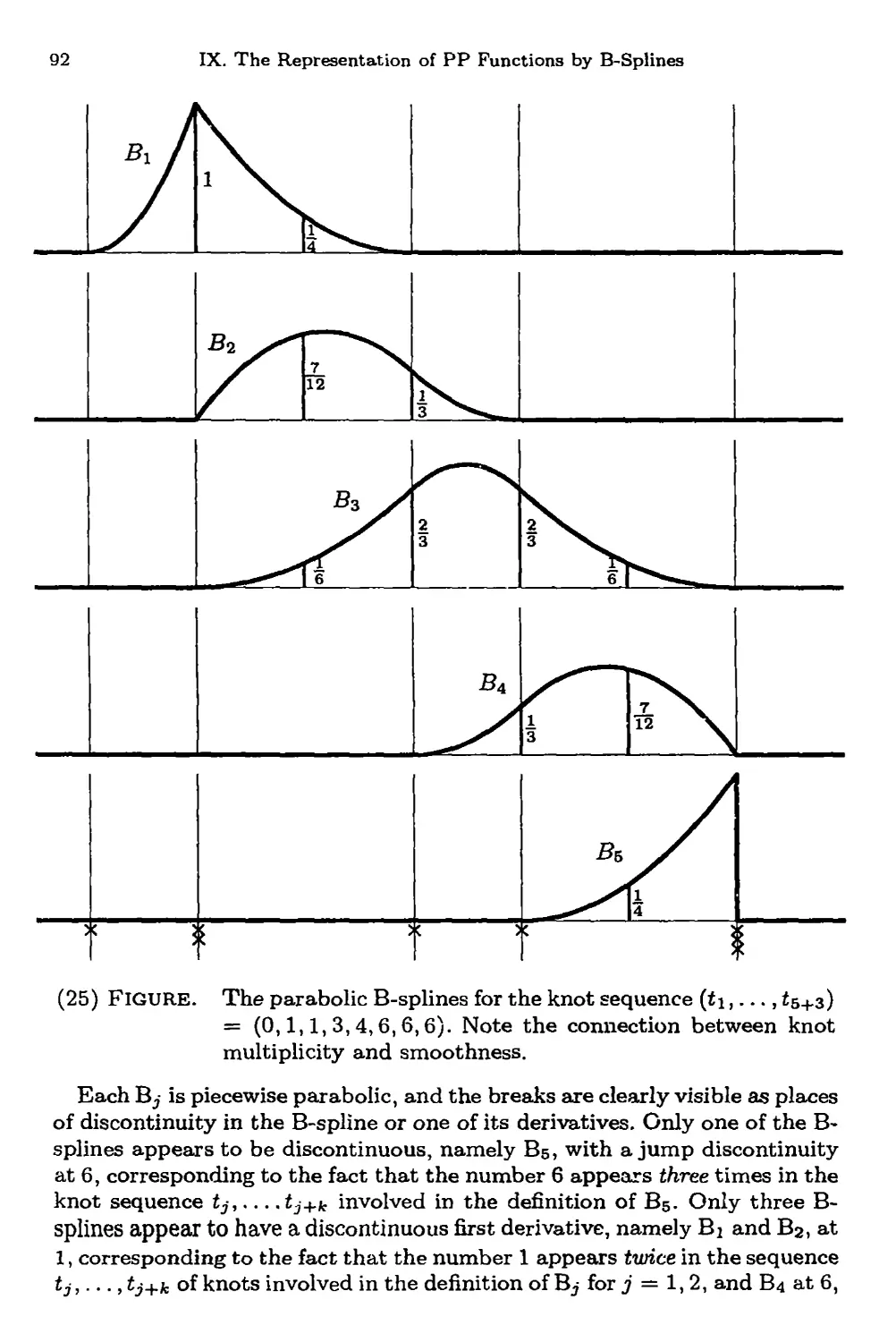
Example: A sequence of parabolic B-splines 91
The spline space $k,t 93
The polynomials in $k,t 94
The pp functions in $k,t 96
В stands for basis 99
Conversion from one form to the other 101
Example: Conversion to B-form 103
Problems 106
X • The Stable Evaluation of B-Splines and Splines
Stable evaluation of B-splines 109
The subroutine BSPLVB 109
Example: To plot B-splines 113
Example: To plot the polynomials that make up a B-spline 114
Diffeientiation 115
The subroutine BSPLPP 117
Example: Computing a B-spline once again 120
The subroutine BVALUE 121
Example: Computing a B-Spline one more time 126
Integration 127
Problems 128
XI ¦ The B-Spline Series, Control Points, and Knot Insertion
Bounding spline values in terms of "nearby" coefficients 131
Control points and control polygon 133
Knot insertion 135
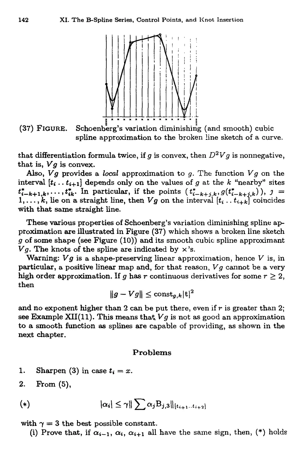
Variation diminution 138
Schoenberg's variation diminishing spline approximation 141
Problems 142
XII ¦ Local Spline Approximation and the Distance from Splines
The distance of a continuous function from $fctt 145
The distance of a smooth function from Sjt.t 148
Example: Schoenberg's variation-diminishing spline approximation 149
Local schemes that provide best possible approximation order 152
Good knot placement 156

xii Contents
The subroutine NEWNOT 159
Example: A failure for NEWNOT 161
The distance from $^>7г 163
Example: A failure for CUBSPL 165
Example: Knot placement works when used with a local scheme 167
Problems 169
XIII • Spline Interpolation
The Schoenberg-Whitney Theorem 171
Bandedness of the spline collocation matrix 173
Total positivity of the spline collocation matrix 169
The subroutine SPLINT 175
The interplay between knots and data sites 180
Even order interpolation at knots 182
Example: A large ||J|| amplifies noise 183
Interpolation at knot averages 185
Example: Cubic spline interpolation at knot averages with good knots 186
Interpolation at the Chebyshev-Demko sites 189
Optimal interpolation 193
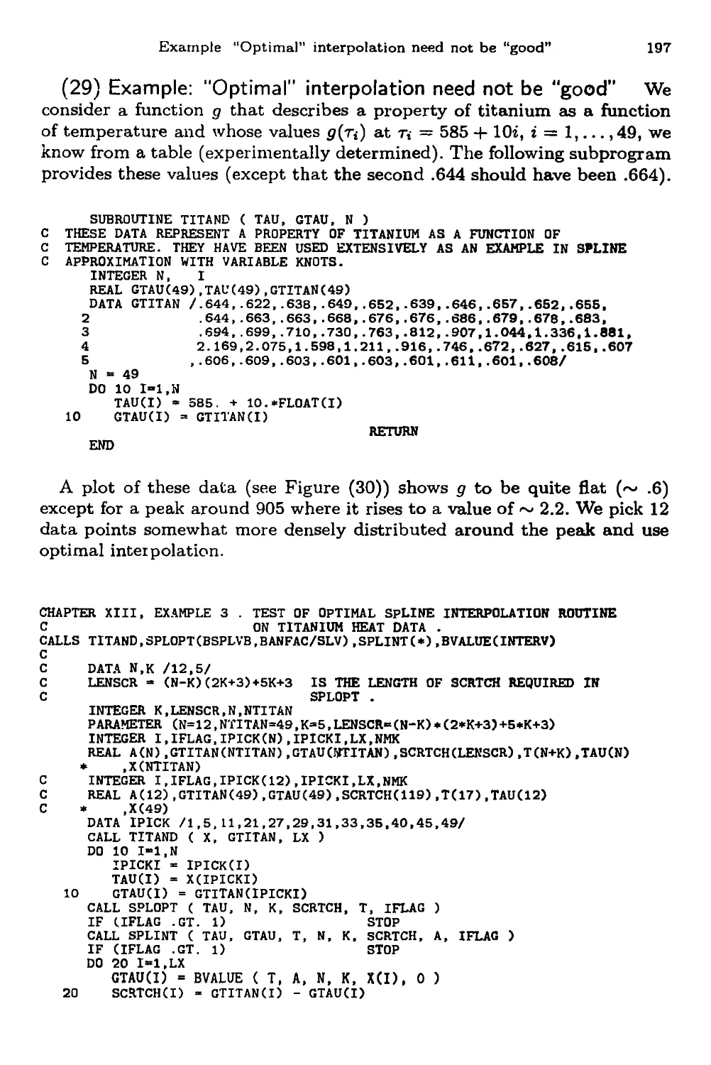
Example: "Optimal" interpolation need not be "good" 197
Osculatory spline interpolation 200
Problems 204
XIV • Smoothing and Least-Squares Approximation
The smoothing spline of Schoenberg and Reinsch 207
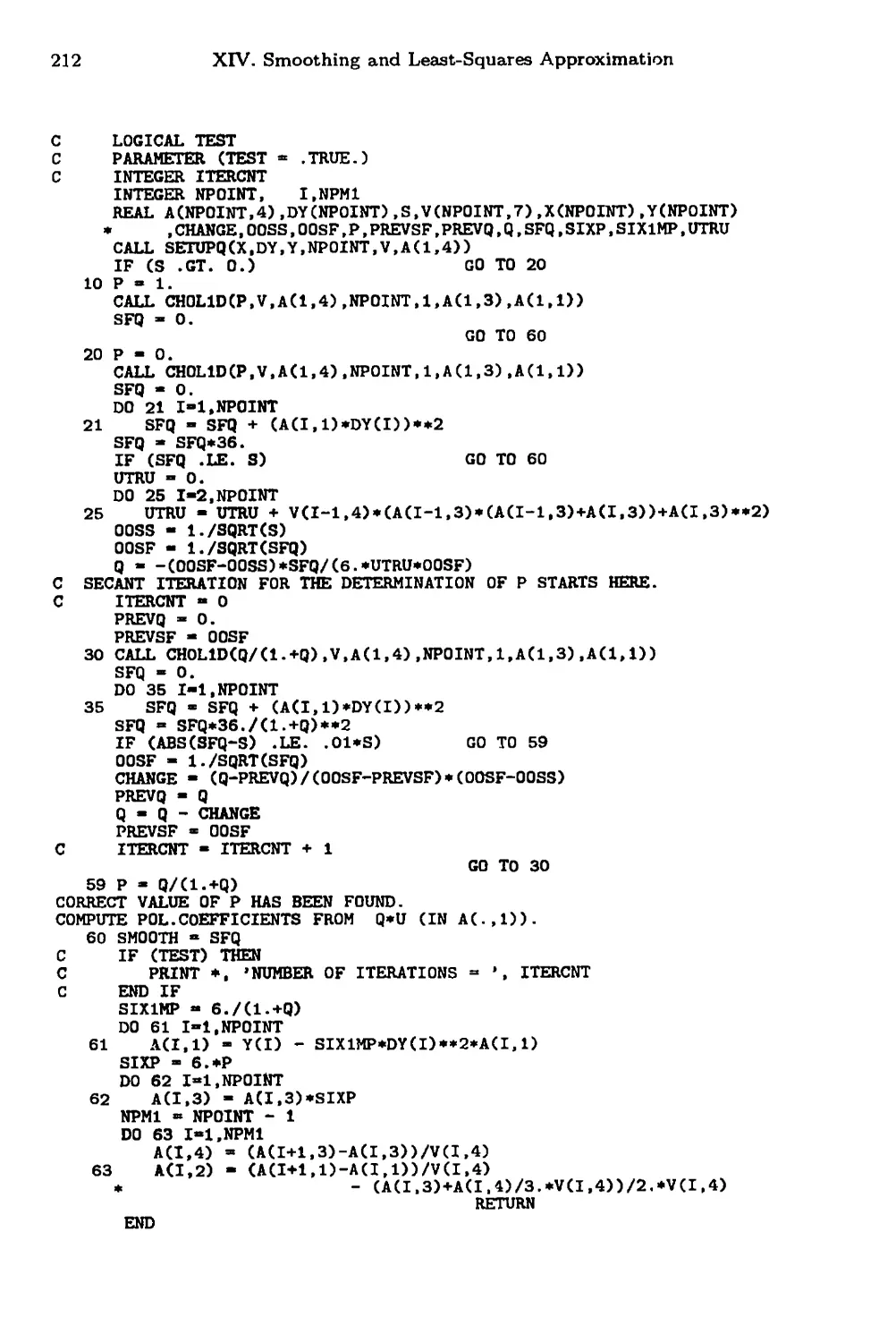
The subroutine SMOOTH and its subroutines 211
Example: The cubic smoothing spline 214
Least-squares approximation 220
Least-squares approximation from $fc,t 223
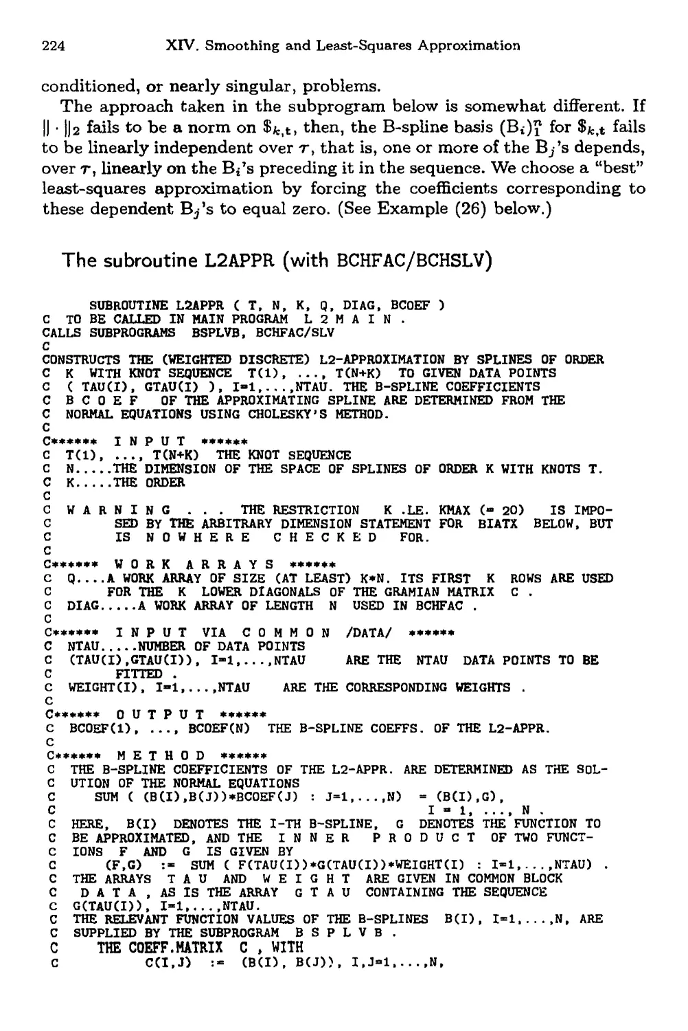
The subroutine L2APPR (with BCHFAC/BCHSLV) 224
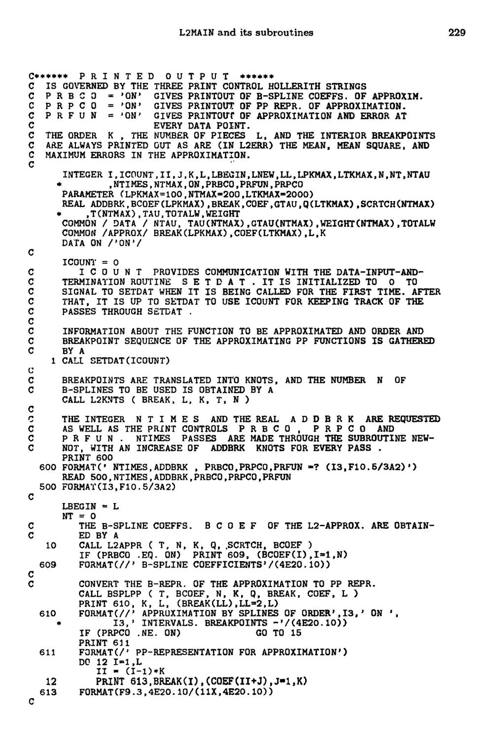
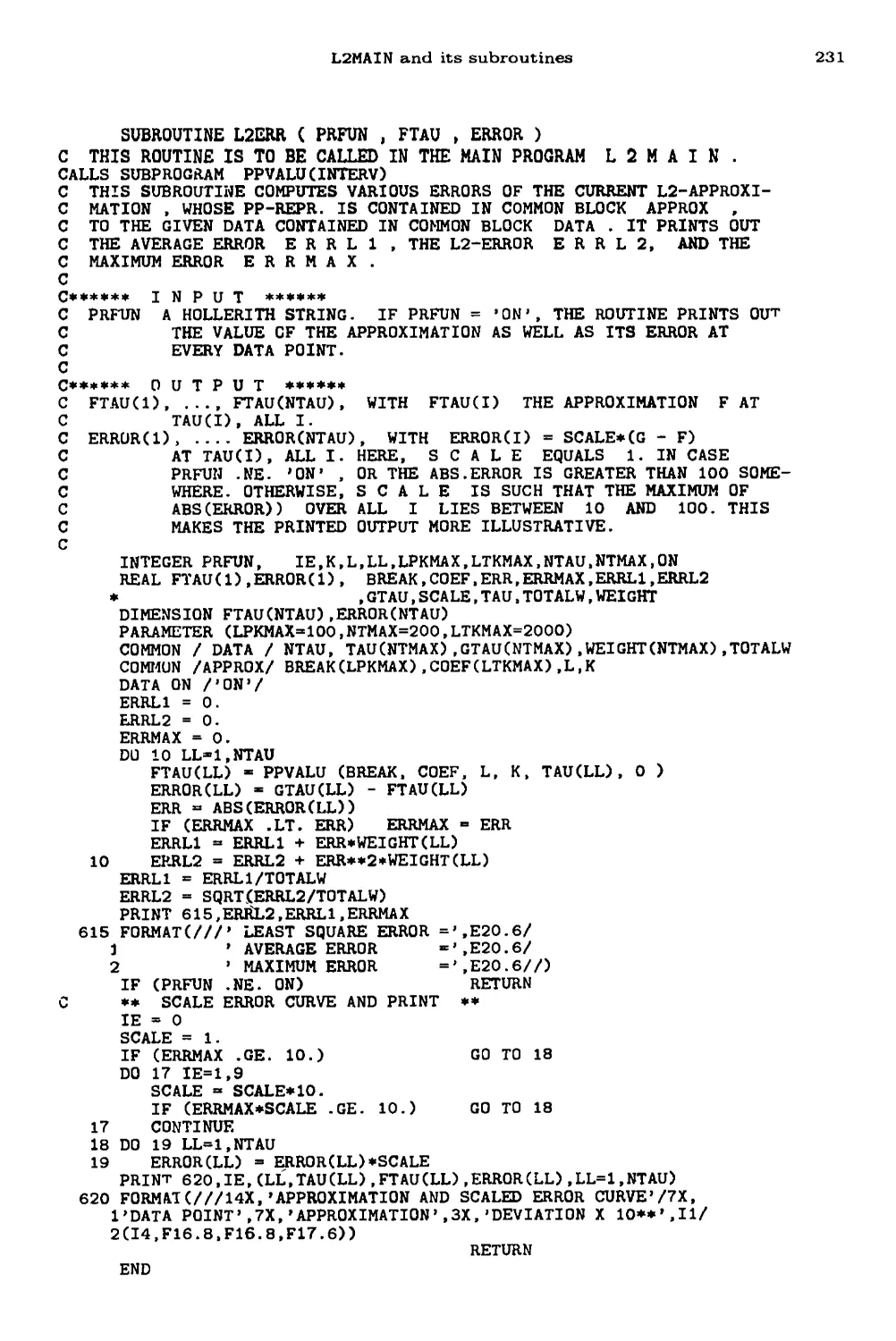
L2MAIN and its subroutines 228
The use of L2APPR 232
Example: Fewer sign changes in the error than perhaps expected 232
Example: The noise plateau in the error 235
Example: Once more the Titanium Heat data 237
Least-squares approximation by splines with variable knots 239
Example: Approximation to the Titanium Heat data from $4,9 239
Problems 240

Contents xiii
XV ¦ The Numerical Solution of an Ordinary Differential Equation
by Collocation
Mathematical background 243
The almost block diagonal character of the system of collocation
equations; EQBLOK, PUTIT 246
The subroutine BSPLVD 251
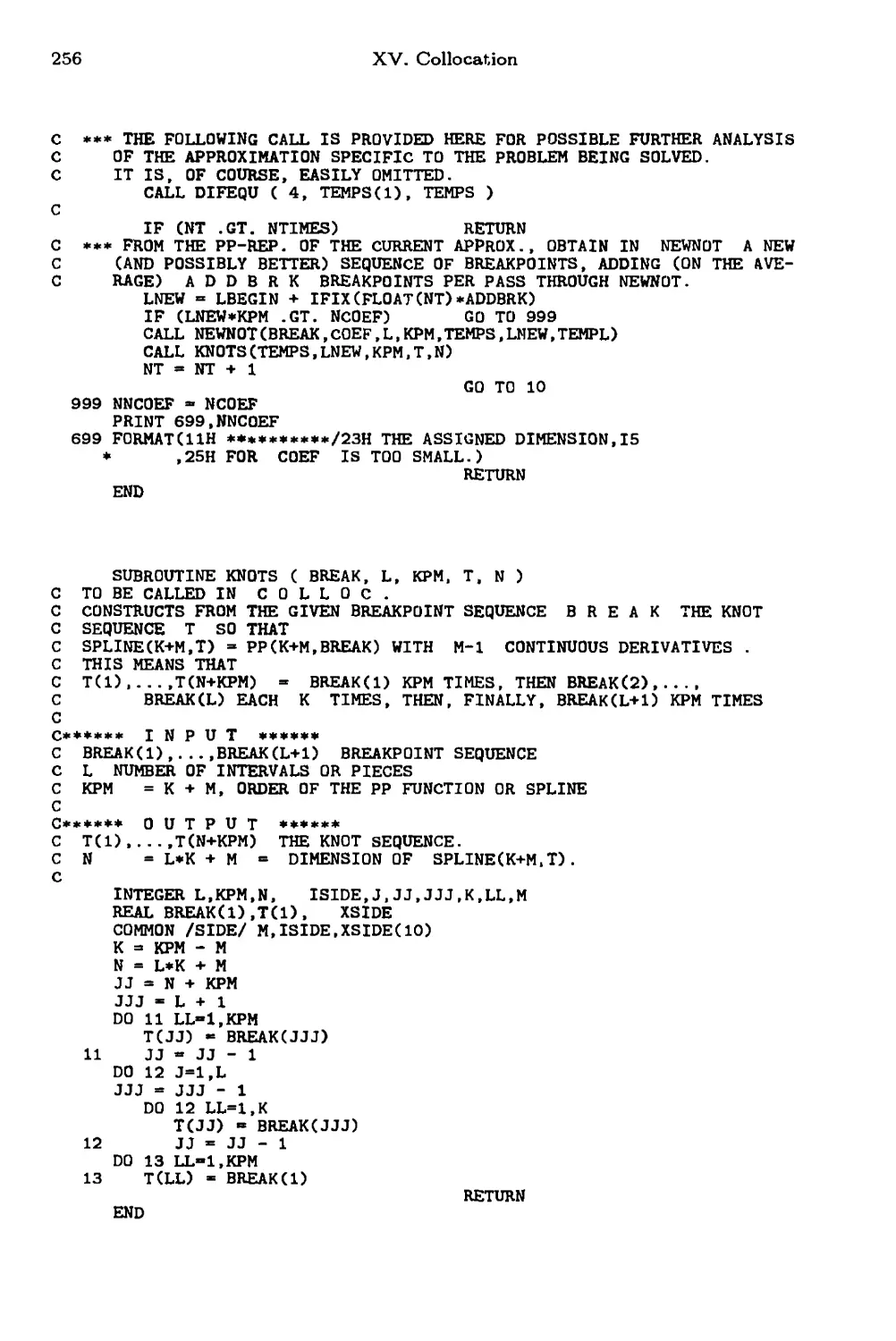
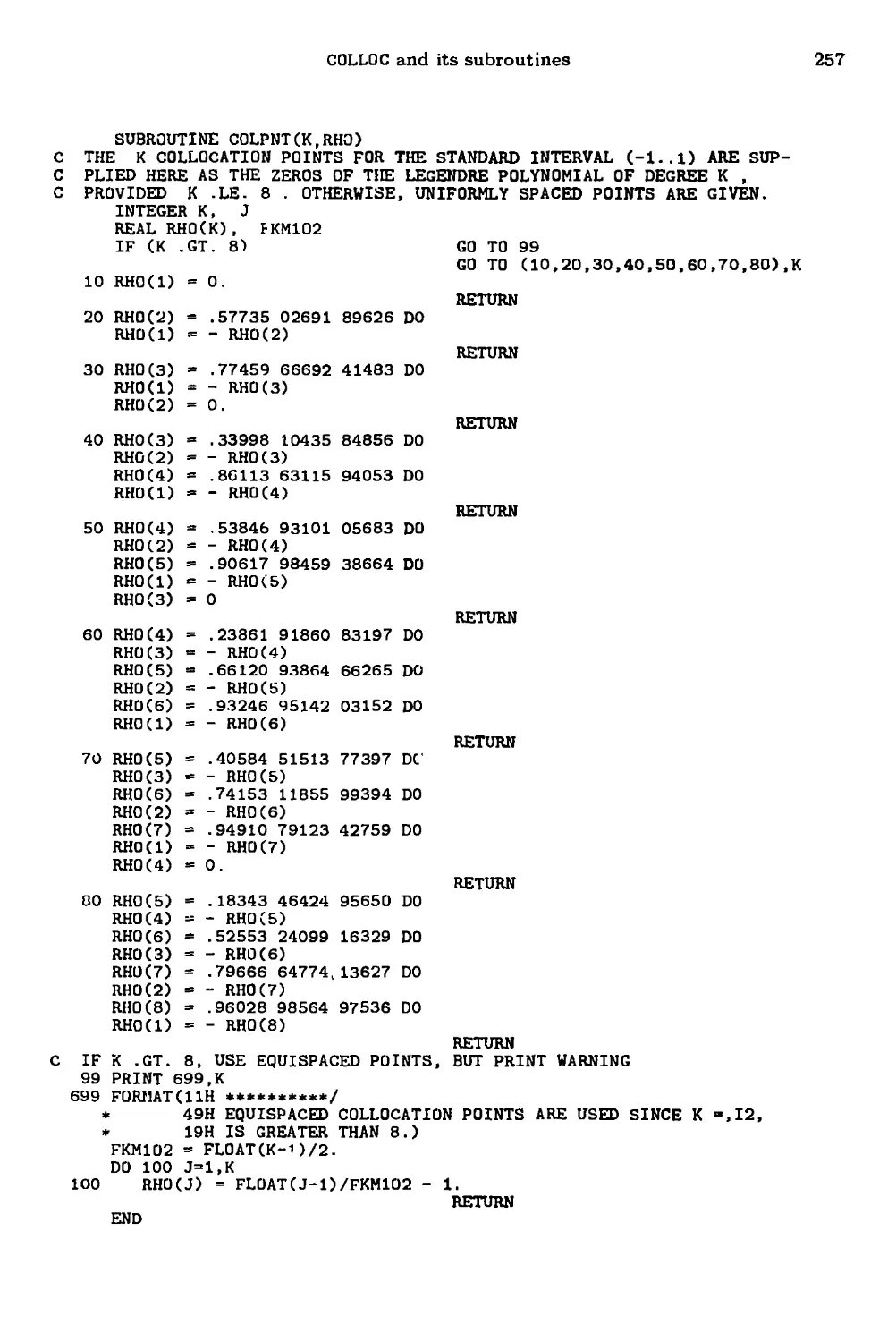
COLLOC and its subroutines 253
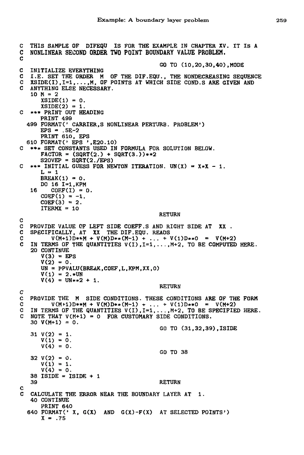
Example: A second order nonlinear two-point boundary-value
problem with a boundary layer 258
Problems 261
XVI • Taut Splines, Periodic Splines, Cardinal Splines and
the Approximation of Curves
Lack of data 263
"Extraneous" inflection points 264
Spline in tension 264
Example: Coping with a large endslope 265
A taut cubic spline 266
Example: Taut cubic spline interpolation to Titanium Heat data 275
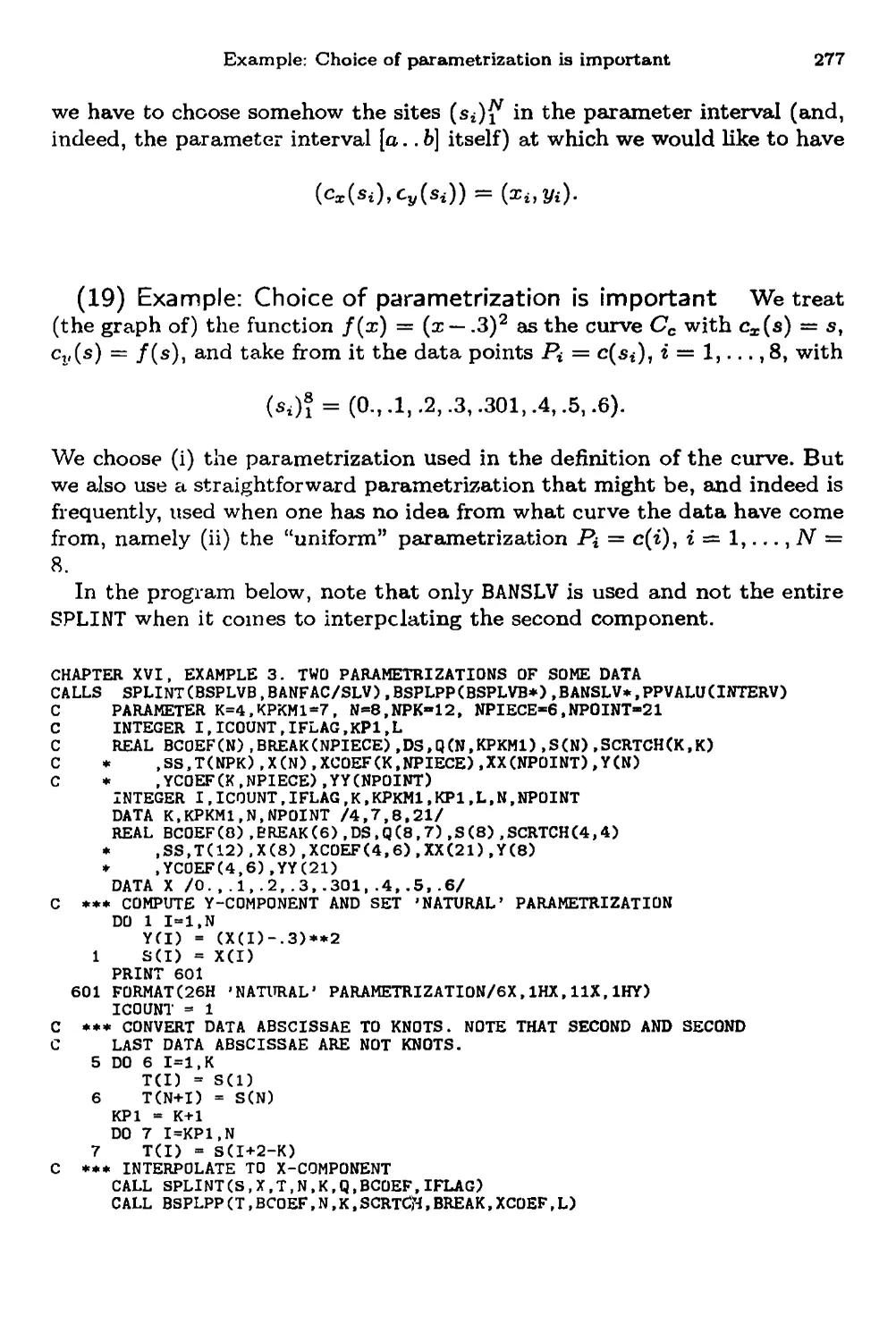
Proper choice of parametrization 276
Example: Choice of parametrization is important 277
The approximation of a curve 279
Nonlinear splines 280
Periodic splines 282
Cardinal splines 283
Example: Conversion to ppform is cheaper when knots are uniform 284
Example: Cubic spline interpolation at uniformly spaced sites 284
Periodic splines on uniform meshes 285
Example: Periodic spline interpolation to uniformly spaced data
and harmonic analysis 287
Problems 289
XVII ¦ Surface Approximation by Tensor Products
An abstract linear interpolation scheme 291
Tensor product of two linear spaces of functions 293
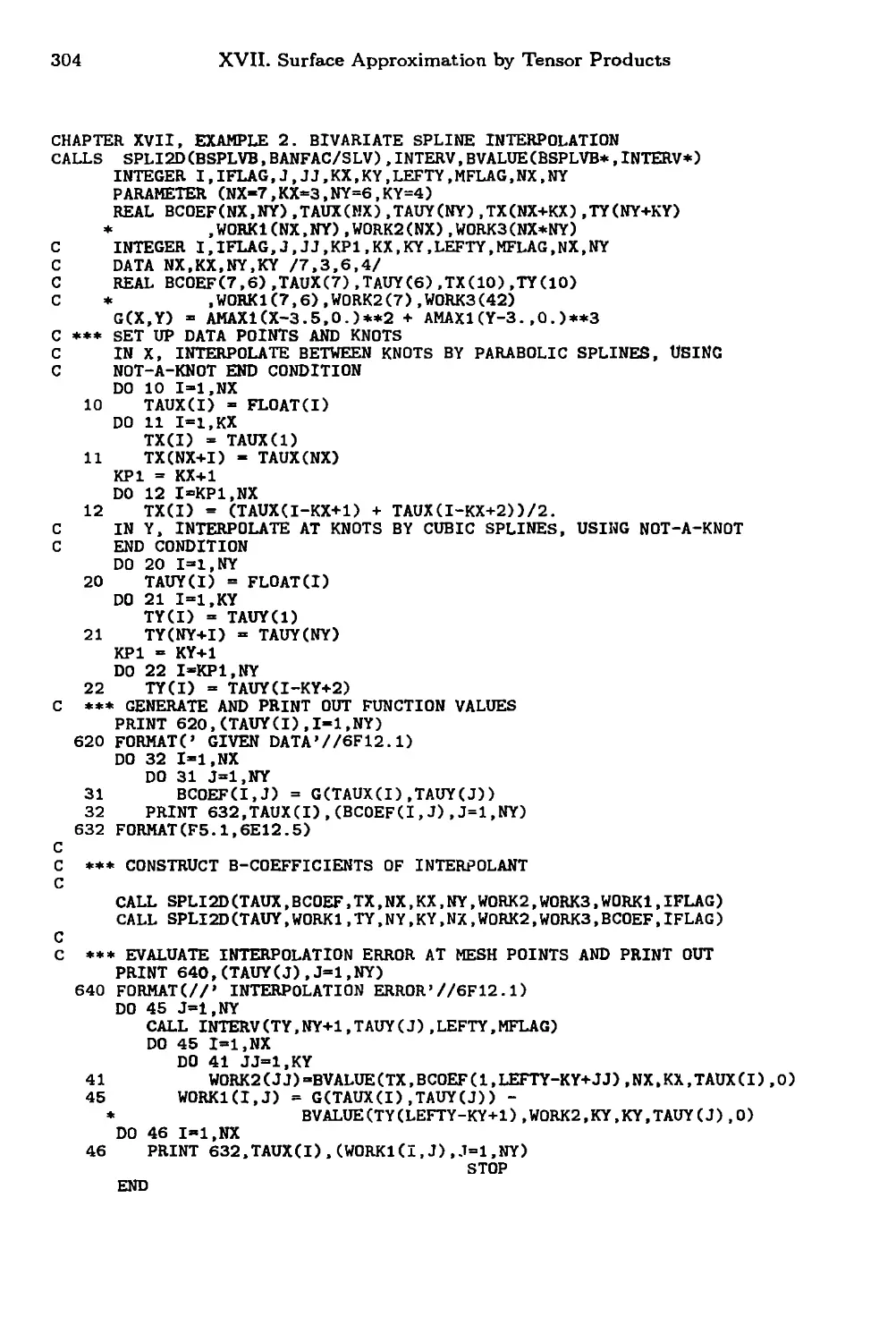
Example: Evaluation of a tensor product spline. 297
The tensor product of two linear interpolation schemes 297
The calculation of a tensor product interpolant 299

xiv Contents
Example: Tensor product spline interpolation 301
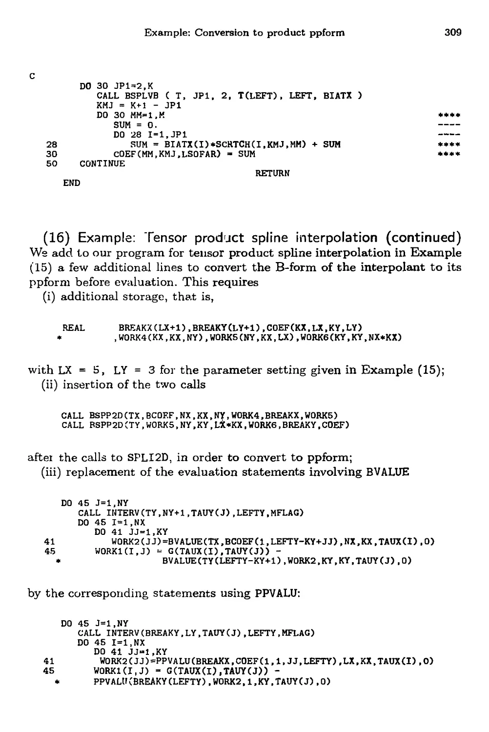
The ppform of a tensor product spline 305
The evaluation of a tensor product spline from its ppform 305
Conversion from B-form to ppform 307
Example: Tensor product spline interpolation (continued) 309
Limitations of tensor product approximation and alternatives 310
Problems 311
Postscript on Things Not Covered 313
Appendix: Fortran Programs
Fortran programs 315
List of Fortran programs 315
Listing of S0LVEBL0K Package 318
Bibliography 331
Index
341

Notation
Here is a detailed list of all the notation used in this book. Readers will
have come across some of them, perhaps most of them. Still, better to bore
them now than to mystify them later.
:= is the sign indicating "equal by definition". It is asymmetric as such a
sign should be (as none of the customary alternatives, such as =, or = ,
or =, etc., are). Its meaning: "a := b" indicates that a is the quantity
to be defined or explained, and b provides the definition or explanation,
and "b =: a" has the same meaning.
{ а;, у, jz, ... } :— the set comprising the elements x, y, z, ... .
{ x G X : P(x) } := the set of elements of X having the property P(x).
(x, y, -..) := the sequence whose first term is x, whose second term is y, ...
#S := the number of elements (or terms) in the set (or sequence) S.
0 :— the empty set.
IN:= {1,2,3,...}.
ZZ:= {...,-2,-1,0,1,2,...}.
IR := the set of real numbers.
С := the set of complex numbers.
J := the complex conjugate of the complex number z.
[a .. b] :— { x G IR : a < x < b }, a closed interval. This leaves [a, b] free to
denote a first divided difference (or, perhaps, the matrix with the two
columns a and b).
(a . .b) := { x G IR : a < x < b }, an open interval. This leaves (a, b) free tc
denote a particular sequence, e.g., a point in the plane (or, perhaps, the
inner product of two vectors in some inner product space). Analogously,
[a .. b) and (a .. b] denote half-open intervals.
constQi...iUr := a constant that may depend on a,...,w.
xv

xvi Notation
f:A —> B:a н-> f(a) describes the function / as being defined on
A =: dom / (called its domain) and taking values in the set В =: tar /
(called its target), and carrying the typical element a G A to the
element /(a) ? B. For example, F: IR —> IR: x н-> exp(x) describes the
exponential function. I will use at times /:аи /(a) if the domain and
target of / are understood from the context. Thus, \i\ f i—> /0 /(x)dx
describes the linear functional \x that takes the number fQ f(x) dx as
its value at the function /, presumably denned on [0.. 1] and integrable
there.
supp/ := {x G dom/ : /(x) ф 0}, the support of/. Note that, in Analysis,
it is the closure of this set that is, by definition, the support of /.
/|/ := g: I —> B: a «-» /(a), the restriction of / to /.
h ~* \ n_ := /г approaches 0 through negative va^ues-
f(a+) := lim /(a + h), f(a~) := lim /(a + /i).
jumpa/ := /(a+) — /(a-), the jump in / across a.
#(x) = О (/(#)) (in words,"g(x) is of order /(x)") as x approaches а : =
lim sup | 4© | < oo. The lim sup itself is called the order constant of
x—*a '
this order relation.
g(x) = o(f(x)) (in words, "g(x) is of higher order than /(x)") as x
approaches а := lim т4§^ = 0-
x—*a J\x/
/(•,y) := the function of one variable obtained from the function
f:X x Y —> Z by holding the second variable at a fixed value y.
Also, fa G(-, y)g(y) dy describes the function that results when a certain
integral operator is applied to the function g.
(x)+ := max{x,0}, the truncation function.
lnx := the natural logarithm of x.
[xj := max{ n G 7L : n < x }, the floor function.
\x\ := min{n G ZZ : n > x }, the ceiling function.
?i := a Lagrange polynomial (p. 2).
(-)-:^ (-1Г-
(r) :== ri/fe!ir\; j a binomial coefficient.
?n := The Euler spline of degree n (p. 65).
Boldface symbols denote sequences or vectors, the ith term or entry is
denoted by the same letter in ordinary type and subscripted by i. Thus,

r> (r0> (n)?, (т*)?=ц (т*г : i = 1,...,тг), and (rb...,rn) are various ways
of describing the same n-vector.
m := (m,..., m), for m e ZS.
Xn := {(x;)i :*ieX, all г}.
Дгг := ri+i — r», the forward difference.
Vri := Гг — Ti_i, the backward difference.
S~r := number of strong sign changes in r (p. 138).
S+r := number of weak sign changes in r (p. 232).
Y> / тг + rr+i + ¦ ¦ ¦ + r5, if r < s;
& \o, ifr>5.
Yli Ъ := YlTii with r and 5 understood from the context.
n^{;',Tr+r
if r < 5;
if r > s.
For nondecreasing sequences or meshes r, we use
|r| := тахг At*, the mesh size.
Л/г := maxitj Ati/At^, the global mesh ratio.
mr := maxji_^j=:i Ati/Atj, the local mesh ratio.
fi+1/2 := (^ +Ti+i)/2 .
Matrices are usually denoted by capital letters, their entries by
corresponding lower case letters doubly subscripted. Д (a^), (a;,:?)™'™,
(an ... ain \
j ¦ "- are various ways of describing the
Oml - - ¦ а-тп J
same matrix.
AT := (aji)"=i;liii the transpose of A.
Ля := (oji)"=i;{ii, the conjugate transpose or Hermitian of Л.
det>l := the determinant of A.
Г 1 7 = ?"
<^i := s n • / ¦ > the Kronecker Delta.
J I 0 г ^ 3
span(y?i) := { Х^г Q»^i ¦ Скг G IR}, the linear combinations of the sequence
(<pi)™ of elements of a linear space X. Such a sequence is a basis for
its span in case it is linearly independent, that is, in case Yli a^i = 0
implies that а = 0. We note that the linear independence of such a
sequence (y?i)? *s almost invariably proved by exhibiting a corresponding
sequence (A*)" of linear functionals on X for which the matrix (Xiipi) is
invertible, e.g., Xipj ~ 6ij, for all г, j. In such acase, dimspan(y?i)" = n.

xviii
Notation
П<А: := П^-.1 := linear space of polynomials of order к (р. 1).
^<fc,€ := П*:-1,? := linear space of pp functions of order к with break
sequence ? (p. 70).
D* f '¦= Jth derivative of /; for / G U<kt$, see p. 70.
^<fc.?,«' :~ П^-1,С,^ := linear subspace of П<^^ consisting of those
elements that satisfy continuity conditions specified by v (p. 82).
%kx '¦— span(Bi,fc,t), linear space of splines of order к with knot sequence
t (p. 93).
Bi := Bi?A:.t := *th B-spline of order к with knot sequence t (p. 87).
$/c,n := U{ / G $fc>t : ti = ¦ ¦ ¦ — tk = a, tn+i = - - • = ?n+fc = b } (pp. 163,
239).
$JJ^ := "natural" splines of order к for the sites x (p. 207).
C[a .. b] := { f: [a .. b] —> IR : / continuous }.
11/11 := max{ \f(x)\ : a < x < &}, the uniform norm of / G С [a .. b]. (We
note that HZ + pll < 11/Ц +|Ы| and ||a/|| = |a|||/|| for f,g G C\a .. b]
and a G IR).
u(f\ h) '¦= max{ \f(x) — f(y)\ : x,y G [a .. b], \x — y\ < h }, the modulus of
continuity for / G C[a .. b] (p. 25).
dist (p, 5) := inf{ ||p - /|| : / G 5 }, the distance of g G C[a .. b] from the
subset S of C[a .. 6].
C^[a .. b] := { /: [a .. 6] —> IR : / is n times continuously differentiable }.
[Ti,..., Tj]f := divided difference of order j — г of /, at the sites т*,..., Tj
(p. 3). In particular, [г*]: / >—> /(r»).
Special spline approximation maps:
Ik := interpolation by splines of order к (р. 182),
Lk := Least-squares approximation by splines of order к (р. 220),
V := Schoenberg's variation diminishing spline approximation (p. 141).

I
Polynomial Interpolation
In this introductory chapter, we state, mostly without proof, those
basic facts about polynomial interpolation and divided differences needed in
subsequent chapters. The reader who is unfamiliar with some of this
material is encouraged to consult textbooks such as Isaacson & Keller [1966]
or Conte &; de Boor [1980] for a more detailed presentation.
One uses polynomials for approximation because they can be evaluated,
differentiated, and integrated easily and in finitely many steps using the
basic arithmetic operations of addition, subtraction, and multiplication. A
polynomial of order n is a function of the form
n
(1) p{x) = ai + a2x H h anxn_1 = y^ajX3'*1,
i.e., a polynomial of degree < n. It turns out to be more convenient to
work with the order of a polynomial than with its degree since the set of
all polynomials of degree n fails to be a linear space, while the set of all
polynomials of older n forms a linear space, denoted here by
П<7г = n<7i_i = IIn_i.
Note that a polynomial of order n has exactly n degrees of freedom.
Note also that, in MATLAB, hence in the SPLINE TOOLBOX (de Boor
[1990]2), the coefficient sequence a = [a(l) , ... ,a(n)] of a
polynomial of order 71 starts with the highest coefficient. In particular, if x is a
scalar, then the MATLAB command polyval(a,x) returns the number
a(l)*x~(n-l) + a(2)*x~(n-2) + ... + a(n-l)*x + a(n)
1

2
I. Polynomial Interpolation
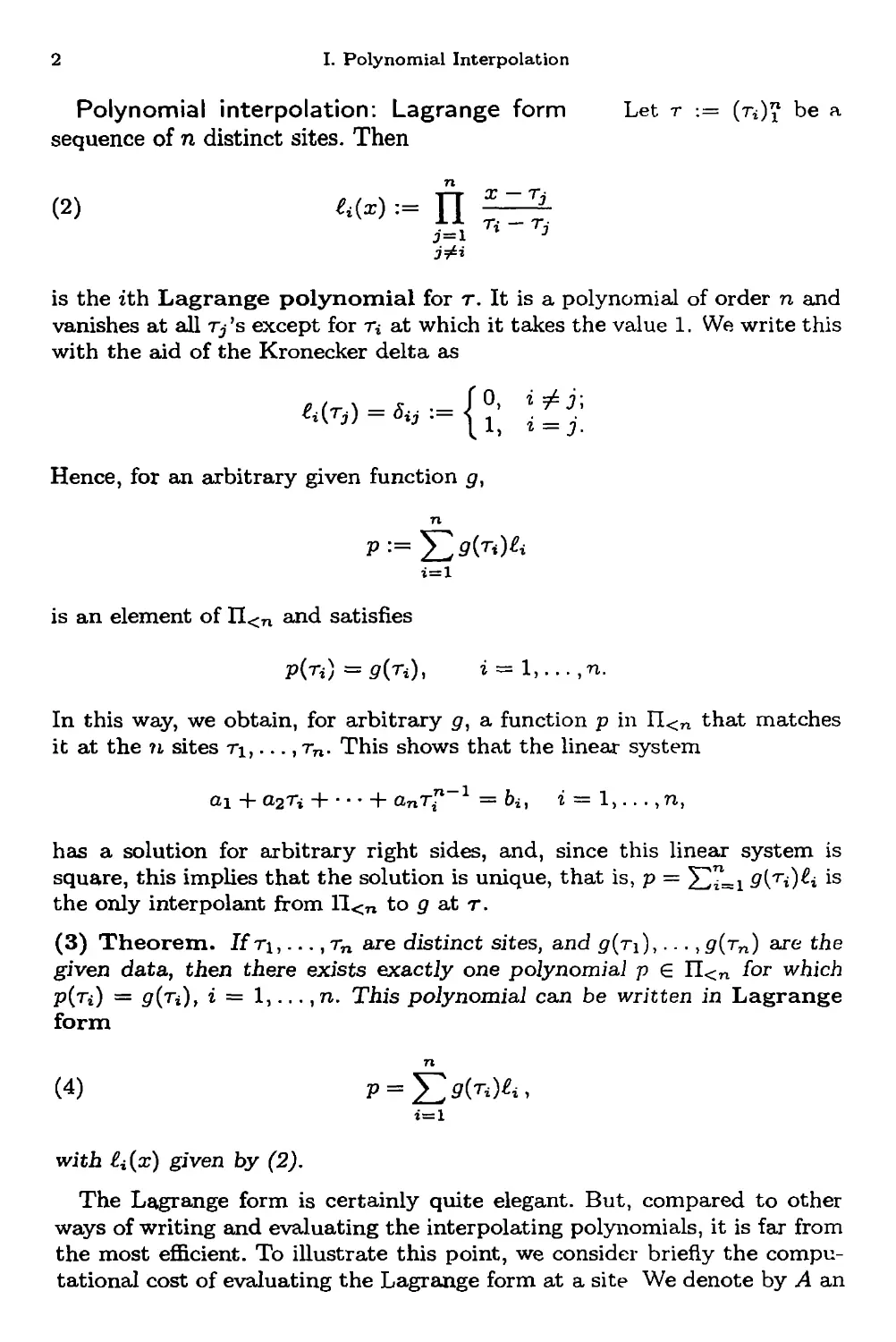
Polynomial interpolation: Lagrange form Let r := (тч)? be a
sequence of n distinct sites. Then
(2) /<(*) := ft EZJL
Эфг
is the ith Lagrange polynomial for r. It is a polynomial of order n and
vanishes at all r/s except for т* at which it takes the value 1. We write this
with the aid of the Kronecker delta as
Hence, for an arbitrary given function p,
n
г=1
is an element of П<п and satisfies
Р(ъ) = д{ъ)> i = l,...,n.
In this way, we obtain, for arbitrary <?, a function p in П<п that matches
it at the n sites т\,..., rn. This shows that the linear system
ai +a2Ti H h anrf_1 = Ъи г — 1,... ,n,
has a solution for arbitrary right sides, and, since this linear system is
square, this implies that the solution is unique, that is, p — Yl^i 9{Ti)U is
the only interpolant from П<7г to p at т.
(3) Theorem. Ifr\,..., rn are distinct sites, and g(r\),..., g(rn) are the
given data, then there exists exactly one polynomial p e П<п for which
р(ъ) = д(ъ), г = 1,... ,n. This polynomial can be written in Lagrange
form
n
(4) P = $>(r04,
with ?i(^) given by (2).
The Lagrange form is certainly quite elegant. But, compared to other
ways of writing and evaluating the interpolating polynomials, it is far from
the most efficient. To illustrate this point, we consider briefly the
computational cost of evaluating the Lagrange form at a site We denote by A an

Divided differences and Newton form
3
addition or subtraction, and by M/D a multiplication or division. Straight
evaluation of the Lagrange form takes
(2n - 2)A + (n - 2)M + (n - \)D
for each of the n numbers ?»(a;), and then
(n — l)-4 + nM
for forming (4) from the р(т») and the ^(.т). Even if one is clever about it
and computes
Yi :=p(rO/П(гг-^), г = l,...,n,
once and for all, and then computes p(x) by
n
р(ж) = <р(.т) У" —-^— ,
T-f -T — Г»
г=1
it still takes
(2п- 1)Л + пА/ + тиО
per site, compared to
(2п-1)Л+(п- 1)М
for the Newton form to be discussed next. And things get much worse if
we want to compute derivatives!
Of all the customary forms for the interpolating polynomial, I prefer
the Newton form. It strikes me as the best compromise between ease of
construction and ease of evaluation. In addition, it leads to a very
simple analysis ot interpolation error and even allows one to discuss and use
osculatory polynomial interpolation with no additional effort.
Polynomial Interpolation: Divided differences and Newton form
There are many ways of defining divided differences. I prefer the following
(somewhat nonconstructive)
(5) Definition. The fcth divided difference of a function g at the
sites г*, -.. ^Ъ+к is the leading coefficient (that is, the coefficient of xk)
of the polynomial of order к + 1 that agrees with д at the sequence
(тг,... ,rz+fc) (in the sense of Definition (12) below). It is denoted by
[Т»,... ,Т*+А:]0.

4 I. Polynomial Interpolation
This definition has the following immediate consequences.
(i) If Pi G П<г agrees with д at rb ..., т* for i = к and к + 1, then
(6) Pk+i(x) =рк(х) + (х~тг)---{х- rk)[ru ... ,Tfc+i]p.
For, we know that pk+i —pk is a polynomial of order к4-1 that vanishes at
T\,..., Tk and has [ti, ..., Tfc+ijp as its leading coefficient, therefore must
be of the form
Pk+i{x) - pk(x) = <?(* - та)¦••(x - rfc)
with C= [Ti,...,Tfc+i]^.
This property shows that divided differences can be used to build up the
interpolating polynomial by adding the data sites r* one at a time. In this
way, we obtain
Pn{x) = Pl{x) + (P2(x) - Pl(x)) + h {Pn{x) - Pn-l{x))
= lri]9+ (x - T1)[ri,T2}g + (x - ti)(x - т2)[тх,т2,т3]д-\-
f- (x - n) ¦ • ¦ (x ~ rn_i)[ri,..., rn]g.
This is the Newton form,
n
(?) Pn(x) = ]P(x - гх) - - - (x - г»_1)[гь ..., Ti]g,
г=1
for the polynomial pn of order n that agrees with g at ть..., rn. (Here,
(x - n) • • • {x — Tj) := 1 if г > j.)
(ii) [г*,..., Ti+k)g ^ a symmetric function of its arguments т*,..., Ti+k,
that is, it depends only on the numbers ти... , Ti+fc and not on the order
in which they occur in the argument list. This is clear from the definition
since the interpolating polynomial depends only on the data points and not
on the order in which we write down these points.
(iii) [ri,... ,ъ+к}д is iinear in g, that is, if / = ocg + ph for some
functions g and h and some numbers a and /3, then [ri7... ,ri+k]f =
а[т*,..., Ti+k]g + Р[тг, -.., Ti+k]h, as follows from the uniqueness of the
interpolating polynomial.
The next property is essential for the material in Chapter X.
(iv) (Leibniz' formula). If f = gh, that is, f(x) = g(x)h(x) for all x,
then
i+k
[Т^ . . . , 74+fc]/ = 5^(h, . . . , Tr]p)([rrj . . .,Ti+k]h).
For the proof, observe that the function
i+k i+k
]Г(х-Гг) • ¦ • {х-тг^)[ти ..., rr]p^(x~rs+i) ¦ • • (х-п+к)[т3,..., ri+k}h
г=г з=г

Divided differences and Newton form
5
agrees with / at т,,..., ri+k since, by (7), the first factor agrees with g
and the second factor agrees with h there. Now multiply out and split the
resulting double sum into two parts:
r,s=i r<s r>s
Note that ^Z vanishes at т*,..., Ti+k. Therefore, also ^ must agree with
f at Tj,... ,Ti+k But ^2 is a polynomial of order к + 1. Therefore, its
leading coefficient which is
5^(fa, ¦ ¦ • ,rr]g) ([rs,... yri+k]h)
r = s
must equal [т^,..., Ti+k]f. (I learned this particular argument from W. D.
Kammler.)
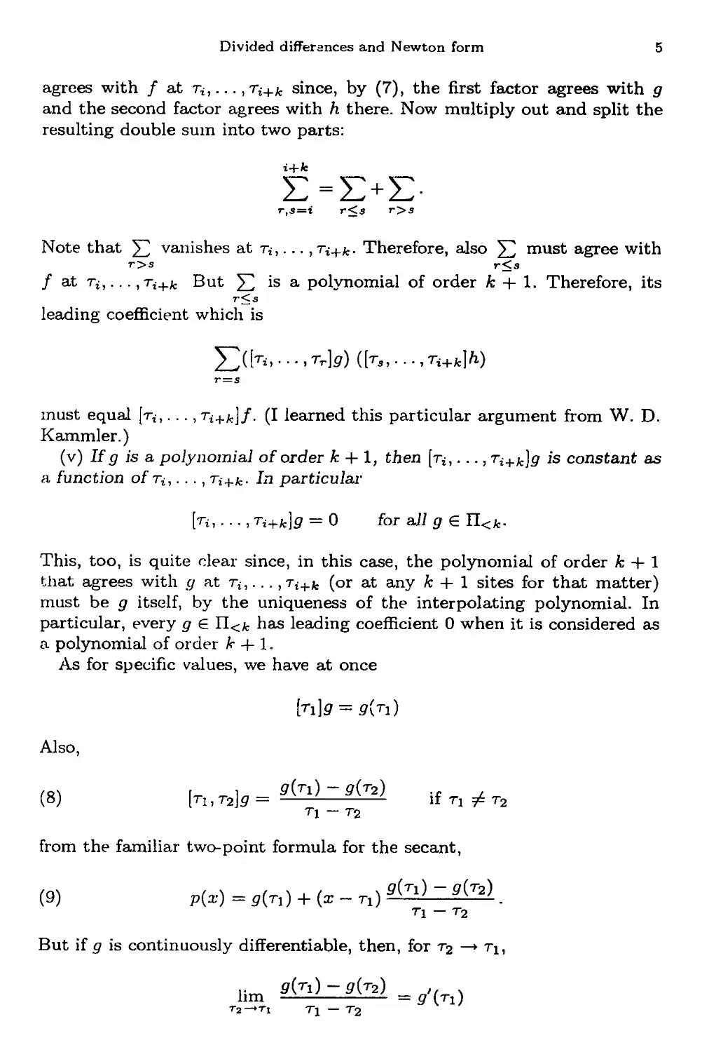
(v) If g is a polynomial of order к + 1, then [т*,..., ri+k)g is constant as
a, function of Ti,..., ri+k. In particular
[ru . .., ri+k]g = 0 for all g G U<k.
This, too, is quite clear since, in this case, the polynomial of order к + 1
that agrees with g at r^,... ,Тг+д. (or at any к + 1 sites for that matter)
must be g itself, by the uniqueness of the interpolating polynomial. In
particular, every g e U<k has leading coefficient 0 when it is considered as
a polynomial of order к + 1.
As for specific values, we have at once
[r\)g = g{Ti)
Also,
(8) \Ti,T2\g = if ti ф r2
from the familiar two-point formula for the secant,
(9) P(x)=9(r1) + (x-n)9{r^-9^.
П — r2
But if g is continuously differentiable, then, for r2 —> Ti,
lim g(Tl)-g(T2)^g'(n)
r2—»Ti Ti — T2

6
I. Polynomial Interpolation
and the secant (9) goes over into the tangent
(10) p(x)=9{Ti) + {x-n)g'{n)
that agrees with g in the value and slope at т\. This justifies the statement
that the polynomial p given by (10) agrees with g at the sites T\ and гь
that is, two-fold at т\. With this wording, the definition of the first divided
difference implies that
(11) [т1,т2]д = д'(тг) if rx = r2.
Also, we see that [ri,T2]p is a continuous function of its arguments.
Repeated interpolation at a site is called osculatory interpolation
since it produces higher than first order contact between the function and
its interpolant (osculari means "to kiss" in Latin). The precise definition
is as follows.
(12) Definition. Let r := (т*)]1 be a sequence of sites net necessarily
distinct. We say that the function p agrees with the function g at
r provided that, for every site ? that occurs m times in the sequence
t\j. . - ,тп, р and g agree m-fold at ?, that is,
P{i~l4Q = 9{i-l){<) forz = l,...,m.
The definition of the feth divided difference [т*,... ,Ti+k]g of д is to be
taken in this sense when some or all of the sites 74,..., ri+k coincide.
For the proof of the following additional properties of the kth divided
difference, we refer the reader to Issacson &; Keller [1966] or to Conte & de
Boor [1980] (although these properties could be proven directly from the
definition).
(vi) [t?, ..., Ti+k]g is a continuous function of its к + 1 arguments in case
g € C(k\ that is, g has к continuous derivatives.
(vii) If g G C^k\ that is, g has к continuous derivatives, then there exists
a site ? in the smallest interval containing Ti,..., ri+k sc that
[Tu...,Tt+k]g=gW(Q/k\.
(viii) For computations, it is important to note that
fa, • • - ,ri+k]g = в^ if Ti = • ¦ • = T,+fcl g € &k\
while
[Ti,...,Ti+k]g =
(13)
[tj, ... ,Tr-i,Tr+i,... ,Ti+k]g — [74,... 7rs_bTs+i,... ,Ti+k]g
if тГ1 т3 are any two distinct sites in the sequence тг,..., ri+k. The
arbitrariness in the choice of rr and r3 here is to be expected in view of the
symmetry property (ii).

Divided differences arid Newton form 7
(14) Theorem (Osculatory interpolation). If g € C(n), that is, g has
n continuous derxvativeSj and r = (т*)™ is a sequence of n arbitrary sites
(not necessarily distinct), then, for all x,
(15) g(x) = pn(x) + {x - tx) ¦ ¦ • (x - тп)[т1,... ,тп,х]д,
with
71
(16) pn(x) := y^(s-r1)---(a;--T3i_1)[T1,...,Ti]ff.
i=l
In particuiar, pn is the unique polynomial of order n that agrees with д at
т.
Note how, in (15), the error g(x) — pn(x) of polynomial interpolation
appears in the form of the "next" term for the Newton form. One obtains
(15) from its simplest (and obvious) case
(17) g(x) = д(тг) + (x - rl)[rux]g
by induction on n, as follows. If we already know that
g(x) =Pk(x) + (x-Ti) •• -(a; - Tk)[Ti,... ,rfc, x]g,
then, applying (17) (with T\ replaced by Tk+i) to [тъ,..., Tk,x]g as a
function of x, we get
[rb... ,Tk,x]g = [ri,...,rfc+i]p + (я;- тк+1)[тк+1,х]([т1:... ,rfc, -]д)
which shows that
0(s) =Pa:+i(2:) + (a;-Ti) • • ¦ (a; - Tfc+i)[Tjfc+i, аг]([ть ..., rfc, •]$).
This implies that, for any у^п,..., тк+\: the polynomial
Pfc+ifa) + (a: - n)---(a:- Tfc+i)[Tfc+1, y]([n,. . . , Tfcl -]$)
of order к + 2 agrees with p at n,. . . ,rk+i and at y, hence its leading
coefficient must equal [ti, ... , Tfc+i,y]<?, that is,
fafc+i,2/]([T;L,...,Tb-]0) = [ri,...,rfc+i,y]p
for all у ф ri,... ,Tfc+i. But then, the continuity property (vi) shows
that this equality must hold for у = ti, . .. , Tfc+i, too. This advances the
inductive hypothesis. It also shows that, for у ф тк+\,
In,-» rfc+b y)9 = fab+ь y]([Ti, • ¦ • , г*, •]$)
_ [ri,...,Tfc,y]ff - [Tb...,Tfc,Tfc+i]g
У - -пь+i

8
I. Polynomial Interpolation
and so provides, incidentally, a proof for (viii) and shows explicitly hov/ the
(k 4- l)st divided difference arises as the first divided difference of a feth
divided difference, thus explaining the name.
The notion that osculatory interpolation is repeated interpolation at sites
is further supported by the following observation: In (15) and (16), let all
sites Ti,..., rn coalesce,
T! = ¦ • • =Tn=T.
Then we obtain the formula (using (viii) and (vii))
?(n)(d)
(18) g(x) = Pn(x) 4- (x — r)n ^—- , some ?x between r and x,
with
(Щ рп(х)=^(х-гГ1^'1У,
which is the standard truncated Taylor series with differential remainder
(or error) term. Note that the truncated Taylor series (19) does indeed agree
with g n-fold at r, that is, Pn (т) = д^~хЦт) for i = 1,..., n.
Divided difference table The coefficients
[n]g, [п,т2]д, ..., [ru...,rn]g
for the Newton form (7) are efficiently computed in a divided difference
table:
interp.
sites
T4
T-n-l
тп
values
9(ti )
P(T2)
дЫ)
дЫ)
д(тп-1)
9(гтг)
first
div. diff.
[n»n]g
[г2,гз]д
[ъ,Т4]д
[тп-\,тп
)я
second
divided diff.
[Г2,тз,т4]д
Ь"тг-2,ТП_1,
тп]д
(тг - 2)nd
.. divided diff.
[Ti,...,Tn-i]p
• [Т2,...,Т,г]0
(n-l)st
divided diff.
[ti . ¦ ¦ ¦, Tn]g
Assume that the interpolation sites are so ordered that repeated sites
occur together, that is, so that т* = ri+r can only hold if also n = ri+\ —
• • • = Ti+r_i = Ti+r. Then, on computing [ri:... ,т*+г]р, either т* = ri+ri

Evaluation of the Newton form 9
in which case [т*,..., ri+r]g = g^{Ti)/r\ must be given, or else т* ф ri+r,
in which case
гппл u ^ i„ _ tr<+b ¦ ¦ • > rM-r]g - И,..., Tj+r-i]g
(20) [Ti, . . - , Ti + rl0 = ,
hence can be computed from the two entries next to it in the preceding
column. This makes it possible to generate the entries of the divided
difference table column by column from the given data. The top diagonal then
contains the desired coefficients of the Newton form (7). The (arithmetic)
operation count is
(21) Example: Osculatory interpolation to the logarithm For
g{x) = In a:, estimate $(1.5) by the number p4(l-5), with p4 the cubic
polynomial that agrees with g at 1, 1, 2, 2 (that is, in value and slope at 1
and 2). We set tip the divided difference table
r g(r) 1. div. diff. 2. div. diff. 3. div. diff.
~ 0
1 0
2 .693147
2 .693147
Note that, because of the coincidences in the data sites, the first and
third entry in the first divided difference column had to be given data. We
read off the top diagonal of the table that
p4(x) = 0 + (a: - 1)1 + (a: - l)2(-.306853) + (x - l)2(x - 2)(.113706)
and then compute, by hook or by crook, that p4(1.5) = .409074 «
.405465 = In 1.5. D
Evaluation of the Newton form Given an arbitrary sequence
П,..., rn_i of sites, any polynomial p of order n can be written in exactly
one way as
n
(22) p(x) = ^2(x - ti) • • • (a; - П-Х)сц
1.
-.306853
.693147 .113706
-.193147
.5

10 I. Polynomial Interpolation
for suitable coefficients ai,...,an. Indeed, with rn an additional site, we
know that the particular choice
o-i = [n,-.-iTi]p, i = 1,... ,n,
makes the right side of (22) into the unique polynomial of order n that
agrees with patr= (r1?..., rn), hence, since p is itself such a polynomial,
it must agree with the right side for that choice of the a*. We call (22) the
Newton form centered at ть ... ,rn_! for p.
The Newton form (22) can be evaluated at a site in
(n-l)(2A+M)
arithmetic operations since it can be written in the following nested form
p(x) = ai + (x - ri){a2 + (я: - r2)[a3-h
-.¦ + (*- Tn_2)(an-i + (x - rn__i)an) • ¦ ¦)}.
This suggests the following algorithm.
(23) Algorithm: Nested Multiplication. We are given the centers
Ti,...,rn_i and associated coefficients a1?...,an in the corresponding
Newton form (22) for some p G П<п, and aiso another site то-
1 6n := an
2 for к = n- l,n- 2, ...,1, do:
2/1 bk := ak + (r0 - т*)6*+1.
Then b\ = p(ro) = 5Z(td—n) ' ¦ • Сло —T»-i)oi- Moreover, all the bk carry
useful information about pt for we have the important property that
( . p{x) = 6i + (x - r0)62 + (a: - r0)(x - Ti)b3 -r • • •
• • ¦ + (a; - t0)(x - n) • • • (x - тп_2)Ья.
In words, the algorithm derives from the Newton form for p based on the
centers n,... ,7^-1 the Newton form for the same polynomial p but now
based on the centers то, n,..., rn_2-
One way to prove (24) is to observe that, from the algorithm,
bfc+i = (bk — ak)/(rQ - Tfc)
so that, since 6j = р(то) &nd ak = [rj,... ,rfc]p for all fc, we must have
bk = [to, ... ,Tfc_i]p for all fc by induction on k. Therefore, the right side of
(24) is the polynomial of order n that agrees with p at то, ..., rn_b hence
must be p itself.
This argument brings up the important point that the algorithm may
be visualized as a scheme for filling in an additional diagonal on top of the

Computing the derivatives 11
divided difference table for p, but working from right to left as shown here.
interp. first second (n - 2)nd (n - l)st
sites values div. diff. div. diff. ... div. diff. div. diff.
r_i cx
то bi c3
b2
Tl Oi 63 Cn-i
a2 Cn
T2 ' аз bn-i
гз • • an_i
o-n.
We can repeat the algorithm, starting with the sites ro,...,rn_2 and
the coefficients bi,...,bn and an additional site r_1? obtaining then the
coefficients ci,..., c^ that fit into the diagonal on top of the bfc's, that is,
for which
p{x) = ci + (x - r-i)c2 + • • • + (a; - r-i) • • • (a; - Tn^3)cn.
We leave it to the reader to invent the corresponding algorithm for filling
in additional diagonals on the bottom of the divided difference table.
The algorithm is particularly handy for the efficient calculation of
derivatives of p at a site since p^') (r)/j\ appears as the (j + l)st coefficient in any
Newton form for p in which the first j + 1 centers all equal r.
(25) Example: Computing the derivatives of a polynomial in
Newton form We use the algorithm to fill in three additional diagonals in
the divided difference table for p\ constructed in (21)Example, using each
time the point 1.5 as the new site. The last computed diagonal (see the full
table on the next page) then gives the scaled derivatives of p\ at 1.5, that
is, the Taylor coefficients.
In particular, pi{x) = .409074 + .664721(x - 1.5) - ,2Ъ{х - 1.5)2 +
.113706(.x-1.5)3.
We note in passing that this algorithm provides the most efficient
(known) way to shift the origin for polynomials in the ordinary power form
a).

12
г
1.5
1.5
1.5
1.0
1.0
2.0
2.0
9(r)
.409 0735
.409 0735
.409 0735
0
0
.693 147
.693 147
Г. Polynomial Interpolation
1. div. diff.
.664 7205
.6647205
.818147
1.0
.693 147
.5
2. div. diff.
-.25
-.306 853
-.363 706
-.306 853
-.193147
3. div. diff.
.113 706
.113 706
.113 706
.113 706
Other polynomial forms and conditions We have mentioned so
far only two polynomial forms, the Lagrange form and the Newton form.
The power form which we used to define polynomials is a special case of
the Newton form. There are several other forms in common use, chiefly
expansions in orthogonal polynomials. Such expansions are of the form
n
(26) P = $>iPi-i
with {Pi) a sequence of polynomials satisfying a three-term recurrence,
(27) P_i(x):=0, Po(*):=l,
V ; Pi+i{x) := Ai(x - Bi)Pi{x) - dPi-i(x)% г - 0,1, 2....
for certain coefficients Ai ф 0, Btl Сг-. Note that the Newton form (22)
(although not based on orthogonal polynomials) fits this pattern, with Ai =
1, Bi = Ti+it C{ = 0, all г. A surprisingly simple and very effective such
basis (Pi) is provided by the Chebyshev polynomials for which
A0 =1, Bo = 0
Aj =2, Bj = 0, Cj = 1, j = 1,2,3,....
Evaluation of such a form (26) is efficiently accomplished by a
generalization of the Nested Multiplication algorithm, based on the three-term
recurrence (27) (see, for example, Conte & de Boor [1980:6.3]).
One is tempted to use such forms in preference to the power form because
of considerations of condition. The condition of the representation (26) in

Other polynomial forms and conditions 13
terms of the basis (Pi)™ for П<п measures the possible relative change in p
as a result of a unit change in the coefficient vector a = (а»). То be specific,
we consider all polynomials as functions on the interval [a. .6], and measure
the size of a polynomial p by the number
Ibll :=== max |p(a;)|.
a<x<b
Also, we measure the size of the vector a = (a^) by the number
N1 := ,ma* Ы-
1<г<п
Then, for all coefficient vectors a,
(28) т||а||<||?>Р;_1||<М||а||
i
with
(29) m := mm || ? aJVi||/||a||, M := max || ^a.P^ ||/||a||.
i i
The condition (number) of the representation (26) is then defined as
M
(30) cond(A) := —
m
and is used as follows.
In constructing that representation (26), we are bound to make rounding
errors so that, instead of the vector a, we actually produce the perturbed
vector a 4- Ssl. Consequently, we will not have the polynomial p, but the
perturbed polynomial p + Sp = 2^i(a* + ^ai)Pi-i- Now, by (28),
™||*а|| < Ш < М»га11
М||а|| - ||p|| - т||а||
showing that a change in a of relative size ||(5a||/||a|| may result in a relative
change ||<5p||/||p|| in p as large as cond(Pi) times the relative change in a
(and at least l/cond(Plt) as large). The larger the condition, the greater
the possible effect of a "small" relative change of error in a on the function
represented.
If Рг(х) := (х/Ъ)г~1, г — 1,..., n, and, without loss of generality,
\a\ < 6,
then
M
= max II >^CiPi-i|| = n.

14
I. Polynomial Interpolation
For the lower bound m, we use the identity
to conclude that
-i b(i)(0)^
m = max max L -—
o<i<nPen<n i\\\p\\
If now 0 < a < b, then it is known (see, for example, Rivlin [l974:p. 93])
that
|PW(0)| (0 a + b ( 2 У
with Tn_i the Chebyshev polynomial of degree n — 1. Further,
max
р€П<
i=0
We conclude that
a + 36 , 1 a + 3b
^n-iT—-)Л< ГГ <Tn-i -.——).
о — a m о — a
Since Tn_!(a;) ~ (l/2)(x - v7*2 + l)n_1 for large \x\, it follows that the
condition of the scaled power basis ((-/&)*)o~ f°r polynomials on the
interval [a .. 6] becomes very large, even for fixed n, as the interval length
b — a becomes small compared with the right end point b.
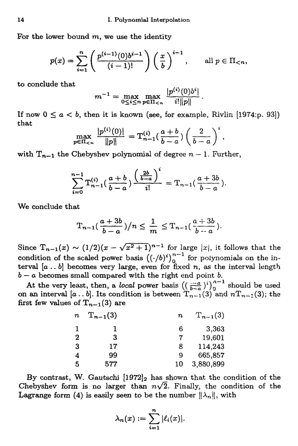
At the very least, then, a local power basis (( j—2- )г)^ should be used
on an interval [a.. 6]. Its condition is between Tn_i(3) and nTn_:(3); the
first few values of Tn_i(3) are
n
1
2
3
4
5
Tn-i(3)
1
3
17
99
577
n
6
7
8
9
10
Tn-i(3)
3,363
19,601
114,243
665,857
3,880,899
By contrast, W. Gautschi [1972]г has shown that the condition of the
Chebyshev form is no larger than n\/2. Finally, the condition of the
Lagrange form (4) is easily seen to be the number ]|Anl|, with
An(x) := f>(x)|.

Problems
15
As is pointed out in the next chapter,
||An||~(2/7r)lnn + l
if we choose the Chebyshev sites 11(9) as the sites r. Thus, the Lagrange
form based on the Chebyshev sites is about the best conditioned polynomial
form available.
Nevertheless, we will use the local power form throughout this book
because of its simplicity, the easy access to derivatives it affords, and because
we do not intend to deal with polynomials of order higher than 15 or 20.
Still, the reader should be aware of this potential source of trouble and
be prepared to switch to some better conditioned form, for example the
Chebyshev form, if need be. For this, see Problems 7 and II.3.
Problems
1. Given the divided difference table for the polynomial p e П<6, based
on the sites ti,...,T6, locate in it the coefficients for the Newton form
for p using the centers (а) т3,Т4, t2,T5,ti,t6; (b) Тб,тъ,т4,тз, T2,Ti; (c)
Т4,Т5,г6,гз,г2,г1; (d) r4>r5,r6, r3, T27r2.
2. Assume that TAU(г) = тг, D(i) = д(тг), г = 1,... , п.
(a) Verify that, after the execution of the following statements,
1 for к = l,...,n-l, do:
1/1 for i = 1,.,.,71-k, do:
1/1/1 D(i) := (D(i+1) - D(i))/(TAU(i+k) - TAU(i))
we have D(i) = [т*,..., Tn]g for г = 1,..., п.
(b) Hence, verify that the subsequent calculation
2 value := D(l)
3 for к = 2,...,n, do:
3/1 value := D(k) + value*(x - TAU(k))
produces the value pn(x) at x of the polynomial pn of order n that agrees
with ga.tr.
(c) Finally, verify that the subsequent calculation
4 for к = 2, . . . ,7i, do:
4/1 for i = 2,...,n+2-k, do:
4/1/1 D(i) := D(i) + D(i-l)*(x - TAU(i+k-2))
produces the coefficients in the Taylor expansion around x for pn, that is,
D(x)=p<ln-i>(x)/(n-i)!, г = 1,...,п.
3. Let p4 be the polynomial of order 4 that agrees with the function In
at 1, 2, 3, 4. Prove that p4(x) > ln(a:) for 2 < x < 3.
4. Construct the polynomial p& of order 6 that agrees with the
function sin at 0, 0, 7г/4, 7г/4, 7г/2, 7г/2. Use the error formula (15) along

16
I. Polynomial Interpolation
with the divided difference Property (vii) to estimate the maximum error
max{ | sin(x) — рб{х)\ '• 0 < x < 7r/2 } and compare it with the maximum
error found by checking the error at 50 sites, say, in the interval [0 .. 7r/2].
5. Prove that [rb ... ,rn](l/x) = (-l)n~V(ri • • -rn). (Hint: Use Leibniz'
formula on the product (l/x)x, and induction.)
6. Prove: If p(x) = 23^ аг ( |5f ) » and all a,i are of the same sign, then
the relative change ||?p||/||p(| (on [a .. b]) caused by a change 5b. in the
coefficient vector a is no bigger than n||i5a||/||a||.
Conclude that the condition as defined in the text measures only the
worst possible case. Also, develop a theory of "condition at a point" that
parallels and refines the overall condition discussed in the text.
7. The Chebyshev form for p G П<п is specified by the end points a
and b of some interval and the coefficients ai,...,an for which p(x) =
E?^Ti_i(y), with у = y(x) := (2x - (b + a))/(b - a) and T0{x) ': = 1,
Тг(х) :=x,Ti+x(x) :=2xTi(x)-Ti-i(x),i = 1,2,3 Write a FUNCTION
CHBVALCCCOEF, NTERM, X) that has CCOEF = (a,6,ab ... ,an), NTERMS
= n + 2, and argument X as input, and returns the value p(X), using the
three-term recurrence in the process. See, for example, FUNCTION CHEB,
Conte & de Boor [1980:p. 258].
8. Prove (for example by induction) that for arbitrary nondecreasing
r = (ri,..., rn), there exist unique constants d1?..., dTL, so that the linear
functional [7*1,... , rn] can be written
n
[П , . . . , Tn] = 2^, di [Tm(i) .-¦•iT't],
г=1
with
m(i) := min{j < г : Tj — Ti}, all i.
In other words, the divided difference of g at r is uniquely writeable as a
weighted sum of values and certain of the derivatives of g at the Ti.
9. Prove Micchelli's observation that [a:o,... ,Xj](- — xo)f = fci,... ,Xj]f.
10. Prove Micchelli's handy (see Problem 5) observation that a divided
difference identity is valid for all (smooth enough) / if it is known to hold
for all / of the form f(x) = l/(x — a), a G JR.

II
Limitations of Polynomial
Approximation
In this chapter, we show that the polynomial interpolant is very sensitive
to the choice of interpolation sites. We stress the fact that polynomial
interpolation at appropriately chosen sites (for example, the Chebyshev points)
produces an approximation that, for all practical purposes, differs very little
from the best possible approximant by polynomials of the same order. This
allows us to illustrate the essential limitation of polynomial approximation:
If the function to be approximated is badly behaved anywhere in the
interval of approximation, then the approximation is poor everywhere. This
global dependence on local properties can be avoided when using piecewise
polynomial approximants.
Uniform spacing of data can have bad consequences We cite the
(1) Runge example: Consider the polynomial pn of order n that agrees
with the function g(x) : = 1/(1 + 25a:2) at the following n uniformly spaced
sites in [—1 .. 1]:
П := (г- l)/i- 1, г = l,...,n, with h := 2/(n - 1).
The function g being without apparent defect (after all, g is even analytic
in a neighborhood of the interval of approximation [—1 .. 1]), we would
expect the maximum error
||en|| := max \g(x) - pn(x)\
to decrease toward zero as n increases. In the program below, we estimate
the maximum error ||en|| by the maximum value obtained when evaluating
the absolute value of g— pn at 20 sites in each of the n —1 intervals [т<_1. .т»],
г = 2,..., п. In this and later examples, we anticipate that, as a function of
n, ||en|| decreases to zero like /3na for some constant /3 and some (negative)
17

18 H. Limitations of Polynomial Approximation
Constant a. If ||en|| ~ /?na, then ||en|]/||em|| ~ (п/т)0, and we can estimate
the decay exponent a from two errors ||en|| and ||em|| by
(2) a „ log(|knll)-log(l[e^H)
log(n/m)
In the following program, the decay exponent is estimated in this way from
successive maximum errors.
CHAPTER II. RUNGE EXAMPLE
INTEGER I,ISTEP,J.K,N,NMK,NM1
REAL ALOGER,ALGERP,D(20),DECAY.DX,ERRMAX,G,H,PNATX,STEP.TAU(20),X
DATA STEP, ISTEP /20., 20/
G(X) * l./(l.+(5.*X)**2)
PRINT 600
600 F0RMATC28H N MAX.ERROR DECAY EXP.//)
DECAY « 0.
DO 40 N~2,20,2
С CHOOSE INTERPOLATION POINTS TAUCl) TAUCN) , EQUALLY
С SPACED IN (-1 .. 1), AND SET D(I) = G(TAU(I)), 1=1,...,N.
NM1 = N-l
H » 2./FL0ATCNM1)
DO 10 1*1,N
TAU(I) * FL0AT(I-1)*H - 1.
10 D(I) ~ G(TAU(D)
С CALCULATE THE DIVIDED DIFFERENCES FOR THE NEWTON FORM.
С
DO 20 K~1,NM1
NMK - N-K
DO 20 I«1,NMK
20 D(I) *» (D(I+l)-D(I))/(TAU(I+K)-TAUfI))
С "
С ESTIMATE MAX.INTERPOLATION ERROR ON (-1 ..1).
ERRMAX «* 0.
DO 30 I»2,N
DX « (TAU(I)-TAU(I-1))/STEP
DO 30 J-l,ISTEP
X » TAU(I-l) + FL0AT(J)*DX
С EVALUATE INTERP.POL. BY NESTED MULTIPLICATION
С
PNATX =- D(l)
DO 29 K«2,N
29 PNATX - D(K) + (X-TAU(K))*PNATX
30 ERRMAX - AMAX1(ERRMAX,ABS(G(X)-PNATX))
ALOGER - ALOG(ERRMAX)
IF CN .GT. 2) DECAY »
* (ALOGER - ALGERP)/AL0G(FL0AT(N)/FL0AT(N-2))
ALGERP « ALOGER
40 PRINT 640,N,ERRMAX,DECAY
«40 F0RMAT(I3,E12.4,F11.2)
STOP
END

Runge example
19
N
о
4
6
8
10
12
14
16
18
20
MAX.ERROR
0.9615E+00
0.7070E+00
0.4327E+00
0.2474E+00
0.2994E+00
0.5567E+00
0.1069E+01
0.20Э9Е+01
0.4222E+01
0.8573E+01
DECAY EX]
0.00
-0.44
-1.21
-1.94
0.86
3.40
4.23
5.05
5.93
6.72
In the program listing above, we have marked the divided difference
calculation and the evaluation of the Newton form to stress how simple
these calculations really are.
Prom the output, we learn that, contrary to expectations, the
interpolation error for this example actually increases with n. In fact, our estimates
for the decay exponent become eventually positive and growing so that
||en|| grows with n at an ever increasing rate. ?
The following discussion provides an explanation of this disturbing
situation. We denote by
(3) P„9
the polynomial of order n that agrees with a given g at the given n sites
of the sequence r. We assume that the interpolation site sequence lies in
some interval [a .. 6], and we measure the size of a continuous function /
on [a .. b] by
(4) ll/ll := max \f(x)\.
a<x<b
Further, we recall from 1(2) the Lagrange polynomials
^(*):=П(*-т,)/(т;-т;),
in terms of which
\(Png)(x)\ = |I>fa)'i(*)| < 1>(т;)1Кг(*)| < (тгах|5(7ч)|)?|А(*)|.
i i г
We introduce the so-called Lebesgue function
Tl
(5) A„(i):=^|4(i)|.
i = l

20
II. Limitations of Polynomial Approximation
(6) Figure. The Chebyshev sites for the interval [a .. b] are obtained
by subdividing the semicircle over it into n equal arcs and
then projecting the midpoint of each arc onto the interval.
Since max* |<?(тг)| < ||<?||, we obtain the estimate
(7) \\Png\\ < \\K\\ |Ы|,
and this estimate is known to be sharp, that is, there exist functions g
(other than the zero function) for which ||Pn5|| = ||\г|| 1Ы' (see Problem
2).
On the other hand, for uniformly spaced interpolation sites,
||An||-2n/(enlnn)
(as first proved by A. N. Turetskii, in 1940; see the survey article L. Brut-
man [1997]). Hence, as n gets larger, Png may fail entirely to approximate
g for the simple reason that ||'Рп<?|| gets larger and larger.
Chebyshev sites are good Fortunately, this situation can be
remedied if we have the freedom to choose the interpolation sites.
(8) Theorem. If Ть...,^ аге chosen as the zeros of the Chebyshev
polynomial of degree n for the interval [a .. b], that is,
(9) Tj=rf :=(а + Ъ- (a _ b) Cos( <^=-^ ))/2, 3 = !.••¦,«.
then, with A? the corresponding Lebesgue function, we have
||А?||<(2/тг)1пп + 4.
For a proof, see, for example, T. Rivlin [1969:pp. 93-96]. M. J. D. Powell
[1967] has computed ||A?|| for the Chebyshev sites for various values of n

Chebyshev sites are good
21
(10) FIGURE. The size of the Lebesgue function for the Chebyshev sites
(solid) and the expanded Chebyshev sites (dashed).
(his v(n) equals our 1 + ||A?||). Figure (10) summarizes his results. It is
possible to improve on this slightly by using the expanded Chebyshev
sites
( . / L4 cos((2^ - 1)тг/(2п)) \ in
(11) r4:=(a + 6-(a-b) ^^ j /2, ,-l....,n,
instead. L. Brutman [1978] has shown that
(2/тг)(1пп) + .5 < ||A* || < (2/тг)(1пп) + .73
and that, for all n, ||A^|| is within .201 of the smallest value for ||An||
possible by proper choice of r. Numerical evidence strongly suggests that
the difference between ||А?|| and the smallest possible value for ||An|| is
never more than .02.

22
II. Limitations of Polynomial Approximation
Runge example with Chebyshev sites We change our experimental
interpolation program to read in the 10-loop
TAU(I) = C0S(FL0AT(2 * I - 1) * PI0V2N)
with the line H=2. /FLOAT (NM1) before the 10-ioop replaced by
PI0V2N = 3.1415926535/FL0AT(2 * N)
The program now produces the output
N
2
4
6
8
10
12
14
16
18
20
MAX.ERROR
0.9259+00
0.7503+00
0.5559+00
0.3917+00
0.2692+00
0.1828+00
0.1234+00
0.8311-01
0.5591-01
0.3759-01
DECAY EXP.
0.00
-0.30
-0.74
-1.22
-1.68
-2.12
-2.55
-2.96
-3.37
.-3.77
(with MAX. ERROR an estimate on [ti .. rn] only). ?
This is quite satisfactory, so let's take something tougher.
(12) Squareroot example We take g(x) := y/T+H on [-1.. l], that
is, we modify our experimental interpolation program further by changing
line 5, from G(X) = l./(l. + (5.*X)**2) to
G(X) = SQRT(1. + X)
This produces the output
N
2
4
6
8
10
12
14
16
18
20
MAX.ERROR
0.7925-01
0.3005-01
0.1905-01
0.1404-01
0.1114-01
0.9242-02
0.7900-02
0.6900-02
0.9425-02
0.1061+00
DECAY EXP.
0.00
-1.40
-1.12
-1.06
-1.04
-1.02
-1.02
-1.01
2.65
22.98
which shows the maximum error ||en|| to decrease only like n""1. This is due
to the singularity of g at x = — 1. (The increase in the error for n = 18,20
is due to roundoff; see Problem 3.)
If we put the singularity inside of [—1 .. 1], things get even worse. E.g.,
for g(x) = y/\x\ on [—1 .. 1], we get

Squareroot example
23
N
2
4
6
8
10
12
14
16
18
20
MAX.ERROR
0.8407+00
0.5475+00
0.4402+00
0.3791+00
0.3382+00
0.3083+00
0.2853+00
0.2666+00
0.2512+00
0.2383+00
DECAY EXP
0.00
-0.62
-0.54
-0.52
-0.51
-0.51
-0.50
-0.51
-0.51
-0.50
Our complaint here is that the error, while decreasing, decreases far too
slowly if we are seeking several places of accuracy. As the output indicates,
we have for this particular g
||en|| ~ const ¦ n~l/2.
Hence, if we wanted an error of 10-3, then we would want
10-3 = ||en|| = (||en||/||eao||)||eao|| « .2384,^/20)-^
or
(n/20) « (.2384)2106,
that is, we would need n ~ 1.14 million. ?
The following discussion might help to explain this situation. Recall from
Theorem 1(14) that the interpolation error satisfies
en(aO = g(x) — Png(x) = {x - n) ••¦ (a; - rn)[rt,... ,тп,х]д
while, by Property I(vii) of the divided difference,
fa,...,T„,z]$ = e(T0(C)/nl
for some ?x in the interior of the smallest interval containing ti, ..., rn and
x. This provides the estimate
(13) ||5_p^||<||(.-ri)...(.-r„)||^axb^-^.
Now, it so happens that
,(Ъ-аГ
(14) min ||(._T1).--(--Tn)|| = 2-
a.<T\<'-<Tn<0 4"
and that this minimum is taken on when the interpolation sites are the
Chebyshev sites. This means that we have done already as well as possible
as far as the choice of interpolation sites is concerned. The difficulty in
controlling the interpolation error then must lie with the second factor in
(13),
mav lg(n)(0l
max : .
а<с<ь n!
Indeed, in our case, g^ becomes infinitely large in [a .. b] for all n > 1.

24 II. Limitations of Polynomial Approximation
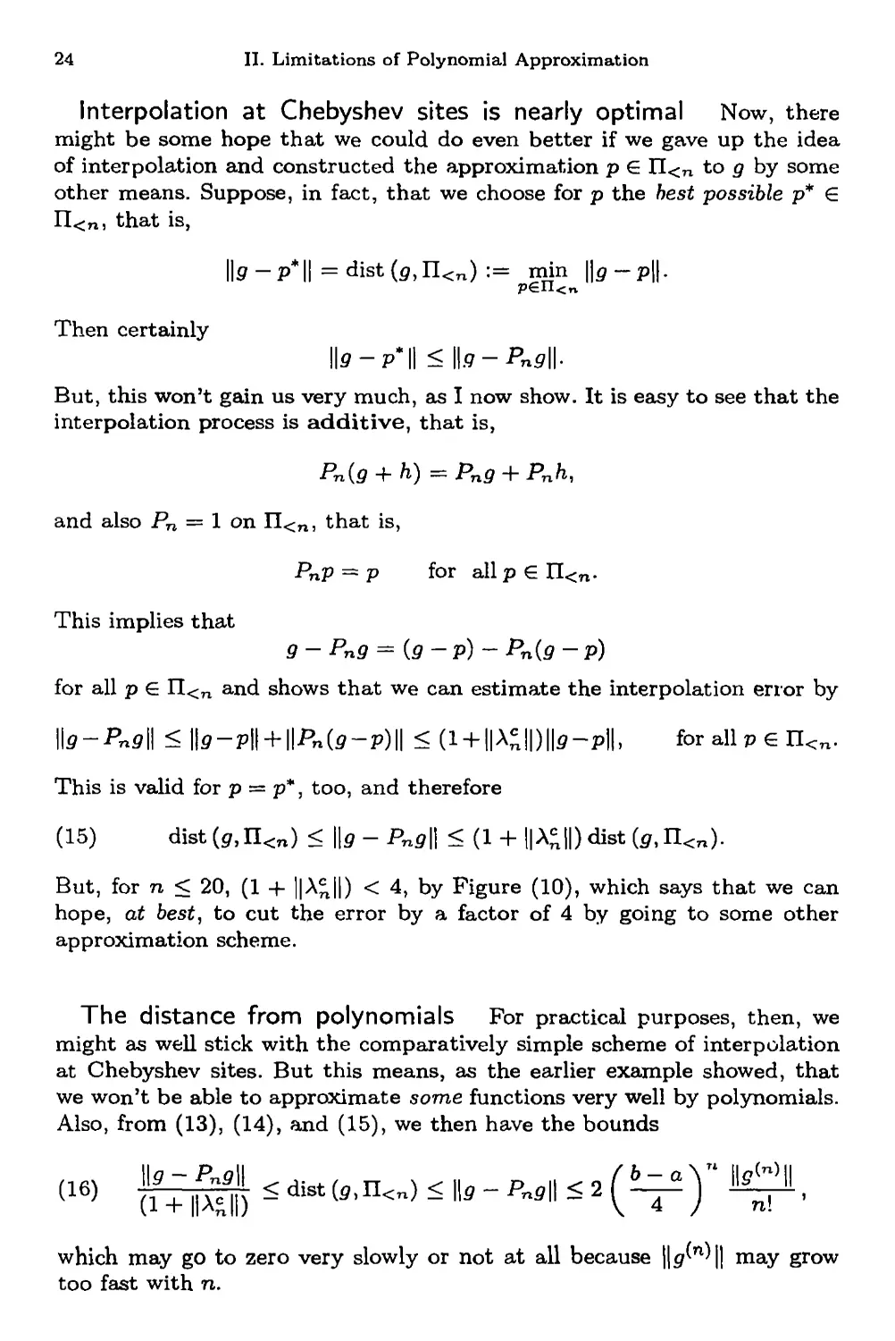
Interpolation at Chebyshev sites is nearly optimal Now, there
might be some hope that we could do even better if we gave up the idea
of interpolation and constructed the approximation p G П<п to g by some
other means. Suppose, in fact, that we choose for p the best possible p* G
n<n, that is,
||<?_pl=dist(s,n<n):= mrln Il0-Pll-
Then certainly
l|e-p*||<||.9-PnS||.
But, this won't gain us very much, as I now show. It is easy to see that the
interpolation process is additive, that is,
Pn{g + h) =Png + Pnh,
and also Pn = 1 on П<п, that is,
PnP = p for all p G П<п.
This implies that
9 ~ Pn9 = {g-p)~ Pn{g ~ P)
for all p G П<п and shows that we can estimate the interpolation error by
\\9-Pn9\\ <||0-p|| + ||Pn(s-p)|| <(1 + ||A?||)||S-P||, forallpen<n.
This is valid for p = p*, too, and therefore
(15) dist(g,n<n) < \\g - Png\\ < (1 + ||A?||) dirt (*, П<п).
But, for n < 20, (1 + ||A?||) < 4, by Figure (10), which says that we can
hope, at best, to cut the error by a factor of 4 by going to some other
approximation scheme.
The distance from polynomials For practical purposes, then, we
might as well stick with the comparatively simple scheme of interpolation
at Chebyshev sites. But this means, as the earlier example showed, that
we won't be able to approximate some functions very well by polynomials.
Also, from (13), (14), and (15), we then have the bounds
which may go to zero very slowly or not at all because ||g^n^|| may grow
too fast with n.

The distance from polynomials
25
-1
(17) Figure. For g(x) = v^on [-1/.1], max|^(x) -g(y)\ in a strip of
width h occurs when 0 lies on the boundary of the strip,
and then max \g(x) — g(y)\ = \g(0)—g(h)\ = y/h. Therefore,
u)(g\ k) = y/h.
Approximation theory provides rather precise statements about the rate
at which dist (g, П<п) goes to zero for various classes of functions g. An
appropriate classification turns out to be one based on the number of
continuous derivatives a function has and, within the class C^[a .. b] of
functions having r continuous derivatives, on the modulus of continuity of
the rth derivatives For g G C[a. .b], that is, for a function g continuous on
[a .. b], the modulus of continuity of g at h is denoted by u>(g; h) and
is defined by
(18) w(g\h) :=sup{\g{x) - g(y)\ : xyy G [a .. 6], \x - y\ < h}.
It is clear that u(g; h) is monotone in h and subadditive in h (that is,
u(g; h -f- к) < u(g\ h) f u(g; к)) and that (for a finite interval [a .. b])
(19)
lim uj(g;h) = 0,
h—*0+
for all g G C\a..b],
but the rate at which uj(g; h) approaches 0 as h —> 0+ varies widely among
continuous functions. The following are simple, yet practically useful,
examples: The fastest possible rate for a function g that isn't identically constant
is u(g; h) < consth (see Problem 5). This rate is achieved by all functions
g with continuous first derivative, that is,
(20) ltge C<»[a .. 6], then ш(д; h) < \\g'\\h.

26
II. Limitations of Polynomial Approximation
If, more generally, u>(g', h.) < Kh for some constant К and all (positive)
Л, then g is said to be Lipschitz continuous. Piecewise continuously
differentiable functions in C\a .. b] belong to this class which is therefore
much larger than the class C^ [a. .b] of continuously differentiable functions
on [a. .6]. An even larger class consists of those continuous functions on [a. .b]
that satisfy a Holder condition with exponent a for some a G (0 .. 1).
This means that
w(g\ h) < Kha for some К and all (positive) h.
For instance,
(21) u(g; h) < ti* for the function g(x) := \x\<* on [-1 .. 1].
A typical example for the use of this classification is
(22) Jackson's Theorem. If g G C^[a .. b], that is, g has r continuous
derivatives on [a .. b]} and n > r + 1, then
(23) dist(5)n<n) <constr (iziy^M. 2(пЬ_~а_г)).
Here, the constant can be chosen as
constr := 6(3e)r/(l + r).
A proof of this theorem can be found, for example, in T. Rivlin
[1969:p. 23].
Our last example shows that this estimate is sharp, in general, as far
as the order of convergence, that is, the decay exponent, is concerned. For
g(x) = л/\х\ on [—1 .. 1], we have, as already noted in (21),
u(g;h) = \g{h)-g(0)\ = h1/*
and so, from (23) with r = 0,
dist (g, n<n) < const - n~1/2
which is the rate that we observed numerically in Example (12).
There are, of course, functions that are efficiently approximated by
polynomials, namely (well behaved) analytic functions. For an analytic p,
dist(p,n<n) = 0(e—)
for some positive a. But, if g has only r derivatives, then (23) describes
correctly how well we can approximate g by polynomials of order n.
The fact that (23) is sharp in general means that the only way for making

Problems
27
the error small is to make (6 — o)/(n — 1) small. We accomplish this by
letting n increase and/or making (b — a) small. Since we are given [a.. b] in
advance, we can achieve the latter only by partitioning [a. .b] appropriately
into small intervals, on each of which we then approximate g by a suitable
polynomial, that is, by using -piece-wise polynomial approximation.
Note that cutting [a .. b] in this way into к pieces or Using polynomials
of order kn will have the same effect on the bound (23) and corresponds
either way to a fc-fold increase in the degrees of freedom. But these
degrees of freedom enter the approximation process differently. Evaluation
of a polynomial of order kn involves kn coefficients and basis functions
whose complexity increases with the order fcn, while evaluation of a piece-
wise polynomial function of order n with к pieces at a site involves only n
coefficients and a local basis of fixed complexity no matter how big к might
be. This structural difference also strongly influences the construction of
approximations, requiring the solution of a full system in the polynomial
case and usually only a banded system in the piecewise polynomial case.
Also, use of polynomials of order 20 or higher requires special care in the
representation of such polynomials (Chebyshev expansions or some other
orthogonal expansion must be used, see the discussion of condition in
Chapter I), while use of a larger number of low order polynomial pieces is no
more delicate than the use of one such polynomial. Finally, interpolation
in a table, that is, to equally spaced data, by piecewise polynomials leads
to no difficulties, in contrast to what happens when just one polynomial is
used, as we saw with the Runge example (1).
For these and other reasons, it is usually much more efficient to make
(b — a) small than to increase n. This is the justification for piecewise
polynomial approximation.
Problems
1, Every continuous function g on [a .. b] has a (unique) best uniform
approximation p* from II<fc on [a . . b], that is, there is one and only one
p* ? n<fc so that \\g —p*\\ = dist (giH<fz). This best uniform approximation
p* is characterized by equioscillation of the error (see, for example, Rivlin
[1969: p. 26]): Let p € Tl<k and e := g — p the error in the approximation p
to g. Then \\e\\ = dist (g, H<k) if and only if there are sites а < хг < ¦ ¦ • <
Хк+i ? b for which
e(xi)e(xi+l) = H|e||2, i = 1,..., fc.
(a) Conclude that a best approximation to g from П<^ on [a .. b] must
interpolate g at к distinct sites (at least) in that interval.
(b) Conclude that dist (^,II<fc) = constg</fc)(?) for some а < ? < b, in case
g has к continuous derivatives, with const5 depending on the sites at which
the best approximation interpolates g.

28
II. Limitations of Polynomial Approximation
(c) Conclude that dist (p, П<*) > (2(Ь - a)fc/4fc)xnine<«<b \g{k){x)/k\\.
(Hint: use (14) and 1(14).)
2. Prove that the inequality (7) is sharp. (Hint: Pick x in [a .. b] for
which An(?) = ||A||; such a site must exist since An is continuous and
positive. Then choose 04 •= signum ?*(?), all z, and construct a continuous
function g on [a .. b] with g{Ti) = &i, all 2, and ||^|| — 1, for instance by
linear interpolation in, and constant extrapolation from, the table (т^сг^),
i = 1,..., n. Then show that \\Png\\ - ||An|||b||.)
3. The roundoff visible in the Squareroot Example (12) could be fought
by a careful ordering of the interpolation points. But, the best remedy is to
construct the Chebyshev form of the interpolating polynomial. This
construction is greatly facilitated by the fact that the Chebyshev poJynomiais
To,Ti,... ,Tn_i are orthogonal with respect to the discrete inner product
</.»>¦¦=?/WW*?)
based on the Chebyshev sites r* :— cos((2« — l)7r/(2rc)), 2 = 1,..., ra, for
the interval [—1 .. 1] (see for example, Rivlin [1974]). This means that
(Ti.Tj-) = 0 for г ф j. Also, (T;,T*> = n/2 for г = 1,... ,n - 1, while
(T0, To) = n. Note that the Chebyshev sites (rc) for the interval, as given
by (9), are related to the т? by y(r?) = rz*, with
y(x):={2x-{b + a))/(b-a).
(a) Prove that the polynomial Png of order n that agrees with g at the
Chebyshev sites (rf) can be written
n
(Рпд)(х) = ^снТ*-1{у(х)),
with
n
ai+l := ^д{т?)Т<{т;)/(Т1,Т<), г = 1,... ,n.
(b) Develop a subroutine CHBINT(A, B, G, N, CCQEF, NTERMS) that
returns, in CCOEF and NTERMS, the Chebyshev form for Png (as denned in
Problem 1.7), given the endpoints А, В of the interval in question, the
number N of interpolation points to be used, and a FUNCTION G(X) that
provides function values of g on demand. Note that, with
^:=0(т;)Т*_1(т;), ail i,j,

Problems
29
one has аг — ]Г\ Vj^/N, and
[ 2r?vj%i-i -vjyi_2, i > 2,
Also, one can forget or overwrite bjj as soon as Vj^+2 has been constructed,
provided one has by then calculated CCOEF(i + 2) = 2(?V Vj,i)/N-
Incidentally, it is also possible (for certain values of N) to make use here
of the Fast Fourier Transform.
(c) Repeat the calculations in the Squareroot Example (12) above, but use
CHBINT, and CHBVAL of Problem 1.7, to uncover the amount of roundoff
contaminating the calculations reported there.
Note: A routine like CHBINT is very useful for the construction of the
Chebyshev form of a polynomial from some other form or information.
4. The calculation of \\g\\ = max{ |<?(x)l :a<a;<b}isa nontrivial task.
Prove that, for p G П<п, though, a good and cheap approximation to ||p||
is provided by ||p||c. := max{ |р(т?)| : г = 1,.. . , n }, with (r€c) given by (9).
By what number cn must one multiply ||p||c to ensure that с^ЦрЦс > ||p||?
5. Prove that g is a constant in case u>(g\ h) = o(h). (Hint: Show that
then g is differentiable everywhere and g1 = 0.)
6 Prove that uj(g: h) is a monotone and subadditive function of h, that is,
u{g\ h) < u>(g; h + k) < u*(g\ h) +u>(g\ k) for nonnegative h and fc. Conclude
that oj(g\ ah) < \oi\uj{g\ h) for a > 0, with \a\ := min{ n € ZZ : a < n }.

Ill
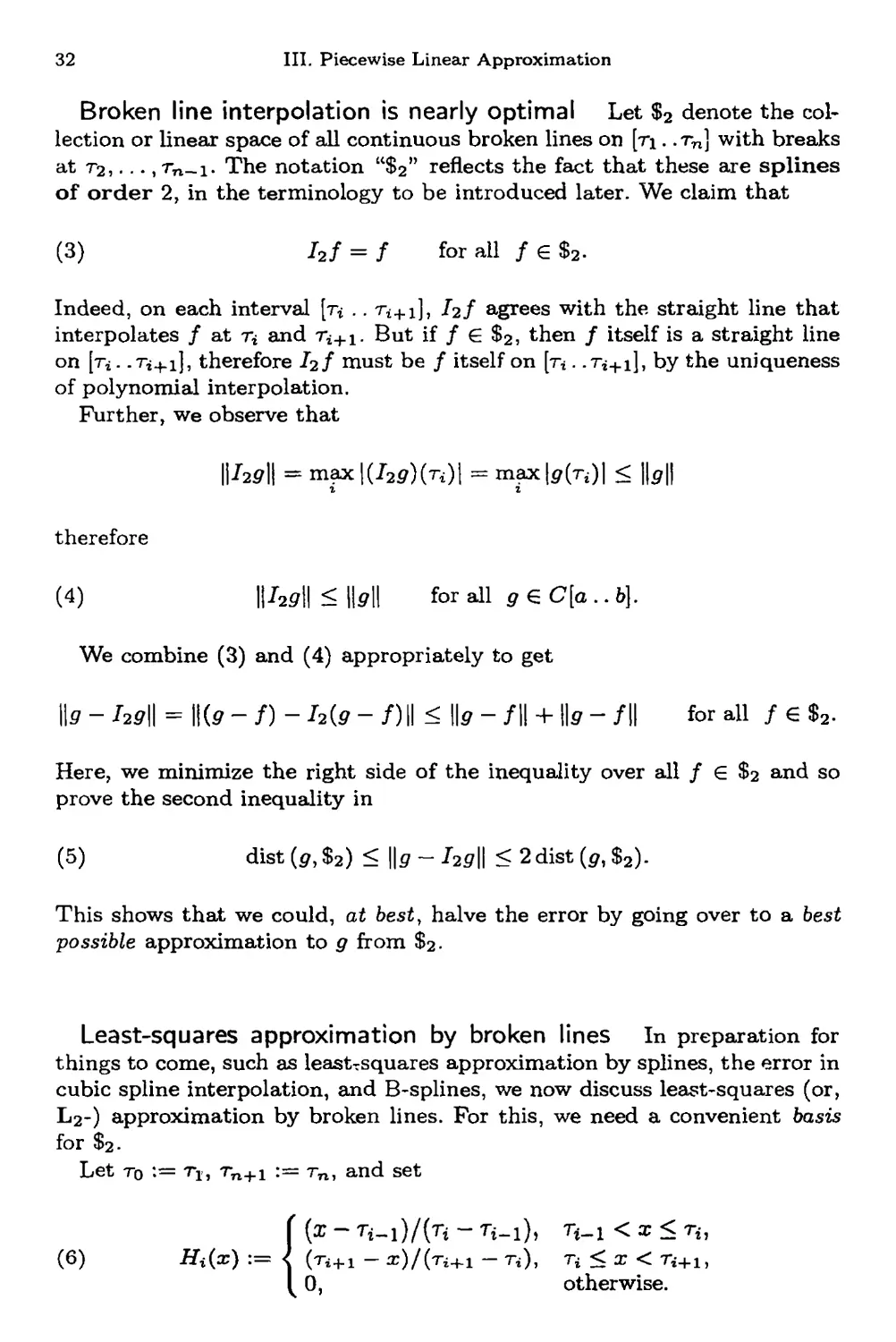
Piecewise Linear Approximation
Piecewise linear approximation may not have the practical significance
of cubic spline, or even higher order, approximation. But it shows most of
the essential features of piecewise polynomial approximation in a simple
and easily understandable setting.
Broken line interpolation We denote the piecewise linear, or broken
line, interpolant to g at points ti, ..., rn with
a = т\ < • • • < rn = b
by It.9- The subscript 2 refers to the order of the polynomial pieces that
make up the interpolant. The interpolant is given by
I2g(x) := g(Ti) H- (x - Ti)[TUri+1\g on n < x < ri+1,
i = 1,..., n — 1.
Since
g(x) = g(Ti) + (x -Ti)[Ti,Ti+i]g + (re - Т;)(х - Ti+1)[ru ri+1, x]g,
we have, for n < x < Tj+i,
g(x) - I2g(x) = (x-Ti)(x- ri+1)[ruri+l,x]g.
Therefore, with Ar» := (ri+1 — r^), we get the error estimate
\g(x) - I2g(x)\ < (ATl/2)* max |</'(C)/2|
Ti<C<T4+l
in case g has two continuous derivatives, hence, with \r\ := maxi Атг,
(2) \\9 - hg\\ < l\r\2\\g"\\.
Clearly, we can make this error bound as small as we like simply by
making At* small for all г. And, while this increases the number of parameters
needed to describe the approximating function / = I2g, it does not really
increase the complexity of / locally since, locally, / is always just a straight
line.
31

32
III. Piecewise Linear Approximation
Broken line interpolation is nearly optimal Let $2 denote the
collection or linear space of all continuous broken lines on [т\. .тп) with breaks
at r2,. .. ,rn_i. The notation "$2" reflects the fact that these are splines
of order 2, in the terminology to be introduced later. We claim that
(3) hf = f for all /€$a.
Indeed, on each interval [т* .. ri+1], /2/ agrees with the straight line that
interpolates / at т* and ri+1. But if / € $2, then / itself is a straight line
on [Ti. .Ti+i], therefore /2/ must be / itself on [r±. .Ti+i], by the uniqueness
of polynomial interpolation.
Further, we observe that
||I20|| =max|(J2<7)(Ti)| = max\д{п)\ < \\д\\
г г
therefore
(4) Ра0||<1Ы1 for all ge C[a..b].
We combine (3) and (4) appropriately to get
Из - hg\\ = \\(g - /) - h{g - /)|| < \\g - /II + \\g - /II for all / e Sa.
Here, we minimize the right side of the inequality over all / G $2 and so
prove the second inequality in
(5) dist(<?,$2) < \\g~hg\\ <2dist(<?,$2).
This shows that we could, at best, halve the error by going over to a best
possible approximation to g from $2.
Least-squares approximation by broken lines In preparation for
things to come, such as leastTsquares approximation by splines, the error in
cubic spline interpolation, and B-splines, we now discuss least-squares (or,
L2-) approximation by broken lines. For this, we need a convenient basis
for $2-
Let T0 := rj, rn+i := rn, and set
{(x - Ti-i)/(Ti - Ti_i), Tt_i <x<ru
(ri+1 - x)/(ri+1 - Ti), n<x < Ti+i,
0, otherwise.

Least-squares approximation by broken lines
.#3 V4^4
33
r0 = a - т\ r2 r3 r4 r5 rn_i rn = b = rn+i
(7) Figure. Some of the elements of the standard basis for $2-
These functions have been called hat functions or, more learnedly, cha-
peau functions. Clearly, Hi € $2, all i, and, as is obvious from Figure
(7),
Hi(Tj) = 5i3, = |0| *^-i for alii, j.
This shows that V]™ g{ji)Hi is an element of $2 that agrees with g at
гь ¦ • • ? 7"n> while, by (3), I29 is the only element of $2 with that property.
This establishes the "Lagrange form"
(8)
/а$ = 1>(т«)Я,
for the broken line interpolant. It also implies that (Hi)™ is a basis for
$2, that is, every broken line on [r\ .. rn] with breaks at T2,... ,rn_i can
be written in exactly one way as a linear combination of the H^s. The
coordinates of a given / 6 $2 with respect to the basis (i/i)? consist simply
of its values (/(ti),..., /(rn)) at the breaks, that is,
(9)
f = Ylf(TJHi foraU -f G$2-
Let L^g be the least-squares approximation to g from $2, that is, L^g €¦ $2
and
/ \g{x) - L2g{x)\2dx = min / |p(rc) - f(x)\2dx .
We determine L2p with the aid of the normal equations; that is, we find a
minimum of
/
\g(x)-J2ajHj(x)\2dx
by setting its first partial derivatives with respect to ai,...,an to zero.
This gives the linear system
(10) J2 J / #;(*)#;(*) dxj oj = J Hi(x)g(x)dx,
i = 1,... ,n,

34 III. Piecewise Linear Approximation
for the coefficients {cti)i of the broken-line L2-approximation to gy
n
The integrals involved are easily evaluated. We get, more explicitly, the
linear system
(11) Ь ЛЬ
= ft:= f Hi(x)g(x)dx
i = 1,... ,n,
(with ao,an+1 of no interest since Дго = Дтп = 0). The coefficient matrix
is tridiagonal, and strictly diagonally dominant. The system has therefore
exactly one solution and this solution can be obtained efficiently and stably
by Gauss elimination without pivoting (see, for example, Forsythe &: Moler
[1967]).
(12) Theorem. The ^-approximation L2g to g € C[a .. b], that is, to a
continuous function g on [a .. b], by elements of $2 satisfies
(13) ||L2<?|| < 3|M|.
Hence, since L2 is additive and L2f = / for all f ? $2, we have
(14) \\9-L2g\\<4dist(g,$2).
PROOF. To bound \\L2gW = maxi \(Ь2д)(п)\ — max* |a»| in terms of
1Ы1> we multiply, for each г, both sides of the ith equation in (11) by
6/(ri+i — Ti~i) to obtain the equivalent linear system
(15) Ат*~г a^! + 2ai+ — ai+1=3A, г = 1,...,п,
for the coefficients (aj of L2g. This system is strictly diagonally dominant
uniformly in r (since n+i — t*_i = Ar^i + Аъ), and this we can exploit
as follows: If j is such that
l<*jl = IHI :=тах|ач|,
г
then, from the jth equation in (15),
\2а5\ = \Щ - (o^iAr^i +oi+1ATi)/(Ar^1 + ATj)\ < 3|Д| + |а,|
or,
1И<3|&|<3||/5Ц.

Good meshes
35
On the other hand,
& = J Hi{x)g{x)dx
with
(16) Щх) := (2/(r<+i - п-г))Щх)
positive for т4_1 < a; < Ti+i and zero otherwise, and f Hi(x) dx = 1. Thus
|ft| = \flii(x)g(x)dx\ < ffii(x)dx-max{\g(x)\ : n^ < x < ri+1 } <
Ml
This proves that ||L2?|| ^ 3||p||. But (14) follows from this and from the
fact that L2f = /, for all / € $2, and L2(/ -h g) = L2/ + L2?, much as (5)
follows from (3) and (4) (see Problem 2). ?
The use of diagonal dominance to bound the solution of a linear system
in terms of the right side has been standard in Numerical Analysis for some
time. But the first spline paper to employ the technique is Sharma Sz Meir
[1966] in which Theorem (12) is proved this way (modulo the identification
made in Corollary V(9)).
Good meshes We observed earlier that, with \r\ := max* |Ar^|,
(2) ||*-J3*||< ||т|2||Л1
in case g G C^ and concluded that we could make the interpolation error
arbitrarily small by making |r| small. In particular, for a uniform mesh,
we get
(17) \\9 - hg\\ < | (?^)2 IIЛ1 = О (n-2) ,
with n, the number of interpolation points, equal to the degrees of freedom
used. Here, we have used the symbol "O (n~2)" (read "big oh of n-2") to
express the fact that the decay exponent for the bounxLin (17) is at least
as small as —2. See p. xvi for a full explanation.
Even if g is only continuous, for example g" might be infinite somewhere,
or g' is not defined somewhere, we can still make the error small by making
\r\ = max* Атг small. On n < x < ri+\, we have
(I2g){x) = ((ri+1 - x)g{ri) + (я - п)д{т1+1))/&т{
and
((ri+1 - x) + (x - п))/Аъ = (\ri+1 ~ x\ + \x - ъ\)/Аъ = 1,

36
Ш. Piecewise Linear Approximation
therefore
\g{x) - I2g{x)\ < ((ri+i - x)\g{x) - р(т,)| + (* - r<)|0(a:) - g(ri+1)\) / An
< max max{ |#(:r) - р(г*)|, |s(x) - p(ri+i)i }
<w(5;ArO.
Hence, by 11(19),
(18) \\g - I2g\\ < u>{g; \r\) |r<^Q > 0.
For the Squareroot Example 11(12),
g(x) = -y/W on [a .. 6] = [-1 .. 1],
and uniformly spaced interpolation sites, this gives
(19) II? - hg\\ = О (n-1'2)
which is no gain in the convergence rate over polynomials (except that
polynomials of order n are more complex objects than are broken lines
with n pieces). But, because we have the location of the breaks at our
disposal, we can do much better.
(20) Theorem. Ifg € C^2\a .. b), that is, if g has two continuous
derivatives inside the interval (a .. b), and \g"\ is monotone near a and b, and
faWi*)]1'2** < oof then, with T2 < - - • < Tn-i chosen so that
(21) Г \g"{x)\V2 dx = 1^1 Г |</'(*)|1/2da;, all i,
J a n~l ia
we have
7«|| = О (n-2)
A simple proof of this can be found in de Boor [1973]. We will discuss
such theorems for arbitrary order in Chapter XII. Note that this theorem
not only claims the possibility of good convergence to functions with
singularities at the ends of the interval, but it also indicates how the breaks
should be chosen to achieve the optimal convergence rate О (п~2) •
For the Squareroot Example 11(12), we consider only (0. .1], for simplicity;
the interval [—1 .. 0] can be handled by symmetry. For x > 0, g"{x) =
-(l/4)x-3'2, therefore
f \gf,{x)\^2dx = i f'x-^dx = \-AtV* < oo.
Jo 2 7o 2

Problems
37
We therefore want
For this choice, as one verifies directly (see Problem 6),
\\g-l#\\ = max \(g-I2g)(x)\<(n-l)-2/2
or
(22) \\g-I2g\\=o(n-2).
This shows that, for this choice of breaks, the decay exponent is —2. This
is to be compared with the decay exponent of only —1/2 for the uniformly
spaced breaks demonstrated earlier, and with the same decay exponent
— 1/2 obtained in Example 11(12) when approximating g by polynomials
with the same number of free parameters.
Problems
1. Verify that broken line interpolation preserves monotonicity and
convexity.
2. For g G C[a. .&], let Pg be an approximation to g in the linear subspace
S of C[a .. b] so that (i) Pg = g whenever g € 5, (ii) P(g + h) = Pg + Ph
for every g,heC[a.. b]f and (iii) ||P|| := sup{ ||Р<7||/|Ы| : g ? С [a .. b] } is
finite. Prove that then
№-.P0||<fl + ||P||) diet (0,5).
3. Let $! :={/'./? $2}, that is, $j is the linear space of piecewise
constant functions on [a .. b] with breaks r2, - - -, r^-j.
(a) Show that dist(g,$x) < и(д]\т\/2) for g € C[a .. b]. (Note: We take
here 11/11 := sup{ |/(a:)| : x e [a .. b] \ {r2,... ,rn_i} } in order to avoid
discussing what the value of an / € $1 at a break might be.)
(b) Show that \\g' — (/^УИ < 2dist (<?', $1) for any continuously dif-
ferentiable g, and even \\g' — (l2p)'|| = ^(lrl) if 9* 1S Lipschitz
continuous.
(c) Show that, for any three times continuously differentiable gy and with
Ti+i/2 := (Ti + ri+1)/2,
тад |(^ - I**)'(T,+ i,a)| = О (|Г|2) .
4. Use the estimate ||d|| < 3||/?|| obtained in the proof of Theorem (12)

38
III. Piecewise Linear Approximation
to conclude that (11) has one and only one solution for given g.
5. Let 0 < a < b, and let / be the straight line that interpolates g{x) :=
y/x at a and 6.
(a) Show that max{ \g(x)-f(x)\ :a<x<b}= \ (v^- \A)2/( V^+\A)-
(b) Use part (a) of this problem and (5) above to prove that the distance
of g(x) := y/x on [—1 .. 1] from broken lines with uniformly spaced breaks
goes to zero faster than n~~ll2.
6. Use Problem 5(a) to verify (22). For this, show that for the
interpolation sites n = ((г — l)/(rc — l))4, г = 1,..., n, broken line interpolation to
y/x on [0 .. 1] has maximum absolute error in [т* .. r^] equal to
^-J2+(-_i)0/(4(n-i)2)-
7. Verify numerically that \\g — hg]] = О (n-2) in case g(x) = sin s/x
and n = ((г - l)/(n - l))4, г = 1 п.

IV
Piecewise Cubic Interpolation;
CUBSPL
Broken lines are neither very smooth nor very efficient approximators.
Both for a smoother approximation and for a more efficient approximation,
one has to go to piecewise polynomial approximation with higher order
pieces. The most popular choice continues to be a cubic approximating
function. In this chapter, we describe various schemes for piecewise cubic
interpolation and give a program for cubic spline interpolation with various
end conditions.
Given the data g(ri),..., g(rn) with a = rj < • • • < rn = 6, we construct
a piecewise cubic interpolant / to g as follows. On each interval [r^.. ri+i\,
we have / agree with some polynomial Pi of order 4,
(i)
f(x) = Pi{x) for Ti < x < ri+x for some Pi € П<4, г = 1,.. ., n — 1.
The ith polynomial piece Pi is made to satisfy the conditions
(2) Pi^ = P^' Pi(Ti+1) = 9(ri+1) n_l
U i?(T0 = *i, J?(ri+1) = si+1 % '""
Here, sb ..., sn are free parameters. The resulting piecewise cubic function
/ agrees with g at T\,..., rn and is in C^ [a . b], that is, is continuous and
has a continuous first derivative on [a.. b], regardless of how we choose the
free "slopes" (si)?.
In order to compute the coefficients of the ith polynomial piece Pi, we
use its Newton form
Pi(x) = Pi(Ti) + (X - Ti)[rU пЩ + (x - Т,)2[^, Tif Ti + 1}Pi
+ (X - Ti)2{x— Ti+l)[Ti,Ti,Ti+1,Ti+i]Pi.
We determine its coefficients from a divided difference table for Pi based
on the data (2) for P*:
39

40 IV. Piecewise Cubic Interpolation
[]p l,]P [,,]p l,,,]P
П g(n)
Ti д(ъ)
[n,Ti+i]g
Ti+i g{ri+i)
Si+l
[TiiTi+i]g — Si
At*
si+i - [Ti,TiJrl\g
An
Si + l + Si - 2[Ti,Ti+i]g
n+i g{ri+i)
This shows that, in terms of the shifted powers (x — r$)r,
(4) Pi(x) = cM + c2,i(x - r^ + c3yi{x - n)2 + c4>i(x - 74)3
with
(5)
Cl,i = Pi{Ti) = ^(Ti),
С2,г = ^'(Гг) = *г,
C3)i = P/'(Ti)/2 = [Тг,Гг,П+1]^- ДГг([гЬГг,ГИ.1,^+1]Д),
= ([Ti,ri+i]^- Si)/Ari -c4iiAri,
C4,*= Р1"{ъ)/6 = (я* + в*+1«2[г4|г*+1Ь)/(Дт4)3.
Different piecewise cubic interpolation schemes differ in the choice of the
slopes (si)J. We discuss the best known choices.
Piecewise cubic Hermite interpolation Here, one chooses s* =
^'(ri), all г, thereby making the approximation local. This means that
the ith piece Pi depends only on information from, or near, the interval
[ri .. ri+1]. From Theorem 1(14), we have, for т* < x < г^.ц, that
ЫХ) - /(*)! = К00" П)2(Х ~ Тг+1)2[тиТиТг+1,Тг+г1х}у\
<(ДП/2)4 ma* |^(C)|/4!,
hence, with \r\ := max* At*,
(6) ||ff-/|| <(l/384)|r|4||ffW||
in case p € C^[a .. fc]. For equally spaced sites (At* = (b — a)/{n — 1), all
г), we get
(7) \\g - /II = О (n-4)
that is, the decay exponent for the error in piecewise cubic Hermite
interpolation is at Jeast —4 if the function g has four continuous derivatives.

Runge example continued
41
(8) Runge example continued We consider again the Runge
example 11(1): We interpolate g(x) := (1+25X2)-1 on [-1..1] at n = l + (i-l)Ji,
г = 1,..., n, with h := 2/(n — 1), but this time by piecewise cubic Hermite
interpolation. The two major changes in the program are outlined.
CHAPTER IV. RUNGE EXAMPLE, WITH CUBIC HERMITE INTERPOLATION
INTEGER I,ISTEP,J,N,NMl
REAL AL0GERlALGERP,C(4,20)1DECAYfDIVDFlfDIVDF3,DTAU,DX,ERRMAXfGfH
* ,PNATX,STEP,TAU(20)
DATA STEP, ISTEP /20., 20/
G(X) = l./(l.+(5.*X)**2)
PRINT 600
600 FORMAT(28H N MAX.ERROR DECAY EXP.//)
DECAY = 0.
DO 40 N=2,20,2
С CHOOSE INTERPOLATION POINTS TAU(l), ..., TAU(N) , EQUALLY
С SPACED IN (-1 ..1), AND SET C(lfI) - G(TAU(I))f C(2fI) =
С GPRIME(TAUQ)) = -50.*TAU(I)*G(TAU(I))**2f I-1.....M.
NM1 - N-l
H = 2./FL0ATCNM1)
DO 10 1=1,N
TAU(I) = FL0ATU-1)*H - 1.
C(1,I) = G(TAU(I))
10 C(2,I) = -50.*TAU(I)*C(1,I)**2
С CALCULATE THE COEFFICIENTS OF THE POLYNOMIAL PIECES
С
DO 20 1=1,NM1
DTAU = TAUCI+1) - TAU(I)
DIVDF1 = (C(1,I+1) - C(lfI))/DTAU
DIVDF3 - C(2,I) + C(2,I+1) - 2.*DIVDF1
C(3,I) = (OIVDFl - C(2,I) - DIVDF3)/DTAU
20 С(4,I) = (DIVDF3/DTAU)/DTAU
С
С ESTIMATE MAX.INTERPOLATION ERROR ON (-1 .. 1) .
ERRMAX = 0.
DO 30 1=2,N
DX = (TAU(I)-TAU(I-1))/STEP
DO 30 J=l,ISTEP
H = FLOAT(J)*DX
С EVALUATE (I-l)ST CUBIC PIECE
С
PNATX = C(1,I-1)+H»(C(2,I-1)+H»(C(31I-1)+H*C(41I-1)))
30 ERRMAX = AMAXl(ERRMAX,ABS(G(TAU(I-l)+H)-PNATX))
ALOGER = ALOG(ERRMAX)
IF (N .GT. 2) DECAY =
* (ALOGER - ALGERP)/AL0G(FL0AT(N)/FL0AT(N-2))
ALGERP = ALOGER
40 PRINT 640,N,ERRMAX,DECAY
640 F0RMAT(I3,E12.4,F11.2)
STOP
END

42
IV. Piecewise Cubic Interpolation
N
2
4
6
8
10
12
14
16
18
20
MAX.ERROR
0.9601+00
0.7275+00
0.4900+00
0.3289+00
0.2286+00
0.1666+00
0.1244+00
0.9640-01
0.7669-01
0.6234-01
DECAY EXP.
0.00
-0.40
-0.97
-1.39
-1.63
-1.77
-1.86
-1.91
-1.94
-1.97
N
2
4
6
8
10
12
14
16
18
20
MAX.ERROR
0.9246+00
0.5407+00
0.2500+00
0.1141+00
0.5562-01
0.2932-01
0.1661-01
0.1000-01
0.6339-02
0.4195-02
DECAY EXP
0.00
-0.77
-1.90
-2.73
-3.22
-3.51
-3.69
-3.80
-3.87
-3.92
The resulting output is shown above, to the right. The output on the left
came from an incorrect first run, and I decided to include it here to show
the usefulness of computing decay exponents. I knew I must have made
a mistake since the output showed only О (п~2) convergence in contrast
to (7). As it turned out, I had used —2 instead of —50 in the statement
labeled 10 in the program, hence had computed the slopes of g incorrectly;
see Problem 3(e).
Piecewise cubic Bessel interpolation Here, one chooses sz as the
slope at Ti of the polynomial p of order 3 that agrees with g at Ti_i, r*, 74+1.
A short calculation gives
= &Ti[Tj-l,Ti}g + ATi-i[Tj7Ti + i]g
which shows that Bessel interpolation is also a local method. Bessel
interpolation provides only an О (|r|3)-approximation since Sj, as given by (9),
is only an О (|r|2)-approximation to g'fa) ; see Problems 3 and 4 (or try
it right now for g := (• - Ti_i)(- - тч)(- - 74+0).
W
Akima's interpolation Akima's interpolation was developed by Akima
[1970] in order to combat wiggles in the interpolant. It, too, is a local
method, but it is not additive, that is, the interpolant to a sum of two
functions is, in general, different from the sum of the corresponding interpolants.
Akima chooses
Wi+i[Ti-itTj]fl +Wt-i[TUTi+i]g
(10) Si =
with
(u)
The approximation provided by this scheme is, in general, only of
order О (\т\2); see Problems 3 and 5. The subroutine IQHSCU in the IMSL
subroutine library [1977] embodies this scheme.
faiTj+ils-fo-bTjtel-

Boundary conditions
43
Cubic spline interpolation Here, the free slopes s2,...,sn_i are
determined from the condition that / should be twice continuously dif-
ferentiable, that is, so that / has also a continuous second derivative. This
gives the conditions that, for i — 2,..., n — 1,
Pi'-1(n) = Pi'{Ti)
or
2c3,i-i +6c4ii_iATi_i = 2c3>i
or
2{[ri-l,ri\g --Sj-x) Щтитг+Х]д - Si)
г h4c4i_iAri_i = 2c4jiAri,
leading to the linear system
s^iAt* + s&iAri-! 4- An) + si+1Ari^1 =
bi := 3(ATi[Tt_i,Ti]0 +ATi_i[Ti,Ti+i]0), г = 2,...,n- l.
Assuming that the endslopes, si and s„, have been chosen somehow (see
below), we now have in (12) a tridiagonal linear system of n—2 equations for
the n — 2 unknowns S2,..., sn_i which is strictly row diagonally dominant.
Hence the system has exactly one solution, and this solution can be found
without any difficulty by Gauss elimination without pivoting (see Forsythe
& Moler [1967]).
Boundary conditions . The various choices for s\ and s-n about to
be discussed are useful for piecewise cubic Bessel interpolation, Akima's
interpolation scheme and similar schemes as well as for cubic spline
interpolation. But we discuss them only in teims of spline interpolation.
(i) If g' is known at n and rn, then it is natural to choose S\ = #4Ti)
and sn = ^'(rn). The resulting spline interpolant
f = hg
agrees with g at ro,...,rn+i (with r0 := rb rn+i := rn) and has been
called the complete cubic spline interpolant of g.
(ii) If g" is known at the end points, then one can force f" = g" at the
end points by adding the equation
(13) 2si + s2 = 3[тьт2]<7 + (АтО^'ЧтО/г
at the beginning of (12) and appending the corresponding equation
(14) sn_! + 2sn = 3[rn_ltrn]5 + (Атп-О^^гО/г.

44
IV. Piecewise Cubic Interpolation
(15) FIGURE. Cubic spline interpolation to f(x) = cos(a:) at r = ((i —
1)7г : г — 1,..., 7) and with various end conditions. Going
from top to bottom at either end, the conditions used are:
1. match second (first) derivative at left (right) end (but
don't interpolate to second nor second-last data point);
2. periodic, complete (both indistinguishable from /); 3.
free-end or natural (note the straight ends); 4. first end
derivatives estimated by local cubic interpolation; 5. not-
a-knot.
(iii) So-called natural spline interpolation results from the free-end
conditions
(16) f"(n) = /"(t„) = 0.
In spite of its positive sounding name, natural spline interpolation has
little to recommend it from an approximation-theoretic point of view. The
arbitrary assignment (16) produces О (|r|2)-errors near the ends (unless
also д"(т\) = p"(rn) = 0) and so dramatically reduces the overall rate of
convergence of the interpolation method.
(iv) If one knows nothing about the end point derivatives, then one should
try the not-a-knot condition (from de Boor [1966]). Here, one chooses Si
and sn so that Pi = P2 and Pn_2 = Pn-i (that is, the first and the last
interior knots are not active). This requires that /'" be continuous across

Boundary conditions 45
т2 and rn_x and so means adding the equation
SiAr2-!-S2(T3 -Ti) =
(1T) (Лг! + 2(r3 - TQlAralTbTalfl + (ATi)2[r2,T3]g
гз-ri
at the beginning of (12) and appending the corresponding equation
sn-i(rn — rn-2) -I- SnArn_2 =
(18) (Arrt-i)2[rn-2,rrt_1]g + (2(rn -rn_2) +Arn^i)Arn.2[rn-brnlff
Tn — Tn_2
One may alternatively think of this boundary condition as requiring both
the first and the last polynomial piece to interpolate g at an additional site
that is not a break. This means that we have n — 3 polynomial pieces rather
than n - 1, with the first piece R\ agreeing with / on [т\ .. тз] and such
that P\{ri) = g(Ti), г — 1,2,3, and Р{{т$) = S3, and, similarly, the last
piece, Pn-3, making up / on [rn_2. . rn] and such that Рп-з(ъ) = gfc) for
i — n — 2,n — l,n and -Рп--з(гп-г) = sn-2- This would change the linear
system (and the notation) slightly, but the resulting function / would be
identical with the one constructed the earlier way.
Interpreted this way, we have here the first illustration of the fact that,
in piecewise polynomial interpolation, interpoiation sites and breaks need
not coincide.
(v) A somewhat different technique in the absence of derivative
information at the boundaiy consists in computing an estimate for g\ g" or even
gf" at the boundary points a and b by computing the corresponding
derivatives of the cubic polynomial that matches g at the four data sites nearest
to the boundary point, and then forcing / to match that derivative value.
We leave it to the reader to work out the requisite additional equations. As
with the not-a-knot condition, the resulting approximation is О (|т|4) (see
Swartz & Varga [1972]).
(vi) Curtis &; Powell (see Hayes [1970:Ch.4]) have an interesting
justification for the end condition (/-p)(r3/2) = (/ — д){т~ь/2)> w*th T(2i+i)/2 : =
(Ti + ri+l)/2.
(vii) Note that one can freely choose to have different conditions at the
two ends of the interval.
There follows a FORTRAN program CUBSPL for computing the cubic spline
interpolant. It allows for prescribing end slopes, end second derivatives,
or for prescribing nothing at all, in which case the not-a-knot condition
is used. In anticipation of later programs, the ith polynomial piece P» is
written here as
Pi(x) = Clti -r C2>i(x - n) + Сз,г(* - r,)2/2 + C4li(x - т<)3/6

46
IV. Piecewise Cubic Interpolation
instead of in the earlier way given in (4).
SUBROUTINE CUBSPL ( TAU, C, N, IBCBEG, IBCEND )
С ************************ INPUT ***************************
С N - NUMBER OF DATA POINTS, ASSUMED TO BE .GE. 2.
С (TAUCI), C(1,I), 1=1,...,N) - ABSDTSSAE AND ORDINATES OF THE
С DATA POINTS, TAU IS ASSUMED TO BE STRICTLY INCREASING.
С IBCBEG, IBCEND =- BOUNDARY CONDITION INDICATORS, AND
С C(2,l). C(2,N) - BOUNDARY CONDITION INFORMATION. SPECIFICALLY,
С IBCBEG - О MEANS NO BOUNDARY CONDITION AT TAU(l) IS GIVEN.
С IN THIS CASE, THE NOT-A-KNOT CONDITION IS USED, I.E. THE
С JUMP IN THE THIRD DERIVATIVE ACROSS TAUC2) IS FORCED TO
С ZERO, THUS THE FIRST AND THE SECOND CUBIC POLYNOMIAL PIECES
С ARE MADE TO COINCIDE.)
С IBCBEG - 1 MEANS THAT THE SLOPE AT TAU(l) IS MADE TO EQUAL
С CC2,1), SUPPLIED BY INPUT.
С IBCBEG - 2 MEANS THAT THE SECOND DERIVATIVE AT TAU(l) IS
С MADE TO EQUAL C(2,l), SUPPLIED BY INPUT.
С IBCEND - 0, 1, OR 2 HAS ANALOGOUS MEANING CONCERNING THE
С BOUNDARY CONDITION AT TAU(N), WITH THE ADDITIONAL INFOR-
C MATION TAKEN FROM C(2,N).
с *********************** output **************************
С C(J,I), J«l 4; 1=1 L (= N-l) = THE POLYNOMIAL COEFFICIENTS
С OF THE CUBIC INTERPOLATING SPLINE WITH INTERIOR KNOTS (OR
С JOINTS) TAU(2), . .., TAU(N-l). PRECISELY, IN THE INTERVAL
С (TAUCI) .. TAUCl+1)), THE SPLINE F IS GIVEN BY
С F(X) - CCl>I)+H*(C(2,I)+H*(C(3iI)+H*CC4,l)/3.)/2.)
С WHERE H - X - TAUCI). THE FUNCTION PROGRAM +PPVALU+ MAY BE
С USED TO EVALUATE F OR ITS DERIVATIVES FROM TAU,C, L = N-l,
С AND K«4.
INTEGER IBCBEG,IBCEND,N, I,J,L,M
REAL C(4,N),TAU(N), DIVDF1,DIVDF3,DTAU,G
C****** A TRIDIAGONAL LINEAR SYSTEM FOR THE UNKNOWN SLOPES S(I) OF
С F AT TAUCI), I«1,...,N, IS GENERATED AND THEN SOLVED BY GAUSS ELIM-
C INATION, WITH SCI) ENDING UP IN C(2,I), ALL I.
С ССЗ,.) AND C(4,.) ARE USED INITIALLY FOR TEMPORARY STORAGE.
L - N-l
COMPUTE FIRST DIFFERENCES OF TAU SEQUENCE AND STORE IN C(3,.). ALSO,
COMPUTE FIRST DIVIDED DIFFERENCE OF DATA AND STORE IN С(4,.).
DO 10 M-*2,N
CC3.M) - TAU(M) - TAUCM-1)
10 CC4,M) = CC(l.M) - CC1,M-1))/CC3,M)
CONSTRUCT FIRST EQUATION FROM THE BOUNDARY CONDITION, OF THE FORM
С C(4,1)*S(1) + CC3,1)*S(2) - C(2,l)
IF (IBCBEG-1) 11,15,16
11 IF CN .GT. 2) GO TO 12
С NO CONDITION AT LEFT END AND N - 2.
CC4.1) - 1.
CC3.1) - 1.
CC2.1) - 2.*C(4,2)
GO TO 25
С NOT-A-KNOT CONDITION AT LEFT END AND N .GT. 2.
12 CC4,1) « CC3.3)
C(3 l) *¦ 0C3 2) + C(3 3)
СС2Л) «CCCC3,2)+2.*CC3,l))*CC4,2)*C(3l3)+C(3,2)**2*Cf4,3))/C(3,l)
GO TO 19
С SLOPE PRESCRIBED AT LEFT END.
15 C(4,l) - 1.
CC3.1) - 0.
GO TO 18

The subroutine CUBSPL
С SECOND DERIVATIVE PRESCRIBED AT LEFT END.
16 C(4,l) « 2.
C(3,l) = 1.
CC2.1) - 3.*C(4,2) - C(3,2)/2.*C(2,1)
18 IF(N .EQ. 2) GO TO 25
С IF THERE ARE INTERIOR KNOTS, GENERATE THE CORRESP. EQUATIONS AND CAR-
C RY OUT THE FORWARD PASS OF GAUSS ELIMINATION, AFTER WHICH THE M-TH
С EQUATION READS C(4,M)*S(M) + C(3,M)*S(M+1) = C(2,M).
1Э DO 20 M=2fL
G *= -C(3,M+1)/C(4,M-1)
C(2fM) = G*C(2,M-1) + 3.*(C(3fM)*C(4,M+l)+C(3,M+l)*C(4,M))
20 C4,M) = G*C(3,M-1) + 2.*(C(3,M) + C(3,M+1))
CONSTRUCT LAST EQUATION FROM THE SECOND BOUNDARY CONDITION, OF THE FORM
С (-G*C(4,N-1))*S(N-1) + C(4,N)*S(N) = C(2,N)
С IF SLOPE IS PRESCRIBED AT RIGHT END, ONE CAN GO DIRECTLY TO BACK-
С SUBSTITUTION, SINCE С ARRAY HAPPENS TO BE SET UP JUST RIGHT FOR IT
С AT THIS POINT.
IF (IBCEND-1) 21,30,24
21 IF (N .EQ. 3 -AND. IBCBEG .EQ. 0) GO TO 22
С NOT-J-KNOT AND N .GE. 3, AND EITHER N.GT.3 OR ALSO NOT-A-KNOT AT
С LEFT END POINT.
G = C(3,N-1) + C(3,N)
CC2.N) = ((C(3,N)+2.*G)*C(4,N)*C(3,N-1)
* + C(3,N)**2*(C(l,N-l)-C(l,N-2))/C(3,N-l))/G
G = -G/C(4,N-1)
C(4,N) = C(3,N-1)
GO TO 29
С EITHER (N=3 AND NOT-A-KNOT ALSO AT LEFT) OR (N=2 AND NOT NOT-A-
C KNOT AT LEFT END POINT).
22 C(2,N) = 2.*C(4,N)
C(4,N) = 1.
GO TO 28
С SECOND DERIVATIVE PRESCRIBED AT RIGHT ENDPOINT.
24 C(2,N) = 3.*C(4,N) + C(3,N)/2.*C(2,N)
C(4,N) = 2.
GO TO 28
25 IF (IBCEND-1) 26,30,24
26 IF (IBCBEG .GT. 0) GO TO 22
С NOT-A-KNOT AT RIGHT ENDPOINT AND AT LEFT ENDPOINT AND N = 2.
C(2,N) = C(4,N)
GO TO 30
28 G = -l./C(4fN-l)
COMPLETE FORWARD PASS OF GAUSS ELIMINATION.
29 C(4,N) = G*C(3,N-1) + C(4,N)
C(2,N) - (G*C(2,N-1) + C(2,N))/C(4,N)
CARRY OUT BACK SUBSTITUTION
30 J = L
40 C(2,J) « (C(2,J) - C(3,J)*C(2,J+1))/C(4,J)
J - J - 1
IF (J .GT. 0) GO TO 40
C****** GENERATE CUBIC COEFFICIENTS IN EACH INTERVAL, I.E., THE DERIV-S
С AT ITS LEFT ENDPOINT, FROM VALUE AND SLOPE AT ITS ENDPOINTS.
DO 50 1=2,N
DTAU = C(3,I)
DIVDF1 = (C(1,I) - C(1,I-1))/DTAU
DIVDF3 = C(2,I-1) + C(2,I) - 2.+DIVDF1
C(3,I-1) = 2.*(DIVDF1 - C(2,I-1) - DIVDF3)/DTAU
50 C(4,I-1) = (DIVDF3/DTAU)*(6./DTAU)
RETURN
END

48
IV. Piecewise Cubic Interpolation
Problems
1. Another popular piecewise cubic interpolation scheme is based on
choosing Si so that the tangent to / at r* has equal angle with the
secant at Ti-x,Ti and the secant at Ti,ri+i. Work out the formula for s$ in
terms of [п-1,п]д and [т^п+Цд.
2. (The cubic Hermite basis) Prove that an arbitrary cubic polynomial
p can be written uniquely as
p{x) = p(Q)<pi(x) 4- p(h)<p2(x) 4- р'(0)?>з(аО + j/(h)<p4(x)
for given h ф 0, with
<Pi(x) := l+y2(2y-3), <p2(x) := <px{h - x) = 1 - tp^x),
у := я/Л,
?>з(ж) := s(l-y)2, ^W :== -<^з(Л-а;),
Hence,
P{x) = p(0) + (р(Л) - p(0))y2(3 - 2y) + (p'(0)(l -y)- P'(h)y)x(l - y).
3. (Error in piecewise cubic interpolation)
(a) Use Problem 2 to show that the error in a piecewise cubic interpolant
f to g can be written
e:=g-f = g-fH+E,
with fH the piecewise cubic Hermite interpolant and
ВД ¦= ^ (г,) -^^— - е (ri+1) -^ j ^ ,
Note that ef(rj) = gf{rj) — sj7 all j.
(b) Conclude from (a) and from (6) above that, for a sufficiently smooth
9, \\g - /II < \\g ~fH\\ + \t\ max, |е'(т«)|/4, or
\\9 ~ /II = О (|r|4) + max |е'(т4)|0 (|r|).
(c) Prove that, in general, piecewise cubic Bessel interpolation (with
prescribed endslopes) is О (|r|3).
(d) Prove that Akima's interpolation scheme (for example, with prescribed
endslopes) is О (|r|2).
(e) In the incorrect first run of the program for the Runge example (8)
with piecewise cubic Hermite interpolation, we have тахг|е'(тг)| « 3.25

Problems
49
regardless of r, hence (b) would allow only the conclusion that \\E\\ =
0(|r|), yet the numbers showed \\E\\ = О (|r|2). Explain! (Hint: Show by
additional printout that, for the range of n considered, the maximum error
occurs in the middle interval that is centered around zero, then show that
||i?|| = О (h2) on that interval [—h/2 .. h/2]y because of the systematic
nature of the error in the slopes).
4. Adapt the experimental program in Example (8) to carry out piecewise
cubic Bessel interpolation (with prescribed endslopes). Then verify that
the error in Bessel interpolation is in general no better than О (|r|3) by
interpolating g(x) = x3 on [0 .. 1] on a mesh r that is uniform except for
one site, say the first interior site, that is twice as far from its left neighbor
than from its right.
5. Adapt the experimental program in Example (8) to carry out Akima's
interpolation (with st = [r0,ri]g = tffa) and sn = [rn,rn+i]g = g'(rn)).
Then verify that Akima's scheme is, in general, no better than О (|r|2) by
applying it to g{x) = x2 on [0 .. 1] for a uniform r.
Also, appreciate the effect of a nonuniform r by interpolating g(x) = x2
on [0.. 1] on a mesh derived from a uniform one by moving every other site
halfway toward its neighbor on the right. Look at the error!
6. A common approach to cubic spline interpolation expresses the cubic
piece Pi in terms of its values at r* and ri+\ and its second derivative, m*
and mi+i at r, and tv+i, respectively. The free parameters mi,..., mn are
then determined so that Pl-ifc) = Р/(Тг), г = 2,..., n — 1.
(a) Derive the formula corresponding to (4) and (5) for this approach.
(b) Determine the linear system for the m^s. (Remark: I have given
preference to the approach in the text because it relates cubic spline interpolation
explicitly to a host of other piecewise cubic interpolation schemes.)
7. (Convergence of complete cubic spline interpolation)
(a) Use the techniques of Chapter III to show that the solution («г)^1 °f
(12) for given si,s7l satisfies
max|st| < max{|*i|, max |6,-|/(ri+1 - Тг-i), |sn| }•
? 1<г<п
(b) Conclude that the complete cubic spline interpolant satisfies
IKWH < 3.75 m«c \[ruri+1]g\.
0<г<п
(Hint: show that (hg)'(Ti+1/2) = § [ruri+i\g-(si+s^+i)/4, with ri+1/2 :=
{?i + ri+1)/2. Then use the fact that, for p € П<з, max{ \p(x)\ : a < x <
b } < (5/4) max{ |p(a)|, \p( sf* ) |, \p(b)\ }; see Problem II.4).
(c) Deduce from (b) and from Problem III.2 that
\\9'~(h9y\\<4.75dist(g',$3),

50 IV. Piecewise Cubic Interpolation
with $3 := { / G C<l>(n ..rn]: /Цтч..т<+1] е П<3, all t}.
(d) Deduce from (c) that \\g-hg\\ < (19/8)|t|||s'||, in case g has a bounded
first derivative.
8. Derive (17) from (2), (3), and P{"(r2) = i^'te), then derive (18) from
(17) by an appropriate change of variables.
9. Here is the cumulative distribution N = N(age), i.e., as a function of
age, of Bulgarian women giving birth, tabulated in five-year intervals
age I15
N J 0
20
7,442
25
26,703
30
41,088
35
47,635
40
49,758
45
50,209
50
50,266
Fit these data with a cubic spline, using CUBSPL and the end conditions
/'(15) = /'(50) = 0. Then draw /' on [15. .50], and also draw the histogram
or piecewise constant function that, on [т*. .rl+i], has the value (N(ri+i) —
N(ri))/5, with n := 10 + 5t, i = 1,..., 8. Compare with Figure VIII(2).
This example is taken from L. I. Boneva, D. G. Kendall & I. Stefanov
[1971].

V
Best Approximation Properties of
Complete Cubic Spline Interpolation
and Its Error
We show that the complete cubic spline interpolant / = I4g to g,
constructed in the preceding chapter, minimizes Ja [f"(x)]2 dx over all twice
differentiable functions / that agree with g at ть,... ,Tn+i. This is the
property that gave rise to the name "spline". We also show that the error
||5-/45||isO(|r|4).
Consider again the data sites
a = ro = ti < • ¦ ¦ < rn = rn+1 = b.
In the preceding chapter, we constructed for the given g its complete cubic
spline interpolant I±g for those data sites. To recall, I±g agrees with g at
(ri)o+1 (m particular, (/4*7)' = 9' at T\ and rn since ro = Ti and rn+i = rn),
and is a cubic spline on [a.. b] with interior knots r2,..., rn_i, that is
a twice continuously differentiable, piecewise cubic function on [a .. b] with
breaks T2,. -., rn_i. We denote the class or linear space of all cubic splines
on [a .. b] with interior knots at r2,..., Tn-i by
$4.
We derive the various best approximation properties of the complete
cubic spline interpolant from the following simple lemma which relates the
interpolant to least-squares approximation to its second derivative from $2,
the linear space of continuous broken lines on [a. .b] with breaks r2,..., rn_i
as introduced in Chapter III.
(1) Lemma. If g is twice differentiable, then the second derivative of the
interpolation error e :¦= g — I±g is orthogonal to $2, that is,
(2) J e"(x)y>(x) dx = 0 for all у 6 $2.
Proof. The customary proof of this lemma uses nothing more than
integration by parts and can therefore be supplied directly by the reader.
51

52
V. Complete Cubic Spline Interpolation
t
(3) Figure. The function f(x) = (x — t)+
In anticipation of material in subsequent chapters, I prefer to prove the
lemma via the-integral representation for the second divided difference, as
follows.
From Taylor's expansion with integral remainder, we have
h(x) = h{a) + (x - a)ti(a) + /* (x - t)h"(t) dt
J a
for any twice differentiable function h. Since the second divided difference
of any straight line is zero, we obtain
(4) [Тг-иТиП+1}}1=[ъ_иТг,П+1] f (x-t)h"(t)dty
J a
where the divided difference on the right is taken of the function of x defined
by the integral. Note that the independent variable x appears in two places
there. In order to simplify things and talce the divided difference inside of
the integral, we introduce the truncated function
(x — t)+ :~ max{0,a; — ?},
depicted in Figure (3). With this function, we can write
I (x-t)h"(t)dt = J (x-t) + h/f(t)dt, for a < x < 6,
and so may rewrite (4) as
pb nb
[т4_1,Тг,7Ч+1]Л= / [ri-1,Ti,Ti+1){x-t) + h"{t)dt= / H^h"(t) dt/2
where Hi is the piecewise linear "hat" function 111(16); that is,
Hi(t) :=2[тг_1,т*,Тг+1](:с-?) +
2 ( (t - Ti-O/ATVb Ti-1 < t < TU
-— < (ri+i - t)/Aru Ti<t < ri+b
hi ri-\ ^o, otherwise,

Smoothest interpolation property 53
is twice a second divided difference of (x —1)+ for each fixed t as a function
of x.
Now, since the interpolation error e = g — I±g vanishes at all the 74's, its
second divided differences at these sites are therefore also zero, that is,
0=[ri-i>rilri+i]e = y Hi(t)e"(t)dt,
t = l,...,n.
This shows e" to be orthogonal to each of the n functions H\^..., Hn, and,
since these span $2, the lemma follows. ?
(5) Theorem. (Pythagoras) For every twice continuously difFerentiable
function g on [a . . b],
(6) f [g"[x)]2 dx = [ [(I4g)"(x)]2 dx + f\(g - I4g)"(x))2 dx.
Ja Ja Ja
PROOF. We have
/V(*)]2cl*= / [{Ug)"{t) + e"{t)]2dt
J a J a
= / Khg)"(t)}2dt + 2 f (I4g)"(t)e"(t)dt + f [e"(t))2dt.
Ja Ja Ja
But f*(Ii9)"(t)er'{t) dt = 0 by Lemma (1), since (I4g)" G $2. П
(7) Corollary. Among all functions f with two continuous derivatives
that agree with the function д at the sites то,..., rn+i, the particular
function I^g uniquely minimizes fa[f"{t)]2 dt.
Proof. For any such function /, we must have /4/ = J40, therefore,
from Theorem (5),
(8)
[\f"{t)]*dt= [b[(I4g)"(t)}*dt+ fb[f"(t)-(Ii9)"(t)]2dt
Ja Ja Ja
> / l(hg)"{t)]2dt,
J a
and the inequality becomes equality if and only if /" = (/4*7)", which,
because of the interpolation conditions, is equivalent to / = I±g. П

54
V. Complete Cubic Spline Interpolation
This is the smoothest interpolation property of cubic spline
interpolation. The function / = hg minimizes (approximately only!) the strain
energy
t/"(<)}2
J a
At
[l+(/'(t))2l5/2
over all function curves passing through the given data. In this sense I^g
approximates the position of a flexible thin beam or draftman's spline
forced through the given data. This is the reason behind Schoenberg's [1946]
choice of the words "spline" curve and "spline" function.
(9) Corollary- The second derivative of the complete cubic spline
interpolate to the function g is the least-squares approximation from the space
$2 of broken lines to the second derivative of g, that is,
(/40)" =W).
PROOF. Let s e $2, and take h(x) := f*(x - t)+s(t) dt. Then h" — s,
and h G $4, consequently I^h = h and so (/4/1)" = h" = s and h — I\h = 0.
Therefore, substitution of g — h for g in Theorem (5) gives
/V(x) - s(x)]2 dx = Л(( W - *)(*)la dx + [Ь[(д - l49)"(x)}2 dx
>?[g"(x)-(I4g)"(x)}2dx
with equality if and only if {I\g)" = s* Hence ?2(0") = hg"•
An alternative proof is based directly on Lemma (1). We know by that
lemma that there are coefficients (cti)? so that {hg)" = Y?i ajHj anc*
/aV' - И*знэ)н* *0fort = l n (with Hj given by 111(6)). But
these last orthogonality conditions can also be written
?(|#<Я,)а; =/#*/',
г = 1, ... ,n,
which, on comparing with 111(10), we recognize as the normal equations
for the determination of the least-squares approximation L^g" = 2j аз^з
to g" from $2. D
The corollary comprises the best approximation property of
complete cubic spline interpolation. As a bonus, we obtain at once from
Theorem 111(12) that
\\{h9)"\\<4g"\\
and that, for a function g with four continuous derivatives,
l|e"« = W - ih9)"\\ <4 dist(g",$2) < i|r|a||9W||.

Best approximation property 55
Prom this, we obtain a bound on the maximum interpolation error ||e|| as
follows. If ъ < x < Ti+i, then
e(x) = е(ъ) + (x-Ti)[Ti,Ti+1]e + (x - т{){х - тч+О^Тг+ь х]е
= 0 + 0 + (x - г*)(х - Ti+i)e"(C*)/2
for some C* in (r* .. Ti+i). Therefore, we then have
|e(z)| < (Ari/2)2 max |e"(C)l/2.
Thus ||e|| < ||r|2||e"|| < ||T|24dist(p,,,$2), which proves
(10) Corollary. For a twice continuously differentiable function g,
(И) ll<7-/4P||< i|r|2dist(<A$2).
Therefore, from equation 111(2),
(12) №-/4Р||<^М4||<,<4>||
in case g has four continuous derivatives.
Actually, as proved by Hall [1968],
(13) \\9-h9\\< щ|г|4||р<4>||,
and the constant (5/384) is best possible, as proved by Hall & Meyer [1976]
(see Problem 2(c) and Problem VI.5(c)).
Finally, for completeness, we recall from Problem IV.7 that
19
(14) №-/4<7||< T|r|dist(p',$3)
in case g is differentiable.
Cubic spline interpolation also provides acceptable approximations to
derivatives and is therefore a popular means for numerical differentiation.
We saw already that
(15) \\g" - (I4<7)"|l < 4dist(p",$2) < i|r|2||<,<4>||.
Actually, Hall & Meyer [1976] proved that
(16) ||<7"-(WI!< ||r|2||flW||.

56 V. Complete Cubic Spline Interpolation
AlsoT from Problem IV.7 and Problem III.2,
19
(17) ||s'- (/45)'II < Tdist(<7',$3)
while, from Problem 2,
(18) maxtfin) - (hg)'(n)\ < i|r|3||fl<4>||
and, by Problem 5, for a uniform r, even
(19) тах^ЧтО - (J4fl)'(r,)| < ^|г|4||Л
that is, one order higher. Somewhat more effort shows that
(20) lls'-(WII<^M3lls(4)ll
and that this estimate is best possible (see Problem VI.5); see Hall &
Meyer [1976]. Finally, the quality of approximation to the third derivative
may depend on the spacing of r. Hall & Meyer [1976] show that
(21) ||ff(s) - (J4<7)(3>|| <\(MT + 1/Mt)|t|||9<4>||,
with the global mesh ratio Mr given by
(22) MT := \r\/ min An.
z=l,...,n— 1
Problems
1. Derive (14) from Problem IV.7(d). (Hint: in Problem IV.7(d),
substitute g — h for дл with h(x) \— f* s(t) dt and s E $3 arbitrary, then minimize
over s.)
2. (Proof of (13)) Let e\ := fi'(r<)i ^ h with e := g — I^g, and assume
that g has four continuous derivatives.
(a) Prove that (ej) satisfies the equation
6ie'i__l + 2e'i + (l-6i)e'i+1 = f3i
with Si := Атг/(п+х - 7i_i),
A := №(-Дт4.039(4)(СГ) + (1 " й)(ДтОУ4>(С,+)]/24,
and СГ.С e h_i .. ri+i), i = 2,...,n - 1. (Hint: By IV(12), ^e^ +

Problems
57
2e; + (l-*deUl=^(r*-l)+2*^
(1 — Oi)[tj, Ti+i]<7), all г. Now verify (for example, by Taylor expansion or by
Problem 3), and then use, the fact that, for a sufficiently smooth function
F,
(*) 2F'(0) 4- F'(h) - 3(0, h\F=~ F"(0) + (/i3/24)F<4>(C)
for some ? between 0 and h. (This fixes a flaw in the argument for (13)
given in Hall [1968].))
(b) Use the considerations of Problem IV.7(a) to conclude from (a) that
тах,|в;|<|г|3||^4)||/24.
(c) Prove (13) from (b) using Problem IV.3(b).
3. Derive the identity (*) in Problem 2(a) above in the following way:
Integrate the identity F'{x) = F'(0)+F"(0)x + [0,0, /i]F'-:r2 + [0,0, h,x]F'-
x'2(x — h) (obtained from Theorem 1(14)) from 0 to h, then use the mean
value theorem for integrals and the fact that [0,0, h,x]Ff = (^')'"(0/3!
for some ? between 0 arid h (if x is in that interval).
4. Identify the linear system 111(11) or 111(15) with the linear system
derived in Problem IV.6(b).
5. Carry the expansion (*) in Problem 2(a) one step further, that is,
prove that
2F'(0) + F'(h) - 3(0, h]F=-± F"(0) + ^ F<4>(0) + ^ F<5>(0
for some ? between 0 and h. Then use this expansion to show that, for a
uniform r, even max» |e?| < |7-|4||^(5)||/60. In words, complete cubic spline
interpolation at uniformly spaced data, sites gives О (™~4) approximation
even to the slopes at the data sites.
6. Let n := (?:- l)/(n - 1), г = 1,..., п.
(a) Show that the function e(x) := (x — Ti)2(x — ri+i)2, r* < x < ri+i,
i = 1,..., n — 1, is of the form x4 — f(x) for some / € $4.
(b) Conclude that e is the error in the complete cubic spline interpolant
to x4. Then conclude that the overall error in /' as an approximation of g'
(with g(x) = x4 in this example) is no better than О (n-3) even though
maxjejl = 0(n~4).
A function of the form x4 — f(x) for some / ? $4 is called a monospline
of degree 4.
7. Let /20 be the broken line interpolant to g, at the sites а = T\ < • • • <
тп = 6, as introduced in 111(8). Prove that, for every piecewise continuously
differentiable function g,
f (g'(x)]2dx = f {{hg)'{x)]2Ax + f [(g-I2g)'(x)]2dx.

58 V. Complete Cubic Spline Interpolation
Conclude that {I29)' = ?i(5')i with L\ least-squares approximation from
$x :=s= {/':/€ $2} = all piecewise constant functions on [a .. b]
with breaks Г2,,.. ,rn_i. Conclude also that broken line interpolation is
"smoothest" in the sense that f^Khg)'(x)]2 dx < f*[f'(x)]2dx for all
piecewise continuously differentiable / that agree with g at r.

VI
Parabolic Spline Interpolation
In this chapter, we discuss briefly interpolation by parabolic splines in
order to make the point that, in piecewise polynomial interpolation, it might
be advantageous at times to interpolate at sites other than the breaks.
In the process, we come upon the exponential decay of certain influence
functions, and expand on this in the problems.
We begin again with given data g(ri),..., g(rn) at data sites a = r\ <
• • ¦ < rn = b. Suppose first that we proceed exactly as in the construction
of a piecewise cubic interpolant in Chapter IV. We choose the interpolant
/ to g to consist of parabolic pieces,
f(x) = Pi(x) on r» < x < Тг+i for some Pi e П<3, i = 1,... ,n - 1.
Then
(1) Pi(n) = g{n), Pi{ri+i) = p(ri+1)f
which leaves one degree of freedom for each piece still to be determined.
We take this degree of freedom in the form
(2) Pi(Ti+i/2) = Vi+u with Ti+i/2 := (п -Ьтг+0/2,
and now look for ways of choosing these numbers г>2,. - -, vn- We could
determine these additional parameters from some local considerations. For
instance, we could choose гч+i = 5(^1+1/2) if tne latter numbers are
available, thus interpolating g at the sites ri+i/2i i = 2,...,n, as well. The
reader is familiar with the resulting interpolation scheme in a somewhat
disguised form: If we integrate the resulting piecewise parabolic interpolant
/ for g, we obtain a general form of Simpson's rule for fa g(x) dx.
Another idea is to determine г^, г = 2,..., n, so as to make the
interpolating function / a parabolic spline, that is, so as to make the function
/ continuously difFerentiable. In order to derive the resulting linear system
59

60 VI. Parabolic Spline Interpolation
for the numbers г>*, we write Pi in Newton form
Pi{x) = Рг(ъ) + (х- ъ)[п,ъ+1/2]Рг
+ (x- ъ){х - Ti+1/2)[Ti,ri+1/2,Ti+i].Pi
= Pi(n) + {x- Ti)s+ + (x- n)(x - ri+1/2)(sr+i - St)/Ari
with the abbreviations
st • = fa,Ti+1/a]P* = (Vi+i - p(rO)/(Ar,/2),
sz~+i : = h+i/2.^+i]Pi = (flfa+i) - vi+i)/(ATi/2).
Then
*?M = *,+ + (r* + r,+1/2)(s-+1 - st)/Ar, = (3e+ - s"+1)/2,
P/-l(rO = S+.j + (Г* - Гг-l + T* - Г*_1/2)(вГ - stl)/^^-l
= (3er-*ti)/2-
The continuity of the first derivative of / is therefore ensured if, for г =
2,...,n-l,
or
(3e€- - stJ/2 = (3.+ - s-+1)/2.
A reordering of the terms produces the linear system
Avi/Ari-i 4- 4vi+i/An
(3) = (3д(т0 + ^(Ti-OJ/Ar*-! + (3^) + ff(ri+i))/AT4l
г = 2,..., n — 1,
of n—2 equations in the n — 1 unknowns г>2,..., г>п. If we now determine one
of the unknowns, for example, г>2, explicitly by some additional condition,
then the system (3) is uniquely solvable for из,... ,г/п. We abbreviate the
right side of the ith equation of (3) to bi, and then obtain simply
(4) vi+1 = (Дтч/4)&* - {Атг/Атг-г)уи i = 2,... ,п - 1.
In order to understand the one remaining degree of freedom better,
consider two interpolating parabolic splines / and / determined by (3) from the
same data, but with different choices for the parameter г>2. Their difference
d:=f-f
is then a parabolic spline on [a .. 6] that vanishes at its breaks r2,..., rn_i
and vanishes also at a and at 6. Further, from (4),
d(ri+1/2) = -(AVATi-i)d(Ti-i/2) = (-)*"ЧД^/Дт1)с?(тз/2).

Paiabolic spline interpolation at knot averages
61
Therefore, for uniformly spaced data, that is, for r* = a + (i — l)h, all г,
with h :~ (b — a)/(n — 1), we have
(5) f{x)-f{x) = [/(T3/2) -/(T3/2)](-)i-1p((*-ri)/fc) on n < x < Ti+1
with
p(x) :— 4x(l — x).
This shows that the choice of v2 affects the resulting interpolant / more
or less equally in the entire interval and should therefore probably not be
¦based on some local datum such as the value of g at some additional site.
This behavior of the difference f(x) — f(x) due to different choices of the
one remaining degree of freedom also reflects the fact that the linear system
(3) fails to be strictly diagonally dominant regardless of how we pick the
required additional condition.
We do not encounter such difficulties if we construct the interpolant
instead in the form
f(x) = Рг{х) on fг < x < fi+ъ for some Pi e П<з, г = 1,... ,n,
with the breaks fi,..., fn+i chosen so that
fi<a = Ti<?2<Ti<&<T3<-"< Tn_1 < fn < Tn = b < fn+1.
For instance, we might (as first proposed, in the case of uniformly spaced
data sites, by Subbotin [1967]) choose the breaks midway between the data
sites,
6 = Tt-l/2 = (Ti +Ti_i)/2, i = 2,...,П.
The interpolation conditions impose just one condition on each polynomial
piece,
(6) Pi(rx) = д(п), г = 1,...,п.
We are therefore free to choose two additional parameters per polynomial
piece. We choose the conditions
(7) Л (6) = Vt, -Rte+i) = vt+i, г = l,...,n,
which then pins down each piece and makes the resulting / continuous,
regardless of how these additional parameters, v\}... ,vn+i, are chosen. Of
course, we do assume now that f 1 < a and b < fn+i-
If we choose the parameters v\7..., vn+i by interpolation, that is, V{ =
g(?i), all i, then we are back to the scheme connected with Simpson's
rule mentioned earlier. Instead, w<d chose v2,...,vn to make / again a

62 VI. Parabolic Spline Interpolation
parabolic spline, that is, so as to make /' continuous. We derive the requisite
equations for the v^s as follows. Write Pi in Newton form,
Pi(x) = Pifo) + (я - &)[6,т,]Р4 + (a: - ft)(z - n)[ft,n,ft+i]Pi.
From the data (6) and (7), we get the divided difference table for Pi5
ft Vi
n gin) ^ (si+1 -st)/Aft
ft+1 Vi+1
with the abbreviations
s,+ := [Ь,т№ = (д{п) - Vi)/(Ti - ft),
ei+l := h.fi+llft = (Vt+l - 0(r»))/(ft+l - ?i),
in terms of which
(8) Pi(x) = Vi + (*-&)*+ + (х-Ь)(х-п)(з-+1-з+)/АЬ
= Ci.i + (Ж - ft)c2ji + (ж - $г)2С3)г
where
(9) ci.t = ^, с2)г = st + (ft - гОсз,*, c3ti = (s.~+1 - st)/Aft.
From (8) and (9), we obtain
Pitti) = *г+ + (6 " Г*)(5Г+1 ~ ^)/Aft
and
^-l(6) = *i+-i + (6 - 6-1 + 6 - Ti-iHs- ~ S+-J/A6-1
= s~ + (ft - r,_i)(«4- - S+_1)/A^_1.
The continuity of /' is therefore ensured if, for г — 2,..., n,
or
't + (6 - 1)(*Г+1 - *?)/*€* = -S" + (6 - Ti-i)(er - atx)/A&-i
or, after collecting terms,

Parabolic spline interpolation at knot averages 63
After appropriate reordering of terms, this gives the linear system
(10) ^ ^
= (oti-i 4- ft-i^Ti-!) + (a» 4- Pi)g{Ti), i = 2,..., n,
where we have used the abbreviations
cti :- l/(r* - 6). A := l/(Ci+i - П).
Note that (10) is strictly column diagonally dominant, hence safely solvable
for V2,.. -, vn by Gauss elimination without pivoting once we prescribe the
two free parameters, v\ and vn+i.
In order to demonstrate the promised contrast to the earlier scheme of
parabolic spline interpolation at breaks, we now consider the effect of a
particular choice for v\ and vn+i on the interpolant from (10). For this, we
choose the data sites again equally spaced, and choose the breaks midway
between the data sites,
3
П = а + (1 — L)h, & = a-\- {i— — )/i, all г, with h := (6 — a)/(n — 1).
One verifies directly that, on [a.. b], the function di, given by
(11) dx{x) = p({x - Сг)/Н)/Х^1 on &<х< ?+b all i,
with Л the absolutely larger solution of A2 + 6Л -f* 1 =0, that is, A :=
-3 - л/8 = -5.828427 - • -, and
p(x) := 2(A 4- l)x2 - (ЗА + l)x + A,
is a parabolic spline with breaks ?21 ¦ ¦ ¦ ifn that vanishes at all the data
sites ri,...,rn and has value 1 at ?1. Also, d\ decays exponentially as x
increases, by a factor of almost 1/6 per interval (& .. fi+i). The function
dn+it obtained by reflecting d\ across the midpoint (a + 6)/2, that is,
dn и :=¦¦ P((6+i " x)/h)/\n+l-' on ? < * < gi+lf all i,
is then also a parabolic spline with breaks ?2,---»?n and vanishes at
Ti» • • ¦ j rn> but has the value 1 at fn+i and decays exponentially as x
decreases away from 6.
If now / and / are two interpolating parabolic splines obtained from (10)
from the same data but with possibly different choices for v\ and vn+i, then
their difference is necessarily of the form
/ - / = otd\ + /3dn+i

64 VI. Parabolic Spline Interpolation
with a and /3 satisfying
adi(ft) + /?dn+i(ft) == **i ¦¦= /tfi)-M),
adi(fn+i) + /3dn+1(fn+i) = 5vri+i :— /(fn+i) -/(Cn+i).
Since di(gi) = dn+i(Cn+i) = 1, and dn+i(fi) = di(Cn+i) = 1/An, we
conclude that a « 5t?i and /3 и <k>n+1. This shows that the choice of v\ and
vn+i only affects the interpolant / "near" a and 6, respectively. It therefore
makes sense to derive these parameters from local considerations.
Typically, one might choose v\ as the value of g at ?i. This one might
do even in the limiting case when fi approaches a — n, in which case
one ends up interpolating to g in value and slope at a = Ti. In fact, every
one of the ways of choosing the additional boundary conditions in cubic
spline interpolation discussed in Chapter IV is, with appropriate changes,
applicable here, too.
Problems
1. Parabolic spline interpolation at midpoints, that is, at sites halfway
between breaks, was introduced and thoroughly studied by Marsden [1974]
from which all but (d) below are taken. However, for uniformly spaced data.
the idea and the analysis go back at least to Subbotin [1967].
Let n = (& + 6+i)/2, i = l,-..,n, with fi < • < fn+i arbitrary,
and denote the resulting parabolic spline interpolant (with vi — #(?i),
Vn+i = 0(fn+i)) to 9 by hg.
(a) Verify that (10) simplifies to
SiVt-x + Згч + (1 - Л)уг+1 = 4(U0(t»-i) 4- (1 - ^)p(n)),
with Si := Д&/(&+1 -&-i), t = 2,...,n- 1.
(b) Use the diagonal dominance of the linear system in (a) to conclude that
max* \vt\ < 2 max* \д(п)\ (with r0 = ?u rn+1 = fn+i).
(c) Conclude that even ||/30|| < 21Ы1- (Hint: With / := 73p, show that, for
f< < ж < 6+i,
(А^)^(^) = 2(а:-гО(ггДх-6+0 + г;г+1(х-еО)+^(^)4(2:-6)(6+1~а:)
(recall the Lagrange form!), then infer, using (b), that
1/(^)1 < (пмк|»,|)2|х-71|/Д€4 + |Я(т4)|4|х-6||й+1 -*|/(Д6)2 < 2|Ы|.)
(d) Deduce from (c) and from V(21) that
№-/3S||< |К|3||Р(8)П-

Problems
65
2. (a) Give а sequence r for which there does not exist f so that r* =
(?; +fi+i)/2, all i. What does that imply about the scheme in Problem 1?
(b) Simplify (10) for the case when fj+i = ri+1/2 := (т* + r»+i)/2, i =
1,..., n - 1, v/ith f! = rb fn+i = rn, and /' = g' at ri and rn.
Call the resulting interpolant 1$д.
(c) Prove that \\g — /3p|| < const|7-|||p'||, and determine an appropriate
const. (Hint: With / = I^g, establish the tridiagonal linear system for the
quantities Si := /'(&)> г = 1,... ,n, then proceed as in Problem IV.7.)
3. (Euler splines) The parabolic spline (5) is an example of a (scaled
and shifted) Euler spline (see, for example, Schoenberg [1973:Lecture 4]).
(a) The Euler polynomials E0, Ei, E2, - -., are characterized by the fact that
Eo(x) = 1 and, for n > 0, E^ = En_x and <p(En) := (En(l)+En(0))/2 = 0.
Thus, if En_i is already known, then En can be generated as En = E —
?>(E), with E(x) := /'En-iWdt. Verify that
Ei (ж) =--x- 1/2, E2(x) = x2/2 - rr/2, E3(ar) = x3/6 - x2/4 + 1/24,
and construct E4.
(b) Let En be the extension of En on [0 .. 1] to all of IR via the functional
equation En(x 4- 1) —- --En(x), that is,
En(x):=(-)NEn(i-[il).
Prove that En has n — 1 continuous derivatives.
En is a close cousin of Schoenberg's Euler spline ?n. Precisely, ?n =
En/En(0) for odd ra, and ?n = En(- - \ )/En( \) for even n.
(c) Verify (by induction on n) that En(:r) vanishes at ~ if n is odd and at
0 if n is even (and positive) and nowhere else in [0 .. 1). Conclude that En
is strictly monotone between its extreme values that occur at the integers
if n is odd and at the half integers if n is even. In particular,
i.p 11 _ / |En(0)|, n odd;
11 n|l"l|En(|)|, "even.
4. The parabolic spline (11) is an example of a (scaled and shifted)
exponential Euler spline (see, ДЪг example, Schoenberg [1973:Lecture
4]). Let Л Ф 1 be a number, real or complex. The A-Euler polynomials
Eq,Ei,E2, • • ¦ are characterized by the fact that Eq(o;) = 1, and for n > 0,
(E*)' = E^_, and ^л(Ёп) := (E*(l) - AE*(0))/(1 - A) = 0. Thus, for
A = — 1, we get again the Euler polynomials of Problem 3.
Let E* be the extension of E* on [0 .. 1] to all of IR by the functional
equation E„{x + 1) = AE?(z), that is,
E?(z):=Al*JE?(*-L*J).

66 VI. Parabolic Spline Interpolation
(a) Prove that Ё? has n — 1 continuous derivatives.
(b) Construct Er> in general, then determine Л so that Ё2 (\) =0 and
compare the resulting exponential Euler spline E? with the function d\ in
en).
(c) Construct also E3 in general, then determine Л so that E3 (0) = 0. There
should be two solutions, \\ and Аг, with Л2 < —1 < Ai and Ai = I/A2.
5. (V(13) and V(21) are sharp). Consider complete cubic spline
interpolation at the sites r» = i, iI = 1,..., n (with To = 1, i'n+i = n). Let do := E31
(with Ai as determined in Problem 4(c)) and set dn+i(x) := —d0(n-b 1 — x).
(a) Verify that do, rfn+i G $4 and that d0(l) = d'n+1(n) ф 0, d0(n) —
^n+i(l) = ^oU)^?"1- Conclude that, with Ё4 the Euler spline of Problem
3, the system
ado + Pd'n+1 = Ё4 at 1 and n
has exactly one solution and that, for large n,
(-)—\8 = a»E;(l)/d&(l).
(b) Conclude that I4XE4) = ado + pdn+\.
(c) Let n = 2r. Verify that, on [r .. r 4- 1], and for g = E4,
д-1Ад = ЪА + <Э{\\),
while ||Ё4||/||Ё?4)|| = 5/384 and ||Ё4||/||Ё'4|| = 1/24. Infer (by letting n ->
00) that the constants in V(13) and V(21) are best possible.
6. Write the complete cubic spline interpolant in Lagrange form,
n
with Ci the cubic spline that vanishes at Tj for all j Ф i and has the value
1 at т», г = 1,..., n and Co, Cn+i analogously defined,
(a) Construct d (for example, by CUBSPL) for a uniform т and verify
numerically that
ед«с((я-го/л)
with h := \t\ and С the cubic spline with breaks at the integers and of the
form
[ аЁ**(*)> Kx;
C(x) := t аЁ^(а;) + (1-г)3, 0 < x < 1;
[c(-:c), x <0.
Here, a := 3/(Ез1)'(0), and Ё?х is the exponential Euler spline determined
in Problem 4. In particular, verify that the function С is a cubic spline,

Problems 67
that is, a piecewise cubic function with two continuous derivatives.
(b) Conclude that a satisfactory approximation to the cubic spline
interpolant I4g at a uniform r can be obtained by the local scheme
{11Г9) (*) := ? д{П)С{ ^=^ ), for т, < x < rj+1,
j — r<i<j+r
(see Buneman [1973]). Specifically, show that r = 4 gives about 1%
accuracy.
7. Develop such a local scheme for parabolic spline interpolation of
Problem 1.

VII
A Representation for Piecewise
Polynomial Functions;
PPVALU, INTERV
Experience has shown that piecewise polynomial functions of order
higher than four supply at times much more efficient approximations than
do piecewise parabolic or piecewise cubic functions, especially when the
breaks are chosen properly. For this reason, we discuss in this chapter
ways to represent piecewise polynomial functions of arbitrary order in a
computer.
We begin with a formal definition.
Piecewise polynomial functions Let f := (&)i+1 be a strictly
increasing sequence of points, and let A: be a positive integer. If Pi,...,P/
is any sequence cf I polynomials, each of order к (that is, of degree < k),
then we define the corresponding piecewise polynomial or pp function
/ of order A: by the prescription
(1) /(*) :=Pi{x) if?i<x < &+1; i = 1,.. .1.
The points & are called the breaks (or, breakpoints) of /. Whenever
convenient, we think of such a function / as defined on the whole real line
IR by extension of the first and the last piece, that is,
(2) f(x) — lPl№* ifx^^
With this, ?i and ?/+1 are, strictly speaking, not breaks, and the pp function
/ could be defined without any reference to them. We retain these two
points nevertheless as part of the specification of a pp function since they
specify the interval on which such a pp function is originally defined, and
which we will refer to as the basic interval for that pp function. Also, we
use the point ?i in the "ppform" to be described below.
It should be noted that (2) amounts to extrapolation. Therefore, away
from the original interval [?i .. f j+i], /, as extended by (2), may reflect
69

70
VII. A Representation for PP Functions
(3) FIGURE. A pp function of some order, with Z = 7.
the original intent of its construction as badly as would the product of any
other extrapolation technique. To reiterate, we use (2) for convenience and
not because of any inherent quality or truth.
At the (interior) breaks ?2>--->&, the function / is as yet undefined.
In a sense, the pp function / has two values at such a site, namely the
value /(?Г) = Pi-i(?i) it gets from the left piece and the value /(?г+) =
Рг{(,%) it gets from the right piece. For definiteness and in order to obtain
a (single-valued) function, the programs below arbitrarily choose to make
/ continuous from the right, that is,
(4) №):=ЯФ, fort = 2,...,/.
We will continue nevertheless to think of the pp function / as having two
values at each break. Of course, this becomes a moot point in case the
function / is continuous. But, unless / consists of just one polynomial,
some derivative of / is discontinuous and is a pp function so that this point
has to be discussed and settled in any case.
It follows that two pp functions agree iff they consist of the same
polynomial pieces, broken at the same sites. Of course, if one is made
right-continuous and the other left-continuous, then they may not agree at
the breaks, but we will nevertheless think of them as being the same pp
function.
We denote the collection of all such pp functions of order /c with break
sequence ? = (&)i+1 by
It is clear that H<k,z is a linear space. Its dimension is kl since each of its
elements consists of I polynomial pieces and each polynomial piece has к
freely choosable polynomial coefficients (see Problem 4). Abstractly, Tl<kt?
is the direct sum of I copies of II<fc.
As already implied by an earlier remark, we consider the jth derivative
D\f

Piecewise polynomial functions
71
of the pp function / to be the pp function of order к — j with the same
break sequence and put together from the jth derivatives of the polynomial
pieces that make up /. This definition avoids a lot of fancy mathematical
footwork when it comes to a discussion of the derivatives of a pp function at
a break. In return, the definition has to be treated with care in the context
of the fundamental theorem of calculus.
(5) Proposition. The pp function f satisfies
f(x) - /(a) = fX{Df)(t) dt for all x
J а
if and only if f is a continuous function.
The first derivative Df of a piecewise constant function /, for example,
is identically zero by our definition, therefore equal to the usual derivative
of the function / if and only if / is actually a constant function.
A pp function can be represented in a computer in a variety of ways. If
such a function / and some of its derivatives are to be evaluated at many
sites (for graphing purposes, say), then the following representation seems
most convenient and efficient:
(6) Definition. The ppform for / G H<k? consists of
(?) the integers к and l} giving order and number of its pieces, respectively;
(ii) the strictly increasing sequence ?i, ?2* • • - > €1+1 of its breaks; and
(Hi) the matrix С = (Cji)j=1\li=:1 of its right derivatives at the breaks, that
is, the numbers
C3i:=D*-lf(€t), j = l,...,k; i = l,...,l.
In terms of these numbers, the value of the jth derivative D? f of / at a
site x is found (in PPVALU) as
fc-i
(7) D*f{x) = ? Cm+i,i{x - &Г~7(™ - i)l,
771=j
where (with the earlier conventions) г is the integer such that
either : г = 1 and x < ?2
(8) or : 1 < г < I and & < x < ^+1
or : г = I and ?1 < x.
To be sure, the ppform in the SPLINE TOOLBOX (de Boor [1990]2) stores
differently normalized coefficients and stores them differently, in part
because, as mentioned at the beginning of Chapter I, MATLAB stores poly-

72 VII. A Representation for PP Functions
nomial coefficients in order from highest to lowest. Explicitly, if с is the
coefficient array in the ppform of some pp function / of order к generated
in the SPLINE TOOLBOX (de Boor [1990]2) and with break sequence f, then
к
f{x) = ? c{i,j)(x - &)*-', for ?t<x< 6+1-
The following MATLAB statement would convert such an array с into the
corresponding array С needed in this book's ppform:
С = (c(:,k:-l:l).»).*repmat(cumprodC[1 1:k-l]).',1,1);
The subroutine PPVALU It follows that a FORTRAN program for the
evaluation of a pp function requires as input the integers к and I, some
one-dimensional array BREAK containing f and some two-dimensional array
COEF containing the matrix C. Here is such a function subprogram, for the
evaluation of a pp function or its derivatives according to (7).
REAL FUNCTION PPVALU (BREAK, COEF, L, K, X, JDERIV )
CALLS INTERV
CALCULATES VALUE AT X OF JDERIV-TH DERIVATIVE OF PP FCT FROM PP-REPP.
С
С****** INPUT ******
С BREAK, COEF, L, К FORMS THE PP-REPRESENTATION OF THE FUNCTION F
С TO BE EVALUATED. SPECIFICALLY, THE J-TH DERIVATIVE OF F IS
С GIVEN BY
С
С CD**J)F(X) - C0EF(J+1,I) + H*(C0EF(J+2,I) + H*( ... (C0EF(K-1,I) +
С + H*C0EF(K,I)/(K-J-l))/(K-J-2) ... )/2)/l
С
С WITH H « X - BREAKU), AND
С
С I = MAX( 1 , MAX( J , BREAK(J) .LE. X , 1 .LE. J .LE. L ) ).
С
С Х THE POINT AT WHICH TO EVALUATE.
С JDERIV INTEGER GIVING THE ORDER OF THE DERIVATIVE TO BE EVALUAT-
C ED. A S S U M E D TO BE ZERO OR POSITIVE.
С
С****** OUTPUT ******
С PPVALU THE VALUE OF THE (JDERIV) -TH DERIVATIVE OF F AT X.
С
С****** METHOD ******
С THE INTERVAL INDEX I , APPROPRIATE FOR X , IS FOUND THROUGH A
С CALL TO INTERV . THE FORMULA ABOVE FOR THE JDERIV-TH DERIVATIVE
С OF F IS THEN EVALUATED (BY NESTED MULTIPLICATION).
С
INTEGER JDERIV,K,L, I,M,NDUMMY
REAL BREAK(L+1),C0EF(K,L),XJ FMMJDR.H
PPVALU - 0.
FMMJDR = К - JDERIV
С DERIVATIVES OF ORDER К OR HIGHER ARE IDENTICALLY ZERO.
IF (FMMJDR .LE. 0.) GO TO 99
С

The subroutine PPVALU
73
С FIND INDEX I OF LARGEST BREAKPOINT TO THE LEFT OF X .
CALL INTERV ( BREAK, L+l, X, I, NDUMMY )
С
С EVALUATE JDERIV-TH DERIVATFOE OF I-TH POLYNOMIAL PIECE AT X .
H - X - BREAK(I)
M = К
9 PPVALU = (PPVALU/FMMJDR)*H + COEF(M,I)
M = M - 1
FMMJDR = FMMJDR - 1.
IF (FMMJDR .GT. 0.) GO TO 9
99 RETURN
END
The choice of the derivatives Cyy = D*~xf(t?) rather than the usual
polynomial coefficients c^ := Dj~1f{€t)/U ~ !)• ш tne ppform allows
for a uniform treatment of the function / and all its derivatives during
evaluation. If one is merely interested in values of /, then it would be more
efficient to have available the polynomial coefficients Cji since this would
avoid the formation of, and division by, the numbers l,...,fc — 1 when
evaluating the function / at a site (thus cutting the work in two). On the
other hand, evaluation of the jth derivative for j > 0 would become much
trickier since
fc-i
DJf(x) = ? с„1+1Л(х - &)т"'™!/(т - j)!, for ft < x < &+i-
m=j
One would compute the value of / from the coefficients CSMALLC j , I) = Cjyj
simply by
DO 8 M=K,1,-1
8 PPVALU = PPVALU*H + CSMALL(M,I)
and the value of the first derivative Df of / by
DO 9 M=K-i,l,-l
9 PPVALU = PPVALU*H + FLOAT(M)*CSMALL(M+1,I)
and these would be special cases. For the general case of computing
?>JDERIV/(X) for JDERIV > 1, the 10-loop in PPVALU would have to be
changed to something like the following:
DO 10 M=k,JDERIV+l,-l
PPVALU * (PPVALU/FMMJD)*FLOAT(M)*H + CSMALL(M,I)
10 FMMJD = FMMJD - 1.
DO 11 M=2,JDERIV
11 PPVALU = PPVALU*FL0AT(M)
PPVALU uses a subroutine INTERV, given below, to place the argument X
within the break sequence. Some people have objected to the use of INTERV
in PPVALU, contending that the added efficiency achieved is not worth being

74
VII. A Representation for PP Functions
saddled with a routine as complex as INTERV appears to be. A possible
alternative would be to carry out bisection (or, binary search) directly in
PPVALU. One could even bring in one of the features of INTERV, namely
retain the interval index I from one call to the next and first test whether
I < L and BREAK(I) < X < BREAK(I + l), going into the binary search only
if this test fails. I have nevertheless kept INTERV since the problem it solves
comes up repeatedly later on and since I cannot see how its complexity
could be of any concern to the user, as long as it is efficient.
It may happen, though, that the interval index I appropriate for a given
X is obvious from the context, in which case I would make use of the routine
PVALUE, discussed in Problem 1, instead.
The subroutine INTERV Here is a routine for determining the interval
index I for X with respect to the break sequence f.
SUBROUTINE INTERV ( XT, LXT, X, LEFT, MFLAG )
COMPUTES LEFT * MAX( I : XT(I) .LT. XT(LXT) .AND. XT(I) .LE. X )
С
С****** INPUT ******
С XT A REAL SEQUENCE, OF LENGTH LXT , ASSUMED TO BE NONDECREASING
С LXT NUMBER OF TERMS IN THE SEQUENCE XT .
С X THE POINT WHOSE LOCATION WITH RESPECT TO THE SEQUENCE XT IS
С ТО BE DETERMINED.
С
с****** output ******
С LEFT, MFLAG BOTH INTEGERS, WHOSE VALUE IS
С
С 1 -1 IF X .LT, XTCl)
CI 0 IF XT(I) .LE. X .LT. XTU+1)
CI 0 IF XT(I) .LT. X .EQ. XTU+1) .EQ. XT(LXT)
CI 1 IF XT(I) .LT. XT(I+1) .EQ. XT(LXT) .LT. X
С
С IN PARTICULAR, MFLAG « 0 IS THE 'USUAL' CASE. MFLAG .NE. 0
С INDICATES THAT X LIES OUTSIDE THE CLOSED INTERVAL
С XTCl) .LE. Y .LE. XT(LXT) . THE ASYMMETRIC TREATMENT OF THE
С INTERVALS IS DUE TO THE DECISION TO MAKE ALL PP FUNCTIONS CONT-
C INUOUS FROM THE RIGHT, BUT, BY RETURNING MFLAG = 0 EVEN IF
С X - XT(LXT), THERE IS THE OPTION OF HAVING THE COMPUTED PP FUNCTION
С CONTINUOUS FROM THE LEFT AT XT(LXT) .
С
С****** METHOD ******
С THE PROGRAM IS DESIGNED TO BE EFFICIENT IN THE COMMON SITUATION THAT
С IT IS CALLED REPEATEDLY, WITH X TAKEN FROM AN INCREASING OR DECREA-
C SING SEQUENCE. THIS WILL HAPPEN. E.G., WHEN A PP FUNCTION IS TO BE
С GRAPHED. THE FIRST GUESS FOR LEFT fctS THEREFORE TAKEN TO BE THE VAL-
C UE RETURNED AT THE PREVIOUS CALL AND STORED IN THE LOCAL VARIA-
С BLE ILO . A FIRST CHECK ASCERTAINS THAT ILO .LT. LXT (THIS IS NEC-
C ESSARY SINCE THE PRESENT CALL MAY HAVE NOTHING TO DO WITH THE PREVl-
C OUS CALL). THEN, IF XT(ILO) .LE. X .LT. XT(ILO+i;, WE SET LEFT =
С ILO AND ARE DONE AFTER JUST THREE COMPARISONS.
С OTHERWISE, WE REPEATEDLY DOUBLE THE DIFFERENCE ISTEP = IHI - ILO
С WHILE ALSO MOVING ILO AND IHI IN THE DIRECTION OF X , UNTIL
С XT(ILO) .LE. X -LT. XT(IHI) ,
С AFTER WHICH WE USE BISECTION TO GET, IN ADDITION, ILO+1 = IHI .
С LEFT - ILO IS THEN RETURNED.
С

The subroutine INTERV
75
INTEGER LEFT,LXT,MFLAG> IHI,ILO,ISTEP,MIDDLE
REAL X.XT(LXT)
DATA ILO /1/
SAVE ILO
IHI * ILO + 1
IF (IHI .LT. LXT) GO TO 20
IF (X .GE. XT(LXT)) GO TO 110
IF (LXT ,LE. 1) GO TO 90
ILO = LXT - 1
IHI = LXT
31
IF (X .GE. XT(IHI))
IF (X .GE. XT(ILO))
**** NOW X .LT. XT(ILO)
ISTEP = 1
IHI - ILO
ILO - IHI - ISTEP
IF (ILO .LE. 1)
IF (X .GE. XT(ILO))
ISTEP = ISTEP*2
GO TO 40
GO TO 100
DECREASE ILO TO CAPTURE X
GO TO 35
GO TO 50
GO TO 31
35
С
40
41
45
С
С
50
С
53
с****
90
100
ILO = 1
IF (X .LT. XT(1))
**** NOW X .GE.
ISTEP = 1
ILO *= IHI
IHI = ILO + ISTEP
IF (IHI .GE. LXT)
IF (X .LT. XT(IHI))
ISTEP - ISTEP*2
IF (X .GE. XT(LXT))
IHI - LXT
**** NOW XT(ILO) .
MIDDLE = (ILO + IHI)/2
IF (MIDDLE .EQ. ILO)
NOTE. IT IS ASSUMED THAT
IF (X .LT. XT(MIDDLE))
ILO = MIDDLE
IHI = MIDDLE
SET OUTPUT AND RETURN.
MFLAG °= -1
LEFT - 1
MFLAG = 0
LEFT « ILO
XT(IHI)
LE.
X .LT
MIDDLE =
GO TO 90
GO TO 50
. INCREASE
GO TO 45
GO TO 50
GO TO 41
GO TO 110
. XT(IHI) .
GO TO 100
IHI TO CAPTURE X
NARROW THE INTERVAL
ILO IN CASE IHI « ILO+1 .
GO TO 53
GO TO 50
GO TO 50
RETURN
RETURN
110 MFLAG = 1
IF (X .EQ. XT(LXT)) MFLAG = 0
LEFT = LXT
111 IF (LEFT .EQ. 1)
LEFT = LEFT - 1
IF (XT(LEFT) .LT. XT(LXT))
END
RETURN
RETURN
GO TO 111
The problem of locating a site within an increasing sequence of sites
is solved quite differently in the SPLINE TOOLBOX (de Boor [1990]2), in

76
VII. A Representation for PP Functions
part because there one wants to take advantage of the fact that MATLAB
provides vector arithmetic, hence encourages the 'simultaneous' evaluation
of a function at all the sites in a given sequence (or matrix). This therefore
requires the determination of the correct index sequence I for given site
sequence X with respect to the break sequence XI. This is accomplished (in
sorted) by computing first
[ignored,index] = sort([XI(l:L) X]);
which supplies, in ignored, the entries of the concatenated sequence
s :=(XI(1 :L),X) in nondecreasing order. More importantly, it supplies, in
index, the information of how to reorder the sequence s to obtain that
nondecreasing sequence ignored. Precisely, ignored = s(index). For
example, if XI(1:L) = (1,2,3) while X = (0,1,2,3,4), then the above command
produces
index = 41526378
Since XI(1:L) comes first in s, we know that, in the sequence index, the
numbers 1,... ,L refer to entries of XI, while the numbers greater than L
refer to entries of X. Hence, the MATLAB command j=f ind(index>L) returns
the positions in the sorted sequence of the entries from X. So, assuming X
itself to be ordered, the only reason why X(i) would not occur in position i
in the sorted sequence is because there are entries from XI to the left of it. In
fact, the difference, j (i)-i, of the position of X(i) in the sorted sequence
and i, equals the number of entries from XI to the left of it. Therefore,
XI(j(i)-i) is the breakpoint closest to X(i) from the left, hence j(i)-i
is the index we are looking for.
In our example, the corresponding calculation
I = find(index>L) - (1:length(X));
gives 1 = 01233, which is exactly the sequence we want for this
example, - except for that initial 0 which tells us that there are 0 entries
of XI(1:L) to the left of X(l), that is, X(l) < XI(1). For such X(l), we
want to use the first break interval, and we can achieve that using the max
function to ensure that we get at least the value 1. Altogether, this gives
the simple command sequence
[ignored,index] =* sort([XI(l:L) X]);
I = max(find(index>L) - (1 :length(X)) , 1 );
which, for our example, produces the desired 1 = 112 3 3.

Problems
77
Prdblems
1. Write an abbreviated version
FUNCTION PVALUE( XLEFT, COEF, K, X, JDERIV )
of PPVALU that returns the JDERlV-th derivative at X of the function / given
by
к
f(x) := ]P COEF(m)(a; - XLEFT)m_1/(^ - 1)! •
m=l
How would you use it in place of PPVALU to evaluate a pp function at some
x, given the ppform for / in BREAK, COEF, L, K, in case you know already
the interval index I appropriate for x?
2. Consider the problem of making pp functions continuous from the left.
Possible solutions:
(i) Write a subprogram
SUBROUTINE INTRVL ( XT, LXT, K, LEFT, MFLAG )
that returns LEFT = min{ LXT,min{j : 1 < j < LXT,X < XT(^) } }, and use
it in PPVALU in place of INTERV.
(ii) Continue to use INTERV in PPVALU, but decrease I by one in case
X = BREAK(I) and I < 2.
Both (i) and (ii) require, in effect, a modified version of PPVALU that we
will call, for later reference,
FUNCTION PPVLLC ( BREAK, COEF, L, K, X, JDERIV )
(iii) Give up on PPVALU and PPVLLC altogether, but evaluate / by two
subroutine calls:
CALL IOFX ( BREAK, I, X, I, MFLAG )
FX = PVALUE (BREAK(l), C0EF(1,I), K, X, JDERIV )
with PVALUE as constructed in Problem 1, and IOFX equal to INTERV or
INTRVL depending on what is wanted.
Discuss the relative advantages and disadvantages of these approaches
and propose, perhaps, alternatives of your own, given that a pp function
is to be considered, in the same program, at times left-continuous and at
times right-continuous.
3. Write a
FUNCTION PCVALU ( BREAK, COEF, L, K, X )
that would use Problem 1.7 to evaluate a pp function from its piecewise
Chebyshev form, contained in BREAK, COEF, L, K. (This corresponds to the
ppform for / except that now C0EF(-,I) contains the Chebyshev
coefficients for the I-th polynomial piece.) How would you construct the more

78
VII. A Representation for PP Functions
general routine that would also return the value of some derivative if
desired?
4. Prove that, with ?j < • • • < ?i+i, H<kt? is a linear space of dimension
n := kl.
This is not really a problem for anyone familiar with basic linear algebra.
The proof requires the following (standard) steps:
(a) Verify that H<k^ is a linear space. (You may take as given that
the collection IR of all real-valued functions on IR is a linear space if
vector addition and scalar multiplication are defined pointwise, that is,
(/ + 0)(aO := /(*) + ?(*), (<*/)(*) := <*(/(*)). all ж e IR, all functions f,gy
all a ? IR. Then it is only necessary %o show that II<fc,? is a subspace of
E , that is, П<&,? is nonempty and is closed under addition and scalar
multiplication: fyg€ П<ь,?, a G IR implies / 4- g,af ? П<А;,?.)
(b) Verify that dimll<fc?? < n = kl. (This requires you to show that II<fc)?
is generated by n (or fewer) functions, that is, you must exhibit functions
<Pi» • • • i^m all in П<?,?, with the property that every / in H<k? can be
written as a linear combination of them, that is, / = ^2i a^i for some
suitable coefficients (c*i).) Note: it is possible to combine (a) and (b) by
showing that H<k,? consists of exactly all possible linear combinations of
certain n functions.
(c) Verify that dimll<fci^ > n. (This requires you to exhibit a
function sequence ^i,...,^n that is linearly independent, that is, for which
^*2&iipi = 0 is possible only if ai = • • • = an = 0. Such linear independence
is invariably shown by exhibiting a corresponding sequence Ai,.. •, An of
linear functionals for which the matrix (\i4?j : i,j == 1,... ,n) is obviously
invertible, that is, is triangular with nonzero diagonal terms. For the case at
hand, you might consider the linear functionals A given by A/ := f^{?%)•)
The bonus of all this work is a basis for the space, that is, a sequence
ipi,..., {pki that is both generating and linearly independent.
5. Prove Proposition (5).

VIII
The Spaces П^^ and the
Truncated Power Basis
The typical computational problem involving pp functions can be stated
as follows: We are given some information about a certain function g and
are required to construct a particular function / in П<*;,? that satisfies the
same conditions g is known to satisfy (see Chapter XIII— XVII for
examples). In addition, the function / is to have a certain number of continuous
derivatives. Formalization of these latter, homogeneous conditions leads to
the subspaces U<fCj?jV оШ<^, and computational efficiency demands the
construction of a convenient basis for these subspaces.
In this chapter, we introduce the somewhat popular truncated power
basis for the space n<fcf? „ and point out its failings.
We begin with an example.
(1) Example: The smoothing of a histogram by parabolic splines
(2) FIGURE. Parabolic "area matching" spline approximation to a
histogram.
Some people object to histograms or bar graphs and would draw a smooth
79

80 VIII. The Spaces !!<*:,?,„ and the Truncated Power Basis
curve through them as a more satisfying representation of the underlying
distribution g whose sampling produces the histogram. One can argue the
point whether anything (other than aesthetic satisfaction) is gained by the
procedure. But, suppose we are given such a histogram and wish to smooth
it. This means that we are given sites
Ti < r2 < • > • < rn+1
and (usually nonnegative) numbers h\, h^,..., /in? with hi the height over
the open interval (т*. .ri+1), all i. The usual interpretation of these numbers
is that hiAri is (approximately) equal to the integral of the underlying
distribution g over the interval [т* .. ъ+х] (recall that Лг^ := ri+1 — r^). It
therefore makes sense to demand of our smooth version / that it satisfy
the "interpolation" conditions
Ti + l
f(x)dx = ЫАп, г = 1,... ,n.
We choose the function / to be a parabolic spline, that is, a continuous pp
function of order 3 with a continuous first derivative,
and choose the break sequence ? to coincide with the sequence r. If the
underlying distribution g is smooth and vanishes outside the interval [ti ..
Tn+i], then we would have p^(ri) = 9^(rn+i) = 0 for j = 0,1,... to the
extent of the smoothness of the distribution g. So we impose the additional
interpolation conditions
/(ri) = /(Tn+1) = 0.
This gives altogether n + 2 interpolation conditions and 2(n — 1)
homogeneous conditions, for a total of 3rc conditions on the 3n polynomial
coefficients (Cji)*^; Z=i m ^ne Ppf°rrn for the function / (recall that C^ :=
D^1 f(?*))- The resulting linear system has the following appearance.
(3)
Си = 0
interpolation at т\
Сц + С21 —f1- + С31 ~е^" = ^i
area matching on [n . . T2]
Сц + C2iAr! + C31 ^ - Cia =0
continuity of / across тъ
C-2\ + C3iAri - C22 = 0
continuity of Df across T2
Ci2 + Q22 —f2- + C32 —g2- = hi
area matching on [т2 .. тз)
Ci2 + С22ЛТ2 + C32 ^J2- - ¦ • • = 0
continuity of f across тз
Съъ ¦+- С32Ат2 — • • • = 0
continuity of ?>/ across тз
... = .. etc.
?
/

Almost block diagonal linear systems
81
Schematically, this linear system has the following almost block diagonal
form (all nonzero matrix entries are indicated by a x):
^ I
I
: X X X
J X X X X I
! x x x
|~X X X
X X X X
XX X
Tx x x
X X X X
XX X
1
The package SOLVEBLOK given in the Appendix is designed to solve such
systems efficiently, by Gauss elimination with partial pivoting. Incidentally,
the factorization methods of Carasso &: Laurent [1969] and Munteanu &:
Schumaker [1973] for such systems also use Gauss elimination with
partial pivoting, but in so cleverly disguised a form that probably even their
originators didn't notice this.
There is really no objection to determining the solution of such problems
by solving linear systems such as (3), except for the fact that such systems
contain many homogeneous equations. For instance, (3) is two-thirds
homogeneous. This means that two-thirds of the equations that make up
(3) could be solved once and for all, leaving a much smaller system (one-
third the size of (3)) to be solved for any particular g. One accomplishes
this reduction by constructing a linearly independent function sequence
<Рь ^2,. • -, with as many entries as there are interpolation conditions, and
each satisfying all the homogeneous conditions. Our function / is then
found in the form
з
with the coefficients (a_j) determined from the information about g. In
effect, the homogeneous conditions tell us that / is to belong to some
subs-pace of H<kt? (namely the subspace of all functions in H<k? satisfying
these homogeneous conditions), and the above construction amounts to
finding some basis for that subspace.
We identify the subspaces of interest first, and then give a basis for each
of them.

82 VIII. The Spaces П<^,^>1/ and the Truncated Power Basis
The space П<^ ? u The typical homogeneous conditions require that
the pp function / € П<ь,? be constructed to have a certain number of
continuous derivatives. We write these conditions in the form
(4) jump^D-*"1/ = 0 for j = 1,..., Vi and i = 2,..., /,
for some vector и := (1^)2 of nonnegative integers. Here, щ counts the
number of continuity conditions required at ?*. In particular, г/г- = 0 moans
that we impose no continuity condition whatever at &. Further, we are
using here the abbreviation (or linear functional)
(5) jumpa/:=/(a+)-/(a-)
which is read "the jump of the function / at, or across, the site a".
As the conditions (4) are linear and homogeneous, the subset of all / G
II<fc,? satisfying (4) for a given vector v is a linear subspace of n<fc^. The
reader should verify this fact if it seems unfamiliar. We denote this subspace
by
n<fc.?,i/.
In this notation, the set of parabolic splines needed in the smoothing of a
histogram earlier becomes the set n<3^iV with i/ = 2 := (2,..., 2).
We now have a convenient notation for the set of all pp functions
satisfying certain common homogeneous conditions. But, if we are to make use
of this space TL<kt?,v in computations, we need a basis for it, that is, we
need a sequence (pi,(p2, - • •, of functions, all in n<jfcf?F„ and such that every
element / of II<Ar,?1i/ can be written in one and only one way as a linear
combination
з
of the sequence ipu<p2y -• •
The truncated power basis for Il^g and П<д. ^ u Recall from
V(3) the definition
(x — ?)+ := max{:c — t, 0},
in terms of which we define the truncated power function
(я;); := (a;+)p, r = 0,l,2,....
The function f(x) := (x — ?)!j_ is a piecewise polynomial, of order r 4-1,
with just one (active) break, at ?, and is continuous at f in case r > 0, while,
for r = 0, it has a jump across ?, of size 1. Since D{- — g)T+ = r(- — 0+"1»
we see that (• — ?)!}_ has г — 1 continuous derivatives, with a jump in the
rth derivative across ?, of size H.

The truncated power basis for TL<fc ^ and Ti<fc ^f?,
83
& X
(6) FIGURE. The functions 6(x - f) +, 6(2: - ?) + , 3(:r - ?) + , (ж - 0 + -
Note the increasing smoothness across 2: = ?, as evidenced
by the fact that each is the derivative of its neighbor to
the right.
What about (x)+? Since a0 = 1 for any nonzero a, we have (x)+ = 1 for
x > 0, but for x < 0 we would need to know the value of 0°, something
undefined. That being so, we are free to define it, as follows:
0° := 0.
Thus, (x)% = 0 for x < 0.
With this, (x — ?)^ is a pp function of x even for r = 0 and, as a pp
function, is determined by its polynomial pieces and break(s). In particular,
it has, in general, two values at its sole break. If it is evaluated in PPVALU,
then (0)5. = {0+)% = 1, while PPVLLC would give (0)° = (0~)^
)% = 0.
(?)
Now define the linear functionals Xij and corresponding functions ip^ by
Ai3j- \jump^/, * = 2 J;
™X>~\{x-&+/?., г = 2 1,
for j — 0,..., к — 1. It is clear that each function (pij is in H<k,i- Also, from
what has been said already,
(8)
^ij<Prs = $irUj3
(1, if
\0, Ot
i = r and j = s,
otherwise.
This shows that the double sequence {<fij) is linearly independent. Since
(<Pij) consists of kl functions and H<kt? has dimension kl, as proved in

84 VIII. The Spaces H<k?,v and the Truncated Power Basis
Problem VII.4, we conclude that ((fij) is a basis for H<k>i- This means
that every / e П<к? has a unique representation of the form
and that, by (7) and (8), this representation can be written quite explicitly
as
i
(9) я*) = ^/^tfiXs-ьу/ji + ? Eo^p^/x*-&i/il
Now note that the jumps of the various derivatives of the
function / across the various breaks appear explicitly as coefficients in the
representation (9) for /. This makes the enforcement of the constraints
(10) jumpfcjD'"""1/= Q for j = l,...,i/i and i = 2,...,Z
very easy: We simply restrict attention to those functions / of the form (9)
for which these coefficients are zero. This means that the double sequence
(or set)
(11) cpij, j = i/i,...,*-! and i = 2,...,J
is a basis for П<ь,?,|/. Here, we have set v\ := 0. In other words, every
function / in П<^1^>1/ can be written in exactly one way in the form
i fc-i
At first glance, the basis (ч>гз) seems tailormade for our problems
involving pp functions of some smoothness. But, in comparing the representation
(9) with the ppform VII(6), two complaints come to mind:
(i) The value of / at a site x can involve considerably more than just к
of the coefficients if I is "large".
(ii) For very nonuniform ?, some of the basis functions ipij become nearly
linearly dependent on the others. This means that small changes in the
coefficients might produce much smaller or much larger changes in the function
represented. This possible bad condition (see pp. 12ff) of the truncated
power basis will also result in badly conditioned linear systems (analogous
to the system (3)) for the coefficients of / with respect to the truncated
power basis.

Example: The truncated power basis can be bad
85
2.4-
1 *}-
l.o
0.2-
&
i!i
у
и
3.1
A
V
M
&
ел
i
•
т
9.1
'
(12) FIGURE. A broken line that causes difficulties for the truncated
power basis.
(13) Example. The truncated power basis can be bad Construct
the function / as a broken line, that is, / G П<2)^ПС(0)) such that /(&) =
1.3, all г, except that /(?5) — 2.4 and /(?б) = -2. We choose the breaks
(fi)}1 as indicated in Figure (12). We have / G Tl<2^,u with и = (1,..., 1).
Therefore
l
f(x) = a + P(x- Ci) + ]Га*(а: - &)+
2
and ol = 1.3, /3 = /'(?1) = 0, and a* = 0 except that
(a4, ¦ • ¦, a7) = (1Л/Д&, -2.2/Л - 1.1/Д&,1.1/Д& + 2.2/Л, -1.1/Д&).
As h := А?б becomes small, we get {x — ?5)4. ~ (ж — ?б)-н and,
correspondingly, —as ~ ав ^> 1. This leads to loss of significance in the evaluation of
the function /. If, for example, we choose ?5 = 4.5 and ?б = 4.8, so that
h = .3, and we use two significant decimal digit arithmetic (with rounding,
a tie going to the neaiest even number), then we obtain
а = 1.3, 0 = 0, а4 = .79, а5 = -8.1, а6 = 8.2, а7 = -.85,
while all other a^'s are zero. If we then evaluate / at x = 9.5, we get the
value 2.1 instead of the correct 1.3. ?
For this example, the remedy is obvious: Use the hat functions 111(6),
given by the rule
Г (а- - &_i/A&_l5 &_i < x < ?,
Hiix) = \ (&+i - *)/Д&, 6 < x < &+L
[ 0, otherwise.
Here, we use some ?0 < ?1 and some ?12 > ?11. Now
f(x) = 1.3Нг(х) + •••¦+- 1.3H4(x) + 2.4Я5(х) + .2Яб(а;) + 1.3#7(я) + - • ¦

86 VIII. The Spaces n<fci€il/ and the TVuncated Power Basis
and, again with 2 decimal digit arithmetic, we find
/(9.5) = 1.3(.4/.9) + 1.3(.5/.9) = 1.3 • .44 + 1.33 • .56 = .57 f .73 = 1.3 .
In fact, one could even let h = Д?з approach 0 and still have the function
/ well represented by the basis functions (Hi).
In the general case, both objections to the truncated power basis
mentioned earlier can be overcome (at least for moderate k) by a generalization
of the "hat" functions, the so called B-splines. These are obtained by
forming analytically certain linear combinations of the truncated power
functions to obtain a new basis for H<k,?tv whose elements each vanish
outside a "small" interval, as described in the next chapter.
Problems
1. Show that П<з,тПС^> = { DF : F в П<4>г ПС(2) }, and that П<4)ГП
С<2> = $4 (of p. 51, with (т*)у replaced by (V*)?4-1). Conclude that the
approximation / to the distribution g in Example (1) can be constructed
as the derivative / = DF of F G $4 for which F(ri) = Y^j<ih3^T^
г = l,...,n -f 1 (in particular, Ffa) = 0) and F'(ti) = F'(rn+1) = 0.
Hence identify Figure (2) with the results of Problem IV.9.
2. Prove that И<к,?,и is a Jinear subspace of H<kt? (see Problem VII.4).
3. Prove: If <pi9,.., (pn is linearly independent and Л := (aij) is an m x
n matrix whose m rows form a linearly independent sequence, then the
sequence -ф\,..., фт, with ipi :== YL QijPjj all i, is aJso linearly independent.
4. (a) Use Problem IV.2 to construct a basis (<pf) for П<4^12, with
2 := (2,..., 2), in such a way that the coordinates for / € П<4)^12 with
respect to this basis are (/(ft), /'(ft), /(?>)> /'(&)¦ ¦ ¦ -, /(u+i), /'(ft+i))-
(b) Express the homogeneous conditions
jump^D2/ = 0, г = 2,...,/,
in terms of the coordinates for / with respect to the basis (<p{*) found in
(a). Where have you seen these equations before?
(c) Construct /i, /2 as linear combinations of (</?{*,..., <Pq) both with
continuous second derivatives and so that (/i,/a) is linearly independent.
Can you choose /i, /2 to be nonnegative on [ft .. ?3]?
(d) Use (c) to get a basis for П<4|^1з ( you might need Problem 3 to show
that you have gotten a basis for П<4>^>з). What is the relationship of П<4^з
to $4 on p. 51?

IX
The Representation of PP Functions
by B-Splines
In this chapter, we define kth order B-splines as appropriately scaled fcth
divided differences of the truncated power function and prove that every
space n<fc,?,i/ has a basis consisting of such basis splines or B-splines.
This gives rise to the B-form for a pp function.
Here is the definition of a B-spline as originally given by Curry &:
Schoenberg [1947] (though with a different normalization).
(1) Definition. Let t := (tj) be a nondecreasing"sequence (which may be
finite, infinite or biinfinite). The jth (normalized) B-spline of order к
for the knot sequence t is denoted by BJtfc)t and is defined by the rule
(2) Bitktt(x) := (tj+k - ^)[tif..., t,+fc](. - x)X~\ all x e JR.
Note that, by 1(13),
(3) B^,,(:r)-fo+1,...,^+^
The "placeholder" notation is used to indicate that the /cth divided
difference of the function (t — x)+_1 of the two variables t and x is to be taken
by fixing x and considering (t — х)^Гг as a function of t alone. The resulting
number depends, of course, on the particular value of x we choose, that is,
the resulting number varies as we vary x, and so we obtain eventually the
function Bjfc>t of x.
We will usually write
Bj or Bjk == &jtk instead of Bj^t
as long as the к and the t can be inferred from the context.
In this chapter and in the next two, we will record various properties of
the B-spline, in hopes of making it thereby as familiar and real an object
for the reader as, say, the sine function.
All these properties could (see, e.g., the first edition of this book) be
derived directly from the above definition with the aid of the various di-
87

88
IX. The Representation of PP Functions by B-Splines
vided difference properties recorded in Chapter I. However, it turns out
(see de Boor & Hollig [1987] and de Boor [1993]) to be just as efficient
(and less hard on readers not familiar with divided differences) to establish
just one property, namely the B-spline recurrence relation, and then derive
everything else from this without recourse to divided differences. It is even
possible (see (41)) to derive the equality (2) from the recurrence relation,
thus making it possible to start B-spline theory with the recurrence
relations, though this may leave open the question of how one would come up
with the recurrence relation in the first place.
The Curry-Schoenberg definition was based on the observation that, at
least for tj < • • • < tj+fc, the function defined in (2) is obviously pp of order
к and, in any case, has small support in the sense that
(4) Bilfcft(x) =0 for x <? [tj .. tj+k].
For, if x ? [tj .. tj+k], then g := (¦ — ^)+*"1 is a polynomial of order к on
[tj .. tj+k] and therefore, by I(v), we have [tj,... ,tj+fc]p = 0. Further, the
Curry-Schoenberg B-spline
(5) %,t:~BilM
Ч+k —tj
is differently normalized. It arises naturally when one applies the divided
difference to both sides of the Taylor identity
f = Y,Drf>(a)(.- aY/r\ + f'(¦ - s)^1 Dkf ds/k\
r<k Ja
to obtain (under the assumption that tj,..., tj+k G [a .. b])
(6) [tj,...,tj+k]f = { Mjik,tDkf/kl
showing that Mjtktt is the Реало kernel for the divided difference. In
particular, with f{x) = xk,
(7) /
The notation Nj^,t for Bjtfc,t is quite common, in distinction to Mj,k,t-
The Bjk are so normalized that
(8) ?Bjfc = l on[t++fc_1
.*
S+U»
that is, on (ir+fc-i •• *s+i), hence also in the (one-sided) limit at the
endpoints of this interval; see (36).

A recurrence relation for B-splines 89
Two special knot sequences For two frequently used knot sequences,
the various details to follow simplify significantly.
One is the uniform knot sequence, t = ZZ = (..., —1,0,1,2,...). The
corresponding B-splines are called cardinal. For a given k, these cardinal
B-splines are integer translates of each other since (see Problem 2)
(9) Вм,ш(а:) = E(-)fc_r (*) (»¦-*- J)+"V(* - 1)!,
r=0 ^ '
thus greatly simplifying their study.
The other is the knot sequence
IB :=(... ,0,0,0,1,1,1,...)
which has just the two knots, 0 and 1, but both with infinite multiplicity.
For this knot sequence, there are just к nontrivial B-splines of order k,
namely the restriction to [0 .. 1] of the polynomials
Ь^_!(х):= (к ~ Лх^-^! ~ хУ, j = 0,...,k-l,
familiar from the Bernstein polynomial (see, e.g., Rivlin [1969:p. 12])
fc-i
(io) ?/(}fcfi>bi.*-i
3=0
of order к for the function /. The sequence (bj^—i : j = 0,..., к — 1) is
a basis for II<fc, giving rise to the Bernstein-Bezier form, or BBform,
much used in CAGD.
It is very instructive to specialize the various discussions to follow to
these particular two knot sequences.
A recurrence relation for B-splines Directly from the definition,
вя = (• - *j+i)+ - (• - tj)+
is the characteristic function of the ?th knot interval, that is,
<"> b^)={S: oth^rse<tj+i:
Note that, in conformity with the convention adopted in Chapter VII, these
functions are continuous from the right. Other choices could have been
made. The only constraint is that these Bj should form a partition of
unity, that is,
(12) ]ГВЯ = 1-
3
In particular,
t5 — t3+i ==ф Bji = 0.
Starting with these first-order B-splines, one may construct higher-order
B-splines with the aid of the following

90 IX. The Representation of PP Functions by B-Splines
(13) B-spline Property (i): Recurrence relation. For к > 1,
(14) Bjfc =u^fcBj>fc-i + (1 -u^+itfc)Bj+i,fc-b
with
x — t»
(15) ujk(x) :=
"j
^j+Л—l — tj
PROOF. Apply Leibniz' formula I(iv) for the kth divided difference of
a product to the particular product
(t-x)k+-l=(t-x){t-x)k+-2.
This gives
(16) l*i.---.*i+fc](--a:)+"1 =
(tj - x)fo,... ,ti+fc](. - x)*T2 + lfo+i, ¦ • ¦ ,tj+fc](- - x)+"2
since [tf](- - x) = (^ - a:), [tj,tj+1](- - x) = 1, while [ij,... ,tr](- - x) = 0
for r > j 4-1. Now,
? ¦ — x
(t,- -x)[tj,...,tj+k] = —^ —([«i+ii...,*j+fci - [^,---^j+fc-i])-
lj-\-k " *j
Therefore, (16) can also be stated as
(17)
to,...,*j+fc](--x)$.-1 =
¦ [tit...,^-ж--.т)Г2 + ;j+* ; \ti+1,...,tj+k}(.-xf-\
and this, after multiplication by (ij+k — tj), is (14). П
Thus, the second-order B-spline is given by
Bj2 = Wj<2.Bj\ 4- (1 — CJj-M^-Bj + l,! >
hence consists, in general, of two nontrivial linear pieces which join
continuously to form a piecewise linear function that vanishes outside the interval
[tj .. tj+i). For this reason, Bj2 is also called a linear B-spline. If, however,
for example tj = tj+i, then Bj2 consists of only one nontrivial linear piece,
has a jump at fy, but is still continuous at tj+i.
The third-order 3-spline is given by
Bj3 = Wj3Bj2 + (1 — <^j + 1,3)Bj + ii2
(18) = U>jZb>j2&jl + (^j3(l - ^+1,2) + (1 - Wj+i13)Wj+l,2)Bi + i|1
+ C1 -^j+l,3)(l -^+2,2)6^+2,1,

Example: A sequence of parabolic B-splines
91
hence, in general, consists of three (nontrivial) parabolic pieces that join
to form a C^ function that vanishes outside [tj .. tj+г)-
After к — 1 applications of the recurrence, we obtain Bjk in the form
j+k-l
(19) Bjk = J2 brkBrU
r=j
with each of the к brk a polynomial of order к (as the sum of products of
к — 1 linear polynomials; in fact, each brk in (19) is of degree к — 1). This
establishes most of the following:
(20) B-spline Property (ii): Support and positivity. The B-spline
B^fc.t is pp of order к with breaks tj,..., tj+k, hence made up of at most к
nontrivial polynomial pieces, vanishes outside the interval [tj . .tj+k), and
is positive on the interior of that interval, that is,
(21) Biifcit(aO > 0, tj <x< tj+k
while
(22) tj = tj+k => Bjk = 0.
PROOF. Only (21) still needs proof. Certainly Bji is positive on (tj ..
tj+i). Assuming (21) to hold for к < r, the positivity of both u>jr and
(1 — tJj+i.r) on (tj .. tj+r) implies with (14) that (21) also holds for к = т.
D
The B-spline Bj-^t depends only on the к 4-1 knots tj,..., tj+k- For this
reason, the alternative notation
(23) Biifcit=:B(-|tJ-1...>^+fc)
is also quite common.
The actual smoothness of Bjk depends on the multiplicity with which
the break & appears in the knot sequence (tj,... ,tj+k)] see (49).
(24) Example: A sequence of parabolic B-splines Figure (25)
shows the five parabolic B-splines for the knot sequence (0,1,1,3,4, 6, 6, 6).
Property (ii) is clearly indicated. Also (8) is illustrated at a few sites, where
function values are given numerically. Note that, in conformity with (8),
Y^i Bj(x) = 1 only on [tk ¦. tn+\] = [1 .. 6]. In particular, on [0 .. 1), the
sum is not equal to 1.

92
IX. The Representation of PP Functions by B-Splines
(25) FIGURE. The parabolic B-splines for the knot sequence (?1,..., ?5+3)
= (0,1,1,3,4,6,6,6). Note the connection between knot
multiplicity and smoothness.
Each Bj is piecewise parabolic, and the breaks are clearly visible as places
of discontinuity in the B-spline or one of its derivatives. Only one of the B-
splines appears to be discontinuous, namely B5, with a jump discontinuity
at 6, corresponding to the fact that the number 6 appears three times in the
knot sequence tj, tj+k involved in the definition of B5. Only three B-
splines appear to have a discontinuous first derivative, namely Bi and B2, at
1, corresponding to the fact that the number 1 appears twice in the sequence
tj,... ,tj+k of knots involved in the definition of Bj for j = 1,2, and B4 at 6,

The spline space $fcjt
93
with 6 appearing twice in the knot sequence (3, 4,6, 6) corresponding to B4.
Note that B3 appears to have a continuous first derivative at 1; its defining
knot sequence, (?3, ?4, is, te) = (1, 3,4,6), contains the number 1 only once.
At all other breaks, the functions Bj have, at worst, a discontinuity in
the second derivative. E.g., on [1 .. 3], B3 is a parabola, concave upward,
hence has a positive (constant) second derivative there, while, on [3 .. 4],
it is concave downward, so jump3.D2B3 < 0. This connection between knot
multiplicity and smoothness is basic to the use of B-splines and will be
explored further below. ?
The spline space $д. t
(26) Definition. A spline function of order к with knot sequence
t is any linear combination of B-splines of order к for the knot sequence t.
The collection of all such functions ::s denoted by $k,t- In symbols,
^ г '
We will have little occasion in this book to consider infinite or biinfinite
knot sequences. But if t is infinite or biinfinite, then the infinite sum in this
definition is meant to be taken pointwise, that is, the value of the function
X^OfiBi at the site x is simply the value of the sum ?2га»В*(х) which
makes good sense since the latter sum has at most к nonzero terms, by
B-spline Property (ii); see (27).
(27) Figure. Suppoit of the leftmost and the rightmost B-spline of order
к that is nonzero on (tj .. tj+i).
This definition of "spline function" may leave the reader in doubt as to
what exactly spline functions "are". The reader may further protest that
Chapters III-VI already contain definitions of such things as cubic splines
or parabolic splines and that those definitions do not jibe completely with
the above definition. This latter objection is justified. But, before discussing
it, we take up the more fundamental question of what exactly splines,
according to the Definition (26), "are", i.e., exactly what kind of functions
make up $k,t-
It is obvious from B-spline Property (ii) that
$fc,t ^ n<fc,t,

94
IX. The Representation of PP Functions by B-Splines
but it takes some work to prove the Curry-Schoenberg Theorem (44) below,
to the effect that
$fc,t = n<fci^ii/
for some break sequence f and some sequence i/, with this equality only
holding on the "basic interval" associated with the knot sequence t.
This last caveat is related to the difficulty that already occurs when we
want to make use of the following immediate consequence of the recurrence
relation (14):
(28) ^2<*jBjk ^YK^k^j + (1 -c^Oaj_i)Bj,fc-i.
3 3
If t has a first knot, that is, t = (*i,*2? • • •)> then the sum on the left in (28)
starts with j = 1, but the sum on the right can only start with j = 2 since
it contains the term ctj-i. To circumvent this difficulty we agree in this
case (and in the corresponding case when t has a last entry) to extend t to
a biinfinite knot sequence in any way whatsoever, denoting the extension
again by t. However, this increases the number of available B-splines, hence
also increases the spline space. Since we are still only interested in our
original spline space, we further agree to choose the additional B-spline
coefficients to be zero. But, to be quite certain that none of the additional
knots or B-splines matter, we restrict attention to the largest interval not
intersected by the interior of the support of any of the additional B-splines,
We call this the basic interval for $*|t and denote it
(29) Ifc,t = (t_..t+),
with
t_ .__ ftfc, if t = (ti,...); t ._ Г*п+ъ if t = (...,tn+fc);
~ * \ inf j tj, otherwise, + ' \ sup^ tj, otherwise.
In practice, the knot sequence is finite, having both a first and a last
knot. In this case, one chooses Iktt to be closed, and this is fine for the
left endpoint, since we have long agreed to make all pp functions right-
continuous. However, for this to work properly at the right endpoint, we
modify the above B-spline definition to make each B-spline left-continuous
at the right endpoint of the basic interval. (The first edition of this book
failed to do this, unfortunately.)
The polynomials in $? t We now use (28) to show that $fc,t
contains all polynomials of order fc, and even give a formula for the B-spline
coefficients for p G П<^.

The polynomials in $k,t 95
(30) B-spline Property (iii): Marsden's Identity. For any r e IR,
(3i) (•-r)fc-1 = x;vifc(r)Bjfc
3
with
(32) <ipjk(r) := (tj+1 - т)¦-¦ (tj+k-i - r).
Proof. Consider (28) for the special sequence
ai = Фзк(т), all;/.
Then, for B^fc-i ^ 0, i.e., for tj < tj+k-u
ujjkocj + (1-Wjfc)aj_! = Vj,fc-i(r)(wjfc(^+fc-i -т) + (1-(*;,¦*)(*,¦ - т))
= Vj,fc-i(r)(--T)
since, for any /,
Ujkf{tj+k-\) + (1 - Ujk)f(tj)
is the unique straight line that agrees with / at i^ and ij+fc_i, hence must
equal / if, as is the case for us here, / is itself a straight line. Therefore,
by induction,
3 3
and the last sum equals 1, by (12), since ф^х = 1. ?
To be sure, from the definition (32), ф^ is the product of no
factors, hence equals 1 by definition, as that is the definition appropriate
in inductive arguments such as the one just given.
Since r in (31) is arbitrary, it follows (see Problem 11) that $k,t contains
all polynomials of order к. More than that, we can easily obtain an explicit
expression in terms of the Bjk for any p G П<А:, as follows. Divide (31) by
(k — 1)!, then differentiate it г/ — 1 times with respect to r to obtain
(33) (*-„)! - 2-, (FTTji B"<> ">0-
Now use this identity in the Taylor formula
valid for any p € n<fc, to conclude that
(34) p = Y^ ХзЪР Bjfc, P e n<fc>
з
with the linear functional Xjk given by the rule
(35) W ¦= 2L, (fc-1)! *{''
To be sure, (34) holds only on the basic interval 7fcjt-
The following two special cases of (34) deserve special attention.

96 IX. The Representation of PP Functions by B-Splines
(36) B-spline Property (iv): (positive and local) partition of
unity. The sequence (B3k) provides a positive and JocaJ partition of unity,
that is, each B^fc is positive on (tj .. tj+k), is zero off [tj .. i^+fc], and
(37) J2Bik = * on Ik*'
PROOF. Only the last assertion needs proof. It follows at once from
(34) with the choice p = 1. ?
By choosing p € П<2 (and choosing к > 1), we obtain from (34)
(38) B-spline Property (v): Knot averages. For к > 1 and any ? 6
П<2,
з
with t*jk the Greville sites:
(39) tjk := —- , aJi j.
PROOF. Indeed, since Dk~2ipjk is a linear polynomial that vanishes at
t*-k, the assertion follows from (34). D
Because of the importance of these knot averages, the SPLINE
TOOLBOX (de Boor [1990]г) contains the command aveknt(t,A;) which supplies
them.
The pp functions in $? t Marsden's identity (31) even provides a
B-spline expansion for certain truncated powers, because of the following
simple observation.
Since tj <U < tj+k implies Du~1ipjk(ti) = 0 foi v < #tL, with
#U := #{r : tr = u)
the multiplicity of U in the knot sequence t, the choice т =¦ J» in (33)
leaves as possibly nonzero terms in that sum only terms with support either
entirely to the left of U or else entirely to the right of ?*¦ This implies that
(40) (*-„)! - *-< (jfcTi)! jk' ° < " ^ #'<¦ T "'*-
(41) Remark Equation (40) provides all the information needed to
deduce the equation (2) which is traditionally used to define the B-spline,

The pp functions in $k,t 97
thus closing the loop that has led us from that definition to the recurrence
relation and thence, via Marsden's identity, to (40). Indeed, by defining
rfk := (*j+i -•)+•-(*j+k-i -¦)+« alii,
we are entitled to write (40) (for the case i/ = 1) as
(42) (--т)^1 = !>&(r>B*- ret>
з
in which the summation is, once again, over all j. The function ip% agrees
with 7pjiz at (U : i < j + fc), and agrees with the zero polynomial at (?» •
i > j). Since both ipjk and 0 are polynomials of order к, it follows that
[*t, • ¦ •, и+к]-ф+к = 0 for j ф i.
Therefore, applying [?;,..., ii+fc] to both sides of (42) as functions of r, we
find that
[tu ..., ti+k](x - Oi"1 = [**, • • •, П+кЫк Вл(х).
Since ф'Ук agrees at (?г-,..., ?1+fc) with the fcth degree polynomial
(T _ i \ ( — \k-l
т i—> — фгк(т) = ~— rk + lower order terms,
ti+к — ti *i+k "~ ti
it follows, with (-)fc"1(^ - -)+_1 = (¦ - *)+~\ that
It follows from (40) that
(43) (¦ - tx)X"v G $fc,t for 1 < и < фи
(on /fc,t)) and so implies the major part of the following basic theorem.
(44) Theorem. (Curry and Schoenberg) For a given strictly increasing
sequence ? = (fi)i+1, &nd a given nonnega.tive integer sequence и = (1^)2
with i/i < к, а.11 г, set
i i
n := к + N (к — i/i) = kl — Vj i/i = dim n<fc^tl/
i=2 i=2
and iefc t := (*i)"+A: be the nondecrea&ing sequence obtained from f by the

98
IX. The Representation of PP Functions by B-Splines
following two requirements:
(i) for г = 2,..., /, the number & occurs exactly к - щ times in t;
00 t\ < *2 < • • • < *fc < fi and ?i+i < tn+i < • • • < tn+fc-
Then, the sequence Bi,..., Bn ofB-splines of order к for the knot sequence
t is a basis for H<k^,t/f considered as functions on Ik,t = \tk - - *n+i]- -fa
symbols, then
$fc,t =n<fc,?,i/: ОП 7fcjf
PROOF. The proof is basic Linear Algebra. Let 7 = [a.. 6] := [t*... tn+i]
be the basic interval for $k,t- By its very definition, the space $^ t is spanned
by the n-sequence (Bj : j = 1,... ,n), and, by (40), contains the sequence
(45) (.~a)/c^,M = l,...,fc;(.^ti)i""M^ = l---5#^>^a<ti<b,
of
i
*+ ? #*г = * + Х>-^=П
a<ti<b i=2
terms which, from Chapter VIII, is known to be a basis for II<fc}?rl/. D
A different proof can be found in the original paper, Curry & Schoenberg
[1966]. Note the following remarkable consequence cf this theorem: Bjk
has one more continuous derivative than do the two functions, Bj^k-i and
Bj+ijfc_i, hence, the two weights, tjjk and (1 — usj+itk)> in the recurrence
relation (14) must be exactly right to cancel, at each U, г = j,... ,j + &, the
jump discontinuities in a certain derivative of the two lower-order B-splines.
(46) Remark The argument from Linear Algebra used in the proof
of the Curry-Schoenberg theorem is tfoe following: Suppose that we know
a basis, (Д,..., /n), for the linear subspace F and that we further know
a sequence (pi,... ,gm) whose span, 6?, contains each of the fa. Then, of
course, F С G and so
n = dim F < dim G < m.
If we now know, in addition, that n = m, then necessarily F = G. Moreover,
then necessarily dimG = n> hence the sequence (ръ---»5п) must be a
basis for G since it is minimally spanning. In particular, it must be linearly
independent. О
(47) B-spline Property (vi): Local linear independence. For any
knot sequence t, and any interval 7 = [a .. b] С Ik,t containing finitely
many of the U 7 the sequence
? == (Bj.fc.tl/= B*fct4/ ^0)
is a basis for Tl<k,etv\i» with ? the strictly increasing sequence containing a,

В stands for basis 99
b, as well as every ti e I, and v^ := k — min(fc, #{r : tT = &})• In particular,
В is linearly independent.
PROOF. If t contains any knot of multiplicity > k> reduce its
multiplicity to k. This will only remove B-splines that are 0, hence will not change
the sequence B. Further, omit from t any ti for which neither B» nor Bi_fc
has support in I. This, too, will not change B. At this point, В consists of
the restriction to J of all B-splines of order к for the knot sequence t, with
each interior break & occurring exactly к — i/t times in t, hence Theorem
(44) finishes the proof. D
(48) Corollary. For all p <E n<fc, DT{\jkp) = 0.
PROOF. Since the B-spline sequence (Bjk) is linearly independent, the
coefficients in (34) are uniquely determined. In particular, they cannot
depend on the free parameter т that appears in the Definition (35) of \3k-
D
В Stands for basis The Curry-Schoenberg Theorem enables the
construction of a B-spline basis for any particular pp space !!<*:,?,i/, by
providing a recipe for an appropriate knot sequence t. This choice of t
translates the desired amount of smoothness at a break (as specified by
u) into a corresponding number of knots at that site, with fewer knots
corresponding to more continuity conditions, in such a way that always
(49) number of continuity conditions at ? + number of knots at f = k.
Thus a k-fold knot at a site corresponds to no continuity conditions
whatever at that site while, on the other extreme, no knot at a site enforces к
continuity conditions there, that is, the two polynomial pieces meeting there
must agree identically (by Theorem 1(14)). In addition to these ?22(k — I/»)
(interior) knots ?2 < *fc+i < • • * < *n < €t, there are к initial and к final
knots that are arbitrary except that they must not lie in the interior of the
basic interval [fi .. fj+i].
The theorem leaves open the choice of the first к and of the last к knots.
A convenient choice is
tx = • • • = tk = ?1, tn+i = ¦ • = tn+k = fj+i
which then allows one to include the choice of these knots under the same
pattern as the choice of the other knots, by using
v\ = 0 = v\+\-
In a way, we impose no continuity conditions at the endpoints ?1 and &+1

100
IX. The Representation of PP Functions by B-Splines
of the interval of interest. This is consistent with the fact that the B-spline
basis provides a valid representation for elements of Tl<k,$,i/ only on the
interval [tk . .*n+i], that is, it makes the basic interval for $k,t coincide with
the basic interval for П<^^)|/.
With this choice for the end knots, the construction of the knot sequence
t = (ti)it+fc from the break sequence ? = (&)i+1 and the integer sequence
v = (i/t)i+1 is carried out in the SPLINE TOOLBOX (de Boor [1990]2) by
the command t = augknt(?,i/) ; this can be visualized as in the following
diagram.
breaks ?l & & ¦ ¦ • Zl fr+i
no. of continuity v\ = 0 1/2 "3 • • • Щ «/l+i = 0
conditions
corresp. knot
multiplicity fc — 1/1 = fc к — vi к — vz ¦•• к — щ к — i/j+i = к
resulting knots I I : :
*к *2fc-t/2 t3k — U2 — V3 *n *n+fc
(50) FIGURE. Converting breaks and continuity conditions into
knots of appropriate multiplicity.
Theorem (44) allows Us to represent pp functions in terms of B-splines
and so gives rise to the B-form for a pp function.
(51) Definition. The B-form for / € П<к,?,1, consists of
(i) the integers к and n, giving the order of f (as a pp function) and the
number of linear parameters (that is, n = kl — ?^ щ = dimn<fc,f,i/>),
respectively;
(ii) the vector t = (и)™+к containing the knots (possibly partially
coincident and constructed from ? and и as in Theorem (44)) in increasing
order; and
(in) the vector ot = (cKi)™ of the coefficients off with respect to the B-spline
basis (Bi)j1 for H<ki?yv on the knot sequence t.
In terms of these quantities, the value of / at a site x in [tk .. *n+i] is
given by
71
(52) /(*) = X>3i(*).
In particular, if tj < x < tJ + i for some j G {A:,.. ., n}, then
3
f(x)= Yl **B,(.t).
i=i-k+\

Conversion from one form to the other
101
This means that we have recaptured an important feature of the ppform,
namely that the value at a site depends only on к of the coefficients.
Note that the B-form for a pp function of order к involves at least 2k
knots (and usually more). By contrast, a spline function of order к may
have as few as к + 1 knots (but not fewer). If we construct the ppform (see
Definition V1I(6)) for a spline of order к with the n + к knots *i,..., tn+k
on the interval [a.. b] — [t\.. ?n+fc] of interest, we may end up with as many
asn + fc - 1 polynomial pieces. If now t\ < t^ and tn+k-i < *n+fcj then,
on constructing the B-form for this pp function on [a .. b] = [ti .. ?n+fc]> we
obtain a spline with n + k + 2(k — 1) knots. The additional knots derive from
those arbitrary additional к — 1 knots at each end. But, if all computations
have been carried out exactly (that is, without rounding errors), then we
would find that the first A: —1 and the last k— 1 B-spline coefficients in the B-
form obtained are zero as they must be, because of the linear independence
of the B-spline sequence (see Problem X.4).
Conversion from one form to the other Conversion from a B-form
to the ppform for / is easily accomplished if one knows how to evaluate and
differentiate (52) stably and efficiently: the I + 1 distinct sites among the
numbers ?fc,..., ?n+i are found (with / determined by such a search) and
stored in f i,..., &+i in increasing order and, for г = 1,..., Z, the number
?^-1/(f^*) is computed and stored in CVj, j = 1,...,A;. We discuss the
subroutine BSPLPP which accomplishes this conversion in the next chapter
after we hove described how to evaluate B-splines stably and efficiently.
The conversion from the ppform to a B-form for / is more difficult
because the ppform contains no explicit information about the smoothness
of / at breaks, that is, about the (minimal) knot multiplicity necessary
to represent / as a spline function, nor could such information be derived
reliably numerically, that is, in finite precision arithmetic, from the ppform.
But if / is, by some means, known to lie in Yl<ky^lI/ for a certain i/, then the
appropriate knot sequence t can be constructed from ? and v as in
Theorem (44) and the corresponding coefficient sequence a. can be obtained
from (55) below. If / is so representable, then the sites Tj that appear
(implicitly) in that formula can always be chosen to be one of the breaks & so
that the required derivatives can be read off directly from the ppform of /.
This is exactly what is done, with some care, in the conversion command
fn2fm(pp, 'В-') in the SPLINE TOOLBOX (de Boor [1990]2).
The formula (55) is based on the observation that (34) holds, in fact, for
every p G $fc,t provided that the point r appearing in the Definition (35)
of \jb is chosen from the interval [t^ .. t~+k]. Here, having, for example,
T=*ft means that D'' 'lf(r) = lim^_0+ -D"-1/(*j + h).

102 IX. The Representation of PP Functions by В-Splines
(53) B-spline Property (vii): Dual functionals. (de Boor & Fix
[1973]) For any / 6 8fcft»
/ = /JAjfe/Bjfc,
з
with
and'tf <Tj< tj+k, all j. Hence
(55) ^tfc(]PaJBj) ~ a*' alli-
j
It is remarkable that Tj can be chosen arbitrarily in the interval [it. .t~+fc] •
The reason behind this is Corollary (48).
PROOF. It is sufficient to prove that, for any г,
(56) AtfcBj =<5ij, allj.
For this, assume that т* G [t+ .. *7+il* Then (56) is trivially satisfied for
every
j #{r-k+l,...,r} =: J.
For J € J, let pj be the polynomial of order к that agrees with Bj on
[tr..tr+i].Then
AifcBj = Xikpj.
On the other hand,
(57) p3 =Y2(X*kP^Ps>
since this holds on \tr .. ?r+i] by (34). This forces XikPj (= ^ikBj) to equal
5ij, since the sequence (pa : s € J) is linearly independent, by (34) (since
(34) shows that the A;-sequence {jp3 : s € J) spans the fc-dimensional space
П<л, hence must be a basis for П<ь) or, more directly, by the local linear
independence (47) of the B-splines. D

Example: Conversion to B-form
103
(58) Example: Conversion to B-form Find the B-form of
(59) f(x) = (x- 3)(x - 6)(x - 9)
on [0.. 10] as a cubic spline with simple interior knots 1, 2,..., 9. Then t\ =
... = t4 = 0; t4+i = i for i = 1,..., 9; and, finally, ?n+i = ¦ • • = ?n+4 = 10
with к — 4 and n = 13. In (54), we choose ту = tj+2, all J, in which case
the formula specializes to
(60) a, = f(tj+2)+±{Atj+2-Atj+1)f'(tj+2)-±Atj+1Atj+2f"(tj+2)/2.
By way of an exercise, we find the truncated Taylor expansion for / around
0, that is the numbers ?)г/(0)/г!, г = 1,2,3,4, from its Newton form (59)
by the Nested Multiplication Algorithm 1(23). Starting from the boldfaced
diagonal, this produces the next three diagonals in a divided difference
table for / as follows.
X
75
6
9
0
0
/(*)
0
-162
-162
l.d.d
0
18
99
99
2.d.d.
0
-3
-9
-18
3.d.d
1
1
1
1
0 -162
This shows that f(x) = -162 + x(99 + x(-18 + x)). The program below
uses nested multiplication to find from this the numbers /(^+2)1 /4*j+2)
and /"(*j+2)/2 and then calculates olj by (60). The program also computes
the value of / at the Greville sites
(61) t*jk = (tj+l + ¦ • • + ^+fc-i)/(fc ~ 1) =: TAVE(j)
from (39) in order to bring out the important point that olj ~ f(tjk)- This
becomes even more striking when we increase the number of knots, using
the points ] /2,1. 3/2,..., 9,19/2 as interior knots; see Figure (62). We pick
up on this very important point in Chapter XI.

104
IX. The Representation of PP Functions by B-Splines
CHAPTER IX. EXAMPLE COMPARING THE B-REPRESENTATION OF A CUBIC F
С ITS VALUES AT KNOT AVERAGES.
WITH
INTEGER I,ID,J,JJ,N,NM4
REAL BC0EFC23),D(4),D0(4)fDTIPl,DTIP2,F(23)fT(27),TAVE(23),X
THE TAYLOR COEFFICIENTS AT 0 FOR THE POLYNOMIAL F ARE
DATA DO /-162.,99.,-18.,1./
SET UP KNOT SEQUENCE IN THE ARRAY T .
N = 13
DO 5 1=1,4
TCI) =» 0.
5 TCN+I) =» 10.
NM4 - N-4
DO 6 I»1,NM4
6 T(I+4) - FLOAT(I)
DO 50 I-l.N
USE NESTED MULTIPLICATION TO GET TAYLOR COEFFICIENTS D AT
T(I+2) FROM THOSE AT 0 .
DO 20 J-1,4
20 D(J) - DO(J)
DO 21 J-1,3
ID = 4
DO 21 JJ-J.3
tD - ID-1
21 D(ID) * D(ID) + D(ID+l)*T(I+2)
COMPUTE B-SPLINE COEFFICIENTS BY FORMULA (9).
DTIP1 = T(I+2) - T(I+1)
DTIP2 = T(I+3) - T(I+2)
BCOEF(I) = D(l) + (D(2)*(DTIP2-DTIPl)-D(3)*DTIPl*DTIP2)/3.
EVALUATE F AT CORRESP. KNOT AVERAGE.
TAVE(I) - (TCI+1) + TCI+2) + T(I+3))/3.
X = TAVE(I)
50 F(I) - D0(1) + X*(D0(2) + X*(D0(3) + X*D0(4)))
PRINT 650, (I.TAVECD, F(I), BCOEF(I),I=1,N)
650 F0RMAT(45H I TAVE(I) F AT TAVE(I) BCOEF(I)//
* <I3fFl0.5,2F16.5))
STOP
END
I
1
2
3
4
5
6
7
8
9
10
11
12
13
TAVE(I)
0.00000
0.33333
1.00000
2.00000
3.00000
4.00000
5.00000
6.00000
7.00000
8.00000
9.00000
9.66667
10,00000
F AT TAVE(I)
-162.00000
-130.96297
-80.00000
-28.00000
0.00000
10.00000
8.00000
0.00000
-8.00000
-10.00000
0.00000
16.29628
28.00000
BCOEF(I)
-162.00000
-129.00000
-75.00000
-24.00000
3.00000
12.00000
9.00000
0.00000
-9.00000
-12.00000
-3.00000
15.00000
28.00000

What is a spline?
105
(62) FIGURE. B-spline coefficients model the function they represent. A
cubic polynomial / on [0.. 10] and its B-spline coefficients
{olj) plotted to show that olj ~ f(tjk)- The points marked
x come from the uniform knot sequence 0,1,..., 10, those
marked О from the finer uniform knot sequence 0, 1/2, ...,
10.
?
We now return to the objection voiced earlier that our Definition (26) of a
spline function does not completely jibe with the definition of a cubic spline
or a parabolic spline given in Chapter III—VI. In these earlier chapters,
and in the early history of spline theory (see, for example, Schoenberg
[1946]), a spline function of order к was defined to be a pp function of
order к on some (finite or infinite) interval with к —2 continuous derivatives
there. In other words, "spline function" meant a pp function that was as
smooth as it could be without simply reducing to a polynomial. But it
Was soon found that pp functions of less than this maximum smoothness
were also quite interesting and useful. For instance, piecewise cubic Hermite
interpolation or piecewise cubic Bessel interpolation is at times preferred to
cubic spline interpolation. Some people have called such pp functions with
less than maximum (nontrivial) smoothness deficient splines. I will not
use this term here since it contains a value judgement for which I have no
justification. Rather, I call such functions splines with multiple knots since

106 IX. The Representation of PP Functions by B-Splines
(63) FIGURE. The formation of a double knot.
we can think of them as having been obtained from a spline with simple
knots (that is, one of the original splines) by letting some knots coalesce.
This is illustrated in Figure (63), where a discontinuous piecewise linear
function is shown as the limit of a linear spline with simple knots as two
knots coalesce.
But, with this extension of the word "spline", all pp functions become
splines, and one wonders why one should bother with the term "spline"
at all. In order to retain some special and useful meaning for the word
"spline", I have adopted the definition of spline function, given earlier in
this chapter, as linear combination of B-splines. In this way, the notion
of "spline" is simply a particular way of looking at pp functions. This way
makes it particularly easy to see the nearby splines with simple knots when
looking at a particular pp function. This is so because a B-spline doesn't
change much if one changes its к +1 knots a little bit. Therefore, if one has
multiple knots, then it is very easy to find a B-spline almost like it with
simple knots: Simply replace each knot of multiplicity r > I by r simple
knots nearby.
Problems
1. Verify the numerical values given in Figure (25) by constructing the
appropriate divided difference tables.
2. (a) Prove formula (9) for the cardinal B-spline (Hint: Verify, by
induction on n, the formula n![0,1,..., n]/ = Дп/(0) := ЕГ=о(~)п^(?)/(*)•)
(b) Use the formula in a program to graph B* for к = 5, 10, 15, 20. (Any
problems?)

Problems 107
3. Prove: If / is pp of order k, with
and jumpTDJ/ = С for j = 0,..., к — 1, then / = q = p.
4. Verify the assertion in Theorem (44) that dimll<fc^jl/ = &+^2(fc—щ).
5. Prove: If / G $jt,t vanishes outside the interval [tr .. ts] for some
r < s < r + к} then / = 0. Conclude that B-splines are splines of minimal
support. (Hint: Use (53).)
6. Consider the linear functional A* of (53) as a function of т*, that is,
consider the function
Af(r) := 1>)*-р1$-г)(т)?>'--1/(т).
r=l
(a) Prove that Af{r) does not depend on r in case / G n<fc. (Hint: Prove
that Af G n<fc and calculate A'f.)
(b) Prove directly, that is, without recourse to Theorem (44) or (53), that
Af(r) does not depend on r in case U < r < ti+k and / G n<fc^>v,
assuming t is derived from ? and i/ as in Theorem (44). (Because of (a),
this only requires showing that jumptj Aj = 0 for tj in (?* .. ?i+fc)-)
7. Verity that the spline approximation Ag := ?3i(^i5)BifJt,t is /oca/ and
satisfies Ap = g for all <7 G $jt,t-
8. (a) Verity that /JiBj = ^ for к = 3, t arbitrary, and
Mi? := (-p(*i+i) + 4p(ti+3/2) - 5(ti+2))/2,
with ti+3/2 := (ti+i -r U+2)/2.
(b) Verify that the approximation Ар := ?^(/-Цр)Вг,з^ satisfies ||p —Ap|| <
4dist (g, $fc|t). (Hint: Use the fact that the Bi are nonnegative and form a
partition of unity, also use Problem III.2.)
(c) Prove that the approximation scheme in (b) is local.
9. In Figure (62), half of the B-coefficients marked 0 seem to lie on the
broken line defined by the B-coefficients marked x. Prove that this is no
accident.
10. Use Problem 1.8 to obtain the following truncated-power
representation of the B-spline:
B,(x) = (tj+k - ti) |> (tr - хГ-М (J'l^
for certain weights dr and with m(r) :— max{s : r — s > j,tr-s = tr},
r = j, •¦ -J + Л.
11. Prove that, for any T\ < • • • < r^, the sequence ((• — ъ)к~1 : j =
1,..., k) is a basis for II<fc.

X
The Stable Evaluation of B-Splines
and Splines;
BSPLVB, BVALUE, BSPLPP
In this chapter, we continue our discussion of the properties of B-splines,
albeit in terms of splines, that is, linear combinations of B-splines or the
B-spline series. We concentrate on the differentiation and integration of
splines and on their stable evaluation with the aid of the recurrence relation.
Also, once we are able to evaluate a spline and its derivatives safely, we can
convert from B-form to ppform as outlined in the preceding chapter.
Stable evaluation of B-splines The direct evaluation of the B-spline
Bi from its definition IX(2) as a divided difference has to be carried out with
caution because of the possible loss of significance during the computation
of the various difference quotients (Problem IX. 2). Also, special provisions
have to be made in the case of repeated or multiple knots (Problem IX.1).
Such a calculation would, in fact, amount to evaluating Bi from its
representation in terms of the truncated power basis (see Problem IX. 10) and
would, therefore, be beset with precisely the difficulties that we hoped to
avoid by introducing the B-spline basis in the first place.
Fortunately, it is posbible to evaluate B-splines with the aid of the
recurrence relation IX(14) which requires no special arrangement for multiple
knots and does not suffer (unnecessary) loss of significance (see Cox [1972]
for a rounding error analysis of the process). B-splines became a viable
computational tool only after the discovery (e.g., de Boor [1971], Cox [1972])
of these recurrence relations.
The subroutine BSPLVB The recurrence relation IX(14) leads
directly to an algorithm for the simultaneous generation of the values at x of
the к B-splines of order к that are possibly not zero there.
Suppose ti < t{+\ and x G [U .. t*+i]. The values of all B-splines not
automatically zero at x fit into a triangular array as follows (we write Bjr
instead of 3jr(x) to keep the table simple).
109

110
0
За
0
X. The Stable Evaluation of B-Splines and Splines
0
Bi-1,2
Bi2
0
0
Bi-2,3
Bi-1,3
0
0
Вг_/с+2,/с-1
Bi-fc+3,fc-i
Br-l,Jt-l
Bi,fc~i
0
0
Bi~fc+i,fc
Bi~fc+2,/c
Bi-/c+3./c
Bi-i.fc
Bijt
(1) Figure. The triangular array of B-splines of order < к that are
nonzero on [U .. U+i].
The boundary of O's in this table is a reminder of the fact that all other
B-splines (of order к or less) not mentioned explicitly in the table vanish
at x.
It is clear that we can generate this triangular table column by column,
since we know the first column by 1X^11), and can compute each entry
in a subsequent coluznn by IX(14). Of course, in the computation of the
first and the last nonzero entry in a column, we use the fact that one
of their neighbors to the left is zero. Suppose we have already computed
the j numbers Bi_j+i?j(x),..., Bij(x) and have stored them in the vector
b := {br){. К the vector V := (br)i+1 is to contain the j + 1 numbers
Bi-jj+i(x),... ,В*^+1(ж) of the next column in that ordei, then, by IX(14),
(2) К = (x - U-j + r-i) 7 ^~ + №+r - *) Ьг
ti+r—l ~~ ti—j + r— 1 ti + r ~ ti-.j + r
for r = 1,..., j + 1 and with 6n := bj+i := 0. Introduce the quantities
6Sj := x — U-j + 3, 6a :=ti+s — x, s = l,...,fc — 1.
Then we can write (2) in the form
br-i , гЯ К
(3)
К-1'-'^ТбГ,+6"ф1р' '- г+1'

The subroutine BSPLVB
111
Note that our assumption ti < ti+i ensures that none of the denominators
in (3) vanishes; in fact, they are all at least as big as Ati. Note also that
6rj = *i+l-r> With
6S := x — ti+i^3
conveniently independent of j.
The computation of (6J.) and (br) as in (3) can be arranged as follows.
2/3 b\ := 0
2/4 for r = 1,..., j, do:
2/4/1 term :=br/(5f+1_r + 6*)
2/4/2 Vr := Vr 4- (5*.term
2/4/3 Vr+l := <^+1_r-term
Here, it is possible to store b' over b by using an additional word of
temporary storage. Starting with j = 1, in which case b has the single entry
bi = 1, repetition of the 2/4-loop for j = 1,..., к — 1 produces eventually
in b the desired vector of к numbers Bi-k-\-itk(z),... ,В^(а;), as follows.
1 bi := 1
2 for j = 1,... ,fc - 1, do:
2/1 6?:=ti+j-x
2/2 Sf :=x-ti+l-j
, 2/3 saved := 0
W 2/4 for r= l,...,j, do:
2/4/1 term := br/(<5* + 6!f+1_r)
2/4/2 br := saved + ?*-term
2/4/3 saved := <5j-+1_r-t erm
2/5 bj+i := saved
This algorithm is carried out in the following subprogram BSPLVB.
SUBROUTINE BSPLVB ( T, JHIGH, INDEX, X, LEFT, BIATX )
С FROM * A PRACTICAL GUIDE TO SPLINES * BY C. DE BOOR
CALCULATES THE VALUE OF ALL POSSIBLY NONZERO B-SPLINES AT X OF ORDER
С
С JOUT = MAXC JHIGH , <J-H)*(INDEX-l) )
С
С WITH KNOT SEQUENCE T .
С
С****** INPUT ******
С Т KNOT SEQUENCE, OF LENGTH LEFT + JOUT , ASSUMED TO BE NONDE-
C CREASING. ASSUMPTION- . .
С T(LEFT) .LT. TCLEFT + l)
С DIVISION BY ZERO WILL RESULT IF TCLEFT) = T(LEFT+l)
С INDEX INTEGERS WHICH DETERMINE THE ORDER JOUT = MAX(JHIGH,
С (J+lWlNDEX-D) OF THE B-SPLINES WHOSE VALUES AT X ARE TO
С BE RETURNED. INDEX IS USED TO AVOID RECALCULATIONS WHEN SEVE-
C RAL COLUMNS OF THE TRIANGULAR ARRAY OF B-SPLINE VALUES ARE NEE-
C DED (E.G., IN BSPLPP OR IN BSPLVD ). PRECISELY,
С IF INDEX - 1 ,
С THE CALCULATION STARTS FROM SCRATCH AND THE ENTIRE TRIANGULAR
С ARRAY OF B-SPLINE VALUES OF ORDERS 1,2,...,JHIGH IS GENERATED

112
X. The Stable Evaluation of B-Splines and Splines
С ORDER BY ORDER , I.E., COLUMN BY COLUMN .
С IF INDEX = 2 ,
С ONLY THE B-SPLINE VALUES OF ORDER J+lf J+2, .... JOUT ARE GE-
C NERATED, THE ASSUMPTION BEING THAT BIATX , J , DELTAL , DELTAR
С ARE, ON ENTRY, AS THEY WERE ON EXIT AT THE PREVIOUS CALL.
С JHIGH,
С IN PARTICULAR, IF JHIGH - Of THEN JOUT - J+l, I.E., JUST
С THE NEXT COLUMN OF B-SPLINE VALUES IS GENERATED.
С
С WARNING... THE RESTRICTION JOUT .LE. JMAX (= 20) IS IM-
C POSED ARBITRARILY BY THE DIMENSION STATEMENT FOR DELTAL AND
С DELTAR BELOW, BUT IS NOWHERE CHECKED FOR.
С
С Х THE POINT AT WHICH THE B-SPLINES ARE TO BE EVALUATED.
С LEFT AN INTEGER CHOSEN (USUALLY) SO THAT
С T(LEFT) .LE. X .LE. T(LEFT+1) .
С
С****** OUTPUT ******
С BIATX ARRAY OF LENGTH JOUT , WITH BIATX(I) CONTAINING THE VAL-
C UE AT X OF THE POLYNOMIAL OF ORDER JOUT WHICH AGREES WITH
С THE B-SPLINE B(LEFT-JOUT+I,JOUT,T) ON THE INTERVAL (T(LEFT)..
С T(LEFT+D) .
С
С****** METHOD ******
С THE RECURRENCE RELATION
С
С X - T(I) T(I+J+1) - X
С B(I,J+1)(X) - B(I,J)(X) + B(I+1,J)(X)
С T(I+J)-T(I) T(I+J+1)-T(I+1)
С
С IS USED (REPEATEDLY) TO GENERATE THE (J+D-VECTOR B(LEFT-J, J+l) (X) ,
С ...,B(LEFT,J+1)(X) FROM THE J-VECTOR B(LEFT-J+1,J)(X),...,
С B(LEFT,J)(X), STORING THE NEW VALUES IN BIATX OVEB THE OLD. THE
С FACTS THAT
С B(I,1) »1 IF T(I) .LE. X .LT. T(I+1)
С AND THAT
С B(I,J)(X) = 0 UNLESS T(I) .LE. X .LT. T(I+J)
С ARE USED. THE PARTICULAR ORGANIZATION OF THE CALCULATIONS FOLLOWS AL-
C GORITHM (9) IN CHAPTER X OF THE 1998 TEXT.
С
INTEGER INDEX,JHIGH,LEFT, I,J,JMAX,JP1
PARAMETER (JMAX » 20)
REAL BIATX,T,X, DELTAL(JMAX) ,DELTAR(JMAX) .SAVED,TERM
DIMENSION BIATX(JOUT), T(LEFT+JOUT)
DATA J/1/
SAVE J,DELTAL,DELTAR
С
GO TO (10,20), INDEX
10 J = 1
BIATX (1) =- 1.
IF (J .GE. JHIGH) GO TO 99
С
20 JP1 = J + 1
DELTAR(J) = TOEFT+J) - X
DELTAL(J) « X - T(LEFT+1-J)
SAVED - 0.
DO 26 I-l.J
TERM » BIATX(I)/(DELTAR(I) + DELTAL(JPl-I))
BIATX(I) - SAVED + DELTAR(I)*TERM
26 SAVED - DELTAL(JP1-I)*TERM
BIATX(JPl) - SAVED
J = JP1
IF (J .LT. JHIGH) GO TO 20
С
99 RETURN
END

Example: To Plot B-splines.
113
(5) Example: To plot B-splines We should like to encourage the
reader to look at fcth order B-splines for various values of к and various
choices of knots. For this reason, we supply here a sample program that
uses BSPLVB in order to plot all the B-splines of a given order for a given
knot sequence. It happens to be set up to supply the data necessary to plot
the parabolic B-splines in Figure IX(25), but is easily changed. For the
plotting of a single B-spline, we recommend the function BVALUE discussed
later in this chapter.
CHAPTER X. EXAMPLE 1. PLOTTING SOME B-SPLINES
CALLS BSPLVB, INTERV
INTEGER I,J,К,LEFT,LEFTMK,MFLAG, N,NPOINT
REAL DX,T(10),VALUES(7),X,XL
С DIMENSION, ORDER AND KNOT SEQUENCE FOR SPLINE SPACE ARE SPECIFIED...
DATA N,K /7,3/, T /3*0.,2*1.,3.,4.,3*6./
С B-SPLINE VALUES ARE INITIALIZED TO 0., NUMBER OF EVALUATION POINTS...
DATA VALUES /7*0./, NPOINT /31/
С SET LEFTMOST EVALUATION POINT XL , AND SPACING DX TO BE USED...
XL = T(K)
DX = (T(N+1)-T(K))/FL0AT(NP0INT-1)
С
PRINT 600,(1,1-1.5)
600 FORMATOl X>,8X,5('B\I1,'(X)\7X))
С
DO 10 1=1,NPOINT
X = XL + FL0AT(I-1)*DX
С LOCATE X WITH RESPECT TO KNOT ARRAY T .
CALL INTERV ( T, N+l, X, LEFT, MFLAG )
LEFTMK = LEFT - К
С GET B(I,K)(X) IN VALUES(I) , 1-1 N . К OF THESE,
С VIZ. B(LEFT-K+1,K)(X), .... B(LEFT,K)(X), ARE SUPPLIED BY
С BSPLVB . ALL OTHERS ARE KNOWN TO BE ZERO A PRIORI.
CALL BSPLVB ( T, K, 1, X, LEFT, VALUES(LEFTMK+1) )
С
PRINT 610, X, (VALUES(J),J=3,7)
610 F0RMAT(F7.3,5F12.7)
С
С ZERO OUT THE VALUES JUST COMPUTED IN PREPARATION FOR NEXT
С EVALUATION POINT .
DO 10 J=1,K
10 VALUES(LEFTMK+J) = 0.
STOP
END
D

114
X. The Stable Evaluation of B-Splines and Splines
(6) FIGURE. The four cubic polynomials that make up a certain cubic
B-spline.
(7) Example: To plot the polynomials that make up a B-spline
The input parameter LEFT for BSPLVB is to be chosen so that
T(LEFT) <T(LEFT+1)
and so that
T(LEFT) < X < T(LEFT + l).
The first condition is absolutely necessary to avoid division by zero, but
what if the second condition is violated? A check of equation (2) assures
us, by induction on j, that the algorithm (4) generates the value at x of
certain к polynomials, each of order fc, regardless of any relationship that
the specific value x might have to the (fixed) index i. Since the process (4)
does give us the value at x of the B-splines B^-jt+ifc,..., B^jt if we choose
ti <x < ti+i, it follows that the algorithm (4) generates, for given x, the
value at x of the к polynomials pi_fc+i,... ,pi of order к for which
Pi-r(x) = Bi_r,fc(:c) for U < x < ti+ll r = 0,..., к - 1.
This observation allows us to compute these polynomials, and so permits
us to illustrate how a function as smooth as a cubic B-spline is put together
from polynomial pieces. The data for Figure (6) were obtained from BSPLVB
with the aid of the following program.

Differentiation
115
CHAPTER X. EXAMPLE 2. PLOTTING THE POL,S WHICH MAKE UP A B-SPLINE
CALLS BSPLVB
С
INTEGER IA,LEFT
REAL BIATX(4),T(ll)fVALUES(4),X
С KNOT SEQUENCE SET HERE
DATA T / 4*0.,1.,3.,4.,4*6. /
DO 20 IA=1,40
X = FL0AT(IA)/5. - 1.
DO 10 LEFT=4,7
CALL BSPLVB ( T, 4, 1, X, LEFT, BIATX )
С
С ACCORDING TO BSPLVB LISTING, BIATXC) NOW CONTAINS VALUE
С AT X OF POLYNOMIAL WHICH AGREES ON THE INTERVAL ( T(LEFT)
С ..TCLEFT+П ) WITH THE B-SPLINE B(LEFT-4 + . ,4,T) . HENCE,
С BIATX(8-LEFT) NOW CONTAINS VALUE OF THAT POLYNOMIAL FOR
С BCLEFT-4 +C8-LEFT) ,4,T) = B(4,4,T) . SINCE THIS B-SPLINE
С HAS SUPPORT (T(4),T(8)), IT MAKES SENSE TO RUN LEFT = 4,
С . . . ,7, STORING THE RESULTING VALUES IN VALUES(l)
С VALUES(4) FOR LATER PRINTING.
С
10 VALUES(LEFT-3) = BIATX(8-LEFT)
20 PRINT 620, X, VALUES
620 FORMAT(F10.1,4F20.8)
STC
END
Differentiation The fact that the first derivative Dx(t - x)\ l with
respect to x of the pp function g(x) = {t — x)^1 is given by
Dx(t - x)k+~l = -(fc - l)(t - x)%-2
may be used to conclude from IX(3) that
DBik(x) = ([ti+ь ..., ti+k] - [U,..., t<+fc_i]) ?>«(¦ - х)к+~г
(8) = -(* - l)(fe+i, .. -, U+k] - [ti9..., t<+fc-i])(- - x)%-2
\ 4+k — Ч+д Ч+fc-l —H J
though this requires justification of the interchange Dx[.. .](• — x)1^1 —
[. - ]DX{- — x)1^1 (for example via Problem IX.10). In accordance with our
promise to develop the entire B-spline theory directly from the recurrence
relation, without recourse to divided differences, we now prove (8) with the
aid of the dual functionals IX(54) and via the B-spline series.
We begin with the observation that
(9) D$fc>t = {Df:fG $M} = $fc-i,t,

116 X. The Stable Evaluation of B-Splines and Splines
as follows from the Curry-Schoenberg Theorem IX(44). Therefore, by
IX(53), for any /€$fcft»
Af = l>iffc_iAf)Biifc_llt
з
with
fc-i
\ilk-iDf = ^(-W-^j^ii^D^^Dfiryik - 2)!, all j.
r=l
Compare this with the coefficients
W = ?(-?>)-Чк^-'-ДтУСЛ - 1)!, all j,
in the B-spline expansion / = ^ Xjkf^jk for /. Since
subtracting the latter from the former gives
(t,-+A:-i - tj)i;jtk-x = ipjk - Vi-i.fc.
Therefore,
(10) Aiifc_1Z?= (fe-l)^-^.
This proves
(11) B-spline Property (viii): Differentiation.
(12) 2>(S>B,*) = (*-!)? ^l^B,fc_,
This shows that the first derivative of a spline function ?V ayBj-jt can
be found simply by differencing its B-spline coefficients, thereby obtaining
the B-spline coefficients of its first derivative, a spline of one order lower.
We have left the limits of summation in (12) unspecified. The precise
formulation is
Я+1
D( Va^tl =
(12')
ЧЁ^ф'^ёй^-"
ar_i := 0 =: as+i.

The subroutine BSPLPP
117
In a way, formula (12) and subsequent formulas are written for biinfi-
nite sums. They apply to finite sums after these have been made formally
biinfinite through the adjunction of zero terms.
On the other hand, if we are interested in the fixed interval [tr • -?e], then
s-l
(13) ]Га,В^= Yl а^зк on[tr..ts],
from which we have
(14) D(j2«3Bjk)= ]T (k-1) "j~a>-} Bjik^ on[tr..ts],
^ j J ;=r~k+2 b>fc-l 4
since Bj-tjt_i vanishes identically on [tr . .ts] for j g [r — к + 2 .. s — 1], that
is, we need not bring in additional coefficients as we did in (12').
P.epeated application of (12) produces the following formula for the mth
derivative of a spline:
for m = 0;
for m > 0 .
(15)
with
(i6)
Dml
\
a(m+l) .= 1
3 ' 3
ar,
a<m> - *(™\
(tr+k-m -tr)/(k -m) *
We have taken here the factor (fc — m) as a divisor into the denominator in
order to stress the fact that we are indeed computing a difference quotient
of sorts, with the step {tr+k^Tn — tr)/(k — m) an "average mesh length".
This implies that
(17) aj.m+1) = Vmar/hTn in case t is uniform, that is, Д?г = h, all r.
Here, Vm denotes the mth backward difference, that is, V771 := VCV771*"1)
and Var := ar — ar_b
In general, the formula (16) may lead to division by zero. But, if indeed
tr+k-m — tr = 0, then Вг>к-тп = О by IX(22), and, as we will follow the
useful maxim
anything times zero is zero,
it really doesn't matter how we interpret the definition of afm in this
case. In computations, one simply refrains from attempting to compute
^(m+1) .n cas^ ?r+fc_m — tr = 0.
The subroutine BSPLPP We are now in a position to discuss the
subroutine BSPLPP for the construction of the ppform for a pp function /
from a B-form for /.

118
X. The Stable Evaluation of B-Splines and Splines
SUBROUTINE BSPLPP ( T, BCOEF, N, K, SCRTCH, BREAK, COEF, L )
CALLS BSPLVB
С
CONVERTS THE B-REPRESENTATION T, BCOEFr N, К OF SOME SPLINE INTO ITS
С PP-REPRESENTATION BREAK, COEF, L, К .
С
С****** INPUT ******
С Т KNOT SEQUENCE, OF LENGTH N+K
С BCOEF B-SPLINE COEFFICIENT SEQUENCE, OF LENGTH N
С N LENGTH OF BCOEF AND DIMENSION OF SPLINE SPACE SPLINE(K.T)
С К ORDER OF THE SPLINE
С
С WARNING ... THE RESTRICTION К .LE. KMAX (= 20) IS IMPO-
C SED BY THE ARBITRARY DIMENSION STATEMENT FOR ВТATX BELOW, BUT
С IS NOWHERE CHECKED FOR.
С
С****** WORK AREA ******
С SCRTCH OF SIZE (K,K) , NEEDED TO CONTAIN BCOEFFS OF A PIECE OF
С THE SPLINE AND ITS K-1 DERIVATIVES
С
С****** OUTPUT ******
С BREAK BREAKPOINT SEQUENCE, OF LENGTH L+l, CONTAINS (IN INCREAS-
C ING ORDER) THE DISTINCT POINTS IN THE SEQUENCE T(K),...,T(N+1)
С COEF ARRAY OF SIZE <K,L)f WITH COEF(I,J) = (I-l)ST DERIVATIVE OF
С SPLINE AT BREAK(J) FROM THE RIGHT
С L NUMBER OF POLYNOMIAL PIECES WHICH MAKE UP THE SPLINE IN THE IN-
С TERVAL (TOO, TCN+D)
С
С****** METHOD ******
С FOR EACH BREAKPOINT INTERVAL, THE К RELEVANT B-COEFFS OF THE
С SPLINE ARE FOUND AND THEN DIFFERENCED REPEATEDLY TO GET THE B-COEFFS
С OF ALL THE DERIVATIVES OF THE SPLINE ON THAT INTERVAL. THE SPLINE AND
С ITS FIRST K-1 DERIVATIVES ARE THEN EVALUATED AT THE LEFT END POINT
С OF THAT INTERVAL, USING BSPLVB REPEATEDLY TO DETAIN THE VALUES OF
С ALL B-SPLINES OF THE APPROPRIATE ORDER AT THAT POINT.
С
INTEGER K.L.N, I,J,JP1,KMAX,KMJ,LEFT,LSOFAR
PARAMETER (KMAX - 20)
REAL BCOEF(N),BREAK,COEF,T, SCRTCH(K.K)
* ,BIATX(KMAX),DIFF,FACTOR,SUM
DIMENSION BREAK(L+1),C0EF(K,L),T(N+K)
LSOFAR - 0
BREAK(l) - T(K)
DO 50 LEFT«K,N
С FIND THE NEXT NONTRIVIAL KNOT INTERVAL.
IF (T(LEFT+1) .EQ. T(LEFT)) GO TO 50
LSOFAR - LSOFAR + 1
BREAK(LSOFAR+1) - T(LEFT+1)
IF (K .GT. 1) GO TO 9
COEFU,LSOFAR) * BCOEF(LEFT)
GO TO 50
С STORE THE К B-SPLINE COEFF.S RELEVANT TO CURRENT KNOT INTERVAL
С IN SCRTCH(.,1) .
9 DO 10 I«lfK
10 SCRTCH(I.l) *¦ BCOEF(LEFT-K+I)
С
С FOR J-1,-..,K-1, COMPUTE THE K-J B-SPLINE COEFF.S RELEVANT TO
С CURRENT KNOT INTERVAL FOR THE J-TH DERIVATIVE BY DIFFERENCING
С THOSE FOR THE (J-l)ST DERIVATIVE, AND STORE IN SCRTCHC.,J+l) .

The subroutine BSPLPP
119
DO 20 JPl=2fK
J - JP1 - 1
KHJ = К - J
DO 20 I-l.KMJ
DIFF * TCLEFT+I) - T(LEFT+I - KHJ)
IF (DIFF .GT. 0.) SCRTCH(I,JP1) =
* (SCRTCH(I+1,J)-SCRTCH(I,J))/DIFF
20 CONTINUE
С
С FOR J = 0, ..., K-l, FIND THE VALUES AT T(LEFT) OF THE J+l
С B-SPLINES OF ORDER J+l WHOSE SUPPORT CONTAINS THE CURRENT
С KNOT INTERVAL FROM THOSE OF ORDER J (IN BIATX ), THEN COMB-
C INE WITH THE B-SPLINE COEFF.S (IN SCRTCH(.,K-J) ) FOUND EARLIER
С ТО COMPUTE THE (K-J-l)ST DERIVATIVE AT T(LEFT) OF THE GIVEN
С SPLINE.
С NOTE. IF THE REPEATED CALLS TO BSPLVB ARE THOUGHT TO GENE-
С RATE TOO MUCH OVERHEAD, THEN REPLACE THE FIRST CALL BY
С BIATX(l) » 1.
С AND THE SUBSEQUENT CALL BY THE STATEMENT
С J = JP1 - 1
С FOLLOWED BY A DIRECT COPY OF THE LINES
С DELTAR(J) * T(LEFT+J) - X
С
С BIATX(J+1) - SAVED
С FROM ESPLVB . DELTAL(KMAX) AND DELTAR(KMAX) WOULD HAVE TO
С APPEAR IN A DIMENSION STATEMENT, OF COURSE.
С
CALL BSPLVB ( T, 1, 1, T(LEFT), LEFT, BIATX )
CO?F(K,LSOFAR) - SCRTCH(l.K)
DO 30 JP1=2,K
CALL BSPLVB ( T, JP1, 2, T(LEFT), LEFT, BIATX )
KMJ = K+l - JP1
SUM = 0.
DO 28 1=1,JP1
28 SUM = BIATX(I)*SCRTCH(I,KMJ) + SUM
30 COEF(KMJ,LSOFAR) = SUM
50 CONTINUE
L = LSOFAR
IF (K .EQ. 1) RETURN
FACTOR = 1.
DO 60 1=2,К
FACTOR = FACT0R*FL0AT(K+1-I)
DO 60 J=l,LSOFAR
60 COEF(I,J) - COEF(I,J)*FACTOR
RETURN
END
As already mentioned in Chapter IX, we must find the L + 1 distinct
points ?i < • ¦ ¦ < ?L+i among the numbers T(K), ..., T(N+1), store them
(in increasing order) in BREAK(1), ..., BREAK(L+l) and then compute, for
i = 1,... ,L and for j = 1,... ,K, the number D3~~1f(<€i~) and store it in
C0EFO',z).
Suppose & = T(LEFT) < T(LEFT + 1) for some i < L. Then &+1 =
T(LEFT+ 1), and
к
f = 22 аЬЕГГ-/с+гВЬЕГТ_Л+гЛ ОП [ft . . Cr+l\y
r=l
with agreement 'at' ft and frj_x (that is, of the one-sided limits) justified

120 X. The Stable Evaluation of B-Splines and Splines
since, on (?i • • ?i+i), both sides are just polynomials. Therefore, by (15),
к
&f= ? *{??fc+rBurT-fc+r.fc-i on itf.-cr+il
r=j+l
for j = 0,..., fc — 1, with Qfr as given by (16). If we put the k — j numbers
aLEFT-.fc+r *nto ^Ъе (j + l)st column of the two-dimensional array A as
follows,
А(Г, J" + 1) «- QfLEFT-fc+j+r i Г = 1, . . . , fc - J,
then (16) translates into
(18) A(r, 1) «- CtLEFT-fc+r, Г = 1, . . . , к
and
A(r+l,j)-A(r,j)
(19) A(r,J + 1} *~ ** J) T(LEFT + r) - T(LEFT + r - fc + j) '
r = l,...,fc-j; j = l,...,fc-1.
Once these coefficients are computed, we then find
with 6r := BLEFT-/b+j+r,fc-j($ib)T r = 1> ¦ • ¦ > k ~ Jr obtained from the
subroutine BSPLVB mentioned earlier by a CALL BSPLVB ( T, fc-j, 1, &>
LEFT, b ). A final change of variables, in which fc — j - 1 is substituted
for j, then leads to the DO 30 loop.
(20) Example: Computing a B-spline once again This time, we
use the subprogram just discussed to recompute the cubic B-spline whose
polynomial pieces we obtained in Example (7) with the aid of BSPLVB.
After we obtain the ppform for the spline
/ := ^^<5i4Bi4 = B4
with the knot sequence t := (0, 0, 0, 0, 1, 2, 3, 4, 6, 6, 6, 6) via BSPLPP, we
evaluate the B-spline / on a fine mesh with the aid of PPVALU (and INTERV)
introduced in Chapter VII.

The subroutine BVALUE
121
CHAPTER X. EXAMPLE 3. CONSTRUCTION AND EVALUATION OF THE PP-REPRESENTAT-
C ION OF A B-SPLINE.
CALLS BSPLPP(BSPLVB),PPVALU(INTERV)
С
INTEGER IA.L
REAL BC0EF(7),BREAK(5),C0EF(4,4),SCRTCH(4,4),T(11),VALUE,X
С SET KNOT SEQUENCE T AND B-COEFFS FOR B(4f4,T)
DATA T / 4*0.,1..3.,4-,4*6. /, BCOEF / 3*0.,1.,3*0. /
С CONSTRUCT PP-REPRESENTATION
CALL BSPLPP ( T, BCOEF, 7, 4, SCRTCH, BREAK, dOEF, L )
С
С AS A CHECK, EVALUATE B(4,4,T) FROM ITS PP-REPR. ON A FINE MESH.
С THE VALUES SHOULD AGREE WITH (SOME OF) THOSE GENERATED IN
С EXAMPLE 2 .
DO 20 IA=1,40
X = FL0AT(IA)/5. - 1.
VALUE - PPVALU ( BREAK, COEF, L, 4, X, 0 )
20 PRINT 620, X, VALUE
620 F0RMAT(F10.1,F20.8)
STOP
END
?
The subroutine BVALUE The construction used in BSPLPP can be
exploited in a slightly more general setup to provide the value of the first
so many derivatives of a spline from its B-form. This is done, for example,
in the subprogram BSPLEV of de Boor [1971] and de Boor [1977] ь but we do
not consider it here. Instead, we now discuss the subprogram BVALUE which
is analogous to PPVALU in that it provides the value of the jth derivative
of a spline at some site, but from its B-form rather than its ppform.
REAL FUNCTION BVALUE < T, BCOEF, N, K, X, JDERIV )
CALLS INTERV
С
CALCULATES VALUE ЛТ X OF JDERIV-TH DERIVATIVE OF SPLINE FROM B-REPR.
С THE SPLINE IS TAKEN TO BE CONTINUOUS FROM THE RIGHT, EXCEPT AT THE
С RIGHTMOST KNOT, WHERE IT IS TAKEN TO BE CONTINUOUS FROM THE LEFT.
С
С****** INPUT ******
С T, BCOEF, N, К FORMS THE B-REPRESENTATION OF THE SPLINE F TO
С BE EVALUATED. SPECIFICALLY,
С T KNOT SEQUENCE, OF LENGTH N+K, ASSUMED NONDECREASING.
С BCOEF B-COEFFICIENT SEQUENCE, OF LENGTH N .
С N LENGTH OF BCOEF AND DIMENSION OF SPLINE(K,T),
С ASSUMED POSITIVE .
С К ORDER OF THE SPLINE .
С
С WARNING. . . THE RESTRICTION К .LE. KMAX (-20) IS IMPOSED
С ARBITRARILY BY THE DIMENSION STATEMENT FOR AJ, DL, DR BELOW,
С BUT IS NOWHERE CHECKED FOR.
С

122
X. The Stable Evaluation of B-Splines and Splines
С X THE POINT AT WHICH TO EVALUATE .
С JDERIV INTEGER GIVING THE ORDER OF THE DERIVATIVE TO BE EVALUATED
С ASSUMED TO BE ZERO OR POSITIVE.
С
С****** OUTPUT ******
С BVALUE THE VALUE OF THE (JDERIV)-TH DERIVATIVE CF F AT X .
С
С****** METHOD ******
С THE NONTRIVIAL KNOT INTERVAL [T(D.-T(I+1)) CONTAINING X IS LO-
С CATED WITH THE AID OF INTERV . THE К B-COEFFS OF F RELEVANT FOR
С THIS INTERVAL ARE THEN OBTAINED FROM BCOEF (OR TAKEN TO BE ZERO IF
С NOT EXPLICITLY AVAILABLE) AND ARE THEN DIFFERENCED JDERIV TIMES TO
С OBTAIN THE B-COEFFS OF (D**JDERIV)F RELEVANT FOR THAT INTERVAL.
С PRECISELY. WITH J - JDERIV, WE HAVE FROM X. (15-16) OF THE TEXT THAT
С
С (D**J)F - SUM ( BCOEF(.,J)*B(.,K-J,T) )
С
С WHERE
С / BCOEF(.),
С /
С BCOEF(.fJ) - / BCOEF(.,J-l) - BCOEF(.-l,J-l)
С /
С / (T(.+K-J) - T(.))/(K-J)
с
С THEN, WE USE REPEATEDLY THE FACT THAT
С
С SUM ( A(.)*B(.,M,T)(X) ) - SUM ( A(.,X)*B(.fM-l,T)(X) )
С WITH
С (X - T(.))*A(.) + (T(.+M-l) - X)*A(.-1)
С A(.,X) -
С (X - T(.)) + (T(.+M-l) - X)
С
С ТО WRITE (D**J)F(X) EVENTUALLY AS A LINEAR COMBINATION OF B-SPLINES
С OF ORDER 1 , AND THE COEFFICIENT FOR B(I,1,T)(X) MUST THEN 3E THE
С DESIRED NUMBER (D**J)F(X). (SEE X.(25-29) OF TEXT).
С
INTEGER JDERIV,K,N, I,ILO,IMK,J,JC,JCMIN,JCMAX,JJ.KMAX,KMJ,KM1
* ,MFLAG,NMI,JDRVP1
PARAMETER (KMAX - 20)
REAL BC0EF(N),T(N+K),X, AJ(KMAX),DL(KMAX)fDR(KMAX),FKMJ
BVALUE - 0.
IF (JDERIV .GE. K) GO TO 99
С
С *** FIND I S.T. 1 .LE. I .LT. N+K AND T(I) .LT. T(I+1) AND
С T(I) .LE. X .LT. TCI+1) . IF NO SUCH I CAN BE FOUND, X LIES
С OUTSIDE THE SUPPORT OF THE SPLINE F , HENCE BVALUE « 0.
С (THE ASYMMETRY IN THIS CHOICE OF I MAKES F RIGHTCONTINUOUS, EXCEPT
С AT T(N+K) WHERE IT IS LEFTCONTINUOUS.)
CALL INTERV ( T, N+K, X, I, MFLAG )
IF (MFLAG .NE. 0) GO TO 99
С *** IF К ¦ 1 (AND JDERIV - O), BVALUE - BCOEF(I).
KM1 - К - 1
IF (KM1 ,GT. 0) GO TO 1
BVALUE - BCOEF(I)
GO TO 99
С
С *** STORE THE К B-SPLINE COEFFICIENTS RELEVANT FOR THE KNOT INTERVAL
С (TCI)..TCI+1» IN AJC1),...,AJ(K) AND COMPUTE DL(J) = X - TCI+1-J),
С DRCJ) - TCI+J) - X, J*1,...,K-1 . SET ANY OF THE AJ NOT OBTAINABLE
С FROM INPUT TO ZERO. SET ANY T.S NOT OBTAINABLE EQUAL TO T(l) OR
С ТО TCN+K) APPROPRIATELY.
J .EQ. 0
J .GT. 0

The subroutine BVAL.UE
123
JCMIN - 1
IMK - I - К
IF (IMK .GE. 0) GO TO 8
JCMIN = 1 - IMK
DO 5 J-1,1
DL(J) = X - TCI+1-J)
DO 6 J=I,KM1
AJ(K-J) = 0.
DL(J) * DL(I)
GO TO 10
8 DO 9 J=1,KM1
9 DL(J) = X - TU+l-J)
10 JCMAX = К
NMI = N - I
IF (NMI .GE. 0) GO TO 18
JCMAX = К + NMI
DO 15 J=l,JCMAX
15 DR(J) = T(I+J) - X
DO 16 J=JCMAX,KM1
AJ(J+1) = 0.
16 DR(J) * DR(JCMAX)
GO TO 20
18 DO 19 J=1,KM1
19 DR(J) « T(I+J) - X
20 DO 21 JC=JCMIN,JCMAX
21 AJ(JC) = BCOEF(IMK + JC)
С
С *** DIFFERENCE THE COEFFICIENTS JDERIV TIMES.
IF (JDERIV .EQ. 0) GO TO 30
DO 23 J-1,JDERIV
KMJ = K-J
FKMJ - FLOAT(KMJ)
ILO = KMJ
DO 23 JJ=1,KMJ
AJ(JJ) « ((AJ(JJ+1) - AJ(JJ))/(DL(ILQ) + DR( JJ)))*FKMJ
23 ILO = ILO - 1
С
С *** COMPUTE VALUE AT X IN (T(I),T(I+1)) OF JDERIV-TH DERIVATIVE,
С GIVEN ITS RELEVANT B-SPLINE COEFFS IN AJ(l),...,AJ(K-JDERIV).
30 IF (JDERIV .EQ. KM1) GO TO 39
JDRVP1 = JDERIV + 1
DO 33 J=JDRVP1,KM1
KMJ = K-J
ILO = KMJ
DO 33 JJ-l.KMJ
AJ(JJ) = (AJ(JJ+1)*DL(IL0) + AJ(JJ)*DR(JJ))/(DL(ILO)+DR(JJ))
33 ILO = ILO - 1
39 BVALUE ¦ AJ(1)
С
99 RETURN
END
The calculation is based on the formula (15) for the derivatives of a spline
and on the recurrence relation IX (14).
We locate i so that U < X < ti+i and then compute the K-JDERIV
relevant B-spline coefficients for the JDERIV-th derivative of / according to
(18) and (19). This means that we initialize
(21) A(r, 1) <- BCQEF(i - К + г), г = 1,..., K,

124 X. The Stable Evaluation of B-Splines and Splines
and then compute
(22) A^ + lj^CK-J)^1^"^, ^1—K"^
*K-i+i-r + *P j = 1, • • ¦, JDERIV.
Here, we have used the abbreviations
&L ¦= X - T(i + 1 - s), 5f := Т(г 4- s) - X, s = 1,..., К - 1
introduced earlier in the discussion of BSPLVB.
Now we know that, with m := JDERIV, x := X, and к := К,
/с—тп
(23) ?>m/(x) = Y, A(r, m + 1)B«
r=l
We could therefore finish the calculations with an appeal to the subprogram
BSPLVB for the values of the requisite B-splines. It is more efficient, though,
to make use of the first algorithm in de Boor [1972], of which the derivation
of IX(19) is a particular example and which is as follows.
Consider first the case m = JDERIV = 0, that is, we want to evaluate the
spline / itself. Prom the recurrence relation IX(14), we obtain that
f{x) = y^arBrfc(3:)
r
= X>, Х"*Г, B^-xfr) + ^>r tr+"~X Вг+ц.-гЮ.
r zr+k-l — tr ^ tr+fc — tr+i
Now change the dummy variable of the summation in the second sum from
r to r — 1 and recombine the two sums to get that
r
with
(24) <*М(х) := (* ~ *r)o?r + (tr+k-i - x)ar-i
If we repeat this process again and again, then we obtain the fact that
(25) Л:г) = ^а1?+1)(х)Вг,к_,(х), j = 0,...,fe-l
Г
with
. (* ~ tr)qW{x) + (tr+fc-j - x)c^]_x(x)
(26) аУ+11(х) := { tr+fc-j-tr ' J > U'
ar, j = 0.

The subroutine BVALUE
125
This means that we have rewritten the spline / of order fc as a linear
combination of B-splines of order fc— j, but with coefficients which are not
constant anymore but are polynomials of order j 4- 1 in the independent
variable x.
Now take j — к — 1 in (25) and take U < x < ti+i. Then
вгЛ_,(*)=вг1(*) = jj; rr-*
Therefore
f(x) = <xlf\x) for U < x < ti+l.
This makes it possible to evaluate our spline / at the site x in [U .. ti+i)
by constructing successively the entries in the following table.
*M ,(*)
Ui-k+2\
[1] ( \
a[f](x)
[i] / \
a[2](x)
CKi —'. Oc\ 1(X)
(27) FIGURE. Table of polynomials otf* of order j, constructible column
by column by (26) and producing eventually the
polynomial a\ * of order к that agrees with the spline ^д ocsBsk
on the open interval (U .. ti+\).
The leftmost column consists of the B-spline coefficients for / pertinent to
the interval [ti .. U+i]. Every entry in a subsequent column is obtainable,
according to (26), as a convex combination of its two neighbors to the left
if, as we assume, ?; < x < ti+\.
Suppose we put the к— j-f-1 numbers orP^k , ¦,..., a^ into the jth column
of the two-dimensional array A,
A(r, j) - <*Wk+._1+r, r = l,...,k-j + l.
Then (26) can be written
A, .J.„ ^-3 + i-rA(r + l,j)+6^A(r,j)
(28) Sk-j+l-r + 5т
r = l,...,k-j; j = l,...,fc -1,

126
X. The Stable Evaluation of B-Splines and Splines
where we, once again, use the abbreviations
5f? := x -ti+i_r, 6* :=U+r ~x, r = 1,..., к - 1.
We have shown that, if we initialize
A(r, 1) <~ «i-fc+r, r = 1,..., fc
and then compute the remaining entries in the triangular array A according
to (28), then
A(l, fe) = /(*) = ^ arBrk(x)
r
for ti < x < ti+i. Consequently, if we compute the к — m numbers
А(г,ттг+1), r = 1,... , fc — m, by (22), and then compute, according to (28),
(29) А(^ + 1)< St^TW,
rsl,.t,,fc-j; J = m+ l,...,fe - 1,
then
A(l,fc) = Dm/(a:) for t; <x < ti+1.
The subprogram BVALUE employs the two steps (22) and (29). The first
part of the program takes care of the possibility that there might not be к
B-spline coefficients for the interval [tir .Ji+i]. This happens when 1 < г < к
and/or n < г < n + k. In this case, we could suitably restrict the indices
appearing in (22) and (29). But, since this case is likely to be exceptional,
it seems inefficient to burden the calculations (22) and (29) in this way
with additional index calculations. Rather, we simply choose the "missing"
coefficients to be zero and then choose the correspondingly missing knots
(whose choice is then entirely immaterial except for the necessity of avoiding
division by zero) to equal the first or the last given knot as the case may
be.
One would expect to use BVALUE if a spline is to be evaluated no more
than about two or three times per polynomial piece (see problem X.3).
Otherwise, it would be more efficient to convert first to ppform via BSLPP
and then use PPVALU for the evaluation.
(30) Example: Computing a B-spline one more time We compute
once more the values of the B-spline of order 4 with knots (0, 1, 3, 4, 6) on
a fine mesh, but use BVALUE this time. Note that, in contrast to Examples
(7) and (20), we do not need to invent (explicitly) additional knots.

Integration
127
CHAPTER X. EXAMPLE 4. CONSTRUCTION OF A B-SPLINE VIA BVALUE
CALLS BVALUEUNTERV)
INTEGER IA
REAL BC0EF(1),TC5),VALUE,X
С SET KNOT SEQUENCE T AND B-COEFFS FOR B(l,4fT)
DATA T / 0.,1.,3..4.,6. / . BCOEF / 1. /
С EVALUATE Ba,4,T) ON A FINE MESH. ON (0,6), THE VALUES SHOULD
С COINCIDE WITH THOSE OBTAINED IN EXAMPLE 3 .
DO 20 IA=«1,40
X = FL0AT(IA)*.2 - 1.
VALUE - BVALUE < T, BCOEF, 1, 4, X, 0 )
20 PRINT 620, X, VALUE
620 FORMAT(F10.1,F20.8)
STOP
END
Integration We know from formula (12) for the derivative of a spline
that
»(E«w)-E*^b„.
This implies that ?V а*В»& is the first derivative of the spline ?V /3iBi,k+i
provided k(/3i — /%-i)/(t*+fc — U) = ai7 all i, or
(31) ft = ft-i + (*г(и+к - U)/K all i.
This allows us to prescribe one B-spline coefficient in the anti-derivative
for a spline arbitrarily, and all other coefficients are then determined by
(31). In formulae, the most general anti-derivative for the spline Ylia^ik
is given by ^ AB^fc+i with
(32) ^^{%1'-СйЬ)/к^,к \
\ - Ei+i ajW+k - tj)/k, г
> г0;
and с and го arbitrary.
Here, we have again taken the tack that even if our spline ?V a^Bifc has
only finitely many knots, we nevertheless treat it as a spline with infinitely
many knots by adjoining suitable zero terms. This is quite necessary
because a spline with finitely many knots usually has no anti-derivative with
finitely many knots. Indeed, for a specific spline / = ^У\ <х%&гк> we manage
to construct an antiderivative YliPi&i,k+i with & = 0 for all г < 1 by
choosing с = 0, г'о = 1 in (32). But then
n
0i = ^aj(tj + fc ~tj)/k for 2 = 71,71+1,... .
3 = 1

128
X. The Stable Evaluation of B-Splines and Splines
It follows that the spline ?3" o^Bi* is the derivative of a spline with finitely
many knots if and only if 22" c*j(tj+k — tj) = 0.
Of course, these infinitely many coefficients need not worry us if we are
only interested in the integral over an interval containing a finite number
of knots. We find that
(33) f ?>Afc(y)dy = J2 (1>^+* - ^)/к)Вг,к+1{х)
Jt* 2=1 i=l ^j=l '
on ti < x < ts.
Problems
1. Partial B-form. It is easy to pick out of the B-form for a spline / in
T, BCOEF, N, К a partial representation.
(a) Verify that the input list T(I-K+1) , BC0EF(I-K+i) , К, К (for BSPLPP)
describes the B-form for /|(tci)..tu+i))-
(b) What part of T, BCOEF, N, К would give the B-form for /|(tu)..tcj))?
(c) What if I < К in (a) or (b)? Could an appropriate representation usable
in BVALUE still be picked out?
2. Use BSPLPP to calculate the value and first fc— 1 derivatives of a spline
at just one knot T (i). (Don't cause any more computations than absolutely
necessary).
3. Give an operation count (floating-point operations) as a function of к
for the evaluation of a spline of order к at one site
(a) by BVALUE;
(b) by PPVALU.
(c) Give such a count as a function of к and / for the cost of converting
from B-form to ppform by BSPLPP.
(d) For how many interpolation sites (per interval) is it cheaper to convert
and use PPVALU than to use BVALUE?
4. Take a spline in B-form (for example, a B-spline), convert to ppform
by BSPLPP, then use IX(53) and Theorem IX(44) to construct a B-form for
the resulting pp function and compare with the B-form you started with.
5. Use Leibniz' formula I(iv) to establish a recurrence relation that relates
the jth derivative of a B-spline to that of two B-splines of one order less.
6. Change BVALUE into a routine BVALLC that treats splines as left-
continuous functions (cf. Problem VII.2).
7. Prove: If z occurs exactly m times in the sequence ?i+i, - ¦ ¦ >?*+fc-b
and r := к — 1 — го, then
л -Z~U- . jumpzDrBt.fc,1 + Ь+к~2 jumpaDrBi+ltfc-i = 0.
*i + fc-l — ?i Ч + fc ~ 4+1

Problems
129
8. (a) Prove that / := ±2™ &i&i,k,t is the first derivative of a spline (with
finite support) if and only if Y^i &i(U+k — ti) = 0.
(b) Prove that / is also a second derivative of a spline (with finite support)
n n—1
if and only if in addition $2 ai(ti+k — U) J2 (tj+k-i - tj) = 0.
г=1 j — i
(c) If you have the courage, state and prove the r conditions on (c^)
necessary and sufficient for / to be the rth derivative of a spline of finite
support.
9. Use (15) and (16) to show that, for / = Y^i ai&i,k,t with ?r-fc+i =
¦ ¦ ¦ = tr <. tr+\ = • • • = tr_fS,
{D4) (M = {k~1){Atry~J) Д'«г-*+1, for j = 0,..., s.
This shows that the choice ?i = •¦•=* ?fc = a, and tn+i = • • • = tn+k = b,
of the end knots as proposed in Chapter IX makes the imposition of end
conditions on / and its derivatives particularly easy.
10. Develop an alternate routine ESPLPP that makes no use of BSPLVB
but rather uses algorithm (25) - (26) to derive the local polynomial
coefficients of the polynomial piece of / = Yli &г&г,к on [tm .. ?m+i] from
Qm_fc+i,...,am. (Hint: Express each of the polynomials local
polynomial form.)
How could this idea be used to derive a routine that evaluates
simultaneously / and its first s derivatives at some site z in [tm .. ?m+i]? (Hint:
ct](x) = ? /(i_1)(^)(^ - *)*~7(* - 1)!.)
г=1

XI
The B-Spline Series, Control Points,
and Knot Insertion
In Example IX(58), we made the point that B-spline coefficients model
the function they represent. In the present chapter, we document this
assertion in more detail by continuing the list of properties of B-splines begun in
Chapter IX, paying special attention to the control points of a spline and
introducing knot insertion as a remarkably efficient tool for establishing
the shape-preserving properties of a spline fit and the total positivity of the
B-spline collocation matrix that underlies them.
Throughout this chapter, let t := (ti)™+k with U < U+k, all г, and
tx = • • • = tk = a, tn+i = • • - = tn+k = b so that, in particular
[a..b] = [ffc..*n+i]
is the basic interval; also, let B* = Bi.fc.t, г = 1,..., n, and let $ = $fc)t.
Bounding spline values in terms of "nearby" coefficients Recall
from B-spline Property IX(iv) (see IX(36)) that the B-spline sequence (Bi)J
provides a "local" and nonnegative partition of unity on [a .. b]. This gives
the following property (to add to the list begun in Chapter IX):
(1) B-spline Property (ix): Convex hull. For U < x < ti+iy the
value of the spline function f := ?V a^Bj at the site x is a strictly convex
combination of the к numbers cti+i-A:, - • •, cti.
г
Indeed, if U < x < ti+u then f(x) = ^ ajBj(x), while all Bj(x)
are nonnegative and sum to 1.
(2) Corollary. IfU <x< ti+i and f = J2j aj&j> tnen
(3) min{ai+i_fc,...,ai} < f{x) < max{ ai+i-k,..., cti }.
In words, the values of the spline / = 5Z &j&j on ^e interval [U .. U+i]
are bounded, above and below, by the к B-spline coefficients "nearby" (see
131

132 XL The B-Spline Series, Control Points, and Knot Insertion
Problem 1). On the other hand, any B-spline coefficient is closely related
to the values of / "nearby", as the following property shows. We use the
abbreviation
11/11/:= sup |/(x)|.
xel
(4) B-spline Property (x): Good condition. (В*)? is a relatively well
conditioned basis for $ in the sense that there exists a positive constant
?>fcToo, which depends only on к and not on the particular knot sequence t,
so that for all i,
(5) i«<i^.~llE^B4t<+„.t<+t_,r
з
Smallest possible values for DkyQo are
к
DkiOQ
2 3 4
1 3 5.5680 ••
5
• 12.0886 ••
6
- 22.7869-¦•
Based on numerical calculations^ it is conjectured that, in general,
Dk>00 ~ 2fe"3/2.
Proof sketch. Choose r4 in the dual functional formula IX(54),
Xik* - 2- —(fc^TTi— D /ы'
t/=l ч у
for the ith B-spline coefficient a* of / G $k,t to lie in a largest knot interval
[tr . .tr+i] in [ti+1. .t4+fc-i]. Then \{-D)kJu^ik{ri)\ < constlA^I^^1 (since
Dk~ui)ik{Ti) is a certain sum of products of v — 1 factors of the form ts — r»
with s € {г + 1,..., г + fc — 1}), while, by Markov's Inequality (see Rivlin
[1969]), for г* in any knot interval [tr .. ?r+i] in [U .. U+k],
\В»-Ч{П)\ < const||/||[tr..tr+l)/|A^|!/-1,
both inequalities for certain t- and г-independent constants. This shows
that |ojj| < const||/||[tT...tr+1) < const||/||[ti+I..ti+fc_ij for a certain constant
independent of г and t. D
The existence of such a constant -Dfcj00 goes back to de Boor [1968], but
the proof there is unnecessarily involved. A different proof (along the line
of the above proof sketch) can be found in de Boor [1976]2- The specific
numerical values for DkyOQ given above are computed with the aid of de Boor
[1990]i. The best bound so far is obtained in Scherer & Shadrin [1999]:
Let / := YLjaj^j- Since B-splines sum up to one, (5) implies that
\cti — c\ < Dk,oo\\f — c||[ti+1..ti+fc_,] for any particular constant с For the
particular constant с := (M + m)/2 with ™ := ™* {f(x) : tl+l <x<
ti+fc-i }, we get ||/ - cH^^..^^] = (M - m)/2. This give the following
converse to Corollary (2).

Control points and control polygon 133
(6) Corollary. Let f = J2j ctjBj and /([*<+1 -. *i+fc-i]) = [m .. M].~Then
(7)
M + m
OLi "
< ^fc.oo X •
Finally, the assertion that (Bj) is a relatively well conditioned basis for
$ is properly expressed by the following corollary which combines (5) and
(3).
(8) Corollary. D^WaW < || ?о*В,|| < ||a|| := max,- |oy|.
The point to note here once again is that Dkl00 does not depend on t.
Control points and control polygon The close relationship between
the value of a spline and the "nearby" B-spline coefficients has led to the
definition and use of "control point". This term had its origin in Computer-
Aided Geometric Design, where spline curves rather than spline functions
are used. Here, a spline curve is, by definition, a vector-valued spline,
that is, a spline with values in the plane or in 3-space. Correspondingly, its
B-spline coefficients are then points in the plane or in 3-space, and their
sequence is called the control point sequence of that spline curve.
Now, the graph of a spline function (or, scalar-valued spline) / € $ defines
a curve, namely the planar curve
*¦-> (x,/(*)),
and this is actually a spline curve, that is, a spline with sector-valued
coefficients, since, by B-spline Property IX(v),
х = ^2^кВЛх)у are [а..Ь],
j
where (see IX(39))
tjk- ?—j , alb.
For this reason, one calls
(9) ( Pj := (fik, as) G Ш? : j = 1,. -., n)
the control point sequence of the spline function *T,- atj-B.,- G $fclt.

134 XI. The B-Spline Series» Control Points, and Knot Insertion
(10) FIGURE. A control polygon exaggerates the corresponding spline.
Any crossing of the spline by some straight line is bracketed
by crossings of the control polygon by that straight line.
Finally, the control polygon
(11) Ckitf
of a spline / G $ is the broken line with the spline's control point sequence
as vertex sequence. The control polygon is an exaggerated version or
caricature of the spline itself, hence makes it easy to locate certain important
features (zeros, regions of convexity/concavity, etc) of the spline; see, e.g.,
Figure (10).
The close connection between a spline and its control polygon is also
evidenced by the following proposition.
(12) Proposition. If the spline f 6 $ is continuously differentia bie, then
(13) |oy - Щк)\ < constfcltni-D2/!!^,..^^).
PROOF. We know from (5) that
\<Xi\ = \*ikf\<Dkoo\\f\\[h+l.b+k_l].
Further, recall from the knot-averages B-spline property (see IX(38)) that
*jfcP = P{t*jk), aU p € П<2.
Choosing, in particular,
p:=f{t*Sk) + (--tSk)Df(r3k),
that is, the linear Taylor polynomial for / at t!jfc, we get
K--/(^fe)l = i^(/-p)l < constl!/--?!!^..,.^.,]
< const -(tj+k-i -tj+>)2 \\D2f\\\tJ+,..tj+k-y)-

Knot insertion
135
(15) Corollary. For any continuously different iable / € $,
||/-Cfc,t/|| < const|t|2||?>2/||.
Proof. Let tjk < x < t^+lk and let p be the linear polynomial that
agrees with / at t*jk and t*j+1 k. Then
\f(x)-P(x)\ < |(t;+1|fc - ^fc)2||D2/||[t;fc..t;+i fc],
while
\p{x)-Ckttf{x)\ < max{|/(t*fc^a,)M/(t*+1)fc^a,+1)|} < const|t|2||D2/||,
by the Proposition. ?
The proposition and its corollary are nicely illustrated in Figure IX(62).
Now, directly from the Curry-Schoenberg theorem IX(44), the spline
space $ = $k,t is a subspace of $fc~ for any knot sequence t that is a
refinement of the knot sequence t. In symbols:
(16) tCt => $ = $fc>t С $fcT.
This means that we can rewrite any / e $ as a spline with a refined knot
sequence t and, by choosing the meshsize |t| small enough, be certain that
the control polygon Ok^f is close to the spline itself. This has immediate
appeal when generating a computer graph of a spline since most graphing
programs only plot broken lines anyway. Have a look at Figure (17) which
shows the spline from Figure (10) along with its control polygons obtained
by repeated midpoint refinement in which the next knot sequence is
obtained by inserting into the current knot sequence all its knot interval
midpoints.
Of course, this requires a way, preferably fast, for constructing the
Inform of / ? $ as an element of $fc-? from its B-form based on t. One such
way is provided by knot insertion, to which we turn next.
Knot insertion Any refinement t of the knot sequence t can be reached
by adding or inserting knots one at a time, as first proposed by Wolfgang
Boehm [1980]. We derive his algorithm with the aid of the dual functional
formula IX(54), much as we derived the differentiation formula X(12), by
comparing coefficients. There being nothing to calculate for the case к =
1, we avoid certain mostly notational complications by assuming к > 1
throughout this discussion.

136 XI. The B-Spline Series, Control Points, and Knot Insertion
(17) Figure. After three midpoint refinements, the control polygon of
this spline is graphically indistinguishable from the spline.
Assume that t is obtained from t by the insertion of one additional term,
x say, with
- = (h, for tj <x\
\ tj-i>
for tj-i > X.
Then (see Problem 11), for any j,
(18) t*jk = (1-Qjk(x))t*_hk + Qjk(x)t*jk,
with
f 0, for x < tj\
(19)
Ujk ¦ X I
Mx) =
[1.
tj+k-1 — tj
for tj < x < tj+k-i\
for t,-+fc_i < x
the broken Une that agrees with u>jk (see IX(15)) on the interval (tj. ,tj+k-i)
and is constant outside it; for tj = tj+k~i, it's just (• —1,-) + -
We know from the dual functional formula IX(54) that the jth B-spline
coefficient for / G $ as an element of $fc~ can be computed as
(20)
with
= V?/ = ]?
(fc-l)!
!¦/-1
Пъ)
"Фэк ¦¦= {tj+i -¦)¦•• (ty+fc-i - •). aH J:
while its jth B-spline coefficient as an element of $ is
fc
otj = Aj.fc.t/ •¦= ^2
(fc-l)!
D"-'/^).
Now note that i/jjk appears linearly in (20), hence all we need to do in order
to relate otj to the at's is to express, if possible, ipjk as a weighted sum of
the life's, substitute the resulting expression into (20) and multiply out to
obtain Sj as the corresponding weighted sum of the a^s.

Knot insertion
137
For this, note that
Hence, correspondingly, ctj = a^ or = ct,_i, respectively, for these cases.
There is therefore some thought needed only for the case tj<x< tj+k-i.
In this case, we look at the particular weighted sum
u'lV'j-i.jfc+^aV'jJfc = (tj + i -^--'(tj+k^-^iwiitj -•)+w2(tj+k-i -•))•
This agrees with ipjk exactly when
(w1 {tj - -) + w2 (*j+fc-i - •)) = (*— ')>
that is, when
w\ = 1 — 0^(2;) and tU2 = ^-fc(a;).
By using Qjk instead of cjjfc, we obtain the formula
(21) Xj := AJiJt- = (1 - ^jk(x))Xj-iyk + ?jk(x)\jk, all j,
that covers aM cases. This proves the following.
(22) B-spline Property (xi): Knot insertion. (W. Boehm [1980]) If
the knot sequence t is obtained from the knot sequence t by the insertion of
just one term, x say, then, for any f S $, YLj aj&j,k,t := / =• J2j &3^j,k?
with
(23) 6^ = (1 - Qjk(x))<Xj-i + ?.,¦*( :г )о^, all j.
The calculation (23) has the following pretty graphical interpretation
(and is usually so described in CAGD); see Figure (26).
(24) Corollary. If the knot sequence t is obtained from the knot sequence
t by the insertion of just one term, then, for any f € $, the vertices Pj =
(fj,ctj) cfCk^f lie on Cfc?t/, that is,
Ck?f®k)==Ck}tf(t*k)y allj.
In other words, the refined control polygon can be constructed as the broken
line interpolant at the sites (t*) to the original control polygon.
Proof. By IX(38), the particular spline p : x v-> x on [a .. b] has the
numbers tjk as its B-spline coefficients, hence (22) implies that
(25) Pj = (1 -Qjk{x))P^x +Qjk(x)Pjy all j
(with Pj = (t^otj), all j). ?

138
XI. The B-Spline Series, Control Points, and Knot Insertion
о ' о
Pj-l
*J+1 <?
tj-2 *
9 U
**J+3
(26) FIGURE. Insertion of the point x = 2 into the knot sequence
(0,0,0,0,1,3,5,5,5,5) with к = 4 produces the heavily
drawn control polygon from that of Figure (10).
W. Boehm [1980] already points out that, for tj < x < tj+k-i and
with j = r, the calculation (23) is exactly the one for a?](x) in X(24),
the first step in the evaluation of / 6 $ at the site x. More than that,
when (22) is used to insert x к — 1 times, then the calculations carried out
are exactly those of the first algorithm in de Boor [1972] and described
in Chapter X. This conforms with the fact that, with t the knot sequence
obtained from t by inserting x exactly as many times as are needed to have
tj < ?j+i = x < ?j+fc_i < tj+ki
в.
: B,,fc,T
is the only B-spline of order к for the knot sequence t that is not zero at
x, hence must equal 1 there, and therefore we must have olj = f{x) for the
corresponding B-spline coefficient for / € $fc~-
Variation diminution It is customary to denote the number of sign
changes in a sequence a = {ai)™ by S~a. To be precise, S~a is the largest
integer r with the property that for some 1 < j\ < ••- < jr+i < n>
*ji+i
< 0 for i = 1,..., r.

Variation diminution
139
(27) Lemma. (Lane & Riesenfeld [1983]) If a is the B-spline coefficient
sequence obtained from the coefficient sequence a for f € $ by the insertion
of (zero or more) knots into t, then
S~5< S_a.
PROOF. It is sufficient to prove this for the special case of insertion
of just one knot. In that case, though, it is an immediate consequence of
Corollary (24). ?
One denotes similarly, for a function /, the number of its sign changes by
S~/ and defines it as the supremum over all numbers S~(/(ri),..., f(rr))
with r arbitrary and r\ < • • • < rr arbitrary in the domain of /.
(28) Corollary. (Schoenberg [1967]) The number of sign changes in the
spline function ?\- ct,-Bj is not bigger than the number of sign changes in
its B-spline coefficient sequence a = (o^), that is,
S-(?>,Bj) <S"o.
3
PROOF. Set / := ^o^B-,. Insert into t each of the entries of a given
sequence r = (r\-< ••• < rr) enough times to have each appear in the
resulting refined knot sequence t exactly k— 1 times. Then (/(ti), ..., f(rr))
is a subsequence of the resulting B-spline coefficient sequence a for /, hence,
by the Lemma,
s-(/(n),...,/(rr))<s-a<s-a.
?
With the formula X(12) for the derivative of a spline, this implies that
a B-spline of order к > 1 is unimodal in the sense that it has exactly
one maximum. More than that, it is bell-shaped in the sense that, for
j; = 0,..., к — 1, its jth derivative has at most j sign changes.
Actually, Corollary (28) is a special case of the following slightly more
sophisticated statement.
(29) B-spline Property (xii): Variation diminution. Iff = Y2j aj&j
and T\ < • ¦ • < rr are such that /(т*_1)/(г{) < 0, all i, then one can find
indices 1 < j\ < ¦ ¦ • < jr < n so that
(30) а*Вл(т4)/(гО > о fbri = l r.
In this particular form, Property (xii) is proved in de Boor [1976]i. But
the proof there is merely a refinement of arguments by Karlin [1968: Ch.
10, Thm 4.1 & Ch. 2, Thm. 3.2] in support of the above Corollary (28).
Here is a simple proof, based on knot insertion.

140 XI. The B-Spline Series, Control Points, and Knot Insertion
PROOF OF (29). Let t be the refinement of the knot sequence t that
contains each of the sites ri+1/2 = (ъ + Ti+\)/2 exactly к times. Then
the index sets I* := {г : Bjk(Ti) Ф 0}, г = 1,... ,r, are pairwise disjoint.
Further, assuming without loss of generality that f(r\) < 0, we must have
(—Y&ji > 0 for some ji G U, all i. Thus
й^В^г(гг) fin) > 0 for г = 1,... ,r,
with ji < • • • < jr. Inductive application of the following lemma therefore
finishes the proof. D
(31) Lemma. Let f =: ?V ctjBj and assume that, for some ^ < • • ¦ < rr,
/(ri)/(ri4-i) < 0> a^ *¦ If there exist 1 < j\ < • • - < jr < n + 1 so that
З-.В-.^ОЛп) >0 for г = 1,...,г,
with a the B-spline coefficient sequence for f with respect to the knot
sequence t obtained from t by the insertion of just one knot, then there
also exist 1 < j\ < • • • < jr < n so that
(32) ^¦iBJt(ri)/(n)>0 for г=1,...,г.
PROOF. By (23), we must have otjOh > 0 for either j = ji — 1 or
j = ji, while Bj(rf) > 0 for both (since R-> (г*) > О). Therefore, we can
choose ji 6 {ji — l,ji}, all г, so that (32) holds, and certainly j\ < • - • < jr
since (ji) is strictly increasing. However, since а^а^+1 < 0, all г, there can
be no equality here. D
B-spline Property (xii) is more precise than Corollary (28) in that it also
connects the places at which the spline function / changes sign with the
places at which its B-spline coefficient sequence changes sign. For each г,
the index ji corresponding to the site r* must be "near" Ti in the sense
that В^(г^) ф 0, that is, tjt <T{ < tji+k, and also the coefficient ctji must
be nonzero and have the same sign as the number Л7"*)- То illustrate this
point further, suppose that the spline function / = ?\. ctjBj has к — 1
simple zeros in the open interval (tr .. tr+i)- It then follows that we can
find sites n < • ¦ • < Tfc all in the open interval (tr .. ?r+i) over which the
function / changes sign, that is, for which f(ri-i)f(ri) < 0, г = 2,..., к.
Property (xii) then requires the existence of к indices 1 < j\ < ¦ • • < jk < n
so that B^ (г») Ф 0 and 0^/(74) > 0 for г = 1,..., к. But, since the к sites
7"i, • • •, т~к all lie in the same interval [tr .. ?r+i]i there are only к distinct
indices m for which Bm(ri) ^ 0 for some г = 1,..., к, namely the indices
r +1 - к,..., r. Consequently, ji = (r +1 - к) + (г - 1) = г - к + г, and so
аг-к+г1{п) > 0. г = 1,..., fc,

Schoenberg's variation diminishing spline approximation
141
that is, the к coefficients that determine the spline / on the interval [tr ..
tr+i] must strictly alternate in sign and with the same orientation as that
of /. If / is positive on the left end portion of the interval [tr .. ?r+i]i then
the leftmost coefficient for that interval, that is, the number ar+i_fc, must
also be positive.
We conclude that, for moderate к (that is, for moderately small Dk,oo),
the sequence a of B-spline coefficients (or, more precisely the control
polygon) for a spline function / gives a fair idea of the graph of /.
Schoenberg's variation diminishing spline approximation
We continue to assume that к > 1. Corollary (28) and Proposition (12)
form the basis for a very effective "shape preserving" spline approximation
method of much use in Computer Aided Design (cf., for example, Riesenfeld
[1973] or Barnhill & Riesenfeld [1974]). For a given function g on [a .. b],
this spline approximation is defined by
71
(33) Vg:=J2g(t*ik)Bi on [a.. b],
г=1
with t* := (*Jfc)5J the knot averages given in IX(39). Prom Corollary (28)
and the definition of S~g, we know that
(34) S-Vg<S-(g(t:k))<S-g.
But more is true. By IX(38),
(35) VI = ? for all straight lines L
We combine this fact with (34) to obtain the following description of
the shape-preserving or variation diminishing character of Schoenberg's
transformation V:
(36) S-(Vg-?)<S'(g-?) for all ieU<2.
In words, the spline approximation Vg to g crosses any particular straight
line at most as many times as does д itself. This is illustrated in Figure
(10) for the special case that д happens to be the control polygon for Vg.
This suggests that V maps nonnegative functions to nonnegative
functions, monotone functions to monotone functions, and convex functions to
convex functions. A proof of these claims is immediate: Since the B-splines
are nonnegative, so is Vg for nonnegative g. Therefore, if g is monotone
nondecreasing, then, by the formula X(12) for the derivative of a spline,
DVg is nonnegative, hence Vg is monotone nondecreasing. Finally, using

142 XI. The B-Spline Series, Control Points, and Knot Insertion
(37) FIGURE. Schoenberg's variation diminishing (and smooth) cubic
spline approximation to the broken line sketch of a curve.
that differentiation formula twice, if g is convex, then D2Vg is nonnegative,
that is, Vg is convex.
Also, Vg provides a local approximation to g. The function Vg on the
interval [U .. U+i] depends only on the values of g at the к "nearby" sites
*i-fc+i,fcf-»*7fc- In particular, if the points (tJ_fc+iifc,p(tJ_fc+,-ifc)), 3 =
1,..., fc, lie on a straight line, then Vg on the interval [t* .. U+k\ coincides
with that same straight line.
These various properties of Schoenberg's variation diminishing spline
approximation are illustrated in Figure (37) which shows a broken line sketch
g of some shape (see Figure (10)) and its smooth cubic spline approximant
Vg. The knots of the spline are indicated by x's.
Warning: Vg is a shape-preserving linear approximation, hence V is, in
particular, a positive linear map and, for that reason, Vg cannot be a very
high order approximation. If g has r continuous derivatives for some r > 2,
then
\\9-V9\\ <const5,fc|t|2
and no exponent higher than 2 can be put there, even if r is greater than 2;
see Example XII(ll). This means that Vg is not as good an approximation
to a smooth function as splines are capable of providing, as shown in the
next chapter.
Problems
1. Sharpen (3) in case U = x.
2. From (5),
(*)
\оц\ <7ll5ZajBj,3lliti+1..t,+ai
with 7 = 3 the best possible constant.
(i) Prove that, if a»_i, а», а\+\ all have the same sign, then, (*) holds

Problems
143
even with 7 = 2. (Hint: Make use of Problem IX.8.)
(ii) What is the smallest value of 7 we can choose in (*) in case oti-i —
3. Verify that Corollary (8) carries real information by the following
numerical experiment: Calculate ||/|| for the spline of order 20 with a bi-
infinite uniform knot sequence (say, with knots at the integers) and with
B-coefficients a* = (—)г, all i. How big a 7 must you choose to have \ai\ <
7||/|| be true? Now change just one coefficient from (—)г to (—)г + .0001
(that is, in the fourth significant place) and calculate the resulting change
in ll/l]. In what significant digit did ||/|| change?
4. Prove: (i) If / = ?\ агВ^з (that is, / is a parabolic spline), then / is
monotone on [tr.. t3\ if and only if the corresponding B-coefficient sequence
{<*i)sr^\ 1S monotone, (ii) Prove that (i) does not generalize to higher order
splines by constructing a parabolic spline that is positive on [tr .. ts] while
some of the coefficients ar_i,..., as-2 are negative. To what an extent
does (i) generalize to higher order splines?
5. Verify B-spline Property (xii) directly for the coefficients found in
Example IX(58).
6. Let / = Ei^Bi>fc; then Df = E^B^-i, by X(15)-X(16). Prove
thatS-(a<2>) > 1+S~(a), in case ct has only finitely many nonzero entries.
Then conclude that the B-spline coefficient sequence for the ^"th derivative
of a B-spline has exactly j strong sign changes.
7. Prove that Vg = g at every ti with U — ••• = *t+fc-i» and, in
particular, at a and b.
8. Verify that, for n = к and [a .. 6] = [0 .. 1], Vg is the Bernstein
polynomial of order к for g (see IX(10)).
9. Generate the spline curve of Figure (37) with the aid of BVALUE from
the function table
T
9(r)
0
2
1/3
1/2
4/3
9/2
3
5
13/3
0
5
5/2
10. Prove that, for any continuous / G $ with B-spline coefficient
sequence a and any x € [tj .. tj+k], \ctj - f{x)\ < const|t| ||-D/||[ti. ti+fc] for
some const that is independent of / or t.
11. When the single knot ? is inserted into t to obtain the knot sequence
t, then, for some г,
{tj, foij < г;
С, for j = г;
tj-u for j > *,
with г uniquely determined by the condition ?г_1 < С < U г/that condition
obtains. In the contrary case, there are, offhand, several choices for г. Does

144 XI. The B-Spline Series, Control Points, and Knot Insertion
it matter which one one chooses? Test this question by proving (18).
12. Work out the details of knot insertion for the special case к = 1,
being sure to identify the places in the text where the assumption к > 1
was explicitly needed.
13. (Blossoming) Consider the dual functional formula IX(54) ns it
depends on t, and as a linear functional on II<fc. Specifically, prove the
following.
(a) Xj is a function of tf+i, -.., tj+k-i only, that is,
Xj = X(tj+1,..., tj+k-x), all j,
for a certain linear functional Л on II<fc parametrized by fc— 1 variables.
(Recall that, for p G H<k, ^jP is independent of t^.)
(b) Л is symmetric, that is, A(sx,... zsk-i) = A(s7r(1),..., S7r(fc-i)) for
every permutation 7Г of order к — 1.
(c) Л is multiaffine, that is, an affine function of each of its к — 1
arguments. (To recall, a map / : V —> W is affine if f(av -f- (1 — а)ги) =
ctf{v) + (1 — ot)f{w) for all v, w e V and all real scalars a.)
(c) For any x € JR, A(ar,x,..., x) = [x], that is, equal to evaluation at x.
It follows that, for each p ? n<fc, the scalar-valued map blossom{p) :
(sb ... ,Sfc-i) i-> A(si,... ,Sfc-i)p is symmetric, multiaffine, and satisfies
blossom(p)(x,. .,x) = p(z), all x. This identifies blossom(p) as the
polar form or blossom of p, the latter a term introduced by L. Ramshaw
[1989] who uses this insight for an alternative approach to knot refinement
that has become very popular in CAGD. These observations, using the
term 'polar form', were already made by de Casteljau in the 60's (see, e.g.,
de Casteljau [1963]), but did not become public knowledge until Ramshaw's
work.

XII
Local Spline Approximation and the
Distance from Splines;
NEWNOT
In this chapter, we use Schoenberg's variation diminishing spline
approximation and other local approximation schemes in order to establish how
well a function of a certain smoothness can possibly be approximated by
splines of a certain order. Such results provide an ideal against which one
may then measure the actual performance of a specific spline approximation
scheme.
We continue to use the setup of the preceding chapter. We have a knot
sequence t = (U)7l+k with U < ti+k, all г, and t\ ¦-= • • • = tk = a, tn+i —
• ¦ ¦ = tn+к == b so that
[a..b] = [tk ..tn+i].
We are interested in approximating a certain function g on [a. .b] by splines
of order к with knot sequence t, that is, by elements of $fcit. We use the
abbreviation
\\g\\ := твх\д(х)\
a<x<b
and the modulus of continuity
u>(g\h) := max{ \g{x) - g(y)\ : \x - y\ < h,x,y € [a .. b]}
of the function p, both familiar from 11(18).
The distance of a continuous function from $^.t Choose тг <
• • < тп in any way whatsoever in [a .. b] and consider the fcth order spline
approximation Ag to the continuous function g on [a .. b], constructed
simply as follows:
(1) ^==?>(Ti)B, on[o..b].
The transformation A reproduces constants, that is, Ag = g in case g
145

146 XII. The Distance from Splines
is a constant function, g(x) = с for аЦ x in [a .. b]. This is so because,
by IX(37), B-splines sum up to one. This property, together with the fact
that B-splines are non-negative and have small support (that is, the rest of
Property IX(iv)), make it very easy to establish a useful estimate for the
error in the approximation scheme (1). The argument is entirely analogous
to the one given in Chapter III for the error estimate 111(18).
Take a site x in some interval [tj .. t,+i] in [a .. 6]. Then
{Ag)(x)= ? д{п)В,(х)
i=j+l-k
(see Figure IX(27)), while also
g(x)=g(?) ]T B,(x)= ? ff(x)B((4)
since B-splines sum up to one. Therefore
g[x) - (Ag)(x) = ? (g(x) - д(п))В,{х),
and, taking absolute values on both sides and using the non-negativity of
the B-splines,
\g(x) - {Ag)(x)\ < ? \g(x) - д(п)\В>(т)
< max{ \g(x) - g(n)\ : j - к <i < j }.
Now choose the r^s appropriately, each n "near" the support of B*. For
instance, we might choose
Ъ = ti+k/2i г = 1,... ,n
where we declare
*i+fc/2 ¦= (*i+(fc-l)/2 + *i+(fc+l)/2)/2
in case к is odd. Then
max{ \g{x) - д(ъ)\: j - к < г < j }
< max{\p(x) -g(y)l : x,ij G fo+i-fc/2 - - tj+il or Х,У S fo . .tj+fc/2]}
<w(p;fclt|/2)
<L(fe + l)/2ju;(p;|t|),

The distance of a continuous function from $k,t
147
(using the monotonicity and subadditivity of u>(g\ •), see Problem II-6), with
|t| := max AU
i
the mesh size of the knot sequence t, as before. We conclude that
\\g-Ag\\<l(k + l)/2}u(g;\t\)
and therefore
(2) dist (g, $k}t) := min{ \\g - s\\ : s G $k,t } < constkuj(g\ |t|).
If we choose r^ = t*k = (ti+i + - ¦ • 4- ti+k_\)/(k — 1), all г, then the
transformation A becomes Schoenberg's variation diminishing
approximation method V XI(33). A more careful analysis by Marsden [1972] of the
error g — Vg produces the following striking estimate:
(3) dist (g, $fc,t) < \\g - Vg\\ < 2u>(g; min { -^=5 • МлДкЩ})
which brings in the order of the spline as well as the mesh size |t| of the
knot sequence and so establishes a kind of connection between the estimate
(2) and Jackson's theorem 11(22).
The estimate (2) shows that the distance of any continuous function g
from $k,t goes to zero with the mesh size |t|. This says that we can
approximate continuous functions arbitrarily well by splines of a fixed order if we
are willing to use many knots. The estimate shows further that dist (p, $A:,t)
goes to zero at least as fast as the modulus of continuity uj(g; |t|) of g at
|t| goes to zero with |t|. It is possible to show that this estimate is sharp
in the sense that, for some continuous function g and some sequence (t) of
knot sequences with |t| —» 0, the best approximation error goes to zero no
faster than the bound in (2). The reader is reminded of the discussion of
broken line approximation with a uniform knot sequence on [—1.. 1] to the
function g(x) = л/Щ in Chapter III (see 111(19)) and taken up again in
Problem III.5 there. To recall, for g(x) = ^/\x\, v(g] h) = h1^2 while, with
h = 2/N and with ih, г = —N + 1,..., N — 1, the interior knots in [-1.. 1]
for our spline, with I4 broken line interpolation,
dist(p,$2,t) > ||0 - JjtfH/2 = (л/Л/4)/2 = Itl1'2/»-
In this example, the continuous function g has a singularity, and this is
typical for functions for which the bound (2) is sharp as far as the order
in |t| is concerned. For smooth functions, that is, for functions with many
continuous derivatives, much better estimates can be given.

148
XII. The Distance from Splines
The distance of a smooth function from $?t can be bounded in
various ways. Here is a quickie.
The distance of the function p from $fct is the same as the distance of
the function g — s from $kyt in case s is itself a spline of order к with knots
t. In symbols,
dist (p, $fc>t) = dist (g — s, $fc,t) for all s € $fc)t.
Therefore, by (2),
dist (p, Si^t) < constfc u>{g ~ s; |t|) for all s ? $fcit П C[a . . b].
Further, from 11(20),
w(9-s;h) <h\\Dg-Ds\\
in case g and s are sufficiently smooth; having them both piecewise
continuously differentiable suffices. We conclude that
dist (p,$fc,t) < const* |t| || Dp - Ds|| for all s € $fc|t П C[a .. b]
and, on choosing s so as to make this bound as small as possible and
recalling from X(9) that
$fc_ljt = {Ds:s € $A:,t П C[a .. 6] } on [a .. fr],
we finally obtain the estimate
(4) dist (p, $fcft) < const* |t| dist (Dp, $fc_ljt)
in case g has a piecewise continuous derivative.
Of course, we can use (2) again, this time to estimate dist (Dp, $/e--i,t)>
in case Dg is continuous and so get
(5) dist (p, $fcit) < const; \t\w(Dg\ |t|)
with const; := const^constfc-i- If the function p is even smoother and if
к — 1 > 1, we can now repeat the procedure and find that
dist (p, $fcit) < const; lt|2w(D2p; |t|)
with const; := const;constfc_2- Proceeding in this way, we obtain the
analog of Jackson's theorem for polynomials (Theorem 11(22)).

Example Schoenberg's variation diminishing spline approximation 149
(6) Theorem (Jackson type). For j = 0 , Л: — 1, there exists const^j
so that, for all t = {ti)\l+k with
(7) ti = • ¦ • = tk = а < tfc+i < ¦ ¦ • < b = tn+1 = • • • = tn+k
and for all g e СЩа-.Ъ),
(8) dist (</, Sfc>t) < constfcJ Щ*ш(ГРд\ |t|).
In particular, for j = A. — 1, we get
(9) dist (p, $M) < const* It^HD^H
in case g has к continuous derivative? (since then u>(Dk~lg\ h) < hJ\Dkg§).
The theorem states that the distance of a smooth function from $k}t
goes to zero at least as fast as the kth power of the mesh size |t|. This
order cannot be improved except in a trivial case in which the distance is
obviously zero, as the following theorem shows.
(10) Theorem (Saturation theorem). Suppose (C ) is a sequence of
breaks sequences satisfying the following mixing condition: For some
positive number p and aii n and aii interior breaks f| there exists h > n
with dist(f(Tl),f(fi)) > p|f(T°|. (This condition is, for example, satisfied by
the sequence of uniform partitions.) Then dist (g,U<k^(n>) = o(|?^|fc)
implies that g € H<:k-
For a proof and further such results, see DeVore & Richards [1973].
Theorem (6) only tells us at what rate a best approximation to a smooth
function g from $kit converges to g as we make the mesh size |t| small.
It does not tell us how to construct such an approximation. The reader
may feel chat the proof of Theorem (6) is based on a construction, namely
the approximation Ад ~ Yli9(ri)^i to g that gave us the bound (2). In
response to this, we illustrate by an example the important fact that the
error in the approximation Ag to g is, in general, no better than О (|?|2)
no matter how smooth the function g might be.
(11) Example: The degree of approximation of Schoenberg's
variation diminishing spline approximation We take the interval of
interest to be [a .. 6] = [0 .. 1], take the knots in (0 .. 1) uniform, that is,
tk+i = ih, i = 1, ¦ ¦ ¦ , N — 1, with Nh = 1, and consider Schoenberg's spline
approximation
i
to the specific function g(x) = x2. Clearly, this function g has derivatives

150 XII. The Distance from Splines
of ail orders, it is even analytic, and so offers the transformation V a fair
chance for showing just how well it can approximate to smooth functions.
Take к > 2. Then, on the interval [0 .. 1], our parabola g agrees with
some spline of order к whatever knots t we might pick. We compute its
B-spline coefficients directly from IX(55):
and so conclude that the error on [0 .. 1] is given by
P - ^ «7 = ]Г>А with Si := {-)k-3Dk-3i>ik{t'ik)2/{k - 1)!, alii.
i
Further,
3 = 1
fc-2 k-1
+ J]E ti+jti+r(-X)k-3+\.O.t.].
3 = 1r=3+l
Therefore, using the fact that t*k = ?2j«i U+j/{k — 1)> we obtain
|/[(fc-l)(fc-2)]
(-)^rw-T-^H«*-'w>),-i;^
and so
*< = (-)*-3^-3)(^)2/(fc-l)!
^ ' 3 = 1
k-1
3 =
j^i
For a uniformly spaced knot sequence t with mesh size |t| = /i, this
expression simplifies. If ti+j = ti + jh, j =¦ 1,..., к — 1, then
«-[(")-*
2 2 fe(2fc - 1)
/(k-2) = -h2k/\2.

Example: Schoenberg's variation diminishing spline approximation 151
We conclude that the error in the approximation Vg = ?i g(t*k)Bi to
our parabola g is given by
i
with
ei = ~h2k/12 for i = к - 1,..., n - к + 2
in case of a knot sequence t with uniform mesh size h on [0 .. 1]. But
this implies that the error is constantly equal to —h2k/12 on the interval
[?2(fc-i) - - *n+i-fc]- In particular, the error is no better than О (h2) even
though our function g has infinitely many derivatives.
On the other hand, the error g — Vg is always О (|t|2) in case the function
g has two continuous derivatives. This can be seen as follows: Take x ?
[tj .. tj+i] and let p be the straight line that agrees with the function g
at the site x twice, that is, p(x) = g(x) -f g,(x)(x — x). Therefore Vp = p,
hence
g-Vg = g-p- V(g - p).
But, since the function g — p vanishes at x, it follows that the error at x is
given by
ff(*)-(Vff)(*) = -vo,-p)(x) = - J2 c»-p)(*i)Bi.
Consequently,
\g(S) - {Vg){?)\ < max{ \{g - p)(x)\ : t*+1_fc,fc < x < t'k }.
Now, the function g—p vanishes twofold at x, therefore is of order h2 in any
interval of length h containing x. Precisely, we have from Theorem 1(14)
that
Kff-P)(a0l = (x-x)2|[x,x,x]p|
and therefore, with I(vii),
\g&) - (Vg)(x)\ <max{ (t,-+1 - fi+1_kJc, (t*k - ttf }\\g"\\/2
<constfc|t|2||<,"||-
We conclude that
(12) ||g-Kp||<constfc|t|2||3"|| for all <, e C<2>.
П

152 XII. The Distance from Splines
Local spline approximation schemes that provide the best
possible order of approximation The argument for the |t|2-convergence of
Schoenberg's approximation Vg to a smooth function g just given contains
a very simple idea for the construction of spline approximation schemes
that realize the potential order of approximation to smooth functions as
expressed in Theorem (6). We take the time to discuss this idea in some
detail because such schemes also allow us to gain some insight into the
effect of knot placement on the achievable accuracy of approximation.
Suppose we constructed a spline approximation Ag in $fc>t in the form
n
(13) Ag = Y,^i9)Vi
i=l
with each fag a number that depends linearly and continuously on the
continuous function g, that is, fa is a continuous linear functional on C[a..
b]. This means that
Mi(P + /) = Pi9 + /л/, V-i{ag) = Oi/jLig
and that
(14) \^g\ < |Ы| ЦАЦ for all geC[a..b]
with \\fa\\ := sup{ |Мгр|/||р|| ¦ g ? C[a. .b] } & finite constant, also called the
norm of the linear functional fa. It then follows that our approximation
scheme A is linear,
A(ag) = OiAg , for all a G IR, g e C[a .. 6],
A{g + f)= Ag + Af, for all f,geC[a..b],
and is continuous or bounded, that is,
(15) \\A\\ := sup \\Ag\\/\\g\\ < m*x\\fa\\ < oo
5еС[а..б] г
since, for any site x and any function g,
\(Ag)(x)\ < max\fag\ < (тах||/Хг||)|Ы|
г г
by XI(3) and (14).
The approximation (1) is of this form, with fag = о{ъ)у all г, hence
||mil = lj all i. More generally, one might choose
К
(16) fag = 52/3yff(Ty)

Local spline approximation schemes
153
with Tij sites in [a.. b] and J3ij certain specified real numbers. For such fa,
we then have \\fii\\ < YV \f3±j\. Even more generally than this, one might
choose
(IT) M»5= f </(*)dM,(x)
Ja
with Mi a function of bounded variation, that is, the difference of two
monotone functions, and the integral a Stieltjes integral. This is, in fact,
the most general form for such a number fag and we mention it here only
for the sake of completeness. A special case of (17) is the choice
(18) fag = mi(x)g(x)dx
Ja
for some integrable function m^, that is, some piecewise continuous function
771^, in which case \\fa\\ - Ja \тгц(х)\ dx.
Suppose now, secondly, that, for each г, fa has its support in the interval
[ti .. ti+k}, that is, in the support of B*. By this we mean that (14) can be
strengthened to
(19) \fag\ < \W\ \\g\\[u..ti+k] for all g ? С [a . . b].
If fag is of the form (16), then it will satisfy (19) provided тц € [U .. U+k],
all j. If fag is of the form (18), then it will satisfy (19) provided m* has
its support in [ti .. ti+k], that is, provided rrii(x) = 0 for x ? [ti .. ti+k].
A different way of stating that the linear functional fa has its support in
[U. .ti+k] is to say that fag =± 0 whenever the function g vanishes identically
on [ti .. ti+k].
The resulting spline approximation Ад = Х^г(Мгр)Вг is then local in the
sense that, on the interval [tj .. tj+i]y the approximation Ag to g depends
only on the values of the function g on the interval [tj+i-k • • ?j+fc]- In fact,
we know that on [tj . . tj + i],
3 3
A9 = Y, (м^)Вг and ]Г В, = 1, В, > 0, all г,
i=j+\-k i-j+i^k
therefore, (19) implies the bound
(20) \\Ag\\[tjmmtj+l] < (m^\\fa\\)\\g\\[tj+1^tj+kh all geC[a..b].
In particular, the approximation Ag vanishes on the interval [tj .. tj+\]
identically in case the function g vanishes identically on the slightly larger
interval [tj+i-k - ¦ tj+k]-

154 XII. The Distance from Splines
The last ingredient for our successful local spline approximation scheme
A is the requirement that it reproduce polynomials of order fc, that is,
(21) Ap — p for all p e U<k ¦
Schoenberg's transformation V, for instance, reproduces straight lines and,
in consequence, we were able to prove that \\g — Vg\\ = О (|t|2) for all
sufficiently smooth functions g. The combination of (20) and (21) allows
us to prove, in the same way, that \\g — Ag\\ = О (|t|fc).
(22) Theorem. Let Ag :=* ?Г=1(м»0)Вг, all g G С [а .. b], with (B*)? the
B-spline basis for $fc,t, t satisfying (7)} and m a linear functional on the
continuous functions C[a.. b] satisfying (19), all i. If the transformation A
reproduces H<k, that is, if Ap=p for all p € U<k, then
(23) \\д-Ад\\ < (l+тах\Ы\) const k\\Dkg\\ |t|fc, for all д е С^[а. .6] .
PROOF. For any polynomial p of order A:, we have, by assumption,
д - Ад = д - p - (Ад - p) = д - p - А{д - p).
Therefore, from (20),
\\9 - Ag\\[t3..ti+X] < 1|р-р|11ь-.^+1] + (тщс||^||)||р-р||1ь.+г_к..^+и
< (1 + max ||Mi||) ||p - p||(tJ+1-fc..tj+fci
Now choose the polynomial p of order к to make g — p as small as possible
on [tj+i-k • • tj+fc] to get
(24) \\g - Ag\\[tj..tj+l] < (l+maxil^lDdist^.n^)^^^.^^],
and our assertion (23) follows from this by a reference to 11(16). ?
It is not very difficult to construct such local approximation schemes
satisfying (21). But, to make them theoretically and practically useful schemes,
we must construct them in such a way that the number max* \\^i\\
appearing in (23) or (24) can be bounded independently of t. Only then can such
a scheme claim to achieve the best possible order of approximation. This
makes the construction of such schemes something of a challenge.
The first such scheme can be found in de Boor [1968], with m of the form
к
and Tii,..., Tik the extreme sites of the Chebyshev polynomial of order к

Local spline approximation schemes
155
for the largest interval in [ti+\ .. U+k-i] of the form [t3- .. fy+i], while the
weights (3ij are so chosen that Ap = p for all p € П<?. For к = 2, this gives
Л as broken line interpolation (of Chapter III) (cf. Problem 2). For к = 3,
this gives
n 1
5 = 51 о ( - ff(**+l) + 4Р(*г+3/2) - д(*г+2))Вг,з
г=1 ^
with ti+3/2 := {U+i +^i+2)/2 (cf. Problem IX.8). For fc > 3, the weights /3i3
depend on t, but the choice of the sites тц,..., тц^ in a largest interval [t3 ..
tj+i] in [ti+i . .ti+k^.i] ensures that the number max* ||/Lii|| can be bounded
independently of t. Also, it can be shown that this scheme reproduces not
only II<fc but all of $fc>t (on [a .. b]); see Problem 3. In this connection, see
de Boor [1976]г for a discussion of д* satisfying /ЛгВ3 = 8i3, all j (which
would imply that Af = f for / € $A:,t)-
The quasi-interpolant of de Boor & Fix [1973] does not quite fit the
pattern. It is of the form
n
(25) Qg := J2 (A*ff)Bi
1 = 1
with A» the dual functional IX(54). The scheme is therefore local, it
reproduces П<А: since it even reproduces all of $fc,t on [a .. b]. But it fails to
satisfy (14) since it is not even defined on all of C[a .. b]. Still, an analysis
of the error g — Qg can be carried out along the above lines, as long as g is
a smooth function; see de Boor & Fix [1973].
The quasi-interpolant Q, and similar schemes discussed in Lyche & Schu-
maker [1975], provide a local spline approximation to a smooth function g
which simultaneously approximates the function g and its к — 1 derivatives
to optimal order, at least for knot sequences that are not too nonuniform.
(26) Theorem. Let Qg be the quasi-interpolant to the function g as given
by (25), with Ti = ti+k/2, i = l,---,n Then, there exists constfcj, j =
0,1,..., к — 1, so that, for all t = (ti)™+k satisfying (7) and for all functions
д G Cr(A:~1)[a .. b], that is, for all к — 1 times continuously differenti&ble
functions д on [a .. b], the error in the quasi-interpolsint Qg for g satisfies
\\D*g ~ D>Qg\\ < const^^mt)^-^^!^-1^^-^; |t|)
for j = 0,..., к — 1. Here, mt '¦= max{ Atr/Ats : \r — s\ = 1, к < r, s < n }
is the local mesh ratio for t, and this ratio enters the error bound only
for j > k/2.
A proof can be found in de Boor & Fix [1973]. Also, see Problems 7 and
8 for removal of the rnesh ratio dependence.

156
XII. The Distance from Splines
We mention, for completeness, the theoretically important fact that, for
к > 1, it is possible to choose the linear functionals \x\ in our approximation
scheme A so that
HiBj — Sij, all j,
while /jLi is of the form
3
with Tij certain sites in the interval [U+i .. U+k-i] and ?\. \Pij\ < Afc,oo-
This fact can be found in de Boor [1976]2; it is equivalent to B-spline
Property XI(x) (see XI(4)), where specific values for the constants Dk,oo
can be found. It follows that
\fU9\ < Afc,oo|M|[t*+1. ti+fc_i] for all g G C[a .. b]
while, with this particular choice for the /Vs in (13), we have ABi = B$,
all г, hence our approximation scheme A reproduces all of $k,t- For this
particular scheme, we then obtain the following specialization of (24):
(27) \\9-Ag\\[ti..tJ+l] < (H-^fcfoo)<iist{pin<fc)it,+^fc..«,+fc-l]-
Good knot placement The spline approximation schemes discussed
in this chapter are local and so allow us to gain some insight into the effect
of knot placement on the achievable accuracy of spline approximation. We
have used the resulting bounds so far only to describe dist (#, $fc,t) is terms
of the (global) mesh size |t| = maxi Ati, for example, the bound (9)
dist(g,$fc>t) <constk\\Dkg\\\t\k
or the more elaborate bound in Theorem (26). But we have in (24) and
(27) some specific information about how we might choose t so as to make
the bound in (24) or (27) small.
If we combine (27) with 11(16), then we obtain the bound
(28) \\g - Ae||lt,..tj+1, < coDstfclJrjfllD'slli,
with Ij the interval ttj+2-fc . - tj+k-i] and \Ij\ its length. Clearly, we can
influence this bound in a beneficial way in case the kth derivative of g
varies greatly in size by choosing Ij relatively small in areas where |Z}fc<?|
is relatively large. But exactly how this should be done is not clear.
Exact minimization of the bound in (28) as a function of t = {uyi+1
(satisfying (7)) for fixed n is actually quite difficult. If we are willing to exert
that kind of effort, then we are better off attacking directly the problem of

Good knot placement
157
determining t (satisfying (7)) for fixed n so that dist (p,$fc,t) is as small as
possible. But this is not an easy problem and repays all that effort only if
dist (p, $fc,t) is quite sensitive to the precise location of some or all of the
knots and it is important to approximate the function g well using a spline
with as few knots as possible. In any event, we cannot even attempt to find
such optimal knots unless we know the function g well enough to evaluate
\\g — /|| (see Example XIV(34) for one such attempt).
In typical practical situations, the function g is only known
approximately or known implicitly (for example, as the solution of some differential
equation). Still, we would like to have some scheme of choosing the knot
sequence t appropriately. We cannot hope to place each knot optimally. We
can only hope to obtain an optimal knot distribution or density. This being
so, we now take certain liberties with the placement of individual knots
in order to make the analysis easier. (Results by Barrow & Smith [1979]
serve to justify this simplification.) We group the knots in the open interval
(a .. b) into groups of к — 1 each and let each such group coalesce into a
knot of multiplicity к — 1. If the number of knots for the knot sequence we
have set our hearts on is not an exact multiple of к — 1, then we simply
bring in a few more. Let
C2 < " ' " < Cm
be the distinct sites among these grouped and coalesced knots in the open
interval (a .. b) and set ?i := a, Cm+i -= b. Then, on [a .. 6], $ktt now
coincides with П^,^ П C[a .. b] = H<k?4i, and (28) becomes
(29) Wg-AgW^.^] <constfc||DfcP|ta..c.+1,|AC,|fc) j = l,...,m.
This suggests that we place C2, • • ¦ ,Cm so as to minimize
(30) max||Dfcp||[<:j,.c.+l]|A0|fc.
Since
S(Q,/?):=||D^||[a../3J|/?-a|fc
is a continuous function of a and /3 (if Dkg is continuous) and monotone,
increasing in /3 and decreasing in a, (30) is minimized (for fixed m) when
C.2-, ¦ ¦ ¦»Cm are chosen so that
ll^lllO-O+il^Cjl* = constant forj = l,-..,m.
The exact determination of such Сг> • • •» Cm is a somewhat expensive task
and is not justified anyway, given the approximations we have already made
or are about to make, because we usually do not know the fcth derivative
of p. But, the task is obviously equivalent to determining Сг» ¦ ¦ ¦»Cm so that
(\\Dkg\\{<:j..(:;^l])1/kA<:J = constant for j = 1,... ,m,

158
XII. The Distance from Splines
and therefore produces asymptotically the same distribution of Q's as does
the problem of determining Сг> ¦ • • > Cm so that
(31) f'+X\Dkg(x)\l/kdx= — f \Dkg(x)\^kdx, j = l,...,m.
This latter problem is very easy to solve if we replace the function \Dkg\
by some piecewise constant approximation
h~\Dkg\.
For then
G(x):= fX(h(s))1/kds
is an easily computable, continuous and monotone increasing piecewise
linear function, hence so is its inverse function G"1 (ignoring the possibility of
multivaluedness at some breaks), and the stated task amounts to nothing
more than evaluating the known piecewise linear function G~l at the m — 1
sites jG(b)/m, j = 1,..., m — 1.
It remains to discuss how one might obtain a piecewise constant
approximation h to the function |jDfcg|. Burchard [1977:Lemma 1.5] proposes
to compute first some pp approximation of order к + 1 to g (using some
convenient choice of breaks) and then use the absolute value of its fcth
derivative for the approximation h. A different proposal can be found in
de Boor [1974] and consists of constructing the function h from a current
pp approximation / of order к to g as follows.
It really makes no difference whether we construct the piecewise constant
function h or the continuous piecewise linear function
#(*):= Г h(s)ds.
We can easily obtain one from the other. But, to the extent that h
approximates the function |Dfcp|, its integral H approximates the function
Var {....,Z?*-^:- Г \Dkg(s)\ds.
J а
This latter function we can compute (in principle) from the (k — l)st
derivative of g, hence we can compute an approximation to it from an
approximation to Dk~lg.
Specifically, assume that we have some pp approximation / of order к to
g. Its (k — l)st derivative Dk~xf is then a piecewise constant function and
can be written
(Dk-*f){x) = ox + 2>,(* - Ы°+
J=2

The subroutine NEWNOT
159
with f = (?t)i+1 the break sequence for /. The number Oij is the jump of
Dk~~lf across the break fj, j = 1,... ,1. The total variation of the function
Dk~xf on the interval [a .. x] is therefore
and, taking this to be an approximation to the function Var [e-wX]Dk~lg,
we construct the second order spline function Я as an approximation to
Varja_x]Dk~lf. Specifically, we might choose h = H' G П<1 р so that
¦ 1^3/2
&~?l
on [6 •¦&],
/oo\ h(„\ J ^yi-1/2 , АУг-Ц/2 г с л ,
(32) Л(х) = < f h — <— on \e,i .. &+iJ> 1 < г < /,
1 Si+1 — 4г-1 4г+2 — ?г
where we have used the abbreviations
Vi+1/2 == ?>fc_1/ on [? .. ?+1], aU г.
This amounts to taking for h on [? . .&+i] the slope at (&-1 + 3& + 3f»+i +
?г+г)/8 of the parabola that interpolates the function Var [a„x]Dk~x f at
the three sites f7_i/2, &+1/2 and &+з/2-
The Subroutine NEWNOT The algorithm just outlined is carried out
in the following subprogram
SUBROUTINE NEWNOT ( BREAK, COEF, L, K, BRKNEW, LNEW, COEFG )
С RETURNS LNEW+1 KNOTS IN BRKNEW WHICH ARE EQUIDISTRIBUTED ON (A..B)
С = (BREAK(1)..BREAK(L+1)) WRTO A CERTAIN MONOTONE FCTN G RELATED TO
С THE K-TH ROOT OF THE K-TH DERIVATIVE OF THE PP FUNCTION F WHOSE PP-
C REPRESENTATION IS CONTAINED IN BREAK, COEF, L, К .
С
С****** INPUT ******
С BREAK, COEF, L, К CONTAINS THE PP-REPRESENTATION OF A CERTAIN
С FUNCTION F OF ORDER К . SPECIFICALLY,
С D**(K-1)F(X) = COEF(K.I) FOR BREAK(I) .LE. X .LT. BREAK(I+1)
С LNEW NUMBER OF INTERVALS INTO WHICH THE INTERVAL (A..B) IS TO BE
С SECTIONED BY THE NEW BREAKPOINT SEQUENCE BRKNEW .
С
С****** OUTPUT ******
С BRKNEW ARRAY OF LENGTH LNEW+1 CONTAINING THE NEW BREAKPOINT SE-
C QUENCE
С COEFG THE COEFFICIENT PART OF THE PP-REPR. BREAK, COEFG, L, 2
С FOR THE MONOTONE P.LINEAR FUNCTION G WRTO WHICH BRKNEW WILL
С BE EQUIDISTRIBUTED.
С
С****** OPTIONAL PRINTED OUTPUT ******
С COEFG THE PP COEFFS OF G ARE PRINTED OUT IF IPRINT IS SET
С .GT. 0 IN DATA STATEMENT BELOW.
С

160
XII. The Distance from Splines
C****** METHOD ******
С THE K-TH DERIVATIVE OF THE GIVEN PP FUNCTION F DOES NOT EXIST
С (EXCEPT PERHAPS AS A LINEAR COMBINATION OF DELTA FUNCTIONS). NEVER-
C THELESS, WE CONSTRUCT A P.CONSTANT FUNCTION H WITH BREAKPOINT SE-
C QUENCE BREAK WHICH IS APPROXIMATELY PROPORTIONAL TO ABS(D**K(F)).
С SPECIFICALLY, ON (BREAK(I) . .BREAKU+D) ,
С
С ABSCJUMP AT BREAK(I) OF PC) ABS(JUMP AT BREAKU+1) OF PC)
c H = +
С BREAKCI+1) - BREAK(I-l) BREAK(I+2) - BREAK(I)
С
С WITH PC THE P.CONSTANT (K-l)ST DERIVATIVE OF F .
С THEN, THE P.LINEAR FUNCTION G IS CONSTRUCTED AS
С
С G(X) = INTEGRAL OF H(Y)**(1/K) FOR Y FROM A TO X
С
С AND ITS PP COEFFS. STORED IN COEFG .
С THEN BRKNEW IS DETERMINED BY
С
С BRKNEW(I) = A + G**(-1)((I-1)*STEP) , 1=1,....LNEW+1
С
С WHERE STEP * G(B)/LNEW AND (A . . B) =* (BREAK(l) .. BREAKCL+D) .
С IN THE EVENT THAT PC = D**(K-1)(F) IS CONSTANT IN (A .. B) AND
С THEREFORE H = О IDENTICALLY, BRKNEW IS CHOSEN UNIFORMLY SPACED.
С
INTEGER K,L,LNEW, I,IPRINT,J
REAL BREAKCL+1) , BRKNEW (LNEW+1) ,COEF(K,L) ,C0EFG(2,L) , DIF,DIFPRV
* ,ONEOVK,STEP,STEPI
DATA IPRINT /0/
С
BRKNEW(l) =* BREAK(l)
BRKNEW(LNEW+1) =* BREAK(L+1)
С IF G IS CONSTANT, BRKNEW IS UNIFORM.
IF (L .LE. 1) GO TO 90
С CONSTRUCT THE CONTINUOUS P.LINEAR FUNCTION G .
ONEOVK - l./FLOATCK)
C0EFG(1,1) = 0.
DIFPRV = ABS(C0EF(K,2) - C0EF(K,1))/(BREAK(3)-BREAK(D)
DO 10 1=2,L
DIF - ABS(COEF(K,I) - C0EF(K,I-1))/(BREAK(I+1) - BREAK(I-D)
C0EFG(2,I-1) = (DIF + DIFPRV)**ONEOVK
C0EFG(1,I) = CQEFG(l,I-l)+C0EFG(2,I-l)*(BREAKa>-BREAK(I-l))
10 DIFPRV = DIF
C0EFG(2,L) *= (2.*DIFPRV)**0NE0VK
С STEP = G(B)/LNEW
STEP = (C0EFG(1,L)+C0EFG(2,L)*(BREAK(L+1)-BREAK(L)))/FL0AT(LNEW)
С
IF (IPRINT .GT. 0) PRINT 600, STEP,(I,C0EFG(1,1),C0EFG(2,I),1=1,L)
600 F0RMAT(7H STEP =,E16.7/(I5,2E16.5))
С IF G IS CONSTANT, BRKNEW IS UNIFORM .
IF (STEP .LE. 0.) GO TO 90
С
С FOR 1=2 LNEW, CONSTRUCT BRKNEW(I) = A + G**(-l)(STEPI),
С WITH STEPI * (I-1)*STEP - THIS REQUIRES INVERSION OF THE P.LIN-
С EAR FUNCTION G . FOR THIS, J IS FOUND SO THAT
С GCBREAK(J)) .LE. STEPI -LE. G(BREAK(J+D)
С AND THEN
С BRKNEWtn = BREAK(J) + (STEPI-G(BREAK(J)))/D<KBREAK<J)) .
С THE MIDPOINT IS CHOSEN IF DG(BREAK(J)) = 0 .

Example: A failure for NEWNOT
161
J - 1
DO 30 I=2,LNEW
STEPI = FL0AT(I-1)*STEP
21 IF (J .EQ. L) GO TO 27
IF (STEPI .LE. C0EFG(1,J+1))G0 TO 27
J - J + 1
GO TO 21
27 IF (C0EFG(2,J) .EQ. 0.) GO TO 29
BRKNEW(I) = BREAK(J) + (STEPI - COEFGU, J))/C0EFG(2, J)
GO TO 30
29 BRKNEW(I) = (BREAK(J) + BREAK(J+l))/2.
30 CONTINUE
RETURN
С
С IF G IS CONSTANT, BRKNEW IS UNIFORM .
90 STEP = (BREAK(L+1) - BREAK(l))/FLOAT(LNEW)
DO 93 I=2,LNEW
93 BRKNEW(I) = BREAK(l) + FL0AT(I-1)*STEP
RETURN
END
(33) Example: A failure for NEWNOT We will give examples in later
chapters showing the effectiveness of knot placement algorithms such as the
one encoded in NEWNOT. So we feel safe to begin here with an example where,
somewhat surprisingly, NEWNOT produces only marginal improvements, even
though the function to be approximated is not uniform.
We construct our approximation to the function g{x) := y/x 4- 1 on
[—1.. 1] by cubic spline interpolation, using the routine CUBSPL of Chapter
IV with the "not-a-knot" end condition. The main program below is an
adaption of the program used in 11(1) and IV(8). The initial construction
of an interpolant on a uniform knot sequence to N data points is followed
here by a cycle: the current interpoltJit is used in NEWNOT to construct a
possibly better knot distribution and then, with these new knots, a new
cubic spline interpolant (at those knots) in constructed in CUBSPL. The
number of times this cycle is repeated is specified by the input parameter
ITERMX.
CHAPTER XII, EXAMPLE 2. CUBIC SPLINE INTERPOLATION WITH GOOD KNOTS
CALLS CUBSFL, NEWNOT
INTEGER I,ISTEP,ITER,ITERMX,J,N,NHIGH,NLOW,NMAX,NMl
PARAMETER <NMAX=20)
REAL ALGERP,ALOGER,DECAY,DX,ERRMAX,С(4,NMAX),G,H,PNATX
* ,SCRTCH(2,NMAX).STEP,TAU(NMAX),TAUNEW(NMAX)
С ISTEP AND STEP = FLOAT(ISTEP) SPECIFY POINT DENSITY FOR ERROR DET-
С ERMINATION.
DATA STEP, ISTEP /20., 20/
С THE FUNCTION G IS TO BE INTERPOLATED .
G(X) = SQRTCX+1.)
DECAY я 0.
С READ TN THE NUMBER OF ITERATIONS TO BE CARRIED OUT AND THE LOWER
С AND UPPER LIMIT FOR THE NUMBER N OF DATA POINTS TO BE USED.

162
XII. The Distance from Splines
READ 500,ITERMX.NLQW.NHIGH
500 F0RMATC3I3)
PRINT 600, ITERMX
600 F0RMAT(I4,22H CYCLES THROUGH NEWNOT//
* 28H N MAX.ERROR DECAY EXP./)
С LOOP OVER N - NUMBER OF DATA POINTS -
DO 40 N-NL0W,NHIGH,2
С KNOTS ARE INITIALLY EQUISPACED.
NMi - N-i
H - 2./FLOAT(NMI)
DO 10 I-l.N
10 TAU(I) - FL0AT(I-1)*H - 1.
ITER ¦ 1
С CONSTRUCT CUBIC SPLINE INTERPOLANT. THEN, ITERMX TIMES,
С DETERMINE NEW KNOTS FROM IT AND FIND A NEW INTERPOLANT.
11 DO 15 1*1,N
15 C(1,I) = G(TAU(I))
CALL CUBSPL ( TAU, C, N, 0, 0 )
IF (ITER .GT. ITERMX) GO TO 19
ITER » ITER+1
CALL NEWNOKTAU.C.NMl^.TAUNEW.NMl.SCRTCH)
DO 18 I»1,N
18 TAU(I) - TAUNEW(I)
GO TO 11
19 CONTINUE
С ESTIMATE MAX.INTERPOLATION ERROR ON (-1..1).
ERRMAX - 0.
С LOOP OVER POLYNOMIAL PIECES OF INTERPOLANT .
DO 30 I-1.NM1
DX - (TAU(I+1)-TAU(I))/STEP
С INTERPOLATION ERROR IS CALCULATED AT ISTEP POINTS PER
С POLYNOMIAL PIECE .
DO 30 J«l,ISTEP
H - FLOAT(J)*DX
PNATX * C(l,I)+H*(C(2,n+H*(C(3,I)+H*C(4,I)/3.)/2.)
30 ERRMAX * AMAX1(ERRMAX,ABS(G(TAU(I)+H)-PNATX))
С CALCULATE DECAY EXPONENT .
ALOGER « ALOG(ERRMAX)
IF (N .GT. NLOW) DECAY «
* (ALOGER - ALGERP)/AL0G(FL0AT(N)/FLQAT(N-2))
ALGERP ¦ ALOGER
40 PRINT 640,N,ERRMAX.DECAY
640 F0RMAT(I3,E12.4,F11.2)
END
STOP
0 CYCLES THROUGH NEWNOT 3 CYCLES THROUGH NEWNOT
N
4
6
8
10
12
14
16
18
MAX.ERROR
0.1476+00
0.1114+00
0.9414-01
0.8303-01
0.7510-01
0.6908-01
0.6431-01
0.6041-01
DECAY EXP
0.00
-0.69
-0-59
-0.56
-0.55
-0.54
-0.54
-0.53
20 0.5714-01 -0.53
N
4
6
8
10
12
14
16
18
20
MAX.ERROR
0.1461+00
0.1273+00
0.1068+00
0.9175-01
0.8171-01
0.7197-01
0.6568-01
0.6038-01
0.5683-01
DECAY EXP
0.00
-0.34
-0.61
-0.68
-0.64
-0.82
-0.69
-0.71
-0.58

The distance from $k,n
163
The output shows the maximum interpolation error as a function of the
number of data points, both for uniformly spaced data sites and when, for
each N, NEWNOT was used three times to achieve a better knot
distribution. For the uniformly spaced case, the decay exponent is about —.5, in
accordance with (2) above (recall from Figure 11(17) that, for the function
g(x) = y/x 4- 1 on [—1 .. 1], the modulus of continuity is uj(g\ h) = h1/2).
But, even after three applications of NEWNOT, the decay exponent is still only
around —.6 whereas I had expected it, because of Theorem (34) below, to
be about — .4, the typical exponent for fourth order, or cubic,
approximation. In fact, for all N > 4 tried, the approximation with the "good" knots
is slightly worse than that with the uniform knots.
It is instructive to contemplate the reason for this failure (which was
not apparent to me right away). NEWNOT relies essentially on the jumps in
the third derivative of the cubic interpolant to gauge the size of the fourth
derivative of the function g to be approximated, with a relatively large
jump calling for relatively many knots to be placed near that jump. In our
example, the fourth derivative of the function g grows large near —1 and it
is there that one would wish knots to be placed. Yet, on closer inspection,
it turns out that NEWNOT failed to do this. The reason: the "not-a-knot" end
condition used in CUBSPL explicitly forces the first and the last potential
jumps in the third derivative to be zero, and this makes h of (32) vanish
between the first and the second (and between the second last and the last)
data sites. Therefore NEWNOT puts all breaks well away from the ends of the
interval. The best laid plans ....
The distance from $fc n We consider now briefly just how well a
function can be approximated by splines of a fixed number of knots if these
knots are placed appropriately. This means that we are interested in the
number
dist (?,$*,„)
where $A;,n denotes the collection of all splines of order к with some knot
sequence t = (?i)? with ti = • ¦ • = t^ = a, tn+x = • • • = tn+k = b, and
with n fixed.
The above arguments that led us to the knot placement algorithm above
were derived from considerations by Rice [1969], Burchard [1974], Dodson
[1972] and de Boor [3 973] concerning dist (p, $k,n)- These considerations
produced the following theorem (among others).
(34) Theorem. Assume that the function g is continuous on [a .. b] and
is к times continuously differentiable at all but finitely many sites in [a .. 6]
near which \Dkg\ is monotone, and the kth root of Dkg is integrable, that
is,
rb
/ \Dkg(x)\^kdx<oo.

164 XII. The Distance from Splines
Then
(35) dist(gy$k7n) <constkn-k ff \Dkg(x)\^k dx\ ,
that is, the order of approximation achievable is n~k. This follows from the
fact that, for the choice ? ".= (СО™-1-1 of break sequence so that
Г+* \Dkg{x)\l'kdx = -1 / \Dkg{x)\Vkdx, ^l,...,m,
then
(36) dist(g,n<k?tl)<constkm-k( J \Dkg(x)\1/k dxj .
Theorem 111(20) concerning best broken line approximation is a special
case of this theorem. We can gauge its power by comparing it with Theorem
(6) which states that
(31)
we have then
dist(p,$fc|t) < constfc|t|fc||jDfc0||
oo
in case g has к continuous derivatives on [a .. b]. If we choose here the
knot sequence t uniform inside [a .. b] (so as to make the bound as small
as possible for fixed ra), that is, tk+i = a-\-ih^ г = l,...,n — fc, with
h := (b — a)/(n — A; -f 1), we find that
dist(0,$M) = o(n-fc).
But let the fcth derivative of g become infinite anywhere in [a .. b], and
Theorem (6) ceases to produce such rates of approximation. For the
Example (33) of approximation to g(x) = vi + 1 on [a .. b] = [—1 .. 1], for
instance, already the first derivative becomes infinite and so, for uniform
knot sequence, Theorem (6) produces the estimate
dist(g,$M) = C?(n-1/2)
which is sharp as we saw in the example. Nevertheless, when we compute
the fcth derivative of p, we find
\Dkg(x)\ = HI --¦ ^(* + i)-<»*-4/>
and therefore
|Dfcg(*)r/fc = constfc(i + i)-(*-4/(tt>
which is indeed integrable, that is,

Example: A f^lure foi CUBSPL
165
,1 ,1
/ \Dkg(x)\l'kdx = 2A;const* (x + l)1/(2fc) = 2A;constfc21/(2fc)
which is finite. We would therefore expect to have О (n~fc)-convergence to
this very unsmooth function g(x) = y/x + 1 on [—1.. 1] provided we choose
the knots right. Theorem (34) indicates (as does the earlier discussion of
the knot placement algorithm) that we should choose the knot sequence
according to the break sequence ? for which (31) holds. This we carry out
in the next example.
(37) Example: A failure for CUBSPL We continue our attempts to
approximate the function g(x) ~ y/x + 1 on [a.. b] = [—1.. 1] well by means
of cubic spline interpolation at knots with the not-a-knot end conditions
and using N data points. But this time, we choose those N data sites
explicitly so that the resulting break sequence of our interpolating cubic
spline satisfies (31). Since
f \D4g(s)\1/4ds = const(x^l)^Q
for x > — 1,
this amounts to choosing the N interpolation sites as
(38) Ti=2((»-l)/(tf-l))s-l, i = l,...,N.
The modification of the program for Example (33) to use such data sites
and to make no use of NEWNOT produces the following output
N
4
6
8
10
12
14
MAX.ERROR
0.3834+03
0.1284+03
0.4672+02
0.1138+02
0.0000+00
0.0000+00
DECAY EXP
0.00
-2.70
-3.59
-6.23
-INF
NaN
What a disappointment!
The "INF " we can understand easily enough. For N = 12, we have
т2-т1 = 2(1/11)8 = 4.7 * 10~9 = 0 in single precision on a UNIVAC 1110.
But an error of 383 for N = 4 and of 11 even for N = 10 is disappointing
when the function we wish to approximate lies between 0 and 2. It may
well be (and we would need double precision calculations to verify that)
that, with the good knots, the error decreases like 7V~4, but it seems to
start off so much larger than with the uniformly spaced data sites, it seems

166
XII. The Distance from Splines
hardly worth the effort.
In order to make certain that the program is correct, I also ran it with
the following more uniform interpolation sites
П = 2((i - 1)/(N - l))4 - 1, and r, = 2((* - l)/(N - l))6 - 1.
This produced the following output.
N
4
6
8
10
12
14
16
18
20
MAX.ERROR
0.4882+02
0.1179+02
0.2898+01
0.5748+00
0.1381+00
0.8346-01
0.5395-01
0.4629-01
0.2145-01
DECAY EXP.
0.00
-3.50
-4.88
-7.25
-7.82
-3.27
-3.27
-1.30
-7.30
N
4
6
8
10
12
14
16
18
20
MAX.ERROR
0.5001+01
0.7842+00
0.1217+00
0.5025-01
0.3364-01
0.2408-01
0.1809-01
0.1408-01
0,1129-01
DECAY EXP.
0.00
-4.57
-6.48
-3.96
-2.20
-2.17
-2.14
-2.13
-2.09
Both show an improvement for larger TV compared to uniform spacing,
although the point of improvement comes later as the mesh becomes more
nonuniform. They show a decay exponent of -2 and -3, respectively. (An
analysis of the proof for Theorem (34) would lead one to expect exactly
such rates in these cases.)
In order to explain the difficulty with the data sites (38), we need the
following error bound (see Problem IIL2). If we denote the cubic spline
interpolant to the function g by I^g (as we did in Chapter IV), then we
can show that
(39) ||fl - Цд\\ < (1 + || J4||) dist (g, $4)
with $4 the collection of all cubic splines with knots r2,..., тдг-i inside of
[-1.. 1] and
||J4|| := max { || J4/||/||/|| : / 6 C[-l .. 1], ||/|| ф 0 }
the norm of the interpolation process /4. A proof of (39) goes as follows:
For any / 6 $4, /4/ = /, therefore g — /4p = (g — f) — I^(g — f) for any
/ € $4, hence
\\g - hg\\ < lis - /II + ||J4Gr - /)ll < \\g - /II + p4|| lis - /II-
Now we choose / G $4 to make the right hand side as small as possible;
this produces (39).
The particular choice of the data sites enters the bound (39) in two ways:
(i) It influences the approximation power of the function class /4 since
it determines the knot locations. In our case, we can expect dist (p, $4) to

Example: Knot placement works with a local scheme
167
become smaller (for fixed N) as we come closer to the data sites (38) that
are "right" for our particular g.
(ii) It influences the norm of the approximation process I4. As the data
site sequence becomes more nonuniform, it so happens that the number
IIAII gets larger and larger. Of course, this does not guarantee that the
interpolation error will also get larger since (39) is, after all, only a bound.
But it explains why it gets larger when it does. (See the case of uniform
data sites in polynomial interpolation in Example 11(1).)
Connected with this is a further reason for the failure on Example (37),
namely the fact that, as Ц/4Ц gets larger, the approximation process
becomes less and less local. By this we mean that the error at a site may well
depend on the behavior of the function g anywhere in [a.. b]. But, as soon
as our approximation scheme has this property, then it makes no sense
anymore to adapt a knot sequence to the local behavior of the function. In
other words, knot placement based on the local behavior of the function to
be approximated makes sense only if we use an approximation process Л
that is more or less local, that is, for which we get, at least approximately,
an estimate of the form (28).
(40) Example: Knot placement works when used with a local
approximation scheme To illustrate the point just made, we replace the
cubic spline interpolant at knots in Example (37) by the quasi-interpolant
of Theorem (26) which we know to be a local approximant. We choose
the same knot sequence used implicitly in that example, that is, we use
t = (ti)^+k with к = 4, m = N + 2 and
tl = .. - = U = -1, *4+г =2(i/(N - I))8 - 1, г = 1,..., N - 2,
*m+l = • ¦ ¦ = ?m+4 = 1.
The approximation Qg is then computed as
m
Qg = ЦСА^В;
i-1
with (Bi)T1 the sequence of B-splines of order 4 for t and A**/, from IX(54),
computed as
Xi9 = ^(-)3"^3"^i,4(ri)(^p)(r<)
with ^1,4(2:) := (*г+: — х){и+г — х)(и+з — x)/6. If we choose ъ = *i+2, all
г, then, as already used in Example IX(58) (see IX(59)),
(41) Atf = 0(тО+ ^(Д^+а-Д^УМ"- -Д?г+1Д*г+2р''(*Ч-2)/2.

168
XII. The Distance from Splines
For i = 1, this gives that
Ai</= </(-l) = 0.
For i = 2, this would give X?g — oo. For this reason, we use instead тъ — t$.
This gives
A2p = g{ts) - 2At4g'(ts)/S + (Д*4) V(*s)/6.
CHAPTER XII, EXAMPLE 4. QUASI-INTERPOLANT WITH GOOD KNOTS.
CALLS BSPLPP(BSPLVB)
С
INTEGER IfIRATE,ISTEP,J,L,M,MMK,N,NLOW,NHIGHfNMl
REAL ALGERP,AL0GER,BC0EF(22),BREAK(2O),C(4,20),DECAY,DG.DDG
* ,DTlPliDTIP2,DX,ERRMAX,G,H,PNATX,SCRTCH(4>4),STEP,T<26),TAUI
С ISTEP AND STEP = FLOAT(ISTEP) SPECIFY POINT DENSITY FOR ERROR DET-
C ERMINATION.
DATA STEP, ISTEP /20., 20/
С G IS THE FUNCTION TO BE APPROXIMATED, DG IS ITS FIRST, AND
С DDG ITS SECOND DERIVATIVE .
G(X) - SQRTCX+1.)
DG(X) - .5/G(X)
DDG(X) ¦ -.5*DG(X)/(X+1.)
DECAY - 0.
С READ IN THE EXPONENT IRATE FOR THE KNOT DISTRIBUTION AND THE
С LOWER AND UPPER LIMIT FOR THE NUMBER N
READ 500,IRATE,NLOW,NHIGH
500 F0RMAT(3I3)
PRINT 600
600 FORMAT(28H N MAX.ERROR DECAY EXP./)
С LOOP OVER N = DIMC SPLINEC4,T) ) - 2 .
С N IS CHOSEN AS THE PARAMETER IN ORDER TO AFFORD COMPAR-
C ISDN WITH EXAMPLES 2 AND 3 IN WHICH CUBIC SPLINE INTERP-
C OLATION AT N DATA POINTS WAS USED .
DO 40 N~NL0W,NHIGH,2
NM1 * N-l
H - 1./FL0ATCNM1)
M * N+2
MMK =* M-4
DO 5 1=1,4
T(I) = -1.
5 T(M+I) = 1.
С INTERIOR KNOTS ARE EQUIDISTRIBUTED WITH RESPECT TC THE
С FUNCTION (X + 1)**(1/IRATE) .
DO 6 1=1,MMK
6 T(I+4) = 2.*(FL0AT(I)*H)**IRATE - 1.
С CONSTRUCT QUASI-INTERPGLANT.
С BCOEF(l) - G(-l.) = 0.
BCOEF(l) = 0.
DTIP2 = T(5) - T(4)
TAUI * T(5)
С SPECIAL CHOICE OF TAU(2) TO AVOID INFINITE
С DERIVATIVES OF G AT LEFT ENDPOINT .
BC0EF(2) = G(TAUI) - 2.*DTIP2*DG(TAUI)/3.
* + DTIP2**2*DDG(TAUI)/6.
DO 15 I»3,M
TAUI * TQ+2)
DTIP1 - DTIP2
DTIP2 » TCI+3) - TCI+2)
С FORMULA XII(30) OF TEXT IS USED .
15 BCOEF(I) = G(TAUI) + (DTIP2-DTIPl)*DG(TAUI)/3.
* - DTIPl*DTIP2*DDG(TAUI)/6.
С CONVERT TO PP-REPRESENTATION .

Problems
169
CALL BSPLPPCT.BCOEF.M^.SCRTCH^REAK.CL)
С ESTIMATE MAX.INTERPOLATION ERROR ON (-1..1).
ERRMAX * 0.
С LOOP OVER CUBIC PIECES ...
DO 30 I*=1,L
DX = (BREAK (I + 1)-BREAK(I))/STEP
С ERROR IS CALCULATED AT ISTEP POINTS PER PIECE.
DO 30 J=l,ISTEP
H = FLOAT(J)*DX
PNATX - C(l,I)+H*(C(2iI)+H*(C(3,I)+H*C(4,I>/3.)/2.)
30 ERRMAX = AMAXl(ERRMAX,ABS(G(BREAK<I)+H)-PNATX))
С CALCULATE DECAY EXPONENT .
ALOGER *= ALOG(ERRMAX)
IF (N .GT. NLOW) DECAY =
* (ALOGER - ALGERP)/AL0G(FL0AT(N)/FL0AT(N-2))
ALGERP = ALOGER
40
PRINT 640,NfERRMAX,DECAY
640 F0RMAT(I3,E12.4,F11.2)
END
STOP
The output for
П = 2((i - 1)/(N - l))6 - 1 and r, = 2((i - 1)/(N - l))8 - 1
is as follows:
N
4
6
8
10
12
14
16
13
20
MAX.ERROR
0.7240-rOO
0.9952-01
0.3031-01
0.1197-01
0.5578-02
0.2940-02
0.1688-02
0.1035-02
0.6635-03
DECAY EXP.
0.00
-4.89
-4.13
-4.17
-4.19
-4.16
-4.15
-4.16
-4.15
N
4
6
8
10
12
14
16
18
20
MAX.ERROR
0.4128+00
0.8938-01
0.3258-01
0.1535-01
0.8372-02
0.5060-02
0.3281-02
0.2856-02
0.1289-02
DECAY EXP
0.00
-3.77
-3.51
-3.37
-3.32
-3.27
-3.24
-1.18
-7.55
It shows clearly the О (N~~4) convergence for the correct knots (before
underflow puts an end to it). Also, for the slightly less nonuniform knots,
we get О (N-3) convergence and an impressive improvement over uniform
knots.
Problems
In the following three problems, let A be the approximation map given
by (13).
1. Verify the assertion in the text that A is linear (if each /^ is).
2. Prove: If щд = ?*я1 0у$(ту) and ту 6 fo+i .. t*+jfe-i], all j9 and
Ag — g (on [a .. b]) for every constant function p, then 23J==1 Pij = 1.
Conclude that, if also к = 2, then necessarily tn9 = [U+i]g, all г, and A is

170
XII. The Distance from Splines
broken line interpolation.
3. Prove: If A reproduces П<* and, fd? each i, in has its support in some
interval [tj .. tj+\] contained in [U .. Гг+jfe], then A reproduces all of $jt>t.
4. Use the fact that [x,x,x]g — (gf(x) — [x,x]g)/(x — x) (see I(vii)) and
that [x,x]^ = p'(0 for some ? between x and x to show that
||S - Vg\\ < const* |t|w($'; |t|) for g e C^[a .. b].
5. Cubic spline interpolation (as discussed in Chapters IV and V) is not
local, yet it is possible to construct interpolating cubic splines that are
local. The trick is to use additional knots.
Let (ъ)™ be a sequence of data sites. For each г, construct a cubic spline
Cj with simple knots at the r/s and, possibly* also at the sites Tj+1/2 :=
(tj + tj+i)/2, so that (i) Ci(rj) = 5^, (ii) Ci(x) = 0 for x ? (т*_3 .. тч+з),
(iii) 52iP(ri)Ci = P for all cubic polynomials p (on [a .. b]).
(Ignore the additional difficulties for г — 1,2 and n — 1, n if these prove
too tricky.)
6. Prove the following fact of use in the analysis of finite element
approximation: If g = hf, with / 6 $fc,t and h a continuous function, then
dist(p,$fc,t) < const* w(/i;|t|)||/||. (Hint: Use (27)))
7. Theorem (26) establishes the existence of an approximation Qg 6 $fc,t
to g that simultaneously approximates all derivatives of order < к of g
to optimal order, but, for the higher order derivatives, the error bound
involves the local mesh ratio rrit. Prove the existence of an approximation
Q9 ? $fc,t to g for which
\\gW - DjQg\\ < const*,; |t|fc-'~ W~1}; |t|), for j < fc,
that is, independently of mt. (Hint: Show that any strictly increasing
sequence tk < • • • < tn+i contains a subsequence ?* = ?*<¦••< t^+i = *n+i
for which mi < 4 and |t| < 2|t|. For this, set h := |t| and. with ii already
picked, choose U+i = tr with h/2 <tr — ii < 3h/2; etc.)
8. Theorem (26) as stated applies only to splines with simple knots, as
far as the approximation to higher derivatives is concerned.
Use Problem 7 to show that the conclusion of Problem 7 holds for an
arbitrary knot sequence t. (Hint: If t has multiple (interior) knots,
approximate t by a sequence t with simple knots; then use the fact that the error
bound in Problem 7 depends only on |t| and not on t to let t approach t.)
9. Modify CUBSPL to treat the not-a-knot end condition in the alternative
way outlined on p. 45, that is, without ever making the second and the
second last data sites breaks. Then repeat the calculations of Example (33)
with this modified CUBSPL.

XIII
Spline Interpolation;
SPLINT, SPLOPT
In this chapter, we discuss spline interpolation of arbitrary order and
point out that one has to monitor the interplay between interpolation sites
and knots carefully in order to produce a reasonable interpolation scheme.
We discuss also a particular choice of knots for given data sites with
which spline interpolation becomes the optimal recovery scheme of Mic-
chelli, Rivlin and Winograd. Finally, we mention osculatory interpolation
and complete even-order spline interpolation and its best approximation
properties.
Throughout this chapter, t = (?i)™+fc is a nondecreasing knot sequence,
with U < ti+k, all г, and (Вг)™ is the corresponding sequence of B-splines
of order k.
The Schoenberg-Whitney Theorem Since the sequence (В*)у is
linearly independent, its linear span, that is, the space $ := $fc,t, is
n-dimensional. We therefore expect to accommodate n interpolation
conditions. If the strictly increasing sequence r = (тг)? of data sites is given
somehow, then, for given function p, the spline / := Yl™ °tjRj agrees with
g at r if and only if
n
(1) ^otjBjiTi) =д(п): i = l,...,n.
This is a linear system of n equations in the n-vector a := (скг)? of n
unknowns, with coefficient matrix (Bjfa)), the spline collocation matrix.
As it turns out, it is very easy to check whether this matrix is invertible,
that is, whether (1) has exactly one solution for every choice of g.
(2) Theorem (Schoenberg-Whitney). Let r be strictly increasing and
such that a <ti — --• = ti+r = Tj < b implies r < к — 1. Then the matrix
A := (Bj(Ti)) of the linear system (1) is invertible if and only if
(3) Ь(т,)^0, г = 1,...,п,
171

172
XIII. Spline Interpolation
that is, if and only ifti < r^ < ti+k, alii (except that rx = t+ and rn = ln+k
are also permitted).
The original theorem by Schoenberg & Whitney [1953] involves truncated
power functions rather than B-splines. An elementary proof of the present
theorem, using nothing more than Rolle's Theorem (that is, the fact that
between any two zeros of a differentiable function must lie a zero of its
derivative), can be found in de Boor [1976]i; see also Problem 1.
Actually, one direction is quite simple: If for some г, ti+k < Ti, then the
first г columns of the matrix A have nonzero entries only in the first г — 1
rows, hence this sequence of columns must be linearly dependent, and so,
A cannot be invertible. Again, if r* < ti, then columns г,..., n of A have
nonzero entries only in rows г + l,... ,n, hence A cannot be invertible. This
argument uses nothing more than the fact that both the sequence r and
the sequence of the supports of the B-splines are increasing, hence we have
proved the following.
(4) Proposition. If the matrix (Bmjik{si) : i,j = l,...,r) is invertible
with both (rrij) and (s^ increasing, then Bmijjt(si) ф 0, all i.
For the proof of the converse, we make use of an upper bound on the
number of 'isolated' zeros a spline from $ can have, the bound being easily
provided using knot insertion. Here, we call z an 'isolated' zero of / € $kit
in case f(z) = 0 while
(5) /4~?ЫВ,,М
з
does not vanish at z. Note the use of the superscript t to indicate the
dependence of fb on the particular knot sequence we use to represent the spline
/ as / =: ^2j c*jBj. The importance of the function /* in considerations of
zeros of splines seems to have been first recognized by T. N. T. Goodman
[1994]. For the definition of the number S~a of strong sign changes in the
sequence ot, used in the next statement, see p. 138 (in Chapter XI).
(6) Proposition. If f = Ylj aj^j,k,t vanishes at т = (т\ < • ¦ • < тГ)
while fb = Ylj \aj\Bj,k,t is positive there, then S~oc > r — 1.
PROOF. Since /'(г*) > 0 while /(n) = 0, the sequence (ttjBj(Ti) :
Bj(Ti) ф 0) must have at least one strong sign change, hence, so must the
sequence {ptj : Bj(n) ф 0). This gives altogether r strong sign changes
in ce provided we can be sure that different n generate different sign
changes. Off-hand, this may not be so, but it can be guaranteed by
inserting each of the sites ri+i/2 — (т* + Ti+i)/2, i = l,...,r — 1, into
the knot sequence к times. If ¦? and a are the resulting knot and
coefficient sequence, respectively, then still /*(т*) > О (since, from /*(т*) > О
we know that r» is an isolated zero of /; see Problem 9), while now

Bandedness
173
{j : Bjfc) ф 0} П {j : Bj(rh) ф 0} = 0 for i ф hy hence, with Lemma
XI(27),
S-a > S~a > r.
G
Proof of the Schoenberg-Whitney Theorem. We only need to
prove the 'if \ Since A is square, it is sufficient to prove that Act = 0 implies
a = 0. Consider / — V\ ocjBj with Ace. = 0. If а ф 0 then, by the linear
independence of the B-spline sequence, / ф 0. Let / =: (c. .d) be a maximal
open interval in
SUpp/' = (J (^ ..ti + fc).
Then necessarily / = (cM .. tu+k) for some 1 < f < /x < n, as well as
/ = //:= 53<*jBj on /.
In particular, // has the 'isolated' zeros r^ < • • • < rM, therefore, by
Proposition (6),
S"(al/J...,aM) > /i + 1 - i/,
which is nonsense. ?
The Schoenberg-Whitney Theorem has been generalized in at least two
directions: (i) permission of coincidences in the sequence r corresponding
to osculatory interpolation; and (ii) consideration of a subsequence (Bmj. :
j = l,...,r) instead of the whole sequence (for a suitably longer knot
sequence).
Consideration of repeated interpolation sites as in osculatory
interpolation also raises the question to what an extent Proposition (6) still holds
when r there counts the number of zeros of / with an appropriately defined
multiplicity. See de Boor [1997] for verification that the sharpest result in
this direction, namely that of T. N. T. Goodman [1994], actually uses a
very natural definition of multiplicity of a zero z of f G $, namely the
maximal number of 'isolated' zeros near z achievable by some g € $ in any
particular neighborhood of /.
Bandedness of the spline collocation matrix Assume now that
the n x n matrix (В^(т^)) is indeed invertible, hence t» < r^ < U+k, all г
(with tf = т\ and rn = t~+k permitted). Then, as a major benefit of using
B-splines, our matrix (В^(тг)) must be banded, with fewer than к bands
above the diagonal and fewer than к bands below the diagonal. For,
Bj(ri) фО if and only if tj < r» < tj+k

174
XIII. Spline Interpolation
hence В»(т*) ф 0 and ВДт,-) Ф О together implies that tj < r* < ti+k and
U < n < tj+fc, that is, \j — i| < A. This shows that the matrix (Bj(ri))
iias bandwidth Jess than к (in the sense that Bjfa) = 0 for \j — i\ > к)
in the case of interest. Of course, if the r^s are spaced "in tune with" the
ti's, then the matrix (В^(г*)) might have as few as к bands.
Total positivity of the spline collocation matrix A second
important property of the linear system (1) is the total positivity of its coefficient
matrix. In order to describe this property, we need a notation for subma-
trices of a given matrix. For a given m x n matrix A := (a^) and given
sequences / = (ii,...,zr) and J := (ji, - - -, js), we use the abbreviation
A[ j J :== (aiPig)p=liq=l-
The matrix A is totally positive if and only if all its minors are
nonnegative, that is, if and only if, for r = 1,2,...,
- / *1> • • • i *r Л ~ i 1 < 2i < ¦ • • < 2r < 771
detvll I >0 whenever ~ .
\Ji».--»Jr / 1 < 3\ < ¦¦ < Jr <n
(7) Theorem. (Karlin) The matrix (В^т*)) is totally positive.
PROOF. If t is obtained from t by the insertion of just one knot, and
Bj := B.k~, all j, then
Bj = (1 -wj+l)Bj+1 -hwjbj,
with all Wj G [0.. 1]. Since the determinant of a matrix is a linear function
of the columns of that matrix, we have, for example,
det[...,B,(x),...] =
(1 - wj+i) det[- • •, Bj+1(x), ...]+wj det[- ¦ ¦, Bj(x)y...],
with • • • unchanged in their respective places. It follows that, for any /, J,
det A(I, J) = ^2 7я det A(I, Я),
н
with all the 7# > 0, and the sum, offhand, over certain nondecreasing
sequences, since only neighboring columns of A participate in a column of
A. However, we may omit all H that are not strictly increasing, since the
corresponding determinant is trivially zero. Therefore,
det A(I, J) = ]Г 1И det А{19 #),
Я

The subroutine SPLINT
175
with the 7я > 0 and all H strictly increasing.
Now insert each of the т* enough times so that the resulting refined knot
sequence t contains each T\ exactly к — 1 times. By induction, we have
det A(J, J) = ^ 7Я det А{1, Я),
н
with the 7// > 0 and all H strictly increasing. However, in each row of A,
there is exactly one nonzero entry, namely the entry belonging to B7 with
tj < Ti = tj + i, and that entry equals 1. Further, the sole nonzero entry
in subsequent rows occurs to the right of this one. Thus A(I, H) has a
nonzero entry in every row iff A(I, H) is the identity matrix. Consequently,
det A( J, H) > 0 for any tf, and therefore det A(I, J) > 0. D
A different proof of this theorem can be found in Karlin [1968:X, Thm.
4.1] as a special case of a more general result, or in de Boor [1976]i.
A very simple but practically important consequence of total positivity
is given in the following lemma.
(8) Lemma. If С is invertible and totally positive} then its inverse is
checkerboard, meaning that C~l(i,j)(—iy~j > 0, all i,j.
PROOF. By Cramer's rule,
C-x(iJ) = (-)*-'det C(\j\ \i)/detC.
D
The subroutine SPLINT The total positivity of the collocation matrix
(В>Ы)
is of interest in the present chapter in part because it is possible to show
that a linear system with an (invertible) totally positive coefficient matrix
may be safely solved by Gauss elimination without pivoting (see de Boor
& Pinkus [1977]). Since our matrix (Bj(Ti)) is also banded, this allows us
to solve (1) using no more storage than is required to store the 2/c — 1
possibly nonzero bands of the matrix (В_Дт*)), and also to dispense with
the program complications typical for a storage-efficient banded matrix
solver using row and/or column interchanges.
The following subprogram SPLINT sets up the linear system (1) for given
t and r, and then solves it using a banded matrix solver without pivoting.

176
XIII. Spline Interpolation
SUBROUTINE SPLINT ( TAU, GTAU, T, N, K, Q, BCOEF, IFLAG )
CALLS BSPLVB, BANFAC/SLV
С
С SPLINT PRODUCES THE B-SPLINE COEFF.S BCOEF OF THE SPLINE UF ORDER
С К WITH KNOTS TCI), 1=1,..., N + К , WHICH TAKES ON THE VALUE
С GTAU(I) AT TAU(I), 1=1,..., N .
С
С****** INPUT ******
С TAU ARRAY OF LENGTH N , CONTAINING DATA POINT ABSCISSAE.
С ASSUMPTION... TAU IS STRICTLY INCREASING
С GTAU CORRESPONDING ARRAY OF LENGTH N , CONTAINING DATA POINT OR-
С DINATES
С Т KNOT SEQUENCE, OF LENGTH N+K
С N NUMBER OF DATA POINTS AND DIMENSION OF SPLINE SPACE S(K,T)
С К ORDER OF SPLINE
С
С****** OUTPUT ******
С Q ARRAY OF SIZE (2*K-1)*N , CONTAINING THE TRIANGULAR FACTORIZ-
C ATION OF THE COEFFICIENT MATRIX OF THE LINEAR SYSTEM FOR THE B-
C COEFFICIENTS OF THE SPLINE INTERPOLANT.
С THE B-COEFFS FOR THE INTERPOLANT OF AN ADDITIONAL DATA SET
С (TAU(I),HTAU(I))f 1=1,...,N WITH THE SAME DATA ABSCISSAE CAN
С BE OBTAINED WITHOUT GOING THROUGH ALL THE CALCULATIONS IN THIS
С ROUTINE, SIMPLY BY LOADING HTAU INTO BCOEF AND THEN EXECTJT-
C ING THE CALL BANSLV ( Q, 2*K-1, N, K-l, K-l, BCOEF )
С BCOEF THE B-COEFFICIENTS OF THE INTERPOLANT, OF LENGTH N
С IFLAG AN INTEGER INDICATING SUCCESS (» 1) OR FAILURE (= 2)
С THE LINEAR SYSTEM TO BE SOLVED IS (THEORETICALLY) INVERTIBLE IF
С AND ONLY IF
С TCI) .LT. TAU(I) .LT. T(I+K), ALL I.
С VIOLATION OF THIS CONDITION IS CERTAIN TO LEAD TO IFLAG = 2 .
С
С****** METHOD ******
С THE I-TH EQUATION OF THE LINEAR SYSTEM A*BCOEF = В FOR THE B-CO-
C EFFS OF THE INTERPOLANT ENFORCES INTERPOLATION AT TAU(I), 1=1 N.
С HENCE, BCD = GTAU(I), ALL I, AND A IS A BAND MATRIX WITH 2K-1
С BANDS CIF IT IS INVERTIBLE).
С THE MATRIX A IS GENERATED ROW BY ROW AND STORED, DIAGONAL BY DI-
C AGONAL, IN THE ROWS OF THE ARRAY Q , WITH THE MAIN DIAGONAL GO-
C ING INTO ROW К . SEE COMMENTS IN THE PROGRAM BELOW.
С THE BANDED SYSTEM IS THEN SOLVED BY A CALL TO BANFAC CWHICH CON-
C STRUCTS THE TRIANGULAR FACTORIZATION FOR A AND STORES IT AGAIN IN
С Q ), FOLLOWED BY A CALL TO BANSLV (WHICH THEN OBTAINS THE SOLUTION
С BCOEF BY SUBSTITUTION).
С BANFAC DOES NO PIVOTING, SINCE THE TOTAL POSITIVITY OF THE MATRIX
С A MAKES THIS UNNECESSARY.
С
INTEGER IFLAG,K,N, I.ILP1MX,J,JJ,KM1,KPKM2,LEFT,LENQ,NP1
REAL BCOEF(N),GTAUCN),Q,T,TAUCN), TAUI
DIMENSION Q(2*K-1,N), T(N+K)
NP1 = N + 1
KM1 = К - 1
KPKM2 « 2*KM1
LEFT « К
С ZERO OUT ALL ENTRIES OF Q
LENQ = N*(K+KM1)
DO 5 1*1,LENQ
5 Q(I) = 0.

The subroutine SPLINT
177
С *** LOOP OVER I TO CONSTRUCT THE N INTERPOLATION EQUATIONS
DO 30 1=1,N
TAUI = TAU(I)
ILP1MX = MIN0(I+K,NP1)
С *** FIND LEFT IN THE CLOSED INTERVAL (I .. I+K-l) SUCH THAT
С T(LEFT) .LE. TAU(I) .LT. TCLEFT+1)
С MATRIX IS SINGULAR IF THIS IS NOT POSSIBLE
LEFT = MAXO(LEFT,I)
IF (TAUI .LT. T(LEFT)) GO TO 998
15 IF (TAUI .LT. T(LEFT+D) GO TO 16
LEFT - LEFT + 1
IF (LEFT .LT. ILP1MX) GO TO 15
LEFT - LEFT - 1
IF (TAUI .GT. T(LEFT+1)) GO TO 998
С *** THE I-TH EQUATION ENFORCES INTERPOLATION AT TAUI, HENCE
С A(I,J) = B(J,K,T)(TAUI), ALL J. ONLY THE К ENTRIES WITH J -
С LEFT-K+1,...,LEFT ACTUALLY MIGHT BE NONZERO. THESE К NUMBERS
С ARE RETURNED, IN BCOEF (USED FOR TEMP.STORAGE HERE), BY THE
С FOLLOWING
16 CALL BSPLVB ( T, K, 1, TAUI, LEFT, BCOEF )
С WE THEREFORE WANT BCOEF(J) * B(LEFT-K+J)(TAUI) TO GO INTO
С A(I,LEFT-K+J), I.E., INTO R<I-(LEFT+J)+2*K,(LEFT+J)-K) SINCE
С A(I+J,J) IS TO GO INTO Q(1>K,J), ALL I,J, IF WE CONSIDER Q
С AS A TWO-DIM. ARRAY , WITH 2*K-1 ROWS (SEE COMMENTS IN
С BANFAC). IN THE PRESENT PROGRAM, WE TREAT Q AS AN EQUIVALENT
С ONE-DIMENSIONAL ARRAY (BECAUSE OF FORTRAN RESTRICTIONS ON
С DIMENSION STATEMENTS) . WE THEREFORE WANT BCOEF(J) TO GO INTO
С ENTRY
С I -(LEFT+J) + 2*K + ((LEFT+J) - K-1)*(2*K-1)
С = I-LEFT+1 + (LEFT -K)*(2*K-1) + (2*К-2)*Д
С OF Q .
JJ = I-LEFT+1 + (LEFT-K)*(K+KM1)
DO 30 J=1,K
JJ = JJ+KPKM2
30 Q(JJ) = BCOEF(J)
С
С ***OBTAIN FACTORIZATION OF A , STORED AGAIN IN Q.
CALL BANFAC ( Q, K+KM1, N, KM1, KM1, IFLAG )
GO TO (40,999). IFLAG
С *** SOLVE A*BC0EF = GTAU BY BACKSUBSTITUTION
40 DO 41 1=1,N
41 BCOEF(I) = GTAU(I)
CALL BANSLV ( Q, K+KM1, N, KM1, KM1, BCOEF )
RETURN
998 IFLAG = 2
999 PRINT 699
699 F0RMAT(41H LINEAR SYSTEM IN SPLINT NOT INVERTIBLE)
RETURN
END
The program makes use of an unspecified banded matrix solver BAN-
FAC/BANSLV to solve (I) by Gauss elimination without pivoting. For
completeness, we include here a listing of one such.
SUBROUTINE BANFAC ( W, NROWW, NROW, NBANDL, NBANDU, IFLAG )
С RETURNS IN W THE LU-FACTORIZATION (WITHOUT PIVOTING) OF THE BANDED
С MATRIX A OF ORDER NROV WITH (NBANDL + 1 + NBANDU) BANDS OR DIAG-
C ONALS IN THE WORK ARRAY W .
С
С****** INPUT ******

178
XIII. Spline Interpolation
С W WORK ARRAY OF SIZE (NRQWW,NROW) CONTAINING THE INTERESTING
С PART OF A BANDED MATRIX A , WITH THE DIAGONALS OR BANDS OF A
С STORED IN THE ROWS OF W , WHILE COLUMNS OF A CORRESPOND TO
С COLUMNS OF W . THIS IS THE STORAGE MODE USED IN LINPACK AND
С RESULTS IN EFFICIENT INNERMOST LOOPS.
С EXPLICITLY, A HAS NBANDL BANDS BELOW THE DIAGONAL
С +1 (MAIN) DIAGONAL
С + NBANDU BANDS ABOVE THE DIAGONAL
С AND THUS, WITH MIDDLE - NBANDU + 1,
С ACI+J.J) IS IN W(I+MIDDLE,J) FOR I=-NBANDU,...,NBANDL
С J=l, ..,NROW .
С FOR EXAMPLE, THE INTERESTING ENTRIES OF A (l,2)-BANDED MATRIX
С OF ORDER 9 WOULD APPEAR IK THE FIRST 1H+2 = 4 ROWS OF W
С AS FOLLOWS.
С 13 24 35 46 57 68 79
С 12 23 34 45 56 67 78 89
С 11 22 33 44 55 66 77 88 99
С 21 32 43 54 65 76 87 98
С
С ALL OTHER ENTRIES OF W NOT IDENTIFIED IN THIS WAY WITH AN EN-
С TRY OF A ARE NEVER REFERENCED .
С NROWW ROW DIMENSION OF THE WORK ARRAY W .
С MUST BE .GE. NBANDL + 1 + NBANDU
С NBANDL NUMBER OF BANDS OF A BELOW THE MAIN DIAGONAL
С NBANDU NUMBER OF BANDS OF A ABOVE THE MAIN DIAGONAL .
С
С****** OUTPUT ******
С IFLAG INTEGER INDICATING SUCCESS( = 1) OR FAILURE ( = 2) .
С IF IFLAG - 1, THEN
С W CONTAINS THE LU-FACTORIZATION OF A INTO A UNIT LOWER TRIANGU-
C LAR MATRIX L AND AN UPPER TRIANGULAR MATRIX U (BOTH BANDED)
С AND STORED IN CUSTOMARY FASHJON OVER THE CORRESPONDING ENTRIES
С OF A . THIS MAKES IT POSSIBLE TO SOLVE ANY PARTICULAR LINEAR
С SYSTEM A*X - В FOR X BY A
С CALL BANSLV ( W, NROWW, NROW, NBANDL, NBANDU, В )
С WITH THE SOLUTION X CONTAINED IN В ON RETURN .
С IF IFLAG - 2, THEN
С ONE OF NROW-1, NBANDL,NBANDU FAILED TO BE NONNEGATIVE, OR ELSE
С ONE OF THE POTENTIAL PIVOTS WAS FOUND TO BE ZERO INDICATING
С THAT A DOES NOT HAVE AN LU-FACTORIZATION. THIS IMPLIES THAT
С A IS SINGULAR IN CASE IT IS TOTALLY POSITIVE .
С
С****** METHOD ******
С GAUSS ELIMINATION WITHOUT PIVOTING IS USED. THE ROUTINE IS
С INTENDED FOR USE WITH MATRICES A WHICH DO NOT REQUIRE ROW INTER-
C CHANGES DURING FACTORIZATION, ESPECIALLY FOR THE TOTALLY
С POSITIVE MATRICES WHICH OCCUR IN SPLINE CALCULATIONS.
С THE ROUTINE SHOULD NOT BE USED FOR AN ARBITRARY BANDED MATRIX.
С
INTEGER IFLAG,NBANDL,NBANDU,NROW,NROWW, I,IPK,J,JMAX.K.KMAX
* ,MIDDLE,MIDMK,NROWM1
REAL W(NROWW,NROW), FACTOR,PIVOT
С
IFLAG « 1
MIDDLE « NBANDU + 1
С WCMIDDLE,.) CONTAINS THE MAIN DIAGONAL OF A .
NROWM1 - NROW - 1
IF (NROWM1) 999,900,1
1 IF (NBANDL .GT. 0) GO TO 10
С A IS UPPER TRIANGULAR. CHECK THAT DIAGONAL IS NONZERO .
DO 5 I-1,NR0WM1
IF (WCMIDDLE.I) .EQ. 0.) GO TO 999
5 CONTINUE
GO TO 900
10 IF (NBANDU .GT. 0) GO TO 20

The subroutine SPLINT
179
С A IS LOWER TRIANGULAR. CHECK THAT DIAGONAL IS NONZERO AND
С DIVIDE EACH COLUMN BY ITS DIAGONAL .
DO 15 I-l,NROWMl
PIVOT - W(MIDDLE,I)
IFCPIVOT .EQ. 0.) GO TO 999
JMAX - MINOCNBANDL, NROW - I)
DO 15 J=1,JMAX
15 W(MIDDLE+J,I) = v/(MIDDLE+J,I)/PIVOT
RETURN
С
С A IS NOT JUST A TRIANGULAR MATRIX. CONSTRUCT LU FACTORIZATION
20 DO 50 I=1,NR0WM1
С W(MIDDLE,I) IS PIVOT FOR I-TH STEP .
PIVOT - W(MIDDLE,I)
IF (PIVOT .EQ. 0.) GO TO 999
С JMAX IS THE NUMBER OF-(NONZERO) ENTRIES IN COLUMN I
С BELOW THE DIAGONAL .
JMAX = MINO(NBANDLfNR0W - I)
С DIVIDE EACH ENTRY IN COLUMN I BELOW DIAGONAL BY PIVOT .
DO 32 J=1,JMAX
32 W(MIDDLE+J,I) = W(MIDDLE+J,I)/PIVOT
С KMAX IS THE NUMBER OF (NONZERO) ENTRIES IN ROW I TO
С THE RIGHT OF THE DIAGONAL .
KMAX = MINO(NBANDU,NR0W - I)
С SUBTRACT A(I,I+K)*(I-TH COLUMN) FROM (I+Ю-ТН COLUMN
С (BELOW ROW I ) .
DO 40 K=1,KMAX
IPK = I + К
MIDMK = MIDDLE - К
FACTOR * W(MIDMK.IPK)
DO 40 J-1,JMAX
40 W(MIDMK+J,IPK) - W(MIDMK+J,IPK) - W(MIDDLE+J,I)*FACTOR
50 CONTINUE
С CHECK THE LAST DIAGONAL ENTRY .
900 IF (W(MIDDLE,NROW) .NE. 0.) RETURN
999 IFLAG = 2
RETURN
END
SUBROUTINE BANSLV ( Wf NROWW, NROW, NBANDL, NBANDU, В )
С COMPANION ROUTINE TO BANFAC . IT RETURNS THE SOLUTION X OF THE
С LINEAR SYSTEM A*X - В IN PLACE OF В , GIVEN THE LU-FACTORIZATION
С FOR A IN THE WORKARRAY W .
С
О***** INPUT ******
С W, NROWW,NROW,NBANDL,NBANDU DESCRIBE THE LU-FACTORIZATION OF A
С BANDED MATRIX A OF ORDER NROW AS CONSTRUCTED IN BANFAC .
С FOR DETAILS, SEE BANFAC .
С В RIGHT SIDE OF THE SYSTEM TO BE SOLVED .
С
С****** OUTPUT ******
С В CONTAINS THE SOLUTION X , OF ORDER NROW .
С
С****** METHOD ******
С (WITH A = L*U, AS STORED IN W,) THE UNIT LOWER TRIANGULAR SYSTEM
С L(U*X) = В IS SOLVED FOR Y = U*X, AND Y STORED IN В . THEN THE
С UPPER TRIANGULAR SYSTEM U*X = Y IS SOLVED FOR X . THE CALCUL-
C ATIONS ARE SO ARRANGED THAT THE INNERMOST LOOPS STAY WITHIN COLUMNS.
С

180
XIII. Spline Interpolation
INTEGER NBANDL,NBANDU,NROW,NROWW, I,J,JMAX,MIDDLE,NR0WM1
REAL W(NR0VWfNR0W),B(NR0W)
MIDDLE = NBANDU + 1
IF (NROW .EQ. 1) GO TO 49
NR0WM1 - NROW - 1
IF (NBANDL .EQ. 0) GO TO 30
С FORWARD PASS
С FOR I»l,2 NROW-1, SUBTRACT RIGHT SIDE(I)*(I-TH COLUMN
С OF L ) FROM RIGHT SIDE (BELOW I-TH ROW) .
DO 21 I-1.MR0WM1
JMAX = MINO(NBANDL, NROW-I)
DO 21 J-l.JMAX
21 B(I+J) =• B(I+J) - B(I)*W(MIDDLE+J,I)
С BACKWARD PASS
С FOR I=NR0W,NR0W-1,...,1, DIVIDE RIGHT SIDE(I) BY I-TH DIAG-
C ONAL ENTRY OF U, THEN SUBTRACT RIGHT SIDE(I)*(I-TH COLUMN
С OF U) FROM RIGHT SIDE (ABOVE I-TH ROW).
30 IF (NBANDU .GT. 0) GO TO 40
С A IS LOWER TRIANGULAR .
DO 31 I-l.NROW
31 B(I) - B(I)/W(lfI)
RETURN
40 I - NROW
41 B(I) - B(I)/W(MIDDLE,I)
JMAX - MIN0(NBANDU,I-1)
DO 45 J-l.JMAX
45 B(I-J) - B(I-J) - B(I)*W(MIDDLE-J,I)
1 = 1-1
IF (I .GT. 1) GO TO 41
49 B(l) = B(l)/W(MIDDLEfl)
RETURN
END
Readers unfamiliar with the computational (and theoretical) aspects of
solving systems of linear algebraic equations are urged to consult the fine
textbook on that subject by Forsythe & Moler [1968] or any textbook on
numerical analysis, for example, Conte &; de Boor [1980]. They will then
recognize the splitting of the task of solving (7x = b for x into factoring С
and then solving for x with the aid of that factorization as quite
customary. In fact, the only special feature of BANFAC/BANSLV above compared
to other banded matrix solvers available (see for example, Wilkinson &
Reinsch [1971:pp. 71-92]) is the fact that no pivoting for size is used. This
makes BANFAC/BANSLV in general inappropriate for band matrices other
than totally positive or strictly diagonally dominant ones.
The interplay between knots and data sites We consider now
some bounds on the interpolation error. We continue to measure the size
of a function g by its max-norm
1Ы1 := max \g{x)\
a<x<b
for some fixed interval [a.. b] that also contains all the data sites n,.. ., r
Although we could be more general, we consider only knot sequences t

The interplay between knots and data sites
181
(U)i with a = U = ¦ ¦ ¦ = tk < tk+i < • • • < tn < tn+1 = • • - = tn+k = 6,
just as in Chapter XII. We assume that
Вг(п) >0, t = l,...,n,
so that (1) has exactly one solution and we denote the corresponding
interpolating spline function / = ?\ o^Bi by
Ig.
We derived in Chapter XII the error bound XII(39) for cubic spline
interpolation at knots. The same argument establishes the following more
general result.
(9) Lemma. For every continuous function g on [a .. b], the interpolation
error is bounded by
(10) ||5-/5||<(l + ||/||)dist(p,$fc)t)
with
||/|| := max{ ||/</||/||</|| : g 6 C[a .. b] \ {0} }.
Since Chapter XII already provides us with various bounds on the
number dist (p, $fc,t)i this lemma then focuses attention on the norm \\I\\ of our
interpolation process /.
The linear system (1) becomes singular when the condition (3) is violated.
We therefore expect the number ||/|| to grow large as r* approaches the
limits ti or U+k of its allowable range (and the knot multiplicity of this
limit is < k).
A different cause for large ||/|| is nonuniformity of r, as we saw already
in Example XII(37). To recall, we saw there an interpolation error of more
than 383.4 when using cubic spline interpolation at knots at four (very
nonuniformly spaced) data sites, with g(x} = \/5~TT the function to be
approximated in [—1.. 1]. We know from Example 11(12) that the distance
dist (p, П<4) of the function \/x -\- 1 on [—1 .. 1] from cubic polynomials is
< .03905. Therefore, since П<4 С $4,t whatever t might be, dist (p, $4,t) <
.03005. In consequence, 383.4 < (l + ||/||).03005, therefore
||/||> 12 754,
with a corresponding loss of five decimal places in the accuracy achieved.
The next lemma shows this to be no accident.
(11) Lemma. There exists a positive const * (closely related to the
number D^1^ of B-spline Property XI(x); see XI(4)) so that the norm of the
interpolation process I is bounded below by
min{*3-+fc-.i -tj : (tj ¦.?J-+fc_1)n(Tj..Ti+i) ^0}
\\I\\ > constfc max ^—^ ~—-~ .

182
XIII. Spline Interpolation
A simple proof of this lemma can be found in de Boor [1975]; see Problem
3 below.
The lemma shows that we can make ||/|| arbitrarily large by letting two
interpolation sites approach each other while keeping everything else fixed,
It shows that we should pay careful attention to how we place data sites
and knots so as to avoid making the constant 1 ¦+- j|/|| in (10) large, for a.
large ||/|| would mean throwing away all that approximation power in $k,t-
To be sure, (10) is a bound and does not guarantee a relatively large
interpolation error for every g whenever ||7|| is large. But, as we will see
below, a large ||/|| makes the noise inherent in floating-point calculations
an important contributor to the approximation error.
Even order interpolation at knots For even order k,
к =: 2m
say, one can make most of the data sites also knots. One chooses tk+i,..., tn
so that
tk = a < Ti < - • • < rm < tk+i,
(12) rm+j = tk+j, j = 1,... ,n - /e,
tn < Tn_m+i < ¦ • ¦ < rn < b = tn+i-
For к = 4, this corresponds to cubic spline interpolation with the "not-a-
knot" end condition discussed in Chapter IV (see p. 44). We denote the
resulting interpolation process by Д.
(13) Theorem. There exists a positive constfc^(T,m) which depends on
к = 2m and increases to infinity as the following global mesh ratio
М(т, 7п) := max —
*.J Tj+Tn — Tj
goes to infinityj so that, for every m times continuously differentiable
function gt
\\g - hg\\ < constfciM(r>m) dist (p(m),$m)t)|r|m.
A proof can be adduced from de Boor [1976]з.
This theorem shows that spline interpolation at knots to a smooth
function g produces good results even for nonuniform data site spacing, that is,
even when Lemma (11) shows that ||/fc|| must be very large, and so shows
that a large ||Д|| may have an adverse effect on the quality of the
approximation I^g to (?, but is not guaranteed to do so. But, Theorem (13) uses
the smoothness of the function g and is therefore valid only to the extent
that this smoothness is not destroyed in calculations by noise.

Example: A large ||/|| amplifies noise
183
(14) Example: A large ||7j| amplifies noise We choose к = 4,
g(x) = x3 И- x2 H- x H- 1, hence /45 = 5 in exact arithmetic. We perturb
the function values g{'Ti) by errors of size SIZE, pick n = 7, and T\ <
¦ ¦ ¦ < r7 equally spaced in [0 .. 1], except that Ar3 =: h, initially equal
to 1/6, is allowed to grow small. The program is written to invite further
experimentation.
CHAPTER XIII, EXAMPLE 1. A LARGE NORM AMPLIFIES NOISE-
CALLS SPLINT(BANFAC/SLV,BSPLVB),BSPLPP(BSPLVB*),PPVALU(INTERV).ROUND
С AN INITIALLY UNIFORM DATA POINT DISTRIBUTION OF N POINTS IS
С CHANGED I T E R M X TIMES BY MOVING THE J С L 0 S E -TH DATA POINT
С TOWARD ITS LEFT NEIGHBOR, CUTTING THE DISTANCE BETWEEN THE TWO BY A
С FACTOR OF RATE EACH TIME . TO DEMONSTRATE THE CORRESPONDING
С INCREASE IN THE NORM OF CUBIC SPLINE INTERPOLATION AT THESE DATA
С POINTS, THE DATA ARE TAKEN FROM A CUBIC POLYNOMIAL (WHICH WOULD BE
С INTERPOLATED EXACTLY) BUT WITH NOISE OF SIZE SIZE ADDED. THE RE-
C SULTING NOISE OR ERROR IN THE INTERPOLANT (COMPARED TO THE CUBIC)
С GIVES THE NORM OR NOISE AMPLIFICATION FACTOR AND IS PRINTED OUT
С TOGETHER WITH THE DIMINISHING DISTANCE H BETWEEN THE TWO DATA
С POINTS.
INTEGER I,IFLAG,ISTEP,ITER,ITERMX,J,JCL0SE,L,N,NMAX,NM1
PARAMETER (NMAX-200)
REAL AMAX,BCOEF(NMAX),BREAK(NMAX),C0EF(NMAX*4),DX,FLTNM1,FX
* ,GTAU(NMAX),H,RATE,SCRTCH(NMAX*7),SIZE,STEP,T(NMAX+4),TAU(NMAX),X
С REAL AMAX,BCOEF(200),BREAK(200),COEF(800),DX,FLTNM1,FX
С * ,GTAU(200),H,RATE,SCRTCH(1400),SIZE,STEP,T(204),TAU(200),X
COMMON /ROUNT/ SIZE
DATA STEP, ISTEP / 20., 20 /
С FUNCTION TO BE INTERPOLATED .
G(X) = l.+X*(l.+X*(l.+X))
READ 500,N,ITERMX,JCLOSE,SIZE,RATE
500 FORMAT(3I3/E10.3/E10.3)
PRINT 600,SIZE
600 F0RMATU6H SIZE OF NOISE =,E8.2//
* 25H H MAX.ERROR)
С START WITH UNIFORM DATA POINTS .
NM1 = N - 1
FLTNMJ = FLOAT (NMD
DO 10 1=1,N
10 TAU(I) - FL0ATQ-D/FLTNM1
С SET UP KNOT SEQUENCE FOR NOT-A-KNOT END CONDITION .
DO 11 1=1,4
T(I) = TAU(l)
11 T(N+I) = TAU(N)
DO 12 1=5,N
12 T(I) = TAU(I-2)
С
DO 100 ITER=1,ITERMX
DO 21 1=1,N
21 GTAU(I) * ROUND(G(TAU(I)))
CALL SPLINT ( TAU, GTAU, T, N, 4, SCRTCH, BCOEF, IFLAG )
GO TO (24,23),IFLAG
23 PRINT 623
623 F0RMAT(27H SOMETHING WP.ONG IN SPLINT.)
STOP
24 CALL 3SPLPP ( T, BCOEF, N,4, SCRTCH, BREAK, COEF, L )

184
XIII. Spline Interpolation
25
30
630
100
CALCULATE MAX.INTERPOLATION ERROR .
AMAX «- 0.
DO 30 I«4,N
DX - (BREAKCI-2) - BREAK(I-3))/STEP
DO 25 J*2,ISTEP
X - BREAKCI-2) - DX*FL0AT(J-1)
FX = PPVALU(BREAK,COEF,L,4,X,0)
AMAX « AMAX1(AMAX,ABS(FX-G(X)))
CONTINUE
H - TAU(JCLOSE) - TAUCJCLOSE-1)
PRINT 630,H,AMAX
F0RMAT(E9.2,E15,3)
MOVE TAU(JCLOSE) TOWARD ITS LEFT NEIGHBOR SO AS TO CUT
THEIR DISTANCE BY A FACTOR OF RATE .
TAU(JCLOSE) « (TAUCJCLOSE) + (RATE-1.)*TAU(JCL0SE-1))/RATE
CONTINUE
STOP
END
REAL FUNCTION ROUND ( X )
С FROM * A PRACTICAL GUIDE TO SPLINES * BY С DE BOOR
CALLED IN EXAMPLE 1 OF CHAPTER XIII
REAL X, FLIP,SIZE
COMMON /ROUNT/ SIZE
DATA FLIP /-1./
FLIP « -FLIP
ROUND « X + FLIP*SIZE
RETURN
END
The input N = 7, ITERMX = 10, JCLQSE = 4, SIZE = 10"6 and RATE = 2.
produces the following output, on the left.
SIZE OF NOISE «0.10-05
SIZE OF NOISE «=0.00+00
H
0.17+00
0.83-01
0.42-01
0.21-01
0.10-01
0.52-02
0.26-02
0.13-02
0.65-03
0.33-03
MAX.ERROR
0.143-05
0.250-05
0.691-05
0.159-04
0.353-04
0.672-04
0.146-03
0.259-03
0.570-03
0.111-02
H
0.17+00
0.83-01
0.42-01
0.21-01
0.10-01
0.52-02
0.26-02
0.13-02
0.65-03
0.33-03
MAX - ERROR
0.238-06
0.238-06
0.477-06
0.477-06
0.143-05
0.477-06
0.954-06
0.204-04
0.763-05
0.157-04
The increased magnification of the initial noise is very noticeable. The
magnification factor increases like 1/h, confirming that the lower bound
for ||/|| in Lemma (11) is qualitatively correct. The same input, but with
SIZE = 0., produces the output on the right which shows the same kind of
noise increase even when starting with supposedly correct data, ?
In a very simplified form, the machinery at work here is the following.
If we consider the linear functional Ль of approximate differentiation on

Interpolation at knot averages
185
C[a .. b] given by the rule
a
then its size or norm is
||Ah|| := max{ \\hg\/\\g\\ : g G С [a .. b] \ {0} } = 2/h.
In particular, the norm becomes arbitrarily large when h becomes small.
This corresponds to Lemma (11). But now, for any continuously differ-
entiable function g, Xhg —* g'(a) as h —» 0, hence for a smooth <;, \\нд\
stays bounded even though \\Xh\\ —> oo as Л, —> 0. This corresponds to
Theorem (13). But, finally, if the computed function values are inaccurate
because of the finite precision arithmetic used, then the computed value for
Xhg equals Xhg -\- ?/h, with s the noise or error in the computed function
values. Therefore, the computed number X^g may become quite large as h
becomes small, that is, as the noise irr the data or in the machine arithmetic
becomes the dominating phenomenon. (See also Problem 7.)
Now a final observation to prevent the reader from jumping to
unwarranted conclusions. A large ||/|| does not come from some small Atj
per se. If, for example, the data sites are chosen uniformly spaced, then
\\h\\ < 1-7 • ¦ • regardless of how small each Atj might be!
Interpolation at knot averages If one has the freedom to choose the
data sites (т*) for given knot sequence t, then use of the Greville sites
(15) n = t*k := (*i+1 4- • • • + *i+fc-i)/(* - 1)
is to be recommended. These points are those used in Schoenberg's
variation diminishing approximation XI(33). Call the resulting interpolant I^g.
Then Ц is just broken line interpolation, and H^Jll = 1- ^ can be shown
(Marsden [1974] (see Problem VI.1), de Boor [1975]) that
1|/зИ<2, ||/4*ll<27
(in fact, \\Ц\\ < 3 seems a more realistic, but as yet unproven, bound). It
has been conjectured that
sup || J?|| < oo, for any particular h.
t
However, R.Q. Jia [1988] gives a counterexample to this, for к = 32.
Nevertheless, since
№-/frII <(1+ 1141) dirt (s,$fc.t).
it is likely that, for moderate к (and certainly for к < 4), I%g is about as
good an approximation to g from $ktt as possible.

186
XIII. Spline Interpolation
(16) Example: Cubic spline interpolation at knot averages with
good knots In this example, we conclude our experimentation with
the knot placement algorithm NEWNOT begun in Chapter XII; see Example
XII(33)ff. We now have a cubic spline approximation process at hand which
has a small norm, namely cubic spline interpolation at knot averages. We
return therefore to the goal of Example XII(33), to guess a reasonable
knot distribution from an approximation to the function g{x) = y/\ 4- x in
CHAPTER XIII, EXAMPLE 2. CUBIC SPLINE INTERPOLANT AT KNOT AVERAGES
С WITH GOOD KNOTS.
CALLS SPLINT(BANFAC/SLV.BSPLVB) ,NEWNOT,BSPLPPCBSPLVB*')
INTEGER I,ISTEP,ITER ,ITERMX,N,NHIGH,NMAX,NMK,NLOW
PARAMETER (NMAX-20)
REAL ALGERP,AL0GER,BC0EF(NMAX+2>>BREAKCNMAX),DECAY,DX,ERRMAX
* ,C(4,NMAX),G,GTAU(NMAX),H,PNATX,SCRTCH(NMAX*7).STEP
* fT(NMAX+6).TAU(NMAX).TNEW(NMAX)
С REAL ALGERP,AL0GER,BC0EF(22),BREAK(20J,DECAY,DX.ERRMAX,
С * C(4f20),G,GTAU(20),H,PNATX,SCRTCH(140),STEP,T(26),
С * TAU(20},TNEV(20)
С ISTEP AND STEP » FLOAT(ISTEP) SPECIFY POINT DENSITY FOR ERROR DET-
С ERMINATION.
DATA STEP, ISTEP /20., 20/
С THE FUNCTION G IS TO БЕ INTERPOLATED .
G(X) - SQRTtt+1.)
DECAY - 0.
С READ IN THE NUMBER OF ITERATIONS TO BE CARRIED OUT AND THE LOWER
С AND UPPER LIMIT FOR THE NUMBER N OF DATA POINTS TO BE USED.
READ 500,ITERMX,NL0W, NHIGH
500 FORMAT(313)
PRINT 600, ITERMX
600 F0RMAT(I4,22H CYCLES THROUGH NEWNOT//
* 28H N MAX.ERROR DECAY EXP./)
С LOOP OVER N = NUMBER OF DATA POINTS .
DO 40 N»NL0W,NHIGH,2
4 NMK - N-4
H - 2./FL0ATCNMK+1)
DO 5 I«l,4
T(I) - -1.
5 TCN+I) - 1.
IF (NMK .LT. 1) GO TO 10
DO 6 I«1,NMK
6 T(I+4) - FL0AT(I)*H - 1.
10 ITER - 1
С CONSTRUCT CUBIC SPLINE INTERPOLANT. THEN, ITERMX TIMES,
С DETERMINE NEW KNOTS FROM IT AND FIND A NEW INTERPOLANT.
11 DO 12 I-l.N
TAU(I) - (T(I+l)+T(I+2)+T(I+3))/3.
12 GTAU(I) « G(TAU(D)
CALL SPLINT ( TAU, GTAU, T, N, 4, SCRTCH, BCOEF, IFLAG )
CALL BSPLPP ( T, BCOEF, N, 4, SCRTCH, BREAK, C, L )
IF (ITER .GT. ITERMX) GO TO 19
ITER * ITER + 1
CALL NEWNOT ( BREAK, C, L, 4, TNEW, L, SCRTCH )
15 DO 18 I"2,L
18 T(3+I) * TNEW(I)
С ESTIMATE MAX.INTERPOLATION ERROR ON (-1..1) .
19 ERRMAX - 0.
GO TO 11
С LOOP OVER POLYNOMIAL PIECES DF INTERPOLANT .

Example: Interpolation at knot averages
187
DO 30 1=1 ,L
DX « (BREAK(I+1)-BREAK(I))/STEP
С INTERPOLATION ERROR IS CALCULATED AT ISTEP POINTS PER
С POLYNOMIAL PIECE .
DO 30 J«l,ISTEP
H - FLOAT(J)*DX
PNATX = C(l,I)+H*(C(2,I)+H*(C(3,I)+H*C(4,I)/3.)/2".)
30 ERRMAX - AMAX1(ERRMAX,ABS(G(BREAK(I)+H)-PNATX))
С CALCULATE DECAY EXPONENT .
ALOGER = ALOG(ERRMAX)
IF (N .GT. NLOW) DECAY =
* (ALOGER - ALGERP)/AL0G(FL0AT(N)/FLOAT(N-2))
ALGERP = ALOGER
С
40 PRINT 640,N,ERRMAX,DECAY
640 F0RMATU3,E12.4,F11.2)
STOP
END
The program allows one to specify the first and final value for the
number N of data points to be used. For each choice of N, the knots are
initially equally spaced and are then modified through ITERMX cycles through
NEWNOT. ITERMX is specified on input.
The output for N = 2,4,..., 20, and for ITERMX = 0, 3,6, is shown below,
to the left. Both decay rate and error do indeed improve as NEWNOT is used
more and more. But, even with 6 cycles through NEWNOT, we do not get the
hoped for N""4-convergence.
0 CYCLES THROUGH NEWNOT 0 CYCLES THROUGH NEWNOT
N
4
6
8
10
12
14
16
18
20
MAX.ERROR
0.1476+00
0.9126-01
0.7070-01
0.5975-01
0.5270-01
0.4767-01
0.4385-01
0.4082-01
0.3834-01
DECAY EXP.
0.00
-1.19
-0.89
-0-75
-0.69
-0.65
-0.63
-0-61
-0.59
N
4
6
8
10
12
14
16
18
20
MAX.ERROR
0.1476+00
0.9126-01
0.6436-01
0.4381-01
0.2896-01
0.1919-01
0.1278-01
0.8604-02
0.5865-02
DECAY EXP.
0.00
-1.19
-1.21
-1.72
-2-27
-2.67
-3.04
-3.36
-3.64
3
N
4
6
8
10
12
14
16
18
20
CYCLES THROUGH
MAX.ERROR
0.1476+00
0.7753-01
0.4044-01
0.2593-01
0.1822-01
0.1364-01
0.1065-01
0.8637-02
0.7155-02
NEWNOT
DECAY EXP.
0.00
-1.59
-2.26
-1.99
-1.94
-1.88
-1.85
-1.78
-1.79
1
N
4
6
8
10
12
14
16
18
20
CYCLES THROUGH
MAX.ERROR
0.1476+00
0.8335-01
0.5004-01
0.2833-01
0.1647-01
0.9871-02
0.6103-02
0.3895-02
0.2568-02
NEWNOT
DECAY EXP.
0.00
-1.41
-1.77
-2.55
-2.97
-3.32
-3.60
-3.81
-3.95

188
XIII. Spline Interpolation
6 CYCLES THROUGH NEWNOT
N MAX.ERROR DECAY EXP.
2 CYCLES THROUGH NEWNOT
N MAX.ERROR DECAY EXP.
4
6
8
10
12
14
16
18
20
0.1476+00
0.7545-01
0.3413-01
0.1870-01
0.1139-01
0.7548-02
0.5329-02
0.3924-02
0.3009-02
0.00
-1.65
-2.76
-2.70
-2.72
-2.67
-2-61
-2.60
-2.52
4
6
8
10
12
14
16
18
20
0.1476+00
0.7954-01
0.418S-01
0.2240-01
0.1259-01
0.7395-02
0.4526-02
0.2878-02
0.1891-02
0.00
-1.52
-2.23
-2.81
-3.16
-3.45
-3.68
-3.84
-3.99
We try the following reasonable variant. Instead ol starting afresh with
uniform knots for each new N, we use the cubic spline approximation last
computed for the preceding N to determine the initial knots for the next
N. This requires the following modification of the earlier program between
the DO 40 statement and the statement labeled 4.
CHAPTER XIII, EXAMPLE 2M. CUBIC SPLINE INTERP0LANT AT KNOT AVERAGES
С WITH GOOD KNOTS. MODIFIED AROUND LABEL 4.
CALLS SPLINT(BANFAC/SLV,BSPLVB),NEWNOT,BSPLPP(BSPLVB*)
INTEGER I, ISTEP,ITER,ITERMX^.NHIGH.NMAXiNMK.NLOW
PARAMETER (NMAX-20)
REAL ALGERP,AL0GER,BC0EF(NMAX+2),BREAK(NMAX>.DECAY,DX,ERRMAX,
* C(4,NMAX) ,G,GTAU(NMAX) ,H,PNATXfSCRTCH(NMAX*7) fSTEPfT(NMAX+6) ,
* TAU(NMAX),TNEW(NMAX)
С REAL ALGERP,AL0GER,BC0EF(22),BREAK(20),DECAY,DX,ERRMAX,
С * C(4,20),G,GTAU(20),H,PNATX,SCRTCH(140),STEP,T(26),
С * TAU(20),TNEW(20)
С ISTEP AND STEP * FLOAT(ISTEP) SPECIFY POINT DENSITY FOR ERROR DET-
C ERMINATION.
DATA STEP, ISTEP /20.f 20/
С THE FUNCTION G IS TO BE INTERPOLATED .
G(X) * SQRTCX+1.)
DECAY - 0.
С READ IN THE NUMBER OF ITERATIONS TO BE CARRIED OUT AND THE LOWER
С AND UPPER LIMIT FOR THE NUMBER N OF DATA POINTS TO BE USED.
READ 500fITERMX,NL0W,NHIGH
500 FORMAT(313)
PRINT 600, ITERMX
600 F0RMATCI4.22H CYCLES THROUGH NEWNOT//
* 28H N MAX.ERROR DECAY EXP./)
С LOOP OVER N = NUMBER OF DATA POINTS .
DO 40 N«NL0W,NHIGH,2
IF (N .EQ. NLOW)
CALL NEWNOT ( BREAK,
L « L + 2
TC5+L) - 1.
T(6+L) - 1.
ITER »¦ 1
NMK ¦= N-4
H - 2./FL0ATCNMK+1)
DO 5 1-1,4
T(I) - -1.
; TCN+I) - 1.
IF (NMK .LT. 1)
GO TO 4
4, TNEW, L+2, SCRTCH )
GO TO 15
GO TO 10

The Chebyshev-Demko sites
189
DO 6 I=1,NMK
б T(I+4) = FLOAT(I)*H - 1.
10 ITER - 1
С CONSTRUCT CUBIC SPLINE INTERPOLANT. THEN, ITERMX TIMES,
С DETERMINE NEW KNOTS FROM IT AND FIND A NEW INTERPOLANT.
11 DO 12 1=1,N
TAU(I) = (T(I+l)+T(I+2)+T(I+3))/3.
12 GTAU(I) - G(TAU(D)
CALL SPLINT ( TAU, GTAU, T, N, 4, SCRTCH, BCOEF, IFLAG )
CALL BSPLFP ( T, BCOEF, N,4, SCRTCH, BREAK, C, L )
IF (ITER .GT. ITERMX) GO TO 19
ITER = ITER + 1
CALL NEWNOT ( BREAK, C, L, 4, TNEW, L, SCRTCH )
15 DO 18 I=2,L
18 T(3+I) = TNEW(I)
GO TO 11
С ESTIMATE MAX.INTERPOLATION ERROR ON (-1..1) .
19 ERRMAX - 0.
С LOOP OVER POLYNOMIAL PIECES OF INTERPOLANT .
DO 30 1=1,L
DX = (bREAKCI+l)-BREAK(I))/STEP
С INTERPOLATION ERROR IS CALCULATED AT ISTEP POINTS PER
С POLYNOMIAL PIECE .
DO 30 J=l,ISTEP
H = FLOAT(J)*DX
PNATX = C(l,I)+H*(C(2,I)+H>(C(3,I)+H>C(4,I)/3.)/2.)
30 ERRMAX = AMAX1(ERRMAX,ABS(G(BREAK(I)+H)-PNATX))
С CALCULATE DECAY EXPONENT .
ALOGER =• ALOG (ERRMAX)
IF (N .GT. NLOW) DECAY =
* (ALOGER - ALGERP)/AL0G(FL0AT(N)/FL0AT(N-2)>
ALGERP » ALOGER
С
40 PRINT 640,N,ERRMAX,DECAY
640 F0RMAT(I3,E12.4,F11.2)
STOP
END
The resulting output is also listed above, to the right, and shows the
desired О (N-4) convergence after a few applications of NEWNOT. ?
Interpolation at the Chebyshev-Demko sites While, according to
R.Q. Jia [1988], use of knot averages may not guarantee a lsmalT \\Ik\\,
the analogue of the Chebyshev sites 11(9) for polynomial interpolation is
readily available for interpolation from $jt)t as S. Demko [1985] has pointed
out. To be sure, use of these sites rc does not minimize the norm ||l?|| of
the resulting spline interpolation map
n
over all possible choices r of interpolation sites. But it does minimize the
max-norm of the inverse A^-1 of the spline collocation matrix
AT := (Bj(n) :ij = l,...,n)

190 XIII. Spline Interpolation
over all possible choices of r and thereby (see Remark (23)) gives the
t-independent bound
(i7) mw < DkiOQ.
Here and below, the norm ||C|| of a matrix С is taken as its max-norm,
that is
(18) ||C|| := ПСИ» := max ^- = maxV \C{i, j)\
with the vector norm
IN := INoo :=тах|аг»|.
In what is to follow, it will be important to recall from Theorem (7) that
AT is totally positive, hence, by Lemma (8), the inverse of AT, if it exists, is
necessarily checkerboard. In that case, the unique interpolant to any given
g is I?g = YLj <*j&k,T with a = A^l(g(rj) : j = 1,..., n), hence
?Z9\\< WK'Wbl
Consequently,
(i9) mw < \\a-i\\.
With this in mind, Demko proposes to choose as interpolation sites the
sequence r (if any) that minimizes ||A^11|. This turns out to be the sequence
rc of extrema of the Chebyshev spline of order к for the knot sequence
t. This is, by definition, the function
(20) Tktt := ^ dist(B,fspen(B,:i^j))Bi'
with the distance measured in the max-norm. The basis for this choice is
the following lemma.
(21) Lemma. Let /„ =: ?V ajBj satisfy
(22) 1 = (-)--Д(т;) = ||М|, г = 1,...,п,
for some strictly increasing sequence т*. Then
(-)п-*ау = l/dist(Bi,span(Bj : j ^i)), i = l,...,n.

The Chebyshev-Demko sites 191
In particular, /* is uniquely determined by (22).
Proof sketch. Let Л* := Лг. and set
Then /iiBj = Sij, hence, using the checkerboard nature of A~},
J
= 23ИГ1(*.:7)1 = 1Ы1,
while, for any linear functional /2 on any normed linear space X and for
any / e X,
|/i/| = ||/i||dist(/,kerM).
Hence, 1 = dist (/*,ker/ii), while ker/i? = span(Bj : j ф г), and so
|q*| dist (Вг : кег/л») = dist (/*, кег/л*) = 1- ?
(23) Remark This shows that any Д G $k,t satisfying (22) is
necessarily the Chebyshev spline Tfcit, hence that, conversely, the Chebyshev
spline, if it exists, has n local extrema, each of which is a global ex-
tremum, with neighboring extreme values having opposite signs. Also,
a* = А^1(( — )п~г : г = 1,... , n), hence, as A~l is checkerboard,
He'll = IK-1I|.
On the other hand, from B-spline Property XI(x) (see XI(4)),
ll«l <Dk,oo
since || ?\ oJBj-Ц = 1. This, together with (19), proves (17). ?
It remains to prove the existence of the Chebyshev spline.
(24) Proposition. For r = (tj < • ¦ • < rn) with U < г* < Tj+fc, all г, let
ft =: Ylja^ De *ле uiiique element of $k,t that satisfies fr{ri) = ( —)n~\
аЛ г.
Then, minT ||ar|| is taken on, at ат for which fr satisfies the conditions
(22) imposed on fm in Lemma (21).
PROOF. The proof provides (not just coincidentally) an algorithm for
the construction of the minimizing r =: rc. This algorithm is, essentially,
the (second) Remez Algorithm for the construction of a best approximation
in the uniform norm.

192
XIII. Spline Interpolation
We start with the observation that
(-)n_4r >0, all г,
since aT = J^jAzHhM-)*1'* = (-)""*?,¦ \A~l(i,j)\f with the sum nee
essarily positive. Further, since fT strictly alternates in sign at the sequence
7*1,..., тп and vanishes outside (гх.. ?n+fc)j ft follows that /r has n distinct
local extrema <j\ < • • • < o-n, with
(-)**-*/(«¦«) > 1, aU i.
This implies that ii < &i < U+k, all i. Indeed, if, for example, 04 < U for
some г, then BA?(rI/) = 0 for all v < i < /л, showing that, at (o"i,... ,04),
/r agrees with ^.^aJBj. In particular, with Corollary XI(28), we would
have i — 2 > S~(a]",... , ajlx) > S—(^Z -<i aJB.j) = г —1, which is nonsense.
Consequently, there is exactly one fa =: j^ ckJBj with /<r(<Ti) = (—)n*"#,
all г. For any 7 < 1, the difference, fT — 7/^, strictly alternates in sign on
<j\ < • • • < <7n, hence we must have S~(or'r — 7»^) = 71 — 1, and therefore
(25) (-Г-'"! > (-)"-*< > 0, all i.
Iteration of this process generates a sequence /m := УУ. а^Вт, m —
1,2,... (with /1 = /r> /2 = /oOj whose coefficients converge monotonely
to some sequence a*. The corresponding sequences (a™ < ¦•¦ < с™) of
extrema for /m therefore also converge, necessarily to a strictly increasing
sequence r^ < • • • < r? since /m strictly alternates in sign on a™ < ¦ ¦ ¦ <
It follows that the function /* := ?V ctjBj satisfies (22) since 1 =
(-)п_г/т(^Г) while ||/m|| = max* \/т(сг™)\ and /* is the uniform limit
of (/m ' m = 1,2,...). By Lemma (21), this function is uniquely
determined by the conditions (22). In particular, it is independent of the r with
which we started this process. On the other hand, by (25), ||a*|| < ||ar||.
a
A MATLAB program for the calculation of rc for given t can be found in
an example in the SPLINE TOOLBOX (de Boor [1990]2); see chebdem there.
It turns out that a good choice for the r to start off the iteration just
described is the sequence of knot averages (15), and the resulting rc is
often not all that different, so one might not even bother carrying out the
iterations. The only difficulty with interpolation at knot averages is the
unhappy fact that it is, in general, impossible to choose t for given (r^)
so that (15) holds. For example, take к = 3 and r = (1,2,5,6). For this
reason, we describe, finally,

Optimal interpolation
193
Optimal interpolation We have seen now several examples of error
estimates of the form
(26) ||p-5S||<consts||ff(fe)||
with S some approximation scheme. Micchelli, Rivlin, & Winograd [1976]
have determined, for given data sites r, an interpolation scheme S for which
consts in (26) is as small as possible. This scheme, which we will denote
by
SI
S (read "C?tp. ess crowned")
for the obvious reasons, turns out to be given by interpolation at the given
data sites r by splines of order к with its knot sequence t = (и)*+к
determined as follows. Let
[a..b] := [rj ..rn],
choose ti = • ¦ ¦ = tk = a, tn+i = • • • = tn+k = 6, and choose the n — к
points tk+\,..., tn in [a .. b] as the breaks of the unique step function h for
which
\h(x)\ = 1 for all x G[a.. 6], with h(a+) = 1,
h has <n — к sign changes in [a .. b],
rb
f(x)h(x) dx = 0 for every / G $jfe,r-
(27)
J a
The subprogram SPLOPT below calculates this knot sequence t for given
r, using Newton's method, starting with the initial guess
(28) tk+i = r?k = (ri+1 +.--+Ti+k-1)/(k-l), i = l,...fn-fc.
This initial guess for the optimal knots is often very close to the optimum.
This suggests the reasonable alternative of forgetting about the optimal
knots altogether and using instead the knot choice (28) directly, together
with the usual choice for the first and last к "boundary" knots. Such choice
would certainly satisfy the conditions of the Schoenberg-Whitney Theorem.
Details concerning the program SPLOPT can be found in de Boor [1977]2
from which the program is adapted.

194
XIII. Spline Interpolation
SUBROUTINE SPLOPT ( TAU, N, K, SCRTCH, T, IFLAG )
CALLS BSPLVB. BANFAC/SLV
COMPUTES THE KNOTS T FOR THE OPTIMAL RECOVERY SCHEME OF ORDER К
С FOR DATA AT TAU(I), 1-1,...,N .
С
С****** INPUT ******
С TAU ARRAY OF LENGTH N , CONTAINING THE INTERPOLATION POINTS.
С ASSUMED TO BE NONDECREASING, WITH TAU(I).LT.TAUCI+K),ALL I.
С N NUMBER OF DATA POINTS .
С К ORDER OF THE OPTIMAL RECOVERY SCHEME TO BE USED .
С
С****** WORK ARRAY *****
С SCRTCH ARRAY OF LENGTH (N-K)(2K+3) + 5K + 3 . THE VARIOUS
С CONTENTS ARE SPECIFIED IN THE TEXT BELOW .
С
С****** OUTPUT ******
С IFLAG INTEGER INDICATING SUCCESS (=1) OR FAILURE (=2) .
С IF IFLAG « 1, THEN
С Т ARRAY OF LENGTH N+K CONTAINING THE OPTIMAL KNOTS READY FOR
С USE IN OPTIMAL RECOVERY. SPECIFICALLY, T(l) = ... = T(K) =
С TAU(l) AND TCN+1) «... - T(N+K) - TAU(N) , WHILE THE N-K
С INTERIOR KNOTS T(K+1)f . .., T(N) ARE CALCULATED AS DESCRIBED
С BELOW UNDER *METHOD* .
С IF IFLAG - 2, THEN
С К .LT. 3, OR N .LT. K, OR A CERTAIN LINEAR SYSTEM WAS FOUND TO
С BE SINGULAR.
С
С****** PRINTED OUTPUT ******
С A COMMENT WILL BE PRINTED IN CASE IFLAG - 2 OR NEWTON ITERATIONS
С FAILED TO CONVERGE IN N E W T M X ITERATIONS .
С
С****** METHOD ******
С THE (INTERIOR) KNOTS T(K+1) T(N) ARE DETERMINED BY NEWTONS
С METHOD IN SUCH A WAY THAT THE SIGNUM FUNCTION WHICH CHANGES SIGN AT
С T(K+1), .... T(N) AND NOWHERE ELSE IN (TAU(l) .. TAU(N)) IS ORTHOGON-
C AL TO THE SPLINE SPACE SPLINE( К , TAU ) ON THAT INTERVAL .
С LET XI(J) BE THE CURRENT GUESS FOR T(K+J), J-1,...,N-K. THEN
С THE NEXT NEWTON ITERATE IS OF THE FORM
С XI(J) + (-)**(N-K-J)*X(J) , J=1,...,N-K,
С WITH X THE SOLUTION OF THE LINEAR SYSTEM
С C*X - D
С HERE, C(I,J) » B(I)(XI(J)), ALL J, WITH BCD THE I-TH 8-SPLINE OF
С ORDER К FOR THE KNOT SEQUENCE TAUL , ALL I, AND D IS THE VECTOR
С GIVEN BY D(I) - SUM( -A(J) , J-I,...*N )*(TAU(I+K)-TAU(I))/K, ALL I,
С WITH A(I) - SUM ( (-)**(N-K-J)*B(I,K*1,TAU)(XI(J)) , J-1.....N-K )
С FOR I-1,...,N-1, AND A(N) - -.5 .
С (SEE CHAPTER XIII OF TEXT AND REFERENCES THERE FOR A DERIVATION)
С THE FIRST GUESS FOR T(K+J) IS (TAU(J+l)+...+TAU(J+K-1))/(K-1) .
С ITERATION TERMINATES IF MAX(ABS(X(J))) .LT. T О L , WITH
С TOL- TOLRTE *(TAU(N)-TAU(1))/(N-K) ,
С OR ELSE AFTER N E W T M X ITERATIONS , CURRENTLY,
С NEWTMX, TOLRTE / 10, .000001
С
INTEGER IFLAG,K.N, I,ID,INDEX,J,KM1,KPK,KPKM1,KPN,KP1.L.LEFT
*,LEFTMK,LENW,LL,LLMAX,LLMIN,NA,NB,NC,ND,NEWTMX,NEWTON,NMK,NMKM1,NX
REAL SCRTCH,T,TAU(N), DEL,DELMAX,FLOATK,SIGN,SIGNST,SUM
* ,TOL,TOLRTE,XIJ
DIMENSION SCRTCH((N-K)*(2*K+3)+5*K+3), T(N+K)
DATA NEWTMX,TOLRTE/ 10,.000001/
NMK - N-K
IF (NMK) 1,56,2
1 PRINT 601,N,К
601 F0RMAT(13H ARGUMENT N =»,I4,29H IK SPLOPT IS LESS THAN К =,13)
GO TO 999

Optimal interpolation
195
2 IF (K .GT. 2) GO TO 3
PRINT 602,К
602 FORMAT(13H ARGUMENT К »,I3,27H IN SPLOPT IS LESS THAN 3)
GO TO 999
3 NMKM1 - NMK - 1
FLOATK - К
KPK = K+K
KP1 = K+l
KM1 = K-l
KPKM1 = KPK-1
KPN = K+N
SIGNST = -1.
IF (NMK .GT. (NMK/2)*2) SIGNST = 1.
С SCRTCH(I) = TAU-EXTENDED(I), 1=1 N+K+K
NX = N+KPK+1
С SCRTCHU+NX) = XI(I),I=0 N-K+l
NA = NX + NMK + 1
С SCRTCHU+NA) = -A(I), 1=1,...,N
ND = NA + N
С SCRTCHCI+ND) = X(I) ORD(I), 1=1 N-K
NB = ND + NMK
С SCRTCHU+NB) = BIATX(I),I=1,...,K+1
NC = NB + KPl
С SCRTCH(I+(J-1)*(2K-1) + NC) - W(I,J) = CCI-K+J.J), I=J-K,...,J+K,
С J-l,...,N-K.
LENW - KPKM1*NMK
С EXTEND TAU TO A KNOT SEQUENCE AND STORE IN SCRTCH.
DO 5 J=1,K
SCRTCH(J) - TAU(l)
5 SCRTCHCKPN+J) - TAU(N)
DO 6 J«=lfN
6 SCRTCHCK+J) - TAU(J)
С FIRST GUESS FOR SCRTCH (.+NX) = XI .
SCRTCH(NX) = TAU(l)
SCRTCH(NMK+l+NX) - TAU(N)
DO 10 J=1,NMK
SUM * 0.
DO 9 L-1.KM1
9 SUM = SUM + TAU(J+L)
10 SCRTCH(J+NX) - SUM/FL0AT(KM1)
С LAST ENTRY OF SCRTCH (.+NA) - - A IS ALWAYS ...
SCRTCH(N+NA) - .5
С START NEWTON ITERATION.
NEWTON * 1
TOL - TOLRTE*(TAU(N) - TAU(1))/FL0AT(NMK)
С START NEWTON STEP
COMPUTE THE 2K-1 BANDS OF THE MATRIX С AND STORE IN SCRTCH(.+NC),
С AND COMPUTE THE VECTOR SCRTCH(.+NA) - -A.
20 DO 21 1-1,LENW
21 SCRTCHQ+NC) - 0.
DO 22 1=2,N
22 SCRTCH(I-1+NA) - 0.
SIGN - SIGNST
LEFT = KPl
DO 28 J=1,NMK
XIJ - SCRTCHU+NX)
23 IF (XIJ .LT. SCRTCH(LEFT+1))G0 TO 25
LEFT - LEFT + 1
IF (LEFT .LT. KPN) GO TO 23
LEFT - LEFT - 1
25 CALL BSPLVB(SCRTCH1KfliXIJfLEFTiSCRTCH(l+NB))
С THE TAU SEQUENCE IN SCRTCH IS PRECEDED BY К ADDITIONAL KNOTS
С THEREFORE, SCRTCH(LL+NB) NOW CONTAINS BOEFT-2K+LL) (XIJ)
С WHICH IS DESTINED FOR C(LEFT-2K+LL,J), AND THEREFORE FOR

196
XIII. Spline Interpolation
С WCLEFT-K-J+LL, J)= SCRTCH(LEFT-K-J+LL + (J-1)*KPKM1 + NO
С SINCE WE STORE THE 2K-1 BANDS OF С IN THE 2K-1 ROWS OF
С THE WORK ARRAY W, AND W IN TURN IS STORED IN S С R T С Н ,
С WITH W(l,l) * SCRTCHQ + NO .
С ALSO, С BEING OF ORDER N-K, WE WOULD WANT 1 .LE.
С LEFT-2K+LL .LE. N-K OR
С LLMIN =» 2K-LEFT .LE. LL .LE. N-LEFT+K *= LLMAX .
LEFTMK - LEFT-K
INDEX * LEFTMK-J + (J-1)*KPKM1 + NC
LLMIN - MAXO(l,K-LEFTMK)
LLMAX => MINO(K.N-LEFTMK)
DO 26 LL^LLMIN,LLMAX
26 SCRTCH(LL+INDEX) = SCRTCH(LL+NB)
CALL BSPLWSCRTCH.KPl^XIJ.LEFT.SCRTCHU+NB))
ID *= MAXO(0,LEFTMK-KPl)
LLMIN - 1 - MINO(0,LEFTMK-KPl)
DO 27 LL-LLMIN,KPl
ID * ID + 1
27 SCRTCHCID+NA) = SCRTCHCID+NA) - SIGN*SCRTCH(LL+NB)
28 SIGN » -SIGN
CALL BANFAC(SCRTCH(l+NOJKPKMl,NMK,KMl,KMl,IFLAG)
GO TO (45,44),IFLAG
44 PRINT 644
644 F0RMATC32H С IN SPLOPT IS NOT INVERTIBLE)
RETURN
COMPUTE SCRTCH (,+ND) - D FROM SCRTCH (.+NA) - - A .
45 I=N
46 SCRTCH(I-1+NA) = SCRTCH(I-1+NA) + SCRTCH(I+NA)
I =* 1-1
IF (I .GT. 1) GO TO 46
DO 49 I«1,NMK
49 SCRTCHCI+ND) = SCRTCHU+NA) *(TAU(I+K)-TAU(I))/FLOATK
COMPUTE SCRTCH C+ND) *= X .
CALL BANSLVCSCRTCHCl+NO^PKMl^MK.KMl.KMl.SCRTCHCl+ND))
COMPUTE SCRTCH (,+ND) - CHANGE IN XI . MODIFY, IF NECESSARY, TO
С PREVENT NEW XI FROM MOVING MORE THAN 1/3 OF THE WAY TO ITS
С NEIGHBORS. THEN ADD TO XI TO OBTAIN NEW XI -IN SCRTCH(.+NX).
DELMAX = 0.
SIGN - SIGNST
DO 53 I-l.NMK
DEL » SIGN*SCRTCH(I+ND)
DELMAX - AMAX1(DELMAX,ABS(DEL))
IF (DEL .GT. 0.) GO TO 51
DEL - AMAXl(DEL,(SCRTCH(I-l+NX)-SCRTCH(I+NX))/3.)
GO TO 52
51 DEL » AMINl(DEL,(SCRTCH(I+l+NX)-SCRTCH(I+NX))/3.)
52 SIGN = -SIGN
53 SCRTCH(I+NX) = SCRTCH(I+NX) + DEL
CALL IT A DAY IN CASE CHANGE IN XI WAS SMALL ENOUGH OR TOO MANY
С STEPS WERE TAKEN.
IF (DELMAX .LT. TOL) GO TO 54
NEWTON - NEWTON + 1
IF (NEWTON .LE. NEWTMX) GO TO 20
PRINT 653,NEWTMX
653 F0RMAT(33H NO CONVERGENCE IN SPLOPT AFTER,13,14H NEWTON STEPS.)
54 DO 55 1=1,NMK
55 T(K+I) = SCRTCHQ+NX)
56 DO 57 1-1,К
T(I) « TAU(l)
57 T(N+I) - TAU(N)
RETURN
999 IFLAG - 2
RETURN
END

Example "Optimal" interpolation need not be "good"
197
(29) Example: "Optimal" interpolation need not be "good" We
consider a function g that describes a property of titanium as a function
of temperature and whose values р(т*) at r* = 585 + Юг, г = 1,... ,49, we
know from a table (experimentally determined). The following subprogram
provides these values (except that the second .644 should have been .664).
SUBROUTINE TITAND ( TAU, GTAU, N )
С THESE DATA REPRESENT A PROPERTY OF TITANIUM AS A FUNCTION OF
С TEMPERATURE. THEY HAVE BEEN USED EXTENSIVELY AS AN EXAMPLE IN SPLINE
С APPROXIMATION WITH VARIABLE KNOTS.
INTEGER N, I
REAL GTAU(49),TAU(49),GTITAN(49)
DATA GTITAN /.644,.622,.638,.649,.652,.639,.646,.657,.652,.655,
2 .644,.663,.663,.668,.676,.676,.686,.679,.678,-683,
3 .694,.699,.710,.730,.763,.812,.907,1.044,1.336,1.881,
4 2.169,2.075,1.598,1.211,.916,.746,.672,.627,.615,.607
5 ,.606,-609,.603,.601,.603,.601,.611,.601,.608/
N - 49
DO 10 1=1,N
TAU(I) * 585. + 10.*FL0AT(I)
10 GTAU(I) = GTITAN(I)
RETURN
END
A plot of these data (see Figure (30)) shows g to be quite flat (~ .6)
except for a peak around 905 where it rises to a value of ~ 2.2. We pick 12
data points somewhat more densely distributed around the peak and use
optimal interpolation.
CHAPTER XIII, EXAMPLE 3 . TEST OF OPTIMAL SPLINE INTERPOLATION ROUTINE
С ON TITANIUM HEAT DATA .
CALLS TITAND,SPLOPTCBSPLVB.BANFAC/SLV) ,SPLINT(*) ,BVALUE(INTERV)
С
С DATA N,K /12,5/
С LENSCR - (N-K)(2K+3)+5K+3 IS THE LENGTH OF SCRTCH REQUIRED IN
С SPLOPT .
INTEGER K,LENSCR,N,NTITAN
PARAMETER (N=12,NTITAN=49,K*5,LENSCR«(N-K)*(2*K+3)+5*K+3)
INTEGER I,IFLAG,IPICK(N),IPICKI,LX,NMK
REAL A(N) ,GTITAN(NTITAN) .GTAU(JirriTAN) .SCRTCH(LENSCR) ,T(N+K) ,TAU(N)
* .X(NTITAN)
С INTEGER I,IFLAG,IPICK(12)fIPICKI,LX,NMK
С REAL A(12),GTITAN(49),GTAU(49),SCRTCH(119),T(17),TAU(12)
С * ,X(49)
DATA IPICK /1,5,11.21,27,29,31,33,35,40,45,49/
CALL TITAND ( X, GTITAN, LX )
DO 10 I-1,N
IPICKI - IPICK(I)
TAU(I) = X(IPICKI)
10 GTAU(I) = GTITAN(IPICKI)
CALL SPLOPT ( TAU, N, K, SCRTCH, T, IFLAG )
IF СIFLAG .GT. 1) STOP
CALL SPLINT ( TAU, GTAU, T, N, K, SCRTCH, A, IFLAG )
IF (IFLAG .GT. 1) STOP
DO 20 I«1,LX
GTAU(I) = BVALUE ( T, A, N, K, X(I), 0 )
20 SCRTCH(I) - GTITAN(I) - GTAU(I)

198
XIII. Spline Interpolation
Optimal quartic spline interpolant
(30) FIGURE. An optimal quartic spline interpolant (solid) to given data
(*) at twelve points taken from a data sequence (o) of 49
points.
PRINT 620, (I,X(I) ,GTITAN(I) ,GTAU(I) ,SCRTCH(I) ,1=1 ,LX)
620 F0RHAT(41H I, DATA POINT, DATA, INTERPOLANT, ERROR//
2 (I3,F8.0,F10.4,F9.4,E11.3))
NMK - N-K
PRINT 621,(lfT(K+I).I*l,NMK)
621 F0RMATC///16H OPTIMAL KNOTS »/(I5,F15.9))
STOP
END
OPTIMAL KNOTS *
1 730.985412598
2 794.413757324
3 844.476440430
4 880.059509277
5 907.814086914
6 938.000488281
7 976.751708984
Instead of the full output, we give here a picture (Figure (30)) showing
data and approximation. The points of interpolation are easily picked out
since the approximation oscillates so badly around the flat part, having
been set off by the peak. Clearly, more information about the flat part

Example: "Optimal" interpolation need not be "good"
199
needs to be made available to the approximation process (see Problem 5).
Using a lower order spline would help, too (see Example XVI(17)). ?
The optimal interpolation scheme was also derived independently by
Gaffney & Powell [1976]. In fact, the term "optimal interpolation" for it
is due to them; Micchelli, Rivlin & Winograd [1976] call it an "optimal
recovery scheme". Gaffney & Powell came to it by a way of "envelopes",
and we now discuss this idea briefly since it gives us an excuse to question
the basic notion underlying the optimality aspects of spline interpolation,
namely the notion that making a derivative smaller makes the function
smoother.
Gaffney &c Powell [1976] investigate in detail the following question posed
earlier in more generality by Golomb & Weinberger [1959]:
Given that we know the values p(ri),... ,р(тп) and the bound ||g^|| < a,
what can we say about the value g(x) of g at some site x (other than
Tb...,Tn)?
The answer turns out to be surprisingly elegant:
(31) Theorem (Gaffney & Powell [1976]). Let
Ра:={/:ПтЛ=д{П),г = 1,...,п; ||/(fc)||<a}
be the set of all functions on [a.. b] with к derivatives that agree with the
given function д at r and whose kth derivative is uniformly bounded by a.
If Fa is not empty, then it contains two function /i and /2 with the
property that, for any x and any f G Fa, f(x) lies between fi(x) and /2(2;).
Both /1 and /2 are perfect splines of degree к with n — к knots, that
is, both are splines of order k+1 with n — k simple (interior) knots and with
absolutely constant kth derivative, that is, \{Dkfi)(x)\ = \(DKf2)(x)\ = a,
all x.
Gaffney &c Powell come to the optimal interpolant by the following device.
For each a, for which Fa is not empty, the average (/1 + /2)/2 of the two
envelope functions /1 and /2 is also in Fa, and is, in a sense, its center. This
average or center does depend on a, but, as ot grows without bound, the
average converges and, as it turns out, its limit is the optimal interpolant
S g to g discussed earlier.
For the promised questioning, through, we want to make a as small as
possible. It is clear that we cannot make a arbitrarily small in general. For
example, for Fa to be nonempty, we would need k\ct > max* |[rj,..., Ti+fc]#l
since, by divided difference Property I(vii), [r^,..., п+к]д/к\ = g^(Q f°r
some С in the interval containing r»,..., ri+k. It can be shown (see Favard
[1940], de Boor [1976]4) that there is a smallest a for which Fa is not empty,
a* :=min{a:FQ ^0}.
An / G Fa* is a "best interpolant" for g in the sense that, among all in-

200 XIII. Spline Interpolation
Range ot possible values ol interpolants with smallest 5tr» derivative
т 1 1 1 1-
^ ' i 1_ i -j— 1
500 600 700 800 900 1000 1100
temperature
(32) FIGURE. All "best" interpolants to the selected 12 from the given 49
data points must lie between the upper and lower envelope
(solid lines) shown.
terpolants to p, its A;th derivative is as small as possible. Such interpolants
were first studied by Favard [1940] who developed (as explained in complete
detail in de Boor [1976]4) a reasonable way for picking from the possibly
many best interpolants one that is best (or, better than best) among them.
But, it and all other best interpolants would have to lie between the
envelope for Fa*. I am indebted to Patrick Gaffney for the information that the
value q ±= .1838 x 10"5 is very close to a* for the data actually
interpolated in Example (29). The envelope function for that vaiue of a is shown in
Figure (32) along with the Titanium Heat data from which it is taken. Far-
vard's best interpolant and all other "best" interpolants must lie between
those strongly oscillating bounds!! Clearly, the price being paid here for a
uniformly small 5th derivative (we took к = 5 here as in Example (29))
is a "smooth" oscillation. In effect, since a zero 5th derivative implies that
the function is a polynomial of order 5, we are looking for the interpolant
that is most polynomial-like, that is, we are ignoring the reasons that led
us in Chapter II to piecexuise polynomial functions.
Oscillatory spline interpolation As in polynomial interpolation (see
Chapter I), it is possible in spline interpolation to let some of the inter-
10
5
0
o> -5
-10
-15
-20

Osculatory spline interpolation
201
polation sites coalesce and so achieve osculatory or repeated interpolation,
that is, a matching to value and some of the derivatives. To recall, r-fold
interpolation at a point r means matching of derivatives from the zero-
th up to but not including the rth at r. The condition for existence and
uniqueness of an interpolant stays exactly the same as in the case of simple
interpolation points.
(33) Theorem (Karlin &: Ziegler [1966]). Given the nondecreasing
sequence т = (ъ)™ with n < ri+k) all i, assume that
tk < ri+i = ¦¦¦ = ri+r = tj+l = ¦ ¦ ¦ = tj+3 < tn+i implies r + s < k.
Then, for any smooth function g, there exists exactly one f G $k}t that
agrees with д at т if and only ifri E suppB* = (?* .. ti+k), all i.
A simple proof of this theorem can be found in de Boor [1976]i.
It is not hard to extend the subprogram SPLINT to construct osculatory
interpolants, but we do not take the time for it here. Instead, we discuss
briefly a limiting case of even order spline interpolation at knots, namely
complete spline interpolation. In this scheme, the order is even,
к =: 2m,
and the data site sequence is a := T\ = • • • = rm < rm+1 < • • • < rn_m+1 =
¦ ¦ ¦ = rn =: 6. Correspondingly, one chooses the knot sequence
a := ti = ¦ ¦ ¦ = tk < tk+i < • • • < tn < tn+x = • • • = tn+k =: b
with
tk+i = тт+ь г = 1,..., n - к (= n - 2m).
This is the customary generalization of complete cubic spline interpolation
discussed in Chapters IV and V. We take the occasion to prove here its
best approximation properties.
(34) Theorem (Best approximation properties of complete spline
interpolation). Let t = (ti)™+k with к = 2m, a = *i = • • • = tk < tk+i < ?fc+2 <
• • • < tn < tn+i = ¦ ¦ ¦ = tn+k = b and U < U+m for к < г < п + 1 — m.
Denote by
hg
the complete spline interpolant to g from $fc,t> that is, Ikg is the unique
element in $fc>t that agrees with д at r = (r)f := (U)%+^. Then:
(i) The mth derivative DmIkg of the interpolant is the least-squares
approximation from $т,т to the mth derivative of g, that is,
(35) / (D™(g-Ikg)(x))2dx< f ((D^g-f)(z))2 dx for all / € $m,r
J a Jo,

202
ХШ. Spline Interpolation
with equality if and only if f = D^I^g.
(ii) Also, among all functions f with a piecewise continuous mth derivative
that agree with the function д at r, the particular function Ikg is
smoothest in the sense that it uniquely minimizes
I
ь
(Dmf(x))2 dx.
PROOF. The proof parallels the arguments given in Chapter V for
complete spline interpolation. In particular, the proof relies on the following
transcription
(36) [n,...,Ti+m]f= - fBi,m,T(s)(Dmf)(s) ds/m\
ofIX(6) using IX(5).
Apply (36) to the error
e := д - 1кд,
a function that vanishes at 74,..., ri+m, to get that
rb
J В^т,т(*)(Пте)(з) ds = (ri+m - т,)(т - l)![rif..., ri+rn}e = 0,
г = 1,... ,n.
This shows the mth derivative of the error to be orthogonal to the linear
span of (Biimir)l i that is, to $m,T. Since, on the other hand,
DmIkg e {Dmf : / G $fcit } - $т,т (on [a .. 6]),
this proves that Dme is, in particular, orthogonal to D^I^g, and so we
obtain, once again, a special instance of Pythagoras' Theorem:
(37)
t (Dmg(x))
J а
dx =
f (D^hgix))2 dx+ f (D^ig-hg^x))2 dx,
valid for all g with a piecewise continuous mth derivative.
Now, to prove (i), substitute g — / for g in (37) and use the fact that
Ikf = / for / € $fc,t- To prove (ii), use the fact that Ikf = Ikg for any /
that agrees with g at r. ?

Oscillatory spline interpolation 203
These best approximation properties of complete spline interpolation are
still, for many, the major justification for using splines. I have bothered
to mention them here only because the proof brings out the important
connection (36) between divided differences and B-splines. In preparation
for the next chapter, we now indicate the following important consequence
of (36).
(38) Lemma. If t = (ti)™+k is in [a .. b], nondecreasing, with Ь± < ti+k
for all i, and the integrable function д is orthogonal to $k,t on [a .. b], that
is,
rb
f(x)g(x) dx = 0 for all / G $fc|t,
Г
then there exists f = (&)i'+1 in [a .. b], strictly increasing, with U < & <
ti+k-i (any equality holding only in the trivial case when U = ti+k-i),
i = l,...,nr 1, so that д is also orthogonal to $х?-
PROOF. We can always choose a polynomial p of order к so that the
function
G(x) := p(x) + J (x - sfr'gis) ds/(k - 1)!
vanishes at ?1,..., ?&. Further, by (36),
[tu...,ti+k]G-ja {k__im+k_ti) ds,
hence vanishes by assumption. Consequently, G vanishes at all points of
t. Since G is also к — 1 times continuously difFerentiable, (k — l)-fold
application of Rolle's Theorem proves the existence of a strictly increasing
sequence f = (?Г+1) with ?* < & < ti+fc-ь all г, at which
Dk~lG = const + / (• - s)°+g(s) ds
vanishes, which proves the lemma. ?
The following corollary is of particular interest.
(39) Corollary. If, in addition, the function g is continuous, then there
exists т — (ъ)™ strictly increasing, with U < ъ < U+k, aii i, so that
9(п) = 0, г = l,...,n.
PROOF. Lemma (38) says that
g(x) dx = 0
/
for г = 1,..., n, hence, if g is continuous then it must vanish somewhere in
each of these n disjoint intervals (& .. &+i)- О

204
XIII. Spline Interpolation
This corollary proves that any least-squares approximation from $k,t
to some continuous function g can also be gotten by spline interpolation
(apply the corollary to the error in the least-square approximation) at some
appropriate n sites that depend on g. In other words, there isn't all that
much difference between interpolation and least-squares approximation if
one knows which sites to choose. In a way, least-squares approximation is
a very reasonable way to choose the interpolation sites.
Problems
1. (Another proof of the Schoenberg-Whitney Theorem)
(i) Prove: If Bw(rw) = 0, that is, if rv < tv or tv+k < tv, for some v, then
(Bjfa)) is not invertible. (Hint: Assume without loss that rv < tv and
show that then B3(Tr) = 0forl<r<u<s<rc; conclude that columns
v, v + 1,..., n of (Bj(Ti)) form a linearly dependent sequence.)
Now assume, conversely, that tv < rv < tv+kl all v.
(ii) Show that it is sufficient to prove the invertibility of (BJ(ri)) under
the stronger assumption that tv+i < rv < ?„+*_!, all v. (Hint: Show that
the invertibility of (B^n)) follows from the invertiblHty of the two smaller
matrices (Bj(rf))VJ=1 and (BJ(ri))^.==u+1 in case rv < tv+1 artv+k < rv+l.)
(iii) Prove the invertibility of (Bjjk(ri)) by induction on the order k} using
(ii) and Rolle's Theorem.
2. (i) Show that the tridiagonal (square) matrix with general row 1,1,1
is not totally positive.
(ii) Use Theorem (7) to show that the tridiagonal matrix with general row
1, 4, 1 is totally positive.
3. Give a proof of Lemma (11). (Hint: Write Ig = Y^i аг&г,к and use
earlier material to verify that [ruri+1]g = [ru ri+i](lg) = (DIg)(?i) for
some & between т*, Ti+i, while then
\(DIg){Zi)\ = |(fc - 1) ? QJ-Q*-i ВМ_!(6)1 < 2(* - 1)MIM,
j Cj + fc-l - tj
with di := min^+fc-! - tj : (t3 .. tj+k-i) П {n .. ri+i) #0}. Since
||a|| < Dkt00\\Ig\\, one gets from this 2(An)_1 = maxs |[n, ri+ijp|/||ff|| <
max5(2(A: - l)/di)Dkt00\\Ig\\/\\g\\ = (2(k - l)Dk900/di)\\I\\, etc.)
4. Use Lemma (11) to show by an example that the choice of knots at
data site averages does not avoid large ||/||. Show also that the lower bound
for ||J|| in that lemma stays bounded when we choose, instead, the data
sites at knot averages, that is, when r$ = t*k = (52,-Zi ti+j)/(k — 1), all i.
5. For comparison, construct the optimal interpolant of order 3 and of
order 4 in Example (29). Also, construct the optimal interpolant of order
5, but bring in more data points from the flat part, especially from the two

Problems
205
transition regions next to the peak.
6. (i) Prove that the norm ||J|| for spline interpolation at r by / G $fc,t can
be calculated as ||Л||, with A(x) :== Y^i |Ci(x)| the Lebesgue function for
the process, that is, d is the unique element in $* t satisfying Ci{jj) = Sij,
all j.
(ii) Prove that C{ = Y2j ftjBj, with (Aj) the matrix inverse to the matrix
(B,(rO).
(iii) Use Theorem (7) to show that the pij alternate in sign, that is,
(-)i+'7*u >0, alii,j.
(iv) Given that C* changes sign only at the sites Tj for j ф г, set up
a program to calculate (approximately) ||J|| = ||Л||. Then use it to get
as large a lower bound for maxt Ц/4Ц as you can. For what kind of knot
sequence t, do you think, is this maximum taken on?
7. With Xhg := (9(a + h) — p(a))//i, show that, for any particular choice
of g and a and all small h, the computed value of Xhg is not "large" (as
maintained on page 185) but, invariably, 0.
8. Rewrite SPLINT to make use of CWIDTH (see the Appendix for a listing,
but change it to inhibit pivoting) since this would require roughly only half
the storage used by BANFAC/SLV.
9. An isolated zero of a function / is, by definition, any point z that is
the sole site in some neighborhood of z at which the function / vanishes.
Prove that any 'isolated' zero of / G $ktt (as defined on p. 172) is an
isolated zero of /, but that the converse does not hold.

XIV
Smoothing and Least-Squares
Approximation;
SMOOTH, L2APPR
Interpolation is effective as a means of constructing spline approximation
only if sufficiently accurate function values are available. Otherwise, other
methods of approximation must be used. In this chapter, we discuss the
computational aspects of cubic smoothing splines, and of (discrete) least
squares approximation by splines of arbitrary order.
The smoothing spline of Schoenberg and Reinsch Given the
approximate values yi = g(xi) + e* of some supposedly smooth function g at
data sites x\,... ,x;v, and an estimate 6yi of the standard deviation in y^
we try to recover g from these data by constructing the function / = fp
that, for a given parameter p€ (0 .. 1) (to be chosen somehow), minimizes
(D PE (S^T1)2 + (1 - P) ? (/(m>(t»2 dt
over all functions / with m derivatives. Minimization of (1) establishes a
sort of compromise between our desire to stay close to the given data and
our desire to obtain a smooth function, and the choice of p depends on
which of these two conflicting goals we accord the greater importance.
The solution fp turns out to be a spline of order к :=¦ 2m, with simple
knots at X2, ¦ ¦ ¦ ,хдг_1, and satisfying the "natural" end conditions
f?4*i) = #4*n) = 0 for j = m,...,fc-2,
or, for short,
Indeed, it is clear that, in minimizing (1), we need only consider / G $?a^
since, for any choice of /, substitution of its unique interpolant at x in
$?a^ for / in (1) leaves the sum unchanged while possibly decreasing the
integral, by the minimum property of spline interpolation (see Problem 1)
207

208
XIV. Smoothing and Least-Squares Approximation
As p approaches 0, fp converges to the L2-approximant (with respect to
the inner product (g, h) :~ ]T\ g(xi)h(xi)/(5yi)2) from П<т to the data
y, hence we should denote the latter by /o+ rather than by /o, since (1)
is only semidefinite when p = 0, hence has infinitely many mmimizers.
Nevertheless, we will also use /o for it, for simplicity. As p approaches 1, fp
converges to the "natural" spline interpolant to the data у in $?*?, hence we
denote the latter by fy - , since (1) is only semidefinite when p = 1, hence has
many minimizers, but may also use /i for it, for simplicity. Correspondingly,
with
(2) S(/) := Y. (iVi ~ Д*<))/*У*)2.
г=1
S(/p) strictly decreases as p goes from 0+ to 1~, to a value of 0 at p = 1~
(see Problem 2), unless S(/p) = 0 for all p. It is therefore possible to
determine, for given S, the function fs that minimizes J {f^mHx)) dx
over all those / for which S(/) < S simply by finding the smallest p in
[0+ .. I"] for which S(/p) < 5; then fs = fP.
Perhaps one should call fp a Whittaker spline since the proposal to
smooth data by minimizing (1) goes back to Whittaker [1923]. To be
precise, Whittaker only considered uniformly spaced data sites and proposed
to use the sum of squares of mth differences rather than /(/^m4x))2 dx as
a measure of smoothness, but the essential idea on how to balance the two
conflicting goals of accuracy and smoothness (which make up the problem
of smoothing) is there. This idea was picked up again by Schoenberg [1964]
who realized that the above simple solution could be given to Whittaker's
smoothing problem when J(/^m^(a;))dx was used instead of the 771th
differences. С Reinsch [1967], apparently quite independently, proposed the
same scheme and worked out the solution for m — 2 in explicit detail, and
even provided an ALGOL program for the construction of cubic smoothing
splines that is, for example, incorporated as the program ICSSCU in the
IMSL Library [1977].
In Chapter XVII, we encourage the reader to construct a
two-dimensional smoothing routine, and for it we need to redo Reinsch's algorithm
somewhat. We present this variant here, as incorporated in the subprogram
SMOOTH and its subroutines below.
Briefly, the mathematics entering the construction of the cubic smoothing
spline is as follows. We already pointed out that fp would have to be in
$55, that is, in П<4,х П С™ with fp'(xi) = fp(xN) = 0. We can describe
fp on [xi .. Xi+i] completely once we know fp and fp' at х* and Xi+\ (see
Problem IV.6). Set
<4-.= /P(*i). * - №)/2, г = 1,...,ЛГ.
Then the "natural" boundary conditions and the requirement that fp have

The smoothing spline of Schoenberg and Reinsch 209
a continuous first derivative combine to give the linear system
ci = 0
Ci-iAxi-x+^iAx^i + Ax^ + a+iAxi =
3(Aai/Axi - Aa^-i/Axi-i), г = 2,..., TV - 1,
слг = О
for the CiS in term's of the a^s. If we take с := (с*)^-"1 and a := (fli)^ -
note that с has length N — 2 while a is an TV-vector - then we can write
(3) in matrix form as
(4) Re = 3gTa
with R the symmetric tridiagonal matrix of order N — 2 having the general
row
Axi-U 2(Дх;_! + Ax*), Axi
and QT the tridiagonal matrix of order (TV — 2) x N with general row
l/AaJi-i, -l/Axi-i - \/Axu 1/Axi.
Next, we express (1) in terms of a and c. For any straight line ?,
rh
/o
Therefore, at / = /p, (1) has the value
N г i2 ,,.. n N-l
Г (*(*)) 2 da: = (/г/3) [(?(0))2 + *(0)*(h) + (*(fc))2].
^0
In matrix form, this reads
p(y - a)r?»-2(y - a) + | (1 - р)стДс
with D the diagonal matrix \5y\,..., tfywj. But, by (4), с = 3i?~"1QTa, so
that (1) can be written entirely in TGerms of a as
(5) p(y - a)r?»-2(y - a) + 6(1 - p)(R-1QTa)TR(R-1QTA).
Since both D~2 and (lR~1Qt)tR(R~1Qt) are (symmetric and) positive
definite, (5) is minimized when a satisfies
-2pD~2(y - a) + 12(1 - р)(Л-1<?т)тЛ(Л-1<?т)а = О

210 XIV. Smoothing and Least-Squares Approximation
or, using the fact that R"1 = (Я"1)7, and simplifying,
(6) pD-2(y-a) = 2(l-p)Qc.
In particular,
S(/p) = (У - a)TZ?-2(y - a) = [ ^JU ]'
\\DQc\\
2>
with ||b||2 := Yli I^»I2j which allows us to compute S(/p) once we know c.
In order to obtain a linear system for c, we multiply both sides of (6) by
3QTD2 and then use (4) to get
p(3QTy - Лс) = 6(1 - p)QTD2Qc
or
(6(1 - p)QTD2Q + РЯ)с = 3pQTy.
Now let u be such that
с = 3pu.
Then, in summary,
(7) (6(1 - P)QTD2Q + PR)n = QTy
and
(8) S(/p) = (6(l-p))2||DQu||l,
while, by (6),
(9) a = у - 6(1 - p)D2Qu.
FVom this, we obtain the information for the ppform of fp as follows:
fp{xi) = «i
f'P{xi) = Да4/Дх4 - (/?(*4)/2)A*« - (/;'(^)/6)(A*i)2
( } /;'(^) = 6p«i

The subroutine SMOOTH and its subroutines
211
The subroutine SMOOTH and its subroutines Equations (7) - (10)
form the basis for the construction of /5 (= fp for appropriate p in [0.. 1])
for given 5, in SMOOTH and its subroutines.
REAL FUNCTION SMOOTH ( X. Y, DY, NPOINT, S, V, A )
CALLS SETUPQ, CH0L1D
С
С CONSTRUCTS THE CUBIC SMOOTHING SPLINE F TO GIVEN DATA (X(I),Y(I)),
С 1=1,...,NP0INT, WHICH HAS AS SMALL A SECOND DERIVATIVE AS POSSIBLE
С WHILE
С S(F) - SUM( ((Y(I)-F(X(I)))/DY(I))**2 , 1=1,...,NPQINT ) .LE. S .
С
С****** INPUT ******
С X(l),...,X(NP0INT) DATA ABSCISSAE, ASSUMED TO BE STRICTLY
С INCREASING .
С Y(l)f...,Y(NP0INT) CORRESPONDING DATA ORDINATES .
С DY(1) DY(NPOINT) ESTIMATE OF UNCERTAINTY IN DATA, A S S U M-
C E D TO ЕЕ POSITIVE .
С NPOINT NUMBER OF DATA POINTS, ASSUMED .GT. 1
С S UPPER BOUND ON THE DISCRETE WEIGHTED MEAN SQUARE DISTANCE OF
С THE APPROXIMATION F FROM THE DATA .
С
С****** WORK ARRAYS *****
С V OF SIZE (NPOINT,7)
С А OF SIZE (NPOINT,4)
С
С***** OUTPUT *****
С А(.,1) CONTAINS THE SEQUENCE OF SMOOTHED ORDINATES .
С A(I,J) = F*4J-1)(X(I)), J-2,3,4, 1=1 NPOINT-1 , I.E., THE
С FIRST THREE DERIVATIVES OF THE SMOOTHING SPLINE F AT THE
С LEFT END OF EACH OF THE DATA INTERVALS .
С WARNING,.. A WOULD HAVE TO BE TRANSPOSED BEFORE IT
С COULD BE USED IN PPVALU .
С
С****** METHOD ******
С THE MATRICES Q-TRANSP*D AND Q-TRANSP*D**2*Q ARE CONSTRUCTED IN
С S E T U F Q FROM X AND DY , AS IS THE VECTOR QTY = Q-TRANSP*Y -
С THEN, FOR GIVEN P , THE VECTOR U IS DETERMINED IN С Н О L 1 D AS
С THE SOLUTION OF THE LINEAR SYSTEM
С (6(1-P)Q-TRANSP*D**2*Q + P*Q)U = QTY .
С FROM U , THE SMOOTHING SPLINE F (FOR THIS CHOICE OF SMOOTHING PAR-
С AMETER P ) IS OBTAINED IN THE SENSE THAT
С F(X(.)) - Y - 6(1-P)D**2*Q*U AND
С F"(X(.)> = 6*P*U
С THE SMOOTHING PARAMETER P IS FOUND (IF POSSIBLE) SO THAT
С SF(P) - S ,
С WITH SF(P) - S(F) , WHERE F IS THE SMOOTHING SPLINE AS IT DEPENDS
С ON P . IF S - 0, THEN P = 1 . IF SF(O) .LE. S , THEN P = 0 .
С OTHERWISE, THE SECANT METHOD IS USED TO LOCATE AN APPROPRIATE P IN
С THE OPEN INTERVAL (0 .. 1) . HOWEVER, STRAIGHTFORWARD APPLICATION OF
С THE SECANT METHOD, AS DONE IN THE ORIGINAL VERSION OF THIS PROGRAM,
С CAN BE VERY SLOW AND IS INFLUENCED BY THE UNITS IN WHICH X AND Y
С ARE MEASURED, AS C. REINSCH HAS POINTED OUT. INSTEAD, ON RECOMMEND-
C ATION FROM C. REINSCH, THE SECANT METHOD IS APPLIED TO THE FUNCTION
С G:Q -> 1/SQRT{SFQ(Q)} - 1/SQRT{S} .
С WITH SFQ(Q) := SF(Q/(1+Q)), SINCE 1/SQRT{SFQ} IS MONOTONE INCREASING
С AND CLOSE TO LINEAR FOR LARGER Q . ONE STARTS AT Q = 0 WITH A
С NEWTON STEP, I.E.,
С Q_0 » 0, Q_l = -G(0)/G40)
С WITH G'(0) - -(1/2) SFQ(0)~{-3/2} DSFQ, WHERE DSFQ - -12*U-TRANSP*R*U ,
С AND U AS OBTAINED FOR P = 0 . ITERATION TERMINATES AS SOON AS
С ABS(SF - S) .LE. .01*S .
С

212
XIV. Smoothing and Least-Squares Approximation
С LOGICAL TEST
С PARAMETER (TEST * .TRUE.)
С INTEGER ITERCNT
INTEGER NPOINT, I,NPM1
REAL ACNP0INT.4),DY(NPOINT)fS,V(NPOINT,7)^(NPOINT)fY(NPOINT)
* ,CHANGE,OOSS,OOSF,P,PREVSF,PREVQ,Q,SFQ,SIXP,SIX1MP,UTRU
CALL SETUPQ(X,DY,Y,NPOINT,V,A(1,4))
IF (S .GT. 0.) GO TO 20
10 P - 1.
CALL CH0L1D(P,V,A(1,4),NPOINT,1,A(1,3),A(1,1))
SFQ - 0.
GO TO 60
20 P - 0.
CALL CH0L1D(P,V,A(1,4),NPOINT,1,A(l,3),A(1,1))
SFQ - 0.
DO 21 1-1,NPOINT
21 SFQ - SFQ + (A(I,1)*DY(I))**2
SFQ - SFQ*36.
IF (SFQ .LE. S) GO TO 60
UTRU - 0.
DO 25 1-2,NPOINT
25 UTRU - UTRU + V(I-lf4)*(A(I-l,3)*(A(I-l,3)+A(If3))+A(I,3)**2)
OOSS - l./SQRT(S)
OOSF « l./SQRT(SFQ)
Q - -(00SF-00SS)*SFQ/(6.*UTRU*00SF)
С SECANT ITERATION FOR THE DETERMINATION OF P STARTS HERE.
С ITERCNT * 0
PREVQ » 0.
PREVSF - OOSF
30 CALL CH0L1D(Q/(1.+Q),V,A(1,4).NPOINT,1,A(1,3),A(l,1))
SFQ » 0.
DO 35 1-1,NPOINT
35 SFQ - SFQ + (A(I,1)*DY(I))**2
SFQ - SFQ*36./(1.+Q)**2
IF (ABS(SFQ-S) .LE. .01*S) GO TO 59
OOSF - l./SQRT(SFQ)
CHANGE « (Q-PREVQ)/(OOSF-PREVSF)*(OOSF-OOSS)
PREVQ - Q
Q - Q - CHANGE
PREVSF - OOSF
С ITERCNT - ITERCNT + 1
GO TO 30
59 P - Q/(l.+Q)
CORRECT VALUE OF P HAS BEEN FOUND.
COMPUTE POL.COEFFICIENTS FROM Q*U (IN A(.,l)).
60 SMOOTH » SFQ
С IF (TEST) THEN
С PRINT *, 'NUMBER OF ITERATIONS - \ ITERCNT
С END IF
SIX1MP *» 6./(l.+Q)
DO 61 1-1,NPOINT
61 A(I,1) - Y(I) - SIX1MP*DY(I)**2*A(I,1)
SIXP - 6.*P
DO 62 1-1,NPOINT
62 A(If3) - A(I,3)*SIXP
NPM1 « NPOINT - 1
DO 63 I«1,NPM1
A(I,4) - (A(I+1,3)-A(I,3))/V(I,4)
63 A(I,2) - (A(I+1,1)-A(I,1))/V(I,4)
* - (A(I.3)+A(I,4)/3.*V(I,4))/2.*V(I,4)
RETURN
END

The subroutine SMOOTH and its subroutines
213
SUBROUTINE SETUPQ ( X, DYf Y, NPOINT, V, QTY )
С ТО BE CALLED IN SMOOTH
С PUT DELX - XC.+l) - X(.) INTO V(.,4),
С PUT THE THREE BANDS OF Q-TRANSP*D INTO V(.,l-3)f AND
С PUT THE THREE BANDS OF (D*Q)-TRANSP*(D*Q) AT AND ABOVE THE DIAGONAL
С INTO V(.,5-7) .
С HERE, Q IS THE TRIDIAGONAL MATRIX OF ORDER (NPOINT-2,NPOINT)
С WITH GENERAL ROW 1/DELXCI) , -1/DELX(I) - 1/DELX(I+1) , 1/DELXCI+l)
С AND D IS THE DIAGONAL MATRIX WITH GENERAL ROW DY(I) .
INTEGER NPOINT, I,NPM1
REAL DY(NP0INT),QTY(NP0INT),V(NP0INT,7>,X(NP0INT),Y(NP0INT), .
* DIFF.PREV
NPM1 = NPOINT - 1
V(l,4) = X(2) - XC1)
DO 11 I«2,NPM1
V(I,4) = X(I+i) - X(I)
V(I,1) = DY(I-1)/V(I-1,4)
V(I,2) = - DY(I)/V(I,4) - DY(I)/V(I-1,4)
11 V(I,3) = DY(I+1)/V(I,4)
VCNPOINT.l) = 0.
DO 12 I=2,NPM1
12 V(I,S) - V(I,1)**2 + V(I,2)**2 + V(I,3)**2
IF (NPM1 .LT. 3) GO TO 14
DO 13 I=3,NPM1
13 V(I-1,6) = V<I-1,2)*V(I,1> t V(I-1,3)*V(I,2)
14 V(NPM1,6) = 0.
IF (NPM1 .LT. 4) GO TO 16
DO 15 I=4,NPM1
lb V(I-2,7) = V(I-2,3)*V(I,1)
16 V(NPM1-1,7) = 0.
V(NPM1,7) = 0.
CONSTRUCT Q-TRANSP. * Y IN QTY.
PREV = (Y(2) - Y(l))/V(l,4)
DO 21 I=2,NPM1
DIFF = (Y(I+1)-Y(I))/V(I,4)
QTY(I) = DIFF - PREV
21 PREV =« DIFF
RETURN
END
SUBROUTINE CH0L1D ( P, V, QTY, NPOINT, NCOL. U, QU )
С TO BF. CALLED IN SMOOTH
CONSTRUCTS THE UPPER THREE DIAGS. IN V(I,J), 1=2,,NP0INT-1, J-1,3, OF
С THE MATRIX 6*(1-F)*q-TRANSP.*(D**2)*Q + P*R, THEN COMPUTES ITS
С L*L-TRANSP. DECOMPOSITION AND STORES IT ALSO IN V, THEN APPLIES
С FORWARD AND BACKSUBSTITUTION TO THE RIGHT SIDE Q-TRANSP.*Y IN QTY
С TO OBTAIN THE SOLUTION IN U .
INTEGER NCOL.NPCINT, I.NPM1.HPM2
REAL P,qTY(NP0INT),QU(NP0INT),U(NP0INT),V(NP0INT,7)f PREV,RATIO
* ,SIX1MP,TW0P
NPM1 = NPOINT - 1
С CONSTRUCT 6*(1-P)*q-TRANSP.*(D**2)*Q + P*R
SIX1MP = 6.*(1.-P)
TWOP - 2.*P
DO 2 I=2,NPM1
V(T,1) = SIX1MP*V(I,5) + TW0P*(V(I-1,4)+V(I,4>)
V(-I,2) - SIX1MP*V(I,6) + P*V(I,4)
2 V(I,3) = SIX1MP*V(I,7)

214
XIV. Smoothing and Least-Squares Approximation
NPM2 - NPOINT - 2
IF (NPM2 .GE. 2) GO TO 10
U(l) - 0.
U(2) - QTY(2)/V(2,1)
U(3) - 0.
GO TO 41
С FACTORIZATION
10 DO 20 I*2,NPM2
RATIO - V(I,2)/V(I,1)
VCI+1,1) - V(I+1,1) - RATIQ*V<I,2)
V(I+1,2) - V(I+1,2) - RATIQ*V(I,3)
V(I,2) - RATIO
RATIO - V(I,3)/V(I,1)
V(I+2,1) - V(I+2,1) " RATI0*V(I,3)
20 V(I,3) - RATIO
С
С FORWARD SUBSTITUTION
U(l) - 0.
V(l,3) « 0.
U<2) - QTY(2)
DO 30 I-2.NPM2
30 UCI+1) - QTYCI+X) - V(I,2)*U(I) - V(I-1,3)*U(I-1)
С BACK SUBSTITUTION
U(NPOINT) - 0.
U(NPM1) - U(NPMl)/V(NPMlfl)
I - NPM2
40 UCD - U(I)/V(I,l)-U(I+l)*V(If2)-U(I+2)*V(I,3)
I - I - 1
IF (I .GT. 1) GO TO 40
С CONSTRUCT Q*U
41 PREV - 0.
DO 50 I«2,NPOINT
QU(I) - (U(I) - U(I-1))/V(I-1,4)
QU(I-l) « QU(I) - PREV
50 PREV - QU(I)
QU(NPOINT) - -QU(NPOINT)
RETURN
END
The number S has to be chosen somehow. Reinsch [1967] proposes to
choose S somewhere within y/2N of N in case 5yi is a good estimate for the
standard deviation of the ordinate y*- More naively, S represents a knob
that one may set or turn to achieve a satisfactory approximation to the
data. Of course, if one really has no idea how to choose S, then one might
as well dispense with it altogether and twiddle the smoothing parameter p
directly. Else, if one can make precise what constitutes a "satisfactory" fit,
to the data in terms other than the function S(/), then one should change
the program so as to find the p appropriate for such a satisfaction.
Craven & Wahba [1977] propose a much more sophisticated choice for S
based on an estimate of the noise in the data obtained by a process called
"cross validation".
(11) Example: The cubic smoothing spline In order to gain some
feel for how this smoothing technique works and just what the effect of
choosing particular values for S might be, we consider now the smoothing

Example: The cubic smoothing spline
215
S = 600
SsO.6
(12) FIGURE Error in the second derivative of the smoothing spline fs to
noisy data as an approximation to the second derivative of
the underlying smooth function g for various values of the
smoothing parameter S. An S between 30 and 60 seems
optimal.

216
XIV. Smoothing and Least-Squares Approximation
of certain data, equally spaced on [0 .. 6] with mesh spacing 1/10 and
obtained from the B-spline of Examples X(7), X(20), and X(30) by rounding
its values to a certain number of places. Precisely, with NDIGIT input, we
use
Vi = Lfffo) * 10HDIG1T + .5J/10NDIC1T.
An input of NDIGIT = 2, for example, would round the function values to
two places after the decimal point. Correspondingly, we choose
6У1 = .5*10-т1О1Т, all i.
In addition, various values of S are input.
Figure (12) gives the error in the second derivative of the smoothing
spline fs (as an approximation to the second derivative of the underlying
noise-free function g) as a function of the smoothing parameter S. For
large S, fs is simply a straight line. The error therefore is just the second
derivative g" of the underlying function, clearly demonstrating that g is
a cubic spline with simple knots. As S decreases, fg becomes a better
approximation to g" (note that the plotting scale changes). Notice the
spikes in the error at re = 3 and x = 4. These points are knots for p,
indicating that the smoothing spline smooths out these "rough spots" in
the B-spline g. But, while the error decreases until 5 = 30, there is already
some roughness for S = 60, and this roughness increases as S decreases
further, indicating that we are approximating the noise more and more.
For 5 = 6 the second derivative error is already as large as it was for the
simple approximation fs = 0, and, for S < .1, the error remains pretty
much as shown, of size ~ 2.5 and looking like the noise it represents.
The data for Figure (12) were supplied by the following program which
also provides the printed output below in response to the input NDIGIT =
2, NS = 7, S = (600000, 60000, 6000, 600, 60, 6, .6).
CHAPTER XIV, EXAMPLE 1. CUBIC SMOOTHING SPLINE
CALLS BSPLPP(BSPLVB), PPVALU(INTERV), SMOOTH(SETUPQ.CHOLID)
С VALUES FROM A CUBIC B-SPLINE ARE ROUNDED TO NDIGIT PLACES
С AFTER THE DECIMAL POINT, THEN SMOOTHED VIA SMOOTH FOR
С VARIOUS VALUES OF THE CONTROL PARAMETER S .
INTEGER IfISfJfL,LSM,NDIGIT,NPOINT,NS
REAL A(61,4)tBC0EF(7),BREAK(5),C0EF(4f4)fC0EFSM(4,60)>DELY,DY(61)
* fS(20),SCRTCH(427),SFP,T(11),TENT0NfX(61),Y(61)
EQUIVALENCE (SCRTCHfC0EFSM)
DATA T /4*0.,l.,3.f4.,4*6./
DATA BC0EF /3*0.,1.,3*0./
CALL BSPLPP(T,BC0EF,7,4,SCRTCH,BREAK,C0EF,L)
NP0INT « 61
READ 500,NDIGITfNSf(S(I),I=l,Ns)
500 F0RMAT(2I3/(E10.4))
PRINT 600.NDIGIT
600 F0RMATC24H EXACT VALUES ROUNDED T0,I2,21H DIGITS AFTER DECIMAL
* ,7H POINT./)

Example: The cubic smoothing spline
217
TENTON - 10.**NDIGIT
DELY = .5/TENTON
DO 10 I-1.NP0INT
X(I) = .l*FL0AT(I-i)
Y(I) - PPVALU(BREAK,C0EF,L,4,X(I),0)
Y(I) * FL0AT(IFIX(Y(I)*TENT0N + .5))/TENT0N
DY(I) = DELY
DO 15 I=lfNP0INTf5
DO 15 J=l,4
A(I.J) = PPVALU(BREAK,C0EF,L,4,X(I),J-1)
PRINT 615fa,(A(I,J),J=l,4),I=l,NP0INT,5)
615 F0RMAT(52H VALUE AND DERIVATIVES OF NOISEFREE FUNCTION AT SOME
* ,7H P0INTS/CI4.4E15.7))
DO 20 TS*=1,NS
Y, DY, NPOINT„ S(IS), SCRTCH, A )
10
15
SFP - SMOOTH (
LSM = NPOINT -
DO 16 1=1.LSM
DO 16 J=l,4
COEFSM(J,I> *= A(I,J)
DO 18 1=1,NPOINT,5
DO 18 J=l,4
A(I,J) - PPVALU(XfC0EFSM,LSM.4,X(I)fJ-l)
PRINT 620, S(IS), SFP, (I,(A(I,J),J«1,4),I~1,NP0INT,5)
620 F0RMATC15H PRESCRIBED S =,E10.3,23H, S(SM00THING SPLINE)- «,E10.3/
* 54H VALUE AND DERIVATIVES OF SMOOTHING SPLINE AT CORRESP.
* ,7H P0INTS/U4.4E15.7))
STOP
END
16
18
20
EXACT VALUES ROUNDED TO 2 DIGITS AFTER DECIMAL POINT.
VALUE AND DERIVATIVES OF NOISEFREE FUNCTION AT SOME POINTS
1
6
11
16
21
26
31
36
41
46
51
56
61
0000000+00
1041667-01
8333334-01
2562500+00
4666667+00
6270834+00
0.6500000+00
0.4895834+00
0.2666667+00
0.1125000+00
0.3333333-01
0.4166633-02
0.2980232-07
0.0000000+00
0.6250000-01
0.2500000+00
0.4125000+00
0.4000000+00
0.2125000+00
-0.1500000+00
,4375000+00
4000000+00
2250000+00
1000000+00
.2499998-01
0000000+00
0.0000000+00
0.2500000+00
0.5000000+00
0.1500000+00
-0.1999999+00
0.5000000+00
0.5000000+00
-0.6999999+00
-0.6999999+00
-0.6999999+00
PRESCRIBED S * 0.600+06, S(SMOOTHING SPLINE)
-0.5500000+00 -0.6999999+00
-0.9000000+00 0.1300000+01
-0.2500000+00 0.1300000+01
0.4000000+00 -0.2000000+00
0.3000000+00 -0.2000000+00
0.20.00000+00 -0
о.idooooo+oo -o
0.0Q00000+00 -0
2000000+00
2000000+00
2000000+00
137+06
VALUE AND DERIVATIVES OF SMOOTHING SPLINE AT CORRESP. POINTS
1 0.2949416Ю0 -0.1681417-01
6 0.2865339+00 -0.1685768-01
11 0.2781245+00 -0-1674324-01
16 0.2697705+00 -0.1671850-01
21 0.2614206+00 -0.1718161-01
26 0.2530047+00 -0.1644847-01
31 0.2450134+00 -0.1582173-01
36 0.2371033+00 -0.1604510-01
41 0.2291455+00 -0.1577170-01
46 0.2212827+00 -0.1576947-01
51 0.2134389+00 -0.1572163-01
56 0.2056005+00 -0.1565324-01
61 0.1977749+00 -0.1565041-01
0.0000000+00
0.0000000+00
0.0000000+00
0000000+00
0000000+00
0000000+00
0000000+00
0000000+00
0000000+00
0000000+00
0000000+00
0000000+00
0000000+00
0.0000000+00
0.0000000+00
0.0000000+00
0.0000000+00
0.0000000+00
0.0000000+00
0.0000000+00
0.0000000+00
0.0000000+00
0.0000000+00
0.0000000+00
0.0000000+00
0.0000000+00

218
XIV. Smoothing and Least-Squares Approximation
PRESCRIBED S - 0.600+06, S(SM00THING SPLINE) - 0.563+05
VALUE AND DERIVATIVES OF SMOOTHING SPLINE AT CORRESP. POINTS
1 О.1010348+00 0.1354746+00 0.0000000+00
6 О.1686429+00 О.1344858+00 -0.5560694-02
11 0.2345982+00 0.1278783+00 -0.2305775-01
16 0.2945381+00 0Л095352+00 -0.5174045-01
21 О.3415664+00 0.7594109-01
26 0.3681809+00 0.2872458-01
31 0.3691794+00 -0.2517581-01 -0.1065227+00
36 0.3438948+00 -0.7462048-01 -0.8767027-01
41 0.2967495+00 -0.1114196+00 -0.5777792-01
46 0.2350807+00 -0.1330217+00 -0.2963798-01
51 0.1657661+00 -0.1427211+00 -0.1067606-01
56 0.9353174-01 -0.1455003+00 -0.1883308-02
61 0.2067093-01 -0.1457925+00 0.0000000+00
PRESCRIBED S - 0.600+04, S(SMOOTHING SPLINE) '
VALUE AND DERIVATIVES OF SMOOTHING SPLINE AT CORRESP. POINTS
-0.3162780-02
-0.2470536-01
-0.5013588-01
-0.6411268-01
0.8298301-01 -0.5473658-01
0.1045465+00 -0.2177846-01
0.2283935-01
0.5539618-01
0.6117421-01
0.4636624-01
0.2509925-01
0.7798635-02
0.6470801-03
0.605+04
1
6
11
16
21
26
31
36
41
46
51
56
61
-0.7716598-01 0.2021496+00 0.0000000+00 0.8301824-01
0.2649403-01 0.2195854+00 0.8183185-01 0.1886732+00
1498199+00 0.2780035+00 0.1311077+00 -0.9162558-01
3020968+00 0.3214137+00 0.1600463-01 -0.4003466+00
,4559187+00 0.2747874+00 -0.2108194+00 -0.4661664+00
,5577974+00 0.1163412+00 -0.40Б7107+00 -0.2153067+00
5622612+00 -0.9982967-01 -0.4215109+00
,4662189+00 -0.2677240+00 -0.2242713+00
,3153833+00 -O.3141730+00 0.3059394-01
1695815+00 -0.2573432+00
6311121-01 -0.1694264+00
5010876-02 -0.1108845+00
5553601-01 -0.9707810-01
.2512339+00
, 5341890+00
, 4074625+00
.8701154-01
0.1705836+00
0.1607977+00 -0.1504202+00
0.6852908-01 -0.1928409+00
0.0000000+00 -0.5974786-01
PRESCRIBED S - 0.600+03, S(SMOOTHING SPLINE) * 0.600+03
VALUE AND DERIVATIVES OF SMOOTHING SPLINE AT CORRESP. POINTS
1
6
11
16
21
26
31
36
41
46
51
56
61
0.2963135-01
0.1512813-01
0.1052970+00
2695077+00
4664122+00
6094426+00
6190019+00
7783630-01 0.0000000+00 0.1881339+00
1172208+00 0.1860341+00 0.4513534+00
2556820+00 0.3274755+00 -0.1074531+00
3856237+00 0.14532^01+00 -0.6319802+00
3713391+00 -0.2193756+00 -0.7647599+00
1723370+00 -0.5597129+00 -0.4544454+00
1388132+00 -0.6153280+00 0.4416012+00
4845202+00 -0.3686439+00 -0.2554220+00
2875099+00 -0.3840763+00 0.1638901+00
1252274+00 -0.2533469+00
3494206-01 -0.1145922+00
1165281-03 -0.3661828-01
1190371-01 -0.1897625-01
0.9618705+00
0.5534083+00
0.3071828+00 -0.4325990-01
0.2279970+00 -0.2002214+00
0.8773698-01 -0.2464721+00
0.0000000+00 -0.7557844-01
PRESCRIBED S - 0.600+02, S(SMOOTHING SPLINE) - 0.603+02
VALUE AND DERIVATIVES OF SMOOTHING SPLINE AT CORRESP. POINTS
1
6
11
16
21
26
31
36
41
46
51
56
-0.8416147-02
0.1198798-01
0.8925421-01
0.2591429+00
0.4678741+00
0.6247162+00
0.6391436+00
0.4878075+00
0.2740852+00
0.1133140+00
0.3150384-01
0.2944320-02
61 -0.3065382-02
2586523-01
7529248-01
2504269+00
4062449+00
3973049+00
1993473+00
1522276+00
4132321+00
3996694+00
2373865+00
9931158-01
0.2602729-01
0.6137666-02
0
0
0
0
-0
-0
-0
-0.2530465+00
0.2466919+00
.0000000+00
.2300497+00
.4183564+00
.1576270+00
.2159979+00
0.2517082+00
0.564303У+00
0.2171975+00
0.6430817+00
0.7444684+00
5940326+00 -0.7218559+00
7221369+00 0.5304460+00
0.1288554+01
0.5556253+00
0.3303083+00 -0.1859542+00
0.2192190+00 -0.2914580+00
0-9219799-01
0.0000000+00
-0.2136636+00
-0.9167875-01

Example: The cubic smoothing spline
219
PRESCRIBED S - 0.600+01, S(SM0OTHlNG SPLINE) » 0.605+01
VALUE AND DERIVATIVES OF SMOOTHING SPLINE AT CORRESP. POINTS
1 -0.7999242-04 -0.3257304-02 0.0000000+00 0.2954947+00
6 0.1196487-01 0.5915504-01 0.3677506+00 -0.1823948+01
11 0.0113957-01 0.2499736+00 0.6289370+00 -0.2046229+01
16 0.2597238+00 0.4002945+00 -0.4620701-01 0.7237461+00
21 0.4704015+00 0.4034437+00 -0.4443774+00 -0.1941344+01
26 0.6287857+00 0.2456323+00 -0.3231080+00 -0.2005794+01
31 0.6490487+00 -0.1505089+00 -0.9929882+00 0.1608802+01
36 0.4882288+00 -0.4450468+00 -0.4194268+00 0.6207655+01
41 0.2690169+00 -0.4038542+00 0.1528473-01 0.2161185+01
46 0.1116075+00 -0.2372213+00 0.3930041+00 -0.2912464+00
51 0.2980389-01 -0.9930097-01 0.3888030+00 0.4782237+00
56 0.2238924-02 -0.4050584-01 0.4133657+00 -0.2117302+01
61 0.2720560-04 0.1763557-03 0.0000000+00 0.1004984+00
PRESCRIBED S =- 0.600+00, SCSMOOTHING SPLINE) = 0.603+00
VALUE AND DERIVATIVES OF SMOOTHING SPLINE AT CORRESP. POINTS
1 -0.1190162-05 0.1608201-03 0.0000000+00 0.9704943-01
6 0.10663 Г0-01 0.3943658-01 0.1659509+01 -0.1882163+02
11 0.8046399-01 0.2499976+00 0.1445260+01 -0.1891479+02
16 0.2599986+00 0.4000182+00 0.4411477-02 0.4853381-01
21 0.4704916+00 0.3992628+00 0.4598409+00 -0.1890898+02
26 0.6297976+00 0.2591448+00 -0.1208435+01 0.2333732+01
31 0.6500599+00 -0.1500207+00 -0.9769868+00 -0.2431476+01
36 0.4893048+00 -0.4598495+00 -0-1666894+01 0.3546511+02
41 0.2700603+00 -0.3998543+00 0.2349750-01 -0.2357399+01
46 0.1106943+00 -0.2600034+00 0.1668781+01 -0.2137029+02
51 0.2947696-01 -0.9997959-01 -0.4671930+00 0.2131620+02
56 0.6650722-03 -0.6054529-01 0.1655107+01 -0.1888451+02
61 0.6715251-07 -0.4070584-05 0.0000000+00 0.5475827-02
This output shows the increasing roughness (see the third derivative
values, in the last column) of the cubic smoothing spline as the value of S
is decreased toward 0. Reinsch [1967] would pick S between 50 and 72, and
the approximation for S = 60 seems indeed reasonably close to the original
noise-free data, in value and derivatives.
There is a sign of slight trouble, though. The first derivative of the
smoothing spline fs is not as "continuous" as it could be. This is quite
evident for S = 600000 in which case fs should be a straight line, that is,
fs should be constant, yet f's fails to be constant by an amount of 2* 10~~4.
Since the calculations were carried out in better than 7 decimal digit
arithmetic and the function values are of order 1, this means a loss of over
three decimal digits of accuracy in these slopes. For smaller values of 5,
one can make this discontinuity evident by rerunning the calculations but
using the routine PPVLLC instead of PPVALU, thus making the pp function
fs left-continuous (see Problem VII.2), and comparing with the output
listed above. This magnification of rounding errors becomes less prominent
as 5 is chosen smaller and could, of course, be combated easily by going to
higher precision arithmetic. ?
This slight trouble, though, is to me a symptom of a conceptual
difficulty with the smoothing spline. The smoothing spline is chosen from an
approximation family with slightly more degrees of freedom than there are
data points; its (admittedly redundant) ppform consists of about 47V" items

220
XIV. Smoothing and Least-Squares Approximation
compared to the 2ЛГ original data items. These many degrees of freedom
are held in check by the presence of the J(f{x))2 dx term in the expression
to be minimized, but do appear, for instance, to cause the rounding error
trouble mentioned earlier.
It strikes me as more straightforward to approximate noisy data from an
approximation family with many fewer degrees of freedom than there are
data points. There should be enough degrees of freedom to approximate
the underlying function g well, but not enough to approximate also the
faster varying noise. In this, splines are very effective as an approximating
family and least-squares approximation should be considered first since it
leads to a banded and linear system of equations to be solved.
Least-squares approximation is best approximation with respect to a
norm that derives from an inner product. While much of the development
below is valid for any inner product, we will discuss here only discrete inner
products, that is, inner products of the form
N
(13) <Я,Л):=5>(т0Л(п)«>*.
г=1
Here, r is a sequence of data sites in some interval [o .. 6], and we will
assume it to be nondecreasing, for convenience. The sequence w — (vn)^
of weights is assumed to be nonnegative. A typical choice is
(14) Wi := l (Дт,_1 + ДтО/2, г = 2,..., N - 1
{ ArN_!/2, г = ЛГ
in which case {gy h) is a reasonable approximation to the continuous inner
product
/ g(x)h(x) dx.
Other choices for w are used to include trends in the data and/or to reflect
the varying accuracy of, or confidence in, the given data gi ~ д(т{).
We use the customary symbol
||Л||а:=<Л,Л)1/а
for the 'norm' induced by the 'inner product' ( , }¦ The quotes here
constitute an assenting nod to the alert reader who is about to protest that
]| • || 2 is only a seminorm since there are many functions k Other than the
0 function for which Ц/1Ц2 = 0,

Least-squares approximation 221
We will use the Cauchy-Schwarz-inequality
(15) Кв.Л>|<1№1|Л||а.
Let now $ be a finite-dimensional linear space of functions, all on [a.. b].
We seek a best approximation from $ to {g' with respect to the 'norm' \\ • Ц2,
that is, we seek an /* ? $ so that
||y-r||2 = min||'fl'-/||2.
The finite dimensionality of $ guarantees that such an /* actually exists.
We have put g in quotes here because we do not know g. Instead, we intend
to use the approximate value gi whenever the value g{ji) is called for. In
effect, 'g' is an equivalence class of functions.
(16) Lemma. The function f* is a best approximation from $ to lg' with
respect to || • Ц2 if and only if the function f* is in $ and the function
'g' — f*} that is, the error, is orthogonal to $, that is,
(17) for all /e$, (/,У~Г)=0.
Proof. For any function / 6 $, we compute
НУ-/Hi Н1У-Г + r-f\\l
f'Wl + 2(r-f,'g'-r) + \\r-f\\l
(IS)
There
^fore,
1
for
all
= IIV
/€$,
1У - № = НУ- ГП + 11/*- /Hi
in case (17) holds, that is, in case the error lg' — f* is orthogonal to $. But
then, indeed,
НУ - /lb > НУ - ЛЬ, all / в $, with equality iff ||/* - /||2 = 0.
Conversely, assume that, for some / € $, (/, Lg* — /*) ф 0. Then
2(tf, у - n = *(V. у - /*)) > t2\u\\i = и*/»!
for all nonzero t of the same sign as (/, У — /*) and sufficiently close to 0
(since t2 goes to zero faster than t). Hence, for all such ?, we get from (18)
(with —tf substituted for /* — /, hence with / replaced by /* + tf € $)
that
11У-(Г + */)1122<11У-Л&
showing that ther» /* + tf 6 $ is a better approximation. ?

222
XIV. Smoothing and Least-Squares Approximation
This proves, incidentally, that the difference between best
approximations has 'norm' 0, therefore shows that lg' has a unique best approximation
in$ if and only if ||-||2 is a norm on $, that is, if and only if the only function
/ in $ for which ||/||2 = 0 is / = 0.
Assume now that || • ||г is indeed a norm on our linear space $ and that
[<Pi)i is a basis for $. Then we know that (17) has a unique solution /* in
$. Further, one easily verifies that (17) is equivalent to
(19) for i = l,...,n, <^,'<г'-Г)=0,
hence this latter system of equations has a unique solution /* € $. Also,
/* has a unique representation Y^\ аг<?г ш terms of the basis (<?i)i\ hence,
the linear system
n
(20) for г = 1,..., n, fa, У - ]Г <*м) = 0,
has a unique solution (a»). These latter equations constitute the system of
normal equations, usually written
n
(21) for z = l,...,n, 52(Vi.??i)Qfj = <?>i,V>
using the linearity of the inner product { , ) in its second argument.
The determination of/* via the normal system may or may not be a good
thing. It depends on what particular basis (<pi) for $ we happen to have
chosen. If we have somehow succeeded in choosing (</?г) to be orthogonal,
that is, so that
then it is quite easy to solve the normal system; the solution is then simply
On the other hand, we might be unlucky and end up with a basis ((pi) that
is badly conditioned, that is, for which relative changes of a certain size
in the coefficient vector (a*) may result in relative changes in the function
52i &гФг represented of widely varying sizes. A classical example is the basis
У*(а0 = xk~%, i = 1,..., k, for the linear space n<fc on the interval [0 .. 1].
If the inner product
(9» = / 9{x)h(x)dx
Jo
is used, then the coefficient matrix for the normal system (21) is the Hilbert
matrix, the textbook example of an illconditioned matrix. The reader to
whom these considerations are unfamiliar is urged to consult a text on the
numerical solution of linear systems, for example, Forsythe &c Moler [1967],
or the book Lawson Sz Hanson [1974] on "Solving least-squares problems".

Least-squares approximation from $k,t
223
Least-squares approximation from $^t For the specific linear space
$ = h,t of splines, with t = {и)"+к, the B-spline basis (В*)? seems
convenient since it is relatively well conditioned (see Cor. XI(8)), at least for
moderate к. Further, the coefficient matrix for the normal system
n
(22) ]Г<В,,В,)а, = (Bb V), i = l,...,n,
has bandwidth less than A: in the sense that (B^B^) = 0 for \i — j\ >
к. This follows readily from the fact that Bi(x) = 0 for x ? [U .. ti+k]>
hence |г — j\ > к implies that Bi(x)Bj(x) = 0 for all x. Since the matrix
((Вг, Bj)) is also symmetric, this allows one to store it by storing just its к
lower diagonal bands. Further, the matrix is positive (semi)definite. We can
therefore solve (22) by Gauss elimination without pivoting, and, since the
matrix is symmetric, we can carry this out within its lower diagonal bands.
This version of Gauss elimination, without pivoting and for a symmetric
matrix, is called Cholesky factorization: In its squareroot-free form, the
symmetric matrix A is factored into LDLTZ with L a unit lower triangular
matrix and D a diagonal matrix. The triangular system Ly = b is then
solved for y, and, finally, the triangular system DLTx. = у is solved for the
solution x of Ax = y. Further details can be found, for example, in Forsythe
& Moler [1967]. These calculations are carried out in the subprograms
BCHFAC/BCHSLV given below.
We must verify that our discrete 'norm' is, indeed, a norm on $k,t if we
want to make certain that the normal system (22) has exactly one solution.
Since || /|| 2 = 0 implies that, for all г (with Wi ^ 0), /(т$) = О, we are asking
for conditions on r that ensure that (/(т*)) = 0 implies that / = 0. From
the Schoenberg-Whitney Theorem (Theorem XIII(2)), we have at once the
following lemma.
(23) Lemma. The'norm' ||/||2 := (?^(/(т<))2)1/2 with w4 > 0, all i,
and (t^ nondecreasing, is a norm on $k,t if and only if, for some 1 < ji <
-¦•<Jn<N,
ti < Tj. < U+k, г = 1,..., n.
If the condition of this lemma is violated, then / »—> (ХГг wi(f(ri))2)
fails to be a norm on $jtit and the normal system (22) is singular. Since the
normal system always has solutions, by Lemma (16), this implies that it
has many solutions in this case, with any two solutions agreeing at all the
Ti's.
In such a situation, it has been proposed to select a "best" least-squares
approximation by the requirement that it be smallest in some sense among
all least-squares approximations. In effect, the singular problem is made
nonsingular by the imposition of additional conditions on the solution.
This process is also called "regularization" and is also used to rescue ill-

224
XIV. Smoothing and Least-Squares Approximation
conditioned, or nearly singular, problems.
The approach taken in the subprogram below is somewhat different. If
|| ¦ || 2 fails to be a norm on $jt,t, then, the B-spline basis (Вг)У for $k,t fails
to be linearly independent over r, that is, one or more of the B/s depends,
over r, linearly on the Bj's preceding it in the sequence. We choose a "best"
least-squares approximation by forcing the coefficients corresponding to
these dependent В/s to equal zero. (See Example (26) below.)
The subroutine L2APPR (with BCHFAC/BCHSLV)
SUBROUTINE L2APPR ( T, Nf K, q, DIAG, BCOEF )
С TO BE CALLED IN MAIN PROGRAM L 2 M A I N .
CALLS SUBPROGRAMS BSPLVB, BCHFAC/SLV
С
CONSTRUCTS THE (WEIGHTED DISCRETE) L2-APPR0XIMATI0N BY SPLINES OF ORDER
С К WITH KNOT SEQUENCE T(l), . .., T(N+K) TO GIVEN DATA POINTS
С ( TAU(I), GTAU(I) ), 1-1,...,NTAU. THE B-SPLINE COEFFICIENTS
С В С О Е F OF THE APPROXIMATING SPLINE ARE DETERMINED FROM THE
С NORMAL EQUATIONS USING CHOLESKY'S METHOD.
С
С****** INPUT ******
С T(l), ..., TCN+K) THE KNOT SEQUENCE
С N THE DIMENSION OF THE SPACE OF SPLINES OF ORDER К WITH KNOTS T.
С К THE ORDER
С
С WARNING ... THE RESTRICTION К .LE. KMAX (« 20) IS IMPO-
С SED BY THE ARBITRARY DIMENSION STATEMENT FOR BIATX BELOW, BUT
С IS NOWHERE CHECKED FOR.
С
С****** WORK ARRAYS ******
С Q A WORK ARRAY OF SIZE (AT LEAST) K*N. ITS FIRST К ROWS ARE USED
С FOR THE К LOWER DIAGONALS OF THE GRAMIAN MATRIX С .
С DIAG A WORK ARRAY OF LENGTH N USED IN BCHFAC .
С
С****** INPUT VIA COMMON /DATA/ ******
С NTAU NUMBER OF DATA POINTS
С (TAU(I),GTAU(I)), I=1,...,NTAU ARE THE NTAU DATA POINTS TO BE
С FITTED .
С WEIGHT(I), I«1,...,NTAU ARE THE CORRESPONDING WEIGHTS .
С
С****** OUTPUT ******
С BCOEF(l) BCOEF(N) THE B-SPLINE COEFFS. OF THE L2-APPR.
С
С****** METHOD ******
С THE B-SPLINE COEFFICIENTS OF THE L2-APPR. ARE DETERMINED AS THE SQL-
C UTION OF THE NORMAL EQUATIONS
С SUM ( (B(I),B(J))*BCOEF(J) : J=1,...,N) = (B(I),G),
С 1*1 N.
С HERE, B(I) DENOTES THE I-TH B-SPLINE, G DENOTES THE FUNCTION TO
С BE APPROXIMATED, AND THE INNER PRODUCT OF TWO FUNCT-
C IONS F AND G IS GIVEN BY
С (F,G) :- SUM ( F(TAU(I))*G(TAU(I))*WEIGHT(I) : 1=1,...,NTAU) .
С THE ARRAYS T A U AND WEIGHT ARE GIVEN IN COMMON BLOCK
С D A T A , AS IS THE ARRAY G T A U CONTAINING THE SEQUENCE
С G(TAU(I))f 1-1 NTAU.
С THE RELEVANT FUNCTION VALUES OF THE B-SPLINES B(I), 1=1,...,Nf ARE
С SUPPLIED BY THE SUBPROGRAM BSPLVB .
С THE COEFF.MATRIX С , WITH
С C(I,J) :« (B(I), B(J)>, I,J*1....,N,

The subroutine L2APPR
225
С OF THE NORMAL EQUATIONS IS SYMMETRIC AND (2*K~1)-BANDED, THEREFORE
С CAN BE SPECIFIED BY GIVING ITS К BANDS AT OR BELOW THE DIAGONAL. FOR
С 1*1,... ,N, WE STORE
С (B(I)fB(J)> - C(I,J) IN Q(I-J+1,J), J«I....,MINO(I>K-l,N)
С AND THE RIGHT SIDE
С (B(I), G ) IN BCOEF(I) .
С SINCE B-SPLINE VALUES ARE MOST EFFICIENTLY GENERATED BY FINDING SIM-
С ULTANEOUSLY THE VALUE OF EVERY NONZERO B-SPLINE AT ONE POINT,
С THE ENTRIES OF С (I.E., OF Q ), ARE GENERATED BY COMPUTING, FOR
С EACH LL, ALL THE TERMS INVOLVING TAU(LL) SIMULTANEOUSLY AND ADDING
С THEM TO ALL RELEVANT ENTRIES.
INTEGER K,N, I,J,JJ.KMAX.LEFl'.LEFTMK.LL.MM.NTAU.NTMAX
PARAMETER (KMAX=20,NTMAX«200)
RE4L BCOEF(N),DIAG(N),Q(K,N),T(l), BIATX(KMAX),DW,GTAU.TAU,WEIGHT
DIMENSION T(N+K)
COMMON / DATA / NTAU, TAU(NTMAX).GTAU(NTMAX),WEIGHT(NTMAX)
DO 7 J=1,N
BCOEF(J) = 0.
DO 7 1=1,К
7 Q(I,J) = 0.
LEFT = К
LEFTMK = 0
DO 20 LL=1,NTAU
С LOCATE LEFT S.T. TAU(LL) IN (T(LEFT),T(LEFT+1))
10 IF (LEFT .EQ. N) GO TO 15
IF (TAU(LL) .LT. T(LEFT+1)) GO TO 15
LEFT = LEFT+1
LEFTMK = LEFTMK + 1
GO TO 10
15 CALL BSPLVB ( T, K, 1, TAU(LL), LEFT, BIATX )
С BIATX(MM) CONTAINS THE VALUE OF BCLEFT-K+MM) AT TAU(LL).
С HENCE, WITH DW := BIATX(MM)*WEIGHT(LL), THE NUMBER DW*GTAU(LL)
С IS A SUMMAND IN THE INNER PRODUCT
С (B(LEFT-K+MM), G) WHICH GOES INTO BCOEF(LEFT-K+MM)
С AND THE NUMBER BIATX(JJ)*DW CS A SUMMAND IN THE INNER PRODUCT
С (B(LEFT-K+JJ), B(LEFT-K+MM))» INTO QCJJ-MM+1,LEFT-K+MM)
С SINCE (LEFT-K+JJ) - (LEFT-K+MM) +1 - JJ-MM+1.
DO 20 MM=1,K
DW = BIATX(MM)*WEIGHT(LL)
J - LEFTMK + MM
BCOEF(J) = DW*GTAU(LL) + BCOEF(J)
I = 1
DO 20 JJ=MM,K
Q(I,J) = BIATX(JJ)*DW + Q(I,J)
20 1 = 1 + 1
С
С CONSTRUCT CHOLESKY FACTORIZATION FOR С IN Q f THEN USE
С IT TO SOLVE THE NORMAL EQUATIONS
С C*X — BCOEF
С FOR X , AND STORE X IN BCOEF .
CALL BCHFAC ( Q, K, N, DIAG )
CALL BCHSLV ( q, K, N, BCOEF )
RETURN
END

226
XIV. Smoothing and Least-Squares Approximation
SUBROUTINE BCHFAC ( W, NBANDS, NROW, DIAG )
CONSTRUCTS CHOLESKY FACTORIZATION
С С e L * D * L—TRANSPOSE
С WITH L UNIT LOWER TRIANGULAR AND D DIAGONAL, FOR GIVEN MATRIX С OF
С ORDER N R 0 W , IN CASE С IS (SYMMETRIC) POSITIVE SEMIDEFINITE
С AND BANDED , HAVING NBANDS DIAGONALS AT AND BELOW THE
С MAIN DIAGONAL.
С
С****** INPUT ******
С NROW IS THE ORDER OF THE MATRIX С .
С NBANDS INDICATES ITS BANDWIDTH, I.E.,
С C(I,J) - О FOR I-J .GE. NBANDS .
С W WORKARRAY OF SIZE (NBANDS,NROW) CONTAINING THE NBANDS DIAGO-
C NALS IN ITS ROWS, WITH THE MAIN DIAGONAL IN ROW 1 . PRECISELY,
С W(I,J) CONTAINS CU+J-1,J), 1-1,. . .,NBANDS, J=l,...,NROW.
С FOR EXAMPLE, THE INTERESTING ENTRIES OF A SEVEN DIAGONAL SYM-
С METRIC MATRIX С OF ORDER 9 WOULD BE STORED IN W AS
С
С 11 22 33 44 ББ 66 77 88 99
С 21 32 43 54 66 76 87 98
С 31 42 63 64 76 86 97
С 41 62 63 74 86 96
С
С ALL OTHER ENTRIES OF W NOT IDENTIFIED IN THIS WAY WITH AN EN-
С TRY OF С ARE NEVER REFERENCED .
С DIAG IS A WORK ARRAY OF LENGTH NROW .
С
С****** OUTPUT ******
С W CONTAINS THE CHOLESKY FACTORIZATION С «= L*D*L-TRANSP, WITH
С W(1,I) CONTAINING 1/D(I,I)
С AND W(I,J) CONTAINING L(I-1+J,J), 1=2 NBANDS.
С
С****** METHOD ******
С GAUSS ELIMINATION, ADAPTED TO THE SYMMETRY AND BANDEDNESS OF С , IS
С USED .
С NEAR ZERO PIVOTS ARE HANDLED IN A SPECIAL WAY. THE DIAGONAL ELE-
C MENT C(N.N) - W(1,N) IS SAVED INITIALLY IN DIAG(N), ALL N. AT THE N-
C TH ELIMINATION STEP, THE CURRENT PIVOT ELEMENT, VIZ. W(lfN), IS COM-
С PARED WITH ITS ORIGINAL VALUE, DIAG(N). IF, AS THE RESULT OF PRIOR
С ELIMINATION STEPS, THIS ELEMENT HAS BEEN REDUCED BY ABOUT A WORD
С LENGTH» (I.E., IF W(1,N)+DIAG(N) .LE. DIAG(N)), THEN THE PIVOT IS DE-
C CLARED TO BE ZERO, AND THE ENTIRE N-TH ROW IS DECLARED TO BE LINEARLY
С DEPENDENT ON THE PRECEDING ROWS. THIS HAS THE EFFECT OF PRODUCING
С X(N) - О WHEN SOLVING C*X - В FOR X, REGARDLESS OK B. JUSTIFIC-
C ATION FOR THIS IS AS FOLLOWS. IN CONTEMPLATED APPLICATIONS OF THIS
С PROGRAM, THE GIVEN EQUATIONS ARE THE NORMAL EQUATIONS FOR SOME LEAST-
C SQUARES APPROXIMATION PROBLEM, DIAGCTO •* C(N,N) GIVES THE NORM-SQUARE
С OF THE N-TH BASIS FUNCTION, AND, AT THIS POINT, W(1,N) CONTAINS THE
С NORM-SQUARE OF THE ERROR IN THE LEAST-SQUARES APPROXIMATION TO THE N-
C TH BASIS FUNCTION BY LINEAR COMBINATIONS OF THE FIRST N-l . HAVING
С W(1,N)+DIAG(N) .LE. DlAG(N) SIGNIFIES THAT THE N-TH FUNCTION IS LIN-
C EARLY DEPENDENT TO MACHINE ACCURACY ON THE FIRST N-l FUNCTIONS, THERE
С FORE CAN SAFELY BE LEFT OUT FROM THE BASIS OF APPROXIMATING FUNCTIONS
С THE SOLUTION OF A LINEAR SYSTEM
С C*X * В
С IS EFFECTED BY THE SUCCESSION OF THE FOLLOWING TWO CALLS:
С CALL BCHFAC ( V. NBANDS, NROW, DIAG ) , TO GET FACTORIZATION
С CALL BCHSLV ( W, NBANDS, NROW, В ) , TO SOLVE FOR X.
С
INTEGER NBANDS,NROW, I,IMAX,J,JMAX,N
REAL W(NBANDS,NROW),DIAG(NROW), RATIO
IF (NROW .GT. 1) GO TO 9
IF (W(l.l) .GT. 0.) W(l.l) - l./W(l,l)
RETURN
С STORE DIAGONAL OF С IN DIAG.

The subroutine L2APPR
227
9 DO 10 N=»1,NR0W
10 DIAG(N) = W(1,N)
DO 20 N-1,NR0W
IF (WC1,N)+DIAG(N)
DO 14 J=l,NBANDS
14 W(J,N) - 0.
FACTORIZATION
15
17
18
20
.GT. DIAG(N)) GO TO 15
GO TO 20
W(1,N) = 1./WC1.N)
IMAX = MINOCNBANDS-l.NROW - N)
IF (IMAX .LT. 1) GO TO 20
JMAX = IMAX
DO 18 1=1,IMAX
RATIO - W(I+1,N)*W(1,N)
DO 17 J-l.JMAX
W(J,N+I) - W(J,N+I) - W(J+I,N)*RATIO
JMAX =* JMAX - 1
W(I+1,N) » RATIO
CONTINUE
RETURN
END
SUBROUTINE BCHSLV ( W, NBANDS, NROW, В )
С FROM * A PRACTICAL GUIDE TO SPLINES * BY С DE BOOR
С SOLVES THE LINEAR SYSTEM C*X = В OF ORDER NROW FOR X
С PROVIDED W CONTAINS THE CHOLESKY FACTORIZATION FOR THE BANDED (SYM-
C METRIC) POSITIVE DEFINITE MATRIX С AS CONSTRUCTED IN THE SUBROUTINE
С В С Н F А С (qUO VIDE).
С
С****** INPUT ******
С NROW IS THE ORDER OF THE MATRIX С .
NBANDS INDICATES THE BANDWIDTH OF С .
W CONTAINS THE CHOLESKY FACTORIZATION FOR
SUBROUTINE BCHFAC (QUO VIDE)
В THE VECTOR OF LENGTH NROW
AS OUTPUT FROM
CONTAINING THE RIGHT SIDE.
NROW CONTAINING THE SOLUTION.
С
С
С
С
с
с****** output ******
С В THE VECTOR OF LENGTH
С
С****** METHOD ******
С WITH THE FACTORIZATION С -= L*D*L-TRANSPOSE AVAILABLE, WHERE L IS
С UNIT LOWER TRIANGULAR AND D IS DIAGONAL, THE TRIANGULAR SYSTEM
С L*Y - В IS SOLVED, FOR Y (FORWARD SUBSTITUTION), Y IS STORED IN B,
С THE VECTOR D**(-1)*Y IS COMPUTED AND STORED IN B, THEN THE TRIANG-
C ULAR SYSTEM L-TRANSPOSE*X = D**(-1)*Y IS SOLVED FOR X (BACKSUBSTIT-
C UTION).
INTEGER NBANDS,NROW, J,JMAX.N.NBNDM1
REAL W(MBANDS,NROW),B(NROW)
IF (NROW .GT. 1) GO TO 21
B(l) » B(1)*W(1,1)
RETURN

228
XIV. Smoothing and Least-Squares Approximation
С
С FORWARD SUBSTITUTION. SOLVE L*Y - В FOR Y, STORE IN B.
21 NBNDM1 * NBANDS - 1
DO 30 N=1,NR0W
JMAX - MINO(NBNDMl.NROW-N)
IF (JMAX -LT. 1) GO TO 30
DO 2Б J=1,JMAX
2Б B(J+N) = BCJ+N) - W(J+1,N)*B(N)
30 CONTINUE
С
С BACKSUBSTITUTION. SOLVE L-TRANSP.X = D**(-1)*Y FOR X, STORE IN B.
N - NROW
39 B(N) - B(N)*W(1,N)
JMAX - MINO(NBNDM1,NROW-N)
IF (JMAX .LT. 1) GO TO 40
DO ЗБ J»1,JMAX
35 B(N) - B(N) - W(J+1,N)*B(J+N)
40 N - N-l
IF (N .GT. 0) GO TO 39
RETURN
END
L2MAIN and its subroutines For the calculation of least-squares
spline approximation, for example in the examples to follow, we need to
read in the data, construct the appropriate knot sequence from a given
break sequence, evaluate the approximation, and calculate and print out
various measures of the error. We therefore need a program to coordinate
all these activities, including the calculation of a series of approximations
with varying number and location of knots. All this is carried out in
subprograms SETDAT, L2KNTS and L2ERR, and coordinated in the main program
L2MAIN, listed below.
С MAIN PROGRAM FOR LEAST-SQUARES APPROXIMATION BY SPLINES
CALLS SETDAT,L2KNTS>L2APPR(BSPLVB,BCHFAC,BCHSLV),BSPLPP(BSPLVB*)
С ,L2ERR(PPVALU(INTERV)),PPVALU*,NEWNOT
С
С THE PROGRAM, THOUGH OSTENSIBLY WRITTEN FOR L2-APPR0XIMATI0N, IS TYP-
C ICAL FOR PROGRAMS CONSTRUCTING A PP APPROXIMATION TO A FUNCTION GI-
C VEN IN SOME SENSE. THE SUBPROGRAM L2APPR, FOR INSTANCE, COULD
С EASILY BE REPLACED BY ONE CARRYING OUT INTERPOLATION OR SOME OTHER
С FORM OF APPROXIMATION.
С
С****** INPUT ******
С IS EXPECTED IN SETDAT (QUO VIDE), SPECIFYING BOTH THE DATA TO
С BE APPROXIMATED AND THE ORDER AND BREAKPOINT SEQUENCE OF THE PP AP-
C PROXIMATING FUNCTION TO BE USED. FURTHER, SETDAT IS EXPECTED
С ТО TERMINATE THE RUN (FOR LACK OF FURTHER INPUT OR BECAUSE
С ICOUNTHAS REACHED A CRITICAL VALUE).
С THE NUMBER N T I M E S IS READ IN IN THE MAIN PROGRAM. IT SPECI
С FIES THE NUMBER OF PASSES THROUGH THE KNOT IMPROVEMENT ALGORITHM IN
С NEWNCT TO BE MADE. ALSO, A D D В R К IS READ IN TO SPECIFY
С THAT, ON THE AVERAGE, ADDBRK KNOTS ARE TO BE ADDED PER PASS THROUGH
С NEWNOT. FOR EXAMPLE, ADDBRK - .34 WOULD CAUSE A KNOT TO BE ADDED
С EVERY THIRD PASS (AS LONG AS NTIMES .LT. Б0).
С

L2MAIN and its subroutines
229
C****** PRINTED OUTPUT ******
С IS GOVERNED BY THE THREE PRINT CONTROL HOLLERITH STRINGS
С PRBGO = 'ON' GIVES PRINTOUT OF B-SPLINE COEFFS. OF APPROXIM.
С PRPCO = 'ON' GIVES PRINTOUT OF PP REPR. OF APPROXIMATION.
С PRFUN «'ON' GIVES PRINTOUT OF APPROXIMATION AND ERROR AT
С EVERY DATA POINT.
С THE ORDER К , THE NUMBER OF PIECES L, AND THE INTERIOR BREAKPOINTS
С ARE ALWAYS PRINTED OUT AS ARE (IN L2ERR) THE MEAN, MEAN SQUARE, AND
С MAXIMUM ERRORS IN THE APPROXIMATION.
С
INTEGER I,ICOUNT,II,J,K,L,I^EGIN,LNEW,LL,IJ>KMAX,LTKMAX,N,NT,NTAU
* ,NTIMES,NTMAX,ON,PRBCO,PRFUN , PRPCO
PARAMETER (LPKMAX=100,NTMAX=200,LTKMAX=2000)
REAL ADDBRK,BCOEFCLPKMAX),BREAK,COEF,GTAU,Q(LTKMAX),SCRTCH(NTMAX)
* ,T(NTMAX),TAU,TOTALW,WEIGHT
COMMON / DATA / NTAU, TAU(NTMAX),GTAU(NTMAX).WEIGHT(NTMAX).TOTALW
COMMON /APPROX/ BREAK(LPKMAX),COEF(LTKMAX),L,K
DATA ON /'ON'/
С
ICOUNT = О
С I С О U N T PROVIDES COMMUNICATION WITH THE DATA-INPUT-AND-
C TERMINATION ROUTINE SETDAT . IT IS INITIALIZED TO О ТО
С SIGNAL TO SETDAT WHEN IT IS BEING CALLED FOR THE FIRST TIME. AFTER
С THAT, IT IS UP TO SETDAT TO USE ICOUNT FOR KEEPING TRACK OF THE
С PASSES THROUGH SETDAT .
С
С INFORMATION ABOUT THE FUNCTION TO BE APPROXIMATED AND ORDER AND
С BREAKPOINT SEQUENCE OF THE APPROXIMATING PP FUNCTIONS IS GATHERED
С BY A
1 CALL SETDAT(ICOUNT)
С
С BREAKPOINTS ARE TRANSLATED INTO KNOTS, AND THE NUMBER N OF
С B-SPLINES TO BE USED IS OBTAINED BY A
CALL L2KNTS ( BREAK, L, К, Т. N )
С
С THE INTEGER NTIMES AND THE REAL A D D В R К ARE REQUESTED
С AS WELL AS THE PRINT CONTROLS PRBCO, PRPCO AND
С PRFUN. NTIMES PASSES ARE MADE THROUGH THE SUBROUTINE NEW-
C NOT, WITH AN INCREASE OF ADDBRK KNOTS FOR EVERY PASS .
PRINT 600
600 FORMATC NTIMES.ADDBRK , PRBCO,PRPCO,PRFUN «? (I3.F10.Б/ЗА2)')
READ 500,NTIMES,ADDBRK,PRBCO,PRPCO,PRFUN
500 F0RMAT(I3,F10.5/3A2)
С
LBEGIN = L
NT = 0
С THE B-SPLINE COEFFS. В С О E F OF THE L2-APPR0X. ARE OBTAIN-
C ED BY A
10 CALL L2APPR ( TF N, K, Q, .SCRTCH, BCOEF )
IF (PRBCO -EQ. ON) PRINT 609, (BCOEF(I),I»1,N)
609 FORMAT(//' B-SPLINE COEFFICIENTSV(4E20.10))
С
С CONVERT THE B-REPR. OF THE APPROXIMATION TO PP REPR.
CALL BSPLPP ( T, BCOEF, N, K, Q, BREAK, COEF, L )
PRINT 610, K, L, (BREAK(LL),LL=2,L)
610 FORMATC//* APPROXIMATION BY SPLINES OF ORDER',13,' ON ' ,
* 13,' INTERVALS. BREAKPOINTS -VC4E20.10))
IF (PRPCO .NE. ON) GO TO 15
PRINT 631
611 FORMATC/' PP-REPRESENTATION FOR APPROXIMATION')
DO 12 I-l.L
II - CI-1)*K
12 PRINT 613,BREAKCl),(C0EF(II+J)fJ-l,K)
613 F0RMATCF9.3,4E20.10/(1IX,4E20.10))
С

230
XIV. Smoothing and Least-Squares Approximation
С COMPUTE AND PRINT OUT VARIOUS ERROR NORMS BY A
1Б CALL L2ERR ( PRFUN, SCRTCH. Q )
С
С IF NEWNOT HAS BEEN APPLIED LESS THAN N T I M E S TIMES, TRY
С IT AGAIN TO OBTAIN, FROM THE CURRENT APPROX. A POSSIBLY IMPROV-
C ED SEQUENCE OF BREAKPOINTS WITH ADDBRK MORE BREAKPOINTS (ON
С THE AVERAGE) THAN THE CURRENT APPROXIMATION HAS.
С IF ONLY AN INCREASE IN BREAKPOINTS IS WANTED, WITHOUT THE
С ADJUSTMENT THAT NEWNOT PROVIDES, A FAKE NEWNOT ROUTINE COULD BE
С USED HERE WHICH MERELY RETURNS THE BREAKPOINTS FOR L N E W
С EQUAL INTERVALS .
IF (NT .GE. NTIMES) GO TO 1
LNEW - LBEGIN + FLOAT(NT)*ADDBRK
CALL NEWNOT (BREAK, COEF, L, K, SCRTCH, LNEW, T )
CALL L2KNTS ( SCRTCH, LNEW, К, Т» N )
NT - NT + 1
GO TO 10
END
SUBROUTINE L2KNTS ( BREAK, L, K, T, N )
С TO BE CALLED IN MAIN PROGRAM L 2 M A I N .
CONVERTS THE BREAKPOINT SEQUENCE BREAK INTO A CORRESPONDING KNOT
С SEQUENCE T TO ALLOW THE REPR. OF A PP FUNCTION OF ORDER К WITH
С K-2 CONTINUOUS DERIVATIVES AS A SPLINE OF ORDER К WITH KNOT
С SEQUENCE T . THIS MEANS THAT
С T(l), ..., T(N+K) - BREAK(l) К TIMES, THEN BREAK(I), 1=2 L, EACH
С ONCE, THEN BREAK(L+1) К TIMES .
С THEREFORE, N - K-l + L.
С
С****** INPUT ******
С К THE ORDER
С L THE NUMBER OF POLYNOMIAL PIECES
С BREAK(l), ...,BREAK(L+1) THE BREAKPOINT SEQUENCE
С
С****** OUTPUT ******
С Т(1)....,T(N+K) THE KNOT SEQUENCE
С N THE DIMENSION OF THE CORRESP. SPLINE SPACE OF ORDER К .
С
INTEGER K,L,N, l,KMl
REAL BREAK(l).TU)
С DIMENSION BREAK(L+1),T(N+K)
KM1 - К - 1
DO Б 1=1,KM1
Б T(I) - BREAK(l)
DO 6 I-l.L
6 T(KM1+I) - BREAK(I)
N - KM1 + L
DO 7 1*1.К
7 T(N+I) « BREAK(L+1)
RETURN
END

L2MAIN and its subroutines
231
SUBROUTINE L2ERR ( PRFUN , FTAU , ERROR )
С THIS ROUTINE IS TO BE CALLED IN THE MAIN PROGRAM L 2 M A I K .
CALLS SUBPROGRAM PPVALU(INTERV)
С THIS SUBROUTIHE COMPUTES VARIOUS ERRORS OF THE CURRENT L2-APPR0XI-
C MATION , WHOSE PP-REPR. IS CONTAINED IN COMMON BLOCK APPROX ,
С ТО THE GIVEN DATA CONTAINED IN COMMON BLOCK DATA . IT PRINTS OUT
С THE AVERAGE ERROR E R R L 1 , THE L2-ERR0R E R R L 2, AND THE
С MAXIMUM ERROR E R R M A X .
С
С****** INPUT ******
С PRFUN A HOLLERITH STRING. IF PRFUN = 'ON', THE ROUTINE PRINTS OUT
С THE VALUE CF THE APPROXIMATION AS WELL AS ITS ERROR AT
С EVERY DATA POINT.
С
С****** OUTPUT ******
С FTAUO), ..., FTAU(NTAU), WITH FTAU(I) THE APPROXIMATION FAT
С TAU(I), ALL I.
С ERROR(l), ERROR(NTAU), WITH ERROR(I) = SCALE*(G - F)
С AT TAU(I), ALL I. HERE, SCALE EQUALS 1. IN CASE
С PRFUN .NE. 'ON' , OR THE ABS.ERROR IS GREATER THAN 100 SOME-
C WHERE. OTHERWISE, SCALE IS SUCH THAT THE MAXIMUM OF
С ABS(ERROR)) OVER ALL I LIES BETWEEN 10 AND 100. THIS
С MAKES THE PRINTED OUTPUT MORE ILLUSTRATIVE.
С
INTEGER PRFUN, IE,K,L.LL,LPKMAX,LTKMAX,NTAU,NTMAXfON
REAL FTAUCD.ERRORCl), BREAK ,COEF, ERR, ERRMAX.ERRL1 ,ERRL2
* ,GTAU,SCALE,TAU,TOTALW,WEIGHT
DIMENSION FTAU(NTAU),ERROR(NTAU)
PARAMETER (LPKMAX-100,NTMAX=200,LTKMAX=2000)
COMMON / DATA / NTAU, TAU(NTMAX).GTAU(NTMAX),WEIGHT(NTMAX),TOTALW
COMMUN /APPROX/ BREAK(LPKMAX),COEF(LTKMAX),L,K
DATA ON /'ON1/
ERRL1 = 0.
LRRL2 = 0.
ERRMAX = 0.
DO 10 LL=»1,NTAU
FTAU(LL) - PPVALU (BREAK, COEF, L, K, TAU(LL), 0 )
ERROR(LL) - GTAU(LL) - FTAU(LL)
ERR = ABSCERROR(LD)
IF (ERRMAX .LT. ERR) ERRMAX - ERR
ERRL1 = ERRL1 + ERR*WEIGHT(LL)
10 ERRL2 = ERRL2 + ERR**2*WEIGHT(LL)
ERRL1 = ERRL1/TOTALW
ERRL2 = SQRT<ERRL2/T0TALW)
PRINT 615,ERtfL2fERRLl,ERRMAX
615 FORMAT(///' LEAST SQUARE ERROR =
3 ' AVERAGE ERROR
2 » MAXIMUM ERROR
IF (PRFUN .NE. ON)
С ** SCALE ERROR CURVE AND PRINT
IE = 0
SCALE = 1.
IF (ERRMAX .GE. 10.)
DO 17 IE=1,9
SCALE = SCALE*10.
IF (ERRMAX*SCALE .GE. 10.) GO TO 18
17 CONTINUE
18 DO 19 LL=1,NTAU
19 ERROR(LL) - ERROR(LL)*SCALE
PRINT 620,IE,(LL,TAU(LL),FTAU(LL),ERROR(LL),LL=1,NTAU)
620 FORMAT(///14X,'APPROXIMATION AND SCALED ERROR CURVEV7X,
l'DATA POINT»,7X,'APPROXIMATION»,3X,'DEVIATION X 10**1,!!/
2(14^16.8^16.8^17.6))
RETURN
END
,E20
fE20
fE20
.6/
.6/
.6//)
RETURN
**
GO TO 18

232
XIV. Smoothing and Least-Squares Approximation
The use of L2APPR We begin with a discussion of an important
diagnostic aid, namely the number of sign changes in the error
e := У - /*
of the least-squares approximation /* from %kyt- We first prove that, as in
continuous least-squares approximation (see the end of preceding chapter)
from an n-dimensional spline space, the error must have at least n sign
changes.
By Lemma (16), we know that the error e must be orthogonal to $fc,t,
that is, we must have
(/,e) =0 for all /G$fc|t-
This implies that the (rectangular) matrix
maps the N-vector e := {e(rj)wj)^ to zero. The matrix A is totally positive
by Theorem XIII(7), hence, by a strengthening of Proposition XIII(6),
(24) rank Л < S+e,
unless e is identically zero. Here, S+e denoted the number of weak sign
changes in the sequence e, that is, the maximal number of sign changes
achievable by an appropriate assignment of signs to the zero entries of e.
For a proof of (24), see, for example, Karlin [1968:Theorem V.2.2].
By taking account of the bandedness of the matrix A, one proves
(25) Lemma. Assume that || - ||2 is a norm on $k,t (that is, rank Л = n),
and that the error e = lg} — /* in the least squares approximation tc g from
$fc,t is not identically zero on т. Then, the sequence (efjj))^ has at least
n (weak) sign changes, with the i th of these n sign changes occurring "in
the support" of В*, г = 1,..., n.
(26) Example: An approximation with fewer sign changes in the
error than perhaps expected We calculate the discrete least-squares
approximation in the specific case g(x) = x2 4-1 and $fctt = П<2,^ПС[0.. 1]
with
€ =((г-1)/6:г = 1 7)
т =(0,1/2,3/4,7/8>...,1-2-8,1),
Wi = 1, all г.
An appropriate subroutine SETDAT, to be used In L2MAIN, is then

Example: Sign changes in the error
233
SUBROUTINE SETDAT(ICOUNT)
С TO BE CALLED IN MAIN PROGRAM L 2 M A I N .
С THIS ROUTINE IS SET UP TO PROVIDE THE SPECIFIC DATA FOR EXAMPLE 2
С IN CHAPTER XIV. FOR A GENERAL PURPOSE L2-APPROXIMATION PROGRAM, IT
С WOULD HAVE TO BE REPLACED BY A SUBROUTINE READING IN
С NTAU, TAU(I), GTAU(I), 1*1,...,NTAU
С AND READING IN OR SETTING
С К, L, BREAK(I),I=1,...,L+1, AND WEIGHT(I),1-1,...,NTAU,
С AS WELL A3 TOTALW * SUMС WEIGHT(I) , 1-1,...,NTAU).
С ICOUNT IS EQUAL TO ZERO WHEN SETDAT IS CALLED IN L 2 M A I N
С FOR THE FIRST TIME. AFTER THAT, IT IS UP TO SETDAT TO USE ICOUNT
С FOR KEEPING TRACK OF THE PASSES THROUGH SETDAT . THIS IS IMPORTANT
С SINCE L2MAIN RELIES ON SETDAT FOR TERMINATION.
INTEGER ICOUNT, I,K,L,LPKMAX,LP1.LTKMAX,NTAU,NTAUM1,NTMAX
REAL BREAK,COEF,GTAU,STEP,TAU,TOTALW , WEIGHT
PARAMETER (LPKMAX=100,NTMAX=»200,LTKMAX=2000)
COMMON / DATA / NTAU, TAU(NTMAX),GTAU(NTMAX).WEIGHT(NTMAX).TOTALW
COMMON /APPROX/ BREAK(LPKMAX),COEF(LTKMAX),L,K
IF (ICOUNT -GT. 0) STOP
ICOUNT * ICOUNT + 1
NTAU - 10
NTAUM1 = NTAU-1
DO 8 I*1,NTAUM1
8 TAU(I) = 1. - .5**(I-1)
TAU(NTAU) = 1.
DO 9 1*1,NTAU
9 GTAU(I) = TAU(I)**2 + 1.
DO 10 1=1,NTAU
10 WEIGHT(I) = 1.
TOTALW = NTAU
L = 6
LP1 = L+l
STEP « 1./FLOAT(L)
К - 2
DO 11 1=1,LP1
11 BREAK(I) = (I-1)*STEP
RETURN
END
Here is (input and) output from L2MAIN and its subroutines for this
particular choice of SETDAT.
NTIMES.ADDBRK , PRBCO,PRPCO,PRFUN *? (I3.F10.5/3A2)
0 0.
ONONON
B-SPLINE COEFFICIENTS
0.1000000000+01 0.0000000000+00
0.1439158797+01 0.1685841441+01
0.0000000000+00 0.1250000000+01
0.1998644829+01
APPROXIMATION BY SPLINES OF ORDER 2 ON 6 INTERVALS. BREAKPOINTS -
0.1666666716+00 0.3333333433+00 0.5000000000+00 0.6666666865+00
0.8333333731+00

234
XIV. Smoothing and Least-Squares Approximation
PP-REPRESENTATION FOR APPROXIMATION
0.000
0.167
0.333
0.500
0.667
0.833
0.1000000000+01
O.OOOOOOOOOQ+OO
0.0000000000+00
0.1250000000+01
0.1439168797+01
0.1685841441+01
LEAST SqUARE ERROR -
AVERAGE ERROR
MAXIMUM ERROR
0.
0,
0
-0.6000000000+01
0.0000000000+00
0.7500000477+01
0.1134952664+01
0.1480095744+01
0.1876820803+01
,116994-02
.856149-03
.243723-02
1
2
3
4
5
6
7
8
9
10
APPROXIMATION AND SCALED
DATA POINT
0.00000000
0.50000000
0.75000000
0.87500000
0.93750000
0.96875000
0.98437500
0.99218750
0.99609375
1.00000000
APPROXIMATION
1.00000000
1.25000000
1.56250012
1.76404226
1.88134348
1.93999422
1.96931958
1.98398221
1.99131346
1.99864483
ERROR CURVE
DEVIATION X 10**4
0.000000
0.000000
-0.001192
15.827417
-24.372339
-15.176535
-3.254414
4.538298
8.893013
13.551712
Our spline space in this example is of dimension n — 7(=l + k — 1). We
would therefore expect at least seven sign changes in the error. In fact, we
get only five, even if we take the first two entries in the error vector to be
zero (as they would be in exact arithmetic) and so obtain three weak sign
changes in the first four entries of the error vector. A closer look at breaks
and data sites shows that B2 and B3 in the B-spline sequence for t vanish
on r, that is, are linearly dependent on the others in a trivial way. Thus,
$fc,t is only of dimension 5 when restricted to r, and (24) only promises
five sign changes under these circumstances. П
This example also illustrates that the subprogram BCHFAC/BCHSLV is
equipped to deal with such singularity of the normal system, but also shows
that you may not like the result (which, in this case, is identical with the
so-called "best" least-squares approximation).
Lemma (25) provides a simple check that a program for least squares
spline approximation works correctly. It also points out that the least-
squares spline approximant could have been gotten, in principle, by
interpolation, though not usually at some of the given data sites. This shows
that least-squares approximation is perhaps not the method of choice for
the approximation to a smooth and exactly known function, since the
construction of an interpolant, as described in Chapter ХШ, is considerably
cheaper and just as effective provided one has a reasonable way for choosing

Example: The noise plateau in the error
235
appropriate interpolation sites.
Least-squares approximation is very suitable for the recovery of a smooth
function from noisy information. In this case, one thinks of the data gt as
being of the form
9i = 9(ri) + <*i,
with g some "smooth", or "slowly varying", function to be recovered and
the sequence (Si) quite "rough", or "fast varying", distributed around 0, but
of smaller magnitude than g. The trick is to approximate from a function
class $ that is flexible enough to approximate the underlying information
g while still orthogonal to the noise, that is, unable to follow oscillations in
the sequence (Si).
In this situation, one would expect the error vector of a successful fit
to look like "noise", that is, to have many more sign changes than the
approximating class has degrees of freedom. One would also expect the error
not to change much in size when increasing the available degrees of freedom
slightly. In fact, one would expect the error to decrease in size initially as
one approximates from subspaces with an ever increasing dimension until
one reaches a point at which the error consists essentially of noise. Of course,
going much beyond this point will eventually lead to zero error since, with
sufficiently many degrees of freedom, one can simply interpolate. These
considerations are illustrated in the next example.
(27) Example: The noise plateau in the error We construct the
least-squares approximation to rounded values of the function g(x) = e* at
65 sites in [0. .3] from parabolic splines with uniformly spaced simple knots.
We start with no interior knots and then increase the number of knots by
1 each time, using a fake subroutine NEWNOT which merely outputs the new
breaks uniformly spaced. Here is an appropriate subroutine SETDAT.
SUBROUTINE SETDAT(ICOUNT)
С TO BE CALLED IN MAIN PROGRAM L 2 M A I N .
С THIS ROUTINE IS SET UP TO PROVIDE THE SPECIFIC DATA FOR EXAMPLE 3
С IN CHAPTER XIV.
С
INTEGER ICOUNT, I.K.L.LPKMAX.LTKMAX.NTAU.NTMAX
REAL BREAK,COEF,GTAU,STEP,TAU,TOTALW,WEIGHT
PARAMETER (LPKMAX-100,NTMAX=200,LTKMAX=2000)
COMMON / DATA / NTAU, TAU(NTMAX).GTAU(NTMAX),WEIGHT(NTMAX),TOTALW
COMMON /APPROX/ BREAK(LPKMAX),COEF(LTKMAX)JL,K
ROUND(X) - FLOAT(IFIX(X*100.))/100.
IF (ICOUNT .GT. 0) STOP
ICOUNT = ICOUNT + 1
NTAU = 65
STEP = 3,/FL0AT(NTAU-l)
DO 10 1=1,NTAU
TAU(I) = (I-1)*STEP
GTAU(I) =¦ R0UND(EXP(TAU(I)))
10 WEIGHT(I) -= 1.

236
XIV. Smoothing and Least-Squares Approximation
1
-
с
) \
®
<!
•••
^^%8gg5
>
1 U
(28) Figure. As the number of intervals (or polynomial pieces) increases,
the least-square error decreases until it reaches a plateau
whose height is determined by the noise level in the data.
TOTALW - NTAU
L « 1
BREAK(l) - TAU(l)
BREAKC2) - TAU(NTAU)
К * 3
END
RETURN
The output for this example is summarized in Figure (28) where the
logarithm of the least-square error is plotted versus the logarithm of the
number n of intervals. According to Theorem ХЩ6),
dist(p,$3,t)~o(|t|3)
We would therefore expect the error to decay initially like О (n~3). We
have drawn in, therefore, for comparison, a straight line with slope —3. Note
that the error reaches a plateau around n = 10, of height ~ .0025. This
corresponds nicely to the fact that we rounded the exact values to 2 digits
after the decimal point. Note also that we eventually have enough degrees of
freedom to approximate the noise as well; there is real improvement again
around n = 50 while, for n > 65, the error is 2 * 10~7, that is, roundoff. D

Example: Once more the Titanium Heat data
237
(29) Example: Once more the Titanium Heat data In this
example, we use the "optimal" knots derived in Example XIII(29) for
interpolation to some of the data points of the Titanium Heat Data. But this
time, we construct a least-squares approximation to all the data. We also
increase the number of knots repeatedly, each time by 2, using NEWNOT to
obtain a good distribution for them.
Here is an appropriate version of SETDAT.
SUBROUTINE SETDAT(TCOUNT)
С TO BE CALLED IN MAIN PROGRAM L 2 M A I N .
С CALLS TITAND
С THIS ROUTINE IS SET UP TO PROVIDE THE SPECIFIC DATA FOR EXAMPLE 4
С IN CHAPTER XIV.
INTEGER ICOUNT, I,К,L,LPKMAX,LTKMAX,N,NTAU f NTMAX
REAL BREAK,BRKP1С(9),COEF,GTAU,TAU,TOTALW f WEIGHT
PARAMETER (LPKMAX=100fNTMAX«23C.LTKMAX-2000)
COMMON / DATA / NTAU, TAU(NTMAX),GTAU(NTMAX).WEIGHT(NTMAX),TOTALW
COMMON /APPROX/ BREAK(LPKMAX)iCOEF(LTKMAX),LfK
DATA BRKPIC/595.,730.985 f 794.414,844.476 , 880.06,907.814,
* 938.001,976.752,1075./, N/9/
IF (ICOUNT .GT. 0) STOP
ICOUNT = ICOUNT + 1
CALL TITAND ( TAU, GTAU, NTAU )
DO 10 1=1,NTAU
10 WEIGHT(I) = 1.
TOTALW = NTAU
L * N-l
К * 5
DO 11 1=1,N
11 BREAK(I) = BRKPIC(I)
RETURN
END
Instead of a printout, we show data and approximation in a picture, with
an enlarged plot of the error (dashed) superimposed. The error is plotted
in the scale indicated on the right. The breaks used are also indicated, as
diamonds on the zero line for the error. The approximation (see Figure (30))
is considerably better than that achieved in Chapter XIII by interpolation
(see Figure Х1Щ30)). But, the error curve still has quite regular behavior
and the plot of the approximation itself also indicates that it does not as
yet contain all the information in the data. In particular, the error has
12 sign changes, just equal to the dimension of the approximating spline
space.
After four passes through NEWNOT, we have twice as many intervals, and
approximation and error now look quite satisfactory; see Figure (31). In
particular, the error now has 28 sign changes while the dimension of the
approximating spline space is only 20. It seems reasonable that a less smooth
approximation, for example, a spline of order 3 or 4 or a spline of order 5
but only C^ or C(2\ would have been more effective for these data (see
Problem 7).
We alert the reader to Chapter 5 of Hayes [1970], written by M.J.D.
Powell, for a different approach to least-squares (cubic) spline approximation
(see Problem 8).

238
XIV. Smoothing and Least-Squares Approximation
Г -25
О ;П>: 0:Л О^'Р ^..н"^'"^ 0
-.25
(30) FIGURE. Least-squares approximation (solid) to data (o) by quartic
splines with seven interior knots (o), with the error also
shown along with its scale.
ОцОЙбООСООбСООО
fcfcg^frVO.^O'-H.O/V*-
OOOOOQOOOQO
.03
0
-.03
(31) FIGURE. Same as previous figure, except that approximation has
fifteen interior knots, chosen by NEWNOT.
QyjOOOeiOOOOQOSQ^
.04
/'"0.¦'»"''¦ .°\4 0
t -.04
OOOOQOOOOO
(32) FIGURE. Least-squares approximation (solid) to data (o) by cubic
splines with five free (interior) knots (o); also the error, in
its own scale as shown on the right.
D

Example: Least-square approximation from $4,9
239
Least-squares approximation by splines with variable knots We
bring up once more the topic of best approximation by splines with variable
knots, this time in the specific context of least-squares approximation. This
means that we consider least-squares approximation from the function class
(33) $fctn := (J{ / € $M : ti = • • • = tfc = a, tn+i = ¦ ¦. = tn+fc = 6}.
There are many difficulties in constructing best approximations from this
class, all stemming from the fact that this class is nonlinear, that is, the
sum of two functions in $fc,„, is, in general, not in $k,n- This makes it
essentially impossible to characterize a best approximation, that is, to give
computationally useful criteria by which a best approximation can be
recognized and distinguished from other approximations. For the linear case,
we did this earlier by showing that a best approximation must satisfy the
normal equations and vice versa. It is also possible to give the equivalent
of "normal equations" in the nonlinear case. But, while every best
approximation must satisfy these, not every solution of these equations is a best
approximation. Connected with this is the fact that there may be many best
approximations to a given function from $k,n- (If a ball merely touches a
plane, it does so at exactly one point. But a ball may touch a curved surface
at many points.)
The upshot of all this is that it is possible only to check whether a
proposed approximation is best locally. This means that one can try,
numerically, to improve a proposed approximation by "small" changes in the
parameters describing it.
A program for calculating such locally best approximations by cubic
splines with variable knots can be found in de Boor & Rice [1968]. A version
of the program is available as code ICSVKU in the IMSL library [1977].
Jupp [1978] has discussed a peculiar difficulty that arises in the numerical
construction of least-squares approximations from $fc,n and has proposed
an effective remedy.
Already Chapter XII contains a discussion of the merit of finding best
knots. To reiterate, use of a code for finding a (locally) best approximation
from $fcjTl is expensive. It is warranted only when precise placement of some
knots is essential for the quality of the approximation (for example, when
the data exhibit some discontinuity) and an approximation with as few
parameters as possible is wanted. Otherwise, an approximation with two
or three times a many well chosen knots is much cheaper to obtain and,
usually, just as effective.
(34) Example: Least-square approximation to the Titanium Heat
data from $4 9 In de Boor & Rice [1968], a (locally) best approximation
was obtained for the data in Examples XII(40) and (29) by splines of order
4 with five simple (interior) knots. Subsequent investigations by Jupp [1978]

240
XIV. Smoothing and Least-Squares Approximation
showed this to be very nearly a best approximation.
Figure (32) shows the approximation and the error. The approximation
is about as good as the one we obtained in Example (29) with quartic
splines with 15 interior knots. Note, though, the regular behavior of the
error in the first knot interval. Two or three more knots would take care of
it. D
Problems
1. Modify the proof of Theorem Х1Щ34) in order to establish the
following facts about existence and optimality of the "natural" spline
interpolant:
(i) Using the definition of $2m,x given in the text, show that / 6 $2m,x ^ anc*
only if Dmf e $m,x but orthogonal to П<т, that is, f*" Dmf(x)q{x) dx =
0 for all q e П<т.'
(ii) If TV" > 77i, then there exists, for given g, exactly one / 6 $"mx tnat
agrees with g at x = (^t)i^- (Hint: Show that the homogeneous system
/Bi>m>x(x)y7(x) da: = 0, i — 1,..., N — m, has only the trivial solution
(p = 0 in $m,x, for example, by Lemma XIII(38) and its corollary and the
Schoenberg-Whitney theorem, or, by the linear independence of (Bi>m>x)
and Lemma (16). Conclude that the linear system
/ B^rn^{x)ip{x)dx/rn\ = — {xi+rn-Xi)[xu ... ,Хг+гп\д, г = 1,...,ЛГ-т,
J m
has a solution (p € $mlXI and then construct / G $§mx as / = P + /(' —
s)™~1(p(s) ds/(rn — 1)! for an appropriate p G П<т; etc.)
(iii) Conclude from (ii) that / (/(m>(5))2d5 < / (/i(m>)2ds for any smooth
function h that agrees with g at x, with equality if and only if/i^m) = /<m).
(iv) Prom (ii), develop a computational scheme for the construction of the
"natural" interpolant /.
2. Prove that S(fp) (with S given by (2)) strictly decreases as p goes from
0+ to 1-, in case 5(/0+) ф 0. (Hint: Set Fg(f) := qS(f) + (1 - q)T[f), v/ith
T(f) := f{f{rn)(x))2 dx. Then F : p н-» Fp(fp) is the pointwise minimum of
the straight lines q »-* Fq(f), hence strictly concave. This makes S(fp)7 as
the value at q = 1 of the tangent, q »—> Fq(fp), to F at p, strictly decrease
as p increases (and its value at q = 0, i.e., T(/p), strictly increase)
3. Study the rounding error effects in the smoothing spline calculations
by rerunning the calculations, but using PPVLLC instead of PPVALU and
comparing the first derivative values obtained with those of Example (11).
4. Prove the Cauchy-Schwarz-Inequality (15). (Hint: If \\g\\ = \\h\\ = 0,
then 0 < \\g± h\\2 implies (g, h) = 0. Otherwise, without loss, \\h\\ ф 0, and

Problems
241
then 0<\\g- &$ h\\2 does the job.)
5. One way to enforce interpolation to some of the data during least-
squares approximation is to make the weights corresponding to those data
points very large compared to the rest. Investigate the effects of a few
large weights on the accuracy of least-squares construction as carried out
in L2APPR and its subroutines.
6. For x 6 IRn, let x* := ((-)**0". Prove that S~x + S+(x*) = n - 1.
7. Approximate the Titanium Hcj&t data by (i) parabolic and cubic splines
with simple knots (perhaps using the optimal knots for that order and for
the 12 data points used in Example Х1Щ29)) and (ii) by C^-quartics
(that is, all interior knots are triple; this would require some editing of
L2KNTS), and compare with Example (29) and Example Х1Щ29).
8. {A test for noise). According to M.J.D. Powell (see Hayes [1970:
Chapter 5]), one expects the inequality
q я / ^
to hold in case the error тг := yt — f(xi), г = p,..., q, in the approximation
/ to the given data points (x^yi) is essentially noise.
Modify L2MAIN to include a termination criterion based on this test.
Then try it, for example, on the data in Example (27) or (11).
9. Write a program that realizes the following variable knot least squares
cubic spline approximation algorithm.
1 The interval [a.. b] containing all the abscissae of the given data points
is subdivided initially into one or more subintervals; call their collection
M. Also, there is a collection M*, initially empty.
2 While M is not empty, carry cut the following two steps:
2.1 Pick some / ? M, and calculate a discrete least-squares
approximation pj ? П<4 to the data given in I.
2.2 If
^2 r*-^* ^ ]C ri/v^7
(with Ti := yi — pj(xi), and n/ := number of Xi in J), then remove I from
M and put it into M*. Otherwise cut / in two and put both pieces back
into M.
3 At this point (is it certain that this point will always be reached?),
M* contains a partition of the original interval. If f is the break
sequence giving this partition, then we are now certain that the data can
be approximated well from П 4 *. But, since we want a smooth
approximated, we now "pull apart knots", that is, we approximate the data from

242
XIV. Smoothing and Least-Squares Approximation
$4,?» with t := (a,a,a,ay fi.75,?i.76, ?2.25, €2.25, ?2.75, ?2.75, ¦ • -, 6-.25, &-,25,
^+.25,^+.2б,Ь,Ь,Ь,Ь), and &+a := (1 - a)& + a^+ь all a € [0 .. 1].
For "one-pass algorithms" that establish appropriate breaks by
going through the data from left to right, see, for example, K. Ichida, F.
Yoshimoto, and T. Kiyoni [1977].
10. The standard treatment of the smoothing spline concerns the
minimization, over /, of the expression Gp(f) :— S(f) + pT(/), with T(f) :=
J{f^rn\x))2 dxy and with the smoothing parameter p chosen in [0+ .. 00].
Establish the map p и-* р{р) for which fp is the minimum for Gp(p).
11. A useful extension of the smoothing spline construct can be obtained
by considering the weighted roughness measure
ЗД):= [X"\{t)(D™f(t))2dt,
with Л some nonnegative function. It can be shown that, for T = Та,
XDmfp (rather than Dmfp) is in $g?iX.
(a) Show that such fp is piecewise polynomial in case Л is the reciprocal
of a pp function.
(b) Work out the changes needed in SMOOTH in order to handle the special
case when Л is piecewise constant, with breaks only at the Xi.
(See Kulkarni and Laurent [1991] and Bos and Salkauskas [1992] for good
discussions of such weighted splines.)

XV
The Numerical Solution of an
Ordinary Differential Equation by
Collocation;
BSPLVD, COLLOC
The entire chapter is, in effect, just one example. We show how to use
B-splines in the numerical solution of an ordinary differential equation by
collocation. In the process, we construct one more basic routine, this one
for the efficient simultaneous evaluation of all the B-splines and some of
their derivatives at a site.
Until the late 1960's, the area called "numerical solutions of
differential equations" was thought to be completely disjoint from the area called
"approximation theory". But an outburst of mathematical and
computational work on Galerkin's method and other projection methods changed
all that. This outburst was caused by the realization that old standby
techniques like the Rayleigh-Ritz method or Galerkin's method could be made
quite effective if one were to give up on using polynomials or other
analytic functions as trial functions and used piecewise polynomials instead. In
a way, finite difference methods had derived their earlier superiority from
the same source, that is, by being based on piecewise, or local, polynomial
approximation.
There is no hope, in a book such as this, to give a fair description of the
computational aspects of the finite element method, as this conjunction
of projection methods and piecewise polynomial trial functions has come
to be called. Instead, I want to discuss the numerical solution of an ODE
from an approximation theoretic point of view, that is, as an interpolation
process, not unlike the interpolation processes described in the preceding
three chapters.
Mathematical background The mathematical background for this
chapter, as found in de Boor & Swartz [1973], is as follows.
We intend to approximate a function g on [a.. b] that is given to us only
implicitly, as a solution of the differential equation
(1) (Dmg)(x) = F(x;g(x),..., (D"-1^*)), for x e [a .. b]
243

244
XV. Collocation
with side conditions (for example, boundary conditions)
(2) &д = Ci, » = l,...,m.
Here, F = F(x;zo,... , jzm_i) is a real-valued function on IR171"1"1, and we
will assume it to be "sufficiently smooth". Further, the side conditions are
of the form
771
(3) ^2'Wij(Dj-1g)(xi) =: pig = cu г = l,...,m,
for some constants Wij and some sites a < x\ < • • • < xm < b.
These side conditions are linear. Since we are eventually going to linearize
(1) in the computations, we could have made these conditions nonlinear as
well (see Wittenbrink [1973] and Problem 3).
Since (1) is nonlinear, in general, it may happen that (l)-(2) has many
solutions. All we require in that case is that there be a neighborhood around
the specific solution g we have in mind that contains no other solution. Our
hope is to start our iterative scheme (necessary since (1) is nonlinear) within
this neighborhood and then have it converge to this particular solution.
We attempt to approximate g by pp functions, using collocation. This
means that we determine a pp function / so that it exactly satisfies the
differential equation at certain sites, the collocation sites. In a way, these
are sites of interpolation, but, in contrast to interpolation as discussed
earlier, we do not match function values or derivative values at such sites
but, rather, certain combinations of function and derivative values.
Specifically, with ? = (&)i+1 given breaks (with ?i = a, ?j+i = 6, say),
we look for / 6 U<k+m,$ П C(m-V for which
(D-/)(rO=F(Ti;/(Ti),...,(Dm-1/)(ri)), for г = 1,..., kl
Pif = <*, i = 1,. ..,m.
Here, we choose the collocation sites {Ti)\l к per subinterval, and
distributed the same in each subinterval; that is, with
-1 < Q\ < Qi < ••• < Qk < 1
picked somehow, we set
T(i-i)fc+v ¦= [&+i -f ii 4- M&+1 - &)]/2, v = 1,..., k\ i = 1,..., /.
The program below leaves the choice of p — (Qi)\ to a subprogram
COLPNT. The particular specimen of COLPNT given below picks p as the
zeros of the fcth Legendre polynomial, that is, as the Bites that are used in
the standard Gauss quadrature rule. The reason for this can be found in
the following theorem.

Mathematical background
245
(5) Theorem. Assume that the function F in (1) is sufficiently smooth
in a neighborhood of the curve
[a .. 6] - Mm+1 : x -> (*,<?(*),..., D™-lg{x)).
Assume further that the collocation pattern p = (^i)i ln *&e standard
interval [—1 .. 1] has been so chosen that
/ q{x)]J{x-Qi)dx = Q
for every q б П<5. Then the solution f (if it exists) near g of the
approximate problem (4) satisfies
(6) \\D*g - Dlf\\ < const |f |fc+«nin(*,m-i)j г = 0,... ,m.
At the breaks, the approximation is of even higher order, namely
(7) |D4P~/)fe)l < const |f|fc+s, j = l,...,Z + l; г = 0,...,т-1.
Here, const depends on F, д} k, but does not depend on ?.
Since Dxf is pp of order 771 + к — г, the bound (6) shows that Dif
approximates Dxg to optimal order, according to Chapter XII, provided
s > m — i. But the bound (7) shows that the approximation is of better than
optimal order at the specific sites ?1,... ,&+i (if s > m). This phenomenon
is somewhat dramatically called super/convergence. To talk of better than
optimal convergence may sound paiadoxical, but isn't. Our statement that
the order О (|f |m+fc) is best possible for dist (g,U<rn+k^) refers to the
overall size or norm of the error. This does not deny the possibility that
we obtain a much better approximation at certain sites. After all, we can
obtain zero error at certain sites simply by interpolating at these sites.
Note that the choice of p as the zeros of the kth degree Legendre
polynomial allows us to take s = к in the theorem. Thus at the breaks, we
obtain
(8) |Л*(0-/)(6)1= ©(lei*) for j = l,...,l + l.
Since the overall approximation is then only of order О (|f |m+fc), one might
as well forget about che computed approximation and construct instead a
new overall approximation by some local interpolation to / from П<2/ь
matching / m-fold at nearby ?i's.
The approximate problem (4) is nonlinear (in general) and therefore
requires some iterative scheme for its solution. It is shown in de Boor &
Swartz [1973] that (4) can be solved by Newton's method starting with a

246 XV. Collocation
sufficiently close initial guess /0 (provided F is sufficiently smooth and |?|
is sufficiently small). This means that (4) has a solution
/ = lim /r,
r—*oo
with /r+i the solution у € П^+m.e П C^"1^ of the linear problem
(?>ту)(г,) + Y, ъЫ{р*у)(1\) = МП), i = 1, ¦ • •, kl,
(9) з<т
0%У = Сг, г = 1,. . . ,m,
where
(10) ^(x):= (^^yx;fr(x)1...,(Dm-lfr){x)b j = 0,... ,m - 1,
and
(11) /i(z):-F(z;/r(z),...,(D™- Vr)W)+ ^^W(^/r)(x).
The almost block diagonal character of the system of collocation
equations; EQBLOK, PUTIT We express the unknown function у in
(9) as a linear combination of appropriate B-splines. Explicitly, let t :=
(ti)^+k+m be the nondecreasing sequence (generated in the subprogram
KNOTS below from ?, m, and k) that contains each of ?i and &+i к + т
times, and each interior break ?2» • • • 1 €1 к times. Then, n = kl 4- m, and
П<*+7п,€ П С*™-1) = $*+m>t (on [fr .. u+1]).
The solution у of (9) can therefore be written in the form
n
that is, we can determine у by determining its B-coefficient vector a. This
gives the linear system
with the abbreviation
Ly.^D^y+Y^Vj&y
3<m

The almost block diagonal character
247
and Vj given explicitly by (10), h by (11), and /?» by (3).
If the side conditions are appropriately distributed among the collocation
equations, then (12) is an almost block diagonal system. For instance, if we
are dealing with a second-order two-point boundary-value problem and
approximate by pp functions of order 6 with 4 pieces, then, indicating only
the possibly nonzero entries, the (matrix of the) linear system (12) has the
form given in the left half of Figure (13).
X X X X X X
X X X X X X
X X X X X X
X X X X X X
X X X X X X
X X X X X X
X X X X X X
X X X X X X
X X X X X X
X X X X X X
X X X X X X
X X X X X X
X X X X X X
X X X X X X
X X X X X X
X X X X X X
X X X X X X
X X X X X X
® X X X X X
X ® X X X X
X X ® X X X
X X X ® X X[
X X X X ® X I I
I X ® X XXX
I X X ® X X X I
X X X ® X xj
I x x x x ® x| I
I X ® X XXX
I X X ® X X X
X X X ® X X
[x x x x ® x|
I X ® X X X X
I X X ® X X X
X X X ® X X
I X X X X ® X
X X X X X ®
(13) Figure. Matrix for collocation equations for (m, I, k) = (2,4,4)
(left), and in its almost block diagonal form (right).
The zth block corresponds to the zth polynomial piece, that is, to the
interval (?* .. fi+i)- The columns of the ith block correspond to the к + т
B-splines that have this interval in their support, and the rows of the ith
block are made up of the к collocation equations at sites in the interval
(?г- .. ?z+i)> together with the (properly interspersed) side conditions (if
any) at sites in this interval.
Consider now Gauss elimination with partial pivoting applied to the
linear system (12). After к elimination steps in the first block, an interchange
might bring in an equation from the next block. We therefore take all
equations not yet used as pivot equation (in our example above, there will be
just one such equation) and adjoin them to the second block. This makes
sense since these equations now have nonzero entries only in the columns
that belong to the second block.
We then continue the elimination process. The next к steps will take
place entirely within the second block. After that, an interchange might
bring in an equation from the next block. So we take all equations in the
second block not yet used as pivot equation (in our example above, there
will be again just one such equation) and adjoin them to the third block,
etc.
We see that the total space required for each block is found by taking

248
XV. Collocation
the block formed by the к -h m columns and the rows associated with an
interval and extending this block toward the top until its left corner element
is an element of the (main) diagonal of the whole matrix. This is shown in
the right half of Figure (13) for the above example. The additional rows
at the top of each block need not be set initially, they are filled during the
elimination process.
In an Appendix, we give a listing of a package of programs, called SOLVE-
BLOK, for the efficient solution of such almost block diagonal linear systems.
Here, we now give the subprogram EQBLOK and its subroutine PUTIT, for
putting together blocks and right sides for the linear system (12). The
details about the specific differential equation to be solved are left here to a
subroutine DIFEQU, an example of which is given below in Example (15).
SUBROUTINE EQBLOK ( T, N, KPM, W0RK1, W0RK2,
* BLOKS, LENBLK, INTEGS, NBLOKS, В )
CALLS PUTIT(DIFEQU,BSPLVD(BSPLVB))
С TO BE CALLED IN С 0 L L О С
С
С****** INPUT ******
С T THE KNOT SEQUENCE, OF LENGTH N+KPM
С N THE DIMENSION OF THE APPROXIMATING SPLINE SPACE, I.E., THE ORDER
С OF THE LINEAR SYSTEM TO BE CONSTRUCTED.
С KPM = K+M, THE ORDER OF THE APPROXIMATING SPLINE
С LENBLK THE MAXIMUM LENGTH OF THE ARRAY BLOKS AS ALLOWED 3Y THE
С DIMENSION STATEMENT IN COLLOC .
С
С****** WORK AREAS ******
С W0RK1 USED IN PUTIT, OF SIZE (KPM,KPM)
С W0RK2 USED IN PUTIT, OF SIZE (KPM,M+1)
С
С****** OUTPUT ******
С BLOKS THE COEFFICIENT MATRIX OF THE LINEAR SYSTEM, STORED IN AL-
C MOST BLOCK DIAGONAL FORM, OF SIZE
С KPM*SUM(INTEGS(1,I) , 1=1 NBLOKS)
С INTEGS AN INTEGER ARRAY, OF SIZE (3,NBLOKS), DESCRIBING THE BLOCK
С STRUCTURE.
С INTEGS(1,1) * NUMBER OF ROWS IN BLOCK I
С INTEGS(2,I) = NUMBER OF COLUMNS IN BLOCK I
С INTEGS<3,I) « NUMBER OF ELIMINATION STEPS WHICH CAN BE
С CARRIED OUT IN BLOCK I BEFORE PIVOTING MIGHT
С BRING IN AN EQUATION FROM THE NEXT BLOCK.
С NBLOKS NUMBER OF BLOCKS, EqUALS NUMBER OF POLYNOMIAL PIECES
С В THE RIGHT SIDE OF THE LINEAR SYSTEM, STORED CORRESPONDING TO THE
С ALMOST BLOCK DIAGONAL FORM, OF SIZE SUM(INTEGS(1,I) , 1=1,...,
С NBLOKS).
С

The subroutines EqBLOK and PUTIT
249
C****** METHOD ******
С EACH BREAKPOINT INTERVAL GIVES RIS? TO A BLOCK IN THE LINEAR SYSTEM.
С THIS BLOCK IS DETERMINED BY THE К COLLOC.EQUATIONS IN THE INTERVAL
С WITH THE SIDE CONDITIONS (IF ANY) IN THE INTERVAL INTERSPERSED AP-
C PROPRIATELY, AND INVOLVES THE KPM B-SPLINES HAVING THE INTERVAL IN
С THEIR SUPPORT. CORRESPONDINGLY, SUCH A BLOCK HAS NROW - К + ISIDEL
С ROWS, WITH ISIDEL = NUMBER OF SIDE CONDITIONS IN THIS AND THE PREV-
C IOUS INTERVALS, AND NCOL = KPM COLUMNS.
С FURTHER, BECAUSE THE INTERIOR KNOTS HAVE MULTIPLICITY K, WE CAN
С CARRY OUT (IN SLVBLK) К ELIMINATION STEPS IN A BLOCK BEFORE PIVOT-
C TNG MIGHT INVOLVE AN EQUATION FROM THE NEXT BLOCK. IN THE LAST BLOCK,
С OF COURSE, ALL KPM ELIMINATION STEPS WILL BE CARRIED OUT (IN SLVBLK).
С
С SEE THE DETAILED COMMENTS IN THE SOLVEBLOK PACKAGE FOR FURTHER IN-
C FORMATION ABOUT THE ALMOST BLOCK DIAGONAL FORM USED HERE.
INTEGER INTEGS(3,1),KPM,LENBLK,N,NBLOKS, I,INDEX,INDEXB,ISIDE
* ,ISIDEL,ITERMX,K,LEFT,M,NROW
REAL B(l),BL0KS(l),T(N+K),W0RKl(l),W0RK2(l), RHO.XSIDE
COMMON /SIDE/ M, ISIDE, XSIDE(IO)
COMMON /OTHER/ ITERMX,K,RHO(19)
INDEX = 1
INDEXB = 1
1 = 0
ISIDE - 1
DO 20 LEFT-KPM.N.K
I = 1+1
С DETERMINE INTEGS(.,I)
INTEGS(2,I) = KPM
IF (LEFT LT. N) GO TO 14
INTEGS(3,1) = KPM
ISIDEL = M
GO TO 16
14 INTEGS(3,1) = К
С AT THIS POINT, ISIDE-1 GIVES THE NUMBER OF SIDE CONDITIONS
С INCORPORATED SO FAR. ADDING TO THIS THE SIDE CONDITIONS IN THE
С CURRENT INTERVAL GIVES THE NUMBER ISIDEL .
ISIDEL = ISIDE-1
15 IF (ISIDEL .EQ. M) GO TO 16
IF (XSIDE(ISIDEL+1) .GE. T(LEFT+1))
* GO TO 16
ISIDEL = ISIDEL+1
GO TO 15
16 NROW « К + ISIDEL
INTEGS(1,1) = NROW
С THE DETAILED EQUATIONS FOR THIS BLOCK ARE GENERATED AND PUT
С TOGETHER IN PUTIT.
IF (LENBLK .LT. INDEX+NR0W*XPM-1)G0 TO 999
CALL PUTIT(T,KPM,LEFT,W0RK1,W0RK2,BL0KS(INDEX),NROW,B(INDEXB))
INDEX * INDEX + NROW*KPM
20 INDEXB = INDEXB + NROW
NBLOKS = I
RETURN
999 PRINT 699,LENBLK
699 F0RMAT(11H **********/23H THE ASSIGNED DIMENSION,15
* ,38H FOR BLOKS IN COLLOC IS TOO SMALL.)
STOP
END

250
XV. Collocation
SUBROUTINE PUTIT ( T, KPM, LEFT, SCRTCH, DBIATX, Q, NROW, В )
CALLS BSPLVD(BSPLVB),DIFEQU(*)
С TO BE CALLED BY E Q В L О К .
С
С PUTS TOGETHER ONE BLOCK OF THE COLLOCATION EQUATION SYSTEM
С
С****** INPUT ******
С T KNOT SEQUENCE, OF SIZE LEFT+KPM (AT LEAST)
С KPM ORDER OF SPLINE
С LEFT INTEGER INDICATING INTERVAL OF INTEREST, VIZ THE INTERVAL
С (T(LEFT)..TCLEFT+1))
С NROW NUMBER OF ROWS IN BLOCK TO BE PUT TOGETHER
С
С****** WORK AREA ******
С SCRTCH USED IN BSPLVD, OF SIZE (KPM,KPM)
С DBIATX USED TO CONTAIN DERIVATIVES tfF B-SPLINES, OF SIZE (KPM.M+1)
С WITH DBIATX(J,I+1) CONTAINING THE I-TH DERIVATIVE OF THE
С J-TH B-SPLINE OF INTEREST
С
С****** OUTPUT ******
С Q THE BLOCK, OF SIZE (NROW,KPM)
С В THE CORRESPONDING PIECE OF THE RIGHT SIDE, OF SIZE (NROW)
С
С****** METHOD ******
С THE К COLLOCATION EQUATIONS FOR THE INTERVAL (T(LEFT) . .T(LEFT+D)
С ARE CONSTRUCTED WITH THE AID OF THE SUBROUTINE D I F E Q U ( 2,
С . ) AND INTERSPERSED (IN ORDER) WITH THE SIDE CONDITIONS (IF ANY) IN
С THIS INTERVAL, USING DIFEQU(3, . , . ) FOR THE INFORMATION.
С THE BLOCK q HAS KPM COLUMNS, CORRESPONDING TO THE KPM B-
C SPLINES OF ORDER KPM WHICH HAVE THE INTERVAL (T(LEFT) . .T(LEFT+D)
С IN THEIR SUPPORT. THE BLOCK'S DIAGONAL IS PART OF THE DIAGONAL OF THE
С TOTAL SYSTEM. THE FIRST EQUATION IN THIS BLOCK NOT OVERLAPPED BY THE
С PRECEDING BLOCK IS THEREFORE EQUATION LOWROW, WITH LOWROW = 1+
С NUMBER OF SIDE CONDITIONS IN PRECEDING INTERVALS (OR BLOCKS).
С
INTEGER KPM,LEFT,NROW, I,IROW,ISIDE,ITERMX,J,K,LL,LOWROW,M.MODE
* ,MPl
REAL B(l),DBIATX(KPM,l).Q(NROW,KPM),SCRTCH(l),T(l), DX.RHO.SUM
* ,V(20),XM,XSIDE,XX
COMMON /SIDE/ M, ISIDE, XSIDE(IO)
COMMON /OTHER/ ITERMX,K,RH0(19)
MP1 * M+l
DO 10 J»1,KPM
DO 10 I**1,NR0W
10 QU.J) - 0.
XM - (T(LEFT+l)+T(LEFT))/2.
DX - (T(LEFT+l)-T(LEFT))/2.
С
LL - 1
LOWROW * ISIDE
DO 30 IROW*LOWROW,NROW
IF (LL .GT. K) GO TO 22
MODE = 2
С NEXT COLLOCATION POINT IS ...
XX - XM + DX*RHO(LL)
LL - LL + 1
С THE CORRESP.COLLOCATION EQUATION IS NEXT UNLESS THE NEXT SIDE
С CONDITION OCCURS AT A POINT AT, OR TO THE LEFT OF, THE NEXT
С COLLOCATION POINT.
IF (ISIDE .GT. M) GO TO 24
IF (XSIDE(ISIDE) .GT. XX) GO TO 24
LL » LL - 1
22 MODE ш з
XX « XSIDE(ISIDE)
24 CALL DIFEQU ( MODE, XX, V )

The subroutine BSPLVD
251
С THE NEXT EQUATION, A COLLOCATION EQUATION (MODE * 2) OR A SIDE
С CONDITION (MODE - 3), READS
С (*) (V(M+1>*D**M + V(M)*D**(M-1) +...+ V(1)*D**0)F(XX) - V(M+2)
С IN TERMS OF THE INFO SUPPLIED BY DIFEQU . THE CORRESPONDING
С EQUATION FOR THE B-COEFFS OF F THEREFORE HAS THE LEFT SIDE OF
С (*), EVALUATED AT EACH OF THE KPM B-SPLINES HAVING XX IN
С THEIR SUPPORT, AS ITS KPM POSSIBLY NONZERO COEFFICIENTS.
CALL BSPLVD ( T, KPM, XX, LEFT, SCRTCH, DBIATX, MP1 )
DO 26 J=1,KPM
SUM = 0.
DO 25 I=1,MP1
25 SUM = V(I)*DBIATX(J,I> + SUM
26 Q(IROW,J) = SUM
30 B(IROW) - V(M+2)
RETURN
END
The subroutine BSPLVD Construction of the linear system (12) for
the B-coefficients of a Newton iterate requires knowledge of the values
and the first rn derivatives of all the B-splines on t of order к + т at ail
the collocation sites as well as at all side condition sites. The subroutine
PUTIT above relies for this information on a subroutine BSPLVD that we
now discuss.
We already know how to generate the values of the к B-splines of order
A; at a given site in the (closed) support of these B-splines. There are two
possible ways (at least) for generating their derivatives as well. One way
is to work with the recurrence relation for the derivatives of a B-spline,
as has been advocated by Cox (see ref. 2 of Butterfield [1976]). One can
obtain these recurrence relations by substituting a j for the к in each of
the exponents in IX(17), that is, by applying Leibniz' formula I(iv) for the
fcth divided difference of a product to the particular product
(t-xyi+1 = {t-x)(t-xyi+a
(see Problem X.5). Since
jyBj|fc(x) = _ 1} (fc _ j){_y[tu ; ti+k]{. _ x)k-,-it
{ti+k — U)
we then obtain that
k-j-1Dmi,k{x) =
(14)
, X~U + DiBi,k-1(x)+ f'+fc-x ZyEW-^x).
W+fc—1 ~ Ч Ч+к — Ч+1
Another way is to consider a B-spline to be a spline with a particularly

252
XV. Collocation
simple B-coefficient sequence and use X(15) to express the jth derivative
of the spline as a linear combination of B-splines of order к — j. We have
chosen this latter approach in the following subroutine BSPLVD. Support
for this choice can be found in a rounding error analysis of these two (and
other) alternatives as carried out by Butterfield [1976].
SUBROUTINE BSPLVD ( T, Kf X, LEFT, A, DBIATX, NDERIV )
CALLS BSPLVB
CALCULATES VALUE AND DERIV.S OF ALL B-SPLINES WHICH DO NOT VANISH AT X
С
С****** INPUT ******
С Т THE KNOT ARRAY, OF LENGTH LEFT+K (AT LEAST)
С К THE ORDER OF THE B-SPLINES TO BE EVALUATED
С X THE POINT AT WHICH THESE VALUES ARE SOUGHT
С LEFT AN INTEGER INDICATING THE LEFT ENDPOINT OF THE INTERVAL OF
С INTEREST. THE К B-SPLINES WHOSE SUPPORT CONTAINS THE INTERVAL
С (T(LEFT)..TCLEFT+1))
С ARE TO BE CONSIDERED.
С ASSUMPTION IT IS ASSUMED THAT
С TCLEFT) -LT. TCLEFT+1)
С DIVISION BY ZERO WILL RESULT OTHERWISE (IN BSPLVB).
С ALSO, THE OUTPUT IS AS ADVERTISED ONLY IF
С TCLEFT) .LE. X .LE. T(LEFT+1) .
С NDERIV AN INTEGER INDICATING THAT VALUES OF B-SPLINES AND THEIR
С DERIVATIVES UP TO BUT NOT INCLUDING THE NDERIV-TH ARE ASKED
С FOR. ( NDERIV IS REPLACED INTERNALLY BY THE INTEGER M H I G H
С IN (1,K) CLOSEST TO IT.)
С
С A AN ARRAY OF ORDER (KfK), TO CONTAIN B-COEFF.S OF THE DERIVAT-
C IVES OF A CERTAIN ORDER OF THE К B-SPLINES OF INTEREST.
С
С****** OUTPUT ******
С DBIATX AN ARRAY OF ORDER (K,NDERIV). ITS ENTRY CI.M) CONTAINS
С VALUE OF (M-l)ST DERIVATIVE OF (LEFT-K+I)-TH B-SPLINE OF
С ORDER К FOR KNOT SEQUENCE T , 1=1,..., K, M=«lf .. .,NDERIV.
С
С****** METHOD ******
С VALUES AT X OF ALL THE RELEVANT B-SPLINES OF ORDER K,K-1,...,
С K+1-NDERIV ARE GENERATED VIA BSPLVB AND STORED TEMPORARILY IN
С DBIATX . THEN, THE B-COEFFS OF THE REQUIRED DERIVATIVES OF THE B-
C SPLINES OF INTEREST ARE GENERATED BY DIFFERENCING, EACH FROM THE PRE-
C CEDING ONE OF LOWER ORDER, AND COMBINED WITH THE VALUES OF B-SPLINES
С OF CORRESPONDING ORDER IN DBIATX TO PRODUCE THE DESIRED VALUES .
С
INTEGER K,LEFT,NDERIV, I,IDERIV,IL,J,JLOW,JP1MID,KP1,KP1MM
* ,LDUMMY,M,MHIGH
REAL A(KfK),DBIATX(K,NDERIV),T(1),X, FACTOR,FKP1MM,SUM
MHIGH =» MAX0(MIN0(NDERIV,K),1)
С MHIGH IS USUALLY EQUAL TO NDERIV.
KP1 = K+l
CALL BSPLVB(T,KP1-MHIGH,1,X,LEFT,DBIATX)
IF (MHIGH .EQ. 1) GO TO 99
С THE FIRST COLUMN OF DBIATX ALWAYS CONTAINS THE B-SPLINE VALUES
С FOR THE CURRENT ORDER. THESE ARE STORED IN COLUMN K+1-CURRENT
С ORDER BEFORE BSPLVB IS CALLED TO PUT VALUES FOR THE NEXT
С HIGHER ORDER ON TOP OF IT.
IDERIV = MHIGH

COLLOC and its subroutines
253
DO 15 M=2,MHIGH
JP1MTD = 1
DO 11 J=IDERIV,K
DBIATX(J,IDERIV) = DBIATXUP1MID, 1)
11 JP1MID = JP1MID + 1
IDERIV - IDERIV - 1
CALL BSPLVB(T,KP1-IDERIV,2,X,LEFT,DBIATX)
15 CONTINUE
С
С AT THIS POINT, BCLEFT-K+I, K+l-J)(X) IS IN DBIATX(I,J) FOR
С I-J К AND J=l.....MHIGH ('-' NDERIV). IN PARTICULAR, THE
С FIRST COLUMN OF DBIATX IS ALREADY IN FINAL FORM. TO OBTAIN COR-
C RESPONDING DERIVATIVES OF B-SPLINES IN SUBSEQUENT COLUMNS, GENE-
С RATE THEIR B-REPR. BY DIFFERENCING, THEN EVALUATE AT X.
С
JLOW = 1
DO 20 1=1,К
DO 19 J=JLOW,K
19 A(J,I) = 0.
JLOW = I
20 A(I,I) = 1.
С AT THIS POINT, A(.,J) CONTAINS THE B-COEFFS FOR THE J-TH OF THE
С К B-SPLINES OF INTEREST HERE.
С
DO 40 M=2,MHIGH
KP1MM = KP1 - M
FKP1MM = FLOAT(KPIMM)
IL = LEFT
I = К
С
С FOR J=l Kf CONSTRUCT B-COEFFS OF (M-l)ST DERIVATIVE OF
С B-SPLINES FROM THOSE FOR PRECEDING DERIVATIVE BY DIFFERENCING
С AND STORE AGAIN IN A(.,J) . THE FACT THAT A(I,J) - 0 FOR
С I .LT. J IS USED.
DO 25 LDUMMY=1FKP1MM
FACTOR = FKPlMM/(T(IL+KPiMM) - T(ID)
С THE ASSUMPTION THAT T(LEFT).LT.T(LEFT+1) MAKES DENOMINATOR
С IN FACTOR NONZERO.
DO 24 J=1,I
24 A(I.J) = (A(I.J) - A(I-1,J))*FACT0R
IL = IL - 1
25 1=1-1
С
С FOR 1=1,...,К, COMBINE B-COEFFS A(.,I) WITH B-SPLINE VALUES
С STORED IN DBIATXC.M) TO GET VALUE OF (M-l)ST DERIVATIVE OF
С I-TH B-SPLINE (OF INTEREST HERE) AT X , AND STORE IN
С DBIATX(I.M). STORAGE OF THIS VALUE OVER THE VALUE OF A B-SPLINE
С OF ORDER M THERE IS SAFE SINCE THE REMAINING B-SPLINE DERIVAT-
C IVES OF THE SAME ORDER DO NOT USE THIS VALUE DUE TO THE FACT
С THAT A(J,I) = 0 FOR J .LT. I .
DO 40 I=1,K
SUM = 0.
JLOW = MAXO(I.M)
DO 35 J=JLOW,K
35 SUM = A(J,I)*DBIATX(J,M) + SUM
40 DBIATX(I.M) = SUM
99 RETURN
END
COLLOC and its subroutines The following subroutine COLLOC
oversees the iterative solution of (4) by Newton's method, that is, via (9). It

254
XV. Colloci^ion
relies on KNOTS to convert break sequences to knot sequences and uses
COLPNT to supply the Gauss-Legendre sites as collocation sites p for the
standard interval. It uses EQBLOK with PUTIT to put together the linear
system (12), and uses the package SOLVEBLOK, listed in an Appendix, to
solve (12). It also calls on NEWNOT (of Chapter XII) for possible
improvement of the chosen break sequence. A subroutine DIFEQU must be supplied
for each specific ODE to be solved.
SUBROUTINE COLLOC (ALEFT, ARIGHT, LBEGIN, IORDER, NTIMES, ADDBRK, PELERR)
CHAPTER XV, EXAMPLE. SOLUTION OF AN ODE BY COLLOCATION.
CALLS COLPNT, DIFEQU(PPVALU(INTERV)) , KNOTS, EQBLOK(PUTITCDIFEQU*,
С BSPLVD(BSPLVB)))), SLVBLK(VARIOUS SUBPROGRAMS), BSPLPP(BSPLVB*),
С NEWNOT
С
С****** INPUT ******
С ALEFT, ARIGHT ENDPOINTS OF INTERVAL OF APPROXIMATION
С LBEGIN INITIAL NUMBER OF POLYNOMIAL PIECES IN THE APPROXIMATION.
С A UNIFORM BREAKPOINT SEQUENCE 13 CHOSEN.
С IORDER ORDER OF POLYNOMIAL PIECES IN THE APPROXIMATION
С NTIMES NUMBER OF PASSES THROUGH NEWNOT TO BE MADE
С ADDBRK THE NUMBER (POSSIBLY FRACTIONAL) OF BREAKS TO BE ADDED PER
С PASS THROUGH NEWNOT. E.G., IF ADDBRK = .33334, THEN A BREAK-
С POINT WILL BE ADDED AT EVERY THIRD PASS THROUGH NEWNOT.
С RELERR A TOLERANCE. NEWTON ITERATION IS STOPPED IF THE DIFFERENCE
С BETWEEN THE B-COEFFS OF TWO SUCCESSIVE ITERATES IS NO MORE
С THAN RELERR*(ABSOL.LARGEST B-COEFFICIENT).
С
С****** PRINTED OUTPUT *
С CONSISTS OF THE PP-REPRESENTATION OF THE APPROXIMATE SOLUTION,
С AND OF THE ERROR AT SELECTED POINTS.
С
С****** METHOD ******
С THE M-TH ORDER ORDINARY DIFFERENTIAL EQUATION WITH M SIDE CONDIT-
C IONS, TO BE SPECIFIED IN SUBROUTINE D I F E Q U , IS SOLVED APPRQX-
C IMATELY BY COLLOCATION.
С THE APPROXIMATION F TO THE SOLUTION G IS PP OF ORDER K+M WITH
С L PIECES AND M-l CONTINUOUS DERIVATIVES. F IS DETERMINED BY THE
С REQUIREMENT THAT IT SATISFY THE D.E. AT К POINTS PER INTERVAL (TO
С BE SPECIFIED IN COLPNT) AND THE M SIDE CONDITIONS.
С THIS USUALLY NONLINEAR SYSTEM OF EQUATIONS FOR F IS SOLVED BY
С NEWTON'S METHOD. THE RESULTING LINEAR SYSTEM FOR THE B-COEFFS OF AN
С ITERATE IS CONSTRUCTED APPROPRIATELY IN EQBLOK AND THEN SOLVED
С IN SLVBLK , A PROGRAM DESIGNED TO SOLVE ALMOST BLOCK
С DIAGONAL LINEAR SYSTEMS EFFICIENTLY.
С THERE IS AN OPPORTUNITY TO ATTEMPT IMPROVEMENT OF THE BREAKPOINT
С SEQUENCE (BOTH IN NUMBER AND LOCATION) THROUGH USE OF NEWNOT-
С
INTEGER NPIECE
PARAMETER CNPIECE=100)
INTEGER IORDER,LBEGIN,NTIMES, I,IFLAG,II,INTEGS(3,NPIECE),ISIDE
* ,ITERfITERMX,K,KMAX,KPMfL,LFNBLK,LNEW,M,N,NBLOKS
* ,NDIM,NCOEF,NNCOEF,NPIECE,NT
PARAMETER (NDIM=200,KMAX=20,NCOEF=*NPIECE*KMAX,LENBLK=NCOEF)
REAL ADDBRK,ALEFT,ARIGHT,RELERR, A(NDIM),AMAX,ASAVE(NDIM)
* ,B(NDIM).BLQKS(LENBLK),BREAK,COEF,DX,ERR,RHO,T(NDIM)
* ,TEMPL(LENBLK).TEMPS(NDIM),XSIDE
EQUIVALENCE (BLOKS,TEMPL)
COMMON /APPROX/ BREAK(NPIECE) , COHF(NCOEF), L,KPM
COMMON /SIDE/ H, ISIDE, XSIDE(IO)
COMMON /OTHER/ ITERMX,K,RH0(KMAX-1)

COLLOC and its subroutines
255
KPM - IORDER
IF (LBEGIN>KPM .GT. NCOEF) GO TO 999
С *** SET THE VARIOUS PARAMETERS CONCERNING THE PARTICULAR DIF.EQU.
С INCLUDING A FIRST APPROX. IN CASE THE DE IS TO BE SOLVED BY
С ITERATION ( ITERMX .GT. 0) .
CALL DIFEQU (1, TEMPS(l), TEMPS )
С *** OBTAIN THE К COLLOCATION POINTS FOR THE STANDARD INTERVAL.
К = KPM - M
CALL COLPNT ( K, RHO )
С *** THE FOLLOWING FIVE STATEMENTS COULD BE REPLACED BY A READ IN OR-
C DER TO OBTAIN A SPECIFIC (NONUNIFORM) SPACING OF THE BREAKPNTS.
DX - (ARIGHT - ALEFT)/FLOAT(LBEGIN)
TEMPS(1) = ALEFT
DO 4 I=2,LBEGIN
4 TEMPS(I) * TEMPS(I-l) + DX
TEMPS(LBEGINH) - ARIGHT
С *** GENERATE, IN KNOTS, THE REQUIRED KNOTS T(l),...,T(N+KPM).
CALL KNOTS ( TEMPS, LBEGIN, KPM, Tf N )
NT = 1
С *** GENERATE THE ALMOST BLOCK DIAGONAL COEFFICIENT MATRIX BLOKS AND
С RIGHT SIDE Б FROM COLLOCATION EQUATIONS AND SIDE CONDITIONS.
С THEN SOLVE VIA SLVBLK , OBTAINING THE B-REPRESENTATION OF THE AP-
C PROXIMATION IN T , A , N , KPM .
10 CALL EQBLOK(T,N,KPM,TEMPS,A,BLOKS.LENBLK,INTEGS,NBLOKS,B)
CALL SLVBLK(BLOKS,INTEGS,NBLOKS,В,TEMPS,A,IFLAG)
ITER = 1
IF (ITERMX .LE. 1) GO TO 30
С *** SAVE B-SPLINE COEFF. OF CURRENT APPROX. IN ASAVE , THEN GET NEW
С APPROX. AND COMPARE WITH OLD. IF COEFF. ARE MORE THAN RELERR
С APART (RELATIVELY) OR IF NO. OF ITERATIONS IS LESS THAN ITERMX ,
С CONTINUE ITERATING.
20 CALL BSPLPP(T,A,N,KPM,TEMPL,BREAK,COEF,L)
DO 25 1=1,N
25 ASAVE(I) » A(I)
CALL EQBLOK(T,N,KPM.TEMPS,A,BLOKS,LENBLK,INTEGS,NBLOKS,B)
CALL SLVBLK(BLOKS,INTEGS,NBLOKS,В,TEMPS,A,IFLAG)
ERR = 0.
AMAX = 0.
DO 26 I-l.N
AMAX - AMAX1(AMAX,ABS(A(I)))
2G ERR = AMAX1(ERR,ABS(A(I)-ASAVE(I)))
IF (ERR .LE. RELERR*AMAX) GO TO 30
ITER = ITER+1
IF (ITER .LT. ITERMX) GO TO 20
С *** ITERATION (IF ANY) COMPLETED. PRINT OUT APPROX. BASED ON CURRENT
С BREAKPOINT SEQUENCE, THEN TRY TO IMPROVE THE SEQUENCE.
30 PRINT 630IKPMIL,N,(BREAK(I),I=2,L)
630 F0RMAT(47H APPROXIMATION FROM A SPACE OF SPLINES OF ORDER,13
* ,4H ON ,I3,11H INTERVALS,/13H OF DIMENSION,14
* ,16H. BREAKPOINTS -/(5E20.10))
IF (ITERMX .GT. 0) PRINT 635,ITER,ITERMX
635 F0RMAT(6H AFTER,13,3H 0F,I3,20H ALLOWED ITERATIONS,)
CALL BSPLPP(T,A,N,KPM,TEMPL,BREAK,COEF,L)
PRINT 637
637 F0RMAT(46H THE PP REPRESENTATION OF THE APPROXIMATION IS)
DO 38 1=1,L
II = (I-1)*KPM
38 PRINT 638, BREAK(I),(C0EF(II+J),J=1,KPM)
638 F0RMAT(F9.3,E13.6,10E11.3)

256
XV. Collocation
С *** THE FOLLOWING CALL IS PROVIDED HERE FOR POSSIBLE FURTHER ANALYSIS
С OF THE APPROXIMATION SPECIFIC TO THE PROBLEM BEING SOLVED.
С IT IS, OF COURSE, EASILY OMITTED.
CALL DIFEQU ( 4, TEMPS(l), TEMPS )
С
IF (NT .GT. NTIMES) RETURN
С *** FROM THE PP-REP. OF THE CURRENT APPROX., OBTAIN IN NEWNOT A NEW
С (AND POSSIBLY BETTER) SEQUENCE OF BREAKPOINTS, ADDING (ON THE AVE-
C RAGE) A D D В R К BREAKPOINTS PER PASS THROUGH NEWNOT.
LNEW - LBEGIN + IFIX(FLOAT(NT)*ADDBRK)
IF (LNEW*KPM -GT. NCOEF) GO TO 999
CALL NEWNOT(BREAK,COEF,L,KPM,TEMPS,LNEW,TEMPL)
CALL KNOTS(TEMPS,LNEW,KPM,T,N)
NT - NT + 1
GO TO 10
999 NNCOEF - NCOEF
PRINT 699,NNCOEF
699 F0RMATQ1H **********/23H THE ASSIGNED DIMENSION, 15
* ,25H FOR COEF IS TOO SMALL.)
RETURN
END
SUBROUTINE KNOTS ( BREAK, L, KPM, T, N )
С TO BE CALLED IN С О L L О С .
С CONSTRUCTS FROM THE GIVEN BREAKPOINT SEQUENCE BREAK THE KNOT
С SEQUENCE T SO THAT
С SPLINE(K+M,T) = PP(K+M,BREAK) WITH M-l CONTINUOUS DERIVATIVES .
С THIS MEANS THAT
С T(1),...,T(N+KPM) - BREAK(l) KPM TIMES, THEN BREAK(2),...,
С BREAK(L) EACH К TIMES, THEN, FINALLY, BREAK(L+1) KPM TIMES
С
С****** INPUT ******
С BREAK(l),...,BREAK(L+1) BREAKPOINT SEQUENCE
С L NUMBER OF INTERVALS OR PIECES
С KPM = К + M, ORDER OF THE PP FUNCTION OR SPLINE
С
С****** OUTPUT ******
С Т(1),...,T(N+KPM) THE KNOT SEQUENCE.
С N = L*K + M = DIMENSION OF SPLINE(K+M,T).
С
INTEGER L.KPM.N, ISIDE,J,JJ,JJJ,K,LL,M
REAL BREAK(l),T(l), XSIDE
COMMON /SIDE/ M,ISIDE,XSIDE(IO)
К => KPM - M
N = L*K + M
JJ = N + KPM
JJJ = L + 1
DO 11 LL=1,KPM
T(JJ) - BREAK(JJJ)
11 JJ » JJ - 1
DO 12 J=1,L
JJJ - JJJ - 1
DO 12 LL=1,K
T(JJ) « BREAK(JJJ)
12 JJ - JJ - 1
DO 13 LL-l.KPM
13 T(LL) - BREAK(l)
RETURN
END

COLLOC and its subroutines
257
SUBROUTINE COLPNT(K.RHO)
С THE К COLLOCATION POINTS FOR THE STANDARD INTERVAL (-1..1) ARE SUP-
C PLIED HERE AS THE ZEROS OF THE LEGENDRE POLYNOMIAL OF DEGREE К ,
С PROVIDED К -LE. 8 . OTHERWISE, UNIFORMLY SPACED POINTS ARE GIVEN.
INTEGER K, J
REAL RH0(K)f FKM102
IF (K .GT. 8) GO TO 99
GO TO (10,20,30,40,50,60,70,80),К
10 RHO(l) - 0.
RETURN
20 RH0(2) = .57735 02691 89626 DO
RHO(l) « - RH0(2)
RETURN
30 RH0(3) = .77459 66692 41483 DO
RHO(l) = - RH0(3)
RH0C2) = 0.
RETURN
40 RH0C3) * .33998 10435 84856 DO
RH0C2) = - RH0C3)
RH0C4) = .8G113 63115 94053 DO
RHO(l) - - RH0(4)
RETURN
50 RH0C4) = .53846 93101 05683 DO
RH0C2) = - RH0(4)
RH0(5) « .90617 98459 38664 DO
RHO(l) « - RH0(5)
RH0(3) = 0
RETURN
60 RH0(4) = .23861 91860 83197 DO
RH0(3) « - RH0C4)
RH0(5) *= .66120 93864 66265 DO
RH0(2) = - RH0(5)
RH0(6) = .93246 95142 03152 DO
RHO(l) * - RH0C6)
RETURN
70 RH0(5) = .40584 51513 77397 DC
RH0(3) = - RH0(5)
RH0(6) = .74153 11855 99394 DO
RH0(2) « - RH0C6)
RH0(7) = .94910 79123 42759 DO
RHO(l) = - RH0C7)
RH0(4) = 0.
RETURN
00 RH0(5) = .18343 46424 95650 DO
RH0(4) = - RH0(5)
RH0(6) * .52553 24099 16329 DO
RH0(3) - - RH0(6)
RH0(7) = .79666 64774,13627 DO
RH0(2) =» - RH0C7)
RH0C8) * .96028 98564 97536 DO
RHO(l) = - RH0(8)
RETURN
С IF К .GT. 8, USE EQUISPACED POINTS, BUT PRINT WARNING
99 PRINT 699,К
699 F0RMATC11H ***** /
* 49H EQUISPACED COLLOCATION POINTS ARE USED SINCE К -,I2,
* 19H IS GREATER THAN 8.)
FKM102 =* FL0AT(K-i)/2.
DO 100 J=1,K
100 RHO(J) = FL0ATCJ-O/FKM102 - 1,
RETURN
END

258 XV. Collocation
(15) Example: A second order nonlinear two-point boundary-value
problem with a boundary layer This example is taken from Dodson
[1972] who took it from Carrier [1970]. The function to be approximated is
specified by
eg"(x)+[g(x)]2 = l on [0 .. 1]
p'(0)=p(l)=0.
For small e, the solution g is given approximately by
g(x) » 12[?+(х)/(1 + ?+(х))2+г._(х)/(1 + ^(х))2] - 1
with __
e±{x) := (\/2 + \/3)2 exp ((1 ± x)y/2/e)
which cannot be evaluated on a UNI VAC 1110 in single precision (roughly
8 decimal places) without underflow in case e is much smaller than 10~2/2.
The linear problem (9) for the determination of у = fr+i from the
preceding iterate /r becomes
ey"(r») + v0{Ti)y(Ti) = Цтг), г = 1,..., kl,
y'(0) = y(l) = 0,
with
v0(x) = 2/r(x), h(x) = [/r(x)]2 + 1.
The following subroutine DIFEQU incorporates this intormation in a form
expected in C0LL0C and PUTIT. It also,contains the above formula for g.
SUBROUTINE DIFEQU ( MODE, XX, V )
CALLS PPVALU(INTERV)
С TO BE CALLED BY COLLOC, PUTIT
С INFORMATION ABOUT THE DIFFERENTIAL EQUATION IS DISPENSED FROM HERE
С
С****** INPUT ******
С MODE AN INTEGER INDICATING THE TASK TO BE PERFORMED.
С - 1 INITIALIZATION
С - 2 EVALUATE DE AT XX
С «3 SPECIFY THE NEXT.SIDE CONDITION
С «4 ANALYZE THE APPROXIMATION
С XX A POINT AT WHICH INFORMATION IS WANTED
С
С****** OUTPUT ******
С V DEPENDS ON THE MODE . SEE COMMENTS BELOW
С
INTEGER MODE, I,ISlDE,ITERMX,KfKMAX,KPM,L,M,NCOEF,NPIECE
PARAMETER (NPIECE-100, KMAX-20, NCOEF«NPIECE*KMAX)
REAL V(KMAX),XX, BREAK,COEF,EPS,EP1,EP2,ERROR,FACTOR,RHO.SOLUTN
* f S20VEP,UN,X,XSIDE
COMMON /APPROX/ BREAK(NPIECE),COEF(NCOEF),L,KPM
COMMON /SIDE/ M>ISIDE,XSIDE(10)
COMMON /OTHER/ ITERMX,K,RH0(KMAX-"1)
SAVE EPS,FACTOR.S20VEP
С

Example: A boundary layer problem
С THIS SAMPLE OF DIFEQU IS FOR THE EXAMPLE IN CHAPTER XV. IT IS A
С NONLINEAR SECOND ORDER TWO POINT BOUNDARY VALUE PROBLEM.
С
GO TO CIO,20,30,40),MODE
С INITIALIZE EVERYTHING
С I.E. SET THE ORDER M OF THE DIF.EQU.. THE NONDECREASING SEQUENCE
С XSIDEU),I=1,.-.,M, OF POINTS AT WHICH SIDE COND.S ARE GIVEN AND
С ANYTHING ELSE NECESSARY.
10 M = 2
XSIDE(l) = 0.
XSIDEC2) - 1.
С *** PRINT OUT HEADING
PRINT 499
499 FORMAT(' CARRIER,S NONLINEAR PERTURB. PROBLEM1)
EPS - .5E-2
PRINT 610, EPS
610 FORMATS EPS '.E20.10)
С *** SET CONSTANTS USED IN FORMULA FOR SOLUTION BELOW.
FACTOR = (SQRTC2.) + SQRT(3.))**2
S20VEP = SQRTC2./EPS)
С *** INITIAL GUESS FOR NEWTON ITERATION. UN(X) » X*X - 1.
L = 1
BREAK(l) - 0.
DO 16 I-l.KPM
16 COEF(I) = 0.
COEF(l) =* -1.
C0EFC3) = 2.
ITERMX = 10
RETURN
С
С PROVIDE VALUE OF LEFT SIDE COEFF.S AND RIGHT SIDE AT XX .
С SPECIFICALLY, AT XX THE DIF.EQU. READS
С VCM+1)D**M + V(M)D**(M-1) + ... + V(1)D**0 - VCM+2)
С IN TERMS OF THE QUANTITIES V(I),1=1,...,M+2, TO BE COMPUTED HERE.
20 CONTINUE
V(3) « EPS
V(2) = 0.
UN - pPVALU(BREAK,COEFfL,KPMfXX,0)
VCl) « 2.*UN
V(4) «= UN**2 + 1.
RETURN
С
С PROVIDE THE M SIDE CONDITIONS. THESE CONDITIONS ARE OF THE FORM
С V(MH)D**M + V(M)D**(M-1) + ... + V(1)D**0 - V(M+2)
С IN TERMS OF THE QUANTITIES V(I),1=1,...,M+2, TO BE SPECIFIED HERE.
С NOTE THAT V(M+1) = 0 FOR CUSTOMARY SIDE CONDITIONS.
30 V(M+1) = 0.
GO TO (31,32,39),ISIDE
31 V(2) « 1.
VCl) = 0.
V(4) = 0.
GO TO 38
32 V(2) - 0.
VCl) - 1.
VC4) = 0.
38 ISIDE • ISIDE + 1
39 RETURN
С
С CALCULATE THE ERROR NEAR THE BOUNDARY LAYER AT 1.
40 CONTINUE
PRINT 640
640 FORMATС X, GCX) AND G(X)-FCX) AT SELECTED POINTS')
X = .75

260
XV. Collocation
DO 41 1-1,9
EP1 * EXP(S20VEP*(1.-X))*FACT0R
EP2 * EXP(S20VEP*(1.+X))*FACT0R
SOLUTN - 12./(1.+EP1)**2*EP1 + 12./C1,+EP2)**2*EP2 - 1.
ERROR » SOLUTN - PPVALU(BREAK,COEF,L,KPM,X,0)
PRINT 641,X,SOLUTN.ERROR
641 F0RMATC3E20.10)
41 X = X + .03125
RETURN
END
The following driver sets the calculations into motion and produces the
output listed below.
С MAIN PROGRAM FOR EXAMPLE IN CHAPTER XV.
С SOLUTION OF A SECOND ORDER NONLINEAR TWO POINT BOUNDARY VALUE
С PROBLEM ON [0 .. 1] , BY COLLOCATION WITH PP FUNCTIONS HAVING
С PIECES OF ORDER 6 . 2 PASSES THROUGH NEWNOT ARE TO BE MADE,
С WITHOUT ANY KNOTS BEING ADDED. NEWTON ITERATION IS TO ЕЕ STOPPED
С WHEN TWO ITERATES AGREE TO 6 DECIMAL PLACES.
CALL COLLOC(0.,1.,4,6,2,0..l.E-6)
STOP
END
The error printout shows the improvement near the boundary layer
brought about by the repositioning of the breaks through NEWNOT. Not
only is the size of the error reduced, but the number of sign changes in
the error is increased from 2 to 5. Note also the decrease in the number
of Newton steps required. This is due to the fact that the program always
uses the most recent approximation to the solution as the current guess
fr even when the next approximation is to have a different knot sequence.
Finally, note the detailed picture of the approximate solution provided by
the ppform: the sharp change of / near 1 is quite evident.
CARRIER,S NONLINEAR PERTURB. PROBLEM
EPS 0.4999999888-02
APPROXIMATION FROM A SPACE OF SPLINES OF ORDER 6 ON 4 INTERVALS,
OF DIMENSION 18. BREAKPOINTS -
0.2500000000+00 0.5000000000+00 0.7500000000+00
AFTER 5 OF 10 ALLOWED ITERATIONS,
THE PP REPRESENTATION OF THE APPROXIMATION IS
0.000-0.100000+01 0.000+00 -0.381-04 0.252-02 -0.659-01 0.692+00
0.250-0.100000+01 0.101-04 -0.486-03 0.477-01 -0.132+01 0.195+02
0.500-0.999944+00 0.112-02 -0.629-01 0.676+01 -0.188+03 0.280+C4
0.750-0.991799+00 0.163+00 0.452+01-0.139+02 0.21-5+04 0.609-1-05

Problems
261
X, G(X) AND G(X)-
.7500000000+00
.7812500000+00
.8125000000+00
.8437500000+00
.8750000000+00
.9062500000+00
.9375000000+00
.9687500000+00
.1000000000+01
APPROXIMATION FROM
OF DIMENSION 18.
0.4417714477+00
F(X) AT SELECTED POINTS
-0.9918430448+00 -0.4374980927-04
-0.3274083138-03
-0.1661181450-03
0.6934404373-03
-0.9847788215+00
-0.9716256857+00
-0.9472073317+00
-0.9021227360+00
-0.8197249174+00
-0.6719498634+00
-0.4159959555+00
0.0000000000+00
A SPACE OF SPLINES OF ORDER
BREAKPOINTS -
0.6529041529+00 0.8314099312+00
AFTER 2 OF 10 ALLOWED ITERATIONS,
THE PP REPRESENTATION OF THE APPROXIMATION IS
0.1047730446-02
-0.5564689636-03
-0.3465056419-02
-0.3410220146-02
0.0000000000+00
ON 4
INTERVALS,
0.000-0.100000+01 0 .
0.442-0.999983+00 0.
0.653-0.998827+00 0.
0.831-0.958661+00 0 .
000+00 -0.293-03
339-03 -0.198-02
234-01 0.261+00
821+00 0.199+02
0.130-01
0.938+00
0.315+02
-0.969+02
-0.220+00
-0.274+02
-0.820+03
0.235+05
0.149+01
0.550+03
0.242+05
-0.156+06
G(X) AND G(X)-
0.7500000000+00
.7812500000+00
.8125000000+00
.8437500000+00
.8750000000+00
.9062500000+00
.9375000000+00
.9687500000+00
.1000000000+01
APPROXIMATION FROM
OF DIMENSION 18,
0.4450708628+00
¦FCX)
-0.
AT SELECTED POINTS
.9918430448+00 -0.3850460052-04
-0.9847788215+00 0.1472234726-04
-0.9716256857+00 0.1883506775-04
-0.9472073317+00 -0.1868605614-03
-0.9021227360+00 -0.1836419106-03
-0. 8197249174--.00 0.7538199425-03
-0.6719498634+00 0.9310245514-04
-0.4159959555+00 -0.1260221004-02
0.0000000000+00 0.0000000000+00
A SPACE OF SPLINES OF ORDER 6 ON 4
BREAKPOINTS -
0.6789402366+00 0.8465198278+00
AFTER 1 OF 10 ALLOWED ITERATIONS,
THE PP REPRESENTATION OF THE APPROXIMATION IS
0.000-0.100000+01
0.445-0.999981+00
0.679-0.998027+00
0.847-0.944220+00
X, G(X) AND G(X)-F(X)
INTERVALS,
7500000000+00
7812500000+00
8125000000+00
8437500000+00
8750000000+00
9062500000+00
9375000000+00
9687500000+00
1000000000+01
0.670-06 -0.331-03
0.365-03 -0.108-01
C.394-01 0.555+00
0.111+01 0.253+02
0.138-01 -0.231+00
0.161+01 -0.461+02
0.425+02 -0.990+03
-0.248+02 0.291+05
;X) AT SELECTED POINTS
-0.9918430448+00
- 0.9847788215+00
-0.9716256857+00
-0.9472073317+00
-0.9021227360+00
-0.8197249174+00
-0.6719498634+00
-0.4159959555+00
0.0000000000+00
-0.3337860107-04
-0.2211332321-04
0.3129243851-04
-0.6973743439-05
-0.3032088280-03
0.4141330719-03
0.3328919411-03
-0.8399486542-03
0.0000000000+00
0.
0.
0.
-0,
, 155+01
.770+03
.351+05
.254+06
?
Problems
1. Estimate the work involved in setting up the collocation equations
(that is, the labor done in EQBLOK and PUTIT) and compare to the work of
solving the resulting equations (in SLVBLK, that is, by Gauss elimination
with attention being paid to the special structure).
2. (i) If ? is uniform, then the generation of the collocation equations can
be made more efficient by calling BSPLVB only in the first interval.

262 XV. Collocation
(ii) Even if ? *s not uniform, certain savings can be effected in EQBLOK and
PUTIT due to the fact that every B-spline involves at most two ^-intervals,
and some have their support on only one ^-interval.
3. Discuss the proper treatment of nonlinear side conditions. Specifically,
if (2) is replaced by
Gi(xi\g(xi),..., (jD^pHsO) =: &9 = Ci, i = 1,.. -, m,
what would be the appropriate explicit formulation of (9) (assuming that
Gi is a smooth function of its arguments)? (Hint: How was (9) obtained
from (4)?)
4. Identify the above collocation method with implicit Runge-Kutta
methods, in case fag — д^г"г^{а)9 г = 1,... , ттг.
5. Let 771 = 2, к = 4. Prove that the polynomial p ? П<в that agrees with
the collocation approximation / to g at (?г-ъ?г-ь?г>?г,&+ь&+ъ &+г>
&+г) is an О (|?|8)-approximation to g on \?г-\ • ¦ ?г+г]-
6. Set up the relevant equations for solving the integral equation
g(x) + / K(x, y)g(y) dy = h(x) on [a .. 6]
Ja
of the second kind for g by collocation from n<jt,?-
7. What would the relevant equations be for solving (1) by Galerkin's
method using П<тп+к? П C^1"1^?
8. Rework COLLOC and its subroutines to make use instead of the
subroutine CWIDTH given in the appendix which requires less storage than does
SLVBLK.

XVI
Taut Splines, Periodic Splines,
Cardinal Splines and the
Approximation of Curves;
TAUTSP
In this chapter, we discuss various details concerning the approximation
of curves, leading us eventually to a side issue, namely the approximation
by periodic splines with a uniform knot sequence. But, with the exception
of taut splines, or, splines in tension, all is amplification of earlier material.
We will deal with planar curves, that is, with point sets in the (a:, y)-plane
of the form
Cc := {(cx(s),cy(s)) : a < s < &},
for some interval [a. .6] and some (usually continuous) function pair cx, Cy.
The typical computational problem concerns the construction of a curve
Cc that contains a prescribed point sequence (Pi)^ in the plane in that
order. Two aspects of this problem give difficulty. One is the proper choice
for the parametrization. The second problem is lack of data. We will discuss
each of these problems in turn, but begin with the second problem.
Lack of data This is an intuitive and imprecise term that is meant to
describe the following situation. A curve or function has been approximated
by some means, making use of the data provided. It fits the data, yet the
intended user of the approximation protests that it doesn't look right, or,
that she would have drawn it differently. In effect, the data provided were
not sufficient to convey to the approximation scheme the user's wishes.
Of course, such user complaints are at times as unreasonable as they
sound and can then be dealt with simply by requesting more data in the
area where the approximation was felt to be wrong. But, in at least one
situation, there is justification for complaint, and this is in the case of
"extraneous" inflection points. This we discuss now in some detail for the
case of interpolation to a function rather than a curve.
263

264 XVI. Taut Splines, Periodic Splines, Cardinal Splines
"Extraneous" inflection points We are given data (т4,р(г*))у to be
interpolated. Let / be a smooth interpolant to these data. We know from
I(vii) that, for each г, there is a site щ in the open interval (Ti_i .. Tj+i) so
that
[тг-1,т;,т*+1]$ = f"(r)i)/2.
Therefore, corresponding to each sign change in the sequence {Si)^1, with
Si := [г», Ti+i]g — [n, Ti_i]p,
there must be a sign change in the second derivative of /, that is, an
inflection point of /. We call an inflection point of the interpolant / in the
open interval (r».. Ti+1) extraneous if 6i$i+i > 0.
In effect, we insist that the interpolant preserve convexity/concavity of
the data in the following sense: if the broken line interpolant to the data is
convex (concave) on the interval (rr_i .. ra+i), then a "good" interpolant
should be convex (concave) on the interval [ту. .rs]. This prescription allows
only one interpolant on [ti-i .. ri+i] in case Si = 0, namely a straight line.
Spline in tension Schweikert [1966] was the first to deal with the
problem of extraneous inflection points. He proposed the tensioned spline
as a remedy. In constructing this spline, he was guided by the physical
notion of the (graph of the) spline as an elastic band that goes through
rings at the interpolation points in the plane and that is pulled until all
extraneous kinks have been straightened out. In the limit, that is, with a
very strong pull, one obtains the broken line interpolant.
In mathematical terms, Schweikert's tensioned interpolant has two
continuous derivatives and satisfies, between interpolation sites, the differential
equation
(D2-P2)D2y = 0,
with p the tension parameter. For p = 0, this means that the interpolant
is piecewise cubic, that is, just the customary cubic spline interpolant
described in Chapter IV. But, for p > 0, each piece of the interpolant is a
linear combination of the four functions
1, x, epx, e~px.
Algorithms for the construction of such a tensioned spline have been
published in Fortran by A. Cline [1974]. Spath (see, for example, his book Spath
[1974]) has generalized this to allow the tension parameter p to vary from
interval to interval, thus making the procedure moie responsive to the local
behavior of the data. In fact, Spath deals with more general interpolants
that, on the interval [ъ.. Ti+i], have the form
(1)
f(x) = AiU + BiV 4- Cnpi{u) + Dnpi{v)

Example: Coping with a large endslope
265
with
и :— u(x) := (x — т^/Аъ, v := 1 — u,
and tpi a function on [0 .. 1] with <р*(0) = ?>i(l) = 0, and <p?(0)2 ф <р"(1)2.
For tpi(s) = s3 — s, all s, one recovers the cubic spline. The piecewise
tensioned spline fits into this scheme with the choice
ipi(s) = sinh(pis) — ssinh(pi),
with pi the tension parameter for the ith interval.
A different scheme has been proposed by R.V. Soanes, Jr., [1976], who
uses an interpolant that, on the interval [г* .. Ti+i], has the form
f(x) = AiU + BiV + CiUmi + DiVn\
with the possibly fractional exponents m*, n* to be chosen appropriately.
The choice mi ~ n* = 3 reduces this scheme to cubic spline interpolation.
While the Schweikert-Spath tensioned spline has its tension parameters
chosen interval for interval, Soanes chooses the ratio ггц-г/щ data point
for data point.
The only real objection to these and other schemes is that they use
exponential functions instead of polynomials, thereby making evaluation of the
interpolant more expensive and, on some minicomputers, even impractical.
One wonders, therefore, whether the same effect, namely preservation of
convexity/concavity in the data, could not be had while sticking to cubic
splines as interpolants. As it turns out, this is indeed possible. The trick is
to use a cubic spline with additional knots placed so that the interpolant
суп make sharp bends where required without breaking into oscillations as
a consequence.
(2) Example: Coping with a large endslope We are given the
following data /(0) = 0, /'(0) = -Дх>, /(1) = /(2) = 1, /'(2) = -1/2, and
are to construct a concave interpolant.
If we really insist on an infinite slope at 0, there is no way of solving this
problem with polynomial splines. But, if this is merely a design curve, then
a "very large" slope, say /'(0) = 20, will do just as well. But now complete
cubic spline interpolation to these (modified) data produces an interpolant
with two inflection points; see Figure (3).
Quite simply, the cubic polynomial in the first interval cannot bend fast
enough. We help it along by adding just one knot, very close to the s;.te
of difficulty. In effect, we supply "missing data". Specifically, we give the
additional data point (.04, .03). The new interpolant is also shown in
Figure (3); it is concave. The transition from the large endslope to the mild
behavior in the rest of the interval could easily be made less abrupt by
supplying more data, for example by taking points from a spline curve that
fits the original data.

266 XVI. Taut Splines, Periodic Splines, Cardinal Splines
4i 1 1 1 1 г
3.51-
3Г
2Г
i.sj-
i(-
0.5 b
°Г
0 0.5 1 1.5 2
(3) FIGURE. Spline interpolation to a large endslope without (thin) and
with (thick) an additional knot. r-
A taut cubic Spline It took a little experimentation in Example (2)
to find the appropriate additional data point. Typically, one chooses the
abscissa and then experiments with the function value until the curve is
satisfactory. In the following, we describe a more systematic way of introducing
additional knots where required.
We begin with the following special case. We are to interpolate to the
data /(0) = 0, /'(0) = s0i /(1) = 0, /'(1) = *i, by a cubic polynomial.
Prom IV(3)-(4), we get at once that
(4) f(x) = s0x — (2s0 + si)x2 4 (s0 4 si)x3.
We have [0,0,1]/ = —so» [0i 1> 1]/ = si> hence an inflection point in (0.. 1)
would be extraneous in case so^i < 0. On the other hand,
/"(0) = -2(2^0 + *i)> /"(1) = 2(so 4 si).
Thus, / has no (extraneous) inflection points in (0.. 1) if and only if (2so 4
si)(so+2si) < 0. We can write this condition also as (2(so — si)43si)((s0 —
5i)+35i) < 0, or, dividing through by (so —$i)2 and using the abbreviation
z := si/(si - s0), as (2 - 3^)(1 - 3z) < 0.

A taut cubic spline
267
It follows that the cubic interpolant in this case reproduces the
convexity/concavity of the data only if
1/3 < z := sx/(si - s0) < 2/3.
For values of z outside this range, we propose to change the interpolating
function as follows.
Consider first the case z > 2/3. Then the interpolant is required to bend
near 1 more sharply than a monotone cubic can. We therefore replace the
one basis function for П<4 among the four: x, 1-х, x3, (1-х)3, that bends
most sharply near 1, namely x3, by a cubic spline (p with one knot that
bends more sharply near 1 than does x3. For the sake of uniformity, we also
insist that <p(0) = <^'(0) = <p"(0) = 0, y>(l) = 1, and <p" > 0 on [0.. 1]. This
ensures, among other things, that the interpolant has an inflection point in
[0 .. 1] if and only if the coefficients of <p and (1 — x)3 are of opposite sign,
as we will see in a moment. The resulting function y> is given by
<p(x) := (p(x] z) := ax3 -4- (1 — a)
with С = C(z) the additional knot and a = ot{z) a number in [0. .1]. We take
both С and a to be continuous monotone functions of z, with a(2/3) = 1
in order to connect continuously with the usual cubic when z < 2/3, and
with C(l") = 1.
In terms of this new basis, the interpolant now reads
/(x) = Ax + B(l - x) + Op{x\ z) + D(l - x)3
where
-A = С = (s0 + 2в1)/(3(2р - 1))
~B = D = -((3p - l)s0 + si)/(3(2p - 1))
and
p:=v/(l;*)/3 = a + (l-a)/(l-0-
It follows that /"(*) = 6(C(ax + (1 - a)(x - C)+/(l - C)3) + D(l - *)).
This is of one sign in [0 .. 1] if and only if С and D are of the same sign.
The condition that / have no extraneous inflection point in (0.. 1) (in case
sqSi < 0) thus becomes
((3p - l)s0 4- si)(so + 2si) < 0.
Slightly rearranging, dividing through by (so — si)2, and using again z :=
si/(si — so) produces the equivalent condition that
Ш)
((3p-l)-3pz)(l-3z) <0.

268
XVI. Taut Splines, Periodic Splines, Cardinal Splines
The second factor is negative since we are considering the case z > 2/3.
Preservation of convexity/concavity of the modified interpolant therefore
demands (even under the weaker assumption z > 1/3) that z < (3p —
l)/(3p), that is,
3p > 1/(1 - z).
In terms of a, this condition reads a < [1 — (1 — C)/(3(l - ¦Z))]/C- Thus,
choosing a to be as large as possible, we get the formula
Note that a(2/3) = 1 regardless of ?. This also shows that we need
3(1-z) > 1-C
to make certain that a > 0. This condition is satisfied for the choice 1 —
C(z) = 7(1 — z) as long as 7 < 3.
The case z < 1/3 is handled analogously, with the basis function (1 — x)3
replaced by <p(l — x\\ — z) and <p determined as in the case z > 2/3.
We can combine these various cases conveniently into one by considering
the approximation to be of the form
(5) f(x) = Ax + B(l - x) 4- C<p(x: z) ¦+¦ D<p{l - x\l - z)
with
(p(x; z) := ax3 -4- (1 — a)
(6)
a(*):=(l-7/3)/C
e(z):=l-7min{l~z,l/3}
for some 7 G [0.. 3]. As 7 increases, both a. and ? decrease for fixed z. The
overall effect is one of increased "roundness" for increased 7.
The more general case of interpolation to data /(0) = /0, /'(0) = so,
/(1) = /1} /'(1) = s\ is reduced to the present one by subtracting first the
straight line /0 4- (/1 — fo)x. This subtraction does not affect questions of
convexity and concavity, and changes the quantities so and S\ used above
into s0 — (/1 — /0) and s\ — (f\ — /0). If, even more generally, interpolation
to data ffa) = /j, /'(tj) = sj, 3 = hi + 1 is considered, then, instead of
s0 and s\, the relevant quantities are
Si - [r4,Ti+i]/ and si+i - [r^Ti+i]/.
We make use of these considerations in the construction of a "taut'1 cubic
spline interpolant to given data ({ти gfc)))^ by choosing the basis in each
н§

A taut cubic spline 269
interval [r^ .. Ti+i] in the above manner, with the role of Si played by the
slope [Tt_i,r<]/ and the role of Si+i played by [ri+i, Гг+2]/- This means
that the interpolant has the form
(7) At 4 BiU 4 Ci<p(u; z) 4 Dtip{l - щ 1 - z)
on [ri .. ri+i], with
(8) u(x) := (x - тО/Дт*
/ox , _ , ._ / *i+i/(*« + u+i) if SiSt+i > 0, <** 4 Si+1 ф 0
^ } z-Zi.-^ 1/2 otherwise
where
5.j : = [^,tj41]/ - [rj,^.!]/, all j,
as before. We set z — 1/2 in case i = lovi = N— 1.
The particular choice (9) of г makes the interpolant discontinuous as
a function of the data. This means that a small change in the data that
changes the sign of some SiSi+i may change the interpolant drastically. For
this reason, the program below also allows the modified choice
nox , _ , . f l*+il/(l*i| + l*+il) if 1**1 + |*+i| > 0
{ } z-Zi.-^ 1/2 otherwise
which removes an obvious source of discontinuity.
In terms of the quantities fj, /". j = г, i 41, and the number h := Дт^,
the interpolant has the coefficients
At = fi - D,f B< = Н[п,п+г]/ - (С4 - A)
Note that <p"(l; 2) = 6(a 4(1- a)/(l - C)2)> hence
(12) 1 /<?»(!; z) = ^ (1 - C)2/(«(l - O2 + (1 - a))-
We determine the vector (/")f so that the resulting interpolant has two
continuous derivatives. This gives, at each interior data site т*, the equation
/'(T) = /'(*v+). <*
(13)
Ат,_! , / y4i;^-i)-i , y4i;i-zQ-i л \ ,„
^'(1;1-*.-1)Л-1П"\ v"(i;^-i) v"(i;i-«i) Vft

270 XVI- Taut Splines, Periodic Splines, Cardinal Splines
Note that
(ла\ УЧ1;«)-1 = izl (3a-l)(l-Q + 3(l-a)
Kl*> V"{l\z) 6 <*(l-<)2 + (!-«) '
Evaluation of the coefficients in (13) in the manner of (12) and (14) ensures
accuracy as ? —» 1.
If no additional knots are introduced, that is, if a = 1 throughout, then
(12) and (14) show that (13) reduces to
(Дг^х/б)/^ + (Дтч-х/3 + Дт,/3)Д" + (Ьп/в)/^ = Sit
the equation for cubic spline interpolation familiar from Problem IV.6.
We need two more equations to obtain N equations in the N unknowns
(/")?- Of tne several choices of boundary conditions discussed in Chapter
IV, we consider here only the "not-a-knot" condition. This means that we
adjoin the two equations
jumpT2Jr' = 0 = jumpr^t/'".
More explicitly, by (7) and (11), the first of these reads
Г f" f"\ /At - ( ^"(Ц**) f " ^d;l-^2) f„\ ,.
(/2 -Л)/Дп- (,-^т^у/з - ^(1;i^,2)^J/At2'
and the second looks similar. Note that
(лк\ y"(l;z) a(i-C)2 + (1_a)
(10) 4>»>{V}z)-{1 ^A(i_03 + (l-a)'
so that the equation is in computational difficulty if z2 = 0. For this reason,
we write the boundary equation in the form
(16) ^(1;1-г2)Аг2(/2-Л)-
W»{l;l-z2) <p»(l;z2)f3 -/2 JAn'
with an analogous version for the equation jump-^^/'" = 0. Finally, a
detailed analysis shows that these equations should be the second,
respectively the second last, in the total system in order to avoid the necessity of
pivoting.

A taut cubic spline
271
SUBROUTINE TAUTSP ( TAU, GTAU, NTAU, GAMMA, S,
* BREAK, COEF, L, K, IFLAG )
CONSTRUCTS CUBIC SPLINE INTERPOLANT TO GIVEN DATA
С TAU(I), GTAU(I), 1=1,.. .,NTAU.
С IF GAMMA .GT. 0., ADDITIONAL KNOTS ARE INTRODUCED WHERE NEEDED TO
С MAKE THE INTERPOLANT MORE FLEXIBLE LOCALLY. THIS AVOIDS EXTRANEOUS
С INFLECTION POINTS TYPICAL OF CUBIC SPLINE INTERPOLATION AT KNOTS TO
С RAPIDLY CHANGING DATA.
С
С PARAMETERS
С INPUT
С TAU SEQUENCE OF DATA POINTS. MUST BE STRICTLY INCREASING.
С GTAU CORRESPONDING SEQUENCE OF FUNCTION VALUES.
С NTAU NUMBER OF DATA POINTS. MUST BE AT LEAST 4 .
С GAMMA INDICATES WHETHER ADDITIONAL FLEXIBILITY IS DESIRED.
С * 0., NO ADDITIONAL KNOTS
С IN (0.,3.), UNDER CERTAIN CONDITIONS ON THE GIVEN DATA AT
С POINTS 1-1, I, 1+1, AND 1+2, A KNOT IS ADDED IN THE
С I-TH INTERVAL, 1-2,....NTAU-2. SEE DESCRIPTION OF METH-
C OD BELOW. THE INTERPOLANT GETS ROUNDED WITH INCREASING
С GAMMA. A VALUE OF 2.5 FOR GAMMA IS TYPICAL.
С IN (3.,6.), SAME , EXCEPT THAT KNOTS MIGHT ALSO BE ADDED IN
С INTERVALS IN WHICH AN INFLECTION POINT WOULD BE PERMIT-
C TED. A VALUE OF 5.5 FOR GAMMA IS TYPICAL.
С OUTPUT
С BREAK, COEF, L, К GIVE THE PP-REPRESENTATION OF THE INTERPOLANT.
С SPECIFICALLY, FOR BREAK(I) .LE. X .LE. BREAKCl+1), THE
С INTERPOLANT HAS THE FORM
С F(X) = COEFCl.I) +DXCC0EFC2.I) +(DX/2)(C0EF(3,I) +(DX/3)C0EF(4,I)))
С WITH DX * X - BREAK(I) AND I-1,...,L .
С IFLAG = 1, OK
С «2, INPUT WAS INCORRECT. A PRINTOUT SPECIFYING THE MISTAKE
С WAS MADE.
С WORKSPACE
С S IS REQUIRED, OF SIZE (NTAU,6). THE INDIVIDUAL COLUMNS OF THIS
С ARRAY CONTAIN THE FOLLOWING QUANTITIES MENTIONED IN THE WRITE-
C UP AND BELOW.
С S(.,l) = DTAU » TAUC.+l) - TAU
С S(.,2) = DIAG - DIAGONAL IN LINEAR SYSTEM
С S(.,3) =» U - UPPER DIAGONAL IN LINEAR SYSTEM
С S(.,4) - R - RIGHT SIDE FOR LINEAR SYSTEM (INITIALLY)
С - FSECND » SOLUTION OF LINEAR SYSTEM , NAMELY THE SECOND
С DERIVATIVES OF INTERPOLANT AT TAU
С S(.,5) = Z = INDICATOR OF ADDITIONAL KNOTS
С S(.,6) « 1/HSECND(1,X) WITH X = Z OR = 1-Z. SEE BELOW.
С
r* ____.._ METHOD *-— *"—
С ON THE I-TH INTERVAL, (TAU(I)..TAU(I+1)), THE INTERPOLANT IS OF THE
С FORM
С (*) F(U(X)) - A + B*U + C*H(U,Z) + D*H(1-U,1-Z) f
С WITH U = U(X) = (X - TAU(I))/DTAU(I). HERE,
С Z = Z(I) = ADDG(I+1)/(ADDG(I) + ADDG(I+D)
С (= .5, IN CASE THE DENOMINATOR VANISHES). WITH
С ADDG(J) - ABS(DDG(J))f DDG(J) = DG(J+1) - DG(J),
С DG(J) = DIVDIF(J) = (GTAUCJ+1) - GTAU(J))/DTAU(J)
С AND
С H(UfZ) » ALPHA*U**3 + (1 - ALPHA)*(MAX(((U-ZETA)/(1-ZETA)),0)**3
С WITH
С ALPHA(Z) - (l-GAMMA/3)/ZETA
С ZETA(Z) « 1 - GAMMA*MIN((l - Z), 1/3)
С THUS, FOR 1/3 .LE. Z .LE. 2/3, F IS JUST A CUBIC POLYNOMIAL ON
С THE INTERVAL I. OTHERWISE, IT HAS ONE ADDITIONAL KNOT, AT
С TAU(I) + ZETA*DTAU(I) .
С AS Z APPROACHES 1, H(.,Z) HAS AN INCREASINGLY SHARP BEND NEAR 1,
С THUS ALLOWING F TO TURN RAPIDLY NEAR THE ADDITIONAL KNOT.
С IN TERMS OF F(J) - GTAU(J) AND
С FSECND(J) « 2.DERIVATIVE OF F AT TAU(J),

272
XVI. Taut Splines, Periodic Splines, Cardinal Splines
С THE COEFFICIENTS FOR (*) ARE GIVEN AS
С A »= F(I) - D
С В - (FCI+1) - FCD) - (C - D)
С С - FSECND(I+1)*DTAU(I)**2/HSECND(1,Z)
С D - FSECND(l)*DTAU(I)**2/HSECND(l,l-Z)
С HENCE CAN BE COMPUTED ONCE FSECNDCI),1=1,...,NTAU, IS FIXED.
С F IS AUTOMATICALLY CONTINUOUS AND HAS A CONTINUOUS SECOND DERIVAT-
C IVE (EXCEPT WHEN 2 =* О OR 1 FOR SOME I). WE DETERMINE FSCND(.) FROM
С THE REQUIREMENT THAT ALSO THE FIRST DERIVATIVE OF F BE CONTIN-
C UOUS- IN ADDITION, WE REQUIRE THAT THE THIRD DERIVATIVE BE CONTINUOUS
С ACROSS TAU(2) AND ACROSS TAU(NTAU-l) . THIS LEADS TO A STRICTLY
С DIAGONALLY DOMINANT TRIDIAGONAL LINEAR SYSTEM FOR THE FSECND(I)
С WHICH WE SOLVE BY GAUSS ELIMINATION WITHOUT PIVOTING.
С
INTEGER IFLAG,K,L,NTAU, I,METHOD,NTAUM1
REAL BREAK(l),COEF(4,l),GAMMA,GTAU(NTAU),S(NTAU,6),TAU(NTAU)
* .ALPHA,С .D.DELpDENOM.DIVDIF, ENTRY,ENTRY3,FACTOR,FACTR2, GAM
* ,0NEMG3,ONEM2T,RATIO,SIXTH,TEMP,X,Z,2ETA,ZT2
ALPH(X) =» AMINK1..0NEMG3/X)
С
С THERE MUST BE AT LEAST 4 INTERPOLATION POINTS,
IF (NTAU .GE. 4) GO TO 5
PRINT 600,NTAU
600 FORMAT(8H NTAU = ,I4,20H. SHOULD BE .GE. 4 .)
GO TO 999
С
CONSTRUCT DELTA TAU AND FIRST AND SECOND (DIVIDED) DIFFERENCES OF DATA
С
5 NTAUM1 - NTAU - 1
DO 6 I-1.NTAUM1
S(I,1) - TAU(I+1) - TAU(I)
IF (S(l.l) .GT. 0.) GO TO 6
PRINT 610,I,TAU(I),TAU(I+1)
610 F0RMAT(7H POINT ,I3,13H AND THE NEXT,2E15.6,15H ARE DISORDERED)
GO TO 999
6 3(1+1,4) * (GTAU(I+1)-GTAU(I))/SQ,1)
DO 7 I=2,NTAUM1
7 S(I,4) « S(I+1,4) - S(If4)
С
CONSTRUCT SYSTEM OF EQUATIONS FOR SECOND DERIVATIVES AT TAU. AT EACH
С INTERIOR DATA POINT, THERE IS ONE CONTINUITY EQUATION, АГ THE FIRST
С AND THE LAST INTERIOR DATA POINT THERE IS AN ADDITIONAL ONE FOR A
С TOTAL OF NTAU EQUATIONS IN NTAU UNKNOWNS.
С
1 = 2
S(2f2) - S(l,l)/3.
SIXTH - 1./6.
METHOD = 2
GAM - GAMMA
IF (GAM .LE. 0.) METHOD = 1
IF ( GAM .LE. 3.) GO TO 9
METHOD = 3
GAM *= GAM - 3.
9 0NEMG3 - 1. - GAM/3.
С LOOP OVER I
10 CONTINUE
С CONSTRUCT Z(I) AND ZETA(I)
Z = .5
GO TO (19,11,12),METH0D
11 IF (S(I,4)*S(I+1,4) .LT. 0.) GO TO 19
12 TEMP - ABS(S(I+1,4))
DENOM » ABS(S(I,4)) + TEMP
IF (DENOM -EQ. 0.) GO TO 19
Z = TEMP/DENOM
IF (ABS(2 - .5) .LE. SIXTH) Z = .5
19 S(I,5) * Z

A taut cubic spline
273
С ******SET UP PART OF THE I-TH EQUATION WHICH DEPENDS ON
С THE I-TH INTERVAL
IF (Z - .5) 21,22,23
21 ZETA = GAM*Z
ONEMZT = 1. - ZETA
ZT2 = ZETA**2
ALPHA = ALPH(ONEMZT)
FACTOR = ZETA/(ALPHA*CZT2-1.) +1.)
SCI,6) = ZETA+FACTOR/6.
SCI,2) = SCI,2) + SCl,l)*CCl.-ALPHA*0NEMZT)*FACT0R/2. - S(I,6))
С IF Z = О AND THE PREVIOUS Z - 1, THEN DCD - O. SINCE THEN
С ALSO UCl-1) = LCI+1) = 0, ITS VALUE DOES NOT MATTER. RESET
С DCD - 1 TO INSURE NONZERO PIVOT IN ELIMINATION.
IF CSCI,2) .LE. 0 ) S(I,2) - 1.
SCI,3) = S(I,l)/6.
GO TO 25
22 SCI,2) - SCI,2) + SCl,l)/3.
SCI.3) = SCI.D/6.
GO TO 25
23 ONEMZT = GAM*(1. - Z)
ZETA - 1. - ONEMZT
ALPHA = ALPHCZETA)
FACTOR = ONEMZT/(1. - ALPHA*ZETA*Cl.+ONEMZT))
S(I,6) = 0NEMZT*FACT0R/6.
S(I,2) = SCI,2) + 3CI.D/3.
SCI.3) - S(I,6)*S(I,1)
25 IF CI -GT. 2) GO TO 30
3Cl,5) = .5
С ******THE FIRST TWO EQUATIONS ENFORCE CONTINUITY OF THE FIRST AND OF
С THE THIRD DERIVATIVE ACROSS TAUC2).
SCI,2) = S(l,l)/6.
SO,3) = SC2.2)
ENTRY3 = SC2.3)
IF CZ - .5) 26,27,28
26 FACTR2 = ZETA*(ALPHA*(ZT2-1.J + 1.)/(ALPHA*(ZETA*ZT2-1.)+l.)
RATIO = FACTR2*S(2,1)/S(1,2)
S(2,2) = FACTR2*SC2,1) + SCl,D
SC2,3) = -FACTR2*S(1,1)
GO TO 29
27 RATIO = S(2,1)/SC1,2)
SC2.2) = SC2.1) + SC1,1)
SC2,3) = -SCl.D
GO TO 29
28 RATIO = S(2,l)/S(l,2)
S(2,2) = S(2,l) + S(l,l)
S(2,3) * -S(1,1)*6.*ALPHA*S(2,6)
С AT THIS POINT, THE FIRST TWO EQUATIONS READ
С DIAGCD*X1 + UC1)*X2 + ENTRY3+X3 * RC2)
С -RATI0*DIAG(1)*X1 + DIAG(2)*X2 + U(2)*X3 = 0.
С ELIMINATE FIRST UNKNOWN FROM SECOND EQUATION
29 S(2,2) = RATI0*S(1,3) + S(2,2)
SC2,3) = RATI0*ENTRY3 + S(2,3)
SCI,4) = S(2,4)
S(2,4) - RATI0*S(1,4)
GO TO 35
30 CONTINUE
С ******ТНЕ I-TH EQUATION ENFORCES CONTINUITY OF THE FIRST DERIVATIVE
С ACROSS TAU(I>. IT HAS BEEN SET UP IN STATEMENTS 35 UP TO 40
С AND 21 UP TO 25 AND READS NOW
С -RATI0*DIAG(I-1)*XI-1 + DIAG(I)*XI + U(I)*XI+1 - R(I) .
С ELIMINATE (I-l)ST UNKNOWN FROM THIS EQUATION
SCI,2) - RATI0*SCI-1,3) + SCI,2)
SCI,4) = RATI0+SCI-1.4) + S(I,4)

274
XVI. Taut Splines, Periodic Splines, Cardinal Splines
С ******SET UP THE PART OF THE NEXT EQUATION WHICH DEPENDS ON THE
С I-TH INTERVAL.
35 IF (Z - .5) 36,37,38
36 RATIO - -S(I,6)*S(I,1)/S(I,2>
S(I+1,2) » S(I,l)/3.
37 RATIO = -(S(Ifl)/6.)/S(I,2)
SU+1,2) - SCI.D/3.
GO TO 40
GO TO 40
38 RATIO - -(S(I,l)/6.)/S(I,2)
SU+1,2) - S(I,l)*((l.-ZETA*ALPHA)*FACT0R/2. - S(I,6))
c END 0F i loop
40 I - 1+1
IF (I .LT. NTAUM1) GO TO 10
S(I,5) « .5
С
c LAST TWO EQUATIONS
С THE LAST TWO EQUATIONS ENFORCE CONTINUITY OF THIRD DERIVATIVE AND
С OF FIRST DERIVATIVE ACROSS TAU(NTAU-l).
ENTRY - RATI0*SCl-l,3) + SCI,2) + S(I,l)/3.
S(I+1,2) - SCl,D/6.
SCI+1,4) - RATI0*S(I-1,4) + SCI,4)
IF CZ - .5) 41,42,43
41 RATIO * S(I,l)*6.*S(I-lf6)+ALPHA/S(I-l,2)
S(I,2) * RATIO+SCl-1,3) + SCI,1) + S(I-lpl)
S(I,3) « -SCl-1,1)
GO TO 45
42 RATIO * S(I,l)/S(I-lf2)
SCI,2) « RATI0*SCI-1,3) + SCI.1) + SCl-1,1)
SQ,3) * -SCl-1,1)
GO TO 45
43 FACTR2 » QNEMZT*CALPHA*C0NEMZT**2-1.)+1.)/
* CALPHA*C0NEMZT**3~1.)+l.)
RATIO « FACTR2*SCI,1)/SCI-1,2)
SCI,2) - RATIONSCI-1,3) + FACTR2*SU-1,1) + SCI,1>
SCX 3) ¦* "•FACTR2*SfI-1 1}
С AT THIS POINT, THE LAST TWO EQUATIONS READ
С DIAGCI)*XI + UCI)*XI+1 - R(I)
С -RATIO*DIAGU)*XI + DIAGCl+D*XI+l « R(I+1)
С ELIMINATE XI FROM LAST EQUATION
45 SCI,4) * RATI0*SCI-1,4)
RATIO - -ENTRY/SCI,2)
SCI+1,2) * RATI0+SCI.3) + SCI+1,2)
SCI+1,4) - RATI0*SCI,4) + SCI+1,4)
С
С BACK SUBSTITUTION r-
C
SCNTAU.4) » SCNTAU,4)/SCNTAU,2)
50 SCI,4) « CSCI.4) - S(I,3)*S(I+1,4))/SCI.2)
1*1-1
TF CI .GT. 1) GO TO 50
SCI,4) ш CSCl,4)-SCl,3)*SC2,4)-ENTRY3*SC3,4))/SCli2)
С
С CONSTRUCT POLYNOMIAL PIECES
С
BREAK(1) - TAUCD
L - 1
DO 70 I-1.NTAUM1
COEFCl,D e GTAUCI)
C0EFC3.L) * SCI,4)
DIVDIF - CGTAUCI+1)-GTAUCD)/SCI,1)
Z - SCI,5)
IF CZ - .5) 61,62,63
61 IF CZ .EQ. 0.) GO TO 65

Example: Taut cubic spline interpolation
275
ZETA « GAM*Z
ONEMZT - 1. - ZETA
С = S(I+l,4)/6.
D - S(If4)*S(I,6)
L - L + 1
DEL = ZETA*S(I,1)
BREAK(L) = TAUCI) + DEL
ZT2 = ZETA**2
ALPHA - ALPH(ONEMZT)
FACTOR - DNEMZT**2*ALPHA
COEFU.IO - GTAU(I) + DIVDIF*DEL
* + S(I,1)**2*(D*0NEMZT*(FACT0R-1.)+C*ZETA*(ZT2-1.))
C0EF(2,L> e DIVDIF + S(I,1)*(D*(l.-3.*FACT0R)+C*(3.+ZT2-1.))
C0EF(3,L) - 6.*(D*ALPHA*0NEMZT + C*ZETA)
C0EF(4fL) = 6.*(C - D*ALPHA)/S(I,1)
C0EF(4,L-1) * C0EF(4,L) - 6.*D*(1.-ALPHA)/(DEL*ZT2)
C0EF(2,L-1) - C0EF(2fL) - DEL*(C0EF(3,L) -(DEL/2.)*C0EF(4,L-l))
GO TO 68
62 C0EF(2,L> = DIVDIF - S(I,l)*(2.*S(I,4) + S(I+l,4))/6.
C0EF(4,L) - (S(I+1,4)-S(I,4))/S(I,1)
GO TO 68
63 ONEMZT » GAM*(1. - Z)
IF (ONEMZT .EQ. 0.) GO TO 65
ZETA = 1. - ONEMZT
ALPHA - ALPH(ZETA)
С = S(I+1,4)*S(I,6)
D - S(If4)/6.
DEL = ZETA*S(I,1)
BREAK(L+1) = TAU(I) + DEL
CDEF(2,L) - DIVDIF - S(I,1)*(2.*D + C)
C0EF(4,L) - 6.*(C*ALPHA - D)/S(I,1)
L = L + 1
C0EF(4fL) - C0EF(4,L-1) + 6.*(1.-ALPHA)*C/(S(I,1)*0NEMZT**3)
C0EF(3,L) - C0EFC3.L-1) + DEL*C0EF(4,L-1)
C0EF(2fL> ¦ C0EF(2,L-l)+DEL*(C0EF(3fL-l)+(DEL/2.)*C0EF(4fL-l))
COEFU.L) •¦ C0EF(1,L-1)+DEL*(C0EF(2,L-1) + (DEL/2.)*(C0EF(3,L-1)
* +(DEL/3.)*C0EF(4,L-1)))
GO TO 68
65 C0EF(2,L) - DIVDIF
C0EF(3,L) » 0.
C0EF(4,L) = 0.
68 L = L + 1
70 BREAK(L) - TAU(I+1)
L - L - \
К = 4
IFLAG = 1
RETURN
999 IFLAG = 2
RETURN
END
(17) Example: Taut cubic spline interpolation to Titanium Heat
data As an example, we picked the Titanium Heat Data which caused
the optimal quartic interpolant in Example Х1Щ29) to oscillate so wildly.
First, we interpolate by a cubic spline to the same data used in Example
XIII(29), using the "not-a-knot" end condition and obtain, once again,
some oscillations (see Figure (18)). Then, we also construct the taut spline
with 7 = 2.5.

276
XVI. Taut Splines, Periodic Splines, Cardinal Splines
2.41
2.21
2
1.8
1.8
0.8
0.8
»6uQ*uo ?ononnnPQQi
¦eoooeeoe*
(18) FIGURE. The ordinary (dashed) and taut (solid) cubic spline
interpolant to some points of the Titanium Heat Data.
The program for this example differs little from that in Example
Х1Щ29). We simply call on TAUTSP, once with GAMMA = 0. and once with
GAMMA = 2.5, instead of using SPLINT and BSPLPP. ?
Further details about the taut spline can be found in de Boor [1980]. We
note that McAllister & Roulier [1978] also use carefully placed additional
knots to interpolate correctly to data that are both monotone and convex.
We also alert the reader to the paper by G. Nielson [1974] who discusses
a surprising alternative to splines in tension. He develops a cubic spline
in tension that has only one continuous derivative but produces a curve
with continuous tangent and continuous curvature when applied to the
two components of a curve.
With this, we are back to the discussion of curve approximation, and do
now take up the first problem mentioned in the beginning of the chapter.
Proper choice of parametrization A curve may, of course, be
parametrized in many ways, that is, for a given curve Cc, there are infinitely
many continuous function pairs (dx, dy) on [a.. b] for which Cc = Ca- We
could enlarge the set of possible parametrizations further by allowing the
interval [a.. b] to change as well. Hence, we know of the interpolation pair
(cx, °v) tnat ^ should take on certain values Pi = (x*, 2/i), i = 1,..., N, but

Example: Choice of parametrization is important
277
we have to choose somehow the sites (si)? in the parameter interval (and,
indeed, the parameter interval [a. .b] itself) at which we would like to have
(cx($i),Cy(Si)) = (Xi,yi).
(19) Example: Choice of parametrization is important We treat
(the graph of) the function /(x) = (x — .3)2 as the curve Cc with cx(s) = s,
cy(s) — /(s), and take from it the data points Pi = c(5»), г — 1,..., 8, with
(*0? = (0.,.1,.2,.3,.301,.4,.5,.6).
We choose (i) the parametrization used in the definition of the curve. But
we also use a straightforward parametrization that might be, and indeed is
frequently, used when one has no idea from what curve the data have come
from, namely (ii) the "uniform" parametrization Pi = с(г)7 г = 1,..., N =
8.
In the program below, note that only BANSLV is used and not the entire
SPLINT when it comes to interpolating the second component.
CHAPTER XVI, EXAMPLE 3. TWO PARAMETRIZATIONS OF SOME DATA
CALLS SPLINT CBSPLVB,BANFAC/SLV),BSPLPP(BSPLVB*), BANSLV*,PPVALU(INTERV)
С PARAMETER K=4,KPKM1=7, N*8,NPK-12, NPIECE«6,NP0INT«21
С INTEGER I,ICOUNT,IFLAG,KP1,L
С REAL BCOEF(N),BREAK(NPIECE),DS,Q(N ,KPKM1) , S ( N) ,SCRTCH(K,K)
С * ,SSfT(NPK),X(N)fXCOEF(K,NPIECE),XX(NPOINT),Y(N)
С * ,YC0EF(K,NPIECE),YY(NPOINT)
INTEGER I,ICOUNT,IFLAG,К,KPKM1,KP1,L,N,NPOINT
DATA K,KPKMlfN,NPOINT /4,7,8,21/
REAL BCOEF(0),BREAK(6),DS,Q(8,7),S(8),SCRTCH(4,4)
* ,SS>T(12),X(8),XC0EF(4,6),XX(21),Y(8)
* ,YC0EF(4,6)fYY(21)
DATA X /0.,.1,.2,.3,-301,.4,.5,.6/
С *** COMPUTE Y-COMPONENT AND SET 'NATURAL' PARAMETRIZATION
DO 1 1=1,N
Y(I) = (X(I)-.3)**2
1 SCI) = X(I)
PRINT 601
601 F0RMAT(26H 'NATURAL' PARAMETRIZATI0N/6X,1HX,11X,1HY)
ICOUNT = 1
С *** CONVERT DATA ABSCISSAE TO KNOTS. NOTE THAT SECOND AND SECOND
С LAST DATA ABSCISSAE ARE NOT KNOTS.
5 DO 6 1=1,К
T(I) = S(l)
6 TCN+I) = S(N)
KP1 = K+l
DO 7 I=KP1,N
7 TCI) = SCI+2-K)
С *** INTERPOLATE TO X-COMPONENT
CALL SPLINTCS,X,T,N,К,Q,BCOEF,IFLAG)
CALL BSPLPP CT, BCOEF, N, К, SCRTCfl, BREAK, XCOEF, L)

278
XVI. Taut Splines, Periodic Splines, Cardinal Splines
С *** INTERPOLATE TO Y-COMPONENT. SINCE DATA ABSCISSAE AND KNOTS ARE
С THE SAME FOR BOTH COMPONENTS, WE ONLY NEED TO USE 3ACKSUBSTITUTI0N
DO 10 1-1, N
10 BCOEF(I) - Y(I)
CALL BANSLV(Q,KPKMl,N,K-l,K-l,BCOEF)
CALL BSPLPP(T,BCOEF,N,KfSCRTCH,BREAK,YCQEF.L)
С *** EVALUATE CURVE AT SOME POINTS NEAR THE POTENTIAL TROUBLE SPOT,
С THE FOURTH AND FIFTH DATA POINTS.
SS - S(3)
DS - (S(6)-S(3))/FL0AT(NP0INT-1)
DO 20 I-l.NPOINT
XX(I) « PPVALU(BREAK,XCOEF,L,K,SS,0)
YY(I) - PPVALUCBREAK,YC0EF,L,K,SSfO)
20 SS - SS + DS
PRINT 620,(XX(I),YY(I)>I='1,NP0INT)
620 F0RMAT(2F12.7)
IF (ICOUNT .GE. 2) STOP
С *** NOW REPEAT THE WHOLE PROCESS WITH UNIFORM PARAMETRIZATION
ICOUNT - ICOUNT + 1
DO 30 I-l.N
30 SCI) - FLOAT(I)
PRINT 630
630 FORMATC/26H 'UNIFORM» PARAMETRIZATI0N/6X,1HX,11X,1HY)
GO TO 5
END
The data points are approximately uniformly spaced, (.ть у*) = (^/Ю, ((* —
3)/10)2), except that an additional point (.301,10~6) is inserted. Instead of
the printed output, we show in Figure (22) the piece of the resulting curves,
between the points (.2, .01) and (.4, .01). For the parametrization (i), we
expect and get the original curve since both components are polynomials
of order 4. For the "uniform" parametrization, we get a kink or loop in the
resulting interpolating curve (solid). ?
One can, of course, argue that we are only given the data points (P*)?
and nothing else and therefore one way of filling in the curve is as good as
any other. True, but if you don't like little kinks in the curve, then you'd
better pay attention to the parametrization.
Experience has shown that any parametrization that approximates the
arc length of the resulting Curve is suitable. Although considerable effort
and much iteration can be put into a program for making the
parametrization exactly equal to the arc length of the resulting curve, it usually suffices
to choose
(20) 5l = 0, Si+i = Si + л/(Л*г)2 + (Ay,)2, * = !,.. ,ЛГ-1.
If the resulting sequence s of parameter values is not very uniform, then it
is better to use Eugene Lee's [1989] centripetal scheme
(21) ei=0, *+1 = Si + ((Ax,)2 + (Ay{)2) , г = 1,...,ЛГ-1,
as is done in cscvn of the SPLINE TOOLBOX (de Boor [1990]2).

The approximation of a curve
0.2 0.22 0.24 0.26 0.28 0.3 0.32 0.34 0.36 0.38 0.4
(22) FIGURE. Part of a curve (thick) obtained by interpolation to data
taken from a parabola (thin) and approximately uniformly
spaced (with Ax* = .1) except for the pair (.3,0) and
(.301,10-6), but nevertheless uniformly parametrized.
The approximation of a curve In the construction of an
approximation to a curve, one is not limited to interpolation processes. Any process
of approximation to functions can be applied to the two components of a
curve.
This brings up the question of how the approximation might depend
on the particular coordinate system in which we chose to measure the
curve. Suppose we apply the approximation scheme A that produces the
approximation / = Ag from certain information about the function g. Our
approximation to the curve Cc = (cx,Cy) then becomes the curve Сдс =
(Acx, Асу). What if we had used the (u, ^-coordinate system instead, with
the transformation В : (x,y) i—> (u,v) affine, that is,
и = uo +
V = Vq +
+ ЬиуУ
4- bvyy'
all (x,y)
for some fixed point (uo> ^o) and some invertible matrix [ ьиж fe
we would like our approximation process for curves to be invariant under
,v]? Ideally,

280 XVI. Taut Splines; Periodic Splines, Cardinal Splines
such changes of coordinates since the choice of a particular coordinate
system is often arbitrary and a curve exists, in some sense, independently
from the coordinate system that we happen to use to draw it.
(23) Lemma. If the approximation process is iinear, then the
approximation curve С Ac to Сc is invariant under an affine change of coordinates B.
Explicitly, then СЛ(вс) = BCAc-
PROOF. We are to prove that it does not matter whether we first go
over to the new coordinate system and then approximate the two
components or first approximate the two components of a curve and then go
over to the new coordinates. In the former case, we look at Cc in the new
coordinates, as the curve Cd with d = Be, that is,
du = u0 4- buxcx 4- buyCy,
dv = vo 4 bvxcx 4 bvyCyy
and then get the approximation С Ad- But then,
A{du) = u0 4- buxA(cx) 4- buyA(cy),
A(dv) = vo 4- bvxA(cx) 4- bvyA(cy),
by the linearity of A which shows that С Ad = B(Cac)- П
Spline interpolation and discrete Least-squares approximation, as
discussed in Chapters XIII and XIV, are linear approximation processes, as
are the many local schemes discussed in Chapter XII. But taut spline
interpolation discussed above is not linear since the location of the additional
knots depends nonlinearly on the given data. Taut spline interpolation
is homogeneous, that is, A(osg) = os(Ag) for any scalar a. Therefore, а
curve approximation scheme based on taut interpolation is, at least,
invariant under scaling, that is, under coordinate transformations of the form
(x,y) ¦-* (bux,bvy).
Nonlinear splines Any discussion of spline curves requires at least a
mention of nonlinear spline interpolation in which one attempts to solve
the original problem of spline interpolation exactly, by the construction of
a curve with minimum curvature that contains the given points in the given
order. Such a discussion was initiated by Even Mehlum in Mehlum [1964],
and further elucidated in Mehlum [1974], and has also been taken up by
others, e.g., Malcolm [1977], Brunnett [1992], Linner [1996].
In the present context of planar curves and in the present notation, the
mathematical facts are as follows. Let Cc be a planar curve parametrized
by arclength. This means that C'c = (cx, c'y) has unit Euclidean length
everywhere, that is,

Nonlinear splines
281
with L the total length of the curve. Then its (normal) curvature at the
curve point Cc(s) is given by
K(8):=\C'c'ia)U »€[0..L],
that is, equal to the reciprocal of the radius of the circle that has second-
order contact with the curve at that point.
Non-linear spline interpolation seeks to determine such a curve that is
smoothest in the sense that its strain energy, that is, the integral
(24) / K(s)2ds,
is as small as possible among all curves that pass through the given sequence
A,..., Pn of points in IR2 in that given order, starting at Pi and ending at
Pn, and satisfy an additional condition, like taking on a prescribed tangent,
at these two endpoints.
A first difficulty with non-linea:c spline interpolation concerns the length
of the curve, that is, the choice of L. If we leave L as one of the parameters
to be determined by minimization of (24), then, as already pointed out in
Birkhoff&; de Boor [1965], it is possible to make (24) as small as one pleases,
by the simple device of allowing the curve to form huge near-circular loops
between successive points. This device works because the curve given by
the rule
C(s) := о + R{cos(s/R), sin(s/R))y s € [0 .. 2тгД],
has constant curvature, 1/Д, (evident from the fact that it is just a circle
of radius R), and length L = 2тгД, hence (24) evaluates to 2nR(l/R)2 =
2-х/R, and this goes to zero as R —> oo. One therefore looks, more precisely,
for interpolating curves that minimize (24) either for a fixed length, L, or
with L bounded by some given constant. In the latter case, one then looks,
more precisely, for 'critical' values for L.
Between each pair Pi, P»+i, & minimizing Cc can be shown to have to
satisfy the differential equation
-C™ + XC'C = a,
for some constant Л and some constant vector a, and this leads to an explicit
description of that segment of Cc in terms of elliptic integrals that depend
on Л and a and on constants of integration, and requires the determination
of all these constants from the requirement that the curve segment connect
Pi with Pi+\ in such a way that a smooth curve results when these various
segments are concatenated.
The above-cited literature details the resulting difficulties and how they
might be overcome in various ways, for example by approximating, as does
Mehlum, the exact solution by a sequence of properly chosen circular arcs.
With this, we are back to the topic of approximating a given curve.

282
XVI. Taut Splines, Periodic Splines, Cardinal Splines
Periodic Splines If the curve Cc to be approximated is closed, then its
component functions cx, Cy are periodic and it makes sense to approximate
them by periodic splines. Periodic splines of order к on some interval [a.. b]
differ from other such splines only in that they satisfy the periodic boundary
conditions
/<Л(а+) = /<Л(Ь~), j = 0,...,fc-l.
In contrast to other boundary conditions discussed earlier (in Chapter IV
and XIII), periodic boundary conditions are not separated. The typical
linear system for the construction of periodic splines therefore fails to be
banded; the first few unknowns will also appear in the last few equations.
Still, it is possible to modify programs such as BANFAC/SLV in XII and
BCHFAC/SLV in XIV appropriately to cope with this fact efficiently. (See
also the discussion of periodic splines with uniform knot sequences below.)
Periodicity can be built directly into the B-spline basis. If we need a basis
for
S := { / € n<fc,?>„ : ?>'/(?+) = D*/ttr+1). J = 0,..., i/j - 1 }
for some positive integer v\, then we would modify the construction of the
knot sequence, as given in IX(50), as follows. We choose ?i and &+i to be
knots of multiplicity к — v\ only and obtain the remaining end knots by a
periodic extension of the interior knots. Precisely, we would set
tvx+\ = • ¦ ¦ = tk = ?i
and would then determine the remaining end knots by
U = tn-Ul+i — (&+1 — ?x), all i.
In this way, we obtain a basis for U<kx,u in which the (&+i —^-periodicity
is mirrored by the (n — i/i)-periodicity in the B-spline coefficients:
v^ °
/ = 2^а=гВг € S 4=Ф a* s=a„_„1+il г =-- l,...,i/b
In many situations, though, periodicity can be handled to sufficient
accuracy merely by extending the data periodically and approximating it on
an interval somewhat larger than the interval of periodicity. This is
obviously true in case the approximation process is local. See Chapter XII for
some examples. But this is also true in case the approximation process is
essentially local. This imprecise term is meant to describe the situation
where the effect on the approximation Ag of a change in the function g
on some "small" interval [a .. /3] becomes less and less noticeable as one
moves away from the interval [a.. /3]. We discussed an instance in Chapter
VI and brought out the importance of this notion in connection with knot

Cardinal splines
283
placement algorithms in Chapter XII. A typical example is cubic spline
interpolation at knots to data at uniformly spaced sites r» = тп 4- ih, all i.
If one writes the interpolant in Lagrange form,
then the function d is a cubic spline with Ci(rj) = 6^, all 7, and it tells
us explicitly how a change in the datum д{ъ) affects the approximation
Ag. It can be shown (see Birkhoff &: de Boor [1964]) that, in this case,
\Ci(x)\ < A"* for x g [ъ-j .. ri+j], with A = 2 4- л/3 = 3.732... (see
Problem VI.6).
Cardinal splines It often happens that the approximation problem to
be solved can be handled well by splines with equally spaced knots. Such
splines have been called cardinal splines by Schoenberg, and many facts
about them have been gathered in Schoenberg's [1973] beautiful
monograph. Because of their simple knot structure, such splines can be studied
in much more precise detail and there are many computational advantages
connected with their use.
The advantages of cardinal splines over others are typified by the fact
that, for cardinal splines, there is essentially only one B-spline of a given
order. All others of the same order are (dilated) translates of this one.
Explicitly, let Qk denote the B-spline of order к with knots 0,1,..., fc, that
is,
(25) Qk{x):=k[0,...1k](-~x)k+-1.
Then, for the knot sequence t = (to + ih)<^=_^Q,
(26) Bitk9t(x) = Qk((x-ti)/h)9 all t.
Among the consequences of this fact are the following:
(i) Conversion from B-form to ppform is much cheaper than in the general
case. If f = YlaiQk((- ~и)/Ь,)у then
яг/(**) = Y^aiDrQk^ts -*0/л)/лг,
hence
fc-i
hrDrf(t3) = J2 <*s-iDrQk(i), r = 0,..., к - 1.
i=0
The matrix (DrQk(i))k^Lo is constructed once, and then applied to the
appropriate section of the B-coefficient vector a to produce the polynomial
coefficients.

284
XVI. Taut Splines, Periodic Splines, Cardinal Splines
(27) Example: Conversion to ppform is cheaper when knots are
uniform Computer aided design people are using Schoenberg's variation
diminishing spline approximation XI(33), typically with cubic splines, and
with a uniformly spaced data sequence. If the resulting function
/ = X>(*i)B<>4
г
is to be evaluated extensively (as it would if it were to be graphed), then
it pays to convert to ppform. If the spacing of the data sites is ?* "-= *o 4- ih,
all i, then
h2f"(ts)
h3f'"(ts)
1/6 2/3 1/6 0
-1/2 0 1/2 0
1-210
-1 3-3 1
gits-з)
9(^3-2)
0(*j-i)
9(t3)
a
For this and other values of fc, the matrix (DrQk{i))i rLo can be obtained
directly from BSPLVD. If Т(г) = г, г = 1,..., 2fc, then
CALL BSPLVD (T, к, T(fc) , fc, SCRTCH, DBIATX, fc)
produces the array DBIATX of order (fc, fc), with
DBIATX (г + l,fc - r) = DrQk(i),
г = r = 0,
.,fc-l.
(ii) In typical approximation problems, the coefficient matrix is (almost)
Toeplitz. If not only the knots, but also the interpolation conditions are
uniform, then the linear system for the В-coefficients of the approximation
is a Toeplitz matrix, that is, is of the form
\ci—j)iJ
for some fixed sequence (сг). It is possible to give explicit formulae for the
inverse of such a matrix, but this has no practical application. The chief
benefit in computations lies in the fact that such matrices are easy to
generate. Also, the matrices are usually only almost Toeplitz since the end
conditions usually spoil things.
(28) Example: Complete cubic spline interpolation at uniformly
Spaced sites ?4,... , ?n+i has as its linear system for the B-coefficients
of the interpolant the following:
-ai + a3 = 2hgf(U)
cxi-i + 4c*t 4- cti+1 = 6g(ti+2),
-c*n_2 + c*n = 2hg'(tn+i)
г = 2,... ,n — 1,

Periodic splines on uniform meshes
285
assuming that ti = t0 +ih, all г (see Problem IV.5). The matrix is therefore
Toeplitz except for the first and last row.
In Schoenberg's [1973] investigations of cardinal splines over a biinfinite
knot sequence, the various matrices that occur are biinfinite Toeplitz
matrices. The fact that their effect can be easily analyzed with the aid of
the Fourier transform is at the basis of Schoenberg's successful and
elegant analysis. It is possible to recapture the spirit of such analysis in the
practically important case of
Periodic splines on uniform meshes We take a biinfinite uniform
knot sequence t = (ti) with ti = t0 4- ih, all г, and
nh = 1,
and consider all 1-periodic splines of order к with knot sequence t. We
denote their collection by
о
S.
о
If f € $k,t, then / e S if and only if its B-coefficient sequence is n-
periodic, that is,
/ = ^^otiBi^t with &i+n = «г, all г.
This shows S to be a linear space of dimension n. D
For a given 1-periodic function g, we construct an approximation Ag
о
from S by the requirement that
(29) frAg = /2t0, all г,
with
(30) /i?p = }ig(- + ih), all i.
For instance, if we choose ^ig = g(a) for some fixed site a, then fag ~
g(a+ih), and our approximation process is nothing more than interpolation
at the n equispaced sites a + h,a 4- 2/i,..., a 4- nh. Again, least-squares
о
approximation to a 1-periodic function g from S fits into this pattern since
the approximation Ag is then characterized by the fact (see, e.g., Lemma
XIV(16)) that
JBi(x)(Ag)(x)dx=: I Bi(x)g(x) dx,
г s= l,...,n,

286 XVI. Taut Splines, Periodic Splines, Cardinal Splines
and this is of the form (29) with
MP = / Bo(x)g(x)dx,
because of the uniform knot sequence.
о
The corresponding linear system for the В-coefficients a of Ag 6 S has
the form
^{piB^otj = щд, all г.
з
But, because of (30) and since В-Да:) = Во0е — jh)* we have
fuBj = fjBj{- + ih) = MBo(- + (г - j)h) =: b^3.
The hnear system for the coefficients therefore reads
(31) ^^bi-jotj =Мгр, all г.
з
о
We now bring the fact into play that Ag 6 S, that is, a* — ot{+n, all г.
Then (31) reduces to the nth order linear system
n
(32) ^2 ^аз = MiP» г = 1,. . ., n,
with
(33) Cjj := y^bi-j-rn, i,j = l,.,.,n.
r
In the typical situation, /i has its support in the open interval (to .. t^)
and then 6, = /щВ0 = /iB0(* -f гТг) = 0 unless (?0 .. tk) n (?*.. ti+fc) ^ 0, that
is, unless |г| < fc. If then also 2k — 1 < n, then each of the sums in (33) has
at most one nonzero entry.
The coefficient matrix С := (cij) in (32) is a circulant, that is,
Qj = Crs if г — j = r — s(mod n).
This means that the entries of the zth row of С are obtained from the
(г — l)st row by shifting all entries one to the right and putting the last
entry of row г — 1, forced out now, back as the first entry of rov/ г; hence
the name "circulant".
The theory of circulant matrices parallels that of Toeplitz matrices
(which is not too surprising in view of (33)). Consider the vector
v(r) := (wre);el, with w := e2?ri/n (recall that i := y/^1).

Example: Periodic spline interpolation
287
Then
3
with
n
P(x) •= YlClixJ~l
the associated polynomial for C. This shows the basis (v(r))?=1 for
Cn (as a vector space over the complex scalars, C) to consist entirely of
eigenvectors for C, with corresponding eigenvalue sequence (р(с*;г))?=1. In
other words, if we go over to the basis (v^r^)J for <Dn, then every circulant
goes over to a diagonal matrix, with its diagonal entries equal to the values
of its associated polynomial at the nth roots of unity.
In particular, if С is invertible, that is, if р{и)т) ф 0 for r = 1,..., n, then
(see Problem 5) its inverse is also a circulant, and if q is the associated
polynomial of its inverse, then q(u)r) = l/p(u/"), r = 1,... ,n.
This suggests the following way of solving (32):
(i) Express the right side (3 := (fj>i9)i in terms of the basis (v^r^)y, that
is, convert P into VHfi/n, with V := (uir))J>ral and Vй the conjugate
transpose of V.
(ii) "Divide" by Dp := \р{ь>х),... ,p(u»n)J, that is, construct the vector
D^VHP/n.
(iii) Convert back to standard coordinates, that is, premultiply by V —
{Vй/n)"1, to get the solution
(34) CL = VD-lVH(iHg)/n
of (32).
Note that step (i) corresponds to constructing a discrete Fourier
transform of the vector ft, and step (iii) corresponds to constructing its inverse.
For appropriate values of n, the Fast Fourier Transform (see for example,
Van Loan [1992]) is therefore applicable in this process.
(35) Example* Periodic spline interpolation to uniformly spaced
data and harmonic analysis We choosey = g(a)t with a := t0 + kh/2.
Our approximation process then becomes periodic spline interpolation,
either at the knots if к is even, or halfway between the knots if к is odd. For
n > 2k — 1, we can write p{u>r) in the form
j€2Z
making use of the fact that шп~г = l/u»r. But since Bo(to + yh) = Qk{y)
(see (26)) and Qk is even around /c/2, we get the formula
Р("Г) = 5Z Qk(k/2-j)cos(2nrj/n), r = l,...,n.
lil<fc/2

288
XVI. Taut Splines, Periodic Splines, Cardinal Splines
These cosine polynomials already play a basic role in Schoenberg's
fundamental paper Schoenberg [1946].
Since fxig = g(a + jk), all jy we compute explicitly in step (i) the
customary approximation to the discrete Fourier transform for the 1-periodic
function g. For, then
In this connection, it is interesting to note that the first substantial
application of spline functions was carried out by Eagle [1928] in his work on
numerical harmonic analysis. He recognized, as others had before him, that
the number
*¦<*) := - ?ffCjft)e-a-lrJ/"
is a poor approximation to the Fourier coefficient
cr{9)- [ g{x)e~2™xdx
Jo
for r >_ n. For instance, Cn+r(g) = cr(g) for all r, while, for a 1-periodic
function g with к continuous derivatives, Cr(g) = О (r-fc) as r becomes
large. Eagle proposed as a remedy to approximate Cr(g) by Cr(Ag) instead,
with Ag the periodic spline interpolant of the present example. (Eagle called
these functions "lath functions".) He found that Cr{Ag) could be obtained
from Cr{g) in the simple form
(36) cr(Ag) = тгсг(д),
with the so-called attenuation factor rr given by
(37ч T ._ { 1/ ЕГ—oo W(r + *>n))h Jorr^ 0(mod n),
V<) rr .- ^ Q , for r = 0(mod n).
The fact that the discrete Fourier transform of the interpolating spline
is obtainable so simply from the "cheap" approximation cV is due to the
symmetry of the situation. We can write the interpolant in Lagrange form,
n
Ag=: Yle^ + JK)0!-
But the "Lagrange" splines Cj are translates of each other, therefore
n
Ag = ]T P(a + jh)C(- - jh)

Rj oblems
289
о
for the fixed function С 6 S with C(a + jh) = Soj, all j. Consequently,
cr(Ag)=y?2g(a + jh) f C(x - jh)e-2irirx dx
= y2g(a+jh)e~27Tirjh f C(x - jh)e-2irir^-jh) dx
Jo
= ncr(g) f C(x)e-2Kirxdx.
Jo
This shows that
rr = n f C(x)e-2™x dx.
Jo
For further information about attenuation factors (and a proof of (36))
see the detailed paper by W. Gautschi [1972]i. For another substantial
early paper on splines, also on discrete harmonic analysis, see Quade &
Collatz [1938].
A final word. To be sure, I do not advocate using the discrete Fourier
transform (fast or otherwise) merely to construct an approximant such as
the periodic spline interpolant of Example (35). Aside from the restrictions
on n placed by the FFT, the bandedness of the linear system to be solved
makes it cheaper to solve the linear system directly. But, for theoretical
investigations, for the derivation of asymptotic error expansions and for
practical harmonic analysis, the connection between periodic splines on
a uniform knot sequence and circulants, hence with the discrete Fourier
transform, is of prime importance.
Problems
1. Use TAUTSP to interpolate the convex data
0 12 3 4 5
0 0 .001 10. 21. 33.
Can you make the interpolant convex through proper choice of 7?
2. Use TAUTSP to construct an interpolant / to the cubic polynomial
g{x) = x(x2 - 1) at -3, -2, -1, 0, 1, 2, 3. How badly does TAUTSP fail to
reproduce g? Is / G C(2)? Pay special attention to the interval [—1 .. 1].
Show numerically that, nevertheless, \\g — /|| = О (гс"~4) if we interpolate
g on [—3 .. 3] at n + 1 equally spaced sites using TAUTSP.
3. Use spline interpolation to g\x) = sin a: over [—7Г .. 37r] on 21 sites
(using, for example, the not-a-knot end condition). Then check to what an
extent the interpolant on [0 .. 2тг] is 27r-periodic.
4. Supply numerical evidence for the fact that least-squares approxima-

290 XVI. Taut Splines, Periodic Splines, Cardinal Splines
tion by splines is essentially local.
5. Prove that the nth order matrix A is a circulant if and only if Av^r) =
arvw, r = 1,..., n, for some vector oc — (аг)? and with v(r) := (wr^)"=1,
cj := e27ri/n. Conclude that the inverse of a circulant is a circulant. (Hint:
Show that VDVH is a circulant in case D is diagonal.)
6. Prove that f Qk(x + ^)e^ixtdx = (^p-)h. (Hint: Use IX(6).)
7. Prove that JQr(x — y)Qs{y)dy = Qr+s(x). Conclude that the
equations for least-squares approximation by splines of order к and those for
interpolation at knots by splines of order 2k have the same coefficient
matrix in case of uniform knots.

XVII
Surface Approximation by Tensor
Products
In this chapter, we take a slightly more abstract view of linear
approximation methods in order to show how to generalize them to functions of
several variables by the tensor product construction.
Applicability of tensor product methods is limited, but when their use
can be justified, then these methods should be used since they are extremely
efficient compared to other surface approximation techniques.
An abstract linear interpolation scheme Most of the linear
approximation schemes discussed in the preceding chapters (such as interpolation,
least-squares approximation, even collocation to a linear differential
equation) fit into the following abstract framework. For the given function g,
we attempt to construct an approximation Pg in the form X2?=i ajfji w^h
/ь • ¦ •»/n certain fixed functions, on the same domain X on which g is
defined. We construct the specific approximation by interpolation with respect
to linear Junctionals, that is, by the requirement that
(1) XiPg = Ai#, i = 1,. ..,n,
for certain fixed linear Junctionals Ai,...,An, the interpolation
functional.
For instance, we might choose /, = Bi^.t? i = 1,... ,n (to stick to the
spirit of this particular book) and choose Xig = g(ri)i i = 1,..., n for some
T\ < • • • < rn. This is ordinary interpolation. Or, we might take Xig =
[ti, ..., Ti]g, i = 1,..., n, allowing for osculatory interpolation. Again, we
might use Xig = fri+1 g(x)dx, as in the area matching approximation
scheme in Chapter VIII. The reader should be able to supply many more
examples (see Problems 2-4).
The approximation problem does not depend on the individual functions
/ii • • ¦ i /n nor on the individual interpolation functionals Ai,..., An, but
only on the linear span
71
F := sPMfj)i := { J2 аЖ : а е Rn >
291

292
XVII. Surface Approximation by Tensor Products
of the /j-'s and the linear span
n
Л := span(Ai)? := { ^ацХ* : ос е IRn }
of the interpolation functionals. This is quite clear for the //s since we
require the approximation quite explicitly to be of the form ^2&jfj, that
is, to be in F, a statement that makes no reference to the individual /j's
any more. But, also
XiQ = Xih, г = 1,..., n if and only if
V^ ai^i9 = 5Z ai^ih f°r a^ °t G IRn.
г i
We can therefore phrase our linear interpolation problem or LIP as
follows: to find, for given g, an f G F so that
Xf = Xg for all A G Л.
We say that the LIP given by F and Л is correct if it has exactly one
solution for every g G U. Here, U is some nebulous linear space of functions,
all defined on the same domain X, and U contains F. Linearity, to recall,
requires that the sum of any two functions in U and any scalar multiple of
a function in U be also in U. In the preceding chapters, we have dealt with
the linear space U = C(X) of functions continuous on the set X = [a .. 6].
We have also considered the linear space U = C^(X) of all functions
on X = [a .. b] with к continuous derivatives on the interval [a .. b]. In a
moment, we will deal with the linear space
of all functions / of two variables on some rectangle X x Y = [a. .b]x[c. .d\
that have all partial derivatives dl+j f/dxzdyi with i7j<k continuous.
Here is the basic lemma concerning correctness and numerical solution
of the LIP.
Lemma(2). Let {fj)™ be a basis for F and let (At)J be a basis for Л.
Then:
(i) The LIP given by F and Л is correct if and only if the Gramian
matrix
(3) A-^iKf^;^
is invertible. In particular, n = m is a necessary (but not a sufficient)
condition for the correctness of the LIP.

Tensor product of two linear spaces of functions
293
(ii) If the LIP given by F and Л is correct, then the interpolant Pg G F
can be constructed as
n
(4) Pg = Y,aifi> with « = A-l{*i9)-
3=1
PROOF. Since (Л*)? is a basis for Л, we have that / = ?. cijfj is a
solution of the LIP for g if and only if
XiC?2ajfj) = xi9, г = l,...,n,
э
that is, if and only if Аа. = (А*р)?. Invertibility of the Gramian matrix
A therefore guarantees exactly one solution vector a, hence exactly one
solution / e F, and also provides the formula (4).
Assume, for the converse, that A is not invertible. If m > n, this means
the existence of a nonzero vector oc so that Act — 0. But then, since (fj)™
is a basis, it follows that the function / := 5^. ctjfj in F is different from
the zero function, yet interpolates to the zero function, that is, the LIP
with g = 0 has more than one solution. If m < n, then there exists a
nonzero vector a so that aTA = 0T. But then, (A*)" being a basis for Л,
A :— ^tOtiXi vanishes at every /j, hence we have A/ = 0 for every / 6 F.
On the other hand, A being nonzero, there must be some function g G U for
which A# ф 0. The LIP for this function g then fails to have any solutions
since Xg ^ 0 — Xf for all choices f € F. ?
Note that all the action takes place in the interplay between F and Л,
that is, the correctness of the LIP depends only on F and Л and does not
depend on the particular function space U in which F lies and to whose
elements g we wish to interpolate. Once we have established the LIP to be
correct, then we only need to have a way of evaluating the interpolation
functional Ab ..., Xn on a function g in order to interpolate it from F.
Tensor product of two linear spaces of functions The tensor
product of two (or more) algebraic structures is a well understood construct in
abstract algebra. But since we only need a few notions concerning the
tensor product of two linear spaces of functions, we give now a short discussion
of this special case in order to spare the reader an excursion into an abstract
algebra text.
Let U be a linear space of functions, all defined on some set X into the
reals, and let V be, similarly, a linear space of functions defined on some
set Y into IR. For each и G U and v € V, the rule
w(x,y) :=u(x)v(y), (x,y) G X x У,

294
XVII. Surface Approximation by Tensor Products
defines a function on X x Y called the tensor product of и with v and
denoted by
U <g> 17.
Further, the set of all finite linear combinations of functions опЛ'хУ of the
form и <g> v for some и 6 U and some v 6 V is called the tensor product
of U with V and is denoted by U <g> V. Thus,
n
U®V := { ^?^ <*i(ui®Vi) : cti € JR,Ui € U,Vi € V, i = 1,. .. , n; some n},
»=i
and ?/ <g> V is a linear space (of functions on X x У).
A simple and important example is furnished by polynomials in two
variables: Taking U = П<ь, the linear space of polynomials of order /i, as
functions on X = IR, and similarly К = П<ь as functions on Y = IR, we
easily recognize C/<8>V as the linear space H<ih,k of all polynomials in two
variables of degree < h in the first variable and of degree < к in the second
variable, considered as functions on the plane X xY = IR2. A second simple
example arises with the choice U = IRm, the linear space of real m-vectors
considered as functions on X :=¦ { 1,2,... ,m}, and, similarly, V = JRn
considered as the linear space of functions on Y := { 1, 2,... ,n }. In this
case, ?/<g>V is the linear space of all m x n matrices, considered as functions
onX x Y = {(i,j) :i= l,...,7n;j = l,...,n}.
One verifies that the tensor product is bilinear, that is, the map
U xV —> ?/ <g> V : (u, v) ^ u<g>v
is linear in each argument:
(otiui + (X2U2) <g> v = ct\{u\ <g> г>) + аг(^2 ® г>),
In particular,
Г/ <g> V = { ^ щ <g> ^ : u<; G ?/, и^ <E V, all г }
г
which saves a little writing.
Let now Л and \x be linear functionals on U and V, respectively. One
defines Л <g> /x by the rule
г г г
Clearly, if Л <g> /x is a map on U <8> V satisfying (5), then Л (g> /x is a linear
functional on ?/<g>V. But, (5) requires some discussion before we can accept

Tensor product of two linear spaces of functions 295
it as defining a map on U (g> V. For, (5) makes use of the particular form
°f Si ui ® vi> that is, of the particular ii^'s and v^s, to define Л <g> \x on the
function YLi ui ® ui- 0n the other hand, an element w € U ®V may be
written in many different ways. If, for example, w = u<g>v, and и = u\ +u2,
while v = 3vi, then we can write w as
и <S> v or u\ <g> v + ui (g> v or even as (3iti) <g> t>i + it2 <?> v.
Correspondingly, the rule (5) would give
(\u)(fj,v) or (Xui)(fjLv) + (Au2)(a^) or (3Aui)(/*ui) + (Агл2)(мг>)
(among others) for "the" value of (A ® yb)w.
The doubts just raised can be dispelled as follows. If w is any function
on X x У, and у is a particular point in У, then
wy(x) := w(x,y), all x e X,
defines a function гиу on X, the y-section of w. If, in particular,
w = 2_]Ui ® Ui> ^or s01116 (ui» Vi)'s in U x V,
г
then, by the definition of щ (g> г>г, we can compute гуу(о:) as гиу(х) =
^г4г(х)?^(2/); that is,
wv = JZvi(y)ui-
i
This shows that wy 6 U, hence allows us to compute the number Xwy} and
to compute it as
(6) \wy = ^2vi(y)(Xui),
г
using the linearity of A, Let now w\ be the A-section of ги, that is, the
function on Y defined by
и)\(у) := Xwy, all у eY.
The notation is correct, w\ depends only on w and A and not on the
particular u^s and v^s used to represent w since wy depends only on w.
On the other hand, w\ can be computed by (6) as
w\ = У ^(Xui)vj whenever w = \2Ui {

296 XVII. Surface Approximation by Tensor Products
This shows that w\ is an element of V, hence allows us to compute the
number дгуд, and to compute it as
pw\ = ii(^2(\ui)vi) = y^(Xui)(fiVi).
г i
This shows that the number Yli(^ui)(^vi) depends only on A, /2 and the
function w = ^Z^ui <g> Vi and not on the particular constituents (гц), (yi)
of its representation.
We conclude that, for every linear functional A on U and every linear
functional \x on V, (5) defines a linear functional on U (8> V, and this linear
functional satisfies
(7) (A (g> ii)w = ^wn = M^A, for all w e U <8> V.
Here, w^ is the /x-section of ги, that is, w^(x) is the result of applying /j, to
w(x,y) as a function of у for each fixed x € X.
In particular, with (A*) a sequence of linear functional dual to a given
basis (щ) for U (meaning that the Gramian, (\uj) is the identity matrix)
and also (/x/») dual to a given basis (vk) for V, it follows that the Gramian
((Аг <8> u-h){uj <g> Vk)) is the identity matrix and, in particular, (щ < v^) is
a basis for U <g> V.
To give a simple example, let U = V = C(fc)(IR), and let
A = tf\ д = *«
for some a and b, and some integers r,s < fc. By this we mean that
Ли = u(r)(a), и e U, and /хг> = г>(з)(Ь), all v <E V.
Then ?/ <g> V is contained in C^'^IR2), the space of bivariate functions
with all derivatives of order < (к, к) continuous. Further, on U ® V, A (g> fj,
agrees with the linear functional
v := b^f : w н-> (^г+3ги/(^г^3))(а,Ь)
since, for every гл, г> е C^(1R),
i/(u<3 v) = {dr+3/(dxrdys))u(x)v{y)\ «j = u<r>(o)v^(b) = (Au)(/zv).
With /2 changed to
u.v := / v(2/)dy, all г> <= C(*\
A <g> д agrees with the linear functional и given by the rule
vw= 1 (dr/dxr)w(a,y)dy} all tvGC(k,k).

The tensor product of two linear interpolation schemes
297
(8) Example: Evaluation of a tensor product spline. We take U =
$/i,s> У = $fc,t and wish to evaluate the tensor product spline w G U <g> V
at the point (a, 6). Since w = ^2iyj otijBij for some coefficient matrix (a^j)
and for
Bij{x,y) := BiyhyS(x)B^kyt(y),
we can accomplish this by factoring out appropriately. Explicitly,
г 3
or
w(ayb) = 1^(^<XijBiyhyS(a))Bjykyt(b) = m™a»
3 i
with Л := [a], fj. : = [6].
The following program fragment carries out this evaluation with the aid
of the function subprogram BVALUE, using the second formula because of
the way arrays are stored in Fortran. We assume the B-coefficients ay to
be in an array ALPHA, and use the same notation as in the one-variable
case except that the letter X or Y.is added to indicate the variables. Thus,
the knot sequence on the x-variable is TX(1), ..., TX(NX+KX), that for the
^/-variable is TY(1), . . ., TY(NY+KY).
CALL INTERV ( TY, NY, Bf LEFTY, MFLAG )
VALUE «* 0.
IF ( MFLAG .NE. G) GO TO 11
DO 10 J=1,KY
10 BCOEF(J) =• 3VALUE ( TX, ALPHA(1,LEFTY-KY+J), NX, KY, A, 0)
VALUE = BVALUE (TY(LEFTY-KY+1), BCOEF, KY, KY, B, 0)
11 . . .
?
The tensor product of two linear interpolation schemes We are
now ready to consider the product of two univariate interpolation schemes.
The basic facts are contained in the following theorem.
(9) Theorem. Suppose that the Gramian matrix A := (^ifj) for the
sequence /i,. •., fm in U and the sequence Ai,..., Am of linear functionals
on U is invertible, so that the LIP given by
F := span(/i)71 and Л := span(Ai)r
is correct. Similarly, assume that В := {^%9j) is invertible, with </i,... ,gn
in V and /xj,..., fin linear functionals on V, and set
G : = span(ф)Г and M := span(/Xi)™.

298 XVII. Surface Approximation by Tensor Products
Finally, assume that {y%j) is a matrix (or double sequence) of linear
functionak on some linear space W containing U ®V so that
vi0(u®v) = (\u) (&jv) for all iyj and all (u,v) e U x V.
Then:
(i) (fi <8> gj) is a basis for F <g> G, hence
dim F <8> G = (dim F) (dim G) = mn;
(ii) the LIP on W given by F <g> G and span(^ij) is correct;
(in) for given w € W, the interpolant Rw can be computed as
(10) Rw = Ytr{iJ)fi&gj
with
(и) г^г^^л-1!,^^)-1
and
(12) Lw(i, j) := i/ijW, all i,j.
Remark. Here and below, we write D(i,j) rather than Dij or dij for
the (г, j)th entry of the matrix D. D
Proof of the theorem. If w e F®G, then
(13) w = X)r(i>j)/i®ft
for some matrix Г. But then
Lw{r,s) = (\r®V3)w = $^Г(г, j) (Ar/i) (/xeffj)
-^r(i,i)A(r^)5(3,j)
i.i
(AI\BT)(r,s), all r,s.
This shows that
Lw = ЛГБГ.
Since both A and В are invertible by assumption, and since Lw does not
depend on the particular representation (13) for w but only on w, this
implies the uniqueness of the expansion (13) for iu, therefore showing (i).
It follows further that, for a given matrix L and a given w 6 F <8> G, we
nave JL/гу ==
L if and only if the coefficient matrix Г for w with respect to
the basis (/* ® ф) of F <g> G satisfies
Г = А-гЦВт)-\
proving (ii) and (iii). D

The calculation of a tensor product interpolant
299
The calculation of a tensor product interpolant We come now to
the heart of the matter, the computational savings in the construction of
the interpolant Rw to be had by using (11) instead of solving the linear
system
(14) J2(KM (м.^)Г(г, j) = Lw(r, s), all r, 5,
directly for the coefficient matrix Г. Equations (14) constitute a linear
system of тпп equations for the тпп unknowns. Its straightforward solution by
Gauss elimination therefore would require О [(тпп)3) operations (see, for
example, Forsythe Sz Moler [1967] for the facts concerning the numerical
solution of a linear system). Equation (11) offers us the alternative of
forming the product of an m x ro, an m x n, and an n x n matrix, for a total
of О (тп2п 4- тпп2) operations.
Of course, we also have to produce the matrices А~г and B~l. The
straightforward thing would be to construct these matrices explicitly, but
that would be wasteful and less accurate compared to the following
procedure. We can obtain the jih column of the matrix product A~XL by
applying A~l to the jth column Lj of L, that is, by computing x^ :=
A~1Lj. But such an operation corresponds to solving the linear system
A^j) = Lj
for x^, which is precisely the operation we have to carry out when
constructing the interpolant ^ij. /, to the data (Aip)J1 = Lj. In the
preceding chapters, we have followed established procedure and solved
such a linear system Ax = b by constructing a triangular factorization
AeAu — A for A and then computing the solution x in two stages, by
forward substitution, getting у := AJlb, followed by back substitution,
getting x = А~гу = A^1(AJ1h) — A_1b. The computational cost for this
is О (го3) operations for the factorization, and О (jn2n) for applying the
substitution process to the n right sides L\,..., Ln. This gives a total cost
of
О (тп3 + тп2п -h mn2 + n3 J
for computing the coefficients Г via (11), compared to О ((тпп)3) for the
direct attack.
The savings are even more significant if (as is typical for the interpolation
schemes in this book) A and В are band matrices, a fact difficult to exploit
in a direct attack on (14) whatever the actual ordering of Г into a vector
might be.
Schematically, the construction of Г in a program would proceed as
follows. Assume that
INTERA ( A, b, m, Q, x )

300
XVII. Surface Approximation by Tensor Products
carries out the first univariate interpolation process (with INTERB
constructed similarly for the second), using the data vector b of length m
and returning the coefficient vector x, together with the factorization for
A in Q. Assume further that
BSOLVE ( Q, b, m, x, )
produces from the factorization for A in Q and from the right side b the
solution vector x = Л~ХЬ. The following program sketch then would produce
Г from Lw.
CALL INTERA ( A, L™(-,1), m, <2,Г(-,1) )
DO 10 j = 2,n
10 CALL BSOLVE ( Q, Lw(-J), m, r(-,j) )
CALL INTERB ( B, Г(1,-),п<2, Г(1,-) )
DO 20 i = 2, m
20 CALL BSOLVE ( Q, Г(г, •), n, Г(г, •) )
Here, Г(-, j) denotes the jth column of Г taken as a vector, and, similarly,
Г(г, ¦) denotes the ith row of Г taken as a vector. But, while the Fortran
specification GAMMA(1, J), at a place in an argument list where a vector is
expected, does indeed refer to the jth column of the matrix GAMMA as a
vector, the specification GAMMA (1,1) does not perform the same service for
the ith row of GAMMA. One can, of course, adjust to this by introducing an
additional argument ISTEP to deal with a vector whose entries are stored
ISTEP apart in memory. But, rather than play such games, which would
have further ramifications in subroutines called by INTERA, we propose here
the following alternative procedure:
Modify the interpolation routine INTERA slightly so that it works on all
the n right sides L-w(-,l), ..., L™(-,™) in the same call, but stores the
resulting n columns of A~XLW in the n rows of some work array WORK to
be output.
This would change our model routine into something like
INTERA ( A, Lw, m, n, Q, WORK ).
The whole process of constructing Г could then be accomplished by just
two calls,
CALL INTERA ( A, Ltt, m, n, Q, WORK)
CALL INTERB ( B, WORK, AT, m, Q, Г ).
In particular, INTERA and INTERB could be the same routine if interpolation
in x and in у involves the same interpolation scheme. Also, note that Г could
be stored over Lw in practice. For a proof, see de Boor [1979].

Example: Tensor product spline interpolation
301
(15) Example: Tensor product spline interpolation We consider
the following specific situation in Theorem (9). We have
F = $hiS with s=(si)71+'\ and A* = [<n]y i = l,...,m
with &i < • • • < crm. By the Schoenberg-Whitney Theorem XIII(2), this
problem is correct it and only if s» < 04 < si+^, all г, a condition we assume
now. Also, we take
A" = [Sl..Sm+/l], and U = C(X)y
the linear space of continuous functions on the interval X.
Similarly, we take
G = $fc|t with t = (*0?+fc, and /* = M, г = 1,...,п,
with r strictly increasing and t{ < Ti < t^+fc, all г. Also,
y^fo-.tn+fc], and У = С(У).
Then, U eg) К is contained in Щ := C(X x У), the hnear space of
continuous functions on the rectangle X x У, and A* <8> Mj coincides (on U <g> V)
with the linear functional
z/ij : ги н-> w(<Ji,Tj)
of evaluation at the point (04, Tj) 6 AT x У.
The theorem therefore gives us, for given w e C(X x У), exactly one
spline function Rw G F (g> О that agrees with w at the points (cri,Tj),
г = 1,... , m; j = 1,... , n of the given rectangular mesh. Further, this
interpolant can be written in the form
Rw = 5Zr(*>J)?iAs ® Bi,M.
with
Here, each of the three matrices on the right has row index г and column
index j. Once Г is computed, the interpolant could be evaluated as in
Example (8).
To carry out the calculation of Г, we follow the above discussion and
produce an expanded version of SPLINT of Chapter XIII. We call it SPLI2D.
It differs from SPLINT only in that it accepts and works on several data
vectors at the same time and, consequently, puts out several sets of B-
coefficients. We have marked the essential changes with stars in columns
73-76. Additional editorial changes (principally changes in comments and

302
XVII. Surface Approximation by Tensor Products
use of a work array instead of the temporary use of BCOEF) are marked by
dashes in columns 73-76, to keep the record straight.
SUBROUTINE SPLI2D ( TAU, GTAU, T, Nf К, M, WORK, Q, BCOEF, IFLAG )****
CALLS BSPLVB. BANFAC/SLV
С THIS IS AN EXTENDED VERSION OF SPLINT , FOR THE USE IN TENSOR PROD
С UCT INTERPOLATION.
С
С SPLI2D PRODUCES THE B-SPLINE COEFF.S BCOEFCJ,.) OF THE SPLINE OF
С ORDER К WITH KNOTS T (I), 1-1,..., N + К , WHICH TAKES ON THE
С VALUE GTAU (I,J) AT TAU (I), 1-1,..., N , J=l,..., M .
С
С****** INPUT ******
С TAU ARRAY OF LENGTH N , CONTAINING DATA POINT ABSCISSAE.
С ASSUMPTION... TAU IS STRICTLY INCREASING
С GTAU(.,J)..CORRESPONDING ARRAY OF LENGTH N , CONTAINING DATA POINT
С ORDINATES, J«1,...,M
С Т KNOT SEQUENCE, OF LENGTH N+K
С N NUMBER OF DATA POINTS AND DIMENSION OF SPLINE SPACE S(K,T)
С К ORDER OF SPLINE
С М NUMBER OF DATA SETS ****
С
С****** WORK AREA ****** ****
С WORK A VECTOR OF LENGTH N ****
С
С****** OUTPUT ******
С q ARRAY OF SIZE (2*K-1)*N , CONTAINING THE TRIANGULAR FACTORIZ-
C ATION OF THE COEFFICIENT MATRIX OF THE LINEAR SYSTEM FOR THE B-
С COEFFICIENTS OF THE SPLINE INTERPOLANT.
С THE B-COEFFS FOR THE INTERPOLANT OF AN ADDITIONAL DATA SET
С (TAU(I),HTAU(I)), I-1.....N WITH THE SAME DATA ABSCISSAE CAN
С BE OBTAINED WITHOUT GOING THROUGH ALL THE CALCULATIONS IN THIS
С ROUTINE, SIMPLY BY LOADING HTAU INTO BCOEF AND THEN EXECUT-
C ING THE CALL BANSLV ( Q, 2*K-1, N, K-l, K-l, BCOEF )
С BCOEF THE B-COEFFICIENTS OF THE INTERPOLANT, OF LENGTH N
С IFLAG AN INTEGER INDICATING SUCCESS (= 1) OR FAILURE ( = 2)
С THE LINEAR SYSTEM TO BE SOLVED IS (THEORETICALLY) INVERTIBLE IF
С AND ONLY IF
С TCI) .LT. TAU(I) .LT. TAUCI+K), ALL I.
С VIOLATION OF THIS CONDITION IS CERTAIN TO LEAD TO IFLAG - 2 .
С
С****** METHOD ******
С THE I-TH EQUATION OF THE LINEAR SYSTEM A*BC0EF = В FOR THE B-CO-
C EFFS OF THE INTERPOLANT ENFORCES INTERPOLATION AT TAU(l), 1=1,...,N.
С HENCE, B(I) - GTAU(I), ALL I, AND A IS A BAND MATRIX WITH 2K-1
С BANDS (IF IT IS INVERTIBLE).
С THE MATRIX A IS GENERATED ROW BY ROW AND STORED, DIAGONAL BY DI-
C AGONAL, IN THE ROWS OF THE ARRAY Q , WITH THE MAIN DIAGONAL G0-
C ING INTO ROW К . SEE COMMENTS IN THE PROGRAM BELOW.
С THE BANDED SYSTEM IS THEN SOLVED BY A CALL TO BANFAC (WHICH CON-
C STRUCTS THE TRIANGULAR FACTORIZATION FOR A AND STORES IT AGAIN IN
С Q ), FOLLOWED BY A CALL TO BANSLV (WHICH THEN OBTAINS THE SOLUTION
С BCOEF BY SUBSTITUTION).
С BANFAC DOES NO PIVOTING, SINCE THE TOTAL POSITIVITY OF THE MATRIX
С A MAKES THIS UNNECESSARY.
С
INTEGER IFLAG,K,M,N, I.ILP1MX,J,JJ.KMl,KPKM2,I.EFT,LENQ,NP1 ****
REAL BCOEF(M,N),GTAU(N,M),Q(2*K-1,N),T(N+K),TAU(N),W0RK(N), TAUI****
ИР1 - N + 1
KM1 - К - 1
KPKM2 - 2*KM1
LEFT - К

Example: Tensor product spline interpolation
303
С ZERO OUT ALL ENTRIES OF Q
LENQ = N*(K+KH1)
DO 5 I=l,LENq
5 Q(I) = 0.
С
С *** LOOP OVER I TO CONSTRUCT THE N INTERPOLATION EQUATIONS
DO 30 1=1,N
TAUI = TAU(I)
ILP1MX - MIN0(I+K,NP1)
С *** FIND LEFT IN THE CLOSED INTERVAL [I..I+K-1] SUCH THAT
С T(LEFT) .LE. TAU(I) .LT. TCLEFT+1)
С MATRIX IS SINGULAR IF THIS IS NOT POSSIBLE
LEFT = MAXO(LEFT.I)
IF (TAUI .LT. T(LEFT)) GO TO 998
15 IF (TAUI .LT. T(LEFT+1)) GO TO 16
LEFT = LEFT + 1
IF (LEFT ,LT. ILP1MX) GO TO 15
LEFT = LEFT - 1
IF (TAUI .GT. T(LEFT+1)> GO TO 998
С *** THE I-TH EQUATION ENFORCES INTERPOLATION AT TAUI, HENCE
С A(I,J) = B(J,K,T)(TAUI), ALL J. ONLY THE К ENTRIES WITH J =
С LEFT-K+1,....LEFT ACTUALLY MIGHT BE NONZERO. THESE К NUMBERS
С ARE RETURNED, IN WORK (USED FOR TEMP.STORAGE HERE), BY THE
С FOLLOWING
16 CALL BSPLVB ( T, K, 1, TAUI, LEFT, WORK )
С WE THEREFORE WANT WORK(J) = B(LEFT -K+J)(TAUI) TO GO INTO
С A(I,LEFT-K+J), I.E., INTO Q(I-(LEFT+J)+2*K, (LEFT+J)-K) SINCE
С A(I+J,J) IS TO GO INTO Q(I+K,J), ALL I,J, IF WE CONSIDER Q
С AS A TWO-DIM. ARRAY , WITH 2*K-1 ROWS (SEE COMMENTS IN
С BANFAC). IN THE PRESENT PROGRAM, WE TREAT Q AS AN EQUIVALENT
С ONE-DIMENSIONAL ARRAY (BECAUSE OF FORTRAN RESTRICTIONS ON
С DIMENSION STATEMENTS) . WE THEREFORE WANT WORK(J) TO GO INTO
С ENTRY
С I -(LEFT+J) + 2*K + ((LEFT+J) - K-1)*(2*K-1)
С =* I-LEFT+1 + (LEFT -K)*(2*K-1) + (2*K-2)*J
С OF Q .
JJ = I-LEFT+1 + (LEFT-K)*(K+KM1)
DO 30 J-l.K
JJ = JJ+KPKM2
30 Q(JJ) - WORK(J)
С
С ***OBTAIN FACTORIZATION OF A , STORED AGAIN IN Q.
CALL BANFAC ( Q, K+KM1, N, KM1, KM1, IFLAG )
GO TO (40,999), IFLAG
С *** SOLVE A*BCOEF = GTAU BY BACKSUBSTITUTION
40 DO 50 J=1,M
DO 41 1=1,N
41 WORK(I) = GTAU(I.J)
CALL BANSLV ( Q, K+KM1, N, KM1, KMl, WORK )
DO 50 1=1,N
50 BCOEF(J.I) =» WORK(I)
RETURN
998 IFLAG = 2
999 PRINT 699
699 FORMAT(41H LINEAR SYSTEM IN SPLINT NOT INVERTIBLE)
RETURN
END
We make use of SPLI2D in the following simple example of interpolation
to a tensor product spline by tensor product splines of order (3,4).

304
XVII. Surface Approximation by Tensor Products
CHAPTER XVII, EXAMPLE 2. BIVARIATE SPLINE INTERPOLATION
CALLS SPLI2DCBSPLVB,BANFAC/SLV),INTERV,BVALUE(BSPLVB*,INTERV*)
INTEGER I,IFLAG,J,JJ,KX,KY,LEFTY,MFLAG,NX,NY
PARAMETER (NX=7,KX=3,NY=6,KY=4)
REAL BCOEF(NX.NY).TAUX(NX),TAUY(NY)fTX(NX+KX),TY(NY+KY)
* ,W0RKl(NXiNY),W0RK2(NX),W0RK3(NX*NY)
С INTEGER I,IFLAG,J,JJ,KP1,KX,KY,LEFTY,MFLAG,NX,NY
С DATA NX,KX,NY,KY /7,3,6,4/
С REAL BC0EF(7,6),TAUX(7),TAUY(6),TX(10),TY(10)
С * ,W0RK1(7,6),W0RK2(7),W0RK3(42)
G(X,Y) - AMAXl(X-3.5,0.)**2 + AMAXKY-3. ,0. )**3
С *** SET UP DATA POINTS AND KNOTS
С IN X, INTERPOLATE BETWEEN KNOTS BY PARABOLIC SPLINES, USING
С NOT-A-KNOT END CONDITION
DO 10 1=1,NX
10 TAUX(I) - FLOAT(I)
DO 11 1=1,KX
TXCI) = TAUX(l)
11 TXCNX+I) - TAUX(NX)
KP1 = KX+1
DO 12 I*KP1,NX
12 TXCI) = (TAUXU-KX+1) + TAUX(I-KX+2))/2.
С IN Y, INTERPOLATE AT KNOTS BY CUBIC SPLINES, USING NOT-A-KNOT
С END CONDITION
DO 20 I=«1,NY
20 TAUY(I) = FLOAT(I)
DO 21 1=1,KY
TY(I) = TAUY(l)
21 TYCNY+I) = TAUY(NY)
KP1 » KY+1
DO 22 I-KP1,NY
22 TY(I) = TAUYCI-KY+2)
С *** GENERATE AND PRINT OUT FUNCTION VALUES
PRINT 620,<TAUY(I),I=1,NY)
620 FORMATO GIVEN DATAV/6F12.1)
DO 32 1=1fNX
DO 31 J=1,NY
31 BCOEFCI.J) = G(TAUX(I),TAUY(J))
32 PRINT 632,TAUX(I),(BC0EF(I,J),J=1,NY)
632 FORMAT(F5.1,6E12.5)
С
С *** CONSTRUCT B-COEFFICIENTS OF INTERPOLANT
С
CALL SPLI2D(TAUX,BC0EF,TX,NXfKXfNY,WORK2,WORK3,W0RKl,IFLAG)
CALL SPLl2D(TAUY,W0RKl,TY,NY,KY,NX,W0RK2,W0RK3fBC0EF,IFLAG)
С
С *** EVALUATE INTERPOLATION ERROR AT MESH POINTS AND PRINT OUT
PRINT 640,(TAUY(J),J=1,NY)
640 FORMATC//» INTERPOLATION ERROR'//6F12.l)
DO 45 J=1,NY
CALL INTERV(TY,NY+1,TAUY(J),LEFTY,MFLAG)
DO 45 1=1,NX
DO 41 JJ=1,KY
41 W0RK2(JJ)=BVALUE(TX,BC0EF(liLEFTY-KY+JJ),NX,KX,TAUX(I),0)
45 W0RK1(I,J) = G(TAUX(I),TAUY(J)) -
* BVALUE(TY(LEFTY-KY+1),W0RK2fKY,KY,TAUY(J),0)
DO 46 1=1,NX
46 PRINT 632,TAUX(I),(W0RKl(IfJ),.l=l,NY)
STOP
END

The ppform of a tensor product spline
305
INTERPOLATION ERROR
1.0 2.0 3.0 4.0 5.0 6.0
1.0 0.00000+00 0.00000+00-0.11842-14-0.11921-06 0.00000+00 0.00000+00
2.0 0.00000+00-0.44409-15-0.47370-14 0.00000+00 0.00000+00 0.00000+00
3.0 0.00000+00 0.44409-15-0.11842-14-0.11921-06 0.00000+00 0.00000+00
4.0 0.00000+00 0.29802-07 0.00000+00 0.00000+00 0.95367-06 0.00000+00
5.0 0.00000+00 0.00000+00 0.00000+00 0.00000+00 0.19073-05 0.00000+00
6.0 0.00000+00 0.95367-06 0.47684-06 0.14305-05 0.19073-05 0.00000+00
7.0 0.00000+00 0.19073-05 0.95367-06 0.00000+00 0.00000+00 0.00000+00
The output shows the error to be acceptably small (for 27 binary digit
floating-point arithmetic) except in the last row and the last column. Here,
we are led into trouble once again by our use of a right continuous BVALUE
where we should be using a left continuous one when evaluating at the
right most knot. Else, we should take the last к knots greater than the last
interpolation site, or we could first convert to ppform as is done later in
Example (16). D
The ppform of a tensor product spline is, not unexpectedly,
the tensor product of the ppform for univariate splines. Specifically,
assume that the subprogram BSPLPP produces the break sequence (Cx)i+1
for / G $h,s- It then also produces the numbers Gij(f) := /^t_1^ (C/)>
г = l,...,/i, as the polynomial coefficients of / on the jth interval
(Cj .. Cj+i)j 3 — 1, • ¦ • ,^- Correspondingly, if the subprogram BSLPP
produces the break sequence (&)i+1 for g G $k,t, then it also provides the
numbers Cij(g) := g^~^ (ft), г = 1,..., fc, j = 1,... J.
The tensor product of this information, for w e $h,a ® $fc,t, consists of
(i) the integers ?, /i, and ?, /с, gi/ing the number of pieces and the order
for each variable;
(ii) the two sequences (Ci)i+1 and (fi)i+1 of breaks in each variable, thus
providing a rectangular grid;
(iii) the four-dimensional array
/ \ ni-l m — 1 //»-+ ^^k г==1>'-«у'Ч p = lj . . . yt
Ч™,*(™) ~ D* Щ M<?,C)' -•_! fc. 0_i ?¦
J — 1, . . . , Ik, (/ — !,...,<.
This is, indeed, a tensor product, since Ci^P)jyq(f (g> g) = <kfp(f)cjt4(g) for
every f <8>g e $h,s ® $fc,t-
The evaluation of a tensor product spline from its ppform The
typical operations one might perform on a tensor product tu are linear
and, since they usually lead to one more or more numbers, they then must
consist of evaluating one or more linear functionals on the tensor product w.

306
XVII. Surface Approximation by Tensor Products
If such a linear functional и can be written as a tensor product, и = Л <g> /z,
then we can evaluate u(w) by forming the tensor product of the codes for
the evaluation of Л and /x. More explicitly, in order to evaluate the linear
functional Л on some function /, we must have available a representation
for /, say / = 53a*/i> anc^ we niust have a way of calculating A/* for all i.
We then compute Л/ by Х)а*(^Л)* Similarly, we calculate pxg in the form
52Pj{№9j)- If now w € F ® G (with F := span(/z) and G := span(pj)),
then it has a representation w = Y2aijfi ® 9j- Therefore, if и = Л <g) /^ on
F <g> G, then we have
i,j j г
In effect, for each j", we apply our scheme for evaluating Л/ from the
coefficients (a,-) for / to the specific coefficient sequence a^-, a^-, . .., that is, to
the jth column of the coefficient matrix (a»j) for w, thus producing a
number /3j. Then, we apply our scheme for producing цд from the coefficients
(Pj) for g to this particular coefficient sequence.
This procedure was illustrated in Example (8). We now give the
evaluation from the ppform as a second illustration.
We know that
PPVALU ( BREAK, COEF, L, Kt a, j )
returns the number (Djf) (a) if the ppform for / is in BREAK, COEF, L,
K. Therefore, we can calculate the number D^DyW{a, b) from the ppform
BREAKX, BREAKY, COEF, LX, KX, LY, KY for w as follows (assuming that
C0EF(i,p,j\g) = с,1Ру-1д(гу), all i,p,j,q).
CALL INTERV ( BREAKY, LY, a, LEFTY, MFLAG )
DO 10 J=1,KY
10 COEFY(J) » PPVALU(BREAKX,COEF(l,l,J,LEFTY),LX,KX,a,r)
VALUE * PPVALU(BREAKY(LEFTY),C0EFY,l,KY,6,s)
Note the similarity with the program sketch in Example (8). It is clear that
it would be more efficient to work out an expanded version of PPVALU to
combine the various calls to PPVALU in the DO loop into one. It is also clear
that the big calculation in the DO loop need not be repeated if we only
change 6, as long as b remains in the same break interval, that is, as long
as LEFTY remains unchanged.
This brings up the point that evaluation of a tensor product at many
points is done most efficiently when the sites lie in lines parallel to the
coordinate axes, and, because of Fortran, preferably on lines parallel to the
y-axis. To pursue this point a bit further, in such a circumstance, it does
not pay to produce the storage consuming ppform. Rather, one gets the
univariate B-form along that line, converts it to ppform via BSPLPP and
then uses PPVALU.

Conversion from B-form to ppform
307
Conversion from B-form to ppform is another example of
evaluating tensor product linear functionals on a tensor product since it
involves the calculation of the numbers (DlxD^w) (Ср>€?) from the B-form
for w. We generate the corresponding univariate information (D%f)(C?)>
г = 0,..., h — 1; p = 1,..., ?, in one fell swoop, through a
CALL BSPLPP ( T, BCOEF, N, K, WORK, BREAK, COEF, L ),
much as we generate all the B-coefficients of the interpolant from the data
vector by one call to SPLINT. We therefore take here the tack of enlarging
BSPLPP appropriately, to a routine
BSPP2D ( T, BCOEF, N, K, M, SCRTCH, BREAK, COEF, L )
which returns in C0EF(i,.,.) the pp-coefficients for the function whose B-
coefficients are in BC0EF(. ,г), г = 1,..., M. In this, we follow entirely the
suggestion made earlier concerning the formation of the tensor product of
two interpolation schemes.
With such a routine BSPP2D handy, the conversion from the B-form
in TX, TY, BCOEF, NX, NY, KX, KY to the ppform BREAKX, BREAKY,
COEF, LX, LY, KX, KY is accomplished by just two calls to this routine,
namely by
CALLBSPP2D (TX,BCOEF,NX,KX,NY,W0RK1,BREAKX,W0RK2,LX)
CALL BSPP2D (TY,W0RK2,NY,KY,NX*KX,W0RK1,BREAKY,COEF,LY)
Here is such a routine BSPP2D. We have again added stars and dashed
in columns 73-76 of those statements modified in the original BSPLPP to
accommodate a whole matrix of B-spline coefficients as input rather than
just one vector.
SUBROUTINE BSPP2D ( T, BCOEF, N, К, M, SCRTCH, BREAK, COEF) ****
CALLS BSPLVB
С THIS IS AN EXTENDED VERSION OF BSPLPP FOR USE WITH TENSOR PRODUCTS
С
CONVERTS THE В-REPRESENTATION T, BCOEF(-.J), N, К OF SOME SPLINE INTO
С ITS PP-REPRESENTATION BREAK, COEF(J,.,.), L, К , J»l, .-., M .
С
С****** INPUT ******
С Т KNOT SEQUENCE, OF LENGTH N+K
С BCOEFC.J) Б-SPLINE COEFFICIENT SEQUENCE, OF LENGTH N .J-1.....M
С N LENGTH OF BCOEF AND DIMENSION OF SPLINE SPACE SPLINE(K,T)
С К ORDER OF THE SPLINE
С
С WARNING ... THE RESTRICTION К .LE. KMAX (= 20) IS IMPO-
C SED BY THE ARBITRARY DIMENSION STATEMENT FOR BIATX BELOW, BUT
С IS NOWHERE CHECKED FOR.
С
С М NUMBER OF DATA SETS +***
С
С****** WORK AREA *ф****
С SCRTCH OF SIZE (K,K,M), NEEDED Г0 CONTAIN BCOEFFS OF A PIECE OF ****
С THE SPLINE AND ITS K-l DERIVATIVES FOR EACH OF THE M SETS

308
XVII. Surface Approximation by Tensor Products
С
С****** OUTPUT ******
С BREAK BREAKPOINT SEQUENCE, OF LENGTH L+l, CONTAINS (IN INCREAS-
C ING ORDER) THE DISTINCT POINTS IN THE SEQUENCE TOO T(N+1)
С COEF(MM,.,.) ARRAY OF SIZE (K,N), WITH COEF(MM,I,J) - (I-l)ST DER- ****
С IVATIVE OF MM-TH SPLINE AT BREAK(J) FROM THE RIGHT, M№=i,.,M ****
С
С****** METHOD ******
С FOR EACH BREAKPOINT INTERVAL, THE К RELEVANT B-COEFFS OF THE
С SPLINE ARE FOUND AND THEN DIFFERENCED REPEATEDLY TO GET THE B-COEFFS
С OF ALL THE DERIVATIVES OF THE SPLINE ON THAT INTERVAL. THE SPLINE AND
С ITS FIRST K-l DERIVATIVES ARE THEN EVALUATED AT THE LEFT END POINT
С OF THAT INTERVAL, USING BSPLVB REPEATEDLY TO OBTAIN THE VALUES OF
С ALL B-SPLINES OF THE APPROPRIATE ORDER AT THAT POINT.
С
INTEGER K.M.N, I,J,JPlfKMAX,KMJ,LEFT,LSOFAR,MM ****
PARAMETER (KMAX * 20)
REAL BCOEF(N.M),BREAK(N+2-K),C0EF(M,K,N+1-K),T(N+K) ****
* ,SCRTCH(K,K,M),BIATX(KMAX),DIFF,FKMJ,SUM
LSOFAR - 0
BREAK(l) - T(K)
DO 50 LEFT-K.N
С FIND THE NEXT NONTRIVIAL KNOT INTERVAL.
IF (T(LEFT+1) -EQ. T(LEFT)) GO TO 50
LSOFAR = LSOFAR + 1
BREAK(LS0FAR+1) =• T(LEFT+1)
IF (K .GT. 1) GO TO 9
DO 5 MM=1,M ****
5 COEF(MM,1,LSOFAR) = BCOEF(LEFT,MM) ****
GO TO 50
С STORE THE К B-SPLINE COEFF.S RELEVANT TO CURRENT KNOT INTERVAL
С IN SCRTCH(.,1) .
9 DO 10 1=1, К
DO 10 MM=1,M ****
10 SCRTCH(I,1,MM) = BCOEF(LEFT-K+I,MM) ****
С
С FOR J=l,...,K-lf COMPUTE THE K-J B-SPLINE COEFF.S RELEVANT TO
С CURRENT KNOT INTERVAL FOR THE J-TH DERIVATIVE BY DIFFERENCING
С THOSE FOR THE (J-l)ST DERIVATIVE, AND STORE IN SCRTCH(.,J+l) .
DO 20 JP1=2,K
J = JP1 - 1
KMJ - К - J
FKMJ * FLOAT(KMJ)
DO 20 I-l.KMJ
DIFF = (T(LEFT+I) - T(LEFT+I - KMJ))/FKMJ
IF (DIFF .LE. 0.) GO TO 20
DO 15 MM=1,M ***+
15 SCRTCH(I,JP1,MM) - ****
* (SCRTCH(I+1,J,MM) - SCRTCH(I,J,MM))/DIFF ****
20 CONTINUE
С
С FOR J - 0, ..., K-l, FIND THE VALUES AT T(LEFT) OF THE J+l
С B-SPLINES OF ORDER J+l WHOSE SUPPORT CONTAINS THE CURRENT
С KNOT INTERVAL FROM THOSE OF ORDER J (IN BIATX ), THEN COMB-
С INE WITH THE B-SPLINE COEFF.S (IN SCRTCH(.,K-J) ) FOUND EARLIER
С ТО COMPUTE THE (K-J-l)ST DERIVATIVE AT T(LEFT) OF THE GIVEN
С SPLINE.
CALL BSPLVB ( T, 1, 1, T(LEFT), LEFT, BIATX )
DO 25 MM-l.M ****
25 COEF(MM,K,LSOFAR) = SCRTCHU ,K,MM) ****

Example: Conversion to product ppform
309
28
30
50
DO 30 JP1=2,K
CALL BSPLVB ( T, JP1, 2, T(LEFT), LEFT, BIATX )
KMJ = K*l - JP1
DO 30 MM=1.M
SUM = 0.
DO 28 1=1,JP1
SUM = BIATX(I)*SCRTCH(I.KMJ,MM) + SUM
COEF(MM,KMJ,LSOFAR) - SUM
CONTINUE
RETURN
END
4c 4c 4c*
****
****
(16) Example: Tensor product spline interpolation (continued)
We add to our program for tensor product spline interpolation in Example
(15) a few additional lines to convert the B-form of the interpolant to its
ppform before evaluation. This requires
(i) additional storage, that is,
REAL BREAKX(LX+l),BREAKY(LY+l),COEF(KXfLX,KY,LY)
* ,W0RK4(KX,KX,NY),W0RK5(NY,KX,LX),W0RK6(KY,KY,NX4cKX)
with LX = 5, LY = 3 for the parameter setting given in Example (15);
(ii) insertion of the two calls
CALL BSPP2D(TX,BC0F.F,NX,KX,NY,W0RK4,BREAKX,W0RK5)
CALL BSPP2D CTY,W0RK5,NY,KY,LX*KX,W0RK6,BREAKY,C0EF)
aftei the calls to SPLI2D, in order to convert to ppform;
(iii) replacement of the evaluation statements involving BVALUE
DO 45 J=1,NY
CALL INTERV(TY,NY+1,TAUY(J),LEFTY,MFLAG)
DO 45 1=1,NX
DO 41 JJ=1,KY
41 W0RK2(JJ)=BVALUE(TX,BC0EF(l,LEFTY-KY+JJ),NX,KXfTAUX<I)i0)
45 W0RK1(I,J) - G(TAUX(I),TAUY(J)) -
* BVALUE(TY(LEFTY-KY+1),W0RK2,KY,KY,TAUY(J),0)
by the corresponding statements using PPVALU:
DO 45 J=1,NY
CALL INTERV(BREAKY,LY,TAUY(J),LEFTY,MFLAG)
DO 45 1=1,NX
DO 41 JJ»1,KY
41 W0RK2CJJ)=PPVALU(BREAKXfCOEF(lfl»JJ,LEFTY),LX,KX,TAUX(I),0)
45 WORKl(I.J) = G(TAUX(I),TAUY(J)) -
4c PPVALU(BREAKY(LEFTY).W0RK2,l,KY.TAUY(J)f0)

310
XVII. Surface Approximation by Tensor Products
We do not list again the entire program here, but do list the matrix of
interpolation errors produced by it. This time, the error is suitably small
everywhere.
INTERPOLATION ERROR
1.0 2.0 3.0 4.0 5.0 6.0
1.0 0.00000+00 0.71054-14 0.00000+00 0.00000+00 0.95367-06 0.38147-05
2.0 0.00000+00 0.00000+00 0.17764-14 0.59605-07 0.95367-0C 0.57220-05
3.0 0.00000+00-0.71054-14 0.28866-14-0-23842-06 0.00000+00 0.00000+00
4.0 0.00000+00 0.14901-07 0.00000+00-0.11921-06 0.00000-^00 0.57220-05
5.0 0.00000+00 0.23842-06 0.00000+00 0.23842-06 0.47684-05 0.22888-04
6.0 0.00000+00 0.47684-06 0.00000+00 0 47684-06 0.19073-05 0.38147-05
7.0 0.00000+00 0.19073-05 0.00000+00-0.95367-06 0.38147-05 0.15259-04
D
Limitations of tensor product approximation and alternatives
Approximation by tensor products is limited to situations where it makes
sense (or, at least does no harm) to have prefened directions in the approx-
imant. By this we mean that, for example, a function / from $h.,s ®$к>г is a
pp function of order h along lines parallel to the я-axis, and a pp function
of order к along lines parallel to the y-axis, while, along any other lines, it
is a pp function of order h + к — 1.
Again, if the function g to be approximated has a difficult feature, a peak
say, running along a line parallel to the ar-axis, then, by proper refinement
of the mesh in the y-variable, we can adjust to it efficiently. But should this
feature run along a diagonal line, then, in order to approximate well to it,
we must have a fine mesh everywhere in x and y. This means that we end
up having a fine grid even in regions where the function to be approximated
is quite smooth. This is, at the very least, a waste in degrees of freedom
and therefore in storage and computing time.
Another severe limitation of tensor product methods is the requirement
that the information about the function g to be approximated be in tensor
product form, that is, in the form (Ai <8>/ij)G/, i = 1,.. -, m, j = 1,..., n, for
some univariate linear functionals (A*) and (fij). Thus, there is no advantage
to be gained from using tensor products directly over other function classes
when this requirement is not satisfied. E.g., interpolation to data given at
some points in the plane cannot be handled directly by tensor product
methods unless these sites happen to form the set of mesh points of a
rectangular grid. Still, the computational advantage of using tensor product
methods is so large that it pays to bring a problem into this form, for
example, by local methods, if this is possible.
Alternatives to tensor product methods use the finite elements, that
is, approximating functions that are piecewise polynomials over
triangular subdivisions, or quadrilateral subdivisions. There is no hope of giving
an adequate description of these techniques in a few pages. We refer the

Problems
311
interested reader to the survey articles by L.L. Schumaker [1976], and
R.E.Barnhill [1977], and to two specific, useful examples, in the paper by
C. Lawson [1977] and the paper by M.J.D. Powell [1974].
Problems
1. Assume that the LIP on U given by F and Л is correct. Show that
the resulting map P given on U by the rule
XPg = As, all АеЛ, and Pg e F
for g G U is a. linear projector onto F, i.e., a linear idempotent map with
range ran P = F.
Show that, conversely, for any lineal' projector P on U with ranP = F,
there exists a linear subspace Л of linear functionals on U so that Pg is the
solution, for given g € U, of the LIP given by F and Л. (Hint: If (/i)? is
a basis for F, then every f G F can be written uniquely as / = Yli aifi-
Prove that then /i» : / »—> oti is a linear functional on F and consider
Аг := fZiP.)
2. Let Ik denote interpolation at r = {ji)™ by elements of $fc,t, with
t = (U)^+k strictly increasing, and U < r» < ?*+*» all i- Also, let 0 < j < k.
Prove that the map fH) t_> (Ikf)^ is a linear projector with range $fc-j,t
and give a description of the interpolation conditions for the corresponding
interpolation scheme (on U = C(1R), say). (Hint: Look at the proof of
Theorem Х1Щ34).)
3. Identify least-squares approximation as a linear interpolation scheme.
4. Take the differential equation XV(1)~(2) to be linear,
m-l
(Drng)(x)=^Pi(x)(Dlg)(x) for x e [a .. b]
fog = a, i = l,...,m.
Then identify the collocation approximation / in $m+fc,t to the solution g
as an interpolant to /, and describe the interpolation conditions.
5. Write an expanded version
PPVA2D ( BREAKX, BREAKY, COEF, LX, LY, KX, KY, X, Y, JDX, JDY)
of PPVALU.
6. Construct an expanded version of L2APPR. This makes it necessary to
make the data arguments (rather than having them come into L2APPR via
BLOCK COMMON). but then should allow the construction of a least-squares
bivariate spline approximant to data on a rectangular grid by just two calls
to this expanded routine. (Consider an expanded BCHSLV for this purpose.)

312
XVII. Surface Approximation by Tensor Products
7. Produce an expanded version of SMOOTH for the smoothing of data on
a rectangular grid.
8. Demonstrate that a spline interpolant in r variables can be constructed
to data on a hyperrectangular grid by just r calls to the routine SPLI2D
given in the text and try it for r = 3. (See de Boor [1979] if you have
difficulties.)

Postscript on Things Not Covered
This is a brief discussion of some items that a book about splines might
well have been expected to cover but that this one did not.
At least a third of the existing spline literature is concerned with the fact
that splines are solutions to interesting variational problems, yet, with the
exception of Theorem Х1Щ34) and a stab at optimal interpolation, this
variational aspect of splines is not mentioned in this book. This reflects my
judgement that most of this material is not practical (as yet). The same
holds for the related topic of best approximation of linear functionals,
especially optimal quadrature, which, starting with Sard's work as summarized
in Sard [1963], and the work of Golomb &c Weinberger [1959], has produced
much elegant and, at times, hard mathematics. Again, the many
generalized splines that arise naturally if one pursues the variational aspect of
splines have found no place in this book. An exception should have been
made for piecewise exponentials and, perhaps, piecewise rationals. We refer
the reader to Spatb [1974] and to Schaback [1976], and also to Lyche &:
Winther [1979] for a recurrence relation for trigonometric B-splines.
The decision to leave out the above mentioned material was made easy
by the fact that L.L Schumaker is in the process of completing a thorough
monograph on splines in which the variational approach to splines is fully
documented.
It seems somewhat harder to defend the omission of best
approximation in norms other than those derived from an inner product. There is,
for example, a fully developed theory of best approximation by splines with
fixed and with free knots in the uniform norm ||/|| := max{|/(ar)| : a < x <
b} on some interval [a .. b]\ see Rice [1967], Schumaker [1968], Schumaker
[1969], and most recent developments concerning the calculation of best
uniform spline approximants can be found in Cromme [1976]. But, aside
from the fact that I have no practical experience with the construction of
best spline approximants (in norms other than L2), I have not discussed
such matters in this book because I am convinced that, for most practical
purposes, spline approximants obtained by interpolation (in the general
sense described in Chapter XVII) are sufficient. In short, the additional
313

314
Postscript on Things Not Covered
accuracy gained in a best spline approximation over an available good one
is usually not worth the considerable effort required to construct it.
I have no defense but weariness for the failure to provide a fully detailed
discussion of nonlinear splines (see pp. 280f) that arise when one takes
the problem of modeling the draft man's spline seriously. (Cubic spline
interpolation has gotten a lot of publicity out of the claim that it models
the configuration of a thin elastic beam constrained to go through certain
points in the plane. In fact, it does model such a spiine only for small
slopes.)
I also regret not having included a discussion of constrained
approximation. This is an area filled with mathematical and computational difficulties.
Not only is it hard to give a mathematical description of what people
consider "nice" in a fit, but those properties easily recognized as "nice" such
as monotonicity or convexity are not all that easy to control.
The book covers only univariate spline approximation, although the
easy generalization to multivariate problems by tensor products is given
a chapter. This is to me the most painful omission since multivariate
approximation is, at present, an exiting area of research, and practical
results, particularly from the finite element method and from Computer
Aided Design, are already available. On the other hand, it is hard to find a
multivariate definition of "spline" that fully corresponds to the univariate
one adopted in this book. Tensor products of univariate splines, box splines,
and thin-plate or, more generally, Dm-splines are three very successful, but
very different, multivariate spline concepts.
The book contains only one instance of the use of splines in the
solution of functional equations, namely the solution of an ODE by
collocation. It should be emphasized that splines have, by their presence,
contributed greatly to the resurrection of various variational methods for
the solution of ordinary and partial differential equations, such as the
(Rayleigh-Ritz—)Galerkin method, the least-squares method and other
residual reduction methods; see, for example, Varga [1971].

Fortran programs
Fortran programs All the Fortran programs in this book (see the list
below) are presently (1998) available via netlib as the package pppack
which also contains the example programs that are not explicitly listed here.
To get started, send email to netlibQresearch.bell-labs.com, with the
body of the letter just the two words send index. These Fortran programs
also served as the starting point for the SPLINE TOOLBOX (de Boor [1990]2),
a supplement to MathWorks' MATLAB, and version 3 of that toolbox contains
two GUIs that make experimentation with the basic spline approximation
algorithms very easy.
I do not claim, though, that these Fortran programs are production
software. In bringing them to their present stage, I have taken care to test them,
to provide them with comments (much more extensively than I had planned
originally) and to make them reasonably efficient. I have not made them
foolproof, though. Also, while their present versions do make use of various
FORTRAN 77 features, no advantage is taken of FORTRAN 90 features.
I have tried to keep the argument lists short and consistent. They follow
the pattern
input, work area(s), output
and, within each of these groups, arrays precede the integers (if any)
specifying their dimensions. In addition, certain variables retain their meaning
from program to program, for example, К is always the order of some pp
function while L is always the number of polynomial pieces that make up
a particular pp function.
List of Fortran programs Here is a list of Fortran programs
connected with this book. The list is organized as follows:
name of program, page reference, list of programs calling it, followed by
the name of a corresponding command, if any, in the SPLINE TOOLBOX (de
Boor [1990J2), followed by a brief statement of the purpose of the program.
(Names in parentheses refer to programs not listed in this book.)
315

316
Appendix: Fortran Programs
BANFAC/SLV, 177, SPLINT, SPLI2D, SPLOPT, XVIEX3
solution of a banded linear system without row interchanges
BCHFAC/SLV, 226/7, L2APPR,
solution of a banded system with positive definite matrix
BSPLPP, 118, COLLOC, L2MAIN, XEX3, XIIEX4, XIIIEX1, XIIIEX2,
XIVEX1, XVIEX3; fn2fm(f,'pp')
conversion from B-form to ppform
BSPLVB, 111, BSPLPP, BSPLVD, BSPP2D, L2APPR, SPLINT, SPLI2D,
SPLOPT, XEX1, XEX2; spcol
generates value of all B-splines at a site common to their support
BSPLVD, 252, PUTIT, (XVIEX4); spcol
generates values and derivatives of all B-splines at a site common to
their support
BSPP2D, 307, (XVIIEX3); fn2fm(f, 'pp')
extended version of BSPLPP for multivariate work
(BVALLC), 128,
left continuous version of BVALUE
BVALUE, 121, XEX4, XIIIEX3,(XVIIEXl), XVIIEX2, (XVIIEX3); fnval
generates value of spline or of one of its derivatives from B-form
(CHBINT), 28,
constructs the Chebyshev form of the polynomial interpolating at the
Chebyshev sites
(CHBVAL), 16,
evaluates a polynomial at a site from its Chebyshev form
CH0L1D, 213, SMOOTH
subroutine used in SMOOTH
COLLOC, 254, XVEXAMPLE
main routine for the solution of an ODE by collocation
COLPNT, 257, COLLOC
provides the collocation site pattern for COLLOC
CUBSPL, 46, (VIIIEXl), XIIEX2, (XIIEX3), (Problem XII.9); spline,
csapi, csape
constructs cubic spline interpolant to given data and for various end
conditions
CWIDTH, 326, (Problem XIII.8), (Problem XV.8)
solves an almost block diagonal linear system with constant block
width
DIFEQU, 258, COLLOC, PUTIT
specifies differential equation and side conditions for COLLOC
EQBLOK, 248, COLLOC
sets up collocation equations for COLLOC
INTERV, 74, BVALUE, PPVALU, XEX1, XVIIEX2; sorted
locates a site within an increasing sequence of sites
(INTRVL), 77,
version of INTERV suitable for left-continuous pp functions
KNOTS, 256, COLLOC
generates the knot sequence for the approximant in COLLOC
L2APPR, 224, L2MAIN; spap2
constructs least-squares approximation to given data

List of Fortran programs
317
L2ERR, 231, L2MAIN
error evaluator for L2MAIN
L2KNTS, 230, L2MAIN
generates knot sequence for apprcximant in L2MAIN
L2MAIN, 228, (XIVEX2), XIVEX3), (XIVEX4), (XIVEX5)
main program for least-squares spline approximation
NEWNOT, 159, COLLOC. L2MAIN, :CIEX2, XIIIEX2; newknt
knot placement algorithm
(PCVALU), 77,
evaluates pp function on one of its derivatives from piecewise
Chebyshev form
PPVALU, 72, DIFEQU, L2ERR, L2MAIN, XEX3, XIIIEXl, XIVEXl,
XVIEX3, (XVIIEX3); fnval
evaluates a pp function or one of its derivatives from its ppform
(PPVLLC), 77,
left-continuous version of PPVALU
PUTIT, 250, EQBLOK
sets up one block of equations for EQBLOK
(PVALUE), 77,
evaluates a polynomial or one of its derivatives from its shifted power
form
ROUND, 184, XIIIEXl
adds noise to the data in that example
SETDAT, 233, 235, 237, L2MAIN
provides the specific data for L2MAIN
SETUPQ, 213, SMOOTH
sets up a certain matrix Q
SLVBLK, 319, COLLOC; slvblk
solves an almost block diagonal linear system
SMOOTH, 211, XIVEXl; csaps, spaps
calculates the cubic smoothing spline
SPLI2D, 302, XVIIEX2; spapi
extended version of SPLINT suitable for multivariate work
SPLINT, 176, XIIIEXl, XIIIEX2, XIIIEX3, XVIEX3; spapi
constructs a spline interpolant of arbitrary order
SPLOPT, 194, XIIIEX3; optknt
generates the knots for optimal spline interpolation
TAUTSP, 271, (XVIEX2)
constructs a taut cubic spline interpolant to given data
TITAND, 197, XIIIEX3, (XIVEX4), (XIVEX5); titanium
provides the Titanium Heat data used in various examples
IIEXAMPLE, 18,
Runge example
IVEXAMPLE, 41,
Runge example with cubic Hermite interpolation
(VIIIEX1), 79,
the smoothing of a histogram by parabolic splines
IXEXAMPLE, 104,
The B-form of a cubic

318 Appendix: Fortran Programs
XEX1, 113, bspline
to plot B-splines
XEX2, 115,-
plotting the polynomials that make up a B-spline
XEX3, 121,
plotting a B-spline via its ppform
XEX4, 127,
plotting a B-spline via BVALUE
XIIEX2, 161,
a failure for NEWNOT
(XIIEX3), 165,
a failure for CUBSPL
XIIEX4, 168,
quasi-interpolant with good knots
XIIIEX1, 183,
a large norm amplifies noise in interpolant
XIIIEX2, 186,
cubic spline interpolation at knot averages
XIIIEX3, 197,
optimal spline interpolation to Titanium Heat data
XIVEX1, 216,
cubic smoothing spline
XVEXAMPLE, 260, difeqdem
solution of a second order ODE with a boundary layer
(XVIEX2), 275,
taut cubic spline interpolation to Titanium Heat data
XVIEX3, 277,
two parametrizations of some data
XVIIEX2, 304,
bivariate spline interpolation
(XVIIEX3), 309,
bivariate spline interpolation continued
Listing of SOLVEBLOK package Listed below is an extensively
commented version of the SOLVEBLOK package which appeared in C. de Boor &;
R. Weiss, "SOLVEBLOK: a package for solving almost block diagonal
linear systems, with applications to spline approximation and the numerical
solution of ordinary differential equations", ACM Trans. Math. Software 6,
(1980), 80-87.
This package is needed in Chapter XV.

SUBROUTINE SLVBLK ( BLOKS, INTEGS, NBLOKS, B, IPIVOT, X, IFLAG )
THIS PROGRAM SOLVES THE LINEAR SYSTEM A*X * В WHERE A IS AN
ALMOST BLOCK DIAGONAL MATRIX. SUCH ALMOST BLOCK DIAGONAL MATRICES
ARISE NATURALLY IN PIECEWISE POLYNOMIAL INTERPOLATION OR
APPROXIMATION AND IN FINITE ELEMENT METHODS FOR TWO-POINT BOUNDARY VALUE
PROBLEMS. THE PLU FACTORIZATION METHOD IS IMPLEMENTED HERE TO TAKE
ADVANTAGE OF THE SPECIAL STRUCTURE OF SUCH SYSTEMS FOR SAVINGS IN
COMPUTING TIME AND STORAGE REQUIREMENTS.
BLOKS
PARAMETERS
A ONE-DIMENSIONAL ARRAY, OF LENGTH
SUM( INTEGS(1,I)*INTEGS(2,I) ; I = 1,NBLOKS )
ON INPUT, CONTAINS THE BLOCKS OF THE ALMOST BLOCK DIAGONAL
MATRIX A THE ARRAY INTEGS (SEE BELOW AND THE EXAMPLE)
DESCRIBES THE BLOCK STRUCTURE.
ON OUTPUT, CONTAINS CORRESPONDINGLY THE PLU FACTORIZATION
OF A (IF IFLAG .NE. 0). CERTAIN OF THE ENTRIES INTO BLOKS
ARE ARBITRARY (WHERE THE BLOCKS OVERLAP).
INTEGER ARRAY DESCRIPTION OF THE BLOCK STRUCTURE OF A .
INTEGS U,
INTEGS(2,
INTEGS(3,
,1) * NO.
,1) =* NO.
Д) = NO.
I
OF ROWS OF BLOCK I - NROW
OF COLUMNS OF BLOCK I = NCOL
OF ELIM. STEPS IN BLOCK I = LAST
= 1,2,...,NBLOKS
INTEGS
THE LINEAR SYSTEM IS OF ORDER
N = SUM ( INTEGS(3,I) , 1=1,...,NBLOKS ),
BUT THE TOTAL NUMBER OF ROWS IN THE BLOCKS IS
NBROWS - SUM( INTEGS(1,I) ; I = 1,....NBLOKS)
NBLOKS NUMBER OF BLOCKS
В RIGHT SIDE OF THE LINEAR SYSTEM, ARRAY OF LENGTH NBROWS.
CERTAIN OF THE ENTRIES ARE ARBITRARY, CORRESPONDING TO
ROWS OF THE BLOCKS WHICH OVERLAP (SEE BLOCK STRUCTURE AND
THE EXAMPLE BELOW).
IPIVOT ON OUTPUT, INTEGER ARRAY CONTAINING THE PIVOTING SEQUENCE
USED. LENGTH IS NBROWS
X ON OUTPUT, CONTAINS THE COMPUTED SOLUTION (IF IFLAG .NE. 0)
LENGTH IS N.
IFLAG ON OUTPUT, INTEGER
= (-1)**(N0. OF INTERCHANGES DURING FACTORIZATION)
IF A IS INVERTIBLE
=0 IF A IS SINGULAR
AUXILIARY PROGRAMS
FCBLOK (BLOKS,INTEGS,NBLOKS,IPIVOT,SCRTCH,IFLAG) FACTORS THE MATRIX
A , AND IS USED FOR THIS PURPOSE IN SLVBLK. ITS ARGUMENTS
ARE AS IN SLVBLK, EXCEPT FOR
SCRTCH = A WORK ARRAY OF LENGTH MAX(INTEGS(1,I)).
SBELOK (BLOKS,INTEGS,NBLOKS,IPIVOT,B.X) SOLVES THE SYSTEM A*X = В
ONCE A IS FACTORED. THIS IS DONE AUTOMATICALLY BY SLVBLK
FOR ONE RIGHT SIDE B, BUT SUBSEQUENT SOLUTIONS MAY BE
OBTAINED FOR ADDITIONAL B-VECTORS. THE ARGUMENTS ARE ALL
AS IN SLVBLK.
DTBLOK (BLOKS,INTEGS,NBLOKS,IPIVOT,IFLAG,DETSGN,DETLOG) COMPUTES THE
DETERMINANT OF A ONCE SLVBLK OR FCBLOK HAS DONE THE
FACTORIZATION. THE FIRST FIVE ARGUMENTS ARE AS IN SLVBLK.
DETSGN = SIGN OF THE DETERMINANT
DETLOG =» NATURAL LOG OF THE DETERMINANT

320
Appendix: Fortran Programs
BLOCK STRUCTURE OF A
THE NBLOKS BLOCKS ARE STORED CONSECUTIVELY IN THE ARRAY BLOKS .
THE FIRST BLOCK HAS ITS (1,1)-ENTRY AT BLOKS(l), AND, IK THE I-TH
BLOCK HAS ITS С1,1)-ENTRY AT BLOKS(INDEX(I)), THEN
INDEXCI+1) - INDEX(I) + NROW(I)*NCOL(I) .
THE BLOCKS ARE PIECED TOGETHER TO GIVE THE INTERESTING FART OF A
AS FOLLOWS. FOR I = 1,2 NBLOKS-1, THE (1,1)-ENTRY OF THE NEXT
BLOCK (THE (I+DST BLOCK ) CORRESPONDS TO THE (LAST+1,LAST+1)-ENTRY
OF THE CURRENT I-TH BLOCK. RECALL LAST = INTEGS(3,I) AND NOTE THAT
THIS MEANS THAT
A. EVERY BLOCK STARTS ON THE DIAGONAL OF A .
B. THE BLOCKS OVERLAP (USUALLY). THE ROWS OF THE (I+DST BLOCK
WHICH ARE OVERLAPPED BY THE I-TH BLOCK MAY BE ARBITRARILY
DEFINED INITIALLY. THEY ARE OVERWRITTEN DURING ELIMINATION.
THE RIGHT SIDE FOR THE EQUATIONS IN THE I-TH BLOCK ARE STORED
CORRESPONDINGLY AS THE LAST ENTRIES OF A PIECE OF В OF LENGTH NROW
(= INTEGS(1,I)) AND FOLLOWING IMMEDIATELY IN В THE CORRESPONDING
PIECE FOR THE RIGHT SIDE OF THE PRECEDING BLOCK, WITH THE RIGHT SIDE
FOR THE FIRST BLOCK STARTING AT B(l) . IN THIS, THE RIGHT SIDE FOR
AN EQUATION NEED ONLY BE SPECIFIED ONCE ON INPUT, IN THE FIRST BLOCK
IN WHICH THE EQUATION APPEARS.
EXAMPLE AND TEST DRIVER
THE TEST DRIVER FOR THIS PACKAGE CONTAINS AN EXAMPLE, A LINEAR
SYSTEM OF ORDER 11, WHOSE NONZERO ENTRIES ARE INDICATED IN THE
FOLLOWING SCHEMA BY THEIR ROW AND COLUMN INDEX MODULO 10. NEXT TO IT
ARE THE CONTENTS OF THE INTEGS ARRRAY WHEN THE MATRIX IS TAKEN TO
BE ALMOST BLOCK DIAGONAL WITH NBLOKS =- 5, AND BELOW IT ARE THE FIVE
BLOCKS.
NR0W1
11 12 13 14
21 22 23 24
31 32 33 34
LAST1 =2 43 44 45
53 54 55
LAST2 * 3
3, NC0L1 = 4
NR0W2 = 3, NC0L2
LAST3
NR0W3 * 3,
66 67 68 69 NR0W4 =
76 77 78 79 NR0W5
86 87 88 89
- 1 97 98 99 90
NC0L3 « 4
3, NC0L4 = 4
4, NC0L5 =
LAST4
08 09 00 01
18 19 10 11
LAST 5
ACTUAL INPUT TO BLOKS SHOWN BY ROWS OF BLOCKS OF A .
(THE ** ITEMS ARE ARBITRARY, THIS STORAGE IS USED BY SLVBLK)
\
11 12 13 14 / ** ** ** /
21 22 23 24 / 43 44 45 /
31 32 33 34/ 53 54 55/
66 67 68 69 /
76 77 78 79 /
86 87 88 89/
** ** ** **
** ** ** ** /
97 98 99 90/
INDEX
INDEX = 13 INDEX = 22
INDEX - 34
/ 4c 4c ** ** 4c 4c
«4c ** ** **
08 09 00 01
18 19 10 11
INDEX = 46
ACTUAL RIGHT SIDE VALUES WITH ** FOR ARBITRARY VALUES
Bl B2 B3 ** B4 B5 B6 B7 B8 ** ** B9 ** ** BIO Bll
(IT WOULD HAVE BEEN MORE EFFICIENT TO COMBINE BLOCK 3 WITH BLOCK 4)

SLVBLK
321
INTEGER INTEGSO,NBLOKS),IPIVOT(l),IFLAG
REAL BLOKS(l),B(l),X(l)
С IN THE CALL TO FCBLOK, X IS USED FOR TEMPORARY STORAGE.
CALL FCBLOK(BLOKS,INTEGS,NBLOKS,IPIVOT,XfIFLAG)
IF (IFLAG .EQ. 0) RETURN
CALL SBBLOK(BLOKS,INTEGS,NBLOKS,IPIVOT, В, X)
RETURN
END
SUBROUTINE FCBLOK ( BLOKS, INTEGS, NBLOKS. IPIVOT, SCRTCH, IFLAG )
CALLS SUBROUTINES F А С T R В AND S H I F T В .
С
С FCBLOK SUPERVISES THE PLU FACTORIZATION WITH PIVOTING OF
С SCALED ROWS OF THE ALMOST BLOCK DIAGONAL MATRIX STORED IN THE ARRAYS
С BLOKS AND INTEGS .
С
С FACTRB = SUBPROGRAM WHICH CARRIES OUT STEPS i,...,LAST OF GAUSS
С ELIMINATION (WITH PIVOTING) FOR AN INDIVIDUAL BLOCK.
С SHIFTB =* SUBPROGRAM WHICH SHIFTS THE REMAINING ROWS TO THE TOP OF
С THE NEXT BLOCK
С
С PARAMETERS
С BLOKS AN ARRAY THAT INITIALLY CONTAINS THE ALMOST BLOCK DIAGONAL
С MATRIX A TO BE FACTORED, AND ON RETURN CONTAINS THE COM-
С PUTED FACTORIZATION OF A .
С INTEGS AN INTEGER ARRAY DESCRIBING THE BLOCK STRUCTURE OF A .
С NBLOKS THE NUMBER OF BLOCKS IN A .
С IPIVOT AN INTEGER ARRAY OF DIMENSION SUM (INTEGS(1,N) ; N-l,
С ...,NBLOKS) WHICH, ON RETURN, CONTAINS THE PIVOTING STRA-
C TEGY USED.
С SCRTCH WORK AREA REQUIRED, OF LENGTH MAX (INTEGS(1,N) ; M-l,
С ....NBLOKS).
С IFLAG OUTPUT PARAMETER;
С = О IN CASE MATRIX WAS FOUND TO BE SINGULAR.
С OTHERWISE,
С - (-1)**(NUMBER OF ROW INTERCHANGES DURING FACTORIZATION)
С
INTEGER INTEGS(3JNBL0KS),IPIV0T(1),IFLAG, I,INDEX.INDEXB,INDEXN,
* LAST,NCOL,NROW
REAL BLOKS(1),SCRTCH(1)
IFLAG = 1
INDEXB = 1
INDEXN - 1
I = 1
С LOOP OVER THE BLOCKS. I IS LOOP INDEX
10 INDEX « INDEXN
NROW = INTEGS(1,1)
NCOL = INTEGS(2,I)
LAST = INTEGS(3,I)
С CARRY OUT ELIMINATION ON -THE I-TH BLOCK UNTIL NEXT BLOCK
С ENTERS, I.E., FOR COLUMNS 1,...,LAST OF I-TH BLOCK.
CALL FACTR3(BL0KS(INDEX),IPIV0T(INDEXB),SCRTCH,NR0W,NCOL,LAST,
* IFLAG)
С CHECK FOR HAVING REACHED A SINGULAR BLOCK OR THE LAST BLOCK
IF (IFLAG .EQ. 0 .OR. I .EQ. NBLOKS)
* RETURN
I = 1 + 1
INDEXN = NROW*NCCL + INDEX
С PUT THE REST OF THE I-TH BLOCK ONTO THE NEXT BLOCK
CALL SHIFTB(BLOKS(INDEX),IPIVOT(INDEXB),NROW,NCOL,LAST,
* BL0KS(INDEXN),INTECS(1,I),INTEGS(2,I))
INDEXB - INDEXB i- NROW
GO TO 10
END

322
Appendix: Fortr&n Programs
SUBROUTINE FACTRB ( W, IPIVOT, D, NROW, NCOL, LAST, IFLAG )
С ADAPTED FROM P.132 OF »ELEMENT.NUMER.ANALYSIS' BY CONTE-DE BOOR
С
С CONSTRUCTS A PARTIAL PLU FACTORIZATION, CORRESPONDING TO STEPS 1
С LAST IN GAUSS ELIMINATION, FOR THE MATRIX W OF ORDER
С (NROW, NCOL), USING PIVOTING OF SCALED ROWS.
С
С PARAMETERS
С W CONTAINS THE (NROW,NCOL) MATRIX TO BE PARTIALLY FACTORED
С ON INPUT, AND THE PARTIAL FACTORIZATION ON OUTPUT.
С IPIVOT AN INTEGER ARRAY OF LENGTH NROW CONTAINING A RECORD OF THE
С PIVOTING STRATEGY USED; ROW IPIVOT(I) IS USED DURING THE
С I-TH ELIMINATION STEP, 1-1 LAST.
CD A WORK ARRAY OF LENGTH NROW USED TO STORE ROW SIZES
С TEMPORARILY.
С NROW NUMBER OF ROWS OF W.
С NCOL NUMBER OF COLUMNS OF W.
С LAST NUMBER OF ELIMINATION STEPS TO BE CARRIED OUT.
С IFLAG ON OUTPUT, EQUALS IFLAG ON INPUT TIMES (-1)**(NUMBER OF
С ROW INTERCHANGES DURING THE FACTORIZATION PROCESS), IN
С CASE NO ZERO PIVOT WAS ENCOUNTERED.
С OTHERWISE, IFLAG * О ON OUTPUT.
С
INTEGER IPIVOT(NROW),NCOL,LAST,IFLAG, I.IPIVI,IPIVK,J,K,KP1
REAL W(NROW,NCOL),D(NROW), AWIKDI,COLMAX,RATIO,ROWMAX
С INITIALIZE IPIVOT, D
DO 10 I-l.NROW
IPIVOT(I) - I
ROWMAX - 0.
DO 9 J-l.NCOL
9 ROWMAX * AMAXKROWMAX, ABS(W(I,J)))
IF (ROWMAX .EQ. 0.) GO TO 999
10 D(I) * ROWMAX
С GAUSS ELIMINATION WITH PIVOTING OF SCALED ROWS, LOOP OVER K=1,.,LAST
К - 1
С AS PIVOT ROW FOR K-TH STEP, PICK AMONG THE ROWS NOT YET USED,
С I.E., FROM ROWS IPIVOT(K) IPIVOT(NROW) , THE ONE WHOSE K-TH
С ENTRY (COMPARED TO THE ROW SIZE) IS LARGEST. THEN, IF THIS ROW
С DOES NOT TURN OUT TO BE ROW IPIVOT(K), REDEFINE IPIVOT(K) AP-
C PROPRIATELY AND RECORD THIS INTERCHANGE BY CHANGING THE SIGN
С OF I F L A G .
11 IPIVK - IPIVOT(K)
IF (K .EQ. NROW) GO TO 21
J - К
KP1 - K+l
COLMAX - ABS(W(IPIVK,K))/D(IPIVK)
С FIND THE (RELATIVELY) LARGEST PIVOT
DO 15 I-KP1,NR0W
IPIVI - IPIVOT(I)
AWIKDI - ABS(W(IPIVI,K))/D(IPIVI)
IF (AWIKDI .LE. COLMAX) GO TO 15
COLMAX = AWIKDI
J - I
15 CONTINUE
IF (J .EQ. K) feO TO 16
IPIVK - IPIVOT(J)
IPIVOT(J) * IPIVOT(K)
IPIVOT(K) * IPIVK
IFLAG » -IFLAG
16 CONTINUE

С IF PIVOT ELEMENT IS TOO SMALL IN ABSOLUTE VALUE, DECLARE
С MATRIX TO BE NONINVERTIBLE AND QUIT.
IF (ABS(WCIPIVK,K))+D(IPIVK) .LE. D(IPIVK))
* GO TO 999
С OTHERWISE, SUBTRACT THE APPROPRIATE MULTIPLE OF THE PIVOT
С ROW FROM REMAINING ROWS, I.E., THE ROWS IPIVOTCK+1),...,
С IPIVOT(NROW), TO MAKE K-TH ENTRY ZERO. SAVE THE MULTIPLIER IN
С ITS PLACE.
DO 20 I«KP1,NR0W
IPIVI = IPIVOT(I)
W(IPIVI,K) = W(IPIVI,K)/W(IPIVK,K)
RATIO - -W(IPIVI.K)
DO 20 J-KP1.NC0L
20 W(IPIVI.J) = RATIO*W(IPIVK,J) + W(IPIVI,J)
К = KP1
С CHECK FOR HAVING REACHED THE NEXT BLOCK.
IF (K .LE. LAST) GO TO 11
RETURN
С IF LAST .EQ. NROW , CHECK NOW THAT PIVOT ELEMENT IN LAST ROW
С IS NONZERO.
21 IF( ABS(W(IPIVK,NROW))+D(IPIVK) .GT. D(IPIVK) )
* RETURN
С SINGULARITY FLAG SET
999 IFLAG = 0
RETURN
END
SUBROUTINE 3HIFTB ( AI, IPIVOT, NROWI, NCOLI, LAST,
* All, NROWI1, NCOLI1 )
SHIFTS THE ROWS IN CURRENT BLOCK, AI, NOT USED AS PIVOT ROWS, IF
ANY, I.E., ROWS IPIV0TCLAST+1) IPIVOT(NROWI), ONTO THE FIRST
MMAX = NROW-LAST ROWS OF THE NEXT BLOCK, All, WITH COLUMN LAST+J OF
AI GOING TO COLUMN J , J=l JMAX=NCOLI-LAST. THE REMAINING
COLUMNS OF THESE ROWS OF All ARE ZEROED OUT.
PICTURE
ORIGINAL SITUATION AFTER
LAST = 2 COLUMNS HAVE BEEN
DONE IN FACTRB (ASSUMING NO
INTERCHANGES OF ROWS)
1
X X IX X X
1
0 X IX X X
BLOCK I 1
NROWI «4 О О IX X X
NCOLI =* 5 1
LAST =2 О О IX X X
RESULTS IN A NEW BLOCK 1+1
CREATED AND READY TO BE
FACTORED BY NEXT FACTRB CALL-
X X
0 X X X X
BLOCK 1+1
NROWI1= 5
NCOLI1= 5
IX
1
IX
1
IX
X
X
X
X
X
X
X
X
X
X
X
X
IX
1
IX
1
IX
1
IX
1
IX
1—
X 0
X X 0
XXX
XXX
01
1
01
1
XI
1
XI
1
XI
—1
NEW
BLOCK
1+1
INTEGER IPIVOT(NROWI),LAST, IP,J,JMAX,JMAXP1,M,MMAX
REAL AI (NROWI,NCOLI), AIKNR0WI1, NCOLI 1)
MMAX = NROWI - LAST
JMAX = NCOLI - LAST
IF (MMAX .LT. 1 .OR. JMAX .LT. 1) RETURN

324
Appendix: Fortran Programs
С PUT THE REMAINDER OF BLOCK I INTO All
DO 10 M*i,MMAX
IP = IPIVOT(LAST+M)
DO 10 J-l.JMAX
10 AI1(M,J) e AKIP.LAST+J)
IF (JMAX .EQ. NC0LI1) RETURN
С ZERO OUT THE UPPER RIGHT CORNER OF All
JMAXP1 = JMAX + 1
DO 20 J=JMAXP1,NC0LI1
DO 20 M=1,MMAX
20 AI1(M,J) = 0.
RETURN
END
SUBROUTINE SBBLOK ( BLOKS, INTEGS, NBLOKS, IPIVOT, B, X )
CALLS SUBROUTINES S U В F 0 R AND S U В В А К .
С
С SUPERVISES THE SOLUTION (BY FORWARD AND BACKWARD SUBSTITUTION) OF
С THE LINEAR SYSTEM A*X «- В FOR X, WITH THE PLU FACTORIZATION OF A
С ALREADY GENERATED IN F С В L О К . INDIVIDUAL BLOCKS OF EQUATIONS
С ARE SOLVED VIA S U В F 0 R AND S U В В А К .
С
С PARAMETERS
С BLOKS, INTEGS, NBLOKS, IPIVOT ARE AS ON RETURN FROM FCBLCK.
С В THE RIGHT SIDE, STORED CORRESPONDING TO THE STORAGE OF
С THE EQUATIONS. SEE COMMENTS IN S L V В L К FOR DETAILS.
С X SOLUTION VECTOR
С
INTEGER INTEGS(3,NBLOKS),IPIVOT(l), I,INDEX,INDEXB.INDEXX,J,LAST,
* NBP1,NCOL,NROW
REAL BL0KS(1),B(1),X(1)
С
С FORWARD SUBSTITUTION PASS
С
INDEX « 1
INDEXB - 1
INDEXX - 1
DO 20 I-1,NBLOKS
NROW - INTEGS(1,I)
LAST - INTEGS(3,I)
CALL SUBFOR(BLOKS(INDEX),IPIVOT(INDEXB),NROW,LAST,B(INDEXB) ,
* X(INDEXX))
INDEX - NR0W*INTEGS(2,I) + INDEX
INDEXB - INDEXB + NROW
20 INDEXX » INDEXX + LAST
С
С BACK SUBSTITUTION PASS
С
NBP1 = NBLOKS + 1
DO 30 J=l,NBLOKS
I = NBP1 - J
NROW = INTEGS(1,I)
NCOL = INTEGS(2,I)
LAST = INTEGS(3,I)
INDEX - INDEX - NROW*NCOL
INDEXB - INDEXB - NROW
INDEXX - INDEXX - LAST
30 CALL SUBBAK(BLOKS(INDEX),IPIVOT(INDEXB),NROW,NCOL,LAST,
* X(INDEXX))
RETURN
END

.1LVBLK
325
SUBROUTINE SUBFOR ( W, IPIVOT, NROW, LAST, B, X )
С CARRIES OUT THE FORWARD PASS OF SUBSTITUTION FOR THE CURRENT BLOCK,
С I.E., THE ACTION ON THE RIGHT SIDE CORRESPONDING TO THE ELIMINATION
С CARRIED OUT IN F А С T R В FOR THIS BLOCK.
С AT THE END, X(J) CONTAINS THE RIGHT SIDE OF THE TRANSFORMED
С IPIVOT(J)-TH EQUATION IN THIS BLOCK, J=l,...,NROW. THEN, SINCE
С FOR I*=l, . . . ,NROW-LAST, B(NROW+I) IS GOING TO BE USED AS THE RIGHT
С SIDE OF EQUATION I IN THE NEXT BLOCK (SHIFTED OVER THERE FROM
С THIS BLOCK DURING FACTORIZATION), IT IS SET EQUAL TO X(LAST+I) HERE.
С
С PARAMETERS
С W, IPIVOT, NROW, LAST ARE AS ON RETURN FROM FACTRB.
С B(J) IS EXPECTED TO CONTAIN, ON INPUT, THE RIGHT SIDE OF J-TH
С EQUATION FOR THIS BLOCK, J-l,...,NROW.
С BCNROW+J) CONTAINS, ON OUTPUT, THE APPROPRIATELY MODIFIED RIGHT
С SIDE FOR EQUATION J IN< ГЕХТ BLOCK, J=l,....NROW-LAST.
С X(J) CONTAINS, ON OUTPUT, THE APPROPRIATELY MODIFIED RIGHT
С SIDE OF EQUATION IPIVOT(J) IN THIS BLOCK, J=«l, . . . ,LAST (AND
С EVEN FOR J=LAST+1,....NROW).
С
INTEGER IPIVOT(NROW), IP,JMAX,K
С DIMENSION В(NROW + NROW-LAST)
REAL W(NROW,LAST),B(l),X(NROW)
IP = IPIVOT(l)
X(l> = B(IP)
IF (NROW .EQ. 1) GO TO 99
DO 15 K=2,NR0W
IP - IPIVOT(K)
JMAX = AMINO(K-l.LAST)
SUM = 0.
DO 14 J=1,JMAX
14 SUM = W(IP,J)*X(J) + SUM
15 X(K) = B(IP) - SUM
С
С TRANSFER MODIFIED RIGHT SIDES OF EQUATIONS IPIV0T(LAST+1)
С IPIVOT(NROW) TO NEXT BLOCK.
NROWML = NROW - LAST
IF (NROWML .EQ. 0) GO TO 99
LASTP1 = LAST+1
DO 25 K=LASTP1,NR0W
25 B(NROWML+K) = X(K)
99 RETURN
END
SUBROUTINE SUBBAK ( W, IPIVOT, NROW, NCOL, LAST, X )
С CARRIES OUT BACKSUBSTITUTION FOR CURRENT BLOCK.
С
С PARAMETERS
С W, IPIVOT, NROW, NCOL, LAST ARE AS ON RETURN FROM FACTRB.
С Х(1),....X(NCOL) CONTAINS, ON INPUT, THE RIGHT SIDE FOR THE
С EQUATIONS IN THIS BLOCK AFTER BACKSUBSTITUTION HAS BEEN
С CARRIED UP TO BUT NOT INCLUDING EQUATION IPIVOT(LAST).
С MEANS THAT X(J) CONTAINS THE RIGHT SIDE OF EQUATION IPI-
C VOT(J) AS MODIFIED DURING ELIMINATION, J-l,....LAST, WHILE
С FOR Л .GT. LAST, X(J) IS ALREADY A COMPONENT OF THE SOLUT-
С ION VECTOR.
С X(l),....X(NCOL) CONTAINS, ON OUTPUT, THE COMPONENTS OF THE SOLUT-
C ION CORRESPONDING TO THE PRESENT BLOCK.
С
INTEGER IPIVOT(NROW).LAST, IP,J,K,KP1
REAL W(NROW,HCOL),X(NCOL), SW
К = LAST
IP - IPIVOT(K)
SUM - 0.
IF (K -EQ. NCOL) GO TO 4
KP1 -= K+l
2 DO 3 J-KP1.NC0L

326
Appendix: Fortran Programs
3 SUM - W(IP,J)*X(J) + SUM
4 X(K) - <X(K) - SUM)/W(IP,K)
IF (K ,EQ. 1) RETURN
KP1 - К
К ш К—1
IP - IPIVOT(K)
SUM - 0.
GO TO 2
END
SUBROUTINE DTBLOK ( BLOKS, INTEGS, NBLOKS, IPIVOT, IFLAG,
* DETSGN, DETLOG )
С COMPUTES THE DETERMINANT OF AN ALMOST BLOCK DIAGONAL MATRIX WHOSE
С PLU FACTORIZATION HAS BEEN OBTAINED PREVIOUSLY IN FCBLOK.
С *** THE LOGARITHM OF THE DETERMINANT IS COMPUTED INSTEAD OF THE
С DETERMINANT ITSELF TO AVOID THE DANGER OF OVERFLOW OR UNDERFLOW
С INHERENT IN THIS CALCULATION.
С
С PARAMETERS
С BLOKS, INTEGS, NBLOKS, IPIVOT, IFLAG ARE AS ON RETURN FROM FCBLOK.
С IN PARTICULAR, IFLAG = (-1)**(NUMBER OF INTERCHANGES DUR-
C ING FACTORIZATION) IF SUCCESSFUL, OTHERWISE IFLAG = 0.
С DETSGN ON OUTPUT, CONTAINS THE SIGN OF THE DETERMINANT.
С DETLOG ON OUTPUT, CONTAINS THE NATURAL LOGARITHM OF THE DETERMI-
C NANT IF DETERMINANT IS NOT ZERO. OTHERWISE CONTAINS 0.
С
INTEGER INTEGS(3,NBLOKS).IPIVOT(l),IFLAG, I,INDEXP,IP,K,LAST
REAL BLOKS(l),DETSGN,DETLOG
С
DETSGN « IFLAG
DETLOG - 0.
IF (IFLAG .EQ. 0) RETURN
INDEX - 0
INDEXP - 0
DO 2 1-1.NBLOKS
NROW - INTEGS(1,1)
LAST = INTEGS(3,I)
DO 1 K-l.LAST
IP - INDEX + NR0W*(K-1) + IPIVOT(INDEXP+K)
DETLOG - DETLOG + ALOG(ABS(BLOKS(IP)))
1 DETSGN - DETSGN*SIGN(1.,BLOKS(IP))
INDEX - NR0W*INTEGS(2,I) + INDE?
2 INDEXP « INDEXP + NROW
RETURN
END
Here is a subroutine for solving linear systems involving B-splines which
uses less storage than does SLVBLK, but does not save the factorization.
SUBROUTINE CWIDTH ( W,B,NEQU,NCOLS,INTEGS,NBLOKS, D, X,IFLAG )
С THIS PROGRAM IS A VARIATION OF THE THEME IN THE ALGORITHM BANDET1
С BY MARTIN AND WILKINSON (NUMER.MATH. 9(1976)279-307). IT SOLVES
С THE LINEAR SYSTEM
С A*X » В
С OF NEQU EQUATIONS IN CASE A IS ALMOST BLOCK DIAGONAL WITH ALL
С BLOCKS HAVING NCOLS COLUMNS USING NO MORE STORAGE THAN IT TAKES TO
С STORE THE INTERESTING PART OF A . SUCH SYSTEMS OCCUR IN THE DETERM-
C INATION OF THE B-SPLINE COEFFICIENTS OF A SPLINE APPROXIMATION.
С
С PARAMETERS
С W ON INPUT, A TWO-DIMENSIONAL ARRAY OF SIZE (NEQU,NC0L3) CONTAIN-

С ING THE INTERESTING PART OF THE ALMOST BLOCK DIAGONAL COEFFICI-
C ENT MATRIX A (SEE DESCRIPTION AND EXAMPLE BELOW). THE ARRAY
С INTEGS DESCRIBES THE STORAGE SCHEME.
С ON OUTPUT, W CONTAINS THE UPPER TRIANGULAR FACTOR U OF THE
С LU FACTORIZATION OF A POSSIBLY PERMUTED VERSION OF A . IN PAR-
C TICULAR, THE DETERMINANT OF A COULD NOW BE FOUND AS
С IFLAG*W(1,1)*W(2,D* ... * W(NEQU,1)
С В ON INPUT, THE RIGHT SIDE OF THE LINEAR SYSTEM, OF LENGTH NEQU.
С THE CONTENTS OF В ARE CHANGED DURING EXECUTION.
С NEQU NUMBER OF EQUATIONS IN SYSTEM
С NCOLS BLOCK WIDTH, I.E., NUMBER OF COLUMNS IN EACH BLOCK.
С INTEGS INTEGER ARRAY, OF SIZE (2,NEQU), DESCRIBING THE BLOCK STRUCT-
С URE OF A .
С INTEGS(l.I) = NO. OF ROWS IN BLOCK I =* NROW
С INTEGS(2,I) = NO. OF ELIMINATION STEPS IN BLOCK I
С - OVERHANG OVER NEXT BLOCK - LAST
С NBLOKS NUMBER OF BLOCKS
С D WORK ARRAY, TO CONTAIN ROW SIZES . IF STORAGE IS SCARCE, THE
С ARRAY X COULD BE USED IN THE CALLING SEQUENCE FOR D .
С X ON OUTPUT, CONTAINS COMPUTED SOLUTION (IF IFLAG .NE. 0), OF
С LENGTH NEQU .
С IFLAG ON OUTPUT, INTEGER
С = (-1)**(NO.OF INTERCHANGES DURING ELIMINATION)
С IF A IS INVERTIBLE
С = О IF A IS SINGULAR
С
С BLOCK STRUCTURE OF A
С THE INTERESTING PART OF A IS TAKEN TO CONSIST OF NBLOKS CON-
C SECUTIVE BLOCKS, WITH THE I-TH BLOCK MADE UP OF NROWI = INTEGS(1,1)
С CONSECUTIVE ROWS AND NCOLS CONSECUTIVE COLUMNS OF A , AND WITH
С THE FIRST LASTI = INTEGS(2,I) COLUMNS TO THE LEFT OF THE NEXT BLOCK.
С THESE BLOCKS ARE STORED CONSECUTIVELY IN THE WORKARRAY W .
С FOR EXAMPLE, HERE IS AN 11TH ORDER MATRIX AND ITS ARRANGEMENT IN
С THE WORKARRAY W . (THE INTERESTING ENTRIES OF A ARE INDICATED BY
С THEIR ROW AND COLUMN INDEX MODULO 10.)
С
С A W
С
С NROW1=3
С 11 12 13 14 11 12 13 14
С 21 22 23 24 21 22 23 24
С 31 32 33 34 NR0W2=2 31 32 33 34
С LAST1=2 43 44 45 46 43 44 45 46
С 53 54 55 56 NR0W3=3 53 54 55 56
С LAST2=3 66 67 68 69 66 67 68 69
С 76 77 78 79 76 77 78 79
С 86 87 88 89 NR0W4=1 86 87 88 89
С LAST3=1 97 98 99 90 NR0W5=2 97 98 99 90
С LAST4=1 08 09 00 01 08 09 00 01
С 18 19 10 11 18 19 10 11
С LAST5=4
С
С FOR THIS INTERPRETATION OF A AS AN ALMOST BLOCK DIAGONAL MATRIX,
С WE HAVE NBLOKS - 5 , AND THE INTEGS ARRAY IS
С
С 1= 1 2 3 4 5
с к=
С INTEGS(K.I) = 1 3 2 3 12
С 2 2 3 114
С
С METHOD
С GAUSS ELIMINATION WITH SCALED PARTIAL PIVOTING IS USED, BUT MULT-
C IPLIERS ARE NOT SAVED IN ORDER TO SAVE STORAGE. RATHER, THE
С RIGHT SIDE IS OPERATED ON DURING ELIMINATION.
С THE TWO PARAMETERS

328
Appendix: Fortran Programs
С IPVTEQ AND L A S T E Q
С ARE USED TO KEEP TRACK OF THE ACTION. IPVTEQ IS THE INDEX OF THE
С VARIABLE TO BE ELIMINATED NEXT, FROM EQUATIONS IPVTEQ+1,...,LASTEQ,
С USING EQUATION IPVTEQ (POSSIBLY AFTER AN INTERCHANGE) AS THE PIVOT
С EQUATION. THE ENTRIES IN THE PIVOT COLUMN ARE ALWAYS IN COLUMN
С 1 OF W . THIS IS ACCOMPLISHED BY PUTTING THE ENTRIES IN ROWS
С IPVTEQ+1 LASTEQ REVISED BY THE ELIMINATION OF THE IPVTEQ-TH
С VARIABLE ONE TO THE LEFT IN W . IN THIS WAY, THE COLUMNS OF THE
С EQUATIONS IN A GIVEN BLOCK (AS STORED IN W ) WILL BE ALIGNED WITH
С THOSE OF THE NEXT BLOCK AT THE MOMENT WHEN THESE NEXT EQUATIONS BE-
C COME INVOLVED IN THE ELIMINATION PROCESS.
С THUS,\FOR THE ABOVE EXAMPLE, THE FIRST ELIMINATION STEPS PROCEED
С AS FOLLOWS.
С
С *11 12 13 14 11 12 13 14 11 12 13 14 11 12 13 14
С *21 22 23 24 «22 23 24 22 23 24 22 23 24
С *31 32 33 34 *32 33 34 *33 34 33 34
С 43 44 45 46 43 44 45 46 *43 44 45 46 *44 45 46 ETC.
С 53 54 55 56 53 54 55 56 *53 54 55 56 «54 55 56
С 66 67 68 6Э 66 67 68 69 66 67 68 69 66 67 68 69
С
С
С IN ALL OTHER RESPECTS, THE PROCEDURE IS STANDARD, INCLUDING THE
С SCALED PARTIAL PIVOTING.
С
INTEGER IFLAG,INTEGS(2,NBLOKS),NCOLS,NEQU, I,II,ICOUNT,IPVTEQ
* ,ISTAR,J,LASTCL,LASTEQ,LASTI,NEXTEQ,NROWAD
REAL B(NEQU),D(NEQU),W(NEQU,NCOLS),X(NEQU), AWIIOD.COLMAX
* ,ROWMAX,TEMP
IFLAG - 1
IPVTEQ » О
LASTEQ - О
С THE I-LOOP RUNS OVER THE BLOCKS
DO 50 I-1,NBLOKS
С
С THE EQUATIONS FOR THE CURRENT BLOCK ARE ADDED TO THOSE CURRENT-
C LY INVOLVED IN THE ELIMINATION PROCESS, BY INCREASING LASTEQ
С BY INTEGS(l.I) AFTER THE ROWSIZE OF THESE EQUATIONS HAS BEEN
С RECORDED IN THE ARRAY D .
С
NROWAD « INTEGS(lfI)
DO 10 IC0UNT=1,NROWAD
NEXTEQ * LASTEQ + ICOUNT
ROWMAX *= 0.
DO 5 J-1,NCOLS
5 ROWMAX = AMAXl(ROWMAXfABS(W(NEXTEQ,J),>)
IF (ROWMAX .EQ. 0.) GO TO 999
10 D(NEXTEQ) = ROWMAX
LASTEQ = LASTEQ + NROWAD
С
С THERE WILL BE LASTI =* INTEGS(2,I) ELIMINATION STEPS BEFORE
С THE EQUATIONS IN THE NEXT BLOCK BECOME INVOLVED. FURTHER,
С LASTCL RECORDS THE NUMBER OF COLUMNS INVOLVED IN THE CUR-
C RENT ELIMINATION STEP. IT STARTS EQUAL TO NCOLS WHEN A BLOCK
С FIRST BECOMES INVOLVED AND THEN DROPS BY ONE AFTER EACH ELIM-
C INATION STEP.
С
LASTCL = NCOLS
LASTI - INTEGS(2,I)
DO 30 ICOUNT-1,LASTI
IPVTEQ " IPVTEQ + 1
IF (IPVTEQ .LT. LASTEQ) GO TO 11
IF ( ABS(W(IPVTEQ,1))+D(IPVTEQ) .GT. D(IPVTEQ) )
* GO TO 50
GO TO 999

CWIDTH
329
С DETERMINE THE SMALLEST I S T A R IN (IPVTEQ,LASTEQ) FOR
С WHICH ABS(W(ISTAR,1))/D(ISTAR) IS AS LARGE AS POSSIBLE, AND
С INTERCHANGE EQUATIONS IPVTEQ AND ISTAR IN CASE IPVTEQ
С .LT. ISTAR .
С
11 COI.MAX = ABS(W(IPVTEQ,l))/DUPVTEQ)
ISTAR - IPVTEQ
IPVTP1 « IPVTEQ + 1
DO 13 IX=IPVTPlfLASTEQ
AWIIOD = ABSCWQl,l.)/D(H)
IF (AWIIOD -LE. СОНМАХ) GO TO 13
COLMAX = AWIIOD
ISTAR =11
13 CONTINUE
IF ( ABS(W(ISTAR,1))+D(ISTAR) .EQ. D(ISTAR) )
* GO TO 999
IF CISTAR .EQ. IPVTEQ) GO TO 16
IFLAG = -IFLAG
TEMP = D(ISTAR)
DCISTAR) = DCIPVTEQ)
DCIPVTEQ) = TEMP
TEMP = В СISTAR)
B(ISTAR) = BCIPVTEQ)
В(IPVTEQ) = TEMP
DO 14 J=l,LASTCL
TEMP = WСISTAR,J)
W(ISTAR,J) = W(IPVTEQ.J)
14 WCIPVTEQ,J) = TEMP
С
С SUBTRACT THE APPROPRIATE MULTIPLE OF EQUATION IPVTEQ FROM
С EQUATIONS TPVTEQ+1 LASTEQ TO MAKE THE COEFFICIENT OF THE
С IPVTEQ-TH UNKNOWN (PRESENTLY IN COLUMN 1 OF W ) ZERO, BUT
С STORE THE NEW COEFFICIENTS IN W ONE TO THE LEFT FROM THE OLD.
С
16 DO 20 TI=IPVTP1,LASTEQ
RATIO = WCII,1)/WCIPVTEQ,1)
DO 18 J=2,LASTCL
18 WUI,J-1) - WQI,J) - RATI0*W( IPVTEQ, J)
W(IIfLASTCL) - 0.
20 B(II) = B(IT) - RATI0*B(IPVTEQ)
30 LASTCL = LASTCL - 1
50 CONTINUE
С
С AT THIS POINT, W AND В CONTAIN AN UPPER TRIANGULAR LINEAR SYSTEM
С EQUIVALENT TO THE ORIGINAL ONE, WITH W(IfJ) CONTAINING ENTRY
С CI, I-l+J ) OF THE COEFFICIENT MATRIX. SOLVE THIS SYSTEM BY BACKSUB-
С STITUTION, TAKING INTO ACCOUNT ITS BLOCK STRUCTURE.
С
С I-LOOP OVER THE BLOCKS, IN REVERSE ORDER
I = NBLOKS
59 LASTI = INTEGSC2,I)
JMAX = NCOLS - LASTI
DO 70 IC0UNT=1,LASTI
SUM = 0.
IF CJMAX .EQ. 0) GO TO 61
DO 60 J=1,JMAX
60 SUM = SUM + X(IPVTEQ+J)*W(IPVTEQ,J+1)
61 X(IPVTEQ) - (B(IPVTEQ)-SUM)/W(IPVTEQ,1)
JMAX = JKAX + 1
70 IPVTEQ = IPVTEQ - 1
1 = 1-1
IF (I .GT. 0) GO TO 59
RETURN
999 IFLAG
END
RETURN

Bibliography
* J. H. Ahlberg, E. N. NlLSON, AND J. L. Walsh [1967], The Theory
of Splines and Their Applications, Academic Press (New York).
H. АкША [1970], "A new method of interpolation and smooth curve
fitting based on local procedures", J. Assoc. Comput. Mach. 17, 589-602; p.
42.
R. E. BaRNHILL [1977], "Representation and approximation of surfaces",
in Mathematical Software III (J. R. Rice, ed), Academic Press (New York),
68-119; p. 311.
* R. E. BaRNHILL AND R. F. RIESENFELD (eds.) [1974], Computer Aided
Geometric Design, Academic Press (New York); p. 141-
D. L. BaRROW and P. W. Smith [1978], "Asymptotic properties of best
Z/2[0,1] approximation by splines with variable knots", Quart. Appl. Math.
36, 293-304; p. 157.
G. BlRKHOFF and C. DE Boor [1964], "Error bounds for spline
interpolation", J. Math. Mech. 13, 827-835; p. 282.
G. BlRKHOFF AND C. R. DE BOOR [1965], "Piecewise polynomial
interpolation and approximation", in Approximation of Functions (H. L.
Garabedian, ed), Elsevier (New York), 164-190; p. 281.
WOLFGANG ВОЕНМ [1980], "Inserting new knots into B-spline curves",
Computer-Aided Design 12(4), 199-201; p. 1S5, 137, 138.
* K. BOHMER [1974], Spline-Funktionen, Teubner (Stuttgart).
* K. BOHMER, G. MEINARDUS, AND W. ScHEMPP [1974], Tagung iiber
Spline-Funktionen, Bibliographisches Institut (Mannheim).
L. I. Boneva, D. G. Kendall, and I. Stefanov [1971], "Spline
transformations: Three new diagnostic aids for the statistical data-analyst", J.
of the Royal Statistical Soc. Series В 33, 1-70; p. 50.
C. DE BOOR [1966], "The method of projections as applied to the
numerical solution of two point boundary value problems using cubic splines",
dissertation, Univ. Michigan; p. 44-
331

332
Bibliography
С. DE Boor [1968], "On uniform approximation by splines", J. Approx.
Theory 1, 219-235; p. 132, 154.
C. DE Boor [1971], "Subroutine package for calculating with B-splines",
Techn.Rep. LA-4728-MS, Los Alamos Sci.Lab, Los Alamos NM; p. 109,
121.
C. DE Boor [1972], "On calculating with B-splines", J. Approx. Theory
6, 50-62; p. 124, 138.
C. DE BOOR [1973], "Good approximation by splines with variable knots",
in Spline Functions and Approximation Theory, ISNM 21 (A. Meir and A.
Sharma, eds), Birkhauser Verlag (Basel), 57-72; p. 36, 173.
C. DE Boor [1974], "Good approximation by splines with variable knots.
II", in Numerical Solution of Differential Equations (G. A. Watson, ed),
Springer (Berlin), 12-20; p. 158.
C. DE BOOR [1975], "On bounding spline interpolation", J. Approx.
Theory 14, 191-203; p. 182, 185.
C. DE Boor [1976]i, "Total positivity of the spline collocation matrix",
Indiana Univ. Math. J. 25, 541-551; p. 138, 172, 175, 201.
C. DE Boor [1976] 2, "On local linear functionals which vanish at all B-
splines but one", in Theory of Approximation with Applications (A. G. Law
and N. В. Sahney, eds), Academic Press (New York), 120-145; p. 132, 154,
156.
C. DE BOOR [1976]з, "A bound on the Loo-norm of L2-approximation by
splines in terms of a global mesh ratio", Math. Сотр. 30(136), 765-771;
p. 182.
C. DE BOOR [1976]4, "On 'best' interpolation", J. Approx. Theory 16,
28-42; p. 199.
C. DE BOOR [1977]b "Package for calculating with B-splines", SIAM J.
Numer. Anal. 14, 441-472; p. 121.
C. DE BOOR [1977]2, "Computational aspects of optimal recovery", in
Optimal Estimation in Approximation Theory (C. Micchelli and T. Rivlin,
eds), Plenum (New York), 69-91; p. 193.
C. DE BOOR [1979], "Efficient computer manipulation of tensor products",
ACM Trans. Math. Software 5, 173-182. Corrigenda: 525; p. 299, 312.
C. DE BOOR [1980], "A taut cubic spline", to appear (ms); p. 276.
C. DE Boor [1990]i, "The exact condition of the B-spline basis may be
hard to determine", J. Approx. Theory 60, 344-359; p. 132.
rhl2
* С DE BOOR [1990]ь Spline Toolbox (for use with MATLAB), The Math-
Works, Inc. (21 Eliot St., South Natick MA 01760); p. 1, 71, 75, 96, 100,
101, 192, 278, 315.

Bibliography
333
С. DE BOOR [1993], "B(asic)-spline basics", in Fundamental Developments
of Computer-Aided Geometric Modeling (Les Piegl, ed), Academic Press
(London), 27-49; p. 88.
C. DE Boor [1997], "The multiplicity of a spline zero", Annals of
Numerical Mathematics 4, 229-238; p. 173.
С DE Boor AND G. J. Fix [1973], "Spline approximation by quasi-
interpolants", J. Approx. Theory 8, 19-45; p. 102, 155.
C. DE Boor and K. Hollig [1987], "B-splines without divided
differences", in Geometric Modeling: Algorithms and New Trends (G. E. Farin,
ed), SIAM Publications (Philadelphia), 21-27; p. 88.
C. DE Boor and A. PiNKUS [1977], "Backward error analysis for totally
positive linear systems", Numer. Math. 27, 485-490; p. 175.
C. DE Boor AND J. R. Rice [1968], "Least squares cubic spline
approximation I. Fixed knots/II. Variable knots", Comp.Sci.Dpt. TR 20/21,
Purdue University (available at ftp.cs.wisc.edu/Approx) ; p. 239.
C. DE Boor AND В. Swartz [1973], "Collocation at Gaussian points",
SIAM J. Numer. Anal. 10, 582-606; p. 243, 245.
L. Bos and K. Salkauskas [1992], "Weighted splines based on piecewise
polynomial weight functions", in Curve and Surface Design (H. Hagen, ed),
SIAM Publications, SIAM (Philadelphia PA), 87-98; p. 242.
Guido Brunnett [1992], "Properties of minimal-energy splines", in
Curve and Surface Design (H. Hagen, ed), SIAM Publications, SIAM
(Philadelphia PA), 3-22; p. 280.
L. Brutman [1978], "On the Lebesgue function for polynomial
interpolation", SIAM J. Numer. Anal. 15, 694-704; p. 21.
L. Brutman [1997], "Lebesgue functions for polynomial interpolation -
a survey", Annals of Numerical Mathematics 4, 111-127; p. 20.
O. BUNEMAN [1973], "On-line spline fitting", Stanford University Institute
for Plasma Research Rpt. 507 (Palo Alto CA); p. 67,
H. G. BURCHARD [1974], "Splines (with optimal knots) are better", Appi
Anal. 3, 309-319; p. 163.
H. BURCHARD [1977], "On the degree of convergence of piecewise
polynomial approximation on optimal meshes", Trans. Amer. Math, Soc. 234,
531-559; p. 158.
K. R. BUTTERFIELD [1976], "The computation of all the derivatives of a
B-spline basis", J. Inst. Math. Applies. 17, 15-25; p. 251, 252.
С Carasso AND P. J. LAURENT [1969], "On the numerical construction
and the practical use of interpolating Spline Functions", in Info. Processing
68, Vol. I (xxx, ed), North Holland (Amsterdam), 86-89; p. 81.
G. F. CARRIER [1970], "Singular perturbation theory and geophysics",
SIAM Review 12, 175-193; p. 258.

334
Bibliography
P. DE Casteljau [1963], "Courbes et Surfaces a Poles", Andre Citroen
Automobiles SA, Paris; p. 144.
A. K. CLINE [1974], "Scalar- and planar-valued curve fitting in one and
two dimensions using splines under tension", Comm. ACM '17, 218-223 ;
p. 264*
* S. CONTE AND C. DE BOOR [1980], Elementary Numerical Analysis,
3rd Edition, xii + 428p, McGraw-Hill (New York); p. 1, 6, 12, 16, ISO.
M. G. COX [1972], "The numerical evaluation of ?-splines", J. Inst Math.
Applies. 107 134-149; p. 109.
Peter Craven and Grace Wahba [1979], "Smoothing noisy data with
spline functions estimating the correct degree of smoothing by the method
of generalized cross validation", Numer. Math. 31, 377-403; p. 2Ц.
LUDWIG J. CROMME [1976], "Eine Klasse von Verfahren zur Ermit-
tlung bester nichtlinearer Tschebyscheff-Approximation", Numer. Math.
25, 447-459; p. 313.
H. B. Curry and I. J. Schoenberg [1947], "On spline distributions and
their limits: The Polya distribution functions", Bull. Amer. Math. Soc. 53,
1114; p. 87.
H. B. Curry and I. J. Schoenberg [1966], "On Polya frequency
functions IV: the fundamental spline functions and their limits", J. Analyse
Math. 17, 71-107; p. 98.
S. DEMKO [1985], "On the existence of interpolating projections onto
spline spaces", J. Approx. Theory 43, 151-156; p. 189.
R. DeVoRE AND F. RICHARDS [1973], "The degree of approximation by
Chebyshevian splines", Trans. Amer. Math. Soc. 181, 401-418; p. Ц9.
D. S. DODSON [1972], "Optimal order approximation by polynomial spline
functions", dissertation, Purdue Univ.; p. 163, 258.
A. EAGLE [1928], "On the relations between Fourier constants of a periodic
function and the coefficients determined by harmonic analysis", Philos.
Mag. 5, 113-132; p. 288.
J, FavaRD [1940], "Sur ^interpolation", J. Math. Pures Appl. 19, 281-306;
p. 199» 200,
* George E. Forsythe and Cleve B. Moler [1967], Computer
Methods of Linear Algebraic Systems, Prentice-Hall (Englewood Cliffs NJ); p.
34, 43, 180f 222, 223, 299.
P. W. Gapfney and M. J. D. Powell [1982], "Optimal interpolation",
in Numerical Analysis Dundee, 1981 (G. A. Watson, ed), Springer Lecture
Notes 912 (Berlin), 90-99; p. 199.
W. GAUTSCHI [1972]i, "Attenuation factors in practical Fourier analysis",
Numer, Math. 18, 373-400; p. 282.

Bibliography
335
W. GaUTSCHI [1972]2, "The condition of orthogonal polynomials", Math.
Сотр. 26, 923-924; p. Ц.
* M. GOLOMB [1962], Lectures on Theory of Approximation, Applied
Math. Division, Argonne National Laboratory (Argonne IL).
M. Golomb and H. F. Weinberger [1959], "Optimal approximation
and error bounds", in On Numerical Approximation (R. E. Langer, ed), U.
Wis. Press (Madison), 117-190; p. 199, 313.
T. N. T. GOODMAN [1994], "New bounds on the zeros of spline functions",
J. Approx. Theory 76(1), 123-130; p. 172, 173.
* T. N. E. GREVILLE (ed.) [1969], Theory and Applications of Spline
Functions, Academic Press (New York).
C. A. Hall [1968], "On error bounds for spline interpolation", J. Approx.
Theory 1, 209-218; p. 55, 56.
C. A. Hall and W. W. Meyer [1976], "Optimal error bounds for cubic
spline interpolation", J. Approx. Theory 16, 105-122; p. 55, 56.
* J. G. Hayes (ed.) [1970], Numerical Approximation to Functions and
Data, Athlone Press (London); p. 45, 237, 241.
K. ICHIDA, F. YOSHIMOTO, AND T. KlYOMO [1977], "Curve fitting by a
one-pass method with a piecewise cubic polynomial", ACM Trans. Math.
Software 3, 164-174; p. 241.
IMSL, International Mathematical and Statistical Libraries, Inc,
Computer Subroutines Libraries in Mathematics and Statistics, April 1977,
Sixth Floor, GNB Building, 7500 Bellaire Blvd, Houston TX 77036,
(713)772-1927. ; p. 42, 208, 239.
* E. Isaacson and H. B. Keller [1966], Analysis of Numerical Methods,
Wiley (New York); p. 1, 6.
RONG-QlNG Jta [1988], "Spline interpolation at knot averages", Constr.
Approx. 4, 1-7; p. 185, 189.
D. L. JUPP [1978], "Approximation to data by splines with free knots",
SIAM J. Numer. Anal. 15, 328-343; p. 239.
* S. KARLIN [1968], Total Positivity, Stanford Univ. Press (Stanford); p.
139, 175, 232.
* S. KARLIN AND W. J. STUDDEN [1966], Tschebycheff Systems: With
Applications in Analysis and Statistics, Interscience (New York).
S. KARLIN AND Z. ZlEGLER [1966], "Chebyshevian spline functions",
SIAM J. Numer. Anal. 3, 514-543; p. 201.
R. KULKARNI AND P. J. LAURENT [1991], "Q-splines", Numer.
Algorithms 1, 45-73; p. 242.
J. M. Lane and R. F. Riesenfeld [1983], "A geometric proof for
the variation diminishing property of B-spline approximation", J. Approx.
Theory 37, 1-4; p. 139.

336
Bibliography
* P. J. LAURENT [1972], Approximation et Optimisation, Hermann
(Paris).
С L. LAWSON [1977], "Software for C1 surface interpolation", in
Mathematical Software III (J. R. Rice, ed), Academic Press (New York), 161-194;
p. 311.
* С L. LAWSON AND R. J. HANSON [1974], Solving Least Squares
Problems, Prentice-Hall (Englewood Cliffs NJ); p. 222.
E. T. Y. Lee [1989], "Choosing nodes in parametric curve interpolation",
Computer-Aided Design 21, 363-370; p. 278.
ANDERS LlNNER [1996], "Unified representations of nonlinear splines", J.
Approx. Theory 84(3), 315-0-350; p. 280.
T. Lyche and L. L. SCHUMAKER [1975], "Local spline approximation
methods", J. Approx. Theory 15, 294-325; p. 155.
T. LYCHE AND R. Winther [1979], "A stable recurrence relation for
trigonometric B-splines", J. Approx. Theory 25, 266-279; p. 313.
Michael A. Malcolm [1977], "On the computation of nonlinear spline
functions", SIAM J. Numer. Anal 14, 254-282; p. 280, ЗЦ.
M. J. MARSDEN [1972], "On uniform spline approximation", J. Approx.
Theory 6, 249-253; p. Ц7.
M. J. MARSDEN [1974], "Quadratic spline interplation", Bull. Amer.
Math. Soc. 80, 903-906; p. 64, 185.
David F. McAllister and John A. Roulier [1978], "Interpolation by
convex quadratic splines", Math. Сотр. 32(144), 1154-1162 ; p. 276.
E. MEHLUM [1964], "A curve-fitting method based on a variational
criterion", BIT 4, 213-223; p. 280, ЗЦ.
E. MEHLUM [1974], "Non-linear splines", in Computer Aided Geometric
Design (R. E. Barnhill and R. F. Riesenfeld, eds), Academic Press (New
York), 173-207; p. 280, ЗЦ-
Charles A. Micchelli, T. J. Rivlin, and S. Winograd [1976], "The
optimal recovery of smooth functions", Numer. Math. 26, 191-200; p. 193,
199.
M. J. MUNTEANU AND L. L. ScHUMAKER [1973], "On a method of
Carasso and Laurent for constructing interpolating splines*', Math. Сотр.
27(122), 317-325; p. 81.
G. M. NlELSON [1974], "Some piecewise polynomial alternatives to splines
under tension", in Computer Aided Geometric Design (R. E. Barnhill and
R. F. Riesenfeld, eds), Academic Press (New York), 209-235; p. 276.
* G. NtJRNBERGER [1989], Approximation by Spline Functions, Springer-
Verlag (Berlin).

Bibliography
337
M. J. D. Powell [1967], "On tbe maximum errors of polynomial
approximations defined by interpolation and least squares criteria", Computer J.
9, 404-407; p. 20.
M. J. D. Powell [1974], "Piecewise quadratic surface fitting for
contour plotting", in Software for Numerical Mathematics (D. J. Evans, ed),
Academic Press (London), 253-271; p. 311.
* P. M. Prenter [1975], Splines and Variational Methods, Wiley (New
York).
W. QUADE AND L. COLLATZ [1938], "Zur Interpolationstheorie der reellen
periodischen Funktionen", Sitzungsber. der Preuss. Akad. Wiss., Phys.
Math. 30, 383-429; p. 289.
L. Ramshaw [1989], "Blossoms are polar forms", Comput. Aided Geom.
Design 6(4), 323-358; p. 144.
C. H. REINSCH [1967], "Smoothing by spline functions", Numer. Math.
10, 177-183; p. 208, 2Ц, 219
John R. Rice [1967], ''Characterization of Tchebycheff approximations
by splines", SIAM J. Numer. Anal. 4, 557-565 ; p. SIS.
J. R. RlCE [1969], "On the degree of convergence of nonlinear spline
approximation", in Approximation with Special Emphasis on Spline Functions
(I. J. Schoenberg, ed), Academic Press (New York), 349-365; p. 163.
R. RlESENFELD [1973], "Applications of B-spline approximation to
geometric problems of computer-aided design", dissertation, Syracuse Univ; p.
Щ.
* T. J. RlVLIN [1969], An Introduction to the Approximation of Functions,
Blaisdell (Walton, Mass); p. 20, 26, 27, 89, 132.
* Theodore J. Rivlin [1974], The Chebyshev Polynomials, John Wiley
and Sons (New York); p. Ц, 28.
P. L. J. VAN Roou AND F. SCHURER [1974], "A Bibliography on Spline
Functions", in Spline-Funktionen (K. Bohmer, G. Meinardus, and W.
Schempp, eds), Bibliographisches Institut (Mannheim), 315-415.
* A. SARD [1963], Linear Approximation, Math. Survey 9, AMS
(Providence RI); p. 313.
* A. Sard and S. Weintraub [1971], A Book of Splines, Wiley (New
York).
R. ScHABACK [1976], "Calculation of best approximations by rational
splines", in Approximation Theory, II (G. G. Lorentz, С. К. Chui, and L.
L. Schumaker, eds), Academic Press (New York), 533-539; p. 313.
K. Scherer and A. Yu. Shadain [1999], "New upper bound for the
B-spline basis condition number. II. A proof of de Boor's 2fc-conjecture",
J. Approx. Theory 99(2), 217-229; p. 132.

338
Bibliography
I. J. ScHOENBERG [1946], "Contributions to the problem of
approximation of equidistant data by analytic functions, Part A: On the problem of
smoothing or graduation, a first class of analytic approximation formulas",
Quart. AppL Math. 4, 45-99, 112-141; p. 54, 105, 288.
I. J. ScHOENBERG [1964], "Spline functions and the problem of
graduation", Proc. Amer. Math. Soc. 52, 947-950; p. 208.
I. J. SCHOENBERG [1967], "On spline functions", in Inequalities I (O.
Shisha, ed), Academic Press (New York), 255-291; p. 139.
* I. J. SCHOENBERG (ed.) [1969], Approximation with Special Emphasis
on Spline Functions, Academic Press (New York).
* I. J. SCHOENBERG [1973], Cardinal Spline Interpolation, CBMS, SIAM
(Philadelphia); p. 65, 283, 285.
I. J. SCHOENBERG AND A. WHITNEY [1953], "On Polya frequency
functions. III. The positivity of translation determinants with an application to
the interpolation problem by spline curves", Trans. Amer. Math. Soc. 74,
246-259; p. 172,
* M. H. ScHULTZ [1973], Spline Analysis, Prentice-Hall (Englewood
Cliffs, NJ).
L. L. SCHUMAKER [1968]i, "Uniform approximation by Tchebychefhan
spline functions, II. Free knots", SIAM J. Numer. Anal. 5, 647-656; p.
SIS.
L. L. SCHUMAKER [1969]2, "Uniform approximation by Tchebycheffian
spline functions", J. Math. Mech. 18, 369-377 ; p. 313.
L. L. SCHUMAKER [1976], "Fitting surfaces to scattered data", in
Approximation Theory, II (G. G. Lorentz, C. K. Chui, and L. L. Schumaker, eds),
Academic Press (New York), 203-268; p. 311.
* L. L. SCHUMAKER [1981], Spline Functions: Basic Th eory, Wiley (New
York).
D. G. SCHWEIKERT [1966], "An interpolation curve using a spline in
tension", J. Math. Phys. 45, 312-317; p. 264.
A. SHARMA AND A. MEIR [1966], "Degree of approximation of spline
interpolation", J. Math. Mech. 15(5), 759-767; p. 35.
ROYCE W., JR. SOANES [1976], "VP-splines, an extension of twice dif-
ferentiable interpolation", in Proc. 1976 Army Numerical Analysis and
Computers Conf., ARO Report 76-3 (xxx, ed), U.S. Army Res. Office,
P.O. Box 12211 (Research Triangle Park NC), 141-152; p. 265.
* H. SpATH [1974], Spline Algorithms for Curves and Surfaces, translated
by W. D. Hoskins and H. W. Sager, Utilitas Math. (Winnipeg); p. 264,
SIS.
* H. SPATH [1990], Eindimensionale Spline-Algorithmen, Oldenbourg
(Munchen).

Bibliography 339
* H. SPATH [1991], Zweidimensionale Spline-Interpolations-Algorithmen,
Oldenbourg (Munchen).
* S. B. STECHKIN and Yu. Subbotin [1976], Splines in Numerical
Mathematics, Izd. Nauka (Moscow).
Y. N, Subbotin [1967], "On piecewise-polynomial (spline) interpolation",
Mat Zamethi 1, 63-70; p. 61, 64.
B. K. Swartz AND R. VaRGa [1972], "Error bounds for spline and L-
spline interpolation", J. Approx. Theory 6, 6-49; p. 44-
* CHARLES Van Loan [1992], Computational Frameworks for the Fast
Fourier Transform, SIAM (Philadelphia); p. 287.
* R. S. VARGA [1971], Functional Analysis and Approximation Theory in
Numerical Analysis, CBMS Vol. 3, SIAM (Philadelphia PA); p. 314.
E. T. WHITTAKER [1923], "On a new method of graduation", Proc
Edinburgh Math. Soc. 41, 63-75; p. 208.
* J. H. WILKINSON AND С REINSCH [1971], Linear Algebra, Springer
Verlag (New York); p. 180.
K. A. WitTENBRINK [1973], "High order projection methods of moment-
and collocation-type for nonlinear boundary value problems", Computing
11, 255-274; p. 244.
Note: A reasonably complete (and searchable) list of publications
concerning splines is available at http://www.es .wise . edu/~deboor/bib.

Index
additive 24
affine 144
agrees at 6
Akima's interpolation 42, 48, 49
almost block diagonal 81, 246-248
area matching 79, 80, 291
associated polynomial 287
attenuation factor 288
augknt 100
aveknt 96
В means basis 99
B-form 100, 284, 307
partial 128
B-spline 98, 99
cardinal 89
definition 87
differentiation of a 116
formula for 89
integration of a 127
normalized 87
differently 88
picture of cubic 114
picture of parabolic 92
property (i) 90
property (ii) 91
property (iii) 95
property (iv) 96
property (v) 96
property (vi) 98
property (vii) 102
property (viii) 116
property (ix) 131
property (x) 132
property (xi) 137
property (xii) 139
recurrence relation for 89
stable evaluation of 109
backward difference xvii
bandwidth (of a matrix) 174
basic interval
of the ppform 69
for $M 94
basis spline 87, 98, 99
BBform 89
bell-shaped 139
Bernstein polynomial 89, 143
Bernstein-Bezier form 89
Bessel interpolation 42, 48, 105
best approximation property 54,
203, 221
blossom 144
blossoming 144
boundary conditions (for
interpolation) 43, 64, 208, 270
break 61, 69
breakpoint 69
broken line 31
interpolation 31
341

342
Index
cardinal 89
B-spline 106
spline 283
Cauchy-Schwarz-Inequality 221, 240
ceiling xvi
centers for a Newton form 10
centripetal 278
chapeau function 33
Chebyshev
form 14, 16, 28
piecewise 77
polynomial 12, 28
sites 14, 20
expanded 21
spline 190
checkerboard 175
Cholesky factorization 223
circulant 286
collocation
matrix 171, 173, 175
sites 244
complete spline interpolation 43, 51,
201, 284
convergence of 49
condition of a basis 13, 85, 132, 222
condition of the B-spline basis 132
constrained approximation 314
continuity conditions 82
continuous from the left 77
continuous from the right 70
control point 133
control polygon 133
conversion
from B-form to ppform 101, 284,
307
to B-form 103
correct interpolation problem 292
Cramer's rule 175
Curry-Schoenberg
B-spline 88
Theorem 97, 116, 135
curvature 281
dfccay exponent 18
decay, exponential 63
deficient spline 105
derivative of a pp 70
diagonal dominance 34, 35, 43, 60,
61, 180
differentation of a spline 116
distance xiii, 24, 37, 145, 148, 163,
181
divided difference xviii, 3-6
property (i) 3
property (ii) 4
property (iii) 4
property (iv) 4
property (v) 5
property (vi) 6
property (vii) 6
property (viii) 6
table 8, 9, 62, 103
definition of 3
domain (of a function) xvi
draftsman's spline 54, 314
dual functional 102, 115
elastic beam 314
equioscillation 27
essentially local 282, 290
Euler
polynomial 65
generalized 65
spline xvi/65
expanded Chebyshev sites 21
exponential decay 63
exponential Eulcr spline 65
extraneous inflection point 264
extrapolation 70
factcrization methods, for almost
block-diagonal linear systems 81
finite element method 243, 314
floor xvi
fn2fm 101

Index
343
Fortran 315
forward difference xvii
Fourier transform 285, 287, 288
free-end condition 44
function notation xvi
Galerkin's method 243, 314
Gauss elimination 34, 43, 63, 81,
175, 177, 223, 247, 261, 299
Gauss quadrature 244
global mesh ratio xvii, 56, 182
Gramian matrix 292
graph of a function 133
hat function 33, 52, 85
Hermite basis 48. 86
Hermite interpolation 40, 41, 105
histogram 50, 79
Holder continuous 26
Horner's method 10
inner product 207
integration of a spline 127
interior knot 51
interpolation
functional 291
problem, linear = LIP 292
abstract linear scheme 291
Akima's 42
Bessel 42
broken line 31
complete spline 43, 49, 51, 201,
284
cubic spline 43, 186
Hermite 40, 41
"natural" spline 44, 207, 240
optimal 193, 197, 199, 204
osculatory 6, 7, 171, 200, 291
parabolic spline 59
periodic spline 287
piecewise cubic 39
interpolation (continued)
smoothest 54
tensor product spline 301
isolated zero 172, 205
Jackson type theorem (for splines)
149
Jackson's Theorem 26, 147, 148
knot
average 96, 133, 185
insertion 135, 137, 138
interior 51
multiplicity 96
placement 152, 156, 186
optimal 156, 238, 239
sequence 87
Lagrange form
for $2 33
of a polynomial 2
of a spline 66, 282, 288
Lagrange
polynomial 2
spline 288
lath function 288
least-squares approximation 33, 51,
57, 220
Lebesgue function 19, 205
left-continuous 94, 70
Leibniz' formula 4
linear 152, 174
Algebra 98
independence 98
interpolation problem 292
LIP 292
Lipschitz continuous 26
local approximation scheme 40, 42,
67, 107, 142, 152, 153-155, 167,
170, 243
local mesh ratio xvii, 155

344
Index
Markov's Inequality 132
Marsden's identity 95
maxim, useful 117
mesh ratio
global 56, 182
local 155
mesh size xvii, 35, 147
midpoint refinement 135
mixing condition 149
modulus of continuity xviii, 25, 145
monospline 57
multiaffine 144
multiple knots 92, 100, 109
multiplicity 96
of a spline zero 173
nested form 10
Nested multiplication 10, 12, 103
Newton form 4
Newton form
centered at 10
evaluation of 10
noise in data 182, 183, 185, 214, 216,
220, 235, 241
nonlinear 280
norm of a
function xviii, 13, 132
linear functional 152
vector 13
n interpolation process 166, 181
normal equations 33, 54, 222, 239
not-a-knot end condition 44, 161,
170, 182, 270, 289
numerical differentiation 55
optimal
interpolation 24, 32, 193, 197, 199,
204, 240, 275, 313
quadrature 313
recovery scheme 171, 199
order constant xvi
order of a polynomial 1
order (continued)
of a spline 87
O(-), o(.) xi, 26, 35
orthogonal 28, 51, 53, 203, 221, 222
polynomials 12, 27
osculatory 173
interpolation 6, 7, 171, 200, 291
parabolic spline interpolation 59
at knots 59
at midpoints 61
parametrization 263, 276
partition of unity 89, 96, 107, 131
Peano kernel for the divided
difference 88
perfect spline 199
periodic spline interpolation 287
piecewise cubic interpolation 39
piecewise polynomial 69
placeholder notation xi, 87
planar curve 263
polar form 144
polynomial xviii, 1
order 1
power form 1
pp = piecewise polynomial xviii, 31,
69, 200, 263
derivative of 71
ppform 71, 100, 284, 305, 307
in the SPLINE TOOLBOX 71
preferred directions (in tensor
product approximation) 310
Pythagoras 53, 203
quasi-interpolant 155, 167
Rayleigh-Ritz method 243
recurrence relations for B-splines 89
regularization 223
Remez Algorithm 191
right-continuous 70, §4
roughness measure, weighted 242

Index
345
Runge example 17, 22, 27, 41
saturation 149
Schoenberg-Whitney theorem ]71,
193, 204, 223, 240, 301
section (of a function of two
variables) 295
shape preserving 131, 134, 141, 142
sign changes 139
number of, S~r xi, 138
weak, S+т xi, 232
Simpson's rule 59, 61
singularity 22, 147, 234
smooth 114, 142, 148, 149, 154, 155,
182, 185, 200, 201, 207, 208
smoothest 53, 202, 281
smoothing 207, 208, 214
smoothness 145, 182, 208
sorted 76
spline
B- 87
best approximation property 51,
201
cardinal 283, 285
collocation matrix 171
complete 43, 51, 171, 201, 284
cubic 43, 51, 66, 105, 141, 161,
166, 182, 186, 214, 237, 238, 241,
264
cubic B- 114
curve 133
deficient 105
definition xviii, 93, 105
draftman's 54
generalized 313
in tension 263, 264, 275
interpolation at knot
averages 185
mono- 57
"natural" xviii: 44, 207
nonlinear 280, 314
of minimal support 107
spline (continued)
order of a 93
parabolic 59, 64, 67, 79, 91, 105,
113, 235, 241
perfect 199
periodic 282, 285
smoothest interpolation
property 54, 58, 202
smoothing 207
taut 266
tensor product 297
weighted 242
strain energy 54, 281
subadditive 25
superconvergence 245
support
of a function xvi
minimal 107
symmetric 4, 144
target (of a function) xvi
Taylor
formula 95
identity 88
series, truncated 8
tensor product
of two functions 294
of two spaces 294
of two linear interpolation
schemes 297
spline interpolation 301
thin beam 54
Titanium Heat data 197, 200, 237,
239, 241, 275
Toeplitz matrix 284
totally positive 174, 232
truncated function 52
truncated power function 82, 172
truncated Taylor series 8
truncation xvi
truth 70
uniform knot sequence 89

346
Index
uniformly spaced 57
unimodal 139
variable knots 156, 238
variation
diminishing xviii, 141, 145,
diminution 138, 139
variational method 314
variational problem 313
vector-valued 133
weighted roughness measure 242
149 weighted splines 242
Whittaker spline 208

Applied Mathematical Sciences
1 John: Partial Differential Equations, 4th ed.
2 Sirovich: Techniques of Asymptotic Analysis.
3 Hale: Theory of Functional Differential Equations,
2nd ed.
4 Percus: Combinatorial Methods.
5 von Mises/Friedrichs: Fluid Dynamics.
6 Freiberger/Grenander: A Short Course in
Computational Probability and Statistics.
7. Pipkin: Lectures on Viscoelasticity Theory.
8 Giacaglia: Perturbation Methods in Non-linear
Systems.
9. Friedrichs: Spectral Theory of Operators in
Hilbert Space.
10. Stroud: Numerical Quadrature and Solution of
Ordinary Differential Equations.
11. Wolovich: Linear Multivariable Systems.
12 Berkovitz: Optimal Control Theory.
13. Bluman/Cole: Similarity Methods for Differential
Equations.
14 Yoshizawa: Stability Theory and the Existence of
Periodic Solution and Almost Periodic Solutions
15 Braun. Differential Equations and Their
Applications, 3rd ed.
16 Lefschetz: Applications of Algebraic Topology
17 Collatz/Wetterling: Optimization Problems
18 Grenander: Pattern Synthesis: Lectures in Pattern
Theory, Vol. I.
19 Marsden/McCracken: Hopf Bifurcation and Its
Applications.
20 Driver: Ordinary and Delay Differential
Equations
21 Courant/Friedrichs: Supersonic Flow and Shock
Waves.
22 Rouche/Habets/Laloy: Stability Theory by
Liapunov's Direct Method.
23. Lamperti: Stochastic Processes: A Survey of the
Mathematical Theory.
24. Grenander: Pattern Analysis: Lectures in Pattern
Theory, Vol. II.
25 Davies: Integral Transforms and Their
Applications, 2nd ed.
26 Kushner/Clark: Stochastic Approximation
Methods for Constrained and Unconstrained
Systems.
27 de Boor: A Practical Guide to Splines, Rev. ed.
28. Keilson: Markov Chain Models—Rarity and
Exponentiali ty.
29 de Veubeke: A Course in Elasticity.
30 Sniatycki: Geometric Quantization and Quantum
Mechanics.
31 Reid: Sturmian Theory for Ordinary Differential
Equations.
32 Meis/Markowitz: Numerical Solution of Partial
Differential Equations.
33. Grenander: Regular Structures: Lectures in
Pattern Theory, Vol. Ш.
34. Kevorkian/Cole: Perturbation Methods in Applied
Mathematics.
35. Carr: Applications of Centre Manifold Theory
36. Bengtsson/Ghil/Kdllin- Dynamic Meteorology:
Data Assimilation Methods.
37. Saperstone: Semidynamical Systems in Infinite
Dimensional Spaces.
38. Lichtenberg/Lieberman: Regular and Chaotic
Dynamics, 2nd ed.
39. Piccini/Stampacchia/Vidossich: Ordinary
Differential Equations in Rn.
40. Naylor/Sell: Linear Operator Theory in
Engineering and Science.
41 Sparrow: The Lorenz Equations: Bifurcations,
Chaos, and Strange Attractors.
42. Guckenheimer/Holmes: Nonlinear Oscillations,
Dynamical Systems, and Bifurcations of Vector
Fields
43 Ockendon/Taylor: Inviscid Fluid Flowj.
44 Pazy: Semigroups of Linear Operators and
Applications to Partial Differential Equations.
45 Glashojf/Gustafson: Linear Operations and
Approximation: An Introduction to the Theoretical
Analysis and Numerical Treatment of Semi-
Infinite Programs.
46 Wilcox: Scattering Theory for Diffraction
Gratings.
47. Hale et al: An Introduction to Infinite Dimensional
Dynamical Systems—Geometric Theory.
48 Murray: Asymptotic Analysis.
49. Ladyzhenskaya: The Boundary-Value Problems of
Mathematical Physics.
50 Wilcox: Sound Propagation in Stratified Fluids.
51 Golubitsky/Schaeffer: Bifurcation and Groups in
Bifurcation Theory, Vol. I.
52. Chipot: Variational Inequalities and Flow in
Porous Media.
53. Majda: Compressible Fluid Flow and System of
Conservation Laws in Several Space Variables.
54. Wasow: Linear Turning Point Theory.
55. Yosida: Operational Calculus: A Theory of
Hyperfunctions.
56 Chang/Howes: Nonlinear Singular Perturbation
Phenomena' Theory and Applications.
57. Reinhardt: Analysis of Approximation Methods
for Differential and Integral Equations
58. Dwoyer/Hussaini/Voigt (eds): Theoretical
Approaches to Turbulence.
59. Sanders/Verhulst: Averaging Methods in
Nonlinear Dynamical Systems.
(continued following index)

Applied Mathematical Sciences
(continuedfrom page ii)
60. Ghil/Childress: Topics in Geophysical Dynamics:
Atmospheric Dynamics, Dynamo Theory and
Climate Dynamics.
61 Sattinger/Weaver: Lie Groups and Algebras with
Applications to Physics, Geometry, and
Mechanics.
62. LaSalle: The Stability and Control of Discrete
Processes.
63. Grasman: Asymptotic Methods of Relaxation
Oscillations aod Applications.
64. Hsu: Cell-to-Cell Mapping: A Method of Global
Analysis for Nonlinear Systems.
65. Rand/Aimbruster: Perturbation Methods,
Bifurcation Theory and Computer Algebra
66. Hlavdcek/Haslinger/Necasl/LovCsek: Solution of
Variational Inequalities in Mechanics.
67. Cercignani: The Boltzmann Equation and Its
Applications.
68. Temam: Infinite-Dimensional Dynamical Systems
in Mechanics and Physics, 2nd ed.
69. Golubitsky/Stewart/Schaeffer: Singularities and
Groups in Bifurcation Theory, Vol. П.
70. Constantin/Foias/Nicolaenka/Temam: Integral
Manifolds and Inertial Manifolds for Dissipative
Partial Differential Equations.
71. Catlin: Estimation, Control, and the Discrete
Kalman Filter.
72. Lochak/Meunier: Multiphase Averaging for
Classical Systems.
73. Wiggins: Global Bifurcations and Chaos.
74. Mawhin/Willem: Critical Point Theory and
Hamiltoman Systems.
75. Abraham/Marsden/Ratiu: Manifolds, Tensor
Analysis, and Applications, 2nd ed.
76 Lagerstrom: Matched Asymptotic Expansions:
Ideas and Techniques.
77. Aldous: Probability Approximations via the
Poisson Clumping Heuristic.
78. Dacorogna: Direct Methods in the Calculus of
Variations
79. Herndndez-Lerma: Adaptive Markov Processes.
80. Lawden: Elliptic Functions and Applications.
81. Bluman/Kumei: Symmetries and Differential
Equations
82. Kress: Linear Integral Equations. 2nd ed.
83. Bebernes/Eberly: Mathematical Problems from
Combustion Theory.
84. Joseph: Fluid Dynamics of Viscoelastic Fluids
85. Yang: Wave Packets and Their Bifurcations in
Geophysical Fluid Dynamics.
86. Dendrinos/Sonis: Chaos and Socio-Spatial
Dynamics.
87. Weder: Spectral and Scattering Theory for Wave
Propagation in Perturbed Stratified Media.
88. Bogaevski/Povzner: Algebraic Methods in
Nonlinear Perturbation Theory.
89 O'Malley: Singular Perturbation Methods for
Ordinary Differential Equations.
90. Meyer/Hall: Introduction to Hamiltoman
Dynamical Systems and the N-body Problem.
91 Siraughan: The Energy Method, Stability, and
Nonlinear Convection.
92 Naber: The Geometry of Minkowski Spacetime
93 Colton/Kress: Inverse Acoustic and
Electromagnetic Scattering Theory, 2nd ed.
94 Hoppensteadt: Analysis and Simulation of Chaotic
Systems, 2nd ed.
95 Hackbusch: Iterative Solution of Large Sparse
Systems of Equations.
96 Marchioro/Pulvirenti: Mathematical Theory of
Incompressible Nonviscous Fluids.
97. Lasota/Mackey: Chaos, Fractals, and Noise:
Stochastic Aspects of Dynamics, 2nd ed.
98 de Boor/Hollig/Riemenschneider: Box Splines
99 Hale/Lunel: Introduction to Functional Differential
Equations
100. Sirovich (ed): Trends and Perspectives in
Applied Mathematics.
101 Nusse/Yorke: Dynamics: Numerical Explorations,
2nd ed.
102 Chossat/Iooss: The Couette-Taylor Problem
103 Chorin: Vorticity and Turbulence.
104 Farkas: Periodic Motions.
105. Wiggins: Normally Hyperbolic Invariant
Manifolds in Dynamical Systems
106. Cercignani/Illner/Pulvirenti: The Mathematical
Theory of Dilute Gases.
107 Antman: Nonlinear Problems of Elasticity.
108. Zeidler: Applied Functional Analysis:
Applications to Mathematical Physics.
109 Zeidler: Applied Functional Analysis: Main
Principles and Their Applications.
110 Diekmann/van Gils/Verduyn Lunel/Walther:
Delay Equations: Functional-, Complex-, and
Nonlinear Analysis.
111 Visintin: Differential Models of Hysteresis.
112. Kuznetsov: Elements of Applied Bifurcation
Theory, 2nd ed.
113. Hislop/Sigal: Introduction to Spectral Theory
With Applications to Schrodinger Operators
114 Kevorkian/Cole: Multiple Scale and Singular
Perturbation Methods.
115. Taylor: Partial Differential Equations I, Basic
Theory.
116. Taylor: Partial Differential Equations II,
Qualitative Studies of Linear Equations.
(continued on next page)

Applied Mathematical Sciences
(continued from previous page)
117. Taylor: Partial Differentia] Equations Ш,
Nonlinear Equations.
118. Godlewski/Raviart: Numerical Approximation of
Hyperbolic Systems of Conservation Laws.
119. Wu: Theory and Applications of Partial Functional
Differentia] Equations.
120. Kirsch: An Introduction to the Mathematical
Theory of Inverse Problems.
121. Brokate/Sprekels: Hysteresis and Phase
Transitions.
122. Gliklikh: Global Analysis in Mathematical
Physics: Geometric and Stochastic Methods.
123. Le/Schmitt: Global Bifurcation in Variational
Inequalities: Applications to Obstacle and
Unilateral Problems.
124. Polah Optimization: Algorithms and Consistent
Approximations.
125 Arnold/Khesin: Topological Methods in
Hydrodynamics.
126. Hoppensteadt/Izhikevich: Weakly Connected
Neural Networks.
127 Isakov: Inverse Problems for Partial Differential
Equations.
128. Li/Wiggins: Invariant Manifolds and Fibrations
for Perturbed Nonlinear Schrodinger Equations.
129. Muller: Analysis of Spherical Symmetries in
Euclidean Spaces.
130 Feintuch: Robust Control Theory in Hilbert
Space.
131. Ericksen: Introduction to the Thermodynamics of
Solids, Revised ed.
132. Ihlenburg: Finite Element Analysis of Acoustic
Scattering.
133. Vorovich: Nonlinear Theory of Shallow Shells.
134 Vein/Dale: Determinants and Their Applications in
Mathematical Physics.
135. Drew/Passman: Theory of Multicomponent
Fluids.
136 Cioranescu/Saint Jean Paulin: Homogenization
of Reticulated Structures.
137. Gurtin: Configurational Forces as Basic Concepts
of Continuum Physics.
138 Haller: Chaos Near Resonance.
139. Sulem/Sulem. The Nonlinear Schrbdinger
Equation: Self-Focusing and Wave Collapse.
140. Cherkaev: Variational Methods for Structural
Optimization.
141 Naber: Topology, Geometry, and Gauge Fields:
Interactions.
142. Schmid/Henningson: Stability and Transition in
Shear Flows.
143. Sell/You: Dynamics of Evolutionary Equations.
144. Nedilec: Acoustic and Electromagnetic Equations:
Integral Representations for
Harmonic Problems.
145. Newton: The N-Vortex Problem:
Analytical Techniques.
146 Allaire: Shape Optimization by the
Homogenization Method.
147. Aubert/Kornprobst: Mathematical Problems in
Image Processing: Partial Differential Equations
and the Calculus of Variations.