Polymeric Nanocomposites: Theory and Practice - Bhattacharya S.N., Kamal M.R., Gupta R.K.

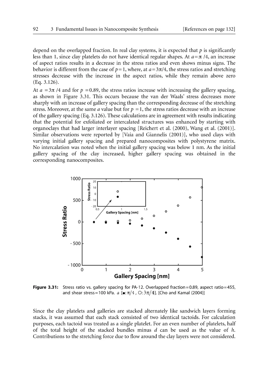
Author: Bhattacharya S.N. Kamal M.R. Gupta R.K.

Tags: polymers materials science

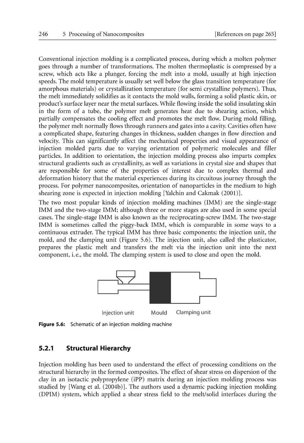
ISBN: 978-1-56990-374-2

Year: 2008

Similar

Construction Manual for Polymers + Membranes

Rediction of polymer properties

Bioenergy Research: Advances and Applications

LR Parsing. Theory and practice

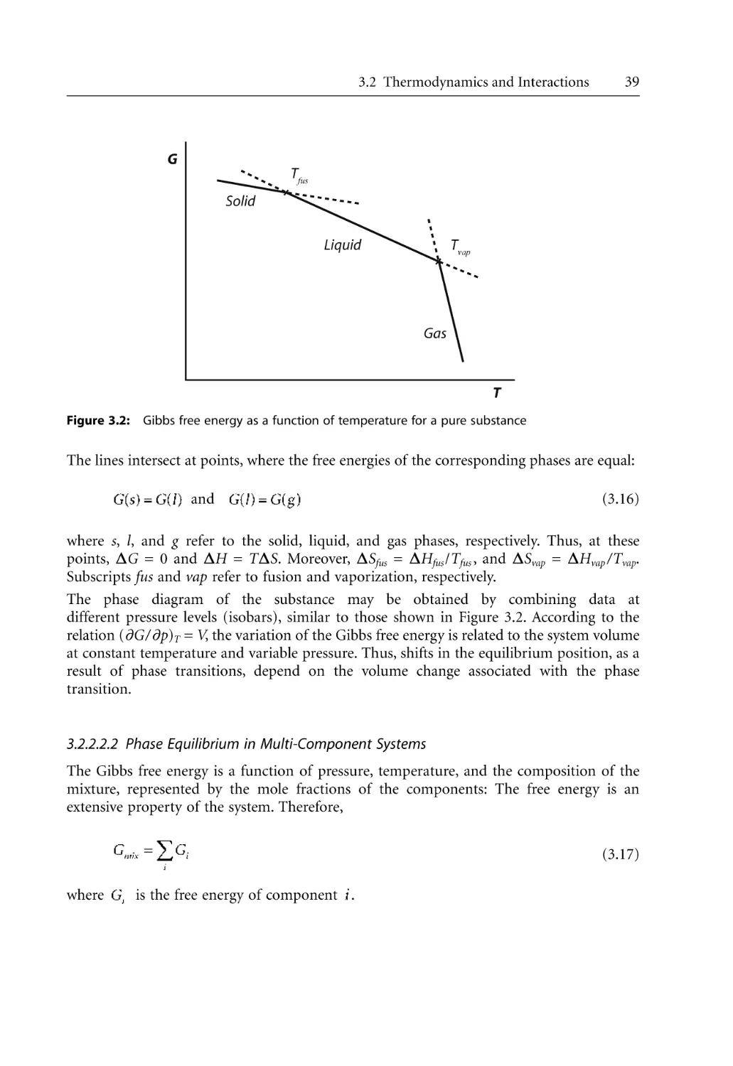
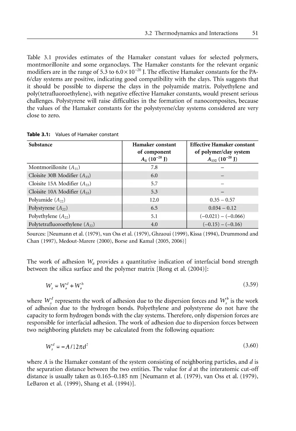
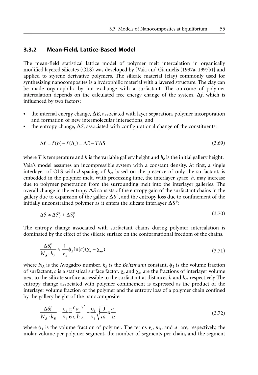
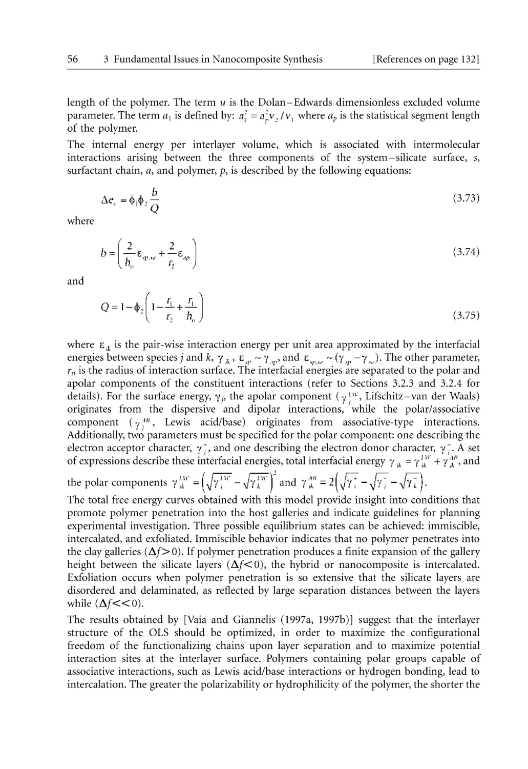
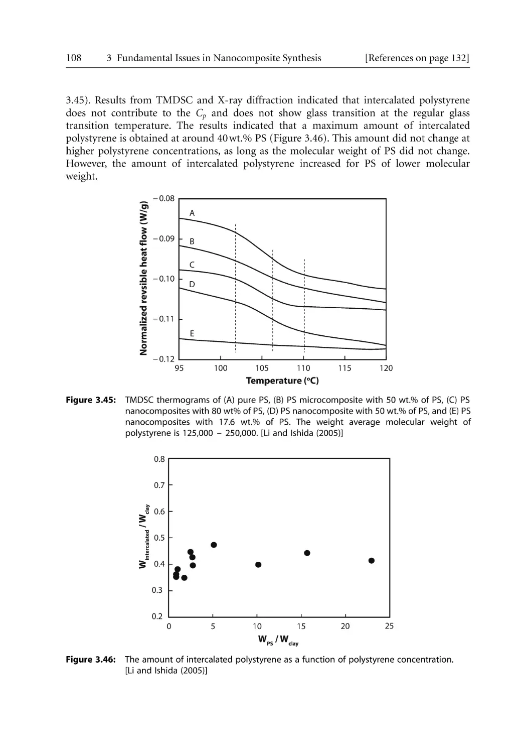
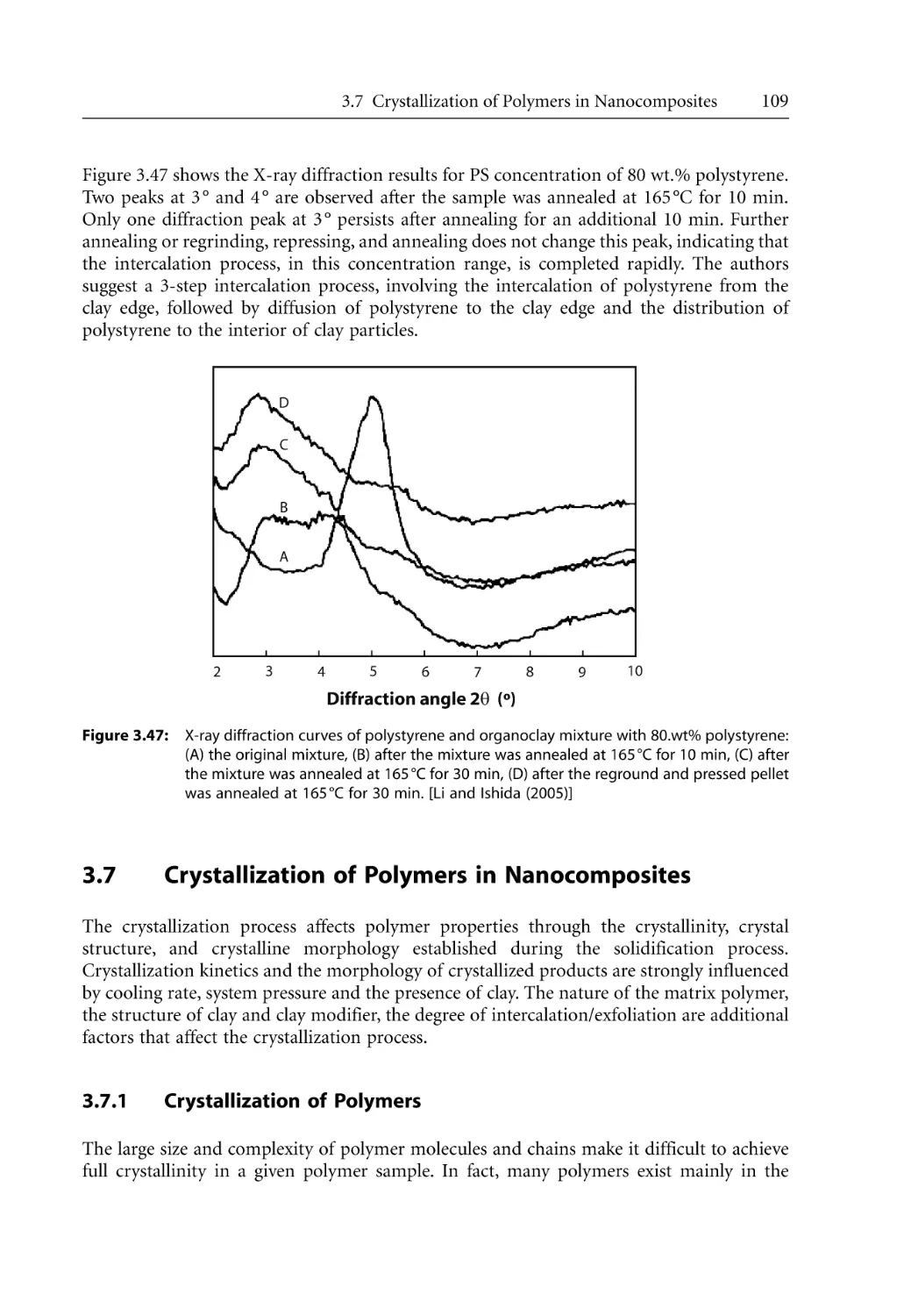
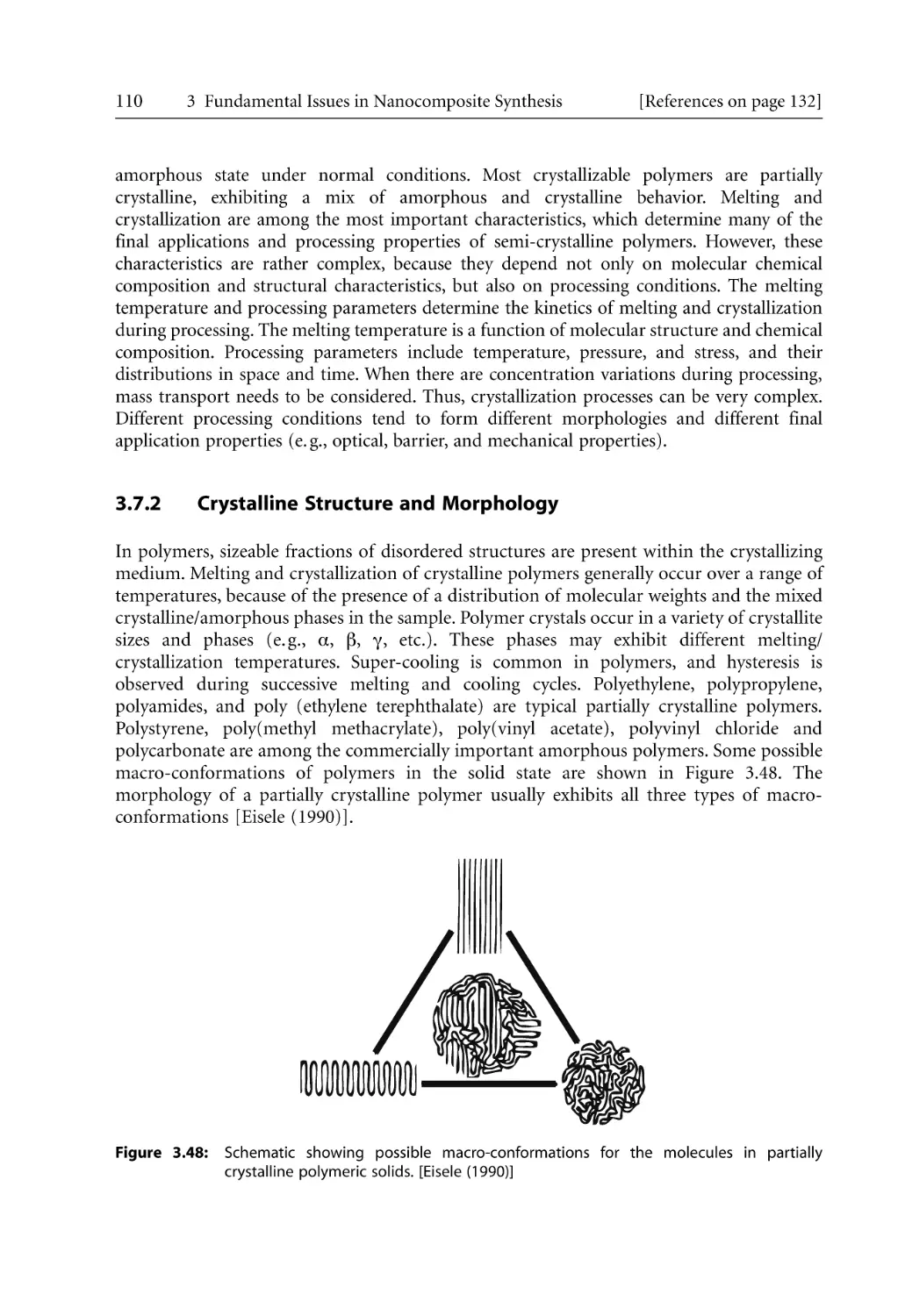
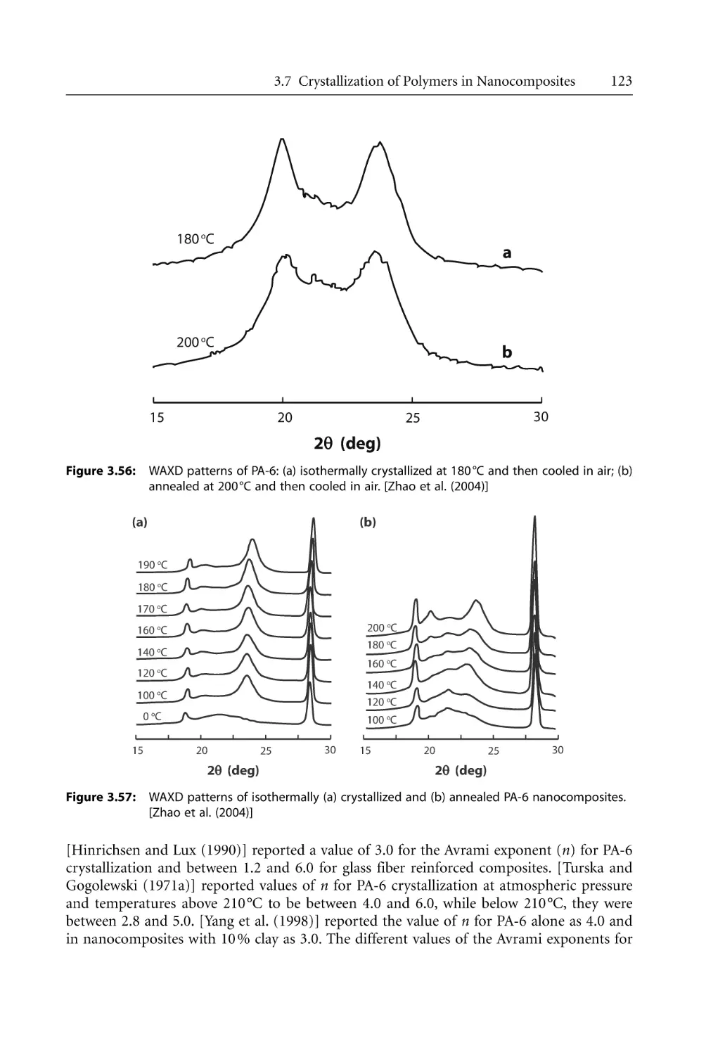
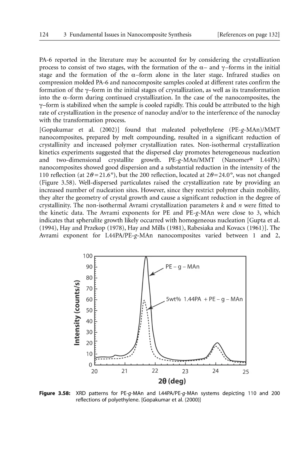
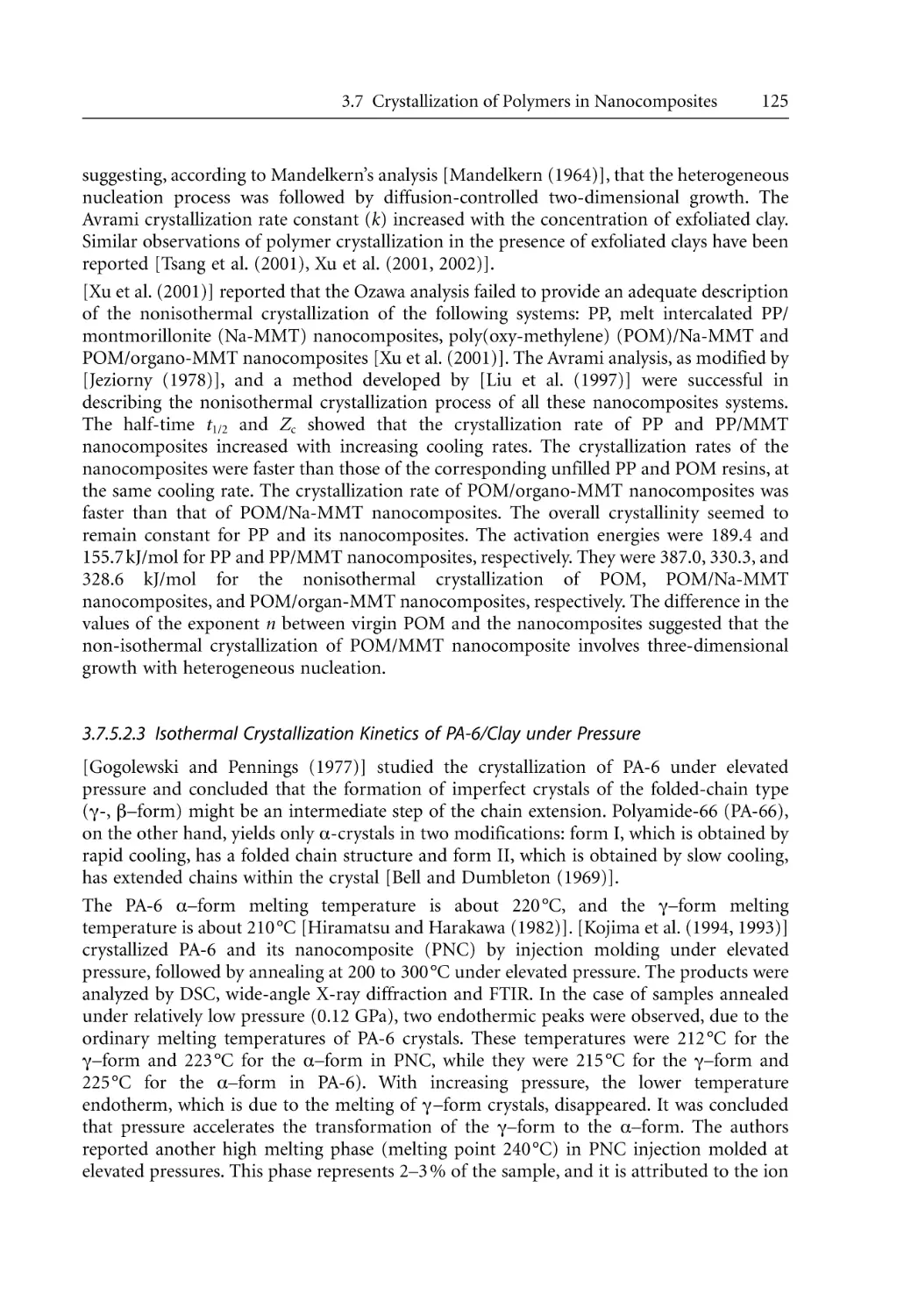
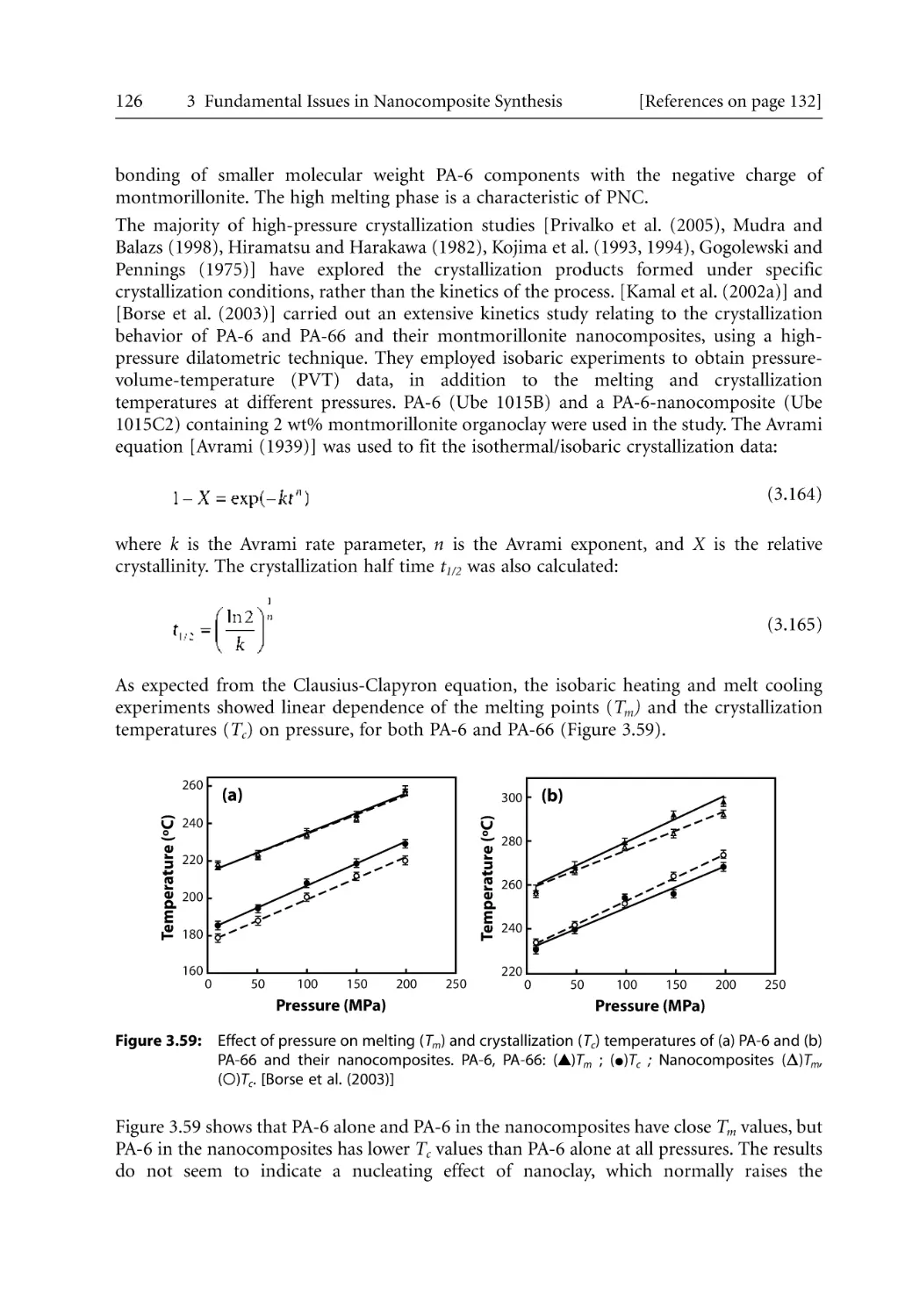
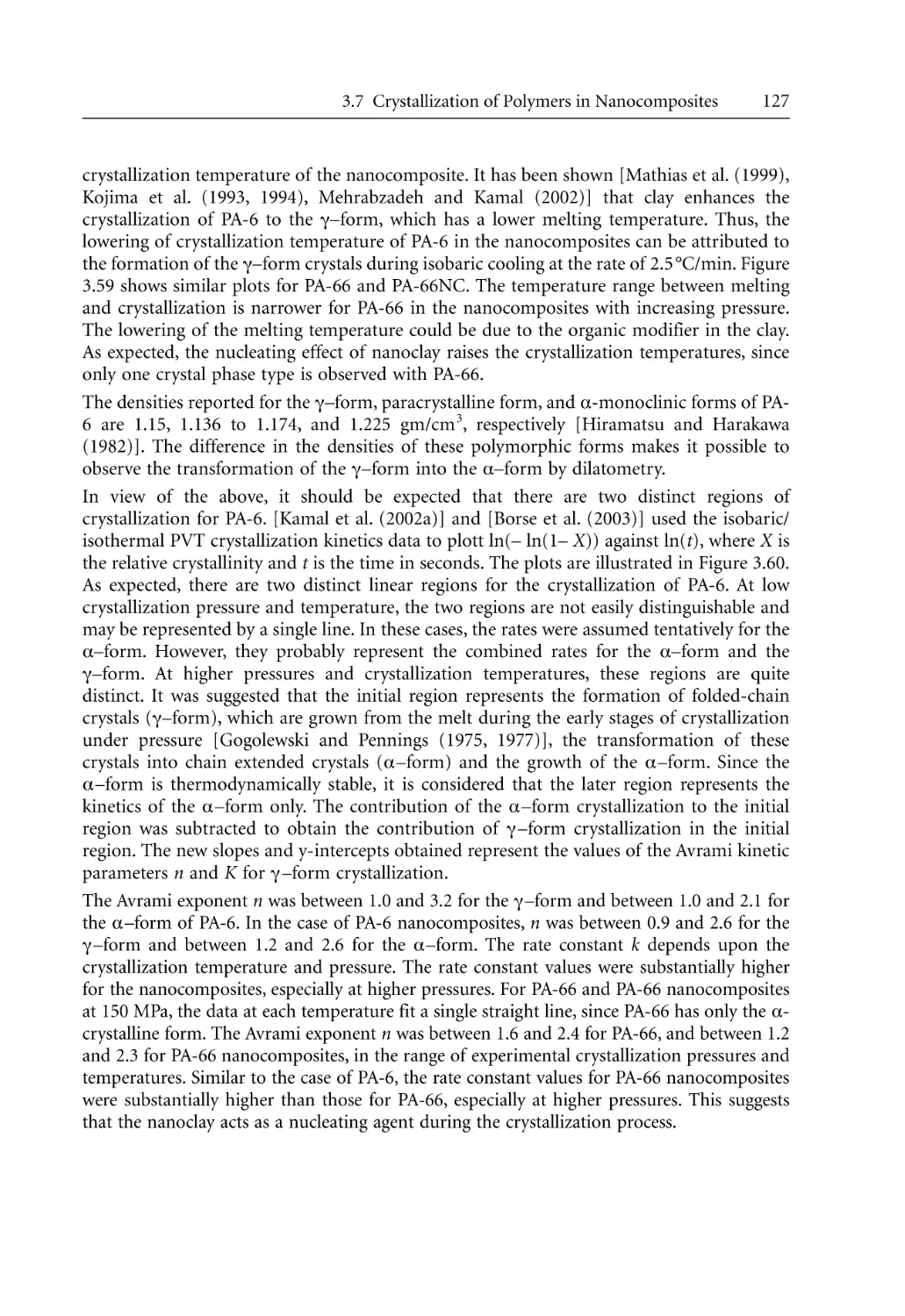
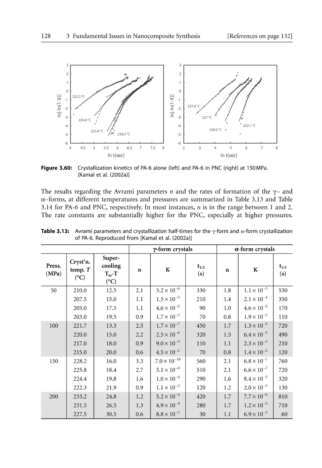
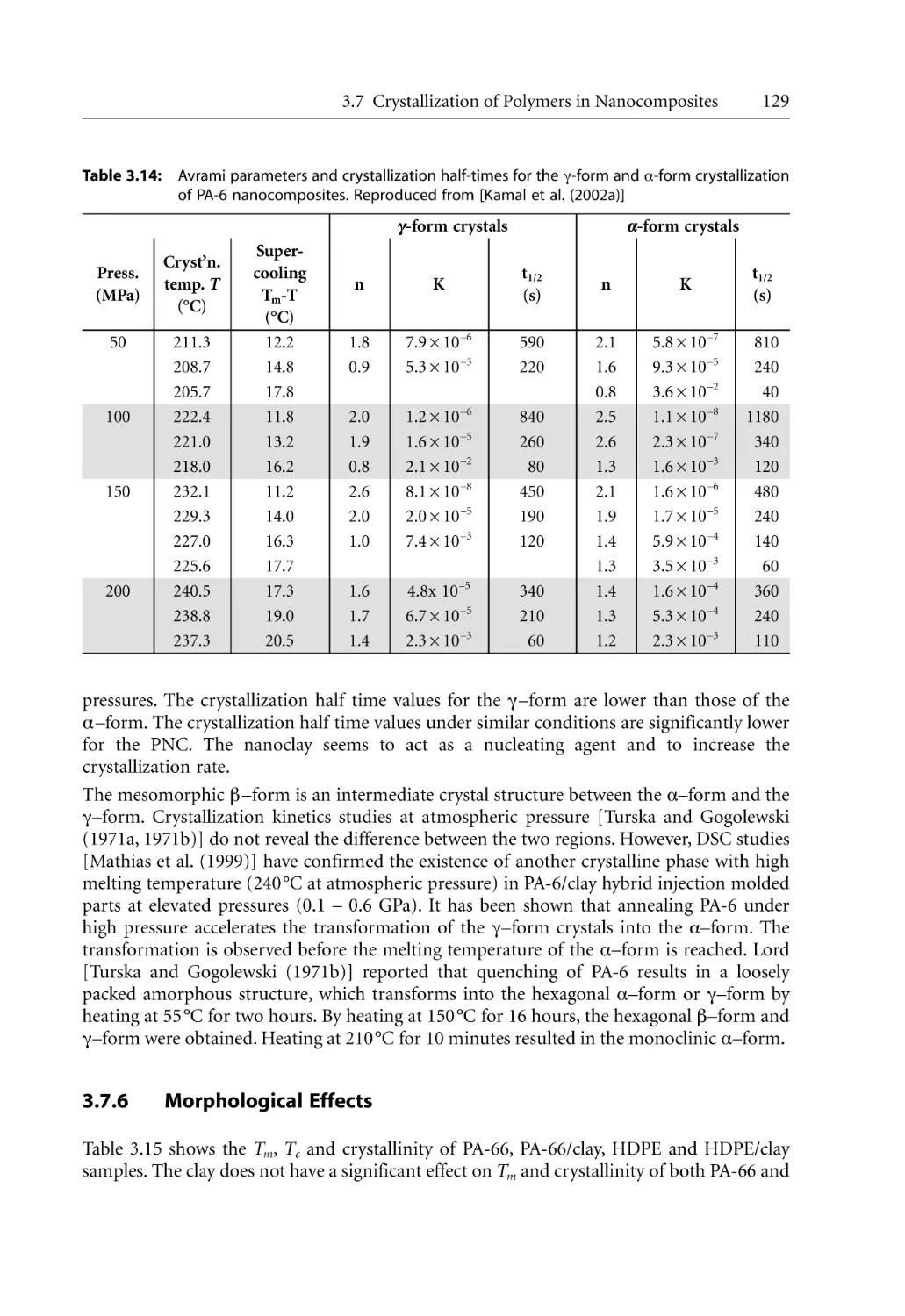
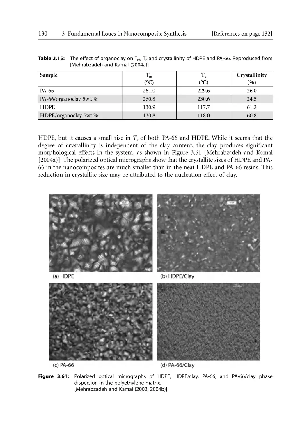
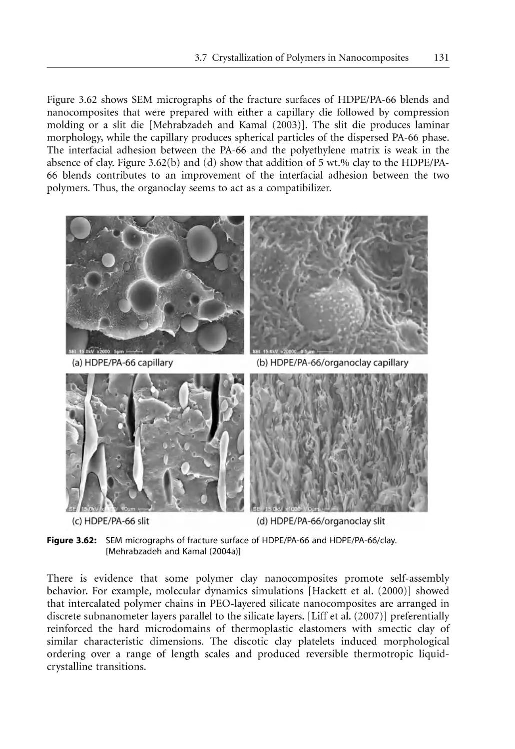
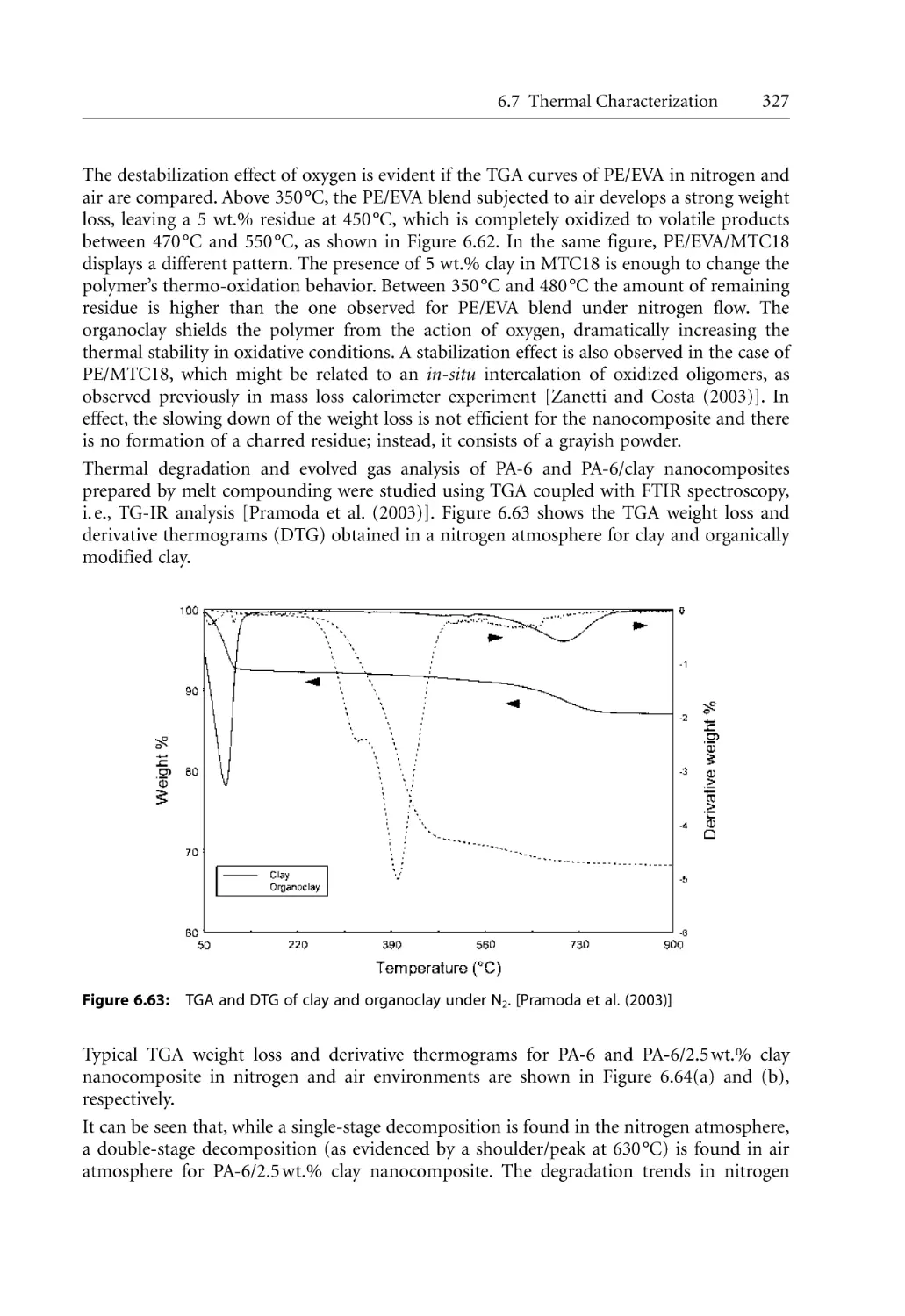
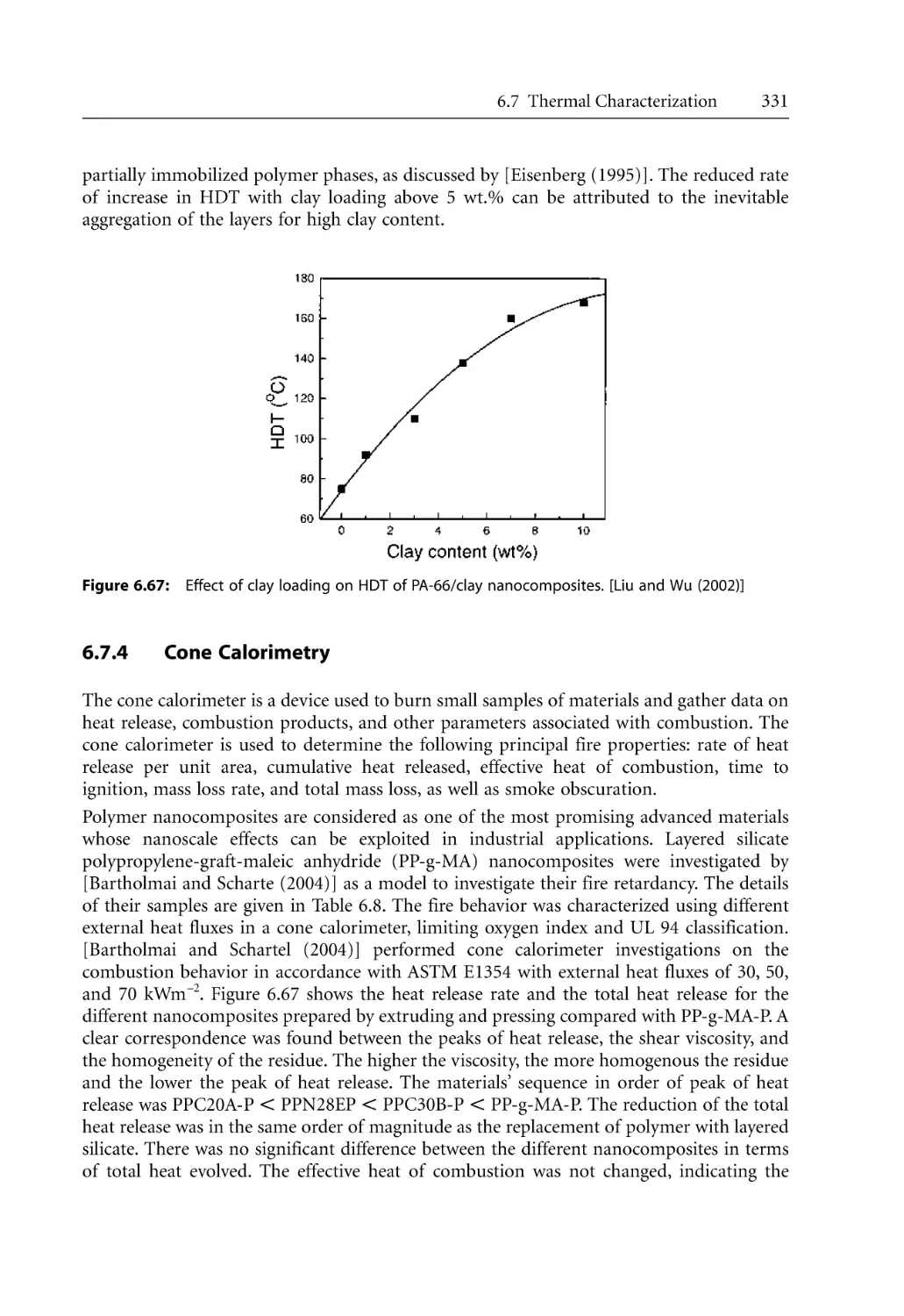
Text

Bhattacharya / Kamal / Gupta
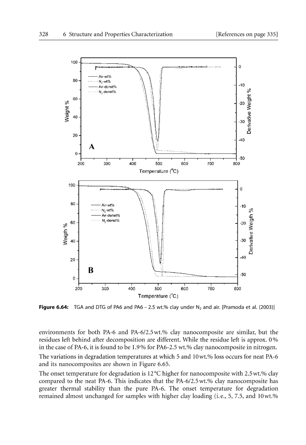
Polymeric Nanocomposites

Sati N. Bhattacharya
Musa R. Kamal
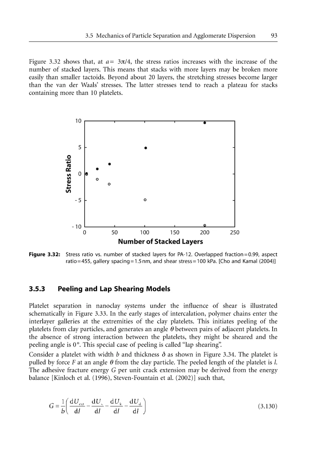
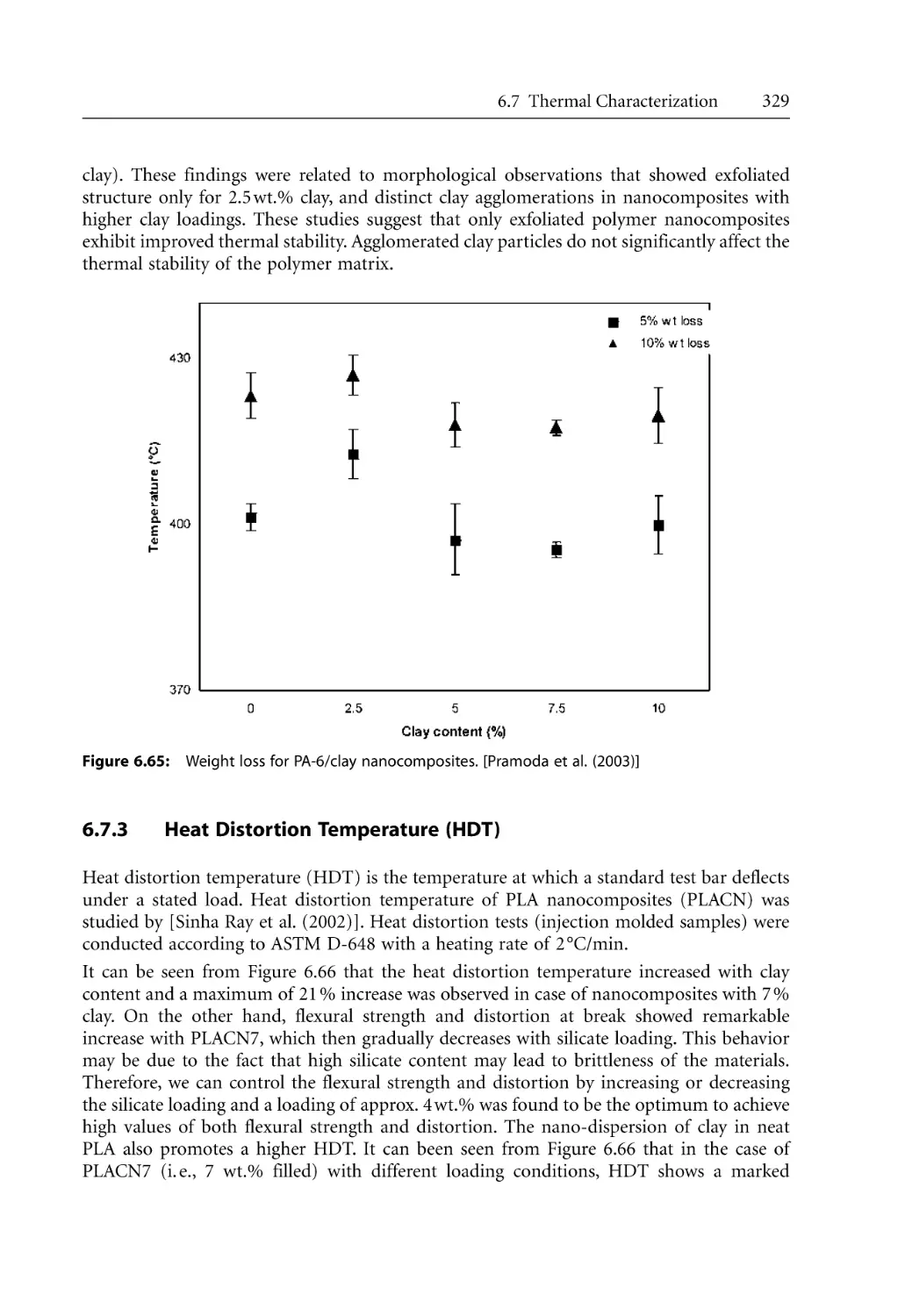
Rahul K. Gupta

Polymeric
Nanocomposites
Theory and Practice

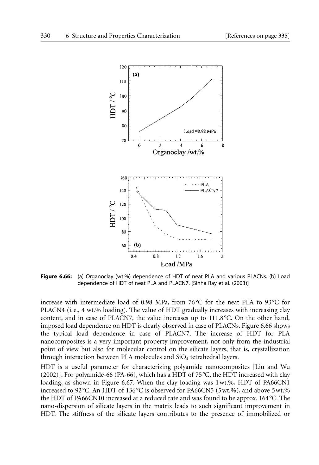
Carl Hanser Publishers, Munich • Hanser Gardner Publications, Cincinnati

The Authors:
Prof. Sati N. Bhattacharya, RMIT University, Rheology and Materials Processing Center, School of Civil, Environmental and
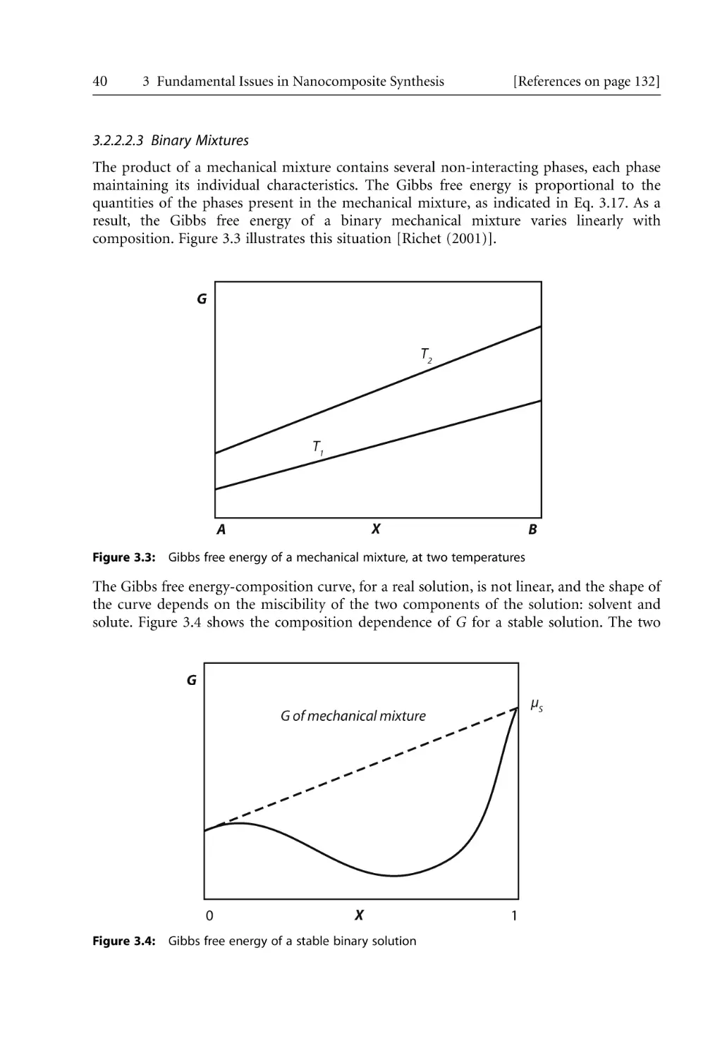
Chemical Engineering, Melbourne, VIC, Australia
Dr. Rahul K. Gupta, RMIT University, Rheology and Materials Processing Center, School of Civil, Environmental and
Chemical Engineering, Melbourne, VIC, Australia
Prof. Musa R. Kamal, McGill University, Department of Chemical Engineering, Montréal, Quebec, Canada
Distributed in the USA and in Canada by
Hanser Gardner Publications, Inc.
6915 Valley Avenue, Cincinnati, Ohio 45244-3029, USA
Fax: (513) 527-8801
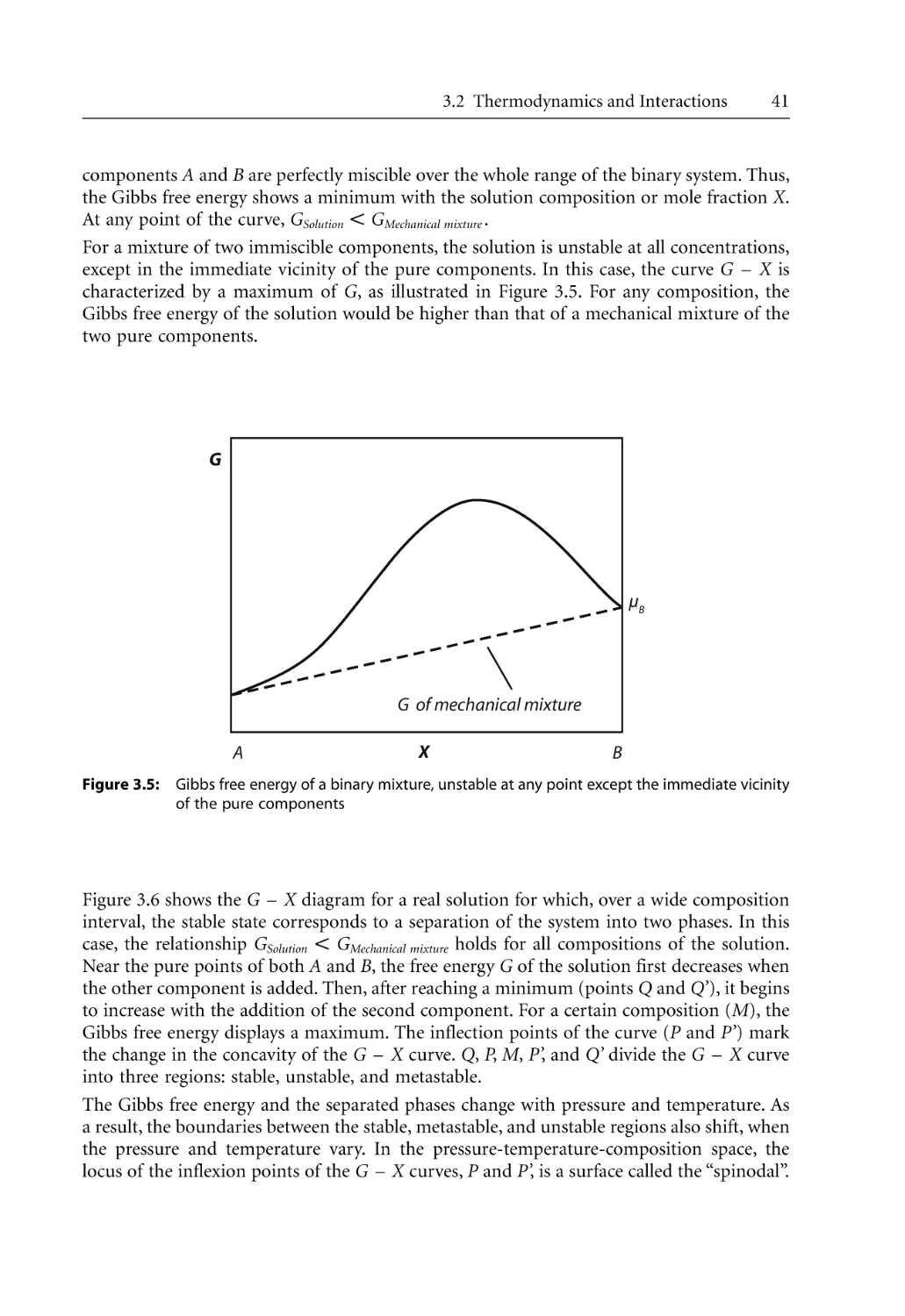
Phone: (513) 527-8977 or 1-800-950-8977
www.hansergardner.com
Distributed in all other countries by
Carl Hanser Verlag
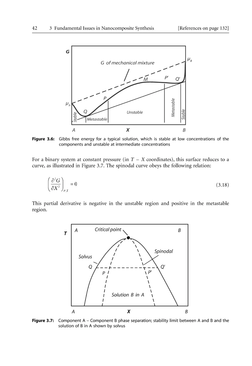
Postfach 86 04 20, 81631 München, Germany
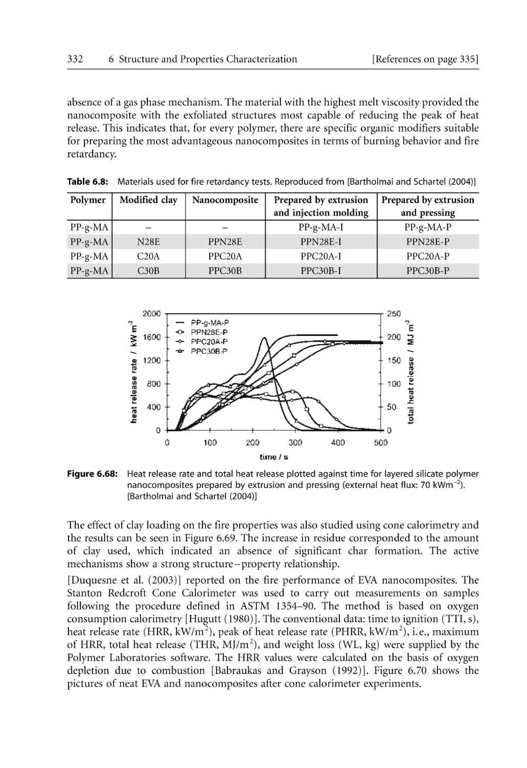
Fax: +49 (89) 98 48 09
www.hanser.de
The use of general descriptive names, trademarks, etc., in this publication, even if the former are not especially identiﬁed, is
not to be taken as a sign that such names, as understood by the Trade Marks and Merchandise Marks Act, may accordingly
be used freely by anyone.
While the advice and information in this book are believed to be true and accurate at the date of going to press, neither the
authors nor the editors nor the publisher can accept any legal responsibility for any errors or omissions that may be made.
The publisher makes no warranty, express or implied, with respect to the material contained herein.
Library of Congress Cataloging-in-Publication Data
Bhattacharya, Sati N.
Polymeric nanocomposites : theory and practice / Sati N. Bhattacharya, Musa
R. Kamal, Rahul K. Gupta.
p. cm.
Includes index.
ISBN 978-1-56990-374-2 (hardcover)
1. Nanostructured materials. 2. Polymeric composites. I. Kamal, Musa
R. (Musa Rasim), 1934- II. Gupta, Rahul K. III. Title.
TA418.9.N35B43 2007
620.1‘92--dc22
2007026090
Bibliograﬁsche Information Der Deutschen Bibliothek
Die Deutsche Bibliothek verzeichnet diese Publikation in der Deutschen Nationalbibliograﬁe;
detaillierte bibliograﬁsche Daten sind im Internet über <http://dnb.d-nb.de> abrufbar.
ISBN 978-3-446-40270-6
All rights reserved. No part of this book may be reproduced or transmitted in any form or by any means, electronic or
mechanical, including photocopying or by any information storage and retrieval system, without permission in wirting
from the publisher.

© Carl Hanser Verlag, Munich 2008
Production Management: Steffen Jörg
Typeset by Mitterweger & Partner, Plankstadt, Germany
Coverconcept: Marc Müller-Bremer, Rebranding, München, Germany
Coverdesign: MCP • Susanne Kraus GbR, Holzkirchen, Germany
Printed and bound by Druckhaus »Thomas Müntzer« GmbH, Bad Langensalza, Germany

Preface

Nanostructured multi-phase polymers have generated great interest with promise to
produce a new generation of materials displaying enhanced physical, mechanical, thermal,
electrical, magnetic, and optical properties. The key to the success of nanocomposites hinges
on the ability to exploit the potential of nano-structuring in the final product. Therefore, it
is important to develop practical and economical formulations and processing methods for
tailoring a sustainable material configuration at the nanoscale level. Recently, much progress
has been made in meeting this challenge and in developing a wide range of commercial
processes, products, and devices as a result of the research efforts and advances by many
scientists, engineers, and technologists. While a large number of scientific papers and some
books on polymer nanocomposites have been published, there is a clear need to bring
together the scientific knowledge and the engineering developments relating to these
materials in terms of synthesis, characterisation, production, and application. This book
deals with clay-based polymer nanocomposites, which have been the subject of extensive
research in the last decade. Besides its low cost, clay has a plate-like geometry, which could
impart excellent product properties under optimum nanostructuring conditions.
The book provides an overview of the compositionprocessingproductapplication relationships
in the field of polymer nanocomposites. It deals with the fundamental principles that govern
the synthesis and behavior of polymer/clay nanocomposites, such as thermodynamics,
kinetics, rheology, and morphology. Other chapters cover practical aspects, such as processing,
performance, and some commercial applications of polymer/clay nanocomposites in selected
industries, such as packaging, automotive, electronic, and telecommunications. It is hoped
that the book will serve as a reference and guide for those who work in various aspects of
the nanocomposite industry and technology or wish to learn about these promising new
materials.
The preparation of this book has been possible due to the active support and help received
from many colleagues, research staff and graduate students. The authors would like to
express their sincere thanks to all these individuals for the direct and indirect efforts and
contributions to the preparation of this book: Dr. S. Raha, Mr. M. Reddy, Mr. M. Pannirselvam
and Mr. S. Bhattacharya, Dr F Cser, Dr R Prasad, Dr. M. Al-Wohoush, Dr. L. Ionescu Vasii,
Dr. N. Borse, Dr. K. Kim, Dr. L. Feng, Mr. J. Uribe-Calderon, Ms. O. Tavichai, Mr. C. Lungu,
and Mr. N. Nassar. We also wish to express our appreciation to our respective universities,
RMIT and McGill, and the various granting agencies in Australia and Canada for material
and moral support that made it possible to produce this book.
Sati N. Bhattacharya
Rahul K. Gupta
Musa R. Kamal

Table of Content

1 Introduction . . . . . . . . . . . . . . . . . . . . . . . . . . . . . . . . . . . . . . . . . . . . . . . . . . . . . . . . . .
1.1 Polymer Nanocomposites . . . . . . . . . . . . . . . . . . . . . . . . . . . . . . . . . . . . . . . . . . .
1.2 Commercial Potential. . . . . . . . . . . . . . . . . . . . . . . . . . . . . . . . . . . . . . . . . . . . . . .
1.3 Book Structure . . . . . . . . . . . . . . . . . . . . . . . . . . . . . . . . . . . . . . . . . . . . . . . . . . . .
1.4 References . . . . . . . . . . . . . . . . . . . . . . . . . . . . . . . . . . . . . . . . . . . . . . . . . . . . . . . .

1
1
2
3
4

2 Preparation and Synthesis. . . . . . . . . . . . . . . . . . . . . . . . . . . . . . . . . . . . . . . . . . . . . . .
2.1 Polymer Nanocomposites . . . . . . . . . . . . . . . . . . . . . . . . . . . . . . . . . . . . . . . . . . .
2.1.1 Morphology of Polymer-Layered Silicate Nanocomposites . . . . . . . . . .
2.1.2 Structure of Layered Silicates . . . . . . . . . . . . . . . . . . . . . . . . . . . . . . . . . .
2.1.3 Organically Modified Clay. . . . . . . . . . . . . . . . . . . . . . . . . . . . . . . . . . . . .
2.1.4 Formation of Polymer Nanocomposites . . . . . . . . . . . . . . . . . . . . . . . . .
2.1.5 Effect of Cation Exchange Capacity on Organoclay . . . . . . . . . . . . . . . .
2.1.6 Effect of Organic Cation Structure on Organoclay. . . . . . . . . . . . . . . . .
2.2 Nanocomposites Preparation and Synthesis . . . . . . . . . . . . . . . . . . . . . . . . . . . .
2.2.1 Solution Dispersion . . . . . . . . . . . . . . . . . . . . . . . . . . . . . . . . . . . . . . . . . .
2.2.2 In-Situ Polymerization . . . . . . . . . . . . . . . . . . . . . . . . . . . . . . . . . . . . . . . .
2.2.3 Melt Intercalation . . . . . . . . . . . . . . . . . . . . . . . . . . . . . . . . . . . . . . . . . . . .
2.2.4 Effect of Mixing . . . . . . . . . . . . . . . . . . . . . . . . . . . . . . . . . . . . . . . . . . . . .
2.3 Polymer Matrices: Thermoplastics, Thermosets, Elastomers, Natural, and
Biodegradable Polymers. . . . . . . . . . . . . . . . . . . . . . . . . . . . . . . . . . . . . . . . . . . . .
2.3.1 Thermoplastics . . . . . . . . . . . . . . . . . . . . . . . . . . . . . . . . . . . . . . . . . . . . . .
2.3.1.1 Polyethylene . . . . . . . . . . . . . . . . . . . . . . . . . . . . . . . . . . . . . . . . .
2.3.1.2 Polypropylene . . . . . . . . . . . . . . . . . . . . . . . . . . . . . . . . . . . . . . .
2.3.1.3 Ethylene-Vinyl Acetate (EVA) Copolymers. . . . . . . . . . . . . . . .
2.3.1.4 Polyamides . . . . . . . . . . . . . . . . . . . . . . . . . . . . . . . . . . . . . . . . . .
2.3.1.5 Poly(Ethylene Terephtalate) (PET) . . . . . . . . . . . . . . . . . . . . . .
2.3.1.6 Polystyrene. . . . . . . . . . . . . . . . . . . . . . . . . . . . . . . . . . . . . . . . . .
2.3.2 Elastomers . . . . . . . . . . . . . . . . . . . . . . . . . . . . . . . . . . . . . . . . . . . . . . . . . .
2.3.3 Thermosets . . . . . . . . . . . . . . . . . . . . . . . . . . . . . . . . . . . . . . . . . . . . . . . . .
2.3.3.1 Epoxy Nanocomposites. . . . . . . . . . . . . . . . . . . . . . . . . . . . . . . .
2.3.3.2 Polyurethane . . . . . . . . . . . . . . . . . . . . . . . . . . . . . . . . . . . . . . . .
2.3.4 Natural and Biodegradable Polymers . . . . . . . . . . . . . . . . . . . . . . . . . . . .

5
5
6
7
9
10
11
12
12
13
15
16
20

3 Fundamental Issues in Nanocomposite Synthesis . . . . . . . . . . . . . . . . . . . . . . . . . . .
3.1 Introduction . . . . . . . . . . . . . . . . . . . . . . . . . . . . . . . . . . . . . . . . . . . . . . . . . . . . . .
3.2 Thermodynamics and Interactions . . . . . . . . . . . . . . . . . . . . . . . . . . . . . . . . . . . .
3.2.1 General Thermodynamic Relationships . . . . . . . . . . . . . . . . . . . . . . . . . .

35
35
36
36

22
23
23
23
24
25
25
26
27
28
28
28
29

Inhalt

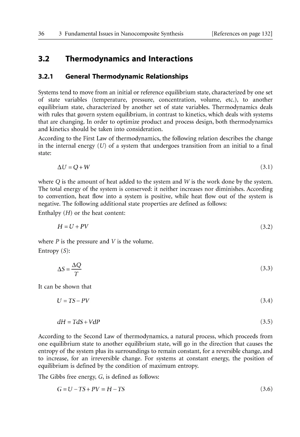
3.3

3.4

3.5

3.6

3.7

3.8

3.2.2 Multi-Component Systems . . . . . . . . . . . . . . . . . . . . . . . . . . . . . . . . . . . .
3.2.2.1 Chemical Potential . . . . . . . . . . . . . . . . . . . . . . . . . . . . . . . . . . .
3.2.2.2 Phase Equilibria and Phase Diagrams. . . . . . . . . . . . . . . . . . . .
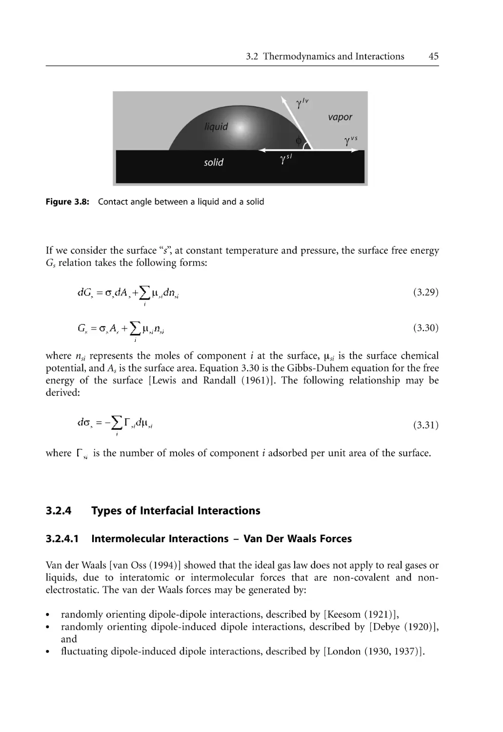
3.2.3 Surface Free Energy . . . . . . . . . . . . . . . . . . . . . . . . . . . . . . . . . . . . . . . . . .
3.2.4 Types of Interfacial Interactions . . . . . . . . . . . . . . . . . . . . . . . . . . . . . . . .
3.2.4.1 Intermolecular Interactions Van Der Waals Forces . . . . . . . . .
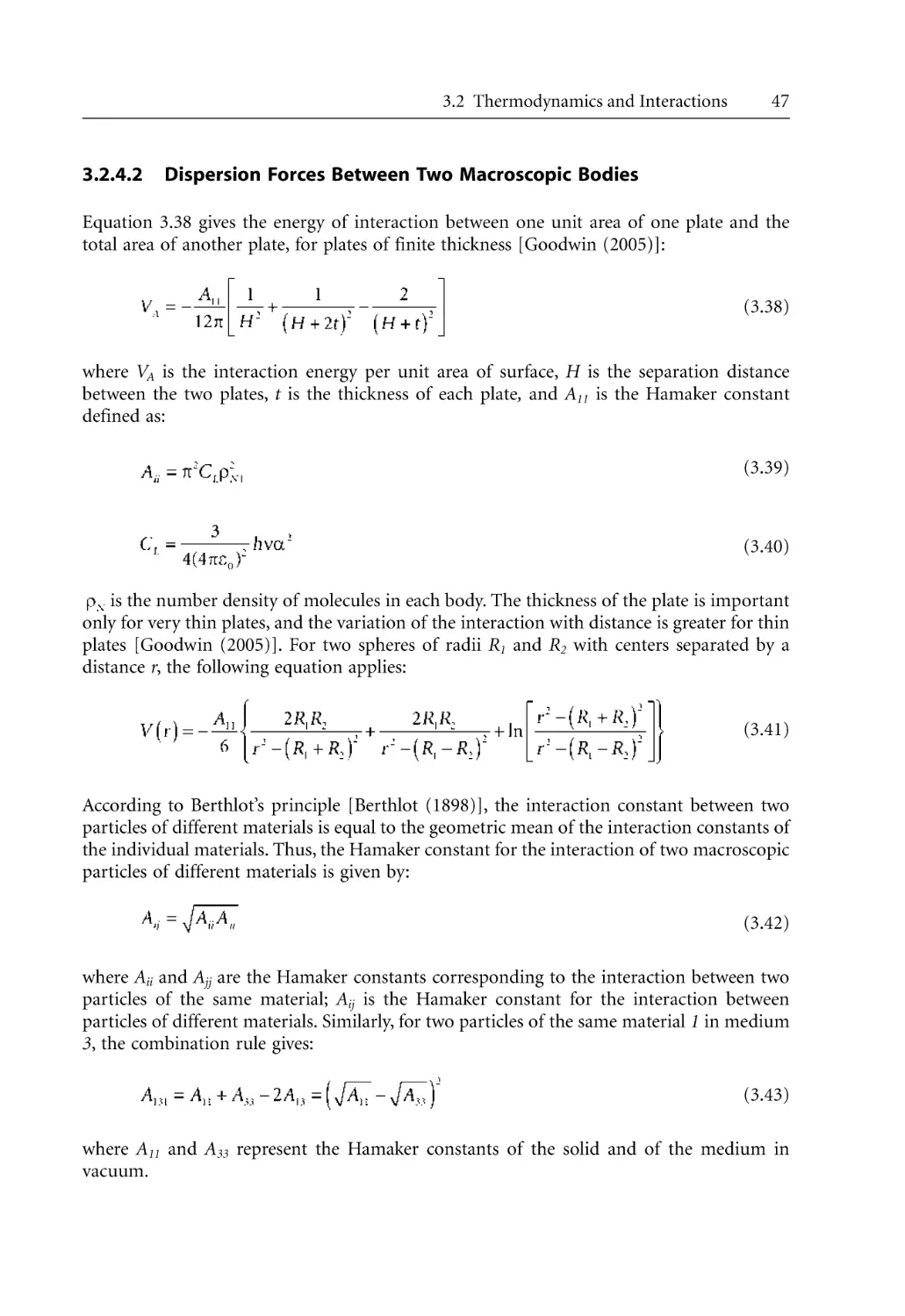
3.2.4.2 Dispersion Forces Between Two Macroscopic Bodies . . . . . . .
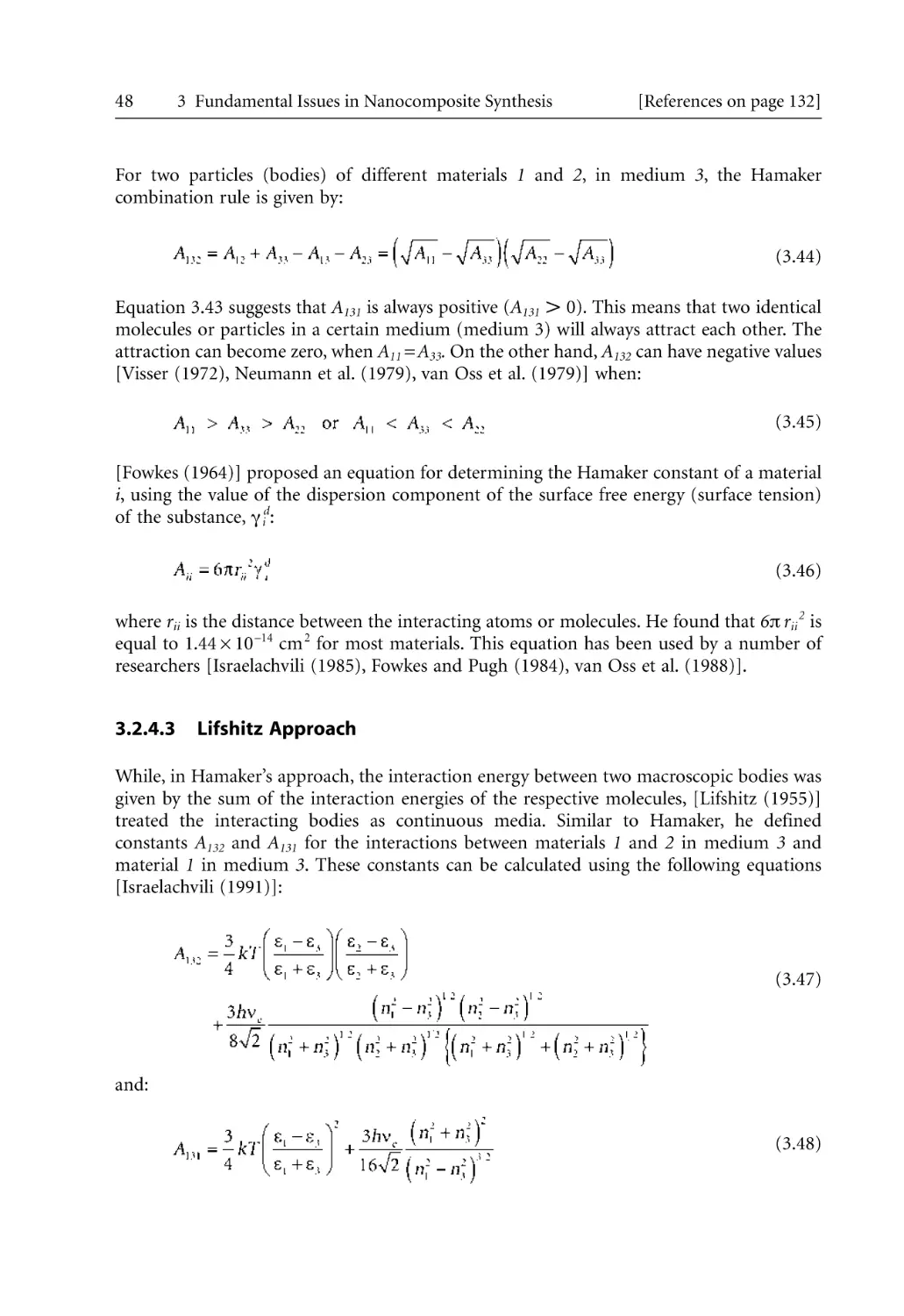
3.2.4.3 Lifshitz Approach . . . . . . . . . . . . . . . . . . . . . . . . . . . . . . . . . . . .
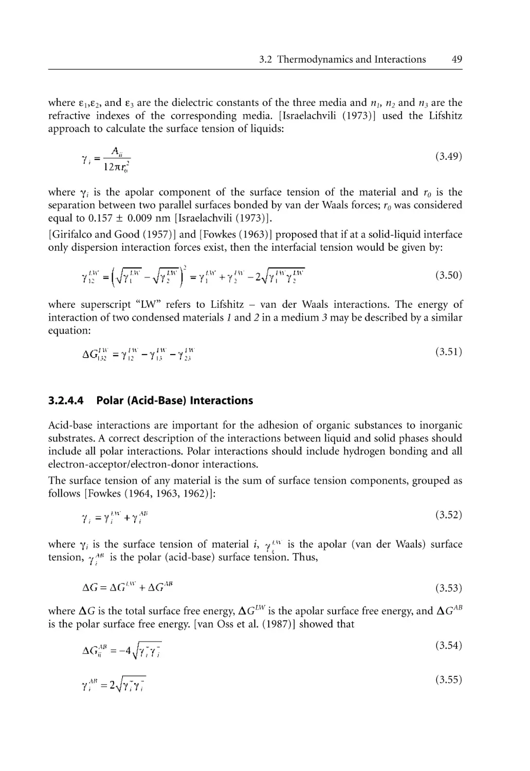
3.2.4.4 Polar (Acid-Base) Interactions . . . . . . . . . . . . . . . . . . . . . . . . . .
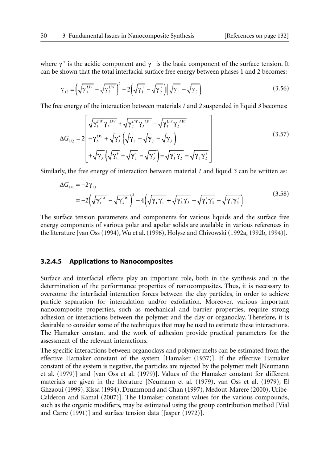
3.2.4.5 Applications to Nanocomposites . . . . . . . . . . . . . . . . . . . . . . . .
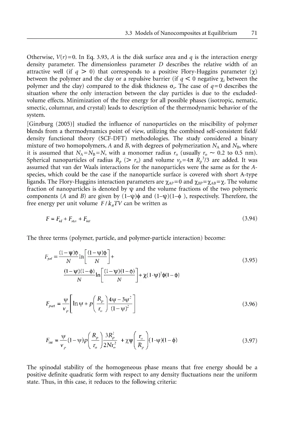
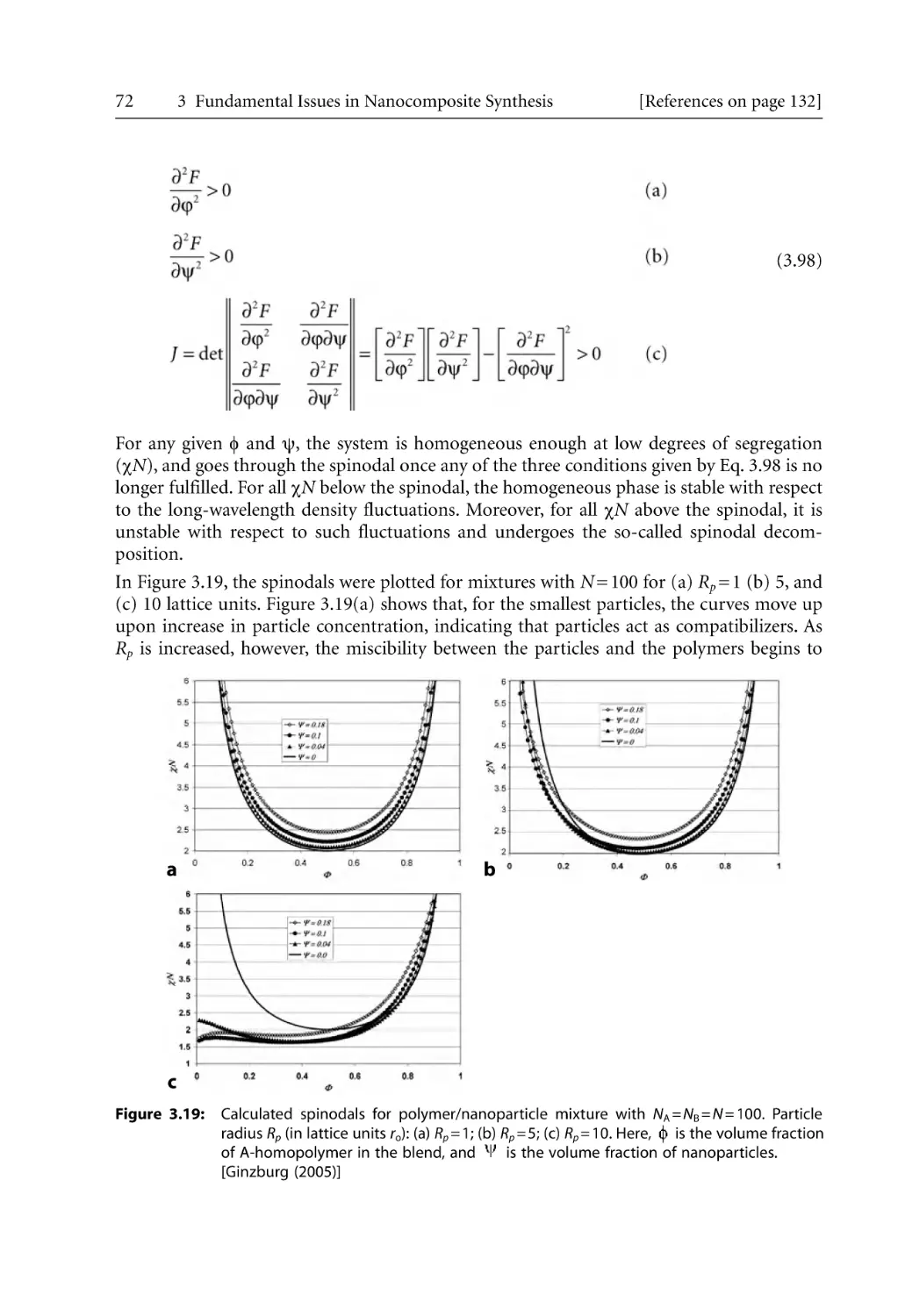
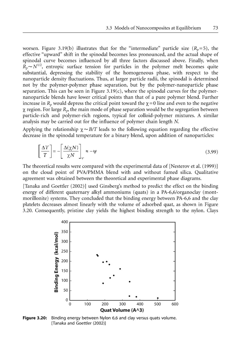
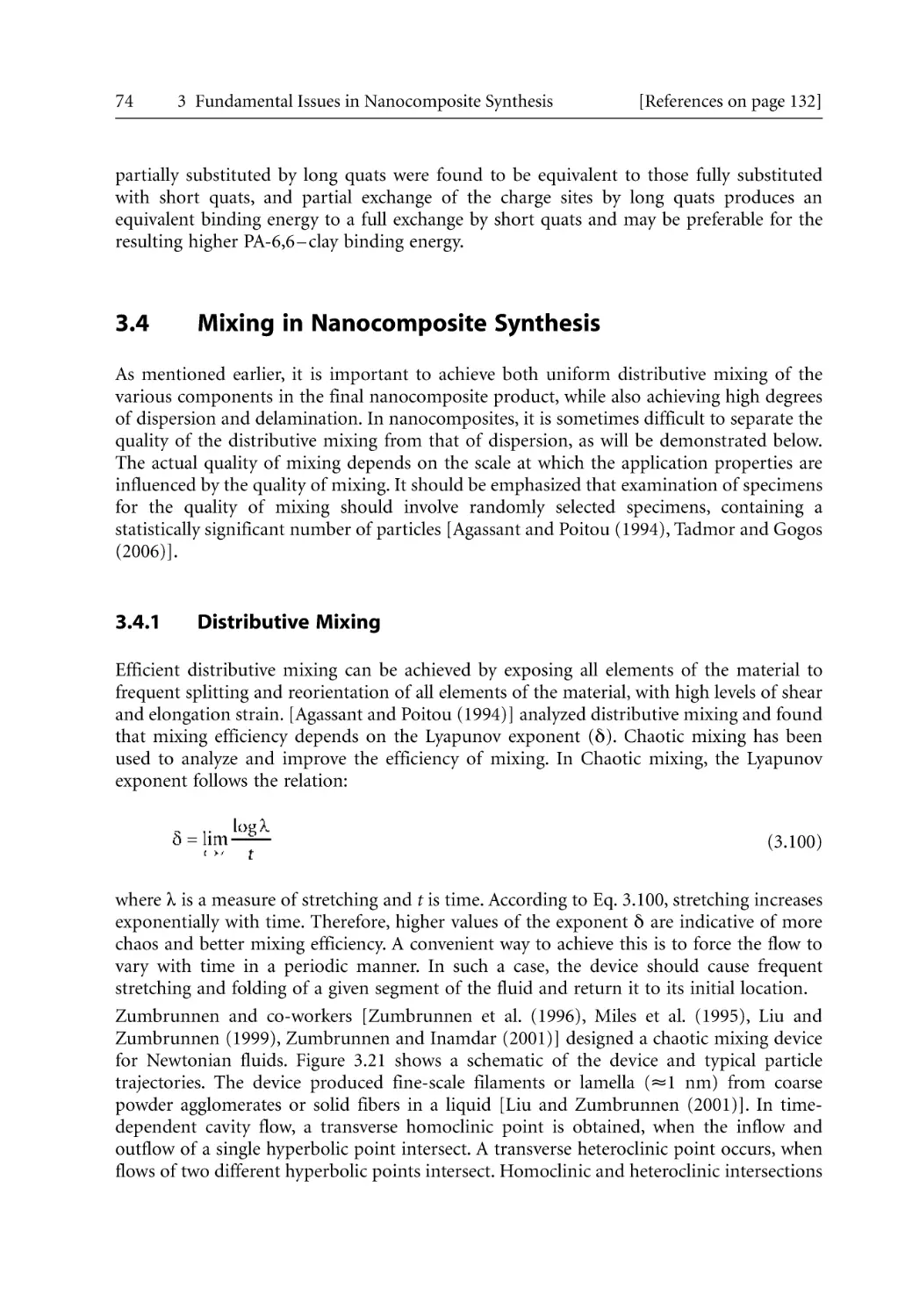
Models of Nanocomposites at Equilibrium . . . . . . . . . . . . . . . . . . . . . . . . . . . . .
3.3.1 Introduction . . . . . . . . . . . . . . . . . . . . . . . . . . . . . . . . . . . . . . . . . . . . . . . .
3.3.2 Mean-Field, Lattice-Based Model . . . . . . . . . . . . . . . . . . . . . . . . . . . . . . .
3.3.3 Self-Consistent Field Approach (SFC) . . . . . . . . . . . . . . . . . . . . . . . . . . .
3.3.4 Density Functional Theory (DFT) . . . . . . . . . . . . . . . . . . . . . . . . . . . . . .
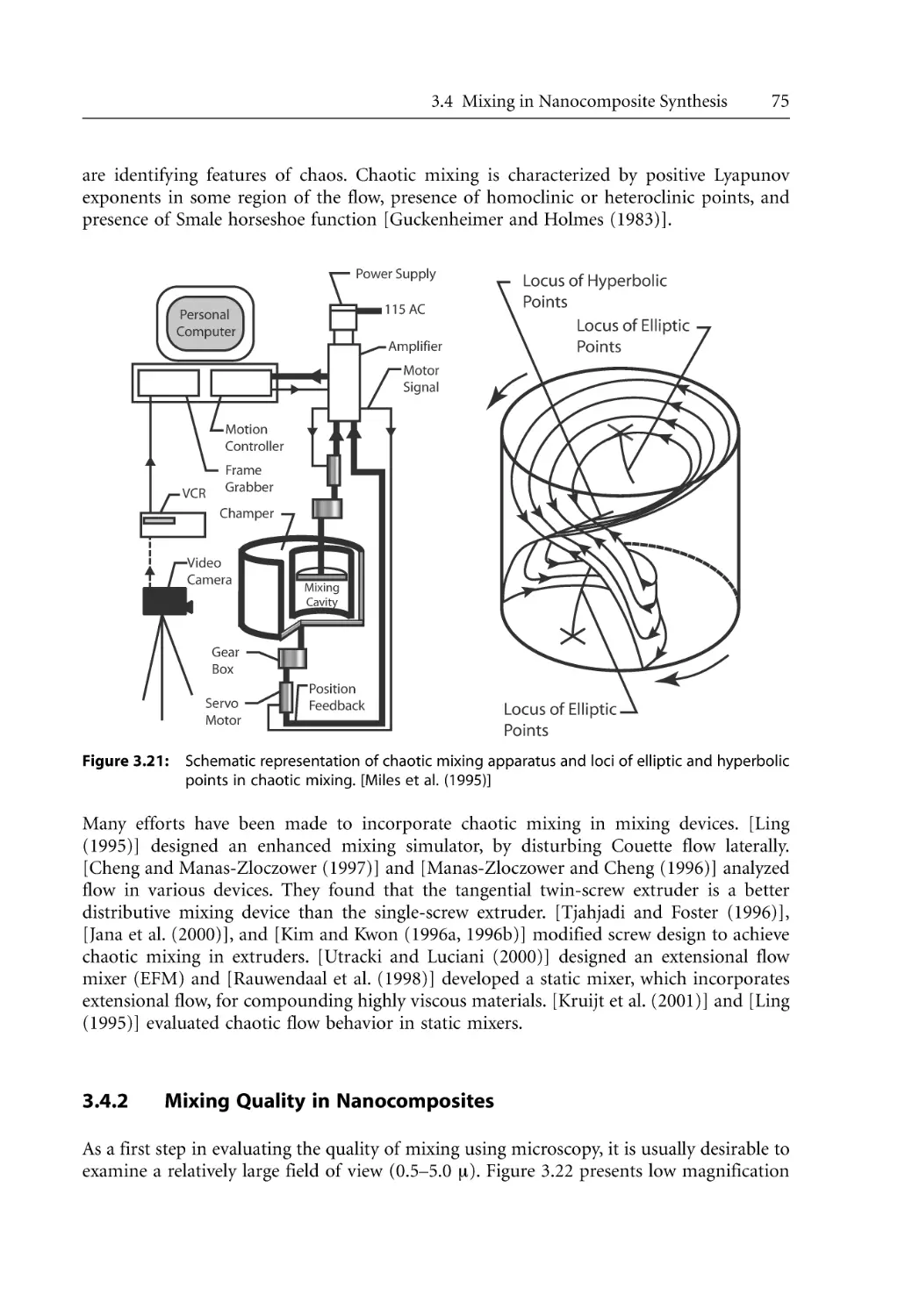
Mixing in Nanocomposite Synthesis . . . . . . . . . . . . . . . . . . . . . . . . . . . . . . . . . .
3.4.1 Distributive Mixing . . . . . . . . . . . . . . . . . . . . . . . . . . . . . . . . . . . . . . . . . .
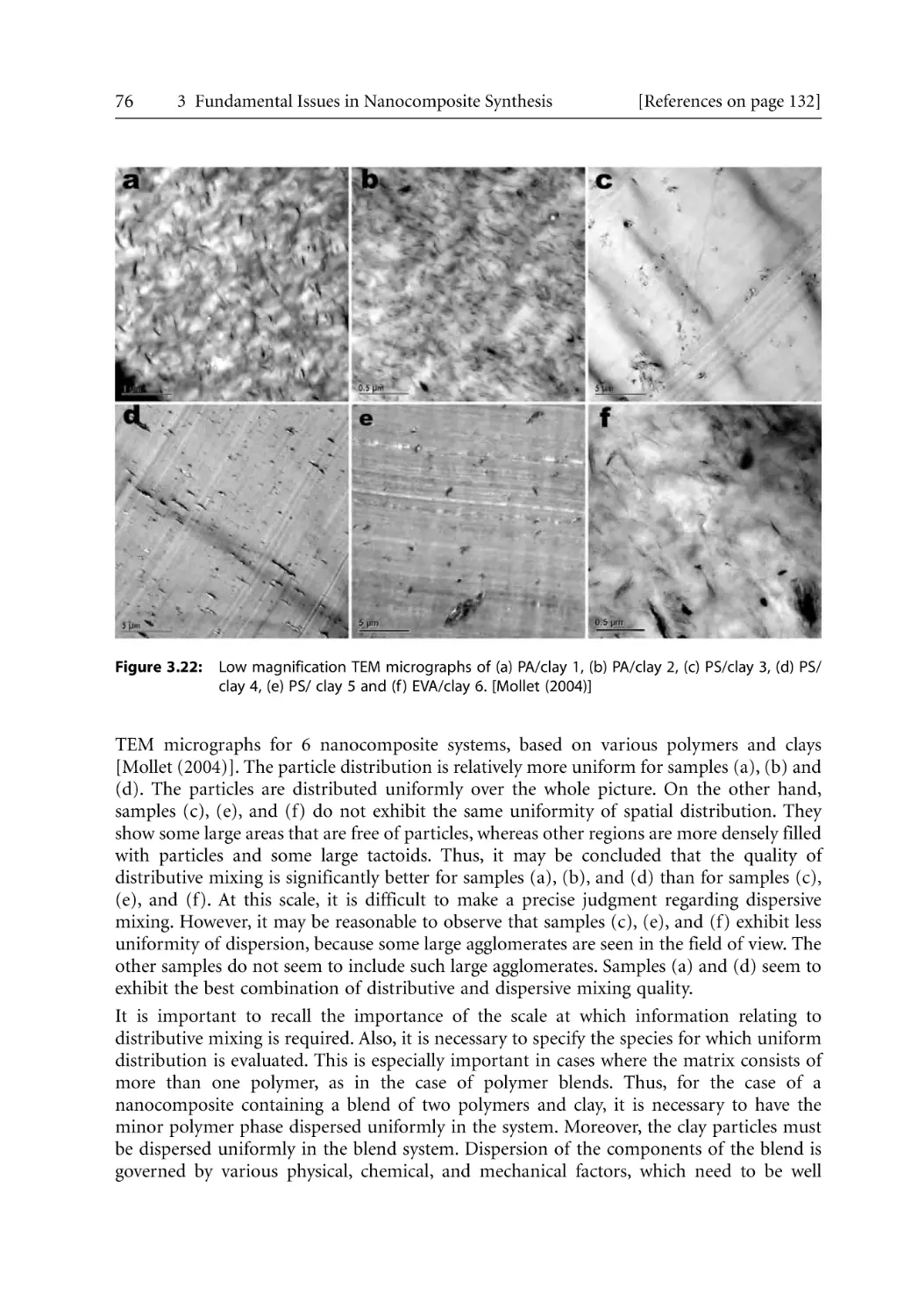
3.4.2 Mixing Quality in Nanocomposites . . . . . . . . . . . . . . . . . . . . . . . . . . . . .
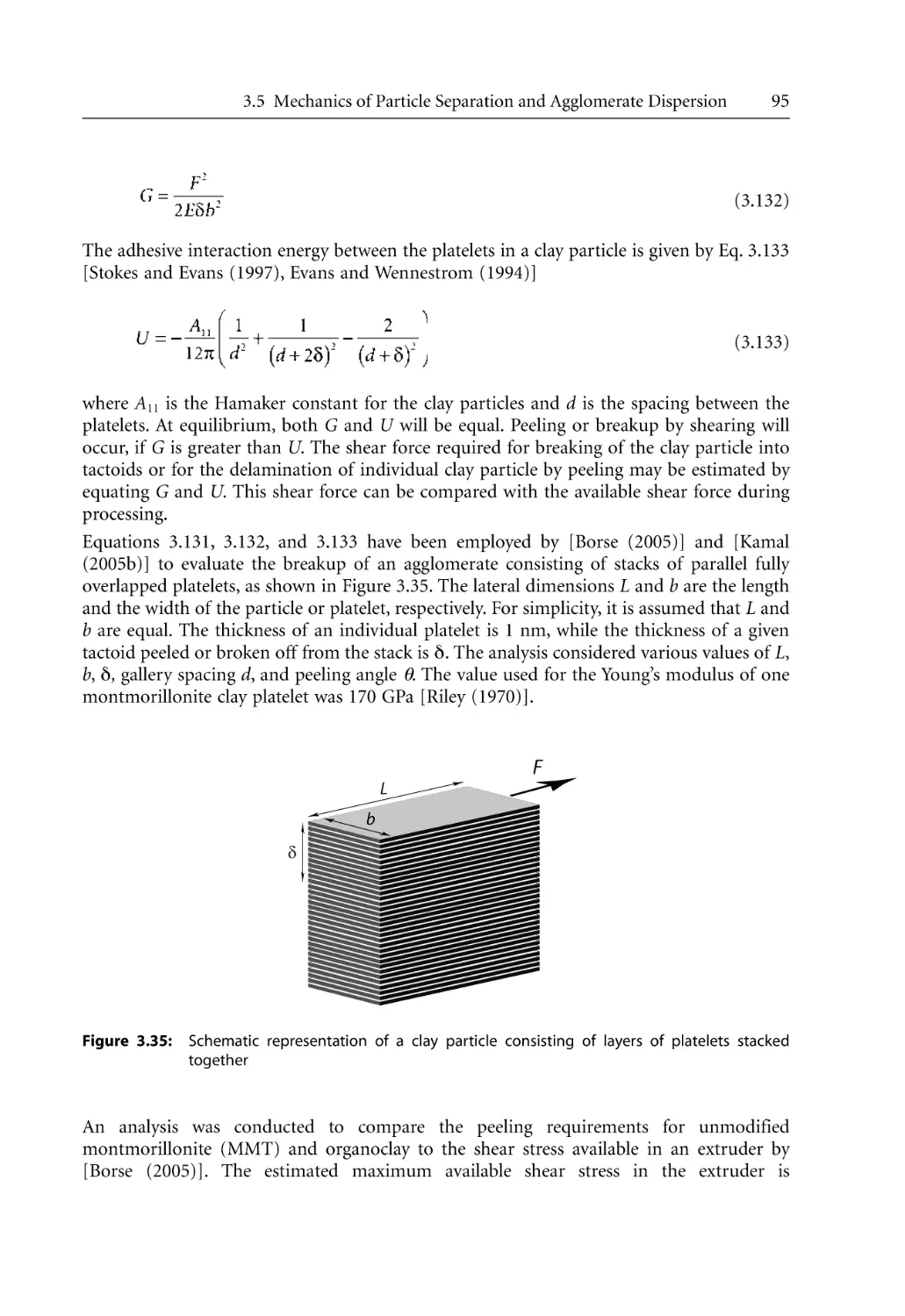
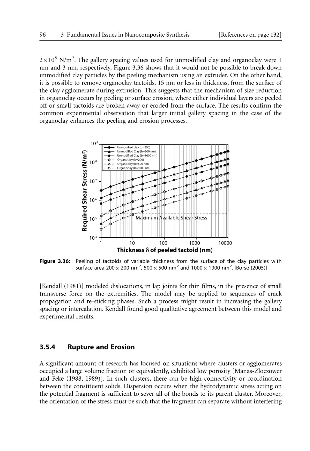
Mechanics of Particle Separation and Agglomerate Dispersion. . . . . . . . . . . . .
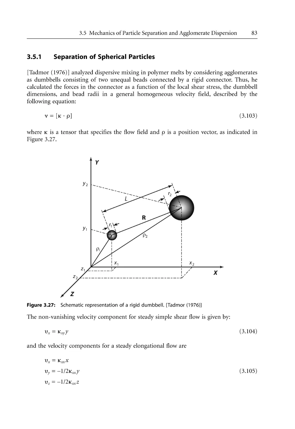
3.5.1 Separation of Spherical Particles. . . . . . . . . . . . . . . . . . . . . . . . . . . . . . . .
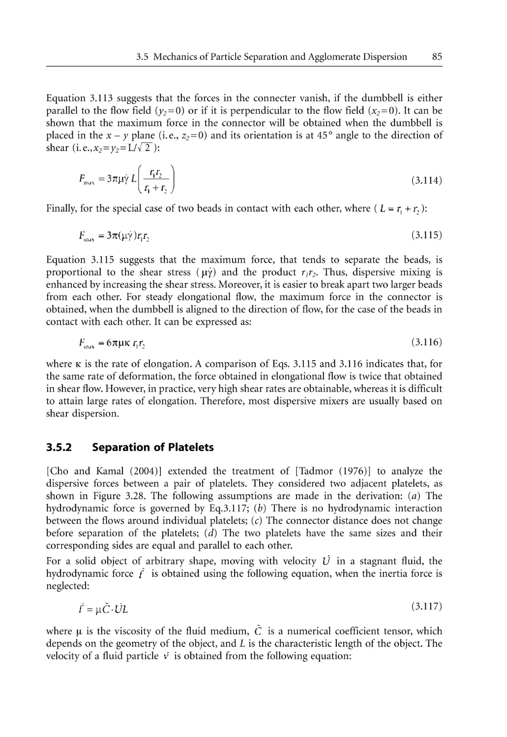
3.5.2 Separation of Platelets . . . . . . . . . . . . . . . . . . . . . . . . . . . . . . . . . . . . . . . .
3.5.3 Peeling and Lap Shearing Models. . . . . . . . . . . . . . . . . . . . . . . . . . . . . . .
3.5.4 Rupture and Erosion . . . . . . . . . . . . . . . . . . . . . . . . . . . . . . . . . . . . . . . . .
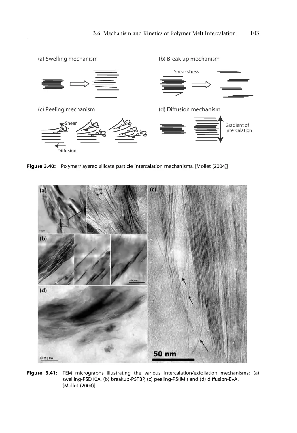
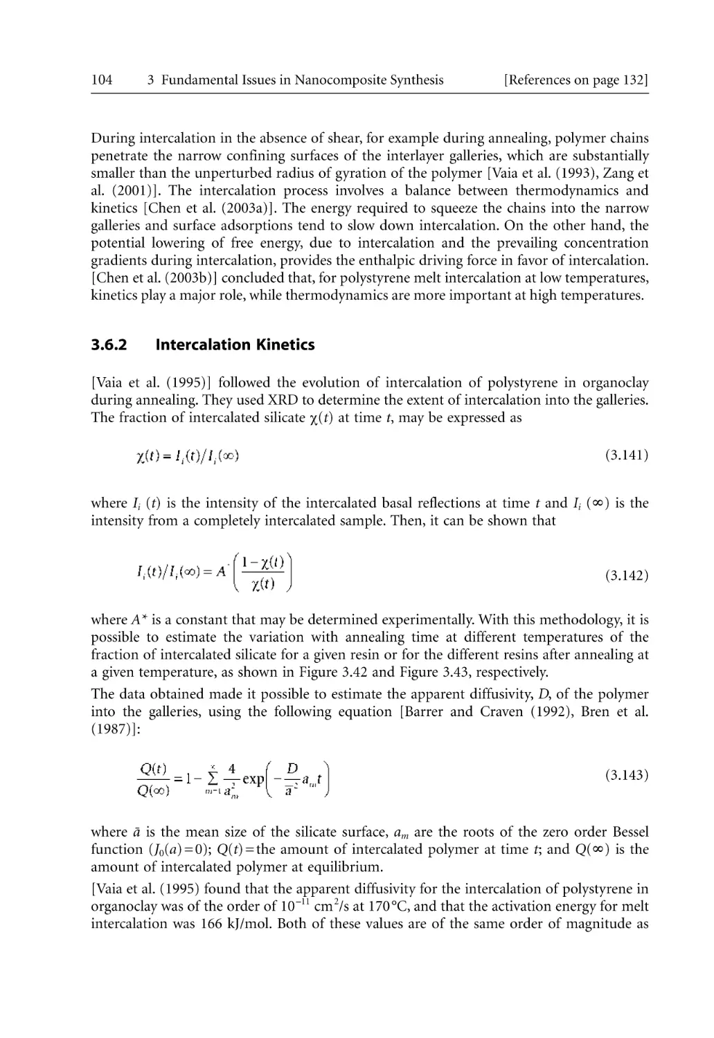
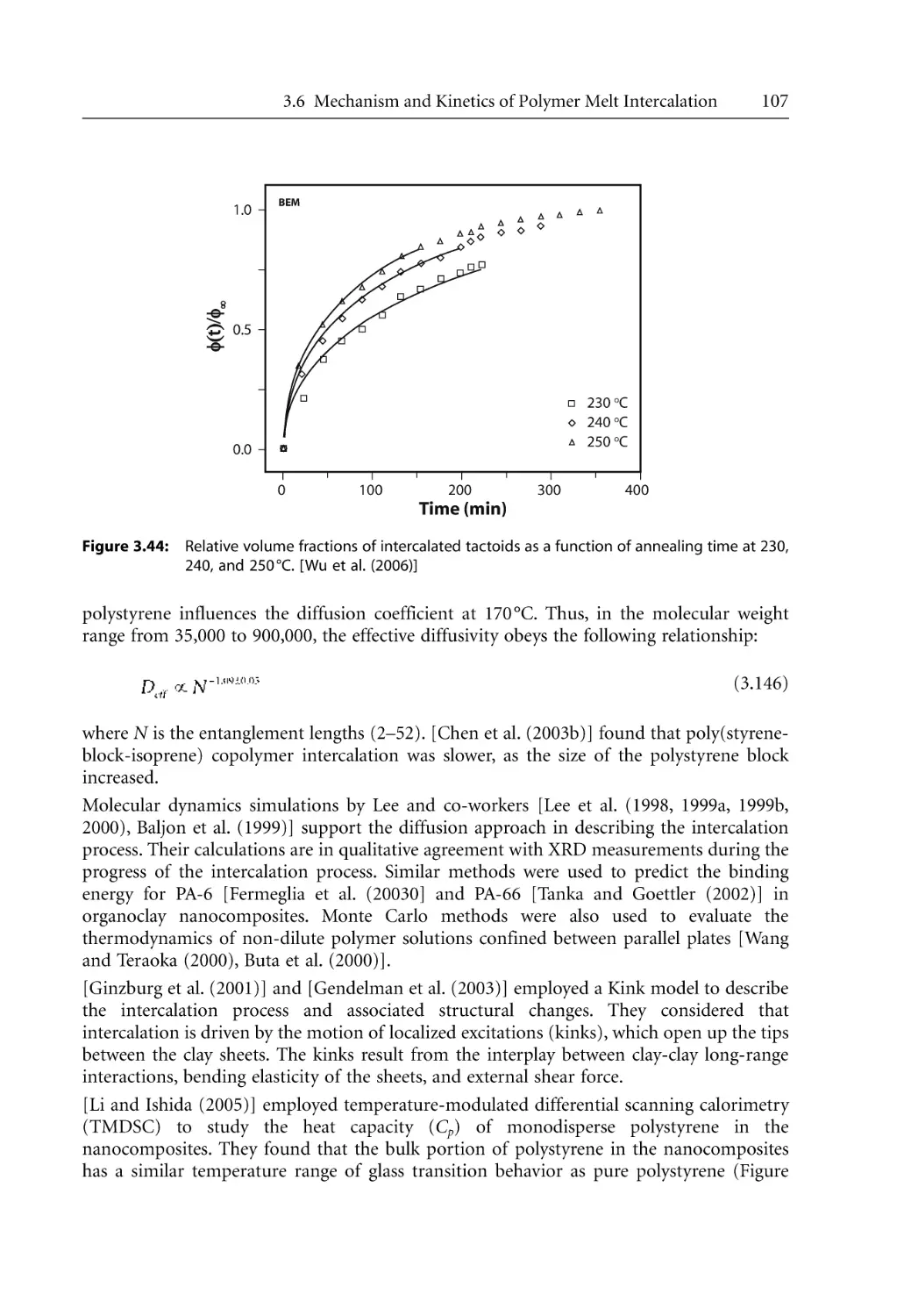
Mechanism and Kinetics of Polymer Melt Intercalation . . . . . . . . . . . . . . . . . .
3.6.1 Intercalation Mechanism . . . . . . . . . . . . . . . . . . . . . . . . . . . . . . . . . . . . . .
3.6.2 Intercalation Kinetics . . . . . . . . . . . . . . . . . . . . . . . . . . . . . . . . . . . . . . . . .
Crystallization of Polymers in Nanocomposites . . . . . . . . . . . . . . . . . . . . . . . . .
3.7.1 Crystallization of Polymers . . . . . . . . . . . . . . . . . . . . . . . . . . . . . . . . . . . .
3.7.2 Crystalline Structure and Morphology. . . . . . . . . . . . . . . . . . . . . . . . . . .
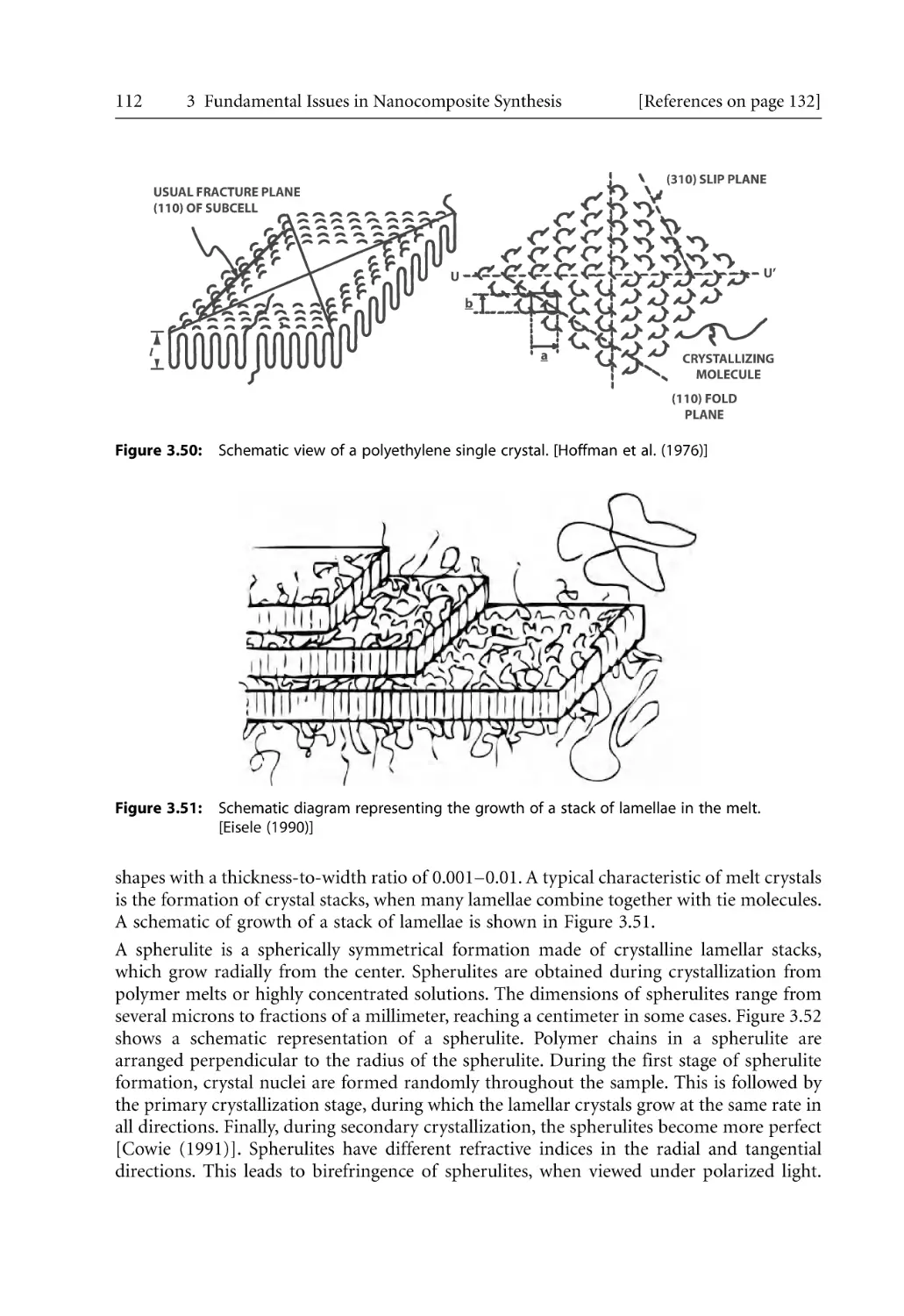
3.7.2.1 Folded Chain Model . . . . . . . . . . . . . . . . . . . . . . . . . . . . . . . . .
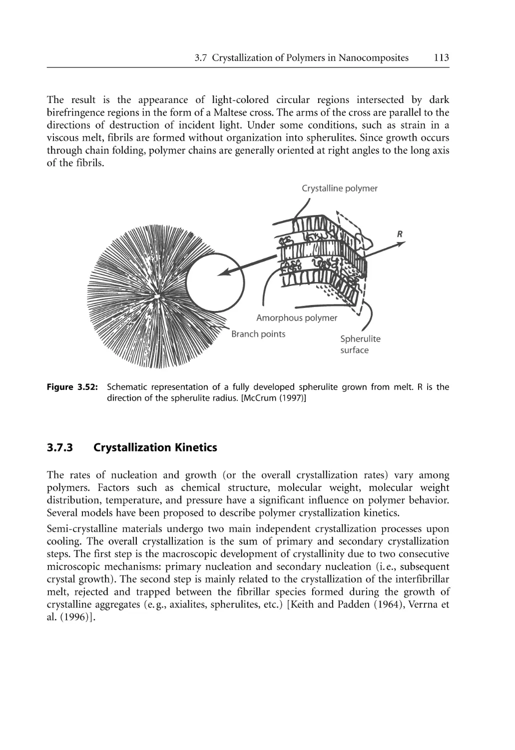
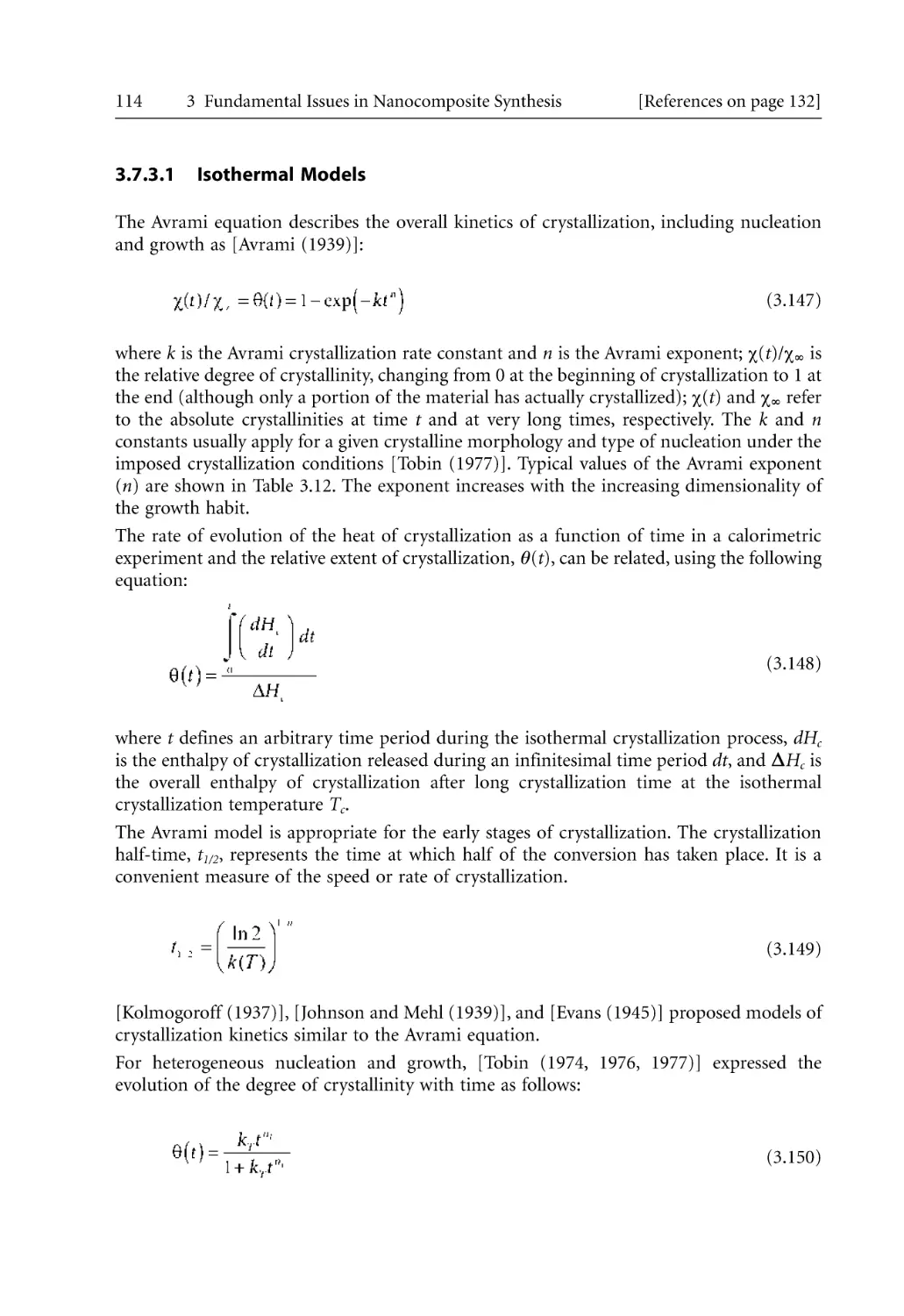
3.7.2.2 Crystallization from Polymer Melts. . . . . . . . . . . . . . . . . . . . . .
3.7.3 Crystallization Kinetics . . . . . . . . . . . . . . . . . . . . . . . . . . . . . . . . . . . . . . .
3.7.3.1 Isothermal Models . . . . . . . . . . . . . . . . . . . . . . . . . . . . . . . . . . .
3.7.3.2 Non-Isothermal Models . . . . . . . . . . . . . . . . . . . . . . . . . . . . . . .
3.7.3.3 Nucleation and Growth: Lauritzen-Hoffman Growth
Theory . . . . . . . . . . . . . . . . . . . . . . . . . . . . . . . . . . . . . . . . . . . . .
3.7.4 The Crystalline Structure of PA-6. . . . . . . . . . . . . . . . . . . . . . . . . . . . . . .
3.7.5 Polymer Crystallization in Nanocomposites . . . . . . . . . . . . . . . . . . . . . .
3.7.5.1 General Considerations . . . . . . . . . . . . . . . . . . . . . . . . . . . . . . .
3.7.5.2 Crystallization Kinetics . . . . . . . . . . . . . . . . . . . . . . . . . . . . . . . .
3.7.6 Morphological Effects . . . . . . . . . . . . . . . . . . . . . . . . . . . . . . . . . . . . . . . .
References . . . . . . . . . . . . . . . . . . . . . . . . . . . . . . . . . . . . . . . . . . . . . . . . . . . . . . . .

38
38
38
43
45
45
47
48
49
50
53
53
55
60
69
74
74
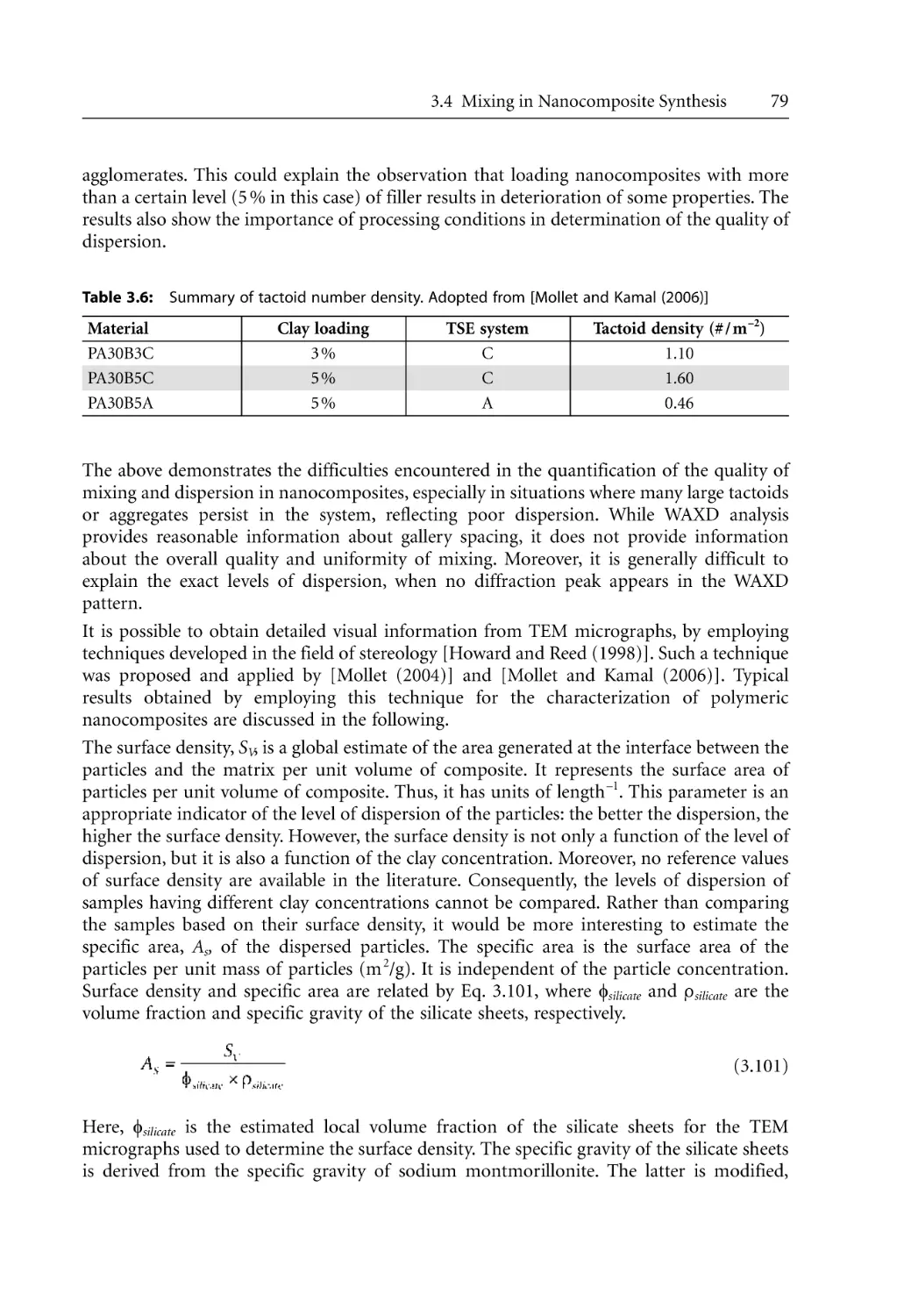
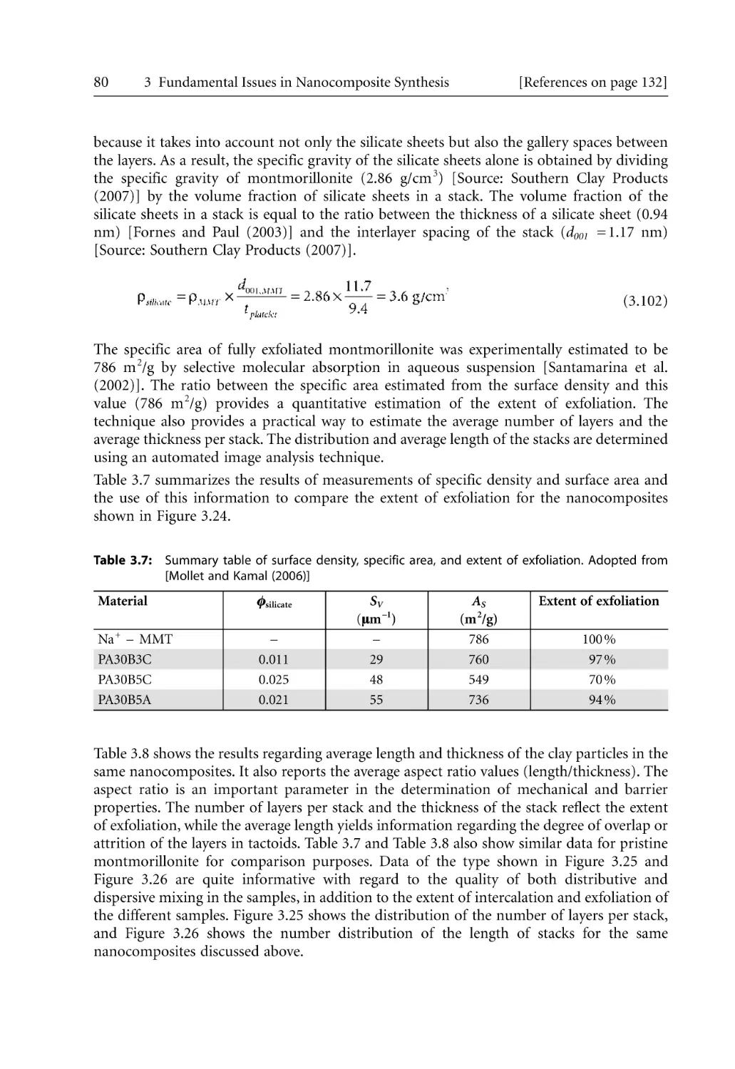
76
82
83
85
93
96
100
101
104
109
109
110
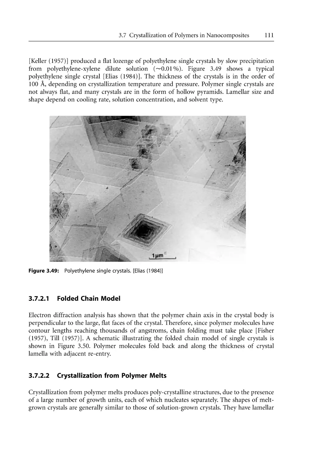
111
111
113
114
116
117
119
120
120
121
129
132

4 Rheology of Nanocomposites . . . . . . . . . . . . . . . . . . . . . . . . . . . . . . . . . . . . . . . . . . . . 145
4.1 Rheology of Multiphase Systems. . . . . . . . . . . . . . . . . . . . . . . . . . . . . . . . . . . . . . 145
4.2 Rheology of Polymer/Clay Nanocomposites . . . . . . . . . . . . . . . . . . . . . . . . . . . . 146

Inhalt

4.3
4.4

Recent Studies on Rheology . . . . . . . . . . . . . . . . . . . . . . . . . . . . . . . . . . . . . . . . .
Measurement Techniques. . . . . . . . . . . . . . . . . . . . . . . . . . . . . . . . . . . . . . . . . . . .
4.4.1 Steady Shear Measurements . . . . . . . . . . . . . . . . . . . . . . . . . . . . . . . . . . .
4.4.2 Dynamic Shear Measurements . . . . . . . . . . . . . . . . . . . . . . . . . . . . . . . . .
4.4.3 Extensional Rheology Measurements . . . . . . . . . . . . . . . . . . . . . . . . . . . .
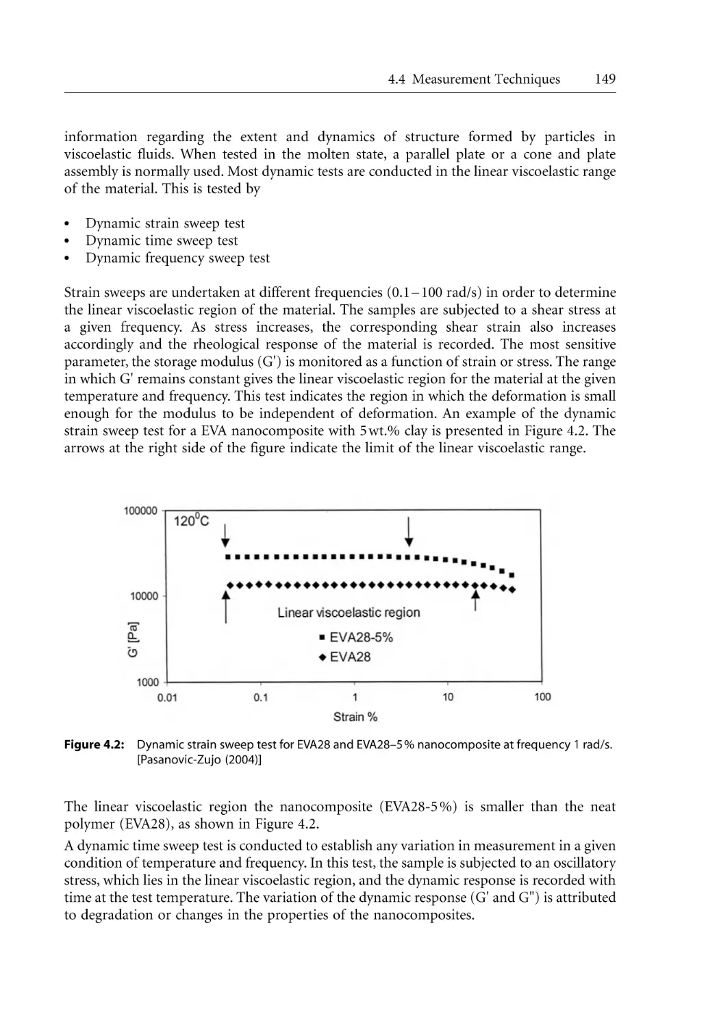
4.4.3.1 Meissner-Type Rheometer . . . . . . . . . . . . . . . . . . . . . . . . . . . . .
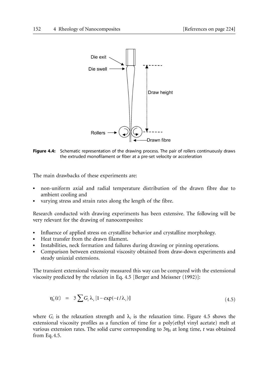
4.4.3.2 Drawing of Molten Monofilament After Extrusion . . . . . . . . .
4.4.4 Measured Parameters . . . . . . . . . . . . . . . . . . . . . . . . . . . . . . . . . . . . . . . . .
4.5 Steady Shear Rheology . . . . . . . . . . . . . . . . . . . . . . . . . . . . . . . . . . . . . . . . . . . . . .
4.5.1 Steady Shear Rheology of Nanocomposites . . . . . . . . . . . . . . . . . . . . . . .
4.5.2 Shear Thinning Behavior. . . . . . . . . . . . . . . . . . . . . . . . . . . . . . . . . . . . . .
4.5.3 Normal Stress Behavior . . . . . . . . . . . . . . . . . . . . . . . . . . . . . . . . . . . . . . .
4.6 Dynamic Rheology . . . . . . . . . . . . . . . . . . . . . . . . . . . . . . . . . . . . . . . . . . . . . . . . .
4.6.1 Dynamic Rheology of Nanocomposites . . . . . . . . . . . . . . . . . . . . . . . . . .
4.6.2 Percolation Threshold . . . . . . . . . . . . . . . . . . . . . . . . . . . . . . . . . . . . . . . .
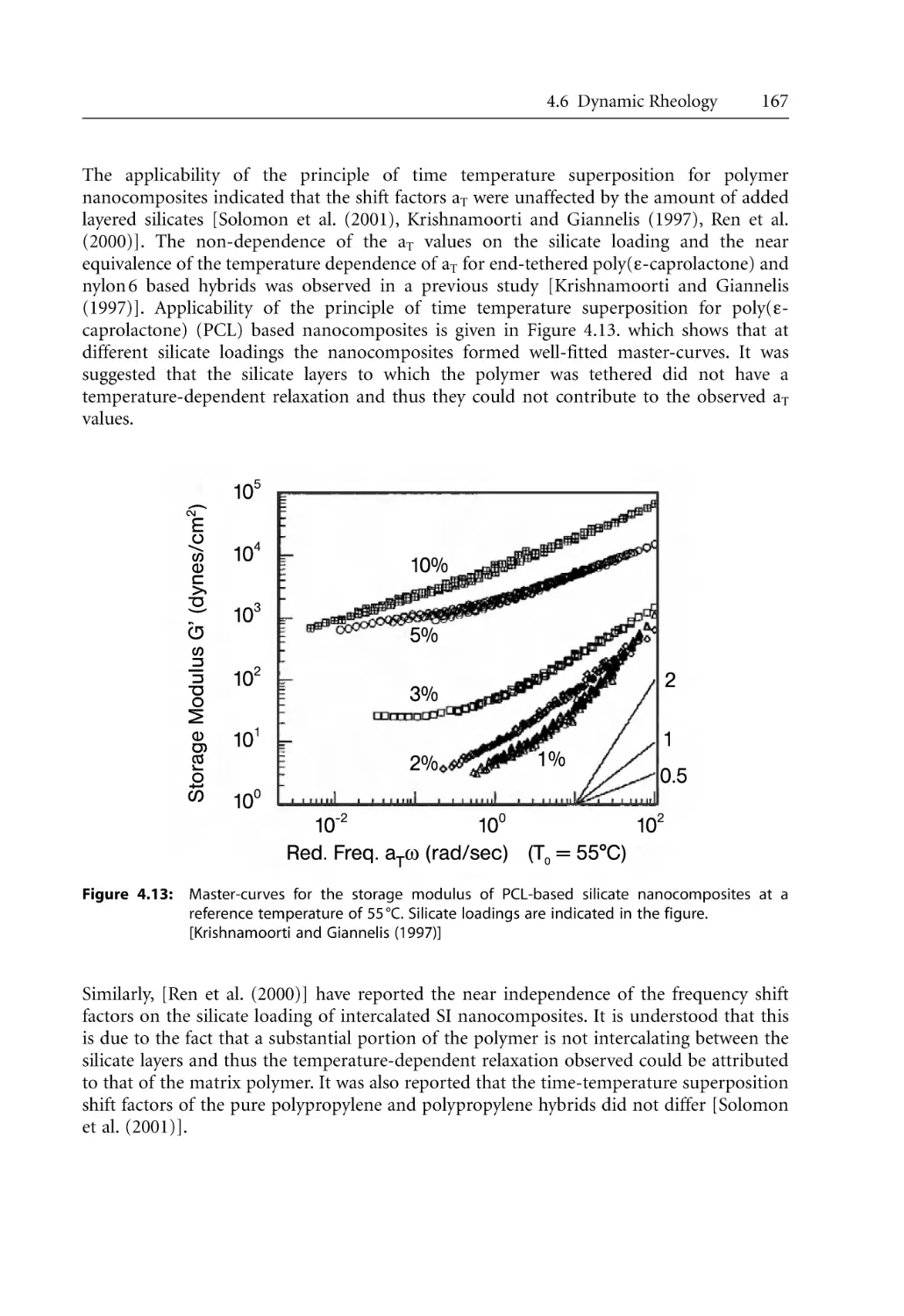
4.6.3 Time-Temperature Superposition. . . . . . . . . . . . . . . . . . . . . . . . . . . . . . .
4.6.4 Cox-Merz Rule . . . . . . . . . . . . . . . . . . . . . . . . . . . . . . . . . . . . . . . . . . . . . .
4.7 Non Linear Viscoelastic Properties . . . . . . . . . . . . . . . . . . . . . . . . . . . . . . . . . . . .
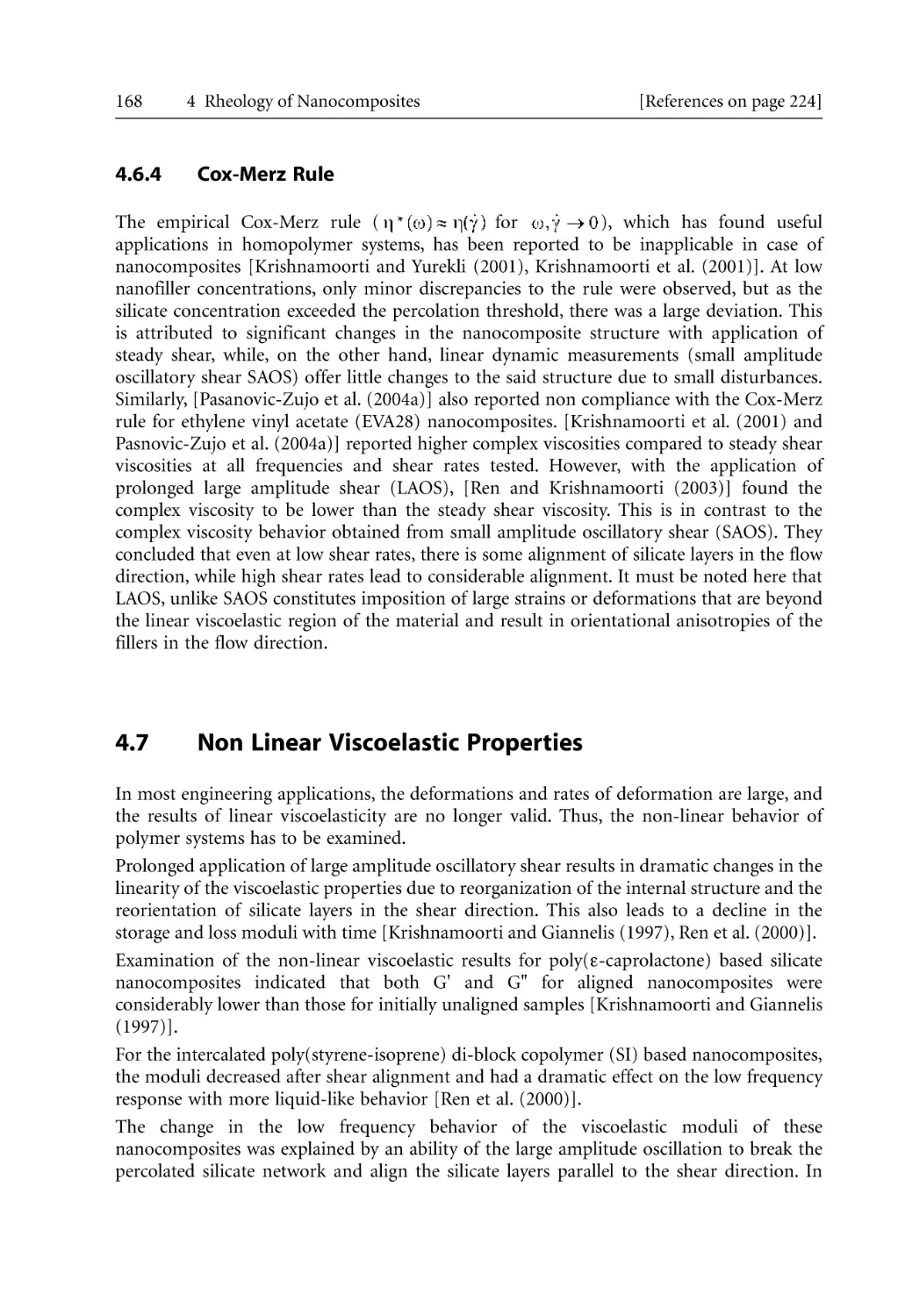
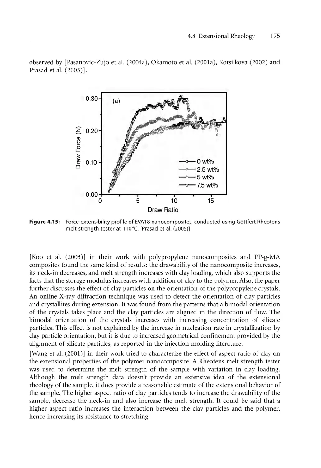
4.8 Extensional Rheology . . . . . . . . . . . . . . . . . . . . . . . . . . . . . . . . . . . . . . . . . . . . . . .
4.8.1 Fundamentals . . . . . . . . . . . . . . . . . . . . . . . . . . . . . . . . . . . . . . . . . . . . . . .
4.8.2 Extensional Rheology of Nanocomposites . . . . . . . . . . . . . . . . . . . . . . . .
4.8.3 Drawing of Molten Monofilament after Extrusion. . . . . . . . . . . . . . . . .
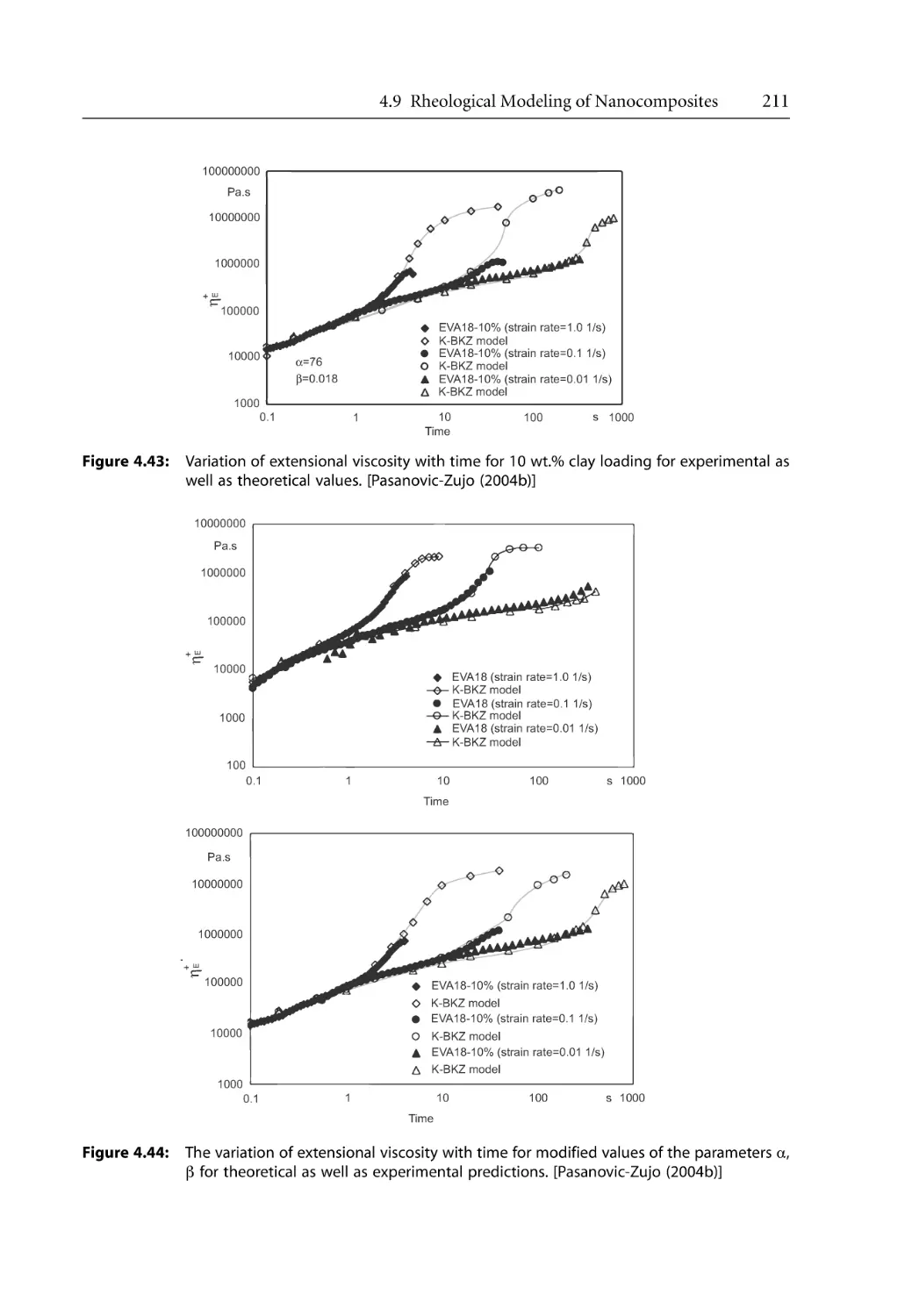
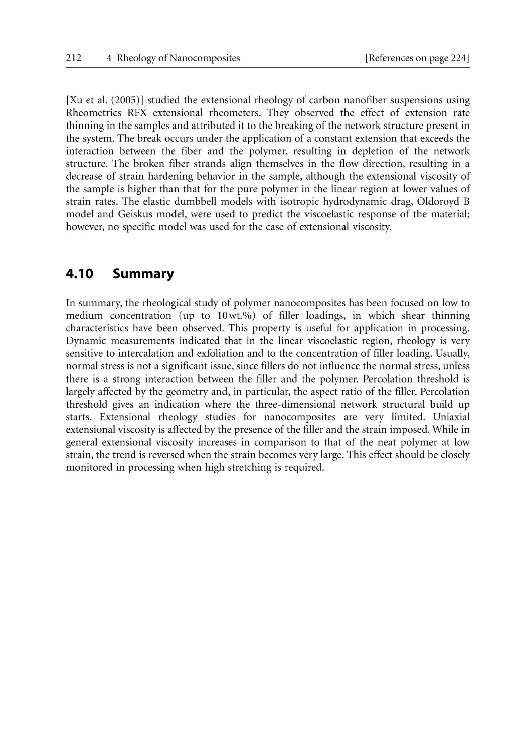
4.9 Rheological Modeling of Nanocomposites. . . . . . . . . . . . . . . . . . . . . . . . . . . . . .
4.9.1 Steady Shear Models . . . . . . . . . . . . . . . . . . . . . . . . . . . . . . . . . . . . . . . . .
4.9.1.1 Herschel Berkeley Model . . . . . . . . . . . . . . . . . . . . . . . . . . . . . .
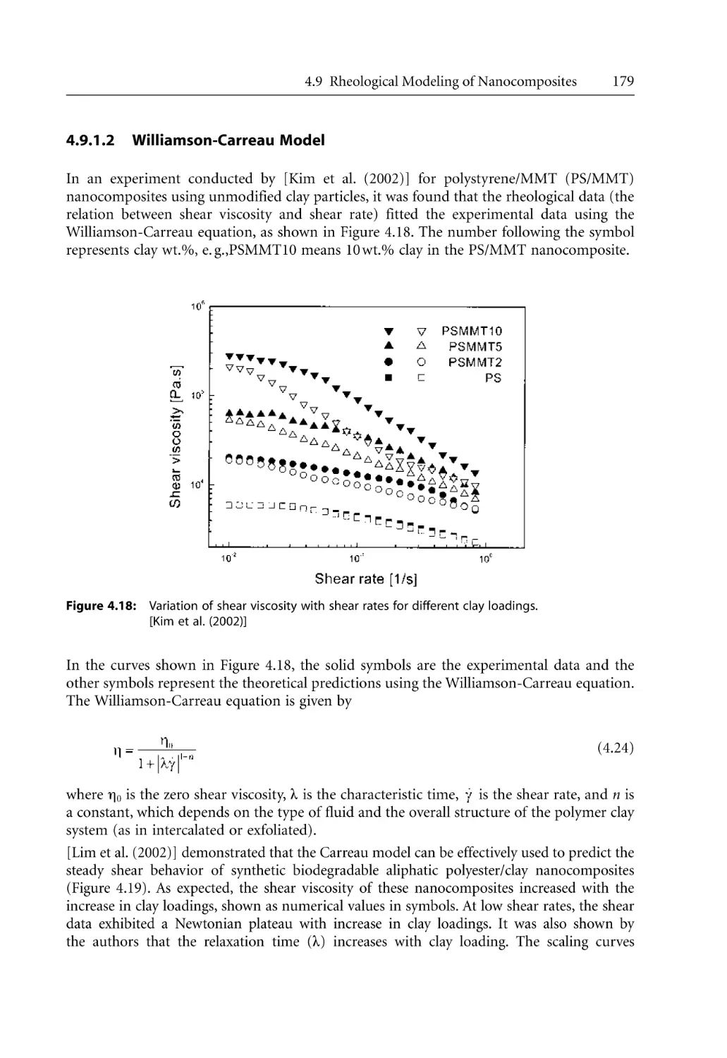
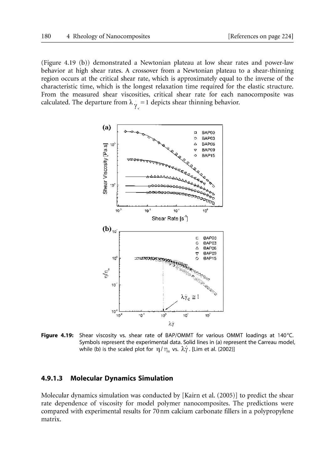
4.9.1.2 Williamson-Carreau Model . . . . . . . . . . . . . . . . . . . . . . . . . . . .
4.9.1.3 Molecular Dynamics Simulation . . . . . . . . . . . . . . . . . . . . . . . .
4.9.1.4 Coarse-Grained Computer Simulation . . . . . . . . . . . . . . . . . . .
4.9.2 Viscoelastic Models . . . . . . . . . . . . . . . . . . . . . . . . . . . . . . . . . . . . . . . . . .
4.9.2.1 The Network Model . . . . . . . . . . . . . . . . . . . . . . . . . . . . . . . . . .
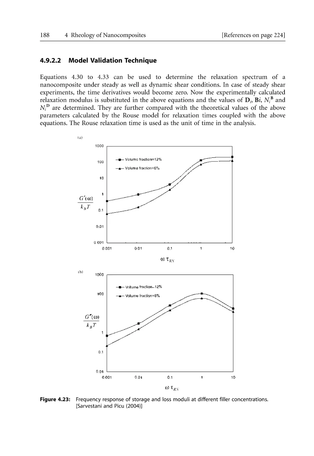
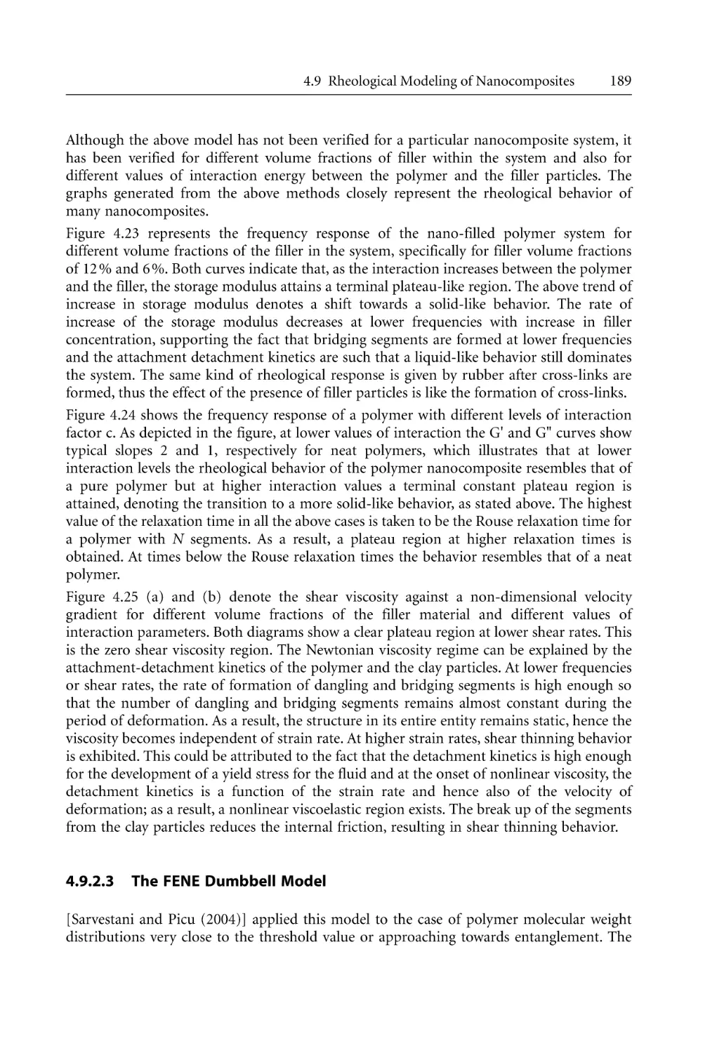
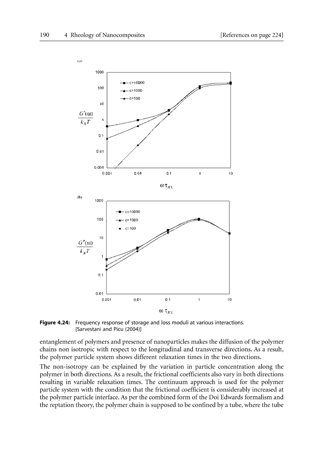
4.9.2.2 Model Validation Technique. . . . . . . . . . . . . . . . . . . . . . . . . . . .
4.9.2.3 The FENE Dumbbell Model . . . . . . . . . . . . . . . . . . . . . . . . . . .
4.9.2.4 Molecular Dynamic Simulation. . . . . . . . . . . . . . . . . . . . . . . . .
4.9.2.5 Bi-Mode FENE Dumbbell Model . . . . . . . . . . . . . . . . . . . . . . .
4.9.3 Extensional Rheology. . . . . . . . . . . . . . . . . . . . . . . . . . . . . . . . . . . . . . . . .
4.9.3.1 K-BKZ Model . . . . . . . . . . . . . . . . . . . . . . . . . . . . . . . . . . . . . . .
4.9.3.2 Validation Technique . . . . . . . . . . . . . . . . . . . . . . . . . . . . . . . . .
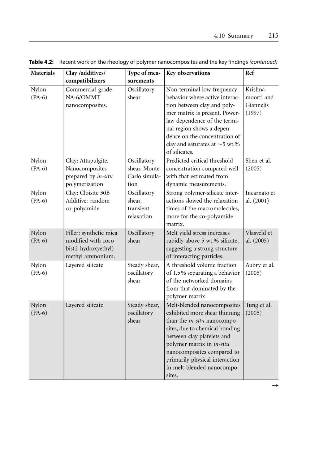
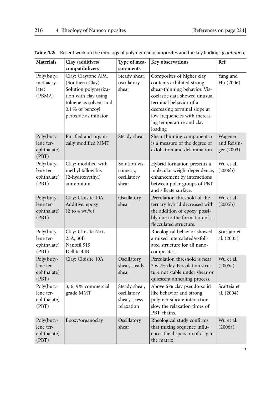
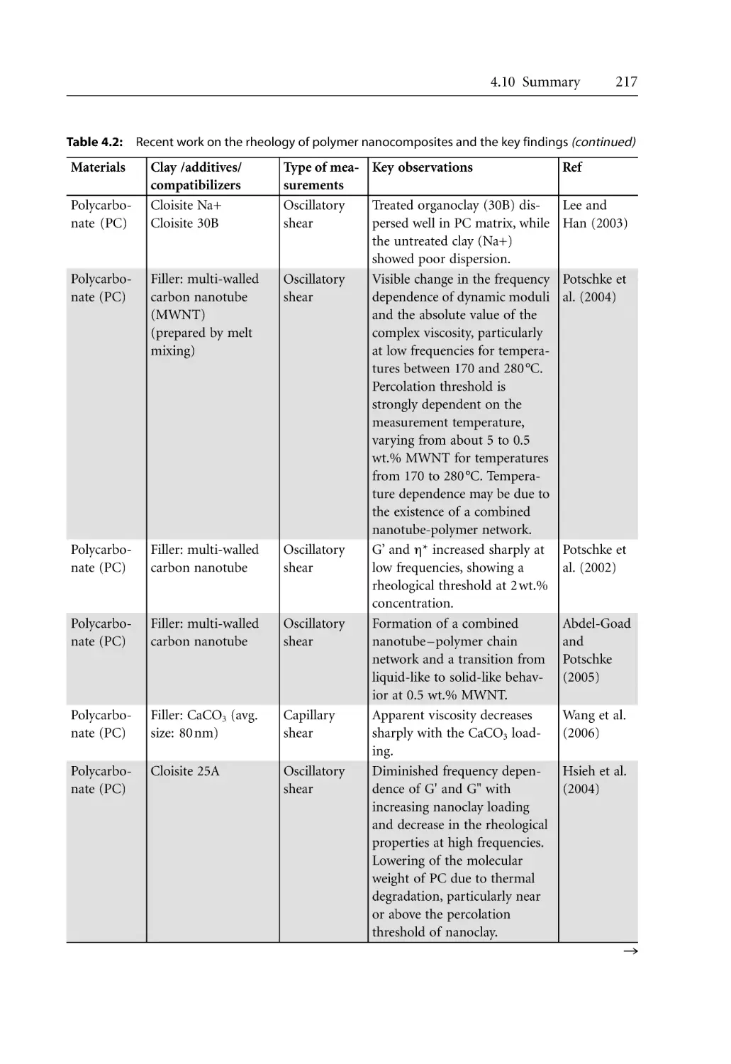
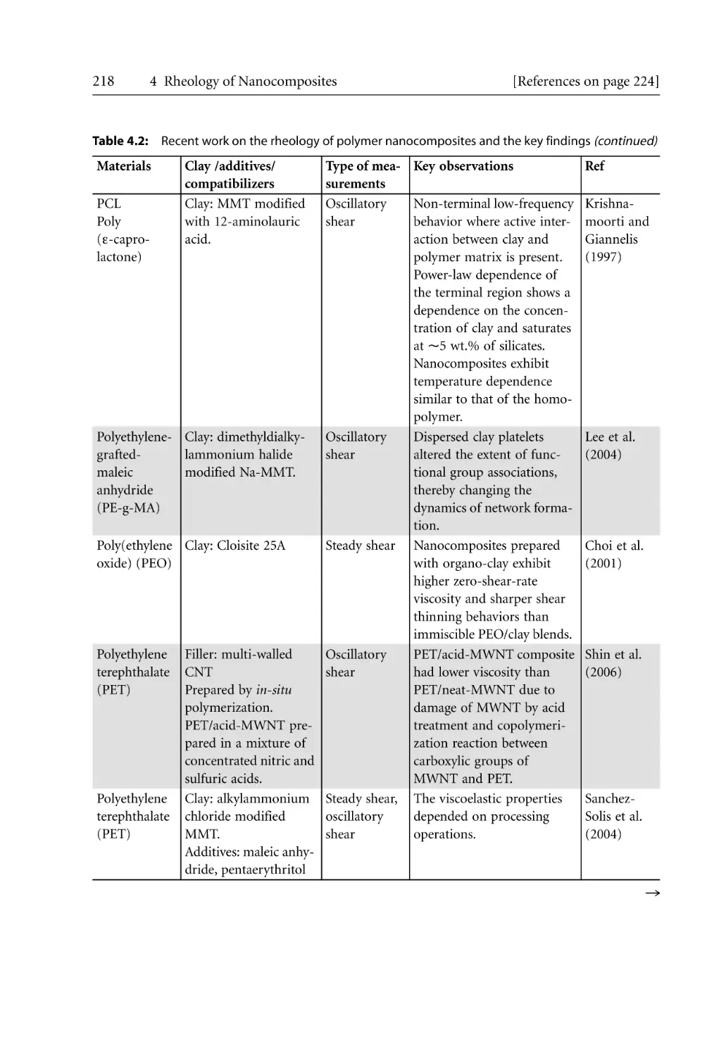
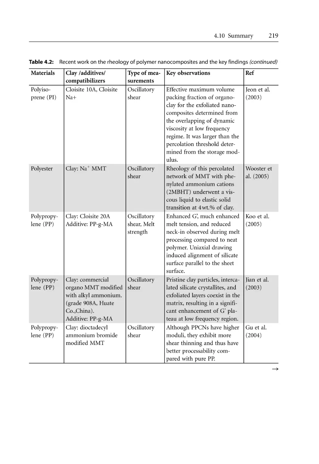
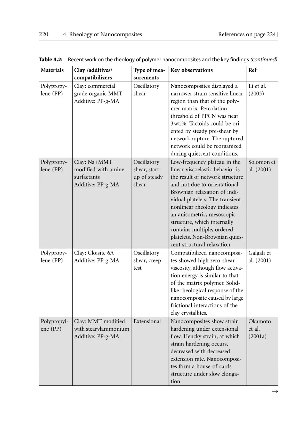
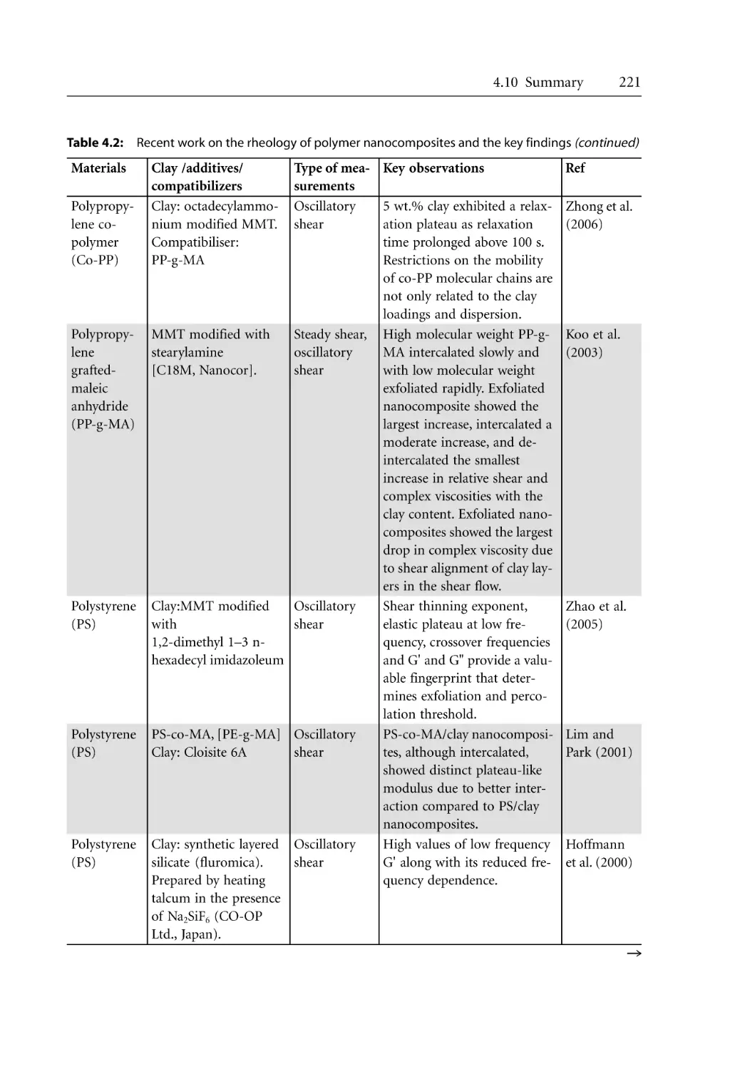
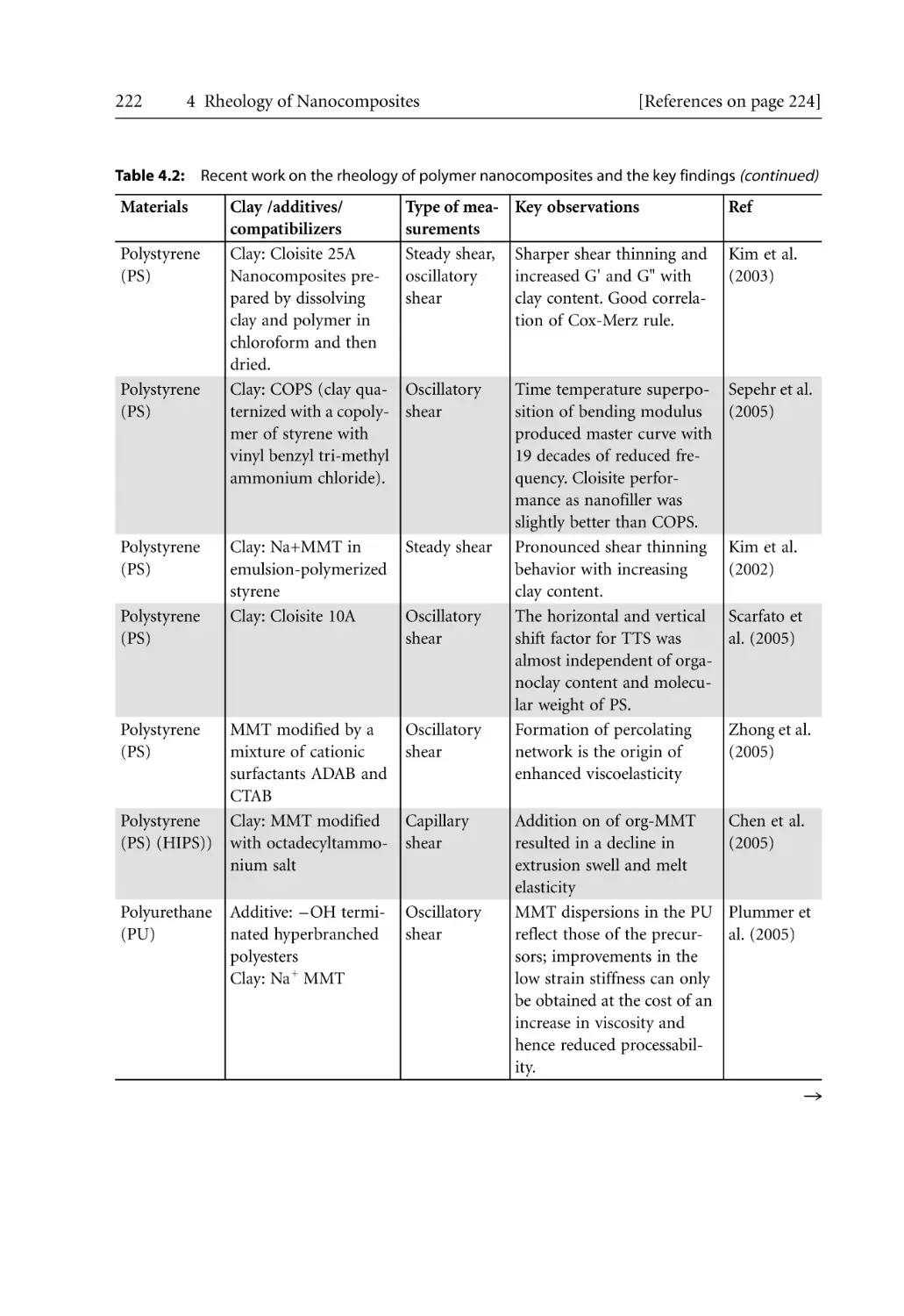
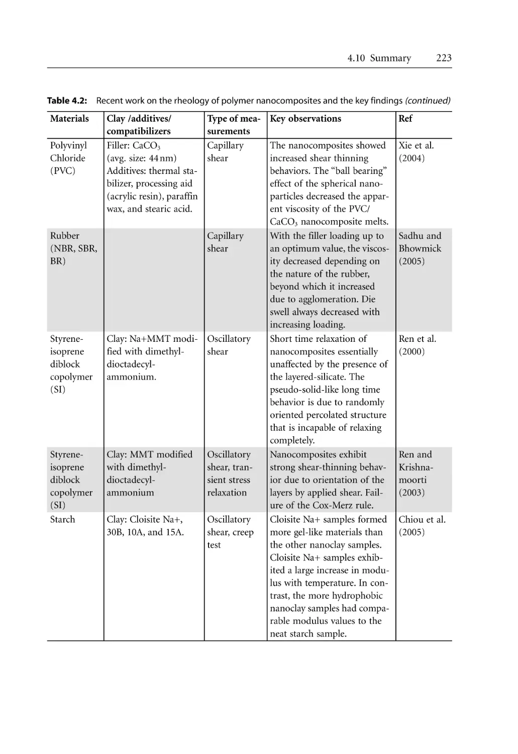
4.10 Summary . . . . . . . . . . . . . . . . . . . . . . . . . . . . . . . . . . . . . . . . . . . . . . . . . . . . . . . . .

146
147
147
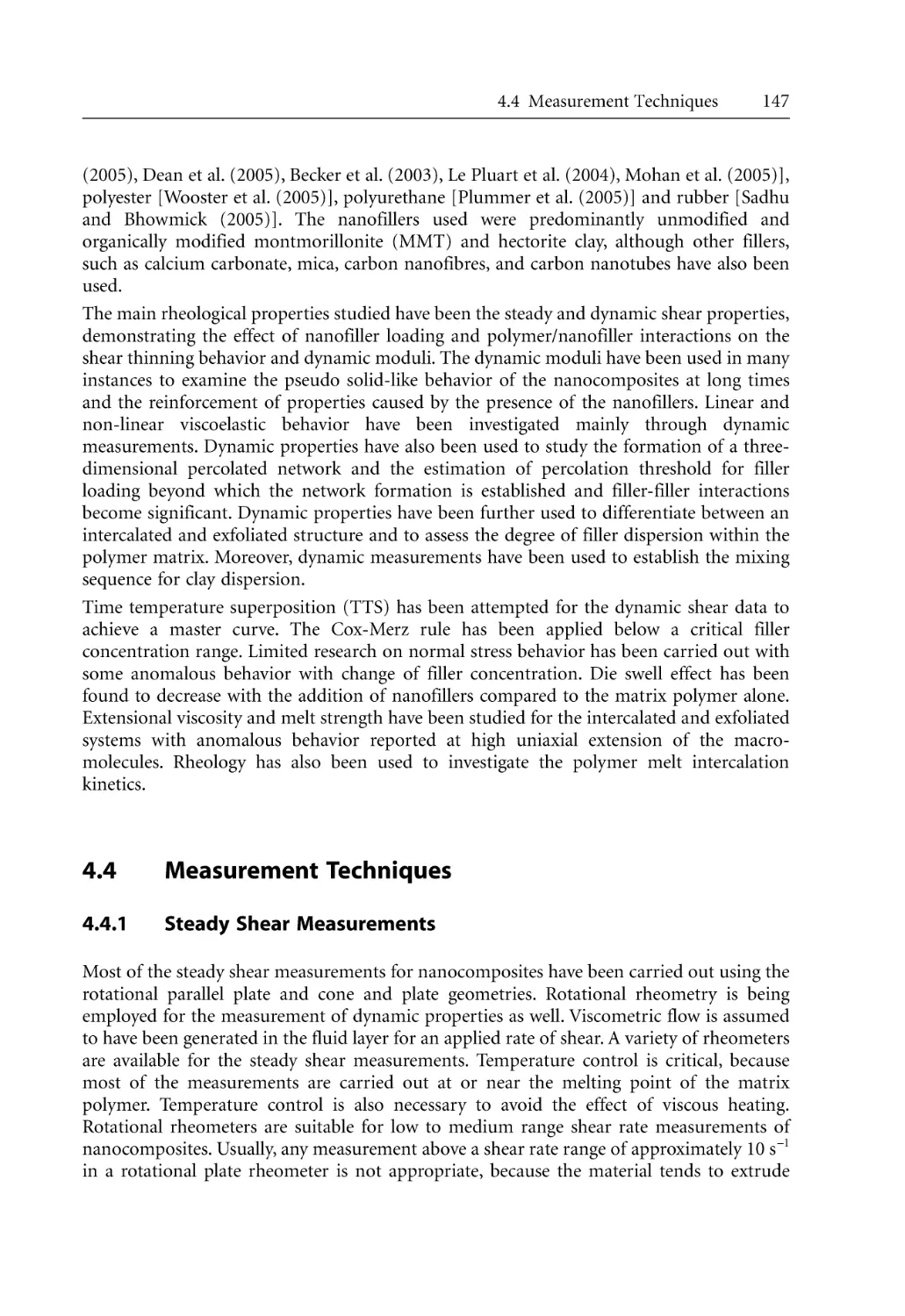
148
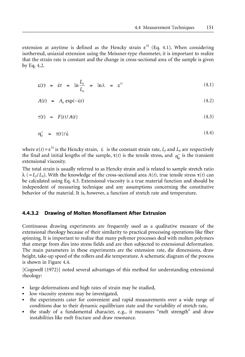
150
150
151
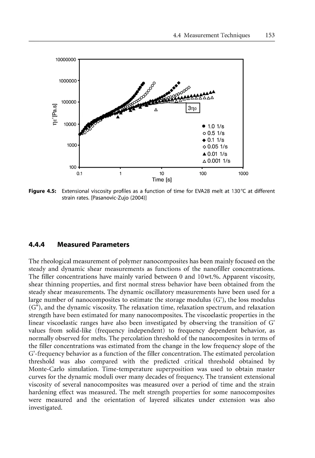
153
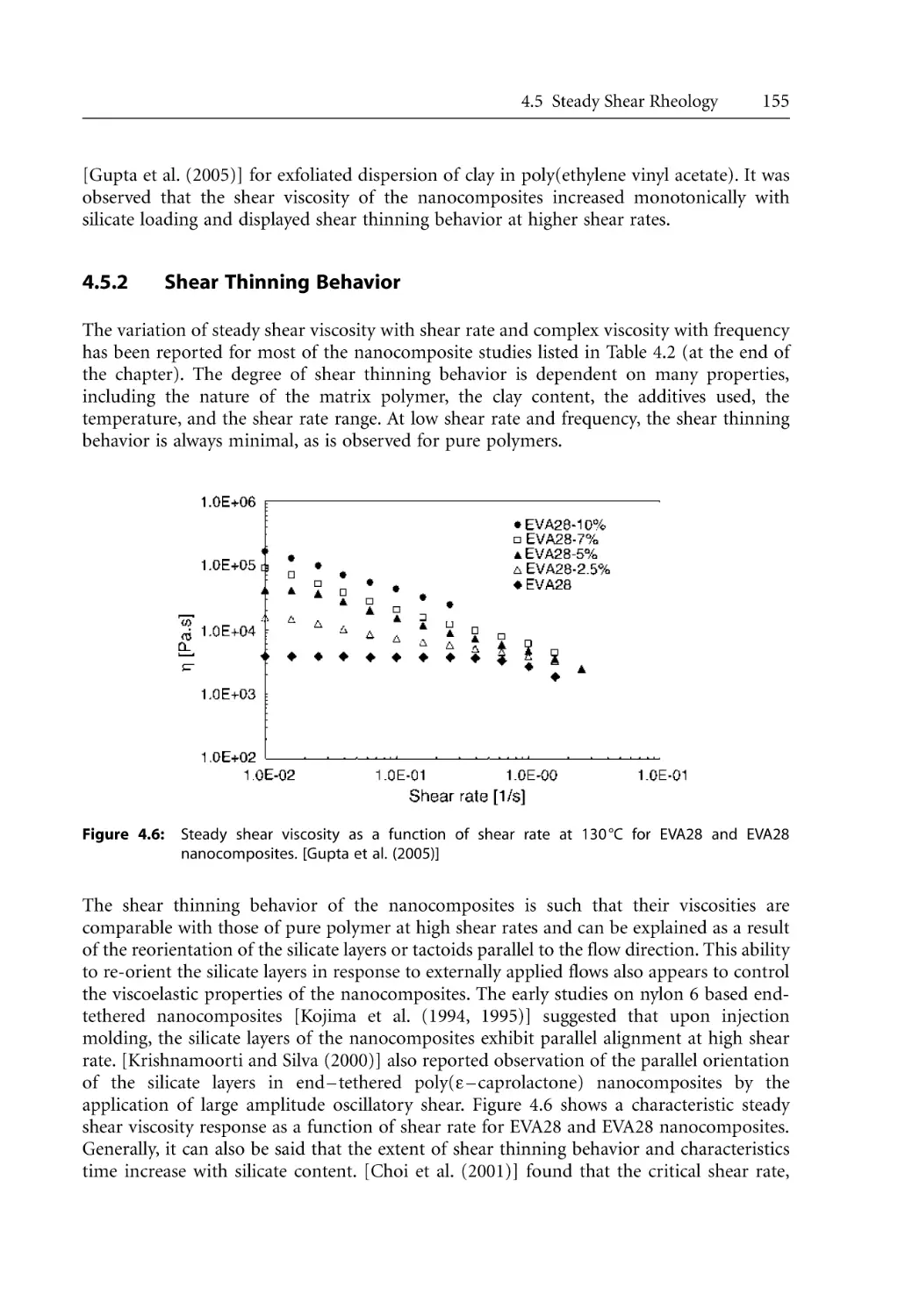
154
154
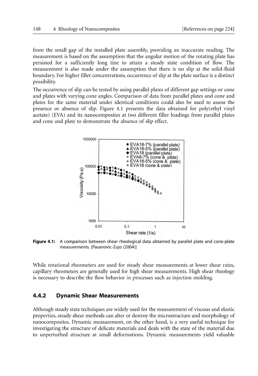
155
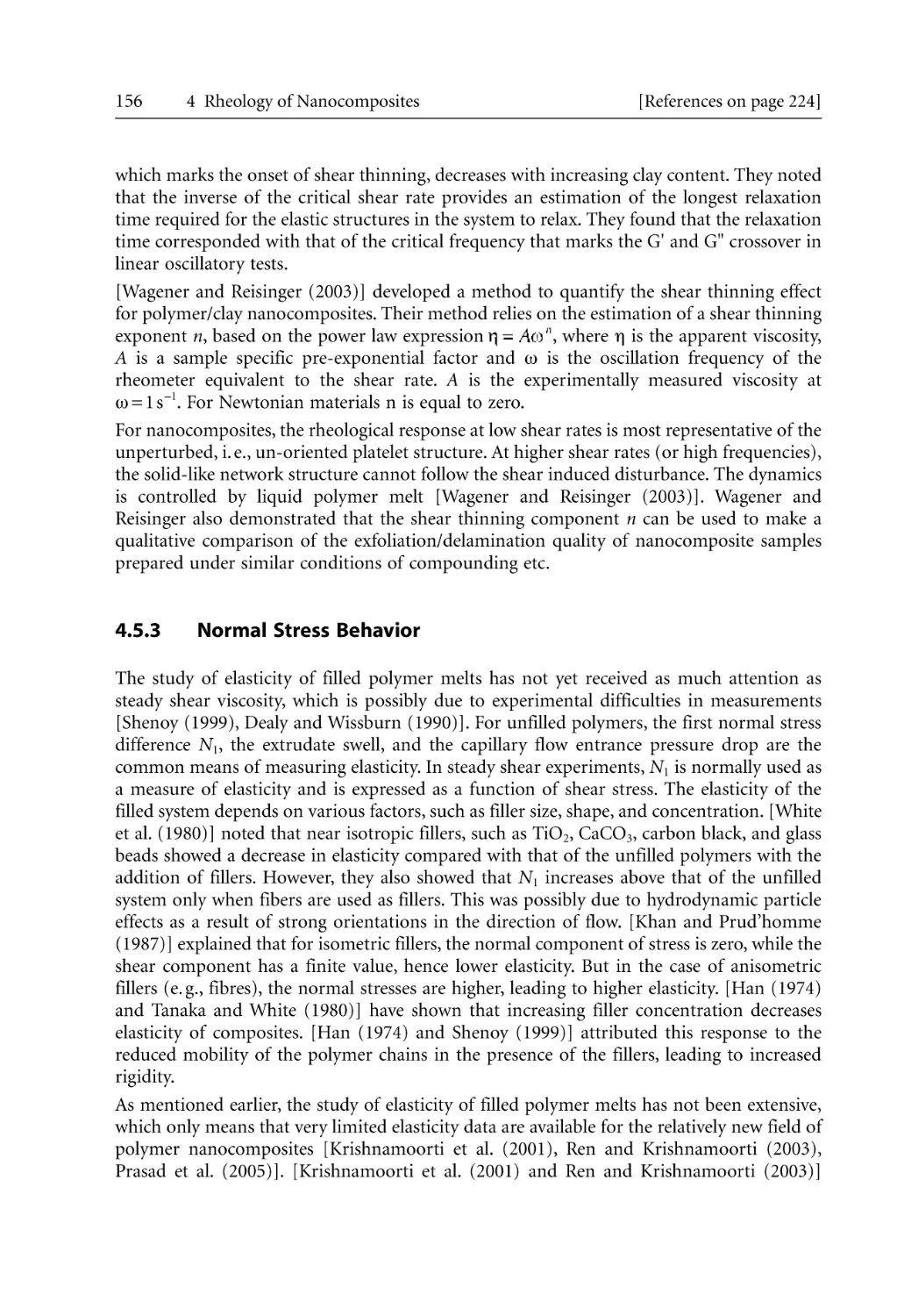
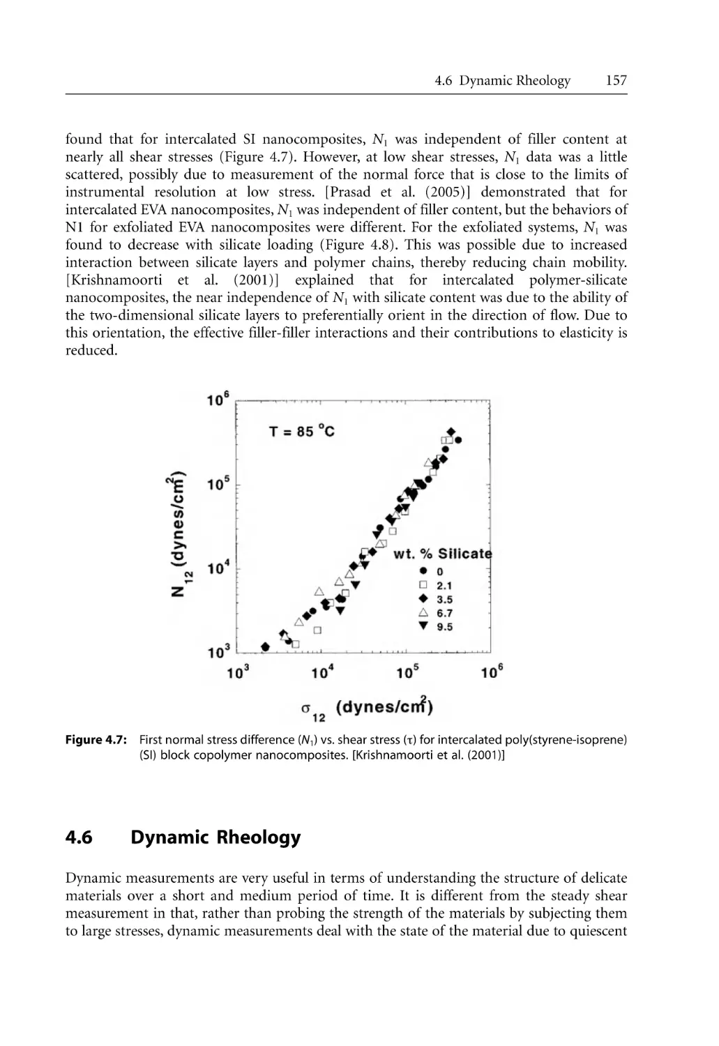
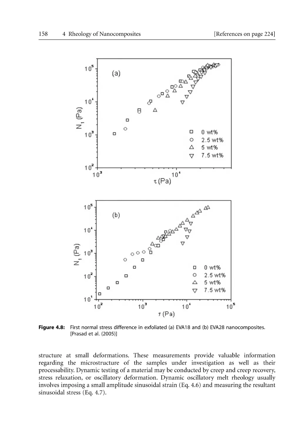
156
157
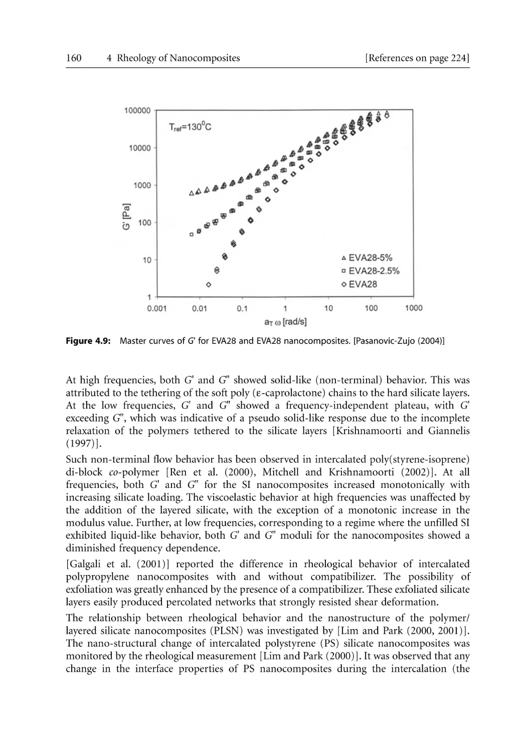
159
161
166
168
168
170
170
172
173
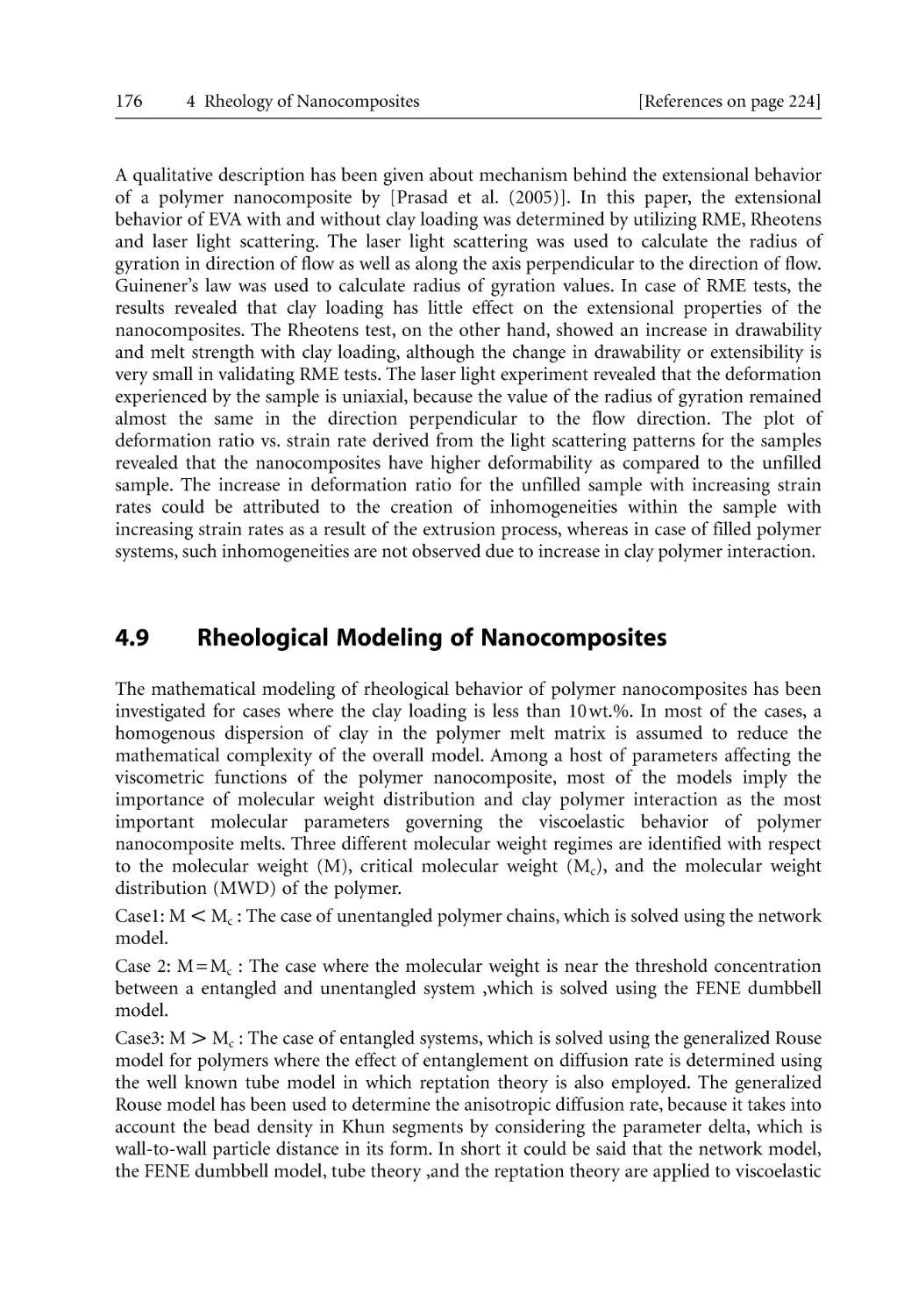
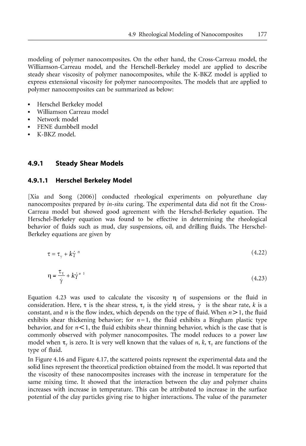
176
177
177
179
180
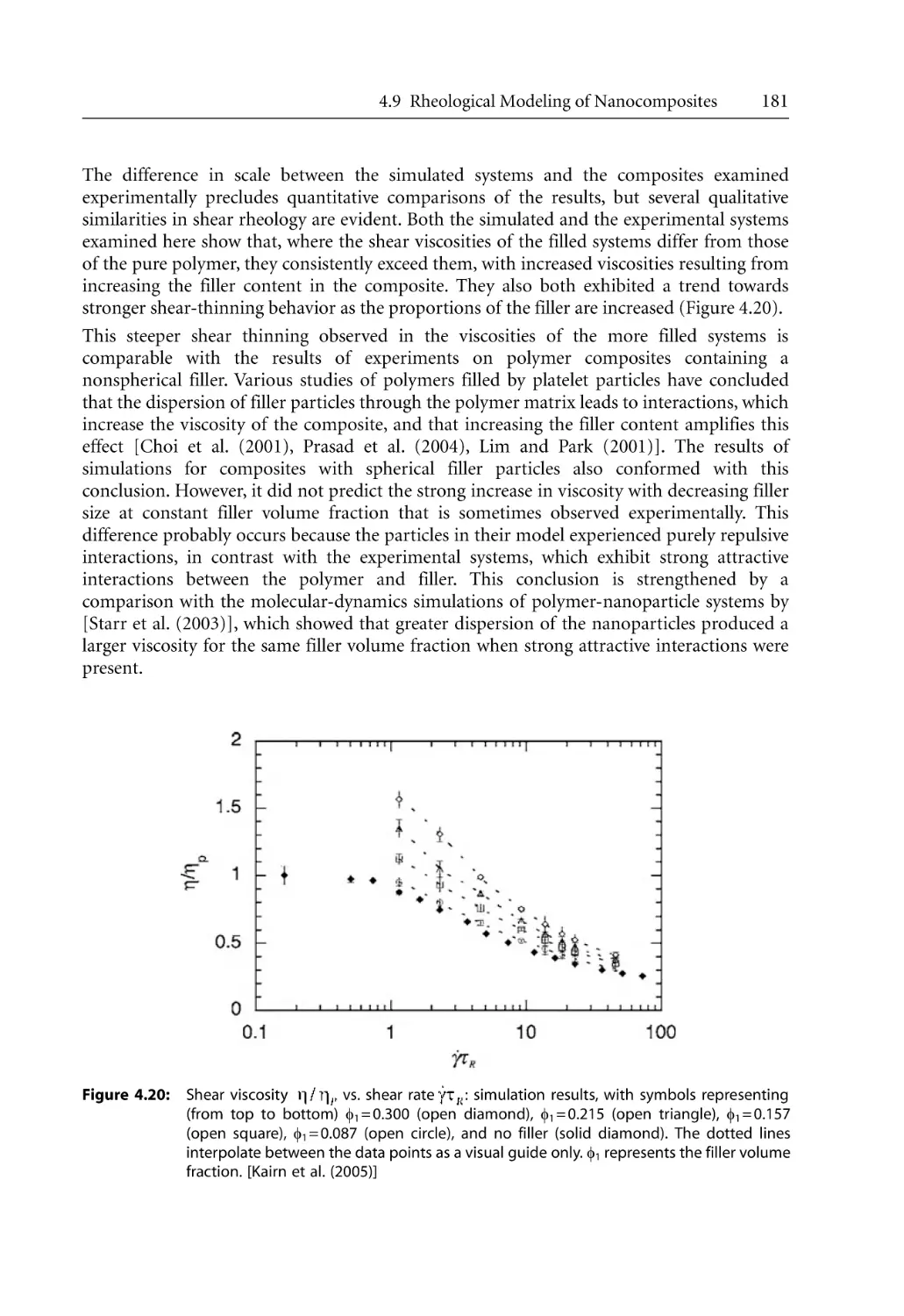
182
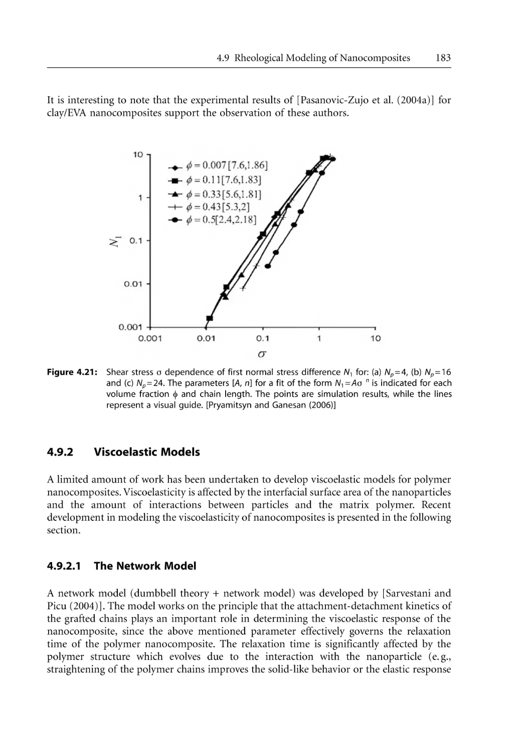
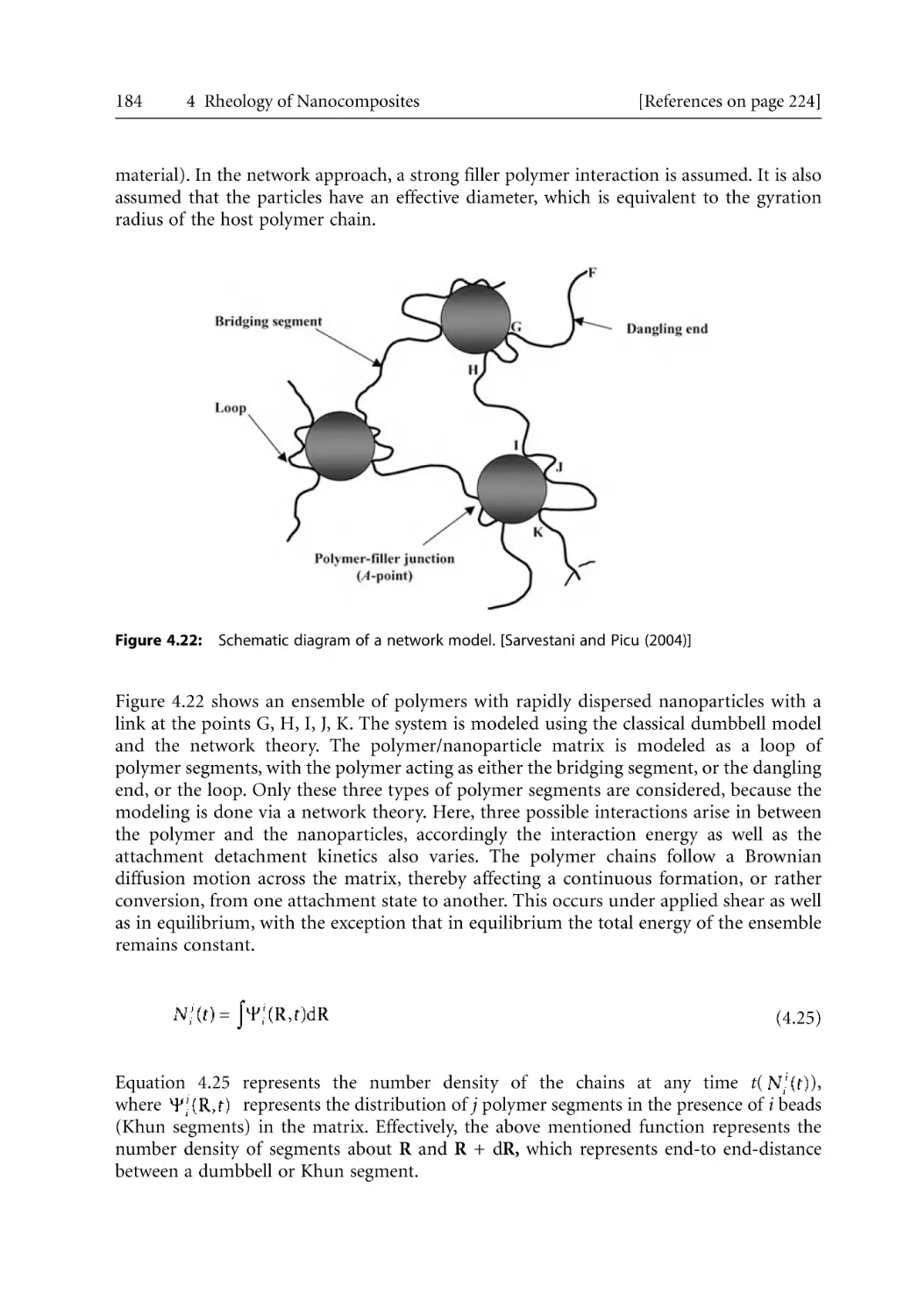
183
183
188
189
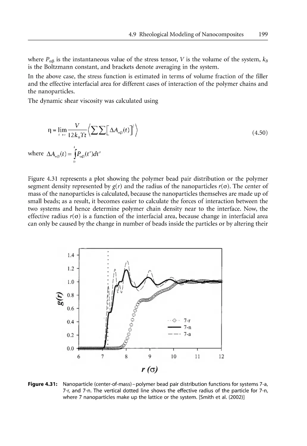
197
202
206
208
209
212

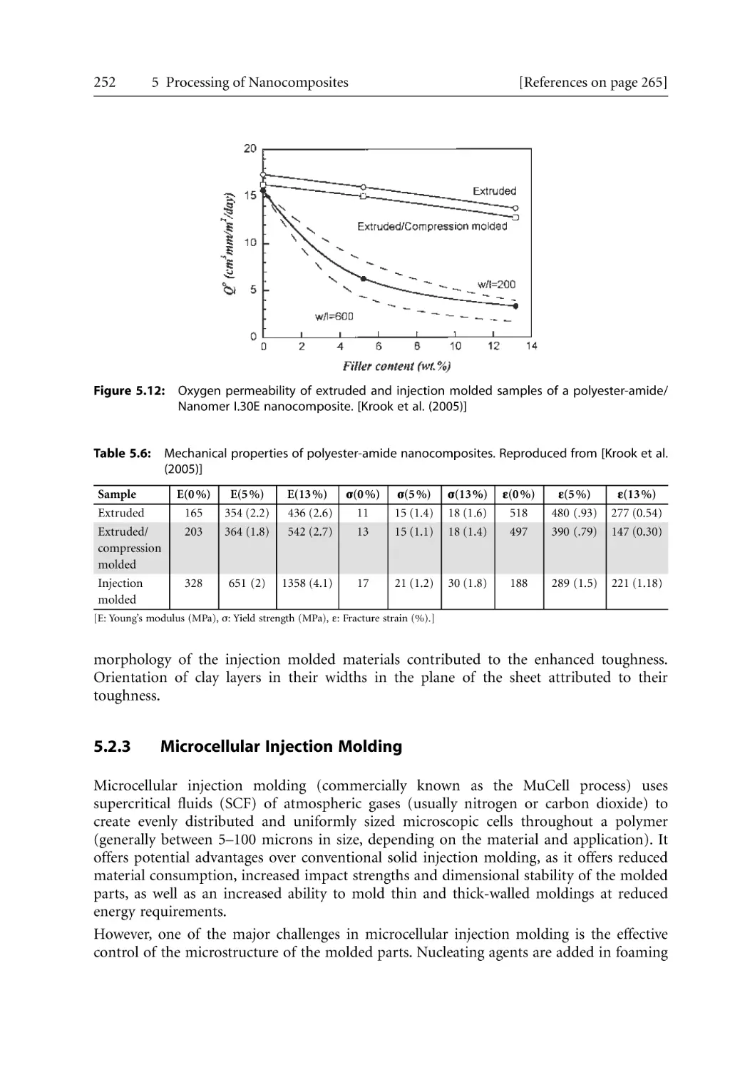
5 Processing of Nanocomposites . . . . . . . . . . . . . . . . . . . . . . . . . . . . . . . . . . . . . . . . . . .
5.1 Introduction . . . . . . . . . . . . . . . . . . . . . . . . . . . . . . . . . . . . . . . . . . . . . . . . . . . . . .
5.1 Extrusion . . . . . . . . . . . . . . . . . . . . . . . . . . . . . . . . . . . . . . . . . . . . . . . . . . . . . . . . .
5.1.1 Dispersion of Clay . . . . . . . . . . . . . . . . . . . . . . . . . . . . . . . . . . . . . . . . . . .
5.1.2 Effect of Extruder Types . . . . . . . . . . . . . . . . . . . . . . . . . . . . . . . . . . . . . .
5.1.3 Effect of Processing Conditions . . . . . . . . . . . . . . . . . . . . . . . . . . . . . . . .
5.2 Injection Molding. . . . . . . . . . . . . . . . . . . . . . . . . . . . . . . . . . . . . . . . . . . . . . . . . .

233
233
234
235
240
245
245

XII

Inhalt

5.2.1 Structural Hierarchy. . . . . . . . . . . . . . . . . . . . . . . . . . . . . . . . . . . . . . . . . .
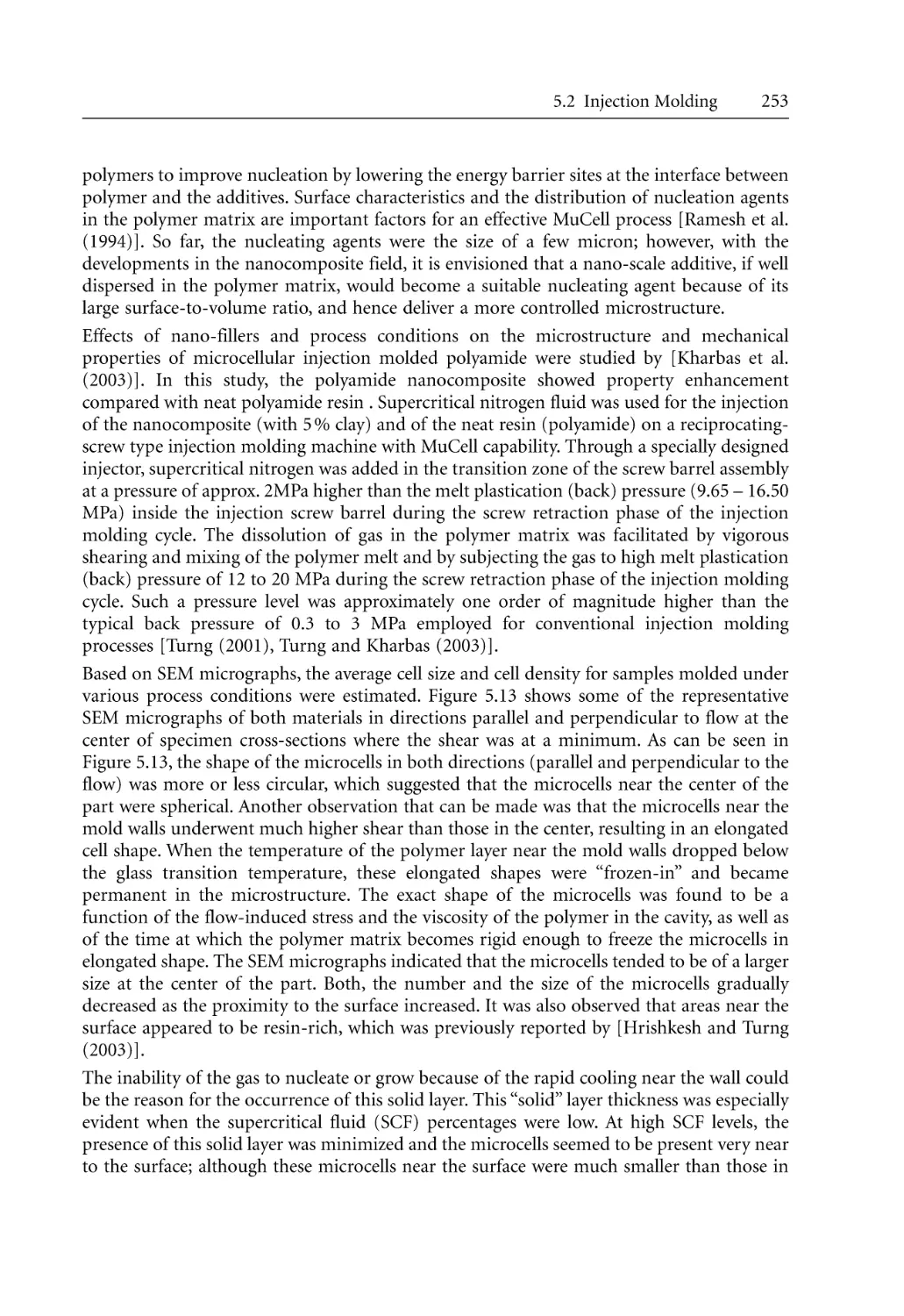
5.2.2 Barrier and Mechanical Properties for Injection Molded Products. . . .
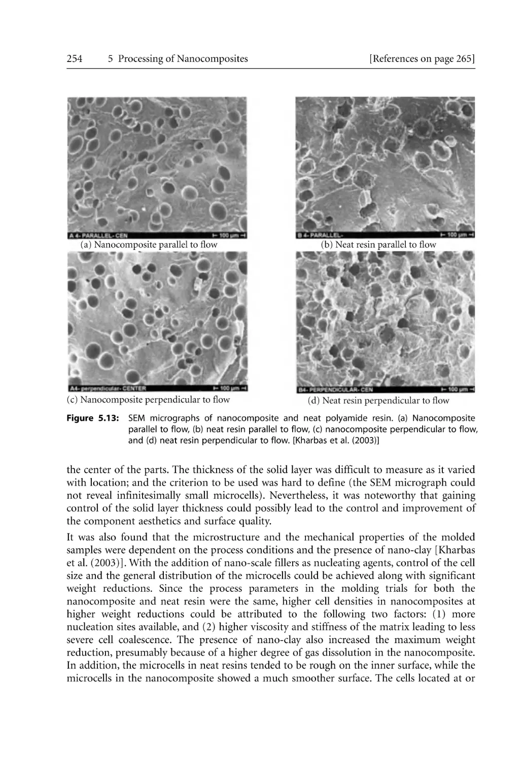
5.2.3 Microcellular Injection Molding . . . . . . . . . . . . . . . . . . . . . . . . . . . . . . . .
Blow Molding . . . . . . . . . . . . . . . . . . . . . . . . . . . . . . . . . . . . . . . . . . . . . . . . . . . . .
5.3.1 Barrier Properties of Blow Molded Products . . . . . . . . . . . . . . . . . . . . .
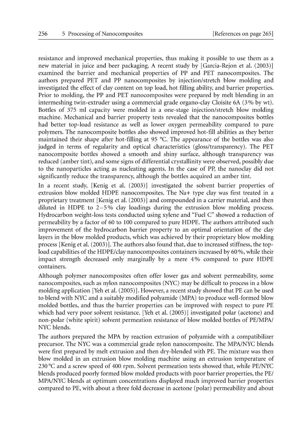
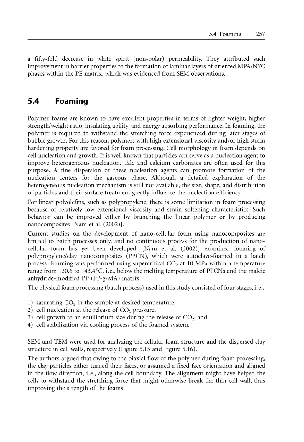
Foaming. . . . . . . . . . . . . . . . . . . . . . . . . . . . . . . . . . . . . . . . . . . . . . . . . . . . . . . . . .
Rotational Molding . . . . . . . . . . . . . . . . . . . . . . . . . . . . . . . . . . . . . . . . . . . . . . . .

246
251
252
255
255
257
263

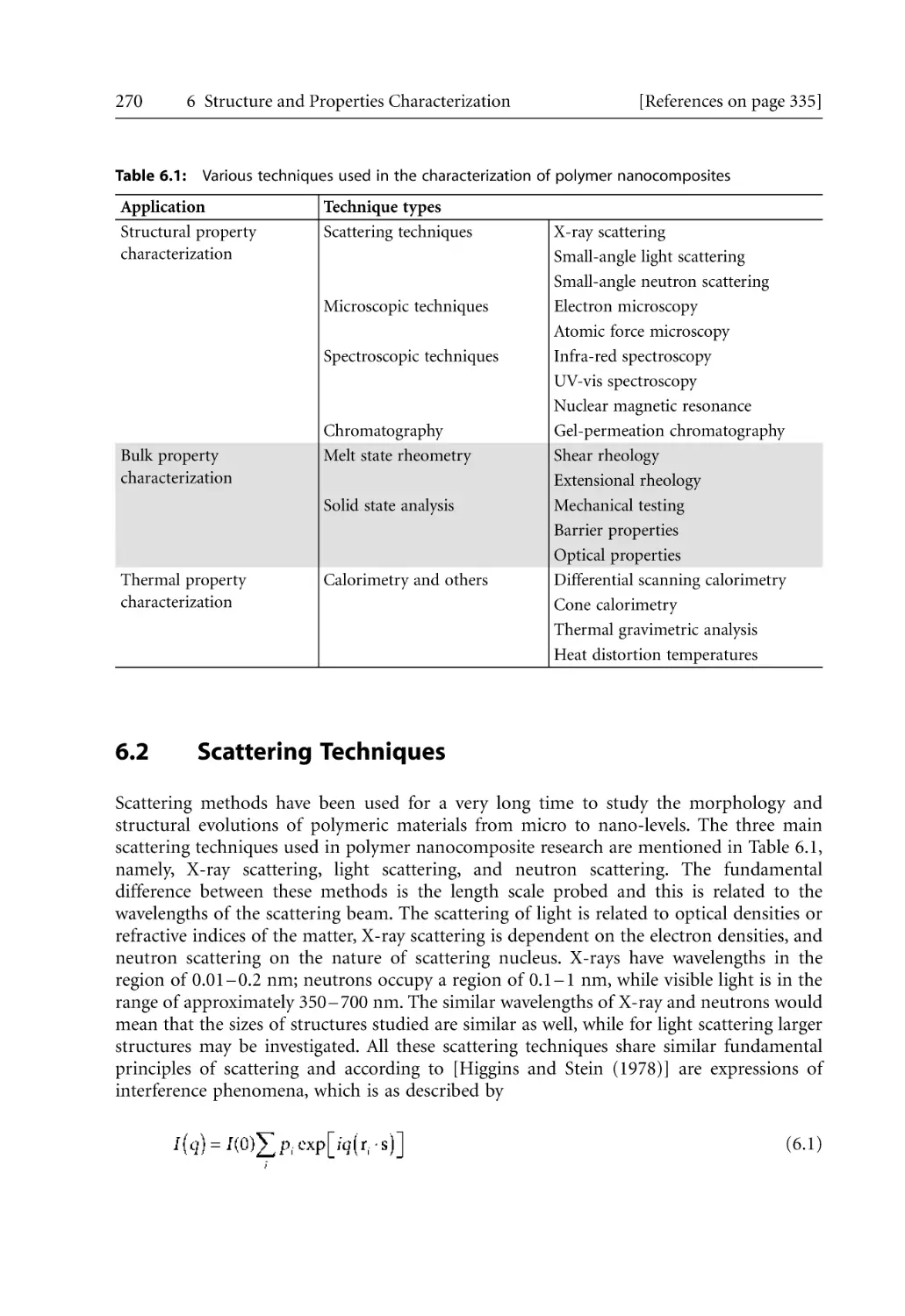
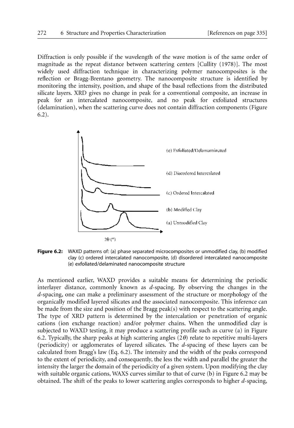
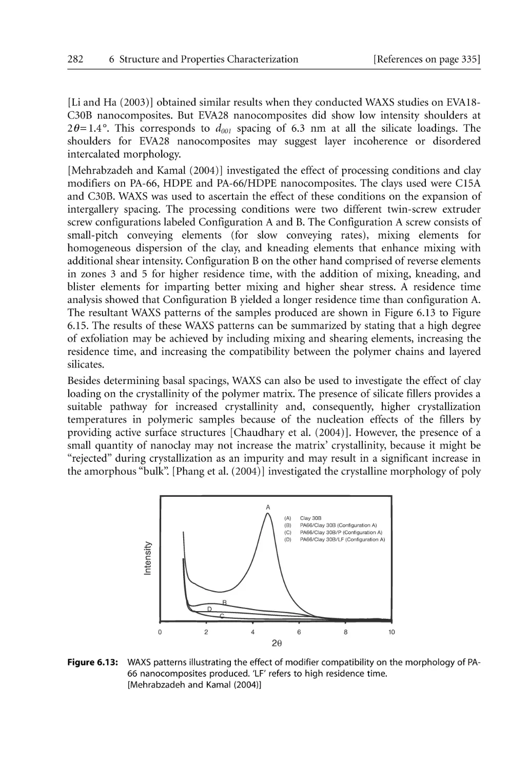
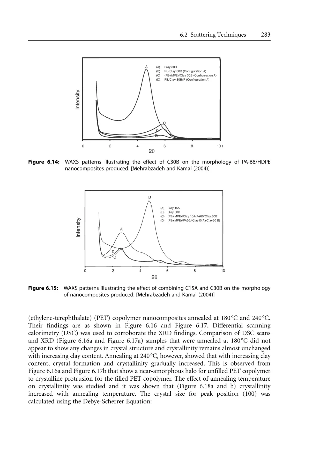
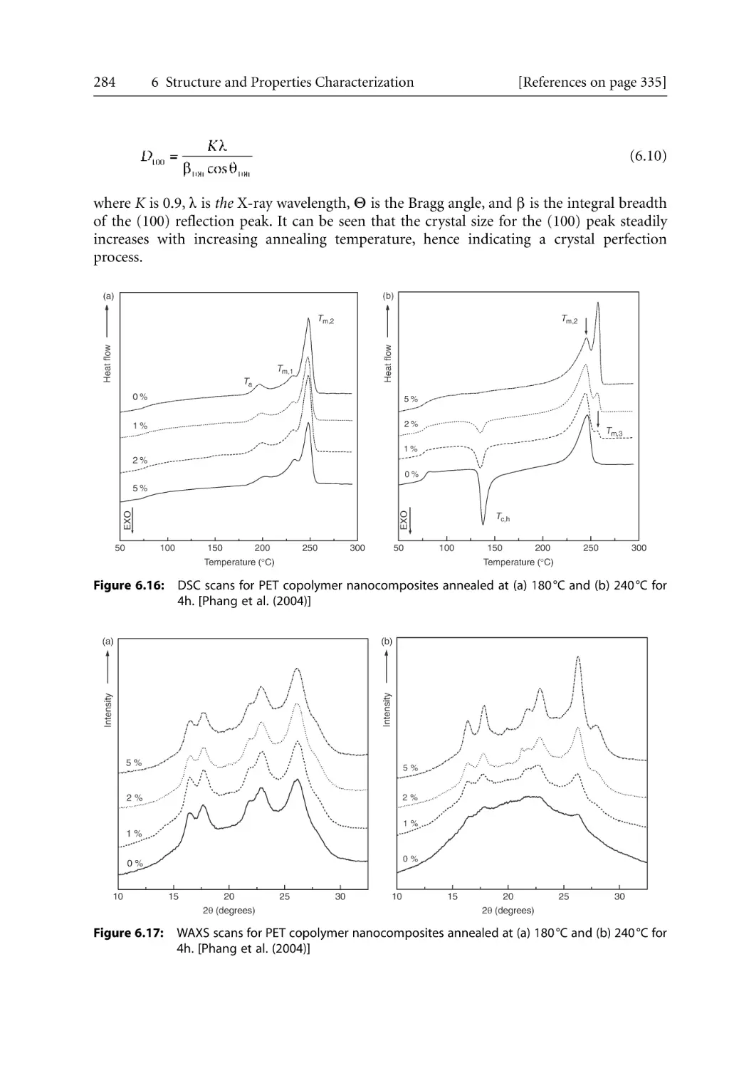
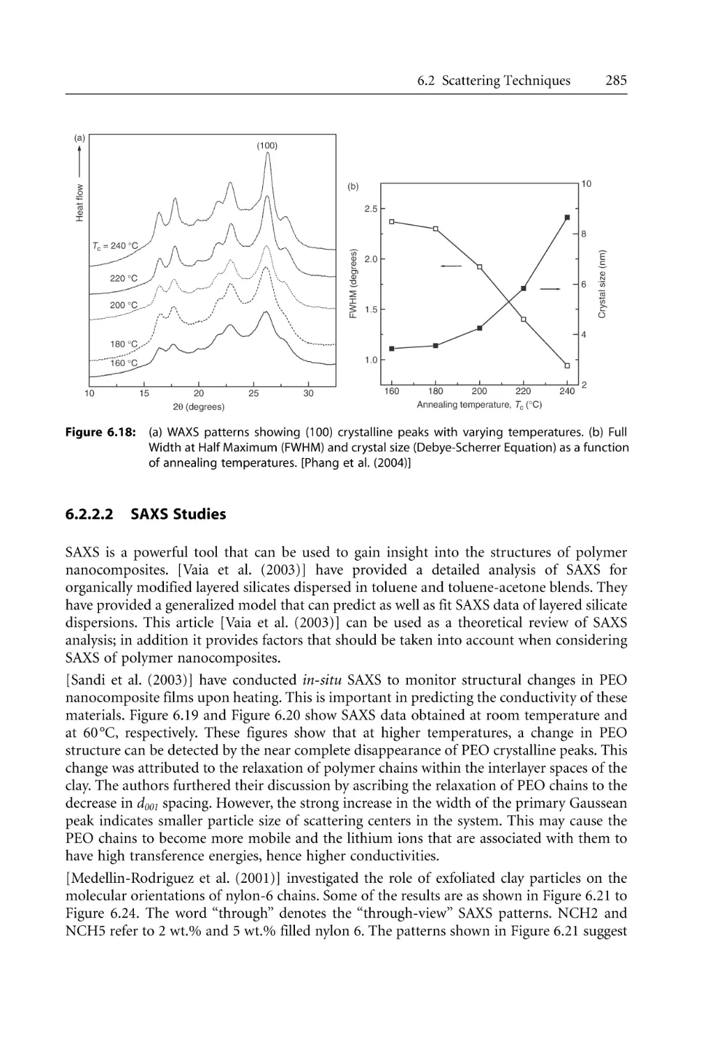
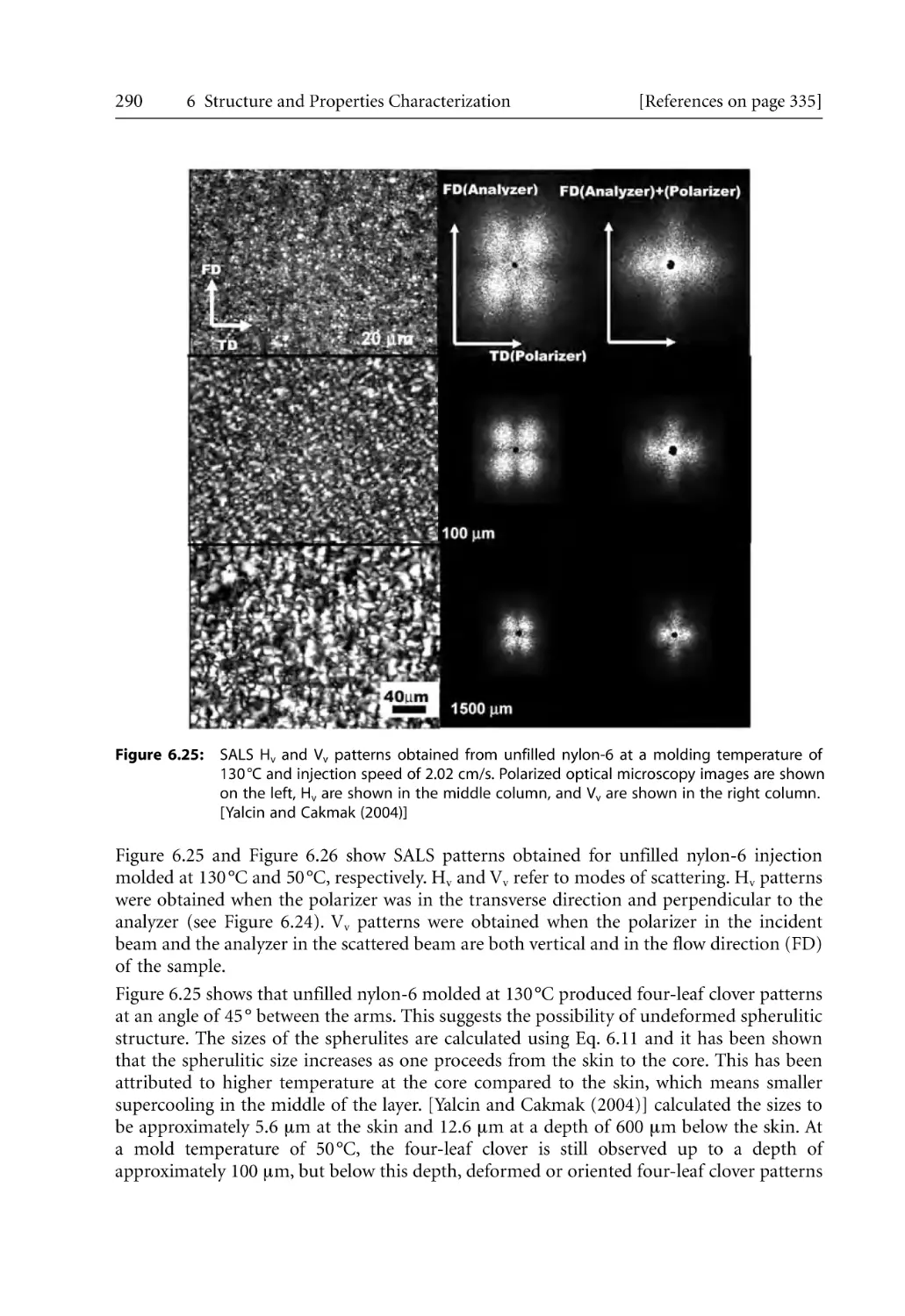
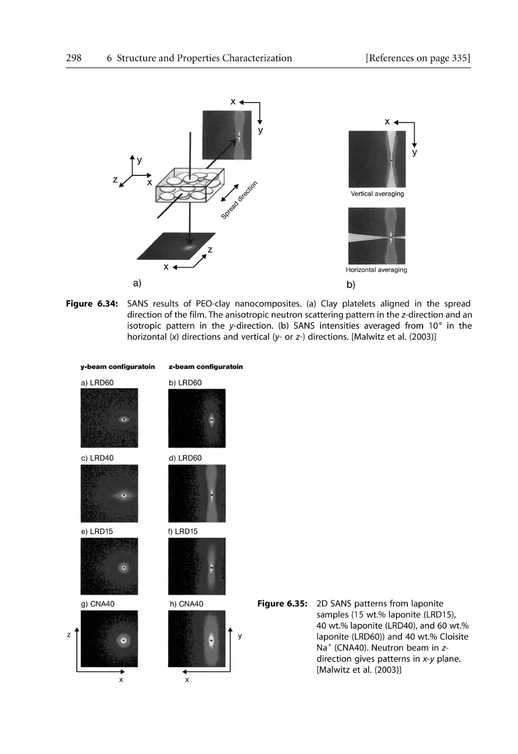
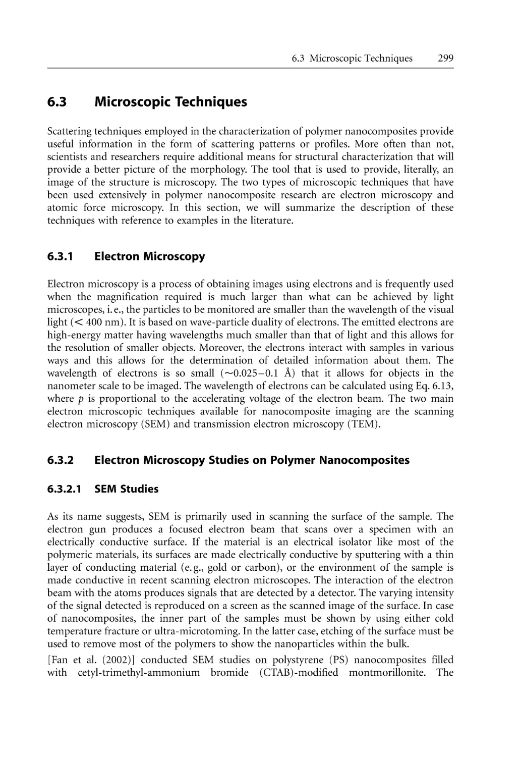
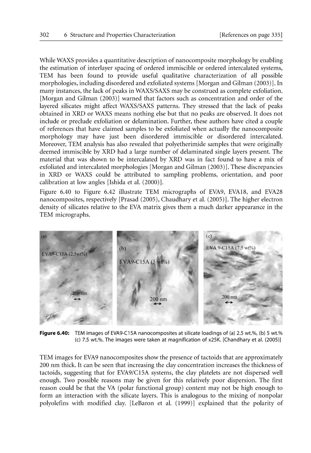
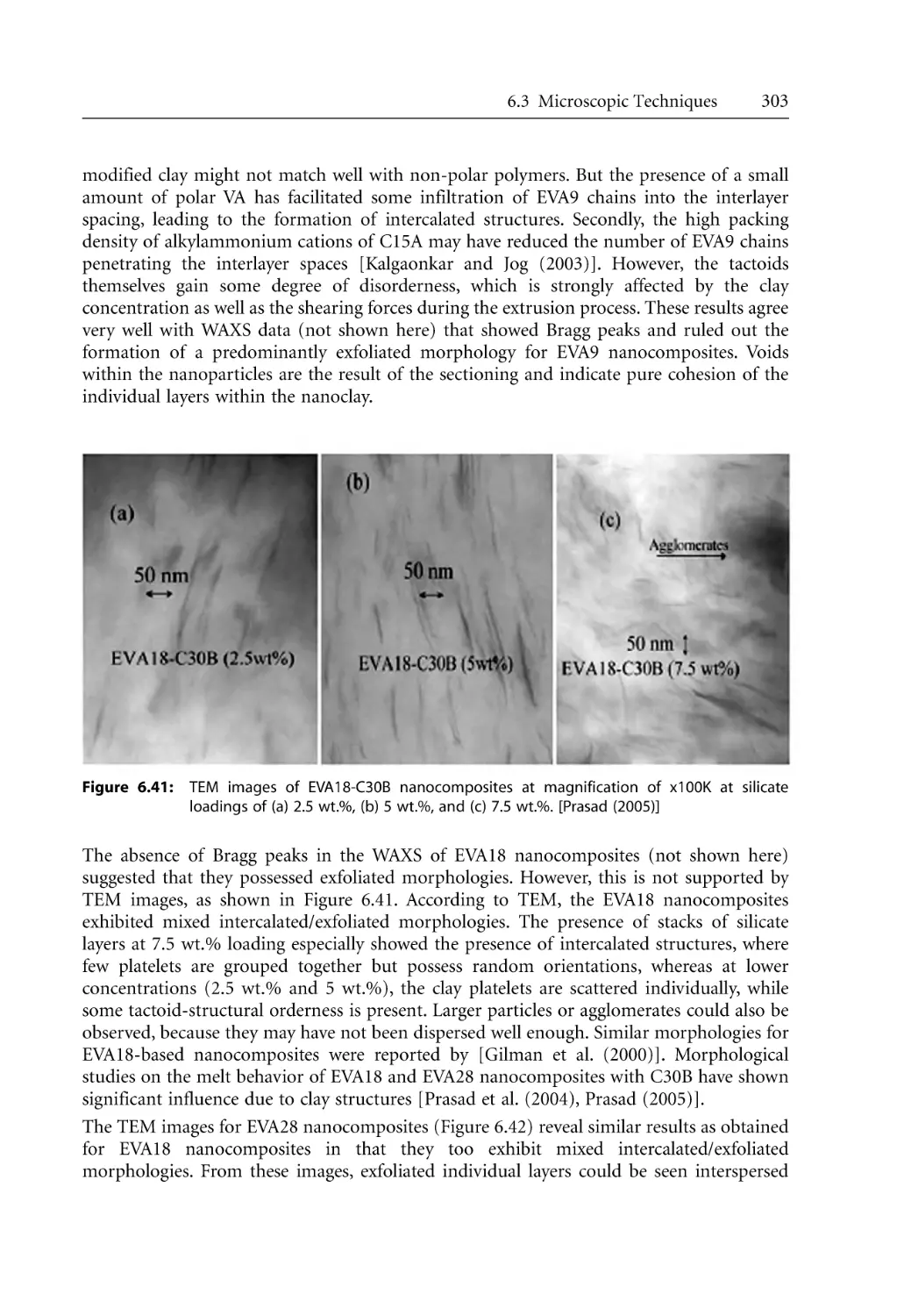
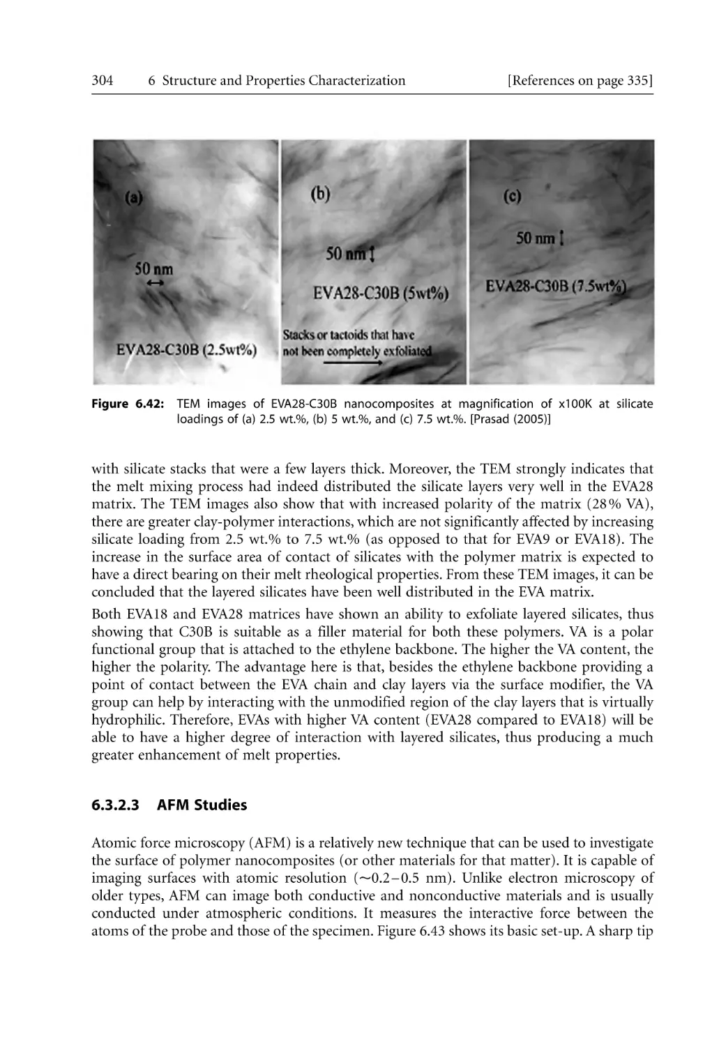
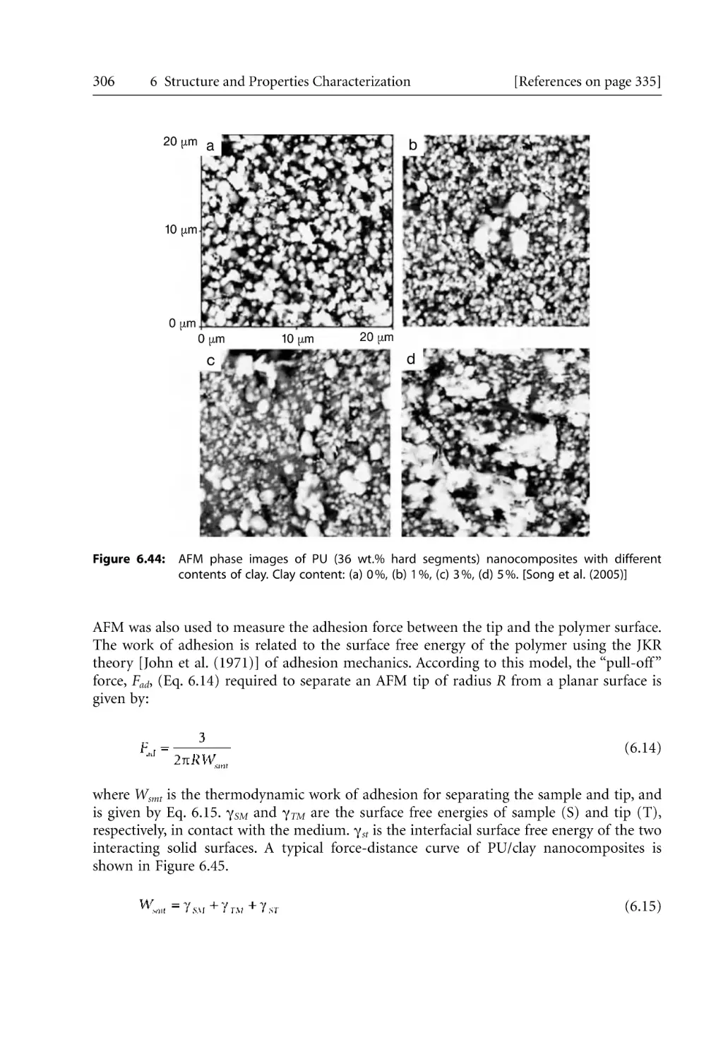
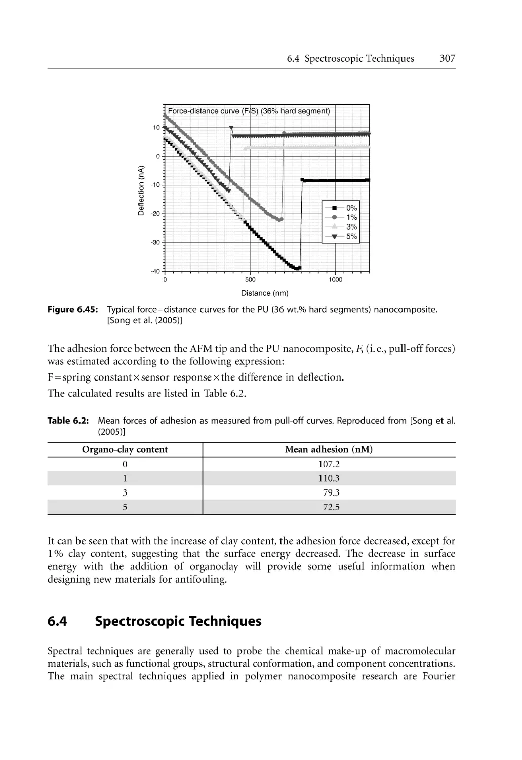
6 Structure and Properties Characterization. . . . . . . . . . . . . . . . . . . . . . . . . . . . . . . . .
6.1 Introduction . . . . . . . . . . . . . . . . . . . . . . . . . . . . . . . . . . . . . . . . . . . . . . . . . . . . . .
6.2 Scattering Techniques. . . . . . . . . . . . . . . . . . . . . . . . . . . . . . . . . . . . . . . . . . . . . . .
6.2.1 X-ray Scattering Fundamentals . . . . . . . . . . . . . . . . . . . . . . . . . . . . . . . . .
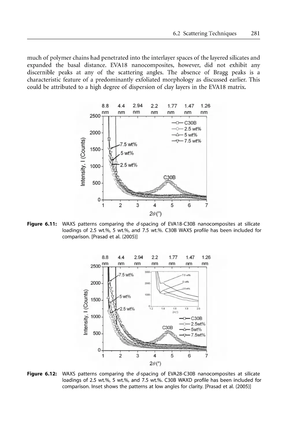
6.2.2 X-Ray Scattering Studies on Polymer Nanocomposites . . . . . . . . . . . . .
6.2.2.1 WAXS Studies . . . . . . . . . . . . . . . . . . . . . . . . . . . . . . . . . . . . . . .
6.2.2.2 SAXS Studies . . . . . . . . . . . . . . . . . . . . . . . . . . . . . . . . . . . . . . . .
6.2.3 Small Angle Light Scattering (SALS) . . . . . . . . . . . . . . . . . . . . . . . . . . . .
6.2.3.1 SALS Techniques . . . . . . . . . . . . . . . . . . . . . . . . . . . . . . . . . . . . .
6.2.3.2 SALS Studies on Polymer Nanocomposites . . . . . . . . . . . . . . .
6.2.4 Small Angle Neutron Scattering (SANS) . . . . . . . . . . . . . . . . . . . . . . . . .
6.2.4.1 SANS Techniques . . . . . . . . . . . . . . . . . . . . . . . . . . . . . . . . . . . .
6.2.4.2 SANS Studies on Polymer Nanocomposites . . . . . . . . . . . . . . .
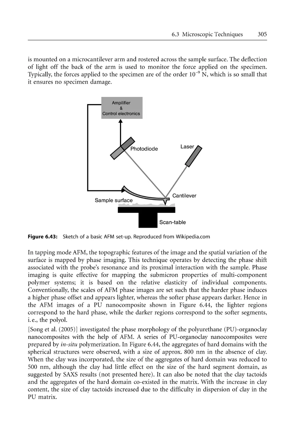
6.3 Microscopic Techniques . . . . . . . . . . . . . . . . . . . . . . . . . . . . . . . . . . . . . . . . . . . . .
6.3.1 Electron Microscopy . . . . . . . . . . . . . . . . . . . . . . . . . . . . . . . . . . . . . . . . .
6.3.2 Electron Microscopy Studies on Polymer Nanocomposites . . . . . . . . . .
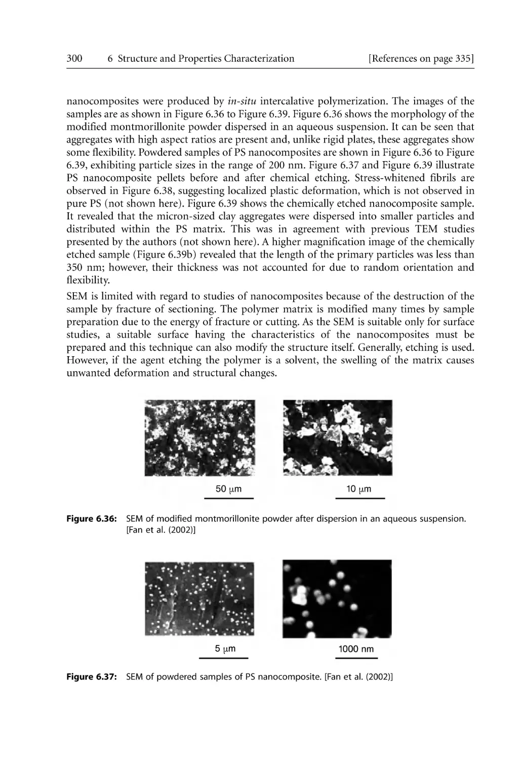
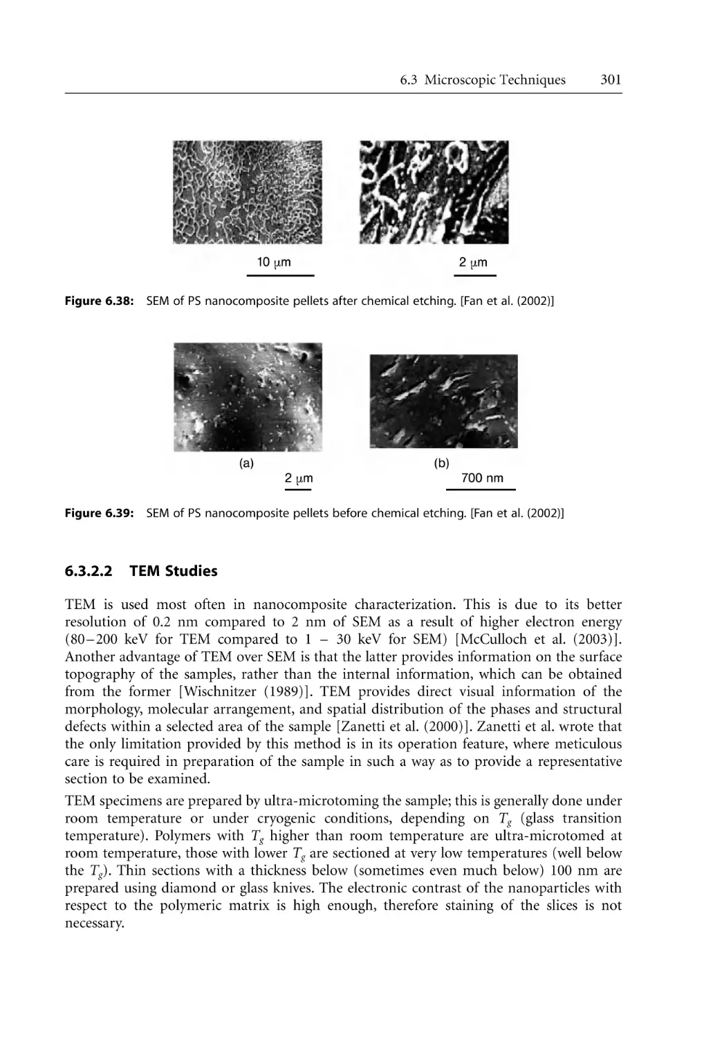
6.3.2.1 SEM Studies. . . . . . . . . . . . . . . . . . . . . . . . . . . . . . . . . . . . . . . . .
6.3.2.2 TEM Studies . . . . . . . . . . . . . . . . . . . . . . . . . . . . . . . . . . . . . . . .
6.3.2.3 AFM Studies . . . . . . . . . . . . . . . . . . . . . . . . . . . . . . . . . . . . . . . .
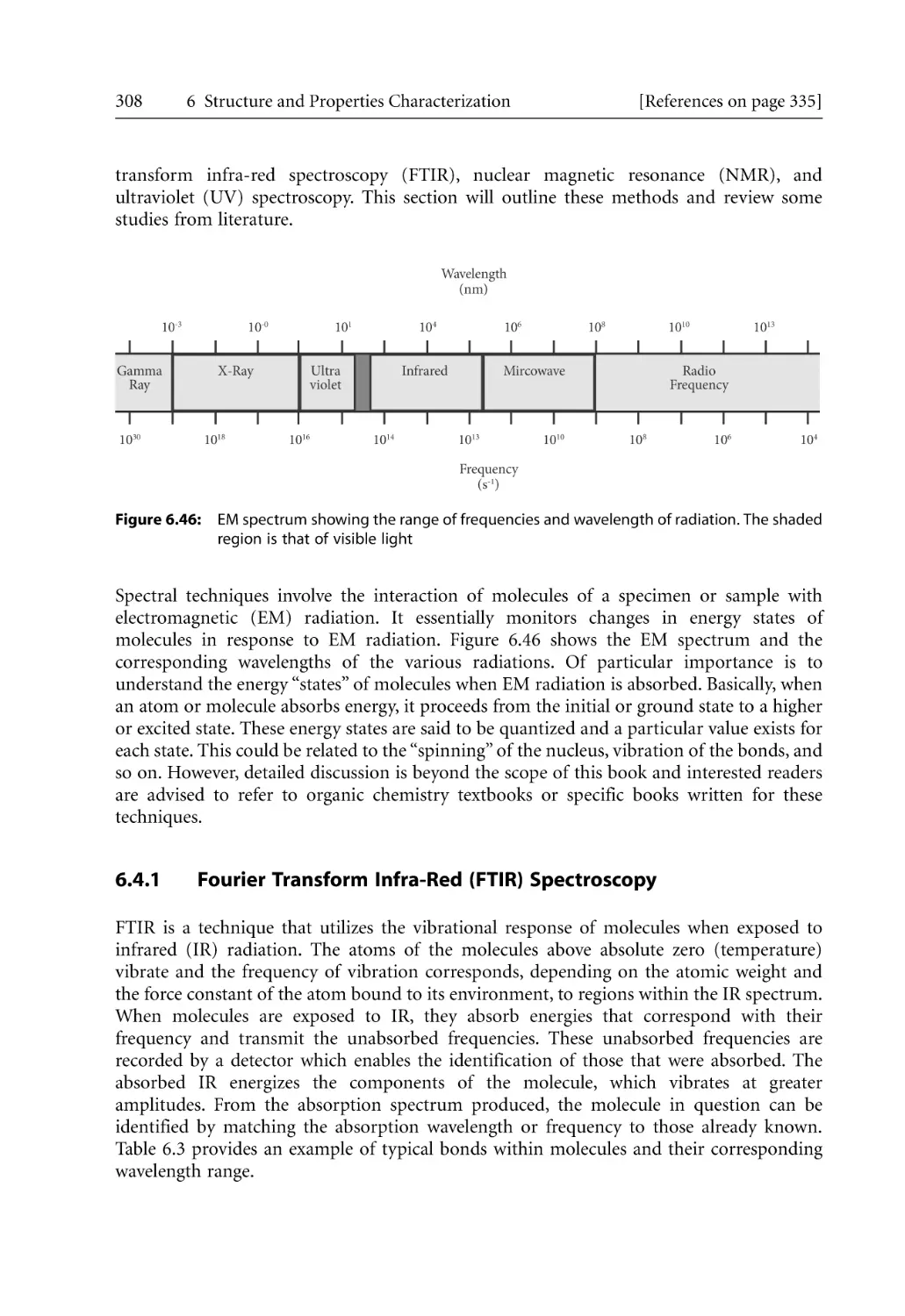
6.4 Spectroscopic Techniques . . . . . . . . . . . . . . . . . . . . . . . . . . . . . . . . . . . . . . . . . . .
6.4.1 Fourier Transform Infra-Red (FTIR) Spectroscopy . . . . . . . . . . . . . . . .
6.4.2 Nuclear Magnetic Resonance (NMR). . . . . . . . . . . . . . . . . . . . . . . . . . . .
6.4.3 Ultraviolet (UV) Spectroscopy . . . . . . . . . . . . . . . . . . . . . . . . . . . . . . . . .
6.5 Chromatography. . . . . . . . . . . . . . . . . . . . . . . . . . . . . . . . . . . . . . . . . . . . . . . . . . .
6.6 Solid-State Characterization: Mechanical Testing . . . . . . . . . . . . . . . . . . . . . . . .
6.6.1 Mechanical Testing . . . . . . . . . . . . . . . . . . . . . . . . . . . . . . . . . . . . . . . . . . .
6.6.2 Dynamic Mechanical Analysis (DMA) . . . . . . . . . . . . . . . . . . . . . . . . . . .
6.7 Thermal Characterization . . . . . . . . . . . . . . . . . . . . . . . . . . . . . . . . . . . . . . . . . . .
6.7.1 Differential Scanning Calorimetry (DSC) . . . . . . . . . . . . . . . . . . . . . . . .
6.7.2 Thermal Gravimetric Analysis (TGA) . . . . . . . . . . . . . . . . . . . . . . . . . . .
6.7.3 Heat Distortion Temperature (HDT). . . . . . . . . . . . . . . . . . . . . . . . . . . .
6.7.4 Cone Calorimetry. . . . . . . . . . . . . . . . . . . . . . . . . . . . . . . . . . . . . . . . . . . .

269
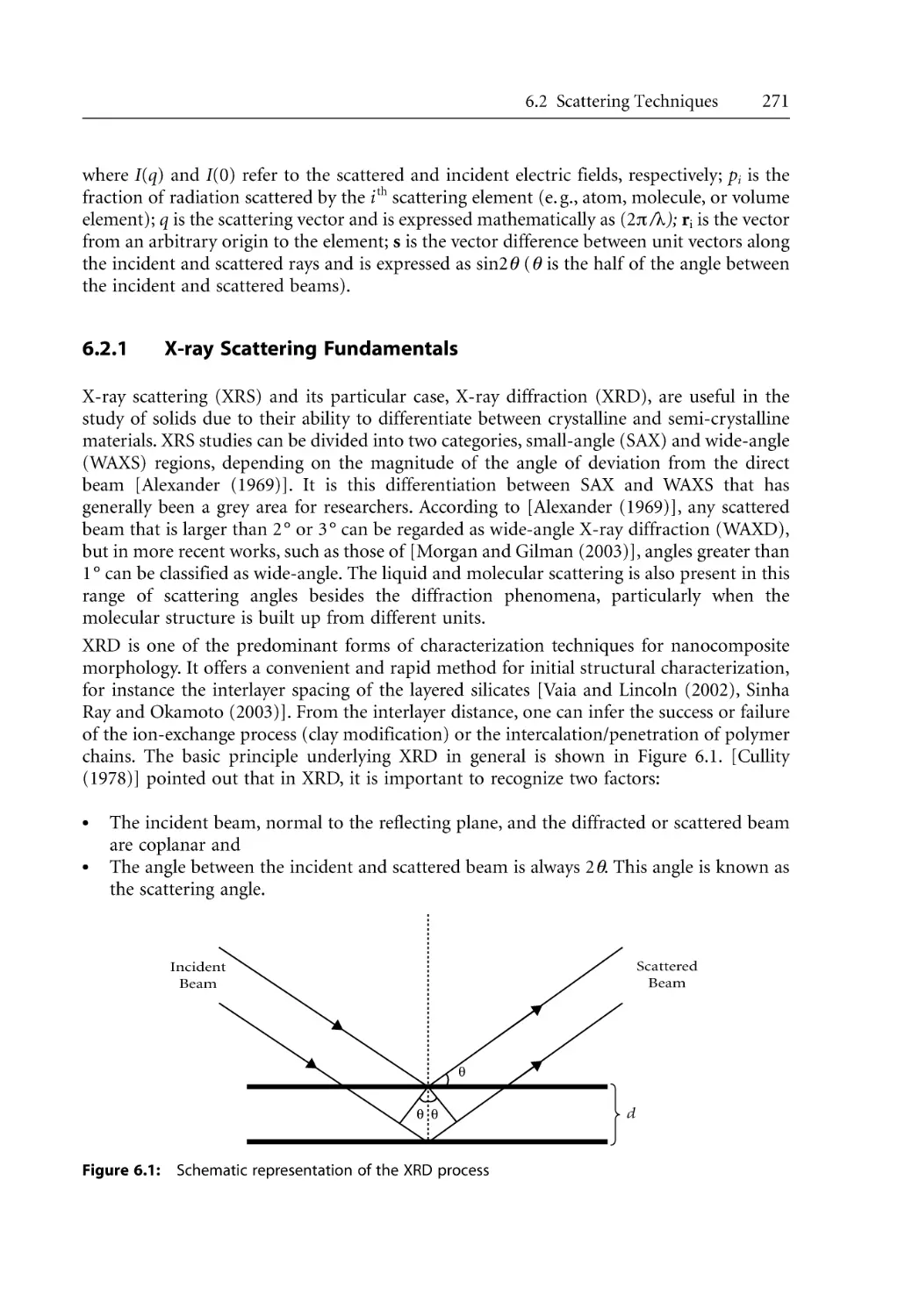
269
270
271
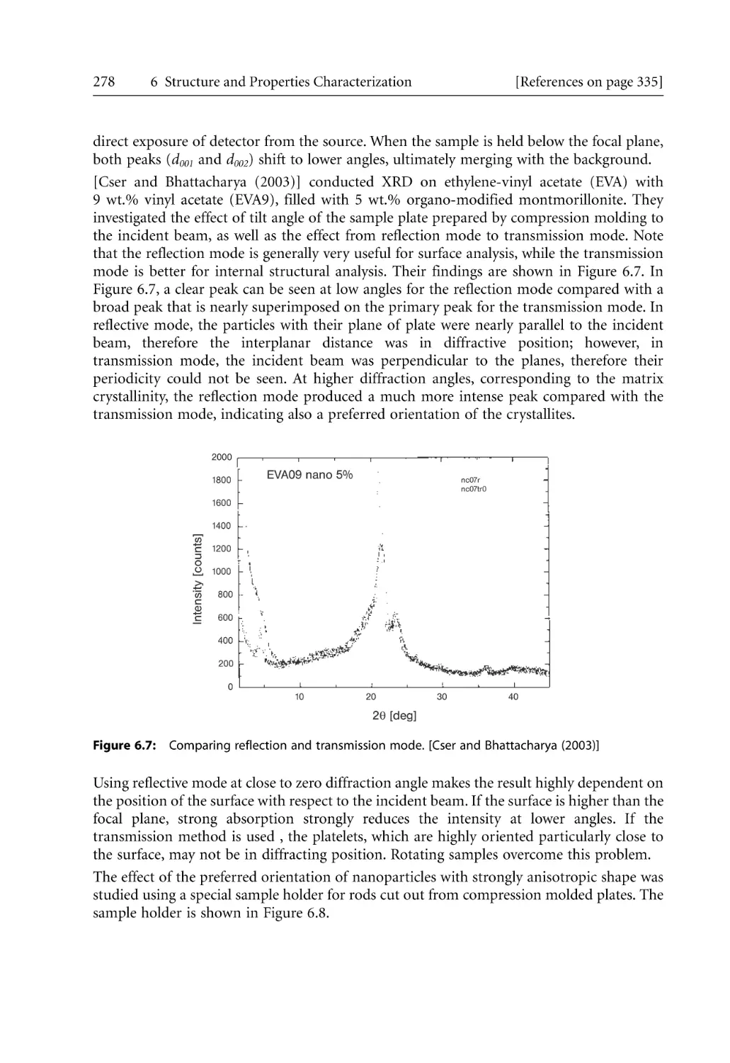
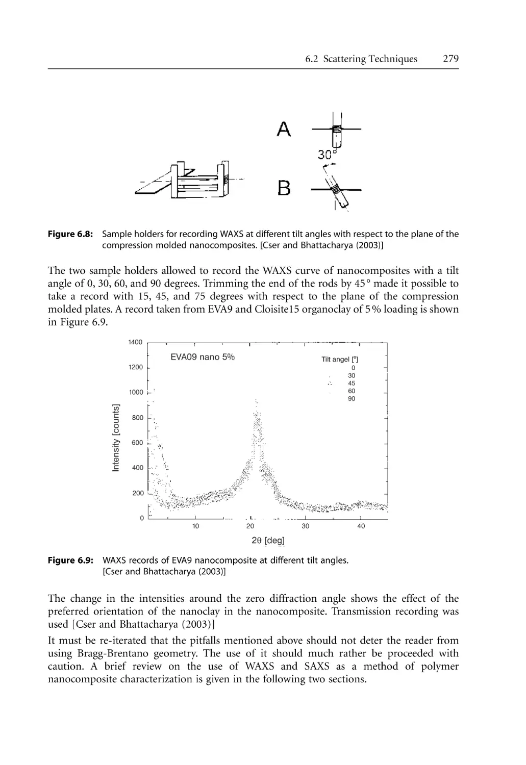
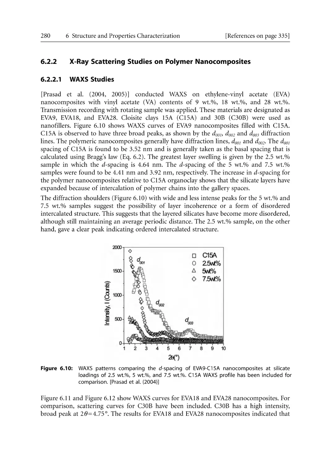
280
280
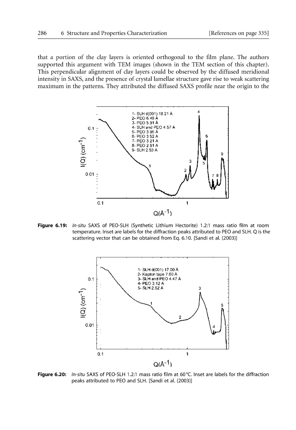
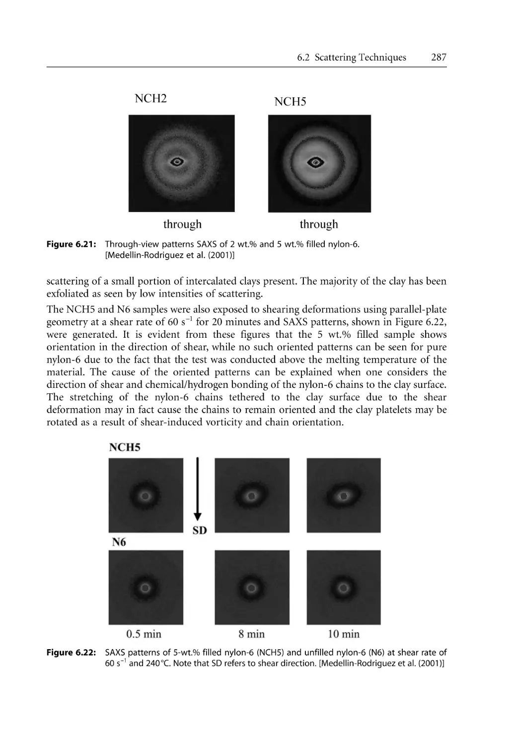
285
288
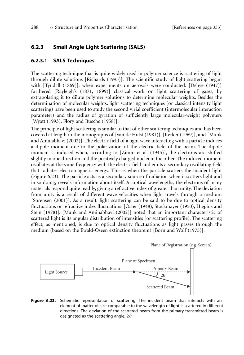
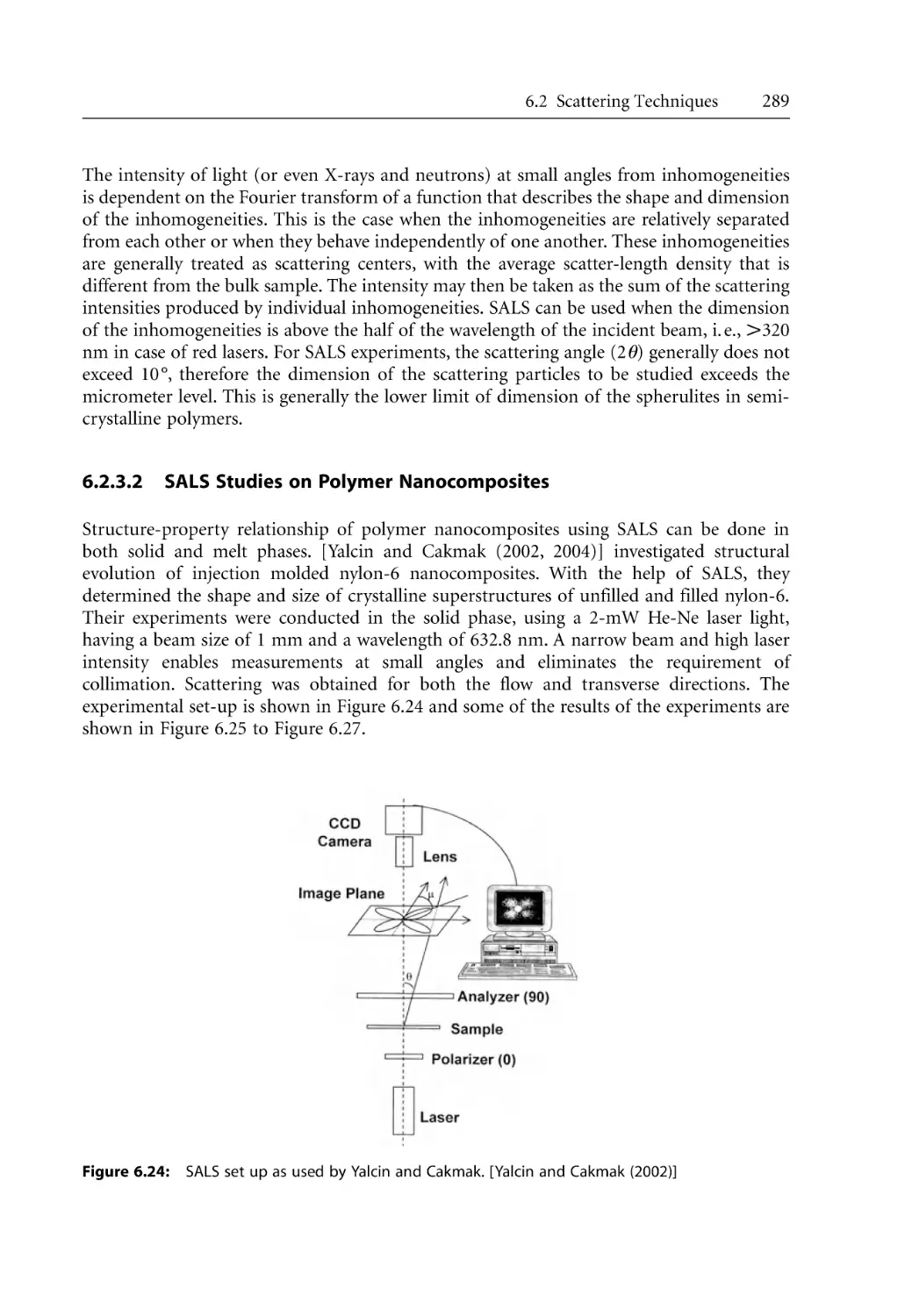
288
289
297
297
297
299
299
299
299
301
304
307
308
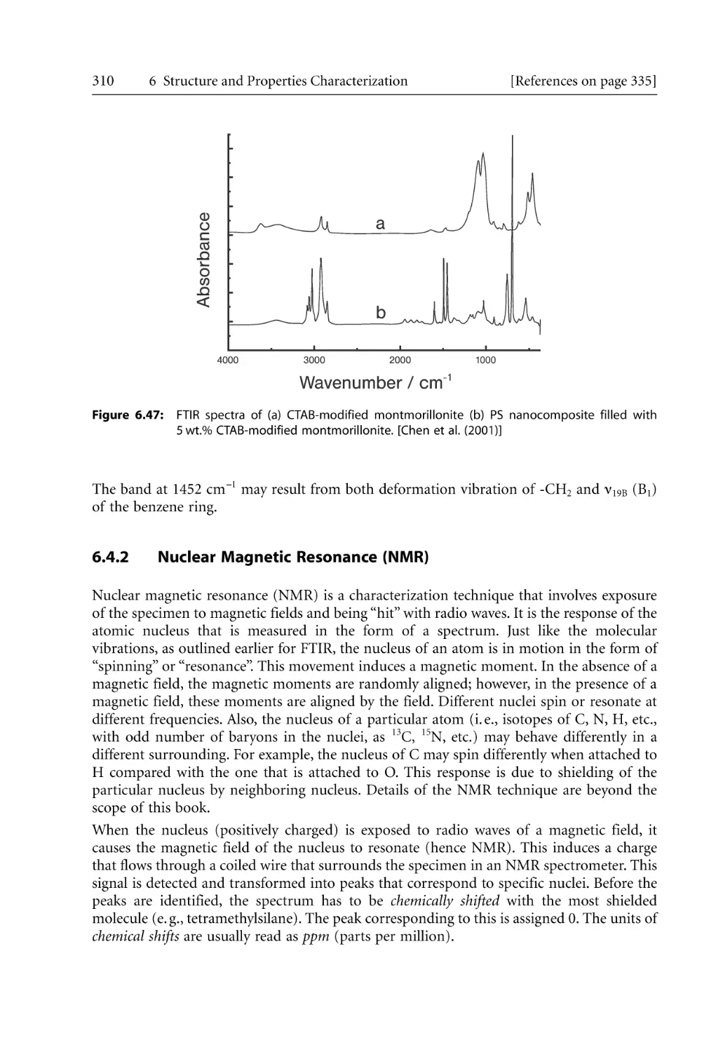
310
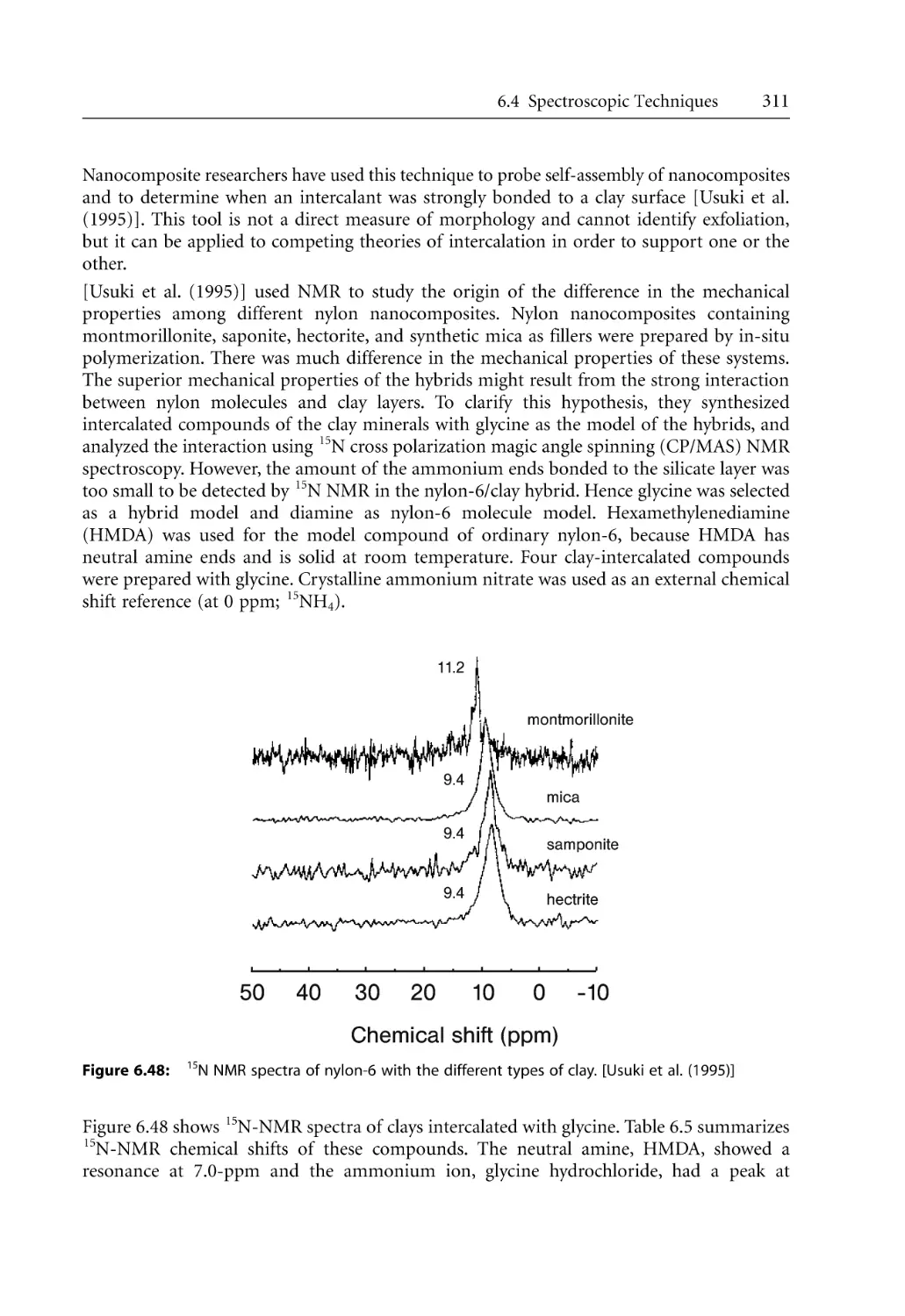
312
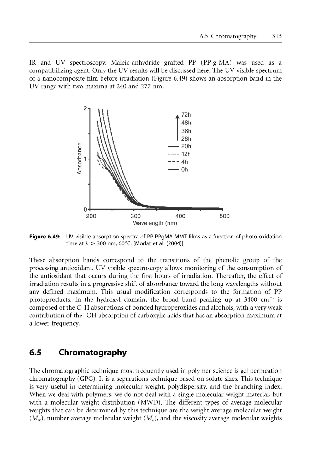
313
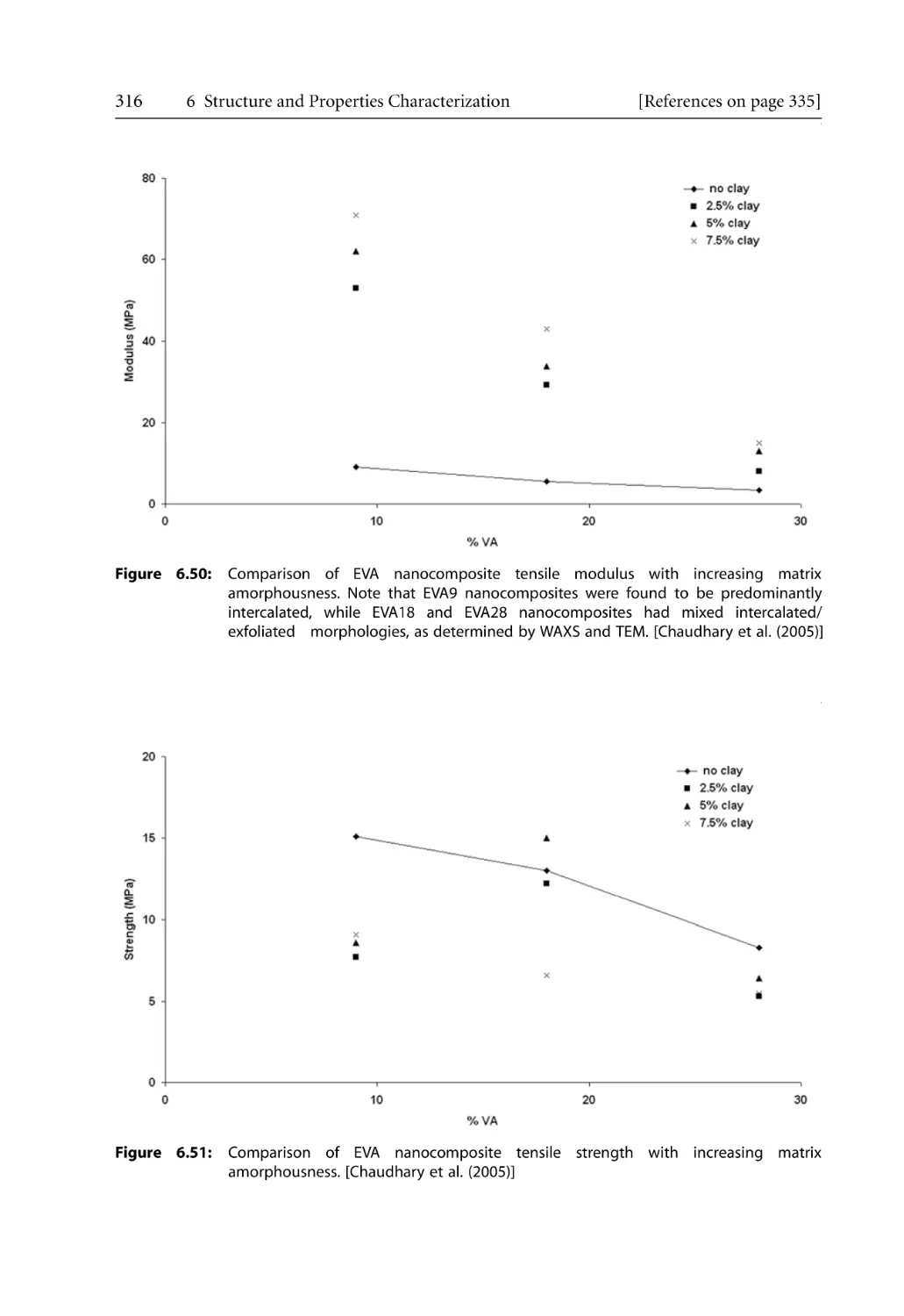
315
315
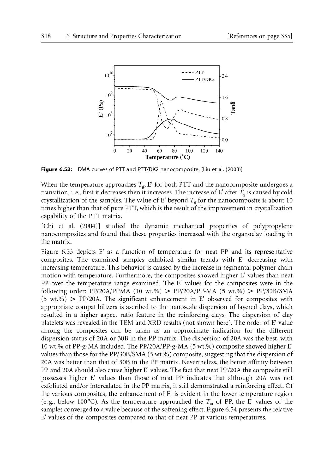
317
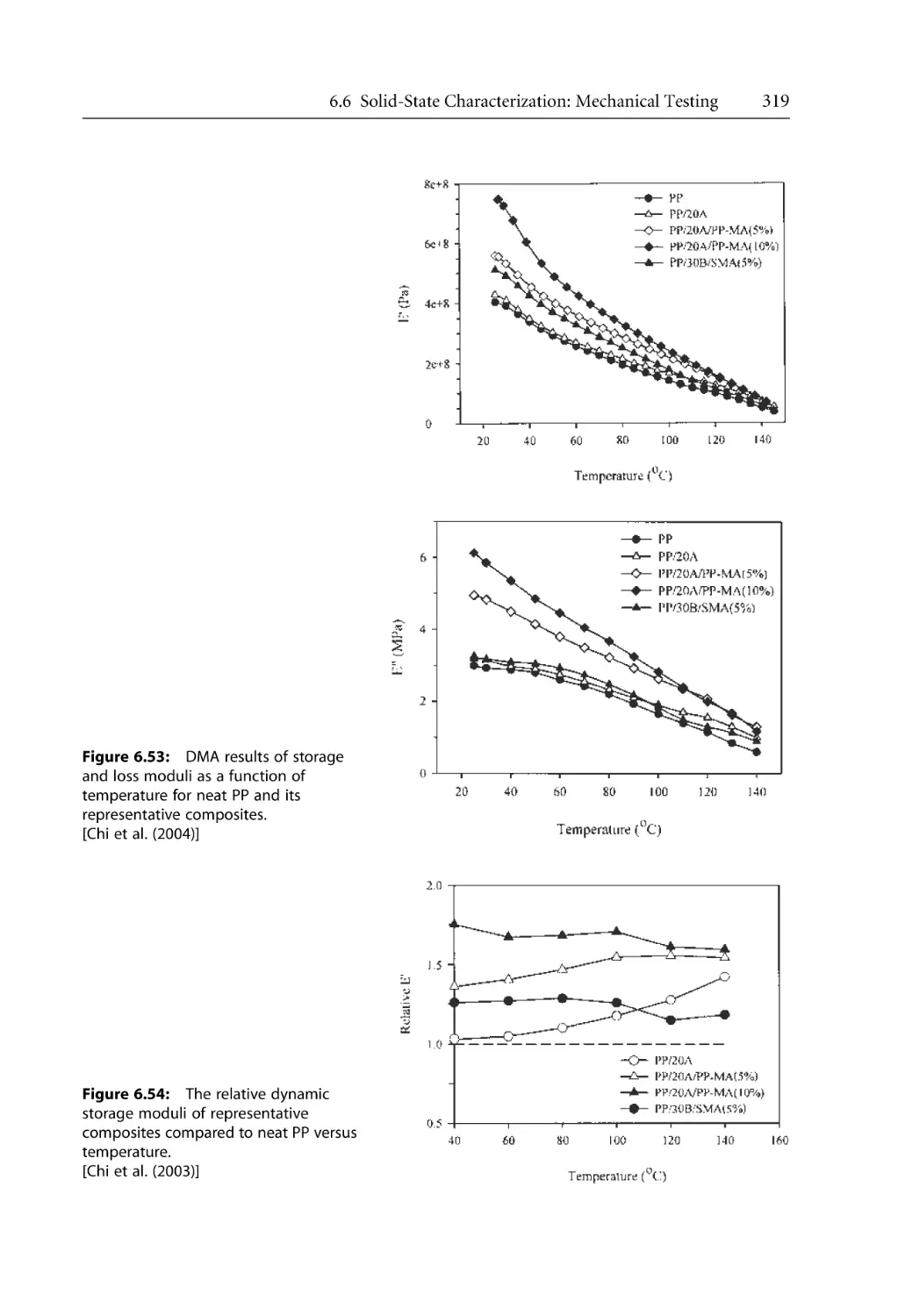
320
320
325
329
331

5.3
5.4
5.5

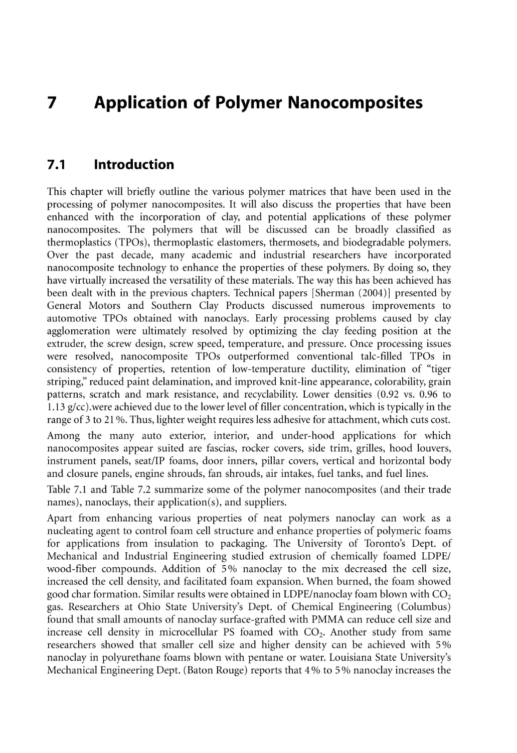
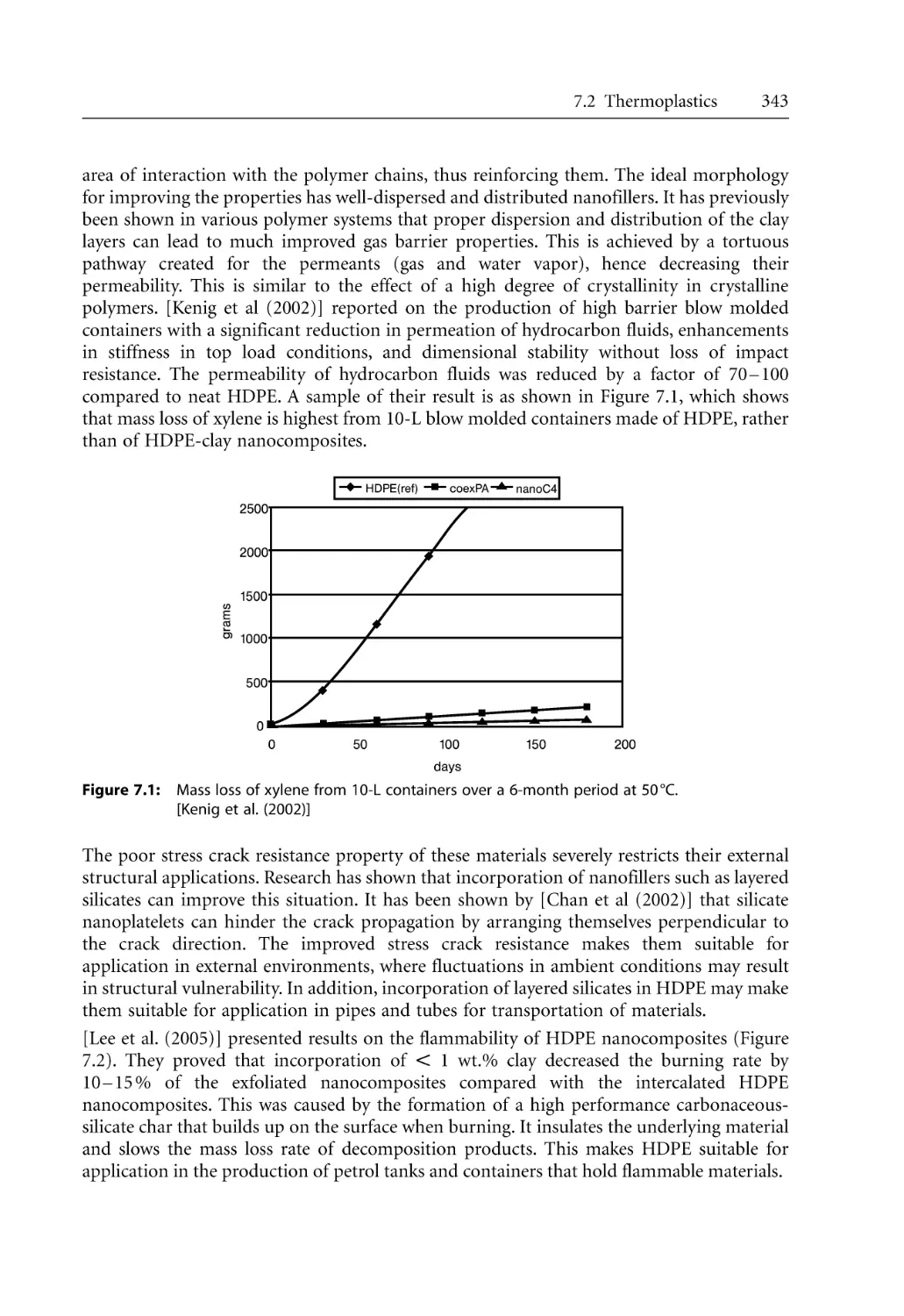
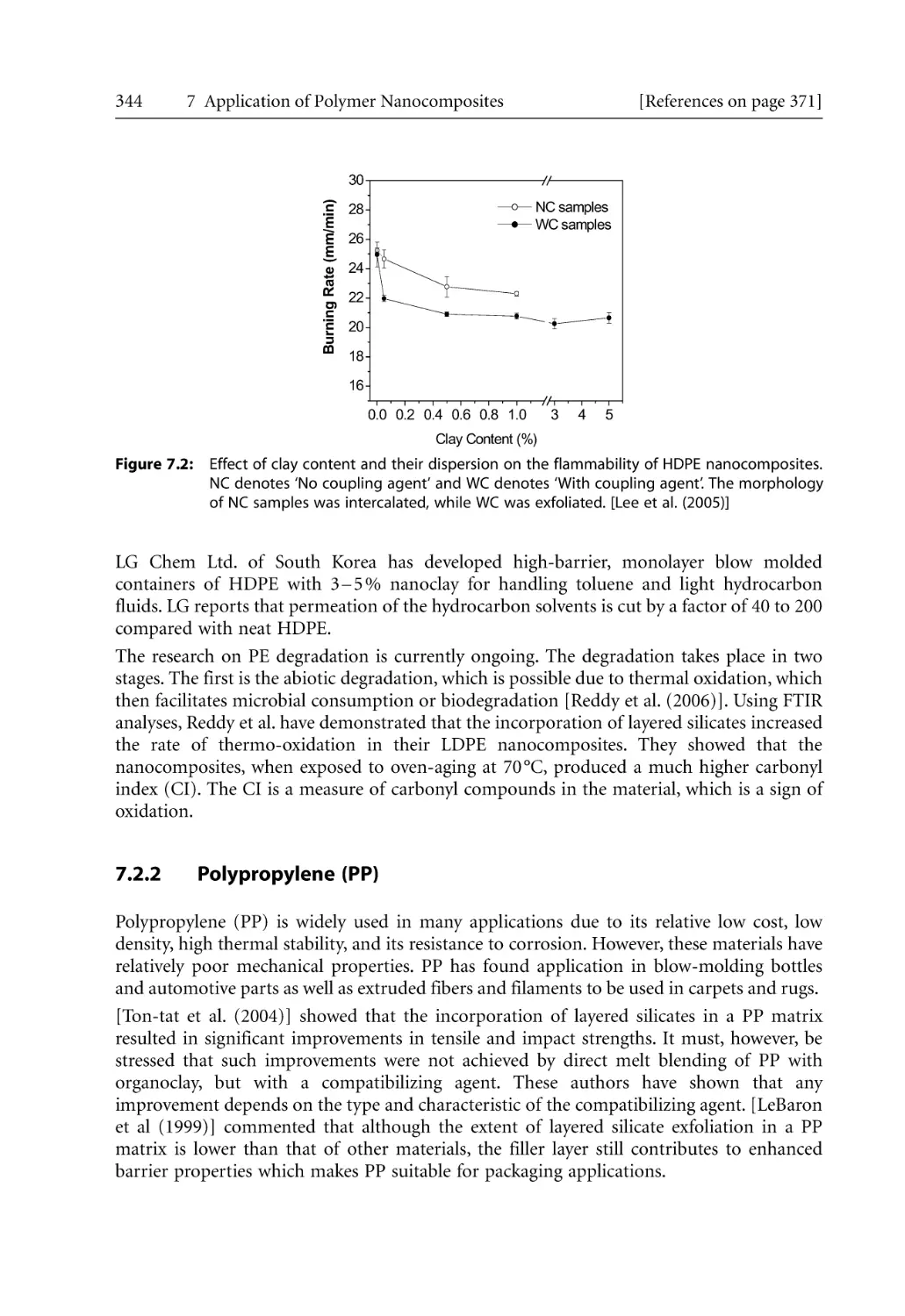
7 Application of Polymer Nanocomposites . . . . . . . . . . . . . . . . . . . . . . . . . . . . . . . . . . 339
7.1 Introduction . . . . . . . . . . . . . . . . . . . . . . . . . . . . . . . . . . . . . . . . . . . . . . . . . . . . . . 339
7.2 Thermoplastics . . . . . . . . . . . . . . . . . . . . . . . . . . . . . . . . . . . . . . . . . . . . . . . . . . . . 341

Inhalt

7.2.1 Polyethylene (PE) . . . . . . . . . . . . . . . . . . . . . . . . . . . . . . . . . . . . . . . . . . . .
7.2.2 Polypropylene (PP) . . . . . . . . . . . . . . . . . . . . . . . . . . . . . . . . . . . . . . . . . .
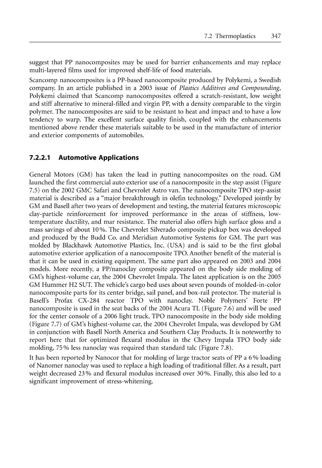
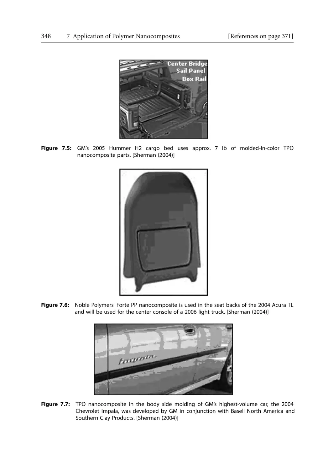
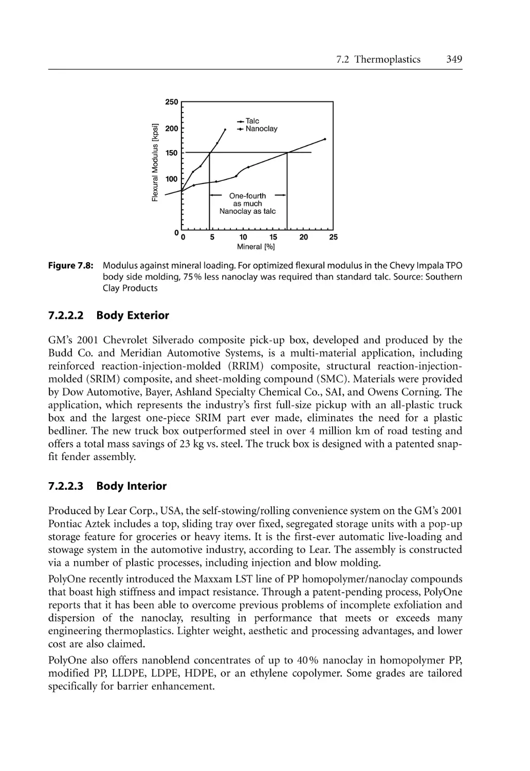
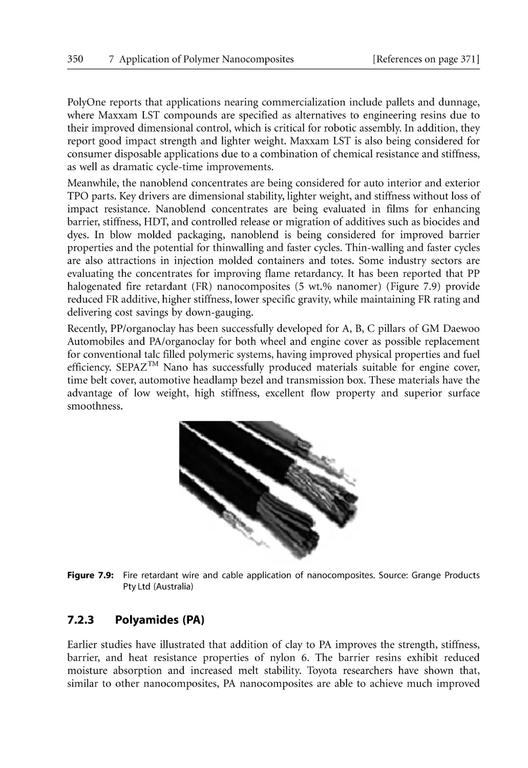
7.2.2.1 Automotive Applications . . . . . . . . . . . . . . . . . . . . . . . . . . . . . .
7.2.2.2 Body Exterior. . . . . . . . . . . . . . . . . . . . . . . . . . . . . . . . . . . . . . . .
7.2.2.3 Body Interior . . . . . . . . . . . . . . . . . . . . . . . . . . . . . . . . . . . . . . . .
7.2.3 Polyamides (PA) . . . . . . . . . . . . . . . . . . . . . . . . . . . . . . . . . . . . . . . . . . . . .
7.2.4 Ethylene-Vinyl Acetate (EVA) . . . . . . . . . . . . . . . . . . . . . . . . . . . . . . . . . .
7.2.5 Polyethylene Terephthalate (PET). . . . . . . . . . . . . . . . . . . . . . . . . . . . . . .
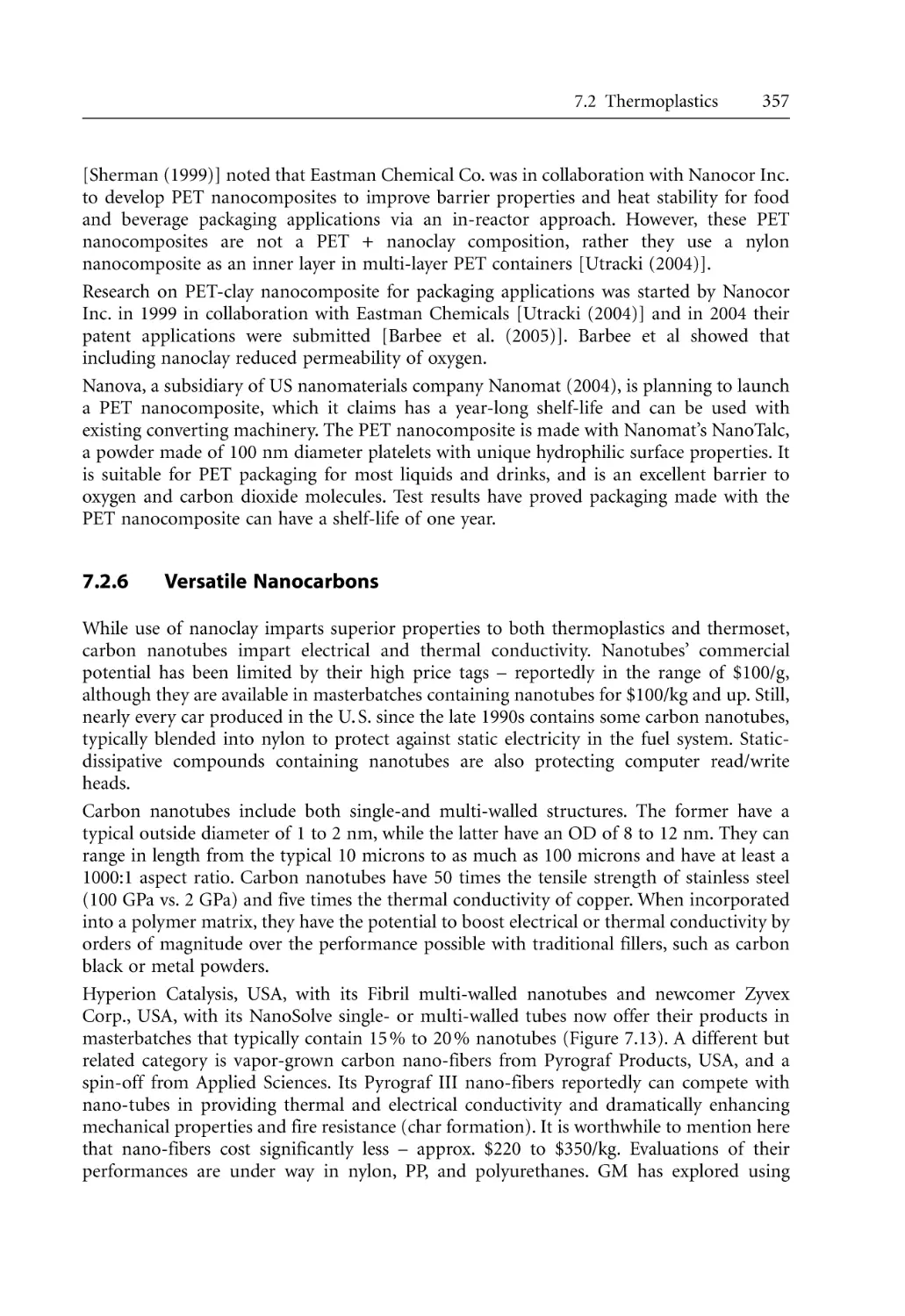
7.2.6 Versatile Nanocarbons . . . . . . . . . . . . . . . . . . . . . . . . . . . . . . . . . . . . . . . .
7.3 Thermosets . . . . . . . . . . . . . . . . . . . . . . . . . . . . . . . . . . . . . . . . . . . . . . . . . . . . . . .
7.3.1 Polyurethanes (PU) . . . . . . . . . . . . . . . . . . . . . . . . . . . . . . . . . . . . . . . . . .
7.3.2 Epoxies . . . . . . . . . . . . . . . . . . . . . . . . . . . . . . . . . . . . . . . . . . . . . . . . . . . .
7.3.3 Unsaturated Polyesters (UPE) . . . . . . . . . . . . . . . . . . . . . . . . . . . . . . . . . .
7.3.4 Phenolics . . . . . . . . . . . . . . . . . . . . . . . . . . . . . . . . . . . . . . . . . . . . . . . . . . .
7.4 Biodegradable Polymers. . . . . . . . . . . . . . . . . . . . . . . . . . . . . . . . . . . . . . . . . . . . .
7.4.1 Polylactide (PLA) and its Nanocomposites . . . . . . . . . . . . . . . . . . . . . . .
7.4.2 Polycaprolactone (PCL) . . . . . . . . . . . . . . . . . . . . . . . . . . . . . . . . . . . . . . .
7.4.3 Starch. . . . . . . . . . . . . . . . . . . . . . . . . . . . . . . . . . . . . . . . . . . . . . . . . . . . . .
7.5 Final Comments . . . . . . . . . . . . . . . . . . . . . . . . . . . . . . . . . . . . . . . . . . . . . . . . . . .

XIII

342
344
347
349
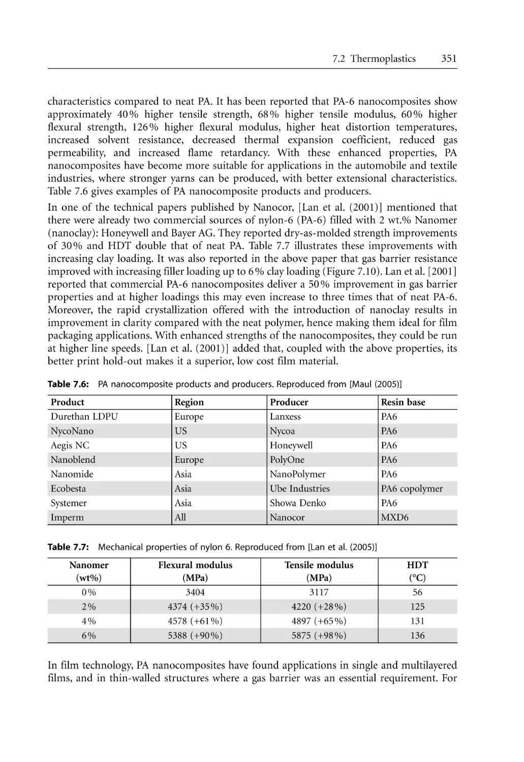
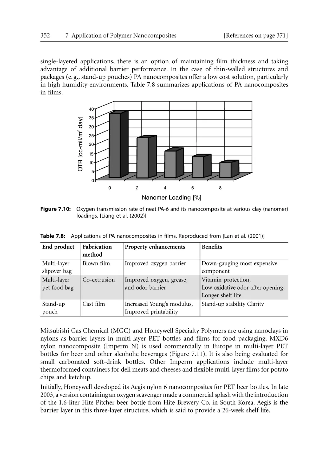
350
351
355
357
358
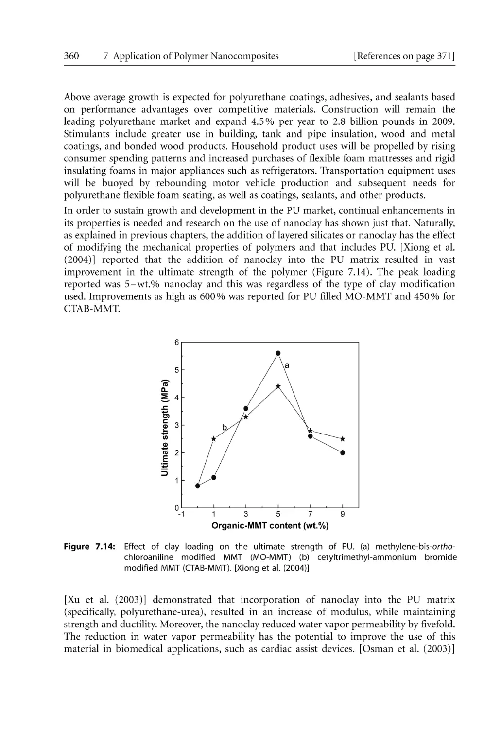
359
360
362
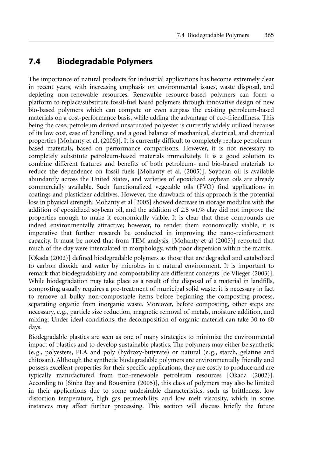
364
364
366
367
368
369
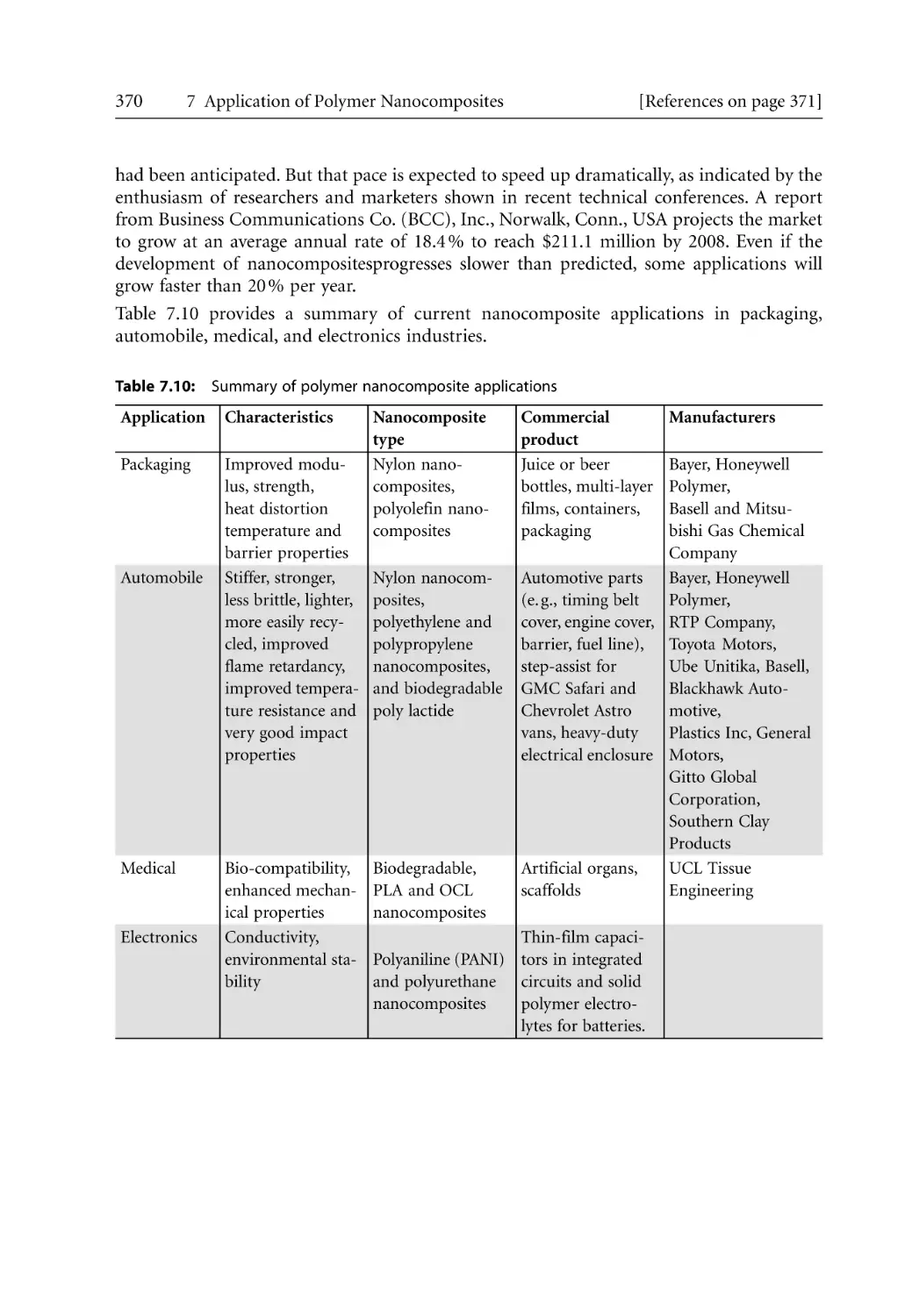
370

Introduction

Nanotechnology has created a key revolution in the 21 st century exploiting the new
properties, phenomena and functionalities exhibited by matters when dealt at the level of
few nanometers as opposed to hundred nanometers and above. Nanoscale materials are
already recognized as unique because they produce qualitatively new behavior when
compared with their macroscopic counterparts. It is understood that when the domain size
within the materials becomes comparable with the physical length scale, such as segments of
a polymer macromolecule, the expected physical phenomena and the response to any
external disturbance do not follow the established principles. The scientific phenomena
occurring in nanoscale systems can only be explained by new theoretical principles and by
experimental techniques which are in the process of development. The challenge is to
manage the transition region where nanoscale phenomena are evolving from microscopic
and macroscopic bulk properties. The linking of molecular interaction to nanostructures to
bulk properties is a challenge, both scientifically and technologically. Another challenge is to
understand how deliberate tailoring at the nanoscale can produce novel and controlled
functionalities of these materials.

1.1

Polymer Nanocomposites

Nanocomposite technology is a newly developed field, in which nanofillers are added to a
polymer to reinforce and provide novel characteristics. Nanocomposite technology is
applicable to a wide range of polymers from thermoplastics and thermosets to elastomers.
Two decades ago, researchers from Toyota Central Research and Development produced a
new group of polymer-clay complexes or composites, which was aptly called polymerlayered silicate nanocomposites or polymer nanocomposites. Today, there is a variety of
nanofillers used in nanocomposites. Cost and availability continue to change as the field is
relatively new and several of these fillers are still being developed. The most common types
of fillers are natural clays (mined, refined and treated), synthetic clays, nanostructured
silicas, nanoceramics, nanocalcium carbonates and nanotubes (carbon based). The
properties conferred by the nanoparticles to the polymer matrix are remarkable. The
property enhancements have allowed these materials to commercially compete with
traditional materials. [Collister (2001)] lists some of the property improvements as:
Efficient reinforcement with minimal loss in ductility and impact strength,
Thermal endurance,
Flame retardance,
Improved liquid and gas barrier properties,
Improved abrasion resistance,
Reduced shrinkage and residual loss, and
Altered electrical, electronic and optical properties.

1 Introduction

[References on page 4]

Layered silicates (clay) dispersed as reinforcement in an engineering polymer matrix is one
of the most important forms of polymer nanocomposites. Amongst all the potential
nanocomposites precursors, those based on clay and layered silicate have been more widely
studied, probably because the starting clay materials are easily available and because their
intercalation chemistry has been studied for a long time [Van Olphen (1977)]. The
commercial use of intercalated clay for industrial application goes back many decades. Early
application reported during the 1930s – to the 1950s for intercalated clay was paper coating
(hydrophilic application) and lubricants, grease and oil based mud (hydrophobic
application). First use of polymer/clay composites using onium compounds to intercalate
montmorillonite clay MMT was reported in 1950 [Carter et al. (1950)]. Polymerization of
vinyl monomer in the presence of intercalated MMT was later reported [Blumslein (1961)].
The manufacture of LDPE/clay hybrid (1:1) was reported in a patent by Nahin and
Bucklund in 1963 [Nahin and Backlund (1963)]. Fujiwara and Sakamoto filed a patent
application for ammonium salt intercalated clays for hydrophobic matrices in 1976
[Fujiwara and Sakamoto (1976)]. Organo-clay was added to the monomer before
polymerization of PA. The first patent by the Toyota group for in situ polymerization of
styrene and other vinyl monomers in the presence of clay was obtained in 1984. The first US
patent for PA6/clay nanocomposites, where clay was used in small quantities, was obtained
in 1989 [Usuki et al. (1989)].
Few nanocomposites have been produced commercially, but their potential applications
have fuelled frenzy in the research arena [Zerda and Lesser (2001)]. For example, in the US,
research funding for the National Nanotechnology Initiative in 2003 alone exceeded US
$ 600 Million.

1.2

Commercial Potential

The first commercial nanocomposite product was based on the Toyota process of in-reactor
processing of caprolactum and montmorillonite to produce a polyamide 6-clay product.
This product has been commercially available for several years. General motor uses a large
amount of polyolefin-based clay nanocomposites for some of its vehicle parts. Mitsubishi
Gas Chemical Company [Sherman (2004)] offers nylon-6 based nanocomposites with
highly improved gas barrier properties compared to unfilled nylon-6, ethylene-vinyl alcohol
(EVOH) and polypropylene (PP).
Although the potential for the commercial application of nanocomposites is enormous, the
actual application has been occurring at a very slow pace. In many instances, the
performance of the developed nanocomposites did not meet the expectations, e. g., not very
significant increase in their useful properties or drop in mechanical or optical properties.
While it has been shown that the modulus or stiffness of thermoplastics can be increased by
adding very small amounts of clay, in many cases it comes with the disadvantage of
decreasing strength. Addition of clay to polymers, such as nylon-6 and EVA, increases the
gas barrier properties but their optical properties may be compromised. Performance not
yet meeting expectations may not be due to any inherent flaws in the concept of
nanocomposite technology. It is rather due to the fact that the developments in this new area

1.3 Book Structure

are still in their infant stage. The production of nanocomposite is very system-specific. The
understanding of the chemistry of filler modification, the physics and thermodynamics of
filler dispersion, and the interplay of filler-polymer at the interphase is crucial to the
development of customized nanocomposites.
Currently, work in the nanocomposite area is mostly confined to the laboratory stage, where
their structure and properties are evaluated at a fundamental level, new methods of
intercalation and exfoliation are developed, and new applications are explored. While the
science of nanocomposites has been extensively explored, with a good understanding of the
theories and principles behind the development of these novel materials, there is limited
literature that can act as a comprehensive guide, especially in the areas of rheology,
processing and applications. This book aims to fill this gap by providing a critical review of
recent work on clay based nanocomposite rheology, current processing practice of these
materials and current and future applications.

1.3

Book Structure

The chapters are organized to present the fundamentals of preparation, synthesis, rheology,
processing, properties characterization, and application of nanocomposites. In Chapter 2, an
introduction to the structure of layered silicate and the morphology of polymer layered
silicate nanocomposites are presented. A brief discussion on the various techniques used for
nanocomposite preparation and synthesis is given. Methods used to produce intercalated
and exfoliated clay structures using major thermoplastic and thermoset polymers,
elastomers, and natural and biodegradable polymers are provided. Chapter 3 presents the
fundamental issues in nanocomposite synthesis and the kinetics of polymer intercalation
and exfoliation with some discussion of the modeling of melt intercalation kinetics. This
chapter also includes a section discussing the crystalline properties and crystallization
kinetics of polymer nanocomposites.
Rheology of polymer/clay nanocomposites is presented in Chapter 4. A summary of the
recent study on the rheology of nanocomposites is listed in terms of key findings reported
in literature. Steady and dynamic shear rheology and extensional rheology of various
nanocomposites are described and the relationship with developed morphology is
discussed. Current literature on the steady shear and viscoelastic models for these materials
are presented. Modeling study also includes extensional theology, although this area has not
yet received much attention.
Chapter 5 presents recent work on the processing of polymer nanocomposites. Key polymer
processes, such as extrusion, injection molding, blow molding and foaming are included in
this chapter. Until now, only a limited amount of work has been done on the processing of
these materials, except for mixing and extrusion. A brief description of the barrier and
mechanical properties of the injection molded parts has been given here.
Structures and properties characterization are presented in Chapter 6. In the last decade, a
significant amount of research has been carried out to understand the structure,
morphology and physical, thermal, mechanical, optical and gas barrier properties of these
materials. Scattering techniques presented include X-ray, light scattering and neutron

1 Introduction

[References on page 4]

scattering. Microscopic techniques including scanning electron, transmission electron and
atomic force microscopy, spectroscopic techniques, such as FTIR, NMR and UV methods
for the analysis of nanocomposites are discussed. Solid state characterization includes
different types of mechanical testing. The chapter concludes with the thermal
characterization in terms of DSC, TGA and heat distortion temperature.
Chapter 7 deals with the application of polymer nanocomposites in product development.
A number of applications are reported for products in automotive and packaging industries.
The book concludes with a list of possible applications for these materials in the coming
decade.

1.4

References

Blumstein, A. (1961), “Etudes des polymerization en couche adsorbee”, Bull. Soc. Chim., 899-905
Carter, L. W., Hendricks, J. G., Bolley, D. S., (1950), “Elastomer Reinforced with a Modified Clay”, US
Patent 2,531,396
Collister, J., (2001), “Commercialisation of polymer nanocomposites”, In: “Polymer nanocomposites,
synthesis characterisation and modelling”, Krishnamoorti, R., and Vaia, R. A., (Eds.), American
Chemical Society, 7-14.
Fujiwara, S., and Sakamoto, T., (1976), “Method for manufacturing a clay-polyamide composite”, Japan
Kokai, 109,998, to Unitika Ltd.
Nahin, P. G., and Backlund, P. S., “Organoclay-polyolefin compositions”, US Pat., 3,084,117,
(02.04.1963), Appl. 04.04.1961, to Union Oil Co.
Sherman, L. M., (2004), “Chasing Nanocomposites”, Plastics Technology Online, www.ptonline.com,
(downloaded on 08/19/2006)
Usuki, A., Mizutani, T., Fukushima, Y., Fujimoto, M., Fukomori, K., Kojima, Y., Sato, N., Kurauchi, T.,
and Kamikaito, O., “Composite Materials Containing a Layered Silicate”, United States Patent
4,889,885, (Dec 26, 1989)
Van Olphen, H., (1977), “An introduction to clay colloid chemistry”, John Wiley and Sons, New York
Zerda, A. S., and Lesser, A. J., (2001), “Intercalated clay nanocomposites: morphology, mechanics and
fracture behaviour”, J. Polym. Sci. Part B, 39 (11), 1139-1146

Preparation and Synthesis

2.1

Polymer Nanocomposites

The current scientific and engineering knowledge is rather expansive and so is the number
of published literature. The literature on these materials covers a wide area and deals with
various aspects, such as rheology, processing, and modeling of polymer-clay interactions.
This chapter will provide a literature survey on layered silicates as nanofillers, the
preparation and synthesis of polymer-layered silicate nanocomposites, and the various
polymeric materials used in the synthesis of these nanocomposites. There are many other
features of non-clay based nanocomposites, including those having particular optical
properties, e. g., specific UV or IR absorption [Shelm and Schmidt (2003)].
The addition of fillers as reinforcements for polymers has been practiced for many years. As
mentioned earlier, these fillers provide enhancements to the properties of the unfilled
polymers. Clay minerals have long been used as performance enhancing fillers. For instance,
the incorporation of clay (metakaolin) in plasticized PVC has been reported to improve
electrical properties [Rothon (1999)]. Polymer/clay complexes have also been used by soil
scientists in many soil processes, such as mineral cycling and weathering, profile
development and aggregate stabilization [Theng (1982)]. In drilling-fluid technology, nonionic polymers are introduced to clay suspensions to reduce swelling [Olphen (1963)].
Over the last couple of decades, it has been widely reported that with the incorporation of
clay minerals, polymer property enhancements could be augmented further if these fillers
are dispersed in nanometer scales rather than the usual micro- or larger scales. Clay minerals
render themselves quite easily to this dispersion. The dispersion and distribution of clay
particles (from micro-sized to nano-sized) in polymeric materials are generally called
polymer nanocomposites.
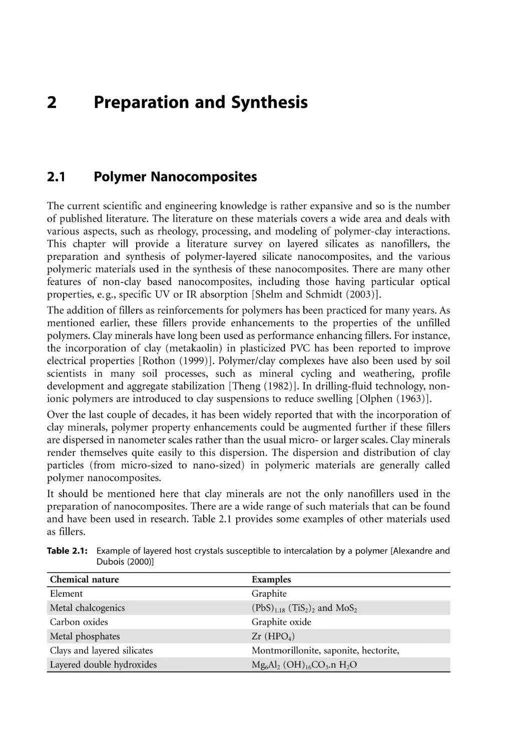
It should be mentioned here that clay minerals are not the only nanofillers used in the
preparation of nanocomposites. There are a wide range of such materials that can be found
and have been used in research. Table 2.1 provides some examples of other materials used
as fillers.
Table 2.1: Example of layered host crystals susceptible to intercalation by a polymer [Alexandre and
Dubois (2000)]

Chemical nature
Element
Metal chalcogenics
Carbon oxides
Metal phosphates
Clays and layered silicates
Layered double hydroxides

Examples
Graphite
(PbS)1.18 (TiS2)2 and MoS2
Graphite oxide
Zr (HPO4)
Montmorillonite, saponite, hectorite,
Mg6Al2 (OH)16CO3.n H2O

2 Preparation and Synthesis

2.1.1

[References on page 30]

Morphology of Polymer-Layered Silicate Nanocomposites

Structurally, polymer/clay complexes can be classified as either nanocomposites or
“conventional composites”. The classification depends on the nature and interaction of the
components as well as on the preparation technique. The nature and interaction of the
components refers to the type of silicate material, the organic material used to render the
hydrophilic silicates organophilic, and the nature of the polymer matrix. The preparation
technique pertains to mechanical factors that facilitate the penetration or intercalation of
polymer chains into the layers of silicate. Ultimately, this may lead to exfoliation, i. e.,
delamination of silicates into individual layers. These mechanical factors include the
mechanical shear or extension employed, residence time, and type of mixer. Depending on
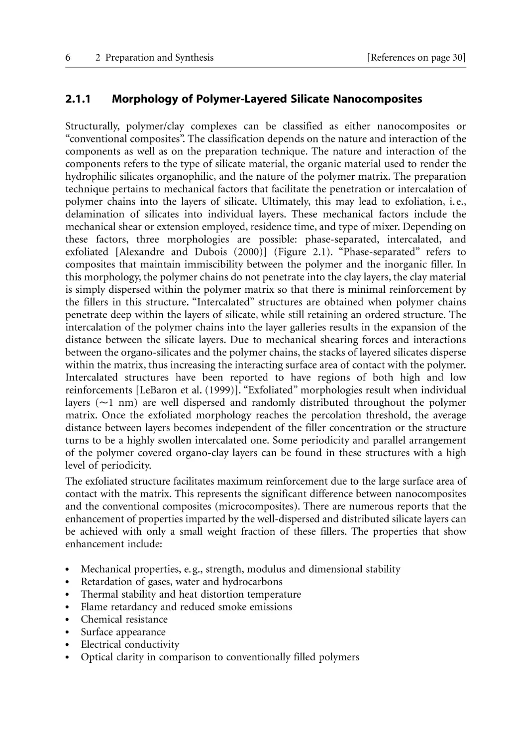
these factors, three morphologies are possible: phase-separated, intercalated, and
exfoliated [Alexandre and Dubois (2000)] (Figure 2.1). “Phase-separated” refers to
composites that maintain immiscibility between the polymer and the inorganic filler. In
this morphology, the polymer chains do not penetrate into the clay layers, the clay material
is simply dispersed within the polymer matrix so that there is minimal reinforcement by
the fillers in this structure. “Intercalated” structures are obtained when polymer chains
penetrate deep within the layers of silicate, while still retaining an ordered structure. The
intercalation of the polymer chains into the layer galleries results in the expansion of the
distance between the silicate layers. Due to mechanical shearing forces and interactions
between the organo-silicates and the polymer chains, the stacks of layered silicates disperse
within the matrix, thus increasing the interacting surface area of contact with the polymer.
Intercalated structures have been reported to have regions of both high and low
reinforcements [LeBaron et al. (1999)]. “Exfoliated” morphologies result when individual
layers ( 1 nm) are well dispersed and randomly distributed throughout the polymer
matrix. Once the exfoliated morphology reaches the percolation threshold, the average
distance between layers becomes independent of the filler concentration or the structure
turns to be a highly swollen intercalated one. Some periodicity and parallel arrangement
of the polymer covered organo-clay layers can be found in these structures with a high
level of periodicity.
The exfoliated structure facilitates maximum reinforcement due to the large surface area of
contact with the matrix. This represents the significant difference between nanocomposites
and the conventional composites (microcomposites). There are numerous reports that the
enhancement of properties imparted by the well-dispersed and distributed silicate layers can
be achieved with only a small weight fraction of these fillers. The properties that show
enhancement include:
Mechanical properties, e. g., strength, modulus and dimensional stability
Retardation of gases, water and hydrocarbons
Thermal stability and heat distortion temperature
Flame retardancy and reduced smoke emissions
Chemical resistance
Surface appearance
Electrical conductivity
Optical clarity in comparison to conventionally filled polymers

2.1 Polymer Nanocomposites

Realistically, however, many systems fall between these idealized morphologies. [Vaia
(2000)] explained that kinetics related to Brownian motion and shear alignment of the
layers coupled with processing histories (e. g., melt processing) produce positional and
orientational correlations between the plates, i. e., the exfoliated structure turns to be a
highly swollen intercalated one. [Vaia (2000)] added that these kinetic factors could be
attributed to the developed morphologies exhibiting nano- (1–100 nm), meso- (100–500
nm) and micro-level (500–10000 nm) features.

Layered silicate

(a)
Phase separated
(microcomposite)

(b)
Intercalated
(nanocomposite)

Polymer

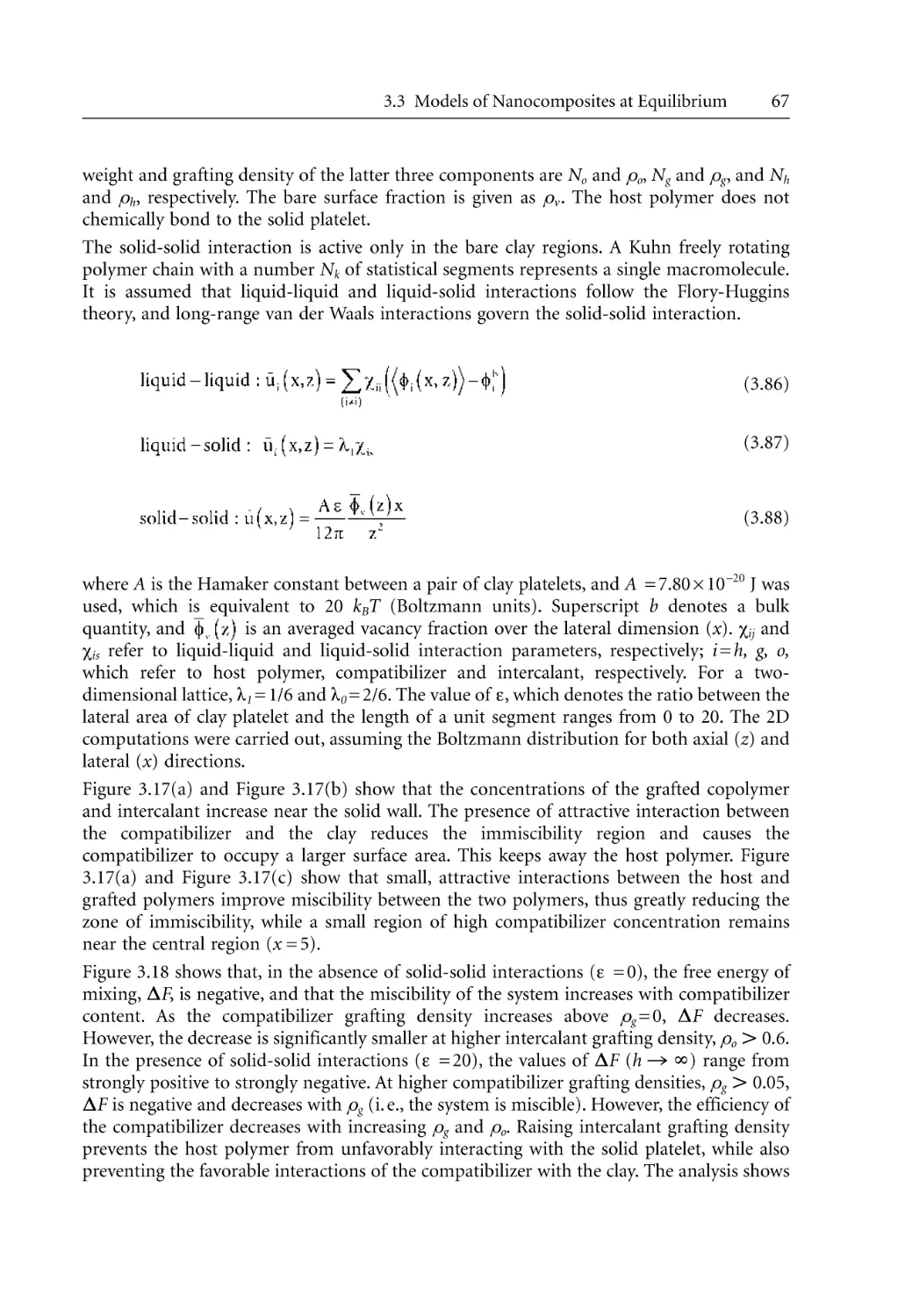
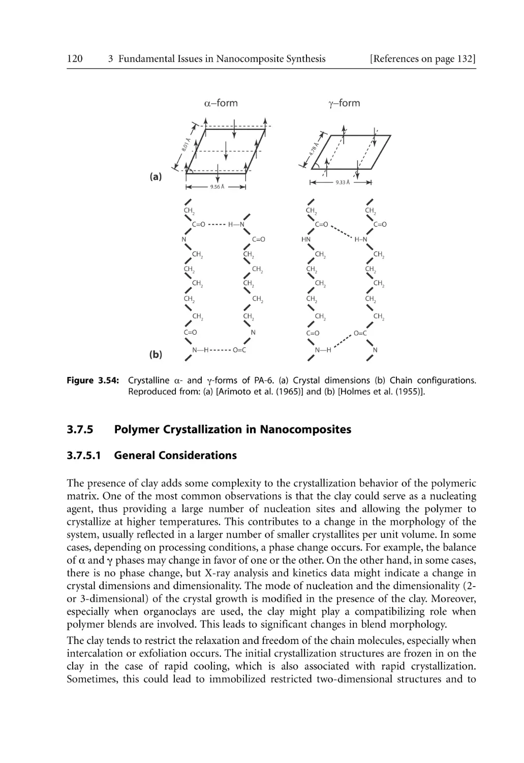
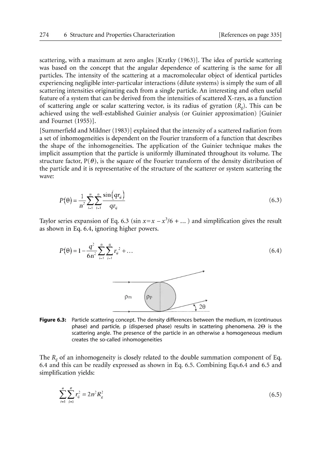
Figure 2.1: Scheme of different types of composites arising from the interaction of layered silicates
and polymers: (a) phase separated micro-composite; (b) intercalated nanocomposite and
(c) exfoliated nanocomposite. [Alexandre and Dubois (2000)]

2.1.2

Structure of Layered Silicates

Layered materials such as silicates are suitable for the design of nanocomposites due to their
lamellar elements that have high in-plane strength and stiffness and a high aspect ratio
( 50). The clay material has a very high specific surface area of about 750 m 2/g (e. g.,
montmorillonite). Almost all groups of lamellar solids, especially smectite clays, are the
material of choice for nanocomposite materials for two reasons [Dennis et al. (2001), Wang
et al. (2000)]:
Their rich intercalation chemistry allows them to be chemically modified and made
compatible with organic polymers for dispersal on a nanometer scale.
They can be easily acquired at low costs.
The layered silicates that are commonly used in nanocomposites belong to the structural
family called 2:1 phyllosilicates [Alexandre and Dubois (2000)]. An example of this is

2 Preparation and Synthesis

[References on page 30]

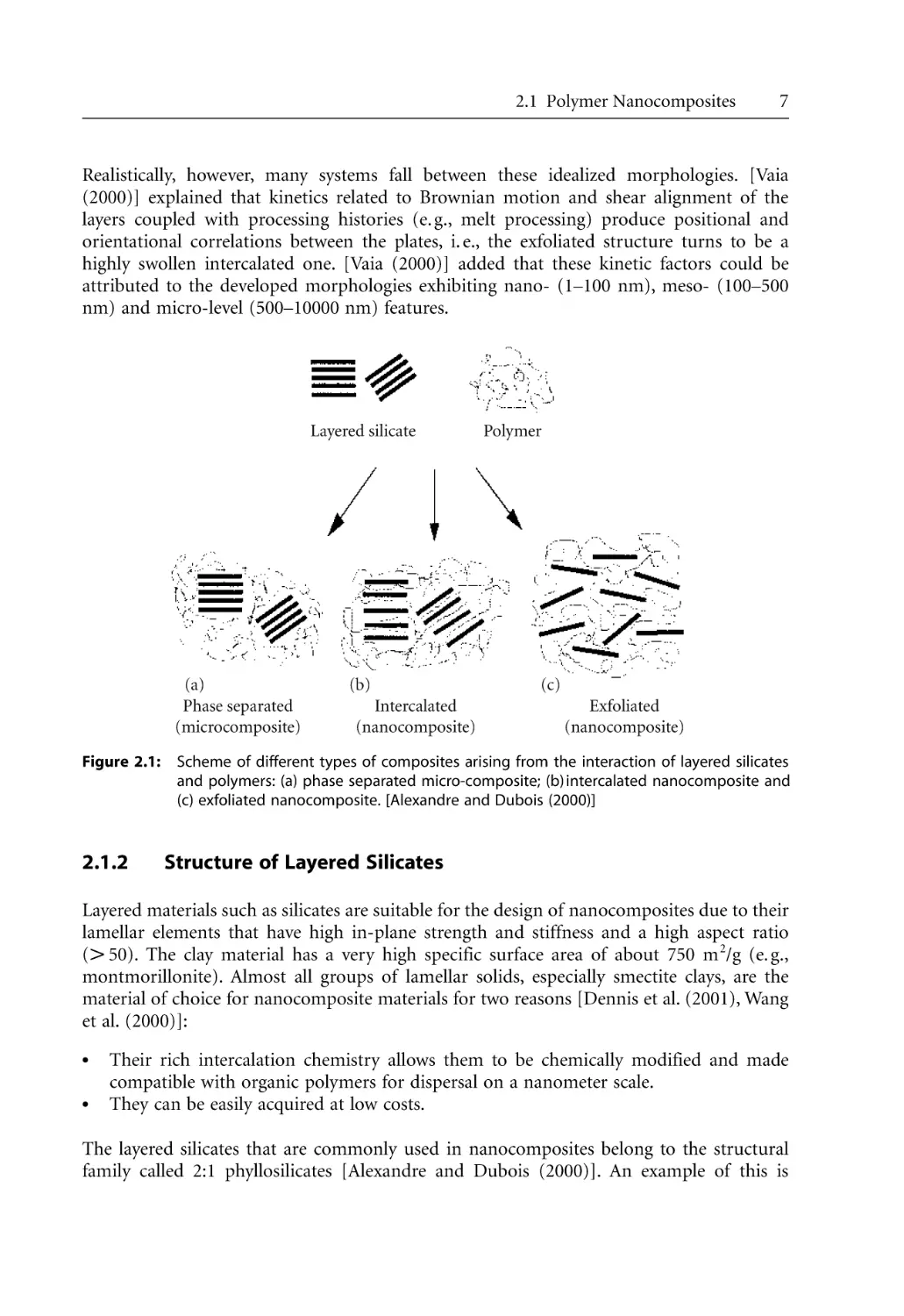
Na-montmorillonite. Na-montmorillonite is a 2:1 layered silicate and swells when contacted
by water [Zhu et al. (1998)]. This process of swelling is known as crystalline swelling.
The lattice crystal structure is comprised of two-dimensional, 1 nm thick layers. These
are made up of two outer tetrahedral sheets of silica (SiO4) fused onto an inner layer,
which is composed of an octahedral sheet of alumina (general formula for montmorillonite
is (0.5Ca,Na)0.7 (Al,Mg,Fe)4 (Si,Al)8 O20 (OH)4 and for bentonite Al2-xMe 2+x(SiO3)3.
Me +x..H2SiO3 Me 2+ is Mg, Fe, etc, where Me + is Li, Na, K, Cs + etc and x varied between 0.1
and 0.4) (Figure 2.2).

Figure 2.2: Structure of 2:1 phyllosilicates. [Giannelis et al. (1999)]

The lateral dimensions of these layers vary from 300 Å to several microns long. The stacking
of the layers and the inter-stack ionic forces result in a regular gap. This gap is called the
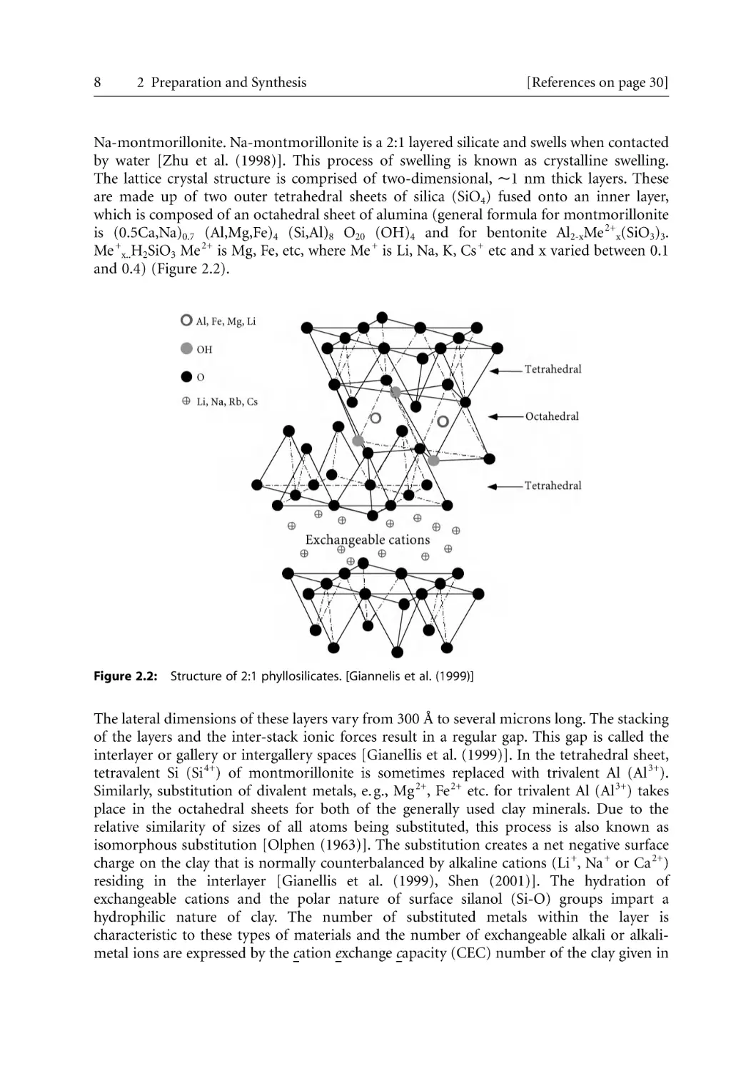
interlayer or gallery or intergallery spaces [Gianellis et al. (1999)]. In the tetrahedral sheet,
tetravalent Si (Si 4+) of montmorillonite is sometimes replaced with trivalent Al (Al 3+).
Similarly, substitution of divalent metals, e. g., Mg 2+, Fe 2+ etc. for trivalent Al (Al 3+) takes
place in the octahedral sheets for both of the generally used clay minerals. Due to the
relative similarity of sizes of all atoms being substituted, this process is also known as
isomorphous substitution [Olphen (1963)]. The substitution creates a net negative surface
charge on the clay that is normally counterbalanced by alkaline cations (Li +, Na + or Ca 2+)
residing in the interlayer [Gianellis et al. (1999), Shen (2001)]. The hydration of
exchangeable cations and the polar nature of surface silanol (Si-O) groups impart a
hydrophilic nature of clay. The number of substituted metals within the layer is
characteristic to these types of materials and the number of exchangeable alkali or alkalimetal ions are expressed by the cation exchange capacity (CEC) number of the clay given in

2.1 Polymer Nanocomposites

meq/100 g of clay units. For a smectic clay with a CEC value of 100, the × value is 0.35 and
there is a negative charge at around each 0.7 nm distance on both surfaces of the layers. The
hydration of these exchangeable cations and the polar nature of surface silanol (Si-O)
groups impart a hydrophilic nature to the clay. This results in water being preferentially
taken up by these surfaces, thus rendering non-polar organic molecules unable to compete
with the strongly bound water on the adsorption sites of the clay surface [Choy et al.
(1997)].

2.1.3

Organically Modified Clay

The layered structure of clay allows expansion after wetting. [Shen (2001)] noted that Li +,
Na + or Ca 2+ cations in the intergallery are strongly hydrated in the presence of water. The
strong polar nature of montmorillonite renders it ineffective to the sorption of nonpolar
polymers. In order to render these hydrophilic fillers more organophilic, the hydrated
cations of the interlayer need to be exchanged with cationic surfactants, such as
alkylammonium (quaternary ammonium cations), typically with chain lengths longer than
eight carbon atoms (C8). The modification (called ion-exchange reaction) lowers the surface
energy, hence rendering the clay compatible with nonpolar polymer molecules [Alexandre
and Dubois (2000)]. The negative charge formed on the surface of the silicate during the ion
exchange reaction implies that the cationic head of the alkylammonium is preferentially
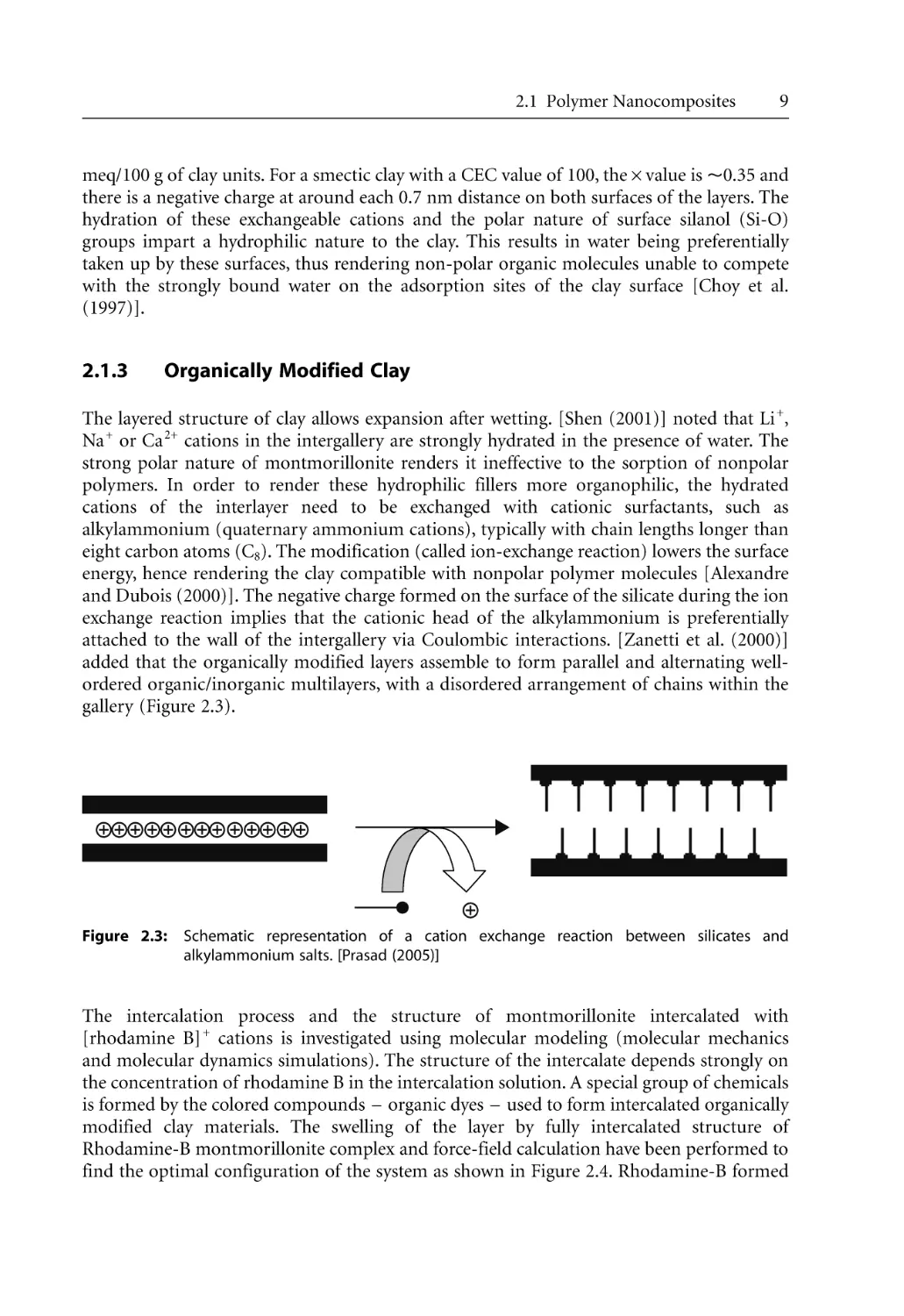
attached to the wall of the intergallery via Coulombic interactions. [Zanetti et al. (2000)]
added that the organically modified layers assemble to form parallel and alternating wellordered organic/inorganic multilayers, with a disordered arrangement of chains within the
gallery (Figure 2.3).

Figure 2.3: Schematic representation of a cation exchange reaction between silicates and
alkylammonium salts. [Prasad (2005)]

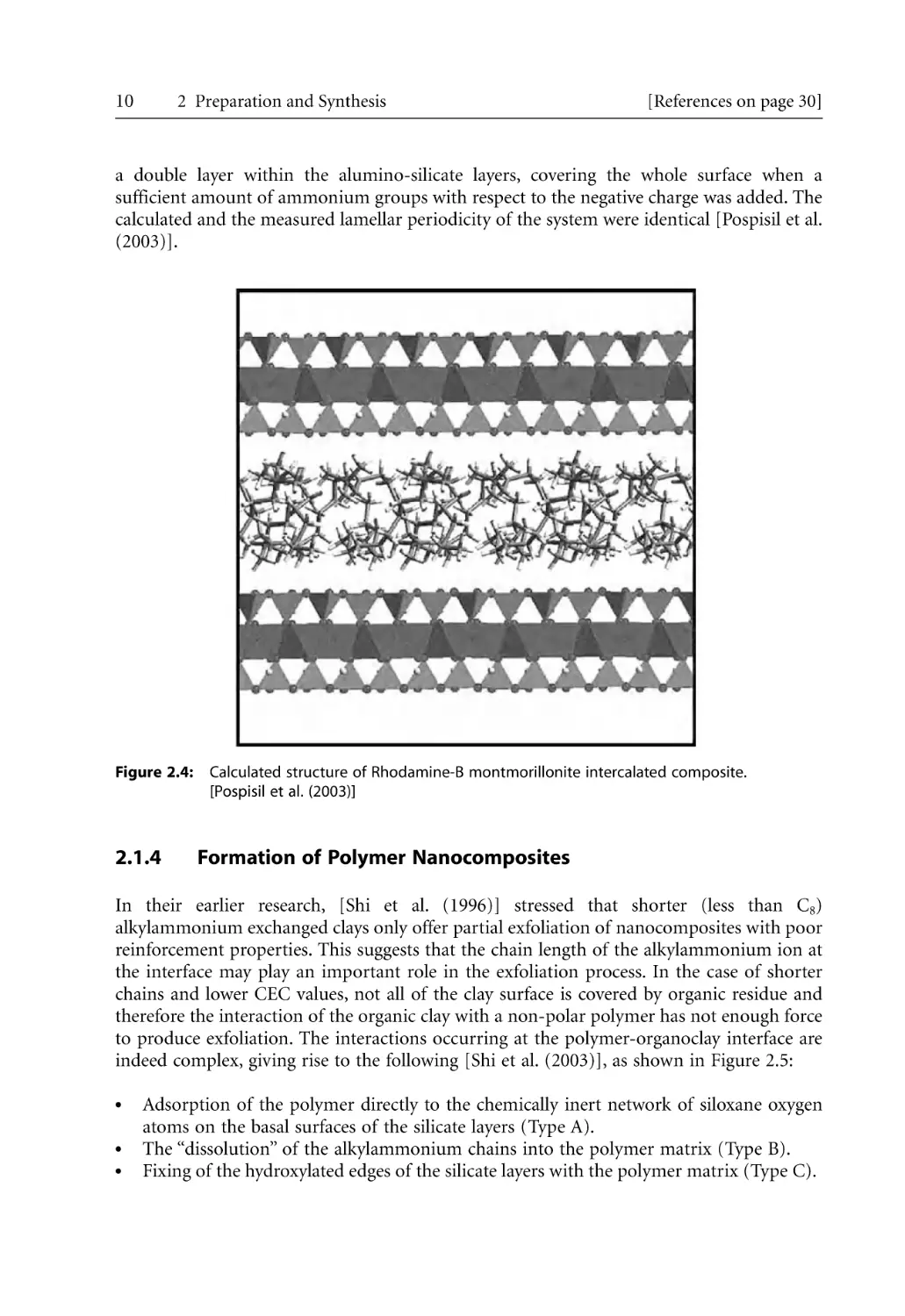
The intercalation process and the structure of montmorillonite intercalated with
[rhodamine B] + cations is investigated using molecular modeling (molecular mechanics
and molecular dynamics simulations). The structure of the intercalate depends strongly on
the concentration of rhodamine B in the intercalation solution. A special group of chemicals
is formed by the colored compounds – organic dyes – used to form intercalated organically
modified clay materials. The swelling of the layer by fully intercalated structure of
Rhodamine-B montmorillonite complex and force-field calculation have been performed to
find the optimal configuration of the system as shown in Figure 2.4. Rhodamine-B formed

2 Preparation and Synthesis

[References on page 30]

a double layer within the alumino-silicate layers, covering the whole surface when a
sufficient amount of ammonium groups with respect to the negative charge was added. The
calculated and the measured lamellar periodicity of the system were identical [Pospisil et al.
(2003)].

Figure 2.4: Calculated structure of Rhodamine-B montmorillonite intercalated composite.
[Pospisil et al. (2003)]

2.1.4

Formation of Polymer Nanocomposites

In their earlier research, [Shi et al. (1996)] stressed that shorter (less than C8)
alkylammonium exchanged clays only offer partial exfoliation of nanocomposites with poor
reinforcement properties. This suggests that the chain length of the alkylammonium ion at
the interface may play an important role in the exfoliation process. In the case of shorter
chains and lower CEC values, not all of the clay surface is covered by organic residue and
therefore the interaction of the organic clay with a non-polar polymer has not enough force
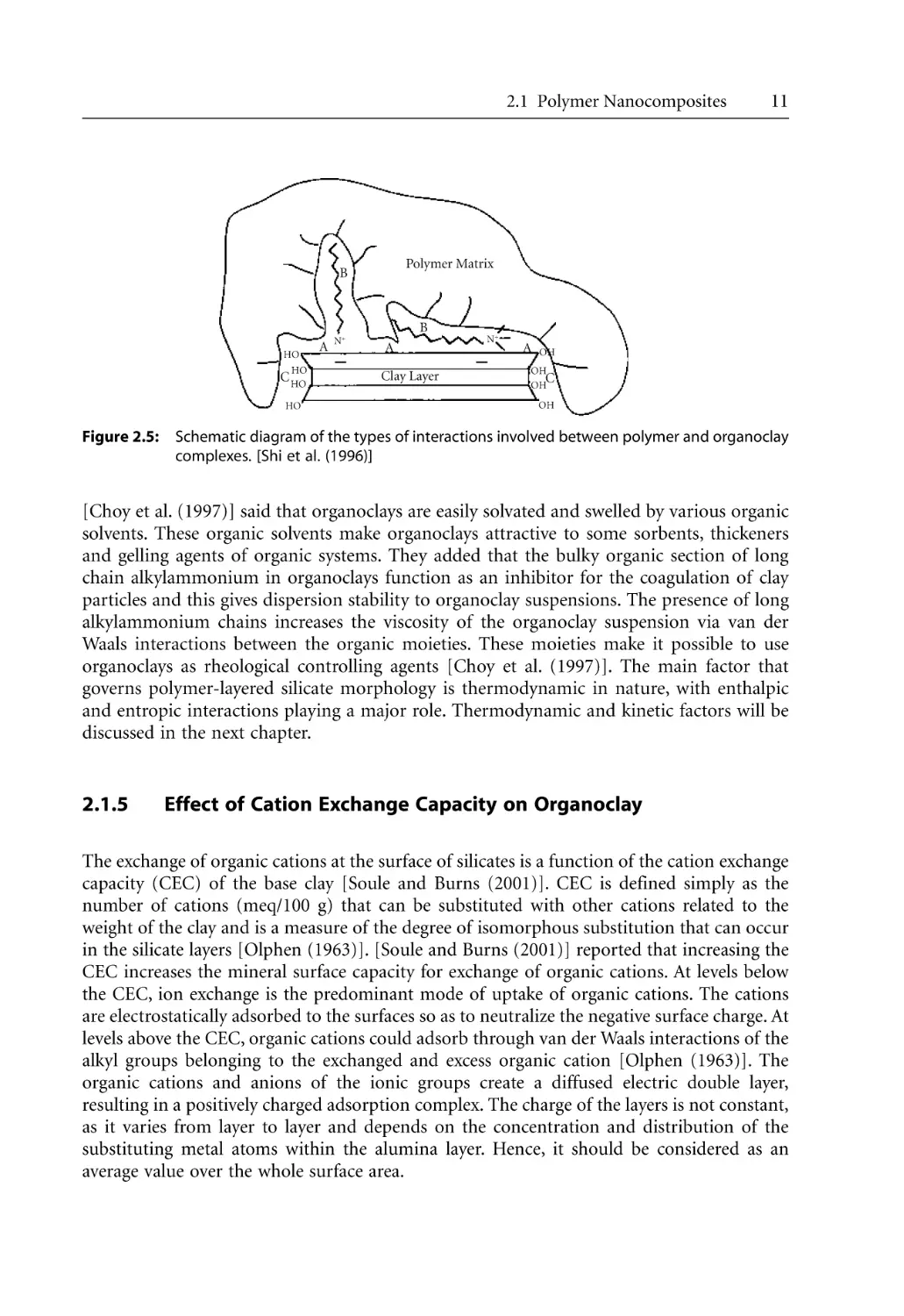
to produce exfoliation. The interactions occurring at the polymer-organoclay interface are
indeed complex, giving rise to the following [Shi et al. (2003)], as shown in Figure 2.5:
Adsorption of the polymer directly to the chemically inert network of siloxane oxygen
atoms on the basal surfaces of the silicate layers (Type A).
The “dissolution” of the alkylammonium chains into the polymer matrix (Type B).
Fixing of the hydroxylated edges of the silicate layers with the polymer matrix (Type C).

2.1 Polymer Nanocomposites

Polymer Matrix

B
HO
HO
C HO
HO

Figure 2.5:

N+

A
Clay Layer

N+

OH
C
OH
OH

Schematic diagram of the types of interactions involved between polymer and organoclay
complexes. [Shi et al. (1996)]

[Choy et al. (1997)] said that organoclays are easily solvated and swelled by various organic
solvents. These organic solvents make organoclays attractive to some sorbents, thickeners
and gelling agents of organic systems. They added that the bulky organic section of long
chain alkylammonium in organoclays function as an inhibitor for the coagulation of clay
particles and this gives dispersion stability to organoclay suspensions. The presence of long
alkylammonium chains increases the viscosity of the organoclay suspension via van der
Waals interactions between the organic moieties. These moieties make it possible to use
organoclays as rheological controlling agents [Choy et al. (1997)]. The main factor that
governs polymer-layered silicate morphology is thermodynamic in nature, with enthalpic
and entropic interactions playing a major role. Thermodynamic and kinetic factors will be
discussed in the next chapter.

2.1.5

Effect of Cation Exchange Capacity on Organoclay

The exchange of organic cations at the surface of silicates is a function of the cation exchange
capacity (CEC) of the base clay [Soule and Burns (2001)]. CEC is defined simply as the
number of cations (meq/100 g) that can be substituted with other cations related to the
weight of the clay and is a measure of the degree of isomorphous substitution that can occur
in the silicate layers [Olphen (1963)]. [Soule and Burns (2001)] reported that increasing the
CEC increases the mineral surface capacity for exchange of organic cations. At levels below
the CEC, ion exchange is the predominant mode of uptake of organic cations. The cations
are electrostatically adsorbed to the surfaces so as to neutralize the negative surface charge. At
levels above the CEC, organic cations could adsorb through van der Waals interactions of the
alkyl groups belonging to the exchanged and excess organic cation [Olphen (1963)]. The
organic cations and anions of the ionic groups create a diffused electric double layer,
resulting in a positively charged adsorption complex. The charge of the layers is not constant,
as it varies from layer to layer and depends on the concentration and distribution of the
substituting metal atoms within the alumina layer. Hence, it should be considered as an
average value over the whole surface area.

2 Preparation and Synthesis

2.1.6

[References on page 30]

Effect of Organic Cation Structure on Organoclay

The arrangement of organic cations on the mineral surface is a function of the cation
structure and mineral charge [Soule and Burns (2001)]. Where alkylammonium cations of
the form [(CH3)3NR] + (R = alkyl hydrocarbon chain) are present, X-ray diffraction (XRD)
has shown that carbon chains can arrange themselves as monolayers (13.7 Å), bilayers
(17.7 Å) or pseudotrimolecular layers (21.7 Å) on bentonite surfaces [Soule and Burns
(2001)]. The gallery spacing in organo-modified clay normally ranges between 4 and 4.5 Å
and is usually determined by the length of the alkyl chain and its orientation. The organic
cations are much larger than their inorganic counterparts and force the spacing of the layers
apart when they are intercalated onto the internal surfaces.
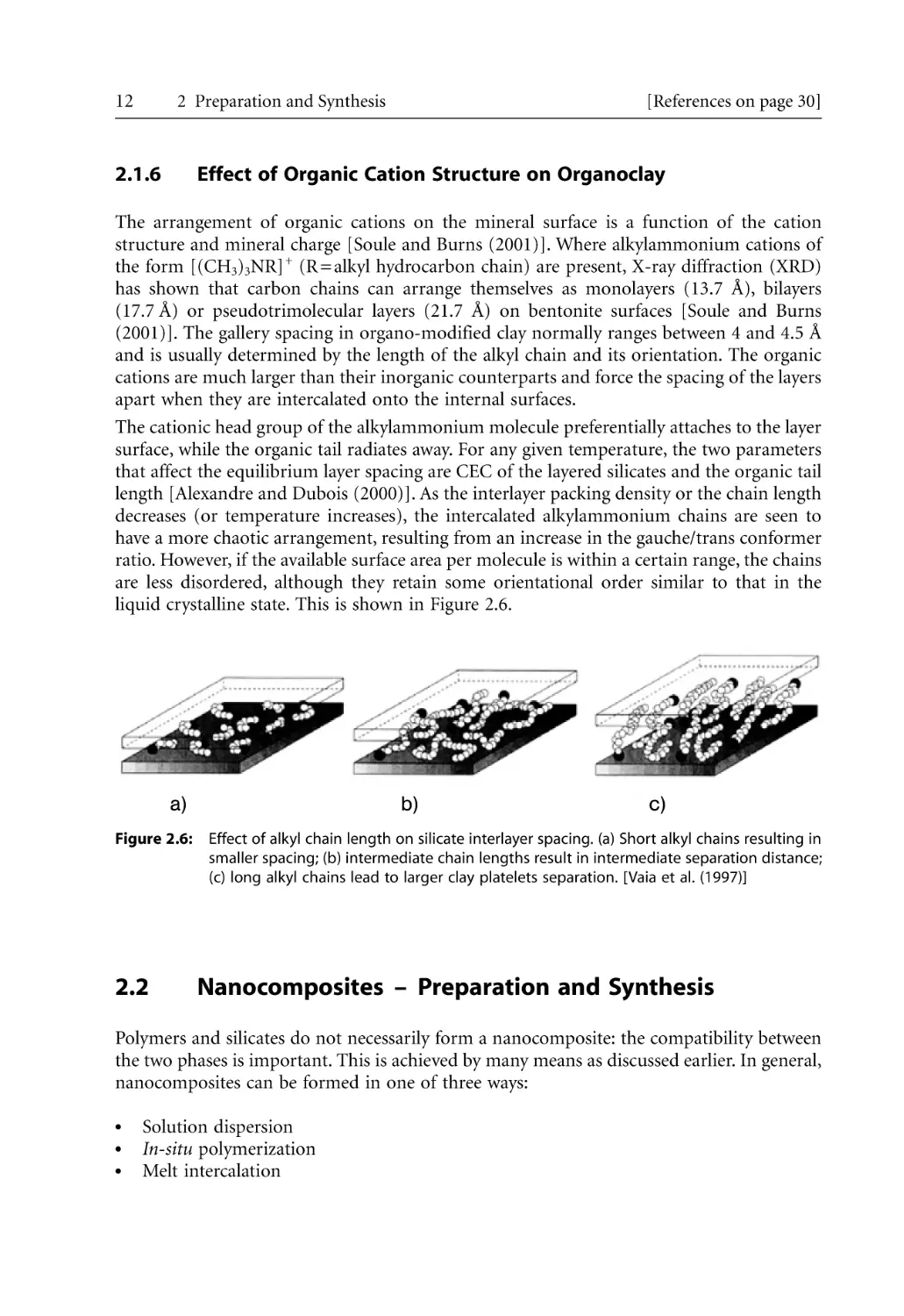
The cationic head group of the alkylammonium molecule preferentially attaches to the layer
surface, while the organic tail radiates away. For any given temperature, the two parameters
that affect the equilibrium layer spacing are CEC of the layered silicates and the organic tail
length [Alexandre and Dubois (2000)]. As the interlayer packing density or the chain length
decreases (or temperature increases), the intercalated alkylammonium chains are seen to
have a more chaotic arrangement, resulting from an increase in the gauche/trans conformer
ratio. However, if the available surface area per molecule is within a certain range, the chains
are less disordered, although they retain some orientational order similar to that in the
liquid crystalline state. This is shown in Figure 2.6.

Figure 2.6: Effect of alkyl chain length on silicate interlayer spacing. (a) Short alkyl chains resulting in
smaller spacing; (b) intermediate chain lengths result in intermediate separation distance;
(c) long alkyl chains lead to larger clay platelets separation. [Vaia et al. (1997)]

2.2

Nanocomposites – Preparation and Synthesis

Polymers and silicates do not necessarily form a nanocomposite: the compatibility between
the two phases is important. This is achieved by many means as discussed earlier. In general,
nanocomposites can be formed in one of three ways:
Solution dispersion
In-situ polymerization
Melt intercalation

2.2 Nanocomposites – Preparation and Synthesis

In this section, we will discuss each of the techniques and types of polymer matrices
involved in this process.

2.2.1

Solution Dispersion

The solution dispersion method involves mixing a preformed polymer solution with clay.
This is based on a solvent system in which the polymer or pre-polymer is soluble and the
silicate layers are swellable. The layered silicate is first swollen in a solvent, such as water,
chloroform, or toluene. When the polymer and layered silicate solutions are mixed, the
polymer chains intercalate and displace the solvent within the interlayer of the silicate. Upon
solvent removal, the intercalated structure remains, resulting in polymer/layered silicate
(PLS) nanocomposite. In this method, the nature of solvents is critical in facilitating the
insertion of polymers between the silicate layers, polarity of the medium being a
determining factor for intercalations [Theng (1979)].
For the overall process, in which polymer is exchanged with the previously intercalated
solvent in the gallery, a negative variation of the Gibbs free energy is required. The driving
force for the polymer intercalation into layered silicate from solution is the entropy gained
by desorption of solvent molecules, which compensates for the decreased entropy of the
confined, intercalated chains [Vaia and Giannelis (1997)]. To achieve this goal, either the
polymer must be polar enough to have a positive interaction energy with the surface of the
clay or the clay must be organically modified.
Polymers typically used in solution dispersion are polyethylene oxide (PEO), polyvinyl
alcohol (PVOH), polyimide (PI) or polyurethanes (PU), polyamide (PA), and high-density
polyethylene (HDPE) with surface modified clay. [Aranda and Ruiz-Hitzky (1992)] reported
the first preparation of PEO/MMT nanocomposites by this method. They performed a
series of experiments to intercalate Na +-MMT into PEO, using different polar solvents
(water, methanol, acetonitrile, and 1:1 mixtures of water/methanol and methanol/
acetonitrile). The high polarity of water swelled Na +-MMT, provoking cracking of the PEO
films. Methanol was not suitable as a solvent for high molecular weight (HMW) PEO,
whereas water/methanol mixtures appeared to be useful for intercalations, although
cracking of the resulting materials was frequently observed. PEO intercalated compounds,
derived from the homoionic M +n-MMT and M +n hectorite, could satisfactorily be obtained
using anhydrous acetonitrile or a methanol/acetonitrile mixture as solvents.
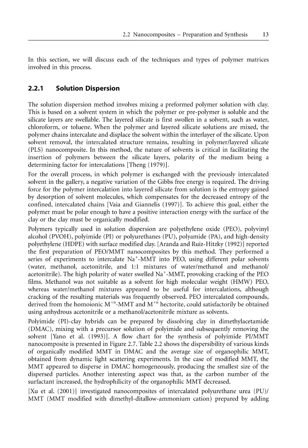
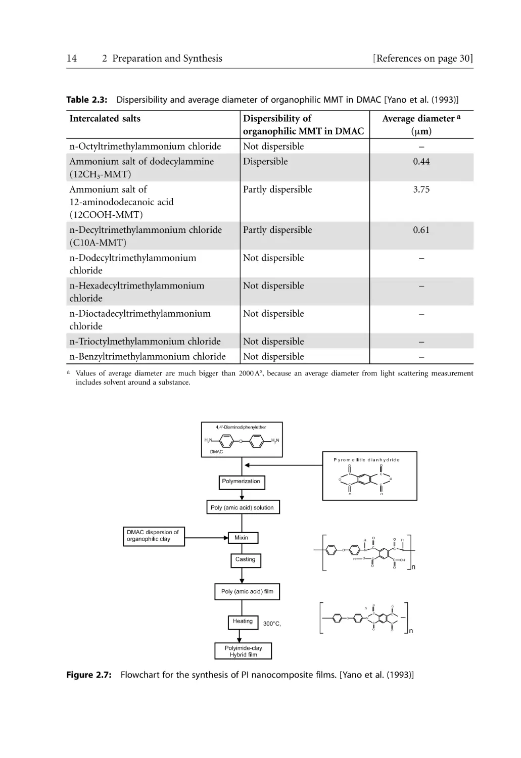
Polyimide (PI)-clay hybrids can be prepared by dissolving clay in dimethylacetamide
(DMAC), mixing with a precursor solution of polyimide and subsequently removing the
solvent [Yano et al. (1993)]. A flow chart for the synthesis of polyimide PI/MMT
nanocomposite is presented in Figure 2.7. Table 2.2 shows the dispersibility of various kinds
of organically modified MMT in DMAC and the average size of organophilic MMT,
obtained from dynamic light scattering experiments. In the case of modified MMT, the
MMT appeared to disperse in DMAC homogeneously, producing the smallest size of the
dispersed particles. Another interesting aspect was that, as the carbon number of the
surfactant increased, the hydrophilicity of the organophilic MMT decreased.
[Xu et al. (2001)] investigated nanocomposites of intercalated polyurethane urea (PU)/
MMT (MMT modified with dimethyl-ditallow-ammonium cation) prepared by adding

2 Preparation and Synthesis

[References on page 30]

Table 2.3: Dispersibility and average diameter of organophilic MMT in DMAC [Yano et al. (1993)]

Intercalated salts

Average diameter a
(mm)

Dispersibility of
organophilic MMT in DMAC

n-Octyltrimethylammonium chloride

Not dispersible

Ammonium salt of dodecylammine
(12CH3-MMT)

Dispersible

0.44

–

Ammonium salt of
12-aminododecanoic acid
(12COOH-MMT)

Partly dispersible

3.75

n-Decyltrimethylammonium chloride
(C10A-MMT)

Partly dispersible

0.61

n-Dodecyltrimethylammonium
chloride

Not dispersible

–

n-Hexadecyltrimethylammonium
chloride

Not dispersible

–

n-Dioctadecyltrimethylammonium
chloride

Not dispersible

–

n-Trioctylmethylammonium chloride

Not dispersible

–

n-Benzyltrimethylammonium chloride

Not dispersible

–

a Values of average diameter are much bigger than 2000 A°, because an average diameter from light scattering measurement

includes solvent around a substance.

4,4'-Diaminodiphenylether
H2N

H2N

DMAC
P y r o m e lli t i c d ia n h y d r id e
O

O
C

Polymerization

Poly (amic acid) solution

DMAC dispersion of
organophilic clay

Mixin

H
O

Casting

Poly (amic acid) film
n

Heating

300°C,

Polyimide-clay
Hybrid film

Figure 2.7: Flowchart for the synthesis of PI nanocomposite films. [Yano et al. (1993)]

2.2 Nanocomposites – Preparation and Synthesis

organo-modified layered silicate suspended in toluene drop-wise to the solution of PU in
DMAC. This method, however, is applicable for certain polymer/solvent pairs, and useful for
intercalation of polymers with little or no polarity; it facilitates production of thin films
with intercalated and oriented clay layers. However, from a commercial point of view, this
method involves copious use of organic solvents, which may be hazardous to personnel and
the environment, which renders it economically prohibitive.

2.2.2

In-Situ Polymerization

In-situ polymerization involves the dispersion and distribution of clay layers in the
monomer followed by polymerization. The layered silicate is swollen within the liquid
monomer or a monomer solution so that polymer formation can occur between the
intercalated sheets. Polymerization can be initiated either by heat or radiation, diffusion of
a suitable initiator, or by an organic initiator or catalyst fixed through cation exchange inside
the interlayer before the swelling step.
This technique has been known for a long time [Theng (1979)]. However, in-situ
polymerization technique gained considerable momentum since the report of synthesis of a
Nylon-6/MMT nanocomposite by the Toyota research group [Okada et al. (1990)], where
very small amounts of layered silicate loading resulted in pronounced improvements in
thermal and mechanical properties.
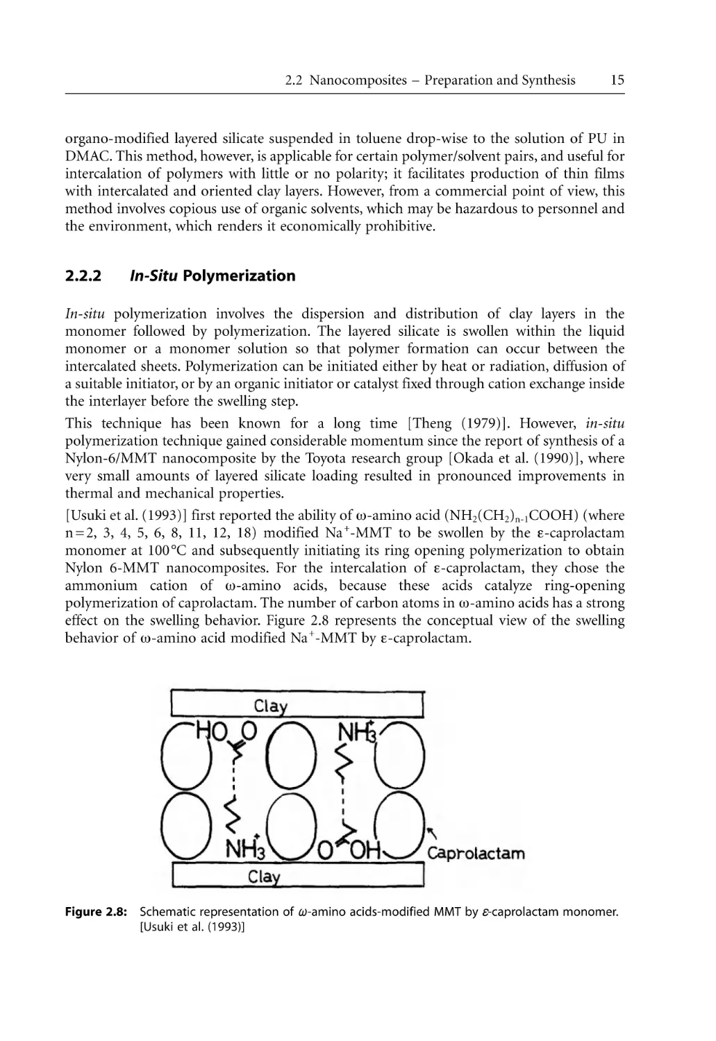
[Usuki et al. (1993)] first reported the ability of w-amino acid (NH2(CH2)n-1COOH) (where
n = 2, 3, 4, 5, 6, 8, 11, 12, 18) modified Na +-MMT to be swollen by the e-caprolactam
monomer at 100 °C and subsequently initiating its ring opening polymerization to obtain
Nylon 6-MMT nanocomposites. For the intercalation of e-caprolactam, they chose the
ammonium cation of w-amino acids, because these acids catalyze ring-opening
polymerization of caprolactam. The number of carbon atoms in w-amino acids has a strong
effect on the swelling behavior. Figure 2.8 represents the conceptual view of the swelling
behavior of w-amino acid modified Na +-MMT by e-caprolactam.

Figure 2.8: Schematic representation of
[Usuki et al. (1993)]

-amino acids-modified MMT by -caprolactam monomer.

2 Preparation and Synthesis

[References on page 30]

For the preparation of polycaprolactone (PCL)-based nanocomposites, [Giannelis (1996)]
modified MMT using protonated amino-lauric acid and dispersed the modified MMT in
liquid e-caprolactone before polymerizing at high temperatures. The nanocomposites were
prepared by mixing up to 30 wt% of the modified MMT with dried and freshly distilled ecaprolactone for a couple of hours, followed by ring opening polymerization under stirring
at 170 °C for 48 h.
PE/layered silicate nanocomposites have also been prepared by in-situ intercalative
polymerization of ethylene using the so-called polymerization filling technique [Alexandre
et al. (2002)]. In this case, the polymerizing catalyzer is fixed on the clay surface and the
polymerization is carried out using the modified clay as catalyzer. Pristine MMT and
hectorite were first treated with trimethylaluminum-depleted methylaluminoxane, before
being contacted by a Ti-based constrained-geometry catalyst. The nanocomposite was
formed by addition and polymerization of ethylene. In the absence of a chain transfer agent,
ultra HMW polyethylene was produced. The tensile properties of these nanocomposites
were poor and essentially independent of the nature and content of the silicate. Upon
hydrogen addition, the molecular weight of the polyethylene was decreased with a
corresponding improvement of mechanical properties. The formation of exfoliated
nanocomposites was confirmed by X-ray diffraction (XRD) and Transmission Electron
Microscopy (TEM).
[Akelah (1995)] used in-situ intercalative polymerization techniques for the preparation of
PS-based nanocomposites. He modified Na +-MMT and Ca 2+-MMT with vinyl-benzyltrimethyl ammonium cation, using an ion exchange reaction, then used these modified
MMTs for the preparation of nanocomposites. The modified clays were dispersed and
swelled in various solvent and co-solvent mixtures, such as acetonitrile, acetonitrile/toluene
and acetonitrile/THF. It was observed that the extent of intercalation depended on the
nature of the solvent used. Although this seems to be an effective method for preparation of
PS-based nanocomposites, one drawback of this procedure was that the macromolecule
produced was not pure PS, but rather a copolymer between styrene and vinyl-benzyltrimethylammonium cations.
Another example of in-situ preparation of PS-based nanocomposites was reported by [Doh
and Cho (1998)], who used MMT for the preparation of PS based nanocomposites. They
compared the ability of several tetra-alkylammonium cations incorporated in Na +-MMT by
exchange reaction through free radical polymerization of styrene. They found that the
structural affinity between the styrene monomer and the surfactant of modified MMT plays
an important role in the final structure and properties of the nanocomposites.

2.2.3

Melt Intercalation

Melt intercalation is the most widely used method in polymer/clay nanocomposite
preparation, and it has tremendous potential for industrial application. An advantage of this
method over the others is that no solvent is required. The melt blending process involves
mixing the layered silicate by annealing, statically or under shear, with polymer pellets while
heating the mixture above the softening point of the polymer. During the annealing process,
the polymer chains diffuse from the bulk polymer melt into the galleries between the silicate

2.2 Nanocomposites – Preparation and Synthesis

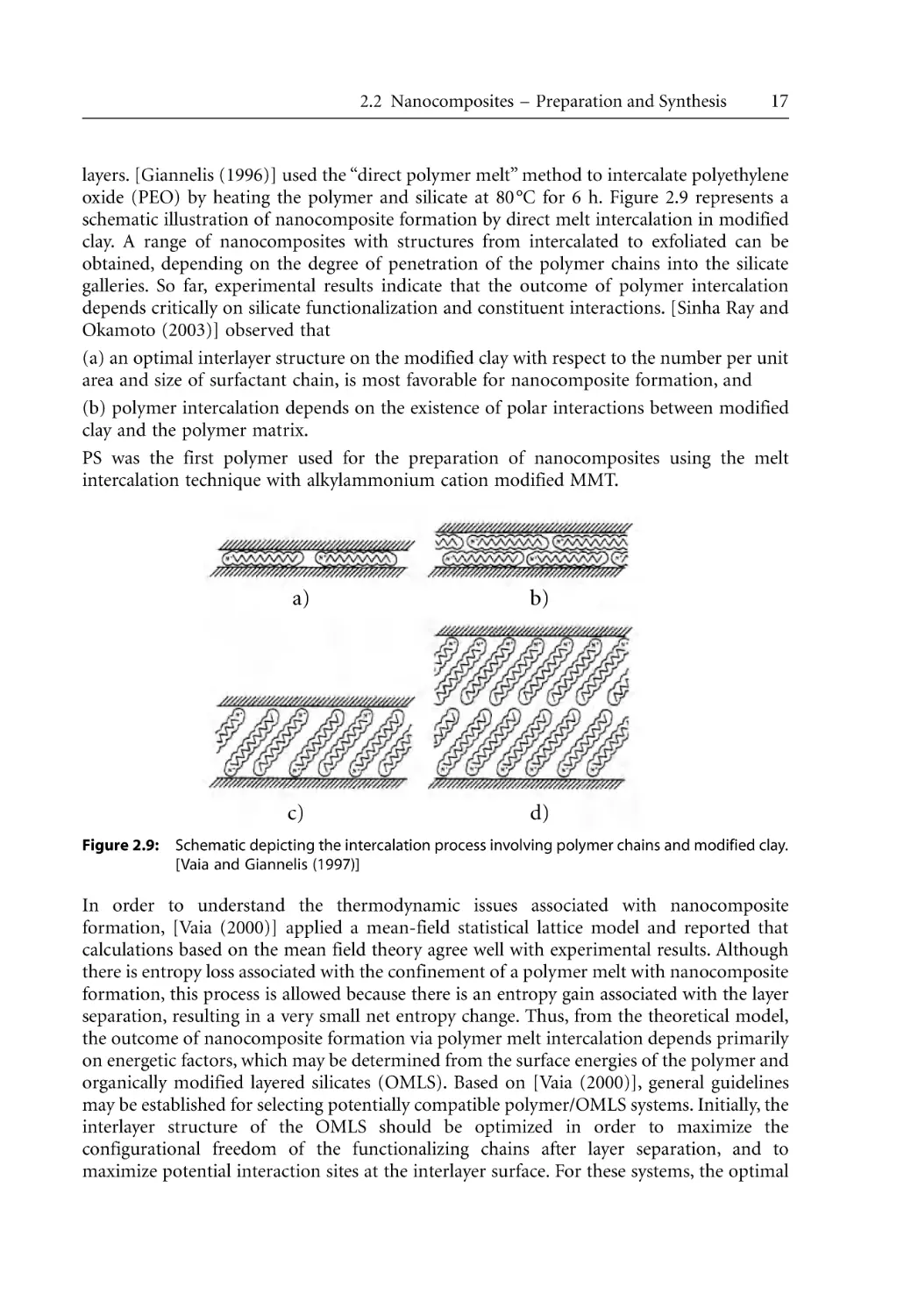
layers. [Giannelis (1996)] used the “direct polymer melt” method to intercalate polyethylene
oxide (PEO) by heating the polymer and silicate at 80 °C for 6 h. Figure 2.9 represents a
schematic illustration of nanocomposite formation by direct melt intercalation in modified
clay. A range of nanocomposites with structures from intercalated to exfoliated can be
obtained, depending on the degree of penetration of the polymer chains into the silicate
galleries. So far, experimental results indicate that the outcome of polymer intercalation
depends critically on silicate functionalization and constituent interactions. [Sinha Ray and
Okamoto (2003)] observed that
(a) an optimal interlayer structure on the modified clay with respect to the number per unit
area and size of surfactant chain, is most favorable for nanocomposite formation, and
(b) polymer intercalation depends on the existence of polar interactions between modified
clay and the polymer matrix.
PS was the first polymer used for the preparation of nanocomposites using the melt
intercalation technique with alkylammonium cation modified MMT.

Figure 2.9:

Schematic depicting the intercalation process involving polymer chains and modified clay.
[Vaia and Giannelis (1997)]

In order to understand the thermodynamic issues associated with nanocomposite
formation, [Vaia (2000)] applied a mean-field statistical lattice model and reported that
calculations based on the mean field theory agree well with experimental results. Although
there is entropy loss associated with the confinement of a polymer melt with nanocomposite
formation, this process is allowed because there is an entropy gain associated with the layer
separation, resulting in a very small net entropy change. Thus, from the theoretical model,
the outcome of nanocomposite formation via polymer melt intercalation depends primarily
on energetic factors, which may be determined from the surface energies of the polymer and
organically modified layered silicates (OMLS). Based on [Vaia (2000)], general guidelines
may be established for selecting potentially compatible polymer/OMLS systems. Initially, the
interlayer structure of the OMLS should be optimized in order to maximize the
configurational freedom of the functionalizing chains after layer separation, and to
maximize potential interaction sites at the interlayer surface. For these systems, the optimal

2 Preparation and Synthesis

[References on page 30]

structures exhibit a slightly more extensive chain arrangement than those with a pseudobilayer. Polymers containing polar groups are capable of associative interactions, such as
Lewis-acid/Lewis-base interactions or hydrogen bonding, thus leading to intercalation. The
polarizability or hydrophilicity of the polymer also depends on the size of the functional
group, as shorter functional groups lead to improved hydrophilicity in order to minimize
unfavorable interactions between the aliphatic chains and the polymer.
Polystyrene (PS) was the first polymer used for the preparation of nanocomposites using the
melt intercalation technique with alkylammonium cation modified MMT. [Vaia et al.
(1993)] prepared PS-nanocomposites by mixing PS with organo-modified layered silicates.
The WAXD patterns of the hybrid before heating showed peaks characteristic of the pure
OMLS, and during heating, the OMLS peaks were progressively reduced while a new set of
peaks corresponding to the PS/OMLS appeared. After 25 h, the hybrid exhibited a WAXD
pattern corresponding predominantly to that of the intercalated structure. The same
authors also carried out experiments under the same conditions using Na +-MMT, but
WAXD patterns did not show any intercalation of PS into the silicate galleries, emphasizing
the importance of polymer/clay interactions. They also attempted to intercalate a solution of
PS in toluene with the same OMLS used for melt intercalation, but this resulted in
intercalation of the solvent instead of PS. From the above observation, it can be concluded
that direct melt mixing enhances the scope of polymer intercalation as it eliminates the
competing host – solvent and polymer – solvent interactions.
Propylene (PP) is one of the most widely used polyolefin polymers. Since it has no polar
groups in the chain, direct intercalation of PP in the silicate galleries is impossible. To
overcome this difficulty, [Usuki et al. (1997)] first reported a novel approach to prepare PP/
nanocomposites using a functional oligomer (PP – OH) with polar telechelic OH groups
as a compatibilizer. In this approach, PP – OH was intercalated between the layers of
2C18-MMT, and then it was melt mixed with PP to obtain the nanocomposite with
intercalated structure. [Kawasumi et al. (1997)] reported the preparation of PP/MMT
nanocomposites obtained by melt blending of PP, a maleic anhydride grafted PP oligomer
(PP-g-MA), and clays modified with stearylammonium using a twin-screw extruder. This
study used two different types of maleic anhydride modified PP oligomer with different
amounts of maleic anhydride groups and two types of organically modified clays to
understand the miscibility effect of the oligomers on the dispersibility of the OMLS in the
PP matrix. In addition, they also studied the effect of hybridization on the mechanical
properties when compared with neat PP and PP/nanocomposites without oligomers.
WAXD analyses and TEM observations established the intercalated structure for all
nanocomposites. On the basis of WAXD patterns and TEM images, they proposed a possible
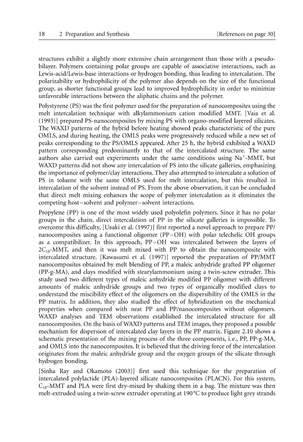
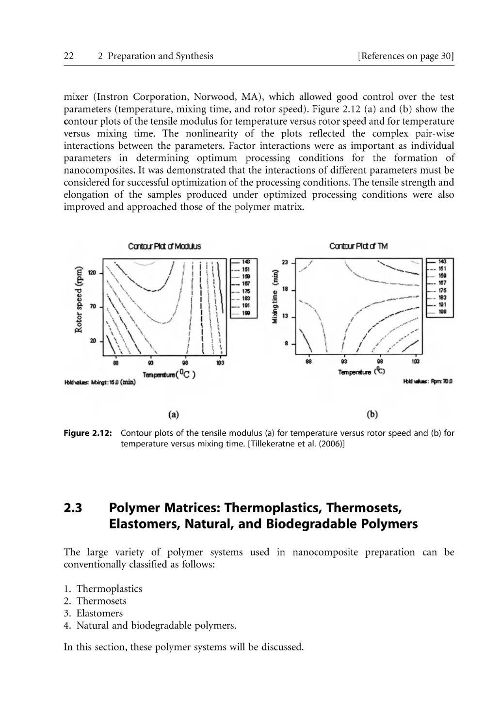
mechanism for dispersion of intercalated clay layers in the PP matrix. Figure 2.10 shows a
schematic presentation of the mixing process of the three components, i. e., PP, PP-g-MA,
and OMLS into the nanocomposites. It is believed that the driving force of the intercalation
originates from the maleic anhydride group and the oxygen groups of the silicate through
hydrogen bonding.
[Sinha Ray and Okamoto (2003)] first used this technique for the preparation of
intercalated polylactide (PLA)-layered silicate nanocomposites (PLACN). For this system,
C18-MMT and PLA were first dry-mixed by shaking them in a bag. The mixture was then
melt-extruded using a twin-screw extruder operating at 190 °C to produce light grey strands

2.2 Nanocomposites – Preparation and Synthesis

Stearyl
ammonium

Silicate Layer
of Clay

PP-Ma
Oligomer
Maleic Anhydride
Group

Figure 2.10: Schematic representation
of organophilic MMT dispersion
in PP matrix with PP-g-MA as
the compatibilizer.
[Kawasumi et al. (1997)]

of PLACNs. Nanocomposites loaded with a very small amount of o-PCL as a compatibilizer
were also prepared in order to understand the effect of o-PCL on the morphology and
properties of PLACNs.
Maleic anhydride (MA) grafted polyethylene (PE-g-MA)-clay nanocomposites were
prepared using melt intercalation [Wang et al. (2000)]. The extent of exfoliation and
intercalation completely depended on the hydrophilicity of the polyethylene grafted with
MA and the chain length of the organic modifier in the clay. An exfoliated nanocomposite
was obtained when the number of methylene groups in the alkylamine (organic modifier)
was larger than 16. This nanocomposite, with clay modified with dimethyl-dihydrogenatedtallow ammonium cations or octadecylammonium cations, had a maleic anhydride grafting
level higher than about 0.1 wt%.

2 Preparation and Synthesis

[References on page 30]

In another investigation, [Gopakumar et al. (2002)] prepared polyethylene nanocomposites
with and without grafting maleic anhydride by melt compounding and studied the
influence of the exfoliation of layered silicates on their physical properties. Nanocomposites
with grafting showed exfoliated structure, whereas nanocomposites without grafting showed
phase separated structure. They concluded that two conditions are required to produce the
necessary intensity of surface interactions to exfoliate and disperse the clay in a polyolefin
matrix. Firstly, the montmorillonite clay must be ion-exchanged to reduce the cohesive
forces between clay platelets. Secondly, the polyolefin must be chemically modified to
improve adhesion between the polymer matrix and the clay filler. This study also provides
an explanation for surface interactions, such as polar anhydride functionality promoting
dipole and/or hydrogen bonding between the filler and the polyolefin, thus leading to
improved dispersion of the clay in the polymer matrix. Thus, grafting is important in
preparing the polyethylene nanocomposites by melt intercalation techniques.

2.2.4

Effect of Mixing

[Cho and Paul (2001)] demonstrated that the degree of intercalation/exfoliation depends on
the type of organoclay, the extruder and the screw configuration. In the preparation of
nylon 6 nanocomposites it was shown that the mechanical properties were affected by the
degree of exfoliation, which was dependent on the processing conditions as well as the clay
chemical treatment. Melt compounding was used with two different extruders. These nylon
6 nanocomposites were prepared using a Haake intermeshing co-rotating twin screw
extruder with a 30 mm diameter screw having a center-line spacing of 26 mm and a 305 mm
screw length. Most of the compounding was carried out using a barrel temperature of
240 °C, a screw speed of 180 rpm, and a feed rate of 920 g/h. For comparative purposes, a
Killion single screw extruder was also used. The mean value of the residence time reported
by these two extruder/screw speed configuration was 5.3 min for the Haake, and 2.35 min
for the Killion extruder. Details of the residence time distribution of the two extruders are
shown in Figure 2.11 and Table 2.4.
Table 2.4: Details of processing conditions for the production of PA-6 nanocomposites
[Cho and Paul (2001)]

Equipment type

Processing conditions

Manufacturer

Single screw extruder

Screw speed: 40 rpm
Barrel temp.: 240 °C
Feed rate: fully fed

Killion

Modular intermeshing corotating twin screw extruder

Screw speed: 180 rpm
Barrel temp.: 240 °C
Feed rate: 920 g/h

Haake

Injection molding

Screw speed: 150 rpm
Barrel temp.: 260 °C
Injection pressure: 70 bar
Holding pressure: 35 bar
Molding temp.: 80 °C

Arburg Allrounder

2.2 Nanocomposites – Preparation and Synthesis

Figure 2.11: Residence time distribution curves at the die exit for the single screw extruder at 40 rpm
and for the modular intermeshing co-rotating twin screw extruder at 180 rpm.
[Cho and Paul (2001)]

It was suggested that a high degree of exfoliation by melt processing seems to require
sufficient residence time in the extruder and an appropriate shear history. In the case of
nylon 6 nanocomposites, well exfoliated morphologies showed continuous improvement in
strength and modulus relative to the neat nylon 6 matrix as more organoclay was added.
However, loss of ductility was reported beyond a certain clay loading.
[Chaudhary et al. (2005)] evaluated the influence of processing, as a function of shear and
diffusion, and influence of polymer crystallinity, as a function of the blend morphology, on
the clay gallery spacing and the corresponding nanocomposite mechanical (tensile)
properties. The aim was to quantitatively understand the effect of combined intercalation
and exfoliation on the nanocomposites’ mechanical behavior and to correlate the basal
spacing (in the clay galleries) with the tensile properties. Using HDPE as the base matrix and
EVA (9 % VA) as the carrier of C15A organo-modified montmorillonite clay, an
experimental design was carried out with 20 % EVA9 and 5 % clay. Shear was represented by
a combination of screw speed and temperature and diffusion was represented by the mixing
time in the design. It was found that there was a direct and quantifiable relationship between
the basal spacing and the tensile properties of the clay-polymer blend nanocomposites;
interestingly, there seemed to be a threshold basal spacing for clay concentration of 5 %
( 4 nm) for a significant increase in the mechanical properties of the composites. Further,
EVA9 is found to be a good carrier of C15A, as indicated by the simultaneous increase in the
tensile modulus and strength ( 25 %), showing that a skeleton-like support structure of
clay platelets could be developed in the HDPE matrix.
Recently, [Tillekeratne et al. (2006)] also studied the effect of mixing parameters on EVA9
nanocomposites. The nanocomposites were produced in a Haake Rheocord 90 internal

2 Preparation and Synthesis

[References on page 30]

mixer (Instron Corporation, Norwood, MA), which allowed good control over the test
parameters (temperature, mixing time, and rotor speed). Figure 2.12 (a) and (b) show the
contour plots of the tensile modulus for temperature versus rotor speed and for temperature
versus mixing time. The nonlinearity of the plots reflected the complex pair-wise
interactions between the parameters. Factor interactions were as important as individual
parameters in determining optimum processing conditions for the formation of
nanocomposites. It was demonstrated that the interactions of different parameters must be
considered for successful optimization of the processing conditions. The tensile strength and
elongation of the samples produced under optimized processing conditions were also
improved and approached those of the polymer matrix.

Figure 2.12: Contour plots of the tensile modulus (a) for temperature versus rotor speed and (b) for
temperature versus mixing time. [Tillekeratne et al. (2006)]

2.3

Polymer Matrices: Thermoplastics, Thermosets,
Elastomers, Natural, and Biodegradable Polymers

The large variety of polymer systems used in nanocomposite preparation can be
conventionally classified as follows:
1.
2.
3.
4.

Thermoplastics
Thermosets
Elastomers
Natural and biodegradable polymers.

In this section, these polymer systems will be discussed.

2.3 Polymer Matrices: Thermoplastics, Thermosets, Elastomers, Natural ...

2.3.1

Thermoplastics

Thermoplastics, such as polypropylene (PP), polyethylene (PE), copolymers, such as poly
(ethylene-co vinyl acetate) (EVA), poly(ethylene propylene diene) rubber (EPDM), polyamides
(PA), poly-thylene terephtalate (PET), polystyrene (PST) and poly (1-butene) have been
used as polymer matrices for the preparation of nanocomposites.

2.3.1.1

Polyethylene

Polyethylene is one of the most widely used polyolefinic polymers. Since it does not include
any polar group on its backbone, it is not possible to disperse the hydrophilic silicate layers
by polyethylene without using suitable compatibilizers.
In general, layered silicate is modified with alkylammonium to facilitate its interaction with
the polymer, because alkylammonium makes the hydrophilic silicate surface organophilic.
However, the organically modified silicate does not disperse well in nonpolar polyolefins
because of their hydrophobic nature. Consequently, the enthalpy term of the mixing is
positive or zero, therefore only the entropy term can help the system to be mixed. [Jeon et
al. (1998)] reported that the intercalated morphology of high-density polyethylene (HDPE)
nanocomposites can be prepared by solution blending of HDPE with sodium
montmorillonite cation exchanged with protonated dodecylamine. However, the presence of
fairly large stacks indicated poor dispersion. Only when in-situ polymerization was
performed, polyethylene/silicate showed an exfoliated morphology. It was earlier thought
that in-situ polymerization is the best way of producing polyethylene nanocomposites, until
it was discovered that modified oligomer can mediate the polarity between silicate layers
and polymer [Usuki et al. (1997), Kawasumi et al. (1997), Kato et al. (1997)].

2.3.1.2

Polypropylene

Polypropylene (PP) has also been widely used for the preparation of nanocomposites.
However, as in the case of PE, no direct intercalation of PP is possible within the organically
modified silicate layers. [Kato et al. (1997)] described the melt intercalation of PP chains
modified with either maleic anhydride (PP-g-MA) or hydroxyl groups (PP-OH) in
octadecylammonium-exchanged montmorillonite. When PP-g-MA or PP-OH was melt
blended under shearing with modified montmorillonite, intercalated nanocomposites were
obtained. XRD was used to confirm intercalation, which showed an increase in the layer
spacing. It should be noted, however, that the PP-g-MA matrix with a very low maleic
anhydride content may not intercalate, as a minimal functionalization of the PP chains is
required for intercalation to proceed. The authors also examined the effect of polymer to
clay ratio on the intercalation extent and showed that intercalation increased when the
PP-g-MA fraction was increased.
Intercalation of PP-g-MA in modified clay was used in order to prepare PP-based
nanocomposites [Kawasumi et al. (1997), Hasegawa et al. (1998)]. In both studies, the three
components (PP, PP-g-MA and modified clay) were melt blended in a twin-screw extruder

2 Preparation and Synthesis

[References on page 30]

at 210 °C in order to obtain composites filled with 5 wt% clay. Formation of an exfoliated
structure was observed for:
relatively high PP-g-MA content (typically 22 wt%),
sufficient polar functionalization of PP-g-MA chains (acid value = 26 mg KOH/g for
Mw = 40000).
However, the relative content in maleic anhydride cannot exceed a given value in order to
keep some miscibility between the PP-g-MA and PP chains. Indeed, when too many
carboxyl groups are spread along the polyolefin chains (e. g., acid value = 52 mg KOH/g), no
further increase in the interlayer spacing was obtained in clay/PP/PP-g-MA blends, leading
rather to the dispersion of PP-g-MA intercalated clay in the PP matrix.
Another way to obtain nanocomposites from organo-modified clays and PP has been
recently proposed by [Wolf et al. (1999)]. In this technique, the authors modified a
commercially available organoammonium-exchanged montmorillonite using an organic
swelling agent (boiling point 100 – 200 °C, such as ethylene glycol, naphtha or heptane) in
order to increase the interlayer spacing. The swollen organo-modified clay was then
compounded with PP in a twin-screw extruder at 250 °C. The swelling agent was volatized
during the extrusion process, leading to the formation of a nanocomposite, which did not
present any crystalline reflection in the XRD patterns.

2.3.1.3

Ethylene-Vinyl Acetate (EVA) Copolymers

EVA copolymers with various vinyl acetate (VA) contents (9, 18 and 28 wt% VA) have been
used as matrices for the preparation of nanocomposites [Prasad et al. (2005)]. The presence
of polar groups (ester group of the VA moieties) in the chains improves the ability of these
copolymers to intercalate with organo-modified MMT. Several exchanging cations bearing
either simple alkyl chains or aliphatic chains terminated by a carboxylic group have been
studied for modifying MMT. Nanocomposites were only formed when EVA copolymers
were melt blended at 130 °C with non-functionalized organo-MMT, such as those
exchanged with dimethyl-dioctadecyl ammonium. A partially intercalated and partially
exfoliated structure was observed by both the presence of peaks characteristic of the
intercalation process in the XRD patterns (Table 2.5) and appearance of dispersed silicate
layers in TEM micrographs (not shown here). This intercalation/exfoliation morphology
occurs even at low vinyl acetate content (4.2 mol %) in the copolymer matrix, while no
intercalation was observed for HDPE. Moreover, it is independent of the processing
temperature. A set of experiments based on the EVA matrix containing 10.8 wt.% of VA has
shown the presence of mixed intercalated/exfoliated morphologies at various filler contents
(from 1 to 50 wt.% of Mont-C2N2C18). However, the extent of exfoliation was found to
decrease at higher filler loadings.
With the same EVA matrix, the use of ammonium cations functionalized with carboxylic
groups did not lead to the formation of an intercalated structure (last two entries in Table
2.5), indicating that the functionalization of the clay interlayer is detrimental to the
intercalation process. EVA copolymers appear to easily form nanocomposites, even if totally
exfoliated structures have not been achieved yet.

2.3 Polymer Matrices: Thermoplastics, Thermosets, Elastomers, Natural ...

Table 2.5:

Interlayer spacing of various organo-modified MMT and the nanocomposites. Reproduced
from [Alexandre and Dubios (2000)]

Code

Cation
+

Mont-Na

Mont-2CN2C18

(CH3)2N +(C18H37)2
+

Interlayer spacing (Å)
In modified clay

In EVA composite

12.2

12.6

31.9

40.3

Mont-NC11COOH

H3N C11H22COOH

16.3

16.7

Mont-3CNC21COOH

(CH3)3N +C21H42COOH

20.1

2.3.1.4

Polyamides

Polyamides (PA) are arguably the most studied and reported polymer nanocomposite due to
their affinity to the polar layered silicates, hence ease of preparation. Literature regarding PA
nanocomposites is abound; studies ranging from molecular dynamics to processing and
application can be found.
The two major types of polyamides are nylon 6 and nylon 66. Nylon 6, or polycaprolactam,
is prepared by the polymerization of caprolactam. Poly (hexamethylene adipamide), or
nylon 66, is derived from the condensation polymerization of hexamethylene diamine with
adipic acid. Polyamides are crystalline polymers. Their key features include a high degree of
solvent resistance, toughness, and fatigue resistance. Nylons do exhibit a tendency to creep
under applied load. Glass fibers or mineral fillers are often used to enhance the properties
of polyamides. In addition, the properties of nylon are greatly affected by moisture. The
largest area of application for nylons is in fibers. Molded applications include automotive
components, related machine parts (gears, cams, pulleys, rollers, boat propellers, etc.),
appliance parts, and electrical insulation.
Earlier studies have illustrated that the addition of clay to PA has improved the strength,
stiffness, barrier, and heat resistance properties of nylon 6. The barrier resins exhibit reduced
moisture absorption and increased melt stability. Toyota researchers (1989) have shown that,
similar to other nanocomposites, PA nanocomposites are able to achieve much improved
characteristics compared to neat PA. It has been reported that PA6 nanocomposites show
approximately 40 % higher tensile strength, 68 % higher tensile modulus, 60 % higher flexural
strength, 126 % higher flexural modulus, higher heat distortion temperatures, increased
solvent resistance, decreased thermal expansion coefficient, reduced gas permeability, and
increased flame retardancy. With these enhanced properties, PA nanocomposites have found
increased application in the automobile and textile industries, where stronger yarns could be
produced, with better extensional characteristics.

2.3.1.5

Poly(Ethylene Terephtalate) (PET)

PET is a thermoplastic material that has contributed to applications in a wide array of fields,
both in fiber and non-fiber applications (such as packaging, electrical, automotive,
constructions, electronics). Moreover, these applications are made more attractive to

2 Preparation and Synthesis

[References on page 30]

manufacturers and consumers as PET combines low cost with good chemical resistance and
good spinnability. According to [Tsai (2000)], the addition of layered silicates in PET is not
expected to impair these desirable attributes, but acts as a heterogeneous nucleating agent,
which increases the overall crystallization rate and slightly increases the crystalline fraction.
The fact that clay particles are impermeable is also expected to improve barrier properties of
the PET nanocomposite to gases and water vapor [Wang et al. (2004)].
[Costache et al. (2006)] reported that the preparation of PET nanocomposites presents a
challenge because of the high processing temperature of their nanocomposites. The
polycondensation reactions to synthesize PET take place at approximately 280 °C, and the
challenge here lies in the fact that this temperature is well above the decomposition
temperature of the ammonium surfactants used to render the hydrophilic clay organophilic.
This means that neither melt-blending, nor straight-forward in-situ polymerization can be
employed for PET and ammonium modified clays.
To avoid the thermal degradation of the ammonium surfactants, [Ou et al. (2004)] prepared
PET nanocomposites via solution blending, which does not require elevated temperatures
and consequently is not degrading the surfactants. Other researchers [Wu et al. (1997), Imai
et al. (2002, 2003)] used surfactants that have high thermal stability, which enables the use
of in-situ polymerization or melt blending as means to prepare the nanocomposite. [Davis
et al. (2002)] employed alkyl chain imidazolium and [Zhu et al. (2001]) used phosphonium
halides. These cationic surfactants, when employed as modifiers for layered-silicate clay
fillers, allow for direct melt blended PET nanocomposites, without requiring extensive
modifications of the existing production facilities or the use of organic solvents, which
would have posed a health and occupational risk and consequently impeded their industrial
applications.
[Tsai (2000)] noted that PET monomers (ethylene glycol and terephthalic acid) are polar
compounds. When in-situ polymerization is used to prepare the nanocomposites, the
polarity of the polymer decreases and its molecular weight increases. This leads to phase
separation of the clay and polymer, making it imperative to ensure compatibility between
the clay and PET. For this reason, patents are available covering the modification technology
of hydrophilic clay.

2.3.1.6

Polystyrene

Polystyrene (PS) is one of the four major groups of thermoplastics that has found a niche
in polymer nanocomposite technology. Although it has remarkable intrinsic electrical
properties with exceptional dielectric strength, its physical properties however have room
for much improvement. It has also poor gas barrier properties. PS polymers are very
versatile and can be either rigid or foamed. Some of its applications include protective
packaging, containers, lids, bottles, trays, and tumblers.
Traditionally, property improvements have been attained by copolymerization with other
monomers and polymers. For instance, its tensile strength may be enhanced by
copolymerization with acrylonitrile to produce SAN. Copolymerization with acrylonitrile
and butadiene produces ABS, which, due to improved mechanical properties, may be used
as an engineering plastics material. Styrene-butadiene rubber (SBR) is a copolymerization

2.3 Polymer Matrices: Thermoplastics, Thermosets, Elastomers, Natural ...

of styrene and butadiene in approximate ratios of 1:25. PS are generally processed by
injection molding, extrusion of finished products, or thermoforming of sheets. In the last
few years, several researchers have shown that incorporation of layered silicates offers the
potential of enhancing the properties of PS.
[Yilmazer and Osden (2006)] compared in-situ polymerization, melt-intercalation, and
masterbatch preparation techniques of PS nanocomposite techniques. It was generally
found that all three techniques produced nanocomposites with improved tensile and impact
properties up to a certain content. Beyond this critical loading, these physical properties
seemed to undergo a decline. Maximum property enhancements for all three methods were
at 0.73 wt% loading. For the in-situ polymerized PS nanocomposites at 0.73 wt%, tensile
strength improvements of almost 50 % and impact strength improvements of almost 30 %
were recorded. These results certainly augur well for PS, which are generally considered to
be brittle. [Vyazovkin et al. (2004)] reported on the improvement of thermal stability of PS
after the addition of layered silicates using TGA under air and N2. That conclusion was
drawn from the observation of residue when PS nanocomposites were thermally degraded,
while no such residue was reported for the virgin polymer. Moreover, the degradation
temperature was increased by 30 – 40 °C. In addition, [Gilman et al. (2000)] showed that
incorporation of layered silicates can significantly decrease flammability of the polymer.

2.3.2

Elastomers

[Burnside and Giannelis (1995)] have described the two-step preparation of silicon rubberbased nanocomposites. First, silanol-terminated poly(dimethyl siloxane) (PDMS,
Mw = 18000) was melt blended at room temperature with dimethyl-ditallow ammoniumexchanged montmorillonite, followed by cross-linking of the silanol end groups with tetraethyl-orthosilicate (TEOS) in the presence of bis(2-ethylhexanoate) as catalyst at room
temperature. However, in order to obtain exfoliated nanocomposites (as characterized by
featureless XRD patterns), several conditions were required, such as mixing the modified
clay and PDMS under sonication and addition of a small quantity of water (typically
corresponding to monolayer coverage of the silicate surface). The nature of both silicon
matrix and clay modifier plays an important role in intercalation/exfoliation. For example,
neither exfoliation nor intercalation can occur if montmorillonite is modified with benzyldimethyl-octadecyl ammonium cation or if excess water is added. However, intercalation
was observed when a PDMS-poly (diphenyl-siloxane) random copolymer containing
14 ± 18 mol% diphenyl-siloxane units was used. The results again emphasize the key
importance of obtaining the right match between matrix and organoclay in order to
optimize exfoliation. More recently, [Wang et al. (2000)] have prepared a series of
intercalated PDMS nanocomposites by dispersing a hexadecyl-trimethyl-ammonium
exchanged montmorillonite in a silanol-terminated PDMS and curing at room temperature.
[Okada and co-workers (1990), (1991)] obtained a nitrile rubber (NBR)-based nanocomposite
in a dual-step synthesis. They first modified Na-MMT through cation exchange with an
amino end-capped poly (butadiene-acrylonitrile) oligomer cationized by HCl in water. This
modified clay was then melt blended on a two-roll mill with NBR and the usual additives for
vulcanization, such as sulfur and ZnO, were added in order to obtain vulcanized rubber

2 Preparation and Synthesis

[References on page 30]

sheets after compression molding. Even if no direct and objective evidence of the
nanostructure was reported, a large number of properties (gas permeability, enhanced
mechanical properties) tend to demonstrate that the behavior of these NBR-based
composites is in the range of what is usually observed for nanocomposites.

2.3.3

Thermosets

2.3.3.1

Epoxy Nanocomposites

In-situ polymerization has also been used for the preparation of different thermoset
nanocomposites. The studies on epoxy systems considered the ring opening polymerization
of epoxides to form polyether nanocomposites. Studies of both rubbery and glassy epoxy/
clay nanocomposites using different types of amine curing agents were conducted and the
mechanisms leading to the monolayer exfoliation of clay layers in thermoset epoxy systems
were elucidated. In addition, the polymer/clay interfacial properties have been shown to play
a dominant role in determining the performance benefits derived from nanolayer
exfoliation.
[Messersmith and Giannelis (1994)] first reported the preparation of epoxy resin based
nanocomposites of OMLS. They analyzed the effects of different curing agents and curing
conditions on the formation of nanocomposites based on the diglycidyl ether of bisphenolA (DGEBA), and MMT modified by bis(2-hydroxyethyl) methyl hydrogenated tallow
alkylammonium cation. They found that modified clay dispersed readily in DGEBA when
sonicated for a short time period, as determined by the increase in viscosity at relatively low
shear rates and the clarity of the suspension changing from opaque to semitransparent. The
increase in viscosity was attributed to the formation of a so-called “house-of-cards”
structure, in which the edge-to-edge and edge-to-face interactions between dispersed layers
form a percolation structure. WAXD patterns of uncured clay-DGEBA samples also
indicated that intercalation occurred.
In another study, [Lan and Pinnavaia (1994)] reported the preparation of nanocomposites
with a rubber epoxy matrix obtained from DGEBA derivatives cured with a diamine so as
to reach sub-ambient glass transition temperatures. It has been shown that, depending on
the alkyl chains length of modified MMT, an intercalated and partially exfoliated or totally
exfoliated nanocomposite may be obtained. The same authors also studied other
parameters, such as the nature of alkyl ammonium cations present in the gallery and
the effect of the CEC of the MMT when DGEBA was cured with m-phenylene diamine.
Similar studies were also conducted by [Zilg et al. (1999)], who cured DGEBA with
hexahydrophthalic acid anhydride in the presence of different types of clays, and also
modified with a wide variety of surfactants.

2.3.3.2

Polyurethane

Polyurethane (PU) is becoming increasingly important as an engineering material because
it has excellent abrasion resistance and displays properties of both elastomers and plastics.

2.3 Polymer Matrices: Thermoplastics, Thermosets, Elastomers, Natural ...

Conventional PU, however, is known to exhibit poor resistance to heat, which limits its
applications.
[Wang and Pinnavaia (1998)] have synthesized intercalated nanocomposites based on
elastomeric polyurethanes. An organo-montmorillonite modified with the protonated
dodecylamine or octadecylamine is swollen in a polyol, such as ethylene glycol, poly
(ethylene glycol), or Voranol (glycerol propoxylate with molecular weight ranging from 700
to 3000), then cross-linked using a commercial methylene-diphenyl-diisocyanate
prepolymer (Rubinate). After curing at 50 °C for 12 h, an intercalated nanocomposite was
obtained with an interlayer spacing of 50 Å.

2.3.4

Natural and Biodegradable Polymers

Natural and biodegradable polymers are a new generation of polymers that are relatively
friendly to the environment with little or no impact when disposed. Such polymers include
polylactide (PLA), starch, and cellulose among others. Although these polymers are
considered to be environmentally-friendly, they have relatively weak mechanical properties,
such as brittleness, low heat distortion, low tensile strength, and their use in packaging is
limited due to high gas permeability [Sinha Ray and Bousmina (2005)]. Addition of
nanoscale fillers has been shown to improve these properties significantly, allowing these
polymers to be used in applications such as disposable food service items, food packaging,
health care products, packing foams and agricultural mulch film.
PLA polymers are linear aliphatic polyesters, generally produced by ring-opening
polymerization of lactide monomers. According to [Sinha Ray and Okamoto (2003)], their
mechanical properties, thermal plasticity and biocompatibility are generally good and have
much promise in many applications. They have, however, shown that the addition of
nanoscale modified montmorillonite increased both solid and melt state properties, such as
flexural properties, rheological properties, reduced gas permeability and increased rate of
biodegradability. These nanocomposites were prepared by melt intercalation, using a twinscrew extruder and the final morphologies ranged from intercalated/flocculated to mix
intercalated/exfoliated. The structure obtained for the respective nanocomposites depended
very much on the organic modifier used for clay surface modification. Similar enhancements
of properties were reported by [Ogata et al. (1997)]. However, their nanocomposites were
flocculated [Ogata et al. (1997)] and property enhancements seemed to be moderate.
Polycaprolactone (PCL) is a linear polyester manufactured by ring-opening polymerization
of e-caprolactone. It is a semicrystalline polymer with a degree of crystallinity of approx.
50 %. It exhibits a rather low glass transition temperature and melting point. The PCL chain
is flexible and exhibits high elongation at break and low modulus. Its physical properties and
commercial availability make it very attractive, not only as a substitute material for
nondegradable polymers for commodity applications, but also as a plastic material for
medical and agricultural applications. The main drawback of PCL is its low melting point
(65 °C), which can be overcome by blending it with other polymers or by radiation crosslinking processes resulting in enhanced properties for a wide range of applications. Many
attempts to prepare PCL nanocomposites with much improved mechanical and materials
properties than that of neat PCL have been reported [Ray and Bousmina (2005)].

2 Preparation and Synthesis

[References on page 30]

Starch is an inexpensive abundant product, available on a renewable basis from corn and
other crops. It is totally biodegradable in a wide variety of environments and allows the
development of totally degradable products for specific market needs. Starch can be
destructurized applying sufficient work and heat to almost completely destroy its
crystallinity. High pressure extrusion equipment is used to heat the starchy materials during
processing, and continually compress them. Destructurized starch behaves as a
thermoplastic polymer and can be processed like a traditional plastic; when applied alone,
however, its sensitivity to humidity makes it unsuitable for most applications. The main use
of destructurized starch alone is in soluble compostable foams, such as loose-fillers, and
other expanded items as a replacement for polystyrene. The two main components of starch
are polymers of glucose: amylose (MW 105 – 106), an essentially linear molecule and
amylopectin (MW 107 – 109), a highly branched molecule. Amylopectin is the major
component of starch and may be considered as one of the largest naturally occurring
macromolecules. Starch granules are semi-crystalline, with crystallinity varying from 15 to
45 %, depending on the source. The term native starch is mostly used for industrially
extracted starch. It is an inexpensive and abundant product, available from potato, corn,
wheat, and tapioca. Thermoplastic starch (TPS) or destructurized starch (DS) is a
homogeneous thermoplastic substance made from native starch by swelling in a solvent
(plasticizer) and a consecutive “extrusion” treatment consisting of a combined kneading and
heating process. Due to the destructurization treatment, the starch undergoes a thermomechanical transformation from the semi-crystalline starch granules into a homogeneous
amorphous polymeric material. Water and glycerol are mainly used as plasticizers, with
glycerol having a less plasticizing effect in TPS compared to water, which plays a dominant
role with respect to the properties of thermoplastic starch
One of the major problems connected with the use of most of the natural polymers, such as
starch, is their high water permeability and associated swelling behavior in contact with
water. All this contributes to a considerable loss of mechanical properties, which prohibits
straightforward use in most applications. Because of the hydrophilic and low mechanical
properties of starch, the property profile of these materials is insufficient for advanced
applications like food packaging. [De Vlieger (2005)] acknowledged that the incorporation
of nano-clay sheets into biopolymers has a large positive effect on the water sensitivity and
related stability problems of bioplastic products. The nature of this positive effect lies in the
fact that clay particles act as barrier elements, because the highly crystalline silicate sheets
are essentially nonpermeable, even for small gas molecules like oxygen or water. This has a
large effect on the migration speed of both incoming molecules (water or gases) as well as
for molecules that tend to migrate out of the biopolymer, such as water used as a plasticizer
in TPS. In other words, nanocomposite materials with well dispersed nano-scaled barrier
elements will not only show increased mechanical properties but also an increased longtime stability of these properties and a related reduction of ageing effects.

References
Akelah, A., (1995), “Polystyrene/clay nanocomposites”. In: Prasad, P. N., Mark, J. E., and Ting, F. J.
(Eds.): “Polymers and other advanced materials. Emerging technologies and business opportunities”
Plenum Press (New York), 625–630

References

Alexandre, M. and Dubois, P., (2000), “Polymer-Layered Silicate Nanocomposites: Preparation,
Properties and Uses of New Class of Materials”, Mater. Sci. Eng., 28, 1–63.
Alexandre, M., Beyer, G., Henrist, C., Cloots, R., Rulmont, A., and Dubois, P., (2001), “Preparation and
Properties of Layered Silicate Nanocomposites Based on Ethylene Vinyl Acetate Copolymers”,
Macromol. Rapid Commun., 22 (8) , 643–646.
Alexandre, M., Dubois, P., Sun, T., Graces, J. M., and Jerome, R., (2002), “Polyethylene-layered silicate
nanocomposites prepared by the polymerization-filling technique: synthesis and mechanical
properties”, Polymer, 43 (8), 2123–2132.
Aranda, P., and Ruiz-Hitzky, E., (1992), “Poly (ethylene oxide)-silicate intercalation materials”, Chem.
Mater., 4, 1395–1403.
Burnside S. D., and Giannelis E. P., (1995), “Synthesis and properties of new poly(dimethylsiloxane)
nanocomposites”, Chem. Mater., 7, 1597–1600.
Cho, J. W., and Paul, D. R., (2001), “Nylon 6 nanocomposites by melt compounding”, Polymer, 42 (3),
1083–1094.
Choy, J. H., Kwak, S. Y., Han, Y. S., and Kim, B. W., (1997), “New Organo-Montmorillonite Complexes
with Hydrophobic and Hydrophilic Functions”, Mater. Letters, 33 (3), 143–147.
Costache, M. C., Heidecker, M. J., Manias, E., and Wilkie, C. A., (2006), “Preparation and
Characterization of Poly(Ethylene Terephthalate)/Clay Nanocomposites by Melt Blending using
Thermally Stable Surfactants”, Polymers for Advanced Technology, (In Press), Published online in
Wiley InterScience (www.interscience.wiley.com). DOI: 10.1002/pat.752.
Davis, C. H., Mathias, L. J., Gilman, J. W., Schiraldi, D. A., Shields, J. R., Trulove, P., Sutto, T. E., and
Delong, H. C., (2002), “Effects of Melt-Processing Conditions on the Quality of Poly(Ethylene
Terephthalate) Montmorillonite Clay Nanocomposites”, J. Polym. Sci. Part B, 40 (23), 2661–2666.
Dennis, H. R., Hunter, D. L., Chang, D., Kim, S., White, J. L., Cho, J. W. and Paul, D. R., (2001), “Effect of
Melt Processing Conditions on the Extent of Exfoliation in Organoclay-Based Nanocomposites”,
Polymer, 42 (23), 9513–9522.
Doh, J. G, and Cho, I., (1998), “Synthesis and properties of polystyrene organoammonium
montmorillonite hybrid”, Polym. Bull., 41 (5), 511–518.
Giannelis, E. P., (1996), “Polymer layered silicate nanocomposites”, Adv. Mater., 8 (1), 29–35.
Giannelis, E. P., Krishnamoorti, R. and Manias, E., (1999), “Polymer-Silicate Nanocomposites: modeled
systems for confined polymers and polymer brushes” in Polymers in Confined Environments, Adv.
Polym. Sci., 138/1999, 107–147. Springer Berlin / Heidelberg.
Gopakumar, T. G., Lee, J. A., Kontopoulou, M., and Parent, J. S., (2002), “Influence of clay exfoliation on
the physical properties of montmorillonite/polyethylene composites”, Polymer, 43 (20), 5483–5491.
Hasegawa, N., Kawasumi, M., Kato, M., Usuki, A., and Okada, A., (1998), “Preparation and mechanical
properties of polypropylene± clay hybrids using a maleic anhydride-modified polypropylene
oligomer”, J. Appl. Polym. Sci., 67 (1), 87–92.
Imai, Y., Inukay, Y., and Tateyama, H., (2003), “Properties of Poly(Ethylene Terephthalate)/Layered
Silicate Nanocomposites Prepared by Two-Step Polymerization Procedure”, Polymer , 35 (3), 230–235.
Imai, Y., Nishimura, S., Abe, E., Tateyama, H., Abiko, A., Aoyama, T., and Taguchi, H., (2002), “HighModulus Poly(Ethylene Terephthalate)/Expandable Fluorine Mica Nanocomposites with a Novel
Reactive Compatibilizer”, Chem. Mater., 14, 477–479.
Jeon, H. G., Jung, H. T., Lee, S. W., and Hudson, S. D., (1998), “Morphology of polymer/silicate
nanocomposites. High density polyethylene and a nitrile copolymer”, Polym. Bull., 41 (1) , 107–113.

2 Preparation and Synthesis

[References on page 30]

Kato, M., Usuki, A., and Okada, A., (1997), “Synthesis of polypropylene oligomer – clay intercalation
compounds”, J. Appl. Polym. Sci., 66 (9), 1781–1785.
Kawasumi, M., Hasegawa, N., Kato, M., Usuki, A., and Okada, A., (1997), “Preparation and mechanical
properties of polypropylene – clay hybrids”, Macromolecules, 30 (20), 6333–6338.
Lan, T., and Pinnavaia, T. J., (1994), “Clay-reinforced epoxy nanocomposites”, Chem. Mater., 6,
2216–2219.
LeBaron, P. C., Wang, Z., and Pinnavaia, T. J., (1999), “Polymer-Layered Silicate Nanocomposites: An
Overview”, Appl. Clay Sci., 15 (1), 11–29.
Messersmith, P. B., and Giannelis, E. P., (1994), “Synthesis and characterization of layered silicate-epoxy
nanocomposites”, Chem. Mater., 6, 1719–1725.
Ogata, N., Jimenez, G., Kawai, H., and Ogihara, J., (1997), “Structure and Thermal/Mechanical
Properties of Poly(L-Lactide)-Clay Blend”, J. Polym. Sci. Part B, 35 (2), 389–396.
Okada, A., Fukumori, K., Usuki, A., Kojima, Y., Kurauchi, T., and Kamigaito, O., (1991), “Rubber-clay
hybrid: Synthesis and Properties”, Polym. Chem., 32 (2), 540–541.
Okada, A., Kawasumi, M., Usuki, A., Kojima, Y., Kurauchi, T., and Kamigaito, O., (1990), “Synthesis and
properties of nylon-6/clay hybrids”, In: Schaefer, D. W., and Mark, J. E. (Eds.): “Polymer based
molecular composites”, MRS Symposium Proceedings 1990, Pittsburgh, 171, 45–50.
Ou, C. F., Ho, M. T., and Ling, J. R., (2004), “Synthesis and Characterization of Poly(Ethylene
Terephthalate) Nanocomposites with Organoclay”, J. Appl. Polym. Sci., 91 (1), 140–145.
Pospisil, M., Capkova, P., Weissmannova, H., Klika, Z., Trchova, M., Chmielova, M., and Weiss, Z.,
(2003), “Structure analysis of montmorillonite intercalated with rhodamine B: modeling and
experiment”, J. Mol. Model., 9 (1), 39–46.
Prasad, R., (2005), “Melt Strength and Morphology of Ethylene-Vinyl Acetate Copolymer (EVA)Layered Silicate Nanocomposites”, PhD Thesis, RMIT University (Australia).
Rothon, R. N., (1999), “Mineral Fillers in Thermoplastics: Filler Manufacture and Characterisation”,
Adv. Polym. Sci., 139/1999, 67–107.
Schelm, S., and Smith, G. B., (2003), “Dilute LaB6 nanoparticles in polymer as optimized clear solar
control glazing”, Appl. Phys. Letters, 82 (24), 4346–4348.
Shen, Y. H., (2001), “Preparations of Organobentonite using Nonionic Surfactants”, Chemosphere, 44
(5), 989–995.
Shi, H., Lan, T. and Pinnavaia, T. J., (1996), “Interfacial Effects on the Reinforcement Properties of
Polymer-Organoclay Nanocomposites”, Chem. Mater., 8 (8), 1584–1587.
Sinha Ray, S., and Bousmina, M., (2005), “Biodegradable Polymers and Their Layered Silicate
Nanocomposites: In: Greening the 21 st Century Materials World”, Prog. Mater. Sci., 50, 962–1079.
Sinha Ray, S., and Okamoto, M., (2003), “Biodegradable Polylactide and its Nanocomposites: Opening
a New Dimension for Plastics and Composites”, Macromol. Rapid Commun., 24 (14), 815–840.
Sinha Ray, S., and Okamoto, M., (2003), “Polymer/layered silicate nanocomposites: a review from
preparation to processing”, Prog. Polym. Sci., 28 (11), 1539 – 1641.
Soule, N. M., and Burns, S. E., (2001), “Effects of Organic Cation Structure on Behavior of
Organobentonites”, J. Geotechnical and Geoenvironmental Eng., 127 (4), 363–370.
Theng, B. K. G., (1979), “Formation and properties of clay – polymer complexes”. Elsevier
(Amsterdam).
Theng, B. K. G., (1982), “Clay-Polymer Interactions: Summary and Perspectives”, Clay and Clay
Minerals, 30 (1), 1–10.

References

Tillekeratne, M., Jollands, M., Cser, F., and Bhattacharya, S. N., (2006), “Role of Mixing Parameters in
the Preparation of Poly(ethylene vinyl acetate) Nanocomposites by Melt Blending”, J. Appl. Polym. Sci.,
100 (4), 2652–2658.
Tsai, T. Y., (2000), “Polyethylene Terephthalate-Clay Nanocomposites”, In: “Polymer-Clay
Nanocomposites”, Pinnavaia, T. J., and Beall, G. W. (Eds.), John Wiley and Sons (New York), 173–192.
Usuki, A., Kawasumi, M., Kojima, Y., Okada, A., Kurauchi, T., and Kamigaito, O., (1993), “Swelling
behavior of montmorillonite cation-exchanged for omega-amino acids by e-caprolactam”, J. Mater.
Res., 8 (5), 1174–1178.
Usuki, A., Kato, M., Okada, A., and Kurauchi, T., (1997), “Synthesis of polypropylene-clay hybrid”, J.
Appl. Polym. Sci., 63 (1), 137–138.
Vaia, R. A., and Giannelis, E. P., (1997), “Lattice Model of Polymer Melt Intercalation in OrganicallyModified Layered Silicates”, Macromolecules, 30 (25), 7990–7999.
Vaia, R. A., Ishii, H., and Giannelis, E. P., (1993), “Synthesis and properties of two-dimensional
nanostructures by direct intercalation of polymer melts in layered silicates”, Chem. Mater., 5,
1694–1696.
Vaia, R. A., Teukolsky, R. K., and Giannelis, E. P., (1994), “Interlayer Structure and Molecular
Environment of Alkylammonium Layered Silicates”, Chem. Mater., 6, 1017–1022.
Vaia, R., (2000), “Structural Characterization of Polymer-Layered Silicate Nanocomposites”, In:
“Polymer-Clay Nanocomposites”, Pinnavaia, T. J, and Beall, G. W. (Eds.), John Wiley and Sons (New
York), 229–266.
Van Olphen, H., (1963), “An Introduction to Clay Colloid Chemistry”, John Wiley (New York).
Wang, T., Chen, L., Chua, Y. C., and Lu, X., (2004), “Crystalline Morphology and Isothermal
Crystallization Kinetics of Poly(Ethylene Terephthalate)/Clay Nanocomposites”, J. Appl. Polym. Sci., 94
(4), 1381–1388.
Wang, Z., and Pinnavaia, T. J., (1998), “Nanolayer reinforcement of elastomeric polyurethane”, Chem.
Mater. 10 (7), 3769–3771.
Wang, Z., Massam, J., and Pinnavaia, T. J., (2000), “Epoxy-Clay Nanocomposites”, In: “Polymer-Clay
Nanocomposites”, Pinnavaia, T. J., and Beall, G. W. (Eds.), John Wiley and Sons (New York), 127–149.
Wolf, D., Fuchs, A., Wagenknecht, U., Kretzschmar, B., Jehnichen, D., and Haussler, L., (1999),
“Nanocomposites of polyolefin clay hybrids”, In: “Proceedings of the Eurofiller’99”, (Lyon-Villeurbanne, 6–9 September 1999).
Wu, D., Chen, F., and Li, R., (1997), “Reaction Kinetics and Simulations for Solid-State Polymerization
of Poly(Ethylene Terephthalate)”, Macromolecules, 30 (22), 6737–6742.
Xu, R., Manias, E., Snyder, A. J., and Runt, J., (2001), “New biomedical poly (urethane urea)-layered
silicate nanocomposites”, Macromolecules (Notes), 34, 337–339.
Yano, K., Usuki, A., Okada, A., Karauchi, T., and Kamigaito, O., (1993), “Synthesis and properties of
polyimide – clay hybrid”, J. Polym. Sci. Part A, 31 (10), 2493–2498.
Zanetti, M., Lomakin, S. and Camino, G., (2000), “Polymer Layered Silicate Nanocomposites”,
Molecular Mater. Eng., 279 (1), 1–9.
Zhu, L., Ren, X. and Yu, S., (1998), “Use of Cetyltrimethylammonium-Bromide Bentonite to Remove
Organic Contaminants of Varying Polar Character from Water”, Environmental Sci. Tech., 32 (21),
3374–3378.
Zilg, C., Mulhaupt, R., and Finter, J., (1999), “Morphology and toughness/ stiffness balance of
nanocomposites based upon anhydride cured epoxy resins and layered silicates”, Macromol. Chem.
Phys., 200 (3), 661 – 670.

Fundamental Issues in Nanocomposite
Synthesis

3.1

Introduction

The process of synthesis or production of polymer/clay nanocomposites involves the
uniform dispersion of agglomerates of clay particles within a polymeric matrix. Ultimately,
the nanocomposites would incorporate smaller intercalated clay particles, fully exfoliated
individual clay platelets, or a mixed intercalated/exfoliated system. In order to qualify as a
nanocomposite, which exhibits useful mechanical, barrier, electrical, thermal, and other
properties, the system must satisfy the following requirements.
The final state of the polymer/clay system must represent a thermodynamic equilibrium
state. Otherwise, if it is not an equilibrium state, any change during a possible transition
to an equilibrium or more probable state should not have a significant negative influence
on the performance of the material during application in the field.
In both intercalated and exfoliated nanocomposites, there must be sufficient adhesive or
other interaction forces between the clay or organoclay and the matrix, so that the
product can withstand the stresses and strains encountered under application
conditions.
The clay agglomerates, tactoids, or platelets must be distributed uniformly within the
polymer matrix. This is usually achieved by distributive mixing. In exfoliated systems,
the clay agglomerates must be separated into individual clay platelets distributed
uniformly in the system.
In intercalated systems, the polymer matrix must diffuse or flow into the gallery space
between the clay platelets. The rate of intercalation or exfoliation should be such that the
process could be completed within the range of the acceptable overall processing time.
While the matrix and/or the clay might undergo some changes during the
nanocomposite synthesis process, these changes must not compromise the integrity of
the nanocomposites. Various chemical and physical changes normally occur during
nanocomposite synthesis (e. g., chemical degradation of polymer and/or surfactant,
crystallization, phase and morphological changes, etc.).
The above factors should be taken into consideration in nanocomposite synthesis and in
product and process design, while taking into account the relevant fundamental principles
of physics, chemistry, thermodynamics, kinetics, and mechanics. In this chapter, we attempt
to highlight some of the principles and relevant literature relating to the above issues.
Rheological aspects are covered in Chapter 4.
For more details on some of the specific topics that are discussed in this chapter, the reader
is referred to the following useful sources [Utracki (2004a, 2004b), Pinavia and Beall (2001),
Ajayan et al. (2003), Goldstein (1997), Giese and van Oss (2002), Agassant and Poitou
(1994), Tadmor and Gogos (2006)].

3 Fundamental Issues in Nanocomposite Synthesis

3.2

Thermodynamics and Interactions

3.2.1

General Thermodynamic Relationships

[References on page 132]

Systems tend to move from an initial or reference equilibrium state, characterized by one set
of state variables (temperature, pressure, concentration, volume, etc.), to another
equilibrium state, characterized by another set of state variables. Thermodynamics deals
with rules that govern system equilibrium, in contrast to kinetics, which deals with systems
that are changing. In order to optimize product and process design, both thermodynamics
and kinetics should be taken into consideration.
According to the First Law of thermodynamics, the following relation describes the change
in the internal energy (U) of a system that undergoes transition from an initial to a final
state:
(3.1)
where Q is the amount of heat added to the system and W is the work done by the system.
The total energy of the system is conserved: it neither increases nor diminishes. According
to convention, heat flow into a system is positive, while heat flow out of the system is
negative. The following additional state properties are defined as follows:
Enthalpy (H) or the heat content:
(3.2)
where P is the pressure and V is the volume.
Entropy (S):
(3.3)
It can be shown that
(3.4)
(3.5)
According to the Second Law of thermodynamics, a natural process, which proceeds from
one equilibrium state to another equilibrium state, will go in the direction that causes the
entropy of the system plus its surroundings to remain constant, for a reversible change, and
to increase, for an irreversible change. For systems at constant energy, the position of
equilibrium is defined by the condition of maximum entropy.
The Gibbs free energy, G, is defined as follows:
(3.6)

3.2 Thermodynamics and Interactions

For constant temperature and pressure,
(3.7)
Equation 3.6 suggests that the Gibbs free energy represents the balance between the
tendencies of the system to maximize its entropy and to minimize its enthalpy at constant
pressure. At higher temperatures, the contribution of entropy change, S, to the free energy
change (–T S 0), becomes more important than the variation of enthalpy, as illustrated
in Figure 3.1.

G = H − TS

Energy

Enthalpy, H
TS

Gibbs free energy, G

§ wG ·
¨
¸ = −S
© w T ¹S

T
Figure 3.1: Graphic representation of Gibbs free energy as the difference between the enthalpic and
entropic contributions

The Gibbs free energy may also be defined as the amount of thermodynamic energy of a
system, which can be converted into non-expansion work at constant temperature and
pressure. Consider a system at constant temperature and pressure. Due to the variation of
the volume, at equilibrium, an infinitesimal variation of reversible work can be written as:
(3.8)
where
is work non-related to the variation of the system’s volume, i. e., non-expansion
work. If the temperature is constant and the volume changes during the process, the total
work done by the system will be higher than the reversible work. It can be shown that for a
spontaneous process at constant P and T:
(3.9)
Thus,
(3.10)
When

= dG = 0, G attains its minimum and the system is at equilibrium.

3 Fundamental Issues in Nanocomposite Synthesis

3.2.2

Multi-Component Systems

3.2.2.1

Chemical Potential

[References on page 132]

If the system incorporates a number of components:Vy
(3.11)
where ni is the mole fraction of component i. The chemical potential for component i, mi, is
defined as follows:
(3.12)
The subscript j refers to all components in the system, except i. At equilibrium, the chemical
potential of each component must be equal in all parts of the system. At constant P and T,
Equation 3.12 becomes:
(3.13)
Equation 3.13 shows that non-expansion work variation can arise from changes in the
composition of the system. Chemical potential is an intensive property, and it can be
regarded as the driving force of chemical systems to equilibrium. For multi-component
systems, in which the chemical composition changes:
(3.14)
where
is the number of moles of component in the system.
The configurational contribution to the entropy of mixing in a binary system containing
mole fractions XA and XB of species A and B, respectively, is given by:
(3.15)
where c is the number of sites per mole.

3.2.2.2

Phase Equilibria and Phase Diagrams

3.2.2.2.1 One Component Systems
Figure 3.2 shows the evolution of the Gibbs free energy as a function of temperature
at constant pressure [Smith (2004)]. The two changes in the slope of the (G – T)
curve correspond to the two-phase transitions: solid-liquid and liquid-gas. Since
(qG/qT)p = –S, the slopes of the curves reflect the entropies of the phases. The gas phase has
the largest negative slope and, accordingly, the highest entropies. Its free energy is lower at
higher temperatures. It is the most stable phase at high temperatures.

3.2 Thermodynamics and Interactions

G
Tfus
Solid
Tvap

Liquid

Gas

T
Figure 3.2: Gibbs free energy as a function of temperature for a pure substance

The lines intersect at points, where the free energies of the corresponding phases are equal:
and

(3.16)

where s, l, and g refer to the solid, liquid, and gas phases, respectively. Thus, at these
points, G = 0 and H = T S. Moreover, Sfus = Hfus /Tfus , and Svap = Hvap /Tvap.
Subscripts fus and vap refer to fusion and vaporization, respectively.
The phase diagram of the substance may be obtained by combining data at
different pressure levels (isobars), similar to those shown in Figure 3.2. According to the
relation (qG/qp)T = V, the variation of the Gibbs free energy is related to the system volume
at constant temperature and variable pressure. Thus, shifts in the equilibrium position, as a
result of phase transitions, depend on the volume change associated with the phase
transition.

3.2.2.2.2 Phase Equilibrium in Multi-Component Systems
The Gibbs free energy is a function of pressure, temperature, and the composition of the
mixture, represented by the mole fractions of the components: The free energy is an
extensive property of the system. Therefore,
(3.17)
where

is the free energy of component .

3 Fundamental Issues in Nanocomposite Synthesis

[References on page 132]

3.2.2.2.3 Binary Mixtures
The product of a mechanical mixture contains several non-interacting phases, each phase
maintaining its individual characteristics. The Gibbs free energy is proportional to the
quantities of the phases present in the mechanical mixture, as indicated in Eq. 3.17. As a
result, the Gibbs free energy of a binary mechanical mixture varies linearly with
composition. Figure 3.3 illustrates this situation [Richet (2001)].

Figure 3.3: Gibbs free energy of a mechanical mixture, at two temperatures

The Gibbs free energy-composition curve, for a real solution, is not linear, and the shape of
the curve depends on the miscibility of the two components of the solution: solvent and
solute. Figure 3.4 shows the composition dependence of G for a stable solution. The two

G
μS

G of mechanical mixture

Figure 3.4: Gibbs free energy of a stable binary solution

3.2 Thermodynamics and Interactions

components A and B are perfectly miscible over the whole range of the binary system. Thus,
the Gibbs free energy shows a minimum with the solution composition or mole fraction X.
At any point of the curve, GSolution GMechanical mixture .
For a mixture of two immiscible components, the solution is unstable at all concentrations,
except in the immediate vicinity of the pure components. In this case, the curve G – X is
characterized by a maximum of G, as illustrated in Figure 3.5. For any composition, the
Gibbs free energy of the solution would be higher than that of a mechanical mixture of the
two pure components.

μB

G of mechanical mixture
A

Figure 3.5: Gibbs free energy of a binary mixture, unstable at any point except the immediate vicinity
of the pure components

Figure 3.6 shows the G – X diagram for a real solution for which, over a wide composition
interval, the stable state corresponds to a separation of the system into two phases. In this
GMechanical mixture holds for all compositions of the solution.
case, the relationship GSolution
Near the pure points of both A and B, the free energy G of the solution first decreases when
the other component is added. Then, after reaching a minimum (points Q and Q’), it begins
to increase with the addition of the second component. For a certain composition (M), the
Gibbs free energy displays a maximum. The inflection points of the curve (P and P’) mark
the change in the concavity of the G – X curve. Q, P, M, P’, and Q’ divide the G – X curve
into three regions: stable, unstable, and metastable.
The Gibbs free energy and the separated phases change with pressure and temperature. As
a result, the boundaries between the stable, metastable, and unstable regions also shift, when
the pressure and temperature vary. In the pressure-temperature-composition space, the
locus of the inflexion points of the G – X curves, P and P’, is a surface called the “spinodal”.

3 Fundamental Issues in Nanocomposite Synthesis

[References on page 132]

G
μB

G of mechanical mixture
P’

Stable

μA
Q

Unstable

Metastable

A
Figure 3.6:

Stable

Metastable

Q’

Gibbs free energy for a typical solution, which is stable at low concentrations of the
components and unstable at intermediate concentrations

For a binary system at constant pressure (in T – X coordinates), this surface reduces to a
curve, as illustrated in Figure 3.7. The spinodal curve obeys the following relation:

(3.18)

This partial derivative is negative in the unstable region and positive in the metastable
region.

Critical point

Spinodal
Solvus
Q

Q’
P’

Solution B in A
A
Figure 3.7:

Component A – Component B phase separation; stability limit between A and B and the
solution of B in A shown by solvus

3.2 Thermodynamics and Interactions

In the pressure-temperature-composition space, the boundary between the metastability
and stability defines another surface called solvus or bimodal. At the homogenization
temperature, the solvus is tangential to the spinodal. At constant pressure, this surface
(solvus) reduces to a curve, as shown in Figure 3.7. The point where the solvus is tangential
to the spinodal is the critical point. At this point, the distinction between the two phases can
no longer be made. This critical point is defined by:

(3.19)
Equation 3.17 may be used to calculate the critical composition. Systems may exhibit a
higher critical solution temperature (HCST), as in this case, or a lower solution critical
temperature (LCST). In the latter case, the phase diagram will show a minimum.
The following relationships can be derived for an ideal solution containing mole fractions Xi
of species i:
(3.20)
(3.21)
(3.22)
(3.23)

(3.24)

The entropy of mixing given above is the ideal entropy of mixing. It applies to completely
random mixing of the components and represents the limiting behavior for mixtures. The
ideality condition implies that the molecules of all components interact in identical manner.
In real solutions, the entropies of mixing are positive.

3.2.3

Surface Free Energy

A typical molecule in a solid or liquid sample is completely surrounded by other molecules.
Thus, the intermolecular forces (cohesive forces) are balanced, and the net internal force is
zero. This is not true at the surface, because there is an imbalance as the local chemical
environment changes and the net internal force is not zero. The net effect is the presence of
an excess energy at the surface, called “surface free energy”. The imbalance generates a
surface tension (s) which acts to minimize the surface area. The surface (free) energy is

3 Fundamental Issues in Nanocomposite Synthesis

[References on page 132]

defined as the work required to increase the area of a surface by a unit area or to create a
new surface of a unit area. The magnitude of this work is proportional to the area of the new
surface:
(3.25)
where s is the surface tension. Typical units of surface tension are joules per square meter
(J · m –2) (surface energy) or N · m –1 (surface tension). At constant pressure and temperature,
the work of creating surfaces is related to the Gibbs free energy:

(3.26)
Since s is positive, surfaces spontaneously contract, dA 0, then dG 0.
When two immiscible phases (i and j) meet, the interaction between the substances involved
occurs at their interfaces. At the interface, the net internal force of each phase is not zero and
will lead to the appearance of a tension called interfacial tension (sij or gij). Interfacial
tension is somewhat similar to surface tension in that cohesive forces are also involved.
However, the main forces involved in interfacial tension are adhesive forces, i. e., tension
between phases.
The work required to separate two immiscible liquids a and b, in contact, is related to the
surface tension at the interface by the equation:
(3.27)
where
is the work of adhesion,
is the work of cohesion of phase a,
is the
work of cohesion of phase b, and
is the interfacial tension at the interface between the
phases a and b.
At a liquid-solid interface, if the liquid-solid adhesive forces are stronger than the liquidliquid cohesive forces, the liquid will tend to spread over or wet the solid surface. If the
liquid-liquid cohesive forces are stronger than the liquid-solid adhesive forces, then the
liquid does not wet the solid surface. The liquid will tend to form a droplet. Wetting ability
of a liquid is a function of the surface energies of the solid-gas interface, the liquid-gas
interface, and the solid-liquid interface. One way to quantify the liquid surface wetting
characteristics is to measure the contact angle of a drop of liquid placed on the surface of
the solid. As shown in Figure 3.8, the contact angle (f), is the angle formed by the solid/
liquid interface and the liquid/vapor interface, measured from the side of the liquid. The
contact angle should be less than 90 degrees for the liquids to wet a given surface.
The fundamental thermodynamics equation for mixtures, including surface effects,
becomes:
(3.28)

3.2 Thermodynamics and Interactions

J lv
vapor
liquid

I
solid

J vs

J sl

Figure 3.8: Contact angle between a liquid and a solid

If we consider the surface “s”, at constant temperature and pressure, the surface free energy
Gs relation takes the following forms:
(3.29)
(3.30)
where nsi represents the moles of component i at the surface, msi is the surface chemical
potential, and As is the surface area. Equation 3.30 is the Gibbs-Duhem equation for the free
energy of the surface [Lewis and Randall (1961)]. The following relationship may be
derived:
(3.31)
where

is the number of moles of component i adsorbed per unit area of the surface.

3.2.4

Types of Interfacial Interactions

3.2.4.1

Intermolecular Interactions – Van Der Waals Forces

Van der Waals [van Oss (1994)] showed that the ideal gas law does not apply to real gases or
liquids, due to interatomic or intermolecular forces that are non-covalent and nonelectrostatic. The van der Waals forces may be generated by:
randomly orienting dipole-dipole interactions, described by [Keesom (1921)],
randomly orienting dipole-induced dipole interactions, described by [Debye (1920)],
and
fluctuating dipole-induced dipole interactions, described by [London (1930, 1937)].

3 Fundamental Issues in Nanocomposite Synthesis

[References on page 132]

The interaction energy due to Keesom interactions random dipole-dipole interactions is
given by:
(3.32)
where V is the potential energy, m1, m2 are dipole moments, eo is the dielectric permittivity
in vacuum (8.854 × 10 –12 C 2/J · m), k is Boltzmann’s constant (1.381 × 10 –23 J/K), T is the
absolute temperature (K), r is the distance between interacting atoms or molecules, and CK
is a constant which depends on the particular type of molecule being considered. The minus
sign in the equation of free energy indicates that the orientation energy is due to attraction
forces. The Debye and London interactions are described by the following equations:
(3.33)
where a is polarizability (C 2m 2 J –1), and CD is the Debye constant, which is a function of the
polarizability and the dipole moment of the two different interacting molecules:
(3.34)

(3.35)
where h is Plank’s constant (6.626 × 10 –34 Js), v is frequency or fluctuation (s –1), and CL is the
London constant and the minus sign indicates that the dispersion forces are also due to the
intermolecular attractions. For two similar atoms, CL is proportional to the ionization
energy of the outer electrons, hv1, and its polarizability:
(3.36)
For two different types of molecules:
(3.37)

The three forces mentioned above are based on the attraction between dipoles. For all of
them, the dependence of free energy on interaction distance is the same: V(r) r –6. Among
the three van der Waals interactions, only the London-van der Waals (dispersion)
interaction has a significant importance for macroscopic bodies in condensed systems
[Overbeek and Sparnaay (1952), Fowkes (1983)]. The London-van der Waals forces play an
important role in processes such as adhesion, coagulation, and flocculation, as well as in
polymer conformation and physical adsorption.

3.2 Thermodynamics and Interactions

3.2.4.2

Dispersion Forces Between Two Macroscopic Bodies

Equation 3.38 gives the energy of interaction between one unit area of one plate and the
total area of another plate, for plates of finite thickness [Goodwin (2005)]:
(3.38)
where VA is the interaction energy per unit area of surface, H is the separation distance
between the two plates, t is the thickness of each plate, and A11 is the Hamaker constant
defined as:
(3.39)

(3.40)
is the number density of molecules in each body. The thickness of the plate is important
only for very thin plates, and the variation of the interaction with distance is greater for thin
plates [Goodwin (2005)]. For two spheres of radii R1 and R2 with centers separated by a
distance r, the following equation applies:
(3.41)

According to Berthlot’s principle [Berthlot (1898)], the interaction constant between two
particles of different materials is equal to the geometric mean of the interaction constants of
the individual materials. Thus, the Hamaker constant for the interaction of two macroscopic
particles of different materials is given by:
(3.42)
where Aii and Ajj are the Hamaker constants corresponding to the interaction between two
particles of the same material; Aij is the Hamaker constant for the interaction between
particles of different materials. Similarly, for two particles of the same material 1 in medium
3, the combination rule gives:
(3.43)
where A11 and A33 represent the Hamaker constants of the solid and of the medium in
vacuum.

3 Fundamental Issues in Nanocomposite Synthesis

[References on page 132]

For two particles (bodies) of different materials 1 and 2, in medium 3, the Hamaker
combination rule is given by:
(3.44)
Equation 3.43 suggests that A131 is always positive (A131 0). This means that two identical
molecules or particles in a certain medium (medium 3) will always attract each other. The
attraction can become zero, when A11 = A33. On the other hand, A132 can have negative values
[Visser (1972), Neumann et al. (1979), van Oss et al. (1979)] when:
(3.45)
[Fowkes (1964)] proposed an equation for determining the Hamaker constant of a material
i, using the value of the dispersion component of the surface free energy (surface tension)
of the substance, g id:
(3.46)
where rii is the distance between the interacting atoms or molecules. He found that 6p rii 2 is
equal to 1.44 × 10 –14 cm 2 for most materials. This equation has been used by a number of
researchers [Israelachvili (1985), Fowkes and Pugh (1984), van Oss et al. (1988)].

3.2.4.3

Lifshitz Approach

While, in Hamaker’s approach, the interaction energy between two macroscopic bodies was
given by the sum of the interaction energies of the respective molecules, [Lifshitz (1955)]
treated the interacting bodies as continuous media. Similar to Hamaker, he defined
constants A132 and A131 for the interactions between materials 1 and 2 in medium 3 and
material 1 in medium 3. These constants can be calculated using the following equations
[Israelachvili (1991)]:

(3.47)

and:
(3.48)

3.2 Thermodynamics and Interactions

where e1,e2, and e3 are the dielectric constants of the three media and n1, n2 and n3 are the
refractive indexes of the corresponding media. [Israelachvili (1973)] used the Lifshitz
approach to calculate the surface tension of liquids:
(3.49)
where gi is the apolar component of the surface tension of the material and r0 is the
separation between two parallel surfaces bonded by van der Waals forces; r0 was considered
equal to 0.157 ± 0.009 nm [Israelachvili (1973)].
[Girifalco and Good (1957)] and [Fowkes (1963)] proposed that if at a solid-liquid interface
only dispersion interaction forces exist, then the interfacial tension would be given by:
(3.50)
where superscript “LW” refers to Lifshitz – van der Waals interactions. The energy of
interaction of two condensed materials 1 and 2 in a medium 3 may be described by a similar
equation:
(3.51)

3.2.4.4

Polar (Acid-Base) Interactions

Acid-base interactions are important for the adhesion of organic substances to inorganic
substrates. A correct description of the interactions between liquid and solid phases should
include all polar interactions. Polar interactions should include hydrogen bonding and all
electron-acceptor/electron-donor interactions.
The surface tension of any material is the sum of surface tension components, grouped as
follows [Fowkes (1964, 1963, 1962)]:
(3.52)
is the apolar (van der Waals) surface
where gi is the surface tension of material i,
tension,
is the polar (acid-base) surface tension. Thus,
(3.53)
where G is the total surface free energy, G LW is the apolar surface free energy, and
is the polar surface free energy. [van Oss et al. (1987)] showed that

G AB
(3.54)
(3.55)

3 Fundamental Issues in Nanocomposite Synthesis

[References on page 132]

where g + is the acidic component and g – is the basic component of the surface tension. It
can be shown that the total interfacial surface free energy between phases 1 and 2 becomes:
(3.56)
The free energy of the interaction between materials 1 and 2 suspended in liquid 3 becomes:

(3.57)

Similarly, the free energy of interaction between material 1 and liquid 3 can be written as:
(3.58)

The surface tension parameters and components for various liquids and the surface free
energy components of various polar and apolar solids are available in various references in
the literature [van Oss (1994), Wu et al. (1996), Holysz and Chivowski (1992a, 1992b, 1994)].

3.2.4.5

Applications to Nanocomposites

Surface and interfacial effects play an important role, both in the synthesis and in the
determination of the performance properties of nanocomposites. Thus, it is necessary to
overcome the interfacial interaction forces between the clay particles, in order to achieve
particle separation for intercalation and/or exfoliation. Moreover, various important
nanocomposite properties, such as mechanical and barrier properties, require strong
adhesion or interactions between the polymer and the clay or organoclay. Therefore, it is
desirable to consider some of the techniques that may be used to estimate these interactions.
The Hamaker constant and the work of adhesion provide practical parameters for the
assessment of the relevant interactions.
The specific interactions between organoclays and polymer melts can be estimated from the
effective Hamaker constant of the system [Hamaker (1937)]. If the effective Hamaker
constant of the system is negative, the particles are rejected by the polymer melt [Neumann
et al. (1979)] and [van Oss et al. (1979)]. Values of the Hamaker constant for different
materials are given in the literature [Neumann et al. (1979), van Oss et al. (1979), El
Ghzaoui (1999), Kissa (1994), Drummond and Chan (1997), Medout-Marere (2000), UribeCalderon and Kamal (2007)]. The Hamaker constant values for the various compounds,
such as the organic modifiers, may be estimated using the group contribution method [Vial
and Carre (1991)] and surface tension data [Jasper (1972)].

3.2 Thermodynamics and Interactions

Table 3.1 provides estimates of the Hamaker constant values for selected polymers,
montmorillonite and some organoclays. The Hamaker constants for the relevant organic
modifiers are in the range of 5.3 to 6.0 × 10 –20 J. The effective Hamaker constants for the PA6/clay systems are positive, indicating good compatibility with the clays. This suggests that
it should be possible to disperse the clays in the polyamide matrix. Polyethylene and
poly(tetrafluoroethylene), with negative effective Hamaker constants, would present serious
challenges. Polystyrene will raise difficulties in the formation of nanocomposites, because
the values of the Hamaker constants for the polystyrene/clay systems considered are very
close to zero.
Table 3.1: Values of Hamaker constant

Substance

Montmorillonite (A11)
Cloisite 30B Modifier (A33)
Cloisite 15A Modifier (A33)
Cloisite 10A Modifier (A33)
Polyamide (A22)
Polystyrene (A22)
Polyethylene (A22)
Polytetrafluoroethylene (A22)

Hamaker constant
of component
Aii (10 –20 J)
7.8
6.0
5.7
5.3
12.0
6.5
5.1
4.0

Effective Hamaker constant
of polymer/clay system
A132 (10 –20 J)
–
–
–
–
0.35 – 0.57
0.034 – 0.12
(–0.021) – (–0.066)
(–0.15) – (–0.16)

Sources: [Neumann et al. (1979), van Oss et al. (1979), Ghzaoui (1999), Kissa (1994), Drummond and
Chan (1997), Medout-Marere (2000), Borse and Kamal (2005, 2006)]

The work of adhesion Wa provides a quantitative indication of interfacial bond strength
between the silica surface and the polymer matrix [Rong et al. (2004)]:
(3.59)
where
represents the work of adhesion due to the dispersion forces and
is the work
of adhesion due to the hydrogen bonds. Polyethylene and polystyrene do not have the
capacity to form hydrogen bonds with the clay systems. Therefore, only dispersion forces are
responsible for interfacial adhesion. The work of adhesion due to dispersion forces between
two neighboring platelets may be calculated from the following equation:
(3.60)
where A is the Hamaker constant of the system consisting of neighboring particles, and d is
the separation distance between the two entities. The value for d at the interatomic cut-off
distance is usually taken as 0.165–0.185 nm [Neumann et al. (1979), van Oss et al. (1979),
LeBaron et al. (1999), Shang et al. (1994)].

3 Fundamental Issues in Nanocomposite Synthesis

[References on page 132]

In the case of PA-6/clay nanocomposites, the effective Hamaker constant for the clay/
polymer system may be used to estimate only the dispersion forces between the clay and
polymer. The forces due to hydrogen bonding may be calculated from the density of the
hydrogen bonds between the clay platelets and the polymer and the bond energy of N–H
bonds. This component should be added to the dispersion component, in order to estimate
the contribution due to hydrogen bonding.
Table 3.2 summarizes the calculated values of the effective Hamaker constant, work of
adhesion from dispersion forces, work of adhesion from hydrogen bonding, and the total
work of adhesion between the clay platelets and the polymer matrix, for some clay/polymer
systems [Borse and Kamal (2006)]. These results show that the major contribution to the
total work of adhesion for the PA-6/Cloisite 30B system comes from hydrogen bonding,
which is absent in the case of the PA-6/Cloisite 15A system. The total work of adhesion is
highest for the PA-6/Cloisite Na + system, which is untreated clay. This is due to the very
close proximity of the platelets to each other ( 1 nm) and the strong attraction between
them. As a result, it is difficult to achieve exfoliation of untreated clay. The total adhesive
force between the clay particles and polymer matrix is low.
Table 3.2 suggests that, if the untreated clay could be exfoliated by some means, it would
produce PA-6 nanocomposites with the highest property enhancements, because such a
system produces the highest work of adhesion value.
Table 3.2:

Work of adhesion for different polymer/clay systems. Reproduced from [Borse and Kamal
(2006)]

Clay/polymer
system
PA-6/Cloisite 30B
PA-6/Cloisite 15A
PA-6/Cloisite Na +
PS/Cloisite 10A

Effective Hamaker const. A132
(J)
0.3484 × 10 –20
0.4364 × 10 –20
9.675 × 10 –20
0.1214 × 10 –20

Wa d
(J/m 2)
0.279 × 10 –2
0.349 × 10 –2
7.75 × 10 –2
0.0972 × 10 –2

Wa h
(J/m 2)
5.0 × 10 –2
–
1.19 × 10 –2
–

Total Wa
(J/m 2)
5.279 × 10 –2
0.349 × 10 –2
8.94 × 10 –2
0.0972 × 10 –2

The surface tension g of two polystyrene resins (PS1510 (low viscosity) and PS1220 (high
viscosity)) and four different phosphonium surfactants (Ph1 – Ph4) was measured at both
room temperature and 220 °C [Uribe-Calderon and Kamal (2007)]. Organoclays were
prepared, using montmorillonite modified with each of the above surfactants. The sessile
drop method was used to measure the interfacial tension at 220 °C between the two resins
and the organoclays. The resulting data were used to estimate the Hamaker constants and
thermodynamic work of adhesion for each of the PS/organoclay combinations. The
molecular weights of the polymers and the compounds are shown in Table 3.3.
Table 3.4 shows the data for g, g12, the Hamaker constant A11, and the work of adhesion Wa
for the various systems: surfactant, PS, PS/phosphonium clay (PC). These data were in
agreement with experimental observations regarding the differences in the extent of
intercalation and flexural modulus of the corresponding nanocomposites.

3.3 Models of Nanocomposites at Equilibrium

Table 3.3:

Molecular weights of resins and surfactants. Reproduced from [Uribe-Calderon and Kamal
(2007)]

Mw (g/mol)

PS 1220
310 000

PS 1510
230 000

Ph1
434

Ph2
487

Ph3
532

Ph4
294

Table 3.4: Surface Tension and Hamaker constant values for PS, clay and the nanocomposites. Reproduced from [Uribe-Calderon and Kamal (2007)]

(mJ/m 2)

A11×10 20
(J)

25 °C
41.5
40.8
47.0
40.5
39.8
45.0

220 °C
23.0
23.5
16.6
11.9
10.3
16.4

220 °C
–
–
3.40
2.44
2.11
3.36

Material

PS 1510
PS 1220
Ph 1
Ph 2
Ph 3
Ph 4

(mJ/m 2)
PS1550/
PC
–
–
1.19
2.47
3.17
0.57

(mJ/m 2)
PS1220/
PC
–
–
1.34
3.09
2.63
0.71

Wa
(mJ/m 2)
PS1510/
PC
–
–
88.28
81.60
81.39
86.15

3.3

Models of Nanocomposites at Equilibrium

3.3.1

Introduction

Wa
(mJ/m 2)
PS1220/
PC
–
–
85.88
81.35
80.10
83.47

One of the main advantages of polymer-clay nanocomposites is that a small amount of
nanoscale clay platelets, dispersed in a polymer, can dramatically alter many of the
important properties of the system [Giannelis (1996), Vaia and Ginnelis (2001)]. However,
the maximum property improvements are typically realized when the nanoscale clay sheets
are individually dispersed in the polymer. Unfortunately, careful analysis suggests that the
fully exfoliated systems are not favored in the equilibrium state(s) for many polymer-clay
compositions, irrespective of the effort made during nanocomposite preparation. In many
instances, clay platelets clump together in phase-separated domains, or interlayer galleries
are partially penetrated by the polymer to form an intercalated structure. One of the most
common strategies employed for promoting the dispersion of the inorganic clay particles in
the polymer is to enhance their miscibility with the polymer matrix. According to this
approach, the natural cations in the clay are exchanged with ionic organic surfactant
molecules to produce organoclays [Jang et al. (2005)]. This approach provides a controllable
mechanism by which exfoliation or improved intercalation are enhanced for a given
polymer-clay combination. Other methods involve the use of compatibilizers (e. g., block
copolymers or functionalized polymers) that would exhibit higher affinity to the clay or the
organoclay. In this section, we consider thermodynamic models that attempt to evaluate the
equilibrium states of various polymer-clay systems. The roles of the incorporation of

3 Fundamental Issues in Nanocomposite Synthesis

[References on page 132]

surfactants to modify the clay or of compatibilizers to enhance polymer-clay interactions
will be considered. It should be emphasized that such models, employing statistical
thermodynamics [Hill (1962, 1963, 1964)] and various lattice and cell models of the
nanocomposite system, generally lack direct quantitative experimental proof, since they
usually refer to idealized situations and involve various assumptions [Hill (2001a, 2001b),
Hesselink (1969), Dolan and Edwards (1975), Gerber and Moore (1977), Scheutjens and
Fleer (1985)]. In essence, most of the models considered in this section attempt to evaluate
the feasibility of the establishment of some equilibrium nanocomposite structures (e. g.,
exfoliation, intercalation, gallery expansion, etc.) for various compositions under specified
conditions. This is normally achieved by evaluating the relationship between free energy
change ( F or f) and interlayer spacing for specified compositions and conditions.
The fundamental equation for the internal energy, U, in the absence of an external field is
expressed as:
(3.61)
where S is the entropy, which is a function of the extensive variables (U, V, N) in a onecomponent system, T the absolute temperature, P the pressure, V the volume, m the chemical
potential, and N is the number of particles. In differential form, Eq. 3.61 becomes:
(3.62)
The following relations may be derived:
(3.63)

(3.64)
(3.65)

By combining Eq. 3.62 with Eqs.3.63, 3.64 and 3.65, the Gibbs – Duhem relation is obtained.
(3.66)
Equation 3.66 implies that the intensive quantities (m, T, P) are not all independent
variables, since the following relations exist among them:
(3.67)
and
(3.68)

3.3 Models of Nanocomposites at Equilibrium

3.3.2

Mean-Field, Lattice-Based Model

The mean-field statistical lattice model of polymer melt intercalation in organically
modified layered silicates (OLS) was developed by [Vaia and Giannelis (1997a, 1997b)] and
applied to styrene derivative polymers. The silicate material (clay) commonly used for
synthesizing nanocomposites is a hydrophilic material with a layered structure. The clay can
be made organophilic by ion exchange with a surfactant. The outcome of polymer
intercalation depends on the calculated free energy change of the system, f, which is
influenced by two factors:
the internal energy change, E, associated with layer separation, polymer incorporation
and formation of new intermolecular interactions, and
the entropy change, S, associated with configurational change of the constituents:
(3.69)
where T is temperature and h is the variable gallery height and ho is the initial gallery height.
Vaia’s model assumes an incompressible system with a constant density. At first, a single
interlayer of OLS with d-spacing of ho, based on the presence of only the surfactant, is
embedded in the polymer melt. With processing time, the interlayer space, h, may increase
due to polymer penetration from the surrounding melt into the interlayer galleries. The
overall change in the entropy S consists of the entropy gain of the surfactant chains in the
gallery due to expansion of the gallery S a, and the entropy loss due to confinement of the
initially unconstrained polymer as it enters the silicate interlayer S p:
(3.70)
The entropy change associated with surfactant chains during polymer intercalation is
dominated by the effect of the silicate surface on the conformational freedom of the chains.
(3.71)
where NA is the Avogadro number, kB is the Boltzmann constant, f 2 is the volume fraction
of surfactant, c is a statistical surface factor. Xs and Xso are the fractions of interlayer volume
next to the silicate surface accessible to the surfactant at distances h and ho, respectively The
entropy change associated with polymer confinement is expressed as the product of the
interlayer volume fraction of the polymer and the entropy loss of a polymer chain confined
by the gallery height of the nanocomposite:
(3.72)
where f 1 is the volume fraction of polymer. The terms v1, m1, and a1 are, respectively, the
molar volume per polymer segment, the number of segments per chain, and the segment

3 Fundamental Issues in Nanocomposite Synthesis

[References on page 132]

length of the polymer. The term u is the Dolan – Edwards dimensionless excluded volume
where ap is the statistical segment length
parameter. The term a1 is defined by:
of the polymer.
The internal energy per interlayer volume, which is associated with intermolecular
interactions arising between the three components of the system – silicate surface, s,
surfactant chain, a, and polymer, p, is described by the following equations:
(3.73)
where
(3.74)
and
(3.75)
where
is the pair-wise interaction energy per unit area approximated by the interfacial
energies between species j and k,
,
, and
. The other parameter,
ri, is the radius of interaction surface. The interfacial energies are separated to the polar and
apolar components of the constituent interactions (refer to Sections 3.2.3 and 3.2.4 for
, Lifschitz – van der Waals)
details). For the surface energy, g j, the apolar component (
originates from the dispersive and dipolar interactions, while the polar/associative
component (
, Lewis acid/base) originates from associative-type interactions.
Additionally, two parameters must be specified for the polar component: one describing the
electron acceptor character, , and one describing the electron donor character, . A set
of expressions describe these interfacial energies, total interfacial energy
, and
the polar components

and

The total free energy curves obtained with this model provide insight into conditions that
promote polymer penetration into the host galleries and indicate guidelines for planning
experimental investigation. Three possible equilibrium states can be achieved: immiscible,
intercalated, and exfoliated. Immiscible behavior indicates that no polymer penetrates into
the clay galleries ( f 0). If polymer penetration produces a finite expansion of the gallery
height between the silicate layers ( f 0), the hybrid or nanocomposite is intercalated.
Exfoliation occurs when polymer penetration is so extensive that the silicate layers are
disordered and delaminated, as reflected by large separation distances between the layers
0).
while ( f
The results obtained by [Vaia and Giannelis (1997a, 1997b)] suggest that the interlayer
structure of the OLS should be optimized, in order to maximize the configurational
freedom of the functionalizing chains upon layer separation and to maximize potential
interaction sites at the interlayer surface. Polymers containing polar groups capable of
associative interactions, such as Lewis acid/base interactions or hydrogen bonding, lead to
intercalation. The greater the polarizability or hydrophilicity of the polymer, the shorter the

3.3 Models of Nanocomposites at Equilibrium

functional groups in the OLS should be in order to minimize unfavorable interactions
between the aliphatic chains and the polymer.
The calculated change of entropy for the chains and polymer as a function of the change in
gallery height during the diffusion of macromolecules into the galleries is shown in Figure
3.9 for an arbitrary polymer and a silicate functionalized with octadecylammonium groups.
The corresponding changes in free energy are shown in Figure 3.10.

h Δsv / NAkB, m−2

4 x 10−6
4

Δsv

h∞ − h0

ΔsvChain
ΔsvPolymer

−2

−4
0.0

0.5

1.0

1.5

2.0

2.5

3.0

2h∞− h0

h − h0 , nm
Figure 3.9:

,
, and
as functions of the change in gallery height for an
arbitrary polymer and a silicate functionalized with octadecylammonium groups.
is the change in gallery height for a fully-extended octadecyl chain.
[Vaia and Giannelis (1997a)]
10
(a)

h 'fv , mJ m−2

5
(b)
0
(c)

−5
(d)
− 10
0.0

0.5

1.0

1.5

2.0

2.5

3.0

h − h0 , nm
Figure 3.10: Change of the free energy (
) during intercalation at various
values.
Free energy curves (a) to (d) correspond to
= 0, – 4, – 8, and – 12 mJ/m 2.
[Vaia and Giannelis (1997a)]

3 Fundamental Issues in Nanocomposite Synthesis

[References on page 132]

[Szleifer et al. (1990)] obtained good agreement with the model of Vaia and Gianellis for
estimating the free energy change per 12-carbon end-tethered aliphatic chain, for chains
with different tethering densities. [Meneghetti and Qutubuddin (2005)] employed the
Mean-Field Lattice Model to investigate equilibrium thermodynamics of nanocomposites
formed using organically-modified layered silicate (OLS) and different polymers, both polar
and apolar, such as poly(methyl methacrylate) (PMMA), polypropylene (PP), and
poly(ethylene oxide) (PEO). They compared their results to the results reported by Vaia for
polystyrene (PS). The data used in their calculations are summarized in Table 3.5. The initial
spacing ho was 1.3 nm.

Table 3.5:

Values for interfacial energy ( ) and calculated values for interactions ( ) between polymer
(p), clay (s) and surfactant (a) for different polymers. Reproduced from [Meneghetti and
Qutubuddin (2005)]

Polymer

Polymer – clay system with surfactant (n = 18)

Polystyrene
Poly(methyl methacrylate)
Polypropylene
Poly(ethylene oxide)

(mJ/m 2)
42.0
40.6
25.7
43.0

(mJ/m 2)
0.0
0.0
0.0
0.0

(mJ/m 2)
1.1
12.0
0.0
64.0

(mJ/m 2)
–0.79
–5.89
0.072
–14.51

(mJ/m 2)
–7.16
–11.6
1.57
–21.3

Calculations revealed that the change in entropy for the case of PMMA, PEO, and PP was
similar to that of the polystyrene system, with the polymer losing entropy significantly
compared to the entropy gained by the surfactant chains. This leads to a negative overall
entropy change. On the other hand, the compositions of the different polymers produced
significant changes in the internal energy, due to interactions between the polymer,
surfactant, and clay. This has a profound impact on the ultimate value of the change in free
energy. Thus, the interactions are the primary factor in determining the thermodynamic
feasibility of intercalation/exfoliation.
The results obtained by [Meneghetti and Qutubuddin (2005)] suggest that the strong
polarity of poly(ethylene oxide) (PEO) produces stronger interaction with the surfactant
and the clay surface than the other polymers investigated. This provides a strong driving
force to penetrate the clay galleries. The ultimate influence on the free energy change for the
different systems is shown in Figure 3.11 and Figure 3.12. The predictions are supported by
the experimental results previously obtained by [Vaia et al. (1993)] for PEO intercalation by
melt processing. It should be noted that the calculated free energy change for polypropylene
(PP) remains positive, as shown in Figure 3.12. This may be attributed to the fact that PP is
apolar and exhibits the lowest interaction with the surfactant and with clay. The interaction
parameters e ap and e sp,sa (Table 3.5) are both positive, resulting in a positive internal energy
change. Generally, polypropylene and the modified clay are immiscible, unless some polar
groups such as maleic anhydride (compatibilizer) are incorporated in the chain. In this case,
miscibility is enhanced [Kawasumi et al. (1997)].

3.3 Models of Nanocomposites at Equilibrium

h , nm
1

1.5

2.5

3.5

4.5

0
- 20

h 'fv , mJ m−2

- 40
- 60
PS

- 80

PMMA
- 100

PEO

- 120
- 140
- 160

Figure 3.11: Free energy change calculated for polystyrene, poly(methyl methacrylate), and
poly(ethylene oxide)/ clay – surfactant systems, as a function of gallery height h. The
decreasing free energy in the case of PMMA and PEO indicates that the systems will be
exfoliated at equilibrium. [Meneghetti and Qutubuddin (2005)]

h 'fv (mJ m−2)

25
20
15
10
5
0
1

1.5

2.5

3.5

4.5

h (nm)
Figure 3.12: Free energy change calculated for polypropylene/ clay/ surfactant system as a function
of gallery height h. The free energy change is positive, leading to immiscible system.
[Meneghetti and Qutubuddin (2005)]

3.3.3

3 Fundamental Issues in Nanocomposite Synthesis

[References on page 132]

Self-Consistent Field Approach (SFC)

[Balazs et al. (1998)] and [Lyatskaya and Balazs (1998)] proposed a self-consistent field
(SFC) model to calculate the free energy as a function of the spacing between two surfaces
representing sheets of layered silicate clay mineral. The SFC model is based on the approach
developed by [Fleer et al. (1993)], according to which the phase behavior of polymer
systems is modeled by combining Markov chain statistics with a mean field approximation.
The conformations of the polymers and the tethered surfactants are no longer decoupled,
and the equilibrium conformation of one of the species is intimately influenced by the
configuration of the other. The calculations involve a planar lattice, where one lattice
spacing represents the length of a statistical segment within the polymer chain. The planar
lattice is divided into z = 1 to M layers. In the one-dimensional model, the properties of the
system depend only on z, the direction perpendicular to the interface. The properties of the
system are averaged over the x and y directions; that is, the system is assumed to be
translationally invariant in the lateral direction. The probability Gi(z) that a monomer of
type i is in layer z with respect to the bulk is given by
(3.76)
where the potential ui(z) for a segment of type i in layer z is given by
(3.77)
where u'(z)
is a “hard-core” potential that insures every lattice layer is filled, Xij is the
Flory-Huggins interaction energy between units i and j, and
is the polymer concentration
in the bulk. The fraction of contacts an i segment in the z layer makes with j-type segments
in the adjacent layers is given by
(3.78)
where the l’s are the fractions of neighbors in the adjacent layers: l–1 is for the previous
layer, lo is for the same layer, and l1 is for the following layer.
The overall expression for the excess free energy in terms of the segment density distribution
is expressed as:
(3.79)
where n(z–z') is the short-range interaction function, which is replaced by a summation
over nearest neighbors. Summing the above equation over all z yields the total free energy
(per unit area). The free energy of interaction between two surfaces, F, as a function of
surface separation, H, can be obtained by taking the difference between the total free
energies when the layers are in intimate contact and when they are separated by a distance
H.

3.3 Models of Nanocomposites at Equilibrium

Using the above SCF model, [Lyatskaya and Balazs (1998)] considered two planar surfaces
that lie parallel to each other in the x–y plane and investigated the effect of increasing the
separation between the surfaces in the z direction. The two surfaces are effectively immersed
within a polymer melt. As the separation between the surfaces is increased, polymer chains
from the surrounding “bath” penetrate the gap between the layers.
The SCF model incorporates the adsorption of the polymer on the solid surface, the area
density of a surfactant on the silicate surface, or coverage, given as r (chains/lattice unit); the
length of the surfactant, Ngr; and the length of intercalating homopolymer, N. Enthalpic
interactions were given in terms of separate X values, where X is a Flory-Huggins-type
interaction parameter. The parameter between surfactant and polymer is given as X. It is
(Xssurf ) between silicate surface and surfactant, and (Xsurf ) between silicate surface and
polymer. The model assumes infinitely large clay platelets that are fully covered by the
intercalant; thus, it was considered that the solid-solid interactions between the clay surfaces
were irrelevant.
Figure 3.13 shows how the free energy changes as X was changed. For X 0, F was found
to be greater than zero and consequently, the corresponding mixture would be immiscible
(curves a and b). For X 0, the plots show distinct local minima for F 0 (curves c and
d). Such local minima indicate that the mixture forms an intercalated structure. In
particular, the lowest free energy state is one where the polymers have penetrated the gallery
and enhanced the separation between the plates by a fixed amount. For X 0 (curve e), the
plot indicates that there is a global minimum at large (infinite) separations. Such plots point
to an exfoliated structure, where the sheets are effectively separated from each other and
dispersed within the polymer melt. However, increasing the grafting density r results in
shifting the free energy ( F) towards the positive side, as can be observed when comparing
the plots in Figure 3.14 to those in Figure 3.13. Therefore, a significant increase in the
grafting density destabilizes the mixture. As the surfactant layer becomes denser, it becomes
0.01

(a) F = 0.02
(b) F = 0.01
(c) F = 0.005

'F / A

0.00

(d) F = 0.0
(a) F = - 0.01

- 0.01

- 0.02
0

H
Figure 3.13: Free energy per unit area as a function of surface separation and the polymer/surfactant
= 0). [Balazs et al. (1998)]
interaction parameter (Ngr = 25, = 0.04, N = 100, and

3 Fundamental Issues in Nanocomposite Synthesis

[References on page 132]

0.02

F = 0.02
F = 0.01

'F / A

0.01

F = 0.005
0.00

F = 0.0

- 0.01
0

H
Figure 3.14: Free energy per unit area as a function of surface separation and the polymer/surfactant
interaction parameter (Ngr = 25, r = 0.12, N = 100, and Xsurf = 0). [Balazs et al. (1998)]

harder for the free chains to diffuse in between the non-intercalated platelets and intermix
with the tethered species. It suggests that there is an optimum for forming the PNC.
The effect of the grafting density on intercalation/exfoliation was also observed
experimentally by [Dennis et al. (2001)] who tested Cloisite 15A versus Cloisite 30B during
melt processing. The latter, with the lower grafting density, resulted in exfoliated PNC
compared to the intercalated PNC obtained using Cloisite 15A, which has a higher grafting
density. These results agree with the findings of [Hasegawa et al. (1996)].
[Balazs et al. (1998)] and [Lyatskaya and Balazs (1998)] examined the effect of
compatibilizers and functionalized polymers on the intercalation/exfoliation of clay/
polymer nanocomposites. In one approach, the modification of the clay by a functionalized
homopolymer (compatibilizer) “C” results in a reduction of the interfacial tension
[Lyatskaya et al. (1996)]. However, this showed very little improvement towards
intercalation, indicating the need to incorporate more than 10 % functionalized polymer in
the system. On the other hand, another approach (adding a functionalized polymer to the
melt) had a substantial effect on lowering the free energy, because of the interaction with the
clay surface. The addition of 5 % reactive groups was sufficient for exfoliation. In order to
test the predictions regarding the effect of the compatibilizer, [Beyer et al. (2002)]
synthesized polystyrene (PS)-functionalized montmorillonites of varying molecular weights
through the traditional cation exchange technique, using quaternary amine-terminated PS
surfactants. They evaluated the melt blended PS-grafted-clay/homopolystyrene composites
using small angle X-ray scattering (SAXS) and transmission electron microscopy (TEM).
For 5 wt.% (inorganic content) PS-functionalized montmorillonite, added into a PS matrix
with a molecular weight of 10000 g/mol (replicating X = 0), they observed that all PS
surfactant molecular weights explored (Mn = 1700–17000 g/mol) produced immiscible
blends. They explained that the immiscibility could result from excessive grafting density,

3.3 Models of Nanocomposites at Equilibrium

autophobic dewetting, or too small a difference in the enthalpic interactions between the
clay surface and the surfactant vs. the clay surface and the polymer chain.
[Singh and Balazs (2000)] used the SFC model to investigate the interactions between two
platelet surfaces and the surrounding polymer melt. By systematically varying the
architecture of the chains, from linear to ten-armed stars at a fixed polymer length, they
calculated the free energy of the system as the surfaces separated apart in the different
polymer melts. Overall, their calculations revealed that for fixed N, an increase in the
number of branches decreases the free energy of interaction. Thus, by changing the chain
architecture, the mixture can be altered from a phase-separated system to a thermodynamically stable, intercalated composite. They attributed the enhanced miscibility
between the organically modified clay and the polymer with higher number of branches
primarily to the compactness of the macromolecules.
[Singh and Balazs (2000)] also tested an analytical SFC model for a polymer melt that
contains a volume fraction (f) of monodisperse functionalized chains (length N structural
units) and a volume fraction (1–f) of polydisperse mobile non-functionalized chains (P)
with a diameter (a). Both chains were chemically identical. The model assumes that the
interactions among all monomers are identical. Also, they are the only components attracted
to the clay that has a plane surface A. The expressions obtained for total free energy per unit
area and the amount of adsorbed functionalized chains (Y) are given below. The volume
fraction of attached polymers is Ci and the corresponding volume fraction of the mobile (P)
polymers is Ca.
(3.80)

(3.81)

(3.82)

(3.83)

Application of this model showed that an increase in P leads to an increase in the adsorbed
amount of the functionalized chains. When the lengths of the functionalized and nonfunctionalized chains become comparable and the distances between the particles are close
to Ho, Y takes on high values, indicating that the attached chains form a brush, as was

3 Fundamental Issues in Nanocomposite Synthesis

[References on page 132]

assumed in the model. Reasonable agreement was obtained between the numerical SCF
values and the analytical predictions for Y. At H = Ho, Y reaches the maximum value (Yo),
which does not change when H Ho. Also, the extent of interpenetration of the tethered
and mobile chains increases with increases in N, as reported by [Ferreira et al. (1998)].
[Kudryavtsev et al. (2004)] developed a theoretical model to examine the thermodynamic
equilibrium in a polymer melt mixed with clay modified by a diblock copolymer, which can
be used as an alternative compatibilizer to surfactants or end-functionalized polymer chains
in clay/polymer systems [Balazs et al. (1999)]. The two-step model follows the experimental
procedure of [Fischer et al. (1999)]. According to this procedure, the diblock copolymer first
penetrates into the interlayers formed by long clay sheets, and then the clay with adsorbed
diblock copolymer chains is added to the homopolymer melt. The adsorption step considers
two parallel clay sheets, with area S each, immersed in the melt of diblock copolymer AB.
The copolymer has the following characteristics: block lengths NA and NB; the length and
volume of a structural unit, a and v, respectively, are equal for A and B; the Kuhn segment
of both blocks is “a”; the Flory-Huggins interaction parameter between units A and B is XAB.
The interactions of units A and B with the clay surface were characterized by the (negative)
is the sheet area per one
adsorption energies EA and EB measured in units of kBT. If
adsorbed unit at the maximum degree of adsorption that is determined by the ion capacity
of clay, then the number of units adsorbed on each side of a clay sheet may vary from
0 to
. The aim was to determine equilibrium profile fA(x) of the fraction of units
A across the interlayer width H. The point x = 0 was defined in the center of the interlayer
(–H / 2 x H / 2). The system was assumed to be incompressible. Thus, the local fraction
of units B is fB(x) = 1– fA(x).
When the adsorbing interactions are switched on, copolymer units are redistributed, thus
changing the free energy of the system, which can be expressed in terms of fA(x):
(3.84)
The first two terms in Eq. 3.84, FelA and FelB, represent the elastic energy of blocks due to the
inhomogeneous distribution of units A and B, according to the Lifshitz entropy [Lifshitz
(1968)], while the term Fconf represents the scaling expression for the entropy of
confinement of block copolymer chains in the interlayer [De Gennes (1980), Erukhimovich
et al. (1998)]. Using this model, the variations of fA(x) and F(H) were obtained for
different values of the system parameters.
In the second stage, [Kudryavtsev et al. (2004)] presented a model to examine the mixing of
the homopolymer with the modified clay. After the clay/copolymer system reached
equilibrium in the interlayer of width H = Ho, the change of the free energy upon mixing
with the homopolymer C was calculated. It was assumed that all copolymer chains remained
in the interlayer space during mixing with the homopolymer. The spatial distribution of the
components across the interlayer
was described by the local
fractions
,
, and
. The chain length of homopolymer C was
. The
) and the Flory-Huggins parameters
energy of unit adsorption EC (measured in units of
X AC and X BC described the interactions of C with A and B, respectively. As in the first stage,
all units were characterized by the same length and Kuhn segment (a) and volume (v). The
following equation was solved numerically to determine the dependence of free energy and
other properties on H.

3.3 Models of Nanocomposites at Equilibrium

(3.85)

where

The dependence of the scaled free energy
on the interlayer width H is
illustrated in Figure 3.15 for different values of the system parameters. It shows that if the
homopolymer C is much longer than the hydrophobic block B (
) and rather
incompatible with it (XBC = 0.1), then it would not penetrate into the interlayer at all: curve
1 gives a positive free energy of mixing at all values of H. To facilitate mixing, it is necessary
to choose the homopolymer and block B either with comparable length or with higher
compatibility. In the former case, the number of penetrating homopolymer chains increases,
thus increasing the negative free energy of mixing. Curve 3 illustrates the case for
Nh / NB = 1.6. The free energy shows a minimum at finite H, indicating intercalated clay.
Curves 2 and 4 illustrate the second case. The condition XBC = 0 produces a tendency to
exfoliation, since the free energy continues to decrease at larger interlayer spacing. The
difference between curves 2 and 4 is due to the difference in the interlayer width Ho, which,
in turn, is caused by different values for the adsorption energy of units A (EA = –0.5 for curve
2 and EA = –0.1 for curve 4). Changes in the adsorption energy influence Ho, but they have
little effect on the subsequent mixing of the modified clay with the homopolymer. It would
be possible to obtain a negative free energy of mixing by increasing EC. However, it is not
practically desirable to have EA EC.
[Kim et al. (2004)] employed the SCF approach to consider a four-component system
consisting of clay, short-chain intercalant (surfactant), long-chain end-functionalized
compatibilizer, and host polymer. One- and two-dimensional numerical analyses based on
the self-consistent mean-field approach were carried out. The equilibrium behavior of
400 and
the clay layers was considered for cases under the following conditions: N
–0.02 X 0.02, where N is the chain length of the polymer and X is the Flory-Huggins
interaction parameter for the components.

3 Fundamental Issues in Nanocomposite Synthesis

0.10

[References on page 132]

0.05
0

0.00

H /a

- 0.05

- 0.10

- 0.15
2

- 0.20
- 0.25
- 0.30

Figure 3.15: The dependence of the scaled free energy f on the interlayer width H. The block lengths
are NA = 27 and NB = 63; XBC = 0.1, EA = –0.5, Nh = 1000, Ho a = 5, (curve 1); XBC = 0,
EA = –0.5, Nh = 1000, Ho a = 5, (curve 2); XBC = 0.1, EA = –0.5, Nh = 100, Ho a = 5, (curve 3);
XBC = 0, EA = –0.1, Nh = 1000, Ho a = 9.6 (curve 4); XAB = XAC = 0.01, AB = EC = 0.
[Kudryavtsev et al. (2004)]

One-dimensional simulations were in good agreement with the results of [Balazs et al.
(1998)]. The results with the 2D lattice model were slightly different and intuitively more
realistic than those obtained from the 1D computations. Solid-solid (platelet) interactions
were included, because of the well-established observations regarding thermal instability of
organoclays under normal polymer processing conditions. This normally leads to
progressive removal of the intercalant (surfactant) from the clay surface, often resulting in
the re-aggregation of the platelets [Tanoue et al. (2004)].
Figure 3.16 illustrates the physical space involving a statistical lattice divided into Mx and Mz
layers in the x and z directions, thus averaging in the y direction. The clay platelet is either
bare or partially covered by surfactant, compatibilizer, or host polymer. The molecular
(a) Schematic view of PNC single cell
(Physical model).

(b) Schematic view of PNC lattice with cells
dominated by intercalant, grafted or host
polymer.

Host polymer

Grafted Polymer

Host polymer

Grafted Polymer

Intercalant

Clay plate

Intercalant

Clay plate

Non-occupied (bare surface)

: Host polymer

: Intercalant occupied surface

: Grafted surface

Figure 3.16: Schematic view of physical and modeled systems. [Kim et al. (2004)]

3.3 Models of Nanocomposites at Equilibrium

weight and grafting density of the latter three components are No and ro, Ng and rg, and Nh
and rh, respectively. The bare surface fraction is given as rv . The host polymer does not
chemically bond to the solid platelet.
The solid-solid interaction is active only in the bare clay regions. A Kuhn freely rotating
polymer chain with a number Nk of statistical segments represents a single macromolecule.
It is assumed that liquid-liquid and liquid-solid interactions follow the Flory-Huggins
theory, and long-range van der Waals interactions govern the solid-solid interaction.

(3.86)
(3.87)

(3.88)
where A is the Hamaker constant between a pair of clay platelets, and A = 7.80 × 10 –20 J was
used, which is equivalent to 20 kBT (Boltzmann units). Superscript b denotes a bulk
quantity, and
is an averaged vacancy fraction over the lateral dimension (x). Xij and
Xis refer to liquid-liquid and liquid-solid interaction parameters, respectively; i = h, g, o,
which refer to host polymer, compatibilizer and intercalant, respectively. For a twodimensional lattice, l1 = 1/6 and l0 = 2/6. The value of e, which denotes the ratio between the
lateral area of clay platelet and the length of a unit segment ranges from 0 to 20. The 2D
computations were carried out, assuming the Boltzmann distribution for both axial (z) and
lateral (x) directions.
Figure 3.17(a) and Figure 3.17(b) show that the concentrations of the grafted copolymer
and intercalant increase near the solid wall. The presence of attractive interaction between
the compatibilizer and the clay reduces the immiscibility region and causes the
compatibilizer to occupy a larger surface area. This keeps away the host polymer. Figure
3.17(a) and Figure 3.17(c) show that small, attractive interactions between the host and
grafted polymers improve miscibility between the two polymers, thus greatly reducing the
zone of immiscibility, while a small region of high compatibilizer concentration remains
near the central region (x = 5).
Figure 3.18 shows that, in the absence of solid-solid interactions (e = 0), the free energy of
mixing, F, is negative, and that the miscibility of the system increases with compatibilizer
content. As the compatibilizer grafting density increases above rg = 0, F decreases.
However, the decrease is significantly smaller at higher intercalant grafting density, ro 0.6.
) range from
In the presence of solid-solid interactions (e = 20), the values of F (h
strongly positive to strongly negative. At higher compatibilizer grafting densities, rg 0.05,
F is negative and decreases with rg (i. e., the system is miscible). However, the efficiency of
the compatibilizer decreases with increasing rg and ro. Raising intercalant grafting density
prevents the host polymer from unfavorably interacting with the solid platelet, while also
preventing the favorable interactions of the compatibilizer with the clay. The analysis shows

3 Fundamental Issues in Nanocomposite Synthesis

[References on page 132]

c
Figure 3.17: Influence of the binary interaction parameters on the volume concentration profiles.
Nh = 400, Ng = 200, o = 0.7, g = 0.15, and h = 0.05. [Kim et al. (2004)]

3.3 Models of Nanocomposites at Equilibrium

that a minimum amount of compatibilizer should be used in the system with fractional bare
surface, e. g., at e = 10. Therefore, the concentration of grafted intercalant and compatibilizer must be carefully balanced.

0.04

' F (h = f)

-0.04
H = 20
10
0

-0.08

U=
-0.12

0.5

0.6

0.7

0.8

0
0.05
0.10
0.15
0.20
0.9

Uo
Figure 3.18: Influence of the area-lattice ratio and grafting densities of compatibilizer and intercalant
). Nh = 400, Ng = 200, No = 10, g [0, 0.2], o
on the asymptotic free energy (h
[0.5, 0.9], e [0, 20], Xhg = 0.0, Xhs = 0.01, Xgs = –0.01, Xos = –0.02, and A = 20.
[Kim et al. (2004)]

3.3.4

Density Functional Theory (DFT)

[Ginzburg and Balazs (1999)], [Kuznetsov and Balazs (2000)] and [Balazs et al. (2000)]
adopted the [Somoza-Tarazona (1989)] formalism of the density functional theory (DFT)
[Ramakrishnan and Yussouff (1979)] to modify and expand the SCF theory to include
smectic, columnar, and crystalline phases. The resulting free energy functional can be
minimized with respect to both the orientation and position of single-particle distribution
function of the disks, thus determining all phases and coexistence regions. While the SCF
theory concentrates on polymer – clay composites, the DFT theory is applicable to other
polymer-colloid mixtures. In particular, the latter is useful for composites that contain high
aspect ratio fillers, such as fibers or mica sheets.

3 Fundamental Issues in Nanocomposite Synthesis

[References on page 132]

According to the density functional approach, the free energy of a system can be written as
a functional of the single-particle distribution function (SDF). For spherical particles, the
SDF is a function only of the coordinate (r), and for rigid anisotropic objects, it is a function
of both (r) and the nematic director (n). The free energy is typically written in the form
(3.89
where Fid is the free energy of an “ideal gas” of colloidal particles and polymers, Fster is the
contribution due to the excluded-volume effects for the colloidal (clay) particles, and Fint
represents the enthalpic (attractive or repulsive) interactions between the particles. By
assuming incompressibility and various other assumptions regarding the characteristics of
the particles and the polymers, the above components of the free energy were described by
the following equations.

(3.90)

where
is a number density of the disks, and
is the Onsager orientational
distribution function; N is the chain length of the polymer, and vm and vc are the volumes
of a monomer and clay particle, respectively.

(3.91)
where
is the semi-empirical Carnahan-Starling function, which describes the
excess (nonideal) free energy density for hard spheres as a function of their packing fraction.
The parameter
is the average excluded volume per particle for a given
orientational distribution, and
is the excluded volume per particle for perfectly aligned
ellipsoids.
(3.92)

where the mean-field pair correlation function g(1,2) = 0, if particles overlap, otherwise it
equals 1. The d-function allows only those configurations in which interacting disks are
parallel. If
and
, then the potential function V(r1 – r2) is
expressed as follows,

(3.93)

3.3 Models of Nanocomposites at Equilibrium

Otherwise, V(r) = 0. In Eq. 3.93, A is the disk surface area and q is the interaction energy
density parameter. The dimensionless parameter D describes the relative width of an
0) that corresponds to a positive Flory-Huggins parameter (X)
attractive well (if q
between the polymer and the clay or a repulsive barrier (if q 0 negative Xi between the
polymer and the clay) compared to the disk thickness sz. The case of q = 0 describes the
situation where the only interaction between the clay particles is due to the excludedvolume effects. Minimization of the free energy for all possible phases (isotropic, nematic,
smectic, columnar, and crystal) leads to description of the thermodynamic behavior of the
system.
[Ginzburg (2005)] studied the influence of nanoparticles on the miscibility of polymer
blends from a thermodynamics point of view, utilizing the combined self-consistent field/
density functional theory (SCF-DFT) methodologies. The study considered a binary
mixture of two homopolymers, A and B, with degrees of polymerization NA and NB, where
0.2 to 0.5 nm).
it is assumed that NA = NB = N, with a monomer radius ro (usually ro
Spherical nanoparticles of radius Rp ( ro) and volume vp = 4p Rp 3/3 are added. It was
assumed that van der Waals interactions for the nanoparticles were the same as for the Aspecies, which could be the case if the nanoparticle surface is covered with short A-type
ligands. The Flory-Huggins interaction parameters are XAP = 0 and XBP = XAB = X. The volume
fraction of nanoparticles is denoted by c and the volume fractions of the two polymeric
components (A and B) are given by (1–c)f and (1–c)(1–f ), respectively. Therefore, the
free energy per unit volume
can be written as
(3.94)
The three terms (polymer, particle, and polymer-particle interaction) become:

(3.95)

(3.96)

(3.97)

The spinodal stability of the homogeneous phase means that free energy should be a
positive definite quadratic form with respect to any density fluctuations near the uniform
state. Thus, in this case, it reduces to the following criteria:

3 Fundamental Issues in Nanocomposite Synthesis

[References on page 132]

(3.98)

For any given f and c, the system is homogeneous enough at low degrees of segregation
(XN), and goes through the spinodal once any of the three conditions given by Eq. 3.98 is no
longer fulfilled. For all XN below the spinodal, the homogeneous phase is stable with respect
to the long-wavelength density fluctuations. Moreover, for all XN above the spinodal, it is
unstable with respect to such fluctuations and undergoes the so-called spinodal decomposition.
In Figure 3.19, the spinodals were plotted for mixtures with N = 100 for (a) Rp = 1 (b) 5, and
(c) 10 lattice units. Figure 3.19(a) shows that, for the smallest particles, the curves move up
upon increase in particle concentration, indicating that particles act as compatibilizers. As
Rp is increased, however, the miscibility between the particles and the polymers begins to

c
Figure 3.19: Calculated spinodals for polymer/nanoparticle mixture with NA = NB = N = 100. Particle
radius Rp (in lattice units ro): (a) Rp = 1; (b) Rp = 5; (c) Rp = 10. Here, is the volume fraction
of A-homopolymer in the blend, and
is the volume fraction of nanoparticles.
[Ginzburg (2005)]

3.3 Models of Nanocomposites at Equilibrium

worsen. Figure 3.19(b) illustrates that for the “intermediate” particle size (Rp = 5), the
effective “upward” shift in the spinodal becomes less pronounced, and the actual shape of
spinodal curve becomes influenced by all three factors discussed above. Finally, when
Rp N 1/2, entropic surface tension for particles in the polymer melt becomes quite
substantial, depressing the stability of the homogeneous phase, with respect to the
nanoparticle density fluctuations. Thus, at larger particle radii, the spinodal is determined
not by the polymer-polymer phase separation, but by the polymer-nanoparticle phase
separation. This can be seen in Figure 3.19(c), where the spinodal curves for the polymernanoparticle blends have lower critical points than that of a pure polymer blend. Further
increase in Rp would depress the critical point toward the X = 0 line and even to the negative
X region. For large Rp, the main mode of phase separation would be the segregation between
particle-rich and polymer-rich regions, typical for colloid-polymer mixtures. A similar
analysis may be carried out for the influence of polymer chain length N.
Applying the relationship X B/T leads to the following equation regarding the effective
decrease in the spinodal temperature for a binary blend, upon addition of nanoparticles:
(3.99)
The theoretical results were compared with the experimental data of [Nesterov et al. (1999)]
on the cloud point of PVA/PMMA blend with and without fumed silica. Qualitative
agreement was obtained between the theoretical and experimental phase diagrams.
[Tanaka and Goettler (2002)] used Ginsberg’s method to predict the effect on the binding
energy of different quaternary alkyl ammoniums (quats) in a PA-6,6/organoclay (montmorillonite) systems. They concluded that the binding energy between PA-6,6 and the clay
platelets decreases almost linearly with the volume of adsorbed quat, as shown in Figure
3.20. Consequently, pristine clay yields the highest binding strength to the nylon. Clays

Binding Energy (kcal/mol)

400
350
300
250
200
150
100
50
0
0

100

200

300

400

500

600

Quat Volume (A^3)
Figure 3.20: Binding energy between Nylon 6,6 and clay versus quats volume.
[Tanaka and Goettler (2002)]

3 Fundamental Issues in Nanocomposite Synthesis

[References on page 132]

partially substituted by long quats were found to be equivalent to those fully substituted
with short quats, and partial exchange of the charge sites by long quats produces an
equivalent binding energy to a full exchange by short quats and may be preferable for the
resulting higher PA-6,6 – clay binding energy.

3.4

Mixing in Nanocomposite Synthesis

As mentioned earlier, it is important to achieve both uniform distributive mixing of the
various components in the final nanocomposite product, while also achieving high degrees
of dispersion and delamination. In nanocomposites, it is sometimes difficult to separate the
quality of the distributive mixing from that of dispersion, as will be demonstrated below.
The actual quality of mixing depends on the scale at which the application properties are
influenced by the quality of mixing. It should be emphasized that examination of specimens
for the quality of mixing should involve randomly selected specimens, containing a
statistically significant number of particles [Agassant and Poitou (1994), Tadmor and Gogos
(2006)].

3.4.1

Distributive Mixing

Efficient distributive mixing can be achieved by exposing all elements of the material to
frequent splitting and reorientation of all elements of the material, with high levels of shear
and elongation strain. [Agassant and Poitou (1994)] analyzed distributive mixing and found
that mixing efficiency depends on the Lyapunov exponent (d). Chaotic mixing has been
used to analyze and improve the efficiency of mixing. In Chaotic mixing, the Lyapunov
exponent follows the relation:
(3.100)
where l is a measure of stretching and t is time. According to Eq. 3.100, stretching increases
exponentially with time. Therefore, higher values of the exponent d are indicative of more
chaos and better mixing efficiency. A convenient way to achieve this is to force the flow to
vary with time in a periodic manner. In such a case, the device should cause frequent
stretching and folding of a given segment of the fluid and return it to its initial location.
Zumbrunnen and co-workers [Zumbrunnen et al. (1996), Miles et al. (1995), Liu and
Zumbrunnen (1999), Zumbrunnen and Inamdar (2001)] designed a chaotic mixing device
for Newtonian fluids. Figure 3.21 shows a schematic of the device and typical particle
trajectories. The device produced fine-scale filaments or lamella ( 1 nm) from coarse
powder agglomerates or solid fibers in a liquid [Liu and Zumbrunnen (2001)]. In timedependent cavity flow, a transverse homoclinic point is obtained, when the inflow and
outflow of a single hyperbolic point intersect. A transverse heteroclinic point occurs, when
flows of two different hyperbolic points intersect. Homoclinic and heteroclinic intersections

3.4 Mixing in Nanocomposite Synthesis

are identifying features of chaos. Chaotic mixing is characterized by positive Lyapunov
exponents in some region of the flow, presence of homoclinic or heteroclinic points, and
presence of Smale horseshoe function [Guckenheimer and Holmes (1983)].
Power Supply
115 AC

Personal
Computer

Amplifier

Locus of Hyperbolic
Points
Locus of Elliptic
Points

Motor
Signal
Motion
Controller
VCR

Frame
Grabber
Champer

Video
Camera

Mixing
Cavity

Gear
Box
Servo
Motor

Position
Feedback

Locus of Elliptic
Points

Figure 3.21: Schematic representation of chaotic mixing apparatus and loci of elliptic and hyperbolic
points in chaotic mixing. [Miles et al. (1995)]

Many efforts have been made to incorporate chaotic mixing in mixing devices. [Ling
(1995)] designed an enhanced mixing simulator, by disturbing Couette flow laterally.
[Cheng and Manas-Zloczower (1997)] and [Manas-Zloczower and Cheng (1996)] analyzed
flow in various devices. They found that the tangential twin-screw extruder is a better
distributive mixing device than the single-screw extruder. [Tjahjadi and Foster (1996)],
[Jana et al. (2000)], and [Kim and Kwon (1996a, 1996b)] modified screw design to achieve
chaotic mixing in extruders. [Utracki and Luciani (2000)] designed an extensional flow
mixer (EFM) and [Rauwendaal et al. (1998)] developed a static mixer, which incorporates
extensional flow, for compounding highly viscous materials. [Kruijt et al. (2001)] and [Ling
(1995)] evaluated chaotic flow behavior in static mixers.

3.4.2

Mixing Quality in Nanocomposites

As a first step in evaluating the quality of mixing using microscopy, it is usually desirable to
examine a relatively large field of view (0.5–5.0 m). Figure 3.22 presents low magnification

3 Fundamental Issues in Nanocomposite Synthesis

[References on page 132]

Figure 3.22: Low magnification TEM micrographs of (a) PA/clay 1, (b) PA/clay 2, (c) PS/clay 3, (d) PS/
clay 4, (e) PS/ clay 5 and (f ) EVA/clay 6. [Mollet (2004)]

TEM micrographs for 6 nanocomposite systems, based on various polymers and clays
[Mollet (2004)]. The particle distribution is relatively more uniform for samples (a), (b) and
(d). The particles are distributed uniformly over the whole picture. On the other hand,
samples (c), (e), and (f) do not exhibit the same uniformity of spatial distribution. They
show some large areas that are free of particles, whereas other regions are more densely filled
with particles and some large tactoids. Thus, it may be concluded that the quality of
distributive mixing is significantly better for samples (a), (b), and (d) than for samples (c),
(e), and (f). At this scale, it is difficult to make a precise judgment regarding dispersive
mixing. However, it may be reasonable to observe that samples (c), (e), and (f) exhibit less
uniformity of dispersion, because some large agglomerates are seen in the field of view. The
other samples do not seem to include such large agglomerates. Samples (a) and (d) seem to
exhibit the best combination of distributive and dispersive mixing quality.
It is important to recall the importance of the scale at which information relating to
distributive mixing is required. Also, it is necessary to specify the species for which uniform
distribution is evaluated. This is especially important in cases where the matrix consists of
more than one polymer, as in the case of polymer blends. Thus, for the case of a
nanocomposite containing a blend of two polymers and clay, it is necessary to have the
minor polymer phase dispersed uniformly in the system. Moreover, the clay particles must
be dispersed uniformly in the blend system. Dispersion of the components of the blend is
governed by various physical, chemical, and mechanical factors, which need to be well

3.4 Mixing in Nanocomposite Synthesis

understood when handling such systems. An interesting question arises with polymer blend
nanocomposites in relation to the distribution of the silicate clay platelets among the
polymeric components of the blends. This is generally governed by factors such as
interactions, affinity, and compatibility between the individual polymeric components of
the blend and the clay. For example, Figure 3.23 [Kamal (2005a)] shows element analysis
results obtained on the fracture surface of samples of PA-6/HDPE/organoclay
nanocomposites [Mehrabzadeh and Kamal (2002)]. Elemental analysis was carried out on
the fracture surface, using scanning electron microscopy (SEM) coupled with an energy
dispersive spectroscopy (EDS) X-ray system. Figure 3.23(a) shows the element analysis for
the major phase of the blend (HDPE), while Figure 3.23(b) shows the element analysis for
the minor phase of the blend (PA-6). The characteristic peak of the Si associated with the
clay appears in both the major phase and the minor phase. However, analysis of the silicon
bands indicates that there is more Si in the minor phase (PA-6) than in the major (HDPE)
phase. This suggests that the clay has more affinity to the PA-6.

Figure 3.23: X-ray element analysis data for HDPE/PA-6/clay (5wt%) (a) major phase and (b) minor
phase. [Mehrabzadeh and Kamal (2002)]

[Liff et al. (2007)] preferentially reinforced the hard micro-domains of thermoplastic
elastomers with smectic clay of similar characteristic dimensions. The discotic clay platelets
induce morphological ordering over a range of length scales and produce reversible
thermotropic liquid-crystalline transitions. Application of this method to some blockcopolymers has the potential for producing new materials with interesting engineering
properties.
Figure 3.24 shows TEM micrographs at medium magnification [Mollet and Kamal (2006)].
The nanocomposites were prepared under the same processing conditions in the same
conventional twin-screw extruder (TSE) system “C”. Samples PA30B3C and PA30B5C are
PA-6 nanocomposites, incorporating 3 and 5 %, respectively, of the same organoclay. The
third sample, PA30B5A, is loaded with 5 % of the same organoclay, but it was processed in
a modified TSE system “A”, which provides higher intensity of mixing. At this magnification,

3 Fundamental Issues in Nanocomposite Synthesis

[References on page 132]

(a)

(b)

(c)

Figure 3.24: Medium magnification TEM micrographs of (a) PA30B3C, (b) PA30B5C and (c) PA30B5A.
[Mollet and Kamal (2006)]

it is difficult to make a clear visual distinction between the qualities of distributive and
dispersive mixing. The quality of the micrographs can influence the comparison. A
reasonably informative but cumbersome method is to count the number of particles of each
size within randomly selected specified areas in a number of micrographs, and to compare
the results for the size distributions from the different randomly selected areas. Statistically
representative samples are required for such an exercise. A simpler, but much less accurate,
alternative is to count the number of large tactoids in a number of representative
micrographs and to estimate the average number of large tactoids per unit area. For
illustration purposes, the density (number/unit area) of the residual large tactoids was
estimated from a set of five micrographs for each of the above samples. The results, which
are reported in Table 3.6, show that increasing the clay loading results in more large

3.4 Mixing in Nanocomposite Synthesis

agglomerates. This could explain the observation that loading nanocomposites with more
than a certain level (5 % in this case) of filler results in deterioration of some properties. The
results also show the importance of processing conditions in determination of the quality of
dispersion.
Table 3.6: Summary of tactoid number density. Adopted from [Mollet and Kamal (2006)]

Material
PA30B3C
PA30B5C
PA30B5A

Clay loading
3%
5%
5%

TSE system
C
C
A

Tactoid density (# / m –2)
1.10
1.60
0.46

The above demonstrates the difficulties encountered in the quantification of the quality of
mixing and dispersion in nanocomposites, especially in situations where many large tactoids
or aggregates persist in the system, reflecting poor dispersion. While WAXD analysis
provides reasonable information about gallery spacing, it does not provide information
about the overall quality and uniformity of mixing. Moreover, it is generally difficult to
explain the exact levels of dispersion, when no diffraction peak appears in the WAXD
pattern.
It is possible to obtain detailed visual information from TEM micrographs, by employing
techniques developed in the field of stereology [Howard and Reed (1998)]. Such a technique
was proposed and applied by [Mollet (2004)] and [Mollet and Kamal (2006)]. Typical
results obtained by employing this technique for the characterization of polymeric
nanocomposites are discussed in the following.
The surface density, SV, is a global estimate of the area generated at the interface between the
particles and the matrix per unit volume of composite. It represents the surface area of
particles per unit volume of composite. Thus, it has units of length –1. This parameter is an
appropriate indicator of the level of dispersion of the particles: the better the dispersion, the
higher the surface density. However, the surface density is not only a function of the level of
dispersion, but it is also a function of the clay concentration. Moreover, no reference values
of surface density are available in the literature. Consequently, the levels of dispersion of
samples having different clay concentrations cannot be compared. Rather than comparing
the samples based on their surface density, it would be more interesting to estimate the
specific area, As, of the dispersed particles. The specific area is the surface area of the
particles per unit mass of particles (m 2/g). It is independent of the particle concentration.
Surface density and specific area are related by Eq. 3.101, where fsilicate and rsilicate are the
volume fraction and specific gravity of the silicate sheets, respectively.
(3.101)
Here, fsilicate is the estimated local volume fraction of the silicate sheets for the TEM
micrographs used to determine the surface density. The specific gravity of the silicate sheets
is derived from the specific gravity of sodium montmorillonite. The latter is modified,

3 Fundamental Issues in Nanocomposite Synthesis

[References on page 132]

because it takes into account not only the silicate sheets but also the gallery spaces between
the layers. As a result, the specific gravity of the silicate sheets alone is obtained by dividing
the specific gravity of montmorillonite (2.86 g/cm 3) [Source: Southern Clay Products
(2007)] by the volume fraction of silicate sheets in a stack. The volume fraction of the
silicate sheets in a stack is equal to the ratio between the thickness of a silicate sheet (0.94
nm) [Fornes and Paul (2003)] and the interlayer spacing of the stack (d001 = 1.17 nm)
[Source: Southern Clay Products (2007)].
(3.102)
The specific area of fully exfoliated montmorillonite was experimentally estimated to be
786 m 2/g by selective molecular absorption in aqueous suspension [Santamarina et al.
(2002)]. The ratio between the specific area estimated from the surface density and this
value (786 m 2/g) provides a quantitative estimation of the extent of exfoliation. The
technique also provides a practical way to estimate the average number of layers and the
average thickness per stack. The distribution and average length of the stacks are determined
using an automated image analysis technique.
Table 3.7 summarizes the results of measurements of specific density and surface area and
the use of this information to compare the extent of exfoliation for the nanocomposites
shown in Figure 3.24.
Table 3.7: Summary table of surface density, specific area, and extent of exfoliation. Adopted from
[Mollet and Kamal (2006)]

Material
Na + – MMT
PA30B3C
PA30B5C
PA30B5A

silicate

–
0.011
0.025
0.021

SV
( m –1)
–
29
48
55

AS
(m 2/g)
786
760
549
736

Extent of exfoliation
100 %
97 %
70 %
94 %

Table 3.8 shows the results regarding average length and thickness of the clay particles in the
same nanocomposites. It also reports the average aspect ratio values (length/thickness). The
aspect ratio is an important parameter in the determination of mechanical and barrier
properties. The number of layers per stack and the thickness of the stack reflect the extent
of exfoliation, while the average length yields information regarding the degree of overlap or
attrition of the layers in tactoids. Table 3.7 and Table 3.8 also show similar data for pristine
montmorillonite for comparison purposes. Data of the type shown in Figure 3.25 and
Figure 3.26 are quite informative with regard to the quality of both distributive and
dispersive mixing in the samples, in addition to the extent of intercalation and exfoliation of
the different samples. Figure 3.25 shows the distribution of the number of layers per stack,
and Figure 3.26 shows the number distribution of the length of stacks for the same
nanocomposites discussed above.

3.4 Mixing in Nanocomposite Synthesis

Table 3.8: Summary of particle dimensions and aspect ratios. Adopted from [Mollet and Kamal
(2006)]

PA30B3C
PA30B5C
PA30B5A
Silicate sheet

PA30B5C
Avg no of layers per stack: 1.8
Avg thickness of stacks: 4.8 nm
No of stacks: 85
Interlayer distance: 4.1 nm

Normalized frequency (%)

–
Length, l
bs (nm)
117
139
140
140

Avg # of layers
–
per stack, N
1.6
1.8
1.4
1.0

60
50
40
30
20

–
= l t–

Aspect ratio,
47
29
74
149

PA30B5A
Avg no of layers per stack: 1.4
Avg thickness of stacks: 1.9 nm
No of stacks: 94
Interlayer distance: 2.5 nm

70
60
50
40
30
20
10

0
1

6
>5

No of layers composing the stacks, Ni

(a)
80

(b)

>5
6

No of layers composing the stacks, Ni

PA30B3C
Avg no of layers per stack: 1.6
Avg thickness of stacks: 2.5 nm
No of stacks: 89
Interlayer distance: 3.0 nm

Normalized frequency (%)

–
Thickness, t
(nm)
2.5
4.8
1.9
0.94

Normalized frequency (%)

Material

60
50
40
30
20
10
0
1

(c)

>5
6

No of layers composing the stacks, Ni

Figure 3.25: Distribution of number of silicate sheets per stack and other structural parameters for
three nanocomposites: (a) PA30B5C (b) PA30B5A (c) PA30B3C. [Mollet and Kamal (2006)]

3 Fundamental Issues in Nanocomposite Synthesis

[References on page 132]

PA30B5A

Avg length: 140 nm
St Dev: 76 nm
No of particles: 828

0.06

0.04

0.02

normalized frequency

Avg length: 140 nm
St Dev: 76 nm
No of particles: 828

0.06

0.04

0.02

0.00

(a)

normalized frequency

PA30B5A

100

200

300

400

500

(b)

length of the particle (nm)

0.10

PA30B3C

0.08

Avg length: 117 nm
St Dev: 60 nm
No of particles: 1104

100

200

300

400

500

length of the particle (nm)

0.06

0.04

0.02

0.00
0

(c)

100

200

300

400

500

length of the particle (nm)

Figure 3.26: Particles length distribution for (a) PA30B5C, (b) PA30B5A, (c) PA30B3C.
[Mollet and Kamal (2006)]

3.5

Mechanics of Particle Separation and Agglomerate
Dispersion

Effective distributive mixing that uniformly distributes the clay particles in the matrix is an
important requirement to produce good quality nanocomposite materials. However, it is
essential that the original agglomerates of pristine clay or organoclay be broken down to
much smaller agglomerates (tactoids), and preferably to individual platelets. Exfoliation of
the particles into individual platelets is most desirable, in order to maximize the surface area
of the clay and of the contact between the clay and the matrix. In many cases, the clay
agglomerates are broken down into tactoids. In such a case, it is desirable to have the
smallest possible size for the tactoids. Moreover, intercalation of the clay galleries by the
polymer is critical, when the agglomerates are broken down into tactoids. This section
discusses the modalities and mechanics of particle deagglomeration and separation into
tactoids and platelets.

3.5 Mechanics of Particle Separation and Agglomerate Dispersion

3.5.1

Separation of Spherical Particles

[Tadmor (1976)] analyzed dispersive mixing in polymer melts by considering agglomerates
as dumbbells consisting of two unequal beads connected by a rigid connector. Thus, he
calculated the forces in the connector as a function of the local shear stress, the dumbbell
dimensions, and bead radii in a general homogeneous velocity field, described by the
following equation:
v = [k · r]

(3.103)

where k is a tensor that specifies the flow field and r is a position vector, as indicated in
Figure 3.27.

Y
y2
r2

L
R
r1

U2
U1

Z
Figure 3.27: Schematic representation of a rigid dumbbell. [Tadmor (1976)]

The non-vanishing velocity component for steady simple shear flow is given by:
ux = kxy y

(3.104)

and the velocity components for a steady elongational flow are
ux = kxx x
uy = –1/2kxx y
uz = –1/2kxx z

(3.105)

3 Fundamental Issues in Nanocomposite Synthesis

[References on page 132]

The equations of motion can be written for each bead, as follows:
(3.106)
(3.107)
is the velocity
where F is the force in the connector, vi is the local fluid velocity at bead i,
of bead i, and zi is the viscous drag on bead i, which, according to Stokes’ law, is given by the
following expression.
(3.108)
The acceleration term may be neglected, in comparison with the other terms. Therefore,
(3.109)
where R = r1 + r2, while F has a non-vanishing component only in the direction of the rigid
connector. Thus, R · F = LF. Therefore, the magnitude of the force in the connector maybe
expressed as:
(3.110)

Equation 3.110 indicates that the force in the connector is proportional to the harmonic
mean of the viscous drag on the beads and proportional to [k : RR] / L, which depends on
the flow field, the orientation of the dumbbell, and its size.
In general, for the breakup of rigid agglomerates in steady simple shear flow and in steady
elongational flow, the term [k : RR] is a scalar. It consists of the following components:

[k : RR]

= k11R1 R1 + k12R2 R1 + k13R3 R1
+k21R1 R2 + k22R2 R2 + k23R3 R2

(3.111)

+k31R1 R3 + k32R2 R3 + k33R3 R3
For simple shear flow,
(3.112)
where, x1 and y1 are the coordinates of bead 1 and x2 and y2 are those of bead 2. If the
coordinate system is placed at the center of bead 1 and recalling that kxy is simply the
shear rate for this particular flow situation, Eq. 3.110 reduces to:
(3.113)

3.5 Mechanics of Particle Separation and Agglomerate Dispersion

Equation 3.113 suggests that the forces in the connecter vanish, if the dumbbell is either
parallel to the flow field (y2 = 0) or if it is perpendicular to the flow field (x2 = 0). It can be
shown that the maximum force in the connector will be obtained when the dumbbell is
placed in the x – y plane (i. e., z2 = 0) and its orientation is at 45 ° angle to the direction of
shear (i. e., x2 = y2 = L/ 2 ):
(3.114)
Finally, for the special case of two beads in contact with each other, where (

):
(3.115)

Equation 3.115 suggests that the maximum force, that tends to separate the beads, is
proportional to the shear stress ( ) and the product r1r2. Thus, dispersive mixing is
enhanced by increasing the shear stress. Moreover, it is easier to break apart two larger beads
from each other. For steady elongational flow, the maximum force in the connector is
obtained, when the dumbbell is aligned to the direction of flow, for the case of the beads in
contact with each other. It can be expressed as:
(3.116)
where k is the rate of elongation. A comparison of Eqs. 3.115 and 3.116 indicates that, for
the same rate of deformation, the force obtained in elongational flow is twice that obtained
in shear flow. However, in practice, very high shear rates are obtainable, whereas it is difficult
to attain large rates of elongation. Therefore, most dispersive mixers are usually based on
shear dispersion.

3.5.2

Separation of Platelets

[Cho and Kamal (2004)] extended the treatment of [Tadmor (1976)] to analyze the
dispersive forces between a pair of platelets. They considered two adjacent platelets, as
shown in Figure 3.28. The following assumptions are made in the derivation: (a) The
hydrodynamic force is governed by Eq.3.117; (b) There is no hydrodynamic interaction
between the flows around individual platelets; (c) The connector distance does not change
before separation of the platelets; (d) The two platelets have the same sizes and their
corresponding sides are equal and parallel to each other.
For a solid object of arbitrary shape, moving with velocity
in a stagnant fluid, the
hydrodynamic force
is obtained using the following equation, when the inertia force is
neglected:
(3.117)
where m is the viscosity of the fluid medium,
is a numerical coefficient tensor, which
depends on the geometry of the object, and L is the characteristic length of the object. The
velocity of a fluid particle is obtained from the following equation:

3 Fundamental Issues in Nanocomposite Synthesis

[References on page 132]

Figure 3.28: Schematics of platelets under flow. [Cho and Kamal (2004)]

(3.118)
where k̃ is the velocity gradient tensor, and x– is the position vector of the particle.
The force balance for each platelet yields the following equations:
(3.119)
(3.120)
where
is the mass of the platelet,
and
are the accelerations of the upper and
lower platelets, respectively,
and
are the velocities of the upper and lower platelets,
respectively,
and
are the fluid velocities at the centers of the upper and lower
platelets, respectively, ignoring the presence of the platelets, m is the viscosity of the fluid
medium, L is the length of the platelet, and
is the stretching force between the platelets.

3.5 Mechanics of Particle Separation and Agglomerate Dispersion

Using a treatment similar to that followed by [Tadmor (1976)], the component of
direction of the connector vector
is obtained:

in the

(3.121)

According to [Hiemenz (1986)] and [Stokes and Evans (1997)], the van der Waals’ force
between the two square platelets may be obtained from the following equation:

(3.122)

where
is the spacing between the two platelets, h is the thickness of the platelet, Acpc is the
Hamaker constant, when the polymer is present between the two platelets, and subscripts c
and p represent clay platelet and polymer, respectively. As indicated earlier, the parameter
Acpc may be obtained from the individual Hamaker constants for the clay and polymer.
When the fraction of the surface of each platelet overlapping with another platelet is “p”, the
effective van der Waals force in the connector direction is:

(3.123)

where f is the angle that the connector vector makes with the platelets (Figure 3.28). Thus,
the following condition must be satisfied, in order for separation of the two platelets to
occur:

(3.124)

The left-hand side of Eq. 3.124 can be termed as the nominal stretching stress. The ratio of
the nominal stretching stress to the fully overlapping van der Waals’ stress (right-hand side)
can be used as a criterion for the feasibility of exfoliation of clays in polymer melt flows. It
will be referred to here as the stretching stress ratio or the stress ratio. Values larger than 1
suggest that separation of two platelets (i. e., exfoliation) is possible.
For simple shear flow,
becomes:

(3.125)

3 Fundamental Issues in Nanocomposite Synthesis

[References on page 132]

Equation 3.124 becomes:

(3.126)

where
is the shear rate; a, b , and g are the angles that the connector vector makes with
the 1, 2, and 3 axes, respectively, and C11, C21, and C31 are coefficients related to drag, lift,
and side forces, respectively, that act on the platelets (Figure 3.28).
Equation 3.126 shows that the stress ratio is a function of viscosity of the matrix, shear rate,
gallery spacing between the platelets, the length and thickness of the platelets, the direction
cosines of the connector vector, the overlapped area fractions of the two platelets, the angle
that the connector vector makes with the platelets, and the Hamaker constant. When p = 1,
an increase of shear stress level, gallery spacing, or thickness of the platelet and a decrease of
length of the platelet or the Hamaker constant can increase the stretching stress ratio for two
platelet systems, when a = p/4, where a is the angle that platelets make with the 1–3 plane.
In order to make separation of two platelets possible under elongational flow, the next
condition must be satisfied:

(3.127)

is the elongation rate [Bird et al. (1987)].
where, 0 b 1, and
To calculate stretching forces for different values of overlapped fraction, gallery spacing,
thickness and length of platelets, shear rate, viscosity of the fluid, and the Hamaker constant,
one needs to know f , the direction cosines of the connector vector (i. e., cos a, cos b, and
cos g), and some components of the numerical coefficient tensor, . For simplification, it
is assumed that the platelet is always parallel to the 3–axis. Such assumption indicates that
the side force acting on the platelet is always zero.
Because hydrodynamic force is determined by Equation 3.117, C11 and C21, for square
platelets, become:

(3.128)

3.5 Mechanics of Particle Separation and Agglomerate Dispersion

(3.129)
when the platelets are perpendicular and
where C11n and C11t are the 11-components of
parallel to the flow direction, respectively.
There are no experimental data in the literature for drag coefficients of platelets in the low
Reynolds Number range 0.1. However, many reports [Tamada et al. (1983)] exist for the
region of Reynolds Number 0.1. For clays in a polymer matrix, the Reynolds Number is
much smaller than 0.1, because of the nano-scale size of the platelets and the high viscosity
of polymer melts. When the inertia force is neglected, the drag coefficients are reciprocally
proportional to the Reynolds Number with a constant slope. This means that the
components C11 and C21 are independent of the Reynolds Number, unlike the drag
coefficients. Fortunately, plots of experimental normal and tangential drag coefficients vs.
Reynolds number yield almost straight lines in the region below Re = 0.2. Under the
assumption that the slope is applicable in the region of Reynolds numbers below 0.1, C11
and C21 may be obtained for each a.
The Hamaker constants [Stokes and Evans (1997)] were calculated for polyamide-12,
polystyrene, and polyethylene [Medout-Marere (2000), Vial and Carre (1991), Tagawa et al.
(1989), Evans and Wennestrom (1994)]. The data are shown in Table 3.9. The Hamaker
constant of the montmorillonite/polyamide-12 (PA-12) system was used for the base case,
except when a different polymer was explicitly considered. According to [Olphen (1963)],
the thickness of one montmorillonite platelet is about 0.66 nm.
Table 3.9: Hamaker constants for pure materials or clay-polymer pairs

Montmorillonite
Polyamide-12
Polystyrene
Polyethylene

Acc or App
(J)
7.80 × 10 –20
6.82 × 10 –20
6.58 × 10 –20
5.90 × 10 –20

Acpc
(J)
–
3.29 × 10 –22
5.18 × 10 –22
1.32 × 10 –21

Reference
Medout-Marere (2000)
Tagawa et al. (1989)
Evans and Wennestrom (1994)
Vial and Carre (1991)

For any value of f, angle “a” covers a range from 0 to 2p. In simple shear flow, “a” is the angle
that the flow plane makes with the platelets. For each set of f and a, there are 8 possible
geometrical arrangements of two parallel platelets, when p is less than 1, while there is only
one possible arrangement in the case where p = 1. The arrangements are symmetrical relative
to the 1–2 plane. The magnitudes and signs of stretching forces are the same for each
symmetrical pair. In addition, the stretching stresses and stretching stress ratios have a
repeating period of 2p for “a”. Therefore, only four stretching stresses and stretching stress
a
2p are needed to evaluate the possibility of separation of the two
ratios over 0
platelets.
Mean values of f–average stretching stresses and average stretching stress ratios were
obtained. For partially overlapping platelets, the maxima could occur at either p /4 or 3p /4
and similarly for the minima. On the other hand, for p = 1, the maxima and minima always

3 Fundamental Issues in Nanocomposite Synthesis

[References on page 132]

appear at p /4 and 3p /4. Therefore, comparison of these mean values at selected values of
“a” should be helpful in the numerical analysis of exfoliation phenomena.
Shear stress level may be manipulated by changing the melt viscosity or the shear rate. As
shear stress changes between 100 and 500 kPa, the stretching stresses vary between -4.7 and
4.7 kPa, depending on “a” (Figure 3.29). The negative sign indicates compressive stress
acting on the two platelets. It should be observed that there exists a large difference between
the magnitudes of the stretching stresses and shear stress levels. Therefore, it is not
appropriate to compare shear stress to van der Waals’ stress, in order to evaluate the
feasibility of exfoliation. In addition, the variation of stretching stress with “a” is quite large.
The stretching stresses or stress ratios vary from zero to levels where separation of platelets
is possible. Figure 3.29 shows that the magnitude of the stress ratios increases with an
increase of shear stress level. This agrees with the experimental observation that exfoliation
is more likely for high molecular weight polymer/clay systems [Fornes et al. (2001)] and for
high shear rates [Krook et al. (2002)].

8
6

Stress Ratio

4
2
0
-2
-4
-6
-8
0

0.785

1.571

2.356

3.142

a [rad]
Figure 3.29: Stretching stress ratio vs. shear stress level for PA-12. Overlapped fraction = 0.99, aspect
ratio = 758, gallery spacing = 3.0 nm, viscosity = 1000 Pa.s, and van der Waals’ stress = 606
Pa. Shear stress (kPa) [+:100, :200, × :300, : 400, : 500]. [Cho and Kamal (2004)]

The calculations showed that the stress ratios at a =
increase with the decrease of the
Hamaker constants of montmorillonite-polymer pairs, as illustrated in Figure 3.30. For the
montmorillonite-polyamide-12 pair, the small difference between the Hamaker constants of
montmorillonite and polyamide-12 causes the Hamaker constant to be small, resulting in
large stress ratios. This finding is supported by the fact that, while some results have
indicated good potential for exfoliation or intercalation in polyamide systems [Fornes et al.
(2001)], the same does not apply for unmodified polystyrene or polyethylene, which have
significantly lower Hamaker constants. [Xu et al. (2003)] showed that, upon adding maleic

3.5 Mechanics of Particle Separation and Agglomerate Dispersion

anhydride (MA) grafted-polypropylene to a PP matrix, higher degrees of intercalation could
be achieved, as indicated in Table 3.10. The Hamaker constant values for the compositions
used by [Xu et al. (2003)] should increase with the MAPP content.
2.0
1.5

Stress Ratio

1.0
0.5
0.0.
- 0.5
- 1.0
- 1.5
- 20
0

0.785

1.571

2.356

3.142

a [rad]
Figure 3.30: Stress ratio vs. the Hamaker constant. Aspect ratio = 303, gallery spacing = 2.0 nm,
shear stress = 100 kPa, and van der Waals’ stress = 606 Pa. The Hamaker constants
[+: 1.32 × 10 –21 (polyethylene), :5.18 × 10 –22 (polystyrene), × : 3.29 × 10 –22 (polyamide12)]. [Cho and Kamal (2004)]
Table 3.10: Effect of Hamaker constant on intercalation. Reproduced from [Xu et al. (2003)]

Graft efficiency 0.6 wt%

Graft efficiency 0.9 wt%

PP/MAPP/clay
0/0/100
98/0/2
92/6/2
88/10/2
78/20/2
68/30/2
88/10/2
78/20/2
68/30/2

d (nm)
1.90
1.92
1.96
3.59
3.80
3.84
3.74
4.01
4.12

MAPP: Maleic anhydride grafted PP; clay: organoclay.

The calculations show that increasing the overlapped fraction, for a = 3p/4 results in
decreasing the stress ratios and stretching stresses. The stress ratios and stretching stresses
are quite high at overlapped fractions far from p = 1. However, as p approaches 1, the stress
ratios can become less than 1 and even show negative values. The signs of both parameters

3 Fundamental Issues in Nanocomposite Synthesis

[References on page 132]

depend on the overlapped fraction. In real clay systems, it is expected that p is significantly
less than 1, since clay platelets do not have identical regular shapes. At a = p /4, an increase
of aspect ratios results in a decrease in the stress ratios and even shows minus signs. The
behavior is different from the case of p = 1, where, at a = 3p/4, the stress ratios and stretching
stresses decrease with the increase in the aspect ratios, while they remain above zero
(Eq. 3.126).
At a = 3p /4 and for p = 0.89, the stress ratios increase with increasing the gallery spacing,
as shown in Figure 3.31. This occurs because the van der Waals’ stress decreases more
sharply with an increase of gallery spacing than the corresponding decrease of the stretching
stress. Moreover, at the same a value but for p = 1, the stress ratios decrease with an increase
of the gallery spacing (Eq. 3.126). These calculations are in agreement with results indicating
that the potential for exfoliated or intercalated structures was enhanced by starting with
organoclays that had larger interlayer spacing [Reichert et al. (2000), Wang et al. (2001)].
Similar observations were reported by [Vaia and Giannelis (2001)], who used clays with
varying initial gallery spacing and prepared nanocomposites with polystyrene matrix.
No intercalation was noted when the initial gallery spacing was below 1 nm. As the initial
gallery spacing of the clay increased, higher gallery spacing was obtained in the
corresponding nanocomposites.

Stress Ratio

1000

Stress Ratio

500

20
10
0
- 10
- 20
0.5

1.5

Gallery Spacing [nm]

- 500

- 1000
0

Gallery Spacing [nm]
Figure 3.31: Stress ratio vs. gallery spacing for PA-12. Overlapped fraction = 0.89, aspect ratio = 455,
, :
]. [Cho and Kamal (2004)]
and shear stress = 100 kPa. [ :

Since the clay platelets and galleries are stacked alternately like sandwich layers forming
stacks, it was assumed that each stack consisted of two identical tactoids. For calculation
purposes, each tactoid was treated as a single platelet. For an even number of platelets, half
of the total height of the stacked bundles minus d can be used as the value of h.
Contributions to the stretching force due to flow around the clay layers were not considered.

3.5 Mechanics of Particle Separation and Agglomerate Dispersion

Figure 3.32 shows that, at a = 3p/4, the stress ratios increases with the increase of the
number of stacked layers. This means that stacks with more layers may be broken more
easily than smaller tactoids. Beyond about 20 layers, the stretching stresses become larger
than the van der Waals’ stresses. The latter stresses tend to reach a plateau for stacks
containing more than 10 platelets.

Stress Ratio

-5

- 10
0

100

150

200

250

Number of Stacked Layers
Figure 3.32: Stress ratio vs. number of stacked layers for PA-12. Overlapped fraction = 0.99, aspect
ratio = 455, gallery spacing = 1.5 nm, and shear stress = 100 kPa. [Cho and Kamal (2004)]

3.5.3

Peeling and Lap Shearing Models

Platelet separation in nanoclay systems under the influence of shear is illustrated
schematically in Figure 3.33. In the early stages of intercalation, polymer chains enter the
interlayer galleries at the extremities of the clay platelets. This initiates peeling of the
platelets from clay particles, and generates an angle y between pairs of adjacent platelets. In
the absence of strong interaction between the platelets, they might be sheared and the
peeling angle is 0 °. This special case of peeling is called “lap shearing”.
Consider a platelet with width b and thickness d as shown in Figure 3.34. The platelet is
pulled by force F at an angle y from the clay particle. The peeled length of the platelet is l.
The adhesive fracture energy G per unit crack extension may be derived from the energy
balance [Kinloch et al. (1996), Steven-Fountain et al. (2002)] such that,

(3.130)

3 Fundamental Issues in Nanocomposite Synthesis

[References on page 132]

where Uext is the external work, Us is the stored strain energy, Uk is the kinetic energy and Ud
is the energy dissipated during bending or stretching of the peeling arm.

Figure 3.33: Schematic representation of exfoliation process: (a) peeling (b) lap shearing

Width b

Figure 3.34: Peeling model

If the peeling rate is slow, increments of kinetic energy may be considered negligible. If the
peeling angle and thickness of the tape do not vary, the energy stored in bending remains
constant and its contribution to G is negligible. Under these conditions, it can be shown that
the adhesive fracture energy G is given by Eq. 3.131 [Borse (2005)]:

(3.131)

where E is Young’s modulus for the platelets. It is interesting to note that the adhesive
fracture energy or the energy to start peeling is independent of the length of the platelet but
depends on its width and thickness.
When polymer chains have low or no affinity towards the organic modifier between the
gallery spaces, polymer chains may not diffuse between the platelets. In this case, the process
may be treated as lap shearing and the adhesive fracture energy is given as:

3.5 Mechanics of Particle Separation and Agglomerate Dispersion

(3.132)
The adhesive interaction energy between the platelets in a clay particle is given by Eq. 3.133
[Stokes and Evans (1997), Evans and Wennestrom (1994)]

(3.133)
where A11 is the Hamaker constant for the clay particles and d is the spacing between the
platelets. At equilibrium, both G and U will be equal. Peeling or breakup by shearing will
occur, if G is greater than U. The shear force required for breaking of the clay particle into
tactoids or for the delamination of individual clay particle by peeling may be estimated by
equating G and U. This shear force can be compared with the available shear force during
processing.
Equations 3.131, 3.132, and 3.133 have been employed by [Borse (2005)] and [Kamal
(2005b)] to evaluate the breakup of an agglomerate consisting of stacks of parallel fully
overlapped platelets, as shown in Figure 3.35. The lateral dimensions L and b are the length
and the width of the particle or platelet, respectively. For simplicity, it is assumed that L and
b are equal. The thickness of an individual platelet is 1 nm, while the thickness of a given
tactoid peeled or broken off from the stack is d. The analysis considered various values of L,
b, d, gallery spacing d, and peeling angle y. The value used for the Young’s modulus of one
montmorillonite clay platelet was 170 GPa [Riley (1970)].

F
L
b
G

Figure 3.35: Schematic representation of a clay particle consisting of layers of platelets stacked
together

An analysis was conducted to compare the peeling requirements for unmodified
montmorillonite (MMT) and organoclay to the shear stress available in an extruder by
[Borse (2005)]. The estimated maximum available shear stress in the extruder is

3 Fundamental Issues in Nanocomposite Synthesis

[References on page 132]

2 × 10 5 N/m 2. The gallery spacing values used for unmodified clay and organoclay were 1
nm and 3 nm, respectively. Figure 3.36 shows that it would not be possible to break down
unmodified clay particles by the peeling mechanism using an extruder. On the other hand,
it is possible to remove organoclay tactoids, 15 nm or less in thickness, from the surface of
the clay agglomerate during extrusion. This suggests that the mechanism of size reduction
in organoclay occurs by peeling or surface erosion, where either individual layers are peeled
off or small tactoids are broken away or eroded from the surface. The results confirm the
common experimental observation that larger initial gallery spacing in the case of the
organoclay enhances the peeling and erosion processes.

Required Shear Stress (N/m2)

10 9

Unmodified clay (b=200)
Unmodified Clay (b=500 nm)
Unmodified Clay (b=1000 nm)
Organoclay (b=200)
Organoclay (b=500 nm)
Organoclay (b=1000 nm)

10 8

10 7

10 6
Maximum Available Shear Stress

10 5

10 4
1

100

1000

10000

Thickness G of peeled tactoid (nm)
Figure 3.36: Peeling of tactoids of variable thickness from the surface of the clay particles with
surface area 200 200 nm 2, 500 500 nm 2 and 1000 1000 nm 2. [Borse (2005)]

[Kendall (1981)] modeled dislocations, in lap joints for thin films, in the presence of small
transverse force on the extremities. The model may be applied to sequences of crack
propagation and re-sticking phases. Such a process might result in increasing the gallery
spacing or intercalation. Kendall found good qualitative agreement between this model and
experimental results.

3.5.4

Rupture and Erosion

A significant amount of research has focused on situations where clusters or agglomerates
occupied a large volume fraction or equivalently, exhibited low porosity [Manas-Zloczower
and Feke (1988, 1989)]. In such clusters, there can be high connectivity or coordination
between the constituent solids. Dispersion occurs when the hydrodynamic stress acting on
the potential fragment is sufficient to sever all of the bonds to its parent cluster. Moreover,
the orientation of the stress must be such that the fragment can separate without interfering

3.5 Mechanics of Particle Separation and Agglomerate Dispersion

with the parent cluster. Dense clusters may be treated as a continuum (i. e., as a uniformly
porous sphere) or as a uniform assembly of spheres. In some cases, fractals are used to
describe position-dependent internal structure.
[Rwei et al. (1990, 1991)] observed two distinct breakup mechanisms, denoted as “rupture”
and “erosion“. Simple kinetic rate laws for the erosion process were established by [Rwei et
al. (1992)] and [Lee et al. (1993)]. The critical stress for erosion is smaller than that for
rupture. The critical shear rate for breakup of carbon black pellets was found to be inversely
proportional to the viscosity of the fluid and the critical shear stress. In addition, the ratio
of applied stress to cohesive strength was found to be a significant parameter for
determining the final particle size distribution. Using silica agglomerates, [Seyvet and
Navard (2000)] showed that a third mechanism can occur, i. e., detachment of fragments
due to agglomerate collision. This mechanism requires a much lower overall stress than
erosion and rupture. The fragment concentration produced by collision at a given time is
proportional to the square of the applied shear rate.
[Bohin et al. (1996)] studied, both experimentally and theoretically, the dispersion of
agglomerates in dilute suspensions by hydrodynamic shear. The hydrodynamic force acting
on the cluster was estimated, following the approach of [Bagster and Tomi (1974)]. The
cluster was treated as an isolated impermeable sphere in a simple shear flow field at low
Reynolds number. Therefore, the hydrodynamic force, Fh, acting on the mid-plane of the
cluster in the principal strain direction is
(3.134)
where m is the fluid viscosity, is the shear rate and R is the radius of the cluster. The
hydrodynamic force that acts on a fragment is smaller than the value given by the above
equation and depends on the surface area of the fragment exposed to the flow. The cohesive
force resisting dispersion, Fc, depends on the number of bonds, Nb, which must be severed
in order for the fragment to detach. It can be calculated form Fc = HNb, where H is a mean
interparticle force. For sparse agglomerates, Fc is expected to be independent of cluster size,
since both H and Nb would be constant. This is in contrast to other types of agglomerates,
such as dense agglomerates in which the cohesive strength will scale with the size of the
fragment, or agglomerates having a non-uniform structure, which exhibit a cohesive
strength that varies with position.
The rate at which erosion occurs for sparse agglomerates is proportional to the excess of the
hydrodynamic force acting on a fragment relative to its cohesive strength:
(3.135)
where b is a factor that refers to the fraction of the overall hydrodynamic force that bears on
the fragment, which reflects the fragment size, and K is a proportionality factor related to
the structure of the agglomerate. Based on the results of [Rwei et al. (1990)], b depends on
the packing density in the agglomerate, but it is independent of R. Thus, the mid-plane

3 Fundamental Issues in Nanocomposite Synthesis

[References on page 132]

hydrodynamic force required to initiate erosion must exceed Fc /b. While Hh scales with R 2,
Fc may exhibit a different dependency on cluster size. This suggests that there will be an
optimum agglomerate size, where the hydrodynamic force matches the cohesive force
binding the fragment to the parent cluster, and no further erosion is expected.
In the case of dense agglomerates, the cohesive force scales with R 2, since the number of
bonds holding the fragment together should be proportional to its surface area. In this case,
if the hydrodynamic force based on the initial size of the agglomerate is sufficient to initiate
erosion, then complete erosion of the parent cluster is expected, since the hydrodynamic
force will exceed the cohesive force for all values of R. For the case of sparse agglomerates,
Fc is independent of the parent cluster size. Substitution of Equation 3.134 into Eq. 3.135
and integration give:

(3.136)
where Fo is the initial agglomerate size and Y is the ratio of the hydrodynamic force acting
on a potential fragment to the cohesive force binding that fragment to the parent cluster:
(3.137)
Equation 3.136 is a two-parameter model with the lumped parameters being Y and (KFc).
For long times, it predicts the ultimate agglomerate size ( ) or,
defined as
follows:
(3.138)
or

(3.139)
Furthermore, the initial erosion rate can be expressed as

(3.140)
The validity of the above model was tested experimentally for the kinetics of dispersion of
silica agglomerates in silicone polymers in simple shear flows, especially with regard to the
scaling relationships suggested by Eq. 3.138. Figures 3.37 and 3.38 show the experimental
results for the erosion kinetics of silica agglomerates and compare model predictions with
the experimental results. The values of the fitting parameters for model predictions are

3.5 Mechanics of Particle Separation and Agglomerate Dispersion

shown in Table 3.11. The results indicate good agreement between the experimental data
and the fitting model. The infiltration of the suspending fluid into the agglomerate
significantly affects the mechanism and kinetic rates of dispersion, as well as the fragment
size distribution. Agglomerates that were soaked in the processing fluid for extended periods
of time were found to better resist dispersion than dry agglomerates or agglomerates soaked
for short periods of time.
0.40
0.35

1-R / R0

0.30
0.25
0.20
0.15
0.10
0.05
0.00
0

100

200

300

400

500

600

TIME (sec)
Figure 3.37: Erosion kinetics for silica agglomerates of different initial diameter. A fixed shear stress
(
) of 755 Pa was applied in all experiments. Symbols are as follows: ( ) 2.58 ±
0.11 mm; ( ) 2.86 ± 0.12 mm; ( ) 3.09 ± 0.10 mm. Parameters for the curve fits are
shown in Table 3.11. [Bohin et al. (1996)]
0.5

1-R / R0

0.4

0.3

0.2

0.1

0.0

100

200

300

400

500

TIME (sec)
Figure 3.38: Erosion kinetics for silica agglomerates of diameter 2.86 + 0.12 mm at various shear
stresses ( ). Symbols are as follows: (( ) 225 Pa; ( ) 580 Pa; ( ) 755 Pa; ( ) 939 Pa;
( ) 1213 Pa. [Bohin et al. (1996)]

100

3 Fundamental Issues in Nanocomposite Synthesis

[References on page 132]

Table 3.11: Influence of the initial agglomerate size on the erosion rate ( = 0.14 g/cm 3, = 60 Pa s).
Reproduced from [Bohin et al. (1996)]

Characteristic shear
stress, ·
(Pa)
755
755
755

Initial agglomerate
diameter, 2Ro
(mm)
3.09
2.86
2.58

KFc x 10 5

(dimensionless)
1.498
1.396
1.248

(m/s)
1.102
0.982
1.527

(N)
6.310
6.219
6.336

[Rumpf (1962)] suggested that the limiting strength of an agglomerate is reached when the
applied normal stress exceeds the adhesion forces. Thus, he assumed that the agglomerate
rupture occurs with simultaneous collapse of the interparticle links at the rupture surface.
However, according to [Kendall et al. (1986)] and [Kendall (1988)], agglomerate failure
could occur at the points in the solid agglomerate that may be weaker than the adhesive
strength of the interface. Following this argument Kendall and co-workers [Kendall and
Stainton (2001), Kendall (1997, 2002)], and Kinloch et al. (1996)] proposed relationships
and models that may be applied to nanocomposite exfoliation. [Coury and Aguiar (1995)]
reviewed the above models of agglomerate rupture. [Park and Jana (2003)] attributed the
exfoliation of nanoclay particles in epoxy-clay nanocomposites to the elastic force exerted by
cross-linked epoxy resin in the clay galleries of the intercalated tactoids. Other models were
proposed by [Reddi and Bonala (1997)] and [Fedodeyev (1999)].

3.6

Mechanism and Kinetics of Polymer Melt Intercalation

It is generally difficult to synthesize polymer/clay nanocomposites, in which the clay is
completely delaminated or exfoliated into individual platelets. In fact, many of the systems
referred to as nanocomposites consist of a variety of types of mixtures including the following:
(i)

The clay is exfoliated, and each clay platelet is completely surrounded by polymer. This
is the ideal nanocomposite.
(ii) The clay appears as small-intercalated agglomerates or tactoids. Polymer has
penetrated the interlayer galleries to form intercalated structures. Many real polymer/
clay nanocomposites fall in this category.
(iii) The clay agglomerates are broken down to smaller agglomerates, but the size of
agglomerates remains too large, in the micron range, and they have no polymer in
the interlayer galleries. In this case, the system behaves as a conventional filled nanocomposite or as a phase-separated mixture.
(iv) In many real systems, the nanocomposite consists of a mixture of exfoliated and
intercalated structures.
Categories (i), (ii), and (iv) are of the greatest interest for commercial applications. In the
latter two categories, intercalation is the key process. Even in category (i), the formation of
intercalated structures may be an intermediate step in the generation of exfoliated

3.6 Mechanism and Kinetics of Polymer Melt Intercalation

101

structures. In previous sections, we considered the thermodynamics, interactions, and
mechanics relevant to the formation of both exfoliated and intercalated structures. In this
section, we discuss the kinetics of the intercalation process, in order to evaluate the rates at
which intercalation occurs in addition to some of the factors that influence these rates.

3.6.1

Intercalation Mechanism

[Dennis et al. (2001), Fornes et al. (2001), Dennis et al. (2000), Cho and Paul (2001)] carried
out experiments to evaluate the influence of shear on the intercalation or dispersion of
organically modified montmorillonite during melt processing of nanocomposites. They
used two different clay treatments and four different types of extruders: single screw (SS)
and twin screw (TS). The latter were counter-rotating intermeshing (CnRI) or nonintermeshing (CnRNI) and co-rotating CoR). The extrusion conditions were such that they
covered a wide range of shear rates from low shear (LS) to medium shear (MS) and high
shear (HS). Their results are shown in Figure 3.39. The results regarding the degree of
dispersion, as indicated by transmission electron microscopy (TEM), suggest that the
dispersion does not exhibit a consistent dependence on shear intensity. On the other hand,
it appears that there is a significant dependence of the degree of dispersion on the residence
30
CnRI
MS

CoR

TEM Dispersion

CnRNI
SS

10
LS

0
0

100

120

140

160

180

Mean Residence Time
Figure 3.39: Effect of residence time on the degree of dispersion of PA-6/organoclay plotted against
mean residence time in seconds. [Dennis et al. (2000)]

time of the melt in the extruder. This seems to suggest that kinetic factors, especially
diffusion and the rate of melt penetration into the clay galleries, play an important role in
the process. Similarly, [Meharabzadeh and Kamal (2002, 2003)] found that exfoliation in the

102

3 Fundamental Issues in Nanocomposite Synthesis

[References on page 132]

twin-screw extruder is enhanced by incorporation of mixing and shearing elements that lead
to high residence time of PA-6/HDPE/clay melts in the extruder. Ko and co-workers [Ko et
al. (2002), Kim et al. (2002)] found that diffusion of PA-6 into the galleries played an
important role, but they also found that shear has a significant influence on exfoliation.
[Shen et al. (1998)] reported that intercalation was faster in poly(ethylene oxide)/organoclay
melt systems at higher temperatures. They suggested that a pressure threshold of about 70
MPa was required, but higher pressure did not improve the extent of exfoliation, since
further increase up to 210 MPa had no influence on the intercalation process. [Huang et al.
(2003)] used different arrangements, such as fluted mixing elements, chaos screw, and Kenics
static mixer with a single screw extruder, to prepare polypropylene nanocomposites. The
highest intercalation was obtained with the Kenics static mixer attachment. [Dolgovskij et al.
(2003)] prepared polypropylene nanocomposites using five different types of mixers: an
internal mixer, two lab-scale co-rotating vertical twin-screw mixers, co-rotating twin-screw
extruder and a multilayer extrusion system. Unexpectedly, the mixers with lowest shear, such
as vertical twin-screw mixers and the multilayer extruder, showed the highest intercalation.
Based on their results on the effect of residence time in extruders on intercalation, [Dennis et
al. (2001), Fornes et al. (2001)] proposed that dispersion and intercalation occur in two steps,
which probably occur simultaneously: (i) breaking down of clay agglomerates to smaller
tactoids due to processing stresses and (ii) the penetration of the galleries by the polymer
by a combined diffusion and shear controlled process. [Mollet (2004)], based on TEM
observations with a variety of systems, proposed the following four mechanisms, illustrated in
Fig. 3.40, that may be involved in the intercalation/exfoliation processes.
(a) Swelling: while swelling is generally considered to occur as a result of polymer
intercalation into the galleries, it has been noted that such swelling could also occur in the
absence of any diffusion of matrix material into the galleries. It could occur because of
pressure increase due to the degradation of the surfactant molecules, with the volatiles
remaining trapped in the gallery.
(b) Breakup: the organic treatment of the clay seems to reduce the cohesive forces that keep
the stacks aggregated together. In fact, while the stack size in the PSTBP specimen is
much smaller than in the case of PSD10A, the interlayer spacing does not differ much
from that of the pristine organoclay (see Fig. 3.40). Figure 3.41(b) shows indications of
the presence of fracture lines, at which tactoid breakdown is initiated under the
influence of compounding stresses [Vaia et al. (1996)].
(c) Peeling: silicate sheets at the edge of the particle are peeled off, under the shear stress
exerted by the polymer matrix on the outer layers. The process is more effective when
the clay is properly wetted by the matrix. It has been shown that peeling of organoclay
particles requires significantly lower shear stress than platelet delamination by shearing
[Borse (2005)].
(d) Diffusion: in this case, intercalation occurs by the penetration of a front of polymer melt
diffusing from the edges to the center of the clay tactoid [Fornes et al. (2001)]. Silicate
layers are more intercalated at the edges than at the center of the tactoid. The interlayer
distance gradually increases from the center of the tactoid toward the edges.
The above mechanisms are illustrated schematically in Figure 3.40 [Mollet (2004)] and
demonstrated with TEM images in Figure 3.41 [Mollet (2004)]. Obviously, it is not
necessary that all of these mechanisms be involved in all systems and/or at the same time.

3.6 Mechanism and Kinetics of Polymer Melt Intercalation

(a) Swelling mechanism

103

(b) Break up mechanism
Shear stress

(d) Diffusion mechanism
Gradient of
intercalation

Diffusion

Figure 3.40: Polymer/layered silicate particle intercalation mechanisms. [Mollet (2004)]

Figure 3.41: TEM micrographs illustrating the various intercalation/exfoliation mechanisms : (a)
swelling-PSD10A, (b) breakup-PSTBP, (c) peeling-PS(IMI) and (d) diffusion-EVA.
[Mollet (2004)]

104

3 Fundamental Issues in Nanocomposite Synthesis

[References on page 132]

During intercalation in the absence of shear, for example during annealing, polymer chains
penetrate the narrow confining surfaces of the interlayer galleries, which are substantially
smaller than the unperturbed radius of gyration of the polymer [Vaia et al. (1993), Zang et
al. (2001)]. The intercalation process involves a balance between thermodynamics and
kinetics [Chen et al. (2003a)]. The energy required to squeeze the chains into the narrow
galleries and surface adsorptions tend to slow down intercalation. On the other hand, the
potential lowering of free energy, due to intercalation and the prevailing concentration
gradients during intercalation, provides the enthalpic driving force in favor of intercalation.
[Chen et al. (2003b)] concluded that, for polystyrene melt intercalation at low temperatures,
kinetics play a major role, while thermodynamics are more important at high temperatures.

3.6.2

Intercalation Kinetics

[Vaia et al. (1995)] followed the evolution of intercalation of polystyrene in organoclay
during annealing. They used XRD to determine the extent of intercalation into the galleries.
The fraction of intercalated silicate X(t) at time t, may be expressed as
(3.141)
where Ii (t) is the intensity of the intercalated basal reflections at time t and Ii ( ) is the
intensity from a completely intercalated sample. Then, it can be shown that

(3.142)
where A* is a constant that may be determined experimentally. With this methodology, it is
possible to estimate the variation with annealing time at different temperatures of the
fraction of intercalated silicate for a given resin or for the different resins after annealing at
a given temperature, as shown in Figure 3.42 and Figure 3.43, respectively.
The data obtained made it possible to estimate the apparent diffusivity, D, of the polymer
into the galleries, using the following equation [Barrer and Craven (1992), Bren et al.
(1987)]:
(3.143)

where ā is the mean size of the silicate surface, am are the roots of the zero order Bessel
function (J0(a) = 0); Q(t) = the amount of intercalated polymer at time t; and Q( ) is the
amount of intercalated polymer at equilibrium.
[Vaia et al. (1995) found that the apparent diffusivity for the intercalation of polystyrene in
organoclay was of the order of 10 –11 cm 2/s at 170 °C, and that the activation energy for melt
intercalation was 166 kJ/mol. Both of these values are of the same order of magnitude as

3.6 Mechanism and Kinetics of Polymer Melt Intercalation

105

1.0
0.8

0.6
0.4
180 oC
170 oC
165 oC
160 oC
155 oC

0.2
0.0
0

100

200

300

400

Time (min)
Figure 3.42: Progress of fraction of silicate intercalated after annealing at different temperatures for
PS30. Lines are fit of data to Eq. 3.142. [Vaia et al. (1995)]

1.0
0.8

0.6
0.4
PS30
PS68
PS90
PS152

0.2
0.0
0

100

200

300

400

Time (min)
Figure 3.43: Progress of fraction of silicate intercalated after annealing the different resins for
different times at 180 °C. Lines are fit of data to Eq. 3.142. [Vaia et al. (1995)]

those of the corresponding properties for self-diffusion of polystyrene [Vaia et al. (1995),
Giannelis et al. (1999), Green and Cramer (1986), Antonietti et al. (1984)]. Thus, Vaia
concluded that the rate-determining step for intercalation is the diffusion of polymer to the
tactoids, rather than the rate of penetration of the interlayer galleries.

106

3 Fundamental Issues in Nanocomposite Synthesis

[References on page 132]

[Zhang et al. (2001)] assumed that intercalation is a first-order kinetics process following
the relation:
(3.144)
where ki is the rate constant of intercalation and F(t) is the extent of intercalation. The
estimated activation energy for intercalation of PA-1010 in montmorillonite organoclay was
124 kJ/mol.
[Li et al. (2003)] employed rheological measurements to follow the evolution of melt
intercalation of maleic anhydride-grafted-polypropylene/clay nanocomposites. They used
data on viscosity and storage modulus to calculate the apparent intercalation diffusivities,
which were of the order of 10 –12 cm 2/s. The estimated activation energy for intercalation was
84 kJ/mol.
[Wu et al. (2006)] made rheological measurements to study the melt intercalation kinetics
of PBT/clay nanocomposites. They compressed multilayer two PBT and one PE/MMT films
into a laminated sheet. The relative volume fraction of intercalated tactoids was estimated
from the rheological parameters of viscosity and storage modulus at lower frequencies.
Thus, they calculated the apparent diffusivities for mass transport into the primary particles
at different temperatures. They used the following equation to relate the volume fraction of
the filler in the mixture at time t, f(t), to the critical percolation volume fraction or
percolation threshold, f * [Bicerano et al. (1999)]:

(3.145)
where
and
are the zero-shear viscosity of the matrix fluid and the zero-shear
viscosity of the dispersing fluid, respectively. Ultimately, they were able to calculate the
evolution of the volume fraction of the intercalated tactoids f(t)/f( ), where f( ) is the
terminal volume fraction of intercalated tactoids at the end of annealing (Figure 3.44). The
estimated effective diffusion coefficient at 230 °C was 0.7 × 10 –13 cm 2/s. They found that the
activation energy for PBT/clay intercalation increases from 12.68 ± 1.2 to 15.22 ± 0.6 kJ/mol
when a higher molecular weight PBT was used. They attributed this to the interactions of
polar groups on PBT chains with the silicate surface.
According to [Manias et al. (2000)], the apparent intercalation diffusion coefficient depends
on various factors, such as the type of surfactant, the polymer molecular weight, and the
temperature. In some cases, the diffusivity of the polymer in the galleries is larger than the
self-diffusion coefficient in the bulk of the matrix. Thus, the polymer diffusion coefficient
increases by one order of magnitude, as the carbon content of the surfactant increases from
12 to 18 carbons [Manias et al. (2000)]. They argued that the enhanced motion of the
polymer in the galleries must be influenced by the surfactant, which can influence polymer
motion only when the latter is in the galleries. Moreover, the chemical potential, due to the
concentration gradient in the galleries, is a driving force for intercalation, while selfdiffusion in the bulk is driven by entropy. They also found that the molecular weight of

3.6 Mechanism and Kinetics of Polymer Melt Intercalation

I(t)/I
I(
)/If

1.0

107

BEM

0.5

230 oC
240 oC
250 oC

0.0
0

100

200

300

400

Time (min)
Figure 3.44: Relative volume fractions of intercalated tactoids as a function of annealing time at 230,
240, and 250 °C. [Wu et al. (2006)]

polystyrene influences the diffusion coefficient at 170 °C. Thus, in the molecular weight
range from 35,000 to 900,000, the effective diffusivity obeys the following relationship:
(3.146)
where N is the entanglement lengths (2–52). [Chen et al. (2003b)] found that poly(styreneblock-isoprene) copolymer intercalation was slower, as the size of the polystyrene block
increased.
Molecular dynamics simulations by Lee and co-workers [Lee et al. (1998, 1999a, 1999b,
2000), Baljon et al. (1999)] support the diffusion approach in describing the intercalation
process. Their calculations are in qualitative agreement with XRD measurements during the
progress of the intercalation process. Similar methods were used to predict the binding
energy for PA-6 [Fermeglia et al. (20030] and PA-66 [Tanka and Goettler (2002)] in
organoclay nanocomposites. Monte Carlo methods were also used to evaluate the
thermodynamics of non-dilute polymer solutions confined between parallel plates [Wang
and Teraoka (2000), Buta et al. (2000)].
[Ginzburg et al. (2001)] and [Gendelman et al. (2003)] employed a Kink model to describe
the intercalation process and associated structural changes. They considered that
intercalation is driven by the motion of localized excitations (kinks), which open up the tips
between the clay sheets. The kinks result from the interplay between clay-clay long-range
interactions, bending elasticity of the sheets, and external shear force.
[Li and Ishida (2005)] employed temperature-modulated differential scanning calorimetry
(TMDSC) to study the heat capacity (Cp) of monodisperse polystyrene in the
nanocomposites. They found that the bulk portion of polystyrene in the nanocomposites
has a similar temperature range of glass transition behavior as pure polystyrene (Figure

108

3 Fundamental Issues in Nanocomposite Synthesis

[References on page 132]

Normalized revsible heat flow (W/g)

3.45). Results from TMDSC and X-ray diffraction indicated that intercalated polystyrene
does not contribute to the Cp and does not show glass transition at the regular glass
transition temperature. The results indicated that a maximum amount of intercalated
polystyrene is obtained at around 40 wt.% PS (Figure 3.46). This amount did not change at
higher polystyrene concentrations, as long as the molecular weight of PS did not change.
However, the amount of intercalated polystyrene increased for PS of lower molecular
weight.
− 0.08
A
− 0.09

B
C

− 0.10

− 0.11
E
− 0.12
95

100

105

110

115

120

Temperature (oC)
Figure 3.45: TMDSC thermograms of (A) pure PS, (B) PS microcomposite with 50 wt.% of PS, (C) PS
nanocomposites with 80 wt% of PS, (D) PS nanocomposite with 50 wt.% of PS, and (E) PS
nanocomposites with 17.6 wt.% of PS. The weight average molecular weight of
polystyrene is 125,000 – 250,000. [Li and Ishida (2005)]
0.8

Wintercalated / Wclay

0.7
0.6
0.5
0.4
0.3
0.2
0

WPS / Wclay
Figure 3.46: The amount of intercalated polystyrene as a function of polystyrene concentration.
[Li and Ishida (2005)]

3.7 Crystallization of Polymers in Nanocomposites

109

Figure 3.47 shows the X-ray diffraction results for PS concentration of 80 wt.% polystyrene.
Two peaks at 3 ° and 4 ° are observed after the sample was annealed at 165 °C for 10 min.
Only one diffraction peak at 3 ° persists after annealing for an additional 10 min. Further
annealing or regrinding, repressing, and annealing does not change this peak, indicating that
the intercalation process, in this concentration range, is completed rapidly. The authors
suggest a 3-step intercalation process, involving the intercalation of polystyrene from the
clay edge, followed by diffusion of polystyrene to the clay edge and the distribution of
polystyrene to the interior of clay particles.

D
C

B
A

Diffraction angle 2T (º)
Figure 3.47: X-ray diffraction curves of polystyrene and organoclay mixture with 80.wt% polystyrene:
(A) the original mixture, (B) after the mixture was annealed at 165 °C for 10 min, (C) after
the mixture was annealed at 165 °C for 30 min, (D) after the reground and pressed pellet
was annealed at 165 °C for 30 min. [Li and Ishida (2005)]

3.7

Crystallization of Polymers in Nanocomposites

The crystallization process affects polymer properties through the crystallinity, crystal
structure, and crystalline morphology established during the solidification process.
Crystallization kinetics and the morphology of crystallized products are strongly influenced
by cooling rate, system pressure and the presence of clay. The nature of the matrix polymer,
the structure of clay and clay modifier, the degree of intercalation/exfoliation are additional
factors that affect the crystallization process.

3.7.1

Crystallization of Polymers

The large size and complexity of polymer molecules and chains make it difficult to achieve
full crystallinity in a given polymer sample. In fact, many polymers exist mainly in the

110

3 Fundamental Issues in Nanocomposite Synthesis

[References on page 132]

amorphous state under normal conditions. Most crystallizable polymers are partially
crystalline, exhibiting a mix of amorphous and crystalline behavior. Melting and
crystallization are among the most important characteristics, which determine many of the
final applications and processing properties of semi-crystalline polymers. However, these
characteristics are rather complex, because they depend not only on molecular chemical
composition and structural characteristics, but also on processing conditions. The melting
temperature and processing parameters determine the kinetics of melting and crystallization
during processing. The melting temperature is a function of molecular structure and chemical
composition. Processing parameters include temperature, pressure, and stress, and their
distributions in space and time. When there are concentration variations during processing,
mass transport needs to be considered. Thus, crystallization processes can be very complex.
Different processing conditions tend to form different morphologies and different final
application properties (e. g., optical, barrier, and mechanical properties).

3.7.2

Crystalline Structure and Morphology

In polymers, sizeable fractions of disordered structures are present within the crystallizing
medium. Melting and crystallization of crystalline polymers generally occur over a range of
temperatures, because of the presence of a distribution of molecular weights and the mixed
crystalline/amorphous phases in the sample. Polymer crystals occur in a variety of crystallite
sizes and phases (e. g., a, b, g, etc.). These phases may exhibit different melting/
crystallization temperatures. Super-cooling is common in polymers, and hysteresis is
observed during successive melting and cooling cycles. Polyethylene, polypropylene,
polyamides, and poly (ethylene terephthalate) are typical partially crystalline polymers.
Polystyrene, poly(methyl methacrylate), poly(vinyl acetate), polyvinyl chloride and
polycarbonate are among the commercially important amorphous polymers. Some possible
macro-conformations of polymers in the solid state are shown in Figure 3.48. The
morphology of a partially crystalline polymer usually exhibits all three types of macroconformations [Eisele (1990)].

Figure 3.48: Schematic showing possible macro-conformations for the molecules in partially
crystalline polymeric solids. [Eisele (1990)]

3.7 Crystallization of Polymers in Nanocomposites

111

[Keller (1957)] produced a flat lozenge of polyethylene single crystals by slow precipitation
from polyethylene-xylene dilute solution ( 0.01 %). Figure 3.49 shows a typical
polyethylene single crystal [Elias (1984)]. The thickness of the crystals is in the order of
100 Å, depending on crystallization temperature and pressure. Polymer single crystals are
not always flat, and many crystals are in the form of hollow pyramids. Lamellar size and
shape depend on cooling rate, solution concentration, and solvent type.

Figure 3.49: Polyethylene single crystals. [Elias (1984)]

3.7.2.1

Folded Chain Model

Electron diffraction analysis has shown that the polymer chain axis in the crystal body is
perpendicular to the large, flat faces of the crystal. Therefore, since polymer molecules have
contour lengths reaching thousands of angstroms, chain folding must take place [Fisher
(1957), Till (1957)]. A schematic illustrating the folded chain model of single crystals is
shown in Figure 3.50. Polymer molecules fold back and along the thickness of crystal
lamella with adjacent re-entry.

3.7.2.2

Crystallization from Polymer Melts

Crystallization from polymer melts produces poly-crystalline structures, due to the presence
of a large number of growth units, each of which nucleates separately. The shapes of meltgrown crystals are generally similar to those of solution-grown crystals. They have lamellar

112

3 Fundamental Issues in Nanocomposite Synthesis

[References on page 132]

(310) SLIP PLANE
USUAL FRACTURE PLANE
(110) OF SUBCELL

U’

U
b

CRYSTALLIZING
MOLECULE
(110) FOLD
PLANE

Figure 3.50: Schematic view of a polyethylene single crystal. [Hoffman et al. (1976)]

Figure 3.51: Schematic diagram representing the growth of a stack of lamellae in the melt.
[Eisele (1990)]

shapes with a thickness-to-width ratio of 0.001–0.01. A typical characteristic of melt crystals
is the formation of crystal stacks, when many lamellae combine together with tie molecules.
A schematic of growth of a stack of lamellae is shown in Figure 3.51.
A spherulite is a spherically symmetrical formation made of crystalline lamellar stacks,
which grow radially from the center. Spherulites are obtained during crystallization from
polymer melts or highly concentrated solutions. The dimensions of spherulites range from
several microns to fractions of a millimeter, reaching a centimeter in some cases. Figure 3.52
shows a schematic representation of a spherulite. Polymer chains in a spherulite are
arranged perpendicular to the radius of the spherulite. During the first stage of spherulite
formation, crystal nuclei are formed randomly throughout the sample. This is followed by
the primary crystallization stage, during which the lamellar crystals grow at the same rate in
all directions. Finally, during secondary crystallization, the spherulites become more perfect
[Cowie (1991)]. Spherulites have different refractive indices in the radial and tangential
directions. This leads to birefringence of spherulites, when viewed under polarized light.

3.7 Crystallization of Polymers in Nanocomposites

113

The result is the appearance of light-colored circular regions intersected by dark
birefringence regions in the form of a Maltese cross. The arms of the cross are parallel to the
directions of destruction of incident light. Under some conditions, such as strain in a
viscous melt, fibrils are formed without organization into spherulites. Since growth occurs
through chain folding, polymer chains are generally oriented at right angles to the long axis
of the fibrils.
Crystalline polymer

Amorphous polymer
Branch points

Spherulite
surface

Figure 3.52: Schematic representation of a fully developed spherulite grown from melt. R is the
direction of the spherulite radius. [McCrum (1997)]

3.7.3

Crystallization Kinetics

The rates of nucleation and growth (or the overall crystallization rates) vary among
polymers. Factors such as chemical structure, molecular weight, molecular weight
distribution, temperature, and pressure have a significant influence on polymer behavior.
Several models have been proposed to describe polymer crystallization kinetics.
Semi-crystalline materials undergo two main independent crystallization processes upon
cooling. The overall crystallization is the sum of primary and secondary crystallization
steps. The first step is the macroscopic development of crystallinity due to two consecutive
microscopic mechanisms: primary nucleation and secondary nucleation (i. e., subsequent
crystal growth). The second step is mainly related to the crystallization of the interfibrillar
melt, rejected and trapped between the fibrillar species formed during the growth of
crystalline aggregates (e. g., axialites, spherulites, etc.) [Keith and Padden (1964), Verrna et
al. (1996)].

114

3.7.3.1

3 Fundamental Issues in Nanocomposite Synthesis

[References on page 132]

Isothermal Models

The Avrami equation describes the overall kinetics of crystallization, including nucleation
and growth as [Avrami (1939)]:
(3.147)
where k is the Avrami crystallization rate constant and n is the Avrami exponent; X(t)/X is
the relative degree of crystallinity, changing from 0 at the beginning of crystallization to 1 at
the end (although only a portion of the material has actually crystallized); X(t) and X refer
to the absolute crystallinities at time t and at very long times, respectively. The k and n
constants usually apply for a given crystalline morphology and type of nucleation under the
imposed crystallization conditions [Tobin (1977)]. Typical values of the Avrami exponent
(n) are shown in Table 3.12. The exponent increases with the increasing dimensionality of
the growth habit.
The rate of evolution of the heat of crystallization as a function of time in a calorimetric
experiment and the relative extent of crystallization, y(t), can be related, using the following
equation:

(3.148)

where t defines an arbitrary time period during the isothermal crystallization process, dHc
is the enthalpy of crystallization released during an infinitesimal time period dt, and Hc is
the overall enthalpy of crystallization after long crystallization time at the isothermal
crystallization temperature Tc.
The Avrami model is appropriate for the early stages of crystallization. The crystallization
half-time, t1/2, represents the time at which half of the conversion has taken place. It is a
convenient measure of the speed or rate of crystallization.

(3.149)
[Kolmogoroff (1937)], [Johnson and Mehl (1939)], and [Evans (1945)] proposed models of
crystallization kinetics similar to the Avrami equation.
For heterogeneous nucleation and growth, [Tobin (1974, 1976, 1977)] expressed the
evolution of the degree of crystallinity with time as follows:

(3.150)

3.7 Crystallization of Polymers in Nanocomposites

115

where y(t) is the relative crystallinity as a function of time, kT is the Tobin crystallization
rate constant, and nT is the Tobin exponent, which is not necessarily an integer, as in the
Avrami model. The Tobin exponent is governed by different types of nucleation and growth
mechanisms [Tobin (1976, 1977)].

Table 3.12: Avrami exponent (n) for different nucleation and growth mechanisms. Reproduced from
[Gedde (1995)]

Growth geometry
Line
Two-dimensional
Circular
Three-dimensional
Spherical
Fibrillar
Circular lamellar
Solid sheaf

Athermal
1

Thermal
2

3
4

3
1
2
5

2
3
6

[Malkin et al. (1984)] proposed a macrokinetic model that describes the overall
crystallization rate, allowing for variations in the rates of nucleation and growth:
(3.151)
where y (t) is the relative degree of crystallinity as a function of time. The constants C0 and
C1 are temperature dependent, and may be obtained from the kinetic parameters of the
Avrami analysis, ka and na, by the following relations:
(3.152)

(3.153)

3.7.3.2

Non-Isothermal Models

[Nakamura et al. (1972)] developed the following modification to the Avrami equation for
non-isothermal kinetics:
(3.154)

116

3 Fundamental Issues in Nanocomposite Synthesis

[References on page 132]

where K(T) is the non-isothermal crystallization rate constant. It is related to the Avrami
isothermal crystallization rate parameters n and k as follows:
(3.155)
where 1/t1/2 is a temperature dependent overall rate of crystallization, and n is the Avrami
index from the isothermal experiments. Differentiation of Eq. 3.154 leads to the rate form
of the Nakamura equation, which is commonly used in process modeling:
(3.156)
where y is the relative crystallinity at time t.
[Ozawa (1971)] extended the Avrami isothermal model to the non-isothermal case by
assuming a constant cooling rate, l. He proposed the following equation:

(3.157)

where
is the crystallinity at the end of the crystallization process, X(T) is the crystallinity
at temperature T, K(T) is the cooling function of non-isothermal crystallization at
temperature T, and no is the Ozawa index, which takes values between 1 and 4 [Spruiell and
White (1975)]. By taking the logarithm of both sides of Eq. 3.157 twice at constant
temperature, it follows that:

(3.158)
By plotting the term on the left-hand side versus ln l –1 , a straight line is obtained. The slope
and the intercept yield values for n and K(T), respectively.
[Hammami and Mehrotra (1992)] transformed Ozawa’s equation into:

(3.159)
where t denotes the time required to cool the sample melt from the equilibrium melting
temperature
to T, and the function c is given by:
(3.160)

3.7 Crystallization of Polymers in Nanocomposites

117

where T is the degree of supercooling, The similarity between Eq. 3.159 and the Avrami
equation suggests that c may be treated as an overall crystallization rate constant.
[Ziabicki (1986)] derived an empirical mathematical relationship for the temperature
dependence of the crystallization half times:

(3.161)

where (1/t1/2)max, Tmax and D can be determined from the experimental data and describe,
respectively, the time when the crystallization reaches 50 % of its maximum value, the
temperature where the maximum rate is achieved, and the temperature interval (midwidth) of the bell-shaped plot of the rate (k) versus temperature.

3.7.3.3

Nucleation and Growth: Lauritzen-Hoffman Growth Theory

Nucleation is the process of forming stable nuclei. The change in free energy during
crystallization may be considered as the sum of the negative value of the crystallization free
energy and the positive value of the surface energy. Nucleation occurs more readily at lower
crystallization temperatures, because of the lower critical nucleus size and the lower free
energy barrier associated with the process. Nucleation can be divided into two principle
types: homogeneous and heterogeneous nucleation. Homogeneous nucleation consists of
the spontaneous aggregation of polymer chains at temperatures lower than the melting
point. Supercooling to 50–100 K below the equilibrium melting temperature is needed
to achieve true homogeneous nucleation. In fact, homogeneous nucleation rarely occurs.
Instead, crystallization is usually initiated at foreign particles, i. e., heterogeneous nucleation.
Crystal growth occurs after the stable nuclei have been established by formation of a
secondary nucleus, which is followed by a series of tertiary nucleation events [Gedde (1995),
Sharples (1966)]. The growth of nuclei may be one-, two- or three-dimensional, resulting in
rods, discs, and spheres, respectively. At the end, the growing elements collide, and the
growth stops at the places of their contact.
The Lauritzen-Hoffman (LH) growth theory [Hoffman and Weeks (1962) and Hoffman et
al. (1976)] proposes that the polymer crystal growth mechanism can be divided into three
regimes, depending on crystallization temperature. The growth regimes I, II and III occur at
high, moderate, and low temperatures, respectively. In regime I, the lateral growth rate is
significantly greater than the growth rate in the perpendicular direction, giving monolayer
stems. This regime gives axialitic morphology. The growth rate in the perpendicular
direction is higher in regimes II and III. Spherulitic morphology is obtained from both of
these regimes. The LH theory leads to Eq. 3.162 for the linear growth rate, G, as a function
of the degree of supercooling T [Hoffman and Miller (1988, 1989), Monasse and Haudin
is
(1985)], which is defined as ( –Tc). Here, Tc is the crystallization temperature and
the Flory equilibrium melting temperature.

118

3 Fundamental Issues in Nanocomposite Synthesis

[References on page 132]

(3.162)

where G0 (m/s) is the rate constant, which depends on segmental flexibility and the
regularity of polymers;
is the energy of activation for the transport of chain units across
the crystal-liquid,
= 5736 Cal/mol for polyethylene [Ulrich and Price (1976)]; Kg with
units (K 2) is the kinetic rate constant for secondary nucleation. Kg can be divided into KgI,
KgII, and KgIII for regimes I, II and III, respectively.
KgI = KgIII =

4b0sseTm0
k Hm

and KgII =

2b0sseTm0
k Hm

where b0 is the width of stem; s is the specific free energy of the surface; se is the folding
surface free energy; k is the Boltzmann constant; R is the gas constant; and
.

ln G + Q*D / RTC

The three growth regimes may be illustrated in the natural logarithmic plot of Eq. 3.162, as
shown in Figure 3.53.

III
I
II

Tm / Tc ¨Tf
Figure 3.53: Schematic curve of growth rate regimes. [Gedde (1995)]

[Kamal et al. (2002b)] proposed a modification of Eq. 3.162, which replaces
in T with
Tm C,n*, the melting temperature for copolymer crystals with stems containing the maximum
possible number of structural units, n *. Moreover, [Tavichai et al. (2006)] proposed the
following modification of Eq. 3.162, in order to incorporate the effect of shear on crystal
growth rates:

3.7 Crystallization of Polymers in Nanocomposites

119

(3.163)

where A and C are empirical constants and

3.7.4

is the shear rate.

The Crystalline Structure of PA-6

As indicated in various parts of this book, many polymers have been used to synthesize
polymer/clay nanocomposites. These polymers could be amorphous or partially crystalline.
Since the present section deals with crystallization aspects, only crystallizable polymers will
be considered. Polyamides (PA) were the first polymers employed in the production of
polymer/clay nanocomposites. Moreover, it has been relatively easy to realize significant
levels of intercalation and/or exfoliation in polyamide resins such as nylon-6 (PA-6), by
virtue of their polar molecular structure. Thus, a large number of studies are available in the
literature regarding various theoretical and experimental aspects associated with PA-6/clay
nanocomposites, including crystallization behavior. The following discussion relating to the
crystallization behavior in polymer/clay systems will therefore include a significant part
dealing with the crystallization behavior of PA polymers and PA/clay nanocomposites. The
general characteristics of PA-6 crystallization behavior should be helpful in understanding
the crystallization behavior of other semi-crystalline polymers.
Polyamide (PA-6) has a sheet-like structure, due to the hydrogen bonds that are formed
within specific crystallographic planes [Holmes (1955), Arimoto (1965), (Kohan (1995)]. It
also exhibits three crystalline forms that generally coexist in various amounts (Figure 3.54):
the stable monoclinic a–form, which has a fully extended planar zigzag chain
conformation, with H-bonds lying between antiparallel chains;
the monoclinic g–form, which has a chain twist in the amide groups with respect to the
methylene segment, and the pleated sheets of parallel chains are joined by hydrogen
bonds;
the metastable pseudo-hexagonal b–form includes stacking of parallel and anti-parallel
chains, paracrystalline disorder, faults in H-bond sheet-like setting, and H-bonded layers
normal, instead of parallel, to the chain axis [Sandeman and Keller (1956)]. The b– and
g–forms are similar from the crystallographic standpoint, and its chain conformation is
similar to that of the amorphous component [Kohan (1995)].
The PA-6 a–form melting temperature is about 220 °C and the g–form melting temperature
is about 210 °C [Hiramatsu and Harakawa (1982)]. Nucleating agents increase the rate of
crystallization of PA-6, which shortens the cycle time in injection molding, decreases the
spherulite size and results in the development of a more uniform structure with enhanced
mechanical properties [Mudra and Balazs (1998)].

120

3 Fundamental Issues in Nanocomposite Synthesis

γ−form

4.7
8

8.0
1Å

α−form

[References on page 132]

(a)

9.33 Å

9.56 Å

CH2
C=O

CH2
H—N

C=O
CH2

CH2
CH2

CH2

C=O

(b)

N—H

N
O=C

CH2
C=O

C=O
H–N

HN
CH2
CH2

CH2
CH2
CH2

CH2
CH2

CH2

CH2
C=O
N—H

CH2
O=C
N

Figure 3.54: Crystalline a- and g-forms of PA-6. (a) Crystal dimensions (b) Chain configurations.
Reproduced from: (a) [Arimoto et al. (1965)] and (b) [Holmes et al. (1955)].

3.7.5

Polymer Crystallization in Nanocomposites

3.7.5.1

General Considerations

The presence of clay adds some complexity to the crystallization behavior of the polymeric
matrix. One of the most common observations is that the clay could serve as a nucleating
agent, thus providing a large number of nucleation sites and allowing the polymer to
crystallize at higher temperatures. This contributes to a change in the morphology of the
system, usually reflected in a larger number of smaller crystallites per unit volume. In some
cases, depending on processing conditions, a phase change occurs. For example, the balance
of a and g phases may change in favor of one or the other. On the other hand, in some cases,
there is no phase change, but X-ray analysis and kinetics data might indicate a change in
crystal dimensions and dimensionality. The mode of nucleation and the dimensionality (2or 3-dimensional) of the crystal growth is modified in the presence of the clay. Moreover,
especially when organoclays are used, the clay might play a compatibilizing role when
polymer blends are involved. This leads to significant changes in blend morphology.
The clay tends to restrict the relaxation and freedom of the chain molecules, especially when
intercalation or exfoliation occurs. The initial crystallization structures are frozen in on the
clay in the case of rapid cooling, which is also associated with rapid crystallization.
Sometimes, this could lead to immobilized restricted two-dimensional structures and to

3.7 Crystallization of Polymers in Nanocomposites

121

gamma phase formation (for example, in PA-6) [Privalko et al. (2005)]. On the other hand,
at low cooling rates, the material has enough time to relax, but the crystallization rate is
slow. Therefore, the net effect is lower crystallinity.

3.7.5.2

Crystallization Kinetics

3.7.5.2.1 Isothermal Crystallization
[Borse et al. (2003)] reported isothermal DSC crystallization data at atmospheric pressure
and different temperatures for PA-6 neat resin, PA-6NC nanocomposite, PA-66 neat resin,
and PA-66NC nanocomposite. The designation NC refers to nanocomposites. The DSC
crystallization kinetics data follow the Avrami equation and show only one region of
crystallization.The Avrami exponent n for PA-6 and PA-6NC was between 2.3 and 2.6. For
PA-66 and PA-66NC, it was between 2.5 and 2.8.
[Fornes and Paul (2003)] observed that very low levels of clay in polyamide-6
nanocomposites result in dramatic increases in crystallization rates relative to pure
polyamide. The largest enhancement of crystallization rate was observed for high molecular
weight PA-6. [Mathias et al. (1999)] reported that clay induces the generation of g crystal
phase in PA-6, while maintaining the same percent crystallinity. [Kojima et al. (1993, 1994)]
studied crystallization of polyamide-6 nanocomposite by annealing under pressure. After
annealing under elevated pressure, the fraction of the g–form decreased.
[Wu and Wu (2002)] used X-ray diffraction and differential scanning calorimetry to
investigate structural changes in polyamide-6, polyamide-66, and their nanocomposites.
Addition of clay increased the crystallization rate. Formation of the g–form in polyamide-6
depended on the rate of cooling from the melt and the presence of clay. Higher cooling rate
and the presence of clay resulted in higher amounts of g–form. Polyamide-66 and its
nanocomposites showed only a–form. [Liu et al. (2002a)] also reported increased rate of
crystallization in polyamide-66 with the addition of clay. However, they also reported the
presence of the g–form in polyamide-66 nanocomposites. [Wu et al. (2002)] synthesized
and characterized nylon-12/clay nanocomposites and reported that clay increased the rate of
crystallization, but overall crystallinity was reduced.
Crystallization behavior in polypropylene nanocomposites was studied by [Ma et al.
(2002)], who found that the rate of crystallization was higher in nanocomposites. The
crystallinity of polypropylene/clay nanocomposites decreased with the increase of the clay
concentration and the spherulite size was smaller. [Maiti et al. (2002a, 2002b)] reported
similar results and found that the inclusion of clay resulted in higher g–form in
polypropylene/clay nanocomposites. [Hambir et al. (2002)] found increased crystallization
rates as well as higher storage moduli for polypropylene nanocomposites. [Wu et al. (2001)]
found that clay favored the formation of trans b–form in syndiotactic polystyrene.
3.7.5.2.2 Nonisothermal Crystallization
[Liu et al. (2002b)] and [Wu et al. (2001)] observed that, while the crystallinity of PA-6
decreased as the cooling rate was increased, the crystallinity of melt compounded PA-6
nanocomposites incorporating organically modified montmorillonite (CO-MMT) increased

122

3 Fundamental Issues in Nanocomposite Synthesis

[References on page 132]

significantly as the cooling rate was increased, as shown in Figure 3.55. At the highest
cooling rates under quenching in liquid nitrogen, neat PA-6 was amorphous. At the low
cooling rates, mainly the a–form and sometimes a mixture of a– and g–forms were
observed. The g–form increased with cooling rate and totally dominated for the extremely
high cooling rates. The maximum in degree of crystallinity of the nanocomposites with
5 wt% MMT content was explained by the effect of the nanofiller content on the fractions
of tightly and loosely bound polymer [Tsagaropoulos and Eissenberg (1995)]. At MMT
contents higher than 5 wt%, silicate layer re-agglomeration occured and the degree of
crystallinity decreased. Thus, the silicate layers were less effective in promoting crystallinity
at high concentration.
100
Cooling in oil-bath
Cooling in air
Quenching in water
Quenching in liquid nitrogen

90
80

Xc (%)

70
60
50
40
30
20
10
0
0

CO-MMT content (wt%)
Figure 3.55: Crystallinity, XC, of PA-6 and PA-6/MMT versus CO-MMT content under different cooling
conditions. [Lin et al. (2002a)]

[Zhao et al. (2004)] conducted WAXD studies on PA-6 films, isothermally crystallized above
170 °C or annealed at 200 °C and then quenched in ice water. As shown in Figure 3.56 and
Figure 3.57, all PA-6/montmorillonite nanocomposite films exhibited a strong crystalline
peak at 2y = 28.58 °. This peak did not appear when the isothermally crystallized or annealed
PA-6 films were cooled in air. However, annealing above 140 °C resulted in a crystalline
double peak between the a1 and a2 peaks.
The formation of the kinetically favored g–form generally precedes the crystallization of
PA-6 to the thermodynamically stable a–form. Yet, the DSC crystallization kinetics data fit
a single straight line. On the other hand, the data for PA-6 and PA-6NC from high-pressure
dilatometry fit two lines, showing two crystallization zones. Differential scanning
calorimetry is based on monitoring the differential heat flow between the sample and the
reference pan. Since the g–form and the a–form are the polymorphic forms of PA-6, their
transformations involve only shifting of H-bonds. The heats of fusion of these forms may
not differ substantially. While making linear calibration plots for calculating the degree of
crystallinity of PA-6 by DSC, [Coppola et al. (1975)] assumed the heats of fusion of g and
a crystals to be equal. The change in the heat flow during the transformation of the g–form
into the a–form may not be noticeable; hence, the data fit a single line.

3.7 Crystallization of Polymers in Nanocomposites

180 oC

123

200 oC

2T (deg)
Figure 3.56: WAXD patterns of PA-6: (a) isothermally crystallized at 180 °C and then cooled in air; (b)
annealed at 200 °C and then cooled in air. [Zhao et al. (2004)]

(a)

(b)

190 oC
180 oC
170 oC
200 oC

160 oC

180 oC

140 oC

160 oC

120 oC

140 oC

100 oC

120 oC

0 oC
15

100 oC
20

2θ (deg)

Figure 3.57: WAXD patterns of isothermally (a) crystallized and (b) annealed PA-6 nanocomposites.
[Zhao et al. (2004)]

[Hinrichsen and Lux (1990)] reported a value of 3.0 for the Avrami exponent (n) for PA-6
crystallization and between 1.2 and 6.0 for glass fiber reinforced composites. [Turska and
Gogolewski (1971a)] reported values of n for PA-6 crystallization at atmospheric pressure
and temperatures above 210 °C to be between 4.0 and 6.0, while below 210 °C, they were
between 2.8 and 5.0. [Yang et al. (1998)] reported the value of n for PA-6 alone as 4.0 and
in nanocomposites with 10 % clay as 3.0. The different values of the Avrami exponents for

124

3 Fundamental Issues in Nanocomposite Synthesis

[References on page 132]

PA-6 reported in the literature may be accounted for by considering the crystallization
process to consist of two stages, with the formation of the a– and g–forms in the initial
stage and the formation of the a–form alone in the later stage. Infrared studies on
compression molded PA-6 and nanocomposite samples cooled at different rates confirm the
formation of the g–form in the initial stages of crystallization, as well as its transformation
into the a–form during continued crystallization. In the case of the nanocomposites, the
g–form is stabilized when the sample is cooled rapidly. This could be attributed to the high
rate of crystallization in the presence of nanoclay and/or to the interference of the nanoclay
with the transformation process.
[Gopakumar et al. (2002)] found that maleated polyethylene (PE-g-MAn)/MMT
nanocomposites, prepared by melt compounding, resulted in a significant reduction of
crystallinity and increased polymer crystallization rates. Non-isothermal crystallization
kinetics experiments suggested that the dispersed clay promotes heterogeneous nucleation
and two-dimensional crystallite growth. PE-g-MAn/MMT (Nanomer® I.44PA)
nanocomposites showed good dispersion and a substantial reduction in the intensity of the
110 reflection (at 2y = 21.6 °), but the 200 reflection, located at 2y = 24.0 °, was not changed
(Figure 3.58). Well-dispersed particulates raised the crystallization rate by providing an
increased number of nucleation sites. However, since they restrict polymer chain mobility,
they alter the geometry of crystal growth and cause a significant reduction in the degree of
crystallinity. The non-isothermal Avrami crystallization parameters k and n were fitted to
the kinetic data. The Avrami exponents for PE and PE-g-MAn were close to 3, which
indicates that spherulite growth likely occurred with homogeneous nucleation [Gupta et al.
(1994), Hay and Przekop (1978), Hay and Mills (1981), Rabesiaka and Kovacs (1961)]. The
Avrami exponent for I.44PA/PE-g-MAn nanocomposites varied between 1 and 2,
100
PE – g – MAn

Intensity (counts/s)

90
80
70

5wt% 1.44PA + PE – g – MAn

60
50
40
30
20
10
0
20

2θ (deg)
Figure 3.58: XRD patterns for PE-g-MAn and I.44PA/PE-g-MAn systems depicting 110 and 200
reflections of polyethylene. [Gopakumar et al. (2000)]

3.7 Crystallization of Polymers in Nanocomposites

125

suggesting, according to Mandelkern’s analysis [Mandelkern (1964)], that the heterogeneous
nucleation process was followed by diffusion-controlled two-dimensional growth. The
Avrami crystallization rate constant (k) increased with the concentration of exfoliated clay.
Similar observations of polymer crystallization in the presence of exfoliated clays have been
reported [Tsang et al. (2001), Xu et al. (2001, 2002)].
[Xu et al. (2001)] reported that the Ozawa analysis failed to provide an adequate description
of the nonisothermal crystallization of the following systems: PP, melt intercalated PP/
montmorillonite (Na-MMT) nanocomposites, poly(oxy-methylene) (POM)/Na-MMT and
POM/organo-MMT nanocomposites [Xu et al. (2001)]. The Avrami analysis, as modified by
[Jeziorny (1978)], and a method developed by [Liu et al. (1997)] were successful in
describing the nonisothermal crystallization process of all these nanocomposites systems.
The half-time t1/2 and Zc showed that the crystallization rate of PP and PP/MMT
nanocomposites increased with increasing cooling rates. The crystallization rates of the
nanocomposites were faster than those of the corresponding unfilled PP and POM resins, at
the same cooling rate. The crystallization rate of POM/organo-MMT nanocomposites was
faster than that of POM/Na-MMT nanocomposites. The overall crystallinity seemed to
remain constant for PP and its nanocomposites. The activation energies were 189.4 and
155.7 kJ/mol for PP and PP/MMT nanocomposites, respectively. They were 387.0, 330.3, and
328.6 kJ/mol for the nonisothermal crystallization of POM, POM/Na-MMT
nanocomposites, and POM/organ-MMT nanocomposites, respectively. The difference in the
values of the exponent n between virgin POM and the nanocomposites suggested that the
non-isothermal crystallization of POM/MMT nanocomposite involves three-dimensional
growth with heterogeneous nucleation.
3.7.5.2.3 Isothermal Crystallization Kinetics of PA-6/Clay under Pressure
[Gogolewski and Pennings (1977)] studied the crystallization of PA-6 under elevated
pressure and concluded that the formation of imperfect crystals of the folded-chain type
(g-, b–form) might be an intermediate step of the chain extension. Polyamide-66 (PA-66),
on the other hand, yields only a-crystals in two modifications: form I, which is obtained by
rapid cooling, has a folded chain structure and form II, which is obtained by slow cooling,
has extended chains within the crystal [Bell and Dumbleton (1969)].
The PA-6 a–form melting temperature is about 220 °C, and the g–form melting
temperature is about 210 °C [Hiramatsu and Harakawa (1982)]. [Kojima et al. (1994, 1993)]
crystallized PA-6 and its nanocomposite (PNC) by injection molding under elevated
pressure, followed by annealing at 200 to 300 °C under elevated pressure. The products were
analyzed by DSC, wide-angle X-ray diffraction and FTIR. In the case of samples annealed
under relatively low pressure (0.12 GPa), two endothermic peaks were observed, due to the
ordinary melting temperatures of PA-6 crystals. These temperatures were 212 °C for the
g–form and 223 °C for the a–form in PNC, while they were 215 °C for the g–form and
225 °C for the a–form in PA-6). With increasing pressure, the lower temperature
endotherm, which is due to the melting of g–form crystals, disappeared. It was concluded
that pressure accelerates the transformation of the g–form to the a–form. The authors
reported another high melting phase (melting point 240 °C) in PNC injection molded at
elevated pressures. This phase represents 2–3 % of the sample, and it is attributed to the ion

126

3 Fundamental Issues in Nanocomposite Synthesis

[References on page 132]

bonding of smaller molecular weight PA-6 components with the negative charge of
montmorillonite. The high melting phase is a characteristic of PNC.
The majority of high-pressure crystallization studies [Privalko et al. (2005), Mudra and
Balazs (1998), Hiramatsu and Harakawa (1982), Kojima et al. (1993, 1994), Gogolewski and
Pennings (1975)] have explored the crystallization products formed under specific
crystallization conditions, rather than the kinetics of the process. [Kamal et al. (2002a)] and
[Borse et al. (2003)] carried out an extensive kinetics study relating to the crystallization
behavior of PA-6 and PA-66 and their montmorillonite nanocomposites, using a highpressure dilatometric technique. They employed isobaric experiments to obtain pressurevolume-temperature (PVT) data, in addition to the melting and crystallization
temperatures at different pressures. PA-6 (Ube 1015B) and a PA-6-nanocomposite (Ube
1015C2) containing 2 wt% montmorillonite organoclay were used in the study. The Avrami
equation [Avrami (1939)] was used to fit the isothermal/isobaric crystallization data:
(3.164)
where k is the Avrami rate parameter, n is the Avrami exponent, and X is the relative
crystallinity. The crystallization half time t1/2 was also calculated:
(3.165)
As expected from the Clausius-Clapyron equation, the isobaric heating and melt cooling
experiments showed linear dependence of the melting points (Tm) and the crystallization
temperatures (Tc) on pressure, for both PA-6 and PA-66 (Figure 3.59).
(a)

(b)

300

Temperature (ºC)

260
240
220
200
180
160

280
260
240
220

100

150

Pressure (MPa)

200

250

100

150

200

250

Pressure (MPa)

Figure 3.59: Effect of pressure on melting (Tm) and crystallization (Tc) temperatures of (a) PA-6 and (b)
PA-66 and their nanocomposites. PA-6, PA-66: ( )Tm ; ( )Tc ; Nanocomposites ( )Tm,
( )Tc. [Borse et al. (2003)]

Figure 3.59 shows that PA-6 alone and PA-6 in the nanocomposites have close Tm values, but
PA-6 in the nanocomposites has lower Tc values than PA-6 alone at all pressures. The results
do not seem to indicate a nucleating effect of nanoclay, which normally raises the

3.7 Crystallization of Polymers in Nanocomposites

127

crystallization temperature of the nanocomposite. It has been shown [Mathias et al. (1999),
Kojima et al. (1993, 1994), Mehrabzadeh and Kamal (2002)] that clay enhances the
crystallization of PA-6 to the g–form, which has a lower melting temperature. Thus, the
lowering of crystallization temperature of PA-6 in the nanocomposites can be attributed to
the formation of the g–form crystals during isobaric cooling at the rate of 2.5 °C/min. Figure
3.59 shows similar plots for PA-66 and PA-66NC. The temperature range between melting
and crystallization is narrower for PA-66 in the nanocomposites with increasing pressure.
The lowering of the melting temperature could be due to the organic modifier in the clay.
As expected, the nucleating effect of nanoclay raises the crystallization temperatures, since
only one crystal phase type is observed with PA-66.
The densities reported for the g–form, paracrystalline form, and a-monoclinic forms of PA6 are 1.15, 1.136 to 1.174, and 1.225 gm/cm 3, respectively [Hiramatsu and Harakawa
(1982)]. The difference in the densities of these polymorphic forms makes it possible to
observe the transformation of the g–form into the a–form by dilatometry.
In view of the above, it should be expected that there are two distinct regions of
crystallization for PA-6. [Kamal et al. (2002a)] and [Borse et al. (2003)] used the isobaric/
isothermal PVT crystallization kinetics data to plott ln(– ln(1– X)) against ln(t), where X is
the relative crystallinity and t is the time in seconds. The plots are illustrated in Figure 3.60.
As expected, there are two distinct linear regions for the crystallization of PA-6. At low
crystallization pressure and temperature, the two regions are not easily distinguishable and
may be represented by a single line. In these cases, the rates were assumed tentatively for the
a–form. However, they probably represent the combined rates for the a–form and the
g–form. At higher pressures and crystallization temperatures, these regions are quite
distinct. It was suggested that the initial region represents the formation of folded-chain
crystals (g–form), which are grown from the melt during the early stages of crystallization
under pressure [Gogolewski and Pennings (1975, 1977)], the transformation of these
crystals into chain extended crystals (a–form) and the growth of the a–form. Since the
a–form is thermodynamically stable, it is considered that the later region represents the
kinetics of the a–form only. The contribution of the a–form crystallization to the initial
region was subtracted to obtain the contribution of g–form crystallization in the initial
region. The new slopes and y-intercepts obtained represent the values of the Avrami kinetic
parameters n and K for g–form crystallization.
The Avrami exponent n was between 1.0 and 3.2 for the g–form and between 1.0 and 2.1 for
the a–form of PA-6. In the case of PA-6 nanocomposites, n was between 0.9 and 2.6 for the
g–form and between 1.2 and 2.6 for the a–form. The rate constant k depends upon the
crystallization temperature and pressure. The rate constant values were substantially higher
for the nanocomposites, especially at higher pressures. For PA-66 and PA-66 nanocomposites
at 150 MPa, the data at each temperature fit a single straight line, since PA-66 has only the acrystalline form. The Avrami exponent n was between 1.6 and 2.4 for PA-66, and between 1.2
and 2.3 for PA-66 nanocomposites, in the range of experimental crystallization pressures and
temperatures. Similar to the case of PA-6, the rate constant values for PA-66 nanocomposites
were substantially higher than those for PA-66, especially at higher pressures. This suggests
that the nanoclay acts as a nucleating agent during the crystallization process.

128

3 Fundamental Issues in Nanocomposite Synthesis

1
0

ln[-ln(1-X)]

[References on page 132]

222.3 °C

-1
-2
-3

224.4 °C

-4

-1
225.6 °C

-2
-3

227 °C

-4

232.1 °C
229.3 °C

225.8 °C

-5

228.2 °C

-5

-6

-6
4

4.5

5.5

6.5

7.5

ln t(sec)

Figure 3.60: Crystallization kinetics of PA-6 alone (left) and PA-6 in PNC (right) at 150 MPa.
[Kamal et al. (2002a)]

The results regarding the Avrami parameters n and the rates of formation of the g– and
a–forms, at different temperatures and pressures are summarized in Table 3.13 and Table
3.14 for PA-6 and PNC, respectively. In most instances, n is in the range between 1 and 2.
The rate constants are substantially higher for the PNC, especially at higher pressures.
Table 3.13: Avrami parameters and crystallization half-times for the g-form and a-form crystallization
of PA-6. Reproduced from [Kamal et al. (2002a)]

-form crystals
Press.
(MPa)
50

100

150

200

Cryst’n.
temp. T
(°C)
210.0
207.5
205.0
203.0
221.7
220.0
217.0
215.0
228.2
225.8
224.4
222.3
233.2
231.5
227.5

Supercooling
Tm-T
(°C)
12.5
15.0
17.5
19.5
13.3
15.0
18.0
20.0
16.0
18.4
19.8
21.9
24.8
26.5
30.5

-form crystals

t1/2
(s)

2.1
1.1
1.1
0.9
2.5
2.2
0.9
0.6
3.3
2.7
1.6
0.9
1.2
1.3
0.6

3.2 × 10 –6
1.5 × 10 –3
4.6 × 10 –3
1.7 × 10 –2
1.7 × 10 –7
2.5 × 10 –6
9.0 × 10 –3
4.5 × 10 –2
7.0 × 10 –10
3.1 × 10 –8
1.0 × 10 –4
1.1 × 10 –2
5.2 × 10 –4
4.9 × 10 –4
8.8 × 10 –2

330
210
90
70
450
320
110
70
560
510
290
120
420
280
30

1.8
1.4
1.0
0.8
1.7
1.5
1.1
0.8
2.1
2.1
1.6
1.2
1.7
1.7
1.1

1.1 × 10 –5
2.1 × 10 –4
4.6 × 10 –3
1.9 × 10 –2
1.3 × 10 –5
6.4 × 10 –5
2.3 × 10 –3
1.4 × 10 –2
6.8 × 10 –7
6.6 × 10 –7
8.4 × 10 –5
2.0 × 10 –3
7.7 × 10 –6
1.2 × 10 –5
6.9 × 10 –3

530
350
170
110
720
490
210
120
760
720
320
130
810
710
60

3.7 Crystallization of Polymers in Nanocomposites

129

Table 3.14: Avrami parameters and crystallization half-times for the g-form and a-form crystallization
of PA-6 nanocomposites. Reproduced from [Kamal et al. (2002a)]

-form crystals
Press.
(MPa)
50

100

150

200

Cryst’n.
temp. T
(°C)
211.3
208.7
205.7
222.4
221.0
218.0
232.1
229.3
227.0
225.6
240.5
238.8
237.3

Supercooling
Tm-T
(°C)
12.2
14.8
17.8
11.8
13.2
16.2
11.2
14.0
16.3
17.7
17.3
19.0
20.5

-form crystals

t1/2
(s)

1.8
0.9

7.9 × 10 –6
5.3 × 10 –3

590
220

2.0
1.9
0.8
2.6
2.0
1.0

1.2 × 10 –6
1.6 × 10 –5
2.1 × 10 –2
8.1 × 10 –8
2.0 × 10 –5
7.4 × 10 –3

840
260
80
450
190
120

1.6
1.7
1.4

4.8x 10 –5
6.7 × 10 –5
2.3 × 10 –3

340
210
60

t1/2
(s)

2.1
1.6
0.8
2.5
2.6
1.3
2.1
1.9
1.4
1.3
1.4
1.3
1.2

5.8 × 10 –7
9.3 × 10 –5
3.6 × 10 –2
1.1 × 10 –8
2.3 × 10 –7
1.6 × 10 –3
1.6 × 10 –6
1.7 × 10 –5
5.9 × 10 –4
3.5 × 10 –3
1.6 × 10 –4
5.3 × 10 –4
2.3 × 10 –3

810
240
40
1180
340
120
480
240
140
60
360
240
110

pressures. The crystallization half time values for the g–form are lower than those of the
a–form. The crystallization half time values under similar conditions are significantly lower
for the PNC. The nanoclay seems to act as a nucleating agent and to increase the
crystallization rate.
The mesomorphic b–form is an intermediate crystal structure between the a–form and the
g–form. Crystallization kinetics studies at atmospheric pressure [Turska and Gogolewski
(1971a, 1971b)] do not reveal the difference between the two regions. However, DSC studies
[Mathias et al. (1999)] have confirmed the existence of another crystalline phase with high
melting temperature (240 °C at atmospheric pressure) in PA-6/clay hybrid injection molded
parts at elevated pressures (0.1 – 0.6 GPa). It has been shown that annealing PA-6 under
high pressure accelerates the transformation of the g–form crystals into the a–form. The
transformation is observed before the melting temperature of the a–form is reached. Lord
[Turska and Gogolewski (1971b)] reported that quenching of PA-6 results in a loosely
packed amorphous structure, which transforms into the hexagonal a–form or g–form by
heating at 55 °C for two hours. By heating at 150 °C for 16 hours, the hexagonal b–form and
g–form were obtained. Heating at 210 °C for 10 minutes resulted in the monoclinic a–form.

3.7.6

Morphological Effects

Table 3.15 shows the Tm, Tc and crystallinity of PA-66, PA-66/clay, HDPE and HDPE/clay
samples. The clay does not have a significant effect on Tm and crystallinity of both PA-66 and

130

3 Fundamental Issues in Nanocomposite Synthesis

[References on page 132]

Table 3.15: The effect of organoclay on Tm, Tc and crystallinity of HDPE and PA-66. Reproduced from
[Mehrabzadeh and Kamal (2004a)]

Sample
PA-66
PA-66/organoclay 5wt.%
HDPE
HDPE/organoclay 5wt.%

Tm
(°C)
261.0
260.8
130.9
130.8

Tc
(°C)
229.6
230.6
117.7
118.0

Crystallinity
(%)
26.0
24.5
61.2
60.8

HDPE, but it causes a small rise in Tc of both PA-66 and HDPE. While it seems that the
degree of crystallinity is independent of the clay content, the clay produces significant
morphological effects in the system, as shown in Figure 3.61 [Mehrabzadeh and Kamal
[2004a)]. The polarized optical micrographs show that the crystallite sizes of HDPE and PA66 in the nanocomposites are much smaller than in the neat HDPE and PA-66 resins. This
reduction in crystallite size may be attributed to the nucleation effect of clay.

Figure 3.61: Polarized optical micrographs of HDPE, HDPE/clay, PA-66, and PA-66/clay phase
dispersion in the polyethylene matrix.
[Mehrabzadeh and Kamal (2002, 2004b)]

3.7 Crystallization of Polymers in Nanocomposites

131

Figure 3.62 shows SEM micrographs of the fracture surfaces of HDPE/PA-66 blends and
nanocomposites that were prepared with either a capillary die followed by compression
molding or a slit die [Mehrabzadeh and Kamal (2003)]. The slit die produces laminar
morphology, while the capillary produces spherical particles of the dispersed PA-66 phase.
The interfacial adhesion between the PA-66 and the polyethylene matrix is weak in the
absence of clay. Figure 3.62(b) and (d) show that addition of 5 wt.% clay to the HDPE/PA66 blends contributes to an improvement of the interfacial adhesion between the two
polymers. Thus, the organoclay seems to act as a compatibilizer.

Figure 3.62: SEM micrographs of fracture surface of HDPE/PA-66 and HDPE/PA-66/clay.
[Mehrabzadeh and Kamal (2004a)]

There is evidence that some polymer clay nanocomposites promote self-assembly
behavior. For example, molecular dynamics simulations [Hackett et al. (2000)] showed
that intercalated polymer chains in PEO-layered silicate nanocomposites are arranged in
discrete subnanometer layers parallel to the silicate layers. [Liff et al. (2007)] preferentially
reinforced the hard microdomains of thermoplastic elastomers with smectic clay of
similar characteristic dimensions. The discotic clay platelets induced morphological
ordering over a range of length scales and produced reversible thermotropic liquidcrystalline transitions.

132

3.8

3 Fundamental Issues in Nanocomposite Synthesis

[References on page 132]

References

Agassant, J. F., and Poitou, A., (1994), “Mixing and Compounding of Polymers: Theory and Practice”,
Manas-Zloczower, Tadmor, I., Z. (Eds.), Hanser Publisher, Munich.
Ajayan, P. M., Schadler, L. S., and Braun, P. V., (2003), “Nanocomposite Science and Technology”, WileyVCH, Weinheim.
Antonietti, M., Coutandin, J., Grutter, R., and Sillescu, R. H., (1984), “Diffusion of labeled
macromolecules in molten polystyrenes studied by a holographic grating technique”, Macromolecules,
17(4), 798–802.
Arimoto, H., Ishibashi, M., Hirai, M., Chatani, Y. (1965), “Crystal structure of the g-form of nylon 6”,
Journal of Polymer Science, Part A: General Papers, 3(1), 317–326
Avrami, M., (1939), “Kinetics of Phase Change. I: General Theory”, J. Chem. Phys., 7(12), 1103–1112.
Bagster, D. F. and Tomi, D., (1974) “Stresses within a sphere in simple flow fields”, Chem. Eng. Sci.,
29(8), 1773–1783.
Balazs, A. C., Ginzburg, V., Qiu, F., Peng, G. and Jasnow, D., (2000) “Multi-scale model for binary
mixtures containing nanoscopic particles”, J. Phy. Chem., 104(15), 411–3422.
Balazs, A. C., Singh, C. and Zhulina, E., (1998), “Modeling the interactions between polymers and clay
surfaces through self-consistent field theory”, Macromolecules, 31(23), 8370–8381.
Balazs, A. C., Singh, C., Zhulina, E., and Lyatskaya, Y., (1999), “Modeling the phase behavior of
polymer/clay nanocomposites”, Accounts of Chemical Research, 32(8), 651–657.
Baljon, A. R. C., Lee, J. Y. and Loring, R. F., (1999), “Molecular view of polymer flow into a strongly
attractive slit”, J. Chem. Phys., 111(19), 9068–9072.
Barrer, R. M. and Craven, R. J. B., (1992), “Smectite molecular sieves. Part 4.-Kinetics of intercalation in
microporous fluorhectorites”, J. Chem. Soc., 88(4), 645–651.
Bell, J. P. and Dumbleton, J. H., (1969), “Relation between melting behavior and physical structure in
polymers”, J. Polym. Sci. Physics Edition, 7(6), 1033–1057.
Berthlot, D., (1898), “On mixtures of gases”, Comptes Rendus Hebdomadaires des Seances de
l’Academie des Sciences, 126, 1703.
Beyer, F. L., Tan, N. C. B., Dasgupta, A. and Galvin, M. E., (2002), “Polymer-layered silicate
nanocomposites from model surfactants”, Chem. Mater., 14(7), 2983–2988.
Bicerano, J., Douglas, J. F., and Brune, D. A, (1999), “Model for the viscosity of particle dispersions”, J.
Macromol. Sci. – Reviews in Macromolecular Chem. and Phys, 39(4), 561–642.
Bird, R. B., Armstrong, R. C. and Hassager, O., (1987), “Dynamics of Polymeric Liquids”, Volume 1 (2 nd
Ed.), John Wiley & Sons (New York).
Bohin, F., Manas-Zloczower, I. and Feke, D. L., (1996), “Kinetics of dispersion for sparse agglomerates
in simple shear flows: Application to silica agglomerates in silicone polymers”, Chem. Eng. Sci., 51(23),
5193–5204.
Borse N. K., (2005), “Melt Processing of Thermoplastic/Clay Nanocomposites”, Ph.D. Thesis, McGill
University, Montreal, Canada.
Borse, N. K. and Kamal, M. R., (2006), “Melt processing effects on the structure and mechanical
properties of PA-6/clay nanocomposites”, Polym. Eng. Sci, 46(8), 1094–1103.
Borse, N. K., Kamal, M. R. and Hasni, S., (2003), “Isothermal crystallization kinetics of polyamide-6,
polyamide-66 and their nanocomposites”, SPE ANTEC Tech. Papers, 1413–1417.
Borse, N. K. and Kamal, M. R., (2005), PNC-2005 conference, Boucherville, Quebec, Canada.

3.8 References

133

Breen, C., Deane, T., Flynn, J. J. and Reynolds, D., (1987), “Vapor-phase sorption kinetics for methanol,
propan-2-ol, and 2- methylpropan-2-ol on Al3+, Cr3+, and Fe3+- exchanged montmorillonite”, Clays
and Clay Minerals, 35(5), 336–342.
Buta, D., Freed, K. F. and Szleifer, I., (2000), “Thermodynamic properties of lattice polymers: Monte
Carlo simulations and mean-field theories”, J. Chem. Phys., 112(13), 6040–6048.
Chen, H., Schmidt, D. F., Pitsikalis, M., Hadjichristidis, N., Zang, Y., Wiesner, U. and Giannelis, E. P.,
(2003), “Poly (styrene-block-isoprene) nanocomposites: Kinetics of intercalation and effects of
copolymer on intercalation behaviors”, J. Poly. Sci: Part B, 41(24), 3264 -3271.
Chen, H., Shah, D. and Giannelis, E. P., (2003), “Polymer nanocomposites: interplay between
thermodynamics and kinetics”, Polymer, 44(2), 243–244.
Cheng, H. and Manas-Zloczower, I., (1997) “Chaotic features of flow in polymer processing
equipment-relevance to distributive mixing”, Inter. Poly. Processing, 12(2), 83–91.
Cho, J. W. and Paul, D. R., (2001), “Nylon 6 nanocomposites by melt compounding”, Polymer, 42(3),
1083–1094.
Cho, Y. G. and Kamal, M. R., (2004) “Estimation of stress for separation of two platelets”, Poly. Eng. and
Sci., 44(6), 1187–1195.
Coppola, G., Filippini, R. and Pallesi, B., (1975) “Measurement of crystallinity of polyamide-6 by DSC
(differential scanning calorimetry)”, Polymer, 16(7), 546–547.
Coury, J. R. and Aguiar, M. L., (1995) “Rupture of dry agglomerates”, Powder Technology, 85(1), 37–43.
Cowie, J. G., (1991) “Polymers: Chemisry and Physics of Modern Materials”Polymers: Chemistry and
Physics of Modern Materials”, Chapman & Hall, New York
Debye, P., (1920) “Van der Waals’ cohesion forces”, Physik Z., 21, 178–187.
De Gennes, P. G., (1980), “Conformations of Polymers Attached to an Interface”, Macromolecules, 13(5),
1069–1075.
Dennis, H. R., Hunter, D. L., Chang, D., Kim, S., White, J. L., Cho, J. W. and Paul, D. R., (2001) “Effect of
melt processing conditions on the extent of exfoliation in organoclay-based nanocomposites”, Polymer,
42(23), 9513–9522.
Dennis, H. R., Hunter, D. L., Chang, D., Kim, S., White, J. L., Cho, J. W. and Paul, D. R., (2000),
“Nanocomposites: The importance of processing”, SPE ANTEC Tech. Papers, 428–432.
Dolan, A. K. and Edwards, (1975), S. F., Proc. R. Soc. London and Ser. A, 343(1635), 427–442.
Dolgovskij, M. K., Fasulo, P. D., Lortie, F., Macosko, C. W., Ottaviani, R. A. and Rodgers, W. R., (2003),
“Effect of mixer type on exfoliation of polypropylene nanocomposites”, SPE ANTEC Tech. Papers,
2255–2259.
Drummond, C. J. and Chan, D. Y. C., (1997), “Van der Waals interaction, surface free energies, and
contact angles: Dispersive polymers and liquids”, Langmuir, 13(14), 3890–3895.
Eisele, U., (1990), “Introduction to polymer physics”, Springer-Verlag, Berlin.
El Ghzaoui, A.E, (1999), “Determination of contact angles: Consistency between experiment and
theory”, J. Applied Phy., 86(5), 2920–2922.
Elias H, (1984) “Macromolecules: structure and properties”, 1, (2 nd Ed.), Plenum, New York.
Erukhimovich, I., Govorun, E. N. and Litmanovich, A. D., (1998), “Stabilization of polymer blend
structure by diblock copolymers”, Macromolecular Theory and Simulations, 7(2), 233–239.
Evans, D. F. and Wenneström, H., (1994), “The Colloidal Domain: Where Physics, Chemistry, Biology,
and Technology Meet”, VCH Publishers, New York.

134

3 Fundamental Issues in Nanocomposite Synthesis

[References on page 132]

Evans, U. R., (1945), “Laws of expanding circles and spheres in relation to the lateral growth of surface
films and the grain size of metals”, Trans. Faraday Soc., 41,365–374.
Fedodeyev, V. I., (1999), “Molecular interaction of disk-shaped colloidal particles”, Colloids and Surfaces
A: Physicochemical and Eng. Aspect, 160(2), 129–133.
Fermeglia, M., Ferrone, M. and Pricl, S., (2003) “Computer simulation of nylon-6/organoclay
nanocomposites: Prediction of the binding energy”, Fluid Phase Equilibria, 212(1–2), 315–329.
Ferreira, P. G., Ajdari, A. and Leibler, L. (1998) “Scaling law for entropic effects at interfaces between
grafted layers and polymer melts”, Macromolecules, 31(12), 3994–4003.
Fischer, H. R., Gielgens, L. H. and Koster, T. P. M., (1999) “Nanocomposites from polymers and layered
minerals”, Acta Polymerica, 50(4), 122–126.
Fleer, G., Cohen-Stuart, M. A., Scheutjens, J. M., Cosgrove, T. and Vincent, B., (1993) “Polymers at
Interfaces”, Chapman and Hall, London.
Fornes, T. D. and Paul, D. R., (2003) “Crystallization behavior of nylon 6 nanocomposites”, Polymer,
44(14), 3945–3961.
Fornes, T. D. and Paul, D. R., (2003) “Modeling properties of nylon 6/clay nanocomposites using
composite theories”, Polymer 44(17), 4993–5013.
Fornes, T. D., Yoon, P. J., Keskkula, H. and Paul, D. R., (2001), “Nylon 6 nanocomposites: The effect of
matrix molecular weight”, Polymer, 42(25), 9929–9940.
Fowkes, F. M., (1963), “Additivity of intermolecular forces at interfaces. I. Determination of the
contribution to surface and interfacial tensions of dispersion forces in various liquids”, J. of Phy. Chem.
67(12), 2538–2541.
Fowkes, F. M., (1962), “Determination of interfacial tensions, contact angles, and dispersion forces in
surfaces by assuming additivity of intermolecular interactions in surfaces “, J. of Phys. Chem. 66, 382.
Fowkes, F. M., (1964), “Attractive forces at interfaces”, J. of Industrial and Engineering Chemistry, 56(12),
40–52.
Fowkes, F. M., (1983), “Acid-base interactions in polymer adhesion”, in “Physicochemical Aspects of
Polymer Surfaces”, in: Physicochemical Aspects of Polymer Surfaces, Mittal K.L (Ed.), 583–603,
Plenum, New York,
Fowkes, F. M. and Pugh, R. J., (1984), “Steric and electrostatic contributions to the colloidal properties
of nonaqueous dispersions”, ACS Symposium Series, 240(Polym. Adsorpt. Dispersion Stab.), 331–354.
Gedde, U. W., (1995), “Polymer physics”, Chapman & Hall, London.
Gendelman, O. V., Manevitch, L. I. and Manevitch, O. L., (2003), “Solitonic mechanism of structural
transition in polymer-clay nanocomposites”, J. of Chemical Physics, 119(2), 1066–1069.
Gerber, P. R. and Moore, M. A., (1977), Macromolecules, 10(2), 476–481.
Giannelis, E. P., (1996), “Polymer layered silicate nanocomposites”, Advanced Materials, 8(1), 29–35.
Giannelis, E. P., Chen, H., Demeter, J. and Manias, E., (1999) “Mobility of polymers in nanometer slits:
kinetics of polymer melt intercalation in layered silicates”, Polymer Preprints, 40(22), 91–92.
Giese, R. F. and Van Oss, C. J., (2002), “Colloid and Surface Properties of Clays and Related Minerals”,
Marcel Dekker Inc., New York.
Ginzburg, V. and Balazs A. C., (1999), “Calculating phase diagrams of polymer-platelet mixtures using
density functional theory: implications for polymer/clay composites”, Macromolecules, 32(17),
5681–5688.
Ginzburg, V. V., (2005), “Influence of Nanoparticles on Miscibility of Polymer Blends. A Simple
Theory”, Macromolecules, 38(6), 2362–2367.

3.8 References

135

Ginzburg, V. V., Gendelman, O. V., and Manevitch, L. I., (2001), “Simple “kink” model of melt
intercalation in polymer-clay nanocomposites”, Physical Review Letters, 86(22), 5073–5075.
Girifalco, L. A. and Good, R. J., (1975), “A theory for the estimation of surface and interfacial energies.
I. Derivation and application to interfacial tension”, J. of Physical Chemistry, 61, 904–909.
Gogolewski, S., and Pennings, A. J., (1977), “Crystallization of polyamides under elevated pressure – 4.
Annealing of nylon-6 (polycapramide) under pressure”, Polymer, 18(7), 654–659.
Gogolewski, S. and Pennings, A. J., (1975), “Crystallization of polyamides under elevated pressure: 2.
Pressure-induced crystallization of nylon-6 (polycapramide) from the melt”, Polymer, 16(9), 673–679.
Goldstein, N., (1997), Handbook of Nanophase Materials, Marcel Dekker Inc., New York.
Goodwin, J., (2005), “Colloids and Interfaces with Surfactants and Polymers – An Introduction”, John
Wiley & Sons Ltd, 71–77.
Gopakumar, T. G., Lee, J. A., Kontopoulou, M. and Parent, J. S., (2002), “Influence of clay exfoliation on
the physical properties of montmorillonite/polyethylene composites”, Polymer, 43(20), 5483–5491.
Green, P. F. and Kramer, E. J., (1986), “Tracer diffusion coefficient in polystyrene”, J. Mater. Res., 1(1),
202–204.
Guckenheimer, J. and Holmes, P., “Nonlinear Oscillations, Dynamical Systems and Bifurcations of
Vector Fields”, Springer, New York.
Gupta, A. K., Rana, S. K. and Deopura, B. L., (1994), “Crystallization kinetics of high-density
polyethylene/linear low-density polyethylene blend”, J. of Applied Poly. Sci., 51(2), 231–239.
Hacket, E., Manias, E. and Giannelis, E. P., (2000), “Computer simulation studies of PEO/layer silicate
nanocomposites”, Chem. of Mat., 12(8), 2161–2167.
Hamaker, H. C., (1937), “The London-van der Waals attraction between spherical particles”, Physica, 4,
1058–1072.
Hambir, S., Bulakh, N. and Jog, J. P., (2002), “Polypropylene/clay nanocomposites: Effect of
compatibilizer on the thermal, crystallization and dynamic mechanical behavior”, Poly. Eng. and Sci.,
42(9), 1800–1807.
Hammami, A. and Mehrotra, A. K., (1992), “Non-isothermal Crystallization Kinetics of n-Paraffins
with Chain Lengths Between Thirty and Fifty”, Thermochimica Acta, 211, 137–153.
Hasegawa, R., Aoki, Y. and Doi, M., (1996), “Optimum graft density for dispersing particles in polymer
melts”, Macromolecules, 29(20), 6656–6662.
Hay, J. N. and Mills, P. J., (1981), “Use of differential scanning calorimetry to study polymer
crystallization kinetics”, Polymer, 23(9), 1380–1384.
Hay, J. N. and Przekop, Z. J., (1978), “On a nonexponential transformation equation for spherulitic
crystallization”, J. of Poly. Sci.: Poly. Phys. Edition, 16(1), 81–89.
Hesselink, F. T., (1969), “On the density distribution of segments of a terminally adsorbed
macromolecule”, J. of Phy. Chem., 73(10), 3488–3490.
Hiemenz, P. C., (1986), “Principles of Colloid and Surface Chemistry”, (2 nd Ed.), Marcel Dekker, New
York.
Hill, T. L., (2001), “Perspective: Nanothermodynamics”, Nano Letters, 1(3), 111 -112.
Hill, T. L., (2001), “A Different Approach to Nanothermodynamics”, Nano Letters, 1(5), 273 -275.
Hill, T. L., (1962), “Thermodynamics of small systems”, J. Chem. Phys., 36(12), 3182–3197.
Hill, T. L., (1963), “Thermodynamics of Small Systems”, Part I, Benjamin: New York.
Hill, T. L., (1964), “Thermodynamics of Small Systems”, Part II, Benjamin: New York.

136

3 Fundamental Issues in Nanocomposite Synthesis

[References on page 132]

Hinrichsen, G. and Lux, F., (1990), “Crystallization Kinetics of highly filled glass fibre/polyamide 6
composites”, Poly. Bulletin, 24(1), 79–86.
Hiramatsu, N. and Harakawa, S., (1982), “Melting and transformation behaviour of gamma-form
nylon 6 under high pressure”, Polymer J., 14(3), 165–171.
Hoffman, J. D., Davis, G. T. and Lauritzen, J. I., (1976) “The rate of crystallization of linear polymers
with chain folding”, in: Treatise on solid state chemistry, Hannay, N. B. (Ed.), Vol. 3, 497–614, Plenum,
New York.
Hoffman, J. D. and Miller, R. L., (1989), “Response to criticism of nucleation theory as applied to
crystallization of lamellar polymers”, Macromolecules, 22(8), 3502–3505.
Hoffman, J. D. and Miller, R. L., (1988), “Test of the reptation concept: Crystal growth rate as a function
of molecular weight in polyethylene crystallized from the melt”, Macromolecules, 21(10), 3038–3051.
Hoffman, J. D. and Weeks, J. J., (1962), “Melting process and the equilibrium melting temperature of
polychlorotrifluoroethylene”, J. Res. Natl. Bur. Stand., 66A(1), 13–18.
Holmes, D. R., Bunn, C. W. and Smith, D. J., (1955), “The crystal structure of polycaproamide, nylon 6”,
Journal of Polymer Science, 17, 159–177
Holysz, L. and Chibowski, E., (1992), “Surface free energy components and floatability of barite
precovered with sodium dodecyl sulfate”, Langmuir, 8(1), 303–308.
Holysz, L. and Chibowski, E., (1994), “Surface Free Energy Components of Calcium Carbonate and
Their Changes Due to Radiofrequency Electric Field Treatment”, J. of Colloid and Interface Sci., 164(1),
245–251.
Holysz, L. and Chibowski, E., (1992), “Surface free energy components of a-alumina from thin-layer
wicking”, Langmuir, 8(1), 717–721.
Howard, C. V. and Reed, M. G., (1998), “Unbiased stereology: Three dimensional measurements in
microscopy”, Oxford: Bios Scientific Publishers, Springer, New York.
Huang, H-X, Wang, C-Y, Huang, Y-F, Jiang, G. and Zhang, Y-H, (2003), “Effect of mixing element in a
single screw extruder on the microstructure of polypropylene/montmorillonite nanocomposites”, SPE
ANTEC Tech. Papers, 2223–2227.
Israelachvili, J. N., (1973), “Van der Waals forces in biological systems”, Quarterly Reviews of Biophysics,
6(4), 341–387.
Israelachvili, J. N., (1985), “Intermolecular and Surface Forces: With Applications to Colloidal and
Biological Systems”, Academic Press, London, Orlando.
Israelachvili, J. N., (1991), “Intermolecular and Surface Forces”, (2 nd Ed.), Academic Press, London.
Jana S. C., Scott, E. W. and Sundararaj, U., (2000), “Single extruder screw for efficient blending of
miscible and immiscible polymeric materials”, US Patent 6 132 076.
Jang, B. N., Wang, D and Wilkie, C. A., (2005), “Relationship between the solubility parameter of
polymers and the clay dispersion in polymer/clay nanocomposites and the role of the surfactant”,
Macromolecules, 38(15), 6533–6543.
Jasper J. J., (1972), “Surface tension of pure liquid compounds”, J. of Phy. and Chem. Reference Data,
1(4), 841–1009.
Jeziorny, A., (1978), “Parameters Characterizing The Kinetics of The Non-Isothermal Crystallization of
Poly(Ethylene Terephthalate) Determined by M. D. S. C.”, Polymer, 19(10), 1142–1144.
Johnson, W. A. and Mehl, K. F., (1939), “Reaction kinetics in processes of nucleation and growth”, Am.
Inst. Mining Met. Engrs., Inst. Metals Div., Tech. Pub., Tech. Pub. No. 1089.

3.8 References

137

Kamal, M. R., (2005a), “Characterization of Nanocomposites and their Constituents”, Workshop,
PNC-2005 Conference, NRCC / IMI Boucherville, QC, Canada.
Kamal, M. R., (2005b), “Integrated approach to the preparation of polymer/clay nanocomposites by
melt processing”, International Workshop on Polymer Nanocomposites – Recent Developments and
Applications, May 23 – 25, Melbourne, Australia, 1–17.
Kamal, M. R., Borse, N. K. and Garcia-Rejon, A., (2002a), “The effect of pressure and clay on the
crystallization behavior and kinetics of polyamide-6 in nanocomposites”, Poly. Eng. and Sci., 42(9),
1883–1896.
Kamal, M. R., Feng, L. and Huang, T., (2002b), “A generalized equation for the prediction of melting
temperatures of homopolymers and copolymers”, Canadian J. for Chem. Eng., 80(3), 432–442.
Kawasumi, M., Hasedawa, N., Kato, M., Usuki, A. and Okada, A., (1997), “Preparation and mechanical
properties of polypropylene-clay hybrids”, Macromolecules, 30(20), 6333 – 6338.
Keesom, W. H., (1921), “The van der Waals attractive force. Correction”, Physik. Z., 22, 643–634.
Keith, H. D. and Padden, F. J., (1964), “Spherulitic Crystallization from the Melt. I. Fractionation and
Impurity Segregation and Their Influence on Crystalline Morphology”, J. of Applied Physics, 35(4),
1270–1285.
Keller, A., (1957), “Single crystals in polymers: evidence of a folded-chain configuration”, Philos.Mag.
2, 1171–1175.
Kendall, K., (1997), “Adhesion and composites”, Composite Interfaces, 4(5), 299–311.
Kendall, K., (1988), “Agglomerate strength”, Powder Metallurgy, 31(1), 28–31.
Kendall, K., (1981), “Interfacial dislocations in tough adhesive composites”, Philosophical Magazine A:
Physics of Condensed Matter: Structure Defects and Mechanical Properties, 43(3), 713–729.
Kendall, K., (2002), “Molecular adhesion and elastic deformations”, Proceedings of Annual Meeting of
Adhesion Society, 25, 11–13.
Kendall, K., NcNalford, N. and Birchall, J. D., (1986), “The strength of green bodies”, British Ceramic
Proceedings, 37(Spec. Ceram 8), 225–265.
Kendall, K. and Stainton, C., (2001), “Adhesion and aggregation of fine particles”, Powder Technology,
121(2–3), 223–229.
Kim, K., Utracki, L. A. and Kamal, M. R., (2004), “Numerical simulation of polymer nanocomposites
using self-consistent mean-field model”, J. of Chem. Phys., 121(21), 10766–10777.
Kim, S. J. and Kwon, T. H., (1996), “Enhancement of mixing performance of single-screw extrusion
processes via chaotic flows: Part I. Basic concepts and experimental study”, Adv. in Poly. Tech., 15(1),
41–54.
Kim, S. J. and Kwon, T. H., (1996), “Enhancement of mixing performance of single-screw extrusion
processes via chaotic flows: Part II. Numerical study”, Adv. in Poly. Tech., 15(1), 55–69.
Kim, S. W., Jo, W. H., Lee, M. S., Ko, M. B. and Zho, J. Y., (2002), “Effects of shear on melt exfoliation of
clay in preparation of nylon 6/organoclay nanocomposites”, Poly. Journal, 34(3), 103–111.
Kinloch, A. J., Lau, C. C. and Williams, J. G., (1996), “Modelling the fracture behaviour of adhesive
joints”, J. of Adhesion, 59(1–4), 217–224.
Kissa, E., (1994), “Fluorinated surfactants and Repellents”, Marcel Dekker Inc., New York.
Ko, M. B., Zho, J. Y., Jo, W. H. and Lee, M. S., (2002), “Effect of matrix viscosity on clay dispersion in
preparation of polymer/organoclay nanocomposites”, Fibers and Polymers, 3(3), 103–108.
Kohan, M. I., (1995), “Nylon Plastics Handbook”, Hanser Publishers, Munich, 109–124.
Kojima, Y., Matsuoka, T., Takahashi, H. and Kurauchi, T., (1994), “Crystallization of nylon 6-clay hybrid
by annealing under elevated pressure”, J. of Applied Poly. Sci., 51(4), 683–687.

138

3 Fundamental Issues in Nanocomposite Synthesis

[References on page 132]

Kojima, Y., Matsuoka, T., Takahashi, H. and Kurauchi, T., (1993), “Crystallization of a nylon-6-clay
hybrid by injection molding under elevated pressure”, J. of Mater. Sci. Letters, 12(21), 1714–1715.
Kolmogoroff, A. N., (1937), “On statistical theory of crystallization of metals, Izvest Akad., Nauk SSR,
Ser. Math., 1, 355.
Krook, M., Albertsson, A. C., Gedde, U. W. and Hedenqvist, M. S., (2002), “Barrier and mechanical
properties of montmorillonite/polyesteramide nanocomposites”, Poly. Eng. and Sci., 42(6), 1238–1246.
Kruijt, P. G. M., Galaktionov, O. S., Peters, G. W. M. and Meijer, H. E. H., (2001), “The mapping method
for mixing optimization (Part II: Transport in a corotating twin screw extruder)”, International Poly.
Processing, 16(2), 151–160.
Kudryavtsev, Y. V., Govorun, E. N., Litmanovich, A. D. and Fischer, H. R., (2004), “Polymer Melt
Intercalation in Clay Modified by Diblock Copolymers”, Macromolecular Theory and Simulations,
13(5), 392–399.
Kuznetsov, D. V. and Balazs, A. C., (2000), “Scaling theory for end-functionalized polymers confined
between two surfaces”, Mat. Research Society Symposium – Proceedings, 629: ”Interfaces, Adhesion and
Processing in Polymer Systems”, FF2.8.1-FF2.8.6.
LeBaron, P. C., Wang, Z. and Pinnavaia, T. J., (1999), “Polymer-layered silicate nanocomposites: An
overview”, Applied Clay Sci., 15(1–2), 11–29.
Lee, J. Y., Baljon, A. R. C. and Loring, R. F., (1999), “Pontaneous swelling of layered nanostructures by a
polymer melt”, J. of Chem. Phy., 111(21), 9754–9760.
Lee, J. Y., Baljon, A. R. C., Loring, R. F. and Panagiotopoulos, A. Z., (1998), “Simulation of polymer melt
intercalation in layered nanocomposites”, J. of Chem. Phy., 109(23), 10321–10330.
Lee, J. Y., Baljon, A. R. C., Loring, R. F. and Panagiotopoulos, A. Z., (1999), “Modelling intercalation
kinetics of polymer silicate nanocomposites”, Materials Research Society Symposium – Proceedings,
543, 131–135.
Lee, J. Y., Baljon, A. R. C., Sogah, D. Y. and Loring, R. F., (2000), “Molecular dynamics study of the
intercalation of diblock copolymers into layered silicates”, J. of Chem. Phys., 112(20), 9112–9119.
Lee, Y., Feke, D. L. and Manas-Zloczower, Ica, (1993), “Dispersion of titanium dioxide agglomerates in
viscous media”, Chem. Eng. Sci., 48(19), 3363–3372.
Lewis, G. N. and Randall, M., (1961), “Thermodynamics”, McGraw-Hill Book Company, 470–491.
Li, J., Zhou, C., Wang, G. and Zhao, D., (2003), “Study on kinetics of polymer melt intercalation by a
rheological approach”, J. of Applied Poly. Sci., 89(2), 318–323.
Li, Y. and Ishida, H., (2005), “A study of morphology and intercalation kinetics of polystyrene –
Organoclay nanocomposites”, Macromolecules, 38(15), 6513–6519.
Liff, S. M., Kumar, N. and Mckinley, G. H., (2007), “High-performance elastomeric nanocomposites via
solvent-exchange processing”, Nature Materials, 6(1), 76–83.
Lifshitz, E. M., (1955), “The theory of molecular attraction forces between solid bodies”, Zhurnal
Eksperimental’noi i Teoreticheskoi Fiziki, 29, 94–110.
Lifshitz, E. M., (1968), “Statistical theory of biopolymers”, Zhurnal Eksperimental’noi i Teoreticheskoi
Fiziki, 55(6), 2408–2422.
Ling, F. H., (1995), (1995), “Chaotic mixing in the enhanced mixing simulator”, Poly. Eng. and Sci.,
35(11), 929–941.
Ling, F. H., (1995), “Chaotic mixing in the Kenics static mixer”, SPE ANTEC Tech. Papers, 130–134.

3.8 References

139

Liu X., Wu Q., Berglund, L. A. and Qi, Z., (2002a), “Investigation on unusual crystallization behavior in
polyamide 6/montmorillonite nanocomposites”, Macromolecular Materials and Engineering, 287(8),
515–522.
Liu, T. X., Mo, Z. S., Wang, S.E and Zhang, H. F., (1997), “Nonisothermal melt and cold crystallization
kinetics of poly(aryl ether ether ketone ketone)”, Poly. Eng. and Sci., 37(3), 568–575.
Liu, X., Wu, Q. and Berglund, L. A., (2002b), “Polymorphism in polyamide 66/clay nanocomposites”,
Polymer, 43(18), 4967–4972.
Liu, Y. H. and Zumbrunnen, D. A., (1999), “Toughness enhancement in polymer blends due to the insitu formation by chaotic mixing of fine-scale extended structures”, J. of Materials Sci., 34(8),
1921–1931.
London, F., (1930), “Properties and applications of molecular forces”, Z. physik. Chem., 11(B), 222–251.
London, F., (1937), “The general theory of molecular forces”, Transactions of the Faraday Society, 33,
8–26.
Lord, F. W., (1974), “Transition and relaxation processes in [omega]-amino acid polyamides”, Polymer,
15(1), 42–48.
Lyatskaya, Y. and Balazs, A. C., (1998), “Modeling the phase behavior of polymer-clay composites”,
Macromolecules, 31(19), 6676- 6680.
Lyatskaya, Y., Gersappe, D., Gross, N. A. and Balazs, A. C., (1996), “Designing compatibilizers to reduce
interfacial tension in polymer blends”, J. of Physical Chemistry, 100(5), 1449–1458.
Ma, J., Zhang, S., Qi, Z., Li, G. and Hu, Y., (2002), “Crystallization behaviors of polypropylene/
montmorillonite nanocomposites”, J. of Applied Polymer Sci., 83(9), 1978–1985.
Maiti, P., Nam, P. H., Okamoto, M., Hasegawa, N. and Usuki, A., (2002), “Influence of crystallization on
intercalation, morphology, and mechanical properties of polypropylene/clay nanocomposites”,
Macromolecules, 35(6), 2042–2049.
Maiti, P., Nam, P. H., Okamoto, M., Kotaka, T., Hasegawa, N. and Usuki, A., (2002), “The effect of
crystallization on the structure and morphology of polypropylene/clay nanocomposites”, Poly. Eng.
and Sci., 42(9), 1864–1871.
Malkin, A. Y., Beghishev, V. P., Keapin, I. A. and Bolgov, S. A., (1984), “General treatment of polymer
crystallization kinetics – Part 1. A new macrokinetic equation and its experimental verification”, Poly.
Eng. and Sci., 24(18), 1396–1401.
Manas-Zloczower, I. and Cheng, H., (1996), “Analysis of mixing efficiency in polymer processing
equipment”, Macromolecular Symposia, 112, 77–84.
Manas-Zloczower, I. and Feke, D. L., (1989), “Analysis of Agglomerate Rupture in Linear Flow Fields”,
Int. Polym. Proc. J., 4(1), 3–8.
Manas-Zloczower, I. and Feke, D. L., (1988), “Analysis of Agglomerate Separation in Linear Flow Fields”,
International Polymer Processing, 2(3–4), 185–190.
Mandelkern, L., (1964), “Crystallization of polymers”, McGraw-Hill, New York.
Manias, E., Chen, H., Krishnamoorti, R., Genzer, J., Kramer, E. J. and Giannelis, E. P., (2000),
“Intercalation kinetics of long polymers in 2 nm confinements”, Macromolecules, 33(21), 7955–7966.
Mathias L. J., Davis, R. D. and Jarrett, W. L., (1999), “Observation of a and g Crystal Forms and
Amorphous Regions of Nylon 6-Clay Nanocomposites Using Solid-State 15N Nuclear Magnetic
Resonance”, Macromolecules, 32(23), 7958–7960.
McCrum, N. G., Buckley, C. P., Bucknall, C. B., (1997), “Principles of polymer engineering”, (2 nd Ed.),
Oxford University Press, Oxford, New York

140

3 Fundamental Issues in Nanocomposite Synthesis

[References on page 132]

Médout-Marère, V., (2000), “A simple experimental way of measuring the Hamaker constant A11 of
divided solids by immersion calorimetry in apolar liquids”, J. of Colloid and Interface Science, 228(2),
434–437.
Mehrabzadeh, M. and Kamal, M. R., (2003), “Melt processing of PA-66/clay, HDPE/clay and HDPE/
PA-66/clay”, PNC-2003 Conference, NRCC/IMI Boucherville, QC, Canada.
Mehrabzadeh, M. and Kamal, M. R., (2004a), “Melt processing of PA-66/clay, HDPE/clay and HDPE/
PA-66/clay nanocomposites”, Poly. Eng. and Sci., 44(5), 1152–1161.
Mehrabzadeh, M. and Kamal, M. R., (2002), “Polymer-clay nanocomposites based on blends of
polyamide-6 and polyethylene”, Canadian J. of Chem. Eng., 80(6), 1083–1092.
Mehrabzadeh, M. and Kamal, M. R., (2004b), “The characteristics of PA-6/clay and PA-66/clay
nanocomposites”, SPE ANTEC Tech. Papers, 1330–1335.
Mehrabzadeh, M. and Kamal, M. R., (2003), “Synthesise and characterization of high density
polyethylene clay nanocomposites”, SPE ANTEC Tech. Papers, 2260 -2264.
Meneghetti, P. and Qutubuddin, S, (2005), “Application of mean-field model of polymer melt
intercalation in organo-silicates for nanocomposites”, J. Col and Interface Science, 288(2), 387–389.
Miles, K. C., Nagarajan, B. and Zumbrunnen, D. A., (1995), “Three-dimensional chaotic mixing of
fluids in a cylindrical cavity”, Journal of Fluids Engineering, Transactions of the ASME, 117(4), 582–588.
Mollet, V., (2004), “Characterization of Exfoliation and Intercalation in Polymer / Layered Silicate
Nanocomposites”, M. Eng. Thesis, McGill University, Montreal, Canada.
Mollet, V. A. and Kamal, M. R., (2006), “Quantitative Characterization of Exfoliation in Polyamide-6 /
Layered Silicate Nanocomposites”, J. of Polymer Eng, 26(8–9), 757–782.
Monasse, B. and Haudin, J. M., (1985), “Growth transition and morphology change in polypropylene”,
Colloid and Polymer Science, 263(10), 822–831.
Mudra, I. and Balázs, G., (1998), “Comparative study of efficiency of nucleating agents in PA-6”, J.
Thermal Analysis and Calorimetry, 52(2), 355–361.
Nakamura, K., Watanabe, T., Katayama, K. and Amano, T., (1972), “Some aspects of nonisothermal
crystallization of polymers. I. Relationship between crystallization temperature, crystallinity, and
cooling conditions”, J. of Applied Poly. Sci., 16(5), 1077–1091.
Nesterov, A. E. and Lipatov, Y. S., (1999), “Compatibilizing effect of a filler in binary polymer mixtures”,
Polymer, 40(5), 1347–1349.
Neumann, A. W., Omenyi, S. N. and van Oss, C. J., (1979), “Negative hamaker coefficients – 2. Phase
separation of polymer solutions”, Colloid Polymer Sci., 257(4), 413–419.
Overbeek, J. Th. G. and Sparnaay, M. J., (1952), “Long-range attractive forces between macroscopic
objects”, J. of Colloid Science, 7, 343–345.
Ozawa, T., (1971), “Kinetics of non- isothermal crystallization”, Polymer, 12(3), 150–158.
Park, J. and Jana, S., (2003), “Mechanism of exfoliation of nanoclay particles in epoxy-clay
nanocomposites”, Macromolecules, 36(8), 2758–2768.
Pinavia, T. J. and Beall, S. W., (2001), “Polymer-Clay Nanocomposites”, John Wiley and Sons Inc., New York.
Privalko, V. P., Dinzhos, R. V. and Privalko, E. G., (2005), “Enthalpy relaxation in the cooling/heating
cycles of polyamide 6/ organoclay nanocomposites. II. Melting behavior”, J. of Macromolecular Sci.,
Part B: Physics, 44(4), 431–443.
Rabesiaka, J. and Kovacs, A. J., (1961), “Isothermal crystallization kinetics of polyethylene. III. Influence
of the sample preparation”, J. of Applied Physics, 32, 2314–2320.
Ramakrishnan, T. V. and Yussouff, M., (1979), “First-principle order-parameter theory of freezing”,
Physical Review B: Condensed Matter and Materials Physics, 19(5), 2775–2794.

3.8 References

141

Rauwendaal, C., Osswald, T., Gramann, P., and Davis, B., (1998), “New dispersive mixers for single
screw extruders”, SPE ANTEC Tech. Papers, 162–166.
Reddi, L. N. and Bonala, M. V. S., (1997), “Critical shear stress and its relationship with cohesion for
sand-kaolinite mixtures”, Canadian Geotechnical Journal, 34(1), 26–33.
Reichert, P., Nitz, H., Klinke, S., Brandsch, R., Thomann, R. and Mulhaupt, R., (2000), “Poly(propylene)/
organoclay nanocomposite formation: Influence of compatibilizer functionality and organoclay
modification”, Macromolecular Materials and Eng., 275, 8–17.
Richet, P., (2001), “The Physical Basis of Thermodynamics”, 166–170, and 215–242., Plenum, New York
Riley, V. R., (1970), Polymer Conference Series, University of Utah, Utah.
Rong, M. Z., Zhang, M. Q., Pan, S. L., Lehmann, B.and Friedrich, K., (2004), “Analysis of the interfacial
interactions in polypropylene/silica nanocomposites”, Polymer International, 53(2), 176–183.
Rumpf, H., “Agglomeration, Knepper”, W. A. (Ed.) (1962) Wiley-Interscience New York.
Rwei S. P., Manas-Zloczower I. and Feke D. L., (1991), “Characterization of agglomerate dispersion by
erosion in simple shear flows”, Poly. Eng. and Sci., 31(8), 558–562.
Rwei S. P., Manas-Zloczower I. and Feke D. L., (1990), “Observation of carbon black agglomerate
dispersion in simple shear flows”, Poly. Eng. and Sci., 30(12), 701–706.
Rwei, S. P., Manas-Zloczower, I. and Feke, D. L., (1992), “Analysis of dispersion of carbon black in
polymeric melts and its effect on compound properties”, Poly. Eng. and Sci., 32(2), 130–135.
Sandeman, I. and Keller, A., (1956), “Crystallinity studies of polyamides by infrared, specific volume,
and x-ray methods”, J. of Poly. Sci., 19, 401–435.
Santamarina, J. C., Klein, K. A., Wang, Y. H. and Prencke E., (2002), “Specific surface: determination and
relevance”, Can. Geotech. J., 39(1), 233–241.
Scheutjens, J. M. H. M. and Fleer, G. J., (1985), “Interaction between two adsorbed polymer layers”,
Macromolecules, 18(10), 1882–900.
Seyvet, O. and Navard, P., (2000), “Collision-induced dispersion of agglomerate suspensions in a shear
flow”, J. of Applied Poly. Sci., 78(5), 1130–1133.
Shang, S. W., Williams, J. W. and Soderholm, K-J. M., (1994), “How the work of adhesion affects the
mechanical properties of silica-filled polymer composites”, J. of Mat. Sci., 29(9), 2406–2416.
Sharples, A, (1966), “Introduction to polymer crystallization”, Edward Arnold, London.
Shen, Z., Simon, G. P. and Cheng, Y-B., (1998), “The effects of processing parameters on melt
intercalation of polymer-silicate nanocomposites”, J. Aust. Ceramic Soc., 34(2), 1–6.
Singh, C. and Balazs, A. C., (2000), “Effect of polymer architecture on the miscibility of polymer/clay
mixtures”, Polymer International, 49(5), 469–471.
Smith, E. B., (2004), “Basic Chemical Thermodynamics”, Imperial College Press, New York.
Somoza, A. M. and Tarazona, P., (1989), “Density functional approximation for hard-body crystals”, J.
of Chem. Phys., 91(1), 517–527.
Southern Clay Products Product Bulletin/Cloisite® Cloisite® Na+, (2007), Typical Physical Properties
Bulletin, www.scprod.com.
Spruiell, J.E and White, J. L., (1975), “Structure development during polymer processing: Studies of the
melt spinning of polyethylene and polypropylene fibers”, Poly. Eng. and Sci., 15(9), 660–667.
Steven-Fountain, A. J., Atkins, A. G., Jeronimidis, G., Vincent, J. F. V., Farrar, D. F. and Chivers, R. A.,
(2002), “The effect of flexible substrates on pressure-sensitive adhesive performance”, International J.
of Adhesion and Adhesives, 22(6), 423–430.

142

3 Fundamental Issues in Nanocomposite Synthesis

[References on page 132]

Stokes, R. J. and Evans, D. F. (1997), “Fundamentals of Interfacial Engineering”, Wiley-VCH Inc.,
Chichester, New York.
Szleifer, I., Ben-Shaul, A. and Gelbart, W. M., (1990), “Chain packing statistics and thermodynamics of
amphiphile monolayers”, J. of Phys.Chem., 94(12), 5081–5089.
Tadmor, Z., (1976), “Forces in Dispersive Mixing”, Industrial and Eng. Chem., Fundamentals, 15(4),
346–348.
Tadmor, Z. and Gogos, C. G., (2006), “Principles of Polymer Processing”, Wiley-Interscience, Hoboken,
New Jersey.
Tagawa, M., Gotoh, K., Yokokura, M., Syutoh, A. and Takechi, S., (1989), “Influence of surface properties
of particles on their adhesion and removal”, Colloid and Poly. Sci., 267(5), 434–439.
Tamada, K., Miura, H. and Miyagi, T., (1983), “Low- Reynolds-number flow past a cylindrical body”,
J. Fluid Mechanics, 132, 445–455.
Tanaka, G. and Goettler, L. A., (2002), “Predicting the binding energy for nylon 6, 6/clay
nanocomposites by molecular modeling”, Polymer, 43(2), 541–553.
Tanoue, S., Utracki, L. A., Garcia-Rejon, A., Sammut, P., Ton-That, M.-T., Pesneau, I., Kamal, M. R. and
Lyngaae-Jorgensen, J., (2004), “Melt compounding of different grades of polystyrene with organoclay.
Part 2: Rheological properties”, Poly. Eng.and Sci., 44(6), 1061–1076.
Tavichai, O., Feng, L. and Kamal, M. R., (2006), “Crystalline spherulitic growth kinetics during shear
for linear low-density polyethylene”, Poly. Eng. and Sci., 46 (10), 1468–1475.
Till, P. H., Jr., (1957), “The growth of single crystals of linear polyethylene”, J. of Poly. Sci., 24, 301–306.
Tjahjadi, M. and Foster, R. W., (1996), US Patent 5 551 777.
Tobin, M. C., (1974), “Theory of phase transition kinetics with growth site impingement, I”, J. Polym.
Sci. Phys. Ed, 12(2), 399–406.
Tobin, M. C., (1976), “Theory of phase transition kinetics with growth site impingement. II”, J. Poly.
Sci. Phys. Ed, 14(12), 2253–2257.
Tobin, M. C., (1977), “Theory of phase transition kinetics with growth site impingement. III”, J. Poly.
Sci. Phys. Ed, 15(12), 2269–2270.
Tsagaropoulos, G. and Eisenberg, A., (1995), “Dynamic mechanical study of the factors affecting the two
glass transition behavior of filled polymers. Similarities and differences with random ionomers”,
Macromolecules, 28(18), 6067–6077.
Tseng, C.-R., Lee, H.-Y. and Chang, F.-C., (2001), “Crystallization kinetics and crystallization behavior
of syndiotactic polystyrene/clay nanocomposites” J. of Poly. Sci., Part B: Polymer Physics, 39(17),
2097–2107.
Turska, E. and Gogolewski, S., (1971), “Study on crystallization of nylon-6 (polycapramide): Part 2.
Effect of molecular weight on isothermal crystallization kinetics”, Polymer, 12(10), 629–641.
Turska, E. and Gogolewski, S., (1971), “Study on crystallization of nylon-6 (polycapramide): Part 1.
Isothermal crystallization”, Polymer, 12(10), 616–628.
Ulrich R. and Price, F, (1976), “Nucleation behavior of sheared poly (ethylene oxide) melts”, J. of
Applied Poly. Sci., 20(4), 1095–1105.
Uribe-Calderon, J. and Kamal, M. R., (2007), SPE ANTEC Tech. Papers, In press.
Utracki, L. A., (2004), “Clay-Containing Polymeric Nanocomposites”, 1, RAPRA, Shawbury, UK.
Utracki, L. A., (2004), “Clay-Containing Polymeric Nanocomposites”, 2, RAPRA, Shawbury, UK.
Utracki, L. A. and Luciani, A., (2000), “Mixing in extensional flow field”, Applied Rheology, 10(1), 10–21.

3.8 References

143

Vaia, R. A. and Giannelis, E. P., (1997), “Polymer melt intercalation in organically-modified layered
silicates: Model predictions and experiment”, Macromolecules, 30(25), 8000 – 8009.
Vaia, R. A. and Giannelis, E. P., (1997), “Lattice Model of Polymer Melt Intercalation in OrganicallyModified Layered Silicates”, Macromolecules, 30(25), 7990 – 7999.
Vaia, R. A. and Giannelis, E. P., (2001), “Polymer nanocomposites: Status and opportunities”, MRS Bull,
26(5), 394–401.
Vaia, R. A., Ishii, H. and Giannelis, E. P., (1993), “Synthesis and properties of two-dimensional
nanostructures by direct intercalation of polymer melts in layered silicates”, Chemistry of Materials,
5(12), 1694–1696.
Vaia, R. A., Jandt, K. D., Kramer, E. J. and Giannelis, E. P., (1995), “Kinetics of polymer melt
intercalation”, Macromolecules, 28(24), 8080–8085.
Vaia, R. A., Jandt, K. D., Kramer, E. J. and Giannelis, E. P., (1996), “Microstructural Evolution of Melt
Intercalated Polymer-Organically Modified Layered Silicates Nanocomposites”, Chemistry of Materials,
8(11), 2628–2635.
Van Olphen, H., (1963), “An Introduction to Clay Colloid Chemistry”, John Wiley & Sons, New York,
London, Sydney, Toronto.
Van Oss, C. J., Chaudhury, M. K. and Good, R. J., (1988), “Interfacial Lifshitz-van der Waals and polar
interactions in macroscopic systems”, Chemical Reviews, 88(6), 927–941.
Van Oss, C. J., Chaudhury, M. K. and Good, R. J., (1987), “Monopolar surfaces”, Adv. Colloid Interface
Sci., 28(1), 35–64.
Van Oss, C. J., (1994), “Interfacial Forces in Aqueous Media”, Marcel Decker Inc, New York.
Van Oss, C. J., Omenyi, S. N. and Neumann, A. W., (1979), “Negative Hamaker coefficients – 2. Phase
separation of polymer solutions”, Colloid Polymer Sci., 257(7), 737–744.
Verrna, R., Marand, H. and Hsiao, B., (1996), “Morphological changes during secondary crystallization
and subsequent melting in poly(ether ether ketone) as studied by real time small angle X-ray
scattering”, Macromolecules, 29(26), 7767–7775.
Vial, J. and Carré, A., (1991), “Calculation of Hamaker constant and surface energy of polymers by a
simple group contribution method”, International J. of Adhesion and Adhesives, 11(3), 140–143.
Visser, J., (1972), “Hamaker constants: Comparison between Hamaker constants and Lifshitz-van der
Waals constants”, Advances in Colloid and Interface Science, 3(4), 331–63.
Wang, K. H., Xu, M., Choi, Y. S. and Chung, I. J., (2001), “Effect of aspect ratio of clay on melt
extensional process of maleated polyethylene/clay nanocomposites”, Polymer Bulletin, 46(6), 8–17.
Wang, Y. and Teraoka, I., (2000), “Crossover from two- to three-dimensional contraction of polymer
chains in semidilute solutions confined to a narrow slit”, Macromolecules, 33(18), 6901–6903.
Wu, D., Zhou, C. and Zheng, H., (2006), “A rheological study on kinetics of poly(butylene
terephthalate) melt intercalation”, J. of Applied Poly. Sci., 99(4), 1865–1871.
Wu, H. D., Tseng, C. R. and Chang, F. C., (2001), “Chain conformation and crystallization behavior of
the syndiotactic polystyrene nanocomposites studied using Fourier transform infrared analysis”,
Macromolecules, 34(9), 2992–2999.
Wu, Q., Liu, X. and Berglund, L. A., (2001), “An unusual crystallization behavior in polyamide 6/
montmorillonite nanocomposites”, Macromolecular Rapid Communications, 22(17), 1438–1440.
Wu, T. M. and Wu, J. Y., (2002), “Structural analysis of polyamide/clay nanocomposites”, J. of
Macromolecular Science, Physics, B41(1), 17–31.

144

3 Fundamental Issues in Nanocomposite Synthesis

[References on page 132]

Wu, W., Giese Jr., R. F. and Van Oss, C. J., (1996), “Change in surface properties of solids caused by
grinding”, Powder Technology, 89(2), 129–132.
Wu, Z., Zhou, C., Qi, R. and Zhang, H., (2002), “Synthesis and characterization of nylon 1012/clay
nanocomposite”, J. of Applied Poly. Sci., 83(11), 2403–2410.
Xu, W., Ge, M. and He, P., (2001), “Nonisothermal crystallization kinetics of polyoxymethylene/
montmorillonite nanocomposite”, J. of Applied Poly. Sci., 82(9), 2281–2289.
Xu, W., Ge, M. and He, P., (2002), “Nonisothermal crystallization kinetics of polypropylene/
montmorillonite nanocomposites”, J. of Poly. Sci., Part B: Polymer Physics, 40(5), 408–414.
Xu, W., Liang, G., Wang, W., Tang, S., He, P. and Pan, E.-P., (2003), “PP – PP-g-MAH – Org-MMT
Nanocomposites. I. Intercalation Behavior and Microstructure”, J. of Applied Poly. Sci., 88(14),
3225–3231.
Yang, F., Ou, Y. and Yu, Z., (1998), “Polyamide 6/silica nanocomposites prepared by in situ
polymerization”, J. of Applied Poly. Sci., 69(2), 355–361.
Zhang, G., Li, Y., Yan, D., Yang, X. and Zhou, E., (2001), “The kinetics of Nylon 10 melt intercalation
in montmorillonite”, Polymer Preprints, 42(2), 322–323.
Zhao, Z., Zheng, W., Yu, W., Tian, H. and Li, H., (2004), “Unusual Crystallization Behavior in Nylon-6
and Nylon-6/Montmorillonite Nanocomposite Films”, Macromolecular Rapid Communications, 25(14),
1340–1344.
Ziabicki, A., (1986), “Generalized theory of nucleation kinetics. IV. Nucleation as diffusion in the space
of cluster dimensions, positions, orientations, and internal structure”, J. of Chem. Phys., 85(5),
3042–3057.
Zumbrunnen, D. A. and Inamdar, S., (2001), “Novel sub-micron highly multi-layered polymer films
formed by continuous flow chaotic mixing”, Chemical Eng. Sci., 56(12), 3893 -3897.
Zumbrunnen, D. A., Miles, K. C. and Liu, Y. H., (1996), “Auto-processing of very fine-scale composite
materials by chaotic mixing of melts”, Composites Part A: Applied Science and Manufacturing, 27(1),
37–47.

Rheology of Nanocomposites

4.1

Rheology of Multiphase Systems

Rheology of multiphase systems is affected by the discontinuity of material properties from
point to point in the material domain, presence of a concentration gradient due to
inhomogeneity, and orientation of the flow element due to the presence of dispersed phases.
Rheology is affected by morphology, which is the product of a large number of properties
of the dispersed and continuous phases and interactions between these phases. The
morphology of a multiphase system is often modified by the strength of the flow field
resulting from the applied stress. It is therefore expected that the rheological property of a
multiphase system will vary from low to high applied stress. Morphology refers to the
physical structure of a material described in terms of the shape, orientation and
distributions of the dispersed and the continuous phases. Morphology is affected by the
nature of flow due to the change in the orientation of the dispersed phase and the induced
concentration gradient.
Rheology of multiphase systems does not follow the basic principle of continuity, because
there is variation of material properties from one point to another. The rheology is not
isotropic, because the flow imposes orientation of particles or domains within the matrix. In
addition, the concept of homogeneity, which is a requirement of continuum mechanics, is
not followed, because the presence of phases leads to the development of concentration
gradients. Yet, the rheology of multiphase systems is expressed in terms of general
rheological functions such as shear viscosity, shear modulus, extensional viscosity and so on.
Multiphase flow rheometry is based on the principle that the length scale of the flow is
much larger compared to the size of the flow domain. This way, the multiphase system is
treated as a homogenous system and the measured property is a ”bulk” rheological behavior.
The three main types of flow used in the rheological measurement are steady state shearing,
dynamic shearing, and extensional flow. The steady state shearing can induce significant
deformation and morphological change in the form of orientation and distribution of
phases and interfacial areas. The dynamic shearing, on the other hand, has less effect on
morphological change, as the measurements are normally carried out in the linear
viscoelastic range, thereby restricting the range of deformation during measurement.
Extensional flow leads to uniform deformation and absence of vorticity. However, extension
may lead to significant change in morphology and orientation of the dispersed phase in the
form of particles, lamellae or fibrils.

146

4.2

4 Rheology of Nanocomposites

[References on page 224]

Rheology of Polymer/Clay Nanocomposites

The rheology of clay based nanocomposite is affected by the nature of the structure formed,
depending on the interactions between components, level of intercalation/ exfoliation, the
imposed stresses, and the form of phase distribution and orientation of flow domains. The
attachment of the macromolecules to the clay layers through the intercalants can produce
’end-tethers”, resembling a highly branched clay platelet, which is significantly affected by
the external flow field. The low mobility of the platelets is reflected by the increased
viscosity, viscoelasticity, modulus among others.
Rheology has been extensively used in the study of nanocomposites in conjunction with
basic characterization techniques (e. g., XRD, SEM, and TEM). The advantages of
rheological methods relative to others are that the measurements can be performed in the
melt state and that differential rheological methods can be utilized to study the response of
the nanocomposite structures to both linear and non – linear deformation and to predict
how it will respond to various processing conditions. A disadvantage is that they probe the
hybrid structure only indirectly [Solomon et al. (2001)].
Similar to those of general multi-phase systems, rheological measurements of polymer
nanocomposites can be divided into three major categories: dynamic, steady and extensional
measurements. The difference between each of these tests is in the way the material is
deformed. Melt rheological properties are dictated by a combination of mesoscopic
structure and the strength of the interaction between the polymer and the layered silicate.
Further, the mesoscopic structure would be crucially dependent not only on the strength of
the polymer/layered silicate interaction, but also on the inherent viscoelastic properties of
the matrix in which the layers, or collection of layers, are dispersed [Krishnamoorti and
Silva (2000)].

4.3

Recent Studies on Rheology

A large number of rheology studies on polymer nanocomposites have been reported in the
literature in the last few years. A list of many of the important papers published recently in
the literature is given in Table 4.2 at the end of this chapter. The rheology study has been
largely focused on nanocomposites using a thermoplastic matrix, although some on
thermosets and rubber have also been reported. The materials mainly used are polyolefins
[Kelarakis et al. (2005), Chae et al. (2006), Lee et al. (2004), Koo et al. (2005), Jian et al.
(2003), Gu et al. (2004), Li et al. (2003), Koo et al. (2003)], polystyrene [Zhao et al. (2005),
Lim and Park (2001), Hoffmann et al. (2000), Kim et al. (2003), Sepehr et al. (2005), Kim et
al. (2002), Tanoue et al. (2004), Zhong et al. (2005), Chen et al. (2005)], polyethylene
terephthalate [Shin et al. (2006), Sanchez-Solis et al. (2004)], polybutylene terephthalate
[Wagener and Reisinger (2003), Wu et al. (2005a), Wu et al. (2005b), Wu et al. (2006a), Wu
et al. (2006b), Scarfato et al. (2005), Scatteria et al. (2004)], polyamide [Shen et al. (2005),
Incarnato et al. (2001), Vlasveld et al. (2005), Aubry et al. (2005), Tung et al. (2005)],
polycarbonate [Lee and Han (2003), Potschke et al. (2004), Potschke et al. (2002), AbdelGoad and Potschke (2005), Wang et al. (2006), Hsieh et al. (2004)], epoxy [Kotsilkova et al.

4.4 Measurement Techniques

147

(2005), Dean et al. (2005), Becker et al. (2003), Le Pluart et al. (2004), Mohan et al. (2005)],
polyester [Wooster et al. (2005)], polyurethane [Plummer et al. (2005)] and rubber [Sadhu
and Bhowmick (2005)]. The nanofillers used were predominantly unmodified and
organically modified montmorillonite (MMT) and hectorite clay, although other fillers,
such as calcium carbonate, mica, carbon nanofibres, and carbon nanotubes have also been
used.
The main rheological properties studied have been the steady and dynamic shear properties,
demonstrating the effect of nanofiller loading and polymer/nanofiller interactions on the
shear thinning behavior and dynamic moduli. The dynamic moduli have been used in many
instances to examine the pseudo solid-like behavior of the nanocomposites at long times
and the reinforcement of properties caused by the presence of the nanofillers. Linear and
non-linear viscoelastic behavior have been investigated mainly through dynamic
measurements. Dynamic properties have also been used to study the formation of a threedimensional percolated network and the estimation of percolation threshold for filler
loading beyond which the network formation is established and filler-filler interactions
become significant. Dynamic properties have been further used to differentiate between an
intercalated and exfoliated structure and to assess the degree of filler dispersion within the
polymer matrix. Moreover, dynamic measurements have been used to establish the mixing
sequence for clay dispersion.
Time temperature superposition (TTS) has been attempted for the dynamic shear data to
achieve a master curve. The Cox-Merz rule has been applied below a critical filler
concentration range. Limited research on normal stress behavior has been carried out with
some anomalous behavior with change of filler concentration. Die swell effect has been
found to decrease with the addition of nanofillers compared to the matrix polymer alone.
Extensional viscosity and melt strength have been studied for the intercalated and exfoliated
systems with anomalous behavior reported at high uniaxial extension of the macromolecules. Rheology has also been used to investigate the polymer melt intercalation
kinetics.

4.4

Measurement Techniques

4.4.1

Steady Shear Measurements

Most of the steady shear measurements for nanocomposites have been carried out using the
rotational parallel plate and cone and plate geometries. Rotational rheometry is being
employed for the measurement of dynamic properties as well. Viscometric flow is assumed
to have been generated in the fluid layer for an applied rate of shear. A variety of rheometers
are available for the steady shear measurements. Temperature control is critical, because
most of the measurements are carried out at or near the melting point of the matrix
polymer. Temperature control is also necessary to avoid the effect of viscous heating.
Rotational rheometers are suitable for low to medium range shear rate measurements of
nanocomposites. Usually, any measurement above a shear rate range of approximately 10 s –1
in a rotational plate rheometer is not appropriate, because the material tends to extrude

148

4 Rheology of Nanocomposites

[References on page 224]

from the small gap of the installed plate assembly, providing an inaccurate reading. The
measurement is based on the assumption that the angular motion of the rotating plate has
persisted for a sufficiently long tine to attain a steady state condition of flow. The
measurement is also made under the assumption that there is no slip at the solid-fluid
boundary. For higher filler concentrations, occurrence of slip at the plate surface is a distinct
possibility.
The occurrence of slip can be tested by using parallel plates of different gap settings or cone
and plates with varying cone angles. Comparison of data from parallel plates and cone and
plates for the same material under identical conditions could also be used to assess the
presence or absence of slip. Figure 4.1 presents the data obtained for poly(ethyl vinyl
acetate) (EVA) and its nanocomposites at two different filler loadings from parallel plates
and cone and plate to demonstrate the absence of slip effect.

Figure 4.1: A comparison between shear rheological data obtained by parallel plate and cone-plate
measurements. [Pasanovic-Zujo (2004)]

While rotational rheometers are used for steady shear measurements at lower shear rates,
capillary rheometers are generally used for high shear measurements. High shear rheology
is necessary to describe the flow behavior in processes such as injection molding.

4.4.2

Dynamic Shear Measurements

Although steady state techniques are widely used for the measurement of viscous and elastic
properties, steady shear methods can alter or destroy the microstructure and morphology of
nanocomposites. Dynamic measurement, on the other hand, is a very useful technique for
investigating the structure of delicate materials and deals with the state of the material due
to unperturbed structure at small deformations. Dynamic measurements yield valuable

4.4 Measurement Techniques

149

information regarding the extent and dynamics of structure formed by particles in
viscoelastic fluids. When tested in the molten state, a parallel plate or a cone and plate
assembly is normally used. Most dynamic tests are conducted in the linear viscoelastic range
of the material. This is tested by
Dynamic strain sweep test
Dynamic time sweep test
Dynamic frequency sweep test
Strain sweeps are undertaken at different frequencies (0.1 – 100 rad/s) in order to determine
the linear viscoelastic region of the material. The samples are subjected to a shear stress at
a given frequency. As stress increases, the corresponding shear strain also increases
accordingly and the rheological response of the material is recorded. The most sensitive
parameter, the storage modulus (G') is monitored as a function of strain or stress. The range
in which G' remains constant gives the linear viscoelastic region for the material at the given
temperature and frequency. This test indicates the region in which the deformation is small
enough for the modulus to be independent of deformation. An example of the dynamic
strain sweep test for a EVA nanocomposite with 5 wt.% clay is presented in Figure 4.2. The
arrows at the right side of the figure indicate the limit of the linear viscoelastic range.

Figure 4.2:

Dynamic strain sweep test for EVA28 and EVA28–5 % nanocomposite at frequency 1 rad/s.
[Pasanovic-Zujo (2004)]

The linear viscoelastic region the nanocomposite (EVA28-5 %) is smaller than the neat
polymer (EVA28), as shown in Figure 4.2.
A dynamic time sweep test is conducted to establish any variation in measurement in a given
condition of temperature and frequency. In this test, the sample is subjected to an oscillatory
stress, which lies in the linear viscoelastic region, and the dynamic response is recorded with
time at the test temperature. The variation of the dynamic response (G' and G") is attributed
to degradation or changes in the properties of the nanocomposites.

150

4.4.3

4 Rheology of Nanocomposites

[References on page 224]

Extensional Rheology Measurements

The commonly used methods for extensional viscosity measurements are
Constant stress measurements that involve sample end separation [Cogswell (1969)] or
constant gauge length (improvisation of Meissner-type equipment [Meissner (1972)]).
Constant strain rate measurements that involve sample end preparation [Ballman
(1965), Meissner (1972)].
Continuous drawing of filament.
Although there are various techniques for measuring extensional flow properties, the two
methods that have been mostly used for polymer nanocomposites are the Meissner-type
rheometer and the continuous drawing of a monofilament.

4.4.3.1

Meissner-Type Rheometer

In the initial Meissner-type rheometer, a rod-shaped sample floating on an oil bath was
uniaxially drawn by a pair of two rotary wheels by clamping the rod-shaped sample at either
end between the wheels. The main material parameter that is often studied using this
extensional apparatus is the transient extensional viscosity or tensile stress growth rate at
constant strain rates. This instrument was later modified by Meissner, replacing the oil bath
by an air-cushion on which a small rectangular specimen (not cylindrical) of the sample was
floated while uniaxially stretched by means of two pairs of rotating metal belts, in order to
eliminate slippage of the melt between the rotating wheels in the earlier instrument. An
idealized illustration of a polymer sample undergoing uniaxial extensional flow is shown in
Figure 4.3. Consider a rod of initial length L0 that is stretched to a final length, Lf at time t,
as indicated in Figure 4.3.

t=0
L0

A(t)

t=t
Lf = L0+ǻL
Figure 4.3: An idealized illustration of a stretching sample

Equations 4.1 to 4.4 describe the relationship between various time dependent parameters
during the measurement of uniaxial extensional viscosity at constant strain rate. The total

4.4 Measurement Techniques

151

extension at anytime is defined as the Hencky strain e H (Eq. 4.1). When considering
isothermal, uniaxial extension using the Meissner-type rheometer, it is important to realize
that the strain rate is constant and the change in cross-sectional area of the sample is given
by Eq. 4.2.

(4.1)
(4.2)
(4.3)
(4.4)
is the constant strain rate, Lf and L0 are respectively
where e(t) = e H is the Hencky strain,
the final and initial lengths of the sample, t(t) is the tensile stress, and
is the transient
extensional viscosity.
The total strain is usually referred to as Hencky strain and is related to sample stretch ratio
l ( = Lf / L0). With the knowledge of the cross-sectional area A(t), true tensile stress t(t) can
be calculated using Eq. 4.3. Extensional viscosity is a true material function and should be
independent of measuring technique and any assumptions concerning the constitutive
behavior of the material. It is, however, a function of stretch rate and temperature.

4.4.3.2

Drawing of Molten Monofilament After Extrusion

Continuous drawing experiments are frequently used as a qualitative measure of the
extensional rheology because of their similarity to practical processing operations like fiber
spinning. It is important to realize that many polymer processes deal with molten polymers
that emerge from dies into stress fields and are then subjected to extensional deformation.
The main parameters in these experiments are the extension rate, die dimensions, draw
height, take-up speed of the rollers and die temperature. A schematic diagram of the process
is shown in Figure 4.4.
[Cogswell (1972)] noted several advantages of this method for understanding extensional
rheology:
large deformations and high rates of strain may be studied,
low viscosity systems may be investigated,
the experiments cater for convenient and rapid measurements over a wide range of
conditions due to their dynamic equilibrium state and the variability of stretch rate,
the study of a fundamental character, e. g., it measures “melt strength” and draw
instabilities like melt fracture and draw resonance.

152

4 Rheology of Nanocomposites

[References on page 224]

Die exit
Die swell

Draw height

Rollers
Drawn fibre

Figure 4.4: Schematic representation of the drawing process. The pair of rollers continuously draws
the extruded monofilament or fiber at a pre-set velocity or acceleration

The main drawbacks of these experiments are:
non-uniform axial and radial temperature distribution of the drawn fibre due to
ambient cooling and
varying stress and strain rates along the length of the fibre.
Research conducted with drawing experiments has been extensive. The following will be
very relevant for the drawing of nanocomposites:
Influence of applied stress on crystalline behavior and crystalline morphology.
Heat transfer from the drawn filament.
Instabilities, neck formation and failures during drawing or pinning operations.
Comparison between extensional viscosity obtained from draw-down experiments and
steady uniaxial extensions.
The transient extensional viscosity measured this way can be compared with the extensional
viscosity predicted by the relation in Eq. 4.5 [Berger and Meissner (1992)]:

(4.5)
where Gi is the relaxation strength and li is the relaxation time. Figure 4.5 shows the
extensional viscosity profiles as a function of time for a poly(ethyl vinyl acetate) melt at
various extension rates. The solid curve corresponding to 3n0 at long time, t was obtained
from Eq. 4.5.

4.4 Measurement Techniques

153

10000000

ηE+[Pa.s]

1000000

100000

3η0
10000

1.0 1/s
0.5 1/s
0.1 1/s
0.05 1/s
0.01 1/s
0.001 1/s

1000

100
0.1

100

1000

Time [s]

Figure 4.5: Extensional viscosity profiles as a function of time for EVA28 melt at 130 °C at different
strain rates. [Pasanovic-Zujo (2004)]

4.4.4

Measured Parameters

The rheological measurement of polymer nanocomposites has been mainly focused on the
steady and dynamic shear measurements as functions of the nanofiller concentrations.
The filler concentrations have mainly varied between 0 and 10 wt.%. Apparent viscosity,
shear thinning properties, and first normal stress behavior have been obtained from the
steady shear measurements. The dynamic oscillatory measurements have been used for a
large number of nanocomposites to estimate the storage modulus (G'), the loss modulus
(G"), and the dynamic viscosity. The relaxation time, relaxation spectrum, and relaxation
strength have been estimated for many nanocomposites. The viscoelastic properties in the
linear viscoelastic ranges have also been investigated by observing the transition of G'
values from solid-like (frequency independent) to frequency dependent behavior, as
normally observed for melts. The percolation threshold of the nanocomposites in terms of
the filler concentrations was estimated from the change in the low frequency slope of the
G'-frequency behavior as a function of the filler concentration. The estimated percolation
threshold was also compared with the predicted critical threshold obtained by
Monte-Carlo simulation. Time-temperature superposition was used to obtain master
curves for the dynamic moduli over many decades of frequency. The transient extensional
viscosity of several nanocomposites was measured over a period of time and the strain
hardening effect was measured. The melt strength properties for some nanocomposites
were measured and the orientation of layered silicates under extension was also
investigated.

154

4 Rheology of Nanocomposites

4.5

Steady Shear Rheology

4.5.1

Steady Shear Rheology of Nanocomposites

[References on page 224]

An understanding of the steady flow is essential in polymer rheology because many
industrial processes, such as extrusion and flow in many types of die, encounter steady shear
flow behavior. The steady shear viscoelasticity provides complementary information to the
linear and non-linear dynamic oscillatory shear measurements regarding the quiescent
structure and the ability of shear to deform and reorient silicate layers in the
nanocomposites. The important rheological parameters measured with the imposition of
shear are viscosity n, shear stress t , and the first normal stress difference N1 ( = t11 – t22).
Despite its closeness to processing characteristics, it is surprising that, unlike dynamic or
oscillatory shear, steady shear rheology studies have not been as prevalent. This is possibly
due to the fact that nanocomposites as materials are relatively new and that many
researchers feel that the understanding of the microstructure is more important. There are
many published articles that report on the steady state rheological behavior of particulate
filled systems that have been conducted over many decades. [Shenoy (1999)] has provided
an extensive review on the effect of various filler characteristics on the steady state
rheological response. These characteristics include effect of filler concentration, size, size
distribution, shape, surface treatment and the polymer matrix itself. Interestingly, when
dealing with polymer nanocomposites, all these factors as a whole need to be considered.
These same properties will apply to linear viscoelastic properties also. For example, it has
been reported widely that increasing the concentration of layered silicates, decreasing the
size to nanometer level, having large length/diameter ratio (anisometric or anisotropic), and
rendering the hydrophilic silicates organophilic greatly improves their rheological (as well as
other physical properties). In nanocomposites, all these factors are taken into account.
Steady shear viscosities for nanocomposites at low shear rates have been found to diverge
from the Newtonian plateau. The divergence gets larger with increasing filler concentration.
At low shear rate, the nanocomposites with very small quantities of silicates result in a high
value of zero-shear viscosity, but above the percolation threshold, the zero shear viscosity is
not observed due to the presence of yield stress. Yield stress was observed for poly(styreneisoprene) (SI) nanocomposites, suggesting the presence of mesoscopic structure where the
tactoids of the silicate layers are unable to relax independently [Krishnamoorti and Yurekli
(2001)]. Yield stress can be expected in the presence of small sized mesoscopic structures
and also due to a decrease in the inter particle distance [Le Meins et al. (2002)]. Thus, at low
shear rates, the network of dispersed clay layers remains unaffected by the imposed flow. At
high particle loadings, no evidence of low shear plateau viscosity is exhibited [Solomon et
al. (2001)]. In fact, the dispersion and interaction of silicate layers in the polymer matrix
provide resistance to flow at low shear rates. This indicates the presence of yield stress.
On the other hand, at high shear rates, the silicate loading has only a relatively small
influence on the steady state viscosity. At high shear rates, the poly(ethylene oxide) (PEO)
nanocomposites exhibit shear thinning behavior with viscosity comparable to that of pure
PEO [Hyun et al. (2001)]. A similar trend has been observed by many researchers
including [Krishnamoorti et al. (1996)] for a series of intercalated poly(dimethyl-codiphenylsiloxane)/layered silicate nanocomposites with different silicate loadings and

4.5 Steady Shear Rheology

155

[Gupta et al. (2005)] for exfoliated dispersion of clay in poly(ethylene vinyl acetate). It was
observed that the shear viscosity of the nanocomposites increased monotonically with
silicate loading and displayed shear thinning behavior at higher shear rates.

4.5.2

Shear Thinning Behavior

The variation of steady shear viscosity with shear rate and complex viscosity with frequency
has been reported for most of the nanocomposite studies listed in Table 4.2 (at the end of
the chapter). The degree of shear thinning behavior is dependent on many properties,
including the nature of the matrix polymer, the clay content, the additives used, the
temperature, and the shear rate range. At low shear rate and frequency, the shear thinning
behavior is always minimal, as is observed for pure polymers.

Figure 4.6: Steady shear viscosity as a function of shear rate at 130 °C for EVA28 and EVA28
nanocomposites. [Gupta et al. (2005)]

The shear thinning behavior of the nanocomposites is such that their viscosities are
comparable with those of pure polymer at high shear rates and can be explained as a result
of the reorientation of the silicate layers or tactoids parallel to the flow direction. This ability
to re-orient the silicate layers in response to externally applied flows also appears to control
the viscoelastic properties of the nanocomposites. The early studies on nylon 6 based endtethered nanocomposites [Kojima et al. (1994, 1995)] suggested that upon injection
molding, the silicate layers of the nanocomposites exhibit parallel alignment at high shear
rate. [Krishnamoorti and Silva (2000)] also reported observation of the parallel orientation
of the silicate layers in end – tethered poly(e – caprolactone) nanocomposites by the
application of large amplitude oscillatory shear. Figure 4.6 shows a characteristic steady
shear viscosity response as a function of shear rate for EVA28 and EVA28 nanocomposites.
Generally, it can also be said that the extent of shear thinning behavior and characteristics
time increase with silicate content. [Choi et al. (2001)] found that the critical shear rate,

156

4 Rheology of Nanocomposites

[References on page 224]

which marks the onset of shear thinning, decreases with increasing clay content. They noted
that the inverse of the critical shear rate provides an estimation of the longest relaxation
time required for the elastic structures in the system to relax. They found that the relaxation
time corresponded with that of the critical frequency that marks the G' and G" crossover in
linear oscillatory tests.
[Wagener and Reisinger (2003)] developed a method to quantify the shear thinning effect
for polymer/clay nanocomposites. Their method relies on the estimation of a shear thinning
exponent n, based on the power law expression
, where n is the apparent viscosity,
A is a sample specific pre-exponential factor and w is the oscillation frequency of the
rheometer equivalent to the shear rate. A is the experimentally measured viscosity at
w = 1 s –1. For Newtonian materials n is equal to zero.
For nanocomposites, the rheological response at low shear rates is most representative of the
unperturbed, i. e., un-oriented platelet structure. At higher shear rates (or high frequencies),
the solid-like network structure cannot follow the shear induced disturbance. The dynamics
is controlled by liquid polymer melt [Wagener and Reisinger (2003)]. Wagener and
Reisinger also demonstrated that the shear thinning component n can be used to make a
qualitative comparison of the exfoliation/delamination quality of nanocomposite samples
prepared under similar conditions of compounding etc.

4.5.3

Normal Stress Behavior

The study of elasticity of filled polymer melts has not yet received as much attention as
steady shear viscosity, which is possibly due to experimental difficulties in measurements
[Shenoy (1999), Dealy and Wissburn (1990)]. For unfilled polymers, the first normal stress
difference N1, the extrudate swell, and the capillary flow entrance pressure drop are the
common means of measuring elasticity. In steady shear experiments, N1 is normally used as
a measure of elasticity and is expressed as a function of shear stress. The elasticity of the
filled system depends on various factors, such as filler size, shape, and concentration. [White
et al. (1980)] noted that near isotropic fillers, such as TiO2, CaCO3, carbon black, and glass
beads showed a decrease in elasticity compared with that of the unfilled polymers with the
addition of fillers. However, they also showed that N1 increases above that of the unfilled
system only when fibers are used as fillers. This was possibly due to hydrodynamic particle
effects as a result of strong orientations in the direction of flow. [Khan and Prud’homme
(1987)] explained that for isometric fillers, the normal component of stress is zero, while the
shear component has a finite value, hence lower elasticity. But in the case of anisometric
fillers (e. g., fibres), the normal stresses are higher, leading to higher elasticity. [Han (1974)
and Tanaka and White (1980)] have shown that increasing filler concentration decreases
elasticity of composites. [Han (1974) and Shenoy (1999)] attributed this response to the
reduced mobility of the polymer chains in the presence of the fillers, leading to increased
rigidity.
As mentioned earlier, the study of elasticity of filled polymer melts has not been extensive,
which only means that very limited elasticity data are available for the relatively new field of
polymer nanocomposites [Krishnamoorti et al. (2001), Ren and Krishnamoorti (2003),
Prasad et al. (2005)]. [Krishnamoorti et al. (2001) and Ren and Krishnamoorti (2003)]

4.6 Dynamic Rheology

157

found that for intercalated SI nanocomposites, N1 was independent of filler content at
nearly all shear stresses (Figure 4.7). However, at low shear stresses, N1 data was a little
scattered, possibly due to measurement of the normal force that is close to the limits of
instrumental resolution at low stress. [Prasad et al. (2005)] demonstrated that for
intercalated EVA nanocomposites, N1 was independent of filler content, but the behaviors of
N1 for exfoliated EVA nanocomposites were different. For the exfoliated systems, N1 was
found to decrease with silicate loading (Figure 4.8). This was possible due to increased
interaction between silicate layers and polymer chains, thereby reducing chain mobility.
[Krishnamoorti et al. (2001)] explained that for intercalated polymer-silicate
nanocomposites, the near independence of N1 with silicate content was due to the ability of
the two-dimensional silicate layers to preferentially orient in the direction of flow. Due to
this orientation, the effective filler-filler interactions and their contributions to elasticity is
reduced.

Figure 4.7: First normal stress difference (N1) vs. shear stress (t) for intercalated poly(styrene-isoprene)
(SI) block copolymer nanocomposites. [Krishnamoorti et al. (2001)]

4.6

Dynamic Rheology

Dynamic measurements are very useful in terms of understanding the structure of delicate
materials over a short and medium period of time. It is different from the steady shear
measurement in that, rather than probing the strength of the materials by subjecting them
to large stresses, dynamic measurements deal with the state of the material due to quiescent

158

4 Rheology of Nanocomposites

[References on page 224]

Figure 4.8: First normal stress difference in exfoliated (a) EVA18 and (b) EVA28 nanocomposites.
[Prasad et al. (2005)]

structure at small deformations. These measurements provide valuable information
regarding the microstructure of the samples under investigation as well as their
processability. Dynamic testing of a material may be conducted by creep and creep recovery,
stress relaxation, or oscillatory deformation. Dynamic oscillatory melt rheology usually
involves imposing a small amplitude sinusoidal strain (Eq. 4.6) and measuring the resultant
sinusoidal stress (Eq. 4.7).

4.6 Dynamic Rheology

159

(4.6)
(4.7)
where g(t) is the sinusoidal strain; g0 is the strain amplitude; w is the frequency of the
oscillation; t(t) is the sinusoidally varying stress; t0 is the stress amplitude; d is the phase lag
angle.
Useful information that can be derived from dynamic oscillatory shear rheology is elastic
(storage) modulus G', viscous (loss) modulus G" and complex viscosity n * (Eqs. 4.8 – 4.10).
These viscoelastic parameters are directly related to the quiescent structure of the materials
concerned.
(4.8)

(4.9)

(4.10)

4.6.1

Dynamic Rheology of Nanocomposites

The melt state linear dynamic oscillatory shear properties of the intercalated and exfoliated
polymer nanocomposites have been widely studied. Table 4.2 provides a summary of the
recent rheological study carried out with polymer nanocomposites. Generally, it was found
that the region of linear viscoelasticity was very sensitive in the presence of clay, especially
at low frequencies. Furthermore, the viscoelastic behavior changed from liquid-like behavior
w 1) to solid-like behavior for
w 2 and G"
for the unfilled polymers (i. e., G'
0
w ). The results presented in Figure 4.9 illustrate that the
nanocomposites (G' and G"
linear viscoelastic response of an EVA nanocomposite (EVA28 with 5 wt.% clay) was
significantly different from that of pure EVA28. It was suggested by [Solomon et al.(2001)]
that the observed linear viscoelastic response in clay-filled polypropylene could be explained
by the formation of a percolated network of the exfoliated layers or by the stacks of
intercalated layers called tactoids. This explanation can be extended to explain the behavior
of many nanocomposites. The linear viscoelastic behavior, as characterized by the storage
and loss moduli, has been earlier reported [Krishnamoorti and Giannelis (1997)] for
exfoliated nylon 6 and poly (e-caprolactone) developed by tethering the chains to the layered
silicates.

160

4 Rheology of Nanocomposites

[References on page 224]

Figure 4.9: Master curves of G' for EVA28 and EVA28 nanocomposites. [Pasanovic-Zujo (2004)]

At high frequencies, both G' and G" showed solid-like (non-terminal) behavior. This was
attributed to the tethering of the soft poly (e-caprolactone) chains to the hard silicate layers.
At the low frequencies, G' and G" showed a frequency-independent plateau, with G'
exceeding G", which was indicative of a pseudo solid-like response due to the incomplete
relaxation of the polymers tethered to the silicate layers [Krishnamoorti and Giannelis
(1997)].
Such non-terminal flow behavior has been observed in intercalated poly(styrene-isoprene)
di-block co-polymer [Ren et al. (2000), Mitchell and Krishnamoorti (2002)]. At all
frequencies, both G' and G" for the SI nanocomposites increased monotonically with
increasing silicate loading. The viscoelastic behavior at high frequencies was unaffected by
the addition of the layered silicate, with the exception of a monotonic increase in the
modulus value. Further, at low frequencies, corresponding to a regime where the unfilled SI
exhibited liquid-like behavior, both G' and G" moduli for the nanocomposites showed a
diminished frequency dependence.
[Galgali et al. (2001)] reported the difference in rheological behavior of intercalated
polypropylene nanocomposites with and without compatibilizer. The possibility of
exfoliation was greatly enhanced by the presence of a compatibilizer. These exfoliated silicate
layers easily produced percolated networks that strongly resisted shear deformation.
The relationship between rheological behavior and the nanostructure of the polymer/
layered silicate nanocomposites (PLSN) was investigated by [Lim and Park (2000, 2001)].
The nano-structural change of intercalated polystyrene (PS) silicate nanocomposites was
monitored by the rheological measurement [Lim and Park (2000)]. It was observed that any
change in the interface properties of PS nanocomposites during the intercalation (the

4.6 Dynamic Rheology

161

annealing at 200 °C in a rheometer heating chamber in N2 atmosphere) was reflected in the
storage modulus. For the PS nanocomposites, the storage modulus increased with increasing
annealing time up to a steady value, suggesting that saturated intercalation had occurred.
Furthermore, [Lim and Park (2001)] have reported a difference in rheological behavior
between intercalated and exfoliated morphology of polymer silicate nanocomposites. The
polystyrene nanocomposites with simple intercalated structure exhibited a slight
enhancement at low frequency having a distinct plateau-like behavior, while the exfoliated
PE-g-MA silicate nanocomposites exhibited both a distinct plateau-like behavior at low
frequency and enhanced moduli at high frequency, due to strong attractive interaction with
the silicate layers. A similar type of rheological response (solid-like behavior, enhanced G'
and G") had been observed in macroscopic filled systems, such as carbon black filled
polystyrene [Lobe and White (1979)]. The major difference between theses materials and
PLSNs is the high loading of fillers in microcomposites (about 25 wt.% for carbon black and
40 – 60 % for glass) compared to PLSNs loadings of 2 – 5 wt.%. The PLSNs show solid-like
behavior at such low loadings due to the very high aspect ratio of silicate layers, their
enhanced dispersion into the polymeric matrix, and their good interaction between silicate
layers and polymer chains.
The important findings reported by various authors are as follows.
With anisotropic fillers (e. g., layered silicates), formation of percolated network
superstructure occurs at a much lower filler loading
Exfoliated systems have shown dramatic increase in linear viscoelastic properties
compared to intercalated systems.
The transition from liquid-like to solid-like nature of the unfilled and filled polymers can be
analyzed from the power-law slopes of G' at low frequencies. This slope characterizes the
quiescent nature of these nanocomposites. [Ferry (1980)] noted that for non-cross-linked
homopolymers, the power-law linear viscoelastic slopes can be expressed as G' ! w 2 and
(and
). G' is used in this analysis because it is very sensitive to changes in
meso-structure of the material. The formation of such structures restricts the mobility of
the polymer chains, thus enhancing the ability to store energy. This energy storage capacity
is depicted as the solid-like response of G' at low frequencies.

4.6.2

Percolation Threshold

In any dispersion, particle-particle interaction is established when the particles come in
contact with each other at increased concentrations. For spherical particles, this
interconnection depends on the geometrical arrangement of particles within the dispersion.
The extent of interconnection alters when the geometrical arrangement or the “structure”
changes from, say, cubic to hexagonal. This structure also determines the likely maximum
allowable concentration of the particles in a dispersion. While a large amount of work, both
theoretical and experimental, has been carried out in the last few decades to estimate the
maximum packing fraction for non-interacting dispersed macro particles, the problem
becomes quite complicated when interacting and anisometric ultra-fine particles with high
aspect ratios are involved.

162

4 Rheology of Nanocomposites

[References on page 224]

Rheological methods have been widely used to detect the presence of interconnecting
structures. A particularly useful technique is to probe into the internal structure by focusing
on the gelation properties [Horst and Winter (2000)]. Physical gels can be viewed as a
percolated three-dimensional network in which the macroscopic connectivity of particles
arises from physical interaction [Kelarakis et al. (2005)]. At the gel point, the viscoelastic
response of the system changes from liquid-like to pseudo solid-like behavior. Dynamic
measurement is very useful in analyzing the viscoelastic response of nano-structured
dispersion, used to predict the boundary of intense inter-particle connectivity or physical
cross-linking often referred to as the percolation threshold. From a rheological view point,
evolution of gel point can be characterized by a zero-slope plateau in the tan d versus
frequency curve at a low frequency. The zero-slope plateau in the tan d curve reflects the
boundary between two opposing factors: the negative value of the slope of the tan d curve
for melts and the positive value for solids. This observation is widely known as WinterChambon criterion [Winter and Chambon (1986)]. This critical gel point is dependent on
the filler loading and temperature. For modified carbon nanofibers in ethylene-propylene
(EP) random co-polymer, this critical gel point has been measured [Kelarakis et al. (2005)]
as a function of wt.% of the carbon nano-fiber, as given in Figure 4.10.

pseudo-solid

T/°C

150
100
liquid-like

50
0.5

c/wt%
Figure 4.10: Critical gelation temperature as a function of nano-fiber filler loading c for modified
carbon nanofiber-EP co-polymer nanocomposites. [Kelarakis et al. (2005)]

The low percolation threshold ( 0.5 wt.%) for the carbon nanofiber/EP co-polymer
nanocomposites, as determined by the rheological method, is directly related to the high
aspect ratio of the nanofiber. The percolation threshold for well-dispersed needle-like
particles has been estimated [Kelarakis et al. (2005)] to be proportional to the inverse of the
aspect ratio with values ranging from 0.0006 to 0.002 (in volume ratio) for aspect ratios
between 250 and 1000, respectively. The percolation cannot be fully defined by the geometry
of dispersion, because it also depends upon the relative strength of polymer-polymer, fillerfiller and polymer-filler interactions.
Temperature is a critical parameter affecting the rigidity and percolation point in
nanocomposites. Moving across the concentration axis in Figure 4.10 it is clear that the
adsorption of polymer to the nanofiller interface leading to an increase in the apparent

4.6 Dynamic Rheology

163

volume fraction of the swollen particle is largely affected by temperature. A nanocomposite
with a given filler concentration can be viewed as a percolated system having a critical
temperature, above which three-dimensional connectivity of the polymer swollen particle is
detected. Table 4.1 presents a summary of some of the recent works on percolation
thresholds for polymer nanocomposites.

Table 4.1: Percolation threshold of polymer nanocomposites: recent findings

Materials
EP (elastomeric
ethylene/
propylene)
(random
copolymer)
Epoxy

Epoxy

Ethylene vinyl
acetate (EVA)
Nylon (PA-6)

Nylon (PA-6)

Poly(butylene
terephthalate)
(PBT)

Clay/additives/
compatibilizers
Filler: PP-grafted CNT

Parameter
correlated
Critical
gelation
temperature
and gelation
stiffness
Clay: benzyl-dimethyl-tallow
Gel storage
alkyl ammonium ion-modified modulus
MMT
Epoxy prepolymer: diglycidyl
ether of bisphenol A. Curing
agent: aliphatic diamine with a
polyoxypropylene backbone
Carbon nanofiller (disordered Trend change
graphite and diamond in a
in low freq.
67:33 ratio)
G' (0.1 rad/s)
1 – 10 vol %
Clay: cetyl-dimethyl-ethylLow freq. G'
ammonium bromide modified slope
MMT
Clay: Cloisite 30B
G', G"
Additive: random
co-polyamide
Clay: Attapulgite.
Monte-Carlo
Nanocomposites prepared by simulation
in-situ polymerization
Clay: Cloisite 10A
Dynamic data
Additive: epoxy (2 to 4 wt.%)

Clay: Cloisite 10A

Low freq. G'

Percolation
threshold
0.5 wt.%

Ref.
Kelarakis et
al. (2005)

0.6 % with Tixo- Le Pluart et
gel and 0.06 %
al. (2004)
with OPTC18.

5 v%

Kotsilkova et
al. (2005)

2.5 wt.%

Gupta et al.
(2005)

6 wt.%

Incarnato et
al. (2001)

3–4 wt.%

Shen et al.
(2005)

Flocculation due Wu et al.
to the presence (2005b)
of epoxy reduces
the percolation
threshold
3 wt.%
Wu et al.
(2005a)

164

4 Rheology of Nanocomposites

[References on page 224]

Table 4.1: Percolation threshold of polymer nanocomposites: recent findings (continued)

Materials

Clay/additives/
compatibilizers
Filler: multi-walled carbon
nanotube
Filler: multi-walled carbon
nanotube

Parameter
correlated
Complex
viscosity
Complex
viscosity

Percolation
threshold
2 wt.%

Polycarbonate
(PC)

Filler: multi-walled carbon
nanotube
(prepared by melt mixing)

Low freq.
dynamic
conductivity
Dynamic
rheology

Polycarbonate
(PC)
Polyisoprene
(PI)

Cloisite 25A

Polyester

Clay: Na + MMT

Low freq. G'
and G"
Low freq G'
slope
Relative
dynamic
viscosity
G' vs G" at
low freq (0.2
rad/s)
Low freq. G'
(0.1 rad/s)

0.99 wt.%
Temperature
dependent
percolation
threshold: 0.5 to
5 wt.% (170 to
280 °C)
Between 3.5 and
5 wt.%
1.9 v%
3.2 v%

Polycarbonate
(PC)
Polycarbonate
(PC)

Polypropylene
(PP)

Cloisite 10A, Cloisite Na+

Clay: commercial grade
organic MMT
Compatibiliser: PP-g-MA
Polystyrene (PS) Clay: COPS (clay quaternized
with a copolymer of styrene
with vinyl benzyl tri-methyl
ammonium chloride).
Polyurethane
Additive: – OH terminated
(PU)
hyperbranched polyesters
Clay: Na + MMT

0.5 wt.%

Ref.
Potschke et
al. (2002)
Abdel-Goad
and Potschke
(2005)
Potschke et
al. (2004)

Hsieh et al.
(2004)
Jeon et al.
(2003)

4 wt.%

Wooster et
al. (2005)

3 wt.%

Li et al.
(2003)

Dynamic
5.8 wt.%
yield stress,
cross-over
frequency
Estimation of fper 1.27/a
aspect ratio a
from [n], and
Predicting
fper from a

Sepehr et al.
(2005)

Plummer et
al. (2005)

Percolation threshold varies widely, depending on the filler-filler and filler-polymer
interaction and the degree of intercalation and exfoliation achieved within the
nanocomposites. Using dynamic rheological methods, the percolation threshold is obtained
from the linear viscoelastic response by measuring the storage (G') and loss (G") moduli of
the nanocomposites. [Pasanovic-Zujo et al. (2004a)] measured G' of EVA28 – natural
sodium bentonite nanocomposites. Their results are shown in Figure 4.11.

4.6 Dynamic Rheology

165

Figure 4.11: Storage and loss moduli for EVA28 and EVA28 nanocomposites at 130 °C.
[Pasanovic-Zujo et al. (2004a)]

Generally EVA28 exhibits liquid-like behavior (G' ! w 2 and G" ! w), where G" exceeds G'
at low frequencies. EVA28 nanocomposites at low frequencies exhibited solid-like behavior,
as observed from Figure 4.11, where G' and also G" became independent of frequency at low
frequencies. Solid-like behavior has been observed with intercalated nanocomposites as well,
but at higher silicate clay loadings [Krishnamoorti and Giannelis (1997), Ren et al. (2000)].
Such solid-like behavior could be due to the strong interaction between exfoliated clay layers
and polymer chains [Galgali et al. (2001)]. Similar behavior has been observed for many
other polymers, including a series of exfoliated nylon, poly(e-caprolactone) and PE-g-MA
clay nanocomposites [Krishnamoorti and Giannelis (1997), Lim and Park (2001)]. In
contrast, the intercalated structure of PS/clay nanocomposites exhibited less pronounced
enhancement of moduli at both low and high frequencies. It is noted that network structure
of clay layers in exfoliated systems occurs at lower clay loadings than that in intercalated
systems.
The effect of silicate loadings on the low frequency dependence of G' can be used to predict
the percolation threshold. An example of this is given in Figure 4.12, where the power-law
slope (a) at low frequency ( 0.01 rad/s) of log G' versus log w is plotted as a function of
silicate loading for EVA28 nanocomposites.
The change in slope of the curve in Figure 4.12 marks the percolation threshold of EVA
nanocomposites above a clay loading of approximately 2.5 wt.%. As discussed earlier, this
threshold corresponds to the formation of a three-dimensional network structure, whereby
silicate layers act as physical cross-linkers, hence forming a meso-structure with enhanced
silicate-silicate interactions. Similar observation for percolation threshold at low silicate
loadings have been made by many workers as listed in Table 4.1, while for intercalated
systems, such as PEO nanocomposites, it occurs above 9 wt.% of clay loadings [Hyun et al.
(2001)].

166

4 Rheology of Nanocomposites

[References on page 224]

Figure 4.12: Percolation threshold of EVA28 nanocomposites. [Gupta et al. (2005)]

In addition to the rheological methods, electrical resistivity has also been used to estimate
the percolation threshold for a carbon nanotube (CNT) polycarbonate system [Potschke et
al. (2002)]. At a very low concentration of CNT, the resistivity gradually decreases with
increasing nanotube concentration. However, at 2 wt.% CNT, a sizable reduction in
resistivity, of the order of 10 10 ohm-cm, is observed. This step-wise change in resistivity
occurs due to the formation of an interconnected structure of CNTs and can be considered
as an electrical percolation threshold. Rheological investigation through dynamic
measurement provided a plateau value for G' at low frequency for 2 wt.% nanotube loading,
indicating a rheological percolation which agrees well with that measured by electrical
resistivity. Electrical resistivity measurement can, however, produce a lower percolation
threshold than that measured by rheological methods [Kelarakis et al. (2005)].

4.6.3

Time-Temperature Superposition

Time temperature superposition (TTS) is a practical means of widening the range of
rheological data over many decades of steady or dynamic shear rate measurements. This can
be achieved by collecting data at various temperatures and shifting to one reference
temperature. Although the viscosity of polymer melts usually decreases with temperature,
the form of temperature dependence is rather complex, particularly in the temperature
region not much higher than the glass transition temperature. Usually, polymer melts that
follow the time temperature superposition rule are considered to be thermorheologically
simple fluids.

4.6 Dynamic Rheology

167

The applicability of the principle of time temperature superposition for polymer
nanocomposites indicated that the shift factors aT were unaffected by the amount of added
layered silicates [Solomon et al. (2001), Krishnamoorti and Giannelis (1997), Ren et al.
(2000)]. The non-dependence of the aT values on the silicate loading and the near
equivalence of the temperature dependence of aT for end-tethered poly(e-caprolactone) and
nylon 6 based hybrids was observed in a previous study [Krishnamoorti and Giannelis
(1997)]. Applicability of the principle of time temperature superposition for poly(ecaprolactone) (PCL) based nanocomposites is given in Figure 4.13. which shows that at
different silicate loadings the nanocomposites formed well-fitted master-curves. It was
suggested that the silicate layers to which the polymer was tethered did not have a
temperature-dependent relaxation and thus they could not contribute to the observed aT
values.

Storage Modulus G’ (dynes/cm2)

104

10%

103
5%
102

101

1
1%

2%
-2

10
10
10
Red. Freq. aTω (rad/sec) (T0 = 55°C)
Figure 4.13:

0.5

100
2

Master-curves for the storage modulus of PCL-based silicate nanocomposites at a
reference temperature of 55 °C. Silicate loadings are indicated in the figure.
[Krishnamoorti and Giannelis (1997)]

Similarly, [Ren et al. (2000)] have reported the near independence of the frequency shift
factors on the silicate loading of intercalated SI nanocomposites. It is understood that this
is due to the fact that a substantial portion of the polymer is not intercalating between the
silicate layers and thus the temperature-dependent relaxation observed could be attributed
to that of the matrix polymer. It was also reported that the time-temperature superposition
shift factors of the pure polypropylene and polypropylene hybrids did not differ [Solomon
et al. (2001)].

168

4.6.4

4 Rheology of Nanocomposites

[References on page 224]

Cox-Merz Rule

The empirical Cox-Merz rule (
for
), which has found useful
applications in homopolymer systems, has been reported to be inapplicable in case of
nanocomposites [Krishnamoorti and Yurekli (2001), Krishnamoorti et al. (2001)]. At low
nanofiller concentrations, only minor discrepancies to the rule were observed, but as the
silicate concentration exceeded the percolation threshold, there was a large deviation. This
is attributed to significant changes in the nanocomposite structure with application of
steady shear, while, on the other hand, linear dynamic measurements (small amplitude
oscillatory shear SAOS) offer little changes to the said structure due to small disturbances.
Similarly, [Pasanovic-Zujo et al. (2004a)] also reported non compliance with the Cox-Merz
rule for ethylene vinyl acetate (EVA28) nanocomposites. [Krishnamoorti et al. (2001) and
Pasnovic-Zujo et al. (2004a)] reported higher complex viscosities compared to steady shear
viscosities at all frequencies and shear rates tested. However, with the application of
prolonged large amplitude shear (LAOS), [Ren and Krishnamoorti (2003)] found the
complex viscosity to be lower than the steady shear viscosity. This is in contrast to the
complex viscosity behavior obtained from small amplitude oscillatory shear (SAOS). They
concluded that even at low shear rates, there is some alignment of silicate layers in the flow
direction, while high shear rates lead to considerable alignment. It must be noted here that
LAOS, unlike SAOS constitutes imposition of large strains or deformations that are beyond
the linear viscoelastic region of the material and result in orientational anisotropies of the
fillers in the flow direction.

4.7

Non Linear Viscoelastic Properties

In most engineering applications, the deformations and rates of deformation are large, and
the results of linear viscoelasticity are no longer valid. Thus, the non-linear behavior of
polymer systems has to be examined.
Prolonged application of large amplitude oscillatory shear results in dramatic changes in the
linearity of the viscoelastic properties due to reorganization of the internal structure and the
reorientation of silicate layers in the shear direction. This also leads to a decline in the
storage and loss moduli with time [Krishnamoorti and Giannelis (1997), Ren et al. (2000)].
Examination of the non-linear viscoelastic results for poly(e-caprolactone) based silicate
nanocomposites indicated that both G' and G" for aligned nanocomposites were
considerably lower than those for initially unaligned samples [Krishnamoorti and Giannelis
(1997)].
For the intercalated poly(styrene-isoprene) di-block copolymer (SI) based nanocomposites,
the moduli decreased after shear alignment and had a dramatic effect on the low frequency
response with more liquid-like behavior [Ren et al. (2000)].
The change in the low frequency behavior of the viscoelastic moduli of these
nanocomposites was explained by an ability of the large amplitude oscillation to break the
percolated silicate network and align the silicate layers parallel to the shear direction. In

4.7 Non Linear Viscoelastic Properties

169

other words, percolation is expected to happen at a much higher silicate loading, which is far
above the concentrations examined in the PLSNs studies. For instance, in the case of
intercalated SI based nanocomposites, the percolation would occur at 44 wt.% of layered
silicate loading.
The nonlinear complex viscosity (n *) as a function of strain amplitude at a fixed frequency
was reported for a series of intercalated SI based nanocomposites by [Krishnamoorti et al.
(2001)]. For the pure SI copolymer and nanocomposites at low strain amplitudes, the
complex viscosity was invariant with strain amplitude, which corresponded to linear
viscoelastic behavior. However, when strain amplitude was above a critical value, the
complex viscosity decreased with increasing strain amplitude. At a certain high strain
amplitude, the complex viscosity of the nanocomposites converged to that of the pure
polymer, which implied that at high strain amplitude the silicate layers aligned along the
flow direction.
On the other hand, different results were observed in similar strain amplitude sweep tests
performed on an aligned end-tethered poly(e-caprolactone) based nanocomposites
[Krishnamoorti and Giannelis (2001)]. The n * at low strain amplitudes was independent of
strain (g0) and was dominated by the viscous response. However, progression to the higher
strain amplitudes led to an increase in n * with a value much higher than that observed at
low strain amplitudes. The observed strain hardening was thought to be due to the high
grafting density and chain stretching beyond critical strain amplitude in response to the
applied shear.
Thus, the nonlinear viscosity behavior is strongly dependent on the interaction between the
polymer chains and the silicate layers. In cases where a weaker interaction exists in the
system, shear thinning character is observed, while with a very strong interacting system
(end-tethered layered silicate nanocomposites), strain hardening behavior is observed.
Recently, [Ren and Krishnamoorti (2003)] reported that the dynamic viscosity after
prolonged large amplitude oscillatory shear alignment for intercalated SI nanocomposites
was less than the shear viscosity at all shear rates. As already mentioned, the complex
viscosity of PLSNs exceeds the shear viscosity. Thus, it was concluded from these data that
at low steady shear rates, some re-orientation of the silicate layers occurs, while at high shear
rates, the flow is governed by the alignment of silicate layers or tactoids of layers.
Obviously, the addition of layered silicates in polymer nanocomposites has a significant
influence on the viscoelastic behavior, because the viscoelastic response depends on the
silicate loading and its morphological structure. In addition, the size of the layered silicate
influences the development of its percolated network structure. [Mitchell and
Krishnamoorti (2002)] have reported the linear viscoelastic properties for a series of
styrene-isoprene (SI) di-block block copolymer based nanocomposites. Different types of
layered silicate were used in the preparation of the nanocomposite with 5 wt.% loading. The
primary difference in various silicate layers was their lateral dimensions, including
synthetically produced silicates fluorohectorite (equivalent disc diameter d 10 mm),
laponite (d 30 nm), and naturally occurring silicate montmorillonite (d = 0.5–1 mm). The
formation of a percolated network structure of the silicate layers on their tactoids resulted
in the development of a solid-like response at low frequencies. Silicate layers with large
aspect ratio (montmorillonite and fluorohectorite) formed a network structure that was

170

4 Rheology of Nanocomposites

[References on page 224]

absent in the case of lower aspect ratio silicate layers (laponite). The solid-like behavior in
case of laponite would only be expected beyond 10 wt.% silicate loading when a network
structure could be formed.

4.8

Extensional Rheology

While simple shear has been the primary mode of polymer deformation for many decades,
it was only in the last two to three decades that the importance of extension deformation
came to the fore [Takahashi et al. (1999), Cogswell (1972)]. Stretching flow occurs in fiber
spinning, blow molding, film blowing, injection molding, and coating of films.
Solidification of polymer melt in operations such as injection molding frequently involves
stretching flows followed by frozen-in strains and stresses, and these have significant effects
on the properties of the final products formed.

4.8.1

Fundamentals

Shearing flows are not the only mode of deformation possible in polymer melts, many
polymer processes such as film blowing, fiber spinning, and blow molding are associated
with another type of flow called extensional flow. An extensional component is present
where streamlines converge and diverge, such as drawing of films and sheets or inflating
bubbles. Extensional viscosity is the measure of the resistance of a material subjected to
stretching flow and is identified by the extensional stress measured in the test divided by the
constant strain rate.
A typical extensional viscosity profile for EVA28 is shown in Figure 4.14. The extensional
viscosity as a function of time can be divided into two regions; the first corresponds to a

Figure 4.14: Extensional viscosity profiles of EVA28 melt at 130 °C at different strain rates.
[Pasanovic-Zujo (2004)]

171

4.8 Extensional Rheology

gradual viscosity increase known as the linear region, and the second to a rapid viscosity
increase known as the nonlinear region [Carreau et al. (1997)]. In the nonlinear region of
deformation, a strain hardening effect is observed. Considerable attention has been paid to
strain hardening behavior of molten polymers, since the strain hardening property is an
excellent indicator of processability, for processes such as blown film extrusion and blow
molding.
Extensional viscosity depends on many characteristic properties such as the molecular
weight and the architecture and internal morphological structure in filled polymer systems.
The total extension e H at anytime t has already been defined in Eq. 4.1.
(4.10)
The time derivative of the extensional strain is shown in Eq. 4.1 reveals the strain rate.
(4.11)
For a constant time derivative of the Hencky strain, the following relation can be obtained:

(4.12)

The strain rate tensor
can be represented in terms of its components in a Cartesian
coordinate system as shown in Eq. 4.13:

(4.13)

Equation (4.13) provides the three strain rate components
,
dimensions during simple uniaxial extension. The applied strain rate
normal component
in the direction of extension, i. e.,

and
in three
is represented by the

(4.14)
The stress sE(t), measured during the extensional flow, is the measured force F(t) divided by
cross sectional area A(t) perpendicular to the direction of flow:

(4.15)

172

4 Rheology of Nanocomposites

[References on page 224]

The measured stress sE is also given by the normal stress difference:
(4.16)
where tij are the components of the stress tensor t.
The uniaxial extensional viscosity nE at constant Hencky strain rate

is defined as:
(4.17)

4.8.2

Extensional Rheology of Nanocomposites

Extensional viscosity of polymer blends and filled systems has been studied over many years.
A review of the studies on uniaxial extensional viscosity of polymer blends has been given
by [Utracki (1989)]. Most of these studies have dealt with immiscible blends, for instance:
polymer blends of high density polyethylene (HDPE) and low density polyethylene (LDPE)
[Valenza et al. (1986)], polymer blends of low density polyethylene, LLDPE and LDPE
[Micic et al. (1997)], polymer blends of polystyrene (PS) and polyethylene (PE) [Utracki
and Sammut (1990)] or blends of LDPE/LDPE-g-PS/PS [Takahashi et al. (1994)]. In some
other series of studies, immiscible blends including block copolymers were used [Hattori et
al. (1992), Tanaka et al. (1994)].
The knowledge of the extensional rheology for filled polymeric systems is limited due to the
general difficulty in measurement of steady extensional viscosity in the presence of solid
fillers. Some of the typical examples of fillers used in engineering thermoplastic are carbon
black, glass beads, calcium carbonate, and titanium dioxide [Lobe and White (1979),
Kobayashi et al. (1995, 1996)]. [Takahashi et al. (1999)] presented the uniaxial viscosities of
LDPE filled with glass beads, glass flakes, talc and glass fibers and investigated their effect on
the strain hardening property. They found that smaller particles with larger aspect ratios
contributed to weaker strain hardening properties. [Kotsilkova (2002)] studied the
extensional behavior of PMMA layered silicate nanocomposites and found that unlike
micro-composites described by [Takahashi et al. (1999)], PMMA nanocomposites exhibited
strain hardening at high strain rates. Extensional flow behavior study includes uniaxial
extension, biaxial extension, and planar extension. Melt spinning and parison sag in blow
molding are examples of uniaxial extension. The film blowing process is an example of
biaxial extension, while film casting invokes deformations intermediate between uniaxial
and planar [Dealy and Wissburn (1990)]. Currently, there is an extensive coverage of
extensional rheological behavior of polymer melts and equipment. An earlier monograph by
[Petrie (1979)] provides detailed theoretical analyses of extensional flows and it summarizes
all literature covered during that period. [Ziabicki (1976)] provided a fundamental review of
the different forms of fiber spinning operations, their kinematics and molecular
orientations of the polymer. Although extensional rheology has been established as an
important aspect of materials processing, such behavior has not been covered in detail with

4.8 Extensional Rheology

173

respect to polymer nanocomposites. Studies on melt extensional properties of polymer
nanocomposites have been reported previously by [Pasanovic-Zujo et al. (2004a, 2004b),
Okamoto et al. (2001a) and Kotsilkova (2002)]. These studies measured tensile stress growth
or transient extensional viscosities at a constant strain rate. Stretching flow studies were
conducted using melt spinning melt technique [Giza et al. (2000)] to investigate fiber
structure formation at various take-up velocities. [Pavlikova et al. (2003) and Zhang et al.
(2004)] conducted fiber-spinning experiments on polypropylene/clay nanocomposites to
study the effect of orientation of the clay and to understand the relationship between the
nanocomposite structure and the polypropylene hybrid fiber properties. [Okamoto et al.
(2001b)] reported on the biaxial flow-induced alignment of silicate layers in polypropylene/
clay nanocomposite foams and structure-property relationships.

4.8.3

Drawing of Molten Monofilament after Extrusion

Continuous drawing experiments are frequently used as qualitative measure of the
extensional rheology because of their similarity to practical processing operations such as
fiber spinning. It is important to realize that many polymer processes deal with molten
polymers that emerge from dies into stress fields and are then subjected to extensional
deformation. In many instances, the final products are formed due to the application of
extensional deformation [Spruiell and White (1975)]. Examples of these are melt spinning
of fibers, blown film extrusion, and to lesser extent blow molding and injection molding.
The main parameters in these experiments are the extrusion rate, die dimensions, draw
height, take up speed of rollers, and draw temperature. A schematic representation of
drawing has already been given in Figure 4.4.
Much of the research conducted with drawing experiments dealt with the following:
Influence of applied stresses on crystallization behavior and crystalline morphology
[Spruiell and White (1975), White et al. (1974)].
Influence of molecular structure on the extensional behavior (e. g., melt strength and
extensibility, draw resonance) [La Mantia and Acierno (1985), Han and Apte (1979),
Han and Lamonte (1972), Goyal (1995), Attalla and Romanini (1983)].
Analysis and modeling of heat transfer from drawn filaments [Denn (1996), Kase and
Matsuo (1965), Gupta and Metzner (1982), Matsuo and Kase (1976), Shah and Pearson
(1972), White (1981), Chung and Iyer (1992)].
Study of instabilities, neck formation and failures during drawing or spinning
operations [Fisher and Denn (1976, 1977), Petrie and Denn (1976), White (1981), Ide
and White (1977), Raghavan and Cuculo (1999)].
Comparing of extensional viscosity obtained from draw down experiments and steady
uniaxial extensions (e. g., Messiner-type rheometer) [Wagner et al. (2002), Muke et al.
(2001)].
Correlating draw down experimental findings to polymer processing (thermoforming,
blow molding and blown film extrusion) [Lau et al. (1998), Field et al. (1999), Ariawan
et al. (2001), Muke et al. (2003)].

174

4 Rheology of Nanocomposites

[References on page 224]

Drawing experiments are usually conducted in laboratories by extruding polymer melts and
drawing the filament between a pair of rotating rollers, as previously shown in Figure 4.4.
These experiments are similar to that of melt spinning, except that in the latter, the filaments
are stretched and rolled around a bobbin, instead of drawn by a pair of rollers.
Melt strength refers to the draw-down force required to break an extruded polymer filament.
It represents the tension that can be applied to the melt without rupture or tearing [Laun
and Schuch (1989)]. It must, however, be noted that this quantity is dependent on the
extrusion and drawing conditions imposed. While the melt strength can be used as a
measure of melt property following extrusion, it is not a well-defined rheological property.
This is because of non-uniform strain and temperature along the drawn filament [Dealy
and Wissburn (1990)]. Moreover, the polymer experiences a significant amount of
preshearing, which has an influence in the subsequent extensional response [Micic et al.
(1996)]. However, in spite of these drawbacks, this type of extensional rheological tests
relates to what happens during polymer processing, where shear and extensional
deformations take place concurrently.
In case of isothermal drawing experiments, transient extensional viscosity measurements
can be calculated according to the methods shown by [Muke et al. (2001)]. [Laun and
Schuch (1989)] provided a simple approximation to the calculation of tensile stress (Eq.
4.19) and strain rate (Eq. 4.20) and consequently the extensional viscosity (Eq. 4.21). Their
calculations are based on process variables at the rip rollers and not along the spin line.
(4.18)

(4.19)

(4.20)

(4.21)
were v is the velocity of the wheels, v0 is the velocity of the extrudate, F is the draw force, A0
is the cross-sectional area of the die and LS is the draw distance.
The melt strength for the nanocomposites of ethylene-vinyl acetate copolymers (EVA)
containing 18 and 28 wt.% vinyl acetate were measured by [Prasad et al. (2005)]. The data
presented in Figure 4.15 show the draw-down force against the draw ratio of
nanocomposites varying in concentrations of upto 7.5 wt.% clay. The force at which the
filament ruptured (melt strength) increased with the loading of clay. Although the draw
force increased with draw ratio, the maximum draw ratio or extensibility decreased with
silicate content. For microfilled systems, similar behavior has been discussed by other
workers [McInerey et al. (2003), Kao et al. (2002)]. The increase in melt strength with
silicate loading relates to high resistance to deformation offered by silicate loadings. This is
similar to strain hardening in extensional viscosity with increased silicate loading as

4.8 Extensional Rheology

175

observed by [Pasanovic-Zujo et al. (2004a), Okamoto et al. (2001a), Kotsilkova (2002) and
Prasad et al. (2005)].

Draw Force (N)

0.30

(a)

0.20

0 wt%
2.5 wt%
5 wt%
7.5 wt%

0.10

0.00
0

10
Draw Ratio

Figure 4.15: Force-extensibility profile of EVA18 nanocomposites, conducted using Göttfert Rheotens
melt strength tester at 110 °C. [Prasad et al. (2005)]

[Koo et al. (2003)] in their work with polypropylene nanocomposites and PP-g-MA
composites found the same kind of results: the drawability of the nanocomposite increases,
its neck-in decreases, and melt strength increases with clay loading, which also supports the
facts that the storage modulus increases with addition of clay to the polymer. Also, the paper
further discusses the effect of clay particles on the orientation of the polypropylene crystals.
An online X-ray diffraction technique was used to detect the orientation of clay particles
and crystallites during extension. It was found from the patterns that a bimodal orientation
of the crystals takes place and the clay particles are aligned in the direction of flow. The
bimodal orientation of the crystals increases with increasing concentration of silicate
particles. This effect is not explained by the increase in nucleation rate in crystallization by
clay particle orientation, but it is due to increased geometrical confinement provided by the
alignment of silicate particles, as reported in the injection molding literature.
[Wang et al. (2001)] in their work tried to characterize the effect of aspect ratio of clay on
the extensional properties of the polymer nanocomposite. A Rheotens melt strength tester
was used to determine the melt strength of the sample with variation in clay loading.
Although the melt strength data doesn’t provide an extensive idea of the extensional
rheology of the sample, it does provide a reasonable estimate of the extensional behavior of
the sample. The higher aspect ratio of clay particles tends to increase the drawability of the
sample, decrease the neck-in and also increase the melt strength. It could be said that a
higher aspect ratio increases the interaction between the clay particles and the polymer,
hence increasing its resistance to stretching.

176

4 Rheology of Nanocomposites

[References on page 224]

A qualitative description has been given about mechanism behind the extensional behavior
of a polymer nanocomposite by [Prasad et al. (2005)]. In this paper, the extensional
behavior of EVA with and without clay loading was determined by utilizing RME, Rheotens
and laser light scattering. The laser light scattering was used to calculate the radius of
gyration in direction of flow as well as along the axis perpendicular to the direction of flow.
Guinener’s law was used to calculate radius of gyration values. In case of RME tests, the
results revealed that clay loading has little effect on the extensional properties of the
nanocomposites. The Rheotens test, on the other hand, showed an increase in drawability
and melt strength with clay loading, although the change in drawability or extensibility is
very small in validating RME tests. The laser light experiment revealed that the deformation
experienced by the sample is uniaxial, because the value of the radius of gyration remained
almost the same in the direction perpendicular to the flow direction. The plot of
deformation ratio vs. strain rate derived from the light scattering patterns for the samples
revealed that the nanocomposites have higher deformability as compared to the unfilled
sample. The increase in deformation ratio for the unfilled sample with increasing strain
rates could be attributed to the creation of inhomogeneities within the sample with
increasing strain rates as a result of the extrusion process, whereas in case of filled polymer
systems, such inhomogeneities are not observed due to increase in clay polymer interaction.

4.9

Rheological Modeling of Nanocomposites

The mathematical modeling of rheological behavior of polymer nanocomposites has been
investigated for cases where the clay loading is less than 10 wt.%. In most of the cases, a
homogenous dispersion of clay in the polymer melt matrix is assumed to reduce the
mathematical complexity of the overall model. Among a host of parameters affecting the
viscometric functions of the polymer nanocomposite, most of the models imply the
importance of molecular weight distribution and clay polymer interaction as the most
important molecular parameters governing the viscoelastic behavior of polymer
nanocomposite melts. Three different molecular weight regimes are identified with respect
to the molecular weight (M), critical molecular weight (Mc), and the molecular weight
distribution (MWD) of the polymer.
Case1: M Mc : The case of unentangled polymer chains, which is solved using the network
model.
Case 2: M = Mc : The case where the molecular weight is near the threshold concentration
between a entangled and unentangled system ,which is solved using the FENE dumbbell
model.
Case3: M Mc : The case of entangled systems, which is solved using the generalized Rouse
model for polymers where the effect of entanglement on diffusion rate is determined using
the well known tube model in which reptation theory is also employed. The generalized
Rouse model has been used to determine the anisotropic diffusion rate, because it takes into
account the bead density in Khun segments by considering the parameter delta, which is
wall-to-wall particle distance in its form. In short it could be said that the network model,
the FENE dumbbell model, tube theory ,and the reptation theory are applied to viscoelastic

4.9 Rheological Modeling of Nanocomposites

177

modeling of polymer nanocomposites. On the other hand, the Cross-Carreau model, the
Williamson-Carreau model, and the Herschell-Berkeley model are applied to describe
steady shear viscosity of polymer nanocomposites, while the K-BKZ model is applied to
express extensional viscosity for polymer nanocomposites. The models that are applied to
polymer nanocomposites can be summarized as below:
Herschel Berkeley model
Williamson Carreau model
Network model
FENE dumbbell model
K-BKZ model.

4.9.1

Steady Shear Models

4.9.1.1

Herschel Berkeley Model

[Xia and Song (2006)] conducted rheological experiments on polyurethane clay
nanocomposites prepared by in-situ curing. The experimental data did not fit the CrossCarreau model but showed good agreement with the Herschel-Berkeley equation. The
Herschel-Berkeley equation was found to be effective in determining the rheological
behavior of fluids such as mud, clay suspensions, oil, and drilling fluids. The HerschelBerkeley equations are given by
(4.22)

(4.23)
Equation 4.23 was used to calculate the viscosity n of suspensions or the fluid in
is the shear rate, k is a
consideration. Here, t is the shear stress, ty is the yield stress,
constant, and n is the flow index, which depends on the type of fluid. When n 1, the fluid
exhibits shear thickening behavior; for n = 1, the fluid exhibits a Bingham plastic type
behavior, and for n 1, the fluid exhibits shear thinning behavior, which is the case that is
commonly observed with polymer nanocomposites. The model reduces to a power law
model when ty is zero. It is very well known that the values of n, k, ty are functions of the
type of fluid.
In Figure 4.16 and Figure 4.17, the scattered points represent the experimental data and the
solid lines represent the theoretical prediction obtained from the model. It was reported that
the viscosity of these nanocomposites increases with the increase in temperature for the
same mixing time. It showed that the interaction between the clay and polymer chains
increases with increase in temperature. This can be attributed to increase in the surface
potential of the clay particles giving rise to higher interactions. The value of the parameter

178

4 Rheology of Nanocomposites

[References on page 224]

n is effective in determining the state of clay particles in the system. When the value of n is
far less than 1, it denotes a significant shear thinning behavior; as a result it could be said
that the clay particles are in an exfoliated state

Polyol
Polyol/Na+ clay
Polyol/15A
Polyol/20A
Polyol/25A
Polyol/10A
Polyol/C30B

Viscosity (Pa s)

25
20
15
10
5
0
0

80
Shear rate (s−1)

120

160

Figure 4.16: Viscosity vs. shear rates for polyol/clay dispersions with various clays. Viscosity
determined at 20 °C. [Xia and Song (2006)]

20 °C
40 °C

Viscosity (Pa s)

60 °C
80 °C

100 °C

15
10
5
0
0

120

160

Shear rate (s−1)
Figure 4.17: Viscosity vs. shear rate for polyol/clay 30B dispersions after mixing for 4 hours at 20, 40,
60, 80, and 100 °C. [Xia and Song (2006)]

4.9 Rheological Modeling of Nanocomposites

4.9.1.2

179

Williamson-Carreau Model

In an experiment conducted by [Kim et al. (2002)] for polystyrene/MMT (PS/MMT)
nanocomposites using unmodified clay particles, it was found that the rheological data (the
relation between shear viscosity and shear rate) fitted the experimental data using the
Williamson-Carreau equation, as shown in Figure 4.18. The number following the symbol
represents clay wt.%, e. g.,PSMMT10 means 10 wt.% clay in the PS/MMT nanocomposite.

Figure 4.18: Variation of shear viscosity with shear rates for different clay loadings.
[Kim et al. (2002)]

In the curves shown in Figure 4.18, the solid symbols are the experimental data and the
other symbols represent the theoretical predictions using the Williamson-Carreau equation.
The Williamson-Carreau equation is given by
(4.24)
where n0 is the zero shear viscosity, l is the characteristic time, is the shear rate, and n is
a constant, which depends on the type of fluid and the overall structure of the polymer clay
system (as in intercalated or exfoliated).
[Lim et al. (2002)] demonstrated that the Carreau model can be effectively used to predict the
steady shear behavior of synthetic biodegradable aliphatic polyester/clay nanocomposites
(Figure 4.19). As expected, the shear viscosity of these nanocomposites increased with the
increase in clay loadings, shown as numerical values in symbols. At low shear rates, the shear
data exhibited a Newtonian plateau with increase in clay loadings. It was also shown by
the authors that the relaxation time (l) increases with clay loading. The scaling curves

180

4 Rheology of Nanocomposites

[References on page 224]

(Figure 4.19 (b)) demonstrated a Newtonian plateau at low shear rates and power-law
behavior at high shear rates. A crossover from a Newtonian plateau to a shear-thinning
region occurs at the critical shear rate, which is approximately equal to the inverse of the
characteristic time, which is the longest relaxation time required for the elastic structure.
From the measured shear viscosities, critical shear rate for each nanocomposite was
calculated. The departure from l = 1 depicts shear thinning behavior.

Figure 4.19: Shear viscosity vs. shear rate of BAP/OMMT for various OMMT loadings at 140 °C.
Symbols represent the experimental data. Solid lines in (a) represent the Carreau model,
while (b) is the scaled plot for
vs.
. [Lim et al. (2002)]

4.9.1.3

Molecular Dynamics Simulation

Molecular dynamics simulation was conducted by [Kairn et al. (2005)] to predict the shear
rate dependence of viscosity for model polymer nanocomposites. The predictions were
compared with experimental results for 70 nm calcium carbonate fillers in a polypropylene
matrix.

4.9 Rheological Modeling of Nanocomposites

181

The difference in scale between the simulated systems and the composites examined
experimentally precludes quantitative comparisons of the results, but several qualitative
similarities in shear rheology are evident. Both the simulated and the experimental systems
examined here show that, where the shear viscosities of the filled systems differ from those
of the pure polymer, they consistently exceed them, with increased viscosities resulting from
increasing the filler content in the composite. They also both exhibited a trend towards
stronger shear-thinning behavior as the proportions of the filler are increased (Figure 4.20).
This steeper shear thinning observed in the viscosities of the more filled systems is
comparable with the results of experiments on polymer composites containing a
nonspherical filler. Various studies of polymers filled by platelet particles have concluded
that the dispersion of filler particles through the polymer matrix leads to interactions, which
increase the viscosity of the composite, and that increasing the filler content amplifies this
effect [Choi et al. (2001), Prasad et al. (2004), Lim and Park (2001)]. The results of
simulations for composites with spherical filler particles also conformed with this
conclusion. However, it did not predict the strong increase in viscosity with decreasing filler
size at constant filler volume fraction that is sometimes observed experimentally. This
difference probably occurs because the particles in their model experienced purely repulsive
interactions, in contrast with the experimental systems, which exhibit strong attractive
interactions between the polymer and filler. This conclusion is strengthened by a
comparison with the molecular-dynamics simulations of polymer-nanoparticle systems by
[Starr et al. (2003)], which showed that greater dispersion of the nanoparticles produced a
larger viscosity for the same filler volume fraction when strong attractive interactions were
present.

Figure 4.20: Shear viscosity
vs. shear rate
: simulation results, with symbols representing
(from top to bottom) f1 = 0.300 (open diamond), f1 = 0.215 (open triangle), f1 = 0.157
(open square), f1 = 0.087 (open circle), and no filler (solid diamond). The dotted lines
interpolate between the data points as a visual guide only. f1 represents the filler volume
fraction. [Kairn et al. (2005)]

182

4 Rheology of Nanocomposites

[References on page 224]

One of the most interesting results of this simulation was the conclusion that a small change
in the particle size of filler particles can qualitatively change the concentration dependence
of the viscosity. When particles of the same size as the polymer beads were added to the
polymer melt, the particles acted as a solvent or a plasticizer and the viscosity decreased, but
if the added particles were only slightly bigger than twice the size of the polymer beads, the
viscosity increased with increasing filler concentration. In the current simulations, the ratio
of the particle radius to the polymer root mean square (rms, radius of gyration) is
approximately 1/2. A reduction in the viscosity of a polymer nanocomposite has been
observed in the experimental system studied by [Mackay et al. (2003)], in which crosslinked polymer nanoparticles and a polymer melt were blended. The particle size to polymer
size ratio in the experimental system was estimated as being of the order of 0.5 up to 1.0,
and the nanoparticles were described as “soft spheres.” Enthalpic effects were deliberately
minimized by dispersing cross-linked polystyrene nanoparticles in a polystyrene melt. The
results for the two particle sizes considered (“polymer nanoparticle” and “polymer solvent”)
confirmed the trends shown by the experimental results and qualitatively agree with the
suggestion by [Mackay et al. (2003)] that free-volume (i. e., packing) effects are largely
responsible for the decrease of the viscosity when very small nanoparticles were added to a
polymer melt.

4.9.1.4

Coarse-Grained Computer Simulation

[Pryamitsyn and Ganesan (2006)] used a coarse-grained computer simulation to delineate
the mechanisms governing the steady shear rheology of polymer nanoparticle composites.
They modeled a system of well-dispersed spherical nanoparticles in untangled polymer
matrices, focusing on regimes where interactions between polymer and particles become
relevant in influencing the dynamical characteristics. The model, however, avoids
orientational effects of the particles, which play a very significant role in the case of layered
clay polymer nanocomposites. The equilibrium and dynamics of this model system is
simulated by a recently proposed variant of the momentum-conserving dissipative particle
dynamics approach [Groot and Warren (1997)]. This model is a representative of a wellcompatibilized nanocomposite melt, in which the polymer wets the particles and thereby
particle aggregation is minimized.
The results suggested that at dilute and semi-dilute nanoparticle concentrations, the
composite shear rheology is shown to be dominated by the shear thinning of polymer
chains, which in turn is modified by the presence of the particles. At higher particle
concentrations, the polymeric contribution to the rheology becomes much less important
and the shear rheology is dominated by the particle stresses.
For the shear rate dependence of viscosity simulations, the results supported the general
trend of dispersions that for all matrices, the addition of particles leads to an increase in the
viscosity of the dispersion and an increased loading of particles leads to an overall increase
in the viscosity of suspensions. However, the results for elasticity do not follow expected
trends. Overall, the addition of particles in all cases leads to a reduction in the elasticity of
the nanocomposite. For dilute particle concentrations and/or larger polymers, the addition
of particles leads to a reduction in first normal stress difference (N1) values, (Figure 4.21).

4.9 Rheological Modeling of Nanocomposites

183

It is interesting to note that the experimental results of [Pasanovic-Zujo et al. (2004a)] for
clay/EVA nanocomposites support the observation of these authors.

Figure 4.21: Shear stress s dependence of first normal stress difference N1 for: (a) Np = 4, (b) Np = 16
and (c) Np = 24. The parameters [A, n] for a fit of the form N1 = As n is indicated for each
volume fraction f and chain length. The points are simulation results, while the lines
represent a visual guide. [Pryamitsyn and Ganesan (2006)]

4.9.2

Viscoelastic Models

A limited amount of work has been undertaken to develop viscoelastic models for polymer
nanocomposites. Viscoelasticity is affected by the interfacial surface area of the nanoparticles
and the amount of interactions between particles and the matrix polymer. Recent
development in modeling the viscoelasticity of nanocomposites is presented in the following
section.

4.9.2.1

The Network Model

A network model (dumbbell theory + network model) was developed by [Sarvestani and
Picu (2004)]. The model works on the principle that the attachment-detachment kinetics of
the grafted chains plays an important role in determining the viscoelastic response of the
nanocomposite, since the above mentioned parameter effectively governs the relaxation
time of the polymer nanocomposite. The relaxation time is significantly affected by the
polymer structure which evolves due to the interaction with the nanoparticle (e. g.,
straightening of the polymer chains improves the solid-like behavior or the elastic response

184

4 Rheology of Nanocomposites

[References on page 224]

material). In the network approach, a strong filler polymer interaction is assumed. It is also
assumed that the particles have an effective diameter, which is equivalent to the gyration
radius of the host polymer chain.

Figure 4.22: Schematic diagram of a network model. [Sarvestani and Picu (2004)]

Figure 4.22 shows an ensemble of polymers with rapidly dispersed nanoparticles with a
link at the points G, H, I, J, K. The system is modeled using the classical dumbbell model
and the network theory. The polymer/nanoparticle matrix is modeled as a loop of
polymer segments, with the polymer acting as either the bridging segment, or the dangling
end, or the loop. Only these three types of polymer segments are considered, because the
modeling is done via a network theory. Here, three possible interactions arise in between
the polymer and the nanoparticles, accordingly the interaction energy as well as the
attachment detachment kinetics also varies. The polymer chains follow a Brownian
diffusion motion across the matrix, thereby affecting a continuous formation, or rather
conversion, from one attachment state to another. This occurs under applied shear as well
as in equilibrium, with the exception that in equilibrium the total energy of the ensemble
remains constant.

(4.25)
Equation 4.25 represents the number density of the chains at any time t(
),
where
represents the distribution of j polymer segments in the presence of i beads
(Khun segments) in the matrix. Effectively, the above mentioned function represents the
number density of segments about R and R + dR, which represents end-to end-distance
between a dumbbell or Khun segment.

4.9 Rheological Modeling of Nanocomposites

Equation 4.26 is used to determine the rate of evolution of bridging segments (

185

), which

is effectively a mass balance equation, where G denotes the rate of formation and D denotes
rate of destruction of the bridging structure.

(4.26)
At this stage, to simplify the mass balance equation, an important assumption is made that
the fillers move affinely. The assumption stated that, because the particle diameters are
equivalent to the polymer chain radius of gyration, a bridging structure is formed; as a
result, the movement of the filler particles is affine or is similar to the motion of the polymer
chains. The case, where the fillers end-to-end distance is greater than twice the radius of
gyration, is not discussed.
Phenomenological relations are used to calculate the destruction and generation function,
because there is no comprehensive mathematical form to express them. Here it is assumed
that the rate of destruction is proportional to the current concentration, as given by Eq.
4.27.
(4.27)
(4.28)
Equation 4.28 is the equation for the rate of formation of bridging segments. The flow
reduced the formation rate of junctions due to kinematics reasons. As a result, the
term
is used to represent the polymer chain density under flow conditions, since the
bridging segment distribution is directly proportional to the rate of flow; as a result,
constants such as l also appear in the equation. Substituting the above mentioned
parameters in the mass balance equation (Eq. 4.26), the following is obtained:

(4.29)
Equation 4.29 is used to calculate the value of the characteristic relaxation time, l, since the
other parameters in the above equation are determined by the thermodynamic modeling of
the polymer particle system using the Monte Carlo simulation results.
The attachment-detachment kinetics is combined with the Arrhenius theory, entropic
energy considerations, and the Rouse relaxation model for polymer chains, a model similar
to the approach taken by [Chernyak and Leonov (1986)]. Then, the increase/decrease in
entropy of the system due to attachment and detachment is calculated. In case of
attachment of nanoparticles to polymer chains, the entropic decrease is governed by two
types of energy changes

186

4 Rheology of Nanocomposites

[References on page 224]

a) The energy difference between the nanoparticle attached to the polymer strand as
compared to the free nanoparticle
b) The energy change as a result of the network model is assumed to be due to the removal
of the nanoparticle from its surrounding cage. The sum total of the above two energies
is the energy needed for attachment
The detachment process is governed by the tension in the polymer strand, which in turn
depends on the flow characteristics and the polymer relaxation spectrum. It is here that a
Rouse relaxation model comes in, which gives the relaxation time for n Khun segments. The
authors developed a set of ordinary differential equations (Eqs. 4.30 – 4.33) to solve for
parameters Ni B, Ni D , Di and Bi

(4.30)

(4.31)

4.9 Rheological Modeling of Nanocomposites

187

(4.32)

(4.33)

In the above equations,
Ni B denotes the number density for formation of bridging segments
Ni D denotes the number density of dangling segments
Di represents the rate of destruction of bridging segments
Bi represents the rate of generation of the bridging segments.
The term in the square bracket within the equations above denotes a type of a flow
activation term.
The relaxation times of the system
are related to the molecular parameters, such as
the frictional coefficient in the end-to-end distance between the particles, by Eq. 4.34:

(4.34)

188

4.9.2.2

4 Rheology of Nanocomposites

[References on page 224]

Model Validation Technique

Equations 4.30 to 4.33 can be used to determine the relaxation spectrum of a
nanocomposite under steady as well as dynamic shear conditions. In case of steady shear
experiments, the time derivatives would become zero. Now the experimentally calculated
relaxation modulus is substituted in the above equations and the values of Di, Bi, Ni B and
Ni D are determined. They are further compared with the theoretical values of the above
parameters calculated by the Rouse model for relaxation times coupled with the above
equations. The Rouse relaxation time is used as the unit of time in the analysis.

Figure 4.23: Frequency response of storage and loss moduli at different filler concentrations.
[Sarvestani and Picu (2004)]

4.9 Rheological Modeling of Nanocomposites

189

Although the above model has not been verified for a particular nanocomposite system, it
has been verified for different volume fractions of filler within the system and also for
different values of interaction energy between the polymer and the filler particles. The
graphs generated from the above methods closely represent the rheological behavior of
many nanocomposites.
Figure 4.23 represents the frequency response of the nano-filled polymer system for
different volume fractions of the filler in the system, specifically for filler volume fractions
of 12 % and 6 %. Both curves indicate that, as the interaction increases between the polymer
and the filler, the storage modulus attains a terminal plateau-like region. The above trend of
increase in storage modulus denotes a shift towards a solid-like behavior. The rate of
increase of the storage modulus decreases at lower frequencies with increase in filler
concentration, supporting the fact that bridging segments are formed at lower frequencies
and the attachment detachment kinetics are such that a liquid-like behavior still dominates
the system. The same kind of rheological response is given by rubber after cross-links are
formed, thus the effect of the presence of filler particles is like the formation of cross-links.
Figure 4.24 shows the frequency response of a polymer with different levels of interaction
factor c. As depicted in the figure, at lower values of interaction the G' and G" curves show
typical slopes 2 and 1, respectively for neat polymers, which illustrates that at lower
interaction levels the rheological behavior of the polymer nanocomposite resembles that of
a pure polymer but at higher interaction values a terminal constant plateau region is
attained, denoting the transition to a more solid-like behavior, as stated above. The highest
value of the relaxation time in all the above cases is taken to be the Rouse relaxation time for
a polymer with N segments. As a result, a plateau region at higher relaxation times is
obtained. At times below the Rouse relaxation times the behavior resembles that of a neat
polymer.
Figure 4.25 (a) and (b) denote the shear viscosity against a non-dimensional velocity
gradient for different volume fractions of the filler material and different values of
interaction parameters. Both diagrams show a clear plateau region at lower shear rates. This
is the zero shear viscosity region. The Newtonian viscosity regime can be explained by the
attachment-detachment kinetics of the polymer and the clay particles. At lower frequencies
or shear rates, the rate of formation of dangling and bridging segments is high enough so
that the number of dangling and bridging segments remains almost constant during the
period of deformation. As a result, the structure in its entire entity remains static, hence the
viscosity becomes independent of strain rate. At higher strain rates, shear thinning behavior
is exhibited. This could be attributed to the fact that the detachment kinetics is high enough
for the development of a yield stress for the fluid and at the onset of nonlinear viscosity, the
detachment kinetics is a function of the strain rate and hence also of the velocity of
deformation; as a result, a nonlinear viscoelastic region exists. The break up of the segments
from the clay particles reduces the internal friction, resulting in shear thinning behavior.

4.9.2.3

The FENE Dumbbell Model

[Sarvestani and Picu (2004)] applied this model to the case of polymer molecular weight
distributions very close to the threshold value or approaching towards entanglement. The

190

4 Rheology of Nanocomposites

[References on page 224]

Figure 4.24: Frequency response of storage and loss moduli at various interactions.
[Sarvestani and Picu (2004)]

entanglement of polymers and presence of nanoparticles makes the diffusion of the polymer
chains non isotropic with respect to the longitudinal and transverse directions. As a result,
the polymer particle system shows different relaxation times in the two directions.
The non-isotropy can be explained by the variation in particle concentration along the
polymer in both directions. As a result, the frictional coefficients also vary in both directions
resulting in variable relaxation times. The continuum approach is used for the polymer
particle system with the condition that the frictional coefficient is considerably increased at
the polymer particle interface. As per the combined form of the Doi Edwards formalism and
the reptation theory, the polymer chain is supposed to be confined by a tube, where the tube

4.9 Rheological Modeling of Nanocomposites

191

Figure 4.25: Viscosity variation with shear rates for different filler concentrations (a) and interaction
parameters (b). [Sarvestani and Picu (2004)]

diameter is equivalent to the entanglement distance. Although the reptation approach takes
into account the hydrodynamic effects of entanglement to diffusion, it does quantitatively
account for the non-isotropy created by the Brownian motion of the polymer chains within
the confined tube. The Brownian motion is found to significantly affect the diffusion rate
due to the variation in the frictional coefficients. As a result, both the above mentioned
factors have a significant role in controlling the relaxation spectrum of the polymer
nanoparticle system and, in turn, its rheological behavior. Thus, the modified encapsulated
dumbbell model is combined with the tube model to account for the above effects. As in the
case of the network model, the generalized bead spring model structure is also employed

192

4 Rheology of Nanocomposites

[References on page 224]

here. The evolution equations for the polymer chains in terms of the end-to-end vector (R)
variation is given by employing a similar approach as the classical Rouse model, where a net
force balance is applied to an evolving chain under motion or static conditions.
(4.35)
where Fi ( e ) represents electrostatic forces, Fi ( Br ) is the force of interaction due to Brownian
motion of the particles, and Fi ( h ) is the hydrodynamic frictional drag force.
The three force terms vary according to the equilibrium structure of the polymer chain,
which is influenced by the motion of the chain under flow.
(4.36)

(4.37)
(4.38)
(4.39)
(4.40)
Here,
is the convective frictional coefficient and D represents the diffusion
coefficient. Because, as stated above, the frictional coefficient is anisotropic, it is a function
of chain velocity in the longitudinal as well as the transverse direction and is given by
(4.41)
As per the theory of convectional constrained release, which states that net diffusion of the
beads in the polymer matrix in both directions is composed of two terms:
(a) The topological diffusion due to polymer chain motion, which disappears in the high
shear rate region because of the slip between the polymer chains and beads, and the selfdiffusion of beads are always present as a result of the net frictional coefficient
represented by two components, as indicated above.
(b) The FENE dumbbell approach is employed in this case, because the model takes into
account the nonlinear viscoelastic behavior arising in polymer nanoparticle systems,
which is very close to the threshold concentration, because at the threshold, any given
volume of the polymer matrix will consist of a large entangled polymer chain with a
small volume fraction of disentangled chains. In fact, at concentrations very close to the
threshold, the polymer system tends to oscillate between the above two equilibrium
structures, because the total energy remains the same. With a simple activation model,
the frictional coefficient is approximated by

4.9 Rheological Modeling of Nanocomposites

193

(4.42)
where

is the characteristic diffusion time or the relaxation time of the

polymer system. Here, U represents the flow activation energy and
molecular level diffusion time, where m is the mass of the beads.

is the

(4.43)

The above two terms in Eq. 4.43 represent the adsorption frictional coefficient
,
where the stress due to adsorption is a function of the surface potential U, the electrostatic
force of attraction F, and temperature T.
The conversion to a dumbbell model is made to reduce the mathematical complexity of the
equations. As such, the equations could be solved for more than two links of the bead with
the polymer chains; however, assuming a dumbbell structure evolution is a fairly good
approximation to validate the modeling technique as such.

(4.44)
As shown above, the diffusion equation depends on the second moment of distribution of
the end-to-end vector. The second moment of distribution is considered to provide better
averaging in cases where directional effects nullify the net effect of an end-to-end vector on
the diffusion equation and, in turn, the frictional coefficients and the relaxation times.
(4.45)

(4.46)

Equation 4.45 represents the evolution equation in terms of second moment of distribution.
Now, Eq. 4.46 can be effectively used to calculate the variation of the second moment of the
end-to-end vector for any flow situation, which in turn can be used to calculate diffusion
coefficients. These have to be further substituted to get the frictional coefficients, which will
finally generate the relaxation time in both directions, transverse as well as longitudinal.
This theoretical relaxation spectrum can be compared with the experimental relaxation
spectrum to validate the model and to account for the nonlinear viscoelastic cases. The
factor A in Eq. 4.46 represents the change in orientation of clay and polymers with interparticle as well as intra-particle interactions. The factor Dl represents the effective rate of

194

4 Rheology of Nanocomposites

[References on page 224]

diffusion in the longitudinal direction, where b is a constant and R0 is the end-to-end
distance vector
(4.47)

(4.48)
The above mentioned term is used to calculate the value of e, where the term in the brackets
represent the net available free surface potential. In simple terms it could be stated that the
amount of interaction is proportional to the instantaneous interfacial surface area and the
available free surface potential. Also, e and e' represent the relative frictional resistance or
the relative diffusion coefficient, respectively.

Figure 4.26: Variation of viscosity with shear rates for different interactions at fixed values of e and e'.
[Sarvestani and Picu (2005)]

Figure 4.26 shows the variation of normalized viscosity with respect to the variation in shear
rates for different levels of polymer filler interaction at a constant value of activation energy
and relative diffusion coefficient. As compared to the previous case, here the data points are
generated using the FENE dumbbell model. The values of e and e' are two non-dimensional
quantities representing the amount of activation energy needed for flow and the nonisotropy in diffusion in longitudinal and transverse directions, respectively. The curve is
generated for e = 10000 and e' = 1, hence it could be concluded that the system is moderately
entangled and the diffusion coefficients will be almost symmetric in both directions,
because the frictional resistance is almost the same in both directions. The curve shows a
Newtonian viscosity region at lower shear rates, because at lower shear rates the attachment/
detachment kinetics are such that they balance each other and the system as such remains
at equilibrium and is static. As a result, it shows its characteristic behavior, which depends

4.9 Rheological Modeling of Nanocomposites

195

on the structure at equilibrium. The relaxation time also increases significantly. A shear
thinning behavior is exhibited at higher shear rates, because at higher shear rates the
detachment rate is higher than the attachment rate. Thus, there is reduction in the frictional
coefficient, the relaxation time, and the viscosity of the system. The onset of shear thinning
behavior shifts towards lower shear rates progressively for increasing values of interaction
between the polymer and the filler. This can be explained by the fact that, as the level of
interaction increases, the polymer is stretched and the quantity of adsorbed chains also
increases, resulting in an increase of the relaxation time. A higher value of relaxation time
leads to higher values of stresses within the polymer and, as a result, a higher viscosity. Now,
as the relaxation time increases, the mobility of the chain also decreases, which in turn
reduces the effective resistance to motion and hence the onset of shear viscosity takes place
at a lower value of shear rates.

Figure 4.27: Orientation of polymer chains within the nanocomposite vs. shear rates.
[Sarvestani and Picu (2005)]

Figure 4.27 shows the variation in the orientation component and the alignment angle,
respectively, with strain rates for different values of the interaction parameters. Again, a
moderately entangled system is taken into consideration. The application of shear rate or
deformation produces chain alignment. The rate of chain alignment increases with higher
interaction between the polymer and the clay. This is logical, because at higher interaction
levels the frictional coefficients between the polymer chains and the filler particles are high
enough to increase the relaxation time and hence the chain alignment increases with
moderate increase in shear rates. At shear rates higher than the average relaxation time, the
alignment decreases with increase in filler concentration, because the relaxation time is
small enough and the interaction high enough to overcome the effect of application of shear
rate. In simple terms, the polymer motion is segregated and hence the alignment effect is
reduced. In addition, all curves finally converge to the same saturation plateau at higher

196

4 Rheology of Nanocomposites

[References on page 224]

strain rates, because at higher strain rates the detachment rates of the polymers from the
particles become much higher and hence the rheological behavior is a function of the
structure of the neat polymer.

Figure 4.28: Viscosity versus affinity at various shear rates. [Sarvestani and Picu (2005)]

Figure 4.28 shows the variation in dynamic viscosity with change in affinity parameter for
a fixed value of interaction and relative frictional resistance for different shear rates. The
curve shows that the effect of the filler on the polymer doesn’t manifest itself for lower
values of affinity up to a value of e = 100. Thus, the curve helps in explaining what kind of
filler volume and concentration is needed to affect the rheological response of the system,
which in turn leads to understanding of what kind of surface treatment is needed for the
filler particles to ensure effective interaction.
The FENE dumbbell model, the network model, and the reptation theory are also
applicable for the cases of extension, but in all the above cases the model has neither been
verified for extensional rheological data nor was it verified by the experiment. The
literature is still sparse with respect to extensional rheological modeling. It has been
reported in the literature that the change in extensional behavior of the polymer
nanocomposite is either due to formation of a “pack of cards” structure or due to
formation of three-dimensional percolation networks, which are the basic assumptions in
the models referred above.
The prediction from the FENE dumbbell model was verified for the case of a solution of
poly(ethylene oxide) (PEO) for a homogenous dispersion of nano-silica particles at a
temperature of 25 °C and presented in Figure 4.29, where the symbols represent the
experimental values and the solid lines the theoretical predictions. The data indicate that
there is a close resemblance between the experimental results and the theoretical
predictions.

4.9 Rheological Modeling of Nanocomposites

197

Figure 4.29: Variation of viscosity with shear rates for experimental as well as theoretical values at
different concentrations of silica (SI). [Sarvestani and Picu (2005)]

4.9.2.4

Molecular Dynamic Simulation

In another approach taken by [Smith et al. (2002)], a molecular dynamic simulation was
used to determine the effect of nanoparticle polymer interface on the viscoelastic behavior
of PNC’s. The dynamic shear material functions were determined as a function of the
polymer particle interfacial area, nanoparticle volume fraction, and the level of interaction
between the two components.
The modeling was done using a simulation package. A cubic lattice unit cell was used as the
system or the control volume for modeling the polymer clay interaction behavior. Each
linear polymer segment present in the unit cell was assumed to comprise of 20 force
centered beads. In this case, spherical beads were used as the basic building blocks of the
components of the system. Almost spherical nanoparticles were constructed using the
beads. The nanoparticles were placed in the unit cell in such a way that a single nanoparticle
was present for a single polymer segment consisting of 20 beads. Only neutral and attractive
force of attraction was considered to model the level of interaction between the particles and
the polymer. A Lennard Jones pair potential was used to model interaction. In case of
neutral interactions, the force of attraction between the polymer beads and the polymer and
particle beads is the same, whereas in the case of attractive interaction, the force of
interaction between the nanoparticles and the polymer beads is twice the amount of
interaction between the polymer beads. The repulsive force arising in both the cases
(whenever the equilibrium separation is exceeded) is given by the repulsive potential form

198

4 Rheology of Nanocomposites

[References on page 224]

of the Lennard Jones pair potential. To understand the effect of the effective interfacial
area, , and the volume fraction, , of the nanoparticles on the viscoelastic properties of
the system, the number of polymer chains in the matrix considered as well as the size or the
radius of the nanoparticles was varied and the change in interactions (neutral (n), repulsive
(r ), attractive (a )) was determined to understand their effect on the equilibrium structure
of the system. The Rouse relaxation time for a finite chain length was used as the unit of
time. Initially, the system was brought to equilibrium with respect to temperature, pressure,
and polymer chain physical state by running the simulation on the ensemble for a certain
Rouse relaxation time. Once the physical state parameters were achieved at equilibrium, the
system was solved for a given number of Rouse relaxation times for different polymer chain
lengths.

Figure 4.30: A representative periodic polymer nanoparticle system or an ensemble.
[Smith et al. (2002)]

Figure 4.30 shows an equilibrium periodic structure developed with 7 nanoparticles and
polymer chain segments consisting of 20 beads each. In the system the nanoparticles are
placed randomly and then their position is varied until the case of minimum energy is
attained.
The viscoelastic material functions was calculated using
(4.49)

4.9 Rheological Modeling of Nanocomposites

199

where Pab is the instantaneous value of the stress tensor, V is the volume of the system, kB
is the Boltzmann constant, and brackets denote averaging in the system.
In the above case, the stress function is estimated in terms of volume fraction of the filler
and the effective interfacial area for different cases of interaction of the polymer chains and
the nanoparticles.
The dynamic shear viscosity was calculated using

(4.50)
where

Figure 4.31 represents a plot showing the polymer bead pair distribution or the polymer
segment density represented by g(r) and the radius of the nanoparticles r(s). The center of
mass of the nanoparticles is calculated, because the nanoparticles themselves are made up of
small beads; as a result, it becomes easier to calculate the forces of interaction between the
two systems and hence determine polymer chain density near to the interface. Now, the
effective radius r(s) is a function of the interfacial area, because change in interfacial area
can only be caused by the change in number of beads inside the particles or by altering their

Figure 4.31: Nanoparticle (center-of-mass) – polymer bead pair distribution functions for systems 7-a,
7-r, and 7-n. The vertical dotted line shows the effective radius of the particle for 7-n,
where 7 nanoparticles make up the lattice or the system. [Smith et al. (2002)]

200

4 Rheology of Nanocomposites

[References on page 224]

positions or locations. In each case, the center of mass of the nanoparticles will be effected
and as a result, the radius of the particles will be different. The vertical dotted line in Figure
4.31 represents the effective nanoparticle radius for a neutral situation of interaction
between the particles and the polymer segments.

Figure 4.32: Normalized polymer matrix viscosity as a function of specific interfacial area. Open and
filled symbols are for Nb = 10 and Nb = 20 chains, respectively. [Smith et al. (2002)]

Figure 4.33: Normalized nanocomposite viscosity as a function of nanoparticle volume fraction.
Open and filled symbols are for Nb = 10 and Nb = 20 chains, respectively.
[Smith et al. (2002)]

4.9 Rheological Modeling of Nanocomposites

201

Figure 4.34: The fraction of interfacial polymer as a function of specific interfacial area for PNCs with
attractive, neutral, and repulsive interactions. Open symbols indicate the fraction of
polymer within the first layer, while closed symbols indicate the fraction of polymer
within the first two layers surface. [Smith et al. (2002)]

Repulsive System
In the case of a repulsive system, a decrease in the system modulus and an increase in the
polymer mobility (which in turn effects the relaxation time) along with a decrease in the
density is observed, as denoted by the above figures. The reduced density of the polymer
matrix is represented by Figure 4.31 , where the polymer chain distribution function is lower
than in the case of neutral, attractive or the pure polymer systems. The increase in mobility
can be linked to the decrease in the matrix viscosity and density. The increase in mobility is
attributed to the faster motion of the polymer chains near to the surface of the repulsive
particles. The nonlinear nature of the curve denotes that the reduction in density is not
homogenous throughout the matrix, but in fact, the decrease in density occurs
predominantly in the layers near the surface of the particles, and hence is governed by the
interfacial area between the polymers and the particles, as also denoted by Figure 4.34. It can
be seen that for the repulsive system, the polymer fraction near the surface is very low,
denoting massive reduction in density near the surface.
Attractive and Neutral Systems
In the cases of attractive and neutral systems, an increase in the modulus and viscosity is
observed along with a reduction in polymer chain mobility. Again, Figures 4.32 to 4.34 show
that the effect is more pronounced near the interface between the polymer and the
nanoparticles and is a function of the interfacial polymer fraction. Here, however, the
increase in viscosity cannot be attributed to chain densification, because the polymer chain
distribution is almost similar to the neutral and the pure polymer systems, unlike the

202

4 Rheology of Nanocomposites

[References on page 224]

repulsive system, where a large deviation was observed, as represented by Figure 4.31 and
Figure 4.34. In this case, the reduction in chain mobility is attributed to the partial
adsorption of polymer chains on the surface of the particles, which also leads to a wide
distribution of mobilities in the attractive case, resulting in higher fluctuations in the
distribution curves, as shown in Figure 4.31. The higher increase in viscosity relative to the
neutral case is due to the adsorption effect of the polymer chains on the nanoparticles. The
adsorption also increases the resistance to motion of the polymer chains, which in turn
causes a higher decrease in mobility as compared to the neutral case. The above model
provides an explanation for the fact that the effect of polymer particle interaction is more
distinct near the interface. As a result, the interfacial area governed by the polymer matrix,
particle size, and volume play a major role in determining the viscoelastic properties of
polymer clay systems.

4.9.2.5

Bi-Mode FENE Dumbbell Model

[Song and Youn (2004)] performed rheological modeling of polymer clay nanocomposites
to understand the effect of the dispersion state of the clay particles on the viscoelastic
behavior of polymer nanocomposites. A new bi-mode FENE dumbell model was used,
which accounted for the well dispersed as well as for the aggregate state of the clay particles.
The above method was applied for the case of CNT/epoxy nanocomposites.

Figure 4.35: Modeling of two kinds of dumbbell sets, (a) aggregated FENE dumbbell, which has lower
mobility and (b) free FENE dumbbell, which has higher mobility. [Song and Youn (2004)]

The FENE dumbbell model was used with the modification that the Hookean spring
connecting two beads was replaced by an elastic spring so that the Khun segment shows a

4.9 Rheological Modeling of Nanocomposites

203

finite extensibility under finite elongational force. Also, since the FENE dumbbell model is
applicable to cases of dilute solutions, it was also applied in the case of CNT/epoxy
suspension since the weight fraction of CNT was very low.
,

(4.51)

Equation 4.51 provides the new parameters that are introduced into the standard FENE
dumbbell model, where na is the number of aggregated dumbbells per unit volume, nf is the
number of free dumbbells per unit volume, and c represents the fraction of aggregated and
free dumbbells in the system.
The instantaneous stress tensor is the sum of the stresses due to the solvent and the
dumbbells. The contribution of the dumbbells to the instantaneous stress tensor in turn
depends on their state of aggregation given by:
(4.52)
The distribution function is related to c as follows
(4.53)
The equations used to determine the distribution functions are as follows:
(4.54)

(4.55)

In the above equations, the hats denote averaging over a given time period.
In these equations:
denotes the distribution of aggregated dumbbells within the system
denotes the distribution of free dumbbells within the system
Qf denotes the net space occupied by free dumbbells
Qa is the net space occupied by aggregated dumbbells
is the connector force of the spring-like element between two beads
is the frictional coefficient of free dumbbells
is the frictional coefficient of aggregated dumbbells
denotes the velocity gradient

204

4 Rheology of Nanocomposites

[References on page 224]

The value of Q in the above equations is analytically determined, using the stochastic
differential equations, which is then combined with the equations, mentioned above to
generate values of the distribution function, which can be used to calculate the apparent
viscosity and the material functions of the system.
Figure 4.36 and Figure 4.37 show the variation in storage and loss modulus with variation
in frequency for experimental data as well as for model predictions.

Figure 4.36: Comparison between predicted and measured storage moduli. The dumbbell data are
fitted based on lH = 0.31 s and nkBT = 210 Pa-s. [Song and Youn (2004)]

Figure 4.37: Comparison between predicted and measured loss moduli. The dumbbell data are fitted
based on lH = 0.31 s and nkBT = 210 Pas. [Song and Youn (2004)]

4.9 Rheological Modeling of Nanocomposites

205

As shown in Figure 4.37, the storage modulus increases with CNT loading, which can be
attributed to the fact that with increase in CNT loading a percolation network structure is
formed. In addition, the relative increase in surface area also contributes to the increase in
modulus. It can also be seen that the increase in storage modulus is higher in absence of the
solvent (ethanol). This can be attributed to the fact that interaction between the polymer
and the CNT decreases in the presence of a solvent. The presence of the solvent also
decreases the relative frictional coefficient due to increased fluidity and mobility. The
experimental values do not exhibit terminal behavior.

Figure 4.38: Complex viscosity variation of epoxy filled nanocomposites with (a) well dispersed CNTs
and (b) poorly dispersed CNTs. [Song and Youn (2004)]

206

4 Rheology of Nanocomposites

[References on page 224]

Interestingly, it has also been found that the relative increase in storage modulus is higher in
case of poorly dispersed CNT as compared to well dispersed CNT. This can be attributed to
the fact that in case of poorly dispersed CNT, the polymer molecules get trapped in between
the voids between the aggregates. As a result, the apparent filler loading acts as if it is higher
than the actual filler loading, resulting in an increase in modulus.
The same behavior is noted for the loss modulus, as denoted in Figure 4.36. The model
values match well with experimental values. In addition, the numerically assumed degree of
dispersion of the clay particles is very close to the actual observed values in both the cases,
which were acquired using TEM and ESEM images.

Figure 4.39: Comparison between predicted and measured steady shear viscosities. The dumbbell
data are fitted based on lH = 2.48 s and nkBT = 8.3 Pa. [Song and Youn (2004)]

Figure 4.38 shows the variation in viscosity depending on the degree of dispersion of CNT
in the polymer matrix. Figure 4.39 shows the comparison between model and experimental
predictions. It can be seen that the increase in viscosity is higher for the poorly dispersed
case as compared to the well dispersed case. The non-Newtonian behavior of the viscosity
is more evident in the poorly dispersed case. This is due to the fact that in the poorly
dispersed case, the relative mobility of the polymer chains decreases due to entrapment in
between the voids and the aggregates. In addition, the experimental values and the model
values match closely in the initial state. The experimental values do not denote a Newtonian
slope region; however, the model prediction does. The above mentioned results can be used
to justify the effect of clay particles on dispersion in a nanocomposite system.

4.9.3

Extensional Rheology

[Sinha Ray and Okamoto (2003)] conducted extensional rheology studies on PLA/clay
nanocomposites. The data generated showed that for nanocomposite melts the extended

4.9 Rheological Modeling of Nanocomposites

207

Trouton rule is not applicable to the case of extension , as compared to the pure polymer
melts. The same results were also observed for PP/OMLS nanocomposites. The result
indicates that although there are flow-induced structural changes in case of extension, they
are different compared to the structural changes taking place under shear flow. In the case
of PLA/clay samples, the effect of strain hardening was observed at higher strain rates. This
value of extensional viscosity increases with increase in strain rates and shows a similarity
with the behavior of the sample under shear measurements. Strong rheopexy of the sample
at low shear rates is indicative of the fact that the process involves structural changes with
an extremely long relaxation time, whereas in the case of extension, it is the reverse because
strain hardening is observed at higher strain rates, denoting structural changes with lower
relaxation times. The clay particles are aligned in the direction of flow. In fact, the alignment
pattern of the clay particles shows the effect of biaxial stretching at higher stretching rates,
which results in a sudden increase in extensional viscosity at higher strain rates. It could be
said that the alignment of clay particle leads to more restricted motion of the polymer
chains, subsequently increasing the viscosity.
[Pasanovic-Zujo et al. (2004a)] also studied the effect of varying the vinyl acetate loading on
extension for EVA/clay nanocomposites. Two different EVA/clay samples (EVA 18, EVA 28)
were prepared with variable amounts of clay loading. It was found that neat EVA28 and
EVA18 samples showed more strain hardening behavior compared to their nanocomposites
at higher strain rates. But in the linear region, the neat polymers showed lower extensional
viscosity compared to the nanocomposite samples. It has been found that by increasing the
vinyl acetate content, a stronger interaction is achieved between the polymer chains and the
clay particles. As a result, the extensional viscosity increases up to a Hencky strain of 4 for
EVA28 nanocomposites, as shown in Figure 4.40. A similar increase in extensional viscosity
was observed for EVA18 nanocomposites, but at a lower Hencky strain of up to 2 (Figure
4.40). Surprisingly, at higher strain rates, the EVA samples by themselves show more

Figure 4.40: Extensional viscosity growth as a function of strain for EVA28, EVA18 and their
nanocomposites at 130 °C and at a strain rate of 1 s –1. [Pasanovic-Zujo et al. (2004a)]

208

4 Rheology of Nanocomposites

[References on page 224]

strain hardening as compared to the samples with clay. Both these results are observed in the
case of uniaxial extensional flow. The decrease in strain hardening behavior with increasing
amounts of clay for EVA is attributed to the stretching of the polymer chains, which in turn
leads to the aggregation of clay particle, reducing the overall interaction between the clay
particles and the polymer chains, which results in the decrease of strain hardening behavior.

4.9.3.1

K-BKZ Model

[Pasanovic-Zujo et al. (2004b)] applied the K-BKZ model to predict the extensional
behavior of nanocomposites. In particular, the model was applied to the case of extension of
EVA-based nanocomposites. The model was able to predict the material function b, which
is also included in the equation for damping function used in the model. The estimation of
the parameter b has a significant effect on predicting the uniaxial extensional viscosity. The
parameter b was adjusted to match the experimental data more accurately. A step shear
stress relaxation test was used to generate the relaxation spectrum of the sample
experimentally. The relaxation data are needed because the generalized Maxwell model
forms a part of the constitutive equation used for the prediction of extensional behavior of
polymer nanocomposites as a memory function. The constitutive equation used has three
components
1. The memory function, providing an insight into the past history of the fluid.It also has
a significant effect during stretching of the fluid because of the induced structural
changes during processing.
2. The strain function during extension as a function of the Hencky stretch rate.
3. The damping function, which allows the polymer system to attain an equilibrium
structure at a given strain rate; in fact, the shape of the damping function also controls
the point of necking in the polymer.
The parameter b cannot be determined by shear response of the sample, thus the shear ratedependent material functions are expressed as a product of the damping function and the
time dependent material function. Under slow flow conditions, when the step strain
increases gradually, nonlinearity appears in the relaxation modulus of the system. To
generate the relaxation modulus, which is dependent only on time, the mathematical
technique of variable separation is used. Now, the time-dependent relaxation modulus can
be compared and used to predict the structural changes within the material under the effect
of extension. The damping function used was the one proposed by [Wagner (1976)] and
fitted to the shear data generated for determining the value of damping parameter, a.

(4.56)

(4.57)

4.9 Rheological Modeling of Nanocomposites

209

(4.58)
(4.59)
(4.60)
(4.61)
(4.62)

In these equations,
is shear stress as a function of time,
is the memory function
of the fluid, given in terms of the generalized Maxwell model, I and II are the invariant
tensors,
represents the damping function parameters, and a and b are constants
depending on the nature of the fluid.

4.9.3.2

Validation Technique

The experimental results of extensional viscosity versus strain rates and extensional viscosity
versus time was generated for EVA18 nanocomposites using RME equipment. As stated
earlier, the damping function, which is only a function of shear rate, and a relaxation
modulus, which is a function of time, can be compared with the experimental viscosity data.
The memory function as such was calculated from the experimental data. The experimental
data was then fitted to Eqs. 4.56 to 4.59 to calculate b. The damping function h(I,II) values
were fitted to the form assumed to calculate a. Following this, the constitutive Eq. 4.56 was
used to predict the values of the stress tensor as a function of time, which was then used to
generate the predicted extensional viscosity for comparison with the experimental results.
Figure 4.41 shows a comparison of the theoretically predicted extensional viscosity with the
experimental data for EVA18.
Figure 4.42 and Figure 4.43 show the extensional behavior of EVA18 nanocomposite for
5 wt.% and 10 wt.% of clay, respectively at various strain rates. As it can be seen from these
figures, EVA18 nanocomposites exhibit strong strain hardening behavior at higher strain
rates, but the strain hardening behavior reduces with increasing amount of clay loadings
compared to that of pure EVA18. The terminal value of the extensional viscosity (at lower
strain rates) continuously increases with increasing value of clay loadings, as compared to
pure EVA. This is due to the increase in modulus, which is caused by the solid-like behavior
of the material caused by the higher amount of interaction between the polymer and the
clay particles. This can be attributed to the fact that at higher strain rates, the polymer
chains are stretched and as a result, there is an aggregation of the clay particles, which in
turn reduces the overall interaction between the polymer and the nanoparticles. The K-BKZ
model, as shown in Figure 4.43, does not fit the experimental data accurately. To fit the
model accurately to the experimental data, the values of a and b are adjusted.

210

4 Rheology of Nanocomposites

[References on page 224]

10000000
Pa.s
1000000

ηE

100000
+

10000
EVA18 (strain rate=1.0 1/s)
K-BKZ model
EVA18 (strain rate=0.1 1/s)
K-BKZ model
EVA18 (strain rate=0.01 1/s)
K-BKZ model

1000
α=11
β=0.018
100
0.1

10
Time

100

s 1000

Figure 4.41: Variation of extensional viscosity with time for different values of strain rates for EVA18.
[Pasanovic-Zujo et al. (2004b)]
10000000

Pa.s
1000000

ηE

100000

EVA18-5% (strain rate=1.0 1/s)
K-BKZ model
EVA18-5% (strain rate=0.1 1/s)
K-BKZ model
EVA18-5% (strain rate=0.01 1/s)
K-BKZ model

10000

α=34
β=0.018
1000

0.1

100

s 1000

Time

Figure 4.42: Variation of extensional viscosity with time at different values of strain rates for EVA18
nanocomposite with 5 wt.% clay, showing experimental as well as theoretical values.
[Pasanovic-Zujo et al. (2004b)]

In particular, the modification of Eq. 4.58 was done on the basis of multiple values of the
parameter b. The use of multiple values of b in the damping function [Luo and Tanner
(1986)] has already proven to provide an accurate prediction of uniaxial extensional
viscosity. An accurate fit to the uniaxial extensional viscosity of pure EVA18 co-polymer has
been obtained by adjusting the parameter b, as shown in Figure 4.44(a). To control the
extensional viscosity of EVA18-5 % and EVA18-10 % nanocomposites, the values of b were
adjusted by multiplying with factors 2 and 4, respectively. The result is a good comparison
between prediction and experimental measurements, as given in Figure 4.44(b) [PasanovicZujo et al. (2004b)] for EVA18-10 % nanocomposites.

4.9 Rheological Modeling of Nanocomposites

211

100000000
Pa.s
10000000

ηE

1000000
+

100000

10000

EVA18-10% (strain rate=1.0 1/s)
K-BKZ model
EVA18-10% (strain rate=0.1 1/s)
K-BKZ model
EVA18-10% (strain rate=0.01 1/s)
K-BKZ model

α=76
β=0.018

1000
0.1

10
Time

100

s 1000

Figure 4.43: Variation of extensional viscosity with time for 10 wt.% clay loading for experimental as
well as theoretical values. [Pasanovic-Zujo (2004b)]
10000000
Pa.s
1000000

ηE

100000
+

10000

EVA18 (strain rate=1.0 1/s)
K-BKZ model
EVA18 (strain rate=0.1 1/s)
K-BKZ model
EVA18 (strain rate=0.01 1/s)
K-BKZ model

1000

100
0.1

100

s 1000

Time
100000000
Pa.s
10000000

ηE

1000000
+

100000

EVA18-10% (strain rate=1.0 1/s)
K-BKZ model
EVA18-10% (strain rate=0.1 1/s)

10000

K-BKZ model
EVA18-10% (strain rate=0.01 1/s)
K-BKZ model

1000
0.1

100

s 1000

Time

Figure 4.44: The variation of extensional viscosity with time for modified values of the parameters a,
b for theoretical as well as experimental predictions. [Pasanovic-Zujo (2004b)]

212

4 Rheology of Nanocomposites

[References on page 224]

[Xu et al. (2005)] studied the extensional rheology of carbon nanofiber suspensions using
Rheometrics RFX extensional rheometers. They observed the effect of extension rate
thinning in the samples and attributed it to the breaking of the network structure present in
the system. The break occurs under the application of a constant extension that exceeds the
interaction between the fiber and the polymer, resulting in depletion of the network
structure. The broken fiber strands align themselves in the flow direction, resulting in a
decrease of strain hardening behavior in the sample, although the extensional viscosity of
the sample is higher than that for the pure polymer in the linear region at lower values of
strain rates. The elastic dumbbell models with isotropic hydrodynamic drag, Oldoroyd B
model and Geiskus model, were used to predict the viscoelastic response of the material;
however, no specific model was used for the case of extensional viscosity.

4.10

Summary

In summary, the rheological study of polymer nanocomposites has been focused on low to
medium concentration (up to 10 wt.%) of filler loadings, in which shear thinning
characteristics have been observed. This property is useful for application in processing.
Dynamic measurements indicated that in the linear viscoelastic region, rheology is very
sensitive to intercalation and exfoliation and to the concentration of filler loading. Usually,
normal stress is not a significant issue, since fillers do not influence the normal stress, unless
there is a strong interaction between the filler and the polymer. Percolation threshold is
largely affected by the geometry and, in particular, the aspect ratio of the filler. Percolation
threshold gives an indication where the three-dimensional network structural build up
starts. Extensional rheology studies for nanocomposites are very limited. Uniaxial
extensional viscosity is affected by the presence of the filler and the strain imposed. While in
general extensional viscosity increases in comparison to that of the neat polymer at low
strain, the trend is reversed when the strain becomes very large. This effect should be closely
monitored in processing when high stretching is required.

4.10 Summary

213

Table 4.2: Recent work on the rheology of polymer nanocomposites and the key findings

Materials

Clay /additives/
compatibilizers
EP
Filler: PP-grafted car(elastomeric bon nano-fiber (CNF)
ethylene/
propylene)
(random
copolymer)

Ref

Epoxy

Kotsilkova
et al. (2005)

Epoxy

Type of mea- Key observations
surements
Oscillatory
Thermo-reversible physical
shear
gelation is induced by modified CNFs at elevated temperatures, with the formation of
a three-dimensional percolated network. Relaxation
exponent decreased.
Carbon nanofiller
Steady shear, Nano-structure changed from
(disordered graphite
oscillatory
a cluster to a network (fracand diamond in a
shear
tal) at 5 vol%. Relaxation
spectrum strongly shifted
67:33 ratio)
toward longer times and Tg
1 – 10 vol %
increased. Relaxation strength
of both the secondary and
primary relaxations increased.
Epoxy : curing agent
Oscillatory
Inter-gallery diffusion before
5:1
shear
curing is essential for exfoliaClay: Cloisite 30-B
tion.
Nanomer I.30E
Oscillatory
Cox-Merz rule can be applied
shear, steady for low layered silicate conshear
centrations below 7.5 wt.%.
Most resin organoclay blends
were well predicted by the
Power Law model, only concentrations of 10 wt.% and
above required the HerschelBuckley (yield stress) model.
Clay: benzyl-dimethyl- Oscillatory
The organoclays form gels in
tallow alkyl
shear
the monomers above the perammonium ioncolation threshold if no shear
modified MMT
is applied and present a
Epoxy prepolymer:
mechanical gel/sol transition
diglycidyl ether of
when shear stress increases.
bisphenol A. Curing
agent: aliphatic
diamine with a
polyoxypropylene
backbone

Kelarakis et
al. (2005)

Dean et al.
(2005)
Becker et al.
(2003)

Le Pluart et
al. (2004)

214

4 Rheology of Nanocomposites

[References on page 224]

Table 4.2: Recent work on the rheology of polymer nanocomposites and the key findings (continued)

Materials

Clay /additives/
compatibilizers
Clay: alkyl-ammonium
MMT
(Garamite 1958,
Southern Clay)
Epoxy resin: diglycidyl
ether of bisphenol-A.
Curing agents: triethylene tetramine and
diaminodiphenylmethane.
Clay: Bentonite modified with cetyldimethyl-ethylammonium-bromide

Type of mea- Key observations
surements
Steady shear The amine ions of the
organoclay aid the polymerization process and favor the
curing at low temperature.

Ref

Oscillatory
shear, steady
shear, extensional

Gupta et al.
(2005)

EVA (ethylene vinyl
acetate)

Clay: Bentonite modified with cetyldimethyl-ethylammonium-bromide

Oscillatory
shear, steady
shear, extensional

High
density
polyethylene
(HDPE)

Clay: Synthesized
Oscillatory
silicalite-1
shear
[Tetrapropylammonium hydroxide,
sodium hydroxide, and
sodium dihydrogenphosphate used with
fumed silica (Cab-OSil M-5)].

Epoxy

EVA (ethylene vinyl
acetate)

Percolation threshold of
EVA28 nanocomposites
reached at filler loading of 2.5
wt.%. Silicate layer networks
may induce solid-like behavior under shear, and reduced
strain hardening phenomena
under uniaxial extensional
flow due to reorganization of
clay layers.
Better clay dispersion at high
polar group (vinyl) content in
EVA. First normal stress difference depends on the silicate
loadings at low shear stresses.
Reduced strain hardening in
nanocomposites due to alignment of clay plates under
extensional flow.
Incorporation of nanoparticles increased melt viscosity, G'
and G" of HDPE. Cole – Cole
plots for pure HDPE showed
a single master curve, while
the addition of 10 and 20
wt.% silicalite-1 exhibited
inflection in the low frequency range.

Mohan et
al. (2005)

PasanovicZujo et al.
(2004a)

Chae et al.
(2006)

4.10 Summary

215

Table 4.2: Recent work on the rheology of polymer nanocomposites and the key findings (continued)

Materials
Nylon
(PA-6)

Nylon
(PA-6)

Clay /additives/
compatibilizers
Commercial grade
NA-6/OMMT
nanocomposites.

Clay: Attapulgite.
Nanocomposites
prepared by in-situ
polymerization
Clay: Cloisite 30B
Additive: random
co-polyamide

Filler: synthetic mica
modified with coco
bis(2-hydroxyethyl)
methyl ammonium.
Layered silicate

Layered silicate

Type of mea- Key observations
surements
Oscillatory
Non-terminal low-frequency
shear
behavior where active interaction between clay and polymer matrix is present. Powerlaw dependence of the terminal region shows a dependence on the concentration of
clay and saturates at 5 wt.%
of silicates.
Oscillatory
Predicted critical threshold
shear, Monte concentration compared well
Carlo simula- with that estimated from
tion
dynamic measurements.
Oscillatory
Strong polymer-silicate intershear,
actions slowed the relaxation
transient
times of the macromolecules,
relaxation
more for the co-polyamide
matrix.
Oscillatory
Melt yield stress increases
shear
rapidly above 5 wt.% silicate,
suggesting a strong structure
of interacting particles.
Steady shear, A threshold volume fraction
oscillatory
of 1.5 % separating a behavior
shear
of the networked domains
from that dominated by the
polymer matrix
Steady shear, Melt-blended nanocomposites
oscillatory
exhibited more shear thinning
shear
than the in-situ nanocomposites, due to chemical bonding
between clay platelets and
polymer matrix in in-situ
nanocomposites compared to
primarily physical interaction
in melt-blended nanocomposites.

Ref
Krishnamoorti and
Giannelis
(1997)

Shen et al.
(2005)

Incarnato et
al. (2001)

Vlasveld et
al. (2005)

Aubry et al.
(2005)

Tung et al.
(2005)

216

4 Rheology of Nanocomposites

[References on page 224]

Table 4.2: Recent work on the rheology of polymer nanocomposites and the key findings (continued)

Materials

Clay /additives/
compatibilizers
Clay: Claytone APA,
(Southern Clay)
Solution polymerization with clay using
toluene as solvent and
0.1 % of benzoyl
peroxide as initiator.

Type of measurements
Steady shear,
oscillatory
shear

Poly(butylene terephthalate)
(PBT)
Poly(butylene terephthalate)
(PBT)

Purified and organically modified MMT

Steady shear

Clay: modified with
methyl tallow bis
(2-hydroxyethyl)
ammonium.

Solution viscometry,
oscillatory
shear

Poly(butylene terephthalate)
(PBT)

Clay: Cloisite 10A
Additive: epoxy
(2 to 4 wt.%)

Oscillatory
shear

Poly(butylene terephthalate)
(PBT)
Poly(butylene terephthalate)
(PBT)
Poly(butylene terephthalate)
(PBT)

Clay: Cloisite Na+,
25A, 30B
Nanofil 919
Dellite 43B
Clay: Cloisite 10A

3, 6, 9 % commercial
grade MMT

Steady shear,
oscillatory
shear, stress
relaxation

Poly(butylene terephthalate)
(PBT)

Epoxy/organoclay

Oscillatory
shear

Poly(butyl
methacrylate)
(PBMA)

Oscillatory
shear, steady
shear

Key observations

Ref

Composites of higher clay
contents exhibited strong
shear-thinning behavior. Viscoelastic data showed unusual
terminal behavior of a
decreasing terminal slope at
low frequencies with increasing temperature and clay
loading
Shear thinning component n
is a measure of the degree of
exfoliation and delamination.

Yang and
Hu (2006)

Hybrid formation presents a
molecular weight dependence,
enhancement by interactions
between polar groups of PBT
and silicate surface.
Percolation threshold of the
ternary hybrid decreased with
the addition of epoxy, possibly due to the formation of a
flocculated structure.
Rheological behavior showed
a mixed intercalated/exfoliated structure for all nanocomposites.
Percolation threshold is near
3 wt.% clay. Percolation structure not stable under shear or
quiescent annealing process.
Above 6 % clay pseudo-solid
like behavior and strong
polymer silicate interaction
slow the relaxation times of
PBT chains.
Rheological study confirms
that mixing sequence influences the dispersion of clay in
the matrix

Wu et al.
(2006b)

Wagener
and Reisinger (2003)

Wu et al.
(2005b)

Scarfato et
al. (2005)

Wu et al.
(2005a)

Scatteia et
al. (2004)

Wu et al.
(2006a)

4.10 Summary

217

Table 4.2: Recent work on the rheology of polymer nanocomposites and the key findings (continued)

Materials
Polycarbonate (PC)

Clay /additives/
compatibilizers
Cloisite Na+
Cloisite 30B

Polycarbonate (PC)

Filler: multi-walled
carbon nanotube
(MWNT)
(prepared by melt
mixing)

Polycarbonate (PC)

Filler: multi-walled
carbon nanotube

Polycarbonate (PC)

Filler: multi-walled
carbon nanotube

Polycarbonate (PC)

Filler: CaCO3 (avg.
size: 80 nm)

Polycarbonate (PC)

Cloisite 25A

Type of mea- Key observations
surements
Oscillatory
Treated organoclay (30B) disshear
persed well in PC matrix, while
the untreated clay (Na+)
showed poor dispersion.
Oscillatory
Visible change in the frequency
shear
dependence of dynamic moduli
and the absolute value of the
complex viscosity, particularly
at low frequencies for temperatures between 170 and 280 °C.
Percolation threshold is
strongly dependent on the
measurement temperature,
varying from about 5 to 0.5
wt.% MWNT for temperatures
from 170 to 280 °C. Temperature dependence may be due to
the existence of a combined
nanotube-polymer network.
Oscillatory
G’ and n* increased sharply at
shear
low frequencies, showing a
rheological threshold at 2 wt.%
concentration.
Oscillatory
Formation of a combined
shear
nanotube – polymer chain
network and a transition from
liquid-like to solid-like behavior at 0.5 wt.% MWNT.
Capillary
Apparent viscosity decreases
shear
sharply with the CaCO3 loading.
Oscillatory
Diminished frequency depenshear
dence of G' and G" with
increasing nanoclay loading
and decrease in the rheological
properties at high frequencies.
Lowering of the molecular
weight of PC due to thermal
degradation, particularly near
or above the percolation
threshold of nanoclay.

Ref
Lee and
Han (2003)

Potschke et
al. (2004)

Potschke et
al. (2002)

Abdel-Goad
and
Potschke
(2005)
Wang et al.
(2006)
Hsieh et al.
(2004)

218

4 Rheology of Nanocomposites

[References on page 224]

Table 4.2: Recent work on the rheology of polymer nanocomposites and the key findings (continued)

Materials

Clay /additives/
compatibilizers
Clay: MMT modified
with 12-aminolauric
acid.

Type of mea- Key observations
surements
PCL
Oscillatory
Non-terminal low-frequency
Poly
shear
behavior where active inter(e-caproaction between clay and
lactone)
polymer matrix is present.
Power-law dependence of
the terminal region shows a
dependence on the concentration of clay and saturates
at 5 wt.% of silicates.
Nanocomposites exhibit
temperature dependence
similar to that of the homopolymer.
Polyethylene- Clay: dimethyldialky- Oscillatory
Dispersed clay platelets
graftedlammonium halide
shear
altered the extent of funcmaleic
modified Na-MMT.
tional group associations,
anhydride
thereby changing the
(PE-g-MA)
dynamics of network formation.
Poly(ethylene Clay: Cloisite 25A
Steady shear Nanocomposites prepared
oxide) (PEO)
with organo-clay exhibit
higher zero-shear-rate
viscosity and sharper shear
thinning behaviors than
immiscible PEO/clay blends.
Polyethylene Filler: multi-walled
Oscillatory
PET/acid-MWNT composite
terephthalate CNT
shear
had lower viscosity than
(PET)
Prepared by in-situ
PET/neat-MWNT due to
polymerization.
damage of MWNT by acid
PET/acid-MWNT pretreatment and copolymeripared in a mixture of
zation reaction between
concentrated nitric and
carboxylic groups of
sulfuric acids.
MWNT and PET.
Polyethylene Clay: alkylammonium Steady shear, The viscoelastic properties
terephthalate chloride modified
oscillatory
depended on processing
(PET)
MMT.
shear
operations.
Additives: maleic anhydride, pentaerythritol

Ref
Krishnamoorti and
Giannelis
(1997)

Lee et al.
(2004)

Choi et al.
(2001)

Shin et al.
(2006)

SanchezSolis et al.
(2004)

4.10 Summary

219

Table 4.2: Recent work on the rheology of polymer nanocomposites and the key findings (continued)

Materials
Polyisoprene (PI)

Polyester

Polypropylene (PP)

Clay /additives/
compatibilizers
Cloisite 10A, Cloisite
Na+

Type of mea- Key observations
surements
Oscillatory
Effective maximum volume
shear
packing fraction of organoclay for the exfoliated nanocomposites determined from
the overlapping of dynamic
viscosity at low frequency
regime. It was larger than the
percolation threshold determined from the storage modulus.
Clay: Na + MMT
Oscillatory
Rheology of this percolated
shear
network of MMT with phenylated ammonium cations
(2MBHT) underwent a viscous liquid to elastic solid
transition at 4 wt.% of clay.
Clay: Cloisite 20A
Oscillatory
Enhanced G’, much enhanced
Additive: PP-g-MA
shear, Melt
melt tension, and reduced
strength
neck-in observed during melt
processing compared to neat
polymer. Uniaxial drawing
induced alignment of silicate
surface parallel to the sheet
surface.
Clay: commercial
Oscillatory
Pristine clay particles, intercaorgano MMT modified shear
lated silicate crystallites, and
with alkyl ammonium.
exfoliated layers coexist in the
(grade 908A, Huate
matrix, resulting in a signifiCo.,China).
cant enhancement of G' plaAdditive: PP-g-MA
teau at low frequency region.
Clay: dioctadecyl
Oscillatory
Although PPCNs have higher
ammonium bromide
shear
moduli, they exhibit more
modified MMT
shear thinning and thus have
better processability compared with pure PP.

Ref
Jeon et al.
(2003)

Wooster et
al. (2005)

Koo et al.
(2005)

Jian et al.
(2003)

Gu et al.
(2004)

220

4 Rheology of Nanocomposites

[References on page 224]

Table 4.2: Recent work on the rheology of polymer nanocomposites and the key findings (continued)

Materials

Clay /additives/
compatibilizers
Clay: commercial
grade organic MMT
Additive: PP-g-MA

Type of mea- Key observations
surements
PolypropyOscillatory
Nanocomposites displayed a
lene (PP)
shear
narrower strain sensitive linear
region than that of the polymer matrix. Percolation
threshold of PPCN was near
3 wt.%. Tactoids could be oriented by steady pre-shear by
network rupture. The ruptured
network could be reorganized
during quiescent conditions.
Polypropy- Clay: Na+MMT
Oscillatory
Low-frequency plateau in the
lene (PP)
modified with amine
shear, startlinear viscoelastic behavior is
surfactants
up of steady the result of network structure
Additive: PP-g-MA
shear
and not due to orientational
Brownian relaxation of individual platelets. The transient
nonlinear rheology indicates
an anisometric, mesoscopic
structure, which internally
contains multiple, ordered
platelets. Non-Brownian quiescent structural relaxation.
Polypropy- Clay: Cloisite 6A
Oscillatory
Compatibilized nanocomposilene (PP)
Additive: PP-g-MA
shear, creep
tes showed high zero-shear
test
viscosity, although flow activation energy is similar to that
of the matrix polymer. Solidlike rheological response of the
nanocomposite caused by large
frictional interactions of the
clay crystallites.
Polypropyl- Clay: MMT modified Extensional
Nanocomposites show strain
ene (PP)
with stearylammonium
hardening under extensional
Additive: PP-g-MA
flow. Hencky strain, at which
strain hardening occurs,
decreased with decreased
extension rate. Nanocomposites form a house-of-cards
structure under slow elongation

Ref
Li et al.
(2003)

Solomon et
al. (2001)

Galgali et
al. (2001)

Okamoto
et al.
(2001a)

4.10 Summary

221

Table 4.2: Recent work on the rheology of polymer nanocomposites and the key findings (continued)

Materials
Polypropylene copolymer
(Co-PP)

Polypropylene
graftedmaleic
anhydride
(PP-g-MA)

Polystyrene
(PS)

Clay /additives/
compatibilizers
Clay: octadecylammonium modified MMT.
Compatibiliser:
PP-g-MA

Type of mea- Key observations
surements
Oscillatory
5 wt.% clay exhibited a relaxshear
ation plateau as relaxation
time prolonged above 100 s.
Restrictions on the mobility
of co-PP molecular chains are
not only related to the clay
loadings and dispersion.
MMT modified with
Steady shear, High molecular weight PP-gstearylamine
oscillatory
MA intercalated slowly and
[C18M, Nanocor].
shear
with low molecular weight
exfoliated rapidly. Exfoliated
nanocomposite showed the
largest increase, intercalated a
moderate increase, and deintercalated the smallest
increase in relative shear and
complex viscosities with the
clay content. Exfoliated nanocomposites showed the largest
drop in complex viscosity due
to shear alignment of clay layers in the shear flow.
Clay:MMT modified
Oscillatory
Shear thinning exponent,
with
shear
elastic plateau at low fre1,2-dimethyl 1–3 nquency, crossover frequencies
hexadecyl imidazoleum
and G' and G" provide a valuable fingerprint that determines exfoliation and percolation threshold.
PS-co-MA, [PE-g-MA] Oscillatory
PS-co-MA/clay nanocomposiClay: Cloisite 6A
shear
tes, although intercalated,
showed distinct plateau-like
modulus due to better interaction compared to PS/clay
nanocomposites.
Clay: synthetic layered Oscillatory
High values of low frequency
silicate (fluromica).
shear
G' along with its reduced frePrepared by heating
quency dependence.
talcum in the presence
of Na2SiF6 (CO-OP
Ltd., Japan).

Ref
Zhong et al.
(2006)

Koo et al.
(2003)

Zhao et al.
(2005)

Lim and
Park (2001)

Hoffmann
et al. (2000)

222

4 Rheology of Nanocomposites

[References on page 224]

Table 4.2: Recent work on the rheology of polymer nanocomposites and the key findings (continued)

Materials
Polystyrene
(PS)

Polystyrene
(PS)

Polystyrene
(PS)
Polystyrene
(PS)

Polystyrene
(PS)

Polystyrene
(PS) (HIPS))

Polyurethane
(PU)

Clay /additives/
compatibilizers
Clay: Cloisite 25A
Nanocomposites prepared by dissolving
clay and polymer in
chloroform and then
dried.
Clay: COPS (clay quaternized with a copolymer of styrene with
vinyl benzyl tri-methyl
ammonium chloride).

Type of measurements
Steady shear,
oscillatory
shear

Key observations

Ref

Sharper shear thinning and
increased G' and G" with
clay content. Good correlation of Cox-Merz rule.

Kim et al.
(2003)

Oscillatory
shear

Sepehr et al.
(2005)

Clay: Na+MMT in
emulsion-polymerized
styrene
Clay: Cloisite 10A

Steady shear

MMT modified by a
mixture of cationic
surfactants ADAB and
CTAB
Clay: MMT modified
with octadecyltammonium salt

Oscillatory
shear

Time temperature superposition of bending modulus
produced master curve with
19 decades of reduced frequency. Cloisite performance as nanofiller was
slightly better than COPS.
Pronounced shear thinning
behavior with increasing
clay content.
The horizontal and vertical
shift factor for TTS was
almost independent of organoclay content and molecular weight of PS.
Formation of percolating
network is the origin of
enhanced viscoelasticity

Chen et al.
(2005)

Additive: – OH terminated hyperbranched
polyesters
Clay: Na + MMT

Oscillatory
shear

Addition on of org-MMT
resulted in a decline in
extrusion swell and melt
elasticity
MMT dispersions in the PU
reflect those of the precursors; improvements in the
low strain stiffness can only
be obtained at the cost of an
increase in viscosity and
hence reduced processability.

Oscillatory
shear

Capillary
shear

Kim et al.
(2002)
Scarfato et
al. (2005)

Zhong et al.
(2005)

Plummer et
al. (2005)

4.10 Summary

223

Table 4.2: Recent work on the rheology of polymer nanocomposites and the key findings (continued)

Materials

Clay /additives/
compatibilizers
Filler: CaCO3
(avg. size: 44 nm)
Additives: thermal stabilizer, processing aid
(acrylic resin), paraffin
wax, and stearic acid.

Type of mea- Key observations
surements
Polyvinyl
Capillary
The nanocomposites showed
Chloride
shear
increased shear thinning
(PVC)
behaviors. The “ball bearing”
effect of the spherical nanoparticles decreased the apparent viscosity of the PVC/
CaCO3 nanocomposite melts.
Rubber
Capillary
With the filler loading up to
(NBR, SBR,
shear
an optimum value, the viscosBR)
ity decreased depending on
the nature of the rubber,
beyond which it increased
due to agglomeration. Die
swell always decreased with
increasing loading.
StyreneClay: Na+MMT modi- Oscillatory
Short time relaxation of
isoprene
fied with dimethylshear
nanocomposites essentially
diblock
dioctadecylunaffected by the presence of
copolymer ammonium.
the layered-silicate. The
(SI)
pseudo-solid-like long time
behavior is due to randomly
oriented percolated structure
that is incapable of relaxing
completely.
StyreneClay: MMT modified Oscillatory
Nanocomposites exhibit
isoprene
with dimethylshear, transtrong shear-thinning behavdiblock
dioctadecylsient stress
ior due to orientation of the
copolymer ammonium
relaxation
layers by applied shear. Fail(SI)
ure of the Cox-Merz rule.
Starch
Clay: Cloisite Na+,
Oscillatory
Cloisite Na+ samples formed
30B, 10A, and 15A.
shear, creep
more gel-like materials than
test
the other nanoclay samples.
Cloisite Na+ samples exhibited a large increase in modulus with temperature. In contrast, the more hydrophobic
nanoclay samples had comparable modulus values to the
neat starch sample.

Ref
Xie et al.
(2004)

Sadhu and
Bhowmick
(2005)

Ren et al.
(2000)

Ren and
Krishnamoorti
(2003)
Chiou et al.
(2005)

224

4 Rheology of Nanocomposites

[References on page 224]

References
Abdel-Goad, M., and Potschke, P., (2005), “Rheological characterization of melt processed
polycarbonate multiwalled carbon nanotube composites”, J. Non-Newtonian Fluid Mech., 128 (1), 2–6.
Ariawan, A. B., Hatzikiriakos, S. G., Goyal, S. K., and Hay, H., (2001), “Effects of molecular structure on
the rheology and processability of blow-molding high-density polyethylene resins”, Adv. Polym. Tech.,
20 (1), 1–13.
Attalla, G., and Romanini, D., (1983), “Influence of molecular structure on the extensional behaviour
of polyethylene melts”, Rheol. Acta, 22(5), 471–475.
Aubry, T., Razafinimaro, T., and Mederic, P., (2005), “Rheological investigation of the melt state elastic
and yield properties of a polyamide-12 layered silicate nanocomposite”, J. Rheol., 49(2), 425–440.
Ballman, R. L., (1965), “Extensional Flow of Polystyrene Melt”, Rheol. Acta, 4 (2), 137–140.
Becker, O., Sopade, P., Bourdonnay, R., Halley, P. J., and Simon, G. P., (2003), “Layered SiIicate
Nanocomposites Based on Various High-Functionality Epoxy Resins. Part II: The Influence of an
Organoclay on the Rheological Behavior of Epoxy Prepolymers”, Polym. Eng. Sci., 43(10), 1683–1690.
Berger, L., and Meissner, J., (1992), “Linear viscoelasticity, simple and planar melt extension of linear
polybutadienes with bimodal molar mass distributions”, Rheol. Acta, 31 (1), 63–74.
Carreau, P. J., De Kee, D. C., and Chhabra, R. P., (1997), “Rheology of Polymeric Systems: Principles and
Application”, Hanser Publishers, New York.
Chae, D. W., Kim, K. J., and Kim, B. C., (2006), “Effects of silicalite-1 nanoparticles on rheological and
physical properties of HDPE”, Polymer, 47 (10) , 3609 – 3615.
Chen, D., Yang, H., He, P., and Zhang, W., (2005), “Rheological and extrusion behavior of intercalated
high-impact polystyrene/organomontmorillonite nanocomposites”, Composites Science and
Technology, 65, 1593–1600.
Chernyak, Y. B., and Leonov, A. I., (1986), “On the theory of the adhesive friction of elastomers”, Wear,
108 (2), 105–138.
Chiou, B. S., Yee, E., Glenn, G. M., and Orts, W. J., (2005), “Rheology of starch-clay nanocomposites”,
Carbohydrate Polymers, 59 (4), 467–475.
Choi, H. J., Kim, S. G., Hyun, Y. H., and Jhon, M. S., (2001), “Preparation and rheological
characterization of solvent cast poly(ethylene oxide)/montmorillonite nanocomposites”, Macromol.
Rapid Commun., 22 (5), 320–325.
Chung B. T. F., and Iyer, V., (1992), “Heat transfer from moving fibers in melt spinning process”, J. Appl.
Polym. Sci., 44 (4), 663–670.
Cogswell, F. N., (1969), “Tensile deformations in molten polymers”, Rheol. Acta, 8 (2), 187–194.
Cogswell, F. N., (1972), “Measuring the extensional rheology of polymer melts”, Transactions of the Soc.
Rheol., 16 (3), 383–403.
Dealy, J. M., and Wissburn, K. F., (1990), “Melt Rheology and Its Roles in Plastics Processing”, Chapman
and Hall, London, New York.
Dean, D., Walker, R., Theodore, M., Hampton, E., and Nyairo, E., (2005), “Chemorheology and
properties of epoxy/layered silicate nanocomposites”, Polymer, 46 (9), 3014–3021.
Denn, M. M., (1996), “Correlations for transport coefficients in textile fiber spinning”, Ind. Eng. Chem.
Res., 35 (9), 2842 -2843.
Ferry, J. D., (1980), “Viscoelastic Properties of Polymers”, John Wiley and Sons, New York.

References

225

Field, G. J., Micic, P., and Bhattacharya, S. N., (1999), “Melt strength and film bubble instability of
LLDPE/LDPE blends”, Polym. Int., 48 (6), 461–466.
Fisher, R. J., and Denn, M. M., (1976), “A theory of isothermal melt spinning and draw resonance”,
AIChE, 22, 236–246.
Fisher, R. J., and Denn, M. M., (1977), “Mechanics of non-isothermal polymer melt spinning”, AIChE,
23 (1), 23–28.
Galgali, G., Ramesh, C., and Lele, A., (2001), “A Rheological Study on the Kinetics of Hybrid Formation
in Polypropylene Nanocomposites”, Macromolecules, 34 (4), 852–858.
Giza, E., Ito, H., Kikutani, T., and Okui, N., (2000), “Fiber structure formation in high speed melt
spinning of polyamide 6/clay hybrid nanocomposites”, J. Macromol. Sci.-Phys., B 39 (4), 545–559.
Goyal, S. K., (1995), “The influence of polymer structure on melt strength behavior of PE resins”,
Plastics Engineering, 51(2), 25–28.
Gu, S. Y., Ren, J., and Wang, Q. F., (2004), “Rheology of Poly(Propylene)/Clay Nanocomposites”, J. Appl.
Polym. Sci., 91 (4) , 2427–2434.
Gupta, R. K., and Metzner, A. B., (1982), “Modeling of Nonisothermal Polymer Processes”, J. Rheol., 26
(2), 181–198.
Gupta, R. K., Pasanovic-Zujo, V., Bhattacharya, S. N., (2005), “Shear and extensional rheology of EVA/
layered silicate-nanocomposites”, J. Non-Newtonian Fluid Mech., 128 (2–3), 116–125.
Groot, R. D., and Warren, P. B., (1997), ”Dissipative particle dynamics: Bridging the gap between
atomistic and nesoscopic simulation”, J. Chem. Phys., 107 (11), 4423–4435.
Han, C. D., (1974), “Rheological properties calcium carbonate-filled polypropylene melts”, J. Appl.
Polym. Sci., 18, 821–829.
Han, C. D., and Apte, S. M., (1979), “Studies on melt spinning: the effects of molecular structure and
cooling conditions on the severity of draw resonance”, J. Appl. Polym. Sci., 24, 61–87.
Han, C. D., and Lamonte, R. R., (1972), “Studies on Melt Spinning. I. Effect of Molecular Structure and
Molecular Weight Distribution on Elongational Viscosity”, J. Rheol., 16 (3), 447–472.
Hattori, T., Takigawa, T., and Masuda, T., (1992), “Uniaxial and biaxial elongational flow of low
density/polystyrene blends”, J. Soc. Rheol. Jpn, 20, 141–145.
Hoffmann, B., Dietrich, C., Thomann, R., Friedrich, C., and Mulhaupt, R., (2000), “Morphology and
rheology of polystyrene nanocomposites based upon organoclay”, Macromol. Rapid Commun., 21 (1),
57–61.
Hsieh, A. J., Moy, P., Beyer, F. I., Madison, P., Napadensky, E., Ren, J., and Krishnamoorti, R., (2004),
“,Mechanical Response and Rheological Properties of Polycarbonate Layered-Silicate
Nanocomposites”, Polym. Eng. Sci., 44 (5), 825–837.
Hyun, Y. H., Lim, S. T., Choi, H. J., and Jhon, M. S., (2001), “Rheology of Poly(ethylene oxide)/
Organoclay Nanocomposites”, Macromolecules, 34 (23), 8084–8093.
Ide, Y., and White, J. L., (1977), “Investigation of Failure During Elongational Flow of Polymer Melts”,
J. Non-Newtonian Fluid Mech., 2, 281–298.
Incarnato, L., Scarfato, P., Scatteia, L., and Acierno, D., (2004), “Rheological behavior of new melt
compounded copolyamide nanocomposites”, Polymer, 45 (10) , 3487–3496.
Jeon, H. S., Rameshwarama, J. K., Kimb, G., and Weinkauf, D. H., (2003), “Characterization of
polyisoprene-clay nanocomposites prepared by solution blending”, Polymer, 44 (19) , 5749–5758.
Jian, L., Zhou, C., Gang, W., Wei, W., Ying, T., and Qing, L., (2003), “Preparation and Linear Rheological
Behavior of PoIypropy1ene/MMT Nanocomposites”, Polym. Composites, 24 (3) , 323–331.

226

4 Rheology of Nanocomposites

[References on page 224]

Kairn, T., Daivis, P. J., Ivanov, I., and Bhattacharya, S. N., (2005), ”Molecular-dynamics simulation of
model polymer nanocomposite rheology and comparison with experiment”, J. Chem. Phys., 123 (19),
194905(1–7).
Kao, N., Chandra, A., and Bhattacharya, S. N., (2002), “Melt strength of calcium carbonate filled
polypropylene melts”, Polym. Int., 51(12) , 1385–1389.
Kase, S., and Matsuo, T., (1965), “Studies on melt spinning. I. Fundamental equations on the dynamics
of melt spinning”, J. Polym. Sci. Part A, 3, 2541–2554.
Kelarakis, A., Yoon, K., Somani, R. J., Chen, X., Hsiao, B. S., and Chu, B., (2005), “Rheological study of
carbon nanofiber induced physical gelation in polyolefin nanocomposite melt”, Polymer, 46 (25),
11591–11599.
Khan, S. A., and Prud’homme, R. K., (1987), “Melt rheology of filled thermoplastics”, Reviews in
chemical engineering, 4, 205–270.
Kim, T. H., Jang, L. W., Lee, D. C., Choi, H. J., and Jhon, M. S., (2002), “Synthesis and Rheology of
Intercalated Polystyrene/Na+ Montmorillonite Nanocomposites”, Macromol. Rapid Commun., 23 (3),
191–195.
Kim, T. H., Lim, S. T., Lee, C. H., Choi, H. J., and Jhon, M. S., (2003), “Preparation and Rheological
Characterization of Intercalated Polystyrene/Organophilic Montmorillonite Nanocomposite “, J. Appl.
Polym. Sci., 87 (13), 2106–2112.
Kobayashi, M., Takahashi, T., Takimoto, J., and Koyama, K., (1995), “Flow-induced whisker orientation
and viscosity for molten composite systems in a uniaxial elongational flow field”, Polymer, 36 (20),
3927–3934.
Kobayashi, M., Takahashi, T., Takimoto, J., and Koyama, K., (1996), “Influence of glass beads on the
elongational viscosity of polyethylene with anomalous strain rate dependence of the strain-hardening”,
Polymer, 37(16), 3745–3747.
Kojima, Y., Usuki, A., Kawasumi, M., Okada, A., Kurauchi, T., Kamigaito, O., Kaji, K., (1994), “Fine
structure of nylon-6-clay hybrid”, J. Polym. Sci.: Part B, 32 (4), 625–630.
Kojima, Y., Usuki, A., Kawasumi, M., Okada, A., Kurauchi, T., Kamigaito, O., Kaji, K., (1995), “Novel
preferred orientation in injection-molded nylon 6-clay hybrid”, J. Polym. Sci.: Part B, 33 (7),
1039–1045.
Koo, C. M., Kim, M. J., Choi, M. H., Kim, S. O., and Chung, I. J., (2003), “Mechanical and Rheological
Properties of the Maleated Polypropylene-Layered Silicate Nanocomposites with Different
Morphology”, J. Appl. Polym. Sci., 88 (66), 1526–1535.
Koo, C. M., Kim, J. H., Wang, K. H., and Chung, I. J., (2005), “Melt-Extensional Properties and
Orientation Behaviors of Polypropylene-Layered Silicate Nanocomposites”, J. Polym. Sci.: Part B, 43(2),
158–167.
Kotsilkova, R., (2002),”Rheology – Structure Relationship of Polymer/Layered Silicate Hybrids”,
Mechanics of Time Dependent Materials, Kluwer Academic: New York, 6, 283–300.
Kotsilkova, R., Fragiadakis, D., and Pissis, P., (2005), “Reinforcement Effect of Carbon Nanofillers in an
Epoxy Resin System: Rheology, Molecular Dynamics, and Mechanical Studies”, J. Polym. Sci. Part B, 43
(5), 522–533.
Krishnamoorti, R., and Giannelis, E. P., (1997). “Rheology of End-Tethered Polymer Layered Silicate
Nanocomposites”, Macromolecules, 30 (14), 4097–4102.
Krishnamoorti, R., and Giannelis, E. P., (2001), “Strain hardening in model polymer brushes under
shear”, Langmuir, 17 (5), 1448–1452.

References

227

Krishnamoorti, R., and Silva, A. S., (2000), “Rheological properties of polymer/layered silicate
nanocomposites”, In: Pinnavaia, T. J., Beall, G. W. (Eds.), Polymer-Clay Nanocomposites, John Wiley
and Sons, New York.
Krishnamoorti, R., and Yurekli, K., (2001), “Rheology of polymer layered silicate nanocomposites”,
Current Opinion in Colloid and Interface Sci., 6 (5), 464–470.
Krishnamoorti, R., Vaia, R. A., and Giannelis, E. P., (1996), “Structure and Dynamics of PolymerLayered Silicate Nanocomposites”, Chem. Mater., 8(8), 1728–1734.
Krishnamoorti, R., Ren, J., and Silva, A. S., (2001), “Shear response of layered silicate nanocomposites”,
J. Chem. Phys., 114 (11), 4968–4973.
La Mantia, F. P., and Acierno, D., (1985), “Influence of the molecular structure on the melt strength and
extensibility of polyethylenes”, Polym. Eng. Sci., 25 (5) , 279–283.
Lau, H. C., Bhattacharya, S. N., and Field, G. J., (1998), “Melt strength of polypropylene: its relevance in
thermoforming”, Polym. Eng. Sci., 38 (11), 1915–1923.
Laun, H. M., and Schuch, H., (1989), “Transient elongational viscosities and drawability of polymer
melts”, J. Rheol., 33 (1), 119–175.
Le Meins, J. F., Moldenaers, P., and Mewis, J., (2002), “Suspensions in Polymer Melts. 1. Effect of Particle
Size on the Shear Flow Behavior”, Ind. Eng. Chem. Res., 41(25), 6297–6304.
Le Pluart, L., Duchet, J., Sautereau, H., Halley, P., and Gerard, J. F., (2004), “Rheological properties of
organoclay suspensions in epoxy network precursors”, Appl. Clay Sci., 25 (3–4), 207–219.
Lee, K. M., and Han, C. D., (2003), “Effect of hydrogen bonding on the rheology of polycarbonate/
organoclay nanocomposites”, Polymer, 44 (16), 4573–4588.
Lee, J. A., Kontopoulou, M., and Scott Parent, J., (2004), “Time and shear dependent rheology of
maleated polyethylene and its nanocomposites”, Polymer, 45 (19), 6595–6600.
Li, J., Zhou, C., Wang, G., and Zhao, D., (2003), “Study on Rheological Behavior of Polypropylene/Clay
Nanocomposites”, J. Appl. Polym. Sci., 89 (13), 3609–3617.
Lim, Y. T., and Park, O. O., (2000), “Rheological evidence for the microstructure of intercalated
polymer/layered silicate nanocomposites”, Macromol. Rapid Commun., 21 (5), 231–235.
Lim, Y. T., and Park, O. O., (2001), “Phase morphology and rheological behavior of polymer/layered
silicate nanocomposites”, Rheol. Acta, 40 (3), 220–229.
Lim, S. T., Hyun, Y. H., and Choi, H. J., (2002), “Synthetic Biodegradable Aliphatic Polyester/
Montmorillonite Nanocomposites”, Chem. Mater., 14 (4), 1839–1844.
Lobe, V. M., and White, J. L., (1979), “An experimental study of the influence of carbon black on the
rheological properties of a polystyrene melt”, Polym. Eng. Sci., 19 (9), 619–624.
Luo, X. L., and Tanner, R. I., (1986), ”A streamline element scheme for solving viscoelastic flow
problems. II: Integral constitutive models”, J. Non-Newtonian Fluid Mech., 22 (1), 61–89.
Matsuo, T., and Kase, S., (1976), “Studies on melt spinning. VII: Temperature profile within the
filament”, J. Appl. Polym. Sci, 20 (2), 367–376.
Mcinerney, L. F., Kao, N., and Bhattacharya, S. N., (2003), “Melt strength and extensibility of talc-filled
polypropylene”, Polym. Eng. Sci., 43 (12), 1821–1829.
Meissner, J., (1972), “Development of a Universal Extensional rheometer, for the uniaxial extension of
polymer melts”, Transactions of the Soc. Rheol., 16, 405–420.
Micic, P., Bhattacharya, S. N., and Field, G., (1996), “Melt strength and elastic behaviour of LLDPE/
LDPE blends”, Int. Polym. Processing, 11(1), 14–20.

228

4 Rheology of Nanocomposites

[References on page 224]

Micic, P., Bhattacharya, S. N., and Field, G., (1997), “Rheological behaviour of LLDPE/LDPE blends
under elongational deformation-effect of temperature”, Int. Polym. Processing, 12 (2), 110–115.
Mitchell, C. A., and Krishnamoorti, R., (2002), “Rheological properties of diblock copolymer/layeredsilicate nanocomposites”, J. Polym. Sci.: Part B, 40 (14), 1434–1443.
Mohan, T. P., Ramesh Kumar, M., and Velmurugan, R., (2005), “Rheology and curing characteristics of
epoxy-clay nanocomposites”, Polym. Int., 54 (12), 1653 – 1659.
Muke, S., Ivanov, I., Kao, N., and Bhattacharya, S. N., (2001), “Extensional rheology of polypropylene
melts from the Rheotens test”, J. Non-Newtonian Fluid Mech., 101 (1), 77–93.
Muke, S., Connell, H., Sbarski, I., and Bhattacharya, S. N., (2003), “Numerical Modelling and
Experimental Verification of Blown Film Processing”, J. Non-Newtonian Fluid Mech., 116 (1), 113–138.
Okamoto, M., Nam, P. H., Maiti, P., Kotaka, T., Hasegawa, N., and Usuki, A., (2001a), “A House of Cards
Structure in Polypropylene/Clay Nanocomposites under Elongational Flow”, Nano Letters, 1(6),
295–298.
Okamoto, M., Nam, P. H., Maiti, P., Kotaka, T., Nakayama, T., Takada, M., Ohshima, M., Usuki, A.,
Hasegawa, N., and Okamoto, H., (2001b), “Biaxial flow induced alignment of silicate layers in
Polypropylene/Clay Nanocomposite foam”, Nano Letters, 1(9), 503–505.
Pasanovic-Zujo, V., (2004), “Extensional Rheology of Polymer Layered Silicate nanocomposites”, PhD
thesis, RMIT University (Australia).
Pasanovic-Zujo, V., Gupta, R. K., and Bhattacharya, S. N., (2004a), “Effect of vinyl acetate content and
silicate loading on EVA nanocomposites under shear and extensional flow”, Rheol. Acta, 43 (2), 99–108.
Pasanovic-Zujo, V., Gupta, R. K., and Bhattacharya, S. N., (2004b), ”A Constitutive Analysis of
Extensional Flow of EVA Nanocomposites”, Int. Polym. Proc., 19 (4), 388–394.
Pavlikova, S., Thomann, R., Reichert, R., Mulhaupt, R., Marcinin, A., and Borsig, E., (2003), “Fiber
spinning from poly(propylene)-organoclay nanocomposite”, J. of Appl. Polym. Sci., 89 (3), 604–611.
Petrie, C. J. S., (1979), “Elongational flows: aspects of the behaviour of model elasticoviscous fluids”,
Pitman, London.
Petrie, C. J. S., and Denn, M. M., (1976), “Instabilities in polymer processing”, AIChE, 22, 209–236.
Plummer, C. J. G., Rodlert, M., Bucaille, J. L., Grunbauer, H. J. M., and Manson, J. A. E., (2005),
“Correlating the rheological and mechanical response of polyurethane nanocomposites containing
hyperbranched polymers”, Polymer, 46 (17), 6543–6553.
Potschke, P., Fornes, T. D., and Paul, D. R., (2002), “Rheological behavior of multiwalled carbon
nanotube/polycarbonate composites”, Polymer, 43 (11), 3247–3255.
Potschke, P., Abdel-Goad, M., Alig, I., Dudkin, S., and Lellinger, D., (2004), “Rheological and dielectrical
characterization of melt mixed polycarbonate-multiwalled carbon nanotube composites”, Polymer, 45
(26), 8863–8870.
Pozzo, D. C., Hollabaugh, K. R., and Walker, L. M., (2005), “Rheology and phase behavior of copolymertemplated nanocomposite materials”, J. Rheol., 49 (3), 759–782.
Prasad, R., (2005), “Melt Strengh and Morphology of Ethylene-Vinyl Acetate (EVA)-Layered Silicate
nanocomposites”, PhD thesis, RMIT University (Australia).
Prasad, R., Pasonovic-Zujo, V., Gupta, R. K., Cser, F., and Bhattacharya, S. N., (2004), ”Morphology of
EVA based nanocomposites under shear and extensional flow”, Polym. Eng. Sci., 44 (7), 1220–1230.
Prasad, R., Gupta, R. K., Cser, F., and Bhattacharya, S. N., (2005), “Extensibility of EVA Based
Nanocomposites”, J. Polym. Eng., 25 (4), 305–330.

References

229

Pryamitsyn, V., and Ganesan, V., (2006), “Mechanism of steady shear rheology in polymer-nanoparticle
composite”, J. Rheol., 50 (5), 655–683.
Raghavan, J. S., and Cuculo, J. A., (1999), Analysis of necking in high-speed spinning”, J. Polym. Sci.:
Part B, 37(14), 1565–1573.
Ren, J., and Krishnamoorti, R., (2003), “Nonlinear Viscoelastic Properties of Layered-Silicate-Based
Intercalated Nanocomposites”, Macromolecules, 36(11), 4443–4451.
Ren, J., Silva, A, S., and Krishnamoorti, R., (2000), “Linear Viscoelasticity of Disordered PolystyrenePolyisoprene Block Copolymer Based Layered-Silicate Nanocomposites”, Macromolecules, 33 (10),
3739–3746.
Sadhu, S., and Bhowmick, A. K., (2005), “Unique Rheological Behavior of Rubber Based
Nanocomposites”, J. Polym. Sci.: Part B, 43 (14), 1854–1864.
Sanchez-Solis, A., Romero-Ibarra, I., Estrada, M. R., Calderas, F., and Manero, O., (2004), “Mechanical
and Rheological Studies on Polyethylene Terephthalate-Montmorillonite Nanocomposites”, Polym.
Eng. Sci., 44, 1094–1102.
Sarvestani, A. S., and Picu, C. R., (2004), “Network model for the viscoelastic behavior of polymer
nanocomposites”, Polymer, 45 (22), 7779–7790.
Sarvestani, A. S., and Picu, C. R., (2005), “A frictional molecular model for the viscoelasticity of
entangled polymer nanocomposites”, Rheol. Acta, 45 (2), 132–141.
Scarfato, P., Scatteia, L., Costa, G., and Acierno, D., (2005), “Effect of the Organoclay Structure on
Morphology and Rheological Response of PBT Nanocomposites”, Macromol. Symp., 228 (1), 125–138.
Scatteia, L., Scarfato, P., and Acierno, D., (2004), “Rheology of PBT-layered silicate nanocomposites
prepared by melt compounding”, Plastics Rubber and Composites, 33 (2), 85–91.
Sepehr, M., Utracki, L. A., Zheng, X., and Wilkie, C. A., (2005), “Polystyrenes with macro-intercalated
organoclay. Part II. Rheology and mechanical performance”, Polymer, 46 (25), 11569–11581.
Shah, Y. T., and Pearson, J. R. A., (1972), “On the Stability of Nonisothermal Fiber Spinning”, Ind. Eng.
Chem. Fundam., 11(2), 145–149.
Shen, L., Lin, Y., Du, Q., Zhong, W., and Yang, Y., (2005), “Preparation and rheology of polyamide-6/
attapulgite nanocomposites and studies on their percolated structure”, Polymer, 46(15), 5758–5766.
Shenoy, A. V., (1999), “Rheology of filled polymer systems”, Kluwer Academic Publisher, London.
Shin, D. H., Yoon, K. H., Kwon, O. H., Min, B. G., and Hwang, C. I, (2006), “Surface Resistivity and
Rheological Behaviors of Carboxylated Multiwall Carbon Nanotube-Filled PET Composite Film”, J.
Appl. Polym. Sci., 99 (3), 900–904.
Sinha Ray, S., and Okamoto, M., (2003), “New Polylactide/Layered Silicate Nanocomposites, Melt
Rheology and Foam Processing”, Macromol. Mater. Eng., 288 (12), 936–944.
Smith, G. D., Bedrov, D., Li, L., and Byutner, O., (2002), ”A molecular dynamics simulation study of the
viscoelastic properties of polymer nanocomposites”, J. Chem. Phys., 117 (20), 9478–9489.
Solomon, M. J., Almusallam, A. S., Seefeldt, K. F., Somwangthanaroj, A., and Vardan, P., (2001),
“,Rheology of Polypropylene/Clay Hybrid Materials”, Macromolecules, 34 (6), 1864–1872.
Song, Y. S., and Youn, J. R., (2004), ”Modeling of rheological behavior of nanocomposites by Brownian
dynamics simulation”, Korea-Australia Rheology Journal, 16 (4), 201–212.
Spruiell, J. E., and White, J. L., (1975), “Structure development during polymer processing: Studies of
the melt spinning of polyethylene and polypropylene fibers”, Polym. Eng. Sci., 15 (9), 660–667.
Starr, F. W., Douglas, J. F., and Glotzer, S. C., (2003), ”Origin of particle clustering in a simulated
polymer nanocomposite and its impact on rheology”, J. Chem. Phys., 119 (3), 1777–1778.

230

4 Rheology of Nanocomposites

[References on page 224]

Takahashi, T., Watanabe, J., Minagawa, K., Koyama, K., (1994), “Effect of ionic interaction on
elongational viscosity of ethylene-based ionomer melts”, Polymer, 35 (26), 5722–5728.
Takahashi, T., Takimoto, J. I., and Koyama, K., (1999), “Uniaxial elongational viscosity of various
polymer composites”, Polym. Composites, 20 (3), 357–366.
Tanaka, H., and White, J. L., (1980), “Experimental investigations of shear and elongational flow
properties of polystyrene melts reinforced with calcium carbonate titanium dioxide and carbon black”,
Polym. Eng. Sci., 20 (14), 949–956.
Tanaka, K., Kyama, K., and Watanaba, J., (1994), “Uniaxial elongational flow of the melt of ethylenepropylene copolymer blends”, Se-I Gakkaishi, 50, 41–46.
Tanoue, S., Utracki, L. A., Garcia-Rejon, A., Sammut, P., Ton-That, M. T., Pesneau, I., Kamal, M. R., and
Lyngaae-Jorgensen, J., (2004), “Melt Compounding of Different Grades of Polystyrene With
Organoclay. Part 2: Rheological Properties”, Polym. Eng. Sci., 44 (6), 1061–1076.
Tung, J., Gupta, R. K., Simon, G. P., Edward, G. H., and Bhattacharya, S. N., (2005), “,Rheological and
mechanical comparative study of in situ polymerized and melt-blended nylon 6 nanocomposites”,
Polymer, 46 (23), 10405–10418.
Utracki, L. A., (1989), “Polymer Alloys and Blends: Thermodynamics and Rheology”, Hanser, New
York.
Utracki, L. A., and Sammut, P., (1990), “On the uniaxial elongational flow of polystyrene/polyethylene
blends”, Polym. Eng. Sci., 30 (17), 1019–1026.
Valenza, A., La Mantia, F. P., and Acierno, D., (1986), “The rheological behavior of HDPE/LDPE
blends: Isothermal elongation at constant stretching rate”, J. Rheol., 30 (6), 1085–1092.
Vlasveld, D. P. N., de Jong, M., Bersee, H. E. N., Gotsis, A. D., and Picken, S. J., (2005), “The relation
between rheological and mechanical properties of PA6 nano- and micro-composites”, Polymer, 46 (23),
10279–10289.
Wagener. R., and Reisinger, T. J. G., (2003), “A rheological method to compare the degree of exfoliation
of nanocomposites”, Polymer, 44 (24), 7513–7518.
Wagner, M. H., (1976), ”Analysis of time-dependent non-linear stress-growth data for shear and
elongational flow of a low-density branched polyethylene melt”, Rheol. Acta, 15 (2), 136–142.
Wagner, M. H., Bastian, H., Bernnat, A., Kurzbeck, S., and Chai, C. K., (2002), “Determination of
elongational viscosity of polymer melts by RME and Rheotens experiments”, Rheol. Acta, 41 (4),
316–325.
Wang, K. H., Xu, M., Choi, Y. S., and Chung, I. J., (2001), “Effect of aspect ratio of clay on melt
extensional process of maleated polyethylene/clay nanocomposites”, Polym. Bulletin, 46 (6), 499–505.
Wang, Z., Xie, G., Wang, X., Li, G., and Zhang, Z., (2006), “Rheology enhancement of polycarbonate/
calcium carbonate nanocomposites prepared by melt-compounding”, Materials Letters, 60 (8),
1035–1038.
White, J. L., (1981), “Dynamics, Heat Transfer and Rheological Aspects of Melt Spinning: A Critical
Review”, Polym. Eng. Reviews, 1, 297–362.
White, J. L., Dharod, K. C., and Clark, E. S., (1974), “Interaction of Melt Spinning and Drawing
Variables on the Crystalline Morphology and Mechanical Properties of High-Density and LowDensity Polyethylene fiber”, J. Appl. Polym. Sci., 18 (9), 2539–2568.
White, J. L., Czarnecki, L., and Tanaka, H., (1980), “Experimental studies of the influence of particle
and fiber reinforcement on the rheological properties of polymer melts”, Rubber Chemistry and
Technology, 53, 825–835.

References

231

Winter, H. H., and Chambon, F., (1986), “Analysis of Linear Viscoelasticity of a Crosslinking Polymer
at the Gel Point”, J. Rheol., 30 (2), 367–382.
Wooster, T. J., Abrol, S., and MacFarlane, D. R., (2005), “Rheological and mechanical properties of
percolated cyanate ester nanocomposites”, Polymer, 46 (19), 8011–8017.
Wu, D., Zhou, C., Hong, Z., Mao, D., and Bian, Z., (2005a), “Study on rheological behaviour of
poly(butylene terephthalate)/montmorillonite nanocomposites”, European Polymer Journal, 41 (9),
2199–2207.
Wu, D., Zhou, C., Yu, W., and Xie, F., (2005b), “ Study on rheological behaviour of poly(butylene
terephthalate)/montmorillonite nanocomposites Effect of Flocculated Structure on Rheology of
Poly(butylene terephthalate)/Clay Nanocomposites”, J. Polym. Sci. Part B, 43 (19), 2807–2818.
Wu, D., Zhou, C., Yu, W., and Xie, F., (2006a), “Effect of Blending Sequence on the Morphologies of
Poly(butylene terephthalate)/Epoxy/Clay Nanocomposites by a Rheological Approach”, J. Appl. Polym.
Sci., 99 (1), 340–346.
Wu, D., Zhou, C., and Zheng, H., (2006b), “A Rheological Study on Kinetics of Poly(butylene
terephthalate) Melt Intercalation”, J. Appl. Polym. Sci., 99 (4), 1865–1871.
Xia, H., and Song, M., (2006), “Intercalation and exfoliation behaviour of clay layers in branched
polyol and polyurethane/clay nanocomposites”, Polym. Int., 55 (2), 229–235.
Xie, X. L., Liu, Q. X., Li, R. K. Y., Zhou, X. P., Zhang, Q. X., Yu, Z. Z., and Mai, Y. W., (2004), “Rheological
and mechanical properties of PVC/CaCO3 nanocomposites prepared by in situ polymerization”,
Polymer, 45 (19), 6665–6673.
Xu, J., Chatterjee, S., Koelling, K. W., Wang, Y., and Bechtel, S. E., (2005), “Shear and extensional
rheology of carbon nanofiber suspensions”, Rheol. Acta, 44 (6), 537–562.
Yang, I. K., and Hu, C. C., (2006), “Preparation and rheological characterization of poly(n-butyl
methacrylate)/montmorillonite composites”, European Polymer Journal, 42 (2), 402–409.
Zhang, X., Yang, M., Zhao, Y., Zhang, S., Dong, X., Liu, X., Wang, D., and Xu, D., (2004),
“Polypropylene/montmorillonite composites and their application in hybrid fiber preparation by
melt-spinning”, J. of Appl. Polym. Sci., 92 (1), 552–558.
Zhao, J., Morgan, A. B., and Harris, J. D., (2005), “Rheological characterization of polystyrene-clay
nanocomposites to compare the degree of exfoliation and dispersion”, Polymer, 46 (20), 8641–8660.
Zhong, W., Qiao, X., Sun, K., Zhang, G., and Chen, X., (2006), “The Linear Viscoelastic Properties of
Copolypropylene-Clay Nanocomposites”, J. Appl. Polym. Sci., 99 (4), 1523–1529.
Zhong, Y., Zhu, Z., and Wang, S. Q., (2005), “Synthesis and rheological properties of polystyrene /
layered silicate nanocomposite”, Polymer, 46 (9), 3006–3013.
Ziabicki, A., (1976), “Fundamentals of fibre formation: the science of fibre spinning and drawing”,
John Wiley and Sons, London.

Processing of Nanocomposites

5.1

Introduction

Recent scientific research has demonstrated that many properties of polymeric materials can
be significantly improved by adding nano-scale layered clay materials as fillers. From both,
the industrial and commercial point of view, processing of these nanocomposites is the key
to the development of useful and competitive products for the market. Until recently,
development of nanocomposites was mostly focused on development of treated clays to
make them compatible with the base polymers and thus improve the ease with which the
clay can be dispersed. However, the production of nanocomposites on a commercial scale
has yet to be fully realized, because their performance characteristics are still being
evaluated.
The extent of intercalation and exfoliation of clay platelets within the polymer matrix has
been observed to have significant implications for the final properties of the nanocomposite,
irrespective of whether the polymer is a thermoplastic, a thermoset, or an elastomer. Thus,
the important consideration regarding the processing of polymer nanocomposites is the
production of nanocomposites with the required degree of intercalation and/or exfoliation.
Nanocomposites have been prepared initially by in-situ polymerization of a monomer/clay
mixture. In-situ polymerization and solution intercalation methods involve organic solvents
that are environment malign and expensive, with the methods limited to few polymers only,
thus making it difficult for wider applications. As a consequence, melt intercalation or direct
compounding of clay and polymer has become significant as a more effective and versatile
process. This process has many advantages over in-situ polymerization and solution
intercalation process, especially as the absence of organic solvents makes this method
environmentally benign. Moreover, the melt intercalation method utilizes conventional
polymer processing techniques, such as extrusion, mixing and compounding, thus making
it easier for the polymer processing industry to adopt and integrate it within their
production lines.
Formation of polymer clay nanocomposites by melt intercalation is a complicated process
involving polymer chains diffusing from the bulk polymer into the interlayers or galleries of
the clay structure. Nanocomposites with structures varying from intercalated to exfoliated
can be obtained, depending on the depth of penetration of the polymer chains within the
clay interlayer. The clay is organically modified in most cases to provide an optimal
interlayer structure favorable for nanocomposite formation. Polymer intercalation depends
on the possibility of polar interaction of organically modified clay and the polymer matrix.
Initially, the mixture of the polymer and modified clay is annealed above the softening point
of the polymer to facilitate the diffusion of the bulk polymer chains into the clay interlayers.
Uniform dispersion of clay is extremely important in compounding nanocomposites, as it
significantly influences the final properties of the nanocomposite. Hence, it is important to
understand the mechanism of clay dispersion and the key processing factors that influence

234

5 Processing of Nanocomposites

[References on page 265]

the dispersion and incorporation of the platelets into the polymers [Dennis et al. (2001),
Mehrabzadeh and Kamal (2004)]. [Dennis et al. (2001)] concluded that the clay dispersion
does not directly correlate to the amount of shear applied during the processing of a
polymer/clay mixture, but a combination of two important parameters, residence time and
shear stress, are necessary, particularly for less compatible clays. They proposed a
mechanism of exfoliation by which clay particles first undergo breakup or cleavage along the
platelet interface due to the applied shear and then disperse into a number of smaller
tactoids. However, due to their small size, these tactoids can no longer be broken up into any
smaller particles by the applied shear field alone. Any subsequent dispersion results from the
polymer chains penetrating between platelets and forcing the surface layer to peal off from
the tactoid, thus attacking the clay layer by layer and causing interplatelet fracture.
The main objective of nanocomposite processing is to achieve readily formable products
under the appropriate conditions of deformability and flow, avoiding degradation and any
structure formation that can adversely affect their properties. This chapter will examine the
various polymer processing methods currently used to process nanocomposites, such as
extrusion, injection molding, blow molding, and foaming. Although clay is the frequently
used material for polymeric nanocomposite production, other nanofillers are also used,
including silica, talc, calcium carbonate, alumina, carbon, iron oxide, zinc oxide, magnesium
oxide, silver, nitrides sulphides, or carbides of some of these metals. However, the focus of
this chapter will be primarily on the processing of polymer/clay nanocomposites with
limited reference to other nanofillers.

5.1

Extrusion

Extrusion is one of the preferred methods for nanocomposite processing, as it has already
been a very important direct compounding technique in polymer industry. Extrusion means
the act or process of shaping by forcing through a die, in a machine, i. e., extruder. Although
the treatment of clay is still an important step in the production of polymer
nanocomposites, design and operation of the compounding system is also critical in proper
mixing and in the development of an intercalated/exfoliated structure of the
nanocomposite. Extrusion has been commonly used in the preparation of polymer
nanocomposites through melt intercalation processes. While a large volume of research has
been reported in literature on the role of extrusion in nanocomposite production, very
limited amount of work has been reported on the performance of extruders using polymer
nanocomposites.
Continuous extrusion involves a steady transport of material, which is achieved by using a
rotating member (screw) for the transport of the material. Simple types of continuous
extruders include the single screw extruder and the twin-screw extruder. The type of
extruder and the screw configuration are critical for processing, as they affect both the
residence time and the residence time distribution.

5.1 Extrusion

5.1.1

235

Dispersion of Clay

Nanocomposites formation by melt intercalation is a complicated process, involving
polymer chains diffusing from the bulk polymer melt into the interlayer or galleries,
expansion of silicate layers, exfoliation of silicates from the stacking state, and dispersion of
layers into the polymer melt [Zhang and Sundararaj (2004)]. The degree of dispersion is
generally controlled by the polymer melt viscosity and the average shear rate, as well as the
mean residence time during the extrusion process.
A number of studies have found that the residence time during the extrusion process and
the degree of backmixing have a significant effect on the dispersion of the organo-clay and
its exfoliation, especially for those clays that are otherwise difficult to exfoliate within a given
polymer matrix [Dennis et al. (2001), Mehrabzadeh and Kamal (2004)]. [Dennis et al.
(2001)] investigated the effect of extruder mean residence time and residence time
distribution on the dispersion and delamination of organo-clay (Cloisite 15A) and PA-6
nanocomposites. Table 5.1 and Figure 5.1 show some results of these authors’ work. The
extruder mean residence time was measured by introducing a pulse of aluminum tracers at
Table 5.1:

Extruder mean residence time and degree of backmixing for different extruder types and
screw configurations as measured by Dennis et al. during preparation of Cloisite 15A/PA-6
nanocomposites. Reproduced from [Dennis et al. (2001)]

Extruder and screw type
Single screw
Co-rotating intermeshing
(Low shear configuration)
Co-rotating intermeshing
(medium shear configuration)
Counter-rotating non-intermeshing
(Medium shear configuration)

Figure 5.1:

Extruder mean
residence time (s)
141
67

Normalized variance, representing
the degree of backmixing
0.0049
0.090

153

0.113

162

0.0653

Wide angle X-ray diffraction scans for Cloisite 15A/PA-6 nanocomposites made via different extruder/screw configurations. [Dennis et al. (2001)]

236

5 Processing of Nanocomposites

[References on page 265]

the feed hoppers of the extruders and sampling the extrudate [Dennis et al. (2001)]. The
authors also measured the distribution of the residence time by calculating the variance, and
used the normalized variance as a measure of the degree of backmixing (Table 5.1). It can
be seen in Figure 5.1 that the counter-rotating non-intermeshing extruder (medium-shear
screw configuration) showed the highest residence time with a reasonable degree of
backmixing and resulted in the highest level of dispersion as observed from WAXD analysis;
while the single-screw extruders having the lowest degree of backmixing resulted in the
lowest level of dispersion. Co-rotating intermeshing extruders, which had the highest degree
of backmixing but with somewhat lower mean residence times (Table 5.1), produced
somewhat intermediate levels of dispersion (Figure 5.1).
The effects of thermodynamics and shear conditions on the structure and properties of the
nanocomposites were investigated by [Lew et al. (2003)], who subjected the polymer
nanocomposites to different levels of shear rate during the compounding process.
Compounding of PA-12 pellets was done using a Killon-KN150 single screw extruder fitted
with a 38 mm diameter barrier-design screw (L/D ratio: 25/1). The extrusion temperature
profile was 185 °C at feed to 225 °C at the die. Blending of 5 wt.% clay with nylon was done
with screw speeds of 12.5, 25, 37.5 and 50 rpm. The degree of dispersion was tested by
analyzing the nanocomposites by WAXD, TEM, and dual capillary rheometry. Figure 5.2
shows the results of the above workers. From the WAXD results (Figure 5.2a), it is evident
that clay dispersion in the polymer matrix was different for different amounts of shear
applied. High shear with less residence time produced limited delamination of clay without
significant improvement in interlayer spacing. Very high shear force in fact broke the clay
tactoids into even thinner stacks without any intercalation by the polymer within the gallery
spacing. At lower shear rates and high residence times, a marked expansion in interlayer
spacing of the layered silicate galleries was observed. This may be due to the enhanced
intercalation of the clay galleries caused by the penetration and continuous diffusion of the
polymer chains into silicate layers. The rheological experiments (Figure 5.2b) showed low
and high melt viscosities for high-shear and low-shear samples, respectively. Considering the
rheological properties of the polymer melt, optimization of clay delamination and
intercalation can be achieved by fine-tuning the parameters of the extrusion process.
Feeding of clay into the extruder also has an effect on clay dispersion [Anderson (2000)]. A
study was carried out on extrusion-compounding of polypropylene nanocomposites
modified by maleation [Wang et al. (2004a)]. PP/PP-g-MA/clay nanocomposites were
prepared using an intermeshing, co-rotating, self-wiping twin screw extruder (with
D = 31.2 mm and L/D = 45). The screw had 10 segmented barrels with three kneading zones.
The first kneading zone started at the second barrel with high-shear disk blocks and ended
with neutral blocks. The second one started at the fourth barrel and was fitted with highshear elements and ended with reverse elements. The third one started at the seventh barrel
with a wide-pitched low-shear element. In the first and the second kneading zones, more
severe shearing action was assumed because of the high-shear disk blocks and the presence
of reverse elements. The reverse elements resisted the forward flow, resulting in an increase
of residence time in the mixing section. It was expected that the filler particles would
experience high intensity of dispersive mixing in the first and the second kneading zones
and the distributive mixing in the third kneading zone as the wide-pitched element only
induced gentle shearing and homogenization of the polymer melt. The screw configuration
and element geometries are shown in Figure 5.3.

5.1 Extrusion

Figure 5.2:

237

Effects of applied shear during extrusion on the exfoliation of the PA-12 nanocomposites,
as characterized by (a) WAXD and (b) dual capillary rheometer. [Lew et al. (2003)]

238

5 Processing of Nanocomposites

Figure 5.3:

[References on page 265]

Different screw configurations in the co-rotating twin-screw extruder used by Wang et al.
(2004a).

In the above study, the authors found that the feeding sequences, as shown respectively in
Figure 5.3a and Figure 5.3b, also had an effect on clay dispersion. Rheological experiments
of the melt of the masterbatch showed different melt viscosities at different feed locations,
with the let-down fed sample showing the highest melt viscosity and the hopper-fed sample
showing the lowest viscosity (Figure 5.4a), suggesting a better degree of delamination in the
former case. The storage modulus of the let-down fed sample also showed an almost 1.6
times increase compared to that of pure PP, while for side fed and hopper fed samples the
modulus enhancement was less (Figure 5.4b).
The effect of extruder screw speeds or RPM on the level of dispersion has also been
investigated by studying the morphology and rheology of the nanocomposites. Melt
compounded polyamide and a co-polyamide based nanocomposites prepared by a counterrotating intermeshing twin-screw extruder at different screw speeds were investigated
through rheological experiments by [Incarnato et al. (2004)]. The complex viscosity of the
co-polyamide nanocomposites at different extrusion rate is shown in Figure 5.5. While the
neat co-polyamide showed no change in complex viscosity in the whole range of angular

5.1 Extrusion

239

Figure 5.4: (a) Relative dynamic viscosity and (b) relative storage modulus of PP/PB3150/I30
nanocomposites from different feeding sequences to neat PP. [Wang et al. (2004a)]

frequency, the nanocomposites showed higher complex viscosities, especially at low
frequencies, indicating the formation of a structural network by the dispersed clay layers. At
higher frequencies, the shear thinning behavior of the nanocomposites increased with
extrusion rate, showing a better dispersion of clay platelets. The TEM micrographs (Figure
5.5) also confirmed that higher extrusion RPM resulted in better dispersion of the clay.

240

5 Processing of Nanocomposites

Figure 5.5:

5.1.2

[References on page 265]

Complex viscosity curves (255 °C) and TEM micrographs for Cloisite 30B and co-polyamide
(a statistical co-polymer, grade ADS) based nanocomposites, prepared at different
extrusion rates (50, 80 and 100 RPM). [Incarnato et al. (2004)]

Effect of Extruder Types

Single and twin screw extruders have been widely employed in melt intercalation processes
to produce thermoplastic based nanocomposites. A similar approach was also used to
produce elastomer based nanocomposites [Ray and Bhowmick (2001), Vu et al. (2001), Ma
et al. (2001)]. The melt intercalation method proved to be suitable for the preparation of
liquid crystal based nanocomposites [Vaia and Giannelis (2001)]. As the key challenge in
nanocomposites production is the uniform dispersion of clay particles being reduced from
several microns in diameter into thousands of nanometer-thick platelets, it is important to
choose a processing technique that is flexible in design and has capability of combining
residence time with dispersive and distributive mixing [Cho and Paul (2001), Dennis et al.
(2001)].
Table 5.2 provides a list of recent studies that evaluated the performance of different types
of extruders and their screw configurations for preparation of different polymer/clay
nanocomposites. It can be seen in Table 5.2 that the twin screw extruder shows much better
performance compared to the single screw extruder.
A number of studies have shown that the processing conditions have to be optimized in
order to optimize the dispersion of the clay platelets. [Cho and Paul (2001)] studied PA-6
nanocomposites by melt processing in single-screw and twin screw extruders, and found
that exfoliation of clay was not so extensive in single screw operation, because undispersed
tactoids were still easily observed even after a second pass. The authors suggested that full
exfoliation is most unlikely to be achieved in a single screw extruder, because the amount of

5.1 Extrusion

241

Table 5.2: Performance of extrusion process in preparation of polymer/clay nanocomposites

Resin
PA-6

PA-6

Clay
30B

Extruder type
Single screw

15A

Co-rotating intermeshing
Counter-rotating
intermeshing
Counter-rotating
non-intermeshing
Single screw

PA-66

30B

HDPE

15A

PET

EVA-14

PP/PPg-MA

HexadecylMMT
15A

20A

Characterization
TEM, WAXD

Poor, with larger
clay tactoids/intercalants
Good delamination
and dispersion
Good delamination
and dispersion
Good delamination
and dispersion
WAXD, TEM
Mostly exfoliated

Co-rotating intermeshing
Counter-rotating
intermeshing
Counter-rotating
non-intermeshing
Co-rotating intermeshing with mixing and kneading
elements
Co-rotating interWAXD, TEM
meshing (with mixing and kneading
elements)
Co-rotating interWAXD, TEM
meshing (with mixing and kneading
elements) plus
reverse elements
Co-rotating mini
WAXD, TEM
twin-screw extruder
Counter-rotating
intermeshing twin
screw compounder
Self-wiping corotating twin screw
extruder

Dispersion
Ref.
Good, partially
Dennis et al.
delaminated
(2001)
Good delamination
and dispersion
Good delamination
and dispersion
Good delamination
and dispersion

Mehrabzadeh and
Kamal
(2004)

No intercalation or
exfoliation

Intercalated/exfoliated

Intercalated/exfoli- Davis et al.
ated
(2002)

WAXD, rheology,
TGA

Intercalated

Gianelli et
al. (2004)

WAXD, rheology

Intercalated/
exfoliated

Lertwimolnun and
Vergnes
(2006)

242

5 Processing of Nanocomposites

[References on page 265]

Table 5.2: Performance of extrusion process in preparation of polymer/clay nanocomposites (continued)

Resin
PA-6

Clay
Extruder type
Nanomer Twin-screw extruI.30TC
der

Characterization
WAXD, TEM

EVA-9

15A

WAXD, rheology

Dispersion
Exfoliated (clay
5 %); exfoliated/
intercalated (clay
5–10 %)
Intercalated

WAXD

Intercalated

WAXD, FTIR

Intercalated

WAXD, rheology

Exfoliated

30B
PP/PP- Nanomer Twin-screw extrug-MA
948
der
PP/SMA Nanomer Exfoliated
919
Nanomer Intercalated
948
PP/PA-6 Na-MMT Co-rotating twinwith
screw extruder
DODDMA-Cl

Intercalated
WAXD, TEM,
rheology

Exfoliated

Boucard et
al. (2003)

Feng et al.
(2004)

PET
(with
MAH
and
pentaerythrytol
Polyesteramide

WAXD, DSC

Intercalated/exfoliated, concentrated
at PP/PA-6 interface, and migration
within PP phase
Intercalated/
exfoliated

PP/PPg-MA

EVA

PP/PPg-MA

Twin-screw extruder
Na-MMT Co-rotating twinorganoscrew extruder
modified
by DODDMA-Br
20A
Twin-screw extruder
15A

15A

Twin-screw
extruder

Co-rotating twinscrew extruder

WAXD, TEM

Nanomer Counter-rotating
WAXD, TEM, DSC Intercalated
I.30E
twin-screw extruder

Ref.
Liu et al.
(2004)

Prasad et al.
(2004)
Wang et al.
(2005)

Zhang and
Sundararaj
(2004)
Zhu and
Zanthos
(2004)

SanchezSolis et al.
(2003)

Krook et al.
(2002)

5.1 Extrusion

243

shear is inadequate and the residence time is very short. A long residence time and a suitable
shear stress are necessary to cause delamination of the clay. Nylon 6 nanocomposites with
better dispersion can be obtained over a broad range of processing conditions in the twin
screw extruder, as demonstrated by [Cho and Paul (2001)], shown in Table 5.3. The authors
showed that the twin screw extruder produces nanocomposites of far superior mechanical
properties in comparison to those produced by a single screw extruder.
Table 5.3:

Mechanical properties of nylon 6/clay 95/05 composites with various processing parameters. Reproduced from [Cho and Paul (2001)]

Composition

Extruder
type

Nylon 6
N6/organoclay
95/05

Twin screw
Single screw
Single screw
(2 passes)
Twin screw

N6/organoclay

Twin screw
(2 passes)

Barrel
Screw
Izod
tempera- speed impact
ture
strength
(°C)
(RPM)
(J/m)
240
180
38 ± 4
240
40
34 ± 5
240
40
33 ± 8
230
240
240
240
280
240

180
80
180
280
180
180

46 ± 6
41 ± 4
38 ± 3
47 ± 8
44 ± 6
56 ± 4

Modulus

Yield
strength

(GPa)
2.66 ± 0.2
3.47 ± 0.1
3.53 ± 0.1

(MPa)
64.2 ± 0.8
74.0 ± 1.6
76.9 ± 0.4

Elongation at
break
(%)
40 ± 8
12 ± 3
13 ± 1

3.66 ± 0.0
3.66 ± 0.2
3.66 ± 0.1
3.85 ± 0.1
3.72 ± 0.1
3.72 ± 0.1

82.1 ± 0.8
82.4 ± 2.0
83.4 ± 0.7
87.6 ± 0.8
81.1 ± 0.6
85.7 ± 0.2

29 ± 3
36 ± 9
38 ± 19
38 ± 19
32 ± 4
33 ± 6

From Table 5.3, it can be seen that the materials that were compounded by single screw
extruders compared favorably in modulus but were inferior to the twin-screw compounded
materials with respect to yield strength and impact strength. Similar studies [Dennis et al.
(2001), Mehrabzadeh and Kamal (2004)] also indicated that a compatible clay, such as
Cloisite 30B, can be partially exfoliated by a single screw extruder to produce polyamide
nanocomposites, but for less compatible organo-clay such as Cloisite 15A, twin screw
extruders are necessary to obtain good dispersion.
A modular design of the twin-screw extruder allows configurations to perform specific
sequencing of operations within the extruder. One option is to introduce the clay and the
polymer at the same feed location at the beginning of the extruder. The other option is to
introduce clay further downstream of the extruder after the polymer has been melted. Both
methods have their advantages and disadvantages. In the former case, both polymer and clay
are subjected to high dispersive stresses, leading to a break down of clay layers. In the latter
case, the dispersion of clay may be a problem, leaving many agglomerates within the system.
Apart from feed location, the choice and sequencing of mixing units are also very important
in transforming several micron-thick clay tactoids to nanometer scale platelets [Anderson
(2003)]. For purely dispersive mixing, a series of wide disc kneading blocks would be
sufficient. However, according to [Dennis et al. (2001)], the degree of dispersion cannot be

244

5 Processing of Nanocomposites

[References on page 265]

directly correlated to the imposed shear, and for less compatible organo-clay a combination
of residence time and shear stress was most effective.
[Gianelli et al. (2004)] studied the effect of processing conditions on EVA nanocomposites.
The filled materials were prepared using four different apparatus: a discontinuous batch
mixer, a single-screw extruder, a counter-rotating intermeshing twin screw compounder, and
a co-rotating intermeshing twin screw extruder. The performance of these extruders in terms
of opening the interlayer distance within the clay is examined in Table 5.4 and Table 5.5.
Table 5.4:

Compounding apparatus, processing conditions and clay interlayer distances for EVA nanocomposites prepared by [Gianelli et al. (2004)]

Sample code

Compounding apparatus

Rotation speed

A (master)
B (A+EVA)
C (A+EVA)
D (A+EVA)
E (A+EVA)
F
G

Compounder (counter-rotating)
Twin screw extruder (co-rotating)
Compounder (counter-rotating)
Single screw extruder
Mixer
Mixer
Compounder (counter-rotating)

(RPM)
60
150
60
60
150
150
60

Interlayer distance
(XRD results)
(nm)
3.78 ± 0.01
3.57 ± 0.01
3.63 ± 0.01
4.06 ± 0.01
3.83 ± 0.01
4.08 ± 0.01
4.10 ± 0.01

Table 5.5: Clay interlayer distances and mechanical properties for EVA nanocomposites (as described
in Table 5.4). Reproduced from [Gianelli et al. (2004)]

Sample code

EVA
B
C
D
E
F
G

(MPa)
51
110
113
100
101
77
73

(MPa)
19.4
17.1
17.5
17.0
21.0
18.4
19.1

(%)
640
648
626
683
661
618
633

Interlayer distance
(XRD results)
(nm)
–
3.57
3.63
4.06
3.83
4.08
4.10

It is evident that the elastic modulus of the nanocomposites increased significantly and
reached a value of more than twice that of pure polymer in some instances. The samples F
and G showed the lowest values for the modulus, which were however still 1.5 times higher
than that of pure EVA. Since the exfoliated morphology shows the highest increase in the
elastic modulus, the above results indicate the presence of a mixed morphology, with a
larger degree of exfoliation in the nanocomposite samples B to E compared to F and G. This
work also showed that the processing type plays a significant role on the clay interaction
within the polymer matrix.

5.2 Injection Molding

5.1.3

245

Effect of Processing Conditions

During the preparation of nanocomposites by extrusion, the processing conditions play a
major role, because they can control the shear stress and the residence time with the
extruder, which are the two important parameters for the required level of dispersion of the
clay. A high screw speed or RPM can produce higher shear stresses, facilitating the break-up
of clay particles. However, a high RPM also increases the viscous heating, leading to the
degradation of clay. The residence time would also decrease at higher RPMs, giving the
polymer chains less time to diffuse with the clay galleries. On the other hand, a lower screw
speed would not produce enough shear stress, required for the initial breakup of the clay
aggregates into smaller tactoids. Hence, a balance is required with an optimal screw speed
that can apply enough shear and at the same time with minimal viscous heating.
The residence time can be improved by using multiple passes through the extruder, which
can ensure enough diffusion time for exfoliation. Recent studies [Pasanovic-Zujo (2004),
Prasad (2004)] with EVA nanocomposites showed a total residence time of about 30 min
was required to produce EVA-28 nanocomposites with an exfoliated structure. Using a
counter-rotating intermeshing twin-screw extruder at 75 RPM with a residence time of
about 100 s, the authors reported that with about 20 to 25 passes, a reasonable degree of clay
dispersion within the EVA-28 matrix was obtained.
Certain processing conditions during melt blending can maximize the clay agglomeration,
while others will minimize it and therefore a balance of processing parameters is required
[Fasulo et al. (2004)]. The clay can agglomerate when the processing temperature is high,
because there is more chance of degradation of the intercalant or surfactant that exists
between the clay sheets [Mehrabzadeh and Kamal (2004)]. Such degradation can occur
prior to the wetting of the filler by the molten resin. With a degraded intercalant, the surface
tension of the unmodified clay sheets leads to agglomeration. If the feed rate is high, there
is a greater chance of forming a mass of clay that can then experience increased pressure as
it is processed in the extruder and thereby create agglomerates. On the other hand, a low
screw rotation speed would impart less energy to the clay sheets, leading to a slowing down
of the breakdown of the clay stacks, which in turn would reduce the extent of exfoliation of
the filler material.

5.2

Injection Molding

Injection molding is a versatile process that can rapidly produce high quality plastic
components and parts with accurate dimensions, and that is widely used for molding of
thermoplastic materials. This process is also common for thermoset materials, although
specialized set-up is required to regulate the heat input to the polymer to stop premature
solidification in the barrel. Conventional injection molding machines can use numerous
materials, utilizing a wide variety of molding equipment. In addition to the standard
moldings, many modifications have been made to the molds to produce specialized and
complex components such as compact disc.

246

5 Processing of Nanocomposites

[References on page 265]

Conventional injection molding is a complicated process, during which a molten polymer
goes through a number of transformations. The molten thermoplastic is compressed by a
screw, which acts like a plunger, forcing the melt into a mold, usually at high injection
speeds. The mold temperature is usually set well below the glass transition temperature (for
amorphous materials) or crystallization temperature (for semi crystalline polymers). Thus,
the melt immediately solidifies as it contacts the mold walls, forming a solid plastic skin, or
product’s surface layer near the metal surfaces. While flowing inside the solid insulating skin
in the form of a tube, the polymer melt generates heat due to shearing action, which
partially compensates the cooling effect and promotes the melt flow. During mold filling,
the polymer melt normally flows through runners and gates into a cavity. Cavities often have
a complicated shape, featuring changes in thickness, sudden changes in flow direction and
velocity. This can significantly affect the mechanical properties and visual appearance of
injection molded parts due to varying orientation of polymeric molecules and filler
particles. In addition to orientation, the injection molding process also imparts complex
structural gradients such as crystallinity, as well as variations in crystal size and shapes that
are responsible for some of the properties of interest due to complex thermal and
deformation history that the material experiences during its circuitous journey through the
process. For polymer nanocomposites, orientation of nanoparticles in the medium to high
shearing zone is expected in injection molding [Yalchin and Cakmak (2001)].
The two most popular kinds of injection molding machines (IMM) are the single-stage
IMM and the two-stage IMM; although three or more stages are also used in some special
cases. The single-stage IMM is also known as the reciprocating-screw IMM. The two-stage
IMM is sometimes called the piggy-back IMM, which is comparable in some ways to a
continuous extruder. The typical IMM has three basic components: the injection unit, the
mold, and the clamping unit (Figure 5.6). The injection unit, also called the plasticator,
prepares the plastic melt and transfers the melt via the injection unit into the next
component, i. e., the mold. The clamping system is used to close and open the mold.

Injection unit

Mould

Clamping unit

Figure 5.6: Schematic of an injection molding machine

5.2.1

Structural Hierarchy

Injection molding has been used to understand the effect of processing conditions on the
structural hierarchy in the formed composites. The effect of shear stress on dispersion of the
clay in an isotactic polypropylene (iPP) matrix during an injection molding process was
studied by [Wang et al. (2004b)]. The authors used a dynamic packing injection molding
(DPIM) system, which applied a shear stress field to the melt/solid interfaces during the

5.2 Injection Molding

247

packing stage by means of hydraulically actuated pistons. The schematic representation of
the DPIM used is shown in Figure 5.7. The premixed PP/clay blends were compounded
directly in the DPIM, in which the melt was first injected into the mold and then forced to
move repeatedly through the chamber (legend 6 in Figure 5.7) by two reciprocating pistons
(legends 3 and 9) that moved reversibly with the same frequency. As the solidification
progressively occurred, starting from the mold wall towards the core, a special orientation
region between the skin and the core was produced via the imposed reversible shear field
during the cooling of the composite melt. The dispersion of clay in the skin, core and the
orientation regions of the prepared nanocomposites was studied by XRD, TEM, and by
mechanical testing.
5 4

Figure 5.7: The schematic representation of DIPM (dynamic packing injection molding): (1) nozzle, (2)
sprue A, (3) piston A, (4) runner A, (5) connector, (6) specimen, (7) connector, (8) runner B,
(9) piston B and (10) sprue B. [Wang et al. (2004b)]

The PP/clay blends were compounded directly in the DPIM, in which PP in powdered form
was premixed directly with the clay and fed directly to the DPIM without any pre-extrusion.
Three different systems were investigated by the authors:
1. PPCN1 – iPP and pristine montmorillonite iPP/MMT (95/5);
2. PPCN2 – iPP and organically modified montmorillonite iPP/OMT (95/5); and
3. PPCN3 – iPP, PP-MA and OMMT iPP/PP-MA/OMMT (85/10/5).
In contrast to the conventional static samples, which comprised of a skin zone and a core
zone, the cross-sections of the dynamic samples showed a shear-induced morphology with
a core in the centre, an oriented zone surrounding the core, and the skin layer.
The SEM images (Figure 5.8) showed the breakdown of the clay particles for all three
samples prepared by dynamic injection molding, when compared to their counterparts
obtained by static packing injection molding. For example, for PPCN1, the particle size was
down from 10 micron to 1 – 5 micron, for PPCN2 from 0.3 – 0.5 micron to 0.05 – 0.2
micron, and for PPCN3 it was down from 0.1 – 0.3 micron to 0.05 – 0.1 micron. The effect
of modified clay on the morphology was examined by TEM micrographs, which are shown
in Figure 5.9. It is evident from the micrograph that a tactoid structure was present in the
static sample, where an intercalated and more uniform dispersed structure was observed in

248

5 Processing of Nanocomposites

[References on page 265]

Figure 5.8: SEM micrographs representing the dispersed structures of MMT layers in: (a) and (d)
PPCN1; (b) and (e) PPCN2 ;(c) and (f ) PPCN3. (a), (b) and (c) are static specimens; (d), (e)
and (f ) are 1.0 Hz dynamic specimens. [Wang et al. (2004b)]

5.2 Injection Molding

249

the dynamic sample. Hence, it was found that both clay chemistry and shear are important
to obtain a better dispersion.

200 nm

200 nm
(a)

(b)

Figure 5.9: TEM micrographs showing OMMT tactoids dispersed in (a) static specimen and (b) 1.0 Hz
dynamic specimen of PPCN2. [Wang et al. (2004b)]

The development of a hierarchical microstructure in the dynamic sample is shown in the
TEM micrograph in Figure 5.10. The authors argued that the enhanced viscosity of the
polymeric hybrid and the shear stress resulted in an orientation of the random coils of PP
chains and clay sheets along the applied shear stress direction, and the intercalation and
solidification were to be expected to take place simultaneously in the oriented zone, which
resulted in the intercalated morphology. However, a longer time was needed to cool down
the sample at the core due to the heat released by the friction during shearing. This would
allow the intercalated PP chains to relax and force the ordered MMT layers away from each
other and ultimately initiate the exfoliated morphology in the core region, as the mean
square radius of gyration of relaxation macromolecule coil is larger than that of the
extended one.
The effect of nanoparticles and processing conditions on the development of structural
hierarchy in injection molded nylon composites was also investigated by [Yalchin and
Cakmak (2001)]. The authors studied the melting transition and crystallization behavior of
compression molded nylon-6 and its nanocomposites using DSC and WAXD techniques,
and investigated the structural hierarchy developed along and across the flow direction
using optical microscopy. Melting transition behavior of the melt compounded
nanocomposite was found to be different from the polymerized sample and from pure
nylon. As it can be seen in Figure 5.11a, the melt compounded nylon had two crystalline
regions, a and g. The melt compounded nanocomposite crystallized at a higher temperature
(Tch = 182 °C) compared to both the pure resin (Tch = 175 °C) and the polymerized

250

5 Processing of Nanocomposites

[References on page 265]

(d)

Figure 5.10: XRD pattern and TEM micrographs representing the variations of microstructure in (a)
skin, (b) oriented zone, and (c) core of PPCN3. (d) WAXD patterns representing the
microstructure development from skin to core region in 1.0 Hz dynamic PPCN3.
[Wang et al. (2004b)]

nanocomposite sample (Tch = 174 °C). It was proposed by the authors that in the case of
melt compounded nanocomposite the nanoparticles offer surface nucleation sites for the
crystallization, and that the crystallization occurs at a faster rate and at a higher
temperature. Presumably, this was due to their larger sizes and to poorer dispersion, because
in melt compounded nanocomposites, the dispersion of the particles is expected to be
poorer, whereas in the polymerized nanocomposite, due to molecular level interactions
between the filler and the resin, the constituents act as single constituents, where they show
unique independent crystallization behavior.
The above authors also examined the morphology of injection molded pure nylon-6 and
nylon-6 nanocomposites from skin to core under a cross polarizer. The skin is a featureless
extensional layer formed by rapid cooling of polymer chains slapped against the cold wall of
a mold after being deformed biaxially in the fountain flow region. For pure nylon-6, when
molded at 130 °C, the skin region disappeared and very small crystals were observed in that
region. However, for nylon-6 nanocomposites molded at 130 °C, significant orientation and

5.2 Injection Molding

251

Polymerized
Nylon 6 nano

Endo

Pure Nylon 6

Melt
Compounded
Nylon 6 nano

Melt
Compounded
Nylon 6 nano
Polymerized
Nylon 6 nano

100
200
Temperatur [°C]

300

120

170

220

Temperature [°C]

Figure 5.11: (a) Melting transitions and (b) crystallization behaviors of pure nylon 6 and nylon 6
nanocomposites from the melt. [Yalcin and Cakmak (2001)]

crystallinity level were recorded, which was evidenced by the substantial level of optical
anisotropies observed under polarized optical microscopy.

5.2.2

Barrier and Mechanical Properties for Injection Molded Products

Injection molding of nanocomposites also has an effect on the barrier properties when
compared to their preparation by extrusion. [Krook et al. (2005)] studied biodegradable
polyesteramide/MMT nanocomposites prepared by injection molding and compared their
counterparts prepared from extrusion and compression molding. Oxygen permeability tests
(Figure 5.12) showed that the permeability was much lower for injection molded
nancomposites compared to extruded samples. The improvement in the barrier properties
achieved by injection molding, as compared to extrusion and extrusion/compression
molding, was probably due to a combined effect of the higher crystallinity, lower void
content, and a greater degree of filler polymer orientation.
Table 5.6 presents the data from these authors’ work for Young’s modulus (E), yield stress
(s), and fracture strain (e) of the injection molded sheets. It can be seen that the modulus
and yield stress increased with increasing filler content. The higher crystallinity of injection
molded specimens made them stiffer, which yielded at a higher stress level than the
corresponding extruded and extruded/compression molded materials. Also, toughness was
high in the injection molded samples. The lower void content and the actual composite

252

5 Processing of Nanocomposites

[References on page 265]

Figure 5.12: Oxygen permeability of extruded and injection molded samples of a polyester-amide/
Nanomer I.30E nanocomposite. [Krook et al. (2005)]

Table 5.6: Mechanical properties of polyester-amide nanocomposites. Reproduced from [Krook et al.
(2005)]
Sample
Extruded
Extruded/
compression
molded
Injection
molded

E(0 %)
165
203

E(5 %)
354 (2.2)
364 (1.8)

E(13 %)
436 (2.6)
542 (2.7)

(0 %)
11
13

(5 %)
15 (1.4)
15 (1.1)

(13 %)
18 (1.6)
18 (1.4)

(0 %)
518
497

(5 %)
480 (.93)
390 (.79)

(13 %)
277 (0.54)
147 (0.30)

328

651 (2)

1358 (4.1)

21 (1.2)

30 (1.8)

188

289 (1.5)

221 (1.18)

[E: Young’s modulus (MPa), s: Yield strength (MPa), e: Fracture strain (%).]

morphology of the injection molded materials contributed to the enhanced toughness.
Orientation of clay layers in their widths in the plane of the sheet attributed to their
toughness.

5.2.3

Microcellular Injection Molding

Microcellular injection molding (commercially known as the MuCell process) uses
supercritical fluids (SCF) of atmospheric gases (usually nitrogen or carbon dioxide) to
create evenly distributed and uniformly sized microscopic cells throughout a polymer
(generally between 5–100 microns in size, depending on the material and application). It
offers potential advantages over conventional solid injection molding, as it offers reduced
material consumption, increased impact strengths and dimensional stability of the molded
parts, as well as an increased ability to mold thin and thick-walled moldings at reduced
energy requirements.
However, one of the major challenges in microcellular injection molding is the effective
control of the microstructure of the molded parts. Nucleating agents are added in foaming

5.2 Injection Molding

253

polymers to improve nucleation by lowering the energy barrier sites at the interface between
polymer and the additives. Surface characteristics and the distribution of nucleation agents
in the polymer matrix are important factors for an effective MuCell process [Ramesh et al.
(1994)]. So far, the nucleating agents were the size of a few micron; however, with the
developments in the nanocomposite field, it is envisioned that a nano-scale additive, if well
dispersed in the polymer matrix, would become a suitable nucleating agent because of its
large surface-to-volume ratio, and hence deliver a more controlled microstructure.
Effects of nano-fillers and process conditions on the microstructure and mechanical
properties of microcellular injection molded polyamide were studied by [Kharbas et al.
(2003)]. In this study, the polyamide nanocomposite showed property enhancement
compared with neat polyamide resin . Supercritical nitrogen fluid was used for the injection
of the nanocomposite (with 5 % clay) and of the neat resin (polyamide) on a reciprocatingscrew type injection molding machine with MuCell capability. Through a specially designed
injector, supercritical nitrogen was added in the transition zone of the screw barrel assembly
at a pressure of approx. 2MPa higher than the melt plastication (back) pressure (9.65 – 16.50
MPa) inside the injection screw barrel during the screw retraction phase of the injection
molding cycle. The dissolution of gas in the polymer matrix was facilitated by vigorous
shearing and mixing of the polymer melt and by subjecting the gas to high melt plastication
(back) pressure of 12 to 20 MPa during the screw retraction phase of the injection molding
cycle. Such a pressure level was approximately one order of magnitude higher than the
typical back pressure of 0.3 to 3 MPa employed for conventional injection molding
processes [Turng (2001), Turng and Kharbas (2003)].
Based on SEM micrographs, the average cell size and cell density for samples molded under
various process conditions were estimated. Figure 5.13 shows some of the representative
SEM micrographs of both materials in directions parallel and perpendicular to flow at the
center of specimen cross-sections where the shear was at a minimum. As can be seen in
Figure 5.13, the shape of the microcells in both directions (parallel and perpendicular to the
flow) was more or less circular, which suggested that the microcells near the center of the
part were spherical. Another observation that can be made was that the microcells near the
mold walls underwent much higher shear than those in the center, resulting in an elongated
cell shape. When the temperature of the polymer layer near the mold walls dropped below
the glass transition temperature, these elongated shapes were “frozen-in” and became
permanent in the microstructure. The exact shape of the microcells was found to be a
function of the flow-induced stress and the viscosity of the polymer in the cavity, as well as
of the time at which the polymer matrix becomes rigid enough to freeze the microcells in
elongated shape. The SEM micrographs indicated that the microcells tended to be of a larger
size at the center of the part. Both, the number and the size of the microcells gradually
decreased as the proximity to the surface increased. It was also observed that areas near the
surface appeared to be resin-rich, which was previously reported by [Hrishkesh and Turng
(2003)].
The inability of the gas to nucleate or grow because of the rapid cooling near the wall could
be the reason for the occurrence of this solid layer. This “solid” layer thickness was especially
evident when the supercritical fluid (SCF) percentages were low. At high SCF levels, the
presence of this solid layer was minimized and the microcells seemed to be present very near
to the surface; although these microcells near the surface were much smaller than those in

254

5 Processing of Nanocomposites

[References on page 265]

(a) Nanocomposite parallel to flow

(b) Neat resin parallel to flow

(d) Neat resin perpendicular to flow

Figure 5.13: SEM micrographs of nanocomposite and neat polyamide resin. (a) Nanocomposite
parallel to flow, (b) neat resin parallel to flow, (c) nanocomposite perpendicular to flow,
and (d) neat resin perpendicular to flow. [Kharbas et al. (2003)]

the center of the parts. The thickness of the solid layer was difficult to measure as it varied
with location; and the criterion to be used was hard to define (the SEM micrograph could
not reveal infinitesimally small microcells). Nevertheless, it was noteworthy that gaining
control of the solid layer thickness could possibly lead to the control and improvement of
the component aesthetics and surface quality.
It was also found that the microstructure and the mechanical properties of the molded
samples were dependent on the process conditions and the presence of nano-clay [Kharbas
et al. (2003)]. With the addition of nano-scale fillers as nucleating agents, control of the cell
size and the general distribution of the microcells could be achieved along with significant
weight reductions. Since the process parameters in the molding trials for both the
nanocomposite and neat resin were the same, higher cell densities in nanocomposites at
higher weight reductions could be attributed to the following two factors: (1) more
nucleation sites available, and (2) higher viscosity and stiffness of the matrix leading to less
severe cell coalescence. The presence of nano-clay also increased the maximum weight
reduction, presumably because of a higher degree of gas dissolution in the nanocomposite.
In addition, the microcells in neat resins tended to be rough on the inner surface, while the
microcells in the nanocomposite showed a much smoother surface. The cells located at or

5.3 Blow Molding

255

near the center of the molded sample were larger and spherical, while the cells near the
sample edge were smaller and elongated, due to the shear and rapid cooling.
It was also noted by these authors that an optimal process condition would result in
desirable cell size and density, and thus better mechanical properties. The highest tensile
strength was observed at the highest levels of shot size, melt plastication pressures, injection
speed, and supercritical fluid level and at the lowest level of melt temperature. In the
microcellular injection process, molding conditions have been found to determine the
crystalline structure, which in turn affect the smoothness and wall structure of the cells
produced [Yuan and Turng (2005)]. Nanoclays in the microcellular injection molding
process promoted the g-form and suppressed the a-crystalline structure of PA6. With the
addition of nanoclay, a small and dense microcellular structure with a smooth cell wall
surface was achieved. [Yuan and Turng (2005)] noted that appropriate amounts of nanoclay
and optimal molding conditions produced finer and denser microcell structures, leading to
better mechanical properties.

5.3

Blow Molding

Blow molding is a process used in conjunction with extrusion. The die forms a molten tube
of thermoplastic material. Using compressed air, the tube is then blown to conform to the
interior of a chilled mold which clamps around the tube. Overall, the goal is to produce a
uniform melt, form it into a tube with the desired cross section and blow it into the exact
shape of the product. This process is intended for use in manufacturing hollow plastic
products and its principal advantage is its ability to produce hollow shapes without having
to join two or more separately molded parts. This method is used to manufacture items,
such as commercial drums, jars, and bottles. The most widely used polymers are HDPE,
U-PVC, PET, and PP. The blow molding technology has now extended to industrial
molding, producing items such as air ducts or fuel tanks for the automotive industry.
Recently, a number of studies have appeared in the literature on blow molding of polymeric
nanocomposites [Huang et al. (2002), Kenig et al. (2002), Garcia-Rejon et al. (2001), Yeh et
al. (2005)]. However, most of these studies have mainly focused on the improvement of gas
and solvent barrier properties of the formed products.

5.3.1

Barrier Properties of Blow Molded Products

The injection/stretch blow molding process is used to produce containers such as bottles
finished with threads. Polymer nanocomposites are now being used in injection/stretch
blow molding in applications such as fruit-juice or beer packaging. In fruit-juice and beer
packaging, the O2 barrier property plays a very important role in the selection of the
packaging material. Materials such HDPE, PP or PET can provide little O2 barrier in such
applications due to their relatively high O2 permeability, and hence for the fruit-juice or beer
industry, the packaging of choice has so far was glass bottles (or metal cans). However, use
of nanocomposites with well-dispersed clay layers can provide good O2 permeation

256

5 Processing of Nanocomposites

[References on page 265]

resistance and improved mechanical properties, thus making it possible to use them as a
new material in juice and beer packaging. A recent study by [Garcia-Rejon et al. (2003)]
examined the barrier and mechanical properties of PP and PET nanocomposites. The
authors prepared PET and PP nanocomposites by injection/stretch blow molding and
investigated the effect of clay content on top load, hot filling ability, and barrier properties.
Prior to molding, the PP and PET nanocomposites were prepared by melt blending in an
intermeshing twin-extruder using a commercial grade organo-clay Cloisite 6A (3 % by wt).
Bottles of 375 ml capacity were molded in a one-stage injection/stretch blow molding
machine. Mechanical and barrier property tests revealed that the nanocomposites bottles
had better top-load resistance as well as lower oxygen permeability compared to pure
polymers. The nanocomposite bottles also showed improved hot-fill abilities as they better
maintained their shape after hot-filling at 95 °C. The appearance of the bottles was also
judged in terms of regularity and optical characteristics (gloss/transparency). The PET
nanocomposite bottles showed a smooth and shiny surface, although transparency was
reduced (amber tint), and some signs of differential crystallinity were observed, possibly due
to the nanoparticles acting as nucleating agents. In the case of PP, the nanoclay did not
significantly reduce the transparency, although the bottles acquired an amber tint.
In a recent study, [Kenig et al. (2003)] investigated the solvent barrier properties of
extrusion blow molded HDPE nanocomposites. The Na+ type clay was first treated in a
proprietary treatment [Kenig et al. (2003)] and compounded in a carrier material, and then
diluted in HDPE to 2 – 5 % clay loadings during the extrusion blow molding process.
Hydrocarbon weight-loss tests conducted using xylene and “Fuel C” showed a reduction of
permeability by a factor of 60 to 100 compared to pure HDPE. The authors attributed such
improvement of the hydrocarbon barrier property to an optimal orientation of the clay
layers in the blow molded products, which was achieved by their proprietary blow molding
process [Kenig et al. (2003)]. The authors also found that, due to increased stiffness, the topload capabilities of the HDPE/clay nanocomposites containers increased by 60 %, while their
impact strength decreased only marginally by a mere 4 % compared to pure HDPE
containers.
Although polymer nanocomposites often offer lower gas and solvent permeability, some
nanocomposites, such as nylon nanocomposites (NYC) may be difficult to process in a blow
molding application [Yeh et al. (2005)]. However, a recent study showed that PE can be used
to blend with NYC and a suitably modified polyamide (MPA) to produce well-formed blow
molded bottles, and thus the barrier properties can be improved with respect to pure PE
which had very poor solvent resistance. [Yeh et al. (2005)] investigated polar (acetone) and
non-polar (white spirit) solvent permeation resistance of blow molded bottles of PE/MPA/
NYC blends.
The authors prepared the MPA by reaction extrusion of polyamide with a compatibilizer
precursor. The NYC was a commercial grade nylon nanocomposite. The MPA/NYC blends
were first prepared by melt extrusion and then dry-blended with PE. The mixture was then
blow molded in an extrusion blow molding machine using an extrusion temperature of
230 °C and a screw speed of 400 rpm. Solvent permeation tests showed that, while PE/NYC
blends produced poorly formed blow molded products with poor barrier properties, the PE/
MPA/NYC blends at optimum concentrations displayed much improved barrier properties
compared to PE, with about a three fold decrease in acetone (polar) permeability and about

5.4 Foaming

257

a fifty-fold decrease in white spirit (non-polar) permeability. They attributed such
improvement in barrier properties to the formation of laminar layers of oriented MPA/NYC
phases within the PE matrix, which was evidenced from SEM observations.

5.4

Foaming

Polymer foams are known to have excellent properties in terms of lighter weight, higher
strength/weight ratio, insulating ability, and energy absorbing performance. In foaming, the
polymer is required to withstand the stretching force experienced during later stages of
bubble growth. For this reason, polymers with high extensional viscosity and/or high strain
hardening property are favored for foam processing. Cell morphology in foam depends on
cell nucleation and growth. It is well known that particles can serve as a nucleation agent to
improve heterogeneous nucleation. Talc and calcium carbonates are often used for this
purpose. A fine dispersion of these nucleation agents can promote formation of the
nucleation centers for the gaseous phase. Although a detailed explanation of the
heterogeneous nucleation mechanism is still not available, the size, shape, and distribution
of particles and their surface treatment greatly influence the nucleation efficiency.
For linear polyolefins, such as polypropylene, there is some limitation in foam processing
because of relatively low extensional viscosity and strain softening characteristics. Such
behavior can be improved either by branching the linear polymer or by producing
nanocomposites [Nam et al. (2002)].
Current studies on the development of nano-cellular foam using nanocomposites are
limited to batch processes only, and no continuous process for the production of nanocellular foam has yet been developed. [Nam et al. (2002)] examined foaming of
polypropylene/clay nanocomposites (PPCN), which were autoclave-foamed in a batch
process. Foaming was performed using supercritical CO2 at 10 MPa within a temperature
range from 130.6 to 143.4 °C, i. e., below the melting temperature of PPCNs and the maleic
anhydride-modified PP (PP-g-MA) matrix.
The physical foam processing (batch process) used in this study consisted of four stages, i. e.,
1)
2)
3)
4)

saturating CO2 in the sample at desired temperature,
cell nucleation at the release of CO2 pressure,
cell growth to an equilibrium size during the release of CO2, and
cell stabilization via cooling process of the foamed system.

SEM and TEM were used for analyzing the cellular foam structure and the dispersed clay
structure in cell walls, respectively (Figure 5.15 and Figure 5.16).
The authors argued that owing to the biaxial flow of the polymer during foam processing,
the clay particles either turned their faces, or assumed a fixed face orientation and aligned
in the flow direction, i. e., along the cell boundary. The alignment might have helped the
cells to withstand the stretching force that might otherwise break the thin cell wall, thus
improving the strength of the foams.

258

5 Processing of Nanocomposites

[References on page 265]

Pressure gauge

Autoclave
Band
heater
Sample

Cooling water jacket CO2 gas cylinder

Figure 5.14: Schematic representation of the
autoclave setup for batch production
of PPNC foam. [Nam et al. (2002)]

Figure 5.15: SEM micrographs for PP-g-MA and PPCN foamed at various temperatures.
[Nam et al. (2002)]

5.4 Foaming

259

Figure 5.16: TEM micrographs for PPCN4 foamed at 134.7 °C: (a) mono-cell wall; (b) junction of three
contacting cells. [Nam et al. (2002)]

SEM micrographs in the Figure 5.15 showed that homogenous cells were formed within
PP-g-MA, PPCN2 (2 wt.% clay), and PPCN4 (4 wt.% clay). However, in the case of PPCN
7.5 (7.5 wt.% clay), the results showed a non-uniform cell structure. The distribution
function of cell sizes from SEM images was also calculated. PPCN7.5 exhibited a bimodal
distribution of cell size, while all the other samples almost obeyed a Gaussian distribution.
The authors also made an interesting observation regarding the structure and dispersion of
clay particles around an individual cell and at the junction of the three cell walls. As it can
be seen in Figure 5.16a, for a single cell, the clay particles are aligned along the cell wall in
the interface between the solid and the gas phase. The orientation of the clay particles with
respect to the cell wall was found to be almost parallel. For the three contacting cell walls
(Figure 5.16b), a random dispersion of clay in the central area of the junction was observed.
This indicated the existence of a stagnation flow region of materials under the growth of
three contacting cell.
It was also found that the cell density increased slightly and in an orderly fashion for
PP-MA, PPCN2, and PPCN4 (4 wt.% clay), and increased strongly from PPCN4 to PPCN
7.5 (7.5 wt.% clay). This indicates that the PP-g-MA with an improved polarity (obtained by
modifying the PP chain with MA) and the originally polar clay might produce sufficient
interaction between themselves and with the supercritical CO2, resulting in a higher cell
density. Furthermore, the organophilic clay present within the matrix probably contributed
to the cell nucleation as a heterogeneous nucleating agent. Thus, addition of clay into the
matrix resulted in an increase in the cell density of the foams. With increase in temperature,
PP-g-MA and PPCN2 showed an increasing cell size, while PPCN4 and PPCN7.5 exhibited
a constant cell size. This was probably due to the viscosity behavior of PP-g-MA and PPCNs
with increasing foaming temperature. In case of temperature dependence of cell density,
PP-g-MA and PPCN2 indicated a decreasing tendency, while PPCN4 and PPCN7.5 showed
an almost constant cell density with increasing temperature. This behavior was due to the
slight decrease of the supercritical CO2 dissolved into the matrix for PP-g-MA and PPCN2
and the action of the heterogenous sites (organoclay) in cell nucleation for PPCN4 and
PPCN7.5 as the prominent factor with increasing foaming temperature. Both cell density
and cell size affect mass density of the foams. Here, the mass density decreased with

260

5 Processing of Nanocomposites

[References on page 265]

increasing foaming temperature. From the above results, it was suggested that such behavior
of mass density was due to the competition between the cell nucleation and the cell growth.
In case of PP-g-MA and PPCN2, it was probably due to the cell growth and coalescence and,
in PPCN4 and PPCN7.5, it was presumably due to the cell nucleation.
Results from the above mentioned study by [Nam et al. (2002)] showed many interesting
information about the foam processing of PPCNs. These PP/clay nanocomposite foams,
especially in PPCN2 and PPCN4, showed homogeneity in cell size of 30 – 120 mm, high cell
density of about 10 7 – 10 8 cell/mL, high cell wall thickness of 5 – 15 mm, the low mass density
of 0.05 – 0.3 g/mL, thus promising successful applications of PP/clay nanocomposites in
foam processing. Furthermore, the clay particles in foam processing showed a typical
structure suitable for withstanding stretching force, which can lead to the improvement of
mechanical properties for foam materials.
Attempts have also been made to use nanocomposites to create polymer foams with
controlled cell structure. Moreover, clay may further improve the foam properties, e. g.,
mechanical and barrier properties, as well as fire resistance properties. The effect of clay
dispersion and clay concentration on the cell structure was investigated by [Zeng et al.
(2001)]. Polystyrene/clay nanocomposites were prepared by both in-situ and by melt
blending using two organo-clays: one using Cloisite 20A, and the other using a custommodified organophilic clay treated with 2-methacryloyloxyethylhexadecyldimethyl
ammonium bromide (MHABS). TEM results, performed on the prepared 5 % clay-loaded
nanocomposites, showed an intercalated structure in PS/Cloisite-20A with the presence of
large aggregates, while the PS/MHABS system showed an exfoliated morphology. Batch
foaming was performed for both types of nanocomposites under 120 °C and at 1200 psi
CO2 pressure delivered via a syringe pump. The system was allowed to equilibrate for 24 h
for CO2 to reach saturation within the PS matrix. The pressure was then rapidly released
and the foamed cells were fixed by cooling with water. With the addition of clay, the cell size
decreased and the cell density increased compared to pure PS. SEM image analysis was used
to obtain the average cell size and cell density, and the result is shown in Figure 5.17. In the
presence of 5 % Cloisite 20A, the cell size decreased from 20 mm to15 mm, and the cell
density increased from 8.2 × 10 7 to1.31 × 10 8 cells/mL. On the other hand, the exfoliated
nanocomposite foam (PS/MHABS) showed an even further decrease in average cell size
(11 mm) together with an increased cell density of around 4.2 × 10 8 cells/mL.
cell size

Cell Size (microns)

1.E+09

20
18
16

1.E+08

14
12
10

1.E+07
PS

PS/5%20A

Cell Density (cells/cc)

cell density

PS/5%MHABS

Figure 5.17: Comparison of cell size and density of PS and PS/clay nanocomposites foams.
[Zeng et al. [2001)]

5.4 Foaming

261

During the foaming process, the clay may serve as a heterogeneous nucleation agent,
allowing more sites to nucleate and grow. This leads to an increase in cell density. While
more cells start to grow at the same time, there is less opportunity for the individual cells to
grow bigger, leading to a smaller cell size. In intercalated nanocomposites, most clay exists as
stacks of layers or tactoids, serving as nucleation sites. On the other hand, in exfoliated
nanocomposites, clay is present mostly as individual layers and usually the distance between
the layers is greater than the effective radius of gyration of a polymer chain. Unlike in
intercalated nanocomposites, where polymer chain penetration is limited and the major
contact area is the outer surface of the tactoids, in exfoliated nanocomposites the individual
layer is in direct contact with the matrix, providing a much larger interfacial area for CO2
adsorption and cell nucleation. In other words, once exfoliated, the effective particle
concentration is higher and the number of nucleation sites becomes larger. As a result, the
exfoliated nanocomposite foam shows the highest cell density and the smallest cell size.
Another recent study has reported the development of nano-cellular foam using
biodegradable polylactide nanocomposite (PLA) with enhanced properties [Fujimoto et
al. (2003)]. Foams of PLA were prepared in a batch process in an autoclave using
carbon dioxide at 140 – 150 °C. Two types of clays were used in this work as detailed in
Table 5.7.
Table 5.7: Specification of clay used in this research. Reproduced from [Fujimoto et al. (2003)]

OMLS code

Pristine LS

ODA

Montmorillonite
Montmorillonite

SBE
a)
b)

Particle
length
(nm)
150
100

Cation exchange Salt cation a)
capacity
mequiv.(100 g) –1
110
Octadecylammonium
90

Octadecyltrimethylammonium

Nanocomposite code b)
PLA/ODA5
(3.5)
PLA/SBE5
(3.5)

Organic cations used for the modification of L. S.
‘5’ indicates the wt.% of OMLS. Value in parentheses indicate the amounts of inorganic materials used.

SEM was used to study the cell structure. It can be seen in the Figure 5.18 that homogenous
cells were formed in the case of both nanocomposites, while the neat PLA showed nonuniform cell structure with a larger cell size than that of nanocomposites foam, indicating
that clay acts as nucleating agent for foaming process. Also, they calculated the distribution
function of cell size from SEM images; the nanocomposite foams obeyed a Gaussian
distribution. In the case of PLA/SBE5, it can be seen that the width of the distribution peaks,
which indicates the dispersity of the cell size, became narrower, accompanied by a finer
dispersion of silicate particles.

262

5 Processing of Nanocomposites

[References on page 265]

Figure 5.18: (i) SEM images of the freeze-fracture surface of (a) neat PLA and two different
nanocomposite foams (b) PLA/ODA5 and (c) PLA/SBE5. (ii) Gaussian distribution of cell
diameters in (a) PLA/ODA5 and (b) PLA/SBE5 foam. [Fujimoto et al. (2003)]

5.5 Rotational Molding

5.5

263

Rotational Molding

The process of rotational molding is relatively simple in concept. Heat is used to melt and
fuse a plastic resin inside a closed mold without using pressure. Rotational molding is
performed by a mold mounted on a machine capable of rotating on two axes
simultaneously. Solid or liquid resin is then placed within the mold and heat is applied.
Rotation distributes the plastic into a uniform coating on the inside of the mold until the
plastic part cools and sets. This process is used to make hollow configurations. Common
rotationally molded products include shipping drums, storage tanks, some consumer
furniture, toys, and low volume vehicle components.
The rotational molding industry faces a key challenge in developing new composite
materials with enhanced properties. The requisite attributes of a good “rotomolding” resin
are grindability, sinterability, thermal stability, and low moisture uptake. Conventional fillers
such as glass fibers, mica, talc, and other minerals improve stiffness but at the expense of
other properties, such as impact properties, ease of processing, wear on equipment, part
density, and recyclability. Currently, a range of liquid or powdered materials, such as
polyamides acrylics, PP, PS, ABS, PC, polyurethanes, etc. have been employed for
rotomolding. PE is one of the most commonly used materials for this process.
Polyethylene-layered silicate nanocomposites for rotational molding were studied by
[Martin et al. (2003)]. The sintering behavior of the nanocomposites was qualitatively
assessed via hot-stage microscopy, which indicated that the choice of nanofiller plays an
important role in terms of producing nanocomposite
The authors prepared two PE nanocomposites with two different nanoclays, named A and
B, by melt blending MAH-g-LLDPE in a twin-screw extruder with co-rotating screws at
155 °C and at 25 RPM. A recycle channel (with a recycle time of 2 min) allowed the material
to be recycled for a period of time to improve dispersion of the clay. Qualitative sinterability
tests were carried out on a hot-stage microscope under a controlled heating rate of 10 °C/min.
Nanocomposite and host polymer powders were prepared by milling pellets of the materials
using a laboratory-sized grinding mill under cryogenic conditions. Rheological tests
performed on the nanocomposites showed that the variation of complex viscosity (n*) and
storage modulus (G') were critical to the sinterability of the rotomolding powder. It was
observed that PE/nanoclay-B, which had lower n* and G' at low shear rates, were easier to
mold than PE/nanoclay-A. XRD and TEM studies showed intercalated and disrupted
structure for nanocomposite containing nanoclay B, while with the nanoclay A, a well
exfoliated structure was observed. Sinterability tests were carried out on the MAH-g-PE
based resin and the nanocomposites to determine if the type of organoclay had an effect on
the melting and sintering of the final product. Figure 5.19 shows the coalescence of particles
over a sequence of increasing temperatures. The hot-stage microscope images illustrate, in
a qualitative sense, that the base PE sintered more readily than the nanocomposites, and that
the nanoclay B-based nanocomposite sintered more readily than the nanoclay A-based
nanocomposite.
These results also indicated that the nanoclay B based nanocomposite would probably
perform better and enable lower molding cycle times and lower temperatures than the
nanoclay A-based nanocomposite.

264

5 Processing of Nanocomposites

[References on page 265]

MAHPE host polymer

6% Nanoclay A NC

150 °C

155 °C

170 °C

210 °C

206 °C

200 °C

6% NanoclayB NC

Figure 5.19: Illustration of the sintering behavior of the base MAH-g-PE resin and its nanocomposites
incorporating 6 % organo-silicate, as obtained by hot-stage microscopy.
[Martin et al. (2003)]

Mechanical properties of rotationally molded nanocomposites were studied and compared
with injection molded samples by [Hanna et al. (2003)]. The blends were tumble-mixed in
various portions prior to melt compounding, using a single screw extruder which was fitted
with a barrier screw to promote good dispersion of the clay. A range of polyethylene/clay/
compatibilizer blends were prepared with 4 wt.% clay loading and at compatibilizer
concentrations of 2 %, 6 %, and 10 % by weight (Blends 1, 2, and 3, respectively).
Impact, flexural, and tensile specimens were prepared by injection molding and
rotomolding. For the purposes of rotational molding, the various compounded blends were
ground from pellet form to a fine powder, using a grinding machine with 12” milling plates
with a gap size of 500 microns. The powder was then molded, using an aluminum cube with
the dimensions 330 × 300 × 300 mm to a thickness of 3 mm on a Ferry Rotospeed Carousel
type machine at an oven temperature of 300 °C and a peak internal air temperature of
200 °C. XRD and SEM studies showed that the clay was poorly dispersed in the polyethylene
matrix for rotomolded samples. Even two passes through the compounder did not improve
the extent of dispersion. In general, it is observed that injection molded composites have
superior tensile, flexural, and impact properties compared to those of rotomolded samples.
The longer heating cycle and very low shear during the rotomolding process mean that the
orientation of the filler will be negligible. This implies that polymer mechanical properties
will not be influenced by the filler orientation.
Apart from layered silicates, nanofillers, such as CaCO3, have also been used in small
amounts to increase the modulus, impact strength, and toughness of the rotomolded
polymer with minimal effects on ultimate stress and strain. With less than 1 % of nano
CaCO3 in PP, the tensile modulus and impact performance of the rotomolded product were
found to increase [Harkin-Jones and Kanokboriboon (2005)].

References

265

References
Andersen, P. G., (2000), “Twin Screw Extrusion Guidelines for Compounding Nanocomposites”,
ANTEC 2000, 1, 219–223.
Andersen, P. G., (2003), “Processing Nanocomposites on a Kneader Reciprocating Single Screw
Compounding System”, ANTEC 2003, 1, 283–287.
Boucard, S., Duchet, J., Gerard, J. F., Prele, P., and Gonzalez, S., (2003), “Processing of PolypropyleneClay Hybrids”, Macromol. Symp., 194 (1), 241–246.
Cho, J. W., and Paul, D. R., (2001). “Nylon 6 nanocomposites by melt compounding”, Polymer, 42 (3),
1083–1094.
Davis, C. H., Mathias, L. J., Gilman, J. W., Schiraldi, D. A., Shields, J. R., Trulove, P., Sutto, T. E., and
Delong, H. C., (2002), “Effects of Melt-Processing Conditions on the Quality of Poly(ethylene
terephthalate) Montmorillonite Clay Nanocomposites”, J. Polym. Sci.: Part B: Polym. Phys., 40 (23),
2661–2666.
Dennis, H. R., Hunter, D. L., Chang, D., Kim, S., White, L. J., Cho, J. W., and Paul, D. R., (2001), “Effect
of melt processing conditions on the extent of exfoliation in organoclay-based nanocomposites”,
Polymer, 42 (23), 9513–9522.
Fasulo, P. D., Rodgers, W. R., Ottaviani, R. A., and Hunter, D. L., (2004), “Extrusion Processing of TPO
Nanocomposites”, Polym. Eng. Sci., 44 (6), 1036–1045.
Feng, M., Gong, F., Zhao, C., Chen, G., Zhang, S., and Yang, M., (2004), “Effect of clay on the
morphology of blends of poly(propylene) and polyamide 6/clay nanocomposites”, Polym. Int., 53 (10),
1529–1537.
Fujimoto, Y., Sinha Ray, S., Okamoto, M., Ogami, A., Yamada, K., and Ueda, K., (2003), “WellControlled Biodegradable Nanocomposite Foams: From Microcellular to Nanocellular”, Macromol.
Rapid Commun., 24 (7), 457 – 461.
Garcia-Rejon, A., Simard, Y., and DeGrandpre, C., (2001), “Injection/Stretch Blow Moulding of
Polymer/Clay Nanocomposites”, ANTEC 2001, 1, 372–377.
Gianelli, W., Camino, G., Dintcheva, T. N., Verso, S. L., and Mantia, F. P. L., (2004), “EVAMontmorillonite Nanocomposites: Effect of Processing Conditions”, Macromol. Mater. Eng., 289 (3),
238–244.
Hanna, P. R. W., McNally, T., Harknin-Jones, E., and McMillian, P., (2003), “Mechanical Properties of
Rotationally Moulded Nanocomposites”, ANTEC 2003, 1, 1184–1188.
Harkin-Jones, E, and Kanokboriboon, A. K., (2005), “Rotational moulding of polypropylene-nano
CaCO3 nanocomposites”, PPS-21, Leipzig, June 2005.
Huang, H. X., Huang, Y. F., Wang, C. Y., Yang, S. L., Zhang, Y. H., and Lu, S., (2002), “Microstructure of
Blow Moulded Bottles from Polyolefin Nanocomposites Prepared by Melt Compounding”, ANTEC
2002 , 2., 1099–1102.
Incarnato, L., Scarfato, P., Scatteia, L., and Acierno, D., (2004), “Rheological behavior of new melt
compounded copolyamide nanocomposites”, Polymer, 45 (10), 3487 – 3496.
Kenig, S., Shepelv, O., and Weiner, F., (2002), “High Barrier Blow Moulded Containers Based on Nano
Clay Composites”, ANTEC 2002, 1, 34–39.
Kharbas, H., Nelson, P., Yuan, M., Gong, S., and Turng, L. S., (2003), “Effects of Nano-Fillers and Process
Conditions on the Microstructure and Mechanical Properties of Microcellular Injection Molded
Polyamide Nanocomposites”, Polym. Eng. Sci., 24 (6), 655–671.

266

5 Processing of Nanocomposites

[References on page 265]

Krook, M., Albertsson, A. C., Gedde, U. W., and Hedenqvist, M. S., (2002), “Barrier and mechanical
properties of montmorillonite/polyesteramide nanocomposites” Polym. Eng. Sci., 42 (6), 1238–1246.
Krook, M., Morgan, G., and Hedenqvist, M. S., (2005), “Barrier and Mechanical Properties of Injection
Molded Montmorillonite/Polyesteramide Nanocomposites”, Polym. Eng. Sci., 45 (1), 135–141.
Lertwimolnun, W., and Vergnes, B., (2006), “Effect of Processing Conditions on the Formation of
Polypropylene/Organoclay Nanocomposites in a Twin Screw Extruder”, Polym. Eng. Sci., 46(3),
314 – 323.
Lew, C. Y., Murphy, W. R., McNally, G. M., Abe, K., Yanai, S., and Brennan, G. P., (2003), “Mechanisms of
Clay Exfoliation in a Polymer Matrix during an Extrusion Process: A Structure Property Relationship”,
SPE Antec, 2, 1418–1423.
Liu, T., Tjiu, W. C., He, C., Na, S. S., and Chung, T. S., (2004), “A processing-induced clay dispersion and
its effect on the structure and properties of polyamide 6”, Polym. Int., 53(4), 392–399.
Ma, J., Zhang, S., and Qi, Z., (2001), ”Synthesis and characterization of elastomeric polyurethane/clay
nanocomposites“, J. Appl Polym Sci, 82 (6), 1444–1448.
Martin, D., Halley, P., Truss, R., Murphy, M., Jackson, O., and Kwon, O. H., (2003), “Polyethylene-layered
silicate nanocomposites for rotational moulding”, Polym. Int., 52(11), 1774 – 1779.
Mehrabzadeh, M., and Kamal, M. R., (2004), “Melt Processing of PA-66/Clay, HDPE/Clay and HDPE/
PA-66/Clay Nanocomposites”, Polym. Eng. Sci., 44 (6), 1152–1161.
Nam, P. H., Maiti. P., Okamoto, M., Kotaka, T., Nakayama, T., Takada, M., Ohshima, M., Usuki, A.,
Hasegawa, N., and Okamoto, H., (2002), “Foam Processing and Cellular Structure of Polypropylene/
Clay Nanocomposites”, Polym. Eng. Sci., 42 (9), 1907–1918.
Pasanovic-Zujo, V., (2004), “Extensional Rheology of Polymer layered Silicate Nanocomposites”, PhD
thesis, RMIT University (Australia).
Prasad, R., (2005), “Melt Strength and Morphology of Ethylene-Vinyl Acetate (EVA)-Layered Silicate
Nanocomposites”, PhD thesis, RMIT University (Australia).
Prasad, R., Pasanovic-Zujo, V., Gupta, R. K., Cser, F., and Bhattacharya, S. N., (2004), “Morphology of
EVA Based Nanocomposites Under Shear and Extensional Flow”, Polym. Eng. Sci., 44 (7), 1220–1230.
Ramseh, N. S., Rasmussen, D. H., and Campbell, G. A., (1994), “The heterogeneous nucleation of
microcellular foams assisted by the survival of microvoids in polymers containing low glass transition
particles. Part I: Mathematical modeling and numerical simulation”, Polym. Eng. Sci., 34 (22), 1685.
Ray, S., and Bhowmick, A. K., (2001), “Synthesis, characterization and properties of montmorillonite
clay-polyacrylate hybrid material and its effect on the properties of engage-clay hybrid
composite“,Rubber Chem. Technol., 74 (5), 835.
Sanchez-Solis, A., Garcia-Rejon, A., and Manero, O., (2003), “Production of Nanocomposites of PETMontmorillonite Clay by an Extrusion Process”, Macromol. Symp., 192 (1), 281–292.
Turng, L. S., (2001), “Special and Emerging Injection Molding Processes”, J. Inj. Molding Tech., 5(3),
160–179.
Turng, L. S., and Kharbas, H., (2003), “Effect of Process Conditions on the Weld-Line Strength and
Microstructure of Microcellular Injection Molded Parts”, Polym. Eng. Sci., 43 (1), 157–168.
Vaia, R. A., and Giannelis, E. P., (2001), “Effect of Process Conditions on the Weld-Line Strength and
Microstructure of Microcellular Injection Molded Parts Liquid crystal polymer nanocomposites:
direct intercalation of thermotropic liquid crystalline polymers into layered silicates”, Polymer, 42 (3),
1281–1285.
Vu, Y. T., Mark, J. E., Pham, L. H., and Engelhardt, M., (2001), “Clay nanolayer reinforcement of cis-1,4polyisoprene and epoxidized natural rubber“J. Polym. Sci., 82 (6), 1391–1403

References

267

Wang, K., Liang, S., Du, R., Zhang, Q., and Fu, Q., (2004b), “The interplay of thermodynamics and
shear on the dispersion of polymer nanocomposite”, Polymer, 45 (23), 7953 – 7960.
Wang, K., Liang, S., Zhang, Q., Du, R., and Fu, Q., (2005), “An Observation of Accelerated Exfoliation
in iPP/Organoclay Nanocomposite as Induced by Repeated Shear during Melt Solidification”, J. Polym.
Sci.: Part B: Polym. Phys., 43 (15), 2005–2012.
Wang, Y., Chen, F. B., and Wu, K. C., (2004a), “Twin-Screw Extrusion Compounding of Polypropylene/
Organoclay Nanocomposites Modified by Maleated Polypropylenes”, J. Appl. Polym. Sci., 93, 100 – 112.
Yalcin, B, and Cakmak, M., (2001), “Effect of Nanoparticles and Processing Conditions on the
Development of Structural Hierarchy in Injection Moulded Nylon Composites”, ANTEC 2001, 2,
861–866.
Yeh, J. T., Yao, W. H., and Chen, C. C., (2005), “Polar and Non-Polar Solvent Permeation Resistance of
Blow-Moulded Bottles of Polyethylene/Blends of Modified Polyamide and Polyamide 6 Clay
Nanocomposite”, J. Polym. Res., 12 (4), 279 – 287.
Yuan, M., and Turng, L. S., (2005), “Microstructure and mechanical properties of microcellular
injection moulded polyamide-6 nanocomposites”, Polymer, 46 (18), 7273–7292.
Zeng, C., Han, X., Lee, J. L., Koelling, W. K., and Tomasko, D. L., (2002), “Structure of Nanocomposite
Foams”, ANTEC 2002, 2, 588–593.
Zhang, F., and Sundararaj, U., (2004), “Nanocomposites of Ethylene-Vinyl Acetate Copolymer (EVA)
and Organoclay Prepared by Twin-Screw Melt Extrusion”, Polym. Composite, 25 (5), 535–542.
Zhu, L., and Xanthos, M., (2004), “Effects of Process Conditions and Mixing Protocols on Structure of
Extruded Polypropylene Nanocomposites”, J. Appl. Polym. Sci., 93 (4), 1891–1899.

Structure and Properties Characterization

6.1

Introduction

In order to characterize the properties of polymer nanocomposites and understand their
responses to external stimuli, such as stress, thermal, or concentration gradients, it is
important to have an insight into their structure and morphology. The properties of
polymer/clay nanocomposites are mostly governed by two major factors:
Dispersion and distribution of the nanofillers within the polymer matrix.
Interactions between the polymer chains and nanofillers.
Both factors play important roles in deciding on possible the applications for the final
product. For instance, in packaging of food, it is important to ensure that the nanofillers are
well dispersed and distributed in the polymer matrix, thereby increasing barrier properties
against oxygen and moisture, which would otherwise result in degradation of the contents.
Interactions between nanofiller and polymer chains play important roles, especially in
adding to the strength of the materials against applied forces or stresses.
Over the years, various techniques have been devised to investigate the structure of the
nanocomposites. [Matsumura and Glasser (2000)] studied the structure of cellulose-based
nanocomposites using atomic force microscopy (AFM) and found the usefulness of this
technique in providing variations in the topography of the samples analyzed. [Tahani et al.
(1999) used fluorescence spectroscopies to determine adsorption of cationic surfactants on
sodium-montmorillonite. [Messersmith and Giannelis (1993)] made use of the solid-state
nuclear magnetic resonance (NMR) technique to determine the local dynamics of the
intercalated chains in e-caprolactone nanocomposites. A survey of early literature on
polymer nanocomposite research clearly shows that the most commonly used technique for
characterization was X-ray diffraction (XRD), specifically wide-angle X-ray diffraction
(WAXD). With time, other techniques have been developed. A list of the commonly used
techniques that are widely used in nanocomposites studies is summarized in Table 6.1. This
is by no means exhaustive as new techniques are continually being developed. This chapter
will focus on providing some theoretical background and applications of these
characterization techniques in polymer nanocomposite research. In addition to the
characterization of the materials, these techniques are often used in industry as a means of
process optimization. For example, viscosity data (rheological measurements) are often used
with thermal data, such as melting temperatures (differential scanning calorimetry
measurements), to model blown-film processes. In this chapter, basic principles of these
different techniques and their application to polymer nanocomposites will also be
described.

270

6 Structure and Properties Characterization

[References on page 335]

Table 6.1: Various techniques used in the characterization of polymer nanocomposites

Application
Structural property
characterization

Technique types
Scattering techniques

Microscopic techniques
Spectroscopic techniques

Bulk property
characterization

Chromatography
Melt state rheometry
Solid state analysis

Thermal property
characterization

6.2

Calorimetry and others

X-ray scattering
Small-angle light scattering
Small-angle neutron scattering
Electron microscopy
Atomic force microscopy
Infra-red spectroscopy
UV-vis spectroscopy
Nuclear magnetic resonance
Gel-permeation chromatography
Shear rheology
Extensional rheology
Mechanical testing
Barrier properties
Optical properties
Differential scanning calorimetry
Cone calorimetry
Thermal gravimetric analysis
Heat distortion temperatures

Scattering Techniques

Scattering methods have been used for a very long time to study the morphology and
structural evolutions of polymeric materials from micro to nano-levels. The three main
scattering techniques used in polymer nanocomposite research are mentioned in Table 6.1,
namely, X-ray scattering, light scattering, and neutron scattering. The fundamental
difference between these methods is the length scale probed and this is related to the
wavelengths of the scattering beam. The scattering of light is related to optical densities or
refractive indices of the matter, X-ray scattering is dependent on the electron densities, and
neutron scattering on the nature of scattering nucleus. X-rays have wavelengths in the
region of 0.01 – 0.2 nm; neutrons occupy a region of 0.1 – 1 nm, while visible light is in the
range of approximately 350 – 700 nm. The similar wavelengths of X-ray and neutrons would
mean that the sizes of structures studied are similar as well, while for light scattering larger
structures may be investigated. All these scattering techniques share similar fundamental
principles of scattering and according to [Higgins and Stein (1978)] are expressions of
interference phenomena, which is as described by
(6.1)

6.2 Scattering Techniques

271

where I(q) and I(0) refer to the scattered and incident electric fields, respectively; pi is the
fraction of radiation scattered by the i th scattering element (e. g., atom, molecule, or volume
element); q is the scattering vector and is expressed mathematically as (2p /l); ri is the vector
from an arbitrary origin to the element; s is the vector difference between unit vectors along
the incident and scattered rays and is expressed as sin2y (y is the half of the angle between
the incident and scattered beams).

6.2.1

X-ray Scattering Fundamentals

X-ray scattering (XRS) and its particular case, X-ray diffraction (XRD), are useful in the
study of solids due to their ability to differentiate between crystalline and semi-crystalline
materials. XRS studies can be divided into two categories, small-angle (SAX) and wide-angle
(WAXS) regions, depending on the magnitude of the angle of deviation from the direct
beam [Alexander (1969)]. It is this differentiation between SAX and WAXS that has
generally been a grey area for researchers. According to [Alexander (1969)], any scattered
beam that is larger than 2 ° or 3 ° can be regarded as wide-angle X-ray diffraction (WAXD),
but in more recent works, such as those of [Morgan and Gilman (2003)], angles greater than
1 ° can be classified as wide-angle. The liquid and molecular scattering is also present in this
range of scattering angles besides the diffraction phenomena, particularly when the
molecular structure is built up from different units.
XRD is one of the predominant forms of characterization techniques for nanocomposite
morphology. It offers a convenient and rapid method for initial structural characterization,
for instance the interlayer spacing of the layered silicates [Vaia and Lincoln (2002), Sinha
Ray and Okamoto (2003)]. From the interlayer distance, one can infer the success or failure
of the ion-exchange process (clay modification) or the intercalation/penetration of polymer
chains. The basic principle underlying XRD in general is shown in Figure 6.1. [Cullity
(1978)] pointed out that in XRD, it is important to recognize two factors:
The incident beam, normal to the reflecting plane, and the diffracted or scattered beam
are coplanar and
The angle between the incident and scattered beam is always 2y. This angle is known as
the scattering angle.

Scattered
Beam

Incident
Beam

θ
θ θ

Figure 6.1: Schematic representation of the XRD process

272

6 Structure and Properties Characterization

[References on page 335]

Diffraction is only possible if the wavelength of the wave motion is of the same order of
magnitude as the repeat distance between scattering centers [Cullity (1978)]. The most
widely used diffraction technique in characterizing polymer nanocomposites is the
reflection or Bragg-Brentano geometry. The nanocomposite structure is identified by
monitoring the intensity, position, and shape of the basal reflections from the distributed
silicate layers. XRD gives no change in peak for a conventional composite, an increase in
peak for an intercalated nanocomposite, and no peak for exfoliated structures
(delamination), when the scattering curve does not contain diffraction components (Figure
6.2).

Figure 6.2: WAXD patterns of: (a) phase separated microcomposites or unmodified clay, (b) modified
clay (c) ordered intercalated nanocomposite, (d) disordered intercalated nanocomposite
(e) exfoliated/delaminated nanocomposite structure

As mentioned earlier, WAXD provides a suitable means for determining the periodic
interlayer distance, commonly known as d-spacing. By observing the changes in the
d-spacing, one can make a preliminary assessment of the structure or morphology of the
organically modified layered silicates and the associated nanocomposite. This inference can
be made from the size and position of the Bragg peak(s) with respect to the scattering angle.
The type of XRD pattern is determined by the intercalation or penetration of organic
cations (ion exchange reaction) and/or polymer chains. When the unmodified clay is
subjected to WAXD testing, it may produce a scattering profile such as curve (a) in Figure
6.2. Typically, the sharp peaks at high scattering angles (2y) relate to repetitive multi-layers
(periodicity) or agglomerates of layered silicates. The d-spacing of these layers can be
calculated from Bragg’s law (Eq. 6.2). The intensity and the width of the peaks correspond
to the extent of periodicity, and consequently, the less the width and parallel the greater the
intensity the larger the domain of the periodicity of a given system. Upon modifying the clay
with suitable organic cations, WAXS curves similar to that of curve (b) in Figure 6.2 may be
obtained. The shift of the peaks to lower scattering angles corresponds to higher d-spacing,

6.2 Scattering Techniques

273

as according to Bragg’s law, the d-spacing is inversely proportional to the scattering angle in
this range. Moreover, smaller peaks in any case correspond to smaller periodicity or clay
stacks (also called tactoids). Curve (c), curve (d) and curve (e) in Figure 6.2 portray possible
scattering results upon the diffusion of polymer chains into the interlayer spaces. The shift
of peaks to lower angles means that the penetrations of polymer chains within the layered
silicates have pushed the silicate layers further apart. Curve (c) is identified with structures
that are ordered intercalated. This means that, although the polymer chains have pushed the
layers apart, the periodicities of the layers are maintained. Of course, the size of the stacks
may have become smaller, depending on the intensity of the peaks. Curve (d) corresponds
to nanocomposite structures that are intercalated, therefore the line width is increased, but
they exhibit a disordered stacking of layers. The shoulder peak reveals that, due to a degree
of incoherence in layers, a less defined peak is produced with a loss in intensity. Curve (e) is
typical of an exfoliated or delaminated morphology where no definite peak of diffraction is
present; however, the scattering near to the zero angle shows electron density
inhomogeneities on the scale of the exfoliated lamellar thickness. This XRD profile is
normally produced when there is extensive layer separation.
(6.2)
where: n is an integer which is normally taken as 1 for the basic periodicity and is 2, 3, etc.
for higher sub-periodicity that might also be present in the diffraction curve; l is the
wavelength of radiation; d is the interlayer distance or d-spacing; y is half scattering angle.
The discussion provided above is applicable to both SAXS and WAXS, the difference
between them is that scattering angle for the former is generally restricted to 2y 1 °. This
1°
restriction, however, should not be seen as a disadvantage. Applying Eq. 6.2, 2y
corresponds to d-spacings greater than 8.8 nm. This equates to distances where layer-layer
interactions are virtually negligible and morphology may be described as exfoliated or
delaminated. The principal difference between SAXS and WAXS lies in the mechanism that
produces scattering. In WAXS, scattering arises from regular and periodic variations in
electron density over large length scales, while SAXS patterns are due to inhomogeneous
electron densities in the matter that range from nano to micro length scales. SAXS
1 o. As dictated by Bragg’s
measurements typically are concerned with scattering angles
Law, the diffraction information about structures with large d-spacings lies in this region.
Therefore, the SAXS technique is commonly used for probing large length scale structures,
such as high molecular weight polymers, biological macromolecules (proteins, nucleic acids,
etc.), and self-assembled superstructures (e. g., surfactant templated mesoporous materials).
SAXS measurements are technically challenging because of the small angular separation of
the direct beam (which is very intense) and the scattered beam. Large specimen-to-detector
distances (0.5 m – 10 m) and high quality collimating optics are used to achieve good signalto-noise ratio in the SAXS measurement.
According to [Alexander (1969)], the scattering angle in SAXS is inversely proportional to
the size of electron density inhomogeneities. The size of these inhomogeneities may be
related to scattering vector, q, such that R q –1.
[Guinier (1939)] introduced the concept of “particle scattering” (Figure 6.3), where he
demonstrated that a single colloidal particle could produce diffused X-ray small-angle

274

6 Structure and Properties Characterization

[References on page 335]

scattering, with a maximum at zero angles [Kratky (1963)]. The idea of particle scattering
was based on the concept that the angular dependence of scattering is the same for all
particles. The intensity of the scattering at a macromolecular object of identical particles
experiencing negligible inter-particular interactions (dilute systems) is simply the sum of all
scattering intensities originating each from a single particle. An interesting and often useful
feature of a system that can be derived from the intensities of scattered X-rays, as a function
of scattering angle or scalar scattering vector, is its radius of gyration (Rg). This can be
achieved using the well-established Guinier analysis (or Guinier approximation) [Guinier
and Fournet (1955)].
[Summerfield and Mildner (1983)] explained that the intensity of a scattered radiation from
a set of inhomogeneities is dependent on the Fourier transform of a function that describes
the shape of the inhomogeneities. The application of the Guinier technique makes the
implicit assumption that the particle is uniformly illuminated throughout its volume. The
structure factor, P(y ), is the square of the Fourier transform of the density distribution of
the particle and it is representative of the structure of the scatterer or system scattering the
wave:

(6.3)
Taylor series expansion of Eq. 6.3 (sin x = x – x 3/6 + ... ) and simplification gives the result
as shown in Eq. 6.4, ignoring higher powers.
(6.4)

ρm

ρp
2θ

Figure 6.3: Particle scattering concept. The density differences between the medium, m (continuous
phase) and particle, p (dispersed phase) results in scattering phenomena. 2Y is the
scattering angle. The presence of the particle in an otherwise a homogeneous medium
creates the so-called inhomogeneities

The Rg of an inhomogeneity is closely related to the double summation component of Eq.
6.4 and this can be readily expressed as shown in Eq. 6.5. Combining Eqs.6.4 and 6.5 and
simplification yields:
(6.5)

6.2 Scattering Techniques

275

(6.6)
By taking into account the first two terms on the right-hand side of Eq. 6.6, it can be further
simplified to
(6.7)
At small angles, this equation can be simplified to:

(6.8)
where q is the scattering wave vector as described in Eq. 6.9; I(q) is the intensity of scattered
radiation; I(0) is the intensity of the incident beam; n is the number of scatterers; rij 2 is the
square of the distance of a point on the scatterer from its center of gravity (Figure 6.4).
Y

r
ry
rX

rZ
Z

Figure 6.4: Calculation of r, square of the distance of scattering center from its center of gravity
(denoted by point ‘O’)

(6.9)
where: y is half scattering angle; l is wavelength of the electromagnetic wave in the medium.
However, Bragg’s law gives the smallest periodic distance that can be investigated.
The Guinier approximation, as mentioned earlier, does not require knowledge of shape and
associated scattering factors of the particle. The determination of Rg from Guinier’s law
proceeds by plotting I (q) vs. q to obtain a Gaussian distribution (Figure 6.5(a)) and a plot

276

6 Structure and Properties Characterization

[References on page 335]

of ln [I (q)] vs. q 2 produces a linear plot (Figure 6.5(b)) with intercept ln [(I0)] and slope of
Rg 2/3. The latter plot is also known as the Guinier plot. For monodisperse spherical systems,
the law is obeyed over large angular ranges, but where there is departure from
0 is still valid and related to Rg.
monodispersity or sphericity, the limiting slope as q
The Guinier approximation has found widespread use in scattering techniques due to its
ease of use. [Kratky (1963)] used this method to analyze shapes and sizes of biological
materials subjected to small-angle X-ray scattering (SAXS). He had also provided a table
that enabled calculation of particle sizes from Rg values. [Cser and Bhattacharya (2003)]

(a)

I(q)

q (units of inverse length)

(b)

ln[I(q)]
Line of Slope
Rg2/3

q2
Figure 6.5: (a) Gaussian plot (b) Guinier plots used in Guinier’s approximation to calculate Rg of
scatterers

6.2 Scattering Techniques

277

used this to investigate the orientation and degree of exfoliation of layered silicates in EVA
nanocomposites. They varied the angle of tilt and calculated thickness of exfoliated lamellae.
Since their recordings began at 2y = 1.5 °, no information of superperiodicity and/or
structure could be obtained. Using SAXS, [Shang and Rice (2001)] used a modified Guinier
approximation that takes into account electron density fluctuations within the scatterers
(reiterating the fact that, for the validity of this method, the scatterers themselves should be
homogeneous in density). It was this inhomogeneity of scatterer electron density that led to
incorrect geometric values of clay platelets. Moreover, this analytical technique has found
widespread use in small angle light scattering (SALS) and small angle neutron scattering
(SANS). The application of Guinier’s approximation will be briefly discussed in the
following sections.
As mentioned earlier, the most commonly used method in XRD is the reflection of BraggBrentano geometry. Although the reflection mode is useful in providing a basic
characterization of the polymer nanocomposites, it should be used with caution. [Vaia and
Liu (2002)] have provided factors that may affect characterization using reflection mode
only, such as:
Concentration
y-dependent factors such as alignment, roughness and sampling depth
Background
To illustrate the shortcomings, [Vaia and Liu (2002)] and [Cser and Bhattacharya (2003)]
conducted XRD using different sets of conditions. [Vaia and Liu (2002)] demonstrated the
effect of source slits and sample alignment using epoxy nanocomposites, the results of
which are as shown in Figure 6.6. Clearly, the peak positions and extent of background
scattering depend on the type of source slits used (0.5 ° and 1.0 °) and the distance of the
sample from the focal plane (0 mm, 250 mm, and 500 mm). They have shown that smaller
slits restrict the incident beam, thus reducing parasitic scatter from the sample holder and

Figure 6.6: Dependence of peak position as a function of sample focal distance and source slits.
[Vaia and Lin (2002)]

278

6 Structure and Properties Characterization

[References on page 335]

direct exposure of detector from the source. When the sample is held below the focal plane,
both peaks (d001 and d002) shift to lower angles, ultimately merging with the background.
[Cser and Bhattacharya (2003)] conducted XRD on ethylene-vinyl acetate (EVA) with
9 wt.% vinyl acetate (EVA9), filled with 5 wt.% organo-modified montmorillonite. They
investigated the effect of tilt angle of the sample plate prepared by compression molding to
the incident beam, as well as the effect from reflection mode to transmission mode. Note
that the reflection mode is generally very useful for surface analysis, while the transmission
mode is better for internal structural analysis. Their findings are shown in Figure 6.7. In
Figure 6.7, a clear peak can be seen at low angles for the reflection mode compared with a
broad peak that is nearly superimposed on the primary peak for the transmission mode. In
reflective mode, the particles with their plane of plate were nearly parallel to the incident
beam, therefore the interplanar distance was in diffractive position; however, in
transmission mode, the incident beam was perpendicular to the planes, therefore their
periodicity could not be seen. At higher diffraction angles, corresponding to the matrix
crystallinity, the reflection mode produced a much more intense peak compared with the
transmission mode, indicating also a preferred orientation of the crystallites.
2000
1800

EVA09 nano 5%

nc07r
nc07tr0

1600

Intensity [counts]

1400
1200
1000
800
600
400
200
0
10

2θ [deg]

Figure 6.7: Comparing reflection and transmission mode. [Cser and Bhattacharya (2003)]

Using reflective mode at close to zero diffraction angle makes the result highly dependent on
the position of the surface with respect to the incident beam. If the surface is higher than the
focal plane, strong absorption strongly reduces the intensity at lower angles. If the
transmission method is used , the platelets, which are highly oriented particularly close to
the surface, may not be in diffracting position. Rotating samples overcome this problem.
The effect of the preferred orientation of nanoparticles with strongly anisotropic shape was
studied using a special sample holder for rods cut out from compression molded plates. The
sample holder is shown in Figure 6.8.

6.2 Scattering Techniques

279

Figure 6.8: Sample holders for recording WAXS at different tilt angles with respect to the plane of the
compression molded nanocomposites. [Cser and Bhattacharya (2003)]

The two sample holders allowed to record the WAXS curve of nanocomposites with a tilt
angle of 0, 30, 60, and 90 degrees. Trimming the end of the rods by 45 ° made it possible to
take a record with 15, 45, and 75 degrees with respect to the plane of the compression
molded plates. A record taken from EVA9 and Cloisite15 organoclay of 5 % loading is shown
in Figure 6.9.
1400

EVA09 nano 5%

Tilt angel [°]

1200

0
30
45
60
90

Intensity [counts]

1000

800

600

400

200

0
10

2θ [deg]

Figure 6.9: WAXS records of EVA9 nanocomposite at different tilt angles.
[Cser and Bhattacharya (2003)]

The change in the intensities around the zero diffraction angle shows the effect of the
preferred orientation of the nanoclay in the nanocomposite. Transmission recording was
used [Cser and Bhattacharya (2003)]
It must be re-iterated that the pitfalls mentioned above should not deter the reader from
using Bragg-Brentano geometry. The use of it should much rather be proceeded with
caution. A brief review on the use of WAXS and SAXS as a method of polymer
nanocomposite characterization is given in the following two sections.

280

6 Structure and Properties Characterization

[References on page 335]

6.2.2

X-Ray Scattering Studies on Polymer Nanocomposites

6.2.2.1

WAXS Studies

[Prasad et al. (2004, 2005)] conducted WAXS on ethylene-vinyl acetate (EVA)
nanocomposites with vinyl acetate (VA) contents of 9 wt.%, 18 wt.%, and 28 wt.%.
Transmission recording with rotating sample was applied. These materials are designated as
EVA9, EVA18, and EVA28. Cloisite clays 15A (C15A) and 30B (C30B) were used as
nanofillers. Figure 6.10 shows WAXS curves of EVA9 nanocomposites filled with C15A.
C15A is observed to have three broad peaks, as shown by the d001, d002 and d003 diffraction
lines. The polymeric nanocomposites generally have diffraction lines, d001 and d002. The d001
spacing of C15A is found to be 3.52 nm and is generally taken as the basal spacing that is
calculated using Bragg’s law (Eq. 6.2). The greatest layer swelling is given by the 2.5 wt.%
sample in which the d-spacing is 4.64 nm. The d-spacing of the 5 wt.% and 7.5 wt.%
samples were found to be 4.41 nm and 3.92 nm, respectively. The increase in d-spacing for
the polymer nanocomposites relative to C15A organoclay shows that the silicate layers have
expanded because of intercalation of polymer chains into the gallery spaces.
The diffraction shoulders (Figure 6.10) with wide and less intense peaks for the 5 wt.% and
7.5 wt.% samples suggest the possibility of layer incoherence or a form of disordered
intercalated structure. This suggests that the layered silicates have become more disordered,
although still maintaining an average periodic distance. The 2.5 wt.% sample, on the other
hand, gave a clear peak indicating ordered intercalated structure.

Figure 6.10: WAXS patterns comparing the d-spacing of EVA9-C15A nanocomposites at silicate
loadings of 2.5 wt.%, 5 wt.%, and 7.5 wt.%. C15A WAXS profile has been included for
comparison. [Prasad et al. (2004)]

Figure 6.11 and Figure 6.12 show WAXS curves for EVA18 and EVA28 nanocomposites. For
comparison, scattering curves for C30B have been included. C30B has a high intensity,
broad peak at 2y = 4.75 °. The results for EVA18 and EVA28 nanocomposites indicated that

6.2 Scattering Techniques

281

much of polymer chains had penetrated into the interlayer spaces of the layered silicates and
expanded the basal distance. EVA18 nanocomposites, however, did not exhibit any
discernible peaks at any of the scattering angles. The absence of Bragg peaks is a
characteristic feature of a predominantly exfoliated morphology as discussed earlier. This
could be attributed to a high degree of dispersion of clay layers in the EVA18 matrix.

Figure 6.11: WAXS patterns comparing the d-spacing of EVA18-C30B nanocomposites at silicate
loadings of 2.5 wt.%, 5 wt.%, and 7.5 wt.%. C30B WAXS profile has been included for
comparison. [Prasad et al. (2005)]

Figure 6.12: WAXS patterns comparing the d-spacing of EVA28-C30B nanocomposites at silicate
loadings of 2.5 wt.%, 5 wt.%, and 7.5 wt.%. C30B WAXD profile has been included for
comparison. Inset shows the patterns at low angles for clarity. [Prasad et al. (2005)]

282

6 Structure and Properties Characterization

[References on page 335]

[Li and Ha (2003)] obtained similar results when they conducted WAXS studies on EVA18C30B nanocomposites. But EVA28 nanocomposites did show low intensity shoulders at
2y = 1.4 °. This corresponds to d001 spacing of 6.3 nm at all the silicate loadings. The
shoulders for EVA28 nanocomposites may suggest layer incoherence or disordered
intercalated morphology.
[Mehrabzadeh and Kamal (2004)] investigated the effect of processing conditions and clay
modifiers on PA-66, HDPE and PA-66/HDPE nanocomposites. The clays used were C15A
and C30B. WAXS was used to ascertain the effect of these conditions on the expansion of
intergallery spacing. The processing conditions were two different twin-screw extruder
screw configurations labeled Configuration A and B. The Configuration A screw consists of
small-pitch conveying elements (for slow conveying rates), mixing elements for
homogeneous dispersion of the clay, and kneading elements that enhance mixing with
additional shear intensity. Configuration B on the other hand comprised of reverse elements
in zones 3 and 5 for higher residence time, with the addition of mixing, kneading, and
blister elements for imparting better mixing and higher shear stress. A residence time
analysis showed that Configuration B yielded a longer residence time than configuration A.
The resultant WAXS patterns of the samples produced are shown in Figure 6.13 to Figure
6.15. The results of these WAXS patterns can be summarized by stating that a high degree
of exfoliation may be achieved by including mixing and shearing elements, increasing the
residence time, and increasing the compatibility between the polymer chains and layered
silicates.
Besides determining basal spacings, WAXS can also be used to investigate the effect of clay
loading on the crystallinity of the polymer matrix. The presence of silicate fillers provides a
suitable pathway for increased crystallinity and, consequently, higher crystallization
temperatures in polymeric samples because of the nucleation effects of the fillers by
providing active surface structures [Chaudhary et al. (2004)]. However, the presence of a
small quantity of nanoclay may not increase the matrix’ crystallinity, because it might be
“rejected” during crystallization as an impurity and may result in a significant increase in
the amorphous “bulk”. [Phang et al. (2004)] investigated the crystalline morphology of poly
A

Intensity

(A)
(B)
(C)
(D)

Clay 30B
PA66/Clay 30B (Configuration A)
PA66/Clay 30B/P (Configuration A)
PA66/Clay 30B/LF (Configuration A)

B
D
C
0

2θ

Figure 6.13: WAXS patterns illustrating the effect of modifier compatibility on the morphology of PA66 nanocomposites produced. ‘LF’ refers to high residence time.
[Mehrabzadeh and Kamal (2004)]

6.2 Scattering Techniques

Clay 30B
PE/Clay 30B (Configuration A)
(PE+MPE)/Clay 30B (Configuration A)
PE/Clay 30B/P (Configuration A)

Intensity

(A)
(B)
(C)
(D)

283

C
D
B
0

2θ

Figure 6.14: WAXS patterns illustrating the effect of C30B on the morphology of PA-66/HDPE
nanocomposites produced. [Mehrabzadeh and Kamal (2004)]

Intensity

(A)
(B)
(C)
(D)

Clay 15A
Clay 30B
(PE+MPE)/Clay 15A/PA66/Clay 30B
(PE+MPE)/PA66/(Clay15 A+Clay30 B)

D
C

2θ

Figure 6.15: WAXS patterns illustrating the effect of combining C15A and C30B on the morphology
of nanocomposites produced. [Mehrabzadeh and Kamal (2004)]

(ethylene-terephthalate) (PET) copolymer nanocomposites annealed at 180 °C and 240 °C.
Their findings are as shown in Figure 6.16 and Figure 6.17. Differential scanning
calorimetry (DSC) was used to corroborate the XRD findings. Comparison of DSC scans
and XRD (Figure 6.16a and Figure 6.17a) samples that were annealed at 180 °C did not
appear to show any changes in crystal structure and crystallinity remains almost unchanged
with increasing clay content. Annealing at 240 °C, however, showed that with increasing clay
content, crystal formation and crystallinity gradually increased. This is observed from
Figure 6.16a and Figure 6.17b that show a near-amorphous halo for unfilled PET copolymer
to crystalline protrusion for the filled PET copolymer. The effect of annealing temperature
on crystallinity was studied and it was shown that (Figure 6.18a and b) crystallinity
increased with annealing temperature. The crystal size for peak position (100) was
calculated using the Debye-Scherrer Equation:

284

6 Structure and Properties Characterization

[References on page 335]

(6.10)
where K is 0.9, l is the X-ray wavelength, Y is the Bragg angle, and b is the integral breadth
of the (100) reflection peak. It can be seen that the crystal size for the (100) peak steadily
increases with increasing annealing temperature, hence indicating a crystal perfection
process.
(b)

(a)

Tm,2
Heat flow

Heat flow

Tm,2

Tm,1
Ta
0%

Tm,3

2%
0%

EXO

100

150

200

250

300

Tc,h
100

Temperature (°C)

150

200

250

300

Temperature (°C)

Figure 6.16: DSC scans for PET copolymer nanocomposites annealed at (a) 180 °C and (b) 240 °C for
4h. [Phang et al. (2004)]
(b)

Intensity

(a)

2%
1%

1%
0%

20
2θ (degrees)

2θ (degrees)

Figure 6.17: WAXS scans for PET copolymer nanocomposites annealed at (a) 180 °C and (b) 240 °C for
4h. [Phang et al. (2004)]

285

6.2 Scattering Techniques

(a)

(100)

Heat flow

(b)
2.5

FWHM (degrees)

220 °C
200 °C

2.0
6
1.5
4

180 °C

1.0

160 °C

Crystal size (nm)

Tc = 240 °C

20
2θ (degrees)

160

180
200
220
Annealing temperature, Tc (°C)

240

Figure 6.18: (a) WAXS patterns showing (100) crystalline peaks with varying temperatures. (b) Full
Width at Half Maximum (FWHM) and crystal size (Debye-Scherrer Equation) as a function
of annealing temperatures. [Phang et al. (2004)]

6.2.2.2

SAXS Studies

SAXS is a powerful tool that can be used to gain insight into the structures of polymer
nanocomposites. [Vaia et al. (2003)] have provided a detailed analysis of SAXS for
organically modified layered silicates dispersed in toluene and toluene-acetone blends. They
have provided a generalized model that can predict as well as fit SAXS data of layered silicate
dispersions. This article [Vaia et al. (2003)] can be used as a theoretical review of SAXS
analysis; in addition it provides factors that should be taken into account when considering
SAXS of polymer nanocomposites.
[Sandi et al. (2003)] have conducted in-situ SAXS to monitor structural changes in PEO
nanocomposite films upon heating. This is important in predicting the conductivity of these
materials. Figure 6.19 and Figure 6.20 show SAXS data obtained at room temperature and
at 60 °C, respectively. These figures show that at higher temperatures, a change in PEO
structure can be detected by the near complete disappearance of PEO crystalline peaks. This
change was attributed to the relaxation of polymer chains within the interlayer spaces of the
clay. The authors furthered their discussion by ascribing the relaxation of PEO chains to the
decrease in d001 spacing. However, the strong increase in the width of the primary Gaussean
peak indicates smaller particle size of scattering centers in the system. This may cause the
PEO chains to become more mobile and the lithium ions that are associated with them to
have high transference energies, hence higher conductivities.
[Medellin-Rodriguez et al. (2001)] investigated the role of exfoliated clay particles on the
molecular orientations of nylon-6 chains. Some of the results are as shown in Figure 6.21 to
Figure 6.24. The word “through” denotes the “through-view” SAXS patterns. NCH2 and
NCH5 refer to 2 wt.% and 5 wt.% filled nylon 6. The patterns shown in Figure 6.21 suggest

286

6 Structure and Properties Characterization

[References on page 335]

that a portion of the clay layers is oriented orthogonal to the film plane. The authors
supported this argument with TEM images (shown in the TEM section of this chapter).
This perpendicular alignment of clay layers could be observed by the diffused meridional
intensity in SAXS, and the presence of crystal lamellae structure gave rise to weak scattering
maximum in the patterns. They attributed the diffused SAXS profile near the origin to the

Figure 6.19: In-situ SAXS of PEO-SLH (Synthetic Lithium Hectorite) 1.2:1 mass ratio film at room
temperature. Inset are labels for the diffraction peaks attributed to PEO and SLH. Q is the
scattering vector that can be obtained from Eq. 6.10. [Sandi et al. (2003)]

Figure 6.20: In-situ SAXS of PEO-SLH 1.2:1 mass ratio film at 60 °C. Inset are labels for the diffraction
peaks attributed to PEO and SLH. [Sandi et al. (2003)]

6.2 Scattering Techniques

NCH2

through

287

NCH5

through

Figure 6.21: Through-view patterns SAXS of 2 wt.% and 5 wt.% filled nylon-6.
[Medellin-Rodriguez et al. (2001)]

scattering of a small portion of intercalated clays present. The majority of the clay has been
exfoliated as seen by low intensities of scattering.
The NCH5 and N6 samples were also exposed to shearing deformations using parallel-plate
geometry at a shear rate of 60 s –1 for 20 minutes and SAXS patterns, shown in Figure 6.22,
were generated. It is evident from these figures that the 5 wt.% filled sample shows
orientation in the direction of shear, while no such oriented patterns can be seen for pure
nylon-6 due to the fact that the test was conducted above the melting temperature of the
material. The cause of the oriented patterns can be explained when one considers the
direction of shear and chemical/hydrogen bonding of the nylon-6 chains to the clay surface.
The stretching of the nylon-6 chains tethered to the clay surface due to the shear
deformation may in fact cause the chains to remain oriented and the clay platelets may be
rotated as a result of shear-induced vorticity and chain orientation.

Figure 6.22: SAXS patterns of 5-wt.% filled nylon-6 (NCH5) and unfilled nylon-6 (N6) at shear rate of
60 s –1 and 240 °C. Note that SD refers to shear direction. [Medellin-Rodriguez et al. (2001)]

288

6 Structure and Properties Characterization

6.2.3

Small Angle Light Scattering (SALS)

6.2.3.1

SALS Techniques

[References on page 335]

The scattering technique that is quite widely used in polymer science is scattering of light
through dilute solutions [Richards (1995)]. The scientific study of light scattering began
with [Tyndall (1869)], when experiments on aerosols were conducted. [Debye (1947)]
furthered [Rayleigh’s (1871, 1899)] classical work on light scattering of gases, by
extrapolating it to dilute polymer solutions to determine molecular weights. Besides the
determination of molecular weights, light scattering techniques (or classical intensity light
scattering) have been used to study the second virial coefficient (intermolecular interaction
parameter) and the radius of gyration of sufficiently large molecular-weight polymers
[Wyatt (1993), Flory and Bueche (1958)].
The principle of light scattering is similar to that of other scattering techniques and has been
covered at length in the monographs of [van de Hulst (1981)], [Kerker (1969)], and [Munk
and Aminabhavi (2002)]. The electric field of a light wave interacting with a particle induces
a dipole moment due to the polarization of the electric field of the beam. The dipole
moment is induced when, according to [Zimm et al. (1945)], the electrons are shifted
slightly in one direction and the positively charged nuclei in the other. The induced moment
oscillates at the same frequency with the electric field and emits a secondary oscillating field
that radiates electromagnetic energy. This is when the particle scatters the incident light
(Figure 6.23). The particle acts as a secondary source of radiation when it scatters light and
in so doing, reveals information about itself. At optical wavelengths, the electrons of many
materials respond quite readily, giving a refractive index of greater than unity. The deviation
from unity is a result of different wave velocities when light travels through a medium
[Sorensen (2001)]. As a result, light scattering can be said to be due to optical density
fluctuations or refractive-index fluctuations [Oster (1948), Stockmayer (1950), Higgins and
Stein (1978)]. [Munk and Aminabhavi (2002)] noted that an important characteristic of
scattered light is its angular distribution of intensities (or scattering profile). The scattering
effect, as mentioned, is due to optical density fluctuations as light passes through the
medium (based on the Ewald-Oseen extinction theorem) [Born and Wolf (1975)].
Plane of Registration (e.g. Screen)

Plane of Specimen
Light Source

Incedent Beam

Primary Beam
2θ
Scattered Beam

Figure 6.23: Schematic representation of scattering. The incident beam that interacts with an
element of matter of size comparable to the wavelength of light is scattered in different
directions. The deviation of the scattered beam from the primary transmitted beam is
designated as the scattering angle, 2y

6.2 Scattering Techniques

289

The intensity of light (or even X-rays and neutrons) at small angles from inhomogeneities
is dependent on the Fourier transform of a function that describes the shape and dimension
of the inhomogeneities. This is the case when the inhomogeneities are relatively separated
from each other or when they behave independently of one another. These inhomogeneities
are generally treated as scattering centers, with the average scatter-length density that is
different from the bulk sample. The intensity may then be taken as the sum of the scattering
intensities produced by individual inhomogeneities. SALS can be used when the dimension
of the inhomogeneities is above the half of the wavelength of the incident beam, i. e., 320
nm in case of red lasers. For SALS experiments, the scattering angle (2y) generally does not
exceed 10 °, therefore the dimension of the scattering particles to be studied exceeds the
micrometer level. This is generally the lower limit of dimension of the spherulites in semicrystalline polymers.

6.2.3.2

SALS Studies on Polymer Nanocomposites

Structure-property relationship of polymer nanocomposites using SALS can be done in
both solid and melt phases. [Yalcin and Cakmak (2002, 2004)] investigated structural
evolution of injection molded nylon-6 nanocomposites. With the help of SALS, they
determined the shape and size of crystalline superstructures of unfilled and filled nylon-6.
Their experiments were conducted in the solid phase, using a 2-mW He-Ne laser light,
having a beam size of 1 mm and a wavelength of 632.8 nm. A narrow beam and high laser
intensity enables measurements at small angles and eliminates the requirement of
collimation. Scattering was obtained for both the flow and transverse directions. The
experimental set-up is shown in Figure 6.24 and some of the results of the experiments are
shown in Figure 6.25 to Figure 6.27.

Figure 6.24: SALS set up as used by Yalcin and Cakmak. [Yalcin and Cakmak (2002)]

290

6 Structure and Properties Characterization

[References on page 335]

Figure 6.25: SALS Hv and Vv patterns obtained from unfilled nylon-6 at a molding temperature of
130 °C and injection speed of 2.02 cm/s. Polarized optical microscopy images are shown
on the left, Hv are shown in the middle column, and Vv are shown in the right column.
[Yalcin and Cakmak (2004)]

Figure 6.25 and Figure 6.26 show SALS patterns obtained for unfilled nylon-6 injection
molded at 130 °C and 50 °C, respectively. Hv and Vv refer to modes of scattering. Hv patterns
were obtained when the polarizer was in the transverse direction and perpendicular to the
analyzer (see Figure 6.24). Vv patterns were obtained when the polarizer in the incident
beam and the analyzer in the scattered beam are both vertical and in the flow direction (FD)
of the sample.
Figure 6.25 shows that unfilled nylon-6 molded at 130 °C produced four-leaf clover patterns
at an angle of 45 ° between the arms. This suggests the possibility of undeformed spherulitic
structure. The sizes of the spherulites are calculated using Eq. 6.11 and it has been shown
that the spherulitic size increases as one proceeds from the skin to the core. This has been
attributed to higher temperature at the core compared to the skin, which means smaller
supercooling in the middle of the layer. [Yalcin and Cakmak (2004)] calculated the sizes to
be approximately 5.6 mm at the skin and 12.6 mm at a depth of 600 mm below the skin. At
a mold temperature of 50 °C, the four-leaf clover is still observed up to a depth of
approximately 100 mm, but below this depth, deformed or oriented four-leaf clover patterns

6.2 Scattering Techniques

291

Figure 6.26: SALS Hv and Vv patterns obtained from unfilled nylon-6 at a molding temperature of
50 °C and injection speed of 2.02 cm/s. Polarized optical microscopy images are shown
on the left, Hv are shown in the middle column, and Vv are shown in the right column.
[Yalcin and Cakmak (2004)]

with smaller angles between the arms in the flow direction were observed. This suggests the
possibility of elongated crystallites in the transverse direction. The polarized optical
microscopic images support the findings of SALS, as they too indicated the difference in
spherulitic sizes at different depths.
(6.11)

292

6 Structure and Properties Characterization

[References on page 335]

Figure 6.27: SALS Hv and Vv patterns obtained from nylon-6 nanocomposites at a molding
temperature of 130 °C and injection speed of 2.02 cm/s. [Yalcin and Cakmak (2004)]

With the addition of layered silicates, the SALS patterns indicated the presence of different
microstructural layers, as shown in Figure 6.27. Vv patterns were generally isotropic near the
surface regions and present throughout the thickness with some anisotropic component
superposed at different depths. The increased nucleation effect rendered by the presence of
these fillers (data not shown here) suppressed the formation of complete spherulites.
[Prasad et al. (2004)] analyzed the orientation and deformation of polymer nanocomposites
undergoing extensional deformation in molten polymer strands. Laser light scattering
technique was used to analyze the structural evolution of the drawn molten material
following its exit from the die of the single screw extruder (Figure 6.28). Scattering patterns
were obtained at different positions along the roller drawn strands using different rates of
extension and overall rates of extrusion. The positions from the die exit varied from 25 mm
to 165 mm, with acceleration at the nip roller of 12 mm/s 2. Light scattering was conducted
for the unfilled EVA as well as for the 2.5 wt.% and 5 wt.% nanocomposites. Figure 6.29
shows the schematic of the light scattering experiment set-up. A solid state 1 mW red laser
of common light pens was used as a light source and the scattering image formed on a
semitransparent screen was recorded by a commercial digital camera. The digital images
were used for further processing of scattering data.
Typical two-dimensional scattering images obtained for drawn 5 wt.%-filled EVA9
nanocomposites are shown in Figure 6.30. The horizontally oriented pattern is associated
with oriented scattering particles or inhomogeneities. It should be noted that scattering is a
consequence of an inhomogeneous optical density of the material. [Norris and Stein (1958)]
explained that these scattering patterns have the highest intensity perpendicular to the

6.2 Scattering Techniques

Haake Single Screw
Extruder

Die

Counterrotating wheels

293

Extrudate

Göttfert
Rheotens

Figure 6.28: Schematic of melt-drawing set-up. [Prasad (2005)]

Extrudate
(Sample)
Laser

Screen

Lens

Digital Camera
Slits

2θ

Laser Beam
Optical Bench

Cover

Figure 6.29: Schematic of the laser light scattering (LLS) equipment. As the extrudate descends and
is pulled by the twin rollers of the Gottfert Rheotens melt strength tester (Figure 6.28).
[Prasad (2005)]

highest dimension of the scattering particle. It is due to this inverse relationship that the
highest length scale (horizontal) in the scattering image, as shown in Figure 6.30,
corresponds to the direction orthogonal to the stretch axis or machine direction. Guinier’s
approximation (as outlined earlier in Section 6.2.1) was used to calculate the Rg of the
optical inhomogeneity (or scattering domain) in the direction parallel and orthogonal to
the flow.
The data processed by [Prasad et al. (2005)] yielded about a hundred data points for each
nanocomposite tested although they recorded approximately ten times as much. The
average radius Rg both in the direction of extension and orthogonal to it has been plotted in

294

6 Structure and Properties Characterization

[References on page 335]

Figure 6.31 for the 5 wt.% nanocomposite. A linear least square fit was drawn through the
points to establish an average for all the positions studied. This fit is equivalent to a master
curve of the deformation experienced by the drawn material. The Rg was plotted as a
function of total extensional strain as experienced by each material element, which is as
defined in Eq. 6.12 (vw and v0 refer to velocities of wheels and extrudate, respectively). The
ratio in the parentheses is simply the draw or stretch ratio.

(6.12)
Figure 6.31 shows the processed data for Rg in two directions. It is clear from the figure that
the deformation experienced by the drawn filament at any point is uniaxial, since Rg
corresponding to the direction perpendicular to extensional axis remains almost unchanged
with extensional strain. The greatest amount of deformation is experienced in the direction
of extension or drawing.

Figure 6.30: Light scattering image of 5 wt.%-filled EVA filament drawn at 130 °C with a nip roller
acceleration of 12 mm/s 2. [Prasad et al. (2004)]

6.2 Scattering Techniques

295

Perpendicular to extensional axis
Parallel to extensional axis

Radius of Gyration, R, (μm)

5
4
3
2
1
0
0.0

0.5

1.0

1.5

2.0

2.5

3.0

Extensional Strain = In (Draw Ratio)

Figure 6.31: Radius of gyration of scattering particle in orthogonal and in the direction of extensional
deformation for the 5 wt.% nanocomposites at 130 °C. [Prasad et al. (2004)]

Figure 6.32 is a plot of deformation ratio as a function of extensional strain and it describes
the extent of deformation experienced by the drawn material. From this figure, it is
interesting to note that there is an increase in deformation ratio for the unfilled polymer
(EVA) with increase in extensional strain. It is presumed that this behavior pattern is due to
some inhomogeneity generated within the polymer due to the extrusion process. Similar
patterns were observed for other unfilled polymer melts, such as low-density polyethylene
and polypropylene subjected to extensional strain. This pattern was absent when the light
scattering tests were carried out for non-deformed polymer melts held between two glass
plates. It can, however, be seen that the deformation ratio of the filled EVA is much higher
than that of the unfilled polymer as the experiment proceeds towards rupture of the drawn

Deformation Ratio

0wt%
25wt%
5wt%

0
0.0

0.5

1.0

1.5

2.0

2.5

3.0

3.5

Extensional Strain = In (Draw Ratio)
Figure 6.32: Deformation ratio as a function of extensional strain for various silicate loadings
undergoing extensional deformation at 130 °C. [Prasad et al. (2004)]

296

6 Structure and Properties Characterization

[References on page 335]

filament. The initial deformation ratios of the nanocomposites tested were nearly identical
to that of the unfilled material, as at this stage the drawing process was just starting. The
scattering patterns obtained here were nearly circular for all materials studied, suggesting
that the only form of deformation here originated in the die. As the experiment proceeded,
the deformabilities of the two filled systems were almost identical to each other, but higher
than that of the unfilled material. The higher extent of deformability for the filled systems
is possibly due to increased particle orientation, leading to an increase in the degree of fillerfiller interactions, enabling the fillers to withstand higher tensile stresses. The scattering
patterns exhibited nearly circular shapes at the start of extension, changing to extremely
elongated elliptical shapes at higher drawing velocities (Figure 6.33a – d).

Figure 6.33: Morphological evolution of scattering particle undergoing extensional deformation
(Rheotens at 130 °C). (a) Start of test, (b) and (c) intermediate stages of test and (d) just
before rupture of the strand. [Prasad et al. (2004)]

6.2 Scattering Techniques

6.2.4

Small Angle Neutron Scattering (SANS)

6.2.4.1

SANS Techniques

297

The underlying principles of SALS, SAXS, and SANS are essentially the same, except that of
the wavelength, and hence the length scale is the probing parameter. The use of neutron
scattering is valuable in probing polymer nanocomposite samples. When a neutron
approaches an atomic nucleus, it is repelled by nuclear forces, resulting in a scattered
neutron beam. The scattered neutron interferes as any other wave, making it useful in
evaluating structures similar to that obtained by SAXS and SALS. Just like the Bragg relation
that follows the XRD analysis, neutrons observe de Broglie relation (Eq. 6.13), where l is the
wavelength, h is the Plank’s constant, and p refers to momentum. A monochromatic neutron
beam can be achieved if their velocities are uniform. This will enable them to be used in
investigating the same size structures as SAXS. However, it must be noted that both SAXS
and SANS are complementary.
(6.13)
Neutrons are scattered by atomic nuclei and this provides information regarding their
position. The intensity of scattering is dependent on the interaction of the neutron and its
spin with the whole nuclear structure [Munk and Aminabhavi (2002)]. Isotopes of the same
element exhibit distinct scattering behavior. Zero-nuclear spin isotopes ( 12C, 16O) produce
coherent neutron scattering, while others produce incoherent scattering that yields no useful
information but adds to background signal. Particularly important is the hydrogen and its
isotope, deuterium, in this structure analytical method. They have excellent neutron
scattering power and as they are complementary in scattering nature, the substitution of
some hydrogen atoms in organic material may increase the scattering phenomenon in
mixed systems. Polyolefins can be well studied in this manner, which makes neutron
scattering very important for structural studies of polyolefins.

6.2.4.2

SANS Studies on Polymer Nanocomposites

[Malwitz et al. (2003)] reported on the orientation of platelets in poly (ethylene oxide)
(PEO) nanocomposite films. Figure 6.34 shows 2-D patterns obtained in y- and z- beam
directions. From the figure, it can be confirmed that the predominant orientation of clay is
in the direction of spread.
Figure 6.35 illustrates SANS results obtained for PEO nanocomposite films based on
Laponite (LRD) (at various concentrations) and Cloisite Na + (CNA) at various clay loading
in the y- and z-directions. The scattering patterns in the y-directions show slight anisotropy
for LRD 40 wt.% (LRD40) and 60 wt.% (LRD60) filled PEO films, but not for 15 wt.% filled
LRD (LRD15) and 40 wt.% filled CNA (CNA40). In the z-direction, strong anisotropy was
present for all samples, with LRD40 showing strong distinct features. The isotropic pattern
in the y-direction and anisotropic pattern in the z-direction indicated that the platelets
aligned with their surface perpendicular to the film plane for all loadings.

298

6 Structure and Properties Characterization

[References on page 335]

x
x

y
z

Vertical averaging

Sp
re
a

di
re
c

tio
n

z
x

Horizontal averaging

Figure 6.34: SANS results of PEO-clay nanocomposites. (a) Clay platelets aligned in the spread
direction of the film. The anisotropic neutron scattering pattern in the z-direction and an
isotropic pattern in the y-direction. (b) SANS intensities averaged from 10 ° in the
horizontal (x) directions and vertical (y- or z-) directions. [Malwitz et al. (2003)]
y-beam configuratoin

z-beam configuratoin

a) LRD60

b) LRD60

c) LRD40

d) LRD60

e) LRD15

f) LRD15

g) CNA40

h) CNA40

Figure 6.35: 2D SANS patterns from laponite
samples (15 wt.% laponite (LRD15),
40 wt.% laponite (LRD40), and 60 wt.%
laponite (LRD60)) and 40 wt.% Cloisite
Na + (CNA40). Neutron beam in zdirection gives patterns in x-y plane.
[Malwitz et al. (2003)]

6.3 Microscopic Techniques

6.3

299

Microscopic Techniques

Scattering techniques employed in the characterization of polymer nanocomposites provide
useful information in the form of scattering patterns or profiles. More often than not,
scientists and researchers require additional means for structural characterization that will
provide a better picture of the morphology. The tool that is used to provide, literally, an
image of the structure is microscopy. The two types of microscopic techniques that have
been used extensively in polymer nanocomposite research are electron microscopy and
atomic force microscopy. In this section, we will summarize the description of these
techniques with reference to examples in the literature.

6.3.1

Electron Microscopy

Electron microscopy is a process of obtaining images using electrons and is frequently used
when the magnification required is much larger than what can be achieved by light
microscopes, i. e., the particles to be monitored are smaller than the wavelength of the visual
light ( 400 nm). It is based on wave-particle duality of electrons. The emitted electrons are
high-energy matter having wavelengths much smaller than that of light and this allows for
the resolution of smaller objects. Moreover, the electrons interact with samples in various
ways and this allows for the determination of detailed information about them. The
wavelength of electrons is so small ( 0.025 – 0.1 Å) that it allows for objects in the
nanometer scale to be imaged. The wavelength of electrons can be calculated using Eq. 6.13,
where p is proportional to the accelerating voltage of the electron beam. The two main
electron microscopic techniques available for nanocomposite imaging are the scanning
electron microscopy (SEM) and transmission electron microscopy (TEM).

6.3.2

Electron Microscopy Studies on Polymer Nanocomposites

6.3.2.1

SEM Studies

As its name suggests, SEM is primarily used in scanning the surface of the sample. The
electron gun produces a focused electron beam that scans over a specimen with an
electrically conductive surface. If the material is an electrical isolator like most of the
polymeric materials, its surfaces are made electrically conductive by sputtering with a thin
layer of conducting material (e. g., gold or carbon), or the environment of the sample is
made conductive in recent scanning electron microscopes. The interaction of the electron
beam with the atoms produces signals that are detected by a detector. The varying intensity
of the signal detected is reproduced on a screen as the scanned image of the surface. In case
of nanocomposites, the inner part of the samples must be shown by using either cold
temperature fracture or ultra-microtoming. In the latter case, etching of the surface must be
used to remove most of the polymers to show the nanoparticles within the bulk.
[Fan et al. (2002)] conducted SEM studies on polystyrene (PS) nanocomposites filled
with cetyl-trimethyl-ammonium bromide (CTAB)-modified montmorillonite. The

300

6 Structure and Properties Characterization

[References on page 335]

nanocomposites were produced by in-situ intercalative polymerization. The images of the
samples are as shown in Figure 6.36 to Figure 6.39. Figure 6.36 shows the morphology of the
modified montmorillonite powder dispersed in an aqueous suspension. It can be seen that
aggregates with high aspect ratios are present and, unlike rigid plates, these aggregates show
some flexibility. Powdered samples of PS nanocomposites are shown in Figure 6.36 to Figure
6.39, exhibiting particle sizes in the range of 200 nm. Figure 6.37 and Figure 6.39 illustrate
PS nanocomposite pellets before and after chemical etching. Stress-whitened fibrils are
observed in Figure 6.38, suggesting localized plastic deformation, which is not observed in
pure PS (not shown here). Figure 6.39 shows the chemically etched nanocomposite sample.
It revealed that the micron-sized clay aggregates were dispersed into smaller particles and
distributed within the PS matrix. This was in agreement with previous TEM studies
presented by the authors (not shown here). A higher magnification image of the chemically
etched sample (Figure 6.39b) revealed that the length of the primary particles was less than
350 nm; however, their thickness was not accounted for due to random orientation and
flexibility.
SEM is limited with regard to studies of nanocomposites because of the destruction of the
sample by fracture of sectioning. The polymer matrix is modified many times by sample
preparation due to the energy of fracture or cutting. As the SEM is suitable only for surface
studies, a suitable surface having the characteristics of the nanocomposites must be
prepared and this technique can also modify the structure itself. Generally, etching is used.
However, if the agent etching the polymer is a solvent, the swelling of the matrix causes
unwanted deformation and structural changes.

50 μm

10 μm

Figure 6.36: SEM of modified montmorillonite powder after dispersion in an aqueous suspension.
[Fan et al. (2002)]

5 μm

1000 nm

Figure 6.37: SEM of powdered samples of PS nanocomposite. [Fan et al. (2002)]

6.3 Microscopic Techniques

10 μm

301

2 μm

Figure 6.38: SEM of PS nanocomposite pellets after chemical etching. [Fan et al. (2002)]

(a)

(b)
2 μm

700 nm

Figure 6.39: SEM of PS nanocomposite pellets before chemical etching. [Fan et al. (2002)]

6.3.2.2

TEM Studies

TEM is used most often in nanocomposite characterization. This is due to its better
resolution of 0.2 nm compared to 2 nm of SEM as a result of higher electron energy
(80 – 200 keV for TEM compared to 1 – 30 keV for SEM) [McCulloch et al. (2003)].
Another advantage of TEM over SEM is that the latter provides information on the surface
topography of the samples, rather than the internal information, which can be obtained
from the former [Wischnitzer (1989)]. TEM provides direct visual information of the
morphology, molecular arrangement, and spatial distribution of the phases and structural
defects within a selected area of the sample [Zanetti et al. (2000)]. Zanetti et al. wrote that
the only limitation provided by this method is in its operation feature, where meticulous
care is required in preparation of the sample in such a way as to provide a representative
section to be examined.
TEM specimens are prepared by ultra-microtoming the sample; this is generally done under
room temperature or under cryogenic conditions, depending on Tg (glass transition
temperature). Polymers with Tg higher than room temperature are ultra-microtomed at
room temperature, those with lower Tg are sectioned at very low temperatures (well below
the Tg). Thin sections with a thickness below (sometimes even much below) 100 nm are
prepared using diamond or glass knives. The electronic contrast of the nanoparticles with
respect to the polymeric matrix is high enough, therefore staining of the slices is not
necessary.

302

6 Structure and Properties Characterization

[References on page 335]

While WAXS provides a quantitative description of nanocomposite morphology by enabling
the estimation of interlayer spacing of ordered immiscible or ordered intercalated systems,
TEM has been found to provide useful qualitative characterization of all possible
morphologies, including disordered and exfoliated systems [Morgan and Gilman (2003)]. In
many instances, the lack of peaks in WAXS/SAXS may be construed as complete exfoliation.
[Morgan and Gilman (2003)] warned that factors such as concentration and order of the
layered silicates might affect WAXS/SAXS patterns. They stressed that the lack of peaks
obtained in XRD or WAXS means nothing else but that no peaks are observed. It does not
include or preclude exfoliation or delamination. Further, these authors have cited a couple
of references that have claimed samples to be exfoliated when actually the nanocomposite
morphology may have just been disordered immiscible or disordered intercalated.
Moreover, TEM analysis has also revealed that polyetherimide samples that were originally
deemed immiscible by XRD had a large number of delaminated single layers present. The
material that was shown to be intercalated by XRD was in fact found to have a mix of
exfoliated and intercalated morphologies [Morgan and Gilman (2003)]. These discrepancies
in XRD or WAXS could be attributed to sampling problems, orientation, and poor
calibration at low angles [Ishida et al. (2000)].
Figure 6.40 to Figure 6.42 illustrate TEM micrographs of EVA9, EVA18, and EVA28
nanocomposites, respectively [Prasad (2005), Chaudhary et al. (2005)]. The higher electron
density of silicates relative to the EVA matrix gives them a much darker appearance in the
TEM micrographs.

Figure 6.40: TEM images of EVA9-C15A nanocomposites at silicate loadings of (a) 2.5 wt.%, (b) 5 wt.%
(c) 7.5 wt.%. The images were taken at magnification of x25K. [Chandhary et al. (2005)]

TEM images for EVA9 nanocomposites show the presence of tactoids that are approximately
200 nm thick. It can be seen that increasing the clay concentration increases the thickness of
tactoids, suggesting that for EVA9/C15A systems, the clay platelets are not dispersed well
enough. Two possible reasons may be given for this relatively poor dispersion. The first
reason could be that the VA (polar functional group) content may not be high enough to
form an interaction with the silicate layers. This is analogous to the mixing of nonpolar
polyolefins with modified clay. [LeBaron et al. (1999)] explained that the polarity of

6.3 Microscopic Techniques

303

modified clay might not match well with non-polar polymers. But the presence of a small
amount of polar VA has facilitated some infiltration of EVA9 chains into the interlayer
spacing, leading to the formation of intercalated structures. Secondly, the high packing
density of alkylammonium cations of C15A may have reduced the number of EVA9 chains
penetrating the interlayer spaces [Kalgaonkar and Jog (2003)]. However, the tactoids
themselves gain some degree of disorderness, which is strongly affected by the clay
concentration as well as the shearing forces during the extrusion process. These results agree
very well with WAXS data (not shown here) that showed Bragg peaks and ruled out the
formation of a predominantly exfoliated morphology for EVA9 nanocomposites. Voids
within the nanoparticles are the result of the sectioning and indicate pure cohesion of the
individual layers within the nanoclay.

Figure 6.41: TEM images of EVA18-C30B nanocomposites at magnification of x100K at silicate
loadings of (a) 2.5 wt.%, (b) 5 wt.%, and (c) 7.5 wt.%. [Prasad (2005)]

The absence of Bragg peaks in the WAXS of EVA18 nanocomposites (not shown here)
suggested that they possessed exfoliated morphologies. However, this is not supported by
TEM images, as shown in Figure 6.41. According to TEM, the EVA18 nanocomposites
exhibited mixed intercalated/exfoliated morphologies. The presence of stacks of silicate
layers at 7.5 wt.% loading especially showed the presence of intercalated structures, where
few platelets are grouped together but possess random orientations, whereas at lower
concentrations (2.5 wt.% and 5 wt.%), the clay platelets are scattered individually, while
some tactoid-structural orderness is present. Larger particles or agglomerates could also be
observed, because they may have not been dispersed well enough. Similar morphologies for
EVA18-based nanocomposites were reported by [Gilman et al. (2000)]. Morphological
studies on the melt behavior of EVA18 and EVA28 nanocomposites with C30B have shown
significant influence due to clay structures [Prasad et al. (2004), Prasad (2005)].
The TEM images for EVA28 nanocomposites (Figure 6.42) reveal similar results as obtained
for EVA18 nanocomposites in that they too exhibit mixed intercalated/exfoliated
morphologies. From these images, exfoliated individual layers could be seen interspersed

304

6 Structure and Properties Characterization

[References on page 335]

Figure 6.42: TEM images of EVA28-C30B nanocomposites at magnification of x100K at silicate
loadings of (a) 2.5 wt.%, (b) 5 wt.%, and (c) 7.5 wt.%. [Prasad (2005)]

with silicate stacks that were a few layers thick. Moreover, the TEM strongly indicates that
the melt mixing process had indeed distributed the silicate layers very well in the EVA28
matrix. The TEM images also show that with increased polarity of the matrix (28 % VA),
there are greater clay-polymer interactions, which are not significantly affected by increasing
silicate loading from 2.5 wt.% to 7.5 wt.% (as opposed to that for EVA9 or EVA18). The
increase in the surface area of contact of silicates with the polymer matrix is expected to
have a direct bearing on their melt rheological properties. From these TEM images, it can be
concluded that the layered silicates have been well distributed in the EVA matrix.
Both EVA18 and EVA28 matrices have shown an ability to exfoliate layered silicates, thus
showing that C30B is suitable as a filler material for both these polymers. VA is a polar
functional group that is attached to the ethylene backbone. The higher the VA content, the
higher the polarity. The advantage here is that, besides the ethylene backbone providing a
point of contact between the EVA chain and clay layers via the surface modifier, the VA
group can help by interacting with the unmodified region of the clay layers that is virtually
hydrophilic. Therefore, EVAs with higher VA content (EVA28 compared to EVA18) will be
able to have a higher degree of interaction with layered silicates, thus producing a much
greater enhancement of melt properties.

6.3.2.3

AFM Studies

Atomic force microscopy (AFM) is a relatively new technique that can be used to investigate
the surface of polymer nanocomposites (or other materials for that matter). It is capable of
imaging surfaces with atomic resolution ( 0.2 – 0.5 nm). Unlike electron microscopy of
older types, AFM can image both conductive and nonconductive materials and is usually
conducted under atmospheric conditions. It measures the interactive force between the
atoms of the probe and those of the specimen. Figure 6.43 shows its basic set-up. A sharp tip

6.3 Microscopic Techniques

305

is mounted on a microcantilever arm and rostered across the sample surface. The deflection
of light off the back of the arm is used to monitor the force applied on the specimen.
Typically, the forces applied to the specimen are of the order 10 –9 N, which is so small that
it ensures no specimen damage.
Ampilifier
&
Control electronics

Photodiode

Laser

Cantilever
Sample surface

Scan-table

Figure 6.43: Sketch of a basic AFM set-up. Reproduced from Wikipedia.com

In tapping mode AFM, the topographic features of the image and the spatial variation of the
surface is mapped by phase imaging. This technique operates by detecting the phase shift
associated with the probe’s resonance and its proximal interaction with the sample. Phase
imaging is quite effective for mapping the submicron properties of multi-component
polymer systems; it is based on the relative elasticity of individual components.
Conventionally, the scales of AFM phase images are set such that the harder phase induces
a higher phase offset and appears lighter, whereas the softer phase appears darker. Hence in
the AFM images of a PU nanocomposite shown in Figure 6.44, the lighter regions
correspond to the hard phase, while the darker regions correspond to the softer segments,
i. e., the polyol.
[Song et al. (2005)] investigated the phase morphology of the polyurethane (PU)-organoclay
nanocomposites with the help of AFM. A series of PU-organoclay nanocomposites were
prepared by in-situ polymerization. In Figure 6.44, the aggregates of hard domains with the
spherical structures were observed, with a size of approx. 800 nm in the absence of clay.
When the clay was incorporated, the size of the aggregates of hard domain was reduced to
500 nm, although the clay had little effect on the size of the hard segment domain, as
suggested by SAXS results (not presented here). It can also be noted that the clay tactoids
and the aggregates of the hard domain co-existed in the matrix. With the increase in clay
content, the size of clay tactoids increased due to the difficulty in dispersion of clay in the
PU matrix.

306

6 Structure and Properties Characterization

20 μm

[References on page 335]

10 μm

0 μm
0 μm

10 μm

20 μm

Figure 6.44: AFM phase images of PU (36 wt.% hard segments) nanocomposites with different
contents of clay. Clay content: (a) 0 %, (b) 1 %, (c) 3 %, (d) 5 %. [Song et al. (2005)]

AFM was also used to measure the adhesion force between the tip and the polymer surface.
The work of adhesion is related to the surface free energy of the polymer using the JKR
theory [John et al. (1971)] of adhesion mechanics. According to this model, the “pull-off ”
force, Fad, (Eq. 6.14) required to separate an AFM tip of radius R from a planar surface is
given by:
(6.14)
where Wsmt is the thermodynamic work of adhesion for separating the sample and tip, and
is given by Eq. 6.15. gSM and gTM are the surface free energies of sample (S) and tip (T),
respectively, in contact with the medium. gst is the interfacial surface free energy of the two
interacting solid surfaces. A typical force-distance curve of PU/clay nanocomposites is
shown in Figure 6.45.
(6.15)

6.4 Spectroscopic Techniques

307

Force-distance curve (F/S) (36% hard segment)
10

Deflection (nA)

-10

0%
1%
3%
5%

-20

-30

-40
0

500

1000

Distance (nm)

Figure 6.45: Typical force – distance curves for the PU (36 wt.% hard segments) nanocomposite.
[Song et al. (2005)]

The adhesion force between the AFM tip and the PU nanocomposite, F, (i. e., pull-off forces)
was estimated according to the following expression:
F = spring constant × sensor response × the difference in deflection.
The calculated results are listed in Table 6.2.
Table 6.2: Mean forces of adhesion as measured from pull-off curves. Reproduced from [Song et al.
(2005)]

Organo-clay content
0
1
3
5

Mean adhesion (nM)
107.2
110.3
79.3
72.5

It can be seen that with the increase of clay content, the adhesion force decreased, except for
1 % clay content, suggesting that the surface energy decreased. The decrease in surface
energy with the addition of organoclay will provide some useful information when
designing new materials for antifouling.

6.4

Spectroscopic Techniques

Spectral techniques are generally used to probe the chemical make-up of macromolecular
materials, such as functional groups, structural conformation, and component concentrations.
The main spectral techniques applied in polymer nanocomposite research are Fourier

308

6 Structure and Properties Characterization

[References on page 335]

transform infra-red spectroscopy (FTIR), nuclear magnetic resonance (NMR), and
ultraviolet (UV) spectroscopy. This section will outline these methods and review some
studies from literature.
Wavelength
(nm)
10-3
Gamma
Ray

1030

10-0
X-Ray

1018

101

104

Ultra
violet

1016

106

Infrared

1014

108

1010

Mircowave

1013

1010

1013

Radio
Frequency

108

106

104

Frequency
(s-1)

Figure 6.46: EM spectrum showing the range of frequencies and wavelength of radiation. The shaded
region is that of visible light

Spectral techniques involve the interaction of molecules of a specimen or sample with
electromagnetic (EM) radiation. It essentially monitors changes in energy states of
molecules in response to EM radiation. Figure 6.46 shows the EM spectrum and the
corresponding wavelengths of the various radiations. Of particular importance is to
understand the energy “states” of molecules when EM radiation is absorbed. Basically, when
an atom or molecule absorbs energy, it proceeds from the initial or ground state to a higher
or excited state. These energy states are said to be quantized and a particular value exists for
each state. This could be related to the “spinning” of the nucleus, vibration of the bonds, and
so on. However, detailed discussion is beyond the scope of this book and interested readers
are advised to refer to organic chemistry textbooks or specific books written for these
techniques.

6.4.1

Fourier Transform Infra-Red (FTIR) Spectroscopy

FTIR is a technique that utilizes the vibrational response of molecules when exposed to
infrared (IR) radiation. The atoms of the molecules above absolute zero (temperature)
vibrate and the frequency of vibration corresponds, depending on the atomic weight and
the force constant of the atom bound to its environment, to regions within the IR spectrum.
When molecules are exposed to IR, they absorb energies that correspond with their
frequency and transmit the unabsorbed frequencies. These unabsorbed frequencies are
recorded by a detector which enables the identification of those that were absorbed. The
absorbed IR energizes the components of the molecule, which vibrates at greater
amplitudes. From the absorption spectrum produced, the molecule in question can be
identified by matching the absorption wavelength or frequency to those already known.
Table 6.3 provides an example of typical bonds within molecules and their corresponding
wavelength range.

6.4 Spectroscopic Techniques

309

Table 6.3: Example of atomic groups and their corresponding IR absorption wavelengths. Note that
the wavelengths quoted here are for “stretch” vibrational motions

Absorption wavelength (cm –1)
1870 – 1650
3640 – 3250
1160 – 1030
2980 – 2850
3460 – 3280

Molecule
C=O
O–H
C – OH
C–H
N–H

[Chen et al. (2001)] used FTIR spectroscopy to investigate the dispersibility of layered silicates
in PS matrix. The spectrum obtained for their samples is shown in Figure 6.47. The
hydrophilic montmorillonite clay was treated with CTAB. Infrared assignments of CTABmontmorillonite and PS spectrum were considered. The IR spectra of CTAB-montmorillonite
are given in Table 6.4. The absorption bands at 2922 and 2851 cm –1 in Figure 6.47(a) are due
to the C-H asymmetric and symmetric stretching vibrations of CTAB, respectively. The broad
infra-red absorption bands at 3429 and 1635 cm –1 are characteristic of the stretching and
deformation vibrations of the interlayer water of montmorillonite. The band at 3627 cm –1
results from the -OH stretching vibration of montmorillonite. Additionally, the two very
strong absorption bands at 1091 and 1039 cm –1 are ascribed to Si-O stretching vibrations of
montmorillonite. The other two strong absorption bands at 519 and 466 cm –1 may result from
Al-O stretching band and Si-O bending vibrations of montmorillonite.
Table 6.4:

FTIR absorption frequencies for CTAB-modified MMT. Reproduced from [Chen et al. (2001)]

Frequency (cm –1)
3627
3429
2922
2851
1635
1091, 1039
519, 466
a)

Intensity a)
m
m
s
ms
w
vs
vs

Tentative assignment
-OH stretching of MMT
Interlayer H2O stretching of MMT
C-H asymmetric stretching of CTAB
C-H symmetric stretching of CTAB
Interlayer H2O deformation of MMT
Si-O stretching of MMT
Al-O stretching and Si-O bending of MMT

s: strong, m: medium, w: weak, vs: very strong, ms: medium strong

Figure 6.47(b) shows the FTIR spectra of the nanocomposites. The two absorption bands at
1092 and 465 cm –1 can be assigned to the MMT, as we know the CTAB-MMT band pattern.
The weak bands are due to the low clay content, although they confirm the presence of the
clay. Since small amounts of the powdered sample for FTIR measurement were chosen
randomly, the presence of these two bands in the PS nanocomposite might indicate that
after polymerization, the montmorillonite has been transformed into small particles and
dispersed homogeneously in the PS matrix. The absorption bands at 2923 cm –1 and
2851 cm –1 are the asymmetric and symmetric stretching vibrations of -CH2, respectively.

6 Structure and Properties Characterization

Absorbance

310

[References on page 335]

b
4000

3000

2000

1000
-1

Wavenumber / cm

Figure 6.47: FTIR spectra of (a) CTAB-modified montmorillonite (b) PS nanocomposite filled with
5 wt.% CTAB-modified montmorillonite. [Chen et al. (2001)]

The band at 1452 cm –1 may result from both deformation vibration of -CH2 and v19B (B1)
of the benzene ring.

6.4.2

Nuclear Magnetic Resonance (NMR)

Nuclear magnetic resonance (NMR) is a characterization technique that involves exposure
of the specimen to magnetic fields and being “hit” with radio waves. It is the response of the
atomic nucleus that is measured in the form of a spectrum. Just like the molecular
vibrations, as outlined earlier for FTIR, the nucleus of an atom is in motion in the form of
“spinning” or “resonance”. This movement induces a magnetic moment. In the absence of a
magnetic field, the magnetic moments are randomly aligned; however, in the presence of a
magnetic field, these moments are aligned by the field. Different nuclei spin or resonate at
different frequencies. Also, the nucleus of a particular atom (i. e., isotopes of C, N, H, etc.,
with odd number of baryons in the nuclei, as 13C, 15N, etc.) may behave differently in a
different surrounding. For example, the nucleus of C may spin differently when attached to
H compared with the one that is attached to O. This response is due to shielding of the
particular nucleus by neighboring nucleus. Details of the NMR technique are beyond the
scope of this book.
When the nucleus (positively charged) is exposed to radio waves of a magnetic field, it
causes the magnetic field of the nucleus to resonate (hence NMR). This induces a charge
that flows through a coiled wire that surrounds the specimen in an NMR spectrometer. This
signal is detected and transformed into peaks that correspond to specific nuclei. Before the
peaks are identified, the spectrum has to be chemically shifted with the most shielded
molecule (e. g., tetramethylsilane). The peak corresponding to this is assigned 0. The units of
chemical shifts are usually read as ppm (parts per million).

6.4 Spectroscopic Techniques

311

Nanocomposite researchers have used this technique to probe self-assembly of nanocomposites
and to determine when an intercalant was strongly bonded to a clay surface [Usuki et al.
(1995)]. This tool is not a direct measure of morphology and cannot identify exfoliation,
but it can be applied to competing theories of intercalation in order to support one or the
other.
[Usuki et al. (1995)] used NMR to study the origin of the difference in the mechanical
properties among different nylon nanocomposites. Nylon nanocomposites containing
montmorillonite, saponite, hectorite, and synthetic mica as fillers were prepared by in-situ
polymerization. There was much difference in the mechanical properties of these systems.
The superior mechanical properties of the hybrids might result from the strong interaction
between nylon molecules and clay layers. To clarify this hypothesis, they synthesized
intercalated compounds of the clay minerals with glycine as the model of the hybrids, and
analyzed the interaction using 15N cross polarization magic angle spinning (CP/MAS) NMR
spectroscopy. However, the amount of the ammonium ends bonded to the silicate layer was
too small to be detected by 15N NMR in the nylon-6/clay hybrid. Hence glycine was selected
as a hybrid model and diamine as nylon-6 molecule model. Hexamethylenediamine
(HMDA) was used for the model compound of ordinary nylon-6, because HMDA has
neutral amine ends and is solid at room temperature. Four clay-intercalated compounds
were prepared with glycine. Crystalline ammonium nitrate was used as an external chemical
shift reference (at 0 ppm; 15NH4).

11.2
montmorillonite

9.4
mica
9.4

samponite

9.4

hectrite

-10

Chemical shift (ppm)
Figure 6.48:

N NMR spectra of nylon-6 with the different types of clay. [Usuki et al. (1995)]

Figure 6.48 shows 15N-NMR spectra of clays intercalated with glycine. Table 6.5 summarizes
15
N-NMR chemical shifts of these compounds. The neutral amine, HMDA, showed a
resonance at 7.0-ppm and the ammonium ion, glycine hydrochloride, had a peak at

312

6 Structure and Properties Characterization

[References on page 335]

15.6 ppm. The peaks of the glycine selected as a hybrid model and diamine as a nylon-6
molecule model intercalated in the clays appeared around the region between HMDA and
glycine hydrochloride. In montmorillonite, the shoulder on the low field side of the main peak
at 11.2 ppm was an unresolved signal. Among the main four peaks, the glycine intercalated in
montmorillonite had the most downfield resonance. The large down field resonance means
that there is less shielding by the electrons at the nucleus. The chemical shift becomes larger
as the electron charge density of the nitrogen atom becomes smaller. The 15N-NMR result
reveals that the electron charge density on the nitrogen of glycine in montmorillonite was the
smallest in all intercalated compounds. In other words, the nitrogen atoms in
montmorillonite have much positive polarization and largely interact with the silicate layers.
Table 6.5:

N NMR chemical shifts. Reproduced from [Usuki et al. (1995)]

Compounds
Cl-NH3 +CH2COOH
MMT-NH3 +CH2COOH
Mica–NH3 +CH2COOH
Saponite-NH3 +CH2COOH
Hectorite-NH3 +CH2COOH
HDMA

Chemical shift (ppm)
15.6
11.2
9.4
8.4
8.3
7.0

ppm relative to 15NH4NO3

6.4.3

Ultraviolet (UV) Spectroscopy

Ultraviolet spectroscopy (UV wavelength = 200 – 400 nm) corresponds to electronic
excitations between the energy levels that correspond to the molecular orbitals of the
systems. In particular, transitions involving p orbitals and lone pairs (n = non-bonding) are
important; therefore UV-visible spectroscopy is mostly used for identifying conjugated
systems which tend to have stronger absorptions. This method is not very useful in
obtaining structural information. The shape and absorbance of the spectra can be measured
with good precision. The measurement of absorbance provides a useful means of calculating
concentrations of macromolecules.
According to [Munk and Aminabhavi (2002)], the energy and probability of an electronic
excitation (position of absorbance peak and extinction coefficient) depends strongly on the
structure of the chromophore (unit of the molecule that is responsible for the absorption).
The lowest energy transition is that between the highest occupied molecular orbital
(HOMO) and the lowest unoccupied molecular orbital (LUMO) in the ground state. The
absorption of the EM radiation excites an electron to the LUMO and creates an excited state.
The more highly conjugated the system, the smaller the HOMO-LUMO gap and therefore
the lower the frequency and the longer the wavelength, l. The colors we see in inks, dyes,
flowers, etc. are typically due to highly conjugated organic molecules. This is called the
chromophore, of which the most common are C = C (p to p*) and C = O (n to p*) systems.
[Morlat et al. (2004)] investigated the photo-oxidation of polypropylene (PP) melt
intercalated with organically modified montmorillonite (MMT) nanocomposites using

6.5 Chromatography

313

IR and UV spectroscopy. Maleic-anhydride grafted PP (PP-g-MA) was used as a
compatibilizing agent. Only the UV results will be discussed here. The UV-visible spectrum
of a nanocomposite film before irradiation (Figure 6.49) shows an absorption band in the
UV range with two maxima at 240 and 277 nm.

Absorbance

0
200

72h
48h
36h
28h
20h
12h
4h
0h

300
400
Wavelength (nm)

500

Figure 6.49: UV-visible absorption spectra of PP-PPgMA-MMT films as a function of photo-oxidation
time at l 300 nm, 60 °C. [Morlat et al. (2004)]

These absorption bands correspond to the transitions of the phenolic group of the
processing antioxidant. UV visible spectroscopy allows monitoring of the consumption of
the antioxidant that occurs during the first hours of irradiation. Thereafter, the effect of
irradiation results in a progressive shift of absorbance toward the long wavelengths without
any defined maximum. This usual modification corresponds to the formation of PP
photoproducts. In the hydroxyl domain, the broad band peaking up at 3400 cm –1 is
composed of the O-H absorptions of bonded hydroperoxides and alcohols, with a very weak
contribution of the -OH absorption of carboxylic acids that has an absorption maximum at
a lower frequency.

6.5

Chromatography

The chromatographic technique most frequently used in polymer science is gel permeation
chromatography (GPC). It is a separations technique based on solute sizes. This technique
is very useful in determining molecular weight, polydispersity, and the branching index.
When we deal with polymers, we do not deal with a single molecular weight material, but
with a molecular weight distribution (MWD). The different types of average molecular
weights that can be determined by this technique are the weight average molecular weight
(Mw), number average molecular weight (Mn), and the viscosity average molecular weights

314

6 Structure and Properties Characterization

[References on page 335]

(Mv). Mw is based on the concept of the highest “concentration” of molecular weights

(

); M

is simply the ratio of total molecular weights of

all samples and total number of polymer molecules

(

where wi is the weight fraction of the component, Ni is the number of molecules with
molecular weight of Mi. Mv, on the other hand, is a molecular weight based on the viscosity.
The polydispersity index (PI) is the ratio of Mw and Mn and relates to the distribution of
molecular weights in the polymer. A polydispersity index of 1 corresponds to a
monodisperse material, whereas a higher polydispersity corresponds to a wider distribution
of the molecular weights of the macromolecules.
GPC analysis is conducted on polymer solutions and directly results in the hydrodynamic
volume of the dissolved polymer. As this is the case, the polymer is first dissolved in a
suitable solvent, for example tetrahydrofuran (THF) or 1,2,4-trichlorobenzene (TCB),
among others. The solution is then injected into a porous gelled column. The gelled material
may be cross-linked PS, dextran, polyacrylamide, or even styrene-divinylbenzene copolymer (Styragel). The cross-linking ensures that it does not dissolve in the carrier solvent.
The porosity of the column is varied to determine the molecular weights. The higher
molecular weights are eluted first and the small ones last.
When dealing with filled materials, such as polymer nanocomposites, where the clay will not
dissolve in the organic solvent, it is imperative that suitable filters are used before the test.
The main use of GPC in polymer nanocomposites is to identify the changes in the polymer
with the incorporation of the nanofiller.
[Yei et al. (2004)] used GPC to study the variation of the molecular weight in polystyrene
nanocomposites. Molecular weights and molecular weight distributions were characterized
by GPC using THF as an eluent. The molecular weight calibration curve was obtained using
polystyrene standards (this is most often the case). Table 6.6 lists the molecular weights of
PS in nanocomposites under similar emulsion polymerization conditions. The virgin PS
showed a higher average molecular weight and a lower PI than the two nanocomposites.
Table 6.6: Molecular weights as determined using GPC. Note that CPC (cetylpyridinium chloride) and
POSS (polyhedral oligomeric silsesquioxane) were used to modify the surface of the clay).
Reproduced from [Yei et al. (2004)]

Sample
PS
CPC/Clay/PS
POSS/Clay/PS

Mn ( × 10 3) a
26.1
22.5
21.9

Mw ( × 10 3) b
31.8
30.8
31.1

PDI (Mw/Mn) c
1.22
1.37
1.42

Number-average molecular weight (Mn)
Weight-average molecular weights (Mn) were determined by GPC
c
Polydispersity index, Mw/Mn
b

GPC measurement was done to test the biodegradability in the poly(butylene succinate)
(PBS)/layered silicate nanocomposites [Okamoto et al. (2003)]. Samples recovered from
compost were tested. The number-average molecular weight (Mn) and weight-average
molecular weight (Mw) of the PBS matrix (before and after nanocomposites preparation)

6.6 Solid-State Characterization: Mechanical Testing

315

were determined with GPC, with polystyrene standards for calibration and chloroform as a
carrier solvent at 40 °C with a flow rate of 1 mL/min. GPC data clearly indicated that the
extent of molecular weight loss was the same for all samples. Further, this shows that the
extent of hydrolysis was the same regardless of whether it was pure or filled PBS, suggesting
that the layered silicates had no contribution to the biodegradation process.

6.6

Solid-State Characterization: Mechanical Testing

6.6.1

Mechanical Testing

Mechanical testing is essential in determining the final mechanical properties of the
product. These tests reveal whether the product can perform as per specification. For initial
assessments, tensile strength, tensile modulus, and elongation are measured. Tensile strength
is a measure of the material’s strength under tensile loading. The modulus measures the
material’s resistance to deformation and is simply the initial linear slope of tensile strengthstrain curve. Elongation is the extent to which the material can be stretched or deformed
before its break. The toughness of the sample is the energy required to break the sample and
is calculated from the area under the stress-strain curve.
[Chaudhary et al. (2005)] reported on the mechanical properties of EVA nanocomposites.
The measurement of modulus deals with the initial slope between stress and strain, where
stress is proportional to the strain. It is known that, irrespective of the particle size, a welldispersed system causes reduction in mobility and the degree of short-range chain
alignment, thus offering resistance to the movement of polymeric chains under stress and
increasing the modulus, as seen in Figure 6.50. In polymer/nanoclay systems, the mechanical
behavior depends on other important factors that need attention. Under identical mixing
conditions, it is possible that the dispersion of nanoclays is different for different polymer
matrices. This could be due to the increased polarity of the matrix (such as increasing the
VA content in case of EVA) that results in different levels of filler-polymer interaction and
causes differing levels of amorphousness in the matrix. Other than filler dispersion and
homogenization, variation in the amount of amorphousness has proven to influence the
mechanical properties of composites.
Figure 6.51 shows the tensile strength data for an EVA nanocomposite family. The tensile
strength, or the maximum stress at break, expresses the load that the material can bear
before it ruptures. The tensile strength may vary strongly depending on the nature of the
interactions between the matrix and the filler. Usually, the strength property exhibits higher
sensitivity towards (a) the interfacial adhesion of polymer/clay and (b) the polymer’s ability
to align in response to applied stress. Therefore, its measurement provides significant
qualitative information on the morphology.
It was earlier seen that with increasing concentration of nanofiller, there is an increase in
composite tensile modulus (Figure 6.50). This is a common observation, regardless of the
nature of the filler (viz. micro- or nano-filled systems), because of the simple reason that
inclusion of particles with higher modulus than that of the matrix always increases the
composite’s initial resistance against an applied stress. [Hauldin (1982)] indicated that an

316

6 Structure and Properties Characterization

[References on page 335]

Figure 6.50: Comparison of EVA nanocomposite tensile modulus with increasing matrix
amorphousness. Note that EVA9 nanocomposites were found to be predominantly
intercalated, while EVA18 and EVA28 nanocomposites had mixed intercalated/
exfoliated morphologies, as determined by WAXS and TEM. [Chaudhary et al. (2005)]

Figure 6.51: Comparison of EVA nanocomposite tensile strength with increasing matrix
amorphousness. [Chaudhary et al. (2005)]

6.6 Solid-State Characterization: Mechanical Testing

317

increase in composite modulus is due to filler-matrix interaction capability and for microfilled systems, the application of silane is required to improve the interaction; however, with
nanoclay filled systems, the increased interaction is a result of the extremely high surface area
generated by the high aspect ratio of the nanoclay. For 7.5 wt.% clay loading, approx. 7-fold
and 9-fold increases in modulus were observed for EVA9 and EVA18, respectively. Even for
EVA28, which is rubbery, the addition of 7.5 wt.% nanoclay increased the modulus by approx.
5-fold. Clearly, the promise of nanocomposites (small filler volume content resulting in large
property improvement) is achieved for the EVA family, with EVA18 as the best intercalated/
exfoliated system; the WAXD/TEM data is corroborated by the tensile measurements.
The tensile strength data (Figure 6.51) suggest that EVA9 nanocomposites behaved
differently as compared to the higher VA content family members; here, the strength slightly
increased with increasing clay concentration. However, there is a clear indication that
addition of nanoclay reduced the strength of the EVA9 matrix by approx. 50 %. This
reduction in strength is possibly due to the lack of formation of a flexible clay network
structure and the rigidity imparted by the randomly oriented cluster of tactoids that were
dispersed in the matrix (TEM data not presented here). EVA18 and EVA28 also show similar
trends (reduced strength with addition of nanoclay), but the relative percentage reduction is
lower than that of EVA9. In fact, EVA18/5 %C30B even showed improved tensile strength
compared to pure polymer. This can be attributed to the presence of a flexible clay network
structure and the ability of this intercalated or exfoliated structure to absorb greater energy
under deformation. Finally, the strength data also demonstrate EVA18’s superiority in
forming nanocomposite systems.

6.6.2

Dynamic Mechanical Analysis (DMA)

Dynamic mechanical analysis (DMA), also known as dynamic mechanical thermal analysis
(DMTA), is a technique used to study the mechanical and thermal behavior of materials.
This technique is most useful for characterizing the viscoelastic nature of polymers.
Basically, an oscillating force is applied to the sample and the resulting deformation of the
sample is measured. From this, the stiffness of the sample can be determined and the sample
modulus can be calculated. By measuring the time lag in the displacement compared to the
applied force it is possible to determine the damping properties of the material. In this
section, DMA studies on polypropylene, polyvinyl alcohol, and poly (trimethylene
terephthalate) nanocomposites are presented.
The poly (trimethylene terephthalate) (PTT)/clay nanocomposite has been successfully
prepared via melt intercalation using a co-rotating twin screw extruder and the
nanocomposite was characterized by dynamic mechanical analysis and other techniques
[Liu et al. (2003)]. DMA showed that glass transition temperature (Tg) and the storage
modulus E' of the PTT matrix of the nanocomposite are higher than those of pure PTT.
Figure 6.52 shows the DMA curves of PTT and the nanocomposite. It can be observed that
the tan d peak of the nanocomposite (glass transition temperature, Tg) shifts to 75.7 °C from
62.6 °C for pure PTT and becomes broader and weaker compared to that of PTT. This can
be explained by the existence of strong interactions between clay and the PTT matrix, which
limits the movement of the PTT chain segments. In addition, the storage modulus (E') of
the nanocomposite is higher than that of pure PTT in the range of testing temperature.

6 Structure and Properties Characterization

PTT
PTT/DK2

E' (Pa)

[References on page 335]

2.4

1.6

Tanδ

318

0.8
7

0.0
0

100

120

140

Temperature (˚C)
Figure 6.52: DMA curves of PTT and PTT/DK2 nanocomposite. [Liu et al. (2003)]

When the temperature approaches Tg, E' for both PTT and the nanocomposite undergoes a
transition, i. e., first it decreases then it increases. The increase of E' after Tg is caused by cold
crystallization of the samples. The value of E' beyond Tg for the nanocomposite is about 10
times higher than that of pure PTT, which is the result of the improvement in crystallization
capability of the PTT matrix.
[Chi et al. (2004)] studied the dynamic mechanical properties of polypropylene
nanocomposites and found that these properties increased with the organoclay loading in
the matrix.
Figure 6.53 depicts E' as a function of temperature for neat PP and its representative
composites. The examined samples exhibited similar trends with E' decreasing with
increasing temperature. This behavior is caused by the increase in segmental polymer chain
motion with temperature. Furthermore, the composites showed higher E' values than neat
PP over the temperature range examined. The E' values for the composites were in the
PP/20A/PP-MA (5 wt.%)
PP/30B/SMA
following order: PP/20A/PPMA (10 wt.%)
PP/20A. The significant enhancement in E' observed for composites with
(5 wt.%)
appropriate compatibilizers is ascribed to the nanoscale dispersion of layered clays, which
resulted in a higher aspect ratio feature in the reinforcing clays. The dispersion of clay
platelets was revealed in the TEM and XRD results (not shown here). The order of E' value
among the composites can be taken as an approximate indication for the different
dispersion status of 20A or 30B in the PP matrix. The dispersion of 20A was the best, with
10 wt.% of PP-g-MA included. The PP/20A/PP-g-MA (5 wt.%) composite showed higher E'
values than those for the PP/30B/SMA (5 wt.%) composite, suggesting that the dispersion of
20A was better than that of 30B in the PP matrix. Nevertheless, the better affinity between
PP and 20A should also cause higher E' values. The fact that neat PP/20A the composite still
possesses higher E' values than those of neat PP indicates that although 20A was not
exfoliated and/or intercalated in the PP matrix, it still demonstrated a reinforcing effect. Of
the various composites, the enhancement of E' is evident in the lower temperature region
(e. g., below 100 °C). As the temperature approached the Tm of PP, the E' values of the
samples converged to a value because of the softening effect. Figure 6.54 presents the relative
E' values of the composites compared to that of neat PP at various temperatures.

6.6 Solid-State Characterization: Mechanical Testing

Figure 6.53: DMA results of storage
and loss moduli as a function of
temperature for neat PP and its
representative composites.
[Chi et al. (2004)]

Figure 6.54: The relative dynamic
storage moduli of representative
composites compared to neat PP versus
temperature.
[Chi et al. (2003)]

319

320

6.7

6 Structure and Properties Characterization

[References on page 335]

Thermal Characterization

Thermal characterizations are generally defined as techniques in which a property of a
specimen is continuously measured through a pre-determined temperature profile. The
main thermal techniques are differential scanning calorimetry (DSC), thermal gravimetric
analysis (TGA), dynamic mechanical analyzer (DMA), heat distortion temperatures (HDT),
and cone calorimetry. Thermal analysis is based on the detection of changes in the heat
content (enthalpy) or the specific heat of a sample with temperature.

6.7.1

Differential Scanning Calorimetry (DSC)

DSC is a technique which is part of a group of techniques called thermal analysis (TA). As
thermal energy is supplied to the sample, its enthalpy increases and the temperature rises by
an amount determined by the specific heat of the sample. The specific heat of a material
changes slowly with temperature in a particular physical state, but alters sharply or
discontinuously when a change of state takes place. Apart from increasing the sample
temperature, the supply of thermal energy may also induce physical or chemical changes in
the sample (e. g., melting or decomposition) accompanied by a change in enthalpy in the
form of the latent heat of fusion, heat of reaction, or others. Such enthalpy changes may be
detected by thermal analysis and can be related to the processes occurring in the sample.
DSC differs fundamentally from DTA in the sense that in DSC, the sample and reference are
both maintained at the same set temperature predetermined by the program, even during a
thermal event within the sample. There are basically two ways to measure the amount of
energy that has to be supplied to or withdrawn from the sample to maintain zero
temperature difference between the sample and the reference. In the most common way
used by Perkin-Elmer in their devices, the sample and reference are placed in identical
environments, in metal pans on individual bases, each of which contains a platinum
resistance thermometer (or thermocouple) and a heater (Figure 6.55).

Sample

Reference
Reference

Resistance
thermometer
Heater

Sample
base
Figure 6.55: DSC experimental arrangement

Resistance
thermometer
Heater

Reference
base

6.7 Thermal Characterization

321

The temperatures of the two thermometers are compared, and the electrical power supplied
to each heater is adjusted so that the temperatures of both the sample and the reference
remain equal to the programmed temperature, i. e., any temperature difference, which
would result from a thermal event in the sample, is “nulled”. The ordinate signal, the rate of
energy absorption by the sample, is proportional to the specific heat of the sample, since the
specific heat at any temperature determines the amount of thermal energy necessary to
change the sample temperature by a given amount. It is also proportional to the rate of
change in the temperature and called heat flow. All DSC techniques measure the heat flow
into or from the sample depending on the conditions. Any transition accompanied by a
change in specific heat produces a discontinuity in the power signal, and exothermic or
endothermic enthalpy changes give peaks whose areas are proportional to the total enthalpy
change (Figure 6.56).

heat
flow

tempretature

Figure 6.56: Typical DSC curve

Another concept is used for direct measuring the heat flow during the heat treatment of the
material instead of the power necessary to maintain the same temperature for the sample
and the reference material. In this case, the sample and the reference material are positioned
on the top of a heat conductive metal plate and the temperature of its environment is
changed according to a program. The difference between the heat flow of the reference
material and that of the sample causes only a small temperature difference in the position
of the metal plates where the two samples are placed. This is the original DSC technique
used by TA Instruments, mainly connected to a modulated temperature program, called
temperature modulated DSC (TMDSC).
In this case, the linear temperature program is modified either by a sinusoid or by a jigsaw
shape of temperature program using different amplitude and frequency of the modification.
Two components appear in the responding heat flow. One is in phase with the temperature
change, the other one is out of phase. Fourier analysis of the last couple of minutes section
of the heat flow enables to produce true heat capacities parallel to the heat flow discussed
above.
Figure 6.57 shows a representative example of the records of two basic components of EVA9
polymer.

322

6 Structure and Properties Characterization

[References on page 335]

100

150

0.4

Heat flow [VV/g]

0.0

Heatflon on cooling

Heat capacities

integration limit
-0.2

Heat capacity [J/g. °C]

4
0.2

Heatflon on heating
0
0

100

150

Temperature [°C]

Figure 6.57: Total heat flow and heat capacity curves of EVA9 polymer sample using temperature
modulated DSC. [Cser et al. (2002)]

Exothermic heat flows are represented downwards in Figure 6.57. We see two heat flow
curves. One was recorded with a heating, the other one with a cooling program. They show
the melting and the crystallization processes. The heat capacity curves represented by the
dotted line show the same process; however, as the crystallization process is a nonequilibrium, i. e., non reversible process, the heat capacities show only a jump at the end.
The basic lines of the heat capacities of the heating and cooling parts join at a given
temperature and then they are identical at lower temperature ranges. They are identical in
the polymeric melts, as well. This makes it possible to determine the lower integration limit
in order to obtain the degree of crystallinity.
Varying the amplitude, the frequency of the modulation together with the rate of average
change of the overall temperature, comprehensive data regarding the heat capacities of the
polymeric system can be obtained. It allows a direct comparison of the true heat capacities
of the samples with small changes in their structure and conclusions can be drawn on this
basis.
Although DSC equipment utilizing heat conductivity principles is particularly suitable to test
crystallinity of polymers, it is unsuitable to study the crystallization process, because the
equipment is “lazy”. It needs a longer initiation time and the linear change of the temperature
can hardly exceed 20 K/min overall heating or cooling rate. However, the precise
determination of the crystallinity in polymers does not need a high rate of temperature
change because of the ability of the polymeric system to undergo such a fast transitions. An
experience show that a 1–2 K/min overall heating rate seems to be a good compromise
between the polymeric nature and the technical requirements [Cser et al. (1997)].
DSC has been used to study the structure and orientation of polyethylene, ethyl-vinyl
acetate, polyamide, epoxy, and polyurethane nanocomposites. The crystallization behavior
and crystal forms in the high-density polyethylene/polyamide 66/clay nanocomposites were
evaluated using DSC, XRD, and FTIR [Mehrabzadeh and Kamal (2004)].

6.7 Thermal Characterization

323

Differential scanning calorimetry (DSC) was used to study the effect of clay on crystallinity
of PA-66 and HDPE. The melting peak, Tm, crystallization peak, Tc, and the crystallinity of
the samples were measured from the second heating scans. Figure 6.58 shows the heating
and cooling scans of PA-66 and PA-66/clay.
The heating scans show that PA-66 has two melting peaks, one at approx. 261 °C (Form I or
a) and one at 252 °C (Form II or b). Clay content does not appear to influence the crystal
forms. Contrary to PA-6, there is no evidence of the presence of the g form. All the cooling
scans show only one exothermic peak. In heating scans of HDPE and HDPE/clay, only one
endothermic peak is observed. The clay does not seem to have an effect on the melting
temperature and crystallinity of the HDPE. Also, in cooling scan traces, there is only one
exothermic peak. Table 6.7 shows the Tm, Tc and crystallinity of PA-66, PA-66/clay, HDPE,
and HDPE/clay samples. While the clay does not have any significant effect on Tm and
crystallinity of either PA-66 or HDPE, it causes a small rise in Tc of both polymers. It seems
that the degree of crystallinity is independent of the clay content, but clay acts as a
nucleation agent and contributes to a rise of the crystallization temperature and reduction
of crystallite size [Kamal et al. (2004)].

Figure 6.58: DSC traces of heating and cooling scans of PA-66 and PA-66/clay.
[Mehrabzadeh and Kamal (2004)]

324

6 Structure and Properties Characterization

[References on page 335]

Table 6.7: Tm, Tc and crystallinity of the samples. Reproduced from [Mehrabzadeh and Kamal (2004)]

Sample
PA-66
PA-66/clay 15A, 5 wt.%
HDPE
HDPE/clay 15A, 5 wt.%

Tm (°C)
261.0
260.8
130.9
130.8

Tm (°C)
229.6
230.6
117.7
118.0

Crystallinity (%)
26.0
24.5
61.2
60.8

[Wu et al. (2001)] carried out non-isothermal analysis of polyamide 6 nanocomposites.
Figure 6.59 shows the crystallinity of PA-6 nanocomposites and neat PA-6.
36
x

Crystallinity (%)

35
34

x
x

PA6
x

33
32

PA6/MMT
30
29
0

Cooling rate (°C/min)
Figure 6.59: Degree of crystallinity of PA-6 and PA-6/MMT at various cooling rates, based on DSC
data. [Wu et al. (2001)]

The crystallinity of PA-6 and PA-6/MMT can be determined from the enthalpy evolved
during crystallization using the following equation:
(6.16)
where Xc-DSC means the degree of crystallinity determined by DSC, Hc is the integrated
heat below the melting section of the DSC signal, Hm is the melting enthalpy of the
crystalline polymer, and 1-f is the weight fraction of the polymer in the mixture.
From Figure 6.59 it can be seen that for PA-6, the degree of crystallinity decreased with
increasing cooling rate, as is typically observed. As cooling rate increases, there is less time
for the conformational changes required during crystallization.
Finally, we show a TMDSC result on EVA9-nanoclay composite given in Figure 6.60.
A heating and cooling rate of 2 K/min with sinusoidal modulation of 40 s periodicity and
0.6 K modulation amplitude was used to obtain the data. The curves show a decrease in the

6.7 Thermal Characterization

325

Heat capacity (Cp) [J/g °C]

Heat capacities

Temperature [°C]

Figure 6.60: Heat capacity curves of EVA9 reference material compared to its nanocomposites of 1.5,
2.0 and 5.0 wt.% nanoclay (NC) loading. [Tillekeratne et al. (2002)]

heat capacities with increasing load of nanoclay. The quantitative comparison, however,
shows that heat capacities of the nanocomposites are weighted sums of those of the
components. The nanoclay forms intercalated structures in the EVA9 matrix, which has
insignificant effect on the crystallization and melting process of the bulk polymer
[Tillekeratne et al. (2002)].

6.7.2

Thermal Gravimetric Analysis (TGA)

Thermal gravimetric analysis (TGA) involves continuous weighing of a small sample (ca
10 mg) in a controlled atmosphere (e. g., air or nitrogen) as the temperature is increased at
a programmed linear rate. The thermogram shown in Figure 6.61 illustrates weight losses
due to desorption of gases (e. g., moisture) and decomposition (e. g., HBr loss from halo
butyl, CO2, from calcium carbonate filler). TGA is a very simple technique for quantitatively
analyzing the filler content of a polymer compound (e. g., carbon black decomposed in air
but not nitrogen). While oil can be readily detected in the thermogram, its evaporation or
degradation almost always overlaps with the temperature range of hydrocarbon polymer
degradation. The curves cannot be reliably deconvoluted, since the actual decomposition
range of a polymer in a polymer blend can be affected by the sample morphology.
Thermal degradation of polyethylene, epoxy, polystyrene, and polyamide nanocomposites
has been studied using thermogravimetric analysis. The thermal degradation behavior of
polyethylene nanocomposites was studied using TGA, while the chemical evolution in the
solid residue was studied with an infrared microscope [Zanetti et al. (2004)]. Thermal
degradation was carried out in both nitrogen and air environment.

326

6 Structure and Properties Characterization

[References on page 335]

weight loss curve
100
-HBr

Weight [%]

polymer
oil

derivative curve
oil
“peak”

carbon
black
inorganic
filler
polymer
200

300

400

500

600

Figure 6.61: Thermogram of
an elastomer

0
Temperature [°C]

100

Weight [%]

PE/EVA/MTC18
PE/MTC18
PE/EVA

0
200

250

300

350

400

450

500

550

Temperature [°C]

100

Weight [%]

PE/EVA/MTC18
PE/MTC18
PE/EVA

0
200

250

300

350

400

Temperature [°C]

450

500

550

Figure 6.62: TGA curves in
nitrogen and air for polymer matrix,
nanocomposite and microcomposite
(heating ramp of 10 °C/min).
[Zanetti et al. (2004)]

6.7 Thermal Characterization

327

The destabilization effect of oxygen is evident if the TGA curves of PE/EVA in nitrogen and
air are compared. Above 350 °C, the PE/EVA blend subjected to air develops a strong weight
loss, leaving a 5 wt.% residue at 450 °C, which is completely oxidized to volatile products
between 470 °C and 550 °C, as shown in Figure 6.62. In the same figure, PE/EVA/MTC18
displays a different pattern. The presence of 5 wt.% clay in MTC18 is enough to change the
polymer’s thermo-oxidation behavior. Between 350 °C and 480 °C the amount of remaining
residue is higher than the one observed for PE/EVA blend under nitrogen flow. The
organoclay shields the polymer from the action of oxygen, dramatically increasing the
thermal stability in oxidative conditions. A stabilization effect is also observed in the case of
PE/MTC18, which might be related to an in-situ intercalation of oxidized oligomers, as
observed previously in mass loss calorimeter experiment [Zanetti and Costa (2003)]. In
effect, the slowing down of the weight loss is not efficient for the nanocomposite and there
is no formation of a charred residue; instead, it consists of a grayish powder.
Thermal degradation and evolved gas analysis of PA-6 and PA-6/clay nanocomposites
prepared by melt compounding were studied using TGA coupled with FTIR spectroscopy,
i. e., TG-IR analysis [Pramoda et al. (2003)]. Figure 6.63 shows the TGA weight loss and
derivative thermograms (DTG) obtained in a nitrogen atmosphere for clay and organically
modified clay.

Figure 6.63: TGA and DTG of clay and organoclay under N2. [Pramoda et al. (2003)]

Typical TGA weight loss and derivative thermograms for PA-6 and PA-6/2.5 wt.% clay
nanocomposite in nitrogen and air environments are shown in Figure 6.64(a) and (b),
respectively.
It can be seen that, while a single-stage decomposition is found in the nitrogen atmosphere,
a double-stage decomposition (as evidenced by a shoulder/peak at 630 °C) is found in air
atmosphere for PA-6/2.5 wt.% clay nanocomposite. The degradation trends in nitrogen

328

6 Structure and Properties Characterization

[References on page 335]

Figure 6.64: TGA and DTG of PA6 and PA6 – 2.5 wt.% clay under N2 and air. [Pramoda et al. (2003)]

environments for both PA-6 and PA-6/2.5 wt.% clay nanocomposite are similar, but the
residues left behind after decomposition are different. While the residue left is approx. 0 %
in the case of PA-6, it is found to be 1.9 % for PA6-2.5 wt.% clay nanocomposite in nitrogen.
The variations in degradation temperatures at which 5 and 10 wt.% loss occurs for neat PA-6
and its nanocomposites are shown in Figure 6.65.
The onset temperature for degradation is 12 °C higher for nanocomposite with 2.5 wt.% clay
compared to the neat PA-6. This indicates that the PA-6/2.5 wt.% clay nanocomposite has
greater thermal stability than the pure PA-6. The onset temperature for degradation
remained almost unchanged for samples with higher clay loading (i. e., 5, 7.5, and 10 wt.%

6.7 Thermal Characterization

329

clay). These findings were related to morphological observations that showed exfoliated
structure only for 2.5 wt.% clay, and distinct clay agglomerations in nanocomposites with
higher clay loadings. These studies suggest that only exfoliated polymer nanocomposites
exhibit improved thermal stability. Agglomerated clay particles do not significantly affect the
thermal stability of the polymer matrix.

Figure 6.65: Weight loss for PA-6/clay nanocomposites. [Pramoda et al. (2003)]

6.7.3

Heat Distortion Temperature (HDT)

Heat distortion temperature (HDT) is the temperature at which a standard test bar deflects
under a stated load. Heat distortion temperature of PLA nanocomposites (PLACN) was
studied by [Sinha Ray et al. (2002)]. Heat distortion tests (injection molded samples) were
conducted according to ASTM D-648 with a heating rate of 2 °C/min.
It can be seen from Figure 6.66 that the heat distortion temperature increased with clay
content and a maximum of 21 % increase was observed in case of nanocomposites with 7 %
clay. On the other hand, flexural strength and distortion at break showed remarkable
increase with PLACN7, which then gradually decreases with silicate loading. This behavior
may be due to the fact that high silicate content may lead to brittleness of the materials.
Therefore, we can control the flexural strength and distortion by increasing or decreasing
the silicate loading and a loading of approx. 4 wt.% was found to be the optimum to achieve
high values of both flexural strength and distortion. The nano-dispersion of clay in neat
PLA also promotes a higher HDT. It can been seen from Figure 6.66 that in the case of
PLACN7 (i. e., 7 wt.% filled) with different loading conditions, HDT shows a marked

330

6 Structure and Properties Characterization

[References on page 335]

Figure 6.66: (a) Organoclay (wt.%) dependence of HDT of neat PLA and various PLACNs. (b) Load
dependence of HDT of neat PLA and PLACN7. [Sinha Ray et al. (2003)]

increase with intermediate load of 0.98 MPa, from 76 °C for the neat PLA to 93 °C for
PLACN4 (i. e., 4 wt.% loading). The value of HDT gradually increases with increasing clay
content, and in case of PLACN7, the value increases up to 111.8 °C. On the other hand,
imposed load dependence on HDT is clearly observed in case of PLACNs. Figure 6.66 shows
the typical load dependence in case of PLACN7. The increase of HDT for PLA
nanocomposites is a very important property improvement, not only from the industrial
point of view but also for molecular control on the silicate layers, that is, crystallization
through interaction between PLA molecules and SiO4 tetrahedral layers.
HDT is a useful parameter for characterizing polyamide nanocomposites [Liu and Wu
(2002)]. For polyamide-66 (PA-66), which has a HDT of 75 °C, the HDT increased with clay
loading, as shown in Figure 6.67. When the clay loading was 1 wt.%, HDT of PA66CN1
increased to 92 °C. An HDT of 136 °C is observed for PA66CN5 (5 wt.%), and above 5 wt.%
the HDT of PA66CN10 increased at a reduced rate and was found to be approx. 164 °C. The
nano-dispersion of silicate layers in the matrix leads to such significant improvement in
HDT. The stiffness of the silicate layers contributes to the presence of immobilized or

6.7 Thermal Characterization

331

partially immobilized polymer phases, as discussed by [Eisenberg (1995)]. The reduced rate
of increase in HDT with clay loading above 5 wt.% can be attributed to the inevitable
aggregation of the layers for high clay content.

Figure 6.67: Effect of clay loading on HDT of PA-66/clay nanocomposites. [Liu and Wu (2002)]

6.7.4

Cone Calorimetry

The cone calorimeter is a device used to burn small samples of materials and gather data on
heat release, combustion products, and other parameters associated with combustion. The
cone calorimeter is used to determine the following principal fire properties: rate of heat
release per unit area, cumulative heat released, effective heat of combustion, time to
ignition, mass loss rate, and total mass loss, as well as smoke obscuration.
Polymer nanocomposites are considered as one of the most promising advanced materials
whose nanoscale effects can be exploited in industrial applications. Layered silicate
polypropylene-graft-maleic anhydride (PP-g-MA) nanocomposites were investigated by
[Bartholmai and Scharte (2004)] as a model to investigate their fire retardancy. The details
of their samples are given in Table 6.8. The fire behavior was characterized using different
external heat fluxes in a cone calorimeter, limiting oxygen index and UL 94 classification.
[Bartholmai and Schartel (2004)] performed cone calorimeter investigations on the
combustion behavior in accordance with ASTM E1354 with external heat fluxes of 30, 50,
and 70 kWm –2. Figure 6.67 shows the heat release rate and the total heat release for the
different nanocomposites prepared by extruding and pressing compared with PP-g-MA-P. A
clear correspondence was found between the peaks of heat release, the shear viscosity, and
the homogeneity of the residue. The higher the viscosity, the more homogenous the residue
and the lower the peak of heat release. The materials’ sequence in order of peak of heat
release was PPC20A-P PPN28EP PPC30B-P PP-g-MA-P. The reduction of the total
heat release was in the same order of magnitude as the replacement of polymer with layered
silicate. There was no significant difference between the different nanocomposites in terms
of total heat evolved. The effective heat of combustion was not changed, indicating the

332

6 Structure and Properties Characterization

[References on page 335]

absence of a gas phase mechanism. The material with the highest melt viscosity provided the
nanocomposite with the exfoliated structures most capable of reducing the peak of heat
release. This indicates that, for every polymer, there are specific organic modifiers suitable
for preparing the most advantageous nanocomposites in terms of burning behavior and fire
retardancy.
Table 6.8: Materials used for fire retardancy tests. Reproduced from [Bartholmai and Schartel (2004)]

Polymer

Modified clay

Nanocomposite

PP-g-MA
PP-g-MA
PP-g-MA
PP-g-MA

–
N28E
C20A
C30B

–
PPN28E
PPC20A
PPC30B

Prepared by extrusion
and injection molding
PP-g-MA-I
PPN28E-I
PPC20A-I
PPC30B-I

Prepared by extrusion
and pressing
PP-g-MA-P
PPN28E-P
PPC20A-P
PPC30B-P

Figure 6.68: Heat release rate and total heat release plotted against time for layered silicate polymer
nanocomposites prepared by extrusion and pressing (external heat flux: 70 kWm –2).
[Bartholmai and Schartel (2004)]

The effect of clay loading on the fire properties was also studied using cone calorimetry and
the results can be seen in Figure 6.69. The increase in residue corresponded to the amount
of clay used, which indicated an absence of significant char formation. The active
mechanisms show a strong structure – property relationship.
[Duquesne et al. (2003)] reported on the fire performance of EVA nanocomposites. The
Stanton Redcroft Cone Calorimeter was used to carry out measurements on samples
following the procedure defined in ASTM 1354–90. The method is based on oxygen
consumption calorimetry [Hugutt (1980)]. The conventional data: time to ignition (TTI, s),
heat release rate (HRR, kW/m 2), peak of heat release rate (PHRR, kW/m 2), i. e., maximum
of HRR, total heat release (THR, MJ/m 2), and weight loss (WL, kg) were supplied by the
Polymer Laboratories software. The HRR values were calculated on the basis of oxygen
depletion due to combustion [Babraukas and Grayson (1992)]. Figure 6.70 shows the
pictures of neat EVA and nanocomposites after cone calorimeter experiments.

6.7 Thermal Characterization

333

Figure 6.69: Heat release rate and total heat release for PPC20A-P plotted against time, prepared with
different amounts of clay added (external heat flux 30 kWm –2).
[Bartholmai and Schartel (2004)]

Figure 6.70: Pictures of the residue after cone calorimeter experiment for EVA, EVA/30B-5, and
EVA/Na +-5. [Duquesne et al. (2003)]

The effect of clay on the fire properties is given in Table 6.9. The PHRR is clearly reduced
when clay is added to the polymer (relative decrease of 25 % for Cloisite Na + and of 50 % for
Cloisite 30B). It is well established that the nature of the cations, which compensate the
negative charge of the silicate layer, affects the dispersion of the filler in the matrix as well
as the fire retardant behavior of the composite. However, as generally observed, the TTI is
reduced and the THR is similar for pure polymer compared with clay-containing polymer.
The combustion behavior of the EVA/30B-5 differs from other systems (EVA and EVA/Na +),
because no melted polymer is observed during the cone calorimeter test. Moreover,
comparison of the residues after the cone calorimeter experiment (Figure 6.69)
demonstrates the different behavior of the three materials. The pure polymer does not give
any residue, whereas the EVA/Na+-5 gives a powdery grey residue as “ashes” and the EVA/
30B-5 system gives a fragile but approx. 3 mm thick carbonaceous residue. As a
consequence, it may be assumed that in the case of EVA/30B-5, polymeric fragments are
trapped by the silica layer, which results in reduced performance of interest because the
evolution of the degradation products, that is to say the evolution of fuel feeding the flames,
is slowed down when compared with virgin EVA. This effect is demonstrated by comparing
the weight loss (WL) curves of an EVA/Na +-5 system with the one of EVA/30B-5 (Figure

334

6 Structure and Properties Characterization

[References on page 335]

6.71). In fact, in the case of Cloisite 30B, the rate of WL decreases in comparison with EVA
copolymer, which is not the case for Cloisite Na +. For EVA/Na +-5, the rate of WL is slowly
affected but the degradation begins earlier (decrease in TTI). As a consequence, these
observations enable to propose that the degradation of the polymer is similar for pure EVA
and for clay containing systems, but the rate of degradation is affected by the presence of
clay. On heating, the clay forms a barrier on the surface of the material, which slows down
the evolution of degradation products, resulting in a decrease of the HRR peak, but a similar
value of THR.
Table 6.9: Cone calorimeter results. Reproduced from [Duquesne et al. (2003)]

Material
EVA/Na+-5
EVA/30B-5
EVA/30B-3
EVA/30B-10
EVA

TTI (s)
34 ± 3
36 ± 3
44 ± 3
44 ± 5
48 ± 3

PHRR (kW/m 2)
1200 ± 120
780 ± 80
860 ± 90
630 ± 60
1550 ± 150

THR (MJ/m 2)
97 ± 10
107 ± 10
94 ± 10
99 ± 10
102 ± 10

Figure 6.71: Weight loss curves versus time for EVA, EVA/30B-5,and EVA/Na +-5.
[Duquesne et al. (2003)]

WL (wt.%)
95.7
96.9
98.0
91.4
100

References

335

References
Alexander, L., (1969), “X-Ray Diffraction Methods in Polymer Science”, Wiley-Interscience (New York).
Babrauskas, V., and Grayson, S. J., (1992), “Heat Release in Fires”, Elsevier Applied Science Publishers
(London).
Bartholmai, M., and Schartel, B., (2004), “Layered Silicate Polymer Nanocomposites: New Approach or
Illusion for Fire Retardancy? Investigations of the Potentials and the Tasks Using a Model System”,
Polym. Adv. Tech., 15 (7), 355–364.
Born, M., and Wolf, E., (1975), “Principles of Optics”, Pergamon Press (Oxford).
Chaudhary, D. S., Prasad, R., Gupta, R. K., and Bhattacharya, S. N., (2005), “Morphological Influence
on Mechanical Characterization of EVA-Clay Nanocomposites”, Polym. Eng. Sci., 45 (7), 889–897.
Chen, G., Liu, S., Chen, S. and Qi, Z., (2001), “FTIR Spectra, Thermal Properties and Dispersibility of
a Polystyrene/Montmorillonite Nanocomposite”, Macromol. Chem. Phys., 202 (7), 1189–1193.
Chiu, F. C., Lai, S. M., Chen, J. W., and Chu, P. H., (2004), “Combined Effects of Clay Modifications and
Compatibilizers on the Formation and Physical Properties of Melt-Mixed Polypropylene/Clay
Nanocomposites”, J. Polym. Sci. Part B, 42 (22), 4139–4150.
Cser, F., and Bhattacharya, S. N., (2002), Private communication, unpublished work, RMIT University,
Melbourne, Australia.
Cser, F., and Bhattacharya, S. N., (2003), “Study of the Orientation and Degree of Exfoliation of
Nanoparticles in Poly (ethylene-vinyl acetate) Nanocomposites”, J. Appl. Polym. Sci., 90 (11),
3026–3031.
Cullity, B. D., (1978), “Elements of X-Ray Diffraction”, 2 nd Ed, Addison-Wesley (Massachusetts).
Debye, P., (1947), “Molecular-Weight Determination by Light Scattering”, J. Phys. Colloid Chem., 51,
18–32.
Duquesne, S., Jama, C., Le Bras, M., Delobel, R., Recourt, P., and Gloaguen, J. M., (2003), “Elaboration
of EVA-Nanoclay Systems-Characterization, Thermal Behaviour and Fire Performance”, Composites
Sci. Tech., 63, 1141–1148.
Fan, J., Liu, S., Chen, G., and Qi, Z., (2002), “SEM Study of Polystyrene/Clay Nanocomposites”, J. Appl.
Polym. Sci., 83 (1), 66–69.
Flory, P. J., and Bueche, A. M., (1958), “Theory of Light Scattering by Polymer Solutions”, J. Polym. Sci.,
27, 219–229.
Guinier, A., and Fournet, G., (1955), “Small Angle Scattering of X-Rays”, John Wiley and Sons (New
York).
Guinier, A., (1939), “La Diffraction Des Rayons X Aus Trespetits Angles: Application a L’etude de
Phenomes Ultramicroscopiques”, Annalen der Physik, 12, 161–237 (in French).
Higgins, J. S., and Stein, R. S., (1978), “Recent Developments in Polymer Applications of Small-Angle
Neutron, X-ray and Light Scattering”, J. Appl. Crystallography, 11, 346–375.
Ishida, H., Campbell, S., and Blackwell, J., (2000), “General Approach to Nanocomposite Preparation”,
Chem. Mater., 12, 1260–1267.
Kalgaonkar, R. A., and Jog, J. P., (2003), “Copolyester/Layered Silicate Nanocomposite: The Effect of the
Molecular Size and Molecular Structure of the Intercalant on the Structure and Viscoelastic Properties
of the Nanocomposites”, J. Polym. Sci.: Part B, 41 (23), 3102–3113.
Kerker, M., (1969), “The Scattering of Light and Other Electromagnetic Radiation”, Academic Press
(New York).

336

6 Structure and Properties Characterization

[References on page 335]

Kratky, O., (1963), “X-Ray Small Angle Scattering with Substances of Biological Interest in Diluted
Solutions”, Progress in Biophysics and Molecular Biology, 13, 105–173.
LeBaron, P. C., Wang, Z., and Pinnavaia, T. J., (1999), “Polymer-Layered Silicate Nanocomposites: An
Overview”, Appl. Clay Sci., 15 (1), 11–29.
Li, X., and Ha, C. S., (2003), “Nanostructure of EVA/Organoclay Nanocomposites: Effects of Kinds of
Organoclays and Grafting of Maleic Anhydride onto EVA”, J. Appl. Polym. Sci., 87 (12), 1901–1909.
Liu, X., and Wu, Q., (2002), “Polyamide 66/Clay Nanocomposites via Melt Intercalation”, Macromol.
Mater. Eng., 287 (3), 180–186.
Liu, Z., Chen, K., and Yan, D., (2003), “Crystallization, Morphology and Dynamic Mechanical
Properties of Poly(Trimethylene Terephthalate)/Clay Nanocomposites”, European Polym. Journal, 39
(12), 2359 – 2366.
Malwitz, M. M., Lin-Gibson, S., Hobbie, E. K., Butler, P. D., and Schmidt, G., (2003), “Orientation of
Platelets in Multilayered Nanocomposite Polymer Films”, J. Polym. Sci.: Part B, 41 (24), 3237–3248.
Matsumura, H., and Glasser, W. G., (2000), “Cellulosic Nanocomposites II: Studies by Atomic Force
Microscopy”, J. Appl. Polym. Sci., 78 (13), 2254–2261.
McCulloch, D., Harland, J., and Francis, P., (2003), “Notes on Transmission Electron Microscopy”,
RMIT Microscopy and Micro-analysis Facility, Depart. Appl. Phys., RMIT University (Australia).
Medellin-Rodriguez, F. J., Burger, C., Hsiao, B. S., Chu, B., Vaia, R., and Phillips, S., (2001), “TimeResolved Shear Behavior of End-Tethered Nylon 6-Clay Nanocomposites Followed by Non-Isothermal
Crystallization”, Polymer, 42 (21), 9015–9023.
Mehrabzadeh, M., and Kamal, M. R., (2004), “Melt Processing PA-66/Clay, HDPE/Clay and HDPE/PA66/Clay Nanocomposites”, Polym. Eng. Sci., 44 (6), 1152–1161.
Messersmith, P. B., and Giannelis, E. P., (1993), “Polymer-Layered Silicate Nanocomposites: In Situ
Intercalative Polymerization of e-Caprolactone in Layered Silicates”, Chem. Mater., 5, 1064–1066.
Morgan, A. B., and Gilman, J. W., (2003), “Characterization of Polymer-Layered Silicate (Clay)
Nanocomposites by Transmission Electron Microscopy and X-Ray Diffraction: A Comparative Study”,
J. Appl. Polym. Sci., 87 (8), 1329–1338.
Morlat, S., Mailhot, B., Gonzalez, D., and Gardette, J. L., (2004), “Photo-Oxidation of Polypropylene/
Montmorillonite Nanocomposites. 1: Influence of Nanoclay and Compatibilizing Agent”, Chem.
Mater., 16, 377–383.
Munk, P., and Aminabhavi, T. M., (2002), “Introduction to Macromolecular Science”, 2 nd Ed, John
Wiley and Sons (New York).
Norris, F. H., and Stein, R. S., (1958), “The Scattering of Light from Thin Polymer Films. IV. Scattering
from Oriented Polymers”, J. Polym. Sci., 27 (115), 87–114.
Okamoto, K., Sinha Ray, S., and Okamoto, M., (2003), “New Poly(Butylene Succinate)/Layered Silicate
Nanocomposites. II. Effect of Organically Modified Layered Silicates on Structure, Properties, Melt
Rheology, and Biodegradability”, J. Polym. Sci.: Part B, 41 (24), 3160–3172.
Oster, G., (1948), “The Scattering of Light and Its Applications to Chemistry”, Chem. Rev., 43, 319–367.
Phang, I. Y., Pramoda, K. P., Liu, T., and He, C., (2004), “Crystallization and Melting Behavior of
Polyester/Clay Nanocomposites”, Polym. Int., 53 (9), 1282–1289.
Pramoda, K. P., Liu, T., Liu, Z., He, C., and Sue, H. J., (2003), “Thermal Degradation Behavior of
Polyamide 6/Clay Nanocomposites”, Polym. Degradation and Stability, 81 (1), 47–56.
Prasad, R., Gupta, R. K., Cser, F., and Bhattacharya, S. N., (2005), “Extensibility of EVA Based
Nanocomposites”, J. Polym. Eng., 25 (4), 305–330.

References

337

Prasad, R., Pasanovic-Zujo, V., Gupta, R. K., Cser, F., and Bhattacharya, S. N., (2004), “Morphology of
EVA Based Nanocomposites Under Shear and Extensional Flow”, Polym. Eng. Sci., 44 (7), 1220–1230.
Sinha Ray, S., Yamada, K., Okamoto, M., and Ueda, K., (2003), “New Polylactide-Layered Silicate
Nanocomposites. 2. Concurrent Improvements of Material Properties, Biodegradability and Melt
Rheology”, Polymer, 44 (3), 857–866.
Rayleigh, J. W. S., (1871), “On the Light from Sky, Its Polarization and Colour”, Philosophical Magazine,
107–120, 274–279.
Rayleigh, J. W. S., (1899), “On the Transmission of Light Through an Atmosphere Containing Small
Particles in Suspension, and On the Origin of the Blue of the Sky”, Philosophical Magazine, 47,
375–384.
Richards, R. W., (1995), “Introduction”, In: “Scattering Methods in Polymer Science”, Richards, R. W.
(Ed.), EllisHorwood (London), 1–5.
Sandi, G., Joachin, H., Kizilel, R., Seifert, S., and Carrado, K. A., (2003), “In-Situ SAXS Study of the
Structural Changes of Polymer Nanocomposites Used in Battery Applications”, Chem. Mater., 15 (4),
838–843.
Shang, C., and Rice, J. A., (2001), “Interpretation of Small-Angle X-Ray Scattering Data from Dilute
Montmorillonite Suspensions Using a Modified Guinier Approximation”, Physical Rev. E (Statistical,
Nonlinear and Soft Matter Physics), 64 (2), pp 021401–021406.
Sinha Ray, S., and Okamoto, M., (2003), “Polymer/Layered Silicate Nanocomposites: A Review from
Preparation to Processing”, Progress in Polym. Sci., 28 (11), 1539–1641.
Song, M., Xia, H. S., Yao, K. J., and Hourston, D. J., (2005), “A Study on Phase Morphology and Surface
Properties of Polyurethane/Organoclay Nanocomposite”, European Polym. Journal, 41 (2), 259–266.
Sorensen, C. M., (2001), “Light Scattering by Fractal Aggregates: A Review”, Aerosol Sci. Tech., 35 (2),
648–687.
Stockmayer, W. H., (1950), “Light Scattering in Multi-Component Systems”, J. Chem. Phys., 18 (1),
58–61.
Summerfield, G. C., and Mildner, D. F. R., (1983), “Small-Angle Scattering with Azimuthal Symmetry”,
J. Appl. Crystallography, 16, 384–389.
Tahani, A., Karroua, M., Van Damme, H., Levitz, P., and Bergaya, F., (1999), “Adsorption of a Cationic
Surfactant on a Na-Montmorillonite: Inspection of Adsorption Layer by X-Ray and Fluorescence
Spectroscopies”, J. Colloidal and Interface Sci., 216 (2), 242–249.
Tillekeratne, M., Cser, F., Jollands, M., and Bhattacharya, S. N., (2002), unpublished data.
Tsagaropoulos, G., and Eisenberg, A., (1995), “Dynamic Mechanical Study of the Factors Affecting the
Two Glass Transition Behavior of Filled Polymers. Similarities and Differences with Random
Ionomers”, Macromolecules, 28 (18), 6067–6077.
Tyndall, J., (1869), “On the Blue Color of the Sky, the Polarization of Skylight and the Polarization of
Light by Cloudy Matter Generally”, Philosophical Magazine, 37, 384–394.
Usuki, A., Koiwai, A., Kojima, Y., Kawasumi, M., Okada, A., Kurauchi, T., and Kamigaito, O., (1995),
“Interaction of Nylon 6-Clay Surface and Mechanical Properties of Nylon 6-Clay Hybrid”, J. Appl.
Polym. Sci., 55 (1), 119–123.
Vaia, R. A., and Lincoln, D., (2002), “Mesoscopic Structure of Polymer-Inorganic Nanocomposites”, In:
“Polymer Nanocomposites: Synthesis, Characterization and Modelling”, Krishnamoorti, R. and Vaia,
R. A. (Eds.), American Chemical Society (Washington), 804, 99–115.
Vaia, R. A., and Liu, W., (2002), “X-Ray Powder Diffraction of Polymer/Layered Silicate
Nanocomposites: Model and Practice”, J. Polym. Sci.: Part B, 40 (15), 1590–1600.

338

6 Structure and Properties Characterization

[References on page 335]

Vaia, R. A., Liu, W., and Koerner, H., (2003), “Analysis of Small-Angle Scattering of Suspensions of
Organically Modified Montmorillonite: Implications to Phase Behavior of Polymer Nanocomposites”,
J. Polym. Sci.: Part B, 41 (24), 3214–3236.
Van de Hulst, H. C., (1981), “Light Scattering by Small Particles”, Dover Publications (New York).
Wischnitzer, S., (1989), “Introduction to Electron Microscopy”, 3 rd Ed, Pergamon Press (New York).
Wu, Q., Liu, X., and Berglund, L. A., (2001), “An Unusual Crystallization Behavior in Polyamide 6/
Montmorillonite Nanocomposites”, Macromol. Rapid Commun., 22 (17), 1438–1440
Wu, S., Dingjun, J., Ouyang, X., Wu, F., and Shen, J., (2004), “The Structure and Properties of PA6/
MMT Nanocomposites Prepared by Melt Compounding”, Polym. Eng. Sci., 44 (11), 2070–2075.
Wyatt, P. J., (1993), “Light Scattering and the Absolute Characterization of Macromolecules (Review)”,
Analytica Chimica Acta, 272, 1–40.
Yalcin, B., and Cakmak, M., (2002), “Investigation of Microstructure Developed in Injection Molded
Nylon 6 Nanocomposites”, ANTEC 2002 Plastics Annual Conference: Volume 2: Materials, 2285–2290.
Yalcin, B., and Cakmak, M., (2004), “Superstructural Hierarchy Developed in Coupled High Shear/
High Thermal Gradient Conditions of Injection Molding Nylon 6 Nanocomposites”, Polymer, 45 (8),
2691–2710.
Yei, D. R., Kuo, S. W., Su, Y. C., and Chang, F. C., (2004), “Enhanced Thermal Properties of PS
Nanocomposites Formed From Inorganic POSS-Treated Montmorillonite”, Polymer, 45 (8),
2633–2640.
Zanetti, M., and Costa, L., (2004), “Preparation and Combustion Behaviour of Polymer/Layered
Silicate Nanocomposites Based Upon PE and EVA”, Polymer, 45 (13), 4367–4373.
Zanetti, M., Bracco, P., and Costa, L., (2004), “Thermal Degradation Behaviour of PE/Clay
Nanocomposites”, Polymer Degradation and Stability, 85 (1), 657–665.
Zanetti, M., Lomakin, S., and Camino, G., (2000), “Polymer Layered Silicate Nanocomposites”,
Molecular Mater. Eng., 279 (1), 1–9.
Zimm, B., Stein, R. S. and Doty, P., (1945), “Classical Theory of Light Scattering from Solutions- A
Review”, Polymer Bulletin, 1, 90–119.

Application of Polymer Nanocomposites

7.1

Introduction

This chapter will briefly outline the various polymer matrices that have been used in the
processing of polymer nanocomposites. It will also discuss the properties that have been
enhanced with the incorporation of clay, and potential applications of these polymer
nanocomposites. The polymers that will be discussed can be broadly classified as
thermoplastics (TPOs), thermoplastic elastomers, thermosets, and biodegradable polymers.
Over the past decade, many academic and industrial researchers have incorporated
nanocomposite technology to enhance the properties of these polymers. By doing so, they
have virtually increased the versatility of these materials. The way this has been achieved has
been dealt with in the previous chapters. Technical papers [Sherman (2004)] presented by
General Motors and Southern Clay Products discussed numerous improvements to
automotive TPOs obtained with nanoclays. Early processing problems caused by clay
agglomeration were ultimately resolved by optimizing the clay feeding position at the
extruder, the screw design, screw speed, temperature, and pressure. Once processing issues
were resolved, nanocomposite TPOs outperformed conventional talc-filled TPOs in
consistency of properties, retention of low-temperature ductility, elimination of “tiger
striping,” reduced paint delamination, and improved knit-line appearance, colorability, grain
patterns, scratch and mark resistance, and recyclability. Lower densities (0.92 vs. 0.96 to
1.13 g/cc).were achieved due to the lower level of filler concentration, which is typically in the
range of 3 to 21 %. Thus, lighter weight requires less adhesive for attachment, which cuts cost.
Among the many auto exterior, interior, and under-hood applications for which
nanocomposites appear suited are fascias, rocker covers, side trim, grilles, hood louvers,
instrument panels, seat/IP foams, door inners, pillar covers, vertical and horizontal body
and closure panels, engine shrouds, fan shrouds, air intakes, fuel tanks, and fuel lines.
Table 7.1 and Table 7.2 summarize some of the polymer nanocomposites (and their trade
names), nanoclays, their application(s), and suppliers.
Apart from enhancing various properties of neat polymers nanoclay can work as a
nucleating agent to control foam cell structure and enhance properties of polymeric foams
for applications from insulation to packaging. The University of Toronto’s Dept. of
Mechanical and Industrial Engineering studied extrusion of chemically foamed LDPE/
wood-fiber compounds. Addition of 5 % nanoclay to the mix decreased the cell size,
increased the cell density, and facilitated foam expansion. When burned, the foam showed
good char formation. Similar results were obtained in LDPE/nanoclay foam blown with CO2
gas. Researchers at Ohio State University’s Dept. of Chemical Engineering (Columbus)
found that small amounts of nanoclay surface-grafted with PMMA can reduce cell size and
increase cell density in microcellular PS foamed with CO2. Another study from same
researchers showed that smaller cell size and higher density can be achieved with 5 %
nanoclay in polyurethane foams blown with pentane or water. Louisiana State University’s
Mechanical Engineering Dept. (Baton Rouge) reports that 4 % to 5 % nanoclay increases the

340

7 Application of Polymer Nanocomposites

[References on page 371]

flexural strength and elongation of epoxy syntactic foams used as core materials for
sandwich composites in structural applications.
With US Air Force support, Triton Systems Inc., USA developed a polymer with high barrier
resistance, which is currently being used in various space applications. It is also being used
for the helium containing heel cusion of the athletic shoe (Converse He:01). Multi-layer
food tray packaging consisting of nanoclay is also finding applications in the commercial
world for extended shelf-life of foods and beverages. Presently, NASA is using these trays for
“Meals Ready- to-Eat” (MRE) which remains fresh for up to three years in astronaut’s
packaged food related to space exploration.
Table 7.1: Summary of polymer-clay nanocomposite applications and suppliers. Source [Bins and
Associates (2005)]

Polymer matrix

Nanofiller

Target market

Nylon 6

Organo-clay

Barrier films

PP
Nylon 12

Organo-clay
Nano-tubes

Packaging
Electrically conductive

PPO/Nylon

Nano-tube

Automotive painted parts

Nylon 6
Barrier Nylon
PETG, PBT
PPS, PC, PP
EVA

Organo-clay
Organo-clay
Nano-tube

Multi-purpose
Bottles and film
Electrically conductive

Organo-clay

Wire and cable

Nylon 6
PP
Nylon MDX6
Unsaturated polyester
Nylon 6, PP

Organo-clay
Organo-clay
Organo-clay
Organo-clay
Organo-clay

Nylon 6
Acetal
Nylon 6, 12
Nylon 6, 66
Nylon 6
UHMWPE

Clay, mica
Clay, mica
Organo-clay
Organo-clay
Organo-clay
Organo-clay

Multi-purpose
Molding
PET beer bottles
Marine, transportation
Multi-purpose, electrically
conductive
Flame retardance
Multi-purpose
Multi-purpose
Auto fuel systems
Multi-purpose
Earthquake-resistant pipe

Masterbatches

Pellet

thermoplastic olefin and urethane, styrene ethylene butylenestyrene, ethylene vinyl acetate

Supplier and
tradename
Bayer AG
(Durethan LPDU)
Clariant
Creanova
(Vestamid)
GE Plastics
(Noryl GTX)
Honeywell
(Aegis)
Hyperion
Kabelwerk Eupen of
Belgium
Nanocor
(Imperm)
Polymeric Supply
RTP
Showa Denko
(Systemer)
Ube
(Ecobesta)
Unitika
Yantai Haili Ind. &
Commerce of China
PolyOne Corporation,
Clariant Corporation,
RTP Company

7.2 Thermoplastics

341

Table 7.2: Summary of commercial clay products, characteristics, possible applications, and producer/
suppliers. Source [Bins and Associates (2005)]

Product
Nanomers

Characteristics
Microfine powder

Closite

Organophilic

Bentone

With a broad range of
polarity

Nanofil

Improve the mechanical,
thermal and barrier
properties
Planomers
Additive, enhance mechanical barrier properties,
thermal stability and flame
resistance
PlanoColors
Nanopigments, e. g., blue,
red, green, yellow, high
UV-stability
PlanoCoatings Additive, excellent transparency and improved
barrier properties
ORMLAS TM
High barrier and moisture
(Organically
resistance
Modified Layered Aluminium Silicate)

7.2

Applications
Nylon, epoxy, unsaturated
polyester, engineering resins
Additives, enhance flexural
and tensile modulus, barrier
properties and flame retardance of thermoplastics
Additives to enhance mechanical, flame retardant and barrier properties of thermoset
and thermoplastics
Thermoplastics and thermosets

Producer/Supplier
Nanocor

Electric and electronic, medical and healthcare, adhesive,
building and construction
materials
Decorative coloring, UV-stable
coloring, heavy metal free coloring
Transparent packaging materials, protective coatings, transparent barrier coatings
Packaging materials (multilayer food tray)

TNO, Eindhoven
(www.tno.nl)

Southern Clay Products

Elementis Specialties

Sud-Chemie

TNO, Eindhoven
(www.tno.nl)
TNO, Eindhoven
(www.tno.nl)
Triton Systems, Inc.,
USA
(www.tritonsys.com)

Thermoplastics

Thermoplastics generally consist of long chains of carbon atoms covalently bonded
together. They may possess either a linear or a branched macromolecular structure. They
can simply be described as being able to deform plastically and flow on heating. Examples
of thermoplastics include polyethylene, polystyrene, polyamide, ethylene-vinyl acetate
copolymer, ethylene-vinyl alcohol, and others.

342

7.2.1

7 Application of Polymer Nanocomposites

[References on page 371]

Polyethylene (PE)

Polyethylene (PE) is formed by the polymerization of ethylene monomers. Branched (PE)
are typically produced via free-radical polymerization, while linear PE is produced using
Ziegler-Natta polymerization. With the current influx of improved technology, there is a
relatively wide classification of PE available. Polyethylene is classified into several different
categories based mostly on its density and branching. The mechanical properties of PE
depend significantly on variables, such as the extent and type of branching, the crystal
structure, and the molecular weight. The three main groups of PE are HDPE (high density
PE), LDPE (low density PE), and LLDPE (linear low density PE). Modifications of these
three main groups have been researched and produced for various applications, but have not
been used in nanocomposite preparations as yet. Due to the nature and characteristics of
PE, it can be found in a variety of commercial applications, which are summarized in Table
7.3.
Table 7.3: Applications of polyethylene

Uses
Adhesives
Agricultural films
Electrical wires and cables
Packaging (film)
– Flexible food
– Stretch films
– Shrink films
– Trash and can liners
– Carry-out bags
– Heavy duty sacks
– Extrusion coatings
Rotational molding
Injection molding
Blow molding

LDPE
x
x

Speciality PE
copolymers
x
x
x

LLDPE

HDPE

x
x

x
x
x

Although polyethylenes are relatively versatile and render themselves to a wide range of
applications, they have some shortcomings. Some of these include low stress crack resistance
and, depending on their crystallinity, high permeability to gases and water vapor. Currently,
to improve their application, they are often used in multilayer systems to improve their
barrier and stress crack resistance properties. Moreover, polyethylenes are not readily
biodegradable, thus are not considered environmentally friendly. Their degradation takes
place over centuries and has been a cause for concern. One way of overcoming this issue,
which has been widely encouraged and advertised, is through recycling.
The introduction of nanofillers has in many ways provided opportunities to overcome the
shortfalls of plastics in general. Layered silicates, as mentioned earlier, provide a high surface

7.2 Thermoplastics

343

area of interaction with the polymer chains, thus reinforcing them. The ideal morphology
for improving the properties has well-dispersed and distributed nanofillers. It has previously
been shown in various polymer systems that proper dispersion and distribution of the clay
layers can lead to much improved gas barrier properties. This is achieved by a tortuous
pathway created for the permeants (gas and water vapor), hence decreasing their
permeability. This is similar to the effect of a high degree of crystallinity in crystalline
polymers. [Kenig et al (2002)] reported on the production of high barrier blow molded
containers with a significant reduction in permeation of hydrocarbon fluids, enhancements
in stiffness in top load conditions, and dimensional stability without loss of impact
resistance. The permeability of hydrocarbon fluids was reduced by a factor of 70 – 100
compared to neat HDPE. A sample of their result is as shown in Figure 7.1, which shows
that mass loss of xylene is highest from 10-L blow molded containers made of HDPE, rather
than of HDPE-clay nanocomposites.
HDPE(ref)

coexPA

nanoC4

2500

2000

grams

1500
1000

500
0
0

100

150

200

days

Figure 7.1: Mass loss of xylene from 10-L containers over a 6-month period at 50 °C.
[Kenig et al. (2002)]

The poor stress crack resistance property of these materials severely restricts their external
structural applications. Research has shown that incorporation of nanofillers such as layered
silicates can improve this situation. It has been shown by [Chan et al (2002)] that silicate
nanoplatelets can hinder the crack propagation by arranging themselves perpendicular to
the crack direction. The improved stress crack resistance makes them suitable for
application in external environments, where fluctuations in ambient conditions may result
in structural vulnerability. In addition, incorporation of layered silicates in HDPE may make
them suitable for application in pipes and tubes for transportation of materials.
[Lee et al. (2005)] presented results on the flammability of HDPE nanocomposites (Figure
1 wt.% clay decreased the burning rate by
7.2). They proved that incorporation of
10 – 15 % of the exfoliated nanocomposites compared with the intercalated HDPE
nanocomposites. This was caused by the formation of a high performance carbonaceoussilicate char that builds up on the surface when burning. It insulates the underlying material
and slows the mass loss rate of decomposition products. This makes HDPE suitable for
application in the production of petrol tanks and containers that hold flammable materials.

344

7 Application of Polymer Nanocomposites

[References on page 371]

Burning Rate (mm/min)

30
NC samples
WC samples

28
26
24
22
20
18
16
0.0 0.2 0.4 0.6 0.8 1.0

Clay Content (%)

Figure 7.2: Effect of clay content and their dispersion on the flammability of HDPE nanocomposites.
NC denotes ‘No coupling agent’ and WC denotes ‘With coupling agent’. The morphology
of NC samples was intercalated, while WC was exfoliated. [Lee et al. (2005)]

LG Chem Ltd. of South Korea has developed high-barrier, monolayer blow molded
containers of HDPE with 3 – 5 % nanoclay for handling toluene and light hydrocarbon
fluids. LG reports that permeation of the hydrocarbon solvents is cut by a factor of 40 to 200
compared with neat HDPE.
The research on PE degradation is currently ongoing. The degradation takes place in two
stages. The first is the abiotic degradation, which is possible due to thermal oxidation, which
then facilitates microbial consumption or biodegradation [Reddy et al. (2006)]. Using FTIR
analyses, Reddy et al. have demonstrated that the incorporation of layered silicates increased
the rate of thermo-oxidation in their LDPE nanocomposites. They showed that the
nanocomposites, when exposed to oven-aging at 70 °C, produced a much higher carbonyl
index (CI). The CI is a measure of carbonyl compounds in the material, which is a sign of
oxidation.

7.2.2

Polypropylene (PP)

Polypropylene (PP) is widely used in many applications due to its relative low cost, low
density, high thermal stability, and its resistance to corrosion. However, these materials have
relatively poor mechanical properties. PP has found application in blow-molding bottles
and automotive parts as well as extruded fibers and filaments to be used in carpets and rugs.
[Ton-tat et al. (2004)] showed that the incorporation of layered silicates in a PP matrix
resulted in significant improvements in tensile and impact strengths. It must, however, be
stressed that such improvements were not achieved by direct melt blending of PP with
organoclay, but with a compatibilizing agent. These authors have shown that any
improvement depends on the type and characteristic of the compatibilizing agent. [LeBaron
et al (1999)] commented that although the extent of layered silicate exfoliation in a PP
matrix is lower than that of other materials, the filler layer still contributes to enhanced
barrier properties which makes PP suitable for packaging applications.

7.2 Thermoplastics

345

[Nam et al. (2001)] showed that incorporation of layered silicates significantly increased the
heat distortion temperature (HDT) of PP. They explained that the improvement of HDT
originated from the greater mechanical stability of the nanocomposite compared to the neat
polymer.
[Wagenknecht et al. (2001)] prepared PP-clay nanocomposites by masterbatch technology.
PP-g-MA was used to increase the intercalation of PP chains into the interlayer spacing of
the layered silicates. Natural and synthetic clays were used as fillers. TEM showed that the
nanocomposites formed had good exfoliation. The fire-retardant test used was a vertical
burn test (UL 94), as shown in Figure 7.3. The analysis was based on the time it took for the
first burning drops to occur upon ignition. The authors reported an increase in time with an
increase in clay loading (Figure 7.4). The authors, however, commented that the observed
effect may not be enough to render the nanocomposite fire-retardant, but at least the
loading of fire retardants for these composite materials may be reduced.

Figure 7.3: Vertical burn test as used by Wagenknecht and co-workers. [Wagenknecht et al. (2001)]

[Lan et al. (2001)] of Nanocor Inc. observed that nanocomposites produced from low meltflow homopolymer PPs offer the best mechanical improvements, while producing excellent
gas barrier properties. Their findings are as shown in Table 7.4 and Table 7.5. The
enhancements of these critical mechanical properties augur well for the material’s
application in packaging (bottles and films) and automotive industries. General Motors
(GM) announced the use of PP nanocomposites as an exterior step assist for its 2002 vans.
It was reported that the initial polymer of choice was nylon-6, but the loss of toughness with
5 wt.% addition of clay was enough to derail any thought of its use. PP (and other
thermoplastic polyolefins) nanocomposites offer 20 % lower density and 50 % less cost per

346

7 Application of Polymer Nanocomposites

[References on page 371]

100

Time (s)

80
60
40
20
0
0

Clay loading (wt.-%)

Figure 7.4: Time taken for the first burning drop to form from sample ignition.
[Wagenknecht et al. (2001)]

pound compared to engineering plastics [Leaversuch (2001)]. Kenneth Sinclair (Consultant
and Head of STA Research, Washington, USA) (2001) commented that PP nanocomposites
have the opportunity to expand their application in the automobile industry, quite possibly
replacing some metallic and engineering plastics components. In addition, Sinclair pointed
out that PP nanocomposites are stiffer and are easier to process compared to the neat
polymer. The combined net saving in cost due to 40 % reduction in wall thickness and 25 %
reduction in cycle time will amount to 60 to 80 % per part.
Table 7.5 illustrates the gas barrier property of PP nanocomposites. The oxygen
transmission (OTR) and CO2 permeability could be reduced by 47 %, and 24 %, respectively,
while water vapor permeability is reduced by a modest 14 %. These encouraging results
Table 7.4: Mechanical property enhancements of homopolymer PP. Reproduced from [Lan et al.
(2001)]

Process

Injection
molding
Injection
molding

PP type

Clay addition
Tensile
level
modulus
(%)
(MPa)
Homopolymer
–
1412
(low melt flow)
6%
2804 (+98 %)
Homopolymer
–
1327
(medium melt flow)
6%
2180 (+64 %)

Flexural
modulus
(MPa)
1148
2043 (+78%)
1196
1777 (+49%)

HDT
(°C)
87
116 (+33 %)
86
109 (+26 %)

Table 7.5: Barrier properties of h-PP. Reproduced from [Lan et al. (2001)]

Film
process
Cast

PP type
Random
copolymer

Clay addition
level (%)
–
6%

OTR
(cc-mil/m 2 day)
3350
2540 (+24 %)

CO2
(cc-mil/m 2 day)
13800
720 (+47 %)

H2O
(cc-mil/m 2 day)
0.22
0.19 (+14 %)

7.2 Thermoplastics

347

suggest that PP nanocomposites may be used for barrier enhancements and may replace
multi-layered films used for improved shelf-life of food materials.
Scancomp nanocomposites is a PP-based nanocomposite produced by Polykemi, a Swedish
company. In an article published in a 2003 issue of Plastics Additives and Compounding,
Polykemi claimed that Scancomp nanocomposites offered a scratch-resistant, low weight
and stiff alternative to mineral-filled and virgin PP, with a density comparable to the virgin
polymer. The nanocomposites are said to be resistant to heat and impact and to have a low
tendency to warp. The excellent surface quality finish, coupled with the enhancements
mentioned above render these materials suitable to be used in the manufacture of interior
and exterior components of automobiles.

7.2.2.1

Automotive Applications

General Motors (GM) has taken the lead in putting nanocomposites on the road. GM
launched the first commercial auto exterior use of a nanocomposite in the step assist (Figure
7.5) on the 2002 GMC Safari and Chevrolet Astro van. The nanocomposite TPO step-assist
material is described as a “major breakthrough in olefin technology.” Developed jointly by
GM and Basell after two years of development and testing, the material features microscopic
clay-particle reinforcement for improved performance in the areas of stiffness, lowtemperature ductility, and mar resistance. The material also offers high surface gloss and a
mass savings of about 10 %. The Chevrolet Silverado composite pickup box was developed
and produced by the Budd Co. and Meridian Automotive Systems for GM. The part was
molded by Blackhawk Automotive Plastics, Inc. (USA) and is said to be the first global
automotive exterior application of a nanocomposite TPO. Another benefit of the material is
that it can be used in existing equipment. The same part also appeared on 2003 and 2004
models. More recently, a PP/nanoclay composite appeared on the body side molding of
GM’s highest-volume car, the 2004 Chevrolet Impala. The latest application is on the 2005
GM Hummer H2 SUT. The vehicle’s cargo bed uses about seven pounds of molded-in-color
nanocomposite parts for its center bridge, sail panel, and box-rail protector. The material is
Basell’s Profax CX-284 reactor TPO with nanoclay. Noble Polymers’ Forte PP
nanocomposite is used in the seat backs of the 2004 Acura TL (Figure 7.6) and will be used
for the center console of a 2006 light truck. TPO nanocomposite in the body side molding
(Figure 7.7) of GM’s highest-volume car, the 2004 Chevrolet Impala, was developed by GM
in conjunction with Basell North America and Southern Clay Products. It is noteworthy to
report here that for optimized flexural modulus in the Chevy Impala TPO body side
molding, 75 % less nanoclay was required than standard talc (Figure 7.8).
It has been reported by Nanocor that for molding of large tractor seats of PP a 6 % loading
of Nanomer nanoclay was used to replace a high loading of traditional filler. As a result, part
weight decreased 23 % and flexural modulus increased over 30 %. Finally, this also led to a
significant improvement of stress-whitening.

348

7 Application of Polymer Nanocomposites

[References on page 371]

Figure 7.5: GM’s 2005 Hummer H2 cargo bed uses approx. 7 lb of molded-in-color TPO
nanocomposite parts. [Sherman (2004)]

Figure 7.6: Noble Polymers’ Forte PP nanocomposite is used in the seat backs of the 2004 Acura TL
and will be used for the center console of a 2006 light truck. [Sherman (2004)]

Figure 7.7: TPO nanocomposite in the body side molding of GM’s highest-volume car, the 2004
Chevrolet Impala, was developed by GM in conjunction with Basell North America and
Southern Clay Products. [Sherman (2004)]

7.2 Thermoplastics

349

Flexural Modulus [kpsi]

250
Talc
Nanoclay

200
150
100

One-fourth
as much
Nanoclay as talc
0

10
15
Mineral [%]

Figure 7.8: Modulus against mineral loading. For optimized flexural modulus in the Chevy Impala TPO
body side molding, 75 % less nanoclay was required than standard talc. Source: Southern
Clay Products

7.2.2.2

Body Exterior

GM’s 2001 Chevrolet Silverado composite pick-up box, developed and produced by the
Budd Co. and Meridian Automotive Systems, is a multi-material application, including
reinforced reaction-injection-molded (RRIM) composite, structural reaction-injectionmolded (SRIM) composite, and sheet-molding compound (SMC). Materials were provided
by Dow Automotive, Bayer, Ashland Specialty Chemical Co., SAI, and Owens Corning. The
application, which represents the industry’s first full-size pickup with an all-plastic truck
box and the largest one-piece SRIM part ever made, eliminates the need for a plastic
bedliner. The new truck box outperformed steel in over 4 million km of road testing and
offers a total mass savings of 23 kg vs. steel. The truck box is designed with a patented snapfit fender assembly.

7.2.2.3

Body Interior

Produced by Lear Corp., USA, the self-stowing/rolling convenience system on the GM’s 2001
Pontiac Aztek includes a top, sliding tray over fixed, segregated storage units with a pop-up
storage feature for groceries or heavy items. It is the first-ever automatic live-loading and
stowage system in the automotive industry, according to Lear. The assembly is constructed
via a number of plastic processes, including injection and blow molding.
PolyOne recently introduced the Maxxam LST line of PP homopolymer/nanoclay compounds
that boast high stiffness and impact resistance. Through a patent-pending process, PolyOne
reports that it has been able to overcome previous problems of incomplete exfoliation and
dispersion of the nanoclay, resulting in performance that meets or exceeds many
engineering thermoplastics. Lighter weight, aesthetic and processing advantages, and lower
cost are also claimed.
PolyOne also offers nanoblend concentrates of up to 40 % nanoclay in homopolymer PP,
modified PP, LLDPE, LDPE, HDPE, or an ethylene copolymer. Some grades are tailored
specifically for barrier enhancement.

350

7 Application of Polymer Nanocomposites

[References on page 371]

PolyOne reports that applications nearing commercialization include pallets and dunnage,
where Maxxam LST compounds are specified as alternatives to engineering resins due to
their improved dimensional control, which is critical for robotic assembly. In addition, they
report good impact strength and lighter weight. Maxxam LST is also being considered for
consumer disposable applications due to a combination of chemical resistance and stiffness,
as well as dramatic cycle-time improvements.
Meanwhile, the nanoblend concentrates are being considered for auto interior and exterior
TPO parts. Key drivers are dimensional stability, lighter weight, and stiffness without loss of
impact resistance. Nanoblend concentrates are being evaluated in films for enhancing
barrier, stiffness, HDT, and controlled release or migration of additives such as biocides and
dyes. In blow molded packaging, nanoblend is being considered for improved barrier
properties and the potential for thinwalling and faster cycles. Thin-walling and faster cycles
are also attractions in injection molded containers and totes. Some industry sectors are
evaluating the concentrates for improving flame retardancy. It has been reported that PP
halogenated fire retardant (FR) nanocomposites (5 wt.% nanomer) (Figure 7.9) provide
reduced FR additive, higher stiffness, lower specific gravity, while maintaining FR rating and
delivering cost savings by down-gauging.
Recently, PP/organoclay has been successfully developed for A, B, C pillars of GM Daewoo
Automobiles and PA/organoclay for both wheel and engine cover as possible replacement
for conventional talc filled polymeric systems, having improved physical properties and fuel
efficiency. SEPAZ TM Nano has successfully produced materials suitable for engine cover,
time belt cover, automotive headlamp bezel and transmission box. These materials have the
advantage of low weight, high stiffness, excellent flow property and superior surface
smoothness.

Figure 7.9:

7.2.3

Fire retardant wire and cable application of nanocomposites. Source: Grange Products
Pty Ltd (Australia)

Polyamides (PA)

Earlier studies have illustrated that addition of clay to PA improves the strength, stiffness,
barrier, and heat resistance properties of nylon 6. The barrier resins exhibit reduced
moisture absorption and increased melt stability. Toyota researchers have shown that,
similar to other nanocomposites, PA nanocomposites are able to achieve much improved

7.2 Thermoplastics

351

characteristics compared to neat PA. It has been reported that PA-6 nanocomposites show
approximately 40 % higher tensile strength, 68 % higher tensile modulus, 60 % higher
flexural strength, 126 % higher flexural modulus, higher heat distortion temperatures,
increased solvent resistance, decreased thermal expansion coefficient, reduced gas
permeability, and increased flame retardancy. With these enhanced properties, PA
nanocomposites have become more suitable for applications in the automobile and textile
industries, where stronger yarns can be produced, with better extensional characteristics.
Table 7.6 gives examples of PA nanocomposite products and producers.
In one of the technical papers published by Nanocor, [Lan et al. (2001)] mentioned that
there were already two commercial sources of nylon-6 (PA-6) filled with 2 wt.% Nanomer
(nanoclay): Honeywell and Bayer AG. They reported dry-as-molded strength improvements
of 30 % and HDT double that of neat PA. Table 7.7 illustrates these improvements with
increasing clay loading. It was also reported in the above paper that gas barrier resistance
improved with increasing filler loading up to 6 % clay loading (Figure 7.10). Lan et al. [2001]
reported that commercial PA-6 nanocomposites deliver a 50 % improvement in gas barrier
properties and at higher loadings this may even increase to three times that of neat PA-6.
Moreover, the rapid crystallization offered with the introduction of nanoclay results in
improvement in clarity compared with the neat polymer, hence making them ideal for film
packaging applications. With enhanced strengths of the nanocomposites, they could be run
at higher line speeds. [Lan et al. (2001)] added that, coupled with the above properties, its
better print hold-out makes it a superior, low cost film material.
Table 7.6: PA nanocomposite products and producers. Reproduced from [Maul (2005)]

Product
Durethan LDPU
NycoNano
Aegis NC
Nanoblend
Nanomide
Ecobesta
Systemer
Imperm

Region
Europe
US
US
Europe
Asia
Asia
Asia
All

Producer
Lanxess
Nycoa
Honeywell
PolyOne
NanoPolymer
Ube Industries
Showa Denko
Nanocor

Resin base
PA6
PA6
PA6
PA6
PA6
PA6 copolymer
PA6
MXD6

Table 7.7: Mechanical properties of nylon 6. Reproduced from [Lan et al. (2005)]

Nanomer
(wt%)
0%
2%
4%
6%

Flexural modulus
(MPa)
3404
4374 (+35 %)
4578 (+61 %)
5388 (+90 %)

Tensile modulus
(MPa)
3117
4220 (+28 %)
4897 (+65 %)
5875 (+98 %)

HDT
(°C)
56
125
131
136

In film technology, PA nanocomposites have found applications in single and multilayered
films, and in thin-walled structures where a gas barrier was an essential requirement. For

352

7 Application of Polymer Nanocomposites

[References on page 371]

single-layered applications, there is an option of maintaining film thickness and taking
advantage of additional barrier performance. In the case of thin-walled structures and
packages (e. g., stand-up pouches) PA nanocomposites offer a low cost solution, particularly
in high humidity environments. Table 7.8 summarizes applications of PA nanocomposites
in films.

OTR [cc-mil/m2.day]

40
35
30
25
20
15
10
5
0
0

Nanomer Loading [%]
Figure 7.10: Oxygen transmission rate of neat PA-6 and its nanocomposite at various clay (nanomer)
loadings. [Liang et al. (2002)]

Table 7.8: Applications of PA nanocomposites in films. Reproduced from [Lan et al. (2001)]

End product
Multi-layer
slipover bag
Multi-layer
pet food bag
Stand-up
pouch

Fabrication
method
Blown film

Property enhancements

Benefits

Improved oxygen barrier

Down-gauging most expensive
component
Vitamin protection,
Low oxidative odor after opening,
Longer shelf life
Stand-up stability Clarity

Co-extrusion

Improved oxygen, grease,
and odor barrier

Cast film

Increased Young’s modulus,
Improved printability

Mitsubishi Gas Chemical (MGC) and Honeywell Specialty Polymers are using nanoclays in
nylons as barrier layers in multi-layer PET bottles and films for food packaging. MXD6
nylon nanocomposite (Imperm N) is used commercially in Europe in multi-layer PET
bottles for beer and other alcoholic beverages (Figure 7.11). It is also being evaluated for
small carbonated soft-drink bottles. Other Imperm applications include multi-layer
thermoformed containers for deli meats and cheeses and flexible multi-layer films for potato
chips and ketchup.
Initially, Honeywell developed its Aegis nylon 6 nanocomposites for PET beer bottles. In late
2003, a version containing an oxygen scavenger made a commercial splash with the introduction
of the 1.6-liter Hite Pitcher beer bottle from Hite Brewery Co. in South Korea. Aegis is the
barrier layer in this three-layer structure, which is said to provide a 26-week shelf life.

7.2 Thermoplastics

353

Honeywell is developing other Aegis nanocomposite grades (without oxygen scavenger) as
replacements for EVOH in films and pouches. Such grades reportedly are lower in cost than
EVOH, provide a better barrier allowing for lightweighting, and also have better puncture
resistance and good clarity (because of their size, nano-particles do not interfere with light
transmission).

Figure 7.11: Honeywell’s Aegis nylon 6 nanocomposites have been used
in high-barrier PET beer bottles and are also being
considered as a replacement for EVOH in films and pouches.
[Sherman (2004)]

The U. S. military and NASA, in conjunction with Triton Systems, Inc., Chelmsford, Mass.,
are looking into nanoclay as a barrier enhancer for EVOH in long-shelf-life packaging. An
experimental thermoformed food tray was made from EVOH plus 3 % of Southern Clay’s
Cloisite in a layer sandwiched between two PP layers. It reportedly imparts three- to fiveyear shelf life without refrigeration, plus good clarity, processability, and recyclability.
Alcoa CSI, Crawfordsville, Ind. (USA), is seeking a patent on coextruded barrier liners for
plastic bottle caps for beer, juice, or carbonated soft drinks. The liners include a layer of
nylon 6/nanoclay composite plus one or two EVA layers with oxygen scavengers. This liner
is said to outperform other barrier materials at very high humidity (95 % to 96 % RH).
Figure 7.12 shows light housings as yet another use of nylon 6 nanocomposites. It was
reported that the finished products have smooth surfaces and save approx. 22 % material
weight as compared to conventional materials.
SPEAZ TM Nano has developed a fast cycle time grade of Nylon 66 nanocomposites for cable
tie, bobbin and connector to replace conventional Nylon 66, as these new materials possess
good tensile strength, high stiffness and price competitiveness over Nylon 66. Nylon 6
nanocomposite grade has been recently marketed by the RTP Company, suitable for single
layer fuel tank. It has the obvious advantage over multi-layer construction in recyclability
and cost.

354

7 Application of Polymer Nanocomposites

[References on page 371]

Figure 7.12: Construction of light housing with the use of Nylon 6 and clay. Source: Grange Products
Pty Ltd (Australia)

Nano Flame Retardants
Extensive research at NIST, USA has established nanoclays’ effectiveness as flame-retardant
synergists. NIST reported that nanoclay levels of 2 % and 5 % in nylon 6 reduced the rate of
heat release by 32 % and 63 %, respectively. Specialty compounder Foster Corp., USA
recently demonstrated that higher levels (13.9 %) of nanoclay can be added to nylon 12
elastomers to achieve UL 94V-0 ratings at 1/8-in. thickness. Used as a char former, the
nanoclay allows the typical 50 % loading of halogen/antimony oxide flame-retardant system
to be cut in half, which significantly reduces detrimental effects on physical properties. The
company first introduced nylon 12/nanoclay compounds for tubing and film in 2001.

7.2.4

Ethylene-Vinyl Acetate (EVA)

EVA copolymers are commercially used predominantly in the areas of coating, laminating,
and in the film industries. The presence of the bulky polar pendent, VA, provides the
ethylene backbone an opportunity to manipulate the end properties of the copolymer by
varying and optimizing the VA content [Baker and Mead (2000)]. The low VA content
copolymers (e. g., 9 wt%) are essentially modified low-density polyethylenes (LDPE). They
have a reduced regular structure compared to the higher VA content EVA copolymers. The
VA is a relatively cheap co-monomer that is non-toxic, hence allowing the copolymer to be
used in food packaging industries. The copolymer with 28 wt% VA content is used in hotmelt coatings and adhesive industries. The enhanced intermolecular bonding between vinyl
acetate ether and carbonyl linkages is promoted by increased polarity due to high VA
content [Baker and Mead (2000)]. Hence, the higher the VA content, the more polar the
EVA. An increased VA content reduces matrix crystallinity as well. This material is generally
considered to be flexible with good adhesion characteristics and stress-cracking resistance.

7.2 Thermoplastics

355

Although VA renders the copolymer suitable for packaging applications, it has the
disadvantage of compromised permeability to gases such as oxygen, carbon dioxide and
water vapor. [Massey (2003)] explained that the degree of crystallinity plays a role in barrier
properties. According to [Massey (2003)], crystallites within a structure are impermeable,
such that permeates seek out amorphous regions in order to penetrate. The reduced
crystallinity of EVA matrices thus makes it vulnerable to diffusion of gases and water vapor.
Here, fillers such as layered silicates play an important role. Massey [2003] noted that the use
of inert fillers affects barrier properties of the polymer matrix. An important point
mentioned is that fillers that are compatible with and have a high degree of adhesion to the
polymer decrease the permeability, improving barrier properties.
Due to the chain arrangements of EVA, it has some deficiencies, which limits its application.
However, it has been shown that incorporation of layered silicates has tremendously
improved its characteristics. Researchers have studied the impact of clay addition on the
rheology, mechanical properties, and gas barrier characteristics of these materials.
[Prasad et al. (2004, 2005), Pasanovic-Zujo et al. (2004a) and Gupta et al. (2005)] have
shown a monotonic increase in linear viscoelastic response at clay loadings ranging between
2.5 and 10 wt.%. This increase is consistent with the formation of a three-dimensional
network structure that has contributed to enhancements in several of its properties. [Prasad
et al. (2005)] has shown that at higher loadings, there was a possibility of yield stress
development due to the network structures formed. Melt strengths of the filled systems were
enhanced with the addition of these fillers, but this was at the expense of their extensibility
and presence of flow instabilities, which have an effect on processing.
[Chaudhary et al. (2005), and Zhang and Sundararaj (2004)] worked on the mechanical
properties of EVA nanocomposites. While these researchers studied the effect of clay loading
on mechanical properties, the difference in their respective approach was in the type of clay
modifier used and the use of maleated EVA by Zhang and Sundararaj [2004]. Regardless of
the type of clay used, both researchers showed that increasing VA content increases the
extent of intercalation of the polymer chains into the silicate layers. Moreover, increasing
silicate loadings enhanced their tensile strength and modulus.
In general, EVA nanocomposites have much improved stiffness, thermal stability, reduced
flammability, better resistance to diffusing gases, and improved solvent/chemical resistance.
Moreover, clarity of films was not affected with the addition of clay. The major area of
application is certainly in the packaging industry. This may even be extended to food
packaging applications, where EVA has been cleared by the US Federal Drug Administration
(FDA). With improved melt tensile strength characteristics, they may easily be used as
stretched films. DuPont currently uses EVA as a component of multi-layer packaging that
includes HDPE and PET. With improved toughness and rigidity, they may find improved
application in midsoles of shoes, where EVA is currently used. The addition of nanoclay may
in fact provide better support, without compromising the weight (mass) of the shoe.
Germany’s Süd-Chemie (U. S. office in Louisville, Ky.) offers modified nanoclays called
Nanofil as flame retardants. They recently developed halogen-free EVA/PE wire and cable
compounds containing 3 to 5 % of new Nanofil SE 3000 plus 52 to 55 % alumina trihydrate
or magnesium hydroxide (typically used at 65 % levels). The results are improved
mechanical properties, smoother cable, and higher extrusion speeds. According to Hyperion

356

7 Application of Polymer Nanocomposites

[References on page 371]

Catalysis, two recent studies show that multi-walled carbon nanotubes may act as flame
retardants without use of halogen. In both EVA and maleic-anhydride-modified PP, 2.4 to
4.8 % loadings of nanotubes show heat-release rates comparable to or better than those
obtained with nanoclays.

7.2.5

Polyethylene Terephthalate (PET)

PET ( poly(oxyethylene oxyterephthaloyl)) is clear, tough, and has good gas and moisture
barrier properties. It is commonly used in soft drink bottles and many injection molded
consumer product containers. Other applications include strapping as well as both food and
non-food containers. It is non toxic and, in combination with various filler materials, such
as glass particles, shows improvement in gas barrier properties and mechanical strength and
hence is used for various packaging applications.. One of the advantages of PET is that it is
fully recyclable and in its recycled form, PET has found applications in spinning fiber for
carpet yarns, producing fiberfill and geo-textiles. Besides packaging and fiber applications,
PET is used in medical applications, such as for making surgical meshes, vascular grafts,
sewing cuffs, and heart valves. Just as in food and beverage packaging, its chemical inertness,
biocompatibility, and stability have made PET a widely used material for medical
applications.
According to [Bucklow and Butler (2000)], the development of a clear, plastic, cost effective
consumer package for oxygen-sensitive beverages has long been a technical and
manufacturing goal of the packaging industry. PET bottles are typically one seventh the
weight of an equivalent glass container, they do not break or smash, and are already well
established for carbonated soft drinks, particularly in the larger two- and three-liter sizes.
PET has also, over recent years, taken a significant market share from glass and metal
containers in the single serving size. However, the principle obstacle to the introduction of
a PET container for beer is that PET does not offer good barrier properties to oxygen and
carbon dioxide. The shelf life of a beer depends on how long it keeps its flavor, which is
limited by exposure to oxygen, particularly for light beers with subtle flavor characteristics.
These delicate flavors are also adversely affected as levels of carbonation decrease. The focus
of recent materials developments has therefore been to improve the barrier properties of
PET to these two gases, to achieve longer shelf life needed to meet both consumer and retail
requirements.
According to [Ross (2004)] of Baverstam Associates Inc. (Consultants of Advanced
Materials), the development of plastic beer bottles has been on the horizon for many years
but is finally gaining momentum. Oxygen scavenging, coating, and barrier technologies are
critical for the introduction of PET in packaging of oxygen sensitive beverages such as beer.
The barriers to adopting plastic materials for beer packaging are not only technical and cost
related, but also cultural and consumer preference driven in the very traditional beer
markets. However, the recent developments suggest that this barrier is being overcome,
especially in the key German market. Once the PET packaging industry gains 50 % market
share in beer bottling, it would double the world market for PET resins in packaging.
Currently, the world market share for PET in soft drinks is gradually approaching 50 %.

7.2 Thermoplastics

357

[Sherman (1999)] noted that Eastman Chemical Co. was in collaboration with Nanocor Inc.
to develop PET nanocomposites to improve barrier properties and heat stability for food
and beverage packaging applications via an in-reactor approach. However, these PET
nanocomposites are not a PET + nanoclay composition, rather they use a nylon
nanocomposite as an inner layer in multi-layer PET containers [Utracki (2004)].
Research on PET-clay nanocomposite for packaging applications was started by Nanocor
Inc. in 1999 in collaboration with Eastman Chemicals [Utracki (2004)] and in 2004 their
patent applications were submitted [Barbee et al. (2005)]. Barbee et al showed that
including nanoclay reduced permeability of oxygen.
Nanova, a subsidiary of US nanomaterials company Nanomat (2004), is planning to launch
a PET nanocomposite, which it claims has a year-long shelf-life and can be used with
existing converting machinery. The PET nanocomposite is made with Nanomat’s NanoTalc,
a powder made of 100 nm diameter platelets with unique hydrophilic surface properties. It
is suitable for PET packaging for most liquids and drinks, and is an excellent barrier to
oxygen and carbon dioxide molecules. Test results have proved packaging made with the
PET nanocomposite can have a shelf-life of one year.

7.2.6

Versatile Nanocarbons

While use of nanoclay imparts superior properties to both thermoplastics and thermoset,
carbon nanotubes impart electrical and thermal conductivity. Nanotubes’ commercial
potential has been limited by their high price tags – reportedly in the range of $100/g,
although they are available in masterbatches containing nanotubes for $100/kg and up. Still,
nearly every car produced in the U. S. since the late 1990s contains some carbon nanotubes,
typically blended into nylon to protect against static electricity in the fuel system. Staticdissipative compounds containing nanotubes are also protecting computer read/write
heads.
Carbon nanotubes include both single-and multi-walled structures. The former have a
typical outside diameter of 1 to 2 nm, while the latter have an OD of 8 to 12 nm. They can
range in length from the typical 10 microns to as much as 100 microns and have at least a
1000:1 aspect ratio. Carbon nanotubes have 50 times the tensile strength of stainless steel
(100 GPa vs. 2 GPa) and five times the thermal conductivity of copper. When incorporated
into a polymer matrix, they have the potential to boost electrical or thermal conductivity by
orders of magnitude over the performance possible with traditional fillers, such as carbon
black or metal powders.
Hyperion Catalysis, USA, with its Fibril multi-walled nanotubes and newcomer Zyvex
Corp., USA, with its NanoSolve single- or multi-walled tubes now offer their products in
masterbatches that typically contain 15 % to 20 % nanotubes (Figure 7.13). A different but
related category is vapor-grown carbon nano-fibers from Pyrograf Products, USA, and a
spin-off from Applied Sciences. Its Pyrograf III nano-fibers reportedly can compete with
nano-tubes in providing thermal and electrical conductivity and dramatically enhancing
mechanical properties and fire resistance (char formation). It is worthwhile to mention here
that nano-fibers cost significantly less – approx. $220 to $350/kg. Evaluations of their
performances are under way in nylon, PP, and polyurethanes. GM has explored using

358

7 Application of Polymer Nanocomposites

[References on page 371]

carbon nanotubes to replace current thermoset structural composites. The main focus of
GM’s research is in reducing reinforcement levels in Class A applications by replacing
continuous carbon fibers with nanotubes or short nano-fibers. Nanotubes also have the
potential to reduce the coefficient of thermal expansion of plastics more effectively.

Figure 7.13: Carbon nanotubes, such as the multi-walled fibrils from Hyperion Catalysis, have 50
times the tensile strength of stainless steel and five times the thermal conductivity of
copper. [Sherman (2004)]

7.3

Thermosets

Thermoset polymers are basically cross linked polymers as compared to thermoplastic
polymers which are straight or branched chain polymers. The cross links present in a
thermosetting polymer eventually break down on heating, which in turn results in polymer
degradation coupled with irreversible structural modifications. There is a striking structural
similarity between the thermosetting polymers and thermoplastic nanocomposites of
nonpolar molecules, since rheologically thermosetting polymers behave like elastic solids
.The cross linking density as well as the binding force is higher in case of thermosetting
polymers; as a result, they normally do not show a viscous flow behavior like thermoplastic
nanocomposites. The effect of structure on crystallinity is significant and a lot of research
has been done in this area. Thermosetting polymers include phenolic resins, epoxies,
polyurethanes, and unsaturated polyesters.
According to a market report published by [Frost and Sullivan (2005)], reinforced
thermosets, such as unsaturated polyester and epoxies, are riding a popularity wave with

7.3 Thermosets

359

their superior strength and better heat/corrosion resistance. They are steadily replacing
traditional materials, such as wood, steel, and other metals, in major industries, such as
building and construction, automotive, electrical, and marine applications. This demand to
substitute traditional materials with reinforced thermosets supplements the need for these
emerging materials in new and different end applications, thus significantly augmenting
market growth.
The current demand is for custom-made reinforced thermosets, depending on the external
factors affecting each application. “Due to their specialized features and properties, they are
now being used in sanitary ware, wind energy, and other domestic industries that were using
traditional materials due to their cost advantage,” says the analyst of this study [Frost and
Sullivan (2005)]. “The concept of better suited, long-lasting materials has been given
priority over cost even in niche markets.”
Reinforced thermosets is elbowing out traditional materials from many end-user markets
due to their many advantages of high strength, light weight, flexibility in design, parts
consolidation, high dielectric strength, dimensional stability, corrosion resistance, and low
tooling costs. For instance, in the transportation industry, composite structural
components’ tremendous strength-to-weight properties and impressive design flexibility
have given them an edge over traditional materials.
Aerospace companies and high-performance sporting goods use premium composite
materials including carbon fibers and epoxies for their robustness and light weight.
Additionally, due to their electrical insulating properties, composites are widely used in
appliances, tools, and other machinery [Frost and Sullivan (2005)]. Corrosion-resistant
composite tanks and pipes offer extended service life over metals, further encouraging the
uptake of reinforced thermosets.

7.3.1

Polyurethanes (PU)

According to Freedonia Group Inc (2006), a market research organisation, PU demand is
forecast to increase 3.2 % annually to 7.5 billion pounds by 2009 at a resin cost of USD 7.4
billion. They believe that much PU growth will take place in cushioning and insulation with
the bulk ( 37 %) being utilized in the construction industry. Rigid polyurethane foam will
present the best opportunities through 2009, expanding 4.5 % annually to 2.4 billion
pounds. Increases will be attributable to opportunities in the insulation area based on rapid
expansion in the non-residential building construction segment. Rigid urethane foam is a
highly efficient thermal insulating material with widespread building, tank, pipe and
appliance uses. The material may also be foamed-in-place or used as the core insulating
material in structural panels.
Thermoplastic urethanes (TPUs) will exhibit the most rapid growth, based on their good
strength and resiliency. TPUs are relatively expensive, however, which limits demand largely
to niche markets that require their unique blend of qualities. Flexible polyurethane foam
demand is projected to grow at a below average pace through 2009, based on mature
cushioning applications in furniture, carpet backing, and other areas. Best opportunities are
anticipated in bedding areas as a result of inroads made by all-foam mattresses and pillows.

360

7 Application of Polymer Nanocomposites

[References on page 371]

Above average growth is expected for polyurethane coatings, adhesives, and sealants based
on performance advantages over competitive materials. Construction will remain the
leading polyurethane market and expand 4.5 % per year to 2.8 billion pounds in 2009.
Stimulants include greater use in building, tank and pipe insulation, wood and metal
coatings, and bonded wood products. Household product uses will be propelled by rising
consumer spending patterns and increased purchases of flexible foam mattresses and rigid
insulating foams in major appliances such as refrigerators. Transportation equipment uses
will be buoyed by rebounding motor vehicle production and subsequent needs for
polyurethane flexible foam seating, as well as coatings, sealants, and other products.
In order to sustain growth and development in the PU market, continual enhancements in
its properties is needed and research on the use of nanoclay has shown just that. Naturally,
as explained in previous chapters, the addition of layered silicates or nanoclay has the effect
of modifying the mechanical properties of polymers and that includes PU. [Xiong et al.
(2004)] reported that the addition of nanoclay into the PU matrix resulted in vast
improvement in the ultimate strength of the polymer (Figure 7.14). The peak loading
reported was 5 – wt.% nanoclay and this was regardless of the type of clay modification
used. Improvements as high as 600 % was reported for PU filled MO-MMT and 450 % for
CTAB-MMT.
6

Ultimate strength (MPa)

5
4
3

2
1
0
-1

Organic-MMT content (wt.%)

Figure 7.14: Effect of clay loading on the ultimate strength of PU. (a) methylene-bis-orthochloroaniline modified MMT (MO-MMT) (b) cetyltrimethyl-ammonium bromide
modified MMT (CTAB-MMT). [Xiong et al. (2004)]

[Xu et al. (2003)] demonstrated that incorporation of nanoclay into the PU matrix
(specifically, polyurethane-urea), resulted in an increase of modulus, while maintaining
strength and ductility. Moreover, the nanoclay reduced water vapor permeability by fivefold.
The reduction in water vapor permeability has the potential to improve the use of this
material in biomedical applications, such as cardiac assist devices. [Osman et al. (2003)]

7.3 Thermosets

361

investigated the effect of layered silicates on PU adhesive. PU adhesives are used for
laminates in food packaging as they are flexible and have a wide temperature application
range. But as [Osman et al. (2003)] explained, the role of PU adhesives is limited to being
a tie-layer and their deficiency lies in the fact that their resistance to gas permeability is low.
A typical packaging laminate would consist of a polyolefin layer that serves as a water vapor
barrier and a PET layer that serves as an oxygen barrier. Besides the PU layer adding value
to the adhesive component, there is potential for it to lead to a reduction in laminate
thickness and to savings in materials. A polyurethane gas-barrier can also be used as a
coating layer that replaces one of the films in the laminate.
Other possible areas in which PU nanocomposites can play a role are listed below [Frost and
Sullivan (2005)]:
Cardiovascular devices
Stent coatings
Intervertebral disc components
Surgical gloves
Pacemakers and their caps
Footwear
Golf balls

7.3.2

Epoxies

Epoxy thermosets are used in a variety of applications, such as coatings, adhesives, and
electronics or in composites in the transportation industry. Although the polyfunctional
reactivity of most epoxy systems leads to a high crosslink density meeting the required matrix
rigidity, brittleness of these materials can be problematic. In most applications, the polymer
is thus combined with at least one other phase, such as short or long fibers (carbon, graphite,
glass, or Kevlar) or a rubbery phase for toughening [Becker and Simon (2005)]. Epoxy
nanocomposites have attracted much interest within the nanocomposites research field in the
last few years. The addition of nanoclay has the potential of a range of benefits similar to the
previously discussed polymers, namely, enhanced modulus, strength, fracture toughness,
impact resistance, gas and liquid barrier, and improved flame retardance. [Becker and Simon
(2005)] mentioned that the ability to improve toughness, particularly in highly cross-linked
epoxies, was perhaps not totally expected, based on the loss of ductility seen in thermoplastic
matrices, such as fully-exfoliated clays observed in nylon 6 matrices. The incorporation of
layered silicates at low concentration certainly has its advantages, not only from a physical
property (hence applications) point of view, but also in terms of the processing economics.
In 2003, Hanser Chemie AG and Robert Bosch GmbH collaborated on the production of
epoxy nanocomposites based on silica, rather than layered silicates. It was envisaged then
that the nanocomposite could have application in automobile electronics. It was also
reported that enhanced properties will provide for an intelligent, highly integrated product
that is needed for the manufacture of vehicles with low fuel consumption and high
reliability. Hanser Chemie AG has since extended the use of these nanocomposites to
electronic and structural components of buildings.

362

7 Application of Polymer Nanocomposites

[References on page 371]

[Hackman and Hollaway (2006)] investigated the use of layered silicates in epoxy as
structural components for civil engineering applications. They explained that presently,
fiber-reinforced composites are increasingly used in the civil infrastructure, ranging from
internal and external reinforcement of concrete, wraps for seismic retrofit of columns,
composite structural systems, and bridge decks. Although these composites offer great
benefits, their overall durability particularly when under load and exposed to harsh and
changing environmental conditions presents a drawback. [Hackman and Hollaway (2006)]
believe that nanocomposites based on layered silicates have the potential to reduce the
permeability of polymer composites against ingress of corrosive substances and to aid a
variety of other mechanical and thermal properties.
In dental restorative work, 2,2-bis[4-(3-methacryloxy-2-hydroxypropoxy)phenyl]propane
(Bis-GMA) or triethylene-glycol-dimethacrylate (TEGDMA) are the two typical organic
matrices used. Bis-GMA is the primary organic ingredient in nearly every commercial
restorative resin. Although the composite based on Bis-GMA has become vital for dental
restoration due to its superior aesthetic quality, simple operation technique, and enhanced
mechanical strength, there are still problems. The linear shrinkage of microfilled composites
ranges from 2 to 3 % after curing. Hybrid composites and micro-hybrid composites shrink
from 0.6 to 1.4 %. Such shrinkage causes micro-leakage, a well-known effect of contraction
gaps on the interface of resin and tooth. Saliva, fluid, food residue, and microorganisms
trapped in the gaps lead to decayed teeth and damaged enamel, which is a major problem
in current restorative and aesthetic dentistry. The aim of the research conducted by [Chen
et al. (2003)] was to provide a material with low polymerization shrinkage, while exhibiting
good mechanical strength. Their investigation revealed that nanocomposites exhibit low
polymerization shrinkage of only a quarter of that of current composites, with comparable
thermal coefficient of expansion. The strong interfacial interactions between the resin and
fillers at the nanoscale were demonstrated by an observed high strength and high thermal
stability of the nanocomposite. It was concluded from the research that the developed epoxy
resin based nanocomposite demonstrated low shrinkage and high strength and is suitable
for dental restorative material applications. However, it must be stated that the filler was
nanosilica.
The use of epoxy nanocomposites has gained entry in stereolithography. [Jiguet et al.
(2006)] investigated a SU-8 photoresist, which is a negative tone epoxy-based resist, initially
developed by IBM. It was designed for the micro-fabrication of high aspect-ratio
microcomponents for micro-electrical mechanical systems (MEMS). Due to its high
sensitivity, high resolution, low optical absorption, high thermal stability, and good chemical
resistance, SU-8 is widely used for various applications, such as structures or supports for
microstructures and basic material for molding or packaging. However, the properties of
SU-8 depend on the processing conditions, such as time and temperature of curing and
irradiation dose. The degree of cross-linking of the polymer is directly dependent on the
previously cited parameters, and results in specific physico-chemical properties of the
polymer. In particular, the glass transition temperature of SU-8 evolves with the degree of
cross-linking. The SU-8 polymer shows a higher glass transition temperature when having
a fully cross-linked network. It results in a higher shrinkage and internal stress for the
produced SU-8 structures, and it can consequently result in cracks and adhesion problems.
It is well known that these issues may be overcome by the addition of a second phase into

7.3 Thermosets

363

the matrix. [Jiguet et al. (2006)[ reported on the use of novel silica-SU8 nanocomposite
photoresists. These new formulation showed better sensitivity than the traditional SU-8
photoresist. In addition, the photo-patterned nanocomposite structures have a lower
coefficient of thermal expansion than pure SU-8 and also low internal stress. It was
concluded that these new photosensitive materials with low loadings of nanosilica are
indeed promising for micro-fabrication applications.

7.3.3

Unsaturated Polyesters (UPE)

Unsaturated polyester resins (UPE) have been known for many years. The production of
UPRs started in the 1930s. Recently, their manufacture has reached a peak level. UPEs are,
along with polyurethanes, the most important cross-linkable polymeric materials. The
importance of UPEs is due to their important fields of application, mainly in glass fiber
reinforced plastics. The rapid increase in the share of UPEs in the plastics market,
comprising also highly filled materials, coatings, and cast objects etc., is due to their simple
processing. UPE are bi-component systems comprising an UPE pre-polymer (alkyd) that is
usually dissolved in styrene monomer. In the presence of a peroxide catalyst, the system
cures to an insoluble, infusible, cross-linked matrix resin. The multi-component system
gives rise to the possibility of numerous approaches in synthesizing UPE nanocomposites.
UPE nanocomposites find application in fiber reinforced products used in the marine,
transportation and construction industries. UPE nanocomposite formulations are available
from [Polymeric Supply Inc. (2006)] (Fort Pierce, FL). These formulations provide greater
chemical resistance, especially to corrosive chemicals and sea water. Depending on the
specific corrosive test ASTM D 543, relative uptakes can be reduced by 70 %. UPE
nanocomposites are also more dimensionally stable and fire resistant. UPE-fiberglass
nanocomposites are being used for boat accessories. In addition to the above benefits,
accessories are less prone to color fading. Sag control is another major benefit, also seen in
epoxy formulations. Sag control is the ability of the liquid resin to properly wet out and
adhere to fiberglass matting prior to curing. Fumed silica has traditionally been used for sag
control. Nanomers bring to thermosets the same type of rheology as fumed silica, and
therefore provide sag control in addition to cured property improvements. Nanomers are
easier to disperse and are less costly, delivering the cured resin benefits at little-to-no cost
increase compared to existing formulations.

7.3.4

Phenolics

Phenolic resin is one of the widely used thermosetting resins because of its excellent ablative
property, structural integrity, thermal stability, and solvent resistance. It has excellent
insulating properties and can be continuously used up to 150 °C.The resins are relatively
cheap and easy to mold. Their applications are typically as bonding, adhesive and insulating
materials, as well as laminates for building, furniture, panels, and automobile parts.
However, phenolic resin-layered silicate nanocomposites have remained relatively
unexplored in the polymer-layered silicate nanocomposite field. This is because it is very

364

7 Application of Polymer Nanocomposites

[References on page 371]

difficult for phenolic resin to intercalate into the silicate gallery as a result of its threedimensional structure and rigidity, even when uncured. To overcome these difficulties,
[Usuki et al. (1989)] tried to synthesize these nanocomposites composed of novolac resin
and montmorillonite modified by 4-aminophenol hydrochloride via an intercalative
polymerization method. In addition, using linear novolac resin, [Lee and Giannelis (1997)]
first tried to synthesize phenolic nanocomposites via melt intercalation. However, they did
not report data sufficient for understanding its morphology, curing behavior, and the
mechanical properties of these materials. Recently, [Wang et al. (2002)] synthesized phenolic
nanocomposites by condensation polymerization of phenol and formaldehyde catalyzed by
H-montmorillonite. However, their system included only uncured nanocomposites, and no
mechanical and thermal properties were provided. [Choi and Chung (2003)] showed,
however, that it is possible to produce nanocomposites of phenolics, and this depends very
much on the type of clay modification used. They reported improvements on thermal
stability and mechanical properties.
[Black (2004)] reported that the U. S. Air Force Office of Scientific Research (AFOSR)
sponsored a project to investigate how nanofillers might improve the erosion resistance and
heat transfer characteristics of solid rocket nozzle ablatives. According to [Black (2004)],
project researcher Joseph H. Koo of the University of Texas at Austin noted that three types
of nanoparticles were dispersed in a Borden Chemical resole-type phenolic: Cloisite
montmorillonite (MMT) nanoclay from Southern Clay Products (Princeton, N. J., U. S. A.);
vapor-grown Pyrograf III carbon nanofibers from Applied Sciences Inc. (Cedarville, Ohio,
U. S. A.); and polyhedral oligomeric silsesquioxane (POSS), a hybrid silica/silicone
nanoparticle from Hybrid Plastics (Hattiesburg, Miss., U. S. A.) which behaves like a ceramic
filler in severe environments.
[Black (2004)] also reported on the carbon/phenolic composite samples prepared by Cytec.
Coupons were bonded to a steel substrate with an imbedded thermocouple to monitor
backside heat-soaked temperature. All the nanocomposite samples, together with an
industry-standard ablative material, were placed in a laboratory-scale solid rocket motor
device, capable of producing an exhaust plume with abrasive aluminum oxide particles,
with flame temperatures up to 2200 °C and plume velocity of approximately 2000 m/s.
Results of the testing showed that all of the nanofillers improved the erosion resistance of
the composite material. Carbon nanofibers at a 28 wt% loading showed the lowest erosion
rate of any sample. Measured heat-soaked temperatures also were lower in the
nanocomposite samples, compared to the baseline ablative material. Polymer
nanocomposites hold great promise for future high-temperature applications: The greatest
challenge is to select the nanoparticles that are most compatible with the polymer matrix
resin, and then develop an optimal processing technique to uniformly disperse them.
Preliminary results show a huge potential market for nanomodified materials in highperformance applications. There is also ongoing research into the use of nanofillers in
polyimides for improved properties.
“We see a definite need for a reduction in the material cost and part flyaway cost for these
resins,” says AFRL’s Thorp. “But we’re very excited by the advancements that have been
made, and RTM processing appears promising. More commercial use is inevitable.”

7.4 Biodegradable Polymers

7.4

365

Biodegradable Polymers

The importance of natural products for industrial applications has become extremely clear
in recent years, with increasing emphasis on environmental issues, waste disposal, and
depleting non-renewable resources. Renewable resource-based polymers can form a
platform to replace/substitute fossil-fuel based polymers through innovative design of new
bio-based polymers which can compete or even surpass the existing petroleum-based
materials on a cost-performance basis, while adding the advantage of eco-friendliness. This
being the case, petroleum derived unsaturated polyester is currently widely utilized because
of its low cost, ease of handling, and a good balance of mechanical, electrical, and chemical
properties [Mohanty et al. (2005)]. It is currently difficult to completely replace petroleumbased materials, based on performance comparisons. However, it is not necessary to
completely substitute petroleum-based materials immediately. It is a good solution to
combine different features and benefits of both petroleum- and bio-based materials to
reduce the dependence on fossil fuels [Mohanty et al. (2005)]. Soybean oil is available
abundantly across the United States, and varieties of epoxidized soybean oils are already
commercially available. Such functionalized vegetable oils (FVO) find applications in
coatings and plasticizer additives. However, the drawback of this approach is the potential
loss in physical strength. Mohanty et al [2005] showed decrease in storage modulus with the
addition of epoxidized soybean oil, and the addition of 2.5 wt.% clay did not improve the
properties enough to make it economically viable. It is clear that these compounds are
indeed environmentally attractive; however, to render them economically viable, it is
imperative that further research be conducted in improving the nano-reinforcement
capacity. It must be noted that from TEM analysis, [Mohanty et al (2005)] reported that
much of the clay were intercalated in morphology, with poor dispersion within the matrix.
[Okada (2002)] defined biodegradable polymers as those that are degraded and catabolized
to carbon dioxide and water by microbes in a natural environment. It is important to
remark that biodegradability and compostability are different concepts [de Vlieger (2003)].
While biodegradation may take place as a result of the disposal of a material in landfills,
composting usually requires a pre-treatment of municipal solid waste; it is necessary in fact
to remove all bulky non-compostable items before beginning the composting process,
separating organic from inorganic waste. Moreover, before composting, other steps are
necessary, e. g., particle size reduction, magnetic removal of metals, moisture addition, and
mixing. Under ideal conditions, the decomposition of organic material can take 30 to 60
days.
Biodegradable plastics are seen as one of many strategies to minimize the environmental
impact of plastics and to develop sustainable plastics. The polymers may either be synthetic
(e. g., polyesters, PLA and poly (hydroxy-butyrate) or natural (e. g., starch, gelatine and
chitosan). Although the synthetic biodegradable polymers are environmentally friendly and
possess excellent properties for their specific applications, they are costly to produce and are
typically manufactured from non-renewable petroleum resources [Okada (2002)].
According to [Sinha Ray and Bousmina (2005)], this class of polymers may also be limited
in their applications due to some undesirable characteristics, such as brittleness, low
distortion temperature, high gas permeability, and low melt viscosity, which in some
instances may affect further processing. This section will discuss briefly the future

366

7 Application of Polymer Nanocomposites

[References on page 371]

applications of some biodegradable polymer nanocomposites, namely, polylactide (PLA),
starch and polycaprolactone (PCL). Table 7.9 summarizes some of the biodegradable
polymers presently in the market.
Table 7.9:

Trade names and suppliers of some biodegradable polymers on the market. Reproduced
from [de Vlieger (2003)]

Material
Starch based
Starch based
Thermoplastic starch
Thermoplastic starch
Polylactide/PLA
Polylactide/PLA
Polylactide/PLA
Polylactide/PLA
(Co)polyester
(Co)polyester
(Co)polyester
(Co)polyester
Polycaprolactone
Polycaprolactone

7.4.1

Supplier
Novamont
Biotec
Avebe
National Starch
(Nanomont licensee)
Cargill Dow
Mitsui
Hycail
Galactic
BASF
Eastman Chemical
Du Pont
Showa Highpolymer
Union Carbide
Solvay

Trade name
MaterBi
Bioplast
Paragon
Ecofoam
Envirofil
Nature Works PLA
Lacea
Galactic
Ecoflex
Easter Bio
Biomax
Bionolle
Tone polymer
CAPA

Polylactide (PLA) and its Nanocomposites

Polylactide (PLA) is a polymer that behaves quite similarly to polyolefins and can be
converted into plastic products by standard processing methods, such as injection molding
and extrusion. It has potential for use in the packaging industry as well as in hygiene
applications. Currently, a main obstacle is the high price of the raw material and the lack of
a composting infrastructure in the European, Japanese, and US markets [De Vlieger (2003)].
The current global market for lactic acid demand is 100,000 tons per annum, of which more
than 75 % is used in the food industry. Perhaps the biggest opportunities for PLA lie in
fibers and films. For instance, worldwide demand for non-woven fabrics for hygiene
application is 400,000 tons per annum. Other important market niches can be found in the
agricultural industry such as crop covers and compostable bags.
PLA has gained much interest in recent years, because it is being commercially produced on
a large scale at a reasonable price and it has some unique properties, such as high modulus,
excellent flavor and aroma barrier capabilities, and good heat sealability. PLA has been used
for biomedical applications, such as sutures and drug delivery devices, for many years,
mostly in the form of a copolymer of PLA and polyglycolide (PGA). As PLA has become
more affordable, it has also found applications for fast food serviceware, grocery and
composting bags, mulch films, and controlled release matrices for fertilizers, pesticides, and

7.4 Biodegradable Polymers

367

herbicides, etc. Although biodegradability is important for such applications, the fact that
PLA is derived from renewable resources makes it even more attractive from an
environmental standpoint, as mentioned previously. In the foreseeable future, PLA can
become an alternative to traditional commodity plastics for everyday applications. However,
broader application of PLA is hindered by its brittleness. According to [Li et al. (2005)],
there are many studies that have investigated toughening PLA through reaction or blending
with either biodegradable or non-biodegradable polymers, low molecular weight additives,
or rubbers with a varying degree of success. While the resulting PLA material systems have
higher impact strength or strain at break, these improvements are often accompanied by the
deterioration of other mechanical properties, in particular modulus and strength. [Li et al.
(2005)] believe that the modulus and strength of PLA can be improved by adding a small
amount of organically-modified montmorillonite nanoclay, which was considered previously
by [Sinha Ray and Okamoto (2003)]. Aside from improved mechanical properties, polymer
nanoclay nanocomposites also exhibit higher heat deflection temperatures, lower thermal
expansion coefficients, and better flame-retardant characteristics at very low nanoclay loading
levels (usually less than 5 wt.%) [Sinha Ray and Bousmina (2005)].
The incorporation of fillers has certainly helped widen the areas of application for these
polymers. An area where PLA lags is in the packaging industry, particularly, in hot food
applications, because of. PLA’s low heat distortion temperatures. [Sinha Ray and Bousmina
(2005)] showed that with incorporation of nanoclay, the HDT was increased from 76 °C for
unfilled PLA to 115 °C for 10 wt.% filled PLA. However, it must be added that the HDT of
the unfilled and filled systems generally decrease with increasing load and that the only way
to improve the HDT at high loads is to enhance the interactions between the layered silicates
and the PLA chains. [Chang et al. (2003)] demonstrated the reduced oxygen permeability
with the incorporation of clay. In fact, oxygen permeability was halved when clay loading
was increased to 10 wt.%, which improved the barrier properties. Therefore, it can easily be
seen that incorporation of nanoclay fillers can help improve the suitability for packaging
application of these materials, without worrying about the decreasing supply of nonrenewable petroleum resources.

7.4.2

Polycaprolactone (PCL)

Polycaprolactone (PCL) is a linear polyester manufactured by ring-opening polymerization
of e-caprolactone. It is a semicrystalline polymer with a degree of crystallinity of approx.
50 %. It has a rather low glass transition temperature and melting point. The PCL chain is
flexible and exhibits high elongation at break and low modulus. Its physical properties and
commercial availability make it very attractive, not only as a substitute material for
nondegradable polymers for commodity applications, but also as a specific plastic for
medical and agricultural applications. The main drawback of PCL is its low melting point
(65 °C), which can be overcome by blending it with other polymers or by radiation crosslinking processes, resulting in enhanced properties for a wide range of application. There
has been a lot of attempts to prepare PCL nanocomposites with much improved mechanical
and materials properties compared to neat PCL [Sinha Ray and Bousmina (2005)].

368

7 Application of Polymer Nanocomposites

[References on page 371]

Since it was developed, PCL has been a biodegradable polymer of interest for medical
applications, such as drug delivery systems. More recently, it has also been applied to the
food packaging industry [Di et al. (2003)]. As polymer-organoclay composites provide
significant improvements in mechanical, thermal and gas barrier properties and in
processability for the foam-producing process, it is expected that PCL-organoclay
nanocomposites could make PCL suitable for more applications. It was reported [Di et al.
(2003)] that these nanocomposites exhibited a significant reduction in water-vapor
permeability, which makes it effective in packaging and drug delivery applications, as
mentioned.

7.4.3

Starch

Starch is an inexpensive agricultural product, abundantly available from corn and other
crops. It is totally biodegradable in a wide variety of environments and allows the
development of totally degradable products for specific market needs. Starch can be
destructurized by applying sufficient work and heat to almost completely destroy its
crystallinity. This is achieved by using high pressure extrusion heat to starchy materials
during processing, and continually compressing them. Destructurized starch behaves like a
thermoplastic polymer and can be processed like a traditional plastic. However, when used
alone, its sensitivity to humidity makes it unsuitable for most applications.
The two main components of starch are the polymers of glucose: amylose (MW 105 – 106),
an essentially linear molecule and amylopectin (MW 107 – 109), a highly branched
molecule. Amylopectin is the major component of starch and may be considered as one of
the largest naturally occurring macromolecules. Starch granules are semi-crystalline, with
crystallinity varying from 15 to 45 %, depending on the source. The term “native starch” is
mostly used for industrially extracted starch. It is an inexpensive ( 0.7 $/kg) and abundant
product, available from potato, corn, maize, wheat and tapioca. Thermoplastic starch (TPS)
or destructurized starch (DS) is a homogeneous thermoplastic substance made from native
starch by swelling in a solvent (plasticizer) and a consecutive extrusion treatment consisting
of a combined kneading and heating process. Due to the destructurization treatment, the
starch undergoes a thermo-mechanical transformation from the semi-crystalline starch
granules into a homogeneous amorphous polymeric material. Water and glycerol are mainly
used as plasticizers, with glycerol having a less plasticizing effect in TPS compared to water,
which plays a dominant role with respect to the properties of thermoplastic starch.
One of the major problems connected with the use of most of the natural polymers, such as
starch, is their high water permeability and associated swelling behavior in contact with
water. All this contributes to a considerable loss of mechanical properties, which prohibits
straightforward use in most applications. Because of the hydrophilic and low mechanical
properties of starch, the property profile of these materials is insufficient for advanced
applications, such as food packaging. The few applications for unmodified thermoplastic
starch, which do not involve the use of polymeric substances to form blends, are packaging
chips, packaging for capsules and as packaging for food products (e. g., separate layers in
boxes of chocolates) but never in direct contact with food. Their hydrophilic character, their
reduced processability (with respect to polyolefins), and their insufficient mechanical
properties represent particular drawbacks [De Vlieger (2003)].

7.5 Final Comments

369

The main use of destructured starch alone is in soluble compostable foams, such as loosefillers, and other expanded items as a replacement for polystyrene. Destructured starch can
be compatibilized with different synthetic polymers to satisfy a broad spectrum of market
needs. Thermoplastic starch composites can reach starch contents higher than 50 %. The
starch-based films in the market are constituted mainly of destructured starch complexed
with thermoplastic polyesters, such as poly-e-caprolactone. These films are biodegradable
and compostable and are generally certified by “OK Compost” label according to DIN 54900
[Bastioli (2000)].
[De Vlieger (2003)] acknowledged that the incorporation of nano-clay sheets into
biopolymers has a large positive effect on the water sensitivity and related stability problems
of bioplastic products. The nature of this positive effect lies in the fact that clay particles act
as barrier elements since the highly crystalline silicate sheets are essentially non-permeable,
even for small gas molecules such as oxygen or water. This has a large effect on the
migration speed of both incoming molecules (water or gases) as well as for molecules that
tend to migrate out of the biopolymer, e. g.,the water used as a plasticizer in TPS. In other
words, nano-composite materials with well dispersed nano-scaled barrier elements will not
only show increased mechanical properties but also an increased long-time stability of these
properties and a related reduction of ageing effects.
[Avella et al. (1993)] produced novel biodegradable starch nanocomposite films to be used
as food packaging. These were obtained by homogeneously dispersing montmorillonite
nanoparticles in different starch-based materials via polymer melt processing techniques.
Structural and mechanical characterizations of the nanocomposite films were performed.
The results demonstrated a good intercalation of the polymeric phase into clay interlayer
galleries, together with an increase of mechanical parameters, such as modulus and tensile
strength. Finally, the conformity of starch nanocomposites with actual regulations and
European directives on biodegradable materials was verified by migration tests and by
putting the films into contact with vegetables and simulants.
Recently, Plantic Technologies (www.plantic.com.au) marketed a biodegradable product as
an alternative to conventional plastics. The biodegradable material is derived from corn
starch. Currently, as part of their product range, the company is producing confectionery
trays. It is claimed that these materials have an excellent gas, taint and odor barrier property
suitable for packaging food products.

7.5

Final Comments

It is clear that the commercial applications of nanocomposites are still in their infancy, but
if the market forecasts are right, nanocomposites could turn out to have a significant
impact. Polymers reinforced with as little as 2 – 5 % of these particles via melt compounding
or in-situ polymerization exhibit dramatic improvements in thermo-mechanical properties,
barrier properties, and flame retardancy. They can also outperform standard fillers and
fibers in raising heat resistance, dimensional stability, and electrical conductivity.
Dispersions of nano-scale reinforcements in polymers are already entering the marketplace
in automotive and packaging applications, albeit in a low-profile manner and slower than

370

7 Application of Polymer Nanocomposites

[References on page 371]

had been anticipated. But that pace is expected to speed up dramatically, as indicated by the
enthusiasm of researchers and marketers shown in recent technical conferences. A report
from Business Communications Co. (BCC), Inc., Norwalk, Conn., USA projects the market
to grow at an average annual rate of 18.4 % to reach $211.1 million by 2008. Even if the
development of nanocompositesprogresses slower than predicted, some applications will
grow faster than 20 % per year.
Table 7.10 provides a summary of current nanocomposite applications in packaging,
automobile, medical, and electronics industries.
Table 7.10: Summary of polymer nanocomposite applications

Application

Characteristics

Packaging

Improved modulus, strength,
heat distortion
temperature and
barrier properties
Stiffer, stronger,
less brittle, lighter,
more easily recycled, improved
flame retardancy,
improved temperature resistance and
very good impact
properties

Automobile

Medical

Electronics

Bio-compatibility,
enhanced mechanical properties
Conductivity,
environmental stability

Nanocomposite
type
Nylon nanocomposites,
polyolefin nanocomposites
Nylon nanocomposites,
polyethylene and
polypropylene
nanocomposites,
and biodegradable
poly lactide

Biodegradable,
PLA and OCL
nanocomposites

Commercial
product
Juice or beer
bottles, multi-layer
films, containers,
packaging

Manufacturers

Bayer, Honeywell
Polymer,
Basell and Mitsubishi Gas Chemical
Company
Automotive parts
Bayer, Honeywell
(e. g., timing belt
Polymer,
cover, engine cover, RTP Company,
barrier, fuel line), Toyota Motors,
step-assist for
Ube Unitika, Basell,
GMC Safari and
Blackhawk AutoChevrolet Astro
motive,
vans, heavy-duty
Plastics Inc, General
electrical enclosure Motors,
Gitto Global
Corporation,
Southern Clay
Products
Artificial organs,
UCL Tissue
scaffolds
Engineering

Thin-film capaciPolyaniline (PANI) tors in integrated
and polyurethane circuits and solid
nanocomposites
polymer electrolytes for batteries.

References

371

References
Anonymous, (2003), “Nanocomposite Alternative to Traditional PP”, Plastics Additivies and
Compounding, 5(3), 13.
Anonymous, (2005), “US Packaging Supplier to Trial Nanocomposite Films”, Nanotechnology in Paper
and Packaging News, PIRA International, 1 (9), www.nanometrix.com, (downloaded on 19/08/2006).
Avella, M., De Vlieger, J. J., Errico, M. E., Fischer, S., Vacca, P., and Volpe, M. G., (2005), “Biodegradable
starch/clay nanocomposite films for food packaging applications”, Food Chemistry, 93 (33), 467–474.
Baker, A-M. M., and Mead, J., (2000), “Thermoplastics” In: “Modern Plastics Handbook”, Harper, C. A.
(Ed.), McGraw-Hill (New York), 1.1–1.92.
Barbee, R. B., Matayabas, J. C., Trexler, J. W., Piner, R. L., Gilmer, J. W., Connell, G. W., Owens, J. T., and
Turner, S. R., (2004), “Process for Preparing High Barrier Nanocomposites”, US Patent 6713547,
www.freepatentsonline.com, (downloaded on 20/08/2006).
Bastioli, C., (2000), “Global status of the production of biobased packaging materials”, Conference
proceedings, The Food Biopack Conference, Copenhagen, August 27 – 29, edited by C. J. Weber, 2 – 7.
Becker, O., and Simon, G. P., (2005), “Epoxy Layered Silicate Nanocomposites”, Advances in Polymer
Science, 179 (151), 29–82.
Bharadwaj, R. K., (2001), “Modeling the Barrier Properties of Polymer-Layered Silicate
Nanocomposites”, Macromolecules, 34 (26), 9189–9192.
Black, S., (2004), “Are High Temperature Thermoset Resins Ready to go Commercial?”, High
Performance Composites, www.compositesworld.com, downloaded on 14/08/2006.
Bucklow, I., and Butler, P., (2000), “Plastic Beer Bottles”, Materials World, 8, 14–17.
Chan, C-M., Wu, J., Li, J-X., and Cheung, Y-K., (2002), “Polypropylene/Calcium Carbonate
Nanocomposites”, Polymer, 43 (10), 2981–2992.
Chang, J-H., An, Y. U. and Sur, G. S., (2003), “Poly(Lactic Acid) Nanocomposites with Various
Organoclays.I. Thermomechanical Properties, Morphology and Gas Permeability”, J. Polym. Sci. Part
B, 41 (1), 94–103.
Chaudhary, D. S., Prasad, R., Gupta, R. K. and Bhattacharya, S. N., (2005), “Morphological Influence on
Mechanical Characterization of EVA-Clay Nanocomposites”, Polym. Eng. Sci., 45 (6), 889–897.
Chen, C., Khobaib. M., and Curliss, D., (2003), “Epoxy Layered-Silicate Nanocomposites”, Prog. Organic
Coatings, 47, 376–383.
Choi, M. H., and Chung, I. J., (2003), “Mechanical and Thermal Properties of Phenolic Resins
Nanocomposites Synthesized by Melt Intercalation”, J. Appl. Polym. Sci., 90 (9), 2316–2321.
De Vlieger, J. J., (2003), “Green Plastics for Food Packaging”, In: “Novel Food Packaging Techniques”,
Ahvenainen, R. (Ed.), 519–534.
Di, Y., Innace, S., Di Maio, E., and Nicolais, L., (2003), “Nanocomposites by Melt Intercalation Based on
Polycaprolactone and Organoclay”, J. Polym. Sci. Part B, 41 (7), 670–678.
Finnigan, B., Campbell, K., Edwards, G., Halley, P., Truss, R., Whittaker, A., Jack, K., and Martin, D.,
(2005), “The Influence of Organo-Layered Silicate Aspect Ratio on Polyurethane Nanocomposite
Structure and Properties”, In: “International Workshop on Polymer Nanocomposites: Recent
Developments and Applications”, Rheology and Materials Processing Centre, RMIT University, May
2005, Melbourne, Australia.
Freedonia Group, (2006), “Polyurethane to 2009”, www.freedonia.com, (downloaded on 01/08/2006).

372

7 Application of Polymer Nanocomposites

[References on page 371]

Frost and Sullivan, (2005), “U.S. Reinforced Thermoset Market”, www.marketresearch.com,
(downloaded on 01/08/2006).
Hackman, I., and Hollaway, L., (2006), “Epoxy-Layered Silicate Nanocomposites for Civil Engineering”,
Composites Part A, Applied Science and Manufacturing, 37, 1161–1170.
http://www.recoveredplastics.com/pete.htm, (downloaded on 20/08/2006).
Jiguet, S., Bertsch, A., Judelewicz, M., Hofmann, H., and Renaud, P., (2006), “SU-8 Nanocomposite
Photoresist with Low Stress Properties for Microfabrication Applications”, Microelectronic Engineering,
83 (10), 1966–1970.
Kenig, S., Ophir, A., Shepelev, O., and Weiner, F., (2002), “High Barrier Blow Molded Containers Based
on Nanoclay Composites”, Antec 2002, Volume 1, 1449–1455.
Liang, Y., Qian, J., Cho, J. W., Psihogios, V., and Lan, T., (2002), “Applications of Plastic
Nanocomposites”, Nanocor tech. papers, Nanocor.
Leaversuch, R., (2001), “Nanocomposites Broaden Role in Automotive, Barrier Packaging”, Plastics
Technology Online, www.ptonline.com, (downloaded 10/07/2006).
LeBaron, P. C., Wang, Z. and Pinnavaia, T. J., (1999), “Polymer-Layered Silicate Nanocomposites: An
Overview”, Applied Clay Science, 15 (1), 11–29.
Lee, J. D., and Giannelis, E. P., (1997), Proc ACS, Division of Polymer Materials Science and
Engineering (PMSE), 77, 605.
Lee, Y. H., Zheng, W. G., Park, C. B., and Kontopoulou, M., (2005), “Effect of Clay Dispersion on the
Mechanical Properties and Flammability of Polyethylene/Clay Nanocomposites”, Antec 2005, Volume
1, 1428–1432
Li, T., Gong, S. and Turng, L-S., (2005), “Biobased Polylactide (PLA) Nanocomposites”, Antec 2005,
Volume 1, 759–763.
Massey, L. K., (2003), “Permeability Properties of Plastics and Elastomers: A Guide to Packaging and
Barrier Materials”, Williams Andrew Publishing.
Maul, P., (2005), “Barrier Enhancement using Additives”, In: Pira International Conference: Fillers,
Pigments and Additives for Plastics in Packaging Applications, Brussels (Belgium).
Mohanty, A., Miyagawa, H., Burgueno, R., and Misra, M., (2005), “Biobased Nanocomposites from
Blends of Organo-Clay and Blends of Unsaturated Polyester and Functionalized Vegetable Oil”, Antec
2005, Volume 2, 1310–1314.
Nam, P. H., Maiti, P., Okamoto, M., Kotaka, T., Hasegawa, N., and Usuki, A., (2001), “A Hierarchical
Structure and Properties of Intercalated Propylene/Clay Nanocomposites”, Polymer, 42 (23),
9633–9640.
Okada, M., (2002), “Chemical Syntheses of Biodegradable Polymers”, Progress in Polymer Science, 27
(1), 87–133.
Osman, M. A., Mittal, V., Morbidelli, M., and Suter, U. W., (2003), “Polyurethane Adhesive
Nanocomposites as Gas Permeation Barrier”, Macromolecules, 36 (26), 9851–9858.
Pasanovic-Zujo, V., Gupta, R. K., and Bhattacharya, S. N., (2004), “Effect of Vinyl Acetate Content and
Silicate Loading on EVA Nanocomposites Under Shear and Extensional Flow”, Rheologica Acta, 43 (2),
99–108.
Gupta, R. K., Pasanovic-Zujo, V., and Bhattacharya, S. N., (2005), “Shear and Extensional Behavior of
EVA/Layered Silicate Nanocomposites”, Journal of Non-Newtonian Fluid Mechanics, 128 (2–3),
116–125.

References

373

Prasad, R., Gupta, R. K., Cser, F., and Bhattacharya, S. N., (2005), “Extensibility of EVA Based
Nanocomposites”, J. Polym. Eng., 25 (4), 305–330.
Prasad, R., Pasanovic-Zujo, V., Gupta, R. K., Cser, F., and Bhattacharya, S. N., (2004), “Morphology of
EVA Based Nanocomposites Under Shear and Extensional Flow”, Polym. Eng. Sci., 44 (7), 1220–1230.
Sinha Ray, S., and Bousmina, M., (2005), “Biodegradable Nanocomposites and their Layered Silicate
Nanocomposites: In Greening the 21 st Century Materials World”, Prog. Mater. Sci., 50 (8), 962–1079.
Sinha Ray, S., and Okamoto, M., (2003), “Biodegradable Polylactide and Its Nanocomposites: Opening
a New Dimension for Plastics and Composites”, Macromol. Rapid Commun., 24 (14), 815–840.
Reddy, M. M., Gupta, R. K., Bhattacharya, S. N., and Parthasarathy, R., (2006), “Accelerated
Environmental Degradation Studies of Polyethylene Nanocomposites”, PPS-22 Conference, Yamagata,
Japan.
Ross, F., (2004), “Materials Technology for Gas Impermeable Packaging”, Baverstam Associates
Electronic Newsletter, 4(2), www.baverstam.com (downloaded on 19/08/2006).
Sherman, L. M., (1999), “Nanocomposites: A Little Goes a Long Way”, Plastics Technology Online,
www.ptonline.com, (downloaded on 19/08/2006).
Sherman, L. M., (2004), “Chasing Nanocomposites”, Plastics Technology Online, www.ptonline.com,
(downloaded on 19/08/2006).
Ton-That, M.-T., Perrin-Sarazin, F., Cole, K. C., Bureau, M. N., and Denault, J., (2004), “Polyolefin
Nanocomposites: Formulation and Development”, Polym. Eng. Sci., 44 (7), 1212–1219.
Usuki, A., Mizutani, T., Fukushima, Y., Fujimoto, M., Fukomori, K., Kojima, Y., Sato, N., Kurauchi, T.,
and Kamikaito, O., (1989), “Composite Materials Containing a Layered Silicate”, United States Patent
4889885, Dec 26, 1989 www.freepatentsonline.com, downloaded on 14/08/2006.
Utracki, L. A., (2004), “Clay-Containing Polymeric Nanocomposites”, Vol 2, Rapra Technology Ltd.
(UK).
Wagenknecht, U., Kretzchmar, B., and Reinhardt, (2001), “Preparing Fire Retardant Polypropylene/Clay
Nanocomposites by Compounding”, PPS-17 Conference, Montreal, Canada.
Wang, H., Zhao, T., Zhi, L., Yan, Y. and Yu, Y., (2002), www.hanser-chemie.com, downloaded on 14/08/
2006.
Xiong, J., Liu, Y., Yang, X., and Wang, X., (2004), “Thermal and Mechanical Properties of Polyurethane/
Montmorillonite Nanocomposites Based on a Novel Reactive Modifier”, Polym. Degradation and
Stability, 86 (3), 549–555.
Xu, R., Manias, E., Snyder, A. J., and Runt, J., (2003), “Low Permeability Biomedical Polyurethane
Nanocomposites”, Journal of Biomedical Materials Research, 64A, 114–119.
Zhang, F., and Sundararaj, U., (2004), “Nanocomposites of Ethylene-Vinyl Acetate Copolymer (EVA)
and Organoclay Prepared by Twin-Screw Melt Extrusion”, Polymer Composite, 25 (5), 535–542.

Index

A
acetal 340
activation energy 104, 106, 125, 193, 194,
220
adhesion, mean forces of 307
adhesive fracture energy 93
adsorption 9, 11, 61, 64, 162, 202, 261,
269
– energy 64, 65
– frictional coefficient 193
AFM phase images 306
AFM set-up 305
agglomerate dispersion 82
alkyl chain imidazolium 26
alkylammonium 9–12, 17, 23, 28, 214,
219, 303
– chloride 218
– quaternary ammonium cations 9
amine surfactants 220
12-aminolauric acid 218
ammonium 213
– surfactants 26
annealing 16, 105, 109, 121, 122, 125,
129, 161, 216, 283, 284
application of polymer nanocomposites
339
applications of polyethylene 342
aspect ratio 69, 80, 81, 91, 92, 161, 162,
164, 169, 175, 212, 317, 318, 357, 362
atomic force microscopy (AFM) 304
Attapulgite 163, 215
automotive applications 347
average diameter of organophilic MMT
14
Avrami equation 114, 115
Avrami parameters 128

B
barrier 251, 353, 357, 361, 366
– nylon 340
– property 80, 251, 256, 270, 341, 346,
355, 356, 367–370
basal spacing 21, 280, 282
bending modulus 222
Bentone 341
Bentonite modified with cetyl-dimethylethyl-ammonium-bromide 214
benzyl-dimethyl-tallow alkyl 213
– ammonium 163
binary mixtures 40
binding energy 73
biodegradable polymer 29, 365, 366
blend 21, 72, 76, 120, 325, 359
– of LDPE/LDPE-g-PS/PS 172
blow molding 170, 255, 256
blown film 352
body exterior 349
body interior 349
Bragg peaks 281, 303
Bragg’s law 272
breakup 84, 95, 197, 02, 103, 234, 245
Brownian diffusion 184
C
C15A 303
C30B 304
CaCO3 217, 223
capillary shear 222, 223
carbon nanofiber 147, 357
carbon nanofiller 213
carbon nanotube (CNT) polycarbonate
147, 166

376

Index

carbon oxide 5
carbonate 147
cast film 352
cation exchange 15, 27
– capacity (CEC) 9–12, 28, 261
– reaction 9
cationic surfactant 9, 222, 269
cell density 261
cell nucleation 261
cell size 261
cell structure 261
cetyl-dimethyl-ethyl-ammoniumbromide 214
chaotic mixing 74, 75
characteristic relaxation time 185
chemical potential 38
chitosan 365
chromatography 313
clays and layered silicates 5
Claytone APA 216
Cloisite 341
– clay 280
– Na+ 52, 216, 217
Cloisite 6A 220, 221
Cloisite 10A 52, 163, 216, 222
– Modifier 51
– Cloisite Na+ 164, 219
Cloisite 15A 52, 62
– Modifier 51
Cloisite 20A 219
Cloisite 25A 217, 222
Cloisite 30B 52, 62, 163, 213, 215, 217
– Modifier 51
CNT/epoxy 202
co-extrusion 352
coco bis(2-hydroxyethyl) methyl ammonium 215
commercial clay product 341
compatibilizer 53, 62, 64, 66, 69, 72, 131,
160, 213, 256, 264, 318
complete exfoliation 302
complex viscosity 168, 217, 240, 263
cone calorimetry 331
constant strain rate 150
constant stress measurements 150
contact angle 44

continuous drawing of filament 150
co-polyester 366
COPS 164, 222
Cox-Merz 147, 168, 213, 222, 223
creep 220
critical frequency 156
cross-linked polystyrene 182
crystal growth 117
crystal structure 109
– of PA-6 119
– and morphology 110
crystallinity 21, 29, 109, 113–116, 121,
122, 124, 129, 130, 246, 256, 282,
322–324, 342, 354, 358, 367, 368
crystallization 35, 109, 110, 173, 246, 249,
250, 251, 282, 318, 322, 324, 325, 351
– half-time 114, 117, 128
– kinetics 113
– – of PA-6/clay under pressure 125
– rate 26
– – constant 114
– temperature 110, 126
D
d-spacing 272
d001 278
d002 278
Debye 46
degree of exfoliation 21, 244, 277, 282
degree of intercalation 164
Dellite 43B 216
density functional theory 69, 71
diblock copolymer 64
die swell 147, 223
Differential Scanning Calorimetry (DSC)
320
diffusion 15, 21, 57, 101, 102, 109, 190,
213, 233, 236, 273, 355
– coefficient 107, 192, 194
– rate 176
– time 193, 245
dimensions 8
dimethyl-dioctadecyl-ammonium 223
dimethyl-dialkyl-ammonium halide 218
dispersive mixing 78, 80, 83, 85, 236, 243

Index

distributive mixing 35, 74, 236, 240
DMA curves 318
drawing 173
DSC experimental arrangement 320
DSC scans 284
dynamic frequency sweep 149
dynamic mechanical analysis (DMA)
317
dynamic strain sweep 149
dynamic time sweep 149
dynamic viscosity 153, 219, 239
E
effect of clay loading on HDT 331
effective diffusion coefficient 106
elastomer 22, 27, 240, 326, 354
electrical properties 5
electrical resistivity 166
electrically conductive 340
element analysis 77
elongation strain 74
elongational flow 83, 88
elongational force 203
end-tethered 155, 169
enthalpy 36
entropy 36
– mixing 38, 43
epoxy 100, 146, 163, 205, 213, 214, 277,
322, 325, 341, 362, 363
– nanocomposites 28
equilibrium state 56
erosion 96
– kinetics 99
– rate 98, 100, 364
– resistance 364
ethylene vinyl acetate (EVA) 25, 148, 149,
159, 163, 165, 174–176, 183, 207, 214,
242, 277, 278, 280, 292, 294, 295, 302,
315, 316, 322, 332–334, 340, 354
163, 322, 354
– copolymers 24
EVA-9 242, 280, 302, 303, 316
EVA-14 241
EVA-18 209, 280, 302–304, 316
EVA-28 280, 302, 304, 316

377

exfoliated 6, 17, 24, 53, 59, 92, 125, 147,
155, 159, 161, 241, 242, 273, 287, 316
– clay layers 165
– EVA nanocomposites 157
– morphology 23, 249, 260, 281, 303
– nanocomposite 7, 16, 27, 261
– state 178
– exfoliated structure 61, 263, 272, 329
exfoliation 6, 10, 20, 24, 28, 50, 52, 56,
65, 87, 100, 102, 120, 164, 212, 235, 237,
240, 245, 311, 344
– delamination 156
– extent of 19, 80, 102
– process 94
extensional 220
– deformation 151, 173, 292, 295, 296
– flow 75, 145, 170, 208, 214, 220
– rheology 150, 170, 172
– strain 171
– viscosity 147, 150, 171, 172, 212, 257
extruder mean residence time 235
extrusion 234
– compounding 236
F
fiber spinning 151, 170, 172, 173
fibril 145
filler 5
film blowing 170
First Law of Thermodynamics 36
first normal stress difference 154,
156–158, 182, 183
flame retardance 341, 361
flammability of HDPE 344
flexural modulus 25, 349, 351
Flory-Huggins interaction energy 60
foaming process 261
folded chain model 111
food packaging 352
force–distance curves 307
Fourier Transform Infra-Red (FTIR)
spectroscopy 308
FTIR absorption frequencies 309
FTIR spectra 310
free energy of mixing 65, 67
fully exfoliated montmorillonite 80

378

Index

G
gallery 8
– spacing 92
gelatine 365
Gibbs free energy 36
Gibbs-Duhem equation 45
glass transition temperature 317
grafting density 61, 62, 67, 169
growth regimes 118
Guinier analysis 274

H
Hamaker constant 47, 51, 53, 89, 91
HDPE (high density PE) 13, 21, 130, 241,
255, 342
– /PA-66 blends 131
HDT 345, 346, 351
heat capacity 325
heat distortion temperature (HDT) 329
heat of crystallization 114
hectorite 5, 147
Hencky strain 151, 171, 172, 207, 220
heteroclinic 74
high-density polyethylene (HDPE) 13,
21, 130, 241, 255, 342
– /polyamide 66/clay nanocomposites
322
homoclinic 74
hydrodynamic force 85, 97, 98
hydrophilic 8

I
in-situ 311
– intercalative 16
– polymerization 12, 15, 23, 26–28, 163,
215, 218, 233, 305
incomplete exfoliation 349
injection molding 170, 245
interaction 58
– energy 13, 46, 95, 184, 189
– parameter 61, 67, 68, 71, 189, 195
intercalated 12, 13, 17, 35, 92, 147, 157,
159, 161, 165, 242

intercalated
– EVA nanocomposites 157
– nanocomposite 7
– poly(styrene-isoprene) di-block co-polymer 160
– salts 14
– structure 6, 18, 165
– /exfoliated 29, 35, 241, 242
intercalation 5, 6, 15, 19, 50, 120, 212,
311
– kinetics 104
– mechanism 101, 103
– process 17
– /exfoliation 20, 58, 103, 146
interfacial energy 58
interfacial interaction 50
intergallery spaces 8
interlayer 8
– distance 272
– spacing 25
internal energy 36
isotactic polypropylene 246
isothermal crystallization 121
isothermal models 114

K
K-BKZ model 208
Keesom interactions 46
Kuhn segment 64, 67, 186

L
lamellae 112, 145
lamellar crystals 112
laminar morphology 131
lap shearing 93, 94
large amplitude shear 168
2D lattice model 66
Lauritzen-Hoffman growth theory 117
layered double hydroxides 5
layered host crystals 5
layered silicate 5, 7, 8, 12, 13, 215, 277,
302
LDPE (low density PE) 295, 342

Index

Lifshitz approach 48
light scattering 288
– image 294
linear viscoelasticity 159, 168
LLDPE (linear low density PE) 342
London interactions 46
loss modulus 206
low-density polyethylene 295, 342
Lyapunov exponent 74
M
maleated polyethylene 124
maleic anhydride 18, 20, 23, 91, 257, 313,
356
– compatibilizer 58
– grafted polyethylene 19
– grafted polypropylene 91
– grafted-polypropylene/clay 106
masterbatch 27, 340
mean forces of adhesion 307
mean-field, lattice-based model 55
mechanical properties 243, 244, 251, 252,
351
– enhancements 346
mechanical testing 315
Meissner-type rheometer 150
melt compounding 20, 124, 264, 327
melt intercalation 12, 16, 19, 23, 27, 29,
55, 100, 104, 106
– kinetics 106, 147
melt mixing 164, 217
melt strength 147, 151, 153, 173–176,
219, 355
melt viscosity 214, 235
melting 322
– point 126
– temperature 110
metal chalcogenics 5
metal phosphates 5
mica 147
microcellular injection molding 252
mixing 20, 74, 233, 234
– elements 102, 282
– quality 75
– simulator 75

379

mixing
– time 21, 177
MMT 222
– modified with stearylamine 221
modified polyamide (MPA) 256
modulus 146, 221, 223
molecular dynamics 9, 25, 107, 131, 180
monofilament 173
Monte Carlo simulation 215
montmorillonite 5, 7, 8, 51, 89
– intercalated composite 10
morphological effects 129
morphology 6, 145, 316
MuCell process 252
multi-layer PET bottles 352
multi-walled carbon nanotube 164, 217,
357
multi-walled CNT 218
multiphase flow rheometry 145
N
Na + MMT 164, 219, 220, 222
Nakamura equation 116
nanocomposite foams 262
nanocomposite morphology 302
nanocomposite flame retardants 354
Nanofil 341
Nanofil 919 216
nanofiller 5, 147, 234, 264, 269, 343, 364
nanomer 341
– I.30E 213
nanotube 340, 357
natural and biodegradable polymers 22
natural products 365
neck formation 152, 173
NMR chemical shifts 312
NMR spectra 311
nominal stretching stress 87
non linear complex viscosity 169
non linear viscoelastic properties 168
non-isothermal crystallization 116, 121
non-isothermal kinetics 115
non-isothermal model 115
normal stress 156
Nuclear Magnetic Resonance (NMR) 310

380

Index

nucleation 117
nylon (see also PA and polyamide) 15,
119, 163, 165, 236, 243, 249, 251, 340,
341, 352, 353, 357, 370
nylon 6 20, 21, 25, 52, 155, 241–243, 251,
340, 353
– ethylene-vinyl alcohol (EVOH) 2
nylon 6, 12 121, 340
nylon 6, 66 25, 340
nylon MDX6 340

O
octadecylammonium 57
– modified MMT 221
– salt 222
OLS 55–58
one component systems 38
organic MMT 220
organically modified clay 9
organically modified layered aluminium
silicate 341
organically modified layered silicates
(OLS) 55–58
organically modified layered silicates
(OMLS) 17
organoclay 10–12, 27, 35, 82, 92, 130,
213, 216, 217, 222, 243, 263
– (wt.%) dependence of HDT 330
orientation 70, 84, 96, 145, 146, 153, 156
oscillatory shear 213–215, 217, 220, 223
– transient stress relaxation 223
overall crystallinity 125
overlapped fraction 88, 92
oxygen permeability 252
oxygen transmission 352
Ozawa index 116

P
PA (see also nylon and polyamide)
– nanocomposite products 351
PA-6 20, 21, 25, 52, 155, 241–243, 251,
340, 353
PA-12 90, 328

PA-66 73, 241
packaging 370
particle dimension 81
particle scattering 273, 274
particle separation 50, 82
Particle length distribution 82
PBT 106
PDMS-poly (diphenyl-siloxane) random
copolymer 27
PE-g-MA 165
PE/EVA blend 327
Peeling 93–96, 102
PEO 13, 131, 165, 285, 286, 298
percolation 28, 163
– threshold 106, 147, 153, 154, 161, 162,
164, 165, 166, 212–214, 216, 217,
219–221
PET 241, 255, 256, 361
– beer bottles 340, 353
– copolymer 283
phase equilibrium 38
– in multi-component systems 39
phase separated micro-composite 6, 7
phenolics 363
phosphonium 26
– surfactants 52
photo-oxidation 312
phyllosilicates 7
physical adsorption 46
PI 14
PLA 206, 262, 329, 330, 365, 367, 370
planomers 341
PMMA 172, 339
polar (acid-base) interactions 49
poly (ethylene oxide) (PEO) 297
poly (ethylene terephthalate) (PET) 110
poly (hydroxy-butyrate) 365
poly lactide 370
poly (trimethylene terephthalate) (PTT)
317
polyamide 13, 51, 110, 322, 325, 350
polyamide (PA) (see also nylon and PA)
13
polyamide-12 89, 91
– acrylics, PP, PS, ABS, PC,
polyurethanes 263

Index

polyaniline 370
poly(butyl methacrylate) (PBMA) 216
poly(butylene terephthalate) (PBT) 163
polycaprolactam 25
polycaprolactone 366, 367
polycarbonate 146, 164
poly(dimethyl siloxane 27
poly(dimethyl-co-diphenylsiloxane) 154
poly( -caprolactone) 165, 169
polyester 164, 219, 365
polyethylene 20, 23, 51, 89, 90, 91, 110,
111, 118, 263, 264, 322, 325, 342, 370
polyethylene oxide (PEO) 13, 17, 58, 59, 196
polyethylene (PE) 342
polyethylene single crystal 111, 112
polyethylene terephthalate (PET) 25, 146,
218, 356
poly(ethylene vinyl acetate) 155
polyimide 13, 364
polyisoprene 164, 219
polylactide 29, 366
– nanocomposite (PLA) 18, 261, 366
polymer crystallization in
nanocomposites 120
polymer nanocomposites 5, 340
polymerization 311
poly(methyl methacrylate) (PMMA) 58,
59, 110
polyolefin 370
polypropylene (PP) 2, 23, 58, 59, 102,
110, 121, 159, 160, 164, 167, 173, 175,
180, 236, 257, 295, 312, 317, 344, 370
– graft-maleic anhydride (PP-g-MA) 331
polystyrene (PS) 18, 26, 30, 51, 52, 58,
89, 90–92, 105, 107, 108, 110, 146, 160,
164, 179, 221, 222, 260, 299, 314, 315,
325, 369
– melt intercalation 104
– functionalized montmorillonites 62
– block-isoprene copolymer 107
– isoprene 154, 157
– isoprene di-block copolymer (SI) 168
polytetrafluoroethylene 51
polyurethane (PU) 13, 28, 29, 147, 164,
177, 222, 305, 322, 357, 358–360, 361,
363, 370

381

poly(vinyl acetate) 110
polyvinyl alcohol (PVOH) 13, 317
polyvinyl chloride (PVC) 110, 223
POSS (polyhedral oligomeric silsesquioxane) 314
power law 156
PP 255, 256, 340, 345, 357
PP-g-MA 24, 164, 219–221, 345
PP-grafted carbon nano-fiber 213
PP-grafted CNT 163
PP/PA-6 242
PP/PP-g-MA 241, 242
PP/SMA 242
PPO/nylon 340
preparation and synthesis 5
PS-co-MA, [PE-g-MA] 221
PTT 318
PVA/PMMA 73
PVC 255

Q
quality of mixing 74, 79
quaternary alkyl ammoniums

R
radius of gyration 295
relaxation modulus 188, 208
relaxation spectrum 153, 186, 188, 191,
193, 208, 213
relaxation strength 152, 153, 213
relaxation time 152, 153, 156, 179, 180,
183, 186–188, 190, 193, 195, 198, 207,
215, 216, 221
reorientation 155, 168
residence time 20, 21, 101, 234, 235, 240,
245, 282
reversible work 37
rheological measurements 106
rheology 145
– of polymer nanocomposites 215
Rheotens 176
– melt strength 293
rigid dumbbell 83

382

Index

rotational molding 263
rotational rheometry 147
rubber 223
rupture 96, 97, 220, 295, 296
S
SANS 298
saponite 5
saturated intercalation 161
SAXS patterns 285
scanning electron microscopy 77, 299
scattering angle 273
scattering techniques 270
secondary crystallization 112
self-consistent field (SFC) 60
self-diffusion 105
SEM micrographs 248
separation of platelets 85
shear 21, 218, 237
– dispersion 85
– force 95
– rate 84, 90
– stress 83, 90
– thinning 154, 155, 169, 177, 178, 180,
181, 189, 195, 212, 215,216, 219,
221–223, 239
– viscosity 179
shift factor 167, 222
simple shear flow 83, 84, 87
single screw 243
slip 148, 192
Small Angle Light Scattering (SALS) 288
Small Angle Neutron Scattering (SANS)
297
solid-like behavior 165
solid-solid interaction 67
solution dispersion 12, 13
sonication 27
specific area 7, 79
spherulite 112
spinodal 41
– stability 71
starch 29, 30, 365, 366, 368
start-up of steady shear 220
steady elongational flow 84

steady shear 147, 148, 213, 214, 222
– viscoelasticity 154
– viscosity 177
stearylammonium 220
stereology 79
storage and loss moduli 319
storage modulus 106, 149, 153, 159, 161,
163, 167, 189, 205, 206, 219, 238, 239,
263, 317
stretching stress ratio 87, 90
styrene-isoprene (SI) di-block block copolymer 169, 223
surface adsorption 104
surface density, specific area 79, 80
surface free energy 43
surface tension 44, 53
surfactant 53, 64
swelling 8, 9, 15, 30, 102, 280, 300, 368
– agent 24
syndiotactic polystyrene 121
synthetic layered silicate 221
synthetic mica 215
T
tactoid 79, 93, 155
TEM 301
– images 302–304
– micrographs 76, 78, 79, 240, 249, 250,
259, 302
temperature modulated DSC (TMDSC)
321
tensile modulus 22, 25, 264, 315, 341, 351
tensile strength 315, 355
tethered surfactants 60
tetrapropylammonium hydroxide used
with fumed silica (Cab-O-Sil M-5) 214
TGA 326, 327, 328
thermal degradation 325
thermal gravimetric analysis (TGA) 325
thermal instability of organoclays 66
thermal stability 26
thermoplastic 22, 23
– elastomers 77, 131, 339
– starch 366
thermosets 22, 28, 358

Index

time temperature superposition 147, 153,
166, 167, 222
TMDSC 107, 108, 324
transient relaxation 215
transmission electron microscopy (TEM)
62, 101
transparent barrier coating 341
transparent packaging 341
twin screw 243
typical DSC curve 321
U
UHMWPE 340
ultra HMW polyethylene 16
Ultraviolet (UV) Spectroscopy 312
unsaturated polyester 340, 341, 363
V
van der Waals’ force 45, 87
versatile nanocarbons 357
viscoelasticity 146, 147, 183, 222
viscosity 28, 85, 90, 106, 146, 166, 218,
220–223, 331

383

W
wide-angle X-ray diffraction (WAXD)
271
– pattern 272
WAXS 283, 302
– pattern 282, 285
– scan 284
Williamson-Carreau Model 179
work of adhesion 44, 51, 52
X
X-ray diffraction (XRD) 109, 271
X-ray scattering (SAXS) 62, 271
Y
yield stress 154, 164, 177, 189, 213, 215,
251, 355
Young’s modulus 94
Z
zero-shear viscosity 154
zero-shear-rate 218