/


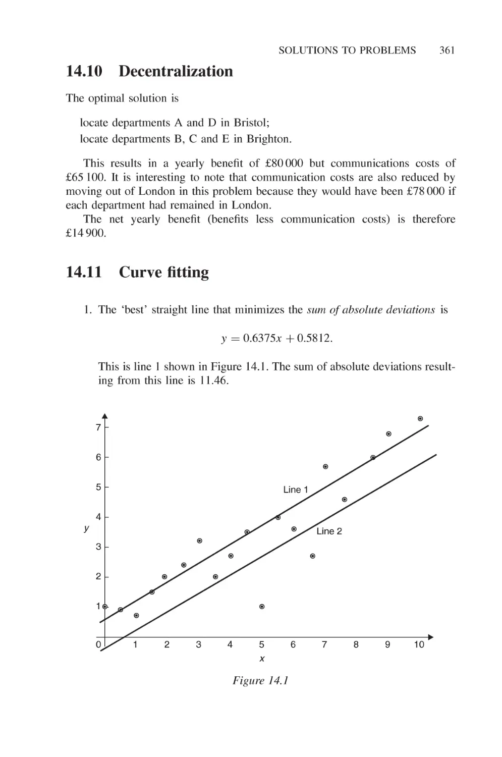


Text
H. PAUL WILLIAMS
Mo elB ilding
in Mathematical
Programming
FIFTH EDITION
) WILEY
Model Building in
Mathematical Programming
Model Building in
Mathematical Programming
Fifth Edition
H. Paul Williams
London School of Economics, UK
)WILEY
A John Wiley & Sons, Ltd., Publication
Copyright © 1978, 1985, 1990, 1993, 1999, 2013 by John Wiley & Sons Ltd,
The Atrium, Southern Gate, Chichester,
West Sussex P019 8SQ, England
Telephone (+44) 1243 779777
This edition first published 2013
Registered office
John Wiley & Sons Ltd, The Atrium, Southern Gate, Chichester, West Sussex, P019 8SQ, United Kingdom
For details of our global editorial offices, for customer services and for information about how to apply for
permission to reuse the copyright material in this book please see our website at www.wiley.com.
The right of the author to be identified as the author of this work has been asserted in accordance with the
Copyright, Designs and Patents Act 1988.
All rights reserved. No part of this publication may be reproduced, stored in a retrieval system, or transmitted,
in any form or by any means, electronic, mechanical, photocopying, recording or otherwise, except as
permitted by the UK Copyright, Designs and Patents Act 1988, without the prior permission of the publisher.
Wiley also publishes its books in a variety of electronic formats. Some content that appears in print may not
be available in electronic books.
Designations used by companies to distinguish their products are often claimed as trademarks. All brand
names and product names used in this book are trade names, service marks, trademarks or registered
trademarks of their respective owners. The publisher is not associated with any product or vendor mentioned
in this book. This publication is designed to provide accurate and authoritative information in regard to the
subject matter covered. It is sold on the understanding that the publisher is not engaged in rendering
professional services. If professional advice or other expert assistance is required, the services of a competent
professional should be sought.
Library of Congress Cataloging-in-Publication Data
Williams, H. P.
Model building in mathematical programming / H. Paul Williams. - 5th ed.
p. cm.
Includes bibliographical references and index.
ISBN 978-1-118-44333-0 (pbk.)
1. Programming (Mathematics) 2. Mathematical models. I. Title.
T57.7.W55 2013
519.7-dc23
2012037292
A catalogue record for this book is available from the British Library.
ISBN: 978-1-118-44333-0
Set in 10pt/12pt Times by Laserwords Private Limited, Chennai, India
To Eileen, Anna, Alexander and Eleanor
Contents
Preface xvii
Part I 1
1 Introduction 3
1.1 The concept of a model 3
1.2 Mathematical programming models 5
2 Solving mathematical programming models 11
2.1 Algorithms and packages 11
2.1.1 Reduction 12
2.1.2 Starting solutions 12
2.1.3 Simple bounding constraints 12
2.1.4 Ranged constraints 13
2.1.5 Generalized upper bounding constraints 13
2.1.6 Sensitivity analysis 13
2.2 Practical considerations 13
2.3 Decision support and expert systems 16
2.4 Constraint programming (CP) 17
3 Building linear programming models 21
3.1 The importance of linearity 21
3.2 Defining objectives 23
3.2.1 Single objectives 24
3.2.2 Multiple and conflicting objectives 26
3.2.3 Minimax objectives 27
3.2.4 Ratio objectives 28
3.2.5 Non-existent and non-optimizable objectives 29
3.3 Defining constraints 29
3.3.1 Productive capacity constraints 29
3.3.2 Raw material availabilities 30
3.3.3 Marketing demands and limitations 30
3.3.4 Material balance (continuity) constraints 30
CONTENTS
31
31
32
32
34
35
35
3.4 How to build a good model 36
36
37
37
38
40
3.5 The use of modelling languages 40
41
41
41
41
41
42
42
42
43
43
43
43
43
4 Structured linear programming models 45
4.1 Multiple plant, product and period models 45
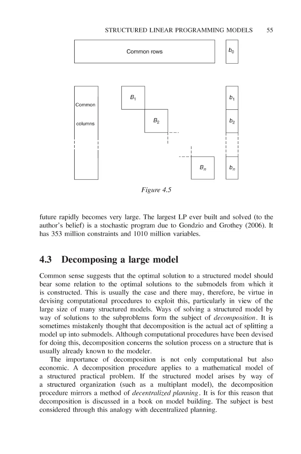
4.2 Stochastic programmes 53
4.3 Decomposing a large model 55
4.3.1 The submodels 63
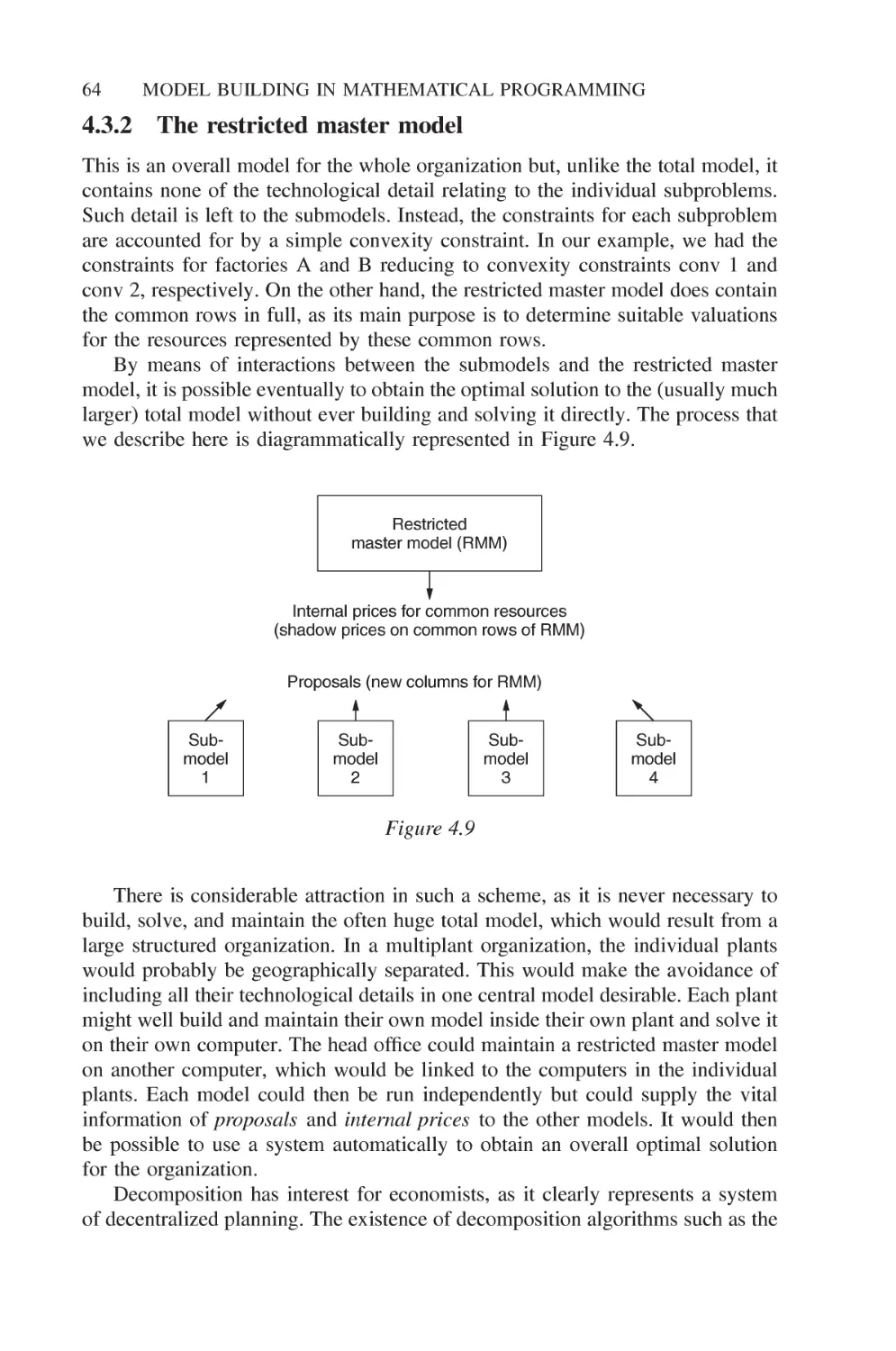
4.3.2 The restricted master model 64
5 Applications and special types of mathematical
programming model 67
5.1 Typical applications 67
5.1.1 The petroleum industry 68
5.1.2 The chemical industry 68
5.1.3 Manufacturing industry 68
5.1.4 Transport and distribution 69
5.1.5 Finance 69
5.1.6 Agriculture 70
3.3.5
3.3.6
3.3.7
3.3.8
3.3.9
3.3.10
3.3.11
Quality stipulations
Hard and soft constraints
Chance constraints
Conflicting constraints
Redundant constraints
Simple and generalized upper bounds
Unusual constraints
How to build a good model
3.4.1
3.4.2
3.4.3
3.4.4
3.4.5
The use
3.5.1
3.5.2
3.5.3
3.5.4
3.5.5
3.5.6
3.5.7
3.5.8
Ease of understanding the model
Ease of detecting errors in the model
Ease of computing the solution
Modal formulation
Units of measurement
of modelling languages
A more natural input format
Debugging is made easier
Modification is made easier
Repetition is automated
Special purpose generators using a high level
language
Matrix block building systems
Data structuring systems
Mathematical languages
3.5.8.1 SETs
3.5.8.2 DATA
3.5.8.3 VARIABLES
3.5.8.4 OBJECTIVE
3.5.8.5 CONSTRAINTS
CONTENTS
IX
5.1.7 Health 70
5.1.8 Mining 70
5.1.9 Manpower planning 71
5.1.10 Food 71
5.1.11 Energy 71
5.1.12 Pulp and paper 72
5.1.13 Advertising 72
5.1.14 Defence 72
5.1.15 The supply chain 72
5.1.16 Other applications 73
5.2 Economic models 74
5.2.1 The static model 74
5.2.2 The dynamic model 80
5.2.3 Aggregation 81
5.3 Network models 81
5.3.1 The transportation problem 82
5.3.2 The assignment problem 87
5.3.3 The transhipment problem 88
5.3.4 The minimum cost flow problem 89
5.3.5 The shortest path problem 93
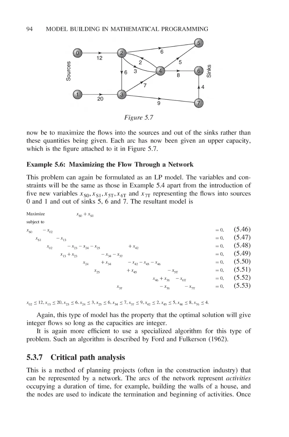
5.3.6 Maximum flow through a network 93
5.3.7 Critical path analysis 94
5.4 Converting linear programs to networks 98
6 Interpreting and using the solution of a linear
programming model 103
6.1 Validating a model 103
6.1.1 Infeasible models 103
6.1.2 Unbounded models 104
6.1.3 Solvable models 105
6.2 Economic interpretations 107
6.2.1 The dual model 109
6.2.2 Shadow prices 112
6.2.3 Productive capacity constraints 114
6.2.4 Raw material availabilities 114
6.2.5 Marketing demands and limitations 114
6.2.6 Material balance (continuity) constraints 114
6.2.7 Quality stipulations 114
6.2.8 Reduced costs 116
6.3 Sensitivity analysis and the stability of a model 121
6.3.1 Right-hand side ranges 121
6.3.2 Objective ranges 125
6.3.3 Ranges on interior coefficients 128
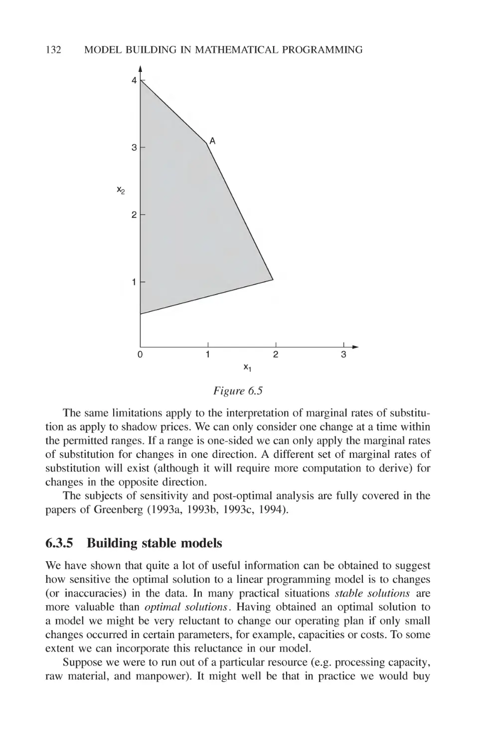
6.3.4 Marginal rates of substitution 131
6.3.5 Building stable models 132
CONTENTS
6.4 Further investigations using a model 133
6.5 Presentation of the solutions 135
7 Non-linear models 137
7.1 Typical applications 137
7.2 Local and global optima 140
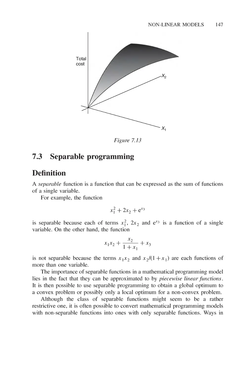
7.3 Separable programming 147
7.4 Converting a problem to a separable model 153
8 Integer programming 155
8.1 Introduction 155
8.2 The applicability of integer programming 156
8.2.1 Problems with discrete inputs and outputs 156
8.2.2 Problems with logical conditions 158
8.2.3 Combinatorial problems 158
8.2.4 Non-linear problems 160
8.2.5 Network problems 161
8.3 Solving integer programming models 162
8.3.1 Cutting planes methods 162
8.3.2 Enumerative methods 163
8.3.3 Pseudo-Boolean methods 163
8.3.4 Branch and bound methods 164
9 Building integer programming models I 165
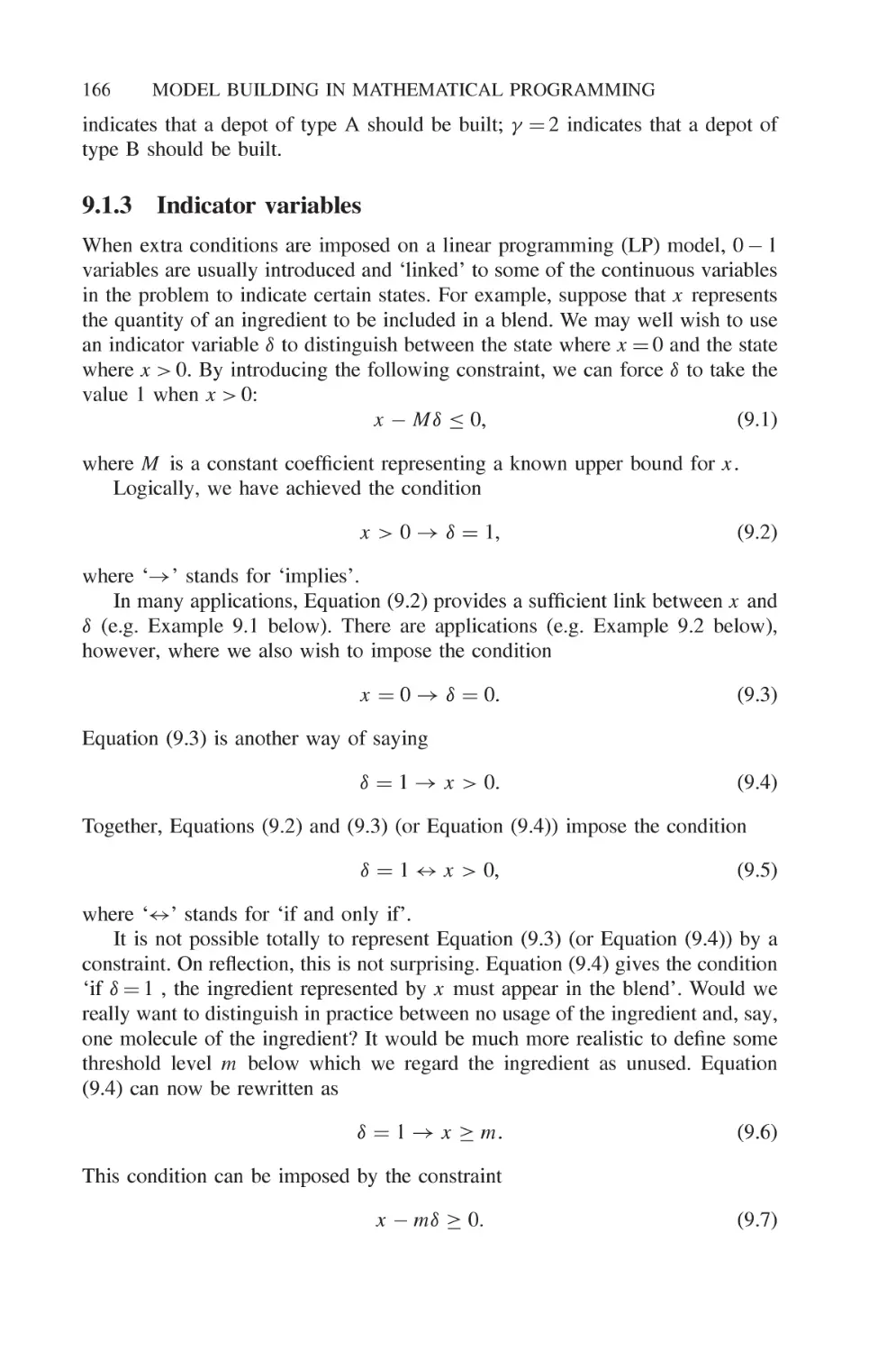
9.1 The uses of discrete variables 165
9.1.1 Indivisible (discrete) quantities 165
9.1.2 Decision variables 165
9.1.3 Indicator variables 166
9.2 Logical conditions and 0-1 variables 172
9.3 Special ordered sets of variables 177
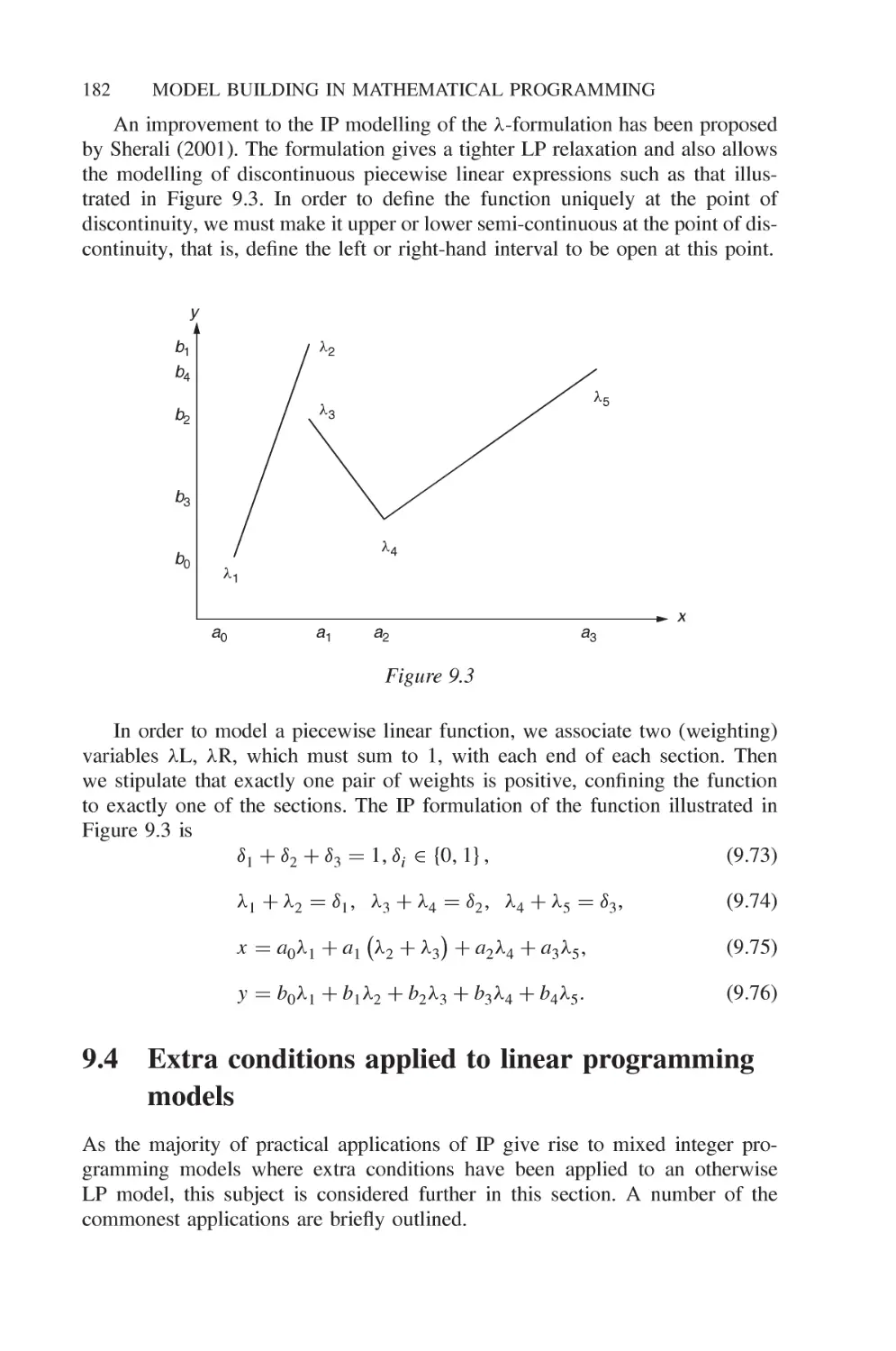
9.4 Extra conditions applied to linear programming models 182
9.4.1 Disjunctive constraints 183
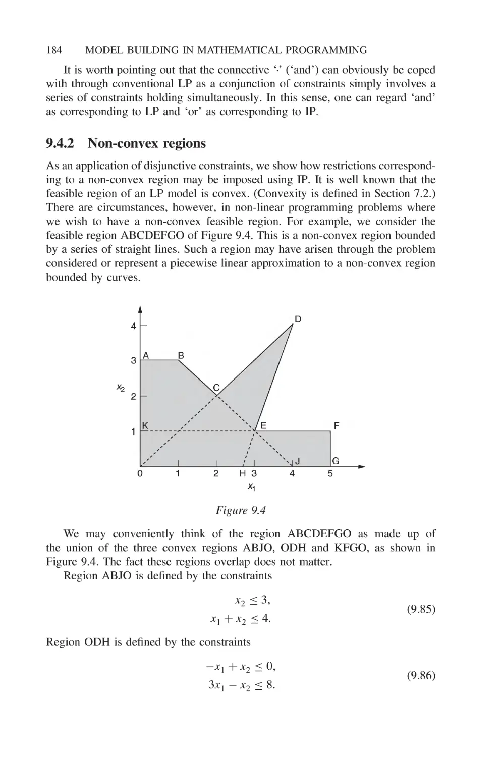
9.4.2 Non-convex regions 184
9.4.3 Limiting the number of variables in a solution 186
9.4.4 Sequentially dependent decisions 186
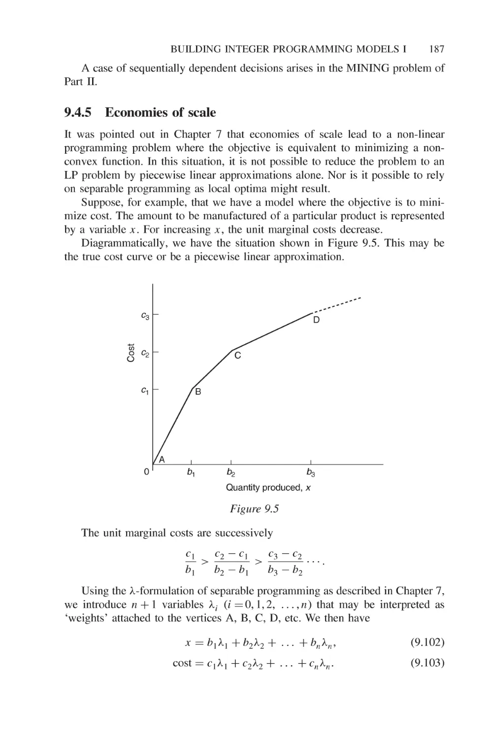
9.4.5 Economies of scale 187
9.4.6 Discrete capacity extensions 188
9.4.7 Maximax objectives 188
9.5 Special kinds of integer programming model 189
9.5.1 Set covering problems 189
9.5.2 Set packing problems 191
9.5.3 Set partitioning problems 193
9.5.4 The knapsack problem 195
9.5.5 The travelling salesman problem 195
9.5.6 The vehicle routing problem 198
CONTENTS
XI
9.5.7 The quadratic assignment problem 199
9.6 Column generation 201
10 Building integer programming models II 207
10.1 Good and bad formulations 207
10.1.1 The number of variables in an IP model 207
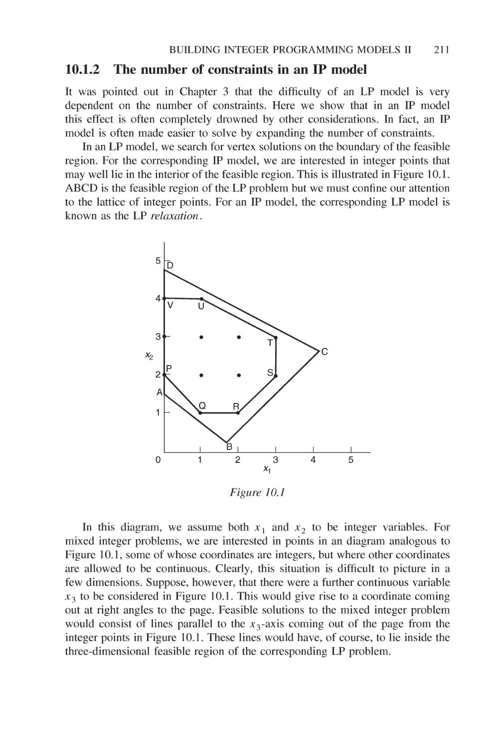
10.1.2 The number of constraints in an IP model 211
10.2 Simplifying an integer programming model 218
10.2.1 Tightening bounds 218
10.2.2 Simplifying a single integer constraint to another
single integer constraint 220
10.2.3 Simplifying a single integer constraint to a collection
of integer constraints 222
10.2.4 Simplifying collections of constraints 226
10.2.5 Discontinuous variables 228
10.2.6 An alternative formulation for disjunctive
constraints 229
10.2.7 Symmetry 230
10.3 Economic information obtainable by integer programming 231
10.4 Sensitivity analysis and the stability of a model 238
10.4.1 Sensitivity analysis and integer programming 238
10.4.2 Building a stable model 239
10.5 When and how to use integer programming 240
11 The implementation of a mathematical programming system
of planning 243
11.1 Acceptance and implementation 243
11.2 The unification of organizational functions 245
11.3 Centralization versus decentralization 247
11.4 The collection of data and the maintenance of a model 249
Part II 251
253
253
255
255
256
256
257
257
258
258
258
The problems
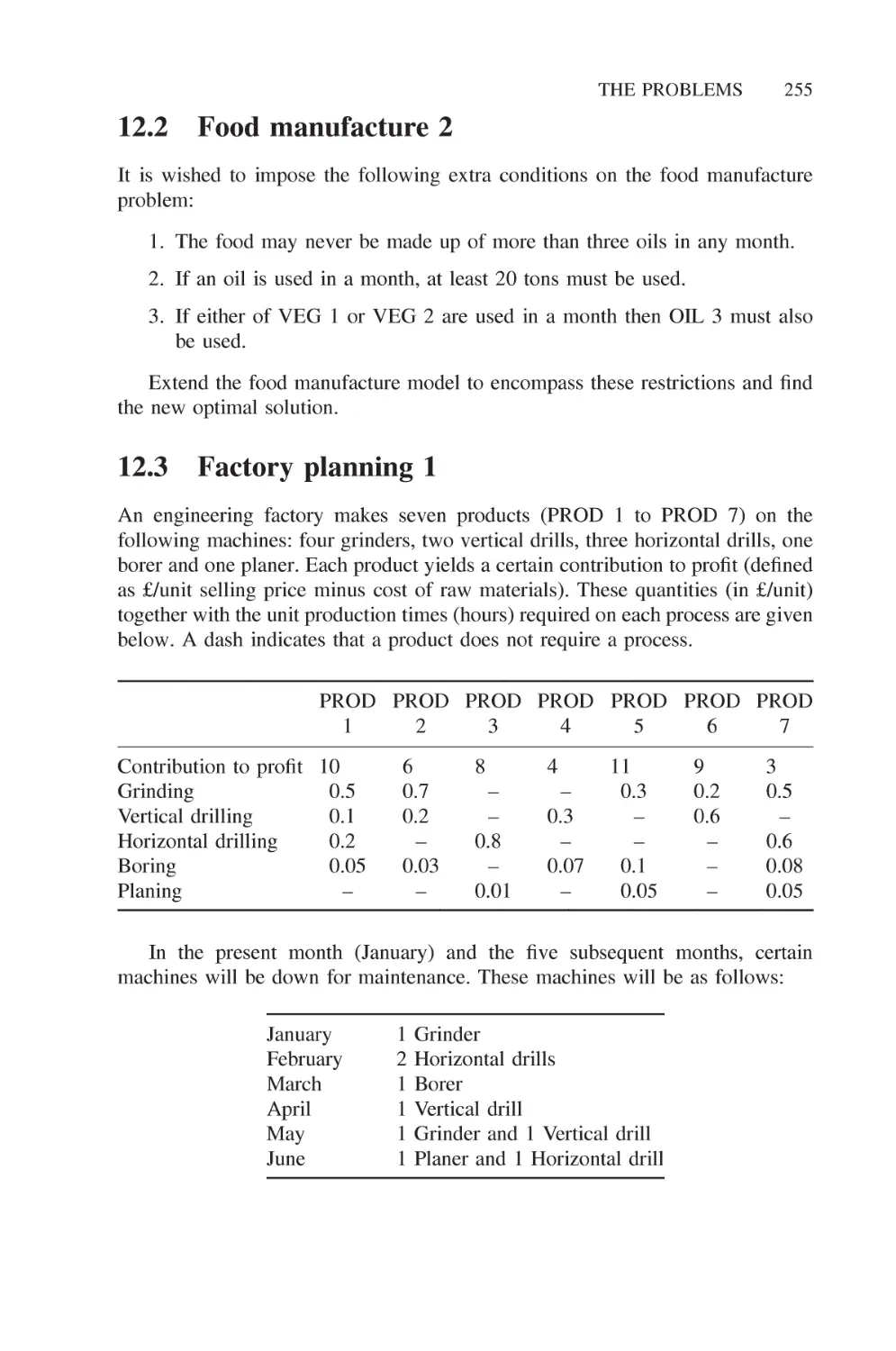
12.1
12.2
12.3
12.4
12.5
Food manufacture 1
Food manufacture 2
Factory planning 1
Factory planning 2
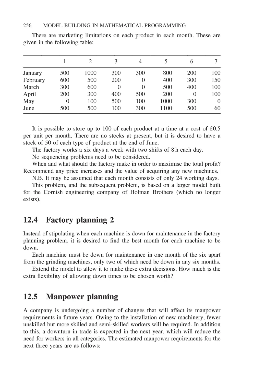
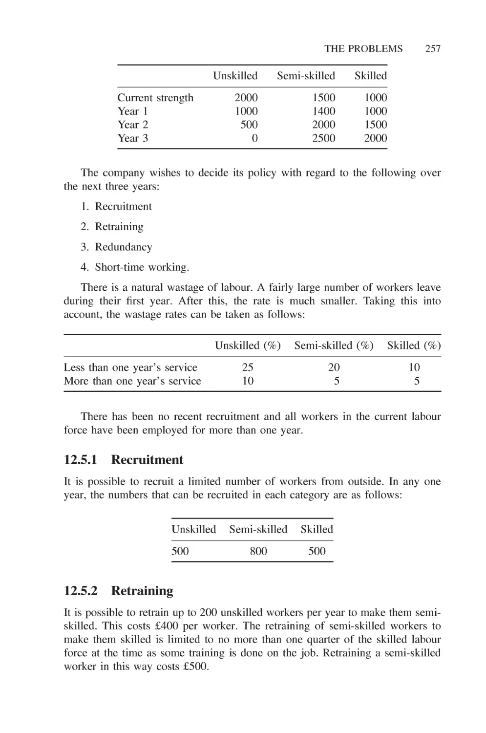
Manpower planning
12.5.1
12.5.2
12.5.3
12.5.4
12.5.5
Recruitment
Retraining
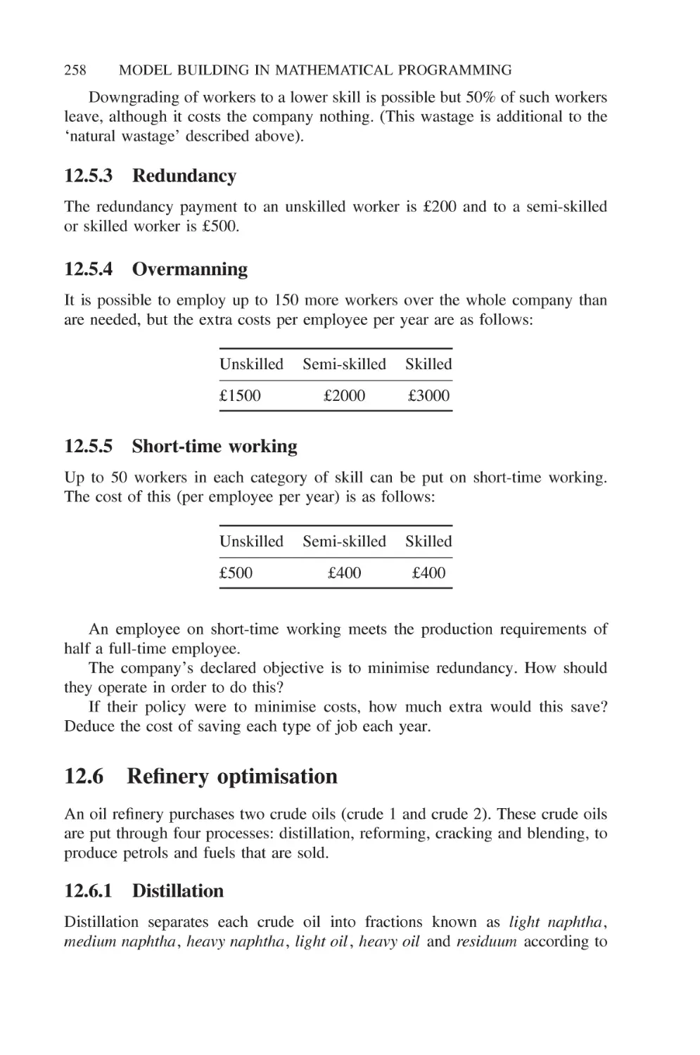
Redundancy
Overmanning
Short-time working
Xll
CONTENTS
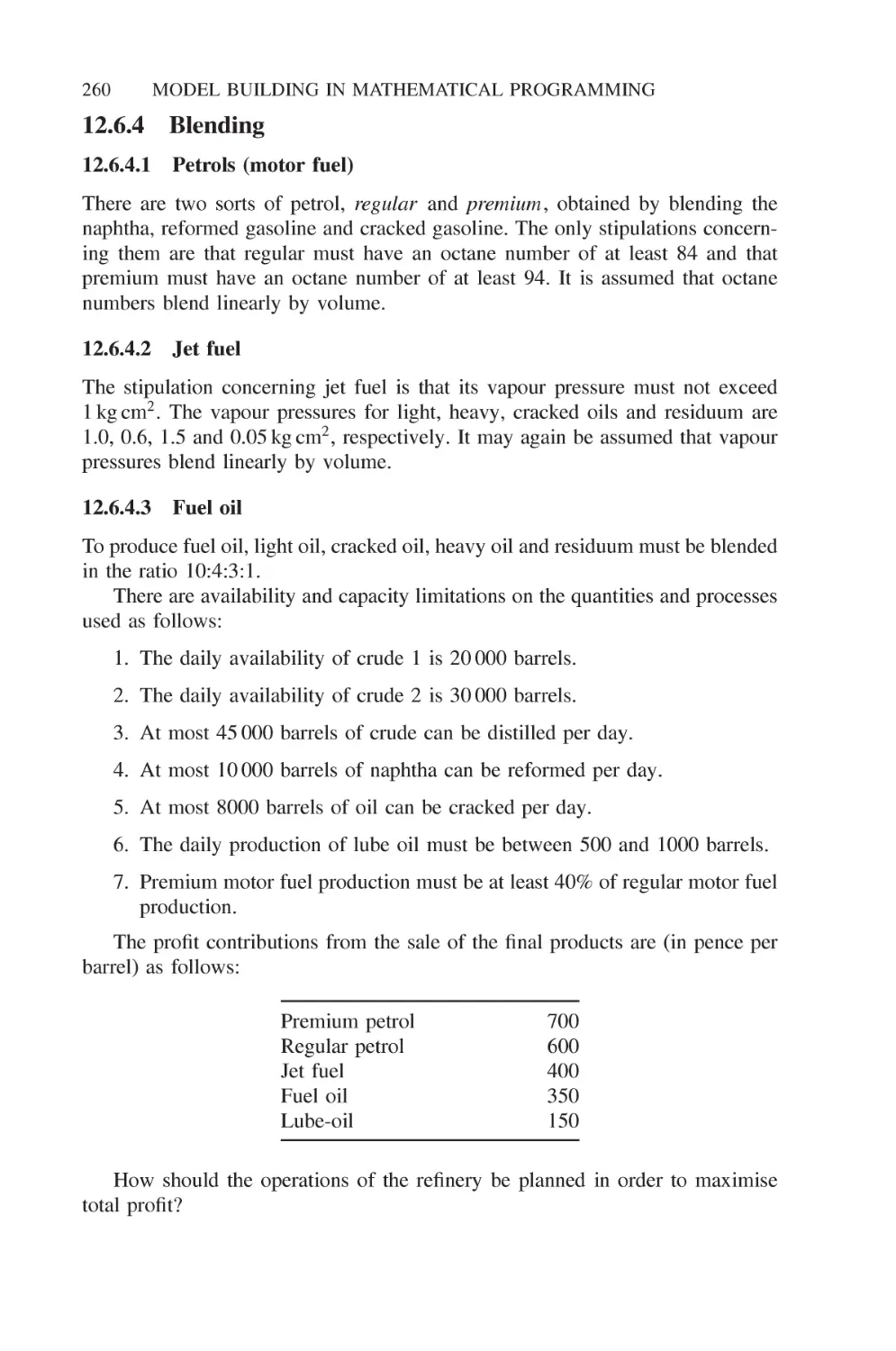
12.6 Refinery optimisation 258
12.6.1 Distillation 258
12.6.2 Reforming 259
12.6.3 Cracking 259
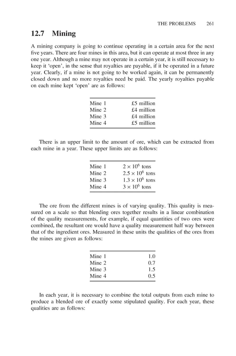
12.6.4 Blending 260
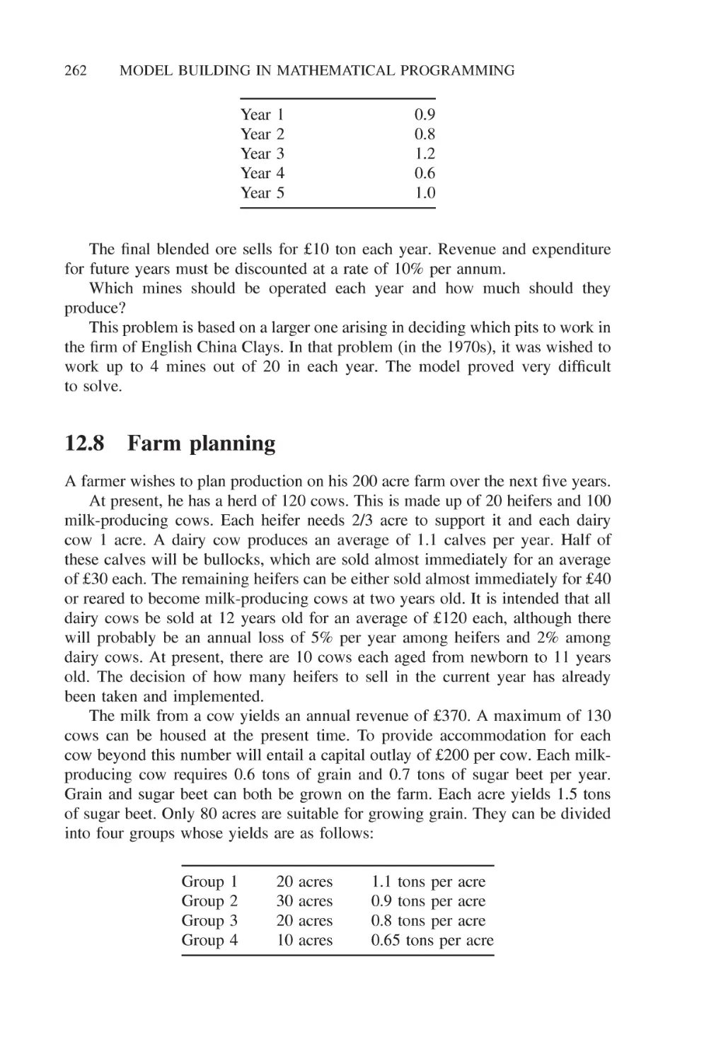
12.7 Mining 261
12.8 Farm planning 262
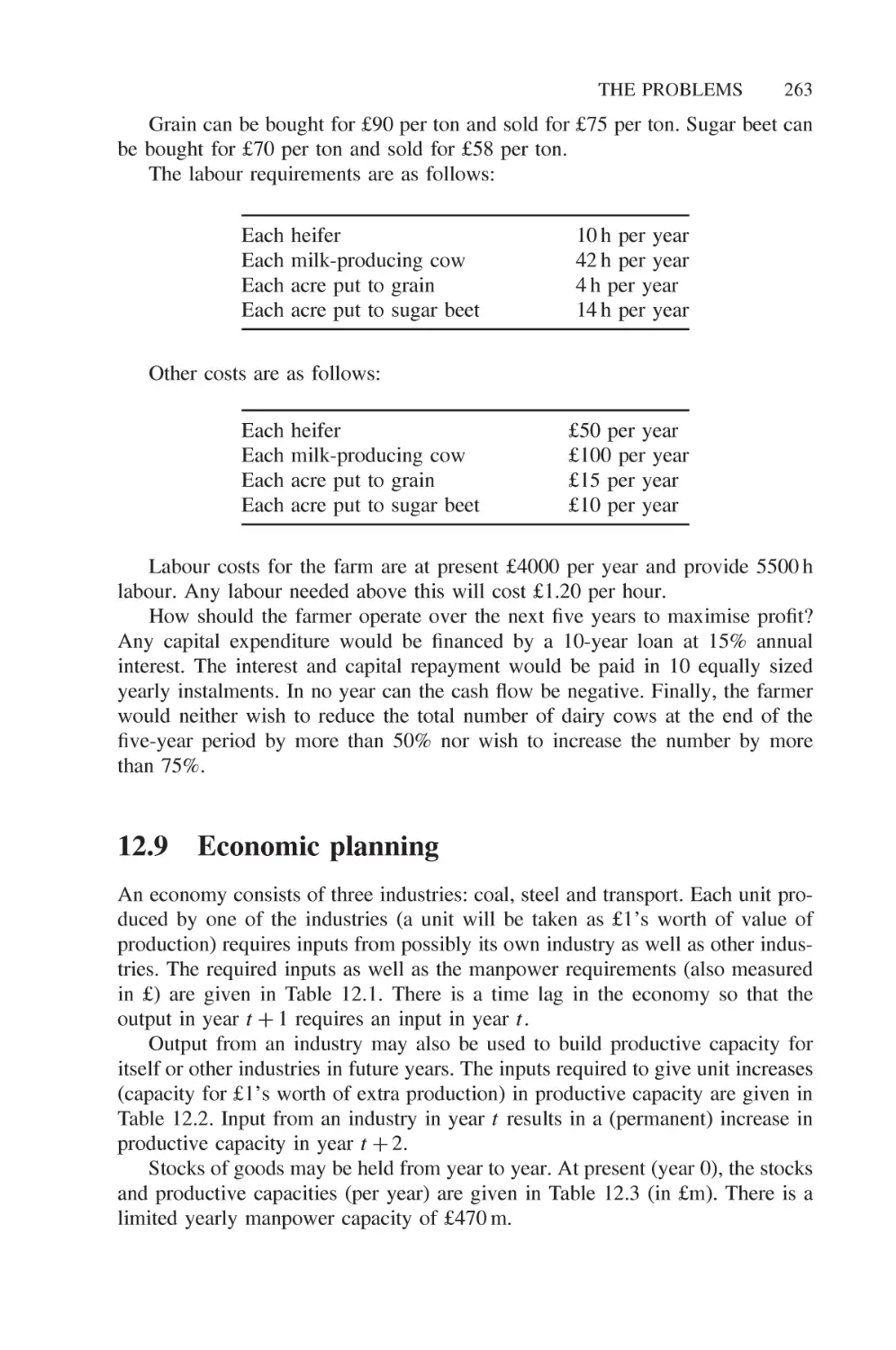
12.9 Economic planning 263
12.10 Decentralisation 265
12.11 Curve fitting 266
12.12 Logical design 266
12.13 Market sharing 267
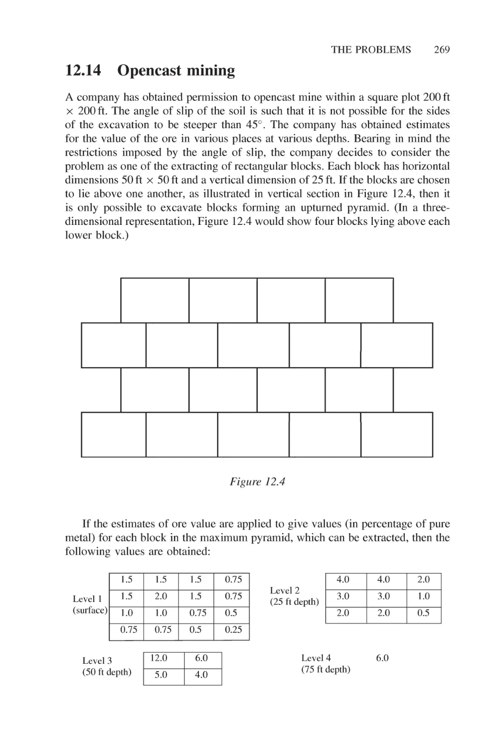
12.14 Opencast mining 269
12.15 Tariff rates (power generation) 270
12.16 Hydro power 271
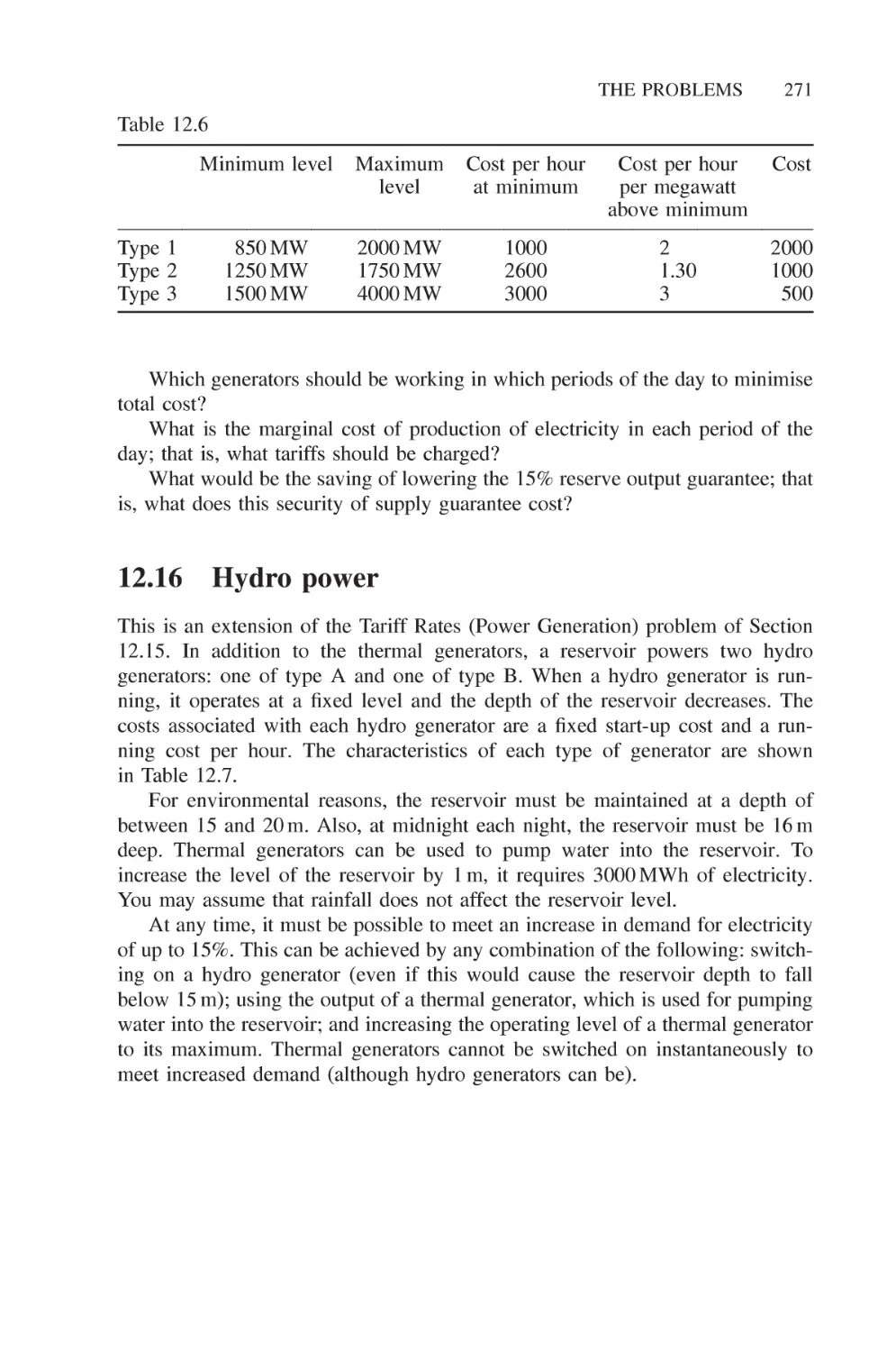
12.17 Three-dimensional noughts and crosses 272
12.18 Optimising a constraint 273
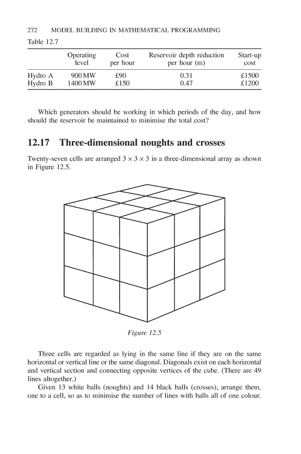
12.19 Distribution 1 273
12.20 Depot location (distribution 2) 275
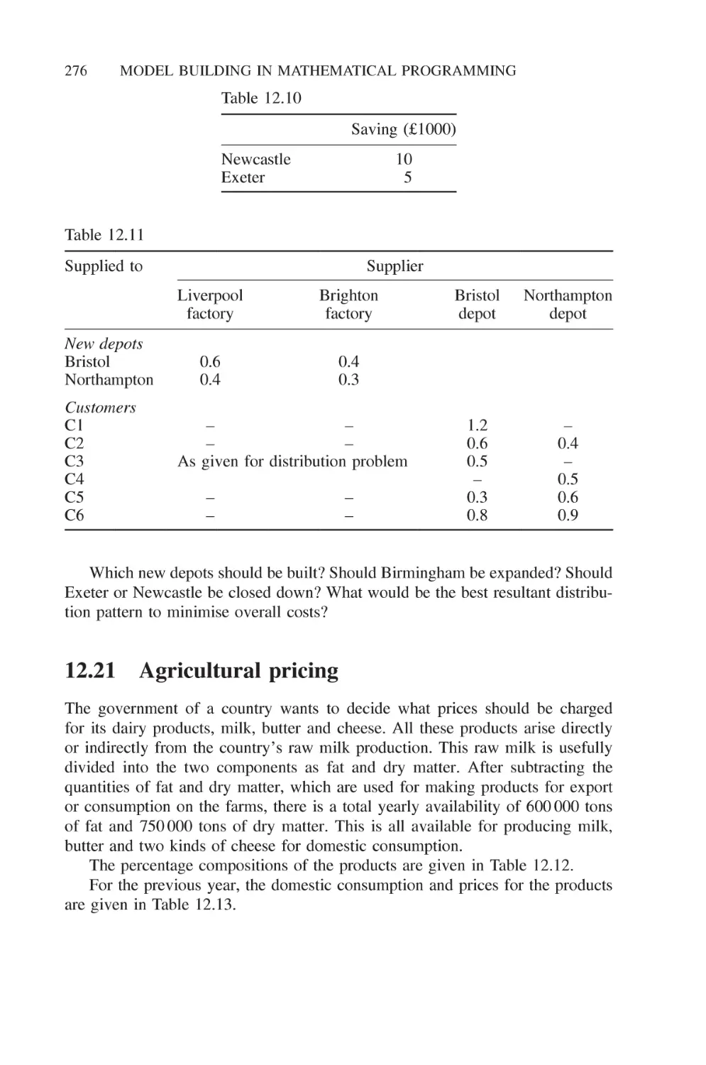
12.21 Agricultural pricing 276
12.22 Efficiency analysis 278
12.23 Milk collection 278
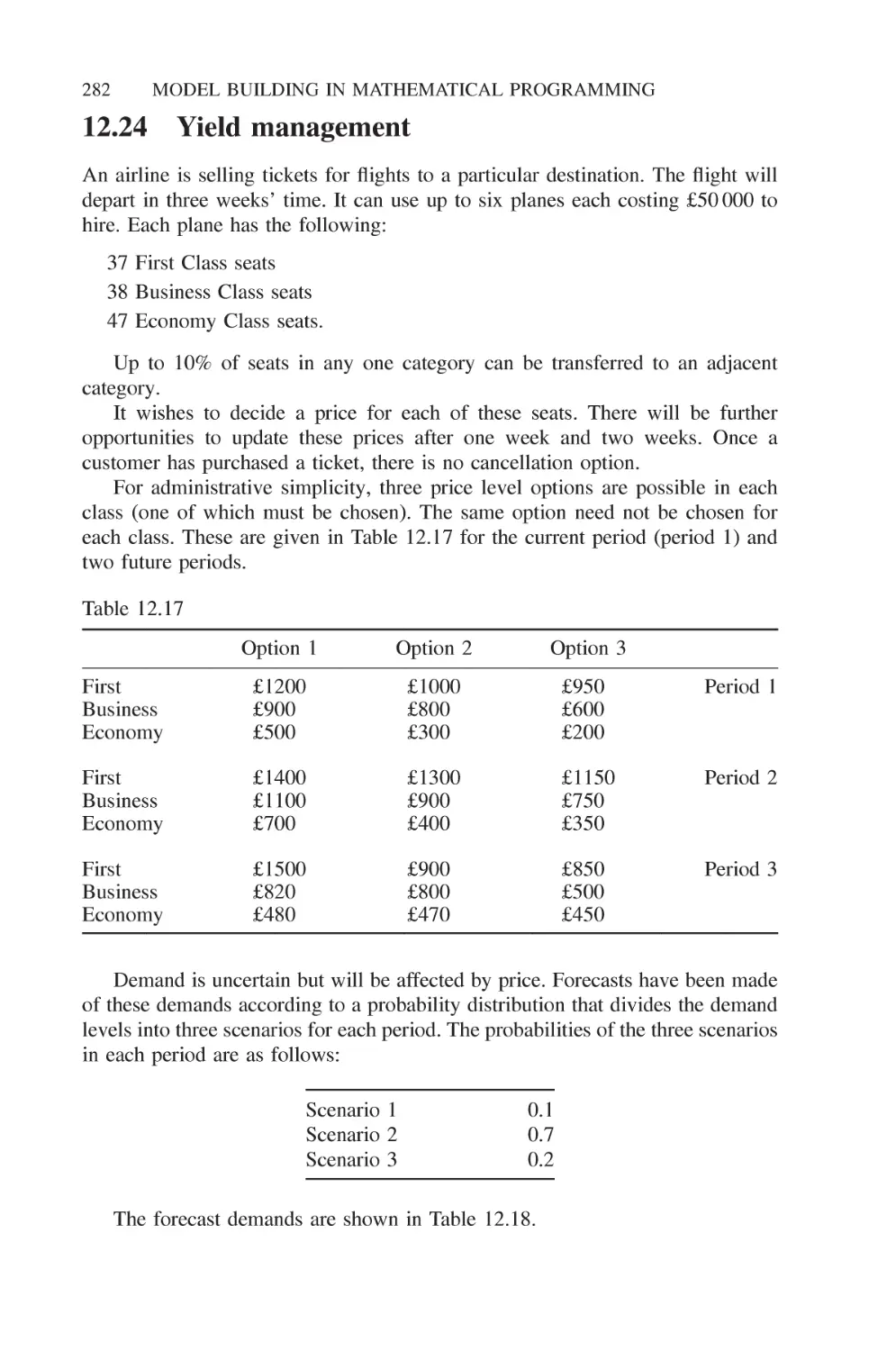
12.24 Yield management 282
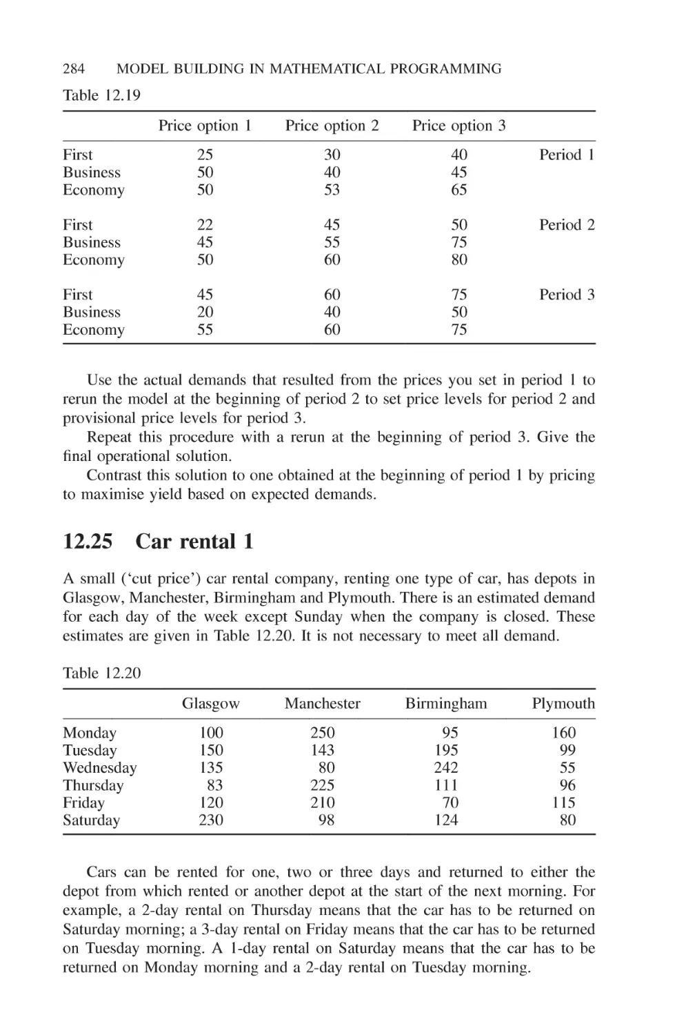
12.25 Car rental 1 284
12.26 Car rental 2 287
12.27 Lost baggage distribution 287
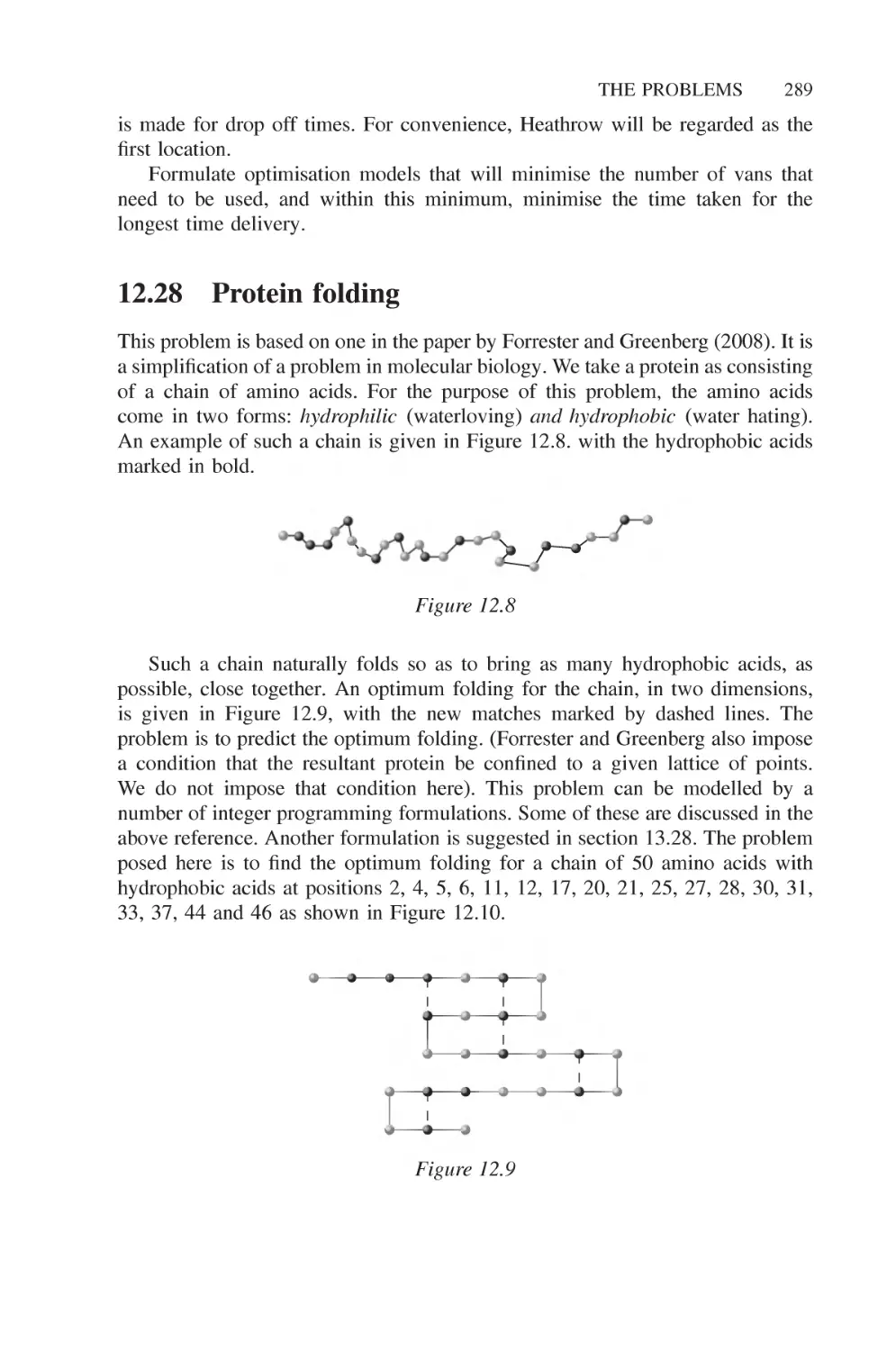
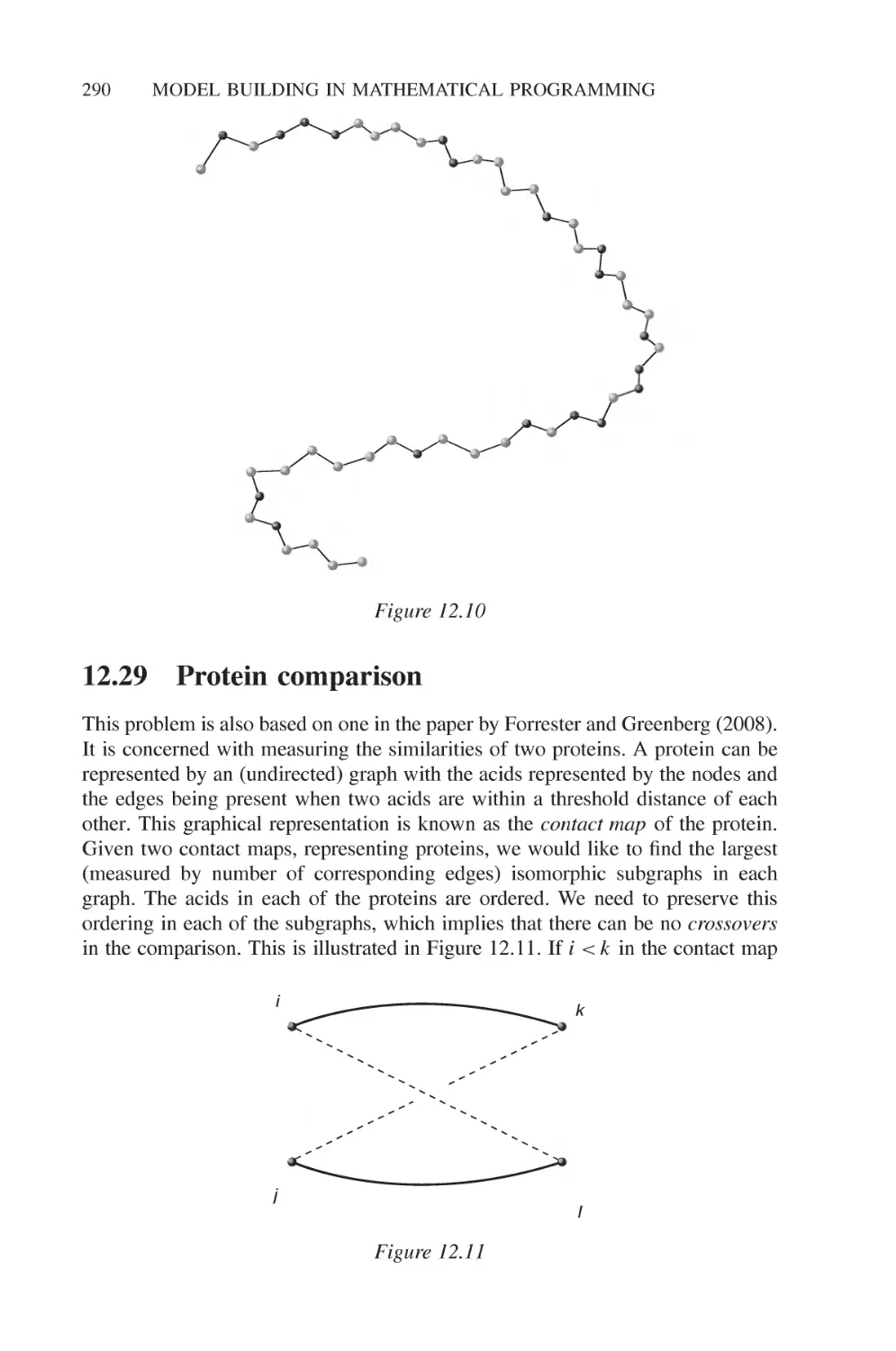
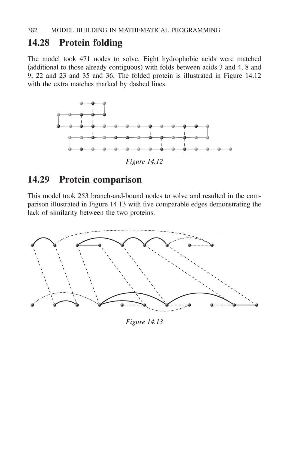
12.28 Protein folding 289
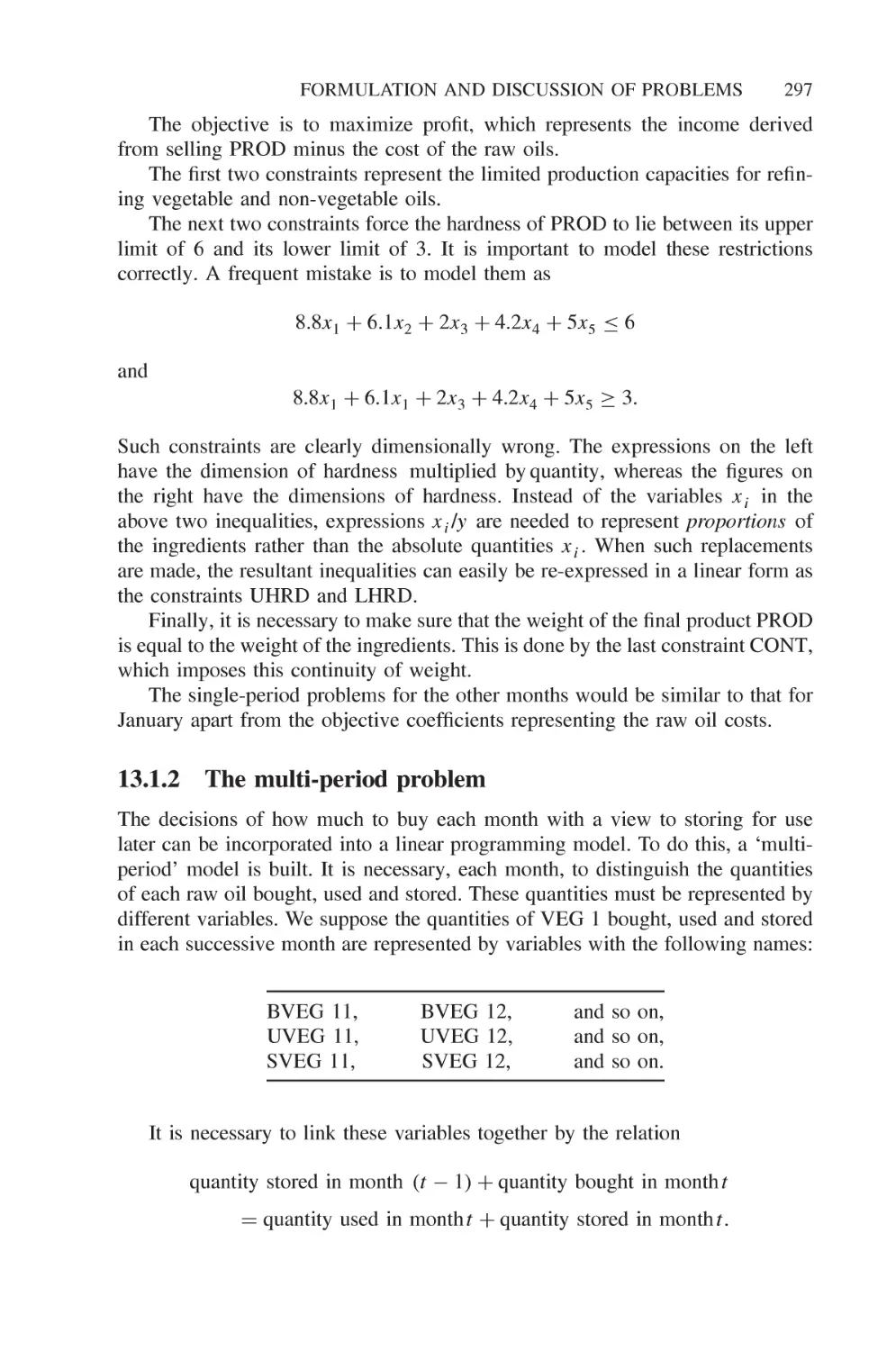
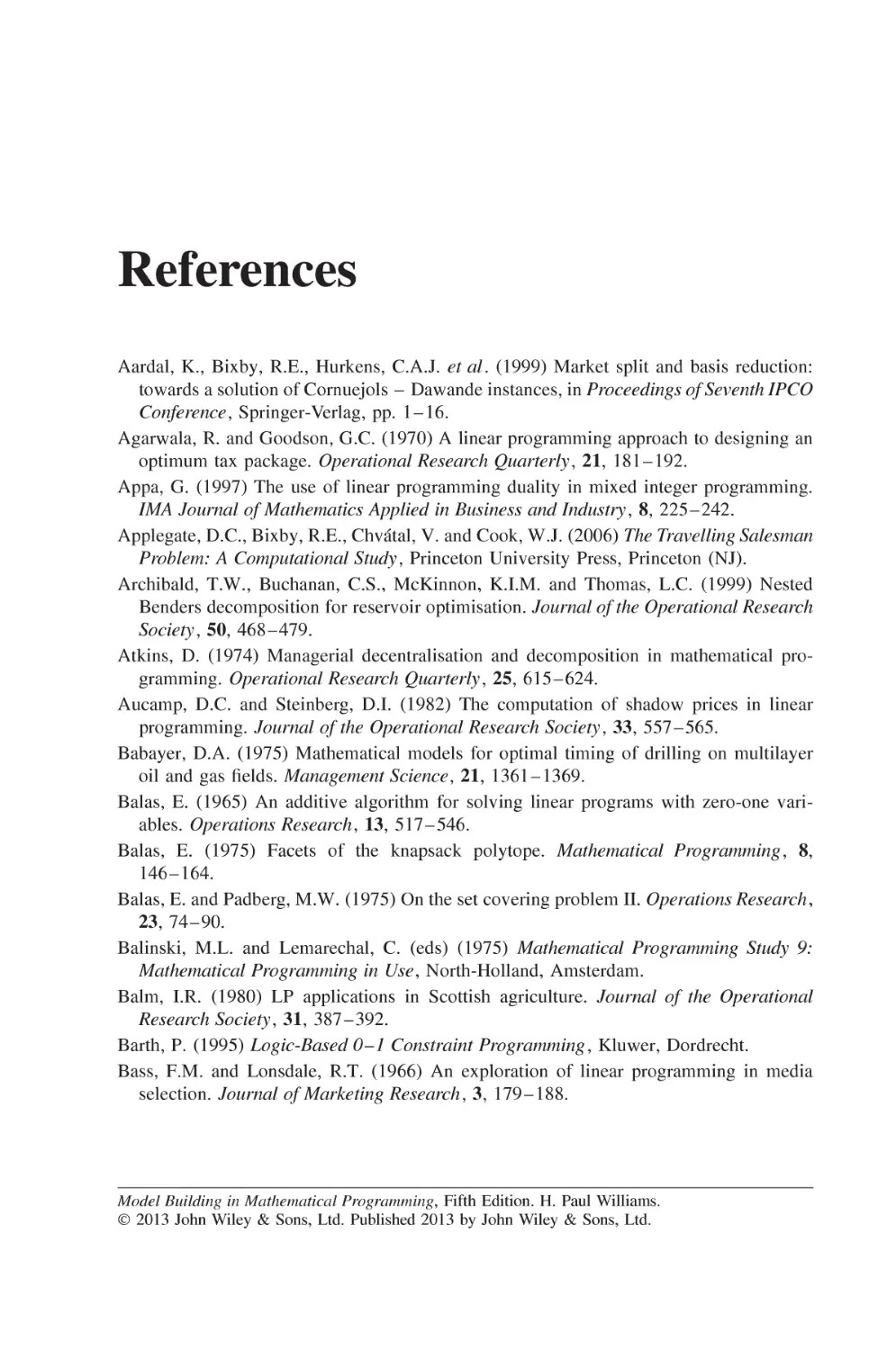
12.29 Protein comparison 290
Part III 293
13 Formulation and discussion of problems 295
13.1 Food manufacture 1 296
13.1.1 The single-period problem 296
13.1.2 The multi-period problem 297
13.2 Food manufacture 2 299
13.3 Factory planning 1 300
13.3.1 The single-period problem 300
13.3.2 The multi-period problem 301
13.4 Factory planning 2 302
13.4.1 Extra variables 302
13.4.2 Revised constraints 303
13.5 Manpower planning 303
13.5.1 Variables 304
13.5.2
13.5.3
Constraints
Initial conditions
Refinery optimization
13.6.1
13.6.2
13.6.3
Mining
13.7.1
13.7.2
13.7.3
Variables
Constraints
Objective
Variables
Constraints
Objective
CONTENTS xiii
305
305
13.6 Refinery optimization 306
307
308
310
13.7 Mining 310
310
311
312
13.8 Farm planning 312
13.8.1 Variables 312
13.8.2 Constraints 313
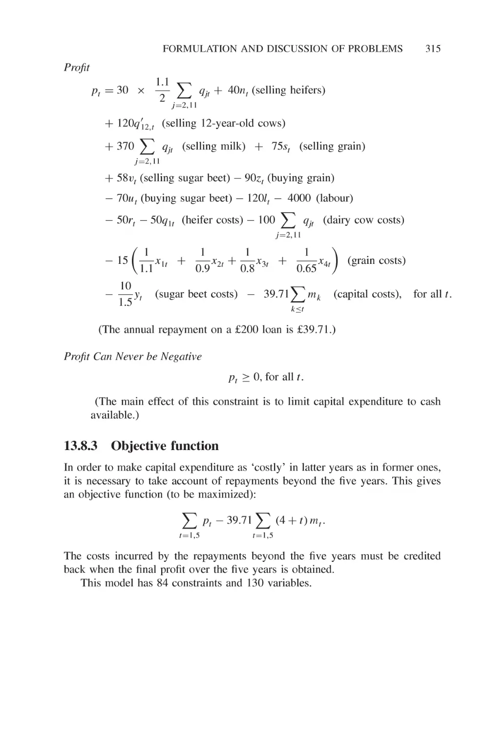
13.8.3 Objective function 315
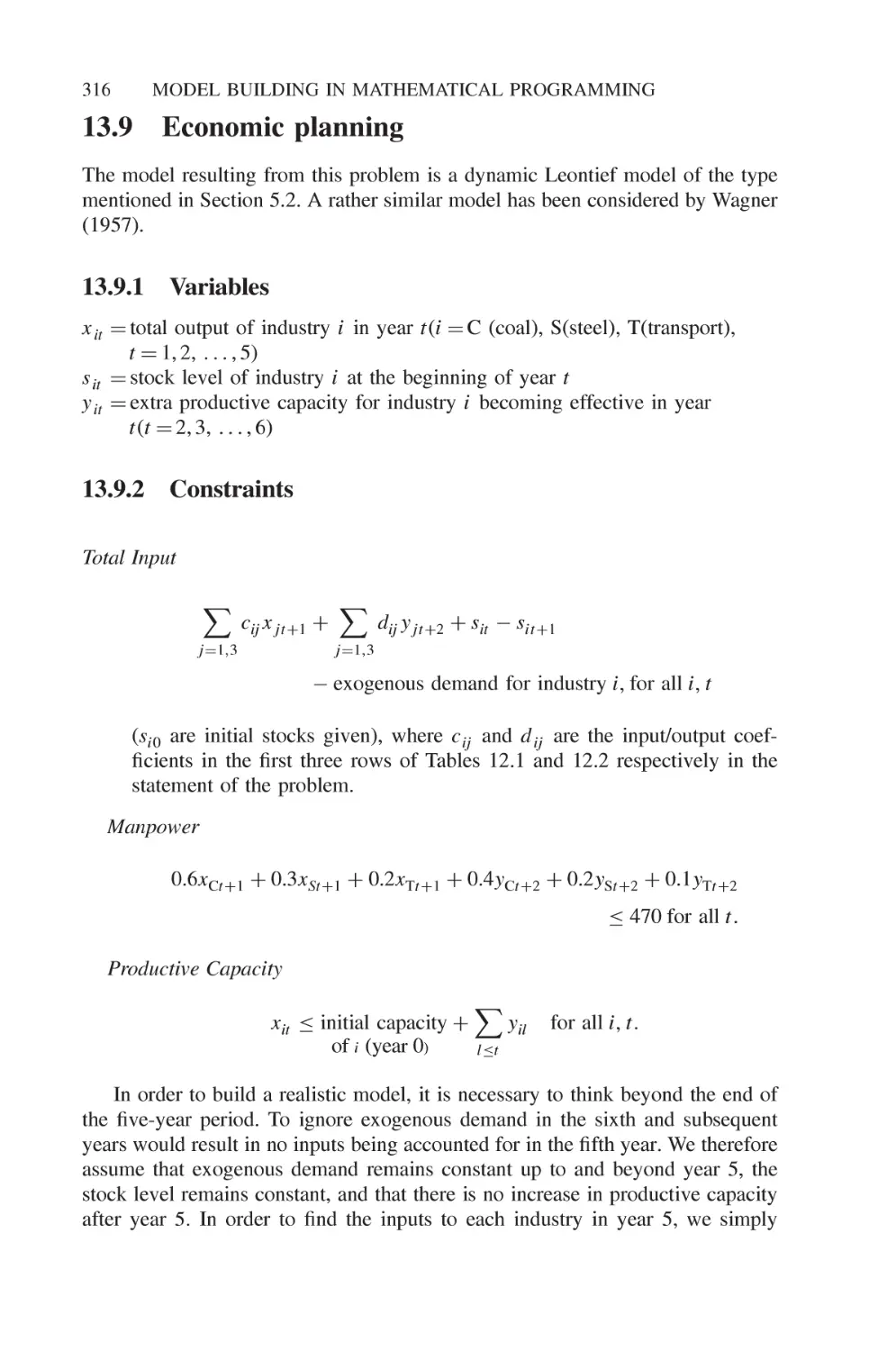
13.9 Economic planning 316
13.9.1 Variables 316
13.9.2 Constraints 316
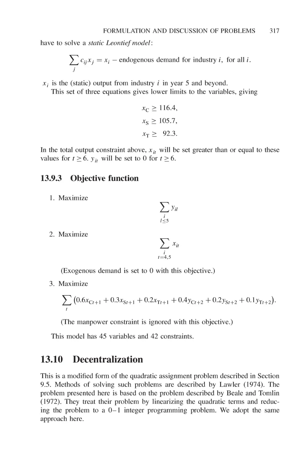
13.9.3 Objective function 317
13.10 Decentralization 317
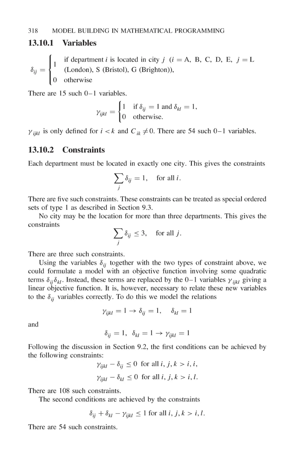
13.10.1 Variables 318
13.10.2 Constraints 318
13.10.3 Objective 319
13.11 Curve fitting 319
13.12 Logical design 320
13.13 Market sharing 322
13.14 Opencast mining 324
13.15 Tariff rates (power generation) 325
13.15.1 Variables 325
13.15.2 Constraints 325
13.15.3 Objective function (to be minimized) 326
13.16 Hydro power 326
13.16.1 Variables 326
13.16.2 Constraints 326
13.16.3 Objective function (to be minimized) 327
13.17 Three-dimensional noughts and crosses 327
13.17.1 Variables 327
13.17.2 Constraints 328
13.17.3 Objective 328
13.18 Optimizing a constraint 328
13.19 Distribution 1 330
13.19.1 Variables 331
13.19.2 Constraints 331
13.19.3 Objectives 332
13.20 Depot location (distribution 2) 332
13.21 Agricultural pricing 333
XIV
CONTENTS
13.22
13.23
13.24
13.25
13.26
13.27
13.28
13.29
Efficiency analysis
Milk collection
13.23.1 Variables
13.23.2 Constraints
13.23.3 Objective
Yield management
13.24.1 Variables
13.24.2 Constraints
13.24.3 Objective
Car rental 1
13.25.1 Indices
13.25.2 Given data
13.25.3 Variables
13.25.4 Constraints
13.25.5 Objective
Car rental 2
Lost baggage distribution
13.27.1 Variables
13.27.2 Objective
13.27.3 Constraints
Protein folding
Protein comparison
335
336
336
336
337
337
338
338
340
340
340
340
341
341
342
342
343
343
344
344
344
345
Part IV 347
14 Solutions to problems 349
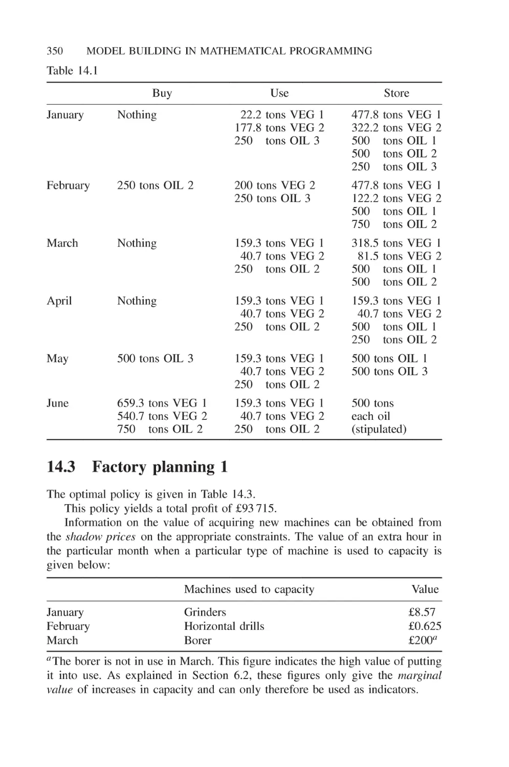
14.1 Food manufacture 1 349
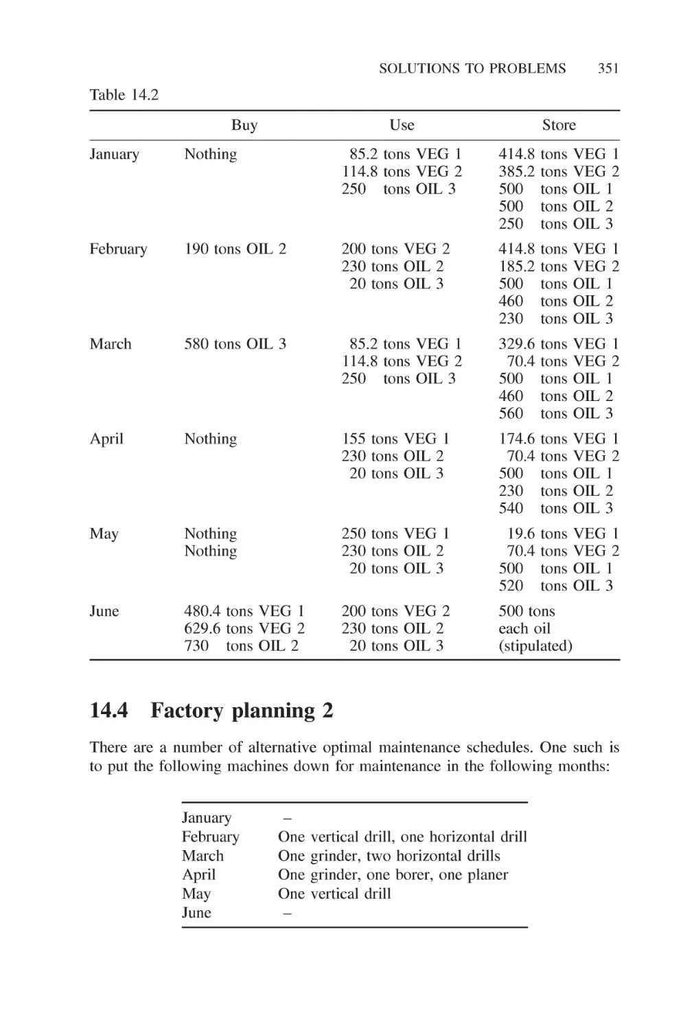
14.2 Food manufacture 2 349
14.3 Factory planning 1 350
14.4 Factory planning 2 351
14.5 Manpower planning 354
14.6 Refinery optimization 356
14.7 Mining 357
14.8 Farm planning 358
14.9 Economic planning 359
14.10 Decentralization 361
14.11 Curve fitting 361
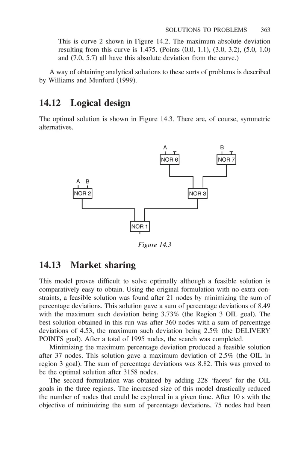
14.12 Logical design 363
14.13 Market sharing 363
14.14 Opencast mining 364
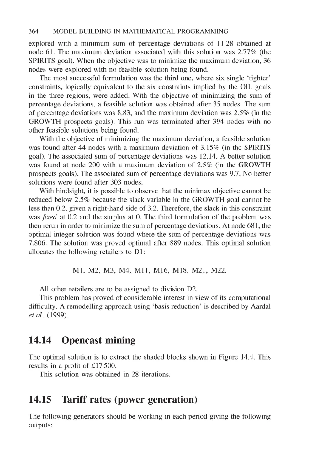
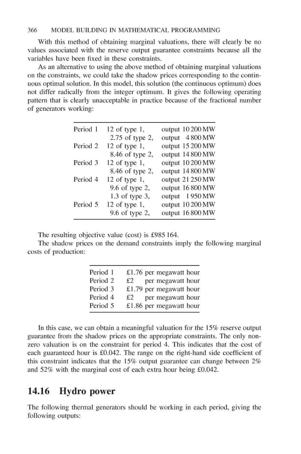
14.15 Tariff rates (power generation) 364
14.16 Hydro power 366
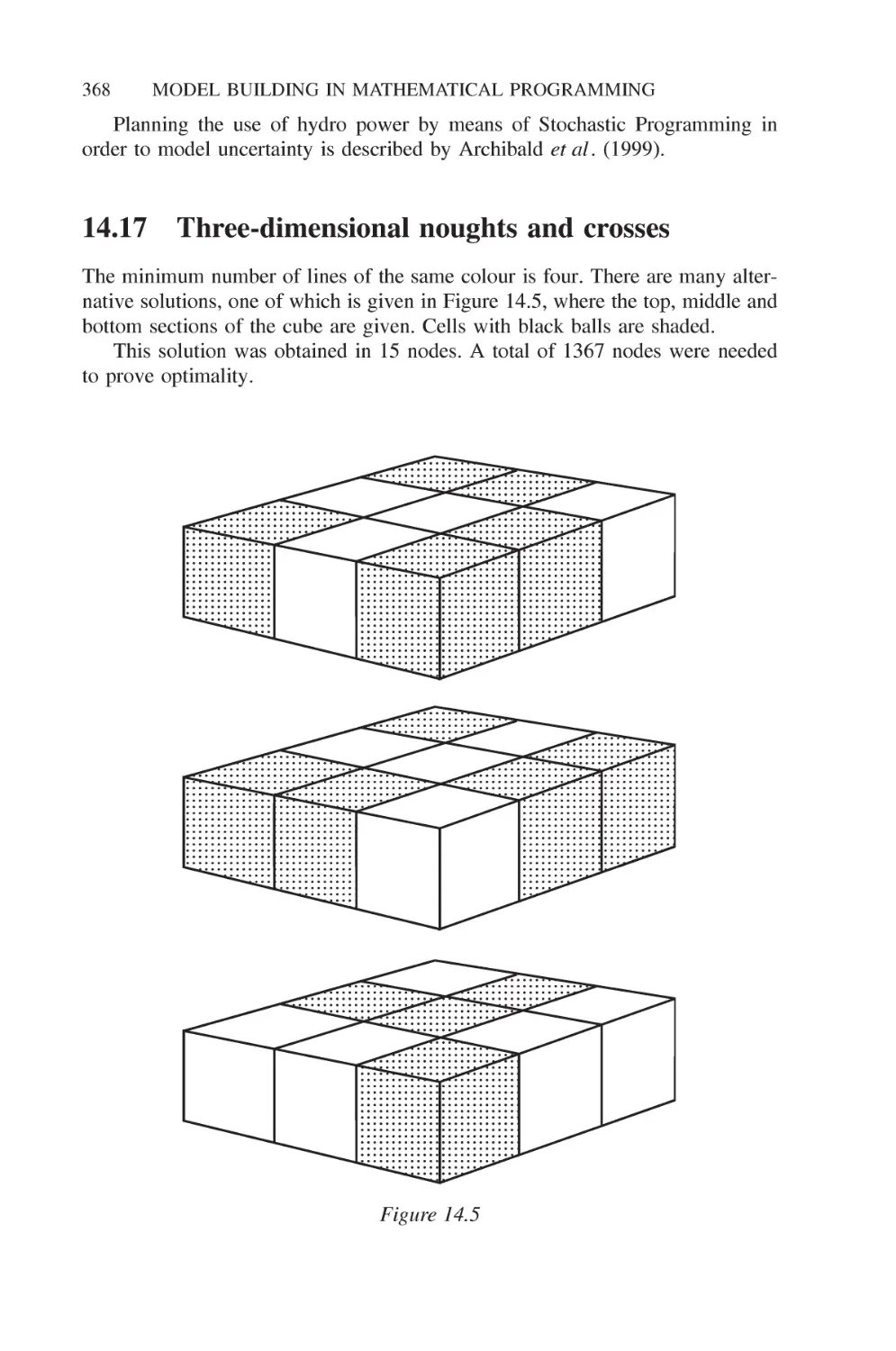
14.17 Three-dimensional noughts and crosses 368
14.18 Optimizing a constraint 369
CONTENTS xv
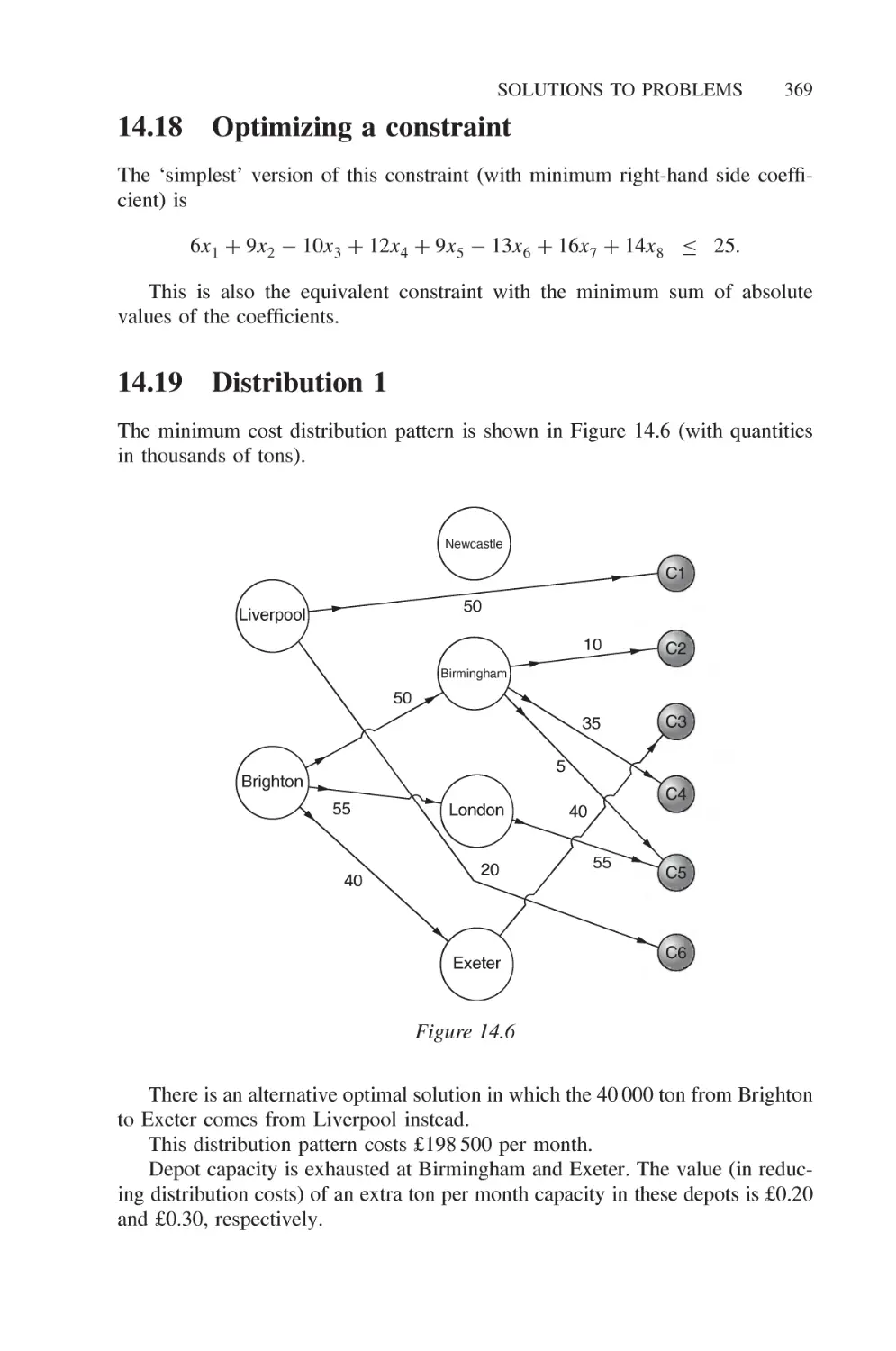
14.19 Distribution 1 369
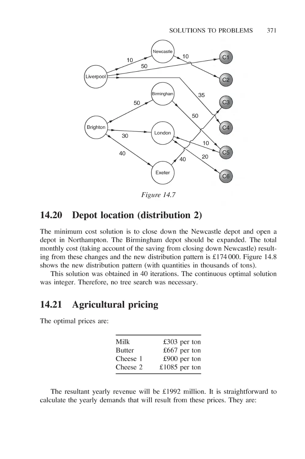
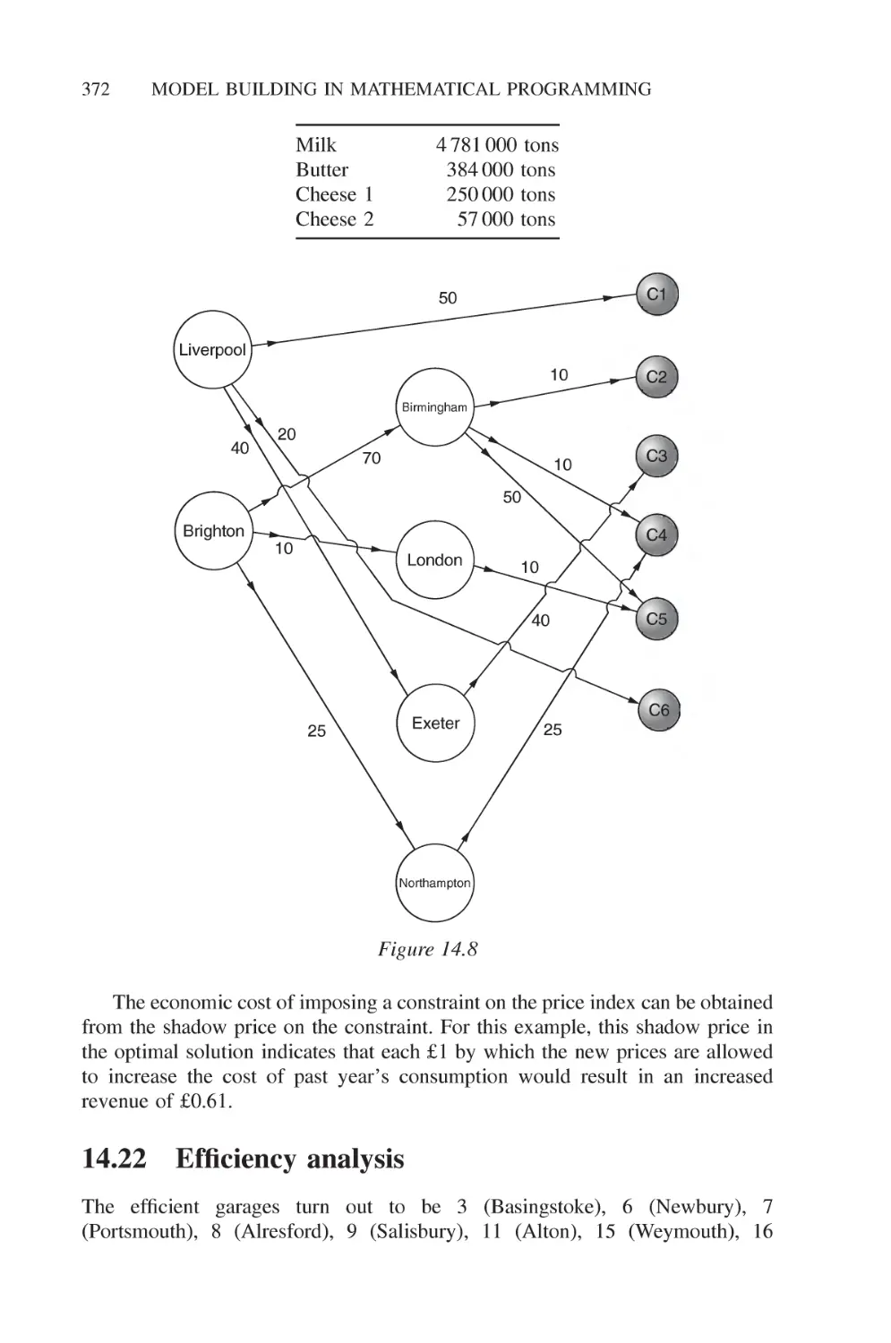
14.20 Depot location (distribution 2) 371
14.21 Agricultural pricing 371
14.22 Efficiency analysis 372
14.23 Milk collection 374
14.24 Yield management 376
14.25 Car rental 379
14.26 Car rental 2 380
14.27 Lost baggage distribution 380
14.28 Protein folding 382
14.29 Protein comparison 382
References 383
Author index 397
Subject index
401
Preface
Mathematical programmes are among the most widely used models in operational
research and management science. In many cases their application has been so
successful that their use has passed out of operational research departments to
become an accepted routine planning tool. It is therefore rather surprising that
comparatively little attention has been paid in the literature to the problems of
formulating and building mathematical programming models or even deciding
when such a model is applicable. Most published work has tended to be of
two kinds. Firstly, case studies of particular applications have been described
in the operational research journals and journals relating to specific industries.
Secondly, research work on new algorithms for special classes of problems has
provided much material for the more theoretical journals. This book attempts to
fill the gap by, in Part I, discussing the general principles of model building in
mathematical programming. In Part II, 29 practical problems are presented to
which mathematical programming can be applied. By simplifying the problems,
much of the tedious institutional detail of case studies is avoided. It is hoped,
however, that the essence of the problems is preserved and easily understood.
Finally, in Parts III and IV, suggested formulations and solutions to the problems
are given together with some computational experience.
Many books already exist on mathematical programming or, in particular,
linear programming. Most such books adopt the conventional approach of paying
a great deal of attention to algorithms. Since the algorithmic side has been so
well and fully covered by other texts, it is given much less attention in this book.
The concentration here is more on the building and interpreting of models rather
than on the solution process. Nevertheless, it is hoped that this book may spur
the reader to delve more deeply into the often challenging algorithmic side of the
subject as well. It is, however, the author's contention that the practical problems
and model building aspect should come first. This may then provide a motivation
for finding out how to solve such models. Although desirable, knowledge of
algorithms is no longer necessary if practical use is to be made of mathematical
programming. The solution of practical models is now largely automated by the
use of commercial package programs that are discussed in Chapter 2.
For the reader with some prior knowledge of mathematical programming,
parts of this book may seem trivial and can be skipped or read quickly. Other
parts are, however, rather more advanced and present fairly new material. This is
particularly true of the chapters on integer programming. Indeed, this book can
xviii PREFACE
be treated in a nonsequential manner. There is much cross-referencing to enable
the reader to pass from one relevant section to another. This book is aimed at
three types of readers:
1. It is intended to provide students in universities and polytechnics with a
solid foundation in the principles of model building as well as the more
mathematical, algorithmic side of the subject, which is conventionally
taught. For students who finally go on to use mathematical programming
to solve real problems, the model building aspect is probably the more
important. The problems in Part II provide practical exercises in problem
formulation. By formulating models and solving them with the aid of a
computer, students learn the art of formulation in the most satisfying way
possible. They can compare their numerical solutions with those of other
students obtained from differently build models. In this way they learn
how to validate a model.
It is also hoped that these problems will be of use to research students seeking
new algorithms for solving mathematical programming problems. Very often they
have to rely on trivial or randomly generated models to test their computational
procedures. Such models are far from typical of those found in the real world.
Moreover, they are one (or more) steps removed from practical situations. They
therefore obscure the need for efficient formulations as well as algorithms.
2. This book is also intended to provide managers with a fairly nontechnical
appreciation of the scope and limitations of mathematical programming.
In addition, by looking at the practical problems described in Part II they
may recognize a situation in their own organization to which they had not
realized mathematical programming could be applied.
3. Finally, constructing a mathematical model of an organization provides
one of the best methods of understanding that organization. It is hoped
that the general reader will be able to use the principles described in this
book to build mathematical models and thereby learn about the functioning
of systems, which purely verbal descriptions fail to explain. It has been
the author's experience that the process of building a model of an
organization can often be more beneficial even than the obtaining of a solution.
A greater understanding of the complex interconnections between different
facets of an organization is forced upon anybody who realistically attempts
to model that organization.
Part I of this book describes the principles of building mathematical
programming models and how they may arise in practice. In particular, linear
programming, integer programming and separable programming models are described.
A discussion of the practical aspects of solving such models and a very full
discussion of the interpretation of their solutions is included.
PREFACE
Part II presents each of the 29 practical problems in sufficient detail to enable
the reader to build a mathematical programming model using the numerical data.
In some cases the origin of the problem is mentioned.
Part III discusses each problem in detail and presents a possible formulation
as a mathematical programming model.
Part IV gives the optimal solutions obtained from the formulations presented
in Part III. Some computational experience is also given in order to give the
reader some feel of the computational difficulty of solving the particular type of
model.
It is hoped that readers will attempt to formulate and possibly solve the
problems for themselves before proceeding to Parts III and IV.
By presenting 29 problems from widely different contexts the power of the
technique of mathematical programming in giving a method of tackling them all
should be apparent. Some problems are intentionally "unusual" in the hope that
they may suggest the application of mathematical programming in rather novel
areas.
Many references are given at the end of the book. The list is not intended to
provide a complete bibliography of the vast number of case studies published.
Many excellent case studies have been ignored. The list should, however, provide
a representative sample which can be used as a starting point for a deeper search
into the literature.
Many people have both knowingly and unknowingly helped in the
preparation of successive editions of this book with their suggestions and opinions.
In particular I would like to thank Gautam Appa, Sheena and Robert Ashford,
Martin Beale, Tony Brearley, Ian Buchanan, Colin dayman, Lewis Corner,
Martyn Jeffreys, Bob Jeroslow, Clifford Jones, Bernard Kemp, Ailsa Land,
Adolfo Fonseca Manjarres, Kenneth McKinnon, Gautam Mitra, Heiner Miiller-
Merbach, Bjorn Nygreen, Pat Rivett, Richard Thomas, Steven Vajda and Will
Watkins. I must express a great debt of gratitude to Robin Day of Edinburgh
University, whose deep computing knowledge and programming ability helped
me immensely in building the models for early editions of this book and
implementing our design of the modelling system MAGIC. This has now
been replaced by the system NEWMAGIC, which has been written by George
Skondras. It is available with the optimizer EMSOL. All the models in the
book have been built and solved in this system. The models, formulated in Part
III, have been modelled in the NEWMAGIC language and are available on
the website: www.wiley.com/go/model_building_mathematical_
programming
Since the first edition was written, computational power has increased
immensely. Solution times for the models are therefore, in most cases, of little
relevance and are ignored. A few of the models are still difficult to solve. In
these cases, some computational experience is given.
The fourth edition has been enhanced by new sections or models on Constraint
Logic Programming, Data Envelopment Analysis, Hydro Electricity Generation,
PREFACE
Milk Distribution and Yield Management in an airline together with state-of-the-
art material and extra references on a number of topics and applications. I am
very grateful to Kenneth McKinnon for advice and help with these models.
It is gratifying to know how well this book has been received together with
the demand for a fourth edition.
Preface to the Fifth Edition
The fifth edition includes new sections on Stochastic Programming and Column
Generation, a subsection on the Vehicle Routing problem and an enhanced section
on Constraint Logic Programming. In addition, the subsection on modelling
nonlinear functions and constraints, by integer variables, has been improved with
a more versatile formulation. Many other small clarifications and improvements
have also been included.
Five new problems have been added: a Car Rental and Return problem and
an extension, an Airport Lost Baggage Distribution problem and two problems
in Molecular Biology.
New references have been added, although it is recognized that it is impossible
to mention all the excellent papers that have been written since earlier editions
of this book. I apologize to the many authors of these papers who have not been
cited.
A number of people have given me advice on improving and correcting
the fourth edition to produce this fifth edition. In particular, I would like to
mention Harvey Greenberg, John Hooker, Cormac Lucas, Andrew McGee and
Ken McKinnon. They have all helped validate the new material. Also, a number
of correspondents have pointed out small typos. I am grateful to them all.
PAUL WILLIAMS
Winchester, England
Parti
1
Introduction
1.1 The concept of a model
Many applications of science make use of models. The term 'model' is usually
used for a structure that has been built with the purpose of exhibiting features and
characteristics of some other objects. Generally, only some of these features and
characteristics will be retained in the model depending upon the use to which
it is to be put. Sometimes, such models are concrete, as is a model aircraft
used for wind tunnel experiments. More often, in operational research, we will
be concerned with abstract models. These models will usually be mathematical
in that algebraic symbolism will be used to mirror the internal relationships in
the object (often an organization) being modelled. Our attention will mainly be
confined to such mathematical models, although the term 'model' is sometimes
used more widely to include purely descriptive models.
The essential feature of a mathematical model in operational research is that
it involves a set of mathematical relationships (such as equations, inequalities
and logical dependencies) that correspond to some more down-to-earth
relationships in the real world (such as technological relationships, physical laws and
marketing constraints).
There are a number of motives for building such models:
1. The actual exercise of building a model often reveals relationships that
were not apparent to many people. As a result, a greater understanding is
achieved of the object being modelled.
2. Having built a model it is usually possible to analyse it mathematically to
help suggest courses of action that might not otherwise be apparent.
3. Experimentation is possible with a model, whereas it is often not possible
or desirable to experiment with the object being modelled. It would
Model Building in Mathematical Programming, Fifth Edition. H. Paul Williams.
© 2013 John Wiley & Sons, Ltd. Published 2013 by John Wiley & Sons, Ltd.
4 MODEL BUILDING IN MATHEMATICAL PROGRAMMING
clearly be politically difficult, as well as undesirable, to experiment
with unconventional economic measures in a country if there were a
high probability of disastrous failure. The pursuit of such courageous
experiments would be more (though not perhaps totally) acceptable on a
mathematical model.
It is important to realize that a model is really defined by the relationships that
it incorporates. These relationships are, to a large extent, independent of the data
in the model. A model may be used on many different occasions with differing
data, for example, costs, technological coefficients and resource availabilities. We
would usually still think of it as the same model even though some coefficients
have been changed. This distinction is not, of course, total. Radical changes in the
data would usually be thought of as a change in the relationships and therefore
the model.
Many models used in operational research (and other areas such as
engineering and economics) take standard forms. The mathematical programming type of
model that we consider in this book is probably the most commonly used standard
type of model. Other examples of some commonly used mathematical models are
simulation models, network planning models, econometric models and time series
models. There are many other types of model, all of which arise sufficiently often
in practice to make them areas worthy of study in their own right. It should be
emphasized, however, that any such list of standard types of model is unlikely to
be exhaustive or exclusive. There are always practical situations that cannot be
modelled in a standard way. The building, analysing and experimenting with such
new types of model may still be a valuable activity. Often, practical problems can
be modelled in more than one standard way (as well as in non-standard ways). It
has long been realized by operational research workers that the comparison and
contrasting of results from different types of model can be extremely valuable.
Many misconceptions exist about the value of mathematical models,
particularly when used for planning purposes. At one extreme, there are people who
deny that models have any value at all when put to such purposes. Their
criticisms are often based on the impossibility of satisfactorily quantifying much of
the required data, for example, attaching a cost or utility to a social value. A
less severe criticism surrounds the lack of precision of much of the data that
may go into a mathematical model; for example, if there is doubt surrounding
100000 of the coefficients in a model, how can we have any confidence in an
answer it produces? The first of these criticisms is a difficult one to counter
and has been tackled at much greater length by many defenders of cost-benefit
analysis. It seems undeniable, however, that many decisions concerning unquan-
tifiable concepts, however, they are made, involve an implicit quantification that
cannot be avoided. Making such a quantification explicit by incorporating it in
a mathematical model seems more honest as well as scientific. The second
criticism concerning accuracy of the data should be considered in relation to each
specific model. Although many coefficients in a model may be inaccurate, it is
INTRODUCTION 5
still possible that the structure of the model results in little inaccuracy in the
solution. This subject is mentioned in depth in Sections 4.2 and 6.3.
At the opposite extreme to the people who utter the above criticisms are those
who place an almost metaphysical faith in a mathematical model for
decisionmaking (particularly if it involves using a computer). The quality of the answers
that a model produces obviously depends on the accuracy of the structure and data
of the model. For mathematical programming models, the definition of the
objective clearly affects the answer as well. Uncritical faith in a model is obviously
unwarranted and dangerous. Such an attitude results from a total misconception
of how a model should be used. To accept the first answer produced by a
mathematical model without further analysis and questioning should be very rare.
A model should be used as one of a number of tools for decision-making. The
answer that a model produces should be subjected to close scrutiny. If it represents
an unacceptable operating plan, then the reasons for unacceptability should be
spelled out and if possible incorporated in a modified model. Should the answer
be acceptable, it might be wise only to regard it as an option. The specification
of another objective function (in the case of a mathematical programming model)
might result in a different option. By successive questioning of the answers and
altering the model (or its objective), it should be possible to clarify the options
available and obtain a greater understanding of what is possible.
1.2 Mathematical programming models
It should be pointed out immediately that mathematical programming is very
different from computer programming. Mathematical programming is
'programming' in the sense of 'planning'. As such, it need have nothing to do with
computers. The confusion over the use of the word 'programming' is widespread
and unfortunate. Inevitably, mathematical programming becomes involved with
computing as practical problems almost always involve large quantities of data
and arithmetic that can only reasonably be tackled by the calculating power
of a computer. The correct relationship between computers and mathematical
programming should, however, be understood.
The common feature that mathematical programming models have is that they
all involve optimization. We wish to maximize something or minimize something.
The quantity that we wish to maximize or minimize is known as an objective
function. Unfortunately, the realization that mathematical programming is
concerned with optimizing an objective often leads people summarily to dismiss
mathematical programming as being inapplicable in practical situations where
there is no clear objective or there are a multiplicity of objectives. Such an
attitude is often unwarranted because, as we shall see in Chapter 3, there is often
value in optimizing some aspect of a model when in real life there is no clear-cut
single objective.
In this book, we confine our attention to some special types of mathematical
programming model. These can most easily be classified as linear programming
6 MODEL BUILDING IN MATHEMATICAL PROGRAMMING
(LP) models, non-linear programming (NLP) models and integer programming
(IP) models. We begin by describing what an LP model is by means of two
small examples.
Example 1.1: A Linear Programming (LP) Model (Product Mix)
An engineering factory can produce five types of product (PROD 1, PROD 2,
PROD 5) by using two production processes: grinding and drilling.
After deducting raw material costs, each unit of each product yields the
following contributions to profit:
PROD 1
£550
PROD 2
£600
PROD 3
£350
PROD 4
£400
PROD 5
£200
Each unit requires a certain time on each process. These are given below (in
hours). A dash indicates when a process is not needed.
Grinding
Drilling
PROD 1
12
10
PROD 2
20
8
PROD 3
16
PROD 4
25
PROD 5
15
In addition, the final assembly of each unit of each product uses 20 hours of
an employee's time.
The factory has three grinding machines and two drilling machines and works
a six-day week with two shifts of 8 hours on each day. Eight workers are
employed in assembly, each working one shift a day.
The problem is to find how much of each product is to be manufactured so
as to maximize the total profit contribution.
This is a very simple example of the so-called 'product mix' application
of LP.
In order to create a mathematical model, we introduce variables x},x2, ..., jc5
representing the numbers of PROD 1, PROD 2, ..., PROD 5 that should be
produced in a week. As each unit of PROD 1 yields £550 contribution to profit
and each unit of PROD 2 yields £600 contribution to profit, etc., our total profit
contribution will be represented by the expression:
550jcj + 600jc2 + 350jc3 + 400*4 + 200jc5. (1.1)
The objective of the factory is to choose xl9x2, ... ,x5 so as to make the value
of this expression as high as possible, that is, Expression (1.1) is the objective
function that we wish to maximize (in this case).
INTRODUCTION 7
Clearly, our processing and labour capacities, to some extent, limit the values
that the Xj can take. Given that we have only three grinding machines working
for a total of 96 hours a week each, we have 288 hours of grinding capacity
available. Each unit of PROD 1 uses 12 hours grinding. xl units will therefore
use 12* j hours. Similarly, x2 units of PROD 2 will use 2(k2 hours. The total
amount of grinding capacity that we use in a week is given by the expression on
the left-hand side of Inequality (1.2):
12*! + 20jc2 + 25jc4 + 15jc5 < 288. (1.2)
Inequality (1.2) is a mathematical way of saying that we cannot use up more
than the 288 hours of grinding available per week. Inequality (1.2) is known as
a constraint. It restricts (or constrains) the possible values that the variables x}
can take.
The drilling capacity is 192 hours a week. This gives rise to the following
constraint:
lOjq + 8jc2 + 16jc3 < 192. (1.3)
Finally, the fact that we have only a total of eight assembly workers each working
48 hours a week gives us a labour capacity of 384 hours. As each unit of each
product uses 20 hours of this capacity, we have the constraint
20*! + 20jc2 + 2(k3 + 2(k4 + 2(k5 < 384. (1.4)
We have now expressed our original practical problem as a mathematical model.
The particular form that this model takes is that of an LP model. This model
is now a well-defined mathematical problem. We wish to find values for the
variables xx,x2, ...,x5 that make expression (1.1) (the objective function) as
large as possible but still satisfy constraints (1.2)-(1.4). You should be aware of
why the term 'linear' is applied to this particular type of problem. Expression
(1.1) and the left-hand sides of constraints (1.2)-(1.4) are all linear. Nowhere do
we get terms like x\, xyx2 or log* appearing.
There are a number of implicit assumptions in this model that we should be
aware of. Firstly, we must obviously assume that the variables xl9x2, ... ,x5 are
not allowed to be negative, that is, we do not make negative quantities of any
product. We might explicitly state these conditions by the extra constraints
x1,x2, ... , *5 > 0. (1.5)
In most LP models the non-negativity constraints (1.5) are implicitly assumed to
apply unless we state otherwise. Secondly, we have assumed that the variables
xl9x2, ...,x5 can take fractional values, for example, it is meaningful to make
2.36 units of PROD 1. This assumption may or may not be entirely warranted.
If, for example, PROD 1 represented gallons of beer, fractional quantities would
be acceptable. On the other hand, if it represented numbers of motor cars, it
would not be meaningful. In practice, the assumption that the variables can be
8 MODEL BUILDING IN MATHEMATICAL PROGRAMMING
fractional is perfectly acceptable in this type of model, if the errors involved in
rounding to the nearest integer are not great. If this is not the case, we have to
resort to IP.
The model above illustrates some of the essential features of an LP model:
1. There is a single linear expression (the objective function) to be maximized
or minimized.
2. There is a series of constraints in the form of linear expressions, which
must not exceed (<) some specified value. LP constraints can also be of the
form '>' and '=', indicating that the value of certain linear expressions
must not fall below a specified value or must exactly equal a specified
value.
3. The set of coefficients 288, 192, 384, on the right-hand sides of constraints
(1.2)-(1.4), is generally known as the right-hand side column.
Practical models will, of course, be much bigger (more variables and
constraints) and more complicated but they must always have the above three
essential features. The optimal solution to the above model is included in
Section 6.2.
In order to give a wider picture of how LP models can arise, we give a second
small example of a practical problem.
Example 1.2: A Linear Programming Model (Blending)
A food is manufactured by refining raw oils and blending them together. The
raw oils come in two categories:
Vegetable oils VEG 1
VEG2
Non-vegetable oils OIL 1
OIL 2
OIL 3
Vegetable oils and non-vegetable oils require different production lines for
refining. In any month, it is not possible to refine more than 200 tons of vegetable
oil and more than 250 tons of non-vegetable oils. There is no loss of weight in
the refining process and the cost of refining may be ignored.
There is a technological restriction of hardness in the final product. In the
units in which hardness is measured, this must lie between 3 and 6. It is assumed
that hardness blends linearly. The costs (per ton) and hardness of the raw oils are
Cost
Hardness
VEG 1
£110
8.8
VEG 2
£120
6.1
OIL 1
£130
2.0
OIL 2
£110
4.2
OIL 3
£115
5.0
The final product sells for £150 per ton.
INTRODUCTION 9
How should the food manufacturer make their product in order to maximize
their net profit?
This is another very common type of application of LP although, of course,
practical problems will be, generally, much bigger.
Variables are introduced to represent the unknown quantities. xl9x2, ...,*5
represent the quantities (tons) of VEG 1, VEG 2, OIL 1, OIL 2 and OIL 3 that
should be bought, refined and blended in a month, y represents the quantity of
the product that should be made. Our objective is to maximize the net profit:
— IIOjcj - 120*2 - 13(k3 - 110*4 - 115*5 + l5°y- (1-6)
The refining capacities give the following two constraints:
*!+*2<200, (1.7)
*3 + *4+*5 <250. (1.8)
The hardness limitations on the final product are imposed by the following two
constraints:
8.8*! + 6.1jc2 + 2*3 + 4.2*4 + 5x5 - 6v < 0, (1.9)
8.8*! + 6.1*2 + 2*3 + 4.2*4 + 5x5 - 3v > 0. (1.10)
Finally it is necessary to make sure that the weight of the final product is equal
to the weight of the ingredients. This is done by a continuity constraint:
*1 +*2 +*3 +*4 +*5 - y = 0. (l.H)
The objective function (1.6) (to be maximized) together with constraints
(1.7)-(1.11) make up our LP model.
The linearity assumption of LP is not always warranted in a practical problem,
although it makes any model computationally much easier to solve. When we
have to incorporate non-linear terms in a model (either in the objective function or
the constraints) we obtain an non-linear programming (NLP) model. In Chapter 7,
we will see how such models may arise and a method of modelling a wide class
of such problems using separable programming. Nevertheless, such models are
usually far more difficult to solve.
Finally, the assumption that variables can be allowed to take fractional values
is not always warranted. When we insist that some or all of the variables in
an LP model must take integer (whole number) values we obtain an integer
programming (IP) model. Such models are again much more difficult to solve
than conventional LP models. We will see in Chapters 8-10 that IP opens up
the possibility of modelling a surprisingly wide range of practical problems.
Another type of model that we discuss in Section 4.2 is known as a stochastic
programming model. This arises when some of the data are uncertain but can
be specified by a probability distribution. Although data in many LP models
may be uncertain, their representation by expected values alone may not be
10 MODEL BUILDING IN MATHEMATICAL PROGRAMMING
sufficient. Situations in which a more explicit recognition of the probabilistic
nature of data may be made, but the resultant model still converted to a linear
program, are described. In Chapter 3, we mention chance-constrained models and
in Chapter 4, multi-staged models with recourse, both of which fall in the category
of stochastic programming. An example of the use of this latter type of model is
given in Sections 12.24, 13.24 and 14.24 where it is applied to determining the
price of airline tickets over successive periods in the face of uncertain demand.
A good reference to stochastic programming is Kail and Wallace (1994).
2
Solving mathematical
programming models
2.1 Algorithms and packages
A set of mathematical rules for solving a particular class of problem or model
is known as an algorithm. We are interested in algorithms for solving linear
programming (LP), separable programming and integer programming IP models.
An algorithm can be programmed into a set of computer routines for solving
the corresponding type of model assuming the model is presented to the
computer in a specified format. For algorithms that are used frequently, it turns out
to be worth writing very sophisticated and efficient computer programmes for
use with many different models. Such programmes usually consist of a
number of algorithms collected together as a 'package' of computer routines. Many
such package programmes are available commercially for solving mathematical
programming models. They usually contain algorithms for solving LP models,
separable programming models and IP models. These packages are written by
computer manufacturers, consultancy firms and software houses. They are
frequently very sophisticated and represent many person-years of programming
effort. When a mathematical programming model is built, it is usually worth
making use of an existing package to solve it rather than getting diverted onto
the task of programming the computer to solve the model oneself.
The algorithms that are almost invariably used in commercially available
packages are (i) the revised simplex algorithm for LP models; (ii) the separable
extension of the revised simplex algorithm for separable programming models;
and (iii) the branch and bound algorithm for IP models.
It is beyond the scope of this book to describe these algorithms in detail.
Algorithms (i) and (ii) are well described in Beale (1968). Algorithm (iii) is
Model Building in Mathematical Programming, Fifth Edition. H. Paul Williams.
© 2013 John Wiley & Sons, Ltd. Published 2013 by John Wiley & Sons, Ltd.
12 MODEL BUILDING IN MATHEMATICAL PROGRAMMING
outlined in Section 8.3 and well described in Nemhauser and Wolsey (1988).
Although the above three algorithms are not the only methods of solving the
corresponding models, they have proved to be the most efficient general methods.
It should also be emphasized that the algorithms are not totally independent.
Hence, the desirability of incorporating them in the same package. Algorithm
(ii) is simply a modification of (i) and would use the same computer programme
that would make the necessary changes in execution on recognizing a separable
model. Algorithm (iii) uses (i) as its first phase and then performs a tree search
procedure as described in Section 8.3.
One of the advantages of package programmes is that they are generally very
flexible to use. They contain many procedures and options that may be used or
ignored as the user thinks fit. We outline some of the extra facilities which most
packages offer besides the three basic algorithms mentioned above.
2.1.1 Reduction
Some packages have a procedure for detecting and removing redundancies in a
model and so reducing its size and hence time to solve. Such procedures usually
go under the name REDUCE, PRESOLVE or ANALYSE. This topic is discussed
further in Section 3.4.
2.1.2 Starting solutions
Most packages enable a user to specify a starting solution for a model if he/she
wishes. If this starting solution is reasonably close to the optimal solution, the
time to solve the model can be reduced considerably.
2.1.3 Simple bounding constraints
A particularly simple type of constraint that often occurs in a model is of the form
x<U,
where U is a constant. For example, if x represented a quantity of a product to
be made, U might represent a marketing limitation. Instead of expressing such
a constraint as a conventional constraint row in a model, it is more efficient
simply to regard the variable x as having an upper bound of U. The revised
simplex algorithm has been modified to cope with such a bound algorithmically
(the bounded variable version of the revised simplex). Lower bound constraints
such as
x > L
need not be specified as conventional constraint rows either but may be dealt
with analogously. Most computer packages can deal with bounds on variables in
this way.
SOLVING MATHEMATICAL PROGRAMMING MODELS 13
2.1.4 Ranged constraints
It is sometimes necessary to place upper and lower bounds on the level of some
activity represented by a linear expression. This could be done by two constraints
such as
J2 ajxj < bi and J2 aJxJ - b2'
j J
A more compact and convenient way to do this is to specify only the first
constraint above together with a range of b1-b2 on the constraint. The effect of
a range is to limit the slack variable (which will be introduced into the constraint
by the package) to have an upper bound of b{-b2, so implying the second of
the above constraints. Most commercial packages have the facility for defining
such ranges (not to be confused with ranging in sensitivity analysis, discussed
below) on constraints.
2.1.5 Generalized upper bounding constraints
Constraints representing a bound on a sum of variables such as
xl + x2 H 1" xn < M
are very common in many LP models. Such a constraint is sometimes referred
to by saying that there is a generalized upper bound (GUB) of M on the set
of variables (x1,x2, ... ,xn). If a considerable proportion of the constraints in a
model are of this form and each such set of variables is exclusive of variables
in any other set, then it is efficient to use the so-called GUB extension of the
revised simplex algorithm. When this is used, it is not necessary to specify these
constraints as rows of the model but treat them in a slightly analogous way to
simple bounds on single variables. The use of this extension to the algorithm
usually makes the solution of a model far quicker.
2.1.6 Sensitivity analysis
When the optimal solution of a model is obtained, there is often interest in
investigating the effects of changes in the objective and right-hand side coefficients
(and sometimes other coefficients) on this solution. Ranging is the name of a
method of finding limits (ranges) within which one of these coefficients can be
changed to have a predicted effect on the solution. Such information is very
valuable in performing a sensitivity analysis on a model. This topic is discussed
at length in Section 6.3 for LP models. Almost all commercial packages have a
range facility.
2.2 Practical considerations
In order to demonstrate how a model is presented to a computer package and the
form in which the solution is presented, we will consider the second example
14 MODEL BUILDING IN MATHEMATICAL PROGRAMMING
given in Section 1.2. This blending problem is obviously much smaller than most
realistic models but serves to show the form in which a model might be presented.
This problem was converted into a model involving five constraints and six
variables. It is convenient to name the variables VEG 1, VEG 2, OIL 1, OIL 2,
OIL 3 and PROD. The objective is conveniently named PROF (profit) and the
constraints VVEG (vegetable refining), NVEG (non-vegetable refining), UHAR
(upper hardness), LHAR (lower hardness) and CONT (continuity). The data are
conveniently drawn up in the matrix presented in Table 2.1. It will be seen that the
right-hand side coefficients are regarded as a column and named CAP (capacity).
Blank cells indicate a zero coefficient.
Table 2.1
PROF
VVEG
NVEG
UHAR
LHAR
CONT
VEG 1
-110
1
8.8
8.8
1.0
VEG 2
-120
1
6.1
6.1
1.0
OIL 1
-130
1
2.0
2.0
1.0
OIL 2
-110
1
4.2
4.2
1.0
OIL 3
-115
1
5.0
5.0
1.0
PROD
150
-6.0
-3.0
-1.0
<
<
<
>
=
CAP
200
250
The information in Table 2.1 would generally be presented to the computer
through a modelling language. There is, however, a standard format for presenting
such information to most computer packages, and almost all modelling languages
could convert a model to this format. This is known as MPS (mathematical
programming system) format. Other format designs exist, but MPS format is the
most universal. The presented data would be as in Table 2.1.
These data are divided into three main sections: the ROWS section, the
COLUMNS section and the RHS section. After naming the problem BLEND,
the ROWS section consists of a listing of the rows in the model together with a
designator N, L, G or E. N stands for a non-constraint row - clearly the objective
row must not be a constraint; L stands for a less-than-or-equal (<) constraint; G
stands for a greater-than-or-equal (>) constraint; E stands for an equality (=)
constraint. The COLUMNS section contains the body of the matrix coefficients.
These are scanned column by column with up to two non-zero coefficients in
a statement (zero coefficients are ignored). Each statement contains the column
name, row names and corresponding matrix coefficients. Finally, the RHS section
is regarded as a column using the same format as the COLUMNS section. The
END ATA entry indicates the end of the data.
Clearly, it may sometimes be necessary to put in other data as well (such
as bounds). The format for such data can always be found from the appropriate
manual for a package.
With large models, the solution procedures used will probably be more
complicated than the standard 'default' methods of the package being used. There are
SOLVING MATHEMATICAL PROGRAMMING MODELS 15
many refinements to the basic algorithms which the user can exploit if he or she
thinks it desirable. It should be emphasized that there are few hard-and-fast rules
concerning when these modifications should be used. A mathematical
programming package should not be regarded as a 'black box' to be used in the same
way with every model on all computers. Experience with solving the same model
again and again on a particular computer with small modifications to the data
should enable the user to understand what algorithmic refinements prove efficient
or inefficient with the model and computer installation. Experimentation with
different strategies and even different packages is always desirable if a model is to
be used frequently.
NAME
ROWS
NPROF
L VVEG
LNVEG
LUHRD
GLHRD
ECONT
COLUMNS
VEG
VEG
VEG
VEG
VEG
VEG
OIL
OIL
OIL
OIL
OIL
OIL
OIL
OIL
OIL
PROD
PROD
RHS
RHS00001
END ATA
BLEND
01
01
01
02
02
02
01
01
01
02
02
02
03
03
03
PROF
UHRD
CONT
PROF
UHRD
CONT
PROF
UHRD
CONT
PROF
UHRD
CONT
PROF
UHRD
CONT
PROF
LHRD
VVEG
-110.000000
8.800000
1.000000
-120.000000
6.100000
1.000000
-130.000000
2.000000
1.000000
-110.000000
4.200000
1.000000
-115.000000
5.000000
1.000000
150.000000
-3.000000
200.000000
VVEG
LHRD
VVEG
LHRD
NVEG
LHRD
NVEG
LHRD
NVEG
LHRD
UHRD
CONT
NVEG
1.000000
8.800000
1.000000
6.100000
1.000000
2.000000
1.000000
4.200000
1.000000
5.000000
-6.000000
-1.000000
250.000000
One computational consideration that is very important with large models is
mentioned briefly. This concerns starting the solution procedure at an intermediate
stage. There are two main reasons why one might wish to do this. First, one might
16 MODEL BUILDING IN MATHEMATICAL PROGRAMMING
be resolving a model with slightly modified data. Clearly, it would be desirable
to exploit one's knowledge of a previous optimal solution to save computation
in obtaining the new optimal solution. With linear and separable programming
models, it is usually fairly easy to do this with a package, although it is much
more difficult for IP models. Most packages have the facility to SAVE a solution
on a file. Through the control programme, it is usually possible to RESTORE
(or REINSTATE) such a solution as the starting point for a new run. A second
reason for wishing to SAVE and RESTORE solutions is that one may wish to
terminate a run prematurely. Possibly, the run may be taking a long time and a
more urgent job has to go on the computer. Alternatively, the calculations may be
running into numerical difficulty and have to be abandoned. In order not to waste
the (sometimes considerable) computer time already expended, the intermediate
(non-optimal) solution obtained just before termination can be saved and used as
a starting point for a subsequent run. It is common to save intermediate solutions
at regular intervals in the course of a run. In this way, the last such solution
before termination is always available.
2.3 Decision support and expert systems
Some mathematical programming algorithms are incorporated in computer
software designed for specific applications. Such systems are sometimes referred
to as decision support systems. Often, they are incorporated into management
information systems. They usually perform a large number of other functions as
well as, possibly, solving a model. These functions probably include accessing
databases and interacting with managers or decision makers in a 'user friendly'
manner. If such systems do incorporate mathematical programming algorithms
then many of the modelling and algorithmic aspects are removed from the user
who can concentrate on their specific application. In designing and writing such
systems, however, it is obviously necessary to automate many of the model
building and interpreting procedures discussed in this book.
As decision support systems become more sophisticated, they are likely to
present users with possible choices of decision besides the simpler tasks of
storing, structuring and presenting data. Such choices may well necessitate the use of
mathematical programming, although this function will be hidden from the user.
Another related concept in computer applications software is that of expert
systems. These systems also pay great attention to the user interface. They are,
for example, sometimes designed to accept 'informal problem definitions' and
by interacting with users, to help them build up a more precise definition of
the problem, possibly in the form of a model. This information is combined
with 'expert' information built up in the past in order to help decision making.
The computational procedures used often involve mathematical programming
concepts (e.g. tree searches in IP as described in Section 8.3). While expert
systems are beyond the scope of this book, the design and writing of such systems
should again depend on mathematical programming and modelling concepts.
SOLVING MATHEMATICAL PROGRAMMING MODELS 17
The use of mathematical programming in artificial intelligence and expert
systems, in particular, is described by Jeroslow (1985) and Williams (1987).
2.4 Constraint programming (CP)
This is a different approach to solving many problems that can also be solved
by IP. It is also, sometimes, known as constraint satisfaction or finite domain
programming. While the methods used can be regarded as less sophisticated, in
a conventional mathematical sense, they use more sophisticated computer
science techniques. They have representational advantages that can make problems
easier to model and, sometimes, easier to solve in view of the more concise
representation. Therefore, we discuss the subject here. It seems likely that hybrid
systems will eventually emerge in which the modelling capabilities of constraint
programming (CP) are used in modelling languages for systems that use either
CP or IP for solving the models. The integration of the two approaches is
discussed by Hooker (2011) who has helped to design such a system SIMPL (Yunes
etal. (2010)).
In CP, each variable has a finite domain of possible values. Constraints
connect (or restrict) the possible combinations of values that the variables can take.
These constraints are of a richer variety than the linear constraints of IP (although
these are also included) and are usually expressed in the form of predicates, which
must be true or false. They are also known as global (or meta) constraints since
they are applied (if used) to the model as a whole and incorporated in the CP
system used. That is in contrast to 'local' or 'procedural' constraints which can
be constructed by the user to aid the solution process. Conventional IP models
use only declarative constraints, so making a clear distinction between the
statement of the model and the solution procedure. For illustration, we give some
of the more common global constraints that are used in CP systems (often with
different names).
all _different (x{,x2, .. .,xn) means that all the variables in the predicate must
take distinct values. While this condition can be modelled by a conventional IP
formulation, it is more cumbersome. Once one of the variables has been set to
one of the values in its domain (either temporarily or permanently), this predicate
implies that the value must be taken out of the domain of the other variables (a
process known as constraint propagation). In this way, constraint propagation is
used progressively to restrict the domain of the variables until a feasible set of
values can be found for each variable, or it can be shown that none exists. This has
similarities to REDUCE, PRESOLVE and ANALYSE discussed in Section 3.4
when applied to bound reduction. CP, however, allows 'domain reduction' as
well as 'bound reduction'.
Other useful predicates for modelling are
The ^ predicate stipulated by a constraint of the form X^y*/ ^b.
j
18 MODEL BUILDING IN MATHEMATICAL PROGRAMMING
The cardinality predicate written in a form such as cardm (x{,x2, . ..,xn\v)
meaning that exactly m of the variables xx,x2, • ..,*w must take the
value v.
The cumulative ((t1,t2, ... ,tn),(D1,D2, ... ,Dn),(C l,C2, ...,C„), C)
predicate restricts n jobs to start at times tl9t2, •••,*„ when they have
durations DX,D2, ... ,Dn consume a resource in amounts C1? C2, ..., Cn
and cannot be using a total of more than C units of the resource at
any time.
The circuit (xx,x2, ...,xn) predicate stipulates that the numbers x{,
x2, ■ • • ,xn are a permutation of 1,2, ..., n where xi is the number, in the
permutation, occurring after /. Whatsmore, the permutation must be such
that it represents a complete circuit, that is, there are no sub-circuits (see
Chapter 9 in relation to the travelling salesman problem).
The element (j,(xl9x2, ...,xn),z) predicate sets z equal to thejth element
in list of variables (xl9x2, ... ,xn).
The lex — greater predicate can be written in the form (xx,x2, ... ,xn) > lex
(v1,v2, ...,.yj. It is true if x1=y1,x2=y2, .. .,xr=yr,xr+1 >)V + i-
While all the above predicates can be modelled (often in more than one way)
using conventional IP variables and constraints, this may be cumbersome and
difficult.
There are many more global constraints/predicates available with most
commercial CP systems described in the associated manual.
There are a number of situations where CP is more flexible than IP.
For example, it is common, when building an IP model (Chapter 9), to wish
to use 'assignment' variables such as xLj = 1 if and only if / is assigned to j. In
CP, this would be done by a function/ (/) =j.
Another common condition is to wish to specify the 'inverse' function, that
is, given j, find / such that/ (/) =j. This can be done by a version of the element
predicate, for example, element {j J (/),/), which specifies whether the inverse
of j is /.
The problems to which CP is applied often exhibit a large degree of
symmetry. This may be among the constraints (predicates), solutions or both. For
example, ii9i2, ...,/„ may be identical entities that have to be assigned to entities
j] J*2' • • • Jn- Rather than enumerating all the equivalent solutions, computation
can be radically reduced by, for example, using lex — greater to give a priority
order to the solutions. This problem also arises with conventional IP models, and
improved modelling can also be used there (Chapter 10).
CP is mainly useful where one is trying to find a solution from an often
astronomic, number of possibilities. This often happens with combinatorial problems
(Chapter 8) where one is trying to find a 'needle in a haystack', that is, a
solution to a complicated set of conditions where few or none exist. It is less useful
where one is seeking an optimal solution to a problem with many feasible
solutions, for example, the travelling salesman problem (Chapter 9) or if a problem
SOLVING MATHEMATICAL PROGRAMMING MODELS 19
has no objective function, or all that is sought is a feasible solution. It usually
lacks the ability to prove optimality (apart from by imposing successively weaker
constraints on the objective until feasibility is obtained). Conventional IP uses
the concept of a (usually LP) relaxation (Section 8.3) to restrict the tree search
for an optimal solution. This is done since the relaxation gives a bound on the
optimal objective value (an upper bound for a maximization or a lower bound
for a minimization). This gives it great strength. However, CP uses more
sophisticated branching strategies than IP. Such algorithmic considerations are beyond
the scope of this book.
There is considerable interest in using predicates, such as those used in CP, for
modelling in IP (and then converting to a conventional IP formulation). An early
paper by McKinnon and Williams (1989) shows how all the constraints of any IP
model can be formulated using the nested at_leastm (x1,x2, ...,xjv) (meaning
'at least m ofx1?x2, .. .,xn must take the value v') predicate. Comparisons and
connections between IP and CP are discussed by Barth (1995), Bockmayr and
Kasper (1998), Brailsford etal. (1996), Proll and Smith (1998), Darby-Dowman
and Little (1998), Hooker (1998) and Wilson and Williams (1998). Different ways
of formulating the all_different predicate using IP is discussed by Williams and
Yan (2001).
3
Building linear programming
models
3.1 The importance of linearity
It was pointed out in Section 1.2 that a linear programming model demands that
the objective function and constraints involve linear expressions. Nowhere can
we have terms such as x\,oxx orx^ appearing. For many practical problems,
this is a considerable limitation and rules out the use of linear programming.
Nonlinear expressions can, however, sometimes be converted into a suitable linear
form. The reason why linear programming models are given so much attention in
comparison with non-linear programming models is that they are much easier to
solve. Care should also be taken, however, to make sure that a linear programming
model is only fitted to situations where it represents a valid model or justified
approximation. It is easy to be influenced by the comparative ease with which
linear programming models can be solved compared with non-linear ones.
It is worth giving an indication of why linear programming models can be
solved more easily than non-linear ones. In order to do this, we use a two-variable
model, as it can be represented geometrically.
Maximize 3x} + 2x2
subject to Xj + x2 < 4,
2xj + x2 < 5,
-xx + 4jc2 > 2,
*1>*2 — 0-
Model Building in Mathematical Programming, Fifth Edition. H. Paul Williams.
© 2013 John Wiley & Sons, Ltd. Published 2013 by John Wiley & Sons, Ltd.
22 MODEL BUILDING IN MATHEMATICAL PROGRAMMING
The values of the variables xx and x2 can be regarded as the coordinates of
the points in Figure 3.1.
Figure 3.1
The optimal solution is represented by point A where 3xx + 2x2 has a value
of 9. Any point on the broken line in Figure 3.1 will give the objective 3xx + 2x2
this value.
Other values of the objective correspond to a line parallel to this. It should be
obvious geometrically that in any two-variable example, the optimal solution will
always lie on the boundary of the feasible (shaded) region. Usually, it will occur
at a vertex such as A. It is possible, however, that the objective lines might be
parallel to one of the sides of the feasible region. For example, if the objective
function in the above example were \xx -\-2x2, the objective lines would be
parallel to AC in Figure 3.1. The point A would then still be an optimal solution
but C would be also, and any point between A and C. We would have a case of
BUILDING LINEAR PROGRAMMING MODELS 23
alternative solutions. This topic is discussed at greater detail in Sections 6.2 and
6.3. Our focus here, however, is to show that the optimal solution (if there is
one) always lies on the boundary of the feasible region. In fact, even if the case
of alternative solutions does arise, there will always be an optimal solution that
lies at a vertex. This last fact generalizes to problems with more variables (which
would need more dimensions to be represented geometrically). It is this fact that
makes linear programming models comparatively easy to solve. The simplex
algorithm works by only examining vertex solutions (rather than the generally
infinite set of feasible solutions).
It should be possible to appreciate that this simple property of linear
programming models may not apply well to non-linear programming models. For models
with a non-linear objective function, the objective lines in two dimensions would
no longer be straight lines. If there were non-linearities in the constraints, the
feasible region might not be bounded by straight lines either. In these
circumstances, the optimal solution might well not lie at a vertex. It might even lie in
the interior of the feasible region. Moreover, having found a solution, it may be
rather difficult to be sure that it is optimal (so-called local optima may exist).
All these considerations are described in Chapter 7. Our purpose here is simply
to indicate the large extent to which linearity makes mathematical programming
models easier to solve.
Finally, it should not be suggested that a linear programming model
always represents an approximation to a non-linear situation. There are many
practical situations where a linear programming model is a totally respectable
representation.
3.2 Defining objectives
With a given set of constraints, different objectives will probably lead to different
optimal solutions. Nevertheless, it should not automatically be assumed that this
will always happen. It is possible that two different objectives can lead to the same
operating pattern. As an extreme case of this, it can happen that the objective
is irrelevant. The constraints of a problem may define a unique solution. For
example, consider the following three constraints:
xl+x2<2, (3.1)
*i > 1, (3.2)
x2>\. (3.3)
These force the solution xx =x2 = 1 no matter what the objective is. Practical
situations do arise where there is no freedom of action and only one feasible solution
is possible. If the model for such a situation is at all complicated, this property
may not be apparent. Should different objective functions always yield the same
optimal solution the property may be suspected and should be investigated as a
24 MODEL BUILDING IN MATHEMATICAL PROGRAMMING
greater understanding of what is being modelled must surely result. In fact, such
a discovery would result in there being no further need for linear programming.
We now assume, however, that we have a problem, where the definition of
a suitable objective is of genuine importance. Possible objectives that might be
suggested for optimization by an organization are as follows:
Maximize profit;
Minimize cost;
Maximize utility;
Maximize turnover;
Maximize return on investment;
Maximize net present value;
Maximize number of employees;
Minimize number of employees;
Minimize redundancy;
Maximize customer satisfaction;
Maximize probability of survival;
Maximize robustness of operating plan.
Many other objectives could be suggested. It could well be that there is
no desire to optimize anything at all. Frequently, a number of objectives will
apply simultaneously. Possibly, some of these objectives will conflict. It is,
however, our contention that mathematical programming can be relevant in any of
these situations, that is, in the case of optimizing single objectives, multiple and
conflicting objectives or problems where there is no optimization of the objective.
3.2.1 Single objectives
Most practical mathematical programming models used in operational research
involve either maximizing profit or minimizing cost. The 'profit' that is
maximized would usually be more accurately referred to as contribution to profit
or the cost as variable cost. In a cost minimization, the cost incorporated in an
objective function would normally only be a variable cost. For example, suppose
each unit of a product produced cost £C. It would only be valid to assume that x
units would cost £Cx if C were a marginal cost, that is, the extra cost incurred
for each extra unit produced. It would normally be incorrect to add in fixed costs
such as administration or capital costs of equipment. An exception to this does
arise with some integer programming models when we allow the model itself to
decide whether or not a certain fixed cost should be incurred; for example, if we
do not make anything we incur no fixed cost, but if we make anything at all
we do incur such a cost. Normally, however, with standard linear programming
models, we are interested only in variable costs. Indeed, a common mistake in
building a model is to use average costs rather than marginal costs. Similarly,
when profit coefficients are calculated, it is only normally correct to subtract
BUILDING LINEAR PROGRAMMING MODELS 25
variable costs from incomes. As a result of this, the term profit contribution
might be more suitable.
In the common situation where a linear programming model is being used
to allocate productive capacity in some sort of optimal manner, there is often
a choice to be made over whether simply to minimize cost or maximize profit.
Normally, a cost minimization involves allocating productive capacity to meet
some specified known demand at minimum cost. Such models will probably
contain constraints such as
J2xij =Di for all/. (3.4)
j
or something analogous, where xtj is the quantity of product / produced by
process j and Dt is the demand for product /.
Should such constraints be left out inadvertently, as sometimes happens, the
minimum cost solution will often turn out to produce nothing! On the other
hand, if a profit maximization model is built, it allows one to be more ambitious.
Instead of specifying constant demands Dt, it is possible to allow the model to
determine optimal production levels for each product. The quantities Dt would
then become variables dt representing these production levels. Constraints (3.4)
would become
^ Xij -dt=0 for all i. (3.5)
j
In order that the model can determine optimal values for the variable dt, they
must be given suitable unit profit contribution coefficients Pt in the objective
function. The model would then be able to weigh up the profits resulting from
different production plans in comparison with the costs incurred and determine
the optimal level of operations. Clearly, such a model is doing rather more than
the simpler cost minimization model. In practice, it may be better to start with a
cost minimization model and get it accepted as a planning tool before extending
the model to be one of profit maximization.
In a profit maximization model, the unit profit contribution figure Pt may
itself depend on the value of the variable d{. The term P idi in the objective
function would no longer be linear. If Pt could be expressed as a function of dt,
a non-linear model could be constructed. An example of this idea is described
by McDonald et al. (1974) in a resource allocation model for the health service.
A complication may arise in defining a monetary objective when the model
represents activities taking place over a period of time. Some method has to be
found for valuing profits or costs in the future in comparison with the present.
The most usual technique is to discount future money at some rate of interest.
Objective coefficients corresponding to the future will then be suitably reduced.
Models where this might be relevant are discussed in Section 4.1 and are known
as multiperiod or dynamic models. A number of problems presented in Part II
give rise to such models. A further complication is illustrated by the ECONOMIC
PLANNING problem of Part II. Here, decisions have to be made regarding
26 MODEL BUILDING IN MATHEMATICAL PROGRAMMING
whether or not to forego profit now in order to invest in new plant so as to make
larger profits in the future. The relative desirabilities of different growth patterns
lead to alternative objective functions.
3.2.2 Multiple and conflicting objectives
A mathematical programming model involves a single objective function that is
to be maximized or minimized. This does not, however, imply that problems with
multiple objectives cannot be tackled. Various modelling techniques and solution
strategies can be applied to such problems.
A first approach to a problem with multiple objectives is to solve the model
a number of times with each objective in turn. The comparison of the different
results may suggest a satisfactory solution to the problem or indicate further
investigations. A fairly obvious example of two objectives, each of which can be
optimized in turn, is given by the MANPOWER PLANNING problem of Part
II. Here, either cost or redundancy can be minimized. The computational task
of using different objectives in turn is eased if each solution is used as a starting
solution to a run with a new objective as mentioned in Section 2.3.
Objectives and constraints can often be interchanged, for example, we may
wish to pursue some desirable social objective so long as costs do not exceed a
specified level, or alternatively, we may wish to minimize cost using the social
consideration as a constraint on our operations. This interplay between objectives
and constraints is a feature of many mathematical programming models, which
is far too rarely recognized. Once a model has been built, it is extremely easy
to convert an objective into a constraint or vice versa. The proper use for such
a model is to solve it a number of times, making such changes. An examination
and discussion of the resultant solutions should lead to an understanding of the
operating options available in the practical situation, which has been modelled.
We therefore have one method of coping with multiple objectives through
treating all but one objective as a constraint. Experiments can then be carried out
by varying the objective to be optimized and the right-hand side values of the
obj ecti ve/cons traints.
Another way of tackling multiple objectives is to take a suitable linear
combination of all the objective functions and optimize that. It is clearly necessary
to attach relative weightings or utilities to the different objectives. What these
weightings should be may often be a matter of personal judgment. Again, it will
probably be necessary to experiment with different such composite objectives
in order to 'map out' a series of possible solutions. Such solutions can then be
presented to the decision makers as policy options. Most commercial packages
allow the user to define and vary the weightings of composite objective functions
very easily. It should not be thought that this approach to multiple objectives is
completely distinct from the approach of treating all but one of the objectives
as a constraint. When a linear programming model is solved, each constraint
has associated with it a 'value' known as a shadow price. These values have
considerable economic importance and are discussed at length in Section 6.2.
BUILDING LINEAR PROGRAMMING MODELS 27
If these shadow prices were to be used as the weightings to be given to the
objectives/constraints in the composite approach that we have described in this
section, then the same optimal solution could be obtained.
When objectives are in conflict, as multiple objectives frequently will be to
some extent, any of the above approaches can be adopted. Care must be taken,
however, when objectives are replaced by constraints not to model conflicting
constraints as such. The resultant model would clearly be infeasible. Conflicting
constraints necessitate a relaxation in some or all of these constraints. Constraints
become goals, which may, or may not, be achieved. The degree of over, or under,
achievement is represented in the objective function. This way of allowing the
model itself to determine how to allow a certain degree of relaxation is described
in Section 3.3 and is sometimes known as goal programming.
There is no one obvious way of dealing with multiple objectives through
mathematical programming. Some or all of the above approaches should be
used in particular circumstances. Given a situation with multiple objectives in
which there are no clearly defined weightings for the objectives no cut-and-dried
approach can ever be possible. Rather than being a cause for regret, this is a
healthy situation. It would be desirable if alternative approaches were adopted
more often in the case of single objective models rather than a once only solution
being obtained and implemented.
3.2.3 Minimax objectives
The following type of objective arises in some situations:
Minimize I Maximum y^ a^Xj I
subject to conventional linear constraints.
This can be converted into a conventional linear programming form by
introducing a variable z to represent the above objective. In addition to the original
constraints, we express the transformed model as
Minimize z
subject to ^ atjXj — z < 0 for all /.
j
The new constraints guarantee that z will be greater than or equal to each
of J2jaijxj f°r aU *'• By minimizing z, it will be driven down to the maximum
of these expressions.
A special example of this type of formulation arises in goal programming
and is discussed in Section 3.3.
It also arises in the formulation of zero-sum games as linear programmes.
28 MODEL BUILDING IN MATHEMATICAL PROGRAMMING
Of course, a maximin objective can easily be dealt with similarly. It should,
however, be pointed out that a maximax (or minimin) objective cannot be dealt
with by linear programming and requires integer programming. This is discussed
in Section 9.4.
3.2.4 Ratio objectives
In some applications, the following non-linear objective arises:
HaJxJ
Maximize j
(or Minimize) V^ /? .x .
j
Rather surprisingly, the resultant model can be converted into a linear
programming form by the following transformations.
(i) Replace the expression ^J— by a variable t.
j
(ii) Represent the products Xj t by variables Wj. The objective now becomes
Maximize Y^ a ■ Wj.
j
(iii) Introduce a constraint
j
in order to satisfy condition (i).
Convert the original constraints of the form
to
Hdjxj=e
j
J2dJwJ-etf°-
It must be pointed out that this transformation is only valid if the denominator
^2jbjXj is always of the same sign and non-zero. If necessary (and it is valid), an
extra constraint must be introduced to ensure this. If ^2jbjXj always be negative
the directions of the inequalities in the constraints above must, of course, be
reversed.
Once the transformed model is solved, the values of the Xj variables can be
found by dividing wy by t.
An interesting application involving this type of objective arises in devising
performance measures for certain organizations where, for example, there is no
BUILDING LINEAR PROGRAMMING MODELS 29
profit criterion that can be used. This is described by Charnes et al. (1978).
The objective arises as a ratio of weighted inputs and outputs of the organization
variables represent the weighting factors. Each organization is allowed to choose
the weighting factors so as to maximize its performance ratio subject to certain
constraints. This subject is now known as data envelopment analysis (DEA). An
illustration and description of its use are given by the EFFICIENCY ANALYSIS
problem in Part II.
3.2.5 Non-existent and non-optimizable objectives
The phrase 'non-optimizable objectives' might be regarded as self-contradictory.
We will, however, take the word 'objective', in this phrase, in the non-technical
sense. In many practical situations, there is no wish to optimize anything. Even
if an organization has certain objectives (such as survival), there may be no
question of optimizing them or possibly any meaning to be attached to the word
'optimization' when so applied. Mathematical programming is sometimes
dismissed rather peremptorily as being concerned with optimization when many
practical problems involve no optimization. Such a dismissal of the technique
is premature. If the problem involves constraints, finding a solution that
satisfies the constraints may be by no means straightforward. Solving a mathematical
programming model of the situation with an arbitrary objective function will at
least enable one to find a feasible solution if it exists, that is, a solution that
satisfies the constraints. The last remark is often very relevant to certain
integer programming models, where a very complex set of constraints may exist.
It is, however, sometimes relevant to the constraints of a conventional linear
programming model. The use of a (contrived) objective is also of value beyond
simply enabling one to create a well-defined mathematical programming model.
By optimizing an objective, or a series of objectives, in turn, 'extreme'
solutions satisfying the constraints are obtained. These extreme solutions can be of
great value in indicating the accuracy or otherwise of the model. Should any of
these solutions be unacceptable from a practical point of view, then the model
is incorrect and should be modified if possible. As stated before, the validation
of a model in this way is often as valuable, if not more valuable, an activity as
that of obtaining solutions to be used in decision making.
3.3 Defining constraints
Some of the most common types of constraint that arise in linear programming
models are classified below.
3.3.1 Productive capacity constraints
These are the sorts of constraints that arose in the product mix example of
Section 1.2. If resources to be used in a productive operation are in limited
30 MODEL BUILDING IN MATHEMATICAL PROGRAMMING
supply, then the relationship between this supply and the possible uses made of
it by the different activities give rise to such a constraint. The resources to be
considered could be processing capacity or manpower.
3.3.2 Raw material availabilities
If certain activities (such as producing products) make use of raw materials that
are in limited supply, then this clearly should result in constraints.
3.3.3 Marketing demands and limitations
If there is a limitation on the amount of a product that can be sold, which could
well result in less of the product being manufactured than would be allowed
by the other constraints, this should be modelled. Such constraints may be of
the form
x < M, (3.6)
where x is the variable representing the quantity to be made and M is the market
limitation.
Minimum marketing limitations might also be imposed if it were necessary
to make at least a certain amount of a product to satisfy some demand. Such
constraints would be of the form:
x > L. (3.7)
Sometimes Inequalities (3.6) or (3.7) might be '=' constraints instead if some
demand had to be met exactly.
The constraints (3.6) and (3.7) (or as equalities) are especially simple. When
the simplex algorithm is used to solve a model, such constraints are more
efficiently dealt with as simple bounds on a variable. This is discussed later in
this chapter.
3.3.4 Material balance (continuity) constraints
It is often necessary to represent the fact that the sum total of the quantities going
into some process equals the sum total coming out. For example, in the blending
problem of Section 1.2, we had to ensure that the weight of the final product
was equal to the total weight of the ingredients. Such conditions are often easily
overlooked. Material balance constraints such as this will usually be of the form:
j k
showing that the total quantity (weight or volume) represented by the Xj
variables must be the same as the total quantity represented by the yk variables.
Sometimes, some coefficients in such a constraint will not be unity, but some
value representing a loss or gain of weight or volume in a particular process.
BUILDING LINEAR PROGRAMMING MODELS 31
3.3.5 Quality stipulations
These constraints usually arise in blending problems where certain ingredients
have certain measurable qualities associated with them. If it is necessary that
the products of blending have qualities within certain limits, then constraints
will result. The blending example of Section 1.2 gave an example of this. Such
constraints may involve, for example, quantities of nutrients in foods, octane
values for petrols and strengths of materials.
We now turn our attention to a number of more abstract considerations
concerning constraints that we feel a model builder should be aware of.
3.3.6 Hard and soft constraints
A linear programming constraint such as
J2ajXj<b (3.9)
j
obviously rules out any solutions in which the sum over j exceeds the quantity b.
There are some situations where this is unrealistic. For example, if Inequality (3.9)
represented a productive capacity limitation or a raw material availability, there
might be practical circumstances in which this limitation would be overruled.
It might sometimes be worthwhile or necessary to buy in extra capacity or raw
materials at a high price. In such circumstances, (3.9) would be an unrealistic
representation of the situation. Other circumstances exist in which it might be
impossible to violate (3.9). For example, (3.9) might be a technological constraint
imposed by the capacity of a pipe whose cross section could not be expanded.
Constraints such as (3.9), which cannot be violated, are sometimes known as
hard constraints. It is often argued that what we need are soft constraints that
can be violated at a certain cost. If (3.9) were to be rewritten as
^ajx -u <b (3.10)
j
and u were given a suitable positive (negative) cost coefficient c for a
minimization (maximization) problem, we would have achieved our desired effect. The
variable b would represent a capacity or raw material availability that could be
expanded to b + u at a cost cu if the optimization of the model found this to
be desirable. Possibly the 'surplus' variable u would be given a simple upper
bound as well to prevent the increase exceeding a specified amount.
If Inequality (3.9) were a '>' constraint, an analogous effect could be achieved
by a 'slack' variable. If Inequality (3.9) be an equality constraint, it would be
possible to allow the right-hand side coefficient b to be overreached or underreached
by modelling it as
22 ajxj + u ~ v = b (3.11)
j
32 MODEL BUILDING IN MATHEMATICAL PROGRAMMING
and giving u and v appropriately weighted coefficients in the objective function.
It should be apparent that either u or v must be zero in the optimal solution.
Any solution in which u and v came out positive could be adjusted to produce
a better solution by subtracting the smaller of u and v from both of them.
An alternative way of viewing such soft constraints is through fuzzy sets,
where a degree of membership corresponds to the amount by which the constraint
is violated. It has, however, been shown by Dyson (1980) that formulations in
terms of fuzzy set theory can be reformulated as conventional LP models with
minimax objectives.
3.3.7 Chance constraints
In some applications, it is desired to specify that a certain constraint be satisfied
with a given probability, for example, we may wish to be 95% confident that a
constraint holds. This situation is written as
Z>,
Xj<b
> j8, (3.12)
where /3 is a probability. In practice, one might expect larger values of /3 to
correspond to higher costs, which should be reflected in the objective function.
This would create a more complicated model. Should no relationship between the
value of /3 and the cost be known (as is often the case) then a rather crude, but
sometimes satisfactory, approach is to replace Inequality (3.12) by a deterministic
equivalent. We would then replace (3.12) by
J2aJxJ^b'> (3'13)
where b' is a number larger than b such that the satisfaction of (3.13) implies
Inequality (3.12). This idea is due to Charnes and Cooper (1959).
3.3.8 Conflicting constraints
It sometimes happens that a problem involves a number of constraints, not all of
which can be satisfied simultaneously. A conventional model would obviously be
infeasible. The objective in such a case is sometimes stipulated to be to satisfy all
the constraints as nearly as possible. We have the case of conflicting objectives
referred to in Section 3.2 but postponed to this section.
The type of model that this situation gives rise to is sometimes known as
a goal programming model. This term was invented by Charnes and Cooper
(1961b), but the type of model that results is still a linear programming model.
BUILDING LINEAR PROGRAMMING MODELS 33
Each constraint is regarded as a 'goal' that must be satisfied as nearly as
possible. For example, if we wished to impose the following constraints:
^2aijxj = fy f°r aU U (3.14)
j
but wanted to allow the possibility of them not all being satisfied exactly, we
would replace them by the 'soft' constraints
^2atjXj + ut - vt = bt. (3.15)
j
We are clearly using the same device described before.
Our objective would be to make sure that each such constraint (3.14) is as
nearly satisfied as possible. There are a number of alternative ways of making
such an objective specific. Two possibilities are as follows:
1. Minimize the sum total of the deviations of the row activities J2jaijxj
from the right-hand side values bt.
2. Minimize the maximum such deviation over the constraints.
For many practical problems which of the above objectives is used is not
very important.
Objective 1 can be dealt with by defining an objective function consisting
of the sum of the slack (u) and surplus (v) variables in the constraints such as
Equation (3.15). Possibly, these variables might be weighted in the objective with
non-unit coefficients to reflect the relative importance of different constraints. An
example of the use of such an objective is given in the MARKET SHARING
problem of Part II. The fact that this is an integer programming model does
not affect the argument, as such models could equally well result from linear
programming models. A linear programming application arises in the CURVE
FITTING problem.
Objective 2 is slightly more complicated to deal with but can surprisingly
still be accomplished in a linear programming model. An extra variable z is
introduced. This variable represents the maximum deviation. We, therefore, have
to impose extra constraints.
z-ut>09 for all/, (3.16)
z-vt>09 for all/. (3.17)
The objective function to be minimized is simply the variable z. Clearly,
the optimal value of z will be no greater than the maximum of ui and vt by
virtue of optimality. Nor can it be smaller than any of ut or vt by virtue of the
constraints (3.16) and (3.17). Therefore, the optimal value of z will be both as
small as possible and exactly equal to the maximum deviation of ^jCl^Xj from
its corresponding right-hand side bt. This type of problem is sometimes known
34 MODEL BUILDING IN MATHEMATICAL PROGRAMMING
as a bottleneck problem. Both the CURVE FITTING and MARKET SHARING
problems illustrate this type of objective.
An interesting example of such a minimax objective is described by Redpath
and Wright (1981) in an application of linear programming to deciding levels
and directions for irradiating cancerous tumours. As an alternative to minimizing
the variance of radiation across a tumour, they minimize the maximum difference
of radiation levels. This can clearly be done by computationally easier linear
programming rather than quadratic programming.
Hooker and Williams (2012) show how equity, in the form of a minimax
objective, can be combined with a utilitarian objective in an integer programming
model.
3.3.9 Redundant constraints
Suppose we have a constraint such as
J2ajXj<b (3.18)
j
in a linear programming model. If, in the optimal solution, the quantity ^L^a^x^
turns out to be less than b, then the constraint (3.18) will be said to be non-binding
(and have a zero shadow price). Such a non-binding constraint could just as well
be left out of the model, as this would not affect the optimal solution. There
may well, however, be good reasons for including such redundant constraints in
a model. First, the redundancy may not be apparent until the model is solved.
The constraint must, therefore, be included in case it turns out to be binding.
Second, if a model is to be used regularly with changes in the data, then the
constraint might become binding with some future data. There would then be
virtue in keeping the constraint to avoid a future remodelling. Third, ranging
information, which is discussed in Section 6.3, depends on constraints that may
well be redundant in the sense of not affecting the optimal solution.
It should be noted that a constraint such as (3.18) can be non-binding even if
the quantity J2jajxj *s equal to b. This happens if the removal of the constraint
does not affect the optimal solution, that is, ^jCijXj must be equal to b for
reasons other than the existence of constraint (3.18). Such non-binding constraints
are recognized by there being a zero shadow price on the constraint in the optimal
solution. Shadow prices are discussed in Section 6.2.
For '>' constraints, analogous results hold. If Inequality (3.18) were such
a constraint, it would be non-binding if J2jajxj exceeded b but possibly still
non-binding if J2jajxj equalled b.
Finally, it should be pointed out that with integer programming, it would
not be true to say that if ^jCLjXj were less than b in Inequality (3.18) then
Inequality (3.18) would be non-binding. Inequality (3.18) could well be binding
and, therefore, not redundant. This is discussed in Section 10.3.
BUILDING LINEAR PROGRAMMING MODELS 35
The advisability or otherwise of including redundant constraints in a model
is discussed in Section 3.3. A quick method of detecting some such redundancies
is also described.
3.3.10 Simple and generalized upper bounds
It was pointed out that marketing constraints often take the particularly simple
forms of Inequality (3.6) or (3.7). Simple bounds on a variable such as these
are more efficiently dealt with through a modification of the simplex algorithm.
Most commercial package programmes use this modification. Such bounds are
not, therefore, specified as conventional constraints but specified as simple bounds
for the appropriate variables. A generalization of simple bounds known as
generalized upper bounds (GUBs) also proves to be of great computational value
in solving a model and therefore worth recognizing. Such constraints are usually
written as
j
The set of variables Xj is said to have a GUB of b. This means that the sum of
these variables must be b. If Equation (3.19) were a '<' constraint instead of an
equality, the addition of a slack variable would obviously convert it to the form
(Equation 3.19). The fact that the coefficients of the variables in Equation (3.19)
are unity is not very important, as scaling can always convert any constraint
with all non-negative coefficients into this form. What is, however, important is
that when a number of constraints such as Equation (3.19) exist, the variables
in them form exclusive sets. A set of variables is said to belong to the GUB
set, if it can belong to no others. If variables are specified as belonging to GUB
sets, it is not necessary to specify the corresponding constraints such as Equation
(3.19). A further modification of the simplex algorithm copes with the implied
constraint in an analogous way to simple bounding constraints. The diagrammatic
representation of a model in Figure 3.2 shows three GUB-type constraints. These
constraints could be removed from the model and treated as GUB sets.
There is normally only virtue in using the GUB modification of the simplex
algorithm if a large number of GUB sets can be isolated. For example, in the
transportation problem, which is discussed in Section 5.3, it can be seen that at
least half of the constraints can be regarded as GUB sets.
The computational advantages of recognizing GUB constraints can be very
great indeed with large models. A way of detecting a large number of such sets
if they exist in a model is described by Brearley et al. (1975).
3.3.11 Unusual constraints
In previous sections, we have concentrated on constraints that can be modelled
using linear programming. It is important, however, not to dismiss 'unusual'
restrictions that may arise in a practical problem as not being able to be so
36
MODEL BUILDING IN MATHEMATICAL PROGRAMMING
Objective function
Right
hand
side
General
constraints
111111
111111111
1 1 1
(D
Figure 3.2
modelled. By extending a model to be an integer programming model, it is
sometimes possible to model such restrictions. For example, a restriction such as
We can only produce product 1 if product 2 is produced but neither
of products 3 or 4 are produced.
could be modelled. This topic is discussed much further in Chapter 9.
3.4 How to build a good model
Possible aims that a model builder has when constructing a model are the ease
of understanding the model, detecting errors in the model and computing the
solution. Ways of trying to achieve and resolve these aims are described below.
3.4.1 Ease of understanding the model
It is often possible to build a compact but realistic model when quantities appear
implicitly rather than explicitly, for example, instead of a non-negative quantity
being represented by a variable y and being equated to an expression f(x) by the
constraint
f(x)-y=09 (3.20)
the variable y does not appear, butf(x) is substituted into all the expressions
where it would appear. Building such compact models often leads to great
difficulty and extra calculation in interpreting the solution. Even though a less-
compact model takes longer to solve, it is often worth the extra time. If, however,
a report writer is used, this may take care of interpretation difficulties, and the
use of compact models is desirable from the point of view of the third aim.
BUILDING LINEAR PROGRAMMING MODELS 37
It is also desirable to use mnemonic names for the variables and constraints
in a problem to ease the interpretation of the solution. The computer input to the
small blending problem illustrated in Section 1.2 shows how such names can be
constructed. A very systematic approach to naming variables and constraints in
a model is described by Beale et al. (1974).
3.4.2 Ease of detecting errors in the model
This aim is clearly linked to the first. Errors can be of two types: (i) clerical
errors such as bad typing and (ii) formulation errors. To avoid the first type of
error, it is desirable to build any but very small models using a matrix generator
(MG) or language.
There is also great value to be obtained from using a PRESOLVE or REDUCE
procedure on a model for error detection. Clerical or formulation errors often
result in a model being unbounded or infeasible. Such conditions can often be
revealed easily using such a procedure. A simple procedure of this kind, which
also simplifies models, is outlined below.
Formulation can sometimes be done with error detection in mind. This point
is illustrated in Section 6.1.
3.4.3 Ease of computing the solution
LP models can use large amounts of computer time, and it is desirable to build
models that can be solved as quickly as possible. This objective can conflict with
the first. In order to meet the first objective, it is desirable to avoid compact
models. If a PRESOLVE or REDUCE procedure is applied after the model has
been built, but before solving it, then dramatic reductions in size can sometimes
be achieved. An algorithm for doing this is described by Brearley et al. (1975).
Karwan etal. (1983) provided a collection of methods for detecting redundancy.
The reduced problem can then be solved, and this solution used to generate a
solution to the original problem.
In order to illustrate the possibility of spotting redundancies in a linear
programming model, we consider the following numerical example:
Maximize 2xA + 3x2 (3.21)
subject to jcj + x2 + x3 — 2x4 < 4, (3.22)
—Xi — x2 + x3 — x4 < 1, (3.23)
xA + x4 < 3, (3.24)
Xi, x2, x3, x4 > 0. (3.25)
As x3 has a negative objective coefficient and the problem is one of
maximization, it is desirable to make x3 as small as possible, x3 has positive coefficients
38 MODEL BUILDING IN MATHEMATICAL PROGRAMMING
in constraints (3.22) and (3.23). As these constraints are both of the '<' type,
there can be no restriction on making x3 as small as possible. Therefore, x3 can
be reduced to its lower bound of zero and hence be regarded as a redundant
variable.
Having removed the variable x3 from the model, constraint (3.23) is worthy
of examination. All the coefficients in this constraint are now negative. Therefore,
the value of the expression on the left-hand side of the inequality relation can
never be positive. This expression must, therefore, always be smaller than the
right-hand side value of 1, indicating that the constraint is redundant and may be
removed from the problem.
The above model could, therefore, be reduced in size. With large models, such
reductions could well lead to substantial reductions in the amount of computation
needed to solve the model. Infeasibilities and unboundedness can also sometimes
be revealed by such a procedure. A model is said to be infeasible, if there is no
solution that satisfies all the constraints (including non-negativity conditions on
the variables). If, on the other hand, there is no limit to the amount by which the
objective function can be optimized, the model is said to be unbounded. Such
conditions in a model usually suggest modelling errors and are discussed in detail
in Section 6.1.
Some package programmes have procedures for reducing models in this way.
Such procedures go under names such as REDUCE, PRESOLVE and
ANALYSE. Problem reduction can be taken considerably further. Using simple bounds
on variables and considering the dual model (the dual of a linear programming
model is described in Section 6.2), the above example can be reduced to
nothing (completely solved). A more complete treatment of reduction is beyond the
scope of this book, as such reduction procedures are usually programmed and
carried out automatically. It is not, therefore, always important that a model
builder knows how to reduce his or her model, although the fact that it can
be simply reduced must have implications for the situation being modelled.
A much fuller treatment of the subject is given in Brearley et al. (1975) and
Karwan etal. (1983).
Substantial reduction in computing time can also often be achieved by
exploiting the special structure of a problem. One such structure that has proved
particularly valuable is the GUB as described in Section 3.3. It is obviously
desirable that the model builder detects such structure if it be present in a problem,
although a few computer packages have facilities for doing this automatically
through procedures such as those described by Brearley, Mitra and Williams.
3.4.4 Modal formulation
In large LP problems, reduction in the number of constraints can be achieved
using modal formulations. If a series of constraints involves only a few
variables, the feasible region for the space of these variables can be considered. For
example, suppose that xA and xB are two of the (non-negative) variables in an
LP model, and they occur in the following constraints:
BUILDING LINEAR PROGRAMMING MODELS 39
xA-\- xB < 7, (3.26)
3xA+xB < 15, (3.27)
xB < 5. (3.28)
The situation can be modelled, as demonstrated in Figure 3.3, by letting the
activities for the 'extreme modes' of operation be represented by variables instead
of xA and xB. If these variables are ^0, kA, X2, X3 and X4, we only have to specify
the single constraint.
k0 + A.j + k2 + ^3 + k4 = 1. (3.29)
5
4
3
2
1
0 12 3 4 5
Figure 3.3
Whenever xA and xB occur in other parts of the model, apart from
constraints (3.26), (3.27) and (3.28) that are now ignored, we substitute the following
expressions:
for xA, 2X2 + 4X3 + 5^; (3.30)
forjt^, 5A.J +5^2 + 3^3. (3.31)
The coefficients for xA are the 'xA coordinates' of Xx, k2, • • •, in Figure 3.3 and
the coefficients of xB are the 'xB coordinates'.
In this case, we have saved two constraints. The ingenious use of this idea
can result in substantial savings in the number of constraints in a model.
Experiments in the use of a special case of this technique are described by
Knolmayer (1982). Smith (1973) discusses the use of this approach to modelling
practical problems. Modal formulations are quite common for particular processes
in the petroleum industry. The REFINERY OPTIMIZATION model demonstrates
40 MODEL BUILDING IN MATHEMATICAL PROGRAMMING
a very simple case of this, where a process has only one mode of operation with
inputs and outputs infixed proportions. In this case, it is better to model the level
of the process as an activity to avoid having to represent the (fixed) relationships
between the inputs and outputs by constraints.
A general methodology for modelling processes with different types of
input-output relations is developed by MuHer-Merbach (1987).
3.4.5 Units of measurement
When a practical situation is modelled, it is important to pay attention to the units
in which quantities are measured. Great disparity in the sizes of the coefficients in
a linear programming model can make such a model difficult, if not impossible, to
solve. For example, it would be stupid to measure profit in pounds if the unit profit
coefficients in the objective function were of the order of millions of pounds.
Similarly, if capacity constraints allowed quantities in thousands of tons, it would
be better to allow each variable to represent a quantity in thousands of tons rather
than in tons. Ideally, units should be chosen so that each non-zero coefficient in
a linear programming model is of a magnitude between 0.1 and 10. In practice,
this may not always be possible. Most commercial package programmes have
procedures for automatically scaling the coefficients of a model before it is
solved. The solution is then automatically unsealed before being printed out.
3.5 The use of modelling languages
A number of computer software aids exist for helping users to structure and
input their problem into a package in the form of a model. Programmes to do
this are sometimes known as matrix generators (MGs). Some such systems are
more usefully thought of as special purpose high level programming languages
and are, therefore, known as modelling languages.
It is now recognized that the main hurdle to the successful application of a
mathematical programming model is often no longer the problem of computing
the solution. Rather, it lies with the interface between the user and the computer.
Some of the difficulties can be overcome by freeing the modeller from the specific
needs of the package used to solve the model.
An ambitious attempt to overcome the user interface problems is described
by Greenberg (1986). A survey of modelling systems is given by Greenberg and
Murphy (1992).
Other systems are described by Buchanan and McKinnon (1987) and
Greenberg et al. (1987). These systems pay attention to the output interface as well as
the input.
A number of quite distinct approaches to building MGs/languages are
described below. Before doing this, however, we specify the main advantages
to be gained from using them.
BUILDING LINEAR PROGRAMMING MODELS 41
3.5.1 A more natural input format
The input formats required by most packages are designed more with the package
in mind than the user. As described in Section 2.2, most commercial packages
use the MPS format. This orders the model by columns in a fixed format based
on the internal ordering of the matrix in the computer. This is often unnatural,
tedious, and a source of clerical error. In addition, this format is far from concise,
requiring a separate data statement for every two coefficients in the model. The
use of a modelling language can overcome all these disadvantages.
3.5.2 Debugging is made easier
As with computer programming, the debugging and verification of a model is
an important and sometimes time-consuming task. The use of a format that the
modeller finds natural makes this task much easier.
3.5.3 Modification is made easier
Models are often used on a regular basis with minor modifications, or once
built may be used experimentally many times with small changes in data. The
separation of the data (which changes) from the structure of the model, in most
modelling languages, facilitates this task.
3.5.4 Repetition is automated
Large models usually arise from the combination or repetition of smaller models,
for example, multiple periods, plants or products, as described in Section 4.1. In
such circumstances, there will be a lot of repetition of particular items of data and
structure. Formats such as MPS demand a repetition of this data, which is both
inefficient and a potential source of error. Modelling languages generally take
account of such repetition very easily through the indexing of time periods, etc.
Some of the distinct approaches adopted by different modelling languages
are outlined below. Fourer (1983) also provides a very good and comprehensive
discussion. The methods can only be understood in detail through the manuals
of the relevant systems.
3.5.5 Special purpose generators using a high level language
It is possible to write a different program, in a general language, for each model
one wishes to build. This approach ignores the similarities in structure that all
mathematical programming models have, however diverse their application area,
as well as the standard format required (e.g. MPS), which is tedious to remember
and incorporate into a general program. It seems more sensible to incorporate
such similarities into a language.
42 MODEL BUILDING IN MATHEMATICAL PROGRAMMING
3.5.6 Matrix block building systems
The often huge matrix of coefficients in a practical model always exhibits a
high degree of structure. The matrix tends to consist of small dense blocks of
coefficients in an otherwise very sparse matrix. These blocks are often repetition
of each other and are linked together by simple matrices such as identity matrices.
The systematic combination and replication of submatrices into larger matrices
in this way is the method used in certain systems. Such systems have functions
that, for example, concatenate and transpose matrices. A defect of such systems
is that they still require users to think in terms of matrices of coefficients, even
though they free them from some of the mechanics of assembling such matrices.
3.5.7 Data structuring systems
Some systems allow the user to structure a model in a diagrammatic form. Flow
diagrams are often particularly helpful. For example, a problem may involve
flows of different raw materials into processes to give products that are then
distributed via depots to customers. The system will allow the user to translate
this representation into the system directly, avoiding algebraic notation. Such
systems can be useful for specific applications, for example, process industries.
They do have the defect that the user needs to learn quite a lot about the system
before he or she can use it.
3.5.8 Mathematical languages
The above approaches all avoid the use of conventional notation, that is, '^'
notation and indexed sets. Indeed, an argument sometimes used in their favour
is that mathematical notation is unnatural to certain users who prefer to think of
their model in other ways. This may well be the case with certain established
applications (e.g. the petroleum industry), where mathematical programming is
so established and important for a conceptual methodology of its own to have
developed. If more generality is required, then conventional mathematical
notation provides a language that is widely understood as well as providing a concise
way of defining many models. The fact that the notation is so widely understood
by anyone with an elementary mathematical training makes learning to use such
a system comparatively easy.
Most general modelling systems, based on mathematical notation, are very
similar. We describe their common features. We then illustrate this by a
formulation of one of the models in Part II using a typical language NEWMAGIC. It
is easy to translate such a model into any of the other, similar, modelling
languages. Such languages require the user to identify the following components of
their model. It is straightforward to see how these elements are used by means of
the example below (although different systems will have varied key words and
syntax rules).
BUILDING LINEAR PROGRAMMING MODELS 43
3.5.8.1 SETs
These usually represent indices for certain classes of linear or integer
programming variables. For example, PROD \, PRODI, PROD 51 might be the variables
representing 57 different products that vary only in their profits and resource
usages. We could define a 'root name' PROD followed by an index from a SET
A = {1, ..., 57}. In most systems, indices can be numbers or names (e.g. towns
or months of the year).
3.5.8.2 DATA
These are usually coefficients for the model, which may be defined in arrays or
read from external files. The items in the arrays or files are often indexed by the
indices described above.
3.5.8.3 VARIABLES
These are the linear or integer programming variables that appear in the model,
typically defined using a root name together with associated indices, for example,
PROD [A]. If the variable is of a special sort, for example, integer, free, binary,
etc., this is usually specified with the variable.
3.5.8.4 OBJECTIVE
This is the Objective Function of the model given with MAXIMIZE or
MINIMIZE. It is given a name and usually defined using J] notation over index
sets defined above but by means of key words such as sum or sigma (as most
keyboards do not support the symbol J]).
3.5.8.5 CONSTRAINTS
These are the conventional linear constraints. They will, probably, also be
indexed.
In addition, such languages will have many other facilities and features that
are specific to the language and are not discussed in this chapter, but explained
in the associated manuals. We give the example in NEWMAGIC below. As with
other languages, it is convenient to include comments that are done here by
including them between the symbols /*, or on a line preceded by !.
MODEL FoodB
DATA
max t = 6 , max i = 5 ;
SET
A = {1. .2}, B={1. .5},
T={l..max t}, X={l..max i};
DATA
cost [T, I] << " cost.dat ",
44 MODEL BUILDING IN MATHEMATICAL PROGRAMMING
hard[I] = [8,8,6.1,2.0,4.2,5.0];
VARIABLES
b[I, T] , u[I,T], s[I,T], Prod[T];
OBJECTIVE
MAXIMIZE
prof=sum{t in T] (150 * Prod[t] - sum{i in 1} [cost[t,±] *
b[i, t] + 5 * s[i, t] ) ) ;
CONSTRAINTS
loil{i in I, 1} : 500 + Jb[i,l] - u[i,l] - s[i,l]=0,
IoiI{i in I, t in T, t > 1} : s[i, t - 1] + Jb[i,t] - u[i,t]
- s[i, t] =0,
weg{t in T} : sum{i in A} u[i,t] < = 200,
voil{t in T} : sum{i in B} u[i,t] < = 250,
lhrd{t in T} : 3 * Prod[t] < = sum{i in 1} hard[i] * u[i,t],
uhrd{t in T} : sum{i in 1} hard[i] * u[i,t] < 6 * Prod[t],
cont{t in T} : sum{i in 1} u [i, t] = Prod[ t] ,
/* Specify bounds for the variables */
for{i in I, t in T, t < maxt} s[i,t] < = 1000,
for{i in 1} s[i, maxt] =500;
/* This is the end of the continuous part of the model. The
section below adds integer variables and extra constraints
to model some logical conditions. Separate VARIABLE and
CONSTRAINT sections are not necessary; they could be included
in the VARIABLE and CONSTRAINT sections above. The keyword
BINARY means an integer variable that can only take the
values 0 or 1 */
VARIABLES
d[J, T] BINARY;
CONSTRAINTS
for{t in T}
I
! Formulate second condition
for{i in A}
[ ! UB on amount of veg. oil refined/month = 200
20 * d[i,t] <=u[i,t], u[i,t] <=200 * d[i,t]
K
for{i in B}
{! UB on amount of non-veg. oil refined/month = 2 50
20 * d[i,t] <=u[i,t], u[i,t] <=250 * d[i,t]
K
! Formulate first condition
sum{i in 1} d[i, t] <=3,
! Formulate third condition
d[l,t] <=d[5,t], d[2,t] <=d[5,t]
};
END MODEL
SOLVE FoodB;
PRINT SOLUTION FOR FoodB > > "FoodB. sol" ;
QUIT;
4
Structured linear
programming models
4.1 Multiple plant, product and period models
The purpose of this section is to show how large linear programming (LP)
models can arise through the combining of smaller models. Almost all very large
models arise in this way. Such models prove to be more powerful as decision
making tools than the submodels from which they are constructed. In order to
illustrate how a multiplant model can arise in this way, we take a very small
illustrative example.
Example 4.1: A Multiplant Model
A company operates in two factories, A and B. Each factory makes two products,
standard and deluxe. A unit of standard gives a profit contribution of £10, while
a unit of deluxe gives a profit contribution of £15.
Each factory uses two processes, grinding and polishing, for producing its
products. Factory A has a grinding capacity of 80 hours per week and
polishing capacity of 60 hours per week. For factory B, these capacities are 60 and
75 hours per week, respectively.
The grinding and polishing times in hours for a unit of each type of product
in each factory are given in the table below.
Grinding
Polishing
Factory A
Standard Deluxe
4 2
2 5
Factory B
Standard Deluxe
5 3
5 6
Model Building in Mathematical Programming, Fifth Edition. H. Paul Williams.
© 2013 John Wiley & Sons, Ltd. Published 2013 by John Wiley & Sons, Ltd.
46 MODEL BUILDING IN MATHEMATICAL PROGRAMMING
It is possible, for example, that factory B has older machines than factory A,
resulting in higher unit processing times.
In addition, each unit of each product uses 4 kg of a raw material, which we
refer to as raw. The company has 120kg of raw available per week. To start
with, we will assume that factory A is allocated 75 kg of raw per week and
factory B the remaining 45 kg per week.
Each factory can build a very simple LP model to maximize its profit
contribution. This is an obvious example of the product mix application of LP mentioned
in Section 1.2. The following are the resultant models:
Factory A's Model
Maximize Profit A 10xj + 15x2
subject to Raw A \xx + 4x2 < 75,
Grinding A 4xx + 2x2 < 80,
Polishing A 2xA + 5x2 < 60,
where x{ is the quantity of standard to be produced in A and x2 is the quantity
of deluxe to be produced in A.
Factory B 's Model
Maximize Profit B 10x3 + 15x4,
subject to Raw B 4x3 + 4x4 < 45,
Grinding B 5x3 + 3x4 < 60,
Polishing B 5x3 + 6x4 < 75,
x3,x4 > 0,
where x3 is the quantity of standard to be produced in B and x4 is the quantity
of deluxe to be produced in B.
These two models can easily be solved graphically. Our purpose is not,
however, to concentrate on the mechanics of solving these individual models. We do,
however, give the optimal solutions below as these will be discussed later.
Optimal Solution to Factory A's Model
Profit is £225 obtained from making 11.25 of standard and 7.5 of deluxe.
There is a surplus grinding capacity of 20 hours.
Optimal Solution to Factory B 's Model
Profit is £168.75 obtained from making 11.25 deluxe. There is a surplus
grinding capacity of 26.25 hours, and a surplus polishing capacity of 7.5 hours.
STRUCTURED LINEAR PROGRAMMING MODELS 47
Suppose now that a company model is built in order to maximize total
profit. We will assume that the factories remain distinct and geographically
separated. We will, however, no longer allocate 75 kg of raw to A and 45 kg to B.
Instead, we will allow the model to decide this allocation. There will now be
a single raw material constraint limiting the company to 120 kg per week. The
resultant model is as follows:
Maximize Profit \0x1 + 15x2 + 10x3 + \5x4
subject to Raw 4xx + 4x2 + 4x3 + 4x4 < 120,
Grinding A 4xx + 2x2 < 80,
Polishing A 2xx + 5x2 < 60,
Grinding B 5x3 + 3x4 < 60,
Polishing B 5x3 + 6x4 < 75,
Xi , X2, X?, X4 ^ U.
The Company Model
The fact that the constraints raw A and raw B of the factory models have been
combined into a single constraint for the company model is of crucial significance.
We are now asking the model to split the 120 kg of raw optimally between A
and B rather than making an arbitrary allocation ourselves. As a consequence,
we would expect a more efficient split resulting in a greater overall company
profit. This is borne out by the optimal solution.
Optimal Solution to the Company Model
Total profit is £404.15, obtained from making 9.17 of standard in A, 8.33 of
deluxe in A and 12.5 of deluxe in B. There is a surplus grinding capacity
in A of 26.67 hours, and a surplus grinding capacity in B of 22.5 hours.
A number of points are worth noting in comparing this solution with those
for factories A and B individually:
1. The total profit is £404.14, which is greater than the combined profit
£393.75 from A and B acting independently.
2. Factory A only contributes £216.65 to the new total profit, whereas it
produced a profit of £225 before. Factory B, however, now contributes
£187.5 to total profit, whereas it only produced £168.75 before.
3. Factory A now uses 70 kg of raw and factory B uses 50 kg.
It is clear that the company model has biased production more toward factory
B than before. This has been done by allocating B 50 kg of raw instead of 45 kg
48 MODEL BUILDING IN MATHEMATICAL PROGRAMMING
and so depriving A of 5 kg. If it had been possible to decide this 70/50 split before,
it would not have been necessary to build a company model. This argument also
applies to much larger, more realistic, multiplant models. Normally, however,
there will be a number of scarce resources that must be shared between plants
rather than the single resource raw, which we consider here. An optimal split
would have to be found for each of these resources. Determining such splits
would obviously be complex. The needs of each plant have to be balanced against
how efficiently they use the scarce resources. In our example, factory B's older
machinery results in it being allocated less of raw than A. To start with, however,
our 75/45 split was over biased in A's favour.
The above example is intended to show how a multiplant model can arise.
It is a method of using LP to cope with allocation problems between plants as
well as help with decision making within plants. The model that we built was a
very simple example of a common sort of structure, which arises in multiplant
models. This is known as a block angular structure. If we detach the coefficients
in the company model and present the problem in a diagrammatic form, we
obtain Figure 4.1.
10
4
4
2
15
4
2
5
10
4
5
5
15
4
3
6
<
<
<
<
<
120
80
60
60
75
Figure 4.1
The first two rows are known as common rows. Obviously, one of the common
rows will always be the objective row. The two diagonally placed blocks of
coefficients are known as submodels. For a more general problem with a number
of shared resources and n plants, we would obtain the general block angular
structure shown in Figure 4.2.
STRUCTURED LINEAR PROGRAMMING MODELS
49
^0
*1
B,
A2
An
B2
.
Bn
bo
*>1
b2
*n
Figure 4.2
A0,Al9 ... ,B1,B2, • • •, are blocks of coefficients. b0,b^, ..., are columns
of coefficients forming the right-hand side. The block A0 may or may not exist
but is sometimes conveniently represented. A0,A1? ..., represent the common
rows. Common constraints in multiplant models usually involve allocating scarce
resources (raw material, processing capacity, labour, etc.) across plants. They
might sometimes represent transport relations between plants. For example, it
might in certain circumstances be advantageous to transport the product of an
intermediate process from one plant to another. The model could conveniently
allow for this if extra variables were introduced into the plants in question to
represent amounts transported. Suppose we simply wanted to allow for transport
from plant 1 to plant 2. This would be accomplished by the constraint
x2 = 0,
(4.1)
where x{ is the quantity transported from 1 into 2 and x2 is the quantity
transported into 2 from 1.
Apart from constraint (4.1), xx would only be involved in constraints relating
to the submodel for plant 1. Similarly, x2 would only be involved in constraints
relating to plant 2. xx (or x2 but not both) would probably be given cost
coefficients in the objective function representing unit transport costs. Constraint (4.1)
clearly gives another common row constraint.
Should a problem with a block angular structure have no common
constraints, it should be obvious that optimizing it simply amounts to optimizing
each subproblem with its appropriate portion of the objective. For our
simple numerical example, if there had been no raw material constraint, we could
have solved each factory's model separately and obtained an overall company
optimum. In fact, as far as the company was concerned, it would have been
perfectly acceptable to treat each factory as autonomous. Once we introduce
50 MODEL BUILDING IN MATHEMATICAL PROGRAMMING
common constraints, however, this will probably no longer be the case, as the
small example demonstrated. The more common constraints there are, the more
interconnected the separate plants must be. In Section 4.2, we discuss how a
knowledge of the optimal solutions to the subproblems might be used to obtain
an optimal solution to the total problem. This can be quite important
computationally, as such structured problems can often be very large and take a long
time to solve if treated as one large model. Common sense would suggest that
the number of common rows would be a good measure of how close the optimal
solution to the total problem was to the sum total of the optimal solutions to
the subproblems. This is usually the case. For problems with only a few
common rows, one might expect there to be virtue in taking account of the optimal
solutions of the subproblems.
The block angular structure exhibited in Figure 4.2 does not arise only in
multiplant models. Multi-product models arise quite frequently in blending
problems. Suppose, for example, that the blending problem that we presented in
Section 1.2 represented only one of a number of products (brands) that a
company manufactured. If the different products used some of the same ingredients
and processing capacity then it would be possible to take account of their
limited supply through a structured model. The individual blending models such as
those presented in Section 1.2 would be unable to help make rational allocations
of such scarce shared resources between products. For example, in Figure 4.2,
B1,B2, • • •, would represent the individual blending constraints for each product.
These subproblems would contain variables such as xtj representing the quantity
of ingredient / in product j. If ingredient / was in limited supply, we would
impose a common constraint:
z2XiJ — availability of ingredient i. (4.2)
j
If ingredient / used atj units of a particular processing capacity in blending
product j, we would have the common constraint:
^2aijxij < total processing capacity available for ingredient i. (4.3)
j
As with multiplant models, multi-product models almost always arise through
combining existing submodels. The submodels can be used to help make
certain operational decisions. By combining such submodels into multiple models,
further decisions can be brought into the realm of LP.
Another way in which the block angular structure of Figure 4.2 arises is in
multi-period models. Suppose that in our blending problem of Section 1.2, we
wanted to determine not just how to blend in a particular month but also how
to purchase each month with the possibility of storing for later use. It would
then be necessary to distinguish between buying, using, and storing. For each
ingredient, there would be three corresponding variables. These would be linked
STRUCTURED LINEAR PROGRAMMING MODELS 51
together by the relations:
Amount in store at end of period (t — 1) + amount bought in period
t = amount used in period t + amount in store at end of period t. (4.4)
These relations give equality constraints. The block angular structure of
Figure 4.2 arises through these equality constraints providing common rows
linking consecutive time periods. Each subproblem Bx consists of the original
blending constraints involving only the 'using' variables. Such a multi-period
model arises from the FOOD MANUFACTURE problem of Part 2. This
problem is the blending problem of Section 1.2 taken over six months with
different raw oil prices for different months. Full details of the formulation of
this problem are given in Part 3.
In a multi-period model of the kind described above, each period need not
necessarily be of the same duration. Some periods might be of a month, while
later months might be aggregated together (with a corresponding increase in
resources represented by right-hand side coefficients). It will, however, be very
likely that B{,B2, • • •, in Figure 4.2 are the same submatrices representing the
same blending constraints in each period. The corresponding rows and columns
of these matrices will of course be distinguished by different names.
The way in which multi-period models should be used is important. Such
a model is usually run with the first period relating to the present times and
subsequent periods relating to the future. As a result, only the operating decisions
suggested by the model for the present month are acted on. Operating decisions
for future months will probably only be taken as provisional. After a further
month (or the appropriate time period) has elapsed, the model will be rerun with
updated data and the first period applying to the new present period. In this way,
a multi-period model is in constant use as both an operating tool for the present
and a provisional planning tool for the future.
A further point of importance in multi-period models concerns what happens
at the end of the last time period in the model. If the stocks at the end of the
last period, which occur in constraint (4.4), are included simply as variables, the
optimal solution will almost always decide that they should be zero. From the
point of view of the model, this would be sensible as it would be the minimum
'cost' or maximum 'profit' solution. In a practical situation, however, the model
is unrealistic as operations will almost certainly continue beyond the end of
the last period and stocks would probably not be allowed to run right down.
One possible way out is to set the final stocks to constant values representing
sensible final levels. It could be argued that the operating plans for the final
period will be very provisional anyway and any inaccuracy that far ahead will
not be serious. This is the suggestion that is made for dealing with both the
multi-period FACTORY PLANNING and FOOD MANUFACTURE problems
of Part 2. An alternative approach that is sometimes adopted is to 'value' the
final stocks in some way, that is, give the appropriate variables positive 'profits'
in a maximization model or negative 'costs' in a minimization model. In effect,
52 MODEL BUILDING IN MATHEMATICAL PROGRAMMING
such a valuation would cause the optimal solution to suggest producing final
stocks to sell if it appeared profitable. Although the organization might never
consider the possibility of selling off final stocks, the fact that they had been
given realistic valuations would cause them to come out at sensible levels.
A description of a highly structured model that is potentially multi-period,
multi-product and multiplant is given by Williams and Redwood (1974).
Another type of structure that often arises in multi-period models is the
staircase structure. This is illustrated in Figure 4.3.
Objective function
^0
B,
A,
B2
A2
B3
!
^n-1
Bn
*1
b2
b3
bn
Figure 4.3
In fact, a staircase structure such as this could be converted into a block
angular structure. If alternate 'steps' such as (A0,B1),(A2,B3) were treated as
subproblem constraints and the intermediate 'steps' as common rows, we would
have a block angular structure. The block angular multi-period model, which was
described above, could also easily be rearranged into a staircase structure.
Another structure that sometimes arises, although less commonly than block
angular and staircase structures, is shown in Figure 4.4.
Objective function
Common
columns
B^
B2
Bn
*>1
b2
bn
Figure 4.4
STRUCTURED LINEAR PROGRAMMING MODELS 53
In this type of model, the subproblems are connected by common columns
rather than rows. Such a structure is the dual to the block angular structure (the
dual is defined in Section 6.2).
The method of Benders (1962) is applicable to solving these types of model
(even if they are not integer programmes). A way in which this type of structure
arises is given in the next section.
4.2 Stochastic programmes
Stochastic programmes are a special type of LP model. Although the title
'Stochastic Programming' is sometimes used, it can convey the misleading
impression that this is another technique. A stochastic programme is a type of
LP, which models uncertainty in a particular way. Stochastic programming is a
special case of robust optimization. In many practical situations, the data in a
resultant LP model is not known with certainty. This may be for a number of
reasons. One is an inability to obtain totally accurate data. Another is that the
model is time staged (discussed in Section 4.1) where certain events, which need
to be modelled, have not yet occurred. Robust optimization encompasses both
these situations, even when we cannot quantify the uncertainty or associated
risks. It is concerned with obtaining solutions that remain reasonably stable
in the face of the uncertainty, whether it can be quantified or not. The use of
sensitivity analysis, which is discussed in Section 6.3, gives information on
how a solution changes with uncertainty in the data. This is a rather limited
analysis that can be misleading in some circumstances, see Kail and Wallace
(1994). A totally risk-averse approach might be to seek a maximin solution (as
discussed in Section 3.2) in order to make the worst possible result (however
unlikely) as little bad as possible. Often, however, this extreme approach is
excessively 'conservative'. A very good discussion of robust optimization is
given by Greenberg and Morrison (2008).
In this section, we confine ourselves to situations where the uncertainty can be
quantified. One way of modelling some such situations is by chance constraints
as discussed in Section 3.3. We will confine ourselves, here, to modelling
situations where some decisions (stage 1) have to be made before other information
becomes available. The result of the stage 1 decisions and the subsequent
availability of extra information allow stage 2 decisions to be made. Unfortunately,
the relative merits of the stage 1 decisions depend on this uncertain information
and the resultant stage 2 decisions. For example, it may be necessary to decide
production (stage 1) before the demand (uncertain) is known. Then as a result
of the production decisions and the subsequent actual demand, stage 2 decisions
must be made regarding selling any excess production at a lower price or extra
production to make up a shortfall at a higher cost.
If it is realistic to consider the uncertain information as taking one of a
(small) finite number of possible values with known probabilities (a discrete
54 MODEL BUILDING IN MATHEMATICAL PROGRAMMING
probability distribution) then a set of distinct stage 2 variables may be introduced
to correspond to each uncertain value. The objective becomes one of minimizing
expected cost. This model then becomes a linear program.
For example, suppose that the production decisions are represented by
stage 1 variables xx,x2, ... ,xn. The excess production or shortfall is represented
by stage 2 variables yi,y2,...,yn,Zi,z2^--^zn. These stage 2 variables
will be replicated m times according to each of the possible demand levels
dj ,dj , ... , dy1 . This gives a model of the form:
Minimize J] cjXj + J>r £ e}yf + J^ fj4
j r \ J J
subject to Z^aijxj — ^i ror a^ production constraints/
3 > ' J for all j and r
Xj,yf, zf >o
where pr are given probabilities and Cj,ej and/y- are production, excess
production, and shortfall costs, respectively.
It is important to realize how such a model might be used. Initial decisions
would be made as a result of stage 1 variables. Only the values of those stage 2
variables would ultimately be used, which corresponded to the subsequent value
of the uncertain information.
Also, it is important to realize the extra information that is incorporated in
such a model. While a 'conventional' model may contain future data in the form
of a single 'point' estimate, a stochastic model represents such data by a series
of estimates, weighted by probabilities. The result may be a 'solution' that is not
as 'good' as the conventional model, in terms of optimal objective, but that is
more likely to be realistic, to be realizable, and to reduce risk. Another way of
viewing such models is one of 'keeping one's options open', that is, not 'putting
all one's eggs in one basket'.
The coefficients of the Xj variables, above, form the common columns of the
LP model, while the variables yp and zj each appear in only the rth block
of the model. The combination of this structure with the block angular structure
sometimes occurs giving models of the form shown in Figure 4.5.
An example of the use of a stochastic program is YIELD MANAGEMENT
(selling airline tickets), which is given in Sections 12.24, 13.24 and 14.24.
References to stochastic programming are Dempster (1980), Kail and Wallace
(1994) and Greenberg and Morrison (2008). Stochastic programmes can become
very large because of the multiplicity of scenarios resulting from successive
periods, that is, from each scenario in the second stage, there will be a number
of scenarios into the third stage, etc. The resultant tree of scenarios into the
STRUCTURED LINEAR PROGRAMMING MODELS
55
Common rows
Common
columns
Si
B2
Bn
bo
&1
b2
bn
Figure 4.5
future rapidly becomes very large. The largest LP ever built and solved (to the
author's belief) is a stochastic program due to Gondzio and Grothey (2006). It
has 353 million constraints and 1010 million variables.
4.3 Decomposing a large model
Common sense suggests that the optimal solution to a structured model should
bear some relation to the optimal solutions to the submodels from which it
is constructed. This is usually the case and there may, therefore, be virtue in
devising computational procedures to exploit this, particularly in view of the
large size of many structured models. Ways of solving a structured model by
way of solutions to the subproblems form the subject of decomposition. It is
sometimes mistakenly thought that decomposition is the actual act of splitting a
model up into submodels. Although computational procedures have been devised
for doing this, decomposition concerns the solution process on a structure that is
usually already known to the modeler.
The importance of decomposition is not only computational but also
economic. A decomposition procedure applies to a mathematical model of
a structured practical problem. If the structured model arises by way of
a structured organization (such as a multiplant model), the decomposition
procedure mirrors a method of decentralized planning. It is for this reason that
decomposition is discussed in a book on model building. The subject is best
considered through this analogy with decentralized planning.
56 MODEL BUILDING IN MATHEMATICAL PROGRAMMING
We will again consider the small illustrative problem of Section 4.1, which
gave rise to the following multiplant model:
Maximize Profit 10xj + 15x2 + \0x3 + 15x4
subject to Raw 4x} + 4x2 + 4x3 + 4x4 < 120,
Grinding A 4^+2*2 < 80,
Polishing A 2x{-\- 5x2 < 60,
Grinding B 5x3 + 3x4 < 60,
Polishing B 5x3 + 6x4 < 75,
x^, x2, x3, x4 > U.
It was seen that splitting the 120 kg of raw between A and B in the ratio 75 :45
led to a non-optimal overall solution. The optimal overall solution showed that
this ratio should be 70:50. Unfortunately, we had to solve the total model in
order to find this optimal split. If we had a method of predetermining this optimal
split, we would be able to solve the individual models for factories A and B and
combine the solutions to give an optimal solution for the total model. For a
general block angular model, as illustrated in Figure 4.2, we would need to find
optimal splits in all the right-hand side coefficients in b0 for the common rows.
Algorithms for the decomposition of a block angular structure based on this
principle do exist. Such methods are known as decomposition by allocation. One
such algorithm is the method of Rosen (1964).
An alternative approach is decomposition by pricing. In a block angular
structure, such as our small example above where common rows represent constraints
on raw material availability, we could try to seek valuations for the limited raw
material. These valuations could be used as internal prices to be charged to the
submodels. If accurate valuations could be obtained, we might hope to get each
submodel optimizing to the overall benefit of the total model. One such approach
to this is the Dantzig-Wolfe decomposition algorithm. A full description of the
algorithm is given in Dantzig (1963). We provide a less rigorous description here
paying attention to the economic analogy with decentralized planning.
To illustrate the method, we again use the small two-factory example. If
it were not for the raw material being in limited supply, we would have the
following submodels for A and B:
Maximize Profit A 10x1 + 15x2
subject to Grinding A 4xx + 2x2 < 80,
Polishing A 2x{ + 5x2 < 60,
x\,x2 — 0;
STRUCTURED LINEAR PROGRAMMING MODELS 57
Maximize Profit B 10x3 + 15x4
subject to Grinding B 5x3 + 3x4 < 60,
Polishing B 5x3 + 6x4 < 75,
x3,x4 > 0.
These submodels should not be confused with the submodels for the same
problem in Section 4.1. The raw availability constraints were included in both
submodels with a suitable allocation of raw material between them. Here, we
are not including such constraints. Instead, an attempt is made to find a suitable
'internal price' for raw and to incorporate this into the submodels. Suppose that
raw were to be internally priced at £p per kilogram. The objective functions for
the above submodels would then become
Profit A (10-4/?) xx + (15 - Ap) x2 (4.5)
and
Profit B (10-4/?) x3 + (15 - Ap) x4. (4.6)
In effect, we have taken multiples of p times the raw material availability
constraints and subtracted them from the objectives. If p is set too low, we might
find that the combined solutions to the submodels use more raw than is available
in which case p should be increased. For example, if p is taken as zero (there is
no internal charge for raw), we obtain the following optimal solutions:
Factory A's Optimal Solution with Raw Valued at 0
Profit is £250 obtained from making 17.5 standard and 5 of deluxe.
Factory B 's Optimal Solution with Raw Valued at 0
Profit is £187.5 obtained from making 12.5 of deluxe.
These solutions are clearly unacceptable to the company as a whole, as they
demand 140 kg of raw, which is more than the 120 kg available. We, therefore
seek some way of estimating a more realistic value for the internal price p.
Whatever the value of p, A and B will have optimal solutions that are vertex
solutions of the submodels presented above. As these models only involve two
variables each, they can be represented graphically. This is shown in Figures 4.6
and 4.7.
With the value of zero for/?, we can easily verify the optimal solutions above
for A and B as being (17.5, 5) in Figure 4.6 and (0, 12.5) in Figure 4.7.
Any feasible solution to the total problem must clearly be feasible with respect
to both subproblems (as well as additionally satisfying raw material availability
limitation). The values of xx and x2 in any feasible solution to the total problem
58
MODEL BUILDING IN MATHEMATICAL PROGRAMMING
i
15
10
5
n
i
(0,12)
(0,0)
^"^^^ (17.5,5)
\ (20,0)
i \
10
*1
15
Figure 4.6
x4
20
Figure 4.7
must, therefore, be a convex linear combination of the vertices of the feasible
region shown in Figure 4.6, that is,
An,A12,A13, and Xu are 'weights' attached to the vertices. They must be non-
negative and satisfy the convexity condition:
Aii +Ai2+Aia+Ai4 — 1.
(4.8)
STRUCTURED LINEAR PROGRAMMING MODELS 59
The vector Equation (4.7) is a way of relating xx and x2 to a new set of variables
ktj by the following two equations:
X{ = 0kn + 20kl2 + 17.5^3 + 0A.14,
x2 = 0^n + 0X12 + 5^13 + \2XU
(4.9)
(4.10)
A similar argument can be applied to the second subproblem represented in
Figure 4.7. This allows x3 and x4 to be related to yet more variables A21, A.22, A.23,
and X24 by the following equations:
X3 = 0Xn + 12^22 + 9^23 + 0^24,
X4 = 0^21 + 0^22 + 5^23 + 12.5^24>
Aoi H~ A29 H~ ^-23 ~l~
^24 — 1-
(4.11)
(4.12)
(4.13)
X2j are 'weights' for vertices in the second subproblem while X2- are 'weights'
in the first subproblem.
It is worth pointing out that what we are really doing is giving modal
formulations, as described in Section 3.4, for each subproblem.
A slight complication arises if the feasible regions of some of the
submodels are 'open', for example, we have the situation shown in Figure 4.8. This
complication is easily dealt with and fully explained in Dantzig (1963).
We can use Equations (4.9)-(4.12) to substitute for xl9 x2, x3 and x4 in the
objective and single common constraint raw of our total model. The grinding
and polishing constraints of the two subproblems will be satisfied so long as
the Xtj are non-negative and satisfy the convexity constraints, Equations (4.8)
Feasible
region
Figure 4.8
60 MODEL BUILDING IN MATHEMATICAL PROGRAMMING
and (4.13). In this way, our multiplant model can be re-expressed as
Maximize
Profit 200A12 + 250A13 + 180A14 + 120A22 + 165A23 + 187.5A24
subject to
Raw 80A12 + 90A13 + 48A14 + 48A22 + 56A23 + 50A24 < 120
conv 1 Xn-\-X12-\- ^i3+ ^-14 = 1,
conv2 A21 + A22 + A23 + A24 = 1.
The above model is known as the master model. It can be interpreted as a model
to find the 'optimum mix' of vertex solutions of each of the submodels. For any
internal price p, which is charged to A and B, they will each produce vertex
solutions. Such vertex solutions give rise to what are known as proposals, as
they represent 'proposed' solutions from the submodels, given the provisional
internal price p for raw. The proposals are the columns of coefficients in the
master model corresponding to a particular vertex of a submodel. For example,
the proposal from the third vertex of the first subproblem is the column
/250\
90
1
V 0/
This proposal is given a weight of X13 in the master model. The role of the
master model is to choose the best combination of all the proposals that have
been obtained.
The master model would generally have far fewer constraints than the original
model. There will be the same number of common rows as in the total model.
Each submodel will, however, have been condensed down into a single convexity
constraint such as conv 1 in the example above. Unfortunately, the saving-in
constraints will generally be more than offset by a vast expansion in the number
of variables. We will have a Xtj variable for each vertex of each submodel.
This could be an astronomical number in a realistic problem. In practice, the
great majority of proposals corresponding to these variables will be zero in an
optimal solution. For a master model with a comparatively small number of
constraints, but a very large number of variables, the great majority of variables
will never enter a solution. We therefore resort to a practice that is used quite
widely in mathematical programming. Columns are generated in the course of
optimization. A column (proposal) is added to the master model only when it
seems worthwhile. This is an example of column generation, which is discussed
in Section 9.6. We therefore deal only with a subset of the possible proposals.
Such a truncated model is known as a restricted master model. Proposals are
STRUCTURED LINEAR PROGRAMMING MODELS 61
added to (and sometimes deleted from) the restricted master model in the course
of optimization. In general, only a very small number of the potential proposals
will ever be generated and added to the restricted master problem.
In order to describe how we proceed, we will consider our small multiplant
model. Instead of using the master model, which we were fortunate enough to
be able to obtain from geometrical considerations in so small an example, we
will work with a restricted master problem. To start with we will take only the
proposals corresponding to kn and X13 from submodel A and k2\ and \1A from
submodel B. This choice is largely arbitrary. How it is made is not important to
our discussion. In practice, a number of 'good' proposals from each submodel
would be used to make up the first version of the restricted master model in order
to have a reasonably realistic model with some substance. Our first restricted
master model is therefore
Maximize Profit 250A.13 + 187.5^24
subject to Raw 90A.13 + 50^24 < 120,
conv 1 ^n+ >^i3 = 1,
conv 2 X2\ + ^24 = 1-
When this model is optimized, we can obtain a 'valuation' for the raw
material. This valuation is the marginal value of the raw constraint in the optimal
solution. Such marginal values for constraints are sometimes known as shadow
prices. They are discussed much more fully together with their economic
interpretation in Section 6.2. In fact, the marginal value associated with a constraint
such as raw is the rate at which the optimal profit would increase for small
('marginal') increases in the right-hand side coefficient. It is sufficient for our
purpose here simply to remark that such valuations for constraints are possible.
With any package programs, these valuations (shadow prices) are presented with
the optimal solution.
If our first restricted master model is optimized, the shadow price on the raw
constraint turns out to be £2.78. This can be taken as value p and used as an
internal price, which factories A and B are charged for each kilogram of raw
that they wish to use. When A is charged, this internal price it will reform its
objective function to take account of the new charge. The new objective function
comes from the expression (4.5) taking p as £2.78. This gives
Profit A - 1.12*! + 3.18jc2. (4.14)
If this objective is used with the constraints of the submodel for A, we obtain
the solution
xx = 0, x2 = 12.
62 MODEL BUILDING IN MATHEMATICAL PROGRAMMING
This clearly corresponds to the vertex (0, 12) in Figure 4.6. The proposal
corresponding to this is the column for Xu. This is easily calculated to be
180\
48
A new variable (A14 but with a different name) is therefore added to the restricted
master problem with this column of coefficients. This new proposal represents
factory A's new provisional production plan given the new internal charge for
raw.
Our attention is now turned to factory B. When they are charged £2.78 per
kilogram for raw, the expression (4.6) gives their objective function as
Profit B - 1.12*3 + 3.18jc4. (4.15)
When this objective is optimized with the constraints of the submodel for factory
B, we obtain the solution
x3 = 0, x4 = 12.5.
We have the vertex (0, 12.5) in Figure 4.7. The proposal corresponding to this is
the column for k2A. This proposal has already been included in our first restricted
master model. We, therefore, conclude that even if factory B is charged at the
suggested rate of £2.78 per kilogram for raw, they would not suggest a new
proposal (provisional production plan).
Having added only the proposal corresponding to A14 to our restricted master
model, it now becomes
Maximize Profit 250A.l3 + 180A.14 + 187.5^24
subject to Raw 90A. 13 + 48A.]4 + 50^24 < 120,
conv 1 kn+ A.13 + kl4 = 1,
conv 2 k2\ + ^24 = 1 •
Optimizing this model, the shadow price on raw turns out to be £1.67. We see
that our previous valuation of £2.78 appears to have been an over estimate.
The cycle is now repeated and each factory is internally charged £1.67 per
kilogram for raw. This gives the following new objectives for A and B:
Profit A 3.32jcj + 8.32jc2, (4.16)
Profit B 3.32*3 + 8.32jc4. (4.17)
When the objective (4.16) is used with the constraints of the submodel for factory
A, the optimal solution obtained is
Xi = 17.5, x2 = 5.
STRUCTURED LINEAR PROGRAMMING MODELS 63
This is the vertex (17.5, 5) in Figure 4.6 and gives the proposal corresponding
to X13. As this proposal has already been incorporated in the restricted master
problem, factory A has no new proposal to offer as a result of the revised internal
charge of £1.67 per kilogram for raw.
Factory B optimizes objective (4.17) subject to the constraints of its submodel.
This results in the solution:
x3 = 0, x4 = 12.5.
This is the vertex (0, 12.5) of Figure 4.7, which results in the proposal
corresponding to X24. As this proposal is already present in the restricted master
model, factory B also has no further useful proposal to add as a result of the
revised charge for raw.
We therefore conclude that factories A and B have submitted all the useful
proposals that they can. The optimal solution to the latest version of the restricted
master model gives the proportions in which these proposals should be used. For
our example, the optimal solution to this restricted master model is
A.13=0.52, A.14=0.48, X24 = l.
This enables us to calculate the optimal values for x1,x2,x3, and x4 by
considering the vertex solutions of the submodels corresponding to ^13 and X14, and
X24. We obtain
(^0,2(-)+0.48(»),
U j=i (12.5) •
This gives us the optimal solution to the total model,
x{ = 9.17, x2 = 8.33, x4 = 12.5,
giving an objective value of £404.15.
Notice, however, that we have obtained the optimal solution to the total model
without solving it directly. Instead, we have dealt with what would generally be
much smaller models. The two types of model we have used are the submodels
and the restricted master model. We further discuss the significance of these
models below.
4.3.1 The submodels
These contain the details relevant to the individual subproblems. For a multiplant
model such as that used in our example, the coefficients in the constraints concern
only the particular factory, that is, grinding and polishing times and capacities in
each factory.
64 MODEL BUILDING IN MATHEMATICAL PROGRAMMING
4.3.2 The restricted master model
This is an overall model for the whole organization but, unlike the total model, it
contains none of the technological detail relating to the individual subproblems.
Such detail is left to the submodels. Instead, the constraints for each subproblem
are accounted for by a simple convexity constraint. In our example, we had the
constraints for factories A and B reducing to convexity constraints conv 1 and
conv 2, respectively. On the other hand, the restricted master model does contain
the common rows in full, as its main purpose is to determine suitable valuations
for the resources represented by these common rows.
By means of interactions between the submodels and the restricted master
model, it is possible eventually to obtain the optimal solution to the (usually much
larger) total model without ever building and solving it directly. The process that
we describe here is diagrammatically represented in Figure 4.9.
Restricted
master model (RMM)
Y
Internal prices for common resources
(shadow prices on common rows of RMM)
Proposals (new columns for RMM)
_/ t t \_
Sub- Sub- Sub-
Submodel model model model
1 2 3 4
Figure 4.9
There is considerable attraction in such a scheme, as it is never necessary to
build, solve, and maintain the often huge total model, which would result from a
large structured organization. In a multiplant organization, the individual plants
would probably be geographically separated. This would make the avoidance of
including all their technological details in one central model desirable. Each plant
might well build and maintain their own model inside their own plant and solve it
on their own computer. The head office could maintain a restricted master model
on another computer, which would be linked to the computers in the individual
plants. Each model could then be run independently but could supply the vital
information of proposals and internal prices to the other models. It would then
be possible to use a system automatically to obtain an overall optimal solution
for the organization.
Decomposition has interest for economists, as it clearly represents a system
of decentralized planning. The existence of decomposition algorithms such as the
STRUCTURED LINEAR PROGRAMMING MODELS 65
Dantzig-Wolfe algorithm demonstrates that it is possible to devise a method of
decentralized planning, which achieves an optimal solution for an organization
considered as a whole. This is done by allowing the suborganizations to decide
their own optimal policies, given limited control from the centre. In the case of
the Dantzig-Wolfe algorithm, this control takes the form of internal prices. For
other methods, it may take the form of allocations. An informal version of such
procedures takes place in many organizations. A discussion of a large number of
decomposition algorithms and their relation to decentralized planning in real life
is given by Atkins (1974).
Decomposition algorithms are also of considerable computational interest, as
they offer a possibility of avoiding the large amount of time needed to solve large
models should those models be structured. Unfortunately, decomposition has only
met with limited computational success. The most widely used algorithm is the
Dantzig-Wolfe algorithm that applies to block angular structured models. There
are many circumstances, however, in which it is more efficient to solve the total
model rather than to use decomposition. The main advice to someone building
a structured model should not be to attempt decomposition on other than an
experimental basis. As experience and knowledge grow, decomposition may well
become a more reliable tool, but at present, the computational experience with
such methods has been disappointing. If a model is to be used very frequently,
experimenting with decomposition might be considered worthwhile. The larger
the model and the smaller the proportion of common rows (for block angular
structures), the more valuable this is likely to be. Sometimes, other aspects of
the structure can be exploited to advantage. An example of this is described by
Williams and Redwood (1974). Computational experiences using Dantzig-Wolfe
decomposition are given by Beale etal. (1965) and Ho and Loute (1981). A very
full description of the computational side of decomposition is given by Lasdon
(1970). Finally, decomposition may commend itself for the purely organizational
considerations resulting from the desirability of decentralized planning.
The use of communication networks for linking computers together makes it
possible to implement a decomposition algorithm splitting the models between
different computers, e.g. the master model in the head office and the submodels
at individual plants. This idea has not, to the author's knowledge, yet been tried.
5
Applications and special types
of mathematical programming
model
5.1 Typical applications
The purpose of this section is to create an awareness of the areas where linear
programming (LP) is applicable. To categorize totally those industries and problems
where LP can, or cannot, be used would be impossible. Some problems clearly
lend themselves to an LP model. For other problems, the use of an LP model
may not provide a totally satisfactory solution but may be considered acceptable
in the absence of other approaches. The decision of when to use, and when not
to use, LP is often a subjective one depending on an individual's experience.
This section can do no more than try to give a 'feel' for those areas in
which LP can be applied. In order to do this, a list of industries and areas in
which the technique has been applied is given. This list is by no means exhaustive
but is intended to include most of the major users. A short discussion is given
of the types of LP models that are of use in each area. References are given to
some of the relevant published case studies. In view of the very wide use that
has been made of LP, it would be almost impossible to seek out every reference
to published case studies. Nor would it be helpful to submerge the reader in a
mass of often superfluous literature. The intention is to give sufficient references
and allowing the reader to follow up published case studies. From the references
given here, it should be possible to find other references if necessary. In many
cases, practical applications are illustrated by problems in Part II.
Although the intention is mainly to consider LP applications in this chapter,
the resultant models can very often naturally be extended by integer programming
Model Building in Mathematical Programming, Fifth Edition. H. Paul Williams.
© 2013 John Wiley & Sons, Ltd. Published 2013 by John Wiley & Sons, Ltd.
68 MODEL BUILDING IN MATHEMATICAL PROGRAMMING
or non-linear programming models. In this way, more complicated or realistic
situations can often be modelled. These topics and further applications are
considered more fully in Chapters 7, 8, 9 and 10.
The subject of LP does not have clearly defined boundaries. Other subjects
impinge on, and merge with, LP. Two types of model that have, to some extent,
been studied independently of LP are considered further in this chapter. Firstly,
economic models, which are sometimes referred to as input-output or Leontief
models, are considered in Section 5.2. Such models can often be regarded as
a special type of LP model. Secondly, network models, which arise frequently
in operational research, are considered in Section 5.3. Such models are, again,
often usefully considered as special types of LP model. Another area that also
has connections with LP is not considered in this book in view of its limited
practical applicability to date. This is the theory of games. Game theory models
can sometimes be converted into LP models (and vice versa).
The following list of applications should indicate the surprisingly wide
applicability of LP and, in consequence, its economic importance. Many more
references exist than are given. The purpose of the references is to give a
'window' into the literature.
5.1.1 The petroleum industry
This is by far the biggest user of LP. Very large models involving thousands,
and occasionally tens of thousands, of constraints have been built. These models
are used to help make a number of decisions starting with where and how to
buy crude oil, how to ship it and which products to produce out of it. Such
'corporate models' contain elements of distribution, resource allocation, blending
and possibly, marketing. A typical example of the sort of model that arises in the
industry is the REFINERY OPTIMIZATION problem of Part II. Descriptions of
the use of LP in the petroleum industry are given by Manne (1956), Catchpole
(1962) and McColl (1969).
5.1.2 The chemical industry
The applications here are rather similar to those in the petroleum industry
although the models are rarely as large. Applications usually involve blending
or resource allocation. An application is described by Royce (1970).
5.1.3 Manufacturing industry
LP is frequently used here for resource allocation. The 'product mix' example
described in Section 1.2 is an example of this type of application. Resources to be
allocated are usually processing capacity, raw materials and manpower. A multi-
period problem of this type, considered in relation to the engineering industry, is
the FACTORY PLANNING problem of Part II. Other common applications of LP
APPLICATIONS AND TYPES OF MATHEMATICAL PROGRAMMING 69
in manufacturing are blending and blast furnace burdening (the steel industry).
Three references to the application of LP here are Lawrence and Flowerdew
(1963), Fabian (1967) and Sutton and Coates (1981).
5.1.4 Transport and distribution
Problems of distribution can often be formulated as LP models. Two classic
examples are the transportation and transhipment problems, which are
considered in Section 5.3 as they involve networks. A simple DISTRIBUTION problem
of this type is presented in Part II. An extension of this problem, DISTRIBUTION
2, involves depot location as well and requires integer programming. Scheduling
problems (e.g. lorries, aircraft, tankers, trains and buses) can often be tackled
through integer programming. One such problem is the MILK COLLECTION
problem given in Part II. Problems of assignment (trains to mines and power
stations) arising in transport have also been tackled through mathematical
programming. A comprehensive description of the use of mathematical programming
in shipping is given in Christiansen et al. (2007). Applications of mathematical
programming in distribution, in general, are described by Eilon et al. (1971) and
Markland (1975).
5.1.5 Finance
A very early application of mathematical programming was in portfolio selection.
This was due to Markowitz (1959). Given a sum of money to invest, the problem
was how to spend it among a portfolio of shares and stocks. The objective was to
maintain a certain expected rate of return from the investment but to minimize the
variance of that return. The model that results is a quadratic programming model.
Agarwala and Goodson (1970) suggest how LP can be used by a government
to design an optimum tax package to achieve some required aim (in particular,
an improvement in the balance of payments).
LP is increasingly being used in accountancy. The economic information that
can be derived from the solution to an LP model can provide accountants with
very useful costing information. This sort of information is described in detail
in Section 6.2. A description of how LP can be used in accountancy is given by
Salkin and Kornbluth (1973).
Spath et al. (1975) describe how an LP model is applied by a mail order firm
in order to minimize the total interest cost on all credits.
An interesting extension of a finance model to allow the user to set goals
interactively (rather than objectives) and operate within the degrees of freedom
permitted by the constraints is described by Jack (1985).
A very important potential area of application is yield (revenue) management,
which is concerned with setting prices for goods at different times in order to
maximize revenue. It is particularly applicable to the hotel, catering, airline and
train industries. An example of its use is the YIELD MANAGEMENT problem
in Part II.
70 MODEL BUILDING IN MATHEMATICAL PROGRAMMING
5.1.6 Agriculture
LP has been used in agriculture for farm management. Such models can be used
to decide what to grow where, how to rotate crops, how to expand production
and where to invest. An example of such a problem is the FARM PLANNING
problem of Part II. Swart etal. (1975) apply a multi-period LP model to planning
the expansion of a large dairy farm. Other general references are Balm (1980)
and Fokkens and Puylaert (1981).
Blending models are often applicable to agriculture problems. It is often
desired to blend together livestock feeds or fertilizer at minimum cost. Glen
(1980) describes a model for beef cattle ration formulation.
Distribution problems often arise in this area. The distribution of farm
products, in particular milk, can be examined by the network type of LP model
described in Section 5.3.
Models for planning the growth and harvesting of a number of agricultural
products are described by Glen (1980, 1988, 1995, 1996, 1997).
Quadratic programming has been used for determining optimal prices for
the sale of milk in the Netherlands. This is described by Louwes et al. (1963).
The AGRICULTURAL PRICING problem of Part II is based on this study.
A mixed integer programming model for irrigation in a developing country is
described by Rose (1973).
5.1.7 Health
The obvious application of mathematical programming in this area is in problems
of resource allocation. How are scarce resources, for example, doctors, nurses,
hospitals, etc., to be used to best effect? In such problems, there will obviously be
considerable doubt concerning the validity of the data, for example, how much of
a nurse's time does a particular type of treatment really need? In spite of doubts
concerning much of the data in such problems, it has been possible to use
mathematical programming models to suggest plausible policy options. McDonald
et al. (1974) describe a non-linear programming model for allocating resources
in the UK health service. Revelle et al. (1969) describe how a non-linear
programming model can be used for controlling tuberculosis in an underdeveloped
country.
Warner and Prawda (1972) describe a mathematical programming model for
scheduling nurses. Redpath and Wright (1981) describe how LP is used to decide
intensity and direction of beams for irradiating cancerous tumours.
5.1.8 Mining
A number of interesting applications of mathematical programming occur in
mining. The straightforward applications are simply ones of resource allocation,
that is, how should manpower and machinery be deployed to best effect?
APPLICATIONS AND TYPES OF MATHEMATICAL PROGRAMMING 71
Blending problems also occur when it is necessary to mix together ores to
achieve some required quality.
Two examples of mining problems are given in Part II. The MINING
problem concerns what combination of mines a company should operate in successive
years. The OPENCAST MINING problem is to decide what the boundaries of an
opencast mine should be. References to the application of mathematical
programming in mining are Young et al. (1963), Meyer (1969) and Boland et al. (2009).
5.1.9 Manpower planning
The possible movement of people between different types of job and its control by
recruitment, promotion, retraining, etc., can be examined by linear programming.
An example of such a problem, MANPOWER PLANNING, is given in Part II.
Applications of mathematical programming to manpower planning are described
by Price and Piskor (1972), Davies (1973), Vajda (1975), Charnes et al. (1975)
and Lilien and Rao (1975).
5.1.10 Food
The food industry makes considerable use of LP. Blending (sausages, meat pies,
margarines, ice cream, etc.) is an obvious application often giving rise to very
small and easily solved models.
Problems of distribution also arise in this industry giving rise to the network
type models described in Section 5.3.
As in other manufacturing industries, problems of resource allocation arise,
which can be tackled through LP.
The FOOD MANUFACTURE problem of Part II is an example of a multi-
period blending problem in the food industry. A more complicated version of this
problem is described by Williams and Redwood (1974). Jones and Rope (1964)
describe another LP model in the food industry.
5.1.11 Energy
The electricity and gas supply industries both use mathematical programming to
deal with problems of resource allocation. The TARIFF RATES (POWER
GENERATION) problem of Part II involves scheduling electric generators to meet
varying loads at different times of day. This problem is similar to that described
by Garver (1963). This problem is extended to the HYDRO POWER model,
which illustrates another important application. Archibald et al. (1999) describe
how a similar problem can be tackled by stochastic dynamic programming.
LP can also be applied to distribution problems involving the design and use
of supply networks.
Applications of mathematical programming in these areas are also described
by Babayer (1975), Fanshel and Lynes (1964), Muckstadt and Koenig (1977) and
Khodaverdian et al. (1986).
72 MODEL BUILDING IN MATHEMATICAL PROGRAMMING
5.1.12 Pulp and paper
Problems of resource allocation in the manufacture of paper give rise to LP
models. Such models frequently involve an element of blending. In addition, the
possibility of recycling waste paper has also been examined by LP as described
by Glassey and Gupta (1974).
A totally different type of problem arising in the paper industry (and the glass
industry) is the trimloss problem. This is the problem of arranging orders for rolls
of paper of different widths so as to minimize the wastage. This problem can be
tackled by linear (or sometimes integer) programming. This problem is described
by Eisemann (1957). It has also been considered by Gilmore and Gomory (1961,
1963). It is used, in Section 9.6, to demonstrate column generation.
5.1.13 Advertising
The problem of spreading one's advertising budget over possible advertising
outlets (television commercials, newspaper advertisements, etc.) has been
approached through mathematical programming. These problems are known as
media scheduling problems.
Authors differ over the usefulness of mathematical programming in tackling
this type of problem. Selected references are Engel and Warshaw (1964), Bass
and Lonsdale (1966) and Charnes et al. (1968). The last-mentioned reference
gives a very full list of references itself.
5.1.14 Defence
Problems of resource allocation give rise to military applications of LP. Such an
application is described by Beard and Mclndoe (1970).
The siting of missile sites is described by Miercort and Soland (1971).
5.1.15 The supply chain
It is apparent, from the discussion of applications above, that many aspects of an
organization are amenable to being modelled using mathematical programming.
This is particularly true of the manufacturing industry but is also true of other
industries such as finance and telecommunications. When optimizing the
operations of only one aspect, or division, of an organization, one is in danger of
losing sight of the 'bigger picture'. Furthermore, there can sometimes be a danger
of damaging part of an organization's operations by optimizing the operations
of another part. For example, concentrating entirely on maximizing production
could result in policies that are infeasible from the point of view of
distribution or marketing. What are needed are integrated models that link together
such different aspects. There is, of course, a danger that such models could
become unwieldy and unusable if approached in the wrong way (the aborting of
APPLICATIONS AND TYPES OF MATHEMATICAL PROGRAMMING 73
the projected huge IT system for the British National Health Service is a stark
reminder). Such major considerations form the subject of information systems
and are beyond the scope of this book. It is usually the case that such integrated
models evolve from existing models of smaller specialist functions. Some of the
discussion in Chapter 4 is relevant to this. Advances in information technology,
for example, communications software, database technology and 'user-friendly'
interfaces have made it easier to create and use such models.
Although applicable in other areas, we illustrate our discussion of supply
chain models by using examples from the manufacturing sector. The following
functions are amenable to optimization:
Purchasing, for example, deciding the best suppliers and quantities of raw
material to buy at the right time.
Inward Distribution, for example, deciding what vehicles to hire, of what
capacities and how to route them.
Inventory Planning, for example, deciding how much to store of both inward
materials and intermediate or final products.
Financial Planning, for example, deciding on whether to finance some
activities by loans and what debt to incur.
Production, for example, how much to make of each product using which
production/manpower capacities and whether to take on extra capacity.
Marketing, for example, what marketing outlets to use and where to deploy
marketing effort.
In addition other, non-mathematical programming models may be relevant,
for example, forecasting and accounting models.
A supply chain model integrates models for all, or some, of these functions,
taking outputs from some as inputs to others, and performs a global optimization,
for example, to maximize total profit.
5.1.16 Other applications
There are numerous other applications of mathematical programming. A few of
the less usual ones are given here as they might otherwise go unnoticed.
Heroux and Wallace (1973) describe a multi-period LP model for land
development.
Souder (1973) discusses the effectiveness of a number of mathematical
programming models for research and development. Feuerman and Weiss (1973)
show how a knapsack integer programming model can be used to help design
multiple choice-type examinations. Kalvaitis and Posgay (1974) apply integer
programming to the problem of selecting the most promising kind of mailing list.
Wardle (1965) applies LP to forestry management.
74 MODEL BUILDING IN MATHEMATICAL PROGRAMMING
Problems of pollution control have been tackled through mathematical
programming. Applications are described by Loucks etal. (1968).
Kraft and Hill (1973) describe a 0-1 integer programming model for selecting
journals for a university library.
Junger et al. (1989) and Ferreira et al. (1993) describe integer programming
models arising in computer design.
Bollapragada etal. (2001) apply integer programming to the civil engineering
problem of truss design, that is, constructing an optimal structure of trusses to
support a given weight, modelling the logical dependencies of trusses.
Trick has applied integer programming extensively to sports scheduling (see,
e.g. Nemhauser and Trick (1998)).
Chang and Sahinidis (2011), among others, have applied integer programming
to DNA sequencing. This has similarities to the (easier) archaeological seriation
problem, which has been considered by Laporte (1976) and Wilkinson (1971),
who formulate this problem as a version of the Travelling Salesman Problem
(see Chapter 9).
The use of LP for performance evaluation in a number of organizations
(particularly in the public sector) through the use of a type of model known as Data
Envelopment Analysis has become important. This is described through the
EFFICIENCY ANALYSIS problem in Part II. References are Charnes et al. (1978),
Farrell (1957), Land (1991) and Thanassoulis etal. (1987).
A much fuller list of papers on mathematical programming applications has
been compiled by Riley and Gass (1958). The special editions of the journal
Mathematical Programming Studies Nos 9 (1975) and 20 (1982) are devoted to
applications.
5.2 Economic models
A widely used type of national economic model is the input-output model
representing the interrelationships between the different sectors of a country's
economy. Such models are often referred to as Leontief models after their
originator, who built such a model of the American economy. This is described by
Leontief (1951). Input-output models are often regarded usefully as a special
type of LP model.
5.2.1 The static model
The output from a particular industry or a sector of an economy is often used
for two purposes: (i) for immediate consumption, for example, coal to be sold to
domestic consumers; (ii) as an input to other industries or sectors of the
economy, for example, coal to provide power for the steel industry. As the outputs
from many industries can be split in this way between (exogenous)
consumption and as (endogenous) inputs into these same industries, a complex set of
interrelationships will exist. The input-output type of model provides about the
simplest way of representing these relationships. A number of strong (and usually
APPLICATIONS AND TYPES OF MATHEMATICAL PROGRAMMING 75
oversimplified) assumptions are made regarding the inter-industry relationships.
The two major assumptions are as follows:
1. The output from each industry is directly proportional to its inputs, for
example, doubling all the inputs to an industry will double its outputs.
2. The inputs to a particular industry are all in fixed proportions, for
example, it is not possible to decrease one input and compensate for
this by increasing another input. These fixed proportions are determined
by the technology of the production process. In other words, there is
non-substitutability of inputs.
In order to demonstrate such a model, we will consider a very simple example.
Example 5.1: A Three-industry Economy
We suppose that we have an economy made up of only three types of industry:
coal, steel and transport. Part of the outputs from these industries are needed
as inputs to others, for example, coal is needed to fire the blast furnaces that
produce steel, steel is needed in the machinery for extracting coal, etc. The
necessary inputs to produce 1 unit of output for each industry are given in the
input-output matrix in Table 5.1.
Table 5.1 An input-output matrix
Inputs
Coal
Steel
Transport
Labour
Coal
0.1
0.1
0.2
0.6
Outputs
Steel
0.5
0.1
0.1
0.3
Transport
0.4
0.2
0.2
0.2
It is usual in such tables to measure all units of production in monetary terms.
We then see that, for example, to produce £1 in worth of coal requires £0.1 of
coal (to provide the necessary power), £0.1 of steel (the steel 'used up' in the
'wear and tear' on the machinery) and £0.2 of transport (for moving the coal from
the mine). In addition, £0.6 of labour is required. Similarly, the other columns of
Table 5.1 give the inputs required (£s) for each pound of steel and each pound
of transport (lorries, cars, trains, etc.).
Notice that the value of each unit of output is exactly matched by the sum
of the values of its inputs.
This economy is assumed to be 'open' in the sense that some of the output
from the above three industries is used for exogenous consumption. We will
assume that these 'external' requirements are (in £ millions)
76 MODEL BUILDING IN MATHEMATICAL PROGRAMMING
Coal 20
Steel 5
Transport 25
Such a set of exogenous demands is known as a bill of goods.
A number of questions naturally arise concerning our economy, which a
mathematical model might be used to answer:
1. How much should each industry produce in total in order to satisfy a given
bill of goods?
2. How much labour would this require?
3. What should the price of each product be?
If variables xc,xs and xt are used to represent the total quantities of coal,
steel and transport produced (in a year) we get the following relationships:
xc = 20 + 0.1 xc + 0.5jcs + 0.4*t, (5.1)
xs = 5 + 0.1jcc + 0.1jcs + 0.2xt, (5.2)
xt = 25 + 0.2jcc + 0.1 xs + 0.2*t. (5.3)
For example, Equation (5.1) tells us that we must produce enough coal to
satisfy external demand (£20m), input to the coal industry (0.1xc), input to the
steel industry (0.5xs) and input to the transport industry (0.4xt)
Equations (5.1), (5.2) and (5.3) can conveniently be rewritten as
0.9jcc - 0.5jcs - 0Axt = 20, (5.4)
-0.1jcc + 0.9jcs - 0.2*t = 5, (5.5)
-0.2jcc - 0.1jcs + 0.8*t = 25. (5.6)
Such a set of equations in the same number of unknowns can generally be
solved uniquely. In this case, we would obtain the solution
jcc = 56.1, jcs=22.4, jct = 48.1.
The total labour requirement can then easily be obtained as
0.6 x 5.61 + 0.3 x 22.4 + 0.2 x 48.1 = 50.
Clearly Equations (5.4)-(5.6) could be regarded as the constraints of an LP
model. An objective function could be constructed and we could maximize it or
minimize it subject to the constraints. As the model stands, however, there would
be little point in doing this as there is generally only one feasible solution. The
objective function would, therefore, have no influence on the solution.
APPLICATIONS AND TYPES OF MATHEMATICAL PROGRAMMING 77
Once, however, we extend this very simple type of input-output model, we
frequently obtain a genuine LP model.
The model described above is unrealistic in a number of respects. Equations
(5.4)-(5.6) give no real limitation to the productive capacity of the economy.
It can fairly easily be shown that so long as a particular, positive, bill of goods
can be produced (the economy is a 'productive' one), then these relationships
guarantee that any bill of goods, however large, can be produced. This is clearly
unrealistic. Firstly, we would expect some limitation on productive capacity
preventing more than a certain amount of output from each industry in a given
period of time. Secondly, we would expect the output from an industry only to
be effective as the input to another industry after a certain time has elapsed. This
second consideration leads to dynamic input-output models, which we consider
below. Before doing this, however, we will consider the problem of modelling
limited productive capacity in the case of a static model.
In our small example, we assumed that once we had decided how much each
industry should produce in order to meet a specified bill of goods, we could
provide the labour required. If labour were in short supply, it might limit our
productive capacity. There would then be interest in seeing what bills of goods
are or are not producible in a particular period of time. Returning to our example,
if we were to limit labour to 40 (£m per year) we could not produce our previous
bill of goods. But what bill of goods could we produce? Answers to this question
can be explored through LP. Variables will now represent our bill of goods:
Coal yc
Steel ys
Transport yt
Equations (5.4)-(5.6) will give the constraints
0.9jcc - 0.5jcs - 0Axt - yc = 0,
-0.1 xc + 0.9jcs - 0.2*t - ys = 0,
-0.2jcc - 0.1 jcs + 0.8*t -yt = 0.
The labour limitation gives the constraint
0.6jcc + 0.3jcs + 0.2*t < 40. (5.10)
Achievable bills of goods will be represented by the values of yc, yr and yt
in feasible solutions to Equations (5.7)-(5.10). Specific solutions can be found
by introducing an objective function. For example, we might wish to maximize
the total output:
xc+xs+xt. (5.11)
(5.7)
(5.8)
(5.9)
78 MODEL BUILDING IN MATHEMATICAL PROGRAMMING
Alternatively, we might weight some outputs more heavily than others by
giving xc, xs and xt different objective coefficients. We might wish simply to
maximize production in one particular sector of the economy, such as steel,
and simply maximize jcs. This is clearly a situation of the type referred to in
Section 3.2 in which it is of interest to experiment with a number of different
objectives rather than simply concentrate on one.
We have considered only labour as a limiting factor in productive capacity. In
practice, there could well be other resource limitations such as processing
capacity, raw material, etc. Such limitations could, of course, easily be incorporated
in a model by extra constraints. Limited resources of this sort are sometimes
known as primary goods. Primary goods only provide inputs to the economy.
They are not produced as outputs as well. A major advantage of treating such
models as LP models is that a lot of subsidiary economic information is also
obtained from solving such a model. Such information is described very fully in
Section 6.2. In particular, valuations are obtained for the constraints of a model.
These valuations are known as shadow prices. For the type of model considered
here, we would obtain meaningful valuations for the primary goods. In this way,
a pricing system could be introduced into our model. This would give suitable
prices for the outputs from all the industries.
Although any number of primary goods can be considered in an LP
formulation of an input-output model, it is quite common only to consider labour. In
practice, particularly in the relatively simple economies of developing countries,
it may well not be unreasonable to consider labour as the overall limitation. If this
can be done, there is another less obvious advantage to be gained in the
applicability of such a model. It has already been pointed out that an input-output
model assumes non-substitutability of the inputs, that is, it is not possible to vary
the relative proportions in which all the inputs are used to produce the output of
a particular industry. In practice, this might well be a far from realistic
assumption. For example, we might well be able to produce each unit of coal by using
more power (more coal) and less machinery (less steel). To model this possibility
would require a variation in the coefficients of the input-output matrix. It has
been shown that if there is only one primary good (usually labour), then it will
only be worthwhile to concentrate on one production process for each
industry. This is the result of the Samuelson substitution theorem, which we will not
prove. Such theoretical results and a fuller description of input-output models
are given in Dorfman et al. (1958). Another good reference is Shapiro (1979).
The importance of this result is that we need not worry about the apparent non-
substitutability limitation so long as we only have one primary good. There will
be one, and only one, best set of inputs (production processes) for each industry.
This best production process will remain the best no matter what bill of goods
we are producing. There is, of course, the problem of finding, for each industry,
the production process which should be used. Once, however, this has been done,
no matter what the bill of goods, we need only incorporate this one production
process (column of the input-output matrix) into all future models. In fact, the
finding of the best production process for each industry can be done by LP.
APPLICATIONS AND TYPES OF MATHEMATICAL PROGRAMMING 79
Table 5.2 An input-output matrix with alternative
production processes
Inputs
Coal
Steel
Transport
Labour
Coal
0.1
0.1
0.2
0.6
0.2
-
0.1
0.7
Outputs
Steel
0.5
0.1
0.1
0.3
0.6
0.1
-
0.3
Transport
0.4
0.2
0.2
0.2
0.6
0.2
0.05
0.15
To illustrate how this may be done as well as illuminating the import of the
Samuelson substitution theorem, we will extend our small example. Table 5.2
gives two possible sets of inputs (production processes) to produce 1 unit of the
three industries.
In practice, there might be many more (possibly an infinite number) than two
processes for each industry.
On the face of it, we might think it advantageous to use some combination
of the two processes for producing coal. The first process is more economical on
coal but uses some steel as well, which the second process does not. Similarly,
some mixture of the two processes for producing steel and the two processes
for producing transport might seem appropriate. Moreover, which processes are
used might seem likely to depend upon the particular bill of goods.
We repeat, however, that our intuitive idea would be false. There will be
exactly one best process for each industry and this will be used whatever bill of
goods we have. Instead of the variables xc,xs and xt in our original model we can
introduce variables xci,xc2,xsl,xs2,xti and xt2 to represent the total quantities of
coal, steel and transport produced by each process. Using the same bill of goods
as before, instead of constraints (5.1)—(5.3), we obtain
xc] + xc2 =20 + 0. 1jcc1 + 0.2jcc2 + 0.5jcs1 + 0.6jcs2 + 0Axtl + 0.6xt2, (5.12)
xsl + xs2 = 5 + 0.1jcc1 + 0.0jcc2 + 0.1jcs1 + 0.1jcs2 + 0.2*tl + 0.2xt2, (5.13)
jctl + xt2 = 25 + 0.2jcc1 + 0.1jcc2 + 0.bcsl + 0.0jcs2 + 0.2*tl + 0.05xt2, (5.14)
These equations can be written as
0.9jcc] + 0.8jcc2 - 0.5jcs1 - 0.6jcs2 - 0Axtl - 0.6xt2 = 20, (5.15)
-0.Lcc] - 0.0jcc2 + 0.9jcs1 + 0.9jcs2 - 0.2*tl - 02xa = 5, (5.16)
-0.2jcc] - 0.1jcc2 - 0.1jcs1 - 0.0jcs2 + 0.8*tl + 0.95xt2 = 25. (5.17)
We are considering labour as the only primary good and will limit ourselves
to 60 (£m). This gives the constraint
0.6jcc] + 0.7jcc2 + 0.3jcs1 + 0.3jcs2 + 0.2*tl + 0.15xt2 < 60. (5.18)
80 MODEL BUILDING IN MATHEMATICAL PROGRAMMING
There will generally be more than one solution to a system such as this. In
order to find the 'best' solution we will define an objective function. One possible
objective function would, of course, be to ignore constraint (5.18) and minimize
the expression on the left-hand side representing labour usage. Alternatively, we
might specify another objective function. For this example, we will do this and
simply maximize total output:
*cl + *c2 + *sl + *s2 + *tl + *t2- (5-19)
Our resultant optimal solution gives
xc\
xo2
*sl
xs2
XW
x\2
= 64.6,
= 0,
= 22.6,
= 0,
= 0,
= 44.6.
Notice that the Samuelson substitution theorem has worked in this case. One
process in each industry is the best to the total exclusion of all the others.
Moreover, it could be shown that these processes will be the best no matter what
the bill of goods is. The optimal solution will be made up of only the variables
xcl,xsl and xa, no matter what the right-hand side coefficients in constraints
(5.15)-(5.18) are. We could, therefore, confine all our attention to these processes
and ignore the others. It should be noted, however, that these 'best' processes
are only the best because of the objective function (5.19) that we have chosen.
If instead of maximizing output, we were to choose another objective, it might
be preferable to switch to another process in some cases. It will never, however,
be worth 'mixing' processes. Once we consider more than a single primary good
such mixing may well, however, become desirable.
5.2.2 The dynamic model
We have pointed out that our static model assumed that we could ignore time lags
between an output being produced and used as an input to another (or the same)
industry. This unrealistic assumption can be avoided by introducing a dynamic
model. It has already been shown in Section 4.1 that LP models can often be
extended to multi-period models. We can do much the same thing with the static
type of input-output model. In practice, some of the output from an economy
will immediately be consumed (e.g. cars for private motoring) while some will go
to increase productive capacity (e.g. factory machinery). Such alternative uses for
the output will result in different possible growth patterns for the economy, that
is, we can live well now but neglect to invest for the future or we can sacrifice
APPLICATIONS AND TYPES OF MATHEMATICAL PROGRAMMING 81
present day consumption in the interests of future wealth-producing capacity.
A simple example of such a problem, ECONOMIC PLANNING, leading to a
dynamic input-output model is given in Part II. Rather than discuss Dynamic
input-output models, the discussion is taken up with the formulation of this
problem in Part III. A description of dynamic input-output models of this type
is given by Wagner (1957).
5.2.3 Aggregation
To sum up the characteristics of a whole industry or sector of an economy in
one column of an input-output matrix obviously requires a large amount of
simplification of the real situation. It is necessary to group together many different
industries into one. This aggregation is necessary in order to obtain a reasonable
size of problem. Most input-output models are aggregated into less than 1000
industries. The problem of aggregation is obviously of paramount concern to
the model builder. Unfortunately, very little theoretical work has been done to
indicate mathematically when aggregation is and is not justified. Three criteria
that common sense would suggest to be good grounds for aggregating
particular industries are (i) substitutability, (ii) complementarity and (iii) similarity of
production processes. Problems of this sort are discussed more fully by Stone
(1960).
In view of their sophistication and efficiency, commercial mathematical
programming packages provide a useful way of solving input-output models. Even
if the model is of the simplest kind described above and only requires the
solution of a set of simultaneous equations, such packages are of use. Almost all
packages contain an inversion routine, which is very useful for inverting large
matrices (sets of simultaneous equations). It should, however, be pointed out that
input-output models are often quite dense. In this respect, they are untypical of
general LP models. As already mentioned in Section 2.1, in a model with 1000
constraints, one would expect only about 1% of the coefficients to be non-zero.
For an input-output model, this figure could well be as high as 50%. As a result,
input-output models can take a long time to solve on a computer and run into
numerical difficulties. It is sometimes worth exploiting the special structure of an
input-output LP model and using a special purpose algorithm. Dantzig (1955)
describes how the simplex algorithm can be adapted to this purpose.
5.3 Network models
The use of models involving networks is very widespread in operational research.
Problems involving distribution, assignment and planning (critical path analysis
and PERT) frequently give rise to the analysis of networks. Many of the resultant
problems can be regarded as special types of LP problem. It is often more efficient
to use special purpose algorithms rather than the revised simplex algorithm.
Nevertheless, it is important for the model builder to be aware when he/she is
82 MODEL BUILDING IN MATHEMATICAL PROGRAMMING
dealing with a special kind of LP model. In order to solve the model it may be
useful for the builder to adapt the simplex algorithm to suit the special structure. It
may even, sometimes, be worth ignoring the special structure and using a general
purpose package program. As such programs are often highly efficient and well-
designed, their speeds outweigh the algorithmic efficiency of less well-designed
but more specialized programs.
It is not intended that the coverage of this topic be comprehensive. The main
aim is simply to show the connection between network models and LP models.
References are given to much fuller treatments of the subject.
5.3.1 The transportation problem
This famous type of problem first described by Hitchcock (1941) is usefully
regarded as one of obtaining the minimum cost flow through a special type of
network.
Suppose that a number of suppliers (S1? S2, ..., Sm) are to provide a number
of customers (T1,T2, ... ,TW) with a commodity. The transportation problem is
how to meet each customer's requirement, while not exceeding the capacity of
any supplier, at minimum cost. Costs are known for supplying 1 unit of the
commodity from each S,- to each T-. In some cases, it may not be possible to
supply a particular customer T- from a particular supplier St. It is sometimes
useful to regard these costs as infinite in such cases. In distribution problems,
these costs will often be related to the distances between S; and T-. It is assumed
that the capacity of each supplier (over some period such as a year) is known
and the requirement of each customer T- is also known. In order to describe the
problem further, we will consider a small numerical example.
Example 5.2: A Transportation Problem
Three suppliers (8^82, S3) are used to provide four customers (T1,T2,T3,T4)
with their requirements for a particular commodity over a year. The yearly
capacities of the suppliers and requirements of the customers are given below (in
suitable units)
Suppliers
Capacities (per year)
Customers
Requirements (per year)
Si
135
Ti
62
S2
56
T2
83
S3
93
T3
39
T4
91
The unit costs for supplying each customer from each supplier are given in
Table 5.3 (in pounds per unit).
We can easily formulate this problem as a conventional LP model by
introducing variables xt: to represent the quantity of the commodity sent from St to
APPLICATIONS AND TYPES OF MATHEMATICAL PROGRAMMING 83
Table 5.3
Supplier
Si
s2
s3
Ti
132
85
106
Customer
T2
_ a
91
89
T3
97
100
T4
103
98
aA dash indicates the impossibility of certain suppliers for
certain depots or customers.
Tj in a year. The resultant model is
Minimize
132jcu + Mx12 + 97jc13 + 103jc14 + 85jc21 + 91jc22 + Mx23 + Mx24
+ 106jc31 + 89jc32 + IOOX33 + 98jc34
subject to
•^11 ~^~ •^12~l~^'13 ~^~ -^14 — 135,
%2\ ~T~ -^22"•"■^'23 > ^24 — '
X3] + -^32~l~-^33 H~ -^34 — 93,
xu +x2] +x3] = 62,
X19 ~T~ -^22 "r" "^32 ~~ oj,
•^13 ~l~-^23 ~l"-^33 = -^"'
X^4 + X24 + X34 = 91,
Xij > 0, all i, j.
This model obviously has a very special structure to which we will refer later.
Notice that we have included variables for non-allowed routes in the model with
objective coefficients M (some very large number). This has been done simply
to preserve the pattern of the model. In practice, if we were to solve the model
as an LP problem of this form, we would simply leave these variables out.
Constraints (5.21)-(5.23) are known as availability constraints. There is one
such constraint for each of the three suppliers. These constraints ensure that the
total quantity out of a supplier (in a year) does not exceed his capacity. Constraints
(5.24)-(5.27) are known as requirement constraints. These constraints ensure that
each customer obtains his requirement. In some formulations of the transportation
problem, constraints (5.21)-(5.23) are treated as '=' instead of '<'. If the sum
total of the availabilities exactly matches the sum total of the requirements, then
this is acceptable as all capacities must obviously be completely exhausted. In a
case such as our numerical example, however, this is not so. Total capacity (284)
exceeds total demand (275). This can be coped with by introducing a dummy
(5.20)
(5.21)
(5.22)
(5.23)
(5.24)
(5.25)
(5.26)
(5.27)
84 MODEL BUILDING IN MATHEMATICAL PROGRAMMING
customer T5 with a requirement for the excess of 9. If the cost of meeting this
requirement of T5 from each supplier S^, is made zero we have equated total
capacity to total demand with no inaccuracy in our modified model. The three
constraints (5.21)-(5.23) could then be made '='. When special algorithms are
used to solve the transportation problem, the employment of devices such as
this is sometimes necessary. For a conventional LP formulation of the problem
this is not necessary. For a general transportation problem with m suppliers
(S1?S2, ... ,Sm) and n customers (T1,T2, ... ,Tn)9 there will be m availability
constraints and n requirement constraints giving a total of m + n constraints. If
each supplier can be potentially used for each customer there will be mn variables
in the LP model. Clearly for practical problems involving large numbers of
suppliers and customers, the LP model could be very large. This is one motive
for using special algorithms.
The above problem can be looked at graphically as illustrated in Figure 5.1.
In the network of Figure 5.1, we have the suppliers S1?S2 and S3 and the
five customers T1,T2,T3,T4, and T5 (including the dummy customer). St and T-
provide the nodes of the network to which we have attached the (positive)
capacities or (negative) requirements. The possible supply patterns S, to Ty provide
the arcs of the network to which we have attached the unit supply costs. Our
problem can now be regarded more abstractly as one where we wish to obtain the
Figure 5.1
APPLICATIONS AND TYPES OF MATHEMATICAL PROGRAMMING 85
minimum cost flow through the network. The S,- nodes are 'sources' for the flow
entering the system and the T- nodes are 'sinks' where flow leaves the system.
We must ensure that there is continuity of flow at each node (total flow in equals
total flow out). These conditions give rise to material balance constraints of the
type discussed in Section 3.3.
If xtj represents the quantity of flow in the arc / to j we obtain the following
constraints:
—xn — xl3 — xl4 — xl5
-^Ol JCrsrs JCrs c
^1 ^9 ^^ %A. ^S
%\l ~r -^21 * *^31
22 32
xl3 + x33
xu + x3A
xl5 + x25 + x35
These constraints are clearly equivalent to the constraints (5.21) to (5.27). We
have, however, added the dummy customer T5. This has resulted in the additional
variables x15,x2s and x35, and an added constraint (5.35), but allowed us to deal
entirely with '=' constraints. We have also revised the signs on both sides of the
availability constraints. For more general minimum cost flow problems, which
we consider later, it is convenient to give negative coefficients to flows out of
a node and positive coefficients to flows in. Therefore, this convention has been
applied here.
The transportation problem also arises in less obvious contexts than
distribution. We give a numerical example below of a production planning problem.
Example 5.3: Production Planning
A company produces a commodity in two shifts (regular working and overtime)
to meet known demands for the present and future. Over the next four months,
the production capacities and demands (in thousands of units producible) are
January February March April
Regular working 100 150 140 160
Overtime 50 75 70 80
Demand 80 200 300 200
The cost of production of each unit is £1 if done in regular working or £1.50
if done in overtime. Units produced can be stored before delivery at a cost of
£0.30 per month per unit.
The problem is how much to produce each month to satisfy present and future
demand.
= -135,
= -56,
= -93,
= 62,
= 83,
= 39,
= 91,
9.
(5.28)
(5.29)
(5.30)
(5.31)
(5.32)
(5.33)
(5.34)
(5.35)
MODEL BUILDING IN MATHEMATICAL PROGRAMMING
It is convenient to summarize the costs in Table 5.4 (in £).
Table 5.4
Prodi
January
February
March
April
nction
Regular
Overtime
Regular
Overtime
Regular
Overtime
Regular
Overtime
January
1
1.5
-
-
-
-
-
-
Demand
February
1.3
1.8
1
1.5
-
-
-
-
March
1.6
2.1
1.3
1.8
1
1.5
-
-
April
1.9
2.4
1.6
2.1
1.3
1.8
1
1.5
Clearly it is impossible to produce for demand of an earlier month. This is
represented by a dash in the positions indicated (an infinite unit cost). The other
unit costs arise from a combination of production and storage costs, for example,
production in January by overtime working for delivery in March gives a unit
cost of £1.50 (production) + £0.60 (storage) = £2.10. This cost matrix is of the
same form as that given for the transportation problem in Table 5.3. Although
the problem here is not one of distribution, it can still therefore be regarded
as a transportation problem. In this case, there are eight sources and five sinks
including the 'surplus' demand of 45 units.
Transportation problems are obviously expressed much more compactly in
a square array such as Tables 5.3 and 5.4 rather than as an LP matrix. This is
one virtue of using a special purpose algorithm. Dantzig (1951) uses the simplex
algorithm but works within this compact format. The special structure results
in the algorithm taking a particularly simple form. An alternative algorithm for
the transportation problem is due to Ford and Fulkerson (1956). This algorithm
is usefully thought of as a special case of a general algorithm for finding the
minimum cost flow through a network. Such problems are considered below and
described in Ford and Fulkerson (1962).
As a result of their special structure, transportation problems are particularly
easy to solve in comparison with other LP problems of comparable size. They
also have (together with some other network flow problems) the very important
property that so long as the availabilities and requirements at the sources and
sinks are integral, the values of the variables in the optimal solution will also
be so. For example, so long as the right-hand side coefficients in the constraints
(5.21)-(5.27) of the LP problem of Example 5.2 are integers, the variable values
in the optimal solution will be as well. This rather surprising property of the
transportation problem is computationally very important in many circumstances as it
APPLICATIONS AND TYPES OF MATHEMATICAL PROGRAMMING 87
avoids the necessity of using integer programming to ensure that variables take
integer values. As will be discussed in Chapters 8, 9 and 10, integer programming
models are generally much more difficult to solve than LP models.
Sufficient conditions for a model to be expressible as a network flow problem
are discussed in Section 10.1. The recognition of such conditions is important
as it allows the use of specialized efficient algorithms and avoids the use of
computationally expensive integer programming.
A further constraint that sometimes applies to transportation problems is that
there are limits to the possible flow from a source to a sink. This gives rise to the
capacitated transportation problem. There may be both lower and upper limits
for the flow in each arc. For the LP formulation of the transportation problem
(such as exemplified in Example 5.2 above) such limits can be accommodated
by simple bounds on the variables:
0<lij <xtj <utj.
Frequently, ltj will be 0. Capacitated transportation problems can, like the
ordinary transportation problem, be solved by straightforward extensions to the
special purpose algorithms mentioned above.
Another non-distribution example of the transportation problem is described
by Stanley et al. (1954), who describe how the problem arises in deciding how
a government should award contracts.
5.3.2 The assignment problem
This is the problem of assigning n people to n jobs so as to maximize some
overall level of competence. For example person / might take an average time
ty to do job j. In order to assign each person to a job and to fill each job so as
to minimize total time for all tasks our problem would be
Minimize /^Jtiixii
subject to l_\xij = 1 ^or a^ J9 (5.36)
j
J2xij = 1 for all/, (5.37)
where
1 if person i is assigned to job j,
Xii = I
J 0 otherwise.
This can obviously be regarded as a special case of the transportation problem.
We can regard it as a problem with n sources and n sinks. Each source has
an availability of 1 unit and each sink has a demand of 1 unit. Constraints
88 MODEL BUILDING IN MATHEMATICAL PROGRAMMING
(5.36) impose the condition that each job be filled. Constraints (5.37) impose the
condition that every person be assigned a job.
It might appear that this problem demands integer programming in order to
ensure that xtj can only take the values 0 or 1. Fortunately, however, because this
problem is a special case of the transportation problem the integrality property
mentioned above holds. If we solve an assignment problem as a conventional
LP model, we can be certain that the optimal solution will give integer values to
the xtj (0 or 1). If marriage is regarded as an assignment problem of this kind,
Dantzig has suggested that the integrality property shows that monogamy leads
to greatest overall happiness!
Obviously assignment problems could be solved as LP models, although the
resultant models could be very large. For example, the assigning of 100 people
to 100 jobs would lead to a model with 10 000 variables. It is much more
efficient to use a specialized algorithm. One of the specialized algorithms for the
transportation problem could obviously be applied. The most efficient method
known is one allied to the Ford and Fulkerson algorithm but more specialized.
This is known as the Hungarian method and is described by Kuhn (1955).
5.3.3 The transhipment problem
This is an extension of the transportation problem, due to Orden (1956). In this
problem, it is possible to distribute the commodity through intermediate sources
and through intermediate sinks as well as from sources to sinks. In Example 5.2,
we could allow flow (at a certain cost) between suppliers S1? S2 and S3 as well as
between customers Tx, T2, T3 and T4. It might be advantageous sometimes to send
a commodity from one supplier to another before dispatching it to the customer.
Similarly, it might be advantageous to send a commodity to a customer via
another customer first. The transhipment problem allows for these possibilities.
If we extend Example 5.2 to allow the use of certain intermediate sources
and sinks, our graphical representation would be of the form of Figure 5.2.
Costs have now been attached to the arcs between sources and the arcs
between sinks. Notice that it is sometimes possible to go either way between
sources (or sinks), at not necessarily the same cost.
It is possible to convert a transhipment problem into a transportation problem.
To do this, the sources and sinks are considered firstly as being all sources and
then as all sinks. When considered as sinks, sources have no availabilities, and
when considered as sources, sinks have no requirements. Flow from a sink to a
source is not allowed. For the transhipment extension of Example 5.2 illustrated
in Figure 5.2, we can draw up the unit cost array of Table 5.5. 'Sources' T1? T2, T3
and T5will have zero availabilities and 'sinks' S1?S2 and S3 zero requirements.
Transhipment problems can obviously be formulated as LP models just
as the transportation problem can. Again, it is often desirable to use a
specialized algorithm such as that described by Dantzig (1951) or by Ford and
Fulkerson (1962).
APPLICATIONS AND TYPES OF MATHEMATICAL PROGRAMMING
89
Figure 5.2
Table 5.5
Sources
Si
s2
s3
Tl
Sinks
T2
T3
T4
(T5)
35
20
25
55
32
85
06
-
15
25
-
91
89
-
-
12
97
-
100
20
12
-
103
-
98
10
-
-
0
0
0
-
-
-
(T5)
As with transportation problems, transhipment problems can be extended to
capacitated transhipment problems where the arcs have upper and lower capacity
limitations. These can also be solved by specialized algorithms.
An application of the transhipment problem outside the field of distribution
is described by Srinivason (1974).
5.3.4 The minimum cost flow problem
The transportation, transhipment and assignment problems are all special cases
of the general problem of finding a minimum cost flow through a network.
90 MODEL BUILDING IN MATHEMATICAL PROGRAMMING
Such problems may have upper and lower capacities attached to the arcs in the
capacitated case. The uncapacitated case will be considered here.
Example 5.4: Minimum Cost Flow
The network in Figure 5.3 has two sources 0 and 1 with availabilities of 10 and
15. There are three sinks 5, 6 and 7 with requirements 9, 10 and 6 respectively.
Each arc has a unit cost of flow associated with it.
Figure 5.3
The arcs are 'directed' in the sense that only flow in the direction marked by
the arrow is allowed. If flow is allowable in the opposite direction as well, this
is indicated by another arc in the reverse direction. This happens in the case of
the two arcs between node 2 and node 4.
The problem is simply to satisfy the requirements at the sinks by flow through
the network from the sources at total minimum cost. In this case, the total
availability exactly equals the total requirement. This can always be made possible by
the use of a dummy sink if necessary as described for the transportation problem
in Example 5.2.
The LP formulation of Example 5.4 is
Minimize
5*02 + 4*n + 2x23 + 6x2a + 5x2c + xM + 2x31 + AxA2 + 6x4c + 3x46 + Ax
*76
subject to
*02
*02
x13 + x23
^23 — x24 — x25 + x42
- x34 - x37
X24 + *34 — X42 — *45 — *46
*25
+ x45
x46 + x76 —
*37
*76
-10,(5.38)
-15,(5.39)
0, (5.40)
0, (5.41)
0, (5.42)
9, (5.43)
10, (5.44)
6. (5.45)
APPLICATIONS AND TYPES OF MATHEMATICAL PROGRAMMING 91
In order to be systematic about this formulation, it is convenient to regard
each constraint as arising from the material balance requirement at each node.
For example, at node 2 it is necessary to ensure that the total flow in (x02 +x42)
is the same as the total flow out (x23 +x24 + x25)- This is achieved by constraint
(5.40). At node 7, which is a sink the total flow in (jc37) must again be the same
as the total flow out (x76 + 6). This gives constraint (5.45).
The matrix of coefficients in constraints (5.38)-(5.45) of the model above
is known as the incidence matrix of the network in Figure 5.3. It clearly has a
very special structure. This structure is further discussed in Section 10.1 as, like
the transportation problem, the minimum cost flow problem (whether capacitated
or not) can be guaranteed to yield an optimal integer solution so long as the
availabilities, requirements and arc capacities are integer values.
As with the other types of model so far discussed in this section, it is generally
more efficient to use specialized algorithms. Those due to Dantzig (1951) and
Ford and Fulkerson (1962) are also applicable here.
A comprehensive survey of applications of the minimum cost network flow
problem is given by Bradley (1975). Other useful references are Glover and
Klingman (1977) and Jensen and Barnes (1980).
It is sometimes possible to convert an LP model into a form that is
immediately convertible into a network flow model. A procedure for doing this, or
showing such a conversion to be impossible, is given in Section 5.4.
If arcs have lower or upper bounds (or both) on their capacities, then (as with
the special case of the transportation problem) it is possible to adapt the special
algorithms to cope with this. It is, however, worth pointing out that such models
can be converted to the uncapacitated case. This might be necessary if a program
was being used which could not deal with such bounds.
Suppose the flow from node / to node j had a lower bound of / (and cost
ctj). An extra node /' can be added with a new arc from / to /'. If there is an
external flow / out of / and into i', as shown in Figure 5.4, this provides the
necessary restriction. Similarly, Figure 5.5 demonstrates how an upper bound of
u can be imposed on the flow in arc i —j.
■■£)—6 — Gb.
Figure 5.4
-u +u
■:xl)—— ©—g&
Figure 5.5
92 MODEL BUILDING IN MATHEMATICAL PROGRAMMING
It is important to ensure that a minimum cost network flow problem is well
defined. For example the unit flow costs are generally non-negative. If
negative costs are allowed it is important to ensure that cost cannot be minimized
indefinitely (giving an unbounded problem). This could happen, for example, if
arc 2-4 were given in a unit cost of —6 instead of +6. Going round the loop
indefinitely would continuously reduce the cost.
A minimum cost network flow problem, DISTRIBUTION, is given in
Part II.
An extension of the problem of finding the minimum cost flow of a single
commodity through a network is the problem of minimizing the cost of the flows
of several commodities through a network. This is the minimum cost multi-
commodity network flow problem. There will be capacity limitations on the flows
of individual commodities through certain arcs as well as capacity limitations on
the total flow of all commodities through individual arcs. For example, in the
network of Figure 5.3, one commodity might flow between source 0 and sink 5
and a second commodity flow between source 1 and sinks 6 and 7. This type
of problem can again be formulated as an LP model. The resultant model has a
block angular structure of the type discussed in Section 4.1. The block angular
structure makes the decomposition procedure of Dantzig and Wolfe, which is
discussed in Section 4.2, applicable. In fact this leads to another LP formulation
of the problem. This aspect of the minimum cost multi-commodity network flow
problem is discussed by Tomlin (1966).
Apart from decomposition there are no special algorithms applicable to the
general minimum cost multi-commodity network flow problem. The (often large)
LP model resulting from such a problem is best solved by the standard revised
simplex algorithm using a package programme.
Charnes and Cooper (1961a) formulate a traffic flow problem as a minimum
cost multi-commodity network flow model.
This extension of the single-commodity network flow LP model to more than
one commodity destroys the property that guarantees an integral optimal solution.
Fractional values for the flows may result from the optimum solution to the LP
model even if all capacities, availabilities and requirements are integral. If the
nature of the problem requires an optimal integer solution it is necessary to resort
to integer programming.
Another important extension of the minimum cost network flow model is the
generalized network flow model. This is sometimes known as the network flow
with gains model. In this extension, the flow in an arc may alter between the
two nodes. A multiplier is then associated with each arc, which gives the factor
by which flow is altered. Situations that require this modification result from,
for example, evaporation, wastage or application of interest rates. Glover and
Klingman (1977) give applications. If it is necessary that the flows be integer
values, then this can no longer be guaranteed from an LP solution. It is necessary
to use integer programming methods. Nevertheless, it is possible to exploit this
simple structure to good effect in the algorithms used. Glover et al. (1978)
describe such a method. In fact, any 0-1 integer programming problem can be
APPLICATIONS AND TYPES OF MATHEMATICAL PROGRAMMING 93
converted into such a generalized network model where flows must be integer
values. This is shown by Glover and Mulvey (1980).
5.3.5 The shortest path problem
This is the problem of finding a shortest path between two nodes through a
network. Rather surprisingly, this problem can be regarded as a special case of
the minimum cost flow problem.
Example 5.5: Finding the Shortest Path Through a Network
In the network in Figure 5.6, we wish to find the shortest path between node 0
and node 8. The lengths of each arc are marked.
Figure 5.6
We can reduce this problem to one of finding a minimum cost flow through
the network by giving node 0 an availability of 1 unit (a source) and giving
node 8 a requirement of 1 unit (a sink). Because of the property that minimum
cost flow (as with transportation, transhipment and assignment) problems have
of guaranteeing integral optimal flows, when solved as LP models, we can be
sure that this minimal cost flow through each arc in Figure 5.6 will be 0 or 1.
Exactly one of the arcs out of node 0 will therefore have a flow of 1 and exactly
one of the flows into node 8 will have a flow of 1. Similarly, intermediate nodes
on the flow path will have exactly one arc with flow in and one with flow out.
The 'cost' of the optimal flow path will give the shortest route between 0 and 8.
Although it is possible to use conventional LP to solve shortest path problems
it would be more efficient to use a specialized algorithm. One of the most efficient
such algorithms is due to Dijkstra (1959).
5.3.6 Maximum flow through a network
When a network has capacity limitations on the flow through arcs there is often
interest in finding the maximum flow of some commodity between sources and
sinks. We will again consider the network of Example 5.4 but our objective will
94 MODEL BUILDING IN MATHEMATICAL PROGRAMMING
Figure 5.7
now be to maximize the flows into the sources and out of the sinks rather than
these quantities being given. Each arc has now been given an upper capacity,
which is the figure attached to it in Figure 5.7.
Example 5.6: Maximizing the Flow Through a Network
This problem can again be formulated as an LP model. The variables and
constraints will be the same as those in Example 5.4 apart from the introduction of
five new variables xS0,xs],x5T,x6T and x1T representing the flows into sources
0 and 1 and out of sinks 5, 6 and 7. The resultant model is
Maximize
subject to
XS0 ~~ X02
XS1
■*sn "■" ■*«-
X,~ XOA X0i
•^23 ^24 "^25
x,o ~r x~r, x^A X,
'34 Arhl
+ x~A xAn xA< xAl
-^42 -^45 "^46
+ *A<
x46 + X16 X6T
0,
0,
0,
0,
0,
0,
0,
0,
(5.46)
(5.47)
(5.48)
(5.49)
(5.50)
(5.51)
(5.52)
(5.53)
Again, this type of model has the property that the optimal solution will give
integer flows so long as the capacities are integer.
It is again more efficient to use a specialized algorithm for this type of
problem. Such an algorithm is described by Ford and Fulkerson (1962).
5.3.7 Critical path analysis
This is a method of planning projects (often in the construction industry) that
can be represented by a network. The arcs of the network represent activities
occupying a duration of time, for example, building the walls of a house, and
the nodes are used to indicate the termination and beginning of activities. Once
APPLICATIONS AND TYPES OF MATHEMATICAL PROGRAMMING 95
a project has been represented by such a network model the network can be
analysed to answer a number of questions such as
1. How long will it take to complete the project?
2. Which activities can be delayed if necessary and by how long without
delaying the overall project?
Such a mathematical analysis of this kind of network is known as critical
path analysis. The arcs for those activities in the network that cannot be delayed
without affecting the overall completion time of the project can be shown to lie
on a path. This critical path is in fact the longest path through the network. The
problem of finding the critical path is a special kind of LP problem although the
special structure of the problem makes a specialized algorithm appropriate.
Example 5.7: Finding the Critical Path in a Network
The network in Figure 5.8 represents a project of building a house. Each arc
represents some activity forming part of the project. The durations (days) of
the activities are attached to the corresponding arcs. The arc 4-2 marked with
a broken line is a dummy activity having no duration. Its only purpose is to
prevent activity 2-5 starting before activity 3-4 has finished.
Dig
foundations,
(A
Lay
foundations
Roofing ^—'Painting
Figure 5.8
In order to formulate this problem as an LP model, we can introduce the
following variables:
t0 start time for activities 0-1,0-3 and 0-2
tx start time for activity 1-3
t2 start time for activity 2-5
t3 start time for activity 3-4
t4 start time for activities 4-2 and 4-5
t5 start time for activity 5-6
z finish time for the project.
96 MODEL BUILDING IN MATHEMATICAL PROGRAMMING
Minimize z
subject to
-*o + h
-to
-k
-h
+ h
+ h
+ H
-h + U
t2 —14
-h
-h
+ t5
+ t5
-h
+ z
> 4,
>12,
> 7,
> 2,
>io,
> 0,
> 5,
> 3,
> 4.
Our model is then
(5.54)
(5.55)
(5.56)
(5.57)
(5.58)
(5.59)
(5.60)
(5.61)
(5.62)
Each constraint represents a sequencing relation between certain activities.
For example activity 3-4 cannot start before activity 1-3 has finished. This
gives ?3 <tl + 2, which leads to constraint (5.57). Finally, as the project cannot
be completed before activity 5-6 is finished, we get constraint (5.62).
On solving this model, we obtain the following results:
Project completion time (z) — 26 days
'o = 0,
*i=4,
h = 17,
'3=7,
U = 17,
t5 = 22.
The critical path is clearly 0-3-4-2-5-6.
Building and conventionally solving the above LP model would be an
inefficient method of finding the critical path. Special algorithms exist and there are
widely used package programs for doing critical path analysis. Many extensions
of the problem of scheduling a project in this way can be considered but are
beyond the scope of this book. A full discussion of this subject is contained in
Lockyer (1967).
One very practical extension of the problem is that of allocating resources to
the activities in a project network. For example, in the network of Figure 5.8 both
activity 4-5 (wiring) and activity 2-5 (roofing) may require people (although
in this contrived example they would probably have different skills). If activity
4-5 requires three people and activity 2-5 requires six and there are only eight
available, the optimal schedule given above is unattainable and one of those
activities will have to be delayed or extended. The problem is then how to
reschedule to achieve some objective. For example, the objective might well be
APPLICATIONS AND TYPES OF MATHEMATICAL PROGRAMMING 97
to delay the overall completion time as little as possible. Alternatively, there
might be a desire to 'smooth' the usage of this and other resources over time.
This extension to the problem is mentioned again in Section 9.5 as it gives
rise to an integer programming extension to the LP problem of the type above.
Nevertheless, integer programming would be generally far too costly in computer
time to justify solving this type of problem in this way. A problem that gives rise
to a very simple network is job-shop scheduling. This problem of scheduling jobs
on machines can be regarded as a problem of allocating resources to activities
in a network. The operations in the job-shop (e.g. machining) give the activities.
Sequencing relations between those operations give a (simple) network structure.
The resources to be allocated are the limited machines.
All the problems described in this section (apart from the minimum cost
multi-commodity network flow problem) are best tackled through specialized
algorithms rather than the revised simplex algorithm available on commercial
package programs. The reason for describing these problems and showing how
they can, if necessary, be modelled as linear programs is that many practical
problems are made up, in part, of network problems. Such problems often, however,
contain additional complications that make it impossible to use a pure network
model. This is where the conventional LP formulation becomes important. Many
practical LP models have a very large network component. Such a feature usually
makes very large models easy to solve using package programs. Some package
programs have special features to take advantage of some of the network
structure within a model. An example of this is the generalized upper bound (GUB)
type of constraint, which was mentioned in Section 3.3. In the LP formulation
of the transportation problem in Example 5.2 constraints (5.21)-(5.23) could be
regarded as GUB constraints and not explicitly represented as constraints if a
package with this facility was used. Alternatively (and preferably because there
are more of them), constraints (5.24)-(5.27) could be represented as GUB
constraints. The use of the GUB facility makes the solution of many network flow
problems (or problems with a network flow component) particularly easy by
conventional LP.
Another virtue in recognizing a network flow component in an LP model
is that many variables are likely to come out at integer values in the optimal
solution. It has been pointed out that this happens for all the variables in most
of the network flow problems described in this section so long as the right-hand
side coefficients are integers. If a model is 'not quite' of a network flow kind it
is probable that the great majority of variables will still take integer values in the
optimal LP solution. The computational difficulties of forcing all these variables
to be integer values by integer programming will be much reduced. This topic
is discussed much more fully in Chapter 10.
There is also great virtue to be gained from remodelling a problem in order to
get it into the form of a network flow model. This then opens up the possibility
of using a special purpose algorithm. An example of how this can sometimes
be done for a practical problem is given by Veinott and Wagner (1962). Dantzig
(1969) shows how a hospital admissions scheduling program can be remodelled
98 MODEL BUILDING IN MATHEMATICAL PROGRAMMING
to give an LP model with a large network flow component. He then exploits
this structure by use of the GUB facility. Other examples of reformulations into
network flow models are Daniel (1973), Wilson and Willis (1983) and Cheshire
etal. (1984).
An automatic way of either converting an LP model to a network flow model
or showing such a conversion to be impossible is given in Section 5.4. The
recognition or conversion of a model as a network structure relieves the need to
use the computationally much more costly methods of integer programming.
In Section 6.2, the concept of the dual of an LP model is described. Every
LP model has a corresponding model known as the dual model. The optimal
solution to the dual model is very closely related to the optimal solution of the
original model. In fact the optimal solution to either one can be derived very
easily from the optimal solution to the other. It turns out that many practical
problems give rise to an LP model that is the dual of a network flow model.
In such circumstances, it could well be worth using a specialized algorithm on
the corresponding network flow model. Moreover, the dual of any of the types
of network flow mode mentioned here (apart from the minimum cost multi-
commodity network flow model) also has the property of guaranteeing optimal
integer solutions (so long as the objective coefficients of the original model are
integers). The recognition of this type of model can, again, be of great
practical importance for this reason. This topic is further discussed in Sections 10.1
and 10.2.
In Part II, the OPENCAST MINING problem can be formulated as the dual of
a network flow problem. The formulation is discussed in Part III. The MINING
problem of Part II can be formulated as an integer programming model, a large
proportion of which is the dual of a network flow model. Some examples of such
models are given in Williams (1982).
One famous network problem that has not been discussed in this section
is the travelling salesman problem. This is the problem of finding a minimum
distance (cost) route round a given set of cities. This problem cannot generally
be solved by an LP model, in spite of its apparent similarity to the assignment
problem. It can, however, be modelled as an integer programming extension to
the assignment problem and is fully discussed in Section 9.5.
5.4 Converting linear programs to networks
The advantages of converting linear programs to minimum cost network flow
models, if possible, have already been discussed in Section 5.3. They are further
discussed in Section 10.1 as minimum cost network flow models have
integer optimal solutions (so long as external flows in and out are integer values).
This relieves the need to use the much more expensive procedures of integer
programming.
We outline a method described by Baston et al. (1991) for converting
linear programs to network flow models. Another procedure, but expressed
APPLICATIONS AND TYPES OF MATHEMATICAL PROGRAMMING 99
in the more abstract language of matroid theory, is given by Bixby and
Cunningham (1980).
In order to illustrate the method, we will take a numerical example.
Minimize
subject to
C\X\ T ^2-^2 ' ^3-^3 ' ^AXA
2x1
6xx + 9x3
—8x1 + 4x2 — 8x4
Jo \ 3X2 ^Xa
Jo \ ■jX'i
+
*5
+ x6
+ x7
+ J8
+ x9
= K
= b2,
= h,
= bA,
= h,
x\ •> x2' x3' x4' *5' x6' Xl' -^8' x9 ^0.
As the conversion does not depend on the objective or right-hand side
coefficients, we give these in a general form. In this example, we assume all the
original constraints were of the '<' form and that slack variables have been
added to make them equations. For '<' constraints surplus variables would be
subtracted. If any of the original constraints were equations then we would add
artificial variables (variables constrained to take the value zero). These logical
(slack, surplus or artificial) variables will represent arcs in the network created.
For the case of artificial variables, these arcs will finally be deleted.
We carry out the following transformations:
1. Scale the rows and columns in order to make the constraint coefficients 0
or ±1 if possible. This may not be possible, in which case, the conversion
to a network is not possible. In most practical problems (such as those
referenced in Section 5.3), for which it is worth attempting a conversion
these coefficients will already be 0 or ±1.
In this example, the resultant scaled coefficients are given below.
6 78 9 12345
2C1 C2 3C3 2C4
1 =bA
1 =\b2
-1 1 = I&3
1
1
1
1
1
1
1
1
1
=h
It is also convenient to number the variables. The logical variables are
numbered 1 to 5 and the original variables 6 to 9.
2. In this step, the signs of the non-zero coefficients (±1) are ignored. The
arcs corresponding to the logical variables are arranged in the form of a
MODEL BUILDING IN MATHEMATICAL PROGRAMMING
spanning tree of the network. This spanning tree must be compatible with
the original variables of the model in the following sense: the original
variables each form a polygon with some of the arcs of the spanning
tree. Figure 5.9 illustrates how this is possible with the example. The arc
corresponding to variable 6 forms a polygon with the arcs of the tree
corresponding to variables 1, 2 and 3 as variable 6 has non-zero entries
in rows 1, 2 and 3. Similarly, as variable 7 has non-zero entries in rows
3, 4 and 5, arc 7 forms a polygon with arcs 3, 4 and 5. Arcs 8 and 9 are
similarly compatible with the tree.
It will not always be possible to find an arrangement of the logical arcs
in the form of a spanning tree, which is compatible with the other arcs in
the manner demonstrated above. In such a case, the network conversion is
not possible. A systematic way of investigating whether it is possible to
construct such a spanning tree, or showing it to be impossible, is described
by Baston etal. (1991).
Having created such an undirected network, the arcs are orientated in
the following manner:
For each polygon the arcs of the tree in the polygon are given a direction
opposite to that of the non-tree arc, when going round the polygon, if
the entry in the column corresponding to this arc is +1. If the entry is
— 1 the arcs are given the same direction. For this example, the resulting
orientations are shown in Figure 5.10. Arc 6, for example, has an opposite
orientation to arcs 1 and 2 (variable 6 has +1 coefficients in rows 1 and
2) and the same orientation to arc 3 (variable 6 has a —1 coefficient in
rows 3) when going round the polygon formed by arcs 1, 2, 3 and 6.
Other arcs are orientated similarly according to this rule. It may not be
possible to orientate the arcs in any manner compatible with the signs of
the coefficients. In such a case, a (directed) network is not constructible.
The (non-tree) arcs in the network are given unit costs equal to the scaled
objective coefficients of corresponding variables.
Each node is given an external flow in equal to the sum of the scaled
right-hand side coefficients of the rows corresponding to those tree-arcs
Figure 5.9
APPLICATIONS AND TYPES OF MATHEMATICAL PROGRAMMING 101
Figure 5.10
leaving the node less the sum of the scaled right-hand side coefficients of
the rows corresponding to those tree-arcs entering the node.
In the example, in Figure 5.10, node C has tree-arc 4 leaving it (row 4 has
scaled right-hand side b4) and tree-arcs 2 and 3 entering it (rows 2 and 3 have
scaled right-hand sides of (l/3)b2 and (1/4)Z?3 respectively). Hence the external
flow into node C is b4 — (l/3)b2 — (1/4)Z?3. (A negative external flow would, of
course, be regarded as a positive flow out.) The other nodes have external flows
calculated in a similar manner.
The resulting directed network with its external flows gives the required
minimum cost network flow model equivalent to the original linear program.
When solved the values of the flows in the arcs may have to be unsealed according
to the scaling factors applied.
6
Interpreting and using the
solution of a linear
programming model
6.1 Validating a model
Having built a linear programming model we should be very careful before we
rely too heavily on the answers it produces. Once a model has been built and
converted into the format necessary for the computer program we will wish
to attempt to solve it. Assuming that there are no obvious clerical or keying
errors (which are usually detected by package programs) there are three possible
outcomes: (i) the model is infeasible; (ii) the model is unbounded; (iii) the model
is solvable.
6.1.1 Infeasible models
A linear programming model is infeasible if the constraints are self-contradictory.
For example, a model which contained the following two constraints would be
infeasible:
x1-\-x2<l, (6.1)
*i + x2 > 2. (6.2)
In practice, the infeasibility would probably be more disguised (unless it arose
through a simple keying error). The program will probably go some way towards
trying to solve the model until it detects that it is infeasible. Most package
programs will print out the infeasible solution obtained at the point when the
program gives up.
Model Building in Mathematical Programming, Fifth Edition. H. Paul Williams.
© 2013 John Wiley & Sons, Ltd. Published 2013 by John Wiley & Sons, Ltd.
104 MODEL BUILDING IN MATHEMATICAL PROGRAMMING
In most situations an infeasible model indicates an error in the mathematical
formulation of the problem. It is, of course, possible that we are trying to devise
some plan that is technologically impossible, but more usually we are modelling
a situation where we know there should be a feasible solution. The detection of
why a model is infeasible can be very difficult. If we have got the infeasible
solution where the program gave up we can see which constraints are unsatisfied
or which variables are negative in this solution. This may enable us to find the
cause of infeasibility fairly easily. It is quite possible, however, that it will not
help. The cause of infeasibility may be fairly subtle. For example, it is impossible
to satisfy each of the following constraints in the presence of the other two:
x{ — x2 > 1, (6.3)
x2 - x3 > 1, (6.4)
-*i +*3 > 1. (6.5)
It might, however, be wrong to single out any one of Inequalities (6.3)-(6.5) as
being an infeasible constraint. What is wrong is the mutual incompatibility of all
three constraints.
Assuming that we are modelling a situation which we know to be realizable,
it should be possible to construct a feasible (but probably non-optimal) solution
to the situation. For example, in a product mix model such as that presented
in Section 1.2 we could take a previous week's mix of products (assuming no
capacity has since been reduced). If our model were a correct representation
of the situation, it should be possible to substitute this constructed (or known)
solution into all the constraints without breaking them. As our model admits no
feasible solution, this substitution must violate some of the constraints in the
model. Any constraints violated in this way must have been modelled wrongly.
They are too restrictive and should be reconsidered.
6.1.2 Unbounded models
A linear programming model is said to be unbounded if its objective function
can be optimized without limit, that is, for a maximization problem the objective
function can be made as large as one wishes or, for a minimization problem,
as small as one wishes. For example, the following trivial linear programming
problem is unbounded as xx +x2 can be made as large as we like without violating
the constraint:
Maximize xx + x2 (6.6)
subject to 2x1 + x2 < 1. (6.7)
While a correctly formulated infeasible model is just possible as we might be
trying to attain the unattainable, a correctly formulated unbounded model is
very unlikely.
INTERPRETING LINEAR PROGRAMMING MODELS 105
As with infeasible models, most package programs print a solution to an
unbounded model before the optimization is terminated on it being seen that the
model is unbounded. This solution can be of help in detecting what is wrong with
the model. On the other hand, detection of unboundedness may well be as difficult
as the detection of infeasibility. An infeasible model has constraints which are
over restrictive whereas an unbounded model either has vital constraints
unrepresented or insufficiently restrictive. Usually, certain physical constraints have
not been modelled. These constraints may well be so obvious as to be forgotten.
A very common type of constraint to omit is a material balance constraint such
as that described in Section 3.3. This sort of constraint is easily overlooked.
If such a constraint has been inadvertently overlooked, the solution which the
package program prints before giving up can be of use in detecting it. A
common sense examination of this solution may reveal that things do not 'add up',
for example, we may find we are producing something without using any raw
material.
In Section 6.2 we define an associated linear programming model for every
model known as the dual model. This model can have important economic
interpretations. If a model is unbounded the corresponding dual model is infeasible. It
is therefore conceivable that a practical unbounded model might arise as the dual
to an infeasible model where we were testing whether a certain course of action
was or was not possible. Should a model be infeasible we should not assume
that its dual will necessarily be unbounded. It is possible that the dual will also
be infeasible.
6.1.3 Solvable models
Should a linear programming model be neither infeasible nor unbounded we will
refer to it as solvable. When we obtain the optimal solution to such a model we
clearly want to know if the answer is sensible. If it is not sensible then there must
be something wrong with our model. The first approach should be to examine the
optimal solution critically simply using common sense. This may well reveal an
obvious nonsense which should enable us to detect and correct a modelling error.
Should the solution still appear sensible we could compare the optimal
objective value with what we might expect in practice. If, in a maximization problem,
this value is lower than we expect, we might suspect that our model is over
restrictive, that is, some constraints are too severe. On the other hand, if the
optimal objective is higher than we expect, we might suspect that our model
is insufficiently restrictive, that is, that some constraints are too weak or have
been left out. For minimization problems these conclusions would obviously
be reversed. To give an example, suppose we were considering a product mix
application such as that considered in Section 1.2. On solving the model we
would obtain a maximum profit contribution. Suppose this profit contribution
was lower than what we already knew we could attain, for example, suppose
it was lower than what we obtained in a previous week (assuming there had
been no subsequent cut-back in productive capacity). In this circumstance we
106 MODEL BUILDING IN MATHEMATICAL PROGRAMMING
would obviously suspect our model to be over restrictive. To find where the over
severe constraints lay we could substitute our known better solution into the
constraints of our model. Some of these constraints will obviously be violated
and must therefore have been modelled incorrectly. Possibly we may find that
there is some productive capacity which we were unaware of but is being used by
the workforce. Our model, even though not yet correct, will already be proving
valuable in helping to discover things we were unaware of.
Thinking again about our product mix model, suppose we find the reverse
situation that the optimal objective value was greater than anything we knew we
could possibly achieve. In this situation our model would obviously be under-
restrictive. The approach here would be to subject the optimal solution proposed
by the model to a very critical examination. This solution could be presented in an
entirely non-technical manner as a proposed operating policy and the appropriate
management asked to spell out why it was impossible. It should then be possible
to use this information to modify constraints or add new constraints.
For situations such as the above, where we are modelling an existing situation,
we obviously have the great advantage of the 'feasible' solutions suggested by
the existing mode of operation. These solutions can be used to test and modify
our model. For situations where we are using linear programming (or any other
sort of model) to design a new situation, for example, decide where to set up
new plant, there may be no obvious 'feasible' solutions to use. Testing the model
may therefore be more difficult. It is still a good approach to try to obtain good
common sense solutions by rule of thumb methods. These solutions may well
reveal errors in our model and show how they may be corrected.
The value of optimizing an objective should be apparent in this discussion on
the validation of linear programming models. By optimizing some quantity we
would expect to be using certain resources (processing capacity, raw materials,
manpower, etc.) to their limit. The resultant optimal solution suggested by the
model would then be fairly likely to violate certain physical restrictions which
had been ignored or modelled incorrectly and thereby highlight them. It is often
desirable to solve the model a number of times with different (possibly contrived)
objectives in order to test out as many constraints as possible. The value of
optimizing an objective (and so using mathematical programming) where there
is no real life objective should be apparent in validating and modifying a model.
It should be obvious from the foregoing discussion that the building and
validation of a model should be a two-way process gradually converging on a more
and more accurate representation of the situation being modelled. Unfortunately,
this process is often ignored or neglected. It can be an extremely valuable
activity leading to a much clearer understanding of what is being modelled. In many
situations this greater understanding may be more valuable than even the optimal
solution to the (validated) model.
It is often possible to build a model with error detection in mind. For example,
suppose we wished to define the following constraint:
J2ajXj<b. (6.8)
j
INTERPRETING LINEAR PROGRAMMING MODELS 107
If there were any danger of this constraint being too severe and making the model
infeasible, we could allow it to be violated at a certain high cost by rewriting
it as
y^ cijXj — u < b (6.9)
j
and giving u a negative ('cost') coefficient in the objective function, assuming
the problem to be a maximization. For a minimization problem u would be given
a positive ('profit') coefficient. In this way the constraint could no longer cause
the model to be infeasible but the violation of the original constraint (6.8) would
be indicated by u appearing in the solution. For certain applications it might be
argued that (6.9) was a more correct formulation of the constraint anyway by,
for example, allowing us to 'buy in' more resources if really needed at a certain
cost rather than restricting us absolutely. This topic was discussed in more detail
in Section 3.3.
Another device can be used to avoid unboundedness occurring in a model.
Each variable can be given a (possibly very large) finite simple upper bound in
the formulation. No variable could then exceed its upper bound but any variable
which rose to its bound would be open to suspicion. This might then lead one
more quickly to the cause of unboundedness in the model.
Finally the desirability of using matrix generators should be re-emphasized
here. By automatically generating a model the possibility of error is greatly
reduced. The validation process itself is greatly simplified as the input to the
matrix generator is usually presented in a much more physically meaningful
form than for a linear programming package.
6.2 Economic interpretations
It will be useful to relate the discussion in this section to a specific type of model
rather than present the material more abstractly. We will use the small product
mix example of Section 1.2 for this purpose. The model was
Maximize 550.^ + 60(k2 + 35(k3 + 40(k4 + 20(k5
subject to Grinding \2xx + 2(k2 + 25x4 + 15x5
Drilling lOjq + 8jc2 + 16jc3
Manpower 20^ + 2(k2 + 2(k3 + 20jc4 + 20jc5
x^, x2, x3, x4, x$ > U.
This problem was that of finding how much to make of five products (PROD 1,
PROD 2, ..., PROD 5) subject to two processing capacity limitations (grinding
and drilling) and a manpower limitation. Practical problems will, of course,
usually be much bigger and more complex. The interpretation of the solution and
the derivation of extra 'economic' information is, however, well illustrated by
<288,
< 192,
<384,
108 MODEL BUILDING IN MATHEMATICAL PROGRAMMING
this example. Other types of application (e.g. blending) will, of course, result in
different interpretations being placed on this information. It should, however, be
possible to relate this information to any real life application after following the
discussion applied to the small example above. The practical problems presented
in Part II provide an excellent means of relating such information to real life
situations.
If the model above is solved (by, for example, the simplex algorithm) the
optimal solution turns out to be
giving an objective value of £10.920, that is, we should make 12 of PROD 1,
7.2 of PROD 2 and none of the other products. This results in a total profit
contribution (over a week) of £10.920.
It can easily be verified that the grinding and manpower capacities are fully
exhausted but that there is slack drilling capacity. This information is usually
given along with the rest of the solution when a package program is used.
It can fairly easily be shown (although it is beyond the scope of this book) that
in a model with m linear constraints (including possibly simple upper bounds)
and a linear objective one would never expect more than m of the variables to
be non-zero in the optimal solution. In the example above one could therefore
be sure that one need never produce more than three products.
In a problem of the above kind there is a considerable amount of extra
economic information, which might be of interest. For example, we can obtain
answers to the following questions:
1. Presumably, products 3-5 are underpriced in comparison with products 1
and 2. How much more expensive should we make them in order for it to
be worth manufacturing them?
2. What is the value of an extra hour of grinding, drilling, or manpower
capacity? Strictly speaking we are interested in the marginal values of each
of these capacities, that is, the effect of very small increases or decreases
in capacity.
This extra information is usually presented with the ordinary solution when
a package program is used. The variables have, associated with them, quantities
known as reduced costs which can be interpreted (in this application) as the
necessary price increases. Each constraint has associated with it a quantity known
as the shadow price which can be interpreted as the marginal effect of increases
(or decreases) in the capacities.
It should be emphasized that when the simplex algorithm (or one of its
variants) is used to solve a model reduced costs and shadow prices arise naturally out
of the optimal solution and most package programs print this information. There
is, however, an alternative, and very illustrative, way of deriving this economic
information which helps to clarify its true meaning. This is through another
INTERPRETING LINEAR PROGRAMMING MODELS 109
associated linear programming model known as the dual model which will now
be described.
6.2.1 The dual model
We will again use the product mix problem above to illustrate this discussion.
Suppose that an accountant were trying to value each of the resources of this
problem (grinding, drilling and manpower capacities) in some way so as to give a
minimal overall valuation to the factory compatible with the optimal production
plan. Let us suppose that the valuations for each hour of each of the capacities
were v1? y2 and y3 (measured in £). The objective would be
Minimize 288 Vj + 192 y2 + 384y3. (6.10)
The accountant wishes to obtain values for y 1? y2 and y3 which totally explain the
optimal production pattern. It should be possible to impute the profit contribution
obtained from each product produced to its usage of the three resources. We
must ensure that the profit contribution for each unit of each product is totally
'covered' by its imputed value. For example each unit of PROD 1 has a profit
contribution of £550. This must be totally accounted for by the 'value' of the
12 hours grinding capacity, 10 hours drilling capacity and 20 hours manpower
capacity used in making this unit. As the values of an hour of each of these
capacities are yx, y2 and y3 (in £) we have
I2y{ + I0y2 + 20y3 > 550 (6.11)
The reason why '>' is used rather than '=' in the above constraint will not be
totally obvious to start with. It should, however, become apparent later.
Similar arguments will relate the hourly values v1? y2 and v3 to the unit profit
contributions of each of the other products. This gives constraints (4.12)-(4.15):
20yx + 8v2 + 20y3 > 600, (6.12)
16y2 + 20y3 >350, (6.13)
25 vj +20v3>400, (6.14)
15vj +v3>200. (6.15)
The objective (6.10) together with the constraints (6.11)—(6.15) give us another
linear programming model. As with most linear programming models we will
implicitly assume that the variables v1? y2 and y3 can only be non-negative. This
new linear programming model is referred to as the dual of the original product
mix model. In contrast the original model is usually referred to as the primal
model.
The derivation of this model may appear somewhat contrived at first but
should become more plausible once we examine its solution.
110 MODEL BUILDING IN MATHEMATICAL PROGRAMMING
Solving this dual model by a suitable algorithm we obtain the optimal solution
vj = 6.25, y2 = 0, y3= 23.75,
giving an objective value of 10 920; that is, we should value each hour of grinding
capacity at £6.25, each hour of drilling capacity at nothing and each hour of
manpower capacity at £23.75. The total valuation of the factory is then £10920.
We can immediately see some connections between this result and the optimal
production plan for the original product mix model:
1. The total valuation of the factory (over a week) is the same as the optimal
objective value of the original model. This seems plausible. The total
'value' of a factory is equal to the value of its optimal productive output.
It follows from the duality theorem of linear programming that this result
will always be true.
2. Drilling capacity was not totally utilized in the optimal solution to the
original primal model. We see that it has been given a zero valuation.
This again seems plausible. As we do not use all the capacity we have,
we are not likely to place much value on it. The result here is another
consequence of the duality theorem of linear programming. If a constraint
is not 'binding' in the optimal primal solution the corresponding dual
variable is zero in the optimal solution to the dual model. Economists
would refer to the drilling capacity as a 'free good', that is, in one sense
it is not worth anything.
Let us examine the optimal solution to the dual problem further and see what
it might suggest to an accountant about the production policy which the factory
should pursue.
Each unit of PROD 1 contributes £550 to profit. It uses up, however, 12 hours
of grinding capacity (valued at £6.25 per hour), 10 hours of drilling capacity
(valued at nothing) and 20 hours of manpower capacity (valued at £23.75 per
hour). The total value imputed to each unit of PROD 1 is therefore
£ (12 x 6.25 + 10 x 0 + 20 x 23.75) = £550,
that is, the profit of £550 which each unit of PROD 1 contributes is exactly
explained by the value imputed to it by virtue of its usage of resources. If we
regarded the dual variables v1? y2 and y3 as 'costs', that is, we charged PROD
1 for its usage of scarce resources then we would come to the conclusion that
PROD 1 produced zero profit. In accounting terms this does not matter as these
'costs' are purely internal accounting devices.
Similarly we find that each unit of PROD 2 has an imputed value (or extra
'cost') of
£ (20 x 6.5 + 8 x 0 + 20 x 23.75) = £600,
showing that the £600 contribution to profit is exactly accounted for.
INTERPRETING LINEAR PROGRAMMING MODELS 111
For each unit of PROD 3 we get an imputed value (or extra 'cost') of
£ (0 x 6.25 + 16 x 0 + 20 x 23.75) = £475.
This 'cost' exceeds its profit contribution by £125. An accountant would conclude
that PROD 3 would 'cost' more (in terms of usage of scarce resources) than it
would contribute to profit. He or she would therefore suggest that PROD 3 not be
manufactured. We came to the same conclusion using our original primal model.
It can easily be verified that PROD 4 and PROD 5 have 'costs' which exceed
their unit profit contributions by £231.25 and £368.75 respectively and should
therefore not be produced.
We are now in a position to see why the '>' rather than '=' constraints in the
dual model are acceptable. If the total activity in the left-hand side (the 'cost') of
a constraint in the dual model strictly exceeds the right-hand side coefficient (the
profit contribution) we do not incur this excess cost by simply not manufacturing
the corresponding product. This gives us a third connection between the optimal
solutions to the dual and primal models:
3. If a product has a negative resultant 'profit' after subtracting its imputed
'costs', we do not make it. This is again a consequence of the duality
theorem in linear programming. If a constraint in the dual model is not
'binding' in the optimal solution to the dual model, then the corresponding
variable is zero in the optimal solution to the primal model. The symmetry
between this property and property 2 should be obvious. This result is
sometimes referred to as the equilibrium theorem. Economically it simply
means that non-binding constraints have zero valuation.
Returning to our accountant's analysis of the problem using the valuations
derived from the dual model we conclude that
(a) At most PROD 1 and PROD 2 should be manufactured (at zero 'internal
profit').
(b) Drilling capacity is not a binding constraint (having a zero valuation).
(Strictly speaking the deduction of (b) is not quite valid. It is certainly true that a
non-binding constraint implies a zero valuation. The converse cannot immediately
be concluded, although it presents no difficulty here. This complication is referred
to later.)
The accountant could therefore eliminate x3, x4 and x5 from the primal
problem, ignore the second (drilling) constraint and treat the remaining two constraints
as equations. This gives
12*! + 20jc2 = 288, (6.16)
20jc1+20jc2 = 384. (6.17)
Solving this pair of simultaneous equations gives us
xx = 12 and x2 = 7.2,
112 MODEL BUILDING IN MATHEMATICAL PROGRAMMING
that is, the accountant deduces the same production plan using his or her
valuations for the three resources as we do from our ordinary (primal) linear
programming model. In practice the derivation of these valuations (values of
the dual variables) by the method we have suggested (building and solving the
dual model) might be just as difficult as, or more difficult than, building and
solving the original (primal) model. Our purpose is, however, to explain a useful
concept. In practice one would not normally build or solve the dual model
(although in some circumstances this model is easier to solve computationally
and might be used for this reason).
The product mix model for which we constructed a dual model was a
maximization with all constraints '<'. For completeness we should define the dual
corresponding to a more general model. It is convenient to regard all problems
as maximizations. In order to cope with a minimization we can negate the
objective function and maximize it. It is also possible to convert all the constraints
to '<'. We do not choose to do this as it is helpful to keep the original model
close to its original form. The dual variable corresponding to a '<' constraint
was a conventional non-negative linear programming variable. A '>' constraint
can be dealt with by only allowing the dual variable to be non-positive. For an
'=' constraint we will allow the dual variable to be unrestricted in sign. Such a
variable is sometimes known as zfree variable.
There is a symmetry concerning duality which should be mentioned although
its main interest is purely mathematical. The dual of a dual model gives the
original model.
6.2.2 Shadow prices
The valuations (values of the dual variables) which we have obtained by this
roundabout means are in fact the shadow prices which we referred to in the
earlier part of this section. They arise naturally, as subsidiary information, out
of the optimal solution to the primal model if the simplex algorithm is used.
It would, often, in fact be possible to deduce the shadow prices from simply
the optimal solution values of the variables by using an argument similar to the
accountancy argument which we used above. We will not, however, discuss the
derivation of the shadow prices any longer as most package programs present
these values in the output of the optimal solution.
It can fairly easily be seen (although we do not do so in this book) that the
values of the dual variables (the shadow prices) represent the effects of small
changes on the right-hand side coefficients, that is, they are marginal valuations.
For example, if we were to increase grinding capacity by a small amount A then
the resultant increase in total profit (after rearranging our optimal production plan)
would be £(6.25 x A). Similarly the decrease in total profit by reducing grinding
capacity would be £(6.25 x A). There will usually be limits within which A can
lie. These limits {ranges) are discussed in the next section. (Strictly speaking it is
INTERPRETING LINEAR PROGRAMMING MODELS 113
possible that one or both of these limits be zero. This complication is discussed
later). It will also only be valid to interpret the shadow prices as referring to
the effect of small changes on one of the right-hand side coefficients at a time,
that is, we could not make small changes in two right-hand side coefficients
simultaneously and conclude that the effect on total profit will be the sum of the
shadow prices.
Shadow prices can be of considerable value in making investment decisions.
For example, each extra hour of grinding capacity is worth £6.25 per week to the
factory. This interpretation remains valid as long as we are permitted to increase
our grinding capacity by a sufficient amount. In the next section we will see
that this capacity can be increased up to 384 hours per week (its upper range)
with each extra unit resulting in an extra £6.25 per week. The effect of increasing
capacity beyond this upper range will result in a smaller (though not immediately
predictable) extra profit per unit of increase. As we can increase grinding capacity
up to 384 hours per week, enabling us to make an extra £600 of profit, we could
decide whether it is worth investing in (or hiring) more grinding machines. We
might compare this with the £23.75 which would result from each extra hour of
manpower capacity (within the permitted range) and decide where limited funds
might be invested to best effect.
The shadow price on a non-binding constraint such as that representing the
drilling capacity is zero. As we might expect there is no value in increasing this
capacity as we do not use all we have already.
Shadow prices are an example of 'opportunity costs'. This is a concept which
accountants are increasingly (although still too rarely) using. For example an
increase in grinding capacity results in an increased opportunity to make more
profit. Similarly a decrease in grinding capacity loses us some opportunity to
make a profit. The shadow price represents the cost of the lost opportunity.
Unlike some of the other costs which accountants use (such as average costs),
opportunity costs are quite a sophisticated concept. They result from a careful
weighing up of the demands which each product makes on the scarce resources
and contributes to profit in return. As a consequence they take into account the
alternative uses to which the resources may be put and the comparative
values of these alternative uses. One would obviously expect such costs to be of
more value than less sophisticated costs. Accountants are becoming increasingly
interested in linear programming as a result. A good description of the
application of linear programming to accountancy is given by Salkin and Kornbluth
(1973).
Our discussion of the interpretation of shadow prices has been confined to our
product mix application. For other applications it should be possible to deduce
the correct interpretation by relating small changes in the right-hand side
coefficients to the physical situation represented by the model. To help with any such
interpretation we suggest meanings which might be attached to the different types
of constraint described in Section 3.3.
114 MODEL BUILDING IN MATHEMATICAL PROGRAMMING
6.2.3 Productive capacity constraints
These are the sort of constraints we have discussed above where the capacity
may represent limited processing or manpower. The interpretation of the shadow
prices on such constraints has been fully dealt with above.
6.2.4 Raw material availabilities
Suppose we have modelled limited raw material availabilities by constraints.
Those raw materials which the model suggests be used to their limit will be
represented by constraints generally (but not always) having a non-zero shadow
price. This shadow price will indicate the value of acquiring more of the raw
material (within the permitted ranges). Similarly it will represent the cost of
cutting back on raw material. This shadow price may be very useful in helping
to decide whether to purchase more of the raw material or not (at a certain cost).
6.2.5 Marketing demands and limitations
The interpretation of the shadow prices here will be the effect on the value of the
objective of altering demands or limitations of the market, for example, forcing
the factory to produce more or less, or increasing or decreasing the maximum
market size. Such a figure can often usefully be compared with the cost of
extra sales effort. Frequently such constraints will take the form of simple upper
bounds, as discussed in Section 3.3. If such simple upper bounds are treated
as such in the model, they will not appear as constraints and therefore have
no shadow price. The desired interpretation can, however, be obtained from the
reduced cost of the bounded variable as described below.
6.2.6 Material balance (continuity) constraints
The shadow price on such constraints may well have no useful interpretation. For
example, the small blending problem (Example 1.2) of Section 1.2 has a material
balance constraint to make sure that the weight of the final product equals the
total weight of the ingredients. The right-hand side value is zero. The shadow
price predicts the effect of altering this zero value. It is hard to see a useful
interpretation for this. In some circumstances the shadow price on a material
balance constraint may be of interest. For example we may be equating our
initial (or final) stocks to some expression involving the variables of the model.
The shadow price will then indicate the effect on the optimal objective value of
changing these stocks. A good example of this is the FOOD MANUFACTURE
model of Part II.
6.2.7 Quality stipulations
Any model which involves blending as part of the total model usually involves
quality stipulations, for example, the proportion of vitamins must not fall below
INTERPRETING LINEAR PROGRAMMING MODELS 115
a certain value or the octane rating of the petrol must not fall below some value.
As an example, the blending problem in Section 1.2 has two quality constraints
indicating a limitation on 'hardness'. The shadow prices of these constraints can
be used to predict the effect on total revenue of relaxing or tightening up on
these hardness stipulations. In some models where the right-hand side coefficient
is itself a quality parameter, the interpretation is straightforward. For our small
example we had a right-hand side value of 0. The upper hardness constraint is
8.8.^ + 6.1*2 + 2jc3 + 4.2jc4 + 5xe - 6v < 0. (6.18)
Suppose this right-hand side coefficient were not 0 but were A. We could rewrite
the constraint as
8.8*! +6.1*2 + 2*3+4.2*4 + 5*5 - (6+ — j y < 0. (6.19)
In order to interpret the effect of a relaxing or tightening of the upper hardness
limitation of 6, we would have to take into account the value of y in the optimal
solution. A unit increase or decrease in the hardness 6 would result in an increase
or decrease of y in the right-hand side and the interpretation of the shadow price
would have to be adjusted accordingly. The derivation of ranges within which
the hardness parameter could validly be altered with this interpretation would be
difficult as the value of y would probably alter as well.
To decide whether a small change in a right-hand side coefficient results in
an increase or decrease in the optimal objective value we should decide whether
the change results in a relaxation or a tightening of the problem. If we relax
a problem slightly, for example, increase the right-hand side coefficient on a
'<' constraint or decrease the right-hand side coefficient on a '>' constraint,
we would expect to at worse have no effect on the optimal objective value and
perhaps improve it. Therefore the optimal objective value in a maximization
problem would possibly get larger and in a minimization problem possibly get
smaller, that is, we would expect to do no worse, possibly to do better in view of
the lessening of the restrictions. For a tightening of the constraints, for example,
reducing the right-hand side coefficients in a '<' constraint and increasing them
in a '>' constraint, we would expect to do worse if anything, that is, possibly
degrade the optimal objective value. In the case of '=' constraints the
improving or degrading effect of small changes in the right-hand side coefficient will
probably be apparent from the meaning of the model.
Rather than formulate mathematical rules for interpreting whether the shadow
price should be added or subtracted from the objective for each unit change in
the corresponding right-hand coefficient it is probably better to follow the above
scheme as different package programs vary in their sign conventions regarding
shadow prices.
The suggested formulation of the TARIFF RATES (POWER GENERATION)
problem in Part III causes the required rates for the sale of electricity to arise as
shadow prices on demand constraints.
116 MODEL BUILDING IN MATHEMATICAL PROGRAMMING
6.2.8 Reduced costs
In our small product mix example we saw that the unit profit contributions of
PROD 1 and PROD 2 are exactly accounted for by the imputed 'costs' derived
from the shadow prices on each constraint. For PROD 3, PROD 4 and PROD
5, however, the imputed costs exceed the unit profit contribution. The amount
by which these unit profit contributions are exceeded in each case is of interest.
These quantities are the reduced costs of these appropriate variables. Note that
any variable which comes out at a non-zero level in the optimal solution has
a zero reduced cost (this result is modified if the variable has a simple upper
bound; the modification is dealt with later).
For our example the reduced costs which we derived earlier for PROD 3, and
could also derive for PROD 4 and PROD 5 are
PROD 3 £125
PROD 4 £231.25
PROD 5 £368.75
If we wanted to make PROD 3 we would have to increase its unit price by
£125 before it was (just) worth making. This price increase would then allow
the profit contribution of PROD 3 to balance the 'costs' imputed to it by way
of its usage of scarce resources. Similarly, the reduced costs of PROD 4 and
PROD 5 indicate price increases necessary for those products. The reduced costs
are usually printed out with the solution values of the variables when a
package program is used and there is no necessity to calculate them by way of the
shadow prices as we have done. Our purpose in using this derivation has been
to indicate the correct interpretation which should be placed on reduced costs.
For other applications the interpretation of reduced costs will be different. In a
blending problem for example (such as that in Section 1.2) the reduced costs
might represent price decreases necessary before it became worth buying and
incorporating an ingredient in a blend.
The above interpretation of reduced costs can be viewed the other way round.
Suppose we insisted on making a small amount of PROD 3. As this will deny
processing and manpower capacity to some of the other products (who could use
it to better effect) we would expect to degrade our total profit. The amount by
which this profit will be degraded for each unit of PROD 3 we make will be
given by the reduced cost (£125) of PROD 3. In fact there will be a limit to
the level at which PROD 3 can be made with this interpretation holding. This
limit is another type of range which will be discussed in the next section. It is
therefore possible to cost a non-optimal decision such as making PROD 3. This
cost results from the lost opportunity to make other, more profitable, products.
It is again an opportunity cost.
We should mention the slight variation in the interpretation of the reduced
costs on variables with a finite simple upper bound as discussed in Section 3.3.
INTERPRETING LINEAR PROGRAMMING MODELS 117
If, in the optimal solution to a model, such a variable comes out at a value below
its simple upper bound, there is no difficulty. The interpretation of the reduced
cost will be exactly the same as that above. Suppose, however, that the variable
were to come out at a value equal to its simple upper bound. This simple upper
bound could well, in this case, be acting as a binding constraint. If the simple
upper bound had been modelled as a conventional constraint, it would then have a
non-zero shadow price which would be interpreted in the usual way. The variable
would, being at a non-zero level, have a zero reduced cost. By modelling this
constraint as a simple upper bound we will have lost the shadow price but it
will appear as the reduced cost of the variable. The correct interpretation of this
reduced cost will be the effect on the objective of forcing the variable down
below its upper bound (degrading the objective) or increasing the upper bound
(improving the objective).
We showed above how the shadow prices (values of the dual variables) could
be used as 'accounting costs' in order to derive the optimal production plan in
the product mix model. It is important to point out that such a procedure will not
always work. This discussion also leads us on to an important feature of some
linear programming models: alternative optimal solutions. Let us consider the
following small linear programming model:
Maximize 3xx + 1.5x2 (6.20)
subject to xx + x2 < 4, (6.21)
2xx + x2 < 5, (6.22)
- jcj + 4x2 > 2, (6.23)
X±,X2 — ^
If the dual model is formulated with dual variables v1? y2 and y3 corresponding
to the three constraints, and then solved we obtain the following result:
Ji=0, .y2 = 1-5, .y3=°
An accountant could then use the values of v1? y2 and v3 as valuations for the
constraints. This would lead the accountant to the following conclusions:
1. The 'accounting cost' attributed to each unit of x} is 3, exactly equalling
its objective coefficient. Similarly the 'accounting cost' attributed to x2 is
1.5 exactly equalling its objective coefficient. Therefore xx and x2 should
both be allowed to be in the solution of the original (primal) model.
2. The second constraint (6.22) has a non-zero valuation and must therefore
be binding (i.e. can be treated as an equation). It would be wrong, however
(as was mentioned in applying the same procedure to the product mix
example), to immediately conclude that the constraints (6.21) and (6.23)
are non-binding as they have zero dual variables (shadow prices).
118
MODEL BUILDING IN MATHEMATICAL PROGRAMMING
Suppose for the moment we did ignore constraints (6.21) and (6.23). We deduce
that x{ and x2 must satisfy the equation
2xi +i9 =5.
(6.24)
This equation obviously does not determine xx and x2 uniquely. It is by no means
obvious how the accountant should proceed from here. In fact it is impossible to
deduce a unique solution to the above model from the solution to the dual model
as the original (primal) model does not possess a unique solution. This is easily
seen geometrically in Figure 6.1.
Different values of the objective function (6.20) correspond to different lines
parallel to PQ. It so happens that PQ is parallel to the edge of AC of the feasible
region created by constraint (6.22). We therefore see that any point on the line
Figure 6.1
INTERPRETING LINEAR PROGRAMMING MODELS 119
AC between (and including) A and C, gives an optimal solution to our model
(objective = 7.5).
All that our accounting information has told us (if we ignore constraints (6.21)
and (6.23)) is that 2x1+x2 = 5, that is, that we must choose points lying on (or
beyond) the line AC. We still have to pay some attention to the constraints (6.21)
and (6.23). If we were to treat constraint (6.21) as binding we would arrive at
the point A. Treating (6.23) as binding would give us point C. As mentioned
in Section 2.2, the simplex algorithm only examines vertex solutions and would
therefore choose either the solution at A (x1 = l,x2 = 3) or the solution at C
(xx = 2,x2 = 1). Most package programs indicate when there are alternative
solutions. They recognize this result by noticing one of the following properties of
the optimal solutions:
1. A binding constraint with a zero shadow price.
2. A variable at zero level with a zero reduced cost.
In our example, if the optimal solution at A had been selected, we would note
that constraint (6.21) was binding but had a zero shadow price. At C it would
be constraint (6.23) that was binding with a zero shadow price.
It might seem rather unlikely that alternative solutions would arise in a
practical linear programming model. In fact this is quite a common occurrence. For
problems with more than two variables the situation will obviously be more
complex. The characterization of all the optimal solutions (all vertex optimal
solutions and various combinations of them) is often very difficult. It is,
however, important to be able to recognize the phenomenon as if one optimal solution
is unacceptable for some reason we have a certain flexibility to look for another
solution without degrading our objective.
One of the purposes of this discussion has been to indicate that applying
valuations (shadow prices) to the constraints of a linear programming model
sometimes does not lead us to a unique solution (operating plan). The converse
situation can also happen. We can have a unique solution (operating plan)
determined by more than one set of valuations. For example, consider the following
small problem:
Maximize 3x} + 2x2 (6.25)
subject to x1 + x2 < 3, (6.26)
2jcj + x2 < 4, (6.27)
4jtj + 3x2 < 10, (6.28)
Xi,x2 > 0.
Let us attach valuations yl9 y2, and y3 to each of the constraints (6.26)-(6.28).
There are a number of valuations which will lead us to the optimal solution. For
example,
120 MODEL BUILDING IN MATHEMATICAL PROGRAMMING
1. y] =1, y2 = l, y3=0;
2. y} = 0, y2 = ±, V3 = ±.
Both these sets of valuations will lead us to the unique optimal solution to
this problem:
giving an objective value of 7.
In a practical problem the question that would naturally arise is how should
we derive a shadow price for our scarce resources given this ambiguity, for
example, what would the value be of increasing the right-hand side value of 3
to 4? Would it be 1 or 0? This problem is again best illustrated by a diagram
(Figure 6.2).
P
3
2
X2
1
0 12 3
Xi
Figure 6.2
The constraints (6.26)-(6.28) give rise to the lines AB, BC and DBE
respectively. Different objective values give rise to lines parallel to PQ, showing that B
represents the optimal solution. The reason for the ambiguity in shadow price is
that we have the 'accidental' result of three constraints going through the same
point. Normally in two dimensions we would only expect two constraints to go
through B. We can therefore regard either one of the constraints (6.26) or (6.28)
as non-binding (having a zero valuation) in the presence of the other constraint.
This leads to the ambiguity in our shadow prices.
INTERPRETING LINEAR PROGRAMMING MODELS 121
In a situation such as this it would not be correct to increase the right-hand
side value of 3 in constraint (6.26) at all using the shadow price of 1. The
upper range of this right-hand side value (with this shadow price) will be 3.
The coefficient is already at its upper range and any further increase will not
alter the objective at the rate suggested by the valuation.
In these situations the shadow price is usually defined as being the rate of
change of value of the objective function with respect to the right-hand side
value. Then it can be shown that the upper shadow price (for increases in right-
hand side value) is the minimum of all the possible valuations and the lower
shadow price (for decreases in right-hand side value) is the maximum of all the
possible valuations. Defining v1? y2, and y3 as shadow prices we have
upper shadow prices yx = 0 y2 = \, v3 = 0;
lower shadow prices yx = 1, y2 = 1, v3 = \.
When a computer package is used, the 'shadow prices' printed out are usually
only the values of the dual variables corresponding to one dual solution. They
are therefore misleading if interpreted as shadow prices according to the above
definition. In fact to evaluate all the alternative dual solutions, and therefore
obtain the true shadow price, would generally be computationally prohibitive. It
is, however, possible to evaluate ranges within which the valuations associated
with any particular dual solution chosen are valid. For example, the upper shadow
price on constraint (6.26) is not 1. If we take the dual solution (i) above, then the
associated upper range on the right-hand side coefficient of 3 is also 3, showing
there is no range within which this coefficient can be increased to reflect a rate-
of-change increase of 1 in the objective. This example is considered again in
Section 6.3, when ranges are discussed. A good discussion of the problem is
given by Aucamp and Steinberg (1982).
It should be pointed out that the two complications we have just discussed
are dual situations. On the one hand we had a unique dual solution leading to
more than one primal solution. The first phenomenon is referred to as alternative
solutions (in the primal model) while the second phenomenon is referred to as
degeneracy (in the primal model).
6.3 Sensitivity analysis and the stability of a model
6.3.1 Right-hand side ranges
In the last section we described how shadow prices can be useful in predicting
the effect of small changes in the right-hand side coefficients on the optimal value
of the objective function. It was pointed out, however, that this interpretation is
only valid in a certain range. In this case the range is known as a right-hand side
range. We will again use the product mix problem of Section 1.2 to illustrate
122 MODEL BUILDING IN MATHEMATICAL PROGRAMMING
our discussion. This gave the model
Maximize 550*] + 600jc2 + 350jc3 + 400jc4 + 200jc5 (6.29)
subject to 12*! + 20jc2 + 25jc4 + 15jc5 < 288, (6.30)
IOjcj + 8jc2+ 16jc3 < 192, (6.31)
20jcj + 20jc2 + 20jc3 + 20jc4 + 20jc5 < 384. (6.32)
We saw that the optimal solution told us to make 12 of PROD 1 and 7.2 of
PROD 2 and nothing of PROD 3, PROD 4 and PROD 5. This resulted in a profit
of £10.920 and exhausted the grinding capacity (constraint (6.30)) and manpower
capacity (constraint (6.32)).
The shadow prices on constraints (6.30)-(6.32) turned out to be 6.25, 0 and
23.75. Increasing the grinding capacity by A hours per week would therefore
result in a weekly increase in a total profit of £(6.25 x A). Similarly, cutting back
on grinding capacity by A hours per week would result in a weekly decrease in
the total profit of £(6.25 x A). We are interested in the limits within which the
change A can take place for this interpretation to apply. For this example these
ranges are as follows:
lower range 230.4
upper range 384,
that is, we can increase grinding capacity by up to 96 hours a week or decrease it
by up to 57.6 hours per week with the predicted effect on profit. Changes outside
these ranges are unpredictable in their effect and require further analysis. The
information that we have got here is, however, of some, if limited, usefulness.
It tells us, for instance, that adding one grinding machine would improve profit
by £(96 x 6.25) = £600 per week. We could not, however, predict the effect on
total profit of taking away a grinding machine as this would take us below the
lower range of the grinding capacity. It would nevertheless be correct to say that
£600 is, if anything, an underestimate for the resultant decrease in profit.
It is important to restate that this interpretation of the effect on the objective
of decreasing or increasing a right-hand side coefficient is only valid if one
coefficient is changed at a time within the permitted ranges. The effect of changing
more than one coefficient at a time, as well as changes outside the permitted
ranges, are efficiently examined by parametric programming, which is discussed
in the next section.
It is beyond the scope of this book to describe how the right-hand side ranges
are calculated. Most computer packages provide these ranges with their solution
output.
For completeness we will give the upper and lower ranges on the other two
capacities: drilling and manpower.
The ranges on the drilling capacity of 192 hours per week are fairly trivial
to obtain. Remember that we are not using all our drilling capacity. In fact we
INTERPRETING LINEAR PROGRAMMING MODELS 123
have a slack capacity of 14.4 hours. This immediately enables us to calculate the
lower range by subtracting this figure from the existing capacity. As we are not
using all our drilling capacity, increasing it without limit can have no effect on
the solution. The ranges are therefore
lower range 177.6
upper range oo.
Within these ranges there will be no change at all in the objective (or optimal
solution) as the shadow price on the (non-binding) drilling constraint is zero.
The ranges on the manpower capacity of 384 hours per week are again non-
trivial to calculate. They turn out to be as follows:
lower range 288
upper range 406.1.
For changes within these ranges the objective changes by £23.75 for each unit
of change. For example an extra worker (48 hours per week) improves profit
by (23.75 x 48) = £1140 per week. This might prove quite valuable information
when compared with the fact that an extra grinding machine is worth only £600
per week.
The meaning of right-hand side ranges is well illustrated geometrically using
a two-variable example:
Maximize 3xx + 2x2 (6.33)
subject to xx + x2 < 4, (6.34)
2xx + x2 < 5, (6.35)
- xv + 4jc2 > 2, (6.36)
X\,x2 > 0.
Geometrically we have the situation in Figure 6.3. The optimal solution is
represented by the point A, giving an objective value of 9. The shadow price on
constraint (6.34) turns out to be 1.
If constraint (6.34) is relaxed by increasing the right-hand side coefficient
from 4 to 4.5 we move the boundary AB of the feasible region to A'B'. The
resultant increase in the objective is 1 x 0.5 = 0.5. We can continue to increase
the right-hand side coefficient to 5 when this boundary of the feasible region
shrinks to the point D. There is clearly no virtue in further increasing the right-
hand side coefficient as the point D will continue to represent the optimal solution.
The upper range on the right-hand side coefficient in constraint (6.34) therefore
is obviously 5.
If constraint (6.34) is tightened by decreasing the right-hand side coefficient,
the boundary AB of the feasible region progressively moves down until
124 MODEL BUILDING IN MATHEMATICAL PROGRAMMING
5
4
3
x2
2
1
0 12 3
Figure 6.3
it becomes CE. This happens when the right-hand side coefficient is 3.
Any decreases in this coefficient between 4 and 3 result in a degradation of
the objective by 1 (the shadow price) for each unit of decrease. The value 3
is the lower range. For decreases in coefficient values below 3 the optimal
objective value will decrease at a greater rate. This rate will not immediately be
predictable from our knowledge of the solution at A. For decreases down to 3
the optimal objective value is represented by points on the line AC. Decreases
below 3 give points on the line CF.
So far we have only suggested using right-hand side ranges together with
shadow prices to investigate the effect which changes on the right-hand side
coefficients have on the optimal objective value. Such investigations sometimes
give rise to the expression post-optimal analysis. Another purpose to which such
information can be put is in investigating the sensitivity of the model to the
right-hand side data. This forms part of a subject known as sensitivity analysis.
We will consider this new use to which right-hand side ranging information
can be put in relation to the product mix model. Suppose we were rather doubtful
about the accuracy of the grinding capacity of 288 hours per week (constraint
(6.30)). In practice it is quite likely that such a figure would be open to doubt
INTERPRETING LINEAR PROGRAMMING MODELS 125
as machines could well be down for maintenance or repair for durations which
were not wholly predictable. How confident should we be in suggesting that
the factory dispenses with making PROD 3, PROD 4 and PROD 5 and only
concentrates on PROD 1 and PROD 2? From our range information we can
immediately say that this should remain the optimal policy as long as the true
capacity figure does not lie outside the limits 230.4-384. Although the policy
(in terms of what is, and is not, made) does not change within these limits, the
levels at which PROD 1 and PROD 2 are made (and the resultant profit) obviously
will change. This information is therefore of limited, but nevertheless sometimes
significant, usefulness. Obviously if there is doubt about one capacity figure
there will probably also be doubt about others and ranging information can only
strictly be applied when one change only is made. Nevertheless such information
does give some indication of the sensitivity of the solution to accuracy in the
right-hand side data. If, for example, the ranges on the right-hand side coefficient
in constraint (6.30) had been very close, say 287-288.5, we would have to be
very careful in applying our suggested solution as it clearly would depend very
critically on the accuracy of the grinding capacity figure.
It should be pointed out that the sensitivity analysis interpretation of the easily
obtained ranges of 177.6 and oo on the non-binding drilling constraint is rather
stronger. As long as this capacity lies within these figures not only will our
optimal solution be no different, but the levels of the variables in that optimal
solution will be unchanged as well.
Changing the right-hand side coefficient on a binding constraint within the
permitted ranges does of course alter the values of the variables in the optimal
solution (as well as the objective value). The rates at which the values of the
variables change are quite easily obtained using most package programs. Such
values are known as marginal rates of substitution and discussed below. Before
doing this, however, we will consider other types of ranging information to be
obtained from a linear programming model.
6.3.2 Objective ranges
It is often useful to know the effects of changes in the objective coefficients on the
optimal solution. Suppose we change an objective coefficient (e.g. a unit profit
contribution or cost). How will this affect the value of the objective function? In
an analogous manner to right-hand side ranges we can define objective ranges.
If a single objective coefficient is changed within these ranges then the optimal
solution values of the variables will not change (although the optimal value of the
objective may change). This is a rather stronger result than in the right-hand side
ranging case where the solution values could change. The result is not altogether
intuitive. If a particular item became more profitable or costly we might expect
to bias our solution towards or away from that item. In fact our solution will not
change at all as long as we remain within the permitted ranges. The situation is
126 MODEL BUILDING IN MATHEMATICAL PROGRAMMING
well described geometrically by means of the two-variable model we used before:
Maximize 3xx + 2x2 (6.37)
subject to xx-\- x2 < 4, (6.38)
2xx + x2 < 5, (6.39)
- xx + 4jc2 > 2, (6.40)
X^X2 — 0-
This gives rise to Figure 6.4. The optimal solution (xx = l,x2 = 3, objective = 9)
is represented by the point A. The line PQ represents the points giving an
objective value of 9.
i \ \ \—^
0 12 3
Figure 6.4
Suppose that the objective coefficient 3 of variable xx were to increase. The
steepness of the line PQ would increase (in a negative sense) but A would still
represent the optimal solution as long as PQ did not rotate (around A) in a
clockwise direction beyond the direction AC. When the objective coefficient of
xx became 4 the objective line would coincide with the line AC. This provides us
with an upper range of 4 for this coefficient. Similarly a lower range is provided
INTERPRETING LINEAR PROGRAMMING MODELS 127
by decreasing this coefficient until the objective line coincides with AB. This
gives a lower range of 2. Note that as long as the objective coefficient of x x
remains within the range 2-4, the optimal solution values of the variables will
be unchanged and represented by point A. This is the slightly unintuitive result
mentioned before. The optimal objective value does of course change if we alter
this coefficient within its ranges. As xx has a value of 1 in the optimal solution,
each unit of increase or decrease in its objective coefficient will obviously provide
an increase or decrease of 1 in the objective value.
Ranges on the objective coefficient of 2 for x2 can be discovered in a similar
manner.
We will now return to our product mix example and present the objective
ranges for that problem. To describe how these ranges are calculated in a problem
which cannot be represented geometrically is beyond the scope of this book. Most
package programs do, however, provide this information. Our main concern is
with the correct interpretation rather than the derivation.
For PROD 1 the ranges on the objective coefficient are
lower range £500
upper range £600.
This means that if we vary the objective coefficient of PROD 1 within these limits
the values of the variables in our optimal solution will not change. We should still
continue to produce 12 of PROD 1, 7.2 of PROD 2 and nothing else. As remarked
before, such a result is often difficult for people with little understanding to accept.
We might expect there to be a gradual and continuous shift towards making more
of PROD 1, the more expensive we make it. In fact the production plan should
not alter at all until PROD 1 produces a unit profit contribution of more than
£600. When this happens there will be a new optimal production plan (almost
certainly involving more of PROD 1) the investigation of which would require
further analysis. The same restrictions apply to the interpretation of objective
ranges as applied in the case of right-hand side ranges. Our interpretation is
only valid within the permitted ranges and if only one change is made in an
objective coefficient. This clearly limits the value of this information somewhat.
Parametric programming provides an efficient means of investigating the effects
of more than one change, possibly outside the ranges.
Although the optimal solution values of the variable do not change within the
ranges, the objective value obviously will. For each £1 that we add to the price
of PROD 1 we obviously improve the objective by £12 as the optimal solution
involves producing 12 of PROD 1.
Similarly objective ranges can be obtained for PROD 2. These turn out to be
lower range £550
upper range £683.3.
128 MODEL BUILDING IN MATHEMATICAL PROGRAMMING
For PROD 3, PROD 4 and PROD 5, which should not be made in the optimal
production plan, the derivation of objective ranges is simple. We have already
seen that PROD 3 must be increased in price by £125 (its reduced cost) before
it is worth making. This gives us its upper range. As it is already too cheap to
be worth making a reduction in price cannot affect the solution. The objective
ranges for PROD 3 are therefore
lower range — oo
upper range £475.
For PROD 4 we have
lower range — oo
upper range £631.25.
For PROD 5 we have
lower range — oo
upper range £568.75.
Objective ranges can be put to a similar use to that which right-hand side ranges
are put in sensitivity analysis. If there were doubt surrounding the true profit
contribution of £550 from PROD 1, we could be sure of our production plan
as long as we knew that this figure was between £500 and £600. The width or
narrowness of the objective ranges enables one to obtain a good feel for the
sensitivity of the solution to changes (or errors in the objective data). In fact
this interpretation is rather stronger than is the case with right-hand side ranges.
Not only will the optimal production policy not change if a coefficient is altered
within its permitted ranges; the values of the variable quantities in that plan will
not alter either.
6.3.3 Ranges on interior coefficients
It is also possible to obtain ranges for other coefficients in a linear
programming model. Sometimes these may provide valuable information in much the
same way that right-hand side and objective ranges do. Generally, however, such
information is far less useful. When a model is built often the only data which
are changed are the objective and right-hand side coefficients (taken together
these are sometimes referred to as the rim of the model). In consequence many
package programs do not provide the facility for obtaining ranges on coefficients
other than in the rim. When such information is obtainable its interpretation and
use is very similar to that in the case of right-hand side and objective ranges.
We must now consider the complication which we described in Section 6.2
when there was ambiguity concerning the valuations (shadow prices) of the
constraints. This ambiguity also extends to the ranging information. Alternative sets
of valuations corresponding to a unique optimal solution lead to alternative sets of
INTERPRETING LINEAR PROGRAMMING MODELS 129
ranges. We will repeat the small example we used before:
Maximize 3x x + 2x2 (6.41)
subject to jcj + x2 < 3, (6.42)
2jcj + x2 < 4, (6.43)
4jcx + 3x2 < 10, (6.44)
X\,x2 > 0.
There are a number of possible valuations for the constraints which give rise to
the optimal solution. We presented the following two where v1? y2 and y3 are
the dual values on constraints (6.42)-(6.44), respectively:
(i) Ji = 1, y2 = l> ^3=°;
(ii) v]=o, y2 = h y3 = h
(i) arises when we regard constraints (6.42) and (6.43) only as binding; (ii) arises
when we regard constraints (6.43) and (6.44) only as binding.
Table 6.1 gives the right-hand side ranges within which the set (i) can be
used as shadow prices.
Table 6.1
Constraint Lower Range Upper Range
(6.42) 2 3
(6.43) 3 4
(6.44) 10 oo
Each range extends on one side of the right-hand side coefficient only. For
example, constraint (6.42) has an upper range of 3, indicating that it would
be incorrect to use a shadow price of 1 on this constraint to predict the effect
of increasing the right-hand side coefficient. It would, however, be correct to
use this as a shadow price to predict the effect of decreasing this coefficient.
Similar arguments apply to the other two constraints. For constraint (6.44) we
can increase the right-hand side coefficient of 10 indefinitely without affecting
the optimal solution or objective value (shadow price of 0). We cannot, however,
decrease this coefficient at all without altering the objective. This last result is
obvious from studying Figure 6.2.
The clue to changes in the right-hand side coefficients in the other directions
is given by the set of valuations (ii) together with their corresponding ranges.
These ranges are given in Table 6.2. For example, increasing the right-hand
side coefficient of 3 has no effect (shadow price of 0) on the objective whereas
130 MODEL BUILDING IN MATHEMATICAL PROGRAMMING
Table 6.2
Constraint Lower Range Upper Range
(6.42) 3 oo
(6.43) 4 5
(6.44) 8 10
decreasing this coefficient does have an effect (shadow price of 1). Similarly the
second set of ranges on the other constraints are in opposite directions indicating
the ranges of interpretation of the second set as shadow prices.
We have demonstrated how two-valued shadow prices can exist for constraints
with different marginal values for decreasing or increasing a right-hand side
coefficient. In solving a practical model using a package program the user will
only be presented with one set of 'shadow prices' corresponding to his or her
optimal solution. Which set of dual values this is will be very arbitrary and depend
upon the manner in which the model was solved. Solving the same model with
exactly the same data could well result in a different set of dual values. The clue
to the limited (one-sided) interpretation which can be placed on these shadow
prices lies in the right-hand side ranges. If some of these ranges lie on one side of
their corresponding right-hand side coefficient only, then this limits the shadow
price to being interpreted for changes in one direction only. To investigate the
effects of changes in the opposite direction alternate sets of dual values and their
corresponding ranges should be sought. Alternatively parametric programming
could be used as discussed in the next section.
It may well seem to the reader that a disproportionate amount of
attention has been paid, in both this and the last section, to the apparently rather
trivial complication concerning alternative valuations (shadow prices) for the
constraints of a linear programming model. As has already been pointed out,
however, this complication is a very common occurrence in practical linear
programming models. It is well known in the computational side of linear
programming as the phenomenon of degeneracy. We have here been concerned
with the economic interpretations concerning degenerate solutions. In view of
the difficulty which many people have in understanding this, we have given it
considerable attention.
A further, rather different, final point should be made concerning the
uniqueness of the ranging information from a model. The inclusion or exclusion of
redundant constraints from a model will obviously not affect the optimal
solution. This could well, however, affect the values of the ranges. Figure 6.3 and
its associated model illustrate this point. Constraint (6.36) gives rise to the edge
CF of the feasible region. The ignoring of constraint (6.36) would obviously not
affect the optimal solution represented by the point A. In this sense constraint
(6.36) is redundant and might never have been modelled in the first place in a
practical situation if its redundancy had been obvious. The presence or absence of
constraint (6.36) will, however, obviously affect the value of the lower right-hand
INTERPRETING LINEAR PROGRAMMING MODELS 131
side range on constraint (6.34). With constraint (6.36) present this lower range
is 3. If constraint (6.36) were removed it would be 2.5.
6.3.4 Marginal rates of substitution
We have seen that there is a certain flexibility in altering a right-hand side
coefficient of a model. As long as we remain with the permitted range the effect on
the objective value is governed (for each unit of change) by the shadow price of
the constraint. This change in the objective value occurs because the values of the
variables in the optimal solution change. The relative rates at which they change
are given by the marginal rates of substitution. It is beyond the scope of this
book to describe how these figures can be calculated but they are obtainable from
the solution output of most package programs. A small geometric example will
illustrate the meaning which should be attached to these figures. Our example is
the same as that used before:
Maximize 3xx + 2x2
subject to xx + x2 < 4, (6.45)
2xx + x2 < 5, (6.46)
- xx + 4jc2 > 2, (6.47)
The feasible region is represented by Figure 6.5. The optimal solution is
represented by point A (xx = 1, x2 = 3 objective = 9).
We have already seen that the right-hand side coefficient of 4 on constraint
(6.45) can be changed within the range 3-5, causing the objective to change by
1 (the shadow price on constraint (6.45)) for each unit of change. The values of
the variables (xx and x2) will also obviously change. Their rates of change, per
unit increase in this right-hand side coefficient, are
xx -1
x2 + 2
that is, Xj will get smaller by one and x2 will get larger by two for each unit of
increase. Decreasing the right-hand side coefficient will obviously produce the
opposite effect.
Such figures can be very valuable in many applications. For example, they
might indicate how a production plan should alter as a certain resource becomes
scarcer or more plentiful. In a blending application they could indicate the rate
at which one ingredient should be substituted for another as it became more
plentiful.
132 MODEL BUILDING IN MATHEMATICAL PROGRAMMING
4
3
x2
2
1
0 12 3
*1
Figure 6.5
The same limitations apply to the interpretation of marginal rates of
substitution as apply to shadow prices. We can only consider one change at a time within
the permitted ranges. If a range is one-sided we can only apply the marginal rates
of substitution for changes in one direction. A different set of marginal rates of
substitution will exist (although it will require more computation to derive) for
changes in the opposite direction.
The subjects of sensitivity and post-optimal analysis are fully covered in the
papers of Greenberg (1993a, 1993b, 1993c, 1994).
6.3.5 Building stable models
We have shown that quite a lot of useful information can be obtained to suggest
how sensitive the optimal solution to a linear programming model is to changes
(or inaccuracies) in the data. In many practical situations stable solutions are
more valuable than optimal solutions. Having obtained an optimal solution to
a model we might be very reluctant to change our operating plan if only small
changes occurred in certain parameters, for example, capacities or costs. To some
extent we can incorporate this reluctance in our model.
Suppose we were to run out of a particular resource (e.g. processing capacity,
raw material, and manpower). It might well be that in practice we would buy
INTERPRETING LINEAR PROGRAMMING MODELS 133
in more in this resource at a cost until this increased cost became prohibitive.
As was pointed out in Section 6.1, this situation can easily be modelled. For
example, suppose the following constraint represented a resource limitation:
^cijXj<b. (6.48)
The alternative representation
E<
u = b (6.49)
would allow the resource's availability to be expanded at a cost per unit of c if u
was given this objective cost (profit of -c) in the objective function. Sometimes
(6.49) is referred to as a 'soft constraint' in contrast to the 'hard constraint' (6.48)
as (6.49) does not provide the total barrier that (6.48) does.
6.4 Further investigations using a model
The previous two sections described how a lot of useful information could be
derived concerning the effects on the optimal solution of changes in the
coefficients of a linear programming model. Such information was, however, limited
in value by the fact that (i) only one coefficient could be changed at a time
and (ii) that coefficient could only be changed within certain ranges. Parametric
programming is a convenient method of investigating the effects of more radical
changes. It is beyond the scope of this book to describe how the method works.
There is virtue, however, in describing how such investigations can be organized
and presented to a computer package. Parametric programming is
computationally quick and therefore provides a cheap means of determining how the optimal
solution changes with alterations in objective and right-hand side coefficients. It
is useful to illustrate the description again by means of a numerical example.
We will again use the product mix model introduced in Section 1.2. In the last
section we saw how the right-hand side coefficients could be varied individually
within their permitted ranges. Suppose that instead we wished to investigate the
possibility of increasing both grinding capacity and manpower simultaneously.
Parametric programming on the right-hand side allows us to carry out such an
investigation as long as the coefficients increase (or decrease) by constant
relative amounts. For example, we could investigate the effect of employing an
extra worker on assembly for each new grinding machine bought. Each increase
of 96 hours per week in grinding capacity will therefore be accompanied by an
increase of 48 hours per week in manpower capacity. If 0 new grinding machines
are bought, the right-hand side vector of coefficients would become
^288\ /96>
192 +<9 0
,384/ \48j
134 MODEL BUILDING IN MATHEMATICAL PROGRAMMING
Parametric programming allows one to specify a change column such as
(3
and limits within which 0 can vary. The procedure will then allow 0 to vary
between these limits and calculate the value of the objective function at various
intervals. For example, the parameter 0 was allowed to vary between 0 (the
original capacities) and 10 (when the new capacities become 1248, 192 and 864
respectively).
Such information can be very valuable in examining the effect of
expansions or contractions in the availability of different resources. The result is well
expressed graphically, as is done for the example we have just discussed in
Figure 6.6.
25000
20000
S
*= 15000
Q.
£ 10000
5000
0 2 4 6 8 10
e
Figure 6.6
Analogous to parametric programming on the right-hand side is
parametric programming on the objective function. For example, in the product mix
model, if we wished to increase the prices of all products by the same amount
simultaneously, we would specify a change row:
(1,1,1,1,1).
A parameter 6 would be allowed to vary between specified limits adding 6 times
this row to the row of objective coefficients. The effect on the optimal objective
view would again be mapped out.
INTERPRETING LINEAR PROGRAMMING MODELS 135
6.5 Presentation of the solutions
This chapter has described a lot of useful information which can be derived from
linear programming models. It is often easy to lose sight of the difficulty which
non-specialists may have in relating such information to the real life situation
which has been modelled. Obscure presentation of information derived from a
linear programming model can lead to complete rejection of the technique.
Computer output is often obscure as a package program is designed to solve any
model no matter what the application is. The output must obviously, therefore,
relate to the mathematical aspects of the model. One way of overcoming the
difficulty is for an intermediate person (possibly the model builder) to convert the
computer output into a written report which can easily be understood. For
models which are run frequently this can be a cumbersome and slow process. Many
organizations have computer programs which read the solution output from the
linear programming package and convert it into a form which relates to the
application. Computer programs which do this are known as report writers. Clearly a
report writer program must be related to the application. As a consequence such
programs are usually purpose written for the type of model solved. Frequently
they are written by the organization using the model rather than by the producer
of the package. A high level language is usually used. It is necessary for the
program to read the solution output from the package. With most packages it is
quite easy to do this by getting the package to write its output on to a file. Many
practitioners would argue in favour of such purpose-built report writers. There
do, however, exist general purpose report writers which sometimes accompany
particular packages. Sometimes these report writers can be used satisfactorily for
the application required.
Report writers are often considered in conjunction with matrix generators
which were discussed in Section 3.5. A matrix generator relates the input for
a linear programming model to the practical problem while a report writer so
relates the output.
In order to show the advantage of a report writer, the information is presented
through a purpose-built report writer for the application. The output should be
self-explanatory.
136 MODEL BUILDING IN MATHEMATICAL PROGRAMMING
DATE: 1 JANUARY 1999
OPTIMAL SOLUTION TO BLEND PROBLEM
TOTAL REVENUE £17 593
MANUFACTURE 450 TONS OF PROD
USE 159 TONS OF VEG1
USE 41 TONS OF VEG2
USE 250 TONS OF OIL2
HARDNESS OF PROD 6.0 UNITS
PRICE REDUCTION NECESSARY BEFORE PURCHASE
OIL1 £12/TON
OIL3 £8/TON
MARGINAL VALUE OF EXTRA REFINING CAPACITY
VEGETABLE OILS £30/TON
NON-VEGETABLE OILS £47/TON
7
Non-linear models
7.1 Typical applications
It has already been pointed out that many mathematical programming models
contain variables representing activities that compete for the use of limited
resources. For a linear programming model to be applicable the following
must apply:
1. there must be constant returns to scale;
2. use of a resource by an activity is proportional to the level of the activity;
3. the total use of a resource by a number of activities is the sum of the uses
by the individual activities.
These conditions are clearly applied in the product mix example of Section 1.2
and the result was the linear programming model given there. All the expressions
in that model are linear. Nowhere do we get expressions such as xf,xxx2 and log
x1. Suppose, however, that the first of the above conditions did not apply. Instead
of each unit of PROD 1 produced contributing £550 to profit, we suppose that
the unit profit contribution depends on the quantity of PROD 1 produced. If this
unit profit contribution increases with the quantity produced we are said to have
increasing returns to scale. For decreases in the unit profit contribution there
is said to be decreasing returns to scale. These two situations together with the
case of a constant return to scale are illustrated in Figures 7.1-7.3 respectively.
In our product mix model each unit of PROD 1 produced contributes £550
to profit. This gives rise to a term 550x]? in the objective function. The whole
objective function is made up of the sum of similar terms and is said to be
linear. As an example of increasing returns to scale we could suppose that the
unit profit contribution depended on xx and was 550 + 2xx. This would give
Model Building in Mathematical Programming, Fifth Edition. H. Paul Williams.
© 2013 John Wiley & Sons, Ltd. Published 2013 by John Wiley & Sons, Ltd.
138
MODEL BUILDING IN MATHEMATICAL PROGRAMMING
Quantity
Figure 7.1
Quantity
Figure 7.2
rise to the non-linear term 2x\ in the objective function. We would now have
a nonlinear model, although the constraints would still be linear expressions. In
practice the non-linear term might not be known explicitly and might simply be
represented graphically as shown in Figure 7.1 or 7.2.
As an example of decreasing returns to scale we could suppose that the unit
profit contribution was 550/(1 -\-xx). This would give rise to the non-linear term
550x^(1 -\-x{) in the objective function.
The above two cases of non-linearities in the objective function arose through
profit margins being affected by increasing or decreasing unit costs arising from
increased production. In a similar way unit profit margins will be altered if unit
selling price is affected by the volume of production. It frequently happens, in
practice, that the unit price, which a product can command, increases with the
NON-LINEAR MODELS
139
Quantity
Figure 7.3
demand for it. In this case it may be convenient to treat unit selling price as
a variable to be determined by the model. For example, if the quantity to be
produced is x, the unit cost is c and the unit selling price is p(x), which depends
on x, we have
profit contribution = (p (x) — c) x = p (x) x —ex.
The term p(x)x introduces a non-linearity into the objective function. An
obvious first approximation is to take p(x) as a linear function of x. If this is
done quadratic terms are introduced into the objective function, resulting in a
quadratic programming model. An example of such a model results from the
AGRICULTURAL PRICING problem of Part II.
A, sometimes, rather more accurate way to reflect the relationship between
p(x) and x is through a price elasticity. We have the following definition of the
price elasticity of demand for a good x:
E =
percentage change in quantity of x demanded
percentage change in p (x)
It is possible to regard Ex as constant for the range of values of x and p{x)
considered. The above definition then leads to
p(x) =
• \/Ex
where k is the price above which the demand is reduced to unity.
For a particular volume of production, x,p(x) gives the unit price at which
this level will exactly balance the demand. The resultant non-linear term in the
objective function will be
p(x)x =kxl~{l,Ex).
140 MODEL BUILDING IN MATHEMATICAL PROGRAMMING
A way in which price elasticities are incorporated in a non-linear programming
model of the British National Health Service is described by McDonald et al.
(1974).
So far, we have described how mathematical programming models with
nonlinear objective functions can arise. Non-linear terms also, sometimes, arise in
the constraints of a mathematical programming model.
For example, in a blending problem (such as that described in Example 1.2),
a quality (such as hardness) might not depend linearly on the ingredient
proportions. Restrictions on such qualities would then give rise to non-linear constraints.
One type of model that has received a certain amount of attention, where
non-linearities occur in the constraints, is the geometric programming type of
model. Here, the non-linear expressions are all polynomials. For example, we
might have the following constraint:
XiXnXn \ ^X-yX'i ^ d2j.
Such models do arise often in engineering problems. They are, however, fairly
rare in managerial applications. A full treatment of the subject is given by Duffin
etal. (1968).
Non-linear programming models are usually far more difficult to solve than
correspondingly sized linear models. It is, however, often possible to solve an
approximation to the model through either linear programming or an extension of
linear programming known as separable programming. Which case is applicable
depends upon an important classification of non-linear models into convex and
non-convex problems. This distinction is explained in the next section.
7.2 Local and global optima
Non-linear programming can be divided usefully into convex programming and
non-convex programming.
Definition
A region of space is said to be convex if the portion of the straight line between
any two points in the region also lies in the region.
For example, the area shaded in Figure 7.4 is a convex region in two-
dimensional space. On the other hand, the area shaded in Figure 7.5 is a non-
convex region since A and B are both points within the region yet the line AB
between them does not lie entirely in the region.
Definition
A function f (x) is said to be convex if the set of points (x,y) where y>f(x)
forms a convex region.
NON-LINEAR MODELS 141
Figure 7.4
Figure 7.5
Figure 7.6
For example, the function x2 is convex, as is demonstrated in Figure 7.6
because the shaded area is a convex region. On the other hand, the function
2-x2 is non-convex, as is demonstrated in Figure 7.7.
It should be intuitive that the concepts of convex and non-convex regions
and functions apply in as many dimensions as required.
Definition
A mathematical programming model is said to be convex if it involves the
minimization of a convex function over a convex feasible region.
142 MODEL BUILDING IN MATHEMATICAL PROGRAMMING
Figure 7.7
Clearly minimizing a convex function is equivalent to maximizing the
negation of a convex function. Such a maximization problem will also therefore be
convex.
Example 7.1: A Convex Programming Model
Minimize x\ — Axx — 2x2
subject to x1 + x2 < 4,
2xx + x2 < 5,
— x1 + 4x2 > 2,
*1>*2 — 0.
The function x\ — Axx — 2x2 is represented in Figure 7.8 and easily seen to be
convex.
This model is represented geometrically in Figure 7.9 with different objective
values represented by the curved lines, which arise from contours of the surface
in Figure 7.8. Clearly, the optimal solution is represented by point A.
It should be obvious that linear programming (LP) is a special case of convex
programming. All LP models can be expressed as minimizations, if necessary, of
linear functions. A linear function obviously satisfies the definition of a convex
function. Moreover, the feasible region defined by a set of linear constraints can
easily be shown to be convex.
NON-LINEAR MODELS
Function
^1
Figure 7.8
Figure 7.9
144 MODEL BUILDING IN MATHEMATICAL PROGRAMMING
Example 7.2: A Non-convex Programming Model
Minimize — Ax\ + 3xA — 6x2
subject to jcj + x2 < 4,
2xy -\- x2 < 5,
- jcx + 4jc2 > 2,
x1?x2 > 0.
The function — Ax\ -\-3xx — 6x2 is represented in Figure 7.10 and seen to be
non-convex, although, of course, the feasible region of the model in Figure 7.9
is still convex.
Figure 7.10
The model is represented geometrically in Figure 7.11.
Again different objective values give rise to the curved lines, which are
contours of the surface in Figure 7.10. Clearly, the optimal solution is at C. For
a larger problem, however, we would not have the geometrical intuition which
we have here. As far as many algorithms (including the separable
programming algorithm) are concerned, the point A would also appear as an optimal
solution. At A the curved line representing this objective value of —19
deviates away from the feasible region in both directions. This would be taken as
evidence in a convex (including linear) programming model that A were the
optimal solution. Figure 7.9 demonstrates how the objective contours for a
convex problem curve away from the feasible region. For our non-convex example,
however, Figure 7.11 demonstrates how the objective contours curve in towards
NON-LINEAR MODELS 145
6
Objective = -32-^
5
Objective = -24 -^
4
Objective = -1 9--h
x2 3
2
1
0 1 2
Figure 7.11
the feasible region and may re-enter it. This, in fact, happens in the example
here. The fact that the objective contour passing through A deviates away from
the feasible region at A in both directions cannot, therefore, be taken as evidence
that it will not re-enter it. In fact, as we can see, it is possible to move out to
a better (smaller) objective contour passing through B. Even then we can move
out to a still better objective contour passing through C. Points A and B
represent what are known as local optima. Many computational procedures (such as
separable programming) can guarantee no more than local optima. Clearly, what
is really required is a true global optimum such as that represented by point C in
Figure 7.11. A fairly graphic way of describing the situation is to consider the
problem of a team of mountaineers on a range of mountains in a thick fog. It is
easy for them to determine when they are at a local optimum, that is, a
mountain peak. The ground will begin to drop in height whichever way they walk.
This does not guarantee, however, that there is not another higher mountain peak
hidden in the fog. The situation of the mountaineers is similar to that of many
non-linear programming algorithms.
The possibility of local optima arising from non-convex programming
models when certain algorithms are used is what makes such models much
146 MODEL BUILDING IN MATHEMATICAL PROGRAMMING
more difficult to solve than convex programming models. With a convex
programming model any optimum found must be a global optimum. To
find a guaranteed global optimum to a non-convex model requires more
sophisticated algorithms than the separable programming algorithm described
in the next section. A satisfactory, though often computationally expensive,
way of tackling such problems is through integer programming as described in
Section 9.3.
A good illustration of the distinction between convex and non-convex
programming models is given by the non-linear programming models mentioned in
Section 7.1, which arise when there are diseconomies of scale and economies of
scale. The former type of model is convex and the latter non-convex. To see why
this is so we first consider the type of cost function that arises when we have
diseconomies of scale. This is illustrated in Figure 7.12. If xx and x2 represent
quantities of two products to be made, diseconomies of scale will result in the
total cost rising faster and faster with increasing values of xx and x2. The result
is clearly a convex cost function (to be minimized).
Total
cost
J
Xo
Figure 7.12
For the case of economies of scale we have the situation represented in
Figure 7.13. xY and x2 again represent quantities of two products to be made.
As x{ and x2 increase, decreasing unit costs result in the total cost rising
less and less quickly. The result is clearly a non-convex cost function (to be
minimized).
NON-LINEAR MODELS 147
Total
cost
7.3 Separable programming
Definition
A separable function is a function that can be expressed as the sum of functions
of a single variable.
For example, the function
x\ + 2jc2 + e*3
is separable because each of terms x\, 2x2 and e*3 is a function of a single
variable. On the other hand, the function
x2
x\x2 + "T", I" x3
1 +*1
is not separable because the terms xxx2 and jc2/(1+*i) are each functions of
more than one variable.
The importance of separable functions in a mathematical programming model
lies in the fact that they can be approximated to by piecewise linear functions.
It is then possible to use separable programming to obtain a global optimum to
a convex problem or possibly only a local optimum for a non-convex problem.
Although the class of separable functions might seem to be a rather
restrictive one, it is often possible to convert mathematical programming models
with non-separable functions into ones with only separable functions. Ways in
148 MODEL BUILDING IN MATHEMATICAL PROGRAMMING
which this may be done are discussed in Section 7.4. In this way a surprisingly
wide class of non-linear programming problems can be converted into separable
programming models.
In order to convert a non-linear programming model into a suitable form for
separable programming, it is necessary to make piecewise linear approximations
to each of the non-linear functions of a single variable. As will become apparent,
it does not matter whether the non-linearities are in the objective function or the
constraints or both. To illustrate the procedure we will consider the non-linear
model given in Example 7.1. The only non-linear term occurring in the model is
x\. A piecewise linear approximation to this function is illustrated in Figure 7.14.
It is easy to see that xx can never exceed 2.5 from the second constraint
of the problem. The piecewise linear approximation to x\ need, therefore, only
be considered for values of xx between 0 and 2.5. The curve between 0 and C
has been divided into three straight line portions. This inevitably introduces some
inaccuracy into the problem. For example, when xx, is 1.5 the transformed model
will regard x\ as 2.5 instead of 2.25. Such inaccuracy can obviously be reduced
by a more refined grid involving more straight line portions. For our purpose,
however, we will content ourselves with the grid indicated in Figure 7.14. If such
an inaccuracy is considered serious, one approach would be to take the value
of x, obtained from the optimal solution, refine the grid in the neighbourhood
of this value, and re-optimize. Some package programs allow one to do this
automatically a number of times, all within one computer run.
7
6
5
4
3
2
1
0 0.5 1 1.5 2 2.5
Figure 7.14
NON-LINEAR MODELS 149
Our aim is to eliminate the non-linear term x\ from our model. We can do
this by replacing it by the single (linear) term y. It is now possible to relate y to
xx by the following relationships:
xl=0k1 + lk2 + 2k3 + 2.5V (7-0
y = 0A.j + IX2 + 4A3 + 6.25V (7.2)
A.j + A2 + ^3 +^4 = I- (7.3)
The Xi are new variables which we introduce into the model. They can be
interpreted as 'weights' to be attached to the vertices 0, A, B and C. It is, however,
necessary to add another stipulation regarding the Xt:
at most two adjacent Xt can be non-zero. (7.4)
The stipulation (7.4) guarantees that corresponding values of xx and y lie on
one of the straight line segments 0A, AB, or BC. For example if X2 = 0.5 and
A3 = 0.5 (other ki being zero) we could get xx = 1.5 and y = 2.5. Clearly, ignoring
stipulation (7.4) would incorrectly allow the possibility of values xx and y off
the piecewise straight line OABC.
Equations (7.1)-(7.3) give rise to constraints that can be added to our original
model (Example 7.1). The term x\ is replaced by y. This results in the following
model:
Minimize y — 4x{ — 2x2
subject to xx + x2 < 4,
2x1 + x2 < 5,
—xl + 4x2 > 2,
-xx + X2 + 2A3 + 2.5A4 = 0,
-y + X2 + 4A3 + 6.25A4 = 0,
X y + A, 2 + ^3 + A4 = 1,
y, Xi, x2, Xy, X2, A3, A4 > 0.
It is important to remember that stipulation (7.4) must apply to the set of variables
Xt. A solution in which, for example, we had Xx = | and X3 = | would not
be acceptable because this results in the wrong relationship between xx and
y (xj). In general stipulation (7.4) cannot be modelled using linear programming
constraints. It can, however, be regarded as a 'logical condition' on the variables
Xt and be modelled using integer programming. This is described in Section 9.3.
Fortunately, in our example here, no difficulty arises over stipulation (7.4). This
is because the original model was convex. Suppose, for example, we were to take
as the set of values Xx = 0.5, X2 = 0.25, X3 = 0.25 and X4 = 0. This clearly breaks
stipulation (7.4). From the relations (7.1) and (7.2) it clearly leads to the point
xx =0.75 and y = 1.25 in Figure 7.14. This is above the piecewise straight line.
As our objective involves minimizing y (xj), we would expect to get a better
solution by taking x x = 0.75 and y = 0.75 when we drop on to the piecewise
straight line. In view of the (convex) shape of the graph we cannot obtain values
150 MODEL BUILDING IN MATHEMATICAL PROGRAMMING
for the Xh which give us points below the piecewise straight line. Therefore, we
must always obtain corresponding values of x x and y, which lie on one of the
line segments by virtue of optimality. Stipulation (7.4) is therefore guaranteed in
this case. We can therefore solve our transformed model by linear programming
and obtain a satisfactory optimal solution. It is not even necessary to resort to
the separable extension of the simplex algorithm that is discussed below. This
happens, however, only because our problem is convex.
For a non-convex problem stipulation (7.4) would generally not be satisfied
automatically. In order to guarantee that it be satisfied, we could resort to the
separable programming modification of the simplex algorithm. In order to demonstrate
the difficulty that a non-convex problem presents, we will make a piecewise
linear approximation to the non-linear term x\ in the non-convex model of Example
7.2. This is demonstrated in Figure 7.15.
16
12
y=x?
8
4
0 0.5 1 1.5 2 2.5
Figure 7.15
This gives us the relationships
X] = 0A.J + 0.5^2 + U3 + 1.5^4 + 2.5^5,
y = 0A.j + 0.125^2 + U3 + 3.375^4 + 15.625^.
As before, the Xt variables can be interpreted as 'weights' attached to the vertices
in Figure 7.15.
The Xt variables must again satisfy the stipulation that at most two
adjacent Xt are non-zero. This time this stipulation is not automatically guaranteed
by optimality. Suppose, for example, that we were to obtain the set of values
^2 = 0.4, ^3 =0.5 and k4 =0.1. This would give xx =0.85 and y = 1.3375. The
point with these coordinates lies above the piecewise line in Figure 7.15. As
our objective function, to be minimized, is dominated by the term —4xx, our
NON-LINEAR MODELS 151
optimization will tend to maximize y. This will tend to take us away from the
piecewise line rather than down on to it. In this (non-convex) case it is therefore
necessary to use an algorithm which does not allow more than two adjacent Xt
to be non-zero.
The separable programming extension of the simplex algorithm due to Miller
(1963) never allows more than two adjacent Xt into the solution; as a result,
it restricts corresponding values of xt and y to the coordinates of points lying on
the desired piecewise straight line.
Unfortunately, with non-convex problems, such as Example 7.2, which was
modelled above, restricting the values of Xt to at most two adjacent ones being
non-zero does not guarantee any more than a local optimum. We could easily
end up at point A or B in Figure 7.11 rather than C.
In both our examples the non-linear functions of a single variable appeared
in the objective function. Should such non-linear functions also appear in the
constraints the analysis is just the same. They are replaced by linear terms and a
piecewise linear approximation made to the non-linear function. Variables Xt are
then introduced in order to relate the new term to the old.
It may not always be easy to decide whether a problem is convex or not.
For known convex problems (such as, problems that are linear apart from
diseconomies of scale) consisting only of separable functions, piecewise linear
approximations are all that are needed. It is not necessary here to use the
separable programming algorithm. For problems that are non-convex (such as problems
with economies of scale) or where it is not known whether or not they are
convex, linear programming is not sufficient. Separable programming can be used
but no more than a local optimum can be guaranteed. It is often possible to solve
such a model a number of times using different strategies to obtain different local
optima. The best of these may then have some chance of being a global optimum.
Such computational considerations are, however, beyond the scope of this book,
but are sometimes described in manuals associated with particular packages. The
only really satisfactory way of being sure of avoiding local optima when a
problem is not known to be convex is to resort to integer programming, which is
generally much more costly in computer time. This is discussed in Sections 9.2
and 9.3.
Before the end of this section an alternative way of modelling a piecewise
linear approximation to a separable function will be described. The formulation
method just described is usually known as the X-form for separable programming
where variables Xt are interpreted as weights attached to the vertices in the piece-
wise straight line. There is an alternative formulation known as the 8-form. In
order to demonstrate the 8 -form we reconsider the piecewise linear
approximation to the function y = x\ shown in Figure 7.4. This approximation is redrawn
in Figure 7.16.
Variables 8X,82, and 83 are introduced to represent proportions of the intervals
OP, PQ, and QR, which are used to make up the value of x x. We then get
Xl =8X +82 + 0.5<53,
(7.5)
152 MODEL BUILDING IN MATHEMATICAL PROGRAMMING
7
6
5
4
y=x?
3
2
1
0 0.5 1 1.5 2 2.5
Figure 7.16
where
0< 5i,52,53 < 1.
As OP and PQ are each of length 1, the coefficients of 8{ and 82 in Equation
(7.5) are 1. The coefficient of 83 is 0.5, reflecting the length of the interval QR.
Similarly,
y =SX+ 352 + 2.25^, (7.6)
where the coefficients of 8}, 82, and 83 are now the lengths of the intervals OS,
ST and TU.
In order to ensure that x x and y are the coordinates of points on the piecewise
lines 0C, we must make the following stipulation:
if any 8t is non-zero, all the preceding 8t must take the value 1
and all the succeeding 8t must take the value 0.
Stipulation (7.7) clearly ensures that xx and y truly represent distances along
their respective axes.
It can be shown that the relaxation associated with the ^-formulation is more
constrained than that associated with the 8-formulation. This is the relaxation
obtained by dropping the 'logical' conditions, (7.4) and (7.7), on the X and 8
variables, as opposed to the LP relaxation obtained by relaxing the IP
formulations (see Section 8.3) making it, generally, easier to solve. This was pointed out
early on by Williams (1985). When the extra, logical conditions are imposed by
-
- u
-T
-s
y^ 1
A/
P
1
V
Q
J 1
C.
R
l_
NON-LINEAR MODELS 153
integer variables as described in Section 9.3 the ^-formulation can be improved
in a way described there.
7.4 Converting a problem to a separable model
The restriction of only allowing non-linear functions to be separable might seem
to impose a severe limitation on the class of problems that can be tackled by
separable programming. Rather, surprisingly, it is possible to convert a very
large class of non-linear programming problems into separable models. When
non-separable functions occur in a model, it is often possible to transform the
model into one with only separable functions.
A very common non-separable function that occurs in practice is the product
of two or more variables. For example, if a term such asi1x2 occurs, the model
is not immediately a separable one because this is a non-linear function of more
than one variable. The model is easily converted into a separable form, however,
by the following transformation:
1. introduce two new variables ux and u2 into the model;
2. relate ux and u2 to xx and x2 by the relations
1 , ,
u\ = 9 \X\ + X2) > C7-8)
U2 = ^ (*1 ~ Xl) ' (7-9)
3. replace the term xxx2 in the model by
2 2
u1 — u2.
It is easy to see by elementary algebra that u\ — u\ is the same as the product
xxx2 as long as (7.8) and (7.9) are added to the model in the form of equality
constraints. The model now contains non-linear functions u\ and u\ of single
variables and is therefore separable. These non-linear terms can be dealt with by
piecewise linear approximations. It is important to remember that u2 might need
to take negative values. When the possible ranges of values for ux and u2 are
considered it may be necessary to either translate u2 by an appropriate amount
or treat it as a 'free' variable. A 'free' variable in linear programming is one
which is not restricted to non-negative values.
Should the product of more than two variables occur in a model (as might
happen, for example, in a geometric programming model), then the above procedure
could be repeated successively to reduce the model to a separable form.
An alternative way of dealing with product terms in a non-linear model is to
use logarithms. We will again consider the example where a product xxx2 of two
variables occurs in a model, although the method clearly generalizes to larger
products. The following transformation can be carried out:
154 MODEL BUILDING IN MATHEMATICAL PROGRAMMING
1. replace xxx2 by a new variable v;
2. relate y to xx and x2 by the equation
log v = logxj +logx2. (7.10)
Equation (7.10) gives a non-linear equality constraint to be added to the model.
The expression in this constraint is, however, separable as we only have
nonlinear functions logv, \ogxY and logx2 of single variables.
Care must be taken, however, when this transformation is made to ensure
that neither xx nor x2 (and consequently y) ever take the value 0. If this were to
happen their logarithms would become — oo. It may be necessary to translate xx
and x2 by certain amounts to avoid this ever happening.
The use of logarithms to convert a non-linear model to a suitable form does,
however, sometimes lead to computational problems. Beale (1975) suggests that
this can happen if both a variable and its logarithm occur together in the same
model. If these are likely to be of widely different orders of magnitude, numerical
inaccuracy may lead to computational difficulties.
Non-linear functions of more than one variable (such as product terms) can be
dealt with in yet another way by generalizing a piecewise linear approximation to
more dimensions. A more complex relationship then has to be specified between
the X;. As with non-convex separable models, this is only really satisfactorily
dealt with through integer programming and is described in Section 9.3.
Many other non-linear functions of more than one variable can be reduced
to non-linear functions of a single variable by the addition of extra variables and
constraints. Ingenuity is often required but the range of non-linear programming
problems that can be made separable in this way is vast. Such transformations
do, however, often greatly increase the size of a model and hence the time to
solve it.
8
Integer programming
8.1 Introduction
A surprisingly wide class of practical problems can be modelled using
integer variables and linear constraints. Sometimes such a model consists
solely of integer variables. That is a pure integer programming (PIP) model.
More commonly, there are both conventional continuous variables together
with integer variables present. Such a model is said to be a mixed integer
programming (MIP) model.
The wide applicability of integer programming (IP) (sometimes known as
discrete programming) as a method of modelling is not obvious. Clearly, we can
think of situations where it is only meaningful to make integral quantities of
certain goods, for example, cars, aeroplanes or houses, or use integral quantities
of some resource, for example, employees. In these cases we might use an IP
model instead of an LP model. Although such obvious applications of IP do occur
they are not common. In fact, in such situations, it is often more desirable to use
conventional LP and round off the optimal solution values to the nearest integers.
The obvious type of application described above obscures the real power of IP
as a method of modelling. Most practical IP models restrict the integer variables to
two values, 0 or 1. Such 0-1 variables are used to represent 'yes or no' decisions.
Logical connections between such decisions can often be imposed using linear
constraints. Such methods of modelling are described in the next chapters.
Before discussing the building of IP models something must be said about the
way in which they are solved. Mathematically, IP models involve many times
as much calculation in solution as similar-sized LP models. The difficulty of
integer problems compared with (continuous) problems involving real or rational
numbers is well known in other branches of mathematics. While an LP model
involving thousands of constraints and variables can almost certainly be solved
in a reasonable amount of time using a modern computer and package program,
Model Building in Mathematical Programming, Fifth Edition. H. Paul Williams.
© 2013 John Wiley & Sons, Ltd. Published 2013 by John Wiley & Sons, Ltd.
156 MODEL BUILDING IN MATHEMATICAL PROGRAMMING
a similar situation does not hold for IP models. There is a considerable danger in
building an IP model only to find no way of solving it in a reasonable time. Ways
of avoiding this unfortunate and embarrassing experience are described in the next
two chapters. In view of this danger as well as the computational difficulty of IP,
Section 8.3 is devoted to methods of solving IP models. This section purposely
outlines in any detail only the most successful method of solving IP models, the
branch and bound method. It is felt necessary that a model builder should have,
at least, this minimum level of understanding as he or she can often influence
the exact way in which the calculation proceeds to great advantage. Moreover,
this most successful method to date of solving IP models receives surprisingly
little attention in theoretical mathematical programming books, possibly because
of its lack of mathematical sophistication.
8.2 The applicability of integer programming
The purpose of this section is to classify loosely the different types of problem for
which IP models may be built. Inevitably, there is a certain amount of overlap in
this classification where particular applications do not fit neatly into any category.
Many practical problems will combine aspects from a number of categories. By
this loose classification, it is hoped to convey a feeling for the type of problem to
which IP is applicable. In some ways the name 'discrete programming' conveys
what this sort of problem is rather better. One of the reasons why IP has not
been applied anywhere near as widely as it might to practical situations is the
failure to recognize when a problem can be cast in this mould. This section
is purposely rather superficial. Little indication is given of the way in which
particular problems may be formulated as IP models. This is left to the next
chapter or in particular cases to the detailed formulations of Part III of this book.
A precise definition of those situations, which can be formulated by IP models,
is given by Meyer (1975) and Jeroslow (1987).
8.2.1 Problems with discrete inputs and outputs
This class of problems includes the most obvious IP applications mentioned
earlier where it is only possible to make whole numbers of products or use
integral units of a resource. Economists sometimes refer to such problems as
having 'lumpy' inputs or outputs. To see why IP is sometimes necessary here,
consider the following very small (and contrived) model:
Maximize xx + x2
subject to — 2xx + 2x2 > 1,
- 8jcj + 10jc2 < 13,
INTEGER PROGRAMMING 157
If the variables represent quantities of two different goods to be made, it is
important to be clear if these outputs should be integral, for example, represent
indivisible goods such as aeroplanes. Should this not be the case and they
represent divisible goods such as gallons of beer, we would be content with treating
the problem as an LP model and taking the (continuous) optimum, which is
1
jc1=4, x2 = 4-. (8.1)
On the other hand, restricting the variables to be integer forces us to accept the
integer optimum, which is
xx = 1, x2= 2. (8.2)
It is very difficult to see how one could arrive at the solution (8.2) from the
continuous optimum (8.1). Rounding the values in (8.1) to the nearest integers
gives an infeasible solution. In some circumstances such as this, it is therefore
necessary to solve such a problem as an IP model. This is obviously likely to
happen when the values of the variables will be small (say less than 5). For most
problems of this type, however, the values of the variables are likely to be much
larger than this and the errors involved in rounding the LP fractional solution
will not be serious. Indeed, solving such a problem as an IP model could well
take a great deal of time in view of the many combinations of integer solutions
that could be considered. An extreme case of this was once seen where a national
agricultural IP model was built. On examination this model was found to be an
IP model only because there were an integral number of cows, hens, pigs, etc.,
in the country considered!
Similar considerations to those above apply to problems where the inputs
rather than (or as well as) the outputs are discrete. Frequently, such an input will
be manpower capacity which, if sufficiently large, may be treated as continuous
(infinitely divisible).
An application that is quite common occurs when an input (usually a
processing capacity or a resource) only occurs at certain discrete values. Apart from
this the model may be a conventional LP model. For example, processing
capacity might be measured in machine hours per week. By buying extra machines
it might be possible to expand processing capacity. It will, however, only be
correct to allow this capacity to expand in steps equal to the machine hours per
week resulting from extra whole machines. IP can be used to model this type of
situation. A related situation to this is presented in the FACTORY PLANNING
2 problem in Part II.
Another particular type of problem in this category where IP must be used is
the knapsack problem. This is an IP problem with a single constraint. A particular
instance where it might arise is in stocking a warehouse. The problem is as
follows: given a limited warehouse capacity, stock the warehouse with goods (of
different volumes) to maximize some objective (such as the total value of goods
in the warehouse). It will generally not be possible to use the LP solution to this
158 MODEL BUILDING IN MATHEMATICAL PROGRAMMING
problem, which is trivial and simply involves stacking the warehouse to capacity
with the most valuable good per unit volume, thereby ignoring the discrete nature
of the goods. Extensions of the knapsack problem arise where extra simple upper
bounding constraints also apply to the variables of the problem. It is again usually
necessary to use IP rather than LP to obtain a meaningful solution. Knapsack
problems do arise in practice but they occur most commonly as subproblems that
have to be solved as part of a much larger LP or IP problem. An example of this
arises in the cutting stock problem, discussed in Section 9.6.
8.2.2 Problems with logical conditions
It frequently happens that it is desired to impose extra conditions on an LP model.
These conditions are sometimes of a logical nature that cannot be modelled by
conventional LP. For example, an LP model might be used to decide how much to
make of each of the possible products in a factory subject to capacity limitations
(the product mix application). It might be desirable to add an extra condition
such as Tf product A is made then product B or C must be made as well'.
By introducing some extra integer variables into the model together with extra
constraints, conditions such as this easily can be imposed. The resultant model is a
mixed integer problem. Any such logical condition as that above can be imposed
on an LP model using IP. This is illustrated in the FOOD MANUFACTURE 2
problem. In addition, that problem also illustrates another common use of IP to
extend an LP model, limiting the number of ingredients in a blend.
The correct formulation of logical conditions sometimes involves considerable
ingenuity and can be done in a number of different ways. Methods of approaching
such a formulation systematically are described in Chapter 9. Williams (2009)
and Hooker (2000) cover the relationship between logic and IP at length.
8.2.3 Combinatorial problems
Many operational research problems have the characteristic of a very large
number of feasible solutions (often an astronomical number) arising from different
orders of carrying out operations or of allocating items or people to different
positions. Such problems are loosely referred to as combinatorial. It is
useful to further subdivide this category into sequencing problems and allocation
problems. A particularly difficult type of sequencing problem arises in job-shop
scheduling where an optimal ordering of operations on different machines in a
job-shop is desired. IP gives a method of modelling this type of situation. There
are a number of possible formulations. Unfortunately, IP has not proved a very
successful way of tackling this problem to date.
Another very well-known sequencing problem is the travelling salesman
problem. This is the problem of finding the optimal order in which to visit a
set of cities and return home covering a minimum distance. There are other
problems which take the same form. For example, the problem of sequencing
operations on a machine so as to minimize total set-up cost takes this form.
INTEGER PROGRAMMING 159
Obviously, the set-up cost for an operation will depend on the preceding
operation and can be regarded as the 'distance' between operations. The travelling
salesman problem is again a very difficult type of problem for which different
IP formulations have been attempted.
A very straightforward allocation problem is given in Part II. This is the
MARKET SHARE problem. The problem involves allocating customers to
divisions in a company for their services. Although the formulation is comparatively
straightforward, problems of this type are not always easy to solve. Problems of
a very similar form arise in project selection and capital budget allocation.
The class of allocation problems includes two problems already mentioned
for which IP is not needed. It has been pointed out in Section 5.3 that in the
transportation problem it is not necessary to impose an integrality requirement.
The LP optimal solution will automatically be integer because of the structure
of the problem. As the assignment problem can be regarded as a special case
of the transportation problem, this property holds for it also. Fortunately, these
two problems, although apparently IP problems, can therefore be treated as LP
problems and solved fairly easily. Other apparently IP problems also have this
property or can be formulated to have this property with great computational
advantage. This topic is treated further in Sections 10.1 and 10.2. A complicated
extension of the assignment problem is the quadratic assignment problem. This
problem occurs where the 'cost of an assignment' is not independent of other
assignments. The resulting problem can be regarded as an assignment problem
with a quadratic objective function. The quadratic terms can be converted into
linear expressions reducing the problem to an IP problem. The quadratic assignment
problem is one of the most difficult combinatorial problems known in
mathematical programming. Fairly small problems can be tackled by reducing the problem
to a linear IP model. The DECENTRALIZATION example of Part II is a
special sort of quadratic assignment problem. The quadratic assignment problem is
discussed further in Section 9.5.
A practical problem that arises and can be regarded as falling into the
allocation category is the assembly line balancing problem. This is the problem of
assigning workers to tasks on a production line to achieve a given production
rate. It is possible to formulate this problem as an IP problem and solve it fairly
easily. The usual formulation results in a special sort of IP model known as a set
partitioning problem. This type of problem is discussed further in Section 9.5.
Another set partitioning problem is the aircrew scheduling problem. This is
the problem of assigning aircrews to sets of flights (rotations or rosters). In
practice, this type of problem frequently involves an enormous number of potential
rosters and is difficult to solve as an IP problem in consequence. This is discussed
further in Section 9.5.
Problems of logical design involving switching circuits or logical gates can
be tackled through IP. Unfortunately, such problems often turn out to be very
large when formulated in this way and so difficult to solve. A small problem of
this kind, LOGICAL DESIGN, is given in Part II.
160 MODEL BUILDING IN MATHEMATICAL PROGRAMMING
The political districting problem is also a set partitioning problem when
regarded as an IP problem. This is the problem of designing constituencies or
electoral districts in order to equalize, as near as possible, political representation.
IP has been used in the United States to solve practical problems of this nature.
A fairly common application of IP is to the depot location problem. This is the
problem of deciding where to locate depots (or warehouses or even factories) in
order to supply customers. Two types of costs may enter the problem, the capital
costs of building the depots and the distribution costs resulting from particular
sites of the depots. This type of problem can be modelled using IP. Frequently, the
resultant model is a mixed integer problem. The DEPOT LOCATION problem
of Part II is an example.
8.2.4 Non-linear problems
As was mentioned in Chapter 7, non-linear problems can sometimes be treated as
IP problems with advantage. If the problem can be expressed in a separable
programming form, it can be solved using either separable programming as described
in Section 7.3 or by IP. Should the problem be convex (this term is explained
in Section 7.2) it may be treated by LP and no difficulty arises. On the other
hand, special methods have to be used for non-convex problems where separable
programming has the disadvantage of producing possibly local optima (this is
again explained in Section 7.2). IP overcomes this difficulty and produces a true
(global) optimal solution, although possibly with considerably more expenditure
in computer time. Problems to which this method is relevant have already been
mentioned in Chapter 7. They include problems involving economies of scale,
quadratic programming problems and geometric programming problems as well
as much more general non-linear programming problems.
The way in which such problems can be converted into a separable form is
described in Chapter 7. How to convert the resultant separable problems into
an IP form is described in Chapter 9. There is, however, an alternative way of
approaching such problems by IP. This is through the use of special ordered sets
of variables. A number of package programs have facilities for dealing with IP
problems in this way to considerable computational advantage. The concept of
special ordered sets and how they may be applied to non-linear problems (as
well as other types of problem) is described by Beale and Tomlin (1969).
A very common application of IP is the fixed charge problem. This occurs
when the cost of an activity involves a threshold set-up cost as well as the usual
costs that rise in proportion to the level of the activity. In this way the problem
can be regarded as non-linear. For example, if it is decided to produce any
amount of a product at all it may be necessary to set up a piece of machinery.
This set-up cost is independent of the quantity produced. It is not possible to
model this situation using conventional LP but it can be modelled very easily
using IP. This is described in Example 9.4.
INTEGER PROGRAMMING 161
8.2.5 Network problems
Many problems in operational research involve networks. A lot of these problems
can be modelled using LP or IP. Those problems, which give rise to LP models,
have already been considered in Section 5.3.
It has already been pointed out in Section 5.3 that the problem of finding the
critical path in a PERT network can be viewed as an LP problem. A secondary
problem often arises in practice. This is the problem of resource allocation on a
PERT network. It may be necessary to alter the order in which certain activities
(arcs) are carried out in view of the limited resources available, for example, we
cannot simultaneously build the walls and lay the floors in a house if there are
not enough workers available. The problem of optimally allocating these limited
resources to the arcs of the PERT network so as to (for example) minimize the
total completion time for a project can be formulated as an IP problem. Although
an IP model is a method of tackling this problem, it is not to be recommended
except in very simple cases. The computational difficulties of solving a complex
problem of this kind by IP can be very great. In practice, non-rigorous heuristic
means are used to obtain useful but non-optimal solutions.
Many IP problems arise in graph theory. A well-known problem to which
IP is relevant is the four-colour problem. It has recently been proved that at
most four colours are needed to colour every country on a map differently from
its neighbouring countries. For any map, IP could be used to find the
minimum number of colours necessary. The above problem can be represented as
the problem of colouring the vertices of a graph so that vertices jointed by an
edge are coloured differently. Other colouring problems arise in graph theory.
For example, it is possible to devise problems involving colouring the edges of
a graph. Although many such problems exist and can be solved using IP, such
considerations are largely beyond the scope of this book. The concern here is
mainly with practical problems. Graph theory and IP has been extensively treated
elsewhere, for example, by Christofides (1975).
The above five categories encompass most of the different types of problem,
which arise to which IP is applicable. In practice, most problems that one meets
fall into the second category. They are LP problems on which it is desired
to impose extra conditions. These extra conditions are frequently of a logical
type. One therefore extends the LP model by adding integer variables and extra
constraints. The extra constraints applied to the integer variables sometimes have
a combinatorial flavour. Sometimes, these extra constraints serve the purpose of
modelling non-linearities in an otherwise LP model.
PIP models arise less frequently in practice. They are usually
combinatorial problems. The comparatively large number of combinatorial problems listed
above should not disguise the fact that the majority of practical IP models are
in the second category and may arise as extensions to almost any application of
LP. Combinatorial problems do arise in practice, however, and are sometimes
162 MODEL BUILDING IN MATHEMATICAL PROGRAMMING
satisfactorily solved through IP. Great care must be exercised, however, when
applying IP to such problems. While IP offers an apparently attractive way of
modelling a combinatorial problem, experience has shown that such models can
be very difficult to solve. It is often desirable to experiment with small-scale
versions of the problem before embarking on a large model. There are also good
and bad ways of formulating such problems from the point of view of ease of
solution; this is discussed in Section 10.1. Also it is hoped that the comparative
solution times given with the solutions to the models in Part IV will be indicators
of the difficulty of certain types of model.
8.3 Solving integer programming models
This section is in no way intended to be a full description of IP algorithms. A
much fuller description is given in Williams (1993). Instead, it is an attempt to
indicate different ways in which IP models may be solved and to suggest how a
model builder may use existing packages in an efficient manner. Some references
to fuller expositions of the algorithmic side of IP are given.
The main approaches to solving IP problems are categorized below. Unlike
LP with the simplex algorithm, no one good IP algorithm has emerged. Different
algorithms prove better with different types of problem, often by exploiting the
structure of special classes of problem. It seems unlikely that a universal IP
algorithm will ever emerge. If it did, it would open up the possibility of solving a very
wide class of problems. Some of these problems (such as the travelling salesman
problem and the quadratic assignment problem) have defied many attempts to
find powerful algorithms for their solution. There is now even some theoretical
evidence resulting from the theory of computational complexity to suggest that a
'universal' IP algorithm is unlikely. The most successful algorithm so far found
to solve practical general IP problems is the branch and bound method described
below. Considering its apparent crudeness the success of this method is
surprising. Almost all commercial packages offering an MIP facility use the algorithm.
In fact, the algorithm is little more than an approach to solving IP problems.
There is great flexibility in the way it can be used. This is one of the reasons
why it is briefly described in a book on model building. Using the branch and
bound method in a way suited to the problem can show dramatic improvements
over less intelligent strategies.
Most methods of solving IP problems fall into one of four broad categories.
There is some overlap between the categories and some particularly successful
approaches to large problems have exploited features of a number of methods.
8.3.1 Cutting planes methods
These methods can be applied to general MIP problems. They usually start
by solving an IP problem as if it were an LP problem by dropping the
integrality requirements (known as the LP relaxation). If the resultant LP solution
INTEGER PROGRAMMING 163
(the continuous optimum) is integer, this solution will also be an integer optimum;
otherwise, extra constraints (cutting planes) are systematically added to the
problem, further constraining it. The new solution to the further constrained problem
may or may not be an integer. By continuing the process until an integer
solution is found or the problem is shown to be infeasible, the IP problem
can be solved.
Although cutting plane methods may appear mathematically fairly elegant,
they have not proved very successful on large problems, although combined with
Branch and Bound methods they can prove very powerful.
The original method of this type is described by Gomory (1958). Further
references are given with the exposition in Chapter 5 of Garfinkel and Nemhauser
(1972).
8.3.2 Enumerative methods
These are generally applied to the special class of 0-1 PIP problems. In theory
there are only a finite (though extremely large) number of possible solutions to
a problem in this class. Although it would be prohibitive to examine all these
possibilities, by use of a tree search it is possible to examine only some solutions
and systematically rule out many others as being infeasible or non-optimal. Such
methods together with their variants and extensions have proved very successful
with certain types of problem and not very successful on others. Commercial
package programs do exist for such methods but are not widely used.
The best known of these methods is Balas's additive algorithm described
by Balas (1965). Other methods are given by Geoffrion (1969). A good overall
exposition is given in Chapter 4 of Garfinkel and Nemhauser (1972).
8.3.3 Pseudo-Boolean methods
Attempts have been made to exploit the obvious analogy between Boolean
algebra and 0-1 PIP problems. A number of algorithms have been developed. As
with other algorithms they work well on some types of problem but less well
on others. This approach is entirely unlike any other for solving IP problems.
The constraints of a problem are expressed not as equations or inequalities but
through Boolean algebra. In some cases, this can give a very concise statement
of the constraints, but in others it is large and unwieldy. As far as the author is
aware no commercial packages capable of accepting practical problems use any
of these methods.
These approaches have been developed by Hammer and are described in
Hammer and Rudeanu (1968), Granot and Hammer (1972) and Hammer and
Peled (1972).
It should not be thought that the specialized 0-1 PIP algorithms are
only of relevance to 0-1 PIP problems. Methods have been developed for
partitioning a MIP problem with 0-1 variables into its continuous and integer
portions. It then becomes necessary, at stages in the optimization, to solve a
164 MODEL BUILDING IN MATHEMATICAL PROGRAMMING
0-1 PIP problem as a subproblem. Clearly, these specialized algorithms might
be applicable. Any discussion of this topic is beyond the scope of this book.
The main reference to this partitioning method is Benders (1962).
8.3.4 Branch and bound methods
It is these methods that have proved most successful, in general, on practical
MIP problems. Such methods are also sometimes classed as enumerative but we
choose to distinguish them from the enumerative methods described earlier.
As with cutting plane methods, the IP problem is first solved as an LP problem
by relaxing the integrality conditions. If the resultant solution (the continuous
optimum) is an integer, the problem is solved; otherwise, we perform a tree
search. Full details are given in Williams (1993).
A very good discussion of efficient solution strategies to use with the branch
and bound method on practical models is given by Forrest etal. (1974). Geoffrion
and Marsten (1972) put the branch and bound method, together with enumeration
methods, which also use a tree search, into a general framework that makes
the basic principles easy to understand. References to the various forms of the
branch and bound method are given in that paper. More recent incorporation of
Cutting Plane methods into Branch and Bound ('Branch and Cut') has proved
very powerful.
A comprehensive survey of IP packages is given by Land and Powell (1979).
9
Building integer programming
models I
9.1 The uses of discrete variables
When integer variables are used in a mathematical programming model, they
may serve a number of purposes. These are described below.
9.1.1 Indivisible (discrete) quantities
This is the obvious use mentioned at the beginning of Chapter 8 where we wish
to use a variable to represent a quantity that can only come in whole numbers
such as aeroplanes, cars, houses or people.
9.1.2 Decision variables
Variables are frequently used in integer programming (IP) to indicate which of
a number of possible decisions should be made. Usually, these variables can
only take the two values, zero or one. Such variables are known as zero-one
(0-1) (or binary) variables. For example, 8 = 1 indicates that a depot should be
built and 8=0 indicates that a depot should not be built. We usually adopt the
convention of using the Greek letter '8' for 0 — 1 variables and reserve Latin
letters for continuous (real or rational) variables.
It is easy to ensure that a variable, which is also specified to be integer, can
only take the two values 0 or 1 by giving the variable a simple upper bound
(SUB) of 1. (All variables are assumed to have a simple lower bound of 0 unless
it is stated to the contrary).
Although decision variables are usually 0—1, they need not always be. For
example we might have y = 0 indicates that no depot should be built; y = 1
Model Building in Mathematical Programming, Fifth Edition. H. Paul Williams.
© 2013 John Wiley & Sons, Ltd. Published 2013 by John Wiley & Sons, Ltd.
166 MODEL BUILDING IN MATHEMATICAL PROGRAMMING
indicates that a depot of type A should be built; y = 2 indicates that a depot of
type B should be built.
9.1.3 Indicator variables
When extra conditions are imposed on a linear programming (LP) model, 0 — 1
variables are usually introduced and 'linked' to some of the continuous variables
in the problem to indicate certain states. For example, suppose that x represents
the quantity of an ingredient to be included in a blend. We may well wish to use
an indicator variable 8 to distinguish between the state where x = 0 and the state
where x > 0. By introducing the following constraint, we can force 8 to take the
value 1 when x > 0:
x - M8 < 0, (9.1)
where M is a constant coefficient representing a known upper bound for x.
Logically, we have achieved the condition
x > 0 -> 8 = 1, (9.2)
where '->►' stands for 'implies'.
In many applications, Equation (9.2) provides a sufficient link between x and
8 (e.g. Example 9.1 below). There are applications (e.g. Example 9.2 below),
however, where we also wish to impose the condition
x = 0 -> 8 = 0. (9.3)
Equation (9.3) is another way of saying
8 = 1 -> x> 0. (9.4)
Together, Equations (9.2) and (9.3) (or Equation (9.4)) impose the condition
8 = 1 *+ x > 0, (9.5)
where '«»' stands for 'if and only if.
It is not possible totally to represent Equation (9.3) (or Equation (9.4)) by a
constraint. On reflection, this is not surprising. Equation (9.4) gives the condition
'if 8 = 1 , the ingredient represented by x must appear in the blend'. Would we
really want to distinguish in practice between no usage of the ingredient and, say,
one molecule of the ingredient? It would be much more realistic to define some
threshold level m below which we regard the ingredient as unused. Equation
(9.4) can now be rewritten as
8 =1 -> x >m. (9.6)
This condition can be imposed by the constraint
x — m8 > 0.
(9.7)
BUILDING INTEGER PROGRAMMING MODELS I 167
Example 9.1: The Fixed Charge Problem
x represents the quantity of a product to be manufactured at a marginal cost of
C x per unit. In addition, if the product is manufactured at all there is a set-up
cost of C2. The position is summarized as follows:
x = 0, total cost = 0,
x > 0, total cost = Cxx + C2.
The situation can be represented graphically as in Figure 9.1.
_L
_L
_L
2 3 4
Quantity manufactured, x
Figure 9.1
Clearly, the total cost is not a linear function of x. It is not even a continuous
function as there is a discontinuity at the origin. Conventional LP is not capable
of handling this situation.
In order to use IP, we introduce an indicator variable 8 so that if any of the
product is manufactured 8 = 1. This can be achieved by constraint (9.1) above.
The variable 8 is given a cost of C2 in the objective function giving the following
expression for the total cost:
Total cost = CjX + C28.
By the introduction of 0-1 variables such as 8 and extra constraints such as
(9.1), to link these variables to the continuous variables such as x, fixed charges
can be introduced into a model if the 8 variables are given objective coefficients
equal to the fixed charges.
168 MODEL BUILDING IN MATHEMATICAL PROGRAMMING
It is worth pointing out that this is a situation where it is not generally
necessary to model the condition (9.3). This condition will automatically be
satisfied at optimality if the objective of the model has the effect of minimizing
cost. Although a solution x = 0, 8 = 1 does not violate the constraints, it is clearly
non-optimal as x = 0, 8=0 will not violate the constraints either but will result
in a smaller total cost.
It would certainly not be invalid to impose condition (9.3) explicitly by a
constraint such as in Equation (9.6) (as long as m was sufficiently small). In
certain circumstances it might even be computationally desirable.
Example 9.2: Blending
(This example is relevant to the FOOD MANUFACTURE 2 problem in Part II.)
xA represents the proportion of ingredient A to be included in a blend; xB
represents the proportion of ingredient B to be included in a blend.
In addition to the conventional quality constraints (for which LP can be
used) connecting these and other variables in the model, it is wished to impose
the following extra condition: if A is included in the blend, B must be included
also.
IP must be used to model this extra condition. A 0-1 indicator variable 8 is
introduced, which will take the value 1 if xA > 0. This is linked to variable xA
by the following constraint of type (1.4):
xA - 8 < 0. (9.8)
Here the coefficient M of constraint (9.1) can conveniently be taken as 1 as
we are dealing with proportions.
We are now in a position to use the new 0-1 variable 8 to impose the
condition
8 = 1 -> xB > 0. (9.9)
In order to impose this condition of Equation (9.4), we must choose some
proportionate level m (say 1/100) below which we regard B as out of the blend.
This gives us the following constraint:
xB - 0.015 >0. (9.10)
We have now imposed the extra condition on the LP model by introducing a
0-1 variable 8 with two extra constraints (9.8) and (9.10).
Notice that here (unlike Example 9.1) it was necessary to introduce a
constraint to represent a condition of type (9.4). The satisfaction of such a condition
could not be guaranteed by optimality. An extension of the extra condition that
we have imposed might be the following: if A is included in the blend, B must be
included also and vice versa. This requires two extra constraints that the reader
might like to formulate.
BUILDING INTEGER PROGRAMMING MODELS I 169
It should be pointed out that any constant coefficient M can be chosen in
constraints of type in Equation (9.1) so long as M is sufficiently big not to
restrict the value of x to an extent not desired in the problem being modelled. In
practical situations, it is usually possible to specify such a value for M. Although
theoretically any sufficiently large value of M will suffice, there is computational
advantage in making M as realistic as possible. This point is explained further
in Section 10.1 of Chapter 10. Similar considerations apply to the coefficient m
in constraints of type in Inequality (9.7).
It is possible to use indicator variables in a similar way to show whether an
inequality holds or does not hold. First, suppose that we wish to indicate whether
the following inequality holds by means of an indicator variable 8
J2aJxJ^b-
j
The following condition is fairly straightforward to formulate. We therefore
model it first:
5 = 1 -► J2aJxJ -b' (9-n)
j
Equation (9.11) can be represented by the constraint
J2 ajxj + M8 < M + b, (9.12)
j
where M is an upper bound for the expression ^2jCijXj —b. It is easy to verify
that Inequality (9.12) has the desired effect, that is, when 8 = 1 the original
constraint is forced to hold and when 8 = 0, no constraint is implied.
A convenient way of constructing Inequality (9.12) from condition (9.11) is to
pursue the following train of reasoning. If 8 = 1 we wish to have J] iajxj ~^° — 0>
that is, if (1 -8) = 0, we wish to have J] iajxj ~^° — 0- This condition is imposed if
Yjajxj-b<M{\-8),
j
where M is a sufficiently large number. In order to find how large M must be,
we consider the case 8=0, giving J2jajxj~b <M.
This shows that we must choose M sufficiently large that this does not give
an undesired constraint. Clearly, M must be chosen to be an upper bound for
the expression ^2jCijXj-b. Rearranging the constraint we have obtained with the
variables on the left, we obtain Inequality (9.12).
We now consider how to model the reverse of constraint (9.11), that is,
J2ajxj <b^> 8 = 1. (9.13)
j
170 MODEL BUILDING IN MATHEMATICAL PROGRAMMING
This is conveniently expressed as
8 = 0^ J2aJxJ ^b> (9'14)
j
that is,
8 = 0^ J2aJxJ >b' (9'15)
j
In dealing with the expression J2jajxj >b,we run into the same difficulties
that we met with the expression x > 0. We must rewrite
2_^ajXj > b as y.ajxj — b + £,
j j
where £ is some small tolerance value beyond which we will regard the constraint
as having been broken. Should the coefficients a ■ be integers as well as the
variables Xj, as often happens in this type of situation, there is no difficulty as £
can be taken as 1.
Equation (9.15) may now be rewritten as
8=0^ -^ajxj+b + £ <0. (9.16)
j
Using an argument similar to that above, we can represent this condition by
the constraint
^ cijXj - (m - £) 8 > b + e, (9.17)
j
where m is a lower bound for the expression
J2aJxJ~b'
j
Should we wish to indicate whether a '>' inequality such as
J2aJxJ^b
j
holds or not by means of an indicator variable 8, the required constraints can
easily be obtained by transforming the above constraint into a '<' form. The
corresponding constraints to Inequalities (9.12) and (9.17) above are
^djXj +m8 >m+b, (9.18)
j
J2ajxj ~(M + £)8 <b-£, (9.19)
BUILDING INTEGER PROGRAMMING MODELS I 171
where m and M are again lower and upper bounds respectively on the expression
J2aJxJ~bi'
j
Finally, to use an indicator variable 8 for an '=' constraint such as
Hajxj=b
j
is slightly more complicated. We can use 8 = 1 to indicate that the '<' and '>'
cases hold simultaneously. This is done by stating both the constraints (9.12) and
(9.18) together.
If 8 = 0, we want to force either the '<' or the '>' constraint to be broken.
This may be done by expressing Inequalities (9.17)—(9.19) with two variables
8' and 8 " giving
J2ajxj -(m-£)8 >b + £, (9.20)
j
J2ajxj ~<M + e)&" <b-e. (9.21)
j
The indicator variable 8 forces the required condition by the extra constraint
8' + 8" - 8 < 1. (9.22)
In some circumstances, we wish to impose a condition of the type (9.11).
Alternatively, we may wish to impose a condition of the type (9.13) or impose
both conditions together. These conditions can be dealt with by the linear
constraints (9.12) or (9.17) taken individually or together.
Example 9.3
Use a 0-1 variable 8 to indicate whether or not the following constraint is
satisfied:
2xx + 3x2 < 1.
(xx and x2 are non-negative continuous variables that cannot exceed 1.)
We wish to impose the following conditions:
8 = 1 -^2xx+3x2< 1, (9.23)
2jc1+3jc2< l->« = 1. (9.24)
Using Inequality (9.12), M may be taken as 4 (=2 + 3 — 1). This gives the
following constraint representation of condition (9.23):
2xx + 3x2 + 48 < 5.
(9.25)
172 MODEL BUILDING IN MATHEMATICAL PROGRAMMING
Using Inequality (9.17), m may be taken as —1(=0 + 0— 1). We take e as
0.1. This gives the following constraint representation of Equation (9.24):
2*x+3jc2+ 1.15 > 1.1. (9.26)
The reader should verify that Inequalities (9.25) and (9.26) have the desired
effect by substituting 0 and 1 for 8.
In all the constraints derived in this section it is computationally desirable to
make m and M as realistic as possible.
9.2 Logical conditions and 0-1 variables
In Section 9.1, it was pointed out that 0-1 variables are often introduced into
an LP (or sometimes an IP) model as decision variables or indicator variables.
Having introduced such variables, it is then possible to represent logical
connections between different decisions or states by linear constraints involving these
0-1 variables. It is at first sight rather surprising that so many different types of
logical condition can be imposed in this way.
Some typical examples of logical conditions that can be so modelled are
given below. Further examples are given by Williams (1977).
1. If no depot is sited here, then it will not be possible to supply any of the
customers from the depot.
2. If the library's subscription to this journal is cancelled, then we must retain
at least one subscription to another journal in this class.
3. If we manufacture product A, we must also manufacture product B or at
least one of products C and D.
4. If this station is closed, then both branch lines terminating at the station
must also be closed.
5. No more than five of the ingredients in this class may be included in the
blend at any one time.
6. If we do not place an electronic module in this position, then no wires can
connect into this position.
7. Either operation A must be finished before operation B starts or vice versa.
It will be convenient to use some notation from Boolean algebra in this
section. This is the so-called set of connectives given below:
V means 'or' (this is inclusive, i.e. A or B or both).
'•' means 'and'.
BUILDING INTEGER PROGRAMMING MODELS I 173
'~' means 'not'.
'—>►' means 'implies' (or 'if ... then').
'«*' means 'if and only if.
These connectives are used to connect propositions denoted by P, Q,P, etc.,
x > 0, x = 0,8 = 1, etc.
For example, if P stands for the proposition T will miss the bus' and Q
stands for the proposition T will be late', then P —>► Q stands for the proposition
'If I miss the bus, then I will be late'. ~P stands for the proposition T will not
miss the bus'.
As another example suppose that Xt stands for the proposition 'Ingredient / is
in the blend' (/ ranges over the ingredients A, B and C). Then XA —>► (XB VXC)
stands for the proposition 'If ingredient A is in the blend then ingredient B or
C (or both) must also be in the blend'. This expression could also be written as
(XA^XB)V(XA^XC).
It is possible to define all these connectives in terms of a subset of them. For
example, they can all be defined in terms of the set {v,~} Such a subset is known
as a complete set of connectives. We do not choose to do this and will retain
the flexibility of using all the connectives listed above. It is important,
however, to realize that certain expressions are equivalent to expressions involving
other connectives. We give all the equivalences below that are sufficient for our
purpose.
To avoid unnecessary brackets, we consider the symbols '~', '•', V and '—>►'
as each being more binding than their successor when written in this order.
For example,
(P • G) V R can be written as P • Q V R,
P -> (G V R) can be written as P -> Q V R,
~~ P is the same as P, (9.27)
P -> Q is the same as ~ P V Q, (9.28)
P -> Q • R is the same as (P -> Q) • (P -+ R), (9.29)
P -+ Qv R is the same as (P -+ Q) V (P -+ R), (9.30)
P • Q -+ R is the same as (P -+ R)v (Q -+ R), (9.31)
P V Q -+ R is the same as (P -+ R) (Q -+ R), (9.32)
-(Pvg) is the same as ~ P • ~ Q, (9.33)
~ (P • Q) is the same as ~ Pv ~ Q. (9.34)
Expressions (9.33) and (9.34) are sometimes known as De Morgan's laws.
Although Boolean algebra provides a convenient means of expressing and
manipulating logical relationships, our purpose here is to express these
relationships in terms of the familiar equations and inequalities of mathematical
174 MODEL BUILDING IN MATHEMATICAL PROGRAMMING
programming. (In one sense, we are performing the opposite process to that used
in the pseudo-Boolean approach to 0-1 programming mentioned in Section 8.3.)
We will suppose that indicator variables have already been introduced in the
manner described in Section 9.1 to represent the decisions or states that we want
logically to relate.
It is important to distinguish propositions and variables at this stage. We use
Xt to stand for the proposition 8t = l where 8t is a 0-1 indicator variable. The
following propositions and constraints can easily be seen to be equivalent:
Xx V X2 is equivalent to 8} + 82 > 1; (9.35)
Xx • X2 is equivalent to 8X = 1, 82 = 1; (9.36)
~ Xx is equivalent to 8X = 0 (or 1-^ = 1); (9.37)
Xx -> X2 is equivalent to 8A - 82 < 0; (9.38)
Xx o X2 is equivalent to 8X - 82 = 0. (9.39)
To illustrate the conversion of a logical condition into a constraint we consider
an example.
Example 9.4: Manufacturing
If either of products A or B (or both) are manufactured, then at least one of
products C, D or E must also be manufactured.
Let Xt stand for the proposition 'Product / is manufactured' (/ is A, B, C, D
or E). We wish to impose the logical condition
(XA v XB) -> (Xc V XD v XE). (9.40)
Indicator variables are introduced to perform the following functions: 8^ = 1
if and only if product / is manufactured; 8 = 1 if the proposition IAVlB holds.
The proposition XAvXB can be represented by the inequality
*a + *b>1- (9-41)
The proposition Xc VXD VlE can be represented by the inequality
8C + 8D + 8E> 1. (9.42)
Firstly, we wish to impose the following condition:
*A + *B > 1 "►* = 1- (9-43)
Using Inequality (9.19) of Section 9.1, we impose this condition by the constraint
8A + 8B - 28 < 0.
(9.44)
BUILDING INTEGER PROGRAMMING MODELS I 175
Secondly, we wish to impose the condition
S = l^Sc + SD+SE>l. (9.45)
Using Inequality (9.18) of Section 9.1, this is achieved by the constraint
-8c-8D-8E + 8 < 0. (9.46)
Hence the required extra condition can be imposed on the original model (LP
or IP) by the following:
1. Introduce 0-1 variables 8A, 8B, 8C, 8D and 8E and link them to the original
(probably continuous) variables by constraints of type (9.1) and (9.7) of
Section 9.1. It is not strictly necessary to include constraints of type (9.7)
for the variables 8A and 8B as it is not necessary to have the conditions
(9.4) of Section 9.1 in these cases.
2. Add the additional constraints (9.44) and (9.46) above.
This is not the only way to model this logical condition. Using the Boolean
identity (9.32) above, it is possible to show that condition (9.40) can be
re-expressed as
[XA -> (Xc v XD v XE)] • [XB -> (Xc V XD v XE)]. (9.47)
The reader should verify that an analysis similar to that above results in
the constraint (9.46) together with the following two constraints in place of
Inequality (9.44):
8A - 8 < 0; (9.48)
8B - 8 < 0. (9.49)
Both ways of modelling the condition are correct. There are computational
advantages in Inequalities (9.48) and (9.49) over (9.44). This is discussed further
in Section 10.1 of Chapter 10.
It is sometimes suggested that polynomial expressions in 0-1 variables are
useful for expressing logical conditions. Such polynomial expressions can always
be replaced by linear expressions with linear constraints, possibly with a
considerable increase in the number of 0-1 variables. For example, the constraint
8X82 = 0 (9.50)
represents the condition
81=0v82=0. (9.51)
More generally, if a product term such as 8V82 were to appear anywhere in a
model, the model could be made linear by the following steps:
176 MODEL BUILDING IN MATHEMATICAL PROGRAMMING
1. Replace 5^2 by a 0-1 variable 83.
2. Impose the logical condition
83 = 1 *+ 8l = 1 • 82 = 1 (9.52)
by means of the extra constraints
(9.53)
An example of the need to linearize products of 0-1 variables in this way
arises in the DECENTRALIZATION problem in Part III. Products involving
more than two variables can be progressively reduced to single variables in a
similar manner.
A major defect of the above formulation is that, if there are n original 0-1
variables, there can be up to n(n — 1) new 0-1 variables and 3n(n — 1) extra
constraints. A much more compact formulation is due to Glover (1975).
Suppose we consider all the terms involving 8X in an expression and group them
together, for example, 8X{282 + 3<53 — 84). We represent this expression by a new
continuous variable w. Then the relations between w and the 8; are as follows:
h
*i
-S2
+ s2
+ s3
+ s3
-h
<o,
<o,
< 1.
8{ = 1 —>► w = 282 + 3<53 — 84,
8{ = 0 -+ w = 0.
We model this by
w > 58{ + 282 + 3<53 - 84 - 5,
w < 282 + 3<53 — <54,
w <58{.
It should be noted, however, that if there relatively few 'connections' between
the variables, that is, each variable forms few products with more than one other
variable, there may be little saving in the size of model.
It is even possible to linearize terms involving a product of a 0-1 variable
with a continuous variable. For example the term x8, where x is continuous and
8 is 0-1, can be treated in the following way:
1. Replace x8 by a continuous variable y.
2. Impose the logical conditions
8 = 0 -► y = 0,
A 1 (9'54)
6 = 1 —> y = x
BUILDING INTEGER PROGRAMMING MODELS I 177
by the extra constraints
y - MS < 0,
-x + y < 0, (9.55)
x - y + M8 < M,
where M is an upper bound for jc (and hence also y).
Other non-linear expressions (such as ratios of polynomials) involving 0-1
variables can also be made linear in similar ways. Such expressions tend to occur
fairly rarely and are not therefore considered further. They do, however, provide
interesting problems of logical formulation using the principles described in this
section and can provide useful exercises for the reader.
The purpose of this section together with Example 9.4 has been to demonstrate
a method of imposing logical conditions on a model. This is by no means the
only way of approaching this kind of modelling. Different rule-of-thumb methods
exist for imposing the desired conditions. Experienced modellers may feel that
they could derive the constraints described here by easier methods. It has been
the author's experience, however, that the following are true:
1. Many people are unaware of the possibility of modelling logical conditions
with 0-1 variables.
2. Among those people who realize that this is possible, many find themselves
unable to capture the required restrictions by 0-1 variables with logical
constraints.
3. It is very easy to model a restriction incorrectly. By using concepts from
Boolean algebra and approaching the modelling in the above manner, it
should be possible satisfactorily to impose the desired logical conditions.
A system for automating the formulation of logical conditions within standard
predicates and implementing them within the language PROLOG is described by
McKinnon and Williams (1989).
Logical conditions are sometimes expressed within a constraint logic
programming language as discussed in Section 2.4. The 'tightest' way (this concept
is explained in Section 8.3) of expressing certain examples using linear
programming constraints is described by Hooker and Yan (1999) and Williams and Yan
(2001). There is a close relationship between logic and 0-1 integer programming,
which is explained in Williams (1995, 2009), Williams and Brailsford (1999) and
Chandru and Hooker (1999).
9.3 Special ordered sets of variables
Two very common types of restriction arise in mathematical programming
problems for which the concept special ordered set of type 1 (SOS1) and special
178 MODEL BUILDING IN MATHEMATICAL PROGRAMMING
ordered set of type 2 (SOS2) have been developed. This concept is due to Beale
and Tomlin (1969).
An SOSl is a set of variables (continuous or integer) within which exactly
one variable must be non-zero.
An SOS2 is a set of variables within which at most two can be non-zero. The
two variables must be adjacent in the ordering given to the set.
It is perfectly possible to model the restrictions that a set of variables belongs
to an SOSl set or an SOS2 set using integer variables and constraints. The
way in which this can be done is described below. There is great computational
advantage to be gained, however, from treating these restrictions algorithmically.
The way in which the branch and bound algorithm can be modified to deal with
SOSl and SOS2 sets is beyond the scope of this book. It is described in Beale
and Tomlin.
Some examples are given on how SOSl sets and SOS2 sets can arise.
Example 9.5: Depot Siting
A depot can be sited at any one of the positions A, B, C, D or E. Only one depot
can be built.
If 0-1 indicator variables 8t are used to perform the following purpose: <$,• = 1
if and only if the depot is sited at / (/ is A, B, C, D or E), then the set of variables
(81,82,83,84,85) can be regarded as an SOSl set.
The SOSl condition together with the constraint
8X + 82 + 83 + 84 + 85 = 1 (9.56)
guarantees integrality and it is not necessary to stipulate that the 8t be integral.
Only if the sites have a natural ordering is there great advantage to be gained in
the SOS formulation.
Example 9.6: Capacity Extension
The capacity C of a plant can be extended in discrete amounts by increasing
levels of investment /.
If the set of variables (80,81,82,83,84,85) is regarded as an SOSl set, then
we can model
C = C181 + C282 + C383 + CA8A + C585, (9.57)
/ = IV8X + I282 + I383 + I484 + I585, (9.58)
<$o + *i + 82 + h + 84 + $5 = 1- (9-59)
It is not necessary to treat the 8; as integer variables as the SOS 1 condition
together with Equation (9.59) forces integrality. Conceptually, it is important to
regard an SOS set as an entity. We can then regard C as a quantity that is a
discrete function of/. This can be regarded as a generalization of a 0-1 variable
to more than two discrete values. Such a generalization is often more useful than
the conventional general integer variable.
BUILDING INTEGER PROGRAMMING MODELS I 179
Although the most common application of SOS 1 sets is to modelling what
would otherwise be 0-1 integer variables with a constraint such as in Equation
(9.59), there are other applications.
The most common application of SOS2 sets is to modelling non-linear
functions as described by the following example.
Example 9.7: Non-linear Functions
In Section 7.3 the concept of a separable set was introduced in order to make a
piecewise linear approximation to a non-linear function of a single variable. Using
the ^-convention for such a separable formulation, we obtained the following
convexity constraint:
A.!+>.2+ •••+>.„ = 1. (9.60)
In addition, in order that the coordinates of x and y should lie on the piece-
wise linear curve in Figure 7.15, it was necessary to impose the following extra
restriction:
At most two adjacent Xs can be non-zero. (9.61)
Instead of approaching this restriction through separable programming with
the danger of local rather than global optima as described in Section 7.2, we can
use an SOS2. The restriction in (9.61) need not be modelled explicitly. Instead,
we can say that the set of variables (A^, A2, ... ,XW) is an SOS2.
The formulation of a non-linear function in Example 9.7 demands that the
non-linear function be separable, that is, the sum of non-linear functions of
a single variable. It was demonstrated in Section 7.4 how models with non-
separable functions may sometimes be converted into models where the non-
linearities are all functions of a single variable. While this is often possible, it
can be cumbersome, increasing the size of the model considerably as well as the
computational difficulty. An alternative is to extend the concept of an SOS set
to that of a chain of linked SOS sets. This has been done by Beale (1980). The
idea is best illustrated by a further example.
Example 9.8: Non-linear Functions of Two or More Variables
Suppose z =g(x,y) is a non-linear function of x and y.
We define a grid of values of (x,y) (not necessarily equidistant) and associate
non-negative 'weightings' Xtj with each point in the grid as shown in Figure 9.2.
If the values of (x,y) at the grid points are denoted by (Xs,Yk) we can
approximate the function z =g(x, y) by means of the following relations:
* = ££XA*> (9.62)
S k
s k
180 MODEL BUILDING IN MATHEMATICAL PROGRAMMING
s k
(9.64)
(9.65)
In addition, it is necessary to impose the following restriction on the X
variables:
At most four neighbouring Xs can be non — zero. (9.66)
This last condition is clearly a generalization of an SOS2 set. We can impose
condition (9.66) in the following way. Let
%s — Z^,Kk> Vk — Z^ ^sk
for all s,k. (§i,§2'§3' • • •) an<^ (*h' *?2> *?3> • • •) wim eacn taken as SOS2 sets.
The SOS2 condition for the first set allows Xs to be non-zero in at most two
neighbouring rows in Figure 9.2. For the second set, the SOS2 condition allows
Xs to be non-zero in at most two neighbouring columns. For example, we might
have §2 = 1/3, §3 = 2/3, t]5 = 1/4, t]6 = 3/4.
X'
14
X'
13
X"
12
X"
11
X'
24
X'
23
X"
22
X"
21
X'
34
X'
33
X'
32
X'
31
X'
44
X'
43
X*
42
X*
41
X'
54
X*
53
X"
52
X*
51
X* X\
64 74
X* X*
63 73
X* X*
62 72
X" X"
61 71
Figure 9.2
The values of § and ?? above could arise from X25 = 1/6, X26 = 1/6, ^35 = 1/12,
A36=7/12, all other A^ being zero. They could, however, also arise from other
values of the Xs, for example, X25 = 1/4, X26 = 1/12, X36 = 2/3, with all other Xs
being zero.
In order to get round this non-uniqueness, we can restrict the non-zero Xs to
vertices of a triangle (such as in the second instance above). A lengthy way of
doing this is to impose the extra constraints:
& = ZX'
(9.67)
and treat the £t as a further SOS2 set.
BUILDING INTEGER PROGRAMMING MODELS I 181
If, however, we are content to restrict the x (or y) to grid values (i.e. not
interpolate in that direction) then the problem does not arise. Indeed we can also
avoid introducing the sets %s so long as within each set ksk, with the same s, the
member of which is non-zero has the same index k. The sets Xsk are then known
as a chain of linked SOS sets as described by Beale (1980) and the restriction
can be dealt with algorithmically.
Some of the problems presented in Part II can be formulated to take
advantage of special ordered sets. In particular, DECENTRALIZATION and LOGIC
DESIGN can exploit SOS1.
While it is desirable to treat SOS sets algorithmically if this facility exists in
the package being used, the restrictions that they imply can be imposed using
0-1 variables and linear constraints. This is now demonstrated.
Suppose (x{,x2, ...,xn) is an SOS1 set. If the variables are not 0-1, we
introduce 0-1 indicator variables 8{,82, ...,#„ and link them to the xt variables
in the conventional way by constraints:
*,-- M^- < 0, i = l,2, ...,w, (9.68)
*/- mA- < 0, i = l,2, ...,w, (9.69)
where Mi and mt are constant coefficients being upper and lower bounds
respectively for xf.
The following constraint is then imposed on the 8t variables:
81+82 + ••• +Sn = 1. (9.70)
If the xt variables are 0-1, we can immediately regard them as the 8t variables
above and only need impose the constraint (9.70).
To model an SOS2 set using 0-1 variables is more complicated. Suppose
(XX,X2, ... ,XW) is an SOS2 set. We introduce 0-1 variables 8X, 82,..., 8n_x
together with the following constraints:
A-i -8X < 0,
X2 -5j -82 < 0,
^3 -82 -83 < 0,
K-\ -8n_2-8n_i <0,
K -K-i <°-
(9.71)
and
*!+*2+ ... +*„_! = !• (9'72)
This formulation suggests the relationship between SOS1 and SOS2 sets as
Equation (9.72) could be dispensed with by regarding the 8t as belonging to an
SOS1 set as long as the 8t each have an upper bound of 1.
182 MODEL BUILDING IN MATHEMATICAL PROGRAMMING
An improvement to the IP modelling of the ^-formulation has been proposed
by Sherali (2001). The formulation gives a tighter LP relaxation and also allows
the modelling of discontinuous piece wise linear expressions such as that
illustrated in Figure 9.3. In order to define the function uniquely at the point of
discontinuity, we must make it upper or lower semi-continuous at the point of
discontinuity, that is, define the left or right-hand interval to be open at this point.
y
Figure 9.3
In order to model a piecewise linear function, we associate two (weighting)
variables ^L, ^R, which must sum to 1, with each end of each section. Then
we stipulate that exactly one pair of weights is positive, confining the function
to exactly one of the sections. The IP formulation of the function illustrated in
Figure 9.3 is
81+82 + 83 = l,8i e{0,l}, (9.73)
A.1 + A2 = 8X, X3 + X4 = 82, A,4 + A5 = 83,
x = a0X1 + ax (k2 + ^3) + a2^A + ^3^5'
y = b^Xy + bxX2 + Z?2^3 + b3XA + b4X5.
(9.74)
(9.75)
(9-76)
9.4 Extra conditions applied to linear programming
models
As the majority of practical applications of IP give rise to mixed integer
programming models where extra conditions have been applied to an otherwise
LP model, this subject is considered further in this section. A number of the
commonest applications are briefly outlined.
BUILDING INTEGER PROGRAMMING MODELS I 183
9.4.1 Disjunctive constraints
Suppose that for an LP problem we do not require all the constraints to hold
simultaneously. We do, however, require at least one subset of constraints to
hold. This could be stated as
Rxv R2V ... V RN, (9.77)
where Rt is the proposition 'The constraints in subset / are satisfied' and
constraints 1,2, ...,N form the subset in question. Expression (9.77) is known as a
disjunction of constraints.
Following the principles of Section 9.1, we introduce N indicator variables
81 to indicate whether the Rt are satisfied. In this case, it is only necessary to
impose the conditions
«. = 1 -► R.. (9.78)
This may be done by constraints of type (9.12) or (9.18) (Section 9.1) taken
singly or together according to whether Rj are '<', '>', or '=' constraints. We
can then impose condition (9.77) by the constraint
8l+82 + --. + 8N>l. (9.79)
An alternative formulation of Expression (9.77) is possible. This is discussed
in Section 10.2 and is due to Jeroslow and Lowe (1984), who report promising
computational results in Jeroslow and Lowe (1985).
A generalization of Expression (9.77) that can arise is the condition
At least k of (Rl9 R2, ... , RN) must be satisfied. (9.80)
This is modelled in a similar way but using the constraint below in place of
Inequality (9.79):
81+82 + --- + 8N >*• (9-81)
A variation of expression (9.80) is the condition
At most k of (Rl9 R2, ... , RN) must be satisfied. (9.82)
To model Expression (9.82) using indicator variables 8t, it is only necessary
to impose the conditions
Rt -+8t = l. (9.83)
This may be done by constraints of type (9.17) or (9.19) (Section 9.1) taken
together or singly according to whether Ri is a '<', '>', or '=' constraint.
Condition (9.82) can then be imposed by the constraint
*i + 82 + • • • + 8N > k. (9.84)
Disjunctions of constraints involve the logical connective V ('or') and
necessitate IP models.
184 MODEL BUILDING IN MATHEMATICAL PROGRAMMING
It is worth pointing out that the connective '•' ('and') can obviously be coped
with through conventional LP as a conjunction of constraints simply involves a
series of constraints holding simultaneously. In this sense, one can regard 'and'
as corresponding to LP and 'or' as corresponding to IP.
9.4.2 Non-convex regions
As an application of disjunctive constraints, we show how restrictions
corresponding to a non-convex region may be imposed using IP. It is well known that the
feasible region of an LP model is convex. (Convexity is defined in Section 7.2.)
There are circumstances, however, in non-linear programming problems where
we wish to have a non-convex feasible region. For example, we consider the
feasible region ABCDEFGO of Figure 9.4. This is a non-convex region bounded
by a series of straight lines. Such a region may have arisen through the problem
considered or represent a piecewise linear approximation to a non-convex region
bounded by curves.
Figure 9.4
We may conveniently think of the region ABCDEFGO as made up of
the union of the three convex regions ABJO, ODH and KFGO, as shown in
Figure 9.4. The fact these regions overlap does not matter.
Region ABJO is defined by the constraints
x2 < 3,
*\ + x2 < 4.
Region ODH is defined by the constraints
—x1 + x2 < 0,
3Xi — Xn < 8.
(9.85)
(9.86)
BUILDING INTEGER PROGRAMMING MODELS I 185
Region KFGO is defined by the constraints
x? < 1,
(9.87)
*i < 5.
We introduce indicator variables 81,82 and 83 to use in the following conditions:
8X = 1 -> (x2 < 3) • (jcj + jc2 < 4), (9.88)
82 = 1 -> (—jcj + jc2 < 0) • (3jcx - jc2 < 8), (9.89)
S3 = 1 -> (jc2 < 1) • (jcj < 5). (9.90)
Equations (9.88)-(9.90) are respectively imposed by the following constraints:
x2 + 5i < 4,
(9.91)
xx + jc2 + 55x < 9,
-jci + x? + 4<59 < 4,
(9.92)
3xj — x2 + 182 < 15,
jc2 + 383 < 4,
(9.93)
jcx < 5.
It is now only necessary to impose the condition that at least one of the set of
Inequalities (9.85), (9.86) or (9.87) must hold. This is done by the constraint
81+82 + 83>l. (9.94)
It would also be possible to cope with a situation in which the feasible region
was disconnected in this way.
There is an alternative formulation for a connected non-convex region, such
as that above, so long as the line joining the origin to any feasible point lies
entirely within the feasible region. Seven 'weighting' variables ^a>^b> •••»^g
are associated with the vertices A,B, ... ,G and incorporated in the following
constraints:
XB + 2XC + 4XD + 3XE + 5A.F + 5A.G - xx = 0, (9.95)
3A.A + 3A.B + 2XC + 4XD + A.E + XF-x2=0, (9.96)
*A + ^B + *C + ^D + *E + ^E + *G < L (9-97)
The X variables are then restricted to form an SOS2. Notice that this is a
generalization of the use of an SOS2 set to model a piecewise linear function
such as that represented by the line ABCDEFG. In that case, constraint (9.97)
would become an equation, that is, the ^s would sum to 1. For the example here,
we simply relax this restriction to give a '<' constraint.
186 MODEL BUILDING IN MATHEMATICAL PROGRAMMING
9.4.3 Limiting the number of variables in a solution
This is another application of disjunctive constraints. It is well known that, in
LP, the optimal solution need never have more variables at a non-zero value
than there are constraints in the problem. Sometimes it is required, however, to
restrict this number still further (to k). To do this requires IP. Indicator variables
81 are introduced to link with each of the n continuous variables xt in the LP
problem by the condition
Xi > 0 -> «! = 1. (9.98)
As before, this condition is imposed by the constraint
*; - Mj8j < 0, (9.99)
where Mt is an upper bound onx(-.
We then impose the condition that at most k of the variables xt can be
non-zero by the constraint
8X + 82 + ... + 8n < k.
A very common application of this type of condition is in limiting the number
of ingredients in a blend. The FOOD MANUFACTURE 2 example of Part II is an
example of this. Another situation in which the condition might arise is where it
is desired to limit the range of products produced in a product mix type LP model.
9.4.4 Sequentially dependent decisions
It sometimes happens that we wish to model a situation in which decisions made
at a particular time will affect decisions made later. Suppose, for example, that
in a multi-period LP model (n periods) we have introduced a decision variable
yt into each period to show how a decision should be made in each period.
We let yt represent the following decisions: yt =0 means the depot should be
permanently closed down; yt = l means the depot should be temporarily closed
(this period only); y t = 2 means the depot should be used in this period. Clearly,
we would wish to impose (among others) the conditions
Y, = 0 -► (kh-i = °) • (Yt+2 = 0) ... (k„ = 0). (9.100)
This may be done by the following constraints:
-2y1 + y2
-2y2 + y3
-2yn_, + Yn < 0.
In this case, the decision variable yt can take three values. More usually, it will
be a 0-1 variable.
< 0,
< 0,
(9.101)
BUILDING INTEGER PROGRAMMING MODELS I 187
A case of sequentially dependent decisions arises in the MINING problem of
Part II.
9.4.5 Economies of scale
It was pointed out in Chapter 7 that economies of scale lead to a non-linear
programming problem where the objective is equivalent to minimizing a non-
convex function. In this situation, it is not possible to reduce the problem to an
LP problem by piecewise linear approximations alone. Nor is it possible to rely
on separable programming as local optima might result.
Suppose, for example, that we have a model where the objective is to
minimize cost. The amount to be manufactured of a particular product is represented
by a variable x. For increasing x, the unit marginal costs decrease.
Diagrammatically, we have the situation shown in Figure 9.5. This may be
the true cost curve or be a piecewise linear approximation.
c3
O Co
o ^
^
0
A
/B
i
*>i
/o
i
th
i
b3
Quantity produced, x
Figure 9.5
The unit marginal costs are successively
c2 ~ c\ c3 ~ c2
Z?3 — b2
Using the ^-formulation of separable programming as described in Chapter 7,
we introduce n + 1 variables Xt (i =0,1,2, ... ,n) that may be interpreted as
'weights' attached to the vertices A, B, C, D, etc. We then have
x = bxkx + b2k2 + ... + bnkn,
cost = ciX1 + c2k2 + • • • + cn\n.
(9.102)
(9.103)
188 MODEL BUILDING IN MATHEMATICAL PROGRAMMING
The set of variables (A0, A^, ... ,Xn) is now regarded as a special ordered set
of type 2. If IP is used, a global optimal solution can be obtained.
It is also, of course, possible to model this situation using the <5-formulation
of separable programming.
9.4.6 Discrete capacity extensions
It is sometimes unrealistic to regard an LP constraint (usually a capacity
constraint) as applying in all circumstances. In real life, it is often possible to violate
the constraint at a certain cost. This topic has already been mentioned in Section
3.3. There, however, we allowed this constraint to be relaxed continuously. Often
this is not possible. Should the constraint be successively relaxed, it may be
possible that it can only be done in finite jumps, for example, we buy in whole new
machines or whole new storage tanks.
Suppose the initial right-hand side (RHS) value is b0 and that this may be
successively increased to b1,b2, ... ,bn.
We have
Y^ajxj ^bi> (9.104)
j
also
lO if £ = 0,
cost = \
I ci otherwise,
where 0 < c1 < c2 < • • • < cn.
This situation may be modelled by introducing 0-1 variables. 80,81,82, etc.,
to represent the successive possible RHS values applying. We then have
(9.105)
The
following
HaJxj-
j
expression
c\
- Mo
-Mi-
is added to the
S.+c
2s2 + ■ ■ ■
bnS,
objective
+ c„Sn.
,<o.
function:
(9.106)
The set of variables (<50,8X, ...,8n) may be treated as an SOS1 set. If this is
done, then the 8j can be regarded as continuous variables having a generalized
upper bound of 1, that is, the integrality requirement may be ignored.
9.4.7 Maximax objectives
Suppose we had the following situation:
Maximize I Maximum I > a^Xx I I
l ' Vr"))
subject to conventional linear constraints.
BUILDING INTEGER PROGRAMMING MODELS I 189
This is analogous to the minimax objective discussed in Section 3.2 but unlike
that case, it cannot be modelled by linear programming.
We can, however, treat it as a case of a disjunctive constraint and use integer
programming. The model can be expressed as
Maximize z
subject to z_]aijxj ~ z = 0 or Y^a2jxj — z = 0 or ...
j J
9.5 Special kinds of integer programming model
The purpose of this section is to describe some well-known special types of IP
model that have received considerable theoretical attention. By describing the
structure of these types of model, it is hoped that the model builder may be
able to recognize when he or she has such a model. Reference to the extensive
literature and computational experience on such models may then be of value.
It should, however, be emphasized that most practical IP models do not fall
into any of these categories but arise as MIP models often extending an existing
LP model. The considerable attention that has been paid to the IP problems
described below should not disguise their limited but nevertheless sometimes
significant practical importance.
9.5.1 Set covering problems
These problems derive their name from the following type of abstract problem.
We are given a set of objects that we number as the set £=(1,2,3, ...,m).
We are also given a class if of subsets of S. Each of these subsets has a cost
associated with it.
The problem is to 'cover' all members of S at minimum cost using members
of if.
For example, suppose S =(1,2,3,4,5) and if = ((1,2), (1,3,5), (2,4,5), (3),
(1), (4,5)) and all members of if have cost 1.
A cover for S would be (1,2), (1,3,5) and (2,4,5).
In order to obtain the minimum cost cover of S in this example, we could
build a 0-1 PIP model. The variables 8t have the following interpretation:
I 1 if the zth member of if is in the cover,
0; = \
10 otherwise.
Constraints are introduced to ensure that each member of S is covered. For
example, in order to cover the member 1 of S, we must have at least one of the
members (1,2), (1,3,5), or (1) of if in the cover. This condition is imposed by
constraint (9.107) below. The other constraints ensure a similar condition for the
other members of S.
190 MODEL BUILDING IN MATHEMATICAL PROGRAMMING
If the objective is simply to minimize the number of members of S used in
the cover, the resultant model is as follows:
Minimize
subject to
si
+ <52
+ s2
82
+ «53
+ <53
*3
+ s4
+ 84
+ &5
+ 85
+ «6.
+ *6
> 1
> 1
> 1
> 1
^2 + ^3 + h > 1
(9.107)
(9.108)
(9.109)
(9.110)
(9.111)
Alternatively, the variables could be given non-unit cost coefficients in the
objective.
This model has a number of important properties:
Property 9.1
The problem is a minimization and all constraints are '>'.
Property 9.2
All RHS coefficients are 1.
Property 9.3
All other matrix coefficients are 0 or 1.
As a result of the abstract set covering application described above, all 0-1
PIP models with the above three properties are known as set covering problems.
Generalizations of the problem exist. If property 9.2 is relaxed and we allow
larger positive integers than 1 for some RHS coefficients, we obtain the weighted
set covering problem. An interpretation of this is that some of the members of
S are to be given greater 'weight' in the covering than others, that is, they must
be covered a certain number of times.
Another generalization that sometimes occurs is when we relax property 9.2
above but also relax property 9.3 to allow matrix coefficients 0 or ± 1. This gives
rise to the generalized set covering problem.
The best known application of set covering problems is to aircrew scheduling.
Here, the members of S can be regarded as 'legs' that an airline has to cover and
the members of if are possible 'rosters' (or rotations) involving particular
combinations of flights. A common requirement is to cover all legs over some period
of time using the minimum number of crews. Each crew is assigned to a roster.
A comprehensive list of applications of set covering problems is given by
Balas and Padberg (1975).
Special algorithms do exist for set covering problems. Two such algorithms
are described in Chapter 4 of Garfinkel and Nemhauser (1972).
BUILDING INTEGER PROGRAMMING MODELS I 191
Set covering problems have an important property that often makes them
comparatively easy to solve by the branch and bound method. It can be shown
that the optimal solution to a set covering problem must be a vertex solution in
the same sense as for LP problems. Unfortunately, this vertex solution will not
generally be (but sometimes is) the optimal vertex solution to the corresponding
LP model. It is, however, often possible to move from this continuous optimum
to the integer optimum in comparatively few steps.
The difficulty of solving set covering problems usually arises not from their
structure but from their size. In practice, models frequently have comparatively
few constraints but an enormous number of variables. There is often considerable
virtue in generating columns for the model in the course of optimization. Column
generation forms the subject of Section 9.6.
9.5.2 Set packing problems
These problems are closely related to set covering problems. The name again
derives from an abstract problem that we first describe.
We are given a set of objects which we number as the set S = (1,2,3, ..., m).
We are also given a class if of subsets of S each of which has a certain value
associated with it.
The problem is to 'pack' as many of the members of if into S as possible to
maximize total value but without any overlap.
For example, suppose S = (1,2,3,4,5,6) and if = ((1,2,5), (1,3), (2,4), (3,6),
(2,3,6)). A pack for S would be (1,2,5) and (3,6).
Again we could build a 0 — 1 PIP model to help solve the problem. The
variables 8t have the following interpretation:
I 1 if the zth member of if is in the pack,
8: = \
10 otherwise.
Constraints are introduced to ensure that no member of S is included in more
than one member of if in the pack, that is, there shall be no overlap. For example,
in order that the member 2 shall not be included more than once we cannot have
more than one of (1,2,5), (2,4) and (2,3,6) in the pack. This condition gives rise
to the constraint (9.113) below. The other constraints ensure similar conditions
for the other members of S.
The objective here is to maximize the number of members of S we can 'pack
in'. For this example the model is
Maximize 8X + 82 + 83 + 84 + 85,
subject to 8x-\-82 < 1, (9.112)
*i +<53 +<$5 <1> (9.H3)
82 +^4 + ^5 <h (9.H4)
192 MODEL BUILDING IN MATHEMATICAL PROGRAMMING
83 <1, (9.115)
*i <1, (9.116)
84 + 85 <1- (9.H7)
(Constraints (9.115) and (9.116) are obviously redundant.)
Like the set covering problem, this model has a number of important
properties:
Property 9.4
The problem is a maximization and all constraints are '<'.
Property 9.5
All RHS coefficients are 1.
Property 9.6
All other matrix coefficients are 0 or 1.
An interesting observation is that the LP problem associated with a set packing
problem with objective coefficients of 1 is the dual of the LP problem associated
with a set covering problem with objective coefficients of 1. This result is of
little obvious significance as far as the optimal solutions to the IP problems are
concerned as there may be a 'duality gap' between these solutions. This term
is explained in Section 10.3. Although a set packing problem with objective
coefficients of 1 is the 'dual' of a set covering problem with objective coefficients
of 1 in this sense, it should be realized that the set S that we wish to cover with
members of if is not the same as the set S that we wish to pack with members
of another class of subsets if. The two examples used above to illustrate set
covering and set packing problems are so chosen as to be dual problems in this
sense, but the set S and class of subsets if are different.
As with the set covering problem there are generalizations of the set packing
problem obtained by relaxing some of the properties 9.4-9.6 above. If property
9.5 is relaxed and we allow positive integral RHS coefficients greater than 1,
we obtain the weighted set packing problem. If we relax property 9.5 as above
together with property 9.6 to allow matrix coefficients of 0 or ±1, we obtain the
generalized set packing problem.
A special sort of packing problem is known as the matching problem. This
problem can be represented by a graph in which the objects S to be packed are
nodes. Each subset from S consists of two members of S and is represented
by an arc of the graph whose end points represent the two members of S. The
problem then becomes one of matching (or pairing) as many vertices as possible
together. Extensive work on this problem has been done by Edmonds (1965).
Set packing problems are equivalent to the class of set partitioning problems,
which we consider next. Applications and references are described there.
BUILDING INTEGER PROGRAMMING MODELS I 193
9.5.3 Set partitioning problems
In this case, we are, as before, given a set of objects that we number as the set
S = (1,2,3, ... ,m) and a class if of subsets of S.
The problem this time is both to cover all the members of S using members
of if and also to have no overlap. We, in this sense, have a combined
covering and packing problem. There is no useful purpose in distinguishing between
maximization and minimization problems here. Both may arise.
As an example, we consider the same S and if used in the example to describe
the set covering problem. The difference is that we must now impose stricter
conditions to ensure that each member of S is in exactly one member of the
partition (or cover and pack combined). This is done by making the constraints
(9.107)-(9.111)'=' instead of '>', giving
*!+*2+ +<55 =1, (9.H8)
«i +<53 =1, (9.119)
82 + <54 =1, (9.120)
83 +<*6 = h (9-121)
82 + 83 +86 =1. (9.122)
For example, a feasible partition of S consists of (1,2), (3) and (4,5).
An easily understood way in which the set partitioning problem can arise is
again in aircrew scheduling. Suppose that we did not allow aircrews to travel as
passengers on other flights. It would then be necessary that each member of S
(a leg) be covered by exactly one member of if (a roster). We would then have
a set partitioning problem in place of the set covering problem.
Another application of the set partitioning problem is to political districting.
In this problem, there is usually an extra constraint fixing the total number of
political districts (or constituencies). The objective is usually to minimize the
maximum deviation of the electorate in a district from the average electorate in a
district. This minimax objective can be dealt with in the way described in Section
3.3. A reference to tackling the problem by IP is Garfinkel and Nemhauser (1970).
We now show the essential equivalence between set partitioning and
set packing problems. If we introduce slack variables into each of the '<'
constraints of a set packing problem, we obtain '=' constraints. These slack
variables can only take the values 0 or 1 and could therefore be regarded with
all the other variables in the problems as 0 — 1 variables. The result would
clearly be a set partitioning problem.
To show the converse is slightly more complicated. Suppose we have a set
partitioning problem. Each constraint will be of the form
ax8x + a282 + • • • + an8n = 1. (9.123)
We introduce an extra 0—1 variable 8 into constraint (9.123) giving
CL181 + a282 + • • • + an8n + 8 = 1.
(9.124)
194 MODEL BUILDING IN MATHEMATICAL PROGRAMMING
If the problem is one of minimization, 8 can be given a sufficiently high
positive cost M in the objective to force 8 to be zero in the optimal solution.
For a maximization problem, making M a negative number with a sufficiently
high absolute value has the same effect. Instead of introducing S explicitly into
the objective function, we can substitute the expression below derived from
Equation (9.124):
1 — a^8^ — a282 — • • • — an8n. (9.125)
There is no loss of generality in replacing Equation (9.124) by the constraint
al8i+ a282 -\ \-an8n<l. (9.126)
If similar transformations are performed for all the other constraints, the set
partitioning problem can be transformed into a set packing problem.
Hence we obtain the result that set packing problems and set partitioning
problems can easily be transformed from one to the other. Both types of problem
possess the property mentioned in connection with the set covering problems,
that is, the optimal solution is always a vertex solution to the corresponding
LP problem.
The set partitioning (or packing) problem is generally even easier to solve
than the set covering problem. It is easy to see from the small numerical example
that a set partitioning problem by using '=' constraints is more constrained
than the corresponding set covering problem. Likewise, the corresponding LP
problem is more constrained. It will be seen in Section 10.1 that constraining
the corresponding LP problem to an IP problem as much as possible is
computationally very desirable.
A comprehensive list of applications and references to the set packing and
partitioning problems is given by Balas and Padberg (1975). Chapter 4 of Garfinkel
and Nemhauser (1972) treats these problems very fully and gives a special
purpose algorithm. Ryan (1992) describes how the set partitioning problem can be
applied to aircrew scheduling.
In view of its close similarity to set partitioning and packing problems it is
rather surprising that the set covering problem has some important differences.
Although the set covering problem is an essentially easy type of problem, to
solve it is distinctly more difficult than the former problems. It is possible to
transform a set partitioning (or packing) problem into a set covering problem
by introducing an extra 0—1 variable with a negative coefficient in Equation
(9.123) and performing analogous substitutions to those described above. The
reverse transformation of a set covering problem to a set partitioning (or
packing) problem is not, however, generally possible, revealing the distinctness of
the problems.
BUILDING INTEGER PROGRAMMING MODELS I 195
9.5.4 The knapsack problem
A PIP model with a single constraint is known as a knapsack problem. Such a
problem can take the form
Maximize pA yx + p2y2 + • • • + pn yn
subject to avyx + a2y2 + • • • + anYn <b, (9.127)
where y j, y2> ..., yw > 0 and take integer values.
The name 'knapsack' arises from the rather contrived application of a hiker
trying to fill her knapsack to maximum total value. Each item she considers taking
with her has a certain value and a certain weight. An overall weight limitation
gives the single constraint.
An obvious extension of the problem is where there are additional upper
bounding constraints on the variables. Most commonly, these upper bounds will
all be 1 giving a 0 — 1 knapsack problem.
Practical applications occasionally arise in project selection and capital
budgeting allocation problems if there is only one constraint. The problem of stocking
a warehouse to maximum value given that the goods stored come in indivisible
units also gives rise to an obvious knapsack problem.
The occurrence of such immediately obvious applications is, however, fairly
rare. Much more commonly, the knapsack problem arises in LP and IP problems
where one generates the columns of the model in the course of optimization. As
such techniques are intimately linked with the algorithmic side of mathematical
programming, they are beyond the scope of this book. The original application
of the knapsack problem in this way was to the cutting stock problem. This is
described by Gilmore and Gomory (1963, 1965) (and in Section 9.6).
In practice, knapsack problems are comparatively easy to solve. The branch
and bound method is not, however, an efficient method to use. If it is desired
to solve a large number of knapsack problems (e.g. when generating columns
for an LP or IP model), it is better to use a more efficient method. Dynamic
programming proves an efficient method of solving knapsack problems. This
method and further references are given in Chapter 6 of Garfinkel and Nemhauser
(1972).
9.5.5 The travelling salesman problem
This problem has received a lot of attention largely because of its conceptual
simplicity. The simplicity with which the problem can be stated is in marked
contrast to the difficulty of solving such problems in practice.
The name 'travelling salesman' arises from the following application.
196 MODEL BUILDING IN MATHEMATICAL PROGRAMMING
A salesman has to set out from home to visit a number of customers before
finally returning home. The problem is to find the order in which he or she should
visit all the customers in order to minimize the total distance covered.
Generalizations and special cases of the problem have been considered. For
example, sometimes it is not necessary that the salesman return home. Often, the
problem itself has special properties, for example, the distance from A to B is
the same as the distance from B to A. The vehicle routing problem can be reduced
to a travelling salesman problem. This is the problem of organizing deliveries
to customers using a number of vehicles of different sizes. The reverse problem
of picking up deliveries (e.g. letters from post office boxes) given a number of
vehicles (or postal workers) can also be treated in this way. This problem is
considered below.
Job sequencing problems in order to minimize set-up costs can be treated as
travelling salesman problems where the 'distance between cities' represents the
'set-up cost between operations'. A not very obvious (nor probably practical)
application of this sort is to sequencing the colours that are used for a single
brush in a series of painting operations. Obviously, the transition between certain
colours will require a more thorough cleaning of the brush than a transition
between other colours. The problem of sequencing the colours to minimize the
total cleaning time gives rise to a travelling salesman problem.
The travelling salesman problem can be formulated as an IP model in a
number of ways. We present one such formulation here. Any solution (not necessarily
optimal) to the problem is referred to as a 'tour'.
Suppose the cities to be visited are numbered 0,1,2, ..., n. 0-1 integer
variables 8tj are introduced with the following interpretation:
I 1 if the tour goes from i to j direct,
lJ 10 otherwise.
The objective is simply to minimize J2ijcij^ij^ where ctj is the distance (or
cost) between / and j.
There are two obvious conditions that must be fulfilled:
Exactly one city must be visited immediately after city i. (9.128)
Exactly one city must be visited immediately before city j. (9.129)
Condition (9.128) is achieved by the constraints
n
J2sij = l> * = <u> •••>"• (9-13°)
7=0
Condition (9.129) is achieved by the constraints
n
J2sij = l> 7=0,1, ...,n. (9.131)
;=o
BUILDING INTEGER PROGRAMMING MODELS I 197
As the model has so far been presented, we have an assignment problem as
described in Section 5.3. Unfortunately, the constraints (9.130) and (9.131) are
not sufficient. Suppose, for example, we were considering a problem with eight
cities {n =7). The solution drawn in Figure 9.6 would satisfy all the conditions
(9.130) and (9.131).
Clearly, we cannot allow subtours such as those shown here.
The problem of adding extra constraints so as to avoid subtours proves quite
difficult. In practice, it is often desirable to add these constraints in the course
of optimization as subtours arise. For example, as a result of the solution to the
'relaxed problem' exhibited by Figure 9.6, we would add the extra constraint
*46 + *64 + *47 + *74 + %7 + x16 < 2- (9.132)
/^A4
0
Figure 9.6
This would rule out any subtour around the cities 4, 6 and 7 (and implicitly
around 0, 1, 2, 3 and 5 if these were the only other cities). Potentially, there
are an exponential number of such subtour elimination constraints, and it would
be impractical to state them all explicitly. Therefore, they are added on an 'as
needed' basis as above. In practice, one rarely needs to add more than a very
small fraction of this exponential number before a solution without subtours is
obtained. When this happens, we clearly have the optimal solution.
There are ingenious ways of producing non-exponential sized formulations
by the introduction of new variables or replacing the variables by new ones with
a different interpretation.
However, all except one of these formulations have weaker LP relaxations
than the conventional formulation, which is due to Dantzig et al. (1954). Orman
and Williams (2006) give eight different formulations and show (surprisingly)
that one can rank the strengths of their LP relaxations, independently of
problem instance. They classify the non-exponential formulations into three distinct
forms. A sequential formulation is due to Miller etal. (1960) who introduce extra
variables representing the sequence numbers in which cities are visited and use
these variables in constraints that prevent subtours. Gavish and Graves (1978)
introduce flow variables, which are only allowed in arcs that are used in the tour.
These, together with the material balance constraints (Section 5.3) of the network
flow problem, prevent subtours. There are a number of variants of this
formulation, for example, Finke et al. (1983). In particular, Wong (1980) and Claus
(1984) give a multi-commodity network flow formulation, which, remarkably,
198 MODEL BUILDING IN MATHEMATICAL PROGRAMMING
has the same strength LP relaxation as the conventional formulation. However it
has, of the order of n3 variables and constraints, which still makes it impractical
to solve the full model in one optimization. Finally time-staged formulations are
given by Vajda (1961) and Fox et al. (1980) who use a third index t so as to
let the new variables 8ijt represent whether the salesman goes from city / to city
j at stage ('time') t .These variables can then be incorporated in constraints to
rule out subtours.
A comprehensive survey of the travelling salesman problem is Lawler et al.
(1995). There have been dramatic advances in solving the problem fairly recently.
Applegate etal. (2006) discuss the computational side. Special algorithms have
been developed. One of the most successful is that of Held and Karp (1971).
There are also variants and extensions of the travelling salesman problem.
One such is the MILK COLLECTION problem described in Part II. This is
based on a paper by Butler et al. (1997). Another is the LOST BAGGAGE
DISTRIBUTION problem also described in Part II.
9.5.6 The vehicle routing problem
This is, practically, the most important extension of the travelling salesman
problem where one has to schedule a number of vehicles, of limited capacity, around
a number of customers. Hence, in addition to the sequencing of the customers
to be visited (the travelling salesman problem) one has to decide which vehicles
visit which customers. Each customer has a known demand (assumed to be of
one commodity, although it is possible, easily to extend to more than one
commodity). Hence the limited vehicle capacities have to be taken into account. In
addition, there are often time window conditions requiring that certain customers
can only receive deliveries between certain times. We give a formulation of this
problem as an extension of that of the travelling salesman problem mentioned
above. As with that formulation, it is generally necessary to add extra constraints
to break subtours in the course of optimization.
Let 8ijk = 1 iff vehicle k goes directly from customer / to customer j,
yik = l iff vehicle k visits customer /, (apart from the depot),
xi =time at which customer / is visited.
We assume that each customer (apart from the depot, regarded as customer
0) is visited by exactly one vehicle, that is, there are no 'split' deliveries to
a customer. For data, we assume there are m vehicles and that vehicle k has
capacity Qk and customer / has requirement qt. Also we assume that the time
taken between customers / and j is dtj and that customer / must take delivery
between times at and br
BUILDING INTEGER PROGRAMMING MODELS I 199
There are a number of possible objectives, for example, minimize the number
of vehicles needed, minimize total cost or minimize maximum time taken by a
vehicle. For illustration, we consider the second objective and assume that the
cost (not necessarly proportional to the time) of going from / to j directly is ctj.
The model is
Minimize ^ ctj 8tjk,
ijk
subject to ^ 8tjk = ^ 8jik = yik, if a vehicle k visits customer i, it is
j j
entered once and left once by k.
y^ yik = 1, if customer i (not 0) is visited by exactly one vehicle.
k
J^ yik < Yu> if vehicle k is used, then it must visit town 1.
i
2_,aiYik — Qk> me combined requirements of customers visited by
i
vehicle k must lie within the capacity of k.
xt — Tj < M(l — 8tjk) — dtj, if customer j is visited immediately after
customer i, then this must be at a time at least dtj greater than the time at
which customer / is visited.
at <xi < b, each customer must be visited within its time window.
Such a formulation could prove very difficult to solve for reasonable-sized
problem instances. Another approach is to use column generation, which is
discussed in Section 9.6. (see also Desrosiers etal. (1984)). In this approach, feasible
routes for a vehicle, that is, obeying the capacity and time window constraints,
are generated separately from the main model, which then selects and combines
them in a feasible and optimal manner.
Variants of this problem are the MILK COLLECTION and LOST BAGGAGE
DISTRIBUTION problems given in Part II.
9.5.7 The quadratic assignment problem
This is a generalization of the assignment problem described in Section 5.3.
Whereas that problem could be treated as an LP problem and was therefore
comparatively easy to solve, the quadratic assignment problem is a genuine IP
problem and often very difficult to solve.
As with the assignment problem, we consider the problem as related to two
sets of objects S and T. S and T both have the same number of members, which
are be indexed 1 ton. The problem is to assign each member of S to exactly
one member of T in order to achieve some objective. There are two sorts of
200 MODEL BUILDING IN MATHEMATICAL PROGRAMMING
conditions we must fulfil:
Each member of S must be assigned to exactly one member of T. (9.133)
Each member of T must have exactly one member of S assigned to it. (9.134)
0—1 variables 8tj can be introduced with the following interpretations:
J 1 if/ (a member of S)is assigned to j (a member of T),
lJ 10 otherwise.
Conditions (9.133) and (9.134) are imposed by the following two types of
constraint:
n
J28tj = 1, i = 1,2, ... ,n. (9.135)
7=1
n
J2S>J = l< 7 = 1,2,...,/.. (9.136)
i=\
The objective is more complex than with the assignment problem. We have
cost coefficients ctjkl, which have the following interpretations. Cp is the cost
incurred by assigning / (a member of S) to j (a member of T) at the same time
as assigning k (a member of S) to / (a member of T). This cost will clearly be
incurred only if 8tj = 1 and 8kl = l, that is, if the product 8tj8kl = 1. The objective
then becomes a quadratic expression in 0 — 1 variables:
n
Minimize J^ cijki8ij8ki- (9.137)
k>i
The condition k>i on the indices prevents the cost of each pair of
assignments being counted twice. It is very common for the coefficients c^kl to be
derived from the product of other coefficients tik and d^ so that
cm=tikdji. (9.138)
In order to understand this rather complicated model, it is worth considering
two applications.
Firstly, we consider S to be a set of n factories and T to be a set of n
cities. The problem is to locate one factory in each city and to minimize total
communication costs between factories. The communication costs depend on
(i) the frequency of communication between each pair of factories and (ii) the
distances between the two cities where each pair of factories is located.
Clearly, some factories will have little to do with each other and can be
located far apart at little cost. On the other hand, some factories may need to
communicate a lot. The cost of communication will depend on the distance
BUILDING INTEGER PROGRAMMING MODELS I 201
apart. In this application, we can interpret the coefficients tik and djt in Equation
(9.138) as follows: tik is the frequency of communication between factories /
and k (measured in appropriate units); djt is the cost per unit of communication
between cities j and / (clearly, this will be related to the distance between j and
/). Obviously, the cost of communication between the factories / and k, located
in cities j and /, will be given by Equation (9.138). The total cost is therefore
represented by the objective function (9.137).
Another application concerns the placement of n electronic modules in n
predetermined positions on a backplate. S represents the set of modules and T
represents the set of positions on the backplate. The modules have to be connected
to each other by a series of wires. If the objective is to minimize the total length
of wire used, we have a quadratic assignment problem similar to the above model.
The coefficients tik and djt have the following interpretations: tik is the number of
wires that must connect module / to the module k, and djt is the distance between
position j and position / on the backplate. Many modifications of the quadratic
assignment problem described above exist. Frequently conditions (9.133) and
(9.134) are relaxed, to allow more than one member of S (or possibly none) to
be assigned to a member of T, where S and T may not have the same number
of members. A modified problem of this sort is the DECENTRALIZATION
example in Part II.
One way of tackling the quadratic assignment problem is to reduce the
problem to a linear 0 — 1 PIP problem. It is necessary to remove the quadratic terms
in the objective function. Two ways of transforming products of 0 — 1 variables
into linear expressions in an IP model were described in Section 9.2. For fairly
small models, the first transformation is possible but for larger models, the result
can be an enormous expansion in the number of variables and constraints in the
model. The solution of a practical problem of this sort by using a similar type
of transformation is described by Beale and Tomlin (1972).
A survey of practical applications, as well as other methods of tackling the
problem, is given by Lawler (1974). He also shows how a different
formulation of the travelling salesman problem, to that given here, leads to a quadratic
assignment problem. It should be pointed out, however, that although a travelling
salesman problem is often difficult to solve, a quadratic assignment problem of
comparable dimensions is usually even harder.
9.6 Column generation
The generation of columns in the course of optimization has already been referred
to in the context of decomposition, in Section 4.3 and the set covering and vehicle
routing problems in Section 9.5. All the relevant models there are characterized
by a very large (often astronomic) number of variables, only a small proportion
of which will feature in the optimal solution. Therefore, it seems more efficient
only to append them to the model, in the course of optimization, if it seems
likely they will be in the optimal solution. Although the method of generation
202 MODEL BUILDING IN MATHEMATICAL PROGRAMMING
will depend on the nature of the model and the optimization method used, it is
still appropriate to consider this general approach in a book on model building.
In principle, but not in practice, all the possible variables could be created at the
beginning. Column generation is frequently applied to special types of integer
programming models. Hence its inclusion in this chapter.
Possible solutions, or components of solutions, are generated separately from
the main (master) model (sometimes by optimizations and sometimes by
heuristics) and appended to it in the course of optimization. In the case of
decomposition, these components are the solutions of subproblems. In the case of the set
covering problem, applied to aircrew scheduling, they might be possible rosters
generated as paths through a space-time diagram of an airline schedule. For the
vehicle routing problem, they would be routes covered by individual vehicles
(respecting capacity constaints and time windows).
We illustrate column generation by means of the cutting stock problem, which
was one of the original applications decribed by Gilmore and Gomory (1961 and
1963). This can be applied to cutting ordered widths of wallpaper from standard
widths to minimize waste or ordered lengths of pipe from standard lengths in
order to minimize the number of standard lengths that need to be cut. The cutting
stock problem can also be regarded as a special case of the bin packing problem
where it is desired to pack a number of items of different sizes into standard size
bins so as to minimize the number of bins used.
Suppose a plumber stocks standard lengths of pipe, all of length 19 m. He
has orders for
12 lengths of 4 m
15 lengths of 5 m
22 lengths of 6 m
How should he cut these lengths out of his standard lengths so as to minimize
the number of standard lengths used?
We firstly give a bad formulation of this problem, as an integer programme,
in order to illustrate the advantage of one based on column generation.
Let xtj = number of pipes of length / (4, 5 or 6 m) cut from standard pipe j
numbering the standard, stocked pipes 1,2,3, ... etc.
8j = 1 if and only if standard pipe j used
The constraints are
Xij < 48j,x2j < 38j,x3j < 38j (standard pipe j only used if it appears
in an order),
AxXj + 5x2j + 6x3j < 19 for j = 1, 2, 3, ... (orders must be within length
of each standard pipe used),
BUILDING INTEGER PROGRAMMING MODELS I 203
2_\x\j > 12, 2_jXij — 15, 2_jXij — ^ (orders must be met).
The objective is
Minimize
Ev
A major defect of this model is that there will be many symmetrically
equivalent solutions, as the standard pipes are indistinguable. Even if symmetry breaking
constraints (Section 10.2) are appended, this model would take a very long time
to solve (the reader might like to try solving this tiny example using a computer
package). We therefore present a much better model based on column generation.
The main constraint above is the second (knapsack) one. The solutions to
this constraint are the possible patterns that can be made up out of the standard
lengths. We give some of the possible patterns below (including the waste, W)
There are obviously more patterns and in a larger example, there will be an
astronomic number, most of which will not be used.
Pattern 1
4
4
5
5
W
Pattern 2
4
4
5
6
Pattern 3
4
5
5
5
A better formulation, using column generation, which finds the minimum
number of such patterns needed is
y. = number of times pattern j is used.
Minimize yl + y2 + y3,
subject to 2yx + 2y2 + Y?> > 12,
2n+ y2 + 3/3 > 15,
y2 > 22.
Note that each variable has a column of constraint coefficients corresponding
to the number of times each of the order lengths occurs in the pattern. The
RHS coefficients are the demands for each length. Solving this model (as an
IP) yields yx =0,y2 = 22,y3=0, requiring 22 standard pipes. Clearly there are
204 MODEL BUILDING IN MATHEMATICAL PROGRAMMING
better solutions if other patterns are used as well. It is possible to devise other
'useful' patterns using the shadow prices from the optimal LP solution to the
current model. To start with these shadow prices turn out to be 0,0,1. If we were
to have a pattern with a lengths of 4 m, b lengths of 5 m and c lengths of 6 m
its reduced cost ('value' in reducing the objective) would be c — 1. We therefore
seek a pattern that maximizes this quantity subject to fitting the pattern into the
standard length, that is, we wish to
Maximize c — 1
subject to 4a + 5b + 6c < 19
Clearly a, b, c are integer variables, giving a knapsack problem. This instance
has the optimal solution a=b=0,c = 3, with objective 2, indicating that this
pattern will reduce the number of pipes used (in the LP relaxation) giving
Pattern 4
6
6
6
W
Hence we have generated a new column that can be appended to the model
to give
Minimize yx + y2 + y3 + y4
subject to 2yx + 2y2 + y?> > 12,
2yi + y2 + 3y3 > 15,
/2 + 3/4 > 22.
This model has optimal IP solution yx=0,y2=4,y3=4,y4=6. requiring
14 standard pipes. The shadow prices are 1/3,0,1/3 which, in order to find another
pattern with maximum reduced cost, leads to
Maximize (1/3) a + (1/3) c - 1,
subject to 4a + 5b + 6c < 19.
This has the optimal solution a =4,/?=0,c=0 with objective value 1/3,
giving
Pattern 5
4
4
4
4
W
BUILDING INTEGER PROGRAMMING MODELS I 205
Appending the column corresponding to this pattern gives
Minimize yx + y2 + y3 + y4 + y5,
subject to 2yl + 2y2 + /3 + 4y5 > 12,
2ft + y2 + 3/3 > 15,
y2 + 3y4 > 22.
This model gives the same solution as before. In fact, this is the overall
optimal solution which has, therefore, been obtained without considering many
of the potential patterns.
10
Building integer programming
models II
10.1 Good and bad formulations
Most of the considerations of Section 3.4 concerning linear programming (LP)
models will also apply to integer programming (IP) models and will not be
reconsidered here. There are, however, some important additional considerations
that must be taken into account when building IP models. The primary additional
consideration is the much greater computational difficulty of solving IP models
over LP models. It is fairly common to build an IP model only to find the cost
of solving it prohibitive. Frequently, it is possible to reformulate the problem,
giving another model that is easier to solve. Such reformulations must often be
considered in conjunction with the solution strategy to be employed. It will be
assumed throughout that the branch and bound method described in Section 8.3
is to be used.
In some respects, much greater flexibility is possible in building IP models
than in building LP models. The flexibility results in a greater divergence between
good and bad models of a practical problem. The purpose of this chapter is to
suggest ways in which good models may be constructed.
It is convenient to consider variables and constraints separately. There is often
the possibility of using many or few variables and many or few constraints in a
model. The considerations governing this will be considered.
10.1.1 The number of variables in an IP model
We confine our attention here to the number of integer variables in an IP model
as this is often regarded as a good indicator of the computational difficulty.
Model Building in Mathematical Programming, Fifth Edition. H. Paul Williams.
© 2013 John Wiley & Sons, Ltd. Published 2013 by John Wiley & Sons, Ltd.
208 MODEL BUILDING IN MATHEMATICAL PROGRAMMING
Suppose we had a 0-1 IP model (either mixed integer or pure integer). If
the model had n 0-1 variables, this would indicate 2n possible settings for the
variables and hence 2n potential nodes hanging at the bottom of the solution tree.
In total there would be 2n +1 — 1 nodes in such a tree. One might therefore expect
the solution time to go up exponentially with the number of 0-1 variables. For
quite modest values of n, 2n is very large, for example, 2100 is greater than one
million raised to the power 5. The situation is not of course anywhere near as bad
as this, as many of the 2n potential nodes will never be examined. The branch
and bound method rules out large sections of the potential tree from examination
as being infeasible or worse than solutions already known. It is, however, worth
pausing to consider the fact that one may sometimes solve 100 0-1 variable IP
problems in a few hundred nodes. This represents only about 0.00 ... 001 per
cent of the potential total where there are 28 zeros after the decimal point. In
view of this very surprising efficiency that the branch and bound method exhibits
over the potential amount of computation, the number of 0-1 variables is often
a very poor indicator of the difficulty of an IP model. We, however, suggest one
circumstance in which the number of such variables might be usefully reduced,
later in this section. Before doing that, we indicate ways in which the number of
integer variables in a model might be increased to good effect.
It is convenient here to describe a well-known device for expanding any
general integer variable in a model to a number of 0-1 variables. Suppose y
is a general (non-negative) integer variable with a known upper bound of u (an
upper bound is required for all integer variables in an IP model if the branch and
bound method is to be used), that is,
0 < y < u.
y may be replaced in this model by the expression
80 + 28, + A82 + 8<53 + • • • + 2r8r, (10.1)
where the 8t are 0-1 variables and 2r is the smallest power of 2 greater than or
equal to u.
It is easy to see that the expression (10.1) can take any possible integral value
between 0 and u by different combinations of values for the 8t variables. Clearly,
the number of 0-1 variables required in an expansion like this is roughly log2ii.
In practice, u will probably be fairly small and the number of 0-1 variables
produced not too large. If, however, this device were employed on a large number
of the variables in the model, the result might be a great expansion in model size.
Generally, there will be little virtue in an expansion of this sort except to facilitate
the use of some specialized algorithm applying only to 0-1 problems. This is
beyond the scope of this book.
Although there is some virtue in keeping an LP model compact, any such
advantages that this may imply for the corresponding IP model are usually
drowned by other much more important considerations. Using the branch and
bound method there is sometimes virtue in introducing extra 0-1 variables
BUILDING INTEGER PROGRAMMING MODELS II 209
as useful variables in the branching process. Such 0-1 variables represent
'dichotomies' in the system being modelled. To make such dichotomies
explicit can be valuable, as is demonstrated in the following example due to
Jeffreys (1974).
Example 10.1
One new factory is to be built. The possible decisions are represented by 0-1
variables 8nb, 8nc, 8sh and 8SC:
5n,b =
5n,c =
8,
s,b
5s,c
11 if the factory is in the north and uses a batch process,
0 otherwise,
I 1 if the factory is in the north and uses a continuous process,
10 otherwise,
I 1 if the factory is in the south and uses a batch process,
10 otherwise,
II if the factory is in the south and uses a continuous process,
10 otherwise,
The condition that only one factory be built can be represented by the constraint
Vb+Vc + *s,b+\c = l- (10-2)
It is not possible, using constraint (10.2), to express the dichotomy 'either we
site the factory in the north or we site it in the south' by a single 0-1 variable.
As this is clearly an important decision, it would be advantageous to have a 0-1
variable indicating the decision. By adding an extra 0-1 variable 8 to represent
this decision, together with the extra constraints
<U + K,c " * = 0, (10.3)
this is possible. 8 is a valuable variable to have at our disposal as use can be
made of it as a variable to branch on in the tree search. The dichotomy 'either
we use a batch process or we use a continuous process' could also be represented
by another 0-1 decision variable in a similar way.
Another use of extra integer variables in a model is to specify the slack
variable in a constraint, made up of only integer variables, as itself being integer.
For example, if all the variables, coefficients and right-hand side are integers in
the constraint
j
210 MODEL BUILDING IN MATHEMATICAL PROGRAMMING
we can put in a slack variable u and specify this variable to be an integer, giving
22 ajxj -\-u =b. (10.6)
j
Normally, such a slack variable would be inserted by the mathematical
programming package used but treated only as a continuous variable. There is advantage
in treating u as an integer variable and giving it priority in the branching process.
When u is the variable branched on, constraint (10.6) will have the effect of a
cutting plane and restrict the feasible region of the corresponding LP problem.
This idea is due to Mitra (1973).
To summarize, there is often advantage in increasing rather than decreasing
the number of integer variables in a model especially if these extra variables are
made use of in the tree search strategy. Such ideas can be used to advantage in
some of the IP problems given in Part II.
In some circumstances, however, there is advantage to be gained in reducing
the number of integer variables. One such case is illustrated in the following
example. Here the problem exhibits a symmetry, which can be computationally
undesirable.
Example 10.2
As part of a larger IP model, the following variables are introduced.
J 1 if lorry / is sent on trip j
lJ 10 otherwise,
where / = {1,2,3} j = {1,2}. The lorries are indistinguishable in terms of running
costs, capacities, etc.
Clearly, corresponding to each possible integer solution, for example,
*11 = 1,*22 = M32 = 1> (10-7)
there will be symmetric integer solutions, for example,
Sl2 = 1,521 = 1,532 = 1. (10.8)
As the branch and bound tree search progresses, each symmetric solution may
be obtained at a separate node.
A better formulation involving fewer integer variables and avoiding the
symmetry could be devised using the following integer variables:
nt = number of lorries sent on trip j.
Solutions (10.7) and (10.8) would now be indistinguishable as the solution
nx = 1, n2=2. (10.9)
BUILDING INTEGER PROGRAMMING MODELS II 211
10.1.2 The number of constraints in an IP model
It was pointed out in Chapter 3 that the difficulty of an LP model is very
dependent on the number of constraints. Here we show that in an IP model
this effect is often completely drowned by other considerations. In fact, an IP
model is often made easier to solve by expanding the number of constraints.
In an LP model, we search for vertex solutions on the boundary of the feasible
region. For the corresponding IP model, we are interested in integer points that
may well lie in the interior of the feasible region. This is illustrated in Figure 10.1.
ABCD is the feasible region of the LP problem but we must confine our attention
to the lattice of integer points. For an IP model, the corresponding LP model is
known as the LP relaxation.
5
4
3<
x2
2<
A
0 12 3 4 5
Figure 10. J
In this diagram, we assume both x{ and x2 to be integer variables. For
mixed integer problems, we are interested in points in an diagram analogous to
Figure 10.1, some of whose coordinates are integers, but where other coordinates
are allowed to be continuous. Clearly, this situation is difficult to picture in a
few dimensions. Suppose, however, that there were a further continuous variable
x3 to be considered in Figure 10.1. This would give rise to a coordinate coming
out at right angles to the page. Feasible solutions to the mixed integer problem
would consist of lines parallel to the x3-axis coming out of the page from the
integer points in Figure 10.1. These lines would have, of course, to lie inside the
three-dimensional feasible region of the corresponding LP problem.
212 MODEL BUILDING IN MATHEMATICAL PROGRAMMING
Ideally, we would like to reformulate the IP model so that the feasible region
of the corresponding LP model becomes PQRSTUV. This is known as the convex
hull of feasible integer points in ABCD. It is the smallest convex set containing
all the feasible integer points. If it were possible to reformulate the IP problem
in this way, we could solve the problem as an LP problem as the integrality
requirement would automatically be satisfied. Such a formulation, where the LP
relaxation gives the convex hull of IP solutions, is known as sharp.
Each vertex (and hence optimal solution) of the new feasible region
PQRSTUV is an integer point. Unfortunately, in many practical problems, the
effort required to obtain the convex hull of integer points would be enormous
and far outweigh the computation needed to solve the original formulation of
the IP problem. There are, however, important classes of problems where one
of the following can happen:
(i) The straightforward formulation results in an IP model where the feasible
region is already the convex hull of integer points.
(ii) The problem can fairly easily be reformulated to give a feasible region
corresponding to the convex hull of integer points.
(iii) By reformulating, it is possible to reduce the feasible region of the LP
problem to nearer that of the convex hull of integer points.
We consider each of these classes of problems in turn.
Case (i) concerns some problems that have already been considered in
Section 5.3. Although superficially these problems might appear to give
rise to PIP (pure integer programming) models, the optimal solution of the
corresponding LP problem always results in integer values for the integer
variables. The model may therefore be treated as an LP problem. Problems
falling into this category include the transportation problem, the minimum
cost network flow problem and the assignment problem. It is sometimes
possible to recognize when an IP model has a structure that guarantees that the
corresponding LP model will have an integer optimal solution. Clearly, it is
very useful to be able to recognize this property as the high computational cost
of IP need not be incurred. Consider the following LP model: Maximize c' x
subject to Ax = b and x > 0.
Here we assume that slack variables have been added to the constraints, if
necessary, to make them all equalities. For the above model to yield an optimal
solution with all variables integer for every objective coefficient vector c and
integer right-hand side b, the matrix A must have a property known as total
unimodularity.
Definition
A matrix A is totally unimodular if every square sub-matrix of A has its
determinant equal to 0 or ±1.
BUILDING INTEGER PROGRAMMING MODELS II 213
The fact that this property guarantees that there will be an integer optimal
solution to the LP model (for any c and integer b) is proved in Garfinkel and
Nemhauser (1972, p. 67). Unfortunately, the above definition of total unimod-
ularity is of little help in detecting the property. To evaluate the determinant
of every square sub-matrix would be prohibitive. There is, however, a property
(which we call P) that is easier to detect, which guarantees total unimodularity.
It is, however, only a sufficient condition, not a necessary condition. Matrices
without property P may still be totally unimodular.
Property P
1. Each element of A is 0, 1 or — 1.
2. No more than two non-zero elements appear in each column.
3. The rows can be partitioned into two subsets P1? and P2 such that
(a) if a column contains two non-zero elements of the same sign, one
element is in each of the subsets;
(b) if a column contains two non-zero elements of opposite sign, both
elements are in the same subset.
A particular case of the property P is when subset P} is empty and P2
consists of all the rows of A. Then for the property to hold, we must have all
columns consisting of either one non-zero element ±1 or two non-zero elements
+ 1 and -1.
As an example of this property holding, we can consider the small
transportation problem of Section 5.3:
-^ii -^13 *^14 "^15 ~~ IjJj
-^21 "^22 "^25 ~~ JO,
—X31 — X32 — *33 ~~ x34 ~~ x35 = ~ 93,
Xn +*21 +x31 = 62,
+X22 +*32 = 84,
x13 +x33 = 39,
Xj4 + X34 = 91,
X15 X25 +x35 = 9.
(10.10)
Each column clearly contains a +1 and a —1, showing the property to hold
and hence guaranteeing total unimodularity. There is often virtue in trying to
reformulate a model in order to try to capture this easily detected property. The
automation of such reformulation (where possible) was described in Section 5.4.
In case (ii) below, the dual situation is illustrated.
Although the property above refers to a partitioning of the rows of a matrix A
into two subsets, the partitioning could equally well apply to the columns. If A
is totally unimodular, its transpose A! must also be totally unimodular. Again,
a particular instance of this property guaranteeing total unimodularity is when
each row of the matrix A of an LP model contains a +1 and a — 1.
214 MODEL BUILDING IN MATHEMATICAL PROGRAMMING
Finally, it should be pointed out that total unimodularity is a strong property
that guarantees integer optimal solutions to an LP problem for all c and integer
b. Many IP models for which the matrix A is not totally unimodular frequently
(although not always) produce integer solutions to the optimal solution of the
corresponding LP problem. In particular, this often happens with the set
packing, partitioning and covering problems discussed in Section 9.5. There are good
reasons why this is likely to happen for these types of problems. Such
considerations are, however, fairly technical and beyond the scope of this book. They
are discussed in Chapter 8 of Garfinkel and Nemhauser (1972). Properties of A
that guarantee integer LP solutions for a specific right-hand side b are discussed
by Padberg (1974) for the case of the set partitioning problem.
The discussion of total unimodularity above applies only to PIP models.
Clearly, there are corresponding considerations for MIP (mixed integer
programming) models, where integer values for the integer variables in the optimal LP
solution are guaranteed. Such considerations are, however, very difficult and there
is little theoretical work as yet that is of value to practical model builders.
Case (ii) above concerns problems where, with a little thought, a
reformulation can result in a model with the total unimodularity property. Consider a
generalization of constraint (9.44):
81+82 + '- + 8n -nS <0, (10.11)
where 8t and 8 are 0-1 variables.
This kind of constraint arises fairly frequently in IP models and represents
the logical condition
j1 = lv«2 = lv-v«B = l->« = l. (10.12)
Sometimes, this condition is more easily thought of as the logical equivalent
condition
8 = 0 -> 8} = 0. 82 = 0, ... , 8n = 0. (10.13)
It was shown in Section 9.2 that by a different argument, constraint (9.44) of
that section can be reformulated using two constraints. A similar reformulation
can be applied here, giving the n constraints
S1-S<09
82 ~ 8 < 0,
(10.14)
8n-8<0.
Should all the constraints in the model be similar to the constraints of
Inequality (10.14) then the dual problem has the property P described above,
BUILDING INTEGER PROGRAMMING MODELS II 215
which guarantees total unimodularity. There is, therefore, great virtue in such
a reformulation as the high computational costs associated with an IP problem
over an LP problem is avoided. An example of a reformulation of a problem in
this way is described by Rhys (1970). He also demonstrates another advantage
of the reformulation as yielding a more meaningful economic interpretation of
the shadow prices. This topic is considered in Section 10.3. A practical example
of a formulation such as that described above is given in Part III where the
formulation of the OPENCAST MINING problem is discussed.
Constraint (10.11) above shows the possibility of sometimes reformulating a
PIP problem that is not totally unimodular in order to make it totally unimodular.
There is also virtue in reformulating an already totally unimodular problem,
which we do not know to be totally unimodular, if by so doing we convert it
into a form where property P applies. Examples of this are given by Veinott and
Wagner (1962) and Daniel (1973). As with case (i), the above discussion of case
(ii) only applies to PIP problems. Again, it must be possible (although difficult)
to generalize these ideas to MIP problems.
Case (iii) concerns problems where there is either no obvious totally
unimodular reformulation or where the problem gives an MIP model. In cases (i)
and (ii), we reduced the feasible region to the convex hull of feasible integer
points, even though this was not obvious from the algebraic treatment given. It
is sometimes possible to go part way towards this aim. Suppose, for example (as
might frequently happen in a MIP model), that only some of the constraints were
of the form (10.11). By expanding these constraints into the series of constraints
(10.14) we would reduce the size of the feasible region of the LP. Even though
the existence of other constraints in the problem might result in some integer
variables taking fractional values in the LP optimal solution, this solution should
be 'nearer' the integer optimal solution than would be the case with the original
model. The term 'nearer' is purposely vague. A reformulation such as this might
result in the objective value at node 1 of the solution tree (e.g. Figure 8.1) being
closer to the objective value of the optimal integer solution when found. On
the other hand, it might result in there being less fractional solution values in
the LP optimum. Whatever the result of the reformulation, one would normally
expect the solution time for the reformulated model to be less than for the
original model. Constraints involving just two coefficients +1 and — 1 also arise in
models involving sequentially dependent decisions as described in Section 9.4.
Such constraints are always to be desired even if their derivation results in an
expansion of the constraints of a model. An example of this is the suggested
formulation in Part III for the MINING problem.
It is worth indicating in another way why a series of constraints such as
in Inequalities (10.14) is preferable to the single constraint (10.11). Although
constraints (10.11) and (10.14) are exactly equivalent in an IP sense, they are
certainly not equivalent in an LP sense. In fact Inequality (10.11) is the sum
of all the constraints in Inequalities (10.14). By adding together constraints in
216 MODEL BUILDING IN MATHEMATICAL PROGRAMMING
an LP problem, one generally weakens their effect. This is what happens here.
Inequality (10.11) admits fractional solutions, which Inequality (10.14) would
not admit. For example, the solution
81 = -,82 = 83 = -9 8 = -, all other 8t = 0 (10.15)
2 4 n
satisfies Inequality (10.11) but breaks Inequalities (10.14) (for n >3).
Hence, Inequalities (10.14) are more effective at ruling out unwanted
fractional solutions.
The ideas discussed above are relevant to the FOOD MANUFACTURE 2
problem, which gives rise to an MIP model and to the DECENTRALIZATION
and LOGICAL DESIGN problems, which give rise to PIP models.
Some of the material so far presented in this section was first published by
Williams (1974). A discussion of some very similar ideas applied to a more
complicated version of the DECENTRALIZATION problem is given in Beale
and Tomlin (1972).
It is also relevant here to discuss the value of the coefficient 'M' when linking
indicator variables to continuous variables by constraints such as in Equations
(9.1), (9.12), (9.19) and (9.21). These types of constraints usually (but not always)
arise in MIP models.
We will consider the simplest way in which such a constraint arises when
we are using a 0-1 variable 8 to indicate the condition below on the continuous
variable x:
jc>0-> « = 1. (10.16)
This condition is represented by the constraint
x-M8<0. (10.17)
So long as M is a true upper bound for x condition (10.16) is imposed, however
large we make M. There is virtue, however, in making M as small as possible
without imposing a spurious restriction on x. This is because by making M
smaller we reduce the size of the feasible region of the LP problem corresponding
to the MIP problem. Suppose, for example, we took M as 1000 when it was
known that x would never exceed 100. The following fractional solution would
satisfy Inequality (10.17):
jc=70, 8 = -, (10.18)
but would violate it if M were taken as 100. There are other good reasons for
making M as realistic as possible. For example, if M were again taken as 1000,
the following fractional solution would satisfy Inequality (10.17):
x=5, 5 = 0.005. (10.19)
BUILDING INTEGER PROGRAMMING MODELS II 217
A small value of 8, such as this, might well fall below the tolerance that
indicates whether a variable is integer or not. If it did, 8 would be taken as 0,
giving the spurious integer solution
x = 5, 8 = 0. (10.20)
If, however, M were made smaller, this would be less likely to happen. Finally,
the inadvisability of having coefficients of widely differing magnitudes, as
mentioned in Section 3.4, makes a small value of M desirable.
It is also sometimes possible to split up a constraint using a coefficient M in
an analogous fashion to the way in which Inequality (10.11) was split up into
Inequalities (10.14). This is demonstrated by the following example.
Example 10.3
J 1 if the depot is built,
10 otherwise.
If the depot is built it can supply customer / with a quantity up to
Mt,i = l,2, ... ,n. If the depot is not built, none of these customers can be
supplied with anything.
xt = quantity supplied to customer /.
These conditions can be imposed by the following constraint:
xl + x2 + ' ' ' + xn ~ M8 < 0, (10.21)
where M=Mj +M2+ ••• +Mn.
On the other hand, the following constraints are superior as the corresponding
LP problem is more constrained:
*i -Mx& <0,
x2 - M28 < 0,
: (10.22)
xn - Mn8 < 0.
To summarize this section, the main objectives of an IP formulation should be
as follows:
1. To use integer variables which can be put to a good purpose in the
branching process of the branch and bound method. If necessary, introduce extra
0-1 variables to create meaningful dichotomies.
218 MODEL BUILDING IN MATHEMATICAL PROGRAMMING
2. To make the LP problem corresponding to the IP problem as constrained
as possible.
3. To use special ordered sets as described in Section 9.3 if it is possible and
the computer package used is capable of dealing with them. This is a final
objective not yet mentioned in this section.
Further ways of reformulating IP models in order to ease their solution are
described in the next section.
Before a large IP model is built, it is often a very good idea to build a small
version of the model first. Experimentation with different solution strategies,
possibly with reformulation, can give one valuable experience before one embarks
on the much larger model.
Sometimes, by examining the structure of a model, it is possible to make
observations that lead one to a tightening of the constraints. A dramatic example
of this (even when the application was unknown) is described by Daniel (1978),
resulting in the solution of a reformulated model in 171 nodes where previously
the tree search had been abandoned after 4757 nodes.
The automatic reformulation of IP models in order to tighten the LP relaxation
is described by Crowder et al. (1983) and Van Roy and Wolsey (1984). The
derivation of facet-defining constraints is discussed by Wolsey (1976, 1989).
10.2 Simplifying an integer programming model
In Section 10.1, it was shown that it is often possible to reformulate an IP model
in order to create another model that is easier to solve. This is sometimes made
possible by considering the practical situation being modelled. In this section, we
are concerned with rather less obvious transformations of an IP model. Again,
the aim is to make the model easier to solve.
10.2.1 Tightening bounds
In Section 3.4, part of the procedure of Brearley et al. (1975) for simplifying LP
models was outlined. The full application of that procedure involves removing
redundant simple bounds in an LP model. It is not, however, generally
worthwhile removing redundant bounds on an integer variable. Instead it is better to
tighten the bounds if possible. The argument for doing this is similar to some
of the reformulation arguments used in Section 10.1. By tightening bounds, the
corresponding LP problem may be made more constrained resulting in the
optimal solution to the LP problem being closer to the optimal IP solution. In order
to illustrate the procedure, a small example from Balas (1965) is used. This
example was also used in the description of the procedure given by Brearley,
Mitra and Williams.
BUILDING INTEGER PROGRAMMING MODELS II 219
Example 10.4
Minimize 5^ + 182 + 10<53 + 384 + 85
subject to 8l-382-\- 583 + 84 - 85 > 2, (Rl)
-2S1 + 682 - 383 - 284 + 285 > 0, (R2)
- <52+ 2<53 -254- <55 > 1. (R3)
The 81 are all 0-1 variables.
1. By constraint (R3)
2<53 > l+<52 + <$4 + 85 > 1.
Hence
($3 > -.
3 ~ 2
As 83 is an integer variable this implied lower bound may be tightened. In
this case (as 83 is 0-1), 83 may be set to 1 and removed from the problem.
2. By constraint (R2)
682 >3 + 28x +284-285 > 1.
Hence
Similarly, the lower bound of 82 may be tightened to 1, so fixing 82 at 1.
3. By constraint (R3)
<$4 < ~85 < 0.
Hence
<$4<0-
Therefore 84 can be fixed at 0.
4. By constraint (R3), 85 < 0. Therefore 85 can be fixed at 0.
5. All the constraints now turn out to be redundant and may be removed.
The only remaining variable is 8{, which must obviously be set to 0.
This example is obviously an extreme case of the effect of tightening bounds in
an IP model as this procedure alone completely solves the problem.
220 MODEL BUILDING IN MATHEMATICAL PROGRAMMING
10.2.2 Simplifying a single integer constraint to another single
integer constraint
Consider the integer constraint
4yj+6y2<9, (10.23)
where y1 and y2 are general integer variables. By looking at this constraint
geometrically in Figure 10.2, it is easy to see that it may also be written as
Yi+2y2<2. (10.24)
In Figure 10.2, the original constraint (10.23) indicates the feasible points
must lie to the left of AB. By shifting the line AB to CD no integer points are
excluded from, and no new integer points are included in, the feasible region.
CD gives rise to the new constraint (10.24).
Clearly, there are advantages in using constraint (10.24) rather than (10.23)
as the feasible region of the corresponding LP problem has been reduced. While
constraints such as (10.23) involving general integer variables do not arise very
frequently such constraints can occur involving only 0-1 variables. We therefore
confine our attention to the 0-1 case. Should more general integer variables be
involved, it is, of course, always possible to expand them into 0-1 variables as
described in Section 10.1. Our problem is now given a constraint such as
al8l + a282 + ''' + an^n — ao> (10.25)
where the 8t are 0-1 variables, to re-express it as an equivalent constraint
b18{ + b282 + • • • + bn8n < b0, (10.26)
2
y2
1
0 1 2
yi
Figure 10.2
BUILDING INTEGER PROGRAMMING MODELS II 221
where Inequality (10.26) is more constrained than Inequality (10.25) in the
corresponding LP problem. There is no loss of generality in assuming all the
coefficients of Inequalities (10.25) and (10.26) to be non-negative as should a
negative coefficient at occur in Inequality (10.25), the corresponding variable 8t
may be complemented by the substitution
*,- = i- *;.
making the new coefficient of <5 • positive.
Clearly '>' constraints can be converted to '<'. Equality constraints are
most conveniently dealt with by converting them into a '<' together with a '>'
constraint. The result will be two simplified constraints in place of the original
single '=' constraint.
The simplification of a pure 0-1 constraint such as in Inequality (10.25) in
order to produce the one in Inequality (10.26) can itself be formulated and solved
as an LP problem. Rather than present the technical details of the procedure here,
a specific problem, OPTIMIZING A CONSTRAINT is given in Part II. The
formulation and discussion in Part III should make the general procedure clear.
If the original constraint to be simplified involved general integer variables,
rather than 0-1 integer variables, and it is desired to replace it by a constraint
in the same variables, then it will be necessary to restrict the new coefficients of
the 0-1 form. For example, suppose we had a general integer variable y (<7).
If its original coefficient were a in the 0-1 form of the constraint, we would
have the term
ayx + 2ay2 + 4ay3, (10.27)
with y1+2y2+4y3 representing variable y, where y1? y2 and y3 are 0-1
variables. The resultant simplification would produce an equivalent term
hYi + b2Yi + hYi- (10.28)
For this term to be replaceable by a term by, wo would have to ensure that
b3=2b2, b2=2bu (10.29)
giving b=bx.
Using the LP formulation described for the 0-1 example in Part II, it would
be necessary to impose conditions such as (10.29) as extra LP constraints for
the general integer case.
The effort of trying to simplify single integer constraints in this way is often
not worthwhile. In many models, these constraints represent logical conditions
and are already in their simplest form as single constraints. Applications where
such simplification could possibly prove worthwhile are project selection and
capital budgeting problems. It also proves worthwhile to simplify single constraints
in this way in the MARKET SHARING problem presented in Part II.
The simplification of a single 0-1 constraint into another single 0-1
constraint considered here has been described by Bradley et al. (1974).
222 MODEL BUILDING IN MATHEMATICAL PROGRAMMING
10.2.3 Simplifying a single integer constraint to a collection
of integer constraints
We again confine our attention to pure 0-1 constraints given that general integer
variables can be expanded, if necessary, into 0-1 variables.
It may often be advantageous to express a single 0-1 constraint as a collection
of 0-1 constraints. We have already seen this in Section 10.1, where constraint
(10.11) was re-expressed as the constraints (10.14). Here, we present a general
procedure for expanding any pure 0-1 constraint into a collection of constraints.
Ideally, we would like to be able to re-express the constraint by a collection of
constraints defining the convex hull of feasible 0-1 solutions. In order to make
this clear, we present an example.
Example 10.5
3«!+ 382-283 + 2<54 + 285 < 4. (10.30)
81 are 0-1 variables.
The convex hull of 0-1 solutions that are feasible according to Expression
(10.27) is given by the constraints
8{+ 82-83+84 < 1, (10.31)
8{+ 82-83+85 < 1, (10.32)
*1+ 82 + 84 + 85 <2> (10.33)
2*i + $2 - h + h + h < 2, (10.34)
8{ + 282 -83+84-\-85<2, (10.35)
together with the trivial constraints, 8t > 0 and 8t < 1.
Unfortunately, no practical procedure has yet been devised for obtaining
constraints defining the convex hull of integer solutions corresponding to a single
0-1 constraint. The faces that form the boundary of the feasible region defined
by an LP problem are known as 'facets'. For two-variable problems, these
facets are one-dimensional lines and can easily be visualized in a diagram such
as Figure 10.2. With three-variable problems, the facets are two-dimensional
planes. For n-variable problems, these facets are (n — l)-dimensional hyper-
planes. Hammer et al. (1975) give a table of the facets of the convex hulls
for all 0-1 constraints involving up to five variables. In order to use this table, it
is first necessary to simplify the constraint to another single constraint using the
procedure mentioned above. It is also possible to obtain the convex hull for
particular types of constraint involving more than five variables. The expansion of
constraint (10.11) into constraints (10.14) in Section 10.1 is obviously an instance
of this. Although a general procedure for producing the convex hull constraints
for a single 0-1 constraint does not yet exist, Balas (1975) gives a procedure
for producing some of the facets of the convex hull. Hammer et al. (1975) and
BUILDING INTEGER PROGRAMMING MODELS II 223
Wolsey (1975) also give similar procedures. They are able to obtain those facets
represented by constraints containing only coefficients 0 and ±1. For example,
the procedure would obtain the constraints (10.31)—(10.33) of Example 10.5.
We now describe this procedure of Balas. Consider the following pure 0-1
constraint:
ax8^ + d2&2 + ^3^3 + ' ' ' + an&n — a0' (10.36)
As before, there is no loss of generality in considering a '<' constraint with all
coefficients non-negative.
Definition
A subset {ii,i2, ..., /r} of the indices 1,2, ..., n of the coefficients in Inequality
(10.33) will be called a cover if at + at + • • • + air > a0.
Clearly, it is not possible for all the 8t corresponding to indices / within a
cover to be 1 simultaneously. This condition may be expressed by the constraint
*ii + *«2 "" "" *»V < ^ - 1- (10-37)
Definition
A cover {ii,i2, •••^Vl ls sa^ t0 be a minimal cover if no proper subset of
{/1? i2, • • •, ir} is also a cover.
Definition
A minimal cover {ii,i2, ..., ir] can be extended in the following way:
1. Choose the largest coefficient at. where / • is a member of the minimal
cover.
2. Take the set of indices {/r + 1,/r + 2, .. .,ir + s} not in the minimal cover
corresponding to coefficients at such that at >at..
3. Add these set of indices to the minimal cover giving {ii,i2, ... ,ir + s}.
This new cover is known as an extended cover.
If {i\,i2, ..., ir] is a minimal cover, it can be augmented to give an extended
cover il9 i2, ..., ir + s. The constraint (10.37) corresponding to the minimal cover
can correspondingly be extended to
*I.1+*/2 + --- + *lV+j<r-l. (10.38)
Definition
If a minimal cover gives rise to an extended cover that is not a proper subset of
any other extended cover arising from a minimal cover with the same number
of indices, the original minimal cover is known as a strong cover.
224 MODEL BUILDING IN MATHEMATICAL PROGRAMMING
Balas shows that if an extended cover arises from a strong cover then the
constraints such as in Inequality (10.38) encompass all the facets of the convex
hull of feasible 0-1 points of Inequality (10.33) that have coefficients 0 or 1.
It is obviously fairly easy to devise a systematic and computationally quick
method of generating all strong covers corresponding to a 0-1 constraint and
therefore obtaining facet constraints such as Inequality (10.38). In this way, any
facet of the convex hull of feasible 0-1 points of a constraint can be defined
when the facet is represented by a constraint involving only coefficients 0 and
±1. Two examples are presented in order to make the process clear.
Example 10.6
This is the same as Example 10.5, only we here show how the constraints
(10.31)—(10.33) involving only coefficients 0 and ±1 are obtained. It is more
convenient to write constraint (10.30) with positive coefficients as
38 { + 382 + 28f3 + 284 + 285 < 6, (10.39)
where 83 = \ — 83.
The minimal covers of constraint (10.39) are
1,2,3},
1,2,4},
1,2,5},
1,3,4},
1,3,5},
1,4,5},
2,3,4},
2,3,5},
2,4, 5}.
(10.40)
(10.41)
(10.42)
(10.43)
(10.44)
(10.45)
(10.46)
(10.47)
(10.48)
These minimal covers can be augmented to produce the extended covers
{1, 2, 3} from the cover (10.40),
{1, 2, 4} from the cover (10.41),
{1, 2, 5} from the cover (10.42),
{1, 2, 3, 4} from the covers (10.43) and (10.46),
{1, 2, 3, 5} from the covers (10.44) and (10.47),
{1, 2, 4, 5} from the covers (10.46) and (10.48),
(10.49)
(10.50)
(10.51)
(10.52)
(10.53)
(10.54)
BUILDING INTEGER PROGRAMMING MODELS II 225
Since (10.49)-(10.51) are proper subsets of the covers (10.52)-(10.54),
respectively, the first three minimal covers, (10.40)-(10.42), are not strong covers. The
remaining minimal covers (10.43)-( 10.48) are, however, strong covers and their
extensions, covers (10.52)-(10.54) give rise to the following facet constraints:
S1+S2 + Sf3 +<$5<2, (10.56)
8A+82 +84 + 85<2. (10.57)
Replacing 8'3 by 1 — 83 gives the three facet constraints (10.31)—(10.33) in
Example 10.5.
Example 10.7
8
w + l
8; =
| 1 if a depot is built,
10 otherwise,
I 1 if customer i is supplied from the depot,
10 otherwise,
where / = 1,2, ... ,n.
At most r (r <n) customers may be supplied from the depot if it is built. If
the depot is not built, clearly nobody can be supplied from it.
The conditions above may be expressed by the constraint
S1+S2 + '" + Sn-rSn+1 <0. (10.58)
This is obviously a generalization of the constraint (10.16).
It is convenient to express Inequality (10.58) with positive coefficients as
where
The minimal covers of (10.59) are
[i,n + 1}, i = 1,2, ... ,n, (10.61)
and all subsets of {1,2, ... ,n] such as
{M2> ••• >Wi} (10-62)
containing r + 1 indices.
Covers (10.61) cannot be further extended.
226 MODEL BUILDING IN MATHEMATICAL PROGRAMMING
All the covers (10.62) do extend to the same extended cover:
{1,2, ... ,w,w + l}. (10.63)
The minimal covers (10.61) and (10.62) in general are of a different size (if
r / 1). Therefore, covers (10.61) and (10.63) are all extensions of strong covers
and give rise (after substituting 1 — 8n + l for 8'n+l) to the constraints
8t-8n+1<0, i = l,2, ..., n, (10.64)
and
*i + 82 + • • • + 8n - 8n+i < r - 1. (10.65)
These constraints do not necessarily all represent facets, but they are particularly
restrictive constraints on the corresponding LP problem and include all the facets
with coefficients 0 or 1. It would therefore be advantageous to append constraints
(10.64) and (10.65) to the original constraint (10.58) in a model.
This way of obtaining particularly 'strong' extra constraints to add to an IP
model could prove of value in the MARKET SHARING problem of Part II.
10.2.4 Simplifying collections of constraints
So far, we have described ways of simplifying individual constraints involving
0-1 variables. What we would ideally like to do would be to simplify the
collection of all the constraints into a collection of constraints defining the convex hull
of feasible integer points. It should be pointed out that simplifying constraints
individually will not generally suffice although it may be computationally
helpful towards the ultimate aim of solving the IP problem more easily. This is
demonstrated by an example.
Example 10.8
Maximize 8X + 282 + £3
subject to 28i + 382 + 283 < 3, (10.66)
8X + 82- 283 < 0. (10.67)
where 8l,82,83 are 0-1 variables.
The optimal solution to the associated LP problem is
*i = 0, S2 = \
3
4'
S3
3
~8'
15
giving an objective of —.
8
BUILDING INTEGER PROGRAMMING MODELS II 227
If constraint (10.66) is replaced by the constraints representing its facets, we
obtain constraint (10.68) in the model below. Constraints (10.69) and (10.70)
come from the two facets of constraint (10.67). The simplified model is then
Maximize 8X + 28 2 + £3
subject to 8X+ 82 + 83< 1, (10.68)
Sx -83< 0, (10.69)
82-83< 0. (10.70)
The optimal solution to the associated LP problem for this reformulated model is
1 1 3
8X = 0, 82 = -, 83 = -, giving an objective of -.
Clearly simplifying constraints individually has not constrained the whole model
sufficiently to guarantee an integer solution to the LP model although the
objective value is closer to the integer optimum:
8} = 0, 82 = 0, 83 = 1, giving an objective of 1.
Unfortunately, no practical procedure is known for producing the convex
hull of the feasible 0-1 points corresponding to a general collection of pure 0-1
constraints. In fact, if such a computationally efficient procedure were known we
could reduce all PIP problems to LP problems and dispense with PIP. Procedures
of this sort do exist for special restricted classes of PIP problems. The best
known is for the matching problem that was mentioned in Section 9.5. The main
reference to the problem is found in Edmonds (1965).
Partial results exist enabling one to obtain some of the facets of the convex
hull for some types of PIP problems. Hammer et al. (1975) have a procedure for
generating the facet constraints involving only coefficients 0 and 1 for a class
of PIP problems they call 'regular'. Within this class of problems are the set
covering problem and the knapsack problem.
Clearly, by being able to cope with the knapsack problem they can also obtain
the facets obtained by Balas for a single constraint. Apart from what has already
been described, none of these partial results seems as yet to give a valuable
formulation tool for practical problems and they will not therefore be described
further.
It should also be pointed out that procedures have been devised for doing the
reverse of what we have described here. A collection of pure integer equality
constraints can be progressively combined with one another to obtain a single
equality constraint giving a knapsack problem. Bradley (1971) describes such a
228 MODEL BUILDING IN MATHEMATICAL PROGRAMMING
procedure. Unfortunately, the resulting coefficients are often enormous. There is
little interest in such a procedure if the corresponding LP problem is to be used
as a starting point for solving the IP problem. The general effect of aggregating
constraints in this way will be to weaken rather than restrict the corresponding
LP problem. Chvatal and Hammer (1975) also describe a procedure for
combining pure 0-1 inequality constraints. A more recent paper is by Bienstock and
McClosky (2012).
Most of the discussion in this section has concerned adding further restrictions
to an IP model in order to restrict the corresponding LP model. Such extra
restrictions can be viewed in the context of cutting planes algorithms for IP.
We are adding cuts to a model in order to eliminate some possible fractional
solutions. Most algorithms which make use of cutting planes generate the extra
constraints in the course of optimization. Our interest here, in a book on model
building, is only in adding cuts to the initial model.
10.2.5 Discontinuous variables
It is sometimes necessary to restrict a continuous variable to segments of
continuous values, for example,
x = 0 or a < x < b or x = c, (10.71)
where 0<a <b <c.
A straightforward approach to follow is that described for disjunctive
constraints in Section 9.4, where 0-1 variables are used to indicate each of the three
(or more) possibilities. A constraint of type (9.79) forces x to satisfy the condition.
There is an alternative formulation that has been suggested by Brearley
(1975), following a more conventional formulation of a blending problem with
logical restrictions by Thomas et al. (1978). This is
x = ay\ + by2 + c82, (10.72)
^1+^1+^2 + ^2 = !> (10.73)
where 8X and 82 are 0-1 integer variables and yx and y2 are (non-negative)
continuous variables.
Condition (10.71) can clearly be generalized or specialized. A common
special case is that of a semi-continuous variable, that is,
x =0 or x >a (a > 0). (10.74)
In order to model this, an upper bound (M) must be specified for x, giving the
formulation
x =ayx + Mv2, (10.75)
8 + yi+y2 = l, (10.76)
where 8 is a 0-1 variable and yx and y2 are (non-negative) continuous variables.
BUILDING INTEGER PROGRAMMING MODELS II 229
10.2.6 An alternative formulation for disjunctive constraints
An alternative formulation for a disjunction of constraints has been given by
Jeroslow and Lowe (1984). In addition, they construct a 'Theory of Mixed
Integer Programming Representability' which begins to put the whole subject on
systematic foundations. The use of Jeroslow's 'disjunctive formulations' has a
considerable theoretical advantage as well as manifesting a practical advantage in
large models. Computational experience is reported in Jeroslow and Lowe (1985).
A comprehensive discussion of the subject is given in the lecture notes of
Jeroslow (1989).
Suppose we have a disjunction of constraints such as (9.77) where each Rk
represents a set of constraints:
J>p*7<^, i = l,2, ...,mk. (10.77)
j
We will suppose that each set of constraints (10.77) in this disjunction has a closed
feasible region. If necessary, this may be achieved by using known bounds on the
quantities in the constraints as is also required in the conventional formulation.
In fact, even if the feasible region is not closed, it is not always necessary to use
such bounds in this new mode of formulation. The exact condition is given in
Jeroslow and Lowe (1984).
Each variable Xj is split into separate variables Xjk with the following
constraints:
Xj = xjX + xj2 -\ h xjN. (10.78)
The new variables replace the original variables in the set of constraints Rk to
which they correspond giving the following constraints:
J2amxjk ~ biA < °> i-1,2, ... ,mk, (10.79)
j
J2h = l (10.80)
k
where 8k are 0-1 integer variables.
Constraint (10.80) forces exactly one 8k to be 1 and the others to be 0.
If 8k is 0, then constraints (10.79) (having a closed feasible region) force the
corresponding Xjk all to be zero. Hence for each j only one component Xjk can
be non-zero making it, by constraint (10.78), equal to Xj and so guaranteeing the
constraints corresponding to Rk.
It can be shown that if each set of constraints (10.77) is a sharp formulation
of Rk, then this resultant formulation of the disjunction is also sharp, that is,
the LP relaxation gives the convex hull of feasible integer solutions. If, for
example, the variables in Inequality (10.77) are all continuous variables, then the
property holds.
230 MODEL BUILDING IN MATHEMATICAL PROGRAMMING
In Section 9.2, it was shown that logical conditions often can be specified
in more than one way. A well-known result in Boolean algebra is that any
proposition can be expressed in a standard form known as disjunctive normal
form, which uses only the and (.), or (v) and not (~) connectives, for example,
(^11 • R12* ' Rlmi) V (^21 • R22* ' R2m2) V ' " V \RN\ • RiV2 ' ' ' RiVm2)
(10.81)
where there is a disjunction of clauses, each of which is made up of a conjunction
of statements Rtj (some of which may be negated statements). Jeroslow suggests
that it is generally better to express a model using this disjunctive normal form
and then use his disjunctive formulation. It is theoretically possible to arrive at
a sharp formulation for any IP this way, by taking account of the fact that any
(bounded) integer variable represents a disjunction of possibilities, for example,
jc=0vjc = 1vjc=2v---V x =m. (10.82)
In practice, the number of variables created by such a formulation can be
prohibitively large as the disjunctive formulation splits variables into components in
the manner described above. A compromise must generally be adopted, which
will not be sharp but is often tighter than a conventional formulation. In practice,
many simplifications of the resultant formulation are often possible (using, e.g.
a reduction procedure).
The possibility of obtaining tighter constraints by introducing extra variables
is discussed by Martin (1987) and Williams and Brailsford (1997).
Two other observations of Jeroslow are worth making here. He points out that
it is desirable, from the sharpness point of view, to apply the and connective
before specifying an IP formulation. This is in contrast to creating IP formulations
of components of a problem and then applying the and connective (i.e. putting
all the resulting constraints together). This is because (in set notation)
Con (S H T) c Con (S) n Con (T) (10.83)
where S and T are sets and Con is the operation of taking the convex hull.
It is also desirable to aim for formulations that are hereditarily sharp, that
is, when certain integer variables are fixed (by the branch and bound algorithm),
the resulting submodels remain sharp.
10.2.7 Symmetry
Sometimes, a model can have a large number of equivalent solutions. For
example, in a distribution problem, we might have variables of the form 8tj = \
if and only if vehicle / visits customer j. If the vehicles were identical, a
solution in which 8l2 = l and 822 = 0 would be equivalent to one in which
8l2 = 0 and 822 = 1- In order to avoid the computational cost of generating both
solutions, we could impose the following extra constraints:
8Xj >82j>..-> 8nj for all j
(10.84)
BUILDING INTEGER PROGRAMMING MODELS II 231
An alternative would be to collect these variables together as rij representing
the number of vehicles that visit customer j. However, in some circumstances,
such an aggregation of variables can weaken the LP relaxation. Such methods of
reducing the generation of symmetrically equivalent solutions will generally be
dependent on the particular model, but it is important to recognize the
computational disadvantages of symmetry in IP (unlike many other branches of
mathematics).
10.3 Economic information obtainable by integer
programming
We saw in Section 6.2 that in addition to the optimal solution values of an LP
problem, important additional economic information can also be obtained from
such quantities as the shadow prices and reduced costs. The dual LP model was
also shown to have an important economic interpretation in many situations. In
addition, a close relationship between the solution to the original model and its
dual exist.
It is worth just briefly pointing out how the duality relationship fails in IP.
Suppose we have an IP maximization problem P. Corresponding to P we have
the LP problem P'. As long as P' is feasible and not unbounded, we have a
solvable dual problem Q'. From duality in LP, we know that
maximum objective of P' = minimum objective of Q'.
By imposing extra integrality requirements on P', we obtain the IP problem P.
Clearly, as P is more constrained than P', we have
maximum objective of P < P' = minimum objective of Qr.
The minimum objective of Q' is the smallest upper bound we can obtain for the
objective of P by a set of valuations on the constraints of P. This contrasts with
the LP case where the dual values provide a strict upper bound (i.e. a bound that
is obtained by the optimum) for the objective. In consequence, the difference
between the maximum objective value of P and the maximum objective of P'
(or minimum objective of Qr) is sometimes known as a duality gap. It can be
regarded (rather loosely) as a measure of how inadequate any dual values will
be when used as shadow prices.
In this section, we attempt to obtain corresponding economic information
from an IP model to that obtainable from an LP model. It will be seen that this
information is much more difficult to come by in the case of IP and is, in some
cases, rather ambiguous. In order to demonstrate the difficulties, we will consider
a 'product mix' problem where the variables in the model represent quantities
of different products to be made and the constraints represent limitations on
productive capacity. It is only meaningful to make integral numbers of each
product.
232 MODEL BUILDING IN MATHEMATICAL PROGRAMMING
Example 10.9
Maximize 12yL + 5y2 + 15y3 + 10y4
subject to 5yx + y2 + 9y3 + 12y4 < 15, (10.85)
2n + 3y2 + 4y3 + y4 < 10, (10.86)
3y{ + 2y2 + 4y3 + 10y4 < 8, (10.87)
YnYi^Y^Y* >0.
The yx are general integer variables.
The optimal integer solution is y1=2, y2=l,y3=0 and y4 = 0, giving an
objective value of 29.
For comparison, the optimal solution to the corresponding LP problem is
y = 2|, y2 =0, y3 =0 and y4 = 0, giving an objective value of 32.
In addition to the fractional solution of the LP problem, we would be able to
obtain answers to such questions as the following:
(Ql) What is the marginal value of increasing fully utilized capacities?
(Q2) How much should a non-manufactured product be increased in price to
make it worth manufacturing?
We saw in Section 6.2 that the answers to Ql came from the shadow prices
on the corresponding constraints. These shadow prices represented valuations
that could be placed on the capacities. Once these optimal valuations have
been obtained, the optimal manufacturing policy can be deduced by simple
accounting. Moreover, the total valuation for all the capacities implied by
these shadow prices is the same as the profit obtainable by the optimal
manufacturing policy.
Unfortunately, there are no such neat values that may be placed on capacities
in the case of an IP model. For example, the capacity represented by constraint
(10.85) is not fully used up in the IP optimal solution. In an LP problem, if a
constraint has slack capacity, as in this case, it represents a free good as described
in Section 6.2 and has a zero shadow price. Such a constraint could be omitted
from the LP model and the optimal solution would be unchanged. In this case,
constraint (10.85) cannot be omitted without changing the optimal solution. We
would therefore like to give the constraint some economic valuation. This gives
the first important difference that must exist between any valuations of constraints
in IP and shadow prices in LP:
(A) If a constraint has positive slack it does not necessarily represent a free
good and may therefore have a positive economic value.
Why this should be so is fairly easy to see as, although there is no virtue in
slightly increasing the right-hand side value of 15 in constraint (10.85), there
clearly is virtue in increasing it by at least 3 as we could then bring two of y3
into the solution in place of two of yx and one of y2.
BUILDING INTEGER PROGRAMMING MODELS II 233
Even if we admit positive valuations on unsatisfied as well as satisfied
capacities, it may still be impossible to arrive at a method of decision-making
through pricing in a similar way to that described in Section 6.2 for LP. This is
demonstrated by the following example.
Example 10.10
Maximize 4t/i + 3y7 + ta
(10.88)
subject to 2yl + 2y2 + Y?> < 7,
where y j, y2, y3 > 0 and take integer values.
The optimal solution is yx=3, y2 = 0, y3 = l. We will attempt to find a
valuation for the constraint that will produce this answer.
Suppose we give the constraint a 'shadow price' (or accounting value) of n,
then to make y3 profitable we must have it < 1. This, however, implies 2it < 3
making y3 also profitable. We know from the optimal solution that y3 is worth
making but that y2 is not.
This example demonstrates a second difference between any economic
valuation of constraints in IP in comparison with shadow prices in LP:
(B) For general IP problems, no valuations will necessarily exist for the
constraints that allow the optimal solution to be obtained in a similar
manner to the LP case.
By 'constraints' in (B) we must, as usual, exclude the feasibility constraints
yi>o.
One way out of the dilemma posed by the IP model above is to obtain
constraints representing the convex hull of feasible integer solutions. (For MIP
models we would of course consider the convex hull of points with integer
coordinates in the dimensions representing integer variables as mentioned in
Section 10.1). The model can then be treated as an LP problem and shadow
prices obtained with desirable properties. Although a procedure for obtaining the
convex hull of integer solutions is computationally often impractical, as discussed
in the last section, it can be applied to certain models making useful economic
information possible. This is demonstrated on a particular type of problem, the
shared fixed cost problem, in Example 10.12 below. In spite of the general
computational difficulties, it is still worth considering this as a theoretical solution
to our dilemma. For the purposes of explanation, we have reformulated the IP
model in Example 10.9, using constraints for the convex hull of feasible integer
points. This gives the model below.
Example 10.11
Maximize 12y1 + 5y2 + 15y3
subject to yx + + y3 < 2, (10.89)
Y\+ Y2+ y3<3, (10-90)
2n+ y2+ 3y3<5, (10.91)
y3 < h (10.92)
234 MODEL BUILDING IN MATHEMATICAL PROGRAMMING
where y 1? y2, y?> > 0 and take integer values. (When it takes an integer value, y4
is clearly forced to be zero by constraint (10.87).)
The shadow prices on the new constraints are
constraint (10.89) shadow price 2
constraint (10.90) shadow price 0
constraint (10.91) shadow price 5
constraint (10.92) shadow price 0
Note that as Example 10.11 is degenerate, there are alternative shadow prices,
as explained in Section 6.2.
Unfortunately, it is not clear how the new constraints (10.89)-(10.92) defining
the convex hull of Example 10.9 can be related back to the original constraints
(10.85)-(10.87). It is therefore difficult to apply the shadow prices above to
give meaningful valuations for the physical constraints of the original model.
An attempt has been made to do this by Gomory and Baumol (1960). They
apply a cutting planes algorithm to the IP model, successively adding constraints
until an integer solution is obtained. Then shadow prices are obtained for the
original constraints and for the added constraints. The shadow prices for the
added constraints are imputed back to the original constraints from which they
were derived. Unfortunately, the valuations they obtain for the original constraints
are not unique and depend on the way in which the cutting planes algorithm is
applied. In addition, they have to include the feasibility conditions yt>0 among
their original constraints. As a result, these constraints may end up being given
non-zero economic valuations. In LP, such valuations could be regarded as the
reduced costs on the variables yt and no difficulty would arise. Variables with
positive reduced costs would be out of the optimal solution. With IP using this
procedure, it would be perfectly possible for the feasibility condition yt >0 to
have non-zero economic values (suggesting that in some sense yt >0 was a
'binding' constraint) and for yt to be in the optimal solution at a positive level.
One way of justifying this would be to regard the economic valuation given to
the feasibility constraint as a cost associated with the indivisibility of yt. Not
only should yt be charged according to the use it makes of scarce capacities, it
should also be charged an extra amount in view of the fact it can only come in
integral quantities.
The fact that a constraint such as yt >0 may have a non-zero valuation in
the Gomory-Baumol system, yet yf may not be at zero level is a special case
of a more general difference between the Gomory-Baumol prices in IP and the
shadow prices in LP:
(C) A free good as represented by a constraint in IP does not necessarily
have a zero Gomory-Baumol price attached to it.
This difference is not as serious as it might first seem as a similar situation
can happen in LP. We saw in Section 6.2 that with degeneracy there are alternate
BUILDING INTEGER PROGRAMMING MODELS II 235
dual solutions, some of which may give non-zero shadow prices to (alternatively)
redundant constraints. This also indicates that the problem of non-uniqueness in
the Gomory-Baumol prices is not confined to IP. It clearly also happens, although
to a much less serious extent, with degenerate problems in LP.
The exact way of obtaining limited economic information from an MIP model
that is used quite widely in practice should be mentioned. This is simply to take
this information from the LP sub-problem at the node in the solution tree that
gave the optimal integer solution. Such information may well be unreliable as
the integer variables should only change by discrete amounts while the economic
information results from the effect of marginal changes. Other integer variables
(particularly 0-1 variables) will have become fixed by the bounds imposed in
the course of evaluating the solution tree and it will not be possible to evaluate
the effect of any changes on these variables.
A variation of this way of obtaining economic information from an MIP model
is to 'fix' all integer variables at their optimal values and only consider the effect
of marginal changes on the continuous variables. This procedure has something to
recommend it as the integer variables usually represent major operating decisions.
Given that these decisions have been accepted, the economic effects of marginal
changes within the basic operating pattern may be of interest.
An example of the need to 'value' the constraints of an MIP model is provided
by the TARIFF RATES (POWER GENERATION) problem in Part II. The rates
at which electricity is sold on different tariffs implicitly value the constraints.
Different ways of doing this are discussed with the solution of the model in
Part IV.
In spite of the difficulties in getting meaningful subsidiary economic
information out of an IP model, there are circumstances where useful information can
be obtained by reformulation of the model. This is discussed by Williams (1981).
We illustrate this in the example below by reformulating a model using the ideas
contained in Section 10.2. The problem considered involves shared fixed costs
and is described by Rhys (1970), to whom these ideas are due.
Example 10.12
In the network of Figure 10.3, the nodes represent capital investments with
the costs associated with them. The arcs represent money-making activities with
the estimated revenues associated with them. To carry out any activity (arc), it
is necessary to use both the resources represented by the nodes at either end
of the arc. The problem is to share the capital investment (fixed) cost
associated with a node in some optimal way among the activities associated with the
arcs joining the node, for example, how should the capital cost of node D be
shared among the arcs AD, BD, CD, and DE? An illustrative way of viewing
this problem is to think of the nodes as stations with the arcs as railways between
those stations.
In order to show how the required economic information can arise through
reformulating an IP model, we first consider a rather different problem.
236 MODEL BUILDING IN MATHEMATICAL PROGRAMMING
Suppose we wish to decide which nodes (stations) to cut in order to make
the whole network (railway system) as profitable as possible. It must be borne in
mind that cutting out a node (station) necessitates cutting out all the arcs (lines)
leading into it. This problem can easily be formulated as an IP problem using
the following 0-1 variables:
if node i is kept,
if node i is cut out;
if arc (ij) is kept,
if arc (ij) is cut;
ij are A, B, C, D, and E.
The objective to be maximized is
-58A - 4<5B - 8<5C - 8<5D - 48E + 18AB + 38AC + 38AD + 8<5BD
+ 4*cd + *de+2*ce- (10.93)
The conditions to be modelled are that certain arcs require certain nodes, that is,
8tj = 1 -> St = 1, 8j = 1. (10.94)
We saw in Section 10.1 that such a condition may be modelled two ways using
either one or two constraints as follows:
-8t -8j+28ij <0 (10.95)
or
St + 8tj < 0,
-8i+8ij <0. (10.96)
The second formulation has the advantage that the model will be totally unimod-
ular and can be solved as an LP problem yielding an integer optimal solution.
8; =
s» = \o
BUILDING INTEGER PROGRAMMING MODELS II 237
Geometrically, we have specified the convex hull of feasible integer points by
the constraints (10.96). As we now have an LP problem, we obtain well-defined
shadow prices on the constraints. In this example, the shadow prices have the
following interpretation.
The shadow price on — 8t + 8tj < 0 is the amount of the capital cost of node
/ that should be met by revenue from arc (//').
Similarly the shadow price on — 8( + 8^ < 0 is the amount of the capital cost
of node j that should be met by revenue from arc (ij).
We have clearly found a way of sharing the capital costs of the nodes among
the arcs. Should any activity not be able to meet the capital cost demanded of it,
it should be cut out. This allocation of capital costs will be such as to lead to the
most profitable network. Using the numbers given on the network in Figure 10.3,
the following shadow prices result as shown in Table 10.1.
Table 10.1
Constraint
-Sa + *ab<0
-8B+8AB<0
-sA + sAC<o
-sc+sAC<o
-sA+sAD<o
-SD + 8AD<0
-sB + sBD<o
-sD+sBD<o
-sc+sCD<o
-SD + 8CD<0
-Sc + SCE<0
-8E + 8CE<0
-8D + 8DE<0
-8E+8DE<0
Shadow Price
5
2
0
3
0
3
2
6
4
0
0
2
0
1
It will be seen that, for example, node C will receive 3 from AC, 4 from CD
and 0 from CE. Clearly node C is no longer viable and must be cut. Applying
similar arguments to all the other nodes, we are left with the optimal network
shown in Figure 10.4.
238 MODEL BUILDING IN MATHEMATICAL PROGRAMMING
Figure 10.4
An interesting observation following from duality in LP is that dividing up
the capital costs of the nodes in other ways among the arcs could not lead to a
more profitable network and could well lead to a less profitable one.
It should have become apparent from all the discussion in this section that
there is no generally satisfactory way of getting the subsidiary economic
information from an IP model that often proves so valuable in the case of LP. This
topic represents a considerable gap in mathematical programming theory. The
subject is more fully discussed in Williams (1979, 1997). Appa (1997) shows
that after fixing the values of integer variables in a mixed integer programming
model, the structural duality of the resulting LP model can sometimes be used.
Greenberg (1998) gives a bibliography.
10.4 Sensitivity analysis and the stability of a model
We saw in Section 6.3 that having built and solved an LP model, it was very
important to see how sensitive the answer was to changes in the data from which
the model was constructed. Using ranging procedures on the objective and right-
hand side coefficients, some insight into this could be obtained. In addition, it
was shown how a model could, to some extent, be built in order to behave
in a 'stable' fashion. Our considerations here are exactly the same as those in
Section 6.3, only they concern IP models. As in the Section 10.3, we will see
that IP models present considerable extra difficulties. This section falls into two
parts. Firstly, we consider ways of testing the sensitivity of the solution of an IP
model. Secondly, we consider how models may be built in order that they may
exhibit stability.
10.4.1 Sensitivity analysis and integer programming
A theoretical way of doing sensitivity analysis on the objective coefficients of a
model would be to replace the constraints by constraints representing the convex
hull of feasible integer points. The model could then be treated as an LP model
and objective ranging performed as described in Section 6.3.
For those PIP models where a reformulation easily yields the constraints for
the convex hull, this is fairly straightforward. Otherwise, it is not a practical way
BUILDING INTEGER PROGRAMMING MODELS II 239
of approaching the problem. Nor does it give a way of performing right-hand
side ranging.
For MIP models solved by the branch and bound method, a sensitivity
analysis can be performed on the LP sub-problem at the node giving the optimal
integer solution. Alternatively, the integer variables can be fixed at their optimal
values and a sensitivity analysis performed on the continuous part of the
problem. These approaches clearly have the same drawbacks as those apparent when
using similar approaches to derive economic information from an IP model as
described in Section 10.3.
The only really satisfactory method of sensitivity analysis in IP involves
solving the model again with changed coefficients and comparing optimal solutions.
Obviously, the subsequent time to solve the model should be able to be reduced
by exploiting the knowledge of the previous solution.
10.4.2 Building a stable model
In an LP model, the optimal value of the objective function varies continuously
as the right-hand side and objective coefficients are changed. In an IP model,
this may not happen. We consider the following very simple example.
Example 10.13
Maximize 40^ + 35<52 + 1553 + 8<54 + 98 5
subject to 85j + 882 + 583 + 4<54 + 385 < 16. (10.97)
where <$1? 82, 83, 84,85 are 0-1 variables.
The optimal solution to this model is 8{ = 1 and 82 = 1, giving an objective
value of 75.
If, however, the right-hand side value of 16 is reduced by a small amount, the
optimal solution changes to 81 = l,84 = l and 85 = 1, giving an objective value
of 57.
The optimal value of the objective function is obviously not a continuous
function of the right-hand side coefficient. In many practical situations, this is
unrealistic. Suppose constraint (10.97) represented a budgetary limitation and
the 0-1 variables referred to capital investments. It is very unlikely that a small
decrease in the budget would cause us radically to alter our plans. A more likely
occurrence is that the budget would be stretched slightly at some increased cost
or the cost of one of the capital investments would be trimmed slightly. It is
important that if this is the case this should be represented in the model. As it
stands, the above example represents a poor model of the situation.
One way to remodel constraint (10.97) is to use the device described in
Section 3.3 in order to allow constraints to be violated at a certain cost. A surplus
240 MODEL BUILDING IN MATHEMATICAL PROGRAMMING
(continuous) variable u is added into constraint (10.97) and given a cost (say 20)
in the objective. This results in the following model:
Maximize 40^ + 3582 + 15<53 + 8<54 + 985 - 20u
subject to SS1 + 882 + 583 + 484 + 385- u < 16. (10.98)
For a right-hand side of 16, the optimal solution is still 8{=82 = 1, giving an
objective value of 75.
If the right-hand side value of 16 is reduced slightly, the effect of u will be
to 'top the budget up' to 16 at a unit cost of 20. For example, if the right-hand
side falls to 15^, u will become \ We will retain the same optimal solution but
the objective will fall by 10 to 65. As the right-hand side is further reduced, the
optimal value of the objective will continue gradually to fall until we reach a
right-hand side value of 15^. We will then have the solution 8 { = 1, 84 = 1 and
85 = 1 as an alternative optimum. If the right-hand side is further reduced, we
will transfer to this alternative optimum. It can be seen that this device of adding
a surplus variable to the problem with a certain cost has two desirable effects on
the model:
1. The optimal objective value becomes a continuous function of the right-
hand side coefficient.
2. The optimal solution values do not change 'suddenly' as the right-hand
side coefficient changes. They are said to be 'semi-continuous' functions
of the right-hand side.
In some applications, we might wish to add a slack (continuous) variable v
as well; giving v a cost in the objective (of say 8). This would result in the
following model:
Maximize 40^ + 3582 + 15<53 + 8<54 + 985 - 20u - 8v
subject to 8^ + 882 + 583 + 484 + 385 - u + v = 16. (10.99)
This topic is not pursued further here as it has been fully covered for LP problems
in Section 6.3. It is important to notice, however, the desirability of forcing the
optimal solution of an IP model to vary 'continuously' with the data coefficients.
Clearly, for many logical type constraints which appear in MIP models, it is
meaningless to use a device such as that above. There are some classes of MIP
models where the continuity property can be shown to hold without further
reformulation. This subject is discussed in greater depth by A. C. Williams (1989).
10.5 When and how to use integer programming
In this section we try, very briefly, to summarize some of the points made in the
preceding three chapters as a quick guide to using IP.
BUILDING INTEGER PROGRAMMING MODELS II 241
1. If a practical problem has any of the characteristics described in Section
8.2, it is worth considering the use of an IP model.
2. Before a decision is made to build an IP model, an estimate should be
made of the potential size. If the number of integer variables is more
than a few hundred, then, unless the problem has a special structure, it is
probable that IP will be computationally too costly.
3. A close examination of the structure of the IP model that would result
from the problem is always worthwhile. Should the model be a PIP model
and have a totally unimodular structure, then LP can be used and models
involving thousands of constraints and variables solved in a reasonable
period of time. If the structure is a PIP model but not totally unimodular
it is worth seeing if it can easily be transformed into a known totally
unimodular structure, as described in Section 10.2. For MIP models or models
where there is no apparent way of producing a unimodular structure, it is
often possible to constrain the corresponding LP problem more tightly. If
it is apparent that the IP model will have one of the other special
structures mentioned in Section 9.5, it is worth examining the literature and
computational experience with the class of problem to get an impression
of the difficulty.
4. Before embarking on the full-scale model, it is worth building a model for a
much smaller version of the problem. Experiments should be performed on
this model to find out how easy it is to solve. If necessary, reformulations
such as those described in Section 10.2 should be tried. Different solution
strategies as mentioned in Section 8.3 should also be experimented with.
5. If the problem appears too difficult to solve as an IP model after
carrying out the above investigations, some heuristic method will have to be
used. Much literature exists on different heuristic algorithms for
operational research problems but this topic is beyond the scope of this book.
For an apparently difficult problem where an IP model still seems
worthwhile, it may also be worth some time being spent on a heuristic approach
to get a fairly good, though probably not optimal, solution. This good
solution can then be exploited in the tree search as a cut-off value for the
objective function as described in Section 8.3.
6. Having built an IP model, it is very important to use an intelligent solution
strategy, using, if possible, one's knowledge of the practical problem. This
has been mentioned briefly in Section 8.3 but is, in the main, beyond the
scope of a book on model building. An extremely good description of this
subject is given by Forrest et al. (1974).
Finally, it should be pointed out that theoretical and computational progress
in IP is being made all the time, making it possible to solve larger and more
complex models.
11
The implementation of a
mathematical programming
system of planning
11.1 Acceptance and implementation
Most of this book has been concerned with the problems of formulating and
interpreting the solution of mathematical programming models. There is,
however, generally another phase to be gone through before the solution of a model
influences the making of real decisions. This final phase is that of gaining
acceptance for, and implementing the solution. Many people who have been involved
with all the phases of formulating a model, solving it, interpreting the solution,
gaining acceptance for the solution, and then implementing it have found the
last two phases to be the most difficult. In some cases, they may have stumbled
fatally at this point. There are a number of lessons to be learnt from such
experiences that are considered in this chapter. Obviously, the problem of acceptance
and implementation will depend on the type of organization involved as well as
the type of application. It is useful here to classify mathematical programming
models for planning into short-, medium- and long-term planning models.
Short-term planning models may be simply 'one off models used to decide
the answer to a specific question, for example, do we build a new factory or not,
what is the optimum design for this communications network? If these questions
are unlikely to recur then there is generally little to be said about the acceptance
and implementation. The solution produced by the model is either used or not
used. For other short-term planning questions that do arise regularly at daily
or weekly intervals, there may be an implementation problem. Firstly, it should
be pointed out that in some cases a mathematical programming model may be
Model Building in Mathematical Programming, Fifth Edition. H. Paul Williams.
© 2013 John Wiley & Sons, Ltd. Published 2013 by John Wiley & Sons, Ltd.
244 MODEL BUILDING IN MATHEMATICAL PROGRAMMING
applicable but unworkable. For example, a complicated distribution or job-shop
scheduling problem may be essentially 'dynamic'. Changes may be taking place
all the time, new orders may be coming in and machines may be breaking down.
It might be impossible to define a once and for all schedule. To adapt such a
schedule to each change might involve a rerun of the model. Unless the changes
were infrequent and the model comparatively quick to solve, such an approach
would be impossible. In such cases, special purpose adaptive (and probably non-
optimal) quick decision rules would probably be used. Some short-term decision
problems that occur regularly can often be tackled through a mathematical
programming model. Day to day blending problems, for example, may be of this
nature. Sometimes fertilizer suppliers or food manufacturers run small linear
programming models for individual orders or blends. In such cases acceptance of the
method must have already been achieved. An organizational problem will also
have had to be solved probably by automating the conversion of the data into
a standard type of model for quick solution by a computer (probably through a
terminal). The use of such short-term operational models creates few other
implementation problems because once accepted their use is fairly straightforward.
Medium-term planning is usually considered to involve periods of a month up
to one or two years. It is for these problems that mathematical programming has
been most widely used to date. Once a medium-term planning model has been
implemented and is being used regularly, it may be incorporated into, or form
a starting point for, a longer term planning model typically looking up to about
six years ahead. The problems of getting acceptance of such models are similar
but usually more acute in the case of longer term planning. Both are considered
together.
Much has been written on the more general problem of how to gain acceptance
for and ensure the implementation of the results of any operational research study.
A clear and useful account of the considerations that should be made is given by
Rivett (1968). The main lesson to be learnt is to involve the potential decision
makers in a model building project at an early stage. If they have lived with
the problems of defining and building a model they will be much more likely
to accept and understand its final use than if it is sprung on them at a late
stage. Early involvement by top management can have its dangers. It is possible
that the development of a model may get bogged down in detailed technical
arguments between managers who would normally never be concerned with such
technicalities. More seriously, a model building project might be rejected at an
early stage through disagreement over detail. These risks are, however, normally
worth taking in comparison with the risk of rejection at the final hurdle. Involving
top management will often be by no means easy. They will need to understand
the potentialities of a mathematical programming model but will probably lack
both detailed technical knowledge as well as detailed departmental knowledge
of some aspects of their company. Some of this detail may well need to be
incorporated into the model. The solution is probably to involve one or two such
managers in the model building project as well as give regular presentations to the
others. There is then of course another danger to be avoided. It is important not
MATHEMATICAL PROGRAMMING SYSTEM OF PLANNING 245
to oversell the model. If it is thought that the model will answer every question,
then later, disillusion may be in store.
Many people have found that a new mathematical programming model has
gained acceptance when the answers which it produces confirm a decision that
has already been made. For example, an important investment decision may
have been made in some other way. If the answer to the model confirms this,
the ultimate regular use of mathematical programming may be assured.
It has already been suggested that sometimes the very exercise of building
a model leads to the explicit recognition of relationships that were not realized
before. In such circumstances the modelling exercise may be as valuable as the
answers produced. When this happens the effect on management may well be to
make the use of mathematical programming more acceptable.
The ultimate acceptance of a regular mathematical programming system
of planning usually requires organizational changes that are considered in the
next section.
A very full and useful description of the experiences in developing and
gaining acceptance for a large long-term planning mathematical programming model
in British Petroleum is described by Stewart (1971).
An analysis of the factors that make for success or failure in implementing the
results of corporate models is given by Harvey (1970). On the result of a survey he
isolates the characteristics of both management and decision problems that lead to
success or failure in the implementation of a model. Problems of implementation
are also discussed very fully in the book by Miller and Starr (1960).
A perceptive analysis of three industrial problems where linear programming
has yielded disappointing results is given by Corner (1979). He draws conclusions
and presents advice on the basis of these experiences.
Finally, as was mentioned in Section 2.3, it seems quite likely that
mathematical programming methods will be incorporated in much larger pieces of
software known as decision support systems. The resultant systems will usually
be tailor-made to specific applications. In this way much of the effort of model
building will be transferred to the computer system. It will then be necessary to
include model building expertise in the designing and writing of such systems.
11.2 The unification of organizational functions
One off the virtues of a corporate planning model is that many interconnections
between different departments and functions in an organization have to be
represented explicitly. The obvious example is production and marketing. In many
manufacturing industries these two functions are kept very separate. The result is
sometimes a divergence of objectives. Production may be trying to satisfy orders
with a reasonable level of productivity. Marketing may be trying to maximize
the total volume of sales rather than concentrating on those that make the
greatest contribution to profit. One of the greatest virtues of a product mix type of
model is that it forces marketing to take account of production costs. The result
246 MODEL BUILDING IN MATHEMATICAL PROGRAMMING
is almost always a reduction in the range of products produced to those that can
be produced most efficiently. In practice with this type of model the
incorporation of the marketing function can present difficulties. As was suggested in
Section 3.2 it may sometimes be politically more acceptable to first of all leave
out the marketing aspect. A model is built simply to meet all market estimates at
minimum production cost. When this type of model has come into regular use it
can fairly easily be extended also to decide quantities to be marketed, taking into
account their profit contributions. The marketing division of a company is often
less able to quantify its data and more reluctant to accept the answers produced
by a model. Indeed, their individual objective may be at variance with that of
the company. Stewart (1971) gives a case history of a linear programming model
built for the Gas Council, which was considered to be of little use for marketing.
In order to give an idea of the different company functions that can be
incorporated in a mathematical programming model, Figure 11.1 demonstrates how
purchasing, operating and planning functions can become involved in a model.
Raw oil ]
purchases^)
Storage
availability
and prices
I Raw
[ availabilities
Vand costs
Production
capacities
and
restrictions
The buyer
Monthly
production
plan
Production
planner
Production
planner
U
Operations
planning
manager
f Production
capacities
and
v restrictions t
Monthly
production
plan
Market \
demands
(all brands) J
Figure 11.1
The model here is described by Williams and Redwood (1974) and takes
in all the functions in the box enclosed by a dotted line. It is a multi-period,
multibrand model for aiding decisions of the purchase of edible oils on the
commodity market and their blending together into foods. The involvement of
different functions and departments in the building and use of a model such as
MATHEMATICAL PROGRAMMING SYSTEM OF PLANNING 247
this can force some degree of centralization on an organization. This aspect is
considered in Section 11.3.
While the explicit recognition of interrelationships in an organization through
a model is desirable, it usually makes extra coordination necessary for the supply
of data to, and the use of, a model. Often, this requires the creation of a special
job or even a small department. Such a coordinating role is often effectively
done through the management accounting department. They are one of the few
departments with an overview of the whole organization.
One of the possibly contentious results of decisions, which may be reached
through a corporate model, should be recognized. Because such a model will
have a corporate objective, this may conflict within the objectives of individual
departments. It has already been pointed out that a marketing division may force
them to reduce their product range and therefore their total volume in the interests
of greater company profit. The disputes that may result in consequence are added
reason for obtaining top management backing for this method of planning. In
Section 4.1 it was demonstrated through a very simple example how a corporate
objective could result in an individual factory having its individual profit reduced
in the interests of overall company profit. Again the possible political implications
are obvious.
Although there may be obvious difficulties in getting different departments to
work more closely together, there can be advantages resulting from a planning
model. The combination of a large amount of data and information in one
computer model can lead to greater convenience. Each department can be given the
relevant portions of a computer run. Problems of communication and
incompatibility of information will be reduced in consequence. One of the by-products of
a corporate model is usually greater contact between departments. Each
department will want to know what information other departments have fed into the
model, because this may affect the suggested plans for their own department.
The correct use of a multi-period model for planning has already been
mentioned in Section 4.1. Such a model may well provide operating information for
the current time period as well as provisional information for future periods.
Such a model would generally be rerun at least once in each period, giving the
same combination of operating information and planning information based on
the best available future estimates that have been fed into the model.
11.3 Centralization versus decentralization
A corporate model obviously brings into its orbit many aspects of an
organization, which might normally be separated into different divisions. Sometimes
these divisions may be separated geographically. In some respects the resulting
greater centralization of planning may seem desirable. The small example of
Section 4.1 demonstrated how individual factories in a company might produce
sub-optimal plans when working independently. In the last section, it was pointed
out how the recognition of the interdependence of different departments in an
248 MODEL BUILDING IN MATHEMATICAL PROGRAMMING
organization often results from a model. Although many of these features are to
some degree desirable, when carried to excess they may be far from desirable. In
fact, the increasing disadvantages of greater and greater centralization have been
a major factor in discouraging the continual growth in the size of mathematical
programming models.
In theory, decomposition, which was discussed in Section 4.2, offers a way
out by avoiding the need to include all the details of an organization in one
total model. Unfortunately, the computational problems of using a
decomposition method in general have not yet been fully resolved. At present, it cannot
be considered to be a sufficiently developed technique to be always usable in
practice. Moreover, mathematical methods of decomposition do not always
correspond to acceptable decentralized planning methods. This aspect of the subject
has been discussed by Atkins (1974).
Stewart (1971) rather surprisingly suggests that the use of a long-term
planning model in British Petroleum led to some degree of decentralization. In
particular, it was then possible for a division to obtain complete information
before making a plan themselves rather than the information being restricted
to head office. This enabled the division to take on more responsibility. On
the other hand, the division now had to work within some centrally defined
objective rather than choose its own objective. People now, however, felt that
they were working to an independent system, in the form of a model, rather
than being simply dictated to by head office. This, to some extent, made
centralization more acceptable.
As was pointed out in Chapter 6, a wealth of information can be obtained
from the solution to a linear programming model. For large corporate models this
excess of information can create difficulties. It is very important to ensure that
departments only get relevant information; otherwise, they can be submerged.
The use of an automatic report writer as discussed in Section 6.5 is obviously
desirable. Such a report writer can be designed to produce the information in
different sections for the use of different departments.
It is necessary to strike a correct balance between the model builders, the
contributors of data and the managers who use the results. There is a great
danger, in a large organization, of them losing touch with one another. Relevant
data may not be used at the right time and inaccurate results may be obtained.
Ideally, management will become accustomed to using a model on a 'what if ...'
basis. They will ask questions which the model builder will be able to answer
quickly by new runs or post-optimal analysis.
The degree of centralization or decentralization, which the use of a model
should be allowed to impose on an organization, must obviously depend very
much on the organization and its ultimate objectives. In consequence, few general
guidelines can be given. The recognition of the problem of centralization is,
however, important. It is interesting that mathematical programming was used
quite widely in the former communist countries for national economic planning.
In the West, this is far less common. Models are usually limited to the level of
individual companies.
MATHEMATICAL PROGRAMMING SYSTEM OF PLANNING 249
11.4 The collection of data and the maintenance
of a model
The collection of data is a major task in building a large mathematical
programming model for the first time. Once this has been done, the organization should
be geared to providing and updating the data regularly. Inevitably, much work
will be involved in collecting suitable data. Coming from different departments,
it will often need to be standardized. Again such standardization and coordination
will ultimately need to be the responsibility of a special person or department
if the model is to be used regularly. As has already been pointed out, a
management accounting department is often a suitable place to which to entrust this
responsibility.
The person entrusted with the regular collection and standardization of the
data must be in a position where he/she is kept up to date with all changes.
These changes will come from different departments. There may be marketing
estimates, changes in productive capacity, technological changes in production
processes, and changes in raw materials costs. Ensuring that all this information
gets incorporated in the model and it remains an up-to-date representation is
no mean task. It may sometimes be necessary to do preliminary processing of
the data. For example, sales estimates may be the result of a regular
forecasting exercise. This may require preliminary computation. It may be necessary to
convert costing data to a suitable form, for example, to ensure that only variable
costs are used. With some packages it is now possible to prepare, manipulate and
present the data though spreadsheets. The solutions are sometimes conveniently
presented in this form also.
The use and regular updating of databases to include all relevant statistical
information is of value when used in conjunction with a mathematical
programming model. Such databases may also be used for other purposes as well within
an organization. It is important, however, to ensure that their organization and
design are compatible with the mathematical programming model used. Most
commercial package programs for mathematical programming can be
incorporated as part of a much larger computer software system (e.g. a decision support
system) using a database.
As with so many computer applications their use does not reduce the need
for employees; instead, it changes the type of employee required and sometimes
increases the total number of people. It should be obvious that the problems of
collecting data and maintaining a model deserve considerable attention and effort
if its use is to be effective. The gain should come from the wider range of policy
options that can be considered as well as their greater reliability.
Part II
12
The problems
There is no significance in the order in which the following 29 problems are
presented. Some are easy to formulate and present no computational difficulties
in solution, while others are more difficult in either or both of these respects.
Some can be solved with linear programming; others require integer programming
or separable programming.
It is suggested that readers attempt to formulate those problems that interest
them before consulting the formulations and solutions proposed in Parts III and
IV. A computer package may be used on the model, or an intuitive (heuristic)
approach to some of the problems may be attempted, using original methods
of the reader's own choosing; answers can then be compared with the optimal
solutions given in Part IV.
Readers wishing to follow the recommended course of solving the models
using a computer package are strongly advised to use a matrix generator/language,
as discussed in Sections 3.5 and 4.3. This will enable them to concentrate on the
structure of the model as well as facilitating error detection and greatly reducing
data preparation.
12.1 Food manufacture 1
A food is manufactured by refining raw oils and blending them together. The
raw oils are of two categories:
Vegetable oils VEG 1
VEG2
Non-vegetable oils OIL 1
OIL 2
OIL 3
Model Building in Mathematical Programming, Fifth Edition. H. Paul Williams.
© 2013 John Wiley & Sons, Ltd. Published 2013 by John Wiley & Sons, Ltd.
254 MODEL BUILDING IN MATHEMATICAL PROGRAMMING
Each oil may be purchased for immediate delivery (January) or bought on the
futures market for delivery in a subsequent month. Prices at present and in the
futures market are given below in (£/ton):
January
February
March
April
May
June
VEG 1
110
130
110
120
100
90
VEG 2
120
130
140
110
120
100
OIL 1
130
110
130
120
150
140
OIL 2
110
90
100
120
110
80
OIL 3
115
115
95
125
105
135
The final product sells at £150 per ton.
Vegetable oils and non-vegetable oils require different production lines for
refining. In any month, it is not possible to refine more than 200 tons of vegetable
oils and more than 250 tons of non-vegetable oils. There is no loss of weight in
the refining process, and the cost of refining may be ignored.
It is possible to store up to 1000 tons of each raw oil for use later. The cost
of storage for vegetable and non-vegetable oil is £5 per ton per month. The final
product cannot be stored, nor can refined oils be stored.
There is a technological restriction of hardness on the final product. In the
units in which hardness is measured, this must lie between 3 and 6. It is assumed
that hardness blends linearly and that the hardnesses of the raw oils are
VEG 1 8.8
VEG 2 6.1
OIL 1 2.0
OIL 2 4.2
OIL 3 5.0
What buying and manufacturing policy should the company pursue in order to
maximise profit?
At present, there are 500 tons of each type of raw oil in storage. It is required
that these stocks will also exist at the end of June.
This problem, and the subsequent problem, is based on a larger model built
for the margarine producer Van den Bergs and Jurgens and discussed in Williams
and Redwood (1974).
THE PROBLEMS 255
12.2 Food manufacture 2
It is wished to impose the following extra conditions on the food manufacture
problem:
1. The food may never be made up of more than three oils in any month.
2. If an oil is used in a month, at least 20 tons must be used.
3. If either of VEG 1 or VEG 2 are used in a month then OIL 3 must also
be used.
Extend the food manufacture model to encompass these restrictions and find
the new optimal solution.
12.3 Factory planning 1
An engineering factory makes seven products (PROD 1 to PROD 7) on the
following machines: four grinders, two vertical drills, three horizontal drills, one
borer and one planer. Each product yields a certain contribution to profit (defined
as £/unit selling price minus cost of raw materials). These quantities (in £/unit)
together with the unit production times (hours) required on each process are given
below. A dash indicates that a product does not require a process.
PROD PROD PROD PROD PROD PROD PROD
12 3 4 5 6 7
Contribution to profit
Grinding
Vertical drilling
Horizontal drilling
Boring
Planing
10
0.5
0.1
0.2
0.05
-
6
0.7
0.2
-
0.03
-
8
-
-
0.8
-
0.01
4
-
0.3
-
0.07
-
11
0.3
-
-
0.1
0.05
9
0.2
0.6
-
-
-
3
0.5
-
0.6
0.08
0.05
In the present month (January) and the five subsequent months, certain
machines will be down for maintenance. These machines will be as follows:
January 1 Grinder
February 2 Horizontal drills
March 1 Borer
April 1 Vertical drill
May 1 Grinder and 1 Vertical drill
June 1 Planer and 1 Horizontal drill
256 MODEL BUILDING IN MATHEMATICAL PROGRAMMING
There are marketing limitations on each product in each month. These are
given in the following table:
January
February
March
April
May
June
1
500
600
300
200
0
500
2
1000
500
600
300
100
500
3
300
200
0
400
500
100
4
300
0
0
500
100
300
5
800
400
500
200
1000
1100
6
200
300
400
0
300
500
7
100
150
100
100
0
60
It is possible to store up to 100 of each product at a time at a cost of £0.5
per unit per month. There are no stocks at present, but it is desired to have a
stock of 50 of each type of product at the end of June.
The factory works a six days a week with two shifts of 8 h each day.
No sequencing problems need to be considered.
When and what should the factory make in order to maximise the total profit?
Recommend any price increases and the value of acquiring any new machines.
N.B. It may be assumed that each month consists of only 24 working days.
This problem, and the subsequent problem, is based on a larger model built
for the Cornish engineering company of Holman Brothers (which no longer
exists).
12.4 Factory planning 2
Instead of stipulating when each machine is down for maintenance in the factory
planning problem, it is desired to find the best month for each machine to be
down.
Each machine must be down for maintenance in one month of the six apart
from the grinding machines, only two of which need be down in any six months.
Extend the model to allow it to make these extra decisions. How much is the
extra flexibility of allowing down times to be chosen worth?
12.5 Manpower planning
A company is undergoing a number of changes that will affect its manpower
requirements in future years. Owing to the installation of new machinery, fewer
unskilled but more skilled and semi-skilled workers will be required. In addition
to this, a downturn in trade is expected in the next year, which will reduce the
need for workers in all categories. The estimated manpower requirements for the
next three years are as follows:
THE PROBLEMS 257
Unskilled Semi-skilled Skilled
Current strength
Year 1
Year 2
Year 3
2000
1000
500
0
1500
1400
2000
2500
1000
1000
1500
2000
The company wishes to decide its policy with regard to the following over
the next three years:
1. Recruitment
2. Retraining
3. Redundancy
4. Short-time working.
There is a natural wastage of labour. A fairly large number of workers leave
during their first year. After this, the rate is much smaller. Taking this into
account, the wastage rates can be taken as follows:
Unskilled (%) Semi-skilled (%) Skilled (%)
Less than one year's service 25 20 10
More than one year's service 10 5 5
There has been no recent recruitment and all workers in the current labour
force have been employed for more than one year.
12.5.1 Recruitment
It is possible to recruit a limited number of workers from outside. In any one
year, the numbers that can be recruited in each category are as follows:
Unskilled Semi-skilled Skilled
500 800 500
12.5.2 Retraining
It is possible to retrain up to 200 unskilled workers per year to make them
semiskilled. This costs £400 per worker. The retraining of semi-skilled workers to
make them skilled is limited to no more than one quarter of the skilled labour
force at the time as some training is done on the job. Retraining a semi-skilled
worker in this way costs £500.
258 MODEL BUILDING IN MATHEMATICAL PROGRAMMING
Downgrading of workers to a lower skill is possible but 50% of such workers
leave, although it costs the company nothing. (This wastage is additional to the
'natural wastage' described above).
12.5.3 Redundancy
The redundancy payment to an unskilled worker is £200 and to a semi-skilled
or skilled worker is £500.
12.5.4 Overmanning
It is possible to employ up to 150 more workers over the whole company than
are needed, but the extra costs per employee per year are as follows:
Unskilled Semi-skilled Skilled
£1500 £2000 £3000
12.5.5 Short-time working
Up to 50 workers in each category of skill can be put on short-time working.
The cost of this (per employee per year) is as follows:
Unskilled Semi-skilled Skilled
£500 £400 £400
An employee on short-time working meets the production requirements of
half a full-time employee.
The company's declared objective is to minimise redundancy. How should
they operate in order to do this?
If their policy were to minimise costs, how much extra would this save?
Deduce the cost of saving each type of job each year.
12.6 Refinery optimisation
An oil refinery purchases two crude oils (crude 1 and crude 2). These crude oils
are put through four processes: distillation, reforming, cracking and blending, to
produce petrols and fuels that are sold.
12.6.1 Distillation
Distillation separates each crude oil into fractions known as light naphtha,
medium naphtha, heavy naphtha, light oil, heavy oil and residuum according to
THE PROBLEMS 259
their boiling points. Light, medium and heavy naphthas have octane numbers of
90, 80 and 70, respectively. The fractions into which one barrel of each type of
crude splits are given in the following table:
Crude 1
Crude 2
Light
naphtha
0.1
0.15
Medium
naphtha
0.2
0.25
Heavy
naphtha
0.2
0.18
Light
oil
0.12
0.08
Heavy
oil
0.2
0.19
Residuum
0.13
0.12
N.B. There is a small amount of wastage in distillation.
12.6.2 Reforming
The naphthas can be used immediately for blending into different grades of
petrol or can go through a process known as reforming. Reforming produces a
product known as reformed gasoline with an octane number of 115. The yields
of reformed gasoline from each barrel of the different naphthas are given as
follows:
1 barrel of light naphtha yields 0.6 barrels of reformed gasoline;
1 barrel of medium naphtha yields 0.52 barrels of reformed gasoline;
1 barrel of heavy naphtha yields 0.45 barrels of reformed gasoline.
12.6.3 Cracking
The oils (light and heavy) can either be used directly for blending into jet fuel or
fuel oil or be put through a process known as catalytic cracking. The catalytic
cracker produces cracked oil and cracked gasoline. Cracked gasoline has an
octane number of 105.
1 barrel of light oil yields 0.68 barrels of cracked oil and 0.28 barrels of
cracked gasoline;
1 barrel of heavy oil yields 0.75 barrels of cracked oil and 0.2 barrels of
cracked gasoline.
Cracked oil is used for blending fuel oil and jet fuel; cracked gasoline is used
for blending petrol.
Residuum can be used for either producing lube-oil or blending into jet fuel
and fuel oil:
1 barrel of residuum yields 0.5 barrels of lube-oil.
260 MODEL BUILDING IN MATHEMATICAL PROGRAMMING
12.6.4 Blending
12.6.4.1 Petrols (motor fuel)
There are two sorts of petrol, regular and premium, obtained by blending the
naphtha, reformed gasoline and cracked gasoline. The only stipulations
concerning them are that regular must have an octane number of at least 84 and that
premium must have an octane number of at least 94. It is assumed that octane
numbers blend linearly by volume.
12.6.4.2 Jet fuel
The stipulation concerning jet fuel is that its vapour pressure must not exceed
lkg cm2. The vapour pressures for light, heavy, cracked oils and residuum are
1.0, 0.6, 1.5 and 0.05 kg cm2, respectively. It may again be assumed that vapour
pressures blend linearly by volume.
12.6.4.3 Fuel oil
To produce fuel oil, light oil, cracked oil, heavy oil and residuum must be blended
in the ratio 10:4:3:1.
There are availability and capacity limitations on the quantities and processes
used as follows:
1. The daily availability of crude 1 is 20000 barrels.
2. The daily availability of crude 2 is 30000 barrels.
3. At most 45 000 barrels of crude can be distilled per day.
4. At most 10000 barrels of naphtha can be reformed per day.
5. At most 8000 barrels of oil can be cracked per day.
6. The daily production of lube oil must be between 500 and 1000 barrels.
7. Premium motor fuel production must be at least 40% of regular motor fuel
production.
The profit contributions from the sale of the final products are (in pence per
barrel) as follows:
Premium petrol 700
Regular petrol 600
Jet fuel 400
Fuel oil 350
Lube-oil 150
How should the operations of the refinery be planned in order to maximise
total profit?
THE PROBLEMS 261
12.7 Mining
A mining company is going to continue operating in a certain area for the next
five years. There are four mines in this area, but it can operate at most three in any
one year. Although a mine may not operate in a certain year, it is still necessary to
keep it 'open', in the sense that royalties are payable, if it be operated in a future
year. Clearly, if a mine is not going to be worked again, it can be permanently
closed down and no more royalties need be paid. The yearly royalties payable
on each mine kept 'open' are as follows:
Mine 1 £5 million
Mine 2 £4 million
Mine 3 £4 million
Mine 4 £5 million
There is an upper limit to the amount of ore, which can be extracted from
each mine in a year. These upper limits are as follows:
Mine 1 2 x 10⁶ tons
Mine 2 2.5 x 10⁶ tons
Mine 3 1.3 x 10⁶ tons
Mine 4 3 x 10⁶ tons
The ore from the different mines is of varying quality. This quality is
measured on a scale so that blending ores together results in a linear combination
of the quality measurements, for example, if equal quantities of two ores were
combined, the resultant ore would have a quality measurement half way between
that of the ingredient ores. Measured in these units the qualities of the ores from
the mines are given as follows:
Mine 1 1.0
Mine 2 0.7
Mine 3 1.5
Mine 4 0.5
In each year, it is necessary to combine the total outputs from each mine to
produce a blended ore of exactly some stipulated quality. For each year, these
qualities are as follows:
262 MODEL BUILDING IN MATHEMATICAL PROGRAMMING
Year 1 0.9
Year 2 0.8
Year 3 1.2
Year 4 0.6
Year 5 1.0
The final blended ore sells for £10 ton each year. Revenue and expenditure
for future years must be discounted at a rate of 10% per annum.
Which mines should be operated each year and how much should they
produce?
This problem is based on a larger one arising in deciding which pits to work in
the firm of English China Clays. In that problem (in the 1970s), it was wished to
work up to 4 mines out of 20 in each year. The model proved very difficult
to solve.
12.8 Farm planning
A farmer wishes to plan production on his 200 acre farm over the next five years.
At present, he has a herd of 120 cows. This is made up of 20 heifers and 100
milk-producing cows. Each heifer needs 2/3 acre to support it and each dairy
cow 1 acre. A dairy cow produces an average of 1.1 calves per year. Half of
these calves will be bullocks, which are sold almost immediately for an average
of £30 each. The remaining heifers can be either sold almost immediately for £40
or reared to become milk-producing cows at two years old. It is intended that all
dairy cows be sold at 12 years old for an average of £120 each, although there
will probably be an annual loss of 5% per year among heifers and 2% among
dairy cows. At present, there are 10 cows each aged from newborn to 11 years
old. The decision of how many heifers to sell in the current year has already
been taken and implemented.
The milk from a cow yields an annual revenue of £370. A maximum of 130
cows can be housed at the present time. To provide accommodation for each
cow beyond this number will entail a capital outlay of £200 per cow. Each milk-
producing cow requires 0.6 tons of grain and 0.7 tons of sugar beet per year.
Grain and sugar beet can both be grown on the farm. Each acre yields 1.5 tons
of sugar beet. Only 80 acres are suitable for growing grain. They can be divided
into four groups whose yields are as follows:
Group 1 20 acres 1.1 tons per acre
Group 2 30 acres 0.9 tons per acre
Group 3 20 acres 0.8 tons per acre
Group 4 10 acres 0.65 tons per acre
THE PROBLEMS 263
Grain can be bought for £90 per ton and sold for £75 per ton. Sugar beet can
be bought for £70 per ton and sold for £58 per ton.
The labour requirements are as follows:
Each heifer 10 h per year
Each milk-producing cow 42 h per year
Each acre put to grain 4 h per year
Each acre put to sugar beet 14 h per year
Other costs are as follows:
Each heifer £50 per year
Each milk-producing cow £100 per year
Each acre put to grain £15 per year
Each acre put to sugar beet £10 per year
Labour costs for the farm are at present £4000 per year and provide 5500 h
labour. Any labour needed above this will cost £1.20 per hour.
How should the farmer operate over the next five years to maximise profit?
Any capital expenditure would be financed by a 10-year loan at 15% annual
interest. The interest and capital repayment would be paid in 10 equally sized
yearly instalments. In no year can the cash flow be negative. Finally, the farmer
would neither wish to reduce the total number of dairy cows at the end of the
five-year period by more than 50% nor wish to increase the number by more
than 75%.
12.9 Economic planning
An economy consists of three industries: coal, steel and transport. Each unit
produced by one of the industries (a unit will be taken as £l's worth of value of
production) requires inputs from possibly its own industry as well as other
industries. The required inputs as well as the manpower requirements (also measured
in £) are given in Table 12.1. There is a time lag in the economy so that the
output in year t + 1 requires an input in year t.
Output from an industry may also be used to build productive capacity for
itself or other industries in future years. The inputs required to give unit increases
(capacity for £l's worth of extra production) in productive capacity are given in
Table 12.2. Input from an industry in year t results in a (permanent) increase in
productive capacity in year t + 2.
Stocks of goods may be held from year to year. At present (year 0), the stocks
and productive capacities (per year) are given in Table 12.3 (in £m). There is a
limited yearly manpower capacity of £470 m.
264 MODEL BUILDING IN MATHEMATICAL PROGRAMMING
Table 12.1
Inputs (year t)
Coal
Steel
Transport
Manpower
Coal
0.1
0.1
0.2
0.6
Outputs (year t-\- 1),
production
Steel
0.5
0.1
0.1
0.3
Transport
0.4
0.2
0.2
0.2
Table 12.2
Inputs (year t)
Coal
Steel
Transport
Manpower
Coal
0.0
0.1
0.2
0.4
Outputs (year t + 2),
productive capacity
Steel
0.7
0.1
0.1
0.2
Transport
0.9
0.2
0.2
0.1
Table 12.3
Coal
Steel
Transport
Stocks
150
80
100
YearO
Productive capacity
300
350
280
It is wished to investigate different possible growth patterns for the economy
over the next five years. In particular, it is desirable to know the growth patterns
that would result from pursuing the following objectives:
1. Maximising total productive capacity at the end of the five years while
meeting an exogenous consumption requirement of £60 m of coal, £60 m
of steel and £30 m of transport in every year (apart from year 0).
2. Maximising total production (rather than productive capacity) in the fourth
and fifth years, but ignoring exogenous demand in each year.
3. Maximising the total manpower requirement (ignoring the manpower
capacity limitation) over the period while meeting the yearly exogenous
demands of (1).
THE PROBLEMS 265
12.10 Decentralisation
A large company wishes to move some of its departments out of London. There
are benefits to be derived from doing this (cheaper housing, government
incentives, easier recruitment, etc.), which have been costed. Also, however, there will
be greater costs of communication between departments. These have also been
costed for all possible locations of each department.
Where should each department be located so as to minimise overall yearly
cost?
The company comprises five departments (A, B, C, D and E). The possible
cities for relocation are Bristol and Brighton, or a department may be kept in
London. None of these cities (including London) may be the location for more
than three of the departments.
Benefits to be derived from each relocation are given (in thousands of pounds
per year) as follows:
Bristol
Brighton
A
10
10
B
15
20
C
10
15
D
20
15
E
5
15
Communication costs are of the form CikDjl9 where Cik is the quantity of
communication between departments / and k per year and Djt is the cost per unit
of communication between cities j and /. Cik and Z> 7 are given by the following
tables:
A
B
C
D
Quantities of communication C l
(in thousands of units)
A B
0.0
- -
- -
-
c
1.0
1.4
-
-
D
1.5
1.2
0.0
-
\k
E
0.0
0.0
2.0
0.7
Costs per unit of communication Dy7
(in£)
Bristol Brighton London
Bristol 5 14 13
Brighton - 5 9
London - - 10
266 MODEL BUILDING IN MATHEMATICAL PROGRAMMING
12.11 Curve fitting
A quantity y is known to depend on another quantity x. A set of corresponding
values has been collected for x and y and is presented in Table 12.4.
1. Fit the 'best' straight line y =bx -\-a to this set of data points. The
objective is to minimise the sum of absolute deviations of each observed value
of y from the value predicted by the linear relationship.
2. Fit the 'best' straight line where the objective is to minimise the maximum
deviation of all the observed values of y from the value predicted by the
linear relationship.
3. Fit the 'best' quadratic curve y =cx2 +bx +a to this set of data points
using the same objectives as in (1) and (2).
Table 12.4
x 0.0
y 1.0
x 5.0
y 1.0
0.5
0.9
5.5
4.0
1.0
0.7
6.0
3.6
1.5
1.5
6.6
2.7
1.9
2.0
7.0
5.7
2.5
2.4
7.6
4.6
3.0
3.2
8.5
6.0
3.5
2.0
9.0
6.8
4.0
2.7
10.0
7.3
4.5
3.5
12.12 Logical design
Logical circuits have a given number of inputs and one output. Impulses may
be applied to the inputs of a given logical circuit, and it will respond by giving
either an output (signal 1) or no output (signal 0). The input impulses are of the
same kind as the outputs, that is, 1 (positive input) or 0 (no input).
In this example, a logical circuit is to be built up of NOR gates. A NOR
gate is a device with two inputs and one output. It has the property that there
is positive output (signal 1) if and only if neither input is positive, that is, both
inputs have the value 0. By connecting such gates together with outputs from one
gate possibly being inputs into another gate, it is possible to construct a circuit
to perform any desired logical function. For example, the circuit illustrated in
Figure 12.1 will respond to the inputs A and B in the way indicated by the
truth table.
The problem here is to construct a circuit using the minimum number of
NOR gates that will perform the logical function specified by the truth table in
Figure 12.2. This problem, together with further references to it, is discussed in
Williams (1974).
'Fan-in' and 'fan-out' are not permitted. That is, more than one output from
a NOR gate cannot lead into one input nor can one output lead into more than
one input.
It may be assumed throughout that the optimal design is a 'subnet' of the
'maximal' net shown in Figure 12.3.
THE PROBLEMS 267
A
I T
NOR
NOR
Output
B
I T
NOR
A
0
0
1
1
B
0
1
0
1
Output
0
0
0
1
A
0
0
1
1
Figure 12.1
Inputs
B
0
1
0
1
Figure 12.2
Outf
0
1
1
0
NOR 4
NOR 2
NOR 5
NOR 6
NOR1
NOR 7
NOR 3
Figure 12.3
12.13 Market sharing
A large company has two divisions, Dl and D2. The company supplies
retailers with oil and spirit. This is a much smaller version of the problem British
Petroleum and Shell faced when they were forced to demerge - one of the largest
demergers in history. The original model proved impossible to solve in 1972.
It is desired to allocate each retailer to either division Dl or division D2.
This division will be the retailer's supplier. As far as possible, this division must
be made so that Dl controls 40% of the market and D2 the remaining 60%. The
retailers are listed below as Ml to M23. Each retailer has an estimated market
for oil and spirit. Retailers Ml to M8 are in region 1; retailers M9 to Ml8
are in region 2 and retailers M19 to M23 are in region 3. Certain retailers are
considered to have good growth prospects and categorised as group A and the
others are in group B. Each retailer has a certain number of delivery points as
given below. It is desired to make the 40/60 split between Dl and D2 in each
of the following respects:
268
MODEL BUILDING IN MATHEMATICAL PROGRAMMING
1. Total number of delivery points
2. Control of spirit market
3. Control of oil market in region 1
4. Control of oil market in region 2
5. Control of oil market in region 3
6. Number of retailers in group A
7. Number of retailers in group B.
There is a certain flexibility in that any share may vary by ±5%. That is, the
share can vary between the limits 35/65 and 45/55.
The primary aim is to find a feasible solution. If, however, there is some
choice then possible objectives are (i) to minimise the sum of the percentage
deviations from the 40/60 split and (ii) to minimise the maximum such deviation.
Build a model to see if the problem has a feasible solution and if so find the
optimal solutions.
The numerical data are given in Table 12.5.
Table 12.5
Retailer
Oil market
(106 gallons)
Delivery
points
Spirit market
(106 gallons)
Growth
category
Region 1
Region 2
Region 3
Ml
M2
M3
M4
M5
M6
M7
M8
M9
M10
Mil
M12
M13
M14
M15
M16
M17
M18
M19
M20
M21
M22
M23
9
13
14
17
18
19
23
21
9
11
17
18
18
17
22
24
36
43
6
15
15
25
39
11
47
44
25
10
26
26
54
18
51
20
105
7
16
34
100
50
21
11
19
14
10
11
34
411
82
157
5
183
14
215
102
21
54
0
6
96
118
112
535
8
53
28
69
65
27
A
A
A
B
A
A
B
B
B
A
B
B
B
B
A
B
B
B
B
A
B
B
B
THE PROBLEMS 269
12.14 Opencast mining
A company has obtained permission to opencast mine within a square plot 200 ft
x 200 ft. The angle of slip of the soil is such that it is not possible for the sides
of the excavation to be steeper than 45°. The company has obtained estimates
for the value of the ore in various places at various depths. Bearing in mind the
restrictions imposed by the angle of slip, the company decides to consider the
problem as one of the extracting of rectangular blocks. Each block has horizontal
dimensions 50 ft x 50 ft and a vertical dimension of 25 ft. If the blocks are chosen
to lie above one another, as illustrated in vertical section in Figure 12.4, then it
is only possible to excavate blocks forming an upturned pyramid. (In a three-
dimensional representation, Figure 12.4 would show four blocks lying above each
lower block.)
Figure 12.4
If the estimates of ore value are applied to give values (in percentage of pure
metal) for each block in the maximum pyramid, which can be extracted, then the
following values are obtained:
Level 1
(surface)
1.5
1.5
1.0
0.75
1.5
2.0
1.0
0.75
1.5
1.5
0.75
0.5
0.75
0.75
0.5
0.25
Level 2
(25 ft depth)
4.0
3.0
2.0
4.0
3.0
2.0
2.0
1.0
0.5
Level 3
(50 ft depth)
12.0
5.0
6.0
4.0
Level 4
(75 ft depth)
6.0
270 MODEL BUILDING IN MATHEMATICAL PROGRAMMING
The cost of extraction increases with depth. At successive levels, the cost of
extracting a block is as follows:
Level 1
Level 2
Level 3
Level 4
£3000
£6000
£8000
£10000
The revenue obtained from a '100% value block' would be £200000. For
each block here, the revenue is proportional to ore value.
Build a model to help decide the best blocks to extract. The objective is to
maximise revenue-cost.
The larger version of this problem arose with open-cast iron mining in South
Africa.
12.15 Tariff rates (power generation)
A number of power stations are committed to meeting the following electricity
load demands over a day:
12 p.m. to 6 a.m. 15 000 MW
6 a.m. to 9 a.m. 30000MW
9 a.m. to 3 p.m. 25 000MW
3 p.m. to 6 p.m. 40000MW
6 p.m. to 12 p.m. 27 000 MW
There are three types of generating unit available: 12 of type 1, 10 of type
2 and five of type 3. Each generator has to work between a minimum and a
maximum level. There is an hourly cost of running each generator at minimum
level. In addition, there is an extra hourly cost for each megawatt at which a
unit is operated above the minimum level. Starting up a generator also involves
a cost. All this information is given in Table 12.6 (with costs in £).
In addition to meeting the estimated load demands there must be sufficient
generators working at any time to make it possible to meet an increase in load of
up to 15%. This increase would have to be accomplished by adjusting the output
of generators already operating within their permitted limits.
Table 12.6
THE PROBLEMS 271
Type 1
Type 2
Type 3
Minimum level
850 MW
1250MW
1500MW
Maximum
level
2000 MW
1750 MW
4000 MW
Cost per hour
at minimum
1000
2600
3000
Cost per hour
per megawatt
above minimum
2
1.30
3
Cost
2000
1000
500
Which generators should be working in which periods of the day to minimise
total cost?
What is the marginal cost of production of electricity in each period of the
day; that is, what tariffs should be charged?
What would be the saving of lowering the 15% reserve output guarantee; that
is, what does this security of supply guarantee cost?
12.16 Hydro power
This is an extension of the Tariff Rates (Power Generation) problem of Section
12.15. In addition to the thermal generators, a reservoir powers two hydro
generators: one of type A and one of type B. When a hydro generator is
running, it operates at a fixed level and the depth of the reservoir decreases. The
costs associated with each hydro generator are a fixed start-up cost and a
running cost per hour. The characteristics of each type of generator are shown
in Table 12.7.
For environmental reasons, the reservoir must be maintained at a depth of
between 15 and 20 m. Also, at midnight each night, the reservoir must be 16 m
deep. Thermal generators can be used to pump water into the reservoir. To
increase the level of the reservoir by 1 m, it requires 3000MWh of electricity.
You may assume that rainfall does not affect the reservoir level.
At any time, it must be possible to meet an increase in demand for electricity
of up to 15%. This can be achieved by any combination of the following:
switching on a hydro generator (even if this would cause the reservoir depth to fall
below 15m); using the output of a thermal generator, which is used for pumping
water into the reservoir; and increasing the operating level of a thermal generator
to its maximum. Thermal generators cannot be switched on instantaneously to
meet increased demand (although hydro generators can be).
272 MODEL BUILDING IN MATHEMATICAL PROGRAMMING
Table 12.7
Hydro A
Hydro B
Operating
level
900 MW
1400 MW
Cost
per hour
£90
£150
Reservoir depth reduction
per hour (m)
0.31
0.47
Start-up
cost
£1500
£1200
Which generators should be working in which periods of the day, and how
should the reservoir be maintained to minimise the total cost?
12.17 Three-dimensional noughts and crosses
Twenty-seven cells are arranged 3 x 3 x 3 in a three-dimensional array as shown
in Figure 12.5.
Figure 12.5
Three cells are regarded as lying in the same line if they are on the same
horizontal or vertical line or the same diagonal. Diagonals exist on each horizontal
and vertical section and connecting opposite vertices of the cube. (There are 49
lines altogether.)
Given 13 white balls (noughts) and 14 black balls (crosses), arrange them,
one to a cell, so as to minimise the number of lines with balls all of one colour.
THE PROBLEMS 273
12.18 Optimising a constraint
In an integer programming problem, the following constraint occurs:
9xx + 13jc2 - 14jc3 + 17jc4 + 13jc5 - 19jc6 + 23jc7 + 2bc8 < 37.
All the variables occurring in this constraint are 0-1 variables, that is, they
can only take the value of 0 or 1.
Find the 'simplest' version of this constraint. The objective is to find another
constraint involving these variables that is logically equivalent to the original
constraint but that has the smallest possible absolute value of the right-hand side
(with all coefficients of similar signs to the original coefficients).
If the objective were to find an equivalent constraint where the sum of the
absolute values of the coefficients (apart from the right-hand side coefficient)
were a minimum what would be the result?
12.19 Distribution 1
A company has two factories, one at Liverpool and one at Brighton. In addition,
it has four depots with storage facilities at Newcastle, Birmingham, London and
Exeter. The company sells its product to six customers CI, C2, ..., C6.
Customers can be supplied from either a depot or the factory directly (see Figure 12.6;
Table 12.8).
Liverpool
(Newcastle]
C6
Factories Depots Customers
Figure 12.6
274 MODEL BUILDING IN MATHEMATICAL PROGRAMMING
Table 12.8
Supplied to
Depots
Newcastle
Birmingham
London
Exeter
Customers
CI
C2
C3
C4
C5
C6
Liverpool
factory
0.5
0.5
1.0
0.2
1.0
-
1.5
2.0
-
1.0
Brighton
factory
-
0.3
0.5
0.2
2.0
-
-
-
-
-
Suppl
Newcastle
depot
-
1.5
0.5
1.5
-
1.0
ier
Birmingham
depot
1.0
0.5
0.5
1.0
0.5
-
London
depot
-
1.5
2.0
-
0.5
1.5
Exeter
depot
-
-
0.2
1.5
0.5
1.5
aA dash indicates the impossibility of certain suppliers for certain depots or customers.
The distribution costs (which are borne by the company) are known; they are
given in Table 12.8 (in £ per ton delivered).
Certain customers have expressed preferences for being supplied from
factories or depots, which they are used to. The preferred suppliers are as follows:
CI Liverpool (factory)
C2 Newcastle (depot)
C3 No preferences
C4 No preferences
C5 Birmingham (depot)
C6 Exeter or London (depots)
Each factory has a monthly capacity given as follows, which cannot be
exceeded:
Liverpool 150000 tons
Brighton 200000 tons
Each depot has a maximum monthly throughput given as follows, which
cannot be exceeded:
Newcastle 70000 tons
Birmingham 50 000 tons
London 100000 tons
Exeter 40 000 tons
THE PROBLEMS 275
Each customer has a monthly requirement given as follows, which must
be met:
CI
C2
C3
C4
cs
C6
50000 tons
10000 tons
40000 tons
35 000 tons
60000 tons
20000 tons
The company would like to determine the following:
1. What distribution pattern would minimise overall cost?
2. What the effect of increasing factory and depot capacities would be on
distribution costs?
3. What the effects of small changes in costs, capacities and requirements
would be on the distribution pattern?
4. Would it be possible to meet all customer preferences regarding suppliers,
and if so what would the extra cost of doing this be?
12.20 Depot location (distribution 2)
In the distribution problem, there is a possibility of opening new depots at Bristol
and Northampton, as well as of enlarging the Birmingham depot.
It is not considered desirable to have more than four depots and if necessary
Newcastle or Exeter (or both) can be closed down.
The monthly costs (in interest charges) of the possible new depots and
expansion at Birmingham are given in Table 12.9 together with the potential monthly
throughputs.
Table 12.9
Bristol
Northampton
Birmingham (expansion)
Cost
(£1000)
12
4
3
Throughput
(1000 tons)
30
25
20
The monthly savings of closing down the Newcastle and Exeter depots are
given in Table 12.10.
The distribution costs involving the new depots are given in Table 12.11 (in
£ per ton delivered).
276 MODEL BUILDING IN MATHEMATICAL PROGRAMMING
Table 12.10
Table 12.11
Supplied to
New depots
Bristol
Northampton
Customers
CI
C2
C3
C4
C5
C6
Newcastle
Exeter
Liverpool
factory
0.6
0.4
-
-
Saving (£1000)
10
5
Supplier
Brighton
factory
0.4
0.3
-
-
As given for distribution problem
-
-
-
-
Bristol
depot
1.2
0.6
0.5
-
0.3
0.8
Northampton
depot
-
0.4
-
0.5
0.6
0.9
Which new depots should be built? Should Birmingham be expanded? Should
Exeter or Newcastle be closed down? What would be the best resultant
distribution pattern to minimise overall costs?
12.21 Agricultural pricing
The government of a country wants to decide what prices should be charged
for its dairy products, milk, butter and cheese. All these products arise directly
or indirectly from the country's raw milk production. This raw milk is usefully
divided into the two components as fat and dry matter. After subtracting the
quantities of fat and dry matter, which are used for making products for export
or consumption on the farms, there is a total yearly availability of 600 000 tons
of fat and 750 000 tons of dry matter. This is all available for producing milk,
butter and two kinds of cheese for domestic consumption.
The percentage compositions of the products are given in Table 12.12.
For the previous year, the domestic consumption and prices for the products
are given in Table 12.13.
Table 12.12
Milk
Butter
Cheese 1
Cheese 2
Table 12.13
Fat
4
80
35
25
Domestic consumption (1000 tons)
Price (£/ton)
Dry matter
9
2
30
40
Milk
4820
297
Butter
320
720
THE PROBLEMS 277
Water
87
18
35
35
Cheese 1
210
1050
Cheese 2
70
815
Price elasticities of demand, relating consumer demand to the prices of each
product, have been calculated on the basis of past statistics. The price elasticity
E of a product is defined by
E =
Percentage decrease in demand
Percentage increase in price
For the two makes of cheese, there will be some degree of substitution in
consumer demand depending on relative prices. This is measured by cross-elasticity
of demand with respect to price. The cross-elasticity EAB from a product A to a
product B is defined by
Percentage increase in demand for A
-ab
Percentage increase in price of B
The elasticities and cross-elasticities are given in Table 12.14.
Table 12.14
Milk Butter
0.4 2.7
Cheese 1
1.1
Cheese 2
0.4
Cheese 1 to
Cheese 2
0.1
Cheese 2 to
Cheese 1
0.4
The objective is to determine what prices and resultant demand will maximise
the total revenue.
278 MODEL BUILDING IN MATHEMATICAL PROGRAMMING
It is, however, politically unacceptable to allow a certain price index to rise.
As a result of the way this index is calculated, this limitation simply demands
that the new prices must be such that the total cost of last year's consumption
would not be increased. A particularly important additional requirement is to
quantify the economic cost of this political limitation.
12.22 Efficiency analysis
A car manufacturer wants to evaluate the efficiencies of different garages, who
have received a franchise to sell its cars. The method to be used is data
envelopment analysis (DEA). References to this technique are given in Section 3.2.
Each garage has a certain number of measurable 'inputs'. These are taken to be
Staff, Showroom Space, Catchment Population in different economic categories
and annual Enquiries for different brands of car. Each garage also has a certain
number of measurable 'outputs'. These are taken to be Number Sold of different
brands of car and annual Profit. Table 12.15 gives the inputs and outputs for
each of the 28 franchised garages.
A central assumption of DEA (although modified models can be built to alter
this assumption) is that constant returns to scale are possible, that is, doubling a
garage's inputs should lead to a doubling of all its outputs. A garage is deemed to
be efficient if it is not possible to find a mixture of proportions of other garages,
whose combined inputs do not exceed those of the garage being considered, but
whose outputs are equal to, or exceed, those of the garage. Should this not be
possible then the garage is deemed to be inefficient and the comparator garages
can be identified.
A linear programming model can be built to identify efficient and inefficient
garages and their comparators.
12.23 Milk collection
A small milk processing company is committed to collecting milk from 20 farms
and taking it back to the depot for processing. The company has one tanker lorry
with a capacity for carrying 80 000 litres of milk. Eleven of the farms are small
and need a collection only every other day. The other nine farms need a collection
every day. The positions of the farms in relation to the depot (numbered 1) are
given in Table 12.16 together with their collection requirements.
Find the optimal route for the tanker lorry on each day, bearing in mind that
it has to (i) visit all the 'every day' farms, (ii) visit some of the 'every other day'
farms and (iii) work within its capacity. On alternate days, it must again visit the
'every day' farms and also visit the 'every other day' farms not visited on the
previous day.
For convenience, a map of the area considered is given in Figure 12.7.
Table 12.15
Garage Inputs Outputs
Staff Show Population in Population in Enquiries Enquiries Alpha Beta Profit
room category 1 category 2 Alpha Beta sales sales (millions)
space (1000 s) (1000 s) model model (1000 s) (1000 s)
(100 m2) (100 s) (100 s)
1
2
3
4
5
6
7
8
9
10
11
12
13
14
15
16
17
18
19
Winchester
Andover
Basingstoke
Poole
Woking
Newbury
Portsmouth
Alresford
Salisbury
Guildford
Alton
Weybridge
Dorchester
Bridport
Weymouth
Portland
Chichester
Petersfield
Petworth
7
6
2
14
10
24
6
8
5
8
7
5
6
11
4
3
5
21
6
8
6
3
9
9
15
7
7.5
5
10
8
6.5
7.5
8
5
3.5
5.5
12
5.5
10
20
40
20
10
15
50
5
10
30
7
9
10
8
10
3
8
6
2
12
30
40
25
10
13
40
8
10
35
8
12
10
10
10
20
10
6
2
8.5
9
2
10
11
25
8.5
9
5
9.5
3
8
7.5
10
7.5
2
7
15
8
4
4.5
1.5
6
5
1.9
3
4
2.5
4.5
2
4.5
4
6
3.5
1.5
3.5
8
5
2
2.3
0.8
2.6
2.4
8
2.5
2.1
2
2.05
1.9
1.8
1.5
2.2
1.8
0.9
1.2
6
1.5
0.6
0.7
0.25
0.86
1
2.6
0.9
0.85
0.65
0.75
0.70
0.63
0.45
0.65
0.62
0.35
0.45
0.25
0.55
1.5
1.6
0.5
1.9
2
4.5
1.6
2
0.9
1.7
0.5
1.4
1.45
2.2
1.6
0.5
1.3
2.9
1.55
(continued overleaf)
00
O
Table 12.15 (continued)
O
o
tfl
r
w
Gar
20
21
22
23
24
25
26
27
28
age
Midhurst
Reading
Southampton
Bournemouth
Henley
Maidenhead
Fareham
Romsey
Ringwood
Staff
3
30
25
19
7
12
4
2
2
Show
room
space
(100m2)
3.6
29
16
10
6
8
6
2.5
3.5
Population in
category 1
(1000 s)
3
120
no
90
5
7
1
1
2
Inputs
Population in
cate
sgory 2
(1000 s)
3
80
80
22
7
10
1
1
2
Enquiries
Alpha
model
(100 s)
2.5
35
27
25
8.5
12
7.5
2.5
1.9
Enquiries
Beta
model
(100 s)
1.5
20
12
13
4.5
7
3.5
1
1.2
Alpha
sales
(1000 s)
0.8
7
6.5
5.5
1.2
4.5
1.1
0.4
0.3
Outputs
Beta
sales
(1000 s)
0.20
2.5
3.5
3.1
0.48
2
0.48
0.1
0.09
Profit
(millions)
0.45
8
5.4
4.5
2
2.3
1.7
0.55
0.4
ILDI
■z,
a
5
2
5
X
tfl
2
g
n
>
t-1
^
o
>
2
3
o
Table 12.16
THE PROBLEMS 281
Farm
1 (Depot)
2
3
4
5
6
7
8
9
10
11
12
13
14
15
16
17
18
19
20
21
Position 10 miles
East
0
-3
1
4
-5
-5
-4
6
3
-1
0
6
2
-2
6
1
-3
-6
2
-6
5
18*
+
6
*20
5
+
2
+
17
+
7
North
0
3
11
7
9
-2
-7
0
-6
-3
-6
4
5
8
10
8
1
5
9
-5
-4
3
+
14* *
16
13*
+1 (Depot)
+10
11*
+ 'Every day' farms
* 'Every other day' farms
Collection <
frequency re
-
Every day
Every day
Every day
Every day
Every day
Every day
Every day
Every day
Every day
Every other day
Every other day
Every other day
Every other day
Every other day
Every other day
Every other day
Every other day
Every other day
Every other day
Every other day
*15
*19
+4
*12
+8
*21
+9
Collection
'quirement
(10001)
-
5
4
3
6
7
3
4
6
5
4
7
3
4
5
6
8
5
7
6
6
Figure 12.7
282 MODEL BUILDING IN MATHEMATICAL PROGRAMMING
12.24 Yield management
An airline is selling tickets for flights to a particular destination. The flight will
depart in three weeks' time. It can use up to six planes each costing £50000 to
hire. Each plane has the following:
37 First Class seats
38 Business Class seats
47 Economy Class seats.
Up to 10% of seats in any one category can be transferred to an adjacent
category.
It wishes to decide a price for each of these seats. There will be further
opportunities to update these prices after one week and two weeks. Once a
customer has purchased a ticket, there is no cancellation option.
For administrative simplicity, three price level options are possible in each
class (one of which must be chosen). The same option need not be chosen for
each class. These are given in Table 12.17 for the current period (period 1) and
two future periods.
Table 12.17
Option 1
Option 2
Option 3
First
Business
Economy
First
Business
Economy
First
Business
Economy
£1200
£900
£500
£1400
£1100
£700
£1500
£820
£480
£1000
£800
£300
£1300
£900
£400
£900
£800
£470
£950
£600
£200
£1150
£750
£350
£850
£500
£450
Period 1
Period 2
Period 3
Demand is uncertain but will be affected by price. Forecasts have been made
of these demands according to a probability distribution that divides the demand
levels into three scenarios for each period. The probabilities of the three scenarios
in each period are as follows:
Scenario 1
Scenario 2
Scenario 3
0.1
0.7
0.2
The forecast demands are shown in Table 12.18.
Table 12.18
THE PROBLEMS 283
First
Business
Economy
First
Business
Economy
First
Business
Economy
First
Business
Economy
First
Business
Economy
First
Business
Economy
First
Business
Economy
First
Business
Economy
First
Business
Economy
Price option 1
10
20
45
20
40
50
45
45
55
20
42
50
10
50
60
50
20
10
30
40
50
30
10
50
50
40
60
Price option 2
15
25
55
25
42
52
50
46
56
25
45
52
40
60
65
55
30
40
35
50
60
40
40
60
70
45
65
Price option 3
20
35
60
35
45
63
60
47
64
35
46
60
50
80
90
80
50
60
40
55
80
60
45
70
80
60
70
Period 1
Scenario 1
Period 1
Scenario 2
Period 1
Scenario 3
Period 2
Scenario 1
Period 2
Scenario 2
Period 2
Scenario 3
Period 3
Scenario 1
Period 3
Scenario 2
Period 3
Scenario 3
Decide price levels for the current period, how many seats to sell in each
class (depending on demand), the provisional number of planes to book and
provisional price levels and seats to sell in future periods in order to maximise
expected yield. You should schedule to be able to meet commitments under all
possible combinations of scenarios.
With hindsight (i.e. not known until the beginning of the next period), it
turned out that demand in each period (depending on the price level you chose)
was as shown in Table 12.19.
284 MODEL BUILDING IN MATHEMATICAL PROGRAMMING
Table 12.19
First
Business
Economy
First
Business
Economy
First
Business
Economy
Price option 1
25
50
50
22
45
50
45
20
55
Price option 2
30
40
53
45
55
60
60
40
60
Price
: option 3
40
45
65
50
75
80
75
50
75
Period 1
Period 2
Period 3
Use the actual demands that resulted from the prices you set in period 1 to
rerun the model at the beginning of period 2 to set price levels for period 2 and
provisional price levels for period 3.
Repeat this procedure with a rerun at the beginning of period 3. Give the
final operational solution.
Contrast this solution to one obtained at the beginning of period 1 by pricing
to maximise yield based on expected demands.
12.25 Car rental 1
A small ('cut price') car rental company, renting one type of car, has depots in
Glasgow, Manchester, Birmingham and Plymouth. There is an estimated demand
for each day of the week except Sunday when the company is closed. These
estimates are given in Table 12.20. It is not necessary to meet all demand.
Table 12.20
Monday
Tuesday
Wednesday
Thursday
Friday
Saturday
Glasgow
100
150
135
83
120
230
Manchester
250
143
80
225
210
98
Birmingham
95
195
242
111
70
124
Plymouth
160
99
55
96
115
80
Cars can be rented for one, two or three days and returned to either the
depot from which rented or another depot at the start of the next morning. For
example, a 2-day rental on Thursday means that the car has to be returned on
Saturday morning; a 3-day rental on Friday means that the car has to be returned
on Tuesday morning. A 1-day rental on Saturday means that the car has to be
returned on Monday morning and a 2-day rental on Tuesday morning.
Table 12.21
THE PROBLEMS 285
From
Glasgow
Manchester
Birmingham
Plymouth
Glasgow
60
15
15
8
Manchester
20
55
20
12
To
Birmingham
10
25
54
27
Plymouth
10
5
11
53
Table 12.22
From
Glasgow
Manchester
Birmingham
Plymouth
Glasgow
20
30
50
Manchester
20
15
35
To
Birmingham
30
15
25
Plymouth
50
35
25
The rental period is independent of the origin and destination. From past
data, the company knows the distribution of rental periods: 55% of cars are hired
for one day, 20% for two days and 25% for three days. The current estimates
of percentages of cars hired from each depot and returned to a given depot
(independent of day) are given in Table 12.21.
The marginal cost, to the company, of renting out a car ('wear and tear',
administration etc.) is estimated as follows:
1-Day hire £20
2-Day hire £25
3-Day hire £30
The 'opportunity cost' (interest on capital, storage, servicing, etc.) of owning
a car is £15 per week.
It is possible to transfer undamaged cars from one depot to another depot,
irrespective of distance. Cars cannot be rented out during the day in which they
are transferred. The costs (£), per car, of transfer are given in Table 12.22.
Ten percent of cars returned by customers are damaged. When this happens,
the customer is charged an excess of £100 (irrespective of the amount of damage
that the company completely covers by its insurance). In addition, the car has
to be transferred to a repair depot, where it will be repaired the following day.
The cost of transferring a damaged car is the same as transferring an undamaged
one (except when the repair depot is the current depot, when it is zero). Again
286 MODEL BUILDING IN MATHEMATICAL PROGRAMMING
the transfer of a damaged car takes a day, unless it is already at a repair depot.
Having arrived at a repair depot, all types of repair (or replacement) take a day.
Only two of the depots have repair capacity. These are (cars/day) as follows:
Manchester 12
Birmingham 20
Having been repaired, the car is available for rental at the depot the next day
or may be transferred to another depot (taking a day). Thus, a car that is returned
damaged on a Wednesday morning is transferred to a repair depot (if not the
current depot) during Wednesday, repaired on Thursday and is available for hire
at the repair depot on Friday morning.
The rental price depends on the number of days for which the car is hired
and whether it is returned to the same depot or not. The prices are given in
Table 12.23 (in £).
Table 12.23
Return to Return to
Same Depot Another Depot
1-Day hire 50 70
2-Day hire 70 100
3-Day hire 120 150
There is a discount of £20 for hiring on a Saturday so long as the car is
returned on Monday morning. This is regarded as a 1-day hire.
For simplicity, we assume the following at the beginning of each day:
1. Customers return cars that are due that day
2. Damaged cars are sent to the repair depot
3. Cars that were transferred from other depots arrive
4. Transfers are sent out
5. Cars are rented out
6. If it is a repair depot, then the repaired cars are available for rental.
In order to maximise weekly profit, the company wants a 'steady state'
solution in which the same expected number will be located at the same depot on
the same day of subsequent weeks.
How many cars should the company own and where should they be located
at the start of each day?
This is a case where the integrality of the cars is not worth modelling.
Rounded fractional solutions are acceptable
THE PROBLEMS 287
12.26 Car rental 2
In the light of the solution to the problem stated in Section 12.25, the company
wants to consider where it might be most worthwhile to expand repair capacity.
The weekly fixed costs, given below, include interest payments on the necessary
loans for expansion.
The options are as follows:
1. Expand repair capacity at Birmingham by 5 cars per day at a fixed cost
per week of £18 000.
2. Further expand repair capacity at Birmingham by 5 cars per day at a fixed
cost per week of £8000.
3. Expand repair capacity at Manchester by 5 cars per day at a fixed cost per
week of £20000.
4. Further expand repair capacity at Manchester by 5 cars per day at a fixed
cost per week of £5000.
5. Create repair capacity at Plymouth of 5 cars per day at a fixed cost per
week of £19 000.
If any of these options is chosen, it must be carried out in its entirety, that
is, there can be no partial expansion. Also, a further expansion at a depot can be
carried out only if the first expansion is also carried out, so for example option
(2) at Birmingham cannot be chosen unless option (1) is also chosen. If option (2)
is chosen, thereby also choosing option (1), these count as two options. Similar
stipulations apply regarding the expansions at Manchester. At most three of the
options can be carried out.
12.27 Lost baggage distribution
A small company with six vans has a contract with a number of airlines to
pick up lost or delayed baggage, belonging to customers in the London area,
from Heathrow airport at 6 p.m. each evening. The contract stipulates that each
customer must have their baggage delivered by 8 p.m. The company requires
a model, which they can solve quickly each evening, to advise them what is
the minimum number of vans they need to use and to which customers each
van should deliver and in what order. There is no practical capacity limitation
on each van. All baggage that needs to be delivered in a two-hour period can
be accommodated in a van. Having ascertained the minimum number of vans
needed, a solution is then sought, which minimises the maximum time taken by
any van.
On a particular evening, the places where deliveries need to be made and the
times to travel between them (in minutes) are given in Table 12.24. No allowance
288
MODEL BUILDING IN MATHEMATICAL PROGRAMMING
inooomcninOinmin^J-O
cocscSi—icsvo^-co^-t-h^-coco
PQ
c
o
B
si
o
2
cncncNCN^^OcNcni^cN
PQ
O
10 o 10 rn 10 10 p
oo in m m h h g
^-
(N
(N
^
3
Ctf
H
m
^D
in
CO
m
CN
o
CN
o
S-H
ta
<D
ffi
O
VO
in
en
in
£
o
c3
ffi
o
in
o
en
W)
_c
Eal
m
^1-
Holbo
(^
"3
C/3
THE PROBLEMS 289
is made for drop off times. For convenience, Heathrow will be regarded as the
first location.
Formulate optimisation models that will minimise the number of vans that
need to be used, and within this minimum, minimise the time taken for the
longest time delivery.
12.28 Protein folding
This problem is based on one in the paper by Forrester and Greenberg (2008). It is
a simplification of a problem in molecular biology. We take a protein as consisting
of a chain of amino acids. For the purpose of this problem, the amino acids
come in two forms: hydrophilic (waterloving) and hydrophobic (water hating).
An example of such a chain is given in Figure 12.8. with the hydrophobic acids
marked in bold.
Figure 12.8
Such a chain naturally folds so as to bring as many hydrophobic acids, as
possible, close together. An optimum folding for the chain, in two dimensions,
is given in Figure 12.9, with the new matches marked by dashed lines. The
problem is to predict the optimum folding. (Forrester and Greenberg also impose
a condition that the resultant protein be confined to a given lattice of points.
We do not impose that condition here). This problem can be modelled by a
number of integer programming formulations. Some of these are discussed in the
above reference. Another formulation is suggested in section 13.28. The problem
posed here is to find the optimum folding for a chain of 50 amino acids with
hydrophobic acids at positions 2, 4, 5, 6, 11, 12, 17, 20, 21, 25, 27, 28, 30, 31,
33, 37, 44 and 46 as shown in Figure 12.10.
Figure 12.9
290 MODEL BUILDING IN MATHEMATICAL PROGRAMMING
/
\
^V
Figure 12.10
12.29 Protein comparison
This problem is also based on one in the paper by Forrester and Greenberg (2008).
It is concerned with measuring the similarities of two proteins. A protein can be
represented by an (undirected) graph with the acids represented by the nodes and
the edges being present when two acids are within a threshold distance of each
other. This graphical representation is known as the contact map of the protein.
Given two contact maps, representing proteins, we would like to find the largest
(measured by number of corresponding edges) isomorphic subgraphs in each
graph. The acids in each of the proteins are ordered. We need to preserve this
ordering in each of the subgraphs, which implies that there can be no crossovers
in the comparison. This is illustrated in Figure 12.11. If / < k in the contact map
Figure 12.11
THE PROBLEMS 291
for the first protein then we cannot have I <j in the second protein, if / is to be
associated with j and k with / in the comparison.
This problem is well known for being very difficult to solve for even modestly
sized proteins.
In Figure 12.12, we give an optimal comparison between two small contact
maps leading to 5 corresponding edges.
Map
1
Map
2
Figure 12.12
The problem, we present here, is to compare the contact maps given in
Figures 12.13 and 12.14.
Figure 12.13
Figure 12.14
Part III
13
Formulation and discussion
of problems
A suggested way of formulating each of the problems of Part II as a mathematical
programming model is described. Each of these formulations is 'good' in the
sense that it proved possible to solve the resultant model in a reasonable time
on the computer system used. With some of the problems, other formulations
were tried only to show that computation times were prohibitive. It must be
emphasized that although the formulations presented here are the best known
to the author, there are probably better formulations possible for some of the
problems. Indeed, one of the purposes of the latter part of this book is to present
concrete problems that may help advance the art of formulation.
All the models described here assume that a computer program is to be
employed using one of the following algorithms:
1. The revised simplex algorithm for linear programming problems.
2. The branch and bound algorithm for integer programming problems.
3. The separable extension to the revised simplex algorithm for separable
programming problems.
These are the three algorithms that are most widely incorporated into commercial
package programs.
For some of the problems, more specialized algorithms might be more
efficient. In practice, the employment of such algorithms is often made difficult
by the absence of efficient computer packages for handling large models. Where
there is, however, obvious advantage to be gained from a specialized algorithm,
this is pointed out in the discussion associated with the formulation description.
Model Building in Mathematical Programming, Fifth Edition. H. Paul Williams.
© 2013 John Wiley & Sons, Ltd. Published 2013 by John Wiley & Sons, Ltd.
296 MODEL BUILDING IN MATHEMATICAL PROGRAMMING
This is particularly true where the model (or its dual) admits a network
formulation. In such cases, it should still, however, be possible to solve the
model reasonably efficiently using one of the above three methods. Sometimes,
it is desirable to build a model in a particular way to suit a particular algorithm
(particularly for integer programming problems). In the formulations here the
models are all built on the assumption that one of the above three algorithms
will be used.
Again, especially with integer programming models, it is often desirable to
build a model with a particular branch and bound solution strategy in mind.
When this is done the suggested strategy is explained.
Most of the models are very easy to solve. For the more difficult ones there
is some computational discussion.
13.1 Food manufacture 1
Blending problems are frequently solved using linear programming. Linear
programming has been used to find 'minimum cost' blends of fertilizer, metal alloys,
clays and many food products, to name only a few. Applications are described
in Fisher and Schruben (1953) and Williams and Redwood (1974), for example.
The problem presented here has two aspects. Firstly, it is a series of simple
blending problems. Secondly, there is a purchasing and storing problem. To
understand how this problem may be formulated, it is convenient to consider
first the blending problem for only one month. This is the single-period problem
that has already been presented as the second example in Section 1.2.
13.1.1 The single-period problem
If no storage of raw oils were allowed, the problem of what to buy and how to
blend in January could be formulated as follows:
Maximize
PROFIT — IIOjcj - 120jc2 - 13(k3 - 110jc4 - 115jc5 + 150y
subject to
VVEG xx + x2 < 200,
NVEG x3 + x4 + x5 < 250,
UHRD 8.8jcl + 6Ax2 + 2x3 + 4.2jc4 + 5x5 - 6y < 0,
LHRD 8.8xx + 6Ax2 + 2x3 + 4.2jc4 + 5x5 - 3v > 0,
CONT xx + x2 + x3 + x4 + x5- y =0.
The variables x1,x2,x3,x4,x5 represent the quantities of the raw oils that should
be bought respectively, that is, VEG 1, VEG 2, OIL 1, OIL 2 and OIL 3. y
represents the quantity of PROD that should be made.
FORMULATION AND DISCUSSION OF PROBLEMS 297
The objective is to maximize profit, which represents the income derived
from selling PROD minus the cost of the raw oils.
The first two constraints represent the limited production capacities for
refining vegetable and non-vegetable oils.
The next two constraints force the hardness of PROD to lie between its upper
limit of 6 and its lower limit of 3. It is important to model these restrictions
correctly. A frequent mistake is to model them as
8.8jcx + 6Ax2 + 2x3 + 4.2jc4 + 5jc5 < 6
and
8.8*! + 6.1jcj + 2x3 + 4.2jc4 + 5x5 > 3-
Such constraints are clearly dimensionally wrong. The expressions on the left
have the dimension of hardness multiplied by quantity, whereas the figures on
the right have the dimensions of hardness. Instead of the variables xt in the
above two inequalities, expressions x{ly are needed to represent proportions of
the ingredients rather than the absolute quantities xt. When such replacements
are made, the resultant inequalities can easily be re-expressed in a linear form as
the constraints UHRD and LHRD.
Finally, it is necessary to make sure that the weight of the final product PROD
is equal to the weight of the ingredients. This is done by the last constraint CONT,
which imposes this continuity of weight.
The single-period problems for the other months would be similar to that for
January apart from the objective coefficients representing the raw oil costs.
13.1.2 The multi-period problem
The decisions of how much to buy each month with a view to storing for use
later can be incorporated into a linear programming model. To do this, a 'multi-
period' model is built. It is necessary, each month, to distinguish the quantities
of each raw oil bought, used and stored. These quantities must be represented by
different variables. We suppose the quantities of VEG 1 bought, used and stored
in each successive month are represented by variables with the following names:
BVEG 11, BVEG 12, and so on,
UVEG 11, UVEG 12, and so on,
SVEG 11, SVEG 12, and so on.
It is necessary to link these variables together by the relation
quantity stored in month (t — 1) + quantity bought in month?
= quantity used in month? + quantity stored in month?.
298 MODEL BUILDING IN MATHEMATICAL PROGRAMMING
Initially (month 0) and finally (month 6), the quantities in store are constants
(500). The relation above involving VEG 1 gives rise to the following constraints:
BVEG 11 - UVEG 11 - SVEG 11 = -500,
SVEG 11 + BVEG 12 - UVEG 12 - SVEG 12 = 0,
SVEG 12 + BVEG 13 - UVEG 13 - SVEG 13 = 0,
SVEG 13 + BVEG 14 - UVEG 14 - SVEG 14 = 0,
SVEG 14 + BVEG 15 - UVEG 15 - SVEG 15 = 0,
SVEG 15 + BVEG 16 - UVEG 16 = 500.
Similar constraints must be specified for the other four raw oils.
It may be more convenient to introduce variables SVEG 10, and so on, and
SVEG 16, and so on, into the model and^/zx them at the value 500.
In the objective function, the 'buying' variables will be given the appropriate
raw oil costs in each month. The storage variables will be given the cost of £5
(or 'profit' of -£5). Separate variables PROD 1, PROD 2, and so on, must be
defined to represent the quantity of PROD to be made in each month. These
variables will each have a profit of £150.
The resulting model will have the following dimensions as well as the single
objective function:
6 x 5 = 30
6 x 5 = 30
Total 60
6 x 5 = 30
6 x 5 = 30
5 x 5 = 25
6
Total 91
buying variables
using variables
storing variables
product variables
variables
blending constraints (as in the single-period model)
storage linking
constraints
constraints
It is also important to realize the use to which a model such as this might
be put for medium-term planning. By solving the model in January, buying and
blending plans could be determined for January together with provisional plans
for the succeeding months. In February, the model would probably be resolved
with revised figures to give firm plans for February together with provisional
plans for succeeding months up to and including July. By this means, the best
use is made of the information for succeeding months to derive an operating
policy for the current month.
FORMULATION AND DISCUSSION OF PROBLEMS 299
13.2 Food manufacture 2
The extra restrictions stipulated are quite common in blending problems. It is
often desired to (i) limit the number of ingredients in a blend; (ii) rule out
small quantities of one ingredient and (iii) impose 'logical conditions' on the
combinations of ingredients.
These restrictions cannot be modelled by conventional linear programming.
Integer programming is the obvious way of imposing the extra restrictions. In
order to do this, it is necessary to introduce 0-1 integer variables into the problem
as described in Section 9.2. For each 'using' variable in the problem, a
corresponding 0-1 variable is also introduced. This variable is used as an indicator of
whether the corresponding ingredient appears in the blend or not. For example,
corresponding to variable UVEG 11, a 0-1 variable DVEG 11 is introduced.
These variables are linked together by two constraints. Supposing xx represents
UVEG 11 and 8X represents DVEG 11, the following extra constraints are added
to the model:
xx - 200^ < 0,
*i - 20<5j > 0.
As 8 x is only allowed to take the integer values 0 and 1, x x can only be non-zero
(i.e. VEG 1 in the blend in month 1) if 8{ = 1 and then it must be at a level of at
least 20 tons. The constant 200 in the first of the above inequalities is a known
upper limit to the level of UVEG 11 (the combined quantities of vegetable oils
used in a month cannot exceed 200). Similar 0-1 variables and corresponding
'linkage' constraints are introduced for the other ingredients. Suppose x2,x3,x4
and x5 represent UVEG 21, UOIL 11; UOIL 21 and UOIL 31, then the following
constraints and 0-1 variables are also introduced:
x2 - 20082 < 0, x2 - 2082 > 0,
x3 - 25083 < 0, x3 - 2083 > 0,
x4 - 25084 < 0, x4 - 2084 > 0,
x5 - 25085 < 0, x5 - 2085 > 0.
All these variables and constraints are repeated for all six months.
In this way, condition 2 in the statement of the problem is automatically
imposed. Condition 1 can be imposed by the constraint
*1 + 82 + $3 + ^4 + <S5 < 3>
and the corresponding constraints for the other five months.
Condition 3 can be imposed in two possible ways: by the single constraints,
81+82- 285 < 0,
300 MODEL BUILDING IN MATHEMATICAL PROGRAMMING
or by the pairs of constraints,
Sx - 85 < 0,
82 ~ 85 < 0.
There is computational advantage to be gained by using the second pair of
constraints as they are 'tighter' in the continuous problem (see Section 10.1). Similar
constraints are, of course, imposed for the other five months.
The model has now been augmented in the following way:
6x5 =
Total
2x6x5=
2x6 =
Total
30
30
60
6
12
78
0-1 variables
extra variables (all integer)
linking constraints
constraints for condition 1
constraints for condition 3
extra constraints
It is also necessary to impose upper bounds of 1 on all the 30 integer variables.
There is probably advantage to be gained from the user specifying a priority
order for the variables in order to control the tree search in the branch and
bound algorithm. The six 85 variables (one for each month) were given priority
in choosing branching variables.
13.3 Factory planning 1
This example is typical of some very common applications of linear
programming. The objective is to find the optimum 'product mix' subject to the production
capacity and the marketing limitations. As with the food manufacture problem,
there are two aspects. Firstly, there is the single-period problem, then the
extension to six months.
13.3.1 The single-period problem
If storage of finished products is not allowed, the model for January can be
formulated as follows:
Maximize
PROFIT 10*!+ 6*2 + 8*3 + 4*4 + ll*5 + 9*6 + 3*7
subject to
GR 0.5*! + 0.7*2 + 0.3*5 + 0.2*6 + 0.5*7 < 1152
VD 0.1*i+ 0.2*2+ 0.3*4+ °-6-*6 < 768
HD 0.2*x+ 0.8*3+ °-6xi < H52
FORMULATION AND DISCUSSION OF PROBLEMS 301
BR 0.05jkj + 0.03x2 + 0.07jk4 + 0.1 *5 + 0.08x7 < 384
PL 0.0 lx3 + 0.05x5 + 0.05x7 < 384
Market 500 1000 300 300 800 200 100
(upper bounds)
where GR, VD, HD, BR and PL stand for grinding, vertical drilling, horizontal
drilling, boring and planing, respectively.
The variables x{ represent the quantities of PROD / to be made.
The single-period problems for the other months would be similar apart from
different market bounds, and different capacity figures for the different types of
machine.
13.3.2 The multi-period problem
It is necessary each month to distinguish the quantities of each product
manufactured from the quantities sold and held over in storage. These quantities must
be represented by different variables. Suppose the quantities of PROD 1
manufactured, sold and held over in successive months are represented by variables
with the following names:
MPROD 11,
SPROD 11,
HPROD 11,
MPROD 12,
SPROD 12,
HPROD 12,
and so on,
and so on,
and so on.
It is necessary to link these variables together by the relation
quantity held in month (t — 1) + quantity manufactured in month?
= quantity sold in month? + quantity held in month?.
Initially (month 0), there is nothing held but finally (month 6) there are 50 of
each product held. This relation involving PROD 1 gives rise to the following
constraints:
MPROD 11 - SPROD 11 - HPROD 11=0,
HPROD 11 + MPROD 12 - SPROD 12 - HPROD 12 = 0,
HPROD 12 + MPROD 13 - SPROD 13 - HPROD 13 = 0,
HPROD 13 + MPROD 14 - SPROD 14 - HPROD 14 = 0,
HPROD 14 + MPROD 15 - SPROD 15 - HPROD 15 = 0,
HPROD 15 + MPROD 16 - SPROD 16 =50.
Similar constraints must be specified for the other six products.
302 MODEL BUILDING IN MATHEMATICAL PROGRAMMING
It may be more convenient to define also variables HPROD 16, HPROD 26,
and so on, and 'fix' them at the value 50.
In the objective function, the 'selling' variables are given the appropriate
'unit profit' figures and the 'holding' variables coefficients of —0.5.
The resulting model has the following dimensions:
6 x 7 = 42 manufacturing variables
6 x 7 = 42 selling variables
6 x 7 = 42 holding variables
Total 126 variables
6 x 5 = 30 capacity constraints
6 x 7 = 42 monthly linking constraints
Total 72 constraints
In addition, in each month, there are market bounds on the seven products
and bounds on the holding quantities. This gives a total of 84 upper bounds.
13.4 Factory planning 2
The extra decisions that this problem requires over the factory planning problem
requires the use of integer programming. This is a clear case of extending a linear
programming model by adding integer variables with extra constraints.
It is convenient to number the different types of machine as below:
Type 1
Type 2
Type 3
Type 4
Type 5
Grinders
Vertical drills
Horizontal drills
Borer
Planer
13.4.1 Extra variables
Integer variables yit are introduced with the following interpretations:
yit = number of machines of type / down from maintenance in month?;
4, 5 yit will have upper bounds of 1,
for/
1, 2 Yit will nave upper bounds of 2,
3 Yit will nave upper bounds of 3.
There are 30 such integer variables.
FORMULATION AND DISCUSSION OF PROBLEMS 303
13.4.2 Revised constraints
The machining capacity constraints in the original model must be changed as
capacity will now depend on the values of yit. For example, the grinding capacity
in month t will now be (in hours)
1536-384y/f.
There will be similar expressions representing the capacities of other machines.
The integer variables yit can be transferred to the left-hand side of the
inequalities. As a result the single-period model for January would become
Maximize
PROFIT
subject to
GR
VD
HD
BR
PL
lOjq + 6x2 + 8x3+ 4x4 + 11*5 + 9x6+ 3x7
0.5*! +0.7x2 + 0.3x5 + 0.2x6 + 0.5x7
0.1*j +0.2x2 +0.3x4 +0.6x6
0.2*i + O.8X3 + °-6x7
0.05X! + 0.03x2 + 0.07x4 + 0.1*5 + 0.08x7
0.01x3 + 0.05x5 + 0.05x7
+ 384yn
+ 384y21
+ 384k31
+ 384y41
+ 384y51
< 1536,
<768,
< H52,
<384,
<384.
The upper market bounds would still apply together with upper bounds on the
new integer variables.
The extension to a multi-period model would be similar to that described
from the original problem.
It is necessary to ensure that each machine (apart from the grinders) is down
for maintenance once in six months. This is achieved by the following constraints:
J2 Yit =
2
3
1
1
for
for
for
for
i = 1,2,
i = 3,
i =4,
i =5.
The new model therefore has five extra constraints.
Clearly, the solution to the original problem implies a feasible (though
probably non-optimal) solution to the new problem. The optimal objective value
obtained there can usefully be used as a cut-off value in the tree search.
An alternative formulation is possible using a 0-1 variable to indicate for each
machine whether it is down for maintenance in a particular month or not. Such
a formulation would have more variables and suffer the drawback, mentioned in
Section 10.1, of producing equivalent alternate solutions in the tree search.
13.5 Manpower planning
A number of applications of linear programming to manpower planning have
been published. Selected references are Davies (1973), Price and Piskor (1972),
who apply goal programming, and Vajda (1975).
304 MODEL BUILDING IN MATHEMATICAL PROGRAMMING
In order to formulate the problem presented here, it will be assumed that
everything happens on the first day of each year. Clearly, this assumption is
far from the truth. It is necessary to make some such assumption as it is only
possible to represent quantities at discrete points of time if linear programming
is to be applied.
On the first day of each year the following changes will take place
simultaneously:
1. Workers will be recruited into all categories.
2. A certain proportion of these will leave immediately (less than one year's
service).
3. A certain proportion of last year's labour force will leave (more than one
year's service).
4. A certain number of workers will be (simultaneously) retrained.
5. A certain number of workers will be declared redundant.
6. A certain number of workers will be put on short time.
13.5.1 Variables
Strength of Labour Force
tSKi = number of skilled workers employed in year /
tSSi = number of semi-skilled workers employed in year /
f US|. = number of unskilled workers employed in year /
Recruitment
uSKi = number of skilled workers recruited in year /
uSSi = number of semi-skilled workers recruited in year /
uUSi = number of unskilled workers recruited in year /
Retraining
vusss; = number of unskilled workers retrained to semi-skilled in year /
vsssk; = number of semi-skilled workers retrained to skilled in year /
Downgrading
vskss; = number of skilled workers downgraded to semi-skilled in year /
iiSKUS/ = number of skilled workers downgraded to unskilled in year /
vssus; = number of semi-skilled workers downgraded to unskilled in year /
Redundancy
wSKi = number of skilled workers made redundant in year /
FORMULATION AND DISCUSSION OF PROBLEMS 305
wSSi = number of semi-skilled workers made redundant in year /
wus/ = number of unskilled workers made redundant in year /
Short-time Working
xSKi = number of skilled workers on short-time working in year /
xSSi = number of semi-skilled workers on short-time working in year /
XjjSi = number of unskilled workers on short-time working in year /
Overmanning
ySKi = number of superfluous skilled workers employed in year /
ySSi = number of superfluous semi-skilled workers employed in year /
yus/ = number of superfluous unskilled workers employed in year /
13.5.2 Constraints
Continuity
tsKi = O-^skz-i' + 0.9iiSK/ + 0.95uSSSK/ - vSKSSi - vSKl]Si - wSKi,
hst = °-95tssi-i + °-8^ss; + °-95^usss; - ^sssk/ + 0.5vSKSSl-
~~ ^SSUS/ ~~ WSSi>
tusi = °-9%s/-i + 0.75iiUSi- - %sss/ + 0.5uSKUS/ + 0.5ussus/ - wVSi.
Retraining Semi-skilled Workers
%ssk; - 0.25fSK/ < 0.
Overmanning
ysKt + ysst + yvst < 15°-
Requirements
tsKi ~ ysKi ~ °-5*sk; = 1000> 1500> 2000 d = 1» 2> 3)>
'ss,- " ysst - 0.5xSSi = 1400, 2000, 2500 (i = 1, 2, 3),
'us; " yvst ~ 0.5*USl- = 1000, 500, 0 (i = 1,2,3).
13.5.3 Initial conditions
The initial conditions are tSK0 = 1000, tsso = 1500, %so = 2000.
306 MODEL BUILDING IN MATHEMATICAL PROGRAMMING
Some variables have upper bounds. These are (for / = 1,2,3)
Recruitment Short-time working Retraining
uSKi < 500 xSKi < 50 vusss/ < 200
«ss,-<800 *ss/<50
«us»<S00 XySi < 50
To minimize redundancy, the objective function is
J]Osk/ + wSSSi + wus/).
i
To minimize cost, the objective function is
I](4«toussi + 500vSSSK/ + 200u>USl- + 500u;ss/ + 500wSKi
i
+ 500*USl- + 400*SSl- + 400*SK|- + 1500vus/ + 2000vss/
+ 3000vSK/).
This formulation has 24 constraints and 60 variables as well as simple upper
bounds on 21 variables.
With most packages, it is convenient to incorporate both objectives into the
model as 'non-constraint' rows. It is then possible to optimize both objectives
within one computer run by means of the control program. In some packages,
it is possible to form a composite objective through the control program, taking
a certain linear combination of the original objectives. Alternatively, one of the
objectives can be made a constraint. For a model such as this, with only two
objectives, the most efficient way of investigating their effect is to treat one as a
constraint and to perform parametric programming on its right-hand side.
13.6 Refinery optimization
The petroleum industry is the major user of linear programming models. This
is a very small version of a typical application. Generally, the models used
will consist of thousands of constraints, linking together possibly more than
one oil refinery, giving a structured model as described in Section 4.1. The
application of linear programming in the petroleum industry is described by
Manne (1956).
FORMULATION AND DISCUSSION OF PROBLEMS 307
13.6.1 Variables
In view of the many different sorts of variables in a model of this sort, it is
convenient to use mnemonic names in this description of the formulation. The
following variables are used to represent quantities of the materials (measured in
barrels):
CRA crude 1
CRB crude 2
LN light naphtha
MN medium naphtha
HN heavy naphtha
LO light oil
HO heavy oil
R residuum
LNRG light naphtha used to produce reformed gasoline
MNRG medium naphtha used to produce reformed gasoline
HNRG heavy naphtha used to produce reformed gasoline
RG reformed gasoline
LOCGO light oil used to produce cracked oil and cracked gasoline
HOCGO heavy oil used to produce cracked oil and cracked gasoline
CG cracked gasoline
CO cracked oil
LNPMF light naphtha used to produce premium motor fuel
LNRMF light naphtha used to produce regular motor fuel
MNPMF medium naphtha used to produce premium motor fuel
MNRMF medium naphtha used to produce regular motor fuel
HNPMF heavy naphtha used to produce premium motor fuel
HNRMF heavy naphtha used to produce regular motor fuel
RGPMF reformed gasoline used to produce premium motor fuel
RGRMF reformed gasoline used to produce regular motor fuel
CGPMF cracked gasoline used to produce premium motor fuel
CGRMF cracked gasoline used to produce regular motor fuel
LOJF light oil used to produce jet fuel
HOJF heavy oil used to produce jet fuel
RJF residuum used to produce jet fuel
COJF cracked oil used to produce jet fuel
RLBO residuum used to produce lube-oil
PMF premium motor fuel
RMF regular motor fuel
JF jet fuel
308 MODEL BUILDING IN MATHEMATICAL PROGRAMMING
FO fuel oil
LBO lube-oil
There are 36 such variables.
13.6.2 Constraints
Availabilities
The limited availability of the crude oils gives simple upper bounding
constraints:
CRA < 20 000,
CRB < 30 000.
Capacities
The distillation capacity constraint is
CRA + CRB < 45 000.
The reforming capacity constraint is
LNRG + MNRG + HNRG < 10 000.
The cracking capacity constraint is
LOCGO + HOCGO < 8000.
The stipulation concerning production of lube-oil gives the following lower
and upper bounding constraints:
LBO > 500,
LBO < 1000.
Continuities
The quantity of light naphtha produced depends on the quantities of the crude
oil used, taking into account the way in which each crude splits under
distillation. This gives
-0.1CRA - 0.15CRB + LN = 0.
Similar constraints exist for MN, HN, LO, HO and R.
The quantity of reformed gasoline produced depends on the quantities of the
naphthas used in the reforming process. This gives the constraint
-0.6 LNRG - 0.52 MNRG - 0.45 HNRG + RG = 0.
FORMULATION AND DISCUSSION OF PROBLEMS 309
The quantities of cracked oil and cracked gasoline produced depend on the
quantities of light and heavy oil used. This gives the constraints
- 0.68 LOCGO - 0.75 HOCGO + CO = 0,
- 0.28 LOCGO - 0.2 HOCGO + CG = 0.
The quantity of lube-oil produced (and sold) is 0.5 times the quantity of
residuum used. This gives
-0.5RLBO + LBO = 0.
The quantities of light naphtha used for reforming and blending are equal to
the quantities available. This gives
-LN + LNRG + LNPMF + LNRMF = 0.
Similar constraints exist for MN and HN.
The quantities of light oil used for cracking and blending are equal to the
quantities available.
For the blending of fuel oil, the proportion of light oil is fixed at 10/18.
Therefore separate variables have not been introduced for this proportion as
it is determined by the variable LO. This gives
-LO + LOCGO + LOJF + 0.55 FO = 0.
Similar constraints exist for HO, CO and R, also involving fixed proportions
of FO, and for CG and RG.
The quantity of premium motor fuel produced is equal to the total quantity of
its ingredients. This gives
-LNPMF - MNPMF - HNPMF - RGPMF - CGPMF + PMF = 0.
Similar constraints exist for RMF and JF.
Premium motor fuel production must be at least 40% of regular motor fuel
production, giving
PMF - 0.4 RMF > 0.
Qualities
It is necessary to stipulate that the octane number of premium motor fuel does
not drop below 94. This is done by the constraint
-90 LNPMF - 80 MNPMF - 70 HNPMF - 115 RGPMF
- 105 CGPMF + 94 PMF < 0.
There is a similar constraint for RMF.
310 MODEL BUILDING IN MATHEMATICAL PROGRAMMING
For jet fuel we have the constraint imposed by vapour pressure. This is
-LOJF - 0.6 HOJF - 1.5 COJF - 0.05 RJF + JF > 0.
This model has 29 constraints together with simple bounds on three
variables.
Some comment should be made concerning the blending of fuel oil where
the ingredients (light, heavy, and cracked oil and residuum) are taken in fixed
proportions. Here it might be preferable to think of the production of FO as an
activity. It is common in the oil industry to think in terms of activities rather
than quantities. In Section 3.4, modal formulations are discussed where activities
represent the extreme modes of operation of a process. Here we have a special
case of a process with one mode of operation. The level of this activity then fixes
the proportions of the ingredients, in a case such as this, automatically.
13.6.3 Objective
The only variables involving a profit (or cost) are the final products. This gives
an objective (in pounds) to be maximized of
7 PMF + 6 RMF + 4 JF + 3.5 FO + 1.5 LBO.
13.7 Mining
This problem has a combinatorial character. In each year a choice of up to three
out of the four possible mines must be chosen for working. There are 15 ways
of doing this each year, giving a total of 155 possible ways of working over five
years. For larger problems with, say, 15 mines being considered over 20 years
the number of possibilities will be astronomical. By using integer programming,
with the branch and bound method, only a fraction of these possibilities need be
investigated.
0-1 variables are introduced to represent decisions whether to work or not
to work a particular mine in a certain year. The different sorts of variables are
described below.
13.7.1 Variables
I 1 if mine i is worked in year t,
10 otherwise.
There are 20 such 0-1 integer variables.
{1 if mine i is 'open' in year t (i.e. royalities are payable)
0 otherwise.
FORMULATION AND DISCUSSION OF PROBLEMS 311
There are 20 such 0-1 integer variables.
xit = output from mine i in year? (millions of tons).
There are 20 such continuous variables.
qt = quantity of blended ore produced in year t (millions of tons).
There are five such continuous variables.
In total, there are therefore 65 variables, of which 40 are integer.
13.7.2 Constraints
xit - MtSit < 0 for all i, t.
M t is the maximum yearly output from mine /. This constraint implies that if
mine / is not worked in year t there can be no output from it in that year. There
are 20 such constraints.
4
J2 8it <3 for ai1 *•
This constraint allows no more than three mines to be worked in any year. There
are five such constraints.
&it — Yit — 0 f°r ail i> *•
According to this constraint, if mine / is 'closed' in year t it cannot be worked
in that year. There are 20 such constraints.
Yit+\ ~ Yu — ^ f°r a^ i* t < 5.
This forces a mine to be closed in all years subsequent to that in which it is first
closed. There are 16 such constraints.
4
i=\
Qt is the quality of the ore from mine / and Pt the quality required in year t.
There are five such blending constraints.
4
y^ xit — qt = 0 for all t.
i=\
This constraint ensures that the tonnage of blended ore in each year equals the
combined tonnage of the constituents. There are five such constraints.
In total there are 71 constraints.
312 MODEL BUILDING IN MATHEMATICAL PROGRAMMING
13.7.3 Objective
The total profit consists of the income from selling the blended ore minus the
royalties payable. This is to be maximized. It can be written
~J2 RitYit+ J2 ^t-
i=\A f=l,5
Rit is the royalty payable on mine / in year t discounted at a rate of 10% per
annum. lt is the selling price of each ton of blended ore in year t discounted at
a rate of 10% per annum. The advantage of this formulation of the problem over
an alternative one is discussed by Williams (1978).
There would seem to be advantage in this model in working mines early
in the hope that they may be closed permanently later. In addition, the
discounting of revenue gives an advantage to working mines early. The suggested
solution strategy is therefore to branch on the variables 8it, giving priority to low
values of t.
13.8 Farm planning
This problem is based on that of Swart et al. (1975). By only considering five
years, the model can be kept reasonably small but inevitably much of the realism
is lost.
There are a number of different ways of formulating this problem. In the
formulation suggested here, a large number of variables are introduced whose
values are effectively fixed by the constraints of the model. These variables
represent the numbers of cows of different ages in each year. For example, the
number of cows of ages 1, 2, and so on, in year 1 will be determined by the initial
numbers of cows given in year 0. Similarly, the numbers of cows of ages 2, 3
and so on, in year 2 will be fixed. It would therefore be possible to calculate the
values of all these variables and not introduce them into the model. While this
would make for a more compact model, it would not be as easy to understand.
Nor does it seem worthwhile to carry out manual calculation best done by a
computer. The most satisfactory course of action is to reduce or presolve the
model in order to determine the fixed values of these variables. Experience with
doing this is reported with the solution in Part IV.
13.8.1 Variables
xit = number of tons of grain grown on group / land in year t
yt = number of tons of sugar beet grown in year t
z t = number of tons of grain bought in year t
FORMULATION AND DISCUSSION OF PROBLEMS
st = number of tons of grain sold in year t
ut = number of tons of sugar beet bought in year t
vt = number of tons of sugar beet sold in year t
lt = extra labour recruited in year t (in units of 100 hours)
mt = capital outlay in year t (in units of £200)
nt = number of heifers sold at birth in year t
q.t = number of cows of age j years in year t
rt = number of cows of age 0 in year t
pt = profit in year t
i = 1,2,3, A\t = 1,2,3,4,5 and j = 1,2, ..., 12. (A variable n6 is also defined to
allow heifers to be sold at the beginning of the sixth year.)
As with other planning models, it is necessary to consider discrete intervals
of time and assume changes occur once in each interval. In this case, we assume
changes occur once each year.
13.8.2 Constraints
Continuity
0U+1 =0.95r„
02,*+i =0.95^lr,
2/+U+1 =0.98^,
7=2,11
Initial Conditions (Fixed Variables)
qjX =9.5, for j = 1, 2,
^■i=9.8, for j = 3, 4, ... ,12.
Accommodation
rt + XI qfi - 13° + Xmfc' for a11 f'
7 = 1,11 k<t
Grain Consumption
E ^^06 Hx*+Zt-St
7=2,11 • \i=l,4
for t = 1,2,3,
for t = 1,2,3,
for all j > l,t = 1,2,3,
nt, for all t.
for all t.
314 MODEL BUILDING IN MATHEMATICAL PROGRAMMING
Sugar Beet Consumption
E au <-^(yt + ut- vt) > fora11 *.
7=2,11
Grain Growing
xlt < 1.1 x20, for all*.
x2t < 0.9 x 30,
x3t < 0.8 x 20,
x4t < 0.65 x 10,
Acreage
—xu -\ x0f -\ x*f -\ xdf -\ yf -\—rt -\—qu
1.1 u 0.9 2t 0.8 3t 0.65 4t 1.5^ 3 ' 3.
+ E Qjt ^ 200> for a11 u
7=2,11
Labour {in 100 hours)
0.1r,+0.
O.l^i, + 0.42 J2 aJt + °-04 ( i7*i* + ^2r + ^*3;
7=2,11 V
1 \ 0.14
+ Qgg ^ J + -yytt < 55 + /, for all f.
End Total
E *75 ^ 175'
7=2,11
E ^ 5: 50.
7=2,11
(This constraint may be specified by a range of 125 on the previous
constraint.)
FORMULATION AND DISCUSSION OF PROBLEMS 315
Profit
1.1 ^
pt = 30 x — 2_^ Qjt + 40n, (selling heifers)
7=2,11
+ \20q'l2t (selling 12-year-old cows)
+ 370 ^ qjt (selling milk) + 15st (selling grain)
7=2,11
+ 58vt (selling sugar beet) — 90zt (buying grain)
- 10ut (buying sugar beet) - 120/, - 4000 (labour)
— 50rt — 50qlt (heifer costs) — 100 ^ qjt (dairy cow costs)
7=2,11
/ 1 1 1 1 \
" 15 ( YJXU + ^gX2t + ^*3r + og^r I (grain costs)
10 V^
yt (sugar beet costs) — 39.712_,mk (capital costs), for all/.
1,5 k<t
(The annual repayment on a £200 loan is £39.71.)
Profit Can Never be Negative
Pt > 0, for all t.
(The main effect of this constraint is to limit capital expenditure to cash
available.)
13.8.3 Objective function
In order to make capital expenditure as 'costly' in latter years as in former ones,
it is necessary to take account of repayments beyond the five years. This gives
an objective function (to be maximized):
£ft-39.7l£(4 + 0"V
t=i,5 t=l,5
The costs incurred by the repayments beyond the five years must be credited
back when the final profit over the five years is obtained.
This model has 84 constraints and 130 variables.
316 MODEL BUILDING IN MATHEMATICAL PROGRAMMING
13.9 Economic planning
The model resulting from this problem is a dynamic Leontief model of the type
mentioned in Section 5.2. A rather similar model has been considered by Wagner
(1957).
13.9.1 Variables
xit = total output of industry / in year t(i =C (coal), S(steel), T(transport),
t = l,2,...,5)
sit = stock level of industry / at the beginning of year t
yit = extra productive capacity for industry / becoming effective in year
t(t =2,3, ...,6)
13.9.2 Constraints
Total Input
/ , cijxjt+l + 2-^f ^ijyjt+2 +sit ~ sit+i
7=1,3 7 = 1,3
— exogenous demand for industry /, for all i, t
(si0 are initial stocks given), where ctj and dtj are the input/output
coefficients in the first three rows of Tables 12.1 and 12.2 respectively in the
statement of the problem.
Manpower
°-6*a+i + °-3-%+i + °-2*Tm + °-4>;a+2 + °-2^+2 + °-1>;Tr+2
< 470for all?.
Productive Capacity
xit < initial capacity + ^ ya for all i,t.
of/(year 0) i<t
In order to build a realistic model, it is necessary to think beyond the end of
the five-year period. To ignore exogenous demand in the sixth and subsequent
years would result in no inputs being accounted for in the fifth year. We therefore
assume that exogenous demand remains constant up to and beyond year 5, the
stock level remains constant, and that there is no increase in productive capacity
after year 5. In order to find the inputs to each industry in year 5, we simply
FORMULATION AND DISCUSSION OF PROBLEMS 317
have to solve a static Leontief model:
y^ ctjXj = xt — endogenous demand for industry i, for all i.
j
X; is the (static) output from industry / in year 5 and beyond.
This set of three equations gives lower limits to the variables, giving
xc > 116.4,
jcs > 105.7,
xT > 92.3.
In the total output constraint above, xit will be set greater than or equal to these
values for t > 6. yit will be set to 0 for t > 6.
13.9.3 Objective function
1. Maximize
i
/<5
2. Maximize
J2xit
i
t=4,5
(Exogenous demand is set to 0 with this objective.)
3. Maximize
J2 (°-6xa+i + °-3*sm + 0.2*T,+1 + 0.4yQ+2 + 0.2vSr+2 + 0.1yTt+2).
t
(The manpower constraint is ignored with this objective.)
This model has 45 variables and 42 constraints.
13.10 Decentralization
This is a modified form of the quadratic assignment problem described in Section
9.5. Methods of solving such problems are described by Lawler (1974). The
problem presented here is based on the problem described by Beale and Tomlin
(1972). They treat their problem by linearizing the quadratic terms and
reducing the problem to a 0-1 integer programming problem. We adopt the same
approach here.
318 MODEL BUILDING IN MATHEMATICAL PROGRAMMING
13.10.1 Variables
su =
if department i is located in city j (i = A, B, C, D, E, j
(London), S (Bristol), G (Brighton)),
0 otherwise
There are 15 such 0-1 variables.
m [0 otherwise.
ytjkl is only defined for / < k and Cik /0. There are 54 such 0-1 variables.
13.10.2 Constraints
Each department must be located in exactly one city. This gives the constraints
j
There are five such constraints. These constraints can be treated as special ordered
sets of type 1 as described in Section 9.3.
No city may be the location for more than three departments. This gives the
constraints
J>7<3, for all j.
j
There are three such constraints.
Using the variables 8tj together with the two types of constraint above, we
could formulate a model with an objective function involving some quadratic
terms 8^8^. Instead, these terms are replaced by the 0-1 variables ytjkl giving a
linear objective function. It is, however, necessary to relate these new variables
to the 8tj variables correctly. To do this we model the relations
Yijki = { ~+ sij = 1» 8ki = *
and
sij = !> **/ = !-► Yiju = l
Following the discussion in Section 9.2, the first conditions can be achieved by
the following constraints:
Yijki - 8^ < 0 for all /, j, k > i, i,
Yijki -Sa<0 for all i, j, k > i, /.
There are 108 such constraints.
The second conditions are achieved by the constraints
sij + su ~ Yijki < 1 for a11 U j, k > i, I.
There are 54 such constraints.
FORMULATION AND DISCUSSION OF PROBLEMS 319
13.10.3 Objective
The objective is to minimize
ij i,j,kj
l<k
where B ^ is the benefit to be gained from locating department / in city j as
given in Part II (for j =L (London), Btj =0). Cik and D7 are given in the tables
in Part II, Section 12.10.
This model has 162 constraints and 69 variables (all 0-1).
Beale and Tomlin formulate their model more compactly. As a consequence,
the corresponding linear programming problem is much less constrained than it
might be (see Section 10.1). They then expand some of the constraints. Use is
then made of the branching strategy to avoid expanding other constraints.
13.11 Curve fitting
This is an application of the goal programming type of formulation discussed
in Section 3.3. Each pair of corresponding data values {xi9y{) gives rise to a
constraint. For cases (1) and (2), these constraints are
bxj + a + ut — vt = yt, i = 1, 2, ... , 19.
Xj and yt are constants (the given values); b,a,Uj and v,- are variables. ut and
vt give the amounts by which the values of yt proposed by the linear
expression differ from the observed values. It is important to allow a and b to be
'free' variables, that is, they can be allowed to take negative as well as positive
values.
In case (1) the objective is to minimize
i i
This model has 19 constraints and 40 variables.
In case (2) it is necessary to introduce another variable z together with 38
more constraints:
z-ut>0, z-vt>0, i = 1,2, ... ,19.
The objective, in this case, is simply to minimize z. This minimum value of z
will clearly be exactly equal to the maximum value of vt and ut.
In case (3), it is necessary to introduce a new (free) variable c into the first
set of constraints to give
cxf + bxj + a + ut — vt = y, i = 1,2, ... ,19.
The same objective functions as in (1) and (2) will apply.
320 MODEL BUILDING IN MATHEMATICAL PROGRAMMING
It is much more usual in statistical problems to minimize the sum of squares
of the deviations as the resultant curve often has desirable statistical properties.
There are, however, some circumstances in which a sum of absolute deviations
is acceptable or even more desirable. Moreover, the possibility of solving this
type of problem by linear programming makes it computationally easy to deal
with large quantities of data.
Minimizing the maximum deviation has certain attractions from the point of
view of presentation. The possibility of a single data point appearing a long way
off the fitted curve is minimized.
13.12 Logical design
In order to simplify the formulation, the optimal circuit can be assumed to be
a subnet of the maximum shown in Figure 13.1. The following 0-1 integer
variables are used:
II if NOR gate i exists, i = 1,2, ... ,7,
0 otherwise;
1 if external input A is an input to gate /,
0 otherwise;
1 if external input B is an input to gate i,
0 otherwise.
xtj is the output from gate / for the combination of external input signals specified
in the jth row of the truth table.
The following constraints are imposed.
A NOR gate can only have an external input if it exists. These conditions are
imposed by the constraints
Sf - tn > 0, Si -ti2>0, i = 1, 2, ... , 7.
If a NOR gate has one (or two) external inputs leading into it, only one (or no)
NOR gates can feed into it. These conditions are imposed by the constraints
Sj +sk + tn + ti2 < 2, i = 1, 2, 3
where j and k are the two NOR gates leading into / in Figure 13.1.
The output signal from NOR gate / must be the correct logical function
(NOR) of the input signals into gate / if gate / exists. Let ay (a constant) be the
value of the external input signal A in the jth row of the truth table. Similarly
si :
FORMULATION AND DISCUSSION OF PROBLEMS
321
NOR 4
NOR 5
NOR 6
NOR 7
NOR 2
NOR 3
NOR1
Figure 13.1
a2j corresponds to the external input signal B. These conditions give
Xji+Xu < 1,
xa+xu < 1,
<xutn+xu < 1,
i = 1,2,3
i = 1,2, ... ,7;
«2/'i2+*i/ < !»
«iz'ii + a2ifi2 + *,7 - si > 0, i = 4, 5, 6, 7;
«l/'il + «2/'i2 + *.// + **/ + Xil ~ Si > 0, 1 = 1, 2, 3.
The above six classes of constraints are defined for / = 1,2, ..., 4, where j and
/: are the NOR gates leading into gate / in Figure 13.1. As the atj are constants,
some of the above constraints are redundant for particular values of / and may
be ignored.
For NOR gate 1, the x u variables are fixed at the values specified in the truth
table, that is,
Xil = U, -^19 —— 1, -^-1^ —— A, X\A = U.
42
13
44
If there is an output signal of 1 from a particular NOR gate for any combination
of the input signals, then that gate must exist.
st - *u > °> i = 1,2, ... ,7, / = 1, 2, 3,4.
In order to avoid a trivial solution containing no NOR gates, it is necessary to
impose a constraint such as
sx > 1
The objective is to minimize X^z-
This model has 154 constraints and 49 variables (all 0-1), including the four
fixed variables. The redundant constraints are included in this total.
322 MODEL BUILDING IN MATHEMATICAL PROGRAMMING
13.13 Market sharing
This problem can be formulated as an integer programming model where each of
the 23 retailers is represented by a 0-1 variable <$,-. If 8t = 1 retailer / is assigned
to division Dl. Otherwise, the retailer is assigned to division D2. Slack and
surplus variables can be introduced into each constraint to provide the required
objective, which is to minimize the sum of the proportionate deviations from the
desired 'goals' of the 40/60 splits. For example, in the oil market in region 3,
we have a total market of 100 (106 gallons). In order to split this 40/60, we have
the constraint
68l9 + 15<520 + 1552] + 25822 + 39823 + y1 - y2 = 40.
yx and y2 are slack and surplus variables which are given a cost of 0.01 in the
first objective function. yx and y2 are also given simple upper bounds of 5. The
other 'goal' constraints can be treated in a similar fashion.
In order to define the second 'minimax' objective, we need to introduce a
variable z together with the constraints
z - — > 0.
wt
for all slack and surplus variables y(, where wt is the total quantity for the 40%
goal constraint with which yi is associated. The second objective is then simply
to minimize z.
The resultant model has 18 constraints and 36 variables, of which 23 are 0-1.
As it stands, this model is a correct representation of the problem but could
prove difficult to solve as one feasible integer solution need bear no resemblance
to another one. In consequence, the tree search for the optimal integer solution
could be fairly random. As the results in Section 14.13 suggest, this model did
prove difficult to solve optimally. One approach to reformulating the problem is
to replace some of the constraints by 'facet' constraints in the manner described
in Section 10.2. For example, the goal constraint above is equivalent to
6819 + 15<$20 + 15521 + 25<522 + 39823 > 35,
6819 + 15<$20 + 1552i + 25<522 + 39823 < 45.
The first of these constraints can be augmented by the following constraints
obtained from strong covers:
^20 + ^22 + ^23 — 1 >
^21 + ^22 + ^23 — 1'
819 + 822 + 823 > 1,
^20 + ^21 + ^23 — 1-
FORMULATION AND DISCUSSION OF PROBLEMS 323
The second of the constraints can be augmented by the constraints
^20 +^23 < 1»
<$2i + <523 < 1»
($22 + ^23 — 1 >
($19 + ^20 + ^22 + ^23 — 2,
($19 + ^21 + ^22 + ^23 — 2,
^20 + ^21 + ^22 + ^23 — 2.
All the other constraints could be treated in a similar fashion. Unfortunately, the
number of such 'facet' constraints derivable from each of the goal constraints for
(1) and (2) in the statement of the problem in Section 12.13 proved prohibitively
large. There are, however, a large but manageable number which can be derived
from (3) and (4) together with those above for (5). In total, the number of such
constraints turned out to be 228. They were enumerated in a trivial amount of
time, using the method described in Section 10.2.
It is still necessary to retain the original constraints, with their slack and
surplus variables providing an objective function, as we are only adding in some
of the 'facet' constraints for each goal constraint.
Unfortunately, this augmented formulation proved difficult to solve largely
as a result of its increased size.
A third possibility is to replace some of the goal constraints by single tighter
constraints. How this may be done for a general 0-1 constraint is described by
Bradley et al. (1974). An example of such a single constraint simplification is
provided by the problem OPTIMIZING A CONSTRAINT, in Section 13.18.
The three goal constraints for (3)-(5) in Section 12.13 can be written as three
pairs of constraints:
98x + 13(52 + 14(53 + 17(54 + 18(55 + \986 + 2387 + 2\8S < 60,
98x + \382 + 14<53 + 1184 + \U5 + \986 + 2367 + 21<58 > 46,
989 + 118l0 + \18[l + 18(512 + 18(513 + I18u + 228l5 + 248l6 + 368l7 + 43618 < 96,
989 + 118l0 + 178[1 + 18(512 + 18613 + I78u + 22815 + 24<5]6 + 36617 + 438ls > 75,
68l9 + 15(52o + 15<52i + 25<522 + 39<523 < 45>
6819 + 15(52o + 15<521 + 25<522 + 39<523 > 35-
Using the method referenced above, it is possible to give six constraints that
have equivalent sets of 0-1 solutions but are 'tighter' in a linear programming
sense. These are
5^ + 7<52 + 8<53 + 984 + 10<55 + 10<56 + 13<57 + 12<58 < 33,
2S1 + 382 + 3<53 + 484 + 485 + 486 + 587 + 5<58 > 11,
869 + 8<510 + 138u + 148n + I48l3 + 13<514 + 17S15 + 198l6 + 28<517 + 348ls < 75,
324 MODEL BUILDING IN MATHEMATICAL PROGRAMMING
8<59 + 8<510 + 148u + 15Sl2 + 15Sl3 + U8U + 18515 + 20<516 + 30<517 + 36<518 > 63,
<519 + 2<520 + 282[ + 3<522 + 4<523 < 5,
<519 + 2<520 + 282\ + 3<522 + 5<523 > 5.
Each of these constraints is the equivalent one, to the corresponding one above,
which has the smallest right-hand side coefficient. These tighter constraints were
derived in a trivial amount of time using linear programming. Details of the
method are described with the example, OPTIMIZING A CONSTRAINT, in
Section 13.18.
It is still necessary to retain the original constraints with their slack and surplus
variables needed in the objective function. This reformulation proved the most
successful. Computational experience is given with the solution in Section 14.13.
13.14 Opencast mining
This problem can be formulated as a pure 0-1 programming problem by
introducing 0-1 variables 8t and numbering the blocks:
11 if block i is extracted,
$1 = \
10 otherwise.
If a block is extracted, then the four blocks above it must also be extracted.
Suppose, for example, that the numbering were such that blocks 2-5 were
directly above 1. The condition could then be imposed by the four constraints
82 ~ &! > 0,
h - S1 > 0,
<54 - S1 > 0,
85 - 8, > 0.
Similar constraints can be imposed for all other blocks (apart from those on the
surface).
The objective is to maximize
i
where
p{ = profit from block/ (revenue — cost of extraction).
This formulation has the extremely important property described in Section
10.1. Each constraint contains one coefficient +1 and one coefficient — 1. This
guarantees a totally unimodular matrix. If the model is solved as a continuous
FORMULATION AND DISCUSSION OF PROBLEMS 325
linear programming model, the optimal solution will be integer automatically.
There is therefore no need to use, computationally much more costly, integer
programming.
This property makes it possible to solve much larger versions of this problem
in a reasonable amount of time. As described in Section 10.1, the dual of this
linear programming model is a network flow problem and could be solved very
efficiently by a specialized network flow algorithm, see Williams (1982).
The model has 56 constraints and 30 variables. Each variable has an upper
bound of 1.
13.15 Tariff rates (power generation)
This problem is based on a model described by Garver (1963). The following
formulation is suggested here.
13.15.1 Variables
n- = number of generating units of type / working in period j (where
j = 1,2,3,4, and 5 are the five periods of the day listed in the question)
stj = number of generators of type / started up in period j
xtj = total output rate from generators of type / in period j
xtj are continuous variables; ntj and stj are general integer variables.
13.15.2 Constraints
Demand must be met in each period:
J2xiJ-DJ fora11^
i
where Dj is demand given in period j.
Output must lie within the limits of the generators working:
*ij > minij> f°r aU i and j,
xtj < Mjiiij, for all i and j,
where mi and M t are the given minimum and maximum output levels for
generators of type /.
The extra guaranteed load requirement must be able to be met without starting
up any more generators:
EMiTi:; > D: for all /.
1 v ~ mo J J
326 MODEL BUILDING IN MATHEMATICAL PROGRAMMING
The number of generators started in period j must equal the increase in number:
Sy > ntj — nij_l, for all i and j,
where ntj is number of generators started in period j (when j = 1, period j -1 is
taken as 5).
In addition, all the integer variables have simple upper bounds corresponding
to the total number of generators of each type.
13.15.3 Objective function (to be minimized)
Cost = J2 Cij (Xij ~ minij) + J2 EiJUiJ + J2 FiSiJ>
ij i,j i,j
where C ^ are costs per hour per megawatt above minimum level multiplied by
the number of hours in the period; Etj are costs per hour for operating at minimum
level multiplied by the number of hours in the period and F\ are start-up costs.
This model has a total of 55 constraints and 30 simple upper bounds. There
are 45 variables, of which 30 are general integer variables.
13.16 Hydro power
The model described in Section 13.15 can be extended by additional variables
and constraints.
13.16.1 Variables
htj =1 if hydro of type / working in period j
= 0 otherwise
where i = 1,2
ttj =1 if hydro of type / started in period j
= 0 otherwise
lj = height of reservoir at beginning of period j
Pj = number of megawatts of pumping in period j
13.16.2 Constraints
The demand constraint becomes
J2 xij + J2 Lihij ~ Pj - DJ for a11 J>
i i
where Li is the operating level of hydro /.
FORMULATION AND DISCUSSION OF PROBLEMS 327
Reservoir level changes resulting from pumping and generation give
''-^-MM + EW*^0 f°rally'
i
where Tj is number of hours in period j and R} is height reduction per hour
caused by hydro j.
The extra load guarantee requirement becomes
EM:U:: > Dj - Y^ L: for all /.
J ~ 100 ^-^
i i
The number of hydros started in period j must equal the increase in number:
ty > hj — hj_i for all i and j.
13.16.3 Objective function (to be minimized)
This needs to be augmented by the terms
ij iJ
where Kt is the cost per hour of hydro / and Gi is the start-up cost of hydro /.
This model has 55 constraints, 25 upper bounds and 75 variables, of which
50 are integer.
13.17 Three-dimensional noughts and crosses
This 'pure' problem is included as it typifies the combinatorial character of quite
a lot of integer programming problems. Clearly, there are an enormous number
of ways of arranging the balls in the three-dimensional array. Such problems
often prove difficult to solve as integer programming models. There is advantage
to be gained from using a heuristic solution first. This solution can then be used
to obtain a cut-off value for the branch and bound tree search as described in
Section 8.3. A discussion of two possible ways of formulating this problem is
given in Williams (1974). The better of those formulations is described here.
13.17.1 Variables
The cells are numbered from 1 to 27. It is convenient to number sequentially
row by row and section by section. Associated with each cell a 0-1 variable 8j
is introduced with the following interpretation:
J 1 if cell j contains a black ball,
7 I 0 if cell j contains a white ball.
There are 27 such 0-1 variables.
328 MODEL BUILDING IN MATHEMATICAL PROGRAMMING
There are 49 possible lines in the cube. With each of these lines, we associate
a 0-1 variable yt with the following interpretations:
II if all the balls in the line / are of the same colour,
0 if there are a mixture of colours of ball in line i.
There are 49 such 0-1 variables.
13.17.2 Constraints
We wish to ensure that the values of the variables yi truly represent the conditions
above. In order to do this, we have to model the condition
Yi = 0 -> 8n + Si2 + Si3 > 1 and Sn + Si2 + 8B < 2,
where zl, /2, and /3 are the numbers of the cells in line /.
This condition can be modelled by the constraints
^•1+^2+^3 -Yi <2>
Sii+Si2 + Si3 + Yi>h
i = 1,2, ... ,49.
In fact, these constraints do not ensure that if yt = 1 all balls will be of the same
colour in the line. When the objective is formulated, it will be clear that this
condition will be guaranteed by optimality.
In order to limit the black balls to 14, we impose the constraint
J
There are a total of 99 constraints.
13.17.3 Objective
In order to minimize the number of lines with balls of a similar colour, we
minimize
En-
i
In total, this model has 99 constraints and 76 0-1 variables.
13.18 Optimizing a constraint
A procedure for simplifying a single 0-1 constraint has been described by
Bradley et al. (1974). We adopt their procedure of using a linear programming
FORMULATION AND DISCUSSION OF PROBLEMS 329
model. It is convenient to consider the constraint in a standard form with
positive coefficients in descending order of magnitude. This can be achieved by the
transformation
yi=x7, y2=H> );3=1--*:6> J4=*4>
ys = l -*3> ?6 = *5> yi=x2> ys=xi
giving
23y1 + 21 y2 + 19v3 + 17v4 + Uy5 + 13v6 + 13v7 + 9v8 < 70.
We wish to find another equivalent constraint of the form
alyl + a2y2 + a3y3 + a4y4 + a5y5 + a6y6 + a7y7 + asv8 < a0.
The ^ coefficients become variables in the linear programming model. In order
to capture the total logical import of the original constraint, we search for subsets
of the indices known as roofs and ceilings. Ceilings are 'maximal' subsets of the
indices of the variables for which the sum of the corresponding coefficients does
not exceed the right-hand side coefficient. Such a subset is maximal in the sense
that no subset properly containing it, or to the left in the implied lexicographical
ordering, can also be a ceiling. For example, the subset {1,2,4,8} is a ceiling,
23 + 21 + 17 + 9 < 70, but any subset properly containing it (e.g. {1,2,4,7, 8})
or to the 'left' of it (e.g. {1,2,4,7}) is not a ceiling. Roofs are 'minimal' subsets
of the indices for which the sum of the corresponding coefficients exceeds the
right-hand side coefficient. Such a subset is 'minimal' in the same sense as a
subset is 'maximal'. For example {2,3,4,5} is a roof, 21 + 19 + 17 + 14 > 70,
but any subset properly contained in it (e.g. {3,4,5}) or to the 'right' of it (e.g.
{2,3,4,6}) is not a roof.
Iff I -t , In, . . . , I y
} is a ceiling, the following condition among the new
coefficients a i is implied:
ai\ +ai2 + '"+air <a0-
If {/1? i2, • • • ,ir} is a roof, the following condition among the new coefficients
a i is implied:
ai\ +ai2 + '"+air >^0 + 1'
It is also necessary to guarantee the ordering of the coefficients. This can be done
by the series of constraints
^1 > ^2 — a3 — ' ' ' — aS'
If these constraints are given together with each constraint corresponding to a roof
or ceiling, then this is a sufficient set of conditions to guarantee that the new 0-1
constraint has exactly the same set of feasible 0-1 solutions as the original 0-1
constraint.
330 MODEL BUILDING IN MATHEMATICAL PROGRAMMING
In order to pursue the first objective, we minimize a0—a3—a5 subject to these
constraints.
8
For the second objective, we minimize /^fl/.
i=\
For this example, the set of ceilings is
{1,2, 3}, {1,2,4, 8}, {1,2, 6, 7}, {1,3, 5, 6}, {2, 3, 4, 6}, {2, 5, 6, 7, 8}.
The set of roofs is
{1, 2, 3, 8}, {1, 2, 5, 7}, {1, 3,4, 7}, {1, 5, 6, 7, 8}, {2, 3, 4, 5}, {3,4, 6, 7, 8}.
The resultant model has 19 constraints and 9 variables.
If the constraint were to involve general integer rather than 0-1 variables,
then we could still formulate the simplification problem in a similar manner after
first converting the constraint to one involving 0-1 variables in the way described
in Section 10.1. It is, however, necessary to ensure, by extra constraints in our
LP model, the correct relationship between the coefficients in the simplified 0-1
form. How this may be done is described in Section 10.2.
13.19 Distribution 1
This problem can be regarded as one of finding the minimum cost flow through
a network. Such network flow problems have been extensively treated in the
mathematical programming literature. A standard reference is Ford and Fulkerson
(1962). Specialized algorithms exist for solving such problems and are described
in Ford and Fulkerson (1962), Jensen and Barnes (1980), Glover and Klingman
(1977) and Bradley (1975).
It is, however, always possible to formulate such problems as ordinary
linear programming models. Such models have the total unimodularity property
described in Section 10.1. This property guarantees that the optimal solution to
the LP problem will be integer as long as the right-hand side coefficients are
integer.
We choose to formulate this problem as an ordinary LP model in order that
we may use the standard revised simplex algorithm. There would be virtue in
using a specialized algorithm. The special features of this sort of problem, which
also make the use of a specialized algorithm worthwhile, fortunately, make the
problem fairly easy to solve as an ordinary LP problem. Sometimes, however,
when formulated in this way, the resultant model is very large. The use of a
specialized algorithm then also becomes desirable as it results in a compact
representation of the problem. As the example presented is very small, such
considerations do not arise here.
FORMULATION AND DISCUSSION OF PROBLEMS 331
The factories, depots and customers will be numbered as below:
Factories
Depots
Customers
1
2
1
2
3
4
CI,
C2,.
Liverpool
Brighton
Newcastle
Birmingham
London
Exeter
..,C6
13.19.1 Variables
x- = quantity sent from factory / to depot j, i = 1,2, j = 1,2,3,4
yik = quantity sent from factory / to customer k, i = 1,2, k = 1,2, .. .,6
Zjk = quantity sent from depot j to customer k, j = 1,2,3,4, k = 1,2, ..., 6
There are 44 such variables.
13.19.2 Constraints
Factory Capacities
J2 xij + J2 ytk ^ capacity, i = 1,2.
k=\
Quantity into Depots
2
^ xtj < capacity, j = 1, 2, 3, 4.
i=l
Quantity out of Depots
6 2
5^*7* =l^*(f ■/ = 1'2'3'4'
k=\ i=\
Customer Requirements
2 4
XI ^ + X zJk = requirement, £ = 1,2, ... ,6.
332 MODEL BUILDING IN MATHEMATICAL PROGRAMMING
The capacity, quantity and requirement figures are given with the statement
of the problem in Part II.
There are 16 such constraints.
13.19.3 Objectives
The first objective is to minimize cost. This is given by
}=} i=2 i=2
7=4 k=6 k=6
J2 cijxij + J2 diky-ik + J2 ejkzjk>
i=\ i=\ y = l
7 = 1 k=l k=\
where the coefficients Cy,dik and ejk are given with the problem in Part II.
The second objective will take the same form as that above, but this time,
the ctj,dik and e^k will be defined as below:
if customer k prefers factory i,
otherwise;
if customer k prefers depot j,
otherwise;
for all /, j.
This objective is to be minimized.
13.20 Depot location (distribution 2)
The linear programming formulation of the distribution problem can be extended
to a mixed integer model to deal with the extra decisions of whether to build or
close down depots. Extra 0-1 integer variables are introduced with the following
interpretations:
if the Newcastle depot is retained,
otherwise;
if the Birmingham depot is expanded,
otherwise;
if the Exeter depot is retained,
otherwise;
if a depot is built at Bristol,
otherwise;
* = {?
Hi
H;
H
H;
FORMULATION AND DISCUSSION OF PROBLEMS 333
J 1 if a depot is built at Northampton,
10 otherwise.
In addition, extra continuous variables xi5, xi6, z5k and z^k are introduced to
represent quantities sent to and from the new depots.
The following constraints are added to the model.
If a depot is closed down or not built, then nothing can be supplied to it or
from it:
2
Hxij^TJsj>
i=\
where Tj is the capacity of depot j.
From Birmingham the quantity supplied to and from the depot must lie within
the extension:
2
X^/2 <50 + 20<$2.
There can be no more than four depots (including Birmingham and London):
*! + 84 + 85 + 86 < 2.
In the objective function, the new xtj and Zjk variables are given their
appropriate costs. The additional expression involving the 8j variables is added to the
objective function:
1081 + 382 + 584 + 12<55 + 486 - 15.
This model has 21 constraints and 65 variables (five are integer and 0-1).
13.21 Agricultural pricing
This problem is based on that described by Louwes et al. (1963).
Let xM,xB,xci and xC2 be the quantities of milk, butter, cheese 1 and cheese
2 consumed (in thousands of tons) and Pm>Pb>Pci ancl/?c2 me^r respective prices
(in £1000 per ton).
The limited availabilities of fat and dry matter give the following two
constraints:
0.04jcm + 0.8 jcb + 0.35jcc1 + 0.25jcC2 < 600,
0.09jcm + 0.02jcb + 0.3 xcl + 0.4 xC2 < 750.
The price index limitation gives (measured in £1000)
4.82/?M + 0.32pB + 0.2lpcl + 0.07pC2 < 1.939.
The objective is to maximize ^iXtpt.
334 MODEL BUILDING IN MATHEMATICAL PROGRAMMING
In addition the x variables are related to the p variables through the price
elasticity relationships:
d*M _ Z7 dPM dxB _ Z7 d^B
— —^M > — ~EB >
xm Pm xb Pb
d*Cl _ Z7 dPd , Z7 dPC2 d^C2 _ Z7 dPC2 , ,-, dPd
— ^Cl "•" ^C1C2 > — ^C2 "•" ^C2C1
XC1 Pel Pd XC2 PC2 Pa
These differential equations can easily be integrated to give the x variables as
expressions involving the p variables. If these expressions are substituted in the
above constraints and the objective function, non-linearities are introduced into
the first two constraints as well as the objective function. The non-linearities could
be separated and approximated to by piecewise linear functions as described in
Section 7.4.
In order to reduce the number of non-linearities in the model, the relationships
implied by the differential equations above can be approximated to by the linear
relationships:
= ~EM
XC\ ~ XC\ _
XC\
XQ2 ~
~ XC2 _
Pm ~ Pm
Pm
X
- Pci ~ Pci
-Ec\ =
Pci
F PC2~
~EQ2 —
PC2
B — XB
xB
+ ^C1C2
+ ^C2C1
F Pb~
= ~EB —
Pb
PC2 ~ PC2
PC2
Pci ~ Pci
Pb
*C2 PC2 Pel
x and p are the known quantities consumed with their prices for the previous
year. The approximation can be regarded as warranted if the resultant values of
x and p do not differ significantly from x and p.
Using the above relationships to substitute for the x variables in the first two
constraints and the objective function gives the model
Maximize - 6492/?M - 1200pi - 220p2cl - 34pl2 + 53pclpC2
+ 6748/?M + 1184/7B + 420pcl + 10pC2
subject to 260pM + 960pB + 10.25pcl - 0.6pC2 > 782,
584/?M + 24pB + 55.2pcl + 5.8/?C2 > 35,
4.82/?M + 032pB + 0.21 pcl + 0.07pC2 < 1.939.
In addition, it is necessary to represent explicitly the non-negativity conditions
on the x variables. These give
Pm < 1-039, pB < 0.987,
220pcl - 26pC2 < 420,
-27pcl + 34pC2 < 70.
FORMULATION AND DISCUSSION OF PROBLEMS 335
This is a quadratic programming model as there are quadratic terms in the
objective function. Special algorithms exist for obtaining a, possibly, local optimum
such as that of Beale (1959). In order to solve the model with a standard
package (if this does not have a quadratic programming facility), we can convert it
into a separable form and approximate the non-linear terms by piecewise linear
expressions.
In order to put this model into a separable form, it is necessary to remove the
term pC\Pc2- This may be done by introducing a new variable q together with
the constraint
Pc\ -PC2-0-194^=0.
(It is important to allow q to be negative, if necessary, by incorporating it in
the model as a 'free' variable.)
The objective function can then be written in the separable form (a sum of
non-linear functions of single variables):
-6492^ - UOOpl - I94p2zi - 8p2C2 - q2 + 6748/?M + 1184ft,
+ 420/?cl+70/?C2.
This transformation also demonstrates that the model is convex (as described in
Section 7.2). Using a piecewise linear approximation to the non-linearities, there
is therefore no danger of obtaining a local optimum with separable programming.
In fact, it is sufficient to use the conventional simplex algorithm. This will enable
one to obtain a true (global) optimum.
Nevertheless, there is no guarantee that models of this sort (if the price
elasticities had been different) will always be convex. Then it would be necessary to use
integer programming to guarantee a global optimum or separable programming
to produce a local optimum.
The solution given in Part IV is based on grids where phq and pf and q2 are
defined in intervals of width 0.05. It is only necessary to define the grids within
the possible ranges of values which pt and q can take. These ranges can be found
by examining the constraints of the model or by using linear programming to
successively maximize and minimize the individual variables pt and q subject
to the constraints.
13.22 Efficiency analysis
There are a number of linear programming formulations of the DEA problem.
Fuller coverage of the subject can be found in Farrell (1957), Charnes et al.
(1978) and Thanassoulis et al. (1987). The formulation we give here is well
described in Land (1991). It should be pointed out that there is also a dual
formulation that is commonly used and relies on finding weighted ratios of outputs
to inputs using the technique mentioned in Section 3.2. This formulation can be
found in the above references.
336 MODEL BUILDING IN MATHEMATICAL PROGRAMMING
For garage j suppose its six inputs are ay to a6j and its three outputs are a7j
to a9j. If we choose a specific garage k, we will seek to find a mixture of the 28
garages whose combined inputs do not exceed those of k but whose combined
output does. Let us choose Xj units of each of the garages. Our constraints
are then
J2aiJxJ -aik * = 1.2, ... ,6;
j
j
Xj,w >0 j = 1,2, ... ,28.
If we choose to maximize w then, so long as we can make w larger than 1,
we will have chosen a mixture of garages whose combined inputs do not exceed
that of the garage under consideration but whose combined outputs do exceed
some of the outputs, demonstrating its inefficiency compared with this mixture.
\lw is usually referred to as the efficiency number.
Should it not be possible to find such a mixture, then the result will be to use
one unit of the garage itself, resulting in a value of 1 for w.
In order to solve this problem, it is necessary to solve the model 28 times for
each value of k. With some modelling/optimization systems, it is possible to do
this automatically.
13.23 Milk collection
This problem is an extension of the travelling salesman problem whose
formulation is discussed in Section 9.5. We extend the formulation given there.
13.23.1 Variables
xtjk = 1 if the tour on day k goes directly between farms / and j
(in either direction) for / < j, k = 1, 2,
= 0 otherwise;
yik = 1 if farm i is visited on the tour on day k for i = 11 to 21, k = 1, 2,
= 0 otherwise.
13.23.2 Constraints
The limited tanker capacity gives
J2Kiyik<C fork = 1,2,
FORMULATION AND DISCUSSION OF PROBLEMS 337
where Kt is the daily pickup requirement from farm / and C is the tanker
capacity.
The limit on visiting some farms only every other day gives
yn +yi2 = 1 for i = 11 to 21.
The need to visit the 'every day' farms on each tour gives
J2 xm + I] xjik =2 fori = I to 10, k = 1,2.
The need to visit the 'every other day' farms on the chosen day gives
J2 xm + J2 xjik-2yik=0 fori = 11 to 21, k = 1,2.
Taking into account the considerations discussed in Chapter 10, these
constraints imply those below for which the associated linear programming relaxation
is more constrained, making the model much easier to solve:
xijk ~ ytk < ° for i = 11 to 21, 7= 11 to 21, j > i, k = 1, 2;
xjik ~ ytk < ° for / = 11 to 21, j = 1 to 21, i > j,k = 1, 2.
In order to prevent unnecessary (and computationally more costly) symmetric
alternative solutions (switching days of visiting farms), it is convenient to set
yl{1 to 1, forcing farm 11 to be visited on the first day.
13.23.3 Objective
Minimize Y^ cijxij
h j
i<j
where ctj is the distance between farm / and farmj.
This model has 65 constraints and 442 variables (all 0-1 integer).
As it is only a relaxation of the true model (the subtour elimination constraints
have been ignored), it will almost certainly be necessary to add these on an 'as
needed' basis during the course of optimization in a similar manner as for the
travelling salesman problem, as described in Section 9.5.
13.24 Yield management
In order to solve this problem, a stochastic program (as mentioned in Section
1.2) will be built. This will be a three-period model. Solving the model for
the first time will give recommended price levels and sales three weeks from
338 MODEL BUILDING IN MATHEMATICAL PROGRAMMING
departure and recommended price levels and sales for subsequent weeks under
all possible scenarios. Account will be taken of the probabilities of these scenarios
in order to maximize expected yield. A week later the model will be rerun, taking
into account the committed sales and revenue in the first week, to redetermine
recommended prices and sales for the second week (i.e. with 'recourse') and the
third week under all possible scenarios. The procedure will be repeated again a
week later.
13.24.1 Variables
plch =1 if price option h chosen for class c in week 1
= 0 otherwise (c = 1,2,3, h = 1,2,3)
p2ich = 1 if price option h chosen for class c in week 2 as a result of scenario
i in week 1
= 0 otherwise (c = 1,2,3, h = 1,2,3, f = 1,2,3)
p3ijch = 1 if price option h chosen for class c in week 3 as a result of scenario
/ in week 1 and scenario j in week 2
= 0 otherwise
slich = number of tickets sold in week 1 for class c under price option h and
scenario /
s2ijch = number of tickets sold in week 2 for class c under price option h if
scenario / holds in week 1 and scenario j in week 2
s3ijkch = number of tickets sold in week 3 for class c under price option if
scenario / holds in week 1, scenario j in week 2 and scenario k in
week 3
rlich = revenue in week 1 from class c under price option h and scenario /
r2ijch = revenue in week 2 from class c under price option h if scenario /
holds in week 1 and scenario j in week 2
r3ijkch = revenue in week 3 from class c under price option h if scenario /
holds in week 1, scenario j in week 2 and scenario k in week 3
utjkc = slack capacity in class c under scenarios ij,k in successive weeks
Vpc = excess capacity in class c under scenarios i,j,k in successive weeks
n = number of planes to fly
While it is necessary to make the p variables 0-1 integer and n integer, the s
variables can be treated as continuous and their values rounded.
13.24.2 Constraints
If a particular price option is chosen (under certain scenarios), then the sales
cannot exceed the estimated demand and the revenue must be the product of the
price and sales. These conditions can be imposed using the device described in
FORMULATION AND DISCUSSION OF PROBLEMS 339
Section 9.2 for modelling the product of a continuous and 0-1 integer variable.
rUch ~ P\chslich — 0>
Plchslich ~ r\ich + ^ich^lich^lch — ^Ich^Uch f°r ail *> c> h,
r2ijch ~ ^2chs2ijch — 0>
P2chs2ijch ~ r2ijch + P2chD2jchP2ich - P2chD2jch f°r a^ *> h c-> h,
r3ijkch ~ ^3chs3ijkch — 0>
^3chs3ijkch ~ r3ijkch + ^3ch^3kchP3ijch — ^3ch^3kch f°r a^ *> ./> ^> C' ^'
where P and D are the given prices and demands for the corresponding periods,
scenarios, classes and options.
The seat capacities must be abided by for all scenarios:
s\ich + s2ijch + s3ijkch + uijkc ~ vijkc ~Ccn<0 for all i, j, k, c,
where Cc is the given capacity per plane for class c.
Adjustment is possible between classes:
uijkc-0ACc<0,
vijkc ~ 0.1CC < 0 for all i, j, k, c,
J2 umc ~ J2 vijkc = 0 for all i, j, k.
c c
Exactly one price option must be chosen in each class under each set of scenarios:
J2 p^ch = l for a11 c>
h
J^Puch = l for all c,
h
J2 PlUxh = l for a11 C-
h
The above set of constraints could be replaced by SOS 1 sets without the need to
declare the p variables integer.
Numbers sold cannot exceed demand:
slich < DlichPlch fora11 UC,K
*2ijch < D2jchP2ich for a11 iJ>c,h,
s3ijkch — ^3kchP3ijch for all i, j,k,C,h.
340 MODEL BUILDING IN MATHEMATICAL PROGRAMMING
Up to six planes can be flown:
n < 6.
13.24.3 Objective
Maximize J^ Qiriich + J2 QiQjr2ijch + J2 QiQjQkr3ijkch ~ 5®n
i,c,h i,j,c,h i,j,k,c,h
(measuring in £1000) where Qt is the probability of scenario /.
This model has 1200 constraints, one bound and 982 variables, of which 117
are 0-1 integer and one general integer.
In defining the data, it is desirable that the demands in the scenarios cover
the extremes as well as the most likely cases. The recommended sales will not
exceed those of the most extreme scenario in the solution to this model. In this
example, it can be seen that final demands (known with hindsight) exceed those
of all scenarios in a few cases. As a result, the solution will not result in sales
to meet all of these demands.
Models for subsequent weeks (with recourse) are obtained from this model
by fixing prices and sales for weeks that have elapsed.
13.25 Car rental 1
We model this problem as a deterministic linear programme. There would be
advantage to be gained from modelling it as a stochastic programme. In order to
do this, we would need to obtain data to quantify the uncertain demand.
13.25.1 Indices
/ J = Glasgow, Manchester, Birmingham, Plymouth
t = Monday, Tuesday, Wednesday, Thursday, Friday, Saturday
k =1, 2, 3 (days hired)
Although this is a 'dynamic' problem, we seek a steady-state solution and can
therefore regard the set of days as 'circular', that is, Monday of a week 'follows'
after the subsequent Saturday; that is, if t = Monday then t — 1 = Saturday.
13.25.2 Given data
Dit = estimated rental demand at depot / on day t as given in Table 12.19
Ptj = proportion of cars rented at depot / to be returned to depot j as given
in Table 12.21
C tj = cost of transfer of a car from depot / to depot j as given in
Table 12.22
Qk = proportion of cars hired for k days
FORMULATION AND DISCUSSION OF PROBLEMS 341
Rj = repair capacity of depot /
RCA^ = rental cost for k days with return to same depot as given in
Table 12.23
RCB^ = rental cost for k days with return to another depot as given in
Table 12.23
RCC = rental cost for Saturday with return to same depot on Monday
RCD = rental cost for Saturday with return to another depot on Monday
CS^ = marginal cost to company of k day hire of a car for all i,t
13.25.3 Variables
n = total number of cars owned
nuit = number of undamaged cars at depot / at the beginning of day t for all
i,t
ndit = number of damaged cars at depot / at the beginning of day t for all i,t
trit = number of cars rented out from depot / at beginning of day t for all i,t
euit = undamaged cars left at depot / during day t for all i,t
edit = damaged cars left at depot / at the beginning of day t for all i,t
tutjt = number of undamaged cars at depot / at the beginning of day t, to be
transferred to depot j for all i,j,t
tdtjt = number of damaged cars at depot / at the beginning of day t,
transferred to depot t for all ij,t
rpit = number of damaged cars to be repaired at depot / on day for all i,t
13.25.4 Constraints
Total number of undamaged cars into depot / on day t
J2°-9PJi Qktrjt-k + J2tuJit-i + rPit-i + euit-\ = nuit for a11 h t.
jk j
Total number of damaged cars into depot / on day t
J20APJi Qktrjt-k + ^2tdjit-\ + edit-i = ndit for a11 U t.
jk j
Total number of undamaged cars out of depot / on day t
trit + J2 tUiP + rpit~l + eUit = UUit fOT a11 *"' U
j
Total number of damaged cars out of depot / on day t
rPit-i + Yl tdijt + edit = ndit for a11 f» u
j
342 MODEL BUILDING IN MATHEMATICAL PROGRAMMING
Repair capacity of depot / on all days
Demand at depot / on day t
trit < Dit for all i,t.
Total number of cars equals number hired out from all depots on Monday for
3 days, plus those on Tuesday for 2 or 3 days, plus all damaged and undamaged
cars in depots at the beginning of Wednesday.
y^ (0.25trn + 0A5tri2 + nui2 + ndi2) = n for all i.
i
13.25.5 Objective
Note that £10 has been added to the profit on each rented car to reflect the
surcharge of £100 charged on the 10% of cars that are returned damaged.
Profit = YJ PuQk(RCAk - CSk + \0)trit
M,r^SATURDAY
+ £ PqQk{RCBk-CSk + \G)tru
ijtk,t^SATURDAY
/SATURDAY
+ J2 PijQi(RCD-CS+10)trit
//SATURDAY
+ YJ PuQk(RCAk-CSk + lO)trit+ YJ PyQ^RCB,-CSk
(SATURDAYS: jSATURDAY/t
+ W)trit
- Yfatuij< ~ E<V^ - 15n-
ijt ijt
This model has a total of 84 constraints and 337 variables.
It is not necessary to constrain the wtjkl to be non-negative. They can be
regarded as 'free' variables. Avoiding these two stipulations helps the model to
solve more easily.
13.26 Car rental 2
We introduce the following 0-1 integer variables with the following
interpretations:
FORMULATION AND DISCUSSION OF PROBLEMS 343
8BX = 1, if the Birmingham repair capacity is expanded by 5 cars per day.
8B2 = 1, if the Birmingham repair capacity is expanded by a further 5 cars per
day.
8M] = 1, if the Manchester repair capacity is expanded by 5 cars per day.
8M2 = 1, if the Manchester repair capacity is expanded by a further 5 cars per
day.
8P = 1, if the Plymouth repair capacity is expanded by 5 cars per day.
The following expression is added to the objective function:
18 000<5B1 + 8 000<$B2 + 20 000<5M1 + 5 000<$M2 + 19 000<5P
together with the following extra constraints:
5B1 > *B2> *M1 > *M2> *B1 + *B2 + $M\ + *M2 + ^P < 3
and the repair capacity constraints for Birmingham, Manchester and Plymouth
have 58m + 5<$B2,5<$M] + 5<5M2 and 5<5P, respectively added.
13.27 Lost baggage distribution
We formulate this problem as an integer programming model. It is an extension
of the travelling salesman problem, discussed in section 9.5. It can be regarded
as a (simple) case of the vehicle routing problem. In the problem here, there
are no vehicle capacites and no time windows for the delivery to each location
(apart from the overall 2 hours guarantee). Nevertheless, it is potentially a very
difficult problem to solve, for more than a modest number of locations. Also it
can give rise to a very large model. There are a number of different ways of
formulating a model, which vary greatly in their size and difficuly of solution.
We suggest a model that is practicable in both size and computational tractibility.
Although the problem is 'symmetric' in the sense that the distance from X to Y
is the same as that from Y to X, we extend the asymmetric formulation of the
travelling salesman problem in order to give the 'time' to return to Heathrow,
after a van has completed all its deliveries, as 0. In this way, only the total time
taken to reach the last delivery is counted within the 2 hours time limit. We are
therefore seeking a 'Hamiltoniam path' (as opposed to a circuit) for each van,
starting from Heathrow.
13.27.1 Variables
All variables are 0-1 and integer
xtjk = 1, iff van k visits, and goes directly from location / to j for all i,j, and
k.
yik = l, iff location / is visited by van k for all i,k.
8k = l, iff van k is used.
344 MODEL BUILDING IN MATHEMATICAL PROGRAMMING
13.27.2 Objective
Minimize ^2k 8k, that is, minimize the number of vans used.
13.27.3 Constraints
ytk < $k ^or a^ i >lj,k if a. location is visited by van k, then it is (obviously)
used
12 ij: i <j cijxijk + 12 ij: i >j :j ^ i cjixjik — 120 f°r a^ k, no van travels for more
than 2 hours. The time from any location back to Heathrow does not count
^2k yik = l for all / (apart from / = 1 = Heathrow), i.e. each location is visited
by exactly one van
12k y\k— 12k ^k > Heathrow is visited by every van
^~\ jp =ytk f°r all./',&. if location j is visited by van k, then there is exactly
one link in
^2i: Xjik =yik for ally, k. if location j is visited by van k, then there is exactly
one link out.
In order to avoid a lot of symmetric solutions (i.e. interchanging identical
vans), we can stipulate
J^yn >&2>-">&6-
i i i
This model has 290 constraints and 1356 variables (all integer).
This is a relaxation of the true model as the subtour elimination constraints
have been ignored. It will, almost certainly be necessary to append some of them,
possibly automatically during the course of optimization.
Having determined the minimum number of vans needed, we fix the values
of the 8k variables, introduce slack variables into the time limit constraints and
minimize the maximum of these.
13.28 Protein folding
We define the following binary variables
xtj =1, iff hydrophobic acid / is matched with acidj (/ <j). (This does not
include those matchings that are predefined by virtue of the acids being
contiguous in the chain.)
yt = 1, iff a fold occurs between the ifh and (/ + l)st acids in the chain.
For each pair of hydrophobic acids / and j, we can match them if (i) they
are not contiguous, that is, already matched, (ii) they have an even number of
acids between them in the chain and (iii) there is exactly one fold between / and
j. This gives rise to the constraints
FORMULATION AND DISCUSSION OF PROBLEMS 345
3>£ +*// < 1 f°r aU k and i,j such that i <k <j and k ^(/ +7 — l)/2
* ~ = v(/ + ■ _ Ly2 for all / j such that (/ +7 — 1) is even.
The objective is
Maximize £_]xij •
ij
This model has 1190 constraints and 196 binary variables.
13.29 Protein comparison
There are a number of possible integer programming formulations of this problem
(discussed in Forrester and Greenberg (2008)). The formulation we give below
results in a large model but is solvable for the instance we are considering.
We define the following variables:
xtj =1, iff node / in Gj is paired with node j in G2
Wp = 1, iff (i,k) is an edge in Gx which is paired with edge (/',/) in G2.
The objective is
Maximize /_jW>
ijki
ijkl
subject to 2_jXiJ — 1 ^or a^ J' ^° n°de m ^1 can ^e Paired with
i
more than one in G2,
2_\xii — 1 f°r a^ * no n°de m ^2 can he paired with more than one in G1?
j
Wiju < xij9 wijkl < xkl if edges (1, k) and (7, /)
are paired then so are the corresponding nodes,
xij + xm — 1 if J < & but / < j there can be no crossovers.
This model has 2160 constraints and 179 variables. It is not necessary to stipulate
that the 80 WpZ variables be integer as this will be satisfied automatically. Also it
is not necessary to constrain the wtjkl to be non-negative. They can be regarded
as 'free' variables Avoiding these two stipulations helps the model to solve
more easily.
Part IV
14
Solutions to problems
Optimal solutions to the problems presented in Part II are given here. The main
purpose in giving the solutions is to allow the reader to check solutions he/she
may have obtained to the same problems. All the solutions given here result
from the formulations presented in Part III. Sometimes, alternative optimal
solutions are possible, as described in Section 6.2, although the optimal value of the
objective function will be unique.
If the reader obtains a different solution to a problem from that given here,
he/she should attempt to validate his/her solution using the principles described
in Section 6.1. In many cases, it is realistic to take the solution given here
to represent the current operating pattern in the situation being modelled. The
different solution obtained can then be validated relative to this solution.
14.1 Food manufacture 1
The optimal policy is given in Table 14.1.
The profit (income from sales — cost of raw oils) derived from this policy is
£107 843. This figure includes storage costs for the last month.
There are alternative optimal solutions.
14.2 Food manufacture 2
This model proved comparatively hard to solve. The optimal solution found is
given in Table 14.2.
The profit (income from sales — cost of raw oils) derived from this
policy is £100279. There are alternative, equally good, solutions. This solution
was obtained after 645 nodes. A total of 2007 nodes were examined to prove
optimality.
Model Building in Mathematical Programming, Fifth Edition. H. Paul Williams.
© 2013 John Wiley & Sons, Ltd. Published 2013 by John Wiley & Sons, Ltd.
350 MODEL BUILDING IN MATHEMATICAL PROGRAMMING
Table 14.1
Buy
Use
Store
January
Nothing
February 250 tons OIL 2
March Nothing
April Nothing
May 500 tons OIL 3
June 659.3 tons VEG 1
540.7 tons VEG 2
750 tons OIL 2
22.2 tons VEG 1
177.8 tons VEG 2
250 tons OIL 3
200 tons VEG 2
250 tons OIL 3
159.3 tons VEG 1
40.7 tons VEG 2
250 tons OIL 2
159.3 tons VEG 1
40.7 tons VEG 2
250 tons OIL 2
159.3 tons VEG 1
40.7 tons VEG 2
250 tons OIL 2
159.3 tons VEG 1
40.7 tons VEG 2
250 tons OIL 2
477.8 tons VEG 1
322.2 tons VEG 2
500 tons OIL 1
500 tons OIL 2
250 tons OIL 3
477.8 tons VEG 1
122.2 tons VEG 2
500 tons OIL 1
750 tons OIL 2
318.5 tons VEG 1
81.5 tons VEG 2
500 tons OIL 1
500 tons OIL 2
159.3 tons VEG 1
40.7 tons VEG 2
500 tons OIL 1
250 tons OIL 2
500 tons OIL 1
500 tons OIL 3
500 tons
each oil
(stipulated)
14.3 Factory planning 1
The optimal policy is given in Table 14.3.
This policy yields a total profit of £93 715.
Information on the value of acquiring new machines can be obtained from
the shadow prices on the appropriate constraints. The value of an extra hour in
the particular month when a particular type of machine is used to capacity is
given below:
Machines used to capacity
Value
January
February
March
Grinders
Horizontal drills
Borer
£8.57
£0.625
£200°
aThe borer is not in use in March. This figure indicates the high value of putting
it into use. As explained in Section 6.2, these figures only give the marginal
value of increases in capacity and can only therefore be used as indicators.
SOLUTIONS TO PROBLEMS 351
Table 14.2
January
February
March
April
May
June
Buy
Nothing
190 tons OIL 2
580 tons OIL 3
Nothing
Nothing
Nothing
480.4 tons VEG 1
629.6 tons VEG 2
730 tons OIL 2
Use
85.2 tons VEG 1
114.8 tons VEG 2
250 tons OIL 3
200 tons VEG 2
230 tons OIL 2
20 tons OIL 3
85.2 tons VEG 1
114.8 tons VEG 2
250 tons OIL 3
155 tons VEG 1
230 tons OIL 2
20 tons OIL 3
250 tons VEG 1
230 tons OIL 2
20 tons OIL 3
200 tons VEG 2
230 tons OIL 2
20 tons OIL 3
Store
414.8 tons VEG 1
385.2 tons VEG 2
500 tons OIL 1
500 tons OIL 2
250 tons OIL 3
414.8 tons VEG 1
185.2 tons VEG 2
500 tons OIL 1
460 tons OIL 2
230 tons OIL 3
329.6 tons VEG 1
70.4 tons VEG 2
500 tons OIL 1
460 tons OIL 2
560 tons OIL 3
174.6 tons VEG 1
70.4 tons VEG 2
500 tons OIL 1
230 tons OIL 2
540 tons OIL 3
19.6 tons VEG 1
70.4 tons VEG 2
500 tons OIL 1
520 tons OIL 3
500 tons
each oil
(stipulated)
14.4 Factory planning 2
There are a number of alternative optimal maintenance schedules. One such is
to put the following machines down for maintenance in the following months:
January -
February One vertical drill, one horizontal drill
March One grinder, two horizontal drills
April One grinder, one borer, one planer
May One vertical drill
June
352 MODEL BUILDING IN MATHEMATICAL PROGRAMMING
Table 14.3
Manufacture
Sell
Hold
January
February
March
April
May
June
500 PROD 1
888.6 PROD 2
382.5 PROD 3
300 PROD 4
800 PROD 5
200 PROD 6
700 PROD 1
600 PROD 2
117.5 PROD 3
500 PROD 5
300 PROD 6
250 PROD 7
400 PROD 6
200 PROD 1
300 PROD 2
400 PROD 3
500 PROD 4
200 PROD 5
100 PROD 7
100 PROD 2
600 PROD 3
100 PROD 4
1100 PROD 5
300 PROD 6
100 PROD 7
550 PROD 1
550 PROD 2
350 PROD 4
550 PROD 6
500 PROD 1
888.6 PROD 2
300 PROD 3
300 PROD 4
800 PROD 5
200 PROD 6
600 PROD 1
500 PROD 2
200 PROD 3
400 PROD 5
300 PROD 6
150 PROD 7
100 PROD 1
100 PROD 2
100 PROD 5
400 PROD 6
100 PROD 7
200 PROD 1
300 PROD 2
400 PROD 3
500 PROD 4
200 PROD 5
100 PROD 7
100 PROD 2
500 PROD 3
100 PROD 4
1000 PROD 5
300 PROD 6
500 PROD 1
500 PROD 2
50 PROD 3
300 PROD 4
50 PROD 5
500 PROD 6
50 PROD 7
82.5 PROD 3
100 PROD 1
100 PROD 2
100 PROD 5
100 PROD 7
Nothing
Nothing
100 PROD 3
100 PROD 5
100 PROD 7
50 of every
product
(stipulated)
This results in the production and marketing plans are shown in Table 14.4.
These plans yield a total profit of £108 855.
There is, therefore, a gain of £15 140 over the six months by seeking an
optimal maintenance schedule instead of the one imposed in the FACTORY
PLANNING solution.
2
X
pq
O
O
H
O
H
O
c/3
g
o
o
H(Nfn^>n
QQQQQ
OOOOO
p4 p4 p4 p4 p4
Oh Oh Oh Oh Oh
OOOOO
OOOOO
l>
PROD
O
O
othing
Z
W)
g
-5
o
^ (N en ^ V") VO
OPROD
OPROD
OPROD
OPROD
OPROD
OPROD
) PROD'
in »n m m >n in ^
~-< cn co ^ m ^o i>
QQQQQQQ
OOOOOOO
p4 p4 p4 p4 p4 p4 p4
Oh Oh Oh Oh Oh Oh Oh
OOOOOOO
OOOOOOO
inocnmooMH
-^ cn cn m ^o i>
QQQQQQ
OOOOOO
p4 p4 p4 p4 p4 p4
Oh Oh Oh Oh Oh Oh
OOOOOO
O O O O O m
^o m cn ^r m ^
—< CN
PROD
PROD
O O
O O
cn ^o
in ^o t>
PROD
PROD
PROD
OOO
OOO
m ^ ^h
^(Nm^irih
QQQQQQ
OOOOOO
p4 p4 p4 p4 p4 p4
Oh Oh Oh Oh Oh Oh
OOOOOO
OOOOOO
(N m^rmvo
QQQQQ
OOOOO
p4 p4 p4 p4 p4
Oh Oh Oh Oh Oh
OOOOO
OOOOO
^(Nn^in^oh
QQQQQQQ
OOOOOOO
p4 p4 p4 p4 p4 p4 p4
Oh Oh Oh Oh Oh Oh Oh
OOOOOOO
O O O O O O ^O
in in ^h cn ^h in
o
H^m^in^h
QQQQQQQ
OOOOOOO
p4 p4 p4 p4 p4 p4 p4
Cu Cu Cu Cu Cu Cu O.
OOOOOOO
OOOOOOO
in O cn cn oo cn ^h
^h cn cn m ^o i>
QQQQQQ
OOOOOO
p4 p4 p4 p4 p4 p4
Cu Cu a cu a a.
OOOOOO
o o o o o m
^h cn cn ^ m ^o i>
QQQQQQQ
OOOOOOO
p4 p4 p4 p4 p4 p4 p4
Oh Oh Oh Oh Oh Oh Oh
OOOOOOO
OOOOOOO
^ l> ^H ^H ^O ^ CN
cn cn ^ m i>
MQ QQQQ
flOOOOO
£ Oh Oh Oh Oh Oh
£00000
^ O O O O O
^^ ^^ ^^ ^^ ^^
cn cn ^- in ^o
QQQQQ
OOOOO
p4 p4 p4 p4 p4
Cl. Cl. Cl. Cl. O.
OOOOO
OOOOO
^h m ^h o cn
^h cn cn ^ m ^o i>
QQQQQQQ
OOOOOOO
p4 p4 p4 p4 p4 p4 p4
Cl. Cl. Cl. Cl. Cl. Cl. a.
OOOOOOO
in in in in in in ^h
inin^ m^inn
^
^t-'
I
3
X)
o
PL,
£
§-
3
354 MODEL BUILDING IN MATHEMATICAL PROGRAMMING
This solution was obtained in 191 nodes. The optimal objective value of
£93 715 for the factory planning solution can be used as an objective cut-off
because this clearly corresponds to a known integer solution. A total of 3320
nodes were needed to prove optimality.
14.5 Manpower planning
With the objective of minimizing redundancy, the optimal policies to pursue are
given below:
itment
Year 1
Year 2
Year 3
Unskilled
0
0
0
Semi-skilled
0
649
677
Skilled
0
500
500
Retraining and downgrading
Year 1
Year 2
Year 3
^edunda
Unskilled to
semi-skilled
200
200
200
ncy
Year 1
Year 2
Year 3
Semi-skilled
to skilled
256
80
132
Unskilled
445
164
232
Semi-skilled
to unskilled
0
0
0
Semi-skilled
0
0
0
Skilled to
unskilled
0
0
0
Skilled
0
0
0
Skilled to
semi-skilled
168
0
0
Short-time working
Unskilled
Semi-skilled
Skilled
Year 1 50 50 50
Year 2 50 0 0
Year 3 50 0 0
SOLUTIONS TO PROBLEMS 355
Overmanning
Year 1
Year 2
Year 3
Unskilled
130
150
150
Semi-skilled
18
0
0
Skilled
0
0
0
These policies result in a total redundancy of 842 workers over the three
years. The total cost of pursuing these policies is £1 438 383.
In order to obtain this total cost, it is important to recognize that there are
alternative solutions and we should choose that with minimum cost.
If the objective is to minimize the cost, the optimal policies are those given
below:
Recruitment
Year 1
Year 2
Year 3
Unskilled
0
0
0
Semi-skilled
0
800
800
Skilled
55
500
500
Retraining and downgrading
Year 1
Year 2
Year 3
Unskilled to
semi-skilled
0
142
96
Semi-skilled
to skilled
0
105
132
Semi-skilled
to unskilled
25
0
0
Skilled to
unskilled
0
0
0
Skilled to
semi-skilled
0
0
0
Redundancy
Year 1
Year 2
Year 3
Unskilled
812
258
354
Semi-skilled
0
0
0
Skilled
0
0
0
356 MODEL BUILDING IN MATHEMATICAL PROGRAMMING
Short-time working
Year 1
Year 2
Year 3
Unskilled
0
0
0
Semi-skilled
0
0
0
Skilled
0
0
0
Overmanning
Year 1
Year 2
Year 3
Unskilled
0
0
0
Semi-skilled
0
0
0
Skilled
0
0
0
These policies cost £498 677 over the three years and result in a total
redundancy of 1424 workers. Again, alternative solutions should be considered if
necessary to ensure that this redundancy is the minimum possible for this
(minimum) level of cost.
Clearly, minimizing costs instead of redundancy saves £939 706 but results
in 582 extra redundancies.
The cost of saving each job (when minimizing redundancy) could, therefore,
be regarded as £1615.
14.6 Refinery optimization
The optimal solution results in a profit of £211 365.
The optimal values of the variables defined in Part III are given below:
CRA
CRB
LN
MN
HN
LO
HO
R
LNRG
MNRG
HNRG
15 000
30000
6000
10 500
8400
4200
8700
5550
0
0
5407
MNPMF
MNRMF
HNPMF
HNRMF
RGPMF
RGRMF
CGPMF
CGRMF
LOJF
HOJF
RJF
3537
6962
0
2993
1344
1089
1936
0
0
4900
4550
SOLUTIONS TO PROBLEMS 357
RG
LOCGO
HOCGO
CG
CO
LNPMF
LNRMF
2433
4200
3800
1936
5706
0
6000
COJF
RLBO
PMF
RMF
JF
FO
LBO
5706
1000
6818
17 044
15 156
0
500
14.7 Mining
The optimal solution is as follows: work the following mines in each year
Year 1 Mines 1, 3, 4
Year 2 Mines 2, 3, 4
Year 3 Mines 1, 3
Year 4 Mines 1, 2, 4
Year 5 Mines 1, 2, 3
Keep every mine open each year apart from mine 4 in year 5.
Produce the following quantities of ore (in millions of tons) from each mine
every year:
Mine 1 Mine 2 Mine 3 Mine 4
Year 1
Year 2
Year 3
Year 4
Year 5
2.0
-
1.95
0.12
2.0
-
2.5
-
2.5
2.17
1.3
1.3
1.3
-
1.3
2.45
2.2
-
3.0
—
Produce the following quantities of blended ore (in millions of tons) each
year:
Year 1 5.75
Year 2 6.00
Year 3 3.25
Year 4 5.62
Year 5 5.47
This solution results in a total profit of £146.84 millions.
358 MODEL BUILDING IN MATHEMATICAL PROGRAMMING
14.8 Farm planning
The optimal plan results in a total profit of £121 719 over the five years. Each
year's detailed plan should be as follows:
Year 1 Grow 22 tons of grain on group 1 land
Grow 91 tons of sugar beet
Buy 37 tons of grain
Sell 23 tons of sugar beet
Sell 31 heifers (leaving 23)
The profit on the year will be £21 906.
Year 2 Grow 22 tons of grain on group 1 land
Grow 94 tons of sugar beet
Buy 35 tons of grain
Sell 27 tons of sugar beet
Sell 41 heifers (leaving 12)
The profit on the year will be £21 888.
Year 3 Grow 22 tons of grain on group 1 land
Grow 3 tons of grain on group 2 land
Grow 98 tons of sugar beet
Buy 38 tons of grain
Sell 25 tons of sugar beet
Sell 57 heifers (leaving none)
The profit on the year will be £25 816.
Year 4 Grow 22 tons of grain on group 1 land
Grow 115 tons of sugar beet
Buy 40 tons of grain
Sell 42 tons of sugar beet
Sell 57 heifers (leaving none)
SOLUTIONS TO PROBLEMS 359
The profit on the year will be £26 826.
Year 5 Grow 22 tons of grain on group 1 land
Grow 131 tons of sugar beet
Buy 33 tons of grain
Sell 67 tons of sugar beet
Sell 51 heifers (leaving none)
The profit on the year will be £25 283.
Only in year 1, the accommodation limits the total number of cows. No
investment should be made in further accommodation.
At the end of the five-year period, there will be 92 dairy cows.
As pointed out in Part III, the numbers of cows of successively increasing
ages in successive years are effectively fixed by the continuity constraints. This
allows the model to be reduced using the procedures mentioned in Section 3.4.
When this is done, a further 18 variables can be fixed (besides the 20 in the
original model) and 38 constraints can be removed.
14.9 Economic planning
With the first objective (maximizing total productive capacity in year 5), the
growth pattern shown in Table 14.5 results in a total productive capacity of
£2142 million in year 5. Quantities are in million pounds.
Table 14.5
Coal capacity
Steel capacity
Transport capacity
Coal output
Steel output
Transport output
Manpower requirement
End of the year
Coal stock
Steel stock
Transport stock
Year 1
300
350
280
260.4
135.3
140.7
270.6
0
0
0
Year 2
300
350
280
293.4
181.7
200.6
367
0
0
0
Year 3
300
350
280
300
193.1
267.2
470
0
0
0
Year 4
489
350
280
17.9
105.7
92.3
150
148.4
0
0
Year 5
1512
350
280
166.4
105.7
92.3
150
0
0
0
360 MODEL BUILDING IN MATHEMATICAL PROGRAMMING
With the second objective (maximizing total production in the fourth and fifth
years), the growth pattern shown in Table 14.6 results in a total output of £2619
millions in those years.
Table 14.6
Coal capacity
Steel capacity
Transport capacity
Coal output
Steel output
Transport output
Manpower requirement
End of the year
Coal stock
Steel stock
Transport stock
Year 1
300
350
280
184.8
86.7
141.3
344.6
31.6
11.5
0
Year 2
430.5
350
280
430.5
153.3
198.4
384.2
16.4
0
0
Year 3
430.5
350
280
430.5
182.9
225.9
470
0
0
0
Year 4
430.5
359.4
519.4
430.5
359.4
519.4
470
0
0
0
Year 5
430.5
359.4
519.4
430.5
359.4
519.4
150
0
176.5
0
With the third objective (maximizing manpower requirements), the growth
pattern shown in Table 14.7 results in a total manpower usage of £2450 millions.
Table 14.7
Coal capacity
Steel capacity
Transport capacity
Coal output
Steel output
Transport output
Manpower requirement
End of the year
Coal stock
Steel stock
Transport stock
Year 1
300
350
280
251.8
134.8
143.6
281.1
0
11
4.2
Year 2
316
350
280
316
179
181.7
333.2
0
0
0
Year 3
320
350
280
319.8
224.1
280
539.7
0
0
0
Year 4
366
350
280
366.3
223.1
279.1
636.8
0
0
0
Year 5
859.4
350
280
859.4
220
276
659.7
0
0
0
The first objective obviously results in effort being concentrated on building
up capacity in the coal industry. This happens because the production of extra
coal capacity uses comparatively little output from the other industries.
With the second objective, more effort is put onto the transport industry.
This results, in part, from the fact that transport uses less manpower than other
industries.
With the third objective, the coal industry is again boosted in view of its
heavy manpower requirement.
SOLUTIONS TO PROBLEMS 361
14.10 Decentralization
The optimal solution is
locate departments A and D in Bristol;
locate departments B, C and E in Brighton.
This results in a yearly benefit of £80000 but communications costs of
£65 100. It is interesting to note that communication costs are also reduced by
moving out of London in this problem because they would have been £78 000 if
each department had remained in London.
The net yearly benefit (benefits less communication costs) is therefore
£14900.
14.11 Curve fitting
1. The 'best' straight line that minimizes the sum of absolute deviations is
y =0.6375* + 0.5812.
This is line 1 shown in Figure 14.1. The sum of absolute deviations
resulting from this line is 11.46.
Figure 14.1
362 MODEL BUILDING IN MATHEMATICAL PROGRAMMING
2. The 'best' straight line that minimizes the maximum absolute deviation is
y = 0.625jc - 0.4.
This is line 2 shown in Figure 14.1. The maximum absolute deviation
resulting from this line is 1.725. (Points (3.0, 3.2), (5.0, 1.0) and (7.0, 5.7)
all have this absolute deviation from the line.) In contrast, line 1 allows
point (5.0, 1.0) to have an absolute deviation of 2.77. On the other hand,
although line 2 allows no point to have an absolute deviation of more than
1.725, the sum of absolute deviations is 19.95 compared with the 11.47
resulting from line 1.
3. The 'best' quadratic curve that minimizes the sum of absolute deviations is
y
= 0.0337jc2 + 0.2945* + 0.9823.
This is curve 1 shown in Figure 14.2. The sum of absolute deviations
resulting from this curve is 10.45.
4. The 'best' quadratic curve that minimizes the maximum absolute
deviation is
y = 0.125jc2 - 0.625jc + 2.475.
A
7
6
5
4
y
3
2
U
0
k
*®
®
i
1
®
i
2
®
®
i__
3
®.
X
I
4
®
®
i
5
®
® *f
Curve 1/7
S / ®
®
i
6
yx)urve 2
®
i i
7 8
Ay
I
9
i h,
10
Figure 14.2
SOLUTIONS TO PROBLEMS 363
This is curve 2 shown in Figure 14.2. The maximum absolute deviation
resulting from this curve is 1.475. (Points (0.0, 1.1), (3.0, 3.2), (5.0, 1.0)
and (7.0, 5.7) all have this absolute deviation from the curve.)
A way of obtaining analytical solutions to these sorts of problems is described
by Williams and Munford (1999).
14.12 Logical design
The optimal solution is shown in Figure 14.3. There are, of course, symmetric
alternatives.
A
J X.
NOR 6
B
J X.
NOR 7
A B
J L
NOR 2
NOR 3
NOR1
Figure 14.3
14.13 Market sharing
This model proves difficult to solve optimally although a feasible solution is
comparatively easy to obtain. Using the original formulation with no extra
constraints, a feasible solution was found after 21 nodes by minimizing the sum of
percentage deviations. This solution gave a sum of percentage deviations of 8.49
with the maximum such deviation being 3.73% (the Region 3 OIL goal). The
best solution obtained in this run was after 360 nodes with a sum of percentage
deviations of 4.53, the maximum such deviation being 2.5% (the DELIVERY
POINTS goal). After a total of 1995 nodes, the search was completed.
Minimizing the maximum percentage deviation produced a feasible solution
after 37 nodes. This solution gave a maximum deviation of 2.5% (the OIL in
region 3 goal). The sum of percentage deviations was 8.82. This was proved to
be the optimal solution after 3158 nodes.
The second formulation was obtained by adding 228 'facets' for the OIL
goals in the three regions. The increased size of this model drastically reduced
the number of nodes that could be explored in a given time. After 10 s with the
objective of minimizing the sum of percentage deviations, 75 nodes had been
364 MODEL BUILDING IN MATHEMATICAL PROGRAMMING
explored with a minimum sum of percentage deviations of 11.28 obtained at
node 61. The maximum deviation associated with this solution was 2.77% (the
SPIRITS goal). When the objective was to minimize the maximum deviation, 36
nodes were explored with no feasible solution being found.
The most successful formulation was the third one, where six single 'tighter'
constraints, logically equivalent to the six constraints implied by the OIL goals
in the three regions, were added. With the objective of minimizing the sum of
percentage deviations, a feasible solution was obtained after 35 nodes. The sum
of percentage deviations was 8.83, and the maximum deviation was 2.5% (in the
GROWTH prospects goals). This run was terminated after 394 nodes with no
other feasible solutions being found.
With the objective of minimizing the maximum deviation, a feasible solution
was found after 44 nodes with a maximum deviation of 3.15% (in the SPIRITS
goal). The associated sum of percentage deviations was 12.14. A better solution
was found at node 200 with a maximum deviation of 2.5% (in the GROWTH
prospects goals). The associated sum of percentage deviations was 9.7. No better
solutions were found after 303 nodes.
With hindsight, it is possible to observe that the minimax objective cannot be
reduced below 2.5% because the slack variable in the GROWTH goal cannot be
less than 0.2, given a right-hand side of 3.2. Therefore, the slack in this constraint
was fixed at 0.2 and the surplus at 0. The third formulation of the problem was
then rerun in order to minimize the sum of percentage deviations. At node 681, the
optimal integer solution was found where the sum of percentage deviations was
7.806. The solution was proved optimal after 889 nodes. This optimal solution
allocates the following retailers to Dl:
Ml, M2, M3, M4, Mil, M16, M18, M21, M22.
All other retailers are to be assigned to division D2.
This problem has proved of considerable interest in view of its computational
difficulty. A remodelling approach using 'basis reduction' is described by Aardal
etal. (1999).
14.14 Opencast mining
The optimal solution is to extract the shaded blocks shown in Figure 14.4. This
results in a profit of £17 500.
This solution was obtained in 28 iterations.
14.15 Tariff rates (power generation)
The following generators should be working in each period giving the following
outputs:
SOLUTIONS TO PROBLEMS 365
Period 1
Period 2
Period 3
Period 4
Period 5
12 of type 1,
3 of type 2,
12 of type 1,
8 of type 2,
12 of type 1,
8 of type 2,
12 of type 1,
9 of type 2,
2 of type 3,
12 of type 1,
9 of type 2,
output 10200MW
output 4 800MW
output 16000MW
output 14000MW
output 11000MW
output 14000MW
output 21 250 MW
output 15 750MW
output 3 000MW
output 11250MW
output 15 750MW
Level 1
(Surface)
Level 2
(25 ft depth)
Level 3
(50 ft depth)
Level 4
(75 ft depth)
I!
2
5
3
□
Figure 14.4
The total daily cost of this operating pattern is £988 540.
Deriving the marginal cost of production from a mixed integer programming
model such as this encounters the difficulties discussed in Section 10.3. We could
adopt the approach of fixing the integer variables at the optimal integer values
and obtaining this economic information from the resulting linear programming
model. The marginal costs then result from any changes within the optimal
operating pattern, that is, without altering the numbers of different types of generator
working in each period (although their levels of operation could vary).
The marginal costs of production per hour are then obtained from the shadow
prices on the demand constraints (divided by the number of hours in the period).
These give:
Period 1 £1.3 per megawatt hour
Period 2 £2 per megawatt hour
Period 3 £2 per megawatt hour
Period 4 £2 per megawatt hour
Period 5 £2 per megawatt hour
366 MODEL BUILDING IN MATHEMATICAL PROGRAMMING
With this method of obtaining marginal valuations, there will clearly be no
values associated with the reserve output guarantee constraints because all the
variables have been fixed in these constraints.
As an alternative to using the above method of obtaining marginal valuations
on the constraints, we could take the shadow prices corresponding to the
continuous optimal solution. In this model, this solution (the continuous optimum) does
not differ radically from the integer optimum. It gives the following operating
pattern that is clearly unacceptable in practice because of the fractional number
of generators working:
Period 1
Period 2
Period 3
Period 4
Period 5
12 of type 1,
2.75 of type 2,
12 of type 1,
8.46 of type 2,
12 of type 1,
8.46 of type 2,
12 of type 1,
9.6 of type 2,
1.3 of type 3,
12 of type 1,
9.6 of type 2,
output 10200MW
output 4 800MW
output 15 200MW
output 14 800MW
output 10200MW
output 14 800MW
output 21 250 MW
output 16 800MW
output 1950MW
output 10200MW
output 16 800MW
The resulting objective value (cost) is £985 164.
The shadow prices on the demand constraints imply the following marginal
costs of production:
Period 1 £1.76 per megawatt hour
Period 2 £2 per megawatt hour
Period 3 £ 1.79 per megawatt hour
Period 4 £2 per megawatt hour
Period 5 £1.86 per megawatt hour
In this case, we can obtain a meaningful valuation for the 15% reserve output
guarantee from the shadow prices on the appropriate constraints. The only
nonzero valuation is on the constraint for period 4. This indicates that the cost of
each guaranteed hour is £0.042. The range on the right-hand side coefficient of
this constraint indicates that the 15% output guarantee can change between 2%
and 52% with the marginal cost of each extra hour being £0.042.
14.16 Hydro power
The following thermal generators should be working in each period, giving the
following outputs:
SOLUTIONS TO PROBLEMS 367
Period 1
Period 2
Period 3
Period 4
Period 5
12 of type 1
3 of type 2
12 of type 1
9 of type 2
12 of type 1
9 of type 2
12 of type 1
9 of type 2
1 of type 3
12 of type 1
9 of type 2
output 10565MW
output 5 250MW
output 14250MW
output 15 750MW
output 10200MW
output 15 750MW
output 21 350 MW
output 15 750MW
output 1500MW
output 10200MW
output 15 750MW
The only hydro generator to work is B in periods 4 and 5, producing an
output of 1400 MW.
Pumping should take place in the following periods at the given levels:
Period 1 815 MW
Period 3 950 MW
Period 5 350 MW
Although it may seem paradoxical to both pump and run Hydro B in period 5,
this is necessary to meet the requirement of the reservoir being at 16 m at the
beginning of period 1, given that the Hydro can work only at a fixed level. It
would be possible to use the model to cost this environmental requirement.
The height of the reservoir at the beginning of each period should be
Period 1 12 m
Period 2 17.63 m
Period 3 17.63 m
Period 4 19.53 m
Period 5 18.12m
The cost of these operations is £986 630.
In solving this model, it is valuable to exploit the fact that the optimal
objective value must be less than or equal to that reported in Section 14.15.
This is for two reasons. First, the optimal solution in Section 14.15 using only
thermal generators is a feasible solution to this model. Second, the 15% extra
output guarantee can be met at no start-up cost using the hydro generators.
When solving this model by the branch-and-bound method, the optimal objective
value in Section 14.15 could be used as an 'objective cut-off to prune the
tree search.
368 MODEL BUILDING IN MATHEMATICAL PROGRAMMING
Planning the use of hydro power by means of Stochastic Programming in
order to model uncertainty is described by Archibald et al. (1999).
14.17 Three-dimensional noughts and crosses
The minimum number of lines of the same colour is four. There are many
alternative solutions, one of which is given in Figure 14.5, where the top, middle and
bottom sections of the cube are given. Cells with black balls are shaded.
This solution was obtained in 15 nodes. A total of 1367 nodes were needed
to prove optimality.
Figure 14.5
SOLUTIONS TO PROBLEMS 369
14.18 Optimizing a constraint
The 'simplest' version of this constraint (with minimum right-hand side
coefficient) is
6xx + 9x2 - 10jc3 + 12jc4 + 9x5 - 13jc6 + 16jc7 + 14jc8 < 25.
This is also the equivalent constraint with the minimum sum of absolute
values of the coefficients.
14.19 Distribution 1
The minimum cost distribution pattern is shown in Figure 14.6 (with quantities
in thousands of tons).
Figure 14.6
There is an alternative optimal solution in which the 40 000 ton from Brighton
to Exeter comes from Liverpool instead.
This distribution pattern costs £198 500 per month.
Depot capacity is exhausted at Birmingham and Exeter. The value (in
reducing distribution costs) of an extra ton per month capacity in these depots is £0.20
and £0.30, respectively.
370 MODEL BUILDING IN MATHEMATICAL PROGRAMMING
This distribution pattern will remain the same as long as the unit distribution
costs remain within certain ranges. These are given below (for routes which are
to be used):
Route
Liverpool to C1
Liverpool to C6
Brighton to Birmingham
Brighton to London
Brighton to Exeter
Birmingham to C2
Birmingham to C4
Birmingham to C5
London to C5
Exeter to C3
Cost range
—oo to 1.5
-oo to 1.2
—oo to 0.5
0.3 to 0.8
-oo to 0.2
-oo to 1.2
-oo to 1.2
0.3 to 0.7
0.3 to 0.8
0 to 0.5
Depot capacities can be altered within certain limits. For the not fully utilized
depots of Newcastle and London changing capacity within these limits has no
effect on the optimal distribution pattern. For Birmingham and Exeter the effect
on total cost will be £0.2 and £0.3 per ton per month within the limits. Outside
certain limits the prediction of the effect requires resolving the problem. The
limits are:
Depot Capacity range
Birmingham 45 000-105 000 tons
Exeter 40 000-95 000 tons
N.B. All the above effects of changes are only valid if one thing is changed
at a time within the permitted ranges. Clearly, the above solution does not satisfy
the customer preferences for suppliers.
By minimizing the second objective, it is possible to reduce the number of
goods sent by non-preferred suppliers to a customer to a minimum. This was
done and revealed that it is impossible to satisfy all preferences. The best that
could be done resulted in the distribution pattern shown in Figure 14.7, where
customer C5 receives 10000 tons from his non-preferred depot of London. This
is the minimum cost such distribution pattern. (There are alternative patterns
which also minimize the number of non-preferences but which cost more.) The
minimum cost here is £246 000, showing that the extra cost of satisfying more
customers preferences is £47 500.
SOLUTIONS TO PROBLEMS 371
Figure 14.7
14.20 Depot location (distribution 2)
The minimum cost solution is to close down the Newcastle depot and open a
depot in Northampton. The Birmingham depot should be expanded. The total
monthly cost (taking account of the saving from closing down Newcastle)
resulting from these changes and the new distribution pattern is £174000. Figure 14.8
shows the new distribution pattern (with quantities in thousands of tons).
This solution was obtained in 40 iterations. The continuous optimal solution
was integer. Therefore, no tree search was necessary.
14.21 Agricultural pricing
The optimal prices are:
Milk £303 per ton
Butter £667 per ton
Cheese 1 £900 per ton
Cheese 2 £1085 per ton
The resultant yearly revenue will be £1992 million. It is straightforward to
calculate the yearly demands that will result from these prices. They are:
372 MODEL BUILDING IN MATHEMATICAL PROGRAMMING
Milk
Butter
Cheese 1
Cheese 2
4781 000 tons
384000 tons
250000 tons
57 000 tons
50
C1
(Liverpool I
40'
Brighton
I Birmingham }
v20
10
70
10
JO
50N
London
C2
C3
C4
10
'40
C5
25
Exeter
'25
C6-
[Northampton
Figure 14.8
The economic cost of imposing a constraint on the price index can be obtained
from the shadow price on the constraint. For this example, this shadow price in
the optimal solution indicates that each £1 by which the new prices are allowed
to increase the cost of past year's consumption would result in an increased
revenue of £0.61.
14.22 Efficiency analysis
The efficient garages turn out to be 3 (Basingstoke), 6 (Newbury), 7
(Portsmouth), 8 (Alresford), 9 (Salisbury), 11 (Alton), 15 (Weymouth), 16
SOLUTIONS TO PROBLEMS 373
(Portland), 18 (Petersfield), 22 (Southampton), 23 (Bournemouth), 24 (Henley),
25 (Maidenhead), 26 (Fareham) and 27 (Romsey).
It should be observed that these garages may be efficient for different reasons.
For example, Newbury has 12 times the staff of Basingstoke but only five times
as much showroom space. It sells 10 times as many Alphas and 10.4 times as
many Betas and makes nine times as much profit. This suggests that it makes
more efficient use of showroom space but less of staff.
The other garages are deemed inefficient. They are listed in Table 14.8 in
decreasing order of efficiency together with the multiples of the efficient garages
that demonstrate them to be inefficient.
Table 14.8
Garage
Efficiency
number
Multiples of efficient garages
19 Petworth
21 Reading
14 Bridport
2 Andover
28 Ringwood
5 Woking
4 Poole
12 Weybridge
1 Winchester
13 Dorchester
20 Midhurst
17 Chichester
10 Guildford
0.988
0.982
0.971
0.917
0.876
0.867
0.862
0.854
0.840
0.839
0.829
0.824
0.814
0.066(6) + 0.015(18) + 0.034(25) + 0.675(26)
1.269(3) + 0.544(15) + 1.199(16) + 2.86(24)
+ 1.37(25)
0.033(3) + 0.470(16) + 0. 783(24) + 0.195(25)
0.857(15)+ 0.215(25)
0.008(3) + 0.320(16) + 0.146(24)
0.952(8) + 0.021(11) + 0.009(22) + 0.148(25)
0.329(3) + 0.757(16) + 0.434(24) + 0.345(25)
0.797(15) + 0.145(25) + 0.018(26)
0.005(7) + 0.416(8) + 0.403(9) + 0.333(15)
+ 0.096(16)
0.134(3)+ 0.104(8)+ 0.119(15)+ 0.752(16)
+ 0.035(24)+ 0.479(26)
0.059(9) + 0.066(15) + 0.472(16) + 0.043(18)
+ 0.009(25)
0.058(3) + 0.097(8) + 0.335(15) + 0.166(16)
+ 0.236(24)+ 0.154(26)
0.425(3) + 0.150(7) + 0.623(8) + 0.192(15)
+ 0.168(16)
For example, the comparators to Petworth taken in the multiples given below
use inputs of:
Staff
Showroom space
Category 1 population
Category 2 population
Alpha enquiries
Beta enquiries
5.02
550 m2
2 (1000s)
2 (1000s)
7.35 (100s)
3.98 (100s)
374 MODEL BUILDING IN MATHEMATICAL PROGRAMMING
to produce outputs of:
1.518 (1000s) Alpha sales
0.568 (1000s) Beta sales
1.568 (million pounds) Profit
Clearly, this uses no more than the inputs used by Petworth but produces
outputs at least 1.0119 times as great.
There is also a useful interpretation of the dual values on the input and output
constraints. These can be regarded as weightings that the particular garage would
like to place on its inputs and outputs so as to maximize this weighted ratio of
outputs to inputs but keep the corresponding ratios for the other garages above
1 (i.e. not allow them to appear inefficient). In the case of Petworth, the dual
values from solving the model turn out to be 0, 0.1557, 0.0618, 0.0158, 0 and 0
for the inputs and 0.1551, 0 and 0.495 for the outputs.
This gives a weighted ratio of
0.1551 x 1.5 +0.495 x 1.55
= 0.988.
0.1557 x 5.5 + 0.0618 x 2 + 0.0158 x 2
This is clearly the efficiency number. Petworth weighs most heavily high
outputs that bring it out in the best light and least heavily high inputs.
The dual formulation referred to in Sections 3.2 and 13.22 chooses the
weights so as to maximize this ratio while not allowing the ratios for other
garages (with these weights) to fall below 1.
14.23 Milk collection
The optimal solution is given in Figure 14.9 with dashes representing the first
day's routes and dotted lines those of the second day. The total distance covered
is 1229 miles.
In the formulation given in Section 13.23, this first solution produced subtours
on day 1 around farms 2, 5 and 18; around 3, 16, 13, 4 and 19 and around 1, 8,
21, 9, 11, 7, 6 and 10 and on day 2, around farms 6, 7 and 20 and around all
the other farms. This infeasible solution covers 1214 miles (there are alternative,
equally good solutions). Subtour elimination constraints were then introduced to
prevent the subtours (on both days to prevent them re-arising on the other day),
resulting in another solution with no subtours on day 1 but subtours on day 2
around farms 1, 2, 17, 6, 7 and 10; around 4, 15, 3, 5, 14, 16 and 13 and around
8, 9 and 21. Subtour elimination constraints were introduced to prevent these
subtours (on both days). This resulted in the optimal solution (no subtours) given
in Figure 14.9.
SOLUTIONS TO PROBLEMS
3
115
181
6
••-■■■
\ 14
\
\
\
\
\
\
\
\
\
\
\
\
•..42
I '••
I
I
17 \
16
131
"ipl (Depot)
.7
.7
\ ^-4
.7
•7
10
X*
■12
/:
/:
/ •
/ •"
/ /
/ :
/
4e
121
1.20
11
^ . • • •
\ "' ..••••■""
y-
7
Figure 14S
/
..-•••••9
# 'Every day' farms
■ 'Every other day' farms
}
These stages required 34, 13 and 272 nodes, respectively. Out of interest, not
introducing the 'disaggregated' constraints described in Section 13.23 resulted in
the first stage taking 1707 nodes.
This problem is based on a larger one described by Butler, Williams and
Yarrow (1997). That larger problem required a more sophisticated solution
approach using generalizations of known results concerning the structure of the
travelling salesman polytope.
376 MODEL BUILDING IN MATHEMATICAL PROGRAMMING
14.24 Yield management
Numbers of seats have been rounded to nearest integers where necessary.
Period 1
Sell tickets at the following prices up to what is available:
First £1200
Business £900
Economy £500
Set provisional prices for period 2:
First £1150 if scenario 1 in period 1
£1150 if scenario 2 in period 1
£1300 if scenario 3 in period 1
Business £1100 for all scenarios in period 1
Economy £700 for all scenarios in period 1
Set provisional prices for period 3:
First £1500 for all scenarios in periods 1 and 2
Business £800 for all scenarios in periods 1 and 2
Economy £480 for all scenarios in period 1 and scenarios 1 and 2
in period 2; £450 for all scenarios in period 1 and
scenario 3 in period 2
(Provisionally) book three planes. Expected revenue is £169 544.
Period 2
Rerunning the model with the demand given (with hindsight) for the price levels
decided for period 1 results in the following recommended decisions for period 2.
Sell tickets at the following prices up to what is available:
First £1150
Business £1100
Economy £700
SOLUTIONS TO PROBLEMS 377
Set provisional prices for period 3:
First £1500 for all scenarios in period 2
Business £800 for all scenarios in period 2
Economy £480 for scenarios 1 and 2 in period 2
£450 for scenario 3 in period 2
(Provisionally) still book three planes. Expected total revenue is now £172 969.
Period 3
Rerunning the model with the known demands and price levels for periods 1 and
2 results in the following recommended decisions for period 3.
Sell tickets at the following prices up to what is available:
First £1500
Business £800
Economy £480
(Provisionally) still book three planes. Expected total revenue is now £176 392.
Solution
The resultant solution at take-off (using demands during the final week) will
therefore be:
Period 1
First Class 25 seats sold at £1200: Yield £30000
Business Class 45 seats sold at £900: Yield £40500
Economy Class 50 seats sold at £500: Yield £25 000
Period 2
First Class 50 seats sold at £1150: Yield £57 500
Business Class 45 seats sold at £1100: Yield £49 500
Economy Class 50 seats sold at £700: Yield £35 000
378 MODEL BUILDING IN MATHEMATICAL PROGRAMMING
Period 3
First Class 40 seats sold at £1500: Yield £60000
Business Class 25 seats sold at £800: Yield £20000
Economy Class 36 seats sold at £480: Yield £17 280
Three planes will be needed. Total yield (subtracting the costs of the planes)
will therefore be £184780.
It will be necessary to reallocate four seats from Business to First Class and
five seats from Economy to Business Class.
If the model is altered to maximize yield subject to expected demand (without
recourse), the resultant solution (allowing for the given demands falling below
those expected) is:
Period 1
First Class 24 seats sold at £1200: Yield £28 800
Business Class 39 seats sold at £900: Yield £35 100
Economy Class 50 seats sold at £500: Yield £25 000
Period 2
First Class 55 seats sold at £1150: Yield £63 250
Business Class 43 seats sold at £1100: Yield £47 300
Economy Class 49 seats sold at £700: Yield £34300
Period 3
First Class 34 seats sold at £0.1500: Yield £51000
Business Class 35 seats sold at £800: Yield £28 000
Economy Class 37 seats sold at £480: Yield £17 760
Three planes are needed. Total yield is £180210.
This can clearly be improved by, in the last period, 'topping-up' to fill vacant
capacity in the most beneficial way, that is, selling 39 Economy Class instead of
37, so filling the three planes.
This increases yield to £181 170, which is still considerably short of the yield
produced by running the Stochastic Program with recourse.
SOLUTIONS TO PROBLEMS 379
14.25 Car rental
The numbers of cars in all aspects of the following solution have been rounded
from the fractional answers that result from the linear programming model.
The company should own 624 cars and pursue the following policies that
will result in a weekly profit of £122398.
The estimated number of undamaged cars in each depot at the beginning of
each day will be as follows (there will also be hired out cars not in any depot).
Monday
Tuesday
Wednesday
Thursday
Friday
Saturday
Glasgow
68
66
70
69
71
65
Manchester
99
94
100
115
102
96
Birmingham
145
154
125
117
126
154
Plymouth
46
39
47
44
44
73
The estimated number of damaged cars in each depot at the beginning of
each day will be as follows.
Monday
Tuesday
Wednesday
Thursday
Friday
Saturday
Glasgow
11
7
8
9
11
7
Manchester
12
12
12
12
12
12
Birmingham
20
20
20
20
20
22
Plymouth
6
4
6
5
5
3
Of the undamaged cars, the following should be rented out each day, for the
periods and destinations in the proportions given in the statement of the problem.
Monday
Tuesday
Wednesday
Thursday
Friday
Saturday
Glasgow
68
66
70
69
71
65
Manchester
99
94
80
115
102
93
Birmingham
95
154
125
111
70
124
Plymouth
46
39
47
44
0
73
380 MODEL BUILDING IN MATHEMATICAL PROGRAMMING
No transfers of undamaged cars should be made but the following transfers
of damaged cars should be made (arriving the following day).
Glasgow to Manchester
Monday Tuesday
3 2
Wednesday
3
Thursday
2
Friday
3
Saturday
2
Glasgow to Birmingham
Monday Tuesday
5 5
Wednesday
3
Thursday
4
Friday
9
Saturday
5
Plymouth to Birmingham
Monday Tuesday
5 3
Wednesday
6
Thursday
5
Friday
5
Saturday
3
The two repair depots of Manchester and Birmingham are fully occupied on
all six days repairing 12 and 20 cars, respectively, each day. Repair capacity is
clearly a limiting factor on the operation of the company. This is reflected by
the high-shadow prices on the repair capacity constraints, which vary between
£617 and £646 per car per day in both repairing depots. A plan to increase repair
capacity forms the subject of problem 12.27. The solution above was obtained
in 153 iterations.
14.26 Car rental 2
Only the Birmingham repair capacity should be increased, using both expansion
options, to expand to 22 cars per day. Repair capacities in all depots are again
fully used.
This allows the company to expand its fleet to 895 cars, resulting in a new
weekly profit of £135 511. All demands still cannot be fully met.
This model solved in 5 nodes.
14.27 Lost baggage distribution
Two vans are needed. Solving the model, defined in Section 13.27 (a relaxation
of the final model), leads to the 'solution' given in Figure 14.10. This required
2263 nodes to solve.
SOLUTIONS TO PROBLEMS
381
Heathrow
A Jslington
1°) Holborn
ersmith _ _ - - -
Battersea
,-cai
/ Barking
<8) fa''
Grefeciwich Woolwich
Dartford(6J
©'"
Bromley
Sutton
Figure 14.10
One van uses the bold lines and the other the dashed lines. Both take 120min.
Clearly, there are unacceptable subtours.
A total of 31 subtour elimination constraints needed to be appended, in 14
stages, in order to obtain a true solution with no subtours (there are a number of
such solutions). This solution required 1296 nodes (a few seconds on a notepad
computer). Fixing the number of vans needed at two and minimizing the
maximum time needed by the vans took a further 561 nodes to solve (no additional
subtour elimination constraints were needed). It produced the two routes
illustrated in Figure 14.11, a bold line and a dashed line The times taken by the vans
to reach their furthest locations are 99 and 100 min, respectively.
®
parking
Heathrow
Bromley
Sutton
Figure 14.11
382 MODEL BUILDING IN MATHEMATICAL PROGRAMMING
14.28 Protein folding
The model took 471 nodes to solve. Eight hydrophobic acids were matched
(additional to those already contiguous) with folds between acids 3 and 4, 8 and
9, 22 and 23 and 35 and 36. The folded protein is illustrated in Figure 14.12
with the extra matches marked by dashed lines.
Figure 14.12
14.29 Protein comparison
This model took 253 branch-and-bound nodes to solve and resulted in the
comparison illustrated in Figure 14.13 with five comparable edges demonstrating the
lack of similarity between the two proteins.
^V
\ \
Figure 14.13
References
Aardal, K., Bixby, R.E., Hurkens, C.A.J, etal. (1999) Market split and basis reduction:
towards a solution of Cornuejols - Dawande instances, in Proceedings of Seventh IP CO
Conference, Springer-Verlag, pp. 1-16.
Agarwala, R. and Goodson, G.C. (1970) A linear programming approach to designing an
optimum tax package. Operational Research Quarterly, 21, 181-192.
Appa, G. (1997) The use of linear programming duality in mixed integer programming.
IMA Journal of Mathematics Applied in Business and Industry, 8, 225-242.
Applegate, D.C, Bixby, R.E., Chvatal, V. and Cook, W.J. (2006) The Travelling Salesman
Problem: A Computational Study, Princeton University Press, Princeton (NJ).
Archibald, T.W., Buchanan, C.S., McKinnon, K.I.M. and Thomas, L.C (1999) Nested
Benders decomposition for reservoir optimisation. Journal of the Operational Research
Society, 50, 468-479.
Atkins, D. (1974) Managerial decentralisation and decomposition in mathematical
programming. Operational Research Quarterly, 25, 615-624.
Aucamp, D.C. and Steinberg, D.I. (1982) The computation of shadow prices in linear
programming. Journal of the Operational Research Society, 33, 557-565.
Babayer, D.A. (1975) Mathematical models for optimal timing of drilling on multilayer
oil and gas fields. Management Science, 21, 1361-1369.
Balas, E. (1965) An additive algorithm for solving linear programs with zero-one
variables. Operations Research, 13, 517-546.
Balas, E. (1975) Facets of the knapsack polytope. Mathematical Programming, 8,
146-164.
Balas, E. and Padberg, M.W. (1975) On the set covering problem II. Operations Research,
23, 74-90.
Balinski, M.L. and Lemarechal, C (eds) (1975) Mathematical Programming Study 9:
Mathematical Programming in Use, North-Holland, Amsterdam.
Balm, I.R. (1980) LP applications in Scottish agriculture. Journal of the Operational
Research Society, 31, 387-392.
Barth, P. (1995) Logic-Based 0-1 Constraint Programming, Kluwer, Dordrecht.
Bass, F.M. and Lonsdale, R.T. (1966) An exploration of linear programming in media
selection. Journal of Marketing Research, 3, 179-188.
Model Building in Mathematical Programming, Fifth Edition. H. Paul Williams.
© 2013 John Wiley & Sons, Ltd. Published 2013 by John Wiley & Sons, Ltd.
384 REFERENCES
Baston, V.J.D., Rahmouni, M.K. and Williams, H.P. (1991) The practical conversion of
linear programmes to network flow models. European Journal of Operational Research,
50, 325-335.
Beale, E.M.L. (1959) On quadratic programming. Naval Research Logistics Quarterly, 6,
227-243.
Beale, E.M.L. (1968) Mathematicul Programming in Practice, Pitman, London.
Beale, E.M.L. (1975) Some uses of mathematical programming systems to solve problems
that are not linear. Operational Research Quarterly, 26, 609-618.
Beale, E.M.L. (1980) Branch and bound methods for numerical optimisation of non-
convex functions, in COMPSTAT 80: Proceedings in Computational Statistics (eds
M.M. Barritt and D. Wishart), Physica Verlag, Wien, pp. 11-20.
Beale, E.M.L., Beare, G.C. and Tatham, P.B. (1974) The DOAE reinforcement and
redeployment study: a case study in mathematical programming, in Mathematical
Programming in Theory and Practice (eds P.L. Hammer and G. Zoutendijk), North-
Holland, Amsterdam.
Beale, E.M.L., Hughes, P.A.B. and Small, R.E. (1965) Experiences in using a
decomposition program. Computer Journal, 8, 13-18.
Beale, E.M.L. and J.A. Tomlin (1969) Special facilities in a general mathematical
programming system for non-convex problems using ordered sets of variables, in
Proceedings of the 5th International Conference on Operations Research, Tavistock,
London (ed. Lawrence J.).
Beale, E.M.L. and Tomlin, J.A. (1972) An integer programming approach to a class of
combinatorial problems. Mathematical Programming, 1, 339-344.
Beard, C.N. and Mclndoe, C.T. (1970) The determination of the least cost mix of transport
aircraft, ships and stockpiled material to provide British forces with adequate
strategic mobility in the future, in Applications of Mathematical Programming Techniques
(ed BealeE.M.L.), English University Press, London.
Benders, J.F. (1962) Partitioning procedures for solving mixed-variable programming
problems. Numerische Mathematik, 4, 238-252.
Bienstock, D, and McClosky B. (2012) Tightening simple mixed-integer sets with
guaranteed bounds, Mathematical Programming, 133(1-2): 337-363 (2012).
Bixby, R.E. and Cunningham, W.H. (1980) Converting linear programmes to network
problems. Mathematics of Operations Research, 5, 321-357.
Bockmayr, A. and Kasper, T. (1998) Branch and Infer: a unifying framework for integer
and finite domain programming. INFORMS Journal on Computing, 10, 287-300.
Boland, N., Dumitrescu, I., Froyland, G. and Greixer, A. (2009) LP disaggregation
approaches to solving the open pit mining production scheduling problem with block
processing selectivity. Computers and Operations Research, 36, 1064-1089.
Bollapragada, S., Ghattas, O. and Hooker, J.N. (2001) Optimal design of truss structures
by mixed logical and integer programming. Operations Research, 49, 49-51.
Bradley, G.H. (1971) Transformation of integer programs to knapsack problems. Discrete
Mathematics, 1, 29-45.
Bradley, G.H. (1975) Survey of deterministic networks. AIIE Transactions, 7, 222-234.
Bradley, G.H., Hammer, P.L. and Wolsey, L. (1974) Coefficient reduction for inequalities
in 0-1 variables. Mathematical Programming, 7, 263-282.
REFERENCES 385
Brailsford, S.C., Hubbard, P.M., Smith, B. and Williams, H.P. (1996) The Progressive
Party problem: a difficult problem of combinatorial optimisation. Computers and
Operations Research, 23, 845-856.
Brearley, A. L. (1975) An investigation into the effects of different algorithmic heuristics
on different formulations of the paint blending problem. Working paper 27. School of
Industrial and Business Studies, Unversity of Warwick, UK.
Brearley, A.L., Mitra, G. and Williams, H.P. (1975) Analysis of mathematical
programming problems prior to applying the simplex algorithm. Mathematical Programming,
8, 54-83.
Buchanan, J.T. and McKinnon, K.I.M. (1987) An animated interactive modelling
system for decision support, in Proceedings of IFORS 87 (ed G. Rand), North-Holland,
Amsterdam.
Butler, M., Williams, H.P. and Yarrow, L.-A. (1997) The 2-period travelling salesman
problem applied to milk collection in Ireland. Computational Optimization and
Applications, 7, 291-306.
Catchpole, A.R. (1962) An application of LP to integrated supply problems in the oil
industry. Operational Research Quarterly, 13, 163-169.
Chandru, V. and Hooker, J.N. (1999) Optimization Methods for Logical Inference, John
Wiley & Sons, Inc., New York.
Chang, Y. and Sahinidis, N.V. (2011) An integer programming approach to DNA sequence
assembly. Computational Biology and Chemistry, 35(4), 251-8.
Charnes, A. and Cooper, W.W. (1959) Chance constrained programming. Management
Science, 6, 73-79.
Charnes, A. and Cooper, W.W. (1961a) Multicopy traffic models, in Theory of Traffic
Flow (ed R. Herman), Elsevier, Amsterdam.
Charnes, A. and Cooper, W.W. (1961b) Management Models and Industrial Applications
of Linear Programming, John Wiley & Sons, Inc., New York.
Charnes, A., Cooper, W.W., Devon, J.K. et al. (1968) A goal programming model for
media planning. Management Science, 14, B431-B436.
Charnes, A., Cooper, W. W., Niehaus, R. J. and Sholtz, D. (1975) A model and a program
for manpower management and planning. Graduate School of Industrial Administration
Reprint No. 383, Carnegie Mellon University.
Charnes, A., Cooper, W.W. and Rhodes, E. (1978) Measuring the efficiency of decision
making units. European Journal of Operational Research, 2, 429-444.
Cheshire, M.K., McKinnon, K.I.M. and Williams, H.P. (1984) The efficient allocation of
private contractors to public works. Journal of the Operational Research Society, 35,
705-709.
Christiansen, M., Fagerholt, K., Nygreen, B. and Ronen, D. (2007) Maritime
transportation, in Handbook in OR and MS, Vol. 14 (eds C. Barnhart and G. Laporte), Elsevier,
Amsterdam.
Christofides, N. (1975) Graph Theory, An Algorithmic Approach, Academic Press London,
London.
Chvatal, V. and Hammer P.L. (1975) Aggregation of inequalities in integer programming.
Paper presented at Workshop on Integer Programming, Bonn, September.
Claus, A. (1984) A new formulation for the travelling salesman problem. SI AM Journal
of Algebraic Discrete Methods, 5, 21-25.
386 REFERENCES
Corner, LJ. (1979) Linear programming: some unsuccessful applications. Omega, 7,
257-262.
Crowder, H., Johnson, E.L. and Padberg, M.W. (1983) Solving large-scale zero-one linear
programming problems. Operational Research, 31, 803-834.
Daniel, R.C. (1973) Phasing out capital equipment. Operational Research Quarterly, 24,
113-116.
Daniel, R.C. (1978) Reducing computational effort in solving a hard integer programme.
ACM SIGMAP Bulletin, (25), 39-44.
Dantzig, G.B. (1951) Application of the simplex method to a transportation problem, in
Activity Analysis of Production and Allocation (ed T.C. Koopmans), John Wiley &
Sons, Inc., New York.
Dantzig, G. B. (1955) Optimal solution of a dynamic Leontief model with substitution.
Rand report RM-1281-1. The Rand Corporation, Santa Monica, CA.
Dantzig, G.B. (1963) Linear Programming and Extensions, Princeton University Press,
Princeton, NJ.
Dantzig, G. B. (1969) A hospital admission problem. Technical report No. 69-15. Stanford
University, California.
Dantzig, G.B., Fulkerson, D.R. and Johnson, S.M. (1954) Solutions of a large scale
travelling salesman problem. Operations Research, 2, 393-410.
Darby-Dowman, K. and Little, J. (1998) Properties of some combinatorial problems and
their effect on the performance of integer programming and constraint logic
programming. INFORMS Journal on Computing, 10, 276-286.
Dash Associates (1993) XPRESS-MP Reference Manual, Dash Associates, Blisworth, UK.
Davies, G.S. (1973) Structural control in a graded manpower system. Management
Science, 20, 76-84.
Dempster, M. (1980) Stochastic Programming, Academic Press, London.
Desrosiers, J., Soumis, F. and Desrosiers, M. (1984) Routing with time windows by
column generation. Networks, 14, 545-565.
Dijkstra, E.W. (1959) A note on two problems in connection with graphs. Numerische
Mathematik, 1, 269-271.
Dorfman, R.P.A., Samuelson, P.A. and Solow, R.M. (1958) Linear Programming and
Economic Analysis, McGraw-Hill, New York.
Duffin, R.J., Peterson, E.L. and Zener, C. (1968) Geometric Programming: Theory and
Application, John Wiley & Sons, Inc., New York.
Dyson, R.G. (1980) Maximin programming, fuzzy linear programming and multicriteria
decision making. Journal of the Operational Research Society, 31, 263-267.
Edmonds, J. (1965) Maximum matching and a polyhedron with 0-1 vertices. Journal of
Research of the National Bureau of Standards, 69B, 125-130.
Eilon, S., Watson-Gandy, C.D.T. and Christofides, N. (1971) Distribution Management-
Mathematical Modelling and Practical Analysis, Griffin, London.
Eisemann, K. (1957) The trim problem. Management Science, 3, 279-284.
Engel, J.F. and Warshaw, M.R. (1964) Allocating advertising dollars by linear
programming. Journal of Advertising Research, 5, 42-48.
Fabian, T. (1967) Blast furnace production planning - a linear programming example.
Management Science, 14, B1-B27.
REFERENCES 387
Fanshel, S. and Lynes, E.S. (1964) Economic power generation using linear programming.
AIEE Transactions on Power Apparatus Systems, 83, 347-356.
Farrell, M.J. (1957) The measurement of productive efficiency. Journal of the Royal
Statistical Society, Series A, 120, 253-290.
Ferreira, C.E., Grotschel, M., Kiefl, S. et al. (1993) Some integer programs arising in the
design of mainframe computers. ZOR-Methods and Models of Operations Research,
38,77-100.
Feuerman, M. and Weiss, H. (1973) A mathematical programming model for test
construction and scoring. Management Science, 19, 961-966.
Finke, G., Claus, A. and Gunn, E. (1983) A two-commodity network flow approach
to the travelling salesman problem, in Combinatorics, Graph Theory and Computing,
Proceedings of the 14th South Eastern Conference, Atlantic University, Florida.
Fisher, W.D. and Schruben, L.W. (1953) Linear programming applied to feed-mixing
under different price conditions. Journal of Farm Economics, 35, 471-483.
Fokkens, B. and Puylaert, M. (1981) A linear programming model for daily harvesting
operations at the large-scale grain farm of the Ijsselmeerpolders Development
Authority. Journal of the Operational Research Society, 32, 535-548.
Ford, L. R. and Fulkerson, D. R. (1956) Solving the Transportation Problem, Rand Report
RM-1736, The Rand Corporation, Santa Monica, CA.
Ford, L.W. and Fulkerson, D.R. (1962) Flows in Networks, Princeton University Press,
Princeton, NJ.
Forrest, J.J.H., Hirst, J.P.H. and Tomlin, J.A. (1974) Practical solution of large mixed
integer programming problems with UMPIRE. Management Science, 20, 736-773.
Forrester, R.J. and Greenberg, H.J. (2008) Quadratic binary programming models in
computational biology. Algorithmic Operations Research, 3, 110-129.
Fourer, R. (1983) Modelling languages versus matrix generators for linear programming.
ACM Transactions on Mathematical Software, 9, 143-183.
Fourer, R. (1998) Extending a general-purpose algebra modelling language to
combinatorial optimization: a logic programming approach, in Advances in Compututional and
Stochastic Optimization, Logic Programming and Heuristic Search (ed D.L. Woodruff),
Kluwer, Boston, MA.
Fox, K.R., Gavish, B. and Graves, S.C. (1980) An /^-constraint formulation of the (time-
dependent) travelling salesman problem. Operations Research, 28, 1018-1021.
Garfinkel, R.S. and Nemhauser, G.L. (1970) Optimal political districting by implicit
enumeration techniques. Management Science, 16, B495-B508.
Garfinkel, R.S. and Nemhauser, G.L. (1972) Integer Programming, John Wiley & Sons,
Inc., New York.
Garver, L.L. (1963) Power scheduling by integer programming. IEEE Transactions on
Power Apparatus and Systems, 81, 730-735.
Gavish, B. and Graves, S. C. (1978) The travelling salesman problem and related
problems. Working paper OR-078-78. Operations Research Center, Massachusetts Institute
of Technology, Cambridge, MA.
Geoffrion, A.M. (1969) An improved implicit enumeration approach for integer
programming. Operations Research, 17, 437-454.
Geoffrion, A.M. and Marsten, R.E. (1972) Integer programming: a framework and state-
of-the-art survey. Management Science, 18, 465-491.
388 REFERENCES
Gilmore, P.C. and Gomory, R.E. (1961) A linear programming approach to the cutting
stock problem part I. Operations Research, 9, 849-859.
Gilmore, P.C. and Gomory, R.E. (1963) A linear programming approach to the cutting
stock problem part II. Operations Research, 11, 863-888.
Gilmore, P.C. and Gomory, R.E. (1965) Multistage cutting stock problems of two and
more dimensions. Operations Research, 13, 94-120.
Glassey, R. and Gupta, V. (1974) A linear programming analysis of paper recycling.
Management Science, 21, 392-408.
Glen, J.J. (1980) A parametric programming method for beef cattle ration formulation.
Journal of the Operational Research Society, 31, 689-698.
Glen, J.J. (1988) A mixed integer programming model for fertilizer policy evaluation.
European Journal of Operational Research, 35, 165-171.
Glen, J.J. (1995) Sustainable yield analysis in a multicohort single species fishery: a
mathematical programming approach. Journal of the Operational Research Society,
46, 1052-1062.
Glen, J.J. (1996) A development planning model for deer farming. Agricultural Systems,
51, 317-337.
Glen, J.J. (1997) An infinite horizon mathematical programming model of a multicohort
single species fishery. Journal of the Operational Research Society, 48, 1095-1104.
Glover, F. (1975) Improved linear integer programming formulations of non-linear integer
problems. Management Science, 22, 455-459.
Glover, F., Hultz, J., Klingman, D. and Stutz, J. (1978) Generalized networks: a
fundamental computer-based planning tool. Management Science, 24, 1209-1220.
Glover, F. and Mulvey, J. (1980) Equivalence of the 0-1 integer programming problem
to discrete generalized and pure networks. Operations Research, 28, 829-835.
Glover, F. and Klingman, D. (1977) Network applications in industry and government.
AIIE Transactions, 9, 363-376.
Goffin, J.-L. and Rousseau, J.-M. (eds) (1982) Mathematical Programming Study 20:
Applications, North-Holland, Amsterdam.
Gomory, R.E. (1958) Outline of an algorithm for integer solutions to linear programs.
Bulletin of the American Mathematical Society, 64, 275-278.
Gomory, R.E. and Baumol, W.J. (1960) Integer programming and pricing. Econometrica,
28, 521-550.
Gondzio, J. and Grothey, A. (2006) Direct solution of linear systems of size 109 arising in
optimization and interior point methods, in Parallel processing and applied mathematics
PPAM, Lecture notes in computer science, Vol. 3911 (eds R. Wyrzykowski etal.), pp.
513-525.
Granot, F. and Hammer, P.L. (1972) On the use of Boolean functions in 0-1 programming.
Methods of Operations Research, 12, 154-184.
Greenberg, H. and Morrison, T. (2008) Robust optimization, Chapter 14, in Operations
Research and Management Science Handbook (ed A.R. Ravindran), CRC Press, Boca
Raton, FL.
Greenberg, H. (1986) A natural language discourse model to explain linear programming
models, Technical Report, University of Colorado, Denver, CO.
Greenberg, H.J. (1993a) How to analyse results of linear programs, part 1: preliminaries.
Interfaces, 23, 56-57.
REFERENCES 389
Greenberg, H.J. (1993b) How to analyse results of linear programs, Part 2: Price
interpretation. Interfaces, 23, 97-114.
Greenberg, H.J. (1993c) How to analyse results of linear programs, Part 3: Infeasibility
diagnosis. Interfaces, 23, 120-139.
Greenberg, H.J. (1994) How to analyse results of linear programs, Part 4: Forcing
substructures. Interfaces, 24, 121-130.
Greenberg, H.J. (1998) An annotated bibliography for post-solution analysis in mixed
integer and combinatorial optimization, in Advances in Computational and Stochastic
Optimization, Logic Programming and Heuristic Search (ed D.L. Woodruff), Kluwer,
Boston, MA.
Greenberg, H., Lucas, C. and Mitra, G. (1987) Computer assisted modelling and
analysis of linear programming problems; towards a unified framework. IMA Journal of
Mathematics in Management, 1, 251 -266.
Greenberg, H. and Murphy, F.H. (1992) A comparison of mathematical programming
modeling systems. Annals of Operations Research, 38, 177-238.
Hammer, P.L. and Peled, U.N. (1972) On the maximisation of a pseudo-Boolean function.
Journal of the ACM, 19, 262-282.
Hammer, P.L., Johnson, E.L. and Peled, U.N. (1975) Facets of regular 0-1 polytopes.
Mathematical Programming, 8, 179-206.
Hammer, P.L. and Rudeanu, S. (1968) Boolean Methods in Operations Research and
Related Areas, Springer-Verlag, Berlin.
Harvey, A. (1970) Factors making for implementation success and failure. Management
Science, 16, B312-B321.
Held, M. and Karp, R.M. (1971) The travelling salesman problem and minimum spanning
trees. Mathematical Programming, 1, 6-25.
Heroux, R.L. and Wallace, W.A. (1973) Linear programming and financial analysis of
the new community development process. Management Science, 19, 857-872.
Hitchcock, F.L. (1941) Distribution of a product from several sources to numerous
localities. Journal of Mathematical Physics, 20, 224-230.
Ho, J.K. and Loute, E. (1981) An advanced implementation of the Dantzig - Wolfe
decomposition algorithm for linear programming. Mathematical Programming, 20,
303-326.
Hooker, J.N. (2000) Logic Based Methods for Optimization, Wiley Inter-Science, New
York.
Hooker, J.N. (2007) Integrated Methods for Optimization, Springer.
Hooker, J.N. (2011) Hybrid modeling, in Hybrid Optimization: The Ten Years of CPAIOR
(eds M. Milano and P. Van Hentenryck), Springer, New York, pp. 11-62.
Hooker, J. N. and Williams H.P. (2012) Combining equity and utilitarianism in a
mathematical programming model, Management Science. 10.1287/mnsc.ll20.1515/ 0025-
1909.
Hooker, J.N. (1998) Constraint satisfaction methods for generating valid cuts, in Advances
in Computational and Stochastic Optimization, Logic Programming and Heuristic
Search (ed D.L. Woodruff), Kluwer, Boston, MA, pp. 1-30.
Hooker, J.N. and Yan, H. (1999) Tight representation of logic constraints as cardinality
rules. Mathematical Programming, 85, 363-377.
390 REFERENCES
IBM (1979) Mathematical Programming System Extended/370 (MPSX/370), Program
Reference Manual, Form number SHI9-1095, IBM Corporation, New York.
Jack, W. (1985) An interactive graphical approach to linear financial models. Journal of
the Operational Research Society, 36, 367-382.
Jeffreys, M. (1974) Some ideas on formulation strategies for integer programming
problems so as to reduce the number of nodes generated by a branch and bound algorithm.
Working paper 74/2, Wootton, Jeffreys and Partners, London.
Jensen, P.A. and Barnes, J.W. (1980) Network Flow Programming, John Wiley & Sons,
Inc., New York.
Jeroslow, R. (1985) An Extension of Mixed-Integer Programming Models and Techniques
to Some Database and artificial intelligence settings. Research report. Georgia Institute
of Technology, Atlanta, GA.
Jeroslow, R. (1987) Representability in mixed integer programming. Discrete Applied
Mathematics, 17, 223-243.
Jeroslow, R. (1989) Logic-Based Decision Support: Mixed Integer Model Formulation,
Annals of Discrete Mathematics, Vol. 40, North-Holland, Amsterdam.
Jeroslow, R.G. and Lowe, J.K. (1984) Modelling with integer variables. Mathematical
Programming Studies, 22, 167-184.
Jeroslow, R.G. and Lowe, J.K. (1985) Experimental results with the new techniques for
integer programming formulations. Journal of the Operational Research Society, 36,
393-403.
Jones, W.G. and Rope, CM. (1964) Linear programming applied to production
planning - a case study. Operational Research Quarterly, 15, 293-302.
Jiinger, M., Martin, A., Reinelt, G. and Weismantel, R. (1989) Simultaneous placement
in the sea of gates layout style. Methods of Operations Research, 62, 275-278.
Kail, P. and Wallace, S.W. (1994) Stochastic Programming, John Wiley & Sons, Ltd,
Chichester.
Kalvaitis, R. and Posgay, A.G. (1974) An application of mixed integer programming in
the direct mail industry. Management Science, 20, 788-792.
Karwan, M.H., Lotfi, V., Telgen, J. and Zionts, S. (1983) Redundancy in Mathematical
Programming: A State of the Art Survey, Springer- Verlag, New York.
Khodaverdian, E., Brameller, A. and Dunnett, R.M. (1986) Semi-rigorous thermal unit
commitment for large scale electrical power systems. IFF Proceedings-C Generation
Transmission and Distribution, 133, 157-164.
Knolmayer, G. (1982) Computational experiments in the formulation of linear product-mix
and non-convex production-investment models. Computers & Operations Research, 9,
207-219.
Kraft, D.H. and Hill, T.W. (1973) The journal selection problem in a university library
system. Management Science, 19, 613-626.
Kuhn, H.W. (1955) The Hungarian method for the assignment problem. Naval Research
Logistics Quarterly, 2, 83-97.
Land, A. (1991) Data envelopment analysis, Chapter 5, in Operations Research in
Management (eds S.C. Littlechild and M.F. Shutler), Prentice Hall, London.
Land, A.H. and Powell, S. (1979) Computer codes for problems of integer programming,
in Discrete Optimization, Annals of Discrete Mathematics, Vol. 5 (eds P.L. Hammer,
E.L. Johnson and B.H. Korte), North-Holland, Amsterdam, pp. 221-269.
REFERENCES 391
Laporte, G. (1976) A comparison of two norms in archaeological seriation. Journal of
Archaeological Science, 3(3), 249-255.
Lasdon, L.S. (1970) Optimization Theory for Large Systems, Macmillan, New York.
Lawler, E. (1974) The quadratic assignment problem: a brief review. Paper presented
at an Advanced Study Institute on Combinatorial Programming, Versailles, France,
September.
Lawler, E.L., Lenstra, J.K., Rinnooy Kan, A.H.G. and Shmoys, D.B. (eds) (1995) The
Travelling Salesman Problem, John Wiley & Sons, Ltd, Chichester.
Lawrence, J.R. and Flowerdew, A.D.J. (1963) Economic models for production planning.
Operational Research Quarterly, 14, 11-30.
Leontief, W. (1951) The Structure of the American Economy, 1919-1931, Oxford
University Press, New York.
Lilien, G.L. and Rao, A.G. (1975) A model for manpower management. Management
Science, 21, 1447-1457.
Lockyer, K.G. (1967) An Introduction to Critical Path Analysis, Pitman, London.
Loucks, O.P., Revelle, C.S. and Lynn, W.R. (1968) Linear programming models for water
pollution control. Management Science, 14, B166-B181.
Louwes, S.L., Boot, J.C.G. and Wage, S. (1963) A quadratic programming approach to
the problem of the optimal use of milk in the Netherlands. Journal of Farm Economics,
45, 309-317.
Lucas, C. and Mitra, G. (1988) Computer assisted mathematical programming (modelling)
system: CAMPS. Computer Journal, 31, 364-375.
McColl, W.H.S. (1969) Management and operations in an oil company. Operational
Research Quarterly, 20(conference issue), 64-65.
McDonald, A.G., Cuddeford, G.C. and Beale, E.M.L. (1974) Mathematical models of the
balance of care. British Medical Bulletin, 30, 262-270.
McKinnon, K.I.M. and Williams, H.P. (1989) Constructing integer programming models
by the predicate calculus. Annals of Operations Research, 21, 227-246.
Manne, A. (1956) Scheduling of Petroleum Refinery Operations, Harvard Economic
Studies, Vol. 48, Harvard University Press, Cambridge, MA.
Markland, R.E. (1975) Analyzing multi-commodity distribution networks having milling-
in-transit features. Management Science, 21, 1405-1416.
Markowitz, H. (1959) Portfolio Section, Wiley, New York.
Martin, R.K. (1987) Generating alternative mixed-integer programming models using
variable redefinition. Operations Research, 35, 820-831.
Meyer, M. (1969) Applying linear programming to the design of ultimate pit limits.
Management Science, 16, B121-B135.
Meyer, R.R. (1975) Integer and mixed-integer programming models: general properties.
Journal of Optimization Theory and Applications, 16, 191-206.
Miercort, F.A. and Soland, R.M. (1971) Optimal allocation of missiles against area and
point defences. Operations Research, 19, 605-617.
Miller, C.E. (1963) The simplex method for local separable programming, in Recent
Advances in Mathematical Programming (eds R.L. Graves and P. Wolfe), McGraw-
Hill, New York, pp. 89-110.
Miller, C.E., Tucker, A.W. and Zemlin, R.A. (1960) Integer programming formulation of
travelling salesman problems. Journal of the ACM, 3, 326-329.
392 REFERENCES
Miller, D.W. and Starr, M.K. (1960) Executive Decisions and Operations Research,
Prentice-Hall, Englewood Cliffs, NJ.
Mitra, G. (1973) Investigation of some branch-and-bound strategies for the solution of
mixed integer linear programs. Mathematical Programming, 4, 155-170.
Muckstadt, J.A. and Koenig, S. (1977) An application of Lagrangian relaxation to
scheduling in power generation systems. Operational Research, 25, 387-403.
Miiller-Merbach, H. (1987) Entwurf von input-output-Modellen. Proceedings in
Operations Research, 1, 18-55.
Nemhauser, G.L. and Trick, M.A. (1998) Scheduling a major college basketball
conference. Operations Research, 46, 1-8.
Nemhauser, G.L. and Wolsey, L.A. (1988) Integer and Combinatorial Optimization,
Wiley, New York.
Orden, A. (1956) The transhipment problem. Management Science, 2, 276-285.
Orman, A.J. and Williams, H.P. (2006) A survey of different integer programming
formulations of the travelling salesman problem, in Optimization, Econometric and Financial
Analysis, Advances In Computational Management Science, Vol. 9 (eds C. Gatu and
E. Kontoghiorghes), Springer, Berlin.
Padberg, M.W. (1974) Perfect zero - one matrices. Mathematical Programming, 6,
180-196.
Price, W.L. and Piskor, W.G. (1972) The application of goal programming to manpower
planning. Information, 10, 221-231.
Proll, L. and Smith, B. (1998) Integer linear programming and constraint
programming approaches to a template design problem. INFORMS Journal on Computing,
10, 265-276.
Redpath, A.T. and Wright, D.H. (1981) Optimization procedures for computerised therapy
planning, in (ed G. Burger), Treatment Planning for External Beam Therapy with
Neutrons, Supplement to Strahlentherapie, Vol. 77, Urban and Schwarzenberg, Miinchen,
pp. 54-59.
Revelle, C, Feldmann, F. and Lynn, W. (1969) An optimization model of tuberculosis
Epidemiology. Management Science, 16, B190-B211.
Rhys, J.M.W. (1970) A selection problem of shared fixed costs and network flows.
Management Science, 17, 200-207.
Riley, V. and Gass, S.I. (1958) Bibliography on Linear Programming and Related
Techniques, Johns Hopkins University Press, Baltimore, MA.
Rivett, B.H.P. (1968) Concepts of Operational Research, Watts, London.
Rose, C.J. (1973) Management science in the developing countries: a comparative
approach to irrigation feasibility. Management Science, 20, 423-438.
Rosen, J.B. (1964) Primal partitioning programming for block diagonal matrices.
Numerische Mathematik, 6, 250-260.
Royce, N.J. (1970) Linear programming applied to the production planning and operation
of a chemical process. Operational Research Quarterly, 21, 61-80.
Ryan, D. (1992) The solution of massive generalised set partitioning problems in aircrew
rostering. Journal of the Operational Research Society, 43, 459-467.
Salkin, G. and Kornbluth, J. (1973) Linear Programming in Financial Planning and
Accounting, Haymarket Publishing, London.
REFERENCES 393
Shapiro, J.F. (1979) Mathematical Programming: Structures and Algorithms, John Wiley
& Sons, Inc., New York.
Sherali, H.D. (2001) On mixed-integer zero-one representations for separable
lower-semicontinuous piece wise-linear functions. Operations Research Letters, 28,
155-160.
Smith, D. (1973) Linear Programming Models in Business, Polytech Publishers, Stockport,
UK.
Souder, W.E. (1973) Analytical effectiveness of mathematical models for R & D project
Section. Management Science, 19, 907-923.
Spath, H., Gutgesell, W. and Grun, G. (1975) Short term liquidity management in a
large concern using linear programming, in Studies in Linear Programming (eds H.M.
Salkiin and J. Saha), North-Holland/American Elsevier, Amsterdam.
Srinivason, V. (1974) A transshipment model for cash management decisions.
Management Science, 20, 1350-1363.
Stanley, E.D., Honig, D. and Gainen, L. (1954) Linear programming in bid evaluation.
Naval Research Logistics, 1, 48-54.
Stewart, R. (1971) How Computers Affect Management, Pan Books, London.
Stone, R. (1960) Input/Output and National Accounts, OECD, Paris.
Sutton, D.W. and Coates, P.A. (1981) On-line mixture calculation system for stainless
steel production by BSC stainless: the least through cost mix system (LTCM). Journal
of the Operational Research Society, 32, 165-169.
Swart, W., Smith, C. and Holderby, T. (1975) Expansion planning for a large dairy
farm, in Studies in Linear Programming (eds H.M. Salkin and J. Saha), North-
Holland/American Elsevier, Amsterdam.
Thanassoulis, E., Dyson, R.G. and Foster, M.J. (1987) Relative efficiency assessments
using data envelopment analysis: an application to data on rates departments. Journal
of the Operational Research Society, 5, 397'-411.
Thomas, G.S., Jennings, J.C. and Abbott, P. (1978) A blending problem using integer
programming on-line. Mathematical Programming Studies, 9, 30-42.
Tomlin, J.A. (1966) Minimum-cost multicommodity network flows. Operations Research,
14, 45-51.
Vajda, S. (1961) Mathematical Programming, Addison-Wesley, Massachusetts-London.
Vajda, S. (1975) Mathematical aspects of manpower planning. Operational Research
Quarterly, 26, 527-542.
Van Roy, T.J. and Wolsey, L.A. (1984) Solving Mixed Integer Programs by Automatic
Reformulation Core Discussion Paper No. 8432, Center for Operations Research and
Econometrics, Universite Catholique de Louvain, Belgium.
Veinott, A.F. and Wagner, H.M. (1962) Optimal capacity scheduling - I. Operations
Research, 10, 518-532.
Wagner, H.M. (1957) A linear programming solution to dynamic Leontief type models.
Management Science, 3, 234-254.
Wardle, P.A. (1965) Forest management and operational research. Management Science,
11, B260-B270.
Warner, D.M. and Prawda, J. (1972) A mathematical programming model for scheduling
nursing personnel in a hospital. Management Science, 9, AW-All.
394 REFERENCES
Wilkinson, E.M. (1971) Archaeological seriation and the travelling salesman problem, in
Hodson F.R., Kendal, D.G. and Taut, P. (Eds), Mathematics in the Archaeological and
Historical Sciences, Edinburgh University Press, 276-285.
Williams, A.C. (1989) Marginal values in mixed integer linear programming.
Mathematical Programming, 44, 67-75.
Williams, H.P. (1974) Experiments in the formulation of integer programming problems.
Mathematical Programming Studies, 2, 180-197.
Williams, H.P. (1977) Logical problems and integer programming. Bulletin of the Institute
of Mathematics and its Applications, 13, 18-20.
Williams, H.P. (1978) The reformulation of two mixed integer programming problems.
Mathematical Programming, 14, 325-331.
Williams, H.P. (1979) The economic interpretation of duality for practical mixed integer
programming models, in Survey of Mathematical Programming (ed A. Prekopa), North-
Holland, Amsterdam.
Williams, H.P. (1981) Reallocating the cost of dependent decisions. Applied Economics,
13, 89-98.
Williams, H.P. (1982) Models with network duals. Journal of the Operational Research
Society, 33, 161-169.
Williams, H.P. (1985) Model Building in Linear and Integer Programming, in Proceedings
ofNato Advanced Study Institute on Mathematical Programming (ed K. Schittkowski),
Springer, Berlin, pp. 25-35.
Williams, H.P. (1987) Linear and integer programming applied to the propositional
calculus. International Journal of Systems Research and Information Science, 2, 81-100.
Williams, H.P. (1993) Model Solving in Mathematical Programming, John Wiley & Sons,
Ltd, Chichester.
Williams, H.P. (1995) Logic applied to integer programming and integer programming
applied to logic. European Journal of Operational Research, 81, 605-616.
Williams, H.P. (1997) Integer programming and pricing revisited. IMA Journal of
Mathematics Applied in Business and Industry, 8, 203-214.
Williams, H.P. (2009) Logic and Integer Programming, Springer, New York.
Williams, H.P. and Brailsford, S.C. (1997) The splitting of variables and constraints
in the formulation of integer programming models. European Journal of Operational
Research, 100, 623-628.
Williams, H.P. and Brailsford, S.C. (1999) Computational logic and integer programming,
in Advances in Linear and Integer Programming (ed J. Beasley), Oxford University
Press, Oxford, pp. 249-281.
Williams, H.P. and Munford, A.G. (1999) Formulae for the L0, Lx and L^ norms. Journal
of Statistical Computation and Simulation, 63, 121-141.
Williams, H.P. and Redwood, A.C. (1974) A structured linear programming model in the
food industry. Operational Research Quarterly, 25, 517-527.
Williams, H.P. and Yan, H. (2001) Representations of the all_different predicate of
constraint satisfaction in integer programming. INFORMS Journal on Computing, 13,
96-103.
Wilson, E.J.G. and Willis, R.J. (1983) Scheduling of telephone betting operators - a case
study. Journal of the Operational Research Society, 33, 999-1006.
REFERENCES 395
Wilson, J.M. and Williams, H.P. (1998) Connections between integer linear programming
and constraint logic programming. INFORMS Journal on Computing, 10, 261-264.
Wolsey, L.A. (1975) Faces for a linear inequality in 0-1 variables. Mathematical
Programming, 8, 165-178.
Wolsey, L.A. (1976) Facets and strong valid inequalities for integer programs. Operations
Research, 24, 367-372.
Wolsey, L.A. (1989) Strong formulations for mixed integer programming: a survey.
Mathematical Programming, 45, 173-191.
Wong, R.T. (1980) Integer programming formulations of the travelling salesman problem.
Proceedings of the IEEE Conference on Circuits and Computers, pp. 149-152.
Young, W., Fergusson, J.G. and Corbishley, B. (1963) Some aspects of planning in coal
mining. Operational Research Quarterly, 14, 31-45.
Yunes, T., Aron, I.D. and Hooker, J.N. (2010) An integrated solver for optimization
problems. Operations Research, 58(2), 342-356.
Author index
Aardal, K., 364
Agarwala, R., 69
Appa, G., 238
Applegate, D. L., 198
Archibald, T. W., 71, 368
Aron, I. D., 393
Atkins, D., 65, 248
Aucamp, D. C, 121
Babayer, D. A., 71
Balas, E., 163, 190, 194, 218,
222-4, 227
Balinski, M.L., 383
Balm, I. R., 70
Barnes, J. W., 91, 330
Barnhart, C, 385
Barth, P., 19
Bass, F. M., 72
Baston, V. J. D., 98, 100
Baumol, W. J., 234-5
Beale, E. M. L., 11, 37, 65, 154,
160, 178-9, 181, 201,
216, 317, 319, 335
Beard, C. N., 72
Beare, G. C., 32, 337
Beasley, J., 345
Benders, J. F., 53, 164
Bienstock, D., 228
Bixby, R. E., 99
Bockmayr, A., 19
Boland, N., 71
Bollapragada, S., 74
Boot, J. L. G., 62, 300, 343
Bradley, G. H., 91, 221, 227, 323,
328, 330
Brailsford, S. C., 19, 177, 230
Brameller, A., 64, 342
Brearley, A. L., 35, 37-8, 218, 228
Buchanan, C. S., 383
Buchanan, J. T., 40
Butler, M., 198, 375
Catchpole, A. R., 68
Chang, Y., 74
Chandru, V., 177
Charnes, A., 29, 32, 71-2, 74, 92,
335
Cheshire, M., 98
Christiansen, M., 69
Christofides, N., 161
Chvatal, V., 228
Claus, A., 197
Coates, P. A., 69
Cook, W. J., 383
Cooper, W. W., 32, 92
Corbishley, B., 63, 345
Corner, L. J., 245
Crowder, H., 218
Cuddeford, G. C, 21, 62, 128, 343
Cunningham, W. H., 99
Daniel, R. C, 98, 215
Dantzig, G. B., 56, 59, 65, 81, 86,
88, 91-2, 97, 197
Darby-Dowman, K., 19
Davies, G. S., 71, 303
Model Building in Mathematical Programming, Fifth Edition. H. Paul Williams.
© 2013 John Wiley & Sons, Ltd. Published 2013 by John Wiley & Sons, Ltd.
398 AUTHOR INDEX
Dempster, M., 54
Desrosiers, J., 386
Desrosiers, M., 199
Devon, J. K., 64, 338
Dijkstra, E. W., 93
Dorfman, R. P. A., 78
Duffin, R. J., 140
Dunnett, R. M., 64, 342
Dyson, R. G., 32
Dumitrescu, L, 384
Edmonds, J., 192, 227
Eilon, S., 69
Eisemann, K., 72
Engel, J. F., 72
Fabian, T., 69
Fagerholt, K., 385
Fanshel, S., 71
Farrell, M. J., 74, 335
Feldmann, C. F., 62, 344
Fergusson, J. G., 63, 345
Feuerman, M., 73
Ferreira, C. E., 74
Finke, G., 197
Fisher, W. D., 296
Flowerdew, A. D. J., 69
Fokkens, B., 70
Ford, L. R., 86, 88, 91, 94, 330
Forrest, J. J. H., 164, 241
Forrester, R. J., 289-90, 345
Foster, M. J., 65, 302, 344
Fourer, R., 41
Fox, K. R., 198
Froyland, G., 384
Fulkerson, D. R., 86, 88, 91,
94, 330
Gainen, L., 78, 344
Garfinkel, R. S., 163, 190, 193-95,
213-14
Garver, L. L., 71, 325
Gass, S. L, 74
Gavish, B., 197
Geoffrion, A. M., 163-4
Gilmore, P. C, 72, 195, 202
Glassey, R., 72
Glen, J. J., 70
Glover, F., 91-3, 176, 330
Gomory, R. E., 72, 163, 195, 202,
234-5
Goodson, G. C, 69
Granot, F., 163
Graves, S. C, 197
Greenberg, H., 40, 53-4, 132, 238,
289-90, 345
Ghattas, O., 384
Gondzio, J., 55
Greixer, G., 384
Grothey, J., 55
Grotschel, M., 387
Grun, G., 61, 344
Gunn, E., 184, 340
Gupta, V., 72
Gutgesell, W., 61, 344
Hammer, P. L., 163, 222, 227-8
Harvey, A., 245
Held, M., 198
Heroux, R. L., 73
Hill, T. W., 74
Hirst, J. P. H., 153, 220, 340
Hitchcock, F. L., 82
Ho, J. K., 65
Hodson, F. R., 394
Holderby, T., 62, 277, 344
Honig, D., 78, 344
Hooker, J. N., 17, 19, 34, 158, 177
Hubbard, P. M., 16, 338
Hughes, P. A. B., 38, 338
Hultz, J., 84, 341
Hurkens, C. A. J., 323, 337
Jack, W., 69
Jeffreys, M., 209
Jennings, J. C., 207, 344
Jensen, P. A., 91, 330
Jeroslow, R. G., 17, 156, 183,
229-30
Johnson, E. L., 197, 202, 206,
339, 341
Johnson, S. M., 184, 339
Jones, W. G., 71
Jiinger, M., 74, 390
AUTHOR INDEX 399
Kail, P., 10, 53-4
Kalvaitis, R., 73
Karp, R. M., 198
Karwan, M. H., 37-8
Kasper, T., 19
Kendal, D. G., 394
Khodaverdian, E., 71
Kiefl, S., 387
Klingman, D., 91-2, 330
Knolmayer, G., 39
Koenig, S., 71
Kornbluth, J., 69, 113
Kraft, D. H., 74
Kuhn, H. W., 88
Land, A., 74, 164, 335
Laporte, G., 74
Lasdon, L. S., 65
Lawler, E., 198, 201, 317
Lawrence, J. R., 69
Learner, D. B., 64, 338
Lemarechal, C., 383
Lenstra, J. K., 184, 323, 337, 342
Leontief, W., 74
Lilien, G. L., 71
Little, J., 19
Lockyer, K. G., 96
Lonsdale, R. T., 72
Lotfi, V., 33-4, 342
Loucks, O. P., 74
Loute, E., 65
Louwes, S. L., 70, 333
Lowe, J., 183, 229
Lucas, C., 36, 341, 343
Lynes, E. S., 71
Lynn, W. R., 62, 65, 343-4
McClosky, B., 228
McColl, W. H. S., 68
McDonald, A. G., 25, 70, 140
Mclndoe, C. T., 72
McKinnon, K. I. M., 19, 40, 177
Manne, A., 68, 306
Markland, R. E., 69
Markowitz, H., 69
Marsten, R. E., 164
Martin, A., 390
Martin, R. K., 230
Meyer, M., 71
Meyer, R. R., 156
Miercort, F. A., 72
Milano, M., 389
Miller, C. E., 150, 197
Miller, D. W., 245
Mitra, G., 38, 210, 218
Morrison, T., 53-4
Muckstadt, J. A., 71
Miiller-Merbach, H., 35, 40, 343
Mulvey, J., 93
Murphy, F., 40
Munford, A. G., 363
Nemhauser, G. L., 12, 74, 163,
190, 193-5, 213-4
Niehaus, R. J., 63, 338
Nygreen, B., 385
Orden, A., 88
Orman, A. J., 197
Padberg, M. W., 190, 194, 214
Peled, U. N., 163
Peterson, E. L., 129, 339
Piskor, W. G., 71, 303
Posgay, A. G., 73
Powell, S., 164
Prawda, J., 70
Price, W. L., 71, 303
Proll, L., 19
Puylaert, M., 70
Rahmouni, M. K., 90-91, 337
Rao, A. G., 71
Redpath, A. T., 34, 70
Redwood, A. C., 52, 65, 71, 246,
254, 296
Reinecke, W., 64, 338
Revelle, C. S., 70
Rhodes, E., 24, 65, 302, 338
Rhys, J. M. W., 215, 235
Riley, V., 74
Rinnooy Kan, A. H. G., 184, 342
Rivett, B. H. P., 244
Ronen, D., 385
Rope, C. M., 71
400 AUTHOR INDEX
Rose, C. J., 70
Rosen, J. B., 56
Royce, N. J., 68
Rudeanu, S., 163
Ryan, D., 194
Sahinidis, N. V., 74
Salkin, G., 69, 113
Samuelson, P. A., 78-80
Sholtz, D., 63, 338
Schruben, L. W., 296
Shapiro, J. F., 78
Schittkowski, K., 394
Sherali, H. D., 182
Shmoys, D. B., 184, 342
Small, R. E., 58, 338
Smeltink, J., 323, 337
Smith, B., 19
Smith, C, 393
Smith, D., 39
Soland, R. M., 72
Solow, R. M., 69, 339
Souder, W. E., 73
Soumis, F., 386
Spath, H., 69
Srinivason, V., 89
Stanley, E. D., 87
Starr, M. K., 245
Steinberg, D. L, 121
Stewart, R., 245-6, 248
Stone, R., 81
Stutz, J., 84, 341
Sutton, D. W., 69
Swart, W., 70, 312
Tatham, P. B., 32, 337
Taut, P., 394
Telgen, J., 33-4, 342
Thanassoulis, E., 74, 335
Thomas, G. S., 228
Thomas, L. C, 63, 326, 337
Tomlin, J. A., 92, 160, 178, 201,
216, 317, 319
Trick, M. A., 74
Tucker, A. W., 184, 343
Vajda, S., 71, 198, 303
Van Hentenryck, P., 389
Van Roy, T. J., 218
Veinott, A. F., 97, 215
Wage, S., 62, 300, 343
Wagner, H. M., 81, 97,
215,316
Wallace, W. A., 10, 53-4, 73
Wallace, S. W., 10, 342
Wardle, P. A., 73
Warner, D. M., 70
Warshaw, M. R., 72
Watson-Gandy, C. D. T., 61, 184,
339
Weismantel, R., 390
Weiss, H., 73
Williams, A. C., 19, 177, 240
Williams, H. P., 34, 52, 65, 71,
172, 197, 218, 238,
246, 254, 294, 327, 363,
375
Wilkinson, E. M., 74, 394
Willis, R. J., 98
Wilson, E. G. J., 98
Wilson, J. M., 19
Wolfe, P., 92
Wolsey, L. A., 12, 218, 223
Wong, R. T., 197
Woodruff, D. L., 340
Wright, D. H., 34, 70
Yan, H., 19, 177
Yarrow, L.-A., 375
Young, W., 71
Yunes, T., 17
Zemlin, R. A., 184, 343
Zener, C., 129, 339
Zionts, S., 33-4, 342
Subject index
acceptance, problem of, 244-5
accountancy, 69, 112-13
advertising industry, 72
aggregation, problem of, 81, 231
AGRICULTURAL PRICING
problem, 70, 139, 276-7,
333-5, 371-2
agriculture, 70
aircrew scheduling, 159, 190,
193-4, 202
airline ticket sales, see yield
management
algorithms, 11
branch and bound, 11, 156, 162,
164, 178, 191, 195,
207-8, 210, 217,
230, 239, 295-6,
300, 310, 327, 367,
382
cutting planes, 162-4, 210, 234
decomposition, 55-6, 64-5, 92,
201-2, 248
enumeration, 164
pseudo-Boolean, 163-4, 174
revised simplex, 11-13, 81, 92,
97, 295, 330
separable extension of revised
simplex, 11, 149,295
all-different predicate, 17, 19
allocation problems, 48, 158-9,
195 see also resource
allocation
alternative optima, 117, 349, 351,
369
applications of mathematical
programming, 69-71,
73
approximations, piecewise linear,
147-8, 150-151, 153-4,
179, 184, 187, 335
artificial intelligence, 17
archaeological seriation, 74
assembly line balancing problem,
159
assignment problem, 87-8, 93, 98,
159, 162, 197, 199-201,
212, 317, see also
quadratic assignment
problem
assignment variable, 18
at-least predicate, 19
basis reduction, 364
blast furnace burdening, 68
blending problems, 14, 30-31,
37, 50-51,71, 114-16,
140, 228, 244, 296, 299
block angular structure, 48-50,
52-4, 56, 65, 92
Boolean algebra, 163, 172, 177,
230
bottleneck problems, 34
bound reduction, 17
bounded variable version of revised
simplex algorithm, 12
Model Building in Mathematical Programming, Fifth Edition. H. Paul Williams.
© 2013 John Wiley & Sons, Ltd. Published 2013 by John Wiley & Sons, Ltd.
402 SUBJECT INDEX
bounds, simple, see generalized
upper bounds; simple
bounds generalized upper
branch and bound algorithm, 11,
178, 230, 295, 300
British Petroleum, 245, 248, 267
cardinality predicate, 18
cancer, irradiation of, 34, 70
capital budgeting, 195, 221
CAR RENTAL PROBLEM,
284-7, 340-343, 379-80
centralized planning, resulting from
use of mathematical
programming, 247-8
chains of linked special ordered
sets, 177-82, 218, 318
chance constrained models, 10
chemical industry, 68
circuit predicate, 18
coefficients, changes in, see
ranging, parametric
programming
objective, 13, 78, 83, 98, 100,
117, 125-7, 134,
167, 192, 212,
238-9, 297
right-hand side, 13-14, 31, 51,
56, 61, 80, 86, 97,
99-101, 111-13,
115, 121-5, 128-31,
133, 239-40, 273,
324, 329-30, 366,
369
technological, 4
combinatorial problems, 18,
158-61
computer communication networks,
58
computer package programs, 10,
144, 153
computer programming, 5, 41
computers, use of, 124, 227, 231
computing the solution, ease of,
37-8
constraint logic programming,
177
constraint satisfaction, see
constraint logic
programming
constraints, 222
availability, 57, 83-5
binding, 111, 119, 125, 234
chance, 32, 53
common, in a structured model,
49-50, 59
conflicting, 27, 32-4
continuity, see material balance
convexity, 59-60, 64, 179
declarative, 18
definition of, 25
disjunctive, 183-4, 186, 189,
228-30
facet, see facets
formulation of, 6-7
generalized upper bounding, see
generalized upper
bounds
global, 18
hard and soft, 31-2, 133
labour, see manpower
local, 17
manpower, 49, 77-9, 316
marketing, 3, 30, 35, 114
material balance, 30, 85, 105,
114, 197
meta, 17
procedural, 17
productive capacity, 29-30, 77,
114
quality, 31, 114-15
raw material availability, 30-1,
47,49, 114
redundant, 34-5, 130, 235,
321-2
relaxation of, 105, 191
requirement, 83-4
significance of number in an IP
model, 190
SUBJECT INDEX 403
simple bounding, see simple
bounds
simplification of in an IP model,
199, 201, 205, 265,
287, 292, 325
tightening of, 115, 218
unusual, 35-6
valuation of, see shadow prices
construction industry, 94
convex functions, 141-2, 187
convex hull, 212, 215, 222, 224,
226-7, 229-30, 233-4,
237-8
convex models, 146, 150
convex programming, 140, 142,
144-6
convex regions, 140-141, 184-5
corporate models, 68, 245, 248
cost-benefit analysis, 4
costs, fixed, 24, 233, 235 287, see
also fixed charge problem
variable; shared fixed cost
problem
covering problem, see set covering
problem
critical path analysis, 81, 94-8
crop rotation, 70
cumulative predicate, 18
CURVE FITTING problem, 33
cutting stock problem, 158, 195,
203
Dantzig-Wolfe decomposition
algorithm, 56, 65
data, 3
collection of, 249
format for presentation to
package, 14, 41
databases, 16, 249
data envelopment analysis, 29, 74,
278
DEA, see data envelopment
analysis
DECENTRALIZATION problem,
176, 216
decentralized planning, 55-6,
64-5, 248 see also
decomposition
decision support systems,
16, 245
decomposition, Dantzig-Wolfe, 56,
65
benders, 53
of models, 54
parallel with decentralized
planning, 64-5
Rosen's algorithm, 56
decreasing returns to scale, see
diseconomies of scale
defence, 72
degeneracy in a model, 121, 130,
234
depot location problem, 69, 160
dichotomies, 209, 217, see also
zero-one variables
discontinuous variables, 228
discrete programming, see integer
programming
diseconomies of scale, 146, 151
disjunction of constraints, see
constraints, disjunctive
disjunctive normal form, 230
distribution, 69-71, 73, 82, 86, 89,
92
DISTRIBUTION 1 problem, 230,
273-5, 330-331, 369-71
DISTRIBUTION 2 problem, see
DEPOT LOCATION
problem
DNA sequencing, 74
domain reduction, 17
dual model, 38, 46, 56, 98, 105,
109-12, 117-18
dual variables, see dual model
duality theorem, 110-111
dynamic models, 25
dynamic programming, 71, 195
economic interpretations of a
model, 105, 107, 130
economic models, 68, 74
404 SUBJECT INDEX
ECONOMIC PLANNING problem,
25
economics, 4
economies of scale, 146, 151, 160,
187-8
efficiency analysis, see data
envelopment analysis
EFFICIENCY ANALYSIS
problem, 74
elasticity of demand, 139, 277
electricity industry, 71, 115, 235,
270-271
element predicate, 18
equilibrium theorem, 112
errors in a model, ease of detection,
36-7
exclusive sets of variables, 13,
35
expert systems, 16-17
facets, 218, 222-7, 322-3, 363
FACTORY PLANNING problem,
255, 300-302, 350-351
FACTORY PLANNING 2 problem,
68, 157, 256, 302-3,
351-4
farm management, 70, 262-3,
358-9
FARM PLANNING problem,
312-15
finance, 69
finite domain programming, see
constraint logic generation
fixed charge problem, 160, 167-8
fixed costs, 24, 233, 235, 287, see
also shared fixed cost
problem, fixed charge
problem
flows in networks, 93-4, 98, 101
food industry, 71
FOOD MANUFACTURE problem,
51, 71, 253-4
FOOD MANUFACTURE 2
problem, 255
forestry, 73
format for presentation of model to
computer package, 14, 41
four-colour problem, 161
free goods, 110, 232, 234
functions, convex, 141-2
linear, 139, 142, 167, 182, 185,
334
non-convex, 133, 136, 172
non-linear, 147, 151, 153-4,
179-2, 335
objective, 5-9, 18, 22-9, 32-3,
38, 40, 49, 57, 61,
76-7, 80, 104, 107,
112, 118, 121, 125,
133-4, 137-40, 147,
150-151, 159, 167,
188, 194, 201, 239,
241,298,302,306,
315, 317, 319,
323-4, 326-7,
333-5, 343
separable, 146-7, 151, 153
fuzzy sets, 32
games, theory of, 68
garages, efficiency of, 278, 336,
372-4
generalized network, 92-3
generalized upper bounds (GUBs),
13, 35, 97, 188
geometric programming, 140, 153,
160
glass industry, 72
global constraints/predicates,
17-19
goal programming, 27, 32,
303, 319
graph theory, 161
Hamiltonian path, 343
health, 25, 70
heuristic methods, 241
Hungarian method, 88
hydro electric generation, 71,
271-2, 326-7, 366-8
SUBJECT INDEX 405
hydro power, see hydro electric
generation
hydro power problem, 326-7,
366-8
implementation, problem of, 243-9
incidence matrix, 91
increasing returns to scale, see
economies of scale
infeasibility, detection of, 103-5
input-output models, see Leontief
models
integer programming, 6, 11, 24,
28-9, 33-4, 36, 43, 67,
69-70, 72-4, 87-8, 92,
97-8, 146, 149, 151,
154-205, 207-41, 253,
273, 289, 295-6, 299,
302,310,317,322,325,
327, 335, 343, 345, 365
integrality property, 88, 159, 162,
164, 178, 188, 212, 231,
286
interpretation of solution, 107
accuracy of, 111, see also
ranging
importance of making easy, 37
investment problems, 178, 235,
239, 245, 359
irrigation, 70
job sequencing problems, 196
job shop scheduling, 97, 158, 244
knapsack problem, 157-8, 195,
204, 227
Leontief models, 68, 74
lex-greater predicate, 18
libraries, journal selection in, 74
linear expressions, 8
linear programming (LP), 5, 7, 131,
169
linear programming relaxation,
337
linearity, importance of, 21-3
linearity, piece wise, 147
logical conditions, see
relationships, logical
logical design, 159, 266-7,
320-321, 363
LOGICAL DESIGN problem,
216
LOST BAGGAGE
DISTRIBUTION
problem, 198-9, 287-8,
343-4, 380-381
mailing lists, construction of, 73
maintenance of a model, 249
management information systems,
16
manpower planning, 26, 71, 256-7,
303-6, 354-6
MANPOWER PLANNING
problem, 26
manufacturing industry, 68-9, 72
marginal rates of substitution, 125,
131-2
marginal values, see shadow prices
maritime transportation, see
shipping.
MARKET SHARING problem,
33-4, 221, 226
marketing, 12, 30, 68, 72-3, 114,
245-7, 256, 300, 352
marketing constraints, 3, 35
master model in decomposition,
60-64
master problem, see master model
matching problem, 192, 227
mathematical model, 3-7, 55, 76
mathematical programming, 5
mathematical relationships, 3
matrix, totally unimodular, 325
incidence, 91
input-output, see Leontief
models
matrix generators, 40, 107, 135
matroids, 99
maximax objectives, 188-9
406 SUBJECT INDEX
maximum flow problem, 93-4
media scheduling, 72
milk, distribution and collection of,
pricing of, 278
MILK COLLECTION problem, 69,
198-9, 278, 336-7,
374-5
military applications, 72
minimax objective, 27-8, 189, 193,
322, 364
minimum cost flow problem, 85,
89, 91, 93
mining industry, 70-71
MINING problem, 71, 98, 187, 215
missile sites, siting of, 72
mixed integer programming (MIP),
see programming, integer
mnemonic names, usefulness of,
37, 307
modal formulations, 38-9, 59, 310
model, 3
abstract, 3
compact, 36-7, 312
concrete, 3
convex, 142-6
corporate, 68, 245, 247-8
dual, 38, 98, 105, 109-12,
117-18, 231
dynamic, 25, 80-81, 316
ease of understanding, 36-7
econometric, 4
infeasible, 32, 37-8, 72, 103-4
input-output, see Leontief model
integer programming, 6, 11, 24,
28-9, 33-4, 36, 43,
67, 69-70, 72-4,
87-8, 92, 97-8, 146,
149, 151, 154-205,
207-41, 253, 273,
289, 295-6, 299,
302, 310, 317, 322,
325, 327, 335, 343,
345, 365
interpreting solution of, 103-35
Leontief, 68, 74, 316-17
linear programming, 6-10,
21-44, 166, 182-9
maintenance of, 249
master, in decomposition, 64-5
mathematical, 3, 6
mathematical programming, 5-6
meta-predicates, 17
multi-period, 50-52, 80, 247,
303
multi-plant, 39
multi-product, 50, 52
network, 4, 68, 81-98
network planning, 4, 68, 81-98
non-convex, 146, 150
non-linear programming, 137-54
non-standard, 4
simulation, 4
solvable, 105-7
stability of, 132-3, 239-40
standard, 4
static, 74-5, 77, 80
structured, 45-65
time series, 4
unbounded, 104-5
zero-one programming, 144,
152, 154, 160, 190
modelling language, 14, 17,
40-42
molecular biology, 289
MPS format, 14, 41
multi-commodity network flow
problem, 92, 97, 197
multi-period models, 50-52, 80,
247, 303
use of for decision making,
50-52, 247
multi-plant models, 39
multi-product models, 50, 52
multiple choice examinations,
construction of, 73
network models, 68, 81-98
use of specialized algorithms for,
261, 297
network planning, see network
models
SUBJECT INDEX 407
networks, see network models
NEWMAGIC modelling language,
42-3
non-convex functions,
non-convex models, 146, 150
non-convex programming, 140,
144-6
non-convex regions, 141, 184-5
non-linear programming, 6, 21, 23,
68, 70, 140, 145-7, 153,
160, 184, 187
objectives, see objective functions
objective functions, 5-9, 18, 22-9,
32-3, 38, 40, 49, 57, 61,
76-7, 80, 104, 107, 112,
118, 121, 125, 133-4,
137-40, 147, 150-151,
159, 167, 188, 194, 201,
239, 241, 298, 302, 306,
315, 317, 319, 323-4,
326-7, 333-5,
343
choice of, 19
coefficients of, 25, 37, 78, 83,
98, 100, 117, 125-7,
134, 167, 192, 212,
238-9, 297
conflicting, 26-7
formulation of, 6
minimax, 27-8, 189, 193, 322,
364
multiple, 26-7
non-existent, 29
non-optimizable, 29
ratio, 28-9
single, 24-6
oil industry, see petroleum industry
oil refining, see petroleum industry
OPENCAST MINING problem, 71,
98, 215, 268-70, 324-5,
364
operational research, 3-4, 24, 68,
81, 158, 161,241,244
opportunity costs, see shadow
prices, reduced costs
optima, alternative, 117, 349, 351,
369
continuous, 366, 371
global, 140, 179, 188
integer, 98, 212, 214-15, 236
local, 23, 145, 151, 160, 187
optimal solutions, see optima
optimization, 5, 24, 29, 39, 53,
60-61, 68, 73, 105, 150,
163, 191, 195, 197-8,
201-2, 306-10, 336-7,
344, 356-7
OPTIMIZING A CONSTRAINT
problem, 221, 323-4,
328-30, 369
package programs, 61, 96-7, 103,
105, 108, 112, 115, 119,
128, 131
packing problem, see set packing
problem
paper industry, see pulp and paper
industry
parametric programming, 122, 127,
130, 133-4, 306
partitioning an IP model, 163
partitioning problem, see set
partitioning problem
performance measures, 28
PERT, 81, 161
petroleum industry, 39, 42, 68, 306
political districting problem, 160
pollution, 74
portfolio selection, 69
post-optimal analysis, 124, 132,
248, see also, parametric
programming; ranging;
sensitivity analysis
power generation, see electricity
industry
POWER GENERATION problem,
see TARIFF RATES
problem
predicate calculus, 165
408 SUBJECT INDEX
predicates, in constraint logic
programming, in
modelling, 17-9, 177
presentation of solutions, 135
price elasticity, see elasticity of
demand
prices, shadow, 26-7, 34, 61-2,
64, 78, 108, 112-14,
128-32, 204, 215,
231-5, 237, 350, 365-6,
372, 380
pricing, of products, see reduced
costs of resources,
shadow prices
primal model, 109-12, 117-8, 121
primary goods, 78
products of variables, 176, 201
product mix problem, 109, 121, 231
production planning, 85-7, see
also product mix problem
production processes, representation
of, 6, 78-9, 249
productive capacity constraints, 6,
78-9, 249
programming, computer, 5
convex, 140, 142, 145
dynamic, 71, 195
geometric, 140, 453, 160
goal, 27, 32, 303, 319
integer, 6, 11,24,28-9,33-4,
36, 43, 67, 69-70,
72-4, 87-8, 92,
97-8, 146, 149, 151,
154-205, 207-41,
253, 273, 288,
295-6, 299, 302,
310, 317, 322, 325,
327, 335, 343, 345,
365
mathematical, 4-19, 23-4,
26-7, 29,
41,60
non-convex, 140, 144-6
non-linear, 6, 21, 23, 68, 70,
140, 145-7, 153-4,
160, 184, 187
parametric, 122, 127, 130,
133-4, 306
quadratic, 34, 69-70, 139, 160,
335
separable, 9, 11, 16, 140, 144-7,
150-151, 153, 160,
179, 187-8, 253,
295, 335
stochastic, 9-10, 53-5, 368
zero-one, 144, 152, 154, 160,
165, 190
project planning, 94-8
project selection problem, 159,
195, 221
PROLOG, 177
proposals, in decomposition, 60
propositional calculus, 152, 161,
163, 165
PROTEIN COMPARISON
problem, 289-90, 345,
382
PROTEIN FOLDING problem,
290-291, 344-5, 382
pulp and paper, 72
recycling of, 72
pure integer programming (PIP),
see integer programming
quadratic assignment problem,
159-62, 199-201, 317
quadratic programming, 34, 69-70,
139, 160, 335
ranges on constraints, 13, 130-131
ranging of coefficients, 128-31
ratio objectives, 28-9
raw materials, availability of, 30,
114
reduced costs, 108, 116-21, 231,
234
reduction of size of models, 11, 32,
278, 318
SUBJECT INDEX 409
redundancy in models, 26, 36-7,
130,258, 354
among constraints, 29, 120
detection of, 37
removal of, 11
REFINERY OPTIMIZATION
problem, 39, 68, 306-10,
356-7
refining oil, see petroleum industry
relationships, logical, 155, 173
mathematical, 3
sequencing, 96-7
technological, 3
relaxation, see linear programming
relaxation
report writers, 135
research and development, planning
of, 73
reservoir management, see hydro
electric generation
resource allocation, 25, 68, 70-72,
161
on a planning network, 89,
150
resource constraints, 3, 42
resources, indivisible, 146, 154,
174
labour, 49, 77-9, 316
productive capacity, 25, 29-30,
77, 114, 231
raw material, 77, 114, 316
scarce, 49, 114
valuation of, 74,78, 111, 117,
119
revenue management, see yield
management
right-hand side coefficients, 13-14,
51, 56, 80, 86, 97,
99-101, 112-13, 115,
121, 124, 128-9, 133,
330
robust optimisation, 53
Samuelson substitution theorem,
78-80
scaling the coefficients of a model,
40
scarce resources, 48-9, 70,
110-111, 113, 116, 120
scenarios, in stochastic
programming, 304
scheduling
aircrew, 159, 190, 193-4, 202
job-shop, 97, 158, 244
media, 72
semicontinuous variables, 207
sensitivity analysis, 13, 53,
121-32, 238-9
separable functions, 146-7, 151,
153
separable programming, 9, 11, 16,
140, 144-52, 160, 179,
187-8, 253, 295, 335
sequencing, problems, 158, 196,
256
relations, 96-7
set covering problem, 189-91, 194,
202, 227
set packing problem, 191-4
set partitioning problem, 159-60,
192-4, 214
set-up costs, 159-60, 167, 196
shadow prices, 26-7, 34, 61-2, 64,
78, 108, 112-24, 128-32,
204,215, 231-5, 237,
350, 365-6, 372, 380
two valued, 130
shared fixed cost problem, 233
sharpness of integer programs,
229-30
shipping, 69
shortest path problem, 93
SIMPL program, 17
simple bounding constraints, see
simple bounds
simple bounds, 12-13, 30, 35, 38,
87, 218, 310
tightening of, 218-9
simplification of integer constraints,
220-226
410 SUBJECT INDEX
slack variables, 13, 31, 33, 35, 99,
193, 209-10, 212, 240,
322-4, 344, 364
solutions, alternative, see optima,
alternative
feasible, 18, 23, 29, 57, 76-7,
104, 106, 158, 211,
268, 363-4, 367
optimal, 8, 12-13, 18-19, 22-3,
27, 32, 34, 46-7,
50-2, 55-7, 60-65,
80, 86, 88, 92, 94,
97-8, 105-106, 108,
110-112, 115-17,
119-20, 122-3,
125-33, 144, 148-9,
155, 159-60, 186,
188, 191-92, 194,
197, 201, 204,
212-15, 218, 227-8,
231-4,236,239-41,
253, 255, 268, 325,
330, 349, 356-7,
361, 363-4, 367,
369, 372, 374
stable, see models, stable
starting, 12, 26
spanning trees, 100
special ordered sets of variables,
177-82, 218, 318
spreadsheets, 249
stability of a model, 132-133,
239-40
staircase structure of a model, 52
starting solutions, 12, 26
static models, 74-5, 77, 80
steel industry, 68, 74, 76
stochastic programming models,
9-10, 53-5, 368
submodels of a structured model,
48, 50, 55-57, 59, 63-4,
230
substitution, in Leontief models,
69,72
surplus variables, 31, 33, 99, 240,
322-4
switching circuits, 159
symmetry (breaking of), 18, 203,
210
TARIFF RATES problem, 63, 105,
214, 247, 270-271, 324
taxation, 69
theory of games, 68
THREE-DIMENSIONAL
NOUGHTS AND
CROSSES problem, 272,
327-8, 368
totally unimodular matrix, 325
transhipment problem, 69, 88-9,
93
transport industry, 76, 360
transportation problem, 35, 82-9,
91,97, 159,212-3
travelling salesman problem, 12,
16, 19, 163-4,209-10,
218, 241, 300, 303, 322,
327, 367, 371
tree searches, 12, 16, 19, 163-4,
209-10,218,241,300,
303,322,327,367,371
trees, spanning, 100
trimloss problem, 72
Tuberculosis, control of, 70
unboundedness, detection of, 38,
105, 107
validation of a model, 29, 106
variables, buying, 43
binary, 44
continuous, 155, 166-7, 171,
175-6, 186, 188,
210-211, 216,229,
235,240,311,325,
333
decision, 165-6, 209
discrete, see integer variables
discontinuous, 228
SUBJECT INDEX 411
dual, see dual model
exclusive sets of, 35
free, 112, 153, 319, 335, 342,
345
indicator, 166-72
integer, 43, 53, 165
products of, 176, 201
significance of number in an IP
model, 187, 219
slack, 13, 31, 33, 35, 99, 193,
209-10,212, 240,
322-4, 344, 364
storing, 50, 298
surplus, 31, 33, 99, 240, 322-4
zero-one, 165, 172-7
vehicle routing problem, 196,
198-9, 202, 343
warehouse location, see depot
location problem
yield management, 54, 278-84,
337-40, 376-8
YIELD MANAGEMENT problem,
69
zero-one programming, 144, 152,
154, 160, 190
zero-one variables, 165,
172-7