G. Ludwig
Foundations
of Quantum Mechanics II
Springer-Verlag
New York Berlin Heidelberg Tokyo

G. Ludwig
Foundations of
Quantum Mechanics II
Translated by Carl A. Hein
With 54 Illustrations
Springer-Verlag
New York Berlin Heidelberg Tokyo

G. Ludwig
Institut fiir Theoretische Physik
Universitat Marburg
Renthof 7
Federal Republic of Germany
Carl A. Hein (Translator)
Dunster House
Swanson Road
Boxboro, MA 01719
U.S.A.
Editors
Wolf Beiglbock
Institut fiir Angewandte Mathematik
Universitat Heidelberg
Im Neuenheimer Feld 5
D-6900 Heidelberg 1
Federal Republic of Germany
New York, NY 10031
U.S.A.
Joseph L. Birman
Department of Physics
The City College of the
City University of New York
Elliott H. Lieb
Department of Physics
Joseph Henry Laboratories
Princeton University
Princeton, NJ 08540
U.S.A.
Tullio Regge
Walter Thirring
Istituto de Fisica Teorica
Universita di Torino
C. so M. d’Azeglio, 46
10125 Torino
Italy
Institut fiir Theoretische Physik
der Universitat Wien
Boltzmanngasse 5
A-1090 Wien
Austria
Library of Congress Cataloging in Publication Data
Ludwig, Gunther, 1918-
Foundations of quantum mechanics.
(Texts and monographs in physics)
Translation of: Die Grundlagen der
Quantenmechanik.
Bibliography: p.
Includes index.
1. Quantum theory. I. Title. II. Series.
QC174.12.L8318 1983	530.Г2	82-10437
Original German edition: Die Grundlagen der Quantenmechanik. Berlin-Heidelberg-
New York: Springer-Verlag, 1954.
© 1985 by Springer-Verlag New York, Inc.
All rights reserved. No part of this book may be translated or reproduced in any
form without written permission from Springer-Verlag, 175 Fifth Avenue, New York,
New York 10010, U.S.A.
Typeset by Composition House Ltd., Salisbury, England.
Printed and bound by R. R. Donnelley & Sons, Harrisonburg, Virginia.
Printed in the United States of America.
987654321
ISBN 0-387-13009-8 Springer-Verlag New York Berlin Heidelberg Tokyo
ISBN 3-540-13009-8 Springer-Verlag Berlin Heidelberg New York Tokyo

Dedicated to my wife

Preface
In this second volume on the Foundations of Quantum Mechanics we shall
show how it is possible, using the methodology presented in Volume I, to
deduce some of the most important applications of quantum mechanics.
These deductions are concerned with the structures of the microsystems
rather than the technical details of the construction of preparation and
registration devices. Accordingly, the only new axioms (relative to Volume I)
which are introduced are concerned with the relationship between ensemble
operators W, effect operators F, and certain construction principles of the
preparation and registration devices. The applications described here are
concerned with the measurement of atomic and molecular structure and of
collision experiments.
An additional and essential step towards a theoretical description of the
preparation and registration procedures is carried out in Chapter XVII.
Here we demonstrate how microscopic collision processes (that is, processes
which can be described by quantum mechanics) can be used to obtain novel
preparation and registration procedures if we take for granted the knowledge
of only a few macroscopic preparation and registration procedures. By clever
use of collision processes we are often able to obtain very precise results for
the operators W and F which describe the total procedures from a very
imprecise knowledge of the macroscopic parts of the preparation and regis¬
tration processes. In this regard experimental physicists have done brilliant
work. In this sense Chapter XVII represents a general theoretical foundation
for the procedures used by experimental physicists.
Thus Chapters II to XVII represent a complete foundation of quantum
vii

viii Preface
theory as far as experimental practice is concerned. Fundamental questions
about the relationships between quantum mechanics and the objective
description of macroscopic systems (that is, a “statistical mechanics”
description), and the related problem of the completion of the measurement
process in the macroscopic domain are not treated in this book. Readers
will find a few critical comments and discussion of these problems in Chapter
XVIII. A fundamental treatment of these problems can be found in [7].
I hope that this second volume, and Volume I, will contribute to the
elimination of false problems in quantum mechanics. The two volumes
present a formulation of quantum mechanics which is self-consistent and
can describe all possible experiments in the application range of the theory.
Whether this description can fulfill the conscious or unconscious ideological
and aesthetic desires of all readers is another problem.
References in the text are made as follows: For references to other sections
of the same chapter, we shall only list the section number of the reference,
for example, §3.1. For references to other chapters, the chapter is also given;
for example, XVII, §2.3 refers to Chapter XVII, Section 2.3. The formulas are
numbered as follows: (2.3.10) refers to the 10th formula in Section 2.3 of the
current chapter. References to formulas in other chapters are given, for
example, by XIV (2.3.10). References to the Appendix are given by AV, §2,
where AV denotes Appendix V.
Again, as in the case of Volume I, I wish to express my deep gratitude to
Mr. Carl A. Hein who has undertaken the difficult task of translating these
two volumes into English. The translation has been especially difficult
because of the wide range of topics discussed in these two volumes, ranging
from the coverage of various specialized areas in advanced mathematics,
philosophical questions in quantum mechanics, and the discussion of
theoretical and experimental aspects of quantum physics. I would also like
to thank Mr. Hein for accommodating my wishes to make late alterations
to the text which I hope will make the book more understandable to readers.
Marburg, January 1984
G. Ludwig

Contents (Volume П)
CHAPTER IX
Representation of Hilbert Spaces by	Function Spaces	l
1 Maximal Decision Observables	1
2 Representation of Ж as J^2(Sp{A\ fi) where Sp(^) is the
Spectrum of a Scale Observable A	6
3 Improper Scalar and Vector Functions Defined on Sp(^)	13
4 Transformation of One Representation into Another	22
5 Position and Momentum Representation	27
6 Degenerate Spectra	36
CHAPTER X
Equations of Motion	40
1 The Heisenberg Picture	40
2 The Schrodinger Picture	48
3 The Interaction Picture	53
4 Time Reversal Transformations	56
CHAPTER XI
The Spectrum of One-Electron Systems	61
1 The Effect of the Emission of a Photon	62
2 Ensembles Consisting of Bound States	71
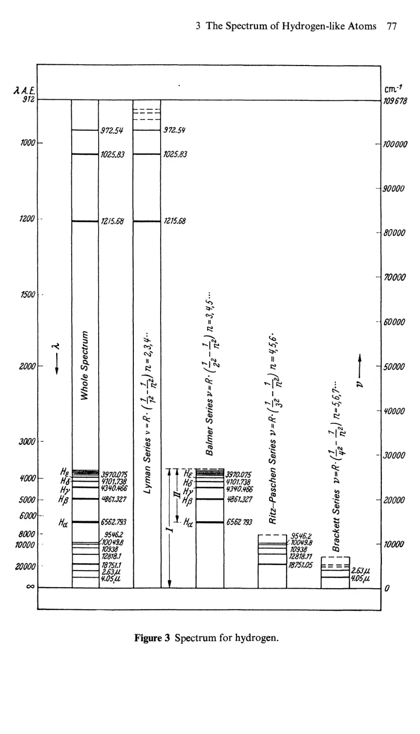
3 The Spectrum of Hydrogen-like Atoms	72
4 The Eigenfunctions for the Discrete Spectrum	78
ix

x Contents (Volume II)
5 The Continuous Spectrum	81
6 Perturbation Theory	84
7 Perturbation Computations and Symmetry	87
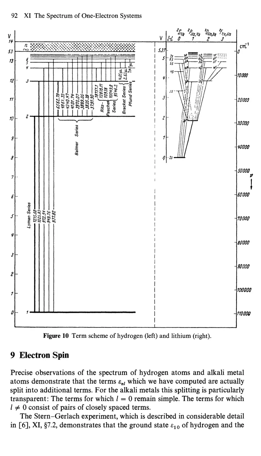
8 The Spectrum of Alkali Atoms	90
9 Electron Spin	92
10 Addition of Angular Momentum	93
11 Fine Structure of Hydrogen and Alkali Metals	99
CHAPTER XII
Spectrum of Two-Electron Systems	104
1 The Hilbert Space and the Hamiltonian Operator for the
Internal Motion of Atoms with n Electrons	104
2 The Spectrum of Two-Electron Atoms	106
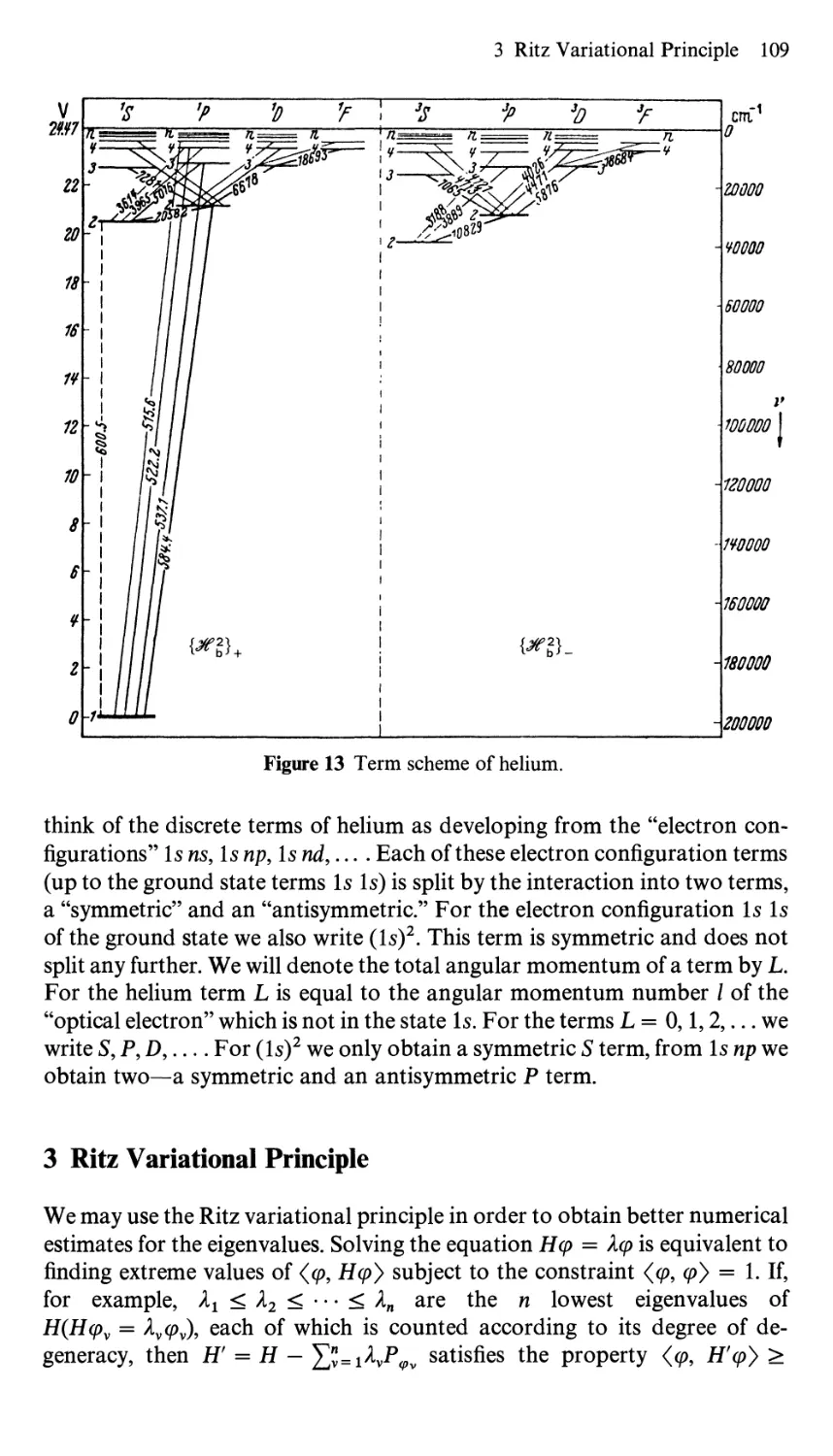
3 Ritz Variational Principle	109
4 The Fine Structure of the Helium Spectrum	114
CHAPTER XIII
Selection Rules and the Intensity of Spectral Lines	117
1 Intensity of Spectral Lines	117
2 Representation Theory and Matrix Elements	118
3 Selection Rules for One-Electron Spectra	120
4 Selection Rules for the Helium Spectrum	123
CHAPTER XIV
Spectra of Many-Electron Systems	124
1 Energy Terms in the Absence of Spin	124
2 Fine Structure Splitting of Spectral Lines	128
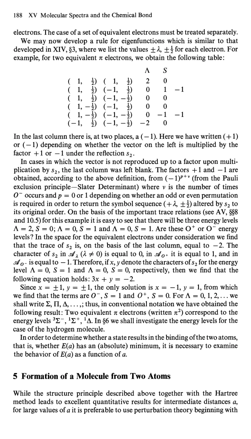
3 Structure Principles	130
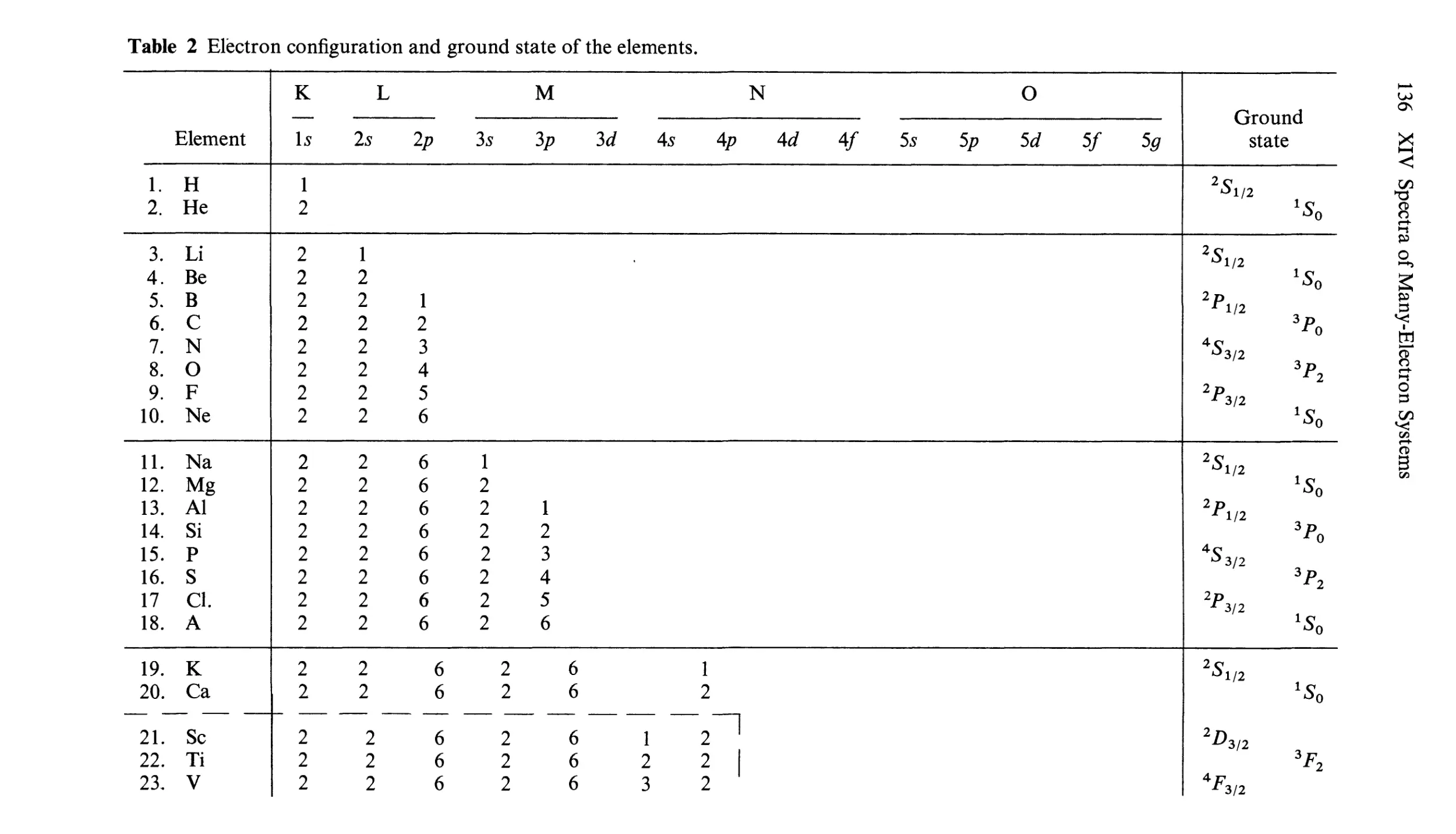
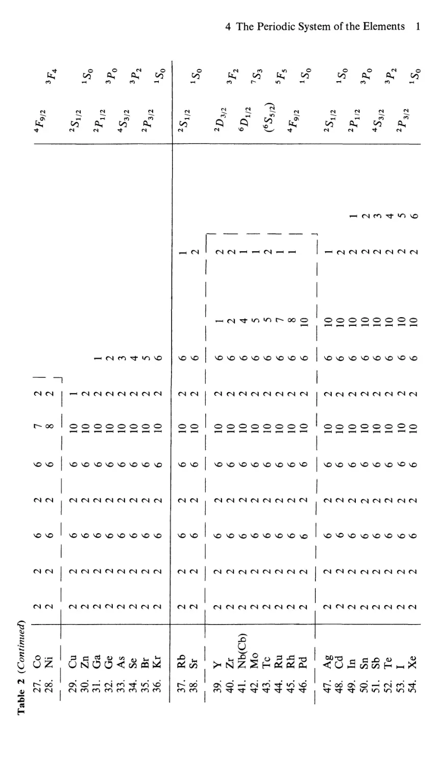
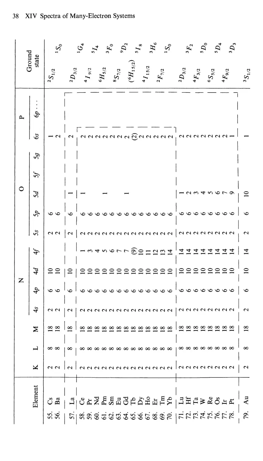
4 The Periodic System of the Elements	135
5 Selection and Intensity Rules	143
6 Zeeman Effect	147
7 / Electron Problems and the Symmetric Group	151
8 The Characters for the Representations of Sf and Un	160
9 Perturbation Computations	170
CHAPTER XV
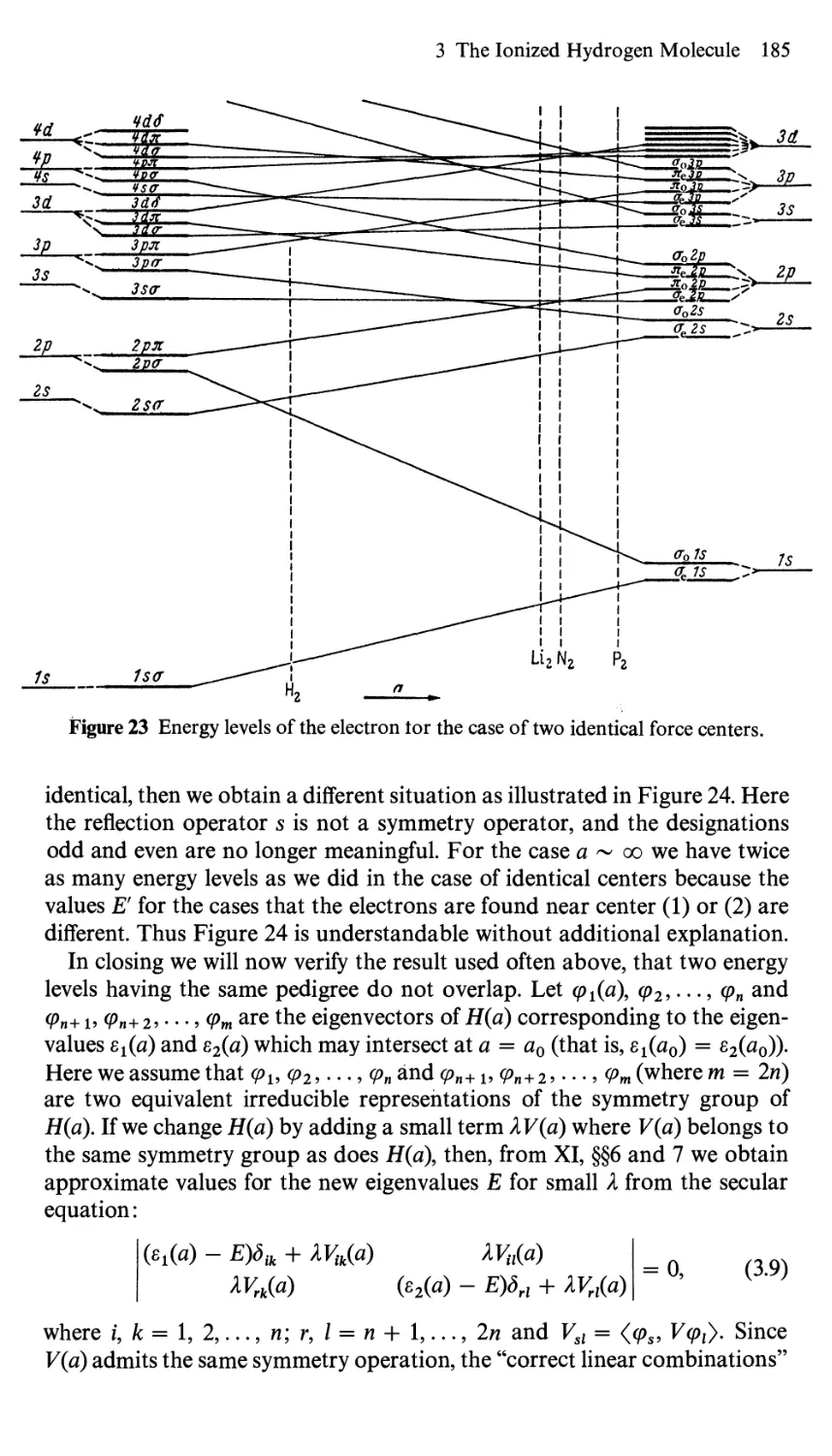
Molecular Spectra and the Chemical	Bond	177
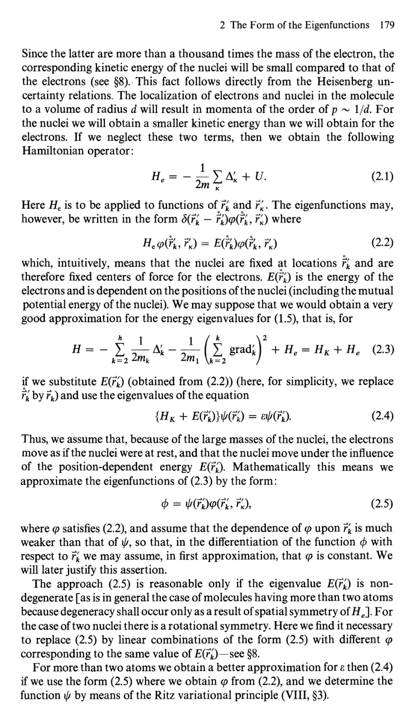
1 The Hamiltonian Operator for a Molecule	177
2 The Form of the Eigenfunctions	178
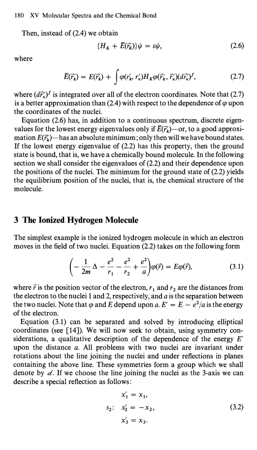
3 The Ionized Hydrogen Molecule	180
4 Structure Principles for Molecular Energy Levels	187

Contents (Volume II) xi
5 Formation of a Molecule from Two Atoms	188
6 The Hydrogen Molecule	191
7 The Chemical Bond	194
8 Spectra of Diatomic Molecules	208
9 The Effect of Electron Spin on Molecular Energy Levels	213
CHAPTER XVI
Scattering Theory	215
1 General Properties of Ensembles Used in Scattering Experiments 215
2 General Properties of Effects Used in Scattering Experiments 222
3 Separation of Center of Mass Motion	224
4 Wave Operators and the Scattering Operator	226
4.1 Definition of the Wave Operators	226
4.2 Some General Properties of Wave Operators	228
4.3 Wave Operators and the Spectral Representation of the
Hamiltonian Operators	233
4.4 The S Operator	236
4.5 A Sufficient Condition for the Existence of Normal Wave
Operators	238
4.6 The Existence of Complete Wave Operators	243
4.7 Stationary Scattering Theory	253
4.8 Scattering of a Pair of Identical Elementary Systems	256
4.9 Multiple-Channel Scattering Theory	257
5 Examples of Wave Operators and Scattering Operators	259
5.1 Scattering of an Elementary System of Spin j by an
Elementary System of Spin 0	259
5.2 The Born Approximation	262
5.3 Scattering of an Electron by a Hydrogen Atom	263
6 Examples of Registrations in Scattering Experiments	268
6.1 The Effect of the “Impact” of a Microsystem on a Surface 269
6.2 Counting Microsystems Scattered into a Solid Angle	275
6.3 The Scattering Cross Section	293
7 Survey of Other Problems in Scattering Theory	297
CHAPTER XVII
The Measurement Process and the Preparation Process 303
1 The Problem of Consistency	304
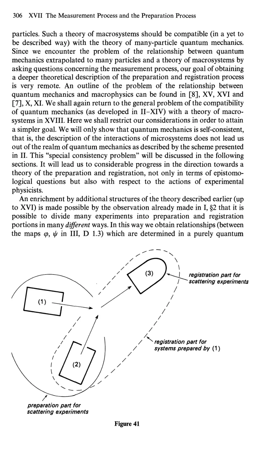
2 Measurement Scattering Processes	307
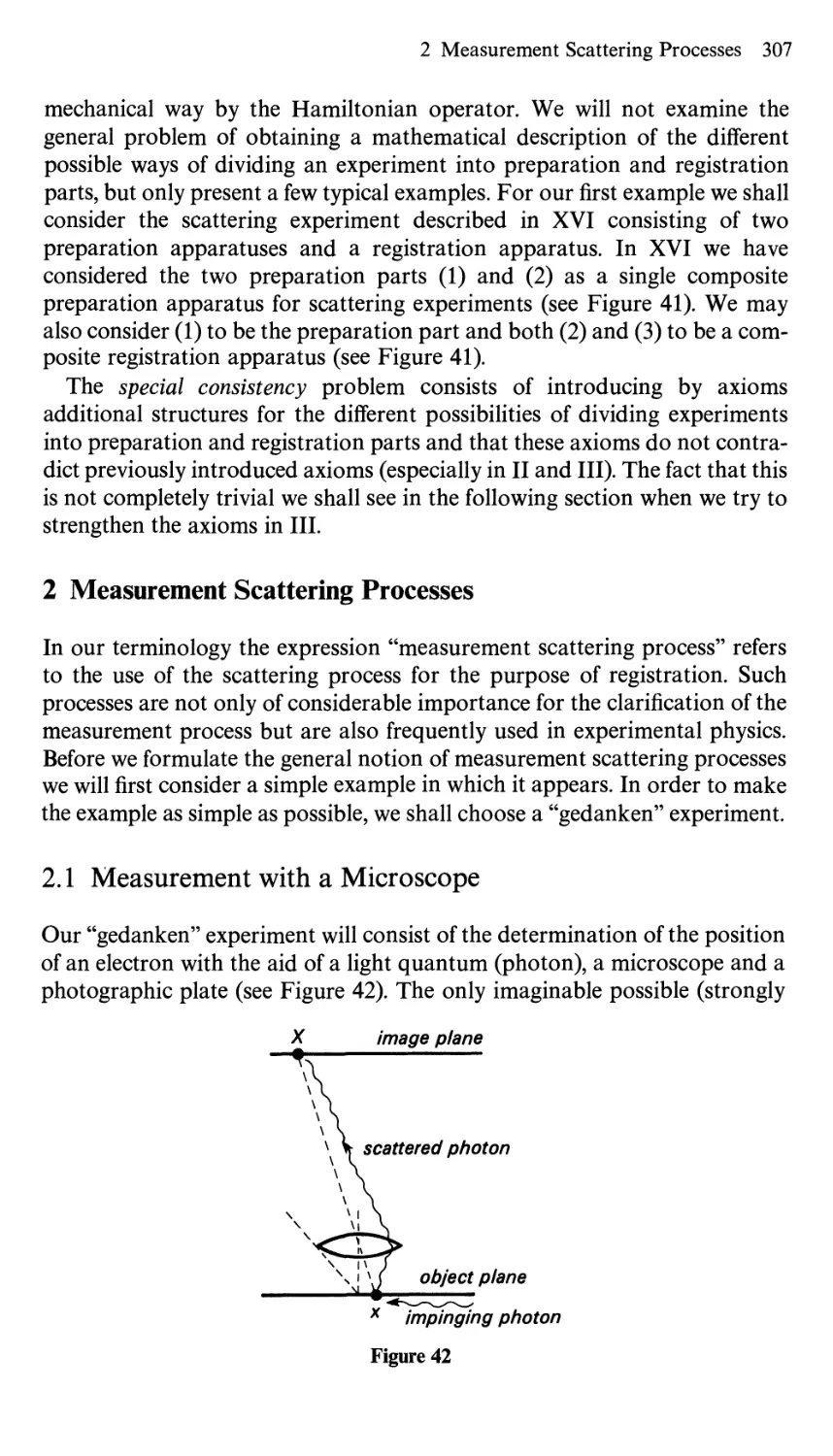
2.1 Measurement with a Microscope	307
2.2 Measurement Scattering Morphisms	311
2.3 Properties of Measurement Scattering Morphisms	313
3 Measurement Transformations	316
3.1 Measurement Transformation Morphisms	317
3.2 Properties of Measurement Transformation Morphisms	317

xii Contents (Volume II)
4 Transpreparations
319
4.1 Reduction of a Preparation Procedure by Means of a
Registration Procedure
321
4.2 Transpreparation by Means of Scattering
323
4.3 Collapse of Wave Packets?
326
4.4 The Einstein-Podolski-Rosen Paradox
330
5 Measurements of the First Kind
334
6 The Physical Importance of Scattering Processes Used for
Registration and Preparation
340
6.1 Sequences of Measurement Scatterings and Measurement
Transformations
341
6.2 Physical Importance of Measurement Scattering and
Measurement Transformations
343
6.3 Chains of Transpreparations
346
6.4 The Importance of Transpreparators for the Preparation
Process
347
6.5 Unstable States
348
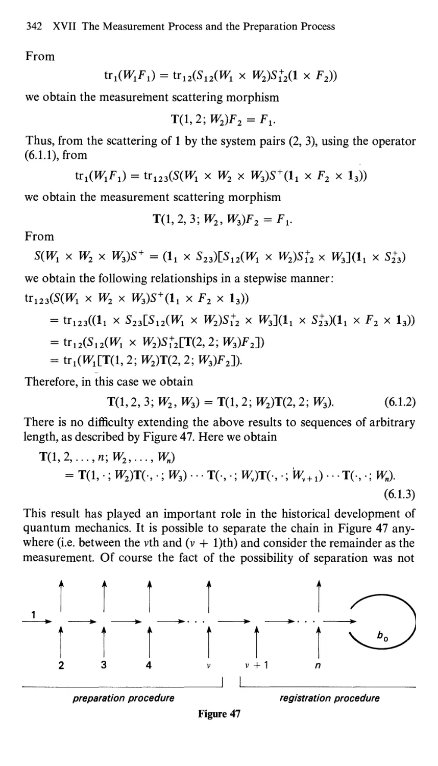
7 Complex Preparation and Registration Processes
354
CHAPTER XVIII
Quantum Mechanics, Macrophysics and Physical
World Views
355
1 Universality of Quantum Mechanics?
355
2 Macroscopic Systems
357
3 Compatibility of the Measurement Process with Preparation and
Registration Procedures
363
4 “Point in Time” of Measurement in Quantum Mechanics?
365
5 Relationships Between Different Theories and Quantum
Mechanics
367
6 Quantum Mechanics and Cosmology
371
7 Quantum Mechanics and Physical World Views
373
APPENDIX V
Groups and Their Representations
375
1 Groups
375
2 Cosets and Invariant Subgroups
376
3 Isomorphisms and Homomorphisms
377
4 Isomorphism Theorem
377
5 Direct Products
378
6 Representations of Groups
379
7 The Irreducible Representations of a Finite Group
380
8 Orthogonality Relations for the Elements of Irreducible
Representation Matrices
383
9 Representations of the Symmetric Group
385

Contents (Volume II) xiii
10 Topological Groups	389
10.1 The Species of Structure: Topological Group	389
10.2 Uniform Structures of Groups	391
10.3 Lie Groups	391
10.4 Representations of Topological Groups	395
10.5 Group Rings of Compact Lie Groups	398
10.6 Representations in Hilbert Space	405
10.7 Representations up to a Factor	407
References	410
Index
414

Contents (Volume I)
CHAPTER I
The Problem: An Axiomatic Basis for Quantum Mechanics
chapter и
Microsystems, Preparation, and Registration Procedures
CHAPTER III
Ensembles and Effects
CHAPTER IV
Coexistent Effects and Coexistent Decompositions
CHAPTER V
Transformations of Registration and Preparation
Procedures. Transformations of Effects and Ensembles
CHAPTER VI
Representation of Groups by Means of Effect
Automorphisms and Mixture Automorphisms
XV

xvi Contents (Volume I)
CHAPTER VII
The Galileo Group
CHAPTER VIII
Composite Systems
APPENDIX I
Summary of Lattice Theory
APPENDIX II
Remarks about Topological and Uniform Structures
APPENDIX III
Banach Spaces
APPENDIX IV
Operators in Hilbert Space
References
List of Frequently Used Symbols
List of Axioms
Index

CHAPTER IX
Representation of Hilbert Spaces by
Function Spaces
The representation of Hilbert spaces in terms of function spaces is of great
importance in the application of quantum mechanics. We have already
encountered such representations in VII, §2 in the form $£ 2(R3, dk! dk2 dk3)
and in VII, §3 in the form J5f 2(R3, dxx dx2 dx3), where we have considered
isomorphic maps of J?2(R3, dxx dx2 dx3) into $£ 2(R3, dkx dk2 dk3) which are
defined by Fourier transforms. Such (and similar) representations are
especially suitable for the treatment of physical problems. This chapter does
not introduce any new axioms, that is, any new physical laws; instead, we
introduce a number of suitably chosen tools for the analysis of the physical
laws in the previous chapters. In this chapter we shall consider only a single
Hilbert space Ж, that is, a single-system type.
1 Maximal Decision Observables
The starting point for our discussion of particular representations of a
Hilbert space is the discussion of measurement scales for observables
presented in IV, §2.5, and, in particular, the discussion of “scale observables”
as described in IV, D 2.5.6.
We shall now assume that we are given a complete Boolean ring
E = E(yb ..., yn) of decision effects, the scale for which is uniquely deter¬
mined by the specification of n scale observables Au ..., An (which mutually
commute, see the remarks preceding IV, D 2.5.6). In IV, §2.5 we have seen
that, to each Boolean ring E of decision effects there exists a finite number of
1

2 IX Representation of Hilbert Spaces by Function Spaces
scale observables Аъ ..., An for which E = E(yl5..., yn). Indeed, we may
choose n = 1.
Because we frequently find that certain Av (and the corresponding scales)
are physically determined on the basis of transformation groups (see, for
example, VII and VIII) we will therefore not assume that n = 1. Since it is
not, however, difficult to extend the structures described for the case n = 1
to the case n > i, the following discussion will be more transparent if, in the
following, we examine the case in which n = 1, and then carry out the exten¬
sion to n > 1 wherever necessary.
A Boolean ring E is said to be maximal, as a subset of G, if there does not
exist a Boolean ring E c: G for which E ^ E. A maximal E is, on the basis of
IV, Th. 1.4.7, complete. According to IV, Th. 1.3.6 E is maximal if there exists
no E e G, E ф E which is commensurable with all elements of E.
Th. 1.1. To each E cz G there exists a maximal E G for which Eel,
The proof of this result follows directly from Zorn’s lemma, because, for a
totally ordered subset of Boolean rings Ея с: G for which E с: Ея, the set
(JA Ея is a Boolean ring.
Since, according to IV, §2.5 each E may be represented as E(yb ..., yn)
we shall, for the purpose of discussion of the representations of Hilbert
space, always use maximal Boolean rings E(yl5..., yn) G.
D 1.1. A maximal Boolean subring of G is said to be a maximal decision
observable. A n-tuple of commuting Au ..., An is said to be maximal if the
Boolean ring E(yl5..., yn) generated by this n-tuple is maximal.
If {^4Я} is a set (not necessarily finite) of self-adjoint commuting operators
and if E is the Boolean ring generated by the spectral families of the ^4Я then
there exists a maximal E for which E E. According to IV, Th. 2.5.6, to E
there exists a у such that E = E(y) and, according to IV, Th. 2.5.9 there
exists a maximal scale observable A for which the corresponding Boolean
ring is equal to E. Since Е(уя) с E с I, is, according to IV, Th. 2.5.11,
a function fx(A). To each set {^4Я} of coexistent (and therefore commensur¬
able) scale observables there exists a scale observable A for which all the ^4Я
are functions of A.
We shall now introduce the following notation: For the Boolean ring
E G and cp e Ж let ^(E, q>) denote the (closed) subspace of Ж generated
by {Ecp\E e E}; let £(E, cp) denote the projection operator corresponding
to <^~(E, cp). Since 1 e E we find that cp e «^(E, cp).
Th. 1.2. £(E, <p) is commensurable to all elements of E.
Proof. For x e ^(£> Ф) it follows that Ex e ^~(£, Ф) for all £eS, since this result is
trivial for all x °f the form Ё(р where £el, since ЕЁ e E. For ф e Ж we find that

1 Maximal Decision Observables 3
£(E, (p) ф e «^(E, (p). Therefore, for £eS we obtain ££(E, (р)ф e <^~(E, (p), that is,
£(E, <p)££(E, (р)ф = ££(E, (р)ф. Since ф was arbitrary it follows that
£(E, (p)EE(L, (p) = ££(E, <p).
From the adjoint equation we obtain £(E, <jp)££(E, (p) = £(E, (p)E and we have
proven that £ and £(E, (p) commute.
Th. 1.3. For E l/iere exists а (ре Ж for which w = Р9 is effective on E,
t/iat is, /or Eel, the following relationship is satisfied:
tr(P„E) = <<p, £<p> = <<p, E2cp} = ||£<jo||2 = 0 => E = 0.
If E is maximal, t/ien t/iere exists a cp e Ж for which <^~(E, q>) = Ж.
Proof. If E is not maximal, then, according to Th. 1.1 there exists a maximal E such
that E e E. If, according to the second part of Th. 1.3, there exists a (p such that
«^(E, (p) = Jf7, then, if for £ e E we obtain ||£<p|| = 0, then for ф from the projection
space of £ and for arbitrary £ e £ we obtain
(cp, E(p} = <£i/^, £<p> = (ф, ЁЕ(р} = <^, ЕЁ(рУ = 0,
that is, ф is orthogonal to all {£<p | £ e £} and therefore is orthogonal to ^(E, (p) =Ж,
from which it follows that ф = 0 and £ = 0.
Now we need only prove the second part of Th. 1.3. We shall assume that E is
maximal. Let {/v} denote a dense denumerable subset in Ж. We define
K= V^(z,zv).
v= 1
Therefore {J%} is an increasing sequence of subspaces. Since Xv e «^”(2, Xv) we find
that Xve Жп for v < n. Thus it follows that \fn Жп = Ж.
We shall now show that, to each Жп there exists а фп such that Жп = ^(E, ф„). We
shall prove this result by induction.
For Ж1 we need only choose ф1 = Xi• Therefore, according to the induction
hypothesis	= ^"(E,	Therefore we find that Жп = <^(E, фп-х) v
^(E, Xn)• Let £„ denote the projection operator on
We therefore obtain £„ = £(E, v £(E, /„). Since, according to Th. 1.2,
£(E, and £(E, xn) are commensurable with all £ e E, then, according to IV,
Th. 1.3.5, £„ is commensurable with all £ e E. Since E is maximal, we therefore find
that £„ e E and £(E, /„) e E.
We now choose фп as follows:
Фп = Фп-1+(1-
By multiplication with an £ e E it follows that
Еф„ = Еф„-1 + E( 1 -
Since £„_! e E and therefore 1 — En_x e E we find that £(1 — En_x) e E and we
obtain £(1 — £„_!)/„ e ^(E, /„). Thus it follows that Еф„еЖп and therefore
<ГЪФп)^Жп.
Since гЕф„ = Еп.1Еф„.1 = ЕЕп-1фп-1 = Ефп_ г we obtain Ефп.1 е
Г(£,ф„) and	=	^(Х,	фп.,)^ Г(Е,Ф„). Since (1-Еп.1)Ефп =
Е( 1 -	= £(1 - Еп- i)Zn = (1 - £„-i)£x„ (because

4 IX Representation of Hilbert Spaces by Function Spaces
=	we	obtain	(1	-	yj =	*„)	n a
«^(E, фп). Since £(E, xn) and En-i are commensurable,
Жп = Жп_, v «Г(Е, Xn) = ^-i v [<Г(Е, b) n
and we therefore obtain Жп cz 5"(E, ф„). Thus we have proven that Жп = «^(E, ф„).
If Жп = Ж from a given value of n, then the theorem is proven. Since \]пЖп = Ж.
EJ^f for each/ e Ж If we set rji = Фи ..., rj„ = (£„ - £„_	then «Г(Е, ?/„) =
n	For a„ / 0 and ||a„||2 < oo we find that
and, since (En — £„_i)<p = a„07„/||*7„||) it follows that^„ e «^"(E, (p) and we therefore
obtain Ж = \/n «^(E, rjn) c: «^(E, cp), that is, «^(E, <p) = Ж
In the next section we shall obtain the following result as a corollary:
Th. 1.4. If \\Еф\\2 is an effective measure over a complete Boolean ring
IcG and there exists аср e Ж for which ^~(E, q>) = Ж, then ^~(E, ф) = Ж.
From this result it follows that
Th. 1.5. If E is complete, and if there exists a cp e Ж for which ^~(E, cp) = Ж,
then to each ф e Ж there corresponds a unique EqG'L for which E0 ф = 0
and Еф ф 0 for all E e E for which E < 1 — E0. In addition, ^~(E, ф) =
(1 — Е0)Ж, t/iat is, £(E, f) = 1 - £0 e E.
Proof. We define £0 as the union of all £ e E for which Еф = 0; since E is complete
£0 e E; therefore £0 is the largest £ e E for which Еф = 0. In the subspace Ж0 =
(1 — Е0)Ж we find that E0 = {£(1 — £0) | £ e E} and (p0 = (1 — E0)(p satisfies all
assumptions of Th. 1.4. Therefore ф = (1 — Е0)ф is a vector from Ж^ for which
^(E0, ф) = Ж0, and we therefore find that
«Г(Е, ф) = Ж0 = (1 - Е0)Ж,
that is, the projection £(E, i/0 which corresponds to ^~(E, i/0 is an element of E.
Th. 1.6. //E is complete, and there exists a q> e Ж for which 3T{E, q>) = Ж,
then E is maximal
Proof. Suppose that E is not maximal. Then there exists a £ ф 0 which is commen¬
surable with all £ e E. For ф e fof it follows that i/0 c: fof and £(E, i/0 < £.
Since ф e «^(E, i^) it follows that \/феЁж ф) = ЁЖ, that is, \/феЁж E(Z, ф) = £.
Since, according to Th. 1.5, £(E, ф) e E and since E is complete, then £ e E in con¬
tradiction to the assumption that £ ф E.
Th. 1.7. For a complete E the following two conditions are equivalent:
(i) E is maximal
(ii) 77iere exists a (p e Ж such that &~(L, (p) = Ж.
The proof follows directly from Th. 1.3 and Th. 1.6.

1 Maximal Decision Observables 5
Th. 1.8. If I, is complete, but not maximal, then there exists at most a de-
numerable set of pairwise orthogonal Ene G which are commensurable to
all elements of E; the Boolean ring E generated by E and by the En is maximal
Proof. Since the En are pairwise orthogonal, there can be at most denumerably many
En. We now consider sets {cpv} of vectors for which the «^(E, (pv) are pairwise ortho¬
gonal. Among these sets there are maximal sets, a result which follows directly from
Zorn’s lemma. Let {<p„} denote such a maximal set. Let ^ = «^"(E, (pn) and En =
£(E, (pn); let E denote the closed Boolean ring generated by E and the En.
If E was not maximal, then there exists а Е0фТ which is commensurable with all
E e E. Thus we obtain
E0 = '£E0En + E0(l-'ZE
where E0En = EnE0.
Since = 5"(E, (pn) = «^(E, En(pn\ the Boolean ring E„ = {££„ | £ e E} is,
according to Th. 1.7, maximal with respect to the Hilbert space 3~n\ therefore
E0En eE„c!. Therefore E0En e E.
If 1 — Yji En Ф 0, then there would exist a x where x = (1 —	^»)x- Since
«Г(Е, x) =	(1	- En)x) = (!-!„ WE, x) it follows that «Г(Е, x) is
1 to all in contradiction to the fact that the {(pn} are maximal. Therefore E0 =
E0En e E and E is therefore maximal.
Th. 1.9. The En in Th. 1.8 can be so chosen such that from EEn = Ofor an
E eT.it follows that EEm = 0 for all m > n.
Proof. We shall begin by using the En in Th. 1.8, and defining the Ё„ for which Th. 1.9
is satisfied. With E obtained from the proof of Th. 1.8, according to Th. 1.3 there
exists a (p for which «^(E, (p) = Ж Since E is complete, the support (IV, Th. 2.1.5)
of the measure \\EEncp\\2 = pn(E) is defined in E and will be denoted by E(n). We
therefore obtain E(n) e E. We therefore obtain (1 — E(n))En = 0, that is, EnE(n) = E„.
Furthermore, from EEn = 0 for E e E it follows that E < 1 — E(n), that is, EE(n) = 0.
We recursively define:
£U У = £(0
E(2Y = E(2) _ £(2)(j _ £(1>) = £(2)£(0
£(3)' = £(3) _£(3) ^ _ £(1) у £(2)) = £(3)(£(1) v £(2)^
£(4)' = £(4) _ £(4)(1 _ £(1) у £(2) у £(3)) = £(4)(£(1) y £(2) y £(3))?
and we then define
£(2)" = £(2)'?
£(3)" = E(3yE(2)
£(4)" = £(4)'(£(2)' у £(3)'^

6 IX Representation of Hilbert Spaces by Function Spaces
and, in the same way, we obtain £(3)"', £(4) ", etc.
The set of all projection operators obtained in the above manner are elements of
E. With the aid of the above, we recursively define the Ёп:
Ёх = EXE(1) + £2[£(2)(1 - £(1))] + £3[£(3)(1 - £(1) v £(2))]
+ £4[£(4)(1 - £(1) v E(2) v £(3)) + • • •,
E2 = E2E(2y + £3[£(3)'(1 - £(2))] + £4[£(4)(1 - E(2y v £(3)')] + • • •,
Ё3 = E3E(3)" + £4[£(4)"(1 - £(3)")] + • • •,
From EnE(n) = En and EnEm = 0 for n ф m it follows that Ёп are pairwise orthogonal.
We must show that the complete Boolean ring generated by the En and E is maximal
and, from ЕЁп = 0 for a E e E we also obtain ЕЁт = 0 for all m > n.
Let ЕЁп = 0, for example, ЕЁ2 = 0, then it follows that E2EE(2y = 0,
E3£[£(3)'( 1 — E(2)'y] = 0,... . Thus it follows that EE(2y < 1 — E(2) and that with
E(2y = E(2)E(1) the relation EE(2y = 0 and then we obtain the relation E3EE(3y = 0,
that is, EE(3y < 1 — E3 and we therefore obtain EE(3y = 0.
Similarly, it follows that ££(4)' = 0, etc. Thus it follows that ЕЕ{2)" = 0, EE(3y' = 0,
EE(4)" =	0,... and we finally obtain ЕЁ3 = 0. Similarly,	from	ЕЁп	= 0 it follows
that ЕЁп+ x	= 0 and therefore EEm = 0 for all m > n.
From the definition of Ёп it follows that
ЁХЕ(1) = EXE{1) = Ex,
£1£(2) = EXE(2) + E2( 1 - £(1)),
£1£(3) = £1£(3) + E2(E(3) - E(1)E{3)) + £3(1 -	£(1)	v	£(2)),
and we obtain
£i = EiE(1),
£2( 1 - £(1)) = ЁхЕ(2) - ЁхЕ(1)Е(2) = ЁхЕ{2\ 1 - £(1)),
£3(1 - £(1) v £(2)) = ExE(3) - ЁХЕ(1)Е(3) - £1E(2)£(3)(1 - £(1)),
Similarly, we proceed with £2, Ё3,... and recognize that the Eu E2,... are
elements of the Boolean ring generated by E and the £ь E2. Thus the complete
Boolean ring generated by E and the Ё„ is equal to that generated by E and the En,
and is therefore also maximal.
2 Representation of Ж as i?2(Sp (A), pi) where Бр(Л) is the
Spectrum of a Scale Observable A
The fact that every complete Boolean ring IcG can be generated by a
scale observable A was explained in IV, §2.5 and emphasized in §1. In §1 we
have also stressed the fact that these considerations can also be applied to the

2 Representation of Ж as	2(Sp(A),	/г) 7
case in which E is generated by an n-tuple of commuting scale observables
Au ..., An. Since we cannot use Th. 1.4-1.8, we shall, for the present, only
assume that there exists a q> e Ж for which ^~(E, cp) = Ж. Then, for each
f e Ж there exists finitely many	and	complex numbers щ such that,
given an s > 0
/- ZaiEi<p
i = 1
< S
is satisfied. We may assume that the E( are pairwise orthogonal, because we
may use, instead of the Eb the pairwise orthogonal atoms of the finite
Boolean subring of E generated by the Et.
According to IV, Th. 2.5.8 we may identify each E e E with a measurable
subset к of the spectrum Sp(^4) of a scale observable A. Let P denote the set
of these measurable subsets к. к is uniquely defined by E up to a set of measure
0. For finitely many orthogonal Eb since Et л Ej = EtEj = 0 for i # j, we
may choose the corresponding subsets kt such that kt n kj = 0 for i # j.
Instead of E{ we shall write E(kt) (where E(k) is defined in the sense of cr(fc)
in IV, Th. 2.5.8); therefore, to each/ e Ж and to each s > 0 there are finitely
many disjoint measurable subsets kt of Sp(^4) for which
/-
i = 1
< в.
(2.1)
For a decomposition Sp(^4) = (J”=i kt (kt nkj = 0 for i # j) of the spec¬
trum of A into measurable subsets kt we define a stepwise function g on
Sp(^4) as follows
g((x) = yi fora ekh
(2.2)
where the yt are complex numbers. From the step function g(oc) we obtain
a vector from Ж as follows:
(2.3)
For a pair of decompositions {/c;} and {fc'} it follows that
Z	I	У1	E(k,)(p\	=	Z	У']УЛЩ)Е(кд(р\\2.
j	i	/	i,j
Since E(kfj)E(ki) = E(k'• n kt\ and from the cr-additive measure over P
given by
we obtain
№ = \\E{k)q>\\\
Z Z yiE(ki)<P ) = Z y'jyitikj n kt).
(2.4)
(2.5)

8 IX Representation of Hilbert Spaces by Function Spaces
For g defined by (2.4) the set of step functions is dense in the Hilbert space
J£2(Sp(A), g). From (2.3) and (2.5) it follows that (2.3) is an isomorphic
mapping of this subset into Ж which has a unique extension as an iso¬
morphism
We write this isomorphism (2.6) in the following form (where/(A) is measur¬
able and quadratically integrable):
where the integral on the right-hand side can be considered to be defined
by this isomorphism. Thus it follows that, for a sequence of step functions
gv(ot) for which gv(a) -* /(a) (in the sense of the norm in 2(Sp(^4), g),
9v = Tji yiV)E(kiv)) is а Cauchy sequence in Ж (where the yjv) are the values
corresponding to the gv according to (2.2)) which satisfies
defines a function of the operator A for measurable /(a); /(a) need not be
quadratically integrable. The operator В = f(A) is a “normal” operator; its
definition domain is the set of all ф e Ж for which J | /(a) |2 d||E(a)^||2 < oo.
If /Ya) is bounded, then so is f(A), where the latter is already defined in
IV, §2.5 (see IV, Th. 2.5.11).
To each operator В in Ж there exists a corresponding operator В in
J£2(Sp(A), g) defined by the isomorphism (2.6), (2.7) (see AIV, §13) as
follows:
is particularly simple. If we replace the integral in (2.10) by the approximation
sum
j£?2(SpC4), g) -> Ж.
(2.6)
/(a) -► / = J /(a) dE(a)(p,
(2.7)
9у	J/(a) dE(a)q>.
(2.8)
We can also choose to use (2.8) as the definition of the integral.
Here we remark that
J /(a) dE{a)
(2.9)
/'(a) = Bf(a) -> Bf = J/'(a) dE(a.)<p.
The mode of action of
(2.10)
x a,•(£(«;) - £(<Xi_ i)),
then it is easy to show that
Af( a) = a/ (a).
(2.11)

2 Representation of Ж as J?2(Sp(A\ g) 9
Similarly, it is easy to prove that for a measurable set к e P
Let ф be a vector in Ж and let ф(а) be the corresponding function in
££2(Sp(^4), \i). Then, for a finite sum it follows that
£	-*■ £ ^ЩдФ
i	i
and for #(a) defined according to (2.2) we obtain
Sf(o#(a) -*• £ 7i ЩдФ-
i
The subspace <^~(E, ф) of Ж therefore corresponds the subspace of
^f2(Sp(^4), g) spanned by all д(ос)ф(ос) where g(oc) are arbitrary step functions;
let ^~(E, ф) denote this subspace. Thus we find that ^~(E, ф) is spanned by
all к(<х)ф(<х) where the h(oc) are bounded measurable functions.
Let denote the measurable set
= {a | a e Sp(^4) and ф(а) ф 0}.	(2.13)
Then we obtain
ф) = {/(a) | /(a) e J^z(Sp(A), ц) and/(a) = 0 for a e SpG4)\fc*}
and we therefore obtain
<Г(1, ф) = Е(кф)Ж.
According to (2.13), (1 — Е(кф))ф(ос) = 0, and we therefore find that
(1 - Е(кф))ф = 0.	(2.14)
If the measure ||£^||2 is effective over E then we must have 1 — E(kl!/) = 0
and we obtain Е(кф)Ж = Ж, that is, ^(E, ф) = Ж, from which we have
also proven Th. 1.5 and 1.8. In particular, the operator A we used at the
beginning must have been a maximal scale observable.
If ф is, in addition to <p, a second vector for which ^~(E, ф) = Ж then with
the help of ф we may define an isomorphism in the same way as we have
done with q> as follows:
i?2(Sp(A), P) - Ж,
r -	(2Л5)
/(«) / = J /(a) dE(a)ij/,
where
p(k) = \\Е(к)ф\\2 = Г \ф(а)\2 йц(а).
Jk
(2.16)

10 IX Representation of Hilbert Spaces by Function Spaces
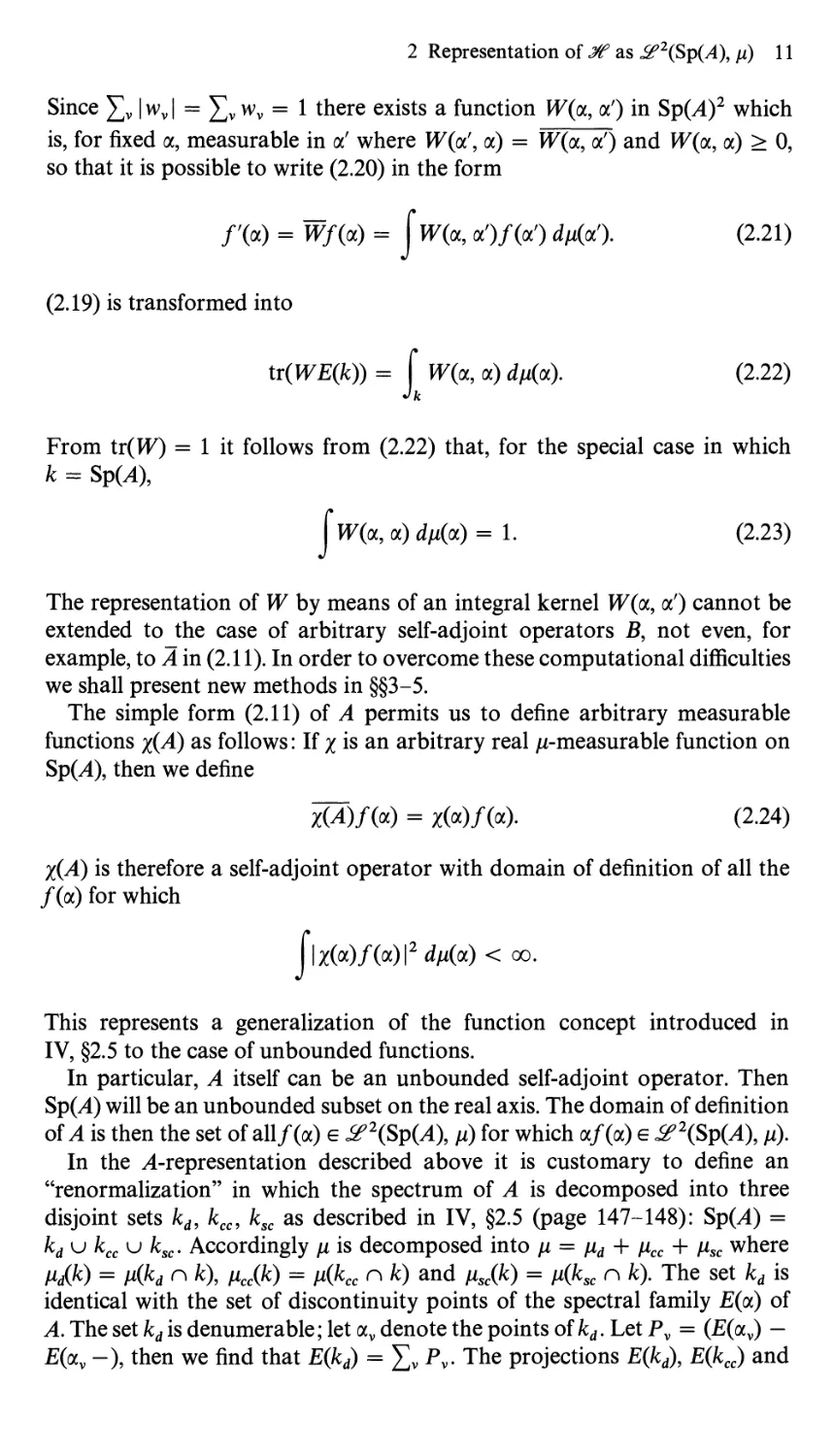
For a step function g(oc) of the form (2.2) where we replace yt by yt it follows
that
This result can be extended to all /(a) e 2(Sp04), fi), that is, the iso¬
morphisms (2.6), (2.7) and (2.13) lead to an isomorphism
We call $£2(Sp(^4), \x) together with the isomorphism (2.6) an ^-represen¬
tation of the Hilbert space Ж (obtained by means of cp). In an ^-representa¬
tion the special simple relations (2.11) and (2.12) hold. Between the
^-representations obtained by means of cp and ф the relationship (2.17) is
satisfied, where ф(ос) is an arbitrary measurable function which is
quadratically integrable with respect to ji and is nonzero almost everywhere
on Sp(^4). According to (2.7) it is clear that in the representation obtained
by means of cp the vector cp corresponds to the function cp{pc) = 1.
In an ^-representation the probability tr(PfE) may be simply calculated
as follows for E e E: To E there exists a measurable set к for which E = E(k).
Then, according to (2.12) we obtain
where (2.18) is the probability that in the measurement of A for an ensemble
W = Pf the scale value of A lies in the subset k.
Is it possible to extend the formula (2.18) to general W1 For W= wvP^v,
wv > 0 and £ wv = 1 it follows that tr(WE(k)) = £v wv tr(P^v£(/c)) and we
therefore obtain
0(a) E ЬЕ(кдФ E УгЩгЖа),
i	i
where Е(к)ф(ос) is given in (2.12). Therefore
0(a) -»• E ЬЩдФ <- 0(аЖа).
£e2(Sp(A), Д) -*■ J2?2(Sp04), n),
/(a) -»• /(a) = /(a)i^(a).
(2.17)
tr(PfE) = </, E(k)f) = j*/(a)E(k)f (а) йф)
(2.18)
tr(WE(k)) = E wv l«Av(a)|2 dn(a).
(2.19)
V
What is the form of the operator W in i?2(Sp(A), ju)? For
jP*/(a) = <Ka) J iA(a')/(a') йф')
it follows that
Wf(а) = E wvlAv(a) f <Av(a')/(a') dф!).
V	J
(2.20)

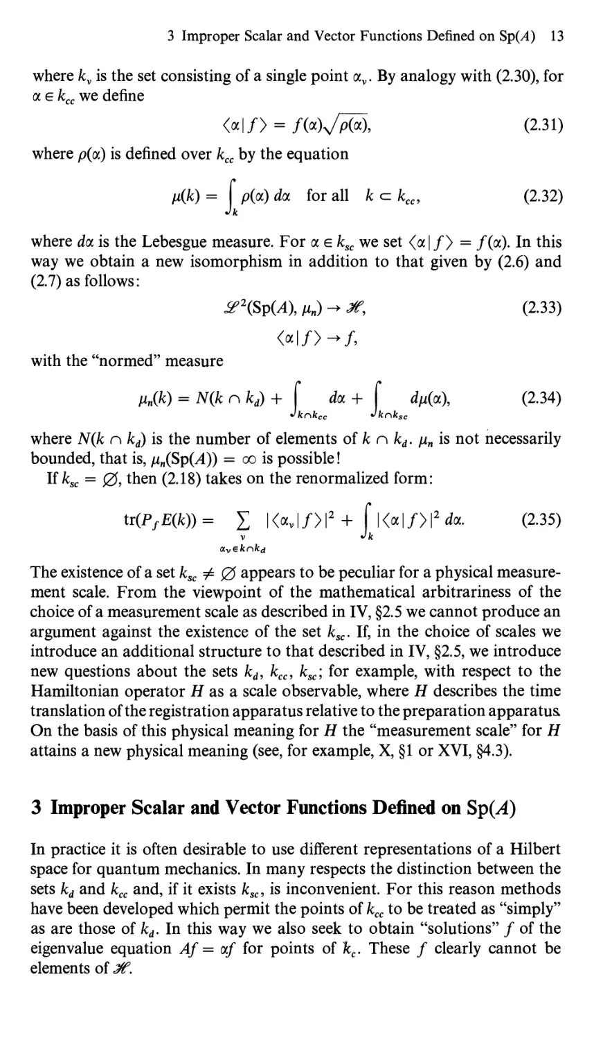
2 Representation of Ж as ^?2(Sp{А), ц) 11
Since |wv| = wv = 1 there exists a function W(oc, a') in Sp(^4)2 which
is, for fixed a, measurable in a' where W{a', a) = Ж(а, a') and Ща, а) > О,
so that it is possible to write (2.20) in the form
/'(a) = Wf(a) = | W(a, a')/(a') d^a').	(2.21)
(2.19)	is transformed into
tr(WE(k)) = f W(a, a) d/<a).	(2.22)
Jfc
From tr(PV) = 1 it follows from (2.22) that, for the special case in which
к = Sp(,4),
J W(a, a) dn{<x) = 1.	(2.23)
The representation of W by means of an integral kernel PV(a, a') cannot be
extended to the case of arbitrary self-adjoint operators В, not even, for
example, to A in (2.11). In order to overcome these computational difficulties
we shall present new methods in §§3-5.
The simple form (2.11) of A permits us to define arbitrary measurable
functions x(A) as follows: If x is an arbitrary real /г-measurable function on
Sp(^4), then we define
zC4)/(«) = z(«)/(a)-	(2.24)
X(A) is therefore a self-adjoint operator with domain of definition of all the
/(a) for which
Jlx(a)/(a)l2 dn(a) < oo.
This represents a generalization of the function concept introduced in
IV, §2.5 to the case of unbounded functions.
In particular, A itself can be an unbounded self-adjoint operator. Then
Sp(^4) will be an unbounded subset on the real axis. The domain of definition
of A is then the set of all/(a) e J£2(Sp(A), ix) for which a/(a) e ^2(Sp(A), pi).
In the ^-representation described above it is customary to define an
“renormalization” in which the spectrum of A is decomposed into three
disjoint	sets	kd, kcc,	ksc	as	described in IV, §2.5	(page	147-148):	Sp(^4) =
kd и kcc	и	ksc.	Accordingly	is decomposed into /x =	/xd	+	ixcc	+ fxsc where
Md(fc) = KK n fc)> Mcc(fc) = KKc n fc) and Msc(fc) = KKc П fc)« The set kd is
identical with the set of discontinuity points of the spectral family E(oc) of
A. The set kd is denumerable; let av denote the points of kd. Let Pv = (E(av) —
£(av —), then we find that E(kd) = £v Pv. The projections E(kd), E(kcc) and

12 IX Representation of Hilbert Spaces by Function Spaces
E(ksc) are pairwise orthogonal, and 1 = E(kd) + E(kcc) + E(ksc). For fd =
E(kd)f,fcc = E(kcc)f, fsc = E(ksc)f the right-hand side of (2.7) takes on the
form / = fd+ fcc + fsc where
Л = £ f(*v)P*<P,
V
/«= f f(«)dE(a)(p,	(2.25)
Jkc
fsc = f /(a) dE(u)(p.
Jksc
From Ж =	q>)	it	follows	that	all	the	Pv	are	one-dimensional	projec¬
tions, because from (2.25) it follows that, for a vector / satisfying Pvf =f
f = f(*v)Pvq>,
that is, all vectors from the projection space of Pv are multiples of a single
vector JPV <p.
The set of solutions of the eigenvalue equation Af = otvf is given by the
set of vectors in the projection space of Pv. Af = otf has a nonzero solution
only for the values of ocvekd. If the eigenspace for the eigenvalue av of A is
one-dimensional, then this eigenvalue is said to be nondegenerate. From
Ж =	cp) it follows that the eigenvalues av are nondegenerate.
For <pv = Pv(p it follows from (2.25) that
/=£/(«,)&+/«+/*. (2-26)
V
Since the <pv are pairwise orthogonal and are orthogonal to fcc,fsc from (2.26)
it follows that
<0v,/> =/(oOI l<Pvl|2
and that
f = ^m(jtl,f)+fc+fsc'	(2'27)
Here ||<pv||2 is the measure fi(kv) where kv consists of the single point av.
Equation (2.27) suggests the following renormalization: Instead of using the
<pv in the expansion (2.27) we use the normalized eigenvectors cpv = фх || <pv ||"1.
Then we obtain
/ = Z	/)	+	fcc	+	fsc	•	(2.28)
V
We now define
<<Pv,/> = <avl/>,	(2.29)
where we consider <av|/> to be a complex function defined on kd. We
obtain
<avl/>=/(av)VMU	(2-30)

3 Improper Scalar and Vector Functions Defined on Sp(T) 13
where kv is the set consisting of a single point av. By analogy with (2.30), for
a e kcc we define
<a|/> = /Wn/pW,	(2.31)
where p(a) is defined over fccc by the equation
= f P(°0 den for all к a kcc,	(2.32)
where doc	is	the Lebesgue measure. For oc e ksc we set <a|/) =	/(a).	In this
way we	obtain a new isomorphism in addition to that given	by (2.6) and
(2.7)	as follows:
З’ЧМА), /О - JT,	(2.33)
<<*|/>->/,
with the “normed” measure
/i„(fc) = N(k n kd) + Г da + j* dn(a),	(2.34)
Jknkcc	Jknksc
where N(k n kd) is the number of elements of к n kd. jan is not necessarily
bounded, that is, jin(Sp(A)) = oo is possible!
If ksc = 0, then (2.18) takes on the renormalized form:
tr(PfE(k)) = I | <av | /> |2 + f | <a | /> |2 da.	(2.35)
V	Л
<xveknkd
The existence of a set ksc	Ф 0 appears to be peculiar for a physical measure¬
ment scale.	From	the	viewpoint of the mathematical arbitrariness	of the
choice of a measurement scale as described in IV, §2.5 we cannot produce an
argument against the existence of the set ksc. If, in the choice of scales we
introduce an additional structure to that described in IV, §2.5, we introduce
new questions about the sets kd, kcc, ksc; for example, with respect to the
Hamiltonian operator H as a scale observable, where H describes the time
translation of the registration apparatus relative to the preparation apparatus
On the basis of this physical meaning for H the “measurement scale” for H
attains a new physical meaning (see, for example, X, §1 or XVI, §4.3).
3 Improper Scalar and Vector Functions Defined on Sp(^4)
In practice it is often desirable to use different representations of a Hilbert
space for quantum mechanics. In many respects the distinction between the
sets kd and kcc and, if it exists ksc, is inconvenient. For this reason methods
have been developed which permit the points of kcc to be treated as “simply”
as are those of kd. In this way we also seek to obtain “solutions” / of the
eigenvalue equation Af = ocf for points of kc. These / clearly cannot be
elements of Ж

14 IX Representation of Hilbert Spaces by Function Spaces
One of these methods is that of the Gelfand triple [1]. A second method
is that developed by Nikodym [2]. In either case there is no “simple”
accessible method which is sufficiently reliable to permit us to attempt to
guarantee (on the basis of general theorems) the mathematical validity of
the computed results. For the most part these methods are used as heuristic
principles, to obtain quick results, the mathematical validity of which can
later be verified in individual cases. In concrete examples it is not unusual
to find unsatisfactory results which do not, however, place the theory itself
in question. Perhaps, in quantum mechanics, a restriction to the mathematics
of Hilbert space is inconvenient. Such a restriction is not necessary since
operators in Hilbert space are only representations of a special Banach space
structure (see III, §3). In this representation there is an additional underlying
structure which we have denoted by 3) (see the discussions in VII, VIII). It
is conceivable that the development of a “theory of 3” could lead to new
practical methods (see also [3]).
Since we do not yet have a satisfactory method for the reformulation of
mathematical problems in Ж we shall now present a brief outline of the
method of Nikodym in order that we may at least have a general method
which underlies the somewhat messy mathematical calculations which will
appear later in this book.
In order to obtain a greater similarity between the general expansion of
/ on the right-hand side of (2.7) and the expansion of / with respect to a
complete orthXnormal basis (pv (the case in which Sp04) = kd), / =
Tjv <Pv(<Pv, /X we shall return to (2.1).
According to IV, Th. 2.5.8 (and the remarks preceding the theorem), for
ke P we obtain
W = л v £(U	(3-1)
U V = 1
where Дм is to be taken over all coverings и of k. For each cp e Ж, \f™= x E(Iv)cp
may be approximated in the norm to arbitrary accuracy by \/^= x E(Iv)cp.
Here we may assume that the intervals Iv are mutually exclusive because we
may easily replace \/v=i EUv) by VJT	disjoint Vp. From (3.1) it
follows that E(k)cp can be approximated arbitrarily well by \Д°=1	f°r
a particular covering u. Therefore, E(k)cp can be arbitrarily well approximated
by \Д= x E(Iv)(p where the intervals 7V are disjoint, that is, it can be ap¬
proximated by the sum x E(Iv)cp.
From (2.1) it follows that each / can be approximated by finite sums
Y,papE(Ip)(p where the Ip are disjoint intervals. Therefore, to each e > 0
there exists a partition of R into finitely many disjoint intervals Ip and there
exists a finite set of complex numbers ap such that
f-Y.aPE{lp)<P <e.
Let /” be, for fixed n, a partition of R into intervals where Sn is the maximum
length of the intervals and suppose Sn -* 0. Then there exists for each e > 0

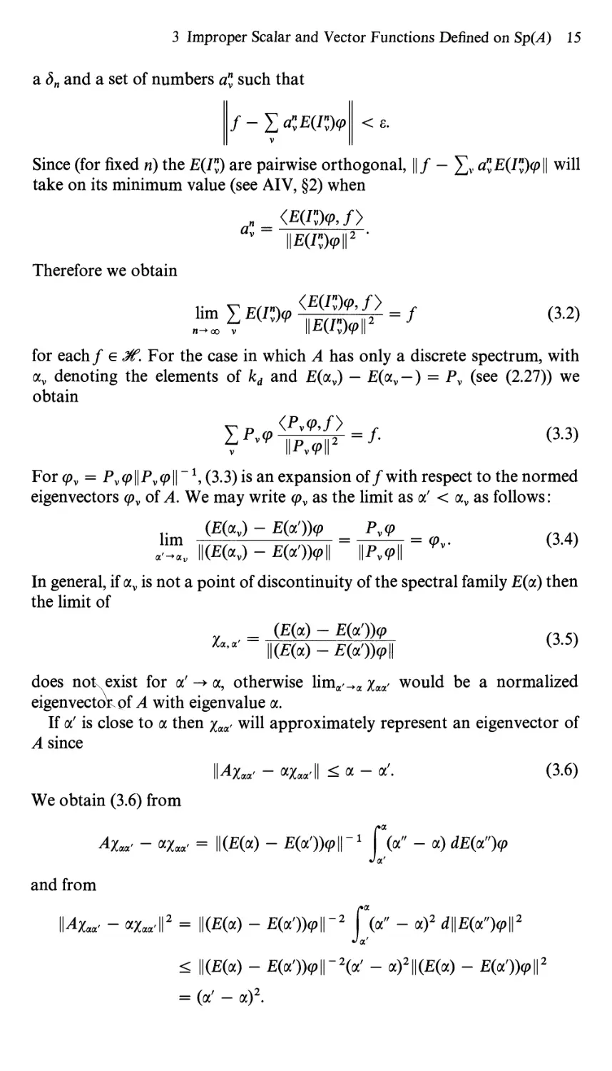
3 Improper Scalar and Vector Functions Defined on Sp(A) 15
a Sn and a set of numbers a” such that
< в.
Since (for fixed n) the £(/”) are pairwise orthogonal, ||/ —	a”E(I")(p\\ will
take on its minimum value (see AIV, §2) when
*v \\Е(Ц)<р\\2 •
Therefore we obtain
JS?**»-'	<32)
for each/ e Jf. For the case in which ^4 has only a discrete spectrum, with
av denoting the elements of kd and £(av) — £(av —) = Pv (see (2.27)) we
obtain
(13>
For cpv = Pv<p||Pv<p|| “ / (3.3) is an expansion off with respect to the normed
eigenvectors <pv of A. We may write <pv as the limit as a' < av as follows:
(E(av) - E(a'))g> Pv(p
||(£(av) - EWM \\PM\	Vv'	^ '
In general, if av is not a point of discontinuity of the spectral family E(a) then
the limit of
= (£(«) - E(ot'))(p	n
/a’a'	||(P(a) — E(ccf))(p\\	^
does not exist for a' -* a, otherwise lima^a x^ would	be a normalized
eigenvector of A with eigenvalue a.
If a' is close to a then xaa' will approximately represent an eigenvector of
A since
MZoa' - baa'll < a - a'.	(3.6)
We obtain (3.6) from
ЛХаа' - ocXaa' = II №) - Е(а'))<рЦ~1 f (a" - a) dE(oc")(p
•la'
and from
Их®' - <%*'II2 = IIC-E(a) - E(a.'))(p\\-2 Г (a" - a)2 d||E(a'>||2
•la'
< ||(-E(a) - E(a'))<p\\~2(a' - a)2||(E(a) - E(a'))<jo||2
= (a' — a)2.

16 IX Representation of Hilbert Spaces by Function Spaces
Equation (3.2) says that, for sufficiently large n each / can be expressed to
arbitrary accuracy by an expansion in terms of “approximate” eigenvectors
Хш> of the form (3.5). This result motivates the following definition of an
“improper” vector function 2(a) on Sp(^4).
For fixed a, 2(a) is a mapping of the interval — oo < a' < a into Ж, that
is, there exists a function x(a, a') which is defined for all (a, a') for which
a' < a where x(a, a') e Ж; 2(a) is defined as the function x(a, a') as a function
of a' for fixed a.
Similarly, an improper complex function a(a) on Sp(^4) is defined with the
aid of a complex function a(a, a').
For/ g Ж, (x(oc, a'),/) = a(a, a') defines, for an improper vector function
2(a), an improper complex function a(a). Here we write a(a) = <2(a),/>-
We may also define improper functions for the case of several variables.
For example, we may define an improper vector function 2(аь а2) by means
of function x(a1? ol\ ; a2, a2) for a* < al9 a2 < a2 where x(ab a*; a2, a2) g
An improper function /)(аь a2) is defined by ^(al5 a\; a2, a2) =
a(al5 ai)x(a2, a2); here we write ^(oq, a2) = 5(a1)2(a2). Similarly, we define
a(v-i, a2) = <K«i), x(a2)> by <z(«i, а'Д x(a2, «2)>; similarly, we may define
2(ai) + 2(аг)5 etc- Note, however, that we can define an improper function
of only one variable а(а)2(а) by a(a, a')z(a, a'). Then
does not hold! For an improper function a2) of two variables we cannot
simply set olx = oc2 instead, we must write [fj(<xl5 a2)]ai =(X2. Here we hope that
no misunderstanding will result from the following formulae.
Let к be a measurable set of the spectrum; let us consider, as in the case of
IV, §2.5, a covering и of к by means of countably many intervals Iv: к с (Jv Iv.
From such a covering we may select a covering consisting of disjoint intervals
as follows: Choose /11 = /1;/2-i-/i is then a set which consists of finitely
many disjoint intervals, so that I2 и Ix may be represented as the union of
the disjoint intervals Ix x and those in I2 4- Iv If 1J™= x may be represented
as the union of disjoint intervals, then the same is true for Im+1 4- (J/?=i A**
In this way we recursively prove our assertion. We need only consider the
coverings consisting of disjoint intervals instead of all possible coverings.
Since к is measurable, there exist sequences of intervals /” such that En =
£v £(/”) is a projection operator and En -> E(k).
We could also assume that the maximum length Sn of the intervals /” tend
towards zero; to do so requires only that we divide the intervals
An improper vector function 2(a) is said to be summable over SpC4) if for
every measurable subset к of Sp(^4) the limit	х(Ц) exists and is independent
of the sequence of coverings un = (Jv I” of disjoint intervals for which
Sn -* 0; for /: a' < • • • < a we have written x(I) instead of x(a, a').
For a summable vector function 2(a) we write, for the definition
a( a)x(a) = [а^Жаг)!
(3.7)

3 Improper Scalar and Vector Functions Defined on Sp(X) 17
We note that, according to the definition (3.7), only the points a e Sp(^4)
occur in the sum J, since к must be a subset of SpG4). If the spectrum is
discrete, that is, Sp(^4) = kd, it follows that for a summable function 2(a) the
limit limg_0 x(av, av — &) = %ve Ж exists for the points av e Sp(^4), where
the latter follows from the fact that (3.7) is satisfied for к = {av}, that is, for
a set consisting of a single point av; from (3.7) it follows that for an arbitrary к:
f Ha) = EZv	(3-8)
Jk	avefc
If E(I)x(I) = x(l), then, from (3.7) it follows that for
9 = f Ha): f Ha) = E(k)g.	(3.9)
Jsp(A) Jk
The improper vector function 2(a) defined by /(/) = E(I)f for fixed
/ e Ж is summable, and trivially satisfies the equation E(I)x(I) = /(/). We
obtain:
f m = f>	f m	= mi-
^Sp(A)	Jk
In this case JSp(A) 2(a) is nothing other than an alternative notation for
г
d£(a)/.
Two improper vector functions 2(a) and fj(oc) are said to be equivalent
(written 2(a) ~ rj(a)) if, for all measurable fc, the following equation is
satisfied:
£z(a) = J Ha)-
(3.10)
From the above 4erivation it follows that, for example, the improper vector
function 2(a), defined in terms of E(I)f, is equivalent to the improper vector
function fj(oc) defined by means of
Е(Л(р || 17/ 7Л и 2	»
ф(а)==
II Щ)<рГ
E(I)<p
\ты
(here := means that	the	expression on the left is defined by the expression to
the right	of	the equal	sign) is an improper vector function, and satisfies
И а) = ф(а)<ф(а), />•	(3.11)
We therefore obtain the expansion
f ф(а)<<р(а), /> = /.	(3.12)
7sPu)

18 IX Representation of Hilbert Spaces by Function Spaces
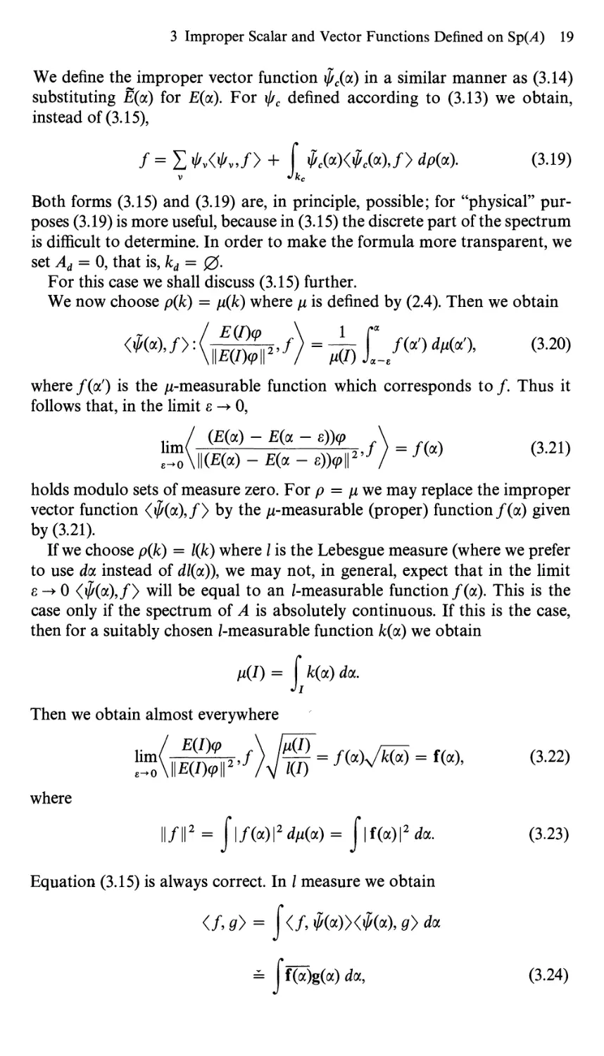
The improper vector function ф(a) itself need not be summable; but the
improper function tf(oc) given by (3.11) must be.
If Sp(^4) is discrete, then (3.12) becomes
I>V< Фу,/> =f,
V
where ij/v are the normed(!) eigenvectors of A:
lim „<!<“■? ~	~ У,,•	(3.13)
£^o Il(£(av) - E{av - e))<jo||
Let p(k) be a positive сг-additive measure over the set P of measurable subsets
of Sp04). It is not assumed that E(k)cp ф 0 implies that p(k) ф 0. In addition,
p(k) need not necessarily be normalized; it is permissible that p(Sp04)) = oo.
However, for all finite intervals I for which E(I) / Owe assume that p(I) Ф 0
and p(I) is finite. Thus an improper function is defined by p(I), which we
denote by dp(a).
For a partition of the а-line into intervals we obtain:
У E(Iy)(P / E(Iv)cp
k ||E(J>|| \\\E(IyM,J
= v E(lv)cp / E{Iv)cp \
v	/ v‘
For the improper vector function
m-—E(I)(p	(3.i4)
mitoWy/rfi)
we obtain, in the limit
/= f	f> dp{a).	(3.15)
JspM)
It is customary to separate the discrete spectrum from the continuous spec¬
trum: Sp(^4) = kdu kc where kc = kcc и ksc (kc = Spc(^4),	kd	=	SpdG4) in
IV, D 2.5.4). For Pv = E(av) — £(av —) (av are the	points	of	the	discrete
spectrum) we define
Ё(сс) = E(cc) - £ Pv	(3.16)
av<a
and
A = Ad + Ac,	(3.17)
where
Ad = Yj %vPv and Ac = a d£(a).
V	V
(3.18)

3 Improper Scalar and Vector Functions Defined on Sp04)	19
We define the improper vector function фс(ос) in a similar manner as (3.14)
substituting E(a) for E(a). For фс defined according to (3.13) we obtain,
instead of (3.15),
Both forms (3.15) and (3.19) are, in principle, possible; for “physical” pur¬
poses (3.19) is more useful, because in (3.15) the discrete part of the spectrum
is difficult to determine. In order to make the formula more transparent, we
set Ad = 0, that is, kd = 0.
For this case we shall discuss (3.15) further.
We now choose p(k) = p(k) where p is defined by (2.4). Then we obtain
where /(a') is the /г-measurable function which corresponds to /. Thus it
follows that, in the limit e -* 0,
holds modulo sets of measure zero. For p = p we may replace the improper
vector function <$(a),/> by the /г-measurable (proper) function /(a) given
If we choose p(k) = l(k) where / is the Lebesgue measure (where we prefer
to use doc instead of dl(oc)\ we may not, in general, expect that in the limit
e -* 0 <$(a),/> wiH be equal to an /-measurable function/(a). This is the
case only if the spectrum of A is absolutely continuous. If this is the case,
then for a suitably chosen /-measurable function k(oc) we obtain
/= £^v<^v./> + f Фс(у-КФс(х),/) dp(a).	(3.19)
(3.21)
by (3.21).
Then we obtain almost everywhere
where
(3.23)
Equation (3.15) is always correct. In / measure we obtain
</, 0> = J</, Ф(Ф<Ф(<х), g) da
= J f(«)g(a) da,
(3.24)

20 IX Representation of Hilbert Spaces by Function Spaces
where the final equal sign = holds only if the spectrum of A is absolutely
continuous. Then, instead of (3.22) we write
<Жа),/> = f(a).	(3.25)
An improper vector function 2(a) is said to belong to the domain of definition
of an operator A if the vectors x(a, a — e) belong to the definition domain of
A for all s which satisfy 0 < e < e0 for some e0. The above ф(а), ф(ос) belong
therefore to the domain of definition of A. If we substitute the vector Af for
/ in (3.12) and observe that <ф( a), Af} = <Аф(ос), /), we obtain
Af = j ф(а)(Аф(а),/у.
We will now show that
ф(а)<Аф(а),/У ~ ф(а)а(ф(а), />:
|<04 - od)E(I)(pjy\ = |<04 - al)E(I)(p, £(/)/>|
< ||04 - al)E(I)(p|| \\E(I)f\\.
According to (3.6) we obtain
\\(A - ccl)E(I)q>\\ <(a- a')\\E(I)<p\\.
Let d be the maximum length of the intervals Iv, then
v E(h)<P / E(Iv)<p \ E(lv)<p / £(/>
k \mv)cp\\ \	\\E(Iv)(p\\	’V	^	v\l|£(7>||,J
= 1
V
For 5 -* 0 we obtain
< <5£ ЦВДЛ12 = 5\\f\\2.
Af = jФ(«)а<^(а)./> = Jф(а)а(ф(а),/У da.	(3.26)
We may therefore replace Аф(ос) by аф(а) and A\j/(<x) by а$(а), respectively;
here we use the notation Аф(<х) ~ аф(а), Аф(ос) ~ а$(а). We call ф(a) or
$(а) the improper eigenvectors of A.
From the continuity of the inner product and, from (3.15), it follows that,
for p = I:
<<£(«'),/> = J W), ШХШАУ da.	(3.27)
Therefore <i^(a'), *A(a)> is an improper function of the two(!) variables
a', a. This function is called the Dirac delta function, which is often written
<5(a' — a) instead of <5(a, a').
For the construction of the ф(a) and $(a) we have made use of our knowl¬
edge of the spectral family E(a). If the spectral family E(a) is not known, then

3 Improper Scalar and Vector Functions Defined on Sp(/4) 21
we may often succeed by proceeding as follows: From
EW= Г ft*XWl/yda'
(3.28)
we seek (often heuristically) to guess ф(ос) as an improper eigenvector for A
from the equation Аф(ос) ~ a$(a) and then construct the operator £(a) from
(3.28). If, for example, A = (1 /i)(d/dx) is an operator in the Hilbert space Ж
defined on quadratically integrable functions over x from — oo to oo then
we seek solutions of the equation (1 /i)(d/dx)g(oc, x) = a#(a, x). We obtain
g(oc, x) = аешх. The g(oc, x) are not vectors(!) in Ж since \g(oc, x)|2 dx is
not convergent. But the J“_g ei<x x da' are vectors in Ж and define an improper
vector function x). With the correct normalization we can set
The representation of the vector / in terms of the improper function
<Ж°0> /) (or> if it is permissible, in terms of thef(a)) is called the ^-represen¬
tation. It is not uniquely determined, because, instead of $(a) we could have
subject to the requirement that the appropriate integrals exist; instead of
<$(a),/) we get the improper function e~i9i<x){\j/((x),f) to represent /.
If В is another maximal self-adjoint operator and x(P) is the corresponding
set of improper eigenvectors of В, then we may obtain an expansion of the
X((t) with respect to the ф(ос) as follows :
<a | /?> is therefore an improper function of the two variables a and /?. Accord¬
ing to (3.31) and (3.15) (with I instead of p) <a | /?> are nothing other than the
improper eigenvectors x{P) °f В in the ^-representation. In the ^-represen¬
tation we obtain (where we use the same symbols for the operator В):
chosen е(в(<х)ф(ос) as the improper vector function providing g(oc) is chosen
Ш) = J$(a)<a|/?>da, where <oc|/?> = (ф(а), *(/?)>.	(3.31)
B<a |)8>
For </J | a) = <a|/?> = <x(P), ф(a)) it follows that
#(<*) = j%(PKP\<*>dP,
(3.32)
(3.33)
so that, for the operator A in the В-representation we obtain
A(p|a> ~ a</?|a>,
(3.34)
that is, the <j8|a) are the improper eigenfunctions of A in the В-representa¬
tion.

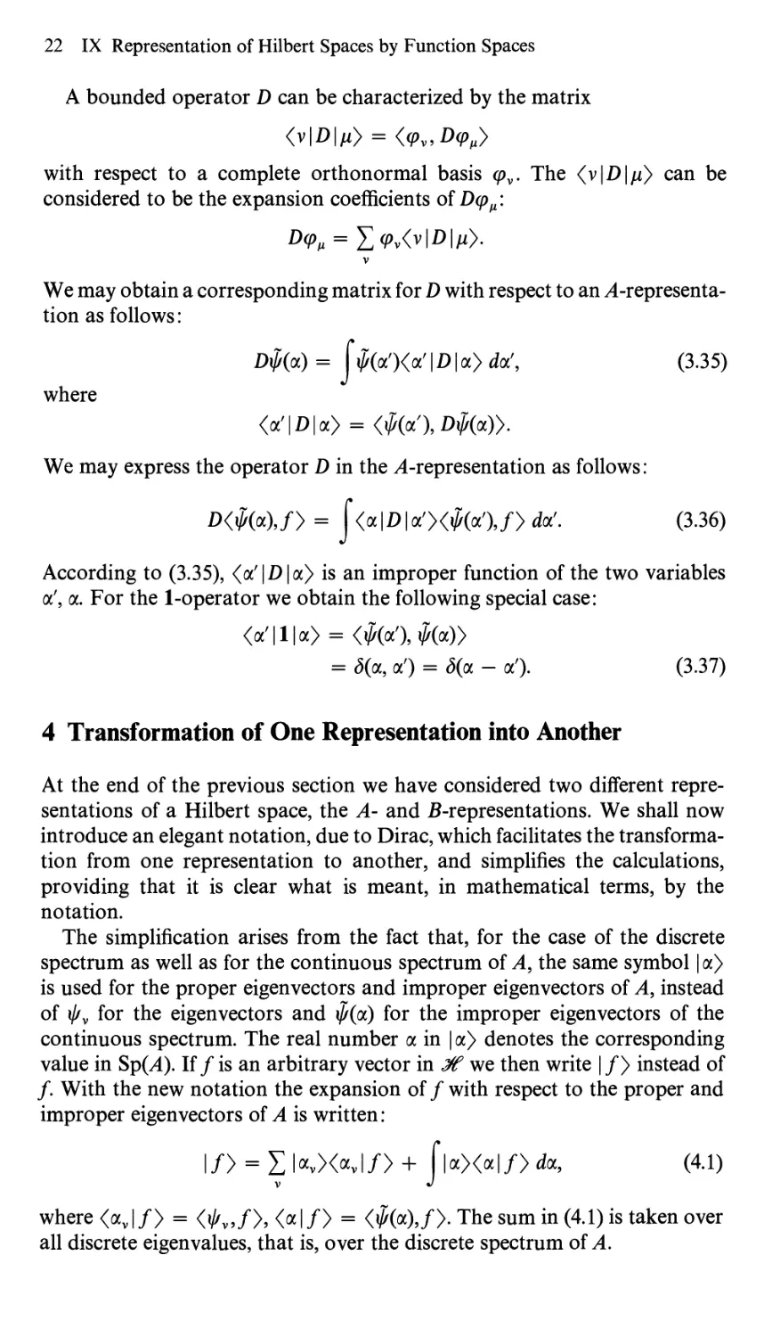
22 IX Representation of Hilbert Spaces by Function Spaces
A bounded operator D can be characterized by the matrix
<v\D\»> = <,(pv, Dcp^}
with respect to a complete orthonormal basis cpv. The {v\D\jn} can be
considered to be the expansion coefficients of Dq7^:
V
We may obtain a corresponding matrix for D with respect to an ^-representa¬
tion as follows:
D\j/(a) = Jф(а')(а' | DI a) da',	(3.35)
where
<a'|D|a> = (ф(а), DiA(a)>.
We may express the operator D in the ^-representation as follows:
= J<a|D|a')<$(a'),/> doc’.	(3.36)
According to (3.35), <a'|D|a) is an improper function of the two variables
a', a. For the 1-operator we obtain the following special case:
<a'|l|a> = <iK<x'), ф(а))
= <5(a, a') = <5(<x - a').	(3.37)
4 Transformation of One Representation into Another
At the end of the previous section we have considered two different repre¬
sentations of a Hilbert space, the A- and Б-representations. We shall now
introduce an elegant notation, due to Dirac, which facilitates the transforma¬
tion from one representation to another, and simplifies the calculations,
providing that it is clear what is meant, in mathematical terms, by the
notation.
The simplification arises from the fact that, for the case of the discrete
spectrum as well as for the continuous spectrum of A, the same symbol | a)
is used for the proper eigenvectors and improper eigenvectors of A, instead
of \j/v for the eigenvectors and ф(а) for the improper eigenvectors of the
continuous spectrum. The real number a in | a) denotes the corresponding
value in Sp(^4). If / is an arbitrary vector in Ж we then write | /) instead of
/. With the new notation the expansion of / with respect to the proper and
improper eigenvectors of A is written:
l/> = ZlO<«vl/>+ f|a><a|/>da,	(4.1)
V	J
where <av|/) =	<a|/>	=	<$(a),/>. The sum in (4.1) is taken over
all discrete eigenvalues, that is, over the discrete spectrum of A.

4 Transformation of One Representation into Another 23
To each vector f e Ж there exists a linear form 1(g) = </, g> on Ж; we
denote this linear form by </1. The value of this linear form for a g e Ж is
</!#> = </> 0>* All bounded linear forms over Ж are of the form </| for
a suitably chosen / (see AIV, §4). The set of </1 is therefore identical to the
Banach space which is	dual to	Ж	(see AIV, §4).
For improper	eigenvectors	|a>	we define an	improper linear form <a| by
<a 19> = <$(<*)> 9> for g e Ж
On the basis of the results of §3 it is not necessary to provide additional
explanation of the new notation. We shall only provide a few examples of
the relationship between the new and old notations as follows:
Pf = l/X/l for / e Ж satisfies ||/|| = 1;	(4.2)
£(a) = £ |av><av| + f |oe><a| da;	(4.3)
v	J	— oo
av<a
A = XXKXtfvl + fa|a><a| da.	(4.4)
V	J
In the ^-representation the vectors/ e Ж are represented by “functions”
<a | /). We then find that
</.0> = £</kX«vlflf>+ Uf\a}(a\g)da.	(4.5)
V	J
Clearly </1 a> = <a | />. In the ^-representation, from (3.26) we obtain
Жа1/> = a<a|/>,	(4.6)
that is, A is the operator which multiplies the function <a|/> by a. If D is
an operator which admits a matrix representation (for example, if D is
bounded) then in the ^-representation we find that:
Я<«1/> = I <a|£>k><avl/>
V
+ J<a|D|oO<a'|/>dx'.	(4-7)
If В is a second maximal self-adjoint operator, then, by analogy with (4.1)
we obtain
1/> = 1ЖХ/У/>+ \\PXP\f>№	(4-8)
U	J
For
l)8> = I>v><av|)8>+ f|a><a|/?>da,
V	*
l«> = £!/*„></*»+ \\PXP\*>dp,
ц	J
(4.9)

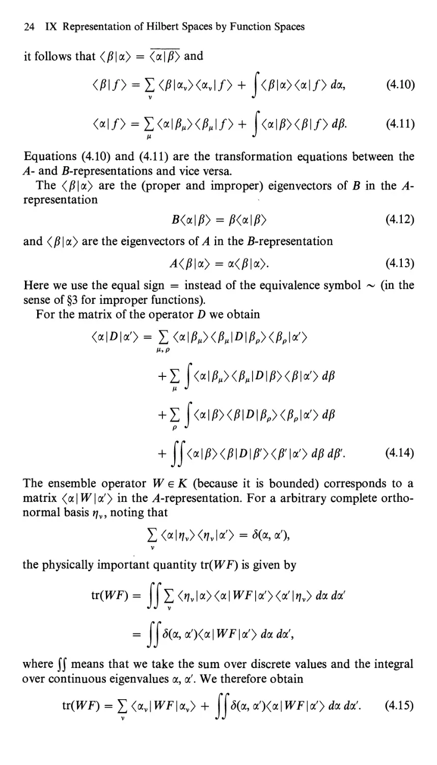
24 IX Representation of Hilbert Spaces by Function Spaces
it follows that <j8|a> = <a | /?> and
</*!/> = E</*K><«vl/> + Up\a)<a\f>da,	(4.10)
V	*
<a|/> = E<«IA,><ft,l/> + \<«\PXP\(4.11)
fi	J
Equations (4.10) and (4.11) are the transformation equations between the
A- and Б-representations and vice versa.
The <j8|a> are the (proper and improper) eigenvectors of Б in the ,4-
representation
Б< a|jS> = jS<a|jS>	(4.12)
and </? | a> are the eigenvectors of A in the Б-representation
Ж/?|а> = а</?|а>.	(4.13)
Here we use the equal sign = instead of the equivalence symbol ~ (in the
sense of §3 for improper functions).
For the matrix of the operator D we obtain
<a|D|a'> = X <а|)8,></дОД></Уа'>
P,P
•E [ЫЪХЪМРХРЮМ
fi J
+ E (<*\PXP\D\Pp><Pp\*>dP
P J
+ jj<a\PXP\D\FXP\*>dpdP-	(4-14)
The ensemble operator W e К (because it is bounded) corresponds to a
matrix <а|РТ|а') in the ^-representation. For a arbitrary complete ortho¬
normal basis rjv, noting that
Е<а|^><^|а'> = <5(a, a'),
V
the physically important quantity tr(WF) is given by
tr(WF) = JJ E in, I а) <a IWF | a') <a' 14v> da da’
= JJ<5(a, a')<a | WF | o') da da',
where JJ means that we take the sum over discrete values and the integral
over continuous eigenvalues a, a'. We therefore obtain
tr (WF) =	Y^<av\WF\avy +	5(a, a'Xa\WF\a'} da da'.	(4.15)
+

4 Transformation of One Representation into Another 25
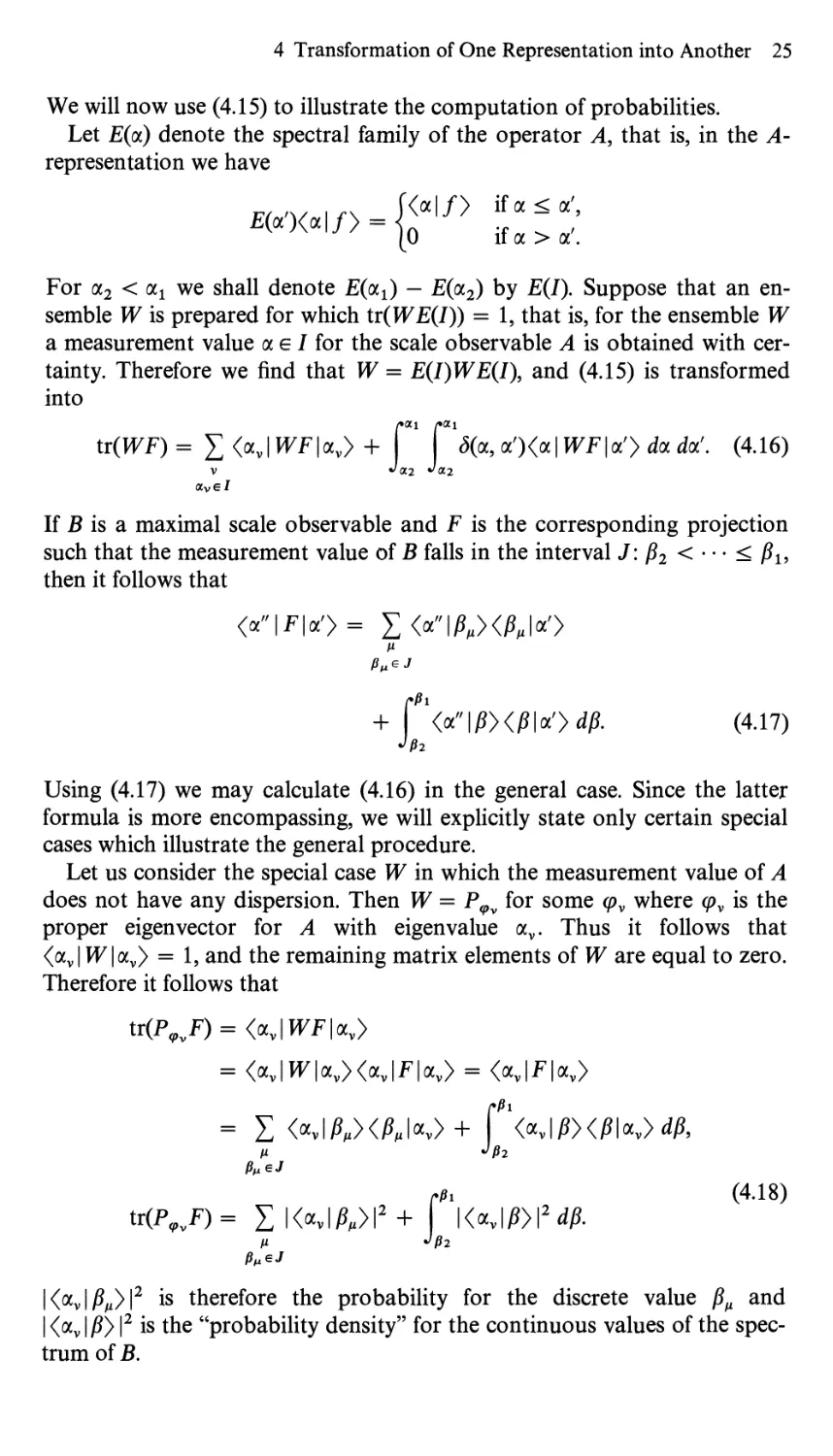
We will now use (4.15) to illustrate the computation of probabilities.
Let E(a) denote the spectral family of the operator A, that is, in the ,4-
representation we have
For oc2 < oq we shall denote E(ocx) — E(oc2) by £(/). Suppose that an en¬
semble W is prepared for which tr(WE(I)) = 1, that is, for the ensemble W
a measurement value a e I for the scale observable A is obtained with cer¬
tainty. Therefore we find that W = E(I)WE(I\ and (4.15) is transformed
into
tr(WF) = £ <av | WF | av> +	<5(a,	a')<a | WF | a') doc docf. (4.16)
If В is a maximal scale observable and F is the corresponding projection
such that the measurement value of В falls in the interval J: f$2 < * * * < Pu
then it follows that
Using (4.17) we may calculate (4.16) in the general case. Since the latter
formula is more encompassing, we will explicitly state only certain special
cases which illustrate the general procedure.
Let us consider the special case W in which the measurement value of A
does not have any dispersion. Then W = P<Pv for some cpv where cpv is the
proper eigenvector for A with eigenvalue av. Thus it follows that
<av| W\ocv} = 1, and the remaining matrix elements of W are equal to zero.
Therefore it follows that
V
Рц e J
(4.17)
tr(P„v.F) = <av|Wm>
= <av|^|av><av|F|av> = <av|F|av>
A.6J
(4.18)
tr(^)= Ei<«vi^)i2+ K«jp)\2dp.
|<av|^)|2 is therefore the probability for the discrete value and
|<av|)8) |2 is the “probability density” for the continuous values of the spec¬
trum of B.

26 IX Representation of Hilbert Spaces by Function Spaces
Suppose that the interval I for which E(I)WE(I) = W is such that I does
not contain any discrete eigenvalues of A. Then from (4.17) and (4.18) it
follows that
tr(WF)= £ f da J* da//?,, |a> <a|VF | a') <a' | /?„>
(I J(X2
+ f'dp f da pda'<j8|a><a|IF|a'><a'|/?>.	(4.19)
* /32	*	ОС2	*0.2
Of particular importance for the evaluation of (4.19) are the “kernels”
КДa', a) = <a'l^)</lja>,
К/a', a) = <a' | /?></? | a).
For the measurement values of the discrete spectrum we obtain the
probability
=	f da f da'K^a', a)<a |	IF | a')	(4.21)
and for the continuous spectrum we obtain the probability density
w{p)=	Г da pda'K/a', a)<a\W\a").	(4.22)
Ja2 *^a2
In general little can be said about (4.21) and (4.22). If the interval
/: a2 < • • • < ax is small, then there can exist values of and /? for which
КДa', a) and КДа', a) are, for all practical purposes, constant for a', a e /,
that is, for an a0 in I we obtain:
К/а', а) « |</У а0>|2,	К/а', а) « |</?|а0>|2.	(4.23)
For such /?д or f} (4.21), (4.22) are transformed into
= K^|a0)|2cw,	(4.24)
w(/?) = |</?|a0)|2cw	(4.25)
with constant
= f‘da pda'<a|lF|a'>.	(4.26)
•'a?.	* CL2
Equations (4.24), (4.25) then show the dependence of the probabilities w^,
or probability density w(/?), upon the values of the spectrum of B. Equations
(4.24), (4.25) hold only for those and /? for which (4.23) is a good approxima¬
tion for a', a^e /. This cannot be the case for all /?д, /? because the following
equation must be satisfied:
£ Г da f da'X^aXal^la')
Ц J(X2 Ja.2
I* oo	pai	/*ai
+ d/M da doc'Kp(ot\ a)<a| PT|a') =
* — со * a.2 *oi2

5 Position and Momentum Representation 27
and (4.23) would lead to the result
<ф]|</Уао>|2 + J” |</?|a0>|2d)8] = 1
in contradiction to the “normalization” equation
+ Г <а\РХРЮ dfi =
(where a and a' lie in the continuous spectrum of A) from which it follows
that
Nevertheless, the physical interpretation of <j8|a> is most intuitively evident
in (4.18), (4.24), (4.25) providing that (4.24) and (4.25) are used with suitable
caution.
5 Position and Momentum Representation
This section will serve to illustrate the discussion in the previous section by
means of special examples. The standard example, the so-called “harmonic
oscillator,” is particularly suited to illustrate those aspects of the structure
of quantum mechanics which will be considered in X, and is of considerable
importance also for “realistic” problems. As an approximation, the harmonic
oscillator plays a large role for molecular spectra (see XV) and provides the
basis for quantum field theory (Fock representation, see, for example, [4]).
The position and momentum representation was originally obtained
from the representation of the Galileo transformation, as we have outlined
in VII, §2. The spaces ££2(R3, dxx dx2 dx3) and ££2(R3, dkx dk2 dk3) describe
the position and momentum representations, and are isomorphically
connected by the Fourier transformation. Here we shall treat the same
problem from the other side in order to illustrate the methods of previous
sections. Here we shall consider the “one-dimensional” case of a position
operator Q and a momentum operator P which satisfies the commutation
relation (see VII (4.22))
PQ-QP = \l.
(5.1)
An “harmonic oscillator” is defined by the Hamiltonian operator
(5.2)
which corresponds to an elementary (one-dimensional) system of mass m
in an external field of the (one-dimensional) potential (mco2/2)Q2 (for external
fields see VIII, §6).

28 IX Representation of Hilbert Spaces by Function Spaces
We now introduce new operators
(5.3)
We obtain
P'Q' - Q'P' = \ 1
(5.4)
and
Я = coH’, where H' = UP'2 + Q'2)-
(5.5)
It suffices, therefore, to find the solution of the problem for g', P', H\ and
the solution for g, P, H is obtained by simple computation. In order to
simplify the notation, we shall omit the ' in g', P' and H'.
We shall now make the following assumptions:
(1) The linear manifold = P)^°=ljm=1 (@pn n @Qn) (where 3f is the
domain of definition of the operators) is dense in Ж.
(2) Pg - gP = -ilin^f.
(3) H = |(P2 + Q2) is a self-adjoint operator with spectral decomposi¬
tion E(s) and E(s)f e <£ for all / e Ж.
The assumptions (1), (2), (3) are satisfied for the position and momentum
operators introduced in VII, §4. Conversely, if (l)-(3) (where (3) can be
weakened somewhat) are satisfied for the position and momentum operators,
then the infinitesimal transformations corresponding to P and g correspond
to a representation of the Galileo group. We refer readers who are interested
in these relationships to [5].
Assumption (1) permits us to construct arbitrary products of the form
Paig/JlPa2g/J2.... Therefore we find that ££ c= <3)H-
We define the operators:
In we therefore find that В = A+, and that the following relationships are
satisfied:
Therefore, in <£ instead of H we may consider the operator N = A+A. From
assumption (3) we obtain:
where £(A) is the spectral family for N; from the latter we may easily obtain
the spectral family for Я.
AA+ - A+A = l and H = A+A + jl.
(5.7)
(5.8)

5 Position and Momentum Representation 29
The spectrum of N cannot be negative, since
</, Nf) = M/ll2 > 0
for all / in S£.
According to Th. 1.3 (even in the case in which N is not maximal) there
exists a cp such that
(£(«) - E(fi))(p Ф 0 for £(a) - E(P) / 0.
If Я is a value from the spectrum of N, then for the vectors
(£(A) - £(A - й))ф
||(£(A) - £(A - е))ф||
we obtain
ВД, в) - AZ(A, e) -> 0.
Conversely, if we are given a set of vectors x(e) for which \\хЛ > 8 an<l
NXe — X'Xe -* 0 then Я' is a point of the spectrum of N; on the other hand, if
A' is not a point of the spectrum, then there exists an interval A' — rj ■ ■ ■ A' + r\
for which £(A + rj) — £(A — r\) = 0, and for every vector / we would find
that ||(N - A'l)/|| > ri\\f\\. From (N - A'l)x(e) 0 for / = y(e) it would
follow that x(s) -* 0 in contradiction to the assumption that ||%(e)|| > 5.
From (5.7) it follows that in X£ the following relationships are satisfied:
AN — NA = A and A+N — NA+ = — A 1. Since the %(A, e) lie in if we
find that
NAx(X, s) = ANx(X, e) - Ax(X, e)
and
NAx(X, e) - (A - 1 )AX(X, e) = A(N - A1)Z(A, e).
For (N - X\)x(X, e) = h we obtain
\\Ah\\2 = <h, Nh> = (h, (N2 - XN)X(X, e)>
< ||/i|| ||(N2 - XNMX, e)|| < \\h\\Xe
(the last relation is obtained in a manner similar to (3.6)). Therefore we
find that Ah -> 0, that is,
(N — (X — 1)1 )Ax(X, e) ^ 0.	(5.9)
In a similar way it is possible to show that
(N - (A + 1)1 )A+x(X, e) -*■ 0.	(5.10)
Since \\A+x(X, 8)||2 = <x(A, e), (N + l)z(A, e)> = 1 + \\AX(X, s)\\2 it
therefore follows that if A is a value of the spectrum of N then so is A + 1.
If \\Ax(X, г) || >5 for all e, then A — 1 will also be a value of the spectrum
of N. Since the spectrum of N is nonnegative it follows that there must be an
integer n for which there exists a sequence £v -* 0 such that An+ '/(A, ev) -> 0

30 IX Representation of Hilbert Spaces by Function Spaces
and \\Апх(Л, ev)|| > S. In addition (TV — (A - n)l)A"x(X, ev) -> 0 must be
satisfied, that is, A — n must belong to the spectrum of N; in addition
(N - (A - n - 1)1 )An+ 1%{X, ev) -► 0 and therefore NAn+ ^(A, ev) -> 0.
From NAnx(X,sv) = A+An+1x(X,sv) and	\\A+An+1x(X,sv) ||2	=
\\A”+1x(X,ev)\\2 + (An+1X(X,sv), NAn+1X{X, ev)> it follows that
A+A"+ lx(K £v) -*• 0, that is, NAni(X, £v) -*• 0. From (N - (A - n)l)A"x(X, £v)
—+ 0 it follows that (A — n)Any(X, £v) -> 0. Since \\A"x(X, £v)|| > 3 we must
have A = n, that is, A is a positive integer n > 0. Therefore the spectrum N
is discrete, and can only contain integers n > 0.
Since NAnx(X, ev) -> 0 and \\x(X, £v)|| > 3 the value 0 is a value in the
spectrum of N. Therefore there exists an eigenvector ф0 of N with eigenvalue
n = 0. We may assume that ||(/>0|| = 1. From Ыф0 = 0 and from ||1V</>0||2 =
\\А+Аф0\\2 = \\Аф01|2 + \\А2ф01|2 it follows that
Аф0 = 0.
(5.11)
Since Ыф0 = 0фо, it follows that, for y(X. s) = ф0 in (5.10), by recursion
Ы(А+)пф0 = п(А+)"ф0. The spectrum of N consists of all integers n > 0
and (А+)”ф0 is an eigenvector of N with eigenvalue n.
We set
ф„ = а„(А+УФо,
(5.12)
where a„ is the normalization factor. From the normalization requirement
|| </>„|| = 1 it follows that
i = m2 =
n — 1
*П~ 1
(Фп-и АА + ф„-!>
an- 1
<(/>„-!,(N + !)</>„-1> = n
Therefore the ф„ will be normalized if we set a„ = 1Д/п!; we obtain
Ф« = -т=(А+УФ0,
<n\
(5.13)
and we obtain
Ыфп = пфп.	(5.14)
Since the фп are eigenvectors which correspond to different eigenvalues, they
are pairwise orthogonal.
If the eigenspace of N for the eigenvalue 0 is multi-dimensional, then we
may introduce a complete orthonormal basis 0(ok) in this eigenspace. We then
define

5 Position and Momentum Representation 31
The ф\k) are normalized and are pairwise orthogonal, that is, they are an
orthonormal set in Ж.	We	will now show that	they are complete.	If this is
not the case, then there	exists	a smallest ri > 0 for which the фjJP do	not span
the entire eigenspace of N with eigenvalue n\ that is, there exists an eigen¬
vector фп, (which is orthogonal to all the ф{к)) of N with eigenvalue n\ which,
according to (3), lies in S£. From n' Ф 0 it follows that Афп> Ф 0 and N(Ail/nr)
= (ri — l)G4i/v). Since Афп, is also orthogonal to all ф$-19 this result
contradicts the condition that n' is the smallest eigenvalue for which the
ф{k) do not span the entire eigenspace.
Let Ж(к) denote the subspace spanned by ф(к) for fixed k; clearly
Ж=^@^(к)-	(5.16)
к
The operators A, A+, Я, P, Q all act in the various Ж{к) in the same way;
thus Ж can be expressed as a direct product as follows:
Ж = Жгх Ж2	(5.17)
with the correspondence
фпи{к\	(5.18)
where the фп form a complete orthonormal basis for Жх and the u(k) form a
complete orthonormal basis for Ж2, and the operators A, A+, H, P, Q all
have the form
A x 1, A+ x 1, etc.	(5.19)
and the A, A+ ..., as operators in Жх obey (5.11), (5.13) and (5.14). It there¬
fore suffices to consider the above operators in Жх where N is maximal
(according to Th. 1.6 we need only choose q> = апфп where a„ # 0 and
|a„|2 < oo).For Жх there exists an iV-representation given by / ^<n|/>.
From
P = \~{A-A+),	Q=^-{A+A+)	(5.20)
'Ф- V2
it follows that

32 IX Representation of Hilbert Spaces by Function Spaces
For f =Yjn Фп(п I /) it therefore follows that, in the iV-representation that
N<n |/> = n<n|/>,
P<n\f> = <n\Pf> = -^д(^/п(п - l|/> - Jn + l<n + l|/>),
Q<n\f> = <n\m = -3=(v£(n- ii/> + xATT <« + ii/»,
<n|P|m> =	-	Jm + l<5„,m+1),
<n|g|m> =	1	+	Vm	+	1(5n,m+i)-	(5.22)
In order to find the Q-representation of it is necessary to solve the eigen¬
value equation for Q:
Q(n\x> = x<ji\x>.	(5.23)
Using (5.22), (5.23) is transformed into
П + ^ <n + l|x> + hr (ji — l|x> = x(n\x}
V 2 x	V	2
if we substitute
<n I x> =	<01 х>Я„(х)	(5.24)
2nn\
from (5.23) we obtain the recursion formula
Hn = 2хЯ„_1 — 2(n — l)Hn-2	(5.25)
with the initial value H0 = 1. The functions defined by this recursion
formula are called the Hermite polynomials. They are identical to the expan¬
sion coefficients of the “generating function”
00	tn
/(*,1) = e~t2+2tx = ex2e-«~*2 = £ Hu(x) -	(5.26)
„ = o ni
from which it follows that

5 Position and Momentum Representation 33
from (5.26) we obtain the relation
H'n(x) = 2nHn_1(x)	(5.28)
and, from
— f(x91) + 2(t - x)/(x, 0 = 0
we obtain the relation (5.25). Since from (5.26) it follows that H0(x) = 1, we
have proven the equivalence of (5.25) and (5.26).
The <n|x> in (5.24) are improper eigenvectors since ^п=о Ки|х>|2 = oo.
We note, however, that
(ji|(py =	(n\x'}	dx'
Jx — E
are approximate eigenvectors of Q since (as we will shortly find)
| <n | cp}\2 < oo. We will now determine <n 10) from the normalization
condition
f <x'|n><n|x> = S(x - x').	(5.29)
n = 0
For this purpose, using (5.27), we obtain
*<*■ *> - ? ЙП	= e"! ? 2*1 H-M(-
From the Fourier expansion
e~x'2 = -ip Г	e-i°>*'e~°>2i4- da
2-sJn j - 00
we obtain
(d \n	1	f00
- — ]e-x'2 = —=	e-iaxXi(o)"e-0,2/4 dcu
<**/ 201^-00
and, using the generating function in (5.26), it follows that
g(x, x') = e*'2 -2- Г е-^е-тщ £ _L Hn(x)(mf dco
2	71	J - oo	n	^ ft •
If00
= Упе*'2 —	gM*-*')	dcD	=	Упех'2д(х	—	x'\
271 J_ oo
where we have used the following identity from the Fourier integral theorem
J_ Г £-ico(x-x ) do) _ ^
271 J-oo
1	Л00
<?*'2	=	e-iox'e-oil4e-(iol2)i	+	2(iol2)X	dco
2. Hi J-к

34 IX Representation of Hilbert Spaces by Function Spaces
Therefore, instead of (5.24) we can write,
<п'х>-7ШТпН-(х)е~'"	<5-3°>
Each vector /e^ can therefore be represented in the Q-representation by
a function <x | /) as follows:
<*l/> = E <*1и><»1/>-
П
In particular, the operator P can be expressed in the Q-representation as
follows:
P<x\D = E ix\n){n\P\my<rn\fy.
n,m
From (5.28) and (5.25) it follows that:
E<x|n><n|P|m> = у ^ (,x\ni)
and we therefore obtain
p<x\f}= ~(*|/>.	(5.31)
The Q-representation can therefore be chosen such that (5.31). In the Q-
representation we must, of course, have | /) = x<x | /), as can easily be
shown.
In the g-representation the Hamiltonian operator H is given by
H=l-(P2 + Q2) = \
In particular, we therefore obtain
_(t^) +x2]-
_(ts) +*2]<*I»> = (» + 5)<*I»>-	(5-32)
If, instead, we begin with the Q-representation which was given in VII, §4,
then we could have used (5.32) in order to calculate <x | n> and then transform
to the iV-representation. We have taken the opposite route in order to
demonstrate the methods of §§1-4.
We will now briefly outline how we may make the transition from the Q-
to the P-representation. In order to determine the transformation coefficients
<x| p> we proceed from the fact that in the Q-representation the <x|p>
must be (improper) eigenvectors of P:
ту-<х|р> = p<x\p)	(5.33)
i ax
from which it follows that

5 Position and Momentum Representation 35
The factor already satisfies the normalization condition
oo
<p'\x)(x\p} = S(p - p’).
The relation (5.34) may be formulated precisely in the sense of §4. <x|p> is
an improper function of two variables x and p :
The reader may visualize the concepts of §4 by means of this example.
We shall now use the <x | n) and <x | p> in order to explicitly compute the
probabilities which were discussed at the end of §4.
Given an ensemble W for which the energy has zero dispersion, that is,
W = Рфп for some n, then the probability of a position measurement is,
according to (4.18) given by the probability density
In Figure 1 <x|n> is displayed; the behavior of |<x|n>|2 as a function of x
can readily be ascertained.
Conversely, given an ensemble W for which the position is in the interval
x — e, x with certainty, it follows that the probability that a measurement of
the energy will be (n + i) is, according to (4.21), given by
w(x) = |<x|n>|2.
where
Kn(x\x") = <x'|n><n|x">.
<x|/7>
n=0
n-3
1 71*2
'Л=7
• n*0
X
Figure 1 Eigenfunctions <x | «> of harmonic oscillators.

36 IX Representation of Hilbert Spaces by Function Spaces
From Figure 1 it is clear that, for small e, the function Kn(x\ x") is, for all
practical purposes, constant in the interval x — e • • • x providing that n is
not too large! If n is not too large, then, according to (4.24) we obtain
From this example it is clear why (5.36) cannot be a good approximation
to (5.35) for all n.
The above derivation makes it possible to determine those ensembles P^
for which equality holds in the Heisenberg uncertainty relation IV (8.3.18).
According to the discussion immediately following IV (8.3.17) equality can
hold if there exists a real number a for which the relation
Q + iocP' is, however, except for a factor and an origin displacement,
identical with the operator A or В = A+ in (5.6). Therefore (5.37) can only
be satisfied for a > 0 and must correspond to the “ground state” of the
harmonic oscillator. We may express (5.37) in the Q-representation as
follows:
which is also normalized, is a Hilbert space vector only if a > 0. For the
position probability density in the ensemble W = P^ we therefore obtain
This form is known as the “Gauss distribution (Gaussian).”
6 Degenerate Spectra
The ^-representation of a Hilbert space is possible if A is maximal, that is,
if the complete Boolean ring E generated by the spectral representation of
A is maximal (D 1.1). E is maximal if there is no decision effect £ £ E which
is commensurable with all elements of E. If av is an eigenvalue of A and Pv
(5.36)
(Q + iaP') = 0
(5.37)
holds, where
P' = P - tr(P„P)l = P - pi,
Q' = Q- tr(P„01 = Q-ql.
[
Thus it follows that
1
£-[(*- «)2/2«] ”	” «)
(5.38)
(5.39)

6 Degenerate Spectra 37
is the projection operator onto the eigenspace for the eigenvalue av then each
Pvel and each E < Pv are commensurable with all elements of £. If A is
maximal, then from E < Pv it follows that either E = Pv or E = 0, that is,
Pv must be one-dimensional. Therefore, to av there exists a uniquely deter¬
mined eigenvector (up to a factor) cpv. In this case we say that the eigenvalue
is nondegenerate. If Sp/4) has only discrete values and is nondegenerate
then £ is maximal (see §5) and PVv e £ for the complete orthonormal basis
of the eigenvectors of A. If E # 0 is commensurable with all P<Pv (and therefore
commutes with all P^J then it follows that EP^ = P^E < P<Pv, that is,
Ecpv = cpv or Ecpv = 0 and E = £'v PVv where £' is the sum over all v for
which Eq>v = <pv. Thus it follows that £e£.
D 6.1. The dimension of a projection Pv onto an eigenspace of A corre¬
sponding to the eigenvalue av is called the degree (order) of the degeneracy
for av. Note that the statements “av is nondegenerate” and “av is degenerate
of order 1” have the same meaning.
We shall now outline how we may obtain an Л-representation for a Hilbert
space for an A which is not maximal, and how the notion of degree of de¬
generacy may be extended to the continuous spectrum.
As we have already mentioned at the beginning of §1, if we are initially
given a nonmaximal A, then there exists a finite set of commensurable decision
observables A, В,..., the combination of which is maximal (D 1.1). The dis¬
cussion of previous sections is applicable to this case. If, for example, A and
В are commensurable, then instead of an Л-representation we will obtain an
(A, ^-representation by means of proper or improper functions in the
(a, /?)-plane as follows: / «-* <a, j8|/>. Since the extension of the preceding
formulas is trivial, we shall not discuss them here. In the following we shall
present the case of position representation for several Qv.
In order to define the notion of the degree of degeneracy more generally
we shall begin with Th. 1.9. Suppose that En (n = 1, 2,...) is a denumerable
set of pairwise orthogonal decision effects which are commensurable with A;
so that the complete Boolean ring generated by the spectral family of A and
by the En is maximal and that from EEn = 0 for an E in the Boolean ring
generated by the spectral family it follows that EEm = 0 for all m > n. For
the operator В = £„=0 nEn and E0 = 1 — £и= x En we find that A and В are
a maximal pair (D 1.1) of scale observables, that is, the complete Boolean
ring £ generated by the spectral family of A and by the En (n = 0, 1, 2,...)
is maximal. According to Th. 1.3 there exists a q> for which ^(£, cp) = Ж.
Therefore the discussions in §2 can be directly applied to A, B.
For an interval L in the (a, j8)-plane of the form L = (al5 a2] x (/?l5 /?2]
we define the measure ja as follows:
KL)= \\E^mB\J)cp\\2,	(6.1)
where I = (al5 a2], J = (jSl5 /?2] and E{A)(X), EiB)(X) are the spectral families
of A and B, respectively. Ж can therefore be represented in terms of <£2(R2, ji).

38 IX Representation of Hilbert Spaces by Function Spaces
Because of the special character of В we may simplify the representation
using functions/(a, n) for n = 1, 2,... for which
We denote the space of quadratically integrable functions /(a, n) (in the
sense of (6.2)) by 2(R x N+, /i). Let Sp„04) denote the set {a| for all al5
a2 where ol1 < a < a2, it follows ||(£(A)(a2) —	#	0}.
We shall now show that Spw(^4) з Spm(^4) for m > n: If а ф Sp„04) then
there exists an interval ocx < а < а2 such that (EiA)(oc2) — EiA)(ocJ)En(p = 0
and therefore we obtain (E{A)(oc2) ~ E{A)(oc1 ))En = 0. Thus, from Th. 1.9 it
also follows that (E{A)(oc2) — EiA)(oc1))Em = 0 for m > n from which it
follows that Sp„04) з Spm(^4).
We shall say that n is the degree of degeneracy of the value a in the con¬
tinuous spectrum of A if n is the largest number for which a e Spw(^4). Here
we permit the value n = oo.
It is easy to generalize the special case of operators Q and P which satisfy
the commutation relations (5.1) onto a set of operators Qh Pt where i = 1,
2,...,/which satisfy the commutation relations:
show that N has eigenvalues n = 0, 1, 2,... and there exists a vector ф0 for
which А(ф0 = 0 for all At. For the complete orthonormal basis ф$] for the
eigenspace of N with eigenvalue 0 the set of vectors
n
(6.2)
where
(6.3)
The inner product is given by
(6.4)
We introduce the operators
and the operator N = Yj= i M At. In the same manner as in §5 it is easy to
forms a complete orthonormal basis in Ж

6 Degenerate Spectra 39
We may, as we have done in §5, express the Hilbert space Ж in the form
Ж = Жъ x Ж2 where the Qh Pt are expressed in the form Qt x 1, Pt x 1;
then, in the position representation Жъ takes on the following form
q>ejfb:	<р*-*(х1,х2,...,х/\<рУ,
Qjcp xjixi, x2,..., xf | <p),
1 d /
Pj<P *-+ j ^ \xi, x2,..., xf I (p).
Жь is often called the orbit space (see VII and VIII).

CHAPTER X
Equations of Motion
In VIII we have established that VIII (6.26) and (6.27) are, in a formal sense,
the most general form for the description of the time translation of a
registration apparatus relative to a preparation apparatus. In VIII, §6
we indicated that we would like to call VIII (6.2.7) the “equations of motion
for quantum mechanics.” In this chapter we shall only be concerned with
formal transformations of the above time translations. For that reason we
shall take VIII (6.27) and (6.16) as our starting point. It will then be possible
to repeat all the formal transformations for VIII (6.26) instead of VIII (6.27).
1 The Heisenberg Picture
We shall call the description of time translation based upon VIII (6.27),
that is,
the so-called Heisenberg picture. In the computation of statistical quantities
and expectation values of the form tv(WBt), W is taken to be constant.
For the special case in which Bt does not “explicitly” depend on t, that is,
dBJdt = 0, it follows that
(1.1)
Bt = utB0u;,
(1.2)
40

1 The Heisenberg Picture 41
where, according to VIII (6.16), the unitary operator U satisfies the dif¬
ferential equation
dUt
~df = iHtUt*	(L3)
where U0 = 1. The solution	of the differential	equation (1.1) for the case
dBJdt = 0 follows,	therefore,	from the solution	of (1.3)	given by (1.2). For
the special case in	which Я	is independent of	time, a	formal solution of
(1.3)	is given by
Ut = eiHt.	(1.4)
Let A and Я be a complete set of commensurable scale observables; let a
and e denote the values of the spectrum of the self-adjoint operators A and Я,
respectively. Then Ut is the operator which multiplies the vectors <e, a|^)
(the vectors ij/ in the ^-representation) by eiet. If we represent B0 by a
matrix, then we may express Bt by the following matrix:
<e, cc\Bt\e', a') = eiiE-s,)t(e., а|Б0|в', a').	(1.5)
The fact that Bt is obtained from B0 by means of a unitary transformation
Ut implies that Bt has the same spectrum as B0 because the spectral repre¬
sentation Et(k) of Bt is obtained from the E0(X) of B0 as follows:
Elk) = UtE0(k)U;.	(1.6)
The solution of the eigenvalue equation Bt q>t = Pcpt follows simply from
B0 cp0 = f}(p0 and is given by cpt = Utcp0. The physical meaning of this situa¬
tion is as follows: The possible measurement values for a scale observable
cannot change with time if there is no time variable external field.
From (1.6) it follows that the statistics of the measurement values do
change with time. The statistics of the measurement values will remain
constant with time for every ensemble only if B0 commutes with all Ht
for all t—then we will obtain Bt = B0 and Et(k) = E0(X). In the case in which
Bt = B0 we say that В = B0 = Bt is a constant or integral of motion.
For our first example of the application of the Heisenberg picture we shall
consider the case of a one-dimensional harmonic oscillator under the
influence of an external field. This example is more than an academic one;
it plays an important role in many realistic physical problems—for example,
as an approximation in molecular physics (see XV, §8) and as a problem in
quantum field theory.
For the external field we shall choose the simple potential field given by
ф(х, t) = —xk(t). Then the Hamiltonian operator Я is given by
1
Н = Ъп P4t) + ~~2~ Q2(t) ~ mX	(L7)
where P(t) and Q(t) are the momentum and position operators, respectively.

42 X Equations of Motion
In addition to scale observables P(t\ Q(t), we shall also discuss the time
behavior of the “energy”
_ , ч 1	4 mco2 ~, 4
HM~b«Pm + — »
For each value of t the operators P(t), Q(t) satisfy the Heisenberg commuta¬
tion relation (see IX (5.1))
*406(0 - 6(0*40 = \ 1-	(1-8)
Since much of the mathematics development for this problem is completely
analogous to that presented in IX, §5 we shall only present an outline.
We introduce the operator A(t) and its adjoint A+(t) as follows:
A(t) = -^= (y/moQ(t) + —7L= p(t)j,
A+(t) =	(y/moQ(t) P(t)j.
(1.9)
1 / /—i
^/2 \	x/mco
J_/ /—i
yjl \	y/mco
From which it follows that:
A(t)A+(t) - A+(t)A(t) = 1,
H0(t) = ojA+(t)A(t) + у 1,
H( = Яо(0 - -jL= (A(t) + A+(t))k(t).
лjzmco
For each value of t there exists a (normalized) vector Ш0(г)еЖ which
satisfies ^4(t)'Po(0 = 0. The vectors
¥„(() =-2==	(l.ii)
ln\
(1.10)
form a complete orthonormal basis in Ж. They are also eigenvectors of
Uo(ty-
H0(tyv„(t) = (n + i)«T„(t).	(1.12)
According to	the	Heisenberg picture we obtain the	time	evolution	of the
observables	of interest P(t), Q(t), H0(t) if we obtain A(t) from	the differential
equation (1.1):
T A(t) = H,A(t) - A(t)H, = — coA(t) +	1.
1	yjlmco
The solution is very simple:
A(t) = е~ш(А(0) +	(1.13)

1 The Heisenberg Picture 43
where
/(t) = -7^= fW^dT.	(1.14)
yJ2mw Jo
We shall write ^„(O) = фп, so that from (1.10) we therefore obtain:
Фп =	(1.15)
п\
According to the general considerations about the eigenvectors and eigen¬
values of Bt we may obtain the eigenvectors of H0(t) from those of H0(0)
by means of the operator Ut. Equation (1.13) gives us the value of the right-
hand side of the following equation:
A(t) = UtA(0)Uf.
Then from (1.11) we obtain
ад = utA+(oyu: ад.	(i.i6)
The eigenvector *F0(t) °f #o(0 corresponding to the eigenvalue co/2 must
have the form
ад = а(0^о,	(1.17)
where we may choose oc(t) = 1. For computational purposes, however, it is
desirable to refrain from this choice. From (1.16), (1.17) it therefore follows
that, in general,
ад = ат,фп	(1.18)
Ut is therefore determined if *РИ(£) is expressed in terms of the orthonormal
basis of the фп and if a(t) is given.
The expansion
ВД = I фт<фт, v,(0>	(1.19)
m
is determined when we have computed <$m, *F„>. From (1.11) it follows that
(фт, ВД) = A= <А(1Гфт, ВД>.	(1.20)
y/nl
According to (1.13) we obtain
A(ty = e~~intot £ ^/M(0)""v.	(1.21)
Furthermore, from (1.15) and the first equation in (1.10) it follows that
А(0)рфт = y/m(m - 1) • • • (m - p + 1 )фт-р.	(1.22)

44 X Equations of Motion
In order to find {фт,х¥п} it therefore suffices to compute <0p, XF0>:
<Ф„, 'Po(O) = -U <А+(0Уфо, Ч0(ф = -L (фо,А(0уЧ>о(ф
VP!	VP!
1 <4>о,[Ж0егга,-/(0]рад>
1
[-/(0]p<4>o, VoW).
Since PFoCOII2 = EpK^P’^oCO)!2 = 1, we must have |<</>0, То(0>|2
= e l/ |2. Since we have not yet chosen the factor a(t) in (1.17) we may choose
<ф0, 'Po(O) = e_(1/2)l/|2. Then we obtain
1
<фр, Ч'оСО) =	(1.23)
2
Then, from (1.20) to (1.23) we obtain:
tfl f
<фт, ^„(0) = К е'"”'е“(1/2)|/,,)12 [-/(t)]m~".
V И!
• i f")[-|/(0l2]v?	Ц-тт,	(1-24)
V=ff\v/	(m-n	+	v)!
where = 0 for m > n and a = n — m for m < n.
The pth derivative of the Laguerre polynomial
is given by
K(X) = i (n\^^(-xy-»(-iy.
v = 0 v (v~ pV-
Therefore, for m < n we obtain
ITU^ 1
<</.„, ад>= /— - еЫю‘е - ™W(f(ty - ">Ц - m( I f(t) 12)	(1.25a)
\j nl nl
for m > n we obtain
<</>т,ад> = Я — einmte ~ <W)\m\\	~	nL™	~ "(| /(012).	(1.25b)
\j ml ml
Thus the expansion (1.19) and the operator Ut defined by (1.18) is determined
up to the factor a(t).
With the aid of the <0m, 4*n(t)y given in (1.25a) and (1.25b) we may now
answer the following physical question: Suppose we are given a preparation
apparatus which prepares an ensemble W for which the measurement of

1 The Heisenberg Picture 45
#0(0) results in the value co(m + £) with certainty. Therefore we must have
tr(PУРфп) = 1, from which it follows that W = Рфт. What is the probability
for the same ensemble that a measurement of H(t) will result in a meaurement
value of co(n + £) (that is, for a time displacement t of the registration ap¬
paratus for H0(0) relative to the preparation apparatus)? It is given by
tr(WP^) = НРфтРупи)) = I<фт, ад>I2.	(1.26)
It remains to compute the factor a(t) in (1.18). From (1.17) and (1.3) it
follows that:
*о(0 =	о	=	-ocU^o + iccHt Utф0
a
= -ад +1Я(ад
a
and we obtain
<ВД, %(t)> = 1 + KVoit), Й,ВД>.
From Ht in (1.10) it follows that
- = - ^ + <*0(0, 't'o(O)*
a l
In order to compute the inner product <lP0,xt/0) we begin with *F0 =
Ей Фп<Фп> Ч\)> аП(1 use (1-23); we obtain:
^0(0 = £ 0„(-/(t))V-,1/2)l/,1)|24=:-
у/п\
By differentiating with respect to time it follows that:
ад = £</»„4=7 e-™'2{n(-fy-4-f) - i(-/)"(// + //)}.
yjnl
Therefore we obtain
<*<>, ад> = а// -//) = l 4== вду“*+f(t)e~n
2 yjzmcD
from which we obtain the following equation for a:
I= ~ у + \ (f(t)eion+
a l	z ^2mco
With a(0) = 1 we finally obtain
.	icot	i	1
a(t) = exp^ - — + -
к(х){/(т)еш + f(z)e-n dX (1.27)
mco Jo	J
Thus we have completely determined Ut.

46 X Equations of Motion
For our second example illustrating the Heisenberg picture we shall
consider an elementary system of mass m in the absence of an external field.
Here we have H = (1/2m) £f=1 Pf. For Pt(t) and Qt(i) it follows from (1.1)
that
Pi(t) = 0, Qi(t) = - Pi(t),
m
Pt is therefore constant with time, and we obtain
Qt(t) = Qi(0) + - Pt.	(1.28)
m
Thus it follows that the expectation value for the position for the ensemble
W is given by
МШФ = triWQfr)) = M(Qi(0)) + 2	M(P;),	(1.29)
m
that is, the expectation value of the position moves with constant velocity
(l/m)M(Pj). If we set
QXf) = QM - мшгж
p\ = Pt- M(Pj)l,
then, from (1.28), (1.29) it follows that:
Q'i(t) = Qm + 2 p;.	(1.30)
m
For the dispersion
disp(&(0) = tv(WQ’tm	(1.31)
we obtain the relation:
disP(6j(t)) = disP(&(0)) + - м(е;(0)р; + p;e;(0))
m
t2
+ — disp (Pf).
m
It is easy to compute the time tm for which disp(Q*(t)) is a minimum. For tm
we obtain
Mmop'i + ржо) = о
from which it follows that
disp(&(0) = disp((2i(tj) + 2~-2—2 disp(P,).	(1.32)
m

1 The Heisenberg Picture 47
Equation (1.32) shows that the dispersion of Qt is quadratic in its time
dependence relative to its minimum value. In addition to (1.32) the Heisenberg
uncertainty relation IV (8.3.18) must be satisfied
[disp^.)]1/2 [disp(ei<0]1/2 > i	(1.33)
If (1.33) is an equality for t = tm then at other times the Heisenberg uncertainty
relation can only be satisfied as an inequality.
In addition to the expectation values, it is also possible to obtain answers
to questions concerning the probabilities for different position and mo¬
mentum values. In order to make computations, we shall consider the
special ensemble W = Р9.
The probability for a momentum value in a region n of momentum space is
constant with time and is given by
I<Рь Рг,Рз\(P>I2 dpt dp2 dp3,	(1.34)
Jn
where (рь р2,Ръ\ cp} is the representation of cp in the momentum representa¬
tion. We will now compute the probability for a measurement of the position
Qi(t). For this purpose we shall transform from the momentum representa¬
tion to the (6i(0, 6г(0> 6з(0) representation. In order to obtain this
representation, we seek the solution of the equations
Qj(t)qx b,2>„ = xjs* „*2,*з	(1-35)
in the momentum representation, where 6/0) is the operator — (l/i)(d/dpj).
Here (1.35) becomes
( T ~^p- + ^Р^РиР2>Рз\Х1’Х2>хЗ> = Х]<Р1,Р2,Рз\х1,Х2,Х3'>
from which it follows that
<Рь Рг>Рз\х2, X2, x3> = ^372 ехр|^-г X (xjPj - ^-pj^j .
From
<xu x2,x3\<P> = J<xu X2, x31pu p2, РзХРь	Рз \<P> dpi dp2 dp3
we find that the probability that a measurement of Qj(t) will result in a
measurement value in the domain is given by:
\(xu x2, x3\(p)\2 dxx dx2 dx3.
Jir
If (p is so chosen that, at time t = 0, it satisfies the Heisenberg uncertainty
relations with an equal sign (where we may obtain an evaluation of IX (5.37)

48 X Equations of Motion
which is analogous to IX (5.38) in the momentum representation) we then
obtain
<Pi, Р2,Рз\<Р> = (^i) expj^-j £ (Pi - щ)у~^ exp|^— ~ £ (Pi ~ ^)2j
and it follows that
<.X1,X2,X3\<p'>
' (2^ Ш {*'* ~ i”J) “ 'I, ^ ‘ ’*]
eXP[_ (?) (Pj ~ 7tj')2] dPl dPl ЛРЗ
- b~V2 eip[~ 4?W I, h ~ (*+?)T]
"“p['~ W I, [? (*; ”	_ Й<x' ‘ ^ ' S7 "']]
• expj^i X
where b = 1/a2 + if/m.
Here it again follows that the probability distribution |<xl5..., \ cp}\2
propagates with velocity (1/т)я;7- where M(pj) = Uj. In this way we obtain
a more precise description of the behavior of this probability distribution
(not only the dispersion given by (1.32)).
2 The Schrddinger Picture
The expression tv(WBt) is used to compute all probabilities and expectation
values. If Bt does not explicitly depend upon the time t, then from (1.2) we
obtain the expression tr(WUtB0 U+). From the property of the trace func¬
tional we may exchange Uf+ with WUtB0; we obtain
tr(PF0 UtB0 C/,+) = tr(u; W0 UtB0),	(2.1)
where we have written W = W0in order to emphasize the fact that W = W0
is constant in time. We now define a time dependent Wt as follows:
Wt= u;w0Ut	(2.2)
we then obtain
tr(PF0B,) = tr (WtB0).	(2.3)
In §1 we have called the expression on the left side of the equation (2.3) the
Heisenberg picture. We call the expression on the right-hand side the
Schrodinger picture. For many purposes it is often mathematically more

2 The Schrodinger Picture 49
convenient to	work with the right-hand side of (2.3), the	Schrodinger picture.
In particular,	the	product representation of the Hilbert	space	introduced in
VIII (2.1) for t = 0 does not change with time (see VIII, §2). The position
representation of the Hilbert space (in which the momentum operators
have the form (l/i)(d/dx)) can be taken to be fixed with time.
If Bt depends explicitly upon the time, that is, if dBJdt ф 0 then, in the
Schrodinger picture we may define an operator
Bt=UjBtUt	(2.4)
which, in the case that dBJdt = 0 is (according to (1.2)) equal to B0. Instead
of (2.3) we find that, in general
tr (W0Bt) = tr (WtBt).	(2.5)
For the special case in which W0 = P(po we obtain
u;pvoutf=u;<p0<<p0, ujy = u;<p0(u;<p0,fy
=	=	pvj,
where
<pt=U?q>0.	(2.6)
Taking the adjoint of equation (1.3), we obtain the following differential
equation for cpt\
фг = Ujut(p0 = ujut(pt = —iUj Ht Ut cpt.
Using definition (2.4) it follows that
1
--cpt = Ht(pt.	(2.7a)
In the same way we obtain the following differential equation for Wt
AW
= i(WtH, — Ht WQ.	(2.7b)
(2.7a) and (2.7b) are called the Schrodinger equations.
What is the form of the operator HJt
As we already mentioned in VIII, §6* in the expression VIII (5.8) for Ht we
are to	use	the	operators	Pt(t)9 Qt(t), S^t). Since	P^t) =^1/^(0)!/^, etc.,
we find	that we	obtain	the	operator Ht if we replace	all Pt,Qi, St in VIII (5.8)
by Pi(0), <2i(0), St(0), that is, if all P*, Qi9 St are chosen to be constant with
time. Nevertheless there can be a remaining time dependence in Ht which
may be due to the time dependence of the external field A, cp, that is, through
an “explicit” time dependence of Ht.
In order to clarify this situation, let us consider an elementary system of
charge e in an external time dependent field. Then we would have

50 X Equations of Motion
From (2.8) it follows that
Й' = ^т A CPi(0) ~ eAi(Qi(0)’ Q2(0)’ Qi(°X 0]2
+ есрШО), Q2(0), бз(0), 0.	(2.9)
If we know that we are in the Schrodinger picture, we may omit the symbol
(0)	in (2.9) and write
Я, = ^ I [Pi ~ eAi(Qu Q2,Q3, t)]2
+ e(p(Qi, Q2, Q3, t),	(2.10)
where we know that the Ph Qt are operators which are constant with time.
With (2.10) the Schrodinger equation (2.7a), as expressed in the position
representation corresponding to Qu Q2, Q3 is given by
-т^<х1,х2,х3|ф(> = ^ £ \j-^-eAk(Xl,x2,x3,t)^ <x1,x2,x3\(pt)
+ e<p(xu x2,x3,tKx1,x2,x3\cp,}.	(2.11)
In Schrodinger’s heuristic development of quantum mechanics equation
(2.11)	is “guessed” with remarkable intuition. From (2.11) it follows that a
wave packet in a “weakly” varying electromagnetic field behave much like
mass points of classical mechanics with the Hamiltonian
1 3
н = -Г- £ (Pk - eAk(qu q2,q3, t)f + e<p(qu q2,q3, 0
2m k=l
(see, for example, [6], XI, §1.2).
If Ht does not explicitly depend upon time, then in both the Heisenberg
and Schrodinger pictures Ht is a time-constant operator: Ht = Ht = H0.
The Schrodinger equation (2.7a) is then given by:
— - cpt = Hcpt, where H = H0.	(2.12)
Let г denote the values of the spectrum of H and let a denote the degeneracy
index for H. In the Я-representation (2.12) becomes
1 d
-~—<e,cc\(pt} = s{s,a.\(pt)	(2.13)
I ot
the solution of which is given by
<г, a | cpt} = e~iEt(e, a|<p0>.	(2.14)
For examples we shall again consider the case of a harmonic oscillator and
a free elementary system.

2 The Schrodinger Picture 51
Let Ut denote the unitary operator for the harmonic oscillator which was
computed in §1. The solution of the Schrodinger equation (2.7a) is given by
9, = u;<p0
and, in the N = ,4+(0),4(0)-representation we obtain
<n\9t> = £ <n\U?\m><m\(p0>
= £ (tn\Ut\ri)(m\(p0y.
m
According to (1.18)
<<£m> ^n> = «(*КФт, и,ф„У = <x(tXm\Ut\n>
and we find that
<т\иЛп> = фКфт9Ч?яУ
Therefore we obtain
<п\<р,'> = ф)'£<?¥н,фя>Оп\<р0'>
= ф)^<ФЛ><т\9о\	(2-15)
m
where <фт, is given by (1.25a), (1.25b) and a(t) is given by (1.27).
Instead of taking a somewhat circuitous route using the Heisenberg
picture, we shall instead directly solve the Schrodinger equation (2.7a) in
the position representation where the latter is given by
2
<x|(joty
2
+ ^y-x2<x|9,У - k(t)x{x\(pty.	(2.16)
For fit) as defined in (1.14) we shall set
y(t) = -4= (e~ionf(t) + e^M),
yjlmw
nit) = - Г4(е-ш/(г) -	(2-17)
i у 2
y(t) and n{t) are solutions for the motion x(t), p(t) for a mass point according
to classical mechanics! Thus we find that solutions of (2.16) are given by
gn(x, t) =   - - - (moj)ll2Hn((moj)ll2(x - у(ф-(тт12>,х-р<1»2
# ei7t(t)xe-ii^(it(x)/2m)dxe-i(o(n+ l/2)f	^ Jg)

52 X Equations of Motion
where
H„((mca)1,2x)e ~(mto/2)*2
J22nl^
are the normalized eigenfunctions of
1	mco2	~
ъ,р + — Q
which correspond to the eigenvalues (n + %)co (see IX (5.30)), that is,
^ Hn((moj)ll2x)e~<mm2/2>x2 = <x|«>.	(2.19)
From (2.18) it therefore follows that 0„(x, 0) = <x|n>. The most general
solution of the Schrodinger equation (2.16) is therefore given by
<X I <Pr> = Ё 9«(x> 00» I (po>-	(2.20)
n = 0
Clearly (2.15) and (2.20) must be the same solution. Since
<x\(pt> = E С*1и>0»1<г>«>
n
and
/•00
0*l<Pt> =	<и|х><х|ф(>/(х
V — 00
from (2.20) it follows that
oo Г /*оо	"|
<n\(pt> = E <n|x>Sfm(x, <?и|фо>-	(2-21)
m = 0 L*' - 00	J
Since the <m|<p0> were arbitrary, by comparison of (2.21) with (2.15) we
obtain
a(OCF^O, фт} = Г (n\x}gm(x, t) dx.	(2.22)
J - CO
We now seek to answer the same physical question as we have in §1. Suppose
that we prepare an ensemble for which the measurement of the observable
H0 (which is constant in time in the Schrodinger picture!) has, at time 0, the
eigenvalue (m + %)co with certainty. Therefore we must have W0 = Pcp0
and <n|<p0> = 5nm. If, for the same ensemble we measure the observable
H0 “at time t” we must use Wt = For the initial value <n|<p0> = Snm
from (2.21) it follows that
/•00
<n\(p,} = {n\x)gm(x, t) dx.	(2.23)
J — 00

3 The Interaction Picture 53
The probability that the measurement value will be со (n + \) is given by
|(n\(pt}|2 in complete agreement with (1.26).
For a free elementary system the Schrodinger equation, as expressed in the
momentum representation, is given by
- т4<Р1>Р2>Рз1<Р»> =	£	P?<Pl,P2,P3l<P(>-
г ot	2m	i=!
The general solution is given by
<Р1,Р2,Рз\(р,> = exP2~ (.£ P?)*
<Р1,Р2,Рз\<Р0>-
The solution of the Schrodinger equation (2.12) in the position representation
-<*„x,\*>. £ i	.l2,x,,ft>
is therefore given by
<xb x2,x3\(pty = j(x1,x2,x3\p1,p2, РзХРи P2, Рз\<Рх> dpU dp2, dp3
• ip и P2, Рз I <Po> dpudp2, dp3,
where
<Pi> P2> Рз\<РоУ = J<Pi> P2, Рз\хи *2’ *3><*i> x2> x3\(p0y dxx dx2 dx3.
If we let
<xlf x2, x3\cpoy =	exp|^—a2 £ ^ ~^2nj(xj ~ ^)JJ.
then from <xl5 x2, x3 \cpt) we obtain the same physical results for the time
behavior for the position probability distribution as we obtained for the
Heisenberg picture at the end of §1.
3 The Interaction Picture
Frequently we find that it is possible to separate the Hamiltonian operator
into two components Я = H° + Я12, where the spectral representation of
H° is easy to determine. In applications H° frequently has the following
form: H° = Я? x 1 + 1 x H2, which refers to the product decomposition
Ж = Ж^ x Ж2 “at time t = 0” for a composite system containing a system
of type 1 and of type 2. Я?, H2 are the Hamiltonians for systems of type 1
and type 2, respectively; see VIII (2.1). Я12 is often called the interaction

54 X Equations of Motion
Hamiltonian, from which we obtain the expression “Interaction Picture.”
Here we assume that H° does not explicitly depend upon the time. Thus,
(according to §2) H° is a time-independent operator. Thus it follows that
ешог = eiHot x ешо2г	(3л)
Thus it follows that
eiS°,(B1 x B2)e-iit0' = (е‘Я°,В1е~Ш0'’) x (ei5“'B2e“(3.2)
Equation (3.2) means that the product representation
remains invariant under unitary transformations of the form (3.1), a result
which is very practical (see XVI).
With Wt defined by (2.2) it follows that, for the expectation value of an
observable in (2.5)
tr (W,Bt) = tr(eiS°' W,e~ 1Й°‘е>Й0,В, e ~ ii}0‘)
= tr( V,+ W0 Vt e™0tBt e ~	( )
where
V, = и,е~‘й°г.	(3.4)
If we simplify our notation as follows:
В, = е‘йо гВге~Шог and W t = Vt+W0Vt	(3.5)
then the expectation values can be written in the form
tr(WfBf).	(3.6)
In (3.6) the operator Wt which describes the ensemble and the operator Bt
are time dependent. The time dependence in (3.6) is therefore divided among
both factors as follows: Bt depends upon the time t as if H° was the
Hamiltonian operator, that is, in the case (3.1) as if there was no interaction
between the subsystems. Bt therefore corresponds to the Heisenberg picture
without interaction.
The time dependence of Wf arises therefore from the interaction. Similarly,
as in the Schrodinger picture, for the special case W = P^o it follows from
(3.5)	that:
W, = P*„ where ф, = у;ф0 = е1й°‘и;ф0.	(3.7)
From differentiating with respect to t and using (1.3) it follows that
-\ф,=
 Н°ф, + е'йо,и?Н,ф0
= -Й°ф, + е‘йо,и^Н,и,е-‘й°гф,.
We find that
U?HtUt = Я, = Я0 + Я,12.

3 The Interaction Picture 55
Since H° commutes with е1Йо\ we therefore finally obtain
-]фг = H(12«A()	(3.8)
where
H12 = eiH0tR,2e-iH0t	(3.9)
represents the operator Я12 in the time dependence of the Heisenberg
picture without interaction (see (3.5)).
As in §§1 and 2 we shall again consider the example of forced oscillation
of a harmonic oscillator with
H° = i_ p2 + ^ q2	H12= _Qk(t)	(3	10)
2m	2
For this case equation (3.8) becomes
-]ф,= -КШЖ,	(3.11)
where Q(t) is to be computed according to the equation of motion of a free
oscillator
<№ = ~Ш P(0 = —moj2Q(t),
m
that is,
Q(t) = 6(0) cos cot H—— P(0) sin cot.	(3.12)
mco
For the 6(0)-representation of the Hilbert space, in which P(0) = (l/i)(d/dx),
(3.11)	is transformed into
T^<x|iA,> = fc(o[x
1	д
cos cot H sin cot — <x|ipt}.	(3.13)
imco	ox
For a special solution for this equation we choose the form
g(x, t) = ei[XKit) + uit)].	(3.14)
For (3.13), with this choice, we obtain
that is,
(xk + u) = k(t)x cos cot H—— k(t)K(t) sin cot,
mco
к = k(t) cos cot, u = —k(t)ic(t) sin cot
mco

56 X Equations of Motion
and we therefore obtain
K(0 = V	[/(0 - /(£)].
r '	<3.15)
u(t) =	 к(т)к(т)	sin сот dx,
J0 mco
where f(t) is defined according to (1.14). In order to find a general solution
of (3.13) we observe that
<*#«> =	~	w(t))g(x, t),
where
«■«) + /(<))
is, for arbitrary /(z), a solution of (3.13) providing that g(x, t) is a solution.
Thus, for the most general solution we obtain:
<*#*> = X(* - w(t))ei[XKit)+uit)].	(3.16)
For t = 0 we obtain w(0) = 0, k(0) = 0, u(0) = 0. /(x) is therefore equal to
<x | \j/oy so that we obtain:
<*#,> = <X - w(0l^oy[3e,c(O + ,,wl-	(3.17)
Since the energy observable H° = (1/2m)P2 + (mco2/2)Q2 is constant with
time in the interaction picture, then so are the eigenvectors <x| n} (in the
Q(O)-representation). The probability that the energy value co(n + £) is
measured at time t, assuming that the ensemble is, at time t = 0, dispersion
free with respect to the measurement value co(m + £) is given by
If
2
(3.18)
which, according to (1.25a, b), (1.26) agrees with | <</>m, lF/l) |2 and, according
to (2.23) agrees with | <ji \ cpt) |2.
4 Time Reversal Transformations
In VII, §7 we have considered parity transformations and have discussed the
problem that it is nontrivial to realize such a transformation by means of
r-automorphisms. The problem of the realization of time reversal trans¬
formations is even more difficult to comprehend.
The time reversal transformations correspond to the time “reflection”
x'v = xv, t' = —t. What is the physical meaning of such a transformation?
The transformation in VII (7.1) can be intuitively visualized with the aid
of a mirror, which gives us some idea on how we may build a “mirror image”
of a registration apparatus. What, however, do we mean by a registration

4 Time Reversal Transformations 57
apparatus for which the time is reversed? Here we may consider the idea of
making a motion picture of experiments with microsystems, and running
the film backwards. By analogy with a mirror image, we may seek to realize
such an experiment by running a motion picture backwards, but it is clear
that this is impossible because the experiments are “irreversible.” We
cannot realize the following process in reverse: microsystems are emitted
by a preparation apparatus, and are detected by a counter (as a registration
apparatus) which, in turn, responds. The response of the counter is not
reversible, and cannot be realized in reverse. In general, the time direction
of the action of the preparation apparatus on the registration apparatus by
means of microsystems is that direction in which entropy increases in the
macroprocesses connected with the preparation and registration. This
directedness is an important fundamental structure underlying quantum
mechanics which cannot be avoided—see, for example, [6], XVI and [7].
Therefore we shall not, at first, discuss the question whether there exists a
realization of time reversal by means of registration procedures. Instead,
we shall define a time reversal transformation T as a В-continuous effect
automorphism for which we obtain a representation of the “extended Galileo
group” by means of effect automorphisms, where the Galileo group is
extended by the addition of the time reversal transformation
s: Xy = xv, t' = —t.
With the help of VII (1.1) it follows that
(A, S. i/, y)s = s(A, - <5, rj, -y).	(4.1)
With the reflection operator r in VII, §7 it follows that
rs = sr.	(4.2)
The operator T can, in principle, transform one system type into another,
a fact of great importance in elementary particle physics. Here we shall assume
(in analogy to the case of the spatial reflection (parity) operator) that T
leaves system types invariant. According to V, §5, in the Hilbert space Ж
of every system type there exists a unitary or anti-unitary operator V which
satisfies
Ty=VyV~1	(4.3)
for уе&'(Ж). From s2 = e it follows that T2y = у and that V2 = el4.
From (4.1) and (4.2) it follows that
U(A, ё, ij, y)VU(A,	= KA, t ij, y)V,	(4.4)
Ui^VUirY1 = e^V.	(4.5)
In Hilbert	space Жп where Ж — Жъ x 4S we define the following	anti-
unitary	operator С as follows: Let w+,w_ denote the basis	vectors	of

58 X Equations of Motion
which were definedjn VII, §3. The vectors of Жп may be written in the follow¬
ing form (where Qt is defined as multiplication by rt, Pt is the operator
l/i grad?():
E (г 1) Г 2 > • • ■ > I Ф > ®1> • • • >	^«n>

where each af runs through the indices + and —. We set
с X <rl9 r2,..., r„ I 	a„>	м., • • • мЯп
«1 «п	(4.6)
= E <^1> *2> rn\<Pl «1> • • • > «B>(al> ®2> • • • > an)U-<tiU-<x2 ' ' '
ai,a„
where (ab a2,..., a„) = 1 for an even number of a; = — 1 and = — 1 for
an odd number. С then transforms	and	{Ж”}_	into themselves.
It is easy to extend the definition of С to the more general case of a composite
system consisting of n electrons and several atomic nuclei; here it would be
necessary to introduce additional position coordinates and additional spin
vectors.
It follows that C2 = (—1)"1 and C~1 = (— 1 )nC. Here it is easy to prove
that
CQt = QtC,
CPt = -P;C,	(4.7)
CSi = -SiC,
CH = HC,
where H is the Hamiltonian operator (without external fields) given by
VIII (5.8).
For the reflection operator defined in VII (7.4) for Ж	=	Жъ	x	U(r),
defined in (4.5), as an operator in Misgiven by U(r) = (R	x	1)	x	(R	x	1) x
• • • x (R x 1). From (4.6) it follows that
CU(r) = U(r)C.	(4.8)
From (4.7) it follows that
CU(A, S, п, у) = U(A, -li},-y)C.	(4.9)
If we multiply (4.4) and (4.5) on the right by C~we obtain
U(A, 5, % y)(VCy1)U(A, 5, ij, y)~1 = A(A, 3, % y)VC~\ (4.10)
t/(r)(FC-1)t/(r)-1 = e^VC~l.	(4.11)
From (4.10)	it	follows	that	the A{A, 3, fj, y) form	a one-dimensional	repre¬
sentation of the	Galileo	group; therefore A(- • •) =	1.	For an elementary system
it therefore follows that VC~l must be a multiple of the unit operator, and
since a number in V is arbitrary, we may set
V = C.
(4.12)

4 Time Reversal Transformations 59
We shall require that (4.12) also holds for the case of a composite system. We
therefore find that, from (4.3)
Ту = CyC~\	(4.13)
For the special case in which у is an element of L, that is, у is an effect, then
there exists a B-continuous effect automorphism defined by (4.13). Note
that this result does not, in any way, explain how the transformation (4.13) is
to be realized in terms of registration procedures. The following question
we cannot answer: Let (b0, b) be an effect procedure; for which other effect
procedures (b'0, b') is the equation C\l/(b0, b)C~1 = фф'о, b') satisfied?
By analogy with the transformation from the Heisenberg to the Schrodinger
picture, we may write
tr(WCBC~x) = tr(C~1WCB).	(4.14)
We may therefore apply the time reversal transformation to the ensemble W;
we obtain
W-> C_1WC = CWC~\	(4.15)
where	we	note	that	C_1 = (—1 )nC. Again, we have	not	explained how,
given	a	preparation	procedure a, we may obtain	another	a'	such that
cp(a') = С<р(я)С-1.
According to (4.9) we obtain the special case
CeiHy = e~iHyC.	(4.16)
In the Schrodinger picture we find that
Wr= e-iHit-x)WxeiHit~x).	(4.17)
Let us define
W'f = CW^C-1	(4.18)
then, from (4.17) it follows that
W'f = CeiH{t ~x)Wxe~iH{t~X)C~1
= е-Ш(*'-т)СЖт C~ V*(‘'~T)	(4.19)
_ e-iB{t'-x)yyi eiH{t'-x)'
Therefore W't> is also an ensemble which satisfies the Schrodinger picture.
If we subject Wt to normal time development from time tltot2 = x>tl
then at the time t, Wx, is transformed into CWXC~1; if we then subject CWX C~1
to normal time development of т to the same interval t2 — tx = т — tx
until t + (t — £1) = 2t — tl5 then, according to (4.19) we obtain at time
2t — tl the ensemble CVFflC_1, that is, the ensemble which is time reversed
with respect to the “initial ensemble” Wtl. This means that we can run the
“quantum mechanical Schrodinger motion picture” Wt backwards in the
form CW2x_tC~ S that is, this “backwards” version is a physical possibility if
the formulation of quantum mechanics described here is a g-G-closed
theory in the sense of [8], §§8 and 10.

60 X Equations of Motion
It is therefore an important question whether for a given preparation
procedure a, it is possible to produce an a' (at least, in principle) such that,
cp(a') « С<р(я)С-1
is satisfied (at least approximately). Clearly, for large systems, in particular,
macrosystems, this is not the case because of their irreversible nature; see,
for example, [6], XV, [7], X and the remarks in Chapter XVIII. A macro¬
scopic extrapolation of quantum mechanics cannot therefore be a g-G-
closed theory for macrosystems than such an extrapolation of quantum
mechanics (see [7], X).
In XVI, §7 we shall return to a discussion of the question whether the
“Quantum Mechanics of Microsystems” can be a g-G-closed theory.

CHAPTER XI
The Spectrum of One-Electron Systems
In IV, §4 we suggested that, in order to obtain a more concrete and en¬
compassing development of the theory, we need to establish the connection
between well-defined (with respect to their technical structure) registration
methods b0, the corresponding Boolean ring	and the operators
g = фф0, b) by introducing axioms which specify the mathematical form
for the operators g = ф(Ъ0, b).
We shall not number these axioms; instead we only note that they are
additional axioms in the sense of the mathematical picture. We also cannot
give a comprehensive description of the technical details of construction
in order to formulate these new mapping principles. We are only able to
obtain an overview of the preparation and registration procedures by using
the concise language of the physicist in which previous knowledge of the
physical phenomena associated with the structure of the apparatus is
already assumed. In accord with this mode of expression we shall, for example,
speak of a “spectral apparatus” without making reference to textbooks of
experimental physics concerning the structure of such an apparatus, or its
resolution capability. In XVII we shall present the first step in the develop¬
ment of an extension of the theory which will provide a more precise descrip¬
tion of the structure of the preparation and registration apparatus and we
shall ascertain the form of the maps 2! Д K, 2F Д L for some examples. In
XVIII we shall examine the extension problem in more detail without
attempting to obtain a solution to the problem. A solution of this problem
can be found in [7], XI. For that reason we must, at least for the present, be
satisfied with the prospect of having to guess or discover individual axioms
61

62 XI The Spectrum of One-Electron Systems
for particular preparation and registration methods.
It is advisable to pursue this route by beginning with special cases (one-
electron spectra) rather than the general case (for example, the problem of
atomic and molecular spectra). It is easier to understand how the special case
leads to the general case rather than to understand an overview of the general
case. For this reason we urge readers to be patient in their consideration
of the systematics when they encounter a previously introduced axiom at a
later point in the development as a special case of a later axiom. In this sense
the previous comments may serve as a justification for the following dis¬
cussion of the light emission for the case of a single electron. This type of
presentation permits us to show the essentials more concisely and the reader
may eventually be able to carry out the necessary generalizations.
1 The Effect of the Emission of a Photon
For the present we shall not attempt to develop a systematic theory in order
to establish the correspondence described earlier between an operator g and
the construction rules for the registration apparatus. Here we shall often use
partially known theories, and other theories (obtained by guesswork) in
order to obtain an expression for the desired operator. We will then introduce
the latter as an “axiom” in our theory.
As is well known (see, for example, [6], XI, §1), the description of the
emission of photons has been very successful. The so-called “spectral
apparatus” is well suited to determine the wavelength of a photon emitted by
an atom, and to register the photon on a “detector” (for example, a photo¬
graphic plate, photomultiplier, etc.). In terms of the discussions presented
in II an atom produced by a preparation apparatus a produces a detection
response b (with the aid of a photon) in the registration apparatus b0, where
b0 is a special spectral apparatus. Normally, a spectral apparatus is an
integrating apparatus. It does not register each individual photon, but
instead records the intensity of the spectral lines, that is, it approximately
measures the number of photons which are confined to the region of a spectral
line.
Which operator g should correspond to the following effect: Within a
time interval At a light quantum (photon) of frequency со is registered by the
spectral apparatus? Here we shall not inquire about the details of the spectral
apparatus—such as the width of the slit, the spatial orientation of the slit, etc.;
instead, we will only inquire about the effect, that “an atom emits a photon
of frequency со in the direction of solid angle dQ. during the time interval
At.” In this way we may obtain, with the help of numerical factors, the
“intensity” of a spectral line measured by a concrete apparatus.
This example demonstrates typical aspects of the theory of many registra¬
tion apparatuses: First a process is treated in a purely quantum mechanical
way (for example, the emission of a photon by an atom). The next step in the
process is then treated classically (for example, the propagation of the

1 The Effect of the Emission of a Photon 63
photon in the spectral apparatus is treated in terms of wave optics). In the
third step we encounter the problem of registration (here, let us consider a
photographic plate) where we need to know either from the theory or from
experiment whether all or only a known fraction of systems subjected to the
preceding processes are actually registered. Here we shall consider only
the first part—the emission of a photon by an atom; we shall assume that the
remaining theory of the spectral apparatus is already known.
At present we are unable to describe the emission process for a photon
purely from quantum mechanics, because it would first be necessary to
develop a quantum mechanical theory for the electromagnetic field. Because
there is no mathematically correct formulation of such a quantum field theory
at present, we have to rely on a very extensive workable and practical system
of computation schemes (the so-called quantum electrodynamics) which
functions well for most problems. We will not use these methods to compute
the desired effect of the emission of a photon; instead, we shall give a some¬
what simple “rule of computation” for this problem, from which we may
obtain the desired operator.
Our starting point will be the classical description of the emission of
electromagnetic radiation by means of a charge-current distribution, as
computed using Maxwell’s equations. We will first describe the charge-
current distributions classically by means of two functions p(x, t) and j(x, t).
We shall then introduce operators for the classical expressions for the
charge-current distribution for a single electron around an atomic nucleus.
These operators will be inferred from the use of the wave-picture for the
electron. Since, in the following computations p and] will occur linearly, the
computations for the corresponding operators p, j will be completely
analogous to those obtained for the classical functions p and j.
The fields generated by p and j are computed from the scalar potential
cp and vector potential A by means of the equations
We shall consider these retarded potentials for distances which are much
greater than the region of the charge and current distribution, where the latter
is characterized by a distance d which roughly corresponds to the “diameter”
of the atom. In this section we shall obtain a quantitative value for d from
quantum mechanics. For the origin of our coordinate system we will choose
the center of mass of the atom; for all practical purposes, since the mass of
the electron can almost be ignored compared to the mass of the nucleus, the
center of mass coincides with the nucleus (see VIII, §§2,4,5). In the transition
Ё = —A — grad cp, В = curl A.
For cp and A we use the formulae for retarded potentials:
(l.i)
(1.2)

64 XI The Spectrum of One-Electron Systems
to quantum mechanics we retain the convention that the position operators
(after separating out the motion of the center of mass) describe the position
relative to center of mass (see, for example, VIII, §2). Here, for simplicity, we
assume that the velocity of the center of mass is so small that the Doppler
frequency shift of the spectral line—the so-called Doppler broadening—can
be neglected. Our discussions can easily be extended in order to take into
account the effect of the motion of the center of mass, that is, for the case in
which an ensemble W has an appreciable probability for large center of mass
motion.
We will now consider an expansion of (p and A according to the following
two viewpoints:
(1) The point x lies far outside the sources of the field, that is, | x | > d.
(2) The wavelength Я of the emitted radiation is much greater than the
size of the atom, that is, Я > d.
We shall now introduce an expression of cp and A in powers of d/\x \ and
d/X as follows:
First, it follows that (since \x'\/\x\ < d/\x\)
We shall obtain an expansion of p and j in terms of the retardation in
t — | x — x' |. A time derivative of p corresponds to (if we consider p expanded
in a time Fourier series) a power of the frequency со, which is proportional
to l/Я. Thus, in the following, we can read, from which power in d/X the
individual terms of the expansion arise. We then obtain (where the position
dependence of p is supressed):
p(t - \x - x'l) = p(t - |3cI) + p(t - |3c|)e + ip(t - |5c|)e2 + • • •,
where г = \x\ — \x — 5c'| = x' • x/\x \ + • • •. If we carry out the expansion
only to terms of first order in 5c'/| 5c | (that is, d/\x \ and d/X) we obtain
The so-called dipole moment is given by
(1.3)
(1.5)
and the charge (which is time independent) is given by
We therefore obtain

1 The Effect of the Emission of a Photon 65
For the vector potential A we obtain an analogous expression, where p is
replaced by J. In the analogous expression for A the individual terms can be
rewritten in such a way that their physical interpretation will be more clearly
evident. Using the continuity equation p + divjr = 0 and, integrating by
parts, (here the surface integrals vanish) we obtain:
Jj(5c', t — \x\)d3x' = Jj • V'5c' d3x' = — Jx' div j d3xf
= Jpx' d3x' = d(t — | x I),
where V' is the vector operator (д/дх\, д/дх'2, д/дх'3).
For an arbitrary constant vector a we obtain
Ja • xj d3xf — Ja • x' j • V'x' d3x' = — JxV' -(jd-x') d3xf
= Jx'3 • x'p d3x' — Jx'j* 2 d3x'.
We may neglect the term	Jx'a • x'p d3x' because	it	is	of order of magnitude
d/13c |	d/X in the expansion.	We may therefore set
J a • x'jd3x' = \ Ja • x'j d3x' — \ ^x'j • a d3xf
= Ja x (3c' x j) d3xf.
Similarly, we obtain
f a • x — d3x' = ~	f a • x j d3xf = — ]- —	f	2	x	(x'	x 7)	d3x'.
J dt dt	J J	2 dt	J	K
We define the magnetic dipole moment
fh = j jx' X j d3x'.	(1.7)
Thus we obtain
л<:5'c) - jil3 “ T#Fx x	<u>
From (1.6) and (1.8) we may compute the fields E and B.
When we make the transition to quantum mechanics we will replace p and
j by operators. In order to discover these operators we shall make use of

66 XI The Spectrum of One-Electron Systems
well-known expressions for p and j from the wave picture (see, for example,
[6], XI (1.3.4), (1.3.5))(without external fields!).
p = <#i2
e
J = ~
m
where we assume that
Jl*AI2 d3x' = 1.
For the “position representation at time =0” (that is, for the representation
corresponding to 6^0), 62(0), 6з(0)) we choose the following operators:
p(x', 0) =	e5(x — x'),
j(x', 0) =	~ jj$(5c - 3c') grad^j + j	grad* 5(x - 3c')	,
where these are to be applied to functions of 5c. These expressions correspond
to the description of the electron as a point charge. These operators should
only be	considered	in a symbolic sense, because	only the integrals	of these
expressions over xf	using test functions have any meaning. The	operators
p(x\ t) and ](x\ t) are obtained from the time displacement operator eiHt
where H is the Hamiltonian operator for the “inner motion,” that is, after
separating out the motion of the center of mass. In symbolic form we may
write
p(3c, t) = e5{Q(t) - 3c'),
j(x, t) = ~ [<5(0(0 - x')P(t) + PmQ(t) - 3c')],
where Q(t) is the position operator at time t and P(t) is the momentum
operator at time t.
From (1.5) it follows that
d(t - \x\) = eQ(t - 15cI)	(1.9)
a result that we could easily have guessed.
From (1.7) it follows that
m = (e/4m)(Q x P — P x Q) = (e/2m)(Q x P)
because, in the cross product_the noncommuting components of Q and P do
not appear. Since L = Q x P is the angular momentum about the nucleus
(see VIII, §2) we obtain
m(t — | x I) = (e/2m)L(t — |5c|).	(1-Ю)
To (1.10) we	must	add the eigenmoment of the electron	which	depends on
the spin as an additional magnetic moment; this topic	will be	discussed later
grad ij/\ + j grad

1 The Effect of the Emission of a Photon 67
(see XIV, §6) and has already been discussed in the context of interactions
with an external field В in VIII (5.8).
With the operators (1.9) and (1.10) E and В then become operators, that is,
we have undergone a transition to a quantum electrodynamic description
of emission of radiation from an atom. As in the classical case we obtain only
an approximation if we substitute the “free motion” of the atom for d(t) and
m(t) and neglect the radiation reaction of the electromagnetic field upon the
atom (for this approximation, see VIII, §5). The small width of a spectral line
is evidence that this approximation is very good, otherwise, the emission
would strongly affect the time dependence and broaden the spectral line.
First we shall consider electric dipole radiation. The corresponding
quantitities will be identified with the index (1). In the fields E and В we shall
neglect all terms which decrease more rapidly than l/|x|; in the so-called
radiation zone we obtain:
be be \x
B(1)=	I
be
(1.11)
В and Ё are therefore orthogonal, and both are orthogonal to the direction
x/|x|.
We may now consider the use of a spectral apparatus to decompose the
fields into individual frequencies. The frequencies with which a given
operator changes are given by
A(t) = eiHtA(0)e~iHt = £ ЕпАф)Ете1^~е^ + • • •,
n, m
where the Em are projections onto the eigenspaces of H with eigenvalues e„
and the remaining terms (+ • • •) are terms from the continuous spectrum.
We therefore obtain the component of A(t) which oscillates with frequency
(Dnm = sn — em as follows:
Anm(t) = EnA(Q)Emeil0nmt + EmA(0)Ene-‘^.	(1.12)
If we substitute the corresponding term dnm for d into (1.11), we then obtain
the corresponding field intensities Ё^ and В
The Poynting energy-flux vector S is given by (l/4n) Ё x В and we there¬
fore obtain
5<i) _	1	1
4n Ixl
* j
Ixl X nm
2 X
(1.13)
In order to avoid misunderstanding, we emphasize the fact that x is a param¬
eter which has nothing to do with the operator d: x is, for example, the
position of the slit in the spectral apparatus, through which, with the help
of (1.13) the energy stream is computed, while d is the operator which

68 XI The Spectrum of One-Electron Systems
describes the motion of the electron relative to the nucleus!. The direction
e = x/\x\ from the radiating atoms to the slit of the spectral apparatus
is therefore associated with the apparatus.
Let AQ denote an element of solid angle; the energy passing through a
surface area | x |2AQ per unit time in a beam of radiation is given by
^\ex'lm\2Aa	(1.14)
If, for dnm we substitute an expression of the form (1.12), then, since
EnEm = EmEn = 0 for m ф n, we obtain:
4
^(e x Ej(0)Em)-(e x Emd(Q)En) АП
CO4	-	-
+ (e x Emd(0)En). (e x EHd(0)EJ AQ.
The second term differs from the first only by the series of factors. For the
translation of the classical formula according to the correspondence principle
there is an uncertainty. Here the physical consideration is that energy can
only be emitted when there is an accompanying energy loss, that is, if the
atom (for en > em) makes a transition from state n into state m. That is, there
is no radiation with frequency oonm if the atom is in state m. This is, however,
the case only if the second term is written in the same order(!) as the first.
Thus, for £n > £m the energy emitted in the direction e into the solid angle
AQ per unit time is given by:
4
Ml °^(e x En d(0)Em) • (e x Emd(Q)E„).	(1.15)
If we divide this expression by the energy conm of a photon, we find that the
“effect” that, in the time interval At a photon of frequency conm is emitted in
direction e into the solid angle AQ is given by
(D^	-»	-»
A<2)F„ _m = At Ml {e x EJ(0)Em)(e x Emd(0)En). (1.16)
By integrating over solid angle, we then find that the effect that, in the time
interval At, a photon of frequency сопт is emitted is given by
4co3
A(1)F„.m = At -^End(0)Em ■ d(0)En,	(1.17)
where we note that J sin2 в dQ, = Sn/3.
Given an ensemble corresponding to the operator We К, the probability
for the “effect” A(n22mF or A^_lmF is given by tr(W(AFn_>m)). Effects for other
frequencies со which are not transition frequencies do not occur, that is, are
zero!

1 The Effect of the Emission of a Photon 69
The formulas (1.16), (1.17) therefore describe the fact that the frequencies
of the spectral lines are to be computed according to the “Bohr frequency
condition” conm = en — em. Furthermore, with the help of (1.17) we may
confirm the fact that the effect Aa)Fn_m (and therefore also A(2)F„_W) are, for
different m and n, coexistent (IV, §1.2), a fact which is necessary for the
“combined registration” of different spectral lines by the same spectral
apparatus (registration method). In order to show that this is the case we
shall now estimate
A(1)F„_m < At%(olmE„r\nm,
where rjnm is the largest eigenvalue of the operator
End(0)Em-mEn.
By means of the expression
^nm^lnm
3 m
(Sn < Em)
a time xn is determined for which x~1 is an order of magnitude estimate for
the width of the spectral line. The time xn is called the lifetime of the nth state.
The formula (1.17) that A(1)F„_m is proportional to At is only valid for At xn.
It is, of course, possible to extend the above considerations for the “effect
of the emission photons” to much longer times t, where we take into account
the fact that several photons can be emitted in sequence; here, we would
obtain more complicated expressions which cannot be expressed in closed
form, since we already know that from the transition probabilities obtained
from (1.17) a “master equation” of the form VIII (5.4) must be solved. For
this reason we shall only consider the case in which At xn\ We therefore
obtain
£A (1)F„m<£„
m
(Em En)
from which we obtain
z A(1)F„~,m < £ £„ < 1;
n, m	n
(Em < En)
therefore we find that the effects A(1)F„_m are coexistent.
As we have previously mentioned, we have only introduced the “derivation”
of (1.16), to obtain the expression (1.16). From here on we will consider (1.16)
as an axiom for the selection of the operator A(2)F„_m together with a corres¬
ponding (not given explicitly) mapping rule between the characteristics of
the construction of a “spectral apparatus” b0 with a registration b for which
*Р(Ь0, b) = AF„_m where AF„_m are obtained from A(2)F„_m by integration
over solid angle (as measured from the slit of the apparatus) and from other
factors which are also determined by the apparatus.

70 XI The Spectrum of One-Electron Systems
The “spectral apparatus” b0 therefore corresponds to an observable (in the
sense of VI, §1)
where the atoms of the Boolean ring are mapped onto the AFn_m. This
observable is, however, not a decision observable! The frequency со may be
used as a measurement scale in the sense of IV, §2.5. This scale has a discrete
spectrum with discrete values conm. Here the scale used has a physically well-
defined sense in terms of the construction of the spectral apparatus. The
observable measured by the spectral apparatus cannot be confused with the
decision observable H (where H is the Hamiltonian operator) although the
point spectrum of the frequencies measured by the spectral apparatus
contains the eigenvalues of H as differences conm = sn — sm\
The expression for magnetic dipole radiation is similar to that obtained
above for electric dipole radiation; here we obtain
Because of this similarity, we shall not list the corresponding formulas.
As we have noted in VIII, §5, the effect of the emission of light is such that
the operator for the time translation by у is not precisely given by elHy. We
must, in addition, describe the “slow” changes in W by an equation of the
form VIII (5.4).
According to (1.17) it is possible to choose, for Anm in VIII (5.4)
(axiomatically!)
On the basis of equation VIII (5.4) the meaning of xn introduced above
becomes clearer, since VIII (5.4) describes how an “excited” state decays.
If WY is the solution of VIII (5.4) then for the probability for the effect con¬
sisting of the emission of a photon of frequency conm in the time interval
t to t + At we would obtain
the Poynting vector is given by
for em < e„,
(1.18)
otherwise.
tr
(1.19)

2 Ensembles Consisting of Bound States 71
2 Ensembles Consisting of Bound States
In many cases it is relatively easy to “guess” the operator W which corres¬
ponds to an ensemble produced by a given preparation procedure from the
structure of the preparation apparatus. We will discuss an example which will
enable us to describe many experiments. Again the derivation will be of a
heuristic nature. The result for W will be asserted as an axiom (together with
a corresponding set of mapping rules for the preparation apparatuses where
the latter are constructed according to definite principles) in close analogy
to what we have earlier described for the case of effect (spectral) apparatuses.
For the purpose of discussion we shall consider an apparatus which
produces an extremely attenuated gas—a so-called ideal gas—composed of
the desired material. Since, in an attenuated state it is permissible to neglect
the mutual interaction of the individual atoms or molecules, we may con¬
sider the individual atoms or molecules to be prepared “in the state of an
ideal gas.” What operator W are we to assign to the ensemble prepared by
this preparation procedure?
According to VIII (1.2) let (we shall neglect the index in	H	denote
the Hamiltonian for the atom or molecule where Hs = P2/2M is the
Hamiltonian operator of the center of mass and where H is the Hamiltonian
operator of the inner structure, where earlier we have called the latter the
rest-energy observable (see VIII, §1). Let 0 denote the absolute temperature
of the gas. Then we set (where /? = 1/0)
where Bs is an operator which refers only to the center of mass coordinates,
and С is a normalization constant determined by the equation tr(W) = 1.
(For the basis of this well-known “Boltzmann-ensemble” (2.1) see, for
example [2], XV, §6.7.)
The operator Bs is, for the most part, not easily determined theoretically.
The following assumption is often found to be useful for the description of an
ensemble of an idealized gas: Let us consider the following vectors from the
“Hilbert space of the center of mass” in the position representation (see the
vectors of minimal APAq uncertainty in X, §1 and IX, §5):
We shall consider (2.2) to be a function of x in the position representation
while p, x' are fitted quantities. For a we choose a quantity which corresponds
to the so-called “mean free path” in the idealized gas present in the prepara¬
tion apparatus. The projection onto the vector (2.2) will be denoted by Pp?•
We then set
W= CBse~m,
(2.1)
Ш
3/4
e~ip’(x-x')e-(\x-x'\2)/a2'
(2.2)
Bs= je~(lll2M^2P^.d3pd3x',
(2.3)

72 XI The Spectrum of One-Electron Systems
where M is the total mass of the atom (or molecule) and x' is to be integrated
over all space in which the ideal gas is present in the preparation apparatus.
Earlier, in §1 we said that we would, for simplicity, neglect Doppler
broadening of spectral lines. By this we mean that for W in (2.1), Bs does not
contain any “large” velocities which would result in a large Doppler broaden¬
ing relative to the resolution capability of the spectral apparatus. Naturally
the considerations of §1 can be quantitatively improved with the help of (2.1),
(2.3). We shall not, however, do so because we would only obtain a more
refined mode of description, which will not, in principle, lead to any new
viewpoints.
The formula (2.1) is usable as an expression for the ensemble of the atoms
(or molecules) prepared by the preparation procedure providing that в is
sufficiently small and (consequently) /? is so large, that is, in
e~t>H = ^е~РЕпЕп + - • •
n
only the sum over discrete eigenvalues sn plays a role. The En are, as in §1, the
projections onto the eigenspaces of Я. We therefore assume that the spectrum
of H which describes the inner structure of the atom (molecule) consists of
discrete (and bounded from below) eigenvalues sn, and a continuous spectrum.
The values for the continuous spectrum do not lead to a convergent ex¬
pression for tr(W) \ if /? is so small that the continuous spectrum of H plays
an important role in an ideal gas state, then it is necessary to take into account
the fact that the gas is actually confined to a finite volume, and it is necessary
to replace H by an H' which takes into account the effect of the walls of the
enclosure. The continuous spectrum of H describes the so-called unbounded
states, in which some of the components of the atoms (molecules) are scattered
through the entire space. We then can no longer speak of atoms or molecules
as the microsystems prepared by using an idealized gas. The discrete spectrum
of H is usually referred to as the set of “bound states.” Therefore (2.1) is
usable only if we may replace e~m by means of a finite sum e~^EnEn over
the lowest eigenvalues sn of H. If the distance from the smallest eigenvalue s0
to the next higher is sufficiently large and в is sufficiently small (that is,
/? is sufficiently large), then we may replace e~m (because a numerical factor
can be taken into С from (2.1)) simply by E0. In this way we can recognize
the great role played by the ground state of an atom or molecule: An en¬
semble W ~ E0 is easy to produce. In the theory of chemical bonding we are
primarily interested only in this E0 and the energy eigenvalue г0, whose
structure we shall investigate extensively in XV.
3 The Spectrum of Hydrogen-like Atoms
A hydrogen-like atom consists of a nucleus of charge Z and a single electron
(see VIII, §§2 and 5). Here we shall only be concerned with the so-called inner
degrees of freedom, that is, we shall ignore the motion of the center of mass.

3 The Spectrum of Hydrogen-like Atoms 73
We shall also ignore the spin of the electron. We will assume that the Hamil¬
tonian operator is given by:
1 ^	Ze2
Я =	— pl	+ V(r), where	V(r)	= -	—.	(3.1)
In this expression m is the reduced mass, which, because of the relative masses
of electron and nucleus, can be taken to be that of the electron; r is the distance
from the nucleus to the electron; P is the operator of (relative) momentum,
which is practically equal to the momentum of the electron.
Since the operator (3.1) has spherical symmetry, we may apply the results
concerning rotations and angular momentum obtained in VII, §3 and VIII,
§1. Since H commutes with all rotations about the center of mass, the sub¬
space ZTlm spanned by cpx(r)Ylm(6, cp) for fixed m and I is invariant under Я,
that is, H only acts upon the variable r in <pv(r). We may therefore choose the
cpv(r) to be (proper or improper) eigenvectors of H.
Since H transforms the different 9"1т (I fixed ;m =	—	1,...,/	—	1,/)
isomorphically, we may choose the same <pv(r) as the eigenvector of H for
all of these values of m. We will characterize these cpv(r) by two indices n and I:
cpni(r) instead	of <pv(r). All	the cpnl Ylm where	m =	— /,	—/+1,...,/	— 1, /
belong	to	the	same	eigenvalue enl of H. enl is	therefore	degenerate	of order
(21 + 1). The eigenspace of H corresponding to the eigenvalue enl is invariant
under the action of the representation of the rotation group. The basis
vectors cpnl Ylm of this eigenspace are eigenvectors of L2 and L3 with eigen¬
values 1(1 + 1) and m, respectively.
The above assertions are direct consequences of general results; we will
now confirm these results directly by computation. For this purpose we shall
divide the momentum P into two components, one in the direction x and
the other orthogonal to x. Only the component which is orthogonal to x
contributes to the angular momentum L = x x P. It follows that
L2 = (5c x P) • (x x P) = x • [P x (5c x P)]
з
= I	-	XkPiX,Pk).
i,k = 1
By taking into account the commutation relations and the relation
ld_
i dr
we obtain
рг--?Ц'2тУ?сг- (з-2)
In spherical coordinates we obtain
1 d ( . „ д 1 d2 Y

YL.
74 XI The Spectrum of One-Electron Systems
Since
t2Ylm = 1(1 + 1 )Y‘n
we therefore obtain
Thus for cpnl we obtain the equation
s [" h I {'2 тг)+»■']+ У(’>- ~ ^ <3-4)
For V(r) = — Ze2/r (3.4) becomes
<Pni + ^ (p'ni + ^ + 2 Ъ- +	=	0,	(3.5)
where
я = 2 menl,	b = mZe2, с = —1(1+ 1).
We must distinguish between two cases: snl < 0 and enl > 0. In the first case
we may, according to the dimension of a, set
r2=	(3.6)
a
From (3.5) we obtain the asymptotic behavior for large values of r as follows:
(pni -\(Pni~ 0, (pni ~ e±rlr°.	(3.7)
ro
Since cpnl is an element of Hilbert space, for large r we must have
<Pm ~ e~rlr°.	(3.8)
For p = 2r/r0 we make the substitution
(pm = e~p'2unl(p)	(3.9)
and for unl(p) we obtain
Ki +	—	ljuni	+
For a trial solution we set
b	=	(3.10)
-a IP P
-ju„, = 0.
UmiP) = Pk Z ацРЦ>
n = 0
where a0 ф 0. By substituting the trial solution in (3.10), and equating powers
of x we obtain
A(A — 1) T 2A — 1(1 H- 1) = A(A T 1) — 1(1 + 1) = 0
from which we conclude that either A = I or A = —I — 1. The second solution
of (3.9) has a singularity at r = 0 and does not belong to the domain of

3 The Spectrum of Hydrogen-like Atoms 75
definition of H (VIII, §5). Therefore, only the first solution А = I is usable. We
therefore set
Ki = pl £ а»р*-	(311)
д = 0
By substituting (3.11) into (3.10) we obtain the following recursion relation
for the a
[(p + I + 1 )(p + /) + 2(p + I + 1) — /(/ + l)]flM+i
(ЗЛ2)
= (p H- I H- 1
If the series a^pp does not have a finite number of terms then, for large r,
unl will behave like e+p because, for large p
~	(Pnl	=
behaves like (for large p) e+p/2 and therefore cannot be an element of Hilbert
space. Therefore, the series must terminate; this may be the case for p = nv.
Thus anv+l = 0, and, according to (3.12) we must have
—= nv + I + 1 = n	(3.13)
from which it follows that
me4Z2
2 n
=	7^2-•	(3-14)
From (3.13) we obtain the following condition for n:
n>l+ 1.	(3.15)
In the domain e < 0, H only has discrete eigenvalues. The eigenvalues sn
are graphically represented in Figure 2. They determine the spectrum of the
hydrogen atom by the equation
»i 1	1
= R -г —
with the Rydberg-constant
R =
n2 m2
me4
2
In the “term-scheme” Figure 2 the perpendicular lines identify the transitions
which lead to spectral lines conm. For m = 1 and n = 2, 3,... we obtain a
series of spectral lines, the Lyman series, which lies in the ultraviolet. For
m = 2 and n = 3,4,... we obtain the Balmer series, for m = 3, n = 4,5,... the
Paschen series, etc. The entire spectrum for hydrogen and its decomposition
into series is represented in Figure 3.

13
12
11
0.15
10
9
8
7
6
5
9
3
2
1
О
The Spectrum of One-Electron Systems
20000
30000
60000
90000
100000
710000
Figure 2 Term scheme of hydrogen.

3 The Spectrum of Hydrogen-like Atoms 77
ЛАЕ
912 ■
1200
1500
2000-
I
со
о
rc:
3000
WOO-
5000
6000-
8000 -
10000
20000
НеЛ
H6-
НГ'
Hp
Ha
972.54
1025.83
12/5.68
3970.075
4101.738
4340.466
«861.327
6562.793
9546.2
12818.1
18751.1
2.63/1
4.05/1
Cv*
<\T
II
£
0)
Co
c:
<B
I
972.54
1025.83
1215.68
у
II
H
Co
<B
QQ
]
ж
H6
1Hn
3970.075
4101.738
4340.466
4861.327
6562793
vS'
II
c?
H ^
I
4*0
и
Q>
Co
c:
0)
•c:
о
<o
T
Nj
9546.2
'-10049.8
10938
12818.17
18751.05
ts
II
Si
II
Co
s
IS
QQ
'-2.63/1
■4.05/1
CDX*;
109678
100000
90000
80000
70000
60000
50000
40000
30000
20000
10000
0
Figure 3 Spectrum for hydrogen.

78 XI The Spectrum of One-Electron Systems
The eigenvalues en of H are multiply degenerate. To eachj)air of values
n, I there are 21 + 1 independent eigenvectors of H and of L. In addition,
for fixed n the “angular momentum quantum number” I can take on values
0,1,..., n — 1. Therefore the degree of degeneracy of en is equal to
V (21 + 1) = n2.
I =0
From symmetry arguments, that is, since H commutes with L3 and L each
eigenvalue eni must be (21 + l)-fold degenerate. For the case in which
V(r) = — Ze2/r the eigenvalues enl for 1 = 0, 1,..., n — 1 “accidentally”
coincide. If V(r) is not the Coulomb potential, then we would expect a greater
manifold snl of energy eigenvalues.
From experience with hydrogen, and the corresponding ions of the
elements helium, lithium, etc. the Balmer terms (3.14) have been exceptionally
well confirmed. Only under extremely high resolution is it possible to show
that each term is not a single term but consists of multiple adjacent terms.
We shall return to this topic later in the book.
4 The Eigenfunctions for the Discrete Spectrum
If we write unX = plwnl(p) then wnl will be a polynomial of nvth degree
(nv = n — I — 1). From the recursion formula (3.12) it follows that
Wni(p) = cniF( — n + I + 1, 21 + 2, p),	(4.1)
where cnl is a constant factor and F(a, /?, p) is the confluent hypergeometric
function defined by
a x a(a 4- 1) x2
F(«,/U) = l+-- + ^- + ....	(4.2)
The wnl(p) may also be written in terms of Laguerre polynomials (see X, §1).
The latter are defined by
d?	dx
Щх) = ^Ых); Lx(x) = ex—, (e~xx2).	(4.3)
We obtain
(4.4)

4 The Eigenfunctions for the Discrete Spectrum 79
and
Щх) = (-1 УХ!	F(A - ц, ц + 1, x).
'A'
A
(4.5)
Thus we obtain
И’nip) = Cnl  	Т+Г7\ L«++'Hp)- (4.6)
, / П + * \
The factor cnl or Dnl is to be chosen such that the entire eigenfunction
where r0 is given by (3.6) and (3.13) since the Ylm are normalized on the surface
of the sphere. We obtain (see [9], Band II, p. 84):
Clearly 1/me2 is the approximate size of the hydrogen atom (Z = 1) in the
ground state (n = 1).
Finally, in terms of the notation introduced in IX we obtain
where r, 0, q> and xu x29 x3 are related by the equations xx = r sin 0 cos cp,
x2 = r sin 0 sin (p,x3 = r cos 0. The quantities <xl5 x2, x3 \en91, m> are also
the coefficients of the position representation in the (Я, L2, L3)-representa-
tion. The set of these coefficients is not complete, because all values г > 0
belong to the continuous spectrum of Я, as we shall see in the next section.
In Figures 4 and 5 we exhibit the behavior of the radial functions <p„*(r).
In Figure 4 the function itself is given. In Figure 5 the charge density within
a spherical shell of radius r to r + dr is given.
A very intuitive picture of the probability density |<xl5 x2, x3\en, /, m)|2
is given by the White models (see Figure 6).
DnlplL2nl++l1(p)e-f,/2Ylm(e, <p)
is normalized. Thus we obtain
°l{i) \p2a+i>e-^L2AV(p)J dp = 1,
(4.7)

80 XI The Spectrum of One-Electron Systems
02
V7
4%.
37
s
Jtl
1
0.7
0 7
75	Z0	25	r
A
02
0.7
i><^-
JZ
^ NNs
70	75	20	25	r	30
A
Figure 5 Charge density within a spherical shell. (42 means n — 4, / = 2.) A — (me2)

п = 1
я = 2
п = 3
= 1
А7 = 2, Я7 = + 1	/7	=	2,	/77	=	О	А7	=	3,	/77	=	±	1	П	=	3,	ГП	=	О
= 2
/7 = 3, /я = ± 2	п	=	3,	/я	= ± 1	п	=	3,	т	=	0	п	=	4,	т	=	О
Figure 6 Probability density |	,	х2, х3, |	/,	гп)	|2.
5 The Continuous Spectrum
In §3 we have assumed that г < 0 and therefore a < 0, so that we set (accord¬
ing to (3.6)) rl = — 1/a. We will now consider the case in which a > 0. For
this case we set rl = 1/a. The asymptotic behavior of cpnl is given by
cpnl ~ e±i(r/ro) instead of by (3.7), from which we conclude that for all values
г > 0 the eigenfunctions are improper.
The computations of §3 can be carried out if we set p = 2i(r/r0). For
cpnl = e~p/2unl(p) we again obtain equation (3.10). The power series expansion
(3.11)	is also valid; the only difference is that the power series does not ter¬
minate. We shall now replace г by the quantity к where к is defined by the
equation k2/2m = г; к is the wave number of a free electron with energy г.
We then may write
where n is, of course, no longer an integer. In order to obtain a closed

82 XI The Spectrum of One-Electron Systems
analytic expression for the above power series we shall begin with the
formula (4.3)
for the Laguerre polynomial.
If/(p) is an analytic function, then the following integral expression holds
in general
A f-n яр)=^ А—dz’
nldpnJKy/ Ini J(z — p)
where the integral is taken over a closed path which contains the point z = p.
Thus it follows that:
L„(p) = ^ ep j>zne~z(z - p)~n~1 dz.	(5.2)
This expression is, however, a solution of the differential equation
pL" + (1 - p)L' + nL = 0	(5.3)
even in the case in which n is not a positive integer. Here we only assume that
the integration path is closed. The fact that equation (5.2) is a solution of the
differential equation (5.3) can be verified by substitution and integration by
parts. The path is closed for arbitrary n (not necessarily only integer or real
values of n) if we choose an integration path such as that illustrated in Figure
7 in which the changes of the integrand which result from the branch points
at z = 0 and z = p are compensated.
According to (3.9) we can write the eigenfunctions as follows
(pni(r)Ylm(Q, (p) where
(Pni = D’e~pl2(ip)lL 2ln :Нр),	(5.4)
that is,
cpnl = De~pl2( — ip)1 j)(z + p)n~l~1e~2z~n~l~1 dz,	(5.5)
Figure 7
Figure 8

5 The Continuous Spectrum 83
where p and n are purely imaginary, and the integration path [obtained by
substituting z z + p] is given in Figure 8. The integral can easily be
expanded into a power series, since the integration path can be enlarged such
that the expansion of (z + p)"-*-1 in terms of p lies in the convergence
domain. In this way we obtain the power series expansion (5.2) which was
introduced earlier.
We are particularly interested in the bahvior of cpnl for large values of r.
For this purpose, let us make the substitution z = p(u — in (5.5). We obtain
9m = D(ip) 1 1 T j)(u + 1)" I 1 (u
ie-Pu dUf
where the integration path is the closed path in Figure 9 which can be
replaced by both loops in Figure 9. We may write cpnl = Xni + Чы) where x
and rj are the integrals over each of the loops. If we expand the integrands in
powers of 1/p, then the asymptotic behavior for large r is given by
Im
e p/2pn
- in(n-l/2)
4nl
epl\~pY
T(n + I + 1)’
p-in(n + l/2)
1 e
Г(-и + /+1)
and for cpnl we obtain
<Pm~ c-
sin(/cr + y)
~kr 5
(5.6)
where
~(n/2)\n\
С =
|Г(И + /+1)Г
у = | n | log 2kr + a
Here a is determined by T(n + I + 1) = \T(n + I + l)|ela. Thus, up to а
normalization factor N, for the continuous spectrum <x|e, /, m> is given by
<x|e, I, m> = N(pnl(r)Ylje, cp),
where n is the value given by (5.1) and (pni is given by (5.4).

84 XI The Spectrum of One-Electron Systems
6 Perturbation Theory
For spherically symmetric potentials other than V(r) = Ze2/r it is, for the
most part, not possible to obtain an exact calculation for the spectrum of Я.
Often, for problems which cannot be solved exactly, it is possible to obtain a
satisfactory “approximate solution” by using the “method of perturbations.”
We will now describe a frequently used general perturbation procedure (in
§§6 and 7 we will discuss this problem in a more general way than is required
for the case of one-electron systems). The method consists of replacing the
Hamiltonian operator Я by an approximate operator H' which we assume
(in the sense of the discussion in [8], §8) is less precise than Я, but describes
experience with a certain more or less well-known accuracy. The investiga¬
tion of perturbation theory presented in [10] is nothing other than a mathe¬
matical attempt to determine the corresponding “imprecision sets” (see [11]
and [8], §§5 and 6), and therefore to solve the problem outlined in [8], §8
concerning the relationships between two theories, one more precise than
the other. Here we shall only outline a procedure by which we may obtain
an approximate H' from an exact Я (which permits us to mathematically
treat the problem) in the hope that this H' will be useful (that is, the corres¬
ponding theory with a given imprecision set in the sense of [8], §§5 and 6 and
[11]	will be useful).
This procedure is tailored to the discrete spectrum for Я. It can be shown
that in the physics of atoms and molecules the Hamiltonian operators can
only have discrete eigenvalues which are at most finitely degenerate. This
fact will be used in the following procedures.
First Step. We seek to decompose the Hamiltonian operator Я into two
parts as follows: Я = Я0 + Я15 such that Я0 contains as much as possible
of Я, and for which the eigenvalue problem of Я0 can be solved. We may, for
example, instead of including V(r) in Я, seek to obtain an approximate
potential V0(r) such that V0(r) contains the “essential” part of V(r), but for
which the eigenvalue problem of Я0 (which contains F0(r)) can be solved.
Hx then has the form Hx = V(r) — V0(r). We shall call Я0 the zeroth
approximation and Hi the perturbation.
The discrete part of Я0 may be written in the form X/»40)^(n0)- According
to the previous remarks, each of the projections Е(„} is finite dimensional.
Second Step. We consider the discrete spectrum e(n0) and determine whether
several eigenvalues are “densely spaced” in groups. Two and e(n02} are to
be considered “densely spaced” if the perturbation Hx displaces the eigen¬
values more strongly or about a magnitude |	—	e(„°}	|. If all the eigenvalues
are densely spaced in this sense, then we can select arbitrary intervals from the
energy scale and collect all e(„0) which lie in the interval into a group; we must
then take into account that the computation of the displacement of the
eigenvalue e(n0) under the perturbation is incorrect in the neighborhood of the
interval boundaries. This can be managed to some extent by the use of over¬
lapping intervals. We will not consider these more complicated cases.

6 Perturbation Theory 85
We therefore assume that the s(„0) (or at least those which are of interest with
respect to the perturbation) are either widely separated or are divided into
groups {e^J (where v is the index of the group) which are widely separated
and contain only a finite number of indices щ in a given group. For
Ev = Yjm (where the sum is taken over the elements щ of the vth group)
we construct the operator
HU> = £ e(0)£(0) + £ evh,Ev = £ EvhEv.	(6.1)
/IV	V
Here we call Я(1) the operator of the first approximation, H = Я(1) + H2
where we call the remainder H2 the perturbation of second order.
The solution of the eigenvalue problem for Я(1) consists of the clearly
finite-dimensional eigenvalue problems for the various Hv = EVHEV. For
the special case in which Ev is identical to F(n0) (that is, s(n0) is not a neighboring
eigenvalue to other eigenvalues of Я0), then
Я(1) = Etf'HE™ = e№0) + £(И0)Я1Я(И0).
Since, in the finite-dimensional subspace determined by F(„0) the operator
e(/l0)F(n0) is a multiple of the unit matrix, we need only determine the eigenvalues
of	The eigenvalue equation for EVHEV, or for £(n0)Hi £(„0), is often
called the secular equation. If we denote the eigenvalues of Я^0)Я1Е(/|0) by
ej^, then, as a first approximation, that is, for the eigenspace of Я(1) we obtain
the values s(n0) +	;	the	eigenvalue for the zeroth approximation s(n0) is, for
different a, split into the eigenvalues s(„0) + of the first approximation. If
E(n0) is one-dimensional, then we naturally do not find any splitting, and we
obtain = (е^Я! |fi(„0)>, that is, the expectation value of Hi in the
eigenstate of Я0 for the (nondegenerate) eigenvalue £(n0).
We have characterized these two important steps of the zeroth and first
approximations without making any assumption concerning the series
expansion in order not to unnecessarily burden the approximation procedure
with the problem of the expansion of the eigenvalues and eigenvectors in
power series of a parameter. For such questions and for questions concerning
the validity of such approximations we refer the reader to [10]. Here we
shall instead seek to formulate an additional approximation step.
We shall begin by considering the decomposition Я = Я(1) + Я2. This
decomposition has the following properties: Let E(M1} denote the projections
onto the eigenspace of Я(1) with the corresponding eigenvalues e*,1* (not to be
confused with the above on the contrary, in the above case it is necessary
to set = e(n0) + ej£Jj). Then from the definition of Я and from the condition
that no two eigenvalues s(u1} from different groups v may coincide it follows
that all expressions of the form E{£)H2E'£) must be equal to 0 (otherwise, the
groups were incorrectly chosen). Since all the E(£)H2E(£) = 0, we must seek
the effect of H2 in another way than that described in the “second step” above.
In order to make an additional step (a third step with respect to the previous
two) we must transform the eigenvectors of Я(1) by a unitary transformation
at least approximately) into the eigenvectors of Я(1) + Я2.

86 XI The Spectrum of One-Electron Systems
We therefore seek a unitary transformation U such that for
e; = u+e^u
(6.2)
the nondiagonal terms E'p(Ha) + H2)Efp for ц ф p are as small as possible.
In this way the spectrum of #(1) + H2 can be approximated by the solution
of the finite-dimensional eigenvalue problem Ep(Ha) + H2)E'p.
From (6.2) it follows that
In order to establish a reference point to compare the magnitudes of different
terms we shall apply a factor X to H2 and set U = eas. In order to obtain
minimal nondiagonal elements we shall choose S such that the expansion of
In order to find the eigenvalues of H' in (6.5) it suffices to solve the finite¬
dimensional eigenvalue problems of
because the multiplication by e~iS on the left and by eiS on the right does not
affect the eigenvalues, but only the eigenvectors. The eigenvectors of (6.6)
need only be multiplied by eiS in order to obtain the eigenvectors of (6.5).
The eigenvalue problem (6.6) again has the form of a secular equation.
Using (6.4) the operator (6.6) is given by
я;(я(1) + h2)ep = u+e^u(h^ + h2)u+e^u.
eas(H{1) + XH^)e~as
has no terms of first order in X. This will be the case if
H2 = цн^\ S].
(6.3)
This condition is satisfied for
„ e[1)h2e(*)
Z - e^Y
(6.4)
From which we obtain
eas(Hw + XH2)e~as = Hw + у i[S, Я2] + • • •.
For the approximation operator for the third step we select
(6.5)
(6.6)
eW+ Z
p(*H)
(6.7a)

7 Perturbation Computations and Symmetry 87
If the eigenvalue	of H{1) is nondegenerate, that is, if E™ is one-dimensional,
then from (6.7a) we obtain the eigenvalue
In (6.7a) or (6.7b) the sum over p can be extended as an integral over the con¬
tinuous spectrum of Я(1) as follows: Let £(1)(e) be the spectral family of Я(1)
(thus will be the discontinuities of £(1)(г) at locations e^). Then, in
general, we may write:
7 Perturbation Computations and Symmetry
We will now continue our discussion of the problem described in §6. We
shall assume a decomposition of the Hamiltonian Я of the form Я = Я0 +
as in §6 where we assume that the spectrum of Я0 is known. Instead of
beginning with the perturbation computation described in §6, we shall
consider an operator Я(Я) = Я0 + Ш1 which depends on Я (in the interval
0 < Я < 1) and seek to determine what we can about the Я dependence of
eigenvalues and eigenspaces for the operator Я(Я), in order to obtain infor¬
mation concerning the spectrum of Я( 1) = Я0 + Hx.
Later we shall encounter Hamiltonian operators which depend on one or
more different parameters (see, for example, the discussion of molecular
spectra in XV, §§3 and 5). In our discussion of this problem we will permit the
parameter Я to take on values which are points in a complete metric space A
in order to obtain general statements concerning the dependence of the
spectrum of the Hamiltonian operator Я(Я) upon Я.
We will now assume that the lower bound of the continuous spectrum of
Я(Я) is a continuous function т/(Я); often rj(X) will be constant. We are only
interested in the discrete portion of the spectrum where the latter is below
т/(Я). If, for a particular value of Я there are infinitely many discrete eigen¬
values of Я(Я) below rj(X), then let rj(X) be the one and only one accumulation
point of these discrete eigenvalues.
Furthermore, it may be possible to number the eigenvalues of this spectrum
below the continuum in such a way that we obtain continuous functions
г„(Я) for which not all the г„(Я) need be defined for all values of Я, namely when
the discrete eigenvalue г„(Я) exists only for an open subset A„ of Л and on
the boundary of A„ approach the value of the continuum limit. We then say
that the eigenvalue г„(Я) emerges from the continuum in the transition from
points outside An to points within An.
(6.7b)
(6.7c)
E$'H2 dE(1'(c)H2E“\

88 XI The Spectrum of One-Electron Systems
The mathematical problem, to find conditions for Я(А) under which the
above assumptions and other assumptions to be made later are satisfied is
investigated in [10].
Some of the eigenvalues e„(A) can, for definite points A, coincide. We will
therefore not assume that the different functions e„(A) are different for all
values of A. On the contrary, it is precisely those points A and their immediate
neighborhoods where several e„(A) are equal which are of special interest.
For each point A the projection operators Ee(X) onto the eigenspaces
corresponding to the different(!) eigenvalues г are defined where г may only
run through the different values of the г„(А) (where A is fixed). Therefore, in
general, it is not possible to define EEn{X)! Therefore we cannot make any
assumptions concerning the continuity of the A dependence of £e(A). A
meaningful continuity assumption for the Ee(X) can only be formulated as
follows (here we assume that all the Ee(X) are finite dimensional):
For fixed A and s we define the subset N(X, s) of all n for which г„(А) = г.
For each point A' we set <t(A', A) = {e'| e'= e„(A') and neN(X, г)} and
Ee(X', X) = £«'„<*', a) EJX). We therefore obtain ЕД, X) = Ee(X). We say
that Ee(X) is continuous at the point A if there exists a neighborhood Y of
A for which Ee(X\ A), as a function of A' (that is, for A' e Y) has the same
dimension as £e(A) and £e(A', A) (as an element of J") is о continuous at the
location A' = A.
We now assume that Ee(X) is, in this sense, continuous in all of Л. The above
neighborhood Y need then only be chosen so small that in Y the г„(А') with
n e N(X, s) does not coincide with another (A) for nf ф N(X, г).
Since the functions г„(А) are continuous, there exists a neighborhood Y of A,
for which the number of different values taken on by e„(A') for A'# A,A'ef
and for the n e N(X, s) is constant (N(X, s) is finite, because the sn(X) have at
most one rj(X) as an accumulation point!). We say that the eigenvalue г splits
in the neighborhood of A into the eigenvalues г'(А') where г'(А') runs through
the different values of г„(А') for n e iV(A, г). We may make statements con¬
cerning this description of splitting if Я(А) commutes with the unitary
operators of a group representation for all A.
If U is such a representation operator, then the commutivity of Я(А)
with U (see AIV, §8) means that all E£X) commute with U, that is, the finite¬
dimensional subspace ъЕ(Х) of the Hilbert space Ж determined by Ee(X) is
left invariant by U and is therefore a representation space for the group. Here
we shall only consider compact or finite groups. We will show that the
reduction of the representation into irreducible parts in ъЕ(Х) has implications
for the possibilities for the splitting of the eigenvalues г in the neighborhood
of A.
As we assumed above, there exists a neighborhood Y of A for which
Ee(Xf, A) has the same dimension as Ee(X) and E£Xf, A) -► £(A) in the cr-topology
if A' -► A. We will now show that £e(A', A) converges to Ee(X) even in the trace-
norm topology.
Let the dimension of Ee(X) be m and let cpv (v = 1,..., m) be a complete
orthonormal basis for the corresponding subspace ^e(A). Because of the weak

7 Perturbation Computations and Symmetry 89
continuity we obtain (<pv, ЕД', X)(pv) = \\EF(X, X)<pJ -» (<pv, Ee(X)(pv> = 1
and therefore Ee(X\ X)(pv -* <pv. Thus it follows that there exists a neighbor-
hood of Я such that we may choose a complete system of orthonormal vectors
UX) (v =	• • • j fw; ЕЁ(Х, Я) has the same dimension as Ee(X)) for Ee(X, Х)Ж
such that Ц^(Я') — cpv || < <5 for all v. From this result we again find that in
the trace norm ||£е(Я', Я) — £е(Я)||в -► 0 for Я' -► Я.
Since, for each unitary operator
||tr(ВД X)U) - tr(EE(X)U)|| < ||ВД Я) - ВДЦ,
the character ^(g) of the representation of a group into the subspace *е(Я', Я)
corresponding to £е(Я/> Я) is continuously mapped into the character Хл(д)
of the representation in *е(Я), from which we obtain the following estimate
(which is independent of the group element g)
Iixig) - Ш\ < ИВД Я) - £.(Я)цв.
Since the number nJ^X) with which the /dh irreducible representation
occurring in *е(Я', Я) can be calculated either by means of an integral of
lAo) over ^e compact group space (finite volume!) or by means of a finite
sum over the group elements (AV, §§8 and 10.5) иДЯ') is continuously mapped
into пм(Я), that is, им(Я') is constant in the neighborhood of Я.
The splitting of the eigenvalue s into eigenvalues s' in the neighborhood
of Я can only occur in such a manner that the sum of the multiplicities of the
eigenvalues s' remains constant. Therefore г can be split into as many s' as
there exist irreducible representations (counted according to their multi¬
plicities) in the eigenspace corresponding to e.
Of particular interest is the case in which Я(Я0), for a particular value
Я0 of Я, commutes with the representation operators of a group ^ but, for
Я Ф Я0 only commutes with the representation operators of a subgroup # of
The irreducible representation of ^ in 4е(Я0) splits into several irreducible
representations of #. This splitting of an irreducible representation of ^ into
several irreducible representations of the subgroup # determines by pure
group-theoretical methods the splitting of an eigenvalue e in the neighbor¬
hood of Я0.
The previous result is one of the itiost important tools for an understanding
which permits us to make at least qualitative statements concerning the
spectrum of a Hamiltonian operator when a quantitative computation
appears to be impossible. Here the consequences of representations in the
eigenspaces becomes more important because the latter determines the
structure of the operators for the effect of the emission of a photon as de¬
scribed by (1.16) and (1.17). We will consider this topic in more detail in
Chapter XIII.
We shall now extend our discussion of the splitting possibilities for an
eigenvalue by considering the representation of a group in the case of the
perturbation calculation described in §6.
The decisive step in the perturbation computation is the secular equation
EVHEV in (6.1) or E<"(H(" + (i/2)\_S, H2J)EJ,1» in (6.6) or (6.7a).

90 XI The Spectrum of One-Electron Systems
If H0 and Hi commute with the representation operators of the group,
then the following operators H, Ev9 E{p\ S, H2 also commute with the
representation operators. The secular equation than has the following form:
In a finite-dimensional subspace 4 of a Hilbert space (the subspace 4 corre¬
sponding to Ex or to E^) we are given a unitary representation of a group and
an operator Я" (= EVHEV or Е{р\Н{1) + (z/2)[S, H2])Eip)) which commutes
with the representation operator. We seek the eigenvalues for the operator Я".
In AIV, §14 we have solved the problem of obtaining the most general form
of an operator H" which commutes with a representation. If M is the set of
the representation operators for the group then from AIV (14.9) it follows
that for Я"
H- = I 011 X H^)Qa,
a
where the space i can, according to AIY (14.7) be written in the form
* = £ 0 jf?) x
CL
and, according to AIV (14.8) the representation operators of the group have
the form
А = Л QMix) x 1)0.
a
The secular equation problem for H" is then reduced to the individual
secular equation problems for the individual Я(а) in Ж(2а).
The dimension of Ж(2а) is, according to AIV, §14, equal to the multiplicity
with which the same irreducible representation (characterized by the index a)
occurs in 4. If an irreducible representation occurs only once, then Ж(2а) is
one-dimensional and Я(а) is the operator, the effect of which is multiplication
by an eigenvalue of Я", that is, the solution of the secular equation is trivial.
For such an a the xvp in AIV (14.5) (where p takes on only a single index value)
are all eigenvectors of H" corresponding to the same eigenvalue. The xvp
obtained from group-theoretical considerations are often said to be the
“correct” linear combinations.
The procedure described here to simplify the secular problem is applicable
to innumerable examples. In order to illustrate this procedure we shall give
examples; in the following section we will consider the case of the alkali
spectrum.
8 The Spectrum of Alkali Atoms
The spectrum of alkali atoms is very similar to the spectrum of hydrogen
atoms. In XVII, §3 we will find that the atoms of the alkali metals series of
the periodic table (lithium, sodium, potassium, rubidium, cesium) can be
treated as one-electron systems, where the electron (the “optical” electron) is
considered to move in the Coulomb field of the nucleus and the average field

8 The Spectrum of Alkali Atoms 91
of the remaining electrons. The potential V(r) for the optical electron has,
for large values of r, the form — e2/r corresponding to the fact that the nuclear
charge Ze is shielded by the remaining Z — 1 electrons. For very small values
of r the charge of the nucleus will be completely effective, and we must have
Y(y) ^ — Ze2/r. We may therefore write the potential as follows:
V(r)= - -+VM
(8.1)
where V^r) is negative, and nonzero only in the vicinity of the nucleus. Let
#0 denote the Hamiltonian of the hydrogen atom and let = V1; from
the discussion of the perturbation calculation in the previous section we
obtain the following result: The eigenspace 2Tn corresponding to the energy
eigenvalue en = —R/n2 of H0 may be decomposed by irreducible representa¬
tions of the rotation group into
^ = "l e	(8.2)
1 = 0
where is the subspace generated by the representation Q)x of the rotation
group which corresponds to the angular momentum quantum number I. In
general the eigenvalue en is split into n eigenvalues enl (I = 0, 1,..., n — 1).
In the first approximation the “correct” linear combinations in the
position representation are given by the eigenfunctions in (4.7). The eigen¬
values in the first approximation are therefore given by:
j + <e„, I, m\V1\s„, I, m},
where <e„, /, m\ |e„, /, m> cannot depend on m, and is given by
(2Zme2\3 (n — I — 1)!
<ew,/, m|	m>	=
n / 2n[(n + /)!]
. 21
(8.3)
(8.4)
l>R
n+l{270
e 2(r/r°)r2 dr.
Since, for fixed n the distribution
21
e~2(rlr0)r2
is, for increasing /, displaced towards larger values of r (see Figure 5) the term
enо is the lowest, and, for increasing /, the values of enl approach —R/n2.
This is precisely the behavior of the alkali metal spectra. In Figure 10 the
spectrum of the lithium atom is compared to that of the hydrogen atom. The
term n = 1 does not exist for lithium; we shall explain this fact in XIV, §3.
For the other terms n = 2, 3,... we observe the behavior described above.
In Figure 10 we give the conventional term notation: The terms
en0, enl, en2, en3 are called S, P, D, F, respectively; the remaining terms proceed
in alphabetical order.

92 XI The Spectrum of One-Electron Systems
9 Electron Spin
Precise observations of the spectrum of hydrogen atoms and alkali metal
atoms demonstrate that the terms snl which we have computed are actually
split into additional terms. For the alkali metals this splitting is particularly
transparent: The terms for which I = 0 remain simple. The terms for which
l Ф 0 consist of pairs of closely spaced terms.
The Stern-Gerlach experiment, which is described in considerable detail
in [6], XI, §7.2, demonstrates that the ground state e10 of hydrogen and the

10 Addition of Angular Momentum 93
e20 of the lithium atom are split into two components. This means that we
cannot consider the electron to be an elementary object of spin 0. The Stern-
Gerlach experiment and the splitting of the terms enl for l Ф 0 suggests that
the electron should be described as a spin \ particle, as we have already
described in VIII, §2.
The Hilbert space Ж for an electron can be described (VII, §2) as the
product space of a position or momentum Hilbert space Жъ with a two-
dimensional spin space 4S: Ж = Жъ x 4S. This is done in the same way in the
case of the relative motion of the electron about the atomic nucleus (VIII, §2).
Our previous assumption for the Hamiltonian operator (3.1) can be
considered to be an approximation H0 where
H0 = Hob x 1,	(9.1)
where Hob is the operator given by (3.1) which is defined in Жъ. H0 is therefore
defined in Ж and has the same spectrum as does H0b. The degeneracy must,
however, be doubled, since every eigenspace of Hob multiplied by the two-
dimensional 4S yields the corresponding eigenspace of H0.
The “improved” Hamiltonian operator described in VIII, §5 may be
written in the form
H = H0 + Hv	(9.2)
10 Addition of Angular Momentum
According to VII,	§3	in	Ж	=	Жъ x the rotation	group	(as a	subgroup of
the Galileo group)	about the	origin (for the relative	coordinate	system used
here, about the nucleus) may be represented by unitary operators of the form
UD = VD x Rd (D is an element of the rotation group) where RD produces
the representation Q)1/2 in 4S. We call the representation in Ж the product
representation of the two representations in Жъ and 4S. The Hamiltonian
operator Я given by (9.1), (9.2) will therefore not commute with VD x 1 as
was the case with H0 = Hob x 1. In the absence of external fields we may,
according to VIII, §1 expect that Я is spherically symmetric, that is
UDH = HUD.	(10.1)
Thus, for the angular momentum operators given in VII (5.3), it follows that
JVH = HJV, where	Jv = Lv x 1 + 1 x Sv.	(10.2)
From	[JV,H] = 0 it follows that	angular momentum is conserved (see
X, §1), that is, Jv = 0. Since Lv x 1 and 1 x Svdo not commute with Я there
is no exact conservation law for these observables. Lv x 1 and 1 x Sv remain
constant with time only in the approximation H = H0 since
[Lv x 1, Я0] =0;	[1 x Sv, Я0] = 0.	(10.3)
We note	that in VII, §§2 and 7 that we have already called	Lv	x	1 the
orbital angular momentum and 1 x Sv the spin angular momentum,
respectively.

94 XI The Spectrum of One-Electron Systems
The problem of determining the eigenvalues and eigenfunctions for the
angular momentum operator Jv is equivalent to the problem of reducing the
product representation given by VD in Ж — Жъ x into irreducible com¬
ponents. We will generalize this problem somewhat by seeking the reduction
of ^ x in the case in which and 3T2 are a pair of arbitrary representa¬
tion spaces. If = Yuk® 4 and ^2 = Z* © ^ where and <ix are irreducible
then it easily follows that x 31 = Z* k © (tk x 4t) where ък x are
invariant subspaces which are not necessarily irreducible. In this way our
problem is reduced to the problem of the reduction of ЗГ. x вГу where
belong to the irreducible representations and Q)r.
It is easy to show that the character of the product representation in
^ x 3T2 is equal to the product of the characters of the individual representa¬
tions in and T2. Let cp = 2a; then, according to VII (3.39) (if we write
X(cp) instead of x(D)) we obtain
Xj(<p)= £ eim*	(10.4)
m= - j
and for the character x(<p) for the representation x Q)y we obtain
x(<p)= £ eim« £ eim'«= £ ei(
pi(m + m')(p
m = — j	m'= ~ j'	m,	m'
=	1 i e**.	(10.5)
J=\j-j'\ k=-J
Therefore we obtain Q)j x Q)y = @j+y + 2j+y-i + • • • + @\j-y\-
For the case in which the angular momentum of the system described by
is equal to j, and that of the second system described by Уу equal to /,
then the total angular momentum J can assume the values
j+fj+/ -1,, и -/1.
For the case Ж = Жь x we have to reduce the spaces 3TX x *s, that is, we
need to add the orbital angular momentum I to the spin angular momentum
(s = x) to obtain a total angular momentum of either j = I + \ or j = I — \
if l Ф 0; for I = 0 only j = \ is possible. Here we say that the spin can either
be added to or subtracted from the orbital angular momentum.
We shall now consider the reduction of the vector space x 3"y, that is,
we shall explicitly identify the subspaces and eigenvectors of	x	&~y which
correspond to the irreducible parts. According to VII (3.35) the	basis vectors
of 2Г} and Э'у may be chosen as follows:
Um= ,	+	==_ and Vm, = V+ - -	(10.6)
s/(.) + m)! (J - m)\	VO" + m')! (f - m')!
where v+, v- and u+, w_ correspond to the same representation ®1/2. We
then expand the expression
Kj = (u+ v_ - w_ v + )j+r~J(u+x + и_ y)j-j'+J(v + x+v. yY~j+J (10.7)

10 Addition of Angular Momentum 95
in powers of x and y. The coefficients of
xJ+MyJ-M
(10.8)
y/\j + M)\(J - M)\
will, as we shall shortly prove, describe the desired linear combinations WJM
of the Um and Vm> (up to a normalization factor) which transform according
to 3)j. К3 may be evaluated in the same way for all J = j + /, j + / — 1,
In order to prove this transformation property of the coefficients of XJM in
К3, we note that Kj is invariant under the action of the group SU2 if the x, у
transform contragradiently (that is, according to the inverse and transposed
transformation; A,_1 is the contragradient transformation corresponding
to A) relative to the u+, w_. Therefore the coefficients of XJM transform
contragradiently with respect to the XJM. For the invariant (w + x + w_y)2J
we obtain
Therefore we find that the (uJ++Mu'L+M)/y/(J + М)! (J — М)! transform
contragradiently with respect to the XJM. Therefore the coefficients of XJM in
Kj transform like
that is, according to Q)j.
In order to determine the coefficients of XJM in Kj we need to compute
(u+x + u_y)2J
+	+	M..J-M
ti _|_ Л li  у
i	uJ++	Mu{_	M
(10.9)
.J + M.J-M
I A. Li
(10.10)
y/(J + M) \ (J — M)\’

96 XI The Spectrum of One-Electron Systems
Instead of p and p we shall use the summation variables m = j — v — p and
m' = p + v — /. We then obtain
•	mu?~	wu++m ~m'xJ + (rn + m')yJ ~ (m+m')	(10.11)
= O' +/ - JV- (j -j’ + JV 0" - j + JV TcJm,m’UmVm.XJm + m,.
mm'
With m + rri = M we obtain
<m- = E(-i)v
V
	v/(j + m)!Q- - m)\{j' +	-	m')!(J	+	M)!(J	-	М)!
v*!0’+/ —J —v)!(/ —v —m)!(J—/ +v + m)!(/' —v + m')!(./—j +v — m')\
(10.12)
Thus, using the normalization factor pj we obtain
Wjm = Pj £ cJm,m,umvm„	(10.13)
mm
(m + m' = M)
Pj is computed from the normalization condition
Ml2 = 1 = \Pj\2 ElcL'l2-
mm'
The sum on the right-hand side must be independent of M because \pj\2
cannot depend on M. We will now consider the case in wliich M = J. Then
for m + m' = J (noting that in (J — m — v)! v < j — m must be satisfied; in
(J — j — mf + v)! = (— j + m + v)! we must have j < m + v) the only
remaining term in the sum is given by
„ j _( 1v-m	y/W	/0	+	rnVif + my.
m,m К ) {J _f +jV (J +f _;)!л/0-	-m')\
= (_1y-» I	@J)!	(j	+	m\(f + m'
V (J ~ f + JV (J + f ~ jV \j ~ m'J\j - m
Therefore we obtain
nJ |2
I C.m'
m, m
(m + m' =J)
(2J)!(-lV'+;-J
(J — j' + j)' (J + f — j) ! m, m'
(m + m' = J)
where we have used the relation

10 Addition of Angular Momentum 97
From
(1 + Z)' " ? (V and (1+Z>' = ?C)Z’
it follows that
(r
(i + zr5 = E (r t= (i + z>41 + zy = e ^
zv+".
Therefore we obtain
CD- s
:
(v + n = x)
Using this fact we obtain
v \rJ ,2	(2J)!(-iy+j-J	(—2J — 2\
L I m'm'	(J -/ + j)! (J	+ / -j)! 0 +/ - j)
m, m
(m + m' = J)
From
it follows that
у | J ,2 _ 	0	+	/	+	J	+	0!
«ж m’m' (•/ - / + j)HJ + / -1)1 0 + / - •/)! (2J + 1)
{m + m' = J)
and
(2J + 1)( J +f-j)\(J- f + j)! Q- + j - J)!
V	0	+	f	+	J	+	1)!
Thus we finally obtain
WJM= E,	(10.14)
m,m
(m + m' = M)
with (for the case in which m + m' = M)
dj . =
m’m Vo + / + J + 1)!
• V(2j + 1)(J + / - i)!(J + / + i)\0 + f - j)! O' + m)!
0 - m)! (/ + m')! (/ - m')\(J + М)! (J - М)!
j + j'-J	I
? ^	^	v!0 +/ - T - v)!t/ - v - m)!(J -/ + v + m)!
(/ — v + m)! (J — / + v — m)!
(10.15)

98 XI The Spectrum of One-Electron Systems
The coefficients	dJm	m> are called	the Clebsch-Gordon	coefficients.	The dJm m>
determine	a	unitary	transformation	for the transition	between	the basis
consisting of the products umvm> to the WJM as follows:
Wm=	^	(10.16)
m, m'
where the unitary matrix is given by
^, m + m' ^m, m' *	(10.17)
Since the 0Lmm .MJ are real, it easily follows that the inverse is given by
“m”m’ =	(10.18)
M,J
and we therefore obtain
umvm.= ]£	(10.19)
J — m + m’
For j = 1 and / = j we obtain the special case
jl+1/2 _ /I + m + 1.	Л^+1/2	_	r	m	+	1.
w’1/2 J 21+1 9	m'~112	yj	21+1	9
Al~ 1/2 _ _	1	dl~i/2 ~ I + m
rf-’1/2~ v 2/ + 1 ’	_1/2	~	J	21	+	1*
(10.20)
If are subspaces of the Hilbert spaces ^ corresponding to physical
systems 1 and 2 with bases um, i;w,, respectively, then the are not only
eigenfunctions of the square of the total angular momentum with eigenvalue
J( J + 1) and are eigenfunctions of the third component of the total angular
momentum with eigenvalue M but are also eigenfunctions of the square of
the angular momentum of both system 1 and 2 with eigenvalues j(J + 1) and
/(/ +1), respectively. They are not, however, eigenfunctions of the third
component of angular momentum for systems 1 and 2. This results from the
fact that the square of the angular momentum of systems 1 and 2 transform
like a scalar quantity under rotations in 2% x and therefore commute with
the operators of the total angular momentum; this is not the case for the
individual components of angular momentum for systems 1 and 2.
We shall denote the total angular momentum quantum number for one
electron by j. Thus we find that
*«. + У£т

11 Fine Structure of Hydrogen and Alkali Metals 99
is a vector in ^ x 4, which is an eigenvector of both J2 and J3 with eigen¬
values /( / + 1) where j = H- \ and M = m + j, respectively, and of L2 with
eigenvalue 1(1 + 1) and of S2 with eigenvalue Щ + 1). The vector
9(r)(-/^? y-+ /irtr	<10'22>
also corresponds to the same eigenvalues j(J + 1) and M of the operators
J2 and J3. All vectors of eigenvalue j(J + 1) of J2 and M of J3 are obtained
by taking the sum of (10.21) and (10.22) with arbitrary fir) and g{r).
11 Fine Structure of Hydrogen and Alkali Metals
The fine structure of the spectrum of alkali metal atoms is easier to visualize
as that of hydrogen. The Hamiltonian operator has the form
H = Hob x 1 + Я,.
We shall write #(Я) = Hob x 1 + and if we let Я increase from 0 to 1,
we will obtain the following behavior for the eigenvalues:
For Я = 0, H commutes not only with UD but also with VD x 1 (and
1 x Rd). For the eigenvalue enl the corresponding eigenspace of Жъ x is
given by tnl x where tnl is spanned by the eigenvectors (pni(r)Ylm(Q, cp),
m = —I, —1+1,..., I The representation corresponding to rotations
described by VD x lintnl x is given by the representation described by
UD in tnl x is @>i+1/2 + ®i-i/2 f°r l Ф 0 and <&lj2 for I = 0. Since, for
0 < Я < 1 H commutes with UD the perturbation Нг splits each term enl into
two terms (for l Ф 0) corresponding to the total angular momentum quantum
numbers j = I + \ and j = I — j. The terms sn0 cannot be split. According to
§7 in the first approximation oi perturbation calculation the correct linear
combination for; = I + \ is obtained from (10.21) by making the substitution
fif) = (pniir). We obtain
For j = I — j we obtain
<iu)
In order to estimate the magnitude of the splitting we ipust know what Нг is.
Each vector ф from Жь x may be written in the form ф = q> + u+ + <p_w_
where<p+ and <p_ are vectors in Жь. We therefore obtain H 1cpu + = ф+ + и + +
^_ + w_ and Нг(ри_ = Ф+-Ы+ +	The	maps cp Ф+ + , cp -► Ф- + ,
cp -► Ф+-, cp -► Ф- - represent linear operators in Жъ which we shall denote
by K+ + cp = ф+ + , K_ + cp = ^_ + ,etc. Thus we find that Hx	x
Exp (v, [i are to be summed over + and — as indices) where Evpup = Sppuv.

100 XI The Spectrum of One-Electron Systems
The may therefore be represented by the four linearly independent
operators (matrices) 1, Sl9 S2, S3. Therefore we obtain
з
Hx = A x 1 + £ Bk X Sfc.	(11.3)
k= 1
Since, under rotations the Sk transform like an (axial) vector, and Hx must
be a scalar, it follows that A must be a scalar and that the Bk must be com¬
ponents of a vector. Since Нг and the Sk are self-adjoint, A and the Bk, as
operators in Жь must also be self-adjoint.
According to VIII (5.8) Hx has the following form:
(1ы>
Since eE = grad V(r) where e is the (positive) elementary charge and V(r)
is the potential energy of the electron it follows that (for atoms with no
external field):
Bk = 2^2 (grad v(r) x P)k-
(11.5)
Since grad V(r) = V'(r)(r/r) and r x P =L, it follows that
According to previous results it follows that tnl x = ol+1/2 ® ot-1/2 where
d/+1/2 and О1-Ц2 are spanned by the vectors (11.1) and (11.2), respectively.
For the vectors x ip <>j (J = I + 2 and j = I — 2) from J\= (L + S)2 =
L2 + S2 + 2L • S, J2x = j(J + l)x, b2^ = /(/ + l)z and S2* = s(s + l)x
(with s = \ as the spin angular momentum) we obtain
2L SX = [J(j + 1) - /(/ + 1) - s(s + 1)]Z.	(11.7)
From (11.3) to (11.6), for a first approximation, we therefore obtain:
snij = sni + Cni + iAi/DO + 1) —	+ 1) — s(s + 1)]?	(11.8)
where Cnt is obtained from A and the Dnl are obtained from Bk. Dnl is given by
the expression:
Dm = 2^2 Jo V'(r)r\<pjr)\2 dr.	(11.9)
The separation of the two terms j = I + i, j = I — \ is therefore given by
£/»h+i/2 — enii-1/2 = Dni(l + i)*	(11.10)
Since V'(r) > 0, the energy eigenvalues increase with increasing j. This is
intuitively evident since the term x Sk has the form (l/2m2)(V'(r)/r)L-S.

11 Fine Structure of Hydrogen and Alkali Metals 101
According to the perturbation computation procedure for enl we replace
V'(r)/r by its mean value (expectation value)
VW) f00
— = V(r)r\cpnl(r)\2 dr
r *0
and we obtain
1 V'(r) - -	- -
гл — LS = DnlLS.	(11.11)
2m r
The angular momenta L and S are therefore coupled with the energy (11.11)
where the latter is a maximum when L and S have the same direction.
The splitting of an alkali metal spectrum by the spin is exhibited by Figure
11. The terms for which I = 0 are not split. According to convention, the
terms are denoted by Sj9 Pj9...9 etc., where S, P correspond to the orbital
angular momentum /.
Figure 11 Term scheme of potassium.

102 XI The Spectrum of One-Electron Systems
For the hydrogen atoms (and corresponding ions) the perturbation energy
is given by H = A x 1 + CL ■ S where
1
Ze2
о iP4 +	4nd(Q),
8m3	8m2	v^'
С =
Ze2
(11.12)
2m r
2„3 ’
The eigenfunctions corresponding to the eigenvalue en = —me4Z2jln2 are
given by
XnijM =	1/2	and XmjM = <Pni(r)WlM112, (11.13)
where j = I + j or I — j and the WjM are given by the expressions in the
brackets in (11.1) and (11.2). We obtain
(nljM\H1\ril'j'M'y = — {nljM\P4\nl'j'M'}
Ze2
+ 8^2 Фио(0)^ю $11' $jl/2 $MM'$jj'
+
Ze2
2m2c2 \
(nljM
iD'O + 1) - Kl + 1) - s(s + 1)],
where the last term contributes only for the case / / 0. Since
(nljM^P2
we therefore obtain
Ze2
n'l'j'M' ) — 8nSnn'dwdjj'dMM'
{nljM |P21nl'fM'} = 2me„Sm,SlvdjrSMM, + 2mZe2(nljM
Using the following notation
= Г rv\(p„,(r)\2r2 dr
Jo
from
{nljM | P41 nl'j'M'} =	£	<nljM | P21 n"l"j"M"Xn"l"j"M" | P21 nl'j'M'}
we finally obtain (since s = %)
{nljM\H1 \ nl'j'M'}
=	2m
i nl	i	nl'
2 + 2Ze2e„ - + Z2e4 -=■
r	r
+ 8^2 (РпоФ^ю <5,1/2 + 4^2 ^3 00' + 1) - 1(1 + 1)

11 Fine Structure of Hydrogen and Alkali Metals 103
2P'
n=z ■
13/г I
ZP.
2s ЛаПЬПс laid Ic 0
VzE
—A
AI=±1 Aj=0,t1
Figure 12 Fine structure of the line n = 3 -► n = 2 of the hydrogen atom.
From
lnl mZe2 Inl m2Z2e%
r n2	r2 n3(l + jУ
lnl	m3Z3e6
7 ~ n\i + l)(/ + i)i
we obtain
(nljMlHAn'l'j'M') = Su.dJrSuu.
r+ !) + /(/+l) + f)
Г lmZV/ 1	3	O'Q'-
[ 2 n3 \/ + 7 4n
]'
W + 1)0 + i)
1 Ze2
+ 8 m2 <Р"°(®^10^Л/2
For j = l±i and for <p„0(0) = (l/^/2)(2mZe2/n)3/2 we obtain, in first
approximation, the fine structure formula
(11.14)
In Figure 12 we exhibit the theoretical values for the line n = 3->n = 2of
the hydrogen atom.

CHAPTER XII
Spectrum of Two-Electron Systems
1 The Hilbert Space and the Hamiltonian Operator for the
Internal Motion of Atoms with n Electrons
According to VIII, §4 the Hilbert space for an atom having n electrons has
the form Жъ x {Ж"}_ where Жь is the Hilbert space of the atomic nucleus
(considered as an elementary system) and Ж = Жь x is the Hilbert space
for a single electron.
In direct analogy with VIII, §2 we will now introduce center of mass and
relative coordinates. Let P and the p(k) denote the momentum operator of the
nucleus and the fcth electron, respectively. Similarly, let Q and q(k) denote the
position vector of the nucleus and the fcth electron. Let M and m denote the
mass of the nucleus and the electron, respectively. We define
л -	+ m Zfc q(k) „ л	-(к) _ -(k) _ a
Qs~	M + nm ~Q’	q' ~q	Q-
Similarly, for the momentum Ps and plk) we introduce
p =	—	P - У n<*>	n№) = n№) + — P
M + nm ' \Pr ’	P	Pr + M +	m s>
Then the Ps, Qs and p(k\ qik) satisfy the same commutation relations as the
P, Q and the p(k\ q(k). Furthermore, we find that

1 The Hilbert Space and the Hamiltonian Operator 105
Since M is large compared to m, we can set
I?+ - ~ -•	<L2>
M m m
Thus, from (1.1) it follows that the Hilbert space of an atom with n electrons
is of the form Ж8 x Ж{ where Ж3 describes the center of mass motion and
Ж{ = {Ж"}_ where Жг = ЖЪг x 4S. Therefore Жх has the same structure
as the Hilbert space for n electrons, except that Жъ is replaced by ЖЬг,
that is, by the orbit space in relative coordinates. From (1.2) it follows that
we obtain a good approximation if we do not modify the mass of the electron
in the Hamiltonian Ht for the inner motion of the electrons.
We may therefore treat an atom with n electrons in the same way as an n
electron system, at least with respect to the inner motion.
We obtain the Hamiltonian operator for the inner motion from VIII
(5.8); here Z denotes the charge number of the nucleus, rt denotes the distance
of the ith electron from the nucleus and rik denotes the distance from the
ith to fcth electron. The Hamiltonian operator is given by:
1 n	n 7p2	1 p2
h=4?/b-,?,"4§^	<»>
ЦФк)
where is a correction term obtained from spin and relativistic effects
which we shall examine in more detail in XIV, §2. Instead of (1.3) we shall
consider a more general operator
н = ^-Ъ(к)2+ iv(rk) + 1- £ £ + Ht	(1.4)
Am k = 1	k	=	1	L	i,k	rik
ЦФк)
in order to leave the possibility open to describe the alkali metal spectra
by using a “mean” field (see XIV, §§3 and 9).
If we identify Ж{ from VIII, §1 with the Hilbert space Ж of n electrons and
we identify from VIII, §1 with H in (1.3) or (1.4) then we may make use
of the general results of VIII, §1. Then we have to identify the representation
operators JR(^) from VIII, §1 with the representation operators VD in Ж
for rotations about the nucleus.
According to VIII (1.7) Ж may be decomposed as follows:
Ж = X ® Ж\	(1.5)
j
where Ж3 is the eigenspace of J2 (where J is the total angular momentum
about the nucleus) corresponding to the eigenvalue j(J +1). Each Жj
may again, according to VIII (1.8) be written as follows:
Ж3 = A3 x	(1.6)
where the representation operators VD in Ж3 may be written in the form
Fd x 1 and the VD in A3 corresponds to the irreducible representation Q)j. Ac¬
cording to VIII, §1 the Ж3 are invariant subspaces of the Hamiltonian

106 XII Spectrum of Two-Electron Systems
operator H; according to (1.6) Я has the form 1 x Hj. Therefore the spectrum
of H will be known if the spectrum of the Hj are known. Chapters XII-XIV
are, for the most part, concerned with finding the Hj and examining their
structure.
2 The Spectrum of Two-Electron Atoms
In the helium atom two electrons move in the field of a doubly charged
nucleus. In order to take into account the corresponding ionized atoms of
subsequent atoms in the periodic table we shall represent the nuclear charge
by Ze. The Hamiltonian operator is given by:
Since, from the case of the hydrogen atom and the alkali metal atoms, we
already know that the influence of the spin is small, we shall first neglect the
effect of Hi and investigate the eigenvalues of H0.
The Hilbert space for the two electrons is therefore {Ж2}-. Clearly
Ж2 = Ж\ x 42. In order to decompose the representation of the symmetric
group S2 in Ж2 into irreducible parts, that is, in order to obtain {Ж2}_ we
shall proceed in two steps as follows:
First we reduce the representation of S2 in ЖI and in 42 separately (where
the permutation operators P in Ж\ and t2 correspond to that defined in
Ж2). Clearly S2 has two representations—the symmetric and the anti¬
symmetric. Thus we obtain Ж\ = {Жъ}+ ф {Ж£}_ and 42 = {t2} +
® {t2}. Thus it follows that:
According to §1 the Hilbert space {Ж2}_ is to be used for the two electrons.
Since HQ does not act upon the vectors of 42 and commutes with permuta¬
tions in Ж1, HQ transforms the vectors of {Ж1}+ and {Ж&}_ into the
subspaces {Ж1}+ and {Ж&}_, respectively; therefore the same is true for
vectors of {Жъ}+ x {^2}_ and {Ж^}- x {^2}+. We may therefore consider
the spectrum of H0 separately in {Ж1)+ and {Ж1}_ .
A precise computation of the eigenvalues of H0 is not possible. For this
reason we shall investigate H0 using the method of perturbations as follows:
Ж2 = {Ж2Ь}+ x K2K ® {Жь2}+ x К2}- ®
X k2}+ © {Жb}- X K2}--
(2.2)
It is easy to show that
pr2}+ = {Ж2Ь}+ x K2}+ 0 {Ж1}- x {*2}_,
pf2}_ =	X	K2}_	0	X	K2}+.
(2.3)
H0 = H0( 1) + Яр( 2) + AW,
(2.4)

2 The Spectrum of Two-Electron Atoms 107
where
1 - Za2	a1
H0(i) = — pf and W = —
Zffll	Г	i	7*i	2
(where we may think of Я as increasing from 0 to 1; see XI, §7).
The eigenvalues of Я0( 1) + Я0(2) in Ж1 are easy to determine. If фх( 1)
is the eigenvector of Я0(1) in Жъ with eigenvalue ev where v replaces the three
indices n, /, m and is the hydrogen eigenfunction XI (4.7) corresponding
to the eigenvalues ev = snlm = en = —R/n2 then the </>v(l)</>M(2) are eigen¬
vectors of Я0(1) + Я0(2) in with eigenvalue eVM = ev + гм; </>M(l)</>v(2)
correspond to the same eigenvalue. In {Ж1)+ the vectors
</>v(l)(/>v(2) and -y= [0v(l)V(2) +	1)0V(2)]	(2.5)
form a complete system of eigenfunctions; similarly
-T [</,v(l)^(2) - 0„(1)0V(2)]	(2.6)
is also such for	The	eigenvalues	ev	+	=	£„*	+	£nT are multiply
degenerate. The lowest eigenvalue is 2s u twice the ground state term for the
helium ion. The values £! + £„' increase until the continuous spectrum begins
at £j (that is, гп> = 0). The discrete eigenvalue + s2 = —2R/4 = —R/2 is
larger than the starting value for the continuous spectrum. Under the per¬
turbation W these discrete eigenvalues	(n	>	2)	become	lost	in	the
continuous spectrum; nevertheless the physical significance of these discrete
eigenvalues will become evident in other cases which we shall encounter later
(anomalous terms, see XIV, §4). If we are interested only in the structure of
the discrete spectrum of Я we may then expect that the eigenvalues of Я for Я
continuously increasing from 0 to 1 arise from the eigenvalues + en of
Я0( 1) + Я0(2). [For the question whether the eigenvalues change con¬
tinuously with Я see XI, §§6 and 7 and [10].] The lowest eigenvalue 2st occurs
only in {Ж%}+ for the eigenvector 01(1)01(2). The remaining + en (n ф 1)
are found in both {Ж1}+ and {Ж1}- and correspond to the eigenvectors
Ф nlm = 4r 1ФМФп1т(2) + Фп1т0)ФШ	(2.7)
and
Упы = Л- [<М1Ж,m(2) - ФшМФШ,	(2.8)
Ф-
respectively. The фп1т, as well as the ynlm, belong to the representation Q)x of
the rotation group if we define UD by means of UD( 1) x UD(2), where UD( 1)
and UD(2) act only on vectors in and Жъ{2\ respectively. The total
angular momentum is therefore given by the quantum number I for one of

108 XII Spectrum of Two-Electron Systems
the electrons. For increasing Я we therefore expect a splitting of the eigen¬
value	the effect of which will be different in {Ж1}+ and {Ж1}_.
The фп1т and the ynim must be the correct linear combinations, first because
W transforms only the vectors of the subspaces {Ж1} + and {Ж1)_ into
themselves and second, Wcommutes with UD. Thus Fn WFn (where Fn is a pro¬
jection operator in the subspace of фп1т or ynlm for fixed n (I = 0,1,..., n — 1))
transforms the vectors фп1т and ynlm into themselves up to a factor (for a proof
of this result see XI, §7). Because H0 commutes with UD the energy eigenvalues
do not depend upon m and we obtain
£! + £„ + and el en + e~h	(2.9)
where = <il/nlm, W\jjnlmy and e;t = <ynlm, Wynlm>. For фп1т = (pnl(r)Ylm(6, cp)
and for the special case in which ф1 = (p^Y0 we therefore obtain
eni = Cni + Anl and sni = Cnl — Anh	(2.10)
where
Cnl = e2 f I0l(^l)|2 I Фп1т(?2) 12 d3rt d3r2
J r12
and
A-m = e2 f “ Ф1(г1)ф„,т(г2)ф1(г2)ф„1т(г1) d3?! d3r2.
J rl2
Intuitively Cnl represents the Coulomb interaction energy of two charge
clouds of charge density = е\ф1\2 and p2 = е\ф2\2- Anl is called the
exchange integral. The energy eigenvalues so obtained are quantitatively very
poor. Essentially better results can be obtained with the aid of the Ritz
variation principle, where the latter is described in the next section.
The qualitative results of the previous discussion are as follows: The term
schemes are decomposed into two classes; the class to which a given eigen¬
vector is assigned depends on whether it belongs to either {J,?l}+ or {^D-
(see Figure 13). The lowest energy value lies in {£Fl) +; there is no corres¬
ponding equivalent eigenvalue in	because	we	cannot	construct an
antisymmetric function from two identical one-electron functions. For all
other terms there exists two equivalent eigenvalues in {34?%}+ and {^D-
which differ by the exchange integral. Since Anl > 0 (for more about the
exchange integral see§3) the terms of {Ж1}- lie somewhat lower than those
in {Ж%}+.
In summary, we may easily obtain the following overview of the terms by
means of the following construction principle: Without the mutual inter¬
action of the electrons we could consider a term to be the sum of two-electron
terms. Here it is customary to introduce the following notation: We shall
denote a state consisting of an electron with principle quantum number n,
angular momentum quantum number I = 0 (that is, s), and a second electron
with principle quantum number ri and angular momentum quantum number
I = 1 (that is, p) by ns rip. By “switching” the interaction we may therefore

3 Ritz Variational Principle 109
think of the discrete terms of helium as developing from the “electron con¬
figurations” Is ns, Is np, 1 snd,... . Each of these electron configuration terms
(up to the ground state terms Is Is) is split by the interaction into two terms,
a “symmetric” and an “antisymmetric.” For the electron configuration Is Is
of the ground state we also write (Is)2. This term is symmetric and does not
split any further. We will denote the total angular momentum of a term by L.
For the helium term L is equal to the angular momentum number I of the
“optical electron” which is not in the state Is. For the terms L = 0,1,2,... we
write S, P, D, For (Is)2 we only obtain a symmetric S term, from Is np we
obtain two—a symmetric and an antisymmetric P term.
3 Ritz Variational Principle
We may use the Ritz variational principle in order to obtain better numerical
estimates for the eigenvalues. Solving the equation Hep = Xcp is equivalent to
finding extreme values of <<p, Hep} subject to the constraint <<p, cp} = 1. If,
for example, At < A2 < • • • < A„ are the n lowest eigenvalues of
H(Hcpv = Av<pv), each of which is counted according to its degree of de¬
generacy, then H' = H — Yjv=iAvP^v satisfies the property <<p, H'cp} >

110 XII Spectrum of Two-Electron Systems
A„<<p, cp} for <<p, cpv} = 0 and H'(pn = 0, v = 1,..., n, a result which im¬
mediately follows from the complete spectral representation of Я. If
<<p, cp} = 1 we therefore obtain (cp,Hcp} = £^=iAv|<<pv, cp}\2 + (cp,Hcp} >
Aj. The minimum Ax of <<p, Hep} will be attained for cp = cpv From the
additional condition <<p, срг} = 0 we obtain <<p, Hep} > A2, A2 will be
attained for cp = cp2; etc.
The method of the Ritz variation problem permits another basis for the
perturbation computation described in XI, §7. Let H = H0 + Hv The
eigenvalues and the eigenvectors of H0 may be known. Two eigenvalues
sa and of Я0 may be relatively closely spaced. We apply the variation
principle as follows: <<p, Hep) is to be minimized subject to the constraint
that <<p, cp} = 1 and cp is orthogonal to all eigenvectors of H with lower
eigenvalues. Instead of seeking cp in the general case, that is, finding an exact
solution of the problem, we shall attempt an approximate solution as follows:
cp =	where the \j/v is a complete orthonormal basis in the space
^ (^a is the eigenspace corresponding to the eigenvalue sa of H with the
basis \j/u ф 2, • • •, Фпа> similarly, ^ is the eigenspace corresponding to the basis
фПа+1,...,фп). The xv are free parameters which are chosen by making
{cp, Hep} an extreme value. The chosen cp are orthogonal to the eigenvectors
of zeroth approximation for the other eigenvalues of H0. On the basis of this
assumption the cp are clearly only approximate solutions. Setting
Ov> = OltfJju)
we seek the extremum of
£a Z lXv|2 + % E	W2 + E	(3.1)
V = 1	V=H«+1	V,	H = 1
subject to the constraint X\xx\2 = 1. If we require that each of the
eigenvectors (xl5..., xn) is orhtogonal to the preceding eigenvectors, then
the solution of the above problem is a series of extreme values г^, г(21},..., ej,1}
which are the eigenvalues for the eigenvalue problem:
- e(vx)K +	£ <v|H.liiyx^ = 0,	(3.2)
n=l
where	га	or sp are chosen depending on whether v < na	or	v >	na.	The
£(i4	44	•	•	•, 4X) are approximate	eigenvalues into which	the	eigenvalues
га, £p pass by the influence of the perturbation. Equation (3.2) is identical with
the secular equation described in XI, 6 which is used to find the eigenvalues
of an operator EVHEV (from the sum in XI (6.1)).
In order to obtain a more precise computation for the ground state of
helium we may seek to obtain the minimum of

3 Ritz Variational Principle 111
subject to the constraint <<p, <p> = 1 by assuming that cp = 01(1)02(2).
Using the method of Lagrange multipliers Я we may take into account the
constraint as follows:
{ф1(1)ф2(2),Н0(1)ф1(1)ф2(2)У
+ <<Ml)</>2(2), Н0(2)ф1(1)ф2(2)}
+ ^i(1)</>2(2),£-<M1W>2(2)^>
- Я<</)1(1)</)2(2), </>i(l)</>2(2» = extremum.	(3.3)
If we replace фк by фк + дфк and then replace дфк by iдфk9 then, from the
condition that the variation of (3.3) must vanish for arbitrary дфк, we obtain
the following pair of equations:
»o(l)0i(l) + <02(2), Яо(2)02(2)>0!(1)
+ U2(2),— ф2(2)Wl) = A<M1),
X 12	'	(3.4)
<<^(1), Я0(1)</>1(1»</>2(2) + Яо(2)02(2)
+ ^1(1),£</»1(1)^2(2) = Я</»2(2)
with the extreme value Я of <0!(1)02(2), #01(1)02(2)).
If we set 0! = 02 = 0 for the ground state of helium (since the latter is
symmetric) we obtain
Я0(1Ж1) + ^(2),	</>(2)^(1) = еф(1),	(3.5)
where e = Я — <0(2), Н0(2)ф(2)). This is, however, the eigenvalue equation
of an electron with the potential energy —Ze2/ri — е^Оч) where
VCri)= -(ф(2),^-ф(2)^	(3.6)
is equal to the potential of the charge density — e \ <p(2) |2. For the ground state
we can assume that ф has spherical symmetry; then (3.6) will depend only
on rv Above all, in order to compute V(r) the quantity 0 must already be
known. It is possible to solve (3.5) by successive approximation where the
V(r) from the previous approximation is used to compute the current
approximation using (3.4). This method, known as the Hartree method of
“selfconsistent” fields is applicable to cases involving more than two electrons.
We will now briefly exhibit the above procedure for the case of the ground
state of helium. For the variational problem we shall seek the extremum of
<0, [#o(0) + #0(2) + e2/r12~\(p}. We select the special form

112 XII Spectrum of Two-Electron Systems
Here only a remains to be chosen. We therefore obtain the variational
problem
2\J—ot2 — Ze2oc) + %e2QL = extremum.
\2m	J
The derivative with respect to a must vanish; thus we obtain a = me2(Z —
and a minimum value e = —me4(Z — ^)2.
From this result we may easily compute the ionization energy of helium.
The latter is the difference in energy between the helium atom and singly
ionized helium. According to XI (3.14) the energy of the helium ion is equal
to —(me4/2)Z2. The iodization energy is equal to
me\(2 - t%)2 - \22~\ = 1.695 Rydberg.
The corresponding experimental value is 1.810 Rydberg = 24.46 eV. In spite
of the simple assumption the agreement is reasonably good. If we completely
neglect the interaction of the electrons then we would obtain a value of
E = —me4Z2. We shall now give the following intuitive interpretation of the
above results: the motion of each electron is such that the charge of the
nucleus Ze appears to be shielded by the other electron such that its effective
value is (Z — Y^)e.
For excited states we must require that фг and ф2 are different, in order
that both equations (3.4) may be simultaneously solved. The fact that one
electron must be at a greater distance from the nucleus than the other suggests
that, for all practical purposes, we may expect that the eigenfunction фг( 1)
will be equal to that of the ground state of the helium ion. \ф2(2)\2 will then
be essentially nonzero where фг( 1)^0. For this reason we may set
(ф2(2\ (е2/г12)ф2(2)} in the first equation of (3.4) equal to a constant
<02(2), (e2/r2)02(2)>. We therefore obtain
2
Яо(1Ж(1) = |A - <</>2(2), Я0(2)</>2(2)> - ( ф2( 2),~ </>2(2)
ф i(l). (3.8)
The solution is given by
</>i( 1) = (mZe2)3l2e~mZe2ri	(3.9)
where
n2
[
Л - <</>2 (2), Я0(2)</>2(2)> - { ф2(2), ~ </>2(2)
mZ e
= £i =
Applying equations (3.4) to ф2(2) we obtain
m72p4\
</>2(2)= U + -^-)фг<Л	(3.10)
which is an eigenvalue equation corresponding to an electron in a potential
field

3 Ritz Variational Principle 113
The expression within the bracket depends only on r2 because ^(l)!2 is
a spherically symmetric charge distribution. R(r2) is, for all practical pur¬
poses, equal to zero for distances greater than (mZe2)-1. For the
(A + mZ2eAr/2) and ф2(2) we therefore obtain eigenvalues sni and eigen¬
vectors фп1т in the same manner as we have already discussed for the case of
the alkali metals spectrum. We may omit the term n = 1 because, in the
orthogonality condition formulated above we have found that ф1(1)ф2(2)
is orthogonal to the ground state (3.7); as an approximation we may replace
this condition by requiring that ф2(2) must be orthogonal to (3.9). The energy
eigenvalue obtained for the excited state is approximately given by A =
sni — mZ2eAr/2 = ent + ev Therefore we find that the states corresponding to
different values of I no longer coincide.
For fixed n and I a particular term can be found in both {Ж1} + and {Ж\} _
because both = ф^ф^Т) + </>„,(l)^(2) as well as Q„) =	1 )</>„,(2) ~
0„*(l)</>i(2) belong to the same eigenvalue.
We must therefore obtain better values for the energy if we solve the
extremal problem for <<p,#<p>||<p||-2 assuming that cp =	+ bQ~t.
Since H commutes with the permutation of the electrons the selections
cp = Clni and cp = Q,~i must yield extremal values. Therefore the energy level
&ni + £i are therefore split into the energy levels:
<Q+,	Г2 =	+	e„,	+ in {Ж2Ь}+	(3.12a)
and
<од, над)ШГ2 = £n + e„i - A-t in {Ж2}_.	(3.12b)
Since the фпЬ are not exactly orthogonal ||Q„j||2 is not exactly equal to 2.
If we neglect this discrepancy then A+t = A~x and is equal to the same
expression as (2.10) except that we need only replace e2/r12 by e2lr\i ~
<(/>1(3), (е2/г32Ж(3». We obtain
Am = e2 f f | <r31 <?>!> |2 j
J Lr12 J	r32	J
<i*210i><i*i I Фп1тУС?110i><i*21 Фп1тУ ^3i*i d%. (3.13)
The exchange integral Anl is responsible for the different values of the energy
levels in {ЖI} + and {Ж\} _.
Anl and — Anl arise from the Coulomb interaction of electrons in the
different states in {Ж1)+ and	respectively,	a	result which is clearly
evident from the first equation in (2.10). How does the energy difference
between these states arise? In (2.10), Cnl is the interaction energy corres¬
ponding to the description of the two electrons as two interacting continuous
charge clouds. If we consider a state </)1(l)</)2(2) then the probability that
electron 1 lies in a volume d3rx about and electron 2 lies in a volume d3r2
about r2 is, in fact, equal to
I<ril01>|2|<r2|02>|2 ^Г1 ^Г2■

114 XII Spectrum of Two-Electron Systems
For the state (1/-^/2)(ф1(1)ф2(2) ± ф1(2)ф2(1)) the above expression is
given by
Ш(г1\ф1у\2\<г2\ф2}\2 + Кгг!^!)!2 |<Г!|^2>|2
± {<?i1</>1 ><^21Фг><г21ф1 ><ri Iф2у
+ <r2|0i><ril</>2><ril</>i><r2|</>2>}] d3rt d3r2.
For rx = r2, for example, for the state ф1(1)ф2(2) the probability is given by
|</i |</>i)|2 | <rx \ ф2}\2 d3r1 d3r2; in the second case, however, we obtain
[I <?11</>1 > |2 I <fi IФ2УI2 + I <?11Ф1 > I2 I <?11Ф2У I2] d3h d3r2.
Therefore either we obtain twice the preceding result or zero. Thus we find
the position probability of the electrons are correlated, that is, they are
mutually dependent. Intuitively, in the case {ЖI} _ the electrons “avoid each
other’s company”; for the case {Ж1} + the electrons “prefer each other’s
company.” Thus it is understandable that the Coulomb repulsion for the
energy levels in {Ж1} + is higher than that in {Ж1)_. For this reason the
exchange integral is often referred to as the Coulomb correlation energy.
4 The Fine Structure of the Helium Spectrum
According to (2.3) the Hilbert space for two electrons is given by
{^2}_ = {Ж2Ь} + x K}_ ® {Ж2Ь}_ x {*2}+.
In order to exhibit the complete set of eigenfunctions (with spin) for the
operator
1 n2 024 Ze2	*2
0 ~ 2m	r, r2 + r12
we must multiply the eigenvectors in {Ж^}+ by antisymmetric vectors of
{t2}- and we must multiply the eigenvectors in {Ж^}_ by symmetric
vectors of {t2} + .
The space t2 which is spanned by the vectors m+(1)m+(2), w+(l)w_(2),
m_(1)m+(2), m_(1)m_(2), can be easily decomposed into {t2}+ and {*2}_ as
follows: {t2}+ has the basis
m+(1)m+(2), —1= (м+(1)м_(2) + m_(1)m+(2)), u_(l)u_(2).
V2
{^2}_ is one-dimensional with basis vector
4=(M1)m-(2) - U-(l)«+(2)).
x/2
In *2 the product representation of the rotation group is given by
3flj2 x 3flj2 = 21 + ^o- The two spin angular momenta can therefore be
added to obtain a total spin angular momentum of S = 1 or S = 0. In order

4 The Fine Structure of the Helium Spectrum 115
that the representation operators for the rotation group commute with per¬
mutations in they must leave the subspaces {t2} + and {^}_ invariant.
Since 2lj2 x 3}lj2 may be decomposed into two irreducible components^
of dimension 3 and 3)0 of dimension 1, we obtain the representation in
{i*}+ and 20 in {*s2}_.
For an energy level corresponding to an electron configuration consisting
of one Is electron together with an electron with principle quantum number n
and orbital angular momentum number I we find that the exact eigenvectors
of H0 in {Ж1)+ must describe the representation S)L of the rotation group
where L = I because the representation will not be affected by “turning on”
the perturbation. Therefore there exist (2L +1) exact eigenvectors
0i(M = -L, —L + 1,..., L — 1, L)
in {Ж1}+ and фй in	respectively,	corresponding	to	the exact
eigenvalues; these exact eigenvectors do not take on the approximate form
(l/v/5)(</)1(l)</)„im(2) + </>„*m(l)(/>i(2))! Let us denote these eigenspaces from
{Ж1)± by * J. Then the complete set of eigenvectors for H0 will consist of
the vectors from the space ^ x {ъ2} _ for the symmetric case in {ЖI} + and
the vectors from the space *£ x {t2} + for the antisymmetric case in {ЖI} _.
Since @0 is the representation of the rotation group in {**}_, we find that
@)L x @)0 = @)L is the representation in ^ x {^}_. The total angular
momentum for both electrons, including orbital and spin is usually denoted
by J. Therefore we obtain J — L. Since the representation of the rotation
group in ^ x {^}_ is irreducible, the symmetric energy levels cannot be
split by means of the spin dependent (but rotation invariant) term H1
of the Hamiltonian operator, the symmetric energy levels remain simple.
The situation is somewhat different for the case x {t2} +. Here we find
that the representation of the rotation group is S)L x = 3)L+1 + 3)L +
3>L-x for L> 1 and 3>0 x	for	L= 0, respectively. The total
angular momentum can therefore take on values J = L + 1,L, L—1 and for
L— 0 only J = 1. Therefore the antisymmetric S term (that is L= 0)
cannot be split by the spin perturbation. In contrast, the other antisym¬
metric energy levels are split into three fine structure energy levels corres¬
ponding to the values J = L — 1, L, L + 1.
The number 2S + 1 is called the multiplicity and is written above and to
the left of the term symbol. For S = 0, гРх is therefore a “singlet” P term
(that is L = 1) with total angular momentum J = 1. For example, for S = 1,
3P2 is a “triplet” P term with total angular momentum J = 2. For helium
the three terms 3P2, 3PX, 3P0 lie closely spaced. Since the symmetric terms
are, according to the Pauli exclusion principle, associated with S = 0 and the
antisymmetric terms are associated with S = 1, it is not necessary to provide
a characterization of the terms according to its symmetry under permutation.
Although an antisymmetric 3SX term (that is, L = 0) is not split, that is, it
has only one component 3SU we still call it a triplet term corresponding to
2S + 1. The number 2S + 1 above the term symbol on the left therefore
specifies both the total spin as well as the symmetry of the vectors in Ж\.

116 XII Spectrum of Two-Electron Systems
By introducing the perturbation we find that the spin angular
momentum and the symmetry of the position functions from {Ж2}+ and
{Ж2} _ are exactly defined only for eigenvectors of the zeroth approximation
(that is, for the “correct” linear combinations). The stronger the influence
of Hl9 the greater the deviation of the exact eigenfunctions from the linear
combinations of the zeroth approximation. The value J, that is, the repre¬
sentation cannot, of course, be changed (see XI, §7).
In order to obtain a quantitative estimate of the magnitude of the splitting
it is necessary to know the form of Hv Since we do not wish to make any
explicit quantitative computation of these effects, we shall delay any such
discussion about the displacement between the individual fine structure
components until we have discussed the case for more than two electrons
and the associated multiplicity 2S + 1.

CHAPTER XIII
Selection Rules and the Intensity of
Spectral Lines
1 Intensity of Spectral Lines
According to XI (1.17) the intensity of spectral lines is determined by the
effect operator for the emission of a photon of frequency conm as follows:
4m3 -w	-i
A'F^m =	EJ{	0) • Emd(0)En.	(1.1)
The probability for the emission of a photon in the time interval At for an
ensemble described by the operator W is given by
4co3	-i
д* tT(WEnd(0). Emd(0)En).	(1.2)
Since El = En we find that
tv(WEnd(0) • Emd(0)En) = tr(En WEnd(0) • Emd(0)En).
We therefore find that we need only be concerned with the components
Wn = En WEn of W. We shall often find that Wn is proportional to En, that is,
Wn = (1 /sn)En tr(WEn) where sn is the dimension of En; this is indeed the case
in XI (2.1) in which
<1J)
where H is the Hamiltonian operator describing the relative motion with
respect to the nucleus. Equation (1.3) describes the case of thermal radiation.
117

118 XIII Selection Rules and the Intensity of Spectral Lines
Except for the factor tr(WEn) which depends upon W and represents the
probability of En in the ensemble, the intensity of the spectral line conm is
essentially determined by the expression (1.2) where we replace Wby (1 /sn)En.
We obtain
4co3
At—^tr(End(0).EMd(0)En).	(1.4)
3s„
Let the three spatial components of d be denoted by dv; let us introduce a
complete orthogonal basis vm for the subspace determined by En. We may
then rewrite (1.4) as follows:
4 m3 Sn Sw 3
At?5! ZEK'«.^>l2.	d-5)
a = 1 P= 1 v = 1
where we have replaced dv(0) by dv.
In order to make assertions concerning the intensity of spectral lines it is
therefore necessary to evaluate the transition matrix elements (vm, dvvmP>.
In (1.5) we have considered the dipole radiation contribution. This is a
good approximation provided (see XI, §1) that the wavelength Я of the
radiation is large compared with the diameter d of the atom. According to
XI (3.6) an estimate of d is given by r0. It remains to show	that, for atoms, Я is
in	fact	substantially greater than the diameter d (Я is	approximately a
thousand times greater than d).
Higher order effects, such as magnetic dipole radiation (see XI, §1) or
quadrupole radiation will only be noticable if all the (vna, dvvmP) are identi¬
cally zero for the transition n -► m. Here we note that it is clear that in the case
of radiation associated with other moments that we would have to replace
(vm,dvvmPy by other matrix elements <twhere A is the
corresponding operator.
2 Representation Theory and Matrix Elements
In a Hilbert space Ж let {фbe a set of vectors (not necessarily linearly
independent) which span a subspace 2Г of Ж. Let Ж be a completely reducible
representation space for a set of operators (see AIY, §14)
Ж = ^ ® ъ2 © * *	(2-1)
where the 4V are irreducible. Let the subspace ST be invariant under the
operators of the representation. If <pv is a complete normed orthogonal
system which is compatible with the decomposition (2.1) then the фд may
be expressed in terms of the <pv as follows:
Ф„ = Т, <P»<V	(2-2)
V
A homomorphic map of ST into is defined by фд -► ^ (pvavll where the
summation may only take place over the cpv in . Thus the irreducible space

2 Representation Theory and Matrix Elements 119
must be isomorphic to an irreducible component of the space or, if fT
has no irreducible component isomorphic to ^, all the aVfl (where the index
v is one of the <pv from ^) must be equal to zero (see AIY, §14).
Let Ж be another representation space which can be completely reduced
as follows:
Ж = li ® ?2 © * * * •	(2*3)
Let фц be a set of vectors (which are not necessarily linearly independent!) in
Ж which transforms under the representation with the same matrix as the
vectors фц, that is, if U is a transformation in Ж of the representation operator
and V is the operator for the same transformation, we therefore find that
иф» = Z ФуРщ and Уфц = Z 'AvPv^-	(2-4)
V	V
Let Xv be a complete normalized system of vectors which is compatible with
the decomposition (2.3). Then we may express the фд as follows :
=	(2-5)
V
Let 4a and be a pair of isomorphic representation spaces. Let
(pXl, <Pa2, • • •, <P*V denote the <pv from and let Xp„ Xp2,	denote	the
from where cpar and Xpx are a pair of isomorphic basis for 4a and Ip, respec¬
tively.
We shall now construct a vector space if from a linearly independent
basis	The number of the vд may be equal to the number	of the фд	and of
the фц.	if may be transformed into a representation space	by means	of the
transformation vд -► vxpw where the pvfl are defined according to (2.4).
A homomorphic mapping of if onto ST is defined by -► ф^. If if has a
decomposition of the form if = i^ + if2 + • • • into irreducible components,
then & must be isomorphic to the sum if + if k2 + • • • of a part of the
ifl9 fj,.... We note that 2Г need not contain all the if because we did not
assume that the фд are linearly independent.
We will now assume that every irreducible component in if occurs exactly
once. If we then construct a vector space iff which is isomorphic to 4a and
Ip using a basis wT for Hf which is isomorphic to the <рЛт and Xpx then the maps
^ Zt wA хц and ^ ^ Zt wxbpTfl are homomorphic maps of if onto iff.
Since if contains only different irreducible components if, all if except at
most one must be mapped onto the null space (see AIY, §14). If ifn is iso¬
morphic to iff then it can be mapped onto the space Hf. The map of ifn onto
Hf is uniquely determined up to a numerical factor (see AIV, §14). Therefore
we obtain
^2^рхЦ9	(2*6)
where the ratio Xx:X2 depends only on 4a and Ip and not upon т and p.
The relations derived above hold for the special case in which Ж — Ж
and if cpv = Xv and 4 =	here the фд	and фд may, of course, be different.

120 XIII Selection Rules and the Intensity of Spectral Lines
Let At be a series of self-adjoint operators such that, for the operator U,
the following representation
UA(U+ = Y.Akdki.	(2.7)
к
holds. The representation <3A is given by the matrix dki. If cpu cp2,..., cpn are
the basis vectors of *1? then the	= ф1к = Atcpk (к = 1, 2,..., n) and
fi = i, к span a representation space	and therefore contains a part of the
irreducible components of the product representation @)A x From
Фш = Ai(pk = £ (pv<(pv, Ai(pky	(2.8)
V
we find that all matrix elements <<pv, Аьсрку for which v is the index for the
vectors cpv in 4a where is not isomorphic to an irreducible representation in
^a x must vanish. If the representation 9)A x contains only
different irreducible components then it is possible to determine the matrix
elements <<pv, Аьсрку up to numerical factors Aa by means of group theory
alone, by investigating the homomorphic maps of a space 'V for the product
representation <3A. x onto v
3 Selection Rules for One-Electron Spectra
In addition to the previously discussed representation of the proper rotation
group (the rotations with determinant +1, which are continuously
connected to the unit element), the representation of all rotations (including
the reflection r:xv = —xv which was introduced in VII, §7) is of great
importance. By analogy with the description of @)<$ as the group of rotations
“about the nucleus” we will consider r to be a “reflection about the nucleus.”
According to VII (7.1) we may represent r by means of a unitary operator
R where R is defined in the momentum representation of Жъ by the equation
R<kuk2,k3\(py = <-/cb -k2, - k3\(p}
and for the position representation by the equation
R(xu х2,хъ\(рУ = <-*!, x2, -x3|<jp>.
In Жъ the (21 + l)-dimensional subspaces tvl with basis vectors cpv(r)Ylm(e, cp)
(m = 1,1 — 1,..., — /) are also invariant under R ; we obtain
Rcpy(r)Ylm(d, cp) = (-l)Wr)Yi,(e, cp).
This follows from the fact that the Ylm are homogeneous polynomials of
degree /in the components ex = sin 0 cos cp,e2 = sin в sin cp,e3 = cos в of the
unit vector.
For a fixed nucleus (that is, for electron coordinates relative to the nucleus)
the Hamiltonian operator is not only invariant under rotations but also under
reflections, that is, (R x 1) H = H(R x 1) also holds for n electrons, where
R acts upon the orbit space and 1 acts in the spin space of n electrons. Later
we will make use of this fact.

3 Selection Rules for One-Electron Spectra 121
If we ignore the spin for a one-electron system, then the eigenspace tnl
corresponding to the eigenvalue snl belongs to the representation @)x of the
rotation group and to the “reflection character” (— l)1. The dipole moment
the electron. The three components of r are the position operators Qu Q2, <23.
Instead of these components we shall use linear combinations of the Qx which,
under rotations, are transformed in the same way as the spherical harmonics
The	therefore transform according to the representation	The reflection
character of the components Ru R0, R_x is (—1). The only transitions
sni sn'i' which can occur are those for which the reflection character of snl
multiplied by the reflection character of du d2, d3 is equal to reflection
character of the energy level e„T and where 2V occurs in the product repre¬
sentation of Q)x x Q)x = @i+i + 21 +	Therefore we find that
(— l)r = (— iy+1 and Г = I + 1 or I or I — 1. The value Г = I clearly does
not satisfy the first condition; we therefore obtain the selection rule I-> I ± 1.
S terms can be combined only with P terms, P terms only with either S or D
terms, etc. In the energy level diagram (Figure 11) the slanted lines indicate
the possible transitions and their corresponding wavelengths.
It is easy to show that, for quadrupole radiation, the selection rules are
I —> I + 2, /, and I — 2.
If we take spin into consideration we find that the eigenfunctions of a term
sn>Vy which arises continuously from snX upon “switching on” the spin belong
to the representation @)j of the rotation group and to the reflection character
( — I)1. Dipole radiation transitions are possible only for energy levels sn,Vj,
of the electron isd = er because r is the position vector from the nucleus to
*0 “ — 6з>
(3.1)
satisfy these conditions, because, according to VII, §3
V v	vyuij iv/i vuvigj iwwo оn'X'j’
for which the reflection character ( — l)r is equal to (— 1)*+1 and the angular

122 XIII Selection Rules and the Intensity of Spectral Lines
momentum quantum number / is equal to j + 1, j or j — 1. The above
selection rules for I need not apply rigorously because the eigenvectors
corresponding to snXj under the operator VD in Жъ need not transform precisely
according to Q)x. However, since j = I ± j, it follows from j ->j — l,j,j + 1
that Г = I + 2, I + 1, I — 1, I — 2 are possible. From ( — l)r = ( — l)l+1 we
exclude the values Г = I — 2, /, I + 2; we therefore find that I -> I ± 1 is
correct.
Using the symmetry group of rotations and reflections it is not difficult
to show that the exact eigenfunctions have the same form as the correct
linear combinations of the zeroth approximation (see XI, §§11.1 and 11.2),
that is,
Мг){^+2Г+\	+	!0''	~‘	+	i
and
**i~M r'-u*+tor;=' -
where, in the zeroth approximation	= (pni = Фпи-ifi- The eigen¬
values snij therefore correspond exactly to the representation 3)x with respect
to the operator VD which acts in Жъ.
The selection rules determine the qualitative structure of a multiplet
spectral line. A transition from an S term (that is, I = 0) can only occur to a
P term (/ = 1). The sodium D doublet, a pair of yellow spectral lines, may be
explained in this way. The P term consists of two levels with j = f and j =
for the S term j = j. Both transitions j = j->j and j = \ j = \ are per¬
mitted. If we consider, for another example, a transition between a D term
and a P term in which both terms are split, we may then expect four closely
K
Zp)
J
■s/г
%
Vz
T
I
I
I
V—■*
Figure 14 Fine structure of a line D -> P.

4 Selection Rules for the Helium Spectrum 123
spaced spectral lines. According to the selection rule for j, the transition
j = f -► j = j does not occur. We therefore only obtain three spectral lines.
For the ratios of the intensity of these lines we may make assertions of a pure
group theoretical type providing that we assume that the exact eigenfunctions
differ only slightly from the correct linear combinations of фП1щ in the zeroth
approximation (XI, §§11.1 and 11.20). This question will be treated in detail
in XIV, §5. In Figure 14 the line thickness provides a crude estimate of the
intensity for the transition.
4 Selection Rules for the Helium Spectrum
For the case of dipole radiation a helium atom term with total angular
momentum quantum number J can only be combined with a term J' = J + 1,
J or J — 1. The proof is obtained from x = 2J+1 + 3)j + S)j-\
directly from the above discussion and from the fact that the eigenspace of a
term with quantum number J the representation of the rotation group is
9j.
For the accuracy with which the exact eigenfunctions may be described
by the “correct linear combinations” of zeroth approximations with respect
to the spin as a perturbation, we may deduce the following additional
selection rules: The eigenfunctions of an S, P, D term correspond to the
representations 20, 3)u	... with respect to the operators VD which act
in Жъ. Since 3>L x 2X = 3L+1 + 3>L + 3>L-U it follows from the above
considerations that the only possible transitions for dipole radiation are
L->L- 1,L,L+ 1.
The reflection symmetry of a term consisting of a Is electron and a second
electron with orbital angular momentum I is obviously (— I)1. Therefore we
must exclude the transition L -► L.
Since the operator for the dipole moment d = e(r1 + r2) (and similarly
for the quadrupole moment) is transformed into himself by permutation of
the electrons, it transforms a vector of the antisymmetric or symmetric
representation of the permutation group (with respect to the permutation
of position coordinates alone) into one of the same type, so that transitions
are possible only between the symmetric terms (and correspondingly between
the antisymmetric terms). An example of such a term system is given by
ortho- and para-helium (see Figure 20). The transitions indicated in Figure 20
illustrate the selection rules for L and for the permutation symmetry. The
lowest level of the 3S terms is therefore said to be metastable. A transition
Is 2s 3S -> (Is)2 XS (not necessarily by means of dipole radiation) is not
absolutely impossible because the exact eigenfunction of Is 2s 3S is not a
product of an antisymmetric position function and a symmetric spin function
as is the case for the correct linear combinations of zeroth order. Such a
transition is, however, seldom seen in the laboratory because an atom in the
state Is 2s 3S in a gas will collide with other atoms (because the ideal gas
considered in XI, §2 is not really ideal!) and must undergo a transition to the
state (Is)2 ^ before it can emit a photon.

CHAPTER XIV
Spectra of Many-Electron Systems
1 Energy Terms in the Absence of Spin
The Hamiltonian operator for / electrons
1 f	f Ze2	f	e2
Zm i= 1	i= 1 ri	i<k
is invariant under the symmetry group of rotations 3)9, the group 01 of
reflections consisting of the elements e and r and the permutation group
Sf9 that is,	under	the group 3f9	x 0t x Sf. The eigenspace	of H0 will
therefore be the	representation	spaces of 0}9 x 01	x S/.	Except for
“accidental”	degeneracies such an	eigenspace of H will	be irreducible with
respect to the group 3f9 x 0t x S/.
If 4 is such an eigenspace, then it can be reduced with respect to the repre¬
sentation of 3>9 as follows:
* =	© ^2 © * * * •	(1-1)
The representation operators for the group S/ in Ж{ commute with the
representation operators for the group 3>9. For this reason (see AIY, §14)
we may choose the basis vectors in ц in such a way that we obtain a matrix of
the form
*1
h
4-i ■
*i-u •
•' *-L
•• ФЬ-ь 1
*2
Фь2
Фь-12 '
• Фь-ы
(1.2a)
*r
Фь-lr ‘
| f • •
•ч
A
A
•• A
124

1 Energy Terms in the Absence of Spin 125
where, for fixed ju, the xj/^n generate the irreducible representation 2L of
and for fixed M, for each M generates the same irreducible representation A
ofS/e The above matrix therefore also spans an irreducible subspace of *
with respect to the group ^ x S/t Since r commutes with respect to the
elements of x S/? we may choose 2Г such that the reflection operator
results in the multiplication of the vectors by either 1 or — 1. Since we assumed
that * is irreducible with respect to x Sf x 01, we therefore find that
Thus the space ST of the basis vectors (1.2a) can, in a formal sense, be
written as a product space (see AIY, §14) as follows:
p = si X «Гд,	(1.2b)
where the representation operators of have the form U x 1 and those of
Sf have the form 1 x Fand, in addition, ZTL and are irreducible with respect
to the rotation group and the permutation group, respectively. We will denote
the basis vectors of by фм (M = — L,..., L), and the basis vectors of ^ by
$v (v = 1,..., r); we then obtain
*Amv = ФмФх-	(1.2c)
Each energy eigenvalue of H0 in Ж{ can therefore be characterized by an
orbital angular momentum L corresponding to the representation @)L and by
a representation A of Sf.
For the case of helium with two electrons L takes the values 0,1,2,... where,
for each value of L with the exception of L = 0, both possible representations
A of S2—the symmetric and antisymmetric—occur. Since the Pauli exclusion
principle must be satisfied, symmetric eigenvectors of Ж\ must be combined
with the antisymmetric vectors of and vice versa. The antisymmetric
vectors in form, according to XIII, §4, an irreducible representation space
for the rotation group with the representation S)0\ the symmetric vectors
form a corresponding irreducible representation space with representation
Thus the symmetric eigenvectors in Ж\ uniquely correspond to the total
spin angular momentum quantum number S = 0, the antisymmetric with
S = 1. Similarly, for the case of/electrons we may make the following claim:
In we may reduce the group ^ x S/? that is, we can choose the basis
vectors usMK in such that they can be ordered as a matrix as follows:
1 •
•• r.s
1
1
i
Msi
MS-11
■ • M-S1
3),
MS2
US-1,2 ■
■ ■ M-S2
%
«4
MS-lr
M-St
2,
Д'
Д'
•• Д'
where each row of the matrix generates a representation space of for
the representation S>L and each column, in the same way, transforms

126 XIV Spectra of Many-Electron Systems
*
according to a representation A' of the symmetric group S^. The matrix
therefore generates a subspace of which is irreducible with respect to
the group ^xS f. The reflection r need not be described because, according
to VII, §7, r behaves like the unit operator in The representation of	in
is given by 3f1J2 x 3flj2 x • • •	x S)lj2 = (@ц2У- The representations
3>s are therefore obtained by reduction of this product representation. Since
S)j x 2r = 9>j+y + {ftj+y-x + • • • +	it follows that
^1/2 X ^1/2 = ^1 +
^1/2 X ^1/2 X ^1/2 = ^3/2 +	^1/2 + ^1/2 = ^3/2 + 2^1/25
®l/2 X ®l/2 X ®l/2 X ®l/2 =	(^l/2>4 = ^2 + № ! + 2®0 5
etc. Therefore the possible S values for / electrons are S = //2, //2 — 1,... i
or 0.
In §7 we shall prove that for a particular value of S there is only one sub¬
space HT\. of *{ and that different S correspond to different A'. Therefore we
obtain:
f/2
*{= I 0^1'.	(1.3b)
S= 1/2,0
According to AIV, §14, the subspace	with basis vectors (1.3a) can be
written as a product space
1Tl = iTs x Hi;	(1.3c)
where we find that the rotation group in and the permutation group in
Hд/ have irreducible representations. Let the basis vectors of iTs be denoted
by usM (M = — S,..., S), and those of	be denoted by mp (/л = 1,..., t);
then we obtain
Mmv = MSMUV.	(1.3d)
We shall now seek the antisymmetric subspace {Жf} _ of Ж* where Ж =
Жъ x ^s, or, what amounts to the same thing, to select the vectors in all the
S' x for the antisymmetric representation of in Ж*. If we use the
form (1.2b) and (1.3c) for S' and then we obtain S' x HT% = (S'L x
HQ x (^ x HQ). Therefore we need to find those vectors in S^ x H^>
which transform according to the antisymmetric representation of S/. The
representation of Sf in S^ x H^> isA x A . When and how often does A x A'
contain the antisymmetric representation? To provide an answer to this
question we shall consider the following more general question for an
arbitrary group: How often does the representation Ap x Aa (the product of
two irreducible representations) contain an irreducible representation Av?
The character x of Ap x Aa clearly satisfies x(a) = хР(а)хЖа)* According to
AV, §8 we find that
Xp(a)xM = Z cp°yJa),
V
(1.4)

To each representation Aa of S/ there exists an “associated” representation
A*/, the matrix of which is ( — l)p times the complex conjugate matrix of Aa.
For A _ as the antisymmetric representation and Aa as the conjugate complex
representation of Aa we obtain Aa> = Aa x A_. Therefore we may rewrite
(1.6) as follows:

128 XIV Spectra of Many-Electron Systems
where Plk is the matrix of the representation A and Pnk( — l)p is the matrix
corresponding to the representation A'. Since the representation of S/ is
unitary, we obtain Р^Рпк = and from (1-9) we therefore obtain
p$ = (-1 )рф.	(1.10)
ф is the desired vector from ^ x Since S’ x = («^ x HQ x
(^a x	the antisymmetric subspace {£T x	x	is	given	by
x HQ x {<£},	(1.11)
where {</>}	is	the	one-dimensional subspace of 3^	x	spanned	by	</>. If we
introduce	the	identification	(1.2c), (1.3d), then,	for	the	basis	vectors of
{ЗГ x iTl'} we may use the
Фтж = \ I UmS*,	(1.12)
tr к
where mL = —L,..., L and ms = —S,..., S. From (1.11) we may write the
basis vectors as follows
ФтАФ	(113)
from which we may easily recognize their transformation properties under
rotations and permutations. {2Г x is the eigenspace corresponding
to an eigenvalue of the energy operator H0 where the influence of the spin
upon the energy has been neglected. Such a term is usually denoted by 2S+1X
where X = S, P, D,... depending on whether L = 0,1, 2,..., 2S + 1 and is
called the multiplicity of the term; it also characterizes the total spin and
the representation A of the permutation group.
2 Fine Structure Splitting of Spectral Lines
The total energy operator must have the form H = H0 4- H' where H'
describes the effect of spin upon the energy. We again consider the operator
#(A) = #0 + A#', where we permit A to increase from 0 to 1. The eigenvalues
of #0, called parent terms, are degenerate of order (2L + 1) • (2S + 1) and
correspond to the eigenvectors фтьт8• The representation of the rotation
group $)% in this eigenspace is $)L x Q)s, a result which directly follows from
(1.13). Since Q)h x $)s — @L+S + @l+s-i + • • • +	the parent terms
will be split into several components corresponding to the total angular
momentum quantum numbers J = L+S, L+S — 1,..., |L — S\ (that is,
for L > S, into 2S + 1 components) because H commutes with the rotation
operators UD = VD x RD (where VD and RD act in Ж{ and r{, respectively).
We shall denote the individual components of the energy level 2S+1X by
the symbol 2S+1Xj.

2 Fine Structure Splitting of Spectral Lines 129
It is easy to determine the correct linear combinations for a perturbation
computation. Since the фтьт8 transform like products $mLUms, from
XI (10.14) we obtain:
ri= I di,Ltns(L, S)(j)mLms.	(2.1)
ть + ms = M
According to VIII (5.8) the operator H has the form: H = H0 + #' where
H' = Yjk=\ Hk providing we exclude external fields. Since Hu H2, H6
commute with VD, they may only result in a displacement of the energy
levels from those of H0. Only #3, #4 and H5 contribute to splitting. From
experience we find that Я4 can, for the most part, be neglected in comparison
to H3 and H5. Therefore we find that the only component of #' which
significantly affects the splitting is an expression of the form Й" = Y)= i Hil
where the H11 may easily be written as diagonal elements of a tensor Hik. Here
Hlk is a tensor in the sense that, for fixed к, the Hik behave, under VD as a vector;
similarly, for fixed i, they behave like a vector under RD. Thus, in the subspace
spanned by фтьГП8 (or Г^) we obtain
(Фmorn's> H Фтьт8) — ^(ФтьтЬ’ ^Ч^ьФтип^	(2*2)
because the matrix elements of the operators Hik are, up to a factor, uniquely
determined by the transformation properties of the Hik. We shall now prove
the above claim.
Under transformations of the form VD the Hik transform according to
and under transformations of the form RD according to In addition to
the rotation group 2# let us consider the group	x 2#, that is, the outer
product of the rotation group with itself. Its elements are clearly all pairs
Dt x Dk of two rotations Dt and Dk (note that Dt x Dk is not the usual product
of two rotations!). We have often investigated the representations of a group
^1 x ^2 (see> f°r example, x Sf in §1). If the irreducible representations
of ^ and are already known, then we know the irreducible representa¬
tions of ^ x g2-For example, if ^ is an irreducible representation space
of and t2 °f ^2 then x 42 is an irreducible representation space for
x ^2? conversely, if 4 is an irreducible representation space of ^ x ^2
then, according to theorems in AIV, §14, we find that 4 can be written in the
form ^ x (as we have often used earlier) where the representation
operators of &l9 У2 have the form U x 1 and 1 x К respectively. If A is the
representation of ^ in and A' is the representation of ^2 *п ^2 then we
denote the representation of У г x &2 in x ъ2 by A * A'. The irreducible
representations of the group x are therefore the 3fj ^ The Hik
are therefore subject to the representation	\	the фтьт8 are subject
to the irreducible representation S)L x S>s (see, for example, (1.13)).
Since (21 % @1) x % @s) = Xs,4=s-i	1	^ ^s'> the ex¬
pansion coefficients of the Н1кфтьт8 with respect to the фтьт8 are identical
to those of the ЦЗкфтьт8 up to a factor (see XIII, §2).
If, in the eigenspace we select the basis (defined in (2.1)) instead of
the basis фтьт8, then the matrix of £f=1 Ha is diagonal and equal to the

130 XIV Spectra of Many-Electron Systems
т multiple of Yj= 1 LtSi = L • S. Since 2L • S = J — L2 — S2 the eigenvalues
of H are split, in a first approximation, by a magnitude
= \ [ Д j + 1) - U.L + 1) - S(S + 1)].	(2.3)
The energy difference between two successive energy levels is given by
AEJ+1 - AEj = t(J+ 1).	(2.4)
If the factor т is positive, we speak of a normal, otherwise of a reversed
multiplet.
Here we note that Lande’s interval rule, given by (2.3), holds, of course,
only for multiplet splitting which is small compared to the separation
between the parent terms. For some atoms such is not the case (see §3).
3 Structure Principles
In order to obtain an overview of the different energy levels of a complicated
atom it is useful to think of the eigenvalues of the operator
1	Ze2	e2
я»- ^Ztf-Z-^+Z^
i	i	ri	i<k	rik
as continuously arising from an operator
H.o = ^ZH? + Z УЫ
where F(r*) takes into consideration the mutual interaction of the electrons
in addition to —Ze2/r*. If we then think of “switching on” in a continuous
manner from #00 to the complete mutual interaction of the electrons, then
we may easily determine which energy levels of H0 result from the energy
levels of #00. The energy values of H00 are equal to snih + &nih + • • • + snflf
where snl is an eigenvalue of the operator \?2 + V(r) corresponding to the
principle quantum number n and the angular momentum quantum number I
This situation is qualitatively analogous to that described in XI, §8. Let inl
denote the eigenspace corresponding to the eigenvalue гп1 in Жъ. Then the
eigenspace corresponding to the eigenvalue snih + • • • + enflf of H00 in
Ж{ will be spanned by tnih x in2i2 x * * • x bnfXf and by all the other spaces
obtained from the latter by the application of the permutation operators.
Let Xnlm (where m = —I, — I + 1,..., 0 denote the basis vectors of tnl; then
the eigenspace T for the above eigenvalue is spanned by the set of all
Xn2hm2( 2), • • •,	where P denotes all elements of Sf and
m all values of —/to /.
The eigenvalues snih + • • • + snflf are called the “electron configuration,”
and is often denoted by (n1l1)(n212) * * • For the case in which some of
the (inji) are identical, we often abbreviate the above expression as follows:
(nihTKnihY2 ’ * * (nxhY* where av is the number of the same (nv/v), that is,
the number of “equivalent” electrons.

3 Structure Principles 131
The reflection character of an electron configuration is clearly ( — l)2i4
Therefore all energy levels of H arising continuously from this electron
configuration as the mutual electron interaction is “turned on” must have the
same reflection character (— l)2i4
In order to determine the energy levels of H0 into which a given electron
configuration is split by the interaction of the electrons we must reduce the
eigenspace & corresponding to the eigenvalue snih + • • • + enfl of H00
according to the group ^ x Sj, that is, we must seek basis vectors ф^ьк
which may be arranged in a matrix of the form (1.2) where the rows and
columns transform according to irreducible representations Q)L of and A
of Sf, respectively. Each such matrix will then give an irreducible representa¬
tion of 39 x Sf. By switching on the interaction the basis vectors may be
changed, that is, фмьк Фмьк- Nevertheless, the representations $)L and A
are not changed. Therefore the type of terms of H0 with respect to their
representation in the form (1.2a) is exactly known from the electron con¬
figuration. A detailed solution of this problem in the manner described above
requires detailed knowledge of the representations of the group S/ and will
be carried out in §7. Since each of these matrices (1.2a) (where ф is replaced
by ф) can only be combined with a particular value of the spin quantum
number S, we may proceed as follows: Instead of determining the фмьк and
later establishing the connection with the	by	means	of	(1.12),	we
immediately seek the
= ~Г X Фгпьк UmSk
vr k
which lie in {Ж*} _. To do this we proceed by making use of the set of eigen¬
vectors of H00 in {Ж1}- — {(,Ж?ъ x	In Ж* the eigenspace of the
eigenvalues snih + • • • + enflf is spanned by the vectors
PXnlllml(^l(l)Xn2l2m2(2)Ufl2(2) • • • Xnf lf m/ZK/A	(3-1)
where takes on values —1{ to lh takes on values — j and j and P runs
through all permutations of S/. The basis vectors for the subspace
corresponding to {Ж*} _ are obtained from the Slater determinant XIII (4.8)
as follows:
,n2hm2H2, ... ,nflfntfHf
= 4= Z(-l)P^llimi(lK,(l) • • • 7.nflfmf(fKf(f). (3.2)
v/! p
Here no pairs (п^т^) may be identical, otherwise the right-hand side of
(3.2)	would be zero. Thus interchanging the order of the (nJxmxfii),
(n2/2m2iu2),..., (inflfmffif) as indices for \l/nihmilll nfifmfM does not lead
to a new vector; we may therefore impose an order, for example, lexiographic
order, as follows:	may be on the left of nklkmkfik only if щ > nk or if
щ = Hfcthen/* > 1когИщ = nkJi = /k,mf > ткогИщ = nkJi = 1к,ть = mk,
& > Hk-

132 XIV Spectra of Many-Electron Systems
We now again consider the transformations VDl x RD2 (where Dx is
independent of D2) as a representation of 29 x The desired <t>mLms
generates an irreducible representation $)L % Q)s with respect to x
Since VD commutes with RD, the reduction of	can again be expressed in
the form of a matrix, where the rows and columns transform according to
representations $)L and @s with respect to VD and UD, respectively. The
matrices obtained in this way yields the desired <j>mLms • The fact that we may
use the entire group 29 x 29 instead of the group rests upon the fact
that H0 commutes with all VDl x RD2. Including the influence of spin we find
that the entire energy operator H commutes only with UD = VD x RD. With
respect to UD the matrix of the фтът8 satisfies the representation Q)L x 3>s =
@l+s + • * * + ^\l-s\ where the latter corresponds to a multiplet splitting.
With the help of the characters it is not difficult to determine the irreducible
representations Q)L « <3S in ST _ and their multiplicity with which they occur.
Since all the transformations VD (as RD) are equivalent to diagonal trans¬
formations we need only consider rotations D about the third axis to find the
characters:
V »//	— J(mi + m2+ ...+mf)oiJ/	И
rDiYnihmiHi ...nflfntfHf c	Ynilimiiii...riflfntfHf
and
RD2ll'nlllmWl,...nflfmm = ei(fll+fl2+ +^П11тчч	(3-4)
The character of the representation of &9 x in ST_ is therefore
^ ^(с&цщ + рЪщ)	^ ^
nihmiHi
where the summation is over permitted values of щ/*т^. The character of
Q)l « S>s is given by
l s
£	£ ei(*mb + Pms)	(36)
mL = -L ms= ~S
We will now show how we may decompose the character (3.5) according to
the characters (3.6). We begin by writing down all possible symbol sequences
in lexiographic order (where nJi is fixed, m* = — li9..., /*; fa = — j, j):
(ni/iWi^i)(n2/2m2^2) • • • (nflfmfnf)	(3.7)
(here two identical symbol sets may not occur). Each such symbol set
characterizes a basis	vector for S’	After each symbol	set	we	may	write
Щ and Y,i	This	pair	of values mi9 ^ can be	arranged in a	table
of the form

3 Structure Principles 133
marked by x’s. For each desired representation S)L * 3>s at each of the
locations mL, ms for mL = — L, —L + 1,..., L, ms = — S, —S + 1,..., S
an x has to be deleted (that is, in total (2L + 1)(2S + 1) x’s). We begin with
the largest possible value of mL, and for this value of mL, the largest possible
value of ms.
Example. Three equivalent p electrons (that is, / = 1):
(n
1 1
j)
(n
1 1
—j)
(n 1
0
2)
<N
II
s
w-
II
w-
(
1
i)
(
1
-i)
(
-1
±)
1
1
2
(
1
i)
(
0
2)
(
0
-i)
1
1
2
(
1
i)
(
0
2)
(
-1
2)
0
3
2
(
1
i)
(
0
2)
(
-1
-i)
0
1
2
(
1
i)
(
0
-2)
(
-1
i)
0
1
2
(
1
~ 2)
(
0
i)
(
-1
2)
0
1
2
It is not necessary to include additional symbol sets because they would
result in negative values for the two sums ть or pt and do not permit
further representations of S)L * S>s. The table has the form
2
1
0
3
2
X
1
2
X
X X
XXX
L = 2, S = j are the largest values of mL and for mL = 2 of ms. For each of
the mL, ms = 2,	1, j; 0, \ one of the x’s has to be deleted. For the rest the
largest values of mL, ms are given by mL = 1, ms = ъ that is, L = 1, S = \
and we finally obtain L = 0, S = f. We therefore obtain three matrices
corresponding to representations 3>2 * ^1/2\ @1 ^ ^1/2 and ^0 * ^3/2-
From the eigenvalue 3eMl of #00, that is, from the electron configuration
(nl)3 we obtain three energy levels of #0—the 2D, 2P and 4S terms.
In practice three rules greatly simplify the process of finding the energy
levels of #0 corresponding to a given electron configuration. We note that
2(2/ + 1) electrons with the same (и, I) values are said to form a full shell
because it is not possible to have more than 2(2/ +1) electrons with the
same (и, I) value. Thus we obtain the following rule: Full shells in an electron
configuration do not increase the term manifold, that is, they may be neglected
in the determination of the terms.
The proof of this fact follows from the fact that in each symbol series all
possible (n, /, m, p) occur for a full (n, /) shell and therefore do not contribute
to Xi rrii and fit.
The second rule states that in each symbol set we can separately treat
groups of equivalent electrons and, afterwards we can combine such groups
without taking into account the Pauli exclusion principle.

134 XIV Spectra of Many-Electron Systems
For example, if we are given two groups of equivalent electrons which
correspond to a set of values m'L, m's and m'l, m's (arising from mt and Y,i ViX
then it is easy to see that for both groups taken together the pair mL, ms can
take on all combinations of values mL = m'L + m'l and ms = m's + т£.
Therefore, if L', S' is a term for the first group and L", S" is one for the second
group, then, for both groups taken together we obtain all possible pairs L, S
for which L= L + L", L' + L" - 1,..., |L - L"| and S = S' + S'', S' +
S" — 1,..., | S' — S"|. We may therefore arbitrarily combine terms of the
individual groups.
The third rule states that h and 2(2/ + 1) — h equivalent (n, /) electrons
yield the same term manifold. This results from the fact that to each symbol
set	(n/m2jU2) • • * of h electrons we can append a symbol set for the
remaining 2(2/ + 1) — h equivalent electrons. For the series of 2(2/ + 1) — h
for	Vi	we °btain the negative value of mh Vi f°r the h electrons,
from which it follows that for both cases we obtain the same manifold of
pairs щ and £, щ.
On the basis of these three rules it is only necessary to specify the terms for
equivalent electrons for the most important cases. These are given in Table 1.
Table 1 Terms of equivalent electrons.
Electron
configuration
Terms
p2
3S 1D 3P
p3
2P 2D 4S
d2
3S lD ‘G 3F
d3
2P 2D{2) 2F 2G 2H 4P
4f
d4
1S(2) 'D(2) 3F 1G(2) 'I
3P(2) 3D 2F{2) 3G 3H 5D
d5
-iS 2P 2D(3) 2F(2) 2G(2)
■		 v 	—
2H 2 j 4p 4D 4p 4q 6S
The procedure described above for determining the energy level terms from
the electron configuration by first “switching on” the interactions of the
electrons and then the effects of spin is called the structure principle, and will
be discussed in the next section on the so-called periodic system of the
elements. In addition, some examples for term schemes will be discussed. In
order to make qualitative statements concerning the location of the terms
we only need the fact that the terms of higher multiplicity (that is, large spin
values) which arise from an electron configuration have lower energy. We
have seen this for the case of two electrons in helium. In some cases the multi-
plet splitting is not small compared to the separation between energy levels
(the so-called parent terms) which arises from an electron configuration
taking only the Coulomb interaction into account. Thus the structure
principles establish the correct energy manifold but do not necessarily
establish the correct location qualitatively. If the effect of spin is small we
shall speak of Russell-Saunders coupling. In this case, as described above,
the orbital angular momentum of the electrons with the quantum number

4 The Periodic System of the Elements 135
lt are added to the total orbital angular momentum with the quantum
number L; similarly, the spins are added to the total spin S. Then the in¬
fluence of the spin splits the parent terms in different fine structure terms
corresponding to different values J of the quantum number for total angular
momentum.
In the extreme opposite case the influence of spin is large compared to the
Coulomb interaction of electrons. This case occurs for large values of
Z(H5 is, according to VIII (5.8), proportional to Z!) and is called jj coupling.
In order to estimate the location of terms it is advantageous, as in the case of
a single electron, to examine the effect of “turning on” the spin perturbation.
The terms &ni will split into components &nij as described for alkali atoms. Then
it is necessary to examine the effect of “turning on” the smaller perturbation
of the Coulomb interaction between the electrons. This may be carried out
by reducing the representation of the rotation group in the eigenspace
corresponding to the energy eigenvalue snihji + • • • + snfifjf- The term
manifold obtained from the electron configuration (nJi) (n2l2) * * * (nflf) in
the manner described above must be the same as that obtained earlier in this
section.
4 The Periodic System of the Elements
In Table 2 the electron configuration of the ground state of atoms and the
symbol for the ground state are given. For helium the Is shell is filled; thus
the ground state must be an 1S0 term. For lithium one electron occupies the
2s shell. The filled Is shell does not contribute to the term manifold; thus, we
may treat lithium as a one-electron problem, as we have done in XII, §8.
Since the Is shell is occupied, the third electron cannot have the configura¬
tion Is (see Figure 10). For beryllium the 2s shell is already filled; thus
the ground state is again an 1S0 term. We may expect that the term scheme
for beryllium will be similar to that of helium, corresponding to the electron
configurations (ls)2(2s)(ns), (ls)2(2s)(np\ (ls)2(2s)(nd\ With the excep¬
tion of the (ls)2(2s)2 term, the terms are singlet and triplet; according to the
above rule the triplet terms have lower energy than the corresponding singlet
terms. This is shown in the left side of Figure 15.
In addition there are terms (see Figure 15) which arise from the con¬
figuration (ls)2(2p)(np) and similar configurations. In part they lie in the
continuum, that is, they are not regular discrete energy eigenvalues (and are
therefore called anomolous terms) because a probability for ionization of
atoms exists but is very small, and as a result there is at most a radiative
transition to a lower energy level.
From boron the 2p shell will be filled until we reach neon, a noble gas.
Later we shall discuss the term schemes for the elements carbon and oxygen.
The further structure of the elements is clearly evident in Table 2. For argon
the 3p shell will be fully occupied. For potassium instead of a 3d electron we
find a 4s electron which is energetically more favorable. Theoretically this

Table 2 Electron configuration and ground state of the elements.
Element
К
Is
L
M
N
О
Ground
state
2s
3s
3d
4s
4p Ad
4/
5s
5 d
5/
1.
H
1
2*^1/2
2.
He
2
'So
3.
Li
2
1
2*^l/2
4.
Be
2
2
'S0
5.
В
2
2
1
2 P
1/2
6.
С
2
2
2
3Po
7.
N
2
2
3
4o
°3/2
8.
О
2
2
4
3 P 2
9.
F
2
2
5
2Рз,2
10.
Ne
2
2
6
'So
11.
Na
2
2
6
1
2 $1/2
12.
Mg
2
2
6
2
'So
13.
A1
2
2
6
2
1
2 p
rl/2
14.
Si
2
2
6
2
2
3Po
15.
P
2
2
6
2
3
4o
^3/2
16.
S
2
2
6
2
4
3 P2
17
Cl.
2
2
6
2
5
2p
3/2
18.
A
2
2
6
2
6
'So
19.
К
2
2
6
2
6
1
2$1/2
20.
Ca
2
2
6
2
6
2
1So
21.
Sc
2
2
6
2
6
1
2 ^
2d3I2
22.
Ti
2
2
6
2
6
2
2 1
3 P2
23.
V
2
2
6
2
6
3
2 '
4Рз/2
136 XIV Spectra of Many-Electron Systems

Table 2 (Continued)
4 The Periodic System of the Elements 1

38 XIV Spectra of Many-Electron Systems

Table 2 (Continued)
4 The Periodic System of the Elements 139

140 XIV Spectra of Many-Electron Systems
result can be obtained only by numerical calculation from the eigenfunctions
of the potassium atom. For calcium the 4s shell is fully occupied. For the
elements numbered from 21 to 28 the 3d shell will become filled. A similar
situation exists in the case of the rare earth elements (numbered 58-70) where
the 4/shell is filled. The chemical behavior is determined by the outer electron
shell; this fact explains the chemical similarity of the rare earth elements.
For an example of an energy level diagram we will consider the case of
carbon (Figure 16). The electron configuration for the ground state of carbon
is (ls)2(2s)2(2p)2, which, according to Table 1 for two equivalent p electrons
results in three terms 1S, XD, 3P. The latter is the term of largest multiplicity
and is therefore the groundstate. For the configuration (ls)2(2s)2(2p)(np)
(where n Ф 2) all possible combinations of orbital and spin angular
momentum are permitted, so that for each such configuration there exists
three singlet and three triplet states. For n > 3 the configurations
(ls)2(2s)2(2p)(ns\ (ls)2(2s)2(2p)(nd) give rise to terms, which, if observed,
are listed in Figure 16. We suppose, however, that the excitation of an electron
from the filled (2s) shell into the (2p) shell will give rise to additional discrete

4 The Periodic System of the Elements 141
terms. In order to determine the terms which arise from the electron con¬
figuration (ls)2(2s)(2p)3 we shall first take note of the possible terms for three
equivalent p electrons from Table 1: 2P, 2D, 4S, that is, we have the following
L, S pairs: 1, \\ 2, \\ 0, f. Note that one 2s electron gives rise to the term
2S, that is, to the pair: 0, From 0, \ and 1, \ we obtain the possible terms
1, 1; 1, 0; from 0, \ and 2, \ we obtain the terms 2, 1; 2, 0; from 0, \ and 0,
| we obtain the terms 0,2 and 0,1. From the configuration (ls)2(2s)(2p)3 we
obtain the six terms 3P, XP9 3D,1Д 5S, 3S. The experimentally observed values
are given in Figure 16. 5S is the lowest energy state for these terms. It plays
an important role for the chemical properties of carbon.
If Figure 17 we present the energy level diagram for oxygen atoms. The
electron configuration for the lowest energy level is (ls)2(2s)2(2p)4 and gives
rise to the same term manifold as does p2, that is, the same as we found for the
carbon atom for the 1S, XD, 3P terms. Here again the last term is both the
term of highest multiplicity and the ground state. These three terms in
Figure 24 are not placed in the same column but are integrated within three
term groups. These three term groups are easy to understand: Excited states

142 XIV Spectra of Many-Electron Systems

5 Selection and Intensity Rules 143
of the oxygen atom give rise to an electron configuration where an electron
of the 2p shell is excited to a higher energy level: (ls)2(2s)2(2p)3(ns\
(ls)2(2s)2(2p)3(np), (ls)2(2s)2(2p)3(nd), etc. where n > 2. In order to deter¬
mine terms for such a configuration it is first necessary to obtain the terms
for three equivalent p electrons according to the table: 2P, 2D, 4S. These also
represent the lowest states for the ogygen ion. 2P is the highest and 4S is the
lowest of these three terms. From the 4S term (the left term group in Figure
17) the (ns) electron gives rise to an 5S and an 3S term; from a (np) electron
we obtain a 5P and a 3P term, etc. From the 2D term of the ion the (ns)
electron gives rise to a 3D and 1£) term. The (np) electron gives rise to the
following six terms: 3P, *Р, 3D, 1D9 3F, *Р. Finally, from the 2P term we obtain
the group of terms on the right in Figure 17.
In Figure 18 we show the term scheme of mercury, the terms of which are,
according to electron configuration given in Table 2, similar to that of helium,
which is indeed the case. Here it is evident that the multiplet splitting is so
large that it stands out in the energy level diagram, especially for the lowest
3P term.
5 Selection and Intensity Rules
From the atom’s dipole moment d = eY£=\ h we may obtain the representa¬
tion of the rotation groupjf we introduce the following linear com¬
binations of the components of d
Pi = —(d± + id2),
Ro = ~d3,	(5.1)
P-i = —( — dx + id 2)
хД
as already described in XIII, §3. Using this result, in XIII, §4 we have obtained
the selection rule J -► J — 1, J, J + 1 for the total angular momentum
quantum number and shown that only terms having different reflection
symmetry properties, that is, only energy levels for which the corresponding
values of YJ= 1 h which differ by an odd number can be combined to produce
dipole radiation. If the parity of an energy level is (— 1) then we append До
the term symbol a small “o” (see Figures 15 and 17).
If the multiplet splitting is small, so that for all practical purposes the
eigenvectors coincide with linear combinations of zeroth approximation
(1.8)	then it follows that (in the same manner as described in XIII, §4) the
selection rule L-> L — 1, L, L + 1 applies, and that only terms of the same
multiplicity 2S + 1 can be combined.
If we may approximate the eigenvector by means of a Slater determinant
(3.2)	of one-electron functions then we obtain an approximate rule which
states that transitions which do not satisfy the selection rule in which only

144 XIV Spectra of Many-Electron Systems
one of the lt may change by either 1 or — 1 will occur with small probability.
This result follows from the fact that d is obtained additively from the dipole
moments ег{ of the individual electrons and that, for a transition the matrix
elements must have at least one ert which is nonzero and that from XIII, §3
it follows that I must satisfy I -► I + 1 or I — 1.
For the case in which the multiplet splitting is small it follows that the
selection rules J -> J — 1, J, J+l and L -► L — 1, L, L + 1 and S -► S are
satisfied and that the transition intensities for multiplet transitions can be
determined on purely group theoretical grounds. We will now consider the
transition between two parent terms with quantum numbers L', S' and L, S.
Since it is possible that L = L we will distinguish both terms by the use of
indices N and N'. The eigenvectors of both terms will, according to (1.8), have
the following form:
4*NLSmLms r3 Yj ФNntLk Minsk’	(^*2)
Г к
For the individual fine structure components J the eigenvectors will be given
approximately by the correct linear combinations (2.1) as follows:
^NLSM — Y dmLms(L, S)(l)NLSmLms-	(5-3)
mL+ms=M
According to XIII, §2 the matrix elements
ORh)nlsjmM = (Tn'L'S'm'9 ^F^lsm)	(5.4)
must be identical up to a factor Pnlsj J to the expansion coefficient of the
product representation of x $)j with respect to the representation
Therefore, using XI (10.17) we obtain
(Rv)nlsjmM ~ Pnlsj J	=	Pnlsj	J	1	(5-5)
The intensity of a multiplet transition J' -* J, L -+ Lis, according to XIII (1.5)
proportional to [1/(2J' + 1)]	|(K„)nlsIm	m'I2-	From (5.5) we obtain
I
NLSJM
N'L'S'J'
Pnlsj
N'L'S'J'M'
HNLSJ
ц,М,М'
Since	is a unitary matrix, we obtain Ym» |	\2	=	1	and	we there¬
fore obtain
тЛт £ кядап2 = \PnlsSjJ'\2-	(5.7)
The intensities of the individual lines J' -► J for the same L -► Lare therefore
given by the | PnlsY I (since S' = S).
According to XIII, §2, using factors t^'5 we obtain:
^цФNLSmjjns — Y {dpmL(lL)TxLS+ 1SфN'L+ lS'mL + nMs
N'
+ ^l(^^TNLS 1Бфм'Ь8ть + цт8

5 Selection and Intensity Rules 145
We therefore obtain
Кц Г NLSM =	X X droLms(L, S) |	4^Mb(^)TivA5(/>iV/L,Smb + jums| *
mL + ms = M iV'	(L'=L-1	J
(5.9)
Since, according to (5.3) and XI (10.19), we have
4*N'L'SmL + fims	+	^^N'L'SM	+	ц	(5.10)
J'
from (5.5) it follows that
PNnlLsS/'	=	tnnlLsS	X	Cms(bS)Cb(lb)C+^s(b',S). (5.11)
ntL + ms = M
If, in particular, we choose M = J ;Mf = J' and therefore jj = J' — J we will
find that
PnlsjJ djj'-j(J, 1) == ThlSs	d'lnLms(LS)d'jlnL+j'-j>ms(L'S)dj'-jimL( 1Ь).
niL + ms = J
(5.12)
Thus, from the preceding result and XI (10.15) we obtain
„iV'L — 1SJ + 1
Pnlsj
TN'L-IS
TNLS
(L+S - J)(L+ S — J — 1)(J - L+ S + 2)( J - L+ S + 1)
(2J + 3)(2J + 2)2L(2L+1)
N'L — 1SJ
Pnlsj
_ N'L— is KL+S- J)(J-L+S + 1)(J + L+S+1)(J + L-S)
_ . _____
L(2L+1)(2J + 2)2J
..N'L - ISJ- 1
Pnlsj
N'L-is IU + L+S + 1)(J + L+ S)( J + L- S)( J + L- S - 1)
: TiVLS л /
2L(2L+ 1)2J(2J — 1)
„N'LSJ + 1
Pnlsj
_ (v'ls /№+S-J)(J + L+S + 2)(J + L-S + 1)(J-L+S+1)
- T'NLS . /
L(3L+2)(2J + 2)(2J + 3)
nN'LSJ
Vnlsj
n,lsJ(J+1) + L(L+1)-S(S + 1)
— TNLS
2yjL(L + 1 )J(J + 1)
nN'LSJ— 1
Pnlsj
_ iv'Ls /№+S- J + 1)(J + L+S + 1)(J + L-S)(J-L+S)
~TNLS I
L(2L+2)(2J-1)2J
(5.13)

146 XIV Spectra of Many-Electron Systems
J
-to
-Vi
%
-to
-to
II
й § S3 fcSt
S M	CSt>4
g? g? S лк
N N N NN
«о 4 4> 4<c
I
c d e f gh
Figure 19 4D -> 4P transition for ionized carbon.
We need not make a special computation of the values p^'tsj1SJ since from
i/o \N'L'SJ'M' 1   i/o \NLSJM |
I K^uJNLSJM I “ I V^uJN'L'SJ'M' I
it follows from (5.5) that
I PnLSJJ I \<Нлц(Л)йм’М + ц\ — \Pn^L,JSJ' \	1)дм,М' + ц I	(5-14)
and, for M = 0, M' = 0 and p = 0 we obtain
\PnlsjJ \doo(Jl) = \Pn^l'sj] dJoo(J'l)-
Thus it follows that
\pNNlLs+jISJ'\ =	(5.15)
In Figure 19 the 4D -► 4P transition of ionized carbon at 6800 A is described.
Here we recognize the separation of the individual fine structure components
corresponding to the interval rule (2.5). The relative intensities of the lines
are indicated by the corresponding thickness.

6 Zeeman Effect 147
6 Zeeman Effect
The rotational symmetry of the Hamiltonian operator for an atom can be
broken by an external field. For an atom in an external field there are
additional terms obtained from H0 in VIII (5.8) given by
2^ Д [ I ^ - eAv(Q(k\ 0)2 + e<p(Q<k\ t)j
and an additional term from H5 in VIII (5.8). If we consider a constant mag¬
netic field consisting of only a B3 component, then the Hamiltonian operator
will contain an expression of the form At = —jB3x2, A2 = ?B3xl9 A3 = 0
for each electron. We therefore obtain
+ e2B,QvJ + (p?>
= Д P(k)2 + BoB3L? + ~ (QV2 + Q<Z)2)Bl\,	(6.1)
where fi0 = —e/2m. From H5 in VIII (5.8) we obtain the additional term
HoB3 = 2S3.	(6.2)
If we neglect the	case of large magnetic fields, then it suffices	to consider only
linear terms in B3; we then find it necessary to add the term
H' = fi0B3(L3 + 2S3)	(6.3)
to the Hamiltonian operator for a free atom. If we compare (6.3) to XI (1.10)
we find that, for electrons with spin (including the case of magnetic di-
poleradiation), it is necessary to replace the magnetic moment m = p0L by the
operator fi0(L + 2S).
Let denote the exact eigenfunctions for an energy level of a free atom.
They span an eigenspace 3} which is invariant under the representation
of the rotation group . The entire Hamiltonian operator including H' is,
however, only invariant under the subgroup of rotations about the 3-axis.
The eigenspace is not irreducible under the action of this subgroup. It
decomposes into the 2J + 1 one-dimensional subspaces which are spanned
by the individual	since, under rotations about	the	3-axis	each	is
multiplied by a factor e~iMa. Thus the external field breaks the (2J + l)-fold
degeneracy of the atomic energy levels.
For the magnitude of the splitting we may only obtain simple assertions
in the extreme cases. If the magnetic field is so weak that the splitting is small
compared with the separation between individual fine structure components
or adjacent energy levels of the free atom, then the splitting can be computed
by perturbation theory. Here, for the eigenfunction we choose the “correct”
linear combination which must be given by the Г^. From (6.3) we obtain
H' = fi0B3(J3 + S3).	(6.4)

148 XIV Spectra of Many-Electron Systems
We obtain J3TJM = MTJM. The matrix elements (TJM, S3TJM) must be deter¬
mined by group theoretical methods, because the theorems from XIII, §2 are
applicable to the SkTJM and the JkTJM. Thus we obtain
<rtr, S3rk) = T<riU J3rJMy = тМдм,м.	(6.5)
Therefore #' has the form of a diagonal matrix (1 + т)Мдм>м with respect
to T^ as a basis of the eigenspace 9], that is, the splitting has the magnitude
ем = (1 + 'c)M[i0B3 = gMfi0B3.	(6.6)
The energy level with the total angular momentum quantum number J is
therefore split into 2J + 1 equidistant terms corresponding to the different
values M of the third component J3 of the total angular momentum.
The factor g = (1 + t) may be simply determined in the case in which the
T^ are, in good approximation, given by the linear combinations (5.3)
In the following we shall consider the operators S and L only in 9} for the
computatioji of the value of g, that is, instead of S, L we shall consider
PjSPj, PjLPj where Pj is the projection operator onto 9}. According to
the above result, in 9} we obtain PjSPj = тPjJPj = тJPj. Thus in 9] we
obtain
PjSPj • J = tJ-JPj = J • PjSPj = tJ(J + 1 )Pj.
On the other hand, we obtain
L2 = (J - S)2 = J2 - J -S - S -J + S2.
For the T^ of the form (5.3) we obtain L2TJM = L(L + 1 )TJM, and STJM =
S(S + 1)Г^. Since PjJ SPj = J PjSPj = tJ(J + 1)PJ? we obtain the
Lande factor
+	(6.7)
2J(J + 1)
For singlet terms, that is, for S = 0 we obtain J = L and therefore g = 1. In
Figure 20 the Zeeman effect for the sodium D line is illustrated. Not all the
transitions M' -► M are permitted. Since, under rotations about the 3-axis,
the Ru R0, are multiplied by e~i<x, 1, eia, only the matrix elements
(R^m'm are different from	zero only for	M' =	M +	ju, that	is,	the	selection
ruleM->M —	1, M,M +	1, a result which we have already obtained in (5.5).
For a transition J' -► J we may now easily state the intensity ratios of the
individual Zeeman components, because, from (5.5) it follows that
(ВД£КгМ = PnlsjJ	(6.8)

6 Zeeman Effect 149
У
П/.
_ 1
:
! !
1
.—<
: i i
: : i
M Mg%	vi
*V, *%	N
.*Vi +’/э
-Уг-Vs
-Vi -1
in
• I
M Mg
■+*/2 +*A
+’/г +*/з
-Уг -Vs
-3/г -S/3
Vi
<
+Уг +7
-1/г -1
ал яа
ала ала
IT I 111
о,	ог
Figure 20 Zeeman effect for the sodium D line.
We therefore obtain
/n \N'L'SJ — 1M+ 1 _ _N'L'SJ
V^l JNLSJM	—	PnLSJ
.j (J - M)(J - M + 1)
V 2J(2J + 1)
,N'L'SJ- 1M
/p \N L SJ -
VA0 JNLSJM
KJ + MKJ-M)
'pNLSJ V J(2J + 1)	’
(D \N'L'SJ— 1M— 1 _ niV'L'SJ-l	+	W	+	-W	1)
V*'- — 1 JNLSJM	—
~ Pnlsj
2J(2J + 1)
/p \N'L'SJM + 1 _ N'L'SJ (J + M + 1)(J	M)
(^i)nlsjm - Pnlsj ^ 2J(J + 1)	’
/о \N'L'SJM _ „N'L'SJ
V^o Jnlsjm — Pnlsj
M
s/J(J + 1)’
/n \N'L'SJM- 1 _ „N'L'SJ
iiv-i Jnlsjm —Pnlsj
(J + M)(J - M + 1)
2J( J + 1)
/p \N'L'SJ + 1M+ 1 N'L'SJ + 1	/(J	+	M	+	2)(J	+	M	+	1)
\^1/NLSJM
““ PN'L'SJ
(2J + 1)(2J + 2)
/ p \N'L'SJ + 1M __ nN'L'SJ+ 1	/(^	+	-^	+	1)(J	M	+	1)
v^o jnlsjm	—Pnlsj
/о \N'L'SJ + 1M— 1 _ -JV'L'SJ +
V^-1 Jnlsjm	—Pnlsj
(J + 1)(2J + 1)
j /(J- M + 2)(J - M + 1)
(2J + 1)2( J + 2)
(6.9)

150 XIV Spectra of Many-Electron Systems
It is easy to show, on the basis of XI, §1, that the Rl9 R_1 correspond to
circular polarization of the radiation observed in the direction of the 3-axis
(a component) and R0 corresponds to a linear polarization orhtogonal to
the 3-direction observed in the direction of the 3-axis (n components).
If the spin perturbation is so small that the Г;^ for the free atom are given
by the linear combination (5.3), and the magnetic field Б, is so strong that
its perturbation is no longer small compared to the spin perturbation, then
both perturbations must be handled at once, that is, we must proceed from
the parent terms with the eigenspace tLS spanned by the фтьГП8. Let H" denote
the additional term of the Hamiltonian operator which takes spin into
account.	For	the linear combinations Г;^ we therefore	obtain	H'TJM =
f[ J( J +	1)	—	L(L + 1) — S(S + 1)] according to (2.3).	On	the other side,
it is clear that
Н'фШьтя = ц0В3(ть + 2ms)<f>mLms	(6.10)
and therefore
H'TJM = fi0B3 £	(^l + 2ms)	(6.11)
ntj^ + ms = M
With
we therefore obtain
Фт^тБ X! ^mLms^mL + ms
J
НТ*и = н>Вг £ £(mt + 2ms)4LmsCmsr£. (6-12)
mb + ms = M J'
For each M— — J, — J + 1,..., J it is necessary to solve the secular
determinant for the eigenvalues sM of the perturbation (with roots eML+s,
sml+s-ij • • • > sm\l-s\ corresponding to the values J = L + S,..., |L — S|):
{f[ J( J + 1) - L(L + 1) - S(S + 1) - eM}6jj’
+ Pовз £ (mL + 2ms) dJmiJns
dfnuns
ms + rriL = M
0,	(6.13)
where the matrix has the indices J, J'. If we multiply this matrix on the right
and on the left by the unitary matrices avv/;MJ/ from XI (10.17), we obtain the
equivalent secular equation
■ 0, (6.14)
l>o B3(mL + 2ms) - eM]5ws/is
+ f £ [J(J + 1) - L(L + 1) - S(S + 1)] d^s dJmLms
J
where mL + ms = fiL + fis = M and the pairs mL, ms; juL, fis are to be con¬
sidered as the matrix indices.
For very small B3 from the first secular equation it follows that
sMj =	+	1) - L(L + 1) - S(S + 1)]
+ ;“о-Вз £ (mL + 2ms) dJmLms
dmbms?
(6.15)
ntL + ms = M

7 / Electron Problems and the Symmetric Group 151
where the latter again leads us to the result (6.6) with the Lande g factor (6.7).
Conversely, iff <4 p0B3, then, from the second form we obtain
«Mms = Mo#3(M + ms)
+ f[ —L(L+ 1) - S(S + 1) + X J(J + 1 )4-msmX-msms].
(6.16)
The essential contribution gives p0B3(M + m) for the splitting. Each of the
Zeeman components arising from the gross structure energy level exhibits a
fine structure splitting f [• • •]; without the term proportional to f, all energy
terms with the same sum M + ms = mL + 2ms will coincide.
The transition from the first to the other extreme case is called the Paschen-
Back effect.
For the case of the alkali metals (S = j, and therefore J = L + j, L — j)
(6.13)	and (6.14) are two-dimensional secular equations. We can solve these
in an elementary way, and discuss the splitting as a function of B3 (for fixed f).
7 / Electron Problems and the Symmetric Group
Until now we have not investigated the representations of the permutation
group in Ж{ because the coupling of these representations with spin angular
momentum has made it possible to solve most problems of interest without
requiring an explicit knowledge of these representations. In order to make
the behavior of the energy levels more evident for the case of / electrons we
will now examine the representations of the permutation group in more detail.
Let г be an и-dimensional vector space (not necessarily a Hilbert space).
We shall now investigate the representation of Sf in the space ЗГ = /. If
<pv is a basis of then the vectors of ЗГ are given by
Ф = £ aVlV2...Vf(pVl(^)(pV2(2)---(pVf(f).	(7.1)
Рф is defined for a permutation P in XIII, §1. The representation of in 2Г
may be completely reduced (see AIY, §14 and AY, §10.6). We can adopt the
basis vectors of ZT for this reduction in the form (see AIV (14.7)):
г = Z + >(v) x *(v)	(7-2)
V
in order that the transformations of have the following form:
p = E Qv(i x p(v>>ev.
V
The Qv are the projections onto the subspaces /(v) x *(v) of ЗГ. The P(v) yield
irreducible representations of in *(v) which are not isomorphic for different
v. With a basis	of ^(v) and v^v) of *(v) we have	as	a	basis for T.
Let Ду) = ^(V)*4V) and ^v) = z^v¥v). Ду) is spanned by the (p fixed) and
l^v) by the (a fixed). The transformations A in which commute with all
the P in are of the form 6V04(V) x 1 )QV where the A{y) are arbitrary. We
shall denote the ring of such transformations A by (LS). Thus ZT is completely

152 XIV Spectra of Many-Electron Systems
reduced by (7.2) relative to the ring (LS). According to AV, §7 all operators
which commute with all operators from (LS) are given by the elements
Yp a(P)P of the group ring <XS of Sf.
The transformations from (LS) will be called symmetric transformations.
From
A(pVl( 1) • • • <pVf(f) = E «v/1) • • •	(7-3)
we easily see that, for symmetric transformations,
fljUl-'-jU/.Vi-'-V/ ~' aH<Xi"-H0cf;Vocl--'Vocf	(7*4)
holds, that is, the matrix elements are not changed if we subject the left and
right sets of indices to the same permutation.
Let if „ denote the ring of all linear transformations in Then we get a
representation of if n in which we denote by if £. if {is then a part of (LS)
because if a is an element of if„ which satisfies <pv = Yu (p^a^ then a is an
operator in ^ defined by
a<pVl( 1) • • • <Pvf(f) = E ' <M/KivA2V2 * aiif у f (7-5)
n
and (7.4) is satisfied. We now assert that the operators in (LS) can be expressed
as linear combinations of operators in if£. Instead of the two indices vf
we shall write lt as an abbreviation. We shall abbreviate the sequence
/i,/2,...,//by the index /.The matrix coefficients	= at
of all symmetric transformations (as a sequence of numbers) form a finite¬
dimensional vector space, a subspace of the vector space of all transformations
The assertion is therefore that the special vectors
a* = ahah • • • aln of the transformations from !£{ span the subspace of all
symmetric transformations. The subspace spanned by all the a* is given by
all the vectors bt which satisfy Yi xtbt = 0 if Yi xi&i = 0 is satisfied for all
oli e £{. If we show that Yi xi^i = 0 implies that Yi xiai = 0, the theorem is
proven.
From
Y Х1а1 ~ H Xhl2 - lfahai2,''aif=Z^	(7*6)
J	W'lf
for arbitrary ax it follows that all coefficients of the same power in au in (7.6)
must vanish. A particular member ahah • • -au repeatedly occurs in (7.6), and
its coefficient is equal to
E Pxh...lf.	(7.7)
P
This coefficient must be equal to zero. The elements ahh...if of (LS) satisfy
Pah...if = ah...if and we obtain
Y xir--ifah--‘if —	(7-8)
h-if
Since all elements of (LS) are linear combinations of elements from the
/(v) are also irreducible as representation spaces of 5£{.

7 / Electron Problems and the Symmetric Group 153
The elements of (LS) are not only linear combinations of elements of <£{
but also of U{ where Un is the group of all unitary transformations in We
can also impose the condition that the determinants of the elements of Un are
equal to 1; these groups are then called SUn (the special unitary groups).
Proof. Let aVVL be the matrix of an element from Un. The condition \aVfl\ = 1 does not
play an essential role; if \av/l\ = a then |a~1/navJ = 1. Since the form	is
homogeneous, we may neglect the factor a1/n. From
Ф _ ^Xlll2' ‘lfaiiah‘ -aif ~ X XHlV1H2V2-"^fVfaHlViaH2V2 * ’ * *Vfv/
I	HV
= 0	(7.9)
it follows that
_ dip
Z da^ = 0.	(7.10)
fiv VU'HV
Since	the	matrix	a	= (аpv)	is unitary, from	(a	+ da)	=	a( 1	+ a+	da) and
(a +	da)+(a	+ da)	= 1	where da = iada, it follows	that	(1	—	j<5a+)(l	+	ida) = 1
and that <5a is a Hermitian matrix. From (7.10) it follows that
£ ~avp5app = 0,	(7.11)
VHP OClvp.
where да = (<5аду). If Bpp = (dip/davp)avp, then for arbitrary Hermitian dfipp it
follows that
Z Вр„<5а№ =
pp.
If the 3Ppp are completely arbitrary we find that
<54* =	and	<52ap* = i(<50„„ - ^)
are Hermitian matrices. Thus, for arbitrary 5Ppp it follows that
Z Bppsppp = 0,
PH
that is, the Bpp — 0. We therefore obtain
dip
Zt^«vP = 0.	(7.12)
v oavp
Since the matrix avp (as a unitary matrix) is not singular, it follows that
dip
= 0.	(7.13)
daVH
Here we note that dip/davp is homogeneous polynomial (like cp) but of degree
/ — 1. By induction it finally follows that (p = 0, that is, the coefficients must
satisfy the same relationships (7.7).
The /(v) are therefore also irreducible subspaces for the representation
(SUn)f of SUn. If the space * is a spin space, then (SU2Y is the representation
(^1/2У of the rotation group. Thus we have proven the theorem used in §§1
and 3 that for the spaces in (1.3c) for / electrons the representation A' of

154 XIV Spectra of Many-Electron Systems
the permutation group uniquely corresponds to the spin angular momentum
quantum number S.
The reduction of S' in the form (7.2) is closely connected to the group ring
Instead of 0t$f we shall consider the ring 0t* of all transformations which
commute with (LS). 01$ is homomorphically or isomorphically mapped onto
01*. 0t* is the ring of all transformations of the form Qv( 1 x B(V))QV. The
ring 0t* may be easily decomposed (for the general case see AV, §7) into left
and right ideals as follows: All elements of 0t* may be written as follows:
I <><>,	(7.14)
Vp<T
where e*^v)u{^ = SVflSa^u^p. For fixed v and a the e*^v) form a basis for an
irreducible left ideal /*(v) of 0t*; for fixed v and p the e*Jv) form a basis for an
irreducible right ideal **(v). The e*{J] are idempotent elements and tf*(v) =
0!*e*(v), t*(v) = e*jjV)0l*. The 4*(v) are uniquely related to the ^ = ^(v)t^v) =
b*{y)S' = e*p^)S', a result which follows directly from the operators e*^v)
described above. The decomposition of the unit element in 0t* into irreducible
idempotent elements e = XP,v£*pV) yields such a decomposition of S' into
invariant irreducible Ду) with respect to (LS), U{ and (SUn)f, respec¬
tively.
If the dimension n > f then the vectors P<pVl(l)<pV2(2) • • • cpVf(f) (v* / vk)
(where the P are all elements of S f) span an (/ !)-dimensional subspace of S' in
which the representation of Sf is isomorphic to the regular representations
of S/ in 01^ f. 0t$f is therefore isomorphic to the ring 0t* because not more
than one element of can be mapped onto the unit element of 01*. Thus it
follows that /*v) = ^S' = e^S' Ф (0) where are irreducible idempotent
elements and ^v) are irreducible right ideals of 0t$f.
If n < f then 0t$f is only homomorphically mapped onto 01*. The elements
of 01$ f which are mapped onto the null element of 0t* clearly form a two-sided
ideal у. From 01$ f as an additive group with operators we may construct the
factor group (factor space) 0t$f!y. It easily follows that 0l$J? = 01*. f is
characterized by fS' = (0). Since 0l$f is completely reducible it follows that
»Bf = ^ + A
where / is clearly a two-sided ideal and / ^ St$Jy. Only the irreducible right
ideals lying in / and its idempotent elements gives rise to invariant sub¬
spaces = e^S'. If the irreducible right ideal ^v) lies in / then all the
tp)epv<! = № lie because / is a two-sided ideal. Thus for a given v either
all equivalent irreducible right ideals (and therefore all e^l (v fixed)) lie in
/ or none do.
The inequivalent idempotent elements of 01$ f are, according to AV, §9,
given by a tableau Tk as ykIkKk. We may set
efl = ykhKk.	(7.15)
(The two-sided ideal spanned by the (к fixed) consists of all elements of
the form	From the meaning of /„, K„ it follows that e[k\ 9~ = 0 if,

7 / Electron Problems and the Symmetric Group 155
in the tableau Tk there are more rows than the dimension of * since we would
then obtain Кк2Г — 0. We therefore obtain a sufficient system of idempotent
elements if we restrict ourselves to tableaux with not more than n rows.
Other representations of S/ which do not belong to these tableaux cannot
occur in ST.
If * is the two-dimensional spin space, then in ^ we find only the representa¬
tion of S/ which belong to tableaux with at most two rows. We shall now
describe how we may explicitly obtain the spin function matrix of the for /
electrons. For this purpose we shall consider such a tableau with at most two
rows. The first row contains g positions more than the second, that is, the
first row has I + g9 the second has I where 21 + g =f We seek to obtain the
subspace ^ of which corresponds to this tableau. Such a can be
obtained from the idempotent element which corresponds to the tableau.
On the basis of the structure of this element, as described in AY, §9, we are led
to the conjecture that a space is obtained from the “spin invariants”
i
A = П [m+(v)m-(/ + g + v) - u-(v)u+(l + g + v)]
v= 1
• П b*+(l +	+	u-(l	+	v)y]	C7-16)
n=l
by means of the coefficients v^ of
S + M..S-M
XSM =	,	  -	,	(7.17)
V(S + М)! (S - М)!
where 2S = g,M = — S, — S + 1,..., S ; for if we apply the permutation s
(where s is given by AY, §9) we then obtain sA = (— VfA and we find that
KA is a multiple of A. If we then apply a permutation r then we find that A is
not mapped into itself, and that we may apply a symmetrization I = r to
A. This is, however, not necessary because, by analogy with XI, §9, it is easy
to see that under rotations the coefficients of XSM transform according to 3ts.
Thus we have indeed found a space Ду). From the vsM (M fixed) we obtain an
entire space	which, transforms according to the corresponding representa¬
tion ofS, when we subject vsM to all permutations. This follows from the fact
that the vector Iv^ = (£r r)vsM must also be in such a space 2$ and that
the must be irreducible, because they correspond to a spin quantum
number S. If we wish to find the representation 3)s and the corresponding
representation A of Sf only in a formal way, then in the expression (7.16) for
A we may formally set ua(l) = ua(2) = • • • uJJ + g) = waand ua(l + g + 1) =
КQ + g + 2) = • • • = uJ2l + g) = va. If we then apply J^rr to A we will
obtain a multiple of A.
We will now use the above results to discuss the coarse structure of energy
levels associated with an electron configuration, without using the spin
functions, as we have done in §3. We will directly investigate which spaces

156 XIV Spectra of Many-Electron Systems
/(v) x *(v) in (7.2) can arise from an electron configuration. Let the initial
electron configuration energy level be given by
e	= a 1enih + cc2Sn2i2 + • • • + aAs/s>	(7.18)
and the corresponding electron configuration is given by
(n^T(n2l2T---(nX)\	(7.19)
where + a2 + • • •	+ as = / In the Hilbert space of an electron (without
spin) let
* = *nih ® K2I2 © * * * © ^nsis>	(7.20)
where bn.h is the eigenspace corresponding to the eigenvalue sn.lr We now
choose S' = S' does not only include the above term e in (7.18) but also
other combinations of the snih. We will now see that it is easy to choose the
subspace in S' which is the eigenspace corresponding to the energy level
(7.18). In S' we may think of Sf as being reduced so that we obtain the form
(7.2). The spaces ^(v) x t(v) are also uniquely characterized by the representa¬
tions of Un. All vectors of the same ^v) correspond to the same eigenvalue of
#0 (neglecting the Coulomb interaction of the electrons), that is, a ^v)
corresponds either to the entire energy level (7.18) or does not correspond
at all. What is the multiplicity of the energy level e (7.18), that is, how many
of the 2(pv) correspond to e? To answer this question we consider the group
Un in Let uv be a basis in * which corresponds to the decomposition (7.20).
All elements of Un are conjugate to the diagonal transformation
Auv = evwv.	(7.21)
According to (7.18) all of the eigenvectors mVi(1)mV2(2) ... uVf(f) with eigen¬
value e will be multiplied by fjv £v in where the £v corresponding to the
vectors uv in ъщ1. occur with multiplicity a*. If X(v)(£1? £2,...) is the character
of the representation of Un in the /(v), that is, in the ^(v) of /(v) x *(v) then X(v)
is a homogeneous polynomial of Jth order in the £v. Thus we may uniquely
decompose X(v) into + X(2v) where X(tv) contains all members of X(v)
which are of order a* in the £v corresponding to the vectors uv in tniU. Thus
X^l, 1,...) is the multiplicity with which the term s occurs in /(v).
We will now proceed from Un to the subgroup of rotations, the representa¬
tion of which decomposes in the irreducible representation
+ ®i2 + * * * + @is,
then the ^(v) are no longer irreducible. The subspace d(v) of /(v) corresponding
to the energy level £ is an invariant subspace with respect to the representation
of the rotation group because, under rotations, the vectors of the tniU transform
only among themselves. The character for the representation of the rotation
group in d(v) is then equal to X{l\eu £2,..., £s) if we replace the sVk corres¬
ponding to the vectors wVl, wV2,..., uV2l+1 of ъщи by eili*> ei(li~1)a,..., e~ili<x.
Setting £ = em we then obtain Х^(е19 e2,..., £s) = T(v)(£). Now, in order to

7 / Electron Problems and the Symmetric Group 157
reduce the rotation group in ^(v) we need only decompose 7(v)(e) into
irreducible characters
L	L+l	_ p — L
Z em =	.	.	(7.22)
m= —L	£	1
We set (e — 1) Xm=-l fim = eL+1 — e-L = <L).It must therefore be possible
to write
(e-l)F(v>(£) = £aL<L>,	(7.23)
L
where the aL are integers and aL > 0. Then the aL are the	multiplicities with
which the	energy	level with orbital angular momentum	L	occurs	in the
^(v) corresponding to the (v)th representation of S^. From (7.23) it follows
that
Z «L<b> = £ aL(eL+1 - e~L)
L	L
= a0s + а^2 + a2e3 + • • • — a0 — a^1 — a2&~2 — • • •.
Therefore, for 7(v)(e) = £v bvev we obtain
аь = bL — bL+l = b_L — b-(L+i)*	(7.24)
The determination of the gross structure terms (the so-called parent terms)
arising from an electron configuration is, in principle, solved in this way if
we know the characters of the irreducible representations of Un in ^(v) which
uniquely correspond to an irreducible representation of that is, uniquely
correspond to a tableau in AY, §9. We will seek these characters in the next
section. We will now show that the representations in *(v) associated with the
representation in spin space are given by a tableau (AY, §9) having two
columns—more generally: Two associated representations belong to two
tableaux which are obtained from each other by exchanging rows and
columns.
Proof. If e = Y,P e(p)P is idempotent and generates the irreducible left ideal I in &Sf by
means of the equation = I, then the trace of an element q in the representation
given by I is equal to the trace of the transformation x -> qxe in the entire because
it is identical to the null transformation outside of I and within I from xe = x is
identical to the transformation x -► qx. We therefore obtain:
X(q) = Ze(rlq-lt).	(7.25)
t
According to AV, §9 the idempotent element corresponding to a tableau has the
form e = у Yjrr Z* (” l)Ss = 7	(“ l)Srs- The idempotent element corresponding
to the tableau obtained from the previous one by interchanging rows and columns
can be chosen as follows:
e* = y £(-l)V = у £ (-l)'Y-V-1 = y^(-iy(rs)_1.	(7.26)
rs	r's'	rs
Thus we find that e*(p) = ( — 1 )pe(p~x); from (7.25) we obtain:
= X*(«) = (-1)^(4)-

158 XIV Spectra of Many-Electron Systems
We will now simplify the search for the gross structure of the energy levels
by considering the composition of two groups of electrons. Let us consider
two groups consisting of f± and f2 electrons where / = f± + /2. We shall
decompose as follows:	x ^2. In the group Sf we shall consider
the two subgroups оъ the permutation group for the fx electrons and e2 the
permutation group for the f2 electrons, respectively, and the subgroup
o’! x a2 containing all mutually independent permutations of the fx and f2
electrons.
In (7.2) the spaces *(v), under the restriction of the group to the subgroup
a1 x a2 are no longer irreducible; instead, the representation of o^ x o2 in
4(v) is split into irreducible components, where each component is of the form
« A2 where and A2 are irreducible representations of ax and <r2,
respectively. Not all transformations which commute with the operators in
(jj x о2 are of the form Qv04(v) x 1)QV, because equivalent representa¬
tions of o’! x a2 can occur in different *(v). For this reason we find it necessary
to consider the groups a t and [/£1 in S' x which permit a decomposition
= Zp + AP) x ^ip) similar to that in (7.2). The fe{P) are irreducible
relative to Un and the 4P) are irreducible relative to We shall also do the
same for = S~2 = X<r + x ^2\ It follows that the decomposition of
S' is given by
P = Z + (AP) x Ai) x № x $>).	(7.27)
P l<r
The representation of x o2 in 4p) x is irreducible and has the form
At * A2. All A which commute with (тг x o2 are of the form
A = QPM(pia) X 1)QPa
where A(P<T) are arbitrary transformations in /(р) x /(<T). Un is represented in
AP) x Aa) by the representation Ж{р) x ${a) where Ж(р\ are the
irreducible representations of Un in feip\	respectively, if(p) x Ж{а) is not
necessarily irreducible; if reducible then it can be decomposed into several
irreducible components, each of which is uniquely related to a representa¬
tion of Sf in S' as follows: fe{p) x Ai = Xv /(v) with some of the ^(v) in (7.2).
If we compare the two decompositions of S' (7.2) and (7.27) we can make
the following conclusion: If the irreducible representation A(v) of in 4(v)
contains the irreducible representation A(f} « Д(2а) of а1 x a2 b times, then
the reducible representation Ж^ x Ж{2] of Un corresponding to A^} x A(2a)
contains the irreducible representation of Un in /(v) corresponding to A(v)
exactly b times.
We will now show that this fact permits us to obtain the energy levels
arising from a given electron configuration in several steps (in §3 a different
method was outlined). In the first step we treat a collection of equivalent
electrons as a whole. In the second step we combine groups of equivalent
electrons.
If, for a given electron configuration, we have two groups of electrons for
which no electron from the first group is equivalent to an electron of the other

7 / Electron Problems and the Symmetric Group 159
group, we may then make use of the subgroup a1 x g2 instead of the group
S/. An irreducible representation At« A2 of at x a3 in occurs in the
representation A corresponding to the spin quantum number S either once
or not at all, depending whether S occurs in the values
Si + S2, Si + S2 — 1,..., | Si — S21,
where Si, S2 are the spin quantum numbers corresponding to At and Д2,
respectively. Since the associated representations are essentially the same,
except for a factor of (—1), it follows that the representation A' of in the
orbit function space contains A\ x Д2 with the same frequency as A
contains the representation Ai x Д2.
We may now use this result to find spaces of the form x 4V) and
x 4(2д) for the two groups of electrons separately which correspond to the
representations A'1? and Д2, @)b2. Since none of the electrons from the
first group is equivalent to any of the electrons in the second group, we may
construct the product space Ду) x ^ x ^v) x corresponding to the
representations A\ * Д2 and	To A'i and A2 there are corres¬
ponding representations A x and K2 in spin space with spin quantum numbers
Si and S2. As we have seen, A'i Д2 occurs exactly once in the representa¬
tion A' of Sf providing A corresponds to one of the values
S = Si + S2, Si ■+- S2 1,..., Isi S2|.
For a given A the energy levels are split by the Coulomb interaction into
different energy levels with different orbital angular momentum
L = Li -f L2, L»i + L2 — 1,..., |L»i — L21.
Thus we have shown that the study of atomic energy levels may be reduced
to the study of groups of equivalent electrons, as described in §3.
The above considerations permit us to obtain a rough picture of the nature
of the chemical bond, that is, of the processes by which atoms bind to form a
molecule. Let us consider the atoms at large distances being slowly brought
together. The energy levels of the electrons in the field of the nuclei depend on
the relative positions of the nuclei. If, for a certain position of the nuclei there
is a relative minimum for the energy, then the atoms may then combine to
form a molecule. A more precise determination concerning the possibility
and the type of such a bonding requires a detailed quantitative evaluation of
the energy levels (see XV, §5). We shall now provide a rough description:
Suppose that the ground states of the atoms belong to the representations
A'i, A2,... of the permutation groups of its electrons. Let their corresponding
spin functions be characterized by their spin values S1? S2,..., and their
representations A1? Д2 of the permutation groups. Then, as the atoms are
brought together these ground states give rise to energy levels of differing
symmetry A', namely those A' found in the representations A\ & Д'2	• • •.
According to the results obtained above, only such A' can be found which are
associated in the spin space with the representation A corresponding to

160 XIV Spectra of Many-Electron Systems
the spin numbers S which are obtained from the reduction of 2Sl x 3>S2 x • • •.
If we call = 2S, v2 = 2S2,... the valence of the atomic states, then we
obtain the possible valences of the molecule directly from the combination
possibilities for the valence lines, a problem which is equivalent to the problem
of the reduction of 2fSl x Q)S2 x • •, •. If we then apply a perturbation com¬
putation by analogy with the computation presented in §9, we will find
that, for the most part, the lowest energy level is the state in which there are
no free valence lines v = 0. We will present a detailed discussion of this topic
in XV, §7.
8 The Characters for the Representations of Sf and Un
In the space 9~ = we shall now compute the trace of a transformation PA
where A, P are elements of Un and Sf, respectively. For A let us choose a
diagonal representation
A(py = ev<pv,	(8.1)
where <pv is a basis for For 9~ we may choose two different systems of basis
vectors: First the 0VlV2...V/ = <pVl(l)<pV2(2) • • • <PV/(/) and second, the
obtained from the decomposition (7.2). Here we obtain
PA(f)Vl...Vf = eVleV2 • • •	(8*2)
We will obtain diagonal elements only if the permutation P of the indices
vx • • • vf does not change the sequence of the indices. If P Ф e this can be only
if some of the indices are identical. Which of the index sets vx---vf will be
transformed into itself under PI Let P be described in terms of a cyclic
representation (see AY, §9) where yl9 y2,... are the lengths of the cycles.
Here we find that P transforms an index set into itself if the individual cycles
permute identical indices. The vectors 0Vl...V/ which are transformed by P
into themselves form a basis for the vector space
*У1 X *y2 x • • •,	(8.3)
where, for example, tyi is spanned by the vectors <pv(Xi)<pv(x2) * * * фХ^)
where x1? x2,...,xyi are the numbers in the cycle у t of P. Therefore we obtain
tr(PA) = trn(A) try2(A) • • •,	(8.4)
where tryi(^) is the trace of A in *yi. It is easy to see that this is equal to
svi = Z”=i 8Г* Thus we find that
tr (PA) = syis72 • • •.	(8.5)
If we use the basis z^v)we obtain
=	rv)	(8.6)
я
and we find that
РАи^У = X u^a^P^.
Яр
(8.7)

8 The Characters for the Representations of S^- and Un 161
From these results, we find that
tr(PA) = 11 flWpw = E x^(P)X^(Sl • • • s„),	(8.8)
V ОЦ	V
where %(v) is the character of the representation (v) of and X(v) is the
character of the corresponding representation of Un.
From (8.4) and (8.8) we therefore obtain the important relationship:
=	(8-9)
V
If we are successful in computing the X(v)(£i •••£„) then we may also compute
the x(v)(P) from (8.9) by using the orthogonality relations (AY, §10.5). Since
A is unitary, £v = ei<Xv where av is real. Since all A of the form (8.1) are diagonal
matrices, they commute; thus we may choose the basis vectors in ^(v) (7.2)
such that the operators A are also diagonal in the representation in ^(v).
Instead of (8.6) we may express the operators A as follows:
^iv)=/iv)(ai*--oc>iv).	(8.10)
with av from (8.1).
Since this provides a representation of A, it follows that if B(pv = eiPvcpv,
then from ABcpv = ei(<Xv+Pv)(pv it follows that
A'X*i • • • «„)/№ • • • Ю = /№i + /*!,...,«п + Ю- (8.11)
Thus it follows that if
= /|v>(0, 0,..., a,, 0 • • • 0),
/iv)(ab ..., a„) = П 9ki(«i)>
1=1
9% (a, + Pi) = 9(ыЫЖ),	(8.12)
and
e№) = l.
Since the gfflfai) are periodic in oct and have magnitude 1 it follows that
Qkifai) = eihm where ht is an integer; we therefore obtain
jtK,..., an) = ^=^.	(8.13)
X(v)(£! •••£„) is therefore a sum of positive and negative powers in the
£v = eiCLv with positive integer coefficients. Since two elements for which {£v}
differ only in the order belong to the same class of conjugate elements,
X(v)(£i •••£„) must be a symmetric functions in the arguments £v.
As we have shown in AY, §10.5, the “volume” element for a class of con¬
jugate elements for ak between ak and ak + dcnk is given by
с| A|2 doti dot2 • • • dan,	(8.14)
where A = Y[t<k fe “ £k) and с is the normalization factor, satisfying
с f | A |2 doix • • • dotn = 1.	(8.15)

162 XIV Spectra of Many-Electron Systems
We obtain
cn- 1
bl
cn-2
el
•• £i
l
cn- 1
e2
cn-2
e2
•• £2
l
«И- 1
bn
cn- 2
bn
•• £„
l
K-
p
l)pPei[(n~
l)ai + («-
-2)012
+ ап_1 + Оап]?	(g16)
where P permutes the ax • • • a„. If we have an arbitrary sum of powers of the
form
ft,-J*i •••*„) = I (-1	(8.17)
P
where hx > h2 > • • • > hn9 then, it is easy to see that
JV*,.-/>„(«1 • • • *n)Ph\ - hJ.Xi ■ ■ ■ a„) da.1 ■ • • dan
n! (2nf if hk = hk,,
0	otherwise.
(8.18)
Thus it follows that с = (n\) 1(2л:) n in (8.15). According to AV, §10.5 for
the characters X(v)(ei •••£„) we obtain the orthogonality relations:
^ J AX'" AX'» dat--. dak = 3Vfl.
1(2 n)‘
Instead of using X(v) we shall use
T(v) = AX(V\
(8.19)
(8.20)
The T^fii •••£„) are therefore antisymmetric power sums in the sv with
integer coefficients ahr..hn. We obtain
From
it follows that
r<v)(£i '••£„)= Z a*,-*„P*,-*„(ai •'' °0-
hi‘-hn
J|r(v)|2 da^-da, = nl(2n)"
E I e*,-J2 = !•
hi"'hn
(8.21)
(8.22)
Since all the ahl...hn are integers, only one of these ahl...hn Ф 0 and is therefore
equal to 1 or — 1, so that for a suitable series ht ■ ■ ■ h„:
r(v)(£i •••£„)= ± Phr-hJ.<*i • •' a«)-
(8.23)
The coefficient of the term eiVk=lhk<Xk in T(v) must be positive, because the term
arises as the product of the term eil,k=^n~k)<Xk of A and a term of the power sum

8 The Characters for the Representations of Sf and Un 163
X(v)(e! •••£„) having only positive coefficients. Thus we find that we must use
the + sign in (8.23). Thus we obtain
*(v)0i • • • e„) = A“ Vftr-л>1''' «»)•	(8-24)
Since the above results (from (8.10) on) hold for any irreducible representa¬
tion of Un (because in (8.10) we have not made any assumption about the
irreducible representation space /(v)) all irreducible characters have the
form (8.24).
Since, according to (8.17), (8.18) the A- 1phl...hn are orthogonal for different
hx > h2 > • • • > hn, the A" 1phl...hn comprise all possible irreducible charac¬
ters for the group Un. The A- 1phi...hn must therefore form a complete system
of functions with respect to the classes (that is, as functions of the ax • • • a„)
(see AV, §10.5). This general group theoretical fact is another proof of the
Fourier theorem: the set of all e~llinm with integer щ form a complete system.
Have we obtained all possible irreducible representations of Un by the
process of reducing the representation U{ (for all /)? To answer this question
we must return to (8.10) and ask how the sequence hx > h2> • • • > hn
depends upon the index (v), that is, upon the corresponding representation
of the permutation group and therefore upon the tableau corresponding to
this representation (see AV, §9).
We shall now seek a basis vector и£v) in ^(v) (/(v) may, according to §7,
correspond to an indempotent element of belonging to a tableau with
row length nl9 n2,..., nk) for which the exponents kv in
Au(k] = e*1^ * * *
form a “largest” possible sequence kl9 k2,... ,kn [kl9kl9... ,kn is said to be
“larger” than k\9 k'2,... 9 k'n if kx > k\ or if k2 > k'2 for kx = k\, etc.]. Since
the vectors in ^(v) may be obtained by application of the idempotent element
yJK to the vectors of S] ^ is spanned only by vectors of the form
yIK(pVl(l)---(pVf(f\
where the groups of the same vf do not have lengths longer than
nu n2,..., nk, otherwise the application of К would result in 0. Thus it
follows that the “largest” possible sequence ku k2, ..., kn is given by пъ
n2,..., nk, that is, kt = щ.
Since r(v) = AX(V) then from (8.16) and (8.24) it follows that the following
relations hold for the ht:
hx = nx + (n - 1), h2 = n2 4- (n - 2), • • •, hn = nn,	(8.25)
where we set nv = 0 for v > k.
According to §7, for sufficiently large n, we obtain subspaces which are
nonzero in for all tableaux and we therefore obtain all possible decom¬
positions / = nx + n2 + • • • + nk where nx > n2 > • • • > nk. The values
hi = щ + (n — I) do not, however, run through all possible sequences
hx > h2 > • • • > hn.

164 XIV Spectra of Many-Electron Systems
If we replace the representation A -► BeU{ by A -► \A\lB where \A \ is
the determinant of A and Z is an integer (Z = 0, +1, + 2,...), then in the space
/(v) we obtain (for fixed Z) a representation with the character | A |zX(v)(8i • • • e„).
If the highest powers of X(v) are given by the ku k2 ... 9 kn then the \A\lX(v)
may be obtained from the series kx + Z, k2 + Z,..., kn + Z. By a suitable
choice for Z we can therefore always obtain positive values of the kt and, for
sufficiently large / we may set the kt = щ.
We therefore obtain all irreducible representations of Un9 reducing
U{ (for all / > 0) and multiplying the irreducible parts of U{ by powers of
the determinant. In particular, we find that the reduction of (SUn)f contains
all irreducible representations of SUn, because the determinants of the
transformations from SUn are equal to 1. The characters for the irreducible
representations of SUn are obtained from (8.24), where we note that = iev =
eFv“v = 1. According to (8.24) we find that two characters with index sets
hl9hl9...9hn and h\9..., h'n are equal if there exists a number Z for which
h[ = ^ + Z. For SUn we can, for example, set hn = 0 and we need only use
all index sets hx > h2 > • • • > hn = 0 in order to obtain all irreducible
characters.
We will now compute the degree with which the representation of Un
occurs in ^(v). Since this degree is the same for SUn, all representations for
which h[ = hi + I have the same degree as that with index set /г*. The degree
N(v) of the representation is
N(v) = X(v)(l, 1,..., 1).
From the formula (8.24) it follows that (in a formal sense) we would obtain
0/0 for N(v\ Therefore we shall now consider the special case av = (n — v)co.
Here we obtain
Phi — hn
gihi(n— l)co	gihi(n— 2)a>	>>#	|
eih2(n- l)co	gih2(n — 2)co	...	|
eihn(n - 1 )co eihn(n -2)(o
l
= П (e** - eihn ~ П № - К)Щ,
i<k	i<k
where the last expression gives the smallest power in at. In the same way we
obtain
A = y[	- ei(n~k)(a) - П (К* “ J)
j<k	j<k
Thus in the limit at -► 0 we obtain:

8 The Characters for the Representations of and Un 165
with
«Г1
«Г2 •
■■ a i
1
A(ab a2,..
■,a«) =
аГ1
nn~ 1
a2
■■ a2
1
«Г1
a"-2 •
u„
• a«
1
Since the X(v) are known, from (8.9) we may compute the x(/i)(P) =
X^Xyu Уг> • • • )• From (8.24) we obtain:
E Хп1П2- „к(У1, 72, ■ ■ -bh-hn = As,Aa • • •.	(8-26)
(n)
where, instead of (v) we use the row lengths nxn2 •	•	• nk of the	corresponding
tableau. From (8.26) it follows that x„1„2...„k(yi,y2>- ••)	is	the coefficient of
• • • ej" in the expansion of Asyisy2 • • • in powers of • • • e„. The degree g
of the representation corresponding to the tableau nx • • • nk is obtained by
substituting yx = y2 = • • • = yf = 1 in 1П1п2-пкЬи y2 • • •), and for this case
we find that sns72--- = s{ =.(£"= i Therefore we find that # is the
coefficient of e^e*2 • • • ej" in the expansion of
(I 8v)r I H^r V2-2 • • • e„°	(8.27)
in powers of the sx • • • e„. (8.27) is, however, equal to
I(-1 Г I I
P	vi• •• v„ v 1 • v2 • vn-
If Pe"“1 • • • e° = ei‘e|2 • • • ej", we therefore obtain
9 = /! I С-1УКЛ1 - fci)! {h2 - /с2)! •••(*„- U!]-1
p
1
1
[h, - (n - 1)]!
[hi - (n
-2)]!
1
1
\h2-(n- 1)]!
[h2 ~ (n
-2)]!
1
1
Lh-(n- 1)]!	№„-(»»-2)]! V
/
h^. h2\■ ■ ■ h„\
h^iix — 1) • • • {hx — n + 2) hxQii — 1) • • • (h1 — n + 3) • • • hx 1
h„(h„ - 1) •••№„- n + 2)	h„(h„	-	1)	•	•	•	(h„	-	n	+	3)	•	•	•	/i„	1

166 XIV Spectra of Many-Electron Systems
By selective subtraction of the columns, for the determinant we obtain
1
A?-1
AT1
h\-2
hr2
К
h„
1
Therefore we obtain:
япл-w
» = <8'28)
For the group SU2 which is the representation of the rotation group in spin
space we may set hx > h2 = 0 in phlh2(su e2), as shown above for the general
case of SUn. If we introduce the quantity S by hx = 2S + 1 then S can take on
the values 0, j, 1, f,.... Thus, setting st = x and e2 = 1/x we obtain
P2S+l,o(el> e2> = *2
(2S + 1)
and
A = x — x *.
Thus, from (8.24) it follows that (using S instead of v)
x(s)(£l, 62> =
X2S+1 _ x~ (2S + 1)
X — X~ 1
= x2S + x2S~2 +
-2 S
If we use SU2 as a representation of the rotation group, then we obtain
x = ei(pl2 where cp is the rotation angle and find that
X(S)(su e2) = eiS<p + ei(S~1)<p + • • • + e~iS<p.
Thus we have again obtained the well-known character of the representa¬
tion @)s of the rotation group. The degree of the representation is therefore
given by
N(S) = (x(SX=0 = 2S + 1.
For the corresponding character Xs(P) °f the representation of Sf in / (^ is
the spin space), it follows from (8.9) that
-2S) =	+ X~n)(xy2 + x~72) • • •. (8.29)
ZxsiPXx28 + x2S~2 +
+ X"
Since in ^ S < 2 f it follows that S = 2/ — к where к is an integer > 0. By
multiplication with x^(l — x2) it follows that for z = x2:
Z Xs(P)(zk
rf+1-к-
) = (1 - z)( 1 + Z71)( 1 + z72) •
Since к < f /2 it follows that Xs(P) is the coefficient of zk on the right side of
this equation. In particular, the degree g of the representation is the co¬
efficient of zk in (1 — z)( 1 + zY, that is,
/!(/ —2/c + 1)
k\(f-k+ 1)
ЬЮ
/ ~ 2k + 1
f-k + 1 •
(8.30)

8 The Characters for the Representations of Sf and Un 167
The characters for the associated representations are given by %'s = ( — 1 )p%s-
The group SU3 plays an important role in elementary particle physics;
we shall therefore discuss the group SU3 as an additional example. We will
not, however, discuss its physical meaning for elementary particle physics.
At this point we could evaluate the formula (8.24) subject to the additional
condition hn — 0 for the case of SU3 (see the above discussion for the general
case of SUn). Actually, it is preferable to make use of the so-called branching
theorems, which we shall now state and prove.
Branching Theorem for the Permutation Group
The irreducible representation of corresponding to a tableau with row
lengths пъ и2,..., nk is decomposed into irreducible representations with
respect to the subgroup S/_ x corresponding to tables with row lengths
n1 - 1 n2	nk,
Hi h2 - 1	•••	Hk,
Hi h2 ••• nk-l,
where we omit those tables for which the line lengths are not decreasing.
Each such irreducible representation of i occurs exactly once.
Proof. Let P be a permutation of Sy_ u that is, a permutation of S which leaves the
last number/ fixed. As a permutation of S , P contains a cycle of length 1 more than it
does as an element of Sf-v From (8.26) we have concluded that in the expansion
Asr 1sy2--- = Yahl-hA'---^n
the coefficient ahi...hn is equal to Хт-щ/Уи Уг> • • •)• If we consider P to be an element
ofS/_1, then with the cycles yu y2,... °f P (as an element of Sf- x) we obtain:
Asnsn ••' = S Xn-JPtfu • • ■ sj".	(8.31)
Here xM1...„k(P)	is the character of P in the irreducible representation of Sf- x	corres¬
ponding to пг • • • nk.
On the other hand, if we consider P as an element of Sf, since sx = x ev (that
is, sy for a cycle length у = 1), we obtain:
A( Z Sv • • • = Z Z»i-*к(Р№ ‘ ‘	(8‘32)
Here Xn’i	-	nu(P)	Is	character of P in the irreducible representation	of Sf	corres¬
ponding to n\ • • • n!k.
If we multiply (8.31) by	г ev and then compare the result to (8.32) using (8.25)
it follows that Xn\ - nu(P)1S sum °I ^ Хщ • ••«*>as given by the branching rule.
Branching Theorem for Un
If we restrict Un to a subgroup Un-i of a (h — l)-dimensional subspace of
* we find that an irreducible representation of Un corresponding to a tableau
with row lengths nu и2,..., nk (or to the values hu h2,..., hk in (8.25))
is decomposed with respect to Un-t into irreducible representations

168 XIV Spectra of Many-Electron Systems
corresponding to tableaux with row lengths n\, ri2,..., nk-1 (or to the
values h'u h'2,..., h'k) where
(8.33)
or
nx > n'l > n2 > n'2 > * * * > n'k-I > nk
hx > h\ > h2 > h'2 > h3 > • • • > h'n_ j > hn,
(8.34)
respectively. Each of the components corresponding to (8.33) (or to (8.34))
occurs exactly once.
Proof. We obtain the mappings of Un-1 if we map, for example, (pn into <p„, that is,
set sn = 1. According to (8.24) and (8.17) we need to compute phl.. .Jal5..., 0) (that is,
set a„ = 0):
eihl“2
... 1
в*1
S21 • '
1
.*>1, • •
.,0) =
eih2C“
eih2oi2
... 1
=
Ph2
£1
8*2 * 1
1
gihfi&2
... 1
phn
£1
8h?
1
phi
£1
8*[2 8*2*
- 41
0
=
ph2
£1
6?"
0Л3 pll2
£1 b2
phn
£2
— 8*2
0
1
Shi — Ehi	8*2 — 8*2
8*[2 — 8*[3	8h22 — 8*2
phl _ ph 2
n 1	и	1
ph2 	 p^3
ЬП ~ 1	ЬП	~	1
еЛ„-1 _ g*„	_	g*.	...	fMn-i	_
and similarly
8\~2
8"Г2
* £1
1
er1
on~ 2
e2
• £2
1
1
1
1
1
рП-2
£1
cn- 3
£1
1
p n — 2
£2
pit- 3
£2
•• 1
(£1
pH 2
n — 1
p"-3
и 1
•• 1
(ex - l)(e2 - 1)---(е11_1 - 1)
= Д(б„,..., s„_ ООч - l)(e2 - 1) • • • (г„_! - 1)
and we then may compute Д 1pHl.. ,hn by using (8.24).
Using the formula;

8 The Characters for the Representations of Sf and Un 169
e^1 1	+	• • •	+ e?2	&h21 1 + • • • + eh22	• • •
sh2~l	+	. . .	+ £h3	£Й2~1 + . . . +	£й3	. . .
+	...	+ shn	£йп-1-1 + ... +	£йп	...
The last determinant is, however, the sum of all determinants of the form
e?1'
chi
e2
£l2
#
£hk- l
ef-
where h'u are all the values for which (8.34) is satisfied. From (8.25) we find
that (8.34) is equivalent to (8.33).
Branching Theorem for SUn
From the branching theorem for Un we immediately obtain a corresponding
branching theorem for SUn, except that only those representations described
by h'u h'2,... for which the h[ differ by a fixed integer are equivalent, as we
have proven earlier.
We will now apply this theorem to SU3! An irreducible representation of
SU3 is characterized by two numbers ll9 /2, because we can set h3 = 0, as we
have shown earlier. According to (8.25)
hx — nx + 2, h2 = n2 + 1, h3 = n3
here we can set h3 = n3 = 0.
A representation corresponding to the numbers
hx > h2 > h3 = 0
is decomposed, as a representation of SU2 into those representations h'u h'2
where
hx > h\ >h2> h'2 > 0.
All representations with the same difference h\ — h'2 = 2S + 1 are equivalent
to the representation h\ = 2S + 1, h2 = 0, that is, to the representation of
SU2 with “spin quantum number” S. Thus it follows that the representation
of SU3 characterized by hl9 h29asa representation of SU2, decomposes into
representations corresponding to spin quantum numbers S where 1 > 2S +
1 < hx — 1, where the representation for the spin quantum number S has the
following multiplicities:
(1)	2S	+	1	>	h2 and 2S	+	1	>	hx	—	h2\ht - (2S	+ 1).
(2)	2S	+	1	>	h2 and 2S	H-	1	^	—	/12*	h2.
(3)	2S	+	1	<	h2 and 2S	+	1	>	hx	—	h2 \	(h1 —	h2).
(4)	2S	+	1	<	h2 and 2S	+	1	<	ht	-	h2:	(2S 4-	1).
from (8.24) we obtain
2f(v)(ei,..., 1) = A“ '(ei,..., e„_ 0

170 XIV Spectra of Many-Electron Systems
Since n1 = hx — 2, n2 = h2 — 1 and n3 = 0 the irreducible representation
of SC/3 in rf characterized by hu h2 occurs in rf with a multiplicity of
/ = hx + h2 — 3.
For the case in which hx = 3, /г2 = 1 we find that / = 1, that is, Sl/3 is
represented by itself in As a representation of the subgroup Sl/2 it is
decomposed in the representations for S = j and S = 0 which occurs once.
For the case in which/г! = 3, h2 = 2 we find that / = 2. The representation
occurs as an irreducible part in * x It decomposes as a representation of
SU2 in both representations for S = 0, j, exactly once each. This representa¬
tion is therefore 1+2 = 3 dimensional.
For hi = 4, h2 = 1 it follows that / = 2, and the decomposition is into
S = 0, j, 1 (each simply). The representation is therefore 1 + 2 + 3 = 6
dimensional.
For hx =4,h2 — 2 it follows that/ = 3. It decomposes into S = 0 (simple),
S = ^(double) and S = 1 (simple). The order of the representation is therefore
1 + 2.2 + 3 = 8.
We will now briefly state a few additional cases. Here d will represent the
order of the representation.
ht = 4, h2 = 3, / = 4; S = 0 (simple), S = j (simple), S = 1
(simple); d=l + 2 + 3 = 6.
hi = 5, Л2 = 1» / = 3; S = 0, j, 1, f (all simple); d = l+ 2 + 3 +
4= 10.
h1 = 5, /г2 = 2, / = 4;	S	=	0 (simple),	S	= j	(double),	S	=	1
(double), S = | (simple);	^	=	1 + 2- 2 + 2-	3 + 4=15.
ht = 5, Л2 = 3, / = 5;	S	=	0 (simple),	S	= i	(double),	S	=	1
(double), S = | (simple);	rf	=	15.
hi = 4, /г2 = 4, / = 6; S = 0,	1,	§ (all simple); rf = 10.
9 Perturbation Computations
In order to make qualitative statements concerning the position of the parent
terms (the multiplet energy levels) it is necessary, in a first approximation, to
use perturbation theory to compute the energy changes for the general case
in the same way as we have used in the case of the helium atom. We will
assume that the Hamiltonian operator is given in the following form.
H = Z Hk + X Vik,	(9.1)
к= 1	i<k
where the Hk act only on the coordinates of the kth electron. Here Vik repre¬
sents the interaction between the ith and kth electron. Vik need not take into
account the entire Coulomb interaction; a part of this interaction, the
shielding of the Coulomb field of the nucleus may be taken into account by

9 Perturbation Computations 171
the Hk. We note that / need not be the total electron number of the atom
because in the vicinity of the nucleus the closed electron shells contribute
primarily to the shielding.
The initial configuration e = ex + e2 + • • • + s„ may consist of in¬
equivalent nondegenerate terms ev. The eigenvectors of Hk corresponding to
the eigenvalue sk may be <pVfc. The eigenvalue problem in zeroth approxi¬
mation is expressed in terms of the space spanned by the P<pVl(l) • • • <pv/(/)
as follows:
<Q?VI(1) • • • cpVf(f), H £ x(P)P(pVl( 1) • • • cpVf(f)y
p	(9	2)
= <Q<Pn( 1) • • • <Pv//)> £ x(p)p<Pv( D • • • <M/)>,
P
where Q and P are permutations. Since H commutes with Q, from the fact that
the <pv. are mutually orthogonal and normalized, it follows that
£ x(P)<<Pv,(l) • • • cpVf(f), £ VikQ~lP(pVl(l) • • • (pVf(f)> = rix(Q), (9.3)
P	i<k
where ц — s — e° = e — sk.
If we set
a(P) = <<pVl(l) • • • cpVf(f), £ VikP~ >V1( 1) • • ■ cpYf(f)} (9.4)
i < к
then the equation can be written in the form
xa = tjx	(9.5)
using the elements
а = ^а(Р)Р and x = 5>(P)P	(9.6)
p	p
from the ring of groups ^S/. The solution of (9.5) can be greatly simplified
by the reduction of the group ring. We need only solve (9.5) in one of the
repective equivalent right ideals. If Xj is a solution corresponding to the eigen¬
value which corresponds to the idempotent element e(v) then the vector
Ф = *1^(1)* --<Pvf(f)
is the corresponding solution of (9.2). Since xx = e(v)x1? we obtain е(х)ф = ф.
Therefore ф is the desired solution for the subspace /(v) corresponding to
e(v) in (7.2). We need only solve (9.5) for those idempotent elements e(v)
(where e(v)x = x) for which the corresponding tableau has at most two
columns, otherwise the Pauli exclusion principle cannot be satisfied using
spin functions.
In our case (e denotes the unit element, (ik) denotes the exchange of the ith
and fcth electrons) we obtain
« = £ <*Wi)• • • <Pv//X £ Ул<рУ1(l) • • • q>Vf(f)>P
P	i<k
= e £ Cik + £ (ik)Aik
i<k	i<k
(9.7)

172 XIV Spectra of Many-Electron Systems
where
cik = <<pVi(0<pVk(k\ Vik<pVi(i)(pVk(k)),	^
Aik = <(pVk(i)<Pvt(k), Vik(pVi(i)<pVk(k)y.
We may formulate the problem (9.2) in such a way as to include the spin
vectors and use the Slater determinant. Then the desired eigenvector of
zeroth approximation will have the following form:
x *(«!,•••, a/) £ (- 1)PP|>V1(1) • • • <pv(/K( 1) • • •»«//)] (9-9>
or, what is the same,
X (- l)p[iVVl(l) • • • <pVf(fy]PU,	(9.10)
P
where
и = £ x(«i • • • «/KX1) • • •««,(/)•
Here	U is a vector	from the spin space of the / electrons.	Here	it is clear that,
on the basis	of the	Pauli exclusion principle, we may transfer	the	eigenvalue
problem to the spin space. According to (9.2) the eigenvalue problem in the
zeroth approximation is described by the equation
E(-1>p(G^,(1)---<pv(/X £ vikP(pVl(i)---cpVf(f))Pu
P	i<k
= »/£(-1 )p<e^.(i) • • • <Pv//)>, Р<Р.Д) • • • <PVf(D>pu■ (9-11)
p
We may set Q = e; the other permutations do not lead to any new problems.
Thus, for
a'(P) = (- l)p<<pVl(l) • • • cpVf{f), X VikP<pVl( 1) • • • <pV/(/)>	(9.12)
i<k
and for a' = a'(P)P in spin space we need to solve the eigenvalue equation
dU = rjU.	(9.13)
The solution of the two equivalent problems (9.5) and (9.13) can be solved
with the aid of the characters of the permutation group as follows:
According to the general derivations in AV, §7 the trace of the right trans¬
formation (9.5) is equal to that of the left transformation ax. If we restrict our
considerations in (9.5) to the subspace given by a single e(v\ then we obtain
the following trace relationships for the sum of the eigenvalues rjt:
X a(P)t\P) = i m,	(9.14)
P	1=1
where r is the dimension of the (v) representation. If we then use the equation
xam = цтх, then from
am = ^ a(P)pJ = £ am(P)P	(9.15)

9 Perturbation Computations 173
it follows that
ZaM'XP) = t ПТ-	(9-16)
P	i	=	1
From these equations it is, in principle, possible to determine the rji.
The problem (9.13) can be treated in a similar manner. The spin space can
be decomposed into products x #2(v) (see (1.3c)) for the different values
of S which belong to different representations A(v) of S/? the characters of
which we shall denote by Xs(P) (see §8). For a given value of S from (9.13) it
follows that:
£аХРЫР)= tli	(9-17)
P	i=l
and, more generally:
E	a'm(P)Xs(P) = t 4? where a'm = £	a'm(P)P.	(9.18)
p	; = i	p
Since the representations of S/ in orbital space are associated with those in
spin space, it is easy to see that both problems lead to the same result.
The problem (9.13) can be treated in an elementary way with the aid of the
spin invariants (7.16). The spin invariants characterize all vectors which
transform in the same way under permutation, that is, an entire column of
the matrix (1.3a). If the representation of S/ corresponding to S has dimension
g then	there are g linearly independent spin invariants	Au..., Ag. We may
then	set	U	=	xvAv; we then obtain the problem
=	(9-19)
P, V	V
We may then compute, in an elementary way (see, for example, XV, §7)
PAV = E A^p^.
We then have the following problem to solve:
E a'(P)P„vXv = nXf
p
If, for a\ we use the special form (obtained from (9.12) using the same pro¬
cedures used in the derivation of (9.7))
a' = e	E Cik - E №A*	(9-20)
i<к	i<k
then in spin space we may transform the problem (9.13) into the following
remarkable form:
Let St and Sk be the spin angular momentum operators for the /th and kth
electrons, then if we choose the basis such that (St + Sk)2 and (Sf + Sk)3 are
in diagonal form,	then St • Sk must be in diagonal form.	According	to XII, §4
there are two cases: The vector	in spin space is antisymmetric in	i	and	к and

174 XIV Spectra of Many-Electron Systems
(Si + Sk)2 has the eigenvalue 0 or the vectors in_spinspace are symmetric
and (St	+	Sk)2	has the eigenvalue^. From (St + Sk)2	= Sf +	St • Sk	+ S% it
follows	that, in	the first case^S^- Sk has the eigenvalue	—§ and, in the	second
case, 2 — j = j. Thus \ + 2S{ • Sk has the possible eigenvalues — 1 and 1. Thus
we have shown that
(ft) = i + 2SrSk.
Thus, from (9.13) we obtain
Гe £ (Cik - Uik) - 2 £ Aikst • Sk] U	= t]U.	(9.21)
L i<k	i<k	J
The Coulomb interaction of the electrons is such that they behave as if their
spin is elastically coupled with the potential energy —2 Y,i<k^ik^i^k-
If the “exchange integral” Aik is positive, as we would expect for the correla¬
tion energy (XII, §3), then the parallel orientation of the spin would lead to
lower energy levels. Classically this fact has the following intuitive explana¬
tion: a change in the state from the parallel position requires work against
the Coulomb(!) interaction, because, on the basis of the Pauli exclusion
principle, a change of the spin is automatically affected by a change in the
correlation in the position probability. If the spin is parallel, then both
electrons “avoid each other’s company”; if antiparallel they “prefer each
other’s company.”
At the beginning we assumed that the initial configuration consists of
nonequivalent nondegenerate energy levels. We shall now present an outline
of how computations are to be made in the event that the above condition is
not satisfied.
Let the electron configuration be given by (n1l1)(n2l2) •••(**///•)• Suppose
that the groups of equivalent electrons contain kl9 k2,... electrons, so that
k1 + k2 + • • • = /. Let a denote the subgroups of which permutes only
equivalent electrons. Two index sets m1? m2,...,mf and m'u m'2,..., m'f are
said to be congruent with respect to a if there exists a permutation in a which
permutes one into the other. We can then classify index sets m1? m2,...,mf
into congruence classes, and choose a representative for each of these. For
the perturbation computation we shall now consider the following eigen¬
functions :
m a
• £ (-1)%1(1Я1(1) • • • K(D • • • М/Й
P
= £'£(- im«vimi(i) • • •	(9.22)
m P
where

9 Perturbation Computations 175
Here means that the sum is to take place only over the representative
index sets	Congruent	index	sets will lead to linearly dependent
functions (see §3). Let V — ]Tl<k Vik\ the eigenvalue problem then can be
written as follows:
Г I (- 1)р<<рИ1)1т1(1) • • • «V,*,(/)’ yp(p^( 1) • • • <p„W/)>PU^
rri P
^ X X ( (tynilimiiX) * * * PtPnilimiiX) * * * (Pnflfnif(fy)
m' P
PUm	(9.23)
Since, for m1 • • • mf and mi • • • m}, only one representative from each con¬
gruence class is present, we find that
<(pn,hmSX) ‘ ‘ ‘ <Pnflfmf(f\ P<Pnilim\0) ‘ ‘ ‘ <Pnflfm'f(f)> = 1	(9-24)
if and only if m\ • • • m'f =	• --mf and P is a permutation from cr which leaves
the index set • • • mf invariant. We shall denote such permutations by Pm.
Thus the right side of (9.23) is equal to
rj £ (-1 )p-PmUmr..mf = ?\Wmv..mf.	(9.25)
Pm
We shall denote the subgroup formed by the elements Pm by am.
Since
* * * Фи///т/(У^)? ^QPm'^Pn\l\m'SX) * * * ^Pn/lfin'f^fyy
= (VmlmSX) • • • <Pnflfmf(f)> VQVmhm’Xi) • • • <Pnflfm'f(f)> (9.26)
we can write the left side of (9.23) as follows:
X'X(^X(-i)e(-i)Pw'
m Q	Pm'
* ((PnilimiiV) * * * (Pnflfmf(f\ VQtynilim'SX) * * * Фи///т/(У*)^
= Z'Z<m,)«(6; »»!••• mf, m\ ■ ■ ■ m'f)QWm,...m,f,	(9.27)
m' Q
where the sum £(m) takes place only over the permutations Q of each left
coset of crm' and where
a(Q; m1 • • • mf,	mi • • • m})	(9.28)
= (- 1)<2<«РИ111т1(1) • • •	VQ(pniiiml(l) ■ ■ ■ (Рп,1,т',{/У>-
Using the following notation
= IT4QI mi • • •m/’ m'i • • • m/)S (9-29)
Q
we may rewrite	the eigenvalue equation (9.23) as follows:
X ^mi•••»!/,mi•• *m/^mi•••»!/	(9.30)

176 XIV Spectra of Many-Electron Systems
If we obtain a rj and WmV..m>s from the above equation, then from (9.22) we
obtain the entire eigenfunction in zeroth approximation as follows:
E' £ (-	•	•	•	<pnfi)mf{rnpumi-mf
m P
= г rm,(-irn<?>nilimi(i) • • •
m Q
We may reduce equation (9.30) by considering its application to a subspace
of spin space corresponding to the spin quantum number S. We may make
the transition from the m1 • • • mf to the different quantum numbers L, mL
of the total orbital angular momentum, where the latter are obtained from
the m1 • • • mf in the manner described in §3 used to obtain the various energy
levels. For the chosen value of S we may, on the basis of the discussions in
§§3 and 7, obtain energy levels with L values L1? L2,... where the terms
and L2S • • • may occur with multiplicities and X2 ..., respectively. Then,
from (9.30) it follows that, with the eigenvalues	(v = 1,2,..., Af), by taking
the trace, we obtain
E'	T}m)a(Q;m1---mf,m1---mf)xs(,Q)
m	Q
|with | £ m, | <
=	£	(2Li	+	1>|£?	+	(2M	+	1)	X	rfl.	(9.31)
Lb v	L,,	v
(with < M)	(with	L,	>	M)
If the = 1, then we have already obtained the eigenvalue rjLi; otherwise we
only obtain the sum i *7l?- Then we may use the iterated equation of
(9.30)
Y' n{k) ,	,	W.	.	=	nkW	(9	32)
jLj wmi	‘-*m/	rrm\	"-m'f	4	rrmr--m/5
where
cl	»	"	cpk» ^ " '	>
umi • • -m/, mi • • -m/	Mmi	•	•	*т/,	mf	•	•	•	•	-m/,	mi	•	•	-m/
from which we can obtain relationships similar to (9.31) for the kth power of
the eigenvalues rj£}.

CHAPTER XV
Molecular Spectra and
the Chemical Bond
1 The Hamiltonian Operator for a Molecule
Let rk and pk (using Latin indices) denote the positions and momenta of the
nuclei and let rK and pK (using Greek indices) denote the positions and
momenta of the electrons, respectively. The Hamiltonian operator for the
nuclei and electrons is then given by
b« + Wk, Ю+hs, (i.i)
Z k=l mk	Zm к= 1
where mk are the masses of the nuclei, m is the mass of an electron and Hs are
the terms involving the spin of the electrons. U is the potential energy
Tt/-> ^ \ _ 1 v	1	1	V — V ^ke
^(Гк? Гк) ~ j Lj	r	9	у	^	r	’
z kl	rkl	z	кХ 'kX	kX	rkX
кФ1	кФХ
where Zke is the charge of the kth nucleus. Let pk = (l/7)gradk and pK =
(l/0gradK. Then we may rewrite (1.1) as follows:

178 XV Molecular Spectra and the Chemical Bond
(1.3)
In order to	separate	the center of mass motion we	shall	now	introduce new
coordinates	(see also	VIII, §§1 and 2) as follows:
ft	f	ft
MR =	£ mkrk + m £ rK; M =	£	mk	+	fm;
k= 1	к= 1	к	—	1
K = rk~ rl9
К = К - R,
where к = 2, 3,..., h and is the position of the first nucleus.
We therefore find that (1.2) is transformed into
H - - Ш4 - i (£	+ 2lM (I,
where A acts upon the coordinates of R, grad^ and upon rI, and A^, grad^
upon r', respectively. Since U and Hs do not depend upon the absolute
position of the particles, that is, they are invariant under translation^ of all
particles, in the new coordinates (1.3) they must be independent of R. The
only term in (1.1) which depends upon R represents the kinetic energy of
the center of mass. We may neglect this term since we are only interested in
the internal energy of the molecule (because we are interested in the spectra
and the binding energy). Therefore we shall set
ft 1	l	/ft	\	2
н=-,?гмл*-^(£Н
-2s|,A'+t, + H-	<L5)
The first two terms represent the kinetic energy of the nuclei; the second term
is the kinetic energy of the first atomic nucleus, the momentum of which (in
center of mass coordinates) is equal to the negative sum of the momenta of
the other nuclei. The following term in (1.4)
(1.6)
s? (i, grad;)!
2M
which represents the effect of the electron motion upon the nucleus should
be taken into account. However, since the mass of the electron is small
compared to that of a nucleus, we find that this term is small compared to
the third term in (1.5), we shall neglect this term as in the case of atoms.
2 The Form of the Eigenfunctions
Here, as in the case of the atomic spectra, we shall for the present neglect the
term Hs in (1.5). We shall investigate the effect of this term later in §9. The
first two terms in (1.5) contain the masses of the nuclei in the denominator.

2 The Form of the Eigenfunctions 179
Since the latter are more than a thousand times the mass of the electron, the
corresponding kinetic energy of the nuclei will be small compared to that of
the electrons (see §8). This fact follows directly from the Heisenberg un¬
certainty relations.. The localization of electrons and nuclei in the molecule
to a volume of radius d will result in momenta of the order of p ~ 1/d. For
the nuclei we will obtain a smaller kinetic energy than we will obtain for the
electrons. If we neglect these two terms, then we obtain the following
Hamiltonian operator:
H-=~Lv-+u-	<21)
Here He is to be applied to functions of r* and г*. The eigenfunctions may,
however, be written in the form 5(rk — rk)(p(rk, r'K) where
= E(Pk)cp(Pk,r'K)	(2.2)
which, intuitively, means that the nuclei are fixed at locations rk and are
therefore fixed centers of force for the electrons. E(rk) is the energy of the
electrons and is dependent on the positions of the nuclei (including the mutual
potential energy of the nuclei). We may suppose that we would obtain a very
good approximation for the energy eigenvalues for (1.5), that is, for
grad;)2 + He =	HK	+	He	(2.3)
k=2 2mk	2m! \кГ2 /
if we substitute	E(rk) (obtained from (2.2)) (here, for simplicity,	we	replace
rk by rk) and use	the eigenvalues of the equation
{HK + Е(гк)}ф(гк) = еф(гк).	(2.4)
Thus, we assume that, because of the large masses of the nuclei, the electrons
move as if the nuclei were at rest, and that the nuclei move under the influence
of the position-dependent energy E(rk). Mathematically this means we
approximate the eigenfunctions of (2.3) by the form:
Ф = Wk)<P(ri KX	(2.5)
where cp satisfies (2.2), and assume that the dependence of cp upon rk is much
weaker than that of ф, so that, in the differentiation of the function ф with
respect to rk we may assume, in first approximation, that (p is constant. We
will later justify this assertion.
The approach (2.5) is reasonable only if the eigenvalue E(rk) is non¬
degenerate [as is in general the case of molecules having more than two atoms
because degeneracy shall occur only as a result of spatial symmetry of HJ. For
the case of two nuclei there is a rotational symmetry. Here we find it necessary
to replace (2.5) by linear combinations of the form (2.5) with different cp
corresponding to the same value of E(rk)—sQQ §8.
For more than two atoms we obtain a better approximation for г then (2.4)
if we use the form (2.5) where we obtain cp from (2.2), and we determine the
function ф by means of the Ritz variational principle (VIII, §3).

180 XV Molecular Spectra and the Chemical Bond
Then, instead of (2.4) we obtain
{HK + Е(Ш = еф,
(2.6)
where
та) = та + J <p(/k, г'к)нк(р{г'к, K)(df;y,	(2.7)
where (dr'KY is integrated over all of the electron coordinates. Note that (2.7)
is a better approximation than (2.4) with respect to the dependence of q> upon
the coordinates of the nuclei.
Equation (2.6) has, in addition to a continuous spectrum, discrete eigen¬
values for the lowest energy eigenvalues only if E(rk)—or, to a good approxi¬
mation E(r'k)—has an absolute minimum; only then will we have bound states.
If the lowest energy eigenvalue of (2.2) has this property, then the ground
state is bound, that is, we have a chemically bound molecule. In the following
section we shall consider the eigenvalues of (2.2) and their dependence upon
the positions of the nuclei. The minimum for the ground state of (2.2) yields
the equilibrium position of the nuclei, that is, the chemical structure of the
molecule.
3 The Ionized Hydrogen Molecule
The simplest example is the ionized hydrogen molecule in which an electron
moves in the field of two nuclei. Equation (2.2) takes on the following form
where r is the position vector of the electron, and r2 are the distances from
the electron to the nuclei 1 and 2, respectively, and a is the separation between
the two nuclei. Note that q> and E depend upon a. E' = E — e2/a is the energy
of the electron.
Equation (3.1) can be separated and solved by introducing elliptical
coordinates (see [14]). We will now seek to obtain, using symmetry con¬
siderations, a qualitative description of the dependence of the energy E'
upon the distance a. All problems with two nuclei are invariant under
rotations about the line joining the nuclei and under reflections in planes
containing the above line. These symmetries form a group which we shall
denote by d. If we choose the line joining the nuclei as the 3-axis we can
describe a special reflection as follows:
(3.1)
(3.2)
х'з = x3.

3 The Ionized Hydrogen Molecule 181
If Da is a rotation about the 3-axis by the	angle a then	it	easily follows that
(e = unit element of the group):
s2Dx = D_xs2,	(s2)2 = e.	(3.3)
Each element of d can be described either	in the form Da	or	s2Da.
The representations of d are easy to find. The rotations Da form an abelian
subgroup of d, the irreducible representations of which are one-dimensional
and are already familiar to us as representations of a subgroup of the entire
spatial rotation group (VII, §3):
= e~imaum	(m = 0, ±i, ± 1, ±f,...).	(3.4)
According to (VII, §3), in the space Жь we need only consider the values
m = 0,1, 2,
Therefore we may choose basis vectors of the form (3.4) for any (not only
for the irreducible case) representation space 0t of d. Since, according to
(3.3)	we obtain
D*(s2uJ = s2D„xum = eim*(s2uj
the two vectors um (with m > 0) and s2 um span an invariant two-dimensional
subspace (with respect to d) of 0t. This subspace is, by construction, clearly
irreducible. The set of all vectors v which are invariant under rotations Da
(that is, Dav = v) forms an invariant subspace 40 with respect to d. The basis
vectors in £0 can be chosen such that they are eigenvectors of s2.
According to the second relation in (3.3) we therefore obtain either
s2 v = v or s2 v = —v. In this manner we obtain all irreducible representa¬
tions of d. They can be characterized by a scalar A > 0. For A > 0 they are
two-dimensional:
DavA = e~iAxvA,
Dv _eiA«v	s2vA	= v_A	(3.5)
UaV-\ — e ^ - At
and, for A = 0 they are one-dimensional. Here it is necessary to distinguish
the two cases 0+:
and 0~
Dav0 = v0,	s2v0 = v0	(3.6a)
Dav0 = v09	s2v0=	—v0.	(3.6b)
We shall denote these representations by	+, stf0~.
Since, in the case of the ionized hydrogen molecule (H2 ), both nuclei have
the same charge, there is an additional symmetry—that of reflections about
the midpoint of the line joining the two nuclei. Let us choose this point as the
origin of coordinates. We then obtain:
s:x\ = -xux2 = -x2,x'3 = -x3.	(3.7)
Since s commutes with d, it is possible to choose the irreducible representa¬
tion of the group generated by s and d such that, for all vectors either

182 XV Molecular Spectra and the Chemical Bond
sv = v or sv = —v, that is, in (3.5) we have two cases; the first, we denote by
Ae satisfies
sv a = V\, sv.A = V-A,
the other, which we denote by A0 satisfies
sv л = -vA, sv.A = ~V-A.
Similar expressions can be found corresponding to (3.6a), (3.6b) for the cases
o:, o;, o;, o~.
For the case of Hjf, (p depends only upon the coordinates of a single
electron; thus for A = 0, cp does not depend upon the polar angle about the
3-axis and is therefore only a function of x3 and + x\. From this it
follows that s2(p = (p, and we may therefore rule out the case 0~.
In order to obtain information about the qualitative behavior of E'(a) we
shall consider the two limiting cases a ~ 0 and a~oo.Fora = 0we obtain
the same energy levels for E'(0) we found in the case of He+ and we therefore
obtain the same structure as we found in the case of the hydrogen atom
(Figure 21). E'(0) is therefore characterized by a principal quantum number n.
For each n the orbital angular momentum can take on values / = 0,1,2,...,
n — 1. To each / there are 2/ + 1 linearly independent eigenvectors. If we
Figure 21 Energy of the electron for the H2 molecule.

3 The Ionized Hydrogen Molecule 183
permit a to increase, then the Hamiltonian operator is no longer invariant
with respect to the entire rotation group, but only with respect to s and d.
The energy levels will therefore be split. From XIII, §3 we know that under
reflection s the eigenfunctions of orbital angular momentum / are multiplied
by ( — 1)*; they are even (e) or odd (o) depending on whether / is even or odd.
For continuous changes in a this property cannot change. For a single
electron we shall write X instead of Л.
The 21 + 1 eigenfunctions for the quantum number / fall with respect to
s and d in the irreducible representation X = /, / — 1,..., 0+ with (e) or (o)
depending on whether / is even or odd. Instead of X = 0, 1, 2,... we often
write (T, 7t, <5,
The ground state n = 1 is nondegenerate and therefore cannot be split.
It corresponds to the energy level o* (Figure 21). The energy level n = 2 is
split, since / = 0 or 1, into the energy levels cr*, a* and nQ. Similarly, the
energy level n = 3 is split, since / = 0,1, 2, into energy levels cr*, cr*, nQ; cr*,
7ce, <5e. The quantitative behavior of the splitting for increasing a can be
obtained by a perturbation calculation. The latter, however, will not provide
a measure of the positions of the energy levels for intermediate distances.
For this purpose it is necessary to consider the opposite case—a ~ oo.
Here we find that the electron is in the vicinity of one of the nuclei, and has
the energy levels associated with the hydrogen atom, as characterized by the
principle quantum number n. To each n there correspond the / values
1 = 0, 1,..., n — 1. Here we note that to each value of n and / there exist
2(2/ + 1) linearly independent eigenfunctions instead of (21 + 1) because
the electron can be found either around the first nucleus <p{1)m or the second
nucleus (p\2)m• Since under reflection about the nucleus, cplm becomes multi¬
plied by (— I)1, it is easy to show that for reflections about the midpoint
between the nuclei we obtain
Ml)* = (- l)'<P(2)m, S<Pl(2)m =	1)V(1 )»•
We therefore obtain the functions
(Pim = (P(l)m + (-l)V(2)m>
(3.o)
<p‘om = <P(l)m - (-l)V(2)m,
which are either even (e) or odd (o) with respect to s. Since the (pleA and (ple-A
form a representation of d, it directly follows that the eigenfunctions corres¬
ponding to an energy level n, I are associated with the irreducible representa¬
tions Ae, A0 where Л = /, I — 1,..., 0; for the case A = 0 the only possible
cases are 0? and ОAs the nuclei approach each other the corresponding
energy levels are split into irreducible representations, as is shown in the
right side of Figure 21. Here we may obtain a numerical estimate of the
initial splitting by means of perturbation theory.
How do the energy levels for a ~ 0 transform into those for a ~ oo as the
distance a changes continuously? It is clear that the representation properties
of the eigenfunctions cannot be changed in a continuous change in a. Thus,
only energy levels having the same representation class (pedigree) can be

184 XV Molecular Spectra and the Chemical Bond
transformed into each other. We shall show below that, in general, energy
levels of the same pedigree cannot overlap.
On the basis of the above two rules it is possible to uniquely determine
which energy levels are transformed into each other as follows: For each
pedigree we need only begin with the lowest energy level and sequentially
identify corresponding pairs of energy levels. In Figure 21 the behavior of
E'(a) is illustrated using precise calculation. The most striking case is that of
the strong decrease in the lowest cr+ energy level with decreasing a. If we
consider E = E' + e2/a (Figure 22) we will find that there is a strong binding
of the two nuclei because there is a pronounced minimum of E(a).
We may now treat the many electron molecule in the same way as we have
in the case of many electron atoms in terms of one electron moving in the
average field generated by the other electrons (Hartree method, XII, §3).
In this way we obtain a one-electron problem with a non-Coulomb central
force which is analogous to the case of the alkali metals described earlier.
Here we find that for different values of / the energy levels no longer coincide
(See Figure 23, left- and right-hand sides). The nature of the splitting and the
meaning of the connection lines in Figure 23 is clear from the above explana¬
tion for the case of two identical force centers. If the two force centers are not
Figure 22 Total energy of the Щ molecule.

3 The Ionized Hydrogen Molecule 185
identical, then we obtain a different situation as illustrated in Figure 24. Here
the reflection operator s is not a symmetry operator, and the designations
odd and even are no longer meaningful. For the case a ~ oo we have twice
as many energy levels as we did in the case of identical centers because the
values E' for the cases that the electrons are found near center (1) or (2) are
different. Thus Figure 24 is understandable without additional explanation.
In closing we will now verify the result used often above, that two energy
levels having the same pedigree do not overlap. Let (px(a), cp2,..., (pn and
cpn+1? cpn+ 2,..., cpm are the eigenvectors of H(a) corresponding to the eigen¬
values s^a) and e2(a) which may intersect at a = a0 (that is, e^ao) = £2(^0))-
Here we assume that (pu cp2 > • • • > <Pn and cpn+1? q>n+2,..., (pm (where m = In)
are two equivalent irreducible representations of the symmetry group of
H(a). If we change H(a) by adding a small term AF(a) where V(a) belongs to
the same symmetry group as does H(a), then, from XI, §§6 and 7 we obtain
approximate values for the new eigenvalues E for small A from the secular
equation:
(e1(a)-E)5ik + XVik(d)	XVa(a)
WJa)	(e2(a)	-	E)3rl + AVJa) ’	'
where i, к = 1, 2,..., n; r, I = n + 1,..., 2n and Vsl = ((ps, Vq>,). Since
V(a) admits the same symmetry operation, the “correct linear combinations”

186 XV Molecular Spectra and the Chemical Bond
can, according to XI, §7, be completely specified as follows: x(px + ycpn+ u
x(Pi + m+2> • • • > where xcpt + ycpn+ x and xcp2 + ycpn+2 correspond to the
same eigenvalue, etc. Thus we find that (3.9) can be replaced by an equivalent
set of two-dimensional secular equations:
81(a) - E + AF1;1(a)	AF1>n+1(a)	=
AF„+1,i(a)	e2(a)	-	£	+	AF„+1;„+1(a)
The difference in the roots Eb E2 of (3.10) are given by
Ei — E2 =	— s2 + AV1}1 — hVn+l>n+l)2 + 4A2| V1>n+1 \2.
Thus we find that — E2 Ф 0 whenever V1>n+ x Ф 0. The terms Ex and E2
cannot, therefore, coincide, as we have assumed (see Figure 25a). If the
<pu ..., (pn and <pn+u---9<Pm belong to different irreducible representations,
then all nondiagonal elements satisfy Vik = 0, then Ex — E2 = ei — e2 +
^1,1 — ^K+i,n+i- terms will therefore be somewhat displaced (by
AVlfl or AVn+l>n+l) and may intersect (see Figure 25b). Since a small per¬
turbation which does not affect the symmetry of the system gives rise to a
separation of two terms of the same pedigree but keeps two terms of different
pedigrees intersecting, the intersection of terms of the same pedigree in
complicated systems is highly unlikely.

4 Structure Principles for Molecular Energy Levels 187
a
b
Figure 25 The behavior of two terms (a) of the same pedigree and (b) of different
pedigree.
4 Structure Principles for Molecular Energy Levels
As in the case of atoms, we shall now seek to obtain an overview of the
electron energy levels for molecules by considering the one-electron eigen¬
functions and “turning on” the mutual interaction of the electrons. For two
atom molecules the invariance groups are the permutation (symmetric)
group for the / electrons and the rotation and reflection groups d. If
both nuclei have the same charge, then we need also include the reflection
operator s given in (3.7). The only difference between this case and the case of
the atom described in XIV, §3 is that the rotation group Q)<g is replaced by
d (or by d and s). The following results obtained earlier remain applicable:
Full shells do not affect the term manifold; n equivalent electrons are
described by the same manifold as is described by a full shell missing n
electrons; equivalent electrons can be separately treated and then joined
together without taking the Pauli exclusion principle into account.
For the atomic case we found it necessary to reduce the representation
x 9r. For two atom molecules it will be necessary to do the same for
^i x If Я > 0 and X > 0 then sdA x sd r will be generated by four
vectors (using (3.5)) vxux>, vxu_x>, v-xuk > v-kv-v viur an^ v_xu_x. span a
subspace of the representation sd k+k> and	v-kuk. for the repre¬
sentation sd |Г_А| (providing Я Ф X). If Я = X then vxu^x + V-xux> belong to
the representation sd0+ and vxu-x — v_xux belong to the representation
sd0-. Thus, for Я > О, X > 0 we obtain
and, trivially,
sd о + x sd o+ — sd q- x sd q- = sd, sd q+ x sdq - =::: sd q- • (4.3)
The formulas (4.1)-(4.3) can be used directly only in cases in which several
inequivalent groups are joined together, each of which consists of equivalent
for Я Ф X,
for Я = X.
(4.1)
In the same way, for X > 0, it is easy to show that
sd x x sdy
(4.2)

188 XV Molecular Spectra and the Chemical Bond
electrons. The case of a set of equivalent electrons must be treated separately.
We may now develop a rule for eigenfunctions which is similar to that
developed in XIV, §3, where we list the values ± A, for each electron. For
example, for two equivalent n electrons, we obtain the following table:
л
s
( 1,
i)
2
0
(-1,
i)
0
1
-1
(-1,
-D
0
0
(-1,
i)
0
0
(-1,
-i)
0
-1
-1
(-1,
4)
-2
0
In the last column there is, at two places, a ( — 1). Here we have written (+1)
or ( — 1) depending on whether the vector on the left is multiplied by the
factor +1 or — 1 under the reflection s2.
In cases in which the vector is not reproduced up to a factor upon multi¬
plication by s2, the last column was left blank. The factors +1 and — 1 are
obtained, according to the above definition, from ( —l)p+v (from the Pauli
exclusion principle—Slater Determinant) where v is the number of times
0~ occurs and p = 0 or 1 depending on whether an odd or even permutation
is required in order to return the symbol sequence (+A, ±%) altered by s2 to
its original order. On the basis of the important trace relations (see AV, §§8
and 10.5) for this example it is easy to see that there will be three energy levels
A = 2, S = 0; A = 0, S = I and A = 0, S = 1. Are these 0+ or O- energy
levels? In the space for the equivalent electrons under consideration we find
that the trace of s2 is, on the basis of the last column, equal to —2. The
character of s2 in srfx (А Ф 0) is equal to 0, in srf0+ it is equal to 1, and in
stf о - is equal to — 1. Therefore, if x, у denote the characters of s2 for the energy
level A = 0, S = 1 and A = 0, S = 0, respectively, then we find that the
following equation holds: Зх + у = —2.
Since x = ± 1, у = ±1, the only solution is x = — 1, у = 1, from which
we find that the terms are 0“, S = 1 and 0 + , S = 0. For A = 0,1, 2,... we
shall write E, П, A,...,; thus, in conventional notation we have obtained the
following result: Two equivalent n electrons (written n2) correspond to the
energy levels 3E“, 1E+, *A. In §6 we shall investigate the energy levels for the
case of the hydrogen molecule.
In order to determine whether a state results in the binding of the two atoms,
that is, whether E(a) has an (absolute) minimum, it is necessary to examine
the behavior of E(a) as a function of a.
5 Formation of a Molecule from Two Atoms
While the structure principle described above together with the Hartree
method leads to excellent quantitative results for intermediate distances a,
for large values of a it is preferable to use perturbation theory beginning with

5 Formation of a Molecule from Two Atoms 189
the “zeroth” approximation of separated atoms in order to determine the
behavior of the energy levels. Using group theory we may precisely determine
the possible terms for the molecule which arise from the energy levels of the
two separated atoms by studying their behavior as the quantity a varies
continuously from oo. Of course, we will obtain the same energy manifold as
we have obtained from §4; here, however, we will determine which molecular
energy levels continuously transform into which atomic energy levels of
the separated atoms.
If we begin with a pair of separated atoms, then we would be concerned
with combining the electrons of one atom with those of another in order to
obtain a new system. Since for a ~ oo we are concerned with two inequivalent
electron groups, we may, according to XIV, §3 obtain the corresponding
energy levels by adding the spins corresponding to the representations of the
permutation group; here we do not have to take the Pauli exclusion principle
into account. For example, if we have two atoms with quantum numbers
L1? and L2, S2, respectively (where L1? L2 are the orbital angular
momentum and Su S2 are the spin angular momentum quantum numbers
corresponding to the representations of the permutation group—note that
we do not consider the effect of spin on the energy), then we obtain energy
levels with S =	+ S2,	+ S2 — 1, • • •, |Si — S2\. To each of these S
values we can associate each possible value of Л.
Under restriction to the subgroup d the representation <dL may be de¬
composed as follows:
We may, therefore, obtain all possible Л values providing we reduce
x dл2 by using (4.1)-(4.3) where Л = Lu Lx - 1,..., 0; Л2 = L2,
L2 — 1,..., 0. For Ax = 0 and Л2 = 0 do we have the representations
or stf о - ? To answer this question we make use of the reflection operator
s2. Let s be the reflection about the origin of the coordinate system. Then we
obtain
where D2(n) is the rotation operator about the 2-axis by the angle n.
From (VII, §3) we find that the vector corresponding to M = 0 is multiplied
by (— 1)L when it is transformed by D2{1t). Therefore we obtain or stf0-
depending on whether ( — l)Lw is equal to +1 or — 1 where w depends on
whether the atom energy level L is even or odd (that is, w = — 1 for energy
levels of the form 2S+1X°; о = odd, see XIV, §5).
If both nuclei are identical, then we need to introduce the character of the
eigenfunction under reflection s about the midpoint as part of the charac¬
terization of the energy level as an index e and o. Here it is evident that for two
different energy levels L1? Sx; L2, S2 of the separated atoms the resulting
energy levels are doubled, once as even (e) and once as odd (o), since we only
need to construct linear combinations as we have in (3.8):
(5.1)
S^2 (it) — ^2(n)S — S2,
(5.2)
(1 + s)(p{l)cp{2); (1 - s)(p(1)(p{2),
(5.3)

190 XV Molecular Spectra and the Chemical Bond
where <p(1) is an eigenfunction for atom (1) for the energy level L1? St and <p(2)
is such for atom (2). For the case of identical atomic energy levels
(Lx = L2,	=	S2)
each term occurs only once because s<p(1)<p(2) is not linearly independent with
respect to (p{i)(p{2) and the eigenfunctions obtained from the latter by per¬
mutation of the electrons. If we reduce siAl x siАг as above for the case
Лх Ф Л2 we would find that the above procedure (even in the case of identical
atomic energy levels) is equivalent to the energy level manifold for inequivalent
electrons; thus, in making linear combinations (5.3) we would find that each
energy level contains both even and odd terms. However, for A\ = Л2 and
Л2 = Ai we find that no new terms are introduced by siM x s/Al(\)
because they are already included in the linear combinations (5.3). For
Ax ф A2 we therefore obtain all terms, both the even and odd terms, but,
independent of the order of the Л1? Л2, each only once.
For the case in which Ax = Л2 the corresponding molecular energy levels
A = 2A1? 0+ or 0~ have only the following reflection characters e which we
shall now derive: For each L, S term of an atom the only position dependent
eigenfunctions (according to XIV (1.2a); here we shall use the symbol cp
instead of ф) q>^ v correspond to a definite spin value; here, for fixed M, the
index v corresponds to representations A of S/. Thus, for the energy levels
A = 2AX the eigenfunctions are given by
Рсрл 2,...,/)^v42)(/+ !>•••> 2/);
the same holds also if we replace Ax by — Ax. Here (1) refers to the eigen¬
function for the first nucleus (a notation which we have often used); 1,2
/ + 1,..., 2/ refer to the coordinates of the If electrons. Here P refers to the
permutation operators for the electrons. Here we find that the reflection s is
identical to reflecting the eigenfunctions <pj^v about the nuclei and exchanging
the electrons of the first atom with those of the second. Since we are con¬
sidering the same atomic energy levels, for the product cp^cp{2) the reflection
s is identical to exchanging the electrons of one atom with the other because
the reflection of the electron coordinates with respect to the nuclei results in
the same factor +1 or — 1 for both <p(1) and <p(2). It is therefore necessary to
determine the factor which multiplies the eigenfunctions for the energy level
A = 2A1? S under interchange of the / electrons of one nucleus with those of
the other nucleus. The representation A of S2/ is characterized by S. According
to XIV, §1 the corresponding representation A' in spin space differs only by
a factor (—l)p; under the exchange of the / electrons of one nucleus with
those of the other we obtain the factor (— l)f. The factor in the representation
A' is obtained from the formula for the addition of the angular momentum
and S2 = to obtain the total spin S is, according to XI, §10, equal to
( — 1У ( — l)s. Therefore we obtain e = (— l)s.
For the case in which A = 0± the eigenfunctions are
P[<PaU(d(1. 2,..., /^‘Al*'(2,(/ + 1, • • • > 2/)
± ф^Л1Ч1)(1, 2,..., /К;*Ч2)(/ + 1,..., 2/)].

6 The Hydrogen Molecule 191
For the case A = 0~ in addition to the above considerations for the case in
which A = 2AX we get an additional factor ( — 1) in order that for A = 0~
the reflection character is e = (—1)5+1 and, only for the case A = 0+ is
simply (- l)s.
After we determine the molecular energy levels corresponding to the energy
levels of the separated atoms, the question remains concerning the quantita¬
tive dependence as a function of the distance a between the nuclei. To begin,
for large values of a, it can be obtained by means of perturbation com¬
putations, as we shall see in the following sections. We may only determine
whether the two atoms are chemically bound from the behavior of E(a).
Since E(a) = z1z2e2/a + E'(a), E'(a) must decrease with decreasing a. This
condition may often be tested by considering the limiting case a = 0. For
a = 0 we obtain an atom with nuclear charge Zx + Z2, the energy levels of
which may be determined from XIV, §3. Here we may easily determine the
molecular energy levels into which a particular energy level for an atom L, S
(with reflection character w) (where Z = Zx + Z2) will be split as a increases
as follows: We have to take the subgroup d of the entire rotation group
thus we find it necessary to reduce the representation Я$ь according to (5.1).
Since the permutation group is not affected by changes in a, S is conserved.
For different atoms the L, S energy levels split into energy levels A = L,
L — 1,..., 0; S. In order to determine whether we obtain a 0+ or an 0"
energy level we must consider the reflection operator s2. As we have already
found in the discussion following (5.2), (— l)*w describes the reflection
character of A = 0 under s2. For identical nuclei we have to include the
reflection s with respect to the midpoint of the two nuclei as a symmetry
operation. For a = 0 this is identical to a reflection about the nucleus. For
this reason the reflection character must be given by e = w.
From the rule that energy levels of the same pedigree cannot intersect we
find that, as we have found for the case of a single electron, it is possible to
determine which energy level for a ~ 0 is transformed into a given energy
level for a ~ oo as a changes continuously from 0 to oo. Atoms having closed
shells have particularly low-energy (singlet) ground states. If both atoms
have the same spin S as a -► oo then the singlet molecular energy level will
have a particularly strong bound state since, for decreasing a, as a -► 0, the
ground state must transform into a low-energy singlet ground state (see the
example in §6). We shall call v = 2S the valence of the atomic state. We then
can state the following rule: The saturation of the valences (for singlet states)
leads to chemical binding. The extent to which this rule is applicable to more
than two atoms will be discussed in §7.
6 The Hydrogen Molecule
We will now consider the hydrogen molecule in more detail as an example of
the energy level scheme for the electrons of a molecule. In Figure 26 the
behavior of the energy levels are qualitatively illustrated as the distance a is

192 XV Molecular Spectra and the Chemical Bond
Figure 26 The behavior of the energy levels of the H2 molecule as the distance a is
varied.
varied. For clarity we have sketched the singlet and triplet terms separately.
On the left-hand side (a = 0) we have the terms of the He atom and their
splitting as the nuclei are separated. The S levels cannot be split; they have
the symmetry character 1,3£e+, as given by the rules of §5. The P levels must
be split into the levels 1,3Ee+, 1,3П(Г; the D levels into 1,3Ze+, 1,3Пе, 1,3Ae. The
energy levels of the H2 molecule may, on the basis of the structure principles
(§5), be considered to be derived from the one-electron terms, (lscr)2 leads to
a single level; \sa2pa leads to two levels 1,3Eo. Since, according to
Figure 22, the level 2pcr of an electron strongly decreases with increasing a,
for H2 it follows that the two levels arising from Isa 2pa and the ground state
are the lowest energy states; the 3E0+ level is unstable because it transforms
into the ground state of the separated atoms, lscr 2pn leads to 1,3П0 levels,
Isa 2sa to 1,3£e+ levels, etc. On the right side (a ~ oo) we obtain the levels of
the separated atoms H + H, where one of the atoms is in the ground state
and the other is in one of the states Is; 2s, p; 3s, p, d, etc. With the help of §5
we may easily show into which levels the terms Is + ns, p,... are split as the
atoms approach each other. The results are illustrated on the right-hand
side of Figure 26. In conclusion we may then connect energy levels having
the same pedigree.
From these qualitative considerations it is already clear that the ground
state 1Se+ leads to a strong chemical bond. We will examine this fact in

6 The Hydrogen Molecule 193
greater detail using perturbation theory. There are basically two methods:
The first begins with separate atoms and considers the mutual interaction
of the electrons and the interaction of the electron with the other nucleus as
the perturbation. The other uses the Hartree method, that is, one electron
functions in the field of both nuclei, and the interaction of the two electrons
is taken into account only globally.
In the first procedure we seek to approximate the eigenfunctions of the
molecule by taking linear combinations of the two functions cpa(l)(pb(2) and
(pb{\)(pa{2) where cpa and cpb are the normed eigenfunctions of the ground
states of the hydrogen atoms a and b, respectively. Since the Hamiltonian
operator is invariant under exchange of the electrons, ф± = фа(1)(рь(2) ±
(pb{\)(pa(2) must be the correct linear combinations for the perturbation
calculation. The energy is therefore given by
Here r12 is the distance between the two electrons, ral is the distance of
electron 1 from nucleus a, etc. Since, for example
E+ is a singlet, E~ is a triplet. If A < 0 then the singlet energy level will lie
below the triplet level. The expression e2/r12 in A yields a positive contri¬
bution (for atoms this term is decisive; for example, for helium the triplet
levels lie below the singlet level!). Here, however, the sign of A is determined
by the two terms —e2/rbl — e2lra2. (For a precise determination of the
integrals A, C, S see [15].)
For the case of an atom (XII, §2) we were able to intuitively justify the
energy differences between the singlet and triplet states by the fact that, for
^ ~	\\	sh—	II	^
110*11
(6.1)
where
it therefore follows from (6.1) that
where
с = I<p„(l)|2 |<Pi,(2)|2 (-			—\d3r! d3r2,
J	Y	12	Гь i	ra2]
A = [(pa(l)(pa(2)(pb(l)(pb(2) (-			—) cZ3?! d3r2,
J	V	12	Гь i Га2
Y 12 ГЬ1 Га2)
s=

194 XV Molecular Spectra and the Chemical Bond
symmetric electron position eigenfunctions, the electrons are closer than
they would be for antisymmetric functions, where the electrons avoid each
other. For the case of a molecule the effect of a symmetric eigenfunction
does not only mean that the electrons would be closer, but that they would
also be found more frequently in the vicinity between the nuclei than would
be the case of an antisymmetric function. However, in the vicinity between
the two nuclei the negative potential energy of the electron in the field of the
two nuclei is very strong, and therefore the presence of the electrons between
the nuclei will be more favorable energetically.
The second procedure simply uses the one-electron function of the H2
molecule. The filling of the Isa state with two electrons leads to a binding,
because, according to Figure 23, both electrons contribute to the binding.
Here we speak of a binding electron pair. Here it is possible to carry out
approximations for the ground state by using the Ritz variation principle
(see XII, §3).
In Figure 27 the observed energy level scheme for H2 is displayed.
7 The Chemical Bond
In order to obtain a theoretical basis for chemistry it is necessary to be able
to determine whether the lowest energy state of the electrons (including the
Coulomb repulsion energy of the nuclei), that is, the energy E(rk) defined

7 The Chemical Bond 195
in (2.2) is a minimum for a particular spatial configuration of the nuclei.
Since an exact solution of the many electron problem for equation (2.2) is
not possible it is necessary to make use of qualitative considerations and
approximation methods. Here we shall not attempt to present a summary of
the methods which can be used in particular cases in order to obtain usable
results [16]. Instead, we shall only examine the general characteristics of
the chemical bond.
For more than two atoms the spatial symmetries are generally lost, and
the only remaining symmetry is that of the permutation of the electrons.
In §5 we have already found that the multiplet characteristics of a molecular
energy level which arise continuously from the energy levels of the separate
atoms are simply obtained by addition of the spins of the individual atoms.
The energy levels which arise from the ground state of the separated atoms
are, in general, not uniquely determined by the multiplet character.
Nevertheless, the following rule is often valid: The addition of spin resulting
in a total spin of zero leads to a state of stronger binding. This is the case
because, as the atoms approach each other, they begin to resemble an atom
with a closed shell, a situation which we have already discussed for the case
of two atoms in §§5 and 6. It is clear that this can only be a rough rule. If,
from each atom we draw the number of lines corresponding to its valence
v = 2S, then there is a parallelism between the reduction of the representation
9fSx x <3)S2 x • • • x <2)Sn for n atoms with spin quantum numbers Su
S2, • • •, Sn and the combinatorics of the valence lines provided that we draw
all “valence diagrams” in such a way that some pairs of the valence lines are
bound together to single lines which run from one atom to another. The
“valence diagrams” arising in this way correspond uniquely to the spin
invariants in XIV, §7. If v = 2S is the valence of an atom, then we choose a
basis for the representation space for as follows
..S + M..S-M
г tS _	U+	U-
Um —
y/(S + М)! (S - M)!’
where u+, u_ are the basis vectors for the representation 3>1/2. We construct
the spin invariants
A= П lu+(v)v-(ji) - МФ+(аГГм П [m+(v)x + w_(v)y]/v, (7.1)
v<n	V
where gVfl is equal to the number of valence lines between the vth and /dh
atom (the bound valences) and fv is equal to the number of free valence lines
of the vth atom. (For the valence scheme given in Figure 28 we obtain
013 = 2, 023 = 1, 012 = О, Л = 1, /2 = /з = о.) The coefficients of
^S+M^S-M
к У
J(S + M)l(S - М)!
XSM =	,	X-	(7.2)

196 XV Molecular Spectra and the Chemical Bond
m2
Figure 28 Valence scheme,
in A transform then according to 9fs. We therefore obtain 2S = £v fv and
/v + E 0VM = Vv	(7-3)
t1
which is equal to the valence of the vth atom.
If we then construct all possible spin invariants subject to the constraint
(7.3)	then we obtain basis vectors for all representations Q)s which occur in
the reduction of 9fSl x ®Sl X • • • x 2Sn. For a given S there exist as many
spin invariants as there are different valence schemes with free valences
given	by	Yjv fv =	2S. It is	easy to give an example which illustrates the fact
that it	is	possible	to have more valence schemes for the same value of S than
is permitted by the $)s in the reduction of the 2Sx x 2fSl x • • •. This is based
on the fact that not all the spin invariants corresponding to S are linearly
independent. The number of complete linearly independent spin invariants
for S must, of course, be equal to the multiplicity of 2fs.
As	an	example, let us consider three atoms, each with	valence	v =	1. We
then	obtain 3flj2	x	®1/2 x 3flj2 = 23flj2 + 3f2j2. For S =	f there	exists a
single spin invariant.
A = П [«+(v)x + M-(v)y].	(7.4)
V=1
For S = j there are three spin invariants
Ax =	[u+(l)x	+ м_(1)у][м+(2)м_(3) - u_(2)u+(3)],
A2 =	[u+(2)x	+ м_(2)у][м+(1)м_(3) - u_(l)u+(2)],	(7.5)
A3 =	[u+(3)x	+ w_(3)j/][w+(l)w_(2) - m_(1)m+(2)].
Note that
A3=A2- Av	(7.6)
Of the three invariants in (7.5) only two are linearly independent.
A much more difficult problem is that of finding the actual bound states
and estimating their binding energies. The valence scheme of chemistry is
only a first qualitative approximation of the real state of affairs. Many atoms
exhibit multiple valences in their chemical behavior. It is not difficult to
explain this situation. If the interaction energy of an atom with other atoms

7 The Chemical Bond 197
in the molecule is not small compared to the difference between one of its
excited states of a different pedigree and the groundstate, then we cannot
exclude the possibility that the energy of a state arising from one of the
excited states of the separate atoms, under continuous change of the separa¬
tion, will lie below the molecular energy level arising from the ground states
of the atoms. One of the most important examples is the carbon atom, the
binding possibilities of which form the basis of all of organic chemistry.
The ground state is (see XIV, §4) a triplet state and is therefore a state of
valence 2. There we have found that there is also a lower lying quintet state,
that is, v = 4 arising from the configuration 2s 2p3. How can such a strong
bound state arise from this quintet state under continuous change of the
separation of the atoms? To answer this question we need to present a more
precise quantitative discussion.
One method, which is based on the Heitler-London theory of the H2
molecule, seeks to estimate the binding energy by using perturbation theory,
beginning with separate atoms. The calculations are completely analogous
to those presented in XIV, §9, so that they need not be repeated here. We could
begin by using the ground states of the free atoms as the zeroth approxima¬
tion. It is advantageous, however, to begin with the one-electron eigen¬
functions of the ground state electron configuration as the starting point of
the perturbation calculation where the mutual interaction of the electrons
in an atom are taken into account by means of average fields (see XIV, §9).
Closed shells can, for the most part, be ignored because they do not play a
significant role in binding because the closed shells of the individual atoms
interact only slightly at an equilibrium distance.
In contrast to XIV, §9 the initial one-electron eigenfunctions belong to
different atoms, and therefore, they need not be mutually orthogonal.
Furthermore, the rotation group is not a symmetry group of the molecule.
For our first example let us choose / atoms, each with an electron outside
its closed shell. Then, we may use the computations in XIV (9.2) to (9.21)
directly. For x(Q) we obtain the equation
where in (7.8) we have neglected terms which are small compared to Cik and
Aik and the nonorthogonality of the <pv.. By analogy with the H2 atom the Cik
and Aik are given by
where raji is the distance between the ith electron and the jth nucleus.
xa = ex,
(7.7)
where
a =
£ a(P)P = e £ Cik + £ (ik)Aik,
(7.8)
P
i<k
i<k
(7.9)

198 XV Molecular Spectra and the Chemical Bond
The solution can be carried out using the method of spin invariants
described in XIV, §9. The computation is similar to the valence scheme, as
we shall later show for a more complicated case. The lowest state corresponds
to a certain linear combination £vxv;4v of the spin invariants, but not
necessarily to a specific valence scheme! (Consider, for example, three H
atoms, and show that the formation of a H3 molecule is impossible!)
If the atoms have several electrons in the outer shells, then we must use
equations XIV (9.22) to (9.30), except that the simplification in which a
transition to a definite total orbital angular momentum is made is not possible
because the molecule is not rotationally invariant.
Let (pnkn denote the one-electron functions, where n = 1, 2,..., N and
kn = 1,..., r„, where closed shells are not taken into account. For fixed n the
cpnkn may correspond to the same energy value for an electron on the nth
atom. Here we have used к instead of m since we can start with other linear
combinations as we have done in XIV (9.22). The secular equation XIV
(9.30)	can be written in terms of spin invariants for the case of / electrons as
follows:
In (7.10) we have neglected all terms for which P Ф e and P Ф (vji) and the
nonorthogonality of the (pnkn; the E„lkni...nfknf differ only slightly (relatively
to the perturbation). Equation (7.10) is already too complicated in order to
be able to solve for the various positions of the nuclei. It is often possible,
however, to choose linear combinations of the cpnkn for which the С and the
A(vfl) are diagonal (at least approximately) with respect to the n^k^- • -nfknf;
riiK'i'"rifK'f in order that (7.10) can be decomposed into a number of
subproblems of the form (7.7) and (7.8). Each of these subproblems is charac¬
terized by a well-defined distribution of the / electrons (independent of their
labeling) in the states (pnikni • • • (pnNknN• Often we may guess which of these
problems leads to the lowest binding energy (see, however, the remarks about
polar bonds below). We will provide a more detailed explanation following
the example of the benzene ring.
For a subproblem we shall replace the indices ..., nfk„f by 1,2
According to the Pauli exclusion principle we may have at most two equal
<pi9 thus we find that the (pt occur only either in identical pairs cpt = cpj or in
simply occupied eigenfunctions.
We may organize the cpt such that the cp( which occur in pairs can be num¬
bered such that q>x = (p2,(p3 = (p4,..., (p2v-i = q>2v and the (p2v+u..., <pf
occur only once. Then a subproblem obtained from (7.10) can be expressed
as follows:
(7.10)
(7.11)
а,к)Ф( 1, 2); (3, 4) • • • ; (2v — 1, 2v).

7 The Chemical Bond 199
Consider the exchange (1, 2). Since q>x = <p2 we find that Alk = A2k, Akl =
Ak2. Since (1, 2)2 = 1 and (1, 2)(2, k)(l, 2) = (i, к) for i, к Ф 1, 2 and
(1,2X1, fc)(l, 2) = (2, /с), (1,2)(2, /c)(l, 2) = (1, k) we therefore obtain
(1, 2)|c - £ Ала *)1(1, 2) = Гс - X Aik(U k)\
L (i,k) J	L	(i,*) J
that is, the permutation (1,2) commutes with the operator
Гс - %Aik(Uk) 1.
L d,k) J
Therefore the ф8 can be chosen such that they are eigenvectors for (1,2).
The eigenvalue +1 can be excluded because of the Pauli exclusion principle
(because cp1 = (p2\); therefore the ф8 must be antisymmetric in 1,2; 3,4; 5,6,
etc. The quantity ^[1 — (1,2)] and the product e = i[l — (1, 2)]
^[1 — (3, 4)] • • • ^[1 — (2v — 1, 2v)] reproduce ф8: еф8 = ф8. Since e
commutes with [C — £(/>k) Aik(i, k)] we therefore obtain
I С - I Aik(i, к)]ф5 = Гс- X Aik(i, к)]еф5
L	(i>k)	J L (i,k) J
= e\C- £ Aik(i, к)\ф3 = (E- Ё)ф5.
L «.*) J
For the spin invariants we shall use the following simplified notation:
u+(l)u-(2) — u_(l)u+(2) = [1,2],
(7.12)
u+(l)x + u_(l)y = [1, z].
Therefore ф5 must have the form
<t>s = [1, 2][3, 4] • • • [2v - 1, 2v] • • • [/c, /] • • • [m, z],	(7.13)
where к, I, m ■ ■ • > 2v.
Thus it is easy to show that
e(l, 2)ф5 - -ф5,
e(l, к)ф3 = 2ф3,
e(\, т)ф5 = $ф8,
е(2, 3)ф5 = ^</>5.
Therefore (7.11) can be written as follows:
Гс-	£	Aik(i, к)]ф5	=	(£ -	£)<fc,	(7.14)
L	«,*>	J
i,k>2\
where
C	= C- i£^ob-i	£	Лл,	(7.15)
^ (a, b)	^	i < 2v
k> 2v

200 XV Molecular Spectra and the Chemical Bond
where E(fl>b) is taken over all pairs a < 2v, b < 2v for which сраФ Фъ- Since С
is independent of the different possible choices of Ф5, its magnitude is
unimportant for the determination of the lowest bound state, that is, the
lowest eigenvalues of (7.14). Equation (7.14) has a form in which the pairwise
(Pi are no longer present, and therefore we omit the first factors [1,2][3,4] ...
in ф8. Therefore we may also omit the constraint i, к > 2v under the summa¬
tion sign in (7.14).
As we have suggested earlier, here we may also characterize the spin
invariants by a valence scheme. To this purpose we place a point on a circle
for each of the remaining functions cp(. Here it is advantageous to line up the
points for <pt of the same atom (see Figure 29; for the benzene ring see Figure
32). Then we add a particular point 0. Then we draw a line connecting pairs
of points such that, with the exception of 0, only one line connects each point;
from О there shall be 2S lines. For each such valence scheme there corresponds
a spin invariant ф8, because a line between the ith and kth point corresponds
to a factor [j, k] in ф8 and a line between the mth point and О corresponds to
a factor [m, z]. All the ф8 formed in this way are not, however, linearly
independent. We obtain a complete system of linearly independent spin
invariants ф8 if we use only those valence schemes in which no lines cross.
Here, on the basis of
ft *]ft m] = ft /][k, m] + ft m][/, k]	(7.16)
we observe that valence schemes which cross can be replaced, step
by step, by noncrossing valence schemes. Thus spin invariants with crossing
can be linearly combined by noncrossing valence schemes. On the other hand,
it is easy to see that the number of noncrossing valence schemes is equal to
the dimension of the representation of the permutation group corresponding
to S. We can also use (7.16) to obtain the expressions (i, к)ф8 in an elementary
way.
It is possible that the problem (7.14) can be reduced further—if the sub¬
space of all the ф8 = [a, b] ... (which contains the same factor [a, b]) is
transformed into itself by С — £ Aik(i, k) and the lowest eigenvalue for an
ф8 lies in this subspace. We shall then refer to [a, b] as a localized valence.
Figure 29

7 The Chemical Bond 201
This is therefore certainly the case if all Aak = 0, Abk = 0 (к Ф a, b). Then
(7.14) is transformed into
IС-	X	Aik(ik)]<t>s = (E- Ё)ф5,	(7.17)
L од) J
i,k^a,b
where
С = С + Aab.
In (7.17) we can neglect the factor [a, b] in ф8. In this way we may eliminate
all localized valences step by step. We then obtain a problem of the same
form (7.14) with С instead of C.
We shall now replace the operator (ik) by |(1 + 4S(I) • Sik)) as we have in
XIV (9.21). Then we obtain the equivalent problem
AikS" • S»>"L = (E- E)4>s.	(7.18)
L Zd,k)	(i,k)	J
If the /th and fcth spin in ф8 is coupled by a valence as follows
[i, fc] = u+(i)u-(k) — u-(i)u+(k)
then we find that S(i) • Ё(к)ф8 = —%ф8. If, on the contrary, i is not connected
by the valence scheme to к then the expectation value
M(S{i) • S{k)) = <(/>s, S{i) • Ё(к)ф8у = 0.
For ф8 as the solution of (7.18) with smallest eigenvalue (ф8 need not belong
to a particular valence scheme, but may be a linear combination!) we may
consider the expectation value of Qik = — iS(0 • Sik) to be a measure for the
occurrence of the	valence i	—	к because, under the localization of valence it
takes on	a value	of 1, and for	noncoupled valence takes on the value 0.
We will now consider the example of the benzene ring, the usual valence
scheme of which is illustrated in Figure 30. We shall shortly find out whether
H
C,
.с. с.
'с
% / чн
н
Figure 30 The usual valence scheme of the benzene ring.

202 XV Molecular Spectra and the Chemical Bond
this valence scheme reflects reality. The valence of carbon in this scheme is
four. As we have already mentioned above, the electron configuration
Is2 2s 2ръ plays a decisive role for the binding, although the ground state of
the С atom arises from Is2 2s2 2p2. We shall replace the four eigenfunctions
which are available for the s and p electrons ф0(г\	(r)	with	m = 1,0, — 1
by other linear combinations. We now select one of the С atoms and choose a
coordinate system for which the third axis is perpendicular to the plane of
the benzene ring. Let eu e2, e3 be the three components of a unit vector, let
Хо = Фо(г\ Zi = eiiAi(r)a1; %2 = е2ФЛг)сс2, Хз = ез'МФз where the
(Xi are normalization constants; we shall choose the following linear com¬
binations :
<Po = \Д Xo +	л/f X2>
(pi = x/Izo + VlZi - \/1хг,
q>2 = Xo ~ Vt xi - Vi Xi,
<Рз =	Хз-
The <p0, <pl9 q>2 have significant charge densities in three directions in the (12)
plane, separated by angles of 120°. The cp0, <pu <p2 are invariant with respect
to rotation about these axes. If we choose the initial functions for each С atom
in this way, then for each С atom we obtain appreciable exchange integrals
for the cpi (i = 0,1,2) only for neighboring С or H atoms which lie in the three
directions, and we find that the chemical bonds illustrated in Figure 31 are
easily localized. Thus we can limit our consideration to the remaining six
electrons which correspond to the eigenfunction cp3. If we number the С
atoms cyclically, then only the exchange integrals A12 = A23 = A34 =
A45 = A56 = A61 = A are significant, reducing the problem to the solution
of the following equation
{€ - A[_(l, 2) + (2, 3) + (3, 4) + (4, 5) + (5, 6) + (6, ШФз = d - Е)ф8.
(7.20)
Figure 31 The localized bonds of the benzene ring.

7 The Chemical Bond 203
The lowest energy level occurs for the case in which S = 0. The five possible
linearly independent spin invariants are given by the following diagrams:
[1,2] [3.4] [5, 6]
Фи) =
[1,6] [2. 5] [3,4]
Фи) =
[2, 1] [3, 6] [4,5]
Figure 32
Under the cyclic perturbation P = (1, 2, 3, 4, 5, 6) we obtain
P0( 1) = 0(2)5	Рф( 2) =	Ф( 1)5	Рф( 3) = Ф( 4)5	Рф( 4)	= Ф( 5)
and Р0<5> = — 0(3),
[(1, 2) + (2, 3) + (3, 4) + (4, 5) + (5, 6) + (6, 1)] = £ Р"(1, 2)Р“".
п = 0
Using (7.16) we may readily calculate (1,2)ф{к) and therefore also
Yjn=о Pn( 1? 2)P“"0(fc). The smallest eigenvalue of (7.20) is given by
E — E = С + A(— 1 + УГЗ) = С + 2.6 A.	(7.21)
For the spin invariant (a linear combination of the 0(k)) belonging to this
eigenvalue the expectation values M(( 1, 2)) = M((2, 3)) are given by
i(l - УГЗ), that is,
М(П12) = М(П23) = • • • = -|M(S(1) • S(2))
= iM(-2(l, 2) + 1) = i(2 + У13)
= 0.62.
Without taking the valence coupling of the atoms, that is, for
M(012) = -.. = 0
we obtain the energy from (7.18) as follows:
E- E = C - ЗА.

204 XV Molecular Spectra and the Chemical Bond
For localized valences, that is, for example, M(Q12) = 1, M(Q23) = 0,
M(Q34) = 1, M(Q45) = 0, M(Q56) = 1, M(Q61) = 0, the energy is equal to
£-£=6 + fA = C+1.5A.
The actual binding energy is therefore approximately A(6 • 0.62 — 3) = 0.7 A
greater than that for local binding. In this case we speak of a resonance of the
valence diagrams, and 0.7 A is called the resonance energy. Using the com¬
putation methods described above we find that additional computation is
required in order to show that the case of the six-sided benzene ring is sub¬
stantially preferred than similar cases of five- or seven-sided rings. We shall
use another method to show that this is the case. See Figure 33 for a com¬
parison of the above results with experiments. The digram illustrates the
distance between two neighboring С atoms for simple a binding and in¬
creasing ж binding (for the concept of a and n binding, see below (page 205)).
Therefore, for simple a binding the distance is 1.54 A; for a + localized n
binding the distance is 1.33 A. The measured distance in benzene is 1.39 A,
which, according to Figure 33 corresponds to approximately
M(Q12) = • • • = 0.66,
from which the fact of resonance of valence diagram is proven.
Whether it is possible to obtain a satisfactory approximation from
beginning with neutral atoms depends upon whether the eigenfunctions
for a bound molecule actually have, to some degree, the form of those of the
separate atoms. This is certainly not the case for the so-called polar bond such
as HC1. As the atoms approach from a ~ oo the eigenfunctions change so
drastically that, in the case of a bound molecule, the electron from the
hydrogen atom is, for all practical purposes, completely attached to the
chlorine atom, Here it is also correct that the bound singlet state of the
molecule is obtained continuously from the state of the separate atoms
Figure 33 The distance between two neighboring С atoms for simple a binding and
increasing n binding.

7 The Chemical Bond 205
(Figure 34); however, a better approximation is obtained from perturbation
theory by beginning with the eigenfunctions of the separate ions Cl“ and H+,
which separately have a highpr energy than that of the neutral atoms (Figure
34). The perturbation calculation beginning with neutral atoms yields a
curve (1) as a function of a (with the transition indicated by a dashed curve),
while that for the ions yields the curve (2). By simultaneous consideration
of both initial states we obtain the solid curves, because terms of the same
pedigree cannot cross over.
A second method which may be used to attack the problem of the chemical
bond is equivalent to the structure principle described in §4 for two molecules.
The mutual interaction of the electrons is taken into account only in the sense
of the Hartree procedure. Here we begin with the one-electron functions, the
corresponding energies of which are qualitatively given in Figures 23 and 24.
These one-electron functions are approximated in terms of linear combina¬
tions of the eigenfunctions for the separated atoms. If we can construct such
linear combinations such that we obtain an essential increase in the electron
charge density between the atoms, then we obtain a decrease in the associated
energy (as we have seen in the case of the H2 molecule in §6), that is, we obtain
a contribution to the binding energy of the molecule. According to the Pauli
exclusion principle, such a state can, on account of the spin, be doubly
occupied. If, in a multi-atom molecule, the linear combination which corres¬
ponds^ the lowest energy state arises from two functions from each of the
atoms, then we may represent these two electrons by a valence line. Here we
speak of a localized valence and of a bounding electron pair. In the H2
molecule we have seen such a bounding electron pair. If the eigenfunctions
are rotationally symmetric about the line joining the two atoms, we then speak
of a a bond. If the eigenfunctions correspond to the representation A = 1 of
the rotation-reflection group d then we speak of a n bond.
For an example we again consider the case of the benzene ring. We need
only consider the electrons which lie outside the (n = 1) shell, because the
electrons in the (n = 1) shell are less perturbed as the atoms approach. For
the four electrons with n = 2we again use the atom functions given in (7.19).
The functions cp0, <pu cp2 between neighboring atoms (C—С and С—H)
result in localized a valences. It now remains to specify one electron and one

206 XV Molecular Spectra and the Chemical Bond
atomic function cp for each С atom, which, for the fcth atom, we shall denote by
ij/k. Let us consider a ring of N С atoms. Let Vk be the potential of the fcth
atom,	which,	for	large distances from the center	of the atom must	behave
like ~	—	e2lrk because the shielding is such that only a single charge remains.
The фк will satisfy the equation
Нкфк = Е0фк with Нк - К + Vk9	(7.22)
where К is the kinetic energy (l/2m)p2. We must determine the eigen¬
functions of the equation
N
Нф = Еф, where H = К +	£ Vk.	(7.23)
k=l
For an approximation to ф we set
Ф = £ акФк	(7-24)
k= 1
and we seek extreme values of <</>, Нф}/(ф, </>). We obtain the system of
equations
£ Hikdk = Eah	(7.25)
k=l
where <^, фк} ~ 5ik and
Hik = (фь нфку = <iAi, НкФкУ +	£	Vtfky.
j*k
Neglecting the nonorthogonality of the ij/h for i Ф к we obtain
Hik = \ Фь £ ^*Afcy-	(7.26)
Hik is, for all practical purposes, nonzero only for neighboring atoms i,
i + 1. As a result we need only consider the terms in the sum Tj*k vj for
which j = i, and we obtain
HUi+1 = <«Ai, FiiA.+i).
Since all the Hik are the same, we set Hit i+ x = — A (A > 0). For i = k, in the
same approximation we obtain
Hu = (фь Wt) = E0 + {фи £ Vrf,j * E0.
We define the operator Tas follows:
Тфк = фк+1 and Тфм = ф1.	(7.27)
We may therefore write the system of equations (7.25) in the form
[£0 - MJ + T~ x)]0 = Еф.	(7.28)

7 The Chemical Bond 207
From TN = 1 it follows that the eigenvalues of T are the Nth roots of
unity e(2nl/N)v. The eigenvalues of (7.28) are therefore given by
2n
Ev = E0 — 2A cos — v with v = 0, 1, 2,..., N — 1.
In order to obtain the eigenvectors фу we consider the condition
ТФv = E flkVit+i = e(2,IivW I
k=l	fc=l
from which it follows that
aj>) _ e — (2ni/N)kv
The N electrons are to be assigned to the eigenfunctions фу in such a way that
pairs in the same state are found in the lowest possible energy levels £v.
The energy level E0 — 2 A is doubly occupied, E0 — 2 A cos 2n/N has
occupancy 4, the others also have occupancy 4. Rings with N = 6, 10, 14
therefore have closed shells and are energetically more favorable. In the case
of localization of valences each of the electrons have an energy of E0 — A,
that is, the total energy would be E = N(E0 — A). Let E = N(E0 — kA).
In Figure 35 we exhibit the dependence of к as a function of N. For the
benzene ring we obtain к = f. A single localized bond corresponds to a
contribution of —2 A to the energy. Therefore /c/2 = 2/3 = 0.67 is the
strength of the n bond in the benzene ring, compared with the value 0.5
neglecting the resonance of the valence diagrams and 0.62 according to the
Heitler-London procedure (Figure 33).

208 XV Molecular Spectra and the Chemical Bond
8 Spectra of Diatomic Molecules
We will only discuss the actual energy levels of the entire molecule for the case
of diatomic molecules. The derivations of §2, in particular, the expression
(2.5) cannot be used without modification, because the energy levels for
Л ф 0 are doubly degenerate. For A = 0, using the expression (2.5), and the
Ritz variation method, we obtain (2.6) and (2.7). For diatomic molecules
(2.6) takes on the special form
- ш + ^ = e^’	(8Л)
where 1/M = \/m1 + l/m2 and r replaces r'k.
According to the contribution of XI, §3, the solutions must take on the form
Mr) = ¥‘Ж (p)g(r),	(8.2)
where g satisfies the equation
X2 W 2— 9 I +	=	£9-	(8-3)
1
2M yr dr2 9 r
We will postpone the solution of this equation until later, where we shall also
consider the case А Ф 0.
The exact eigenvectors of the total Hamiltonian operator must correspond
to a definite total angular momentum quantum number К:
фЫМ = К,К-19...9-К).
Since the are basis vectors corresponding to the representation <2)K of the
rotation group, the entire set of values for are already determined pro¬
viding they are known for a particular position of the vector joining the
nuclei. Let D be a rotation which rotates the vector r (in polar coordinates
в, <p, r) in the direction of the 3-axis, that is, in в = 0, cp = • • •, r). Then we
obtain
<t>Ur;rK) = D<p*(Dr, DrK)
= X Фм(Вг; DrK)DMM = Yj фм'(®> •• •9ri DrK)DMM9 (8-4)
AT	AT
where DM M is the representation matrix in the $)K representation. The rota¬
tion D is a function of в and cp; it is, however, not uniquely determined,
because if D3a is a rotation about the 3-axis by an angle a, then D3aD also
satisfies the condition imposed on D. Thus we obtain
Фм(?1 Ю = X Фм'Ф* • • • ? r? D3aDrK)e lM aDM'M
AT
= X ДзЖ'(0,..., r; DtK)e-iM «DM'M
AT
= X Фм'($9 • • • ? DrK)DM'M9	(8.5)
AT

8 Spectra of Diatomic Molecules 209
where the latter is obtained from D2*Фмг = еш'аФм'> with the result that
the ambiguity of the reaction D plays no role.
Under the assumption that the eigenfunctions can be written, at least
approximately, as a product (2.5) or as a linear combination of such products,
we may therefore write, as an approximation,
Фи Ф, ■■■,r\r'K) = gM'(r)<pXK)>
where DrK =	,	where the (pr(K) belongs only to a single value of the electron
energy E(r). Since </>^, upon multiplication by D3a, is multiplied by the factor
e~lM a, and, since, for a eigenvalue E(r) of the electron energy it must corres¬
pond to a definite quantum number A we find that	..., r, r«) must
(approximately) vanish for M' ф ± A. For A = 0 we therefore obtain
ф$(0,..., r, r*) = g{r)(p{r'K),
ФЪ, = о for M' ф 0.
Thus we obtain
Фм(г, Гк) = g(r)<pr{DrK)D0M.	(8.6)
This is, however, identical to (8.2) and (2.5), because D0M is, up to an un¬
important factor, identical to the spherical harmonics	The D0M are
functions of r: D0M(r). Since D must be such that Dr lies along the 3-axis, the
rotation DD{1) corresponds to the vector D^r, that is, rotates it to the 3-axis.
It follows that
= (DD(1))om — X Dom
M'
As functions of r the D0M belong to the representation <3K. Therefore they
must be equal to (up to a factor) Y^. Therefore, in the case A = 0 we may
identify К (according to (8.2)) with /.
The Hamiltonian operator is also invariant under reflection s of all
coordinates (nuclei and electrons). Thus (8.6) must belong to a definite
reflection character. In order to determine the latter, we observe that
D2{n)s = s2 where D2{n) is the rotation about the 2-axis of angle n. Thus it
follows that
эфм(?', Гк) = Ф1ХФг\srK) = g(r)(p(D'srK)D'0M,
where D' is the rotation which rotates sr in the direction of the 3-axis; there¬
fore D' = D2{n)D. Therefore, since D2{n)s = s2, we obtain
эфм(г; Гк) = g{r)(p{szDrK) X D2{n)0M'DM'M-
M'
According to (VII, §3) the D2{n)0M have the form (-1)*<50М; thus, from
s2 (p(DrK) = S(p(DrK) it follows that
s<№r, rK) = s(-l)Kg(r)cp(DrK)D0M = e(-l)кфкм.
The reflection character with respect to s for (8.6) is therefore ( — 1)K for 0 +
and ( —1)*+1 for О “ terms.

210 XV Molecular Spectra and the Chemical Bond
For Л Ф 0, instead of (8.6), it follows that the approximation for the
eigenvectors is given by
Фм(г; rK) = g+(r)q>A(DrK)DAM + g_(r)(p_A(DrK)D_AM. (8.7)
Since the eigenvectors must belong to a specific reflection character with
respect to s, we may determine the ratio of g+ to : As above, we obtain
$фм(г\ rK) = g+(r)(p\(D'srK)D'AM + g-(r)(p-A(D'srK)D'-AM
= g + {r)<P\{S2DrK) 'ZDHn)\M'DM'M
AT
+ 0_(r)^_A(s2DrK)X ^2(я) — AM'
M'
= e+(r)cp-\(DrK)(-l)K-AD_AM + g _ (r)(pA(DrK)( -1 )* + ADAM..
Since s фм = юфм, we must therefore have
flf-(r) = (-1 )K+Awg+(r).
Both values w = ± 1 are therefore also possible for Л Ф 0 for the approxi¬
mate eigenvectors (here we set g+ = g):
Фм(г, Гк) = g(r)(pA(DrK)DAM + (-1)*+*wg(r)<p _ A(DrK)D _ AM. (8.8)
Using the eigenvectors (8.6) or (8.8) we may apply the Ritz variation principle
in order to determine g(r).
For g(r) we obtain the following differential equation
-2+	№9)
where
U(r) = E(r) +	<M2>	- ^ J<Рл(гк) ^2 <Ра(Ш3КУ (8.10)
and
W(r) = J<?Ж)	<pA{rK){d3rKY,	(8.11)
where M is the orbital angular momentum of the nuclei and
<M2> = \(q>A(DrK)DAM + ( -1)*+AwcpA(DrK)D _ AM,
M2[cpA(DrK)DAM + (-1 y+AW(p_A(DrK)D_AM-]).	(8.12)
The third summand in (8.10) represents only a slight change in E(r) and will
therefore be ignored in the following. The_same is also true for W(r). It only
remains to compute the term (8.12). With L as the orbital angular momentum
of the electrons and К as the total orbital angular momentum, we obtain
К = M + L. The Ц component commutes with the ith component of К,
from which we find that
M2 = (K — L)2 = K2 + L2 — 2K-L = K2 + L2 — 2L- K.

8 Spectra of Diatomic Molecules 211
Thus for К2фм = K(K + 1 )фм, we obtain
<M2> = K(K + 1) + <L2) - 2<L • K).	(8.13)
In the last term we shall, according to VII (3.17) and (3.18), apply the following
substitutions:
К.Ф1 = У(К + M)(K -M+ 1)	!
+ ^(K-M)(K + M + 1) fa+1,
К2ФЬ= -j.J(K + M)(K-M + 1) фкм-,,
+ Lj(K-M)(K + M+ 1) ф«+1,
К3фкм = Мф*.
Thus, we find that all the operators in (8.13) which act on the nuclei co¬
ordinates have disappeared. Since (8.13) is invariant under rotations, we
may choose the position of the line joining the nuclei along the 3-axis (here
the rotation D in (8.8) is equal to 1) such that, according to (8.8) we obtain
DAM = 5Ш and D-лм = «5-ДМ, and, accordingly, only the ф^ for which
M = + A are nonzero. Then, since фА-1 = фА+ x = 0, we obtain
<L • К} = Л [<pA(fK)(d%y = A2,
J	(8.14)
<L2> = A2 + j<pA(rK)(Ll + Ll)(pA(rK)(d3rKy.
The last term in (8.14) cannot, in general, be computed. If we neglect it, as we
have above for the last term in (8.10) and for W(r), then for (8.9) we finally
obtain
“	+ 2jS?[K(K + 0 " л!]9 + mr)e ~	<815)
Here [K{K + 1) — Л2] has a very intuitive meaning as the value of M2.
If the electron angular momentum lies (for all practical purposes) along the
line joining the nuclei^[this is equivalent to neglecting the last term in (8.14)],
it then follows that M is perpendicular to the line joining the nuclei, that is,
К2 = M2 + L2 or M2 = K2 - L2. With K2 -► K(K + 1) and L2 -► Л2 we
obtain the above result.
For Л ф 0 the equation (8.15) is independent of the reflection character w.
The approximate value e obtained in the above manner is therefore the same
for both solutions (8.8). In higher approximations there must be a small
splitting between the energy levels w = +1 and — 1, which has been observed
for large angular momenta.
Equation (8.15) is the eigenvalue equation for an anharmonic oscillator
which oscillates about the position p of the minimum of the function
U(r) = (1/2M)(K(K + 1) — A2)/r2 + E(r). From the large value of the

212 XV Molecular Spectra and the Chemical Bond
mass M, for moderate values of M2 we may approximate U(r) (where r = p0
is the position of the minimum of E(r)) as follows:
ч 1 (.K(K + 1) - A2) , (r - po)2	4 ,	,
(r) = 2M	?	+	2	 (Po) + (po)-
Under the above assumptions the position p of the minimum of U{r) lies
near p0; making a series expansion of U{r) about p0 we obtain
U(r) « E(p0) + х^--(Х + 12)~Д2 + AIK(K + 1) - A2]2
2 M	p%
+ %r - Po)2E"(p0)
and we therefore obtain the eigenvalues
£кп = E(po) + 2M~	~p^	*"	+	1)	—	^2]2
++^ (8лб)
where
1 1
6-
M2 E"(p0)pQ
Here sKn is obtained by adding the electron energy E(p0\ the oscillator energy
co(n + 1/2) where со = Je"/М and the rotation energy
1 ^K(K + 1) - A
Po
The energy level scheme has the structure illustrated in Figure 36. The
transitions between the energy levels produce the spectrum. If the electron
energy and the oscillator energy are held fixed, then by changing the rotation
energy alone we obtain the rotation energy lines in long-wave infrared, the
so-called rotation spectrum. By changing the oscillation and rotation
energies we obtain an infrared spectrum which has fine structure due to
rotation. If we change the electron energy we obtain the band-structure in
the visible part of the spectrum.
The reader may wish to show that the following selection rules are
applicable for dipole radiation:
К К + 1, К but not О -► О,
w —> —w,
A -► A ± 1, but not 0+ -► O' and 0~ -* 0+,
where, for 0+ -► 0+ and 0~ -► 0~ and K^K the transition (since
w —> — w) is forbidden.

9 The Effect of Electron Spin on Molecular Energy Levels 213
Figure 36 Energy level scheme of a diatomic molecule.
The reader will be able to examine the behavior of the eigenfunctions for
the case of molecules having two identical nuclei under exchange of the
nuclei, also after we have taken into account the electron spin in the next
section. How will the eigenfunctions behave in this case of identical nuclei
when both nuclei have the same spin (x) and the nuclei must therefore
satisfy the Pauli exclusion principle (para and ortho hydrogen)?
9 The Effect of Electron Spin on Molecular Energy Levels
The term Hs in (1.1) does not alter the symmetry group. We may therefore
obtain the possible molecular energy levels by “switching on” Hs in the
form XHS (where A changes from 0 to 1). Each molecular energy level belongs
to a particular representation with respect to the permutation of the electrons
which is uniquely related to the spin quantum number S. We therefore need
only add the total orbital angular momentum (quantum number K) and the
spin angular momentum (quantum number S) for the corresponding energy
level in order to obtain the total angular momentum J. This addition there¬
fore leads to a splitting of energy levels with the increasing influence of XHS
into components with total angular momentum quantum numbers J = К +
S,K + S- 1,...,|K-S|.

214 XV Molecular Spectra and the Chemical Bond
If, under complete inclusion of Hs (that is, for Я = 1) the splitting of a
molecular energy level remains small compared to the separation of two
neighboring rotation energy levels, then we have obtained a qualitative
description of the position of the energy levels and we may then apply the
selection rules.
If, on the other hand, the spin splitting is larger than the separation of the
rotation energy levels, we do not obtain a qualitative overview of the energy
levels in this way. Here it would be preferable to take the spin into account
in computing the electron energy levels. The electron energy levels under
consideration with the quantum number A belong to a representation of the
permutation group of the electrons which correspond to a spin quantum
number S. Let Us, I/s_ 1?..., I/_s be the 2S + 1 spin functions (the eigen¬
functions for the spin component about the line joining the nuclei), then,
according to the scheme (5.1) we need only reduce the representations
л x	^ a	x ^s-1> • • • ?	^ a x ^1/2 or ^a x ^0- In order to deter¬
mine whether the function U0 belongs to the representation or stf0- we
need to compute s2 U0. Since s2 = D2(n)s and sU0 = U0 (from VII, §7) from
the remark at the end of (5.2) it follows that s2 U0 = (— 1)SU0, from which it
is possible to decide whether we have the case я/0+ or si0-.
Let denote the representation which arises from this reduction, then
all considerations from §8 are easily applicable if we replace A by Q. The
electron energy levels are characterized by Q instead of by A.
In closing this chapter, we note that more comprehensive methods have
been developed which make the structure of the chemical bond more under¬
standable (see [16]) and which makes it possible to investigate the structure
of molecules by investigating their spectra [17].

CHAPTER XVI
Scattering Theory
In XI we have given several examples of operators W which correspond to
ensembles, and F which correspond to effects that occur in the investigation
of the spectrum of atoms and molecules. Since we do not yet have a more
comprehensive theory which permits us to obtain the maps J' К and
L from information about the construction of the preparation and
registration apparatuses, in XI we have “guessed” the form of the operators
We К and F e L on the basis of partly theoretical and partly heuristic
considerations, in order to formally introduce them as axioms in JtZT. This
procedure shall now be extended to the more comprehensive domain of
experimental results: We shall now consider the large domain of scattering
experiments.
In §1 we shall formulate the general properties of the ensembles W used
in these experiments. In §2 we will do the same for the effects F. Later, in §6
we shall exhibit special operators W and F in order to define the so-called
effective cross section.
1 General Properties of Ensembles Used in
Scattering Experiments
In a scattering experiment different microsystems are shot at each other.
Here we need to recall the considerations in VII concerning composite
systems and interactions. We shall not, however, resort to the route taken
there, but, proceed in a different fashion which assumes the description of
215

216 XVI Scattering Theory
composite systems set forth in VIII and draw conclusions for the case of
scattering experiments. In order not to complicate matters we shall not begin
with the most general case, but restrict our initial consideration to composite
systems consisting of two elementary systems. According to VIII (2.12) the
Hamiltonian operator of the system can be written in the form
is the kinetic energies of the two elementary systems and Hj is the
“interaction”. We shall at first make no assumptions concerning the form of
Hj; later we shall consider the special case in which Hj describes the potential
energy.
Furthermore we shall assume that the two systems (1) and (2) are different
in order that we may use the structure described in VIII, §2. In §4.8 we shall
briefly consider scattering processes for “identical” systems.
In the following we shall prove theorems which are so general that, in
some cases, they call be applied to cases in which the assumptions made above
are not satisfied. For an understanding of these theorems it is desirable to
assume that the assumptions made above are satisfied.
According to VIII and IX a composite system consisting of two elementary
systems (1) and (2) may be most simply described by means of either the
Schrodinger picture or the interaction picture, since in both the Hilbert space
Ж can be described as a product space Ж = Ж x x Ж2 independent of the
time. Here the effects associated with systems (1) and (2) have the form
x 1 and 1 x F2 and are time independent in the Schrodinger picture.
In the Schrodinger picture the operators for the ensembles are time dependent
and have the form (X (2.2))
The Schrodinger picture is particularly suited for the determination of the
form of the operator W for an ensemble from the experimental configuration
of the preparation apparatus. This “intuitiveness” arises from the fact that
the mode of operation of the position operators of both particles is time
independent and is easy to specify in a position representation, and from the
H = H0 + Hj,
(1.1)
where
H0
(1.2)
Wt=Ut+W0Ut9
(1.3a)
where
Ut = eiHt.
In the interaction picture (X (3.4), (3.5)) we find that
yft=vtw0vt9
(1.3b)
(1.4a)
(1.4b)

1 General Properties of Ensembles Used in Scattering Experiments 217
Figure 37
fact that, experimentally, we know that Hj ~ 0 when the distance r12 of the
two particles is large compared to the dimensions of an atom.
A scattering experiment is carried out using a preparation procedure a
which consists of two parts (see Figure 37) in which the first part produces
system (1) and the other produces system (2) and in which both systems are
“shot” at each other. We shall now consider the problem of finding a mathe¬
matical structure to describe the physical situation described above and
illustrated in Figure 37.
We must therefore introduce a new structure into our mathematical
theory. To this purpose we shall introduce a map у of a subset n c 2! x 2!
into 2! together with the following physical meaning (that is, with the
following mapping principle): Let ax and a2 be two preparation procedures
for which the apparatuses can be jointly arranged (that is, (al9 a2) e n) in
such a way as to construct a new preparation procedure a = y(au a2).
We wish to warn the reader (without thinking carefully about the physical
situation) to introduce the axiom that у maps equivalent preparation pro¬
cedures (in the sense of III, D (1.1) into equivalent preparation procedures.
We may easily have reservations about such an axiom. Here we shall not,
however, consider a general setting for such a combination of two preparation
procedures. Instead, we shall only consider a subset nc of n where nc contains
(intuitively speaking) only those pairs (a1? a2) of preparation procedures
which can be combined in scattering experiments, that is, where the prepared
microsystems will interact (see Figure 37) and therefore will not include
pairs (see Figure 38) for which the microsystems are unable to interact.
Our next problem is that of discovering axioms from physical intuition
about the connection between q>y(au a2) and <p(a{)9 cp(a2) for the (au a2) e nc.
We will now present some of these considerations: To this purpose we
shall consider the special case in which the preparation procedure
prepares systems of type (1), a2 prepares systems of type (2), that is, <p(<2i)
and (p(a2) are nonzero only for components of type (1) and (2), respectively.
For this situation we write (not quite rigorously)^!) = Wx and cp(a2) = W2

218 XVI Scattering Theory
<?> Ц
L-U
Figure 38
where and W2 are operators in the Hilbert space Ж^ for (1) and ^ for (2),
respectively.
According to VIII, §2 the effects of systems (1) in the Hilbert space
Ж = ^ x ^ of the composite systems will be described by x 1;
similarly, for systems (2) will be described by 1 x F2 (and, in the Schrodinger
or interaction picture this form is time independent (see X, §§2 and 3)).
If Ex and F2 are decision effects Ex and E2, respectively (it suffices when at
least one is a decision effect), then the effect that both E1 and E2 respond
together is uniquely determined as the product (Ex x 1)(1 x E2) = E1 x E2
(see IV, §1.3).
If the registration apparatus which registers the effects x 1,1 x E2and
Ex x E2 is placed with respect to the preparation apparatus y(au a2) that
the interaction of the systems (1) and (2) with the registration apparatus is
such that, for all practical purposes, the interaction between (1) and (2) has
not yet occurred, then from experience we may conclude that, in physical
approximation, for W = q>(a) where a = y(au a2)
Here we say that the response of the two effects (Ex x 1) and (1 x E2) are
“statistically independent” of each other, that is, the conditional probability
for the response of (1 x E2) provided that (Ex x 1) has responded is the same
as the probability for the response of (1 x E2) without any condition:
where iA(b0?^i) = Ei x 1, ф(Ь0,Ь2) = 1 x E2. From the coexistence of
*A(bo> Ьх), iA(b0, b2) and iKb0,	n ^2) (see EV, Th. 1.3.4) it follows that the
holds. Thus, from (AS 2.3 in II, §3) it is easy to see that
l{a nb0,a nbt n b2) = X{a n b0, a n bx)A(a nbua nb^^ n b2)
tr(W(E1 x E2)) = tr(tF(Ei x 1))	x	E2).
(1.5)
X(a nbu a nbi^ n b2) = X(a n b0,an b2),
(1.6)
relation
iKbo, bi П b2) = IA(b0, Ь^ффо, b2) = Ei x E2
from which we conclude that (1.5) and (1.6) are equivalent.

1 General Properties of Ensembles Used in Scattering Experiments 219
We now define the following reduction operators R x and R2 which will be
of considerable importance later. Fx -> Fx x 1 defines a ^-continuous
effect morphism L(3%) Е{Ж^ x 3#%) (see V, D4.2.1 and VIII (2.2)). There¬
fore there exists a mi-morphism K(3% x 3%)	K(3%) where = R\ (for
the notion of a mi-morphism see V, D 4.1.1). is called the reduction
operator of the composite system onto subsystem (1). By analogy with Rx
R2 is defined as the reduction operator onto subsystem (2).
If we require that (1.5) holds for all Eu £2, then for Wx = R^W, W2 =
R2W,W'= Щ X W2 it follows that
tr((W - W')(E! x E2)) = 0.
For the special case in which E1 = P^, E2 = Рф, ф = (рф it follows that
P<p x Рф = Рф and <0, (W - \У')ф} = 0. If we replace cp by (px + cp2 and
<Pi + 1(р2,апйфЪуф1 + \j/ 2 and ф i + i02 it follows that <0',(IF — W')4>) =
0 for all ф' = ср'ф' and ф = (рф. Since vectors of the form (рф span the entire
Hilbert space, we obtain W — W’ = 0, that is:
W=W1x W2.	(1.7)
In the Schrodinger picture, near the time of preparation the ensemble is
given by (1.7) where W = cp(d) = cpy(au a2). Thus we are now able to formu¬
late our first postulate:
Postulate 1. There exists a time 7] for which (at least in physical
approximation)
WTi = W1Tix W2T.
holds (in the Schrodinger picture).
We shall later return to the question: Which is the topology for which
WT. is supposed to be “approximately equal” to W1T. x W2T. in the case in
which Postulate 1 is not applicable at a fixed time Tt but (as is often assumed
for reasons of producing a simpler mathematical formulation) in the limit
Tt -> -oo?
Postulate 1 expresses the experimental fact that systems (1) and (2) are
generated by means of two “separate” preparation procedures au a2; that is,
the preparation procedure a = y(au a2) for a scattering experiment is
composed of two separate preparation procedures aua2. It is now necessary
to formulate, in mathematical terms, the idea that both systems are “shot at
each other”, as intuitively illustrated by Figure 37. First we wish to exclude the
case which is intuitively illustrated by Figure 38. First we require (both for
the case of Figure 37 and Figure 38) that the preparation procedures are so
chosen that at the designated time 7] the prepared systems (1) and (2) are so
widely separated that the interaction Hj is, for all practical purposes, zero,
that is,
tr(WTiH2j) - 0.	(1.8)
We could require that equality holds in (1.8), but, for mathematical reasons,
such an assignment is awkward. It is preferable to require that the interaction

220 XVI Scattering Theory
Hj is such that for large separations r12 of the two systems Hj is, for all
practical purposes, approximately (but not equal to) zero.
We could at this point introduce a second postulate using (1.8), but we shall
first take an additional step because equation	(1.8)	does	not express the
condition that the systems are “colliding” (as	in Figure	37) rather	than
“separating from each other” (as in Figure 38).
In the situation described in Figure 37 the systems may (they need not
necessarily) interact at times t > Tt, that is, (1.8)	need	not hold for t >	Tt or
tr(WtHj) - 0 for t >	Ti	(1.9)
need not be satisfied. In the situation of Figure 38 (1.9) remains valid for
times t > 7]. This formulation of the distinction between these two cases is
unsatisfactory because in both cases (1.9) is satisfied for t sufficiently large
(that is, for t -> oo) (see §2). Therefore it is preferable to consider times t < 7].
Then the situations described by Figures 37 and 38 are reversed if we con¬
sider the time evolution in the direction t-> — oo. For t < 7] (this is possible
only in the case of gedanken experiments—see the considerations of time
translation in VII, §§1 and 2 and the transformation into the Schrodinger
picture given in X, §2) the situation of the “colliding systems” of Figure 37
results in the condition that
tr(WtHj) - 0 for t < Tt	(1.10)
since (intuitively) the systems before time 7] are more separated than at
time 7]. Now we come to the formulation of the second postulate:
Postulate 2. There exists a time 7] such that (at least in physical approxi¬
mation) the following condition is satisfied:
tr(WHj)~Q fort <7].	(1.11)
For the notion of “physical approximation” see the remarks at the end of the
formulation of Postulate 1.
Since the mathematical requirement of equality in Postulates 1 and 2 is
impossible (that is, leads to contradictions) we shall now reformulate both
postulates, imposing postulates only in the limit as t -> — oo. Then, for
experiments, practical questions remain to establish finite values of time t in
individual cases (in the laboratory scale!) for which the postulates are satisfied
in “physical approximation”.
For the formulation of the physical problem presented here it is meaningless
to investigate the limit	of Wt for t -> — oo. We can show	that	in	the	case in
which the spectrum	of H is continuous that tr(WtA) -> 0	for t	->	±	oo (such
limits are considered in ergodic theory). Physically we are less interested in
the limit of Wt as t -> — oo than we are in the question of whether it is possible
to satisfy (1.11). Certainly we can investigate the limit for	for
t -> — oo, but it is somewhat impractical. Instead of considering the operator
(not necessarily bounded) Hj we shall consider the time evolution of Wt in
the Schrodinger picture:
Wt = e~iHtW0eiHt.	(1.12)

1 General Properties of Ensembles Used in Scattering Experiments 221
Since (1.11) holds for t < 7] we should expect that in the following equation
(which follows from (1.12)) for t < Tt
Wt = e-m-Ti)wTiem{f~Ti)
we may approximately replace H by H0 in the experiment, that is, we obtain
еШ0гще~Ш0г _ eiH0te-iH(t-Ti)^Y^ eiH(t-Ti)e-iH0t
~ еШоГ'Жг.е~ШоГ‘
and therefore find that for t the operator
eiHotWte~iHot	(1.13)
is, for all practical purposes, time independent. Equation (1.13) is nothing
other than the operator W, from (1.4a) in the interaction picture.
It is therefore reasonable to mathematically express Postulate 2 by using
(1.4b) by means of the following limit:
Coll 2. For t -> — oo for W = (py{au a2) the following limit exists
w, = Vt+ W0Vt = eiHote-iHtW0eiHte~iHQt -	(1.14)
in the o{@), 3) topology where Wl0 e K.
With the help of Coll. 2, Postulate 1 may be reformulated in a more
satisfying way as follows: Since for t = T{ we obtain
WTi - JFl0, that is, WTi - eiHoTiWTie-iHoTi,
where WT. satisfies Postulate 1 and since eiHot leaves the product representa¬
tion of an operator invariant, we may replace Postulate 1 as follows:
Coll 1 The operator Wl0 defined according (1.14) has the form
Wl0 = W\о x	(1.15)
W\0 and W'20 are identical to the operators (р{а^)еК{Ж^) and (р(а2)^К(Ж2)
of the Heisenberg picture of systems (1) and (2), as Q' Л К was defined
initially! (See III and X.)
Coll. 1 and 2 do not, of course, guarantee that there exist any which
satisfy (1.14) and (1.15). Certainly this will depend strongly on Hj. A portion
of the discussion in this chapter is dedicated to this problem.
We therefore consider Coll. 1 and 2 to be valid axioms for preparation
procedures describing certain “scattering experiments”, as we have described
above.
Coll. 1 is nothing other than the introduction of an assertion about the
ensembles of prepared pairs with respect to effects of systems (1) and (2),
respectively, that is, with respect to the product representation Ж = Жх x Ж2
of the Hilbert space which, according to VIII, §2, refers to the maps T{}\ T{2\
In the formulation of Coll. 1 we have assumed that the maps T{1\ Tf which
have the meaning given in VIII, §2 exist “before” the scattering.

222 XVI Scattering Theory
Often we find that the limit (1.14) exists not only in the cr(^, 2) topology
but also in the norm topology of If Wf converges in the norm topology
then it follows that Wl0 e K. Whether (1.14) converges in the norm topology
depends upon whether Hj decreases sufficiently rapidly with the separation
r12 of the two systems. For the case of Coulomb interaction which behaves
like 1/r i 2 norm convergence does not occur. In this book we shall not consider
this case further; the reader is referred to [18].
The norm in ^ is the trace norm, which we denote by || • • • ||s. We therefore
obtain
II w,- ^L->0 fort->-00	(1.16)
from which it also follows that
II Wt-w\II, -> 0 for t —> - oo,	(1.17)
where
W\ = e-iHotWi0eiHot	(1.18)
because for unitary operators U the trace norm is invariant
\\A\\S= \\UAU+\\S.
Using Coll. 1 and using the form (1.2) of H0, that is, for
H0 = H01 x 1 + 1 x H02
0	01	02	(1.19)
it follows that
W* = W\t x Wit,	(1.20)
where
W'u = e-iHoitW\0eiHoi\ Wl2t = е-Шо2*\¥120еШо*.
2 General Properties of Effects Used in
Scattering Experiments
Behind the scattering zone, in a region in which after the scattering systems
(1) and (2) are no longer in interaction the systems encounter detectors
(counters, etc.) which register the outgoing systems (1) and/or (2). Therefore
effects (such as those defined in III, D 1.2) will be registered. What is the
special structure of these effects which are registered after the scattering?
Here we do not need to introduce any new structure in the theory because
in VIII, §2 we have already introduced the appropriate structure which
permits us to characterize the effects produced separately by systems (1) and
(2). Here we must only answer the question of what we mean by the expression

2 General Properties of Effects Used in Scattering Experiments 223
“after the scattering” and provide a mathematical description using previously
introduced structures. That is, we wish to develop a mathematical formula¬
tion for the experimental situation (using the theory presented earlier in this
book) in which the registration apparatus is so constructed and positioned
that systems (1) and (2) will interact with the registration apparatus only
after no further interaction between (1) and (2) will occur. This means that
we may compute the probabilities for the activation of the effect responses
for the ensemble Wt (in the Schrodinger picture) for times t in which the
interaction between (1) and (2) is no longer active.
The conditions required on Wt in order to compute the effect responses
“after scattering” are therefore completely similar to that imposed on Wt
before the scattering. While Coll. 2 requires a specific behavior for t -> — oo,
we must therefore assume (!) that for t -> oo there exists a limit as in (1.14)
for which
wt = v;w0vt^wf0	(2.i)
provided that Wt also satisfies the conditions Coll. 1 and Coll. 2. If such an
assumption is not made, it is not possible to easily use a scattering theory
such as presented here. If (2.1) is not satisfied then the simplifications of
scattering theory presented here are somewhat unrealistic. In fact it is
necessary to make modifications in the case in which we use composite
systems (such as atoms) instead of elementary systems.
If scattering theory is applicable, then for a preparation according to a
given preparation procedure a = y(au a2) the corresponding W\ defined in
(1.8) will be approximately equal to the correct Wt (of (1.12)) for —оо <t <Tt.
The time Tt will, of course, depend on the particular preparation procedure a,
that is, upon W\. From time Tt to time 7} the quantity Wt may be significantly
different from W\ and from
W{ = e~iHQtWf0eiHQt.	(2.2)
For t > Tf,Wt will be approximately equal to W{. Clearly 7} will of course
also depend upon the prepared W\.
Using the Schrodinger picture we have sought to derive, in an intuitive
way, the postulates Coll. 1 and Coll. 2 and the assumption (2.1). Here the
time parameter t plays an important role. In fact the use of the limits t -> ± oo
is only an intuitive tool. The actual times for the preparations and registra¬
tions clearly are not represented by t -> — oo and t -> oo, respectively. Since
the difference 7} — 7] are, in practice, very small (a fraction of a second) it is
understandable that the experimental physicists are not concerned whether
the preparation occurred before Tt and the registration occurred after 7}.
They “believe” that the spatial arrangement of the preparation and registra¬
tion apparatus guarantees the condition that Wl0 is determined by a =
y(al9 a2) and that the ensemble W{ may be used to compute the frequency
distribution for the registered effects. Mathematically this problem is a
problem about the relationship between the asymptotic behavior as
t-> ± oo and the asymptotic behavior for large spatial separations. This
question will be discussed in §4.7.

224 XVI Scattering Theory
In summary we may therefore say that the simplification of scattering
theory consists first in the fact that we may easily obtain, on the basis of the
construction of the preparation apparatus in the form a = y(au a2) and the
arrangement of the two parts al9 a2, a mathematical expression for
Wl0 if <;p(ai) and cp(a2) are known and second, that for the computation of the
probability for the registered effects we need only use W{>. Thus we may use
either an “undisturbed Schrodinger picture” or an “undisturbed Heisenberg
picture” for the investigation of the registered effects in the following way:
For the composite system for an effect procedure (b0, b) there corresponds an
operator F = xj/(b0, b), and the probability is to be computed for an exact
W = W0 (see X, §2) using tr(W0F). If F was registered after the scattering
(which is experimentally guaranteed by the spatial arrangement of the
registration apparatus corresponding to b0 relative to the preparation
apparatus corresponding to a) then tr(W0F) « tr(WlF) will be a very good
approximation. If we translate the effect procedure by a time т then we will
obtain the approximations
tr(W0eiHzFe~iHz) * tr(Wf0eiH°zFe-iH°z)	(2.3)
and
tr(W0eiHzFe~iHz) = tr(WZF) « tr(WfF\	(2.4)
where
W{ = e-iHoZWf0eiHoZ.
Equations (2.3) and (2.4) hold for all т > 0; for т < 0 they will, of course, be
valid only if the effects eiHo*Fe~iHo* displaced by т satisfy the assumption that
the registration occurs only after the scattering, or, in experimental situations,
what amounts to the same thing, that Tzb0 may be combined with a in the
sense of III, §1 because the spatial arrangement (far from the interaction area
of the two systems) of b0 to a guarantees that either Tzb0 is always registering
after	the	scattering or cannot be combined with a (see III, §1	and	[6],	XVI
and	[7],	III,	§5).	For an experimental physicist there is no	such	problem
because intuitively, no registration procedure will be used until the prepara¬
tion apparatus is “turned on”.
3 Separation of Center of Mass Motion
Since the interaction Hj is translation invariant, the motion of the center of
mass can be separated (see VIII, §2). Here we will provide a list of the formulas
which are necessary for scattering theory.
In the Hamiltonian operator (VIII (2.12))

3 Separation of Center of Mass Motion 225
we shall, according to VIII (2.9) and VIII (2.18), replace the operators Q1
and Q2 by new operators as follows
2 =	+	(3.2)
+ m2
and
Qr = Qi-Qi;	(3.3)
where Q is the position of the tenter of mass and Qr is the “relative position”.
We shall now obtain the canonically conjugate momentum corresponding
to Q and Qr- According to VIII (2.8) and VIII (2.13) the latter are given by
P = Pi +P2,
(3.4)
p =rrhp _Щр
r M 1 M 2’
where M = m1 + m2. Defining the reduced mass m by the equation
i = —+ J_ = J£_	(3.5)
m m1 m2 m1m2
it follows that
Pr = ml— Pt - — P2V	(3.6)
\Щ m2 )
Defining the “velocity’’^operators by (1/mQPt = Vx and (1/т2)Р^ = V2
we find that (1 /m)Pr —Vy-V2 has the form of the velocity^ vector V of an
“elementary system” with reduced mass m corresponding to Q^The reduced
mass may also be obtained if we rewrite {X/lm^PX + (l/2m2)P2 using P, Pr
(see VIII (2.14)); we find that
H = ^-P2 + ^Pl + Hj.	(3.7)
2 M	2m
According to VIII (1.2) and VIII (2.17) we may write with V = Hj
H = Hb + Ht = H0 + Hj,	(3.8)
where

226 XVI Scattering Theory
In the sense of the product representation VIII (1.1) we therefore obtain
Ut = eiHt = eiHbt	x eiHit	= U\b) x Uf	(3.11)
and
Ut = eiHot = eiHbt	x eiAit	= U\b) x U«\	(3.12)
where
jj(b) = eiHbt>	(ЗЛЗ)
U® = eiHi\	(3.14)
and
U® = eiAit.	(3.15)
4 Wave Operators and the Scattering Operator
In this section we shall be concerned with the mathematical question of
whether the limits considered in §§1 and 2 exist, and how the “jump” from
Wq to	W{	is	to	be calculated. We	can only present a brief insight	into a
mathematically well-developed theory. We	refer readers who are interested
in the mathematical structure of the theory to [10] and [18].
4.1	Definition of the Wave Operators
Our first problem is to investigate the limits considered in (1.14) and (2.1) as
t -> + oo. We shall consider both cases t -> — oo and t -> oo at the same time,
and we shall distinguish between them by using the indices —, + (and
eventually i, /). Multiple indices appearing in the same equation mean that
the formula is valid for both indices ( —, i) and ( + ,/). We shall here in¬
vestigate the stronger condition of convergence in the trace norm topology:
\\u;w0ut - tj+wtfij,II, -» 0 for t -> +00.	(4.1.1)
Since the trace norm is invariant under unitary transformations, we may
rewrite (4.1.1) as follows:
Wo~ VtW^V+l^O	(4.1.2)
or
\W,+ w0vt-
for t -*■ + oo where Vt = UU*.
The behavior of the operator
Vt = Utii;= eiHte~iHot
(4.1.3)

4 Wave Operators and the Scattering Operator 227
is of crucial importance for the validity of relationships of the form (4.1.2).
This operator Vt is, as we have already mentioned in §1, the operator which
describes the time dependence of the ensemble in the interaction picture.
From (4.1.3) and (3.11), (3.12) it follows that:
Vt = (elHbt x elHit)(e~lHbt x е~1Й{Т),
Vt = 1 x еш*е~1Й*.	(4'L4)
Equation (4.1.4) means that in the computation of Vt we need only take
into account relative motion in the center of mass system for the Hamiltonian
operator Ht = Ht + Hj. In Жъ (from the representation of Ж = Жъ x Ж^Ц
acts like the unit operator. With respect to the product representation
Ж = Ж^ x according to (4.1.4) we obtain
Vt = 1 x Q(t) with Q(t) = eiHite~ihit.	(4.1.5)
This condition permits us to restrict our discussion and proofs to con¬
sideration of Q(t).
Conditions (4.1.2) are satisfied if, in the sense of the strong topology (that
is, An -> A for Anq> -> Acp for all cp e Ж) the following equation holds
Q(t) -> Q± for t -> + oo	(4.1.6)
a fact which will be proven in Th. 4.2.2,
In order not to excessively restrict our investigation we shall only require
that Q(t) converges only in a subspace of Ж-х\ then, since Q(t) is unitary it
easily follows that the set of cp e Жх for which Q(t)<p converges is a subspace of
Ж{. Thus, we may write (somewhat more generally than as in (4.1.6):
Q(£)P± -> Q± for t -> ± oo,	(4.1.7)
where P ± is the projection operator onto the subspace where the limit of
Q(t) exists for t -> + oo.
In order to make the formulas in the next sections more tractible we shall
omit the indices i for Жи H( and Ht. Then we may, according to (4.1.5), write
Q(t) = eiHte~iAt.	(4.1.8)
In order to make the dependence on Я, H more noticeable it is desirable to
rewrite (4.1.7) using (4.1.8) as follows:
lim Q(OP± = П±(Я,Я).	(4.1.9)
t-+ ± oo
are called the “wave operators” or “Miller operators”.
The projection onto the subspace upon which Q+(t) is convergent will be
denoted by Q±. In the notation of (4.1.9) we therefore obtain
Q(t)P+ Q+(H, H) for t ± oo,
“ .	(4.1.10)
Q+(t)Q+ ^ П±(Я, Я) for t -*• ± oo.

228 XVI Scattering Theory
In physics instead of I x Q (as an operator in Жь x Ж?) it is common to
write Q; similarly, for I x P± and 1 x Q+ it is common to write P± and
Q±. In this sense then (4.1.10) holds also if Q(t) is replaced by Vt.
4.2	Some General Properties of Wave Operators
In order that we need not deal with unnecessarily many indices, we shall
abbreviate (4.1.9) as follows:
Q(t)P -> Q	(4.2.1)
from which it follows that QP = Q. Since Q(t) is unitary, for cp e РЖ it
follows that
||<p|| = ||Q(0<p|l -> 11ЗД, that is, ||Q<p|| = IMI-
Q is therefore an isometric mapping of РЖ onto a subspace of Ж; we shall
let E denote the projection onto this subspace. Thus from (AIV, §7) it follows
that
Q+Q = P and QQ+ = E.	(4.2.2)
From
||Q(0<p - Ф\\ = II(p - П+(0Ф||
it follows that Q+(0 converges in ЕЖ. In addition, for среРЖ (since ф =
Q<p, that is, cp = С1+ф) we find that Q+(t)E converges to Q+£.
For Q defined	by	Equation (4.1.10) we find that Cl+(t)Q converges, that is,
Q+(0 converges	in	all of (£Ж. Therefore Q > E. If Q	Ф	E	then	Q(t) would
converge in a larger space than РЖ — 0,+ЕЖ. Therefore Q = E, and we
obtain
Q+(0<2 -> and QQ+ = Q.	(4.2.3)
Thus we have proven the following theorem:
Th. 4.2.1. Let Cl(t) be a unitary operator, and let P be the projection operator
onto the convergence space of Q(t). Then the limit Q = lim[Q(t)P] is an
isometric mapping of РЖ onto a subspace 0,Ж. In addition QP = Q,
Q+Q = P, QQ+ = Q,Q+Q = С1+.()Ж is the convergence space of Q,(t) and
Q+(oe->o+.
Th. 4.2.2. Let W > 0, tr(W) = 1 and PWP = W. Then in the trace-norm
topology Q(t)WQ+(t) -> W where W > 0 and tr(W) = 1, and W is given
by W = QWQ =	. For each W satisfying QWQ the following
condition is satisfied: Cl+(t)WQ,(t) -> Q+PFQ.

4 Wave Operators and the Scattering Operator 229
Proof. We first consider the special case in which W = P^. Since PPVP = Pwe
obtain Pep = cp and we therefore obtain Q(t)cp -► 0 = Qcp. Since Q is isometric, we
obtain || <p|| = 1. For cp(t) = Q(t)cp we obtain Q(t)P<pQ+(t) = Рт. We shall now
compute \\Рт - PJS.
The eigenvalues for the operator Pт — Pv may be obtained from the following
equation (here we write cp as an abbreviation for cp(t)):
PJ ~ pt>f =	~ Ф<Ф,/> = я/.
If we set cp = 0<0, cp} + r (therefore 1 = |<0, cp}\2 + ||r||2) then, for the pair of
nonzero eigenvalues k12 = ± 1И1 and we therefore obtain \\pv
(pit)
Pall, = 2||r ||.
Since ||r|| is the shortest distance from cp(t) to the line Л0, we obtain
MO - 0|| > ||r||
and we therefore obtain
l|P*r) - PJ. < 2Mi) - Ф1
Since || <p(t) — 0|| -► 0 we therefore obtain
||Q(t)P^Q+(0-P^L-0.
From ф = Qcp it follows that = QP(pQ+.
For arbitrary W satisfying W = PWP it follows that
V
where wv > 0, wv = 1 and P<pv = <pv. For Q(t)(pv = 4ov(0: <Pv(0	<Pv = ty>v For
W = £v wvwe obtain > 0, tr(#) = 1, W = Q.WQ+ and
||Q(r)tFQ+(r) -WII. =
I wv(P,
<Pv(t)
■PiJ
< I wv||P,
<Pv(t)
+ 2	£	wv
v = N+ 1
Since £v wv = we таУ fifSt choose N and then choose t sufficiently large in order
to obtain
\№)WQ+(t) - W\\s < s.
Th. 4.2.2 shows that in (4.1.2) W{'1 = Q± W0Q± and W0 = Q± W£lCl±.
Thus (4.1.2) is satisfied provided that P± Wfr lP± = W{; \ which is equivalent
to Q± W0Q± = W0. According to III, §6, using the notation in III, D 3.1, the
condition PWP = Wis equivalent to the condition WeK0(l — P) = КХ(Р).
Thus W -> QVFQ+ is a bijective affine map of KX(P) onto K^Q) and W ->
Q+VFQ is the corresponding inverse map.
From W0 = Q_VFoQ^ it follows that the following equation holds in the
Schrodinger picture for all t:
wt = e~iHta_ Wl0Q±eiHt.

230 XVI Scattering Theory
With the help of (1.15) we obtain
Wt = e~iHtQ_(W\o x \¥{20)П±е1Ш.	(4.2.4)
Therefore (4.2.4) is applicable providing that P-(W\0 x Wl20)P- =
x ^2o- Later we will find that “normally” P_ = 1.
Therefore Q_(VF[0 x W20)Q,t is the correct operator in the Heisen¬
berg picture, that is, for ф(ах) = W\0, cp(a2) = W20 we obtain (py(au a2) =
Q_(VP10 x	The	correct operator in the Schrodinger picture is
given by (4.2.4). Both may therefore be used for the computation for the
probabilities for arbitrary effects, regardless of the time at which the registra¬
tion method is applied.
Th. 4.2.3. //Q(t) = eiHte~iHt then РЖ is an invariant subspace of the group
eand (£Ж is an invariant subspace of the group elHt. Then the following
relationships are satisfied: Pel**f = е1**гР, QelHt = elHtQ, Cle1™ = elHtQ and
Q+eiHt = A+.
Proof. From Q(t + т) = еШхеШге~^1е~1^х it follows that Q(t + t) = eiHxQ(t)e~lkx
and we therefore obtain
Q (t + т )eikxP = eiHxQ(t)P.	(4.2.5)
The right	side	converges	with t (for fixed t) towards	eiHxQ.	The	left	side must
therefore also converge; thus eikxP must lie in РЖ, that is,
PeikxP = eikxP	(4.2.6)
must be satisfied for all т.	Thus it follows that РЖ is an	invariant	subspace for the
group elkx. If we take the adjoint operator corresponding to (4.2.6) and replace
т by — t, we then obtain
eikxP = Peikx.	(4.2.7)
With the aid of (4.2.7) equation (4.2.5) is transformed into
Q (t + т )Peikx = eiHxQ(t)P
from which we conclude that, for fixed t, in the limits t -► oo and t ^ — со
Qeikx = eiHxQ.	(4.2.8)
We may obtain equivalent relationships if we replace H by #0, P by Q and Q by Q+.
If Pi < P and Px (as P) commutes with eiflt and if we require that Qx be
the projector onto QPXJ^ it then follows that Qi < Q. We therefore obtain
Q+QPx = Pj and QQ+g! = Qv
From (4.2.8) it follows that
QeiAxP1 = e^ClPi = ^GiQPi,
= QPje’^ = QiOe^'Pi = G^UPi.

4 Wave Operators and the Scattering Operator 231
Since С1Р1Ж = QiЖ, eiHz leaves the subspace 0,ХЖ invariant, and we
therefore obtain
eiHrQi = QieiHr.
Thus we have proven the following theorem:
Th. 4.2.4. //Pi < P and Pi commutes with e1^1 (for all t) (which, for the
case in which Pi = P is satisfied according to Th. 4.2.3) and if Qi is the
projection on £1Р1Ж, then it follows that Qi < Q and Qis invariant with
respect to elHt and it follows that eiHtQi = QieiHt.
Th. 4.2.5. For Pi < P and Qi < Q defined as in Th. 4.2.4, the following
converge in the strong topology:
(a)	еШге~1Й,Р	->	fi,	ei6te~iHtQ	-*•	fi+;
(b)	e~iHtQ - е~‘й,Р	->	0,	eifl,e~iHtQ.	->	P;
(c) (fi - 1 )e~iAtP -*• 0,	(fi+	-	1)е“‘й,Р	-*•	0;
(d) (fiPi - 1 )e~iAtP1 0,	(fi+Qj	-	->	0;
(e)	eiAtCle-iAt	P,	ei&tQ+е~‘йгР ^ P;
(f)	ei6tQ.Ptf-^'-tPu	ei6tQ+Q1e~iAtP1 -* Pt.
For a projector Q2 > Qu that is, for a Q2 satisfying Q2C1Px	the
following convergence properties are satisfied:
(g) (1 - Q2)e~iAtP1 - 0, eifltQ2e“	-	Pu
Proof, (a) follows directly from (4.2.1) and (4.2.3). The relations (a) can be multiplied
on the left (not necessarily on the right!) by a uniformly bounded operator A(t). (b)
then follows from the first relation of (a) by multiplication from the left by e~iHt and
then by eiAt.
If we then use the equation (4.2.8) in the first relation of (b), then we obtain the first
relation of (c) since Q = DP. If we multiply this first relation on the left by Q+, then,
using (4.2.2) we obtain:
(fi+fi - Q+)e~if,,P = (P - Q+)e~i6,P
= (P- a+)Pe~at = (1 - а+)Ре-{Й1
= (1 - Q+)e~i6tP^0.
All relations (b) and (c) can be multiplied on the right by Pt; the same is true for the
first relations from (a). Thus we may multiply the second relation from (a) on the
right by Qv The relations obtained in the above manner from the relations (a) and (c),
are so simple that we shall not take note of them.
If we multiply the first relations in (c) on the right by Pu we obtain
(fi - 1 )e-i6,Pi = (fi -
= (fiPt - 1 )Pe-i&t = (fiPx - 1 )e~i6,P1 -* 0.

232 XVI Scattering Theory
If we then multiply on the left by n+gl5 then from Q+Q1QP1 = Q+QP1 = P{ we
obtain
(P, - a*Ql)e-ifltPi = (P, - Q+fi1)P1e"A
= (1 - Q+e,)Pie'iA' = (1 - Q+Gi)e"*Pi -*■ 0.
Thus we have proven the two relations (d).
If we multiply the relations (c) and (d) on the left by е^г we then obtain the
relations (e) and (f).
If we then multiply the first relation of (d) on the left by a Q2 > Qi (that is, a Q2
satisfying g2QPi = ПРО, we then obtain:
(OPi - е2)е"Л,Л - o.
If we subtract this relation from the first relation of (d), we obtain the first relation
of (g). If we multiply this first relation of (g) on the left by we obtain the second
relation of (g).
Th. 4.2.6. Let 0(Я, Я), P and Q be defined as before; similarly, let 0(Я1? Я),
P and Q. Suppose that Px (where Px < P) commute with e1^1 (then, according
to Th. 4.2.4, <2i = QPiQ+ commutes with elHt) and let <2i commute with P.
Then PQ1 = g2 wi// be a projector which commutes with elHt. For P2 =
Q+Q2Q we obtain P2 ^ Pu and, according to Th. 4.2.4 P2 commutes with
eibt.
Then
Q(H1; H)Q(H,H)P] = 0(ЯЬ H)P2.
In particular, elH''e lt°" converges in РгЖ.
Proof. Sineееш"е-‘н,Р - П(ЯЬ H),sinceGieiH,e“iA'Pi - бАЯ, A) = Q.(H,H)Pl
and since the left-hand side of these two relations are uniformly bounded in norm,
we obtain
eiHt,e-iHtpQieiH,e-iti,Pi _ Q(Hi> Я)£2(Я, Й)Р,.
Using P2 defined above, from Pgx = g2 it follows that
Q2eiH,e~i6,P2 - Q2eiH,e~ib,P1
- Й2Й(Я, Я)Р2 - б2Й(Я, Й)Р, = о
and we obtain
еш 1 'e - iH'G2eiH,e~ib,P2 -» 0(ЯЬ Я)0(Я, A)P,.
Since G2 commutes with ciUt it follows that
eiH',Q2e~ii*‘P2 -+ Q{HU H)Q(H, Й)Р2.
Since Q2QP2 = QP2, from the first equation of (g) Th. 4.2.5 it follows that
(1 - Q2)e~i6‘P2 - 0
and we therefore obtain
еШ|'(1 - Q2)e~a,P2 -> 0.

4 Wave Operators and the Scattering Operator 233
Finally, we obtain
eiHlte-iHtp2 Q(Hi Я)П(Я Я)Рх
Therefore we find that eiHlte~iAtP2 is convergent. Therefore, in the limit, we obtain
П(ЯЬ H)P2 = П(ЯЬ Я)П(Я, Я)РХ.
Th. 4.2.6 may be applied to the following special case in which is defined
as follows: First, we define Qi = P л Q; then Q1 commutes with eiHt since
РЖ and 0,Ж are invariant subspaces with respect to eiHt. Let Px = Q+Q1Q;
then Px commutes with eifit. Since Pgi = Qu we obtain P2 = P1? and with
this P1 we therefore obtain 0(Я1? Я)РХ = 0(Я1? Я)0(Я, Я)РХ.
In the special case in which P commutes with Q, then we may set Px = P
and we obtain P2 = Q+PQQ, and we obtain
П(Я1? Я)Р2 = 0(Я1? Я)0(Я, Я),
where we have already used the relation:
0(Я, Я)Р = 0(Я, Я).
4.3	Wave Operators and the Spectral Representation of the
Hamiltonian Operators
In §4.2 we have discussed the general properties of the wave operator which
follow directly from its definition. We will now consider additional properties
of the wave operator which are related to the spectral representation of the
Hamiltonian operator. For this purpose we shall use the theorem (proven in
AIV, §10; see also VII, §2) that Я (and similarly Я) may be represented as
follows
/*00 /*00
H = sdE( e), eiHt = eiadE(e),	(4.3.1)
J — oo	J — oo
whereby E(s) is uniquely determined by the operator Я.
From (4.3.1) it follows that, for cp e @{Н) (where ^(Я) is the domain of
definition for Я; see, AIV, §10), the following limit exists:
4-	eiHt(p = eiH,H(p = HeiH,q>.
at
Thus it follows that the spectral family E(s) is also uniquely determined by
the operators eiHt (for all t!). If a bounded operator В commutes with all the
eiHt, then for cp e $)(H\ it follows from
BeiHtcp = eiHtBcp
that the left (and therefore also the right) side is differentiable, from which
we conclude that Bcp e and that BH = HB. Thus, together with the
results from AIV, §§8 and 10, it follows that:
eiHtB = BelHt (for all t) is equivalent to E(s)B = BE(e) (for all e). (4.3.2)

234 XVI Scattering Theory
Thus it follows that В commutes with each E from the complete Boolean ring
generated by the spectral family (IV, §1.3).
Examples of such operators В are given by the operators P±, Q± defined
in §4.1. P±, <2+ commute with the spectral family of Я and Я, respectively.
From (4.2.8), using (4.2.3) we obtain
Q^<Q+ = eiH, QQ+ = eiH,Q	(4.3.3)
Let E(e), E(e) denote the spectral families of Я and Я, respectively. Let
E(e) = QE(e)Q+ - Q£(e)PQ+
then E(e) defines a spectral family in the space (}Ж because Q is an isometric
mapping of РЖ onto 0,Ж and E(s)P is a spectral family in РЖ (P commutes
with all E(e)!).
According to equation (4.3.3) we obtain
jeiadE(e) = J* eia d(E(e)Q),
e dE(s) =
e d(E(s)Q).
Since the spectral family is uniquely determined (See AIV, §10), we obtain
QP(e)Q+ - QE(e)PQ+ = E(e)Q	(4.3.4)
(since E(e) commutes with Q, E(s)Q is clearly a spectral family!). Thus, from
(4.3.4), we obtain the following theorem:
Th. 4.3.1. The spectral families E(e)P in РЖ and E(s)Q in 0,Ж are unitarily
equivalent.
According to IV, §2.5 and IX, §§2 and 3 E(e) defines a “spectral measure”
on the set of real numbers which divides the set of real numbers into the set
kd of the discrete spectrum, kcc the absolutely continuous spectrum, ksc the
singular continuous spectrum and k0 where the latter is the complement of
kd и kcc и ksc = 8р(Я) (the sets fcd, fccc, ksc are disjoint). We shall denote the
projectors E(kd\ E(kcc\ E(ksc) by Pd, Pcc, Psc, respectively. Clearly Pcc +
Psc + Pi =1.
We shall denote the corresponding quantities for the spectral family
E(e) by an additional index о as follows: Pd, Pcc9 Psc, respectively.
Each spectral measure E(k) may be decomposed into an absolutely con¬
tinuous part Ecc(k) = E(k n kcc) = PccE(k\ a singular continuous part
Esc(k) = E(k n ksc) = PscE(k) and a discrete part Ed(k) = E(k n kd) =
PdE(k) as follows:
E(fe) - E(k n fccc) + E(k n fcsc) + E(k n kd).
The projections Pcc, Psc, Pd are uniquely determined (see IV, §2.5) because
Pcc^f consists of all vectors <p in Jf7 for which ||Е(/с)ф||2 is absolutely con¬
tinuous with respect to Lebesgue measure; РйЖ consists of all vectors cp in
Ж for which the function ||£(e)<p||2 is constant except for jump discon¬
tinuities ; Psc Ж consists of all vectors (pin Ж for which || E(s)cp ||2 is continuous
but ||£(fc)<p||2 is singular with respect to Lebesgue measure.

4 Wave Operators and the Scattering Operator 235
We shall now use the following abbreviated notation:
Pi = ArcPj P2 = ДсР) Рз = PdP
and
Q, = QP, Q+,	62	=	Ш>2£2+,	e3	=	QP3Q+.
Then, since Pcc + Psc + Pd = 1, we obtain
Р, + Р2 + Рз = Р, 61 + 62 + 63 = 6-
Thus it follows that
пЁсс(к)п+ = qj5ec(jt)p1n+ =
and therefore that E(k)Q1 is absoluely continuous (because for each
(peQ,Jf, E{k)Q,(p = ПЁсс(к)П+ <p is absolutely continuous), that is,
61 > Pcc- Therefore since
E(k)Qi = E(k)PccQx = Ecc(k)Qx
it follows that
QЁсс(№+ = EJk)Q,-
In a similar manner we obtain Q2 < Psc and Q3 < Pd. Thus, multiplying
6 = 61 + 62 + 63 by Pcc it follows that
QiPCc = 6i = PocQ-
Therefore we may also write
€1 Ёсс(к)П+ = Ecc(k)Q.	(4.3.5)
D 4.3.1. A wave operator Q(H, Я) is said to be normal if Pcc < P, that is,
0(Я, Я) is defined at least on Pcc.
In Th. 4.2.5 we may therefore consider the special case in which Px = Pcc
and <2i = PCCQ. From (4.3.5) it then follows that
Th. 4.3.2.	IfQ.	is	normal, then the spectrum of H	in	PCCQ	(that	is, the
absolutely	continuous	part of the spectrum of	H	which	lies in	()Ж) is
unitarily equivalent to the absolutely continuous spectrum of H.
D 4.3.2. If 0(Я, Я) and 0(Я, Я) are normal, that is, P > Pcc and Q > Pcc
then we say that Q(H, Я) is complete.
For a complete operator Q, equation (4.3.5) therefore holds in the special
form
fi Ёсс(к)П+ = EJk),	(4.3.6)
that is,

236 XVI Scattering Theory
Th. 4.3.3. If a is complete, then the absolutely continuous parts of the spectrum
of H and H are unitarily equivalent.
Th. 4.2.6 can easily be formulated for the special case of normal operators
as follows:
Th. 4.3.4. If Q(H, H) and Q(Hl5 H) are normal operators, then the following
equation is satisfied:
а(Яь H)Q(H, H)PCC = Q(Яь H)PCC.
Proof. Since 0(Я, H) is normal, then Pcc < P, and we may therefore set Pi = Pcc in
Th. 4.2.6. Then Qx = QP1Q+ < Pcc. Since 0(ЯЬ Я) is normal, P > Pcc > Qx and
therefore P commutes with Qx. Thus we obtain Q2 = PQ = and we finally obtain
P2=Pl= Pcc-
Th. 4.3.5. If Q(H, H) and Q(H u H) are complete, then Cl(H ^ H) is also
complete and satisfies the equation
Q(Hb H)PCC = £ХЯЬ H)Q(H, H)PCC.
Proof. Since Q(H, H) and 0(ЯЬ Я) are complete, 0(Я, Я) and 0(Я, Я^ are normal,
and we may use Th. 4.3.4. We obtain
П+(Я1; Й)Рlcc = П(Н, H,)PUc = П(Н, H)Q(H, Ht)Plcc
thus the domain of ft(Й, Я,) is larger than Plcc Ж and ft(/°/, //,)is therefore complete.
4.4	The S' Operator
Here we shall only consider the S operator for the case in which both Q+ and
Q_ are complete wave operators. According to Th. 4.2.2 for each W satisfying
KwP„=	W	к	follows	that ЭДЖП(t)- W = £l± WCl+±	for	+00
where W =	PCCWPCC.	The	same situation also holds	for each	W for which
PCCWPCC = W: Q+(t)WQ(t) ->	for	*	->	±	oo.	According	to (4.1.2)
we may replace W by Wfr1 (and W by W0) in the above relations. For
satisfying Pcc W^'Arc = we therefore obtain
Q±Wf0JQX = W0	(4.4.1a)
and
Q + W0Q± = Wf0’\	(4.4.1b)
At the end of §2 we noted that the “jump from Wq to is of crucial
importance in scattering theory. From (4.4.1b) it follows that
W{ = QXW0Q+.

4 Wave Operators and the Scattering Operator 237
If we substitute the following relation (obtained from (4.4.1a))
W0 = Q-W'oQt
into the above, we obtain
w{ = axa_wi0Qta+.
D 4.4.1. The operator S = Q+Q_^cc is called the “Scattering Operator”
or the S operator.
Since we have assumed that Q± is complete, S is therefore a unitary
operator which maps РССЖ into itself. If Pcc = 1 then S would be a unitary
operator in all of Ж. If Q± is not complete, then Q± could be different and
we must carry out investigations which are similar to those carried out in
Th. 4.2.6 in order to describe the behavior of the operator Q+Q _. We therefore
see that it is an important problem to determine the conditions under which
complete wave operators exist.
For the case of a complete wave operator we may, with the help of the S
operator, write
W{ = 51П5+.	(4.4.2)
According to the discussions at the end of §2 we may therefore describe the
scattering process as follows: Before time 7] (which of course, depends upon
Wl0\ that is, for t < 7] we may replace Wt in the Schrodinger picture by
W, ~ е~‘йЖ0е‘Й1.	(4.4.3)
For t > Tt the expression (4.4.3) for Wt is not correct. Since, however, Wt is
prepared for t < 7], the knowledge of the expression (4.4.3) is sufficient for
the description of the preparation.
The “error” caused by the use of elHt instead of eiHt in the time evolution
of Wt is corrected by assuming that “at time t = 0” W makes a sudden tran¬
sition from Wq to W& according to (4.4.2), and that afterwards, the time
evolution is computed with el^\ whereupon for t > 7} we obtain the correct
Wt as follows:
Wt ~ е~‘й,\у{,е1й‘ = e-^'SW^S+e1”1.	(4.4.4)
Using (4.4.4) we may compute the probabilities of “effects F registered after
the scattering” as follows:
tr (e-^SW^S+e^F)	(4.4.5a)
(4.4.5a) holds in the Schrodinger picture, where F is assumed to be constant
in time. In the Heisenberg picture F changes under the time translation of the
effect apparatus by time т according to the expression

238 XVI Scattering Theory
and the probability is computed according to the equation
tr (SW'oS+F,),	(4.4.5b)
where this result is valid only for values of t for which the approximation
of the “free Heisenberg picture” is valid.
In the special case in which Fx is an effect of system (1) (or (2)) then we
replace Fx by Fx x 1 (or 1 x Fx) in (4.4.5b) where the product representation
of Ж = Ж± x Ж2 is the same as that before the scattering (see §1)! The fact
that this situation is not changed is obtained from the transformation
property of Wо in SFFo<S+. If we fix the ensemble, that is, if we rewrite (4.4.5)
in the form
tr(PF‘0FT) with FX = S+FXS	(4.4.5c)
then, in the sense of VIII, §2, the product representation is transformed by S,
that is, the maps T(/}, T(2/} defined in VIII, §2 are obtained from Tf9 Tf as
follows:
rfgi =	S+(T?gi)S,	Tfg2 = S+{Tfg2)S,
respectively, where
g ie^i>	02£p2-
Th. 4.4.1. S commutes with el™.
Proof. From Th. 4.2.3 it follows that
Sei&t	=	П++П_Рссе‘й‘	=	П++П_е‘й'Рсс
=	Pcc	=	eiA‘Q++Q.Pcc =	e*'S.
According to Th. 4.4.1 equation (4.4.5) can be rewritten as follows:
trtSe-^WV^S+F) = tr (e-a,W‘0ei6,S+FS).	(4.4.6)
From Th. 4.4.1 it follows that the jump from Wq to W{ can take place, with
the aid of the S operator, not only “at time t = 0” but also at any time t,
because, according to (4.4.4), for t > 7}, we obtain
Wt ~ e^iA,SW‘0S+eiAt = e~i6(t~z>Se~iflzWl0eiAlS+е‘йи~r)
= e~i6(,~x)SWiTS+e~iAi,~z).
Thus there is no particular time point “zero” for the application of the
scattering operator, but only the two times 7] and 7} (where 7] and 7} depend
upon W$)9 so that (4.4.3) can be used for t < т, and (4.4.4) can be used for
t > Tf. Therefore it is not physically meaningful to speak of a “time point of
scattering”.
4.5	A Sufficient Condition for the Existence of
Normal Wave Operators
According to the discussion of the previous section, it is possible to determine
the structure of a “scattering theory” providing that the existence of the S
operator is assured. This, in turn, depends upon the existence of complete

4 Wave Operators and the Scattering Operator 239
wave operators. According to D4.3.2 a wave operator Cl(H, H) is complete if
both 0(Я, Я) and £2(Я, Я) are normal. Thus, all of the above points to the
question of finding conditions which insure that a wave operator £3(Я, Я)
(or 0(Я, Я)) is normal. This is therefore the central question of scattering
theory, a problem to be discussed following the discussion of the “formal”
properties of the wave operator.
In this section we shall provide sufficient conditions for the existence of
normal wave operators and we shall provide a number of interesting con¬
clusions. The following theorems will be formulated somewhat generally;
they will, for the most part, only be used to show that a wave operator is
normal.
Th. 4.5.1. LetP, as before, denote the projection onto the domain of definition
of Q(H, Я). To a projection Px there may exist a fundamental set X from
Р^Ж (that is, the closed subspace [X] generated by X is РХЖ; see AIV, §2)
which satisfies the following properties: For each <peX there exists а т
for which е~1^сре^(Й) n @(H) for t > % (here @(H) is the domain of
definition for the Hermitian operator H—see AIV, §10) and Ve ^ is con¬
tinuous in t for t > x and \\Уе~^г(р\\ is integrable over t from % to oo (here
we have used the abbreviation H — H = V where V = Hj was defined in
§3). We then obtain Px < P. If the assumptions hold for Px = Pcc, then
£2(Я, Я) is normal; if the same is also true for P\ = Pcc and if we exchange
H and H (and replace Vby(— V)\ then £2(Я, Я) will be complete.
Proof. From (p e X and from e~l^(p e @(H) n @(H) and Q(t)cp = е1Ше~^(р,
according to §4.3 it follows that
-fl(t)<p = iem\H - Н)е-‘й,<р = ieIH,Ve-i6,(p.	(4.5.1)
dt
Since Ve~ ^ was continuous in t, this is also the case for the right-hand side of (4.5.1);
we therefore obtain
2
eimVe-i6t(pdt	(452)
tl
Thus it follows that
||ft(t2)<p - JXfjMI < Г \\Ve-i6‘(p\\ dt.
i
Since, by hypothesis, ||Fe-l7*ty|| is integrable from т to oo, the right-hand side will
be arbitrarily small providing that tu t2 are chosen sufficiently large. Therefore Q(t)(p
converges for t -* oo:
Q(t)(p -► Q(p,
that is cp e РЖ. Since this is true for all (peX, Q(t)(p converges for all cp in the space
spanned by X (see §4.1) and therefore for all cp e PtЖ. Therefore P > Pt.
With the aid of Th. 4.5.1 for certain “interactions” V it may be proven that
0(Я, Я) is normal. Corresponding to §3, we set Я = ЯI•andЯ = Я,-according
to (3.9) and (3.10).

240 XVI Scattering Theory
It is easy to see that the operator Я* = (l/2m)P2 has an absolutely con¬
tinuous spectrui|i fof s > 0, and we obtain Pcc = I. A fundamental set X for
Ж is given by the set of all vectors (with different a):
In order to eliminate unnecessary numerical factors, we shall set m = j, in
order that Й = — A. Then е~^1<р(г — a) describes the “force free” motion
of a wave packet, the position of which at time t = 0 is given by (p(r — a).
According to the discussion at the end of X, §1
We may also consider the case in which the particles have spin. The Hilbert
space Ж{ for the relative motion is, according to VIII (2.23), given by
Жг = ЖгЪ x Ж8 where Ж8 = tl8 x t2s- Here ЖгЪ is the “relative orbit space”
for which the vectors (4.5.3) form a fundamental set and Ж8 is the finite¬
dimensional (!) spin space of the particle pair. A fundamental set for Ж{ is
obtained from the set of all vectors of the form
where the uv (v = 1,..., n) form a basis for Ж8. Thus (4.5.4) is simply multi¬
plied by the uv.
The interaction operator V can be written as a matrix operator Vvfl where
the Vvfi act as operators in ЖгЪ as follows:
We sh^J) at first assume that (as is already implicit in (4.5.6)) that wave
packe{§ of the form (4.5.4) belong to the domain of definition of the operators
. Thus they are elements of @(H) n @(H).
From (4.5.6) it follows that (assuming Jhat the иц are orthonormal):
Since, for arbitrary > 0(£M bM)2 > ^ b2, we find that || Ve ™<pv(r ~ 2)11
is integrable over all t from t = — oo to oo provided that the
are integrable over all t. Now that we have seen that, due to the finite di¬
mensionality of Ж8, that it is “mathematically” sufficient to consider only the
case without spin, we shall omit the indices in (4.5.8) in order to simplify the
notation.
We shall now assume that the operator V is of the form
(4.5.3)
e~i6t(p(r - a) = (1 + 2it)~3l2e~<l?_3|2)/[2( 1 + 2i‘)].	(4.5.4)
cpv(r - a) = e <|F a|2)/2uv,
(4.5.5)
Ve iAt(pv(r -a) = X(T„v<2 i6t<p(r - а))иц.	(4.5.6)
Ve lfn(pv(r - 3)||2 = ^	|	VMVe	‘йг(р(г	-	a)\2	d3r.	(4.5.7)
Гг	11/2
V^e~iHt(p{r - a)|| = J | F„ve_i^V(r - 5)|2 d3r	(4.5.8)
V = v0(r) + X vv(r)
v= 1	OXy
(4.5.9)

4 Wave Operators and the Scattering Operator 241
Then, for
\j/t(ir) = Уе~1™(р(г — a)
and from (4.5.4) it follows that
<At(r) = и о 00(1 + 2it)~312 - (1 + 2it)~5/2 Y, Vv(r)(xv ~ a»)
V= 1
' e-(\r-a\2)/[2(l + 2it)]'
From
lAi1» = (1 + 2it)~ 3/2t>o(r)e-(l’;-S|2)/[2<1 + 2it)],
O'2» = (1 + 2it)~512 Y "vOOOCv - av)e_<|i,_S|2)/[2(1 + 2i')],
V
it follows that
Ш < ll^ll + M2)l
For arbitrary e, where 0 < г < 1 it follows that
|(1 -e)/2
0(1) = (1 + 2it)-1~el2
^ V+Ztt> |r — а|(1_г)/2 (1 + 2it)(1"
e)/2
e
Y vv(r)(Xv - av) ^|(3-£,/2
,//(2) _ Л J.	 lr	al	-(|r-a|)/[2(l+2it)]
Уг -(i+zit)	Iif_3|(3-.W2 (1 + 2i0(3_e)/2
Since y<1_e)/2e_ 3,2/2 < c, and у<3_£)/2е_ 3,2/2 < c2 (for real у > 0) whereci and
c2 are suitable constants, we may estimate (where A > 0 may be chosen
arbitrarily):
(1)	for |r — a | > A
KOOI
lO^OOl < (i + 4t2)-1/2“£/4Cl —
I0l2)00l < (1 + 4t2)_1/2_e/4c2 ■
r — a|(1_e)/2’
y/Y \Vv(r)\2
|r — a|(1_£)/2’
(2) for | r — a | < A we simply obtain
\Ф11\г)\<(1 +4t2y3l*\v0(r)\,
\Ф?\г)\ < (1 + 4t2)_5/4\r-a\ JY KOOl2-

242 XVI Scattering Theory
Г
Thus it follows that
ЛОО
111/',|| dt
exists if there exists an г satisfying 0 < г < 1 for which the integrals
r \v(r)\2	f	il^l2
f „ r _ ?,l-J3r; f *zl_ ^.!-td3r;
*/|r — a\>A 1^*	^1	•'|г-8|>Л \f ^1
(4.5.10)
f \v0(r)\2d3r; f \r-a\2Y \vjr)\2d3r
J\f-a\<A	J\r-a\<A	v-1
exist. The first conditions from (4.5.10) state that the functions v0(r)9 vv(r)
must decrease more quickly, as \r| -► oo than \rx. The Coulomb potential
does not fall within this case, a fact which is not mathematically pleasant. This
fact is, however, not of particular physical importance since there is no
experiment for which we encounter arbitrarily large values of |r|, that is,
distances between the scattered particles. It is frequently useful to multiply
the functions v0(r) and vv(r) by a factor e~a|F| where a -1 corresponds to the
maximum distance of the microsystems in actual experiments, a-1 is
therefore an experimentally determined macroscopic distance. For the
mathematical problem of the limits t -► +00 in the case \v(r)\ ~ \r\~l we
refer readers to [18].
Th. 4.5.2. If V is bounded, then for each q> e РЖ we obtain
||Q,<p — Q,(t)(p\\2 = 2 Im <9, el^xQ, + Ve~^x(p} di.
Proof. Since V is bounded, @(H) = @(Й) and, therefore for (p e @(H) we
obtain е~1^х(рЕ <$(H) n ^(Я). In addition Ve~l^(p is continuous in t, and (4.5.2)
therefore holds for each cp e @(H). We obtain
Ct2
£Kt2)<p — Q(ti)(p = i elHtVe~l^f(p dt.
■'n
Since <$(H) is dense in Ж, and V is bounded, this equation holds for all cp e Ж In
particular, for (p e РЖ, for t2 -► 00 we obtain
лоо
Q(p — Q(t)(p = i J elHxVe~iAxcp dx.
Thus from
||Пф - m<P\\2 = \\П(Р\\2 + \№M2
- 2 Rе<Оф, Q(t)(p> = 2\\(p\\2 — 2 Re<Q<p, Q(t)(p}
= 2 Re(Qcp, Qcp — £l(t)(py

4 Wave Operators and the Scattering Operator 243
it follows that
||n<j» - fi(f)<pll2 = 2 Reji J* <<p, а+еш'Ке-‘й» dt|
Г°°	о
= — 2 Im J <ф, е1^тИ+Уе~1^х(рУ dx,
where we have used Th. 4.2.3.
4.6	The Existence of Complete Wave Operators
In this section we shall seek to find sufficient conditions for V in order to
insure completeness of £2(Я, Я). To this purpose we shall now prove the
following theorem:
Th. 4.6.1. If V = cPf (ll/ll = 1), then £2+(Я, Я) will be complete.
We shall carry out the proof of this theorem in several steps, in which we
first prove a special case of Th. 4.6.1.
Case (a).
Ж — if2(— GO, oo), H(p(x) = X(p(x).
Here P = 1.
Proof. Clearly @(H) = @(H). We therefore use Th. 4.5.1. From
Уе~^<р(х) = c/(x) f f(x')e~ix,t(p(x')dx'
I - oo
it follows that
||Ке~‘^‘((фс)|| = |с| j* f{x)e~ix,<p{x) dx
| J - oo
We now consider only functions cp(x) and /(x) which are twice differentiable and
for x -► +oo decrease towards zero sufficiently fast that the Fourier integral can be
integrated by parts twice
f e~ixtg(x) dx = ^ f eixtg'(x) dx = —^ f eixtg"(x) dx.
J — oo	it	J — oo	(it) J— oo
Then it follows that \\Уе~1Йг(р\\ is integrable for both t -► oo and t -► — oo. Such
functions (p(x) are dense in and therefore for Q(H, H),P= 1.
Since Q exists, according to Th. 4.5.2, for all cp e Ж we obtain
||Q<?> - Q(t)<p\}2 = -2 Im J” О, e‘%2+У<Г‘Й» dx
= 2c Im | <<p, ЛГ/Х/ e~iiiz(py dx	(4.6.1)
< 2|c|[|" \<<p, el6'Q+f>|2 *]12[£° \<f e-‘6zcp}\2 dxj*.

244 XVI Scattering Theory
This estimate is meaningful only if the integrals over x in the last row exist. To show
this we may, in general, estimate
2
dx
Г |<g, е‘й7г> |2 dz = j* f eixzh(x)g(x) dx
J-oo	•'-oo	I	•'-oo
= 2n f \h(x)g(x)\2 dx < 2ng^\\h\\2,	(4.6.2)
•l-oo
where, for the Fourier integral we have used the following general result: From
Jilt ■
1	f°°
u(k) = —=	elkxv(x) dx
J2% J - oo
it follows that
f |w(k)|2 dk = f |i;(x)|2dx.
•l—oo	«1	—	00
Here gs is the effective supremum of g(x). In (4.6.2) we may exchange the estimates of
g and h. The integrals over x therefore exist if one of the two functions g and h (not
only belongs to SP2{ — oo, oo)) but is essentially bounded.
From (4.6.1) for an essentially bounded (p(x) with cps (since ||Q+/|| < \\f\\ = 1!)
it follows that
||Q<j0 - Q(0<pll < 2|с|(2я)1/2<р^ J( {f е"'й»|2^ .
From which it follows that
||0(t2)(p - f2(ti)<?>|| < \\0(t2)(p - Qtpl + ||й<?) - fiKO^II
11/4
< (8rt)1/4|c|1/2<j()i/2|	|</, e 1й»|2^
+ [ Г 1 </’	|2	dT]14}-	(463)
This inequality holds, according to Th. 4.5.2, for all (p e Ж (since P = 1!) with finite
(ps; it is only proven for such /(x) which were twice differentiable and vanish
sufficiently quickly for x -► +oo. The right side of (4.6.3) is defined for all / еЖ,
a result which follows from (4.6.2) for finite (ps. We are therefore led to the conjecture
that (4.6.3) holds for all / e Ж—here we note that Q(£) also depends upon /!
If f еЖ, then there exists a sequence /„ (||/J = 1) which satisfies ||/„ — / II ->0
for which (4.6.3) holds for each /„. We set Hn = H + cPfn and Q„(£) = eiHnte~ . We
then obtain
\\H„ — H\\ = |с| ||Pfn — Pf\\ < 21с| II/, — f\\.
We will now show that ||Q„(£) — Q(£)|| -► 0:
We obtain
||еда„<е-.-й< _ е/Я(е-1йгц = ||eiH„r _ егя,|| = ||е1я„ге-№ _ |||_

4 Wave Operators and the Scattering Operator 245
For а ф e 3>(Hn) = <3(H) we obtain
d
= ieiHnt(Hn _ ще-шгф
dt
and we therefore find that
е1Нпге~1Нгф _ ф
= i f eiHn\Hn - H)e~iHtф dx.
Jo
This equation holds for all ф e Ж since the operators which are found both on the
left and right side are bounded. Therefore for ||^|| = 1 we obtain
\\elHnte lHt\j/ — t^H <
Thus from
f ||(H. - Н)е~Штф|| dx < f IIH„ - ЯII dx = t\\Hn - ЯЦ.
Jo	^0
£%t2)(p -	=	(fi(t2)<p - Cl„(t2)(p)
+ (&n(t2)<p - ^n(ti)<p) + (&„(ti)<p - £Xfi)<p)
we obtain
IIQ,(t2)<p - ^„(fiMI -+ \\&(t2)<p - fifoMI.
For an integral on the right side of (4.6.3) it follows from the triangle inequality that
л°о	“11/2 Г i* oo	o	-11/2	1
J \<fn,e-i6'cp>\2dx^	-|J \<fe-iH'q>y\2 rftj	|
' /.00	“11/2
< J </„ - f e~i&xq>y |2 dx I < (2n)'121|/„ - f\\<ps.
Thus (4.6.3) is proven for all / e Ж (||/|| = 1). From (4.6.3) and (4.6.2) it follows that
Q(t)(p converges for all (ре Ж with finite (ps. Since these (p are dense in Ж, we have
proven that P = 1 in Case (a).
Case (b). Hcc is unitarily equivalent to the operator H defined in Case (a).
V = cPf for arbitrary f e Ж. We obtain P > Pcc.
Proof. We set / = g + h where g = Pccf. Then for а ф е РССЖ: we obtain
\\¥е-‘Ь1(р\\ = |c|\<f,e-iS>Pcc(p}\ = |c{\<Pccf, е~А<р>\ = \c\<д,е-‘й‘(р>\.
Since H in РССЖ is unitarily equivalent to the H in (a), equation (4.6.3) holds as before
with g instead of / and for среРссЖ with finite <ps. Thus it follows that P >PCC.
Case (c). Let S be a Lebesgue measurable set on the reals. Let Ж = i?2(S);
H<p(x) = xcp(x\ H = H + cPf. Then P = 1.
Proof. We will shortly find that H has only an absolutely continuous spectrum.
Ж can be considered to be a subspace of J$?2(— oo, oo) as follows:
Ж = i?2(S) = Ps££2(— oo, oo)

246 XVI Scattering Theory
where Psx(x) = {/(*)for x e S; 0 for x<£S}. Let Я'/(х) = x/(x) for /(x)ei?2(— oo, oo).
Therefore H = P8H'P8. We set H' = Й' + cP'f as an operator in i?2( —oo, oo) for
an /ePsJ£2( — oo, oo). Then the limit
Qcp = lim Q(t)cp = lim еш'ге~^гср
exists for all cp e if2( — oo, oo), and therefore for all cp e Ж\ For cp = Pscp it follows
that
Qcp = lim еШг~^гР8ср = lim еШгР8е~1^гР8ср
since e~iA t commutes with P8 and е1Й г is identical to е^г in Ж Since P8f = f the
operator eiH t does not lead us out of Ж. Therefore we obtain
eiHtPs = P8eiHtPs.
Therefore in Ж we obtain
Qcp = lim еШге~1^гср.
Case (d). Hcc is unitarily equivalent with an operator Я, as we have assumed
in (с). H = H + cPf. Then P > Pcc.
Proof. Ж = РССЖ ® Жг\ ЙРСС = Hcc. As in (с) we extend the space РССЖ to the
space 5£\ — oo, oo) and consider the operators H' and H' = H' + cPf. As in (b) we
decompose f = g + h where h e Жг and g e if2( — oo, oo). Then g is an element of
the subspace РССЖ of $£\ — oo, oo). According to (b) the limit of Q(t) exists in all of
i?2(— oo, oo) whereby, according to (c) Q(t) transforms the subspace РССЖ of
if2( — oo, oo) into itself since деРссЖ
Case (e). H0 is arbitrary, H = H + cPf. Then P > Pcc.
Proof. Let Ж0 denote the subspace of Ж spanned by all the E(s) / (— oo <e< oo) (see
IX, §1). Thus f e Ж0; for each “spectral measurable” function ф(е) for which
j\<p(&)\2 d\\E(e)ff < со
it follows that
g= j<fr(e)dE(s)fejelJ
Ж0 is therefore an invariant subspace of but also of eiHt since f еЖ0.
We set Ж = Ж0ф Жх. Then Ж± is therefore also an invariant subspace of e
and elHt and therefore of Q(t). Since f e Ж0, it follows that (see above (c)) eiHtx = el^x
for all x e and we therefore obtain Q(t)x = x For Px sls the projection onto
Жх Px commutes with Pcc and we therefore obtain
\imQ(t)P1Pcc = QPccP1 = PccP1.
In order to prove that lim Q(t)Pcc exists, it is therefore only necessary to show that
the following limit exists:
mha - Pi),
that is, that lim Q(t)Pcc cp exists for all cp e Ж0.

4 Wave Operators and the Scattering Operator 247
We therefore need only consider the operators eiHt and eiHt in Ж0. We shall denote
these operators by eiH t and eiA>t. Pcc( 1 - РХ)Ж = РССЖ0 is then the subspace of the
absolutely continuous part of Я', since Pcc and (1 — PJ commute. We will show that
H'cc is unitarily equivalent to the operator Я given in (c), and, according to (d)
lim Q(t)Pcccp exists for all cp e Ж0.
Ж0 is spanned by the vectors £(e)/ Let / = g + h where g = Pccf. Then for E(s)g
we obtain
The Ё(е)д and P(s)h span two mutually orthogonal subspaces of Ж0 which together
span all of Ж0. Each vector of the subspace spanned by E0(s)g is absolutely continuous,
The vectors Ё(г)д therefore span РССЖ0.
All the vectors (реРссЖ0 may therefore be represented (see IX, §2) by functions
ф(&) which are defined on a Lebesgue measurable set 5 from — oo < e < oo for which
where H0 ф(е) = еф(г). Therefore the problem posed above corresponds to case (d)
above.
We now prove Th. 4.6.1 as follows:
For Q(H, H) we therefore obtain P > Pcc. Since Q+ = Q(H, H) we may apply (e) and
we obtain Q> Pcc. Thus Q(H, H) is complete.
therefore follows that all the 0(ЯД+15 Нц) are complete.
By finitely many applications of Th. 4.3.5 it follows directly that 0(Я, Я) is
complete.
Since cp is absolutely continuous, <i^, E(s)cp) is absolutely continuous; we therefore
obtain
РссЁ(г)д = Ё(е)Рссд = Ё(е)д.
while the vectors from the subspace spanned by the E0(e)h are orthogonal to РССЖ
'S
Th. 4.6.2. If V = i cvPq>v then 0(Я, Я) is complete.
Proof. Let Hfl = H + YX=i cvP^ Then H = Hn and Яд+1 = Яд + сд+1Р^+1. It
Th. 4.6.3. Let H = J г dE(s) and cp e РССЖ. For
it follows that for а11ф e Ж
— 00
Proof. We begin with
E(e)q>} =
E(e)<p>
 Is de

248 XVI Scattering Theory
from which it follows that
<ip, e~iH,q>y = f
J - oo
e-‘«	jg.
ds
If d(ф, E(s)(py/ds is quadratically integrable with respect to e, it follows directly (as
in (4.6.1)) that
\4<Ф, E(e)<p}
ds
ds.
For ф' = Рссф (since (p is absolutely continuous) it follows that
(ф, E(s)(py = <tE(s)(py = <£(e)ф', E{s)cpy.
Thus, for each measurable set к we obtain
<tА, Е(к)(рУ = {Е(к)ф\Е(к)(рУ
it therefore follows that
\(ф,Е(к)срУ\2 < \\Е(к)ф'\\2 \\Е(к)ср\\2.
Since \\Е(к)ф'\\2 is also absolutely continuous, it therefore follows that
li
d{ф, E(s)(py
ds
ds
rd\\E(sm2dc Г
Jfc ds
* i
ds
Since the above result is valid for every measurable set k, it follows that (almost
everywhere)
d(ф, E(s)cpy
ds
From which we conclude that
Ш, E(s)(py
<
d\\E(sW\\2 d\\E(s)cp\\2
ds
ds
f
ds
- Ml,2 №T a Ml,21*!2
Th. 4.6.4. If V is a trace class operator, then £3(Я, Я) is complete.
(From Th. 4.6.4 it follows, according to Th. 4.3.3, that the absolute con¬
tinuous parts of Я and Я are unitarily equivalent.)
Proof. We need only show that Q(H, H) is normal, then the same is true if we replace
Я with Я for 0(Я, Я) = 0+(Я, Я) and it immediately follows that 0(Я, Я) is
complete.
We have V= cvPwhere Xv°°=i kv| < oo. Let Vn = £;=1 cyP9v, Hn =
Я+ Vn, Q„(t) = еШп*е~^г and let Q„ denote the limit of Q„(t).
According to Th. 4.6.2 the Q„ are normal. According to Th. 4.5.2, for all (реРссЖ
we obtain

4 Wave Operators and the Scattering Operator 249
For
(<р, е^П„+К„е-‘й» = £ cv(q>,	е~%>
v= 1
it follows that (using Th. 4.6.3)
[oo	лоо	“11/2
Z lcvlj |<<Р, е'й'П+<р>|2 Jt I
[oo	/»oo	“11/2
Z lcvl J \<<Pv,e~at<P>\2 dz\
/oo	\	1/2
< 2(2я)1/2М1,( £ |cv|J
[oo	/»oo	“11/2
Z kvlj K^v> е~^г<рУ\2 dx\ ,
Thus we obtain the following inequality
\mt2)<p - n„(tl)<p|| < (8tt)1/4||<jff||i/2|| K||2/4[K^2. <P)1IA + Hfu <p)ml
with trace norm
IIP II. = Z lCvl>
V
where we used the following abbreviated notation:
r(t,<j>)= Z lcvl f 1<«\, е-‘й»|2<*т.
V= 1	Л
Since H = Hn + (V - Vn) and || V - Vn\\ -► 0 it follows that (as shown above)
\\eiHt — eiHnt\\ -► 0 and ||Q(t) — Q„(0II -► 0- Thus it follows that
n	n
m2)cp -	<	(8*)*'4M|	*'2|| Flirwt*. <P)m + r(t„ *>)1/4].
Since
r(t,<p)<2it\\<p\\s\\V\\s
it therefore follows that r(t, (p) -► 0 for t -► oo. Thus lim Q(t) exists for all (реРссЖ
having finite ||<p||s. It only remains to show that the set of all cp with finite ||<p||s is
dense in РССЖ.
Forp(e) = d||E(e)(p||2/de we obtain	p(s)ds = ||<p||2 thusfor/c„ = (e|p(e) > n}:
Е(К)Ф -> 0. Thus it follows that cpn = (1 — E(kn))(p -+ cp and ||<p J2 < n.
Th. 4.6.5. Let H = H + V, let V be a trace class operator and let ф(е) be a
function which satisfies the following conditions: There exists a partition of
— oo • • • oo into finitely many intervals such that ф(е) is differentiable in each
interval, ф'(е) is continuous, of finite variation in each finite sub-interval
and ф'(е) > 0 (therefore ф'(е) Ф 0!). Then 0.(ф(Н\ ф(Н)) is a complete
wave operator, and for all cp еРссЖ the following equation is satisfied:
П(ф(Н), Ф(Н))(р = Q(H, H)cp

250 XVI Scattering Theory
Proof. We must show that
lim
exists and is equal to Q(ff. Й)РСС. Since е‘фт> is (uniformly in t) bounded, it suffices
to show that
_ е~1фШ>,П(Н, Й)РСС -> 0.
From (4.3.6) it follows that
Q(H, Й)	di(e)Pcc =	dE(efl(H,	Й)
and we therefore obtain
е-‘фт‘П(Н, Й) = Q(H, Й)е~‘фф)'.
Thus it remains to prove that
[1 - Q(H, Йу]е-'ф{й),Рсс ->• 0.
It suffices to show that
[1 - ЩН, Йу]е~‘ф(Й)'ср -> 0
holds for a dense set of vectors <p in РССЖ
Using the last estimate from the proof of Th. 4.6.4, for t2 -► oo it follows that:
lllty - m<p\\ < 1М|.1/2(8*|К||s)mr(t,<!>)m-
For the particular case in which Q(0)cp = cp we obtain:
11(12 - 1)<?>!! < II PlIi^STtllFLXVO, cpyi*.
Since
\\Ё(£)ср\\2 = \\е~‘ф^ЁШ\2
we obtain
IMI* = le-^^ll.
and we therefore obtain
||[1 -СКН,Й)-]е-‘фЛ,ср\\ < ||<?>L1/2(87i|| F||s)1/4r(0, е~'ф{й)гср)11А.
We therefore need only show that
r(0, е~1ф(й)‘ср) -с 0
for t -► oo. We obtain:
r(0, е~1ф{й),(р) = X kvl f I <<?>«> е~‘йг~'ф(й>'ср)\2 dx.
v= 1
As in the proof of Th. 4.6.3 we obtain
, d(<p„ Ё(е)ср)
(<р„е-1Йг-‘ф(й),<рУ = Г
J - 00
ds
- ds,

4 Wave Operators and the Scattering Operator 251
where d((pv, £(e)<p>/de is a quadratically integrable function satisfying (since
M = 1):
\d(<pv, Ё(е)(р} 2
/
ds
If we show, that as t -► oo each integral
ds <
! dx -► 0,
Jo
then we also obtain
Jo
r(0, е~'ф^нф) -* 0
< £ |cv|2*|Mi;+ Z |cvI ri<(pv,e-^-^%)l2dT.
v = N+1	v=	1	^0
since (using Th. 4.6.3)
КО, е"‘лй)')
Therefore, it only remains to show that, for
fit, %)= Г е~Ыг~1ф{Л,д(г) ds
J - oo
and a quadratic integrable function g(s)
/•oo
I f(U T) |2 dx -► 0 for £ -► oo.
Jo
f (£, t) is, as a function of t, the Fourier transform of the function e~ l<l>i£)tg(s). If R is the
projection
Г 0 for т < 0,
Rx(z) Ыг) for т > 0,
then Jo \f(U ^)\2dx -► 0 is equivalent to the statement that Яе~1ф(й)гд -► 0. If this
is the case for a basis set of vectors g(s) in the Hilbert space of quadratically integrable
functions of e, then it holds for all quadratically integrable functions g(s). It therefore
suffices to choose g(s) to be characteristic functions for arbitrarily small intervals.
Since the ф(г) may be decomposed into finitely many intervals in which it is con¬
tinuously differentiable, the characteristic functions may be so chosen that ф(г) is
continuously differentiable in the intervals of the characteristic functions. For such
a characteristic function we obtain (for т > 0 and t > 0):
fit, t) = J	е~иг~1ф>1)‘ de = i J (t + t<j>'ie))~1	~ (е-^~‘ФМ‘) ds
[-ist -i<He)nb	лЬ	j
I fit, t)| < (t	+ tf'ia))~1 + (t + tf'ib))"1 + Г	\diT	+	tf'is))~l\-
Ja
We obtain
|(t + t<j>'ie1)y1 - (t + t<t>'(£2)V11 = Wf'isi) - ф\е i))(t + tf'is^y fx +1 ф%е2)У11
< t\f'(e2) - ф%8i)|(t + ct)2,

252 XVI Scattering Theory
where с (>0)!) is the minimum of ф'(г) in the closed interval [a, b]. Therefore we
obtain
Cb	Mt
\d{z + tф\е)) 4 <	•	,2,
J„	(т	+	ct)
where M is the total variation of ф'(е) in the interval [a, b]. Thus it follows that
| /(£, т)|2 < 2(t + ct)~l + Mt(т + ct)2
2c + M
< 2(t + ct) 1 + Me *(t + ct) 1 = —	-
c(t + ct)
and
J|/(r,T)|^T<(2C+2M)21^0
J	С	ct
for t OO.
We shall begin by choosing H = (1/2m)P2 and H = H + V where V is
such that H is bounded from below. We see, that
Q(H, H) = £l(H + al, H + al)
and that the statement “£2(Я, H) is complete” is equivalent to the statement
“£2(Я + al, Я + al) is complete”. We can choose a such that, to Ha =
H + al, Ha = Я + al there exists а <5 > 0 such that Ha > 51 and Ha > 51.
Thus it follows that Я “1 and Я “1 are bounded operators.
Th. 4.6.6.	is a trace class operator then £l(H, H0) exists and
is complete.
Proof. According to Th. 4.6.4, for H' = H~1 and H' = H~ \ Q(H', H') exists and is
complete. ф(е) = — s~1 for e > 5 (with the above <5) and ф(е) = s for e < 5 satisfies
the conditions from Th. 4.6.5. Therefore 0(ф(Я”1), ^(Я”1)) = Q(—Яа, — Яа) is
complete. Since 0±(-Яа, -Яа) = 0-(Яа,Яа) it follows that 0(Яа,Яа) = О(Я,Я0)
is complete.
Now let Fhave the form assumed in §4.5 where t?v(r) = 0 in (4.5.9). For the
sake of simplicity we will now assume that V is bounded. Then, Я = Я + V
is (trivially) bounded from below. We may therefore apply Th. 4.6.6 providing
that Я“1 — Я“1 is a trace class operator.
From Яа = Яа + V it follows that Я“хЯа = 1 — Я“ХК Since V and
Я“х are bounded operators, Я“хЯа is also a bounded operator. Further¬
more it follows that
я;1 - я;1 = -я;‘кя;> = -н^йай;1уй;\
Since Н~ 1ЙХ is bounded, Н, 1 — Й~1 is a trace class operator if Й~11'Яа 1
is a trace class operator. Let V+ be the positive and let (— F_) be the negative

4 Wave Operators and the Scattering Operator 253
part of V. SinceЙа 1 is positive, Ha 1V+Ha 1 is the positive and Ha ’( — V_)HX 1
is the negative part of H~1VH~1. It is therefore sufficient if
tr(#“1V+ Й; >) < oo
and tr(H~1 V„H;V) < oo. This is the case if the condition
J trs(F±(r)) d3r < со
is satisfied where trs is the trace in spin space (see §4.5).
Then we find that
tr (fi;lv±A;1) = Jtr/K±(r))d3r y.
Here it is possible (and of considerable mathematical interest) to improve
the results described above (see [10] and [18]). However, with respect to the
physics described here, no new essential results are obtained, because the
interaction operators between two elementary systems (satisfying VIII (5.8))
do not satisfy all of the conditions for the existence of a complete wave
operator. In §§4.5 and 5.2 we have easily obtained such an operator by means
of a “trick” in which we multiply the interaction operator V by e~ar (where
a > 0 is very small). If there is a singularity at r = 0, we may modify V for
r < д(ё very small) such that V is bounded. Such modifications must not
change (in physical approximation) the spectrum of H nor the wave
operators; otherwise, the Hamiltonian operator defined by VIII (5.8) must
be considered to be physically unusable. Naturally, the mathematical problem
which reflects the above approximation remains to be formulated.
4.7	Stationary Scattering Theory
Earlier, in §§4.1 to 4.6, we have outlined the problem of the wave operator
and scattering operators in terms of “time limits”. We shall now refer to a
number of results of the so-called stationary scattering theory without giving
precise descriptions of the mathematical problems to be found there. This
section shall only serve to establish the connection between this method and
other methods.
We shall begin with (4.5.2). Here we shall assume that the limit
Q(0 Q_ exists in all of Ж, that is, that P = Pcc = 1. Then in the limit we
obtain
I* 00
Q_ = 1 + i eiHtVe-i6t dt.	(4.7.1)
Jo
Similarly, by exchanging H and Й, we obtain
oo
= Q - i \ eiAtVe~mtQdt,
Jo
(4.7.2)

254 XVI Scattering Theory
where Q is defined in §4.2. If Q is complete, then Q = Pcc. From Qi Q_ = 1
and QQ_ = Q_, from (4.7.2) it follows that, by multiplication with Q_
Q_ — 1 + i
00
i e'
Jo
dt.
From (4.2.8) it follows that
Q_ — 1 4- i
Л — 00
el
Jo
iAtVQ- e~iAt dt.
(4.7.3)
Completely analogous equations may be derived for Q +. Equation (4.7.3) for
Q_ has the form of a stationary integral equation because t is only an integra¬
tion variable. It is useful to multiply the integrands in (4.7.3) by a factor eat
and then to take the limit 0 < a -► 0. We obtain
Q_ = 1 +
Л — 00
lim i eL
a-> 0 J 0
(4.7.4)
Equation (4.7.4) has, as a consequence, that it often remains meaningful
when applied to improper eigenvectors of H.
Beginning with the improper eigenvector
<?l‘>“ "(2^575
in the position representation where mg/s, and using the notation
Ur) = &-<j\bu	(4.7.5)
then from (4.7.4) it follows that
гаН-ик2/2т)+с), dtVlj/lff)
= <r\k}u + lim i
a-> 0 Jo
and we therefore obtain
/ о к2
= (r\k}u — lim (Я
2m
(4.7.6)
Equation (4.7.6) is known as the Lippmann-Schwinger equation. In the
position representation it follows that
lim ( r
a-> 0
R ~Y~~ ia.
2m
(2я)3 I/с'2
d3k'.
’!2llm — k2/2m— ioc
This is precisely a Green’s function of the differential operator A — k2l:
, , „л	*”>
Thus (4.7.6) is transformed into
Ш	e*-'u	-	£	ff^l F(rW) Л-.	(47.8)
lim/г (й-f-m)
\ \ 2m )

4 Wave Operators and the Scattering Operator 255
where V as an operator also acts in spin space because xj/^r) must, according
to (4.7.5), be considered as a vector in spin space:
Ф4У) = £ ФкХг)и,,
V
where ф^(г) e ^\ъ and the uv is a basis in (see §4.5).
From (4.7.8) it follows that ф^г) is an eigenvector of H with eigenvalue
k2/2m:
Нф^г) = (H + У)ф0) = — фМ	(4.7.9)
The above equation is only an alternative description of the relationship
(4.3.6) making use of improper eigenvectors.
The solution (4.7.8) of (4.7.9) has the following form: For large r = \r | we
obtain the asymptotic solution:
1	1	fr\	eikr
Equation (4.7.10) is called the “radiation condition” for the solution ф^г)
of (4.7.9). This condition states that ф^(г) differs from a plane wave by the
addition of an out-going spherical wave. The intuitive meaning of (4.7.10)
is very clear: If we consider, in the Schrodinger picture (4.2.4) an ensemble
Wl0 in of the form = P^ where
ф(г) = (2^375 |e‘k'T £ uv%v(k) d3k
then Wt will, according to (4.2.4), be equal to where
ФЛГ) = fФь(г) £ uvyjk)e~i(k2l2m,‘ d3k.	(4.7.11)
J	V
For t < Tt (Ti is defined in §1) we approximately obtain
ф,(г) « (2л)3/'2 Jei(k’r~(k2/2m)t) £ uvyjk) d3k,
that is, a free moving wave packet. Upon reaching the region of interaction
in the vicinity of \r | = 0 spherical waves are produced. For t > 7} we again
obtain free motion, given by
Ф.(г) ~	jei,k	^<k2/2mW	£	Uvyjk)	d3k
1 p ei(kr-(k2/2m)t)	/гД
+ (Zip J r ? SpjP) d3k. (4.7.12)
The solution of (4.7.9) is uniquely determined by the condition (4.7.10), that
is, we obtain (4.7.8), where the latter is nothing other than (4.7.3) since AL is
determined if Q^eik ? is known for all k.

256 XVI Scattering Theory
The problem of solving (4.7.9) subject to the condition (4.7.10) is often
called the problem of stationary scattering theory. In §6 we will discover the
practical value of the solutions ф^г).
The fact that for many practical purposes the knowledge of the operator
Q_ (instead of S = 0+Q_) is sufficient is a direct consequence of (4.7.10). In
the same way we obtain the following result for Q+: £1+ applied to a “free” ф
produces a wave packet which has the same outgoing spherical wave as ф.
Q+ фф-) = rjtfr) is therefore a solution of the free Schrodinger equation (that
is, of (4.7.9) where V = 0) which is identical to ф^г) with respect to the out¬
going spherical wave. Therefore, for rj^r), for large \ r\ we obtain:
1	1 /Л eikr
^ ~ (2яр e‘ Ги + Щт9й\г) r
1 M e~ikr
+	дг)	(4'7ЛЗ)
where h^jr/r) is a yet-to-be-determined amplitude of the incoming spherical
wave. The scattering operator S is determined by
rUr) = S((2^3T2	(4.7.14)
For the effects to be measured after the scattering it is only necessary to
consider the outgoing spherical wave portion of the wave packet
J £ mJ?)e~(k2,2m},yjb d3k.
This outgoing spherical wave portion is identical to the last term on the
right-hand side of (4.7.12). For the application of scattering theory it is
sufficient to know the amplitude g^f/r) of the outgoing spherical wave in
(4.7.10), the knowledge of which is somewhat less than that of Q_ (see §6).
4.8	Scattering of a Pair of Identical Elementary Systems
Earlier, for the sake of conceptual simplicity, we considered only the scattering
of two different elementary systems. In fact most of the considerations of the
previous section did not depend upon this special assumption. We need only
to make a few minimal changes in order to apply the above methods to the
case of two identical systems.
Equation (1.15) from Coll. 1 is to be replaced by an operator Wq from
{^£\}± as follows
W*0 = atW\0 x W{2о + Wio x W\0l	(4.8.1)
where a is a normalization factor, so that tr(PFo) = 1 where tr is the trace
in {Ж\}±.
Here it is important to choose such W\0 and W20 which are mutually
orthogonal (that is W\0Wl2Q = 0), since both preparation procedures

4 Wave Operators and the Scattering Operator 257
(where <p(ax) = W\0) and a2 (where cp{a2) = W20) must be combined to a
single preparation procedure, as described in §1. We have to assume that
(al9 a2)enc implies that <p(ax) and cp{a2) are mutually orthogonal. Many
pseudoproblems will arise if this condition is ignored.
Otherwise, all other considerations remain the same except for the fact
that for the space Ж{ this subspace of ЖгЬ x ^ must be chosen for which the
operator R x Ps from VIII (3.12) takes on a (+1) eigenvalue for Bose
systems and a (— 1) eigenvalue for Fermi systems. Then the operators Q± are
defined in Ж{ as in the previous sections.
In §6.3 we shall provide an example of a scattering process with identical
systems.
4.9	Multiple-Channel Scattering Theory
Up until now we have only considered the mathematical structure associated
with scattering only for the case of elementary systems because in that case
it is easy to obtain a general overview. With respect to the totality of experi¬
ments, the cases of scattering of two composite systems or of an elementary
system with a composite system play a much more encompassing role.
The complication of the scattering theory of composite systems rests upon
the fact that there are multiple “channels”, that is, after the scattering, a
system which is different than the incoming systems may be present.
A system composed of N elementary systems can often be decomposed into
noninteracting parts in several different ways if these parts are widely
separated. The entire system consisting of N elementary systems may, for
example, be decomposed into / parts in which the ith subsystem is such that
it consists of щ elementary systems which are “bound” together. Here we
would therefore obtain N = Ya=i Щ-
A system composed of щ elementary systems is said to be bound if the
ensemble W satisfies the condition
W= (1 x Ed)W{ 1 x Ed\	(4.9.1)
where 1 x Ed refers to the product decomposition VIII (1.1) and the pro¬
jection Ed is the projection onto the subspace of the discrete spectrum of the
Hamiltonian operator Ht in VIII (1.2).
Here we have used Ed as a characterization for the definition of the “bound”
state W according to (4.9.1). There are alternative characterizations (see, for
example, [18]) which are, under certain assumptions about the interaction,
equivalent to (4.9.1).
In order to demonstrate a decomposition of a system consisting of N
elementary systems into “channels” we shall choose N = 3 and assume that
all three systems are of different types. We shall write the Hamiltonian
operator in the following form
H = Я01 + H02 + Я03 + V12 + V23 + F13,
(4.9.2)

258 XVI Scattering Theory
where H0i is the kinetic energy of the zth subsystem and Vik is the interaction
operator between the /th and kth system.
Let Edik denote the projection onto the appropriate subspace of Жь x Жк
into which (after separating out the motion of the center of mass of the two
systems) the Hamiltonian operator Hik = Hoi + H0k + Vik has a point
spectrum. The subspace of the continuous spectrum of H in the space
/ =	can	be split into “channels”, that is, into the following
subspaces as follows:
Channel /_: All three systems are free.
is the subspace of all the cp for which the limit
ф = lim eiHote'iHt(p,	(4.9.3)
t-> - 00
where H0 = H0l + H02 + H03 exists.
Channel (12)_: (1, 2) are bound, 3 is free.
J^12)- is the subspace of all cp for which the limit
ф = lim eiiHo+VuV^iHty	(4.9.4)
t-* — 00
exists and (Edl2 x 1 )ф = ф.
The channels (13)_ and (23) _ may be defined in a completely similar way.
Similar definitions can be made for the limits t oo.
The subspaces c^12)-, ^13)_, Ж{23)- are pairwise orthogonal. In
each of the channels an operator QjL, Q(t2)_, etc* *s defined by (4.9.3),
(4.9.4), etc.	The	domains of	Q(t2)_ ^ц2)_>	etc.,	are not	mutually
orthogonal	(by	choosing suitable assumptions about	the	interaction, the
domains may all be equal to Ж). Thus, in this case, a unique operator
Q_ WQt as was the case in §4.2 does not exist. How do we select the “correct”
W0 in the case of multiple channel theory?
As in the simpler cases which we have seen in §1, this is not a mathematical
question. It is a question of a new structure in which several preparation
procedures are combined to form a new preparation procedure. As in §1, the
individual preparation procedures must be such that, if the corresponding
ensembles are extrapolated backwards in time, that there is, for all practical
purposes, no interaction between the individually prepared systems. Thus,
by analogy with §1, we are led to introduce the following extension of Coll. 1:
If three preparation procedures aua2,a3 (where ak is preparing elementary
systems of type к with cp{ak) = W0k e Жк)) such that the systems are
“shot” at each other, then we set
W0 = Qf_(W0l x W02 x W03)Q}_.
If two preparation procedures al2 and a3 where a3 is preparing elementary
systems of type 3 with cp(a3) = W03e	and	al2	is preparing bound
states of a pair of elementary systems 1,2 according to
ф(^12) — Ho12e^(J^ X J^)

5 Examples of Wave Operators and Scattering Operators 259
such that the two systems are “shot” at each other, then we set
/ W0 = Q(i,2)_(^012 X ^0зХ\][,2)_-
The asymptotic measurement of effects after scattering can already be defined
with the aid of W0 if we know the asymptotic behavior of W0. In general this
problem, of course, cannot be simply analyzed, as, for example, in §4.7. Later
we shall only give an example (see §5.3) because, we cannot give an overview
of the most important applications (for multi-channel theory see, for example,
[19]).
5 Examples of Wave Operators and Scattering Operators
We shall now illustrate the general theory presented in §§1-4 by the use of a
few examples.
5.1	Scattering of an Elementary System of Spin \ by an
Elementary System of Spin 0
In §§3 and 4 we have not taken into account an important symmetry—the
rotational symmetry of the interaction V. In Ж{ = ЖгЬ x ^1/2 we therefore
find it necessary to make use of the reduction of the rotation group which was
carried out in XI, §10. In XI (10.21) and XI (10.22) we obtained vectors which
belong to an irreducible representation 3fj of the rotation group. These two
vectors differ in their symmetry under reflection r-* —r. The scattering
operator S must therefore commute with the operators of the representation
Sfj and the reflection operator.
Since S also commutes with Й, we use the (improper) eigenvectors of Й.
Let gkl(r) denote the solution of the equation (see XI (3.4)):
1 d / 2 dgkl\ /(/ + 1)	2	,
+ — (5U)
Then the functions given by
and
i+ii+i/2	()l_	l~ m+ 1 y/+.	.	l+m	+	2
фкт+1/2	-0«+lW(	/	2/+3	Гт	U++	I	--	3
are improper eigenvectors of S, where the eigenvalue does not depend upon
M; we obtain
S<p&i = ei2'5"(W	(5.1.2)

260 XVI Scattering Theory
where the quantity 5ij(k) is called the phase shift, where the latter is, of course,
only determined up to integer multiples of n. The factor 2 in the exponent is
chosen by convention.
The gki(r) may be directly expressed in terms of Bessel functions. Later we
shall see that they may also be obtained by using other methods than solving
the differential equation (5.1.1) directly.
If the interaction V (approximately) does not depend upon spin, then
Sij(k) will be independent of j. In that case, we write 5ц(к) = <5*(к).
In order to actually compute S we must obtain a method of computing the
dij(k). We will now carry out this computation for the case in which the
interaction V arises from a potential function V(r).
In order to determine Q_ we now seek a solution xj/^f) of equation (4.7.9)
which satisfies (4.7.10). First we seek a solution of (4.7.9) of the form rjki(r)Ylm.
Then it follows that (see the derivation of XI (3.4))
“ 7Jr f2 w) + /(/12 ^ Пы + 2mVir)nkl =	(5ЛЗ)
Setting ukl = rrjkl it follows that
#
- «Ы + /(/	^	+ 2mV(r)ukl = k2uM.	(5.1.4)
Thus it	follows	that if V(r) decreases more rapidly than 1/r as r -► oo then uM
will behave asymptotically like
ukiix) ~ с sin^kr — ^ n + $i(k)j.	(5.1.5)
Later we	shall	show that 8t(k) has been defined in such a	way	that	= 0
for 7=0.
The St(k) will be determined by (5.1.5) up to integer multiples of n because
only solutions uM of (5.1.4) may be used which are regular for r = 0 (see also
XI, §3).
The desired solution ij/fff) must therefore have the form
v-t щ^У) v/ /д \
/ , ^lm	Ym(0, (p\
Im	r
where for the sake of simplicity the polar axis for 0, q> is chosen to be in the
direction of k. For large r, according to (4.7.10) we must have the asymptotic
behavior
I у: й ^ л- +	,»£	(5.1.6)
In order to determine the aXm, we need to expand the plane wave in terms of
spherical harmonics
e*., = £ikr cos в = g дк1(г)У10(в).
1 = 0
(5.1.7)

5 Examples of Wave Operators and Scattering Operators 261
From (5.1.7) it directly follows that gkl(r) must be the solutions of (5.1.1). We
may therefore obtain these solutions in the following form
дЖ) = 2п j'	(5.1.8)
where £ = cos в. For Yl0 given by VII (3.55) it follows that
gkl(r) = фГк ^ J' ^ e** ^ (1 - еУ d£ (5.1.9)
From which we may obtain gkl by repeated integration by parts. Here we
shall only carry out the first integration by parts; we obtain
L+o(?)
where 0(l/r2) means that additional terms decrease at least as rapidly as
1/r2 as r -► oo. We therefore obtain the following asymptotic behavior:
9u(r) ~ 2 y/n у/21 + 1 (- O' singer - 1 я j.
We may choose the yet undefined constants in rjkl such that rjkl has, according
to (5.1.5), the asymptotic behavior
Пы(г) ~ 1 singer ~^n + B,(k)j.
In this way the constants aim in (5.1.6) are uniquely determined. It follows
that
1
(2 nf>2'
1 t Ц* У2/ + 1 (— i)leiSl(k,rjkl(r)Ylo(0). (5.1.10)
(2k)3 12 ,“0 к
Thus fk(6) is also determined by (5.1.6); we obtain
W)= t Yl0(6)lV^j2l + 1	- i). (5.1.11)
/ = 0	K
We shall now determine S. Since Q+xf/j^r) must be a solution of (4.7.9) we may
now write
0 13/2 Т,Ь,дк1(г)Уl0(9),
(2k)
1 = 0

262 XVI Scattering Theory
where bt are undetermined coefficients. Asymtotically it therefore follows
that
I	00	  1	/	1	\
nWfff) ~ (2^172 1 Ь,П(б) 2JIJ21 + Ц-iy-sinlkr - -\.
The outgoing spherical waves of Q+and xj/^jr) must, however be identical
from which it follows that
b, = e2ibm.	(5.1.12)
Therefore we obtain
^ <5U3>
from which it follows that
Sgkl(r)Yl0(6) = e2^gkir)Yl0(Q),	(5-1.14)
that is, St(k) is identical to the quantity <5^(fc) = d^k) defined in (5.12).
Therefore the scattering operator S can be obtained by solving the equation
(5.1.4)	and by computing the phase shifts determined by equation (5.1.5).
5.2	The Born Approximation
The approximate solution of (4.7.8) obtained by an iteration scheme is known
as the Born approximation. Here we shall only consider the first step for the
case in which V(r) is a potential. The first iteration step consists of replacing
ф^г) on the right-hand side of (4.7.8) by (1/(2л)3/2)е*'*. It then follows that
Jk-f	m reik\r-r'\
™-&F-aiF}W=7iym*'iV-
For e = r/\r\, for large \ r\ we obtain the asymptotic behavior:
eik\f-f'\ ^ eik\r\-ikr'-e
In this we obtain the fk(0) defined in (5.1.6):
m= jv(r')eikf <g°-W,
where e0 = k/\ k\. Since в is the angle between к and r it follows that
fk(&) = -2m	■„	1	- -л- f r'V(r') sm(kr'\e0 - e\) dr'
k\e0 ~ e\ Jo
-—m f r'V(r’) sm\2kr' sin ^) dr'.	(5.2.1)
к sin(0/2) J0	V	2

5 Examples of Wave Operators and Scattering Operators 263
We shall now consider the example of Rutherford scattering; in particular,
we shall consider the scattering of an electron by a nucleus of charge Z,
that is, V(r) = — Ze2 jr. In order to make it possible to apply scattering theory,
and in order to obtain better descriptions of real experiments (see §4.5), we
shall replace V(r) by V(r) e~ar and let a -► 0. Then we obtain
<5-i2)
which should, except for small 0, be a good approximation. For в close to
zero it is, however, extremely difficult to distinguish the scattered systems
from nonscattered systems (see §6).
5.3	Scattering of an Electron by a Hydrogen Atom
Here we will now give an example of a multiple-channel scattering experi¬
ment which wiil not only illustrate the general discussions of §4.9 but will
also serve as a demonstration for the discussion to follow in XVII, §§6.2
and 6.4.
The problem of the scattering of an electron by a hydrogen atom will be
simplified in that we shall consider the nucleus as a fixed stationary field of
force. The fact that this is permissible in the case of scattering experiments
because of the large mass of the nucleus (this is also true for the case of light
emission; see XI to XIV) will be justified in more detail in §6.2.
The Hamiltonian operator has the form XII (2.1) where Z = 1. We will
neglect the effect of spin. In stationary scattering theory (that is, in the
determination of Q_) we shall seek a solution ф of
Нф(г b r2) = {^n + E
of the form
Ф±(?1, Г2) = (2n)3<2	±	e‘k'r2(Pi(ri) + Xk(fi, r2)l (5.3.2)
where xi describes the outgoing spherical wave. Here <px(r) is the eigen¬
function for the ground state of the hydrogen atom where the energy
eigenvalue is Ev
We shall now determine the form of Wq according to (4.8.1). To this
purpose we shall make assertions about W\0 and that is, assertions
about how the experiment is to be carried out.
We shall assume that the colliding electrons and the hydrogen atoms are
“unpolarized”, that is, the following condition with respect to the product
representation Жъ x ts of the Hilbert space of an electron holds:
(5.3.1)
W\о = iW\0b x 1,	Ж'20	=	iP*l(f2)	x	1.

264 XVI Scattering Theory
Since we may write
w‘10b = £ wvp*v,
V
where
ФХп) = yl)3/2 J>'‘*<*> d3k
it suffices to only consider the case W\ob = PAccording to (4.8.1) we
obtain
W'0 = а [(P, x PJ x (1 x 1) + (Рф1 x P,) x (1 x 1)]	(5.3.3)
with respect to the product representation (Жь x i2) using the nor¬
malization factor a. As we explained in §4.8, we may assume that ф is ortho¬
gonal to (pv Then, according to (5.3.3) Wl0 as an operator in
{Ж2 x *2}- = {Ж2Ь}+ x К2}- 0 {^ь2}- x K2} + ,
will have the form
Wo = i[P*+ X P0 + Рф_ x PJ,	(5.3.4)
where
h) = —r= 0A(7i)<Pi(r2) + (Pi(r^(r2)l
lA_(rx, Г2) = Д= (^(ri)<jE>i(r2) - (Pl(r^(r2))
where P0 is an operator in 42 and is the projection onto the subspace {^2}-
with total spin 0 and Px is the projection onto {i2} + with total spin 1.
From the form (5.3.4) we suggest that it is reasonable to seek solutions of
the form (5.3.2) because it will then be possible to determine the operator
W= Q_Wl0Q±.
In order to obtain solutions of (5.3.1) of the form (5.3.2) it suffices to first find
solutions ф of (5.3.1) of the form
ф(гь r2) = Jr2 e*6-Vi(r2) + • • •	(5.3.5)
[here + • • • refers to outgoing spherical wave terms] because ф±(г19 r2) =
Ф(тu^i) + Ф(т2>^i) are solutions of (5.3.1) which satisfy the conditions
(5.3.2).
In order to find solutions of (5.3.1) of the form (5.3.5), we decompose H in
the following way:
H = H01 + HA2- — + —	(5.3.6)
rl r 12

5 Examples of Wave Operators and Scattering Operators 265
where
Ho. - iH
H ‘/4-2fi.
A2 2m 2 r2
(5.3.7)
HA is the Hamiltonian operator of the hydrogen atom.
In terms of thejiotation used in XI, §§4 and 5, we may write ф(ги r2) in
the (HA, L2, L3,QX) representation as follows:
Ф(гиГ2)^ <6, /, т;гх\ф}.
(5.3.8)
Here г runs through the discrete and continuous spectrum of HA. In this
representation (5.3.1) becomes
1	-	~)	<e,	/,	m;	г1\ф')	+	e2	£	f	(b
Г,т' Jo \
• (s', I', m';rl |ф} ds' +	£	(	г,	I,	m
I, m
1
s', I', m'
1
\Em V, rri
12
m'; rt | фУ = I — + Et
<e, /, m; гг\фу.
(5.3.9)
In this way <г, /, m\l/rl2\s', Г, m') is a function of rx, namely the matrix
which represents \ rx — r21“1 as an operator in ЖЪг which depends upon the
parameter r x.
Of course, it is not possible to obtain an exact solution of (5.3.9). Thus we
shall consider two approximations.
For the case of low excitation probabilities (that is, for sufficiently slow
electrons) we consider the equation (5.3.9) for s = Ex, where we neglect all
nondiagonal terms of (Ex, 0, 0| l/r12 |e', Г m'>. We therefore obtain
Ax + V(rx)
(Eu 0, 0; rx |ФУ = — (Ex, 0, 0; rx |ф), (5.3.10)
where
V(rl)= ~ — + e2{E1, 0,0
ri
,12
(5.3.11)
F(rx) is, according to (5.3.11), the Coulomb potential for a nucleus shielded
by the charge density —elcp^r)]2. Condition (5.3.5) may then be expressed
as follows
(Е1,0,0;г1\фУ =
1
(2тт)3/2
+
(5.3.12)
where + • • • refers to outgoing spherical wave terms. Here (5.3.10) together
with (5.3.11) represent nothing other than a scattering problem with potential
function V(r). For slow electrons the atom behaves like an elementary system
with the interaction potential V(r) between the atom and the colliding electron
given by (5.3.11). This example illustrates the importance of scattering

266 XVI Scattering Theory
problems (other than the Rutherford scattering in §5.2) which are described
by a potential function.
The quantity fk(6) is determined by the solution of (5.3.10) and the
condition (5.3.12) [its asymptotic behavior] as follows:
a result which is of great importance for the computation of the interaction
cross section in §6.3.
We shall now assume that we have solved (5.3.10). Then, in the next
approximation step of equation (5.3.9) for s = En where n ф 1 we only
retain the sum of two terms:
Condition (5.3.5) takes on the following form for <£„, /, m; г\ф} (n ф 1)
This condition may be satisfied because (6.3.14) represents an inhomo-
geneous equation for <£„, /, m; rx \ф}. For its solution we need only choose
the Green’s function for the operator on the left side of (6.3.14) which satisfies
the “radiation condition”, that is, for large distances, only contains outgoing
spherical waves. In order that such a Green’s function exist, it is necessary
that
that is, the kinetic energy of the colliding electrons must be greater than the
excitation energy En — Ev If, for example, k2/2m < E2 — Eu then there is no
excitation, that is, in the sense of the collision process, for t -► oo only a
scattered electron and an atom in the ground state can remain. For elastic
scattering the solution of (5.3.10) with (5.3.11) is only an approximation,
albeit, a very good one.
In the case in which k2/2m < E2 — Ex there are, according to (5.3.9)
additional possibilities for an elastic collision, namely a term in (5.3.5)
which, for large r2, takes on the form
[
<£„, l, Щ г1\ф}
<£„, /, m; гх\фУ = outgoing spherical waves only. (5.3.15)
that is, the case in which electron # 1 remains in the ground state and electron
#2 is distant from the nucleus. Here (5.3.9) is ill-suited for an approximate

5 Examples of Wave Operators and Scattering Operators 267
computation of this effect because it would be necessary to work with a
complicated eigenfunction <r21 e, /, m> of HA2. Instead, we return to (5.3.1)
and make the following approximation assumption:
ф(ги r2) = x(ri)<Pi(r2) + (pi(rMr2),	(5.3.16)
where %(rx) denotes the solution of (5.3.10) subject to the condition (5.3.12).
From (5.3.1) it follows that with
V(r)=	(5.3.17)
J \r - r’\
we obtain the following equation for r\(r2):
k2'
Ц(г2)
1 A	Ze2	2 f// ч fc2"
" 4Z Л2 + e V(r^ ~ Л~
2m	r2	2m
= e2<p(r2) J^f(rt) -	1	d^i-	(5.3.18)
This equation may be solved in the same way as (5.3.14) with the help of
the Green’s function which satisfies the radiation condition.
The asymptotic form of the solution of (5.3.18) is given by
1	eikr2
(5-3-19)
and determines the important amplitude function hk(0).
We may also seek to obtain another approximation for the solutions of
(5.3.10)	and (5.3.18) by using the Born approximation, as in §5.2. For %(rx)
from (5.3.10) and (5.3.13) it follows that
m С	-
Ш) =~2n) V(r')eikrdV,	(5.3.20)
where V(r) is given by (5.3.11). In order to compute rj from (5.3.18) we
simplify (5.3.18) as follows:
№12.)
where
g(r2) = <pi(r2)	-	|rt	_	r2	d^1'	(5-3-22)
Thus it follows that

268 XVI Scattering Theory
from the asymptotic form (5.3.19) we obtain
yyip^ t*
h(0) = ~ J e~ikr 'e9(r ) d3r',
(5.3.23)
where e is the direction of r2 ■
In the same approximation we may solve (5.3.13). For kj = k2 +
2m{Ey — E„) it follows that
<£„, l, пчг^фу = -
me
(2k)512
■e
and, in asymptotic form, we obtain
Г e
ik„\n-r\
E„, I, m
1
r21
Ei, 0,0
ik-r d3p
(E„,l, m;ri |Ф)
me2 eiknl?l1
/
(2тг)5/2 |rx
ei(ke0-kneyr /EnJifn
r - r2
(5.3.24)
Eu 0, 0 ) d3r\
We will not attempt to evaluate the integrals in (5.3.20), (5.3.23) and (5.3.24).
The derived expressions were obtained more to demonstrate the methods
than to show (in approximation) the exact behavior of the individual
scattering channels (after the scattering).
The system of equations (5.3.9) or the equation (5.3.1) also permit the
possibility of describing the ionization of the hydrogen atom by means of
collisions with electrons. For approximation methods for such computations
we refer readers to the literature [20].
6 Examples of Registrations in Scattering Experiments
Now that we have considered (in §§4 and 5) the mathematical questions
concerning the existence and the computational methods for the Wave
Operators and Scattering Operator, we now turn to physical questions
concerning the registration of systems after the scattering has occurred. In
§2 we have only sought to obtain a mathematical formulation of what we
mean by the expression “after” the scattering process. In order to obtain
experimentally verifiable results we must know which effects are to be
measured in the individual experiments. Since we have not yet developed a
theory which permits us, on the basis of the construction of the registration
apparatus, to draw conclusions about the nature of the corresponding effects,
it remains for us to discover such F with the aid of theoretical considerations
and experimental experience, and then to use the above information in order
to establish axioms together with the corresponding mapping principles. Our
procedures will be completely analogous to the procedures described and
used in XI, §1. We will also show that the registration effects for scattering
experiments are not, in general, decision effects.

6 Examples of Registrations in Scattering Experiments 269
6.1	The Effects of the "Impact” of a Microsystem
on a Surface
The apparatuses by which microsystems are registered in scattering experi¬
ments have, in general, a wide variety of forms. Experimental physicists are
always inventing new registration methods. Here it is usually necessary that
the operator F = фф0, b) which corresponds to a given effect procedure
(b0, b) must be determined from a mixture of theoretical and experimental
considerations. There should be no doubt that working experimental
physicists will take great care in this direction even though they may not
express that care by using such an abstract expression as “seeking the operator
ФФо 9 b)9\ In their considerations, the intuitive desire for a special operator
F = ф(Ь0, b) plays an important role: They seek to construct a “surface”
such that “every microsystem reaching the surface” is registered. What is
the meaning of these “intuitive” words?
We return to the special case of an elementary microsystem. In the
Schrodinger picture, and in the position representation an ensemble of the
form p*. can be described by а фг which satisfies the Schrodinger equation
(6.1.1)
The position probability density is given by
Mf91) = |<r|^f>|2.	(6.1.2)
A direct consequence of (6.1.1) is the equation of continuity
d _
— w(r, t) + div sir, t) = 0,	(6.1.3)
dt
where
s(r, 0 = 2~	grad<r|^f>
- <r|^t> grad<r|^>].	(6.1.4)
Here s(r, t) is called the probability current density because of its role in
equation (6.1.3). Such terminology does not, however, specify if and how the
named quantities may be measured. From Gauss’ theorem it follows that
by integrating (6.1.3) over a volume 'f' bounded by the surface we obtain
Y f w(r,t)d3r+ Г s(r,t)-ndf = 0,	(6.1.5)
at Jy
where n is the (outwardly pointed) unit normal vector to the surface element.
w(r, t) d3r
y
(6.1.6)

270 XVI Scattering Theory
is the probability of finding a microsystem in the volume 'V' for a measure¬
ment of the “position at time £”. This probability may depend upon time.
Since the position at different times are not commensurable, the time
dependence of the probability (6.1.6) cannot be determined by measuring
the position at various times on the same systems; instead, it must be deter¬
mined in the following way: We first measure the “position at time £x” on
systems prepared by a procedure a for which <p(a) = PThen, in another
experiment we measure the “position at time t2” on other microsystems which
are prepared by the same procedure a. The time dependence of (6.1.6) (which
is measurable only in the above way) satisfies (6.1.5). This fact suggests the
following intuitive interpretation of s(r, t):s(r, t) represents something like
the net flow of particles through the surface area. With this intuitive inter¬
pretation, it is easy to be deceived about an actual physical problem: Here it
is often believed that it has been proven that
s(r9 t) • hAf At	(6.1.7)
describes the “probability” that a microsystem has passed through the surface
element Af in the time interval At. Underlying this description there are
physical problems because we do not know how to measure a quantity
like (6.1.7). We will now show that (6.1.7) has the form tv(WA) where W = P^.
Instead of (6.1.7) we shall use the mathematically more precise expression
where may be an arbitrary nonclosed surface. Using the formula
<г\Фг> =	J<к\ф0}е^к2^с13к	(6.1.9)
for the transition from the position to the momentum representation, it
follows that the expression (6.1.8) is equal to
Я Г ‘п2тт‘~'""dt I ^ ^(Е+Ъ)’"dA
• <fc'|iAo> d3k d3kf.
We now define a self-adjoint operator A as follows:
A(k\\j/} = j(k\A\k'}(k'\\j/} d3k\	(6.1.10)
where
<.k\A\k'y = ^3 j* eW2mHk2-k'2)‘dt J	i-(fc	+ k')-ndft
then (6.1.8) takes on the form
j
J#
s(r, о • n df,
(6.1.8)
tr( WA), where W = P^0.
(6.1.11)

6 Examples of Registrations in Scattering Experiments 271
Here (6.1.11) has the form of the Heisenberg picture because Plj/0 is time
independent, while the operator A, under displacements of tu t2 by у changes,
corresponding to the Heisenberg picture. For A given by (6.1.10) tr(WA) is
determined for arbitrary W. What is, however, the physical interpretation of
A in the formula tv(WA)l Is A an observable or an effect? Since A is obviously
not a positive definite operator, A cannot be an effect.
If we interpret A as a decision observable, then from (6.1.10) it follows that
A2 is not a projection operator, that is, A has eigenvalues (and therefore
measurement values) other than 1, 0 and — 1. This is hardly what we would
expect “intuitively” by a probability current. From the expression (6.1.11)
alone we cannot make any conclusions concerning the physical interpreta¬
tion of the operator A! Failure to take heed of this general result often leads
to errors.
The quantity A obtained from (6.1.4) should, however, have something to
do with the passage of a microsystem through a surface S'. Since, however,
there are no objective properties for microsystems described by quantum
mechanics (see IV, §8), it therefore makes no sense to say whether or not a
microsystem, as such, passes through the surface S' in the time interval tx to
f2 • A “registerable” effect can only be produced or not produced at a registra¬
tion apparatus. We must therefore have a registration apparatus which is
capable (at least in principle) to register this “passage”.
As our first attempt it seems that it would be reasonable to indirectly
define an observable (by analogy with the indirect definition of the position
observable) which registers the times for which a system passes from one side
to the other of the surface S'. Here it is reasonable to construct the following
Boolean ring E:
We begin by selecting intervals on the time scale. To each such interval J
we assign a pair of indices ( + ) and (—): S+ and /_.We define E to be the
Boolean ring generated by these intervals S+ and where for each pair
of intervals J+ and /_ we require that J + л = 0.
We now seek to obtain observables E L such that F(J+), F{J J) have
the following intuitive meaning: the microsystem passes through the surface
J in the time interval tx to t2 from left to right and from right to left, respec¬
tively. In order to justify this intuitive description we shall, among other
things, assert that F(S'+) = eiHyF(J+)e~Hy where J’ is obtained from J by
a time displacement y. This requirement cannot be satisfied by a decision
observable! For nondecision observables we have no intuitive basis by which
we may uniquely define the map F. On the contrary, we expect that real
registration procedures should be described by effects which are in-
separable(!) from the actual details of the construction of the registration
apparatus, even in the case in which they appear as intuitively natural as a
registration whether a microsystem “passes” or “strikes” the surface S' or not.
Nevertheless, experimental physicists look for effects after scattering
which, for all practical purposes, do not depend upon the particular con¬
struction of the registration procedures; they measure, for example, the
so-called “interaction cross sections” which depend only on the interaction
between the colliding microsystems. How is this possible?

272 XVI Scattering Theory
This possibility essentially depends upon two facts: First, experimental
physicists use only “collection surfaces” which are large compared to |fc|~1
where the к are the various values of the momentum where (к\ф0У is> f°r all
practical purposes, nonzero. Second, in scattering experiments experimental
physicists do not use ensembles for which differences between various
registration methods are readily detectable. These two different viewpoints
are, of course, not mutually independent because the form of the surface 3F
and the ensemble have to be adapted to each other.
Such situations are not uncommon in physics, but are disturbing to
mathematicians because they are not aesthetically pleasing. Physics does not
always present aesthetically pleasing proofs. In fact, the situation described
above could be considered to be a type of asymptotic approximate descrip¬
tion, which we actually have already introduced from the beginning of our
description of the scattering process. The operator A in (6.1.10) has already
been introduced in order to obtain an asymptotic approximate description
of the effect of a system striking a surface area F.
We now consider a plane E where F will refer to different portions of this
plane. We shall denote the operator defined in (6.1.10) by A{J>, F) where J is
the time interval between £x and t2.
A(F, F) defines an additive measure on the Boolean ring ЪиЕ generated
by the intervals J and the surfaces F, a result which follows directly from
(6.1.10). This measure ЪиЕ -► ^'(Ж) is, however, not positive. Here it may be
suggested splitting A into positive and negative parts. For scalar measures
such a decomposition is upique (see IV, §2.1). We will not discuss this question
for measures for which the domain is a subset of a vector space вй\Ж\
because it is first necessary to examine the physical situation more closely.
The actual situation 6f registration is not identical with any intuitive
description of the passage of microsystems through a surface F. On the
contrary, experimentally we seek to construct “detfption surfaces” in which
the systems can only “strike” the surface from one side in order to produce the
registration effect (see Figure 39). This diagram is to be understood only in
a very symbolic way. The technical details of the construction are not
specified in Figure 39, but apart from all details the construction shall be
Figure 39

6 Examples of Registrations in Scattering Experiments 273
made in such a way that a “sensitive” detecting surface F is defined. The
microsystems interact with the material of the detecting surface in such a way
that a macroscopic effect is triggered at time t.
From the theory of diffraction (in particular, diffraction of light) it is well
known that it is possible to describe the radiation falling on a surface F to
very good approximation as if the radiation from behind (right in Figure 39)
has been shielded, and the radiation from the front is unhindered. The
diffraction phenomena at the apparatus can therefore be neglected, providing
that we are only interested in the radiation falling upon the surface F We
shall now seek to formulate this approximation more precisely.
For simplicity we shall choose the coordinate system such that the plane
E is spanned by the (2) and (3) axis, and the (1) axis points towards the
interior of the apparatus (see Figure 39). Here it is reasonable to characterize
the incoming radiation on the surface F by requiring that the operator A in
(6.1.10)	be replaced by the null operator whenever к • n or k! • n are negative.
We now define an operator F (using the coordinate system introduced above)
as follows:
F(F, F) defines, like A(F, F), an additive measure on the Boolean ring
Sf>£. The conjecture that ЪиЕ -> Ь(Ж) is, unfortunately false, although in
(6.1.12)	kl> 0 and k2 > 0, because the operator defined by (6.1.12) is not
positive definite. Therefore (6.1.12) does not represent an exact observable,
that is, it cannot precisely define the production of effects.
Equation (6.1.12) should, however, approximate the measure $(b0) -► Lpf)
for a registration method b0. On the basis of the actual characteristics of an
apparatus, an experimental physicist knows that the occurrence of a detection
signal cannot be localized to arbitrarily small time intervals (t2 — tx). In
addition, the surface F may not be too small in order that diffraction should
not play a role, as we have described earlier. In addition, a real apparatus
cannot respond to arbitrarily small kv The approximation of &(b0) -► L(3f)
by F(F, F) is therefore meaningful only if At = t2 — tx is not too small, F
is not too small and the ensemble does not contain too small components kA
of momentum.
If At and J is not too small, then
where
<k\F\b
10
otherwise.
e(i/2m)(k*-k’i)dt	eW2-k2)X2+(k'3-k3)x3] dx2dx3

274 XVI Scattering Theory
decreases so rapidly in kl — that in the slowly variable factor (kx + к'х)Дог
all practical purposes may be set equal to k\. Therefore it is reasonable to
choose the following operator #")
and we will not show that this “error” decreases with increasing At and
increasing This “error” has no physical meaning since we already know
that (6.1.12) is only an approximation to an actual registration procedure.
Therefore it is meaningless to consider equation (6.1.12) to be the “correct”
formula and (6.1.13) to be the approximation. We may only hope that real
experiments (where At = t2 — tx and 3* cannot be chosen arbitrarily small)
can be described “in good approximation” by (6.1.13); by making test
experiments, we may determine whether our hopes are justified. An experi¬
mental error can only be defined as the difference between (6.1.13) and the
effect of the actual registration procedure.
We will now show that (6.1.13) actually determines an additive measure
4 Ь(Ж). The additivity of the measure follows directly from (6.1.13).
From
it follows that	is	a	positive	operator.	If	we	show	that	for	tl	-►	—	oo
and t2 -> oo, and for J* = E (the entire plane) then F < 1 we will have proven
that 4 ЦЖ). For ti — oo and t2 -> со, and У = £, from (6.1.13) it
follows that
№
otherwise
instead of F{J, #").
Here we shall not attempt to estimate the “error”
j\ k}(k \ F \ к'У(к' \ ф} d3k d3k'
= ^73- С dt Г dXldx2\ f
(2n) m Jtl	2|Jfcl>
2
e(i/2m)khe-i(k2X2	фу
(k\F\k'} ->	s(E	{k2	-	fc'2)W2	-	k2)S(k'3	-	k3)
<ф,РфУ^ Г \<к\фу\2 d3k < 1.
Jki>0

6 Examples of Registrations in Scattering Experiments 275
For real scattering experiments only such ensembles are used (because they
are simpler to produce) for which W = LvwvP^v where the individual \j/v
have small variance in momentum (W itself can have a larger variance!). If
fc(v) is the average momentum for the ensemble P^v, then we approximately
obtain
tr(P*F)= ff<iAv|£><fc|P|£'><fc'|iAv> d3kd3k'
JJ	(6.1.14)
fc(v) ct2	с	\ г	2
X 1 3 dt dxtdx2 ei[k2X2-k3X3-(k2/2m)tJ<k\i//v)d3/c .
m(2n) Jtl	Jjgr	j Jki> о
The result (6.1.14) is very intuitive, because from
<Г|^(> = (2^ f eili!'r-<k2/2m)t]<kl d3k
(6.1.14) becomes
—	Ct2	Г
tr(P*vF) ~ — dt \ |<0, x2, x3|i^vt>|2 dXi dx2 (6.1.15)
m Л,
where k^wT1 is the mean velocity in the direction of the normal to the
surface and |<0, xl9 x21фпУ | is the position probability function at time t on
the position (x2, x3) on the plane E.
We shall now provide a summary of our considerations: Experimental
evidence shows that it is possible to construct registration methods b0 with
a surface in the sense of Figure 39 in such a way that for the registration
procedure b which produces a signal in the time interval J the effect ф(Ь0, b)
is represented to a high degree of accuracy by J^) providing that no
extremely small values of are present in the ensemble. We call &)
given by (6.1.13) the “effect of the impact of a microsystem on the surface
in the time interval
The intuitiveness of the expression (6.1.15) is the basic reason why it is
usually not necessary to examine the real difficulties associated with the
registration process (and thereby avoid making serious errors), because the
ensembles used in scattering experiments are already so constituted, and the
surfaces 3* so selected that the conditions for the application of (6.1.15) are
satisfied.
Since we are concerned in this book with a realistic and sober conceptual
analysis of quantum mechanics, including the experiments used for measure¬
ment, we have found it necessary to examine the conditions for the applica¬
tion of (6.1.13) and (6.1.15) more closely.
6.2	Counting Microsystems Scattered into a Solid Angle
Now that we have discussed the fundamentals about the effects F(J, &)
which describe the impact of microsystems on a surface in the time interval
«/, we can now proceed to discuss additional specialization and applications.
We shall not carry out all computations and estimates explicitly.

276 XVI Scattering Theory
Scattering experiments are carried out in such a way that the surfaces
A#" are placed at great distances from the scattering region, and the number
of those systems which strike the surface A#" after scattering in a given time
interval J> are measured. The experimental situation described in the previous
sentence will now be expressed in mathematical form, that is, in terms of
assertions about the structure of the prepared ensembles and registered
effects. These assertions will not be laws of nature in a new axiomatic formula¬
tion associated with the theory. Instead they will be brief formulations of the
structure of the experiments which can be verified before carrying out the
“proper scattering experiments”. Here experimental physicists will either
speak of test experiments, calibration of the apparatus or of verification of the
technical specifications of the apparatus. These yet-to-be-formulated
structure assertions are to be deduced in the theory from those relations
which are nothing other than the mathematical formulation of the results of
the test experiments.
In the momentum representation we require that <ki|JF\o|£i> and
frequently introduced concerning the experiments without much discussion
in such words as the following: “We consider experiments in which... is true”.
Here we note such a statement is a substitute for the more precise statement-
additional structures are introduced based upon experimental facts which
have been experimentally verified. Such situations are distasteful to mathe¬
maticians because, by admitting new formal axioms based upon experi¬
mental results, the mathematical part of a physical theory will never be
“axiomatically closed”. Readers who are interested in a more precise con¬
ceptual formulation of this situation are referred to [8] and especially to the
notion of a “real hypothesis” in [8], §10.4.
In this sense we now “consider experiments for which the following is
true”: Before the scattering the ensembles satisfy the requirements made in
§1 where W[0 and W20 are such that the position probability densities
<7i I W[01 ri) and <r21W2o I r2) are nonzero only in a macroscopic neighbor¬
hood of the origin of the laboratory reference system. Here we refer to this
region as the collision region for the experiment.
In the momentum representation we require that <&il	and
(k2\W2o\k2y is nonzero only in a (as small as possible) region about
k? (resp. k2). Here the experimental physicist will seek the smallest possible
dispersion in the momenta for scattering experiments.
Later we shall impose additional requirements on W[0 and Wl20; at present
these requirements will not be well understood:
The position of the collection surface A<F is adjusted relative to the
collision area such that no system will be counted if no scattering is taking
place (that is, when experiments involving only systems of type 1 from
ensemble W\0 or type 2 with ensemble Wl20 are taking place). We say con¬
cisely that the surface A& is not allowed to be placed in the direct beams of
either system 1 or 2.
In addition we require that ASF is placed at a great distance from the
collision domain in order that the normal vector for ASF shall be parallel to

6 Examples of Registrations in Scattering Experiments 277
Figure 40
the direction of the position vector of the surface r (see Figure 40). By this we
mean that | r | is large compared to the size of the scattering region. The vectors
fc?, and ? (towards A#") determine three directions of considerable experi¬
mental importance.
We are now interested in the case in which the surface denoted by A#"
responds only to systems of type 1. Our purpose is to compute the probability
tr(S(W\0 x fn0)S+(W, A#") x 1))	(6.2.1)
under the assumptions made above. The x product in (6.2.1) refers to the
representation Ж = Ж± x Ж2 and F±(J9 AJ) is the effect introduced in
§6.1 for the detection of systems of type 1.
In order to use the assumptions previously introduced for W\09 Wl20, we
rewrite S in the form
5 = 1- 2niT	(6.2.2)
by which we define the operator T. In the absence of the interaction, T would
be the null operator.
The assumption that the undisturbed beam does not hit A3F means that
tv(W\QF^,A3F))*b	(6.2.3)
from which it follows that W\0Fi » 0. Thus, from the relation tr(AB) =
tr(BA) it follows that (6.2.1) is transformed into
(2n)2 tv(T(W\0 x ^0)T + [F1(t/,A#') x 1]).	(6.2.4)
The operator Thas a close relationship with the function g^r/j r |) introduced
in (4.7.10). As we have stated in §5.1,	= ф^г) and Sei1c'f are identical
with respect to the outgoing spherical wave. This means that, for large |r|
/ r \ eikr	e~ikr
-2mTeik f « 0* py — +	.	(6.2.5)
\И/ r	r
In (6.2.5) T is to be understood as an operator in Ж) where occurs in the
product representation VIII (1.1) of Ж. Since S commutes with H, this is also

278 XVI Scattering Theory
the case for T. In the momentum representation we prefer to express T in the
form
(k‘
'\T\b = 4t- ~ t) t&>	(6-2-6)
\2m	2m J
where T(k\ k) is defined only on the energy surface k' = k. Introducing polar
coordinates (r is the polar axis) we obtain
Te*f = jeik'\k'\T\k} d3k'
Г2п	/*00	/*1	/h'2	u2\	^	^
= j dq> j k'2 dk! J d&^di— - —JT(k\ k\
where we note that k! is to be expressed in polar coordinates as follows:
k\ £ = cos 0, <p.
Integrating by parts over £, for large \ r | it follows that
/.00	pik'r /JJ2 u2\	/ у \	p-'k'*
Teikp « 2л: Г k'2dV — sl—-—)T(v-r9k) +	.
Jo	ikr	\2m	2m) \	\r\	)	r
By comparison with (6.2.5) we therefore find that
= — (2n)2m — т(к -4-, fcY
We therefore obtain
and
Щ Til) = - (2nfmT[ k-г k)	(6.2.7a)
p _	(v1	k2\	-	2n eikr / г Л
Г"*{ы ~ 2m)T^ k) Х-тТТЫ’к} (6'17b)
Since Thas, with respect to Ж = Жъ x Ж{9 the form 1 x T (where the latter
does not correspond to the x product in (6.2.4)), it is preferable to express Tin
terms of the momentum representation with respect to Pl9 P2,	and to	use the
separation of	the center of mass, as described in §3. Using	kl9	k2	as the
variables of the (Pl9 P2) representation, and X, к defined by (3.4) and (3.5),
we obtain
К = к^ + k2,
к = fci - ^ k2 = m(— ki-— k,2 \	(6.2.8)
M M	\m1 m2 )

6 Examples of Registrations in Scattering Experiments 279
then, from the form 1 x T with respect to Ж = Жъ x Ж{ we obtain
[£,-£)т<*’Ь (619)
Here (6.2.4) takes on the form (using a as the complex conjugate of a):
\Л'2\Т\кик2} = d(K' - K)S^
kes on the form (using a as the c<
(2k)2 f <k’u %\T\ku k2y<ki I W(0\k'{>
■<к№о\кХ<к7, k'2\T\k'l,k'2>
x%\Fi\Vi>m-kZ)
• d% d3k2 d% d% d3k'{ d3k^ d3k'{' d3k'7,
where, according to §6.1
(6.2.10a)
r‘ i
^teW2m,)(kr2-k\2)t
<k7\F1\k\y = —~ f
т&кУ Jti
ei(!!'-^) fy/kXn y/k'i 'n df
1
(6.2.10b)
(where n = r/\ r |) or is equal to 0 if k\ ■ n or k'{ ■ n is negative.
Using (6.2.9), (6.2.10) takes on the form
(2k)2 fe' - K)S(K"' - K")s(f - Pjsftp- -
J	\2m	2m) \2m	2m)
• T(k', k)T(k'", k"Kki I Wl0\k'{y<k2\ Wl201^>
• <k'l'\Fi |k'i><5(^ - k'Z) d3K' d3k'd3K’"
■d3k"' d3kl d3k2 d3k'[ d3k2
1 CJk'2 k2\„^.^Jk"'2	fc"2\
2m I
T(k'7k'Xki\W20\kiy(k2\W220\%y
■ <k"'IFiIk\yeiCk'2^-f2 d3k' d3k"'
■ d3k1 d3k2 d3k\ d3k2 d3r2,
(6.2.11a)
where, on the right-hand side of the last equation, K' is to be replaced by
it and K'" by it". Since the function S(k'2 — k'Z) occurs in (6.2.10a), we may
replace
2— (k"72 - kf)
2m i
in (6.2.10b) by

280 XVI Scattering Theory
that is, in (6.2.11a) we may replace (k'i\F1 \k\} by the value
*	P2	e(i/2m)(k'"2 — k'2)te(i/2M)(K'"2 — K'2)t
т1(2тг)3 Jtl
• f	■	n\/k"{	■	n	df,
Jap
where we have to set К’" = К", К’ — K.
From (6.2.8) it follows that
(6.2.11b)
k’,-r = k' -r A   К r,
m2
_* m
k2 • r2 = —к! - r2 H К • r2.
ml
Therefore we obtain
k\-r + k'2-r2 = k' • (r — r2) + К • [ —
and similarly,
/ m	m	\
— r + — r2 ,
\m2	mi
—	—	—	-*	(m m \
К . r +	•	r2	=	к!"	.	(г	-	r2)	+	X"	.	—	r	+	—	r2	.
\m2	/
Thus it follows that the integration over к', кcan be carried out separately.
Using (6.2.7b), for large \ r — r21 we obtain for (6.2.11a)
„2 ЛГ2
g - (i/2m)(k2 - k"2)t - (i/2M)(K2 - K"2)t
Jtt '	'
 — fc")|r— ?2|
i(2t02 I,
r-r2
r-r21
Tl к
k\T[k
\Г ~ Г2
•<fell^iol^><fe2|fF‘20|fe2>
gi(k - k")- {m/m2r + m/m i r2)
• d3kl d2k2 d3k\ d3fr2 d3r2,
where k'b k"{, k, k" are defined as follows:
r ~r2
»lzA_ A
\r-h\9 I
(6.2.12)
k'i = к -
к =
г — r21 m2
m r	m	r
— kt — — k2
mi	m2
+	^-fc-r"ra
m
+ — X";
r — r21 m2
k" =
— k'( - — k'i
mi	m2
(6.2.13)
The time dependent exponent can be replaced by the original expression

6 Examples of Registrations in Scattering Experiments 281
Equation (6.2.12) is the general formula for the computation of the proba¬
bility for the impact of a system of type 1 on the surface A#" (at the location r)
in the time interval tx to t%\ This probability depends, in general, upon the
“wave packets” (kl\Wil0\k'[} and <k2Here precise control
measurements are required to determine the structure of these wave packets,
that is, of the particle beams for systems 1 and 2. It is clear that without such
control measurements for the incoming beams scattering experiments will
not work. Generally we seek to keep these to a minimum by choosing special
forms of W\0 and Wl20 in order that we may be able to investigate the inter¬
action between the systems undergoing the scattering jjfocess. We will
consider only two examples to demonstrate how we may choose special forms
of the experimentally prepared ensembles W\0, W\0:
(1) m2> and we choose the average momentum k2 = 0.
(2) the interval tt — t2 is chosen so large (that is, we consider the mathe¬
matical limits U — oo, t2 со) that all the systems striking the
surface A#” are counted (independent of when they strike). We shall
now begin with case (1).
In addition to mjm2 ^ 1 we require that k2/m2 4 kjmi for all ku k2 in
the wave packets. This means not only that the average of the velocities of
system 2 is, for all practical purpose, zero but also that these velocities have
very small dispersions (compared to velocities^of system 1). Under these
assumptions, the velocity of the center of mass K/m is, for all practical pur¬
poses, equal to zero: K/M kjmi.
From these assumptions it follows directly that
к да ku к" да k'[, k\ да kt rJ k’[' да k’[ Г ~ Гг
\r-r2\	\r-r2\
Using (6.2.14) in (6.2.12), the latter takes on the form
1^-1 Cdt f df
(2я) Jt, Jajt J	к	—	r2\
pi(k-k")\r-r2\
\f-r2 I2
• <£ 11 w[ о | h'l +*2~ n'{ ~	+Ь)
• <k21 ^2о1^2> d% d% d3k'[ d3k2 d3r2.	(6.2.15)
From (6.2.15) it follows that r2 need only be integrated over a region for
which \r2 \ < \r\9 as we shall soon see. In order to evaluate (6.2.15) more
precisely, we shall, for |r21	\r | use the following approximation

282 XVI Scattering Theory
From (6.2.13) we obtain the approximation
к - k" =
m T m r
kx k2
m —
— К
m —
— k"
K2
mi m2
mi
m2
/I	I //4 ml Г	ml	Trr	-
~ (fcl — ^l)	k2	’	e0 “J ^2 * e09
m2	m2
where e0 =	Thus,	in	the	exponent we finally obtain
(k - k")\r- r2\ = (fei - K)r - (fcj - k'[)r2 ■ e
- — (k2 - k2) ■ e0r,
m2
(6.2.16)
where e = r/r.
This better estimate is required for the exponent because r and /q can be
relatively large. If we use this approximation, then we can easily perform the
integration over k2 and k2 by using the formula
2 1*По1г2> = ^ ^еГк^\к2т0\к1Уе~Гк1>Ч3к2 d4\
<r
for the transition from the momentum representation to the position repre¬
sentation. Thus from (6.2.15) and using (6.2.16) we obtain
pUkx-k’Or
2nm! f2 dt Г df[ e-mmMk\-W)tkо;
■ T(kte, k{)T{k'[e,	\	W\0\k'[}
• e
Шл
mx _a
mx
mx
r + r2 e0r\wi20\ — r + r2 e0r
m2
, m2	m2
• d3kt d3k'[ d3r2.
We now introduce the new integration variable
m2
r2 = r2 +
mx
mx
m2
r —
enr
m2
(6.2.17)
(6.2.18)
and set df = r2 dco(e), then (6.2.17) is transformed into
2nmi f dt f dco(e) fe l[(kl k'{]
Jtt	J до	J
)r “ (1 / 2m i )(fc? — k'{2)t]
■ кЧПк.е, kjnk’le, ЪХЬ | W\0\k'[y
. e4ki -k'{) -(r'2 + (mxlm2)eor) # e~ i(ki -k'{)(e-r'2 - (mi/m2)f+ (mi/m2)e-e0r)
■ <fi I Що I r2> d% d3k’[ df’2,	(6.2.19)
where A£2 is the solid angle corresponding to the surface

6 Examples of Registrations in Scattering Experiments 283
(?21 ^201^2) is the position probability density of the system 2 at “time
t = 0” if there is no scattering. According to the instructions for the experi¬
ment (j2\Wi20\r'2y is only noticeably different from zero in the collision
region. In addition r must be large compared to the collision region, that is,
I ?21 ^ r- Thus from (6.2.17) it also follows that | r21 < r, from which it follows
that the above assumption about r2 and therefore our approximation
(6.2.18) are justified.
Since the momentum in W\0 has small dispersion, we may approximately
set
(fci - K) = (kt - k'l)e0 + fe1± - k'll9
where fe1±, k'[L are the components of кг and k![ which are orthogonal to e0.
In the case in which T(- • •) does not vary too quickly with the direction of e to
/с, we may set
T{k,l к,) = T(kte9 Mo),	ПкIt	K) = T(k'[e, k’[e0)
(6.2.19) is then transformed into
Inm^kl Г 2 dt f dco(e) ^ e^i-mr + 2(mdm2)r-(ml/m2)e-e0r + e0‘r'2-e^)
Jti J до J
. e-№m)(kl-kf)tT(k^ kle0)T(kll k'[e0)
■ <fei I W[01 k'[ >ei<Sl" - *"1	I w‘201 r2}
■d2klLd2k'[Ld3r'2.	(6.2.20)
Here we may integrate over U11, k'[L. To simplify the notation we set
щ-2	d2k'[L
= <ki,fiAW[o\krun±>,	(6-2.21)
where r1± and r"1L are the components of or r'[ which are orthogonal to
e0. Here (6.2.20) is transformed into
(27r)3m1k? f dt f dco(e)
Jti Jaq
• e-(*/2»>Kfcf -*i'2) Tik^e, kxe0) T(k'[e, k'[ej
■ <ku r'zi\W10\k"u KlYJi IЩоIП> dk1 dk\ d3r2.	(6.2.22)
We obtain a further simplification under the following assumption: If
(h — ti)(ki/mi) is large compared to the size of the collision region and
compared to (1mjm2)r (that is, r is not “too large”), then we may neglect in
the exponent in (6.2.22) («e0 — e) • r2 and the terms in (mjm2)r. If the wave
packet (r^W'lolr^} has the property that, in the “target region” (that is,
where <r21W20 |r2> is essentially different from zero) the quantity
<fel,?2ll^'l0|fcb?21>
J* ei(k 1 -k'{ )(r + 2(milm2)r-(milm2)e'eQr + eQ-r'2-e-r,2)

284 XVI Scattering Theory
does not, for all practical purposes, depend upon r21, then we may integrate
over r2 а11^, using
I
<?2№0\?2> d% = ^W^) = 1
obtain the following expression for the probability of a system striking A2F
in the time interval to £2 •
(2л:)3т1к? f dt f dco(e) femi k'{
Л1 Jao J
• TikJik^Tikle, k'[e0)
• <kuO\W\0\k'[, 0> dk± dk![.	(6.2.23)
The assumption that <kb ^il^iol^b ^21) does not, for all practical
purposes, depend upon r21 in the target region is the so-called postulate of
“homogeneous beam density for system 1”. To see what the notion of a
homogeneous beam density means we now compute the probability for
the impact of particles of type 1 on a surface 2F perpendicular to e0 at the
location r • e0 = x (that is, for the case in which there is no interaction with
particles of type 2). Then, from (6.1.13) we obtain the probability (using the
same approximation)
*?
лз
f dt f d2rl (eil(nil~n'{l)‘f+iki~k,{)x~il/2m^ki-k'i2^
Jti J & J
Wi(27t)3
•<fcil^iol^>rf3fei d4’l
k°i Г'2 Г d^rJ- {ei[(k,~k‘iy
42k Jtl ), J
< *i, h I W‘101 kl rL} dkt dk'[.	(6.2.24)
 	^	l)x	—	(l/2mi)(ki—k'{2)t]
m,~
If, for the location of the surface we set x = 0 and consider (6.2.24) for
different small surfaces A#- in the target region, from (6.2.24) we obtain
k°AF Ct2 Г
— dt e-WmM-kp)| w\0\k'[, rx> dkt dk\, (6.2.25)
2nmi Jti J
where AF is the surface area of and r± is the location of A3F. The proba¬
bility (6.2.25) is constant if rL\W\0\k'[, r±) does not significantly vary
with rL within the target region, that is, if we may replace
(KrlL\W\0\k'i r1±>
by <ki, Ol^olfc'b 0). This is the meaning of a homogeneous beam. From
(6.2.24), in the same approximation for x = r we obtain
k°AF Ct2 С
i I ^ I	(6.2.26)
2nml Jtl
7 ft 2	f*
: I *

6 Examples of Registrations in Scattering Experiments 285
The equation (6.2.26) describes a comparison experiment to (6.2.23) in which
we place the surface A#" directly in the beam path of system 1 in the absence
of the system 2 beam, that is, without scattering. Here it is interesting to
determine whether the probability for time intervals in the case (6.2.23) is
essentially delayed in time compared with the case (6.2.26); see, for example
XVII, §6.5.
For f! -► — oo, t2 -► oo, (6.2.22) is transformed into
(2я)4т1А:? J dco(e) jdk^T^e, Mo)!2	2m)	^6'2'27')
■<ku0\W\o\k'l, 0ydk'l
and from (6.2.25) we obtain
k® AF Г /	\
мимм*1-01^"14’0^ (“'28>
The formulas (6.2.27), (6.2.28) are the basis for the computation of the
experimentally important notion of the “interaction cross section” (see §6.3).
We shall now consider case (2): We further assume that T(ke, ke0) not only
varies slowly with e and e0, but does not vary rapidly with k. This is not the
case when there are sharp “resonances”, that is, when there exist “decaying
states” (see XVII, §6.5) with long lifetimes. For -► — oo and t2 -> oo,
(6.2.12)	takes on the form
m
(2n) m
-I 4 Г
1 v	J	_	J	—	с
е-.-[(1/2т)(Л2-к"2) + (1/2М)(К2-К”2)](^
\r~r2\
T\k0-,
If - r2|
<ki\W[0\k'l)e>
i(ki +k2~ k'{ - icH) • ((m/m2)f + (m/mi)P2)
’ <k21 ^20 \K> d% d% d3kl d3k'i d
(6.2.29)
where
m
m
/с? —	k®e о	—
ml	m2
k[° = k°
(6.2.30)
We will evaluate (6.2.29) for two subcases:
(a) k2=— кi, that is, the center of mass is, on average, at rest. This case
can be realized, for example, by using colliding beams.
08) k2 = 0, that is, system 2 is at rest (on average) before the collision;
system 2 as target for the system 1; this case is called the collision in
the laboratory system.

286 XVI Scattering Theory
For the case (J3) we have already found an expression (6.2.27) using the
assumption mjm2 < 1.
In case (a) from k2= — к? and (6.2.30) it follows that
K° = 0,	k\°	=	k4	7^—rJ~. = k'°.
Ir — r2\
(6.2.31)
As long as the momentum distributions of systems 1 and 2 do not have high
dispersion, we may expand the expressions in the exponent in (6.2.29) into
linear terms in the differences kx — к?, k2 — k2, etc. From (6.2.29) it follows
that since К2 — К"2 is quadratic in the deviations:
„2
-(i/2m)(k2 — k':
m
(2n)m
-J ''/Jjf <.-««-«*]
1	j	\_J	-oo	J	I	r	r21
• T k1
r - r.
% k°
. el(t,+t2-£l-£5)-((m/m2)/+(»/*1)/2)(i3gi d3£2 J3.fr: d3k"2 d3T2.	(6.2.32)
Since the integral over the time is proportional to 5(k — k"), we have set the
factor ei{k~k,,)^~f^ = 1.
In accord with our assumptions, we may approximately set
yn _	YYl	I
k2 - k"2 = 2it? — (kl - fe'O -e0	(k2	- k"2) e0\.	(6.2.33)
Lml	m2	J
Thus, in (6.2.32) we may integrate over d3k1 d3k2 d3kr[ d3k2; we obtain
m2(2n)4 f Jr f fc'i° -n /	”	”	42
m m	k?	I
— r + — r 2 e0dFFio
mt
m m _ k?
— r H r2 г0£
m
m m k?
— r H r2 H e0£
m2	m2
20
m _ m _* к? _
  Г -|- 	 Г2	“1“	  ^0	^	^	^2
m2
According to the assumptions the quantities
m m k?
ri = — r + — r2 e0£
m2
and
m m k?
r2 = — r H r2 H £0 £
m2
are of the order of magnitude of the size of the collision region in order that
neither <r\ | FFi0 |ri> or (f2 \ W20 |r2> are equal to zero. Thus it follows that

6 Examples of Registrations in Scattering Experiments 287
must also be of the same order of magnitude. For r large compared to the
size of the collision region we therefore find
ГПл
r2 ~ r
m2
so that we may replace
Г 2 I
by
1
(1 + m1/m2)2r2
and
r - r7
\r-r2\
by
Г def
- = e.
Г
On the basis of these considerations we may, instead of (6.2.32), also write:
m2k\
 	.	,2	f	dm(e)	(T	Г	e~{il2m)(k2~k'2)t	dt\	(6.2.34)
(1 + m1/m2) m^ln) JAn J [ J-oo	J
• | T(k\e, кГе0)\2{к, \ W\0\k'[Xk2 \ W‘20\%>
. ei(iT1+*2-e;'-^)«m/m2)f+(m/m1)?2)rf3^i	rf3£«
Integration over r2 yields a 5 function. For this reason we may use the
following approximation instead of (6.2.33)
к2 — к!'2 = 2k?(k1 — k'[) -eQ = k\ — k'[2.
From (6.2.34) we therefore obtain the new expression:
,T -OT,2/C\2	,	f	date)	(s(2-(k2- ki2)) | T(k\e, k\e0)\2
(1 -I- mJmtfmTln JAn J \2m	/
• <Ki\W110\KiXK2\W2o№>
.ei(r,+£2-Jl-J"2) ((m/m2)f + (m/m1)?2)^3^i ^ rf3j> d3fy d3f2
We may now carry out the integrations over k2 and U2. Together with
«-«*>)
we finally obtain
m5fc^7C-date) | б(~ (k2 - k’{2 )j | Tk\e, k% \ 2<k, \ W\0\k'[)
i(k! - k'{) ■ ((m/m2)f + (m/mi)r2)
m
m
— r -1	r2
m2	m!
W‘y
20
— r + — r2 ) d3kt d3k'[ d3r2.
m
m2
m t

288 XVI Scattering Theory
Similarly as in the evaluation of (6.2.20) it follows that the impact probability
will be given by
doj(e) |	(k\	-	|	T{k\e, fc°e0)
• <*i, Г211 Mo I*1, I Mo l»2>dfei dk'{ d3?2
and, under the same assumptions, since <fe1; r2± \ W\01 кгг'21> does not, for all
practical purposes, significantly vary with ?2L in the target region, we may
integrate over r'2. We obtain
т2кЧ(2к)
~2П)- f do^e)\T(k%kVeo)\2
Ja n
<5( 2^ fci - 2^ *i2)<*i, 01 Mol*;, 0> dkJ dk'l (6.2.35)
We now consider case (Д): Since k2 = 0, from (6.2.30) it follows that
k° = — k\eо,	kf = k° '	+	—	k\e0.	(6.2.36)
Щ	\r-r21 m2
In the time dependent exponent in (6.2.29) we may write the energy difference
in the form
Since k2 = 0, and since we consider only linear terms in k2; we may neglect
k\ — k22. Equation (6.2.29) then can be written as follows
m2 r r ( 1	1	\	^i(k-k")\f-f2\
(k&°)
2 I
<*iiM0i*;>
•<*2lMol*2>
. Jffii+tt-ti-twwmtv+wmtyh)d*k2 d3k'l d3k2 d3r2. (6.2.37)
Including linear terms in fc2,U2, it follows that
m —	—
k-k”	e0-(k2-k'i),
m2

6 Examples of Registrations in Scattering Experiments 289
where we have set k'[ = fej because of the 5 function. Thus (6.2.37) is trans¬
formed into
Tlk
;о r~r2 P
r2
kf • n
\r-r2\
•	~	^ ((m/m2)?+ (m/mi)?2> ^'(^2 - £>) • ((m/m2)f+(ni/mi)f2 ~ (m/m2)e0|r-r21)
• (feil^iolfe'i'X^l^ol^) d% d3k2 d3k![ d% d3r2.
The integrations over k2, fc2 таУ be carried out as follows:
m2(2n)
kf ■ n
I r-r2l2
m ^ m _ m ^	.	,	m	^	m	_
— r + — r2 e0|r - r2| |^o| — r + ~ r2 - — e0\r - r2
m2
mi
m7
m2 ml m2
• d3ki d3k'[ d3r2.	(6.2.38)
Instead of r2 we introduce the following new integration variable
m	m	m	.
r2 = — r + — r2 e0 r - r2 .	(6.2.39)
m2	ml	m2
Thus (6.2.28) is transformed into
m2(2n)2
T{k° 7^ !Лг,
kf ■ n
\r-r2\*
d?7
dr7
|r
d3kt d3K[ d3f'2,	(6.2.40)
where r2 is considered to be a function of r2 and | drf2/dr21 is the functional
determinant of the transformation (6.2.39). Since r'2 is only of the oMer of
magnitude of the size of the target region, from (6.2.39) we obtain the following
approximation
r + — r2 e0\r - r2 \ « 0
m7
mi
m7
(6.2.41)
which suffices as an approximation for r2 in | r — r21 2. In the same way we
may compute k'° with this approximation according to (6.2.30). We will show

290 XVI Scattering Theory
that k'i has the same direction as r. For simplification we introduce the
following notation
r - r 2	A	_A	r
e =	73—3-r	and	et	=	-г..
\r - r2 I	r
From (6.2.36) it follows that
n? = k°J™e+™e0).
\mi m2 }
From (6.2.41) it follows that
m	m
rei = |rt - r2||— e + — e0
\m1	m2
(6.2.42)
(6.2.43)
Thus it follows that kf has the direction of el = n, so that in (6.2.40) we may
replace kf ■ n by kf. The functional determinant is given by
dr\2	(m\31'	m1 _ Д
^= —	1+	eo*e.	(6.2.44)
dx2	ymj \	m2	J
As earlier, we may forego integration over ku k\ in (6.2.40), in which we use the
ё function to obtain
(£ 1 - £'D •
m
r’2 + — e0\r - r21 = (kl± - k'iJ-r'z±.
m2	J
Thus, under the same assumptions about (k!u r2±l ^2о1^1*2±> we obtain
the impact probability
r dfk
mi Jb& \r —
kf
T —kfe, — k\e0
r 2 I
W‘(ubi,.s)
\mi/ \ m2 /
1
ik\ - k"2)]<fcl, OlIFiolfc;, 0> dki dk![.	(6.2.45)
From (6.2.42) and (6.2.43) it follows that
2
r2 = \r — r2\2
m m
г H e0
m
кi° = k?
m m
г H <?0
m9
(6.2.45) therefore takes on the following form:

6 Examples of Registrations in Scattering Experiments 291
Equation (6.2.43) fixes the “auxiliary” direction e in terms of the experi¬
mentally determined measurement directions ex and e0; using the abbrevia¬
tion X = r/|r — r21 we obtain
Xe, = — e + — 20 and A2 = (— e + — e0Y. (6.2.47)
m i m2	\ml m2 )
Let в denote the experimental value of the scattering angle. We therefore
obtain el • e0 = cos 0. The auxiliary angle 9 is introduced as the angle between
e and e0, that is, e • e0 = cos 9. Thus from (6.2.47) it follows that
1/2
m2	\m2
Therefore (6.2.46) can also be written in the form
m	m
— e Л e0
ml	m2
m Г, .mi n lml
= — 1+2 — cos9+(-i
mi [
m kj(2n)
YYl\
[.mj. n /тД
1+2 — cos 9+1 — I
m2	\m2l	,	7	4
I date±)	:	m,	г(—	/с??, - k?g0)
Jaq	1 + — COS 9	\mi	/
m2
1
5(^(fe2 - fef)J<fel, 0|^o|^, 0> dkt dk'[.	(6.2.48)
According to (6.2.47) the scattering angle в is obtained from the auxiliary
angle 9 as follows
tan в = —(6.2.49)
m1/m2 + cos 9
Here we have provided detailed derivations of several formulas for the
impact probability of systems on surfaces for scattering experiments in order
to illustrate the following problems.
First, it is important to realize that the mathematically idealized limiting
process described in §§2 to 5 for the comparison between theory and experi¬
ment must be reduced to its actual physical meaning, that is, to finite times
and finite distances. The necessary comparisons between the idealized
approximation of the scattering operator and the exact behavior of the wave
packet cannot be carried out because of the level of difficulty. Because of the
small range of the interaction, the idealized approximation obtained by
using the scattering operator is very good.
Second, it is important to realize that it is not sufficient to carry out an
arbitrarily designed scattering experiment, because implicit in the formulas
is the structure of the ensembles W\0, We must, in addition, carry out
additional experiments in order to obtain information concerning the nature
of the beams W\0 and W\0 of systems 1 and 2, respectively. We must there¬
fore always assume that experimentally determined facts must be included in
the mathematical form of the theory, as we have discussed at the beginning
of this section and expressed as the so-called assumptions about W\0, Wl20.

292 XVI Scattering Theory
A third point is evident in the derivations: In order to use simple formulas
such as (6.2.24), (6.2.27), (6.2.35) and (6.2.48), additional approximation
steps are necessary in which, again, because of the level of difficulty, we must
omit even rough estimates of the accuracy of the approximation. In particular,
it is evident that the ratio of the distances of the detection surfaces to the size
of the collision region is more important than the range of the interaction.
However, the concept of the size of the collision region is already an
“approximation”, because every wave packet is, for almost all times, mathe¬
matically extended to infinity. In this relationship, the dispersion of the wave
packet (see X, §§1 and 2) is such that some of the above formulas cannot be
correct for “arbitrarily large” distances.
The previously mentioned estimates of the approximation are described in
experimental physics by the use of the catchword “error estimate”. For con-
ceptial clarity, we emphasize the fact that experiments have, in themselves,
no “errors” since they are the real facts. “Errors” refer exclusively to the
comparison between experiments and mathematically deduced formulas.
Such “errors” may have three different origins. First, every mathematical
theory, that is, every MS' from a SS' (see I) represents reality imperfectly.
Second, real experiments are, in general, not the experiments which one
“wanted” to perform in order to test a mathematical relation, which was
derived in MS’. Third, the relationships derived in MS' are often approxi¬
mations to an exact relation which is too difficult to derive. The first two
points cannot be easily distinguished, since the mapping principles (MsrfS*)
(see I) for experimental facts which cannot be represented in digital terms
require the use of imprecision sets (see [8], §6 and both [6], II and [6], III, §5).
The third point is not concerned with the conceptual structure of a SS', but
only an often used mathematical approximation procedure, which just
permits us to apply a MS' to a reality domain iV\
If the complex structure of the question of the comparison between theory
and experiment were made clear, then we would understand, that we would
prefer, for the most part, to apply methods which are not very precise but
would lead more quickly to the results which we shall obtain in the following
section.
In closing this section we shall extend the results obtained above by
showing how the formulas for the “impact of the microsystems after
scattering” have to be changed for the case of two “identical” systems. First,
we must consider how (6.2.1) is to be changed since the apparatus symbolized
by A#'cannot distinguish between the two “identical” systems 1 and 2.
The purely “symbolic” introduction of the map T0 in VIII (3.5), VIII (3.7)
is of little help because we have to consider the question of the response of a
concrete apparatus.
Since two systems can occur, we consider the more general case of an
apparatus with two detection surfaces A^a and AJV We then obtain the
following coexistent effect processes: In the time interval Ja a system strikes
AJ^; in the time interval Sb a system strikes AJ^, and all logical combina¬
tions of the latter.

6 Examples of Registrations in Scattering Experiments 293
We now consider the following logical combination: In the time interval
Ja a system strikes AND in the time interval Jb a system strikes AJb,
where AJa and AJb are two nonoverlapping portions of a spherical surface
centered on the scattering region. To this effect we assign the effect
F{Ja9 Ajg x F{Jb9 АЩ) + F{Jb9 A&b) x F{J a9 ASFa). (6.2.50)
(6.2.50) is an effect because F{Ja9 AJ^) and F(Jb, A^b) cannot simultaneously
occur, that is, since
F{Ja9 ASFa) + F{Jb9 ASFb) < 1.
It is somewhat more difficult to discuss the case in which AJ^ = AJ^, that is,
only one detction surface is present ASF = ASFa = ASFb. If we assume that the
apparatus characterized by A!F has sufficiently high time resolution that both
systems can be separately counted, then from J>anJb = ф we will obtain
the same formula as (6.2.50) where АУ = AiFa = AJ^. The case that both
systems strike the surface ASF simultaneously can, for sufficiently small АД
for all practical purposes, be excluded. Thus we do not have to consider the
form of such an effect for such a simultaneous impact on a small surface A J*
For the case of multi-channel scattering theory (see, for example, §5.3) in
which one of the two systems is bound on the nucleus after scattering, the
probability for (6.2.50) will be zero. Thus only one of the two systems will
strike the surface ASF. What is the effect operator to be used to describe this
impact?
In complete analogy to (6.2.50) we shall select
F{J9 A&) x 1 + 1 x F(J, ASF)	(6.2.51)
as the effect of the impact of a system on the surface ASF in the time
interval J. For the ensemble used above (one system remains bound) the
operator (6.2.51) acts like an effect because F(J, AtF) x F(J, АЖ) has
expectation value 0. If we would like an effect operator which can also be used
for the case in which both systems are not bound after scattering we may (for
sufficiently small ASF) select
F(f9 ASF) x (1 - F(J9 AjF)) + (1 - F{J9 ASF)) x F(f9 AjF)
+ F(J9 ASF) X F(J9 ASF)
= F(J, ASF) x 1 + 1 x F(J, ASF) - F(J, ASF) x F(J, ASF), (6.2.52)
which can be replaced by (6.2.51) if the expectation value of
F(J9 ASF) x F(J>, ASF)
is zero.
6.3	The Scattering Cross Section
One of the most important experimentally measurable quantities in scattering
theory is the so-called scattering cross section. This quantity is appropriate
for experiments which are configured in such a way that the application of

294 XVI Scattering Theory
the formulas (6.2.27) or (6.2.35) or (6.2.48) is permissible. Then the applica¬
tion of the formula (6.2.28) for test experiments with respect to W\0 will be
appropriate.
The following expression follows directly from (6.2.28):
and is called the “beam density” for the ensemble. (6.3.1) is the probability
density that a system of type 1 will impinge on the surface ^ normalized with
respect to a unit surface area.
We now consider case (1), that is, m2	mv The differential cross section
da is the ratio of the quantities defined by (6.2.27) and (6.3.1), that is,
where in (6.2.27) we have assumed that | T(fc?2, /с?20) | is so weakly dependent
on kl and that {kli0\Wi2O\kb0y has such small dispersion in ku that
I T(kteu k^o) |2, upon integration over kt can be replaced by | T(k?2, k??0) |2.
Then, using (6.2.7a) we may rewrite (6.3.2) as follows:
Using the special notation fk(6) for g^e) in (5.1.6), (6.3.3) is transformed into
where в is the “scattering angle”—the angle between e and e0.
For (6.2.35), that is, for “collisions in the center of mass system (K° = 0)”
we obtain the same result:
or (6.3.4). The reduced mass m no longer appears in da(e)\
For the case in which systems 2 are at rest before the collision (6.2.27) is
a good approximation for (6.2.48) only for the case in which m2> mv If this
is not the case, then from (6.2.48) it follows that
da(e) = (2ж)Ат\ \ Г(/с°е, fe°e0)|2 do>(e),
(6.3.2)
Me) = \gk°t0(e)\2 dm(e).
(6.3.3)
Me) = \Mm2 Me),
(6.3.4)
Me) = m2(2nf\T(k(ie, k\e0)\2 dm(e).
Using (6.2.7a) we may rewrite this expression as follows
da(e) = \gkO'g0(e)\2 doj(e)
(6.3.5)
dofo) = m2(2n)A -b  	i
1 н cos $
1 + 2 — cos 9 +
m2
&
2~l 3/2

6 Examples of Registrations in Scattering Experiments 295
from which, using (6.2.7a) and (5.1.6), we obtain
3/2
da(e i) =
[l +2^±cos3+
_ L ™2	\m2)
1 + —cosS
m2
(6.3.6)
where the angle 9 is related to the scattering angle 6(6 is the angle between
e0 and et!) by the formula (6.2.49).
These	formulas may easily be applied to the	examples in	§5; for	this reason
we shall	not	consider (6.3.6)	any	further, except	to	note	that	it	is	of great
importance for experiments. We have derived it here because of its principle
importance in illuminating the conceptual foundations and the approxima¬
tion schemes which are required in order to obtain (6.3.6). We now return to
(6.3.4)	in which we need only determine | fk(6) |2.
From (5.1.11) it follows that
00	1
\m\2=	£ П(№(0)7ф1 + iч/2/7Тг
1 = 0,г = о	к
■ (-iy-l'e-iinl2)(l-l’Xe2i3lik) - l)(e~2i3l(k) - 1).	(6.3.7)
This formula is practical only in cases in which it suffices to consider only a
small number of terms in I and that is, 5t(k) » 0 for large values of /. The I
value for which 5v(k) » 0 for t > I can be obtained with the aid of the range
of the interaction R as follows: For
Г $> kR we obtain 5v(k) ~ 0.	(6.3.8)
For the special case in which kR 1, then one term I = 0 suffices and we
obtain
\мв)\2 =1 sin2 ад.	(6.3.9)
In this case the differential cross section is isotropic.
The “total cross section” is defined as follows:
5
= jdcj(e).	(6.3.10)
From (6.3.7) it follows that, from the orthogonality of the spherical harmonics:
4n 00
(T = X (21 + I) sin2 8{k).	(6.3.11)
k i=o
From (5.2.2) it follows that the differential cross section for the scattering
of an electron by an atomic nucleus is given by
_ lmZe2V 1_
у 2k2 J sin4 (t
d° = I -*пг I ~.’~4 (e/2) dm.	(6.3.12)

296 XVI Scattering Theory
Here it is important to note that the Rutherford scattering formula (6.3.12) is
not an approximation, even though (5.2.2) was obtained by the use of the
Born approximation. It is also possible to obtain (6.3.12) by using the exact
eigenfunctions of the continuous spectrum given in XI, §5 (see, for example,
[21]). The same result may also be obtained from classical mechanics (see,
for example, [2], XI, §1.1). These results are a consequence of the special
properties of the Coulomb potential.
From (6.3.12) it follows that the total scattering cross section cr = oo. We
note, however, that (6.3.12) is not meaningful for small в in actual experiments,
because the actual experiments are carried out by using apparatuses which
have finite dimensions. In order to test (6.3.12) for very small angles, we
would need a completely empty(!) space of thousands of kilometers between
the preparation and registration apparatus. For the case of a Coulomb field
the total cross section is not a characteristic of the Coulomb field but of the
structure of the actual experimental targets.
In closing we now pay attention to the results of §5.3. From (5.3.4) it
follows that for W = Q_	:
W = ilPa_*+ x P0 + Pn_ф+ x PJ.	(6.3.13)
Thus, using ф^гиг2) defined according to (5.3.5), where we use к as an
index, we obtain
1 Г - 1
J xw -Д [</>#1, Г2) + Фс(г2, rj] d3k
and
П-Ф- = (2^зТТ\x(k)	1Ф01, r2) ~ <Mf2, u)] d3k. (6.3.14)
Let Ft denote the effect of the impact of a microsystem on a surface given in
§6.2. Then, from (6.2.52) and (6.3.13) it follows that
tr^KF, x 1) + (1 x F2) - F, x F2] x 1)
= i[<Q_(A + , (Pi x l)Q_iA + > + 3<Q_iA-, (Pi x 1)Я_<А->]. (6.3.15)
In (6.3.15) we have used the fact that Pi<Pi(ri) = 0 (see also (6.2.51)) since
the effect Fl is measured for large |	|. From (6.3.15), using the approxima-
tnation (5.3.16) together with the asymptotic forms (5.3.13) for
xff) = <Eu 0, 0; г\ф},
and similarly, (5.3.19) for rj(r) we obtain the differential cross section for
elastic scattering:
Me) = um\2 + \кт2 - ¥.Ш)К(в)+mKTm da®- (6.3.16)
Using (5.3.20), (5.3.23) we may compute an approximation of (6.3.16).

7 Survey of Other Problems in Scattering Theory 297
The amplitude hk(9) describes an “exchange effect” for the pair of electrons.
If I hk(0) I ^ I fk(0) I then this effect can be neglected, and we obtain the
approximation
da(e) = \fk(6)\2 dco(e),	(6.3.17)
that is, the same result we have obtained in (6.3.4). The cross section for the
scattering of “slow” electrons on atoms (a similar derivation to that in §5.3
holds also for atoms other than hydrogen atoms) is therefore similar to a
potential scattering. From the formula (6.3.9) it follows that the total cross
section for very slow electrons can “accidently” be very small for certain
energy values, that is, if sin д0(к) « 0 (see, for example, [22]).
From the asymptotic form of the function <£„, /, m; г\ф} defined in §5.3
<£„, /, m; г\ф> « fKnlm(e)	(6.3.18)
noting that (5.3.24) represents an approximation of (6.3.18), we may compute
the total cross section an for the excitation of the energy level En as follows:
0. = t{*Z i \kniM\2 doi{e).	(6.3.19)
К J 1 = 0 m= -I
In order to measure this cross section we need to be able to experimentally
distinguish between the different energies k2/2m, k2/2m (n = 2, 3,...), a topic
which we shall consider in the following section and in XVII, §6.2.
7 Survey of Other Problems in Scattering Theory
In this section we shall only present a brief overview of other problems in
scattering theory. The variety of different scattering experiments for which
quantum mechanics provides a precise description (providing the corres¬
ponding mathematical problems can be solved to reasonable accuracy) is vast.
All possible atoms and molecules can be scattered against each other. In
addition to two-body problems it is also possible to consider three-body
problems.
While it was possible to present a brief overview of the structure of
“bound” atoms and molecules in XI-XV, such an overview of scattering
problems is not possible without the need for an additional book, the scope
of which would be far larger than the present book. Why is there a disparity
between the ability, on the one hand, to describe the structure of atoms and
molecules, and on the other, to describe the scattering process?
The difference lies primarily in the fact that the structure of atoms and
molecules is, for the most part, determined by the discrete spectrum of the
Hamiltonian operators for the different system types; in particular, the
structure of a molecule is often determined by the behavior of the ground
states of the Hamiltonians. The discrete character of the energy levels makes
it possible to make qualitative statements about their structure based upon

298 XVI Scattering Theory
symmetry considerations and by performing an imaginary “continuous
variation of parameters.” We have already considered these in XI to XV.
For the case of the continuous spectrum the situation is completely
different. The spectrum is continuous, and, as such, has no structure (except
for degree of degeneracy [which is always infinite] and the decomposition of
the spectrum into absolutely continuous and singular-continuous com¬
ponents). The physical significance of the continuous spectrum has to be
determined from considerations other than the “possible” energy eigen¬
values. The physical significance is associated with questions which arise in
scattering theory. It is, of course, possible to obtain general statements about
the structure of the wave operator and the scattering operator on the basis
of the symmetry of the Hamiltonian operator; in §5.1 we have considered
examples of such. Readers who are interested in the implications of sym¬
metry for the case of scattering theory are referred to the specialized
literature [23].
Symmetry considerations can be very useful for scattering theory because
they often reduce the work necessary in solving problems and, for many
applications, there are important symmetries associated with cross sections.
In addition to rotational symmetry, reflection and time-reversal symmetries
play an important role (see, for example, [23]).
Symmetry considerations, on the other hand, provide no insights into the
structure of the scattering process, neither in principle or quantitatively. This
has been shown in the general statement of the problem in §4 and the survey
of particular scattering problems in §5.
We now come to an additional distinction—the measurement methods
needed in scattering experiments. The discrete terms of the Hamiltonian
operator determine the discrete frequencies of the emitted radiation in the
simplest way—and already provide experimentally provable results without
making it necessary to provide a precise analysis of the function of a spectral
apparatus. With the aid of simple arguments it is possible to obtain theoretical
expressions for the relative intensities of the spectral lines (see XI, §1). In the
case of the scattering process we must give the measurement process a great
deal of thought, as we have done in §§6.1 and 6.2. In fact, the registration
processes of “striking a surface at time £” discussed are not the only ones used
by experimental physicists. For example, the surface considered in §6.1 can be
experimentally achieved by constructing a hole, through which the system
enters into a complicated apparatus. This apparatus may be such that it is
possible to measure the energy of the incoming systems with, for example,
the aid of fields (see XVII, §6.2). For such a registration there is the problem
that there does not exist a coexistent registration procedure which can resolve
both times of incidence and energies to arbitrary accuracy. Often this fact is
expressed in terms of a Heisenberg uncertainty relation for energy and time:
At AE > i	(7.1)
Although (7.1) appears to have the same form as the uncertainty relation
between position and momentum (see IV, (8.3.18)), there are essential
differences.

7 Survey of Other Problems in Scattering Theory 299
First, we note that time is not a scale observable like position and
momentum, a fact which is physically reasonable but is often (at first)
disturbing to many people (see VII). Second, the relation IV (8.3.18) refers to
the preparation, because it represents the dispersion of position and
momentum in all possible ensembles, as we have discussed in IV, §8.3. Of
course, a relationship which is similar to IV (8.3.18) must hold also for
“measurement errors”, and in IV, §8.3 we have interpreted them in this way.
We may also interpret (7.1) as an assertion about the preparation process,
that is, about the ensemble. Then we must define what we mean by Af and
AF more precisely. The probability for striking a surface at time f can only be
meaningfully defined with the help of (6.1.13) for free moving systems. For
W in the К representation we will therefore define
E =	<k|	W\k}	d3k	and	(AF)2 =	—	F^ (k\W\k) d3k.
(7.2)
Similarly, for F defined by (6.1.13), we may introduce Af. In order to be able
to describe these simply, we introduce the following projection operators.
First, in the К representation we define
“;<S:	c«>
We define a mapping of P+(R |^> on f/(f, x2, x3) by
ri(t, x2,x3)
1	/*O0	/*O0	(*O0
-	 dkl	dk2	dk3^/Г1emx2+kiXз){i,2m)k2,	<1с\фу.	(7.4)
^m(2n)3 Jo	J-oo	J-oo
It then follows that
/*00	r»oo	i*oo
dt dx2 dx3\ri(t,x2,x3)\2
V — 00	V	—	00	V	—	00
=	Г	dkr	Г	dk2 Г dk3\(k\\j/}\2.	(7.5)
vO	•'	—	00	J	—	oo
We define the projection operator Q& as follows
n *,(t v v 'i fat, *2, x3) if (x2, x3) e
С^(,х2,*з)-|0	otherwise
Let A be the multiplication operator (with f) applied to rj according to (7.4).
We define the following, on the basis of (6.1.13) in the following obvious way
t = a~1 tr (Q^P+ WP+Q&A),	(7.7)
(At)2 = a~1 tr«2^P+ WP+QAA -	tlf),	(7-8)
where the normalization factor a is given by
a = tr(Q^P+WP+Q,w).	(7.9)

300 XVI Scattering Theory
A relationship of the form (7.1) can be anticipated only if, in the definition
of AE in (7.2) we replace the ensemble W by the ensemble
W = a~1QpP+WP+Q^	(7.10)
because not all of W (but only W) contributes to the measurement of the
incidence of systems on the surface <F.
If we apply the operator W and the operator В = i(d/dt) to rj using (7.2)
we obtain
E = tr(#B),
(A£)2 = tr(Щв - El)2).	(7-11)
From (7.7), (7.8) we obtain
t = tr(WA),
(112)
(At)2 = tr(W(A - t •1)2).
On the basis of the commutation relation AB — BA = (1/01? from IV (8.3.17)
we obtain (7.1).
In order to avoid errors, we observe that the mapping defined by (7.4) does
not establish an isomorphism between the Hilbert spaces i?2(l?3, d3k) and
if 2(jR3, dt dx2	dx3).	In	order to derive relation (7.1) for	ensembles of the form
W (7.10) it	suffices	to	prove that the map (7.4) is well	defined.
The relation (7.1) implies that it is only interesting to experimentally
analyze the time incidence after the scattering, that is, to make experimental
comparisons between the formulas (6.2.23) and (6.2.26)—if At in (7.12) (for
W before scattering) is not greater than the theoretically expected difference
in the time structure between (6.2.23) and (6.2.26). In particular, it does not
make sense to prepare decaying states in the sense of XVII, §6.5 if, before the
scattering At > т (where т is the decay time; see XVII, §6.5), that is, AE < t_1.
On the contrary, we must choose AE > t_1. Experimentally, for the usual
values of t, there is, of course, no difficulty, because it is experimentally
difficult to make AE small.
For the registration of scattering processes, not only impacts on surfaces
but also completely different methods (such as cloud chambers, bubble
chambers, etc.) are used, the effect procedures are not as simple as those
described in §§6.1 and 6.2. The “evaluation” of such experiments is somewhat
more difficult. Here by “evaluation” we mean nothing other than obtaining
a good (more or less) determination of the effect operator F corresponding
to the procedure. What theory should we use to carry out such an evaluation?
With the help of quantum mechanics, or with classical theories which precede
quantum mechanics? In order to obtain another step in the answer to this
question, in the following chapter we shall investigate certain partial aspects
of the physical processes of preparation and registration. For this purpose
we shall require, as a fundamental assumption, the description of the
scattering process presented in this chapter.
Scattering theory raises another question concerning the possibilities of
preparing and registering—a question which is of great importance for our

7 Survey of Other Problems in Scattering Theory 301
view of quantum mechanics. According to the description of scattering
experiments presented in §1, it appears that it should be a simple matter to
prepare experimentally an ensemble of composite systems in such a manner
that it has the form (1.15) before the scattering, that is, it has the form
W = Q_(W\о x W2oX^ where Q_ is the wave operator introduced in §4.
Our question is as follows: Is it possible to prepare the ensemble
W = CQ-(W\0 x W^0)QlC? Here С is the time reversal operator intro¬
duced in X, §4. What is the structure of W? From CQ_C-1 = Q+ it follows
that W = Q+[CW\0C~1 x CW^C-1]^- W is therefore an ensemble
which “after” the scattering is equal to CPF^C-1 x CW'l20C~l.
If, for example, W\ 0, W{20 describe a pair of colliding beams of systems
1 and 2, respectively, then we must seek to “prepare” W such that, “after”
scattering, two outgoing beams CW\0C~1 and CW\0 C~1 arise. This would
mean that, before the scattering, “infalling spherical waves” must be prepared
which have two strongly correlated spherical waves of systems 1 and 2,
respectively, in such a way that after the scattering two uncorrelated separated
beams CW'^C-1, CW^qC-1 are created. To satisfy this problem will
certainly be considered hopeless by any experimental physicist. Have we
encountered a principle impossibility in the preparation process?
If yes, then quantum mechanics would not be (at least for composite
microsystems) a closed theory (g.G. closed theory in the sense of [8], §10.3).
Then, we need to seek a more comprehensive theory which describes what
really can be prepared.
Where is the place where we have introduced requirements about the
preparation possibilities which are too strong?
It does not appear to be difficult to prepare the two diverging beams
CPFioC-1 and CW^qC'1 as described earlier (as illustrated in Figure 38).
How does the preparation according to Figure 38 differ from the preparation
of W by preparation apparatuses before the scattering?
Let axe 2! be the preparation which corresponds to Figure 38, then
(p(ai) = W where cp is given in III, D 1.3. In very good approximation
cp(a{) ~ CW\0C~1 x CW20 C~ \ since ax can only be combined with those
registration methodes b0e<%0 (II, D 4.3.1) which register after the preparation,
where we may replace W by CW\0C~1 x CW\QC~ L
We seek a preparation procedure a2 which is equivalent to (that is,
cp(a2) = (p(a J = W) and which prepares before scattering, and may be
combined with more registration methods b0 than av Our reason to doubt
that such a possible a2 exists has something to do with Axioms APS 5.1.3 and
APS 5.1.4 from III, §1. If we examine the arguments of III, §1, which lead to
the introduction of APS 5.1.4, we will find that our doubt about the existence
of such an a2 merely raises questions concerning that axiom. Then if b0 is a
registration method which cannot be combined with ax because b0 already
registers before ax prepares, then the equivalence class W to which ax
belongs does not necessarily contain an a2 which may be combined with b0.
The above problem is closely related to the question of the time translation
(1,0,0, y) of registration procedures. If b0l is a registration method which can

302 XVI Scattering Theory
be combined with ai9 then for negative у there does not necessarily exist a
a2 e cp(a i) which can be combined with the translated registration method
^02 = (1? 0, 0, y)b01-
The form of a more comprehensive theory than quantum mechanics is,
as yet, unknown. In [7] there is a proposed solution for systems composed
of “many” elementary systems. For the problem of smaller composite systems
we can only refer readers to [7].

CHAPTER XVII
The Measurement Process and the
Preparation Process
In our terminology the above chapter heading probably should be called
“Registration Procedures and Preparation Procedures” because it is con¬
cerned with a theoretical treatment of the phenomena which we have
described in this book beginning with II, §4. Nevertheless we have used the
expression “Measurement Process” because the literature commonly refers
to the problems which are treated here as the “measurement process in
quantum mechanics”. Actually, the usual quantum mechanics viewpoint is
too one-sided, emphasizing the measurement process (in our terminology—
the registration process). This onesidedness is related to the philosophical
meaning and interpretation of quantum mechanics, where the measurement
process is, of course, a central issue in the problem of meaning.
Because of size limitations, in this book, we find it impossible to provide
an extensive survey of the possible meanings of quantum mechanics and
their corresponding viewpoints concerning the measurement process (see,
for example, [24]). In order to remedy an underlying shortcoming in our
presentation, we will now briefly describe the measurement process in terms
which do not correspond to the principles described in this book.
According to this viewpoint, the problem of measurement is that of
measuring one or more unknown “properties of an object”, that is, determine
whether or not the object under consideration has the given property. If the
measurement is the “determination of a given property” then the objects
must “have” these properties (at least at the time of measurement). Of course
these properties can be changed shortly after the measurement by perturbing
the object (by the measurement apparatus). By an ideal measurement process
303

304 XVII The Measurement Process and the Preparation Process
we mean a measurement process in which a pQSt-measurement perturbation
of the measured quantity does not occur. In this viewpoint the projection
operators are considered to mathematically characterize these properties.
This viewpoint contradicts the principles underlying our formulation of
quantum mechanics and its interpretation in II, §4. In our viewpoint the
preparation and registration procedures are the basis for the interpretation
of quantum mechanics and are not a means for the determination of the
properties of micro-objects (registration procedures) or of the production of
micro-objects having the desired properties (preparation procedures). On
the contrary, we have seriously questioned whether it is possible to attribute
objective properties to microsystems (III, §4 and IV, §8). Therefore the struc¬
ture of preparation and registration procedures is not a means by which we
may experimentally confirm or refute statemefffs about previously interpreted
“micro-objects having properties”. Instead, concepts such as “object”,
“property”, “pseudoproperty” can only be given meaning with the help of
preparation and registration procedures. Therefore, in this connection, the
expression “theory of the measurement process” does not mean to explain
how we may measure properties, but how we {nay make a transition to a
more comprehensive theory (in the sense of [8], §8) than that described earlier
in this book. Here we would like to obtain a theory which will permit us to
use information about the technical construction of the preparation apparatus
and registration apparatus in order to determine the operators W = (p(a)
and F = \j/(b0, b). The fact that we cannot do this in this book reflects the
current state of affairs. At present we must “guess” the operators W and F,
and then axiomatically assert them for certain procedures (see, for example,
XI and XVI). The fundamental difficulty for a complete solution lies in the
fact that we do not know how such a desired theory would be related to
quantum mechanics. The first section of this chapter will provide a brief
survey of these difficulties, the solution of which can be found in [7].
1 The Problem of Consistency
In I we have already described a difficulty in the problem of formulating an
axiomatic basis of quantum mechanics. For microsystems nothing can be
directly measured. A more precise formulation of the notions of direct and
indirect measurements can be found in [8]. Here we shall only intuitively
motivate the difference between these notions, without referring to [8].
By a direct measurement we mean the determination of facts without use
of the	under consideration—here without the use of quantum mechanics.
Of course this does; not mean that we cannot use other theories (so-called
pre-theories). Thus, with respect to quantum mechanics we may use, for
example, classical electrodynamics as a pre-theory, in order, for example, to
speak of a specific electric current.
The so-called classical theories are characterized by the fact they are
theories of “physical objects” (in the sense of III, §4.1 and [8], §12) whose

1 The Problem of Consistency 305
objective properties can be directly measured. The same is not true for the
case of quantum mechanics. Indeed, the microsystems themselves are only
indirectly determinable physically real facts. We have not taken the last fact
into account in our formulation of an axiomatic basis from Chapter II
onward, since we have introduced the set M of microsystems as our basis set.
We have permitted this inconsistency in order not to make our representation
more difficult. In [6], XVI we briefly outline and in [7] we provide more detail
how this inconsistency can be alleviated. The measurement problem in
quantum mechanics would not exist if it were possible to consider micro¬
systems and their properties to be directly measurable.
By indirectly measurable we mean those facts which may be obtained with
the aid of the theory under consideration and can be considered to be real
physical facts, where the determination of indirectly measured facts are
obtained on the basis of direct measurement and by making deductions
within the framework of the theory.
The questions concerning the indirectly determinable facts is not, however,
a problem of measurement, as we shall see later in this chapter. The facts
obtained from indirect measurements (on the basis of direct determinable
preparation and registration procedures) has been the subject of Chapters
III-XVI of this book, beginning with the introduction of ensembles, effects,
decision effects in III, continuing with the discussion of observables and
preparators, the objective properties and pseudoproperties in IV until the
special structure investigations of atoms, molecules and the scattering pro¬
cesses in XI to XVI.
What more shall we expect from the discussions of this chapter? We shall
develop a theory which permits the theoretical description of the interaction
process between the preparation apparatus and the microsystems on the
one hand and the interaction process between the registration apparatus and
the microsystems on the other hand and therefore develop a more compre¬
hensive theory of the maps cp and ф from III, D 1.3. But with the help of what
theory?
For obvious reasons we shall use the formulation of quantum mechanics
developed in II-XVI, because this theory, according to VIII, permits us to
combine systems to form new systems. Thus it is possible to combine micro¬
systems in order to form larger systems such as preparation and registration
apparatuses. This means nothing other than introducing the apparatus
themselves as elements of M. In this way we encounter the problem whether
macrosystems themselves (such as preparation and registration apparatuses)
can actually belong to the fundamental domain of quantum mechanics, as
the concept of fundamental dqjnain is introduced in [8] and [6], III. The
fundamental domain is, however, the domain of experience upon which is
applicable. This problem is not trivial. Adherents to the “universality”
doctrine—those who believe that quantum mechanics is universally valid—
claim that quantum mechanics remains valid for macrosystems, while
sober-minded individuals claim that it is necessary to seek a theory of macro¬
systems which is more comprehensive than the quantum mechanics of many

306 XVII The Measurement Process and the Preparation Process
particles. Such a theory of macrosystems should be compatible (in a yet to
be described way) with the theory of many-particle quantum mechanics.
Since we encounter the problem of the relationship between quantum
mechanics extrapolated to many particles and a theory of macrosystems by
asking questions concerning the measurement process, our goal of obtaining
a deeper theoretical description of the preparation and registration process
is very remote. An outline of the problem of the relationship between
quantum mechanics and macrophysics can be found in [8], XV, XVI and
[7], X, XI. We shall again return to the general problem of the compatibility
of quantum mechanics (as developed in II-XIV) with a theory of macro¬
systems in XVIII. Here we shall restrict our considerations in order to attain
a simpler goal. We will only show that quantum mechanics is self-consistent,
that is, the description of the interactions of microsystems does not lead us
out of the realm of quantum mechanics as described by the scheme presented
in II. This “special consistency problem” will be discussed in the following
sections. It will lead us to considerable progress in the direction towards a
theory of the preparation and registration, not only in terms of epistomo-
logical questions but also with respect to the actions of experimental
physicists.
An enrichment by additional structures of the theory described earlier (up
to XVI) is made possible by the observation already made in I, §2 that it is
possible to divide many experiments into preparation and registration
portions in many different ways. In this way we obtain relationships (between
the maps cp, ф in III, D 1.3) which are determined in a purely quantum
/	n
preparation part for
scattering experiments
Figure 41

2 Measurement Scattering Processes 307
mechanical way by the Hamiltonian operator. We will not examine the
general problem of obtaining a mathematical description of the different
possible ways of dividing an experiment into preparation and registration
parts, but only present a few typical examples. For our first example we shall
consider the scattering experiment described in XVI consisting of two
preparation apparatuses and a registration apparatus. In XVI we have
considered the two preparation parts (1) and (2) as a single composite
preparation apparatus for scattering experiments (see Figure 41). We may
also consider (1) to be the preparation part and both (2) and (3) to be a com¬
posite registration apparatus (see Figure 41).
The special consistency problem consists of introducing by axioms
additional structures for the different possibilities of dividing experiments
into preparation and registration parts and that these axioms do not contra¬
dict previously introduced axioms (especially in II and III). The fact that this
is not completely trivial we shall see in the following section when we try to
strengthen the axioms in III.
2 Measurement Scattering Processes
In our terminology the expression “measurement scattering process” refers
to the use of the scattering process for the purpose of registration. Such
processes are not only of considerable importance for the clarification of the
measurement process but are also frequently used in experimental physics.
Before we formulate the general notion of measurement scattering processes
we will first consider a simple example in which it appears. In order to make
the example as simple as possible, we shall choose a “gedanken” experiment.
2.1	Measurement with a Microscope
Our “gedanken” experiment will consist of the determination of the position
of an electron with the aid of a light quantum (photon), a microscope and a
photographic plate (see Figure 42). The only imaginable possible (strongly
X
image plane
\
\
object plane
x impinging photon
Figure 42

308 XVII The Measurement Process and the Preparation Process
idealized) version of such an experiment requires that the electrons to be
measured are confined to the object plane of a microscope, but they are free
to move within the plane, that is, we are considering two-dimensional
electrons.
We wish to determine the statistics associated with the following experi¬
ment: A light quantum with an approximate experimentally determined
momentum value p impinges onto the object plane from an approximate
well-determined direction. It is then scattered by an electron, passes through
the microscope and blackens a silver grain near X (see Figure 42) on the
photographic plate which lies in the image plane of the microscope. The
position X of the blackened silver grain will, of course, be different for
different trials. Here we wish to make it clear that the statistics for the position
X of the blackened silver grains permits us to determine the statistics for the
position of the electrons in the ensemble W which was used in the experiment.
Now it is necessary that we experimentally fix a time q (at least approxi¬
mately) at which we wish to measure the position—or more correctly—that
we arrange the experimental system in such a way that it corresponds (at
least approximately) to a measurement of <2(^i)* Here we may think of a
situation in which the photons are generated by light flashes which illuminate
the field of the microscope during a time interval t1 — т/2 to q + т/2. Here
we note that т will become larger as the momentum p of the light quanta is
more precisely defined. Here the velocity of light (in the units chosen here) is
taken to be 1; according to the Heisenberg uncertainty relation the position
uncertainty т of the photons corresponds to a momentum uncertainty
Ap > l/т for the photons.
In the Q(t J representation w(r) = <r|PF|r> is the position probability
density for the ensemble W of electrons. We now wish to establish the
relationship between this probability density and the probability density for
the blackened silver grains in the photographic plate. This is usually done as
follows: In Figure 42 the dashed line from X of the blackened grain which
passes through the center of the lens corresponds to a “measured” position
x of the electron. This inference from X to x is a consequence of geometrical
optics; every bundle of light rays emanating from x which passes through the
lens crosses the photographic plate at X. This geometric construction
establishes a correspondence between a surface area F in the image plane with
a surface area F0 in the object plane. For this reason we say that the occurrence
of a blackened silver grain in F corresponds to the determination of a
position measurement in F0.
If b0 denotes the registration method described above consisting of a light
source (which produces the photons), a microscope and a photographic plate,
and if bF denotes the registration procedure in which a silver grain is blackened
in F, then we obtain ф(Ь0, bF) « E(F0) where E(F0) is the decision effect
corresponding to the situation that the position (two-dimensional) of an
electron at time t x lies in F0.
Of course every experimental physicist knows that \//(b0, bF) = E(F0)
cannot be an exact expression because the position of an electron cannot be

2 Measurement Scattering Processes 309
measured without a finite error associated with the finite resolution of the
microscope, and because the scattering does not occur precisely at time
but during the time interval — т/2 and tx + т/2. It is interesting that we
speak of errors here even though an apparatus (as an object of nature) has
a specific function and is not faulty. The expression “error” therefore cannot
refer to the apparatus as such, but to the relationship between the apparatus
and the idealization which we have in mind. We shall discuss this situation
later.
We shall now discuss this gedanken experiment in terms of the registra¬
tion procedures which were presented in III, §4.2 and in terms of the formula¬
tion of quantum mechanics presented in this book, especially those in XVI!
We have already spoken of the blackening of a silver grain in the surface
area F as a registration procedure bF. This expression already contains the
following “idealization” which does not completely correspond to the
experimental situation: A surface area F is a mathematical object, that is, an
idealized concept; therefore, in an exact sense, there is no such “registration”
in which a silver grain located in “F” is blackened. In order to characterize
the actual registration process we must describe the evaluation procedure
more precisely with the aid of a physical grid on the photographic plate. The
blackened silver grains within each cell of the grid are then counted. Since
such an evaluation procedure will, however, be of no significant value if the
magnification of the microscope is so large that the imprecision due to lack
of resolution is larger than the dimensions of the silver grain, we often use the
idealization that the surface Fp of the entire photographic plate is decomposed
into surface area elements F. We have already considered such idealizations
in IV where we have discussed the transition from the “real” Boolean ring
$(b0) to the abstract Boolean ring L and its completion. In this sense the bF
are elements of the “idealized” Boolean ring of surface elements F of the
photographic plate. After we have clarified this step of idealization we shall
make use of it in the following.
If b0 is the registration method (in the sense of II, §4.2) for the above
gedanken experiment, then the bF are registration procedures for which
bF cz b0. Let Fp denote the surface of the entire photographic plate. Clearly
bfp = b0 is incorrect since, in an individual trial a single silver grain need not
necessarily be blackened. Therefore b0\bFp Ф 0. According to the axioms of
quantum mechanics in III, to a surface area F of the photographic plate there
corresponds an effect ф(Ь0, bF)eb. In the sense of the framework presented
in II, III there is, therefore, no “error” in the registration method b0. There
are, therefore, several physical reasons (for example, finite resolution) why
ф(Ь0, bF) Ф E(F0) where F0 is the surface area in the object plane corres¬
ponding to (according to geometrical optics) F. The wish (!) of the experi¬
mental physicist that ф(Ь0, bF) = E(F) is not satisfied by the registration
method described above. Here the word “error” is therefore used by experi¬
mental physicists to describe the discrepancy between the actual registration
method and the “desired” registration method.
We now have obtained a very important result for quantum mechanics.

310 XVII The Measurement Process and the Preparation Process
A measurement error for microsystems does not represent the difference
between a “measured value” and a “real or intrinsic value” of the measured
quantity. According to IV, §8 for microsystems it is impossible to attribute
meaning to the expression “real or intrinsic value” because microsystems have
no objective (that is, intrinsic) properties (with the exception of those
associated with the elements of the center). The “error” associated with the
finite resolution of the microscope is therefore not a difference between the
measurement value x corresponding to the location of a blackened silver
grain X and the “real” position x but is only definable as the difference
between the actually measured effect \j/(b0, bF) and the desired effect E(F0)
of an idealized position measurement procedure. This difference may be
computed, in principle, in the above example (and for many other real
measurements) with the help of quantum mechanics alone. Thus quantum
mechanics itself can provide important contributions for the measurement
of microsystems.
The possibility of using quantum mechanics for the above example
depends upon the following structure of the registration methods. The
measurement process described above may evidently be divided into three
consecutive processes:
1 The scattering of a photon on an electron, in which the presence of
the microscope and photographic plate plays no role.
2 The deflection of the photon after scattering into the lens (microscope
objective).
3 After passing through the microscope, this photon strikes the photo¬
graphic plate, and activates a silver bromide grain, where the latter
turns black when the plate is developed.
The process 1 corresponds to the scattering problem which we have examined
in XVI. We have certainly not considered the scattering between photons
and electrons there because we do not yet have a mathematically “clean”
formulation of quantum electrodynamics. However, if we replace the optical
microscope by an electron microscope and replace the electron to be measured
by a proton, then we may consider process 1 as the scattering of an electron
by a proton, a process which may be described by quantum mechanics.
The process 2 may also be described by quantum mechanics if we replace
the lenses by a refracting medium for photons. Again, this is more meaningful
for the case of an electron microscope where the lenses are obtained by the
use of magnetic fields. Here the deflection of electrons by a field can be
described in terms of the methods described in VIII, §6.
The process 3 cannot be described only in terms of quantum mechanical
processes because the system encounters the macrosystems—the silver
bromide crystals. Here we may, however, make use of the “effect of the
microsystems striking a surface F” described in XVI, §6.1. If the sensitivity
of the photographic plate was 100 percent, then the expression given in
XVI (6.1.13) would be used (for tx-> — oo, t2 -► +°o) to describe the
blackening of a silver grain in the surface F. Otherwise, it is necessary to

2 Measurement Scattering Processes 311
obtain an efficiency factor X where 0 < X < 1 which is to multiply expression
XVI (6.1.13), in order to obtain the “effect of blackening” from the effect of
“striking the surface”.
Our gedanken experiment clearly illustrates why we wish to refer to process
(1)	as a measurement scattering process.
2.2	Measurement Scattering Morphisms
Measurement scattering refer to the processes investigated in XVI but
considered from a special viewpoint, namely, the viewpoint of their applica¬
tion to registration procedures. We now return to Figure 41. The apparatus
(1) represents a preparation procedure a1 which may be used to produce
systems of type 1. We may therefore simply write: ср{ах) = Wt where Wx is an
operator in the Hilbert space for systems of type 1. Similarly apparatus
(2) in Figure 41 represents a preparation procedure a2 which may be used in
order to produce systems of type 2. We therefore write ср(а2) = W2 where W2
is an operator in the Hilbert space for systems of type 2. The registration
apparatus (3) in Figure 41 will register only “after the scattering”.
In the case of scattering experiments we have introduced a new structure
in XVI, §1—a new preparation procedure a = y(au a2) corresponding to the
composite system. We now consider (and this is our new viewpoint) the
apparatuses (2) and (3) together as a registration apparatus for the systems
produced by (1) (see Figure 41). We will now express this viewpoint mathe¬
matically in terms of a new structure which identifies certain pairs (<a2, b0)
and (a2,b) (where a2eQ\ b0e&'0, be$ and b cz b0) with a registration
method B0 and a registration procedure В as follows:
what, for fixed a2, represents an isomorphic mapping of $(b0) onto $(B0).
Of particular interest are the corresponding effects \I/(B0,B) if cp(a2) and
гl/(b0, b) are known. This problem can be solved by purely quantum mechani¬
cal methods.
Here we shall only consider the case in which the scattering of systems 1
onto systems 2 can be described with the aid of a scattering operator. This
is the case when both system types 1 and 2 are elementary system types.
Under these assumptions we have to use the ensemble
for the calculation of the registration probabilities for the apparatus (3) in
Figure 41 (see, for example, XIV, (4.4.5b)) where Wx = <p(fli)> W2 = cp{a2).
According to the meaning of process 1 in the example in §2.1 we will
discuss the case that the system 2 is used for the “measurement of system 1”,
that is, after the collision only system 2 is registered. We therefore assume
(ia2, b0) —> B0,
(a2, b) -► 5,
(2.2.1)
w= S(W1 x W2)S+
(2.2.2)

312 XVII The Measurement Process and the Preparation Process
that the registration apparatus (3) which is described by the registration
method b0 e registers effects of the form 1 x f2, that is,
ф(Ь0,Ь) = 1 xF2.	,	(2.2.3)
From (2.2.2) and (2.2.3) we find that the probability that b responds is given by
X(a nb0,anb) = tr(S(W1 x W2)S+( 1 x F2)\	(2.2.4)
where a is the preparation procedure y{au a2). On the other hand, on the
basis of the correspondence (2.2.1) we find that
A(a n b0, a n b) = Цах n B0, ax n B)
= ЪШаЖк, 5)) = tr^FJ, (2.2.5)
where ф(В0, B) = Fv The correspondence (2.2.1) is a structure which corres¬
ponds to a different division of the experiment into preparation and registra¬
tion parts. Therefore, it is consistent with the formulation of quantum
mechanics presented earlier in this book (up to XVI) only if (2.2.5) is satisfied.
On the basis of quantum mechanics this is the case since the right-hand side
of (2.2.4) is, for fixed Wx and F2, a bounded linear form over Wx e К(ЖХ) and
therefore over $(ЖХ). Thus there exists a Fx e Ж(ЖХ) such that
tr(S(W^ x W2)S+( 1 x F2)) = trX{WXFX).	(2.2.6)
Since the left-hand side of (2.2.6) takes on values between 0 and 1 for
\У1еК(Ж1\ it follows that Р1еЬ(Ж1\ from which we have proven
consistency.
From (2.2.6) it is evident that, for fixed W2, a M continuous effect morphism
Ь(Ж2) -► Ь(Жг) is defined by
T(l,2; W2)F2 = Fx.	(2.2.7)
Here it is easy to discover examples for which T(l, 2; W2) does not, in
general, map the set of decision effects С(Ж2) into the set of decision effects
G(J^). Indeed, to the author’s knowledge, there is no realistic scattering
operator S for which, for suitably chosen W2, the relation
T(l, 2; \У2)0(Ж2) с С(Ж,)
is satisfied. If we introduced additional axioms in Chapter III which lead to a
strengthening of the map ф in the form 3F A G, then (2.2.1) would no longer
be consistent with the previously introduced axioms. The consistency
problem (that is, freedom from contradiction) for further development of
the theory arising from the addition of new structure is nontrivial. The
consistency shown above shows us, conversely, that the axioms introduced
in III were realistic, because the exclusion of the situation described by (2.2.1)
would be unrealistic. Therefore it is particularly important that ф(Ь0, b)eG
does not hold in general.
In order to make evident the fact that (2.2.7) describes the relationship
between the maps 2! К and 3F Л L and the correspondence (2.2.1) we

2 Measurement Scattering Processes 313
rewrite (2.2.7) in the form
Ij/фоЛ) = T(l, 2; (р(а2))ф(Ь0, b).
(2.2.8)
The effect morphism defined by (2.2.6) will be called the measurement
scattering morphism. The use of a scattering of systems of type 1 on systems
of type 2 for the purpose of measurement (that is, registration) of systems of
type 1 will therefore be completely described by a measurement scattering
morphism T(l, 2, W2).
We have introduced the maps cp and ф in (2.2.8) for the purpose of clarifica¬
tion. Later we shall often describe different partitions of experiments into
preparation and registration parts only with words, without providing maps
in the form (2.2.1). We shall only give the corresponding formulas for the
ensembles and effects. We hope that in these cases the physical meaning of
these formulas will be clear, namely, the relation between the different
preparation and registration procedures. In the example from §2.1 the
apparatuses described by b0 and a2 are the “lens and photographic plate”
and “light source”, respectively. The apparatus described by B0 is therefore
the “light source + lens + photographic plate”. The arrangement of the
apparatuses (lens and photographic plate) characterized by b0~in particular,
corresponding to the analysis of the processes 2 in §2.1—have not been
considered here; this will be done in §3.1.
2.3 Properties of Measurement Scattering Morphisms
In XVI we have seen that it does not make sense to speak of a precise “time
point” for the scattering. For this reason the “discontinuous nature” of the
transition from W1 x W2 to S(W1 x W2)S+ is not “physically real”, but
instead is only a symbolic discontinuity which enables us to ignore the detailed
evolution of the systems during the scattering process. In the Schrodinger
picture we may, in principle (as we have seen in XVI, §4.4) attribute the jump
from Wx x W2 to S(W1 x W2)S+ to “any” time. Again, this description makes
evident the fact that there is no precise “time point” associated with the
measurement in applications of the measurement scattering process. Indeed
this is the case even if the time interval of the interaction is relatively short,
we may not, in advance, consider this particular time t as the time at which
an observable is measured, since the observable which we measure for system
1 with the help of the scattering of system 2 will strongly depend on what we
measure for system 2 after the scattering.
If Z2 5 Ь(Ж2) is an observable of system type 2, then, from (2.2.7) and from
the diagram
f2 ЦЖ2)
T(l,2 ;W2)
Ц*i)

314 XVII The Measurement Process and the Preparation Process
we obtain an observable £2 Р{ЖХ). According to (2.2.7) the measurement
of an observable Z2 ^ Ь(Ж2) on system 2 corresponds to the measurement
of an observable Z2 -> Ь(ЖХ) on system 1. In particular it follows that
coexistent effects for systems of type 2 will be coexistent effects for systems of
type 1. This situation can be illustrated by the realization (see IV, §4)
&Фо) Ь(Ж2) of an observable L2 ^ Ь(Ж2) and the corresponding map
Я(Бо)	since	on	account of (2.2.1), ^2(60) and ^t(b0) are isomorphic.
The reader may mind that noncoexistent effects iq can be obtained from
coexistent effects F2 if we alter W2, that is, the preparation procedure a2!
The choice of what we may measure for systems of type 2 after the scattering
on system 1 remains completely open. The measurement scattering process
does not uniquely determine the observables of system 1 which can be
measured by the use of the scattering process. At first this situation is
irritating—because we wish to, with the aid of the measurement process,
determine what is actually registered. The measurement scattering process
itself cannot clarify this final registration because we have to assume that
the final registration is already given by a registration method b0 for system 2.
The set T(l, 2; \¥2)Ь(Ж2) is decisive for the possibility to make conclusions
about systems 1 from the registration of systems 2. This set is a a compact
subset of Ь(Ж2). We therefore call the set T(l, 2; \У2)Ь(Ж2) the “set of
information possibilities” for system 1 on the basis of the measurement
scattering on systems 2 in the ensemble W2.
The extreme case, in which “no” information possibilities may be obtained
from the scattering experiment does not mean that T(l, 2; \¥2)Ь(Ж2) will
be empty, because T(l, 2; W2) contains all iq of the form iq = Я1 where
0 < Я < 1, a result which is easily shown by setting F2 = X1. We shall call
the case in which T(l, 2; \¥2)Ь(Ж2) = {Я1|0 < Я < 1} the case of “no”
information possibilities since effects of the form iq = Я1 do not permit us
to distinguish between the Wx.
The latter case occurs when, for example, there is no interaction between
systems 1 and 2, that is, when S = 1. However, S = 1 is not necessary for
this case, as we shall see from the “examples” following below.
Of particular interest is the case in which
T(l, 2; W2)L(Jf2) = cb(FL)	(2.3.1)
holds for a particular observable L -► Ь{ЖХ). Then we say that the information
possibilities in scattering are restricted to the “measurement of the observable
L L(^))”. For the case in which
T(l, 2; \¥2)ЦЖ2) = ЦЖХ)	(2.3.2)
we say that by the scattering “no information possibilities are lost”.
A	systematic	examination of the relation between	S	and	the sets
T(l, 2;	\¥2)Ь(Ж2) has not yet been done. Here we shall	only	consider certain
“principal” examples, without knowing whether they can be achieved for real
interactions (that is, for realistic Hamiltonian operators). In these examples
we shall set W2 = Рф where феЖ2. Furthermore, for a suitably chosen

2 Measurement Scattering Processes 315
complete orthonormal basis {cpv} in Жх we assume that
= Mv,	(2.3.3)
where	г\хеЖ2.	Since	the (pv\jj are pairwise orthogonal and S is
unitary, the Xvtfv must be pairwise orthogonal:
<Xv*1v, ХцЧцУ	= <Xv, X»X*lv, *i„> =	(23-4)
Case 1.	The xv a**e	pairwise	orthogonal.
For	Wx	= P9	and	S(WX x	W2)S+ = S(P9 x P^)S+	= SP^S+	= PS(pxi/
and cp = Lv (pvocv it follows that
tr(S(Wi x W2)S+( 1 x F2)) = £К|2<»/„^2Ч,>
V
= tr= £ava/>v, f !^>.
Vfl
Since this holds for all vectors <p, that is, for all possible av satisfying
£ki2 = i,
v
it follows that
<<Pv, F^y = dvfl(tiv, F2r]vy,
that is,
fi = E<4v,^v>^.	(2.3.5)
V
The complete (atomic) Boolean subring of G(J^) generated by the P^v is a
maximal decision observable. We will show that the relationship
T(l, 2; Рф)ЦЖ2) croOSO	(2.3.6)
follows directly from (2.3.5).
Since F2 e Ь(Ж2) it follows that 0 < <rjv, F2rjv> <	1. If Av	is	a	sequence of
real numbers for which 0 < Av < 1, then in the a topology it follows that
N	oo
£ W- £
v = 1	v	=	1
since tr(lT^=i AvP^v)-► tr(IV hP<pv) holds for all	WeK,	a	result
which is easily proven with the aid of tr(W) =	<<pv, Wcpv)	=	1.	In	order
to prove (2.3.6) we need only show that, for any finite sum
£ 2vfVvecoCZj)
v= 1
holds. For this purpose we shall renumber the finite sum in order that
At < A2 < A3 < • • • < Ai, holds. Then we may write
£ 2VP„V = A, £ P„v + (A2 - A,) £ P„v
v= 1	v=	1	v = 2
+ (A3 - A2) £ P„v + (Ajy - Aw_!)Pw
v = 3
+ (1 — An)0.

316 XVII The Measurement Process and the Preparation Process
Since
^1 + (^2 — ^l) + (Я3 — ^2) + * * * + (1 — XN) = 1,
it follows that Y,v=i KPq>v *s a convex combination of elements of 2^.
If the rjv are also pairwise orthogonal, then, for a given choice of P2 we find
that ci T(l, 2; Р^)Ь(Ж2) and we obtain
T(l, 2, Рф)ЦЖ2) = ЩХх)	(2.3.7)
and we obtain an example for the case (2.3.1). We may also easily given an
example of an observable for system 2, for which the measurement of system
2 is equivalent to the measurement of the decision observable for system 1.
To this purpose we define Z2 to be the complete Boolean subring of G(Jf2)
which is generated by the Pnv. Then T(l, 2; P^) is the isomorphic map of
Z2 onto for which T(l, 2; РДР^ = P^v. A “measurement of P^v” on
the system 2 therefore corresponds to a measurement of P^v on system 1.
If all the rjv are identical, that is, r\v = rj then we obtain Fx = XI where
X = <r\, F2rj> and T(l, 2; Р^)Ь{Ж2) = {Xl\0 < X < 1}.
Case 2. The rjv are pairwise orthogonal.
As in Case 1, for cp = Lv cpvocv we obtain
Z “v^Ov, FI<j9„> = Z «v%<Xv, Xv><*1v, F2r\tiy
Vfl	Vfl
and we therefore obtain
Ov, F!(?„> = <xv,	F2tlvy.	(2.3.8)
For the special case in which all xv are identical (that is xv = x) it follows that
<(Pv,Pi^> = <^/v? F2rj^y
and we therefore obtain <<p, P^) = (rj,F2rj) where 77 = £v*7vav From
<<p, p!<p> = <77, F2rj) we therefore obtain (2.3.2). The case = X4v is
therefore an example for which no information possibilities are lost. In
particular, we may measure the observable <= 0(Ж1) described earlier in
Case 1 on system 1 by measuring the observable Z2 defined above on system 2.
In the same way we may, however, measure every observable on system 1 by
measuring a corresponding observable on system 2.
3 Measurement Transformations
Process 2 in the example from §2.1, namely, the reflection of a photon by a
lens is an example of a measurement transformation. In general, by a measure¬
ment transformation we mean the application of interactions of other
systems upon the system to be registered in order to register the system by
“previously known” methods after the interaction. Measurement transfor¬
mations are used in great variety by experimental physicists. This topic will
be discussed in great detail in §6.2.

3 Measurement Transformations 317
3.1 Measurement Transformation Morphisms
We shall return to the considerations of §2.2 with the single difference that
we shall measure the system 1 after the scattering, that is, we replace (2.2.3) by
i/s(b0,b) = F{ x 1.	(3.1.1)
Here we have introduced the index / for Fx in order to indicate that this F{
is to	be	registered after the scattering. System 2 will	therefore	only	be used
as a	registration	tool, because, after the scattering	we	shall	only	register
systems of type 1. As in §2.2, from
tr(S(^ x W2)S+(F{ x 1)) =	(3.1.2)
it follows that there exists a S continuous effect morphism T(l, 1; W2) of
L(J^) into itself such that
iKB09B) = F[ = T(1,1;PF2)F{.	(3.1.3)
T(l, 1; W2) is called a measurement transformation morphism. Here it is
evident that the measurement transformations are very useful tools which
permit us to obtain “new” effect procedures (B0, В) from “previously known”
effect procedures (b0, b).
Measurement transformation morphisms may lead to interesting results
even in cases in which no information is transferred from systems 1 to systems
2 (see §2.3). Such a special case occurs if we consider an external field as
system 2 (see VIII, §6). Then the entire measurement transformation can be
considered in terms of the Hilbert space Жх of system 1. The registration
method B0 is obtained from b0 by “switching on” the external field before b0
registers.
Let S denote the scattering operator for the external field. In this case we
replace (3.1.2) by
tx.iSW^Fi) = tr fW.FW	(3.1.4)
Thus it follows that
F\ = S+F{S.	(3.1.5)
Therefore the measurement transformation morphism is defined by
T(l, 1 )F{ = S+F{S.	(3.1.6)
T(l, 1) is therefore an automorphism of Ь(ЖХ) which is determined by the
unitary transformation S.
3.2 Properties of Measurement Transformation Morphisms
From the considerations of §2.3 it simply follows that the measurement
transformation morphisms have the same properties as the measurement
scattering morphisms. They transform coexistent effects into coexistent
effects and observables into observables.

318 XVII The Measurement Process and the Preparation Process
Here it is important to perform a systematic analysis of the relationship
between S and the set T(l, 1; W2)L{J^1) which describes the change of
information possibilities which takes place as the result of the measurement
transformation. Since such an analysis has not yet been done, we will consider
the same examples of operators S as we have demonstrated in §2.3, that is,
we assume (2.3.3).
In Case 1 (in which the Xv are pairwise orthogonal), for W2 = Pф and
= Pv, from
tr(S(Wj x W2)S+(F{ x 1 ))= Ia,a„<Zv,^><4v,^>
V, fX
= trWFi) = £	F\<Pr>
V,fl
we obtain the relation
Ov, Fi<Pv> = <Xv. FixpXriv, П^>-	(3-2.1)
If the rjv are pairwise orthogonal, it follows that
F[ = Z <Xv, F{xv}PVv.	(3.2.2)
V
Thus, as in §2.3 it follows that
Т(Ц;Рф)ЦЖ1) = сб(Е11\	(3.2.3)
where is identical to in §2.3. If we define L{ as the decision observable
defined by the PXv, then we find that in this case T(l, 1; P^) transforms the
observable L{ into the observable
If the rjv are all equal, that is, rjv = r\, then from (3.2.1) it follows that
<<pv, F\cp,} = <Xv, Fix») and we therefore obtain
T(l,l; P^)L(^) =	(3.2.4)
from which we cannot conclude that T(l, 1;P^) is an automorphism of
Ь(ЖХ) because the xv, for example, need not form a complete orthonormal
basis in
In Case 2 (the rjv are pairwise orthogonal) from
tr(S(PV x P^SUFi X 1)) = X KI2<Xv, F{Xv>
V
=	=	X M„Ov, F\<p^/
Vfi
it follows that
Ov, F0„> = <5v/Xv, F(xv>
and we therefore obtain
fi = I<Zv,f{Zv>JV	(3-2.5)
V
Thus it follows that
T(l, \-,P^L{J^) с co(Si)	(3.2.6)

4 Transpreparations 319
with the previously defined The case in which the xv are pairwise ortho¬
gonal we have treated earlier.
If all Xv are identical, that is, xv = Ь ^еп it follows that F\ = Я1 where
Я = F{x} and we obtain
T(l, 1; Р^ЦЖ,) = {Я1|0 < Я < 1}.	(3.2.7)
For our examples, together with the results of §2.3 we obtain: If a scattering
process is extremely unsuitable as a measurement scattering process, then we
will lose no information possibilities from its use as a measurement transfor¬
mation. Conversely, if a scattering process is extremely unsuitable as a
measurement transformation, then no information possibilities are lost for
its use as a measurement scattering process.
The special case of a scattering by an external field is extremely ill-suited
for a measurement scattering process. In this case T(l, 1) is an automorphism
of Ь(ЖХ\ and is therefore extremely well-suited as a measurement transfor¬
mation.
4 Transpreparations
We now return to the measurement situation described by Figure 41 in
which we replace the composite apparatus consisting of the two apparatuses
(1) and (2) by an arbitrary preparation apparatus (1, 2) for systems composed
of systems of type (1) and (2) (see Figure 43). In this way the Hilbert space Ж
of the composite systems can be written (without additional symmetrization)
in the form Ж = Ж± x Ж2 where Fx x 1 and 1 x F2 are the effects which

320 XVII The Measurement Process and the Preparation Process
are produced by subsystems 1 and 2, respectively. We may consider the
registration apparatus (3) in Figure 41 to be composed of two parts (3,1) and
(3, 2) (see Figure 43) where (3, 1) will respond only to systenis of type 1 and
(3, 2) will only respond to systems of type 2.
Let a denote the preparation procedure corresponding to the apparatus
(1,2). We therefore obtain (using somewhat simplified notation—see §2.2)
(p(a) = W where W is an operator in Ж = Ж± x Ж2. The composite
apparatus consisting of (3, 1) and (3, 2) corresponds to a registration method
b0 and a registration procedure b where ф(Ъ0, b) e L(Ж).
It is now necessary to develop an axiomatic formulation of the statement
that apparatus (3) is obtained by combining the two apparatuses (3,1) and
(3, 2). Suppose we are given an $(b01) and an $(b02) such that
ФФоиЬ^еЦз^)
and il/(b02, b2) e Ь(Ж2) where ^2(b01) and &(b02) correspond to the appara¬
tuses (3, 1) and (3, 2), respectively.
Let Z12 be the free Boolean ring generated by the Boolean rings $(b0 J and
&(b02). This new Boolean ring can be easily constructed from the two Boolean
rings 8$(b01) and 8$(b02) by constructing the appropriate “logical switching
network”. We then require that there exists an isomorphic map h of Z12 onto
&(b0). The two rings ${b0l\ 8$(b02) may then be identified with subrings of
Z12, that is, $(b01) may be identified with the ring of all bx л b02 where л is
defined in the abstract Boolean ring L12. In this sense hbx and hb2 are defined
for all bx е&(Ь01) and b2e${b02\ respectively. We then require that
Ij/(b0, hbx n hb2) = ф(Ь01, bt) x ф(Ь02, b2).	(4.1)
The requirement (4.1) is equivalent to the somewhat more physically intuitive
requirement
tr((PT! x wytKV/jfci nhb2)) = tr1(Wl\j/(bou bl))tr(W2il/(bo2, b2)) (4.2)
for all Wl9 W2 : the proof of this statement is left to the reader (see VIII, §2).
Similarly, we suggest that tbe reader prove that ф(Ь0, b) is well defined by
(4.1)	for all be${b0).
In the same way from two observable^ X1 ^ Ь(ЖХ) and Z2 5 Ь(Ж2)
we obtain a uniquely determined observable L12 Д- Ь(ЖХ x Ж2) by taking
the completion Z12 (in the sense of IV, §1.4) of the free Boolean ring Z12
generated by and L2 using the following condition
F(c7i л o2) =	x F2(<t2) for a1 e Z1? a2 e Z2
which is analogous to (4.1).
In the next sections 4.1 to 4.4 we shall examine the structure obtained by
considering the apparatus (1, 2) together with the apparatus (3, 2) as a
preparation apparatus of systems of type (1) (see Figure 43).

4 Transpreparations 321
4.1	Reduction of a Preparation Procedure by Means
of a Registration Procedure
We may represent the preparation apparatus obtained by combining the
apparatuses (1, 2) and (3, 2) (see Figure 43) by a mapping к of a subset of M
into M, that is, by mappiii§ systems of type (1,2) (that is, pairs 1,2) into
systems of type 1 where kx is “partner 1” in the pair x. This formulation
suggests that there is a mapping principle concerned with further experiments
with partner 1.
Here к maps the set a n hb2 (using the above map h) onto a set
a = k(a n hb2). This map which assigns a set a to each pair (a, b2) with
b2 g &(b02) will, for simplicity, also be denoted by k. We now require, as an
axiom, that а ей:
(a,b2)^ae±	(4.1.1)
For fixed a this map is a homomorphism of the Boolean ring &(b02) onto a
Boolean subring of й for which the probabilities satisfy:
A(/c(a, b2) nbou k(a, b2) nbx) = X(anhb2, an hb2 nhbx)	(4.1.2)
(where the latter is an additional axiomatic requirement for к!), since both
sides experimentally yield the same probability where k(a, b2) is considered
to be the preparation procedure on the left-hand side and a is considered to
be the preparation procedure on the right-hand side of (4.1.2).
According to quantum mechanics from (4.1.2) it follows that cp(k(a, b2)) is
known whenever фф02,Ь2) and <p(a) are known. In order to obtain the
expression for cp(k(a, b2)) we begin with
X(a nb0, a n hbx n hb2) = X(a nb0,a n hb2)X{a n hb2, a n hbx n hb2)
from which it follows that
tr((p(a)\l/(b0, hbx n hb2)) = tr((p(a)\l/(b0, hb2))X(a n hb2, a nhbx n hb2).
Using the abbreviated notation <p(a) = W, ф(Ь01, bx) = Fu ф(Ь02, b2) = F2,
frbm (4.1) we obtain
tr (W(FX x F2)) =	x	F2))X(a	nhb2,	an	hbx	n hb2).
From (4.1.2) we finally obtain
tr(W(i x F2mk{a,b2) n bou k(a, b2) n bx) = tr(W(FX x F2)). (4.1.3)
According to (4.1.3) (as we shall shortly find) cp(k(a, b2)) is well defined
providing that tr(PF(l x F2)) Ф 0. This result demonstrates the consistency
of the new structure with the previously developed quantum mechanics.
Here	x F2)) = 0 means that there are no systems of type 1 the partner
2 of which will produce the effect ф(Ь02, b2). In order to calculate cp(k(a, b2))
we rewrite the right-hand side of (4.1.3) as follows:
tr{W{FX x F2)) =	x	F12/2)(F1 x 1)(1 x F2/2))
= tr((l x Fi/2)W( 1 x F12/2)(F1 x 1))
= tr^iKl x Fy2)W(l x F^F.X

322 XVII The Measurement Process and the Preparation Process
where Rx is the reduction operator onto subsystem 1 (see XVI, §1). Thus it
follows that
X(k(a, b2) n bou k(a, b2) n bx) = trх((р(к(а, b2))F J,
An operation measure x is defined by b2 Л S(l;\l/(b02,b2)) on the Boolean
ring ${b02) as follows:
(where П is given in V, D 4.3.1), a result which follows from (4.1.6). By com¬
pletion of the Boolean ring @(b02) to a Boolean ring E2 we obtain from (4.1.7)
a transpreparator Z2 А П in the sense of V, D 4.3.3.
This transpreparator, for fixed a, and therefore for fixed W = <p(a), defines
a preparator E2 A	(in the sense of IV, D 5.4) of RXWas follows
(<xeL):
Z2 may be considered to be an idealized completion of the Boolean ring
which is the image of @(b02) under the map к, where Z2 А К(Жг) describes
the preparator which corresponds to the formation of a preparation apparatus
by means of putting the apparatuses (1, 2) and (3, 2) together.
In our considerations we have chosen a fixed preparation procedure a.
The apparatus (1, 2) itself may, however, correspond to a preparatory It is
not difficult to extend the above considerations to this case. Let E12 К(Ж)
where Ж = Ж^ x Ж2 be the preparator which corresponds to the apparatus
(1, 2). Let Z2 А Ь(Ж2) be the observable corresponding to the apparatus
(3, 2). Let E denote the free (complete) Boolean ring generated by Z12 and Z2.
where
(4.1.4)
Instead of the map cp(a) -► cp(k(a, b2)) we shall consider the map
(p(a)^tr(W(l x F2))q>(k(a,b)\
that is, the map S(l, F2) defined by
S(l, F2)W= Rxl( 1 x Fy2)W(l x F2/2)].	(4.1.5)
K—l~2)>K1 is, as it is easy to show, an operation (see V, D 4.1.2). S(1;F2)
is also defined by means of the following identity:
tr(WiF, x F2)) = trl&S(UF2)WlFl).
(4.1.6)
щь02)Ли
(4.1.7)
Ф) = x(^W-
(4.1.8)
For the observable S2 L(J^2) corresponding to ?Л(Ь02) we therefore find
that
r,(a) = S(l,F2(a))W.
(4.1.9)

4 Transpreparations 323
For <т12 g Z12, a2 e S2 and therefore for cr12 л <x2 g Z the expression
/7(cti2 л cr2) = S(l, F2(<Х2))'/12(^12)	(4.1.10)
defines an additive measure I A K(Jft) which represents a preparator of the
ensemble Rirj12(s12) (where s12 is the unit element of Z12).
The “combination” of the preparator Z12^ K(Jf) with the observable
Z2 L(J%) in the manner described above leads, therefore, to a new prep¬
arator E А	which corresponds to the combination of the apparatuses
(1, 2) and (3, 2) to form a preparation apparatus for systems of type 1.
All the above is consistent with quantum mechanics. However, this
“combination” can be disturbing, as we shall find in §4.4. First we shall
carefully study an often used special case of the above.
4.2	Transpreparation by Means of Scattering
We shall consider the special case of the situation described in §4.1 and illus¬
trated in Figure 43 in which the apparatus (1, 2) is a combination of two
apparatuses (1) and (2) in the sense of a scattering experiment, as we have
described in Figure 41. In this case we do not vary the ensemble produced
by apparatus (2). The apparatuses (3, 1), (3, 2) will register only after the
scattering.
In the considerations of §4.1 we need only replace Why the special choice
S(Wi x W2)S+. By analogy with (4.1.5) from:
S(l, 2; W2,F2)W1 = Rt[(1 x F^SiW, x W2)S+(1 x f|/2)] (4.2.1)
we define an operation (for fixed W2) as follows:
K(,^) sa,2;>r2,F2> K{,^).	(4.2.2)
If we consider the (idealized) observable Z2 5 Ь(Ж2) corresponding to the
apparatus (3.2), then we define a transpreparator
Z2 ^ П,	(4.2.3)
where
X(<t) = S(1,2 ;W2,F2(a)).	(4.2.4)
It describes the transpreparation of an ensemble Wx with the aid of the
scattering on systems 2 from the ensemble W2 and with the help of the
observable Z2 % Ь(Ж2).
For fixed Wl the transpreparator defines a preparator
z2 л
where
ф) = S(l, 2; W2, F2(a))lV1,
(4.2.5)

324 XVII The Measurement Process and the Preparation Process
where
rj(s) = R^SW x W2)S+l
Here we abbreviate rj(s) = W{.
This preparator leads to coexistent decompositions of W{ (see IV, §5). If,
for example, e = g{ is a partition of unity e of Z2 (that is, л Gj = 0 for
i Ф j)then
W{ = YJrj(ai)W1	(4.2.6)
i
is a decomposition of the W{. All such decompositions of W{ obtained from
the same observable L2 Ь(Ж2) are coexistent decompositions (W2 fixed).
If we change the observable Z2 Ь(Ж2), however, then we may obtain
noncoexistent decompositions of the same ensemble W{.
We will illustrate this situation by means of two examples. First, we shall
consider the “theoretical” example of the scattering operator S defined by
(2.3.3). Here we shall only consider the case in which both the rjv and the xv
are pairwise orthogonal We then obtain (2.3.7). Therefore, since all effects
T(l, 2; Рф)Ь(Ж2) are coexistent, we may make the conjecture that all
possible decompositions with the aid of observables Z2 Ь(Ж2) are co¬
existent. This is, however, not the case.
In order to show this we consider, as an observable, Z2 Ь(Ж2) the
decision observable generated by the Pyv where yv e Ж2 is a complete ortho¬
normal basis. In order to compute S(l, 2; Рф, Py) for а у e Ж2, we set Wx = P9
where cp = <Pvav* Then for rj(Py\ according to (4.2.5) it follows that
tr(S(P<p x P^S+iFi x Py)) = trMPy)Fi)-
Since S(P^ x P^)S+ = Рф where ф = £v it follows that
trMPy)Fi) = <Ф> (Fi x Ру)ф}
= T^<btlv,(Fi x Ру)Хц*1»>
Vfi
= Z FlXuKn^ РуЧц>
Xfl
= Z «va/Zv, FrtvXriv, yXy, »?„>.
V/l
For
= Z ЧцУХр
\L
it follows that
ri(Py) = |(5><(5|
and therefore
S(l, 2; P^, Pуj)Pq> =	(4.2.7)
where
<*a = Z <.Я>^<РХУг.>%Ух^
(4.2.8)

4 Transpreparations 325
From
Ф = Z*V>?V <*v
V
we easily obtain
W{ = R^ = YK(pv,(p}\2PXv.	(4.2.9)
V
The decomposition of W{ after the registration of the Pyx is therefore
given by
W{ = Z |<5лХ<5л| = £ ||<5я112РЙА/цгА||.	(4.2.10)
к	к
The decompositions (4.2.10) are not coexistent for arbitrary choices of the yv.
We shall show this for an example:
Ф =	“TrOPl	+ Ф2Х	7i = Pi^i + $2 ^72 ?	У2	=	$2	1	—
and additional	vectors which are orthogonal to	yl9	y2.	Since	HyJ = 1,
l/?il2 + I /?212 = 1. Thus it follows that
<5i =	+	Д2Х2),
V2
^2 = ~'7= (P2X1 ~ P1X2)
Ф-
and dv = 0 for v > 2.
Thus we obtain
W{ = ±PXl + ±PXl	(4.2.11)
with the decomposition corresponding to the effects Pyi, Py2 given by
= |5i><5i| + |^2><^2l
= ^/IIM + ^<52/II <52II*	(4.2.12)
^il^iir1 and 11^2II~1 are two orthonormal vectors in the plane spanned
by Xu X2• The mathematically possible different decompositions (4.2.12)
with “any two” orthogonal vectors in the plane spanned by Xu X2 can also be
“experimentally” produced by choice of the observables {PyJ. If S x is oblique
to Xu X2> then the decompositions (4.2.11) and (4.2.12) are NOT coexistent,
as we have already seen in IV, §6.
For our second example we shall use the gedanken experiment described
in §2.1, which we shall again encounter in a different context in the next
section.
The operation S(l, 2; Wl9F2) defined in (4.2.1) must be closely related
with the measurement scattering morphism described in (2.2.7). From (4.1.6)
it follows that, for the special case in which W = S(Wl x W2)S+
tr(S(Wt x W2)S+(F1 x F2)) = tr1([S(l, 2; W2F2)W1]F1).	(4,2.13)

326 XVII The Measurement Process and the Preparation Process
Using the mapping S'(l, 2; W29F2) which is adjoint to S(l, 2; W29F2) it
follows that
tr(S(WX x W2)S+(F1 x F2)) =	2;	W2,	F2)FJ).	(4.2.14)
For the special case in which F\ = 1, if we compare (4.2.14) with (2.2.6) and
(2.2.7) we obtain the relation:
T(l, 2; W2)F2 = S'(l, 2; W29F2) 1.	(4.2.15)
The observable corresponding to the transpreparator (4.2.4) (the associated
observable in the sense of V, D 4.3.4) is therefore given by E2 -4 Ь(ЖХ) (where
Ffo) = T(l, 2; W2)F2(cr)) and was introduced in the diagram in §2.3. The
effect transformer which corresponds to the transpreparator (4.2.4) in the
sense of V, D 4.3.4 is given by
iXp,
where
xV) = S(1,2;^2,F2(<t)).
Similarly, as described near the end of §4.1, these considerations can be
extended to the case in which the apparatus (1) is not described by a single
preparation procedure nor by a single ensemble Wi but by a preparator
Ex Д	We	shall	now	require that W2 be fixed! Let E be the free (com¬
plete) Boolean ring generated by Ex and E2. For a1 e E1? g2 e E2 and therefore
о! л	g2	g E	we define an	additive measure E A	by means	of
rjia, n	g2) = S(l, 2; W2, F^rj^oJ	(4.2.16)
which is a preparator of the ensemble
Ki[S(4i(ei) X W2)s+l	(4.2.17)
where sx corresponds to the unit element of Ex. This preparator has the
following meaning: It is the preparator for systems of type 1 which are
obtained from the preparator Ex ^ К(Жг) with the help of a scattering on
systems of type 2 and of a further decomposition according to the responses
of the g e E2 (where g is the idealized registration for systems 2).
4.3	Collapse of Wave Packets?
In this section we shall consider a concept which is widely found in the litera¬
ture of the measurement process in quantum mechanics and has led to many
mystical ideas in quantum mechanics—the notion of the collapse (or
reduction) of wave packets. Indeed, this notion has lead to apparent problems
and to various attempts to solve these apparent problems. The mystification
arose from a misunderstanding of J. von Neumann’s description of the
measurement process presented in his famous book Mathematical Founda¬
tions of Quantum Mechanics [25]. In that classic work J. von Neumann con¬
sidered the time dependence of a system 1 under the unitary transformations

4 Transpreparations 327
Ut as described in X. In addition he considered measurement processes
in which a Wx e К(ЖХ) is transformed by the measurement process into
another W[. J. von Neumann obtained the transition from Wx to W\ by
making certain assumptions about the measurement process which we
shall consider in more detail in §5. On the basis of this abstract axiomatic
form it is possible to arrive at the misunderstanding mentioned above in
which the transition Wx -+ W\ is not only considered to be a mathematical
discontinuity but is also considered to be a physical one. The mystifying
notions arise from attributing physical reality to the “jump” at a given time t.
J. von Neumann has shown that the two time dependent processes are
essentially different. The fact that they are different is clear on the basis of
the representation and the interpretation of the two processes that we have
given in VII, VIII, X and in this chapter.
The processes described by Ut describe the “free” system in the sense
described in VII, namely, in the sense that the registration apparatus is
displaced by a time interval t. The “free” propagation of systems 1 between the
preparation and registration apparatus is extended by a time interval of
length t.
By a change from Wx to W\ which occurs as the result of the measurement
process we mean the change of the ensemble Wx before the application of the
registration procedure to W\ after the application of the registration pro¬
cedure which results from interaction with the registration apparatus. But
what change did J. von Neumann intend in his axiomatic formulation?
Disregarding the special form of the J. von Neumann postulate (which we
shall consider in detail in §5), the transition from Wx to W\ is nothing other
than the process described in §4.2 with the aid of the transpreparators (4.2.3)
and (4.2.4) as follows:
Wx -+ W\ = h(o)Wx = AS(1, 2; W29 F2(ct))W19	(4.3.1)
where Я is a normalization factor, so that tr{W\) = 1. Thus W\ is obtained
by decomposition according to the response of cr.
We shall now describe how it was possible to imagine (within the context
of the decompositions (4.3.1)) a collapse of the wave packet by using the
gedanken experiment described in §2.1. In this experiment we find a measure¬
ment scattering process between the light quanta and the electrons to be
measured. Then the light quanta are registered with the aid of a microscope
and photographic plate. Suppose that the ensemble of electrons prepared
before the scattering Wx is one of the P9 where cp has extremely precise
momentum (in the object plane), then in the position representation
<x1? x21 cp} is a very broad function in the object plane.
Without examining the implications of “additional concepts” in quantum
mechanics, many people consider the “wave packet” <x1? x21 cp} to represent
the state of a single electron. Providing that the scattered light quantum is
registered upon the photographic plate, we may (approximately) infer the
location of the electron from the position of the blackened silver grain on
the photographic plate. Suppose, for example, the position of the measured

328 XVII The Measurement Process and the Preparation Process
electron is approximately х(°\ x(20). The following conjecture may appear to
be reasonable: After the measurement not all positions associated with the
wave packet <x1? x2| cp} are possible but only positions in the vicinity of
x(i0), x(20), that is, “the wave packet <x1? x21 cp) has, as a result of the measure¬
ment process, undergone a ‘collapse’ to a wave packet <x1? x21^> which is
strongly concentrated in the vicinity of x^, x(20).”
The somewhat mystifying mode of description outlined above is a result
of the addition of unnecessary preconceived notions to quantum mechanics.
This will become more evident when we consider the following modification
of the gedanken experiment described in Figure 44. The modification consists
of locating the photographic plate in the focal plane instead of in the image
plane. From the location of the blackened points on the photographic plate
it is possible to infer the propagation direction of the scattered light quantum.
If we choose the ensemble W2 of the light quanta before scattering to be one
for which the momentum is precisely fixed, and assume that the absolute
value of the momentum of the light quanta is not changed by the scattering,
then we may infer the momentum change of the electron from the direction
of the scattered light quantum (since the momentum of the electron before
the scattering is fixed). In this modified experiment the wave packet
<x1? x2|<p> does not collapse in space but undergoes a sudden transition
into another wave packet <x1?x2|iI/} which has fixed momentum and
therefore has a large spread in position x1? x2.
The form of the new wave packet which results from the “collapse” of the
wave packet <x1? x2|<p> depends strongly upon where the photographic
plate is placed. In principle it is possible to imagine a microscope which is so
large that we have several hours (after the scattering) to decide where to place
the photographic plate. Here the blackening of the photographic plate which
happens several hours after the scattering will decide the manner in which
the “jump” of the wave packet has occurred (several hours before the
blackening!). This “decision” is, in part, also a decision of our free will!
It is not surprising that the range of explanations for this imagined collapse
of the wave packet is very broad, from the modification of the Schrodinger

4 Transpreparations 329
equation to the interpretation of the wave packet x2\(p) as a mathe¬
matical description of our “knowledge about the electron under considera¬
tion”. We do not need to examine all these attempts, because, according to
the interpretation presented in II, the entire problem of the “collapse of the
wave packet” is not a real problem but is a problem which arises from the
addition of unnecessary ideas.
According to our formulation of quantum mechanics nothing is dis¬
continuous. In particular, the above gedanken experiment may be described
as follows: Electrons 1 of the ensemble Wx = P^ are scattered by light
quanta 2 from ensemble W2, whereupon after the scattering the ensemble is
described by S(P^ x W2)S+ where S is the scattering operator. The “jump
from Р9 x W2 before the scattering to S(P^ x W2)S+ after the scattering is
only a computational rule which permits us to avoid the need to provide a
detailed description of the behavior of the system during the scattering. The
investigations presented in XVI associated with the introduction of the
scattering operator S have made this clear. A true sudden “jump” does not
occur.
The scattered light quanta 2 can be registered by means of a microscope
and photographic plate, the results of which are described by the effects P2.
If Z2 is, as described in §2.1, the Boolean ring of surface elements in the image
plane, then we may decompose the ensemble W{ = R^SiP^ x IV2)S+] for
the electrons with the aid of the preparator L2 A	where
= S(l, 2;W2,F2(g)P(P
according to which surface elements a of the photographic plate have been
blackened. By choosing a “small” a then y\{g) is an ensemble with negligible
dispersion of the position.
We may also consider the Boolean ring Z2 of the surface elements of the
focal plane; then, from the observable Z2 -► Ь(Ж2) we obtain a preparator
Z'2 X К(ЖХ) where
^) = S(1,2;IV2,P'2((t))P^
permits another decomposition of the same ensemble W{. If a e Z2 is a small
g then r\'(a) is an ensemble which has small dispersion in momentum (pro¬
viding that Py and W2 have small dispersion in momentum).
The two preparators Z2 Л Ж][) and Z'2 ^ Ж[) are, of course, not
coexistent! Therefore the corresponding decompositions of W{ are not
coexistent. The transpreparators
Z 8(1 ’ 2’W2’F^'")\ JJ	S(l, 2; W 2, F'li: • •)) jj
are therefore not coexistent. Noncoexistent transpreparators are, however,
typical for quantum mechanics, as we have already seen in IV, §§5 and 6.
The process of decomposition by means of preparators, as described in the
form of Boolean rings Q(a) which has already been introduced in II will
therefore be mystified by such modes of description as the collapse of wave
packets. The possibility of two noncoexistent decompositions of the same

330 XVII The Measurement Process and the Preparation Process
ensemble W{ with the aid of a photographic plate in either the image plane
or focal plane is therefore only an example of the model described in §4.2 with
the decomposition possibilities given by (4.2.8) to (4.2.10).
Nevertheless, we should not conceal the fact that the fundamental quantum
fact: the existence of noncoexistent (indeed, complementary, see IV, D 6.4)
preparators raises a peculiar problem, which, psychologically, is difficult to
avoid. This problem is known as the “Einstein-Podolski-Rosen Paradox”,
although it is not a real paradox, that is, it is not a contradiction in quantum
mechanics. We shall consider this “paradox” in the following section.
4.4	The Einstein-Podolski-Rosen Paradox
The starting point for our discussion of the so-called Einstein-Podolski-
Rosen (EPR) paradox is the discussion in §4.1 (and the somewhat more
specialized discussion in §4.2).
For an observable L2 ^ Ь(Ж2) we obtain a transpreparator
Z2^n,	(4.4.1)
where
X(<t) = S(1,F2(<t)).	(4.4.2)
S(l, F2) is defined by (4.1.5) or (4.1.6). For an arbitrary W e К(Жг x Ж2)
from the above transpreparator we obtain a preparator
S2 Л	(4.4.3)
where
*70) = x(°W	(4.4.4)
for	the	ensemble	Wx	= RXW. The preparator (4.4.3)	permits	coexistent
decompositions	of Wu that is, according to a decomposition	of the unit
s of L2 as follows:
W1 = r/(s)W = £ *70;)^	(4.4.5)
i
Everything depends on the observable Z2 ^ Ь(Ж2). There are now many
experiments by which we may measure the observable Z2 -Д Ь(Ж2) for
systems of type 2 providing that there is no longer any interaction between
systems of type 1 and type 2 for the ensemble W. Examples of such measure¬
ments are the measurements after scattering of systems 1 onto systems 2
which we have discussed in §4.2.
Since there is no longer any “interaction” between systems 1 and systems 2,
the measurement may no longer change the ensemble of systems 1, that is, it
should not make a difference whether systems 2 are measured (and what
observables are measured for systems 2), that is, Wx = Rx Wis not changed by
making an additional measurement (such as scattering systems 2 on systems
3—see §6.1). This description is completely consistent with quantum

4 Transpreparations 331
mechanics. However, with the aid of different observables Z2 ^ Ь(Ж2) we
may obtain different preparators (4.4.3) and therefore obtain different
decompositions of the same ensemble Wv The discussions in §4.2 (4.2.8)-
(4.2.10) provide an example.
In order to illustrate the so-called EPR paradox we shall construct
examples of two observables Z(21}	Ь(Ж2) and L(22)	Ь(Ж2) and we shall
choose an ensemble Wsuch that the corresponding preparators Z(21} ^ К(Жг)
and L(22) n-+	Ж][) of the same ensemble Wx = RXW are complementary in
the sense of IV, D 6.4.
We shall now describe a simple example. Let the systems 1 and 2 be elemen¬
tary systems of spin j. Let the apparatus denoted by (1, 2) in Figure 43 prepare
an ensemble W = cp(a) e К{ЖХ x Ж2) for which the “total spin” is zero, that
is, W satisfies the relation tr(WP) = 1 where P is the following projection
operator in Жь x t
P = 1 x Рф where ф =	[w+(l)w_(2)	— w+(2)w_(l)] e*
v ^
(where Жх = Ж1Ь x Ж2 = Ж2Ъ x *2, Жъ = Ж1Ъ x Ж2Ь, * = ^ x *2). IF
therefore has the form
IL= Wb x Рф9	(4.4.6)
where *s an operator in Жь.
We may choose the apparatus (1, 2) such that (see Figure 45) the systems
1 and 2 leave in completely different directions and therefore after the
preparation are no longer in interaction.
Let the apparatus (3, 2) measure the observable Z2 ^ Ь(Ж2). This observ¬
able will be the decision observable “the measurement of spin in a given
direction й”, that is, we can choose the Boolean ring Z(2} which is generated
by the operators	Pu+ and Pu	in ^2 where u+, w_	e ^2 are	eigenvectors of the
spin	component of systems 2	in direction n. L(2}	will	therefore consist of the
elements 1, Pu+, Pu , Q (as operators in *2).
Then, from (4.4.2), (4.4.3) and (4.1.5), after a simple computation, we obtain :
ri(Pu+) = tWlb x Pu_	(4.4.7)
I	I
Figure 45

332 XVII The Measurement Process and the Preparation Process
as an operator in Ж1Ь x tl9 where Wlb denotes the restriction KiWb of Wb in
Жъ = Ж1Ъ x Ж2Ъ. In the same way we obtain
rj(PuJ = Wit X Pu+.	(4.4.8)
Therefore, with the aid of the observable Е(2И)	Ь(Ж2)	we	obtain	the	de¬
composition of the ensemble
= RlW=Wn x 1	(4.4.9)
in the form
Wl = jWlb x Pu+ + iWlb x Pu_.	(4.4.10)
Here we recommend that the reader verify how the decomposition (4.4.9)
of the ensemble Wl (prepared by the apparatus which consists of the appara¬
tuses (1, 2) and (3, 2)—see Figure 45) is achieved in terms of the responses of
the apparatus (3, 2). The apparatus (3, 1) serves only to test whether our
theory is correct. If, for example, we use (3, 1) to measure spin in the n
direction on the component \Wlb x Pu_ we obtain the value (—j) with
certainty since 1 x Pu_ has no dispersion in \Wlb x Pu_. The response
(+|) of the apparatus (3, 2) is therefore strongly correlated with the response
(—i) of the apparatus (3, 2). The fact that it is possible to produce an ensemble
jWlb x Pu_ in the manner described in Figure 45 with the aid of the com¬
posite apparatus (1, 2) and (3, 2) is certainly not alarming. On the other
hand, it is alarming to find that we may, without changing the apparatus
(1,2), by only rotating the apparatus (3, 2), obtain another preparator which
is complementary to the original!
Choose, for example, first n in the direction of axis 1 of the laboratory
system, and second, in the direction of axis 2; we then obtain two observables
Z(21}	Ь(Ж2) and L(22)	Ь(Ж2) which lead to two preparators of the form
given in (4.4.7) and (4.4.8):
rj(1KPu+) = Wib x Pu_, W(PU) = jWlb x Pu+ (4.4.11)
and
4i2)(P»J = jWlb x Pv_, r,*\Pv_) = twlb x Pv+,	(4.4.12)
where u+, w_ are the eigenvectors of spin in the 1-direction and v+9v- are
the eigenvectors of the spin in the 2-direction.
We now show that from 0 < W < Wlb x Pu_ we obtain the following
relation W = W' x Pu_. ForO < W < Wlb x Pu_ andO < W < Wlb x Pv_
then it follows that W = W' x Pu_ = W" x Pv_ and therefore W = 0
since	x Pu_)( 1 x Pu+)) = 0 and tr((W" x Pv_)( 1 x Pu+)) = tr(W")
tr(Pv_Pu+)) = tr(W")\(v_\u+)\2 and |<i;_ |w+>|2 ф 0. According to IV,
Th. 6.1 the two decompositions
Wl = ±Wlb x 1 = r,v\PH+) +
and
Щ = ili2)(PvJ + r,a\Pv_)

4 Transpreparations 333
are complementary, and, according to IV, D 6.5 the two preparators
L(2X)	K(M[)	and	L(22)	£(J^)	are	complementary
Since this is a very illustrative example for two complementary preparators,
we will now describe this experiment in detail more precisely with the aid of
preparation and registration procedures. Let a denote the preparation
procedure associated with the apparatus (1,2). We therefore have cp(a) = W
where W is given by (4.4.6). Let Ь(01}, b(02) denote the registration methods
defined by the apparatus (3, 2) for the registration of spin in the 1 and 2
directions, respectively.	consists	of the sets b{o\ b{+\ b(l\ 0 where
ффо\ b{+]) = 1 x (1 x Pu+) and ф(Ь{о \ b(i}) = 1 x (1 x Pu_) with respect
to the representation Ж = Жъ x (ъх x *2) °f the Hilbert space Ж. A similar
situation holds for ^?(b(02)).
According to (4.1.1) there exists a к given by
(а,Ь^)Л^,
(а,Ь<+1})Ла<Д
(а, ЬУ) Л a(i>,
where ’) is isomorphically mapped onto J(a(1)). It follows that
ф1») = Wt = iWbl x 1 eK(J%),
ФУ) = Wlb x Pu_,
фУ) = Wlb x Pu+.
From a(1) = ci1'1 и a111 and aU) n «21 = 0 we obtain the following decom¬
position (see IV, §5)
Ф(п) = ?ФУ) + ?фУ).
If we replace (1) by (2) we obtain the analogous formulas by replacing
w+,w_ by
Thus we have obtained two different preparation procedures a(1) and a{2)
where cp(a{1)) = cp(ai2)) = Wx • a(1) is obtained by combining a with Ь(0Х) and
a(2) by combining a with b(02).
j(~(i))	an(j	j(^(2))	^2)	К(Жг)	where	<p#» and <p5<2) are the maps
introduced in §5 therefore represent two complementary preparators. Since
they are complementary, according to IV, D 6.4 we must obtain
a(1) n a(2) = 0.	(4.4.13)
Therefore (4.4.13) is a consequence of the quantum mechanical axioms. Thus
we find that this is a nice example of the structures described more generally
in IV, D 6.4.
The same can be done for the example described in §4.3 of the decom¬
position of an ensemble W{ of electrons after the scattering with the aid of
the registration points on the photographic plate. With the aid of a photo¬
graphic plate in the image plane we may decompose W{ into ensembles which

334 XVII The Measurement Process and the Preparation Process
have little dispersion in position. The same ensemble may also be decom¬
posed, with the aid of a photographic plate in the focal plane into ensembles
which have little dispersion in momentum. Since, according to the Heisen¬
berg uncertainty relation (see IV (8.3.16)) there are no ensembles which have
little dispersion in both position and momentum, we therefore obtain two
complementary decompositions of W{ without influencing the scattered
electrons, namely, by placing the plates in the image and focal planes. For
both these preparations of electrons a{1) (the photographic plate in the image
plane) and a{2) (the photographic plate in the focal plane) we obtain
(p(a{1)) = (p(a{2)) = W{\ Despite this, (4.4.13) must be satisfied!
In this way we obtain a contradiction-free explanation of the EPR
“problem” in quantum mechanics. We obtain EPR paradox from the EPR
problem when we make (apparently) “plausible” conclusions from the
observed phenomena. The apparent “plausibility” results when we believe
that objective content is being transmitted through space by the micro¬
systems (even though the latter are not “tiny spheres”).
The fact that it is possible to decompose ensembles in a complementary
way without making use of the interactions with the microsystems of the
ensemble can only rest upon the fact (or at least a widely held opinion) that
the microsystems are already distinguishable with respect to a “property”
that they will either respond or not respond when they are subjected to
an effect procedure (b0, b) if ф(Ь0, b) is a decision effect, that is, if \j/(b0 ,b)eG.
Otherwise, how would it be possible, with the aid of a particular decom¬
position procedure, to select, without interaction, those microsystems which
respond with certainty to (>b0, b)l
These considerations make it plausible to claim the existence of a set Sh
satisfying the axioms AH 1 and AH 2 which have been introduced in IV, §8.3.
Since we have to introduce AH 1 and AH 2 as axioms, it is clear that our
“plausible” arguments do not represent deductions made from the EPR
phenomena. The mathematical form of a theory cannot be outwitted by
pretending that AH 1 and AH 2 are theorems. If we add AH 1 and AH 2 as
axioms then we obtain a theory which is contradictory and is in this sense a
paradox. The consequence has to be that the so-called “plausibility”
arguments (leading to AH 1 and AH 2) are false!
5 Measurements of the First Kind
In the historical development of quantum mechanics a great role has been
played by “idealized measurements” which are defined by formal axioms.
Such axioms can be found in the first edition of this book (see [26], II, §3). In
this edition such axioms are not needed for the fundamentals presented in II
and III. However, since they have played such an important role, we shall
now consider these “idealized measurements” in order to consider the dubious
existence of such measurements. We cannot derive the existence of such
“idealized measurements” from the axioms we have used for the development
of quantum mechanics.

5 Measurements of the First Kind 335
We now return to the discussion in §§2 and 4. From T£l, 2; W2) we obtain
a new observable Z2 ^4 Ь{ЖХ) from the observable Z2 А Ь(Ж2) as follows
Fi(ff) = T(l, 2; W2)F2(g).	(5.1)
In addition, we obtain the transpreparator Z2 А П as follows:
X(<t) = S(l,2; FF2,F2(<t)).	(5.2)
We define a measurement of the first kind as a measurement scattering
together with an observable Z2 5 Ь(Ж2) such that the relation
tri(Cz(^)P^](l - Fx(g)) = 0	(5.3a)
is satisfied for all a e Z2 and all Wx e К(ЖХ). Equation (5.3a) is equivalent to
tr(S(WX x W2)S + ((l - Fx(g)) x F2(g)) = 0.	(5.3b)
The requirement (5.3a) for a measurement of the first kind has the following
interpretation: After the measurement all those systems of type 1 which are
sorted according to the “response of cr” will correspond to an ensemble in
which Fx(cr) will respond with certainty providing the observable Z2 А Ь(ЖХ)
is measured again.
Measurements which are not measurements of the first kind, that is, for
which (5.3) is not satisfied for all cr e Z2 are often called measurements of the
second kind. If Z2 -4 G(J^), we then speak of measurements of the first kind
for a decision observable. Since in the first decades of the development of
quantum mechanics physicists have only considered decision observables,
in the literature the use of the expression “measurements of the first kind” will,
in the terminology used here, always refer to measurements of the first
kind for a decision observable.
The condition (5.3a) is identical to the condition IV (5.7) for the preparator
Wx(cr) = i(g)Wx since Fx(e + cr) = 1 — Fx(g). Condition (5.3a) therefore
has, as a consequence, the fact that the preparator	which	is	associated
with the measurement of Z2 Ь(Ж2\ for each Wx is a dispersion-free
preparator with respect to the measured observable Z2 -4 Ь(ЖХ). According
to IV, §5 it follows that (5.3a) can be satisfied only if, according to IV (5.12)
where ЁЖ is the support of W{ = %(e)W1 the measure Fx(cr) has the form
Fx(g) = Ex(g) + (1 - EPiW - E\	(5.4)
where Ex{g) e 0(ЖХ) and Ex(g) < Ё, and the Boolean subring (generated by
the Ex(g) with Ё as the unit element) is atomic. Z2 -4 G(J^) is a cr-additive
measure on Z2 with E^s) = Ё, since F^e) = 1.
In order to evaluate this condition, we shall first modify the Boolean ring
Z2. It is possible that Fx(g) = 0 for g Ф 0. Since Fx is a cr-additive measure
and Z2 is complete, there exists a uniquely determined gs which is the support
of the measure Fx(g) (see IV, Th. 2.1.5, where we need only replace m(cr) by
trliWiF^G)) where Wx is effective). We therefore obtain F1(crs) = 1 and
Fi(cr) Ф 0 for 0 Ф g < gs. Instead of Z2 we use the Boolean ring Z2 of all
g < gs where gs is the unit element of Z2. The observable Z2 -4 Ь(ЖХ) may

336 XVII The Measurement Process and the Preparation Process
therefore be replaced by the effective observable I2	L(J^). X2 Ь(Ж2) is a
generalized observable since F2(as) Ф 1. Since Ex(g) < Fx(g) we therefore
obtain E{a) = E{g л gs) for all a e Z2. Therefore we may also consider
Fi(cr) to be a measure on Z2: X2 G(J^) where EiOJ = Ё.
We will now show that if Wx is effective then the projection Ё will be such
that the map X2 Щ р(Ж^) is injective, that is, X2 can be identified with the
Boolean ring generated by the Ex(cr) (where F is the unit element). Thus X2
must be atomic.
In order to show that this is the case, choose an effective . The map
X2 -4 G(J^) is injective if and only if it follows that if a e T2 and Ex(cr) = 0 it
follows that cr = 0. Therefore let Ex(cr) = 0. Then since (5.4) it follows that
ЬхШЮ = tr, iW.F^a))
= tri(Wi(l — E)Fi((7)(1 — Ё)) Ф 0
providing that (1 —E)F1{a){\ — Ё) Ф 0, since Wx was assumed to be
effective.
On the other hand, since 2 is the support of x(<x)Wi, an<i Ei(&) = 0 we
obtain
ЪАШЩШ*)) = ЪШеЖШ*)) = о
from which it follows that
- F 1(0)) =
Suppose that tr^^cr)!^) ф 0, then (5.3a) would fail, and we must have
(1 — E)F1(g)( 1 — Ё) = 0, that is, from Fi(cr) = 0 it follows that Ft(cr) = 0.
Therefore а л as = 0 and since a e X2 it follows that a must be the null
element of X2.
The observable X2 -4 is therefore atomic, and we may replace X2 by
the Boolean ring generated by E i(cr) with Ё as the unit element. Therefore,
instead d| X2 we need only the atoms of X2, that is, pairwise orthogonal
sets of Fu which satisfy the following relationship Eu = Ё.
For (5.4) we now write (where Fu = Fx(crt):
Fn = Eu + (1 - E)Fu( 1 - Ё).	(5.5)
We will now show that for all Wx e К(Ж[) the support of x{g)Wx (for all a)
must be smaller than ЁЖХ.
We begin by choosing an effective Wv Since Wl is effective, Wl = 2V м;уРфу
where wv Ф 0 and the cpv form a complete orthonormal basis. For Ё we
therefore obtain:
tr(S(Wi x W2)S+(( 1 - Ё) x 1)) = 0.	(5.6)
Thus, for all (pv and for W2 = X^P^ and Х^ф 0 we obtain:
0 = tr(S(P„v x PJS+(( 1 ~E)x 1))
= tr(/VJ(l — Ё) x 1)) = ||((1 — Ё) x l)S(pvXtl\\2-

5 Measurements of the First Kind 337
Therefore we obtain
[(1 -E)x llS<pvX, = о
for all (pv and Xfl, that is,
Scp^^eEjfy x Ж2.	(5.7)
Conversely, if (5.7) is satisfied for all <-PvXu, then (5.6) holds. From (5.7) it
follows that
S(pXlleEM[ x	Ж2	(5.8)
for all <p e and all Xfl. Thus it follows that
^(5(1^ x W2)S+((1 -E)x 1)) =	0	(5.9)
for all Wy e К{Жу), that is,
trx(We)^i](l - E)) = 0,	(5.10)
which means that the support of X(e)Wt is smaller than ЁЖ\. Therefore, since
< X(E)Wy it follows that
X(<j)wx = EMcmE	(5-11)
holds for all a.
The condition (5.3a), with the aid of (5.5) takes on the form
tri«](l - Euj) = 0	(5.12)
for all i—this is equivalent to the condition
tr(S(H^ x W2)S+((l - Eu) x F2ij) = 0,	(5.13)
where we have used the simpler notation F2i = F2{а{) for the atoms <r, of Z2.
Since (5.13) holds for all Wy e К ( W\), it follows, as we have seen above,
that S(pXv must, for all Ф e Ж\ and all Xv be eigenvectors having eigenvalue 0
for all operators (1 - Eu) X E2i. What is the subspace of all vectors
ф g x Ж2 for which the condition
[(l-4)xFJ = 0	(5.14)
is satisfied for all /?
ф can consist	only of components *P	for which	(for each	i)	either
[(1 — Eu) x 1]^	= 0 or (1 x ^21)^ = 0.	We note,	however that	[(1 —
Eu) x iy¥ = 0 can hold for at most one	i because	the Eu are	pairwise
orthogonal.	Let	[(1	—	EUo) x lj'F = 0, that is, (EUo	x	1)^	=	■'F.	Thus
(1	x	F2^yP = 0 for	all	i ф i0, that is, only (1 x F2io)x¥	can	be	nonzero. If
Ж21о is the subspace of Ж2 for which all F2i for i Ф i0 act as null operators then
the space of the ф for which (5.14) is satisfied must be equal to
x Ж21.	(5.15)
i
Since 1 = FyiaJ = ^ Fu it follows that
ttfSW x W2)S+(1 x Б F2i)) = 1.	(5.16)

338 XVII The Measurement Process and the Preparation Process
This can be the case only if, for all cp e Жх and all xv the vector Scpxv is an
eigenvector of (1 x F2i) with eigenvalue 1. For Scpxv = ф and as the
components of ф in ЕиЖх x Ж21 from (5.15) it follows that
ф = X Ф, = (1 x £ F2M = £(1 X F2M>t
i	i
from which we obtain
0i = (1 X F2,)</>j.
Let Ж(2) denote the eigenspace of F2i with eigenvalue 1; then from
TJF2i=lF2(<ri) = F2(as) = 1
i	i
it follows that Р2]Ж{2? = 0 for all j ф /, and we find that Жк2х} c= Ж2i.
Therefore the following relationship must be satisfied:
%veX®A^i x Ж%	(5.17)
i
for all (p e Жх and all Xv If is the support of W2 then (5.17) is equivalent to
S(M[ x J^W2) c£e ЕиЖх x Ж%\	(5.18)
i
Conversely, if (5.18) is satisfied, then it follows that (5.13) and therefore
(5.3b) will be satisfied. Certainly we need to guarantee that (5.1) and (5.4)
must also be satisfied in addition to (5.5), that is,
trCW x W2)S+( 1 x F2i)) = trAWJu)
= trAWM + tr^fl - E)Fu( 1 - Ё))	^ }
must be satisfied. For Wx = P^ where cp еРиЖ± the following condition
must also be satisfied:
tr(S(P, x W2))S+( 1 x F2i)) = 1,
that is, (1	x	F2i)S(pxv = Scpxv must be satisfied for all xv-	From	these con¬
siderations we	obtain the following condition which is stronger than	(5.18):
Б(ЕиЖ1 x ЖЦг2) c= EUJ% x Ж{£ for all	i,	(5.20)
and
S((l - Е)Ж1 x JTW2) с £ © ЕиЖ\ x Жл£.
i
From (5.20) it follows that (5.5) holds.
The conditions (5.20) are therefore necessary and sufficient in order to
obtain a measurement of the first kind from S, W2 and E2 ^ Ь(Ж2).
From Б(Жг x Ж2) с Жх х (£f © Ж{2}) it follows that the only portion
of the observable E2 5 Ь(Ж2) which is essential lies in the subspace © Ж{2}.
In Yji © however, the observable E2 Ь(Ж2) behaves like a decision
observable! We may therefore replace it by the decision observable generated
by the projections £(2V on Ж(2V! Therefore a measurement of the first kind

5 Measurements of the First Kind 339
can only take place if, for all “practical purposes” we measure an atomic
decision observable for system 2. Nevertheless Z2 -►	need not be a
decision observable—it only needs to have the structure described by (5.5).
If, however Z2 G(J^) is a decision observable, that is, the Fu in (5.5)
are projection operators, then instead of (5.20) we obtain the following
necessary and sufficient condition for a measurement of the first kind:
S(FUJ^ x Жк2) c= Fu Жх x Жfor all i.	(5.21)
For the case of a decision observable L2 С(Ж1) we define an idealized
measurement of the first kind to be one for which the relations
l(°dW1=FuW1Fu	(5.22)
are satisfied for the atoms at of Z2 and for all Wx e К{ЖХ). From (5.22) it
follows that (5.3a) holds for all a.
Here (5.22) is satisfied for all W e К1(Ж1) if it is satisfied for all P^ for
which (реЖх. Since
X(adPv = *,[(1 x P^2)S(P„ x W2)S+( 1 x P^2)]
it follows from (5.21) that for all <p e FUM\
(1 x Fl{2)S(Pv x W2)S+( 1 x FU?) = S(PV x W2)S+.
On the other side, FuP(pFu = Pv. Therefore, according to (5.22)
= R.SiP^ x W2)S+
for which we conclude that S(PV x W2)S+ = Plp x W2 for suitable W2 ■
Together with (5.21) it follows that S behaves as an operator of the form
S = £ Fu x A2i	(5.23)
i
in the subspace Жх x Жуу2 of Жх x Ж2 where the A2i are isometric maps
The ideal measurements of the first kind are a mathematical example in
which the mappings T(l, 2; W2) and S(l, 2; W2) can be expressed in a simple
form. If (5.23) holds then T(l, 2; W2) is given by
Fy = T(l, 2; W2)F2 = X Flt tr2(W2A^2A2i)
i
and S(l, 2; W2, F2) is given by
S(l, 2; W2,F2)Wy =YJFuWlFlitr2(W2AliF2A2d.
i
The example defined by (2.3.3) and used in §§2.3, 3.2 and 4.2, for the case in
which Xv = <Pv and the rjv are pairwise orthogonal is a special case of (5.23),
namely
S = Z P4>v X Av where AVФ =

340 XVII The Measurement Process and the Preparation Process
The proof that the requirements for a measurement of the first kind and for
ideal measurements of the first kind do not contradict the fact that the
scattering operator is unitary does not mean that such scattering processes
are physically possible because the scattering operator cannot be arbitrarily
chosen but is a consequence of the interaction Hamiltonian operators. We
have not shown that the requirements for measurements of the first kind or
for idealized measurements of the first kind do not contradict the interaction
description described in VIII. In this connection a series of research papers
[27] are of interest because they show that conservation laws (such as the
energy conservation law) already frustrate the possibility to satisfy all the
conditions for measurements of the first kind, that is, contradict the require¬
ments for measurements of the first kind (except for measurements of the
conserved quantities). Despite this situation, in certain limiting cases these
conditions can be “approximately” satisfied.
Although there are no measurements of the first kind for sufficiently many
observables, this situation does not invalidate the possibility towards making
measurements at all and is far from invalidating quantum mechanics although
that impression can be obtained from earlier works which claim that the
possibility of measurement of the first kind is a crucial issue for quantum
mechanics. The special consistency of the use of scattering for the purpose of
registration and preparation in quantum mechanics is assured, that is, does
not lead to contradictions. The complete consistency of the viewpoint
presented in II, III with a theory of the measurement process itself is only
provable if we use a theory of macroscopic systems, a subject we shall return
to in XVIII, and will be described in detail in [7].
6 The Physical Importance of Scattering Processes Used
for Registration and Preparation
In this book the special consistency problem presented in §§2-4 is of particular
importance. In fact, we have described physical processes which also play
an important role in experiments with microsystems, a topic which is largely
neglected in most books on quantum mechanics. The reason for this neglect
arises from the fact that most theoretical physicists consider themselves only
responsible for providing a theoretical description of the “objective structure
of microsystems”, and that the problem of experimental physicists is to make
measurements of the theoretically predicted results. Thus, applications of the
theory described in §§2-4 are, for the most part, only found in books about
experimental physics, although they will not generally be expressed in terms
of the abstract formulation presented in §§2-4. Actually, it is possible to fill
many volumes with such applications.
Since the description of the measurement process in quantum mechanics
in terms of “pre-theories” is not possible, the “usual” neglect of a quantum
mechanical description of the various experimental measurement procedures
(or at least of portions of them) cannot be justified. Unfortunately, because

6 The Physical Importance of Scattering Processes 341
of size limitations, we will not attempt to provide examples of the approximate
computation of measurement scattering morphisms, measurement trans¬
formation morphisms or transpreparators in this book. In order to illustrate
the importance of the theory described in §§2-4 for experiments we shall
provide a few simple practical applications.
6.1	Sequences of Measurement Scatterings and
Measurement Transformations
The gedanken experiment described in §2.1 shows that several of the
processes described in §§2-4 can be carried out consecutively. In the example
given in §2.1 first there was a measurement scattering of electrons by light
quanta, then there was a measurement transformation of light quanta by the
lens, and finally the registration by the photographic plate.
Symbolically it is possible to represent such a sequence by means of
Figure 46. In this diagram 1 represents the microsystems which are to be
registered. First, these microsystems are scattered by systems 2. Then the
systems of type 2 encounter systems of type 3 (which may represent an external
field) for the purpose of undergoing a measurement transformation. The
systems of type 2 are then registered according to the procedure b0.
In quantum mechanics this process can be represented in Hilbert space by
the scattering operator
iS = (li x S2s)(Si2 x 1з)	(6.1.1)
(at least with respect to the ensembles used for systems 2 and 3) where S12
is the scattering operator in x Ж2 for the scattering of systems 1 on 2 and
iS23 is the scattering operator in Ж2 x Жъ for systems (2, 3). From
tr2(W'2F'2) = tr23(S23(W'2 x W3)SUF2 x 13))
we obtain the measurement transformation morphism
T(2, 2; W3)F2 = F'2.
Figure 46

342 XVII The Measurement Process and the Preparation Process
From
triOW = tr 12(S12W x W2)St2( 1 x F2))
we obtain the measurement scattering morphism
T(l,2 ■W2)F2 = F1.
Thus, from the scattering of 1 by the system pairs (2, 3), using the operator
(6.1.1), from
trMFJ = tr123(S(Wi x W2 x PT3)S+(li x F2 x 13))
we obtain the measurement scattering morphism
T(l, 2, 3; W2, W3)F2 = Fx.
From
SW x W2 x PF3)S+ = (1, x	x	W2)SU	x	x	S2+3)
we obtain the following relationships in a stepwise manner:
tr123(S(Wi xlf2x WyS+fl! x F2 x 13))
= tr123((lt x S23[S12(Wi x W2)S+l2 x f^3](li x S23XI1 xF2x 13))
= tr12(S12(^ x W2)St2[T(2, 2; 1F3)F2])
= tr^J^tTCl, 2; Ж,)Т(2, 2; 1F3)F2]).
Therefore, in this case we obtain
T(l, 2, 3; W2, W3) = T(l, 2; 1F2)T(2, 2; W3).	(6.1.2)
There is no difficulty extending the above results to sequences of arbitrary
length, as described by Figure 47. Here we obtain
T(l, 2,..., n; W2,..., W„)
= T(l, •; W2)T(-, •; W3) • • • T(-, •; 1FV)T(-, •; 'Wv+i) ■ ■ ■ T(-, •; W„).
(6.1.3)
This result has played an important role in the historical development of
quantum mechanics. It is possible to separate the chain in Figure 47 any¬
where (i.e. between the vth and (v + l)th) and consider the remainder as the
measurement. Of course the fact of the possibility of separation was not
preparation procedure	registration	procedure
Figure 47

6 The Physical Importance of Scattering Processes 343
Figure 48
historically proven by equation (6.1.3). From this equation it is trivial to
prove that it is possible to divide such a chain arbitrarily into preparation
and registration (see Figure 47) and remain consistent with quantum
mechanics. Here we do not intend to dwell on the “special consistency” in the
remainder of this section. Here we only intend to symbolically represent the
experience of experimental physicists by means of pictures of the form of
Figure 47.
In addition to the registration apparatus at the end of the chain, other
registration apparatuses may be used at other points in the chain, as illu¬
strated by Figure 48. The three apparatuses bou b02,b03 in Figure 48 can be
considered to be ^registration method b0 with respect to the systems of type 1
entering from the left. If we identify these three methods by three observables
Lj Ь(ЖХ\ Z2 Ь(Ж2\ L3 Ь{Ж3\ we then obtain an observable
L Ь{ЖХ) as follows:
tri(WiF 1(a1 a a2 a <r3)) = tr 123(S13[S12(^ x W2)St2 x
X F2(g2) x F3(cr3)))
which is defined on the free Boolean ring L generated by Z1? L2, L3 (see AI, §3).
These examples suffice to show the multiplicity of such sequences for the
construction of registration methods.
6.2	Physical Importance of Measurement Scattering and
Measurement Transformations
We shall now exhibit examples of measurement scattering and measurement
transformations. These examples only serve to illustrate the meaning of
these well-known experimental procedures under this viewpoint. Further¬
more, it is possible to construct more complicated apparatuses from individual
known experimental procedures which can be used for experiments.

344 XVII The Measurement Process and the Preparation Process
The use of “external electromagnetic fields” for the purpose of the measure¬
ment transformation is extensive. An example is the use of electric and
magnetic fields for the deflection of a beam of charged particles for the
“determination of momentum” and the measurement of the quantity e/m.
We will now illustrate the latter experiment.
We will use the form of the Hamiltonian operator given by VIII (6.31). We
will assume that we may produce ensembles which do not have broad
position and momentum dispersion and that we are dealing with fields which
are not varying rapidly in order that the time dependence of the expectation
values of position satisfy Newton’s equations of motion for a mass-point:
mr = e(E + r x B).	(6.2.1)
Derivations of this equation from quantum mechanics can be found in many
of the quantum mechanics textbooks; see, for example, [6], XI, §1.2.
After the interaction with the field has taken place, it is possible to measure
the effect associated with microsystems striking the surface F (see XVI, §6.1).
From (6.2.1) it follows that the quantity e/m can be determined from these
measurements. A precise description of such an apparatus cannot be given
here.
In other well-known apparatuses, fields are used for the determination of
the energy. Other examples of the application of fields are the electro¬
magnetic lenses used in electron microscopes. We also draw attention to the
Stern-Gerlach experiment in which an inhomogeneous magnetic field is
used in order to transform the effect of striking a surface into a measurement
of spin. Although this example is relatively simple, its theoretical description
in terms of quantum mechanics is already complicated and can only be
carried out in an approximate manner (see, for example, [6], XI, §7.2). A
comparison of such a theoretical description of the Stern-Gerlach experiment
with the description given by the experimentalists (which is also theoretical)
will be very informative. It will show the skills required by the experimentalist
to construct with minimum possible work a usable (but not better than
necessary) approximate theory for the description of the processes in his
measurement apparatus. The bending of the beam in the external magnetic
field in the Stern-Gerlach experiment is described in a form which is simplified
as much as possible in order to exhibit the “connection” of the splitting of
the beam with the spin and magnetic moment of the atoms. This “connection”
is nothing other than what we have called a measurement transformation
morphism.
Scattering by other microsystems will frequently also be used (even in cases
in which the complications of the theoretical description are extensive) for
the purpose of measurement transformations, for example, in order to
measure the “polarization” (spin direction).
It is impossible to enumerate all examples in which measurement scattering
is used. We shall only mention a few examples: Scattering of atoms or
molecules (systems 1) by electrons (systems 2), and the subsequent registra¬
tion of the electrons which are interpreted as measurements of the atoms or
molecules. An example of historical importance is the Frank-Hertz experi¬

6 The Physical Importance of Scattering Processes 345
ment in which the energy levels of atoms are measured. Here, in addition to
the scattering of the electrons, a deceleration field is used as a measurement
transformation. Scattering of neutrons (systems 1) by atomic nuclei (systems
2) are used to register neutrons with the aid of effects associated with the
atomic nuclei.
Measurement scattering and, in particular, measurement transformations
are often used in subtle ways in order to increase the accuracy of experiments,
even though the final registration cannot be precisely described. The example
given in §2.1 of the microscope is a good illustration. The fact that the process
of the sensitization of the silver bromide crystals in a photographic plate is
not well Understood and the imprecision in the location of the silver grains
is unimportant because the theoretically derived resolution of the microscope
yields the essential imprecision if the magnification is sufficiently great. Then
we may replace the effect of the blackening of the silver bromide crystals by
the idealized effect of the incidence of a photon on a surface element SF of the
plate.
Despite all the “tricks” in the application of measurement scattering and
measurement transformations, the following problem remains for the
experimental physicist: the fact that microsystems must finally be registered
by a macroscopic registration apparatus, that is, by actual processes on the
macroscopic system. The technological possibilities of such macroscopic
registration apparatuses are very limited. By the use of measurement
scattering processes and measurement transformations it is possible not
only to improve the precision of measurements but also to essentially increase
the set of experimentally usable registration procedures.
This increase in the possibilities for measurements is not only important
from the experimental point of view but it is also indicative of a theoretically
important problem, which we cannot ignore in this book because of its
relevance for our description of quantum mechanics.
One of the unpleasant aspects of the theory presented in XVI-XVII is that,
for certain effect procedures the corresponding effect operators must be
“guessed” and then asserted as axioms. Since quantum mechanics does not
permit direct measurements (that is, measurements which may be described
in terms of pre-theories alone—see I and [8], §10), there was no other way
from II to XVI.
There are, however, two decision observables, which are obtained in a
purely theoretical way from the physical interpretation of Galileo trans¬
formations for elementary systems: Position and Momentum. Clearly the
structure of the corresponding apparatuses is not theoretically determined
(see IV, §4). It is, however possible to test whether an apparatus is built in
such a manner as to satisfy the claims for measurements of position or
momentum. In this sense the position and momentum observables of
elementary systems can be considered to be observables within the frame¬
work of the theory developed in II-X.
As we have seen above we may obtain new registration procedures by the
concatenation of measurement scattering processes and measurement
transformations. Such new registration procedures may be totally described

346 XVII The Measurement Process and the Preparation Process
only by quantum theory (using the interaction Hamiltonians in VIII) if the
final registration in the chain is a registration of the position or momentum
of an elementary system (or of an impact of such a system on a surface
& described by XVI (6.1.13)). What is the subset ЬГ(Ж) <=. ЦЖ) which can be
theoretically achieved by such chains? In terms of the theory there is no need
for additional axioms about concrete effect procedures and the corresponding
effects F e Ь(Ж), providing that one is satisfied with the effects of this subset
ЬГ(Ж). We could be more completely satisfied if we could show that the
subset ЬГ(Ж) so obtained is sufficient to approximate every physical effect
of Ь(Ж). We are, however, far from a solution of this problem.
6.3	Chains of Transpreparations
The total sequence illustrated in Figure 48 can also be considered to be the
preparation procedure for the final ensemble entering into the apparatus b0.
If we use the observables Z2 h ЦЖ2\ Z3 ^ Ь(Ж3) for the description of the
registration methods b02, b03, then the sequence illustrated in Figure 48 can
be considered to represent a transpreparator Z23 А П, where Z23 is the
Boolean ring freely generated by Z2, L3 and x is defined by
1(C2 A *3) = S(!’ 3; ^3, F3(a3mi 2; W2, F2(c2)).	(6.3.1)
Here it is again trivial to write transpreparators for arbitrary long sequences.
In addition, it is possible to pass over from systems of type 1 to systems of
another type by scattering, and consider the entire chain to be a preparation
process by which systems are obtained from the final link in the chain. In
addition, individual elements of the sequence may consist of the use of
external fields. In the latter case, the transpreparator takes on the following
form:
SIF= SWS+,
where S is the scattering operator for the external field.
According to quantum mechanics it is, in principle, possible to compute
the transpreparator for complicated sequences. In order, however, to obtain
a preparator, it is necessary that the beginning of such a sequence be a
macroscopic apparatus. If such is characterized by a preparator А К(Ж[\
then with the aid of the transpreparator x defined by (6.3.1) we obtain a
preparator L A	where	L is the Boolean ring freely generated by
L1? L2, L3 and ц is given by
riipx л <r2 л <r3) = xiPi a <x3>7i(tfi)-	(6.3.2)
If we have a longer sequence, then we can cut the sequence at an arbitrary
place, and interpret the “left-hand part” as the “starting preparator”

6 The Physical Importance of Scattering Processes 347
6.4	The Importance of Transpreparators for the
Preparation Process
It is possible to fill volumes with the description of preparation apparatuses
which are used for transpreparators and also sequences of transpreparators.
Again we must be satisfied by mentioning a number of applications demon¬
strating the importance of transpreparators for experimental physics.
The great accelerators are probably the best-known examples of prepara¬
tion apparatuses in which external fields, often in subtle form are used for
transpreparations. In other apparatuses scattering of microsystems is often
used in order to generate other system types, for example, certain ions,
neutrons and short-lived radioactive nuclei.
In §6.2 we have noted that experimental physicists have a knack in choosing
suitable measurement scattering processes and measurement transformation
processes such that the imprecise theoretical understanding concerning the
last registration apparatus will be meaningless. Similarly experimental
physicists suceed with the aid of transpreparations, to obtain a theoretically
well-defined ensemble even though at the beginning of the sequence we began
with a poorly defined ensemble.
Transpreparators such as measurement scattering and measurement
transformation morphisms are essential items for the verification of quantum
mechanics since in practice we have very few macroscopic apparatuses which
either product microsystems or finally register them.
Is it possible (by analogy with the introduction of position and momentum
observables) to theoretically define certain initial ensembles from the theory
developed in I-X (without the need for the inelegant axioms which were
defined, for example, in XI, §2) in order that we obtain the largest possible
subset of К by use of the transpreparators? Such an implicit definition
of ensembles (such as the implicit definition of position and momentum
observables) is not currently available. If we would have a sufficient large
subset Lex с I of effects such that Lex separates the ensembles (that is,
Kwu 9) = Kw2>g) f°r 9 G Lex implies that = w2), then it would be
possible to test the produced ensembles with the aid of the effects in Lex.
From this viewpoint it is understandable that in most presentations of
quantum mechanics the primary emphasis is not in the preparation problem
but in the measurement problem because in making measurements it is
always possible to test ensembles. This testing can, in many cases, be very
simple. Indeed, in many cases it suffices to test an ensemble using a single
effect F in order to determine W.
It is clear that mixtures of ensembles are not as well suited for the purpose
of experiments as the components of the mixtures (see III, §2). For this
reason experimental physicists generally do not use direct mixtures (III, D 2.3)
of preparation procedures.
The most desirable ensembles from an experimental physicist’s point of
view will be those which correspond to the extreme points of the set К (see
III, D 6.1 and III, Th. 6.5) and are called “irreducible ensembles” or “pure

348 XVII The Measurement Process and the Preparation Process
states”. Here we shall avoid the expression “pure state” because this notion
is often misunderstood—it gives the impression that all systems of a pure
state are “identical”. (This notion leads to peculiar difficulties and to problems
in logic.) Elements x of a preparation procedure a for which cp(a) is an
irreducible ensemble can be distinguished by the effects produced by them,
that is, by the registration procedures b of which they are elements. Micro¬
systems are not physical objects (see IV, §8) and therefore cannot be separated
into “objective identical” categories.
Experimentally, the extreme points of К have the desirable property that
they can be tested by means of a single effect. Suppose that we have con¬
structed an effect procedure (b0,b) for which ф(Ъ0, b) = P9 (see III, Th. 6.5),
then we may easily test whether a We К is equal to Pv because from
tr{WPf) = 1 it follows that W = P^. In such cases we do not need many
effects in order to test W. Therefore, if we can control the registration, we may
then easily test whether we have prepared an irreducible ensemble. How then
may we prepare such irreducible ensembles?
Clearly with the aid of scattering processes and registration procedures,
that is, with well-chosen transpreparators! If we control the registration,
then we may seek a scattering process and a particular observable E2	Ь(Ж2)
such that, for certain elements crf of E2, the ensembles Wu given by
Wli=S(l2;W29F2(cri))W1	(6.4.1)
are irreducible ensembles. Of course, such a selection will unfortunately not
only depend upon the choice of the observable E2 Ь(Ж2) and the scattering
process but also upon the ensembles Wx and W2. The advantage of such an
application of (6.4.1) can be the fact that the methods for the production
of ensembles Wl9 W2 are already known, but that there is no method for the
production of the desired irreducible ensemble Wu. For example, it is easy
to produce atoms (as systems 1) in the ground state. By scattering with
electrons (system 2) it is possible to excite the atoms. By choosing W2 to be an
ensemble which does not have much dispersion in the energy (for example, by
accelerating the electrons in an external field), then by measuring the energy
of the electrons after the scattering (that is, the observable E2 Ь(Ж2))
we may “determine” into which state the atom is excited, that is, we can select
an ensemble Wu of atoms in a particular excited state.
We have presented this example in order to make it clear that the trans¬
preparations are not generally associated with registrations in the sense of
measurements of the first kind (§5).
6.5	Unstable States
Unstable states are frequently found in the realm of atomic dimensions. The
most obvious example is that of radioactive atomic nuclei. The “excited
states” of atoms and molecules described in XI-XV are also unstable states,
which undergo transitions by the emission of photons.

6 The Physical Importance of Scattering Processes 349
There is an extensive literature devoted to unstable states [28]. Since
somewhat complex interactions are required in order to investigate unstable
states, it is understandable that the study of unstable states has lead to a great
variety of approximation methods. We shall not attempt to describe these
methods in this volume.
An attentive reader of the literature will, despite the matters of detail,
readily become aware of the fact that there are deep conceptual uncertainties
associated with the quantum mechanical treatment of unstable states. Indeed,
the concept of an “unstable state” has not been precisely formulated. This is
precisely the point where we must use the theory presented earlier in order to
place this problem in correct perspective.
At first we ask whether “unstable state” refers to the notion of state
defined in III, D 1.1. In this volume we have often used the expression
“ensemble” instead of “state”. Since this problem is indeed concerned with
“certain” ensembles, the problem of “unstable ensembles” is a preparation
problem.
Many of the attempts to solve this problem result from the widespread
notion that the observables and states are attributed to the miscosystems,
avoiding the fact that the problem of unstable states must be a preparation
problem, that is, a problem of producing ensembles with the aid of prepara¬
tion procedures. Often physicists are unaware that the production of such
ensembles is intimately tied up with the preparation process and cannot be
separated from the latter. The usual approach is to seek a formulation of
quantum mechanics, the concepts of which should be defined only in terms of
self-existing properties of microsystems—properties which are detached
from all apparatuses. As we have already seen, such a formulation of quantum
mechanics is unrealistic. Any attempts in this direction must ultimately fail.
In this book we have emphasized the fact that it does not make sense to define
observables without taking into account the apparatus. Despite this we
have often “guessed” the effect operators without knowing the detailed
structure of the apparatus but using only a rough knowledge of the mode of
operation of the apparatus. In this way we have, for example, guessed an
approximate operator for the effect of the impact of a system on a surface
(see XVI, §6).
If, after considering the examples from quantum mechanics described in
XI-XVI, we remain unaware of the fact that effects such as ensembles for a
given procedure are “guessed”, then we may easily be deluded into believing
that these “guessed” quantities are objective quantities (that is, independent
of the procedures used) and that the experimental physicist has to find
apparatuses which measure these quantities. If, on the other hand, we are
aware, that it is impossible to separate the concepts of an observable and a
state from the procedures used, then we will not be under the illusion that it is
possible to introduce the notion of an “unstable state” independent of the
preparation procedures.
If we consider the experimental situations in which unstable states occur
then we discover how easy it is to produce such ensembles. In contrast to this,

350 XVII The Measurement Process and the Preparation Process
it appears to be theoretically difficult to specify preparation procedures for
unstable states and their corresponding operators We K. One frequently
used possibility for the preparation of unstable states is by “irradiating”
microscopic systems, that is, by using scattering processes.
Scattering processes have already been extensively discussed in XVI.
Should we have already treated unstable states there? Yes and no. Yes, in the
sense that we could have already considered the more complicated structures
associated with scattering operators than we have already done. No, because
it is not as simple as in the case of the introduction of the “effect of micro¬
systems striking a surface” to discover the operators which accurately
describe the experimental process of the transpreparation for unstable states.
Intuitively the procedure of irradiation can be roughly described as follows:
After the irradiation, some of the miscrosystems are left in unstable states. In
more detail, after the scattering process we are left with an ensemble of
microsystems, which is generally a mixture which can be decomposed into
components, one of which is that of an unstable state. The latter is made
evident from the fact that, at a later time, microsystems are emitted, usually
obeying an experimental decay law: The number of nondecayed systems is
given by N(t) = N(0)e~t/x; the quantity т is called the mean lifetime.
In order to provide the principal aspects of this problem we shall consider
a simple example, For system 1, which we will “irradiate” with systems of
type 2, we shall consider a composite system consisting of two elementary
systems, one of which is so massive that we may describe it by means of an
external potential field V(r). We shall assume that V(r) has the form as given
in Figure 49. We may then describe system 1 as an elementary system moving
in the potential field V(r). Systems of type 2 which are used to irradiate may
Figure 49

6 The Physical Importance of Scattering Processes 351
have a repulsive interaction W(r12) with system 1, and will have no inter¬
action with the “heavy” system which produces the field V(r). The
Hamiltonian will therefore be given by:
H = ^T1p'+iki>i*v(r''>+w(r'‘)	<651>
We shall assume that the operator Hl0 = (1 /2m+ F^) has a single
discrete nondegenerate eigenvalue — E0 with corresponding eigenvector
<p0(/i) which we shall call the “bound ground state”. We shall assume that the
initial ensemble has the form PV0 x W2. Therefore in the Heisenberg picture
we have to set W = Q_(P^0 x W2)Qt (see VI, §5). We assume that the dis¬
persion in energy of W is much smaller than E0, and that the mean energy is
greater than Vm + E0 where Vm is the maximum of V(r). Then
W = Q_(P^0 x W2)Q±
describes the “elastic” scattering of system 2 as well as the inelastic scattering.
In elastic scattering system 1 remains in the ground state; in an inelastic
scattering system 1 will be expelled and can be detected far from the scattering
system by a detection surface.
In an inelastic scattering it is possible that a “nearly bound state” of energy
Ex (see Figure 49) exists in which system 1 may be found long after the
scattering. This is an example of an unstable state. Ex would be a bound state
if the potential V(r) does not sink below Ex for large r. Here we speak of the
“tunnel effect” in which system 1 “tunnels” through the “mountain” of V(r).
A classical mass-point of energy Ex cannot climb over the mountain, that is,
is “imprisoned” by the potential, even in the case in which the potential
drops below Ex for large r.
How is it possible to prepare an ensemble corresponding to the “unstable
state” having energy Ex intuitively described above?
We can detect the systems 1 and 2 after scattering by the effect of striking a
spherical surface of radius R. Let T denote the time before which all the
systems of type 2 have struck the surface. The experiment shows that systems
of type 1 strike the surface after T and that they have nearly the energy Eu
and that the number of system 1 striking the sphere per unit time decreases
with a time dependence e~t/x. In this experiment R must not be too large. The
following condition must be satisfied:
R < t —,	(6.5.2)
m1
where kx is defined by Ex = kl/2mu that is, kl/ml is the mean velocity of the
systems 1.
Experimentally the “unstable state” of systems 1 can be singled as follows:
All systems of type 1 are selected where the systems of type 2 have lost more
energy than E0 and have struck the sphere before time T, but none of the
systems of type 1 have struck the sphere. This experimental situation charac¬
terizes a preparation procedure a for which ср{а)еК(Ж1) determines the
so-called “unstable state”. How do we determine the operator <p(a)?

352 XVII The Measurement Process and the Preparation Process
First, on a purely quantum mechanical basis, from the Hamiltonian
operator H (6.5.1) it is possible to compute the operation Tc which maps
P<p0 x Щ onto a We К(ЖХ x Ж2\ which, for large distances r2 is identical
to the outgoing waves for the inelastic scattering.
Using the expressions in XVI, §6.2 for the effect of the systems striking a
sprface, we may calculate the probability that systems 1 will strike the
spherical surface in the time interval tt to t2. For t > T this probability
should approximately have the time dependence e~t/x. Tc does not, however,
determine W = cp(a) with the above defined a. We need an additional
operation T which maps TC(P^0 x W2) onto a W e X(J^) and corresponds
to selecting the cases in which no system 1 strikes the surface up to time T.
The knowledge of the “guessed” operator for the effect of striking of system 1
up to time T is not sufficient in order to determine T. In order to compute T
we need a theory of the interaction of the microsystem with the material of
the real sphere, that is, with a macroscopic system. Therefore it is very
understandable that we avoid this physical problem by making some
idealized postulates about T. We have to ask whether such postulates are
realistic. We shall later show how we may, by guessing, obtain completely
unrealistic results.
As we have seen above, the problem of obtaining a preparation procedure
for “unstable states” clearly shows the following: First, that it is not possible
to define unstable states by means of a limiting process as we have done for
the case of scattering, because, in the limit t -+ oo nothing remains of the
unstable states. Second, there is no unique definition because the unstable
states prepared depend precisely on the preparation procedure a that was
used. The physical distinction between such ensembles produced by different
a’s is so minimal, that any definition method for unstable states is admissible
(for example, on poles in the complex plane of the scattering amplitude) if it
is practical and we obtain the physical same results as for the different
experimental preparation methods a.
In the above example cp(a) does not, for all practical purposes, depend upon
R and T if (6.5.2) is satisfied and R and T are neither too small or too large.
Providing that we realize that there are only approximate methods for the
definition of unstable states, we will be able to avoid (as mentioned above)
making errors in the guessing of T. Now we wish to demonstrate an error
which results in a misunderstanding of quantum mechanics in that measure¬
ments are decisions on propositions rather than about processes which must
be described in physical terms. In this misunderstanding it is believed that
ideal measurements of the first kind are the only “true” measurements, that is,
those which correspond to decisions on propositions. Then it is believed that
all measurements in physics must refer back to ideal measurements of the
first kind. Then it becomes possible to believe that a measurement that a
system which has not passed through the spherical surface in the time interval
t to t + At can be idealized to a decision that if the system is in the sphere at
time t it will also be there at time t + At. If E(t) is the projection (in the
Heisenberg picture) for the decision effect that the position at time t is within

6 The Physical Importance of Scattering Processes 353
the sphere, then the idea that the particle does not pass through the sphere
during the time t1 to t2 has to be replaced (with At = (t2 — tx)/n) by a
segment of a subsequent ideal measurement of the first kind that “the position
of the particle at all times t + mAt (m = 0,1,..., n) must lie within the sphere”.
Then the corresponding operation will, according to §5 be given by
W-> E(t2) • • • E(t1 + At)E(t1)WE(t1)E(t1 + At)
• E(t + 2At) • • • E(t2)	(6.5.3)
We may prove that, in the limits At -► 0 (that is, n oo) from (6.5.3) we
obtain an operation Tt2>tl for which
tr (Tt2MWu) = ОДОВДО)	(6.5.4)
holds. If the system is in the sphere at time £, then it will be there at all other
times—it cannot come out. The probability that the system is in the sphere is 1
at all times, although it must, according to experience, decrease according to
e~t/x. If we set T = Tt2ttl for sufficiently small tx and sufficiently large t2,
then we will be in contradiction with experience. Apparently we have imposed
idealized requirements upon T which are absolutely unrealistic, since these
requirements implicitly presuppose that the spherical surface reflect the
systems 1 instead of (in actual experiments) absorbing them and detecting
them. Unfortunately, this situation is described as a paradox, although it is
not one. The fact that an idealized registration defined by means of imposing
requirements is very different from an actual registration of the incidence of a
system has nothing to do with a paradox but only shows th&t it is physically
unrealistic to describe all experiments in terms of decision effects and of ideal
decision measurements of the first kind.
That (6.5.4) holds can be proven exactly [29]. We shall only make (6.5.4)
plausible. From
E(t + At) = E(t) + iAtlHE(t) - £(0Я] + At2 • • •
it follows that
E(t + At)E(t)WE(t)E(t + At)
= E(t)WE(t) + iAtlHE(t)WE(t) - E(t)HE(t)WE(t)
+ E(t)WE(t)HE(t) - E(t)WE(t)H] + At2 • • •.
From which we obtain
tr(E(t + At)E(t)WE(t)E(i + At)) = tr(E(t)WE(t)) + At2 • • •.
In the limit n-+ oo, for n steps, we obtain (6.5.4).
The fact that for a realistic treatment of the preparation of unstable states
it is necessary to introduce an absorbing spherical surface can be experi¬
mentally verified as follows: Suppose, for example, we have an excited atom
in the vicinity of a dielectric surface (a macroscopic system which does not
absorb photons), then the lifetime t, that is, the transition probability for the
emission of a photon is changed. An unstable state is always characterized by

354 XVII The Measurement Process and the Preparation Process
an absorbing neighborhood, which, must, of course, be taken into account.
This makes it “easy” to produce unstable states.
The reader may compare the above considerations to the classical absorber
theory of Wheeler-Feynman [30] and its application to quantum mechanics
by Siissmann [31].
7 Complex Preparation and Registration Processes
In previous discussions (§§2-6) we described processes for which there is a
scattering operator. For more complicated processes the mathematical
description is more difficult. For all collision experiments, however, there
exists a wave operator Q_ which maps the Hilbert space of the incoming
channels into the Hilbert space of the interacting total system. In place of
(2.2.2)	we then have the equation
W= Q_(PFi x W2ya+,	(7.1)
where we must pay attention to the fact that in the formula
tr(WF) = tr(Q_(JFi x W2)Q±F)	(7.2)
the time dependence of F must be taken in the Heisenberg picture with
the entire Hamiltonian operator (including the interaction) (see XVI, §4.9).
. By analogy to the discussion in §2.2, it follows that
tr(Q-(Wl x W2)atF) = tr^Fi)	(7.3)
defines a В-continuous effect morphism Ь(Ж) -► L(J^). Since Q_ is iso¬
metric, it is easy to verify that for W2 = P^, this effect morphism is surjective
(choose to be an arbitrary P9 and set F = Pq_^), that is, no information
possibilities are lost. Only in the case in which W2 is not irreducible is it
possible to lose information possibilities.
Scattering of the most complicated type can therefore be used for the
purpose of registration. Thus, it is not necessary to introduce any new con¬
siderations other than those previously introduced in §§2 and 3.
This short discussion was introduced in order to more easily realize the
manifold ways in which scattering processes described in quantum mechanical
terms may be used in order to obtain new possibilities for registration of
effects by using “known” registration and preparation processes, and to
invent new preparation possibilities by the use of “known” preparation and
registration possibilities.
All the above proves only the “special consistency” of the measurement
problem with quantum mechanics. The “general” consistency problem, that
the preparation and registration procedures (as presented in II) are, in
general, consistent with quantum mechanics, is much more difficult. This
problem will be discussed in XVIII, §3, and solved in [7].
Readers interested in problems described in XVII are referred to the
book of K. Kraus [42].

CHAPTER XVIII
Quantum Mechanics, Macrophysics and
Physical World Views
In closing this book, we shall now recall the route of the development of
quantum mechanics in II-XVII in order to come to some judgment con¬
cerning the place of quantum mechanics in physics as a whole and to discuss
remaining open problems which cannot be examined in this book. We will
consider the question whether it is necessary to consider quantum mechanics
as a revolution in the world view of physics. No other theory has given rise to
more varied and peculiar notions for the meaning of a physical theory. No
other theory has produced as much philosophical discussion.
1 Universality of Quantum Mechanics?
A more or less known decisive preliminary decision concerning the domain
of validity of quantum mechanics has played an important role in discussions
about the philosophical meaning and the physical consequences of quantum
mechanics. It is the preliminary decision that quantum mechanics is, at least
in its fundamental principles, universal, that is, is valid for all physics, and
that all other nonquantum mechanical theories, such as classical, are only
approximation theories relative to quantum mechanics.
The belief in the universality of quantum mechanics has its historical
origins. Despite this, it is necessary to examine this idea with a critical and
sceptical eye.
In the beginning of quantum mechanics after a tentative investigation
towards a comprehensive interpretation of quantum mechanics physicists
were lead to the usual statistical interpretation based upon the fundamental
concepts such as “state” and “observable ” We will not attempt to investigate
355

356 XVIII Quantum Mechanics, Macrophysics and Physical World Views
all the more or less precise ideas which have led to these two concepts. In
practice everything functions well if we are sufficiently practiced, that is, we
have a certain familiarity of these fundamental concepts.
This “familiarity” often lets us forget that quantum mechanics formulated
in this way was not a correct 2PST (see I and [1]) because it did not give any
indication what observables mean and in what state microsystems are to be
found. Did quantum mechanics really make no indication about these?
Certainly it did—with the aid of the correspondence principles. For quantum
mechanics the correspondence principle was not only a means by which we
can guess the route to quantum mechanics but was also a part of the quantum
theory itself, a fact which was clear to more perceptive physicists (see, for
example, [32]). Indeed, at the beginning of quantum mechanics there was
nothing left over but to discover the quantum mechanical observables from
the classical observables using the correspondence principle. Here it was
unconsciously hoped that the classical mechanical observables, the meaning
of which is already known, will also determine the meaning of the corres¬
ponding quantum mechanical operators (according to the correspondence
principle). Physicists hoped that the unknown measurement methods for
the quantum mechanical observables will, in principal, be determined by the
known measurement methods for the corresponding classical observables.
Many physicists were so accustomed to this situation that they were often
unaware that every new operator obtained from the correspondence principle
(for a measurement method for an experiment) is more correctly a new axiom,
and hence represents an extension of quantum mechanics to a more com¬
prehensive theory and that the correspondence principle does not give a
measurement method for these observables. Only the more critical physicists
recognized this gap in quantum mechanics. What is then the general validity
of quantum mechanics, that is, the universality of quantum mechanics if we
always must rely upon the use of the correspondence principle and unknown
measurement methods?
Bound up with the ideal that the concepts of “state” and “observable”
refer only to “micro-objects,” and that measurements consist of the deter¬
mination of observable properties of these micro-objects, many physicists
have not viewed as a defect the need to guess the operators and their ignorance
of the measurement methods. The latter were regarded as a purely experi¬
mental problem. The physical meaning of, for example, the “position,” the
“momentum,” the “angular momentum,” the “energy” did not seem to be
questionable. In “practice” the quantum mechanical description appeared to
function, indeed, even in macroscopic physics, witness the great success of
quantum mechanics in the explanations of the properties of macroscopic
systems, particularly for such curious phenomena such as superconductivity
and superfluidity. Are these successes not a proof of the universality of
quantum mechanics? Should we not assume that all theories of macroscopic
systems are limiting cases for the more exact theory of quantum mechanics?
Although these successes may make the idea of universality of quantum
mechanics more compelling, it is important to note that these successes are

2 Macroscopic Systems 357
not a proof for the validity of the fundamental principles of a theory. The great
success of classical mechanics had led to the notion that “all” of physics can
be reduced to complicated mechanical motion, an idea which, for example,
Laplace has expressed in his tract on probability theory (see, for example,
[6], VI, §4). And, of course, as we now know, physics cannot be reduced to
mechanics.
Since the adherents of the universality of quantum mechanics do not
justify their position only on the successes of quantum mechanics, they have
presented other arguments. Since the author of this book is not an adherent
of the universality viewpoint, he would not be a suitable advocate for the
universality position. For this reason, we refer interested readers to the
original literature (see the extensive bibliography in [33]).
Even if the adherents of the universality of quantum mechanics avoid the
problem of elaborating the bounds (limits) of quantum mechanics, they
necessarily introduce a new difficulty, namely, the need to answer the
following question: How do we obtain a “valid determination” of measure¬
ment results? Here again we find a variety of different approaches, which
range from attempts to show that probability theory itself gives the valid
determination to the introduction of consciousness of the observer or to the
so-called “many worlds” interpretation of quantum mechanics. For such
attempts we refer readers to the original literature [33] and [34].
We now recall that the formulation of the foundations of quantum
mechanics given here began with the notions of preparation and registration
procedures, and makes no claim of universality because quantum mechanical
systems are not physical objects in the sense of III, §4.1 (see also IV, §8.1),
that is, they cannot be objectively described while the selection procedures
themselves require an objective mode for their description! Mathematically
this is expressed in the fact that the structure underlying the notion of a
selection procedure is very similar to that of a Boolean ring while the structure
of species pseudoproperties is only an orthocomplemented (not Boolean)
lattice (see III, §4 and IV, §8). Here, are we not placed in the position in which
the use of selection procedures as our starting point is made doubtful
because the apparatuses used for preparation and registration are built of
atoms and therefore must be properly considered to be quantum mechanical
systems and are therefore not physical objects? Must we therefore switch
over to the universality notion for quantum mechanics which we have just
rejected and seek another basis for the foundations of quantum mechanics?
2 Macroscopic Systems
We are of the opinion that the foundations of quantum mechanics presented
here yields a true picture of reality. Instead of finding it necessary to introduce
fantastic ideas in order to answer the question about the validation of measure¬
ment results, we must, on the basis of our requirements about a (see I
and [8]), examine the following actual physical question: How is it possible,
on the one hand, to objectify the macroscopic systems, that is, how we are to

358 XVIII Quantum Mechanics, Macrophysics and Physical World Views
describe them as physical objects and, on the other hand, apply quantum
mechanics to' macrosystems and be successful in explaining their properties
(properties in the sense of II, §4.1, not pseudoproperties!)?
In the usual formulation of quantum mechanics we begin with the funda¬
mental concepts of state and observable and note the existence of non-
commensurable observables as part of the fundamental structure. This
fundamental structure is determined by the lattice of closed subspaces of a
Hilbert space, and is often called a quantum logic. In our formulation of
quantum mechanics the derived concepts of state and decision observable
are defined in terms of the mathematical description of preparation and
registration procedures as presented in II. In the usual formulation the
description of experiments, that is, of preparation and registration, can only
be done in terms of ordinary language. Therefore it is understandable that
many physicists consider the notion of “quantum logics” to be more funda¬
mental than the “objective” logic of preparation and registration. Do we
have any experimental evidence that there exist noncoexistent observables
for macrosystems? On the contrary, is it not the case that the so-called
fundamental structure of quantum mechanics, the existence of noncom-
mensurable decision effects has not been experimentally confirmed for
macrosystems? Conversely, is it not the case that one of the typical aspects
of macroscopic systems is that only coexistent observables can be measured?
What, then, are the great successes for the application of quantum mechanics
to macrosystems?
First we may question whether the existence of noncommensurable
observables has been experimentally proven for the case of microsystems.
This proof has already been given in XVII. The most transparent case,
although a somewhat idealized gedanken experiment, has been exhibited in
XVII, §§2.1 and 4.3—the experiment with the microscope and the photo¬
graphic plate in the image or focal plane.
If we seek to realize similar experiments for macrosystems we find that
there are insurmountable difficulties in order to reach accuracy sufficiently
high to prove the noncommensurability of the observables under considera¬
tion. Or, expressed differently, for two such noncommensurable decision
observables only those approximation observables (which are not decision
observables) are realizable (in the sense of IV, §4) which are all coexistent.
Therefore there can be no claim that the “validity of quantum logic” has been
experimentally proven for the case of macrosystems.
The formulation of quantum mechanics based upon the structure given
in II permits us to see more clearly what is common and what is different
between microsystems and macrosystems.
It is not known whether there is any one application of statistics in physics
which cannot be carried out with the aid of the structure presented in II (see
also [8], §§11,12). These structures can be applied regardless of whether we
are dealing with micro- or macrosystems. The distinction between macro- and
microsystems becomes evident only when we exceed the axioms introduced
in II. We must therefore ask, in a critical way, whether structure axioms

2 Macroscopic Systems 359
have been introduced in III which are probably not applicable to macro¬
systems.
Some relevant structures have already been discussed in III. There, for
example, the set C, is defined differently for micro- and macrosystems (see
III, §1). There Axiom AV 4s (in III, §3) is not suitable for the description of
macrosystems. Macrosystems, on the contrary, can be described objectively
in a state space Z, and in terms of a time dependent trajectory z(t) in Z. All
known descriptions of macrosystems have this form, whether they are
describing hydrodynamics, the Boltzmann transport equation or Brownian
motion. We do not have space to outline or explain these cases. A presenta¬
tion of such a description can be found in [7] and in [35]; a simplified
mathematical introduction can be found in [6], XV.
We shall now attempt to clarify one aspect of this problem: The circum¬
stances under which it is possible to objectify the mode of description of
the macrosystems which are used for the preparation and registration of
microsystems. First, we note that the measurable attribute for a macrosystem,
that is, its state zgZ at different times t is defined by pre-theories. For
example, for hydrodynamics it is assumed that concepts such as position,
time, density, flow velocity, temperature, etc. are already understood, and
that we know, on the basis of pre-theories, how to measure these quantities.
With respect to microsystems we are not (!) in a position to describe the
so-called observables in terms of pre-theories, as we have already discussed
in I.
On the other hand, macrosystems are also produced for experiment, that is,
they are prepared, and their trajectories are measured, that is, registered.
Often such a description of the preparation and registration is ignored, in
particular, when the behavior of the macrosystems is dynamically determined,
that is, when the trajectories z(t) are determined by their value at a given time,
for example, by z(0). If the use of statistics is required, then macrosystems
can be described in terms of preparation and registration procedures. We
note, however, that it is always possible to describe dynamically determined
systems in terms of statistics as a special case of the fundamental structures
introduced in II. Herein lies the generality of the formulation of statistics
introduced in II. Let Mm,	,	0tOm, 0lm be the sets defined (by analogy with II)
for the macrosystems under consideration. How do these sets relate to the
state space description?
A state space description means that for every system x e Mm there is a
corresponding trajectory z(t). For macrosystems z(t) is not, in general,
defined for all values of t, particularly for arbitrary times t -> — oo before the
macrosystem was produced. It is mathematically convenient to assume that
z(t) is defined only for t > 0 where t — 0 is the time at which the macrosystem
was prepared. Let Y denote the space of trajectories z(t), where we frequently
impose certain continuity requirements upon the elements z(t) of Y (see
[7], [35], [6], XV). A description of macrosystems in state space means that,
in the theory of these systems, a map Mm А У is defined.
A structure & of objective properties is defined on Yas follows: Let E be

360 XVIII Quantum Mechanics, Macrophysics and Physical World Views
the Boolean ring of subsets of Y (for example, the set of Borel sets if Y has a
uniform structure). A property structure on Mm is defined by
# = {.ГЧ^кеЕ}
which, on the basis of the physical meaning of / is a structure of objective
properties, that is, between S, Jm, 0Om, 01m the relations given in III, D 4.1.2
are satisfied. In this case $ is not only “virtual” (see III, D 4.1.1) because S is
distinguished by the physically interpreted structure M ^ Y and is therefore
a set of real properties.
In [7], [35] it is shown how to describe macroscopic systems more precisely
in terms of trajectories in state space, that is, how it is possible to define in a
mathematically more precise manner that a b e 0lm is a registration procedure
for trajectories z(t) in the state space. For us it is only important that the be0m
does not register the systems better than the p e & and that the p e & are, so
to speak, idealizations of the procedures be0m.
Therefore Mm, йт, 0Om, 0!m, $ represent an objective description of
physical objects, namely, the macrosystem under consideration. What,
however, can this objective description of macrosystems have to do with a
quantum mechanics of macrosystems? What do we mean by a quantum
mechanical description of macrosystems?
By a quantum mechanical description of macrosystems we mean that a
macrosystem is considered to be composed (according to VIII, §4) of very
many atom nuclei and electrons. When we assert that this quantum mechanics
of “many-particle systems” is not a closed theory (not a g.G. closed theory in
the sense of [8]), but contains many unrealistic aspects, which must be
resolved by an extension of the theory, thus we assert nothing other than that
the structure introduced in VIII for composite systems is insufficient to
describe reality.
From VIII, §2 it follows that the description of composite systems intro¬
duced there requires a certain set of registration possibilities, which just give
a physical meaning of the representation of the Hilbert space in the form of
product spaces. Do the assumed registration possibilities exist in the case in
which the system consists of very many elementary systems? Is it possible to
measure, for example, the positions and momenta of all these electrons? If it
were not possible then the description of composite systems in the form
presented in VIII is only an approximation for the case in which the systems
are composed of only a few elementary systems. The fact that this form is
questionable for the case of relativistic systems has already been mentioned
in VIII. It is important that the reader be aware of the limitations of this
structure for the description of the composition of elementary systems
because some physicists assume that this structure is universal, many obscure
conclusions are drawn from this generality. Both macrosystems and
relativistic systems indicate that there are limitations of the structure for
composite systems described in VIII, a result which is already evident in the
physical basis of this structure given in VIII.

2 Macroscopic Systems 361
There is another very striking argument that the structure described in
VIII cannot be universal. The method of product spaces can be extended to
arbitrary many systems. But there are not arbitrary many systems in the
world. There must be a limit of the validity of this structure.
Nevertheless we may formulate quantum mechanics for “many” particles
using VIII, that is, for such systems which can also be described in terms of
state spaces Z. If we restrict quantum theory to such systems types of many
particles we will denote the theory by 0>0l'exp, where the index exp shall
indicate that we are considering the formal extrapolation of quantum
mechanics to macrosystems, even though we know that 0*0~qexp has unrealistic
consequences. Although 0>0qexp *s a restriction of the total quantum
mechanics we will, for simplicity, use the same letters M, J, 0O, 0t as in II.
We now have two theories for the same domain of facts, one given by
0>2Tm with Mm, lm, 0!Om, 0!m, Z, Y and and the other 0>0~qexp with M, J,
0tO90t. We conjecture that not all of the elements of J, 0t o,0 are realizable,
but are in part only invented preparation and registration procedures,
invented in order to maintain the structures presented in III—VIII for
^WP- Therefore it is reasonable that the relation between 02Tq^xp and
can be described in the following way: There exists a bijective map Mm Л M
for which ilm c= й, Ш0т с 0O, Шт с= Л, and the representation of the
Galileo group in 0>2Tm and its representation in 0*0~qexp are compatible. We
shall only examine the last condition for the physically important time
translation.
The meaning of the time translation Tx as a displacement of the registration
relative to a preparation in 0>0'qQxp has been described in VII, §1. Here we only
need the fact that b -► Txb is a map of 01 into 01.
In 0>2Tm a time translation operator Tx which maps 0tm into 0tm can be
defined using the trajectories z(t) e Y and has the same physical meaning as
Tx in 0*0~qexp: For this purpose we define for т > 0
Txz(t) = z(t + t).
Txb is then the registration which responds to z(t) in the same manner as
does b to z'(0 = z(t + t). In particular, for p e £ :
Txp = {z(t)\z'(t) = z(t + т )ep}.
For macrosystems Tx is meaningfully defined only for т > 0, that is, for the
semigroup of positive time translations, since z(t) is defined only for t > 0.
(Here we suggest that the reader examine the combination problem (see
III, §1) for the case of macrosystems for negative time displacements!)
For the injection i (as mappings of in 1 and 01 m in 0£) we require that
Am(a n fo0,a n 6) = X((ia) n (ib0), (id) n (ib)),
A((ia) n (iTtb0), (id) n (ЩЪ)) = A((ia) n (Ttib0), (id) n (Ttib)),
where Xm is the probability function in 0*2^.

362 XVIII Quantum Mechanics, Macrophysics and Physical World Views
The mapping Tx in ^«^exP is determined by the operator H given in VIII
(5.8). Then, for given i, the behavior of the trajectories z(t) is determined by
(2.1) and the Hamiltonian operator. This is precisley the essence of what is
called “statistical mechanics”.
The above requirements (2.1) for the embedding i of the theory into
^«^exp represent a research program. Here we may only present a few aspects
of this program, for a more complete description, see [7] and [35]. We shall
only briefly mention a few important aspects.
According to the meaning of there exists, as defined by the pre¬
theories, a measurement of the state z “at time” t. In £Р^ехр such a measure¬
ment “at time” t is not defined, a fact we have shown at the beginning of VII,
and again in XVII, and we shall again consider in §4. Therefore a meaningful
connection between 0>2Tm and ^«^exP can be made only with the help of Tx,
and not with the help of the concept of measurements “at time” t.
It follows that (2.1) cannot be exactly satisfied for all т > 0. Physically
it is sufficient if (2.1) is satisfied (providing that т is not too large), to such an
approximation that the differences between the left- and right-hand sides of
(2.1) cannot be tested because it is impossible to perform sufficiently many
experiments.
The existence of such a map i is called compatibility condition of the
objective mode of description of macrosystems with	The	opinion
proposed here is that the subsets Шт and Шт describe the “physically
possible” preparation and registration procedures.
A general theory which determines the map i has not yet been found. In a
few special cases (e.g. the Boltzmann distribution function) the map i can be
constructed. In practice physicists handle this generally unsolved problem
by “guessing” some of the observables which are in the range of i (some of
the so-called macro-observables) with the aid of the correspondence
principle, physical intuition and luck.
For some it is unacceptable to abandon quantum mechanics as the most
comprehensive theory. Proponents of this viewpoint will often seek, within
the context of ^«^expJ t0 deduce the structures of The first step of such
a deduction would be the derivation of the sets ilm, Ш0т, Шт alone with the
aid of the structure of Hilbert spaces described in VIII and with the aid of
the Hamiltonian operator. Different such attempts have taken place, using
the aid of limiting processes in the sense of increasing “particle number.” But
the structures present in ^«^exp are too weak for such a deduction. We may,
for example, derive electrostatics from electrodynamics, and obtain a theory
which is valid for a restricted domain. Here, however, we require more—why
are only such preparation and registration procedures from Шт and Шт
realizable, and not those from all of 1 and Л ? If we take this physical inter¬
pretation of ilm and Шт seriously then ^«^exp Is not a closed theory. By
replacing	by	the	subsets i£tm, Ш0т, Шт then ^«^exp n° longer has
the form of an axiomatic basis (see I). In particular, the equivalence class
decomposition of i2Lm, etc, is totally changed, that is, we obtain new ensembles
and effect sets, from which we obtain a total change of the structures set
down in III for 0>^qexp.

3 Compatibility of the Measurement Process 363
Although the compatibility of 0>STm with ^«^exp could not be proven in
general, the present studies of this problem show that this compatibility
appears to hold with almost certainty (see [7]).
3 Compatibility of the Measurement Process with
Preparation and Registration Procedures
In XVII we have seen that the quantum mechanical description of some of
the parts of the measurement process is compatible with the viewpoint
presented in II. On the contrary, we cannot, using the methods described in
XVII, explain how we may establish measurement results as objective entities.
Quantum mechanics by itself is not sufficient. Assuming the compatibility
of ^^exp and then, in principle, it is possible to prove that a physical
(but not a purely quantum mechanical) description is compatible with the
viewpoint presented in II.
Here we shall not provide a detailed analysis of the individual steps (see,
for example, [36], [7] and [37]). It suffices, on the contrary, to make clear
that the structure in II can also be deduced from the structures of We
shall not describe these deductions mathematically here; these deductions
can be found in [6], XVI or (somewhat more difficult, but with more detail)
in [7].
Here it is sufficient to outline the deductions as follows: The structure of
experiments with microsystems outlined in I and described mathematically
in II is developed from preparation and registration apparatuses, where the
latter are macrosystems. Preparation and registration apparatuses combined
to an actual experiment also represent a macrosystem which is composed out
of two macrosystems. Thus, to experiment with microsystems we are
immediately confronted only with macrosystems and their trajectories.
The single characteristic of the experiment is that the apparatus is composed
of two parts, and that the first part (the preparation apparatus), influences the
behavior of the second part (the registration apparatus) but not vice versa.
The directedness of this interaction from the preparation part to the registra¬
tion part may be purely defined with the help of macroscopic description of
trajectories (see [6], XVI, §1.3 and [7]).
Thus experiments with microsystems can be described entirely in the
macroscopic domain without the “use of microsystems.”
If we now consider the structure of this directed interaction we must
restrict our considerations (as in the case of any physical theory) to a certain
domain of application, that is, to the fundamental domain. Its boundaries
can be gradually ascertained by introducing additional axioms (called
normative axioms). These axioms can be introduced in such a manner that
we may deduce the structure in II and III, where the set M is, at first, nothing
other than the set of individual interaction processes (see [7] and [6], XVI).
In this way the microsystems appear to be physically real entities which carry
the interaction from the preparation part to the registration part. The

364 XVIII Quantum Mechanics, Macrophysics and Physical World Views
historical discovery of microsystems can therefore be duplicated in a mathe¬
matical form within the context of a theory of macrosystems!
The theory ^«^exp can be applied to the combined preparation and
registration apparatuses as a macrosystem. If the compatibility discussed
in §2 between ^«^exP and *s vabd then it also applies between the
macroscopic description of experiments with microsystems, that is, between
the structure introduced in II and III and the theory ^^exP *. Nevertheless
there exists an essential difference between the physical description of the
subprocesses of preparation and registration in XVII and the description
of the entire processes of preparation and registration in where
and ^«^exp are compatible. This difference arises from the fact that for
macrosystems we regard 0>2Tm rather than ^«^exp as the more comprehensive
theory, and therefore we do not regard all aspects of ^«^exp as real* For
example, the registration process is closed, providing that the trajectories on
the registration apparatus have taken place despite the question whether
these trajectories are ascertained by an “observer” or not? The formal
possibilities in the theory ^«^exp to measure other observables than those
which correspond to the macroscopic observables associated with the
apparatus do not possess any reality. These formal properties belong to the
unrealistic part of ^«^exP* The microscopic observable that is measured by the
registration apparatus is solely determined by this apparatus (and not by
observers) (for a more precise mathematical formulation of this result see
[7]).
We may now illustrate this result using the example discussed in XVII—
the example of the microscope. After the scattering of the photon and the
passage of the photon through the lens, we may still determine whether the
photographic plate lies either in the image or focal plane. If, for example, the
photographic plate lies in the image plane, then the observable is fixed; in
this case, as an approximation observable for the position of the electron.
A bizarre example of the problem of “fixing” the registration result has
been given by Schrodinger—Schrodinger’s cat [38]:
We may construct a bizare case. A cat is imprisoned in a steel chamber, together
with the following infernal machine (which is out of reach of the cat): in a geiger
counter there is a small amount of radioactive substance, so small, that in the
duration of a few hours as few as a single atom decays with equal probability for
none. If the counter responds, a relay is activated, and a hammer breaks a vial of
cyanide. If the system is observed in an hour, we will say that the cat is living if no
atom has decayed. At the first atom decay the cat will be poisoned. The У function
of the entire system is then expressed in the form that the cat is in a mixed state of
being dead and alive.
In our description of quantum mechanics the result is objective, and does
not depend upon whether someone observes the system or not. There are no
“measurement possibilities” in the macroscopic domain other than the
determination of objective results, whether the cat is dead or alive. The
objective completion of the registration is already determined by the action

4 “Point in Time” of Measurement in Quantum Mechanics? 365
or inaction of the hammer, that is, the effect of the microsystem is made
evident in the macrosystem. The objective completion of the registration
exists as soon as the action of the microsystem has reached the macroscopic
domain. Here the objection is sometimes raised that such a description is
inconsistent because it would be necessary to introduce a “discontinuity,”
at a suitable “size” of the system at which the quantum mechanical description
is suddenly transformed into the macroscopic, objective one. We shall return
to this objection in §5.
At the end of a quantum mechanical measurement process we do not need
to consider such notions as the consciousness of an observer nor “my
consciousness” or that of “a friend” (see such discussions in [34]). The
“completion” exists, in our description, in the macroscopic realm, and it
does not matter who notices the result nor in what form the result is ascer¬
tained and “fixed” (for example, in a computer).
4 “Point in Time” of Measurement in Quantum Mechanics?
In VII and in XVII we have shown that, with respect to the registration of
microsystems, it is not physically meaningful to attribute a “point in time”
at which the measurement occurs. In VII we could not exclude the possibility
of introducing additional structure which would permit us to speak of making
a measurement at a particular instant of time. In XVII we saw that quantum
mechanics makes such a possibility doubtful because measurement scattering
processes, like any scattering processes, last a finite time. However, we could
imagine that we speak of idealizations if we speak of the instant of a measure¬
ment, that is, of the idealization that the scattering processes used are “very
short.” The duration of such measurement scattering processes is not so
much determined by the interaction of the systems 1 and 2 rather than by the
ensembles Wt and W2: The duration is the time where the Wt (see XVI, §§1
and 2) perceptibly differ from W\ and Wf.
Even if this duration is very short, the measurement scattering morphism
T(l, 2; W2) (see XVII (2.2.7)) does not directly depend on the “point in time”
of the scattering, since S does not depend on the time where Wt differs from
W\ and W{ (see XVI, §4.4). T(l, 2; W2) depends only indirectly from this
“time” by the ensemble W2 (see also the gedanken experiment in XVII, §2.1).
Therefore a definition of a point in time where the measurement occurs is,
in general, impossible and very artificial for a few cases. We will now show
that such a definition is also not necessary for the interpretation of quantum
mechanics.
But what is then the meaning of the time parameter for a time dependent
decision observable A(t)l In many textbooks we can read that t is the point
of time at which the observable is measured. Is it therefore necessary to
restrict the measurement of time dependent observables A(t) to measurement
processes with “very short” measurement scatterings? Many textbooks seem
to answer this question in the affirmative. Nevertheless this restriction to very

366 XVIII Quantum Mechanics, Macrophysics and Physical World Views
short measurements is not necessary. Only in the case of approximation of
external fields in VIII, §6 it was necessary to presuppose the existence of
“short” measurement processes, but short only compared with the variations
of the fields.
The opinion that the time parameter in A(t) denotes the time where the
observable is measured results from an uncritical transfer from classical
mechanics to quantum mechanics.
For macrosystems we have presupposed (see §2) that it is clear from pre¬
theories what it means to measure the state that a system has at a given time t.
We say that the pre-theories define the “direct” measurements of the states
at various times t. We presuppose, for instance, for a system of mass points
that pre-theories tell us what is meant by position and velocity of the mass
points at a time t. Such a pre-theory may be, for example, geometric optics.
These classical concepts cannot be transferred to quantum mechanics since
the pre-theories for quantum mechanics do not tell us, what is meant by the
position and momentum observables Q(t) and P(t). The pre-theories for
quantum mechanics define only the preparation and registration procedures
and especially the trajectories of the macroscopic preparation and registra¬
tion apparatuses, that is, the states which the apparatuses have at various
times t.
The direct measurements of the states of a classical system at a time t are
already defined without any use of the dynamics of the classical system, for
example, of the dynamics of the system of mass points. But also for classical
systems we may use the dynamics to enlarge the possibilities for measurement
by “indirect” means (for the concept of indirect measurements see [8], §10).
For the system of mass points we may directly measure r{i)(ti) and ^(ti).
Then from the dynamics we obtain the values r(0(t2)J f°r another time
t2, that is, also for a time t2 where direct measurement will no longer be
possible. For example, we may indirectly measure the positions of the planets
for many years B.C.
In quantum mechanics all observables can only be indirectly measured on
the basis of the directly measured trajectories of the apparatuses. Therefore
it is impossible to define a time dependent observable A(t) in the same way
as in classical mechanics, that is, by a direct measurement of A at a time t.
To see this more clearly, we reflect on the following two time dependent
observables A(t) and B(t) where B(t) = A(tx + t) for a fixed tv Both A(t)
and B(t) satisfy the relations
A(t) = eiHtA(0)e~iHt,
,	B(t)	= eiHtB(0)e~iHt.
For which of these two observables A(t) or B(t) is t the so-called time of
measurement? It is just not possible to distinguish A(t) and B{t) by the
(nonexistent) criterion that, for example, the time t in A(t) is the “point in
time” for the measurement of A(t) while the point in time of the measurement
of B(t) is tx + t.

5 Relationships Between Different Theories and Quantum Mechanics 367
Is there no possibility at all of distinguishing between A(t) and B(t)l There
is another possibility: The behavior of the observables under Galileo trans¬
formations. This behavior is a good intrinsic possibility in quantum mechanics
which we have utilized in the definition of Q(t) in VII, §4. In general >4(0) and
B(0) do not have the same behavior under Galileo transformations.
The fact that there is no possibility in 00i'exp to define the values of the
observable “at a time t” does not contradict the compatibility between 00~m
and 00~qexp. The macro-observables which correspond to the trajectories are
not defined in 00^^ alone but are defined in 00'q^ by means of the
imbedding map i. The macro-observables for the states of the macrosystems
at time t are defined in this way.
5 Relationships Between Different Theories and
Quantum Mechanics
Since we do not consider quantum mechanics to be a universal theory, it is
important to survey the relationships between the different theories and their
domains of validity (fundamental domains—see I). We shall use the general
analysis from [8], §8 (see also [6], III, §7). Familiarity with the analysis
presented there is not necessary for an understanding of this section. Our
discussion will be based upon the following diagram, which we shall provide
a detailed explanation later:
Here we do not claim completeness. We only intend to give an example of the
network associated with physical theories. The following will also serve to
help to correctly describe the place of quantum mechanics 00~q in physics.
Here 00~q will denote the theory which we have presented in II-XVII. In the
diagram there are also new theories which we have not described which,
except for knowledge of some of their general structures, are at present only
partially understood. In the diagram these are denoted by 00~n and 00'm.
In §2 we have briefly described the meaning of the theories 00^ and 00~m\
00~n is the desired most comprehensive theory of macrosystems, which
includes the mutual interactions of macrosystems. The expression “macro”
characterizes the domain of application of the theory. Here we must be
00-,
qn

368 XVIII Quantum Mechanics, Macrophysics and Physical World Views
careful not to include cosmology, because such an inclusion would introduce
totally new problems with respect to preparation and registration (see §6).
We shall restrict 0>0~<} to a domain, which we shall call the laboratory domain.
Then in the above diagram 0>0~n will be the most comprehensive theory. It
may, however (at least among the theories presented here), not apply to high
energy interactions in order that it not include elementary particle theory.
We may already imagine some of the structure of 0>0~m. It should describe
macrosystems in terms of trajectories in a state space, as described in §2.
0>0’m would then be a restriction of the more comprehensive theory 0*0^.
The arrow in the diagram from 0>0~4 to 0*0~m represents this restriction.
Many specializations, that is, restrictions of the partially understood theory
0>0'm are familiar to physicists. We shall mention only a few of these restrictions
0>0'h, 0>0'hg, 0*0'b- Here &*0~h, 0>0B and 0>0hg are the theories of hydro¬
dynamics as described by the Navier-Stokes equations, the Boltzmann trans¬
port equation, and the theory of hydrodynamics as applied to the special
case of gases. The arrows again illustrate the restrictions, for example,
indicating that 0*0~hg may be obtained from 0>0'B by restriction.
Of particular interest here is the part of the above diagram which lies to
the right of the vertical line from 0>0’<l to 0>0'm.
0*0^^ may be the restriction of the theory 0>0~m which is appropriate for
the description of directed interaction processes between two macrosystems
(see §3). The theory 0>0~q can be obtained by a restriction of the theory 0*0mw.
The restriction consists of those directed interactions for which the axioms
from III-XVII are usable. In brief, we say that 0>0'q describes the interaction
by means of “microsystems.” 0>0'qn may be the theory which is obtained
from 0>0~q if we begin by using the sets К of ensembles and the sets Lof effects
as fundamental sets and “forget” that К and L are obtained from preparation
and registration procedures. 0>0'qn is therefore the “normal” version of
quantum mechanics. It is customary to formulate this “normal” version by
beginning with the sets deK and deL of extreme points of К and L where the
elements of 8eK are represented by the normed vectors of a Hilbert space
Ж and are called states. The elements of deLare the projection operators and
are frequently called yes-no observables or propositions.
Even though we are only certain that 0>0'q is a theory of microsystems,
using the structure presented in VIII we often extrapolate 0>0'q to “many-
particle systems,” that is, to macrosystems. This tendency of physicists to
extrapolate the fundamental domain of a theory as far as possible, even when
such an extension may be questionable, is completely legitimate in the
evolution of physics. Only by such investigation is it possible to discover the
limitations of a theory. If we extend the fundamental domain of 0>0~q in this
manner to systems composed of arbitrarily many microsystems, then by
restriction of this theory we may obtain the theory 00'q^ which is only
applicable to many-particle systems. The dashed line in the above diagram
refers to such a restriction, in order to indicate that the validity of all the
axioms from III and XVIII for many particle systems (that is, macrosystems)
is highly questionable.

5 Relationships Between Different Theories and Quantum Mechanics 369
The wavy lines in the above diagram indicate embeddings. In §2 we have
described the embedding of 00m into 00qQXV> with the aid of the embedding
map i. The arrow from 00 to 00q^xv means that the embedding of 00m in
^^eXp is perhaps only a special case of the more general embedding of
into 00q^ For the discussion here it is important to note that we consider
00m to be a more comprehensive theory than 00q^xv and that we believe
that the only part of 00q^xv which reflects reality is the part which is the
“image” of 00m under the embedding.
Why then do we actually consider the embedding of 00 and 00m into
^^eXp? That is why the theories 004 and 00m are not completely known.
For the case of 00m only certain partial structures are known, which can,
with the aid of the map i, be completed by adding additional structures. The
known Hamiltonian operator in 00q^ (although we have been very critical
of its introduction in VIII) makes it possible to make precise statements
concerning the dynamics of trajectories in 00m. Thus, we can, for example,
obtain the structure of 00B from the partially known structure of 00m and the
embedding i, if we restrict our considerations in 00m and in 00q^xv to
“attenuated” gases. In [6], XV, §10.2 we have outlined how it is possible (in
the above sense) to derive 00B (and the interaction cross section used in
00^)—in the approximation that 00qexp is approximated by a classical
picture. A more precise description of such a derivation of 00B can be found
in [39]. It is in this sense the wavy arrow from 00B to 00q^v is to be under¬
stood to be a specialization of the embedding of 00m in 00qexv.
Similarly the wavy arrow from 00mw to 00qexp is a specialized case of the
embedding of 00m into 00^ххг This embedding of 00mw into 00qQXV
guarantees the compatibility of quantum mechanics with the introduction
of the preparation and registration structures presented in II, as we have
shown in §3.
A realistic development of 00myn including its embedding in 00qexp would
supply a solution to the following problem which was frequently mentioned
in §3—how the theory 00q must change as we increase the number of particles
in a composite system in order to obtain the theory 00m in the case of “many”
particles.
Here we do not use the term “change” in the mathematical sense of con¬
tinuity. The axioms of II and III cannot be changed in a continuous manner.
This is, however, not a new phenomena in physics. The comparison between a
more comprehensive to a less comprehensive theory cannot always be
carried out in terms of continuous mathematical processes. Thus, for example,
the Newtonian space time theory and the Einstein space time theory of
special relativity are both “correct,” that is, are both useful theories; Einstein’s
theory is more comprehensive than Newton’s, and both appear to mathe¬
matically contradict the other (see, for example, [6], IX, §8).
If in 00myv we consider interactions which are transmitted by physical
systems (as carriers of the interaction—see II, §4.4) where the number of
elementary systems comprising these carriers become larger and larger, then
we must assume that the assumptions made in II, III, VIII become “less and

370 XVIII Quantum Mechanics, Macrophysics and Physical World Views
less realistic.” In 02Гту> this phenomenon must be present because 02Гту> must
not describe any unrealistic interactions. Thus, for example, the embedding i
of 00~m into ^^exp specialized to the embedding of 00~ту> in 02Tq^v must
show that for larger molecules (as carriers of the interaction between the
preparation and registration parts) the axioms set down in И, III, VIII can
no longer be valid, that is, that there must be a more comprehensive theory
00~w of interaction carriers than 00~r Here, for systems consisting of few
“particles” 00~q and 02T^ should be in close agreement. For interaction
carriers consisting of large numbers of elementary systems 00~^ should be
consistent with 00m.
When we assert that there must be a more comprehensive theory 00^
(which we may obtain from 02Tm, providing that 00m is already known) we
should also expect to find noticeable differences in the case of systems com¬
posed of some elementary systems. Have such differences already been
observed?
They have not, because the interest has been in making comparisons
between actual experiments and the theory 00q, and the question as to what
is possible in experiments has not, in general, been made. For the most part
the consequences of the structure of the Hamiltonian operator have been
tested rather than the experimental consequences of the axioms in III.
We now seek to determine the fundamental domain of 00r For elemen¬
tary systems, including coupling with external fields (in the sense of VIII,
§6) 00q appears to describe the possibilities of preparation and registration
very well. The description of the possibilities to prepare composite systems in
“bound” states is excellent providing that the eigenvalues of Я are not “too
close”—where by “too close” we mean that the transition frequency is of the
order of days or years. Thus it is questionable whether, for large molecules
(which have both right- and left-handed forms) the eigenstates of Я can be
prepared or whether Я can be measured as an observable since the right- and
left-handed forms are not eigenstates of Я. The eigenstates of Я are, on the
contrary, superpositions of right- and left-handed forms with transition
frequencies which, for large molecules, are very small, with the consequence
that there are no transitions between right- and left-handed forms.
It is questionable whether all ensembles for unbounded states, that is, for
scattering states can be prepared. We are hard pressed if we inquire about the
experimental possibility to prepare ensembles W' which are obtained from
X (4.15) from W where W is an ensemble prepared in the usual way from
known scattering experiments (see the remarks in X, §4). It seems impossible
to prepare W' = CWC~1 if IF is an unstable state (XVII, §6.5).
We deceive if we believe that although it may be extremely difficult to
experimentally realize many preparations and registrations that they may yet
be possible “in principle.” Can they in fact be realizable “in principle” given
sufficient financial resources? It is precisely here that the more compre¬
hensive theory 00w makes actual physical assertions about the possibilities
of realizing such preparations and registrations.
It is precisely here that the embedding of 00m in 00qQ^ that is, the
specification of the embedding map i together with the Hamiltonian operator

6 Quantum Mechanics and Cosmology 371
H from 00q exp are sufficient to enable us to determine 00^. If the domain
of realistic preparation and registration procedures are known for macro¬
systems, then they can be found for other not-so-large systems. A jump from
00q to 00m or 00<i will therefore not exist. On the contrary there must be a
theory 00^ which is more comprehensive than 00q which describes the
preparation and registration possibilities more realistically than does 00q\
for systems composed of “fewer particles” 00^ and 00q will ((approximately)
make the same assertions about these possibilities.
From this conception of 00^ let us return to the considerations of measure¬
ment scattering in XVII, §2. Then it will be clear that the following description
is unsatisfactory: In a sequence of measurement scattering processes in
which every step is described by 00q> the final step of a scattering on a
macrosystem is a sudden jump which fixes the measurement results. On the
contrary, the registration possibilities become more restricted the larger the
systems which are used to scatter the microsystems. Thus, in the case of
measurement scattering experiments with large molecules measurement
results can be fixed in the molecules themselves, even though additional
physical processes may be required to make the fixed result accessible to
us. The “development” of a silver bromide grain sensitized by a photon
resulting in a silver grain and its observation by a microscope is an example
of such a physical process which makes the objective property “sensitized”
accessible to us.
With the consideration of the fundamental domain of 00q and the dis¬
cussion of the possibilities for a more comprehensive theory 00^, we have
achieved what a physicist would wish for the formulation of a theory and the
determination of its bounds. In II to XVII we have developed 00q and
illustrated it by means of examples. Here in XVIII we have shown the limits
of application of 00r The fact that sharp boundaries cannot be drawn is
typical for any 00. The similarities of a mathematical picture M0 in a
00 with reality are not exact in the fundamental domain, and become less
and less valid as they leave the domain.
We have now concluded our description of 00q. Since some physicists
have used quantum mechanics to.justify certain ideas, we will now pose the
question as whether these ideas can be justified by means of the theory
00q developed here.
6 Quantum Mechanics and Cosmology
In cosmology we seek to obtain general statements about the universe as a
whole. Here we find typical problems concerning the physical reality of
statements about the universe (see, for example, [8], X, §10). In this section
we shall only be concerned with the relationship between quantum mechanics
and cosmology.
In §2 we have given physical arguments for the fact that 00q^v cannot be
the most comprehensive theory for macrosystems. An application of quantum
mechanics to the universe as a whole is clearly not possible in the context of

372 XVIII Quantum Mechanics, Macrophysics and Physical World Views
the formulation of quantum mechanics presented in II-XVII. In this formula¬
tion the notion of statistics presented in II plays a central role. Statistics is a
theory concerned with frequencies of occurrence associated with selection
procedures. Such frequencies of events can only occur in the universe. The
universe is, as a whole, unitary. Therefore it is not meaningful to make
statements of frequency about the universe itself because, in principle, there
are not different universes, but only different parts of the same universe.
Certainly we could imagine universes different from the one in which we live.
Such a universe could not have any physical interaction with our universe
otherwise both would be parts of a more comprehensive universe. Those
who disagree with the analysis presented in §2 which shows that ^^exp can
only approximately describe macrosystems must seek elsewhere for the limits
of applicability of ^«^exP because the universe, as a whole, cannot belong to
the domain of application of 0*^'exp.
Certainly there are attempts which seek to apply quantum mechanics to
the entire universe [34]. What can we make of these attempts? If we examine
these attempts we find that the meaning of quantum mechanics is different
than the theory denoted by SPS'q and developed in II-XVII. Expressions like
“state,” “probability,” “possibility,” etc. will have a different meaning than
that used in the theory presented here. Expressions such as “state,”
“probability,” “possibility” are associated with certain philosophical ideas
which cannot be subjected to physical verification. We do not wish to
prohibit the practice of adding philosophical ideas to a physical theory, but
think that it is reasonable to do so after a theory has a physical interpretation.
We know that many physicists think that every interpretation presupposes
philosophical ideas. One of the reasons for writing this book was to show that
it is possible to interpret quantum mechanics without such philosophical
presuppositions, that is, to interpret it only on the basis of pre-theories.
If, for example, a vector ф from a Hilbert space Ж is said to represent the
“state of the universe,” it would not make sense physically because no one
knows what the “state of the universe” should mean as a physical concept.
If by state we man what is defined in III, D 1.1, then the universe “has” no
state ф because there cannot be an ensemble of universes. The preparation
procedures in SPSTqexp will, in the application of ^«^exp t0 the universe, lead
to absurdity because there is no single preparation procedure for universes,
but there is only a single universe.
On the other hand, no one is forbidden to propose a mathematical theory
JiZT and to add “philosophical” ideas to such a theory. Since an М2Г cannot
in itself have a physical interpretation, it is necessary therefore to supply MS'
by the introduction of mapping principles (MstfgP) (see I) in order to obtain a
If we use the mathematical theory of Hilbert spaces for М2Г in an attempt
to apply it to cosmology, then it is necessary to provide a different interpreta¬
tion than that provided here for quantum mechanics in II and III. Physically
what is important is not the species of structure upon which JIZT is formally
constructed, but what physical interpretation is attributed to the elements
of JiZT (see I and [8], §5). Only if JUT is an axiomatic basis can we easily

7 Quantum Mechanics and Physical World Views 373
determine what structure aspects actually represent reality. The formal
species of structure of Hilbert space cannot be obtained from an axiomatic
basis (as obtained in II and III) if we seek to describe cosmology as a 0>3~.
If we examine attempts to formulate a “quantum theory of the universe” then
we shall readily see that philosophical grounds lead us to introduce such
notions as “state of the universe” as a concept already understood before the
theory, that is, a priori. Then it is possible to arbitrarily argue without
coming to a conclusion whether it is meaningful to formulate a “quantum
mechanics of the universe.” The exponents of such a theory will take the
a priori ideas (which cannot be defined on the basis of pre-theories) as the
sole approach to understanding physics. Others, such as the author of this
book cannot attribute any physical meaning to such ideas and consider them
to be meaningless word games. It is possible only to agree on the portion of
the interpretation of a physical theory, the portion which was denoted by
JistfgP in I (see also [8] and [6], III), namely, the portion which connects
experiments with the mathematical picture MZT.
For the case of a “physical” cosmology the problem of mapping principles
MstfgP is in no way simpler than it was in the case of quantum mechanics.
Cosmological statements about time-space structure cannot be described in
terms of pre-theories based upon experiment. On the contrary, pre-theories
only describe phenomena which can be described “in the laboratory,”
which, in turn, is influenced by the universe. For microsystems such experi¬
ments in a laboratory are carried out in a “shielded” environment; for a
theory of the universe experiments are required which are essentially in¬
fluenced by the universe. In the case of quantum mechanics we seek to draw
conclusions about the structure of the much smaller microsystems from
processes involving “macrosystems” in the laboratory domain. In cosmology
we seek to draw conclusions about the structure of the “much larger”
universe from processes in the laboratory domain. The problem of mapping
principles for cosmology is an interesting one, but one which, for space
limitations, cannot be discussed further in this volume.
7 Quantum Mechanics and Physical World Views
It is often said that special relativity, general relativity and quantum
mechanics have lead to “revolutions” in the world view of physics.
Particularly, in connection with quantum mechanics there have been the
most extensive different philosophies introduced. We refer readers who are
interested in the various philosophical discussions about quantum mechanics
to [40] in which there are thorough critical examinations of the various
philosophical points of view and extensive bibliographies.
The fact that quantum mechanics has been used as the basis for the most
varied philosophical ideas clearly shows that not the physical theory noted
quantum mechanics has philosophical implications but the reverse—that
fundamental philosophical considerations have lead to different ideas about

374 XVIII Quantum Mechanics, Macrophysics and Physical World Views
quantum mechanics. Of course, the formulation of quantum mechanics
presented here rests upon a fundamental physical outlook which is described
in detail in I and in [8] and will now briefly be discussed.
If we consider quantum mechanics to be a theory in the sense described
in this book, then we cannot speak of a revolution in the physical world view.
Instead, we will find that quantum mechanics has led to a critical reexamina¬
tion of what physics is about. In this way quantum mechanics has made it
necessary to abandon preconceived ideas which were believed to be essential
for physics. Such ideas were: physics as the analysis of causal connection,
physics as an explanation of the past, physics as a way to predict the deter¬
ministic course of the world. What remains is physics as a method to discover
the structures of reality, and to use these structures, a method solely based on
objective facts and on the well-defined language of craftsmen. This view is
described in detail in [8] and [6], III, and was briefly outlined in I.
If we consider a physical theory as a method to discover the structures of
reality, and representing these structures by the mathematical structures in
М2Г (see I or, for more detail, see [8] or [6], III), then there will be no
“revolutions” in physics. For example, Newtonian physics and gravitational
theory is as useful now as before despite the introduction of general relativity
(see [6], IX and X). The astronauts travel between the earth and the moon
according to Newton’s laws.
The fact that in this analysis of the structure of reality it has been necessary
to introduce new structures for the case of the universe as well as for the
micro world which surpasses that required for the description of processes in
the laboratory could only be puzzling to those who believe (on some philo¬
sophical ground) in the homogeneity of the structure of nature relative to
scaling in size.
One particular effect of quantum mechanics is particularly important:
the need for sober judgment in physics and to reduce physical theory to what
is real. Thus quantum mechanics forms a catalyst for a new and fruitful
reflection about problems in the philosophy of science. Thus the discussions
about quantum mechanics presented here are leading towards an examina¬
tion of the “fundamantal structure of a physical theory” as presented in [8].
Thus the reduction of prejudices about physics resulting from a reexamina¬
tion of quantum mechanics make it possible to discuss other aspects of reality
in a more meaningful way than before, for example, the problem of
“consciousness” and the problem of free will. In [6], XVII these problems are
briefly discussed.

APPENDIX V
Groups and Their Representations
In the space available here it will not be possible to develop the theory of
group representations in the generality used in VI-VIIL Here we shall only
attempt to provide the most important aspects of representation theory
which are necessary for practical applications in the theory of atomic and
molecular structure. It is hoped that structures used in VI-VIII can be
understood without the proofs. The proofs of the more general theorems can
be found in the specialized literature [41].
1 Groups
A set ^ is said to be a group if there is a structure defined on ^ in terms of a
map ^ x ^	^ (which for a, b, с e<& we will denote by (a, b) ab = с)
which satisfies the following axioms:
(1) (ab)c = a(bc);
(2) there exists ап ее У such that ea = a for every
(3) to each аеУ there exists an element b e У such that ba = e.
From (1) to (3) for x = ab it follows that bx = bab = eb = b. Since, according
to (3) there exists a с such that cb = e it follows that cbx = c(bx) = cb = e
and cbx = (cb)x = ex = x and we therefore obtain x = e, that is, ab = e.
Thus it follows that ae = a(ba) = (<ab)a = ea = a.
Suppose that there exists a b' for which b'a = e. Then it follows that
b' = b’e = b'ab = eb = b, that is, the element b in (3) is uniquely determined
375

376 Appendix V Groups and Their Representations
by a. We therefore write b = a-1. We obtain а~га = аа~г = e and
(a-1)-1 = a.
Similarly it follows that the element e in (2) is uniquely defined since from
e'a — a for all a e У it follows that e' = e'e = e.
If, in addition to (1), (2), (3), the following condition
(4)	ab = ba
is satisfied for all a, be У then ^ is called an Abelian group.
A subset Ж c= ^ is said to be a subgroup if the group operations in ^
satisfy the relation Ж x Ж Ж and if the relations (1), (2), (3) are satisfied.
In order that Ж be a subgroup it is necessary and sufficient that а,ЬеЖ
implies ab~l еЖ.
Proof. For a e G it follows that aa~1 = ee У; from ее У and a eУ it follows that
ea~1 = a~1 еУ\ from a, be У it follows that ab~1e<& and therefore 1)_ 1 = abe&.
All powers am (where a°= e, a~n = (a-1)") of the element a form a sub¬
group. A group for which all the elements are powers of a single element is
said to be cyclic, and is therefore Abelian. Either an Ф am for m Ф n or there
exists а к > 0 for which ak = e because from an = am it follows that an~m =
am~n = e. If v is the smallest positive integer for which av = e, then the
elements a0 = e, a1,..., av~1 are all different and form the entire cyclic group
because, for 0 < r < v it follows that am = aqv+r = ar. If Ж is a subgroup of
this cyclic group and s > 0 is the smallest exponent with as in Ж then for
атеЖ it follows that am = aqs+r = (as)qar and therefore агеЖ; since
0 < r < s it follows that r = 0. Therefore in Ж we find only elements of the
form (<as)q. Since an = e in Ж, we must have n = p • s, that is s must be a divisor
of n. For each divisor s of n the (<as)q form a subgroup.
2 Cosets and Invariant Subgroups
Let Ж be a subset of ^ (not necessarily a subgroup). Let a denote the subset
of ^ which is obtained by multiplying the elements of Ж on the left by a. If
Ж is a subgroup, then we say that а Ж (where a e У) is a left coset and Жа
is a right coset. If a e Ж then аЖ = Ж and conversely since ae = a e Ж In
addition аЖ = ЬЖ if and only if a~ ХЪ e Ж since \i a~xbe Ж then ЬЖ =
аа~хЪЖ — а(а~1ЬЖ) = a^;ifaJf = thena-1fojf = from which it
follows that a~xbe Ж Different cosets have no common elements; if аЖ and
ЬЖ had a common element = bc2 then a~xb =	and	the cosets
would be identical. Each a belongs to a left coset namely аЖ Each coset has
the same cardinality since ac <-> be (for с e Ж) is a bijective map of аЖ onto
pfi. The entire group is the union of its cosets. If j is the number of different
cosets (the “index” of Ж), N the cardinality of G and n the cardinality of Ж,
then N = jn.

4 Isomorphism Theorem 377
If the left cosets are also right cosets then аЖ = Ж a because Ж a is the
right coset which contains a. Then we have Ж = аЖа~1, and Ж is called
an invariant subgroup.
3 Isomorphisms and Homomorphisms
If 8 and 8' are two groups and if there exists a surjective map 8	8' such
that ab a'b', then 8 is said to be homomorphic to and we write 8 ~ 8'.
From ea = a it follows that e!d = a' from which we conclude that e' is the
identity in 8'. From а~га = e it follows that (a_1)'a' = e' from which we
conclude that (a~*)' = (а')~L If 8 А 8' is a (not necessarily surjective) map
satisfying ab aV then /(^) is a subgroup of and 8 ^ f (8) is a homo¬
morphism. If the map 8	8'	is bijective, then 8 is isomorphic to 8' which we
denote by ^ ^
If ^ ~ and if Ж is the subset of 8 which is mapped upon the unit
element e' then Ж is an invariant subgroup in 8.
Proof. If a, be Ж then ab-1 = e'{e') = e' from which we conclude that ab~x e Ж
and Ж is a subgroup. If d is an arbitrary element of 8 then da -> d'e' = d', that is,
dЖ -> d'. Conversely, if x -> d' then d~xx -> (d')_1d' = e' from which we conclude
that d~*xe Ж and that x e dЖ The residue classes dЖ is precisely the set of elements
which are mapped upon d!. In the same way we may show .that Жd is the set of
elements which are mapped upon d!. Therefore dЖ = Жd.
The set of cosets of an invariant subgroup forms a group with the operation
d^Жd2Ж because d^Жd2Ж = d^d2ЖЖ = d^d2Ж ЖdЖ = dЖ (there¬
fore Ж is the unit element), d~1ЖdЖ — Ж. This group is called the factor
group 8/Ж. From 8 ~ 8' it therefore follows that 8' ^ <81Ж where Ж is
the subgroup of 8 (kernel) which is mapped upon e’. On the other hand,
8 ~ <81Ж on the basis of the map a аЖ. For a homomorphic map
8	8'	the	diagram
is commutative.
4 Isomorphism Theorem
Let 8 ~ Then 8 £ 8/Ж where Ж is the set of elements of 8 which are
mapped upon ё, the unit element of #. Let Ж be a subgroup of 8 which is
mapped by the homomorphism (of 8 onto 8) onto Ж Ж is then clearly a
subgroup of 8. Let Ж denote the set of all elements of 8 which are mapped

378 Appendix V Groups and Their Representations
onto Ж Then Ж cz Ж. If a e Ж then Ж is the ensemble of all aJf where
a e Ж, that is, Ж = ЖЖ From this it follows that Ж is a subgroup of ^ since
if ащ and bn2 (a, be Ж and nu n2 e Ж) are two arbitrary elements of Ж then
апхфщУ1 = апхпУЬ'1 = an3b~x (wheren3 = nxn2 1 еЖ). SinceЖЬ~г =
b~ 1Ж it follows that an3b~1 = аЬ~1п4.еЖ because ab~1 e Ж since Ж is a
subgroup. Ж is therefore homomorphically mapped upon Ж. The set of
elements which are mapped onto e is Ж because Ж is a subset of Ж. There¬
fore Ж = Ж/Ж — ЖЖ/Ж From the homomorphism of Ж onto Ж it
follows that Ж £ Ж/Ж n Ж since Ж n Ж is the set of elements of Ж which
are mapped onto e.
Therefore we obtain
ЖЖ/Ж S jr/Jf n Ж	(4.1)
Let ^ be mapped homomorphically onto § and Щ be homomorphically
mapped onto where Л is an invariant subgroup of #. In this way ^ is
homomorphically mapped upon and we therefore find that £
<&1М where Л is the set of elements which are mapped upon the unit element
of §jJi—precisely the same elements which are mapped by the first map of
^ onto ^ to elements of Л. If Ж is the invariant subgroup for which the map
of ^ onto $ to the unit element of then we find that § £ У/Ж. For this
homomorphism of ^ onto § we find that Jt (which contains Ж) is mapped
onto Л, and we therefore obtain Л s Л/Ж. Thus, from 9/Л s 9/Л it
follows that
У/Л ^ (?/Ж)/(Л/Ж).	(4.2)
5 Direct Products
A group ^ is said to be a direct product of two subsets Жх and Ж2
= жг x Ж2
if and only if:
(1) 9 = ЖХЖ2.
(2) Жх and Ж2 are invariant subgroups in
(3) Ж1пЖ2 = {е}.
This is equivalent to the following:
(a) Each of the elements g of ^ can be written in the form g = nxn2 where
Ylx G Жх, П2 G Ж2 .
(b) The elements of Жх commute with all the elements of Ж2.
(c) пъ n2 are uniquely determined by the relation g = nxn2.
Proof. (1), (2), (3) imply (a), (b), (c).
(a) is an immediate consequence of (1). In addition п^пУ еЖ2 because Ж2
is an invariant subgroup. Therefore nxn2ri[xn2 1 gЖ2. n2nxxn2x is, however, an
element of Жи and the same is true for n^w^nj1. According to (3) it follows that

6 Representation of Groups 379
П1«2иГ1и2 1 = е» from which it follows that (b) holds. If nxn2 = n\n'2 then from
(n'1)~1n1 = n2n2 1 is an element of both and Jf2 and is therefore equal to e, from
which we have proven (c).
(a), (b), (c) imply (1), (2), (3):
(1)	follows directly from (a). Since n2 commutes with the elements of it follows
that gJ^g-1 = n^J^n^ni1 = nxJfxri{x = from which we have proven (2).
If m is an element of both Jfx and Jf2, then it can be represented in two ways in the
form n±n2: m = me = em. From uniqueness (c) it follows that m = e.
The generalization of this result to several factors
» = /1x/2x-xi;
is immediate: g = пхп2 • • • nr where the nv all commute and are unique.
For several independently given groups &u • • • > we таУ define a
new group with elements g = gyg2 ■■■ gr where gg’ = (д^Хдгв'г) • • • (fifrffr)-
It is easy to show that 9	^	x x • • • x <gr.
If ^	x/2	x	•••	xij	and	dp	—	Jfx	к	Jf2	-" * Jfp-X х«Л^,+ 1 x
• • • x Jf„ then ^ = Jfp x and n = {e}. Therefore, according to
the isomorphism theorem, = sip and &/dp g Jfp.
6 Representations of Groups
Let ^ be a group and let a map Q of ^ into the set of linear operators for a
vector space 3C be defined such that, for a e ^ and a Q(a) the following
equation
Q(a)Q(b) = Q(ab)
is satisfied, then it follows that the vector space 3C can be written as a direct
sum 9C = 4 + 40 where 4 = Q(e)$" and = (1 — Q(e))$". For w e 4 and for
1; e it follows Q(e)u = и and Q(a)v = 0 for all a e G. If Ж is a Hilbert space
and Q(a) is a unitary operator it directly follows that Q(e) = 1. If Q(e) = 1
then it follows that Q(a_1) = Q(a)_1.
For a fixed representation, for и e 9£ we shall write au instead of Q(a)u by
means of which ^ is a set of linear operators of Ж. We then say that ^ is an
operator domain of 3C (see AIV, §14).
If 9£ is a finite-dimensional Hilbert space and if ^ is a unitary representa¬
tion (that is, all the Q(a) are unitary) then since Q(a~г) = Q(a)+, the operator
domain 9 is completely reducible (see AIV, §14). If 9C is finite dimensional
(but not necessarily a Hilbert space) and if ^ is a finite group, then the
operator domain ^ is completely reducible. This can be shown by introducing
an inner product in such a way that the operators in ^ are unitary. If uu..., un
is a basis for Ж*, then we define a function F(u, v) as follows:
n	n	n
F(u, v) = Y av/?v for и = Y Mv«v and v = Y uvPv
V = 1	V	=	1	V	=	1

380 Appendix V Groups and Their Representations
Let the elements of the group (and therefore the operators of SC) be denoted
by a, b, c,.... Y,a or Yj> shall denote that we are to sum over all finitely many
group elements. We define the inner product as follows:
<w, v) = ]T F(au, av).
a
If b is a different element, then, for с = ab we obtain
<bw, bv) =	abv) = ]T F(cu, c^) = <w, t;>
a	с
because, as we run through all a, с = ab (for fixed b!) runs through all the
elements of the group exactly once because the equation с = ab has an
inverse a = cb~x. Thus all group elements b are unitary with respect to the
above defined inner product.
In §10.6 we shall find that each unitary representation of a finite group or
a compact group is completely reducible in an infinite-dimensional Hilbert
space, and we may apply the theorems of AIV, §14 to 9 (instead of M).
7 The Irreducible Representations of a Finite Group
In order to find all possible irreducible representations of a finite group ^ we
shall consider the group algebra or group ring 0t9. Its elements are defined
by the set of all (formal) sums ]Ta (}aa where the /?a are arbitrary complex
numbers. The sum of two ring elements is defined by (]Ta Paa) + (]Ta yaa) =
(Pa + Уа)я; the product of two elements is defined by (£a Paa) (£b ybb) =
ь РаУъаЬ). It is easy to verify that the usual rules of addition and multi¬
plication for ring elements are satisfied. The unit elements e of ^ is also the
unit elements of the ring.
With respect to addition 01% is therefore an /z-dimensional vector space
(h = order of the group with the operator domain ^ where the product
of a with a ring element t = ]Tb pbb is defined as follows:
at = £ pbab.	(7.1)
b
This representation of 9 in 01% is called the “regular” representation. It is,
according to §6, completely reducible.
An invariant subspace is a subspace of 0t<# which has the following property >
if the subspace contains t, then it contains all at (a e ^), and therefore contains
all (£„ Paa)t = St where s = ptta.
Therefore the invariant subspaces are those subsets { of 01% which contain
the difference s — t for s, t e t and the product st for te £ and arbitrary s in
01 <#. Such subsets of a ring are called left ideals; if a subset contains ts instead,
it is called a right ideal. If both, then it is a two-sided (dual) ideal. 0t<# is
therefore a direct sum of irreducible left ideals,
+ /12 + • • • + t + • • • + {qp	(7.2)
where the tVVL with the same first index are isomorphic.

7 The Irreducible Representations of a Finite Group 381
We now have the following important theorem:
Every irreducible representation of ^ is equivalent to a representation of
^ in one of the fs. In other terms, every irreducible vector space (&)0l where
^ is the operator domain is isomorphic to one of the fs.
We note that every representation of ^ can be extended to a representation
of 0t9 defined in 0 where: (£a/?aa)w = Pa(au)- The decomposition of a
vector space 0 ink) irreducible components is not changed as a result of this
extension of the operator domain.
Let {0l<f)0l be an irreducible representation space of 0t9. Let v be an
arbitrary element of 0. We shall now consider the following map of 01% onto
0 or a subset of 01: s sv (where se0t<#). This map is a homomorphism
(here 019 is considered to be a vector space with the operator domain 0t9)
because, for te0t<$:
ts	(ts)v = t(sv).
Thus 0 must be isomorphic to a direct sum of some of the £ (see AIV, §14).
Since 0 should be irreducible, it follows that 0t is isomorphic to one of the £vfJl.
If, in the decomposition (7.2) we collect the classes of isomorphic	SVfJl by
one subspace /v, the	decomposition of 0# can be written in the	form
0tcg — /i + /2 + • • • + A	(7.3)
with uniquely determined /v (see AIV, §14).
We shall now consider the homomorphic maps of 0t9 onto itself. Let T
denote one of these. Suppose that the unit element is mapped upon t:
Те = t.	(7.4)
Since Г is a homomorphism, it commutes with the elements s of 0# as
operators; it follows that:
Ts = Tse = sTe = st.	(7.5)
Each homomorphism T therefore corresponds to a ring element t for which
Ts = st. Conversely, the map s	st is, for arbitrary t, a homomorphism since.
rs (rs)t = r(st).
If we carry out the two homomorphic maps Tu T2 successively, it follows that
TtT2s = st2tu that is, TXT2 corresponds to t2t1. The map Tx + T2 clearly
corresponds to tx + t2.
The homomorphic maps of a complete reducible vector space are, from
AIV, §14, already known to us. The ring 0t% is therefore “oppositely” iso¬
morphic to the ring of homomorphic maps of 0t<# onto itself, “opposite” in
the sense that Tx T2 corresponds to the product t2tv
Let £$ denote one of the isomorphic maps of A a onto Ад (where
Etys = 0 for all s e tVVL with v ф 1 or /л Ф a), then these maps correspond to

382 Appendix V Groups and Their Representations
elements 4У of 01%. Now, according to AIV, §14, T = £a/?v and there¬
fore every t can be written in the form t = £a/?v 4$ 4/?- From E$E$ =
it follows that 4У4У = 4У* Similarly, in general we obtain:
In the 4/? we have found the decomposition of 0t% into irreducible left ideals:
4V, 4V> е<зъ • • • f°rm the basis (the ^ are linear independent because the
£$ are) of an irreducible left ideal ^ х because
Therefore t will be represented in this left ideal by this basis in terms of the
matrix 4^. The dimension nx of ^ is therefore equal to the number of the
zfla, that is, the number of left ideals isomorphic to The left ideals zflp =
are, however, isomorphic to tfn. We obtain + ti2 Л = Jl9
which therefore has the basis 4У- The /v are therefore rings of dimension nj.
In particular, we obtain e = £PjV 4p*
The number of different irreducible representations of a group is therefore
equal to the number of the /v. If the representation generated by the ring /v
is of degree nv then the dimension of /v is equal to nl, and the dimension of
the ring 0t% is equal to ]TV nl. Since the dimension of 0t% is also equal to the
order h of the group, we obtain the theorem of Burnside: h = ]TV If we
consider a special element a of the group and its decomposition
then the form, as a function of a, that is, as a function on the group
manifold, a complete linear independent system. It is only necessary to
demonstrate the linear independence because the completeness follows from
the fact that there are exactly as many functions as group elements. Suppose
that £p(JV tylg(pvXa) = 0 for all a. Then since t = ^ jSaa = £pffV TpJepi it
follows that = Yja РаврХо) and we therefore obtain £P<TV	= 0 for
all possible values of 4* • This is only possible if all the A(pj are equal to 0.
The center 3£ of a ring is the set of all elements of the ring which commute
with all the elements of the ring. is itself a ring. Let z = Y,a Paa belong to the
center 2£ of the ring 01%. Then for all elements of the ring t ]Ta /?a a = ]Ta fiaat.
This condition is satisfied if it is satisfied for all the elements of the group, that
is, b Yja Paa = Yjn Paab and therefore ]Ta fiabab~1 = ]Ta fiaa. This is the case
if and only if /?a = (}bab-i for all b. An element с from ^ is said to be conjugate
to d if there exists an element b such that с = bdb~x, from which it follows
that d is also conjugate to c. If с is conjugate to d and if d is conjugate to /
then с is also conjugate to f The mutually conjugate elements form separate
equivalence classes. Thus, for an element z of the center of 01% the /?a must be
identical for the elements of the same class. If к = ^ a, where the sum is taken
over all the a in a given class, we can therefore write z = Y* УкК where this
sum is to be taken over all classes. For arbitrary yk this sum is also an element
e(:y$ = Kh-A]-
(7.6)
(7.7)

8 Orthogonality Relations 383
of the center. The dimension of the center is therefore equal to the number of
classes in eg.
On the other hand, z can be expanded as follows: z =	In
order that z commutes with all the elements of it suffices to show that z
commutes with all the e{$. Here we directly see that z must have the form
z = Y £(v)e(v) where e(v) = Y tfl-	(7-8)
v	’	p
Therefore the number of irreducible representations is equal to the number
of classes of conjugate elements.
8 Orthogonality Relations for the Elements of
Irreducible Representation Matrices
In the previous section we have seen that the д^Ца) form a complete linearly
independent system of functions on the group. In addition, they satisfy
certain orthogonality relations. To simplify notation we shall write G(v)(a) =
(д(рХа)У If G(v)(a) is the matrix of the vth irreducible representation in a vector
space t(v) (for example, /vl in the previous section) and G(fl)(a) is the matrix for
the juth representation in № then the matrix product
T= £a G(v)(a)CG^(a_1)
with an arbitrary matrix С of n(v) rows and nitl) columns is a homomorphism
of № onto t(v) since
bT = G(v)(b) £ G(v)(fl)CG^(fl"*)
a
= '£G<-vXba)CGM(a~1)
a
= X G<v)(c)CG<'')(c“1b) = £ G^H^CG^Hc" 1)G(>l)(b)
С	С
= Tb.
Thus (see AIV, §14) Г must be the null operator for v Ф	ц; for	v	=	ц,Т must
be a multiple of the unit matrix E, that is, T = Svfip(v)E.	Therefore	we obtain
I д(Жа)с,рд%\а- >) = <5V„/?<%.•	(8-1)
a, A,p
Since the cXp are completely arbitrary, it follows that
Z 9(кШР1(а-*) = М-с^лр-	(8-2)
a
For v = /л we set к = т and sum over т. Since
E0$(a)0pt(a-1) = <5ря
T
it therefore follows that
E<5p x = №T,SKK, that is, hSp, =

384 Appendix V Groups and Their Representations
where h is the order of the group and n(v) is the degree of the representation.
Thus we obtain
\ I д(ЗШР1(а-1) = M, A,	(8-3)
n a	W
In this sense the functions g(pXa) are mutually orthogonal. If the representa¬
tions are unitary, then we obtain
9%\a~ V) = 9гР{а)
and we therefore obtain
11 <№(аЩа) = MA -!)•	(8-4)
П a	Я
If SC is an arbitrary	representation space, if v is a vector from	SC,	then	for	fixed
Я and v the	i4v)	=	(n{v)/h) ]Ta g{$(al)av sPan an invariant	subspace	i	of SC
since
bu[n = ^T-'Zgl£(a~1)bav
ft a
= V E гЬ)сь
ft С
n(v)
= tE#'1» = I «№)•
ft cp	p
i is therefore either null or the representation in 4 is equivalent to G(v)(a).
If SC is finite dimensional, then the representation in SC can be reduced with
the aid of the ^(a) as follows: Beginning with a basis {vv} of SC, construct,
for each vv, in the manner described above, the subspace v Then SC =	*v.
where we eliminate null spaces and only include multiple occurring spaces *v
once in the sum (since the 4V are irreducible, we either have 4V n ^ = {0} or
К ^ tp — 4V).
If we only wish to know the number of times a certain irreducible represen¬
tation occurs, then the character of the representation is often the most
suitable way. The character of a representation is a function defined on the
group as follows
X(a) = tr (G(a)\	(8.5)
where G(a) is the matrix for the representation. Since the trace is independent
of the choice of basis, x is, the same function for all isomorphic representation
spaces.
Since x(a) = хФаЪ"1), ^ is a function of the class of conjugate elements.
Let x{v)(a) denote the characters of the irreducible representations. We shall
now show that the characters form a complete system of class functions.
Since there are exactly as many characters as there are classes, it is only
necessary to prove their linear independence. Since ]Tvpff Я^д^(а) = 0 is
possible only for the case = 0. It follows if we set Я$ = Я(У)<5Р<Г, that

9 Representations of the Symmetric Group 385
Xvp<r	= Ev A(v)*(v)(a) = 0 can only be satisfied if all the A(v) = 0.
The character x can be uniquely expressed in terms of the x(v) as follows:
X(a) = £ m(v)x{v)(a)	(8.6)
V
It is easy to show that x(a) contains a particular x{v)(a) as often as the vth
irreducible representation occurs, that is, m(v) times. The m(v) are therefore
integers.
If in (8.4) we set к = A and p = t, and we sum over к and p, then we would
obtain
т^^К^Ка-1) = (5„v
^ a
and, since, for finite groups, all representations are unitarily equivalent, we
may choose the representations to be unitary, and obtain
=	(8.7)
ft a
Thus, from (8.7) and by multiplication with x{tlKa) and summing over a we
obtain
w(v) = T Z Х('Ка)х(а)-	(8-8)
rl a
9 Representations of the Symmetric Group
The group of/! permutations of / things is called the symmetric group S.
If is a left ideal of the group ring then it is possible to decompose
as follows:	For	the unit element e we therefore obtain e —
ег + e2. Multiplying on the left by ex we obtain ex = e\ + exe2 and therefore
e\ — ex and еге2 — 0. ex is called an idempotent element.01ъех is identical
to since ex is a left ideal and must be contained in ^; for all elements
a of it follows from e — ex + e2, on the other hand, that a = aet + ae2 —
aex. In order to find the irreducible representation of S, we shall only seek
those idempotent ev for which the left ideal defined by ev is irreducible.
We shall now consider the permutations p to be operators which permute
the order of / things al9a2,...9af:
pd\Cl2 * * * Clf £Jai#a2 • • • #<*/•
For
qata2 * * * cif = Я/}1Я'/}2 * * *
we obtain
pqaxa2 • • • af — apaapa2 • • • apaf.

386 Appendix V Groups and Their Representations
Figure 50
We construct a tableau with к rows with пъ n29...,nk places
(щ > n2 > n3 > • • • > nk, ]TV nv = fX as is shown in Figure 50 for the case
in which / = 12, к = 4,	= 4, n2 = 3, пъ = 3, n4 = 2. We shall represent
such a tableau by Tn where n is an abbreviation for пъ n2,..., nk. Let m1
denote the number of places in the first column, m2 for the second, etc. Then
m1 > m2 > • • • > mk,	=	f and ml = к.
If we arrange the / things at into the places in the tableau, we then obtain
a scheme. A particular sequence аг • • • an of the at may be called the initial
sequence. If we arrange the at into the tableau Tn in its initial sequence
beginning with the first row, then the second, etc., we obtain a special scheme
which we shall denote by Sn. We shall denote the result of applying a permu¬
tation p to the a{ in the scheme Sn by pSn. For a given tableau Tn there are
/! different schemes pSn.
For each tableau the permutations r which only permute the elements of
each row of Sn in itself are uniquely determined; the same is also true for the
permutations s which permute only the elements in the same column. There
are therefore flv(nv)! permutations r and ПД^)- permutations of the
form s.
The (-1У are equal to +1 for an even and -1 for an odd permutation p.
(A permutation p is said to be even or odd depending on whether the permu¬
tation of the uv results in the expression Y\v<n(uv ~ un) changing sign or
not.) For the elements
I„ = Zr and K„ = £(-l)ss	(9.1)
r	s
of the group ring it follows that
rl„ = Inr = I„;	(-1 ysKn = Kn{- Ifs = K„.	(9.2)
Thus it follows that I„ — riv (»v)! h and Kt = Yl (m„)! K„. Therefore I„
and Kn will be, with suitably chosen factors, idempotent elements. 01$ In and
Kn are therefore left ideals in 01$. They are, in general, not irreducible. We
will now show that for a suitable actor yn
€n	УпККп
(9.3)

9 Representations of the Symmetric Group 387
is an idempotent element and the left ideals 0S en are irreducible, and, for
different n (that is, for different tableaux) are inequivalent. For this purpose
we shall now prove the following combinatorial lemma: If pSn and p'Sn> are
two schema for which n>ri (that is nx > rix or nx = n\ and n2 > n'2, or ...)
such that in pSn two of the at never are found in the same row which occur in
p'Sn> in the same column, then n = n' and there exist two permutations r, s
such that pSn = rsp'Sn9 that is, rspf = p.
Proof. Assume that nx > n\. Since the a{ of the first row in pSn must be placed into
different columns in p'Sn> Tn> must have at least nx columns. It follows that щ =
There exists a permutation si such that in the schema s^p'S^ all of the at of the first
row of pSn must be in the first column of . Since all elements at of the second row
of pSn must be in different columns of s^p'S^, it follows that n'2 > n2, from which,
together with n > n' it follows that n2 = n2. By a suitable permutation s2 it is possible
that all the elements of the second row of pSn will also be in the second row of s'^p'S^.
By a repetitive argument, it follows that n = n' and that there is a sequence of per¬
mutations s'v such that in	•	•	• s^s^p'S^ the elements at appear in the same
rows as in pSn. Therefore there exists a permutation r such that pS = rsp'S where
5 = «тГ * ' S'i .
If p is an arbitrary permutation, then for n > nl there exists in Sn a pair of
elements in the same row which occupies places of the same column in
p~1Sn>. If t is the permutation which exchanges these two at in Sn and t! is
the corresponding permutation in p~1Sn>9 then t! = p~ltp. Thus, from (9.2)
and since t2 = 1 it follows that
r„pK„. = Inpp~ltpt'Kn, = Intpt'Kn, = -InpKn,
from which it follows that InpKn, = 0.
Since this is true for each p, it is true for each element of 0 s, that is,
In0sKn, = 0 for n > nl.
For Ln = InKn (Ln Ф 0 because Y,r,s (~ lfrs contains only one term with
the unit element and the factor 1, namely, the case in which r = s = e) it
follows that rLn = Ln = Lns(—l)s. Conversely, if
ra = a = as(— l)s	(9.4)
is satisfied for a ring element a it follows that
ci —	.
To prove this, we write a = £ppa(p). From ras(— l)s — a it follows that
£prpsa(p)(— l)s = ^pPa(p). Therefore, if we set p — e in the sum on the left
and if we set p = rs in the sum on the right we obtain a(rs) = (— 1 )sa(e), that is,
all coefficients a(p) where p may be written as the product of two permuta¬
tions r and s, are equal to (— l)sa(e). If we could show that all the remaining
a(p) vanish, then we would obtain a — oi(e)Ln. If p cannot be written in the
form rs, then all the rsSn are different from Sn. According to the combina¬
torial lemma, in pSn there are two elements ax in the same row which occur
in the same column in Sn.lft is the permutation whicbuexchanges these two

388 Appendix V Groups and Their Representations
elements in pSn, then p ltp does the same in Sn. Thus t is a permutation of
type r and t! = p~~ ltp is one of type s, so that from
Z rqsa(q)( - l)s =
<1 <1
where we set r = t and s = p~ ltp it follows that
- Z tqp~' tpa.(q) = Z «<*(«)•
Thus for the special case in which g = p we obtain
a(p) = — a(p), that is, a(p) = 0
which concludes our proof. Since the element a = InbKn has the property
(9.4)	for an arbitrary element b of &s, it therefore follows that
InbKn = XblnKn = XbLn
and, in particular,
L2 = In{KnIn)Kn = pnLn.
For each b we therefore obtain LnbLn = pbLn • £n — is an irreducible
left ideal otherwise there would be an irreducible left ideal P c= and for an
element V from P it would follow that Ln V = pLn. Since for V it follows that
all aV are in P, either we have LnP — 0 or LnP — (Ln) where (L„) is the one¬
dimensional subspace of spanned by Ln. From LnP = (L„) it follows that
fn =IS L„=	c=	c=	that	is,	zf'	=	tn.	From	LnP	— 0 it follows
that PP = 0. If we decompose e = ё + e according to the decomposition
@s = P + ъ, then, upon multiplication with ё it follows that e'2 = ё and
e e = 0 and finally P =	e'- Since PP = 0, we obtain ё2 = 0, that is,
ё = 0 and therefore P = 0.
We find that L2 Ф 0 and therefore /?„ # 0, otherwise from L* = 0, and
from £nLn = 0 it follows that the trace of the map of onto itself defined
by a	would	be zero, a result which is easily obtained from the choice
of a basis for the decomposition — £n + 4. For the basis of the group
elements it follows that the trace is /! Ln{e) = /! where Ln(p) is given by
Ln = ]Tp pLn(p). From this result it follows that if g is the dimension of fn for
/?„, we obtain
& = 7!
since the trace is, according to the first method, equal to fing. g is computed
in XIV (8.28). From /?и Ф 0 it follows that en =	is an idempotent
element (that is, e2 — en) of tn. It remains to show that two left ideals tn,
correspond to inequivalent representations. Suppose, for example, that
n > ri, then we obtain
ljn, = ln»%Ln. = In&*In.Kn. с /яЯ8^ = 0.

10 Topological Groups 389
In will therefore be represented in tn, by 0. Suppose tn = tn., then In must also
be represented in 4 by 0. We note, however, that
InLn = InInKn = П 4)! hK„ = П (»v)! L„ Ф 0.
V	V
We therefore have as many irreducible inequivalent representations as there
are different tableaux, that is, as many as there are decompositions of / into
a sum of integers / = ]TV nv • This number is identical to the number of classes
of conjugate elements in S. In order to prove this we shall write the permuta¬
tions in “cycle representation”
P = znizn2 • • • znk,	(9.5)
where, for example, the cycle z3 = (2 4 1) yields the following permutation
(2 4 l)a1a2a3a4a5 = a2aA.a3a1a5.
The zni in (9.5) contain only different numbers. Since each such p can be
uniquely represented in the form (9.5), and the cycles zn. in (9.5) commute,
the desired result is not difficult to prove. It is easy to see that
Qzm * * * znk^ = zmzn2 * * * znu9
where the cycles z'n. have the same “length” щ as do the z„., only the numbers
in the cycles are permuted by q. A class of conjugate elements will therefore
consist of all permutations for which the cycles are of the same length щ
where £г nf = /.
10 Topological Groups
Topological groups play an important role in physics. The physical meaning
of topology has been briefly outlined in VI, §1. We shall only attempt to
provide a few important fundamental aspects of topological groups without
detailed proof. The most important theorems for physics are proved in [41].
10.1	The Species of Structure: Topological Group
A group ^ is called a topological group if a topology (All, §1) is defined upon
^ for which the map (<a, b) ab defined on ^ x ^	^ is continuous and
the map a	a"1 is continuous. These conditions are equivalent to the single
condition—the map (<a, b) ab"1 defined on ^ x ^	^ is continuous.
It therefore follows that, for fixed a, the map a ax is a homeomorphism—
that is, a topological isomorphism—of G onto itself. The maps x xa
and x	x~1	are also homeomorphisms.
Thus it follows that if Y' is the neighborhood filter of the unit element,
then arY = {aV | V eY) and Ya are neighborhood filters of a. The topology
of a group is therefore determined by the neighborhood filter of the unit
element.

390 Appendix V Groups and Their Representations
Conversely, if a filter Y is given in 3 such that the following conditions are
satisfied:
(1) The unit element is contained in each element Fof Y\
(2) for each U e Y there exists a Ve Y such that VVa U;
(3) U e Y implies that U"1 eY;
(4) for each aeG and U e Y it follows that aU a"1 eY
(see TG 1—TG 3 in VI, §1.1) then this filter defines a topology on 3 for which
^ is a topological group. For a neighborhood filter of an arbitrary element
a we need only choose the set of all aV where VeY.
A neighborhood V of the unit element for which V1 = V is said to be
symmetric. For arbitrary V, FuF"1, VnV1, VV~X are symmetric
neighborhoods. Thus it easily follows that there exists a set of symmetric
neighborhoods of unity which form a fundamental system of neighborhoods.
We shall only consider separated topological groups. The topology is
separating if and only if the intersection of all neighborhoods of the unit
element is the unit element.
The general theorems about subgroups and invariant subgroups in §§1-4
can be extended as follows: If Ж is a subgroup of 3, then its closure if is also
a subgroup. If Ж is an invariant subgroup, then so is Ж. The center of ^ is a
closed subgroup of 3.
A subgroup Ж of 3 is open if it has at least one interior point, because if
ae Ж is an inner point of Ж then so is b = (ba~ x)a. An open subgroup Ж is
also closed: Let a e Ж and let V be a symmetric neighborhood of the unit
element with V <= Ж. Then we therefore obtain a V n Ж ф ф. Therefore there
exists abeaV с\Ж. Thus, since V is symmetric, a ebV c= ЪЖ c= Ж, that is,
аеЖ.
If V is a symmetric neighborhood of the unit element, then the set of all
products f]v= l av where aveV is a subgroup Ж of 3. Since the unit element
is an interior point of Ж, Ж is both open and closed. Therefore 3\Ж is an
open set. If Ж ф У then ^ is not connected (see All, §4). If ^ is connected,
then ^ is generated by any neighborhood V of the unit element, that is,
every element a of ^ may be represented in the form a = f]"= x av with aveV
Let Jf be the connected component (AII, §4) of the unit element. With
ае/, а"1 Ж must be a connected subset of Since ее а"1 Ж it follows
that а~1Ж а Ж, that is, Ж"1Ж a /, which means that Ж is a subgroup.
For ЪеУ it follows that ЪЖЪ~1 is connected, and ееЬЖЪ_1, that is,
ЪЖЪ"1 c= Ж and therefore ЪЖЪ"1 = Ж since x -» bxb"1 is an automorph¬
ism of <3. Therefore Ж is an invariant subgroup.
For b e 3 it follows that ЪЖ = ЖЪ~1 is a connected set which contains b,
that is, ЪЖ c= Ж where Ж is the connected component of b. For b e Ж it
follows that b~1Ж c= Ж, that is, Ж c= ЪЖ and we therefore find that Ж — ЪЖ.
Since Ж is a connected group, it is generated by all products of the form
where aveV n Ж where V is an arbitrary neighborhood of e.

10 Topological Groups 391
10.2 Uniform Structures of Groups
In a topological group ^ it is a simple matter to define a uniform structure. If
for every neighborhood V of the unit element e we assign a vicinity
{(x,y)| yx_1eF}
we obtain a fundamental system of vicinities, and therefore obtain a uniform
structure called the right uniform structure. Similarly, a left uniform structure
may be defined by {(x, y)\x~1yeV}. The maps x ax and x xa are
isomorphisms for both uniform structures. The map x->x-1 is an iso¬
morphism between the left and right structures. In physical applications most
groups are such that the left and right unform structures are identical.
If the map x x“1 transforms Cauchy filters of the right uniform structure
into Cauchy filters of the right uniform structure, then ^ has a completion #
and the group structure can be extended to #. The right and the left uniform
structures produce the same # (for a proof, see [12]).
If ^ is complete with respect to the right uniform structure, then it is also
complete with respect to the left uniform structure and vice versa (for proof,
see [12]).
If a group ^ has a neighborhood V of e which is either right or left
complete, then ^ is complete. In order to prove this statement, consider a
Cauchy filter in Since S' is a Cauchy filter, there exists an element
MetF which is small of the order of {(x, y)\yx~x eV}. For xxeM we
therefore obtain M a Vxv Since Vxx is complete, the Cauchy filter has a
limit point x0eVxu which also must be a limit point of in
Since every compact set is complete, it follows that every locally compact
group is complete. For a compact group the right- and left-handed uniform
structures must, of course, be identical, namely that of the compact space.
If there exists a denumerable neighborhood basis of the unit element, then
^ is metrizable, a result which follows easily from All, §2.
In applications we only find metrizable and separable groups. It is there¬
fore always possible to introduce a new uniform structure ph of physical
imprecision such that ^ is precompact. For this purpose we choose a metric
fU)
d(x, y). We consider all maps ^ -5 [0, 1] where /$(х) = n~1tg~ 1d(xav, ap)
and fi2J(x) = n~1tg~1d(avx, ap) where {aj is a countable dense subset in
The initial uniform structure ph corresponding to the /(v^ is then pre¬
compact and the maps x ax, x xa are uniformly continuous. For the
completion &ph the group structure can be lost!
10.3 Lie Groups
We shall not present a detailed description of the theory of Lie groups.
Readers who are interested in the full mathematical theory are referred to
the specialized literature, in particular, to [13]. Instead, we shall develop

392 Appendix V Groups and Their Representations
some of the fundamental concepts which are of considerable importance for
quantum mechanics. This importance induced some authors to seek a
formulation of quantum mechanics based entirely on purely group theoretical
methods (possibly in a mystifying way). This section is for those readers who
do not yet have an intensive familiarity with quantum mechanics.
A Lie group ^ is a finite-dimensional topological group which has an
open neighborhood U0 of the unit element which can be mapped homeo-
morphically onto an open set of Rp in such a way that the group operations
are continuously differentiable. This means that for aeU0 there exists a
correspondence a <-> a1,..., ap (where for simplicity we assume that
e <-> 0, 0,..., 0) such that for b <-> jf?1,..., f}p, for с — ab and с <-> у1,..., yp,
the functions yv = /v(a\..., ap; jf?1,..., (}p) are continuously differentiable.
The correspondence a *-> a1,..., ap is called a chart in the neighborhood U0
of e. Other charts can be obtained by using continuously differentiable
transformations.
From Uc = cU0 we obtain a neighborhood of the element c. Each beUc
may then be written as follows: b = ca where aeU0. From a<-> a1,..., ap
and b — ca a oc1,..., ocp we obtain a chart b<-> a1,..., ap for the
elements of Uc.
Let с g Ud and deUc.UcnUd is then an open set. Let / eUc n Ud. Since
/ is an element of Uc we may have / <-> y1,..., yp in the chart of Uc; since / is
an element of Ud we may have/<-> (51,... Sp in the chart of Ud. Thus we have
<5V = gv(y\ • • •, yp)* We will now show that the gv are continuously differ¬
entiable. We have / = ca = db where a <-» y1,..., and b <-> <5\..., <5P. It
follows that b = d_1f = d~ lca. Since с eUd there exists an x e C70 such that
с = dx. Therefore b — xa from which it follows that the gv are continuously
differentiable. In this way ^ is a differentiable manifold. It is not difficult to
show, using similar arguments that the map (a, b) ab is continuously
differentiable.
By left multiplication each aeG corresponds to a transformation
A: Ab — ab. For a chart a <-> a',.,., ap in the neighborhood of e we may
define infinitesimal transformations /v as follows: /v = (да/дос\=0. For
an a which is a neighbor of e we write a — e = Sa = Ivdocv.
In this way the /v form a linearly independent basis in the cotangent space
(as a real vector space) at e. The /v are not group elements but are maps
b Ivb of the elements b e У in the cotangent space at b defined as follows
]T Iyda?b = (Sa)b = ab — b = Sb.
V
If a(s) is a differentiable curve [0,1] -> ^ where a(0) = e and a(l) = a, then
it follows that a(s + ds)a(s) ~1 — e = Zv Iy3cf with the differential form
<5<«v = £ Ql(a(s))dp>l,
where the /V are coordinates of a chart containing a(s). It follows that
da(s) = X a(s)<bv(s).	(10.3.1)

10 Topological Groups 393
The differential equations (10.3.1) together with the initial conditions
a(0) = e yields the solution a( 1) = a. The infinitesimal transformations /v
determine the entire group ^ (as transformations of ^ into itself).
If we choose a curve a(s) for which Scov(s) = pvds where pv is constant,
(10.3.1)	becomes
Therefore there exists at least one neighborhood of e in which it is possible
to introduce a chart a <-> {pv} such that (10.3.2) is satisfied. Then for the
original chart of the ^:(др^/дос\=0 == <5J.
The p* are called the canonical parameters of the Lie group. With respect
to the canonical parameters the group operations are analytic functions of
the parameters. In particular, in a Lie group it is always possible to choose
charts such that the group operations can be differentiated more than once.
Equation (10.3.2) gives us the map b ab if the maps b Ivb are known
for all ЬеУ. According to §10.1 each element of the subset of 9 which is
connected to e can be expressed as a product of elements from an arbitrary
neighborhood U of the element e. Therefore it suffices to know the map
b	I vb for the elements beU. Since the b e U are neighbors of the element e,
the following question is relevant: What aspects of the structure of /v deter¬
mine the subset of ^ which is connected with el The theory of Lie algebras
answers this question. Here we shall only derive the relevant structure,
without proving the existence of Lie groups nor providing a general theory
of the structure of Lie algebras (see, for example, [13]). This structure is of
particular importance for quantum mechanics.
For an element a = e + ]TV Ivdav which is a neighbor of e it follows that,
for any b e &9 the element bab~1 is a neighbor of e:
with the solution
and we therefore obtain
(10.3.2)
bab 1 = e + ]T IpSa1*,
that is:
biyb-1 =
(10.3.3)
For b = b1b2 it follows that
E/,<(b1b2) = h1(b2fvb2-1)br1
= b1Ylip<r$(b2)bi1 =	K(&2).
p
px

394 Appendix V Groups and Their Representations
Thus (10.3.3) is a representation of ^ in the vector space spanned by the /v.
If, in (10.3.3) we choose for b an element which is a neighbor of e,
The structure constants cpp are therefore well defined by the group From
(10.3.4)	it follows directly that cpp — — c£v. From the easily proven Jacobi
identity
Given a real vector space defined by the basis /v, and introducing a “product”
of Ip and /v as follows
for which [/p, /v] = — [/v, Ip] and (10.3.5) holds, then this vector space is
called a Lie algebra. Is there a Lie group which corresponds to each Lie
algebra? This is indeed the case, a fact which we shall not prove here (see, for
example, [13]).
In closing this section we shall consider the following special case: Let ^
be a transformation group of a space into itself, that is, there exists a map
^ x X X such that h(au x) = h(a2, x) for all x implies at = a2. Instead
of writing h(a, x) we shall use the simpler notation ax. If X is a differentiable
manifold and if in ^ there is a chart for a neighborhood of e such that the
map ^ x X -► X is continuously differentiable, then all of the above con¬
siderations about ^ x ^ -► G are applicable to ^ x X -► X. In particular,
the infinitesimal transformations /v can be considered as transformations
P
then from (10.3.3) it follows that, since b 1 = e — ]Tp Ip d(Sp
(10.3.4)
where
it follows that, for the ct
Z	+	C%cxpv	+	c\vcxpp)	=	0.
(10.3.6)
Я
where
Sx = J! Jv* d(^
of x into the cotangent space at the position x. Thus, the transformation ax is,
known from (10.3.1), (10.3.2) if the /vx are known.

10 Topological Groups 395
Conversely, if the transformations /v of X into the cotangent space are
such that they form a Lie algebra, then the transformations a of X into
itself are defined by (10.3.2). It can be shown that these transformations form
a Lie group (see [13]).
10.4	Representations of Topological Groups
By a representation of a topological group ^ we mean a homomorphic and
continuous map of ^ into a topological group of linear transformations of a
vector space (see, for example, the map in the group s/ in VI, §1 or in the
group of unitary operators of a Hilbert space).
A homomorphism / of a topological group ^ into a topological group
is continuous if it is continuous at a point (for example, at the unit element).
If / is continuous, then the invariant subgroup	is closed in ^ since ё
is a closed set in If Jf is the connected component of e in ^ (see §10.1) then
f(Jf) is also connected (All, §4) and is therefore a subgroup of the connected
component Jf' of ё in If / is a bijection and a homeomorphism, then / is
called an isomorphism of the topological groups
Let U be a neighborhood of the unit element ее У and let / be a continuous
map U Л У which satisfies the following conditions: From a, b, ceU and
ab = с imply /(a) f(b) = /(c). Then / is called a local homomorphism. If
f(U) is a neighborhood of ё in and U Л /(£/) is bijective and / is a
homeomorphism of U onto /(I/), then / is called a local isomorphy of ^ and
9'.
The question remains whether a local homomorphism can be extended
as a homomorphism over all of Certainly this can be the case only if ^ is
connected, since in §10.1 we have seen that only the component which is
connected with e can be represented as a product of finitely many elements
of U.
If ^ is connected, then every element b e У can be written in the form
where av e U. Thus, in order that / be a homomorphism,
№ = ns= ! /(<av) must be satisfied. This condition can be satisfied only if
П5-1 flv = №= i < and av,	imply that П"=1 /(«v) = №=1 /«)■
This is, however, not generally the case.
We say that ^ is simply connected if ^ is linearly connected (see All, §4—
every connected Lie group is also linearly connected) and every closed path
can be continuously shrunk to a point. If ^ is simply connected, then the local
homomorphic map / can be extended to all of
In order to prove this statement, we consider a path b(s) with 0 < s < 1
and b(0) = e, b( 1) = b. Since the set 0 < s < 1 is compact, to each neighbor¬
hood Vof e there exists an s such that b(s') e b(s)V, that is, b(s)~ 1b(s') e Vfor
| s' — s\ < a.
If U is a neighborhood of e and U Л <&' is a local homomorphism, we
choose a symmetric neighborhood V for which VV c= U. To V there exists
an e of the type described above. Thus it follows that there exists an increasing

396 Appendix V Groups and Their Representations
sequence of finitely many sv (where s0 = 0, sn = 1) such that b(s)~ 1b(s') e V
for sv_i < s, s' < sv+1. For cv = b(sv+1)_1b(sv) it follows that f|v cv = b.
If we set /(b) = f|v /(cv) it follows that for every refinement of the partition
{sv} we obtain the same value /(b). Since two partitions have a common
refinement, it follows that /(b) depends only on the path b(s). Similarly, we
see that a continuous change of the path b(s) from e to b does not change the
value /(b). Since ^ was assumed to be simply connected, it follows that the
local homomorphism can be continued in one and only one way.
The continuation / is a homomorphism if /(a)/(b) = /(<ab). In order to
show this we consider a path Ct of e to a and a path C2 from e to b. Let C2
be defined by b(s) where b(0) = e, b(l) = b. Then there is a path aC2 from a to
ab given by ab(s). Cx + aC2 is then a path from e to a and then to b. f(ab)
can be considered to be a continuation of / on the path Cx + aC2. By
using a sufficiently fine partition of the path, from local homomorphisms it
follows that /(ab) = /(a)/(b).
If f(U) is a neighborhood of e' in and if is connected then /(^) =
which follows directly from the fact that every element of may be repre¬
sented as a product of elements from f(U).
If / is a local isomorphism, then for the extended /: f{Щ = Ф. The
extended / must not be an isomorphism. If Jf is the closed invariant sub¬
group which is mapped upon e\ then Jf must be a discrete subset of
that is, around each neJf there exists a neighborhood in ^ around n which
contains only n as elements of Jf. Otherwise there would be an element nx of
JT such that every neighborhood of nx would contain an additional
element of Jf and if U is a neighborhood of e then nx U would contain an
element n2 Ф nx (and U would contain the element niln2 Ф e) which con¬
tradicts the fact that / is a local isomorphism.
Jf must be a subset of the center of Proof: Since Jf is an invariant
subgroup, neJf implies that ana-1 eJf. For fixed n, ana-1 is continuous
with a. Since ^ is connected and Jf is discrete, ana~1 must, for continuously
varying a be constant and therefore equal to ene~1 = n, that is, a commutes
with n. Conversely, if Jf is a discrete subgroup of the center of t&jjf is a
topological group if we choose the sets U/Jf as neighborhoods of the unit
element for У/Jf where U are the neighborhoods of the unit element in
Here it is clear that the canonical map ^ У/Jf is a local isomorphism.
In our consideration of the continuation of local homomorphisms we have
assumed that ^ is simply connected. If ^ is (linear, but) multiply connected,
then by the transition to the so-called covering group ^*, we may reduce our
results for the continuation of local homomorphisms to the case of simply
connected, since is simply connected.
If С2 is a path from e to b, then aC2 is a path from a to ab. For Сt as a
path from e to a then С i + aC2 is a path from e to a and then to ab. If C2
is a path from e to b which can be continuously developed from the path
C2 and if C\ can be continuously developed from Съ then C\ + aC2 is a
path from e to ab which can be continuously developed from Ct + aC2. If
instead of the paths from e to a we consider equivalence classes ^ of paths

10 Topological Groups 397
Cx defined from the equivalence relation C\ ~ Съ then Cx + aC2 uniquely
defines a class which we shall denote by + a(€2. Here C[^ Cx means
that can be continuously developed from Cv
The covering group is defined as the set of all pairs (a, #) where
and ^ is a class of paths from e to a (since ^ can be multiply connected, to a
given a there can be several classes) and multiplication is defined by
(a,	)(b,	#2) = (ab, (S1 + a№2)- The unit element of is equal to (e, 0)
where 0 is the class of closed paths С from e to e which can be continuously
shrunk to a point. The element (a-1, #') which is reciprocal to (a, 4>) is
obtained by constructing the path C'\a~l(s) corresponding to the path
C:a(s) where a(0) = e, a( 1) = a.
The topology in is introduced by means of a neighborhood filter of
(e, 0): V = {(a, <S)\aeU, and there exists a С e%> with С c= U} where U
runs through the neighborhoods of e in In this way becomes a topo¬
logical group. The map (a,	a of to ^ is a continuous homo¬
morphism. The invariant subgroup which is mapped onto e is JT — {fe Ш
Jf is called the fundamental group of <3.
is simply connected because a continuous path from (e, 0) to (a, 4>) is
characterized by a path С of e to a where G e%>.
If there exists in ^ a simply connected neighborhood of e (which is the
case for all Lie groups) then the map (a, W) a is a local isomorphism of
to 3. The fundamental group is then a subgroup of the center of
If 3 -> 3' is a local homomorphic map then 3 is also a local
homomorphism. The local homomorphism	may	be	uniquely
extended as a homomorphism
The most important example physically is the three-dimensional rotation
group which was denoted by 3)<# in VII. The topological group 3)<# can be
characterized in terms of the following three-dimensional parameter space
(by which 3)<g becomes a Lie group): The parameters a1? a2, a3 correspond
to a unit vector a i/a, a2/a, a3/a where a = (a2 + a2 + a3)1/2; the unit vector
corresponds to the axis of rotation and a corresponds to the rotation angle
(in the right-handed sense). We require that 0 < a < n. The points a1? a2,
a3 are therefore the points of a sphere of radius n (see Figure 51). Two rota¬
tions a1? a2, a3 (with a = n) and — a1? — a2, — a3 are identical, that is, we
must identify diagonally opposite points of the sphere (see Figure 51).
Clearly is compact, but is not simply connected, because in Figure 52
there is a closed path which cannot be shrunk to a point. The covering group
Figure 51
Figure 52
Figure 53
Figure 54

398 Appendix V Groups and Their Representations
2$ consists (for every a e <3>#) of two elements (a, 9^), (a, #2) where ^ and
#2 are characterized by the two paths Ct and C2 in Figure 53. All other paths
from e to a can be continuously transformed into either Cx or C2. If, for
example, we use two pairs of diametrically opposite points Ръ P and
P2, P'2 (see Figure 54) then we can move P2 continuously toward P\ whereby
P'2 is moved towards Pv The path P\P2 can then be ignored and the remain¬
ing path can be detached from P2 = Px and then formed to Ct. is iso¬
morphic to S)%/Jf where the fundamental group Jf consists of the two
elements (e, 0) and and # is characterized by the path given in Figure
52. It is easy to show that (e, ^)2 = (e, 0). The fundamental group is cyclic
of order 2.
Of particular importance are the above considerations as applied to Lie
groups. If in a finite-dimensional vector space a representation of a Lie
algebra is given in terms of linear transformations which satisfies the commu¬
tation relation (10.3.4), then we obtain a local homomorphism of the Lie
group in the form (10.3.2). A representation of the Lie algebra in terms of
self-adjoint (not necessarily bounded!) operators in a Hilbert space does
not automatically lead to a local homomorphism of the Lie group in terms
of unitary operators. Additional conditions for the definition domain must
be satisfied (see, for example, [5]).
10.5	Group Rings of Compact Lie Groups
Much of the structure of the representation of finite groups can be extended
by analogy to compact groups This is a result of the fact that it is possible
to define an invariant measure on the Borel subsets of ^ and that the measure
of ^ is finite. Here it is possible to replace sums over finite number of elements
of a group by integrals over
A left-invariant measure m is defined by the requirement that for every
Borel set the following relation m(a$~) = m(3T) holds. In order to find
such measures it is sufficient to determine m for the Borel subsets of a neigh¬
borhood U of the unit element, then, for every open set F с- U the relation
m(aV) = m(V) must be satisfied and the aV cover all of G. A measure m
for a Lie group can be explicitly given.
We shall use
which was given in §10.3 for a chart for the vicinity of the unit element e. A
tangential vector da at e will be transformed into the vector bp at a by the
equation
Using the functional determinant (Jacobian)
(10.5.1)

10 Topological Groups 399
permits us to define the following measure m
т(.Г) = с f jda1 ■■■ dap = Г dm(a)	(10.5.2)
Jg- A	J	g-
which satisfies	=	m{ST\	If	the group # is compact, then it is possible
to cover # with a finite number of sets aU where U is an arbitrary neighbor¬
hood of e. Thus m(#) is finite; We choose the constant с such that m(#) = 1.
If # is compact, then the above defined measure is also right invariant.
If, for a neighborhood U of e the relation m(aUa~~l) — m{U) holds then m
is also right invariant because it follows that m(Ua) = m(a~1Ua) = m(U)
since m is left invariant. To prove m(aUа"г) = m(U) it suffices to prove that
the determinant A = \a^(a)\ = 1 where the a* are defined in (10.3.3). Accord¬
ing to §10.3 the a£(a) form a representation of the group. The sequence of
elements an (n = 0,1, 2,...) must, in a compact # have an accumulation
point b. Thus there exists a subsequence aVi which converges towards b.
Thus it follows that AVi -> В = \а^ф)\. Since b"1 is represented by the
reciprocal matrix, В Ф 0 and therefore we find that A — 1.
In addition, for m we obtain
m(iT) = mCT"1)	(10.5.3)
where 2T~1 is the set of reciprocal elements of the set 2Г. It suffices to show
that this is true for the case in which ST — aU where U is a neighborhood of e.
It follows that ЗГ"1 = U“1a“1. Therefore it is sufficient to show that m(U) =
m(U~*) for a small neighborhood of e. An element of U then has the param¬
eter docv; its reciprocal has the parameter — docv, from which it follows that
m(U) =
For an integrable function / over # we therefore obtain
f f(q)dm(q)= f f(ab)dm(a)= f f(bd)dm(a). (10.5.4)
If we reexamine the considerations of §8, it is easy to show that all theorems
are applicable providing that we replace (1 /h)	• • • by J • • • dm(a). For the
matrix elements g{j}(a) of irreducible unitary finite-dimensional representa¬
tions (where different v index different representations) the following
orthogonality relations hold:
f	dm(a) = <5„v<5tK<5pA	(10.5.5)
Yly
and the following equation for the characters hold:
f XM(a)x(v)(a) dm(a) = <5„v.	(10.5.6)
We have not yet, of course, shown that there are sufficiently many irreducible
representations such that the gty{a) form a complete system of functions over
# and that the x{v\a) form a complete system of functions over the classes
of#.

400 Appendix V Groups and Their Representations
That this, is indeed the case we shall show with the help of group rings for
compact groups. The measure dm introduced above defines a Hilbert space
££2(^, dm) (see the end of AIV, §1). We form an algebra by introducing the
following definition of a product: For/, g e JS?2(^, dm) we define
(/ • g)(a) = jf(ab-1)g(b) dm(b)	(10.5.7)
by analogy with the definition for finite groups (§7):
/(«')«'= ^/(аЪФ)аЪ
= £a £ f(ab~ v)e(b)’
a b
where we set a = db. It can be easily proven with the aid of the Schwartz
inequality (AIV, §1) that/ • g e JS?2(^, dm).
We now use the matrix elements д{к1(а) for the different inequivalent
finite-dimensional unitary representations of the group ^ which are elements
of J£?2(^, dm). If the #$(a) are continuous, then, since m(^) = 1 we obtain
дк1(а) e ^2(^, dm). There exists at least one such representation, namely
the (one-dimensional) identity representation. According to (10.5.5) the g^l
form an orthogonal system in ££2(^, dm). The fact that this orthogonal
system is complete will be proven below. First we shall derive a few relation¬
ships which are analogous to those derived in §7.
We define
41(4 =	(10.5.8)
Thus, from (10.5.5) we obtain
(41 • e{p)(a) =	J41 (ba"1)gfXb~ v) dm(b)
= n(v)n('‘> J £ 4»41(« ~1 )g%>(b) dm(b)
= 4,4,4»,
that is,
41 • 4? = 4,4,41	(Ю.5.9)
which is identical to the relation (7.6).

10 Topological Groups 401
The е(к1 (v and Я fixed) span a finite-dimensional subspace *f(Av) of 2(^, dm)
which is a left ideal because
(/ • eS)(a) = J f(ab- ^(b) dm{b)
= n(v) J f(ab~ ^д^ф-1) dm(b)
= »(v) J f(c)g(xi(a~ lc) dm(c)
= n(v> |/(с) I *Шс) dm(c)
= Y,gPe(pvi(a), where gp = f /(c)s$(c) dm(c).
p	J
Similarly it can be shown that all the e(Kv] (only v is fixed) span a dual ideal.
In the ring !£2(^, dm) the elements of ^ are not present. We may, however,
define the elements of ^ as operators in the Hilbert space	dm)	as
follows:
(af)(b) = f (a-xb).	(10.5.10)
It is easy to show that (10.5.10) defines a unitary (infinite-dimensional)
representation of ^ in <5?2(^, dm). It follows that
(ae(£)(b) = e^l(a~ lb) = n(v)g(^(b~la)
= X е<Л(Ь)д«1(а)-
a
Thus *f(Av) is an invariant subspace and /(AV) contains the vth irreducible
representation of The e(Kv] form an orthogonal system where
J екЫ
е(кКа)е$(а) dm(d) = SVfl5pK 5Xaniv)	(10.5.11)
a result which follows directly from (10.5.5) and (10.5.8). If the e^l form a
complete orthogonal system, <5?2(^, dm) decomposes in the form
2(^, dm) = £ ®	=	£	©	/<v>,	(10.5.12)
v, A	v
where /(v) = £A© /(av). The /(v) are finite-dimensional and two-sided ideals.
If the e(xl are not complete, then there exists a vector г Ф 0 which is ortho¬
gonal to all e^\. For r we define
K(d, b)= J r(b"1 dc)r(c) dm(c)

402 Appendix V Groups and Their Representations
and we define the operator К:
(K/)(a)= |K(a, b)f ф) dm(b).
We may therefore also write Kf = f -r-r where r(a) = r(a_1). First we
show that К is a self-adjoint and compact operator (see AIV, §§4 and 9). The
fact that К is self-adjoint follows from
K(b, d) = jr(d~1bc)r(c) dm(c)
= Jr(c')Kb_1 dc') dm(c') — K(d, b).
К is compact, since from
I K(d, b) I < J|r(c)|2 dm(c)
it follows that the following relation
b)|2 dm(d) dm(b) < oo
holds.
Thus К has only discrete eigenvalues, of which those which are nonzero
can only be finitely degenerate. Since г Ф 0, from
</, Kf) = J W)r(b~1 dc)Hc)f(b) dm(d) dm(b) dm(c)
= J/(d)r(b~ 1c“ l)r{d 1c"2)/(fe) dm(d) dm(b) dm(c)
jUrib-'c'Wib) dm(b)
dm(c')
it follows that К is not the null operator, that is К must have a nonzero
eigenvalue.
From
(aKf)(d) = JK(a" 4, b)f(b) dm(b)
= J K(d, ab) f(b) dm(b)
=	b')f(a~lb') dm(b')
= (Kaf)(d)

10 Topological Groups 403
it follows that К commutes with all elements of A finite-dimensional
eigenspace 4 of К with a nonzero eigenvalue X is therefore an invariant
subspace, that is, a representation space of This may be reduced so that
in 4 there exists an irreducible representation, which we call the vth represen¬
tation. Let fp e 4 be the basis vectors which corresponds to this vth representa¬
tion. We obtain Kfp = Xfp.
We will now show that fp e /(v) where /(v) is defined above. For e(v) =
]Tt it follows from / e /(v) that e(v) • / = / • e(v) = /.
Since /(v) is a two-sided ideal, it follows that for arbitrary g: e(v) • g e /(v)
and g • e(v) e /(v). If for a # the relation e(v) - g = g it therefore follows that
g e /(v) and g • e(v) = g.
With fp e 4 defined above it follows that
(e(v) • fP)(a) = Je^(b)fp(b-1a) dm(b)
= je^(b)bfp(a) dm(b)
= Jl e^(b)mg[Jb) dm(b)
= »(v) E Ш f E ШЬ)д%(Ь) dm(b)
a	J	t
= Ш.
Therefore it follows that/p e /(v) and also/p • e(v) = fp. Since K/p = fp • r • f —
Xfp we obtain
fP-e(v) = jfp-r-r-e^.
Since r is orthogonal to /(v) it follows that
(r- e{v))(a) = Jr(b_1)e(v)(ba) dm(b) — J r(b)e{v)(ba) dm(b) = 0
since e{\ba) is, for fixed a, an element of the two-sided ideal /(v). Therefore
we should obtain fp — fp • e(v) = 0. Thus it follows that r — 0.
For an example of a volume measure on a compact group we shall consider
Un the unitary group in an n-dimensional space 4. Each unitary transforma¬
tion A can be represented in terms of a basis in * as follows:
A = UEU+,	(10.5.13)
where £ is a diagonal matrix (with the diagonal elements ev = el0tv) and U is
a transformation which transforms the chosen basis of * (in which £ is
diagonal) into the basis of the eigenvectors of A. For A we will choose the
first n parameters to be the angles av. These parameters have the advantage
that two different transformations with the same parameters av belong to
the same class.

404 Appendix V Groups and Their Representations
How many additional parameters do we need in order to determine A ?
U is, for fixed £, not uniquely determined. Since U transforms the given
basis vectors into the eigenvectors of A, that is, into another basis, U is
determined by the basis vectors which are determined up to a factor eld.
For the first basis vector we therefore find that 2(n — 1) real parameters are
necessary. Since the second is orthogonal to the first, only 2(n — 2) real
parameters have to be chosen. For all n vectors we need n(n — 1) = n2 — n
parameters. The group Un is therefore an n2 parameter group.
From (10.5.13) it follows that
In order to find the volume, we must transport a volume element spanned by
vectors dA near A by the transformation A"1 to the unit element:
5A = A~4A = UE~ldUEU~l + UdEU_1 - UdUU~\
where dU = U"1 dU, 5E = E"1 dE. The volume spanned by the vectors
5A must be identical to that spanned by the vectors dA. If we transform the
vectors dA into d'A by d'A = U~ xdAU, then the volumes must be preserved.
We have
If for U we choose the n(n — 1) parameter, and the additional n parameters
av, then from (10.5.14) it follows that
dA — dUEU+ + UdEU+ - UEU+dUU+.
d'A = E~xdUE -dU + dE.
The matrix elements of d'A are therefore given by
(10.5.14)
dm(A) = с П (■— — 1
1Фк \sl
dm(A) doti • • • dccn,	(10.5.15)
where dm(A) only contains the n(n — 1) parameter for U.
Since ef1 = ё|, we obtain
П (e* - «() П (£k - «() = I A|2>
k<l
k<l

10 Topological Groups 405
where
Co
1
Qn- 2
el
••8! 1
A = П(£( - £k) =
Qn- 1
e2
0П~ 2
e2
£2 l
k<l
о n-1
En~2 ••
• £„ 1
For the integration of the class functions, we may therefore use
с | A|2 doci • • • docn	(10.5.16)
as the volume element.
10.6	Representations in Hilbert Space
A unitary representation of a finite group or a unitary representation of a
compact group which is at least measurable in a Hilbert space Ж is com¬
pletely reducible; its irreducible subspaces are finite dimensional. Since the
computations for finite groups are identical to those for compact groups
providing that sums are replaced by integrals, we shall only prove the above
result for compact groups.
We introduce the following operators in Ж
E$ = Je%(a)U(a) dm(a),	(10.6.1)
where U(a), a e У are the unitary representation operators. With the aid of
(10.5.9) we obtain:
W =	(10.6.2)
In particular we obtain:
ВД?> =	(Ю.6.3)
It is easy to show that the E\are self-adjoint, and are therefore pairwise
orthogonal projection operators.
For e(v) = Yjz 4? (see §10.5) we therefore find that the operators
£(v) = £ e{;Xa)U(a) dm(a) = £ £<?	(10.6.4)
T	T
are projection operators.
Since the e^\ form a complete orthogonal system in 2(^, dm), on the
basis of (10.5.11), for h e j£?2(^, dm) it follows that
h = £ Ji) ек1 f e(Kvl(a)h(a) dm(d).
\ккП	J

406 Appendix V Groups and Their Representations
Since /(v) (see §10.5) is spanned by the (v fixed) it follows that
h(v> = X — 41 f Ш dm(a) e	(10.6.5)
Kkn	J
From (10.5.9) and from (10.6.5) it follows that
eM . fc(v) = <5VjU/i(v).
Therefore we obtain
h = % eiv) • h.	(10.6.6)
V
For the case in which h(b) = < U(b)/, g) it follows that
<U(b)f,g> = £ Гем(а)<{У(а_1Ь)/,0> dm(a)
V J
= X fe(v,(a)<t/(b)/, U(a)g} dm(a)
V
= X dU(b)f, E(v)g}.
V
Since /, g and £/(b) are arbitrary, it follows that
X £(v) = x = 1.	(10-6.7)
V	TV
From (10.6.1) it follows that
U(b)E%= je(;>(a)U(ba) dm(a)
= jeif(b~1c)U(c) dm(c)
= J(t>epc)(c)U(c) dm(c)
= X^(c)t/(c)rfm(cX(b),
T
that is,
U(b)E(;> = X E%g$(b).	(10.6.8)
T
The fact that (ЩЖ is, in the sense of AIV, §14, completely reducible, can
easily proven using (10.6.8). If ZT is an invariant subspace, then	there exists
(using (10.6.7)) for /	ax for which E{f> f Ф 0. The	E$f (v, т	fixed) span
a finite-dimensional irreducible subspace of ZT.
The decomposition of Ж in the form AIV (14.7) is obtained from
Ж<!а) x Ж<2а) = Е(Л)Ж	(10.6.9)

10 Topological Groups 407
We may construct the decomposition of Е(Л)Ж in the product form (10.6.9)
as follows: Choose ап / e Е(а)Ж and а т such that E^f Ф 0. For hx =
E%)f /\\E^f || we introduce the vectors:
hpl = EfX-
From (10.5.8) it follows that E(fi + = and we therefore obtain
<hpl,hi> =	= dpa<huE<$h{) =
since Efjh = h. Ж^ can be defined in terms of the basis vectors hpl. We
obtain
U(a)hPi = Z Kidcpia).
a
We may choose a vector h2 which is orthogonal to all the hpl, and proceed
in a manner similar to the treatment of hx. We obtain in this way the vectors
hpv. Therefore there exists a sequence of vectors hpv for which
U(a)hPv = Z Kv9fP(a)-
a
We now construct the Hilbert space Ж(2a) with a basis uv and fix the following
isomorphism
hpv <-> hpvuv.
According to AIV (14.8) the operators U(a) in Ж have the form
U(a) = J! Eia)(U(a)(o) x l)£(a),	(10.6.10)
a
where the U{a)(a) are operators of the ath irreducible representation. All
operators which commute with the representation have, according to
AIV (14.9) the following form:
В = £ £<“>( 1 x Б(а))Е(а).	(10.6.11)
10.7	Representations up to a Factor
For quantum mechanics unitary representations up to a factor are of special
interest because they correspond to representations in the group stf of
continuous effect isomorphisms (see VI).
The fact that a unitary representation (up to a factor of a compact group)
is completely reducible can easily be proven using the procedure given in
§10.5: If 2Г is an invariant subspace, then there exists a/ such that not
all of the
jx(b)U(b) dm(b) f = 0

408 Appendix V Groups and Their Representations
can be satisfied. For this / the U(a)f, ae& form an invariant subspace
In Sf we define an operator A as follows:
AU(a)f= U(a) jХФ)ЩЬ) dm(b)f.
The operator К = A+A is nonzero. К commutes with all the U(a) and is
compact. Therefore there exists an invariant finite-dimensional and ir¬
reducible subspace in ^
We may therefore restrict our considerations to finite-dimensional unitary
irreducible representations. Such a representation may be given by the U(a).
Let | C7(a) | be the determinant of U(a). It follows that \U(d)\ = eia (a real).
By dividing U(a) by one of the nth roots of ei<x (where n is the dimension of
the representation) we may choose \U(a)\ = 1. In particular, we may choose
U(e) = 1. If | U(a)\ = 1, then each U(a) is uniquely determined up to one of
the nth roots of unity. From the continuity of the map VI (3.3.8) we may
choose a neighborhood V of the unit element such that a-+ U(a) is con¬
tinuous. From U(a)U(b) = co(a, b)U(a, b) it follows that, for a, b e V, the
factor co(a,b) is continuous. For b = e and U(e) = 1 it follows that
co(a, e) = 1. From \ U(a)\\U(b)\ = co(a, b)n\ U(ab)\ it follows that V can be
chosen so small that co(a, b) = 1 for all a, b e V. The map a -> U(a) is then
a local homomorphism of According to §10.4 it follows that this map can
be extended to a homomorphism, that is, to a representation of the covering
group of
Every irreducible unitary representation up to a factor of ^ can therefore,
by selection of suitable factors for each U(a) be made into an irreducible
unitary representation of the covering group	U(a,%>). Con¬
versely, every irreducible unitary representation of produces a represen¬
tation of ^ up to a factor as follows: Since we have assumed that the represen¬
tation (<a, Я>) -> U(a, ^) of is irreducible, the elements of the fundamental
group Jf (as a subset of the center of ^*) must be represented by multiples
of the unit matrix.
The U(a, ^) which represent the elements of a left coset aJf therefore
differ only by a factor. If we define a map ^	by a -+ (a, <€k) where
(а, %>к) is an arbitrarily chosen element of the coset aJf then from a ->
(а, %>к) U(a, %>к) we obtain a representation of ^ up to a factor.
Given a unitary reducible representation up to a factor of then we may
reduce the representation as follows: Ж = ]TV ® 4V where the representations
in 4V are irreducible. By changing the factors for each U(a) in such a manner
that the U(a) may generate in a selected 4vl a local homomorphic represen¬
tation it follows that the U(a\ as operators in all of Ж, form a local homo¬
morphic representation and therefore form a representation of in Ж.
Since this representation is both a representation of as well as a repre¬
sentation up to a factor of the elements of the fundamental group Jf
must be represented by multiples of the unit operator, that is, the representa¬
tion of the fundamental group Jf is equivalent in all the v Conversely, by
combining such irreducible representations of	which yield equivalent

10 Topological Groups 409
representations of the fundamental group JT to form a reducible representa¬
tion of #*, then we obtain a representation of # up to a factor.
If we apply the above considerations to the three-dimensional rotation
group, then from §10.4 it follows that every unitary representation of 39
up to a factor corresponds to a representation of the covering group 3% in
which the element (e, Я>) where ^ is the class of paths of С according to
Figure 52 is represented by either 1 or — 1. Physically this means that a
system type can have only half integer or integer values of spin angular
momentum (see, for example, VII, §3).

References
[1] A. Bohm, The Rigged Hilbert Space and Quantum Mechanics. Springer Lecture
Notes in Physics, vol. 78, 1978.
J. E. Roberts. Rigged Hilbert spaces in quantum mechanics. Commun. Math.
Phys., 3, 98 (1966).
J. P. Antoine. Pirac formalism and symmetry problems in quantum mechanics.
I. General Dirac formalism. J. Math. Phys., 10, 53 (1974).
O. Melsheimer. Rigged Hilbert space formalism as an extended mathematical
formalism for quantum systems. I. General theory. J. Math. Phys., 15, 902 (1974).
O. Melsheimer. Rigged Hilbert space formalism as an extended mathematical
formation for quantum systems. II. Transformation theory in non-relativistic
quantum mechanics. J. Math. Phys., 15, 917 (1974).
[2] О. M. Nikodym. The Mathematical Apparatus for Quantum Theories. New York-
Heidelberg-Berlin: Springer-Verlag, 1966.
[3] R. Werner. Quantum Harmonic Analysis on Phase Space. Preprint, Universitat
Osnabruck, 1983.
R. Werner. Physical uniformities and the state space of nonrelativistic quantum
mechanics. Found Phys., 13, 859 (1983).
[4] M. Reed and B. Simon. Methods of Modern Mathematical Physics, Vol. II. New
York: Academic Press, 1975.
[5] A. O. Barut and R. Raczka. Theory of Group Representations and Applications.
Warszawa: PWN-Polish Scientific Publishers, 1977.
[6] G. Ludwig, Einfuhrung in die Grundlagen der Theoretischen Physik, Vols. I-IV.
Braunschweig: Vieweg, 1974-1979.
[7] G. Ludwig. An Axiomatic Basis for Quantum Mechanics, Vols. I—II. New York-
Heidelberg-Berlin. Springer-Verlag, 1985.
410

References 411
[8] G. Ludwig. Die Grundstrukturen einer Physikalischen Theorie. Berlin-Heidelberg-
New York: Springer-Verlag, 1978.
[9] A. Sommerfeld. Atombau und Spektrallinien. Braunschweig: Vieweg, 1944.
[10] T. Cato. Perturbation Theory for Linear Operators. New York-Heidelberg-
Berlin: Springer-Verlag, 1966.
[11] G. Ludwig. Imprecision in physics. In: Structure and Approximation in Physical
Theories, A. Hartkamper and H.-J. Schmidt (Eds.). New York: Plenum, 1981.
[12] N. Bourbaki. Topologie General, Livre III, Chapitre 3. Groupes Topologiques.
Paris: Hermann, 1960.
English translation: Elements of Mathematics: General Topology, Part I. Reading,
Mass.: Addison-Wesley, 1966.
[13] M. Hausner and J. T. Schwartz. Lie Groups—Lie Algebras. New York: Gordon &
Breach, 1968.
[14] H. Bethe. Quantenmechanik der Ein- und Zwei-Elektronen-probleme. In:
Handbuch der Physik, Vol. XXIV/l. Berlin-Heidelberg-New York: Springer-
Verlag, 1933, p. 530.
M. Kotani, K. Ohno and K. Kayama. Quantum mechanics of electronic structure
of simple molecules. In: Encyclopedia of Physics, Vol. XXXVII/2, Molecules, II,
S. Fliigge (Ed.). New York-Heidelberg-Berlin: Springer-Verlag, 1961, p. 17.
[15] H. Bethe. Quantenmechanik der Ein- und Zwei-Elektronen-probleme. In:
Handbuch der Physik, Vol. XXIV/1. Berlin-Heidelberg-New York: Springer-
Verlag, 1933, p. 536.
M. Kotani, K. Ohmo and K. Kayama. Quantum mechanics of electronic structure
of simple molecules in: Encyclopedia of Physics, Vol. XXXVII/2, Molecules II,
Flugge (Ed.). New York-Heidelberg-Berlin: Springer-Verlag, 1961, p. 17.
[16] O. Sinanoglu. Modern Quantum Chemistry. New York: Academic Press, 1965.
W. H. Muller and H. F. Schaefer (Eds.). Modern Theoretical Chemistry, New
York: Plenum, 1976.
[17] G. Herzberg. Molecular Spectra and Molecular Structure, 2 vols. Princeton:
Van Nostrand, 1966.
[18] W. O. Amrein, J. M. Jauch and К. B. Sinha. Scattering Theory in Quantum
Mechanics. Reading, Mass.: Benjamin, 1977.
W. O. Amrein, Non-Relativistic Quantum Dynamics. Dordrecht: Reidel, 1981.
M. Reed and B. Simon. Methods of Modern Mathematical Physics, Vol. Ill,
Scattering Theory. New York: Academic Press, 1979.
[19] R. G. Newton. Scattering Theory of Waves and Particles. New York-Heidelberg-
Berlin: Springer-Verlag, 1982.
M. Reed and B. Simon. Methods of Modern Mathematical Physics, Vol. Ill,
Scattering Theory. New York: Academic Press, 1979.
[20] N. F. Mott and H. S. W. Massey. The Theory of Atomic Collisions. Oxford:
Clarendon Press, 1965.
[21] H. A. Bethe and E. E. Salpeter, Quantum mechanics of one- and two-electron
systems. In: Encyclopedia of Physics, Vol. XXXV, Atoms I, S. Flugge (Ed.).
New York-Heidelberg-Berlin: Springer-Verlag, 1957, p. 116.
[22] N. F. Mott and H. S. W. Massey. The Theory of Atomic Collisions. Oxford:
Clarendon Press, 1965.

412 References
[23] R. G. Newton. Scattering Theory of Waves and Particles. New York-Heidelberg-
Berlin: Springer-Verlag, 1982.
A. S. Davydov. Quantum Mechanics. Oxford: Pergamon Press, 1965.
[24] B. S. De Witt and N. Graham (Eds.). The Many- Worlds Interpretation of Quantum
Mechanics. Princeton: Princeton University Press, 1973.
B. d’Espagnat (Ed.). Foundations of Quantum Mechanics. New York: Academic
Press, 1971.
M. Jammer. The Philosophy of Quantum Mechanics. New York: Wiley, 1977.
E. Scheibe. The Logical Analysis of Quantum Mechanics. Oxford: Pergamon
Press, 1973.
M. Drieschner. Voraussage-Wahrscheinlichkeit-Objekt. Springer Lecture Notes
in Physics, Vol. 99, 1979.
J. Bub. The Interpretation of Quantum Mechanics. Dordrecht: Reidel, 1974.
C. A. Hooker (Ed.). Contemporary Research in the Foundations and Philosophy
of Quantum Theory. Dordrecht: Reidel, 1973.
C. A. Hooker (Ed.). The Logico-Algebraic Approach to Quantum Mechanics,
Vol. I, Historical Evolution. Dordrecht: Reidel, 1975.
C. A. Hooker (Ed.). The Logico-Algebraic Approach to Quantum Mechanics,
Vol. II, Contemporary Consolidation. Dordrecht: Reidel, 1979.
C. A. Hooker (Ed.). Physical Theory as Logico-OperationalStructure. Dordrecht:
Reidel, 1979.
P. Suppes (Ed.). Logic and Probability in Quantum Mechanics. Dordrecht:
Reidel, 1976.
P. Suppes (Ed.). Studies in the Foundations of Quantum Mechanics. Philosophy
of Science Association, 1980.
A. R. Marlow (Ed.). Mathematical Foundations of Quantum Theory. New York:
Academic Press, 1978.
D. G. Holdsworth and C. A. Hooker. A critical survey of quantum logics. In:
Logic in the Twentieth Century. Milano: Scientia, 1983.
[25] J. von Neumann. Mathematical Foundations of Quantum Mechanics (transl.
R. T. Beyer). Princeton: Princeton University Press, 1955.
[26] G. Ludwig. Die Grundagen der Quantenmechanik. Berlin-Heidelberg-New
York: Springer-Verlag, 1954.
[27] К. E. Hellwig. Measuring processes and additive conservation laws. In: Founda¬
tion of Quantum Mechanics, B. d’Espagnat (Ed.). New York: Academic Press,
1971.
[28] A. Bohm. Quantum Mechanics. New York-Heidelberg-Berlin: Springer-Verlag,
1979.
[29] B. Misra and E. C. G. Sudarshan. The Zeno’s paradox in quantum theory.
J. Math. Phys., 18, 756-763 (1977).
[30] J. A. Wheeler and R. P. Feynman. Interaction with the absorber as a
mechanism of radiation. Rev. Mod. Phys., 17, 157 (1945).
J. A. Wheeler and R. P. Feynman. Classical electrodynamics in terms of direct
interparticle action. Rev. Mod. Phys., 21, 425 (1949).
[31] G. Sussmann. Die spontane Lichtmission in der unitaren Quantenelektrodynamik.
Dissertation, Freie Universitat Berlin, 1951 (Z. Phys., 131, 629-662 (1952)).
[32] P. Jordan. Anschauliche Quantentheorie. Berlin-Heidelberg-New York: Springer-
Verlag, 1936.

References 413
[33] M. Drieschner. Voraussage-Wahrscheinlichkeit-Objekt. Springer Lecture Notes
in Physics, Vol. 99, 1979.
[34] B. S. De Witt and N. Graham (Eds.). The Many- Worlds Interpretation of Quantum
Mechanics. Princeton: Princeton University Press, 1973.
E. Wigner. The Subject of Our Discussions. In: Foundation of Quantum
Mechanics, B. d’Espagnat (Ed.). New York: Academic Press, 1971.
[35] G. Ludwig. The connection between the objective description of macrosystems
and quantum mechanics of “many particles”. In: Old and New Questions in
Physics, Cosmology, Philosophy and Theoretical Biology, A. van der Merwe (Ed.).
New York: Plenum, 1983.
[36] G. Ludwig. Measuring and preparing processes. In: Foundation of Quantum
Mechanics and Ordered Linear Spaces. Springer Lecture Notes in Physics, Vol. 29,
1974.
[37] G. Ludwig, Quantum theory as a theory of interactions between macroscopic
systems which can be described objectively. Erkenntnis, 16, 359-387 (1981).
[38] E. Schrodinger. Die Gegenwartige Situation in der Quantenmechanik. Die
Naturwiss., 23, 807-812, 823-828, 844-849 (1935).
[39] S. Grossmann. Occupation number representation with localized one-particle
functions. Physica, 29, 1373-1392 (1963).
S. Grossmann. Macroscopic time evolution and master equation. Physica, 30,
779-807 (1964).
[40] M. Jammer. The Philosophy of Quantum Mechanics. New York: Wiley, 1977.
E.	Scheibe. The Logical Analysis of Quantum Mechanics. Oxford: Pergamon
Press, 1973.
[41] V. S. Varadarajan. Geometry of Quantum Theory, Vol. II. New York: Van
Nostrand-Reinhold, 1970.
[42] K. Kraus. States, Effects and Operations. Springer Lecture Notes in Physics,
Vol. 190, 1983.

Index
approximation
first 84
operator 86
zeroth 84
^-representation 2, 21
Balmer series 75
beam density 294
benzene ring 201
blackbody radiation. See thermal
radiation
Bohr frequency condition 69
Boltzmann ensemble 71
bonds
a, n 205
Boolean ring
maximal 2
Born approximation 262
bounding electron pair 205
center of mass 225
chemical bond 194
Clebsch-Gordon coefficients 98
collapse of wave packet. See reduction
of wave packet
components
a, n 150
“ correct ” linear combinations 90
coset
left 376
right 376
Coulomb correlation energy 114
covering group 396, 397
cross section
differential 295
total 296
decision observable
maximal 2
differential cross section 294
dipole moment 64
Dirac delta function 20
direct product 378
effect
impact of microsystem on surface in
time interval 275
eigenvalue
degree of degeneracy 37, 38
nondegenerate 12
order of degeneracy 37
electron configurations 109, 130
emission of photons 62
equivalent electrons 130
exchange integral 174
414

Index
fine structure
alkali atoms 99
helium 114
hydrogen 103
splitting of spectral lines 128
function
confluent hyper geometric 78
Dirac delta 20
fundamental group 397
group 375
abelian 376
cyclic 376
ring 380
harmonic oscillator 27, 41, 50, 55
Hartree method 111
Heisenberg picture 40
Heisenberg uncertainty relation
time-energy 298
helium atom 106
hydrogen-like atom 72
hydrogen molecule 191
ionized 180
ideal
left 380
right 380
improper function
complex 16
vector 16
information possibilities
set of 314
intensity of spectral lines 117
interaction picture 54
invariant subgroup 377
Laguerre polynomial 78, 82
Lande factor 148
Lie algebra 394
Lie group 392
Lippmann-Schwinger equation 254
Lyman series 75
magnetic dipole moment 65
master equation 69
measurement scattering
morphism 313
process 307
measurement transformation
morphism 317
measurements
idealized 334
of first kind 335
idealized 339
of second kind 335
method of perturbations 84
Moller operators 227
momentum representation 27
multiple channels 257
noncoexistent transpreparators 329
“optical” electron 90,109
orbit space 39
parent terms 134
Paschen-Back effect 151
Paschen series 75
periodic system of the elements 134
perturbation 84
second order 85
phase shifts 262
position representation 27
probability current density 269
quantum logics 358
radiation condition 255, 266
reduced mass 225
reduction of wave packet 326, 328
reduction operators 219
renormalization 11, 13
representation
character of 384
regular 380
up to a factor 407
Ritz variational principle 109
Russell-Saunders coupling 134
Rutherford scattering 263
Rydberg constant 75
S-operator 237
scattering operator. See ^-operator
scheme 386
Schrodinger picture 48
Schrodinger’s cat 364
secular equation 85
selection rules
helium 123
self-consistent fields 111

416 Index
spectral apparatus 62
spectral family
discontinuity points 11
spectrum
absolutely continuous 234
alkali atoms 90
discrete 234
hydrogen 77
lithium 92
singular continuous 234
spin invariants 155, 195, 200
stationary scattering theory 253
statistically independent 218
structure principles
for molecular energy levels 187
subgroup 376
symmetric group 385
tableau 386
term scheme 75
beryllium 140
carbon 141
hydrogen 76
mercury 142
oxygen 142
potassium 101
terms
S,P,D,F 91,109
thermal radiation 117
time reversal transformations 56
topological group 389
transpreparator 322, 323
universality of quantum mechanics 355
unstable state 349
valence 160
diagrams 195
scheme 196,200
wave operators 227, 235
complete 235
normal 235
White models 79
Zeeman effect 147
zeroth approximation 84

In this second volume of his advanced textbook on quantum me¬
chanics, G. Ludwig shows how it is possible to deduce quantum
mechanics from his theory of macroscopically describable preparation
and registration procedures (see Volume I). This way, the measure¬
ment of quantum phenomena comes into focus, which sets this book
apart from most textbooks of this important field of modem physics.
Here the reader will find a thorough treatment of atomic and molecu¬
lar physics and of collision experiments.
The author intends this book "to contribute to the elimination of false
problems in quantum mechanics... and to present a formulation of
quantum mechanics which is self-consistent and can describe all
possible experiments in the application range of the theory" (from
the Preface).
ISBN 0-387-13909-8
ISBN 3-540-13009-8