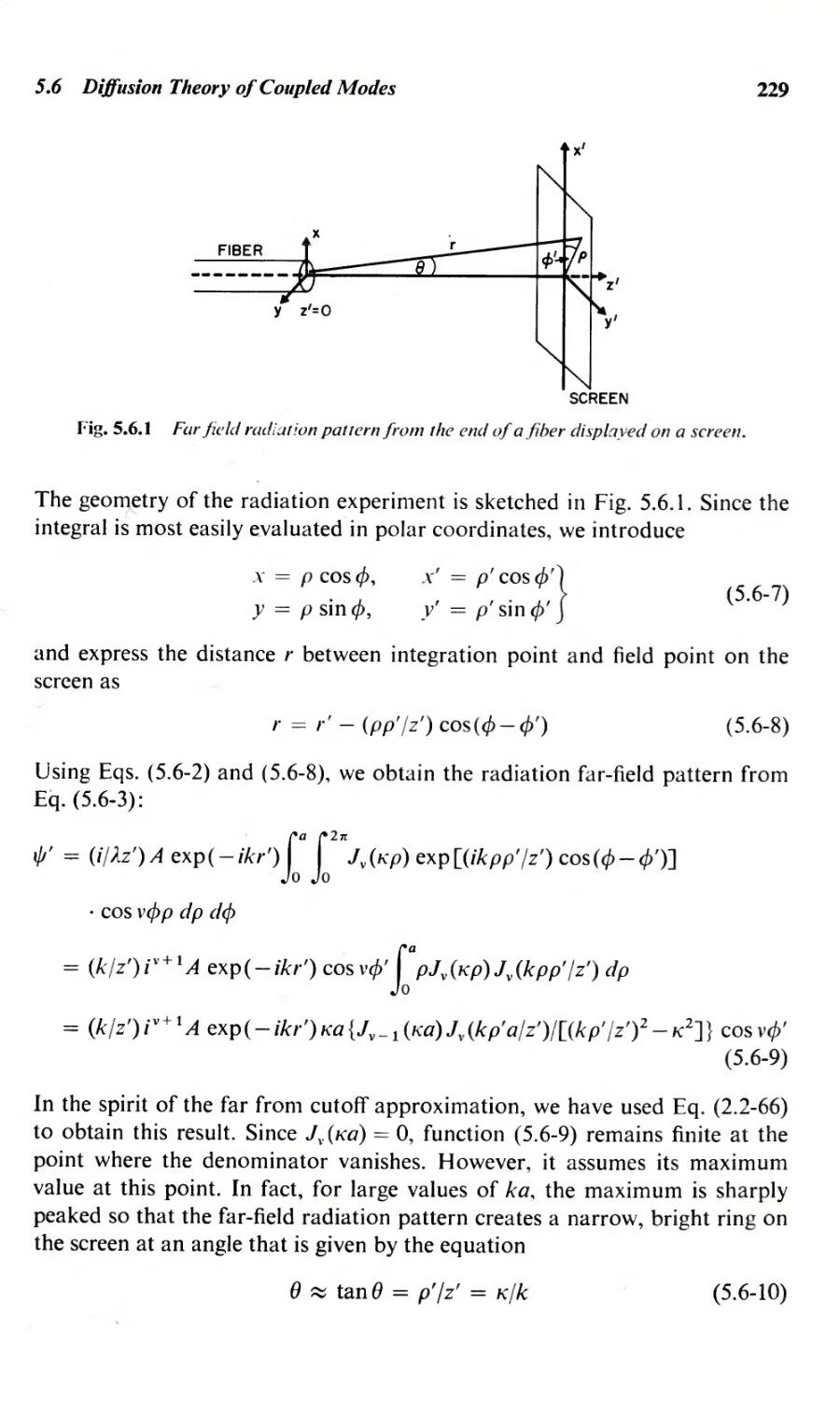
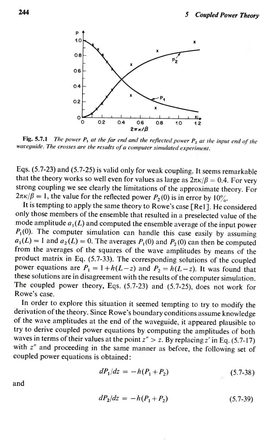
/


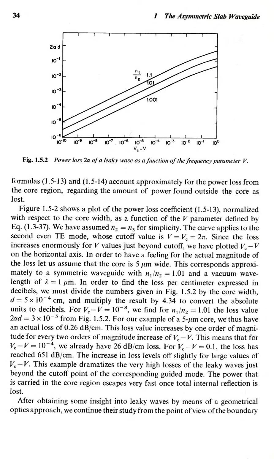
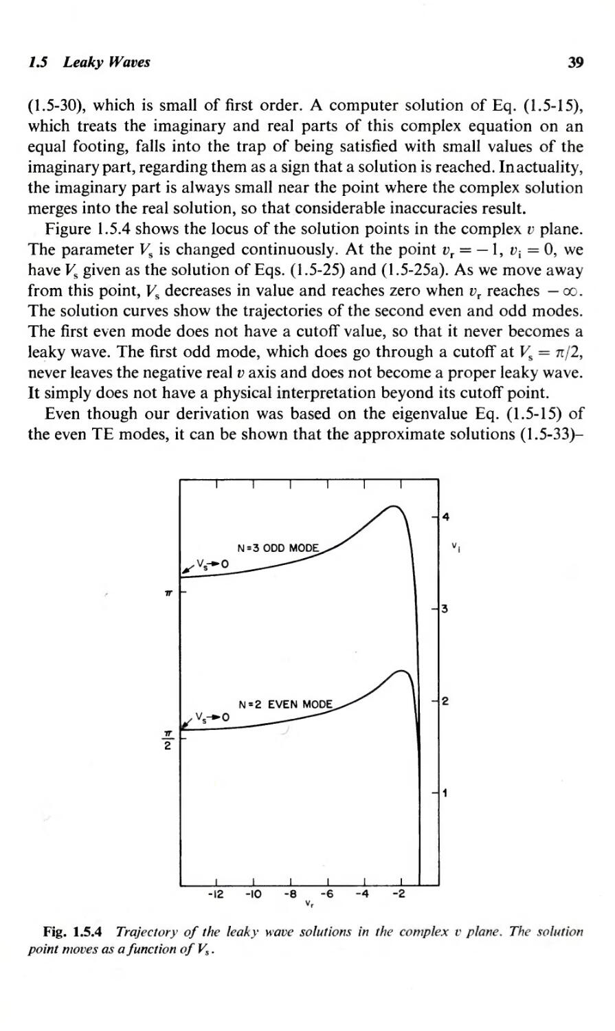
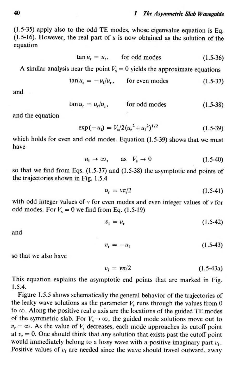


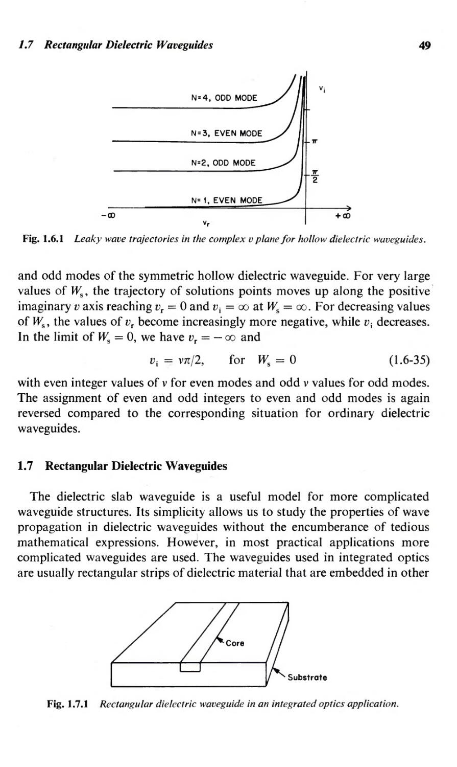


Text
.:J \ :... .\G.;b 4.1 IS"
0.. ..7.8.g.t..ylS" .;;..; .)u
Theory of
Dielectric Optical Waveguides
DIETRICH MARCUSE
Bell Laboratories
Crawford Hill Laboratory
Holmdel, New Jersey
ACADEMIC PRESS New York San Francisco London 1974
A Subsidiary of Harcourt Brace Jovanovich, Publishers
: \
COPYRIGHT CD 1974, BY BELL TELEPHONE LABORATORIES, INCORPORATED
ALL RIGHTS RESERVED.
NO PART OF THIS PUBLICATION MAY BE REPRODUCED OR
TRANSMITTED IN ANY FORM OR BY ANY MEANS, ELECTRONIC
OR MECHANICAL, INCLUDING PHOTOCOPY, RECORDING, OR ANY
INFORMATION STORAGE AND RETRIEVAL SYSTEM, WITHOUT
PERMISSION IN WRITING FROM THE PUBLISHER.
ACADEMIC PRESS, INC. _
111 Fifth Avenue, New York, New York 10003
.
,
United Kingdom Edition pub/" " .
ACADEMIC PRESS, INC.
24/28 Oval Road, L( mdon NWI
""
..
LTD.
0-
Marcuse, Dietrich, I;urt", . .J
Theory of dielectric optical waveguides.} 1), .e.
). ""IM,:>r urn electronics-principles and applications)
..
ibli?gra'Z.hy: p. c{ ? - .lj 0
(. 1 . -y.... Fiber optics. 2. Optical waveguides.
3. Dielectrics. I. Title.
QC448.M37 535'.89 73-21718
ISBN 0-12-470950-8
I h,
Jo..
#0- --
I Ir
'-.
PRINTED IN TIlE UNITED STATES OF AMERICA
Contents
PREFACE
.
IX
Chapter 1.
The Asymmetric Slab Waveguide
1.1 Introduction
1.2 Geometrical Optics Treatment of Slab Waveguides
1.3 Guided Modes of the Asymmetric Slab Waveguide
1.4 Radiation Modes of the Asymmetric Slab Waveguide
1.5 Leaky Waves
1.6 Hollow Dielectric Waveguides
1.7 Rectangular Dielectric Waveguides
1
3
7
19
31
43
49
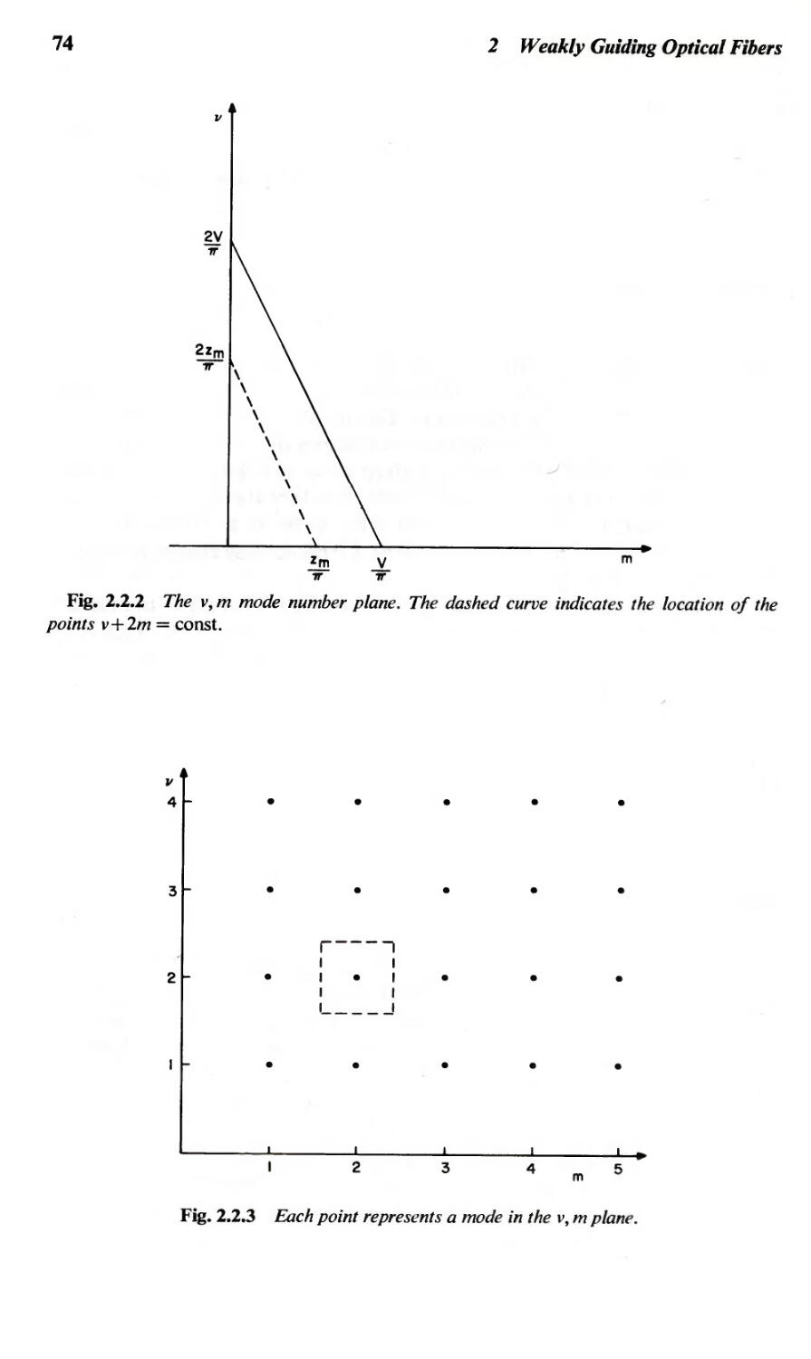
Chapter 2. Weakly Guiding Optical Fibers
2.1 Introduction
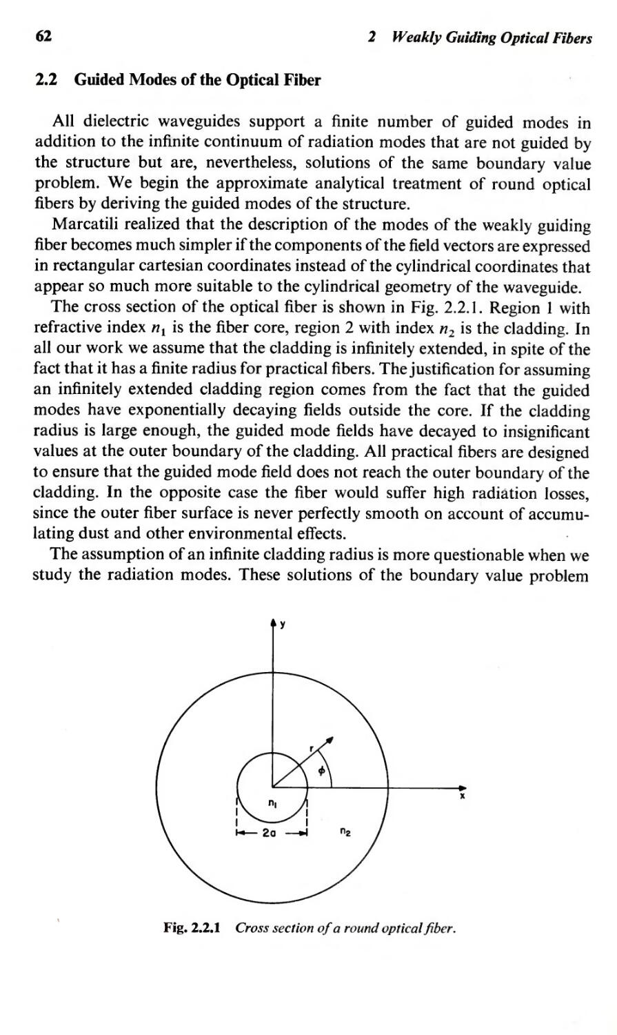
2.2 Guided Modes of the Optical Fiber
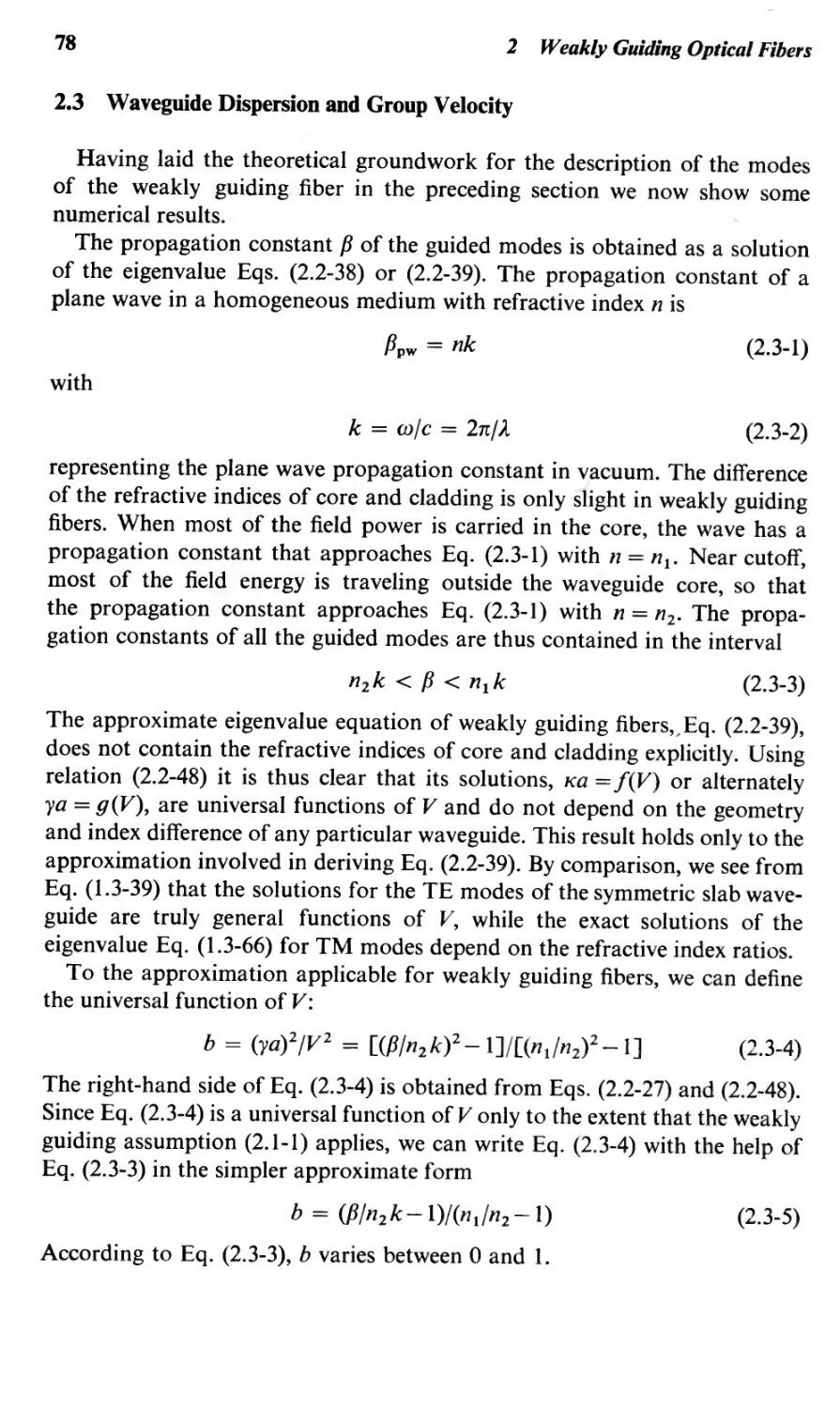
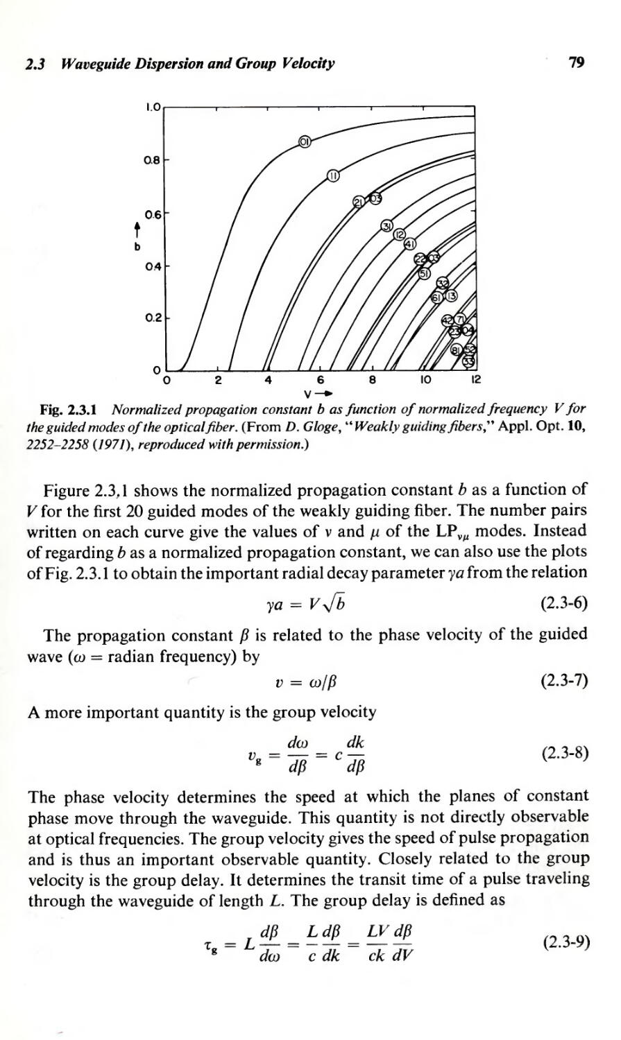
2.3 Waveguide Dispersion and Group Velocity
2.4 Radiation Modes of the Optical Fiber
2.5 Cutoff and Total Internal Reflection
60
62
78
83
89
..
vu
viii Contents
Chapter 3. Coupled Mode Theory
3.1 Introduction
3.2 Expansion in Terms of Ideal Modes
3.3 Expansion in Terms of Local Normal Modes
3.4 Perturbation Solution of the Coupled Amplitude Equations
3.5 Coupling Coefficients for the Asymmetric Slab Waveguide
3.6 Coupling Coefficients for the Optical Fiber
95
98
106
111
116
126
Chapter 4. Applications of the Coupled Mode Theory
4.1 Introduction
4.2 Slab Waveguide with Sinusoidal Deformation
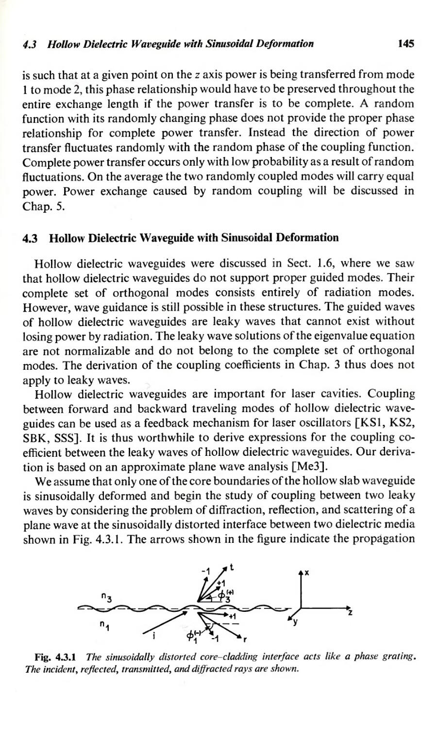
4.3 Hollow Dielectric Waveguide with Sinusoidal Deformation
4.4 Fiber with Sinusoidal Diameter Changes
4.5 Change of Polarization
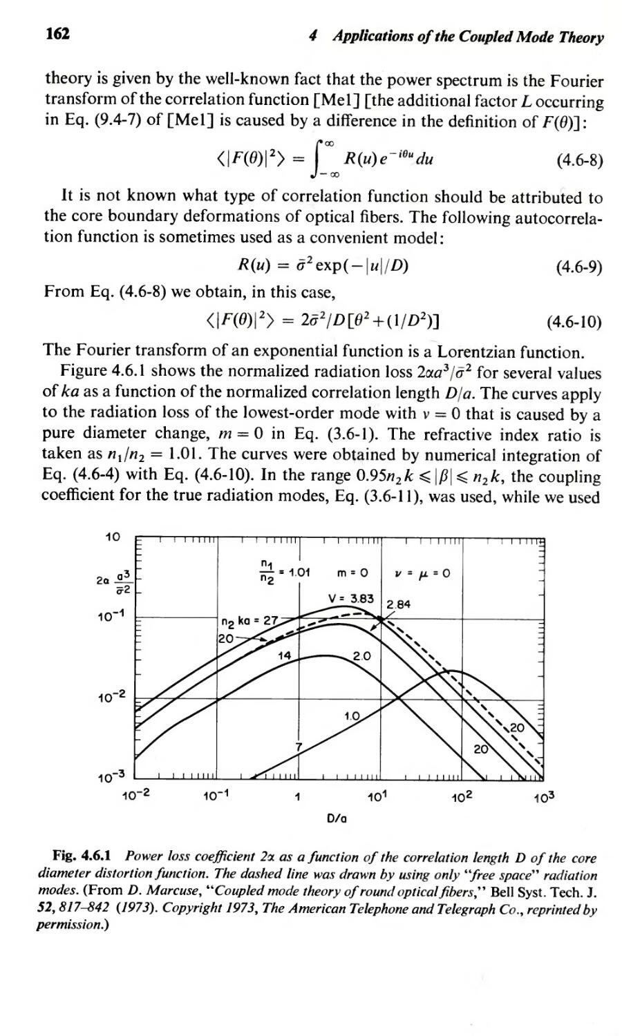
4.6 Fiber with More General Interface Deformations
4.7 Rayleigh Scattering
132
133
145
153
157
160
167
Chapter 5. Coupled Power Theory
5.1 Introduction
5.2 Derivation of Coupled Power Equations
5.3 cw Operation of Multimode Waveguides
5.4 Po\\'er Fluctuations
5.5 Pulse Propagation in Multimode Waveguides
5.6 Diffusion Theory of Coupled Modes
5.7 Power Coupling between Waves Traveling in Opposite Directions
173
175
181
193
201
227
237
References
247
INDEX
251
Preface
The history of communications technology has seen a steady increase of
the carrier frequency used for the transmission of information. With the
invention of the laser this steady climb made a huge jump from millimeter
wavelength to the optical frequency range-an increase by three to four
orders of magnitude.
However, the source of coherent light energy is only one of several steps
that lead to a workable communications system. The next step is the search
for a suitable transmission medium. The early stages of this search were
dominated by attempts to utilize lens systems and mirrors to build light
waveguides. Of the several problems that arise with such waveguides the cost
factor appears at present the most serious detriment for the actual use of lens
waveguides in optical communications systems.
When I wrote my book "Light Transmission Optics," lens waveguides were
still competing successfully with other types of optical waveguides. The glass
fiber guide was just beginning to appear as a serious competitor, but its high
losses made it appear as though its prospects of winning out over the lens
waveguide were not too bright.
Four years have passed since the "Light Transmission Optics" manuscript
was wri tten. During this time a revolution has taken place. The losses of
.
IX
x
Preface
optical glass fibers have been reduced so much (they are presently well below
10 dB/km) that the advantages of the optical fiber for communications
purposes far outweigh all its competitors. The interest of communications
engineers has consequently turned almost exclusively to optical fibers. Much
ne\v knowledge has been accumulated so that a book exclusively devoted to
the theory of dielectric optical waveguides has become necessary.
A second reason for concentrating exclusively on dielectric optical wave-
guides is the rapid growth of integrated optics. This new field is devoted to
the development of microscopic optical circuits based on thin film technology.
The dielectric waveguides used in integrated optics are asymmetric slabs
which have not previously been covered in textbooks. I am presenting the
theory of light transmission through asymmetric slab waveguides from the
point of view of geometrical as well as wave optics. The guided and radiation
modes are derived and leaky waves and an inverted slab waveguide-the
hollow dielectric waveguide which supports only leaky waves-are discussed.
Since 'Light Transmission Optics" was written, a simplified analytical
treatment of round optical fibers has been developed by Snyder and Gloge.
The complexity of the theory of round fibers forced me to limit the discussion
in "Light Transmission Optics" to the description of its guided modes. The
radiation modes and mode conversion and radiation phenomena of this
important structure could only be discussed with the help of the analogy to
the slab waveguide. The new technique of approximating the description of
the round optical fiber is based on the fact that all practical fibers are made
with core and cladding materials whose refractive indices are very nearly
identical. The approximate theory enables us to treat radiation and mode
conversion phenomena of slightly imperfect optical fibers.
Optical communications systems using lasers will probably use single-mode
fibers as light transmission media. However, cheaper and simpler systems are
likely to use luminescent diodes instead of lasers making it necessary to
employ multimode fibers for efficient transmission of light power. Multimode
dielectric optical waveguides have many interesting properties that can be
understood with the help of coupled mode theory. Chapter 3 develops two
approaches to the coupled mode theory. An expansion of the electromagnetic
field in terms of modes of the ideal waveguide as well as the use of local
normal modes are discussed. Both approaches have advantages for certain
applications. The theory of Chapters 1 and 2 is used to derive coupling
coefficients for core-cladding boundary irregularities of the asymmetric slab
waveguide and the round optical fiber.
Chapter 4 presents applications of the coupled mode theory. The radiation
losses of asymmetric slab waveguides and optical fibers caused by core-
cladding boundary imperfections are treated. This chapter also contains a
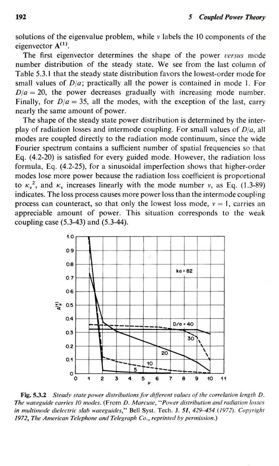
description of a useful approximate method for deriving coupling coefficients
Preface
.
XI
for the usual and the hollow dielectric slab waveguides. The coupled mode
theory is finally applied to the problem of Rayleigh scattering by random
fluctuations of the refractive index.
The problem of the distribution of power over the many possible guided
modes of the multimode waveguide and the effect of mode coupling on pulse
transmission are the subject of the last chapter. We begin with a derivation
of coupled equations for the average power carried by each mode. This
coupled power theory is essential for an understanding of multimode wave-
guides with mode coupling since the complexity of this problem precl udes
its treatment by means of the theory of coupled mode amplitudes. However,
the results of the coupled mode theory are necessary for the derivation of
coupled power equations. We treat coupled power equations for forward and
backward modes, discuss the problem of power distribution versus mode
number, and study pulse propagation. A very useful approximate diffusion
theory of multimode power coupling is presented as an example of analytical
methods for solving the coupled power equations.
The present book contains up to date information necessary for an under-
standing of single as well as multimode optical fibers and the waveguides of
integrated optics. This material is essential for the engineer engaged in the
development of optical communications systems. This book should also be
useful for classroom instruction in universities since the ever increasing
importance of light communications will certainly require its coverage in
engineering colleges.
I would like to thank Mrs. Ann Flemer who supervised the various stages
of typing and reproduction of the manuscript. Many thanks are also due
Mrs. Elizabeth Goldsmith who typed most of the manuscript.
I
The Asymmetric Slab Waveguide
1.1 Introduction
Dielectric slal?s are the simplest optical waveguides. Because of their simple
geometry, guided and radiation modes of slab waveguides can be described
by simple mathematical expressions. The study of slab waveguides and their
properties is thus often useful in gaining an understanding of the wave-
guiding properties of more complicated dielectric waveguides. However,
slab waveguides are not only useful as models for more general types of optical
waveguides, but they are actually employed for light guidance in "integrated
optics circuits [Mr 1, Mr3].
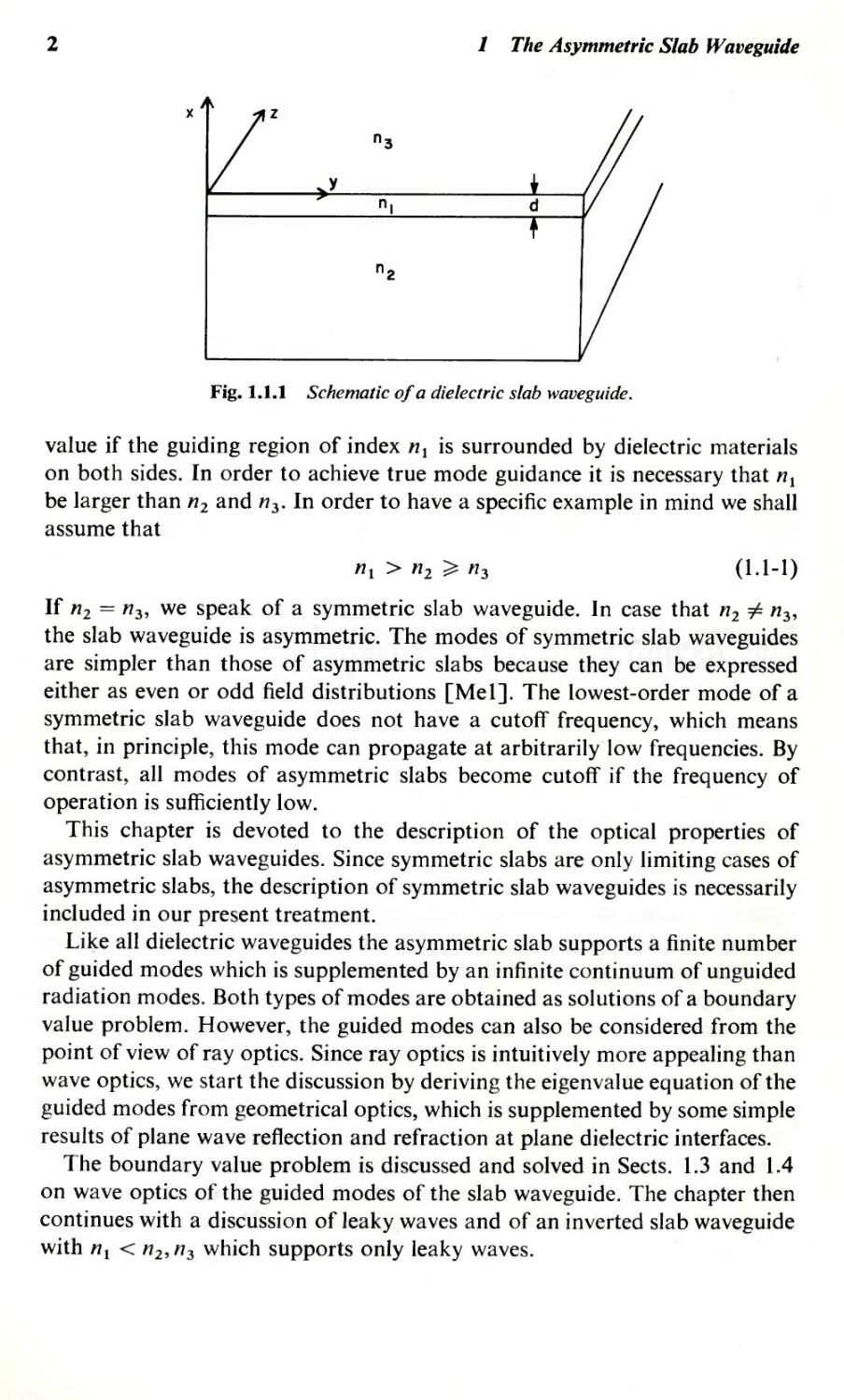
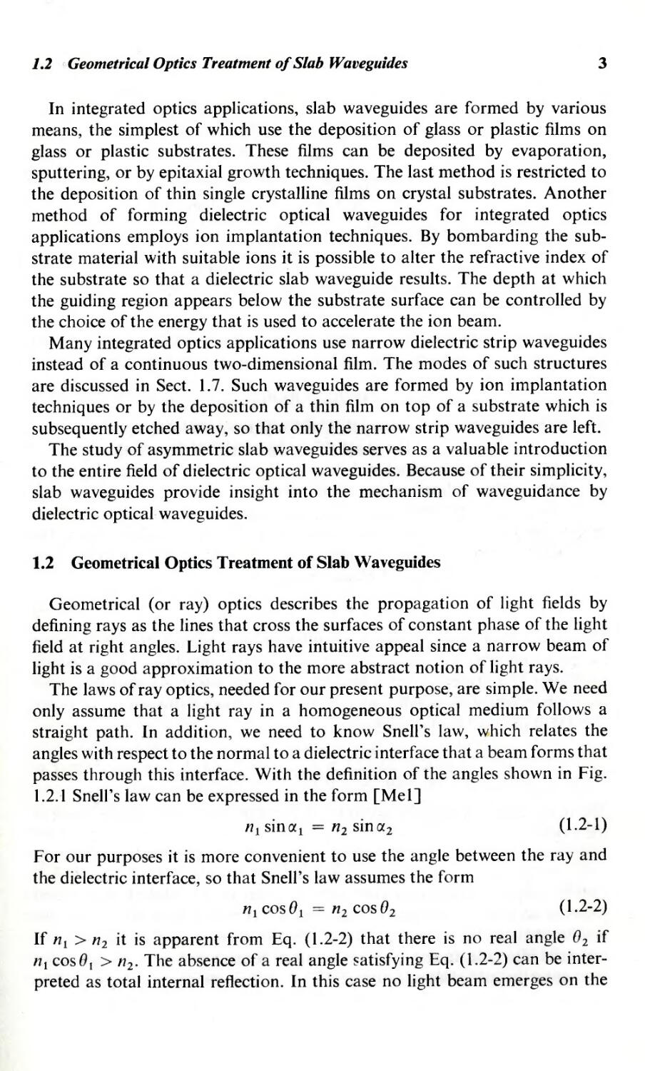
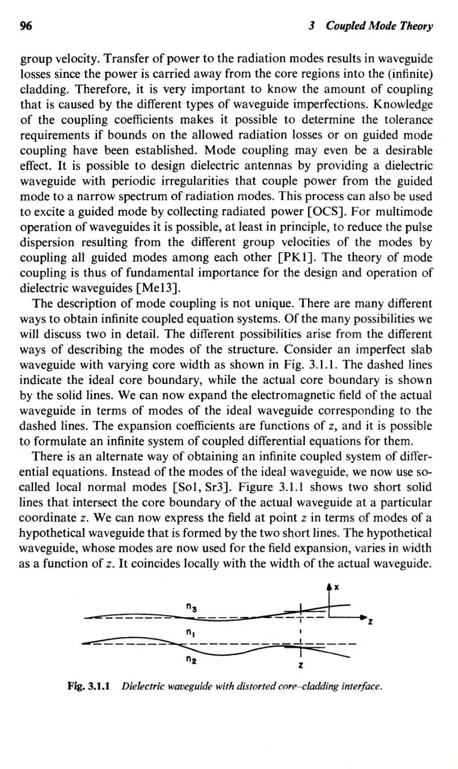
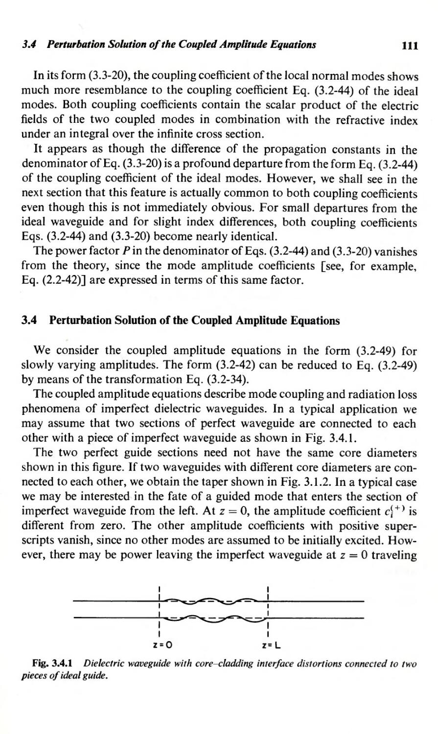
A dielectric slab waveguide is shown schematically in Fig. 1.1.1. The figure
shows a slab waveguide as it would be used in a typical integrated optics
application. The core region of the waveguide is assumed to have refractive
index nl and is deposited on a substrate with refractive index n2. The refractive
index of the medium above the core is indicated as n3. The refractive index n3
may be unity if the region above the core is air, or it may have some other
1
2
1 The Asymmetric Slab Waveguide
x
z
"I
"3
y
"2
Fig. 1.1.1 Schenlatic of a dielectric slab waveguide.
value if the guiding region of index n 1 is surrounded by dielectric materials
on both sides. In order to achieve true mode guidance it is necessary that n 1
be larger than n 2 and n3. In order to have a specific example in mind we shall
assume that
n 1 > n2 n3
(1.1-1)
If n2 = n 3 , we speak of a symmetric slab waveguide. In case that n 2 1= n 3 ,
the slab waveguide is asymmetric. The modes of symmetric slab waveguides
are simpler than those of asymmetric slabs because they can be expressed
either as even or odd field distributions [Mel]. The lowest-order mode of a
symmetric slab waveguide does not have a cutoff frequency, which means
that, in principle, this mode can propagate at arbitrarily low frequencies. By
contrast, all modes of asymmetric slabs become cutoff if the frequency of
operation is sufficiently low.
This chapter is devoted to the description of the optical properties of
asymmetric slab waveguides. Since symmetric slabs are only limiting cases of
asymmetric slabs, the description of symmetric slab waveguides is necessarily
included in our present treatment.
Like all dielectric waveguides the asymmetric slab supports a finite number
of guided modes which is supplemented by an infinite continuum of unguided
radiation modes. Both types of modes are obtained as solutions of a boundary
value problem. However, the guided modes can also be considered from the
point of view of ray optics. Since ray optics is intuitively more appealing than
wave optics, we start the discussion by deriving the eigenvalue equation of the
guided modes from geometrical optics, which is supplemented by some simple
results of plane wave reflection and refraction at plane dielectric interfaces.
The boundary value problem is discussed and solved in Sects. 1.3 and 1.4
on wave optics of the guided modes of the slab waveguide. The chapter then
continues with a discussion of leaky waves and of an inverted slab waveguide
with n 1 < n 2 , n 3 which supports only leaky waves.
1.2 Geometrical Optics Treatment of Slab Waveguides
3
In integrated optics applications, slab waveguides are formed by various
means, the simplest of which use the deposition of glass or plastic films on
glass or plastic substrates. These films can be deposited by evaporation,
sputtering, or by epitaxial growth techniques. The last method is restricted to
the deposition of thin single crystalline films on crystal substrates. Another
method of forming dielectric optical waveguides for integrated optics
applications employs ion implantation techniques. By bombarding the sub-
strate material with suitable ions it is possible to alter the refractive index of
the substrate so that a dielectric slab waveguide results. The depth at which
the guiding region appears below the substrate surface can be controlled by
the choice of the energy that is used to accelerate the ion beam.
Many integrated optics applications use narrow dielectric strip waveguides
instead of a continuous two-dimensional film. The modes of such structures
are discussed in Sect. 1.7. Such waveguides are formed by ion implantation
techniques or by the deposition of a thin film on top of a substrate which is
subsequently etched away so that only the narrow strip waveguides are left.
The study of asymmetric slab waveguides serves as a valuable introduction
to the entire field of dielectric optical waveguides. Because of their simplicity,
slab waveguides provide insight into the mechanism of waveguidance by
dielectric optical waveguides.
1.2 Geometrical Optics Treatment of Slab Waveguides
Geometrical (or ray) optics describes the propagation of light fields by
defining rays as the lines that cross the surfaces of constant phase of the light
field at right angles. Light rays have intuitive appeal since a narrow beam of
light is a good approximation to the more abstract notion of light rays.
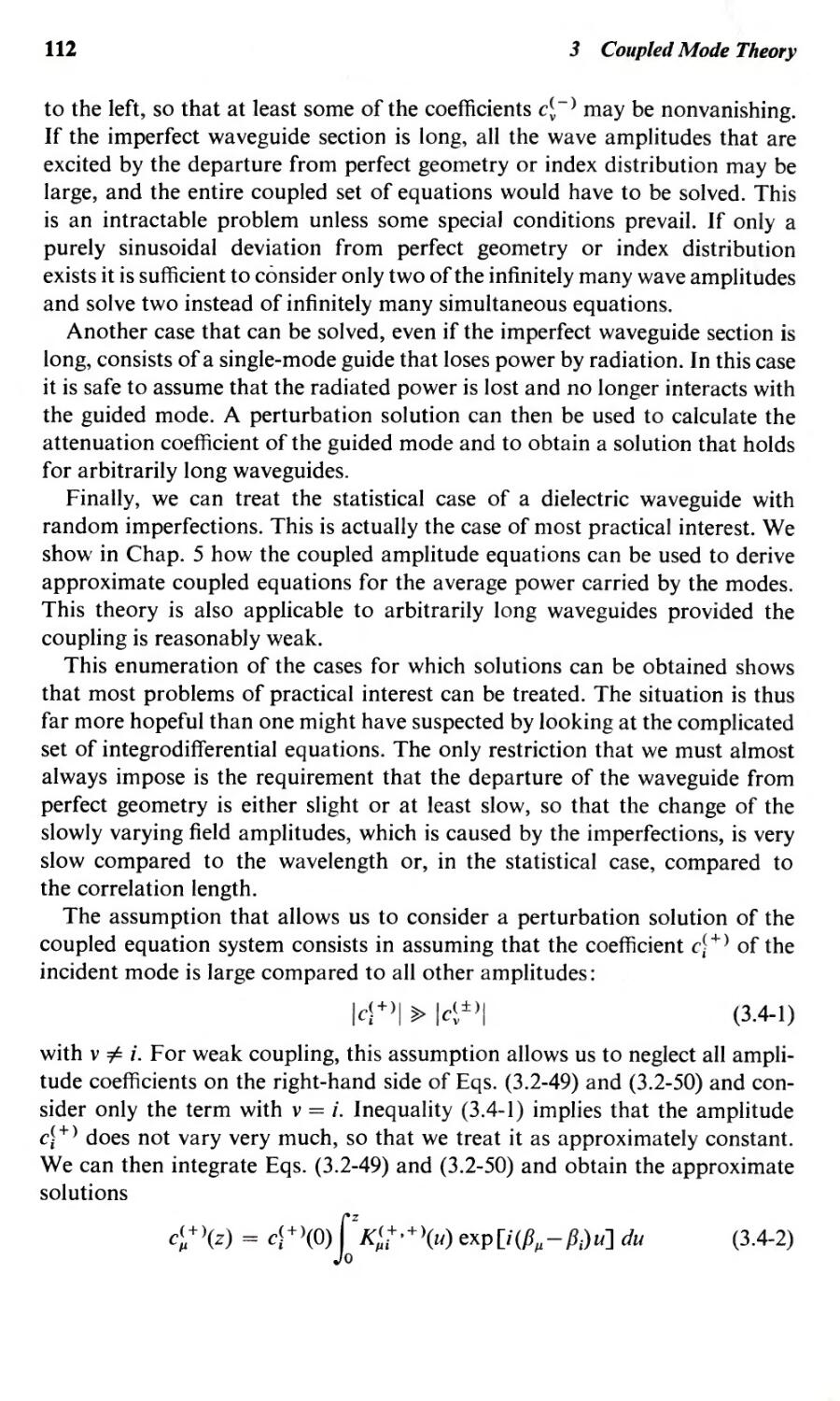
The laws of ray optics, needed for our present purpose, are simple. We need
only assume that a light ray in a homogeneous optical medium follows a
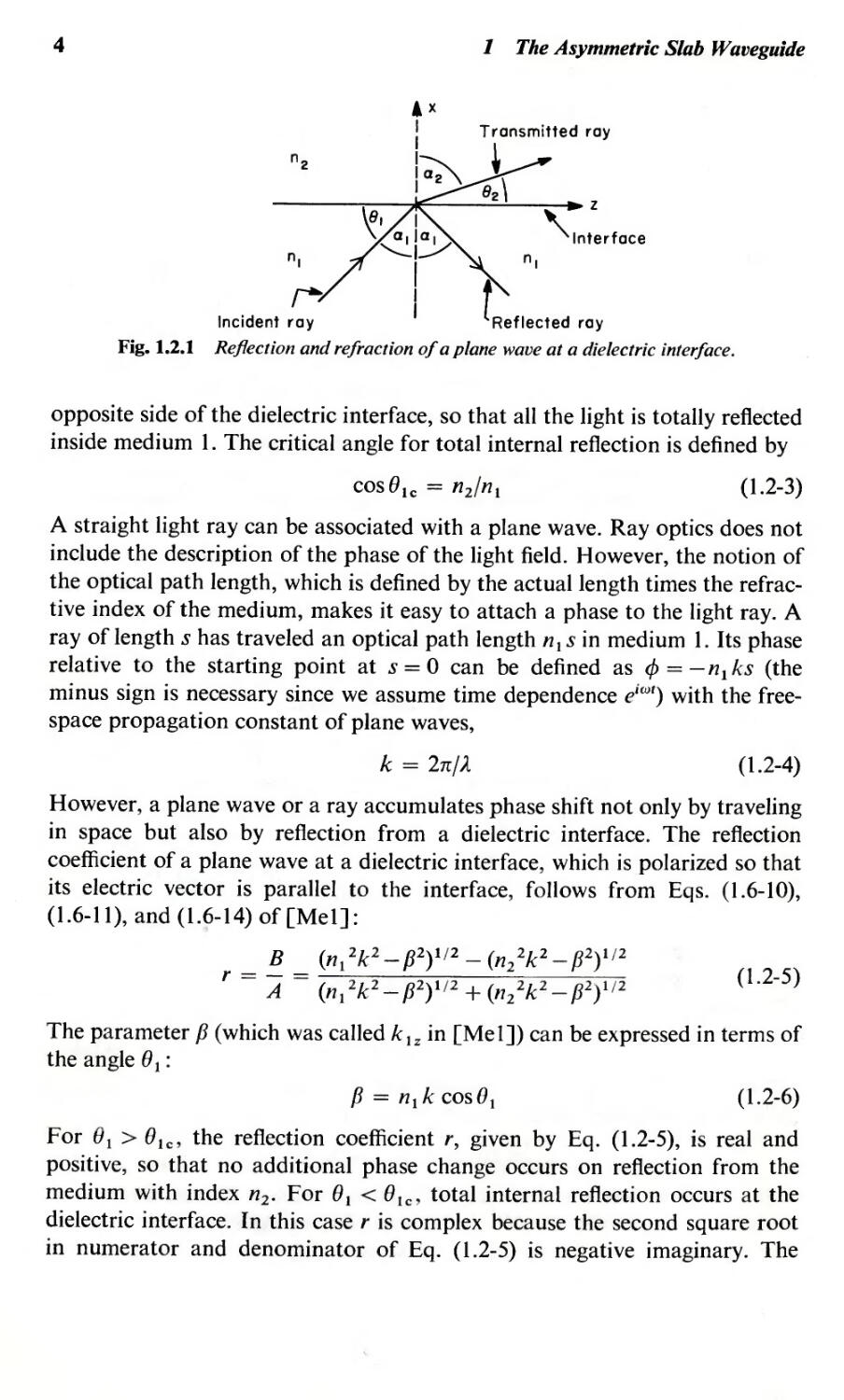
straight path. [n addition, we need to know Snell's law, which relates the
angles with respect to the normal to a dielectric interface that a beam forms that
passes through this interface. With the definition of the angles shown in Fig.
1.2.1 Snell's law can be expressed in the form [Mel]
. .
n 1 sIn CX l = n2 SIn CX2
(1.2-1)
For our purposes it is more convenient to use the angle between the ray and
the dielectric interface, so that Snell's law assumes the form
n l cos 0 1 = nz cos O 2
(1.2-2)
If n l > n2 it is apparent from Eq. (1.2-2) that there is no real angle O 2 if
nl cosO I > n2. The absence of a real angle satisfying Eq. (1.2-2) can be inter-
preted as total internal reflection. In this case no light beam emerges on the
4
1 The Asymmetric Slab Waveguide
"2
z
, Interface
"I
n l
Incident ray tReflected ray
Fig. 1.2.1 Reflection and refraction of a plane wave at a dielectric interface.
opposite side of the dielectric interface, so that all the light is totally reflected
inside medium 1. The critical angle for total internal reflection is defined by
cos OIC = n2/nl
(1.2-3)
A straight light ray can be associated with a plane wave. Ray optics does not
include the description of the phase of the light field. However, the notion of
the optical path length, which is defined by the actual length times the refrac-
tive index of the medium, makes it easy to attach a phase to the light ray. A
ray of length s has traveled an optical path length n 1 s in medium 1. Its phase
relative to the starting point at s = 0 can be defined as l/J = - n 1 ks (the
minus sign is necessary since we assume time dependence e icot ) with the free-
space propagation constant of plane waves,
k = 2n/A
(1.2-4)
However, a plane wave or a ray accumulates phase shift not only by traveling
in space but also by reflection from a dielectric interface. The reflection
coefficient of a plane wave at a dielectric interface, which is polarized so that
its electric vector is parallel to the interface, follows from Eqs. (1.6-10),
(1.6-11), and (1.6-14) of [Me 1]:
B (n 1 2 k 2 - P2)1/2 - (n2 2k2 _ P2)1/2
r = A = (n12k2 _ P2)1/2 + (n/k2 _ P2)1/2 (1.2-5)
The parameter p (which was called k I z in [Me 1]) can be expressed in terms of
the angle 0 1 :
P = n I k cos e I
( 1.2-6)
For 0 I > 0 1 c' the reflection coefficient r, given by Eq. (1.2-5), is real and
positive, so that no additional phase change occurs on reflection from the
medium with index n 2 . For 0 1 < Olc' total internal reflection occurs at the
dielectric interface. In this case r is complex because the second square root
in numerator and denominator of Eq. (1.2-5) is negative imaginary. The
1.2 Geometrical Optics Treatment of Slab Waveguides
5
negative sign is necessary since a decaying instead of a growing wave must
result in medium 2. Under conditions of total internal reflection, a wave that
is polarized with its electric vector parallel to the interface suffers a phase
shift
4> = - 2 arctan [(p2 - n2 2k 2 )1/2 f(nt 2k2 _ P2)1/2]
(1.2-7)
For a wave polarized so that its magnetic vector is parallel to the interface, we
obtain from Eq. (1.6-56) of [Mel] the phase shift
4> = -2 arctan[{n12fn22)(p2-n22k2)1/2f(n12k2-p2)1/2] (1.2-8)
Having collected these few facts from ray optics and the theory of plane
wave reflection at dielectric interfaces enables us to discuss mode guidance in
the slab waveguide and derive the eigenvalue equation for the propagation
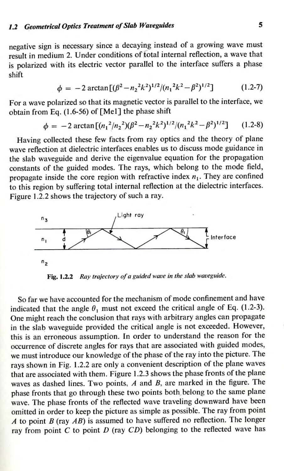
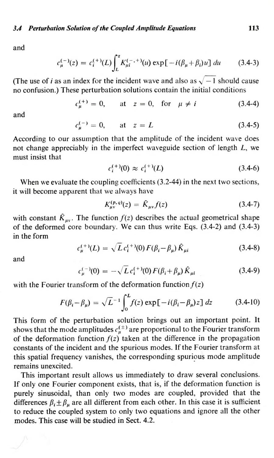
constants of the guided modes. The rays, which belong to the mode field,
propagate inside the core region with refractive index nl. They are confined
to this region by suffering total internal reflection at the dielectric interfaces.
Figure 1.2.2 shows the trajectory of such a ray.
n l
Light ray
..
n 3
Interface
n 2
Fig.l.2.2 Ray trajectory of a guided wave in the slab waveguide.
So far we have accounted for the mechanism of mode confinement and have
indicated that the angle lJ 1 must not exceed the critical angle of Eq. (1.2-3).
One might reach the conclusion that rays with arbitrary angles can propagate
in the sla waveguide provided the critical angle is not exceeded. However,
this is an erroneous assumption. In order to understand the reason for the
occurrence of discrete angles for rays that are associated with guided modes,
we must introduce our knowledge of the phase of the ray into the picture. The
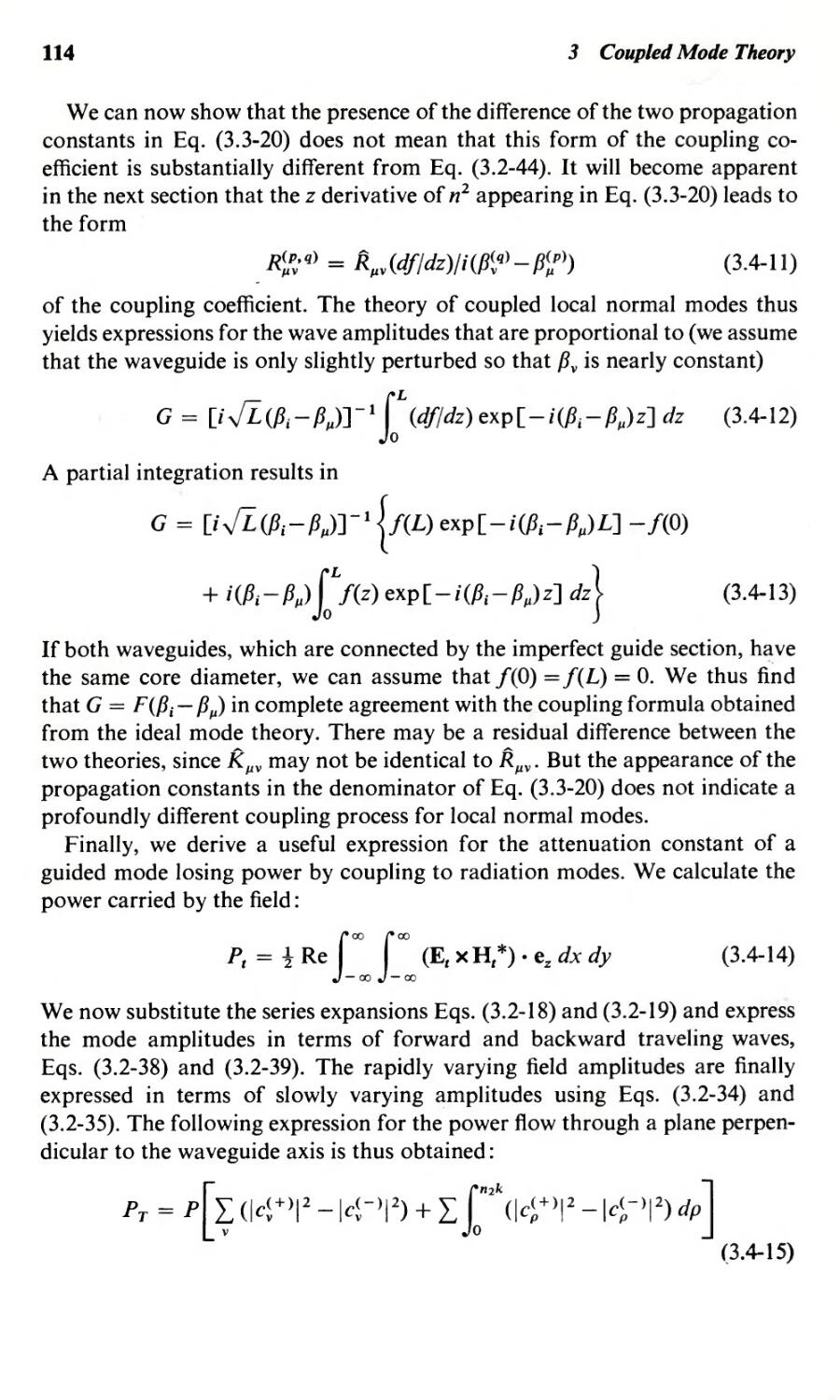
rays shown in Fig. 1.2.2 are only a convenient description of the plane waves
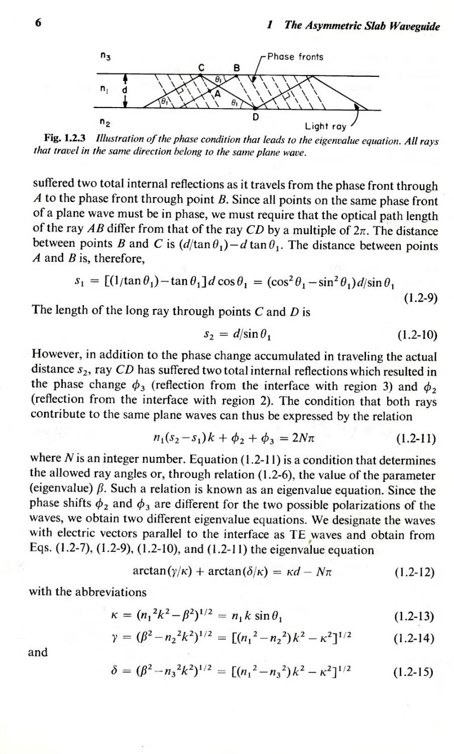
that are associated with them. Figure 1.2.3 shows the phase fronts of the plane
waves as dashed lines. Two points, A and B, are marked in the figure. The
phase fronts that go through these two points both belong to the same plane
wave. The phase fronts of the reflected wave traveling downward have been
omitted in order to keep the picture as simple as possible. The ray from point
A to point B (ray AB) is assumed to have suffered no reflection. The longer
ray from point C to point D (ray CD) belonging to the reflected wave has
6
1 The Asymmetric Slab Waveguide
"3
Phase fronts
"I
"2 Light ray
Fig. 1.2.3 Illustration of the phase condition that leads to the eigenvalue equation. All rays
that travel in the same direction belong to the saIne plane wave.
suffered two total internal reflections as it travels from the phase front through
A to the phase front through point B. Since all points on the same phase front
of a plane wave must be in phase, we must require that the optical path length
of the ray AB differ from that of the ray CD by a multiple of 2IT. The distance
between points Band C is (d/tan () 1) - d tan 0 1 . The distance between points
A and B is, therefore,
SI = [(ljtan0 1 )-tan0 1 ]d cosO. = (COS 2 0 1 -sin 2 ( 1 )d/sinO t
The length of the long ray through points C and D is
S2 = dfsin 0 1
(1.2-9)
(1.2-10)
However, in addition to the phase change accumulated in traveling the actual
distance S2, ray CD has suffered two total internal reflections which resulted in
the phase change 413 (reflection from the interface with region 3) and 412
(reflection from the interface with region 2). The condition that both rays
contribute to the same plane waves can thus be expressed by the relation
n 1 (S 2 - s .) k + 41 2 + 413 = 2N n
( 1.2-11 )
where N is an integer number. Equation (1.2-11) is a condition that determines
the allowed ray angles or, through relation (1.2-6), the value of the parameter
(eigenvalue) p. Such a relation is known as an eigenvalue equation. Since the
phase shifts 412 and 413 are different for the two possible polarizations of the
waves, we obtain two different eigenvalue equations. We designate the waves
with electric vectors parallel to the interface as TE waves and obtain from
Eqs. (1.2-7), (1.2-9), (1.2-10), and (1.2-11) the eigenvalue equation
arctan(Y/K) + arctan(c5fK) = Kd - NIT (1.2-12)
with the abbreviations
K = (n 1 2 k 2 - P2)1/2 = n 1 k sin 0 1
y = (P2 _ n 2 2 k 2 ) 1/2 = [( n 1 2 - n 2 2) k 2 _ K2] 1/2
( 1.2-13)
(1.2-]4)
and
c5 = (P2 - n3 2k 2 )1/2 = [en 1 2 - n 3 2) k 2 _ K2] 1/2
(1.2-15)
1.3 Guided Modes of the Asymmetric Slab Waveguide
\ v,';
7
Taking the tangent of Eq. (1.2-12) transforms the eigenvalue equation for the
TE waves into the form
tanKd = K(y+t5)/(K 2 -yt5)
(1.2-]6)
The corresponding procedure for TM waves results in the eigenvalue equation
tanKd = n121(,2(n32y+n22t5)/(n22n321(,2-ni4yt5)
(1.2-17)
We shall rederive these equations again in the next section by starting from
Maxwell's equations and using the boundary conditions at the dielectric
interfaces. The purpose of the present discussion was to give an intuitive
explanation for the process of mode guidance in slab waveguides and to demon-
strate how the mode conditions (1.2-16) and (1.2-17) can be obtained
,
with the help of simple principles obtained from ray optics and from the
properties of plane waves [Til].
1.3 Guided Modes of the Asymmetric Slab Waveguide
In order to obtain a complete description of the modes of dielectric wave-
guides, Maxwell's equations must be solved [MKl, NMI]. With the help
of the operator (ex' e y , and e z are unit vectors in x,y,z direction)
a a a
V=e-+e-+e-
x ax y ay z az
Maxwell's equations can be written in the form
V x H = f..on2 aE/at
(1.3-1)
(1.3-2)
and
v x E = -/10 aH/at
(1.3-3)
The cross indicates a vector product, Hand E are the magnetic and electric
field vectors, and f..o and /10 are the dielectric permittivity and magnetic
permeability of vacuum. We do not consider magnetic materials in this book
so that the use of the vacuum constant /10 is sufficient. The index of refraction
of the medium is designated by n, and t is the time variable.
We simplify the description of the slab waveguide by assuming that there is
no variation in y direction, which we express symbolically by the equation
a/ay = 0
( 1.3-4)
Condition (1.3-4) is actually no restriction on the generality of the mode
description since it is always possible to rotate the coordinate system in the
yz plane until this condition is satisfied for any given mode. The modes of the
slab waveguide can be classified as TE and TM modes. TE or transverse
8
1 The Asymmetric Slab Waveguide
electric modes do not have a component of the electric field in the direction
of wave propagation, while TM or transverse magnetic modes do not have a
longitudinal magnetic field component. We consider TE and TM modes
separately. The fields of guided modes must vanish at x = + 00.
Guided TE Modes
TE modes have only three field components: Ey, Hx, and Hz. The position
of the coordinate system relative to the slab is shown in Fig. 1.1.1. We assume
that the slab is infinitely extended in the yz plane. We consider only strictly
time harmonic fields whose time dependence, in complex notation, can be
expressed as
e iwt
(1.3-5)
The radian frequency w is related to the actual frequency fby
w = 2nf
(1.3-6)
Since we are interested in obtaining the normal modes of the slab waveguide
we assume that the z dependence of the mode fields is given by the function
-ipz
e
(1.3-7)
By combining the two factors (1.3-5) and (1.3-7) we obtain
ei(wt-Pz)
(1.3-8)
Function (1.3-8) describes a wave traveling in positive z direction with phase
velocity
v = w/P
(1.3-9)
The eigenvalue P is identical to the quantity introduced in Eq. (1.2-6). Factor
(1.3-8) is common to aU field quantities and shall be omitted for brevity. With
Ex = 0, Ez = 0, and By = 0, we obtain from Maxwell's Eqs. (1.3-2), (1.3-3)
with the help of Eq. (1.3-4), and with the time and z dependence given by Eq.
(1.3-8),
- iPHx - (oHz/ox) = iWf"on 2 Ey
iPEy = - iWJlo Hx
oEyjox = -iwJloHz
We thus obtain the H components in terms of the Ey component
Hx = (- i/wJlo) oEy/oz = - (P/WJlo) Ey
(1.3-10)
( 1.3-11 )
(1.3-12)
(1.3-13)
and
Hz = (i/wJlo) oEy/ox
(1.3-14)
1.3 Guided Modes of the Asymmetric Slab Waveguide
9
Substitution of these two equations into Eq. (1.3-10) yields the one-dimensional
reduced wave equation for the Ey component
(o2Ey/ox 2 ) + (n 2 k 2 - P2) Ey = 0 (1.3-15)
with k 2 = W 2 f"oJlo = (2n/A)2. The problem of finding the TE modes of the
slab waveguide has thus become very simple. We only need to find solutions
of the one-dimensional reduced wave Eq. (1.3-15) and obtain the magnetic
field components directly from Eqs. (1.3-13) and (1.3-14). The only remaining
complication is the requirement that the solutions must satisfy the boundary
conditions at the two dielectric interfaces at x = 0 and x = - d. The boundary
conditions require that the tangential E and H fields be continuous at the di-
electric discontinuities. We thus must require that,E y and Hz are continuous
at x = 0 and x = - d. Solutions that satisfy the?e conditions for the Ey
component and vanish at x = + 00 are
E = Ae-"x
y ,
for x O
for o x -d
for x -d
= A cos KX + B sin KX,
= (A cos Kd- B sin Kd)ey(x+d>,
( 1.3-16)
(1.3-17)
(1.3-18)
The refractive index n in Eq. (1.3-15) assumes the value n 3 in region 3 (see
Fig. 1.1.1), for x > 0; n 1 in region 1, for 0 > x > -d; and n2 in region 2, for
x < - d. The parameters K, y, and b are defined by Eqs. (1.2-13)-(1.2-15).
The Ey component shown by these three equations satisfies the reduced wave
Eq. (1.3-15) and is continuous at the two dielectric interfaces. We do not need
the Hx component for the moment. The Hz component is obtained from Eq.
(1.3-14):
. Hz = (- ib/wJlo) Ae-"x,
= (- iK/WJlo) (A sin KX - B cos KX),
for x 0
(1..3-19)
for 0 x -d
(1.3-20)
for x -d (1.3-21)
= (iy/w/lo) (A cos Kd- B sin Kd)ey(x+d>,
The Hz component does not immediately satisfy the boundary conditions.
The requirement of continuity of Hz at x = 0 and x = -d leads to the
following system of equations:
bA + KB = 0
(K sinKd-y cos Kd)A + (K cosKd+y sinKd)B = 0
(1.3-22)
(1.3-23)
This homogeneous equation system has a solution only if the system deter-
minant vanishes. We thus obtain the determinantal or eigenvalue equation
b(K cos Kd+y sin Kd) - K(K sinKd-y cos Kd) = 0
(1.3-24)
10
1 The Asymmetric Slab Waveguide
From Eq. (1.3-22) we obtain
BfA = -fJfK
(1.3-25)
The eigenvalue equation can be written in a different form:
tan Kd = K (y + fJ)f( K 2 - yfJ)
(1.3-26)
We have thus rederived the eigenvalue Eq. (1.2-16) by the precise n1ethods of
this section. The agreement of Eq. (1.3-26) with Eq. (1.2-16) justifies the
heuristic method that was used in the previous section.
For future use it is convenient to express the eigenvalue equation in two
alternate forms:
cosKd = + (K2_yfJ)f[(K2+y2)(K2+fJ2)]1/2
(1.3-27)
and
sin Kd = + K(Y + fJ)f[(K 2 + y2) (K 2 + fJ2)] 1/2
(1.3-28)
The sign of the square root must be the same in both equations. The eigen-
value equation determines the allowed values of the propagation constant p
that enters Eq. (1.3-26), (1.3-27), or (1.3-28) through Eqs. (1.2-13)-(1.2-15).
Equation (1.2-6) defines for each guided n10de a mode angle, which is the
direction of the ray or plane wave that travels inside the core region of the
waveguide with refractive index nl.
The field treatment of the guided wave problem also provides the justifica-
tion for the assumption used in the preceding section that the field inside the
core can be regarded as a superposition of two plane waves. Expression
(1.3-17) for the Ey component of the field in the core consists of sine and cosine
functions. Each of these functions can be decomposed into exponential
functions of the form exp( + iKX). If we reinstate the omitted factor (1.3-8), we
see that the field in the core is formed by the superposition of plane waves of
the form
expi(wt + Kx-f3Z) = expi(wt-K. r)
The propagation vector K can be expressed as
K = + Ke x + Oe y + pe z
(1.3-29)
(1.3-30)
with ex, e y , and e z indicating unit vectors in x, y, and z directions. The vector
r points from the coordinate origin to the point at which the field is being
considered:
r = xe x + ye y + ze z
According to Eq. (1.2-13) we have
K 2 = K 2 + p2 = n12k2
(1.3- 31 )
( 1.3-32)
1.3 Guided Modes of the Asymmetric Slab Waveguide
11
with K indicating the magnitude of the vector K. This discussion makes it
clear that the eigenvalue p-the propagation constant of the guided slab
waveguide modes-is the z component of the propagation vector of plane
waves traveling in the core. Because of condition (1.1-1) the parameter y of
Eq. (1.2-14) becomes imaginary as p becomes larger than n2k. At the point
p = n2 k
(1.3-33)
we have
y=o
(1.3-34)
We see from the field expression (1.3-18) that the field extends undiminished
to infinite distances below the waveguide core, if y = O. When y becomes
imaginary the evanescent field in the substrate region turns into a radiation
field, and the wave is no longer guided by the dielectric waveguide. We say
that the wave reaches its cutoff point or simply that the wave is cutoff when
Eq. (1.3-34) or (1.3-33) is reached. The cutoff condition (1.3-33) can easily
be shown to be identical to the condition for the loss of total internal reflection
from the dielectric interface at x = - d. By eliminating p from Eqs. (1.2-6) and
(1.3-33) we obtain the condition for the critical angle, Eq. (1.2-3). This proves
that cutoff is identical with the loss of total internal reflection. However, this
statement is true only for the slab waveguide and does not necessarily hold for
the round optical fiber to be discussed later.
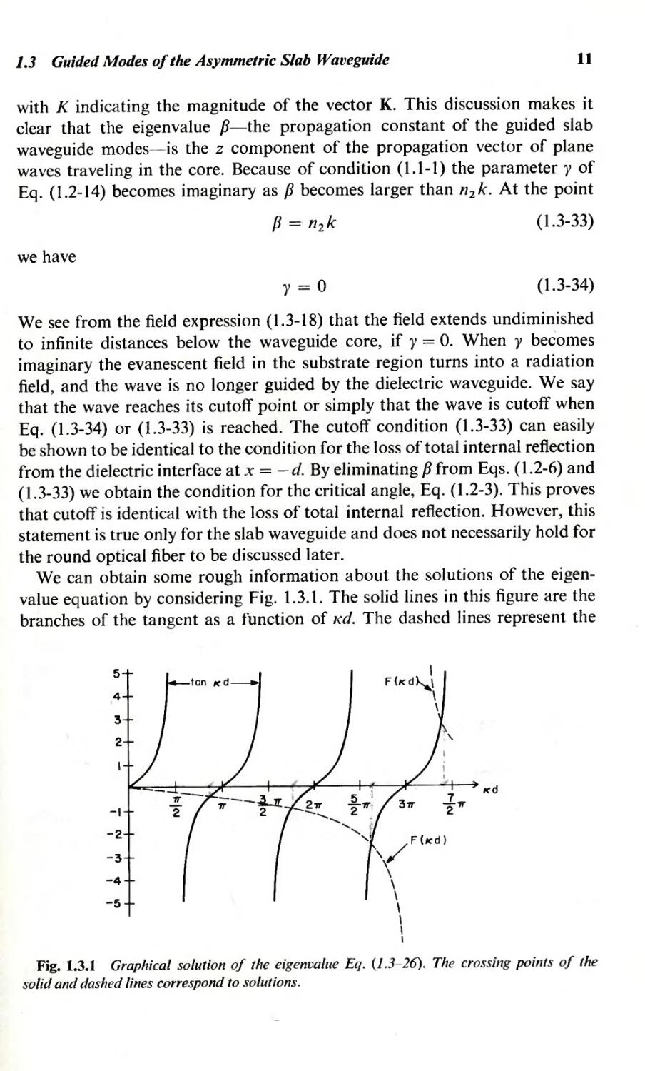
We can obtain some rough information about the solutions of the eigen-
value equation by considering Fig. 1.3.1. The solid lines in this figure are the
branches of the tangent as a function of Kd. The dashed lines represent the
5
4
3
2
,
F (I(' d ,\
\
\
led
-I
-2
-3
-4
-5
_21T
-""'-
........
........
'"
" ,/FIKd)
\
\
\
\
\
\
I
Fig. 1.3.1 Graphical solution of the eigenvalue Eq. (1.3-26). The crossing points of the
solid and dashed lines correspond to solutions.
12
1 The Asynlmetric Slab Waveguide
function F(Kd) that represents the right-hand side of the eigenvalue Eq.
(1.3-26). From Eqs. (1.2-13)-(1.2-15) we obtain
Kd(yd+ d)
F(Kd) = (Kd)2 _ (yd)(M)
Kd{[{nI2-n 2 2 )(kd)2 - (Kd)2] 1/2 + [(n I 2 -n32)(kd)2 _ {Kd)2]1/2}
- (Kd)2 - [(n I 2 -n2 2) (kd)2 - (Kd)2] 1/2 [(n I 2 -n3 2) (kd)2 _ (Kd)2]1/2
( 1.3-35)
The figure was drawn for (n 1 2 -n2 2 )1/2kd= 11, and (n I 2 -n 3 2 )1/2kd= 24.
The pole in the F(Kd) curve occurs at the point where the denominator of
Eq. (1.3-35) vanishes. The F(Kd) curve ends at the point
(n 1 2 -n2 2 )1/2kd = Kd
( 1.3-36)
since one of the square root expressions in Eq. (1.3-35) becomes imaginary as
Kd exceeds the value given by Eq. (1.3-36). The Kd coordinates of the crossing
points of the solid and dashed curves represent solutions of the eigenvalue
Eq. (1.3-26). Each solution gives one TE mode of the slab waveguide. For the
conditions that were used to draw Fig. 1.3.1 we obtain four guided modes. We
define a parameter that combines the difference of the squares of the refractive
indices of core and medium 2 with information about the operating wave-
length and the width of the core:
v = (n 1 2 -n2 2 )1/2kd
(1.3-37)
As the value of V decreases, the endpoint of the dashed curve moves to the
left, so that it crosses fewer branches of the tangent function. For decreasing
values of V the number of guided modes is reduced. If V becomes small
enough the endpoint of the dashed curve moves to the left of the first branch
of the tangent function, so that there are no crossings of the solid and dashed
lines. This means that for sufficiently narrow cores, low frequencies, or
sufficiently small refractive index differences, no guided modes can exist.
However, if the refractive indices of the media above and below the core are
equal, n 3 = n 2 , the endpoint of the dashed curve falls on the Kd axis. In this
case the dashed curve must always cross at least the first branch of the tangent
curve so that at least one guided mode always exists. The symmetric slab
waveguide is thus fundamentally different from the asymmetric slab in that it
always supports at least one guided mode. If n 3 = n 2 , we have y = , and
Eq. (1.3-26) reduces to the simpler form
2 tan Kd/2 2yjK
tan (2Kdj2) = -
] -tan 2 Kdj2 1- (yjK)2
(1.3-38)
1.3 Guided Modes of the Asymmetric Slab Waveguide
13
This is a second-order equation in tan Kdj2 with the solutions
tan Kdj2 = yjK
(1.3-39)
and
tan Kd/2 = - Kjy
(1.3-40)
Equation (1.3-39) is the well-known eigenvalue equation for the even modes
of the symmetric slab waveguide, while Eq. (1.3-40) provides the propagation
constants for the odd modes [Mel]. The fact that even and odd modes result
can be verified from Eq. (1.3-17) by shifting the coordinate origin to the center
of the core of the symmetric slab. Descriptions of the symmetric slab wave-
guide usually use the symbol d for the halfwidth of the core, which explains
why dl2 appears in Eqs. (1.3-39) and (1.3-40) instead of the customary d.
The cutoff value of V for each guided TE mode can be obtained from Eq.
(1.3-26). As we pointed out earlier [see Eq. (1.3-34)J y = 0 is the cutoff point.
We have at the cutoff point of every mode the relation
V c = (Kd)c
We thus obtain from Eqs. (1.2-13), (1.2-15), (1.3-33), and (1.3-26)
V c = arctan [(n22-n32)1/2/(n12-n22)1/2J + vn (1.3-42)
if the arctangent function is restricted to the range 0-nI2. t For the symmetric
slab waveguide we find immediately
(1.3-41)
V c = vn
(1.3-43)
or
(Kdj2)c = vnj2
( 1.3-44)
for integer values of v = 0, 1,2, ... .
It remains to relate the amplitude coefficient A of the electromagnetic field
to the power carried by the mode. The power is obtained by integrating the
z component of the power flow vector (Poynting vector):
Sz = } Re(ExH*). e z
(1.3-45)
over the infinite transverse cross section of the \vaveguide. This notation implies
that Sz is a time averaged quantity. We thus obtain
I J oo (too
(P/lfl!)P = - 2 -00 EyH/dx = (fl/2W/lo)100IEyI2dX
( 1.3-46)
where P is a real, positive quantity. The asterisk indicates complex conjugation.
For the slab with its infinite extension in y direction, P is actually the power per
t Note that we assume n2 n3'
14
1 The Asymmetric Slab Waveguide
unit length (unit length in y direction). The straightforward evaluation of Eq.
(1.3-46) results in
A 2 = 4K 2 wJl o P/IPI[d+(I/y)+(1/J)](K 2 +J 2 ) (1.3-47)
Equations (1.3-27) and (1.3-28) were used to express the amplitude co-
efficient in this simple form. Throughout this book we normalize the modes so
that the mode amplitudes are real quantities.
Guided TM Modes
Transverse magnetic, or TM, modes have the field components Hy, Ex,
and Ez. Assuming again that the time and z dependence of the modes is given
by the factor (1.3-8) we obtain from Maxwell's Eqs. (1.3-2) and (1.3-3)
iPHy = iWf..on2Ex
oB y . 2
OX = lWf..on Ez
(1.3-48)
(1.3-49)
. oEz.
'PEx + ox = lWJ1.o Ry
The electric field components can now be expressed in terms of the By
component:
( 1.3-50)
Ex = (i/n 2 wf.. o ) oBy/oz = (p/n 2 wf.. o ) Hy
( 1 .3- 51 )
and
Ez = (- i/n 2 wf.. o ) oRy/ox
( 1.3-52)
Substitution of these two equations into Eq. (1.3-50) yields the one-dimensional
reduced wave equation for the By component:
(0 2 Ry/ox 2 ) + (n 2 k 2 - P2) By = 0 (1.3-53)
The boundary conditions now require that the By and Ez components be
continuous at the dielectric interfaces x = 0 and x = - d. The solution of
Eq. (1.3-53) that is continuous at the two dielectric interfaces and vanishes at
x = + 00 is given by
for 0 x -d
(1.3-55)
= (P/IPI)(C cosKd-D sin Kd)ey(x+d>, for x -d (1.3-56)
The factor P/IPI is incorporated into the field amplitude to ensure that the
transverse magnetic field changes its sign when the propagation direction is
By = (P/IPI) Ce- lJx ,
= (P/IPI)(C cosKx+D sin KX),
for x 0
(1.3-54)
1.3 Guided Modes of the Asymmetric Slab Waveguide
15
reversed [compare Eq. (3.3-11)]. The Ez component is obtained from Eq.
(1.3-52) :
Ez = (ib/n32wf"O) (P/IPD Ce- lJx , for x 0
(1.3-57)
= (iK/n] 2 W f"O) (P/IPD (C sin KX- D cos KX),
for 0 x -d
(1.3-58)
= (- iy/n 2 2 W f"O) (P/IPD (C cos Kd- D sin Kd)e"'i(x+d>,
for x -d
(1.3-59)
The Ez component does not satisfy the boundary conditions at the two
dielectric interfaces for arbitrary values of C and D. The requirement of con-
tinuity of Ez at x = 0 and x = - d leads to the equation system
(b/n3 2 ) C + (K/n12) D = 0
(1.3-60a)
[(K/nI2) sin Kd-(y/n22) cosKd] C + [(K/n12) cosKd+(y/n2 2 ) sinKd]D = 0
(1.3-60b)
The first equation provides a relation between the two amplitude constants
D/C = -(nI2/n3 2 )b/K
(1.3-61)
The requirement that the system determinant must vanish leads to the eigen-
value equation
(b/1l3 2 ) [(K/n I 2 ) cosKd+(y/n2 2 ) sinKd]
- (K/n 12) [(K/n 12) sin Kd - (y/n2 2) cos Kd] = 0
(1.3-62)
If we divide this equation by cos Kd and group the terms differently, we obtain
again the eigenvalue Eq. (1.2-17):
tan Kd = 111 2K (113 2 Y + n2 2 b )/(n2 2113 2 K 2 - n l 4 yb)
(1.3-63)
We can use this equation to express the cosine and sine functions of Kd in
terms of the mode parameters K, y, and b:
cos Kd = + (112 211 3 2 K 2 -nI 4 yb)/[(n2 4 K 2 + nI4y2)(1l3 4 K 2 +n1 4 b 2 )]1/2
(1.3-64)
and
sin Kd = + 111 2K (113 2y + n2 2 b )/[(n 2 4 K 2 + n14y2)(n3 4 K 2 + 111 4 b 2 )] 1/2
(1.3-65)
Equations (1.3-63)-(1.3-65) are alternate versions of the eigenvalue equation
for TM modes of the stab waveguide.
16
1 The Asymmetric Slab Waveguide
The solutions of Eq. (1.3-63) can be visualized with the help of Fig. 1.3.1.
The dashed curve is slightly shifted for the TM mode case, but the principal
features of the diagram are the same. For the special case of the symmetric
slab we obtain from Eq. (1.3-63), with n 2 = 113 for the even modes,
tan Kd/2 = (Ilt 2 /n2 2)Y/K
( 1.3-66)
and for the odd modes
tan Kd/2 = -(n 2 2 Jn. 2 )K/Y
(1.3-67)
At cutoff the relation (1.3-41) applies. However, the cutoff condition for TM
modes is different from that of TE modes. Instead of Eq. (1.3-42) we now
obtain from Eqs. (1.3-33), (1.3-34), and (1.3-63)
V c = arctan[(n12/n32)(n22-n32)1/2/(n12 n22)t/2] + vn (1.3-68)
The arctangent function is again restricted to the range 0-n/2, v is either zero
or an integer number, and n2 n3 has been assumed. For the symmetric slab,
cutoff conditions (1.3-43) and (1.3-44) apply also to TM modes.
Cutoff conditions (J .3-42) and (1.3-68) can be used to calculate the total
number of modes that can propagate on the slab waveguide. For any given
value of the parameter V defined by Eq. (1.3-37), we must require V < Vc,N+ 1,
with Vc,N+ 1 indicating the cutoff value of V for mode N + I, which is the first
mode that is no longer guided. Since v = 0 corresponds to the first mode,
v = N corresponds to mode N+ 1. For TE modes we thus obtain from Eq.
(1.3-42) the inequality
v < Nn + arctan [(n2 2 - n3 2)1/2 /(n 1 2 - n2 2)1/2]
For the total number of TE or TM modes we have
(] .3-69)
N = [(l/n) {V - arctan [11 (n2 2 - n3 2)1/2 /(nt 2 - n2 2)1/2]} Jint (1.3-70)
The symbol [ ]int indicates that the integer, whose value is just larger than the
value of the number in brackets, must be taken. The parameter 17 is defined as
{ I,
'1 = 2 2
n 1 /n3 ,
for TE modes
for TM modes
(1.3-71)
The total number of TE and TM modes is usually twice the number N given
by Eq. (1.3-70) for TE or TM modes. However, it is possible that the number
ofTE modes is larger than the number ofTM modes, because we always have
nl/n3 > I. In that case the total number of modes is the sum of the number of
TE modes plus the number ofTM modes that are calculated from Eq. (1.3-70).
The amplitude coefficient C can again be related to the total power that is
1.3 Guided Modes of the Asymmetric Slab Waveguide
17
carried by the mode. From Eq. (1.3-45) we obtain, with the help ofEq. (1.3-51),
I I P = f: Ex H / dx = (PI 2wE o) L: [lln 2 (x)]I H y I2dx (1.3-72)
The notation n(x) serves as a reminder that the refractive index is different
in the three sections of the waveguide. With the field expressions (1.3-54)-
(1.3-56) we obtain from Eq. (1.3-72), with the help of Eqs. (1.3-64) and (1.3-65),
2 4WEo P 2 4 2
C = IPI n l n3 "
{ [ 2 2 2 2
4 2 4 2 n( n 2 K +y
. (113 K + n 1 b) d + 4 2 4 2
Y n 2 K +nl Y
+ n/n/ ,,2+8 2 J} -l
b n 4 K 2 + n 4 () 2
3 1
(1.3-73)
A comparison of the expressions for TE and TM modes shows that the
equations describing TM modes are somewhat more cumbersome than the
corresponding equations for TE modes.
Approxilnate Solutions of the Eigenvalue Equations
The eigenvalues K, y, or P (only one of the three is independent of the
others) must be obtained as solutions of Eq. (1.3-26) or (1.3-63). Near cutoff
and far from cutoff it is possible to give approximate solutions in closed form.
We begin by listing near cutoff approximations and assume that n 2 > n 3 ,
causing y to become very small near cutoff, while () remains finite. Right at
cutoff we have V = V c , with
T7 = K d= ( n 2-n 2 ) 1/2k d
Yc c. 1 2 c
( 1.3-74)
which follows fron1 Eqs. (1.2-13) and (1.3-37), with P = n2k. kc is the free-
space propagation constant for the cutoff frequency of the guided mode.
The cutoff value V c is given by Eq. (1.3-42) for the TE-type eigenvalue equations
and by Eq. (1.3-68) for TM-type eigenvalue equations. In order to be able to
cover both cases simultaneously, we introduce the notation
{ nj,
In j = 1,
for TM case
for TE case
(1.3-75)
The cutoff condition thus becomes
V c = VIr + arctan [em 121 m 3 2) (n 2 2 - 113 2 ) 1 /2 /(n 1 2 _112 2 )1/2] (1.3-76)
18
1 The Asymmetric Slab Waveguide
The eigenvalue Eqs. (1.3-26) and (1.3-63) are combined by wri ting
tanKd = m12K(m32y+m22b)/(m32m22K2-m14Yb) (1.3-77)
We now assume that the waveguide is operated close to cutoff of the mode of
interest and use
V=Ve+V
with
v 1
The assumption that the mode is near cutoff also allows us to use
yd V c
From Eq. (1.2-13) we obtain approximately
Kd = V e + v - (y 2 d 2 /2V e )
and from Eq. (1.2-15) we find
bd = be d - (V e v/b e d) + (y 2 d/2b c )
with the abbreviation
bed = [(n22-n32)1/2/(n12-n22)1/2]Ve
(1.3-78)
(1.3-79)
( 1.3 80)
(1.3-81)
(1.3-82)
(1.3-83)
A first-order perturbation solution of Eq. (1.3-77) yields the near cutoff
approximation
[ m 2m 2 ( 1.7 2 + b 2d2 ) J nl 2
1 3"e e 2
yd = I + (j d(m 4v.2+m 4(j 2d2) m 2 V c V
e 3 e lei
(1.3-84)
This approximate solution is valid only for asymmetric waveguides, so that
b y near cutoff. For symmetric guides a different approximation is needed.
If n 2 = n3, we find for the lowest-order solution, v = 0, of Eq. (1.3-77),
yd = (m 1 2 /m2 2) {[(ln 2 4 / mt 4) V 2 + 1]1/2 - I}
( 1.3-85)
The cutoff value is V e = 0 in this case, so that we have V = v. For hjgher-order
modes we have for symmetric waveguides near cutoff
yd = (n1 2 2 /m 1 2) V e V
( 1.3-86)
It is apparent that Eq. (1.3-85) also assumes the form Eq. (1.3-86) for very
small values ofV e V = v, but it is advantageous to use the more complicated
form Eq. (1.3-85) for the lowest-order mode since it gives more accurate results.
Far from cutoff we use the fact that
K y,
and
K b
(1.3-87)
1.4 Radiation Modes of the Asymmetric Slab Waveguide
19
We write
Kd = Koodj(1 +e)
(1.3-88)
with (see Fig. 1.3.1)
Kood = (v+ I)n
(1.3-89)
and with the assumption
e 1
From Eq. (1.3-77) we find the approximation for e:
e = (m3 2 yoo + m22lJoo)/mI2yoolJood
(1.3-90)
(1.3-91)
The notation Yoo and lJ oo is used to indicate that we use K = Koo of Eq. (1.3-89)
to obtain the values ofy and {) from Eqs. (1.2-14) and (1.2-15).
This approximate solution for Kd is remarkably accurate. We could, of
course, have written 1-e instead of (1 +e)-I, but comparison with the exact
solutions of the eigenvalue equations shows that better results are obtained
with the form Eq. (1.3-88). We can go one step further and use a first approxi-
mation for Kd obtained from Eq. (1.3-88) to calculate improved values for y
and {) from Eq s. (1.2-14) and (1.2-15) and use these to calculate improved
values of e fron1 Eq. (1.3-9 I). The far from cutoff approximations are compared
to the exact solutions in Sect. 1.7 describing the rectangular dielectric
waveguide.
The propagation constant p is obtained either from
{3 = (n12k2 - K2)1/2 (1.3-92)
with the help of Eq. (1.3-88) or, for the near cutoff approximation, from Eqs.
(1.3-84)-(1.3-86) and
{3 = (n 2 2 k 2 +y2)1/2
(1.3-93)
1.4 ,Radiation Modes of the Asymmetric Slab Waveguide
A slab waveguide can support guided modes if expression (1.3-70) for the
number of TE or TM modes is larger than zero. However, the number of
guided modes is always finite so that there must be other solutions of Maxwell's
equations that satisfy the boundary conditions in order to provide a complete
set of orthogonal modes. Such additional modes do indeed exist. It is helpful
to resort to a physical argument to illustrate the nature of the various modes
of the waveguide.
In Sect. 1.2 we discussed the mechanism of mode guidance on the basis of
geometrical optics. There it was assumed that a ray or plane wave already
exists inside the waveguide core. Once such a ray was postulated it could be
20
1 The Asymmetric Slab Wavegllide
shown that it would travel in the waveguide without loss of power, provided
that losses in the dielectric material were ignored. The source of the guided
mode field must be presumed to be inside the waveguide core and, if the wave-
guide is infinitely long, the source must be located at minus infinity. The fact
that a source inside the core does not necessarily excite only guided modes shall
not concern us for the moment.
Let us now assume that we place a source of radiation outside the wave-
guide core. It is easy to see that such a source can not contribute to guided
modes if the waveguide structure is perfect. The waves emitted by the source
outside the core reflect and refract at the core boundary, but none of its energy
is trapped and travels inside the core as a guided wave. Jt would require
imaginary angles in order to inject a ray from the outside into the core in such
a way that it travels inside with less than the critical angle for total internal
reflection. According to Snell's law, Eq. (1.2-2), the ray angle inside the
core (whose refractive index is larger than that of the surrounding medium) is
larger than the angle on the outside. A ray that can be refracted into the core
must thus always exceed the critical angle. An imaginary ray angle corresponds
to an evanescent field. Such fields can tunnel into the core from the outside
but are themselves evanescent field tails resulting from total internal reflection
and cannot result from the radiation field of a source outside the waveguide
core.
If we visualize a plane wave impinging on the waveguide core from an
infinite distance we know that a portion of this wave is reflected at the core
boundary, while the remaining energy penetrates through the core and
emerges on the other side as a plane wave. The direction of these plane waves
can be obtained by applying Snell's law repeatedly. A plane wave impinging
on the core from above thus results in a reflected wave above the core and a
transmitted wave below the core. The total field in the region above the core is
thus a standing wave. The resulting radiation field must, of course, be a
solution of Maxwell's equations and it must also satisfy the boundary con-
ditions. In addition, the 1 and z dependence of the field can again be described
by factor (1.3-8). The radiation field thus qualifies in all respects as a mode,
except that it is not confined to the waveguide core but reaches undiminished
to infinite distances in x direction normal to the core. We call modes of this
type radiation modes. Their propagation constants p are not constrained to
a discrete set of values, since they are related to the angle of the incident plane
wave which can be chosen arbitrarily. The values of the propagation constant
thus form a continuum, so that we also speak of the radiation modes as modes
of the continuum.
The radiation modes are necessary to describe radiation phenomena in the
region around the waveguide core. We shall see in later chapters that wave-
guide imperfections cause 'some of the guided mode power to radiate away
1.4 Radiation Modes of the Asymmetric Slab Waveguide
21
into the space outside the core. However, radiation that originates inside the
core results in traveling wave fields in the outside regions, while we have seen
that the radiation modes must be standing waves, at least on one side of the
waveguide core. This has caused considerable confusion and makes it difficult
to understand the mechanism by which the standing wave radiation modes
(standing waves in transverse direction, the modes travel along the z direction)
can contribute to strictly outgoing radiation. Let us first reiterate that there
are no normalizable solutions of Maxwell's equations satisfying the boundary
conditions at the core interface that form only traveling waves outside the
core regions. (Leaky waves do not form standing wave patterns but grow
exponentially in x direction.) This fact can be shown mathematically, but it is
obvious from our physical argument since an incident traveling wave is always
partially reflected at the core boundary resulting in a standing wave. The
resolution of the seeming paradox is obtained when we consider that the
radiation modes form a continuum. It is impossible to excite one single
radiation mode with a source inside the core of a waveguide. In fact, any
mechanism that excites a continuum mode always simultaneously excites
infinitely many continuum modes in its vicinity (vicinity in the sense of p
space). Only an infinitely extended source at infinity could excite a pure
radiation mode. However, such a source is physically impossible. If radiation
is excited by an imperfection of the waveguide it always excites infinitely
many radiation modes, which superimpose then1selves in such a way that the
incoming parts of the standing wave are eliminated by destructive inter-
ference. It is not easy to show this rigorously, but the approximate solution of
the resulting integrals by the method of stationary phase shows clearly that
only the outgoing waves contribute in proper phase, while the incoming wave
components of the radiation modes fail to interfere constructively.
After these introductory remarks we proceed to derive the mathematical
expressions of the radiation mode fields from Maxwell's equations.
TE Radiation Modes
The analysis proceeds in close analogy to the derivation of the guided modes.
The number of nonvanishing field components is the same for both types of
modes. The Hx and Hz field components can again be obtained from Eqs.
(1.3-13) and (1.3-14) in terms of the Ey component. The Ey component is
obtained from the reduced wave Eq. (1.3-15).
We can convince ourselves easily that asymmetric slab waveguides have
two types of radiation modes. As always, we assume that the refractive index
n3 of the region above the core is smaller than the index n2 of the region
below the core. A wave impinging on the core from below can thus suffer
total internal reflection at the interface of regions 1 and 3. In this case we
22
1 The Asymmetric Slab Waveguide
obtain an evanescent field in region 3 and a standing wave in the core and in
region 2. The range of p values that belongs to this type of radiation modes
follows directly from Snell's law (1.2-2). The smallest angle of the incident
ray is O 2 = 0 on the outside but becomes () I inside the core, so that we have
P = n1k cosO I = n 2 k
( 1.4-1 )
The largest P value of the radiation modes thus coincides with the cutoff
value (1.3-33) of the guided modes. The smallest p value which still results in
total internal reflection at the upper core boundary follows again from Snell's
law. This time we must require that the angle 0 3 of the emerging ray in medium
3 vanishes, so that we have
p = nlk cosO l ' = n3 k
(1.4-2)
The range of p values for radiation modes, which have exponentially decaying
fields in region 3, is thus
n3 k IPI < n2 k
(1.4-3)
This type of radiation mode with exponentially decaying fields on one side of
the core is peculiar to the asymmetric slab waveguide. We see from Eq. (1.4-3)
that its range shrinks to zero when n2 = n 3 , that is, when the waveguide is of
the symmetric type. Radiation modes with P values in the range (1.4-3) are
responsible for radiation phenomena with power escaping only into the
substrate (that .is region 2) but not into the space above the core. The electric
field component Ey of radiation modes in the range (1.4-3) is described by the
following expressions:
E = A e il1x
y r ,
for x 0
(1.4-4)
= Ar cos ax + Br sin ax,
for 0 x -d
(1.4-5)
= (Ar cosad-Br sin ad) cosp(x+d)
+ C r sinp(x+d),
for x -d
( 1.4-6)
The constants appearing in these equations are adjusted to assure continuity
of the Ey component at x = 0 and x = -d. The parameters , a, and pare
defined by the equations
A = (n32k2_p2)1/2
a = (n1 2 k 2 _ P2)1/2
( 1.4- 7)
(1.4-8)
and
p = (n2 2k 2 _ P2)1/2
( 1.4-9)
1.4 Radiation Modes of the Asymmetric Slab Waveguide
23
Note that is positive imaginary in the range (1.4-3). The Ey component thus
decays exponentially in region 3 for x > O. This notation was chosen so that
we can keep the same symbol also for the modes outside the range (1.4-3).
The field in space 2, the substrate region, is a standing wave in accordance
with our physical discussion of the origin of radiation modes. The three
amplitude coefficients are necessary to keep the field expressions general. The
Hz component is obtained from the Ey component with the help of Eq.
(1.3-14):
Hz = (- /w/lo)Ar e il1x ,
for x 0
( 1 .4-1 0)
= (-ialw/lo)(Arsinax-Brcosax),
for 0 x -d
(1.4-11)
= (-ipIW/l o ) [(A r cosad-Br sin ad) sinp(x+d)
- C rcosp(x+d)],
for x -d
(1.4-12)
The Ey component already satisfies the boundary conditions at x = 0 and
x = - d. In order to force the Hz component to satisfy the boundary condition,
requiring continuity at the two interfaces, we must satisfy the following two
equations:
-iaB r = Ar
u cos ud Br - p C r = - u sin ud Ar
(1.4-13 )
(1.4-14)
When we determined the guided modes of the asymmetric slab waveguide we
found that the boundary conditions led to a determinantal condition which
furnished the eigenvalue equation from which the allowed values of the
propagation constant P could be determined. Equations (1.4-13) and (1.4-14)
contain three coefficients. We may regard one of them, Ar for example, as
given and then consider the equation system as a set of two inhomogeneous
equations from which Br and C r can be determined. However, the system
determinant must now be nonvanishing so that no eigenvalue equation results.
The values of the propagation constant p thus remain arbitrary and form a
continuum in the range (1.4-3). The two amplitude coefficients can be
expressed in terms of Ar:
Br = (i /p)Ar
C r = [(ulp) sinad+(i /p) cosud]Ar
( 1 .4- 1 5)
( 1 .4-16)
Radiation modes cannot be normalized with respect to a finite amount of
power. If we calculate the integral of the power expression (1.3-46) for one
24
1 The Asymmetric Slab Waveguide
....
radiation mode as given by Eqs. (1.4-4)-(1.4-6), we find that the integral
diverges. However, the normalization of continuum modes can be accom-
plished with the help of the Dirac delta function b (x). Instead of Eg. (1.3-46)
we require for radiation modes
I f 00 - ...... * *
2 -00 [E(p) x H (pi)] · e z dx = Sp(P IIPD P b(p- pi)
(1.4-17)
where P is always real and positive.
This equation has several new features compared to Eq. (1.3-46). The
two field expressions under the integral sign belong to different radiation
modes. The delta function on the right-hand side states that the integral
vanishes if the two modes are different, but that it becomes infinitely large if
both modes are identical. Several features of the expression were introduced
to allow for the fact that the propagation constant P can become imaginary,
as we shall see later. The caret on top of the field quantities states that the
propagation factor (1.3-7) must not be included in the field expressions. It
has been our practice to omit this factor from the equations for simplicity of
notation. However, we now require specifically that this factor be absent
from the field expressions. For real values of P it would not make any difference
whether we include Eq. (1.3-7) in the field expressions, since the complex
conjugation causes this factor to cancel out for p = p', and for p i= p' the
integral vanishes. But for imaginary P values the term (1.3-7) would not cancel,
so that the orthogonality expression would become a function of z.
The ratio P* IIPI causes the right-hand side of the equation to become
negative for waves traveling in negative z direction, so that this factor assures
us that P is always positive. For imaginary P values expression (1.4-17)
becomes imaginary. Since the real part of the expression on the left-hand side
expresses the average power flow, imaginary values of P cause no power to
flow along the z axis. Finally we must explain the factor sp. For real values of
P we always have sp = I. However, for imaginary P we may have to require
sp = -1 in order to keep P positive. For TE modes we always have sp = I for
all possible values of p. For TE modes Eq. (1.4-17) can be written as
(P* 1 2w /l. o ) 5-: Ey(p) E/(p') dx = (P* IIPD P (j(p - p')
(1.4-18)
The arguments p and pi label two different radiation modes. Equations (1.4-17)
and (1.4-18) establish not only the normalization of the radiation modes but
also their orthogonality. It can be shown by direct calculation that relation
(1.4-18) is indeed true. This relation is used to express the amplitude coefficient
Ar of the radiation mode in terms of the factor P appearing in the normalization
and orthogonality condition (1.4-18). The actual calculation requires some
care, since it is necessary to recognize the delta function in the expressions that
1.4 Radiation Modes of the Asymmetric Slab Waveguide
25
result from substitution of Eqs. (1.4-4)-( 1.4-6) into Eq. (1.4- 18). The details of
such a calculation were shown in [Me 1, pp. 316-317]. The calculation results
in the following expression for the ampJitude coefficient Ar:
4w /1 P 2a2 P
A 2 = 0
r IT IPI [p2 (a cos ad- il1 sin ad)2 + a 1 (a sin ad+ il1 cos ad)2]
(1.4-19)
Next we derive the radiation modes for P values in the range
-n3 k P n3 k
(1.4-20)
These modes correspond to plane waves impinging on the core at such angles
that no total internal reflection results at the upper core interface. However,
instead of using only a single plane wave incident from above or below, we
assume that two sources send waves toward the core, one from above and the
other from below. The reason for this choice is not so obvious in the present
case of the asymmetric slab waveguide. However, this procedure results in
even and odd radiation modes in the symmetric case provided the waves are
properly phased. We adjust our radiation modes such that even and odd modes
result in the limit n 2 = n3. The following field expressions satisfy the wave
Eq. (1.3-15) and the boundary conditions:
Ey = Cr[cosl1x+(afl1)Fi sinl1x],
= Cr(cosax+F i sin ax),
for x 0
(1.4-21 )
for 0 x -d
(1.4-22)
= Cr[(cosad-F i sin ad) cosp(x+d)
+ (a/p) (sin ad+ F i cosad) sinp(x+d)],
for x - d
(1.4-23)
These field expressions have already been adjusted so that the Hz component,
which follows from Eq. (1.3-14), is also continuous at the two interfaces. For
simplicity, the detailed expressions for Hz are not given. The parameters
11, a, and p are defined by Eqs. (1.4-7)-(1.4-9). Note however, that in the range
(1.4-20) 11 is a real parameter.
The field expressions for the radiation modes, Eqs. (1.4-21)-(1.4-23),
contain two undetermined constants, C r and F i . One of them, C r , can again
be related to the parameter P of the normalizing expression (1.4- 18). However,
the constant F i remains completely arbitrary. Weare free to choose F i
according to our own convenience. If we use a certain value F 1 , we obtain
one set of radiation modes. A second choice F 2 results in another set of radia-
tion modes. We thus see that we obviously have obtained two independent
types of radiation modes. The freedom of choice of F i is related to the
arbitrary phases of the two plane waves that generate the radiation modes.
26
1 The Asymmetric Slab Waveguide
For future applications it is most important to choose these two types of modes
to be mutually orthogonal. However, even this requirement does not com-
pletely determine both F 1 and F 2 . In the case of the symmetric slab waveguide
this problem was avoided by choosing even and odd radiation modes from the
start. In this case no undetermined parameters occur in the equations. We find
it convenient to choose F 1 and £2 in our present situation in such a way that
even and odd radiation modes result in the limit 112 = 113. This choice is not
dictated by necessity but only by convenience.
The requirement that even and odd radiation modes result in the limit of a
symmetric slab yields the following explicity expressions for £1 and £2:
Fl,2 = [(a 2 - p2) sin 2ad] -1 {(a 2 - p2) cos 2ad + (p/!1) (a 2 _ 2)
+ [(a 2 _p2)2 + 2(p/!1)(a2_p2)(a2_ 2) cos 2ad
+ (p2/!1 2 ) (a 2 _!1 2 )2]1/2} (1.4-24)
Both signs of the square root are used to determine F 1 or F 2 . The plus sign
belongs to the odd modes, while the minus sign belongs to the even modes, in
the limit 112 = 113. The two types of radiation modes are obtained by using
either F 1 or F 2 in the field expressions (1.4-21)-(1.4-23). It can be checked that
the following relation is valid:
F 1 F 2 = - 1
(1.4-25)
The amplitude coefficient C r of the radiation modes can again be related to
the factor P by means of expression (1.4-18):
C 2 = 4WJ1o P
r nlPI
[ a2 ( a2 ) !1 J -l
. (cosad-Fjsinadf + p2 (sinad+Fjcosad)2 + 1+ /),2 Fj2 p
( 1.4-26)
Actually C r also needs the label i = 1 or i = 2, since both values of i are used
to label F i in its denominator. We omit these additional labels in order to keep
the notation simpler.
The parameter p is used to label the radiation modes [see Eq. (1.4-18)]. It
is allowed to assume all values from 0 to 00. If
o p (1122_1l3 2 )1/2k
(1.4-27)
P covers the range of values given by Eq. (1.4-3), so that this range of the
parameter p belongs to the radiation modes (1.4-4)-(1.4-6). As p covers the
range
(1122_113 2 )1/2k p 11 2 k
( 1.4-28)
1.4 Radiation Modes of the Asymmetric Slab Waveguide
27
the corresponding {3 values lie in the range (1.4-20) belonging to the modes
(1.4-21)-(1.4-23). However, p is also allowed to fall in the range
n2k P < 00
(1.4-29)
It is apparent from Eq. (1.4-9) that the corresponding {3 values are imaginary.
The radiation modes that correspond to imaginary {3 values are also described
by Eqs. (1.4-21)-(1.4-23). These modes decay exponentially along the z axis
and are necessary to describe the fine structure of the field in the immediate
vicinity of a waveguide imperfection. Radiation modes of this kind cannot be
generated by a plane wave source at infinity. We have thus found an extension
of the simple intuitive range of radiation modes whose generation could
easily be visualized by physical arguments. Radiation modes with evanescent
fields along the z direction are not very important for most practical appli-
cations. However, they are necessary to form a complete set of orthogonal
modes which is capable of expressing any field distribution satisfying Maxwell's
equations. Evanescent waves of this type are familiar from the theory of hollow
metallic waveguides, where they are associated with waves beyond cutoff.
Cutoff has a different meaning in dielectric waveguides and is not associated
with evanescent waves but with fields that lose power continuously by radia-
tion. Such leaky waves will be discussed in Sect. 1.5. However, we can convince
ourselves that the evanescent waves of our dielectric waveguide do have a
close relationship to the cutoff waves in metallic waveguides. Let us assume that
we enclose the slab waveguide with plane metallic plates on both sides. The
two metal surfaces are assumed to be perfect conductors. The new structure
is a metallic waveguide with a dielectric insert, all the modes of which belong
to a discrete spectrum of {3 values. A finite number of them can propagate,
while an infinite number is beyond cutoff in the usual waveguide sense. These
cutoff modes decay exponentially in z direction. As we allow the metal surfaces
to move further away from the core of the dielectric slab, but keep the region
between core and metal plates filled with the two media with refractive
indices n2 and n3, we find that the modes of the structure assume two different
features. We again obtain the usual guided modes of the dielectric slab wave-
guide which are unaffected by the presence of the metal surfaces, provided
these are sufficiently far away so that the exponentially decaying fields (in
transverse direction) reach them with practically zero intensity. In addition
to these surface modes of the dielectric slab, we find modes of the metallic
waveguide that fill the entire volume between the two reflectors. The {3 values
of these latter modes become closer spaced as the metal surfaces recede more
from the core region and become the continuum of radiation modes in the
limit of infinitely far reflectors. The cutoff modes of the metallic waveguide
remain cutoff even if the reflectors are infinitely far spaced. (This is true only
if we move the nletal plates in discrete jumps so that they are placed at
28
1 The Asymmetric Slab Waveguide
successive zeros of the mode we wish to discuss.) The modes are cutoff in the
sense of metallic waveguides if their transverse nodes follow each other at
distances that are spaced closer than half the plane wave wavelength in the
medium filling the guide. The nature of the evanescent radiation modes is
thus identical to the cutoff modes of metallic waveguides. They are evanescent
because of their rapid transverse variation.
TM Radiation Modes
The TM radiation modes have the same features that we encountered in
discussing TE radiation modes. With restriction (1.3-4) we have only three
nonvanishing field components Hy, Ex, and Ez. The Hy component is obtained
from the reduced wave Eq. (1.3-53), and the components Ex and Ez can be
calculated from Eqs. (1.3-51) and (1.3-52). We list only the Hy component
and find radiation modes in the range (1.4-3) [for a definition of f1, a, and p
see Eqs. (1.4-7)-(1.4-9)]:
By = (P/IP/)DreitJ.x, for x 0 (1.4-30)
= (P/IP/) (Dr cos ax+ G r sin ax), for 0 x -d (1.4-31)
= (P/IPI) [(Dr cosad-G r sin ad) cosp(x+d) + Kr sinp{x+d)],
for x -d (1.4-32)
The By component has been adjusted to satisfy the boundary conditions at
x = 0 and x = - d. The requirement that Ez also satisfy the boundary con-
ditions leads to the determination of the coefficients G r and Kr:
G r = (n! 2 /n3 2) (if1/a) Dr
( 1.4-33)
and
Kr = [(n2 2 /nt 2 ) (a/ p) sin ad + (n2 2 /n3 2) (if1/ p) cos ad] Dr (1.4-34)
From Eq. (1.4-17) we obtain for TM modes, with the help of Eq. (1.3-51),
(Pf 2w8 o) L: (lfn 2 (x)] Hy(p) H/(p') dx = sp(P*fIPi)P(j(P-p')
(1.4-35)
The function n(x) assumes the constant values n j , n 2 , and n3 in the three
regions of the slab. The normalization condition and orthogonality relation
(1.4-35) allows us to express Dr in terms of P:
Dr 2 = (4wGonJ 4 n2 2n3 4 p 2 a 2 P/n IPI) (P* /P)Sp
. [nt4p2(n32a cosad-n 1 2 if1 sinad)2
+ n24a2 (n3 2a sin ad + nt2i cos ad)2] -t (1.4-36)
(The factor sp must be chosen +] or -1 to keep Dr 2 positive.) The TM
1.4 Radiation Modes of the Asynlmetric Slab Waveguide
29
radiation modes of this first type decay exponentially in region 3, for x > 0,
since i is a real negative quantity for P values in the range (1.4-3).
The second type of radiation modes consists of standing waves above and
below the core region. In complete analogy to the TE modes of this type, we
now have
Hy = (PIlpI)Sr[coS x+(n32111t2)(a/ ) R i sin x]
for x 0
(1.4-37)
= (PIIPD Sr(cos ax+ R i sin ax),
for 0 x -d
( 1.4-38)
= (/3II/3DSr[(cosad-Ri sin ad) cosp(x+d)
+ (n2 2 111 1 2 )(alp)(sin ad + R i cos ad) sin p(x+ d)],
for x -d
(1.4-39)
The parameters , a, and p are defined by Eqs. (1.4-7)-(1.4-9), and is a real
quantity in the range (1.4-28) and (1.4-29) which belongs to radiation modes of
this type.
We choose R i so that modes] and 2 are orthogonal and even and odd
radiation modes result in the limit 112 = 113 of the symmetric slab:
R t ,2 = [(112 4 a 2 -1114p2) sin 2ad]-1
. {{11 2 4 a 2 -11t 4 p2) cos 2ad+ (112211132)(p/ )(1134a2-n14 2)
+ [(11 2 4 a 2 - 11 1 4 p2)2 + (112 4 111 3 4 ) (p 2 I 2 ) (11 3 4 a 2 -111 4 2)2
+ 2(112211132)(p/ )(112 4a 2 -11 1 4 p 2)(113 4a 2 -1l14 2) cos 2ad]1/2}
(1.4-40)
R 1 is obtained for the positive sign of the square root, while Rz belongs to the
negative sign. The plus sign leads to odd modes, and the minus sign to even
modes in the limit of a symmetric slab, 11 2 = 113. It must be remembered that
even and odd field distributions are referred to the center of the core. In order
to see that even and odd modes do indeed result from R 2 and R t, it is necessary
to transform Eqs. (1.4-37)-(1.4-39) to a coordinate system that is centered in
the middle of the core.
The amplitude coefficients of the modes are obtained by substituting the
field expressions (1.4-37)-(1.4-39) into Eq. (1.4-35). The tedious calculation
results in
Sr = ( 4WB o Pin IPI) (/3* IP)sp
[ 1 11 2 a 2
. {cosad- R i sin ad)2 + 24 z(sin ad+ R i cos ad)2
112 11 1 P
( 1 11 3 2 a 2 2 ) J - t
+ -+--R. -
113 2 11t4 2 I P
(1.4-41)
30
1 The Asymmetric Slab Waveguide
We must choose sp = + 1 or -1 to keep Sr 2 positive. The radiation modes will
be needed in later sections to calculate radiation losses caused by waveguide
irregularities.
Mode Orthogonality
All waveguide modes are mutually orthogonal to each other. Orthogonality
is defined in the sense of Eq. (1.4-17). If we use any guided or radiation mode
for the field labeled E(p) and any other guided or radiation mode for H(p'),
we find that the integral over the z component of the vector product of the two
mode fields vanishes. The labels p and p' are here used to distinguish between
two different modes. These labels may indicate either guided modes, in which
case they are discrete quantities, or radiation modes, in which case they form
a continuum. Only if E(p) and H(p') belong to the same mode is the result
. of the integration different from zero. For guided modes we can normalize
the field to make the right-hand side equal to the power P carried by the mode.
We always normalize our normal modes so that they carry the same amount
of power, for example 1 W. The function b(p- p') on the right-hand side of
Eq. (1.4-17) indicates a Dirac delta function when both p and p' label con-
tinuum modes. For guided modes we must interpret this symbol as the
Kronecker delta, which is unity when both indices are equal and zero other-
wise. The orthogonality relation (1.4-17) has the physical meaning that the
power carried by the waveguide field is simply the sum of the powers carried
by all the modes. If we consider the superposition of several modes and form
the power of the mode field by calculating the integral of the Poynting vector
over the infinite cross section, we can use Eq. (1.4-17) to convert the expression
for the total power to the sum of the powers carried by each mode. This is not
a trivial statement. In fact, mode orthogonality with respect to average power
as expressed by Eq. (1.4-17) applies only for lossless dielectric waveguides. If
the refractive indices n 1 , nz, and n3 are complex quantities, relation (1.4-17)
does not hold. It will still hold to a good approximation for only slightly
lossy waveguides, but it is no longer strictly true. However, it can be shown
that another orthogonality relation applies, which follows from Eq. (1.4-17)
simply by omitting the complex conjugation from the H field. This mode
orthogonality is more general than the power orthogonality implied by Eq.
(1.4-17). Without the complex conjugation the orthogonality relation holds
for lossy as well as lossless waveguides, but the simple interpretation of power
orthogonality is lost in this case. The quantity Ex H without the complex
conjugate for H does not have a physical meaning. This is the reason we prefer
the form (1.4-17) of the orthogonality relation. The validity of Eq. (1.4-17)
has been proven in many places (see, for example, Sect. 8.5 of [Mel]). Both
types of orthogonality relations can, of course, be verified by direct calculation
using the field expressions for the modes.
1.5 Leaky Waves
31
1.5 Leaky Waves
The guided and radiation modes, whose field expressions we derived in the
last two sections, form a complete orthogonal set of modes. Any field distri-
bution that obeys the restriction (1.3-4) can be expressed by series expansion
into these modes. However, there are other solutions of the eigenvalue Eqs.
(1.3-26) and (1.3-63) that are not part of the complete set of modes [Sol].
These additional solutions do not belong to proper field expressions, since
the fields associated with them diverge at x = + 00. The integrals in Eqs.
(1.3-46) and (1.3-72) diverge and, since these modes have a discrete spectrum,
they cannot even be normalized with the help of the Dirac delta function.
However, if we do not try to compute the total power carried by these modes
and if we ignore the normalization problem, we can interpret them as
representing guided modes beyond the cutoff point.
It is helpful to use physical intuition to understand leaky waves, as these
additional solutions of the eigenvalue problem are called. Using the geo-
metrical optics argument developed in Sect. 1.2 we can obtain an eigenvalue
equation for leaky waves. Since we are now considering waves that are
beyond cutoff from the point of view of the usual guided modes, we must
restrict ourselves to propagation constants in the range
-n2 k < P < n2 k
(1.5-1)
This range of p values belongs to the domain of radiation modes. The leaky
waves to be considered here have thus the same propagation constants as the
radiation modes, except that they form a discrete set instead of a continuum.
In addition, leaky waves are always lossy so that their propagation constants
,
have complex values. We are here about to derive an approximation to the
real part of the complex propagation constants of leaky waves.
In the prange (1.5-1) both square roots appearing in Eq. (1.2-5) are real,
so that there is no phase shift on reflection from the dielectric interface with
region 2. With l/J2 = 0 we obtain from Eq. (1.2-11) with the help of Eqs.
(1.2-9), (1.2-10), (1.2-13), and (1.3-75) the eigenvalue condition
{ Nn + arctan [(m I 2 /m3 2) (£5/K)],
Kd=
Nn,
for £52 > 0
for £52 < 0
(1.5-2)
The real part of the propagation constant is then obtained from Eqs. (1.2-13)
and (1.5-2):
.p = (n I 2 k 2 _K2)1/2
(1.5-3)
This result holds for TE (with m i = 1) and for TM modes (with mi = n i ).
32
1 The Asymmetric Slab Waveguide
We obtain the imaginary part of the propagation constant by considering
the reflection coefficient of plane waves that superimpose themselves on each
other to form the leaky wave in the core. If we use the notation
K = (nl 2k 2 - p2)1/2
P = (n22k2 - {32)1/2
(1.5-4)
(1.5-5)
and
11 = (n3 2k 2 - p2)1/2
we obtain the power reflection coefficient from (1.2-5):
R 2 = Irl 2 = [(K-p)/(K+p)]2
for reflection from medium 2 and t
(1.5-6)
(1.5-7)
R3 = I(K-I1)/(K+ )12
(1.5-8)
for reflection from medium 3. Concentrating on one interface for the moment,
we obtain the power I1P, that is lost per unit length, from the following
equation:
P2 = S(I- R 2 ) sin 8
(1.5-9)
where S is the magnitude of the Poynting vector of the plane wave and indicates
the amount of power that is flowing through the unit area in the direction of
plane wave propagation. 1- R is the ratio of the power flowing normal to the
surface out of region 1 divided by the amount of power that is carried normal
to that surface. Multiplication of I - R by the x component, Sx = S sin 8,
of the Poynting vector yields the power that is lost per unit length of the wave-
guide (see Fig. 1.5.1). Similarly we find the power loss per unit length on the
other interface
I1P3 = S(I - R 3 ) sin 8
(1.5- I 0)
x
n 2
Sx
I
I
I
I
n 1
z
'\ Interface
Sz
Fig. 1.5.1 Illustration of the decomposition of the energy flow vector into components
parallel and perpendicular to the dielectric interface.
t A may be real or imaginary, but p is real in the interval (1.5-1).
1.5 Leaky Waves
33
The power loss coefficient of the leaky wave is defined as the amount of
power that is lost per unit length divided by the power carried in the guide.
The power carried by the plane wave inside the waveguide is
P = Szd = SdcosO
The power loss coefficient 2C( is thus
(1.5-11)
2C( = ( P2 + P3)/2P
(1.5-12)
The factor 2 in the denominator is needed to adjust for the fact that the
combined length over which the power I1Pz + I1P3 is dissipated is twice the
unit length. We define C( as the amplitude loss coefficient, so that 2C( is the power
loss. From Eqs. (1.5-7)-(1.5-12) we finally obtain, with the help of Eqs. (1.2-6)
and (1.2-13), the power loss coefficient for leaky TE waves:
2 [ p 11 + 11 * ] K2
2QC = d (K+ p)2 + 2IK+AJ2 Ii
(1.5-13)
The corresponding formula for leaky TM modes is
2 [ n Z p n Z ( 11 + 11 * ) ] n 2 K Z
2C( = _ 2 + 3 1
d (n z 2 K+n J 2 p)2 211l3zK+nt2111z f3
These equations can be expected to be reasonably accurate for relatively low
losses. For very lossy waves the plane wave concept does not work very well.
It is important to realize that the leaky waves described so far are not modes
of the structure. By definition a mode maintains its shape at all points along
the cross section of the waveguide except for a phase change and except for
an attenuation term of the form e- az in case of lossy modes. The lossy waves,
whose properties we have studied by means of geometrical optics, are transient
phenomena. If we connect a lossless waveguide to a guide whose dimensions
are designed so that it is cutoff for the field distribution traveling in the first
guide, we excite a field that behaves approximately as described by the ray
optics theory of this section. However, this wave changes its shape throughout
the cross section. This change of the field shape is caused by the radiation that
is leaking out of the core region. Modes of dielectric waveguides must be
considered throughout the infinite cross section. Outside the waveguide core
we find more radiation at increasing distances from the core as we follow the
leaky wave in the cutoff waveguide. We know that the true modes with propa-
gation constants in the range (1.5-1) are radiation modes discussed in Sect.
1.4. Our leaky waves can be represented as series expansions in terms of radia-
tion modes. Each radiation mode is lossless by itself. However, the total field
must also be lossless because the power is simply redistributed from inside
the waveguide core to the core region and the region outside the core. The loss
(1 .5-14)
34
1 The Asymmetric Slab Waveguide
2ad
10- 1
10- 2
10- 3
10- 4
10- 9 10- 8 10- 7 10- 6 10- 10- 4 10- 3 10- 2 10- 1 10°
V -v
c
Fig. 1.5.2 Power loss 2ex of a leaky wave as a function of the frequency parameter V.
formulas (1.5-13) and (1.5-14) account approximately for the power loss from
the core region, regarding the amount of power found outside the core as
lost.
Figure 1.5-2 shows a plot of the power loss coefficient (1.5-13), normalized
with respect to the core width, as a function of the V parameter defined by
Eq. (1.3-37). We have assumed n2 = n3 for simplicity. The curve applies to the
second even TE mode, whose cutoff value is V = V c = 2n. Since the loss
increases enormously for V values just beyond cutoff, we have plotted V c - V
on the horizontal axis. In order to have a feeling for the actual magnitude of
the l ss let us assume that the core is 5 pm wide. This corresponds approxi-
mately to a symmetric waveguide with nt/n2 = 1.01 and a vacuum wave-
length of A = 1 pm. In order to find the loss per centimeter expressed in
decibels, we must divide the numbers given in Fig. 1.5.2 by the core width,
d = 5 X 10- 4 cm, and multiply the result by 4.34 to convert the absolute
units to decibels. For V c - V = 10- 8 , we find for nt/ n 2 = 1.01 the loss value
2ad = 3 x 10- 5 from Fig. 1.5.2. For our example of a 5-pm core, we thus have
an actual loss of 0.26 dB/em. This loss value increases by one order of magni-
tude for every two orders of magnitude increase of V c - V. This means that for
Vc-V= 10- 4 , we already have 26 dB/em loss. For Vc-V= 0.1, the loss has
reached 651 dB/em. The increase in loss levels off slightly for large values of
V c - V. This example dramatizes the very high losses of the leaky waves just
beyond the cutoff point of the corresponding guided mode. The power that
is carried in the core region escapes very fast once total internal reflection is
lost.
After obtaining some insight into leaky waves by means of a geometrical
optics approach, we continue their study from the point of view of the boundary
1.5 Leaky Waves
35
value approach. We have defined a guided mode as a solution of Maxwell's
equations satisfying the boundary conditions at the core boundary and
vanishing at x = + 00. By omitting our insistence on vanishing field amplitudes
at infinity, we obtained the radiation mode solutions of our boundary value
problem. The radiation exhibited a continuous spectrum of allowed values of
their propagation constants since we arrived at an inhomogeneous equations
system for the determination of the amplitude coefficients of the field functions.
This fundamental difference between guided and radiation modes was achieved
by allowing incoming as well as outgoing waves to appear outside the wave-
guide core. The incoming waves add their own amplitude coefficients to the
equation system, so that we end up with more undetermined coefficients than
equations to determine them. This results in an inhomogeneous equation
system if we arbitrarily assume that one of the amplitude coefficients is known.
The equation system can then always be solved without the need for requiring
the vanishing of the system determinant. There is, therefore, no determinantal
or eigenvalue equation to restrict the possible values of the propagation
constant.
However, it is possible to drop the requirement of vanishing field amplitudes
at infinity without introducing additional fields corresponding to incoming
waves, as in the case of radiation modes. We could, for example, search for
solutions of the eigenvalue equation for negative instead of positive values of
the parameters y and which determine the amount of field decay outside
the core region. If such solutions did .exist, we would not expect them to
correspond to physically realizable fields, since their field amplitudes would
grow exponentially outside the core region. It turns out that solutions of the
eigenvalue equations with complex values of y and do indeed exist. For
simplicity we study such solutions for the case of the symmetric slab wave-
guide. The even TE modes are determined by the eigenvalue equation
tanu = vju
(1.5-15)
and the odd modes by
tanu = -ujv
(1.5-16)
These equations are identical with Eqs. (1.3-39) and (1.3-40). However, we
are now using the abbreviations
V s = i V = (n 1 2 -n2 2 )1/2(kdj2)
u = Kdj2
( 1. 5-1 7)
(1 . 5-18)
and
v = yd/2 = ( 2_U2)1/2
(1.5-19 )
We discuss the leaky wave solutions of the even mode eigenvalue Eq. (1.5-15)
in detail and state the corresponding results for the odd modes.
36
1 The Asymmetric Slab Waveguide
We begin by exploring the possibility of finding solutions ofEq. (1.5-15) for
negative values of v. We set
v = -w,
with M' > 0
(1.5-20)
and search for solutions of the transcendental equation
tanu = - vju
(1.5-21)
Figure 1.5.3 gives an indication of the possible solutions for real positive
values of t'. The curve - }t'ju was drawn under the assumption that is
slightly less than 7r, so that the second even mode is just beyond cutoff,
according to Eqs. (1.3-43) and (1.5-17). The construction for the usual guided
."
2 ""
/
/
/
I
/
I _ .!!.....
u
,
u
Fig. 1.5.3 Graphical illustration of the un physical solutions of the eigenvalue Eq. (1.5-21).
modes differs from Fig. 1.5.3 by the fact that the dashed line representing the
function vju has the opposite sign and is folded upward to the first quadrant
of the diagram. It is apparent from Fig. 1.5.3 that the dashed line crosses the
tangent curves twice, provided that V s is slightly smaller than n. There is, of
course, also one crossing of the dashed curve with the second branch of the
tangent curve for values V s > lL Here we are in the regime where guided mode
solutions of the second even mode also exist. The solutions of Eq. (1.5-21)
for V s > n represent un physical waves whose amplitudes grow with increasing
distance from the core. The leaky wave solutions, that are apparent from the
construction of Fig. 1.5.3, are also unphysica] but merge continuously into the
complex leaky wave solutions for which some physical rationale can be given.
We are interested primarily in the solution that results from the crossover
of the solid and dashed curve nearest the u axis. We see immediately that this
unphysical solution starts at u = 7r when V s = n, that is, just a the cutoff
1.5 Leaky Waves
37
point of the second guided even TE mode. For decreasing values of the
crossover point moves slowly away from the u axis and yields decreasing
values of the solution u. Then comes the point where the dashed curve
becomes tangential to the tangent curve touching it in only one point. For
even smaller values of V s there are no more real solutions. We shall see
shortly that Eq. (1.5-21) has complex solutions for values of that are too
small to yield a crossing of the solid and dashed curves of Fig. 1.5.3.
The value at which the real unphysical solution of Eq. (1.5-21) just ceases
to exist is of interest. We obtain the solutions at this point by requiring that
the tangents of the functions tan II and - wju are parallel and that Eq. (1.5-21)
is still satisfied. The requirement of parallel tangents leads to the equation
Ijcos 2 u = V s 2 jwu 2
(1.5-22)
From Eq. (1.5-21) we derive
cosu = -ujYs
(1.5-23)
The negative sign of the right-hand side ofEq. (1.5-23) follows from inspection
of the sign of the cosine function for nj2 < u < n and the fact that u and
must both be positive. Equations (1.5-22) and (1.5-23) must both be satisfied
simultaneously. This is possible only if
w = 1
(1.5-24)
The corresponding value of V s is obtained by solving the transcendental Eq.
(1.5-21) with IV = 1 :
tan u = -lju,
for even modes
(1.5-25)
We have thus found the point where real solutions of Eq. (1.5-21) cease to
exist. When we lower the value of below the limit that is obtained from
solutions of Eq. (1.5-25) and the relation
u = (V s 2 _1)1/2 (1.5-25a)
the solutions ofEq. (1.5-21) or (1.5-15), if they exist at all, must be complex.
We expect that the solutions move continuously from real to complex values,
so that the imaginary parts of u and v must be smaI1 We set
u = u + iu.
r I
(1.5-26)
and
v = v + iv.
r I
(1.5-27)
and require that
u i u r ,
Vi V r
(1.5-28)
38
1 The Asymmetric Slab Waveguide
Substitution of Eqs. (1.5-26) and (1.5-27) into Eq. (1.5-15) leads to two
simultaneous equations which assume the form
tan U r = vr/u r
(1.5-29)
and
U j 2/ur2 = vdu r - U j v r /u r 2
(1.5-30)
if we use Eq. (1.5-28) and neglect terms of higher than second order in the
small imaginary quantities. Second-order terms cancel from Eq. (1.5-29) if
we use the fact that V r can deviate from - 1 only by a quantity of first order.
Even though second-order terms are absent from these equations, they are
indeed accurate to the second order of approximation. We need two more
equations to be able to determine the four unknown quantities U r , U i , V r , and
Vi. These additional equations are obtained from Eq. (1. 5-19). We find without
any approximation
U 2 + v 2 - u. 2 _ v. 2 = V 2
r r liS
(1.5-31 )
and
U r U j + V r Vj = 0
...
(1.5-32)
When we solve Eq. (1.5-32) for Vi and substitute this value into Eq. (1.5-30)
we obtain the solution
V = -1
r
(1.5-33)
in agreement with Eq. (1.5-24). This means that the value V r remains constant
to first order of approximation and does not change from its value V r = - 1
which it assumes at the point where the solution becomes complex. Equation
(1.5-29) results again in Eq. (1.5-25), which now applies to the real part U r .
Since U r and V r have been determined, we find the imaginary part Vi from Eqs.
(1.5-31) and (1.5-32):
Vj = (ur/ ) (U r 2 + 1 - V s 2)1/2
(1.5-34)
and also
U i = (I/V s ) (U r 2 + 1- 2)1/2
(1.5-35)
We have thus found approximate leaky wave solutions of the eigenvalue
Eq. (1.5-15) for the even TE modes of the symmetric slab waveguide. A com-
plete solution must be obtained numerically with the aid of a computer. It
may be helpful to point out that computer solutions tend to fail in the region
where our approximate solutions are valid. The reason for this difficulty
becomes apparent when we inspect the approximate forms (1.5-29) and
(1.5-30) of the complex Eq. (1.5-15). The real part of the eigenvalue equation
contains the zero-order terms U r and V r , while the imaginary part leads to Eq.
1.5 Leaky Waves
39
(1.5-30), which is small of first order. A computer solution of Eq. (1.5-15),
which treats the imaginary and real parts of this complex equation on an
equal footing, falls into the trap of being satisfied with small values of the
imaginary part, regarding them as a sign that a solution is reached. In actuality,
the imaginary part is always small near the point where the complex solution
merges into the real solution, so that considerable inaccuracies result.
Figure 1.5.4 shows the locus of the solution points in the complex v plane.
The parameter V s is changed continuously. At the point V r = -1, Vi = 0, we
have V s given as the solution of Eqs. (1.5-25) and (I .5-25a). As we move away
from this point, V s decreases in value and reaches zero when V r reaches - 00.
The solution curves show the trajectories of the second even and odd modes.
The first even mode does not have a cutoff value, so that it never becomes a
leaky wave. The first odd mode, which does go through a cutoff at = n12,
never leaves the negative real v axis and does not become a proper leaky wave.
It simply does not have a physical interpretation beyond its cutoff point.
Even though our derivation was based on the eigenvalue Eq. (1.5-15) of
the even TE modes, it can be shown that the approximate solutions (1.5-33)-
¥ vs o
4
VI
."
:3
v s..... 0
2
."
2
1
-12 -10 -8 -6 -4 -2
V,
Fig. 1.5.4 Trajectory of the leaky wave solutions in the complex v plane. The solution
point moves as a function of .
40
1 The Asymmetric Slab Waveguide
(1.5-35) apply also to the odd TE modes, whose eigenvalue equation is Eq.
(1.5-16). However, the real part of U is now obtained as the solution of the
equation
tan U r = U r ,
for odd modes
(1.5-36)
A similar analysis near the point = 0 yields the approximate equations
tan U r = - uJu r ,
for even modes
(1.5-37)
and
tan U r = ur/u j ,
for odd modes
(1.5-38)
and the equation
exp(-u j ) = Vs/2(ur2+Ui2)1/2
(1.5-39)
which holds for even and odd modes. Equation (1.5-39) shows that we must
have
U i -+ 00,
as -+ 0
(1.5-40)
so that we find from Eqs. (1.5-37) and (1.5-38) the asymptotic end points of
the trajectories shown in Fig. 1.5.4
U r = vn/2
(1.5-41)
with odd integer values of v for even modes and even integer values of v for
odd modes. For V s = 0 we find from Eq. (1.5-19)
V. = U
I r
(1.5-42)
and
v = -u.
r I
(1.5-43)
so that we also have
Vi = vn/2
(1.5-43a)
This equation explains the asymptotic end points that are marked in Fig.
1.5.4.
Figure 1.5.5 shows schematically the general behavior of the trajectories of
the leaky wave solutions as the parameter V s runs through the values from 0
to 00. Along the positive real v axis are the locations of the guided TE modes
of the symmetric slab. For V s -+ 00, the guided mode solutions move out to
Dr = 00. As the value of decreases, each mode approaches its cutoff point
at V r = o. One should think that any solution that exists past the cutoff point
would immediately belong to a lossy wave with a positive imaginary part Vi.
Positive values of Vi are needed since the wave should travel outward, away
1.5 Leaky Waves
41
V o
I
leaky waves
2'77"
3. od d mode
3. even mode
...
2
2. odd mode
...
2. even mode
...
2
GUIDED MODES
-I
v r
Fig. 1.5.5 Schematic representation of the leaky wave solutions of the first four modes in
the complex v plane.
from the core. However, as we have discussed earlier and as is shown in Fig.
1.5.5, the locus of the solution of the eigenvalue equation first moves along
the negative real v axis to the point V r = - 1. Starting at this point the solution
moves out into the complex plane and can now be interpreted as a leaky mode
corresponding to a wave that travels in the waveguide beyond cutoff. However,
the field amplitude grows exponentially as exp[ - (2v r xfd)J for increasing
values of x. We may interpret this behavior as the result of an accumulated
radiation field that builds up from radiation escaping from the waveguide.
Since the. field must be visualized as arriving from z = - 00, it appears
plausible that the accumulated radiation would reach infinite values far from
the core at x = + 00, particularily since it requires an infinitely strong field at
z = - 00 if the field is to reach finite z values with a nonvanishing amplitude.
It is thus possible to associate a certain physical reality with leaky wave
solutions with Vi > O. However, there are also complex solutions of the eigen-
value equation with Vi < 0 which correspond to waves that move inward
toward the core and grow as they travel along the positive z axis. These waves
and the solutions with V r < 0 and Vi = 0 are of no particular practical value.
For small values of Vi' we can easily calculate the loss coefficient of the leaky
wave. We consider a complex propagation constant
P = Pr - ;(1
and obtain from Eqs. (1.2-14) and (1.5-19)
Pr = [n2 2k2 +(2v r fd)2]1/2,
(1.5-44)
(1 = -4VrVi/Prd2,
for Vi 1
(1.5-45)
(1.5-46)
for Vi 1
42
1 The Asymmetric Slab Waveguide
We observe an interesting behavior of the real part of the propagation con-
stant 13 of the leaky mode solution. As the wave approaches cutoff, V r decreases
in value and reaches V r = 0 right at cutoff. At this point we have, not surpris-
ingly, 13r = n2 k . However, we should now expect that 13r < n 2 k as the wave
goes beyond cutoff. Instead, V r becomes negative but stays real, so that we
have again 13r > n2 k quite contrary to our expectations and to the behavior
of the leaky wave transient fields discussed earlier in this section. In fact, as
long as Vi remains small, we have for the real part of the propagation constant
of the leaky mode solution
13r = [n 2 2 k 2 + (4/d 2 )] 1/2
(1.5-47)
independent of the mode number. If we do not neglect Vi we obtain
13r = [n 2 2 k 2 + (V r 2 -Vi 2 ) 4fd2] 1/2 (1.5-48)
Using Eqs. (1.5-17) and (1.5-31) we can write this expression also in the form
13r = [n t 2 k 2 + (U j 2 - U r 2) 4/d 2 ] 1/2 (1.5-49)
For a mode of high order we have U r 1 and obtain from Eq. (1.5-29) with
V r = -1 and from Eq. (1.5-36) the approximation
U r = Nn/2
Neglecting Ui we have from Eq. (1.5-49)
13r = [n t 2k2 - (Nn/d)2] 1/2
(1.5-50)
(1.5- 51)
with even integer N for even modes and odd N for odd modes. This expression
agrees with the 13 value given by Eqs. (1.5-2) and (1.5-3) which we deduced
from our intuitive treatment of leaky waves.
The loss coefficient of Eq. (1.5-46) can be written in the following form if
we use V r = -1 and set U r Jt: 1 in Eq. (1.5-34):
a = (4/ 13d 2 ) [(Nn/2)2 - V s 2] 1/2
(1.5-52)
This approximation also holds only for high-order modes, so that we could
replace U r with Nn/2 according to Eq. (1.5-50). In order to be able to compare
the loss coefficient (1.5-52) with our earlier formula (1.5-13) we must first
introduce the specialization to a symmetric slab waveguide. Setting fJ. = P
and using the fact that for a high-order, relatively low-loss mode we must
have K p, we obtain from Eq. (1.5-13)
a = 2p/13d
( 1.5-53)
Next we replace 13 in Eq. (1.5-5) with expression (1.5-3) and use Eq. (1.5-17)
with the result
CI. = (4/ 13d 2 ) [(Nn/2)2 _ 2] 1/2
( 1.5-54)
1.6 Hollow Dielectric Waveguides
43
We thus see once more that for high-order modes our intuitive theory agrees
with the result obtained from the leaky mode solutions of the eigenvalue
equation. This agreement justifies our interpretation of the leaky mode solu-
tions as belonging to waves that propagate beyond cutoff. It does seem
surprising that we get this agreement. The leaky mode solutions are actually
quite unphysical since their field amplitudes grow with increasing distance
from the waveguide core. As we discussed earlier, power that is radiated
from the core is actually not lost since it is simply redistributed from the core
into the outside region. One wonders why this redistribution of power should
appear as loss in a theory that treats the field throughout all infinite space as
belonging to one and the same mode. It would not have been surprising if we
had had no loss at all. In fact, our leaky mode does not show any loss just
beyond the cutoff point. Only some distance (in ) beyond cutoff does the
propagation constant assume complex values. The loss must thus indicate
power outflow towards infinity in transverse direction. That the loss values of
the leaky mode solution indeed agree with the loss calculation, which
directly consideres the power outflow from the core, is not a trivial result. The
conclusion to be reached from this discussion is that one should regard the
loss coefficient obtained from the complex solutions of the eigenvalue equation
with some reservation, since it is not entirely clear what constitutes loss in
this theory. The intuitive formula (1.5-13) was obtained from the idea of
counting all energy as lost once it escapes from the core. The intuitive theory
does not actually describe a mode but a transient field condition. However,
this is the situation one encounters as a wave enters a waveguide section where
it is cutoff. The formula (1.5-13) must thus be considered more reliable for
such applications.
1.6 Hollow Dielectric Waveguides
The leaky waves and leaky mode solutions discussed in the previous section
occurred for waves that went beyond cutoff in a waveguide capable of sup-
porting guided modes. We now consider a dielectric slab waveguide that does
not support any guided mode in the proper sense of the word. So far we have
always assumed that the slab waveguide of Fig. 1. 1.1 had a core whose
refractive index n 1 was larger than that of the surrounding media. If we
invert the situation and assume that
n l < n3 n 2
(1.6-1 )
we obtain a structure that we call a hollow dielectric waveguide [MS 1]. The
name suggests that the core region may be air or vacuum with n 1 = 1. We
thus think of a hollow channel in a dielectric medium. It is, of course, not
44
1 The Asymmetric Slab Waveguide
necessary that n 1 = 1; the type of leaky waveguide to be discussed here
requires only that relationship (1.6-1) hold. According to Snell's law, Eq.
(1.2-2), there can be no total internal reflection in this case. Every ray leaves
the core with an increased angle after penetrating the core boundary.
Hollow dielectric waveguides have been successfully used in laser resonator
structures [Sh 1]. In this application a gas is confined inside a glass or quartz
tube and is induced to exhibit gain by means of an electrical discharge. Gas
lasers show increasing gain for decreasing tube diameter. The gain depends
on the mechanism that depopulates the lower energy level of the atomic
or molecular system that is used in the laser. This depopulation of the lower
laser level is accomplished by collisions of the molecules with the wall. In a
narrow tube these collisions occur more frequently, thus increasing the gain.
However, as the tube diameter is decreased, the walls of the tube begin to
interact with the electromagnetic field in the cavity. In a typical laser, the
cavity is formed by external mirrors. The laser tube only has the purpose of
confining the gas mixture. As the tube becomes too narrow its walls take part
in shaping the mode field of the laser. This effect could be harmful if we think
in terms of an open laser resonator defined solely by the mirrors. However,
the tube walls can be used to advantage to guide the electromagnetic wave and
thus confine not only the gas mixture but also the fields. The fact that a hollow
dielectric waveguide does not actually have guided modes does not preclude
its usefulness as a waveguide in this laser application. We have seen in the
previous section that leaky waves propagate in dielectric waveguides for some
distance. They may suffer high losses, but the amount of loss depends on the
particular geometry and operating conditions that are being used.
The field of a hollow dielectric waveguide is also described by Eqs. (1.3-16)-
(1.3-26) for TE modes and by Eqs. (1.3-54)-(1.3-63) for TM modes. The
eigenvalue equations have the same form: Eq. (1.3-26) for TE modes and
Eq. (1.3-63) for TM modes. The only difference is that now y and b defined
by Eqs. (1.2-14) and (1.2-15) are imaginary for real values of {3. There are thus
no real solutions of the eigenvalue equations.
We obtain a very useful description of the leaky waves in the hollow
dielectric waveguide by the geometrical optics approach that was used to
describe leaky waves in the usual dielectric waveguide. If we ignore the eigen-
value equation and determine the real and imaginary parts of the propagation
constants simply from the laws of ray optics and plane wave refraction and
reflection at a dielectric interface, we obtain again Eqs. (1.5-2) and (1.5-3) for
the real part of the propagation constant and Eq. (1.5-13) for twice its
imaginary part, which is the power loss coefficient.
However, there is a difference in the behavior of the loss of leaky waves of
ordinary waveguides compared to the leaky waves of hollow dielectric wave-
guides. In ordinary dielectric waveguides with n 1 > n2 n 3 , we can assume
1.6 Hollow Dielectric Waveguides
45
that either p or of Eqs. (1.5-5) and (1.5-6) is very nearly zero, so that we
have K p. For symmetric waveguides this assumption leads to the useful
approximate form (1.5-53) for the loss coefficient. In low-loss hollow dielectric
waveguides, we must assume that the ray impinges on the core boundary with
very small angles, so that K, given by Eq. (1.2-13), is very nearly zero. On the
other side of the core boundary the angles are larger, so that we have
K p
(1.6-2)
and
K f1
(I .6- 3 )
A useful formula for the power loss coefficient 2(X is thus obtained from Eq.
(1. 5-13) :
2et = (21(2 / fJd) (p - 1 + - 1 )
The allowed values of K are given by Eq. (1.5-2):
K = Nn/d
so that we obtain from Eq. (1.5-5)
p = [(W/d)2 + (Nn/d) 2] 1/2
(1.6-4)
(1.6-5)
( 1.6-6)
and from Eq. (1.5-6)
= [(113 2 - 11 2 2 )k2 + (W/d)2 + (Nn/d)2] 1/2
(1.6-7)
with the abbreviation
W = (1122-nI2)1/2kd
Finally, we have for the propagation constant
fJ = [11 1 2 k 2 - (Nn/d)2] 1/2
( 1.6-8)
( 1.6-9)
In order to achieve low leaky wave loss in the hollow dielectric waveguide we
must choose the mode number N small and the core width d large. In addition,
the refractive index difference 113 -11 1 must be made as large as possible. Low-
loss propagation in a hollow dielectric waveguide is thus possible only for
low-order modes in a guide that is capable of supporting very many leaky
modes.
Let us consider an exanlple: We use the free space wavelength )" = 1 pm,
d = 50 tim, 11 1 = 1, 112 = 11] = 1.5, and consider the lowest-order mode with
N = 1. With these values, we obtain from Eq. (1.6-4)
2a = 4.77 x 10- 2 cm -1 = 0.207 dB/cm (1.6-10)
This loss is moderately low. It is far too high for a waveguide for long distance
communications. But it is low enough to be useful for short laser cavities or
46
1 The Asymmetric Slab Waveguide
integrated optics applications. The loss figure can, of course, be reduced to
arbitrarily low values if we use larger values of d. However, we pay a penalty
for trying to reduce the mode loss by increasing the core width. The wave-
guide becomes more vulnerable to losses caused by waveguide curvature.
This effect is discussed in [MS 1].
The leaky modes of the hollow dielectric waveguide do not have cutoff
conditions since they are not properly guided in the usual sense. We obtain
the total number of guided modes traveling in the forward direction by
counting all the modes with positive propagation constant 13. We use the
symbol M to indicate the total number of forward traveling modes (we are
talking only of TE modes for simplicity) and obtain N = M from Eq. (1.6-9)
by requiring that 13 = 0:
M = n1kd/n
( 1.6-11 )
For the condition used in our loss example we find from Eq. (1.6-11) that
M = 150.
We conclude our discussion of hollow dielectric waveguides by considering
the solutions of the eigenvalue Eq. (1.3-39)
tan (Kd/2) = Y/K
(1.6-12)
for the even TE modes of the symmetric hollow slab waveguide with n2 = n3.
The x dependence of the field is given by [see Eqs. (1.3-16) and (1.3-18) with
y = b]
-'}IX
e
(1.6-13 )
We must require that the imaginary part of y is positive in order to assure that
the waves move outward, away from the core. The difference between our
present solution and the solution discussed in the previous section is that,
according to Eq. (1.6-2), the imaginary part of y must now be much larger
than its real part because the imaginary part corresponds to p, while the real
part is even smaller than K. We again set
Kd/2 = U r + iU i
( 1.6-14)
and
yd/2 = V r + iV i
(1.6-15)
and require that
U r U i
(1 .6- 1 6)
and
Vi V r
( 1.6-1 7)
1.6 Hollow Dielectric Waveguides
47
Substitution of Eqs. (1.6-14) and (1.6-15) into Eq. (1.6-12) and use of the
inequalities (1.6-15) and (1.6-17) yields the two simultaneous equations
[tan u r (l - tanh 2 uJ]/(1 + tan 2 U r tanh 2 u i ) = Vi udU r 2
( 1. 6-18)
and
[tanh Ui (I + tan 2 u r )J/(1 + tan 2 U r tanh 2 uJ = vi/u r
(1.6-19)
The right-hand side of Eq. (1.6-19) is very large. If we assume that tan U r 1
and tan U r tanh Ui 1, we obtain from Eq. (1.6-19)
I f u. = v. / u
1 1 r
(1.6-20)
provided that U i itself is small. With the same assumptions we can write Eq.
(1.6-18) approximately in the form
Iju i 2 tanu r = vi u du r 2
(1.6-21)
Next we set (N = odd integer)
U r = Nn/2 - 1]
(1.6-22)
and obtain from Eq. (1.6-21)
1] fU i 2 = Vi ud(Nn/2)2
(1.6-23)
and from Eq. (1.6-20)
u. v. = Nn / 2
1 1
(1.6-24)
The relation
K 2 + y2 = (n12-n22)k2
(1.6-25)
that follows from Eqs. (1.2-13) and (1.2-14) leads, with our present assump-
tions, to the two relations
Vi = [ 2 + (Nn/2)2J1/2
(1.6-26)
and
V r = - (UdVi) Nn/2
(1.6-27)
where we have used the abbreviation
= [n22-n12J1/2kdf2
We now obtain immediately from Eq. (1.6-24)
Nn/2
U i = [ 2+(Nn/2)2]1/2
(1.6-28)
(1.6-29)
48
1 The Asymmetric Slab Waveguide
and from Eqs. (1.6-23), (1.6-24), and (1.6-29)
Nn/2
YJ = 2+(Nn/2)2
Equation (1.6-27) finally yields
(1.6-30)
- (Nn/2)2
v =
r 2+(Nn/2)2
( 1. 6- 31 )
Our approximation is apparently valid for 1.
It is noteworthy that this approximate solution implies that the leaky waves
of the hollow dielectric waveguide also grow in transverse direction away
from the core since V r is negative, so that Eq. (1.6-13) is an exponentially
growing function.
We obtain the propagation constant from the equation
Pr - iet = (n 1 2 k 2 - K 2 )1/2 (1.6-32)
so that we have for its real part
Pr = [n12k2-(Nn/d)2]1/2
( 1.6-33)
and for its imaginary part, which is the amplitude attenuation constant,
U r U i 4 4 (Nn/2)2
a = Pr d 2 = Pr[ 2+(Nn/2)2]1/2d2
Equation (1.6-33) is identical with Eq. (1.6-9) and the equation for the
attenuation constant (1.6-34) is identical with (1.6-4) if we remember that
for the symmetrical slab we must set p = and W = 2 .
The agreement of the solution of the eigenvalue equation with the result
of the geometrical optics treatment is much better for the hollow dielectric
waveguide than it was for the leaky waves of the ordinary dielectric waveguide.
In our present case we did not have to assume that we were dealing with a
high-order mode. The two methods of approximate analysis agree for any
mode, provided that the losses are low. Our results, Eqs. (1.6-26)-(1.6-34),
apply also to the odd modes. It is interesting that we must now associate odd
values of N with even modes and even N values with odd modes, contrary to
the assignment that is listed below Eq. (1.5-51). The difference is caused by
the fact that at the core boundary the fields of low-loss modes in the hollow
dielectric waveguide are very small, while they are strong for the modes of the
ordinary waveguide just below cutoff.
The trajectory of the solution points of the complex v values for 0 <
< 00 is shown schematically in Fig. 1.6.1. This figure was drawn with the
help of numerical computer solutions of the eigenvalue equations for even
( 1.6-34)
1.7 Rectangular Dielectric Waveguides
49
N=3, EVEN MODE
Tr
N=2, ODD MODE
Tr
2
N= 1, EVEN MODE
-CD +CD
v r
V.
I
Fig. 1.6.1 Leaky wave trajectories in the complex v plane for hollow dielectric waveguides.
and odd modes of the symmetric hollow dielectric waveguide. For very large
values of , the trajectory of solutions points moves up along the positive'
imaginary v axis reaching V r = 0 and Vi = 00 at = 00. For decreasing values
of , the values of V r become increasingly more negative, while Vi decreases.
In the limit of = 0, we have V r = - 00 and
V. = vn / 2
I ,
for
W = 0
s
(1.6-35)
with even integer values of v for even modes and odd v values for odd modes.
The assignment of even and odd integers to even and odd modes is again
reversed compared to the corresponding situation for ordinary dielectric
waveguides.
1.7 Rectangular Dielectric Waveguides
The dielectric slab waveguide is a useful model for more complicated
waveguide structures. Its simplicity allows us to study the properties of wave
propagation in dielectric waveguides without the encumberance of tedious
mathematical expressions. However, in most practical applications more
complicated waveguides are used. The waveguides used in integrated optics
are usually rectangular strips of dielectric material that are embedded in other
Fig. 1.7.1 Rectangular dielectric waveguide in an integrated optics application.
50
1 The Asymmetric Slab Waveguide
b
Fig. 1.7.2 Schematic of the five dielectric regions of a rectangular dielectric waveguide.
The field in the shaded regions is ignored in the approxinlation.
x
"3
",
"4
y
"2
dielectrics. Figure 1.7.1 shows the geometry of a rectangular dielectric
waveguide. The rectangular strip is embedded in the material of the substrate
of the integrated circuit. We analyze a structure that is more general: Instead
of assuming that the waveguide core is embedded in the material of a sub-
strate we allow the materials on all four sides of the rectangular core to be
different. This geometry is shown in Fig. 1.7.2. We have chosen the labeling
of the refractive indices to coincide as nearly as possible with Fig. ] .1.1.
An exact analytical treatment of this problem is not possible. Approximate
solutions by numerical methods have been obtained that can be made as
accurate as desired [GLIJ. However, here we are following an approximate
analytical approach that was developed by Marcatili [Mil]. This method
works only for modes far from cutoff. If the mode is not very close to cutoff,
its field is confined almost exclusively to the region of the core, and only very
little field energy is carried in the surrounding media. In particular, there is
very little field energy in the shaded regions of Fig. 1.7.2, so that we can
simplify the analysis by ignoring these regions completely. We can verify the
statement that most of the field is contained in the core by examining the
solutions of the slab waveguide. The ray angle e 1 is small for well-guided modes,
so that we see from Eq. (1.2-6) that the propagation constant approaches
f3 n l k (1.7-1)
Because k is a large quantity, we thus have from Eqs. (1.2-13)-(1.2-15)
K Y (1.7-2)
and
K b
(1.7-3)
According to Eq. (1.3-25) we have I BfA I 1, so that the sine term in the
field expression (1.3-17) predominates over the cosine term. At the upper core
boundary, x = 0, we find that the field is quite weak compared to its maximum
value inside the core. Inequalities (1.7-2) and (1.7-3) also cause sin Kd of
1.7 Rectangular Dielectric Waveguides
51
Eq. (1.3-28) to be small. We thus see from Eq. (1.3-17) that the field is also
weak at the lower core boundary, x = -d. The Ey field amplitude just outside
the core is equal to the value on the inside and drops offwith increasing distance
from the core. It is thus clear that the field in the core is much stronger than the
field outside as long as the mode is not too close to cutoff. The same con-
siderations hold also for the TM mode [Eq. (1.3-55)].
It is possible to express the transverse field components in terms of the
longitudinal components. With the time and z dependence, Eq. (1.3-8), we
obtain from Maxwell's Eqs. (1.3-2) an (1.3-3) (compare p. 13 of [Mel])
Ex = -(i/Kj2)[(fJ oEz/ox) + (Wllo oHz/oy)] (1.7-4)
Ey = -(i/Kj2)[(fJ oEz/oy)-(w/lo oHz/ox)J (1.7-5)
Hx = - (i/ Kj 2) [(fJ oHz/ox) - (wn j 2e o oEz/oy)] (1.7-6)
Hy = -(i/Kj2)[(fJ oHz/oy) + (wnj2eO oEz/ox)] (1.7-7)
The parameter Kj is defined by
Kj = (n j 2 k 2 _fJ2)1/2 (1.7-8)
The refractive index n j assumes the values n 1 , n2, n3, n4, and ns for fields in
the five regions of the waveguide. The longitudinal components Ez and Hz
must satisfy the reduced wave equation
(02t/J/OX2) + (o2t/J/8y2) + Kj2t/J = 0
(1.7-9)
There are two types of modes that the waveguide can support. One type,
which we call E;q modes, is polarized predominantly in the x direction. The
other mode, E;q, is polarized predominantly in the y direction. We can adjust
the amplitude coefficients of Ez and Hz so that one of the transverse field
components vanishes. The following set of field components satisfies the
reduced wave equation and relations (1.7-4)-(1.7-7) and describes an E;q
mode in region 1. The factor (1.3-8) is omitted throughout:
Ex = (iA/KxP) (n12k2-Kx2) sinKx(x+ ) cOSKy(Y+11)
Ey = -iA(Ky/P) COSKx(X+ ) sin K y (Y+11)
H =0
x
Hy = iA (eo//l o )1 / 2 n1 2 (k/Kx) sin Kx(X+ ) cos Ky(Y+ 11)
with k = w 2 e o /l o and
Ez = A cos Kx(X+ ) cos Ky(Y+ 11) (1.7-10)
Hz = -A (e o /ll O )1/2n 1 2 (Ky/Kx)(k/P) sinKx(x+ ) sin K y (Y+l1)
(1.7-11)
(1.7-12)
(1.7-13)
(1.7-14)
(1.7-15)
K 1 2 = n 1 2 k 2 - p2 = Kx 2 + Ky2
(1.7-16)
52
1 The Asymmetric Slab Waveguide
The longitudinal components Ez and Hz were chosen to satisfy the reduced
wave Eq. (1.7-9). This requirement leads to condition (1.7-16). Except for this
restriction Kx and Ky are arbitrary at this point. The sine and cosine functions
were selected so that the contributions of Ez and Hz result in the same functional
dependence of the transverse components. The phase parameters and '1,
which are added to the arguments of the sine and cosine functions, are neces-
sary to make the solution general. We could have used a superposition of a
sine and cosine function with arbitrary amplitude coefficients instead of using
a circular function with an arbitrary amplitude and phase. Both methods are,
of course, equivalent. The various undetermined coefficients become fixed by
the requirement that the fields satisfy the boundary conditions on the four
sides of the core.
The choice of the amplitude coefficient for Hz may appear arbitrary. How-
ever, it was dictated by the desire to make the Hy component vanish. Relation
(1.7-1) results in the inequalities
Kx P
(1 .7-1 7)
and
Ky P (1.7-18)
which follow from Eq. (1.7-16) and apply to modes far from cutoff. Owing to
inequality (1.7-17) we see that Ey Ez. Since Ez Ex we can neglect Ey as a
quantity of second order in KIP. To the approximation used in this analysis
we have thus only four nonvanishing field components.
On the outside we must require all field components in regions 2-5 to
vanish at infinite distance from the core. We are thus limited to use decaying
exponential functions for those coordinates that lead away from the core.
The field components in these regions are chosen similarly to the field in the
core, with the additional requirement that the electric field component
tangential to the particular face of the core passes continuously through the
core boundary. We thus have in region 2
Ez = A cosKx( -d) cOSKy(Y+17) exp[Y2(x+d)] (1.7-19)
Hz = -A (e o lJiO)1/2 n2 2 ( K y IY2) (kiP) cosKx( -d) sin K y (Y+17) exp[Y2(x+d)]
(1.7-20)
Ex = +iA [(Y2 2 + n2 2k2 )/Y2 P] cosKx( -d) cOSKy(Y+17) exp [Y2 (x+d)]
(1.7-21)
Ey 0 (1.7-22)
Hx = 0 (1.7-23)
By = iA(eolllo)1/2 n2 2(kIY2) cosKx( -d) cOSKy(Y+17) exp [Y2 (x+d)]
(1.7-24)
1.7 Rectangular Dielectric Waveguides
53
with
K 2 2 = n2 2k2 - 13 2 = Ky2 - Y2 2
(1.7-25)
The amplitude coefficients of these field components were chosen to ensure
continuity of the Ez component at x = -d and to make Hx = O. The Ey
component vanishes to the same approximation as the Ey component inside
the core. The y-dependent functions were chosen to coincide with the corre-
sponding functions inside the core. Equation (1.7-25) is again a consequence
of Eq. (1.7-9).
The field in region 3 is similarly
Ez = A COSKx cOSKy(Y+17) exp( -Y3X) (1.7-26)
Hz = A (f,O/JiO)1/2 n3 2(K Y /Y3)(k/p) COSKx sin Ky(Y+1J) exp(-Y3X)
(1.7-27)
Ex = - iA [(Y3 2 +n 2 2 k 2 )/Y3/3] cos Kx cos Ky(Y+ 17) exp( -Y3X)
(1.7-28)
(1.7-29)
(1.7-30)
Ey 0
H = 0
x
Hy = -iA(f,o/1l0)1/2 n3 2(k/Y3) COSKx COSKy(Y+1J) exp( -Y3X)
(1.7-31)
with
K3 2 = n3 2k2 - /32 = Ky2 - Y3 2
(1.7-32)
In regions 4 and 5 we adjust the amplitudes so that the strong component Ex
is continuous at the core boundary and obtain in region 4
Ez = A (nt2/n42) cosKy(b+YJ) COSKx(X+ ) exp[ -Y4(y-b)] (1.7-33)
Hz = - A (f,O/1l0)1/ 2n t 2 (Y4/ K x) (k//3) cos Ky(b+ 1J) sin Kx(X+ ) exp [ - Y4 (y - b)]
(1.7-34)
Ex = iA (nt 2 /n4 2) [(n 4 2 k 2 - Kx 2)/Kx /3] cos Ky(b + 17)
x sinKx(x+ ) exp[ -Y4(y-b)]
(1.7-35)
By = iA (f,O/1l0)1/2 nI 2 (kjK x ) cos K y (b+1J) sin Kx(X+ ) exp[ -Y4(y"':"'b)]
(1.7-36)
with
K4 2 = n4 2k2 - /32 = Kx 2 - }'4 2
(1.7-37)
54
1 The Asymmetric Slab Waveguide
In region 5 we have finally
Ez = A (nt2/ns2) COSK y '1 COSKx(X+ ) exp(ysY) (1.7-38)
Hz = A (e o /J1o)I/2 nI 2 (Ys/Kx) (k/P) COS Ky'1 sin Kx(X+ ) exp(ysY)
(1.7-39)
Ex = iA(nt 2 /ns 2 )[(ns2k2-Kx2)/KxP]COSKy'1 sinKx(x+ ) exp(ysY)
(1.7-40)
Hy = iA (e o //l o )I/2 nt 2 (k/Kx) cos Ky '1 sin Kx(X+ ) exp(ysY) (1.7-41)
with
KS2 = ns2k2 - p2 = Kx 2 - Ys2
(1.7-42)
It is noteworthy that, in the spirit of our approximation, the Ex component
is continuous only if we neglect the Kx 2 term in the numerator of the equations
compared to the term n 2 k 2 . The Hx component vanishes exactly, while Ey is
only approximately zero in regions 4 and 5.
We complete the analysis of the modes of the rectangular dielectric wave-
guide by matching the remaining boundary conditions. One tangential electric
field component has already been matched by proper choice of the field
amplitudes. In regions 2 and 3 we require that the Hz component pass con-
tinuously through the core boundary at x = 0 and x = - d. This requirement
also causes Hy to be continuous as required. The remaining tangential com-
ponent Ey, which would have to be continuous in an exact treatment, is
neglected since it is small compared to all other field components. We thus
obtain the following two equations:
(n 1 2 /Kx) sinKx( -d) - (n2 2 /Y2) cosKx( -d) = 0
(1.7-43)
and
(n I 2 /K x ) sin Kx + (n 3 2 / y3 ) cos Kx = 0
(1.7-44)
If the sine and cosine functions in Eq. (1.7-43) are expanded by means of the
addition theorems, these two equations represent a system of homogeneous
simultaneous equations for the two unknowns, sin Kx and cos Kx . A
solution is possible only if the determinant of the equation system vanishes.
We thus obtain the eigenvalue equation
d 2 ( 2 2 )/( 2 2 2 4 )
tanK x = nl Kx n3 Y2 +n2 Y3 n3 n2 Kx -nt Y2Y3
(1.7-45)
We recognize this equation as the eigenvalue equation of TM modes of the
infinite slab, Eq. (1.3-63). It is clear that relative to the two core boundaries
at x = 0 and x = - d the field polarization corresponds to a TM mode,
because the transverse electric field is polarized normal to the core boundary.
1.7 Rectangular Dielectric Waveguides
55
The phase parameter is determined by Eq. (1.7-44):
tan Kx = - (nJ 2 /nI2) (Kx/YJ)
(1.7-46)
which corresponds to Eq. (1.3-61). We see that the eigenvalue Eq. (1.7-45) can
be used to determine Kx, since we can express Y2 in terms of Kx with the help of
Eqs. (1.7-16) and (1.7-25):
Y2 = [(n I 2 -n2 2 )k 2 - Kx2]1!2
(1.7-47)
Similarly it is possible to express YJ in terms of Kx by means of Eqs. (1.7-16)
and (1.7-32):
YJ = [(n I 2 -nJ2)k 2 - Kx2]1!2
(1.7-48)
This leaves Kx as the only unknown quantity in Eq. (1.7-45).
At the core boundaries in regions 4 and 5 we require that Hz assume equal
values on either side of the dielectric interface. The Ex component is already
continuous by our choice of wave amplitudes, provided we neglect Kx 2 com-
pared to n 2 k 2 . We obtain the following two equations from the requirement
of continuity of Hz at y = band y = 0:
Ky sin K y (b+l1) - Y4 cos K y (b+l1) = 0
(1.7-49)
and
Ky sin Ky 11 + Y s COS Ky 11 = 0
(1.7-50)
The Ez component is not continuous at these two interfaces. However, far
from cutoff condition (1.7-2) indicates that (/lo/eo)I/2 Hz of Eq. (1.7-34) is
considerably larger than Ez of Eq. (1.7-33). Matching of the Hz component is
thus more important than letting Ez satisfy the boundary conditions. In
addition, it is obvious that the Ez component satisfies the boundary condition
in the limit n 1 = n4 = ns. The approximation thus gets better for small index
differences.
From Eq. (1.7-50) we find that the phase parameter 11 is given by the relation
tanKyl1 = -Ys/Ky (1.7-51)
In Eq. (1.7-49) we expand the sine and cosine functions by means of the
addition theorems and obtain an equation system for the unknown quantities
sin Ky 11 and cos Ky 11. The condition of vanishing system determinant of this
equation system yields the eigenvalue equation
tanKyb = K y (Y4+YS)/(K y 2 -Y4YS) (1.7-52)
which we recognize as Eq. (1.3-26) for TE modes of the slab. It is also apparent
that Eq. (1.7-51) corresponds to Eq. (1.3-25). This result is reasonable. Ex is
the dominant electric field component of the E;q modes, so that the field
56
1 The Asymmetric Slab Waveguide
appears as a TE mode when viewed from region 4 or 5. Equation (1.7-52)
determines Ky, since we obtain from Eqs. (1.7-16), (1.7-37), and (1.7-42)
Y4 = [(nI2- n 4 2 )k2 - Ky2] 1/2 (1.7-53)
and
Y5 = [(n I 2 -n5 2 ) k 2 - Ky 2]1/2 (1.7-54)
Once Kx and Ky are determined, we obtain the propagation constant from Eq.
(1.7-16) :
p = [n 1 2 k 2 - (Kx2+Ky2)]1/2
(1.7-55)
This completes our determination of the E;q mode. The integers p and q are
the mode numbers which we obtain from the solutions of the two eigenvalue
Eqs. (1.7-45) and (1.7-52). These numbers indicate the number of maxima of
the field distribution in x and y direction. We have obtained a field description
inside the waveguide core and in regions 2-5 as shown in Fig. 1.7.2. However,
in the shaded regions of this figure the field remains unknown. Ignoring these
areas makes it impossible to obtain an exact solution by this method. We have
seen that we could not satisfy all the boundary conditions, even in the four
unshaded regions, since our method is inherently not correct. owever, we
shall see later that our approximation compares favorably with more exact
numerical solutions of the problem.
The E;q modes are obtained in close analogy to the derivation of the E;q
modes. It is now the Ey component that is dominant, while the Ex component
nearly vanishes, and Hy = o. We restrict the description of the field com-
ponents to stating only the Ez and Hz components in all four media. The
corresponding transverse components are obtained by differentiation from
Eqs. (1.7-4)-(1.7-7). We obtain in the core of the waveguide, that is, in
medium 1,
Ez = B COSKx(X+ ) COSKy(Y+ ) (1.7-56)
Hz = B(eo//lO)1/2nI2(Kx/Ky) (k/P) sinKx(x+ ) sinKy(Y+ ) (1.7-57)
In medium 2 we have
Ez = B(n12/n22) cosKx( -d) COSKy(Y+ ) exp[Y2(x+d)] (1.7-58)
Hz = -B(eo//lO)1/2nI2(Y2/Ky) (k/P) cosKx( -d) sin K y (Y+i1) exp [Y2 (x+d)]
(1.7-59)
The following field components belong to medium 3:
Ez = B(nI2/n3 2 ) COSKx COSKy(Y+ ) exp(-Y3X) (1.7-60)
Hz = B(eo//l o )1 / 2 n1 2 (Y3/ K y) (k/P) COS Kx sin Ky(Y+ ) exp( -Y3X)
( 1. 7-61 )
1.7 Rectangular Dielectric Waveguides
57
The field in medium 4 is described by
Ez = B cos Ky(b+ i1) cos Kx(X+ ) exp [-Y4(Y- b)] (1.7-62)
Hz = -B (f..o//lo) 1/2 n4 2 (K x /Y4) (k/fJ) cosKy(b+ij) sinKx(x+ ) exp[ -Y4(y-b)]
(1.7-63)
Finally we have in medium 5:
Ez = B COSKyi1 COSKx(X+ ) exp(ysY) (1.7-64)
Hz = B(f.. O //lO)t/2 ns 2(K x /YS) (k/fJ) COSKyfj sinKx(x+ ) exp(ysY)
(1.7-65)
Equations (1.7-16), (1.7-25), (1.7-32), (1.7-37), and (1.7-42) also apply to this
case.
In regions 2 and 3 we require continuity of the Hz component at the core
boundary and obtain in the usual way the eigenvalue equation for TE modes
of a slab:
tanKxd = K x (Y2+Y3)/(K x 2 -Y2Y3)
and the following equation for ,
tan Kx = Y3/ K x
(1.7-66)
(1.7-67)
Continuity of Ey to first order in Ky/k at these two interfaces is assured by our
choice of the amplitude coefficients of Ez and Hz. The boundary condition
for Ez is not satisfied. However, the magnitude of Ez is small compared to the
other electric field components and, in addition, better compliance with this
boundary condition is obtained for decreasing refractive index differences.
In regions 4 and 5 we match the Hz components on either side of the core
boundary and obtain the eigenvalue equation for TM modes of the
asymmetric slab:
b 2 ( 2 2 )/( 2 2 2 4 )
tan Ky = 11 1 Ky ns Y4 +n4 Ys n4 ns Ky -nt Y4 Ys
and the equation for ij,
(1.7-68)
tan Ky i1 = (ns 2 /nt 2 ) (Ky/Ys)
(1.7-69)
The Hx component becomes continuous after we have matched the Hz com-
ponent. Continuity of the Ez component is assured by our choice of the
amplitude coefficients and the Ex component is neglected, since it is small to
second order in Ky/k compared to the Ey component. The two eigenvalue
equations are again used to determine Kx and Ky, since Yj can be expressed in
terms of Kx and Ky as before. The propagation constant is finally obtained from
Eq. (1.7-55).
Our approximate analysis does not hold near cutoff since the fields detach
themselves from the core and reach strongly into the shaded regions of Fig.
S8
1 The Asymmetric Siah Waveguide
1.7.2. This breakdown of the theory near cutoff is also apparent from the
propagation constant. We write Eq. (1.7-55) in the form
pd = [n 2 2 k 2 d 2 + V 2 - (Kx2+Ky2)d 2 ]l/2 (1.7-70)
If n2 is larger than any of the other refractive indices-except nl-total
internal reflection will first break down at the core boundary x = - d.
According to Eq. (1.3-74) we have right at cutoff V = V c and
Kc d = V c
(1.7-71)
so that the propagation constant assumes the value
p = (n 2 2 k 2 _Ky2)1/2 < n 2 k (1.7-72)
Even if we assume n 2 = n 3 = n 4 = ns, Eq. (1.7-72) implies that the propaga-
tion constant, at the point where the wave is no longer guided, is smaller than
the plane wave propagation constant in the medium outside the waveguide
core. This is an unphysical result which shows that our theory just does not
work near the cutoff point, because when most of the field energy is traveling
outside the core we must have p = n2 k.
Marcatili [Mi 1] has evaluated the results of the approximate field analysis
and compared them to computer solutions of the problem by Goell. Of the
many figures given in Marcatili's paper we reproduce two that apply to the
case of a square guide and of a rectangular guide with b = 2d. In both cases
we have n2 = n3 = n4 = ns. The solid curves in Fig. 1.7.3 were obtained from
exact solutions of the eigenvalue Eqs. (1.7-45), (1.7-52), (1.7-66) and (1.7-68).
The dashed curves show the result of the far from cutoff approximation
(1.3-88) and (1.3-91) of these eigenvalue equations. However, Marcatili used
the approximation
boo = Yoo = (n1 2 - n 2 2) 1/2 k
(1.7-73)
in Eq. (1.3-91). It is apparent how remarkably well this approximation repro-
duces the exact solutions of the eigenvalue equations, particularly far from
cutoff. Finally, Fig. 1.7.3 shows the results of Goell' s computer analysis as
dash-dotted curves. The agreement between the exact solutions of the approxi-
mate theory and the computer solutions of our problem is so close that the two
types of curves are indistinguishable over most of their range. Only very close
to the cutoff point is there a noticeable deviation. The discrepancy between the
approximate analytical solutions and the computer so] utions is most pro-
nounced for the fundamental Efland Ei I modes. (Goell has produced very
interesting pictures of the power distribution of the various modes which are
shown in his paper [Gll].)
Lack of space prevents us from discussing such interesting applications of
our theory as directional couplers formed with two rectangular dielectric
1.7 Rectangular Dielectric Waveguides
S9
N N 0.2
.)It
- (0 )
N N
N N 0
C c
1 I
N N _ 1.2
CQ c "2
- "2 n2 Td E 1 Erl
"
1.0 -L "
nl E;1t E I
1.05 c "2<"'
0.8 ---
b=2d
0.6 k - 211"
- X
.............E x E Y
121 12
0.4
1.2
0.6
0.4
0.2
o
o
"2
"2 "2 d
"I
1.05 'j;; < " ·
b=d
k= 2".
X
E E y EX II JEY II
2, 12
E I 1 E I
(b)
0.4 0.8
1.2 1.6 2.0 2.4 2.8 3.2 3.6 4.0
I 2d
.". v= X (nI 2 -n21/2)
Fig. 1.7.3 Propagation constant p as function of the frequency parameter V for two types
of rectangular dielectric waveguides. The solid curves represent solutions of the eigenvalue
equations of the approximate theory, the dashed curves were obtained from the far from cutoff
approximations, the dash-dotted curves are Geolfs results. (From E. A. J. Marcatili, "Di-
electric rectangular waveguide and directional coupler for integrated optics," Bell. Syst.
Tech. J. 48, 2071-2102 (1969). Copyright 1969, The American Telephone and Telegraph Co.,
reprinted by permission.)
waveguides. This application is also contained in Marcatili's paper. The
simplest method of computing the coupling coefficient between two adjacent
dielectric waveguides consists in applying the coupling formula (10.2-18) or,
in case of identical waveguides, the simplified formula (10.2-22) of [Mel] to
our mode field expressions.
2
Weakly Guiding Optical Fibers
2.1 Introduction
The asymmetric slab waveguides and rectangular dielectric waveguides
discussed in Chap. 1 are used in integrated optics circuits. The distances
bridged by these types of waveguides are usually very short, no more than a few
centimeters. We now turn our attention to optical waveguides for long distance
communications. Such guides may typically be a few kilometers in length. The
most promising waveguide for long distance optical communications purposes
is the round optical fiber, which consists of a core of a dielectric material with
refractive index n 1 and a cladding of another dielectric material whose
refractive index n2 is less than n 1. Interest in optical fibers of this type soared
after it could be demonstrated that low-loss fibers are indeed feasible. The
glass that is routinely used in optical instruments is far too lossy to be useful
for optical fibers suitable for bridging long distances. Losses on the order of
1000 dB/km are not at all unusual and are found in high quality optical
glasses used for the manufacture of lenses. Losses on the order of 100 dB/km
60
2.1 Introduction
61
are exceptionally good for typical high-quality optical materials. However,
the loss figures that are presently being discussed and that have been experi-
mentally demonstrated are on the order of a few decibels per kilometer
[KKM, KSZ]. Optical fibers with such low losses are very exciting and open
up the possibility of new types of communications systems [KHI, MS2].
The theory of optical fibers is well understood and has been described in
several books [Kyl, KBl, Mel]. However, the complete description of the
guided and radiation modes of optical fibers is complicated, so that its
application to the theory of fibers with imperfection is not very practical. It is
our purpose to present a simplified description of the theory of optical fibers
which results in simple expressions that can be used to handle problems of
mode conversion and radiation loss phenomena caused by waveguide
imperfections.
The exact description of the modes of round fibers is involved, since they
are six component hybrid fields of great mathematical complexity. The simpli-
fication in the description of these modes is made possible by the realization
that most fibers for practical applications use core materials whose refractive
index is only very slightly higher than that of the surrounding cladding. By
introducing the assumption that
n 1 - n 2 I
(2.1-1)
..
considerable simplifications result. Instead of a six-component field only four
field components need to be considered, and the field description is further
simplified by use of rectangular cartesian instead of cylindrical coordinates.
The eigenvalue equation of the simplified modes is far less complex than the
corresponding equation of the exact mode fields. The simplified eigenvalue
equation allows us to obtain simple approximate solutions for the regions
close to cutoff and far from cutoff.
It was demonstrated in [Me I] that the simplified modes can be obtained
by superposition of two nearly degenerate modes of the exact solution of the
boundary value problem. This method has the advantage of establishing the
relation of the approximate modes with the exact modes and showing clearly
the limitations and the extent of the approximations. In this book we use the
opposite approach and derive the simplified modes directly from Maxwell's
equations. This procedure has the advantage of greater simplicity, but we
lose the ability to judge the validity of the approximation.
Snyder [SrI] first realized the simplification that results in the eigenvalue
equation if condition (2.1-1) is applicable. Marcatili and Gloge [Gel]
perfected the description of the simplified modes of the round fiber. It was
Gloge who first used the term "weakly guiding fiber'" for a waveguide whose
core and cladding have very nearly the same refractive index.
62
2 Weakly Guiding Optical Fibers
2.2 Guided Modes of the Optical Fiber
All dielectric waveguides support a finite number of guided modes in
addition to the infinite continuum of radiation modes that are not guided by
the structure but are, nevertheless, solutions of the same boundary value
problem. We begin the approximate analytical treatment of round optical
fibers by deriving the guided modes of the structure.
Marcatili realized that the description of the modes of the weakly guiding
fiber becomes much simpler if the components of the field vectors are expressed
in rectangular cartesian coordinates instead of the cylindrical coordinates that
appear so much more suitable to the cylindrical geometry of the waveguide.
The cross section of the optical fiber is shown in Fig. 2.2. I. Region I with
refractive index n 1 is the fiber core, region 2 with index n 2 is the cladding. In
all our work we assume that the cladding is infinitely extended, in spite of the
fact that it has a finite radius for practical fibers. The justification for assuming
an infinitely extended cladding region comes from the fact that the guided
modes have exponentially decaying fields outside the core. If the cladding
radius is large enough, the guided mode fields have decayed to insignificant
values at the outer boundary of the cladding. All practical fibers are designed
to ensure that the guided mode field does not reach the outer boundary of the
cladding. In the opposite case the fiber would suffer high radiation losses,
since the outer fiber surface is never perfectly smooth on account of accumu-
lating dust and other environmental effects.
The assumption of an infinite cladding radius is more questionable when we
study the radiation modes. These solutions of the boundary value problem
y
x
I I
I I
20 ---.a "2
Fig. 2.2.1 Cross section of a round optical fiber.
2.2 Guided Modes of the Optical Fiber
63
reach out to infinity with undiminished strength and are certainly strongly
affected by the outer cladding boundary. However, we can justify our procedure
even for the radiation modes. The finite radius of the cladding has the effect
of trapping some of the radiation field, causing cladding modes to appear.
These modes have a discrete spectrum of allowed values of their propagation
constants. But the density of these modes is much higher than the core modes,
so that they form almost a continuum. When we calculate the interaction of
the core modes with the radiation modes of the fiber with infinite cladding,
we must keep in mind that in actuality we would have coupling of the core
modes and the cladding modes. The fact that a portion of the radiation field
does not actually escape freely but finds itself trapped by reflection at the outer
cladding boundary does not alter our conclusions very much. In most
practical cases cladding modes will be suppressed by a lossy coating on the
outside of the fiber, or they will scatter out of the cladding on account of the
rough outer surface. In either case, power will not endure very long in cladding
modes and may be considered as being lost, just as it would be had it radiated
away freely. In those cases where these conditions are not met it is necessary
to study the interaction of core and cladding modes in detail.
The derivation of the simplified guided modes of the fiber uses again the
longitudinal Ez and Hz components from which the transverse components
are derived by means of Eqs. (1.7-4)-(1.7-7). The longitudinal components
must satisfy the educed wave Eq. (1.7-9) which we now express in cylindrical
coordinates:
a 2 t/! 1 at/! 1 a 2 t/! 2
ar 2 + r ar + r 2 a4J2 + Kj '" = 0
(2.2-1)
with
K. 2 = n. 2 k 2 - f3 2
J J
(2.2-2)
and
k = w(e o /lo)1/2 = 2n/A
(2.2-3)
Equation (2.2-1) is obtained from Maxwell's equations by eliminating the
transverse field components and solving Maxwell's equations for either Ez
or Hz. All field components have the common factor
exp [i(wt- pz)]
(2.2-4)
which we omit from the equations for brevity.
To solve the reduced wave equation we substitute the trial solution
t/! = F(r) cos vlp
(2.2-5)
64
2 Weakly Guiding Optical Fibers
into Eq. (2.2-1), with the result
d 2 F 1 dF ( V2 )
+ - - + K. 2 - - F = 0
dr 2 r dr J r 2
(2.2-6)
The same result would have been obtained had we used the sine instead of the
cosine function in Eq. (2.2-5). Equation (2.2-6) is Bessel's differential equation.
Its solutions are cylinder functions which we indicate collectively by the
symbol
F(r) = Z,,(Kjr)
(2.2-7)
where Z,,(Kjr) may be either a Bessel or a Neumann function. As solutions of
a second-order differential equation there must be two independent types of
functions. In the core region we need to identify Z,,(K 1 r) with a Bessel function,
J" (K 1 r), since the solution must remain finite at r = O.
When we derived the approximate solutions of the modes of the rectangular
waveguide we used Ez and Hz in such a way that one of the transverse field
components vanished. For the same reason we are now using the following
solution of Eq. (2.2-1) in the region r < a:
iAK [ { sin(v+ 1) l/J } { sin (v-I) l/J }]
Ez = 2Pv J v +1 (ICr) _ cos (v + I) 4> + J v - I (ICr) - cos(v":'" I) 4>
(2.2-8)
iAK ( e o ) 1/2 [ { cos(v+ 1) l/J } { cos(v-l) l/J }]
Hz = - 2k /10 J v + 1 (ICr) sin(v+ I) 4> - J V - 1 (ICr) sin(v-I) 4>
(2.2-9)
We have combined two solutions with v+ 1 and v-I in order to achieve
cancellation of the Ex and By components. Instead of Kl we have used our
usual notation
K = Kl = (n 1 2 k 2 _ p" 2)1/2
(2.2-10)
The two choices of sine and cosine functions are intended to obtain a complete
set of orthogonal functions. Since both sine and cosine functions are allowed
as solutions of Eq. (2.2-1), both functions are needed. The upper and lower
set of functions in Eqs. (2.2-8) and (2.2-9) belong together, respectively. We
now obtain the transverse components from Eqs. (2.2-8) and (2.2-9) with the
help of Eqs. (1.7-4)-(1.7-7). In order to be able to carry out the derivations,
we need the relations
o or 0 ol/J 0
-=--+--
ox ox or ox ol/J
(2.2-11)
2.2 Guided Modes of the Optical Fiber
65
and
o or 0 ol/J 0
-=--+--
oy oy or oy ol/J
(2.2-12)
Using the transformations
r = (x 2 + y2)1!2
(2.2-13)
and
l/J = arctan(y/x)
(2.2-14)
we obtain
or/ox = x/r = cos l/J,
or/oy = y/r = sin l/J,
ol/Jlox = - y/r 2 = - (l/r) sin l/J,
(2.2-15)
(2.2-16)
(2.2-17)
and
ol/J/oy = x/r 2 = (l/r) cos l/J
(2.2-18)
At this point we use condition (2.1-1) to simplify the analysis. Since the
propagation constant of the guided mode must lie within the limits
n2k < P < n 1 k
(2.2-19)
..
we use approximately
p = nk
(2.2-20)
with n nl n2. With the help of the functional relations of the Bessel
function, we obtain the following expressions for the transverse field
components
{ cos vl/J }
Ey = AJ,,(Kr) .
SIn VV'
(2.2-21)
and
_ p" ( eo ) 1/2 { COS vl/J }
Hx - -nA IPvl Po Jv(Kr) sin vtjJ
The remaining components are Ex = 0 and Hy o.
Outside the core in the cladding region at r > a, we obtain similarly
(2.2-22)
E = _ Ay J,,(Ka)
z 2p" H l)(iya)
[H < 1) ( . ) { sin (v + 1) l/J
X ,,+1 'yr
- cos(v + 1) l/J
} < 1 ) { sin (v - 1) l/J }]
+ Hv-t(iyr) -cos(v-l)tjJ
(2.2-23)
66
2 Weakly Guiding Optical Fibers
H = Ay ( e o ) 1/2 J,,(Ka)
z 2k Jlo H l)(iya)
[ ( 1 ) . ) { CoS ( v + 1) l/J } ( 1) . ) { CoS (V - 1) l/J }]
x H,,+l(lyr . ( 1) - Hv-I(lyr . ( 1)
sIn V+ 'P sIn v- 'P
(2.2-24)
_ Jv(Ka) (I). { cos vl/J }
Ey - A (1)' ) Hv (lyr) . ,/,
H" (lya sIn V'P
Pv ( e o ) 1 / 2 Jv(Ka) (1) ( . ){ COS vl/J }
H = -nA- - H lyr
x IP"I Jlo H l)(jya) v sin vl/J
The Hankel function of the first kind, H I), has now replaced the Bessel
function. The choice of this function is dictated by the requirement that the
field must vanish at r --+ 00. Only if this requirement is satisfied do we obtain
a guided mode. The parameter y appearing in the argument of the Hankel
function is defined by the usual expression [compare Eq. (1.2-14)]
(2.2- 25)
(2.2-26)
y = -iK 2 = (p,,2-n 2 2 k 2 )1/2
(2.2-27)
For guided modes, whose propagation constants must fall in the interval
(2.2-19), y is a real quantity. This means that the argument of the Hankel
function is imaginary. The amplitude coefficient of these field expressions was
chosen to ensure that Ey remains continuous at the core boundary r = a.
Since the ratios yJ P and KJ P are both small, it is apparent that the longitudinal
field components are much smaller than the transverse components. The
fields are thus almost transverse. The electric field of the mode that is described
by Eqs. (2.2-8), (2.2-9), and (2.2-21)-(2.2-26) is polarized in y direction. For
a complete field description we also need the mode with the orthogonal
polarization. For r < a we obtain by the same arguments as before
iAK [ { cos(v + 1) l/J } { cos(v -1) l/J }]
Ez = 2Pv Jv+I(Kr) sin(v+l)4> - Jv-I(Kr) sin(v-l)4>
(2.2-28)
H = iAK ( e o ) 1/ 2
z 2k /10
[ { sin(v+ 1) cp
x Jv+I(Kr) -cos(v+ 1)4>
} { sin ( v-I) l/J }]
+ J v - I (Kr) _ cos(v-l) 4>
(2.2-29)
{ cos vl/J }
Ex = AJv(Kr) .
sIn V'P
(2.2-30)
2.2 Guided Modes of the Optical Fiber
67
Hy = nA 1 :I(:: YI2Jv(Kr){ : ::: }
and the field in the cladding for r > a is given by
Ay Jv(Ka)
E=--
z 2/3v H I)(iya)
[H ( 1) ( . ) { cos (v + I) 4> } _ H ( 1) ( . ) { cos (v - 1) tP }]
X v+l'yr . v-l'yr .
sIn (v + 1) cp sIn ( v-I) cp
(2.2-32)
(2.2-31)
H = _ Ay ( e o ) I/2 Jv(Ka)
z 2k /10 H l)(iya)
[H (1) ( . ) { sin(v + I) 4>
x v+ 1 lyr
-cos(v+ 1) tP
} +H }l(iyr) { sin(v-l)4> }]
-cos(v-I) tP
(2.2-33)
_ Jv(Ka) (1). { cos v4> }
Ex - A H(1)C ) Hv (l}'r) . A.
v Iya nv
/3v ( e o ) I/2 Jv(Ka) (I). { cos vtP }
Hy = nA - IP I - (1)(") Hv (l}'r) . A.
v /10 Hv Iya - SIn v
(2.2-34)
(2.2-35)
Now we have Ey = 0 and Hx o. We have collected the field expressions for
two types of guided modes whose transverse fields are polarized orthogonally
to each other. These field expressions are approximate solutions of Maxwell's
equations, but they do not yet satisfy all the boundary conditions requiring
the tangential field components to pass continuously through the core
boundary. In order to be able to satisfy the boundary conditions, we need to
transform the transverse field components to cylindrical coordinates. For a
general vector field we obtain the rand 4> components from the x and y
components by means of the transformations
F, = Fx cos cp + Fy sin cp
(2.2-36)
and
Fcp = - Fx sin 4> + Fy cos 4> (2.2-37)
Since either the x or y component of the electric field vanishes, it is apparent
that the EtJ> component is simply proportional to the Ex or Ey components
with the same proportionality factor (the function cos 4> or sin 4» for the fields
on either side of the core boundary. Since we have adjusted the field amplitudes
to ensure that the Ey or Ex components have the same value on either side of
the boundary, we see that continuity of the Ecp components is already achieved.
68
2 Weakly Guiding Optical Fibers
The HtJ> components, if treated exactly, would be multiplied with n 1 and n2
inside and outside the core. However, to the approximation that ignores the
difference of the two refractive indices, we see that continuity of Ecp results in
approximate continuity of Hcp. We thus need to consider only the Ez and
Hz components.
When we equate the Ez components on either side of the core boundary,
we must equate the coefficients ofsin(v+ l)ljJ [or cos(v+ l)ljJ] and sin(v-l)ljJ
[or cos(v-I)4>J separately. Starting with the coefficients of sin(v+ 1)4> [or
cos(v+ 1)4>] we obtain from Eqs. (2.2-8) and (2.2-23) [or alternately from
Eqs. (2.2-28) and (2.2-32)] the following equation:
KJ v + 1 (Ka)/J v (Ka) = iyH )l(iya)/H t)(iya) (2.2-38)
Exactly the same equation results also from the requirement that the Hz
component be continuous at the interface.
When we equate the coefficient of sin(v-l)ljJ [or cos(v-l)ljJ], we obtain
the equation
KJv-t(Ka)/Jv(Ka) = iyH )l(iya)/H l)(iya)
(2.2-39)
Equations (2.2-38) and (2.2-39) are two different forms of the eigenvalue
equation of the simplified modes of the weakly guiding round fiber. If these
two equations were not identical, our problem would have no solution, since
we cannot have two different equations for the one unknown-the propagation
constant. To show the equivalence of the two forms we use the recursion
relation of the cyJinder functions [JEI, GRI]
ZV+1(X) = (2v/x)Zv(x) - ZV-l(X)
(2.2-40)
which holds for the Bessel and Hankel functions. When this recursion relation
is used in Eq. (2.2-38) to replace the functions of order v + 1 with the functions
of order v-I, Eq. (2.2-39) is obtained.
The eigenvalue Eq. (2.2-39) is amazingly simple compared to the compli-
cated form of the exact eigenvalue equation. [See, for example, Eq. (8.2-49) of
[Mel].] However, simplicity has to be bought at a price. The exact eigenvalue
equation has twice as many solutions as the simple Eq. (2.2-39). The exact
field solutions of the round optical fiber are classified as H EVJl or EHvJl modes
[Snl, Mel]. The propagation constants of HE v + 1 ,Jl and EHv-l,Jl modes are
almost identical. They become exactly the same in the limit n 1 -+ n2. We are
thus faced with a case of near degeneracy. Comparison of the simplified mode
solutions with the exact modes shows that the simplified modes are actually a
superposition of HE v + I,Jl and EH v - 1 'Jl modes [Me 1]. The near degeneracy
of the exact theory has thus become a definite degeneracy, and the two types
of modes have merged into one. However, the total number of modes is the
same in both theories, because we now have a fourfold degeneracy since both
2.2 Guided Modes of the Optical Fiber
69
polarizations and both choices of sine or cosine functions lead to the same
eigenvalue equation.
The dispersion curves, representing the propagation constants as functions
of frequency, are very nearly the same for the simplified and exact modes in
case of weakly guiding fibers. Owing to the near degeneracy of the HE and
EH modes, their dispersion curves are almost indistinguishable. The simplified
description is thus able to reproduce the dispersion characteristics of the modes.
This enables us to study the problem of pulse distortion with the use of the
simplified eigenvalue equation. Problems of mode conversion and radiation
losses can also be studied with the help of the simplified modes. Instead of
determining how each HE or EH mode couples to other modes we now find
how the superpositions of HE" + 1,# modes and EH"-l,# modes couple to
each other and to radiation. For purposes of determining the power transfer
between groups of guided modes and for the study of radiation losses we can
gain all the information that is required.
However, in spite of the obvious advantages of the simplified theory, it is
prudent to keep in mind that the simplified modes do not represent true modes
in the usual sense of the word. Even though we cannot determine this fact
from the approximate analysis, comparison with the exact theory teaches
us that the simplified modes must decompose as they travel along the wave-
guide. Because they are actually superpositions of HE" + 1 ,# and EH ,,- 1, #
modes that travel with slightly different velocities, the simplified modes change
their shape as they travel along the guide. This feature of the sin1plified modes
becomes clear when we realize that the field shape of the superposition of two
modes depends on their relative phase relationships. Because of their different
phase velocities the relative phases of the HE" + 1, # and EHv - 1, # modes keep
changing as a function of z, so that the superposition fields also change their
shape. Only after a distance corresponding to one beat wavelength does the
original phase relationship;- and therefore the field shape, restore itself. The
beat wavelength between modes 1 and 2 is defined as A = 27[/({31 - {32).
This discussion makes it clear that the labeling of the simplified modes does
not coincide with the conventional mode labels. A simplified mode with the
label v corresponds to an HE v + 1,# and an EH"-I,# mode. In particular, the
important dominant HEll mode is now characterized by the label v = O. The
label J1 is used to distinguish the different solutions of the eigenvalue equation
for a given value of v.
The amplitude coefficient A of the guided modes can be related to the
power P carried by the modes with the help of
1 1 27t l °O
p = - (ExHy*-EyHx*)rdrdcfJ
2 0 0
which follows from the power density vector Eq. (1.3-45) by integration over
(2.2-41 )
70
2 Weakly Guiding Optical Fibers
the infinite cross section. We obtain the same relation for all four types of
modes:
[ 4(/lo/f..o)1!2y2 P J 1/2
A = e.na2n(n12-n/)eIJ._l(Ka)J.+l(Ka)1
(2.2-42)
with
e" = { 2,
1,
for v = 0
for v i:. 0
(2.2-42a)
A derivation of this formula is given at the end of this section.
The eigenvalue Eq. (2.2-39) must be solved by numerical techniques.
However, near cutoff and far from cutoff of each mode, approximate closed-
form solutions can be worked out. Near cutoff we have the inequality
ya 1
(2.2-43)
We can thus use the approximations of the Hankel functions for small
arguments. For v = 0, we use
H l)(iya) = (2iln) In (ryaI2)
(2.2-44)
with
r = 1.781672
(2.2-45)
For v "# 0, the following approximation holds:
H;I)(iya) = - [i(v - 1) !/n] (2Iiya)"
Substitution of these relations into Eq. (2.2-38) yields, for v = 0,
ya = (2fr) exp[ -(IIKa)J o (Ka)/J 1 (Ka)]
(2.2-46)
(2.2-47)
At cutoff we have ya = 0 and Kc d = V c . This last relation follows from
(K 2 +y2)a 2 = V 2 = (nI2-n22)k 2 a 2 (2.2-48)
We thus obtain the cutoff condition for v = 0 modes from Eq. (2.2-47):
. J 1 (V c ) = 0
(2.2-49)
It is apparent from Eq. (2.2-48) that near cutoff we have, to a good approxi-
mation,
Ka V c + (V - V c ) - [(ya) 2 /2V c ] (2.2-50)
so that we finally find the near cutoff approximation for v = 0 modes
[neglecting the (ya)2 term in Eq. (2.2-50)]
ya = exp [ - Jo(V) J (2.2-51)
r VJ1(V)
2.2 Guided Modes of the Optical Fiber
71
For the modes with v = 1 we obtain from Eqs. (2.2-39), (2.2-44), and (2.2-46),
KaJo(Ka)/J1(Ka) = (ya) 2 In (rya/2) (2.2-52)
The cutoff condition for v = 1 modes is thus
Jo(V c ) = 0
(2.2-53)
We use Eqs. (2.2-50) and (2.2-53) and expand the function Jo(Ka) with the
help of the functional relation for the derivative of Bessel functions,
J,/(Ka) = -(v/Ka) Jv(Ka) + Jv-1(Ka) = (v/Ka) Jv(Ka) - J v + 1 (Ka)
(2.2-54)
(where the prime indicates the derivative with respect to the whole argument)
obtaining
JO(Ka) = -[(V-V c )-(ya)2/2V c ]J 1 (V c )
(2.2-55)
If we now replace Ka with V c on the left-hand side of Eq. (2.2-52) and sub-
stitute Eq. (2.2-55), we obtain, for modes with v = 1,
(ya)2 = 2V c (V-V c )/[1-21n(rya/2)]
(2.2-56)
This is still an implicit equation for ya, but it can easily be solved with a few
iterations. V is obtained as the solution of Eq. (2.2-53).
To find the approximation for v 2 we expand J v - 1 (Ka) with the help of
Eqs. (2.2-50) and (2.2-54) and the cutoff condition
J v - 1 (V c ) = 0,
for v = 2, 3, ...
(2.2-57)
and obtain
J v - 1 (Ka) = -[(V-V c )-(ya)2/2V c ]J v (V c )
(2.2-58)
Equations (2.2-39) and (2.2-50) thus yield the near cutoff approximation for
all modes with v 2
ya = {2[(v-l)jv] Vc(V - V c )} 1/2
(2.2-59)
V c is obtained as the solution of Eq. (2.2-57). The roots of the Bessel functions
which solve Eqs. (2.2-49), (2.2-53), and (2.2-57) can be found in tables of
Bessel functions [Jel, Asl]. In Eq. (2.2-51) we did not expand the Bessel
function J 1 (V) as we did in the other equations. The reason is twofold: The
usual expansion of the type (2.2-55) or (2.2-58) would not work for the V = 0
solution of Eq. (2.2-49), since the expression J 1 (Vc)/V c = % is encountered
in Eq. (2.2-54) for V c = O. It is, of course, easy to determine the limit of this
undetermined ratio. The easiest approach would be to use the small argument
approximation
Jv(V) = (ljv!) (Vj2)V
(2.2-60)
72
2 Weakly Guiding Optical Fihers
of the Bessel functions. However, the second reason for not approximating
Eq. (2.2-51) any further is its wider applicability. A comparison of the
approximate expression (2.2-51) with the exact solution of Eq. (2.2-39) [Mel]
shows that the approximation works well for V values as large as V = 1. The
agreement is poorer if we use approximations for the Bessel functions in Eq.
(2.2-51 ).
It might appear as ifV c = 0 were also an admissible solution of Eq. (2.2-57).
However, we can show with the help of the small argument approximation
(2.2-60) and the small argument approximation (2.2-46) for the Hankel
functions that Kca = V c = 0 is not a solution of Eq. (2.2-39). The right-hand
side of the equation vanishes for}' --+ O. On the left-hand side we have
lim V c J V - 1 (Vc)/J" (V c ) = 2v
v c-+O
(2.2-61 )
This expression vanishes only if v = 0, showing that V c = 0 is allowed only
for v = 0 or for the cutoff condition (2.2-49). This shows that the lowest-
order mode with v = 0 is theoretically not cutoff, since it is guided for
arbitrarily small frequencies or arbitrarily thin cores. However, as a practical
matter, we find with the help of Eq. (2.2-51), ya = 2.2 x 10- 10 , for V = 0.3.
In order to appreciate the meaning of this result we use the large argument
approximation of the Hankel function
H l)(iyr) = (2/niyr)1 / 2 exp { - i[v(n/2) + (nI4)]} exp( -yr)
(2.2-62)
We thus see that for large yr the field, Eq. (2.2-25), outside the core is
proportional to exp ( - yr),
Ey oc exp( -yr)
(2.2-63)
The parameter y is thus a measure for the radius r m at which the field intensity
has decayed to lie of its value at the core boundary. We can define the mode
radius by the equation
r m = a+y-l
(2.2-64)
The mode radius for the lowest-order mode, v = 0, with V = 0.3 is thus
4.5 x 10 9 times the core radius. This means, for all practical purposes, that
the field is no longer guided. It seems advisable to let r m become no more than
lOa. This value is reached for the lowest-order mode, v = 0, if V = 0.95.
Far from cutoff ya becomes large. With Eq. (2.2-62) the eigenvalue Eq.
(2.2-39) assumes its far from cutoff approximation
KaJ"_l(Ka)IJ,,(Ka) = -ya
(2.2-65)
The limiting value K = Koo, which is reached for y --+ 00, is thus given as the
2.2 Guided Modes of the Optical Fiber
73
root of the equation
Jv{Kooa) = 0
(2.2-66)
Using a method developed by Snyder [SrI, Sr7] it was shown in [Mel] that
an approximate solution of Eq. (2.2-65) is
Ka = KOja[I-(2vjV)]1/2v (2.2-67)
It can also be shown that the solution for v = 0 is indeed
Ka = Kooa exp( -ljV) (2.2-68)
as one would expect by taking the limit of Eq. (2.2-67), for v -+ o.
Gloge [Gel] introduced the notation LP vJl modes for the approximate
mode solutions discussed in this section. The first index, v, corresponds to the
integer that enters the circular functions, cos vc/J and sin vc/J. The second index,
/1, labels the roots of Eq. (2.2-39) for a given value of v. The LP o I mode thus
corresponds to the important dominant HEll mode of the exact treatment of
the fiber. Generally, we know that an LP vJl mode is a superposition of
HEv+ I,Jl and EHv-I,Jl modes. The notation LP modes was chosen to suggest
"linearly polarized modes."
For fibers supporting many modes, it is advantageous to be able to estimate
the total number of modes that are possible for a given value of V. According
to Eq. (2.2-67) K is very nearly equal to Koo for very large values of V. We thus
obtain the total number of modes by estimating the number of roots of the
equation
Jv(Zm) = 0
(2.2-69)
This number is constrained by the condition
Zm ::s:; V
(2.2- 70)
An approximate formula for the roots of Eq. (2.2-69) for large values of m is
[ASt]
Kooa = Zm = (v+2m-t)nj2
(2.2-71)
with m = 1,2, 3, .... For constant values of Zm, the integer values of v and m
satisfying Eq. (2.2-71) lie along lines parallel to the dashed line depicted in
Fig. 2.2.2. The largest value of Zm = Ka is obtained from Eq. (2.2-48) with the
cutoff value y = O. It is Zm = V. Neglecting the t term in Eq. (2.2-71), we see
that all values of v and m that are allowed by Eq. (2.2-71) lie inside the triangle
formed by the two coordinate axes and the slanted solid line passing through
the points m = Vjn and v = 2Vjn in Fig. 2.2.2.
Each point with integer coordinate values v and m represents one solution
of Eq. (2.2-69) and, consequently, can be associated with one mode of a given
polarization and l/J dependence. It can be seen with the help of Fig. 2.2.3 that
74
2 Weakly Guiding Optical Fibers
II
2V
.".
\
\
\
\
\
\
\
\
\
\
\
\
2z m
.".
Zm
-;;:-
v
-:;r
m
Fig. 2.2.2 The v, m mode number plane. The dashed curve indicates the location of the
points v + 2m = const.
II
4
.
.
.
.
.
3
.
.
.
.
.
2
.
r---,
I I
I . I
I I
'-___...1
.
.
.
.
.
.
.
.
2
3
4
m
5
Fig. 2.2.3 Each point represents a mode in the v, m plane.
2.2 Guided Modes of the Optical Fiber
75
each representation point occupies a square of unit area in v, m space. The
area in this space thus represents the number of modes. The total number of
modes is four times the area of the triangle shown in Fig. 2.2.2, since each
mode can appear in two mutually orthogonal polarizations and since we can
have the sine or cosine function in Eq. (2.2-21). The area of the triangle is
(V/n)2, so that we obtain the approximate total number of modes that can
exist for a given value of V from
N = 4V 2 /n 2 (2.2-72)
We found earlier [Eq. (1.3-70)] that the total number of TE and TM modes
is 2V/n. The total number of modes of the round fiber is thus equal to the
square of the total number of slab waveguide modes for the same value of V.
However, formula (2.2-72) is not very precise, since we used a number of crude
approximations for its derivation. Formula (1.3-70) for the modes of the slab
[with the restriction (1.3-4)] holds exactly. A better approximation of the
total mode number is given by the formula [Gel]
N = 1 v 2 (2.2- 73)
Finally, we study the distribution of power that is carried by the guided
modes in the core and in the cladding. The amount of power that is contained
...
inside the core is given by
Pcore = L2"Ir(ExH/-EyHx*)drd4> (2.2-74)
Substitution of either Eqs. (2.2-21) and (2.2-22) or (2.2-30) and (2.2-31) yields
the result
Pcore = e,,(n/4) a 2 n(e o /po)1/2 A 2 [J,,2 (Ka) - J,,+ 1 (Ka) J,,_ 1 (Ka)]
(2.2-75)
with
e" = { 2,
1,
for v = 0
for v ¥= 0
(2.2- 76)
For v = 0, we use the relation J- 1 = -J I . The power in the cladding is
obtained similarly by integrating Eq. (2.2-74) from a to infinity:
P cIad = e,,(n/4) a 2 n(e o /po)1/2 A 2 [J,,(Ka)/H 1)(iya)]2
x [H )1 (iya) H :)l (iya) - H 1)2(iya)J (2.2-77)
With the aid of the eigenvalue equation in its two forms (2.2-38) and (2.2-39),
we can eliminate the Hankel functions from Eq. (2.2-77) and obtain
P cIad = - e,,(n/4) a 2 n(e o / Po)1/2 A 2 [J" 2 (Ka) + (K 2 /y2) J,,+ 1 (Ka) J,,_ 1 (Ka)]
(2.2-78)
76
2 Weakly Guiding Optical Fibers
The sum of Pcore + P clad is the total power P. By adding Eqs. (2.2-75) and
(2.2- 78), we obtain Eq. (2.2-42) with the help of Eq. (2.2-48). The negative sign
in front of Eq. (2.2-78) looks disturbing, but for those ya values that are allowed
by the eigenvalue equation, J v + I J V - I is always negative, so that P clad is
always positive. The ratio of cladding power to total power P is obtained by
substitution of Eq. (2.2-42) into Eq. (2.2-78):
P c1ad / P = (I/V 2 ) [(Ka)2 + (ya) 2 J v 2 (Ka)/J v _ 1 (Ka) J v + 1 (Ka)]
Very far from cutoff we approximate Eq. (2.2-67):
(2.2-79)
Ka = Kooa - Kooa/V
(2.2-80)
Expanding the Bessel function with the help of Eqs. (2.2-80), (2.2-66), and
(2.2-54) yields
Jv(Ka) = -K oo aJ v - 1 (K oo a)/V = K oo aJ v + 1 (K oo a)/V
(2.2-81 )
and
Jv:t 1 (Ka) = [I + (v + 1 )/V] Jv:t 1 (Kooa)
(2.2-82)
With these approximations we obtain from Eq. (2.2-79), with the help of Eqs.
(2.2-48) and (2.2-80),
Pclad/P = (K oo a)4[1-(2/V)]/V 4
(2.2-83)
As usual we obtain Kooa as the root ofEq. (2.2-66). The far from cutoffapproxi-
mation (2.2-83) shows clearly that the amount of power carried in the cladding
becomes smaller as V increases.
Near cutoff we have ya 1. For v ¥= 0, we use Eq. (2.2-58) and express the
ratio Jv/J v + I with the help of Eqs. (2.2-38) and (2.2-46) in the form
Jv(Ka)/J v + I (Ka) = Ka/2v
(2.2-84)
Thus we can approximate Eq. (2.2-79) as follows:
Pclad/P = 1 - (ya)2/2v[V c (V-V c )-f(ya)2]
(2.2-85)
To obtain this expression Ka was replaced by V c , which is obtained as the root
of Eq. (2.2-57). The parameter ya must be obtained from Eq. (2.2-51) or
(2.2-59), depending on the value of v. For v 2, where Eq. (2.2-59) applies,
we have
P clad / P = l/v,
for v 2, V = V c
(2.2-86)
We have thus obtained the value of the power ratio at the cutoff point V = V c .
Actually, to this approximation, the ratio is independent of V - V c . However,
2.2 Guided Modes of the Optical Fiber
77
because of Eq. (2.2-57) the derivative of Eq. (2.2-79) taken with respect to V
is negative infinite at V = V c , so that the ratio drops abruptly from the value
1 Iv with increasing V - V c . It is interesting that P clad / P does not start with the
value of unity at the cutoff point of the modes with v 2. This means that a
significant amount of power resides inside the core even at the cutoff point.
For the modes with v = 0 and v = I, PcladlP = 1 at V = V c .
1.0
0.8
t 0.6
Q.
......
c
0.4
0.2
I 13
' 0
'- .
o
o
2
4
6
V-+
8
10
12
Fig. 2.2.4 Fractional power contained in the cladding as a function of the frequency para-
nleter V. (From D. Gloge, "Weakly guiding fibers," Appl. Opt. 10, 2252-2258 (1971), repro-
duced with pernlission.)
For v = 0, we have the cutoff condition (2.2-49), so that the expansion of
J 1 yields, with the help of Eqs. (2.2-50) and (2.2-54),
J 1 (Ka) = [V-V c -(ya)2/2V c ]J o (Ka) (2.2-87)
Using J- 1 = -J I and Eq. (2.2-48), we obtain from Eq. (2.2-79) near cutoff
of the v = 0 modes,
PcladlP = I - (ya)2/[V(V - V c ) - t(ya)2]2
(2.2-88)
with ya of Eq. (2.2-47). The exponential dependence of ya ensures that the
second term in Eq. (2.2-88) vanishes at V = V c , even if V c = O. The power ratio
is thus unity at V = V c . Figure 2.2.4 shows the ratio P clad / P for several modes
as a function of V. The abrupt dropoff from either 1 or I/v at the cutoff of all
modes with v ¥= 0 is quite apparent. Only the LP oI mode carries most of the
power in the cladding for some distance (in terms of V - V c ) from its cutoff
point. Figure 2.2.4 was plotted from Eq. (2.2-79) by Gloge [Gel].
78
2 Weakly Guiding Optical Fibers
2.3 Waveguide Dispersion and Group Velocity
Having laid the theoretical groundwork for the description of the modes
of the weakly guiding fiber in the preceding section we now show some
numerical results.
The propagation constant P of the guided modes is obtained as a solution
of the eigenvalue Eqs. (2.2-38) or (2.2-39). The propagation constant of a
plane wave in a homogeneous medium with refractive index n is
PPW = nk (2.3-1)
with
k = ro/e = 2n/A (2.3-2)
representing the plane wave propagation constant in vacuum. The difference
of the refractive indices of core and cladding is only slight in weakly guiding
fibers. When most of the field power is carried in the core, the wave has a
propagation constant that approaches Eq. (2.3-1) with n = n 1 . Near cutoff,
most of the field energy is traveling outside the waveguide core, so that
the propagation constant approaches Eq. (2.3-1) with n = n 2 . The propa-
gation constants of all the guided modes are thus contained in the interval
n 2 k < P < n1k
(2.3-3)
The approximate eigenvalue equation of weakly guiding fibers"Eq. (2.2-39),
does not contain the refractive indices of core and cladding explicitly. Using
relation (2.2-48) it is thus clear that its solutions, KG = f(V) or alternately
ya = g(V), are universal functions of Vand do not depend on the geometry
and index difference of any particular waveguide. This result holds only to the
approximation involved in deriving Eq. (2.2-39). By comparison, we see from
Eq. (1.3-39) that the solutions for the TE modes of the symmetric slab wave-
guide are truly general functions of V, while the exact solutions of the
eigenvalue Eq. (1.3-66) for TM modes depend on the refractive index ratios.
To the approximation applicable for weakly guiding fibers, we can define
the universal function of V:
b = (ya)2jV 2 = [(pjn 2 k)2-1Jj[(n l jn 2 )2-1J
(2.3-4)
The right-hand side of Eq. (2.3-4) is obtained from Eqs. (2.2-27) and (2.2-48).
Since Eq. (2.3-4) is a universal function of V only to the extent that the weakly
guiding assumption (2.1-1) applies, we can write Eq. (2.3-4) with the help of
Eq. (2.3-3) in the simpler approximate form
b = (pjn2k-l)j(nljn2 -1)
According to Eq. (2.3-3), b varies between 0 and 1.
(2.3-5)
2.3 Waveguide Dispersion and Group Velocity
79
1.0
0.8
0.6
t
b
OA
0.2
o
o 2 4 6 8 10 12
V ---+
Fig. 2.3.1 Normalized propagation constant b as function of normalized frequency V for
the guided nlodes of the optical fiber. (From D. Gloge, "Weakly guiding fibers, " Appl. Opt. 10,
2252-2258 (1971), reproduced with pernlission.)
Figure 2.3.1 shows the normalized propagation constant b as a function of
V for the first 20 guided modes of the weakly guiding fiber. The number pairs
written on each curve give the values of v and J1 of the LP "II modes. Instead
of regarding b as a normalized propagation constant, we can also use the plots
of Fig. 2.3.1 to obtain the important radial decay parameter ya from the relation
ya = V Jb (2.3-6)
The propagation constant fJ is related to the phase velocity of the guided
wave (w = radian frequency) by
(2.3-7)
v = w/fJ
A more important quantity is the group velocity
dw dk
v g = dfJ = C dfJ
The phase velocity determines the speed at which the planes of constant
phase move through the waveguide. This quantity is not directly observable
at optical frequencies. The group velocity gives the speed of pulse propagation
and is thus an important observable quantity. Closely related to the group
velocity is the group delay. It determines the transit time of a pulse traveling
through the waveguide of length L. The group delay is defined as
(2.3-8)
d{3 L d{3 LV dfJ
't -L-------
g - dw - c dk - ck dV
(2.3-9)
80
2 Weakly Guiding Optical Fibers
Adopting Gloge's [Gel] notation, we define
f1 = (n 1 -n 2 )/n 2 1
and write Eq. (2.2-48) approximately as
V = .[in 2 ka
(2.3-10)
(2.3-11)
Equation (2.3-9) contains the derivative of f3. In order to express it in terms of
the normalized propagation constant b, we obtain from Eqs. (2.3-5) and
(2.3-10)
f3 = (b1\+ l)n2k
(2.3-12)
The refractive index parameter 1\ is small. Since the refractive index depends
only slightly on frequency, its derivative is even smaller and shall be neglected.
We thus use the following approach:
d - d J 1\ d(Vb)
d -(bn 2 kf1) = J f1- d (bn2k ) = J d
V V 2a V
(2.3-13)
Using these equations we can write the total group delay as the sum
'l'g = 'l'm + 'l'w
(2.3-14)
with the delay that is characteristic of the material
'l'm = (Lje) d(n2k)jdk
(2.3-15)
and the waveguide delay
'l'w = (Lje) n 2 f1 d(Vb)jdV
(2.3-16)
The derivative appearing in the formula for the waveguide delay can be
eliminated with the help of the eigenvalue Eq. (2.2-39). As a first step we use
Eq. (2.3-4) to obtain
d(Vb) ya d(ya) (ya) 2
-2-
dV - V dV - V 2
(2.3- 17)
Next we take the V derivative of the eigenvalue Eq. (2.2-39) and obtain with
the help of Eqs. (2.2-40) and (2.2-54) (which also holds for the Hankel
functions)
[ J v - I (Ka) J".+ 1 (Ka) ] d(Ka) [ H :)l (iya) H )l (iya) ] d(ya) 0
Ka - 1 + ya - 1 =
J v 2 (Ka) dV [H 1)(iya)]2 dV
(2.3-18)
2.3 Wavegllide Dispersion and Group Velocity
81
We divide Eqs. (2.2-38) and (2.2-39) by y and multiply the resulting equations,
obtaining
H >l (iya) H >l (iya)
[H l >(iya)] 2
From Eq. (2.2-48) we derive
(Ka)2 J,,+ 1 (Ka) J,,_ I (Ka)
(ya)2 J" 2 (Ka)
(2.3-19)
d(Ka) d(ya)
Ka dV + ya dV = V
(2.3-20)
Use of these three equations and (2.3-4) enables us to eliminate the derivative
from Eq. (2.3-17):
d(Vb) _ b [ 1 - 2J,,2(Ka) ]
dV J"_I (Ka) J,,+ I (Ka)
The group delay Eq. (2.3-15), which is characteristic of the material of the
optical fiber, is independent of the particular mode. The waveguide delay
Eq. (2.3-16) with Eq. (2.3-21) is different for every guided mode. A light
pulse that is shared by many guided modes thus splits up into many pulses
"
arriving at the end at different times, corresponding to their group delay
Eq. (2.3-16). This type of pulse dispersion is called "multimode dispersion" to
distinguish it from the "material dispersion" Eq. (2.3-15).
Far from cutoff b approaches unity, while J,,(Ka) goes to zero according
to Eq. (2.2-66). This consideration shows that for V 00, Eq. (2.3-21)
(2.3-21)
2.0
1.2
1.6
f
I O.B
0.4
o
o
2
4
6
V .---.
B
10
12
Fig. 2.3.2 Normalized waveguide group delay as a function of V. (From D. Gloge,
"Weakly guiding fibers," Appl. Opt. 10, 2252-2258 (1971), reproduced with permission.)
82
2 Weakly Guiding Optical Fibers
approaches unity for all modes. Function (2.3-21) is plotted in Fig. 2.3.2 for
the first 20 modes of the fiber. The group delay caused by waveguide dispersion
is obtained from this figure with the help of Eq. (2.3-16). It is apparent from
the figure that the modes with v = 0 and v = ] have zero waveguide delay at
cutoff. However, the total group delay is the sum of the material delay Eq.
(2.3-15) and the waveguide delay Eq. (2.3-16), so that it always remains finite.
At cutoff J V - I (Ka) = 0, according to Eq. (2.2-57), for all modes with v 2.
By using the approximation Eqs. (2.2-58) and (2.2-59) and expressing J v + !
by J v with the help of Eqs. (2.2-40) and (2.2-57), we find the cutoff value of
Eq. (2.3-21) for modes with v 2,
d(Vb)jdV = 2(v-l)jv
(2.3-22)
The normalized propagation constant b was replaced with its value, Eq.
(2.3-4), and approximated with the use of Eq. (2.2-59).
The arrival time difference between the mode with the largest waveguide
group delay and the least delay [which is given by Eq. (2.3-21) assuming the
value unity] is
L\-r = (Lje) (n! - n2) [1- (2fv m )]
(2.3-23)
In this formula V m is the largest v value that can occur for the V at which the
waveguide operates. We see from Fig. 2.2.2 that this value is approximately
v m = 2Vjn.
-'
(2.3-24)
The fastest modes with d(Vb)jdV = 0 have been omitted from this consideration
since it is unlikely that V would be close enough to the cutoff value V c of one
of these modes. Furthermore, a mode with v = 0 or v = 1 close to its cutoff
point would suffer very high losses from accidental bends or irregularities
of the waveguide core, so that it would not take part in the transport of
energy.
Pulse distortion in multimode waveguides is caused predominantly by the
different group delays of the modes. The difference L\'l' in the arrival times of
the leading and trailing edge of the pulse is given by Eqs. (2.3-23) and (2.3-24).
The pulse shape depends on the amount of power that is carried by each mode.
In single-mode fibers, pulse distortion is caused by the fact that the group
velocity is not constant with frequency, so that different portions of the pulse
spectrum travel with different velocities. This effect is much smaller than the
multimode pulse distortion and depends on the frequency content of the signal
and the dispersion curve of the fiber material. In addition to the material
dispersion, single-mode pulse distortion is also caused by the frequency
dependence of the term (2.3-16). However, for most materials the material
dispersion predominates [Ge2].
2.4 Radiation Modes of the Optical Fiber
83
2.4 Radiation Modes of the Optical Fiber
.
The radiation modes of the optical fiber are analogous to the radiation
modes of the slab waveguide discussed in Sect. 1.4. The radiation modes are
necessary to form a complete orthogonal set together with the guided modes.
A series expansion in terms of guided modes plus an integral over radiation
modes is sufficient to express any arbitrary solution of Maxwell's equations.
Such series expansions will be discussed in Chap. 3.
The mathematical description of the guided modes was simplified by the
fact that these modes are very nearly transverse if the refractive index
difference between core and cladding is small. This same simplification is not
possible for all the radiation modes. Just as in the slab waveguide case, the
radiation modes of the fiber have propagation constants that lie in the range
-n 2 k f3 n 2 k
(2.4-1)
In addition there are evanescent modes with a continuous spectrum of
imaginary f3 values in the range
-ioo < f3 < ioo
The combined set of modes is labeled by means of the parameter
p = (n 2 zk 2 - f32)1/2
(2.4-2)
(2.4-3)
tha t covers the range
O p<oo
(2.4-4)
For small values of n 1 -n2, the radiation modes with f3 values near + n2k are
very nearly transverse and can be simplified in just the same way as the guided
modes. However, inside of range (2.4-1), far from the endpoints, the radiation
modes are not even approximately transverse to the waveguide axis. When we
discussed the slab waveguide we pointed out that radiation modes can be
regarded as waves that are incident on the slab at certain angles. These incident
waves are transverse waves with respect to their direction of propagation. But
the electric and magnetic fields may have substantial components in z direc-
tion, so that they are not transverse with respect to the waveguide axis. We are
thus not allowed to use the approximation f3 = nk (using n to approximate
either n I or n2)'
It thus appears as though the radiation modes of the fiber may be far more
complicated than the guided modes. }-Iowever, we can again make use of the
small index difference nl - n2 that permits waves at large angles to pass the
core-cladding interface without appreciable reflection or refraction. Instead
of trying to satisfy the boundary conditions at the core-cladding interface,
84
2 Weakly Guiding Optical Fibers
we now use the opposite approach and ignore this boundary for those radia-
tion modes that lie deeper inside the range (2.4-1). The radiation modes
inside this range are thus "free space" modes, which means they are solutions
of Maxwell's equations in a homogeneous medium. If the medium were
vacuum, they would be truly free space waves. We are thus using two types of
modes in the range (2.4-1). Deeper inside this range we use the modes of
homogeneous space, while very near the endpoints we work out approximate
solutions of Maxwells' equations that satisfy the boundary conditions at the
core-cladding interface. The boundary conditions for modes with IPI n 2 k
are important since they represent waves that impinge on the boundary at
grazing angles suffering significant refraction and reflection [Sr5].
The derivation of the modes with IPI n 2 k is very similar to the derivation
of the guided modes. We use again the approximation P = nk and choose
superpositions of Ez and Hz components that cause one of the transverse
field components to vanish exactly. A second component then vanishes
approximately, so that a four-component field results if the vector components
are expressed in cartesian coordinates. The only difference between our
present treatment and the case of the guided modes is that we now allow
incoming as well as outgoing waves, thus adding one additional amplitude
coefficient, with the result that no determinantal condition needs to be satisfied,
so that no eigenvalue equation for P exists. The propagation constant P
remains arbitrary and ranges through a continuum of values. With this
introduction we simply state the field expressions.
For radiation modes whose E component is polarized predominantly in y
direction and whose propagation constant is IPI n2k, we have, inside the
core at r < Q,
iBa [ { sin(v+ I) cP } { sin (v- J) cP }]
Ez= 2p J +1«(jr) -cos(v+I)4> +J.- 1 «(jr) -cos(v-I)4>
(2.4-5)
_ _ iB ( e o ) 1/ 2 [ O) { cos(v + I) cP } _ ) { cos(v-I) 4> }]
Hz - 2k /10 J + 1 «(jl sin(v + 1) 4> J._ I «(jr sin (v - 1) 4>
(2.4-6)
Ey = BJv(ar) { C sv! }
SIn V'jJ
Hx = -nB 1:1 (:: Y I 2 J .«(jr) { : ::: }
In addition, we have Ex = 0 and Hy O. The parameter a is defined as
a = (n 1 2 k 2 _ P2)1/2
(2.4-7)
(2.4-8)
(2.4-9)
2.4 Radiation Modes of the Optical Fiber
85
In the (infinite) cladding at r > a, the field components are
iCp { (1) (2) { sin(v+ 1) 4> }
Ez = - p [H"+I(pr)+DH"+I(pr)] )
2 -cos(v+ 1 4>
+ [H \(pr)+ DH 2 )I(pr)] { sin (v-I) 4> }}
- cos(v -1) 4>
_ iCp ( 6° ) 1/2 { (I) (2) { cos(v + 1) 4> }
Hz - - 2k 110 [Hv+ l(pr)+DH v + 1 (pr)] sin(v+l)c/J
(2.4-10)
(I) (2) { cos(v-l)cjJ }}
- [H v - 1 (pr)+DH v - 1 (pr)] sin(v-l)c/J
(2.4-11)
{ cos v4> }
E = C[H I)(pr)+DH 2)(pr)] .
y mnv4>
P ( ) 1/2 { }
_ _ _ 6 0 (I) (2) COS v'jJ
Hx - n IPI 110 [Hv (pr)+DH v (pr] sinvc/J
(2.4-12)
(2.4-13)
where H I) and H 2) are the Hankel functions of the first and second kind.
The parameter p is defined by Eq. (2.4-3). The amplitude coefficients C and D
are determined from the requirement that the Ez and Et/J components pass
continuously through the core boundary. The Et/J component is obtained from
Eqs. (2.4-7) and (2.4-12) with the help of Eq. (2.2-37) using Ex = o. Continuity
of the Hz and Ht/J components is approximately satisfied because of our
assumption that n l n2 = n. The boundary conditions and use of the
functional relations for cylinder functions lead to the results
C = (ina/4)[aJ"+I(aa)H 2)(pa)-pJ,,(aa)H ;\(pa)]B (2.4-14)
and
aJ" + I (aa) H 1 )(pa) - pJ" (aa) H )I (pa)
D = - (jJv+l«(ja)H 2)(pa)-pJv«(ja)H >,(pa)
(2.4-15)
These equations were obtained by comparing the coefficients of the
cos(v+ 1)4> and sin(v+ 1)4> terms. Comparison of the coefficients of the cir-
cular functions with (\'-1)4> leads to the same expressions. In the case of Eq.
(2.4-15) this is immediately obvious. Instead of v + 1 we would have v-I in
the equations. The equivalence of these two forms is established with the help
of Eq. (2.2-40). In Eq. (2.4-14), replacing J"-1 and H 2 )1 [which we would
get from the comparison of the (v-l)4> coefficients] with the help of Eq.
(2.2-40) seems to change the sign of the expression. However, we need to
86
-
2 Weakly Guiding Optical Fibers
know that the relation
pH 2)(pa) H )l (pa) - pH l)(pa) H ;)l (pa) = 4/ina
(2.4-16)
was used to obtain Eq. (2.4-14). When we derive the corresponding expression
with v + 1 replaced by v-I, Eq. (2.4-16) causes a sign change of the whole
expression which cancels the sign change that results from application of Eq.
(2.2-40) to the numerator. Once again comparisons of the coefficients of the
two types of circular functions result in the same expressions.
Finally we use the orthogonality relation [compare Eq. (1.4-17)]
1 1 27t 1 00
- [E(p) x H*(p')] · ezr dr d<jJ = Sp(P* /IPI) Pb(p - p')
2 0 0
(2.4-17)
to relate the remaining amplitude coefficient B to P:
B = (/l0/B o )I/4(8pP)1/2
(e. n)1/207r3/21 O"J v-1 (0"0) H 1)(pO) - pJ v (0"0) H :)1 (pO) I (2.4-18)
where e v is defined by Eq. (2.2-42a).
The radiation modes with IPI n 2 k but with the E vector polarized pre-
dominantly in x direction have the form
iBa [ { cos ( v + I) <jJ } { cos ( v-I) <jJ }]
Ez = 2p J.+ 1 (O"r) sin(v+ I)cP - J.- 1 (O"r) sin(v-I)cP
(2.4-19)
H = iBa ( B o ) I/2
z 2k /lo
[ { sin ( v + I) <jJ
x J.+ 1 (O"r) _ cos(v + 1) cP
} + J\'-1(O"r){ _; : := : }]
(2.4-20)
(2.4-21)
{ cosv<jJ }
Ex = BJv(ar) .
sIn V'jJ
P ( B O ) 1/2 { COS v<jJ }
Hy = nB rn f.1o J.(O"r) sin vcP
(2.4-22)
wi th Ey = 0 and Hx O. These expressions hold at r < a. The corresponding
fields in the cladding at r > a are obtained from the field in the core by replacing
a with p and the Bessel functions with combinations of Hankel functions of
the first and second kind. We do not show these fields in detail, but comparison
of the core and cladding fields Eqs. (2.4-5)-(2.4-13) with the above field
expressions for the core field of the opposite polarization should make it
2.4 Radiation Modes of the Optical Fiber
87
clear how these cladding fields are formed. Expressions (2.4-14)-(2.4-18)
also hold for the fields with the orthogonal polarization. The two types of
circular functions that are indicated in all these field expressions belong to the
two possible choices and are necessary to obtain a complete set of functions.
The upper or lower sets of functions belong together.
The transverse field component of these radiation modes were obtained
from the Ez and Hz components with the help of Eqs. (1.7-4)-(1.7-7). This
derivation requires us to use the approximate expression IPI nk for the
propagation constant. As indicated earlier, this procedure is allowed only for
those radiation modes whose propagation constants are close to the ends of the
interval (2.4-1). Deeper inside this interval we must use different approxima-
tions. Since all of our field approximations applied only to the case n 1 - n2 1,
it is logical to use the modes of the homogeneous medium ("free space modes")
to describe radiation modes with P values that are substantially different from
n2 k. Of the infinite choice of forms for these "free space modes" we use a
form that resembles the field expressions of the true radiation modes of the
fiber that we just discussed. We thus choose
iFp [ . { sin(v+ 1) lj> } { sin (v-I) cP }]
Ez = 2p J.+1(pr) -cos(v+ l)cP + J.- 1 (pr) -cos(v-l)cP
(2.4-23)
iFp ( e o ) I/2 [ { cos(v + I) cP } { cos(v -1) lj> }]
Hz = - 2k /10 J.+ 1 (pr) sin(v+ I) cP - J._ 1 (pr) sin (v- I) cP
(2.4-24)
{ cos vlj> }
Ey = FJv(pr) .
sIn Vtp
(2.4-25)
H = _ F ( e o ) I/2 { 2 ( P n2k ) ( ){ cos vlj> }
x 4 k + P Jv pr .
Po sIn Vtp
( n 2 k P )[ { cos(v+2)lj> } { cos(v-2)lj> }]}
+ P - k J.+ 2 (pr) sin(v+2)cP + J.- 2 (pr) sin(v-2)cP
(2.4-26)
H = F ( e o ) I/2 ( P _ n 2 k )
y 4 Po k P
[ { sin(v+2)lj> } { sin(v-2)lj> }]
x J.+ 2 (pr) -cos(v+2)cP - J.- 2 (pr) -cos(v-2)cP
(2.4-27)
88
2 Weakly Guiding Optical Fibers
The Ex component vanishes precisely. These fields hold throughout all of
space. The modes with the orthogonal polarization are
iFp [ { cos(v+ 1) cP } { cos(v-l) cP }J
Ez = 2{3 J.+ t (pr) sin(v + I) cJ> - J.- t (pr) sin(v-I) cP
H = iFP ( B O ) I/2
z 2k Ilo
[ { sin(v+ 1) 4>
x J.+ t (pr) _ cos(v + I) cP
(2.4-28)
} { sin (v-I) 4>
+ J. - 1 (pr) _ cos (v - I) cP
}J
(2.4-29)
(2.4-30)
{ cosv4> }
Ex = FJv(pr) .
sIn v
Hx = _ F ( B O ) I/2 ( /3 _ n 2 k )
4 Ilo k /3
[ { sin(v+ 2) <P } { sin(v- 2) <P }J
x J H2 (pr) -cos(v+2)cP - J.- 2 (pr) -cos(v-2)cP
(2.4-31 )
£ ( B O ) I/2 { ( /3 n2k ) { cos v4> }
H = - - 2 - + - J (pr)
y 4 Ilo k {3 v sin v<p
( /3 n 2 k ) [ { cos(v+2)<p } { cos(v-2) }J}
+ k - P J.+ 2 (pr) sin(v+2)cJ> + J.- 2 (pr) sin(v-2)
(2.4-32)
It is now the Ey component that vanishes identically. The amplitude coefficient
of both polarizations is obtained with the help of Eq. (2.4-17):
F _ _ [ 4Sp (/l0/Bo)I/2kp/3*2 P J 1/2
(2.4-33)
e v n 1/31 (/3*2 + n 2 k 2 )
with e v defined by Eq. (2.2-42a) and sp = + 1 or -1 so that F 2 > o.
The radiation modes of homogeneous space of refractive index n, Eqs.
(2.4-23)-(2.4-32), are exact. However, they are, of course, only approximate
solutions of the waveguide problem with n 1 i= n2- These field solutions
approach the radiation modes of the fiber, Eqs. (2.4-5)-(2.4-22), in the limit
1/31 = nk and n 1 -+ n2 = n. In order to perform this transition, we need the
relations
Jv(x) H )l(X) - J v + 1 (x) H I)(X) = 2/inx
(2.4-34)
and
Jv(X)H ;)l(X) - J v + 1 (x)H!2)(X) = -2/inx
(2.4-35)
2.5 Cutoff and Total Internal Reflection
89
2.5 Cutoff and Total Internal Reflection
In Sect. 1.3 we discussed the cutoff condition for modes of the slab wave-
guide and pointed out its connection with the critical angle of total internal
reflection. In fact, the cutoff condition for slab waveguide modes can be derived
from the critical angle at which total internal reflection is lost at a plane
dielectric interface. The mode fields in round optical fibers can locally be
expressed as quasi-plane waves. Extending our knowledge of the cutoff
condition in slab waveguides, we may be tempted to derive the cutoff condition
for fiber modes by applying the idea of the critical angle of total internal
reflection to the quasi-plane waves of the fiber modes. However, this procedure
leads to the wrong results. For most modes, cutoff in optical fibers is not
related to the loss of total internal reflection. Instead we show in this section
that cutoff in optical fibers is related to the phenomenon of radiation in bent
dielectric waveguides. The two explanations of cutoff-loss of total internal
reflection in slabs and radiation caused by bent dielectric interfaces-do not
contradict each other. The critical angle of total internal reflection is a property
of plane dielectric interfaces. It is not surprising that other phenomena take
over if the plane interface is being curved. The feeling of surprise is associated
with our habit of thinking in terms of geometrical optics, of which total
internal reflection and its critical angle are integral parts.
We base our discussion on the form (2.2-21) of the guided mode field inside
the fiber core. The Bessel function is expressed by its approximation for large
argument and any order number v < Kr [GR1]:
(eit/! + e - it/!)
J,,(Kr) 2
(2n)1/2 [(Kr) - V 2 ]1/4
(2.5-1)
with
.p = [(Kr)2_v 2 ]1/2 - v arccos (vjKr) - (nj4)
(2.5-la)
We express the argument .p of the exponential functions by the first two terms
of a Taylor series expansion in the vicinity of the point r = a:
.p(r) .p(a) + [K 2 _(vja)2]1/2 r + const.
(2.5-2)
Reinstating the omitted factor (2.2-4), we approximate Eq. (2.2-21) with the
help of Eq. (2.5-1):
Ey = AJ,,(Kr) cos vlJ> ei(wt-Pz)
1 (eit/! + e - it/!) ( e i "4> + e - i"4» e - ipz e iwt
""
"" -
2 (2n)1/2[(Kr)2_v 2 ]1/4
This approximation shows that the mode field consists of the superposition
of four plane waves. Instead of traveling parallel to the waveguide axis, these
(2.5-3)
90
2 Weakly Guiding Optical Fibers
quasi-plane waves spiral around the axis. The rays associated with these waves
are called skew rays. The four quasi-plane waves belong to two skew rays
following the path of a right- and left-handed screw. Each ray, in turn, is
decomposed into a component approaching and receding from the core
boundary. For our purposes it is sufficient to consider one of the two skew
rays approaching the dielectric interface. The corresponding quasi-plane
wave follows from Eqs. (2.5-2) and (2.5-3):
exp{ -iKc. r} = exp{ -i{[K2-(vla)2] 1/2 r + (v/a) (acp) + pz}}
(2.5-4)
With the unit vectors e,., e4>' and e z in r, cp, and z directions" we can express
the vector r as
r = reI' + (alfJ) e4> + ze z
and write the propagation vector of the quasi-plane wave in the form
Kc = [K 2 - (v/a)2] 1/2 e r + (vIa) e4> + pe z
(2.5-5)
(2.5-6)
The cosine of the angle between the propagation vector Kc and the direction
normal to the core boundary is given by [Eq. (2.2-10) is used to simplify the
denominator]
cosa = (1/IKcl) Kc. e,. = [K2_(vla)2]1/2Inl k
(2.5-7)
The sine of this angle is correspondingly
sin a = (1- cos 2 a)1/2 = [(n 1 k)2 - K 2 + (vla)2] 1/2 In 1 k
With the help of Eq. (2.2-10) we obtain
n l sin a = [p2+(vla)2]1/2/k
The cutoff condition for guided modes of the fiber is
(2.5-7a)
(2.5-8)
y=o
with y defined by Eq. (2.2-27). Equation (2.5-9) leads to
p = n2 k
(2.5-9)
(2.5-10)
That Eq. (2.5-9) or (2.5-10) is indeed the proper cutoff condition for guided
fiber modes follows from the form of the mode fields outside the fiber core.
Equations (2.2-23)-(2.2-26) show that the field outside the core is expressed by
Hankel functions with the argument iyr. For imaginary argument values, the
Hankel function decays exponentially at infinite distance from the fiber core.
However, as y becomes imaginary the argument of the Hankel function
becomes real. It now describes a radiating cylindrical wave at infinite distances
2.5 Cutoff and Total Internal Reflection
91
from the fiber core. The mode is no longer guided when it loses power by
radiation. It is thus clear that the mode description forces us to accept Eq.
(2.5-9) or (2.5-10) as the cutoff condition.
Let us now look at the angle rJ. right at cutoff. Substitution of Eq. (2.5-10)
into Eq. (2.5-8) results in
nIsin ('l = 112 [1 + (v/n2 ka)2] 1/2
Equation (2.5-11) leads to the inequality
(2.5-11)
III sIn a > n 2 ,
for v i= 0
(2.5-12)
By definition, the critical angle for total internal reflection follows from Eq.
(1.2-1), with a 2 = 0,
.
III sIn ale = 112
(2.5-13)
We are thus forced to the conclusion that, right at the cutoff point of the
guided mode, its direction of propagation with respect to the nomal to the
core-cladding in erface obeys the inequality
a > ale
(2.5-14)
At the cutoff point of the mode field, _ the rays (associated with this field)
impinge on the dielectric interface with an angle that is larger than the critical
angle, so that from the point of view of ray optics total internal reflection is
still taking place. Only if v = 0 do we have 'Y.. = a Ie' so that cutoff coincides
with the loss of total internal reflection.
In order to understand the physical reason for the cutoff in fibers, we take
a look at curved slab waveguides. It is well known that lossless transmission
. through curved slab waveguides is impossible [Mel, Mi2]. Consider a
guided mode traveling in a dielectric slab that is bent into a large hollow
cylinder. The wave is traveling in a direction perpendicular to the axis of the
cylinder. If the radius of curvature is large, the field near the curved slab is
very similar to the field in the straight slab. However, far from the slab, in the
direction away from the cylinder, the exponential field decay is changing into
a radiation field. Since a guided mode is defined as a wave whose field tends to
zero at infinity and does not lose power by radiation, we see that the wave in
the curved slab waveguide is no longer a guided mode in the strict sense. In
fact, in accordance with the discussion in Sect. 1.5 we may call it a leaky wave.
Leaving the outer radius of the cylinder fixed but shrinking the inner radius
results in a solid dielectric rod in the limit of vanishing inner radius. The slab
waveguide mode is being transformed by this transition into a field con-
figuration of the optical fiber. However, this field does not become a guided
mode of the fiber but belongs to the leaky wave solutions. It is a wave
92
2 Weakly Guiding Optical Fibers
beyond cutoff. The rays associated with this field impinge on the dielectric
interface safely above the critical angle for total internal reflection. The loss
of power is caused by the evanescent field outside the waveguide core.
The wave traveling around the circumference of the cylinder drags its
evanescent field along. At increasing distances from the fiber the field is
forced to move faster. At a certain critical radius it would exceed the velocity
of light in the medium outside the fiber core. At this point the field detaches
itself and radiates away. This picture would suggest that any wave with v i= 0
would suffer the same fate, since all waves of this type have a nonvanishing
component of the propagation vector (2.5-6) in circumferential direction. In
order to understand why some modes lose power by radiation while others
are properly guided, we consider the field of the modes outside the fiber core.
The Bessel function is now replaced by a Hankel function. Using the large
argument approximation (2.2-62), we have the following expression for the
field (2.2-25) outside the fiber core.
Ey = BH l)(iyr) cos vifJ ei(wr-Pz)
!(2Jniyr )1/2 Be i '" e -yr [ei(wP-Pz) + e -i(wP+Pz)J e iwr
(2.5-15)
The phase angle I/J assumes the constant value I/J = (v + I {2) (nI2). For guided
modes y is real, so that there are now only two quasi-plane waves spiraling
like right- and left-handed screws around the fiber. The propagation vector
of one of these plane waves is given by
K = (vir) et/J + f3e z
(2.5-16)
This vector does not have a radial component. Its circumferential component
decreases with increasing distance from the fiber axis. At r = 00 the quasi-
plane waves move parallel to the waveguide axis. The mode field outside the
fiber core has the tendency to lose its circumferential component of travel
and to follow the axis of the fiber at large distances. Whether the field loses
power by radiation or whether it can be a properly guided wave depends on
the rate at which the circumferential velocity component decreases. We use
the following expression for the velocity of the quasi-plane wave associated
with the evanescent field outside the fiber:
v(r) = wllKI = kc/[(vlr)2 + f32J 1/2
(2.5-17)
Equation (2.5-17) represents the phase velocity (not the group velocity) of the
quasi-plane wave. However, the explanation of the loss mechanism of bent
dielectric waveguide fields also involves the phase velocity.
Since we have for guided waves
f3 > n2 k
(2.5-18)
2.5 Cutoff and Total Internal Reflection
93
we see that for all radii
vCr) < Cj n 2
(2.5-19)
This shows that guided waves manage to maintain the velocity of their fields
outside the core below the velocity of light, cjn2. If p becomes too small, the
velocity of light is exceeded at some radius that depends on the value of v.
In particular, the wave (discussed above) with p = 0 travels in circumferential
direction without an axial velocity component, so that from Eq. (2.5-17)
we have
vCr) = rkcjv,
for p = 0
(2.5-20)
At r = vj(n2k) this wave exceeds the velocity of light and loses power by
radiation. By maintaining inequality (2.5-18) the guided mode fields do not
reach quasi-plane wave velocities in excess of the light velocity outside the
waveguide core. However, Eq. (2.5-17) shows clearly that all guided modes
reach the conditions
vCr) = Cj n 2
(2.5-21)
at r = 00 at their cutoff points p = n2k. It is thus clear that cutoff means that
the guided mode field is just beginning to move at the velocity of light at
r = 00. At cutoff the guided mode field detaches itself at infinite distances and
radiates a way. This discussion shows that even beyond cutoff the mode losses
may not be very high in very thick optical fibers, since bent slab waveguides
are known to have low radiation losses if their bending radius is large.
For modes with v = 0, cutoff can be explained in the same way as for slab
waveguide modes. Expressions (2.5-6) and (2.5-16) for the propagation
constants of the quasi-plane waves show that there are no circumferential
components of wave propagation if v = O. The field is thus not moving around
the axis of the guide. The cutoff condition for v = 0 modes follows from the
critical angle argument. However, we can explain the critical angle of total
internal reflection also in terms of light velocity. A guided mode field in a slab
(or in a fiber with v = 0) is accompanied by an evanescent wave outside the
core region. As cutoff is approached the velocity of the evanescent field is
increasing. The direction of the quasi-plane wave propagation vectors outside
the core is parallel to the interface. No power is radiating away. However,
as the critical angle (or cutoff) is reached, the evanescent field is just reaching
the velocity of light in the outside medium. If the direction of the quasi-plane
wave propagation vector would remain parallel to the surface, the phase
velocity of the field would exceed the light velocity cjn2" This "catastrophe"
is avoided by a change of the direction of the propagation vector of the quasi-
plane waves. They now acquire a component perpendicular to the interface
so that po wee is radiated away from the surface as the mode goes beyond
94
2 Weakly Guiding Optical Fibers
cutoff. In all cases it is the onset of power loss by radiatioI} that determines
cutoff. The cutoff phenomenon that is related to the critical angle of total
internal reflection and the cutoff for fiber modes with v =F 0 are distinguished
by the location where the quasi plane waves would exceed the velocity of light
if no radiation would occur. For slab waveguide modes and fiber modes with
v = 0, there is no critical distance. Below and right at cutoff, the evanescent
field is moving with uniform velocity everywhere. For modes with v =F 0
the critical distance is located at r = 00.
3
Coupled Mode Theory
3.1 Introduction
The guided modes that we studied in the preceding chapters are waveforms
that can actually be excited. These waves propagate along the axis of the
dielectric waveguide undisturbed provided that the waveguide structure is
free of imperfections. If the dielectric materials of the guide are lossy, the
propagation constant f3 becomes complex. However, for reasonable low loss
the solutions presented in the last two chapters are still valid. The losses of the
modes of weakly guiding fibers are equal to the plane wave loss in the dielectric
material of the guide provided that core and cladding have the same losses.
Actual waveguides are never perfect. There are always index inhomogeneities
or slight changes of the core width. These imperfections cause the modes of
the waveguide to couple among each other. If we excite a pure mode at the
beginning of the guide, some of its power is transferred to other guided modes
and also to the radiation modes. Power transfer to other guided modes results
in signal distortion since each guided mode travels at its own characteristic
95
96
3 Coupled Mode Theory
group velocity. Transfer of power to the radiation modes results in waveguide
losses since the power is carried away from the core regions into the (infinite)
cladding. Therefore, it is very important to know the amount of coupling
that is caused by the different types of waveguide imperfections. Knowledge
of the coupling coefficients makes it possible to determine the tolerance
requirements if bounds on the allowed radiation losses or on guided mode
coupling have been established. Mode coupling may even be a desirable
effect. It is possible to design dielectric antennas by providing a dielectric
waveguide with periodic irregularities that couple power from the guided
mode to a narrow spectrum of radiation modes. This process can also be used
to excite a guided mode by collecting radiated power [OCS]. For multimode
operation of waveguides it is possible, at least in principle, to reduce the pulse
dispersion resulting from the different group velocities of the modes by
coupling all guided modes among each other [PK1]. The theory of mode
coupling is thus of fundamental importance for the design and operation of
dielectric waveguides [Me 13J.
The description of mode coupling is not unique. There are many different
ways to obtain infinite coupled equation systems. Of the many possibilities we
will discuss two in detail. The different possibilities arise from the different
ways of describing the modes of the structure. Consider an imperfect slab
waveguide with varying core width as shown in Fig. 3.1.1. The dashed Jines
indicate the ideal core boundary, while the actual core boundary is shown
by the solid lines. We can now expand the electromagnetic field of the actual
waveguide in terms of modes of the ideal waveguide corresponding to the
dashed lines. The expansion coefficients are functions of z, and it is possible
to formulate an infinite system of coupled differential equations for them.
There is an alternate way of obtaining an infinite coupled system of differ-
ential equations. Instead of the modes of the ideal waveguide, we now use so-
called local normal modes [So I, Sr3J. Figure 3.1.1 shows two short solid
lines that intersect the core boundary of the actual waveguide at a particular
coordinate z. We can now express the field at point z in terms of modes of a
hypothetical waveguide that is formed by the two short lines. The hypothetical
waveguide, whose modes are now used for the field expansion, varies in width
as a function of z. It coincides locally with the width of the actual waveguide.
-
__ 1 _ JX
I
. z
-- - ----
"3
".
- ------ --- ---i - -
"2
z
Fig. 3.1.1 Dielectric waveguide with distorted core-cladding interface.
3.1 Introduction
97
The modes that are used for the field expansion are thus called local normal
modes. These modes are not themselves solutions of Maxwell's equations
since their parameters are functions of z. However, they can be superimposed to
yield a solution of Maxwell's equations that represents the field of the actual
waveguide that we want to describe. The actual procedure for deriving coupled
wave equations with the help of ideal or local normal modes is the subject of
this chapter.
Both types of mode expansions have their advantages for certain types of
problems. The ideal mode expansion is particularly well suited for waveguides
with perfect geometry but with refractive index inhomogeneities. The coupling
coefficients for ideal modes have a simple general form. The coupling co-
efficients for local normal modes are somewhat more complicated, but this
type of expansion is useful for the description of waveguides with imperfect
geometry. Consider, for example, the waveguide taper shown in Fig. 3.1.2.
Ifwe want to describe the field of a guided wave, as it travels along the taper, in
terms of ideal modes of the narrow guide, we find that the coupling coefficients
are nonvanishing everywhere except in those regions where the actual guide
and the ideal guide coincide. In particular, the ideal modes remain coupled on
the wide portion of the straight waveguide that is connected to the tapered
section. This description is correct, but it is certainly less advantageous than
the local normal mode description which results in coupling coefficients that
vanish everywhere except on the tapered portion connecting the two straight
waveguide sections. Both descriptions are exact, but the local normal mode
description is clearly preferable for tapers.
Local norma] modes have an additional advantage for waveguides with
changing core dimensions. We know that the tangential field components
must remain continuous at the core-cladding boundary, while the normal
electric field component is discontinuous at this surface. The local normal
modes have field components that are either continuous or discontinuous at
the same points in space as the total electromagnetic field. The only difficulty
that arises consists in the fact that the tangential components of the local
normal mode fields are not necessarily tangential to the actual core boundary.
However, for core-cladding boundaries with gentle slopes this difference
between the tangential direction of the actual core boundary and the co-
ordinate directions (which are tangential to the ideal waveguide) is only slight.
The expansion in terms of ideal waveguide modes encounters more serious
------
------------------
---------- - - - - ---
Fig. 3.1.2 Dielectric waveguide with tapered core.
98
3 Coupled Mode Theory
difficulties. Since the core boundary of the actual guide does not usually
coincide with the core boundary of the ideal waveguide, the terms of the
series expansion are discontinuous at points where their superposition must
result in a continuous field component, but they are continuous where their
superposition must result in a discontinuous field component. This problem
causes the coupling coefficients of the ideal mode expansion to be different
from the coupling coefficients of the local normal mode expansion even for
very slight deviations of the core boundary from its ideal shape. The difference
between the two expansions and their coupling coefficients decreases for
decreasing values of the index difference between core and cladding.
3.2 Expansion in Terms of Ideal Modes
The guided and radiation modes of dielectric waveguides form a complete
orthogonal set. Orthogonality can be proven either by direct calculation or by
the general method described in [Mel]. Completeness is harder to prove. We
are assuming that our mode systems are complete without attempting to prove
this assertion.
The task of this section consists in finding solutions of Maxwell's equations
for an arbitrary refractive index distribution n = n(x,y, z) [Sr2]. However,
we assume that the magnetic properties of the material are those of vacuum:
v x H = iwe o n 2 E
V x E = -iwJ1 o H
(3.2-1)
(3.2-2)
It is possible to express the longitudinal components Ez and Hz in terms of the
transverse field components. This is accomplished by separating the vectors
into transverse and longitudinal parts designated by the subscripts t and z:
E = Et + Ez
H = Ht + Hz
(3.2-3)
(3.2-4)
The operator V can also be decomposed into its transverse and logitudinal
components:
V = V t + e z J/oz
The curl of the magnetic field vector can now be expressed by its transverse
and logitudinal parts:
(V X H)t = V t x Hz + e z x JHt/Jz
(3.2-5)
and
(VxH)z = V t x Ht
(3.2-6)
3.2 Expansion in Terms of Ideal Modes
99
Similar expressions hold, of course, also for the curl of the electric vector. We
can use Eq. (3.2-6) and the corresponding equation for the electric field vector
to write down the z components of Maxwell's equations. By regrouping the
equations we find from Eqs. (3.2-1), (3.2-2), and (3.2-6)
Ez = (l/iwf"o n 2 ) V t x Ht
(3.2-7)
and
Hz = - (i/iwJ1o) V t x Et
(3.2-8)
These equations show that the longitudinal components Ez and Hz are obtained
from the tangential field vectors by differentiation. We need thus only find
solutions of Et and Ht since the longitudinal components are known auto-
matically once the transverse field components are known. The transverse
parts of Maxwell's equations follow from Eqs. (3.2-1), (3.2-2), and (3.2-5)
and a corresponding equation for the clirl of E. In order to eliminate all
longitudinal field vectors from the equations, we replace Hz (and Ez) in Eq.
(3.2-5) with the help of Eqs. (3.2-7) and (3.2-8):
- (ljiwJ1o) V t X (V t X Et) + (e z x 8H t /Jz) = ;wGo n 2 Et (3.2-9)
(1/;wGo) V t x [(I/n2) V t x Ht] + (e z x JEt/Jz) = - ;wJ1o Ht (3.2-10)
The tangential Maxwell Eqs. (3.2-9) and (3.2-10) are general and hold for any
nonmagnetic material of arbitrary refractfve index distribution
n = n(x,y, z)
(3.2-11)
It is our purpose to express the general field solutions of Eqs. (3.2-9) and
(3.2-10) in terms of modes of the ideal waveguide. Modes are characterized
by the fact that their z dependence can be expressed as
-ipz
e
(3.2-12)
The ideal waveguide is defined by a refractive index distribution
no = no(x,y)
(3.2-13)
that is independent of z. The modes must, of course, also satisfy Maxwell's
equations with n replaced by n . We thus obtain from Eqs. (3.2-9) and (3.2-10)
the following equations for the transverse electric and magnetic field vectors
of the ideal normal modes:
I
- (I/iwJ1o) V t X (V t X Bvt) - iPv(e z x t) = iwf"o no 28 vt
(3.2-14)
(I/iWf"o)V t x [(I/no2)Vtx t] - iPv(e z x8 vt) = -iwJlo t
(3.2-15)
100
3 Coupled Mode Theory
The longitudinal components follow from the transverse components by
differentiation.
B vz = (ljiwB o n02) V t x t
(3.2-16)
(3.2-17)
z = -(ljiwPo)V t X Bvt
,
The solutions of these difficult looking equations have been found for several
types of ideal waveguides in the preceding two chapters. The script letters
indicate that the field vectors belong to normal modes of the waveguide. The
subscript v is used to label the modes. The single subscript is a shorthand
notation for the total number of subscripts needed to label an the modes. This
label also includes TE and TM modes of the slab waveguide or EH and HE
modes of round optical fibers. Since we need to find solutions only for the
transverse parts of the fields, we use series expansions of the transverse field
vectors:
N 1 00
Et = LavEfvt+ L aplfptdp
v=l 0
(3.2-18)
Ht =V fl bv t + L LXJbp tdP
It should be noted that we have used a single amplitude coefficient for both
the Ex and Ey components of the electric field and a different amplitude co-
efficient for both types of transverse magnetic field components. We shaH see
shortly that the amplitude coefficients for the electric and magnetic fields of
the same mode are actuaHy the same. However, the sign of backward traveling
transverse magnetic field components is reversed. This makes it necessary to
give the magnetic field a different coefficient from the outset. We could have
used a field expansion that shows forward and backward traveling modes
explicitly. In this case we could have used the same amplitude coefficient for
the transverse electric and magnetic field component of each forward traveling
mode and also for each backward traveling mode if we accommodated the
sign change of the backward traveling transverse magnetic field component
explicitly in the series expansion.
The reader may wonder why it is not necessary to give each field com-
ponent its own amplitude coefficient. This seems particularly logical since we
would have four different amplitude coefficients and also four equations-
there are two scalar equations contained in Eq. (3.2-9) and two more in Eq.
(3.2-10). The use of only one coefficient for all four transverse vector com-
ponents of each forward and each backward traveling mode is justified by the
fact that each mode must behave as an entity. AH field components of each
mode must change at the same rate since otherwise the mode would loose its
identity.
(3.2-19)
3.2 Expansion in Terms of Ideal Modes
101
The summation in Eqs. (3.2-18) and (3.2-19) extends over all guided modes,
while the integral is extended over the entire range of the p parameter that is
used to label radiation modes. The sum in front of the integral serves as a
reminder that the contributions of the different types of radiation modes (TE
and TM modes in the slab case) must be added. The fields and expansion
coefficients of radiation modes actually need an additional label to distinguish
between these different types of radiation modes. This extra label is omitted
for simplicity of notation. In fact, we now simplify the notation even more by
writing Eqs. (3.2-18) and (3.2-19) in the form
Et = L a v l1vt
v
(3.2-20)
Ht = I bv .t
\I
(3.2-21 )
using the single summation symbol to indicate both the sum over guided
modes and the sum and integral over radiation modes.
The expansion coefficients can be determined by substitution of the field
expansions (3.2-20) and (3.2-21) into Eqs. (3.2-9) and (3.2-10). The question
may be raised whether it is permissible to interchange summation (or inte-
gration) and differentiation since the series expansion expresses discontinuous
field components in case of discontinuous index distributions. This difficulty
can be avoided by assuming that all refractive index distributions are actually
continuous even though the spatial variation may be quite rapid. The fields
belonging to the IoIosrnoothed-out" and the actual discontinuous index dis-
tributions can be arbitrarily close to each other if the "'smoothed-ouf' index
distribution approaches the actual discontinuous distribution arbitrarily
closely. We can even argue that discontinuous index distributions are idealiza-
tions that do not actually occur in nature.
We now substitute the field expansions (3.2-20) and (3.2-21) into the
differential Eqs. (3.2-9) and (3.2-10). Use of mode Eqs. (3.2-14) and (3.2-15)
allows the resulting equations to be expressed in this form:
I {[(dbv/dz)+iPvav](ezx .t) - iWGo{n2-no2)avB\.t} = 0
v (3.2-22)
I {[(dav/dz) + if3v b\.] (e z xo\.t) + (l/ iwG o)b v V t X [(n- 2 -no 2 )(V t X 't)]} = 0
v (3.2-23)
The ideal mode fields are solutions of Eqs. (3.2-14) and (3.2-15) and are
independent of z. The propagation factor (3.2-12) is not included in the mode
field expressions. We have followed the practice of omitting Eq. (3.2-12) from
the mode equations of the preceding two chapters, but it was understood that
this factor had to be added to the field expressions. The script fields used to
denote the modes of the field expansion differ from this procedure in that the
102
3 Coupled Mode Theory
factor (3.2-12) is actually not included in the field expressions and not just
omitted for convenience.
In order to proceed further with our derivation of a coupled equation
system for the mode amplitudes, we need the orthogonality relation (1.4-17):
L: f: C z · (8., x ) dx dy = 2s/l P/l * PbV/lI I P/l I
(3.2-24)
Note that the longitudinal parts of the vectors do not contribute to the left-
hand side of this expression. The symbol VIJ indicates Kronecker's delta
expression for discrete indices v and p. It stands for the Dirac delta function
if both v and J1 are labels of continuum modes and is zero if one of the labels
indicates a guided mode while the other indicates a mode of the continuum.
The factor sJl is always sJl = 1 for guided as well as radiation modes with real
propagation constants. In this case, the asterisk indicating complex conjuga-
tion has no effect. However, for evanescent continuum modes with imaginary
values of the propagation constant PJl' we may need sJl = - 1 in order to keep
.. P positive. However, for imaginary PJl both sides of Eq. (3.2-24) become
imaginary. The proper choice of sign for sJl follows from expressions like Eqs.
(1.4-36), (1.4-41), and (2.4-33). The coefficients sJl must be made either + 1 or
-1 to keep the square of these amplitude coefficients positive. Since it is seldom
necessary to consider coupling to the evanescent modes of the continuous
spectrum, the need to choose a sign other than the positive one for sJl = + 1
rarely arises. The propagation constant PJl is also inherently a positive quantity
so that for rea] values of PJl we have PJl * /IPJlI = + 1.
We take the scalar product of Eq. (3.2-22) with 8Jl and Eq. (3.2-23) with
. After integration over the infinite cross section, we obtain with the help
of the orthogonality relation Eq. (3.2-24)
(dbJl/dz) + iPJl 0Jl = 2 L KJl va v (3.2-25)
v
(daJl/dz) + iPJl bJl = 2 L kJlv b v
v
(3.2-26)
with
- WB o IPJlI f oo f oo 2 2 *
K/l V = 4' P (n -no )8/l t . 8vt dxd y
IS Jl P #l - 00 - 00
(3.2-27)
-1 (Pili f oo f oo * [( ' 1 1 ) ]
k,n = . * t · V t x 1: -"2 V t X t dx dy
4SJl 1WB O P PJl - 00 - 00 n no
(3.2-28)
The field expansion method has thus yielded two sets of infinite integro-
differential equation-s (the summation symbol indicates summation and inte-
gration) for the amplitude coefficients ap' and bp.. The coupling coefficient
3.2 Expansion in Terms of Ideal Modes
103
(3.2-28) appears in an awkward form. In order to simplify it we substitute Eq.
(3.2-16) into Eq. (3.2-28):
k llv = (lf4s u P)(I13 11 If13/) Joooo Joooo .Yt;. · V t x [(lfn 2 )(n 2 -no 2) 8 vz J dx dy
(3.2-29)
It is not hard to see that we can further transform this expression into the form
k llv = (lf4s ll P)(I13 11 If13/) J: L: {lfn 2 )(n 2 -no 2)8 vz · (V t x .Yt;. ) dx dy
(3.2-30)
The validity of this transformation can be checked most easily by writing the
vector expression out in x, y components and performing a partial integration
on each term. The additional terms resulting from the partial integration vanish
directly if one of the two modes is a guided mode. If both modes are radiation
modes the remaining term vanishes in the sense of a delta function with non-
zero argument. By using Eq. (3.2-16) once more we finally obtain
k llv = (wBof4isIlP)(I13lllf131l *) L: L: (no2fn2)(n2-no2)81l . 8 vz dx dy
(3.2-31)
This expression is now of essentially the same form as Eq. (3.2-27) except that
the longitudinal instead of the transverse parts of the electric vector are being
used.
Before proceeding further it is useful to consider the coupled equation
system, Eqs. (3.2-25) and (3.2-26), in the absence of coupling, K lJv = 0 and
KJlv = O. Taking the z derivative of Eq. (3.2-26) and substituting the result into
Eq. (3.2-25) leads to the expression
(d 2 alJ/dz 2 ) + /3 Jl 2 aJl = 0 (3.2-32)
Similarly by differentiating Eq. (3.2-25) and substituting into Eq. (3.2-26), we
obtain
(d 2 blJ/dz 2 ) + {3 Jl 2 bJl = 0
These equations have solutions of the form
aJl = a +) = c +) exp( - i{3pz)
(3.2-33)
(3.2-34)
and
aJl = a -) = c -)exp(i{3Jlz) (3.2-35)
The first of these solutions represents a wave traveling in positive z direction
(the time dependence is expressed by e iro ,), and the second is a wave traveling
104
3 Coupled Mode Theory
in negative z direction. The corresponding solution for b ll follows from Eq.
(3.2-26) :
b p = c +)exp( -iPllz) = a +)
(3.2-36)
and
bJl = -ct-)exp(ippz) = -a -) (3.2-37)
These forms of the solutions-in the absence of coupling-suggest that we
try to separate the variables in Eqs. (3.2-25) and (3.2-26) by introducing the
transformation
a = a( +) + a( - )
Jl Jl Jl
(3.2-38)
and
b = a(+) - a(-)
Jl Jl Jl
(3.2-39)
Substitution of these two expressions into Eqs. (3.2-25) and (3.2-26) results in
(da +)jdz) + iPlla +) - [(da -)jdz)-iPJla -)] = 2 I K p\l(a +)+a -»)
\I (3.2-40)
(da +) jdz) + ip p a +) + [(da -) jdz) - iPJl a -)] = 2 I Kp\l (a +) - a - »
\I (3.2-41)
Addition and subtraction of these two equations finally yields the following
system of coupled wave equations [Mr2] :
da(+) j dz = -i p a(+) + " ( K(+'+)a(+)+K(+'->a(-» ( 3.2-42 )
Jl Jl 11 11\1 \I 11\1 \I
\I
da(-) j dz = i p a(-) + " ( K(-'+)a(+)+K(-'-)a(-»
Jl 11 p 11\1 \I 11\1 \I
\I
(3.2-43)
with the coupling coefficients
K(p, q) = p K + q K
p\l Jl\l 11\1
= (me o /4is p P) L: f: (n 2 -n/)
x [(IPJlljp p»8 r)*. 8 i)+(no2jn2)(IPJlljP P)*)8 :)* · 8!:>] dx dy
(3.2-44)
The sign of sp = + 1 is discussed in connection with Eq. (3.2-24). p and q are
( + ) or ( - ) if they appear as superscripts or + 1 and - 1 as factors. We use
the definitions
P +) = P Jl
P -) = -P Il
D(-) _ .£0(+) _ D
CJ:) Jlt - C!) Jlt - ([) 11'
(3.2-45)
(3.2-46)
(3.2-47)
and
8(-) = -8(+) = -If.
JlZ JlZ fJZ
(3.2-48)
3.2 Expansion in Terms of Ideal Modes
105
The amplitude coefficients a +) and a -) are rapidly varying functions of z.
This can be seen from the solutions (3.2-34) and (3.2-35) in the absence of
coupling. For perturbation solutions of the coupled wave equations it is more
convenient to introduce slowly varying mode amplitudes. In the absence of
coupling, the amplitude coefficients c +) and c -) in Eqs. (3.2-34) and (3.2-35)
are actually constant. For the general case of coupled modes we let c +) and
c -) be functions of z and obtain by substitution of Eqs. (3.2-34) and (3.2-35)
into Eqs. (3.2-42) and (3.2-43) the system of coupled equations
dc +)/dz = I {K : ,+ )c +) exp [i(/3Jl- /3,,)z] + K : ,-)c -) exp [i(/3 Jl + /3,,)z]}
\' (3.2-49)
dc -)/dz = L {K ;'+)c +)exp[ -i(/3Jl+/3,,)z]+K ;'-)c -)exp[ -i(f3 Jl -f3,,)z]}
\' (3.2-50)
We conclude this section with two remarks. The reader may have wondered
why it was not necessary to use boundary conditions to obtain the general
solutions (3.2-18) and (3.2-19) of Maxwell's equations. The explicit use of
boundary conditions in the derivation of the mode field expressions in the
preceding two chapters was necessary only since we did not have any other
way to obtain solutions of Maxwell's equations for the discontinuous refractive
index distribution no = no (x, y) which defines the dielectric waveguide. The
normal mode expansion technique generates solutions of Maxwell's equations
for arbitrary distributions n = n(x,y, z) of the refractive index. Since the
boundary conditions are themselves derived from Maxwell's equations,
solutions of these equations must automatically satisfy the boundary con-
ditions at dielectric discontinuities. Our construction of general solutions was
based on Maxwell's equations and holds for any distribution of refractive
index. It is thus not necessary to invoke boundary conditions separately.
The second remark concerns the appearance of backward traveling waves
in our derivation. It is, of course, natural to expect backward traveling waves
to appear in any general solution of a wave problem. However, there are many
applications where backward traveling waves can be neglected. Furthermore
we have seen that the longitudinal electric field components are often very
much smaller than the transverse components, so that the right-hand side of
Eq. (3.2-41) is very much smaller than the right-hand side of Eq. (3.2-40).
Neglecting the longitudinal field components for the moment allows us to
write Eqs. (3.2-40) and (3.2-41) in terms of the "slowly varying" field amplitudes
as follows:
(dc +)/dz) exp( -i/3Jlz) - (dc -)/dz) exp(i/3Jlz)
= 2 L KJl\, [c +) exp( - i/3\' z) + c -) exp(if3\'z)]
v
(3.2-51)
106
J Coupled Mode Theory
and
(dc +)/dz) exp( -ipp.z) + (dc -)/dz) exp(ipp.z) = 0
(3.2-52)
If we now apply this equation system to a waveguide that provides coupling
between the forward modes but does not cause appreciable power to flow in
backward modes, we may be tempted to set c -) = O. This, however, leads
immediately to a contradiction, since the equation system now states that the
z derivative of c +) must be equal to the nonvanishing right-hand side in Eq.
(3.2-51) but must vanish in Eq. (3.2-52). It thus appears as though our solution
of the problem is not internally consistent. The fallacy in this argument
consists in neglecting the derivative of the field amplitude c -). Even if c1-)
itself is actually negligible, its derivative is not. We see this immediately if we
express c -) in terms of c +), with the help of Eq. (3.2-52),
c -)(z) = _ 1 % (dc +)/du) exp( -2iPp.u) du (3.2-53)
%1
Equation (3.2-52) requires the derivative of c -) to be of the same order of
magnitude as the derivative of c +). But according to Eq. (3.2-53) the field
amplitude c -) cannot build up to appreciable values if the derivative c +) is
a slowly varying function of z. The factor exp( - 2iP p z) causes cancellations
by its rapid oscillation, so that the contribution of the integral does not result
in a growing backward wave amplitude. However, it is not permissible to
neglect the derivatives of c1-) even though the amplitude coefficient itself does
not grow to appreciable values. A physical argument helps to understand the
situation. Coupling at a particular point z along the waveguide feeds power
at the same rate into the forward and backward waves. Whether this power
builds up or remains insignificant depends on the phase relationship of the
incremental amounts of power fed into the waves at other points. A wave
builds up only if the incremental contributions at all points along the waveguide
add up in phase.
3.3 Expansion in Terms of Local Normal Modes
It was explained in the introduction of this chapter that we can express an
arbitrary field in the waveguide also in terms of modes belonging to a fictitious
waveguide that coincides in width locally at the point z at which the field
expansion is being considered. This means that instead of no we now use
no = n(x,y, z)
(3.3-1)
in Eqs. (3.2-14)-(3.2-17). Since there is no z derivative in these mode equations,
z appears simply as a parameter in the solutions. The mathematical form of
the local normal mode field solutions is thus identical in form to the ideal
1.1 Expansion in Terms of Local Normal Modes
107
normal mode expressions and can again be obtained from Chaps. 1 and 2.
However, the waveguide dimensions appearing implicitly in these field
expressions are now functions of z. The local normal modes are orthogonal
among each other at each cross section z along the waveguide, even though they
depend on z as a parameter. They also form a complete set of modes, but they
are not themselves solutions of Maxwell's equations.
We use again the field expansions (3.2-18) and (3.2-19) or their short-hand
versions Eqs. (3.2-20) and (3.2-21). When we substitute these field expansions
into Eqs. (3.2-9) and (3.2-10), we must remember that local normal modes are
functions of z contrary to ideal modes. Keeping this in mind and using the
mode field expressions (3.2-14) and (3.2-15) with Eq. (3.3-1), we obtain
L {[(dbv/dz)+iPvav](e z x ,) + bv(e z XO t/oz)} = 0 (3.3-2)
v
L {[(dav/dz)+iPvbv](e z X 8",) + av(e z xo8"t/ oz )} = 0
(3.3-3)
v
Scalar multiplication of these equations with the complex conjugate transverse
field components and integration over the infinite cross section in the same
manner as in the preceding section yields
(db,)dz) + ippa p = 2 L R pvbv
v
(3.3-4)
(3.3-5)
(dap/dz) + iP p b p - = 2 L S pv a "
v
with
R ". = -(1/4s"PHIP"IIP,,) L: L: e z . (8,,* xa /az) dx dy
(3.3-6)
and
S ". = -(1/4s" P) (IP"IIP" *) f: f: e z · [(a8.1az) x *] dx dy
(3.3-7)
The subscript t is not necessary to label the transverse field components under
the integral signs since the longitudinal components do not contribute in any
case. The transformation to slowly varying mode amplitudes follows the same
procedure that was used in the last section. We thus obtain the following set
of integrodifferential equations (the sum indicates summation as well as
integration) for the amplitudes of local modes:
dc +)ldz . {R '+)c +)exP[i I (fJ,,-P.) dZ]
+ R '-)c -)exp[; I (P" + P'> dZ]} (3.3-8)
108
3 Coupled Mode Theory
with
dc -)/dz = {R '+)C +)exp[ -i I (P,,+P.) dZ]
+ R '-)c -)exp[ -i LZ (P,,-P.> dZ]}
(3.3-9)
R(p,q) = pq R + s
pv pv pv
= - 0/4s" P) L: L: e z · ((iP"I/P P» (8 P). X o:K.(q)/oz)
+ (IPpl/P p)*)[(at' q)/az) xff P).J} dx dy (3.3-10)
The integrals appearing in the exponents of the exponential functions are
necessary since Pv is a function of z. It was explained in connection with Eq.
(3.2-24) that sp. = + 1. The superscripts and factors p and q have the same
meaning as in the preceding section. Since only the transverse electric field
components contribute to the mixed products under the integral sign in Eq.
(3.3-10) the superscripts p and q could actually be omitted from the electric
field vectors, since the sign of the forward and backward traveling transverse
electric field is the same. The transverse magnetic field changes its sign on
changing direction of propagation:
:Ye.( -) = -:Ye.( +) = -:Ye.
P.I pI p.I
(3.3-11)
(3.3-12)
(-) = (+) =
pz pz p.z
The sign of P P) follows from Eqs. (3.2-45) and (3.2-46).
It is necessary to keep in mind that the summation symbol in Eqs. (3.3-8)
and (3.3-9) indicates summation over guided and integration over continuum
modes. The equation system (3.3-8) and (3.3-9) has the same form as the
corresponding set of Eqs. (3.2-49) and (3.2-50) for the ideal modes. The
transformations
c +) = a +)exP[i LZp" dZ]
(3.3-13)
and
c -) = a -)exp[ -i Ip"dZ]
if substituted into Eqs. (3.3-8) and (3.3-9) result in the form (3.2-42) and (3.2-43)
of the coupled set of integrodifferential equations for the rapidly varying mode
amplitudes.
We have used the mode equations in the form (3.2-14) and (3.2-15), with
no given by Eq. (3.3-1) for local normal modes. This form of the equations is
(3.3-14)
3.3 Expansion in Terlns of Local Nornlal Modes
109
awkward for some applications. We thus introduce the longitudinal com-
ponents again and obtain from Eqs. (3.2-] 4)-(3.2-17) with the use of Eq.
(3.3-1) the following simpler form of the mode equations from which the local
normal mode solutions are obtained:
V t X - iPIl(e z x ) = iwn 2 e o 8JJ
(3.3-15)
and
V t x OIL - iPJJ(e z x8 1l ) = -iwJ1o (3.3-16)
The coupling coefficients (3.3-10) for the local normallllode field expansion
are much more conlplicated in form than the coupling coefI1cients (3.2-44)
for the ideal modes. However, it is possible to remove the derivatives of the
field components from Eq. (3.3-] 0), at least for propagating modes with real
values of the propagation constants. Since evanescent radiation modes with
imaginary propagation constants are of little practical importance, this
transformation is well worthwhile.
In order to transform ex pression (3.3-10) to a nlore useful fornl, we take the
scalar product of the complex conjugate of Eq. (3.3-15) with
- (I fi III I f3 P).) co.. CJ) I oz
and of the complex conjugate of Eq. (3.3-16) with
(IPJJ II p P») o:#v(q) loz
and add the resulting equations. After regrouping of terms we obtain
iP P). {(IP JJ II fJ P» ((j P). x oJCy(CJ) loz) + (IPJJ I I P P).) [( j}{j.. q) loz) x yt P).]} · e z
! !
= V, · {(IPlll/f3 P).) (3t; P). x c8 q)/oz) + (IPJJI/P p» [(oy q)/oz) x o p).]}
+ [iIl2(J)eo(I/JJJIIP P)*){J P)*. a8 q)/az]
+ [iWJlo(IPJJI/P P»y£ P)*. oYty(q)/oz] (3.3-17)
The vertical arrows pointing down on the field vectors indicate that these
vectors are being differentiated by the V r operator. The terms without arrows
are understood to be unaffected by this operator. The left-hand side of Eq.
(3.3-17) is of the desired form. On the right-hand side we would like to obtain
a complete divergence expression with V r operating on every term to its right.
To achieve this type of expression we differentiate Eqs. (3.3-15) and (3.3-16)
with respect to z and multiply Eq. (3.3-15) with
(IPJJ II P P» B P).
and Eq. (3.3-16) with
- (IPIlII fJ P).) 3t p).
110
3 Coupled Mode Theory
Addition of the resulting equations results in
-iP q){(IPJlI/P p»)(B p). xo:Yt q)/oz) + (IPJlI/P P).)[(08 q)/az) x3f P).]}. e z
! !
= V t . {(IPJlI/P p).) (:Yf: P ). x 08 q)/oz) + (IPJlI/P P» [(o3t y (q)/oz) x8 P).]}
+ i(oP q)/oz){(IPJlI/P P»(8 P). xe1'e!q») + (IPJlI/P P).)(8 q) x P).)} · e z
- [iweon2(IPJlI/P P»8 P).. 08 q)/oz]
- [iwJ1o(IPJlI/P P).) P).. oe1'e;q)/oz] - iweo(on2/oz)(IPJlI/P P»)8 P).. 8 q)
(3.3-18)
The left-hand side of this expression is again of the form of the integrand of
Eq. (3.3-10). If we add Eqs. (3.3-17) and (3.3-18) we obtain a complete diver-
gence expression, since the terms that are operated on by the V t operator
complement each other in each of the two expressions. After integration over
the infinite xy plane the divergence can be converted to an integral over the
circumference of the infinite circle that surrounds the area of integration in the
xy plane. This line integral vanishes if at least one of the two modes J1 or v is
a guided mode. If both modes are radiation modes the integral vanishes in
the sense of a delta function with nonzero argument. Thus the divergence does
not contribute to the coupling coefficient. The two terms next to the divergence
terms in Eqs. (3.3-17) and (3.3-18) yield, after addition of the two expressions,
. ( IPJlI _ I PJlI )( 2 If Cp )*. olf q) _ :Yf. cP )*. O q» ) ( 3.3-19 )
lW P P). P P) n eo Jl oz J10 Jl oz
This term is zero for real values of the propagation constant but does not
vanish if P P) is imaginary. This is the reason why our present derivation fails
for evanescent modes of the continuous spectrum.
The factor of the of3 q) /oz term vanishes after integration over the infinite
cross section because of the orthogonality relation Eq. (3.2-24). Addition of
Eqs. (3.3-17) and (3.3-18) and integration over the infinite xy plane thus allows
us to convert the coupling coefficient Eq. (3.3-10) to the more useful form
R(p,q) = pwe o f oo f oo on2 Ifcp)* . tf},Cq) dx dy (3.3-20)
JlV 4P(P P) - P q» _ 00 _ 00 oz Jl y
The factor p is + 1 or - 1 as the superscript p is ( + ) or ( -). This form of the
coupling coefficient holds only for modes with real values of p. We could thus
set sJl = 1 and omit the complex conjugation sign from one of the p p). Equation
(3.3-20) is further restricted to off-diagonal terms J1 =1= v or J1 = v and p =1= q.
The diagonal elements with J1 = v and p = q can be combined with PJl in Eqs.
(3.2-42) and (3.2-43) so that they simply lead to a slight change of the propaga-
tion constant.
3.4 Perturbation Solution of the Coupled Amplitude Equations
111
In its form (3.3-20), the coupling coefficient of the local normal modes shows
much more resemblance to the coupling coefficient Eq. (3.2-44) of the ideal
modes. Both coupling coefficients contain the scalar product of the electric
fields of the two coupled modes in combination with the refractive index
under an in tegral over the infinite cross section.
It appears as though the difference of the propagation constants in the
denominator ofEq. (3.3-20) is a profound departure from the form Eq. (3.2-44)
of the coupling coefficient of the ideal modes. However, we shall see in the
next section that this feature is actually common to both coupling coefficients
even though this is not immediately obvious. For small departures from the
ideal waveguide and for slight index differences, both coupling coefficients
Eqs. (3.2-44) and (3.3-20) become nearly identical.
The power factor P in the denominator of Eqs. (3.2-44) and (3.3-20) vanishes
from the theory, since the mode amplitude coefficients [see, for example,
Eq. (2.2-42)] are expressed in terms of this same factor.
3.4 Perturbation Solution of the Coupled Amplitude Equations
We consider the coupled amplitude equations in the form (3.2-49) for
slowly varying amplitudes. The form (3.2-42) can be reduced to Eq. (3.2-49)
by means of the transformation Eq. (3.2-34).
The coupled amplitude equations describe mode coupling and radiation loss
phenomena of imperfect dielectric waveguides. In a typical application we
may assume that two sections of perfect waveguide are connected to each
other with a piece of imperfect waveguide as shown in Fig. 3.4.1.
The two perfect guide sections need not have the same core diameters
shown in this figure. If two waveguides with different core diameters are con-
nected to each other, we obtain the taper shown in Fig. 3.1.2. In a typical case
we may be interested in the fate of a guided mode that enters the section of
imperfect waveguide from the left. At z = 0, the amplitude coefficient c +) is
different from zero. The other amplitude coefficients with positive super-
scripts vanish, since no other modes are assumed to be initially excited. How-
ever, there may be power leaving the imperfect waveguide at z = 0 traveling
I I
I
I I
' '
I I
I I
Z = 0 z= L
Fig. 3.4.1 Dielectric waveguide with core-cladding interface distortions connected to two
pieces of ideal guide.
112
3 COllpled Mode Theory
to the left, so that at least some of the coefficients c -) may be nonvanishing.
If the imperfect waveguide section is long, all the wave amplitudes that are
excited by the departure from perfect geometry or index distribution may be
large, and the entire coupled set of equations \vould have to be solved. This
is an intractable problem unless some speciaJ conditions prevail. If only a
purely sinusoidal deviation from perfect geometry or index distribution
exists it is sufficient to consider only two of the infinitely many wave amplitudes
and solve two instead of infinitely many simultaneous equations.
Another case that can be solved, even if the imperfect waveguide section is
long, consists of a single-mode guide that loses power by radiation. In this case
it is safe to assume that the radiated power is lost and no longer interacts with
the guided mode. A perturbation solution can then be used to calculate the
attenuation coefficient of the guided mode and to obtain a solution that holds
for arbitrarily long waveguides.
Finally, we can treat the statistical case of a dielectric waveguide with
random imperfections. This is actually the case of n10st practical interest. We
sho\\' in Chap. 5 how the coupled amplitude equations can be used to derive
approximate coupled equations for the average power carried by the modes.
This theory is also applicable to arbitrarily long waveguides provided the
coupling is reasonably weak.
This enumeration of the cases for which solutions can be obtained shows
that most problems of practical interest can be treated. The situation is thus
far more hopeful than one might have suspected by looking at the complicated
set of integrodifferential equations. The only restriction that we must almost
always impose is the requirement that the departure of the waveguide from
perfect geometry is either slight or at least slow, so that the change of the
slowly varying field amplitudes, which is caused by the imperfections, is very
slow compared to the wavelength or, in the statistical case, compared to
the correlation length.
The assumption that allows us to consider a perturbation solution of the
coupled equation system consists in assuming that the coefficient c +) of the
incident mode is large compared to all other amplitudes:
Ic +)1 Ic + )1 (3.4-1)
with v =1= i. For weak coupling, this assumption allows us to neglect all ampli-
tude coefficients on the right-hand side of Eqs. (3.2-49) and (3.2-50) and con-
sider only the term with v = i. Inequality (3.4-1) implies that the amplitude
c +) does not vary very much, so that we treat it as approximately constant.
We can then integrate Eqs. (3.2-49) and (3.2-50) and obtain the approximate
solutions
c +>(z) = d+>(O) LZ K i'+)(u) exp[i(PIl-Pi)U] du
(3.4-2)
3.4 Perturbation Solution of the Coupled Amplitude Equations
113
and
c - )(Z) = d + \(L) LZ K i' + )(u) exp [ - i(P/J + Pi) u] du (3.4-3)
(The use of i as an index for the incident wave and also as ,,/ - 1 should cause
no confusion.) These perturbation solutions contain the initial conditions
c( +) == 0 at z == 0 for fli=i (3.4-4)
J.l ' ,
and
c( -) == 0 at z==L (3.4-5)
J.l '
According to our assulnption that the amplitude of the incident wave does
not change appreciably in the imperfect waveguide section of length L, we
must insist that
c +)(O) c +)(L)
(3.4-6)
When we evaluate the coupling coefficients (3.2-44) in the next two sections,
it will become apparent that we always have
KJ ' q)(z) == K J.lv/(z) (3.4-7)
......
with constant K J.l\'. The function I(z) describes the actual geometrical shape
of the deformed core boundary. We can thus write Eqs. (3.4-2) and (3.4-3)
in the form
c + )(L) == L c + )(0) F(/3i - /3J.l) K J.li
(3.4-8)
and
c - >(0) == - ,,/ L c + )(0) F(/3i + /3J.l) K J.li
with the Fourier transform of the deformation functionj(z)
F(Pi-P/J) = JL -1 LLf(z) exp[ -i(Pi-P/J)Z] dz
This form of the perturbation solution brings out an important point. It
shows that the mode amplitudes c + ) are proportional to the Fourier transform
of the deformation function .fez) taken at the difference in the propagation
constants of the incident and the spurious modes. If the Fourier transform at
this spatial frequency vanishes, the corresponding spuri us mode amplitude
remains unexcited.
This important result allows us immediately to draw several conclusions.
If only one Fourier component exists, that is, if the deformation function is
purely sinusoidal, than only two modes are coupled, provided that the
differences /3i + /3Jl are all different from each other. In this case it is sufficient
to reduce the coupled system to only two equations and ignore all the other
modes. This case will be studied in Sect. 4.2.
(3.4-9)
(3.4-10)
114
3 Coupled Mode Theory
We can now show that the presence of the difference of the two propagation
constants in Eq. (3.3-20) does not mean that this form of the coupling co-
efficient is substantially different from Eq. (3.2-44). It will become apparent
in the next section that the z derivative of n 2 appearing in Eq. (3.3-20) leads to
the form
R ,q) = R'lV(df/dz)/i(P q) - P p») (3.4-11)
of the coupling coefficient. The theory of coupled local normal modes thus
yields expressions for the wave amplitudes that are proportional to (we assume
that the waveguide is only slightly perturbed so that p" is nearly constant)
G = [i JL (Pi- p)r 1 L\tif/dZ) exp[ - i(f1i - P,,)z] dz (3.4-12)
A partial integration results in
G = [iJL(f1i-p)r 1 {f(L) exp[ -i(Pi-P,,)L] - f(O)
+ i(Pi-P) LLf(Z) exp[ -i(Pi-P,,)Z] dZ} (3.4-13)
If both waveguides, which are connected by the imperfect guide section, have
the same core diameter, we can assume that 1(0) = f(L) = o. We thus find
that G = F(Pi - P,J in complete agreement with the coupling formula obtained
from the ideal mode theory. There may be a residual difference between the
-" -"
two theories, since K J1\J may not be identical to RJ1\J. But the appearance of the
propagation constants in the denominator of Eq. (3.3-20) does not indicate a
profoundly different coupling process for local normal modes.
Finally, we derive a useful expression for the attenuation constant of a
guided mode losing power by coupling to radiation modes. We calculate the
power carried by the field:
P, = t Re L: L: (E, xH,*) · C z dx dy (3.4-14)
We now substitute the series expansions Eqs. (3.2-18) and (3.2-19) and express
the mode amplitudes in terms of forward and backward traveling waves,
Eqs. (3.2-38) and (3.2-39). The rapidly varying field amplitudes are finally
expressed in terms of slowly varying amplitudes using Eqs. (3.2-34) and
(3.2-35). The following expression for the power flow through a plane perpen-
dicular to the waveguide axis is thus obtained:
P T = p[ (lc +)12 _lc -)12) + I I2 k (lc +)12 _lc -)12) dPJ
(3.4-15)
3.4 Perturbation Solution of the Coupled Amplitude Equations
115
The upper limit on the integral indicates that the evanescent modes do not
carry power. The integral is extended only over propagating radiation modes.
Power flowing in positive z direction appears positive, while power flowing
in negative z direction is counted negative. For the moment we are interested
only in power loss caused by coupling to radiation modes J1 = p. We must
count all power as positive that is lost from the imperfect waveguide section
of length L. We thus use the expression
[n 2 k
/1P = P L Jo (1c +)(LW + Ic -)(OW) dp
(3.4-16)
The mode amplitudes with positive superscripts account for power outflow
at z = L, and the mode amplitudes with negative superscript carry power
away from the imperfect waveguide section through the plane at z = O. With
the help of Eq. (2.4-3) we can transform the integral to the integration variable
P,
[n 2 k [n 2 k
Jo dp = Jo IPI dP/p
(3.4-17)
According to Eqs. (3.4-8) and (3.4-9), the two terms under the integral sign in
Eq. (3.4-16) differ only in the sign of P P = p. The z independent term K pi
is also a function of Pi and p. This functional dependence is understood but is
not indicated explicitly to simplify the notation. When P Il = P changes sign
in going from Eq. (3.4-8) to Eq. (3.4-9), the same sign change must also be
""
made in the implicit dependence of K pi on p. It is therefore convenient to
write Eq. (3.4-16) in the form
f n 2 k
/1P = PI. _n)c +)(LWIPldP/p
(3.4-18)
The quantity 1 c + >(0) 1 2 P represents the power carried by the incident mode.
We thus obtain the power loss coefficient 2et i from Eqs. (3.4-8) and (3.4-18):
f n 2 k
2tXi = /1P/ld+)1 2 PL = I. _n)R pi I2I F (Pi-PW IPI dP/p
(3.4-19)
The factor 2 on the left-hand side is necessary, since we interpret eti as the
amplitude loss coefficient. This expression allows us to ca1culate the radiation
loss suffered by mode i as a result of coupling to the continuous spectrum of
radiation modes. The integral extends over all propagating radiation modes,
and the summation sign reminds us to sum the contributions from the various
types of radiation modes. The power in mode i as a function of z can then be
calculated with the help of the formula
Pi(Z) = Pi(O) exp( -2etiZ)
(3.4-20)
116
3 COllpled Mode Theory
Perturbation theory thus allows us to calculate the power loss coefficient,
which in turn can be used to calculate the actual power loss even for long
dielectric waveguides. The justification for this extension of perturbation
theory to cases of substantial power loss is based on the observation that the
incident guided mode is not altered in its shape by the coupling to the radiation
field. The power that is transferred to the radiation lTIodes radiates away into
the space outside the. waveguide core. We can calculate the small amount of
power loss for a short piece of waveguide using perturbation theory and
obtain Eq. (3.4-19). However, we now apply the same procedure to the next
short section of waveguide and once more obtain Eq. (3.4-19), provided we
interpret I cf +) 1 2 as the power incident on this next waveguide section. Pro-
ceding in this manner with small length increments allows us to calculate any
amount of loss that actually occurs. The result of summing all these loss
contributions is Eq. (3.4-20).
3.5 Coupling Coefficients for the Asymmetric Slab Waveguide
In this and the next section we present a collection of coupling formulas for
slab waveguides and for round optical fibers with core boundary imperfections.
These formulas are derived by substitution of the mode field expressions into
the coupling formula for the local normal mode theory.
There are very many different problems of imperfect optical waveguides
which can be solved with the coupled mode theory presented in Sects. 3.1-3.4.
We limit the derivation of specific coupling expressions to slight core boundary
irregularities and impose condition (1.3-4). Large deviations from the geo-
metry of the perfect waveguide are very hard to evaluate since perturbation
theory is not applicable. However, slight irregularities are of great practical
importance to evaluate tolerance requirements. In case of tapers the core
dimensions are allowed to change appreciably, provided these changes are
gradual. We do not discuss refractive index inhomogeneities. These waveguide
imperfections can easily be treated with the help of the general theory presented
in Sects. 3.2 and 3.3.
Before we begin to apply our coupling formulas, we discuss the relationship
between the coupling coefficient Eq. (3.2-44) for ideal modes and Eq. (3.3-20)
for local normal modes.
The index distributions 110 (x, y) and 11 (x, y, z) define the ideal and actual
dielectric waveguide. For a waveguide that is deformed as indicated in Fig.
3.1.1, the two index distributions coincide everywhere except in the vicinity
of the core boundary. When the core boundary moves outward, the core
index 11 1 extends further than the ideal core, so that \ve have in the region
between the dashed and solid line
n 2 _ 110 2 n 2 11 2
= 1 - 2,3
(3.5-1)
3.5 Coupling Coefficientsfor the Asymmetric Slab Wa'Jeguide
117
In regions where the core boundary moves inward we have similarly
2 2 ( 2 2 )
n -no = - 111 -n2,3
(3.5-2)
in the region between the dashed and solid lines. Everywhere else the equation
11 2 - 110 2 = 0 holds. The assumption of only very slight deviations from the
perfect core geometry allows us to consider the field components to be
approximately constant over the region between the dashed and solid lines in
Fig. 3. I. I. The departure of the core boundary is given by the functions I(z)
for the upper core-cladding interface and 11 (z) for the lower core-cladding
interface. The actual core boundaries are thus
x = I(z)
(3.5-3)
and
x = -d+h(z)
(3.5-4)
The tangential field components are continuous at the core boundary . We
thus take the tangential conlponents out of the integral sign [the integral
extends only over the very narrow region ofwidth[(z) or l1(z) of core displace-
ment] and replaces them by their value at the ideal core boundaries x = 0 and
x = - d. The normal electric field component is discontinuous at the core
boundary. Assuming that the slopes of I(z) and h(z) are very gentle, we
approximate the normal field component by replacing it with {fx. The normal
component just outside the core is related to the normal component just
inside by the equation
(Cx)outside = (11 1 2 /n , 3) (OC'x)inside
(3.5-5)
which expresses the continuity of the normal component of the displacement
vector D = 112EOE. When we refer the field component C x to the value that it
assumes just inside the ideal waveguide core, we must use C x when the core
boundary moves inward, but (n 1 2 /11 , 3) C x when the core boundary moves
outward. The values of 1102/112 that are associated with the C z components are
also different for inward or outward moving core boundaries. We thus obtain
from Eq. (3.2-44) with Eq. (1.3-4) for slight core boundary deviations and real
val ues of {3 p
K(p, q) = PWE o
IlV 4iP
X {(111 2 - 113 2 ) [(z) ['1/(1112/1132) e:xc vx + t: y 8\.y + (1/171) ). C i)]x= 0
- (n 1 2 - 1122) h(z) ['1h(n I 2 /n2 2) Cp*xC vx + Cp C\.y + (1/'1h) t :).t&'\ i)]x= -d}
(3.5-6)
118
.3 Coupled Mode Theory
In y direction the integration was extended only over the unit length instead
of - 00 to 00. The functions 17/ and 17h are defined as follows:
{ n32/nt2, if fez) < 0
11/ =
- n t 2/ n 3 2 , if f( z) > 0
if h(z) > 0
if h(z) < 0
(3.5-7)
_ { n22/nt2,
1'Jh - 2 2
nt /n2 ,
(3.5-8)
These discontinuous functions make the coupling formula rather awkward.
For slight index differences between core and cladding, 11/ and 11h are nearly
unity. A reasonable approximation for slight index differences consists in
replacing 17/ and 11h by their geometric mean values
11/ = [(n 3 2 /nt 2 ) (nt 2 /n3 2)]1/2 = 1 (3.5-9)
and
11h = [(n2 2 /nl 2) (nI 2 / n 2 2)] 1/2 = 1
(3.5-10)
The 11 functions are now treated as constants, which simplifies the evaluation
of Eq. (3.5-6) considerably. For large index difference the approximations
(3.5-9) and (3.5-10) are inaccurate, and the more precise formulas must be
used. It is important to remember that, whereas the coupled mode theory with
the coupling coefficient Eq. (3.2-44) is precise, Eq. (3.5-6) is only an approxi-
mation that holds for very slight core boundary deflections. The approximation
becomes poorer as Eq. (3.5-6) is applied to higher-order modes.
The coupled mode theory for local normal modes is accurate only if
evanescent continuum modes are not needed when the coupling coefficient
Eq. (3.3-20) is used. However, for many practical applications it is convenient
to work out an approximation of this expression that holds for small values of
the derivatives of the deformation functions. We thus assume
Idf/dzl 1,
and
Idh/dzl 1
(3.5-11)
The local normal mode theory has the advantage that the conditions
If(z)1 1 and Ih(z)1 I-which had to be imposed for Eq. (3.5-6) to be
applicable-are now replaced by the more liberal requirements (3.5-11). This
makes even the simplified form of the coupling coefficient (3.3-20), which we
are about to derive, applicable to waveguide tapers.
The derivation of the simplified formula is based on Fig. 3.5.1. The co-
ordinate system x, z corresponds to the coordinates shown in Fig. 3.1.1. The
coordinate z' is tangential to the core boundary at the origin of the coordinate
systems. The proble'11 in the evaluation of Eq. (3.3-20) is caused by the fact
that the refractive index distribution of the slab waveguide is discontinuous at
3.5 Coupling Coefficients/or the Asymmetric Slab Waveguide
119
x
X'
Zl
tangent of
n I core boundary
z
a
Fig. 3.5.1 Graphical aid in the evaluation of the integral in Eq. (3.3-20).
the core boundary, so that the derivative of the index distribution does not
exist. [t is thus necessary to replace the abrupt index change by a smoothed-out
but arbitrary distribution. Figure 3.5.1 shows the upper core boundary of the
slab waveguide. Using restrictions (3.5-11) we assume that the x components
of the field are approximately normal to the interface, while the y and z com-
ponents are (approximately) tangential. The angle r:J. can be expressed by the
derivative of the functionj(z),
tan r:J. = df/ dz
(3.5-12)
Because of the discontinuity of the normal electric field components at the
interface, we must treat the tangential and normal parts of the scalar product
[appearing in Eq. (3.3-20)] separately. The y integration cannot be extended
over the infinite range shown in Eq. (3.3-20) since this would lead to an infinite
result. We regard the coupling coefficient as a quantity that is defined per
unit length (in y direction) and omit the y integral. For the tangential part of
the scalar product, we now obtain
I = f 00 ( on 2 / oz ) C(p). C(q) dx
1 /.It vt oF
-00
(3.5-13)
where the subscript t indicates the y and z components of the field. We con-
sider the refractive index distribution as a function of x' (locally at the origin
of the coordinate system) but not of z' :
n = n(x')
(3.5-14)
120
3 Coupled Mode Theory
We may thus write
on 2 10z = (on 2 lax') (ox'loz) = - (0/1 2 lax') sin ct
(3.5-15)
The integration variable is changed from x to x' with the help of
dx = (dxldx') dx' = dx'/cosr:J.
(3.5-16)
Since the tangential' electric field component is constant across the core
boundary, we can take the field components out of the integral over the in-
finitesimal range over which the derivative of the refractive index is different
from zero and obtain, from Eqs. (3.5-13)-(3.5-16),
f 00 ( on 2 1 0z ) C(p)* cff(q) dx = ( n 2 - 11 2 ) c$'(p)* tf(q) tan rJ.
Jlt vt 1 3 Jlt vt
-00
(3.5-17)
The actual shape of the smoothed-out index distribution does not appear in
the final result. We are thus allowed to let the refractive index change become
as abrupt as desired.
The part of the scalar product containing the normal electric field com-
ponents can also be evaluated, if we use the fact that the field on the cladding
side of the interface is related to the field on the core side by the relation
CX(x') = n I 2 C x (0)ln 2 (x')
(3.5-18)
The field component is a function of x'. The point x' = 0 is assumed to be
located just inside the core at a point where n (x') = 11 1. The refractive index
distribution n(x') is supposed to vary very rapidly but continuously, so that
a very short distance from x' = 0 we have 11 (x') = 113. Relation (3.5-18)
follows from the fact that the normal component of the electric displacement
vector D = Go 11 2 E remains continuous at the core boundary. The normal
part of the scalar product in Eq. (3.3-20) thus contributes the integral
I = f 00 ( on 2 / oz ) C(p)* cff (q) dx
2 JlX vx
-00
= -Ill 4CAi).(O) cW(O) tan 0( f: [I/n 4 (x')] (01l2/ 0X ') dx' (3.5-19)
The integral on the right-hand side of Eq. (3.5-19) can easily be solved with the
result
f 00 ( 011 2 / oz ) (p)* (q) dx = ( n 2 1 n 2 ) ( n 2 - n 2 ) c(p)* (q) tan r:J.
JlX "X 1 3 1 3 JlX \.'x
-00
(3.5-20)
Using Eq. (3.5-12) and a similar procedure for the lower core boundary
finally results in the desired approximation of the coupling coefficient for local
3.5 COli piing Coefficients/or the Asymmetric Slab Wavegllide
121
normal modes:
- p we { d if[ 11 2 ]
(p q) 0 2 2 1 * v * £, (p)* (q)
Rpv' = 4P(P(q) _ P(P») (n l -n 3 ) - d --zCpx8vx+Cpy Cvy+Bpz 8 vz
\I p Z 113 x=f(z)
( 2 2 ) dh [ n 1 2 ffi* £fJ * £fJ .flJ(p)* .flJ(q) ] }
- n 1 - n 2 d {:} px C? \IX + C? py v vy + C? pz C? v z
Z n2 X = -d+h(z)
(3.5-21 )
The field components in this formula are evaluated right at the upper or lower
core boundary inside the core.
The most conspicuous difference between the two coupling coefficients
Eqs. (3.5-6) and (3.5-21) is the fact that Eq. (3.5-21) contains the derivatives
oft(z) and h(z) and has the difference of the propagation constants of the two
coupled modes in its denominator. We have discussed in the previous section
that these two forms are equivalent for slight core boundary deviations. BX
using the equivalence
1 df .
P q) _ P P) dz -+ if(z) (3.5-22)
it is apparent that the t\VO coupling coefficients become identical in the limit
of slight core-cladding index differences and slight core boundary deviations
from the geometry of the perfect waveguide. This result is gratifying and should
have been expected since local and ideal modes become identical for vanishing
departures of the core boundary from the ideal shape. It is actually more
surprising that this agreement of the two coupling coefficients is achieved only
if we consider waveguides with very slight core-cladding index differences
where approximations (3.5-9) and (3.5-10) are valid. Since ideal and local
normal modes become identical for very slight core boundary deflections, one
should expect that the agreement of the two coupling coefficients is independent
of the index difference. However, this naive assumption is justified only if the
two series expansions for ideal and local normal modes become identical term
for term in the limit of vanishing core boundary distortion. An order of
magnitude estimate of these series shows that those terms, which we would
like to neglect in the perturbation treatment of the infinite equation system,
make a contribution that can be of the same magnitude as the term containing
the C i coefficient of the incident wave.
Let us ignore the backward traveling waves for simplicity and substitute the
approximate solution Eq. (3.4-8) into Eq. (3.2-49). We obtain, with h(z) = 0,
dCp/dz = Kllit(Z) ci(z) exp [i(f3 ll - {3i)Z]
+ ci(O) L . { K p . K.J(z) exp [i(P p - P.)z] rzf(u) exp [i(P. - PJu] dU }
v*a Jo
(3.5-23)
122
3 Coupled Mode Theory
The term under the integral sign is actually more complicated than is shown
here; it should contain all the z-dependent terms in Eq. (3.5-6). The function
fez) is considered to be a small quantity of first order. The sum term in Eq.
(3.5-23) is thus a second-order term, provided that only a small number of
terms of the summation contribute. However, this may not be the case. Con-
vergence of the sum can be caused by the fact that the Fourier transform of the
function feu) appearing under the summation sign decreases in magnitude
as the mode number v increases. However, if the Fourier spectrum of the
function fez) is very wide, convergence of the sum is caused by another
mechanism. We have assumed that the field components do not vary appreci-
ably over the range 0 x f(z), so that we replaced the electric fields under
the integral sign in Eq. (3.2-44) with their constant values taken at the position
of the core boundary of the ideal waveguide. For very high-order modes, the
field variation over the range 0 x f(z) becomes important and causes
cancellation of the integral. For sufficiently large values of v, the coupling
coefficient decreases much faster than is apparent from its approximation
(3.5-6). The value at which the high-order modes begin to contribute to
convergence of the sum are obtained from
pf(z) n
(3.5-24)
because the parameter p determines the transverse field variation of the
radiation modes, as is apparent from Eq. (1.4-6). When the product of p
times the maximum value of x, which occurs within the integration range,
reaches n the field begins to reverse its sign within the integration range, thus
forcing rapid decrease of the magnitude of the integral. The sum over radiation
modes is actually an integral over p, so that we have
L = roo dp
" Jo
(3.5-25)
The range p = p over which the integral extends undiminished follows from
Eq. (3.5-24):
p = n/f(z)
(3.5-26)
It is thus apparent that the summation contributes a factor l/f(z) to the right-
hand side ofEq. (3.5-23), so that the two terms are of equal order of magnitude,
contrary to our initial assumption. This conclusion is valid provided that
"'-
convergence is caused not by the Fourier transform term but by the KIl"
factors.
We see that it can happen that the neglected terms make a considerable
contribution and that it is not sufficient to compare the two series expansions
for the ideal and local normal mode theories term by term since there are
other hidden factors that influence the results. This explains why the coupling
3.5 COli piing Coefficients/or the Asymmetric Slab Waveguide
123
coefficients do not become identical, as would be expected from the observa-
tion that the local and ideal modes approach each other arbitrarily closely
whenJ"(z) becomes vanishingly small. The two series have different convergence
behavior and do not become identical in the limit I(z) --+ o.
The preceding discussion may cause the reader to wonder about the value
of the perturbation solutions of the coupled mode theory. Actually the local
normal mode theory gives excellent results for functions I(z) and h (z) with
reasonably narrow Fourier spectra. However the Fourier spectrum that
follows from Eq. (3.5-6) cannot be arbitrarily narrow since it contains the
discontinuous functions 171 and 17h. Only if we are allowed to approximate
these functions by Eqs. (3.5-9) and (3.5-10) is the convergence of the series in
Eq. (3.5-23) determined by the width of the Fourier spectrum of I(z). This
explains why the two types of coupling coefficients become identical only in
the limit nl1n2, 3 --+ 1.
Since the approximations (3.5-9) and (3.5-10) cause the coupling coefficients
(3.5-6) of the ideal mode theory to agree with the coupling coefficients
(3.5-21) of the local normal modes, we shall always use this approximation.
Whether we use form (3.5-6) [with Eqs. (3.5-9) and (3.5-10)] or form (3.5-21)
depends on the problem at hand. For slight random imperfections of the core
boundary, form (3.5-6) is more convenient to use since it contains the functions
I(z) and h(z) and not their derivatives. For tapers we must use Eq. (3.5-21)
since Eq. (3.5-6) is not applicable to this case.
We conclude this section by listing the coupling coefficients for guided
modes and guided and radiation modes caused by core boundary imperfections
of the slab waveguide. The actual derivations of these equations from Eq.
(3.5-21) and the mode equations of Chap. 1 are straightforward and will be
omitted.
Coupling between two guided TE modes J1 and v is governed by the coupling
coefficient
R(P,q) = - pK" K. [(tiffdz)-(sin K" d sin K. d/lsin K" d sin K. dl)(dhfdz)]
JlV (fi q) - P P») {IP p /3vl [d + (l/yp) + (1/(jp)] [d + (I/yv) + (If(jv)]}1 1 2
(3.5-27)
Equations (1.3-27) and (1.3-28) were used to achieve some simplification. The
parameters K, y, and (j are defined by Eqs. (1.2-13)-(1.2-15). The propagation
constants /3Jl and Pv are solutions of the eigenvalue Eq. (1.3-26). If we use Eq.
(3.5-27) to describe a taper, the core width d is a function of z, so that all the
parameters are also z dependent. Coupling of guided modes to radiation modes
must be described by two different coupling coefficients because there are two
types of radiation modes. Coupling of a guided TE mode v to a TE radiation
mode in the range
o p (n22-n32)1/2k
(3.5-28)
124
3 Coupled Mode Theory
is described by
- p( n 2-n 2 ) 1/2kK P
R(p, q) = I 3 v
pv (P q) _ P P») {n IPv P P I [d + (1 /Yv) + (1/b v )]} I 12
. (0' df/dz) - (sinK"d/lsinK"dl)[(nt2-n22)/(nI2-n32)]1/2
[0' cos O'd+ ( /i) sin O'd] (dh/dz)
{p2 [0' cos ad + ( /i) sin ad]2 + a 2 [a sin ad - ( /i) cos ad]2} 1/2
(3.5-29)
The parameters a, p, and are defined by Eqs. (1.4-7)-(1.4-9). A check of the
dimensions reveals that the coupling coefficient (3.5-27) has the dimension of
inverse length, while Eq. (3.5-29) has the dimension of the square root of an
inverse length. This result is indeed correct. Equation (3.3-8) shows clearly
that the coupling coefficients between guided modes must have the dimension
of an inverse length. However, coupling coefficients from guided to radiation
modes or vice versa appear under an integral sign. The dimension of the
coupling coefficients as well as the amplitude coefficient for radiation modes is
different from those of guided modes. Equation (3.4-18) shows that the
dimension of the amplitude coefficients of radiation modes is the square root
of length, since p and P have the dimension of inverse length. The integral
Loo R/l p c p dp
(3.5-30)
that replaces the sum in Eq. (3.3-8) must have the dimension of inverse length.
This is only possible if the coupling coefficient between a guided and a radiation
mode has the dimension of the square root of an inverse length in agreement
with the dimension of Eq. (3.5-29).
The coupling coefficient from a guided TE mode v to a TE radiation mode
in the range
(n22- n 3 2 )1/2k P < n2 k
(3.5-31)
.
IS
( 2 2 ) 1/2 k
R(p,q) = -p n 1 -n3 Kv
pv (P q) _ P P») {n IPv P pi [d + (l/yv) + (1/b v )]} 1/2
· {(df/dz) - (sin Kv dll sin Kv d D [(n I 2 - n2 2)/(n I 2 - n3 2)] 1/2
. (cosad-Fi sin ad) (dhldz)}
. {( cos ad - F i sin ad)2 + (a 2 / p2) (sin ad + F i cos ad)2
+ [1 + (a 2 / 2) Fi 2 ] ( /p)} -1/2
(3.5-32)
The coefficient F i is obtained from Eq. (1.4-24) with i = 1 and 2 indicating
two different types of radiation modes.
3.5 Coupling Coefficients/or tile Asymmetric Slab Waveguide
125
In isotropic media there is no coupling between TE and TM modes of the
slab waveguide. Since we restricted the discussion in this book to waveguides
made of isotropic media, all coupling coefficients between TE and TM modes
vanish.
The coupling coefficients that mediate coupling between the different types
ofTM modes are more complicated in appearance than the corresponding TE
mode coupling coefficients. For this reason we refrain from substituting the
amplitude coefficients of the mode fields explicitly into the coupling coefficients.
Coupling between two guided TM modes is governed by the coupling
coefficient
_ p C C
R(P, q) = JL "
JL" 4Pwe (P (q) - P ( P» ) n 2 n 4
0" JL I 3
{ 2 2 tfjP 2 I 2 2 2 tfh
. (n l -n3 )- , (n3 PJlp"l+pqn 1 b#Lbv)-(nl -n2 )- ,
lZ l=
sin K d si n K d [( 11 4 K 2 + 11 4 (j 2 ) ( n 4 K 2 + n 4 b 2 )] I 1 2
Jl v 3 JI I Jl 3 vI"
. I sin K tf sin K d l '11 4,. 2 + n 4 y 2 )( n 4K 2 + n 4", 2 )
Jl v \ 2 \JL I Jl - 2" 1 Iv
· (n/ IPI'P.I + pqn/yl' y.)}
The factors p and q are + 1 or - 1 depending on the sign of the superscripts p
and q. The mode amplitude coefficients CJl and C... are given by Eq. (1.3-73).
This coupling coefficient was again obtained by substitution of the field
expressions for the guided TM modes of Sect. 1.3 into Eq. (3.5-21). Expressions
(1.3-64) and (1.3-65) were used to achieve some simplification.
Coupling between a guided TM mode and a TM radiation mode in the range
o p (n 2 2 -n 3 2)1/2k (3.5-34)
(3.5-33)
is governed by
_ p C D
R(p,q) = " rp
pv 4Pwe ({3 (q) - P CP» ) n 2n 2
0" p I 3
{ 2 2 tfjP ( nl2 )
· (n l -n3) dz IP.Pp!+pq n/ b.j
dh sin K tf ( n 4K 2 + n 4(j 2 ) 1/2
( 2 2 ) v 3" I "
- nl -n2 - d I . dl 4 2 4 2
Z sIn K" n 2 K" +n 1 1'"
[ ( n 1 2 . ) ( . n I 2 )]}
· IPv{3pl cos atf + -:- sIn ad + pq1'"a sIn atf - -:- cos ad
n3 la n3 lU
(3.5-35)
126
3 Coupled Mode Theory
The parameters K", y", and l>'J are defined by Eqs. (1.2-13)-(1.2-15). The para-
meter (J is obtained from Eq. (1.4-8). The parameter tJ..ji is real and positive for
p values in the range (3.5-34) and is defined by Eq. (1.4-7). The amplitude
coefficients are obtained from Eqs. (1.3-73) and (1.4-36).
The coupling coefficient for a guided mode and a TM radiation mode in the
range
(n22-n32)1/2k P n2 k
(3.5-36)
is, finally,
_ p C S
(p,q) == 'J rp
p" 4PWB ({3 (q)- f3 (P» ) n 2n 2
0" P 1 3
{ 2 2 dj I I
· (n 1 -n 3 ) dz ({3,,{3p- pq b,,(JR i )
dh sin K d ( n 4K 2 + n 4{) 2 ) 1/2
( 2 2 ) "3,, 1 "
- nl -n2 - d I . dl 4 2 4 2
Z SlnK'J n2 K" +nl y"
. [IP. Ppl (cas ud- R i sin ud) + pqy. u(sin ud+ R i cas Ud)]}
(3.5-37)
Many of the parameters in this equation are the same as those of the coupling
coefficients listed above. The amplitude coefficient Srp is given by Eq. (1.4-41).
R i assumes two values that correspond to the two choices of the sign of the
square root in Eq. (1.4-40). The two signs determine two kinds of radiation
modes as explained in Sect. 1.4.
We have expressed all coupling coefficients in terms of the derivatives of the
deformation functionsj(z) and h(z). These derivatives can be replaced by the
functions themselves with the help of the substitution (3.5-22), which is valid
for waveguides with only slight core boundary perturbations. For gentle
tapers the coupling coefficients must be used in the form given in this section.
3.6 Coupling Coefficients for the Optical Fiber
Our aim in this section is to collect formulas for coupling coefficients between
guided modes and guided and radiation modes of the weakly guiding optical
fiber for slight core boundary imperfections. We assume that the core boundary
is determined by the function
r(x,y, z) == a + I(z) cos(m4> + 1/1)
(3.6-1)
The most general core boundary deformation would be obtained if we attach
the subscript m to I(z) and 1/1 and sum over m from 0 to 00. However, for the
sake of simplicity we refrain from using a Fourier series expansion of the most
3.6 Coupling Coefficientsfor the Optical Fiher
127
general core boundary distortion but consider the effect of each term of the
form (3.6-1) separately.
A similar argument as the one leading from Eq. (3.2-44) to Eq. (3.5-6)
allows us to write
K(p,q) = f« p,q)l'i ( z )
Il V Il V J I
(3.6-2)
with
(2ft
R .q) = (p(JJI'oa/4iP)(n/-n2 2 ) Jo C:,. C vt cos(mq, + t/I) dq,
(3.6-3)
The integral in Eq. (3.2-44) extends only over the region of the core displace-
ment (with dx dy = a dr dcf». In the spirit of the weakly guiding fiber approxi-
mation, we have used nl/n2 1 wherever it would have appeared as a factor
in Eq. (3.6-3). The longitudinal electric field components have been omitted
from the scalar product appearing under the integral sign in Eq. (3.6-3). It is
apparent from a comparison of the C z component (2.2-28) and the Ex
component (2.2-30) and using (2.2-65) that to order of magnitude
Cz/C, y/P = (f32-n 2 2 k 2 )1/2/P = (ne 2 - n 22)1/2/ne 1 (3.6-4)
with the effective refractive index ne defined by
P = ne k
The effective refractive index must satisfy the relation
(3.6-5)
n2 < ne < nl
(3.6-6)
Since the difference n 1 -n2 is assumed to be very small the inequality on the
right-hand side of Eq. (3.6-4) is justified. For coupling between guided modes
the contribution of the C z component to the scalar product of the electric
vectors can safely be neglected.
For coupling between a guided and a radiation mode the situation is less
favorable, since the C z components of radiation modes need not be small.
The contribution of the 8z components to the scalar product of the electric
fields becomes more important as the angle of propagation, ex, of the radiation
modes increases. By "angle of propagation," we mean the angle that the direc-
tion of propagation of the outward traveling component of the radial standing
wave makes with the axis of the waveguide. In order to estimate the contribu-
tion of the C z term we consider the expression
(Cz/Ct)g(Cz/Ct)r (y/P g ) (p/Pr) = (y/P g ) tan ex
(3.6-7)
The subscripts g and r indicate guided and radiation modes. For the lowest-
order guided mode (HEll mode)-close to the cutoff of the next guided mode-
we obtain from Eq. (2.2-68) with V = 2.4 the values Ka = 1.58 and ya = 1.8.
128
3 Coupled Mode Theory
With the help of Eqs. (1.3-92) and (2.2-48) we can express the propagation
constant in terms of Ka and V as
pa = {V 2 [1- (n2 2 /n12)] -1 - (Ka)2}1/2
(3.6-8)
For a typical weakly guiding fiber, we may have nl/n2 = 1.005. We thus
obtain pa = 24.04. The ratio of Eq. (3.6-4) is thus yiP = 0.075. It requires an
angle of r:t. = 53° to make the ratio of Eq. (3.6-7) equal to 0.1. This ratio becomes
0.5 for r:t. = 81.5°. Depending on the desired accuracy of the result, we must
restrict the application of our coupling formula that neglects 8z to radiation
that is mainly forward directed. However, our estimate shows that we obtain
at least the correct order of magnitude for coupling to radiation that
approaches the 90° angle quite closely. This estimate was based on the
assumption of single-mode operation of a weakly guiding fiber. For low-order
guided modes in multimode waveguides, the situation is much less favorable.
The ya value of the lowest-order mode approaches V for large values of V.
We thus obtain, for V = 20, the ratio riP = 0.1. The angle tl may now
approach rJ. = 45° until Eq. (3.6-7) becomes 0.1, or Yo = 79° until Eq. (3.6-7)
becomes 0.5.
Neglecting the z component in Eq. (3.6-3), as indicated by limiting the scalar
product of the electric fields to their transverse parts, provides an excellent
approximation for coupling between weakly guided modes. It is still a good
approximation for coupling between a weakly guided and a radiation mode
that is forward directed. As the radiation mode approaches 90°, the approxi-
mation becomes poorer. However an estimate of the correct order of
magnitude is obtained at all angles except for a very narrow region around
90°. The coupling formulas simplify substantially if we neglect the longitudinal
components. We are thus restricting ourselves to this approximation. But it is
important to keep in mind that the following formulas in this section are not
applicable to radiation problems in which the radiation, which is excited by a
guided mode, escapes at a 90° angle with respect to the waveguide axis.
We continue our practice of labeling the modes with the single index Jl or v.
This index coincides with the integral factor appearing in the argument of the
sine or cosine functions in Eqs. (2.2-28)-(2.2-35) and similar mode expressions.
However, in addition to the integer that indicates the cjJ symmetry of the modes,
we need another label that indicates their radial variation, a third label to
indicate the sine or cosine dependence of the mode, and finally a label indi-
cating its polarization. Attaching all these indices to the modes would over-
burden the notation. We thus follow the practice of omitting most of the
cumbersome mode labels, retaining only the label indicating the cjJ symmetry.
The cjJ integration in Eq. (3.6-3) restricts coupling to modes whose 4>
symmetries are related by
p + v = + m
(3.6-9)
3.6 Coupling Coefficients for tile Optical Fiber
129
Substitution of the mode field expressions for guided modes into Eq. (3.6-3)
leads to the following coupling coefficient between guided modes (n n 1 n 2 ):
R (p, q) = e Jlvm PYv Y Jl J v (Kv a) JJl (KJl a)
Jl v ( e Jl e v) 1 / 2 2 i a nk [I J v _ I ( K va) J v + 1 (K va) J Jl _ 1 (K Jl a) J Jl + 1 (K Jl a) I ] 1 / 2
(3.6-10)
The parameters appearing in this and the following coupling coefficients are
defined in Chap. 2. In particular, we find the definition of Kv in Eq. (2.2-10),
ofyv in Eq. (2.2-27), and of e v in Eq. (2.2-42a). The factor P becomes + 1 or -1
depending on the sign of the superscript on the left-hand side of the equation.
The factor e VJlm determines which modes couple to each other and is tabulated
in Table 3.6.1. It can assume only the values 0, 1, 2, and 4. The last column in
Table 3.6.1 indicates the form of the core boundary distortion. The sine or
cosine functions result by using either t/1 = n/2 or t/1 = 0 in Eq. (3.6-3).
Coupling of a guided mode to the forward (or backward) directed radiation
modes Eqs. (2.4-5)-(2.4-22) is governed by the coupling coefficient
f(p,q) = eJlvm
JlV (e V eJl)1/2
p[(n 1 /n 2 )- I]1/2 Yvp l/2 Jv(K"a)JJl(aa)
ina IJ v - I (K,.a) J v + 1 (K v a)1 1 / 2 1 aJ Il - 1 (aa) H l )(pa) - pJJl (aa) Hj l} 1 (pa) I
(3.6-11)
Coupling between a guided mode and the "free space" radiation modes
Eqs. (2.4-23)-(2.4-32) is determined by
K(p,q) = ep,'m p{n[(nd n 2)-1]kp{3}1/2 y .J.(K.a)J p (pa)
JlV (e v e,J I / 2 i[2(f32+n2k2)IJv_l(Kva)Jv+l(Kva)I]1/2
(3.6-12)
Coupling to continuum modes with imaginary propagation constants is, of
course, excluded by the approximations involved in arriving at Eq. (3.6-12).
To appreciate the simplicity of the coupling coefficients, Eqs. (3.6-10)-
(3.6-12), the reader should compare the present theory with the theory
presented in [Me2], which was based on the exact form of the mode field
expressions. However, for many applications the coupling coefficients can be
simplified even further. For multimode applications most of the guided modes
are far from their cutoff point, so that we can utilize far from cutoff approxi-
mations. We write Eq. (2.2-65) in the form
yJv(Ka) = -KJ v - 1 (Ka)
(3.6-13)
130
3 Coupled Mode Theory
TABLE 3.6.1
e a,b
II \1m
Incident mode
Spurious mode
Distortion
cosvtP COS/ltP cos mtP
4, v=p=m=O
2, r= 0, p=m
p = 0,
ell\lm = v = m
1, {o</l=v + m
O</l=m-v
sin vtP sin PtP cos mtP
0, v or p=O
ell\lm = 1, O<p=v + m
-1 O<p=m-v
,
cosvtP sin PtP sin mtP
0, p=O
2, v=O p=m
,
e Il\lm = I, p = v+m
-I O<p=v-m
,
1, O<p=m-v
cosvtP
sin PtP
cos mtP
ell\lm = 0
cosv(J
cosp(J
sin mtP
e llym = 0
sin v(J
sin p(J
sin m(J
e llvm = 0
a The parameter e 11 \1m determines which modes can couple to each other. The symmetries
of the modes and of the core deformation are indicated by the sine and cosine functions
listed in the table (ell\lm = 0, unless specified otherwise).
b From D. Marcuse, "Coupled mode theory of round optical fibers," Bell. Syst. Tech. J.
52, 817-842 (1973). Copyright 1973, The American Telephone and Telegraph Co., reprinted
by permission.
3.6 Coupling Coefficientsfor the Optical Fiher
131
This equation was derived from Eq. (2.2-39) with the help of Eq. (2.2-62).
Proceeding in the same manner from Eq. (2.2-38) results in
yJv(Ka) = KJv + 1 (Ka)
The square root of the product of these two equations is
yJv(Ka) = K !J V - 1 (Ka) J v + 1 (Ka)!1/2 (3.6-15)
Substitution ofEq. (3.6-15) into Eq. (3.6-10) yields the far from cutoff approxi-
mation of the coupling coefficient between two guided modes:
(3.6-14)
R(p,q) = p e pvnl KpKv (3.6-16)
pv (e V e ll )1/2 2iank
The parameter K" is obtained either from Eq. (2.2-67), for v =F 0, or from Eq.
(2.2-68), for v = o.
The coupling coefficients, Eqs. (3.6-11) and (3.6-12), can also be simplified
with the help of Eq. (3.6-15). We obtain the far from cutoff approximation of
Eq. (3.6-11) in the form
j(.<p,q) = pe"wm [(ndn2)-1]1/2(p)1/2KwJ,,(ua)
pv (e v e p )1/2 ina !uJ p - 1 (ua) H l)(pa) - pJp(ua) H 1J 1 (pa)!
(3.6-17)
The far from cutoff approximation of Eq. (3.6-12) is
..... (p,q) _ pell"m {n [(nl/n2) -1] kpfJ}1/2Kv J p (pa)
K"w - (e w e,,)1 / 2 i[2(p2 +n 2 k 2 )]1/2
These far from cutoff approximations of the coupling coefficients for weakly
guiding round fibers are even simpler than the coupling coefficients for the TE
modes of the asymmetric slab waveguide.
(3.6-18)
4
Applications of the Coupled Mode Theory
4.1 Introduction
The coupled mode theory of Chap. 3 is capable of describing, at least in
principle, any type of waveguide imperfection. The general coupling co-
efficients Eq. (3.2-44) for ideal modes and Eq. (3.3-10) for local normal modes
can be used to determine the transfer of power from one mode to any other
mode. Equation (3.3-20) is already restricted to coupling between modes with
rea] propagation constants excluding the evanescent modes of the continuum
of radiation modes. Equations (3.5-6) and (3.5-21) apply only to core boundary
deflections with small values of the deformation functions I(z) and h(z) or
their derivatives. The examples that we consider in this chapter are likewise
restricted to slight core boundary deviations from the geometry of the perfect
dielectric waveguide. A fairly detailed discussion of core boundary imper-
fections for symmetric slab waveguides has already been given in [Me 1]. We
are limiting the discussion in this chapter to core boundary imperfections of
asymmetric slab waveguides and of weakly guiding optical fibers. These
132
4.2 Slab Waveguide with Sinusoidal Deformation
133
examples are important for the determination of scattering losses of inte-
grated optics waveguides and fibers and can also be used for the design of
grating couplers.
The coupled mode theory considers coupling between modes that are
members of a complete orthogonal set. The waves that propagate in hollow
dielectric waveguides are not part of an orthogonal set of normalizable
modes. The coupling coefficients derived in Chap. 3 are thus not directly
applicable to hollow dielectric waveguides. However, we show in Sect. 4.3
how coupling between modes and radiation losses of leaky waves in hollow
dielectric waveguides can be described by means of a plane wave analysis.
4.2 Slab Waveguide \\lith Sinusoidal Deformation
As a first application of the general coupled mode theory, we consider an
asymmetric slab waveguide with sinusoidal deformation of one core boundary
2b
"3
"1
T
d
.
"2
Fig. 4.2.1 Slab waveguide with sinusoidal deformation of one core-cladding interface.
as shown in Fig. 4.2.1. The function f(z) is now given as
fez) = b sin 8z (4.2-1)
while we assume h (z) = O. From Eq. (3.5-27) we obtain the coupling co-
efficient for two guided modes:
R(p,q) = + 2 p R cos OZ
J-lV - J-lV
(4.2-2)
with
...... -KJ-lK"b
R =
J-lV 2 {IPJ-l Pvl [d + (II)' J-l) + (1 1c5J-l)] [d + (l/yv) + (1/c5 v )]} I /2
It was shown in Sect. 3.4, Eq. (3.4-8), that the amplitude of a spurious n10de
can grow to appreciable values only if there is a Fourier coefficient of the
deformation function at the spatial frequency (we ignore the slight z depend-
ence of the Pv of local normal modes):
f1 q) - f1 P) = + 0 (4.2-4)
(4.2-3)
134
4 Applications oltlle Coupled Mode Theory
The plus or minus sign in Eq. (4.2-2) corresponds to the plus or minus sign in
Eq. (4.2-4). This relation is assumed to hold between the two guided modes
and the spatial frequency e of the deformation function. Modes whose
propagation constants violate relation (4.2-4) are not coupled effectively. It
is thus possible to neglect all the modes except the two that obey relation
(4.2-4) and limit the infinite eq.uation system (3.3-8) and (3.3-9) to only two
equations. If more than two modes satisfy relation (4.2-4) simultaneously, all
these modes would have to be considered. However, for a waveguide sup-
porting only a few guided modes, we can assume that relation (4.2-4) is
satisfied for only two of them. The validity of this assumption can be verified
by considering the separation f3 in f3 space of adjacent guided modes. From
Eqs. (1.3-89) and (1.3-92) we obtain
pd -(v+l)n 2 1f3d (4.2-5)
The separation between adjacent modes is thus not constant but increases with
increasing mode number. It is unlikely that Eq. (4.2-4) will hold for more than
two modes simultaneously. Labeling the two modes by the subscripts 1 and 2,
we obtain
dc +>ldz = 2R 11 c +)cosez + R 12 (1 +e-2i8z)c p)
(4.2-6)
and
dc P>ldz = -pR 12 (1 +e2pi8z)c +) + 2R22C p)COsez
(4.2-7)
Mode 1 is supposed to travel in positive z direction, while mode 2 travels
either in positive (p positive) or negative (p negative) direction. The mode
amplitudes C 1 and C 2 are slowly varying functions of z. We may take a spatial
average over a distance in the order of lie. The mode amplitudes and their
derivatives do not change much over this distance, so that we consider their
averages equal to their values at the point z. The spatial averaging eliminates
the sinusoidal functions from the equation, so that we obtain
dc +) Idz = R 12 c P> (4.2-8)
and
dc<[>ldz = -pR12C +)
(4.2-9)
The solutions of these equations depend on whether p is positive or negative.
Considering first the case that p is positive, which means that both modes
travel in positive z direction, we obtain the solutions
( + > ( ) . ......
C 1 Z = A COSK1 2 Z + B slnR 12 z
(4.2-10)
and
(+ > . ...... ......
C2 (z) = -A slnR 12 z + B COSR 12 Z
(4.2-11)
4.2 Slab Waveguide with Sinusoidal Deformation
135
These solutions show that the two modes exchange power periodically as they
travel along the waveguide. The amplitudes A and B depend on the initial
conditions at z = O. For B = 0 we have c +)(O) = A and c +)(O) = O. After
the distance L given by
L = nl2Rt2
(4.2-12)
we find c +)(L) = 0 and c +)(L) = -A. The power has been exchanged and
mode 1 is completely depleted, while all the power resides in mode 2.
To get a feeling for the strength of the coupling process, we consider an
example. We use nl = 1.6, n2 = 1.5, and n3 = 1. The V parameter is chosen
so that two guided TE modes can be supported by the waveguide. We thus
use V = 7, according to Eq. (1.3-42). The cutoff value of the third mode with
v = 2 is V c = 7.392, and the second mode cuts off at V c = 4.25. V = 7 thus
guarantees that only two TE modes can exist, but that both modes are well
guided. From the eigenvalue Eq. (1.3-26) and relations (1.2-13)-(1.2-15), we
obtain the solutions: K 1 d = 2.562, Yt d = 6.514, t d = 12.31, 131 d = 19.95,
and K2d= 5.061, Y2d= 4.836, 2d= 11.51, 132d= 19.47. With these para-
meters we obtain from Eqs. (4.2-3) and (4.2-12)
Lid = 6.03dlb
(4.2-13)
If we assume a vacuum wavelength of A = 1 pm, we have with the above
values d = 2 pm. A total conversion length of L = 1 cm is obtained with an
amplitude of b = 0.0024 pm of the sinusoidally deformed top surface of the
asymmetric slab waveguide. This example shows how very effectively a
sinusoidal deformation of the core boundary couples two guided modes to
each other.
The situation is different if mode 2 travels in the negative z direction. For
p = - 1, both Eqs. (4.2-8) and (4.2-9) have the same sign on the right-hand side.
The solution of the equation system is now
(+> -. .-.
C 1 (z) = A coshR1 2 z + B slnhR 12 z
c ->(z) = A sinhR 12 z + B coshR1 2 z
(4.2-14)
(4.2-15)
The circular functions of the solution Eqs. (4.2-10) and (4.2-11) have now
been replaced with hyperbolic functions. If we consider mode 1 as the incident
wave and mode 2 as the reflected wave, we impose the following boundary
conditions:
Cl+>(O) = A
(4.2-16)
and
C -)( 00) = 0
(4.2-17)
136
4 Applications of the COllpled Mode Theory
From Eqs. (4.2-15) and (4.2-17), we find B = - A, so that Eqs. (4.2-14) and
(4.2-15) assume the form
c +)(z) = A exp( -R 12 Z)
(4.2-18)
and
C -)(Z) = - A exp( -R 12 Z)
(4.2-19)
Both waves decay in positive z direction. However, whereas mode 1 travels in
positive z direction so that it decreases in amplitude in its direction of propaga-
tion, mode 2 grows as it travels in negative z direction. Mode 2 builds up at the
expense of mode 1. At the beginning of the periodically deformed waveguide
at z = 0, both waves have the same amplitude. The waveguide is a periodic
structure with a stop band. Condition (4.2-4) ensures that the incident wave
enters the periodic structure at the peak of the stop band so that it is totally
reflected. However, if the periodic perturbation is only slight, the incident
wave is able to penetrate a considerable distance into the waveguide. At the
distance L given by Eq. (4.2-12), the amplitude of mode 1 has decayed to 0.2IA,
so that the power of the wave has decreased to 4.3% of its initial value. If we
use the same numbers that applied to the first example, we find that the incident
wave decays to 4.3% of its initial power in 1 em if the amplitude of the core
boundary ripple is 0.0024 J1m.
If condition (4.2-4) applies to two guided modes, it means that the mode
with the larger propagation constant can not couple to the radiation modes.
However, the mode with the smaller propagation constant, mode 2, couples
to radiation modes if
P2 - n 2 k e
(4.2-20)
However, both modes may be sufficiently far removed from the continuous
spectrum of radiation modes that neither one suffers radiation loss. In the
two-mode numerical example given above, we had Od = (P 1 - P2)d = 0.48,
and (P2 -n 2 k)d = 0.61, so that even mode 2 is too far from the continuous
spectrum of modes to be able to couple to it.
Coupling of a guided mode to the continuum of radiation modes results
in loss. We again use the sinusoidal deformation function (4.2-1) but assume
that e is large enough, so that condition (4.2-4) holds for the guided mode v
and the radiation mode J1 = p. We limit the discussion to the case that plies
in the interval (3.5-28), so that the guided mode couples to radiation modes
that decay exponentially in x direction into region 3 of the asymmetric slab
waveguide. Radiation losses caused by sinusoidal core boundary perturba-
tions have been studied for symmetric slab waveguides in [Me]]. However,
symmetric slab waveguides do not have exponentially decaying radiation
modes since the range (3.5-28) shrinks to zero for n2 = n3. The radiation
4.2 Slab Waveguide witll Sinusoidal Deformation
137
caused by a sinusoidal core boundary ripple emerges on both sides of the
symmetric slab. For radiation modes of the asymmetric slab in the range
(3.5-28), radiation is directed only into the substrate region 2. Since the process
of radiation can be reversed to excite a guided mode with an incident radiation
field, asymmetric slab waveguides offer the advantage of higher coupling
efficiency, since radiation with only one radiation lobe is possible. One need
only reverse the process of radiation from a guided mode to see that, in
principle, all the irradiated power can be trapped into a guided mode if only
one radiation lobe exists. With two radiation lobes, two properly phased
radiation fields would be necessary to achieve 100% conversion efficiency. This
condition is hard to realize for optical fields. )
From Eqs. (3.5-29), (4.2-1), and (4.2-2) we obtain, with the help of Eq.
( 4.2-4),
R pv = - «11 1 2 -11 3 2)1!2kKv phl2 {7r l{3v {3pl [d + (I/yv) + (IJ1Jv)]} 1!2)
. a/{p2[a cos ad+ (l1/i) sinad]2 + a 2 [a sinad-(I1Ji) cosad]2}1!2
(4.2-21)
The propagation constant (3 p of the radiation modes is not a constant in this
case but a continuous variable. Condition (4.2-4) can therefore be satisfied
only for one exact point of the continuum. However, it will soon become
apparent that only a very narrow range of radiation modes contributes to
radiation losses, so that we make actually no appreciable error by using Eq.
(4.2-4) to remove the difference of the propagation constants appearing in
Eq. (3.5-29).
We obtain the radiation loss coefficient 2et v from Eq. (3.4-19) with K pv
replaced by 2Rpv. [The factor 2 stems from definition (4.2-2).] The Fourier
coefficient follows from Eqs. (3.4-] 0) and (4.2-1):
F({3v-{3p)
= J C 1 L L cos8zexp[ -i(Pv-Pp)z] dz
= JL-t {exp{i[O - ({3v-{3p)]L/2} sinCe - ({3v-{3p)](L/2)J[e - ({3v-{3p)]
+ exp{ -;[0 + ({3v-{3p)]L/2} sin[e + ({3v-{3p)](L/2)/[e + ({3v-{3p)]}
(4.2-22)
In most cases of practical interest, L is much larger than the vacuum wave-
length of light. The expression on the right-hand side of Eq. (4.2-22) is thus
very small unless the argument of one of the functions of the form (sin x)/x
vanishes. (sin x)/x has its maximum value at x = O. Since 0 > 0 and {3v - P p > 0,
only the argument of the first (sin x)Jx function can vanish. The second function
138
4 Applications oftbe Coupled Mode Tbeory
makes only a very small contribution and can be neglected. We thus use the
approximation
F(P,,- P p ) = JL-I {sin[e - (P,,- P p )](L/2)f[e - (P,,- f3p)]}
· exp {ire - (fi,,- /3p)] L/2} (4.2-23)
For large values of L, the peak of the (sin x)/x function in Eq. (4.2-23) is very
narrow so that the other terms, which appear under the integral sign in Eq.
(3.4-19), are constant over the region that contributes to the integral. The
remaining integral over the square of the Fourier coefficient is
f" :k IF{fJv- PpW dp t 5- 00 00 [(sin x)/x] 2 dx = n/2
The radiation loss coefficient of a TE mode for a sinusoidal core boundary
deformation follows now directly from Eqs. (3.4-19), (4.2-21), and (4.2-24):
2cx = {(n 1 2 - n 3 2) k 2 K,,2b 2 / /3" [d + (l/y,,) + (1/c5,,)]}
· pO' 2 /2{p2[O' cosO'd+( /i) sinO'd]2 + 0'2[0' sinO'd-( /i) cosO'd]2}
(4.2-25)
(4.2-24)
The parameters , a, and p are obtained from Eqs. (1.4-7)-(1.4-9), with
P = P p = p" - e
( 4.2-25a)
Similar expressions for the radiation loss coefficients for TE modes in the range
(3.5-31) can be obtained from Eq. (3.5-32). However, in this case we must add
the contributions from the two types of radiation modes corresponding to the
two choices for the sign of the square root in Eq. (1.4-24)-as indicated by
the sun1mation symbol in Eq. (3.4-19). Radiation losses for TM modes can
likewise be calculated from Eqs. (3.5-35) and (3.5-37).
If we regard e as a continuous variable we can vary P according to Eq.
(4.2-25a) and let it range throughout the interval
n3 k < P < n 2 k.
(4.2-26)
Figure 4.2.2 shows the normalized power loss coefficient 2a.d 3 /b 2 as a
function of pd in the interval (3.5-28) that corresponds to the interval (4.2-26).
The curve was drawn for the second guided mode used in the two-mode
example earlier in this section. The guided mode has the propagation constant
/32 d = 19.47, and the waveguide is operated at the value V = 7. The oscillations
in the curve are caused by the fact that the core boundaries reflect the radiation
originating at the sinusoidally deformed upper core boundary. Depending on
the direction at which the radiation is injected into the core region, the reflected
and the direct beams interfere constructively or destructively.
4.2 Slab Waveguide with Sinusoidal Deformation
139
12
10
8
d 3
20-
b 2
6
4
2
2
4
6
8
10
12
14
pd
Fig. 4.2.2 Power loss coefficient 2a of a slab waveguide with sinusoidal core-cladding
interface distortion. The parameter p is related to the spatial frequency 0 of the sinusoidal
distortion, p = [n 2 2 k 2 -(P,,-O)2] 1/2. The loss peaks are leaky wave resonances.
We can look at the interference phenomenon in a different way. We have
seen in Sect. 1.5 that waves which travel in the core region with angles exceeding
the total internal reflection angle (measured with respect to the core boundary)
can be regarded as leaky waves. From Eq. (1.5-2) we find the following
solutions of the transcendental equation, with n 1 = 1.6, n2 = 1.5, 113 = 1,
and V = 7:
N=2 Kd = 7.366, pd = 2.293
,
N=3 Kd = 10.282, pd = 7.531 (4.2-27)
,
N=4 Kd = 13.145, pd = 11.126
,
The parameter pd listed in the last column of Eq. (4.2-27) corresponds to the
abscissa in Fig. 4.2.2 and is related to K by the expression
pd = [(Kd)2 - V 2 ]1/2
(4.2-28)
The values of pd listed in Eq. (4.2-27) coincide with the maxima of the loss
curve in Fig. 4.2.2. The radiation loss peaks can thus be interpreted as
"resonant" power transfer from the guided wave to leaky waves. The coupling
140
4 Applications of the COli pled Mode Theory
between the guided and leaky waves is provided by the sinusoidal core
boundary ripple. The amount of radiation loss that the guided mode suffers
depends on the angle at which the radiation is emitted. Using an average value
of
2(1d 3 /b 2 = 6
(4.2-29)
and the parameters of the last example, d = 2 11m and b = 0.0024 Jim, we
obtain a radiation loss of 2(1 = 0.043 em - 1 = 0.19 db em - 1. When we con-
sider that the same ripple amplitude was sufficient to cause complete power
transfer between two guided modes in 1 em of length, it appears that sinu-
soidal core boundary deformations couple guided modes to radiation modes
less effectively. A loss of 2(1 = 1 cm -1 is caused by a ripple amplitude of
b = 0.012 Jim. Since the vacuum wavelength in our example was chosen to be
;.. = 111 m , these ripple amplitudes are safely within the limits of applicability
of the approximation (4.2-21) for the coupling coefficient.
Our theory allowed us to calculate the radiation losses caused by a sinusoidal
core boundary ripple without ever considering the process of radiation in
detail. The radiation losses could be calculated, since we have a perturbation
solution for the amplitude of the radiation modes that are coupled to the
guided mode. We were thus able to account for the power loss of the guided
mode simply by calculating the power that is carried by the radiation modes.
We conclude our discussion of asymmetric slab waveguides with sinusoidal
core boundary ripples by calculating the far field of the radiation carrying the
power that is coupled out of the guided mode.
We have already derived all the necessary equations and only need to collect
our results. Using the traveling wave representation Eq. (3.2-34), we obtain
the radiation field from the integral expression (3.2-] 8):
E = L oo C tff' e- iPz d p
y p py
o
( 4.2-30)
The expression for the radiation mode field is given in Eq. (1.4-6). Since the
field in region 3 decays exponentially, it does not radiate, so that \ve can
restrict the discussion to region 2. After substitution of the amplitude co-
efficients, we obtain
8 py = [2 (wJ1o p)1/2 /(n IPI)1/2] cos [p (x + d) - '£1]
(4.2-31)
with
tan \}I = [a sin ad - ( /i) cos ad]/[a cos ad + ( /i) sin ad]
(4.2-32)
The expansion coefficient in Eq. (4.2-30) follows from Eqs. (3.4-8) (with
4.2 Slab Waveguide with Sinusoidal Deformation
141
R pv replaced by 2R pv ), (4.2-21), and (4.2-23):
( 2 p ) 1/2 sin [0 - ({Jv - {J)] L/2 .
C p = c.(O) 11: TPT 2ex 0 _ (P. _ p) exp {I [0 - (P. - P)] L/2}
(4.2-33)
Formula (4.2-25) was used to abbreviate the notation.
The amplitude coefficient c p is actually a function of z. However, we have
tacitly assumed that the position z at which the field is to be evaluated is
located somewhat outside the range 0 < z < L. This means that we are
assuming that the sinusoidal ripple persists only over a length L and is
followed by an infinite length of perfect waveguide. The integral in Eq. (3.4-2),
which extends from 0 to the point z where the field is evaluated, contributes
only over the range from 0 to L, since for z > L we have assumedf(z) = o. We
can also state our procedure by saying that we want to consider only the
radiation that is contributed by the section of waveguide of length L. If the
imperfect waveguide is actually longer than L, we ignore the radiation that is
contributed by any other part of it.
The integral (4.2-30) is very complicated, since p is a function of p, and r:L
depends on p in a complex way. Therefore, we can not hope to solve the integral
exactly. However, far from the source of the radiation the problem simplifies,
since for very large values of x and z there are rapidly oscillating functions
under the integral sign that cause almost complete cancellation. The only
contribution to the integral stems from a very narrow region of the integration
range where the rapid oscillations cease. This point is called a stationary point,
and the method of utilizing the rapid oscillations of the integrand and
evaluating only the region around the stationary point is called "the method
of stationary phase" [MW1].
In order to be able to use the method of stationary phase, we move the field
point far from the source of the radiation and assume that z L and x L.
Compared to the rapid variation of the oscillatory functions that contain x
and z, all other terms in the integrand of Eq. (4.2-30) change only slowly. This
statement does not contradict the assumption made earlier that L is much
larger than the wavelength. We concentrate now only on the rapidly varying
terms
cos [p (x + d) - '¥] e - ipz = 1 ei(pd - '1-') ei(px - pz) + 1 e - i(pd - '1-') e - i(px + pz)
(4.2-34)
Because of the very large values of x and z, the two exponential functions
containing these variables vary so rapidly that their oscillations cancel out any
contribution to the integral. However, there are points on the p axis where th
rapid oscillations cease locally. These stationary points occur where the
142
4 Applications of the Coupled Mode Theory
derivative of the exponent of the exponential function vanishes. Using Eq.
(1.4-9) we take the derivative of the exponent and set it equal to zero:
d(px-pz)/dp = x + (p/P)z = 0
(4.2-35)
Equation (4.2-35) defines the stationary point p = Ps. In order to evaluate the
integral, we expand the exponent in a Taylor series around the stationary
point. The Taylor expan ion is carried to the second-order term. We thus
need also the second derivative of the exponent
d2(px-px)/dp2 = (P2+ p 2)Z/P3 = n 2 2 k 2 z/f33
(4.2-36)
Equation (1.4-9) has again been used. In the vicinity of the stationary point
we have approximately
px - pz = psx - psz + (n22k2/2Ps3)z(p_ps)2 + ...
(4.2-37)
The subscript s indicates that the quantities are evaluated at the stationary
point p = Ps. The linear term is absent from this series expansion because of
Eq. (4.2-35).
Equation (4.2-35) has a solution for real positive values of p if x is negative.
Since we are looking for a radiation field in region 2 where we have x < 0 and
z > 0, we are assured that the exponent has a stationary point. By the same
argument we see that the other exponent occurring in Eq. (4.2-34), px+ f3z,
does not have a stationary point. To the approximation considered here, this
exponent and the terms containing it do not contribute to the electric field
(4.2-30). This is a very interesting observation. The field of the radiation mode
(4.2-31) is a standing wave in x direction. We are now demonstrating that this
standing wave field contributes traveling waves if the radiation modes are
superimposed on each other as in Eq. (4.2-30). The standing wave is decom-
posed into the two traveling wave components Eq. (4.2-34). As we have just
seen, only one of these traveling wave components has a stationary point in
the region z > 0 and x < 0, so that it can contribute to the radiation field. The
presence of the stationary point means that it is here where all the radiation
modes superimpose each other in phase. At all other points we have destructive
interference. The method of stationary phase makes it clear that only the
outward traveling parts of the standing wave superimpose each other con-
structively, while the inward traveling parts are destroyed by destructive
interference. In this way the radiation modes provide a traveling wave
radiation field even though each of them individually consists of a standing
wave.
The region over which the stationary part of the oscillatory function con-
tributes is so narrow that all other factors appearing in the integrand of Eq.
(4.2-30) can be regarded as constant and can be taken out of the integration
4.2 Slab Waveguide with Sinusoidal Deformation
143
sign. The remaining integration is of the form
f: exp(;au 2 ) du = (nfa)1 / 2 exp(inf4)
The finite limits on the integral were extended to infinity since the rapidly
varying parts of the integrand do not contribute in any case. Collecting our
results we obtain the following expression for the radiation far field:
(4.2-38)
2(WJ1 P)1/2
Ey = cv(O) /2 (2e< sincp)1/2 exp (in/4) exp[i(n2kdcoscp-'P)]
1t
[ . e n k ) /2] sin(e-pv+n2k coscp)L/2 exp( -in 2 kr)
· exp l( - f'v + n 2 cos'I' L () {3 k rjJ 1/2
- ,,+n2 cos r
(4.2-39)
In addition to the equations listed above, the following relations were used:
x = - r sin cp
z = r cos cp
From these two equations and Eqs. (1.4-9) and (4.2-35), we obtain
Ps = n2 k sincp
( 4.2-40)
(4.2-41)
(4.2-42)
and
Ps = n 2 k cos cp (4.2-43)
The radiation field is proportional to the amplitude c" (0) of the guided
wave that excited it via the sinusoidal core boundary ripple. It is also propor-
tional to (sin cp)1/2, where cp is the angle at which the field point appears as
seen from the source of the radiation. The various phase factors are of no
particular importance. However, the factor [exp ( - in 2 kr)]/r 1/2 identifies the
radiation field as a cylindrical wave. That we obtain a cylindrical instead of a
spherical wave is caused by the shape of the source. Our problem is two-
dimensional in nature, since we have assumed that the slab waveguide is in-
finitely extended in y direction. The ripply core boundary is thus a line source
as seen from an infinite distance. The factor of the form (sinx)/x in Eq.
(4.2-39) modulates the amplitude of the radiation field and produces a very
narrow radiation lobe for large values of L.
The sinusoidal core boundary ripple is thus seen to scatter power out of the
incident guided mode into a direction that is obtained by setting the argument
of the (sin x)/x function equal to zero. The peak of the radiation lobe appears
at
cos cp = (P" - O)/n 2 k
(4.2-44)
144
4 Applications of the COllpled Mode Theory
According to this derivation, 2 of Eq. (4.2-25) appears in Eq. (4.2-39) simply
as an amplitude factor. In order to identify its meaning in the context of the
radiation field study, we determine the power that is carried away by the
radiation field,
I1P = (n 2 kf 2w /lo) L" IEyl2r dcjJ
We introduce the new integration variable
n 2 k coscfJ = u
(4.2-45)
(4.2-46)
and obtain from Eqs. (4.2-39) and (4.2-45), with the help of Eq. (4.2-24),
P/lcv(O)12PL = 2cx (4.2-47)
Since Ic\,(O)1 2 p is the power carried by the guided mode and P/L is the
power radiated per unit length of sinusoidally deformed waveguide, we see
that Eq. (4.2-47) is indeed the correct expression for the radiation loss. The
calculation of the radiation field thus leads to an independent determination of
the radiation loss formula (4.2-25), since 2 was used in the present derivation
only as a convenient abbreviation.
Radiation losses caused by more general core boundary deformations can
be described by superimposing sinusoidal core deformations on each other.
However, we shall not pursue this procedure since a loss formula for general
core boundary deformations has already been derived in Sect. 3.4, Eq.
(3.4-19). Radiation losses for random core boundary perturbations of sym-
metric slab waveguides have been discussed in some detail in Sect. 9.4 of
[Me 1]. In this book we restrict the discussion of radiation effects caused by
random core boundary deviations to weakly guiding round optical fibers (see
Sect. 4.6).
We have shown in this section that two guided modes exchange their power
completely if they are coupled by means of a sinusoidal core boundary
perturbation. From the fact that only one Fourier component of a general
boundary distortion function is instrumental in coupling two guided modes,
the reader might conclude that two modes would still exchange their power
completely provided that a suitable Fourier component of a more general
coupling function existed. That complete power transfer does not occur if the
distortion function is random can be seen by the following argument: A
narrow-band random function can be described by a sinusoidal function with
randomly varying amplitude and phase. However, the phase relationship
between the deformation function and the two guided modes is crucial for the
power transfer process. Whether the power flows from mode I to mode 2 or
vice versa depends on the relative phases of the three functions-the two modes
and the sinusoidal coupling function. If we assume that the phase relationship
4.3 Hollow Dielectric Waveguide with Sinusoidal Deformation
145
is such ihat at a given point on the z axis power is being transferred from mode
1 to mode 2, this phase relationship would have to be preserved throughout the
entire exchange length if the power transfer is to be complete. A random
function with its randomly changing phase does not provide the proper phase
relationship for complete power transfer. Instead the direction of power
transfer fluctuates randomly with the random phase of the coupling function.
Complete power transfer occurs only with low probability as a result of random
fluctuations. On the average the two randomly coupled modes will carry equal
power. Power exchange caused by random coupling will be discussed in
Chap. 5.
4.3 Hollo\v Dielectric Waveguide \vith Sinusoidal Deformation
Hollow dielectric waveguides were discussed in Sect. 1.6, where we saw
that hollow dielectric waveguides do not support proper guided modes. Their
complete set of orthogonal modes consists entirely of radiation modes.
However, wave guidance is still possible in these structures. The guided waves
of hollow dielectric waveguides are leaky waves that cannot exist without
losing power by radiation. The leaky wave solutions of the eigenvalue equation
are not normalizable and do not belong to the complete set of orthogonal
modes. The derivation of the coupling coefficients in Chap. 3 thus does not
apply to leaky waves.
Hollow dielectric waveguides are important for laser cavities. Coupling
between forward and backward traveling modes of hollow dielectric wave-
guides can be used as a feedback mechanism for laser oscillators [KS 1, KS2,
SBK, SSS]. It is thus worthwhile to derive expressions for the coupling co-
efficient between the leaky waves of hollow dielectric waveguides. Our deriva-
tion is based on an approximate plane wave analysis [Me3].
We assume that only one of the core boundaries of the hollow slab waveguide
is sinusoidally deformed and begin the study of coupling between two leaky
waves by considering the problem of diffraction, reflection, and scattering of a
plane wave at the sinusoidally distorted interface between two dielectric media
shown in Fig. 4.3.1. The arrows shown in the figure indicate the propagation
t x
+1
"3 4> 1
z
"1 y
Fig. 4.3.1 The sinusoidally distorted core-cladding interface acts like a phase grating.
The incident, reflected, transnlitted, and diffracted rays are shown.
146
4 Applications of the Coupled Mode Theory
vectors of the incident, reflected, and transmitted plane waves labeled i, r, and
t. The shorter arrows labeled 1 and - 1 indicate scattered plane waves. We
limit the discussion to TE waves because they have lower losses than TM
waves and are thus more important for distributed feedback lasers. TE waves
have only one electric field component, Ey, if their propagation vectors lie in
the xz plane. We consider the problem to first order of perturbation theory.
The fields of zero order are the incident, reflected, and transmitted plane waves.
The scattered waves are assun1ed to be small of first order. The zero-order
field is obtained by considering a plane interface,
Ey = Ai exp[ -i(uox+PoZ)] + Ar exp[i(uox-PoZ)],
for x < 0
(4.3-1)
Ey = At exp[ -i( ox+ Poz),
for x > 0
(4.3-2)
The parameters i\o and u 0 are defined by Eqs. (1.4-7) and (1.4-8). The magnetic
field components are obtained from Eqs. (1.3-13) and (1.3-14). The require-
ment of continuity of Ey and Hz at the dielectric interface at x = 0 yields the
following equations:
Ar = {(uo - i\o)/(i\o + uo)} Ai
(4.3-3)
and
At = { 2u o/(uo+Ao)}Ai
(4.3-4)
The fields (4.3-1) and (4.3-2) do not satisfy the boundary condition if the
dielectric interface is not plane but is described by the function
x = b sin Oz
(4.3-5)
We must add an additional scattered field so that the superposition of Eqs.
(4.3-1) and (4.3-2) with the additional field satisfies the boundary conditions
approximately. The scattered field is assumed to be small and is given by the
equations
e y = L !,(p) exp[i(ux-Pz)] dP,
e y = L:B 3 (P) exp[ -i(Ax+pz)] dP,
Since we do not know a priori what type of scattered wave will result from the
interface distortion, we must express the additional field in the most general
way as a superposition of plane waves. The field in region 1, at x < 0, travels
downward, while the field in region 3, at x > 0, travels upward. The field
expressions are thus chosen to result in scattered waves traveling away from
for x < 0
(4.3-6)
for x > 0
(4.3-7)
4.3 Hollow Dielectric Waveguide with Sinusoidal Deformation
147
the dielectric interface. The magnetic field components are again obtained
from Eqs. (1.3-13) and (1.3-14). The superposition of the zero-order and
first-order fields must now be required to satisfy the boundary condition at the
surface, Eq. (4.3-5), at least approximately. The field amplitudes B i (P) and
the amplitude b of the sinusoidal ripple, Eq. (4.3-5), are both assumed to be
quantities that are small of first order. Products of first-order quantities are
neglected. When we substitute Eq. (4.3-5) into Eqs. (4.3-6) and (4.3-7) we can
expand the exponential function exp (jub sin 8z) in a series expansion. This
results in products of B({3) with powers of b. All these products are of second
and higher order so that they are all negligibly small in the context of first-
order perturbation theory. We thus use x = 0 as the boundary of the first-order
field, Eqs. (4.3-6) and (4.3-7). Continuity of the Ey and Hz components of the
superposition field is achieved if the following equations are satisfied:
Aj(l-iuob sinOz) + Ar(1 +iuob sinOz) + L!l(P) exp[ -i(P-Po)z] dp
= AI(1-iA o b sinOz) + L!3(P) exp[ -i(P-Po)z] dp (4.3-8)
and
- Uo Ai (1- juob sin 8z) + uoAr(1 + ;uob sin 8z)
+ f: B1(P) exp[ -i(P-Po)z] dp
= - Ao AI (1- iAob sin Oz) - f1J ooAB3 (/3) exp [ - i(/3 - Po)z] dp
(4.3-9)
Equation (4.3-8) expresses the continuity of the electric field components, and
Eq. (4.3-9) results from the requirement that the z component of the magnetic
field remain continuous at the boundary. (4.3-5). The exponential functions
with b in their arguments have been expanded up to first-order terms. The
zero-order terms cancel in Eqs. (4.3-8) and (4.3-9) on account of relations
(4.3-3) and (4.3-4). In addition, we find that the first-order terms in Eq. (4.3-8)
containing Ai' Ar, and At also cancel each other. Equation (4.3-8) thus reduces
to
L!l(P} exp[ -i(P-Po)z] dP = L!3(P) exp[ -i(P-Po)z] dp
(4.3-10)
so that we obtain
Bt(f3) = B3 (P)
(4.3-11)
148
4 Applications of the Coupled Mode Theory
With the help of Eqs. (4.3-3) and (4.3-4), Eq. (4.3-9) simplifies to the form
f: (u+ A) Bl (fJ) e- iPz dp = bUo(Ao -Uo) Ai (t!0z _e- iOz ) exp( - iPoz)
(4.3-12)
Equation (4.3-12) can be solved for Bl by multiplication with exp(iP'z) and
integration over z. Using the definition of the delta function
(fJ' - P) = (l/2n) L: exp U{P' - P)z] dz
(4.3-13)
we obtain
f: (U+A)Bl(P) (P' -P) dp
= bao( o-ao)Ai [<5(13' -130+ 0 ) - <5(13' -po-e)] (4.3-14)
With the help of the relation
I F(P) (P' - P) dp = F(P')
(4.3-15)
8 1 (13) is found to be
B 1 (P) = bA j [a o ( o -(7o)/(a+ )] [<5(13 - Po + 0) - (P - Po - e)]
(4.3-16)
The scattered field is finally obtained by substitution of Eq. (4.3-16) into Eq.
(4.3-6):
_ _ [ ex p [i(a( - >x- p( - >z)] exp [i(a< + >x - P( + )z)] ]
e y - b Ai U 0 (Ao U 0) U( - ) + A ( - ) - U( + ) + A ( + ) ,
for x > 0 (4.3-17)
and from Eqs. (4.3-7) and (4.3-11)
_. _ [ ex P [ -i(1\<-)x+p(-)z)] _ exp[ -i(1\<+>X+ P (+>Z)] ]
e y - bA. ao( o ao) (-) 1\(-) (+) (+) ,
a + a +
for x > 0 (4.3-18)
with the definitions
pct) = Po + ()
a(:i:) = (n 1 2 k 2 _ 13< -J: ) 2) 1 12
1\ ( -J:) = ( n 3 2 k 2 _ 13< -J: ) 2) 1 12
(70 = (n 1 2 k 2 -p02)1/2
o = (n3 2k2 -p02)1/2
(4.3-19)
(4.3-20)
(4.3-21)
(4.3-22)
(4.3-23)
4.3 Hollow Dielectric Wavegllide witll Sinllsoidal Deformation
149
The first-order theory of plane wave scattering from a sinusoidally deformed
dielectric interface is interesting in its own right. It shows that a sinusoidally
deformed dielectric interface scatters the incident radiation. Two scattered
waves emerge on either side of the ir:tterface. One set of scattered waves
accompanies the reflected wave in medium I and another set accompanies the
transmitted wave in medium 3. The angle <p of the direction of each wave
indicated in Fig. 4.3.1 is obtained from the equation
cos <p = P/l1ik
( 4.3-24)
The propagation constant 13 indicates either Po, p( +), or p( -), and 11; stands
for 11 1 or 113. The angle is not always real. It can happen that P > l1 i k. In this
case we do not obtain a propagating scattered wave: Either (J or 8 becomes
imaginary, and the corresponding scattered wave decays exponentially from
the dielectric interface in x direction. If the period of the spatial variation of
Eq. (4.3-5) is too short, that is, if
1 0 + 1301> l1ik (4.3-25)
for i = 1 and i = 3, no propagating scattered wave exists. Far from the surface
only the zero-order reflected and transmitted waves can be observed, so that
the interface acts as if it were perfectly smooth. Only in the immediate vicinity
of the distorted surface 'is there any field distortion.
We are now ready to apply our results to the theory of wave coupling and
radiation losses. The present derivation does not only apply to leaky waves of
hollow dielectric waveguides but to TE modes of any type of slab waveguide.
The amplitude coefficients that enter the coupled wave Eqs. (4.2-8) and
(4.2-9) are normalized so that they are dimensionless. Their absolute square
values represent the power carried by the wave relative to an arbitrary power
unit P. The average power flow per unit area in z direction is given by
Sz = IPoll E y l2/2wpo = IPoIIAiI 2 / 2w PO
( 4.3-26)
for the incident plane wave. The total power inside a slab waveguide of width
dfollows from Eq. (1.5-1 I):
Pi = IPoldlAd 2 /2wpo = Ic i l 2 p (4.3-27)
The normalized amplitude is thus
C i = (IPoldj2wl l oP)1/2A i
( 4.3-28)
An analogous calculation leads to the normalized amplitude for the scattered
waves Eq. (4.3-17):
c p) = (IP(p)1 d/2wpo p)I/2bA i (Jo 18 0 - (Joi/(Iu(p) + 8(P) I) (4.3-29)
with p indicating the plus or minus superscript.
150
4 Applications of the Coupled Mode Theory
We have now found the expressions for the normalized amplitudes of the
incident and scattered waves. However, in a coupled wave theory the ampli-
tudes change with z. This feature is still missing in our theory. We introduce
it by a physical argument.
The element that is lacking in our discussion is the fact that the guided waves
in a slab waveguide are composed of plane waves that are reflected back and
forth between the two core boundaries. The scattered wave thus does not
radiate away into space but keeps on interacting with the incident wave. In a
first-order perturbation theory, we need not worry about the depletion of
energy from the incident wave, but we must consider interference effects.
Figure 4.3.2 aids in understanding the interaction between incident and
, v", ,/,
d " / , / "/ /,
,/ ,,/ / '\/ ,
h
Fig.4.3.2 Thisfigure indicates coupling between two guided waves. The solid line represents
the incident wave. The dashed line indicates the second guided wave whose an1plitude builds up
as indicated by the numbers shown in the drawing.
scattered waves. The solid line indicates the zigzag trajectory of the incident
wave inside the waveguide core. The dashed line represents the trajectory
of the scattered wave. The scattered wave starts at the first encounter of the
incident wave with the sinusoidally distorted upper core boundary with an
amplitude C s . However, after one round trip the scattered wave arrives again
at the upper core boundary and is reinforced by an additional scattered wave
that is generated by the incident wave. If the relationship between the propa-
gation constants of the two waves and the spatial frequency of the sinusoidal
boundary distortion obeys Eq. (4.3-19), the newly created scattered wave adds
in phase to the reflected scattered wave, and the amplitude of the combined
scattered waves becomes 2c s . The scattered wave thus grows in amplitude as
indicated by the amplitude values marked on top of the waveguide core in
Fig. 4.3.2. The distance h required for one round trip between the two core
boundaries is obtained from Fig. 4.3.2:
h = 2d/tan cp = 2dP(p) la(p) (4.3-30)
The integer numbers associated with the growth of the scattered wave ampli-
tude Nc s are thus given by
N = z/h
(4.3-31)
For actual waves N is, of course, not an integer but a continuous variable, so
that relation (4.3-31) can be used for any value of z. The scattered wave
4.3 Hollow Dielectric Waveguide with Sinusoidal Deformation
151
amplitude can now be written as a function of z:
c p)(z) = Nc p) = bCia(P)aol 0-aolz/(2IPoP(p)ll/2Ia(P}+ (P)ld)
(4.3-32)
Equations (4.3-28)-(4.3-31) were used to obtain the scattered wave amplitude
in this form. The coupling coefficient follows from Eqs. (4.2-9) and (4.3-32):
l{l/ci){dc P)/dz)1 = R is = aoa(p} lL\o-aol bf{2IPoP(P}l l /2 la(p) + L\(p} I d)
( 4.3-33)
This coupling coefficient between two guided waves applies to any type of
slab waveguide. For regular waveguides with n 1 > 112 n3, the parameters
L\o and L\(p} are imaginary. We thus obtain, with the help of Eqs. (4.3-20)-
(4.3-23) :
I o -aol = I (P) + a(P)1 = (n 1 2 -n3 2 )l/2k
so that Eq. (4.3-33) specializes to
R is = a o a(p)b/2IPoP(P)1 1/2 d
(4.3-34)
( 4.3-35)
A comparison with Eq. (4.2-3) shows that we have rederived the coupling
coefficient between two guided modes of the ordinary slab waveguide. The
only difference between the correct expression (4.2-3) and the approximation
(4.3-35) consists in the fact that the effective width of the core of the slab
waveguide is not d, as we have assumed, but is modified by the penetration
of the evanescent field outside the core region. The effective width of the guide
is different for each mode. Our approximation (4.3-35) thus applies to tightly
guided modes with very large values of y"d and "d.
Since our derivation of Eq. (4.3-32) was not based on any assumption
about mode orthogonality and completeness, Eq. (4.3-33) also holds for leaky
waves of hollow dielectric waveguides. However, it is important to keep in
mind that the derivation of the coupling formula was based on the assumption
that the guided wave in the core region can be approximated by two plane
waves. For very lossy leaky waves this assumption breaks down, since the
parameters a and P are complex quantities. The restriction to low-loss leaky
waves is no series limitation for most applications, since only low-loss waves
are of practical interest.
Specializing the following discussion to low-loss leaky waves, we assume
that
fl l < 113 n2
(4.3-36)
Low losses can only be achieved if the plane waves, whose superposition
forms the guided wave, strike the core boundary at grazing angles. We thus
have for the propagation constants of both guided waves
IPI n 1 k
(4.3-37)
152
4 Applications of the Coupled Mode Theory
The parameters L10 and L1 (p) are both real, and Eq. (4.3-37) implies for both
guided waves, according to Eqs. (4.3-21) and (4.3-23), that
L1 (n32-nt2)1/2k a (4.3-38)
The coupling formula, Eq. (4.3-33), can thus be approximated as follows:
R is = ao a(p)b/ 2n l kd (4.3-39)
That the same result can be obtained from Eqs. (4.3-37) and (4.3-35) and
consequently also from the coupled mode theory Eq. (4.2-3) is perhaps not
surprising, but it could not have been predicted with certainty. We have thus
proved that low-loss leaky waves couple among each other in the same way as
tightly guided modes of ordinary slab waveguides. The important case of
coupling between a forward and backward traveling wave of the same kind
occurs when we use
() = 2Po
(4.3-40)
so that Eq. (4.3-19) yields
P(-) = - Po
and Eqs. (4.3-20) and (4.3-22) show that the relation holds,
a(p) = a 0
(4.3-41)
(4.3-42)
In ordinary dielectric waveguides coupling between a forward and backward
wave of the same kind does not result in radiation losses. In hollow dielectric
waveguides the coupling process is accompanied by radiation losses that must
be added to the inevitable leaky wave losses discussed in Sect. 1.6. With Eq.
(4.3-41) one of the two radiation lobes of Eq. (4.3-18) becomes an evanescent
wave. The other lobe radiates into region 3 carrying away power. This ad-
ditional scattering loss is easily calculated. The power loss coefficient 2a r is
the ratio of power sx, carried away per unit length, divided by the power
2Szd carried inside the waveguide core. The factor 2 is necessary if Sz indicates
the power carried by one of the plane wave components. We thus have
2a r = sx/2Sz d
(4.3-43)
From Eqs. (1.3-14), (4.3-38), and (4.3-18), we obtain
Sx = ! Re(eyh z *) = (L1(-)/201po) leyl2 = b 2 IA i I 2 a0 2 L1(-)/201po
(4.3-44)
Substitution of Eqs. (4.3-26) and (4.3-44) into Eq. (4.3-43) results in the fol-
lowing formula for the radiation loss (coefficient) that accompanies coupling
between a forward and backward traveling mode of a hollow dielectric
waveguide:
2a r = b 2 u 0 2 L1(-)/2IPol d
(4.3-45)
4.4 Fiber with Sinusoidal Diameter Changes
153
With Eqs. (1.6-5) (note that we now use the symbol (J 0 instead of K), (4.3-37),
and (4.3-38), we can write the radiation loss formula in the form
2a r = (Nnb)2 (n3 2 - n 12) 1/2 /2n 1 d 3 (4.3-46)
The loss coefficient of the leaky wave is, according to Eq. (1.6-4),
2et = (2(J02/IPol d)[(l/Po)+(I/ o)]
(4.3-47)
We assume for simplicity n2 = n3, so that we have Po = o and form the ratio
of scattering loss Eq. (4.3-45) to leaky wave loss Eq. (4.3-47):
2a r /2et = A b2 0 (-) A (n3 2 -n 1 2 )k 2 b 2
(4.3-48)
Perturbation theory is only applicable if kb 1. Equation (4.3-48) tells us
that the scattering loss is negligible compared to the inevitable leaky wave loss
for all cases to which our theory applies.
4.4 Fiber with Sinusoidal Diameter Changes
The behavior of round optical fibers with sinusoidal core radius changes is
very similar to that of slab waveguides. Sinusoidal core radius changes couple
two modes to each other so that all the power of one mode can be c upled to
the other mode, provided that relation (4.2-4) holds for only two of the guided
modes. In order to compare the effectiveness of core radius changes of optical
fibers and slab waveguides, we assume thatf(z) in Eq. (3.6-1) is given by Eq.
(4.2-1) and obtain from Eq. (3.6-10) in analogy with Eq. (4.2-2), for v = 0
modes,
K (pq) - 2p R sin ()z
00 - 12
(4.4-1)
with
R 12 = bYl Y2 J o (K l a) J o (K 2 a)/2nakJ 1 (K 1 a) J 1 (K 2 a)
(4.4-2)
Since we have chosen v = 0 for both guided modes, we obtain coupling only
if we set n1 = 0 in Eq. (3.6-1). From Table 3.6.1 we find eooo = 4, and from
Eq. (2.2-42a) we obtain eo = 2. A factor 2 has been separated fronl R 12 by
definition (4.4-1). The indices 1 and 2 httached to K and Y serve as a reminder
that these parameters belong to mode 1 and 2; they are not related to the 4>
symmetry of the modes in this case.
The reader may have noticed that the + sign which entered Eq. (4.2-2) is
absent from Eq. (4.4-1). However, we do obtain the same form (4.2-8) and
(4.2-9) also in this case. The difference in appearance is associated with the
form (3.5-6) and (3.5-21) of the coupling coefficients. In Eq. (4.2-2) we
obtained the two choices for the sign from the fact that either PI - P2 or
P2 - PI appears in the denominator of Eq. (3.5-21). However, since the cosine
154
4 Applications of the Coupled Mode Theory
function appears in Eq. (4.2-2), there is no sign change associated with the
selection of either e iOz or e - i8z as the contributing factor to the final form, Eqs.
(4.2-8) and (4.2-9), of the coupled wave equations. In the present case the sign
of the coupling coefficient does not change, but the change in sign in Eqs.
(4.2-8) and (4.2-9) comes about since we now have the sine function in Eq.
(4.4-1), so that the sign changes as either e iOz or e - iOz contributes to the coupled
equation system.
Far from cutoff, Eq. (3.6-15) can be used to simplify expression (4.4-2):
""-
R 12 = K I K 2 bj2nak
(4.4-3)
In order to show the magnitude of the coupling strength and to compare the
approximation Eq. (4.4-3) with expression (4.4-2), we have plotted in Fig. 4.4.1
(Lja) (bja) = (nj2R 12 a) (bja)
(4.4-4)
as a function of
v = (n l 2 -n22)1/2ka
(4.4-5)
14
8
12
10
L b
a a
6
4
2
o
o
2
4
6
8
10
12
14
16
18
v
Fig. 4.4.1 Conlplete energy exchange length L as afunction of the frequency parameter v.
The solid line represents Eq. (4.4-2), alld the dashed line represents the approxinlate Eq. (4.4-3).
4.4 Fiber with Sinusoidal Diameter Changes
tSS
The length L necessary for one complete exchange of power between the two
modes was defined in Eq. (4.2-12). In order to compare the fiber to the slab
waveguide of Sect. 4.2, we use n. = 1.6 and n2 = 1.5. The solid line in the
figure represents Eq. (4.4-2), and the dashed line was obtained from Eq.
(4.4-3). The parameters K and y were calculated from the eigenvalue Eq.
(2.2-39). The approximation, Eq. (4.4-3), improves for increasing values of V.
For V = 16, the error is only 6%. For a free space wavelength of )1. = 1 11 m
and V = 5, we obtain for this example a core radius of a = 1.43 11m. An
exchange length of L. = 1 em requires a ripple amplitude of b = 0.0013 11 m ,
according to the value Lbja 2 = 6.5 obtained from Fig. 4.4.1. This amplitude
of the sinusoidal core radius change is approximately half the value that was
obtained for the corresponding example in Sect. 4.2. A direct comparison is
hard to make because of the different geometries of the two waveguides.
However, it might be expected that the coupling is more effective for the round
fiber since its entire core boundary is deformed, while only one side of the core
of the slab waveguide was assumed to have a sinusoidal deformation.
We discuss the radiation losses caused by sinusoidal deformations of the
core radius for the case of the lowest-order mode, v = O. From formula
(3.6-11) for coupling to the true radiation modes of the fiber, we obtain with
the help of Eqs. (3.4-19) and (4.2-24) the following expression for the power
loss coefficient:
b 2 2[(n./n2)-I]y 2 J o 2 (Ka) IPIJ o 2 (aa)
2ex = -
a 2 nJ l 2 (Ka) laJ.(aa) H .)(pa)- pJo(aa) Hl 1 )(pa)1 2
(4.4-6)
Using the coupling formula for the "free space" radiation modes, Eq. (3.6-12),
we obtain similarly
2ex = b2 7T.nk[(n./n 2 )-1]y 2 J o 2 (Ka) p 2J o2(aa)
J 1 2 (Ka) p2+(nk)2
(4.4-7)
The parameter P is. obtained from the propagation constant Po of the
guided mode and the spatial frequency () of the sinusoidal core boundary
perturbation,
P = Po - ()
(4.4-8)
Figure 4.4.2 shows 2exa 3 j b 2 as a function of pa,
p = {n 2 2 k 2 _p2)1/2
(4.4-9)
The variation of pa may be considered as being caused by varying (). The solid
line represents Eq. (4.4-6), while the dashed line is a plot of Eq. (4.4-7). We
156
4. Applications of the Coupled Mode Theory
have used Jo(aa) instead of Jo(pa) in Eq. (4.4-7) [compare Eg. (3.6-12)]. The
"free space" radiation modes apply to the case 111 n2, so that the distinction
between a and p disappears. Using a instead of p causes the maxima and zeros
of the solid and dashed lines in Fig. 4.4.2 to coincide.
Figure 4.4.2 was plotted for 111 = ] .6, 11 2 = 1.5, ka = 10, so that V = 5.57.
The solution of the eigenvalue Eg. (2.2-39) yields ya = 3.20. The solid and
dashed lines are remarkably close to each other. For small values of pa, we
expect the solid line to be more accurate, while the dashed line should be more
reliable for large values of pa. The oscillations of both curves are caused by
interference between radiation originating at opposite sides of the sinusoidally
3.5
3.0
2.5
2.0
3 \
2a .Q.
b 2 \
\
1.5 ,
I
I
I
1.0 I
I
I
I
I
0.5
4
6
8
2
10
12
14
po
Fig. 4.4.2 Power loss coefficient 2 as a function oj'the sinusoidal spatial frequency 0 that
enters via p = [n1 2 k 2 -(p\.-O)2JI/2. The solid line was drawn by using the radiation/nodes of
the }l,'al:eguide. The dotted line was drawn by using only the "free space" radiation/11odes.
4.5 CI1ange of Polarization
157
defornled core boundary. This mechanism works equally well for the true
radiation modes of the fiber and for the ' free space" radiation modes. The
corresponding Fig. 4.2.2 for the slab \vaveguide also showed oscillations.
However, they were caused by interference between a direct beam and the
reflection from the other core boundary: We discussed in Sect. 4.2 that this
phenomenon could also be interpreted as leaky wave "resonances." That
leaky waves are not the cause of the oscillations of the curves in Fig. 4.4.2 is
apparent from the fact that the dashed curve shows the same oscillations as
the solid curve. The dashed curve is produced by coupling between the guided
mode and the "free space" radiation modes. The latter do not contain any
information about the core boundary and can thus not be related to leaky
waves of the fiber.
The larger values for the peaks in Fig. 4.2.2 compared to the peak values of
the curves in Fig. 4.4.2 are caused by the normalization. The slab width d, used
to normalize the curves of Fig. 4.2.2, corresponds to 2a of the fiber. If we use
2a instead of a to normalize the curves of Fig. 4.4.2, we would raise the curves
by a factor of 8. This would cause the highest peak in Fig. 4.4.2 to be roughly
twice as large as the corresponding peak in Fig. 4.2.2. This larger value can be
explained by the fact that the entire core boundary of the fiber is sinusoidally
deformed, while only one side of the slab core carries the ripple.
The index ratio of 111/112 = 1.6/1.5 = 1.067 is actually too large for the
"weakly guiding" approximation to be accurate. We used this value to be
able to compare the fiber theory with the slab waveguide theory, at least to
order of magnitude.
Our evaluation of the radiation loss does not include the Ez component in
the scalar product in Eq. (3.6-3). We obtain an estimate of the range of pa
values over which Fig. 4.4.2 is reasonably accurate by using Eq. (3.6-7). With
our choice of paranleters we have approximately y/P g = 0.2. We must keep
the ratio P/13r < 0.5 in order to ensure that the contribution of the Ez com-
ponents renlains less than 10%. This requirement limits pa to the range
o < pa < 7.7. The first peak value in Fig. 4.4.2 is thus reasonably accurate,
with decreasing accuracy for the remaining parts of the curve with pa > 7.7.
The region of applicability of our approximate formula is larger for smaller
values of 111/112 -1. Equation (4.4-2) and the solid line in Fig. 4.4.1 do not
suffer from this problem, which is peculiar to our treatnlent of coupling to
radiation modes.
4.5 Change of Polarization
The modes of the weakly guiding fiber that are listed in Sect. 2.2 are linearly
polarized. In the perfect fiber the linear polarization would be maintained.
However, it is observed that the polarization in an actual fiber changes rapidly,
158
4 Applications of the Coupled Mode Theory
so that a field that has traveled some distance in the fiber emerges unpolarized.
This change in the polarization state can be attributed to deformations of the
core from its circular symmetry or to anisotropy of the fiber material. The
present discussion is limited to polarization changes of the lowest-order
guided mode, with v = 0, caused by elliptical core deformations.
The loss of linear polarization can be described as a coupling process
between orthogonally polarized modes. We have seen in Sect. 2.2 that there
are always two modes of the same kind but with transverse electric field
components that are polarized perpendicular to each other. Core deformations
or anisotropies of the waveguide material couple these orthogonally polarized
modes. to each other causing the polarization of the superposition field of all
the modes to change. The form (3.3-20) of the coupling coefficient shows
clearly that orthogonal electric fields can not couple to each other in an iso-
tropic material. Core deformations in isotropic dielectric waveguides can cause
coupling between perpendicularly polarized modes only via their longitudinal
field components Ez. So far we have neglected the contribution of the Ez
components to the coupling process, since it is much less than the contribution
of the transverse field components, if it exists. In the absence of coupling of the
transverse components, the contribution of the Ez components must be
considered.
We return to the coupling coefficient (3.6-2) and (3.6-3) and replace the
product of the two electric field components by the product of their Ez com-
ponents. With v = 0, we obtain from Eqs. (2.2-8), (2.2-28) (using the upper set
of trigonometric functions), (2.2-42), (3.6-2), and (3.6-3),
[27t
Koo = (/(2 y2f(z )/2inonk P2) Jo sin cP cos cP cos (mcP + 'P) dcP
(4.5-1)
This coupling coefficient applies to two modes whose transverse electric field
components are polarized perpendicular to each other so that only their
Ez components contribute to the coupling process. The refractive index n
indicates an average value of n 1 and n2.
For\}! = 0, the integral in Eq. (4.5-1) vanishes for all value of m. We must
thus set \}J = n12. A finite contribution is obtained only for m = 2. The core
deformation (3.6-1) assumes an elliptical shape for m = 2, so that only
elliptical core deformations couple the two perpendicular v = 0 modes to
each other. We thus have
Koo = K 2 y 2f(z)/4iankp2
(4.5-2)
.
An effective transfer of power can occur only for fez) = constant, since the
propagation constants of the two modes are identical. In a section of ellipticaHy
4.5 Change of Polarization
159
deformed guide, the two modes can exchange their power completely according
to the laws that are expressed in Eqs. (4.2-8)-(4.2-12). Complete transfer of
power from one mode to its perpendicularly polarized counterpart happens in
the distance
L = n/2l K ool = 2nnakP2/K2y2f
(4.5-3)
Instead of the different signs appearing in Eqs (4.2-8) and (4.2-9) we now have
......
the same sign but an imaginary value of R 12 in this case. The factor p is unity,
since we are dealing with modes traveling in the same direction. The coupling
process (4.2-10) and (4.2-11) is unaffected by these changes. Instead of R 12 ,
it is now the absolute value of Koo that appears in the argument of the sine and
cosine functions.
As an example we use the conditions that were applied to the study of the
radiation loss caused by a sinusoidal core boundary ripple. We again use
V = 5.57, with Ka = 2.01 for the lowest-order mode. With these values we
compute pa = 15.9, ya = 5.2, and ka = 10. We use n = 1.55 and assume that
f= a/I 00. The waveguide core deformation is thus only 1% of the radius.
With these values we obtain from Eq. (4.5-3) the relative length
LJa = 2.25 x 10 4
(4.5-4)
With a vacuum wavelength A = 1 j1m, we have a = 1.59 x 10- 4 cm. The
absolute length for a change of polarization by 90° is thus
L = 3.6 cm
(4.5-5)
Even for this slight ellipticity of the waveguide core and the fact that only the
weak Ez components are responsible for the coupling process, we obtain
complete power exchange and thus a change of polarization by 90° in less
than 4 cm of length. This distance is even shorter for higher-order modes. In
an actual waveguide we may expect to find random changes of the core
diameter. The ellipticity is thus slowly changing in direction and orientation,
\vhich causes the polarization to change randomly. Furthermore, there is a
very slight difference in the propagation constants of the two modes in an
elliptically deformed dielectric waveguide. The two perpendicularly polarized
modes will thus slowly get out of step with each other, so that we do not just
have a change in the direction of linear polarization but obtain arbitrary
elliptical polarization. In multimode waveguides the picture is further com-
plicated by the fact that all the modes couple to their perpendicularly polarized
counterparts, so that the polarization of the total wave field becomes random,
resembling the polarization state of incoherent light. This tendency for the
wave to depolarize is increased by slight anisotropies that may be caused by
stresses in the waveguide core.
160
4. Applications of the Coupled Mode Theory
4.6 Fiber with More General Interface Deformations
The radiation losses of optical fibers with random core boundary variations
can be calculated with the help of Eq. (3.4-19). However, the evaluation of this
formula is possible only if the power spectrum of the core distortion function
[(z) [see Eq. (3.6-1)] is known. In most practical cases this function is unknown,
and it is necessary to gain insight into the behavior of the radiation losses by
considering statistical models.
It is also possible to turn the problem around and use Eq. (3.4-19) to deter-
mine the power spectrum IF(O)1 2 . We have seen in Sect 4.2, Eq. (4.2-44), that
the radiation caused by a sinusoidal core boundary ripple of spatial frequency
8 escapes at an angle
cJ> = arccos [(Pi - 8)/n2 k ]
(4.6-1)
Each Fourier component of a more general core distortion function is thus
responsible for radiation escaping in a definite direction. Refraction and
reflection at the outer cladding boundary can be avoided by using an index
matching fluid with refractive index n2. An experimental determination of the
power spectrum of the distortion function requires the use of a single-mode
fiber, since the same process that causes radiation losses would tend to couple
power from the incident guided mode i to other guided modes. Each guided
mode produces a radiation lobe whose direction-given by Eq. (4.6-1)-is
different even for the same value of 8.
Assuming single-mode operation, we transfOrlTI the integral in Eq. (3.4-19)
to the integration variable cJ> using Eq. (4.2-43):
dp = -112 k sin cJ> dcJ> = - p dcJ> (4.6-2)
We can then obtain the fractional amount of power radiated into the angular
interval f1cJ> from Eqs. (3.4-19) and (4.6-2):
f1P = Pi L('L IKpd 2) IPsIIF{O)12 f1cJ> (4.6-3)
The power Pi of the incident guided mode is ICi 1 2 P, and Ps and 0 are defined
by Eqs. (4.2-43) and (4.6-1). The fractional power f1P and the radiation angle
can be measured. If some prior knowledge about the nature of the core
boundary distortion exists, IKpil 2 can be computed from Eqs. (3.6-11) and
(3.6-12), so that the power spectrum IF(8)1 2 can be computed from Eq.
(4.6-3). In most practical cases it is unlikely that we can calculate I R pd 2,
because we do not know to what types of radiation modes the incident n10de
is coupled. A rough idea about the azimuthal symmetry of the core boundary
distortion may be available by observing the azimuthal dependence of the
radiation. However, even if we do not know the nature of the core boundary
distortion, we can still obtain an estimate of the shape of the power spectrum
by assuming that L IKpil 2 is approximately independent of the angle cJ>.
4.6 Fiher with More General Interface Deformations
161
Rawson has made measurements of the angle dependence of the scattered
radiation from a round optical fiber [Rnl]. He found that the radiation
pattern is sharply peaked in the forward direction, indicating that the power
spectrum of the distortion function favors low spatial frequencies. This result
is understandable if we consider that the drawing process has the tendency of
stretching any imperfection existing in the glass preform to long length.
Imperfections of long stretched-out shapes correspond to low spatial
frequencies and hence to small angles.
Interesting insight into the loss properties of imperfect optical fibers can be
obtained by assuming statistical models of the core boundary deformation. If
we take an ensemble average of Eq. (3.4-19), we obtain the following expression
for the average radiation loss:
J n2k
20: = L _n)K pi I 2 <JF(Pi-PW)(IPI/p) dp
(4.6-4)
,
The symbol < ) indicates an ensemble average. Instead of the power spectrum,
we consider the autocorrelation function R(u) of the function f(z). For a
stationary random process this function is defined as
R(u) = <f(z)f(z + u)
(4.6-5)
The assumption of a stationary process is expressed by considering R only as
a function of the displacement u between the two points z and z + u at which
the functional values of f(z) are sampled. The correlation function R(u) has
a maximum at u = 0, since at this point it consists of the average value of the
square of the function. As the value of u is increased, R (u) decreases. This
decrease is caused by the fact that, for some members of the ensemble, f(x)
aSSUlnes different signs at x = z and x = z+ u. For large values of u, R(u)
approaches zero, since there is no longer any correlation between the function
at the two sample points. We define two parameters that characterize the
statistical process:
R(O) = a 2
(4.6-6)
is called the variance of f(z), since we always assume that
<f(z» = 0
(4.6-7)
The distance u = D at which the function R(u) has decreased to a fraction of
its maximum value-usually to 1 fe-is called the correlation length, since it is
a measure for the length over which the displacement of the core boundary are
correlated to each other. The autocorrelation function is useful since it has an
intuitive meaning. The two parameters, correlation length and variance, can
easily be visualized. The square root of the variance, a, is also called the rms
deviation.
The connection of the autocorrelation function with our radiation loss
162
4 Applications of the Coupled Mode Theory
theory is given by the well-known fact that the power spectrum is the Fourier
transform of the correlation function [Met] [the additional factor L occurring
in Eq. (9.4-7) of [Met] is caused by a difference in the definition of F(O)]:
<IF(OW> = {oooo R(u)e- i6u du (4.6-8)
It is not known what type of correlation function should be attributed to
the core boundary deformations of optical fibers. The following autocorrela-
tion function is sometimes used as a convenient model:
R(u) = 0=2exp(-luIID)
From Eq. (4.6-8) we obtain, in this case,
(IF(O)1 2 ) = 20=2ID[02+(ljD 2 )]
(4.6-9)
( 4.6-10)
The Fourier transform of an exponential function is a Lorentzian function.
Figure 4.6.1 shows the normalized radiation loss 2(;(a 3 10=2 for several values
of ka as a function of the normalized correlation length Dla. The curves apply
to the radiation loss of the lowest-order mode with v = 0 that is caused by a
pure diameter change, m = 0 in Eq. (3.6-1). The refractive index ratio is
taken as nt/n2 = 1.01. The curves were obtained by numerical integration of
Eq. (4.6-4) with Eq. (4.6-10). In the range 0.95n 2 k IPI n2 k , the coupling
coefficient for the true radiation modes, Eq. (3.6-11), was used, while we used
10
= 1.01 m = 0 II = P. = 0
v = 3.83
20 0 3
iT2
10- 2
"2 ka = 27
20
10- 1
10- 3
10- 2
10- 1
1
10 1
10 2
10 3
0/0
Fig. 4.6.1 Power loss coefficient 2 as a function of the correlation length D of the core
diameter distortion function. The dashed line was drawn by using only "free space" radiation
modes. (From D. Marcuse, "Coupled mode theory of round opticalfibers," Bell Syst. Tech. J.
52,817-842 (1973). Copyright 1973, The American Telephone and Telegraph Co., reprinted by
permission.)
4.6 Fiber with More General Interface Deformations
163
Eq. (3.6-12) outside this range. The dashed line in the figure was calculated
by using the coupling coefficient Eq. (3.6-12) to the "free space" radiation
modes only. It is apparent that this approximation yields good results only
for small values of the correlation length. To understand this result we
must remember that, according to Eq. (4.6-10), a short correlation length
causes a wide Fourier spectrum. A wide power spectrum, in turn, contains
high spatial frequencies, causing a large amount of radiation to escape at
large angles. For large radiation angles the "'free space" radiation modes are
useful and provide a good approximation. For long correlation length the
Fourier spectrum is narrow and consists mainly of low spatial frequencies.
This causes predominantly forward directed radiation, which must be
described by the true radiation modes of the fiber. It is noteworthy that the solid
curves of Fig. 4.6.1 are in excellent agreement with corresponding curves of
a far more complicated theory that is based on the exact guided and radiation
modes of the fiber [Me2]. This agreement provides a good justification for the
usefulness of the approximate modes derived in Chap. 2.
Figure 4.6.1 shows that the radiation loss peaks between Dla = 1 and
Dla = 10 in most cases. Only for small values of V [see Eq. (4.4-5)] is the
maximum shifted to large values of Dla. It has been found that the loss curve
to the right of the peak value is strongly dependent on the statistical model.
However, at the peak and for small values of Dla to the left of the maximum,
we obtain the same loss curve almost independently of the assumed statistical
model. For this reason we use only the maximum loss values to consider a
few numerical examples. The loss values for large Dla are strongly dependent
on the assumed correlation function and have no general validity.
We discuss the rms deviation a that is required to produce 10 dB/km
radiation loss provided that the statistical situation is such that the maximum
value of each loss curve shown in Fig. 4.6.1 is reached. We assume that the
fiber is operated at a vacuum wavelength of A. = 1 pm. Using the fact that
10 dB/km loss corresponds to 2(1 = 2.3 x 10- 9 pm - 1, we obtain the values
appearing in Table 4.6.1.
TABLE 4.6.1
Core radius a, normalized power loss coefficient 2«, and rms core deviation a
for four different values of ka.
27 3.83
20 2.84
14 2.0
7 1.0
a (,urn) 2(XQ3/ii 2 a (,urn)
4.3 0.14 1.14 x 10- 3
3.18 0.086 9.28 x 10- 4
2.23 0.035 8.54 x 10- 4
1.11 0.023 2.71 x 10- 4
ka V
164
4 Applications of the Coupled Mode Tileory
The table makes it clear that the tolerance requirements for core boundary
perturbations are very stringent indeed. The small values of the rms deviation
ii that cause 10 dB/km radiation loss become even more dramatic when we
realize that 10- 3 pm = 10 A. However, it is necessary to keep in mind that the
figures in Table 4.6.1 represent the worst possible case. Practical experience
has shown that radiation losses of less than 10 d B/km are indeed achievable,
so that we must conclude that the correlation length of practical fibers is
probably very much longer than the worst possible value of 1-10 core radii.
That the correlation length of practical fibers is very long is born out by the
measurements of Rawson [Rnl], which indicate that the Fourier spectrum
peaks at very low spatial frequencies corresponding to long correlation length.
Figure 4.6.2 shows curves that are very similar to those of Fig. 4.6.1, except
that they represent the result of a random ellipticity of the core boundary
corresponding to n1 = 2 in Eq. (3.6-1). The order of magnitude of the radiation
losses caused by random elliptical core deformation is roughly the same as
that caused by random diameter changes. The guided mode whose losses are
show in the figure again has the ljJ symmetry v = 0, but core radius deviations
with In = 2 cause coupling to radiation modes with the ljJ symmetry Ii = 2. It
was again assumed that 111/n2 = 1.01. The radiation modes of the fiber as well
as the "'free space" radiation modes were again used to compute the curves
in Fig. 4.6.2.
We close this section with a discussion of mode coupling caused by curvature
10
2a 0 3
-2
u
"1
- = 1.01
"2
m=2
v=O J.L=2
10- 1
10- 2
10- 3
10- 2
10- 1
1
10 1
10 2
10 3
Ole
Fig. 4.6.2 These curt'es are silnilar to Fig. 4.6.1. The core-cladding intelface is elliptically
distorted in this case. (From D. Marcuse, "Coupled I1lode theory of roulld optical fibers,"
Bell Syst. Tech. J. 52, 817-842 (1973). Copyright 1973, The AI11erican Telephone alld Telegraph
Co., reprinted by per/llission.)
4.6 Fiber with More General Interface Deformations
165
of the waveguide axis. We have seen in Chap. 3 that the coupling coefficients
contain either the distortion functionj(z) or its derivative. The form that the
coupling coefficients assume depends on the modes that are used for the field
expansion (3.2-18) and (3.2-19). The coupling coefficients for modes of the
ideal waveguide are proportional to f(z). This causes coupling among these
modes even if f{::) is constant. The ideal modes are coupled even if the wave-
guide is perfectly uniform but has a constant core radius that is slightly
different from that of the ideal waveguide whose modes are used for the field
expansion. The coupled mode theory can be used in this case to calculate the
normal modes of the uniform waveguide by requiring that the z dependence of
the expansion coefficients is of the form
a \' (z) = A v e - ; pz ( 4.6-11 )
The propagation constant {3 does not depend on the mode index v. Substitution
of Eq. (4.6-11) into Eqs. (3.2-42) and (3.2-43) results in an algebraic eigen-
value problem. The solutions of this equation system yield the modes and
eigenvalues (propagation constant {3) of the modes of the waveguide. This
method can, in principle, be used to determine the modes of an arbitrary
uniform waveguide by means of a field expansion in terms of modes of a
simpler waveguide.
However, for purposes of determining mode coupling to nonuniform
waveguides, the ideal mode expansion may be inconvenient if the inhomo-
geneous waveguide contains long sections of uniform cross section. In this
case a field expansion in terms of local normal modes is preferable. Its
coupling coefficients depend on dffdz and vanish on uniform portions of the
waveguide.
However, we are now going one step further and consider a dielectric
waveguide whose direction changes in space. If we consider two straight,
uniform waveguide sections that are connected by a bend, we have fez) "# 0
and df(z)fdz i= 0 everywhere, perhaps with the exception of one of the two
straight waveguide sections. Not only the ideal modes but also the local
normal modes are coupled on at least one of the straight waveguide sections
connected to the bend. We realize that this awkward behavior is caused by an
inappropriate choice of modes. The ideal modes and the local normal modes
both belong to waveguides whose directions are fixed in space. We have good
reason to expect that we could choose local normal modes of a different type
that belong to a waveguide whose direction is locally tangential to the direc ion
of the waveguide under consideration. The coupling coefficients of these new
local norn1al modes must be proportional to d 2 f/dz 2 so that no coupling
results if the waveguide does not change its direction. We have seen in Sect.
3.4, and expressed in Eq. (3.5-22), thatf(z) is equivalent to
j(z) -+ - [i/(Pv- fJ,JJ (dj/dz) (4.6-12)
166
4 Applications of the Coupled Mode Theory
The transition (4.6-12) corresponds to changing from modes of the ideal
waveguide to local normal modes of straight waveguides that adjust locally
to the cross section of the actual waveguide. The remaining portion of the
coupling coefficients remains unchanged, provided that the radius deform-
ations of the nonuniform waveguide are very slight. We are now prepared to
use the equivalence
fez) -+ - [If{Pv- Pp)2] (d 2 ffdz 2 )
(4.6-13)
We expect that substitution of Eq. (4.6-13) into Eq. (3.6-2) and use of Eqs.
(3.6-10)-(3.6-12) yields coupling coefficients that are suitable to describe mode
coupling caused by waveguide curvature. The same procedure should, of
course, also work for slab waveguides and could be used in Eqs. (3.5-27)-
(3.5-37).
There is an additional effect that needs to be considered when we work with
curved dielectric waveguides. In addition to mode coupling caused by changes
in curvature, curved waveguides exhibit radiation losses that are intrinsic to
uniform bends. Curvature losses have been discussed in [Me 1] and [Mi2];
they are not included in perturbation solutions of the coupled mode theory.
For use in connection with statistical treatments of random mode coupling
in multimode dielectric waveguides, to be discussed in Chap. 5, we briefly
consider here coupling between guided modes caused by waveguide curvature.
Restricting ourselves to the far from cutoff approximation, we obtain from
Eqs. (3.6-2), (3.6-16), and (4.6-13) the coupling coefficient
K pv = - [IJ{Pp- Pv)2] [epvlf(e v e p ) 1/2] (K p Kvf2inka) (d 2 ffdz 2 )
(4.6-14)
We have used nl = 1, since according to Eq. (3.6-1) this corresponds to a
change in the direction of the waveguide axis. Indeed, Eq. (3.6-1) describes
a short, circular bend if we use nl = 1 andf(z) = cz 2 . In the spirit of our exten-
sion of the coupling coefficients of ideal waveguide modes to more general
local normal modes, we must use Eq. (4.6-13) in conjunction with nl = 1.
V sing
fez) = b cos Oz
(4.6-15)
we define
-..
K pv = - 2iR pv cos ()z
and obtain from Eq. (4.6-14)
(4.6-16)
-.. _ 1/2
R pv - [epvlf(evep) ] KJl Kv bf4nka
(4.6-17)
Equations (4.6-16) and (4.6-17) correspond to Eqs. (4.2-2) and (4.2-3). jf we
assume that OI1P of the modes has v = 0, we find from Table 3.6.1 that this
4.7 Rayleigh Scattering
167
mode can be coupled only to a mode with J1 = 1, so that we have
e101/(eO e 1 )1/2 = J2
(4.6-18)
Thus Eq. (4.6-17) becomes
R/l v = K/lKv b / 2 J2nka
(4.6-19)
This formula holds for modes that are far from cutoff. A comparison with the
slab waveguide coupling formula (4.2-3) is possible if we assume /3 /l /3v nk,
"(Jld 1, and tJJld 1. Associating the full width of the slab with the diameter
2a of the fiber, we see that the slab formula differs from the fiber coupling
coefficient (4.6-19) only by a factor of 1/J 2. The slab formula (4.2-3) does not
actually apply to a waveguide with sinusoidal deformation of its axis, since
only one of the two core boundaries is deformed. However, deformation of
the other interface would only contribute a factor of 2 to Eq. (4.2-3), so that
the corresponding formula for a slab with sinusoidally deformed axis (more
accurately we would say axial plane) would be very similar to Eq. (4.2-3) and
hence to Eq. (4.6-19). The order of magnitude of the conversion effects to be
expected from the fiber with sinusoidally deformed axis are thus the same as
those of the slab discussed in Sect. 4.2.
4.7 Rayleigh Scattering
The theory of coupled modes enables us to calculate the power loss to a
plane wave caused by Rayleigh scattering. Rayleigh scattering is of funda-
mental importance since it sets the lower limit to scattering losses in dielectric
materials. In the absence of all other loss mechanisms, waves always lose
power by scattering from inhomogeneities in the dielectric materials.
Maxwell"s theory includes the interaction between electromagnetic fields and
materials by means of the refractive index. The index of refraction and its
square, the dielectric constant, are usually regarded as constant with respect
to the spatial coordinates or as slowly varying functions. This continuum
approach ignores the fact that all matter is composed of atoms or molecules.
On the molecular level, electromagnetic radiation is scattered from the indi-
vidual molecules of the material. This scattering manifests itself as a phase
retardation slowing the progress of the wave. The light that is scattered out
of the original direction of wave propagation is randomly phased, and the
superposition of all the randomly scattered wavelets cancels almost com-
pletely. The forward scattered light superimposes itself coherently. The net
effect of this coherent superposition is described very accurately by the
phenomenological material constants, the refractive index and the dielectric
constant. However, the incoherent light scattering caused by the individual
168
4. Applications of the Coupled Mode Theory
molecules does not cancel completely. A small amount of radiation is actually
scattered out of the light beam and causes Rayleigh scattering losses. These
losses are the fundamental loss limit of dielectric optical waveguides. Absorp-
tion losses and losses caused by the random core-cladding interface deviations
can, in principle, be reduced to arbitrarily small values by purification of the
dielectric materials and by careful manufacture of the dielectric waveguide.
The scattering caused by the random position of the molecules in amorphous
dielectric materials cannot be influenced by the experimenter except by
choosing materials whose Rayleigh scattering is naturally smaller than that
of other dielectrics.
The theory of Rayleigh scattering has been described in [Me 1 OJ on the basis
of a molecular scattering theory. In this book we derive the Rayleigh scattering
formula from the coupled mode theory, assuming that the refractive index
is subject to random fluctuations.
We are considering Rayleigh scattering losses of a plane wave in an in-
finitely extended medium. For purposes of calculation, we assume that the
fluctuations are present only inside a region with the very large volume V,
while the refractive index outside this region is perfectly homogeneous. The
region of volume V is a cube whose sides have the length L, so that V = L 3 .
The modes of the structure are the plane waves of the infinitely extended
homogeneous medium with refractive index no:
Bv = (1/2n) (2WlloP/IPvI)1/2 ev exp[ -i(Kx+ay)] (4.7-])
= (1/2n) (2Wll o P/IPvD 1 / 2 (k v xev/wllo) exp[ -i(Kx+ay)] (4.7-2)
e v is a unit vector that determines the polarization of 8" at right angles to the
propagation vector kv:
e.k=O
" "
(4.7-3)
The propagation vector is defined as (ex, e y , and e z are unit vectors in x, y,
and z direction)
k" = Ke x + ae y + p" e z = nok kv/lk,,1
(4.7-4)
The parameters K and a are the components of the plane wave propagation
vector k" in x and y direction. The label v is an abbreviation for the number
pair K, a. The factor exp( - ip"z) is not included in the expression for the mode
fields since they are solutions of Eqs. (3.3-15) and (3.3-16). The coupling
coefficient (3.2-44) is used in the approximate form
00
K p . = ( wB o/4iP) I I (n 2 -no 2 )11/ · If. dx dy
-co
(4.7-5)
4.7 Rayleigh Scattering
169
This approximation is valid if n (x, y, z) is only very slightly different from no.
Substitution of Eq. (4.7-1) leads to
00
K"v = [ef87!2<1pvP"1)1/2](e,,° e v ) J J (n 2 -n/)
-00
. exp{i[(Kp-K,,)X + (O"p-O",,)y]} dx dy
We write the incident plane wave in the form
8 0 = L- 1 (2wJ10 P/nok)1/2 eo
This wave propagates in z direction with the propagation vector
ko = noke z
The unit vector e z points in z direction and, as usual, we use
k = W (80110)1/2 = 2n/}1.
(4.7-6)
(4.7-7)
(4.7-8)
(4.7-9)
The wave (4.7-7) carries the finite amount of power P through the (very large)
cross section with area L 2 . Comparison with the mode field (4.7-1) shows that
the amplitude of the incident wave is
Co = 2n/L (4.7-10)
The amplitudes of the scattered waves are obtained by first-order perturbation
theory in close analogy to the procedure that leads to Eq. (3.4-8) (L -+ 00 is
implied) :
C\. = c o I L / 2 K,.o exp[i(pv-nok)z] dz
-L12
,
00
= [e (e v . e o )f47!L(n o k IPvI)1/2] J J J (n 2 - no 2) exp [i(kv - ko) ° r] dx dy dz
-00
(4.7-11)
The vector r is defined as
r = xe x + ye y + ze z
The total amount of scattered power is obtained from Eq. (3.4-16):
(4.7-12)
00
Ps = P J J 1 c v l2 dK dO"
(4.7-13)
- 00
Introducing a spherical coordinate system we can express the components
of the propagation vector (4.7-4) in the form
K = nok sin 0 cos ljJ,
0" = no k sin e sin ljJ,
p" = nok cos e
(4.7-14)
170
4 Applications of the Coupled Mode Theory
The integral can thus be transformed to the coordinates e and cjJ with the help of
OK/Oe OK/OcjJ
dK du = au/of) ou/ocP dO dcP = (nok)2 cos 0 sin f) dO dcP
= nokp" dO.
We have used Eq. (4.7-14) and define the element of solid angle as
dO. = sin 0 dfJ dcjJ
( 4. 7-15)
(4.7-16)
The total scattered power can now be expressed as
Ps = p f W dQ
( 4. 7-1 7)
The relative amount of power scattered into the unit element of solid angle is
defined by
W = n o kp"lc,,1 2
00 2
= (e/16n 2 L 2 )(e.. eo)2 f f f (n 2 -n/) exp[i(k.-k o ). r] dx dy dz
-00
(4.7-18)
We take an ensemble average ofEq. (4.7-17) [and consequently ofEq. (4.7-18)].
In analogy with Eq. (4.6-8), we now have
00 2
f f f (1/ 2 - no 2) exp(iK · r) dx dy dz
-00
00
= I! f f f R(u, v, w) exp(iK. u) du dv dw
-00
(4.7-19)
The vector u has the components u, v, and r. The autocorrelation function is
defined as
R(u, v, ll') = ([n 2 (x,y, z) - no 2] [n 2 (x+ u,y+ v, z+ w) - 110 2 ])
(4.7-20)
The refractive index fluctuations that cause Rayleigh scattering are very rapid
compared to the wavelength of light. The exact shape of the autocorrelation
function is thus not important. We use as a statistical model the function
{ «n2 -n02)2),
R ( u v H' ) =
, , 0
,
inside S
outside S
(4.7-21)
4.7 Rayleigh Scattering
171
The region S is a cube of volume D 3 . The' linear dimension D is the correlation
length. With our assumption that D is much shorter than the wavelength of
the scattered radiation, we obtain, from Eqs. (4.7-18)-(4.7-21):
L- 1 W = (k 4 /16n 2 ) D 3 ({n 2 - no 2)2) [{e Yl · e o )2 + (e Y2 · e o )2]
(4.7-22)
Equation (4.7-22) is the important Rayleigh scattering formula. It represents
the relative amount of power that is scattered out of the plane wave per unit
length into the unit element of solid angle. We have incorporated the contri-
butions of the two possible orthogonal polarizations of the scattered waves
indicated by e y 1 and e y2 . The quantity < (n 2 - no 2)2) is the variance of the
square of the refractive index in the volume D 3 .
The power loss factor 2ei caused by Rayleigh scattering can be defined as
21X = elf WdO
(4.7-23)
The integral over the scalar products of the polarization vectors was evaluated
on pp. 369-370 of [MelD] with the result
f [(e vl · eo)2 + (e v2 · eo)2] dO = 8nJ3 (4.7-24)
The power loss coefficient is thus
2ei = (k 4 /6n) D 3 «n 2 - no 2)2)
(4.7-25)
Any further evaluation of the Rayleigh loss formula (4.7-25) requires
knowledge about the statistics of the dielectric material. The result is different
for different types of materials. For idea] gases the fluctuations of the gas
density and hence of the refractive index are known. We use the formula
n = I + (no - 1) (p / Po)
(4.7-26)
The density p is slightly different from the average density Po. Since n - no is
always much less than unity, we can use the approximation
11 2 - no2 2no(n-no) = 2no(no-l)[(p/po)-I]
The ensemble average of the square of this quantity is
«n 2 -no 2 )2) = 4no2(no-I)2<[(p/po)-1]2)
From the theory of statistical mechanics [Tnl] we obtain the result
([(p/Po)_IJ2) = I/ N
(4.7-27)
(4.7-28)
(4.7-29)
where N indicates the number of molecules contained inside the volume whose
average density fluctuations are being considered. In our case this volume is
172
4 Applications of tile Coupled Mode Tileory
D 3 . The number of molecules per unit volume is therefore
N = N jD 3
(4.7-30)
Collecting these results yields the following formula for the Rayleigh scattering
loss in gases:
2a = ( 2n o 2 k 4 j3nN)(no-l)2 (4.7-31)
We have thus rederived Eq. (8.3-61) of [MelO, p. 370]. (Note that the power
loss coefficient was defined by the symbol :f. in [Me I 0]). The calculations based
on scattering by individual molecules thus lead to the same result as the theory
that is based on density fluctuations of the gas. For A = 0.6 pm and air at
atmospheric pressure, the Rayleigh scattering loss is approximately 0.03
dB/km. The Rayleigh scattering loss increases as the fourth power of the light
frequency or decreases as the inverse fourth power of its wavelength.
Equation (4.7-25) is identical with Eq. (9.1.4) of [Krl, p. 489] where
further evaluation of this equation with the help of thermodynamic methods
is also shown.
,..,
a
Coupled Power Theory
5.1 Introduction
This chapter is devoted to multimode waveguides. In Chap. 3 we presented
an exact coupled mode theory that is capable, at least in principle, of handling
any kind of mode conversion and radiation effect that may occur in a multi-
mode or single-mode optical dielectric waveguide. However, the infinite set
of coupled integrodifferential Eq. (3.2-42) is very hard to solve. We have been
able to utilize the coupled wave equations for the derivation of radiation loss
coefficients and for the description of two modes coupled by sinusoidal wave-
guide imperfections. The problem of a randomly deformed multimode
waveguide is too complex to be treated directly with the coupled wave theory.
The complexity of the coupled wave equations is caused by the fact that they
contain too much information. The system of coupled Eqs. (3.2-42) contains
a detailed description of the phase and amplitude of all the modes at any
point z along the waveguide. However, we are never interested in the phases of
the individual modes and only rarely in the exact amplitudes of each mode. For
173
174
5 Coupled Power Theory
most practical purposes, it would suffice to know the average amount of power
carried by each mode or groups of modes. We are interested to know how the
total power carried by the waveguide is distributed among the modes and how
this distribution is changing as a result of coupling and loss processes. One
should expect that this more modest information should be obtainable from
simpler equations. This expectation is indeed justified.
The title of the present chapter shows that we are now dealing with coupled
equations for the power carried by the modes. Actually we should call it
""coupled equations for the average mode power." For the sake of brevity we
omit the explicit reference to the statistical treatment by dropping the word
average and speaking loosely of coupled power equations, leaving it under-
stood that it is always the average power that is meant.
The exact coupled mode equations of Chap. 3 can be used to derive coupled
equations for the average power carried by each mode. The coupled power
eq uations are not exact. In this book we derive coupled power equations from
the exact coupled wave equations by a method that is based on perturbation
theory. The resulting coupled power equations hold only for relatively weak
coupling. However, this weak coupling case is most often encountered in
practical applications. Weak coupling means that changes in the power
distribution take place over distances that are very long compared to the
wavelength of light. Coupling that requires a distance of 1000 wavelengths
for a complete exchange of power between two modes is considered to be weak
in this context. However, compared to the dimensions of our macroscopic
world a distance of 1000 optical wavelengths is approximately only 1 mm long.
The approximate theory is thus applicable to situations where considerable
amounts of power are transferred among the modes over distances of milli-
meters or centimeters. Undesired, random coupling caused by waveguide
imperfections is always weak and is thus accessible to the approximate coupled
power theory.
The coupled power e uations are a set of a finite number of first-order
differential equations with constant and symmetric coefficients. These
.
equations can always be solved at least with the aid of a computer. In certain
special cases it is even possible to transform the system of coupled first-order
differential equations into one partial differential equation. This has the ad-
vantage of offering the possibility of obtaining solutions in closed form for
waveguides with such a large set of guided modes that it can be regarded as a
continuum.
Why are we interested in multimode waveguides? If a source of coherent,
single-mode light is available (that is, if a single-mode laser can be used), it is
possible to excite a single-mode fiber efficiently. However, at the present state
of laser development it is not clear if cheap lasers with long lifetimes may
become available. However, cheap, incoherent light sources are already
5.2 Derivation of COli pled Power Eqllations
175
available. Luminescent diodes, or LEDs for short, deliver several milliwatts of
power, have long lifetimes, and can be operated with low direct current, low
voltage power sources. Since multimode incoherent light cannot efficiently be
launched into a single-mode waveguide, multimode fibers are needed to trans-
mit the light of luminescent diodes. It appears that communications systems
based on the use of luminescent diodes and multimode glass fibers may be very
economical, offering the possibility of transmitting signals of 10-100 MHz
bandwidth or data rates of 10 7 to 10 8 bits. Such a multimode transmission
medium requires the analytical methods of handling problems of wave
propagation in multimode waveguides that are the subject of this chapter.
5.2 Derivation of Coupled Pon'er Equations
In order to derive coupled differential equations for the average power
carried by each mode of a dielectric optical waveguide, we introduce the
quantity
P il = <la Il 1 2 ) = <lc Il 1 2 )
(5.2-1)
The rapidly varying mode amplitude all is related to the slowly varying ampli-
tude C 11 by Eq. (3.2-34). P il is the average power of mode /l. According to
Eq. (3.4-15) we obtain the actual power carried by each mode by multiplying
the absolute square of the expansion coefficient all or c ll with the normalization
coefficient P. So far, the mode amplitudes have always been considered
dimensionless quantities. However, the coupled wave Eqs. (3.2-49) are homo-
geneous in the expansion coefficients c il . We can multiply both sides of Eq
(3.2-49) or (3.3-8) with JP. The product of the mode amplitudes c 11 with 'vIp
is again called c il . It satisfies the same coupled wave Eq. (3.2-49) as the original
mode amplitudes but has the advantage of allowing us to consider Eq. (5.2-1)
as the actual power carried by the mode.
The ensemble average is taken over statistically similar waveguides. We
no longer consider only one individual dielectric waveguide but assume that
we have a very large number of waveguides that are all built according to the
same method but are, nevertheless, not all identical. All these wavegui des
have imperfections coupling their modes among each other. These waveguide
imperfections are all similar in nature. For example, they are all pure diameter
changes, elliptical core defornlations, or random bends of the waveguide
axis. The z dependence of the imperfections is, however, not the same. In
particular, we assume that the phases of periodic wiggles are randomly
distributed throughout the members of the statistical ensemble.
We take the z derivative of the average power (5.2-1):
dPp. _ / dC Il * ) / dC Il * ) _ / dC Il * )
dz - \ dz c ll + \ c ll dz - \ dz c ll + CC
(5.2-2)
176
5 COllpled Power Theory
The notation +cc indicates that the complex conjugate of the term already
appearing in the equation is to be added.
We limit our discussion to forward traveling waves. This allows us to drop
the plus or minus superscripts in Eq. (3.2-49) and dispense with Eq. (3.2-50)
altogether. Coupling to forward traveling guided nlodes occurs for distortion
functions fez) whose Fourier spectra are limited to spatial frequencies in the
range
o < () < 2n2k
(5.2-3)
Rawson's measurements [Rnl] and other corroborating evidence have shown
that most optical fibers have spatial Fourier spectra that satisfy restriction
(5.2-3). There is, however, always a background of a nearly flat Fourier
spectrum that causes Rayleigh scattering from a given guided mode to all
radiation modes and guided modes in forward as well as backward direction.
It is easy to include the radiation losses of this Rayleigh background in our
coupled power theory. The small amount of coupling to backward traveling
guided modes is now neglected. We shall consider coupling among t\VO nl0des
traveling in opposite directions in Sect. 5.7. The coupled \vave Eqs. (3.2-49)
are now written with the help of Eq. (3.4-7):
N
dCJl/dz = L KJlvf(z) cv(z) exp [i(PJl- Pv)z]
v= 1
(5.2-4)
The summation is restricted to the N guided modes of the waveguide. We
substitute Eq. (5.2-4) into Eq. (5.2-2) and obtain
N
dPJl/dz = L KJlv(c v cJl *f(z) exp [i(PJl- Pv)z] + cc
v= 1
(5.2-5)
The triple product of the two mode amplitudes and the distortion function
fez) requires special attention. Since the mode amplitudes C v and cJl are both
taken at the same point z that also enters the argument of fez), it is clear that
these three quantities are not statistically independent. However, we have
discussed in Sect. 4.6 that the statistics of the random function fez) can be
expressed in terms of an autocorrelation function that has appreciable values
only over a limited range of its argument. We thus assume that fez) is a
stationary random process that can be described by an autocorrelation
function with a finite correlation length D. Since the waves approach the point
z from the left (which means from smaJIer values of z), we can make use of the
fact that, owing to the finite correlation length of the function fez), the field
amplitude cv(z') andf(z) are uncorrelated if
z - z' D
(5.2-6)
5.2 Derivation of Coupled Power Equations
177
Because of the assumed lack of correlation we can write
(Cv(z') cJl *(z')f(z) == (cv(z') CIl *(z') (1(z)
(5.2-7)
This discussion leads to the logical conclusion that we must express the
field amplitudes at point z in terms of the field amplitudes at point z'. This is
achieved with the help of the approximate solution of the coupled wave Eq.
(5.2-4). If we can assume that the field amplitudes change only slightly over
distances that are large compared to the correlation length D, we can consider
the field amplitudes C n as nearly constant and obtain the following perturbation
solution of Eq. (5.2-4):
c",(z) = cm(z') + n il Kmn cn(z') f f(x) exp [i(p", - Pn)X] dx (5.2-8)
It is at this point that the weak coupling assumption and ideas of perturbation
theory enter the analysis. Substitution of Eq. (5.2-8) into Eq. (5.2-5) leads to
dP,Jdz = {K"vK,.n(Cn(Z')C/(Z'» exp[i(p,,-pv)z]
· f (f(z)f(x» exp[i(Pv-Pn)x] dx
+ K llv K:n(cv(z') cn*(z') exp[i(pJl-Pv)zJ
. f (f(z)f(x» exp[ -i(P,,-Pn)x] dx + cc}
(5.2-9)
A number of additional assumptions are incorporated in Eq. (5.2-9). We have
used Eq. (5.2-7), as discussed earlier, but we have also assumed that the
average of f(z) vanishes:
(f(z) == 0
(5.2-10)
Contributions of products of the first term on the right-hand side of Eq.
(5.2-8) thus do not appear in Eq. (5.2-9). Products of the second term are
.... ....
proportional to K\'1l Kmn. In the spirit of perturbation theory and the weak
coupling assumption, such second-order terms have been neglected. Only
cross products of the first and the second terms in Eq. (5.2-8) are included in
Eq. (5.2-9). The principle that is expressed in Eq. (5.2-7) was also applied to
quadruple products of two-mode amplitudes and the product of f(z)f(x).
The average of this quadruple product can be expressed as the product of two
averages by the same argument that was advanced above. Next we introduce
the autocorrelation function
R(u) = R( -u) = <f(z)f(z-u)
(5.2-11)
178
5 Coupled Power Theory
Since we have already used the fact that R(u) contributes only over a range
on the order of the correlation length, we can change the lower integration
limit from z' to - 00 and obtain
exp [i(P p - PJz] f (f(z)f(x) exp [i(Pv - Pn)x] dx
= eXP[iCPp-Pn)Z]LooR(U) exp[ -iCPv-Pn)u] du
(5.2-12)
and
exp[icpp-Pv)z] L (f(z)f(x) exp[ -i(Pp-Pn)x] dx
= exp[i(Pn-Pv)z] Loo R(u) exp[i(Pp-Pn)u] du
(5.2-13)
Equation (5.2-9) contains a double summation. However, we argue now
that only diagonal elenlents contribute to the summations. This argument is
based on two assumptions that reinforce each other. One the one hand, we
expect that the phases of the complex field amplitudes are sufficiently random,
so that we have
(C n c ll *) = <l c Il1 2 ) b nJl
(5.2-14)
This equation removes one of the summations from Eq. (5.2-9). However,
even if Eq. (5.2-14) were not valid, we could argue that only nonoscillatory
terms contribute appreciably to the equation system, since oscillatory terms
have the tendency to cancel the contributions from any integration required
to solve the differential Eq. (5.2-9). The oscillatory terms stem from Eqs.
(5.2-12) and (5.2-13). Only if {3Jl = Pn does the oscillatory term in Eq. (5.2-12)
cease to oscillate. We thus obtain the same result, already contained in Eq.
(5.2-14), that only the terms with n = Ji contribute to the first summation term
on the right-hand side of Eq. (5.2-9). A similar argument applies to the second
term, so that we obtain from Eq s. (5.2-1), (5.2-9), and (5.2-14):
dPp(z)/dz = VI ! {[1<pv Kvp P p (z') + IKpvl 2 Pv(z')]
· Loo R(u) exp[i(pp-PJu] du + Cc} (5.2-15)
Equation (5.2-15) is almost in the desired form. It is a system of coupled first-
order differential equations containing only the average power of the modes
but not their amplitudes. The equation system has the flaw of containing
P Il on the left-hand side with the argument z, while the average power on the
right-hand side of the equation is taken at z = z'. However, when we derived
the equation system we had to assume that the slowly varying field amplitudes,
5.2 Derivation of Coupled Power Equations
179
and hence the power, is nearly constant over the range from z' to z. We are
thus justified in replacing the argument z' on the right-hand side with z.
There is an important property of the coupling coefficients KJIV that we can
use to simplify Eq. (5.2-15). This property is a consequence of conservation of
power and can be derived from the coupled wave Eq. (5.2-4). The requirement
that the total power of all the modes must be independent of z in a lossless
system can be expressed as follows:
d 21 1 2 2 ( dCJI * dC#* )
- C = -c +c
dz JI dz # P dz
# P
= L (K#v + K )f(z) c" c# * exp [;({3#- pv)z]
P"
=0
(5.2-16)
Equation (5.2-16) must hold for any combination of mode amplitudes. The
amplitudes are quite arbitrary, since we have considerable freedom in choosing
initial conditions. Equation (5.2-16) can be satisfied for all conceivable initial
conditions only if
....... .......*
K pv = - KVJI
(5.2-17)
With the use of Eq. (5.2-17) we see that the expression inside the square
bracket, on the right-hand side of Eq. (5.2-15), is real. The complex conjugate
terms thus contribute the complex conjugate of the integral already explicitly
stated in Eq. (5.2-15). The sum of the two integrals is
f" R(u) exp[ -i({3,,-PJu] du + f" R(u) exp[i({3,,-{3.)u] du
= foooo R(u) exp [ - i({3" - {3.)u] du
= <IF(Pp-Pv)12) (5.2-18)
In the second integral on the left-hand side, we changed u to - u and used
R(u) = R( - u). The last expression on the right-hand side was inserted using
Eq. (4.6-8).
We can now write the coupled power equations in their final form
N
dPJI/dz = - 2'Y.# P p + L hJIv(P" - P p )
,,= 1
(5.2-19)
with the following expression for the power coupling coefficients:
....... 2 2
h JI " = IKJIvl < IF(P p - Pv)1 )
(5.2-20)
There is an additional term on the right-hand side of Eq. (5.2-19). We intro-
duced the power loss coefficient 2a p in order to extend the validity of the coupled
180
5 Coupled Power Theory
power equations to the lossy case. The loss is a combination of radiation and
heat losses. It is possible to introduce the loss by allowing the propagation
constants {3JI to have a slight imaginary component. However, this additional
feature would complicate the derivation of the coupled power equations
unnecessarily. The additional loss term is so logical that it does not require
any explanation.
The coupled power equations have a simple intuitive meaning. Ifwe assume
that at some point z only mode J1 carries power, we would have
dP)dz = -(21):11+ VI I h l1v ) P I1
(5.2-21)
The loss term is now augmented by the sum over all the coupling coefficients
indicating that the guided mode JI loses power to all the other guided modes.
If, on the other hand, mode J1 should carry no power at a particular point z, we
have
N
dPp/dz = L h JIV Pv
v= 1
( 5.2-22)
The z derivative of PJI is now positive, indicating that this mode gains power
by being coupled to all the other guided modes.
The coupled power equations are so simple and have such clear intuitive
meaning that we could have written them down without any derivation.
However, our derivation has served two purposes. It has shown that the
intuitive form (5.2-19) is indeed valid, at least to the approximation implied
by our derivation. In addition we have obtained the explicit expression
(5.2-20) for the power coupling coefficients. The correct form of the power
coupling coefficients would have been harder to guess.
The coupled power equations are a simple system of first-order differential
equations with constant coefficients. In addition to being constant, we see
from Eq. (5.2-17) that h JI ,. is also symmetric:
h JLV = h"Jl
(5.2-23)
The symmetry of the power spectrum, also contained in Eq. (5.2-20), follows
from the fact that R(u) is an even function of u.
To appreciate the simplicity of the coupled power equations, we take one
more look at the coupled wave Eq. (5.2-4) and recall that j(z) is a random
function of z. There is practically no hope to solve Eq. (5.2-4) for a general
case. Such solutions are hard to obtain even on a computer. The problem of
solving the coupled power Eq. (5.2-19) can always be reduced to an algebraic
eigenvalue problem that can be solved on a computer. Methods for solving
the coupled power equations are discussed in the next section.
5.3 cw Operation of Multimode Waveguides
181
5.3 C\v Operation of Multimode Waveguides
The coupled power Eqs. (5.2-19) do not contain the time coordinate t.
They describe continuous wave (cw) operation of multimode dielectric
waveguides. We solve this system of coupled first-order differential equations
by substitution of
PV(z) = Ave- CTZ
(5.3-1)
into Eq. (5.2-19). The eigenvalue a is independent of the mode label. The
system of differential equations is now converted into a homogeneous system
of N equations with N unknowns Av:
N
L [h Jtv + (a-2cxv-bv)bJLvJAv = 0
v= 1
(5.3-2)
with the abbreviation
N
bJL = L h JLV
v= 1
(5.3-3)
Equation (5.3-2) is an algebraic eigenvalue problem. Its solutions are the N
eigenvectors A (n) and the eigenvalues a(n). The symbol A (n) indicates a column
vector with N elements Av. Since a system of N homogeneous equations has
N eigenvectors and N eigenvalues, we need a system of labels to indicate the
vth element of the nth eigenvector. We thus write this element as A n). The
homogeneous equation system (5.3-2) has solutions only if its determinant
vanishes. We thus obtain the eigenvalues a(n) as solutions of the eigenvalue
equation
det[h JLv + (a-2 v-bv)bJLvJ = 0
(5.3-4)
The notation det [9,1\'] indicates the determinant of the matrix with elements
gJtv. Equation (5.3-4) is a polynomial of order N with N solutions a(n). Not all
the a(n) need to be different from each other. If two of thenl coincide we speak
of degenerate eigenvalues or of a case of degeneracy.
The N eigenvectors A (n) are mutually orthogonal. To prove this assertion
we write the eigenvalue problem Eq. (5.3-2) in the form
N
"' H A(n) = a(n) A(n)
JLV v JL
\' = 1
(5.3-5)
with the matrix elements
HJtv = h Jtv - (2a v + hv) bJLv
The matrix elements are symmetric:
(5.3-6)
HJLv = H vJt
(5.3-7)
182
5 Coupled Power Theory
We multiply Eq. (5.3-5) with A m) and sum over Ji, obtaining
"H A(m) A(n) = O'(n) " A(m) A(n)
L. /l" /l" L. /l /l
",/l P
(5.3-8)
We also use Eq. (5.3-5) with n1 instead of n, multiply with A n), sum, and have
"H A(n) A(m) = O'(m) " A(n) A(m)
L. /l" P" L. /l /l
",/l /l
(5.3-9)
By interchanging the summation indices v and J1 in Eq. (5.3-9), we see with the
help of Eq. (5.3-7) that the left-hand sides of Eqs. (5.3-8) and (5.3-9) are
identical. For a(n) =1= O'(m), we obtain from the difference of Eqs. (5.3-8) and
(5.3-9),
N
" A(m) A(n) = b
L. P P mn
p=1
(5.3-10)
The normalization implied by Eq. (5.3-10) does not follow from this
derivation. However, since the solutions of the homogeneous equation system
(5.3-5) are determined only up to an arbitrary multiplicative constant, it is
convenient to choose the eigenvectors so that they are normalized as indicated
by Eq. (5.3-10). Eigenvectors belonging to a degenerate eigenvalue are not
automatically orthogonal to each other, but it is always possible to use linear
combinations of such eigenvectors, which are still solutions of Eq. (5.3-5) and
are also mutually orthogonal. In this way it is possible to obtain a complete
orthogonal system of N eigenvectors even if some of the eigenvalues are
degenerate.
The orthogonality relation (5.3-10) involves summation over the index Ji
labeling the vector components. There is also another orthogonality relation
involving summation over the label m that specifies the eigenvector. This
second orthogonality relation follows from the fact that any arbitrary vector
B with N components BIl can be expressed as a superposition of eigenvectors:
N
B .= " c A(n)
Jl L. n Il
n=l
(5.3-11)
The expansion coefficients can be expressed in terms of the eigenvectors and
the vector B by multiplying Eq. (5.3-11) with A m), summing over Ji, and using
the orthogonality relation Eq. (5.3-10):
N
C = " A(m)B
m L. Jl /l
/l=1
(5.3-12)
We now choose a special vector B that has the components b llv . The expansion
coefficients for this special vector are
c = A(m)
m "
(5.3-13)
5.3 cw Operation of Multimode Waveguides
183
Substitution of Eq. (5.3-13) into Eq. (5.3-11) leads to the expansion for the
special vector Bil = b ll ,,:
N
" A(n) A(n) = b
i...J Il" Il "
n= 1
(5.3-14)
This is the orthogonality relation of the second kind.
We have found a solution of the coupled power equations. The nth solution
of the eigenvalue problem allows us to write Eq. (5.3-1) in the form
p n)(z) = A n) exp ( - O'(n)z) (5.3-15)
Just as any arbitrary N component vector could be expressed as an expansion
of eigenvectors in form (5.3-11), we can now express the most general solution
of the coupled power equations as
N
P,,(z) = L C n A n) exp( - O'(n)z)
n=1
(5.3-16)
The distribution of power versus mode number v depends on the initial power
distribution at z = 0 which, in principle, can be determined by the experi-
menter. Setting z = 0 in Eq. (5.3-16), we obtain the expansion coefficients Cn'
with the help of Eq. (5.3-12),
N
C n = L A n) P,,(O)
v= 1
(5.3-17)
Equations (5.3-16) and (5.3-17) represent the complete (formal) solution of
the time independent coupled power Eq. (5.2-19). The problem of determining
the distribution of power versus mode number and its change along the wave-
guide is thus reduced to the solution of the algebraic eigenvalue problem,
Eqs. (5.3-2) or (5.3-5).
It might appear as though not much has been gained by the formal solution
(5.3-16) and (5.3-17). However, this general solution allows us to reach an
important conclusion. It is apparent from Eq. (5.3-17) that the distribution
of power versus mode number v depends on the initial power distribution
P,,(O). The eigenvalues O'(n) are all different from each other except, perhaps,
for an occasional degeneracy. Let us assume that at least the first eigenvalue
0'(1) is nondegenerate and that we label the eigenvalues such that
0'(1) < 0'(2) :s:;; 0'(3) :s:;; ... O'(N)
(5.3-18)
holds. It follows from physical arguments that the eigenvalues can not be
negative. If any of the eigenvalues were negative, Pv (z) would become infinitely
large at z -+- 00.
Since all eigenvalues must be positive, it is clear that the terms under the
summation sign in Eq. (5.3-16) decrease at a different rate as z increases. The
184
5 Coupled Power Theory
ratio of the first and second term is
(c l A l)/C2A 2») exp«(j(2) - (j(l»)Z
(5.3-19)
This ratio increases indefinitely as z increases. The first term of the series is
thus dominant over all other terms for sufficiently large values of z. This is a
significant observation. It means that the distribution of power versus mode
number becomes independent of the initial power distribution and depends
only on the shape of the first eigenvector A l) . We say that the power distribu-
tion reaches a steady state after a distance z = Ls given by
Ls = (In K)/( (j(2) _ (j( 1»)
(5.3-20)
The value of K depends on the criterion that we want to apply to the steady
state. If we are satisfied if the first term in the series expansion (5.3-16) is
100 times larger than the second term, we set K = 100 or In K = 4.61. The
steady state po\ver distribution is given by
Pvs(z) = [fl A l)Pv(O)JA I)eXP( -a(l)z)
(5.3-21)
The steady state distribution applies, of course, only to the average power
of the modes. Fluctuations about this average value do occur. However, the
steady state power distribution allows us to define a definite loss value for a
multimode waveguide. As long as the steady state is not yet reached, the
decrease of the power in the multimode fiber depends on the power distribution
versus mode number. A unique loss can not be assigned to this transient
condition of the waveguide. However, once the steady state is reached, the
average power carried by each mode decreases at the same rate, so that the
total power distribution decreases without change of its shape according to
the loss coefficient (j(l). The first eigenvalue and eigenvector thus have im-
portant physical n1eanings. The first eigenvalue represents the steady state
power loss coefficient, while the first eigenvector determines the shape of the
power versus mode number distribution once the steady state is reached.
The other eigenvalues and eigenvectors do not have a physical significance.
They are needed to adjust the actual power distribution at z = 0, and in the
transition region 0 z < Ls, to the initial power distribution that is deter-
mined by the experimental conditions. The difference between (j(2) and (j( 1 )
determines the length of the transition region, but it is important to keep in
mind that the eigenvectors A n), with n > 1, do not represent physically
realizable power distributions. Because of it::; physical meaning as the steady
state power distribution, all elements of the first eigenvector A l) must be
positive:
A (l) 0
\I ,
for all v
(5.3-22)
5.3 ew Operation of Mu/timode Waveguides
185
However, since the sum of the products of all other eigenvectors with A I)
must vanish according to Eq. (5.3-10), at least some of their elements must be
negative. Since negative power has no physical meaning, we see that none of
the eigenvectors, except the first one, have an independent physical reality.
Another interesting fact can be deduced from Eq. (5.3-18). Because of its
meaning as the steady state power loss coefficient, we must have a(l) = 0 in
the lossless case. Inequality (5.3-18) implies that
a(n) > 0, for n"# 1 (5.3-23)
even if there are no losses at all. The strength of the eigenvalues, with the
exception of the first one, determines only the speed with which the power
redistributes itself in the transition region 0 z < Ls.
In the lossless case we have
A I) = -IN- 1 ,
a(l) = 0
(5.3-24)
To prove this assertion we only need to show that the eigenvalue Eq. (5.3-2),
with Cl v = 0, is satisfied by the solution (5.3-24). (Actually it is sufficient if
Cl v = Cl = const. and a(l) = 2Cl.) We obtain from Eqs. (5.3-2) and (5.3-24):
[ (.f l h v) - b JJN-l = 0
That this equation holds follows from Eq. (5.3-3). Solutions of homogeneous
algebraic equation systems are unique except for a constant multiplier.
Equation (5.3-24) is thus the correct solution for the first eigenvector of the
equation system (5.3-2) in the absence of losses. The form of the solution
(5.3-24) satisfies the normalization condition (5.3-10). Equations (5.3-21) and
(5.3-24) indicate that any kind of mode coupling tends to distribute the power
evenly over all the modes provided that it does not introduce radiation losses.
Equations (5.3-10) and (5.3-24) lead to
N
'" A(n) = 0
i..J p. ,
p.=1
for n"# 1
( 5.3-25)
in the lossless case. This equation shows that the unphysical power distributions
represented by the higher-order eigenvectors do not carry power in the lossless
case. Because of Eqs. (5.3-24) and (5.3-25), we obtain from Eqs. (5.3-16) and
(5.3-17) for the total power carried by all the modes in the lossless case
N _ N
P(z) = L Pv(z) = J N c 1 = L Pv(O)
v=1 v=1
( 5.3-26)
This equation shows that the formalism works, for we must certainly expect
that the total power is equal to the power injected into all the modes at z = 0
if there is no loss.
186
5 Coupled Power Theory
T».o Coupled Modes
The general solution of the steady state power distribution, Eq. (5.3-21),
can not be evaluated further unless the specific form of the coupling co-
efficients is given. Only for the case of vanishing losses (or equal losses for all
the modes) did we find the simple solution, Eq. (5.3-24), that indicates that
the power is evenly distributed over alJ the modes once the steady state is
reached. In order to obtain insight into the behavior of the solutions of the
coupled power equations, we limit ourselves to the case of only two guided
modes. The algebraic eigenvalue problem (5.3-2) assumes the simple form
(a- 2C<1 -h) Al + hA 2 = 0
hA I + (a-2C<2-h)A2 = 0
(5.3-27)
(5.3-28)
with
h 12 = h 21 = h
(5.3-29)
The requirement of a vanishing system determinant leads to the eigenvalue
equation
a 2 - 2(C<1 +C<2 +h) a + 4C<t C<2 + 2(C<1 +C(2)h = 0
The two eigenvalues are the solutions of this second-order equation:
am = (a I +a z +h) + [(az -al)z + hZJI/Z
( 5.3-30)
(5.3-31)
The upper and lower superscripts I and 2 are associated with the upper and
lower sign of the square root.
In the lossless case we have a l = C<2 = 0, so that Eq. (5.3-31) specializes to
a(t) = 0
( 5.3-32)
and
a(2) = 2h
(5.3-33)
The first eigenvalue is thus zero in accordance with the general result, and the
second eigenvalue does not vanish even though there are no losses.
If the coupling vanishes, h = 0, we find from Eq. (5.3-31)
a(l) = 2al
(5.3-34)
and
a(2) = 2C<2
( 5.3-35)
The identification of 2C<t with the first eigenvalue is possible if we label the
modes so that we have 1 < a 2 . In the absence of coupling the eigenvalues
become identical with the power loss coefficients of the individual modes.
5.3 cw Operation of Multimode Waveguides
187
The distance (5.3-20) that is required for the transient to die out is now
Ls = (lnK)/2[(el 2 -CX t )2 + h 2 ]1/2
(5.3-36)
The steady state is reached more quickly if the coupling is strong or if the
differential loss is high.
The two eigenvectors are obtained from either one of Eqs. (5.3-27) or
(5.3-28) and (5.3-31). The first eigenvector, in its properly normalized form,
has the components
A\l) = h/J2{[(el 2 -a 1 )2 + h 2 ]1/2 - ( 2 -el t )}1/2 [(el2 -e( 1 )2 + h2]1/4
(5.3-37)
and
A l) = {[(el2 -a 1 )2 + h 2 ]1/2 - (el2 -e( 1 )}1/2/J2[(el 2 -C( 1 )2 + h2]1/4
( 5.3-38)
The components of the second eigenvector are
A (2) - A (l)
1 - 2
(5.3-39)
and
A (2) - - A (l)
2 - 1
(5.3-40)
These two eigenvectors satisfy both orthogonality conditions (5.3-10) and
(5.3-14). We also see that both components of the first eigenvector are positive,
while the components of the second eigenvector have opposite signs.
In the lossless case, a 1 = a 2 = 0, we have for the first eigenvector
A l) = A l) = 1/J2 (5.3-41)
in agreement with Eq. (5.3-24), and for the second eigenvector
A 2) = - A 2) = 1/J2
(5.3-42)
Equation (5.3-41) confirms that both modes carry equal average power in the
lossless case.
In the absence of coupling, h = 0, the first eigenvector has the components
A\l) = 1 (5.3-43)
and
A l) = 0
(5.3-44)
This is an interesting result. It shows that in the steady state all the power is
carried by the mode with the lower loss if coupling between the modes does
not exist. The physical explanation for this result is simple. Since there is no
coupling the lossier mode dies away more rapidly, so that for large values of
z only the lower loss mode, mode 1, carries power.
188
5 Coupled Power Theory
The second eigenvector has the following form in the absence of coupling,
h = 0:
A 2) = 0
( 5.3-45)
and
A 2) = -1
(5.3-46)
There is no physical reality associated with this second eigenvector.
Finally we consider the strong coupling case h ILi 2 - 11 and obtain, by
expanding the square root of Eq. (5.3-31),
(J(l) = (2 1 +2 2)j2 - ('Y..2 -L( 1 )2j2h (5.3-47)
This expression shows that the steady-state loss approaches the average value
of the power loss coefficients of the two modes in case of strong coupling.
The two eigenvalues (J(1) and (J(2) are degenerate only in the trivial case of
no coupling, h = 0, and equal mode losses, Li 1 = Li 2 . In general, (J(l) is not
identical with (J(2).
The Multimode Case
If there are only two guided modes, a complete solution of the coupled
power equations is possible for any arbitrary coupling process. In the multi-
mode case, no closed form solution is available. In the special case that only
neighboring modes are coupled to each other, it is possible to convert the
system of coupled differential equations to a partial differential equation,
provided that the number of guided modes is very large. This conversion of
the coupled equation system (5.2-19) to a partial differential equation is
discussed in Sect. 5.6.
We provide an insight into the multimode behavior of dielectric waveguides
by discussing computer solutions of the eigenvalue problem (5.3-2). In [Me5]
it was assumed that the autocorrelation function of the random coupling
process has Ga ussian shape:
R(u) = o=2 exp [ _(ujD)2]
(5.3-48)
As a consequence, the power spectrum is also Gaussian. From Eqs. (4.6-8)
and (5.3-48) we obtain
(IF(O)1 2 ) = J";co=2D exp[ -(ODj2)2] (5.3-49)
In [Me5] the theory was applied to the TE modes of a symmetric slab wave-
guide. It was assumed that both core interfaces are distorted with the same
power spectrum but with no correlation between them. This causes the
contribution from the two interfaces to add in their contribution to the power
coupling coefficient (5.2-20). We thus have from Eqs. (3.5-22) and (3.5-27),
5.3 cw Operation of Mllltimode Waveguides
189
""'- ""'-
with K /1V = R/1v,
,A. 2_ ",22
IK/1vl - 21\./1 Kv /P/1 Pv [d+ (2/1'/1)] [d+ (2/yv)]
(5.3-50)
The factor 2 in the numerator accounts for the fact that both interfaces of
the slab contribute in an uncorrelated fashion. Since we are considering a
symmetric slab, we have used Yv = l>v. We compare Eq. (5.3-50) with the
corresponding expression for the round fiber whose far from cutoff approxi-
mation follows from Eq. (3.6-16):
IK/1,,12 = (e;,,'m/ev e/1) K/1 2K V 2 /4n 2 k 2 a 2
(5.3-51)
The two expressions are strikingly similar. Far from cutoff we have Yv d 1.
In the weak guidance approximation the relation PIl p" n 2 k 2 can be sub-
stituted in Eq. (5.3-50). If we had e;,,'m/e..,e/1 = 2, the agreement between Eqs.
(5.3-50) and (5.3-51) would be complete, since d corresponds to 2a. It is
certainly possible to have e /1vm = 2, e v = 2, and e /1 = 1, so that the two coupling
coefficients are indeed identical. However, even if we consider guided modes
and coupling processes such that the numerical factors of Eqs. (5.3-50) and
(5.3-51) do not coincide completely, it is clear that the results of the slab
waveguide theory are in very close agreement with the results that apply to
the round optical fiber. The results differ at most by a constant factor that is
easy to include in any actual numerical comparison.
The process that causes coupling among the guided modes also couples
the guided modes to the radiation modes so that radiation losses result. The
radiation losses can be included in the theory through the loss coefficients all
appearing in Eq. (5.2-19). An exact calculation of the radiation losses from
Eq. (3.4-19) is not possible for the power spectrum (5.3-49). An estimate of
the radiation losses was attempted in [Me5].
Figure 5.3.1 shows the first two normalized eigenvalues a(i)a/ii 2 k 2 , for
i = 1 and i = 2, as a function of the normalized correlation length D/a, for
111 = 1.5, nl/112 = 1.01. Since our result was calculated for the symmetric slab
waveguide, a must be associated with d/2.
The first eigenvalue represents the steady state losses of the 10 (solid lines)-
and 21 (dashed lines)-mode slab waveguide. The second eigenvalue is plotted
in Fig. 5.3.1 in order to provide information about the distance Ls, defined
by Eq. (5.3-20), that is required until the steady state is reached. The steady
state loss curves of Fig. 5.3.1 resemble the single-mode radiation loss curves,
Fig. 4.6. I. However, the autocorrelation function was chosen differently in
both cases.
In order to obtain a feeling for the rms deviation required to produce
10 dB/km steady state loss, we again use the peak values of the curves in Fig.
5.3.1 and obtain, for a free space wavelength of A = I /lm for ka = 82, the value
190
5 Coupled Power Theory
i=2
10-
ko = 82,10 MODES-
ka =165,21 MODES--
10- 4
eN
-
:::: N
b Ib
10- 6
10- 7
,
,
I
I
I I
I I
I I
I I
I I
5 10 20 50 100
10- 8
0.01 0.02 0.05 0.1 0.2 0.5 1 2
D/a
Fig. 5.3.1 The first two normalized eigenvalues a( 1) and a(2) are shown as functions of the
correlation length of a Gaussian autocorrelation function. The first eigenvalue a( 1) represents
the power loss coefficient. (From D. Marcuse, uPower distribution and radiation loss in multi-
mode dielectric slab waveguides," Bell Syst. Tech. J. 51, 429 54 (1972). Copyright 1972, The
American Telephone and Telegraph Co., reprinted by permission.)
a = 13 J1m. We find in Fig. 5.3.1 the value (J(1)a/u 2 k 2 = 5x 10- 5 for the 10-
mode case, for D/a = 0.4. A loss of 10 dB/km corresponds to (J(1) = 2.3 X 10- 9
J1m - 1. This loss is caused by an rms deviation of ii = 4 x 10- 3 J1m. For the
21-mode case with ka = 165, we have a = 26.3 J1m, (J{1}a/ii 2 k 2 = 1.3 x 10- 5 ,
so that we find for 10 dB/km loss, ii = 0.01 tim. The larger waveguide is more
tolerant of random core boundary imperfections. However, the relative
tolerance requirement is almost the same in both cases. For the 10-mode
guide we have (ii/a) 100 = 0.03%. The corresponding number for the 21-mode
case is (ii/a) 100 = 0.04%. The relative tolerance re:}uirement for low
(scattering)-loss operation is very stringent indeed. However, it must be
pointed out once more that our tolerance estimates are based on the worst
possible case. There is evidence that the correlation length in actual low-loss
fibers is very much longer than the value we assumed. Because of the very rapid
decrease of the curves of Fig. 5.3.1 with increasing value of D/a, the tolerance
requirement becomes far less stringent for larger values of D/a. Equation
(5.3-49) shows that 2/D corresponds to the spatial bandwidth of the Fourier
spectrum of the distortion function I(z). A narrow Fourier spectrum corre-
sponds to long correlation length. The scattering experiment made by Rawson
5.3 cw Operation of Multimode Waveguides
191
[Rn 1] indicates that the Fourier spectrum is very narrow, so that the actual
correlation length of optical fibers is very long.
Table 5.3.1 contains a listing of the eigenvalues and the components of the
first eigenvector for three different values of the ratio D/a for the IO-mode
case. The labels i and v, labeling the eigenvalues and the components of the
first eigenvector, are different. The label i is used to indicate the 10 different
TABLE 5.3.1
Eigenvalues and the First Eigenvector Q
D/a i or v (a/(j2k 2 )a(f) AP>
1 7.624 x 10- 6 9.999 X 10- 1
2 3.044 x 10- 5 8.486 x 10- 5
3 6.845 x 10- 5 7.160 X 10- 5
4 1.214 X 10- 4 6.789 x 10- 5
0.01 5 1.891 x 10- 4 6.630 x 10- 5
6 2.711 X 10- 4 6.546 x 10- 5
7 3.666 X 10- 4 6.497 x 10- 5
8 4.743 X 10- 4 6.466 x 10- 5
9 5.909 X 10- 4 6.444 x 10- 5
10 7.049 X 10- 4 6.424 x 10- 5
1 5.175 X 10- 6 7.284 x 10- 1
2 1.402 x 10- 5 3.799 X 10- 1
3 4.576 x 10- 5 3.212 x 10- 1
4 1.008 X 10- 4 2.770 X 10- 1
20 5 1.951 X 10- 4 2.376 x 10- 1
6 3.329 X 10- 4 2.011 x 10- 1
7 5.217 X 10- 4 1.648 x 10- 1
8 7.596 X 10- 4 1.248 X 10- 1
9 1.046 X 10- 3 7.475 X 10- 2
10 4.345 x 10- 3 3.129 X 10- 3
I 6.415 X 10- 9 3.296 X 10- 1
2 2.552 X 10- 7 3.294 X 10- 1
3 1.112 x 10- 6 3.293 x 10- 1
4 4.25] x 10- 6 3.291 x 10- 1
35 5 7.789 x 10- 6 3.290 X 10- 1
6 1.608 x 10- 5 3.287 x 10- 1
7 3.149 x 10- 5 3.279 x 10- 1
8 5.837 x 10- 5 3.248 X 10- 1
9 1.036 X 10- 4 3.094 X 10- 1
10 1.765 X 10- 4 2.067 x 10- 1
Q Franl D. Marcuse, uPower distribution and radiation losses in
multimode dielectric slab waveguides,'" Bell. Syst. Tech. J. 51, 429-454
(1972). Copyright 1972, The American Telephone and Telegraph Co.,
reprinted by permission.
192
5 Coupled Power Theory
solutions of the eigenvalue problem, while v labels the 10 components of the
eigenvector A (1).
The first eigenvector determines the shape of the power versus ITIode
number distribution of the steady state. We see from the last column of
Table 5.3.1 that the steady state distribution favors the lowest-order mode for
small values of Dla; practically all the power is contained in mode I. For
Dla = 20, the power decreases gradually with increasing mode number.
Finally, for Dla = 35, all the modes, with the exception of the last, carry
nearly the same amount of power.
The shape of the steady state power distribution is determined by the inter-
play of radiation losses and intermode coupling. For small values of Dla, all
modes are coupled directly to the radiation mode continuum, since the wide
Fourier spectrum contains a sufficient number of spatial frequencies so that
Eq. (4.2-20) is satisfied for every guided mode. However, the radiation loss
formula, Eg. (4.2-25), for a sinusoidal imperfection shows that higher-order
modes lose more power because the radiation loss coefficient is proportional
to Kv 2 , and Kv increases linearly with the mode number v, as Eq. (1.3-89)
indicates. The loss process causes more power loss than the intermode coupling
process can counteract, so that only the lowest loss mode, \' = I, carries an
appreciable amount of power. This situation corresponds to the weak
coupling case (5.3-43) and (5.3-44).
1.0
0.9
0.8
0.7
0.6
-
.... 0.5
ex
0.4
0.3
0.2
0.1
ka = 82
,
,
\
\
"- -- D/a = 40
. --- --- ---
'OIl
............... -, --
30'"
\
\.
.
\
\
""'- \.
-. --.. 10 .........
---.. 1-- _ ..
5 --- ---. --
o
o 1 2 3 4 5 6 7 8 9 10 11
II
Fig. 5.3.2 Steady state power distributions for difjerent values of the correlation length D.
The waveguide carries 10 1110des. (From D. Marcuse, Power distribution and radiation losses
in multinlode dielectric slab waveguides," Bell Syst. Tech. J. 51, 429-454 (/972). Copyright
1972, The American Telephone and Telegraph Co., reprinted by pennission.)
5.4 Power Fluctuations
193
For very long correlation length, the Fourier spectrum is narrow, so that
only the highest-order mode is coupled to the radiation field. The intermode
coupling is thus able to distribute power evenly over all the modes with the
exception of the last one, v == 10, which loses power at a somewhat higher rate
than can be supplied by its neighbors. For very narrow Fourier spectra, only
nearest neighbors couple to each other. In fact, it is possible, at least in
principle, to shape the Fourier spectrum so that all guided modes are coupled
to each other ria the nearest neighbor coupling mechanism, while no radiation
losses occur. This case will be discussed in more detail in Sect. 5.5.
Figure 5.3.2 is a graphical representation of the components of the first
eigenvector corresponding to the shape of the steady state power distribution
versus mode number. The trend from a distribution favoring only the lowest;-
order mode to one that puts equal power in all the modes is clearly discernible.
The plot should actually be a bar graph since only integer values of v have
physical meaning. In order to be able to show several graphs in one figure, we
connected the isolated points of the figure by straight lines. Figure 5.3.2
again describes the la-mode case. The same trend is, however, true for any
mode number. The different average levels of the curves in Fig. 5.3.2 are caused
by the normalization. The square of the power contained in all ten modes
adds up to unity. The refractive indices are again chosen as n 1 == 1.5 and
nt/n2 == 1.01.
5.4 Power Fluctuations
The coupled power theory presented in the two preceding sections deals
with the average power carried by the guided modes. This theory is simple in
comparison to the coupled wave theory of Chap. 3 and gives interesting and
valuable insight into the multimode behavior of dielectric optical waveguides.
However, it is important to remember that it is only the average and not the
actual power that is described by this theory. When the theory predicts equal
power in all the guided modes, we must realize that the actual power distri-
bution that is observed at the output of one individual waveguide may deviate
considerably from the predicted ensemble average. In order to gain insight
into the expected departure from the average value, we study power fluctuation
in th is secti on.
Our approach to the power fluctuation problem is very similar to the
derivation of the coupled power equations in Sect. 5.2. We derive a system of
coupled differential eq uations for the variance of the power by means of
perturbation theory. The resulting equation system can be solved for a special
case that is of practical value.
The variance of the power of mode J1 is defined as
( Pp)2 == «(Qp_pp)2) == (Qp2) _ pp2 (5.4-1)
194
5 Coupled Power Theory
Since the symbol PJl is already defined as the average power, we use the symbol
QJl for the actual power of the mode, and ( > indicates the ensemble average.
With Eq. (5.2-1) and
QJl = cJl cJl *
(5.4-2)
we obtain from Eq. (5.4-1)
d{ PJl)2 /dz = [(cJl cJl * (dcJl/dz) cJl *> + cc] - PJl (dPJl/dz)
(5.4-3)
The symbol cc indicate again that the complex conjugate expression must be
added. Substitution of Eq. (5.2-4) into Eq. (5.4-3) results in
! d(tJ.P,y jdz = [ K/ H (c p c/c. c/f(z) exp [i(P p - P.)z] + ccJ - P p (dP)dz)
(5.4-4)
Proceeding in close analogy to the derivation of the coupled power equations
in Sect. 5.2, we replace all mode amplitudes with the perturbation solution
(5.2-8). The mode amplitudes are now evaluated at the point z' that is several
correlation lengths removed from the point z at which the derivative of the
variance is taken. Because fez) is uncorrelated with the field amplitudes at
z' < z, the ensemble average of the product of mode amplitudes and products
of fez) with itself can be expressed as the product of the ensemble averages.
It may seem disturbing that this process includesf(x), with z' < x < z. How-
ever, f(x) appears in the combination .f(x)f(z). When x approaches z', f(x)
is certainly correlated with the field amplitudes, butf(z) is uncorrelated to all
the other terms under the ensemble average sign, so that the result vanishes.
No error results from combining f(x) with fez) under one average sign. In
addition to Eq. (5.2-8) we use Eq. (5.2-10) and obtain from Eq. (5.4-4)
d( PJl)2 /dz = { I [ KJlv KJl/J (C n C Jl *C V CJl *> exp [i(2f3jJ - f3v - f3n)Z]
n,v
. i (f(z)f(x) exp[i(Pp-Pn)(X-Z)] dx
+ 2KJlv KJl*n (CJl C n *c.... CJl *> exp [i(f3n - Pv)Z]
. f (f(z)f(x) exp[ -i(Pp-Pn)(X-Z)] dx
+ KJlv Kvn (c Jl C Jl * en C Jl *> exp [i(f3Jl- Pn) z]
'i (f(z)f(x) exp[i(P.-Pn)(X-Z)] dXJ + cc}
- PJl I hJlv{Pv- PJl)
v
(5.4-5)
5.4 Power Fluctuations
195
Terms of higher than second order have been neglected. The derivative of the
average power was replaced with the help of Eq. (5.2-19). However, the loss
term has been omitted since we are concentrating on the lossless case for the
moment.
We are now invoking the random phase argument that was also used in the
derivation of the coupled power equations. In the spirit of the random phase
approximation, we use
(C n c p *c v c ll *) == «c ll C Il *)2) b nll b VIl
( - * * ) ( * * )
CIlC" CvC Il == CIlC Il CvC v u"v
(5.4-6)
(5.4-7)
and
(C Il C Il *C n C Il *) == «C Il C Il *)2) b nll
(5.4-8)
Using Eqs. (5.2-17), (5.2-18), (5.2-20), (5.4-2), and (5.4-6)-(5.4-8), we obtain
N
d(AP Il )2 jdz == 2 L h llv (2 (QIl Q v) - (Q 11 2 ) + P Il 2 - P Il Pv)
\'= 1
(5.4-9)
The first term in Eq. (5.4-5) does not appear in Eq. (5.4-9). This ternl would
contain h llll . We omitted it under the assumption that the self-coupling term
in Eq. (5.2-4) vanishes, so that we use KIlIl == O. Self-coupling can only
modify the propagation constant of the wave. For this reason the self-
coupling term K IlJl can be absorbed in P Il . The value of h pll does not affect the
coupled power Eq. (5.2-19) since Pv - P Il == 0, for v == Ji. In Eq. (5.4-9) Q \' is
actually taken at z == z'. However, using the argument that the perturbation
theory is valid only if Qv(z) is very nearly constant over the region between
z' and z, we replace z' with z in Eq. (5.4-9).
With the help of Eqs. (5.3-3) and (5.4-1), we can rewrite Eq. (5.4-9) in the
following way:
N
d(APJl)2jdz == -2b ll (AP Il )2 + 2 I h llv (2(QIl QV)-PIlPV) (5.4-10)
v=1
The term containing b ll == Lv h llv in Eq. (5.2-21) could be interpreted as loss,
since it caused a decrease in the average power level in case only one mode was
excited. The same interpretation can also be given to the h ll term in Eq. (5.4-10).
If only mode Ji carries power the sum vanishes (since we assumed h llP == 0), so
that the variance decreases at a rate proportional to its value.
The derivation of Eq. (5.4-10) was based on the assumption that the modes
do not lose power to radiation or by a heat dissipation mechanism. The coupled
power Eq. (5.2-19) was also derived for a lossless waveguide and the loss term
with 2(111 was inserted phenomenologically. A similar procedure can also be
applied to Eq. (5.4-10). In the absence of mode coupling, the right-hand side
196
5 Coupled Power Theory
of Eq. (5.4-10) vanishes. However, we now assume that each mode suffers a
loss that is determined by the power loss coefficient 2'Y.J1' so that we have
QIl(Z) = QIl(Z') exp[ -2Cl Il (Z-Z')]
( 5.4- 11 )
We assume that a given mode suffers the same loss in every waveguide of the
ensemble. This assumption has the consequence that the average value
decreases at the same rate,
P li = PIl(z') exp[ -2Cl Il (':-Z')]
From Eq. (5.4-1) we now derive
d(AP,Y/dz = d{[AP"t=')]2 exp[ -4')(" (z-z')]}/dz = _4')(,,(AP,,)2
(5.4-13)
( 5 .4-12)
In the absence of coupling, Eq. (5.4-10) must assume the form (5.4-13). For
weak coupling and low losses we expect that these two effects are additive.
U sing the cross correlation
< (Q J1 - P II) (Q v - P ,) > = < Q J1 Q v > - P II P \'
(5.4-14)
and introducing the loss term (5.4-13) yields the following set of differential
equations for the variance of the mode power in lossy waveguides:
N
d(APY/dz = -a,,(APY + 2 L h"v[2({Q,,-P,,)(Q,.-P v ) + P"P,.]
v= 1
( 5.4- 1 5)
with
N
all = 4'Y. 1l + 2 L h ll \,
v= 1
(5.4-16)
The derivative of the variance can be positive or negative. The variance can
increase or decrease depending on the conditions of the power fluctuations at
the point Z and on the interplay between coupling and loss.
Differential Eq. (5.4-15) can easily be integrated, with the result
[ PIl(Z)]2 = [ PIl(O)]2 exp( -allz) + 2 exp( -allz)
. I exp(a" x) .i 1 h"v[2«Q,,- P,,)(Qv- Pv) + P" P.] dx
( 5.4-1 7)
If we knew the average power and the cross correlation for all the modes, we
could calculate the variance from Eq. (5.4-17). The average power can be
obtained from solutions of the coupled power equations, but the cross corre-
lation is not known. In spite of this difficulty we can extract useful information
from Eq. (5.4-17). The cross correlation has the property that it vanishes if
5.4 Power Fluctuations
197
the power carried by the modes is completely random, which means uncor-
related. Because of the existing correlation in the coupling function we can not
expect that the cross correlation vanishes exactly. However, it seems reasonable
to assume that the cross correlation may be small. Since we have no other
information, we neglect the cross correlation term in Eg. (5.4-] 7) in the hope
that the power carried in each mode is only slightly correlated with the power
carried in other modes. For a guide supporting only two guided modes, this
assumption is clearly wrong. As one mode gains power the other mode must
lose an e:}ual amount of power, so that the fluctuations of the two modes are
perfectly correlated. However, one may expect that the modes of a multi mode
waveguide with a large number of guided modes are only slightly correlated.
[n general, we expect that the cross-correlation term is negative. If neighboring
modes are coupled preferentially, hJ1\' is large only for v values close to Ji. As
one mode gains power its neighbors are likely to have decreased in power so
that, as one mode increases above average, the neighboring modes may be
expected to decrease below their average values. As a result we see that the two
terms in the cross-correlation product are more likely to be of opposite signs,
so that the cross correlation is negative. If this is the case, the cross correlation
would tend to counteract the influence of the positive term PJl p\. in Eq.
(5.4-17), so that the variance remains smaller than in the absence of cross
correlation. Neglecting the cross-correlation term thus leads to a pessimistic
result exaggerating the variance.
We have seen in Sect. 5.3 that the average power settles down to a steady
state distribution after an initial transient has died out. The steady state
distribution (5.3-21) is constant except for a common loss term. If we assume
that the waveguides of the ensemble are excited so that the power averages
correspond to the steady state distribution from the beginning, we can replace
the average power terms in Eq. (5.4-17) with
PJl = PflO exp ( - a(1 )z)
(5.4-18)
With Eq. (5.4-18) and without the cross correlation (note that hJlJl = 0 also
removes the term with v = /l) we obtain from Eg. (5.4-17), with APJl (0) = 0,
N
[APfl(Z)]2 = 2{[exp( -2a(1)z)-exp( -aflz)]/(afl-2a(l))} P JlO L hJIvPvO
v= 1
(5.4-19)
We derive an expression for the relative power fluctuations by dividing Eg.
(5.4-19) by the square of Eq. (5.4-18) and taking the square root:
APfl (z) _ [ 1 - exp [ - (aJl- 2a(1))=] N PvO J l/2
- 2 (1) I hfl\'
P JI (z ) a Jl - 2(1 v = 1 P JIO
( 5.4-20)
198
5 Coupled Power Theory
The difference aJl- 2(J( 1) is always positive. For the lossless case, we have
(J(1) = 0, so that GJl-2(J(1) > 0 follows immediately. For high losses (J(I)
approaches 2cx 1 . Since CX 1 <cx v , with v=/:= I, we see from Eq. (5.4-16) that
aJl- 2(J(1) > 0 also in this case. We obtained expression (5.4-20) for the relative
power fluctuations by assuming that the variance vanishes at z = O. This means
that the steady state distribution is actually launched into every waveguide of
the ensemble. Equation (5.4-20) tells us that the relative power fluctuation
does not remain zero even though it is zero initially. It grows monotonically
until it reaches the asymptotic value
L1.P ( 2 N P ) 1/2
Jl "h vO
= (1) L JlV-
PJl aJl- 2(J v = 1 P JlO
(5.4-21 )
In some cases of multimode operation it is desirable to have strong coupling
among the guided modes. Strong coupling in this context means that the
coupling term is considerably larger than the loss term in Eq. (5.4-16). In
case of strong coupling, Eq. (5.4-21) becomes
{ N N } 1/2
AP,,/ P" = vI. 1 h"v (Pvo/ P"o)/ vI. 1 h"v
(5.4-22)
In this case Eq. (5.3-24) applies, indicating that all modes carry equal amounts
of power. We thus obtain finally
PJl/PIl = 1
(5.4-23)
Our derivation makes it clear that Eq. (5.4-23) represents the largest value
that the relative fluctuations can assume. Any existing cross correlation may be
expected to reduce this value. It is also less if the losses play an important role
in determining the steady state distribution.
Our theory has provided us with important information about the power
fluctuations. We have learned that the fluctuations build up steadily until they
reach an asymptotic value that remains constant. The distance required until
this asymptotic value is essentially reached follows from Eq. (5.4-20). If we
use the criterion that the exponential function in Eq. (5.4-20) decreases to
10- 2, we obtain for the distance that is needed for the asymptotic fluctuation
value to be reached
N
LJl = 2.3/(2cx ll - (JO) + L hJlV)
v= 1
( 5.4-24)
In general, the asymptotic distance is different for every mode. Comparison
with Eq. (5.3-20) indicates that the asymptotic distance, which is characteristic
for power fluctuations, is not identical with the distance that is required until
the steady state power distribution is reached.
5.4 Power Fluctuations
199
The relative power fluctuations can become quite large. According to Eq.
(5.4-23), the rms value of the power fluctuation can become equal to the
average value of the power. The fluctuations may thus become as large as
100%. Such large fluctuations are not unusual for physical processes. The
short-term time-averaged power of electrical thermal noise with Gaussian
amplitude distribution is known to fluctuate this way [Bnl]. The probability
distribution for the power fluctuations in multimode waveguides may thus
be expected to follow the same law as thermal noise power fluctuations in
electrical circuits. We thus assume that the probability distribution for QJl
is given by
W(QJl) = p;lexp{-QJl/PJl)
(5.4-25)
With this probability distribution, we find for the variance
(APJl)2 = [1"" W(Q) Q/ dQJlJ - P/ = p/
(5.4-26)
in agreement with Eq. (5.4-23). The fact that the probability distribution
(5.4-25) leads to the correct value for the variance does not prove its validity.
However, it does appear plausible that the mode amplitudes may be Gaussian
random variables, at least to some approximation, so that the probability
distribution (5.4-25) would be obtained for the average power of the modes.
Our discussion of power fluctuations in multimode waveguides may have
created the impression that the coupled power theory is of little value, since
the actual power values fluctuate so much around the average value. The
situation is really not as bad as it may appear at first glance. When the coupled
power theory predicts equal power in all the modes for the strong coupling
case, we know that we cannot expect to find all the power preferentially in the
lowest-order mode. On the other hand, if we obtain a steady state power
distribution, predicting that almost all the power resides in the lowest-order
mode, we do not expect much power in any of the other modes even if the
fluctuations around the predicted average value are as large as 100%. In this
case, the losses are instrumental in determining the shape of the steady state
distribution, so that the power fluctuations may be expected to be considerably
less than 100%. However, even in the worst possible case of 100% fluctuations,
we still gain valuable insight into the power distribution to be expected from
an actual experiment, knowing the distribution of power versus mode number
for the average power.
The situation improves even further if we consider not a single mode but a
large group of modes. In optical multimode waveguides the number of guided
modes can be very large. It is thus impossible to single out any particular mode
for detection. Most experiments that are designed to select some of the guided
200
5 Coupled Power Theory
modes instead of the total output power arriving in all the modes can be
expected to detect an average value over a fairly large number of modes. It is
thus necessary to investigate the fluctuations of groups of modes. Defining the
power carried by a group of M modes as
n+M-l
QAt = I Qv
(5.4-27)
,,=n
we obtain the average value
n+ M - I
PM = L Pv
v=n
( 5.4-28)
and the variance
n+M-l n+M-l
(AP M )2 = (QM 2 ) - P M 2 = L I «QvQJl)-P"PJJ
v=n Jl=n
(5.4-29)
Introducing the cross correlation, Eq. (5.4-14), we have
(AP M )2 = L I «QJl-PJl) (Qv-Pv)
v Jl
( 5.4-30)
With the assumption that there is no correlation between the modes, only the
diagonal elements of Eq. (5.4-30) remain:
n+M-l n+M-l
(AP M )2 = I «Qv- p v)2) = L ( AP v)2
(5.4-31)
v=n
v=n
Finally we assume that all modes of the group have the same average power
and obey Eq. (5.4-23). We thus have
( n+M-l I n+M-l n+M-l ) 1/2
APM/P M = p/ . n 1 p/ . n 1 In 1 = J"M-I
(5.4-32)
The relative fluctuation of the power contained in M equally excited modes is
thus reduced by M -1/2 compared to the relative fluctuation of the power of
one mode. The power that is carried by 100 modes thus fluctuates only by 10%.
This discussion shows that the experimentally observed power fluctuations
may be quite modest if we detect not one signal mode but groups of modes.
The power of all the modes may still fluctuate slightly from one waveguide
to the next since the loss mechanisnl may be slightly different for each wave-
guide. However, for statistically similar guides the fluctuation of the total
power is expected to be very small.
5.5 Pulse Propagation in Multimode Waveguides
201
5.5 Pulse Propagation in Multimode Waveguides
The coupled mode theory presented in the preceding four sections did not
contain the tilne variable, so that it applied only to the cw case. For the pur-
poses of optical communications it is important to know the properties of
pulse propagation in multimode dielectric optical waveguides. This theory
will again be based on a description of the average power carried by each mode.
A time-dependent theory of coupled average power is obtained from the
coupled power equations of Sect. 5.2 by a straightforward generalization.
The propagation of a pulse of arbitrary shape is described by a function of
the following kind:
PJl(Z,t) = GJl(z-vJlt)
(5.5-1)
where PJl is the average power of mode Ii, and vJl is its group velocity. Single-,
mode dispersion of each mode is neglected in our present treatment. The
power pulse (5.5-1) is the solution of the differential equation
(oPJl/OZ) + (l/vJl) (oPJl/ot) = 0
(5.5-2)
We can easily incorporate waveguide losses by using the partial differential
equation
(8PJl/oz) + (l/vJl) (oPJl/8t) = - 2'Y.Jl PJl
The solution of this equation is
P Jl = ex p ( - 2rL Jl z) G Jl (z - V Jl t) ( 5.5-4)
Differential Eqs. (5.5-2) and (5.5-3) apply to a stationary observer who sees
the pulse passing by. An observer moving with the pulse would have the
impression of a continuous process. To him the pulse is not a passing phenom-
enon but appears like a cw signal viewed by a stationary observer. A moving
observer would describe the pulse by dropping the partial time derivative
term if he uses the Z coordinate as his only variable. For the moving observer,
Eq. (5.5-3) has the same form as Eq. (5.2-19) in the absence of coupling,
hJl\' = O. If the modes are coupled it is natural to expect that the moving
observer would describe the pulse by Eq. (5.2-19), since to him it appears very
much like a cw process. The stationary observer would write the same differ-
ential equation in the form
(5.5-3)
N
(8P Jl /oz) + (l/vJl) (oPJl/ot) = - 2 Jl PJl + I hJlv(Pv - PJl)
v=l
(5.5-5)
We use the partial differential Eq. (5.5-5) as the basis of our description of
pulse propagation in multimode optical waveguides. We do not claim that
Eq. (5.5-5) is an exact description of a pulse. The coupled power Eqs. (5.2-19)
202
5 Coupled Power Theory
are not exact but hold only for reasonably weak coupling. If the group
velocities are considerably different for different modes, the pulses spread
apart and even fail to overlap. The pulse does not appear as a cw process even
to the moving observer. The applicability of the time-dependent coupled power
equations is thus clearly limited to long pulses and nearly identical group
velocities. However, Eq. (5.5-5) describes pulse propagation in the multi mode
waveguide correctly in the absence of coupling, hJ.lv = 0, for arbitrary group
velocities. We show in this section that coupling has the tendency to keep the
pulse from spreading even if the group velocities of the modes are different.
It is thus possible that the time dependent coupled power Eqs. (5.5-5) provide
a good description of pulse propagation even for large differences in the group
velocities of the individual modes in case of reasonably strong coupling. This
brief discussion shows that the range of applicability and the accuracy of the
time-dependent coupled power equations is not known. The results that are
obtained from the time-dependent coupled power theory are plausible and
inspire confidence that the theory is indeed a reasonably accurate approxi-
mation to the-as yet unknown-exact theory.
We find a formal solution of the coupled power Eqs. (5.5-5) by using the trial
solution
P = B e - pzeiwt
J.l J.l
(5.5-6)
The time dependence of Eq. (5.5-6) does not mean that the average power of
the mode oscillates with the angular frequency w. In fact, Eq. (5.5-6) does not
have a physical meaning all by itself. Only the superposition of infinitely many
such solutions in the form of a Fourier integral expansion and a superposition
of eigensolutions of an algebraic eigenvalue problem assumes a physical
reality. Substitution of Eq. (5.5-6) into Eq. (5.5-5) results in the following
algebraic eigenval ue problem:
N
L {h lLV + [p - (iwlv a ) - iwV v - 2cx v - b v ] bJ.lv} Bv = 0
v= 1
(5.5-7)
with the abbreviations
V p = (1IvJ.l) - (1 IVa)
(5.5-8)
and
N
b p = I h pv
v= 1
(5.5-9)
The term V p was introduced as a small perturbation to emphasize that the
group velocities v lL of the different modes are nearly eq ual to their average
velocity Va. The assumption V p « 1 IV a allows us to solve the equation system
(5.5-7) by perturbation theory.
5.5 Pulse Propagation in Multimode Waveguides
203
For v = 0, Eq. (5.5-7) is identical with Eq. (5.3-2). To zero order of
approxinlation we find the same eigenvectors as in Sect. 5.3. The zero-order
eigenvalue, p ), can be expressed in terms of the eigenvalue (J(i) of the time-
independent problem,
p ) = (JU) + (iw/v a )
(5.5-10)
and the zero-order eigenvectors are identical to the eigenvectors of the time-
independent problem,
B ) = AU)
( 5.5-11 )
In the general case with VJL i= 0, the eigenvalue problem (5.5-7) is different
from Eq. (5.3-2). However, it is possible to solve the eigenvalue problem
(5.5-7), since its matrix is also symmetrical. We again find N eigenvalues
p(j)(w) and the corresponding N eigenvectors BU)(w). The notation indicates
that the eigenvalues and eigenvectors are functions of w. The general solution
of Eq. (5.5-5) is a superposition of all the eigensolutions of the algebraic
eigenvalue problem for all possible values of the parameter w:
Pp(z,t) = j ft L: cj(w)B:f)(w) exp[ -p(j)(w)z]eiW1dw
The eigenvectors satisfy the orthogonality relations (5.3-10):
(5.5-12)
N
" B(i) BU) = b..
L JL JL lJ
JL=l
(5.5-13)
We determine the expansion coefficient cj(w) in two steps. First we invert
the Fourier transformation and obtain from Eq. (5.5-12), with z = 0,
j ft cj(w)B j)(w) = Of2n) J: Pp(O,t)e-iW1dt (5.5-14)
Next we multiply Eq. (5.5-14) with B k) and sum over /l. Using Eq. (5.5-13)
and replacing k again withj, we have
Cj(w) = (lf2n) J t B:f)(w) L: Pp(O, t) e- iwt dt
Equations (5.5-12) and (5.5-15) represent the complete solution of the time-
dependent coupled power Eq. (5.5-5). The expansion coefficient c j (w)
appearing in Eq. (5.5-12) is determined by Eq. (5.5- 15) in terms of the power
distribution of all the modes as a function of time at z = O. However, this
formal solution is expressed in terms of the solutions of the algebraic eigen-
value problem (5.5-7). Solutions of this problem are hard to obtain analytically
if the number of modes is large. Computer solutions could be obtained, but
(5.5-15)
204
5 COli pled Power Theory
since the eigenvectors and eigenvalues are complex functions of the parameter
w, numerical methods would be very time consuming and costly. For this
reason we proceed to describe an approximate evaluation of Eq. (5.5-5) by
means of perturbation theory.
Perturbation Solution
The eigenvalues and eigenvectors of the algebraic eigenvalue problenl
(5.5-7) depend on VJl. For VJl = 0, we have p(j) = p<J> and B(j> = Bb-i> with
p<J) and B<J> of Eqs. (5.5-10) and (5.5-11). For small values ofV Jl , the solutions
are only slightly different from their value for VJl = O. For this reason we use
the perturbation expansions
p(j) = p<J) + iwp\j) + w 2 p<J>
( 5.5-16)
and
B(j) = B<J> + Bi j > + BY>
(5.5-17)
It is immediately apparent that substitution of Eq. (5.5-17) into Eq. (5.5-12)
results in three terms of decreasing magnitude. The first term with BU) = B )
is by far the largest and most important. We make only a slight error when we
limit expansion (5.5-17) to its first term. However, the eigenvalue enters the
exponent of the z-dependent exponential function in Eq. (5.5-12). Small
changes of the eigenvalue result in very significant changes of the pulse shape
since we must allow z to become very large. The expansion of the eigenvalue
is thus of considerable importance. Before we discuss the explicit evaluation
of the first- and second-order perturbations of the eigenvalue, we study the
effect of the perturbation expansion (5.5-16) on the behavior of light pulses.
Our problem becomes relatively simple if we use a Gaussian shape for the
input pulse at z = 0:
PJl(O, t) = GJl exp[ -(2tl'r)2J
(5.5-18)
where T is the full width at the lie points of the Gaussian distribution. Sub-
stitution of Eq. (5.5-18) into Eq. (5.5-15) results in the following expression
for the expansion coefficient:
Cjtw) = (k j T/4J;) exp[ -(wT/4)2]
(5.5-19)
with
N
k. = A(j)G
J L- Jl Jl
Jl==l
(5.5-20)
We have used only the zero-order term of the perturbation expansion of the
eigenvector Eq. (5.5-17) and replaced B > with AU) according to Eq. (5.5-11).
5.5 Pulse Propagation in Multimode Waveguides
205
Next we substitute Eqs. (5.5-16) and (5.5-19) into the general solution
(5.5-12) of the pulse propagation problem:
PI'(z, t) = (1:/4 J n ) jf ! (k j A}f> exp( - (J{j)z)
. L: exp{iw[t-(z/va)-p\j)z]} exp{ -w 2 [(1: 2 /16)+pY)z]} dW)
(5.5-21)
The terms a(j) and Va enter Eq. (5.5-21) through relation (5.5-10).
The integral in Eq. (5.5-21) extends over w from - 00 to 00. These infinite
integration limits seem to contradict the requirement that wp\j> and w 2 p<.j>
in Eq. (5.5-16) ought to be small quantities. However, the integrand of the
integral in Eq. (5.5-21) drops off rapidly for large values of z. Regardless of the
actual size of p<j>, the effective integration range becomes arbitrarily narrow
as z grows sufficiently large. The perturbation theory is thus always applicable
for large values of z. Close to the input end of the waveguide, for small values
of z, we have to require that the width! of the input pulse nlust be sufficiently
wide if the perturbation theory is to be applicable. However, even if the input
pulse is too narrow for the perturbation theory to hold for small values of z,
its applicability is assured if we only make z large enough, since the function
exp( - w 2 p<j>z) becomes arbitrarily narrow for large values of z. This feature
of the perturbation theory is quite advantageous, since we are most interested
in the pulse shape at the end of long optical waveguides.
After the Fourier integral of the Gaussian function is evaluated with the
help of integration tables, we obtain from Eq. (5.5-21) the solution of our
problem:
P ( t) = [ k . A (j> ( _ (j>_ ) ( _ {t - [(l/v a )+ pF>]Z}2 )]
z, L J exp a... exp / ) 2
j= 1 Tj (1] 2
(5.5-22)
with
Tj = (!2 + 16pY>z)1/2
(5.5-23)
We have seen in our discussion of the steady state power distribution in
Sect. 5.3 that only the first term of series (5.3-16) need to be considered for
large values of z. Since our perturbation solution is more accurate for large
z values, it seems advisable to study the results of the perturbation theory
only for large values of z where the steady state power distribution has
established itself.
The steady state (or equilibrium) solution of our pulse propagation problem
206
5 Coupled Power Theory
is thus
P ( - t) - k A (I) ( _ (1) ) ( _ {t - [ (l/Va)+p I)]Z}2 )
Jl ' - 1 Jl exp a z exp / 2
Tl (T 1 2)
(5.5-24)
with
Tl == 4(p I)Z)1/2
(5.5-25)
Since it was assumed that z is very large, we have neglected T in Eq. (5.5-23).
Before we discuss the many interesting consequences of our result we
return to the problem of determining the first- and second-order perturbations
of the eigenvalues.
Determination of the Perturbed Eigenvalues
We consider the eigenvalue problem
N
" ( H + iwV ) B(k) == P (k) B(k)
Jl\1 Jl\1 \1 Jl
\1=1
(5.5-26)
The matrices H and V are assumed to be real and ,symmetric. The matrix
elements VJl\1 are supposed to be small quantities of first order of magnitude.
The matrix H determines the zero-order eigenvalue problem whose solutions
are assumed to be known:
N
H B(k) == P (k) B(k)
Jl\1 \10 0 JlO
\1= 1
(5.5-27)
To keep the discussion general, we are considering the possibility that at least
some of the eigenvalues are degenerate, in which case there are several eigen-
vectors that belong to the same eigenvalue. In fact, any combination of these
eigenvectors is also an eigenvector of Eq. (5.5-27). We express these linear
combinations of eigenvectors, belonging to the same degenerate eigenvalue,
as follows:
!3(ky) == a(kY) B(ka)
JlO a JlO
a
(5.5-28)
The label a is used to distinguish the different eigenvectors that belong to the
same eigenvalue Pb k ). The summation over a extends over the subspace of
degenerate eigenvectors. There are, of course, as many linearly independent
combinations as there are degenerate eigenvectors. The label y is used to
distinguish between them. The vector space Bb ky ) is of the same dimension as
the vector space that is spanned by Bb ka ). The expansion coefficients a kY) will
be determined by the first-order perturbation theory.
5.5 Pulse Propagation in Multimode Waveguides
207
We use the perturbation expansion
p(k) = pb k ) + iwPlk y ) + w2 p kY)
(5.5-29)
for the eigenvalues. The y label that is attached to the first- and second-order
perturbations of the eigenvalue expresses our expectation that the degeneracy
will be broken by the perturbation, so that we have N values of p\k y ) and N
values of pj,k Y ). In case of degeneracy, the number of different values of Pb k ) is
less than N. A similar perturbation expansion is used for the eigenvectors
B lk ) = B(ky) + B(ky) + B(ky) = B(ky)
p JlO JlI p2 Jl
(5.5-30)
The first terms in Eqs. (5.5-29) and (5.5-30) are of zero order, the second terms
of first order, and the third terms of second order of magnitude. We sub-
stitute Eqs. (5.5-29) and (5.5-30) into Eq. (5.5-26) and equate equal orders of
magnitude separately. This procedure results in the following equations:
N
" H B(ky) = P (k) B(ky)
JlV vO 0 JlO
v= 1
( 5. 5- 31 )
N
" ( H B(ky) + iwV B(k Y » = P (k) B(ky) + iW p (k Y ) B(ky)
JlV vi pv vO 0 pi I JlO
v=1
(5.5-32)
N
" ( H B(ky) + iwV B(k Y » = P (k) BlkY) + iW p (k Y ) B(ky) + W2 p lkY) [j(ky)
L JlV v2 JlV vI 0 Jl2 1 JlI 2 pO
v= I
(5.5-33)
The zero-order Eq. (5.5-31) is satisfied by our choice of the zero-order
solution. In order to solve the second- and third-order equations, we expand
the first-order perturbation of the eigenvector in terms of the zero-order
eigenvectors Bb ky ):
B(ky) = " b(ky) [jUa)
JlI L Ja JlO
Ja
(5.5-34)
Substitution of Eq. (5.5-34) into Eq. (5.5-32) yields, with the help of Eq.
(5.5-31),
N
" P (j)b(k y ) B(ja) + iw " V [j(ky) = P (k) " b(.ky) [jUa) + iW p (ky) [j(ky)
L 0 Ja JlO L JlV vO 0 L Ja JlO 1 pO
ja \1=1 Ja
(5.5-35)
In order to determine the first-order perturbation of the eigenvalue, we multiply
Eq. (5.5-35) with B a'), sum over /1, and use the orthogonality relations
N
" B(ka') BUy) = 0
JlO JlO ,
p=1
if k j
(5.5-36)
and
N
" B (ka') B Ua) -
L. JlO pO - Ukj U aa'
p=l
(5.5-37)
208
5 COllpled Power Theory
With the help of Eq. (5.5-28), we obtain
N N
'" '" '" B(ka')v B(ka)a(ky) = P (kY)a(k y )
L L L J-l0 J-lV vO a 1 a'
J-l=1 v=1 a
(5.5-38)
The zero-order eigenvalues have cancelled. It is convenient to introduce the
abbreviated notation
N N
V( ) = B(ka')V B(ka)
a aLL J-l0 J-lV vO
J-l=lv=1
(5.5-39)
Equation (5.5-38) defines another algebraic eigenvalue problem
L (V - p kY)£5a'a) a kY) = 0
(j
(5.5-40)
This equation system determines the expansion coefficients in Eq. (5.5-28).
The first-order perturbations p\k Y ) of the eigenvalues are obtained from the
condition that the system determinant of Eq. (5.5-40) must vanish:
det ( V(k) - P (k Y ) £5 ) = 0
a' a 1 a' a
(5.5-41)
The number of solutions of this equation is equal to the degree of degeneracy.
If all solutions are different from each other the degeneracy, existing in the
zero-order eigenvalue problem, is broken. In case that 'no degeneracy exists to
zero order, there is only one term in the sum in Eq. (5.5-40), and condition
(5.5-41) simplifies to
p\k) = V(k)
(5.5-42)
The labels y and a are not necessary in this case.
Because V defines a symmetric matrix, the vectors with components
a kY) are mutually orthogonal. As a consequence of this fact and of Eq. (5.5-37)
we have the orthogonality relations
N
R(ky') {juy) = £5 . £5
L J-l0 #0 kJ y'y
p.=1
(5.5-43)
We have now determined the first-order perturbations of the eigenvalues
of the eigenvalue problem Eq. (5.5-26) and have also found the expansion
coefficients for the proper combinations of the zero-order eigenvectors
Eq. (5.5-28). With the help of these results we may now proceed to determine
the expansion coefficients b5 Y) of the first-order perturbations of the eigen-
vectors, Eq. (5.5-34). We multiply Eq. (5.5-35) with {j i6'), sum over /1, and use
the orthogonality relation (5.5-43):
b(kY) = - iw ' R(jy') V {j(ky) /(p U) _ P (k» )
JY' L J-l0 JlV vO 0 0'
JlV
for j i= k (5.5-44)
5.5 Pulse Propagation in .tYultimode Waveguides
209
The index i has again been replaced withj. We simplify the notation by intro-
ducing
N N
_ " ""'(jy') .....(ky)
VjY',ky - L L BJlo VJlV Bvo
Jl=1 v=1
(5.5-45)
The vector Bb ky ) is obtained from Eq. (5.5-28) in case of degeneracy, but it is
simply Bb ky ) = B&k) if no degeneracy exists. The expansion coefficient (5.5-44)
assumes, with the help of Eq. (5.5-45), the simpler form
b(.ky) = - iw V. j(p (j) - P (k» for J . -J.. k
lY' ly',ky 0 0' T
The expansion coefficients (5.5-46) are defined only for j k. The coefficients
bl Y) are obtained from the normalization condition. The eigenvector (5.5-30)
must be normalized:
(5.5-46)
N N
I (B kY»2 = L [(B kJ»2 + 2B '6) B kl)] = 1
Jl=l Jl=l
(5.5-47)
Second-order terms are neglected in Eq. (5.5-47) since we are considering
only first-order perturbation theory for the moment. The zero-order eigen-
vectors are also normalized, so that we obtain, from Eqs. (5.5-47) and (5.5-34),
N
" B(ky) B(ky) = b ky = 0
L JlO Jll ky
Jl=1
(5.5-48)
Eigenvectors belonging to the same value of k but having different y labels
must be orthogonal to each other. This condition results in
N N
I B kY) B kY') = I (B kJ) B '6') + B '6) B k?') + B '6') B Y» = 0
Jl= 1 p= 1 (5.5-49)
Since the zero-order eigenvectors are mutually orthogonal, we obtain, from
Eqs. (5.5-49) and (5.5-34),
bl Y') + bl r) = 0 (5.5-50)
Except for condition (5.5-50) the expansion coefficients b1 Y'), with y' y,
remain arbitrary to first order of perturbation theory. These coefficients are
determined from the second-order eigenvalue Eq. (5.5-33).
For our purposes the second-order perturbation of the eigenvalue is of most
interest. It is obtained by multiplication of Eq. (5.5-33) with B "J), summation
over /1, and application of the orthogonality relation (5.5-43). We obtain,
with the help of Eq. (5.5-48) and with
N N N N
L I B '6) HJlV B Y) = I L B 'i) HJlV B '6)
p=l v=l Jl=l v=1
N
= P (k) " B(ky) B(ky)
o L pO p2
p=l
(5.5-51 )
210
5 Coupled Power Theory
the following expression for the second-order perturbation of the eigenvalue:
N N
W 2 p (k Y ) = iw '\' "fj(ky) V B(ky)
2 o v vI
#=1 v=1
= iw '\' '\' b(ky) fj(kY) V BUY')
L., JY' #0 v \'0
V jy'
(5.5-52)
The last step was accomplished with the help of Eq. (5.5-34). It is easy to prove
that
'\' B(ky)V B ""(ky") = P (ky)
o v \'0 I U yy '
v
(5.5-53)
We use expansion (5.5-28) and obtain.. with the help of Eqs. (5.5-38)-(5.5-40):
'\' a(ky)V( ) a(/"y') = P (k Y ') '\' a( Y)a(ky') = P (k y ')c5
a' a a a I L., a a' 1 yy'
a'a a'
(5.5-54)
The left-hand side of this equation is identical with the left-hand side of Eq.
(5.5-53). Its right-hand side follows from the orthogonality of the eigenvectors
of the eigenvalue problem (5.5-40). This orthogonality relation follows
directly from the symmetry of the matrix elements V by the same method
that was used to prove Eq. (5.3-10). The symmetry ofV is a consequence of
the symmetry of V V, according to its definition (5.5-39).
Because of Eqs. (5.5-48) and (5.5-53), all terms in the sum over y' with
j = k vanish in Eq. (5.5-52). The case j = k can thus be excluded from the
summation. The undetermined coefficients bl ) are not needed for the evalua-
tion of p kY). Substitution of Eqs. (5.5-45) and (5.5-46) into Eq. (5.5-52) yields
the following expression for the second-order perturbation of the eigenvalue:
P (k y ) = '\' 2 . /(p U ) _ P (k» )
2 ky, JY' 0 0
jy'
j*k
(5.5-55)
The symmetry of the matrix element Vjy',ky-defined by Eq. (5.5-45)-was
used in Eq. (5.5-55).
For the sake of completeness, we derive the-as yet undetermined-
expansion coefficient bl r). Even though this coefficient belongs to the expan-
sion of the first-order perturbation of the eigenvector (5.5-34), it is obtained
from the second-order terms, Eq. (5.5-33), of the eigenvalue equation. We
multiply Eq. (5.5-33) with B '6'), sum over J1., and use Eqs. (5.5-31), (5.5-34),
and (5.5-43) to obtain
" " b(ky) [j(ky')V [jUa) = P (kY)b(k y )
L L., Ja o \' vO 1 ky'
v ja
j=l=k
(5.5-56)
The conditionj =1= k follows from Eqs. (5.5-48) and (5.5-53). With the help of
5.5 Pulse Propagation in Multimode Waveguides 211
Eqs. (5.5-45) and (5.5-46), we can express Eq. (5.5-56) as follows:
b ) == (l/p\k Y » r Vja,kyVkY',ja/(P )-Pbk», for y =F y'
/:k (5.5-57)
The first-order perturbation of the eigenvector is now completely determined
by means of Eqs. (5.5-34), (5.5-46), (5.5-48), (5.5-50), and (5.5-57).
We have thus obtained the eigenvalues of equation system (5.5-26) up to
the second order of perturbation theory. The zero-order eigenvalue must
be computed by solving equation system (5.5-27). The first-order perturbation
of the eigenvalue can then be computed directly from Eqs. (5.5-42) and
(5.5-39), in case of nondegenerate eigenvalues, or as the solution of another
eigenvalue problem from Eq. (5.5-41). The second-order perturbation of the
eigenvalues follows by direct calculation from Eq. (5.5-55). The zero-order
eigenvector results as the solution of the eigenvalue problem (5.5-27), and
its first-order perturbation follows from Eq. (5.5-34), with the coefficients
given by Eqs. (5.5-46), (5.5-48), (5.5-50), and (5.5-57). The second-order
correction of the eigenvector has not been calculated, since it is of no interest
to our present discussion.
General Discussion of the Pulse Propagation Problem
In the absence of coupling, the eigenvalue problem, Eq. (5.5-7), has a simple
solution. With hJlv == 0, we obtain for the eigenvalues
p(j) == 2':lj + (iw/v j ) (5.5-58)
and for the components of the corresponding eigenvectors
BU) == A (j) == l> .
Jl Jl Jll
(5.5-59)
These solutions are exact. We see by comparison with Eqs. (5.5-10) and (5.5-16)
that we now have
aU) == 2a.
1
(5.5-60)
(5.5-61 )
pi j ) == (l/vj) - (l/v a )
and
p<j> == 0
(5.5-62)
The general solution of the pulse propagation problem without mode coupling
follows from Eqs. (5.5-22) and (5.5-23):
{ [t- (Z/V Jl )]2 }
P" (z, t) = k" exp( - 2oc" z) exp - (r:/2) 2
(5.5-63)
This solution is also exact. It states that in the absence of coupling, each mode
carries the Gaussian pulse, which was launched at Z == 0, independently of all
212
5 Coupled Power Theory
the other modes. Each mode suffers its characteristic attenuation 2 Jl and
travels at a different group velocity. If the pulses overlap, we receive a
long pulse instead of a sequence of individual short pulses. The signal is
distorted by the group delay differences of the modes. For weakly guiding
optical fibers, we calculated the delay difference in Sect. 2.3. From Eqs.
(2.3-23) and (2.3-24) we obtain, for large V,
Tuc = (LJe) (n 1 -- n 2 ) (5.5-64)
where 8!uc is the width (in time) of the distorted pulse arriving at the end of
the fiber carried by all the uncoupled modes. The pulse width is seen to be
proportional to the length L of the fiber. The difference between the refractive
index of the core, n 1 , and the cladding index n 2 is assumed to be small. The
constant c is the velocity of light in vacuum.
If the modes are coupled among each other, the pulse performance of the
multimode waveguide is changed. There is a transient state near the input end
of the guide where the pulse shape is described as a superposition of Gaussian
functions, Eq. (5.5-22). After the transient has died down, only the first term
in the sum (5.5-22) contributes, so that an equilibrium pulse is reached.
Equation (5.5-24) shows that the shape of this equilibrium pulse is a Gaussian
function of time. It might appear that this Gaussian pulse shape is related to
the fact that we started with a Gaussian pulse at z = O. However, if we let the
width of the input pulse shrink to zero, T = 0, Eq. (5.5-25) is no longer only an
approximation of Eq. (5.5-23), and Eq. (5.5-24) describes the impulse response
of the multimode waveguide. Since the impulse response is a Gaussian
function, it is clear that we always obtain a Gaussian pulse, provided the
equilibrium pulse has spread so much that its width is much larger than the
width of the input pulse of arbitrary shape. The Gaussian pulse shape is caused
by the w 2 term in Eq. (5.5-16). The impulse response is Gaussian if higher-
order terms can be neglected in the perturbation expansion (5.5-16).
The most important feature of the equilibrium pulse is the dependence of
its width on the square root of the waveguide length z. Equation (5.5-64)
shows that the width of a signal carried by uncoupled modes is proportional
to the length of the waveguide. Mode coupling has the beneficial effect of
reducing the spreading of the pulses. The pulses still spread, even if they are
carried by coupled modes, but their width is proportional only to the square
root of the waveguide length instead of being proportional to the length
itself. The actual width of the equilibrium pulse depends on the coupling
strength in a complicated way through Eqs. (5.5-25) and (5.5-55). In order to
gain insight into the dependence of the pulse width on the coupling strength,
we study the two-mode case.
The zero-order eigenvalue problem for the two-mode case has already been
solved. We need only evaluate the first- and second-order perturbation of the
5.5 Pulse Propagation in Multimode Wavegllides
213
eigenvalues. In the absence of degeneracy we obtain the first-order perturba-
tion of the eigenvalue p(l) from Eqs. (5.5-39) (by dropping the subscripts and
superscripts a), (5.5-42), and (5.3-10):
(1) _ ( I 1 ) (1)2 ( 1 1 ) (1)2 _ A\I)2 A I)2
P1 - - - - Al + - - - A 2 - +
VI Va V2 Va V] V 2
1
Va
(5.5-65)
We used Eq. (5.5-11) and
V JlV = [(ljv Jl )-(ljv a )] bJlv
(5.5-66)
The average group velocity is arbitrary. We can always choose it so that
p\l) = O. We thus use Eq. (5.5-65) to define Va. We are free to choose p\ I)
arbitrarily, since it is only the sunl Ijv a + l/p\l) that enters Eq. (5.5-24).
The second-order perturbation of the first eigenvalue follows from Eqs.
(5.5-55) and (5.5-45). Using Eqs. (5.5-10) and (5.5-66), we obtain
1 { II } 2
P ( I) = _ A ( 1 ) A (2) + _ A ( 1 ) A ( 2 )
2 (2) (1) 1 1 2 2
a -a VI V 2
_ [(ljv 2 )-(I/v l )] 2 A(l)2 A (2)2
- (2) (I) I I
a -a
(5.5-67)
The average velocity Va vanished from this expression because of the ortho-
gonality of the eigenvectors. The orthogonality relation (5.3-10) was also
used to convert the expression to the form that is shown on the extreme
right-hand side of Eq. (5.5-67). Use of Eqs. (5.3-31), (5.3-37), and (5.3-38)
allows us to obtain from (5.5-67) and (5.5-25) the following expression for the
width of the equilibrium pulse in the two-mode case:
( I 1 ) h(2L)1/2
TI = V2 - VI [((X2 -lXlf + h 2 r/ 4
We used z = L to indicate the length of the waveguide. Since
(5.5-68)
Tuc = [(ljv 2 )-(I/v))] L
(5.5-69)
is the separation of the two uncoupled pulses, we can define the ratio of the
coupled to uncoupled pulse width
R = Tt/I1Tuc
and find from Eqs. (5.5-68) and (5.5-69) the expression
R = J 2 h/[(rY. 2 -(/.1)2 + h2]3/4 JL
(5.5-70)
( 5.5- 71 )
for the relative improvement of the pulse distortion caused by mode coupling.
Equation (5.5-71) shows that the ratio of coupled to uncoupled pulse width
decreases with increasing waveguide length.
214
5 Coupled Power Theory
The width of the pulse has an interesting dependence on the coupling strength
h. If the coupling is weak compared to the loss difference, h Icx 2 -CXll, we
obtain from Eq. (5.5-68)
Tl = J 2 hl1T:uc/(CX2 - C( 1 )3/2 JL (5.5-72)
In the loss-dominated case the pulse width increases with increasing coupling
strength. This surprising result is explained by a look at Eqs. (5.3-43) and
(5.3-44) for the eigenvector that represent the steady state power distribution
L'ersus mode number in case of high differential loss. We see that all the power
resides in the first mode. Coupling of the two modes tends to put more power
into the second mode. It is thus clear that the pulse width would increase in
this situation. In the absence of coupling the equilibrium pulse width is zero
(for an impulse), since all the power travels in the first mode. Coupling
between the modes forces power into the slower mode, increasing the pulse
wid th.
For strong coupling, h Icx 2 -C{ll, we have
T 1 = (2/hL)1/211T: uc
(5.5-73)
In case of strong coupling the width of the equilibrium pulse decreases with
increasing coupling strength. The steady state power distribution, Eqs.
(5.3-41) and (5.3-42), shows equal power in both modes in this case. Increased
coupling strength facilitates the transfer of power from the slow mode to the
fast mode and vice versa, so that averaging occurs and break up of the power
into two pulses is avoided. At the sanle time we get a narrower pulse with
increasing coupling strength.
In many multimode applications the mode power losses 2':J.jl increase with
mode number. We shall see shortly that sometimes only the highest-order
mode suffers high loss, while the remaining modes have relatively low losses.
Mode coupling transfers power from the low-loss modes to the high-loss
mode, so that the steady state loss increases with increasing coupling strength.
The desirable pulse-width reduction caused by coupling is-at least partially-
offset by increasing losses. We say that we pay a loss penalty for the pulse
distortion reduction. This phenomenon can be studied even in the two-mode
case.
We assunle that the first mode has negligible loss, CX l = 0, and distinguish
between strong and weak coupling depending on whether we have
h (X2
(5.5-74)
or
h (X2
(5.5-75)
5.5 Pulse Propagation in MlIltimode Wat'egllides
215
In case of strong coupling, Eq. (5.5-74), we obtain from Eq. (5.3-31)
a( I) L = el2 [1 - (0:2/2h)] L
(5.5-76)
To the same approximation (0: 2 2 / h 2 is neglected), we have from Eq. (5.5-71)
R 2 = 2/hL
(5.5-77)
Equation (5.5-76) is the power loss coefficient fOf a \vaveguide of length L,
and Eq. (5.5-77) is the relative pulse-width improvement for a guide of the
same length. We can eliminate L from the two equations and express the pulse-
width improvement R in terms of the loss that occurs due to mode coupling:
R 2 (a< 1) L) = (2Cl 2 /h) [I - ( 2/2h)]
(5.5-78)
Formula (5.5-78) is misleading in this form. It gives the impression that the
loss penalty can be decreased fOf a given value of the improvement factor R
by increasing the coupling. However, the power loss 2C{2 is itself a result of
coupling between the guided mode 2 and the continuum of radiation modes.
If the losses had a different origin, both guided modes would have very nearly
the same loss, contrary to OUf assumption. We must thus assume that
:<2 = a 2 h
(5.5-79)
Equation (5.5-78) now assumes the form
R 2 (a(I)L) = 2a2 [1-(a2/ 2 )]
(5.5-80)
showing that the loss penalty is independent of coupling strength. The loss is
determined only by the improvement R that we want to achieve and is inde-
pendent of the amount of coupling and the length of the waveguide. The term
"loss penalty" is very appropriate for this situation, since the amount of relative
improvement in the pulse width that can be achieved depends only on the
amount of loss that we are willing to tolerate.
For weak coupling, Eq. (5.5-75), we have from Eq. (5.3-31)
a(l)L = h[I-(h/2:<2)]L
(5.5-81)
and from Eq. (5.5-71)
R 2 = 2h 2 /r:J.. 2 3 L
(5.5-82)
Multiplication of Eqs. (5.5-81) and (5.5-82) results in
R 2 u(1) L = (2h 3 /0: 2 3) [1- (h/2Cl2)] = (2/a 2 3) [1- (1/ 2a 2)] (5.5-83)
Equation (5.5-79) was used on the right-hand side of this expression. We see
216
5 Coupled Power Theory
again that the loss penalty is independent of the coupling strength. However,
our definition of the improvement factor R is not very useful in this case. We
see from Eq. (5.5-72) that the pulse width of the impulse response goes to
zero in the absence of coupling, whereas the constant width, Eq. (5.5-69),
was used for the definition of R. The improvement factor compares the width
of the equilbrium pulse to the maximum width of the uncoupled signal,
assuming that all modes are actually carrying power. Instead of an improve-
ment a broadening of the pulse results if the coupling strength is increased,
provided that relation (5.5-75) applies.
Reduced Delay Distortion by Intentional Mode Coupling
MuItimode pulse dispersion in optical waveguides can be improved, to
some extent, by mode coupling. As we discussed in Sect. 5.1, multimode
operation is desirable if only an incoherent light source is available. We do
not wish to allow only one mode to survive in the steady state, since most of
the power initially launched into other modes would then be lost in the tran-
sient. Once we have decided on multi mode operation, with most or all of the
modes carrying significant amounts of power, we are interested in counter-
acting multi mode pulse dispersion. In spite of the fact that some amount of
mode coupling may exist unintentionally, we proceed to discuss methods of
improving multimode pulse dispersion by intentional mode coupling.
The power coupling coefficient (5.2-20) consists of a constant term I K v12
that depends on the geometrical nature of the core-cladding interface
deformation. In addition, h v contains the power spectrum of the distortion
functionj(z). If we plan to design intentional mode coupling mechanisms, we
can utilize both factors of Eq. (5.5-20). We have seen in Sect. 3.6 that core-
cladding interface deformations of the type (3.6-1) couple modes of symmetry
v only to modes with J1. = I v + 1111. Using the far from cutoff approximation
(2.2-71 ),
Ka = (v+2N)nj2
(5.5-84)
[we used N to avoid confusion with 111 of Eq. (3.6-1), 1 was neglected] for the
parameter (2.2-10), we can approximate the propagation constant of the fiber
in the following way:
p = (n 1 2 k 2 _K 2 )1/2 = n1k - (K 2 j2n 1 k) = n1k - [(v+2N)2n2j8nlka 2 ]
(5.5-85)
For each mode with a given set of values v and N, there is another mode with
a set of val ues Ji = V + m and N' = N - Inl2 (N' is understood to be the
nearest integer) with nearly the same propagation constant. For a given type
of core interface imperfection, which means for a given value of m, we obtain
5.5 Pulse Propagation in Multimode Waveguides
217
a set of coupled modes whose separation in {3 space is given by
{3 = (rr 2 /811 1 ka 2 )[(v+2N+ 1)2 - (v+2N)2] (rr 2 /411 1 ka 2 )(v+2N)
(5.5-86)
The spacing in {3 space between guided modes is important since-as we have
seen in Sects. 3.4 and 4.2, Eq. (4.2-4)-it is the Fourier component at the
spatial freq uency
o = {3
(5.5-87)
of the distortion function f(z) that is responsible for coupling between two
guided modes. Equation (5.5-86) shows that the mode spacing increases with
increasing mode number. If we design the core boundary distortion intention-
ally with a distortion functionf(z) whose power spectrum-as shown in Fig.
5.5-I-has a cutoff frequency (}c, only modes with
\' + 2N (411 1 ka 2 /rr 2 ) (}c (5.5-88)
are coupled to each other. All modes satisfying Eq. (5.5-88) find themselves
coupled to another guided mode by a suitable Fourier component of the
<IF(8)1 2 > ,.
Fig. 5.5.1 Ideal shape of" the "power spectrunl"
of the core-cladding interface irregularities. (From
D. Marcllse, "Pulse propagation in multimode di-
electric waveguides," Bell Syst. Tech. J. 51, 1199-
J 232 (1972). Copyright 1972, The Afllerican Tele-
phone and Telegraph Co., reprinted by penllission.)
Be e
power spectrum. Modes with larger mode numbers remain uncoupled,
however, since there is no Fourier component available for mode coupling.
The possibility of coupling only lower-order modes among each other, but
leaving the high-order modes uncoupled, is provided by the fact that the mode
spacing increases linearly with increasing mode number according to Eq.
(5.5-86). If it were possible to design a coupling functionf(z) with a predeter-
mined Fourier spectrum, we could achieve coupling among most of the guided
modes without causing coupling of these modes to the continuous spectrum of
radiation modes. Coupling among guided modes without a radiation loss
penalty thus appears feasible.
It may seem ill advised to leave a few high-order modes uncoupled. If these
modes are allowed to travel independently, their lower group velocity would
cause the type of multimode pulse dispersion that we are trying to counteract.
However, some amount of mode coupling is unavoidable because of random
core-cladding interface roughness and random index inhomogeneities. The
218
5 COllpled Power Theory
radiation loss formula (4.2-25) shows that the radiation losses caused by a
single Fourier component of fez) increase as K,.2, that is, proportional to the
square of the mode number. The same law can also be deduced from the
corresponding formula for the optical fiber, Eqs. (4.4-6) and (4.4-7), with the
help of approximation (3.6-15). It is thus apparent that higher-order modes
suffer more radiation losses than lower-order modes. Random core boundary
perturbations cause more radiation losses to high-order DIodes than to low-
order modes. Leaving high-order modes uncoupled (by intentional means)
from the remaining guided modes is thus not necessarily detrimental, since
these modes disappear on account of their higher radiation losses.
However, there is another consideration that must be taken into account.
We have based our discussion of mode coupling and radiation losses entirely
on the results of first-order perturbation theory. It can be shown [Me6,
Me7] that there are higher-order effects that couple guided modes according
to the law
I PI = Me
(5.5-89)
with integer values of M.
Mode coupling can be eXplained in terms of diffraction gratings. A sinu-
soidal core boundary ripple acts on the plane wave components of a guided
wave in a slab waveguide like a phase grating. It is well known that a phase
grating causes diffraction by producing radiation lobes of different order
[Me I]. The first-order perturbation theory used in this book corresponds to
considering only the grating lobes of first order. Coupling between two guided
modes, for example, occurs if the first-order grating lobe produced by the
light field of one mode scatters into the direction that is typical for the plane
wave components of another guided mode. Higher-order grating lobes serve
the same purpose. The integer M appearing in Eq. (5.5-89) indicates the grating
order responsible for mode coupling. M is also the order of perturbation theory
that is required for the calculation of the coupling coefficient in question. In
Eq. (5.5-87), we have M = I corresponding to the first-order grating lobe or
to first-order perturbation theory. The coupling strength depends on the
grating order or the order of perturbation theory required to calculate the
coupling coefficient. For core boundary ripples with small amplitudes, the
first-order grating lobes are by far the most important. Higher-order effects
can safely be neglected for the slight core boundary imperfections occurring
unintentionally. Intentional core boundary ripples with larger amplitudes may
require the consideration of higher-order scattering effects. It was shown in
[Me7] that second-order grating lobes can cause significant radiation losses.
However, even if the core boundary ripples are strong enough to cause
significant higher-order effects, we can still use specially designed power
spectra of the type shown in Fig. 5.5.1 to achieve guided mode coupling
5.5 Pulse Propagation in Multimode Waveguides
219
TABLE 5.5.1
Parameters for the TE Modes of the Slab WaveguideQ,b
kd/2 v K" d/2 P...d/2 (P,,- p,,+ 1)d/2
35 1 1.3821 52.48180 0.05429
(5-mode case) 2 2.7580 52.42751 0.08936
3 4.1193 52.33815 0.12187
4 5.4507 52.21628 0.14679
5 6.7096 52.06949
I 1.4708 104.98970 0.03089
2 2.9047 104.95881 0.05140
3 4.4086 104.90741 0.07281
4 5.8733 104.83560 0.09199
70 5 7.3332 104.74361 0.11186
( 10-mode case) 6 8.7861 104.63175 0.13115
7 10.2286 104.50060 0.14939
8 11. 6544 104.35121 0.16531
9 13.0498 104.18590 0.17295
10 14.3634 104.01295
1 1.5210 21 7.49468 0.01595
2 3.0418 217.47873 0.02658
3 4.5624 217.45214 0.03721
4 6.0826 217.41493 0.04783
5 7.6023 217.36710 0.05844
6 9.1214 217.30865 0.06904
7 10.6396 271.23961 0.07962
8 12.1568 217.15999 0.09018
145 9 13.6728 217.06981 0.10070
(20-mode case) 10 15.1873 216.96911 0.11119
I 1 16.7000 216.85793 O. 12161
12 18.2105 216.73631 0.13197
13 19.7182 216.60434 0.14222
14 21.2226 216.46213 0.15231
15 22.7225 216.30981 0.16218
16 24.2167 216.14764 0.1 7168
17 25.7028 215.97596 0.18051
18 27.1767 215.79545 0.18789
19 28.6291 215.60757 0.19023
20 30.0270 215.41733
Q For n 1 = 1.5, n ./n2 = 1.01.
h Fronl D. Marcuse, "Pulse propagation in multimode dielectric waveguides," Bell. Syst.
Tech. J. 51, 1199-1232 (1972). Copyright 1972, The American Telephone and Telegraph Co.,
reprinted with permission.
220
5 Coupled Power Theory
without having to pay an excessive loss penalty, since we need only to choose
the spatial cutoff frequency in accordance with Eq. (5.5-89) for M == 2 to
avoid radiation losses caused by coupling of guided modes to radiation modes
due to second-order effects.
We close this section with a discussion of the loss penalty that has to be
paid for intentional mode coupling, using the model of the symmetric slab
waveguide as an example. The results obtained from the slab waveguide model
have significance for round optical fibers. We have seen that the coupling
coefficients are of equal order of magnitude for both types of waveguides.
Comparison of Eqs. (1.3-89) and (5.5-84) (using d == 2a) shows that the
compound-mode number v + 2N of the round optical fiber replaces the single-
mode number v of the slab waveguide. If this replacement is made, the analogy
between the two types of waveguides is very close.
The discussion of the loss penalty incurred by coupled guided mode opera-
tion of the symmetric slab waveguide is based on first-order perturbation
theory. If the power spectrum of fez) could be shaped as shown in Fig. 5.5.1,
no loss penalty at all would result. However, it is impossible to devise an
actual spectral distribution with an infinitely sharp cutoff. The loss penalty
is thus caused by the tail of the power spectrum. We use symmetric slab
waveguides that can support 5, 10, 20, and 40 guided modes. The eigenvalues
of Eqs. (1.3-39) and (1.3-40) for even and odd TE modes are listed in Table
5.5.1 for the 5-, 10-, and 20-mode case [Me8].
Two types of power spectra are being considered. First we assume that the
ideal spectrum of Fig. 5.5.1 is modified as shown in Fig. 5.5.2. The mathe-
matical form of this power spectrum is given by the following equation:
{ n ij 2 / (P N - 2 - P N - t ),
<IF(O)1 2 ) ==
Knij2/(PN_2 - PN-t),
for 0 < 0 PN-2 - f3N-l
for 0 == f3N- 1 - PN (5.5-90)
where ij is the rms value of the core boundary distortion. The symmetric slab
waveguide supports N guided modes. The modes v == 1 through v == N - 1 are
coupled strongly by means of the flat portion of the power spectrum shown in
Fig. 5.5.2. Because of the increasing separation between the f3v values of the
guided modes, all modes are coupled if the spectrum extends from zero
<I F(8)1 2 >
Fig.5.5.2 A nlore realistic model of the desir-
able core-cladding interface "power spectrum."
(From D. Marcllse, "Pulse propagation in Inulti-
nlode dielectric slab waveguides," Bell Syst.
Tech. J. 51,1199-/232 (1970). Copyright 1972,
The Anlerican Telephone and Telegraph Co., re-
printed with per/llission.)
\. e
/3 N-1- /3N
5.5 Pulse Propagation in Mliitimode Wat'egllides
221
spatial frequencies to the maximum frequency
Om == {3N-2 - {3N-l
(5.5-91 )
The last mode is coupled to mode N - I by the spatial frequency 0 == {3." - 1 - PN,
whose amplitude corresponds to the tail of the power distribution of Fig.
5.5.2. The amplitude that couples the highest-order mode, v == N, to its neigh-
boring mode, v == N - I, is reduced by a factor K compared to the amplitude
on the flat portion of the spectral distribution.
The power coupling coefficient for the guided slab waveguide modes is
obtained from Eqs. (3.5-27) and (5.2-20) with the assumption that both faces
of the core boundary are distorted with no mutual correlation but with
identical power spectra:
hJ1\' == {2K112 K\,2 / PI1 {3,. [d + (2/y IJJ [d + (2/y\')J} < I F({3Jl- {3\,) 1 2 >
(5.5-92)
Owing to the symmetry of the slab, we have YJl == b l1 . For comparison we also
list the power coupling coefficients for the round fiber in the far from cutoff
approximation using Eq. (3.6-16):
hJl\' == (e;wn/ e ... eJl) (KJl 2K V 2 /4n 2 k 2 a 2 ) < I F({3Jl- {3\,)1 2 >
(5.5-93)
Far from cutoff we use {3 == nk and neglect YJl and Y\' in Eq. (5.5-92). Since we
must use the correspondence d == 2a.. we see that the power coupling co-
efficients for slabs and round fibers are very nearly the same except for a
numerical factor. A slab waveguide with N s == (4/n)(V/2) TE and TM nl0des
[see Eq. (1.3-70)] corresponds to a fiber with N f == 4V 2 /rc 2 . Because of their
definitions, V/2 of the slab corresponds to V of the fiber. For comparable V
numbers, the fiber supports roughly N f == N s 2 /4 modes.
The model calculation for the slab waveguide includes radiation losses by
assigning an arbitrary but large loss value to the highest-order mode N. The
entire ensemble of waveguide modes loses power by being coupled to the lossy
mode N. The actual loss coefficient of mode N is not important provided that
this mode loses power at a higher rate than can be supplied by the neighbors.
All results listed in the remainder of this section were obtained with the help
of numerical computer evaluation of the theory.
Figure 5.5.3 [Me8] shows the product of the square of the improvement
factor
R == Tl/ /).Tuc == 4(p 1)1/2 /[( l/vN) - (I/v.)] (L R )I/2
(5.5-94)
times the loss penalty (J( 1) L R caused by mode coupling in the waveguide of
length L R . The subscript R serves as a renlinder that the length L R is associated
with a pulse delay improvement R. The independent variable in Fig. 5.5.3 is
222
5 Coupled Power Theory
10- 3
10- 0
10- 1
en
...J
w
m
u
w
c
Z
a: 10- 2
...J
-
...
b
N
a::
10- 4
1 6 1 5 1 4 1 3 1 2
K
Fig.5.5.3 The loss penalty R 2 a< 1 )L R (in dB) that must be paidfor a pulse distortion reduction
R (R < 1). The L'ariable K is the fraction to which the "power spectru111 H has decayed fro In its
peak value [see Eq. (5.5-90)]. (From D. Marcuse, "Pulse propagation in 1111llti/1lOde dielectric
waveguides," Bell Syst. Tech. J. 51, 1199-1232 (1972). Copyright 1972, The Alnerican Tele-
phone and Telegraph Co., reprinted with pennission.)
the factor K appearing in Eq. (5.5-90). For a given value of the improvement
factor R (R should be as snlall as possible, only R < 1 corresponds to an
improved pulse delay distortion) the loss penalty increases with increasing
mode number and increasing values of K. It may seem surprising at first
glance that the rms deviation a appearing in Eq. (5.5-90) does not occur in the
variables involved in Fig. 5.5.3. The situation is similar to the two-mode
formulas (5.5-80) and (5.5-83) that do not depend on the magnitude of the
coupling coefficient h. If we divide Eq. (5.3-2) by a 2 we convert the eigenvalue
a(j) to the normalized eigenvalue aU) /a 2 . From Eqs. (5.5-55) and (5.5-94) we
see that the product R 2 a(1) contains the ratio a(1) l(a(1) - a(j»). The normalizing
factor a 2 thus cancels out and does not appear in R 2 a( 1) L R . The loss penalty
curves of Fig. 5.5.3 do not depend on the magnitude but only on the shape of
the power spectrum curve.
The curves of Fig. 5.5.3 were computed for 11 1 = 1.5 and 111/112 = 1.01.
They allow us to read off directly the loss penalty for any given improvement
R. For example, if we want to obtain R = 0.1, which means that the equilibrium
pulse for the coupled-mode case should have one tenth of the width of the pulse
for uncoupled modes, we would have to pay a loss penalty of 1 dB in the 10-
5.5 Pulse Propagation in Multimode Waveguides
223
mode case, 2.5 dB in the 20-mode case and 6 dB in the 40-mode case if we
operate with a power spectrum with K = 10- 4 . These numbers do not tell us
how long a guide we need to get R = 0.1 or the loss penalty figures just stated.
From Table 5.5.1 we find that in the 20-mode case the power spectrum must
drop from its constant value at ()d/2 = (P18 - PI9)d/2 = 0.188 to K = 10- 4
of this peak value at (PI9 - P2o)d/2 = 0.190. This sharp dropoff must happen
in a spectral interval that corresponds to 1 % of the width of the spectrum. If
the slope of the power spectrum is less abrupt, the loss penalty increases
sharply, as can be seen from Fig. 5.5.3. An increase in K of a factor of 10
increases the loss penalty by the same amount.
Because of its normalization, Fig. 5.5.3 contains only a limited amount of
information. If we knew the actual values of R we could calculate the actual
amount of loss for any given length of waveguide. Table 5.5.2 supplies the
TABLE 5.5.2
Numerical Values for the Pulse Distortion in the Absence of Couplingz and
the Normalized Second-Order Perturbation of the Eigenvalue b in the
Presence of Coupling C for the "Power Spectrum" of Eq. (5.5-90)d
Number of
modes
kdj2
c ( 1 1 ) c L\ T uc
n 1 VN - = niL
2v a 2 jj2k2 p l)
d
5
10
20
40
35
70
145
290
3.94 x 10- 3
5.02 x 10- 3
6.69 X 10- 3
8.13 X 10- 3
0.02
0.07
0.4
2.0
a Third column.
h Fourth column.
C The normalized second-order perturbation is nearly independent of K.
d Fr0/11 D. Marcuse, "Pulse propagation in multimode dielectric wave-
guides," Bell. Syst. Tech. J. 51, 1199-1232 (1972). Copyright 1972, The
American Telephone and Telegraph Co., reprinted with permission.
necessary information [Me8]. The first column gives the mode number; the
second column gives the kd values that were used to calculate the eigenvalues
of the modes; the third column gives the normalized pulse width for un-
coupled multimode operation; and the last column supplies the second-order
perturbation of the first eigenvalue of the coupled power eigenvalue problem.
It is fortunate that p l) is independent of K for the small K values appearing
in Fig. 5.5.3. The numerica values for the uncoupled pulse width show that the
approximate Eq. (5.5-64) is not very accurate for small mode numbers. With
224
5 COllpled Power Theory
n 1 = 1.5 and nt/n2 = 1.01, we obtain
(c/nt L) A7: uc = [1- (n2/ ll l)] = 9.9 x 10- 3
(5.5-95)
The corresponding value 8.13 x 10- 3 for the 40-mode case in Table 5.5.2
deviates from this approximation by 18%. However, it is apparent that the
value of Eq. (5.5-95) is approached more closely for large mode numbers.
Some numerical values for a representative example are listed in Table
5.5.3. It is assumed that the improvement factor is R = 0.1, so that a tenfold
improvement of the pulse width over the width of the uncoupled pulses
results. We assunled a vacuum wavelength of ).. = ] 11m, a waveguide length
of L = 1 km and a factor K = 10- 4. The table lists the actual half width d/2
of the slab, the pulse width of the uncoupled pulses in seconds, the rms core-
cladding interface deviation jj in micrometers, and the loss penalty jj< 1) L R in
decibels. We see that more core boundary roughness is required to achieve
R = 0.1 for increasing mode number. However, all (j values are surprisingly
small and show that the first-order perturbation theory, used for the derivation
of the coupling coefficients, is indeed applicable.
TABLE 5.5.3
Numerical Values for the Example Listed in Table 5.5.2 Corresponding to
the "Power Spectrum" of Eq. (5.5-90) or Fig. 5.5.2 Q ,b
Number of
modes
d/2
(urn)
A. T uc
(sec)
a
(pm)
a( 1) L R
(dB)
5
10
20
40
5.57
1 1.1
23.1
46.2
1.97 X 10- 8
2.51 X 10- 8
3.35 X 10- 8
4.07 X 10- 8
1.71 X 10- 2
3.56 X 10- 2
9.16 X 10- 2
2.39 x 10- 1
0.63
1.0
2.3
6.0
Q R = 0.1, A = 1 pm, K = 10-4, L R = 1 km.
b Fronl D. Marcuse, "Pulse propagation in multimode dielectric wave-
guides," Bell. Syst. Tech. J. 51, 1199-1232 (1972). Copyright 1972, The
American Telephone and Telegraph Co., reprinted with pern1ission.
Finally we show the effect of the power spectrum
<1£(0)1 2 ) = In(j2 sin (njln)/AfJ(1 + IOjAfJlm)
(5.5-96)
on the loss penalty of the slab waveguide model. The function of Eq. (5.5-96)
is plotted in Fig. 5.5.4 for different values of the exponent In. The power spectra
of Fig. 5.5.4 are more realistic than the idealized power spectrum of Fig
5.5 Pulse Propagation in Multimode Waveguides
225
1
E
CQ..
10- 1
CD
+
10- 2
o 0.2 0.4 0.6 0.8 1.0 1.2 1.4 1.6
8/
Fig. 5.5.4 A si/nple power law l1u){/el for the "power spectrum:' (From D. Marcllse,
"Pulse propagation in nlulti/node dielectric .,,'al'eguides," Bell Syst. Tech. J. 51, 1199-/232
(1972). Copyright 1972, The Anleric{lll Telephone and Telegraph Co., reprinted with pernlission.)
5.5.2, at least for small values of the exponent m. It may be possible to produce
the mechanical power spectrum by modulating the pulling rate of a fiber by a
suitable mechanism. When the pulling speed is increased, the fiber diameter
decreases and vice versa. The modulation of the pulling speed may be derived
from an electrical signal that may consist either of suitably filtered and
amplified noise or may be synthesized from a superposition of sine waves.
The loss penalty curves, which belong to the power spectra of Eq. (5.5-96)
or Fig. 5.5.4, are shown for the 10-mode case in Fig. 5.5.5. The slab wave-
guide is still the same with n 1 = 1.5 and nl/n2 = 1.01. The most striking feature
of the curves of Fig. 5.5.5 is the fact that a maximum exists as a function of the
width parameter i1fJ of the power spectra. For very narrow width, small
values of i1f3, the modes are coupled only via the tails of the power spectrum,
so that the coupling is weak. The loss is correspondingly reduced since it
depends on the strength of the coupling of the guided modes to the very lossy
last mode, v = N. However, the delay distortion improvement is also slight
for weak coupling. The net result is that the curves become nearly independent
of the coupling strength for small values of Ap. With increasing width of the
power spectrum, the coupling between nearest neighbors increases and spreads
to other modes that are not nearest neighbors of each other. The losses increase
more rapidly than the improvement in the delay distortion, causing a rise of
the curves. For some values of i1p a maximum is reached. The maximum of
the curves separates two regions of different steady state behavior . To the left
of the maxima all modes carry nearly equal power in the steady state. This
situation is desirable from the point of view of efficient power transmission,
226
5 Coupled Power Theory
100
30
10 0
m=4
6
2 10
U)
...J
LIJ
m
- 10- 1
(.)
LIJ
C
Z
a::
...J
-
or
-
b
N
a:
10- 2 10 MODES
200
200
10- 2
l!J.f3d/2
Fig.5.5.5 The loss penalty for the power spectrUlrl of Fig. 5.5.4 for n./n2 = 1.01. (From
D. Marcuse, "Pulse propagation in multimode dielectric waveguides," Bell Syst. Tech. J. 51,
J 199-1232 (1972). Copyright 1972, The Anlerican Telephone and Telegraph Co., reprinted
with permission.)
10- 3
10- 3
10- 1
since there is no loss of power as the steady state distribution establishes itself.
To the right of the maxima, the steady state distribution is altered; most of the
power is now carried by the lowest-order mode. It is clear that the loss penalty
is low in this case, since the pulse delay in1provement is very substantial if
only one or very few modes with nearly equal group velocities carry power.
The curves in Fig. 5.5.3 all belong to the regime in which all modes share in
the power transmission.
The choice on which side of the maxima the multimode waveguide is to be
operated has to be a compromise between the desire for efficient power trans-
mission, favoring operation to the left of the maxima, and the need for narrow
equilibrium pulses that can be obtained to the right of the maxima. To the
5.6 Diffusion Theory of Coupled Modes
227
left of the maxima, in the region where all modes carry nearly equal amounts
of power, a low-loss penalty is achievable only for a power spectrum with
very steep slopes corresponding to a large exponent m.
The curves in Fig. 5.5.5 end to the left of the maxima. Before the endpoint
is reached, the curves tend to level off. This leveling off is related to the fact that
the loss penalty tends to be independent of the coupling strength, as we have
observed earlier. The curves could not be extended beyond the points shown,
because the matrix diagonalization routine used for the numerical computa-
tions failed to work. This failure of the numerical process has an important
physical significance. The coupling between neighboring modes becomes
weaker as the power spectrum narrows. If the power spectrum becomes too
narrow, the coupling strength becomes insignificant and the modes remain
effectively uncoupled. No steady state power distribution and no equilibrium
pulse exists in this case. Any arbitrary power distribution that is launched at
the beginning of the guide at z = 0 persists indefinitely. To the left of the end-
points of the curves in the figure, we are in the region where pulse propagation
is described by the uncoupled pulse formula (5.5-63).
The second-order perturbation of the eigenvalue can not now be expressed
by a single number as in Table 5.5.2, since it is strongly dependent on t!,.p.
For estimates of the performance of pulsed multimode operation with coupled
modes, it is best to consider the power spectra of Fig. 5.5.4 as approximations
to the idealized power spectrum of Fig. 5.5.2 and calculate an effective factor
K. This effective K can then be used to obtain the loss penalty from Fig. 5.5.3,
and the entries of Table 5.5.2 can be used provided that K is sufficiently small.
5.6 Diffusion Theory of Coupled Modes
The coupled po\ver theory described in the preceding sections accounts for
the distribution of the average power among the guided modes of a multi mode
optical waveguide. If only one mode is excited initially, the theory predicts
that the power will spread to the other guided modes. The distribution of
power among the modes is reminiscent of a diffusion process. True diffusion
requires that power distributes itself by being transferred only among im-
mediate neighbors. Since, in general, power can be coupled directly from any
guided mode to any other guided mode, we cannot hope to derive diffusion
equations for the most general power coupling process. However, in some
special cases, nearest neigh bor coupling either predominates over other power
transfer mechanisms or is actually the only possible way by which power can
be distributed among the guided modes. The modes of an infinitely extended
medium with the refractive index distribution
11 = l1o(l-ax 2 )
(5.6-1)
228
5 Coupled Power Theory
have the property that bends of the waveguide axis couple only nearest
neighbors to each other. This type of optical waveguide is ideally suited for
a description of the power coupling process in terms of diffusion equations.
The coupled power theory (5.2-19) or (5.5-5) can be evaluated only if the
number of modes is not too large. The main part of the theory consists in the
diagonalization of an N x N matrix for N guided modes. If N becomes too
large, the numerical diagonalization of the matrix becomes impractical. For
this reason we use the theory for discrete modes to derive a partial differential
equation that is applicable for waveguides that support so many guided modes
that we can regard the discrete set of modes as a quasi continuum. In addition
to large mode numbers, the theory is restricted by the requirement that the
coupling mechanism involves predominantly nearest neighbors. As an
example, we use the modes of the round optical fiber. The extension of our
coupled power theory to a diffusion theory was accomplished by Gloge
[Ge3].
Instead of the integer numbers used to label the guided modes, we introduce
a more directly observable quantity. The modes of an optical fiber can be
observed by allowing the power to escape from the end of the fiber into free
space. Each mode produces a characteristic far-field radiation pattern that
can be calculated with the help of the Kirchhoff-Huygens diffraction theory
[Met]. Since our theory is applicable only to waveguides that support a very
large number of modes, most of the modes must be far from cutoff, so that
almost all of their power is contained in the waveguide core. The field of the
mode can thus be described by Eq. (2.2-21):
t/1 = Ey = AJv(Kp) cos vl/J
(5.6-2)
The radiation far field [fonl the end of a fiber is obtained from the Fraunhofer
approximation of the diffraction integral (see, for example, Eq. (2.2-30) in
[Me 1, p. 38J):
ra (21t
if/ = (i/1z') Jo Jo t/1 (r, </J) e - ikr p dp d</J
(5.6-3)
with
r = [(x' _X)2 + (y' - y)2 + Z'2Jl/2
(5.6-4)
The Fraunhofer approximation consists in neglecting the squares of x and y
and expanding r as follows:
r = " - (xx' + yy')/z'
(5.6-5)
with
r' = (Z'2+ X '2+ y '2)1 / 2
(5.6-6)
5.6 Diffusion Theory of Coupled Modes
229
x
.
r
FIBER
Y Z' = 0
SCREEN
Fig. 5.6.1 Far field radiation pattern /rol11 the end 0/ a fiber displayed on a screen.
The geometry of the radiation experinlent is sketched in Fig. 5.6.1. Since the
integral is most easily evaluated in polar coordinates, we introduce
x == p cos cp,
y == p sin cp,
x' == p' cos CP' }
y' == p' sin cp'
(5.6-7)
and express the distance r between integration point and field point on the
screen as
r == r' - (pp' /z') cos (cp - cp')
(5.6-8)
Using Eqs. (5.6-2) and (5.6-8), we obtain the radiation far-field pattern from
Eq. (5.6-3):
fa f2n
IjI' = (i/AZ')A exp( -ikr') Jo Jo Jv(Kp) exp[(ikpp'/z') CDS(4)-4>')]
. cos vcpp dp d4>
= (k/z') i V + 1 A exp( -ikr') CDS v4>' IPJV(KP) Jv(kpp' /Z') dp
== (k/z') i V + 1 A exp( - ikr') Ka {J v - 1 (Ka) J...(kp' a/z')/[(kp' /Z')2 - K2]} cos vcp'
(5.6-9)
In the spirit of the far fronl cutoff approximation, we have used Eq. (2.2-66)
to obtain this result. Since J... (KG) == 0, function (5.6-9) remains finite at the
point where the denominator vanishes. However, it assumes its maximum
value at this point. In fact, for large values of ka, the maximum is sharply
peaked so that the far-field radiation pattern creates a narrow, bright ring on
the screen at an angle that is given by the equation
() tan () == p' / z' == K / k
(5.6-10)
230
5 Coupled Power Theory
With the help of Eq. (2.2-71) we can relate the far-field radiation angle () to the
compound mode number
M = v+2m
(5.6-11)
as follows:
e = 1 nM/ka
( 5 . 6-12)
The term 1 was neglected in Eq. (2.2-71), since for most modes M is a very
large number. The compound mode number M can be obtained by observing
the radiation far-field angle e. The number v is also directly observable, since
the term cos v ' in Eq. (5.6-9) causes the bright ring on the screen to break up
into
q = 2v
(5.6-13)
bright or dark spots. Observation of the far-field pattern of a single guided
mode provides a simple means of mode identification. If the mode field depends
on the sin vl/J instead of the cos vljJ function, the position of the bright and dark
spots inside the bright ring shifts, as the cos vl/J' function in Eq. (5.6-9) is
accordingly replaced with sin vl/J'. Complete mode identification requires
measuring the polarization of the radiation field.
The maximum angle that can occur is given by Eqs. (2.2-70).. (2.2-71), and
( 5.6-12) :
e = V j ka = ( n 2 -n 2 ) 1/2 ""'-' [ 2n ( n -n )] 1/2
max 1 2 ""'-' 1 2
( 5 . 6-14)
For weakly guiding fibers with n]-n 2 1, Eq. (5.6-14) is always small, and
approximation (5.6-10) is justified. The angle 0 has another simple physical
interpretation. In Sect. 1.2, Eq. (1.2-6), we associated each slab waveguide
mode with a mode angle 0',
-
K = n 1 k sin e' n 1 ke'
(5.6-15)
The angle e' is subtended by the direction of propagation of each plane wave
component of the guided mode and the waveguide axis. The same relation can
be used for the modes of the optical fiber. When the field leaves the waveguide
through the end face, the rays that can be associated with the phase fronts are
broken according to Snell's law. With n2 = I, Cl. 1 = ()', and (12 = (), we obtain
from the small-angle approximation of Eq. (1.2-1)
K = n 1 k()' = k(}
(5.6-16)
The comparison with Eq. (5.6-10) shows that the far-field radiation angle 0
can be interpreted as the mode angle outside the waveguide. Instead of the
diffraction theory we could have used ray optics to find relation (5.6-10).
However, our derivation justified this method that, otherwise, would have been
speculative.
...
5.6 Diffusion Theory of Coupled Modes
231
From Eqs. (5.5-85) and (5.6-16) we obtain the propagation constant of the
mode in terms of the far-field angle,
p = k(n 1 2 -0 2 )1/2 n 1 k[I-(02/2n 1 2 )]
(5.6-17)
The power coupling coefficient hJlv between two guided modes of the fiber can
now be expressed in terms of the angle e. From Eqs. (5.5-93), (5.6-16), and
(5.6-17), we obtain
hJl't. = (k 2 0Jl 20 v 2 /4n12a 2 ) < I F[(k/2n 1 ) (Ov 2 - OJl2)] 12)
(5.6-18)
Table 3.6.1 shows that for the vast majority of modes we have e;vm/( e Jl e v ) = 1,
which is the reason why this factor is absent from Eq. (5.6-18). The subscripts
J1 and v are added to the far-field angle 0 to distinguish the two modes.
The far-field angles, like the mode num bers, are discrete quantities. How-
ever, for fibers supporting a large number of modes, these angles appear to the
experimenter as a continuum. It is thus natural to try to convert the discrete
set of coupled power equations into a partial differential equation using the
far-field radiation angle e as an additional variable. With the assumption that
only nearest neighbors are coupled to each other, we obtain from Eq. (5.2-19),
neglecting the loss term,
iJPvm/ OZ = hV+l,m,vm(Pv+l,m-Pvm) + hV-l,m+l,v,m(Pv-l,m+l-Pvm)
- hvm,v-l.m(Pvm-Pv-l,m) - hvm,v+l,m-l (Pvm-Pv+1,m-l)
(5.6-19)
The numbers v and 111 combine to form the compound mode number (5.6-11).
We have tacitly assumed that mode coupling is caused by random curvature
changes of the waveguide, so that a mode with the label v can couple only to
modes with v+ 1 and v-I.
The power coupling coefficient is only a function of the compound mode
number M. The set of labels v, m corresponds to M, while v + 1, nl as well
as v-I, m + t correspond to M + 1; and v-I, m as well as v + 1, m - 1
correspond to M - 1. We introduce the notation
h =h =h
v+l,m,v,m v-l,m+l,vm M+l,M
Pv,m = PM
(5.6-20)
(5.6-21)
(5.6-22)
(5.6-23)
(5.6-24)
hv,m,v-l,m = hv,m,v+l,m-l = hM,M-l
PV+l,m = PV-l,m+l = P M + I
P v - 1 ,m = Pv+1,m-l = P M - 1
232
5 Coupled Power Theory
The symbol PM indicates the power of one mode with compound mode number
M. The total power of all the modes with fixed M is
PM = MP M
( 5.6-25)
because for each value of M there are M different combinations of v and m
for two orthogonalJy polarized modes. If we add all the equations of form
(5.6-19) with fixed label M, we obtain [Ge3]
M aPM/az = 2(M + l)h M + 1,M(P M + 1 - PM) - 2MhM,M-t (PM - PM-I)
(5.6-26)
It was assumed that all modes with the same value of M carry the same amount
of power. On the left-hand side we now have the total power contained in all
the modes with fixed M. These modes interact with M + 1 modes with mode
number M + 1, and with M modes with modes number M - I.
We use the approximations
P M + l - PM = (OPM+l/aM) AM
(5.6-27)
and
PM - P M - 1 = (aPM/aM) AM
(5.6-28)
By replacing the right-hand side of Eq. (5.6-26) with the help of Eqs. (5.6-27)
and (5.6-28) and using
(M + l)h M + 1 M aP M + l/ aM - Mh M M-l aPM/aM
, ,
= AM a (Mh M M-l aPM/aM)/aM (5.6-29)
,
we obtain
aPM/az = [2(AM)2/M]a(Mh M ,M_t aPM/aM)/aM
We have AM = 1 and obtain from Eq. (5.6-12)
a/aM = (rc/2ka) o/ae
(5.6-30)
(5.6-31 )
This relation and Eq. (5.6-12) allow us to write Eq. (5.6-30) as a partial differ-
ential equation in terms of the cartesian coordinate z and the far-field mode
angle e:
oP(z, e) rc 2 1 a [ ap(z'O) J
oz == - 2rxP(z, e) + 2k2a2 e ae eh (0) ao
(5.6-32)
The loss term appearing in Eq. (5.2-19) has been reinstated.
Equation (5.6-32) has the form of a diffusion equation. For particle
diffusion, the diffusion equation reads
V. (KVp) = ap/at
(5.6-33)
5.6 Diffusion Theory of Coupled Modes
233
where the variable 1 is the time coordinate, K the diffusion coefficient, and p
the particle density. If the particle density is only a function of the radial
distance r in a cylindrical geometry, Eq. (5.6-33) assumes the form
(ljr)o(rK opjor)/cr = opjot
(5.6-34)
Comparison with Eq. (5.6-32) shows clearly that the power density P(z,O)
is taking the place of the particle density, and time is replaced by the length
coordinate z. The diffusion current is proportional to
I = h oPjoO
(5.6-35)
In analogy to Eq. (5.5-5), we obtain for the time-dependent coupled-mode
problem:
oP ] oP = _ 2rf.P rc 2 ( f)h oP )
oz + v(f) 01 + 2k 2 a 2 f) of) of)
(5.6-36)
with
P = P(z, t, fJ)
(5.6-37)
These partial differential equations hold only for very large mode numbers.
The range of the 0 variable is limited by Eq. (5.6-14) to
o e [2n(n 1 - n2)] 1/2 = f)max
(5.6-38)
Since we had to assume nearest neighbor coupling for the derivation of the
partial differential equations, we may assume that only the highest-order mode
is coupled to the radiation field. We can then treat radiation losses in the same
way as in Sect. 5.5. We assume that a (f)) = const., for f) inside interval (5.6-38),
and
a (f)) = 00,
at f) = f)max
( 5.6-39)
Since a mode with infinitely high loss cannot carry power, we require
P(z, 1, f) = 0,
at 0 = Omax
(5.6-40)
The loss is thus replaced by a boundary condition. The partial differential
equations are of second order in the variable O. For a complete determination
of the permissible functions of fJ, we need two initial or boundary conditions.
The second condition is obtained from the realization that power is not being
generated at the point f) = O. Boundary condition (5.6-40) implies power
outflow from guided to radiation modes at the upper boundary of interval
(5.6-38). The rate of power diffusion is determined by the current (5.6-35).
We must thus require
h oP/o8 = 0,
at f) = 0
(5.6-41)
234
5 Coupled Power Theory
Mu/timode Waveguide }fith Random Bends
As an application of the diffusion theory of coupled mode power, we
consider a fiber with randomly bent axis. The coupling coefficient for random
bends was derived in Sect. 4.6, Eq. (4.6-14). From Eqs. (4.6-14) and (5.2-20),
we obtain the power coupling coefficient
hp.v = [Kp.2Kv2/4n2k2a2(pp.-pv)4]<IHI2) (5.6-42)
where H is the Fourier component of the curvature d 2 f/dz 2 . We express KJl and
PJl in terms of the (quasi-) continuous variable () with the help of Eqs. (5.6-10),
(5.6-12), (5.6-16), and (5.6-17) and obtain with
PJl - Pv = (k/n) ()A() = n()/2na (5.6-43)
[where A() = nJ(2ka)] the following expression for the power coupling
coefficient:
h«() = 4n 2 a 2 k 2 C«()/n 4
(5.6-44)
We use the abbreviation
<IH 12) = C«()
(5.6-45)
for the power spectrum of the curvature function. Since v and J1 belong to
neighboring modes, ()v ()Jl () has been used to obtain Eq. (5.6-44).
If we knew the power spectrum of the curvature function we could compute
the losses of the multi mode waveguide and the width of the impulse response
function. Since the power spectrum is determined by the process that is used to
make the optical fiber, no a priori knowledge of its shape is available. For
want of more information, we assume that the power spectrum Eq. (5.6-45)
is constant over the range of spatial frequencies Ap = k()max AO/n [see Eq.
(5.6-43)]. In analogy with Eq. (5.5-90), we obtain, with Eq. (5.6-14) and
A() = n/(2ka),
C«() = 7r K 2 /AP = j2a K 2 /[(n l /n 2 )-1]1/2
(5.6-46)
The rms value of the curvature is designated as K .
The power coupling coefficient (5.6-44) with the power spectrum (5.6-46) is
independent of (). This means that the coupling strength is independent of the
compound mode number. The coupling mechanism that we use in this model
does not assure that only nearest neighbors are coupled. However, we see
from Eqs. (5.6-42) and (5.6-43) that the coupling strength decreases with the
inverse fourth power of the separation between the modes. This means that
nearest neighbors are coupled most strongly and that the coupling strength
decreases rapidly with increasing mode separation. The assumption of nearest
neighbor coupling is thus not exactly correct, but it is a reasonable
approximation.
5.6 Diffusion Theory of Coupled Modes
235
We substitute the trial solution
P = e - (a+ 2a)zG (B)
(5.6-47)
into Eq. (5.6-32), use (5.6-44) and (5.6-46), and consider a. and the group
velocity as constants. We thus obtain
(d 2 G/dB2) + (I/B) (dG/dB) + 02G = 0
(5.6-48)
with
0 2 = n 2 a[(n t /n2)-1]1/2/2J2n 2 a K 2
The solution of Eq. (5.6-48) satisfying (5.6-41) is
G j (B) = J2 J 0 (OJ B)/Bmax J 1 (OJ Bmax)
(5.6-49)
(5.6-50)
where J o and J I are the Bessel functions of zero and first order. Condition
(5.6-40) leads to
OJ Bmax = »'J
( 5 . 6- 51 )
with w j defined as the jth root of the equation
Jo(w j ) = 0
(5.6-52)
The eigenfunctions (5.6-50) form a complete orthogonal set satisfying the
orthogonality condition
(Omax
Jo (JGi((J) Gj((J) d(J = by (5.6-53)
The eigenvalues are obtained from Eqs. (5.6-14), (5.6-49), and (5.6-51):
aU) = J2 a»j 2,,2 /n 2 [(n 1 /n 2 ) - 1]3/2 (5.6-54)
With M'I = 2.405 we obtain for the lowest eigenvalue, which represents the
steady state power loss of the multimode waveguide,
a(1) = 8.18a K 2 /n 2 [(n l /n2)-1]3/2
(5.6-55)
In order to get a feeling for the sensitivity of the muItimode waveguide to
random curvature of its axis, we assume that we can tolerate an excess loss of
10 dB/km corresponding to a 1 = 2.3 x 10- 5 cm -t. With nt/ n 2 = 1.01 and
a core radius a = 50 pm = 5 x 10- 3 cm, we find from Eq. (5.6-55)
I/ K = 4.24 m
( 5.6-56)
The inverse average curvature has the dimension of length and is related to
the average radius of curvature of the waveguide axis. The number in Eq.
(5.6-56) provides an order of magnitude estimate of the permissible average
radius of curvature that leads to 10 dB/km radiation loss. However, this
estimate was based on arbitrary assumptions about the width of the power
236
5 Coupled Power Theory
spectrum of the curvature function. By assuming that the power spectrum is
constant over the narrow spatial frequency range that contributes to mode
coupling but zero outside this range, we obtain an estimate of K that is as
small as possible (with the constraint that the power spectrum is flat over a
limited range). Had we allowed the width of the power spectrum to be larger,
we would have found a smaller value for Eq. (5.6-56). Thus it appears that the
estimate (5.6-56) is pessimistic and that the actual permissible average radii of
curvature may be smaller.
The width of the impulse response is obtained from Eqs. (5.5-25) and (5.5-55).
For the continuum of modes we must write, instead of Eqs. (5.5-45) and
(5.5-66),
Vii = Lllrnax OC j (O){[l Iv (0)] - (llv o )} Cj(O) dO
( 5.6-57)
This expression is properly normalized. Equation (5.5-45) results in J.jj = 1
if we choose V#v = #v. Correspondingly, we must obtain J.jj = I from Eq.
(5.6-57) if the difference of the inverse group velocities is set equal to unity.
However, this normalization is assured according to Eq. (5.6-53).
The inverse group velocity is obtained from Eq. (5.6- 17):
I 1 d/3 n l e 2 fJk dfJ
= - - = - - - - - (5.6-58)
v(fJ) c dk c 2en 1 en 1 dk
The derivative of fJ follows from Eq. (5.6-12):
de/dk = - nM/2k 2 a = - e/k (5.6-59)
If we use V o = c/n I' we obtain, from Eqs. (5.6-58) and (5.6-59),
[I/v(fJ)] - (I/v o ) = fJ2/2en l (5.6-60)
From Eqs. (5.6-14), (5.6-50), (5.6-51), (5.6-57), and (5.6-60), we find
V 1j = 4QIQj/cn(QI2_Qj2)2 = 8n[(n 1 /n2)- I]u'l }1'j/c( rI2-H'j2)2
(5.6-61 )
We are interested only in the second-order perturbation of the first eigenvalue.
We thus have, from Eqs. (5.5-10) and (5.5-55),
N
p l) = L V j/«(J'(j)_(J'(l»
j=2
(5.6-62)
With the help of Eqs. (5.6-54) and (5.6-61), Eq. (5.6-62) can be expressed in
the form
co
p l) = {64n2[(l1t/n2)-1]7/2n2/J2ac2 K 2} L }1'12)V j 2 /(Uj2-U't 2 )5
j=2
= 8.71 x 10- 3 n 2 [(n 1 /n 2 )- I]7/2/ ac 2 K 2
(5.6-63)
5.7 Power COllpling between Waves Traveling in Opposite Directions
237
The width of the impulse response follows from Eqs. (5.5-25) and (5.6-63):
T 1 = 0.373 {n [(n 1 /112) - IJ7 /4 /C K } (L/a)1/2 (5.6-64)
Using Eq. (5.5-64) we obtain the improvement factor R of Eq. (5.5-70) in the
foHowing form:
R = 0.373 [( n 1/ n 2) - I J 3/ 4 / (La) I / 2 K
( 5.6-65)
The quantity of most interest is the loss penalty that must be paid for a
given improvement of the impulse response. The loss of the equilibriunl pulse
is (J 1 L. We thus find, from Eqs. (5.6-55) and (5.6-65),
R2(J 1 L = 0.115 = 0.5 dB (5.6-66)
This is a very interesting result. It shows that the loss penalty depends only
on the amount of relative reduction of the width of the impulse response. It
is independent of the waveguide parameters and the rms value of the wave-
guide curvature. If we want a reduction of the width of the uncoupled impulse
response by a factor ten, R = 0.1, we find from Eq. (5.6-66) that we must pay
for this improvement with an additional loss of 50 dB. An improvement of
R = 0.3 I 6 costs only a loss penalty of 5 dB. These figures do not tell us the
amount of waveguide curvature or the length that is req uired to achieve this
improvement. Using I1t/112 -I = 0.01, a = 5 x 10- 3 cm, L = I km, we find
from Eq. (5.6-65) that an average curvature of K = 5.3 X 10- 3 cm -1 is
required for R = 0.1. The average radius of curvature is Rc = I/ K = 1.9 m.
The argument can, of course, be turned around. If we know that a certain
amount of excess loss is caused by random curvature of the waveguide axis,
we can use this information to predict the amount of width reduction of the
impulse response that is achieved by this mode coupling mechanism.
The diffusion theory provides solutions in closed form for multimode
operation with a very large number of modes. By comparison, the theory of
coupled power equations yielded a solution in closed form only for the two-
mode case. For general shapes of the power spectrum of the distortion function
fez), we are usually not able to solve the partial differential equation. However,
for those cases where solutions of Eq. (5.6-32) can be obtained, this method
is certainly very useful.
5.7 Po\\'er Coupling bet\\'een Waves Traveling in Opposite Directions
In Sect. 5.2 we derived coupled power equations whose applicability is
restricted to waves traveling in the same direction. In some applications we
are interested in the problem of power coupling between two waves that travel
in opposite directions. Even in a waveguide that can support only one guided
mode, we are able to transfer power from the wave that travels in positive
238
5 Coupled Power Theory
z direction to the wave traveling in negative z direction. According to Eq.
(4.2-4), coupling between waves traveling in opposite direction is caused by
spatial frequencies () of the distortion function that are twice as large as the
propagation constant P of the waves,
() = 2p
(5.7-1)
The problem of two randomly coupled modes has been treated by several
authors (see, for example, [Pul, MPK, ReI, YgI, RYI]). Rowe [ReI]
considered waves traveling in opposite directions, but he assumed that the
amplitude of mode I is known at the far end of the waveguide and imposed
the boundary condition that the amplitude of mode 2, traveling in the opposite
direction, is zero at the far end. These peculiar boundary conditions enabled
him to treat the problem by means of a matrix approach. However, the physi-
cally interesting case must use boundary conditions at opposite ends of the
waveguide. Experimentally, the amplitude of wave 1 is usually known at the
near end of the waveguide, while it is also known that no wave is launched at
the far end. Rowe's boundary conditions solve only the problem of the average
amplitude and power of the subensemble of those input waves that are known
to arrive at the far end with a given preselected amplitude.
Both of these statistical problems are solved approximately in this section.
We are using the same perturbation technique for deriving coupled power
equations that we employed in Sect. 5.2. But since the coupled waves are now
traveling in opposite directions, it is not as obvious that we can assume lack
of correlation between wave amplitudes and coupling function at different
points in space. The derivation of coupled power equations for backward
waves thus does not rest on quite as sound a basis as our derivation of coupled
power equations for waves traveling in the same direction. However, computer
simulated experiments are in good agreement with the predictions of the
author's theory. For this reason the author feels that this simple theory is
worth discussing. A particularly interesting feature of the coupled power
equations of waves traveling in opposite directions is the fact that we obtain
two different differential equations for the two statistical problems mentioned
above. The physically meaningful case of a wave that is launched in the positive
direction with a given amplitude, so that boundary conditions must be im-
posed at opposite ends of the waveguide, results in a different differential
equation than Rowe's problem with both boundary conditions at the far end
of the guide. We are thus faced with the unusual situation that a different
differential equation is required for each set of boundary conditions.
Our starting point is the following set of coupled wave equatio'ns [Me9]:
dct/dz = K 11 C I + K I2 C 2 exp[i(Pl +P2)Z]
dc 2 /dz = K 21 C 1 exp [ - i(Pl + P2)z] + K 22 C 2
(5.7-2)
(5.7-3)
5.7 Power Coupling between Waves Traveling in Opposite Directions
239
Equations (5.7-2) and (5.7-3) are identical with (3.2-49) and (3.2-50) if we
restrict the number of modes to one forward and one backward traveling
wave. We introduce the coupling functionj'(z) via
KV/l = KV/lf(z)
(5.7-4)
Coupling between the two waves is accomplished through the spectral com-
ponent of fez) at the spatial frequency f) that is determined from
f) = PI + P2
(5.7-5)
It is apparent that the diagonal and off-diagonal terms in Eqs. (5.7-2) and
(5.7-3) have very different z dependence. The off-diagonal terms contain slowly
varying parts that provide the main contribution to the coupled equations
system. The diagonal terms vary rapidly with the spatial frequency f). Their
contributions cancel, so that we are allowed to neglect these terms. We thus
consider the simpler equations
dcl/dz = K I2 C 2 exp[i(PI +(2)Z]
dc 2 /dz = K 21 C 1 exp[ -i(PI +(2)Z]
(5.7-6)
(5.7-7)
Conservation of power resulted in condition (5.2-17) for the coupling
coefficients of forward traveling waves. The corresponding condition for waves
traveling in opposite directions is different. In order to derive it we form the
expressions for the power carried by the waves,
Qv = cvc v *
(5.7-8)
If wave 1 travels in positive z direction, an increase in power requires that
dQl/dz > 0
(5.7-9)
Mode 2 travels in negative z direction. Power increase for this mode is
expressed by the condition
dQ2/dz < 0
(5.7-10)
Conservation of power for the combined system of the two waves is thus
assured by the relation
(dQI/dz) - (dQ2/dz) = 0
(5.7-11)
Using definition (5.7-8) and the differential Eqs. (5.7-6) and (5.7-7), we obtain
from (5.7-11)
(K I2 -Kil)C 1 *C 2 exp[i(PI +(2)Z] + cc = 0
(5.7-12)
where the notation cc indicates that the complex conjugate of the expression
must be added. Owing to our freedom of choice of initial conditions for the
240
5 COllpled Power Theory
amplitudes of the two waves, Eq. (5.7-12) can only be satisfied if
K 12 = Kil
(5.7-13)
Sincef(z) is a real function, we can substitute Eq. (5.7-4) into Eq. (5.7-]3) and
find
-- --*
K l2 = K 2l
(5.7-14)
After this preliminary discussion we are now ready to commence with the
derivation of the coupled power equations for two waves traveling in opposite
directions. Since we consider lossless systems, we need to derive only the power
equation for the first wave, since the derivative of the second wave follows
from Eq. (5.7-11), which holds also for the ensemble average of the power
Pv = (Qv) = (c v C v *) (5.7-15)
Taking the z derivative ofEq. (5.7-15) and using Eqs. (5.7-4) and (5.7-6) yields
-- * .
dPl/dz = K 12 (C l c 2 f(z» exp[I(Pl +P2)Z] + cc (5.7-16)
Because of its success in Sect. 5.2 we again use the technique of substituting a
perturbation solution of the coupled wave equations into Eq. (5.7-16). How-
ever, the situation is different in our present case. Wave] approaches point z
from the left, while wave 2 approaches from the right. It appears natural to
express the amplitude of wave 1 in terms of its values at a point z' < z but
express the amplitude of wave 2 in terms of its amplitude at z" > z. Thus we
use the following perturbations solutions of Eqs. (5.7-6) and (5.7-7):
c 1 (z) = c 1 (z') + K 12 C 2 (z') l/(X) exp[i(PI + P2)X] dx (5.7-17)
c 2 (z) = C 2 (z") + K 21 C 1 (z") fr<X) exp [ - i(PI + P2)X] dx (5.7-18)
We use the assumption that the autocorrelation function
R(u) = (f(z)f(z + u»
(5.7-19)
has a finite correlation length D. When both waves traveled in the same
direction (Sect. 5.2), we used the fact that the wave amplitudes at the point
z' < z- Dare uncorrelated withf(z). In case of two waves traveling in opposite
directions, this assumption is no longer precisely true. We are now using the
assumption that the wave amplitude c 1 (z') is uncorrelated with fez), and also
that C 2 (z") is uncorrelated with fez). However, the wave amplitude C I at
z = z' is influenced by the amplitude C 2 , whose value, in turn, is affected by
fez). Likewise, C 2 at z = z" is influenced by C l , whose value is dependent on
f(z). There is thus a certain correlation of c 1 (z') and f(z), and also of C 2 (z")
5.7 Power COil pIing between Waves Traveling in Opposite Directions 241
andf(z). However, we are urging that this correlation is only slight. We have
already used the assumption that C I (z) is nearly constant over the distance
z - z' and that C2 is nearly constant over the distance z" - z when we used
approximations (5.7-17) and (5.7-18). Since fez) is correlated with itself only
over the smaller distance D, it is reasonable to assume that C I (z') and C 2 (z")
are almost uncorrelated with fez). The property of uncorrelated wave
amplitudes is not as certain as it was in Sect. 5.2 but we can, nevertheless,
assume that the correlation remains so small as to be negligible to the
approximation involved in using Eqs. (5.7-17) and (5.7-18). The field ampli-
tudes are mostly influenced by the cumulative effect of wave coupling over
large distances outside the interval of length z" - z' . For this reason we use
<C I *(z') c 2 (z")f(z» = 0
(5.7-20)
and
<C I *(z')cl(z")f(z)f(x» <lc 1 (z)1 2 )R(z-x)
(5.7-21)
Equation (5.7-20) is based on the assumption that the average value of f(z)
vanishes. Equation (5.7-21) is based on the discussion of the lack of correlation
between the wave amplitudes and the function fez) and on the assumption
that the field amplitudes are nearly constant over the range between z' and
z. The autocorrelation function R(u) was introduced through its definition
(5.7-19). The assumptions expressed in Eqs. (5.7-20) and (5.7-2]) allow us to
obtain, by substitution of(5.7-]7) and (5.7-18) into (5.7-16):
J ..o
dP1/dz = -K 12 K 21 P 1 -co R(u) exp[i(Pl +P2)U] du
+ K 12 K t2 P 2 foco R(u) exp [i(Pl + P2)UJ du + cc
(5.7-22)
Terms of third order in the coupling coefficient have been neglected. The
integration limits have been extended to infinity since the autocorrelation
function vanishes outside the interval from z' to z". Finally, we use Eq.
(5.7-14), and after adding the complex conjugate term indicated in (5.7-22)
we make use of(5.2-18) to obtain
dPI/dz = h(P2- P l)
(5.7-23)
with the power coupling coefficient
.-. 2 2
h = IK I2 1 <IF(PI +{J2)1 )
From Eq. (5.7-1 I) we also have
dP2/dz = h(P2- P l)
(5.7-24)
(5.7-25)
242
5 Coupled Power Theory
The coupled power Eqs. (5.7-23) and (5.7-25) for waves traveling in opposite
directions have a simple intuitive meaning. Equation (5.7-23) shows that wave
1 gains power from wave 2 if P 2 > PI' and loses power to wave 2 in case that
P 2 < Pl. Power gain of wave 2 is associated with a negative derivative in Eq.
(5.7-25). Wave 2 is thus seen to gain power if PI > P 2 and to lose power if
P 2 > Pt.
The power coupling coefficient Iz is constant. The two Eqs. (5.7-23) and
(5.7-25) have the simple solution
Pl(z) = PI(O)[I + (L-z)h]j(l +hL)
(5.7-26)
and
P 2 (z) = PI (0) (L-z)h/(l +hL)
(5.7-27)
These solutions satisfy the boundary conditions PI (z) = PI (0) at z = 0, and
P 2 (L) = O. This means that no power is injected at the far end into mode 2.
The total amount of power is
P l (L) + P 2 (0) = P l (0)
(5.7-28)
Our solution states that for L 00 all the power is reflected; no power
emerges in mode I at the end of the waveguide. In this respect, the random
coupling process behaves just like a waveguide with a periodic perturbation
causing a stopband for waves satisfying condition (5.7-5), with () now indicating
the spatial frequency of the sinusoidal perturbation. However, there is an
important difference. Solutions (4.2- 18) and (4.2-19) of the purely sinusoidally
distorted waveguide tell us that the power decreases exponentially with
increasing z, whereas solutions (5.7-26) and (5.7-27) indicate that this decrease
is linear in case of random coupling. The random deformation of the waveguide
is not quite as effective as a purely sinusoidal deformation.
In order to check the theory the author performed a computer simulated
experiment [Me9]. It is easy to solve the coupled wave Eqs. (5.7-6) and (5.7-7)
for constant values of the coupling function fez). If the sign of the piecewise
constant coupling function is changed randomly, a waveguide with random
coupling results. The correlation function for a coupling function fez) with
constant value + e over an interval of length D but with randomly varying
sign is given by the expression
) { e2(D-IUI)/D,
R(u =
0,
for lul D
for lul D
(5.7-29)
The power spectrum follows from Eq. (5.2-18):
<IF(PI +P2)1 2 > = [2e 2 /D(PI +P2)2][1 - COS(Pl +P2)D] (5.7-30)
5.7 Power COli piing between Waves Traveling in Opposite Directions 243
The power coupling coefficient is obtained from Eq. (5.7-24):
h = [2K2ID(PI +(2)2][I- COS(PI +P2)D]
(5.7-31)
with
K = elK121
(5.7-32)
The amplitudes of the two waves at the beginning and end of the wave-
guide are related by the matrix equation
( :: ) = MNM N - 1 "'M2Ml( :: )
(where a l = C 1 e- iPz , and a2 = c 2 e iPz ) with each of the matrices given by
(5.7-33)
( cos P'D - ;(PIP') sin P'D + (KIP') sin P'D )
M j = + (KIP') sin P'D cos P' D + ;(PIP') sin P'D
(5.7-34)
with randomly varying signs indicated by plus or minus in Eq. (5.7-34). For
simplicity we have used
PI = P2 = P
(5.7-35)
The parameter P' is defined by
P' = (p2 _ K 2 )1/2
(5.7-36)
In order to verify the statistical coupled power theory, random waveguides
were simulated by generating random plus and minus sign sequences and
computing the product matrix in Eq. (5.7-33) numerically. Once the product
nlatrix is known for a given simulated waveguide, it is easy to compute a l (L)
and a2 (0) by assuming a given value for a l (0) and a 2 (L) = O. This experiment
was repeated 10 times for a given value of K. The resulting wave amplitudes were
used to compute the average powers PI (L) and P 2 (0). For simplicity it was
assumed that 2pD = n12. However, it was also confirmed that the computer
simulated results agreed with formula (5.7-31) for more general choices of the
parameter 2pD. Figure 5.7.1 shows a comparison between theory (solid lines)
and experiment (crosses). The waveguide that was used for this simulated
experiment had a length of L = 500D, with D the length of the sections with
constant coupling. With Eq. (5.7-35) and 2pD = n12, we obtain from Eq.
(5.7-31)
hL = 500 (27rKI P)2 18n 2
(5.7-37)
Figure 5.7.1 shows remarkably good agreement between the coupled power
theory and the results of the computer simulated experiment for values of the
coupling constant that remain below 0.4. The derivation of the coupled power
244
5 Coupled Power Theory
P
1.0
0.4 0.6 0.8
2TrK/
Fig. 5.7.1 The power PI at the far end and the reflected power P 2 at the input end of the
waveguide. The crosses are the results of a COlnputer sinlulated experinlellt.
o
o
x
x
0.8
0.6
0.4
0.2
0.2
1.0
Eqs. (5.7-23) and (5.7-25) is valid only for weak coupling. It seems remarkable
that the theory works so well even for values as large as 2TrK/ f3 == 0.4. For very
strong coupling we see clearly the limitations of the approximate theory. For
2TrK/ f3 == 1, the value for the reflected power P 2 (0) is in error by 10%.
It is tempting to apply the same theory to Rowe's case [Rei]. He considered
only those members of the ensemble that resulted in a preselected value of the
mode amplitude a 1 (L) and computed the ensemble average of the input power
PI (0). The computer siJTIulation can handle this case easily by assuming
a l (L) == 1 and a 2 (L) == O. The averages PI (0) and P 2 (0) can then be computed
from the averages of the squares of the wave amplitudes by means of the
product matrix in Eq. (5.7-33). The corresponding solutions of the coupled
power equations are p. == I +h(L-z) and P 2 == h(L-z). It was found that
these solutions are in disagreement with the results of the computer simulation.
The coupled power theory, Eqs. (5.7-23) and (5.7-25), does not work for
Rowe's case.
In order to explore this situation it seemed tempting to try to modify the
derivation of the theory. Since Rowe"s boundary conditions assume knowledge
of the wave amplitudes at the end of the waveguide, it appeared plausible to
try to derive coupled power equations by computing the amplitudes of both
waves in terms of their values at the point z" > z. By replacingz' in Eq. (5.7-17)
with z" and proceeding in the same manner as before, the following set of
coupled power equations is obtained:
dPI/dz = -h(P I +P 2 )
(5.7-38)
and
dP 2 /dz == - h (PI + P 2 )
(5.7-39)
5.7 Power COllpling hetween Waves Traveling in Opposite Directions
245
For Rowe's boundary conditions PI (L) = 1 and P 2 (L) = 0, we obtain the
following solutions:
P 1 (z) = -!(e 2h (L-z) + 1)
(5.7-40)
and
P2 (z) = ! (e 2h (L-z) -1)
(5.7-41 )
These solutions of the statistical coupled power equations are in reasonably
good agreement with the corresponding computer simulated experiment.
The agreement is poorer in this case, because the results of the individual
samples scatter far more than they do in the case shown in Fig. 5.7.1. The
agreement between theory and an ensemble average over only 10 samples is
not very good. However, the two results are definitely not contradicting each
other. The solutions of Eqs. (5.7-38) and (5.7-39) that satisfy the conventional
boundary conditions PI (0) = I and P 2 (L) = 0 are
P1(z) = (e-2hz+e-2hL)/(] +e- 2hL )
and
P 2 (z) = (e-2hz_e-2hL)/(1 +e- 2hL )
These solutions do not agree well with the experimental results shovvn by the
crosses in Fig. 5.7.1. Solutions (5.7-26) and (5.7-27) are in nluch better agree-
ment with the simulated experinlent.
The coupled power Eqs. (5.7-38) and (5.7-39) follow from Rowe s theory.
They seem to be the correct description of the statistical problem posed by
Rowe.
We are thus faced with the fact that two types of differential equations
describe the two experimental conditions. Each differential equation works
only with the boundary conditions that are appropriate to the statistical
assumptions. This result, that the differential equations are intimately related
to the boundary conditions of the case of interest, is unusual in the context
of ordinary, linear, deterministic theories. However, the statistical theory is
different in nature. When we ask for the solutions of the case where a 1(0)
and 02 (L) are prescribed, we are considering very different experimental
conditions than when we ask for solutions of the case where a 1 (L) and a 2 (L)
are prescribed. In the first case, we are simply considering the ensemble
average of the outcomes of similar experiments that are conducted by launching
the same amount of power into the input end of a waveguide. In the other case,
we must conduct a much larger number of experiments, launch ng different
amounts of power into the input ends of similar waveguides and considering
only those results that yield the same amount of output power for wave I at
the end of the waveguide. After this subensemble is selected, we take the average
246
5 Coupled Power Theory
of the input powers that were necessary to yield the fixed amount of output
power. The two cases are statistically very different from each other. It is
thus not surprising that different differential equations are needed to describe
them. The fact that the boundary conditions are also different for the two' cases
is also related to the different nature of the two experiments. The boundary
conditions as well as the differential equations are an integral part of the
statistical theory. Neither can be selected independently.
References
ASI Abromovitz, M., and Stegun, I. A., "Handbook of Mathematical Functions with
Formulas, Graphs, and Mathematical Tables," National Bureau of Standards
Applied Mathematics Series, Vol. 55. National Bureau of Standards, Washington,
D.C., 1965.
Bnl Beckmann, P., "Probability in Communication Engineering." Harcourt, New
York, 1967.
DSI Dyott, R. B., and Stern, J. R., "Group Delay in glass fibre waveguide," Conference
on Trunk Telecommunications by Guided Waves, lEE Conference Publication.
No. 17, pp. 176-181, Institute of Electrical Engineers, London, 1970.
Gel Gloge, D., "Weakly guiding fibers," Appl. Opt. 10, 2252-2258 (1971).
Ge2 Gloge, D., "Dispersion in weakly guiding fibers," Appl. Opt. 10, 2442-2445
(1971).
Ge3 Gloge, D., .'Optical power flow in multimode fibers," Bell Syst. Tech. J. 51, 1767-
1783 (1972).
Gll Goell, J. E., "A circular-harmonic computer analysis of rectangular dielectric
waveguides," Bell Syst. Tech. J. 48, 2133-2160 (1969).
GRI Grashteyn, I. S., and Ryzhik, I. M., "Tables of Integrals, Series, and Products,"
4th Ed. Academic Press, New York, 1965.
JEI Jahnke, E., and Emde, P., ....Tables of Functions with Formulas and Curves," 4th
Ed. Dover, New York, 1945.
247
248
Jsl
KHI
Kyl
KBI
KKM
KSZ
Krl
KSI
KS2
Mil
Mi2
MSI
Mel
Me2
Me3
Me4
Me5
Me6
Me7
Me8
Me9
Mel0
Mell
Mel2
Me13
Mel4
References
Jones, A. L., "Coupling of optical fibers and scattering in fibers," J. Opt. Soc. Ani.,
55, 261-271 (1965).
Kao, K. C., and Hockham, G. A., "Dielectric fibre surface waveguide for optical
freq uencies," Proc. J EE 113, 1151-1158 (1966).
Kapany, N. S., uFiber Optics." Academic Press, New York, 1967.
Kapany, N. S., and Burke, J. J., "Optical Waveguides." Academic Press, New York,
1972.
Kapron, F. P., Keck, D. B., and Maurer, R. D., "Radiation losses in glass optical
waveguides," Appl. Phys. Leff. 17,423-425 (1970).
Keck, D. B., Schultz, P. C., and Zimar, F., "Attenuation of multi mode glass optical
waveguides," Appl. Phys. Leu. 2I 215-217 (I 972).
Kerker, M., The Scattering of Light and Other Electromagnetic Radiation."
Academic Press, New York, 1969.
Kogelnik, H., and Shank, C. V., "Stimulated emission in a periodic structure,"
Appl. Phys. Leff. 18, 152-154 (1971).
Kogelnik, H., and Shank, C. V., "Coupled wave theory of stimulated emission in
a periodic structure," J. Appl. Phys. 43, 2327-2335 (1972).
Marcatili, E. A. J., "Dielectric rectangular waveguide and directional coupler for
integrated optics," Bell SJ'.fl. Tech. J. 48, 2071-2102 (1969).
Marcatili, E. A. J., "Bends in optical dielectric guides," Bell Syst. Tech. J. 48,
2103-2132 (1969).
Marcatili, E. A. J., and Schmeltzer, R. A., "Hollow metallic and dielectric wave-
guides for long distance optical transmission and lasers," Bell SySl. Tech. J. 43,
1783-1809 (1964).
Marcuse, D., "Light Transmission Optics." Van Nostrand Reinhold, Princeton,
New Jersey, 1972.
Marcuse, D., "Radiation losses of the dominant mode in round dielectric wave-
guides," Bell Syst. Tech. J. 49, 1665-1693 (1970).
Marcuse, D., "Hollow dielectric waveguides for distributed feedback lasers,"
IEEE J. Quantunl Electron. QE-8, 661-669 (1972).
Marcuse, D., "Derivation of coupled power equations," Bell Syst. Tech. J. 51,
229-237 (1972).
Marcuse, D., "Power distribution and radiation losses in multimode dielectric
slab waveguides," Bell Syst. Tech. J. 51,429-454 (1972).
Marcuse, D., Higher-order scattering losses in dielectric waveguides," Bell Syst.
Tech. J. 51, J801-1817 (1972).
Marcuse, D., "Higher-order loss processes and the loss penalty of multimode
operation, ' Bell Syst. Tech. J. 51, 1819-1836 (1972).
Marcuse, D., "Pulse propagation in multimode dielectric waveguides," Bell Syst.
Tech. J. 51, 1199-1232 (1972).
Marcuse, D., "Coupled power equations for backward waves," IEEE Trans.
Microwave Theory Tech. MTT-20, 541-546 (1972).
Marcuse, D., "Engineering Quantum Electrodynamics." Harcourt, New York, 1970.
Marcuse, D., "Pulse propagation in two-mode waveguide," Bell Syst. Tech. J. 51,
1785-1791 (1972).
Marcuse, D., "Fluctuations of the power of coupled modes," Bell Syst. Tech. J. 51,
1793-1800 (1972).
Marcuse, D., "Coupling coefficients for imperfect asymmetric slab waveguides,"
Bell Syst. Tech. J. 52, 63-82 (1973).
Marcuse, D. (ed.), "Integrated Optics." IEEE Press, New York, 1973.
References
249
MWI Mathews, J., and Walker, R. L., "Mathematical Methods of Physics." Benjamin,
New York, 1965.
MS2 Maurer, R. D., and Schultz, P. C., '''Fused Silica Optical Waveguide." U.S. Patent
3,659,915.
MKI McKenna, J., "The excitation of planar dielectric waveguides at p-n junctions I,"
Bell Syst. Tech. J. 46, 1491-1566 (1967).
Mrl Miller, S. E., "Integrated optics: an introduction," Bell Syst. Tech. J. 48,2059-2069
(1969).
Mr2 Miller, S. E., "Coupled wave theory and waveguide applications," Bell Syst. Tech.
J. 33, 661-720 (1954).
Mr3 Miller, S. E., "A survey of integrated optics," IEEE J. Quantu/n Electron. QE-8,
199-205 (1972).
MPK Morrison, J. A., Papanicolaou, G. C., and Keller, J. B., "Mean power transmission
through a slab of random medium," Co/nl1l. Pure Appl. Math. 24, 473-489 (1971).
NM 1 Nelson, D. F., and McKenna, J., "Electromagnetic modes of anisotropic dielectric
waveguides at p-n junctions," J. Appl. Phys. 38, 4057-4074 (1967).
OCS Ogawa, K., Chang, W. S. C., Sopori, B. L., and Rosenbaum, F. J., "'A theoretical
analysis of etched grating couplers for integrated optics," IEEEJ. Quantu/n Electron.
QE-9, 29-42 (1973).
Pul Papanicolaou, G. C., "Wave propagation in a one-dimensional random medium,"
SIAM J. Appl. Math. 21, 13-18 (1971).
Pk 1 Personick, S. D., "Time dispersion in dielectric waveguides," Bell SySf. Tech. J. 50,
843-859 (1971 ).
Rnl Rawson, E. G., "Measurement of angular distribution of light scattered from a
glass fiber optical waveguide," Appl. Opt. 11, 2477-2481 (972).
ReI Rowe, H. E., "Propagation in a one-dimensional random medium," IEEE Trans.
Microwave Theory Tech. MTT-19, 73-80 (1971).
RWI Rowe, H. E., and Warters, W. D., "Transmission in muJt!'11ode waveguide with
random imperfections," Bell. Syst. Tech. J. 41, 1031-1170 (1962).
RYI Rowe, H. E., and Young, D. T., "'Transmission distortion in multimode random
waveguides," IEEE Tran.f. Microwave Theory Tech. MTT-20, 229-237 (1972).
SSS Schinke, D. P., Smith, R. G., Spencer, E. G., and Galvin, M. F., "'Thin-film distri-
buted-feedback laser fabrication by ion milling," Appl. Phys. Left. 21, 494-496
(1972).
SBK Shank, C. V., Bjorkholm, J. E., and Kogelnik, H., "Tunable distributed-feedback
dye laser," Appl. Phl's. Left. 18, 395-396 (1971).
Sol Shevchenko, V. V., "Continuous Transitions in Open Waveguides." Golem Press,
Boulder, Colarado, 1971.
Shl Smith, P. W., "A waveguide laser," Appl. Phys. LeU. 19, 132-134 (1971).
Snl Snitzer, E., "Cylindrical dielectric waveguide modes," J. Opt. Soc. A/n. 51,491-498
(1961).
SO 1 Snitzer, E., and Osterberg, H., "Observed dielectric waveguide modes in the visible
spectrum," J. Opt. Soc. A/n. 5, 499-505 (1961).
SrI Snyder, A. W., "Asymptotic expressions for eigenfunctions and eigenvalues of a
dielectric or optical waveguide," IEEE Trans. Microwave Theory Tech. MTT-17,
1130-1138 (1969).
Sr2 Snyder, A. W., "Coupled mode theory for optical fibers," J. Opt. Soc. AnI. 62,
1267-1277 (1972).
Sr3 Snyder, A. W., "Coupling of modes on a tapered dielectric cylinder," IEEE Trans.
Microwave Theory Tech. MTT-18, 383-392 (1970).
250 References
Sr4 Snyder, A. W., "Mode propagation in a nonuniform cylindrical medium," IEEE
Trans. Microwave Theory Tech. MTT-19, 402-403 (1971).
Sr5 Snyder, A. W., "Continuous mode spectrum of a circular dielectric rod," IEEE
Trans. Microwave Theory Tech. MTT-19, 720-727 (1971).
Sr6 Snyder, A. W., "Radiation losses due to variation of radius on dielectric or optical
fibers," IEEE Trans. Microwave Theory Tech. MTT-18, 608-615 (1970).
Sr7 Snyder, A. W., and De La Rue, R., "Asymptotic solutions of eigenvalue equations
for surface waveguide structures," IEEE Trans. Microwave Theory Tech. MTT-18,
650-651 (1970).
Sr8 Snyder, A. W., "Excitation and scattering of modes on a dielectric or optical fiber,"
IEEE Trans. Microwave Theory Tech. MTT-17, 1138-1144 (1969).
Se 1 Stone, J., "Optical transmission in liquid-core quartz fibers," Appl. Phys. Left. 20,
239-240 (1972).
Ti 1 Tien, P. K., "Light waves in thin films and integrated optics," Appl. Opt. 10, 2395-
2413 (1971).
Tnl Tolman, R. C., "The principles of Statistical Mechanics." Oxford University
Press, London and New York, 1938.
y gl Young, D. T., "Model for relating coupled power equations to coupled amplitude
equations," Bell Syst. Tech. J. 42, 2761-2764 (1963).
J
t
Index
A
Algebraic eigenvalue problem, 181, 202
Amplitude, normalized, 149
Amplitude coefficient
guided TE modes, 14
guided TM modes, 17
simplified modes, 70, 85, 86, 88
TE radiation modes, 25, 26
TM radiation modes, 28, 29
Amplitude distribution, 199
Angle
cri tical, 4
of radiation, 160
Antenna, 96 I
Approximate solution, 17, 48, 64, 70, 112
Approxima tion
far from cutoff, 19, 72
large argument, 72
near cutoff, 17, 18, 70, 71
Arrival time difference, 82
Asymmetric slab, coupling coefficients of,
116-126
Asymmetric slab waveguide, 1, 7
Attenuation coefficient, 33, 34, 42, 48
Autocorrelation function, 161, 170,240,242
Average power, 184
Average radiation loss, 161
B
Backward waves, 238
Beat wavelength, 69
251
252
Bessel function, 64
approximation for large arguments, 89
approximation for large order, 89
approximation for roots, 73
differential equations, 64
functional relations, 68, 71
Boundary condition, 9, 14, 233
C
Circular. bend, 1-66
Cladding, 62
Communication system, 175
Complete set of modes, 31, 107
Complex solution, 37
Complex v-plane, 39, 41, 49
Compound mode number, 220
Computer experiment, 243
Computer simulation, 243
Conservation of power, 179, 239, 240
Continuum modes, 20, 83
Convergence behavior, 123
Conversion length, 135
Core, 62
Core boundary deformation, 126
Core boundary imperfection, 132
Correlation function, 161, 170, 240, 242
exponential, 162
Gaussian, 188
Correlation length, 161, 171
Coupled amplitude equations, 104, 105, 107,
108, 134, 176, 239
Coupled mode theory, 95-131
Coupled modes, diffusion theory, 227
Coupled power equations 179 241 244
derivation of, 175
solution of, 183, 202, 203, 205
time-dependen t, 201
Coupled power theory, 173, 227
Coupled wave equations, 104, 105, 107, 108,
134, 176, 239
approximate solution, 112, 113, 177
perturbation solution, 111, 113, 177
Coupling, nearest neighbors, 233
Coupling caused by curvature, 166
Coupling coefficients, 96, 104, 108, 110, 151,
158, 189
asymmetric slab, 116-126
fiber, 126-131
Index
ideal modes, 104, 116
local normal modes, 108, 110, 121
ower, 179, 241, 243
Coupling condition, 133
Coupling strength, 154
Critical angle, 4
Critical radius, 92
Cross correlation, 196
Curvature function, 234
Curvature loss, 166
Curved slab waveguide, 91
Curved waveguide, 166
Cutoff, 11, 13, 16, 17,89
explanation of, 11, 93
Cutoff condition, 11, 16, 17, 71, 89, 90
Cutoff point, 13
Cutoff value, 13
D
Deformation function, 113
Deformation of core boundary, 126
Deformed core interface, 160
Degeneracy, 181
Degenerate eigenvalues, 206
Delay difference, 212
Delay distortion, 82, 212
reduced, 216
Delta function, 24, 102, 148
Delta symbol, 30
Density fluctuation, 171
Derivative of variance, 196
Dielectric antenna, 96
Differential equation
for Bessel function, 64
for variance, 196
Diffraction grating, 218 '
Diffraction integral, 228
Diffusion current, 233
Diffusion equation, 232
Diffusion theory, 227
Dirac delta function, 24, 102, 148
Dispersion
material, 81
multimode, 81, 216
waveguide, 78
Dispersion curve, 69
Distorted pulse, 212
Distribution
Index
of power, 75, 76
of refractive index, 99
Dominant mode, 69
E
Effective width, 151
EH modes, 68, 69
Eigenvalue, 181, 235
degenera te, 206
first-order, 208
second-order perturbation, 210
Eigenvalue equation, 7,10,13,15,16,31,68
approximate solution of, 17, 48, 70, 71, 73
even TE modes, 13
even TM modes, 16
graphical solution, ] 1
leaky waves, 31
odd TE modes, 13
odd TM modes, 16
rectangular guide, 54, 55, 57
simplified modes, 68
TE modes, 10, 13, 181
TM modes, 15
Eigenvalue problem, 206
Eigenvectors, 181
orthogonal, 182
EIIipticaIIy deformed guide, 159, 164
E q modes, 56
E: q modes, 56
Ensemble, 175
Ensemble average, 161, 175-
Equilibrium pulse, 206, 212
Evanescent field, 11, 27
Evanescent modes, 83
Evanescent waves, 27
Even modes, 13, 16,29
Expansion
ideal modes, 98
local modes, 106
transverse field, 100, 101
Expansion coefficient, 101
F
Far field, 140, 143
Far-field pattern, 229, 230
Far from cutoff approximation, 19, 72, 73
/
253
Fiber
coupling coefficient, 126-131
eIIipticaIIy deformed, 159, 164
interface deformation, 160
muItimode, 175
radiation loss, 155
sinusoidaIly deformed, 153
Fiber core, 62
Fiber modes
guided, 60-77
radiation 83-88
Field
evanescent, 11, 27
scattered, t 46, 148
Field expansion, 100, 101
First-order perturbation, 206-211
Fluctuations, 184, 193
of density, 171
of index, 170
of mode groups, 200
Fourier transform, 113
Fraunhofer approximation, 228
Free-space modes, 84, 87, 168
Frequency, 8
G
Gaussian amplitude distribution, 199
Gaussian distribution, 204
Geometrical optics, 3
Graphical solution of eigenvalue equation,
1 1
Grating lobe, 218
Group delay, 79, 81
Group delay difference, 212
Group velocity, 78, 79
Guided modes, 5, 7, 14, t 45
Guided TE modes, 8
Guided TM modes, 14
H
Hankel functions, 66, 85
approximation for large argument, 72
approximation for small argument, 70
HE modes, 68, 69
Hollow waveguide, 43, 145
sinusoidaIIy deformed, 145
254
I
Ideal mode expansion, 98
Ideal modes, 96, 99, 165
Ideal waveguide, 99
Improvement factor, 213, 221, 237
Incident wave, 146
Incoherent light, 175
Index of refraction, 7
Integrated optics, 1, 49, 133
Integrodifferential equation, 108
Intentional mode coupling, 216
Interface deformation, 160
K
Kronecker delta symbol, 30
L
Large-order approximation, 89
Laser resonator, 44, 145
Leaky mode, 41, 46
Leaky TE wave, 3, 33
Leaky waveguide, 44
Leaky waves, 31, 33, 44, 91, 139, 145
eigenvalue equation, 31
low-loss, 45, 151
proper, 39
Leaky-wave solutions, 35, 36, 38, 41, 42
Leaky-wave trajectory, 49
Light rays, 3
Linearly polarized modes, 73
Local mode expansion, 106
Local normal modes, 96, 107, 165
Longitudinal field components, 99
Loss coefficient, 33, 34,42,137,138,162
leaky-wave, 33, 34, 42, 45, 153
radiation, 115
Lossless case, 185, 187
Loss penalty, 215, 220, 221, 222, 226, 237
Low-loss leaky wave, 45, 151
LP modes, 73
Luminescent diode, 175
M
Material delay, 80
Material dispersion, 81
Index
Maximum angle, 230
Maxwell's equations, 7, 98
Method/of stationary phase, 141-143
M ode angle, 10
Mode continuum, 20, 83
Mode number plane, 74
Mode orthogonality, 30
Mode power, 13, 69, 75, 76
Mode radius, 72
Modes, 7, 8, 14
dominant, 69
EH, 68, 69
evanescent, 83
even, 13, 16, 29
free-space, 84, 87, 168
HE, 68, 69
ideal, 96, 99
leaky, 41
linearly polarized, 73
local, 96
LP, 73
normal, 8, 100
odd, 13, 16, 29
simplified, 61
Mode separation, 134, 217
M ultimode case, 188
M ultimode dispersion, 81, 216
Multimode fiber, 175
Multimode waveguide, 174
N
Near-cutoff approximation, 17, 18, 70, 71
Nearest-neighbor coupling, 233
Neumann function, 64
Normalization, 24
Normalized amplitude, 149
Normal mode expansion, 105
Normal modes, 8, 100
complete set, 27
Number of modes, 16, 73-75
Number of TE modes, 16
Number of TM modes, 16
Numerical example, 34, 45, 135, 140, 155,
159, 163, 172, 190, 219, 223, 235, 237
o
Odd modes, 13, 16, 19
Index
"
Optical fiber, 60
Optical path length, 4
Optical waveguide, 60
Orthogonal eigenvectors, 182
Orthogonality, 24, 30, 102
Orthogonality condition, 24, 235
Orthogonality relation, 30, 86, 102, 182, 183
P
Partial diffraction equation, 232, 233
Path length, 4
Periodic deformation, 136
Periodic structure, 136
Perturbation expansion, 204, 207
Perturbation solution, 111, 177, 204
Perturbation theory, 206
first-order, 206-211
second-order, 210
Perturbed eigenvalue, 206
Phase grating, 218
Phase matching condition, 133, 136
Phase shift, 5
Phase velocity, 8, 79
Plane wave, 10, 168
Plane wave propagation constant, 78
Polarization change, 157
Power carried by mode, 13, 17,24, 69, 75,
114
Power conservation, 179, 239
Power coupling coefficient, 179, 221, 241,
243
Power diffusion, 232, 233
Power distribution, 75, 76, 184, 192
Power flow vector, 13
Power fluctuation, 193-200
relative, 197, 198
Power loss, steady state, 235
Power loss coefficient, 33, 34, 42, 115, 138,
162, 190
leaky waves, 33, 34, 42, 45, 153
steady state, 184, 189
Power orthogonality, 30
Power radiation, 160
Power ratio, 77
Power reflection coefficient, 32
Power spectrum, 160, 217, 220 y 224, 242
curvature, 234
-
Gaussian, 188
255
ideal, 217
Lorentzian, 162
Poynting vector, 13
Probability distribution, 199
Propagation constant, 11, 78, 79
Propagation vector, 10
Proper leaky wave, 39
Pulse delay improvement, 221
Pulse distortion, 82, 212
single mode, 82
muItimode, 82, 212, 213
Pulse propagation, 201, 205,212
discussion, 211
Pulse width, 206, 212, 214, 237
Q
Quasi-plane waves, 89, 90, 92
R
Radian frequency, 8
Radiation angle, 160
Radiation far field, 140, 143, 228
Radiation lobe, 143
Radiation loss, 115, 137, 138, 144, 149, 155,
164, 171
average, 161
Radiation loss curves, 139, 156, 162, 164,
190
Radiation modes, 19, 20, 27, 145
Radiation modes
fiber, 83-88
TE, 21
TM, 28
Radius of curvature, 235
Random bends, 234
Random mode coupling, 166, 238
Rayl igh loss in gases, 172
Rayleigh scattering, 167
formula, 171
loss, 168, 171
Ray optics, 3
Rectangular guide, 49-59
eigenvalue equation, 54, 55, 57
Recursion relation, 68
Reduced delay distortion, 216
256
Reduced wave equation, 9, 14, 63
Reflection coefficient, 4, 32
Reflection, total, 4, 89
Refractive index, 7
Refractive index distribution, 99
Refractive index fluctuation, 170
Relative power fluctuation, 197, 198
Resonant power transfer, 139
rms deviation, 161
Round optical fiber, 60
s
Scattered field, 146, 148
Scattering loss, 137, 138, 144, 149,153, 155,
171
Second-order eigenvalue, 210
Second-order perturbation, 210
Separation between modes, 134, 234
Simplified modes, 61, 68, 69
eigenvalue equation, 68
Simulated experiment, 243
Sinusoidal deformation, 133, 136, 145
Sinusoidal deformed fiber, 153
Skew rays, 90
Slab waveguide, 1, 7
asymmetric, 1, 2, 7
curved, 91
geometric optics treatment, 3
sinusoidally deformed, 133
symmetric, 2, 13
Small argument approximation, 70
Snell's law, 3, 230
Spatial frequency, 133
Stationary point, 141, 142
Stationary process, 161
Statistical ensemble, 175
Statistical model, 162, 163, 170
Steady state, 184
Steady state loss, 184, 189, 235
Steady state power distribution, 184, 192
Stop band, 136
Symmetric slab waveguide, 2, 13
T
Tangential field vectors, 99
TE modes, 7, 55
Index
eigenvalue equation, 10, 13
guided, 8
TE radiation modes, 21
TE waves, 7
Time-dependent coupled modes, 233
Time-dependent theory, 201
TM modes, 7, 14, 54
eigenvalue equation, 15
guided, 14
TM radiation modes, 28
TM waves, 7
Tolerance requirements, 164, 190
Total conversion length, t 35
Total internal reflection, 4, 89
Transmitted wave, 146
Transient phenomena, 33
Transient state, 212
Transverse field component, 8, 14, 99
Two coupled modes, 134, 186, 240
Two-mode case, 213, 240
---
u
Unphysical wave, 36
v
Variance, 161, 196, 200
differential equation, 196
V parameter, 12, 70, 154
w
Wave coupling, 149
Wave equation
cylindrical coordinates, 63
reduced, 9, 14
Waveguide
hollow, 43, 145
ideal, 99
multimode, 174
optical, 60
periodically deformed, 136
rectangular, 49
Waveguide curvature, 166
Waveguide delay, 80, 81
Waveguide dispersion, 78
Index
257
Waveguide imperfections, 132
Waveguide parameters, 6, 12, 22
Waveguide taper, 97
Waves
guided, 5, 7, 8, 14
incident, 146
leaky, 31, 33, 91, 139
reflected, 146
transmitted, 146
unphysical, 36
Waves in opposite directions, 237
Weakly guiding fiber, 60, 61, 68
B 7
C 8
o 9
E 0
F 1
G 2
H 3
I 4
J 5
/