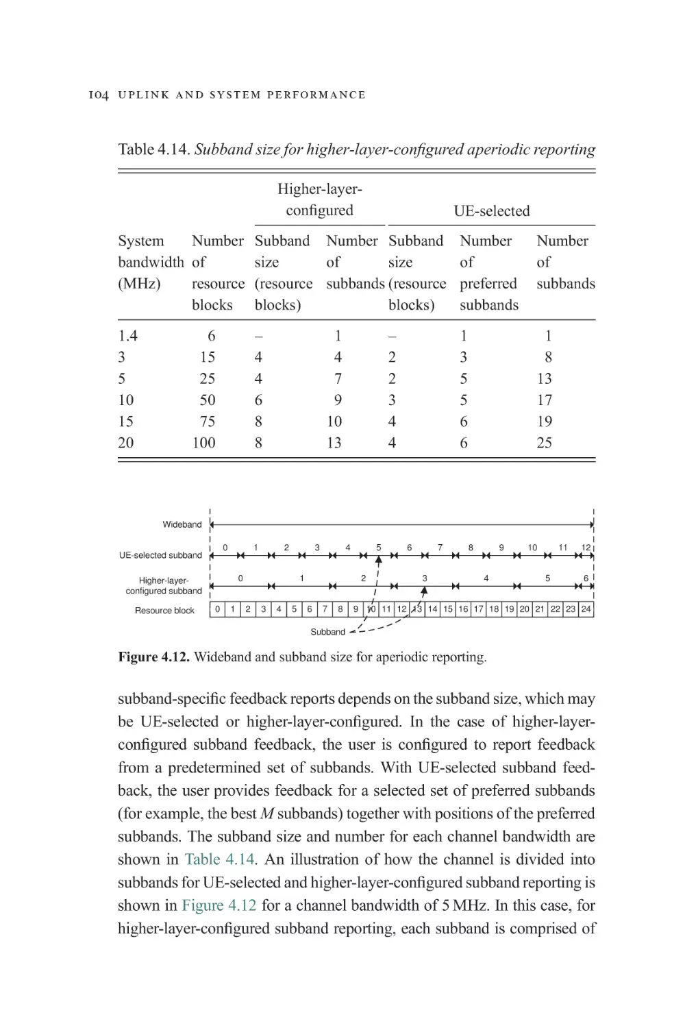
/


Author: Ghosh A. Ratasuk R.
Tags: electronics internet wireless networks
ISBN: 978-0-521-76870-2
Year: 2011


Text
Essentials of LTE and LTE-A
This practical, one-stop guide will quickly bring you up-to-speed on LTE and
LTE-Advanced (LTE-A). With everything you need to know about the theory
and technology behind the standards, this is a must-have for engineers and
managers in the wireless industry.
*
*
*
*
*
*
First book of its kind describing technologies and system performance of
LTE-A
Covers the evolution of digital wireless technology, basics of LTE and LTE-A,
design of downlink and uplink channels, multi-antenna techniques, and heterogeneous networks
Analyzes performance benefits over competing technologies, including
WiMAX and 802.16m
Reflects the latest LTE Release-10 standards
Includes numerous examples, including extensive system and link results
Unique approach is accessible to technical and non-technical readers alike
is a Senior Director and Fellow of the Technical Staff
at Motorola Solutions, where he works in the area of current and future
air-interface technologies for 802.16m, 3GPP LTE, LTE-Advanced, and
other broadband technologies. Since joining Motorola, he has worked
on eight different wireless technologies, and is currently leading
Motorola’s efforts in defining 3GPP LTE and LTE-Advanced physical
layer standards from the concept phase to the adopted baseline.
A M ITA BH A G H O SH
is currently a Distinguished Member of the Technical
Staff at Motorola Solutions. He has extensive experience in 3G/4G cellular
system design and analysis (specifically LTE, HSPA, WiMAX, 1xEV-DV, and
W-CDMA technologies), including algorithm development, performance
analysis and validation, physical layer modeling, and simulations.
R AP EEPAT R ATA SU K
The Cambridge Wireless Essentials Series
Series Editors
william webb Neul, Cambridge, UK
sudhir dixit Nokia, US
A series of concise, practical guides for wireless industry professionals.
Martin Cave, Chris Doyle and William Webb, Essentials of Modern Spectrum
Management
Christopher Haslett, Essentials of Radio Wave Propagation
Stephen Wood and Roberto Aiello, Essentials of UWB
Christopher Cox, Essentials of UMTS
Steve Methley, Essentials of Wireless Mesh Networking
Linda Doyle, Essentials of Cognitive Radio
Nick Hunn, Essentials of Short-Range Wireless
Amitabha Ghosh and Rapeepat Ratasuk, Essentials of LTE and LTE-A
Forthcoming
Abhi Naha and Peter Whale, Essentials of Mobile Handset Design
Barry G. Evans, Essentials of Satellite Communications
David Bartlett, Essentials of Positioning and Location Technology
For further information on any of these titles, the series itself and ordering
information see www.cambridge.org/wirelessessentials
Essentials of LTE
and LTE-A
Amitabha Ghosh and Rapeepat Ratasuk
Motorola Solutions
CAMBRIDGE UNIVERSITY PRESS
Cambridge, New York, Melbourne, Madrid, Cape Town,
Singapore, São Paulo, Delhi, Tokyo, Mexico City
Cambridge University Press
The Edinburgh Building, Cambridge CB2 8RU, UK
Published in the United States of America by Cambridge University Press, New York
www.cambridge.org
Information on this title: www.cambridge.org/9780521768702
© Cambridge University Press 2011
This publication is in copyright. Subject to statutory exception
and to the provisions of relevant collective licensing agreements,
no reproduction of any part may take place without the written
permission of Cambridge University Press.
First published 2011
Printed in the United Kingdom at the University Press, Cambridge
A catalogue record for this publication is available from the British Library
Library of Congress Cataloguing in Publication data
Ghosh, Amitabha, 1958–
Essentials of LTE and LTE-A / Amitabha Ghosh and Rapeepat Ratasuk.
p. cm. – (The Cambridge wireless essentials series)
Includes bibliographical references.
ISBN 978-0-521-76870-2
1. Long-Term Evolution (Telecommunications) I. Ratasuk, Rapeepat. II. Title.
TK5103.48325.G485 2011
621.382–dc22
2011011253
ISBN 978-0-521-76870-2 Hardback
Cambridge University Press has no responsibility for the persistence or
accuracy of URLs for external or third-party internet websites referred to
in this publication, and does not guarantee that any content on such
websites is, or will remain, accurate or appropriate.
To my parents for their continuous support and teaching me the value of
education and thirst for knowledge; and to my family, Chittarupa, Devika,
and Adit, for their support, encouragement, and love.
Amitabha Ghosh
To Tanita, Alisa, and Paul.
Rapeepat Ratasuk
Contents
Preface
Acknowledgments
1
Genesis of wireless broadband technology (from 2G
to 4.5G)
1.1 Genesis of wireless technology
1.2 Key drivers for 4G/4.5G wireless broadband
1.3 Radio spectrum for wireless broadband
References
Additional reading
page xi
xiv
1
1
4
8
9
9
2
LTE overview
2.1 Introduction
2.2 System architecture
2.2.1 E-UTRAN
2.2.2 Evolved packet core
2.2.3 User equipment
2.3 Transmission scheme
2.3.1 OFDMA
2.3.2 SC-FDMA
References
10
10
12
14
16
18
20
20
25
30
3
Downlink transmission and system performance
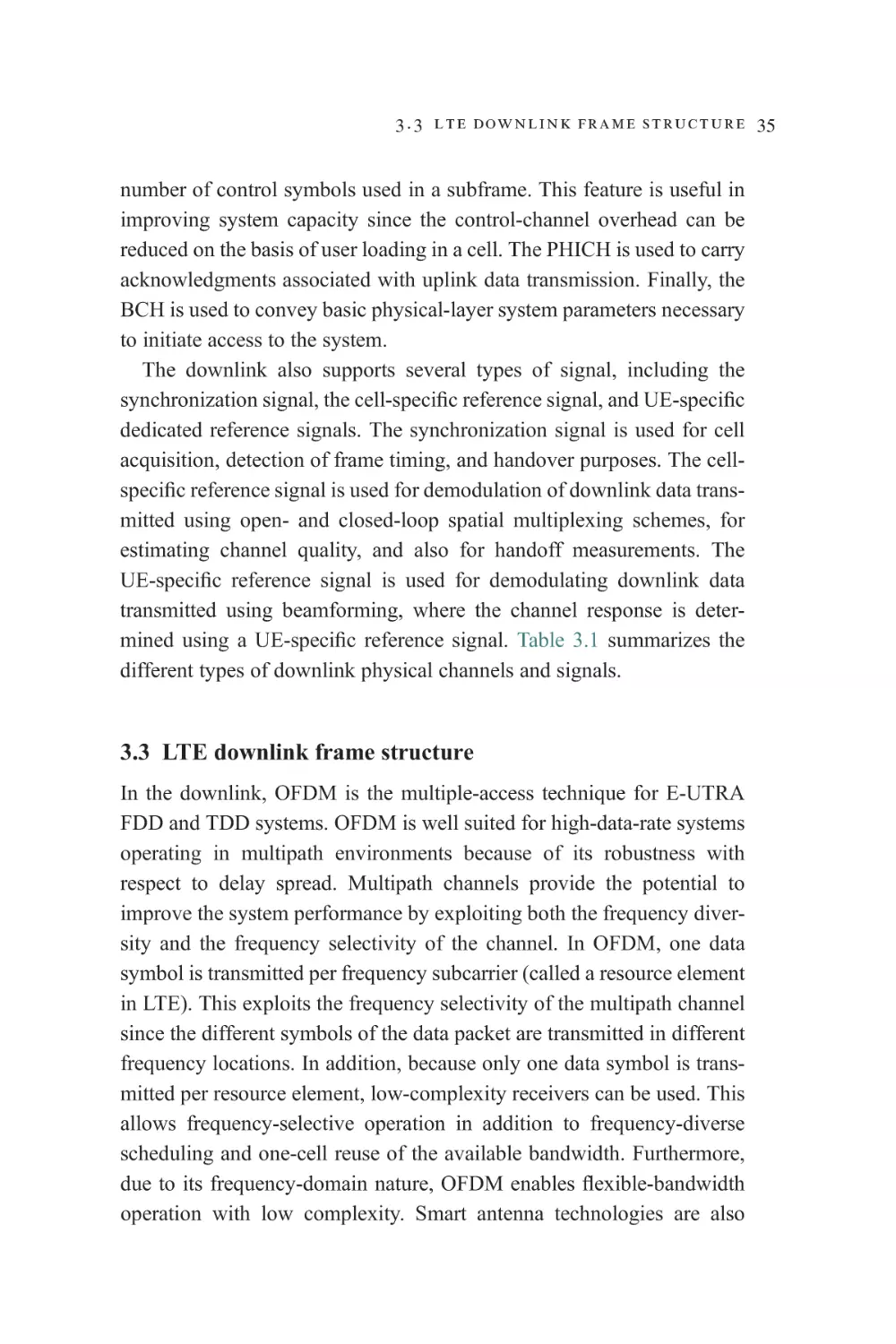
3.1 Introduction
3.2 Mapping between transport and physical channels
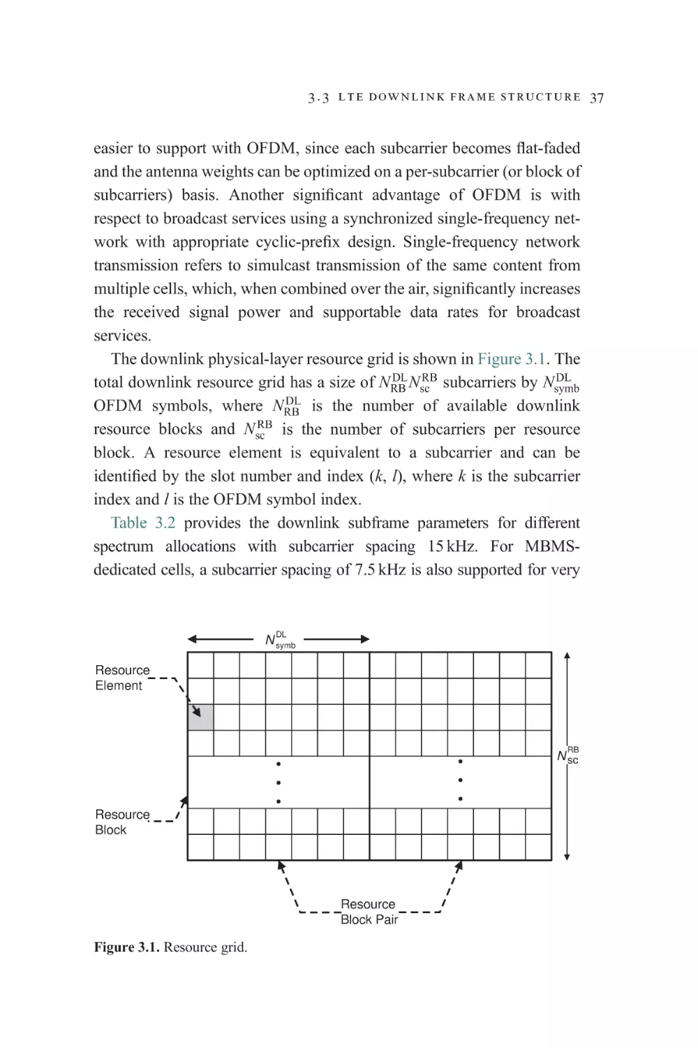
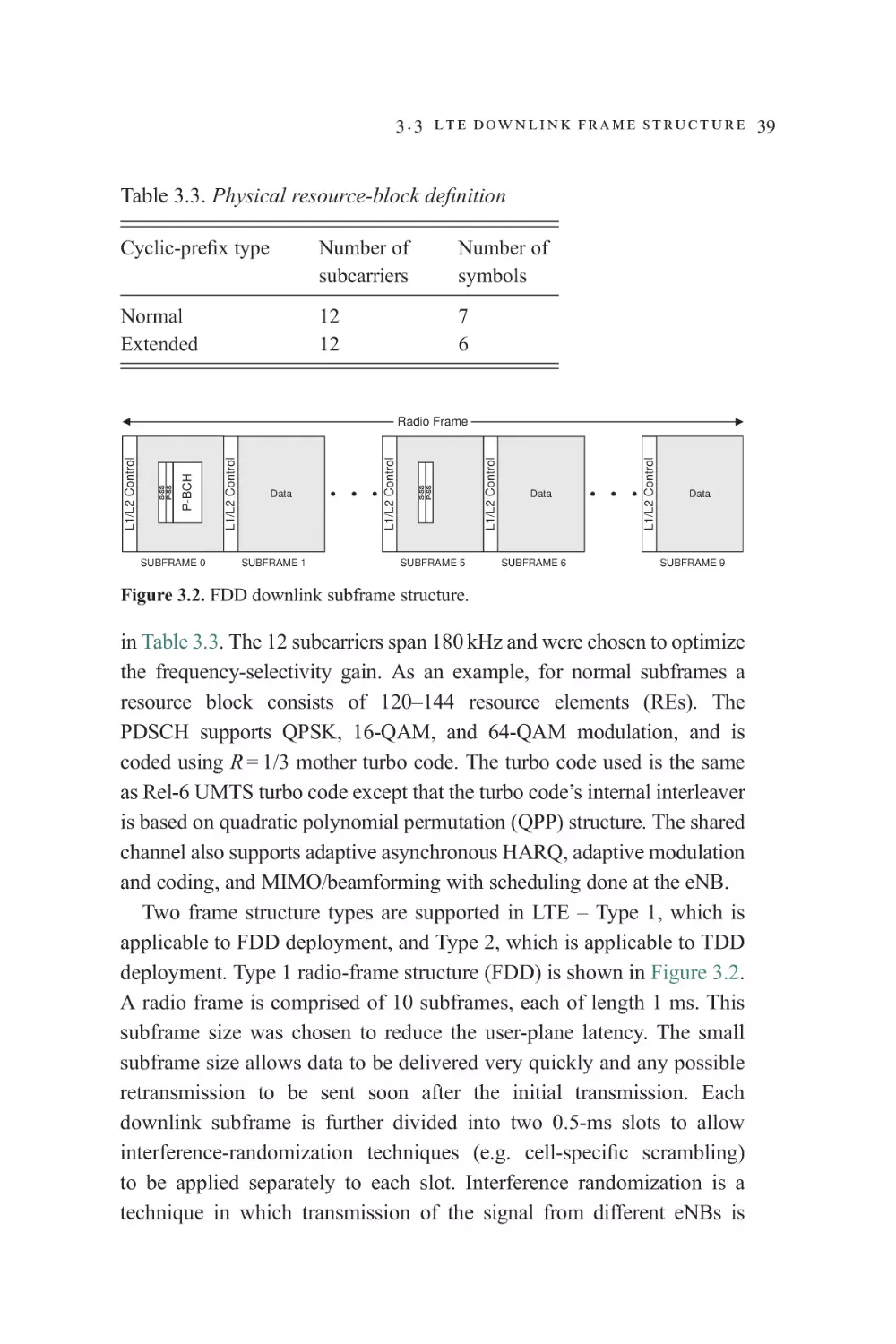
3.3 LTE downlink frame structure
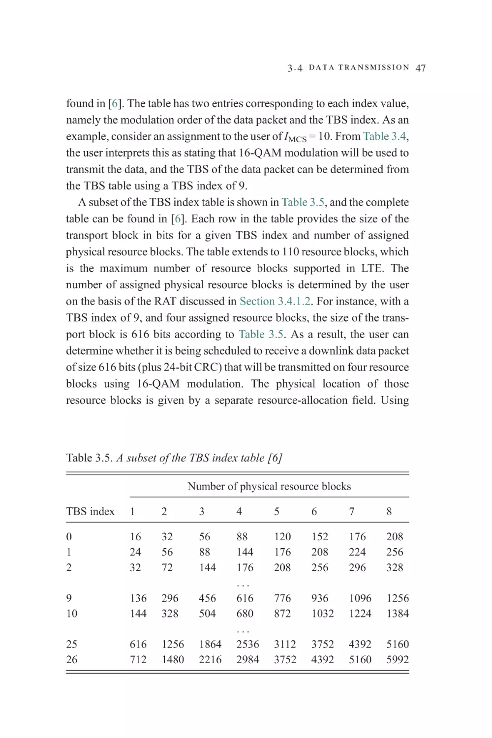
3.4 Data transmission
3.4.1 Shared data channel
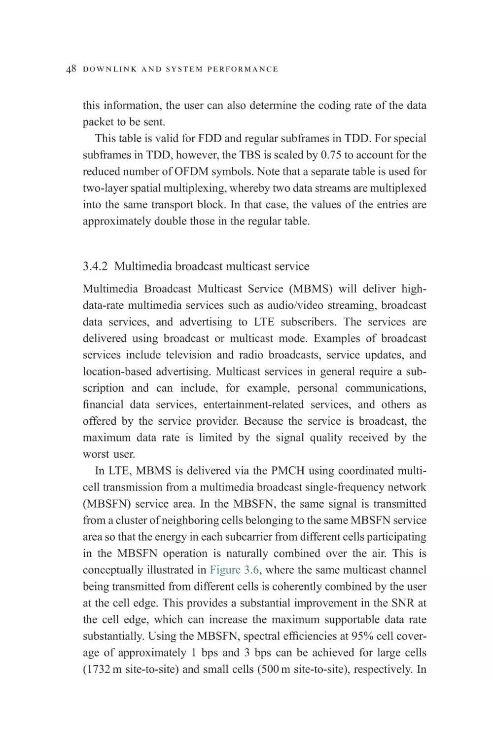
3.4.2 Multimedia broadcast multicast service
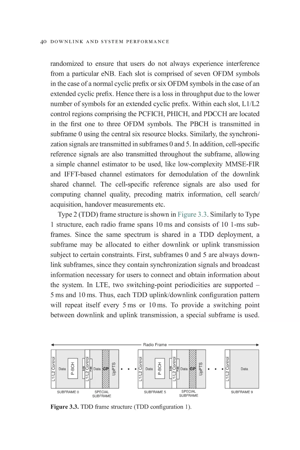
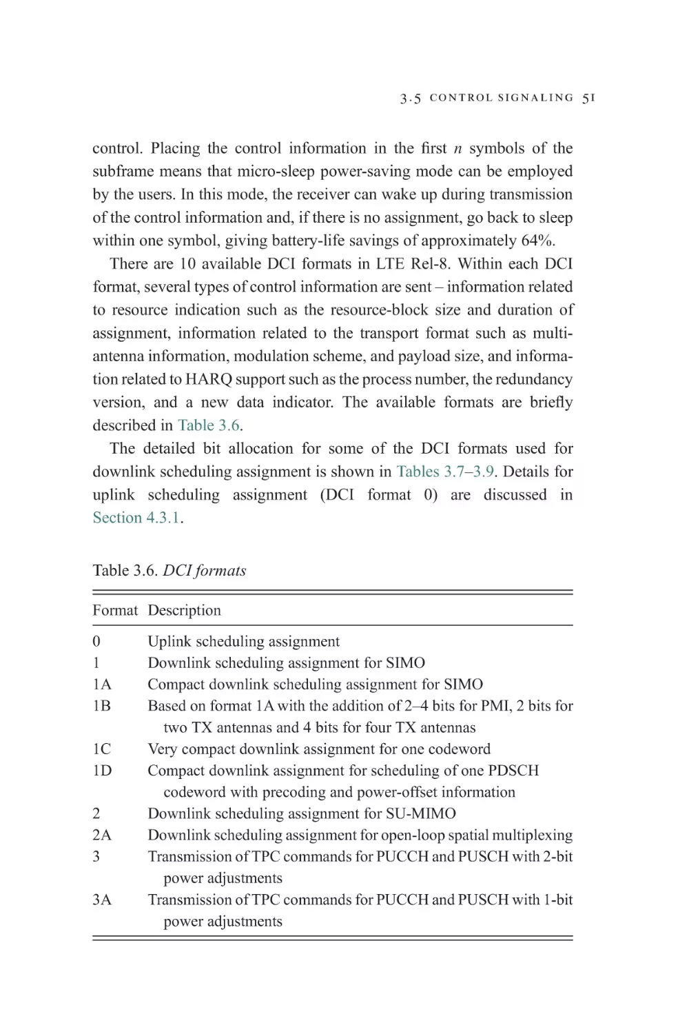
3.5 Control signaling
33
33
34
35
42
42
48
50
vii
viii c o n t e n t s
3.5.1 Physical Downlink Control Channel
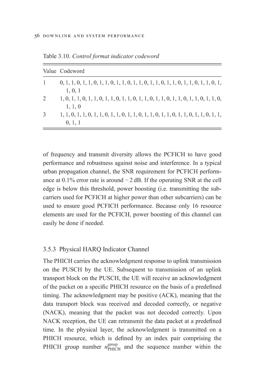
3.5.2 Physical Control Format Indicator
Channel
3.5.3 Physical HARQ Indicator Channel
3.5.4 Physical Broadcast Channel
3.5.5 Paging Control Channel
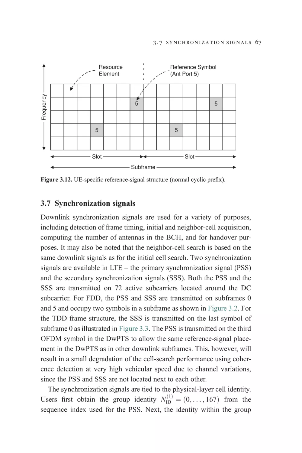
3.6 Downlink reference signal
3.7 Synchronization signals
3.7.1 Cell search and synchronization sequences
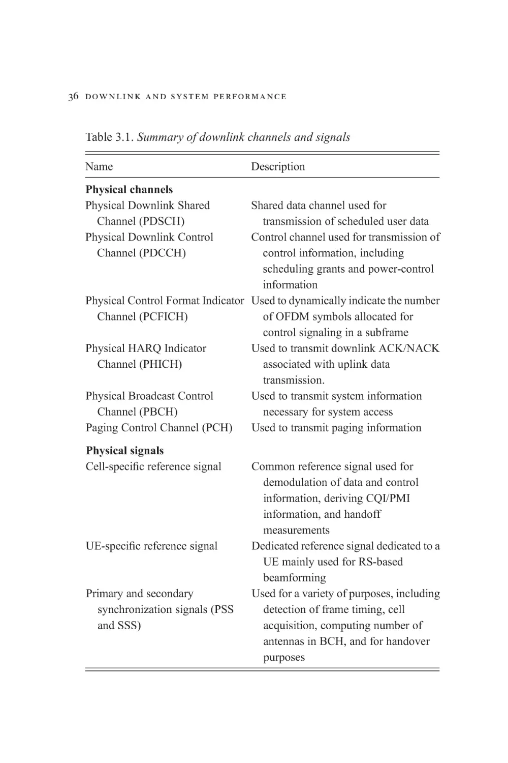
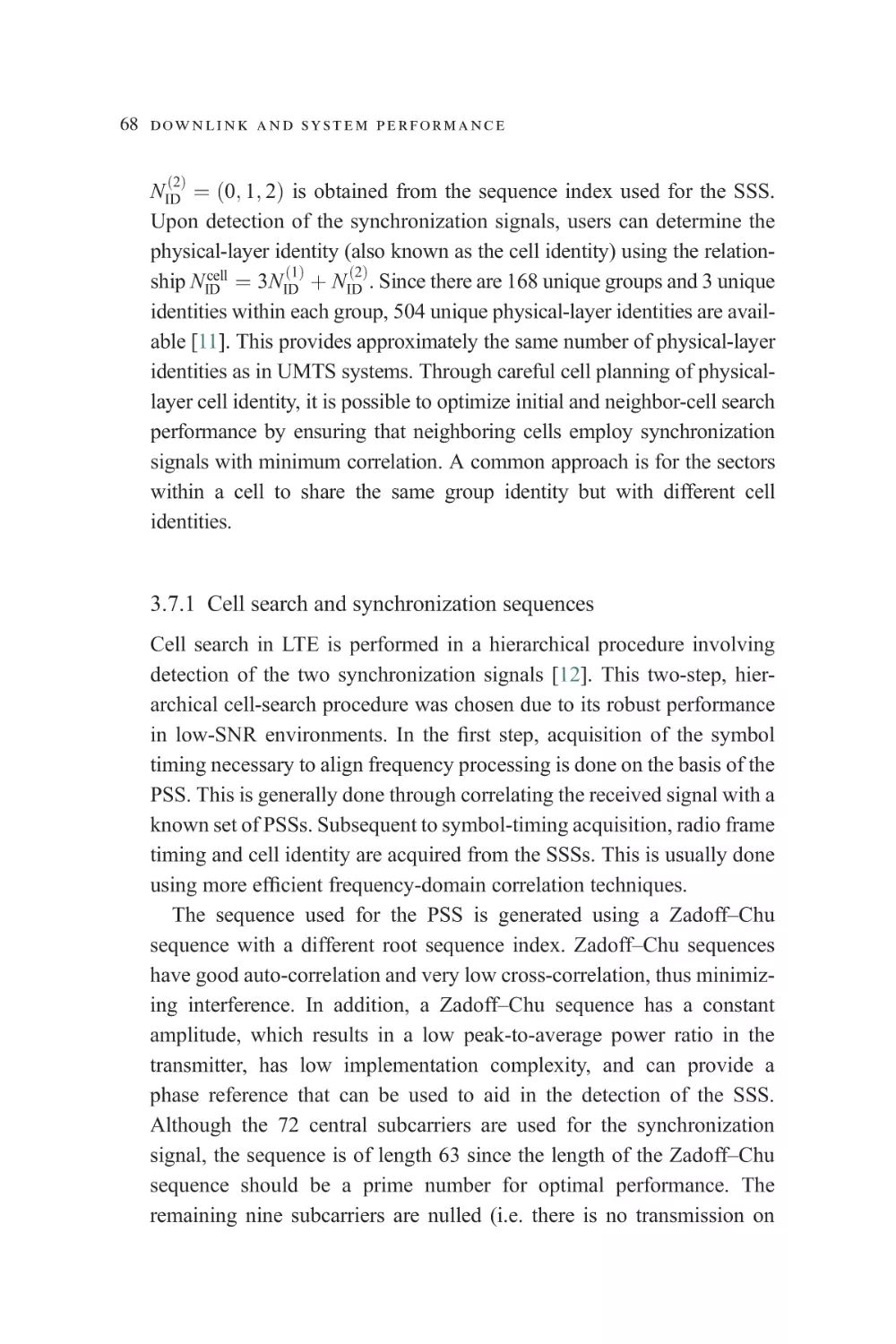
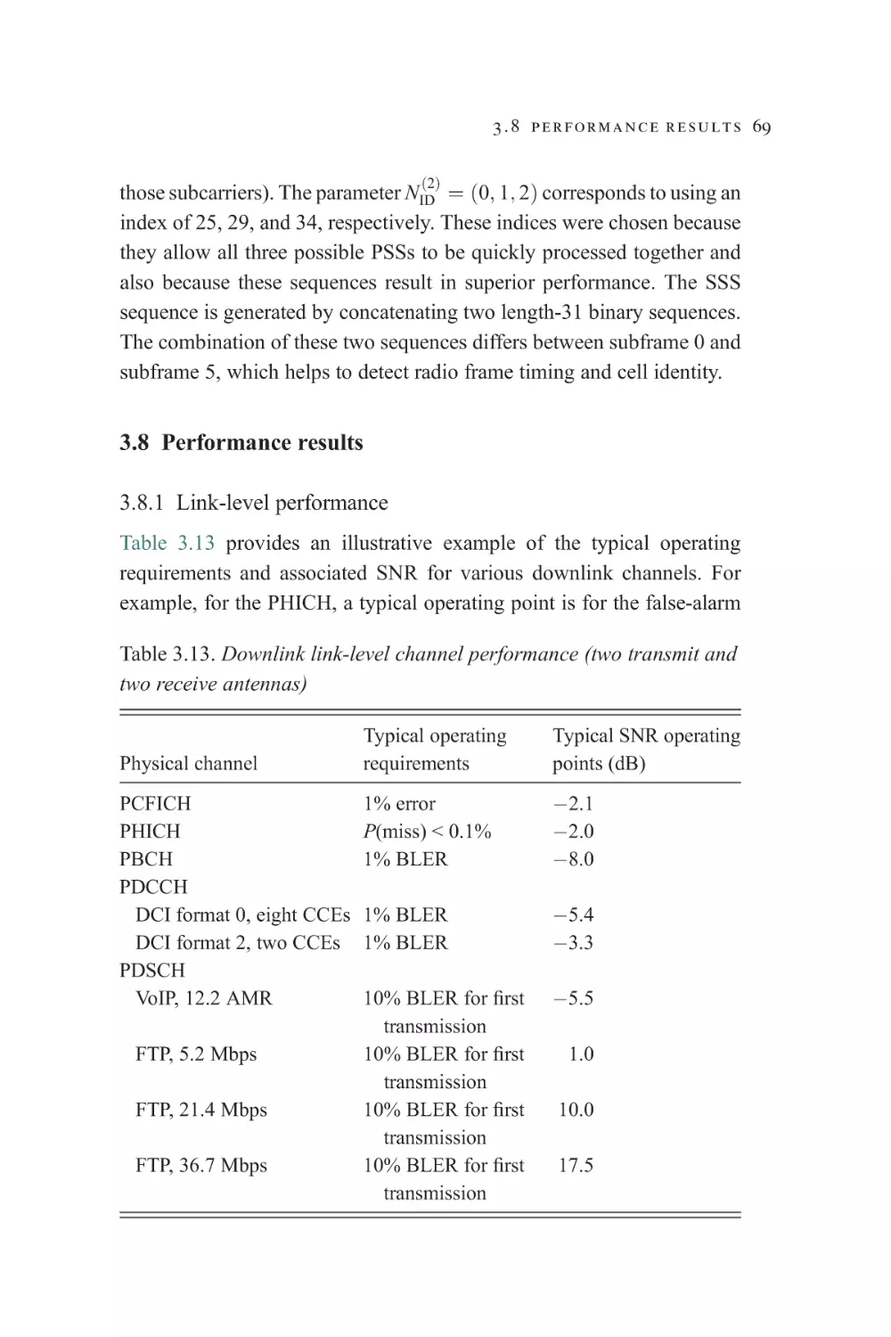
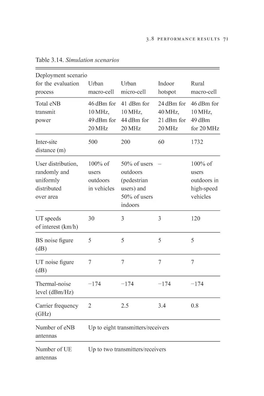
3.8 Performance results
3.8.1 Link-level performance
3.8.2 System-level performance
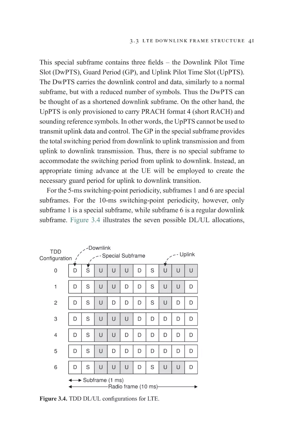
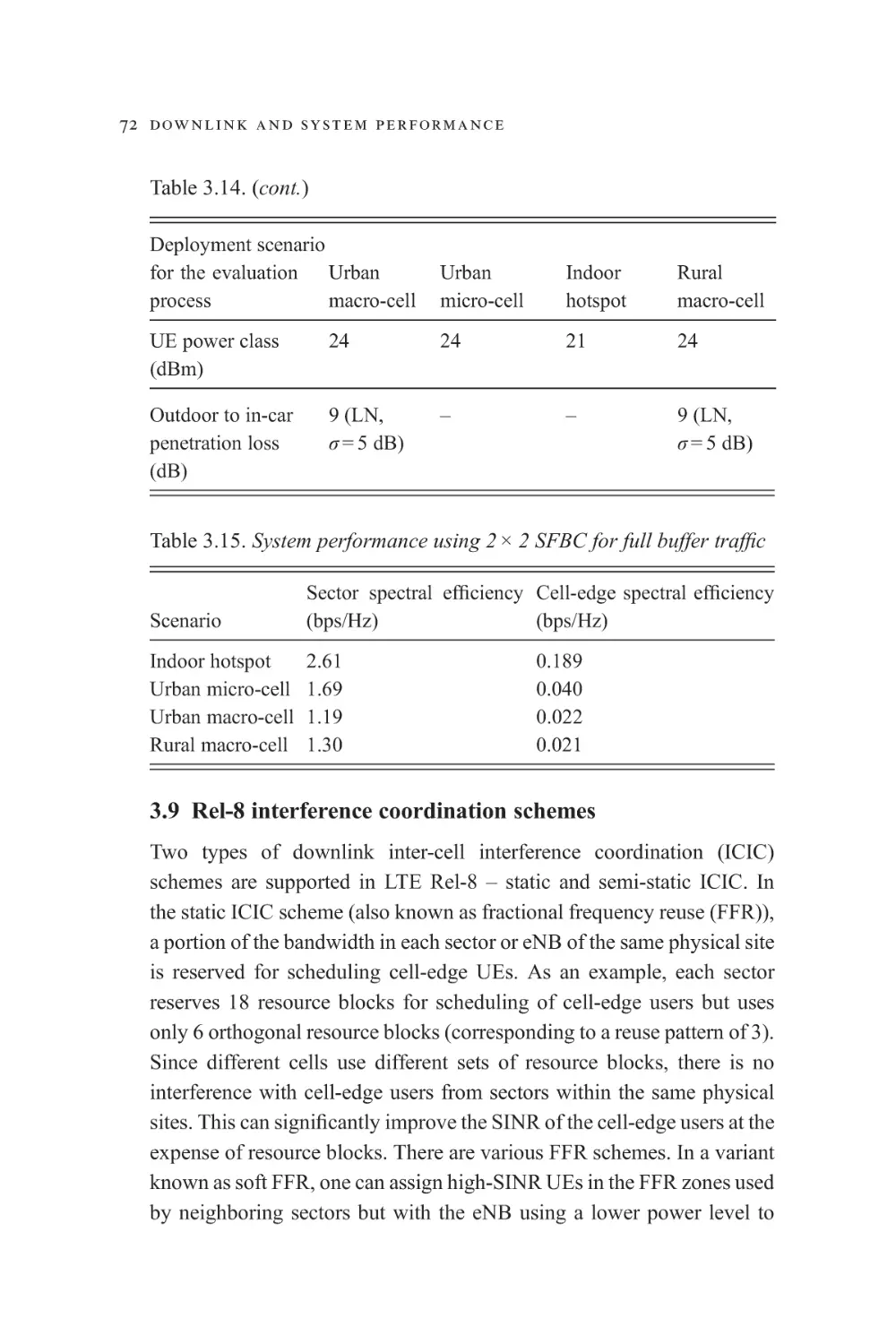
3.9 Rel-8 interference coordination schemes
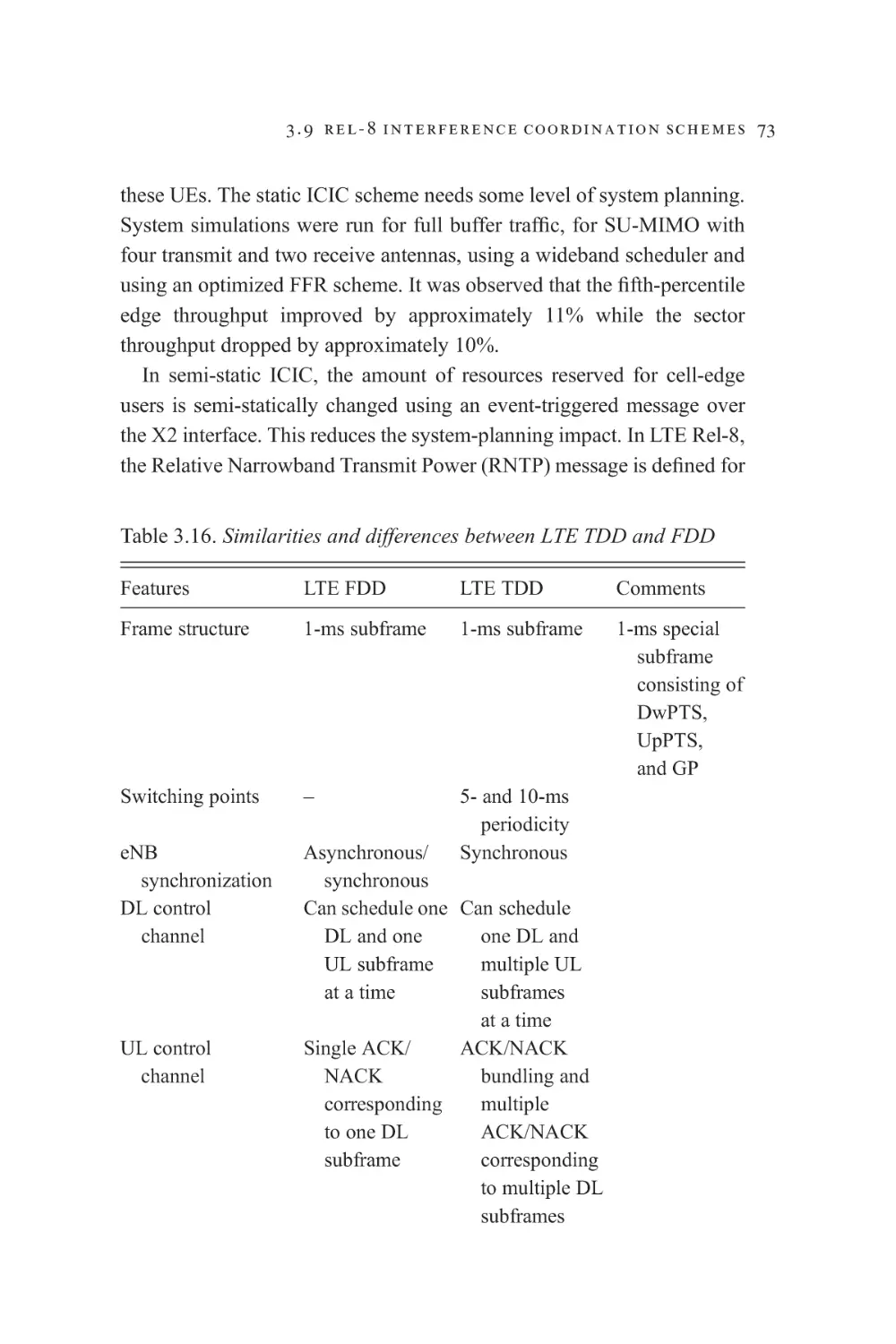
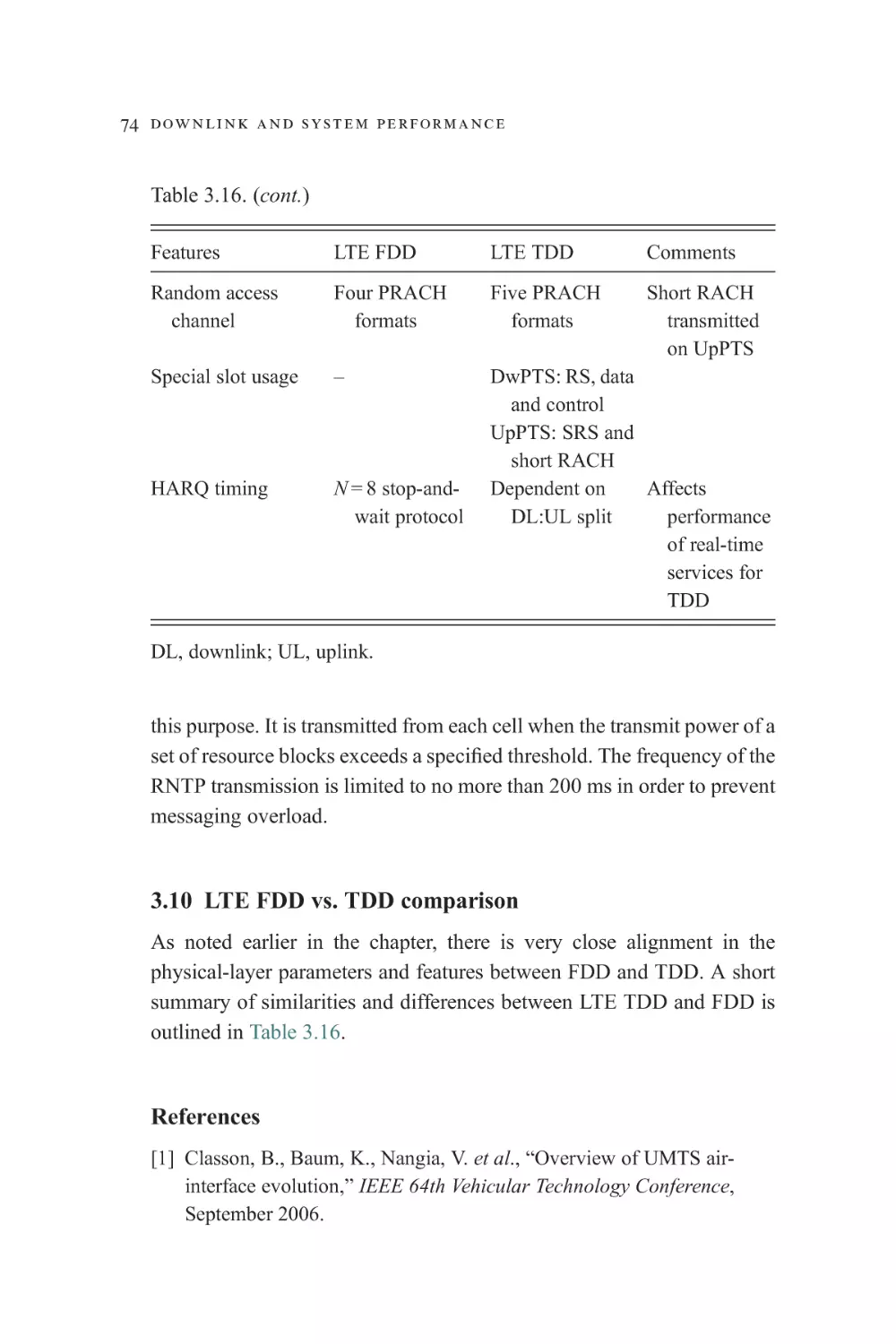
3.10 LTE FDD vs. TDD comparison
References
4
Uplink transmission and system performance
4.1 Introduction
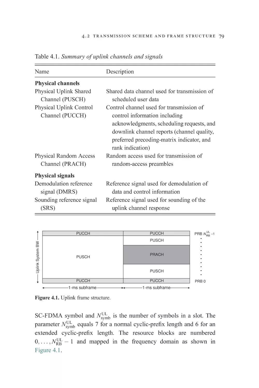
4.2 Transmission scheme and frame structure
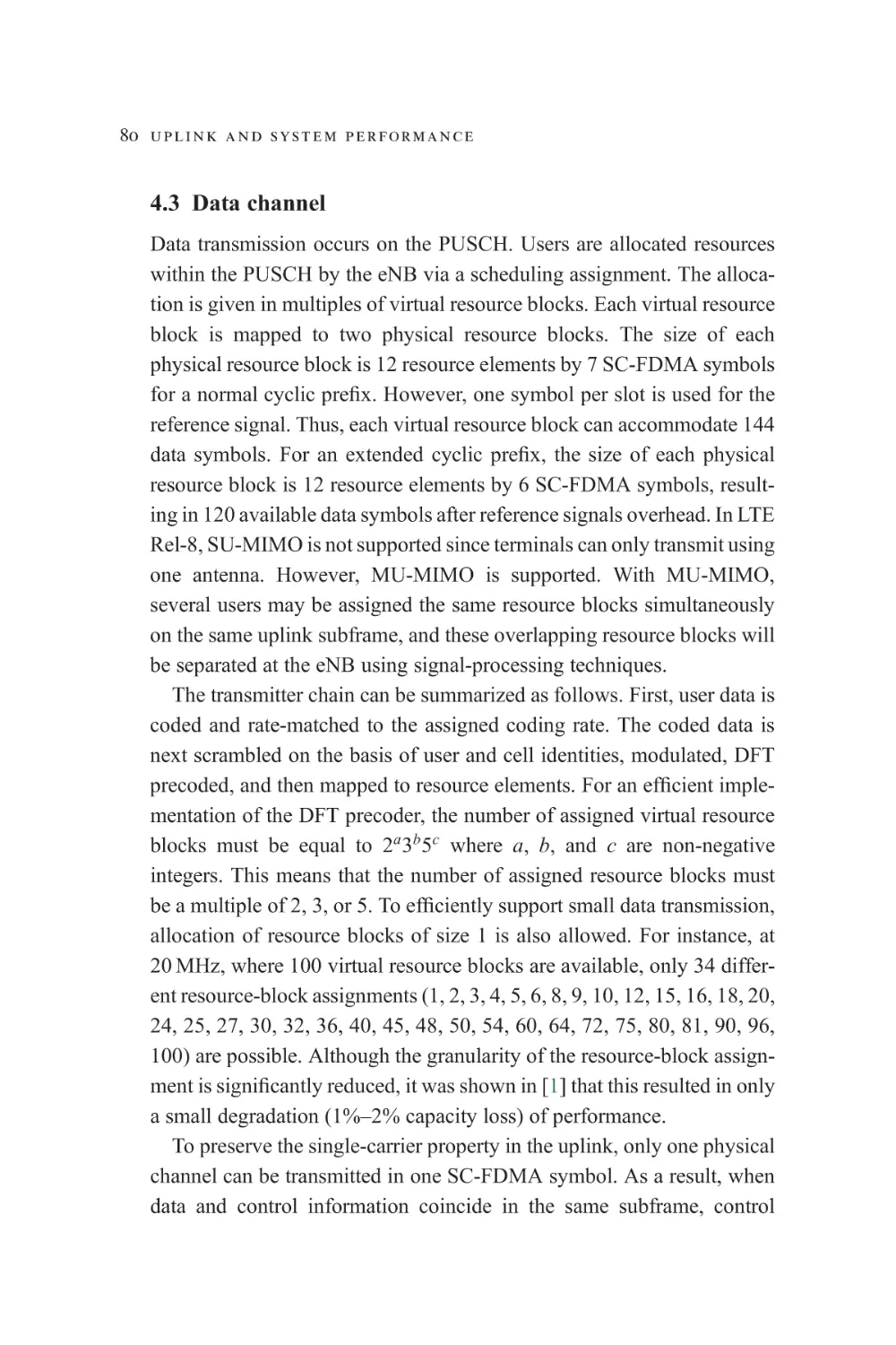
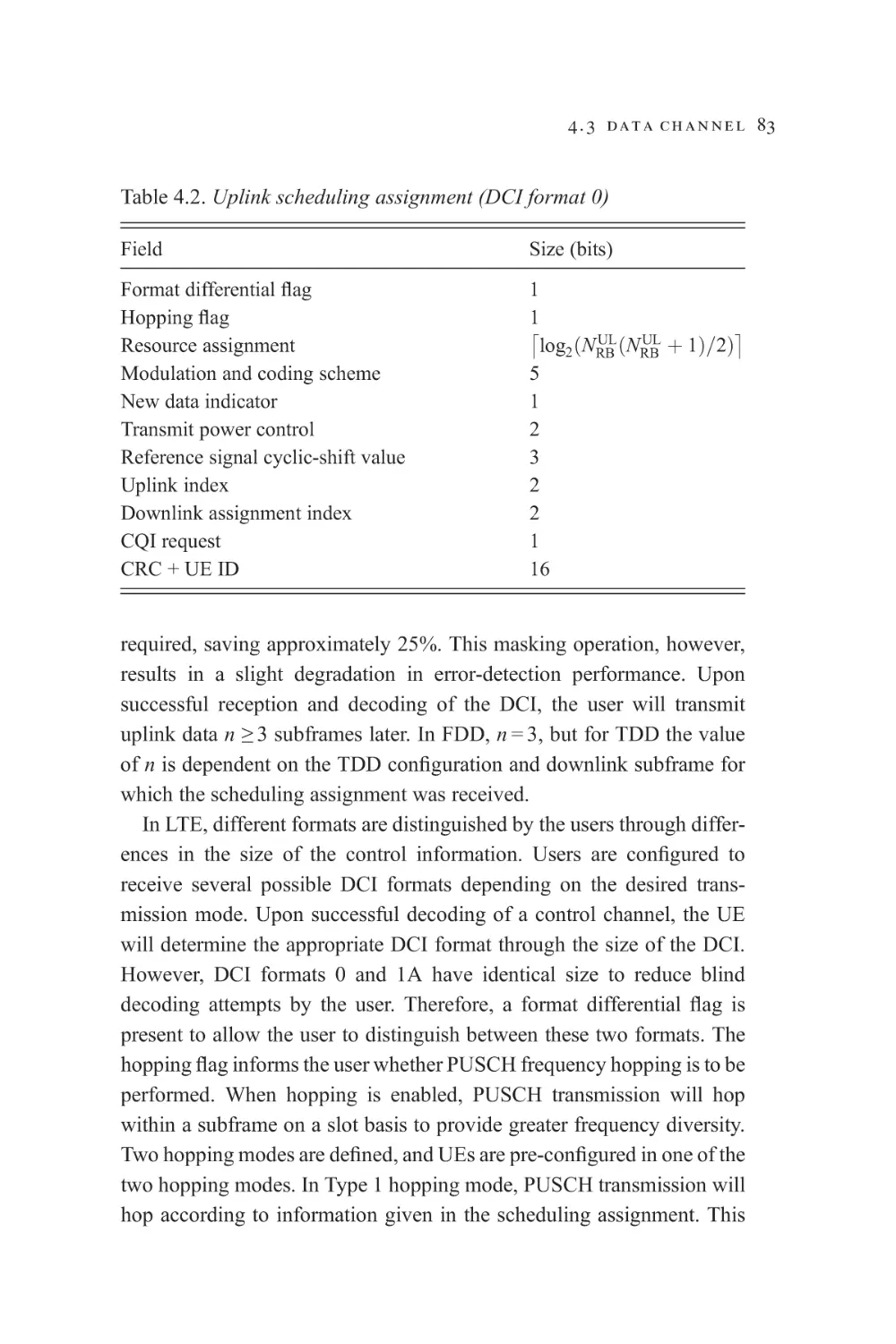
4.3 Data channel
4.3.1 Dynamic uplink scheduling assignment
4.3.2 Semi-persistent uplink scheduling
assignment
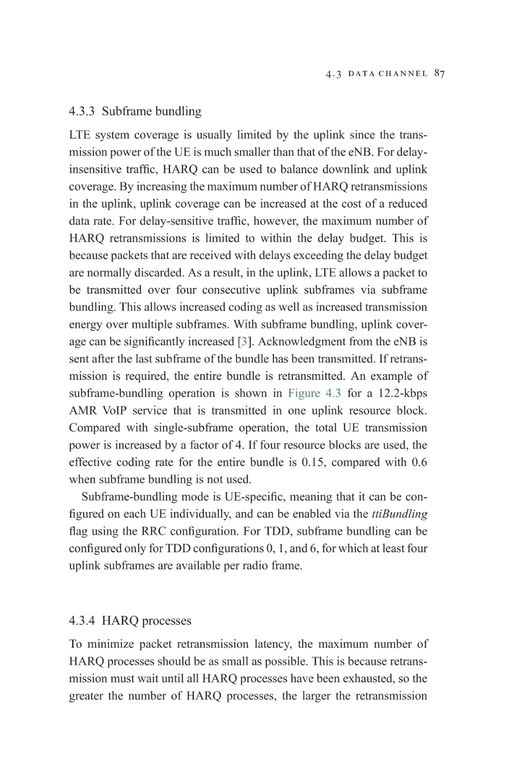
4.3.3 Subframe bundling
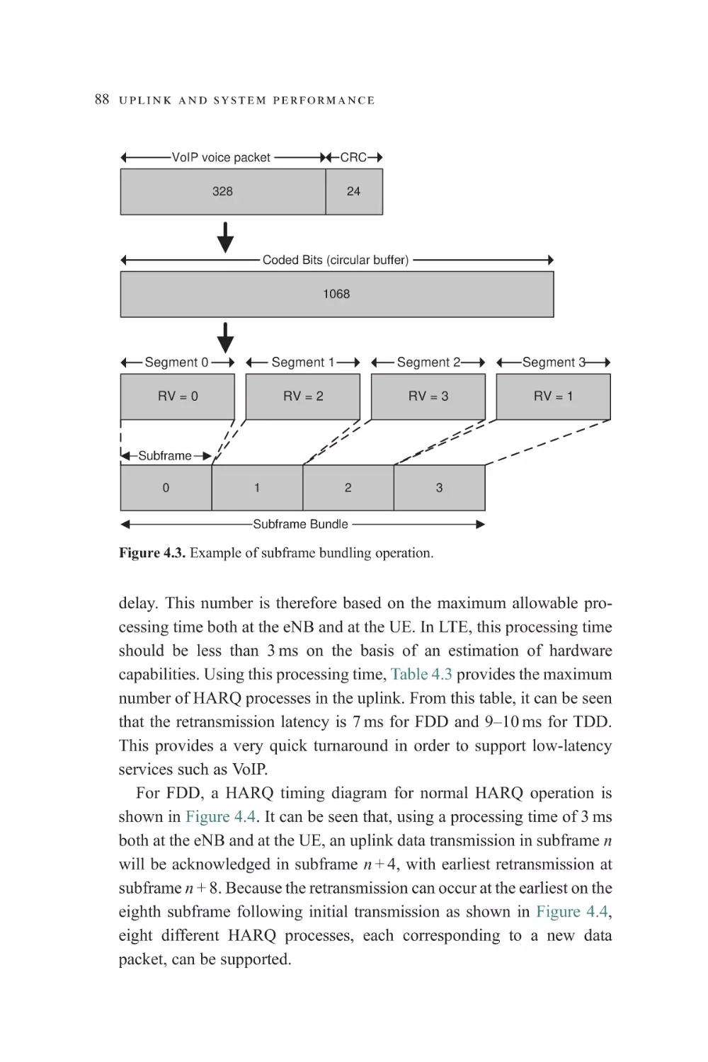
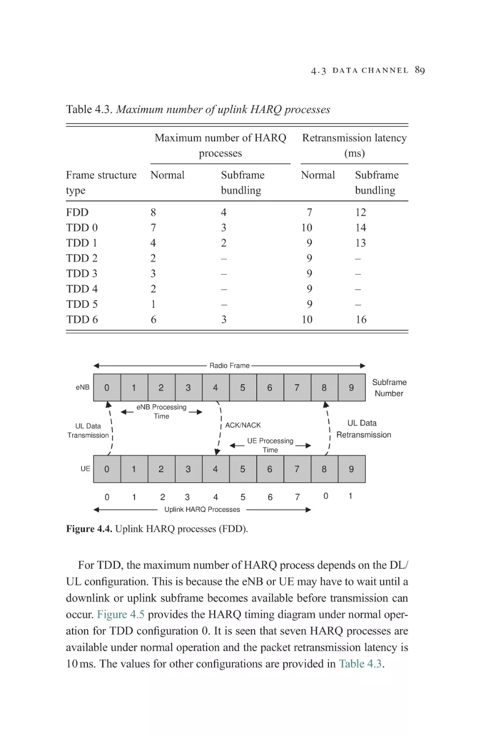
4.3.4 HARQ processes
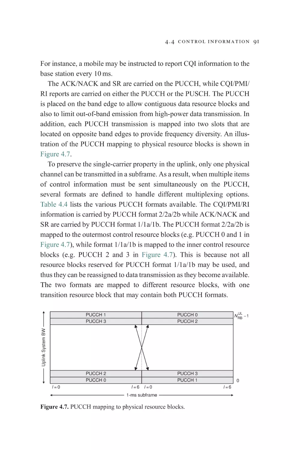
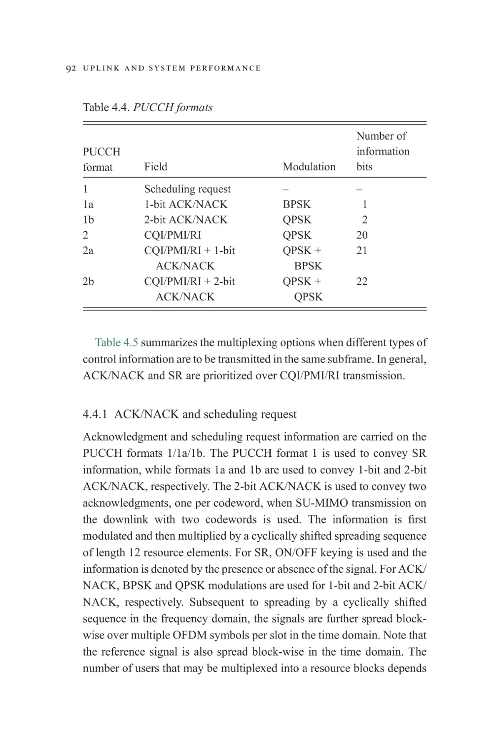
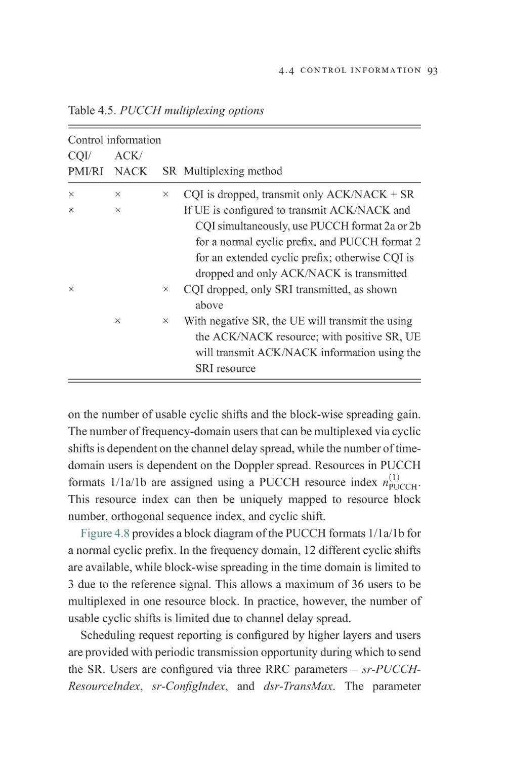
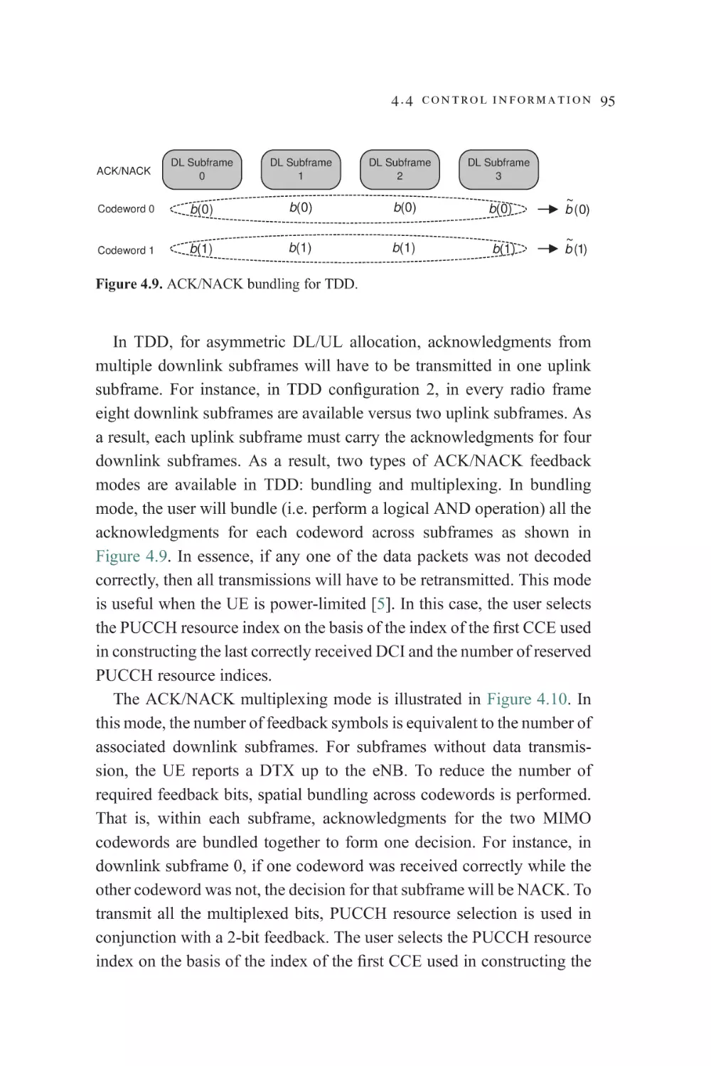
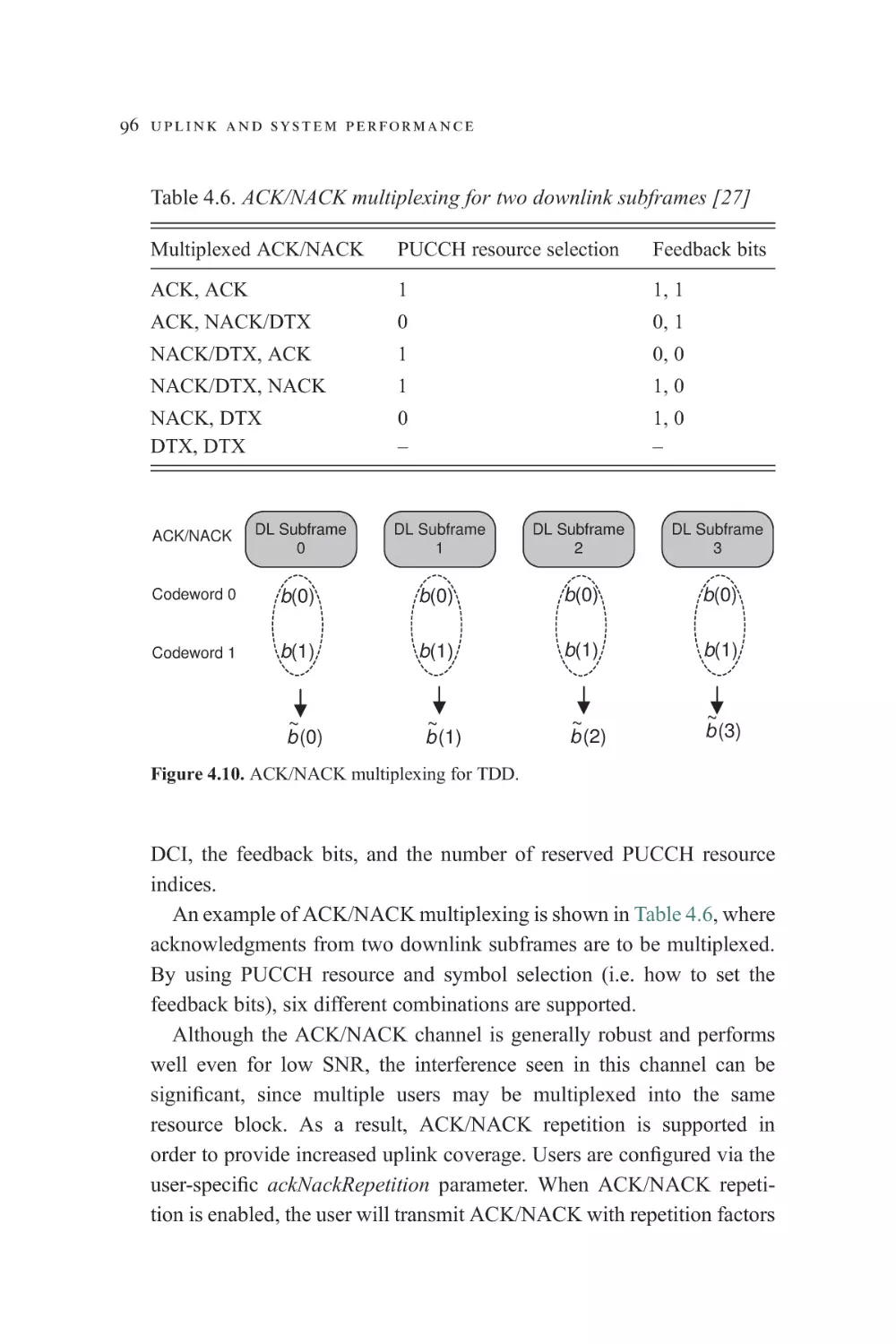
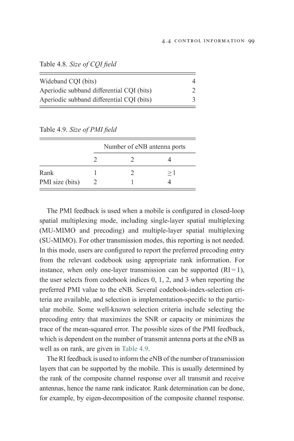
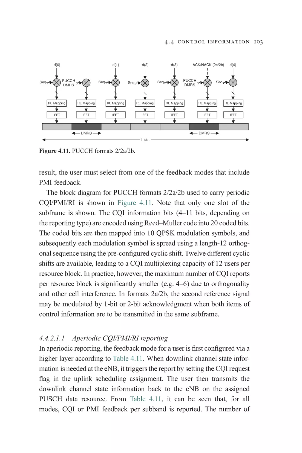
4.4 Control information
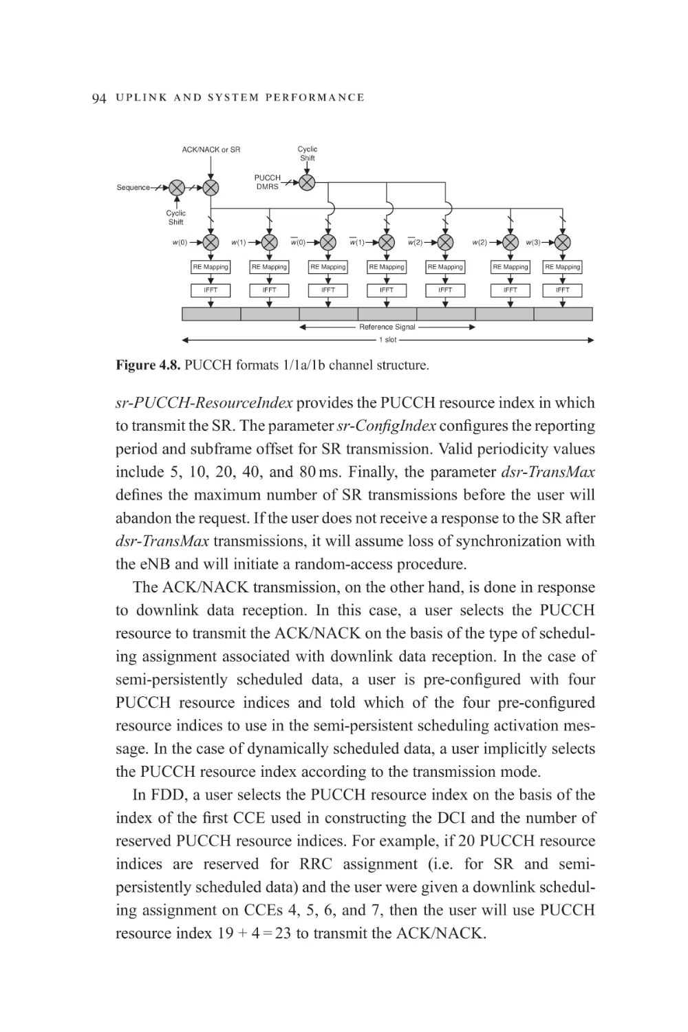
4.4.1 ACK/NACK and scheduling request
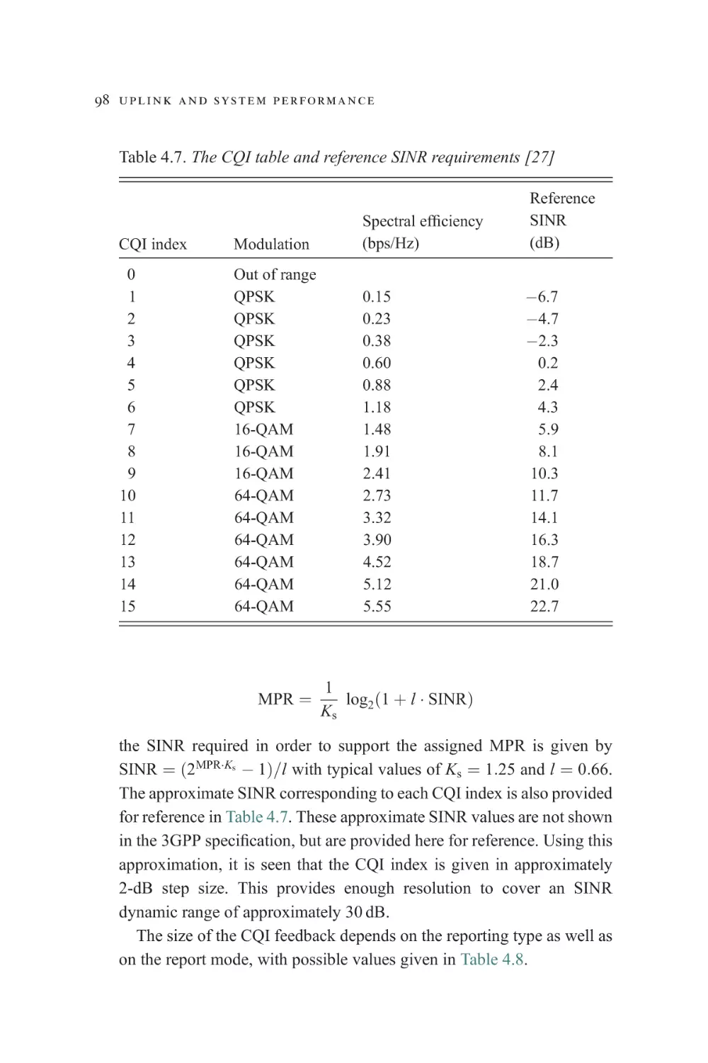
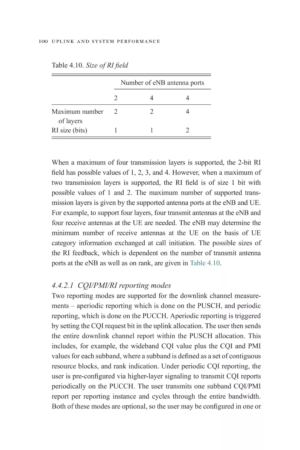
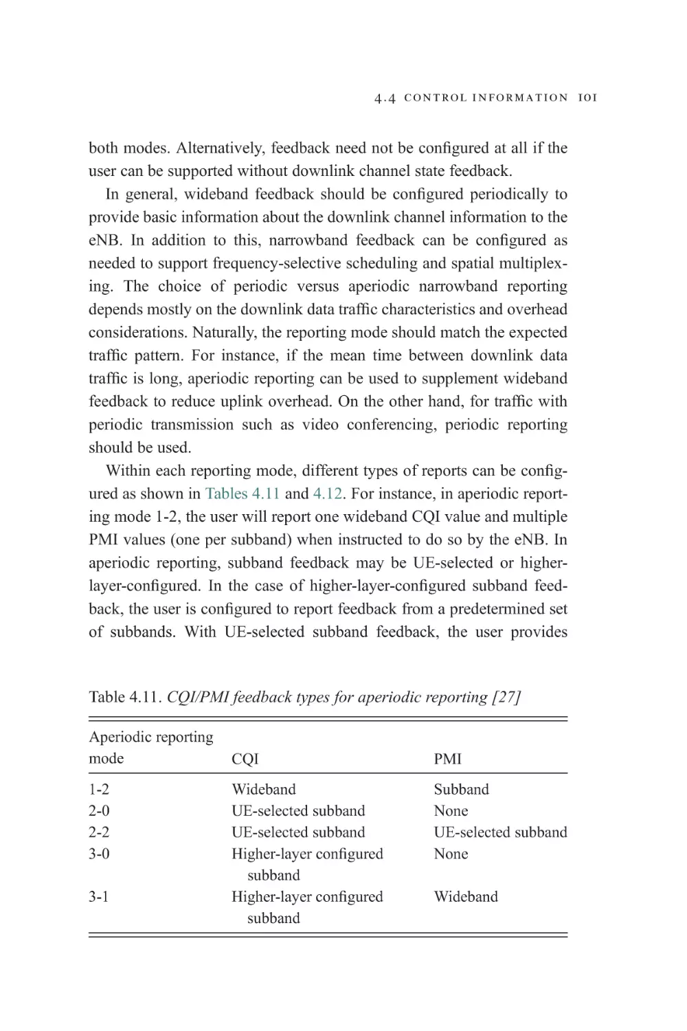
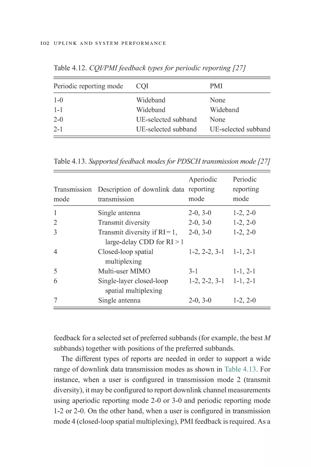
4.4.2 Channel measurement report – CQI/PMI/RI
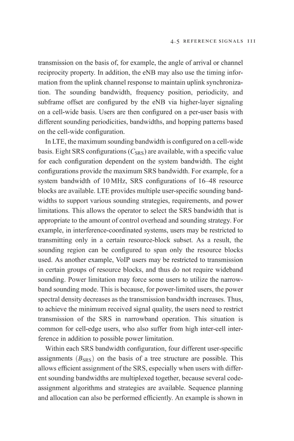
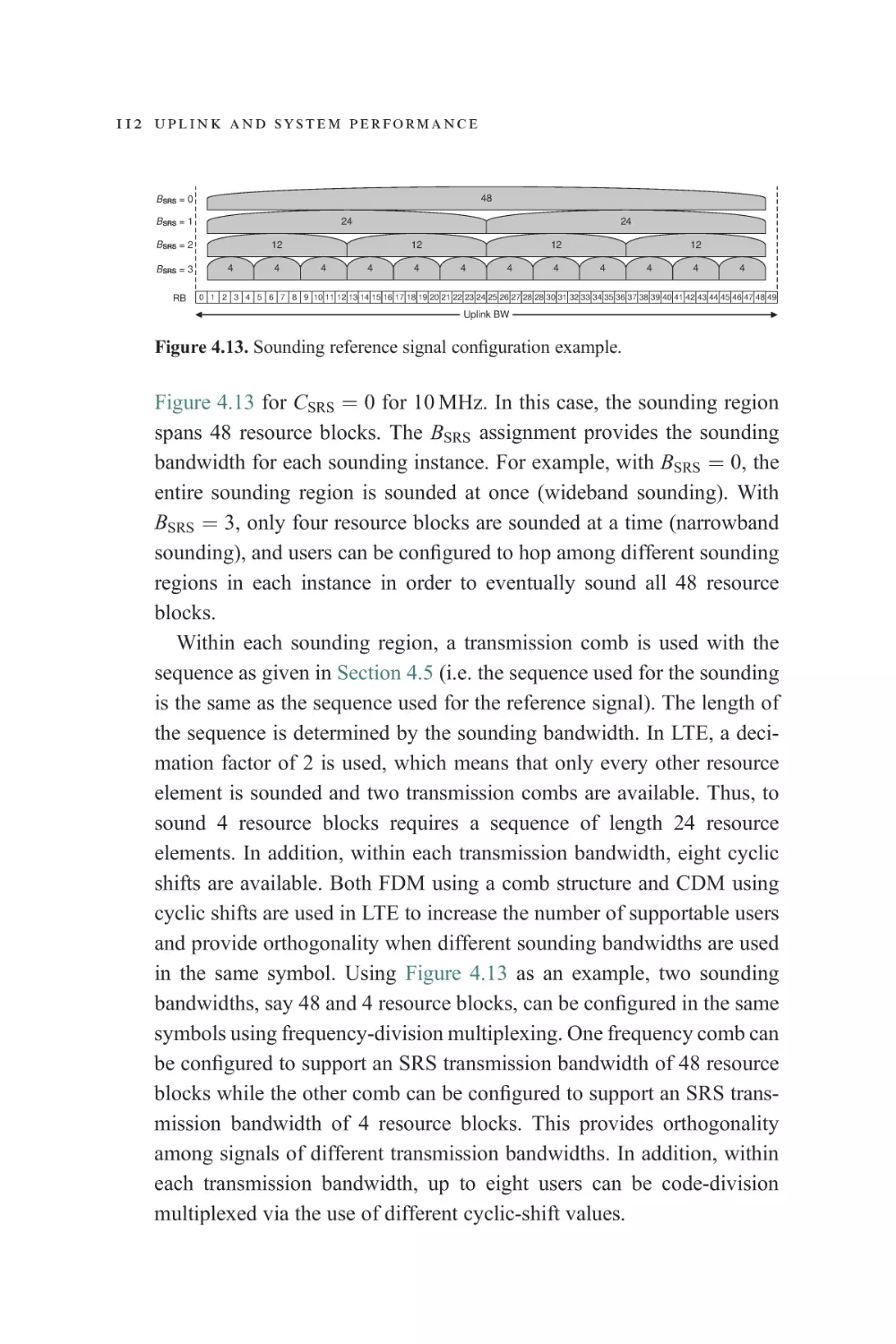
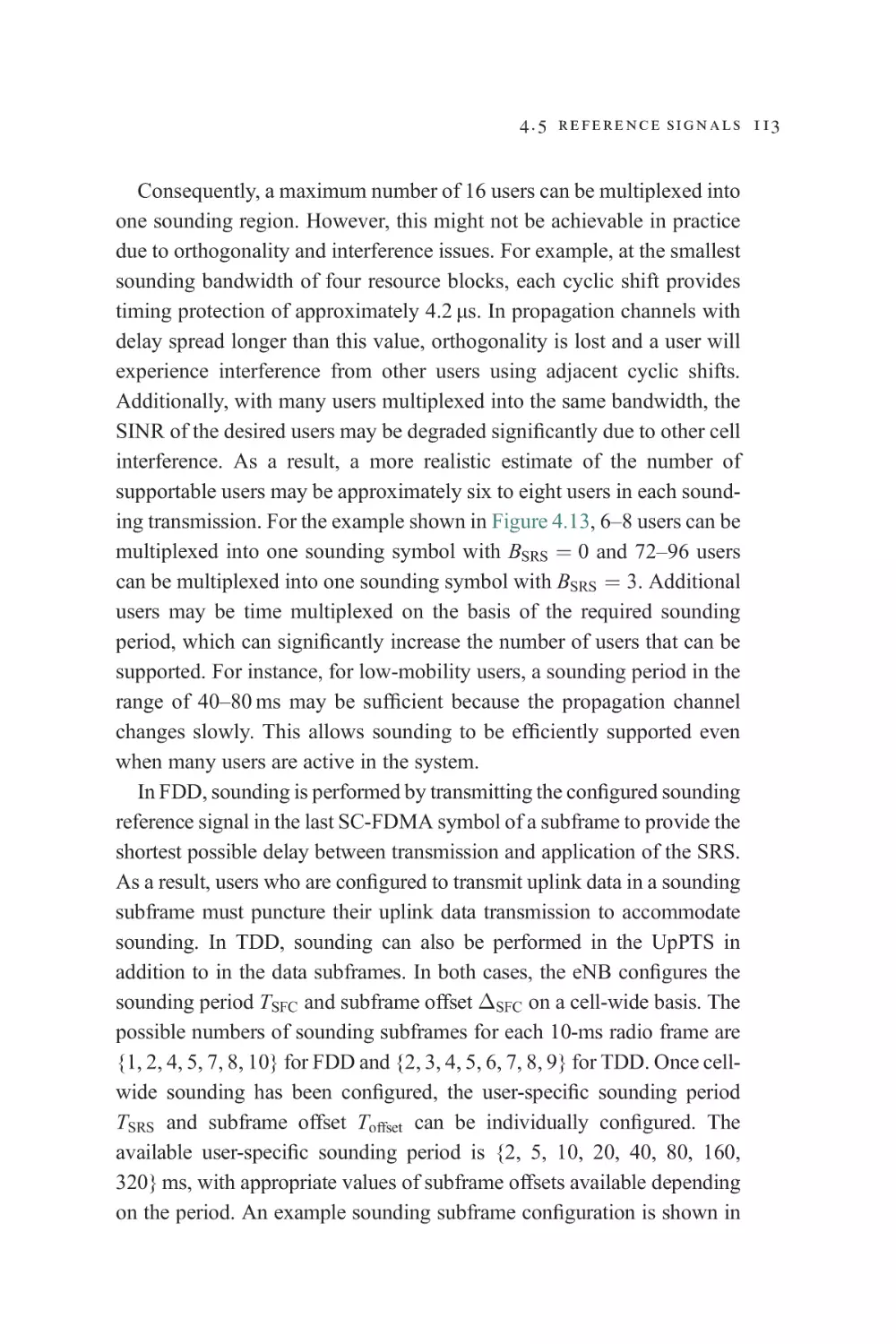
4.5 Reference signals
4.5.1 Demodulation reference signal
4.5.2 Sounding reference signal
4.6 Random access
4.6.1 Random-access procedure
4.7 Timing advance
50
55
56
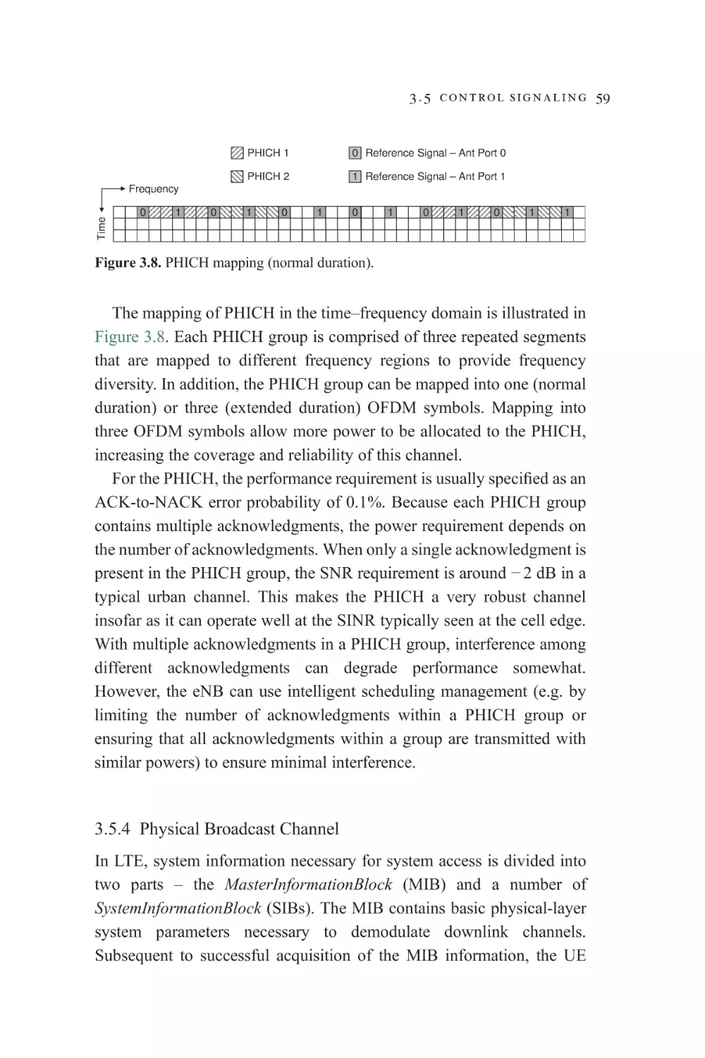
59
62
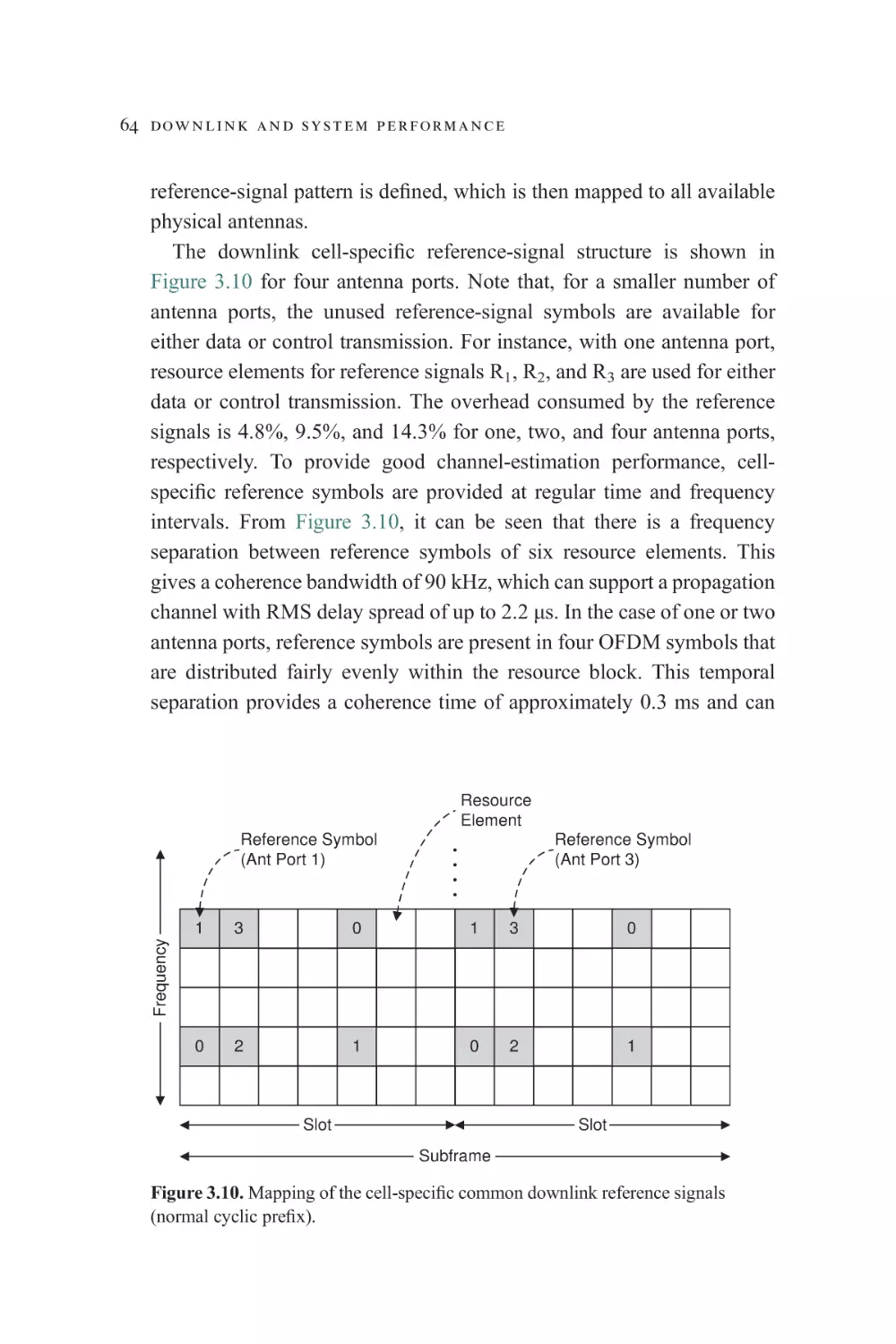
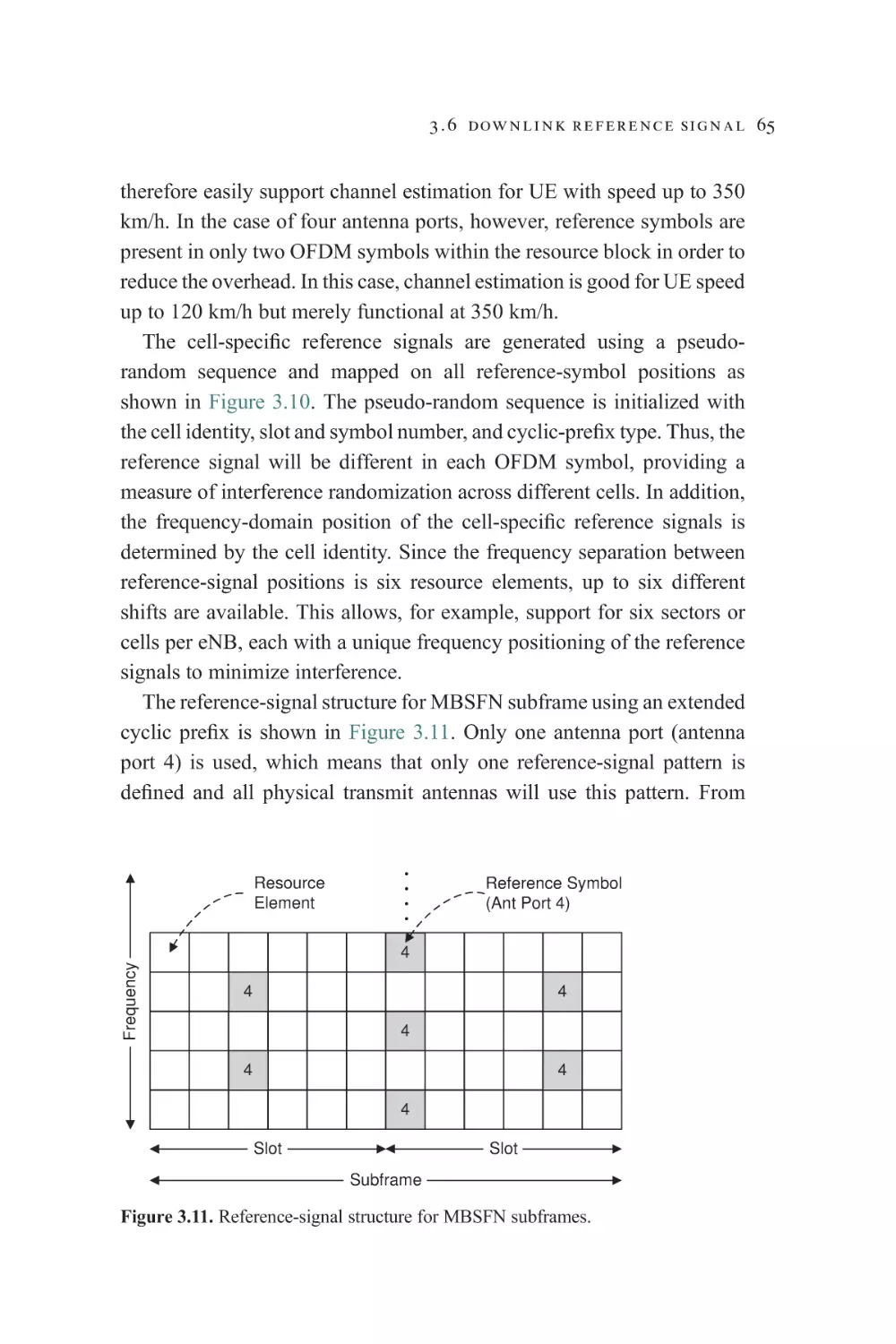
63
67
68
69
69
70
72
74
74
77
77
77
80
82
85
87
87
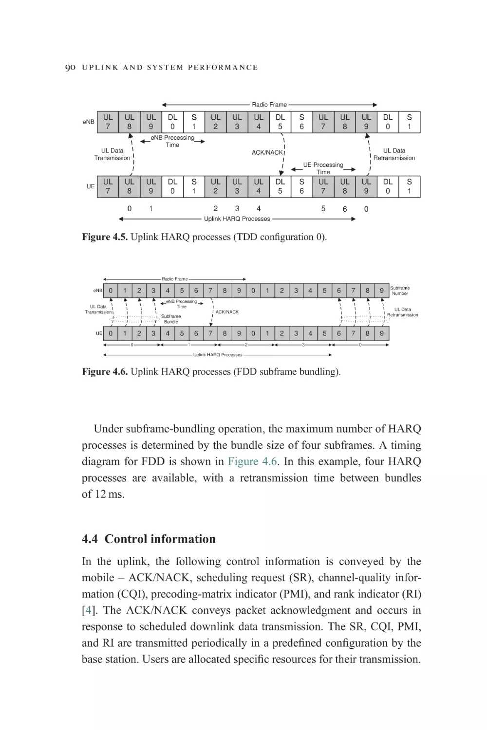
90
92
97
108
110
110
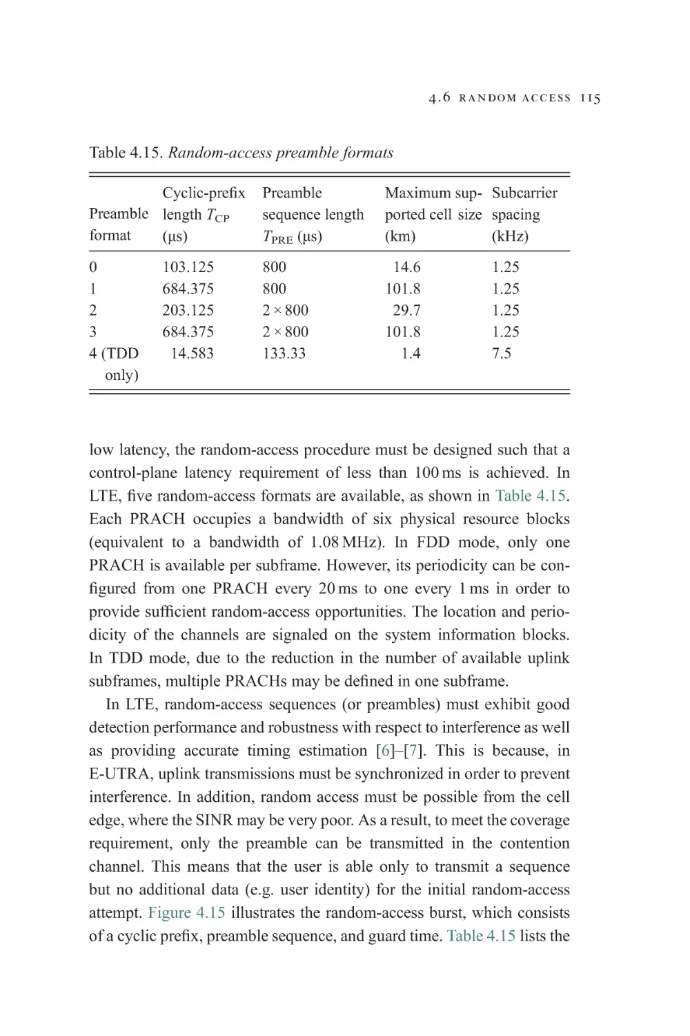
114
118
119
c o n t e n t s ix
5
6
4.8 Power control
4.8.1 Data channel
4.8.2 Control channels
4.8.3 Random-access channel
4.8.4 Sounding reference signal
4.9 Interference coordination schemes
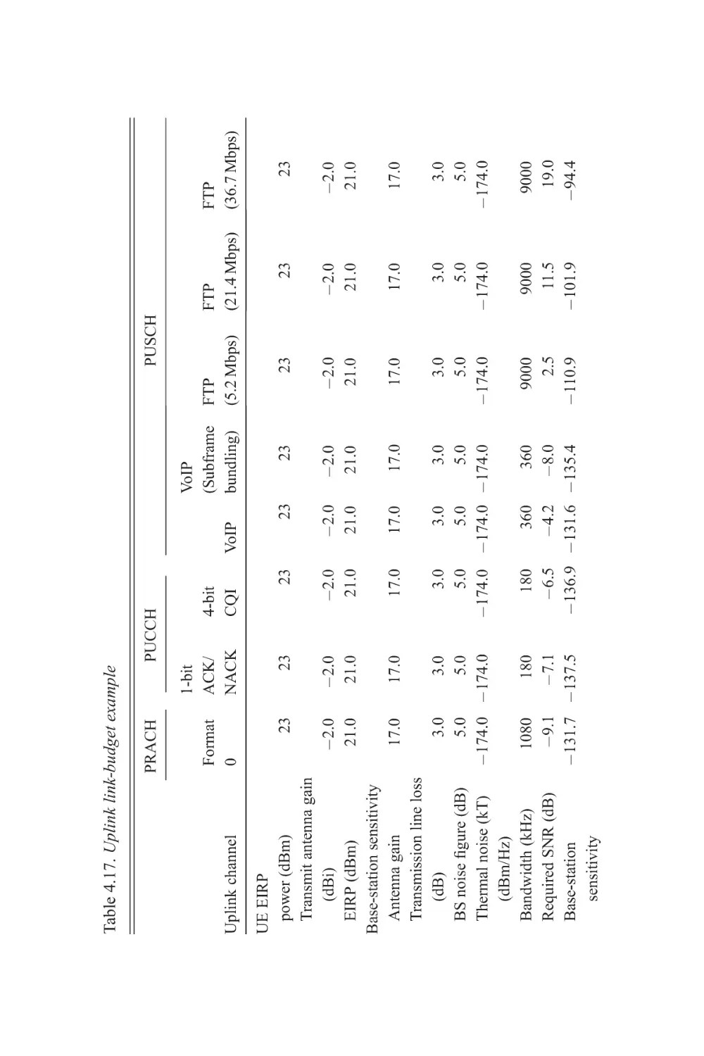
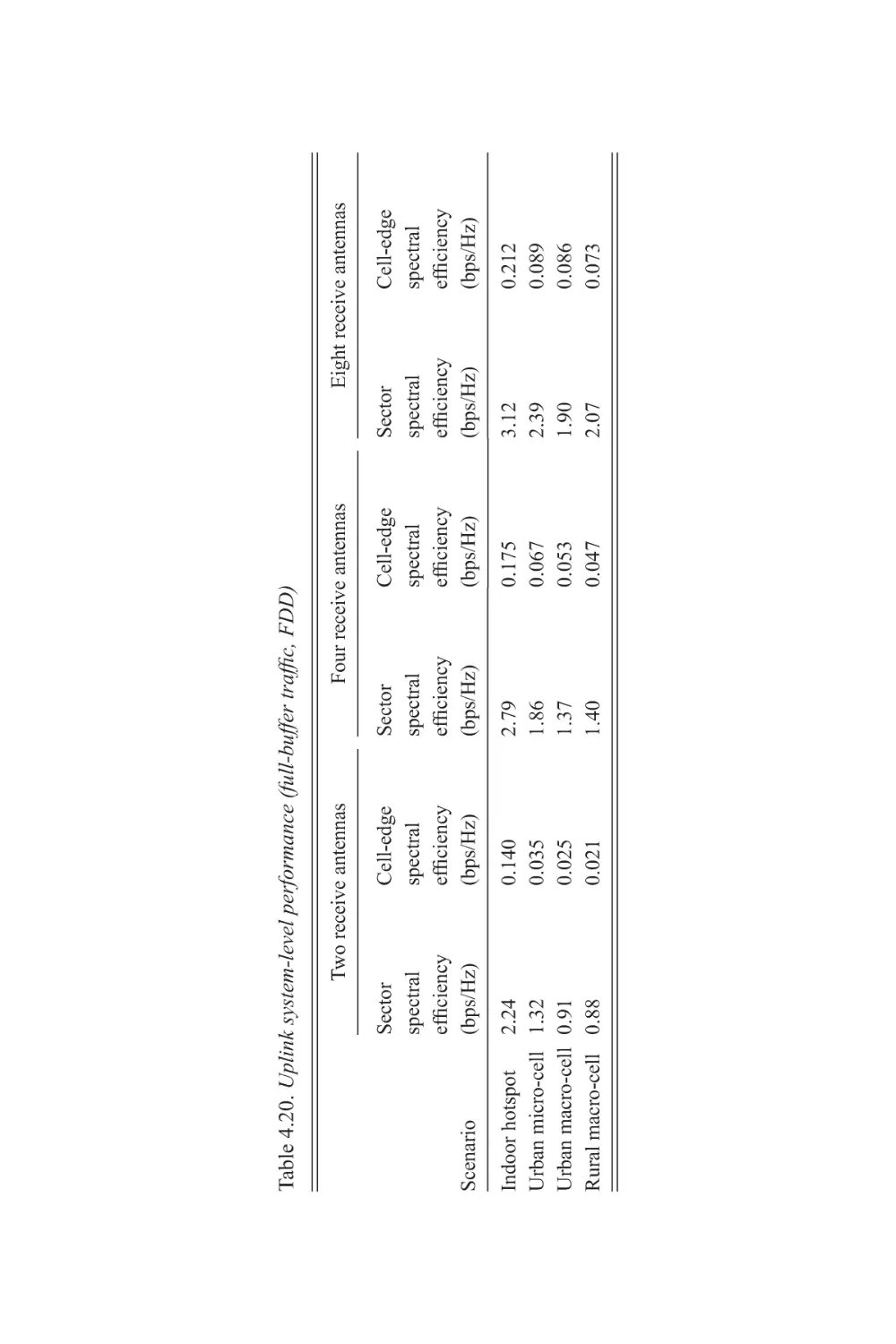
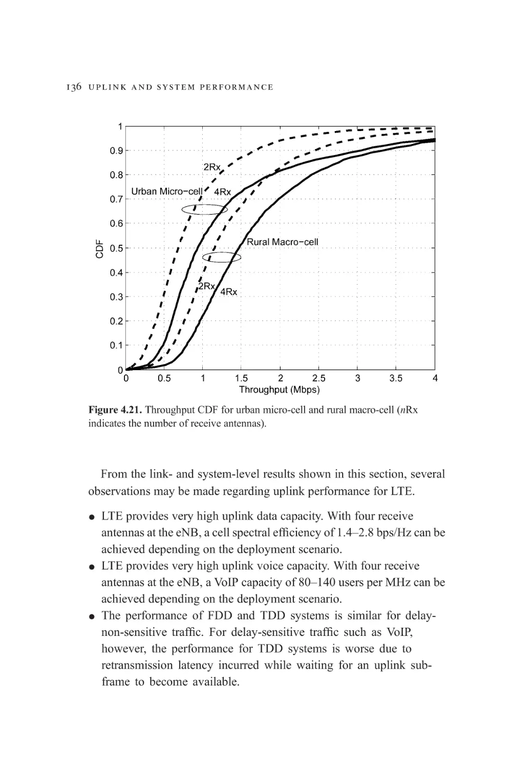
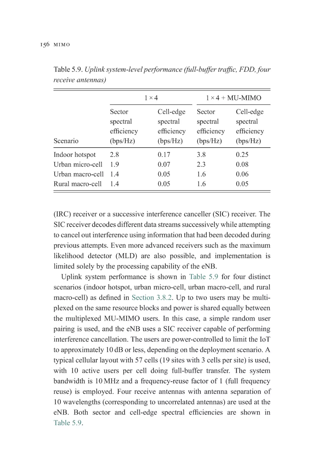
4.10 Performance results
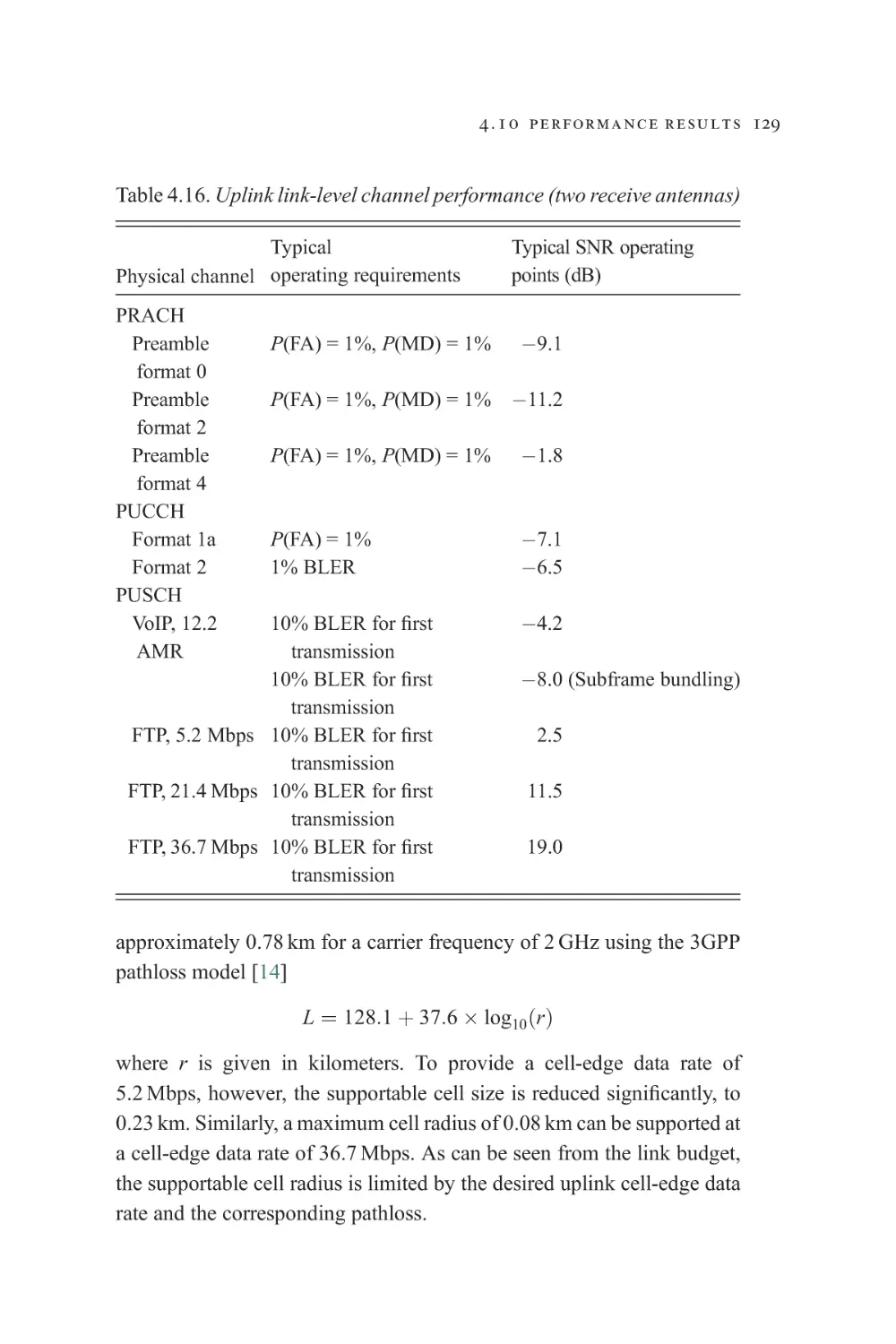
4.10.1 Link-level performance
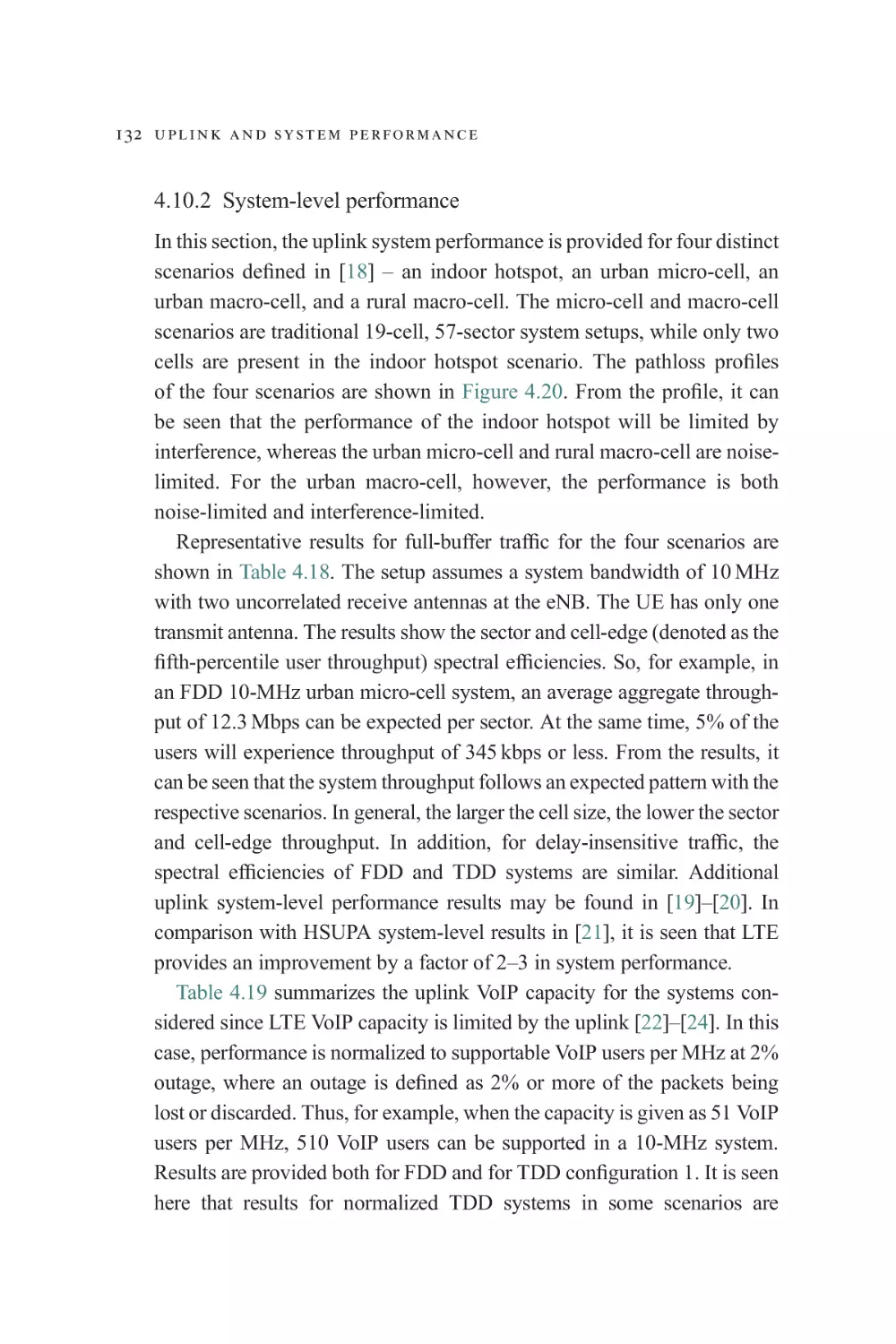
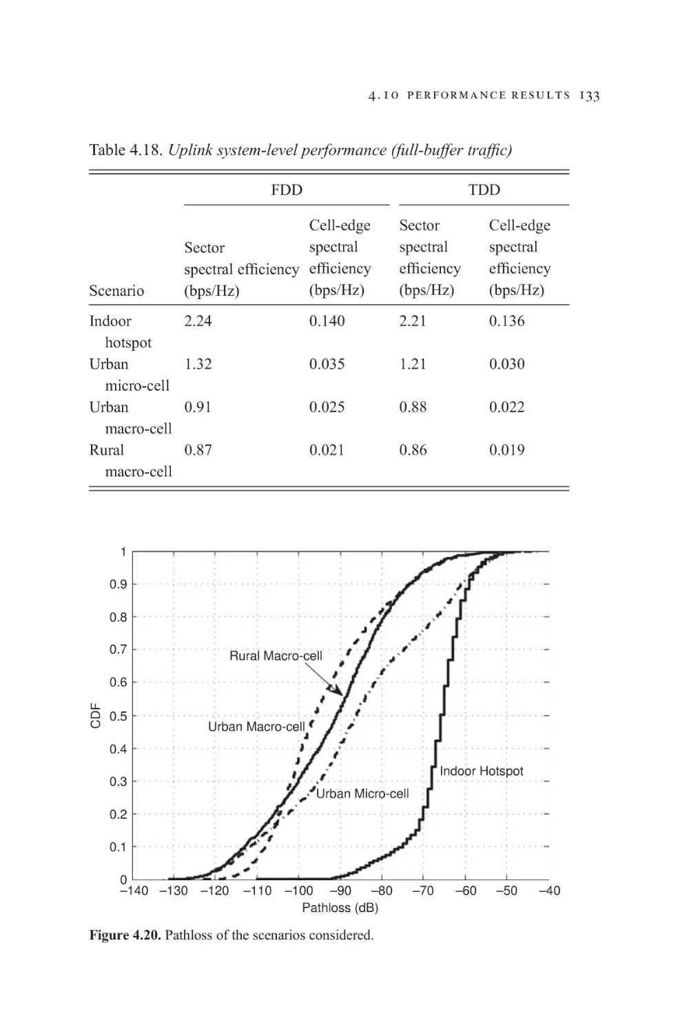
4.10.2 System-level performance
References
122
122
125
126
126
126
128
128
132
137
MIMO
5.1 Introduction
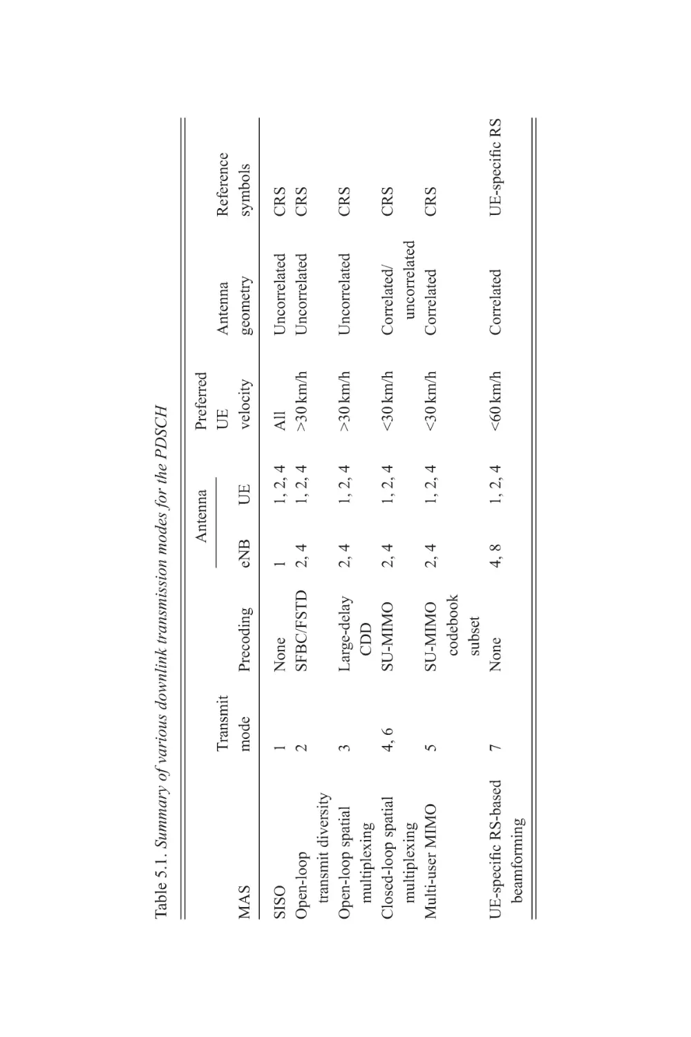
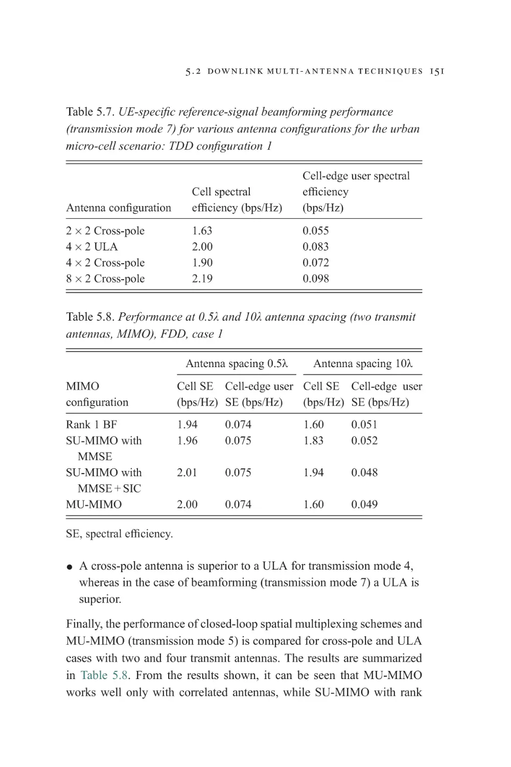
5.2 Downlink multi-antenna techniques
5.2.1 Transmission mode 2: transmit diversity
5.2.2 Transmission mode 3: precoder-based
open-loop spatial multiplexing
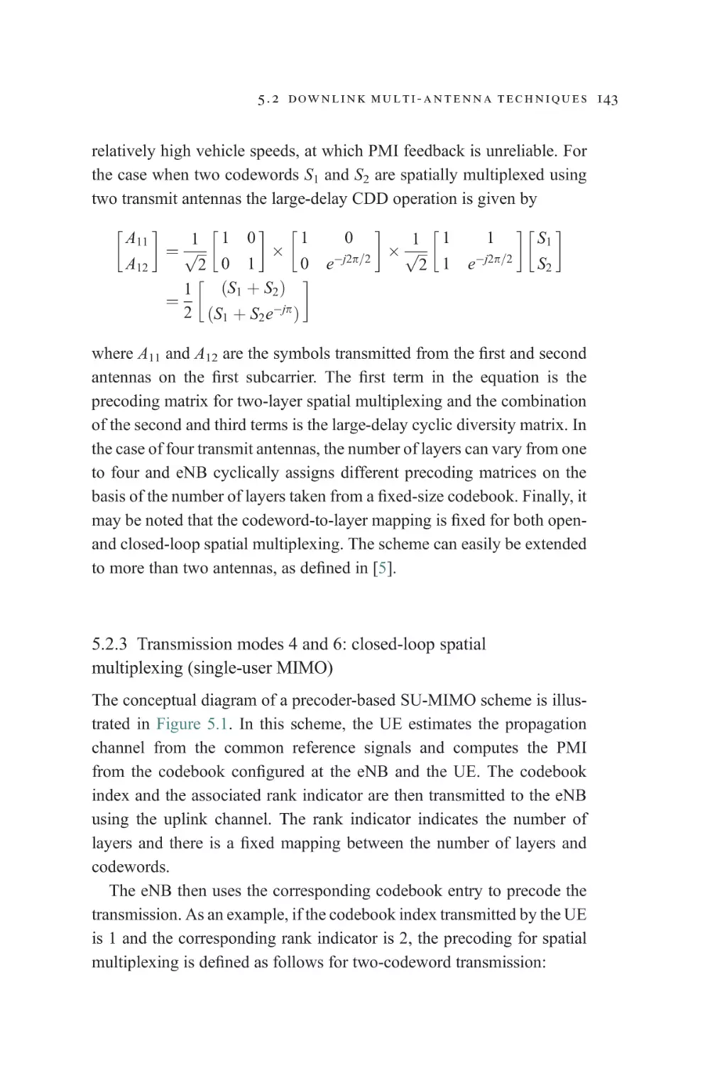
5.2.3 Transmission modes 4 and 6: closed-loop
spatial multiplexing (single-user MIMO)
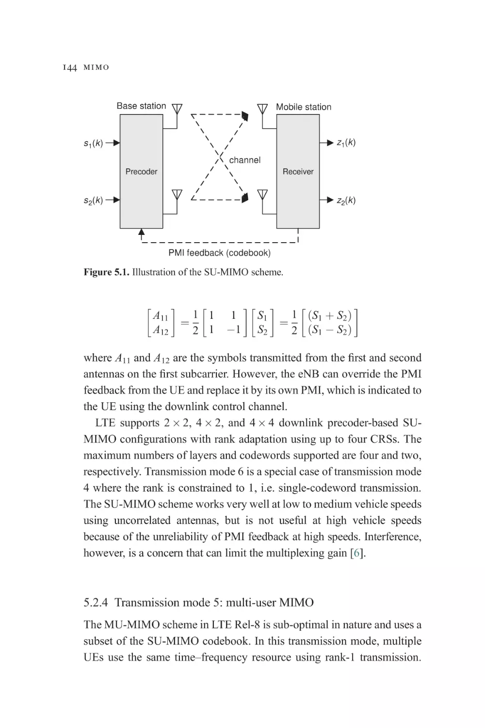
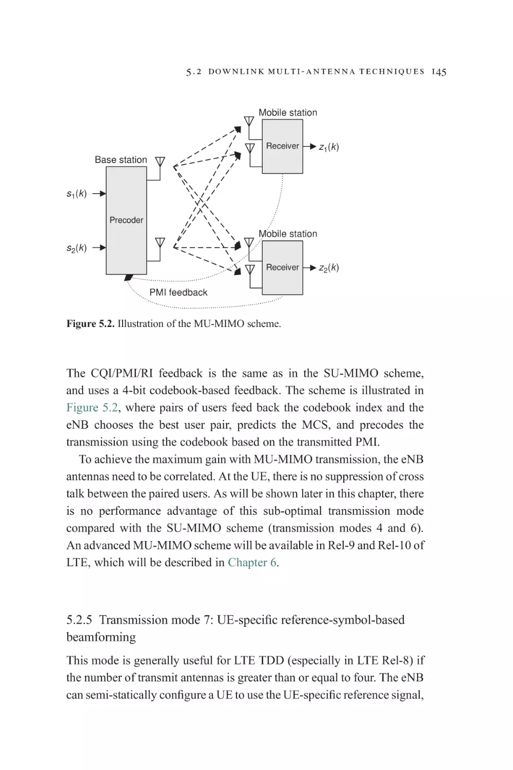
5.2.4 Transmission mode 5: multi-user MIMO
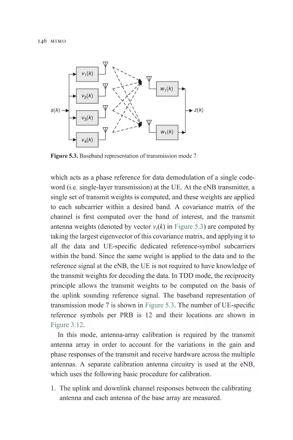
5.2.5 Transmission mode 7: UE-specific
reference-symbol-based beamforming
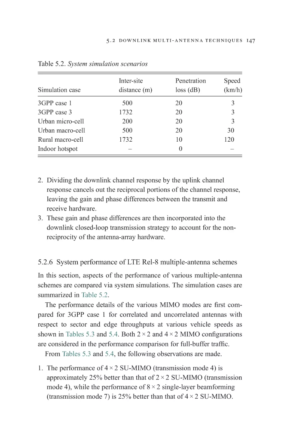
5.2.6 System performance of LTE Rel-8
multiple-antenna schemes
5.3 Uplink multi-antenna techniques
References
139
139
139
142
147
152
157
LTE-Advanced
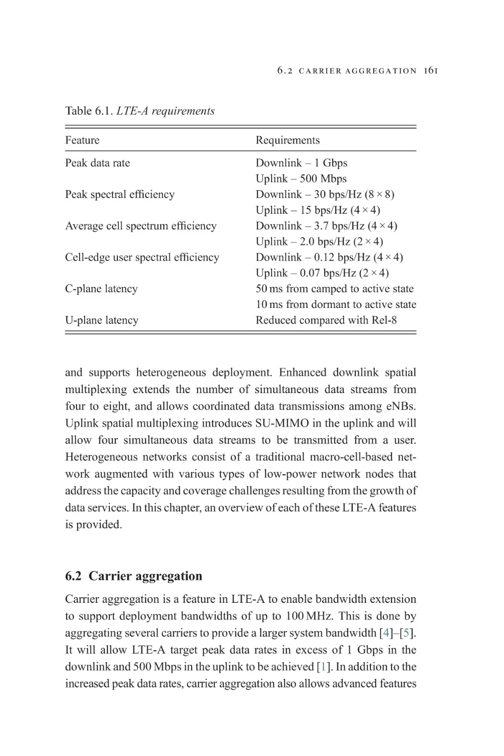
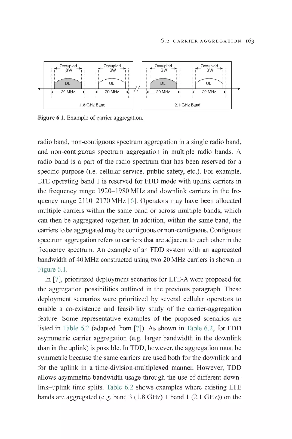
6.1 Introduction
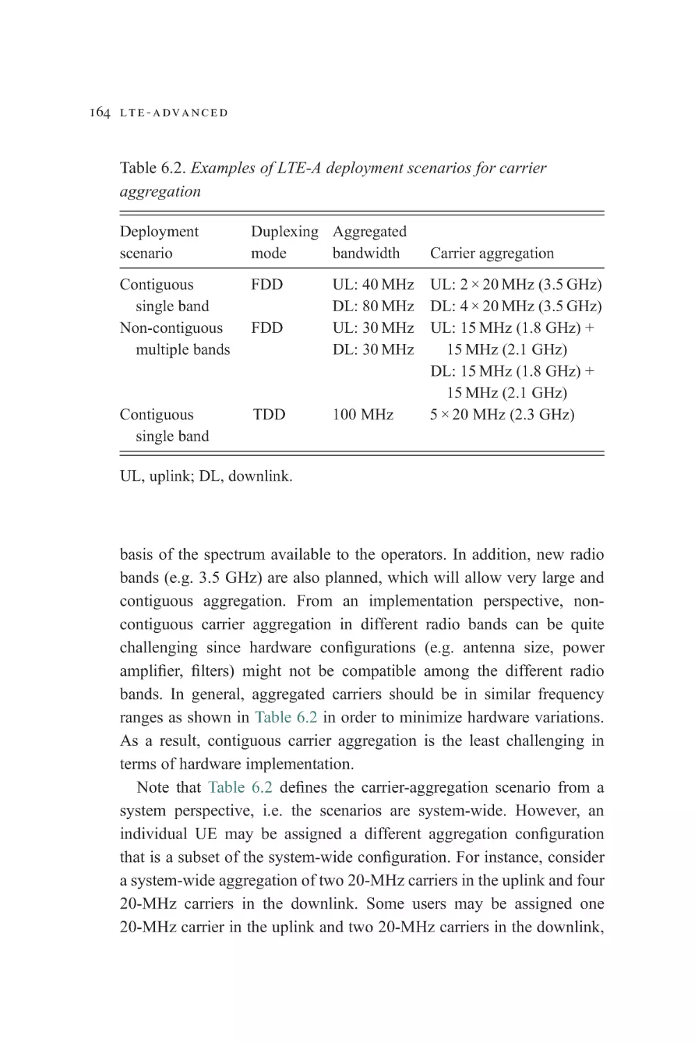
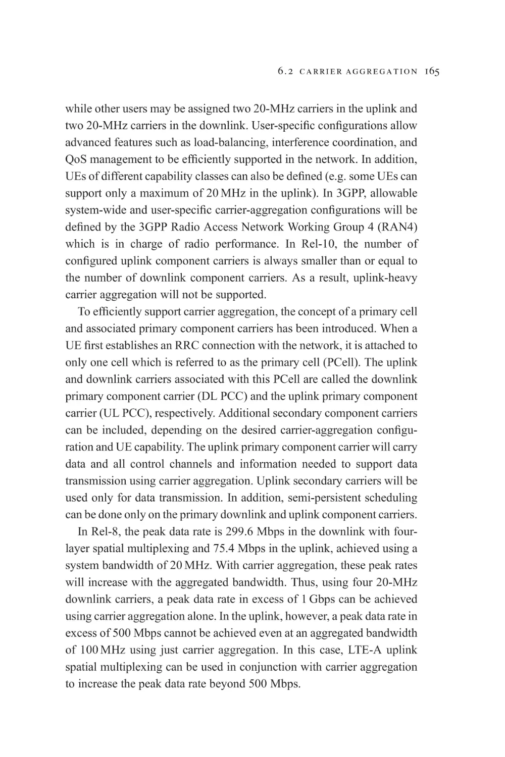
6.2 Carrier aggregation
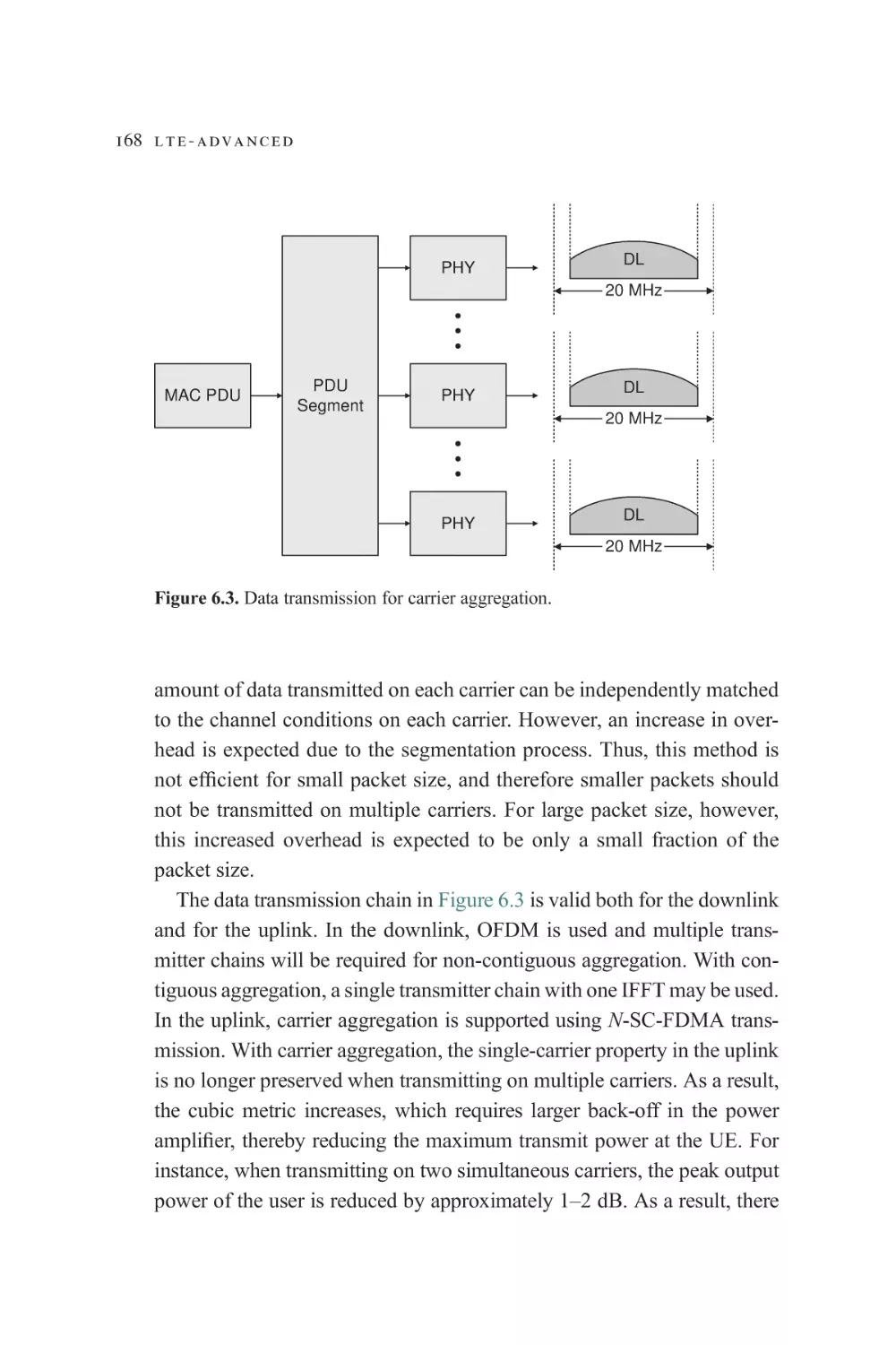
6.2.1 Data transmission
6.2.2 Control signaling
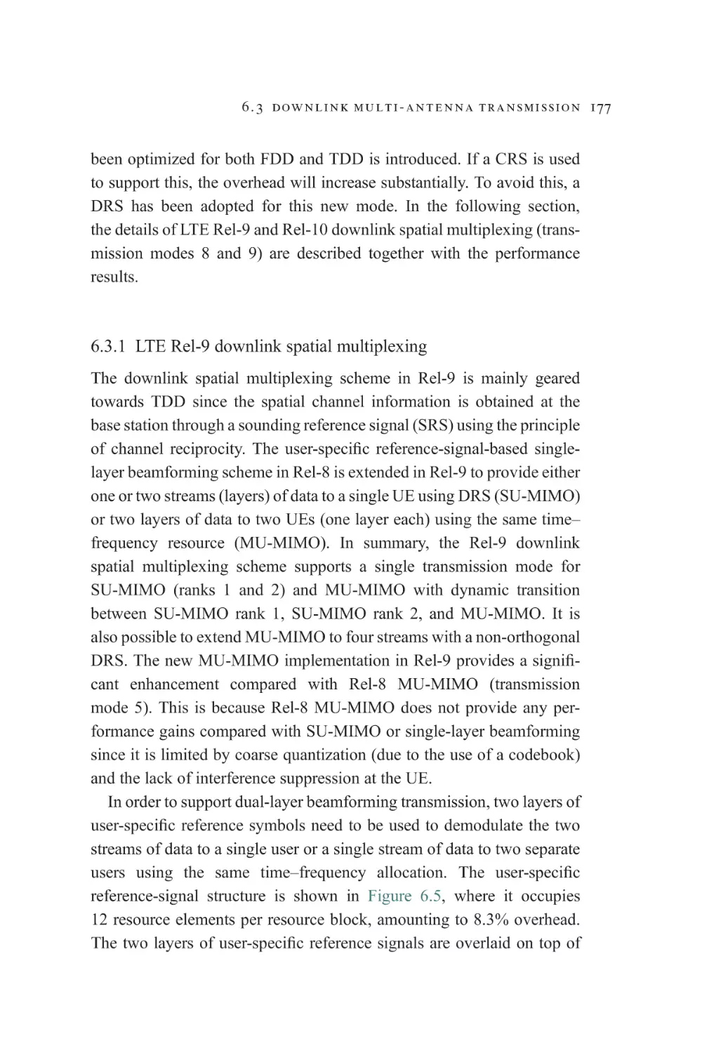
6.3 Downlink multi-antenna transmission
6.3.1 LTE Rel-9 downlink spatial multiplexing
6.3.2 LTE Rel-10 downlink spatial multiplexing
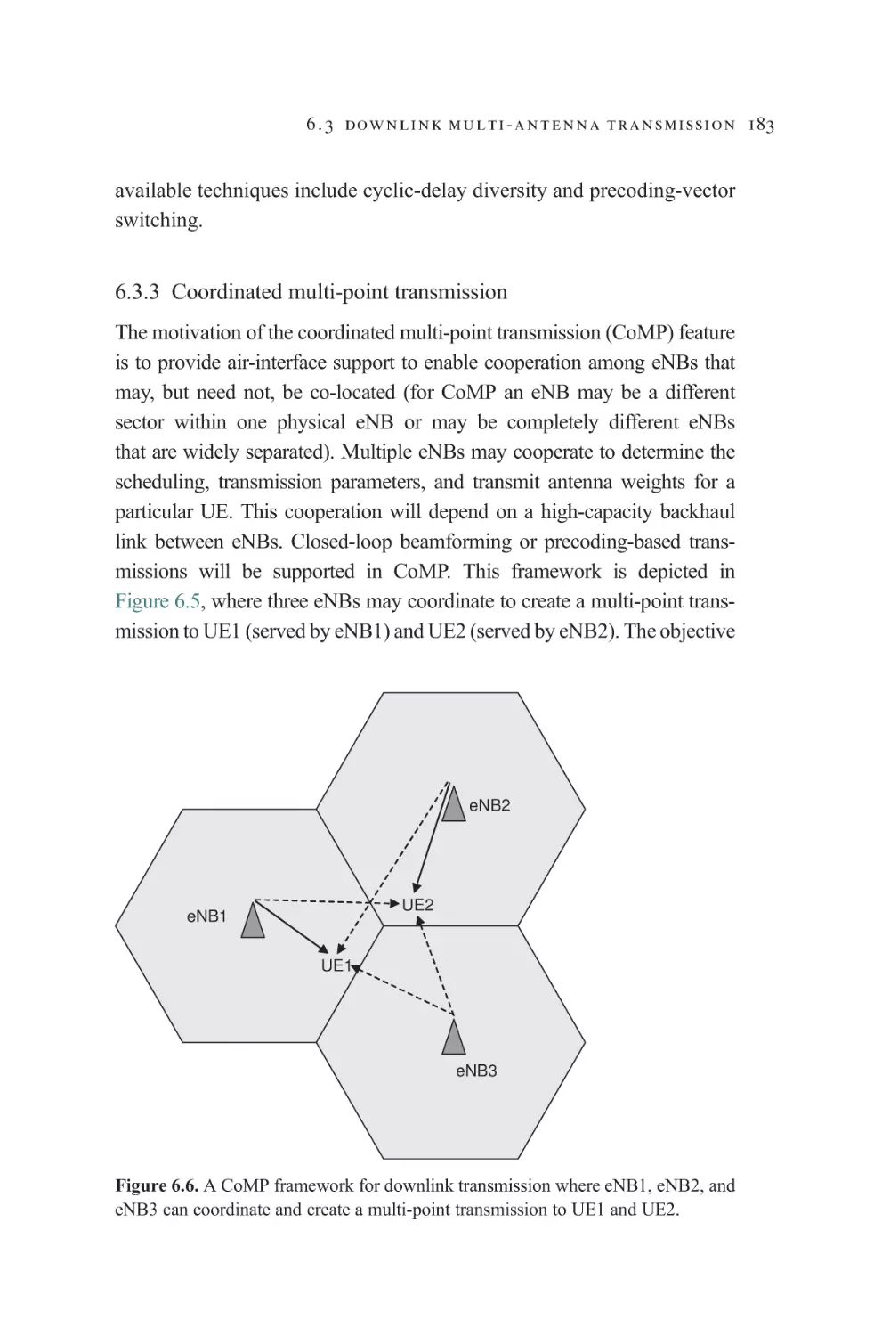
6.3.3 Coordinated multi-point transmission
160
160
161
167
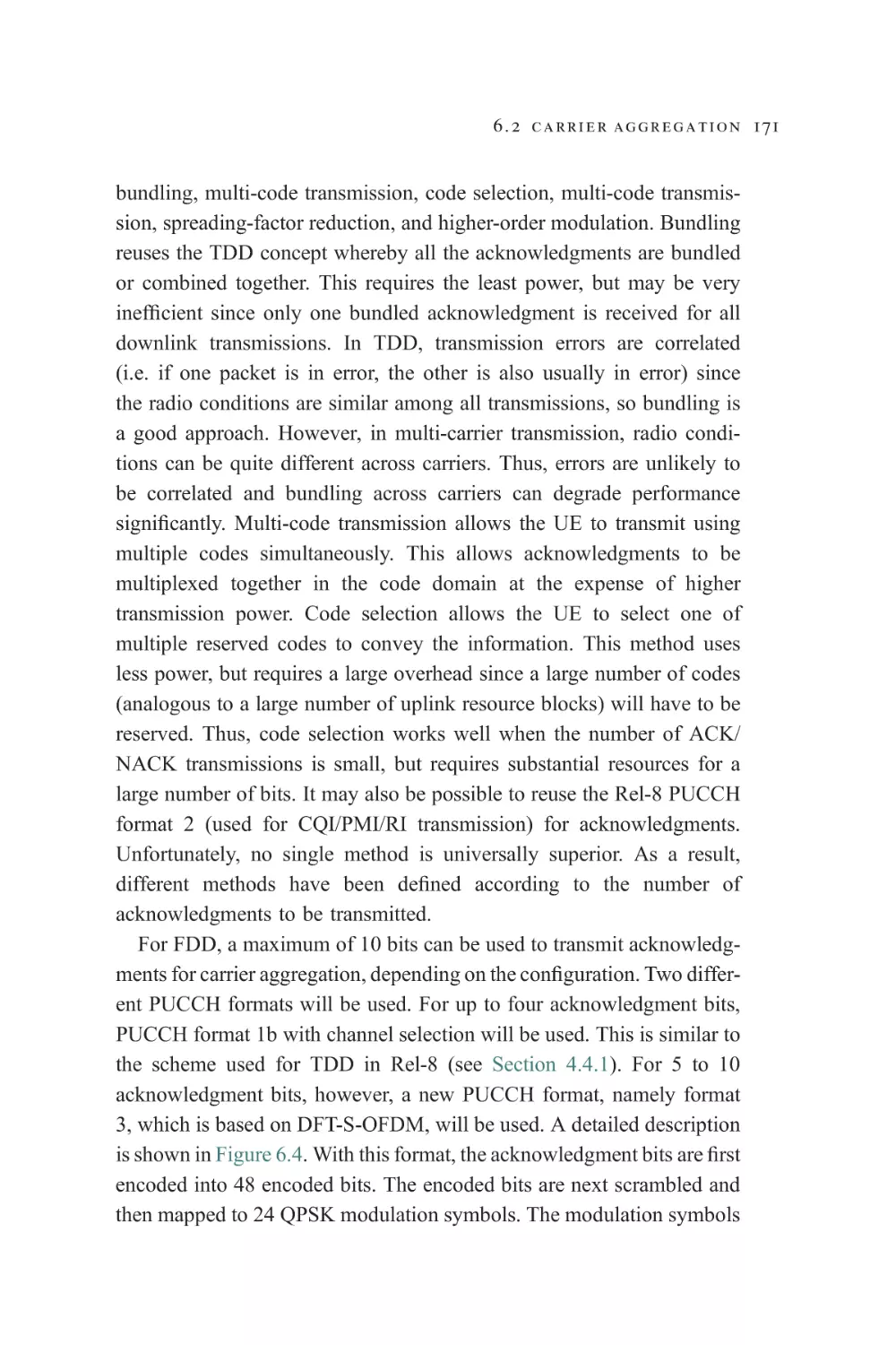
169
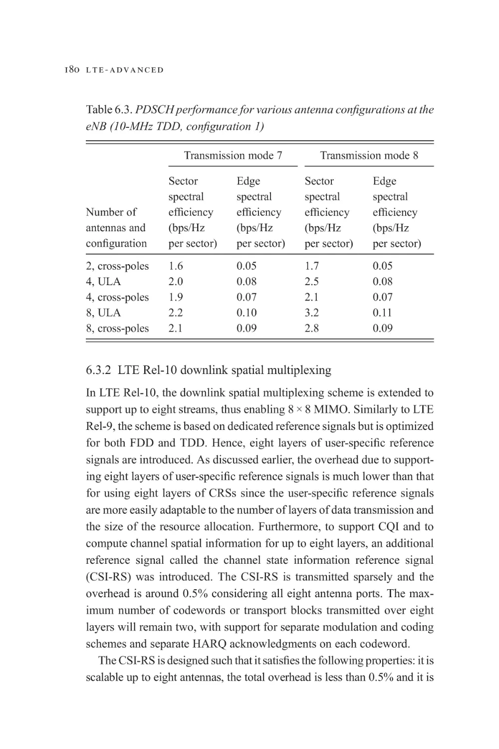
176
177
180
183
142
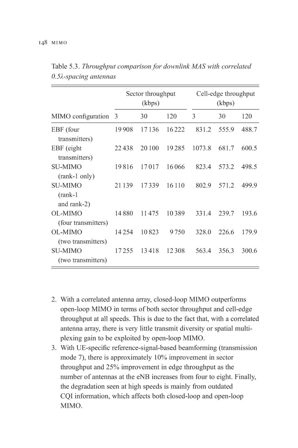
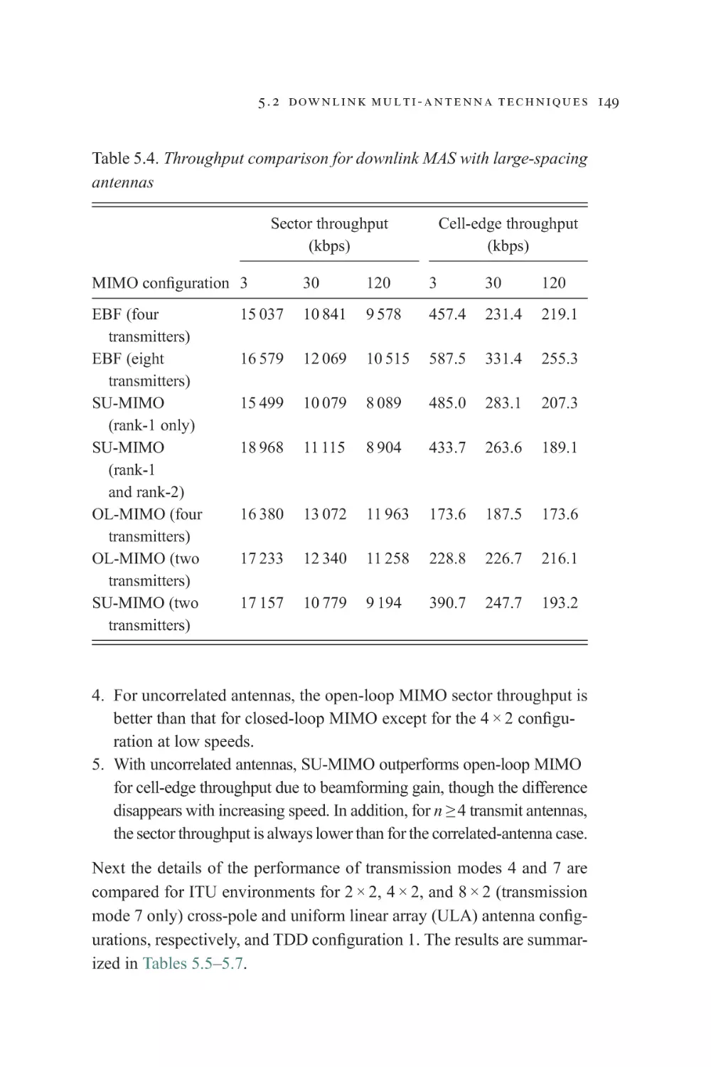
143
144
145
x contents
6.4 Uplink multi-antenna transmission
6.4.1 Control channels
6.4.2 Random-access channel
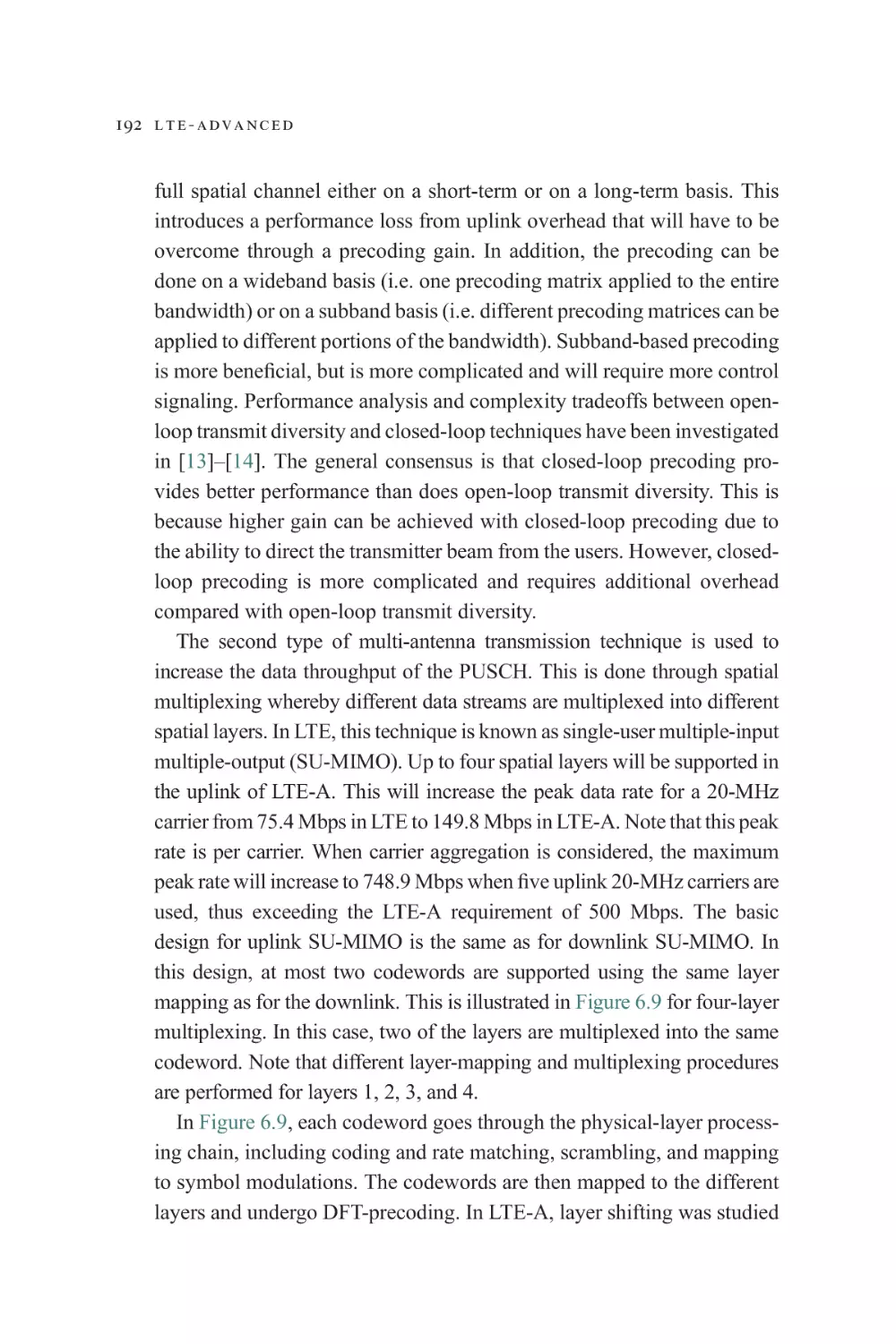
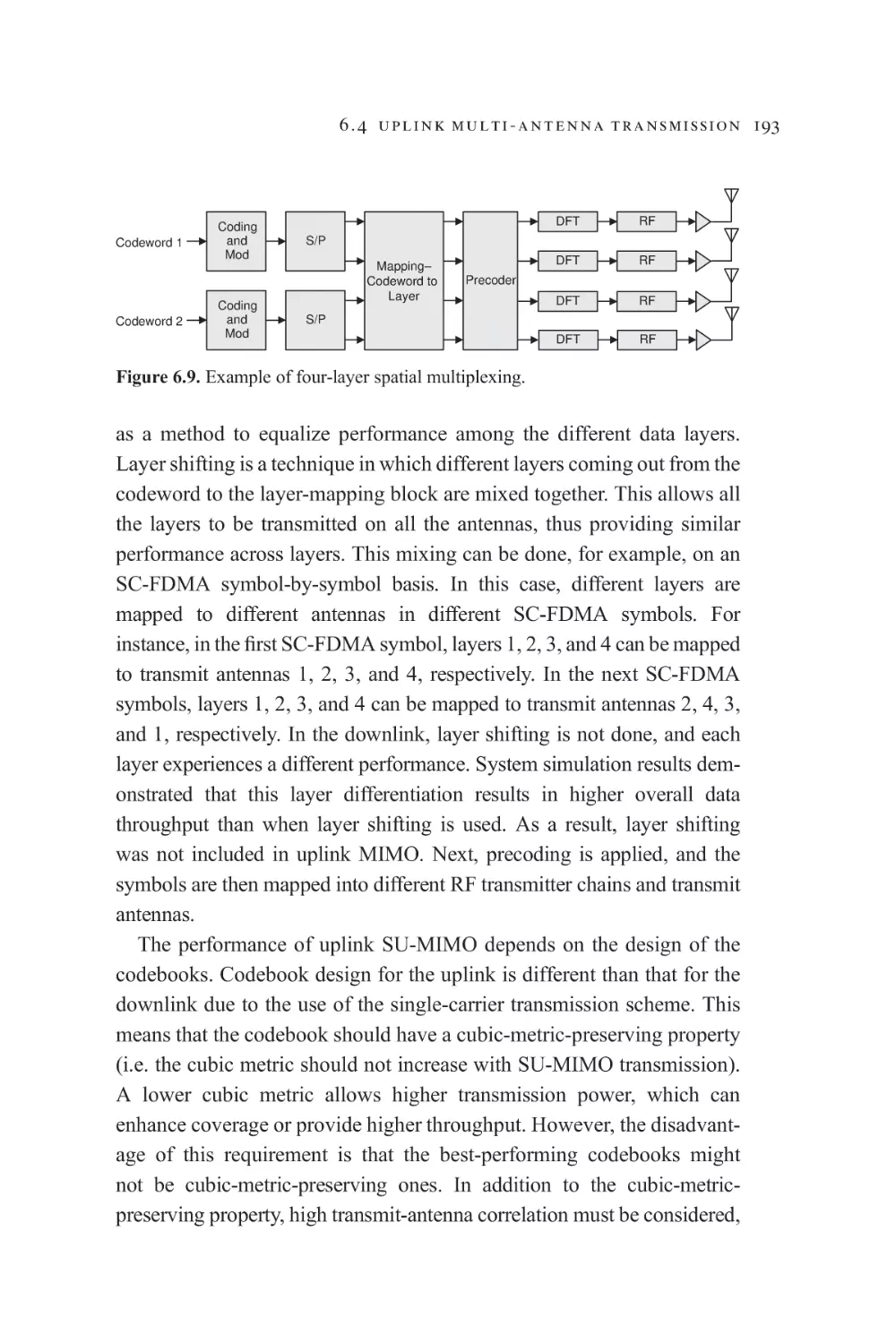
6.4.3 Data channel
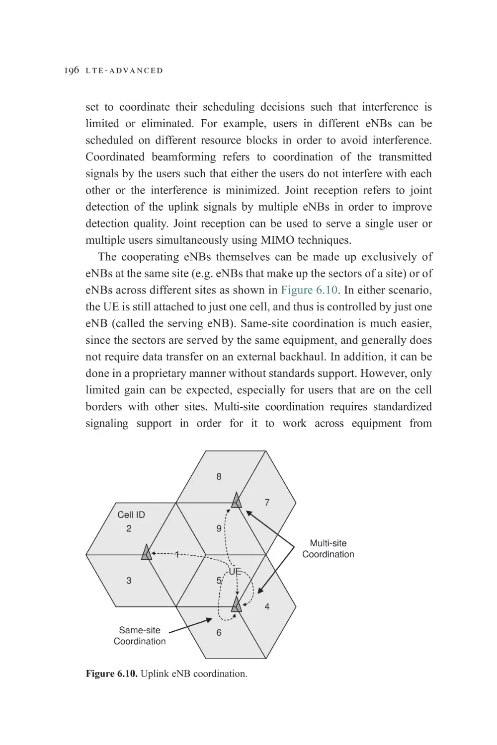
6.4.4 Coordinated multi-point reception
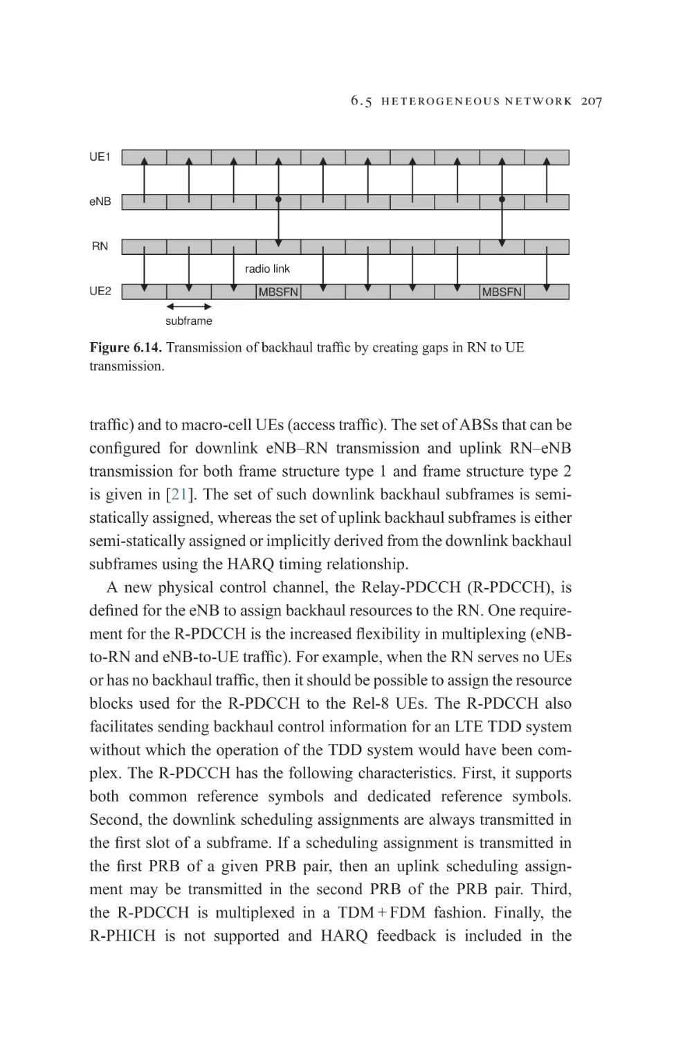
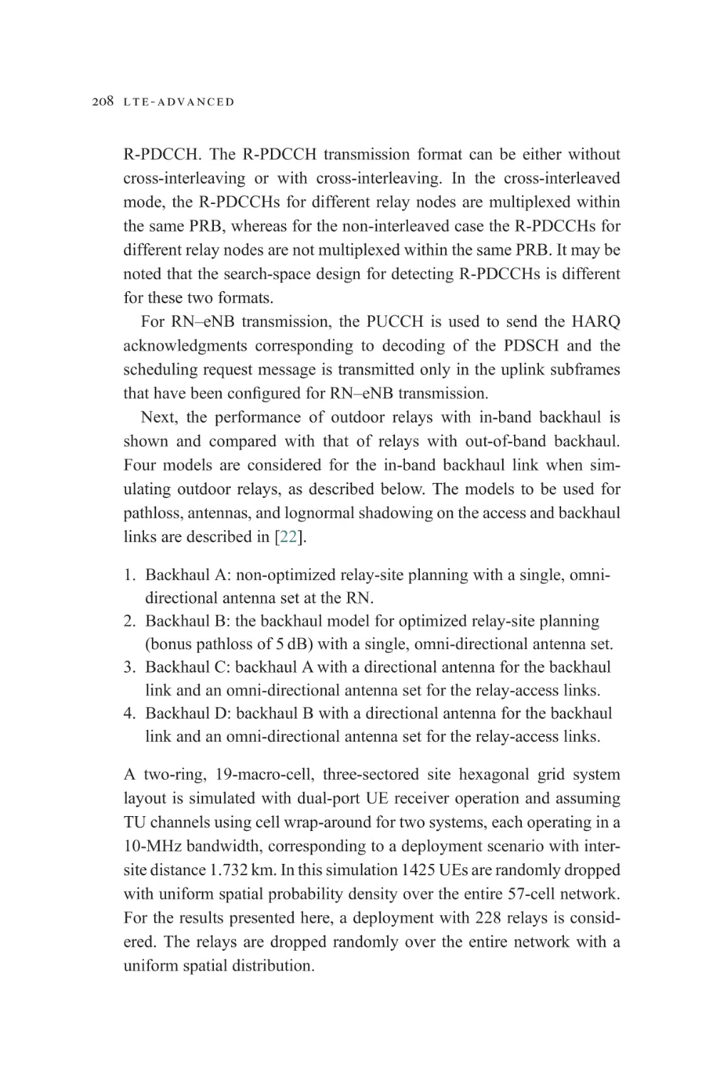
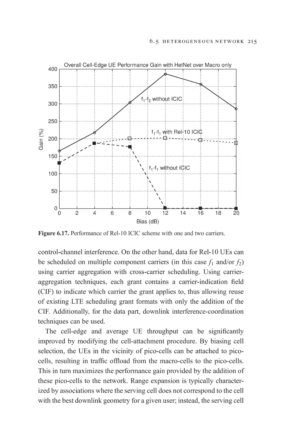
6.5 Heterogeneous network
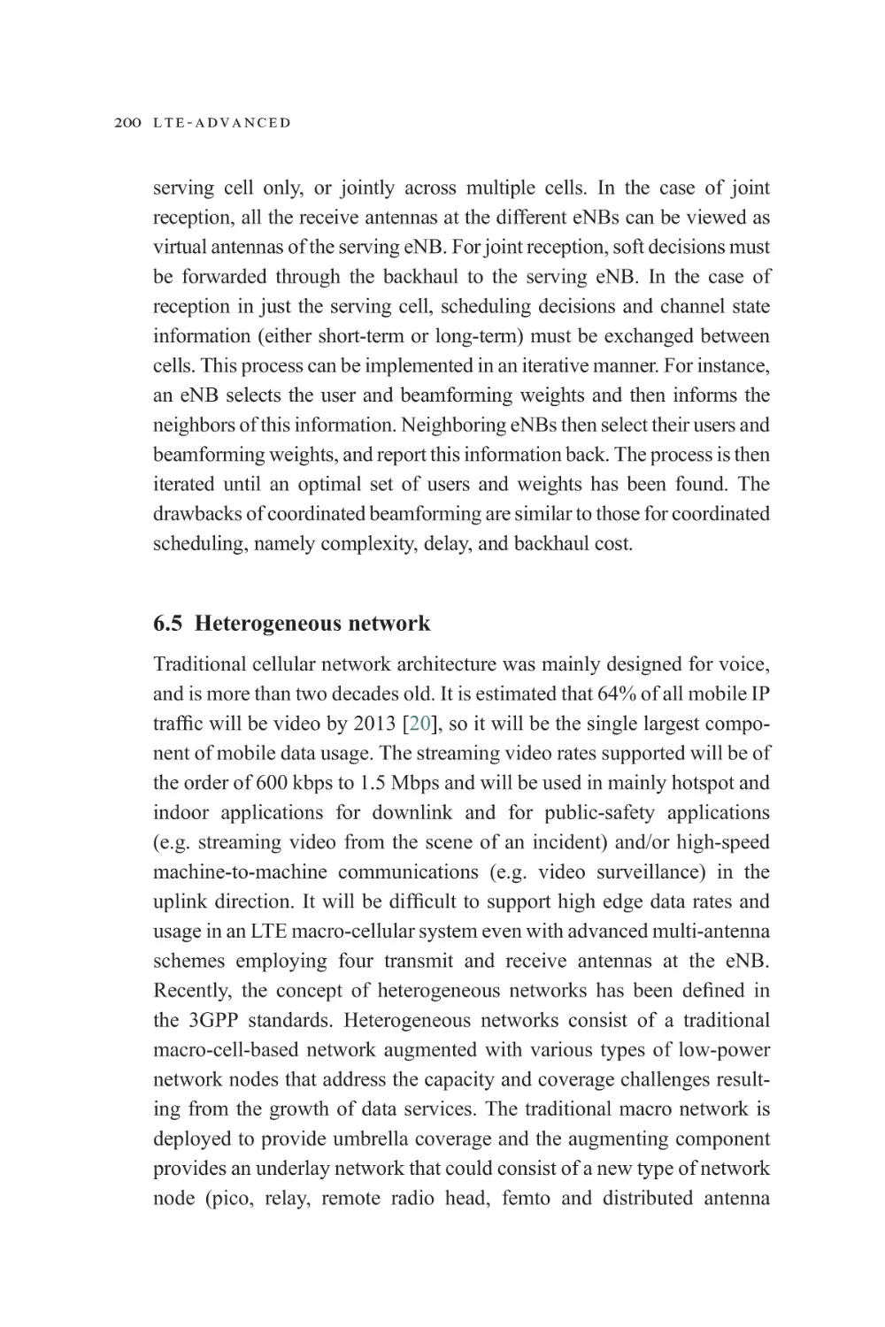
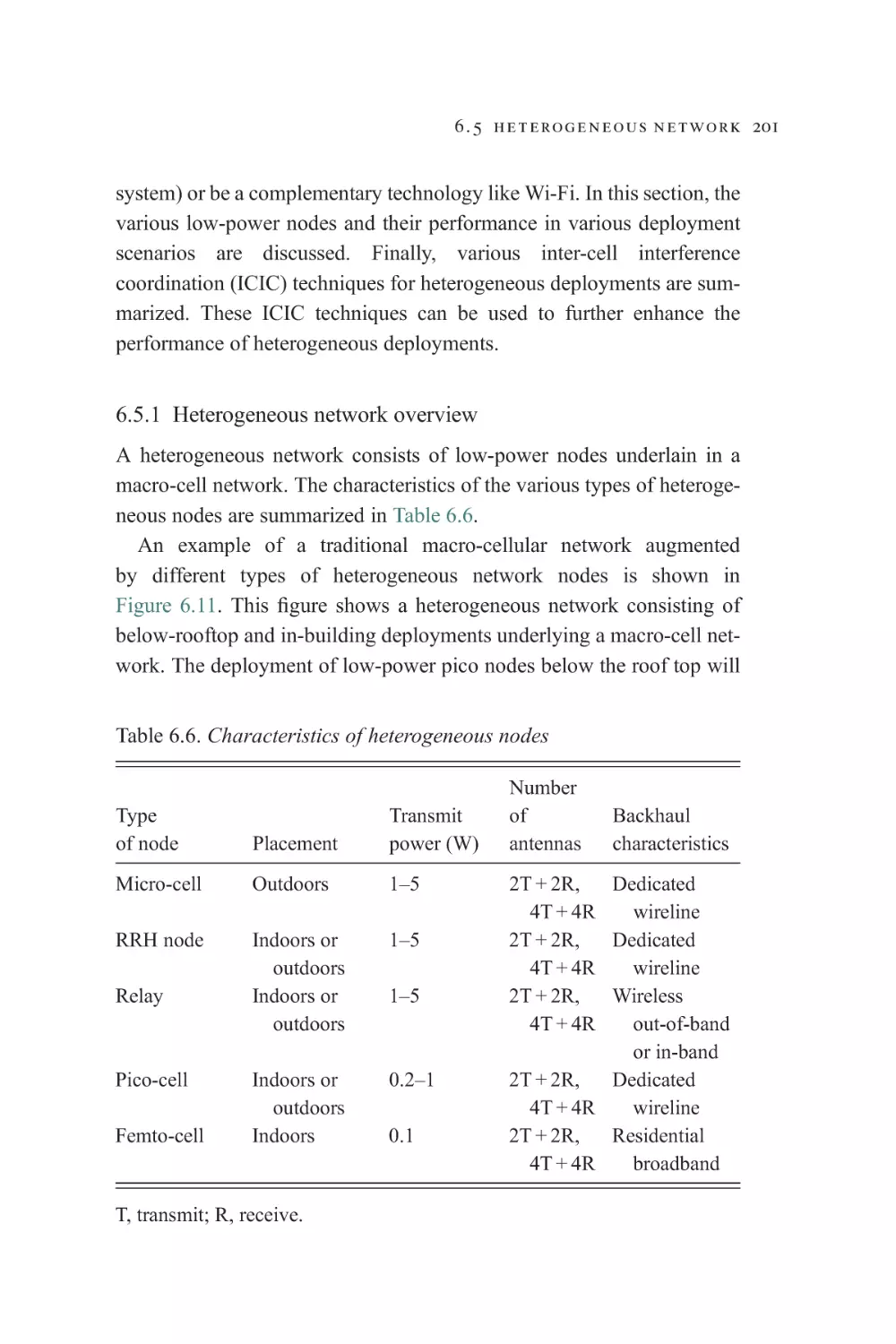
6.5.1 Heterogeneous network overview
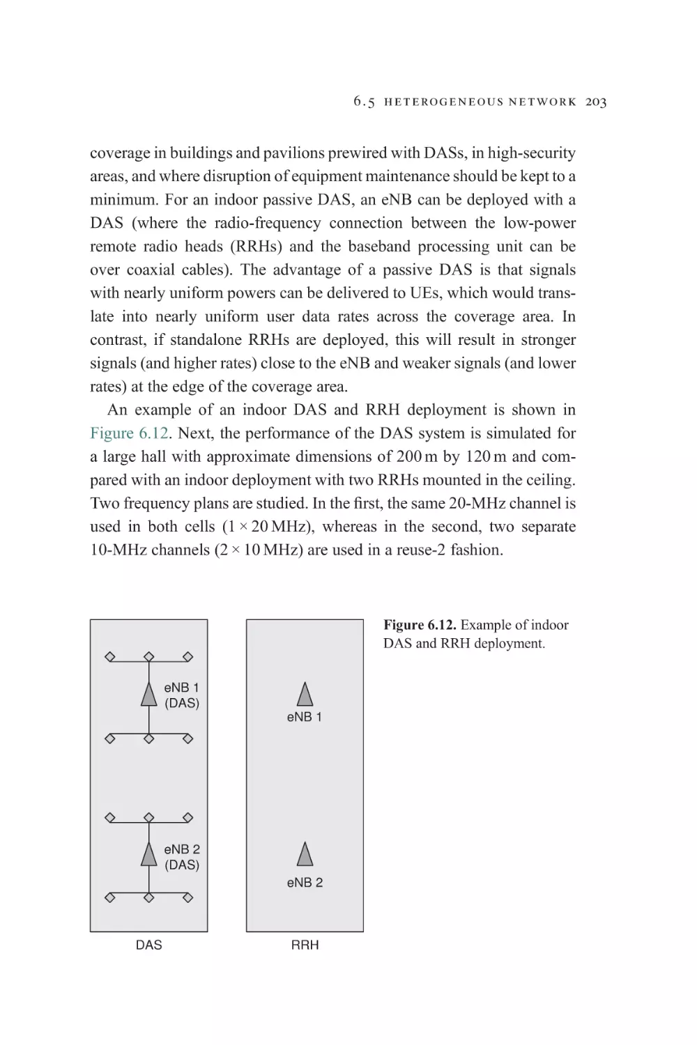
6.5.2 Indoor distributed-antenna system
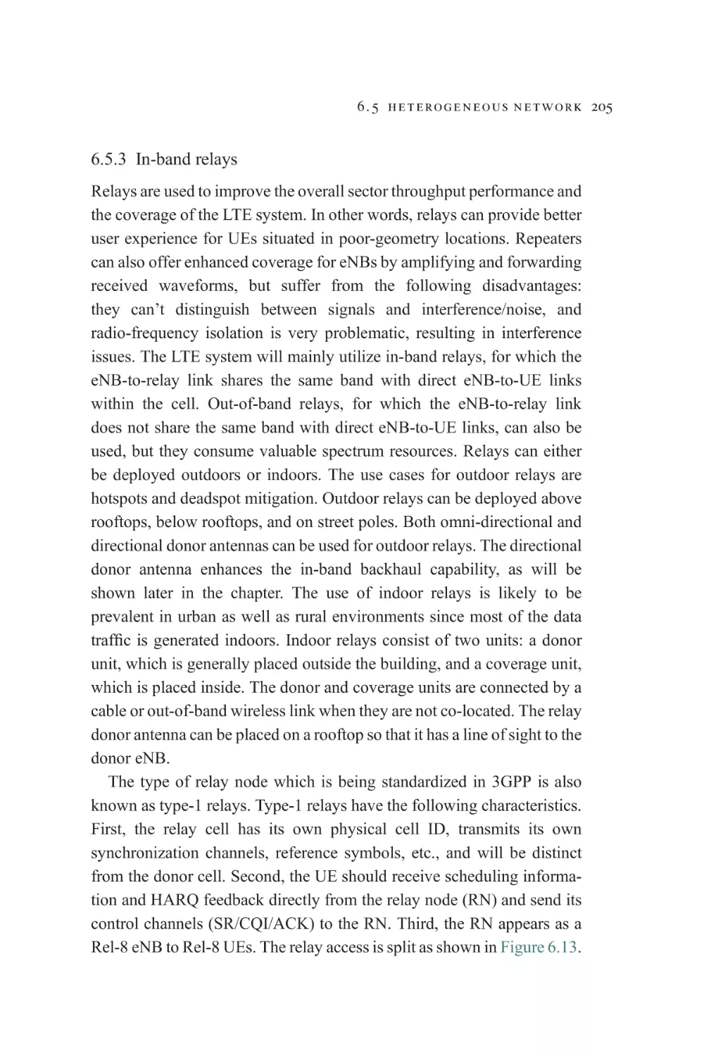
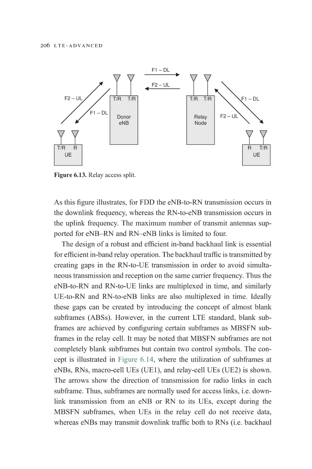
6.5.3 In-band relays
6.5.4 Pico- and femto-cell underlay
6.5.5 Interference-management techniques
for heterogeneous network
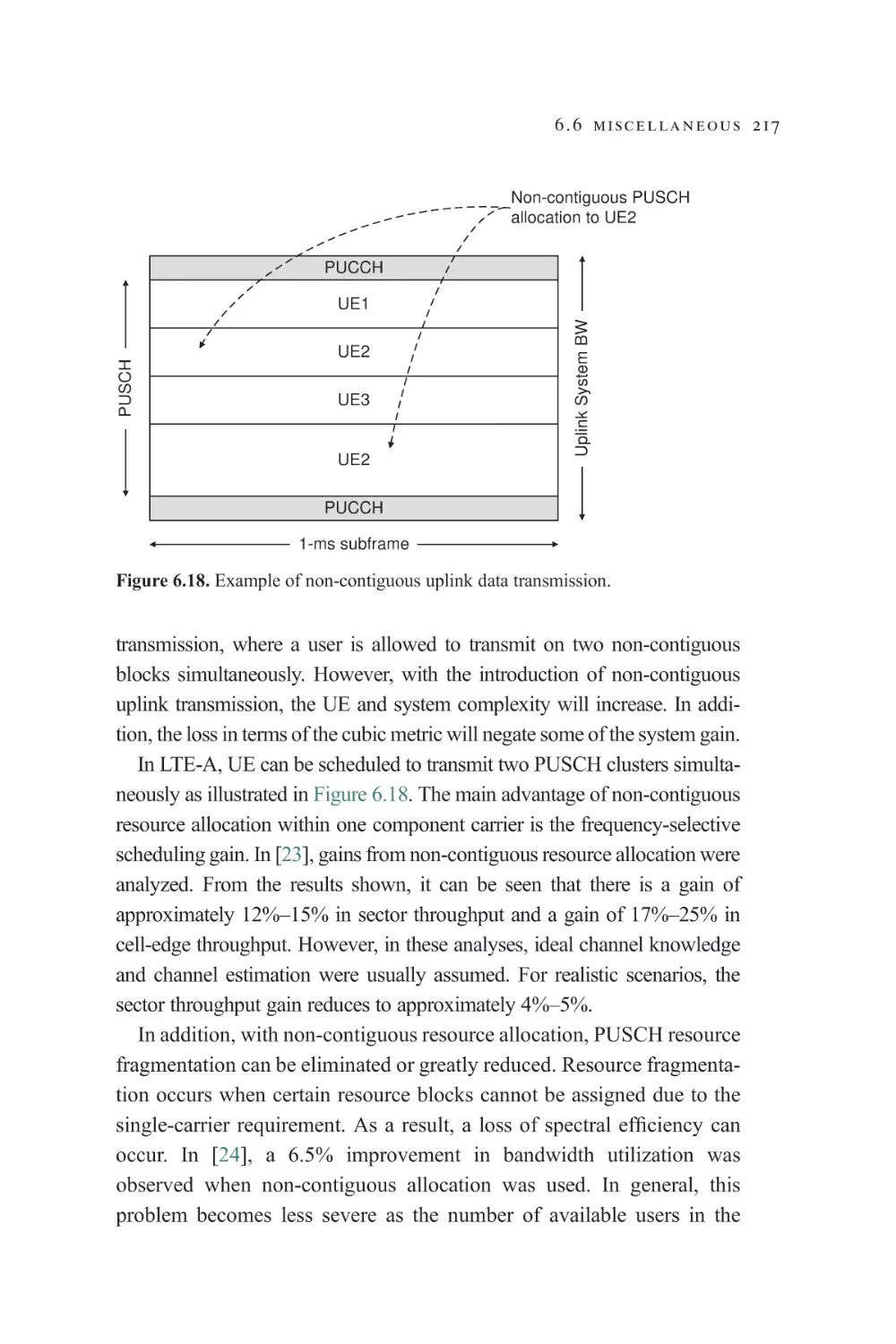
6.6 Miscellaneous
6.6.1 Non-contiguous uplink transmission
6.6.2 Aperiodic SRS
References
Additional reading
7
184
186
189
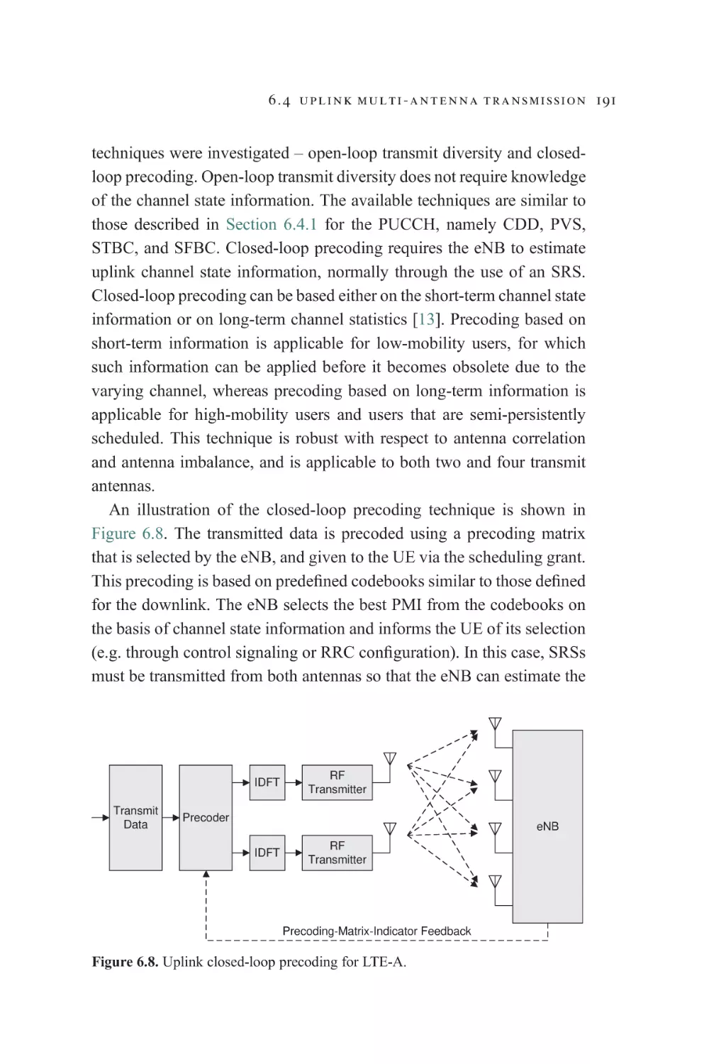
190
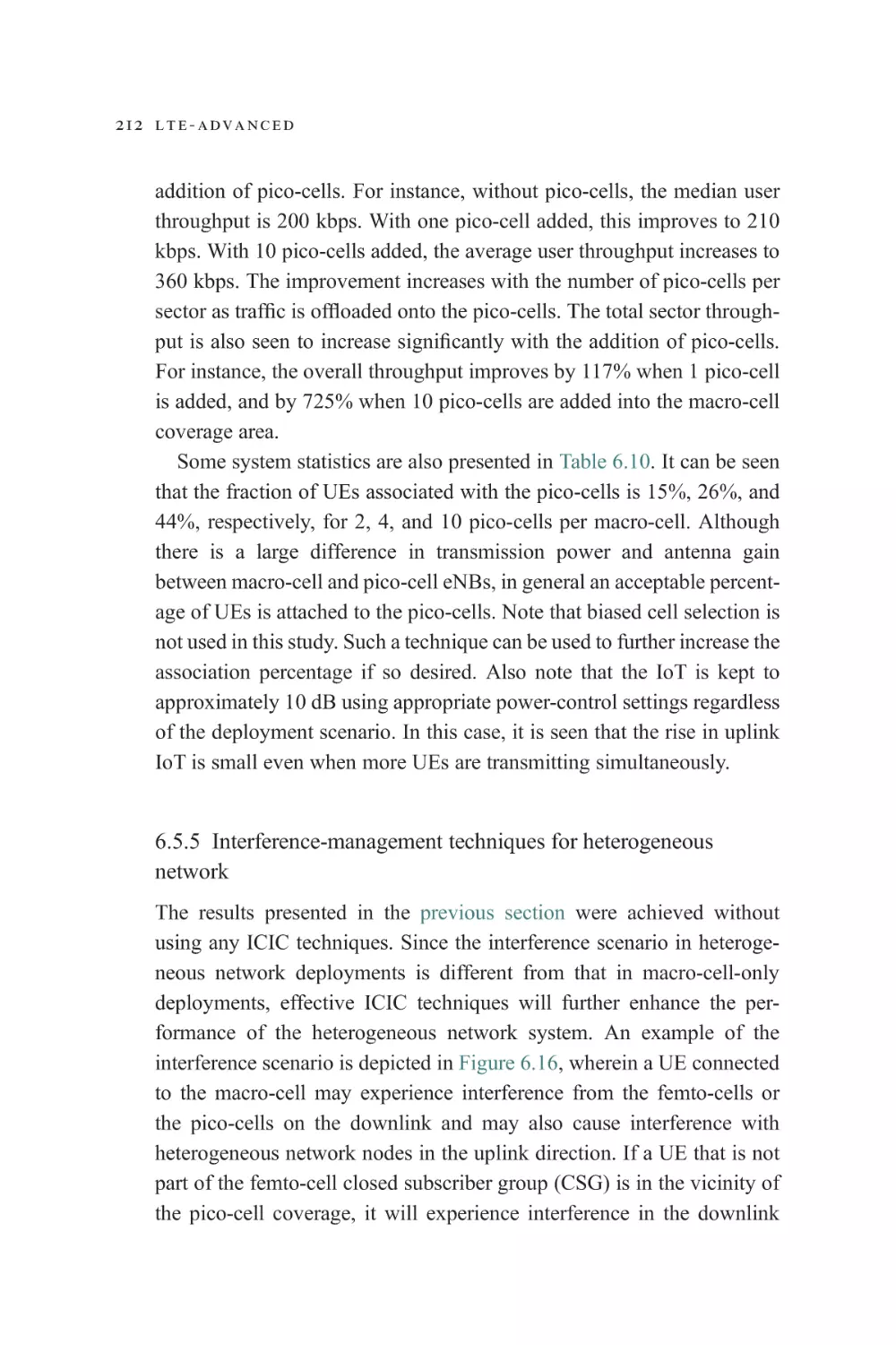
195
200
201
202
205
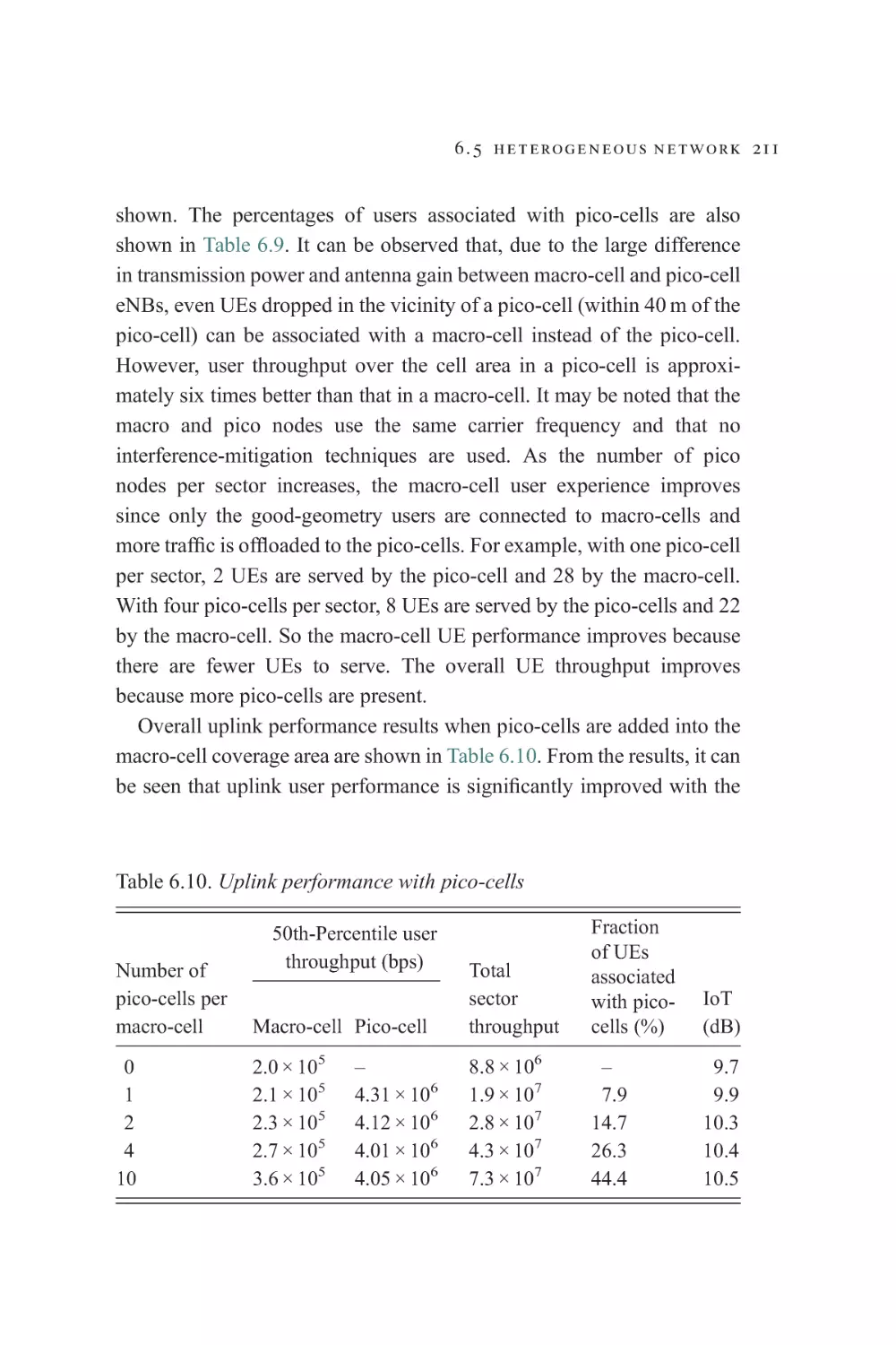
210
212
216
216
218
218
220
Comparison of broadband technologies
7.1 Introduction
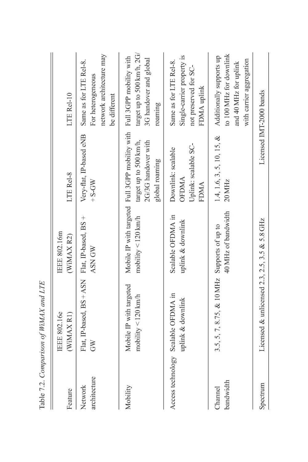
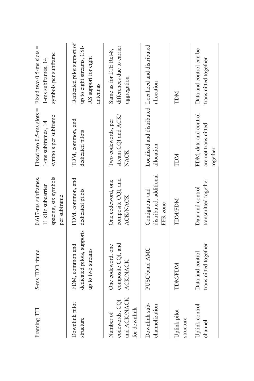
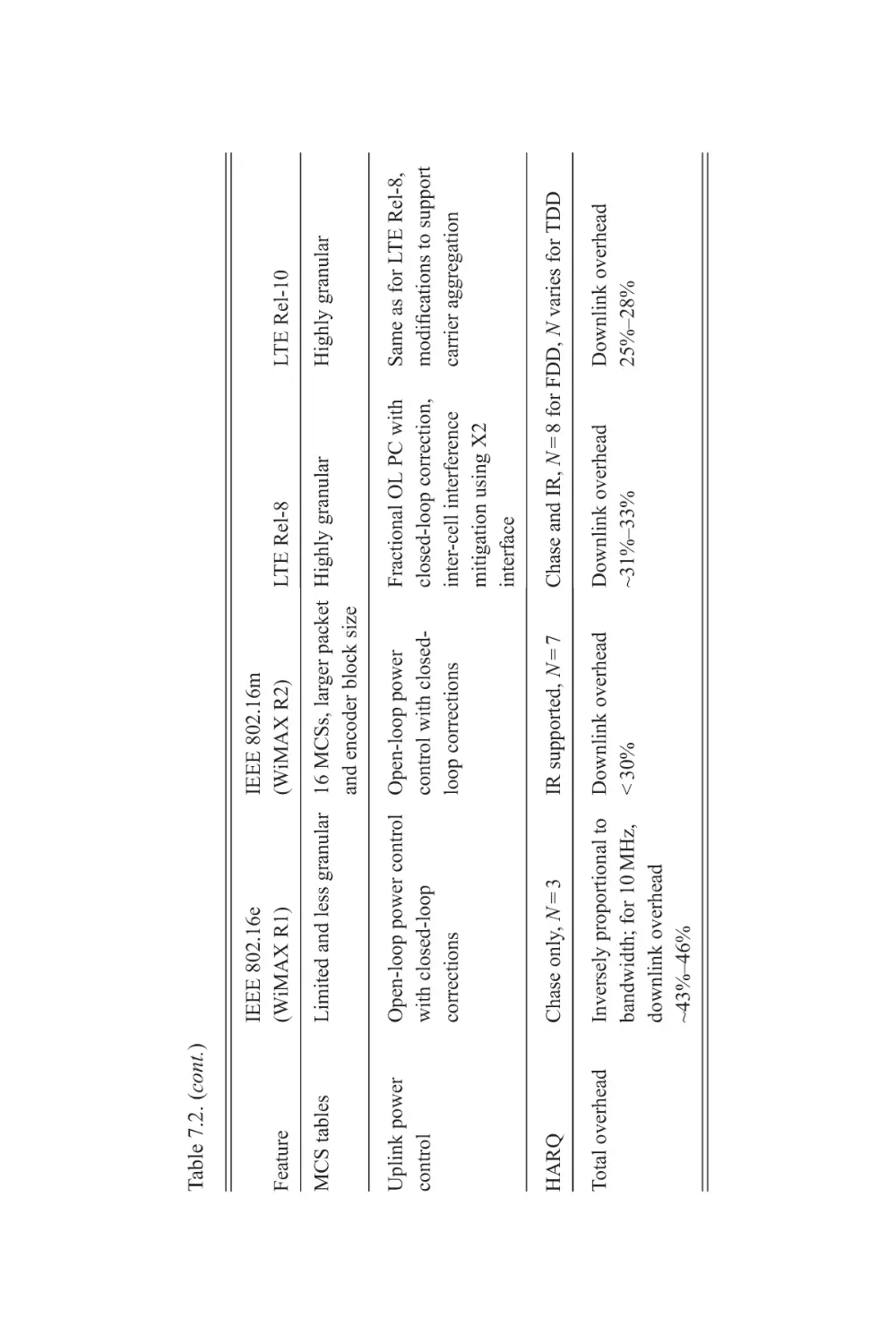
7.2 Feature comparison of wireless broadband
technologies
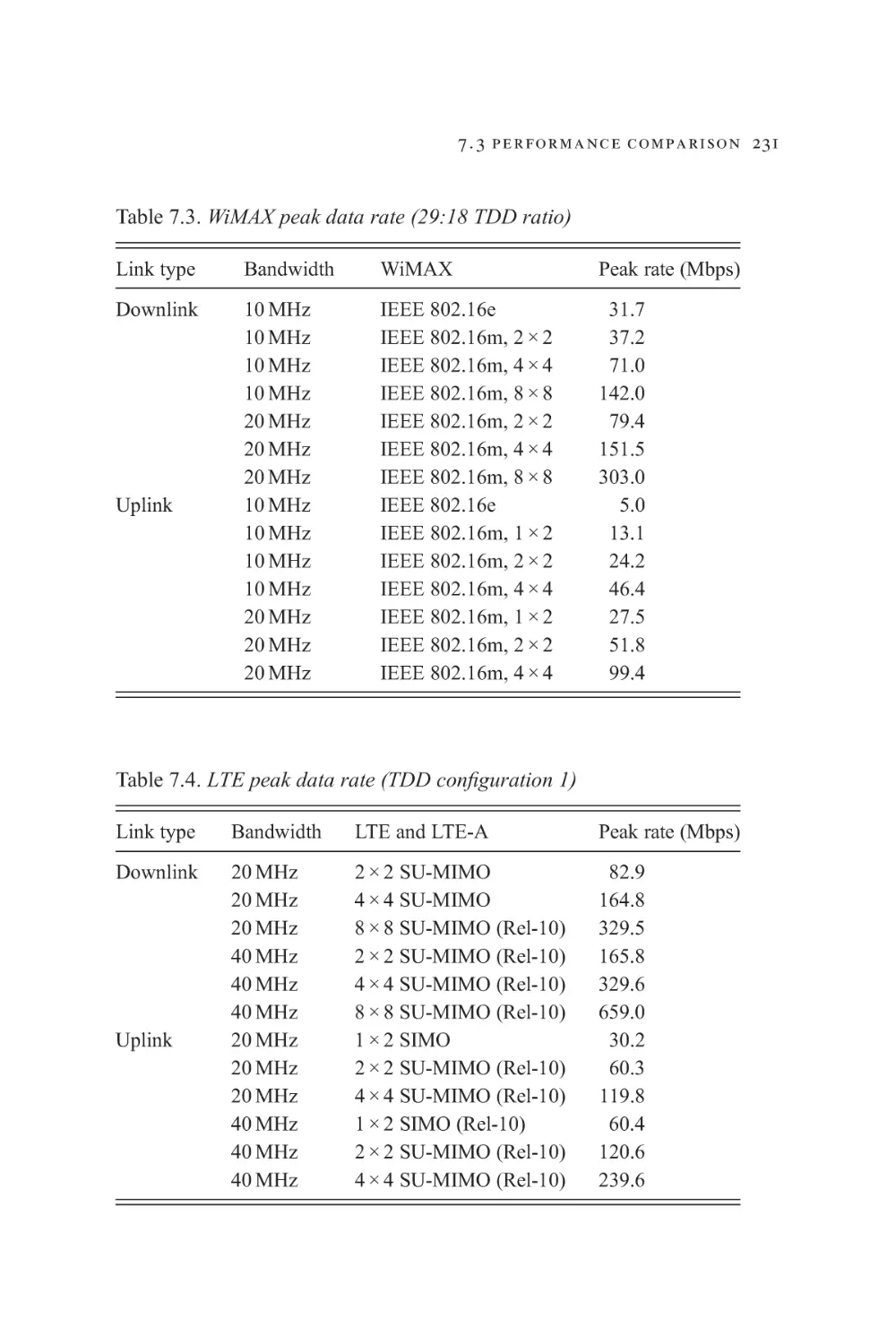
7.3 Performance comparison of LTE/LTE-A and
WiMAX/802.16m
7.4 Migration and co-existence scenarios
Additional reading
222
222
Appendix
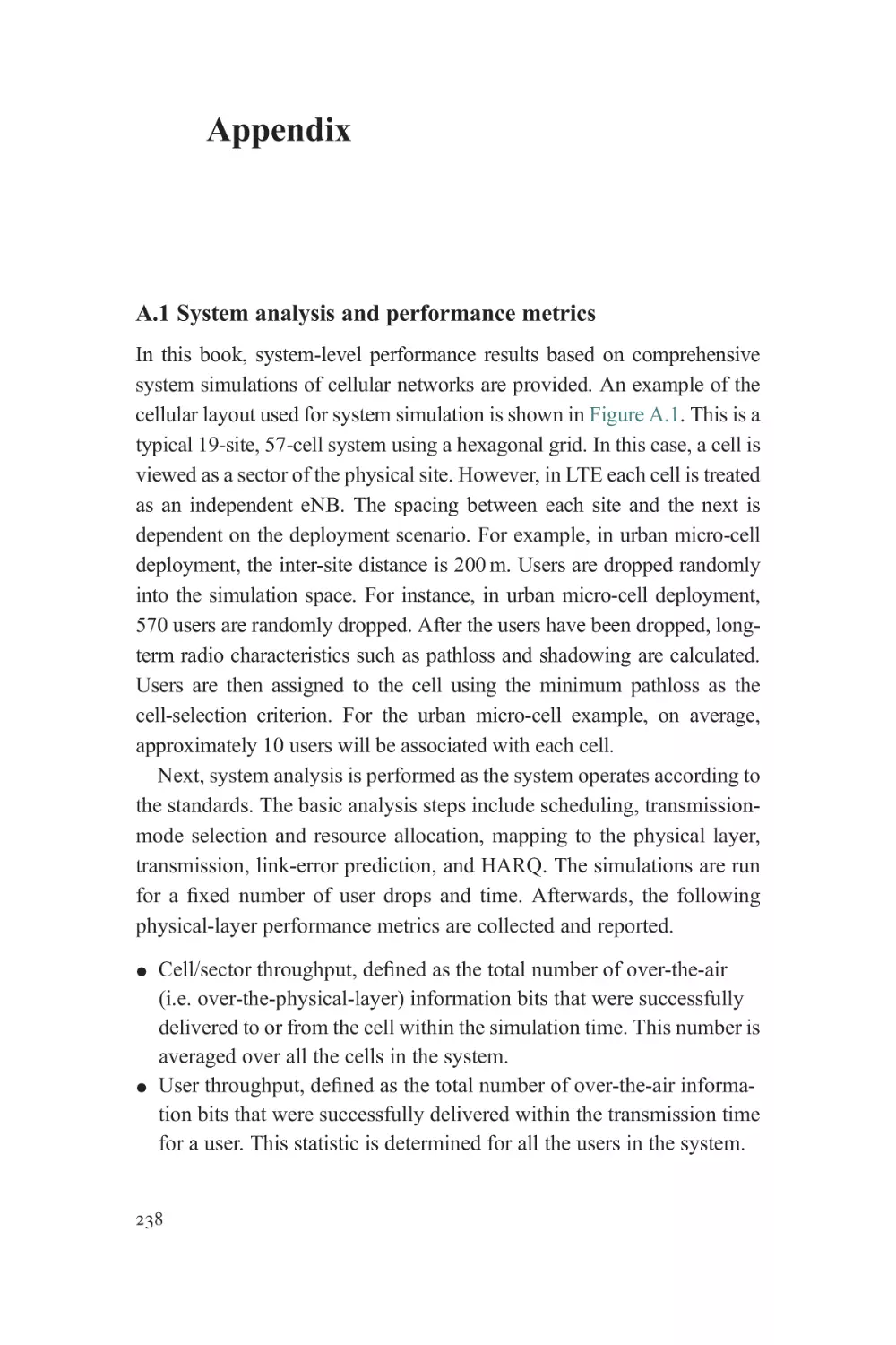
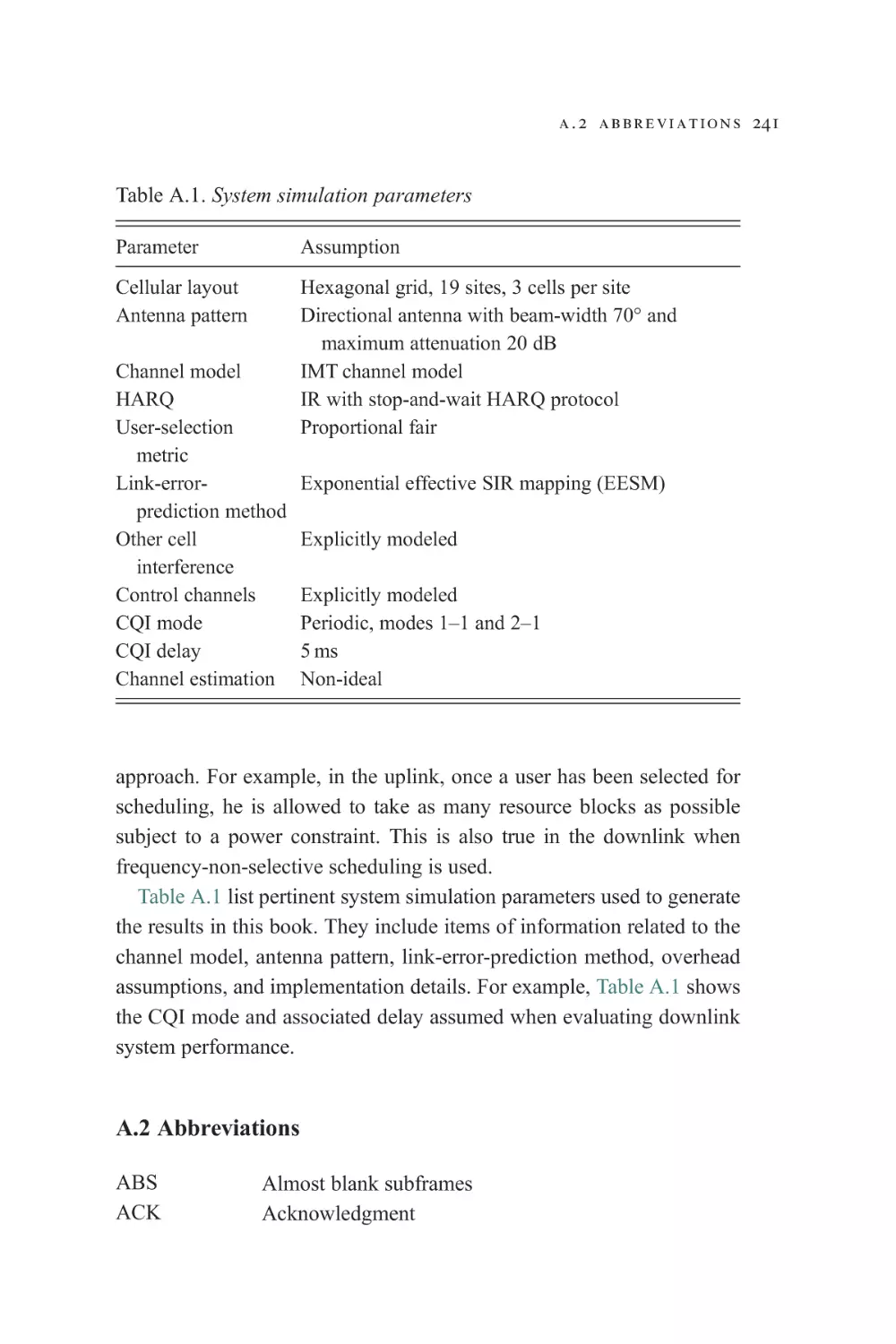
A.1 System analysis and performance metrics
A.2 Abbreviations
Index
238
238
241
247
222
227
232
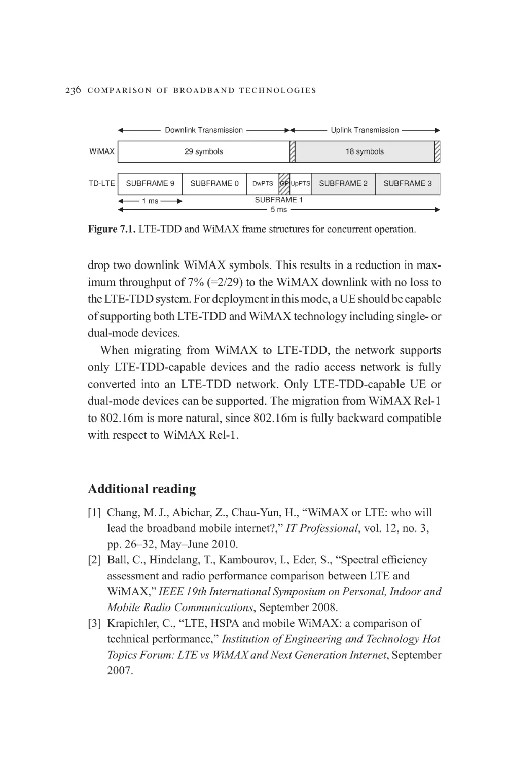
236
Preface
The next-generation wireless broadband technology is changing the way
we work, live, learn, and communicate through effective use of stateof-the-art mobile broadband technology. The packet-data-based revolution started around 2000 with the introduction of 1x Evolved Data Only
(1xEV-DO) and 1x Evolved Data Voice (1xEV-DV) in 3GPP2 and High
Speed Downlink Packet Access (HSDPA) in 3GPP. The wireless broadband fourth-generation technology (4G) is an evolution of the packetbased 3G system and provides a comprehensive evolution of the
Universal Mobile Telecommunications System specifications so as to
remain competitive with other broadband systems such as 802.16e
(WiMAX). Specification work was started in late 2004 on Long Term
Evolution (LTE) of the UMTS Terrestrial Radio Access and Radio Access
Network intended for commercial deployment in 2010. Two main components constitute the LTE system architecture – the Evolved Universal
Terrestrial Radio Access Network (E-UTRAN) and the Evolved Packet
Core (EPC). The goals for the evolved system (E-UTRAN and EPC)
included support for improved system capacity and coverage, high peak
data rates, low latency, reduced operating costs, multi-antenna support,
flexible bandwidth operations, and seamless integration with existing
systems. The standardization work for LTE Rel-8 was completed in early
2009 and commercial LTE systems will be deployed in the 2011–2012
timeframe. LTE Rel-8 is currently evolving to LTE-Advanced (LTE Rel-9
and Rel-10), which will further improve the spectral efficiency, peak rates,
and user experience compared with LTE Rel-8. LTE-Advanced has also
been approved by the International Telecommunication Union (ITU) as an
International Mobile Telecommunications-Advanced (IMT-A) technology.
The book is organized in seven chapters. Chapter 1 gives a timeline and
brief description of the evolution of digital wireless technology starting
with GSM, IS-95, cdma2000 1x, WCDMA Rel-99, HSPA (Rel-5/6),
xi
xii p r e f a c e
WiMAX, LTE, LTE-Advanced, and 802.16m with emphasis on how
supported data rates, throughput, and applications have evolved.
Chapter 2 provides a brief description of LTE requirements and system
architecture together with the basic principles of orthogonal frequencydivision multiple-access (OFDMA) and single-carrier frequency-division
multiple-access (SC-FDMA) technology. Chapter 3 dives into the basic
details of LTE downlink OFDMA transmission including transport and
physical-channel structure, control-channel details, system operations, and
inter-cell interference coordination schemes both for FDD (FrequencyDivision Duplex) and for TDD (Time-Division Duplex) LTE. Aspects of
downlink system performance under various channels and antenna structure
are summarized at the end of the chapter.
Chapter 4 provides the details of LTE uplink transport and physicalchannel structure, control-channel details, random access, system operations, and fractional power control followed by uplink system performance
under various channels and antenna configurations. The LTE system offers
a rich suite of multiple-antenna techniques that can be used in various
scenarios to improve the performance and user experience. Chapter 5
describes various multi-antenna schemes for LTE downlink and uplink
and provides a system-performance comparison of various multi-antenna
schemes. Chapter 6 is devoted to technologies for LTE-Advanced (LTE-A).
The chapter describes the requirements for IMT-A and how LTE-A will
satisfy those requirements using enhanced technologies. The technologies
include support of wider bandwidth using carrier aggregation, uplink
spatial multiplexing, enhanced downlink spatial multiplexing, coordinated
multiple-point transmission and reception, and heterogeneous networks
including relays, distributed antenna systems, and pico-cells. Aspects of
the system performance of these enhancements are presented and compared
with the performance of the legacy LTE system.
Finally, Chapter 7 provides a comparison of LTE/LTE-A with other
competitive broadband systems such as 802.16e/802.16m. As the name
signifies, this chapter outlines both qualitative and quantitative differences
between the 802.16e/802.16m (WiMAX) system and the LTE/LTE-A
system. System performance comparisons between these systems are presented for various reuse schemes and antenna configurations.
p r e f a c e xiii
At the time of writing, there are ongoing discussions within the operator and vendor community regarding further evolution of LTE-A technology. These enhancements will appear in Rel-11 and Rel-12 of 3GPP
and will offer better user experience, lower cost per bit, greener base
stations, and efficient self-organizing networks.
Acknowledgments
Several of our colleagues made a significant impact on the materials
presented in this book. We would like to acknowledge and thank Prakash
Moorut for his comments and suggestions on the spectrum-engineering
aspects, Bishwarup Mondal, who provided critical comments, simulations,
and suggestions for improving the contents related to multi-antenna
systems and heterogeneous networks, Nitin Mangalvedhe for providing
us with some of the simulation results and his in-depth comments relating
to heterogeneous networks, Joe Hoffman for providing help related to the
economic aspect of wireless broadband systems, Mark Cudak for providing us with his expertise on WiMAX-related issues, and Tim Thomas, who
reviewed the entire first draft of the book and provided constructive comments and criticisms. Throughout our professional careers at Motorola we
had the good fortune of working and learning from some of the most
talented people in the cellular industry, including Ken Stewart, Bob
Love, the late Dennis Schaeffer, Fan Wang, Joe Pedziwiatr, Paul
Steinberg, Phil Fleming, Fred Vook, Weimin Xiao, Brian Classon, and
3GPP colleagues, among many others. Finally, we would like to thank our
superiors Sudhakar Ramakrishna and Bill Payne for providing us with
encouragement and support for undertaking this project.
xiv
1
Genesis of wireless broadband
technology (from 2G to 4.5G)
1.1 Genesis of wireless technology
The digital cellular technology revolution started with the introduction of
GSM (Groupe Special Mobile) in the late 1980s. The GSM technology was
based on time-division multiple access (TDMA) and was capable of supporting data services of up to 9.6 kbps. In the early 1990s, IS-95, a standard based
on code-division multiple-access (CDMA) technology was introduced. This
offered data rates of up to 14.4 kbps and improved spectral efficiencies over a
GSM system. Subsequently, both these technologies evolved over time, with
each phase offering higher peak rates and improved sector/edge spectral
efficiencies. Both GSM and IS-95 CDMA evolved in different phases. In
1997, the Generalized Packet Radio System (GPRS) based on packet data
instead of circuit data was standardized, followed by Enhanced Data Rates
for Global Evolution (EDGE). Also, at the end of 1998, the Third-Generation
Partnership Project (3GPP) was started. This was responsible for defining a
third-generation (3G) wideband CDMA (WCDMA) standard based on the
evolved GSM core network. At the same time the GSM standardization work
was moved from ETSI SMG2 to 3GPP, and was called GERAN. Similarly, in
the United States the IS-95 standard evolved to cdma2000 under the umbrella
of Third-Generation Partnership Project 2 (3GPP2).
The packet-data-based revolution started around 2000 with the introduction of cdma2000 1x Evolved Data Only (1xEV-DO) and 1x Evolved Data
Voice (1xEV-DV) in 3GPP2 and High Speed Downlink Packet Access
(HSDPA) in 3GPP. These 3.5G technologies had the following common
attributes: adaptive modulation and coding, hybrid automatic repeat
request, fast scheduling based on smaller frame size, turbo codes, and
de-centralized architecture to reduce latency. In the next phase of development of 3.5G technology, improved uplink functionality was added to 3GPP
and 1xEV-DO systems. Concurrently, advances were made in cdma2000 1x
1
2 wireless broadband technology
technology (i.e. cdma 1x-advanced), which included an advanced vocoder,
mobile receive diversity, an advanced receiver with interference cancellation, and advanced power control. It may be noted that, although 1xEV-DV
was standardized, it never took off as a technology due to the reluctance of
the operator community to adopt the technology and the absence of proper
eco-systems.
A disruptive technology known as mobile WiMAX based on orthogonal frequency-division multiplexing (OFDM) technology was standardized in 2006, and was dubbed the first 4G multiple access system. This
technology was based on the IEEE 802.16e standard and offered scalable
bandwidth up to 20 MHz, higher peak rates, and better spectral efficiencies than those provided by 3.5G systems. With the emergence of packetbased wireless broadband systems such as WiMAX, it was evident that a
comprehensive evolution of UMTS would be required in order for it to
remain competitive in the long term. As a result, work began on Evolved
UMTS Terrestrial Radio Access (E-UTRA) based on the OFDM air
interface. The Long Term Evolution (LTE Rel-8) system supports high
peak data rates and provides low latency, improved system capacity and
coverage, reduced operating costs, efficient multi-antenna support, efficient support for packet data transmission, flexible bandwidth of up to 20
MHz, and seamless integration with existing systems. The CDMA-based
HSPA technology is also being enhanced to support quad carriers (bandwidth up to 20 MHz), MIMO, and higher-order modulation both on the
downlink and on the uplink. A 4G proposal called Ultra Mobile
Broadband (UMB) based on OFDM was also adopted by 3GPP2, but it
failed to make any impact.
Both WiMAX and LTE are currently being enhanced (LTE-Advanced
and 802.16m) so as to support even higher peak rates, higher throughput
and coverage, and lower latencies resulting in a better user experience.
Further, LTE-Advanced and 802.16m also enable one to meet or exceed
IMT-Advanced requirements. Finally, the 4.5G wireless broadband systems will be standardized in 3GPP Rel-12 in the 2013–2017 timeframe. It
is clear that 4.5G systems will further enhance the 4G systems in terms of
user experience, sector spectral efficiency, and peak rates, but the exact
features for 4.5G systems are still being decided.
1.1 genesis 3
The Digital Video Broadcasting (DVB) standards, which include
Mediaflow and Multimedia Broadcast Multicast Service (MBMS)
designed for LTE and HSPA, for global delivery of broadcast services
such as digital television are also evolving to provide better spectral
efficiencies for broadcast services.
The wireless evolution chart of 2G to 4.5G technology migration is
shown in Figure 1.1.
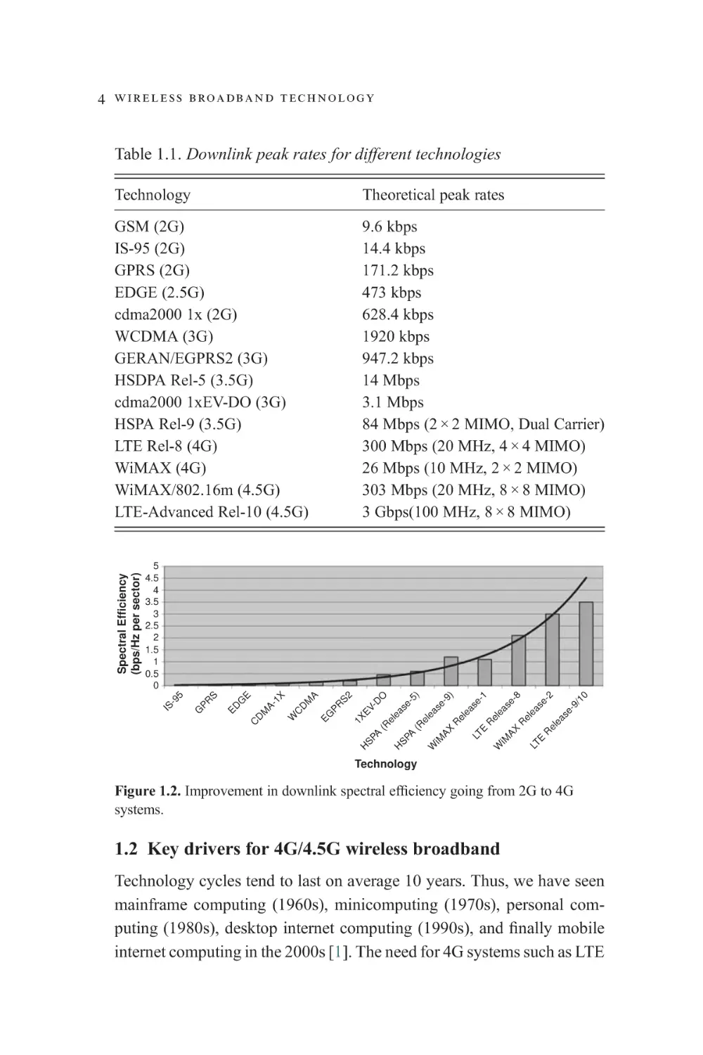
The downlink peak rate improvement on going from 2G to 4.5G
technology is shown in Table 1.1.
The improvement in downlink sector spectral efficiencies on going
from 2G to 4.5G systems is shown in Figure 1.2.
It may be observed from Figure 1.2 that there has been an
improvement by a factor of 30 in sector spectral efficiency with 4G
systems compared with 2G, which results in improved cost per bit.
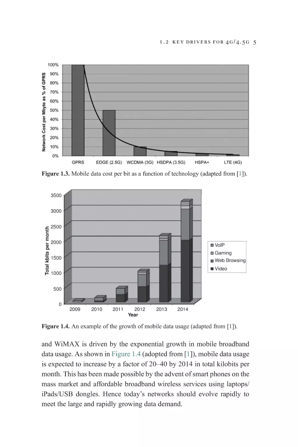
Figure 1.3 shows an example of how mobile broadband cost per bit
decreases exponentially with technology innovation in wireless
technology.
10 kbps
1990
10–100
1994–1996
100–15000 kbps
2000–2005
~150 Mbps
2006–2012
1992
1996–2001
2002–2008
2007–2012
>1 Gbps
2013–2017
2014
IEEE
Evolution
MOBILE
RELAY
802.20
802.16J
Fixed
802.16d
802.16m
802.16e
MBS
EV-DV
IS-95
IS-2000
EV-DO
(Rev. A/B)
EV-DO
BCMCS
PhII/UMB
3GPP2
Evolution
LTE-A
LTE
UMTS
(Rel. 99)
HSUPA
UMTS Long
Term Evolution
HSDPA
MBMS
HSPA+
HSPA-MBMS+
GSM
GPRS
EDGE
EDGE+
DTM
MBMS
Unicast
MBMS+
HSPA
Evolution
GERAN (GSM)
Evolution
Broadcast
Figure 1.1. Standards evolution of wireless technologies (from 2G to 4.5G).
LTE-A+
4 wireless broadband technology
Table 1.1. Downlink peak rates for different technologies
Theoretical peak rates
GSM (2G)
IS-95 (2G)
GPRS (2G)
EDGE (2.5G)
cdma2000 1x (2G)
WCDMA (3G)
GERAN/EGPRS2 (3G)
HSDPA Rel-5 (3.5G)
cdma2000 1xEV-DO (3G)
HSPA Rel-9 (3.5G)
LTE Rel-8 (4G)
WiMAX (4G)
WiMAX/802.16m (4.5G)
LTE-Advanced Rel-10 (4.5G)
9.6 kbps
14.4 kbps
171.2 kbps
473 kbps
628.4 kbps
1920 kbps
947.2 kbps
14 Mbps
3.1 Mbps
84 Mbps (2 × 2 MIMO, Dual Carrier)
300 Mbps (20 MHz, 4 × 4 MIMO)
26 Mbps (10 MHz, 2 × 2 MIMO)
303 Mbps (20 MHz, 8 × 8 MIMO)
3 Gbps(100 MHz, 8 × 8 MIMO)
9/
10
-2
se
as
e-
ea
LT
E
R
el
e
R
AX
iM
W
LT
E
R
el
el
e
ea
as
se
e-
8
-1
9)
eel
R
AX
iM
W
H
SP
A
(R
el
e
as
e-
5)
O
as
EV
-D
el
e
(R
S2
H
SP
A
1X
A
M
D
PR
EG
1X
A-
C
W
E
G
C
D
M
ED
PR
G
IS
S
5
4.5
4
3.5
3
2.5
2
1.5
1
0.5
0
-9
5
Spectral Efficiency
(bps/Hz per sector)
Technology
Technology
Figure 1.2. Improvement in downlink spectral efficiency going from 2G to 4G
systems.
1.2 Key drivers for 4G/4.5G wireless broadband
Technology cycles tend to last on average 10 years. Thus, we have seen
mainframe computing (1960s), minicomputing (1970s), personal computing (1980s), desktop internet computing (1990s), and finally mobile
internet computing in the 2000s [1]. The need for 4G systems such as LTE
1.2 key drivers for 4g/4.5g 5
Figure 1.3. Mobile data cost per bit as a function of technology (adapted from [1]).
3500
Total kbits per month
3000
2500
2000
VolP
Gaming
1500
Web Browsing
Video
1000
500
0
2009
2010
2011
2012
Year
2013
2014
Figure 1.4. An example of the growth of mobile data usage (adapted from [1]).
and WiMAX is driven by the exponential growth in mobile broadband
data usage. As shown in Figure 1.4 (adopted from [1]), mobile data usage
is expected to increase by a factor of 20–40 by 2014 in total kilobits per
month. This has been made possible by the advent of smart phones on the
mass market and affordable broadband wireless services using laptops/
iPads/USB dongles. Hence today’s networks should evolve rapidly to
meet the large and rapidly growing data demand.
6 wireless broadband technology
Table 1.2. Video requirements for different device types/applications
Device type
Smart
phones
Multimedia
phones
Personal
media
players
Standarddefinition
TV
Laptops
Screen
size
(inches) Resolution
Average
MPEG4
data rate
Wireless
(kbps)
Mobility technology
2.5–3
240
Full
3G/4G
600
Full
900
Full
3G/4G/
4.5G
4G/4.5G
1500
Full
4G
3–3.5
4.7
QVGA
(320 × 240)
HVGA
(480 × 320)
VGA
(640 × 480)
<32
SD 480i
(1280 × 720)
12–7
HD 720i
3500
(1280 × 720)
HD 720p
7000
(1280 × 720)
HD 1080p
14000
(1920 × 1080)
Low-tier HD <32
TV
High-tier HD >32
TV
Nomadic 4G/4.5G
Fixed
4G/4.5G
Fixed
4G/4.5G
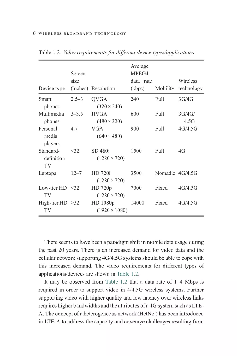
There seems to have been a paradigm shift in mobile data usage during
the past 20 years. There is an increased demand for video data and the
cellular network supporting 4G/4.5G systems should be able to cope with
this increased demand. The video requirements for different types of
applications/devices are shown in Table 1.2.
It may be observed from Table 1.2 that a data rate of 1–4 Mbps is
required in order to support video in 4/4.5G wireless systems. Further
supporting video with higher quality and low latency over wireless links
requires higher bandwidths and the attributes of a 4G system such as LTEA. The concept of a heterogeneous network (HetNet) has been introduced
in LTE-A to address the capacity and coverage challenges resulting from
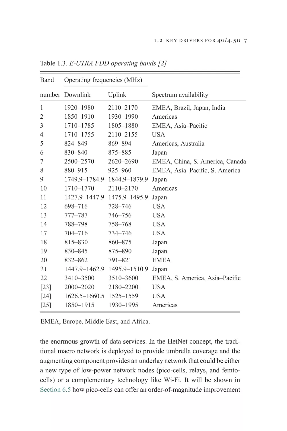
1.2 key drivers for 4g/4.5g 7
Table 1.3. E-UTRA FDD operating bands [2]
Band
Operating frequencies (MHz)
number Downlink
Uplink
Spectrum availability
1
2
3
4
5
6
7
8
9
10
11
12
13
14
17
18
19
20
21
22
[23]
[24]
[25]
2110–2170
1930–1990
1805–1880
2110–2155
869–894
875–885
2620–2690
925–960
1844.9–1879.9
2110–2170
1475.9–1495.9
728–746
746–756
758–768
734–746
860–875
875–890
791–821
1495.9–1510.9
3510–3600
2180–2200
1525–1559
1930–1995
EMEA, Brazil, Japan, India
Americas
EMEA, Asia–Pacific
USA
Americas, Australia
Japan
EMEA, China, S. America, Canada
EMEA, Asia–Pacific, S. America
Japan
Americas
Japan
USA
USA
USA
USA
Japan
Japan
EMEA
Japan
EMEA, S. America, Asia–Pacific
USA
USA
Americas
1920–1980
1850–1910
1710–1785
1710–1755
824–849
830–840
2500–2570
880–915
1749.9–1784.9
1710–1770
1427.9–1447.9
698–716
777–787
788–798
704–716
815–830
830–845
832–862
1447.9–1462.9
3410–3500
2000–2020
1626.5–1660.5
1850–1915
EMEA, Europe, Middle East, and Africa.
the enormous growth of data services. In the HetNet concept, the traditional macro network is deployed to provide umbrella coverage and the
augmenting component provides an underlay network that could be either
a new type of low-power network nodes (pico-cells, relays, and femtocells) or a complementary technology like Wi-Fi. It will be shown in
Section 6.5 how pico-cells can offer an order-of-magnitude improvement
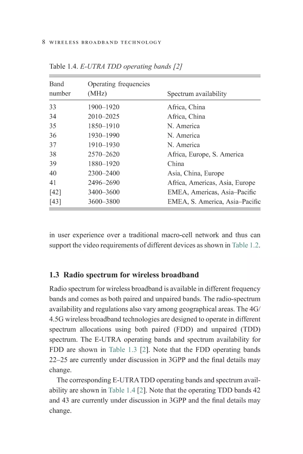
8 wireless broadband technology
Table 1.4. E-UTRA TDD operating bands [2]
Band
number
Operating frequencies
(MHz)
Spectrum availability
33
34
35
36
37
38
39
40
41
[42]
[43]
1900–1920
2010–2025
1850–1910
1930–1990
1910–1930
2570–2620
1880–1920
2300–2400
2496–2690
3400–3600
3600–3800
Africa, China
Africa, China
N. America
N. America
N. America
Africa, Europe, S. America
China
Asia, China, Europe
Africa, Americas, Asia, Europe
EMEA, Americas, Asia–Pacific
EMEA, S. America, Asia–Pacific
in user experience over a traditional macro-cell network and thus can
support the video requirements of different devices as shown in Table 1.2.
1.3 Radio spectrum for wireless broadband
Radio spectrum for wireless broadband is available in different frequency
bands and comes as both paired and unpaired bands. The radio-spectrum
availability and regulations also vary among geographical areas. The 4G/
4.5G wireless broadband technologies are designed to operate in different
spectrum allocations using both paired (FDD) and unpaired (TDD)
spectrum. The E-UTRA operating bands and spectrum availability for
FDD are shown in Table 1.3 [2]. Note that the FDD operating bands
22–25 are currently under discussion in 3GPP and the final details may
change.
The corresponding E-UTRATDD operating bands and spectrum availability are shown in Table 1.4 [2]. Note that the operating TDD bands 42
and 43 are currently under discussion in 3GPP and the final details may
change.
additional reading 9
Operators and regulators across the world are trying to clear enough
spectrum to deploy 4G/4.5G wireless broadband technologies based on
LTE/LTE-A or WiMAX Rel-1/Rel-2 to meet the increased demand for
mobile data usage which tends to account for approximately 60% of the
service revenue. More spectrum is also necessary in order to provide the
higher quality of service required for applications such as video, videoconferencing, and gaming.
References
[1] Morgan Stanley, The Mobile Internet Report Setup, December 15, 2009.
[2] 3GPP TS 36.101, UE radio transmission and reception, v8.5.0, March
2009.
Additional reading
[1] Halonen, T., Romero, J., Melero, J., GSM, GPRS and EDGE
Performance, Evolution Towards 3G/UMTS, 2nd edition, Wiley, 2003.
[2] Iniewski, K., Internet Networks, Wired, Wireless and Optical
Technologies, CRC Press, 2009.
[3] Andrews, J., Ghosh, A., Muhamed, R., Fundamentals of WiMAX,
Prentice Hall, 2007.
[4] Dahlman, E., Parkvall, S., Skold, J., Beming, P., 3G Evolution, HSPA
and LTE for Mobile Broadband, 2nd edition, Academic Press, 2008.
2
LTE overview
2.1 Introduction
Long Term Evolution (LTE) of the Universal Mobile Telecommunications
System (UMTS) was developed to ensure that the technology remains
competitive for the foreseeable future. Requirements for the LTE Rel-8
system include improved system capacity and coverage, improved user
experience through higher data rates and reduced latency, reduced deployment and operating costs, and seamless integration with existing systems.
The requirements may be broken down into different categories – system
performance, latency, coverage, deployment, and complexity. To achieve
these goals, new designs for the radio access networks and system architectures are needed.
A representative list of LTE Rel-8 requirements for the radio access
networks is given in Table 2.1 while the complete set of requirements may
be found in [1]. From a system and user performance perspective, the
following requirements have been defined: peak data rate, cell spectral
efficiency, cell-edge user throughput, and average user throughput. For
the downlink, peak data rates of at least 100 Mbps must be supported for a
system bandwidth of 20 MHz, while for the uplink, peak data rates of at
least 50 Mbps must be supported. Cell, cell-edge user, and average user
performance requirements are defined in terms of spectral efficiency (i.e.
supportable throughput in bits per second per MHz) and in relation to Rel-6
UMTS performance. In general, improvement by a factor of 3–4 is
expected in the downlink while improvement by a factor of 2–3 is expected
in the uplink.
Latency requirements are also defined for the control and user planes.
For the user plane (U-plane), a maximum latency of 5 ms is desired. This
latency is measured as the one-way delay from when a packet is available at
the Internet Protocol (IP) layer to when it arrives at the User Equipment (UE).
10
2 . 1 i n t r o d u c t i o n 11
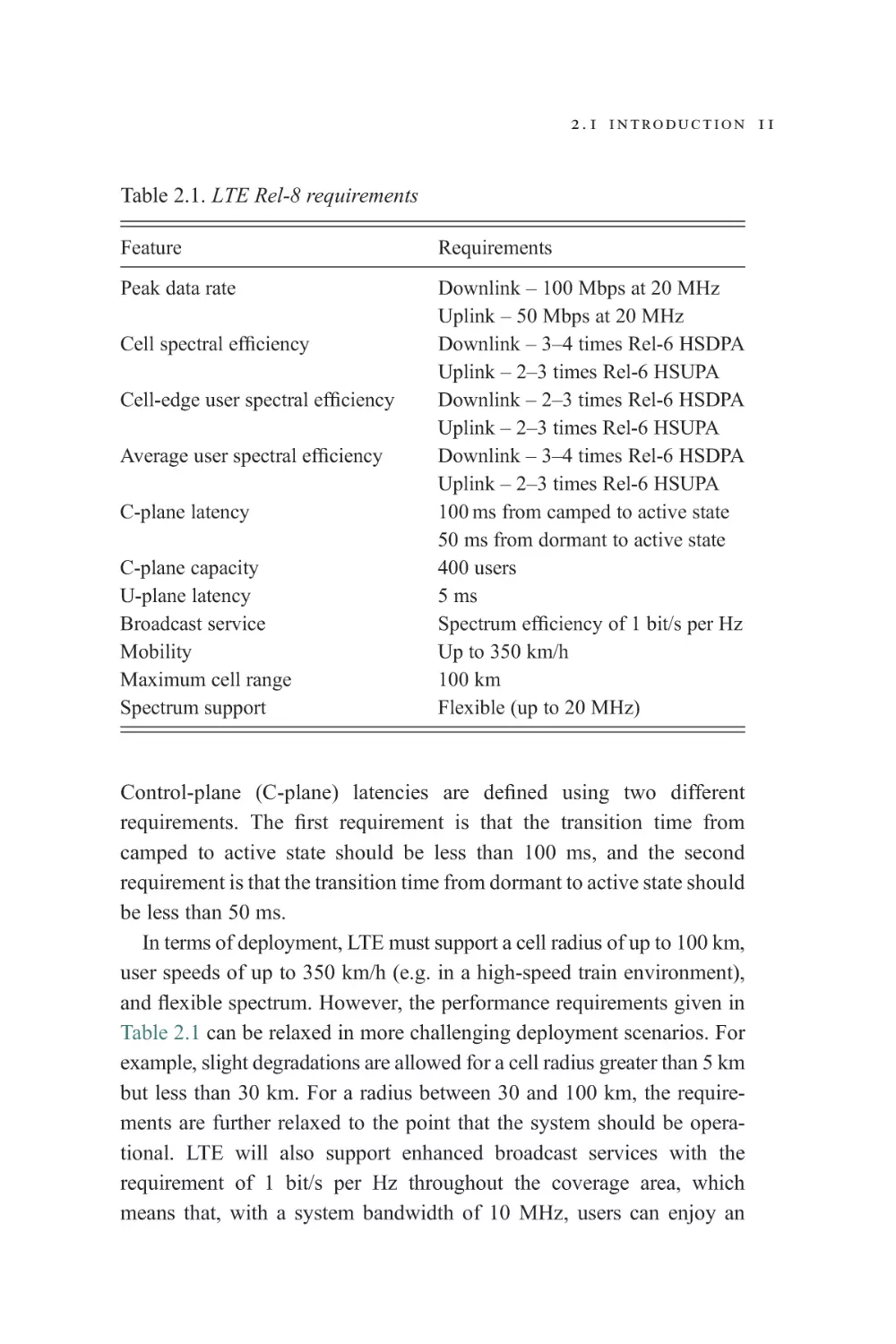
Table 2.1. LTE Rel-8 requirements
Feature
Requirements
Peak data rate
Downlink – 100 Mbps at 20 MHz
Uplink – 50 Mbps at 20 MHz
Downlink – 3–4 times Rel-6 HSDPA
Uplink – 2–3 times Rel-6 HSUPA
Downlink – 2–3 times Rel-6 HSDPA
Uplink – 2–3 times Rel-6 HSUPA
Downlink – 3–4 times Rel-6 HSDPA
Uplink – 2–3 times Rel-6 HSUPA
100 ms from camped to active state
50 ms from dormant to active state
400 users
5 ms
Spectrum efficiency of 1 bit/s per Hz
Up to 350 km/h
100 km
Flexible (up to 20 MHz)
Cell spectral efficiency
Cell-edge user spectral efficiency
Average user spectral efficiency
C-plane latency
C-plane capacity
U-plane latency
Broadcast service
Mobility
Maximum cell range
Spectrum support
Control-plane (C-plane) latencies are defined using two different
requirements. The first requirement is that the transition time from
camped to active state should be less than 100 ms, and the second
requirement is that the transition time from dormant to active state should
be less than 50 ms.
In terms of deployment, LTE must support a cell radius of up to 100 km,
user speeds of up to 350 km/h (e.g. in a high-speed train environment),
and flexible spectrum. However, the performance requirements given in
Table 2.1 can be relaxed in more challenging deployment scenarios. For
example, slight degradations are allowed for a cell radius greater than 5 km
but less than 30 km. For a radius between 30 and 100 km, the requirements are further relaxed to the point that the system should be operational. LTE will also support enhanced broadcast services with the
requirement of 1 bit/s per Hz throughout the coverage area, which
means that, with a system bandwidth of 10 MHz, users can enjoy an
12 l t e o v e r v i e w
aggregate downlink throughput of 10 Mbps. This is equivalent to receiving 50 simultaneous television or radio channels at a data rate of 200 kbps
each.
A feasibility study was conducted in 3GPP to determine whether these
requirements can be met. Results of the feasibility study were captured in
[2] with the conclusion that LTE requirements can be achieved. However,
enhancements in both radio and core networks are needed, including a
new physical layer and a redesign of the network architecture.
Enhancements to the radio access networks were made under LTE
while evolution to the core network was done under System
Architecture Evolution. This chapter provides a basic overview of the
LTE system architecture, including a basic introduction to the new
frequency-domain transmission schemes being used in the physical
layer. The details and performance of the new physical layers are
described in other chapters of this book.
2.2 System architecture
The LTE system architecture is based on the IP and therefore is designed to
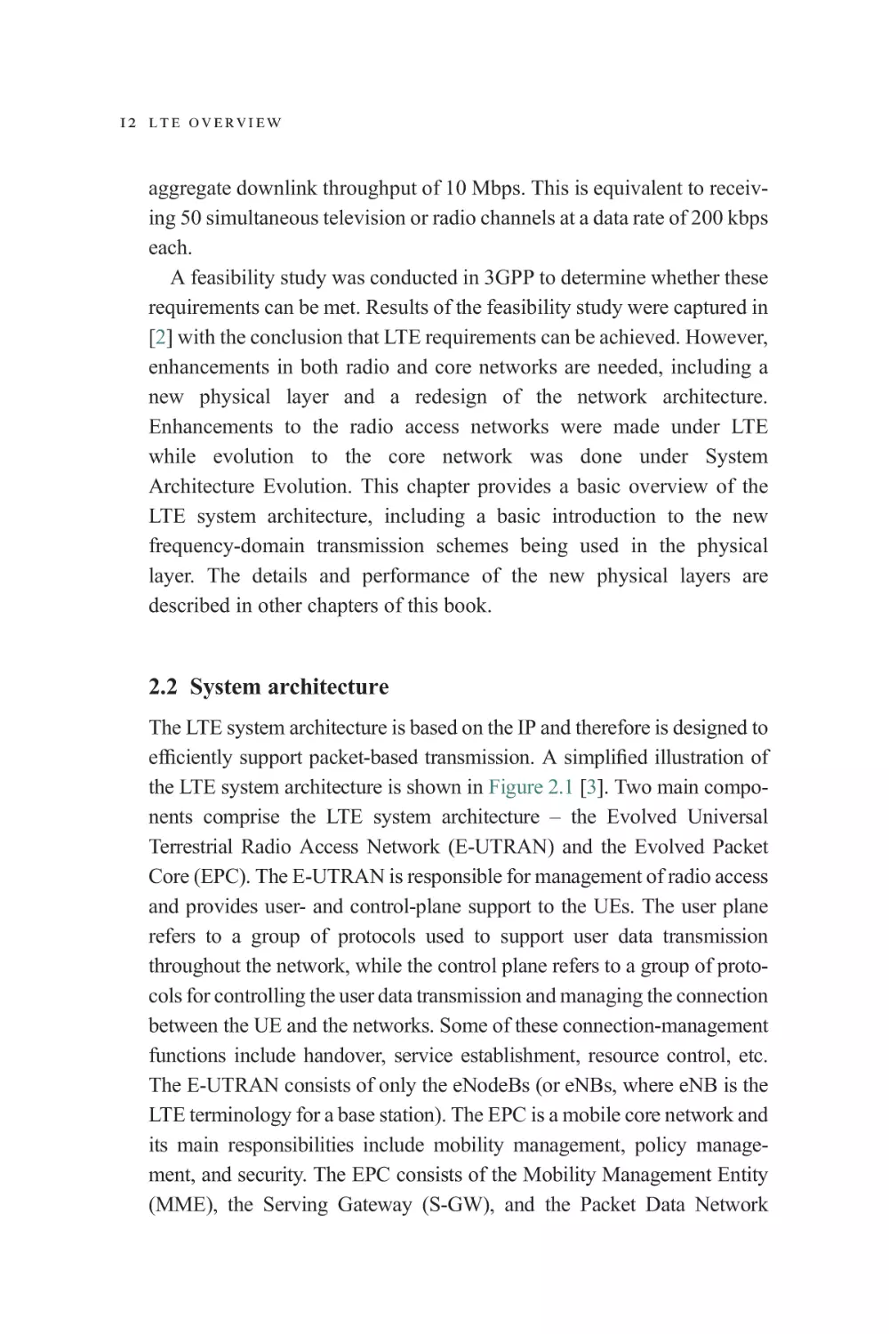
efficiently support packet-based transmission. A simplified illustration of
the LTE system architecture is shown in Figure 2.1 [3]. Two main components comprise the LTE system architecture – the Evolved Universal
Terrestrial Radio Access Network (E-UTRAN) and the Evolved Packet
Core (EPC). The E-UTRAN is responsible for management of radio access
and provides user- and control-plane support to the UEs. The user plane
refers to a group of protocols used to support user data transmission
throughout the network, while the control plane refers to a group of protocols for controlling the user data transmission and managing the connection
between the UE and the networks. Some of these connection-management
functions include handover, service establishment, resource control, etc.
The E-UTRAN consists of only the eNodeBs (or eNBs, where eNB is the
LTE terminology for a base station). The EPC is a mobile core network and
its main responsibilities include mobility management, policy management, and security. The EPC consists of the Mobility Management Entity
(MME), the Serving Gateway (S-GW), and the Packet Data Network
2 . 2 s y s t e m a r c h i t e c t u r e 13
HSS
PCRF
EPC
MME
S-GW
S1-
U
X2
S5
P-GW
SGi
Internet
S1
-U
S1-MME
eNB
S1
-M
ME
eNB
E-UTRAN
UE
UE
Figure 2.1. LTE system architecture.
Gateway (P-GW). Compared with previous 3GPP architectures, this new
architecture has fewer nodes and therefore smaller user-plane latency [4]–[5].
This, however, requires the eNB to perform additional user-plane
functions not traditionally done at the base station, such as ciphering.
Both the E-UTRAN and the EPC are responsible for the quality-of-service
(QoS) control in LTE [6]–[8].
Two main interfaces are defined to provide communication between
different LTE entities – the S1 and X2 interfaces. The X2 interface
provides communication among eNBs and can be used to transfer
user- and control-plane information. Examples of possible inter-eNB
exchanges using the X2 interface include handover information, measurement and interference coordination reports, load measurements, eNB
configuration setups, and forwarding of user data. The S1 interface is
used to connect the eNBs to the EPC (either to the MME or S-GW). The
interface between eNB and S-GW is called S1-U and is used to transfer
user data. The interface between eNB and MME is called S1-MME and
is used to transfer control-plane information. Examples of control-plane
information include mobility support, paging, data service management, location services, and network management [9].
14 l t e o v e r v i e w
2.2.1 E-UTRAN
The E-UTRAN provides air-interface user- and control-plane protocol
management for the users. It supports the following functions: radio
resource management, measurements, access-stratum security, IP header
compression and encryption of the user data stream, MME selection,
user-plane data routing to the S-GW, and scheduling and transmission
of paging messages, broadcast information, and public warning system
messages [3].
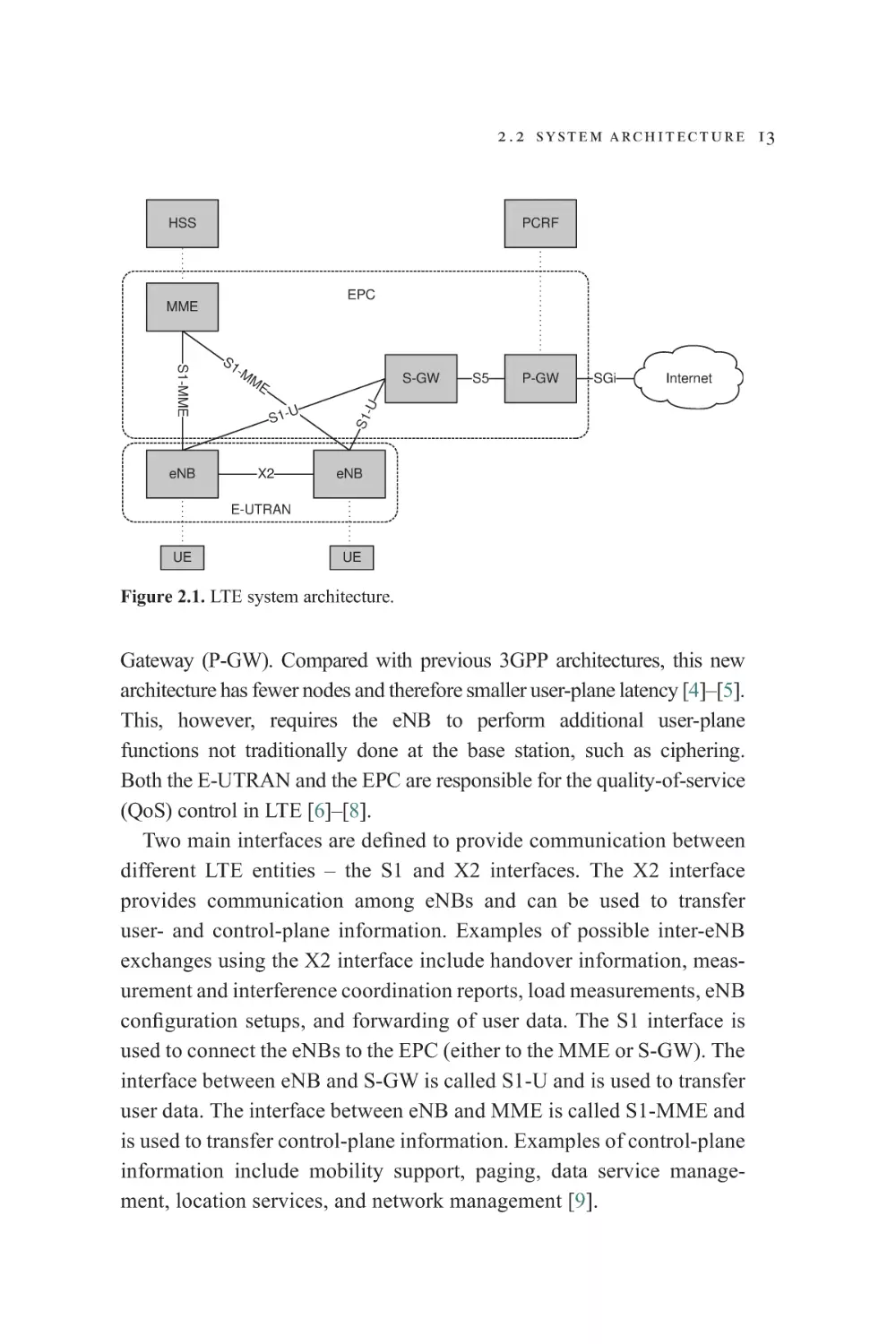
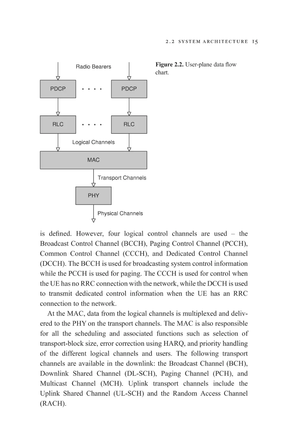
The following user-plane protocols are supported: Packet Data
Convergence Protocol (PDCP), Radio Link Control (RLC), Medium
Access Control (MAC), and Physical layer (PHY). An illustration of
the user-plane data flow chart is shown in Figure 2.2. A radio bearer is
used to transfer data and control between the UE and the E-UTRAN.
User-plane data is sent via traffic radio bearers while control-plane data is
sent using the signaling radio bearers. Several bearers may be established
for the same user, on the basis of traffic types and characteristics. The
PDCP sublayer is responsible for header compression and decompression, security functions such as ciphering and deciphering, and transfer of
user protocol data units to the RLC. In addition, the PDCP sublayer also
ensures in-sequence delivery of user-plane data and retransmission of
service data units during handover. The RLC sublayer will perform
segmentation and reassembly, ARQ error correction, and delivery of the
user protocol data units to the MAC via appropriate logical channels. The
RLC sublayer is also responsible for protocol-error detection and recovery,
RLC re-establishment, and in-sequence delivery of the protocol data
units.
The main functions of the MAC sublayer include mapping between
logical and transport channels, scheduling of data, HARQ, priority handling, and multiplexing/de-multiplexing of MAC service data units. A
logical channel is a data-transfer service offered by the MAC to the RLC,
and can be classified as either a control or a traffic channel. Control logical
channels are used to transfer control-plane information while traffic
logical channels are used to transfer user-plane information. In LTE,
only one logical traffic channel, the Dedicated Traffic Channel (DTCH),
2 . 2 s y s t e m a r c h i t e c t u r e 15
Figure 2.2. User-plane data flow
chart.
Radio Bearers
PDCP
PDCP
RLC
RLC
Logical Channels
MAC
Transport Channels
PHY
Physical Channels
is defined. However, four logical control channels are used – the
Broadcast Control Channel (BCCH), Paging Control Channel (PCCH),
Common Control Channel (CCCH), and Dedicated Control Channel
(DCCH). The BCCH is used for broadcasting system control information
while the PCCH is used for paging. The CCCH is used for control when
the UE has no RRC connection with the network, while the DCCH is used
to transmit dedicated control information when the UE has an RRC
connection to the network.
At the MAC, data from the logical channels is multiplexed and delivered to the PHY on the transport channels. The MAC is also responsible
for all the scheduling and associated functions such as selection of
transport-block size, error correction using HARQ, and priority handling
of the different logical channels and users. The following transport
channels are available in the downlink: the Broadcast Channel (BCH),
Downlink Shared Channel (DL-SCH), Paging Channel (PCH), and
Multicast Channel (MCH). Uplink transport channels include the
Uplink Shared Channel (UL-SCH) and the Random Access Channel
(RACH).
16 l t e o v e r v i e w
At the PHY, the transport channels are mapped into physical channels
for transmission over the air interface. The PHY is responsible for cyclic
redundancy check (CRC) insertion, channel coding, HARQ processing,
scrambling, modulation, link adaptation, power control, and resource
mapping.
The control plane supports the Radio Resource Control (RRC) protocol.
The main functions of the RRC sublayer include system information
broadcast, paging, connection management, security, radio bearer management, mobility functions, QoS management functions, and UE
measurement reporting. Two RRC states are used in LTE – idle and
connected. In the idle state, a user has been assigned an identity but no
RRC connection. In the connected state, a user has an RRC connection,
which allows data transmission and reception with the network.
2.2.2 Evolved packet core
In 2G and 3G mobile broadband systems, two separate core networks
were needed – circuit-switched for voice applications and packetswitched for data applications. In LTE, only a packet-switched mobile
core based on the IP is used. This allows a flat architecture with a smaller
number of network entities. This mobile packet core is called the Evolved
Packet Core (EPC) in LTE. The EPC consists of the following network
elements: the Mobility Management Entity (MME), Serving Gateway
(S-GW), and Packet Data Network Gateway (P-GW). In addition, two
additional logical network elements – the Home Subscriber Server (HSS)
and the Policy Control and Charging Rules Functions (PCRF) – are also
generally included as part of the core network. In LTE, the EPC provides
the following functions: mobility management, session management,
security management, and policy control and charging. Mobility management provides signaling support between the UE and the network using
the Non-Access Stratum (NAS) protocols. Session management refers to
the establishment and management of data bearers. Security management
provides data encryption and authentication services for the users. Policy
control and charging refers to access and control of services as prescribed
by the operator including QoS management, metering, service control
2 . 2 s y s t e m a r c h i t e c t u r e 17
based on user classification, and policy control enforcement. It also is
responsible for charging and billing of services.
The MME serves as the control entity for the EPC and provides the
following main functionalities: NAS signaling and security, P-GW and
S-GW selection, roaming support, user authentication, bearer management, and idle-state mobility handling. The NAS is a functional layer that
provides signaling and traffic between the UE and the packet data
network gateway.
The S-GW manages the user data plane between the eNBs and the
packet data network gateway. As UEs move across areas served by
different eNBs, the S-GW serves as a mobility anchor ensuring continuous data connection. This includes mobility management for handovers
between LTE and other 3GPP technologies. The S-GW is connected to
the eNBs via the S1-U interface.
The P-GW provides data connectivity to the external packet data networks such as the Internet or IP Multimedia Subsystem (IMS) networks.
IMS networks are used to provide multimedia services such as Voice over
Internet Protocol (VoIP), video conferencing, and messaging. Functions
of the P-GW include packet filtering and routing, IP address allocation,
charging and policy enforcement via the PCRF, and lawful interception.
The HSS maintains a database of subscriber-related information [10].
This includes user profile and state information including restrictions on
roaming, QoS, access-point information, security information, location
information, and access/service authorization. It also stores information
about available P-GWs that a user can connect to.
The PCRF has two main functions – policy control and flow-based
charging [11]. It defines the rules and policy associated with this work.
For example, different charging rules such as volume-based, time-based,
and event-based can be enforced. In addition, different rates based on user
characteristics (e.g. roaming versus home) and service characteristics
(e.g. traffic type or guaranteed data rate) can be applied. Policy control
functions include gating control, QoS control, and usage monitoring.
Gating refers to blocking of packets, while usage monitoring refers to
monitoring of network resources. In LTE, all services are delivered
through IP-based connections. To allow differentiation between different
18 l t e o v e r v i e w
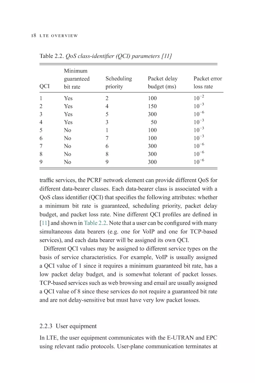
Table 2.2. QoS class-identifier (QCI) parameters [11]
QCI
Minimum
guaranteed
bit rate
Scheduling
priority
Packet delay
budget (ms)
Packet error
loss rate
1
2
3
4
5
6
7
8
9
Yes
Yes
Yes
Yes
No
No
No
No
No
2
4
5
3
1
7
6
8
9
100
150
300
50
100
100
300
300
300
10−2
10−3
10−6
10−3
10−3
10−3
10−6
10−6
10−6
traffic services, the PCRF network element can provide different QoS for
different data-bearer classes. Each data-bearer class is associated with a
QoS class identifier (QCI) that specifies the following attributes: whether
a minimum bit rate is guaranteed, scheduling priority, packet delay
budget, and packet loss rate. Nine different QCI profiles are defined in
[11] and shown in Table 2.2. Note that a user can be configured with many
simultaneous data bearers (e.g. one for VoIP and one for TCP-based
services), and each data bearer will be assigned its own QCI.
Different QCI values may be assigned to different service types on the
basis of service characteristics. For example, VoIP is usually assigned
a QCI value of 1 since it requires a minimum guaranteed bit rate, has a
low packet delay budget, and is somewhat tolerant of packet losses.
TCP-based services such as web browsing and email are usually assigned
a QCI value of 8 since these services do not require a guaranteed bit rate
and are not delay-sensitive but must have very low packet losses.
2.2.3 User equipment
In LTE, the user equipment communicates with the E-UTRAN and EPC
using relevant radio protocols. User-plane communication terminates at
2 . 2 s y s t e m a r c h i t e c t u r e 19
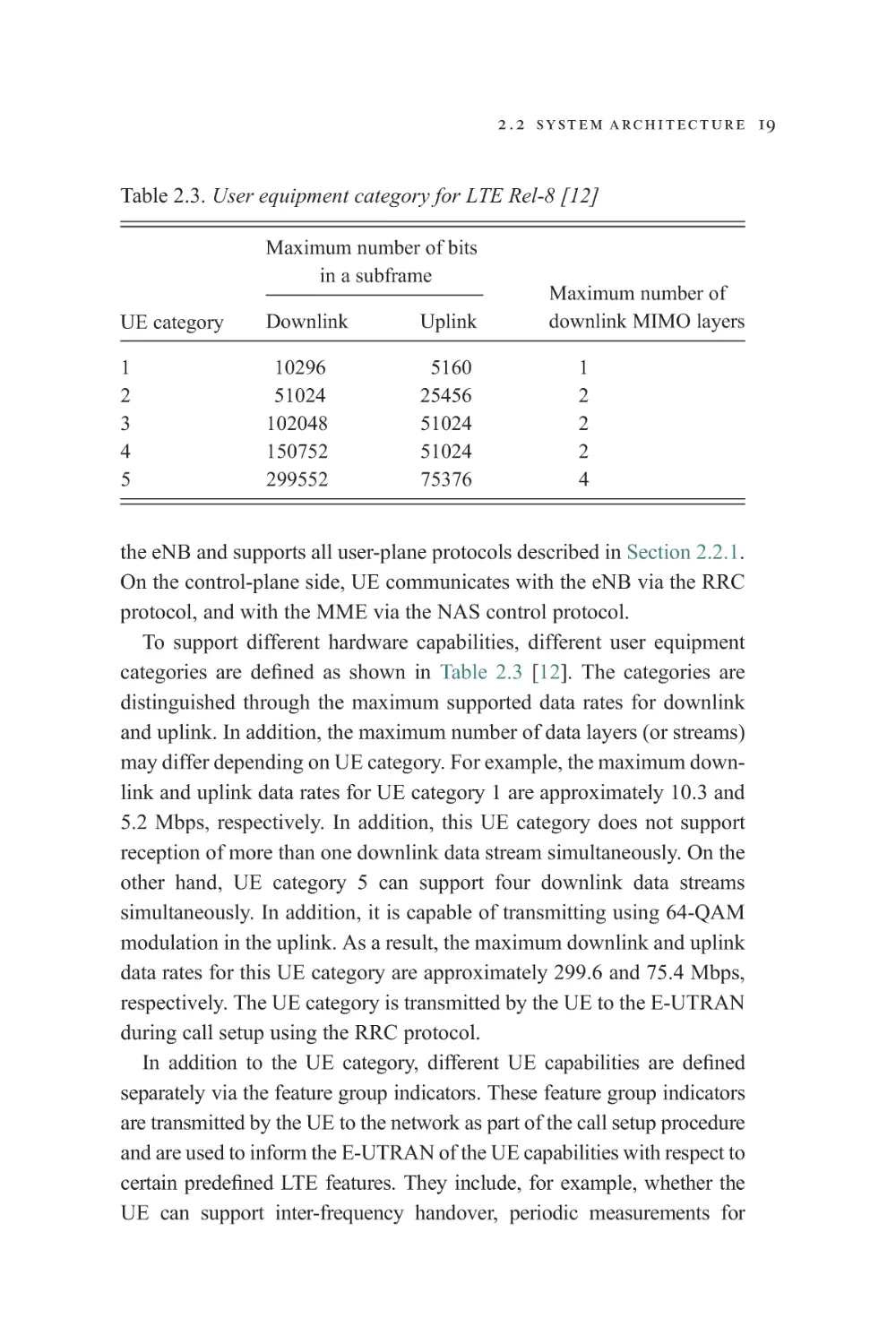
Table 2.3. User equipment category for LTE Rel-8 [12]
Maximum number of bits
in a subframe
UE category
Downlink
Uplink
1
2
3
4
5
10296
51024
102048
150752
299552
5160
25456
51024
51024
75376
Maximum number of
downlink MIMO layers
1
2
2
2
4
the eNB and supports all user-plane protocols described in Section 2.2.1.
On the control-plane side, UE communicates with the eNB via the RRC
protocol, and with the MME via the NAS control protocol.
To support different hardware capabilities, different user equipment
categories are defined as shown in Table 2.3 [12]. The categories are
distinguished through the maximum supported data rates for downlink
and uplink. In addition, the maximum number of data layers (or streams)
may differ depending on UE category. For example, the maximum downlink and uplink data rates for UE category 1 are approximately 10.3 and
5.2 Mbps, respectively. In addition, this UE category does not support
reception of more than one downlink data stream simultaneously. On the
other hand, UE category 5 can support four downlink data streams
simultaneously. In addition, it is capable of transmitting using 64-QAM
modulation in the uplink. As a result, the maximum downlink and uplink
data rates for this UE category are approximately 299.6 and 75.4 Mbps,
respectively. The UE category is transmitted by the UE to the E-UTRAN
during call setup using the RRC protocol.
In addition to the UE category, different UE capabilities are defined
separately via the feature group indicators. These feature group indicators
are transmitted by the UE to the network as part of the call setup procedure
and are used to inform the E-UTRAN of the UE capabilities with respect to
certain predefined LTE features. They include, for example, whether the
UE can support inter-frequency handover, periodic measurements for
20 l t e o v e r v i e w
self-optimized networks, inter-radio access technology measurements,
intra-subframe frequency hopping in the uplink, simultaneous transmission
of uplink control information, and semi-persistent scheduling. On the
basis of the reported UE category and capabilities, the E-UTRAN can be
aware of the different features that can be supported by the user.
2.3 Transmission scheme
In the downlink, OFDMA has been selected as the transmission technique
for LTE. In OFDMA, the frequency resource is divided into parallelfrequency subcarriers [13]–[14]. Each subcarrier is capable of carrying
one modulation symbol. Different subcarriers are grouped together to
form a sub-channel that serves as the basic unit of data transmission. The
main reasons why OFDMA was selected as the basic transmission scheme
for LTE are its high spectral efficiency, low-complexity implementation,
and the ability to easily support advanced features such as frequencyselective scheduling, multiple-input multiple-output (MIMO) transmission,
and interference coordination [15]. In the uplink, SC-FDMA was selected
due to its ability to provide similar advantages to OFDM such as orthogonality among users, frequency-domain scheduling, and robustness with
respect to multipath operation. However, SC-FDMA has a lower requirement for low-power amplifier back-off or de-rating. As a result, the average
transmission power can be much higher using SC-FDMA than it can with
OFDMA. This increases coverage in the uplink and provides higher uplink
data rates to users at the cell edge. Comprehensive reviews of the OFDMA
and SC-FDMA literature may be found in [16]–[17].
2.3.1 OFDMA
OFDMA has several advantages over the wideband code-division
multiple-access (WCDMA) technique used in the previous generations
of UMTS. As demonstrated in [2], OFDMA provides better performance
in terms of spectral efficiency (i.e. how much data can be transmitted for a
given amount of bandwidth) than does WCDMA both for broadcast and
for unicast services. This is due to the lack of inter-symbol interference
2 . 3 t r a n s m i s s i o n s c h e m e 21
User 1
S/P
Subcarrier
Mapping
User N
IFFT
CP
P/S
S/P
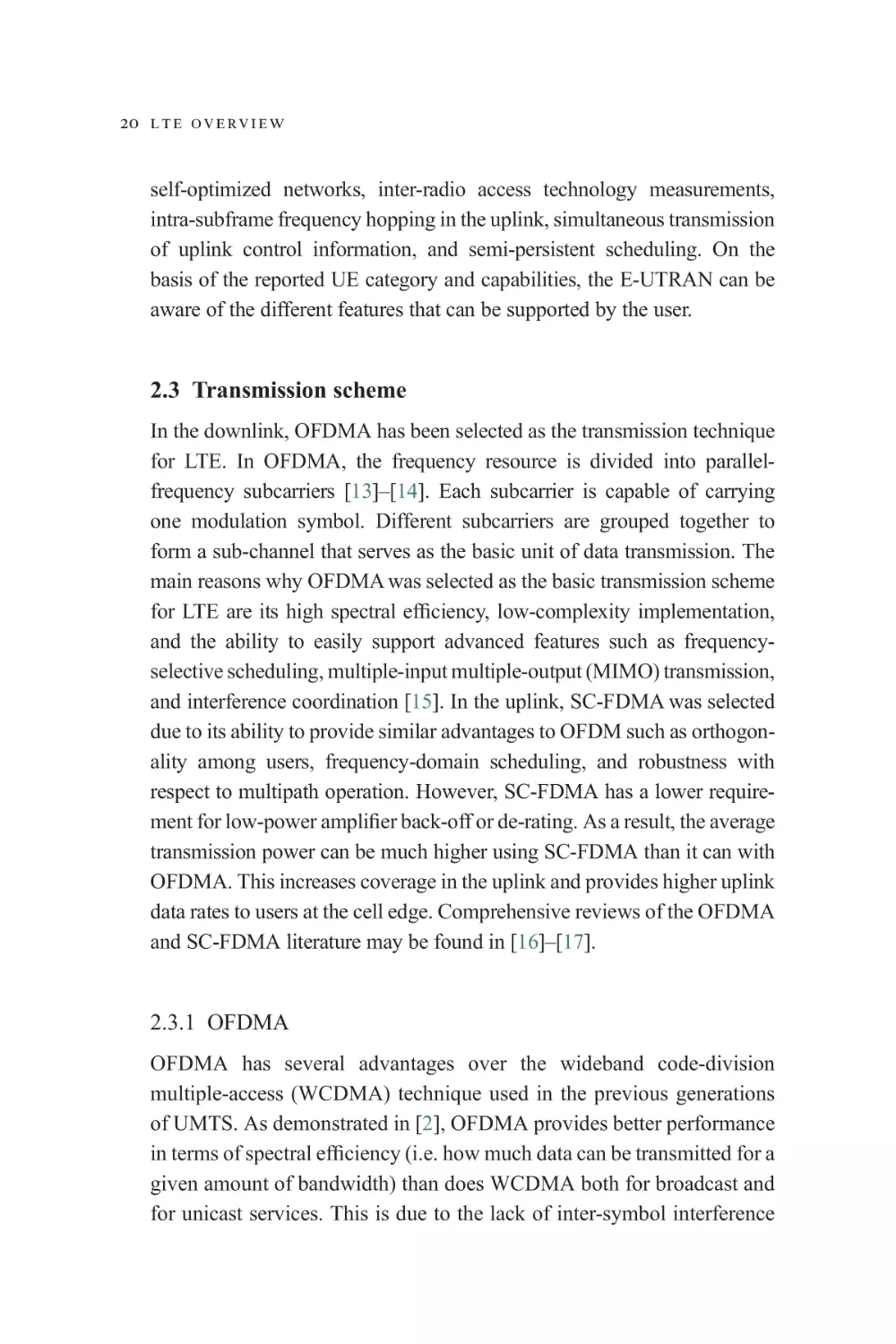
Figure 2.3. Block diagram for OFDMA.
from multipath channels and the absence of intra-cell interference
because users are orthogonal (i.e. they do not interfere with each other)
in the frequency domain. In addition, the OFDMA transmission technique scales easily to different bandwidths, so multiple system bandwidth
configurations can be efficiently supported. In addition, low-complexity
receivers can be used with OFDMA.
In addition, frequency-domain scheduling and MIMO processing techniques can be used. An example of frequency-domain scheduling techniques is frequency-selective scheduling. In frequency-selective scheduling,
users are assigned data only on good frequency bands (i.e. bands with
large gain), which are determined on the basis of channel quality feedback
from the UE. For broadcast services, single-frequency broadcast networks
can be supported. In this case, multiple base stations transmit the same
broadcast signals. The signals are coherently combined at the user, thus
improving performance at the cell edge substantially.
A basic block diagram illustrating OFDMA signal generation for one
OFDM symbol is shown in Figure 2.3. Data symbols from different users
are mapped to different subcarriers depending on the frequency bands
assigned to those users. This is done in the frequency domain. The information is then subjected to an inverse fast Fourier transform (IFFT) to
convert the frequency-domain subcarriers into time-domain signals.
A cyclic prefix is then added, and the signal is ready for transmission.
Note that the basic transmission unit for data is a subframe that spans
multiple OFDM symbols. At the receiver, the reverse operation is performed. The cyclic prefix is removed, then the time-domain signal is
subjected to a fast Fourier transform (FFT) so that the modulation symbols
on each subcarrier can be extracted. Each user then extracts the frequency
22 l t e o v e r v i e w
Subcarrier
Subcarrier Spacing
Resource Block
Resource Block
Center
Frequency
Frequency
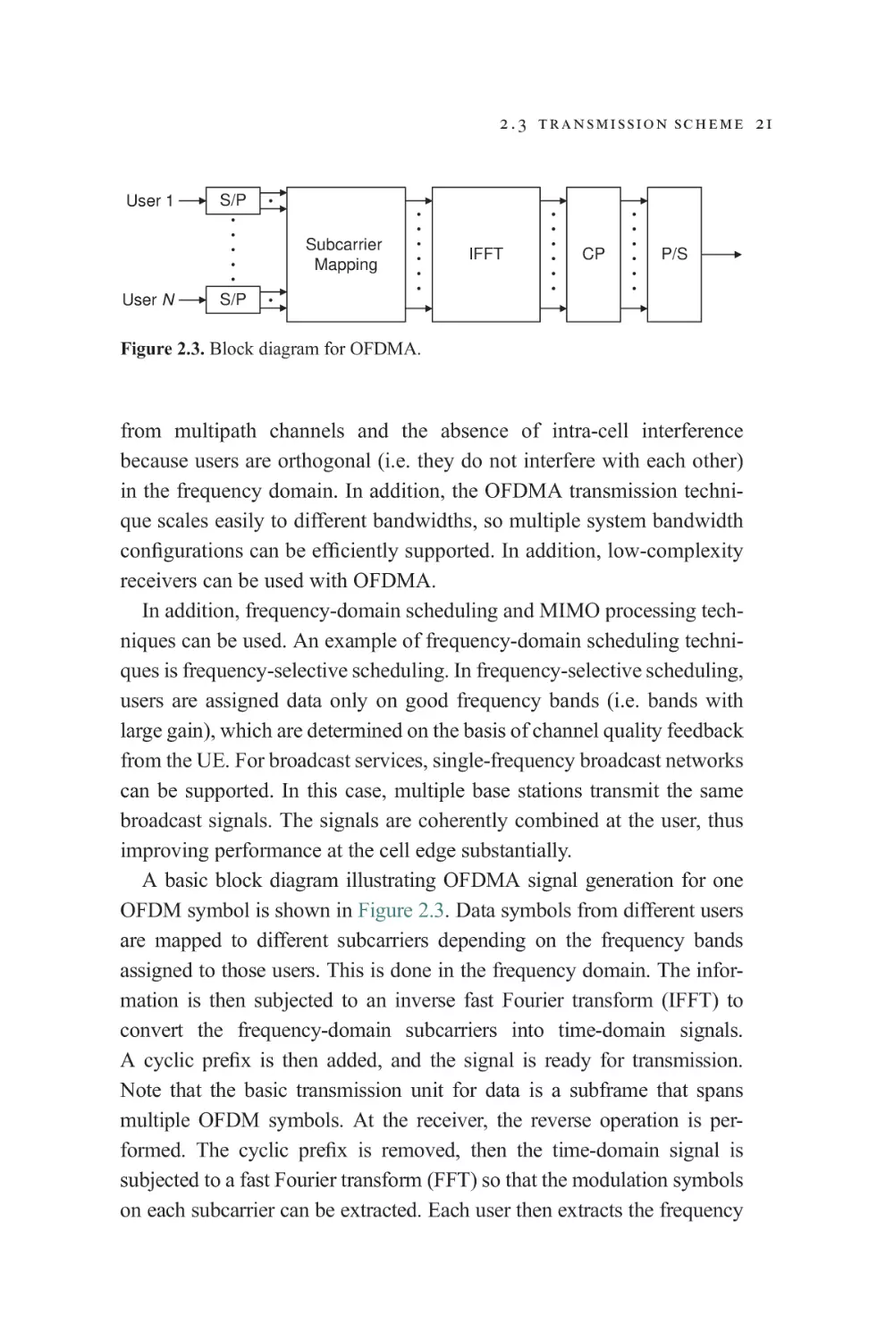
Figure 2.4. Frequency-domain illustration of OFDM.
resource units corresponding to his assigned subcarriers. Equalization is
performed and the data is passed onward for decoding.
A frequency-domain illustration of OFDM transmission is shown in
Figure 2.4, where each data symbol is modulated onto one of the subcarriers. The OFDM parameters must be selected carefully in order to
meet LTE requirements while minimizing overhead. Key design parameters include cyclic-prefix length, subcarrier spacing, and resource-block
size. In LTE, the direct-current (DC) subcarrier (the subcarrier at the
center frequency) is not used since the performance of this subcarrier
can be very poor for certain transmitter and receiver designs. Thus, the
usable subcarriers are located around this center frequency as shown in
Figure 2.4. The subcarrier spacing is the frequency spacing between two
adjacent subcarriers. Small subcarrier spacing means that more subcarriers are available for a given amount of bandwidth, thus increasing the
spectral efficiency since more data symbols are available for a given
amount of bandwidth. In addition, small subcarrier spacing also ensures
that the fading on each subcarrier is frequency-non-selective. However,
performance degrades as subcarrier spacing decreases due to Doppler
shift and phase noise. Doppler shift is caused by UE movement with
larger shift as UE velocity increases. This causes inter-carrier interference
whose degradation increases as the subcarrier spacing decreases. Phase
noise is caused by fluctuations in the frequency of the local oscillator, and
will cause inter-carrier interference as well. To minimize performance
degradation from phase noise, the subcarrier spacing should be greater
than 10 kHz. Furthermore, to support UE up to a speed of 350 km/h, the
subcarrier spacing should be around 9–17 kHz. As a result, a subcarrier
spacing of 15 kHz was chosen for LTE.
2 . 3 t r a n s m i s s i o n s c h e m e 23
CP
Data
OFDM symbol
Time
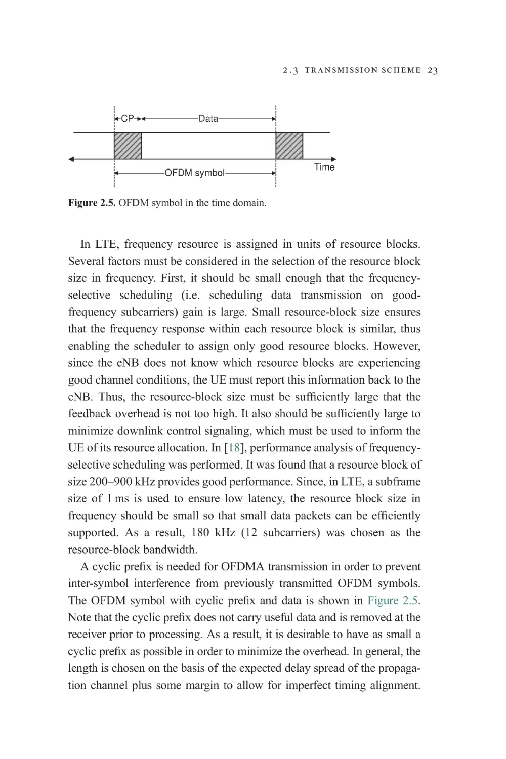
Figure 2.5. OFDM symbol in the time domain.
In LTE, frequency resource is assigned in units of resource blocks.
Several factors must be considered in the selection of the resource block
size in frequency. First, it should be small enough that the frequencyselective scheduling (i.e. scheduling data transmission on goodfrequency subcarriers) gain is large. Small resource-block size ensures
that the frequency response within each resource block is similar, thus
enabling the scheduler to assign only good resource blocks. However,
since the eNB does not know which resource blocks are experiencing
good channel conditions, the UE must report this information back to the
eNB. Thus, the resource-block size must be sufficiently large that the
feedback overhead is not too high. It also should be sufficiently large to
minimize downlink control signaling, which must be used to inform the
UE of its resource allocation. In [18], performance analysis of frequencyselective scheduling was performed. It was found that a resource block of
size 200–900 kHz provides good performance. Since, in LTE, a subframe
size of 1 ms is used to ensure low latency, the resource block size in
frequency should be small so that small data packets can be efficiently
supported. As a result, 180 kHz (12 subcarriers) was chosen as the
resource-block bandwidth.
A cyclic prefix is needed for OFDMA transmission in order to prevent
inter-symbol interference from previously transmitted OFDM symbols.
The OFDM symbol with cyclic prefix and data is shown in Figure 2.5.
Note that the cyclic prefix does not carry useful data and is removed at the
receiver prior to processing. As a result, it is desirable to have as small a
cyclic prefix as possible in order to minimize the overhead. In general, the
length is chosen on the basis of the expected delay spread of the propagation channel plus some margin to allow for imperfect timing alignment.
24 l t e o v e r v i e w
In LTE, three different cyclic-prefix values are supported – normal (~4.7 μs)
and extended (16.6 μs) for subcarrier spacing 15 kHz and extended (33 μs)
for subcarrier spacing 7.5 kHz. Note that the subcarrier spacing 7.5 kHz can
be used only for broadcast transmission. The normal cyclic-prefix length is
approximately 4.7 μs and is sufficient to handle channel delay spread in
most urban and suburban environments. With the data portion of the
OFDM symbol occupying approximately 66.7 μs, this represents a cyclicprefix overhead of 7%. An extended cyclic prefix of length 16.7 μs can be
used for environments with longer delay spread and for broadcast services.
In this case, however, a cyclic-prefix overhead of 25% is incurred.
To support different system bandwidths, different FFT sizes are used in
order to keep the OFDM symbol duration constant. That is, regardless of
the bandwidth, each OFDM symbol is of duration 66.7 μs. This allows the
same subcarrier separation to be supported, thus ensuring that the same
frequency-domain techniques can be applied across multiple bandwidths.
Keeping the symbol duration constant also results in the same subframe
length for all bandwidths, which is very attractive from a design perspective. Although the generation of the OFDM signal is up to implementation, as a guideline an FFT size of 2048 is used for 20 MHz. The FFT sizes
for other bandwidths are then scaled from this value. For example, for
5 MHz, an FFT size of 512 can be used.
The eNB transmission characteristics have to satisfy the standards set
by the 3GPP Radio Access Network Working Group 4 (RAN4) which is
in charge of radio performance and protocol aspects. They include maximum transmit power and dynamic range, unwanted emission, frequency
error, and error-vector magnitude (EVM). The frequency error is defined
as the difference between the actual transmit frequency and the desired
frequency. The frequency error is measured over one transmission subframe and must be within ±0.05 ppm to pass. The EVM is a measurement
of the difference between the transmit signal waveform and its idealized
counterpart. The higher the EVM, the worse the performance. In LTE, the
EVM must be below 17.5%, 12.5%, and 8% for QPSK, 16-QAM, and
64-QAM modulation, respectively. The reason why the EVM requirement is higher for lower-order modulation is that transmission using
2 . 3 t r a n s m i s s i o n s c h e m e 25
lower-order modulation can tolerate more signal distortion before performance loss is substantial. Unwanted emissions are emissions that
occur outside of the occupied bandwidth, thus generating interference
with other radio systems using nearby spectrum. Unwanted emissions can
be caused by the modulation process (called out-of-band emissions) or by
imperfections in the transmitter (called spurious emissions).
2.3.2 SC-FDMA
In the uplink, SC-FDMA is selected due to its ability to provide similar
advantages to OFDM, such as orthogonality among users, frequencydomain equalization, and robustness with respect to multipath operation
while maintaining a low power amplifier back-off or de-rating requirement [19]. The key characteristic of single-carrier transmission is that each
data symbol is transmitted using the entire allocated bandwidth. This is
different than OFDM, where each data symbol is transmitted using only
one subcarrier. Since single-carrier transmission spreads the data power
over the entire bandwidth, it requires lower power amplifier back-off. The
power back-off is the required reduction in the mean transmission power to
ensure that the maximum power stays within the linear region of the power
amplifier. Operating outside of the linear region of the power amplifier
causes signal distortion and interference. For instance, given the maximum
transmit power of 23 dBm (equivalent to 200 mW) and a power amplifier
back-off requirement of 3.4 dB for an OFDM signal, the maximum mean
transmission power is reduced to 19.6 dBm, which will reduce uplink
coverage significantly. A good measure of the power back-off requirement
is the cubic metric, defined in [20] as the cubic power of the signal of
interest compared with a reference signal. Table 2.4 provides the cubicmetric values for OFDMA and SC-FDMA. Another measure of the power
back-off requirement is the peak-to-average power ratio (PAPR). A PAPR
comparison between OFDMA and SC-FDMA has been presented in [21],
showing that the results for SC-FDMA are similar to those for the
cubic-metric gain shown in Table 2.4. The PAPR, however, has been
shown to be a less accurate predictor of amplifier power back-off than the
cubic metric [22].
26 l t e o v e r v i e w
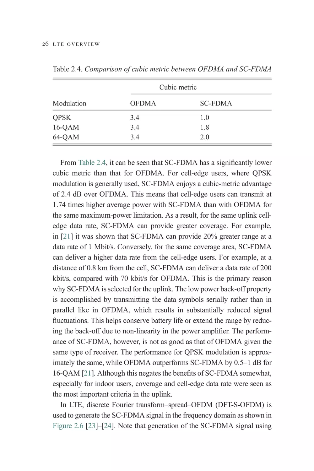
Table 2.4. Comparison of cubic metric between OFDMA and SC-FDMA
Cubic metric
Modulation
OFDMA
SC-FDMA
QPSK
16-QAM
64-QAM
3.4
3.4
3.4
1.0
1.8
2.0
From Table 2.4, it can be seen that SC-FDMA has a significantly lower
cubic metric than that for OFDMA. For cell-edge users, where QPSK
modulation is generally used, SC-FDMA enjoys a cubic-metric advantage
of 2.4 dB over OFDMA. This means that cell-edge users can transmit at
1.74 times higher average power with SC-FDMA than with OFDMA for
the same maximum-power limitation. As a result, for the same uplink celledge data rate, SC-FDMA can provide greater coverage. For example,
in [21] it was shown that SC-FDMA can provide 20% greater range at a
data rate of 1 Mbit/s. Conversely, for the same coverage area, SC-FDMA
can deliver a higher data rate from the cell-edge users. For example, at a
distance of 0.8 km from the cell, SC-FDMA can deliver a data rate of 200
kbit/s, compared with 70 kbit/s for OFDMA. This is the primary reason
why SC-FDMA is selected for the uplink. The low power back-off property
is accomplished by transmitting the data symbols serially rather than in
parallel like in OFDMA, which results in substantially reduced signal
fluctuations. This helps conserve battery life or extend the range by reducing the back-off due to non-linearity in the power amplifier. The performance of SC-FDMA, however, is not as good as that of OFDMA given the
same type of receiver. The performance for QPSK modulation is approximately the same, while OFDMA outperforms SC-FDMA by 0.5–1 dB for
16-QAM [21]. Although this negates the benefits of SC-FDMA somewhat,
especially for indoor users, coverage and cell-edge data rate were seen as
the most important criteria in the uplink.
In LTE, discrete Fourier transform–spread–OFDM (DFT-S-OFDM) is
used to generate the SC-FDMA signal in the frequency domain as shown in
Figure 2.6 [23]–[24]. Note that generation of the SC-FDMA signal using
2 . 3 t r a n s m i s s i o n s c h e m e 27
0
0
Modulated
Symbols
S/P
M-point
DFT
Subcarrier
Mapping
IFFT
CP
P/S
0
0
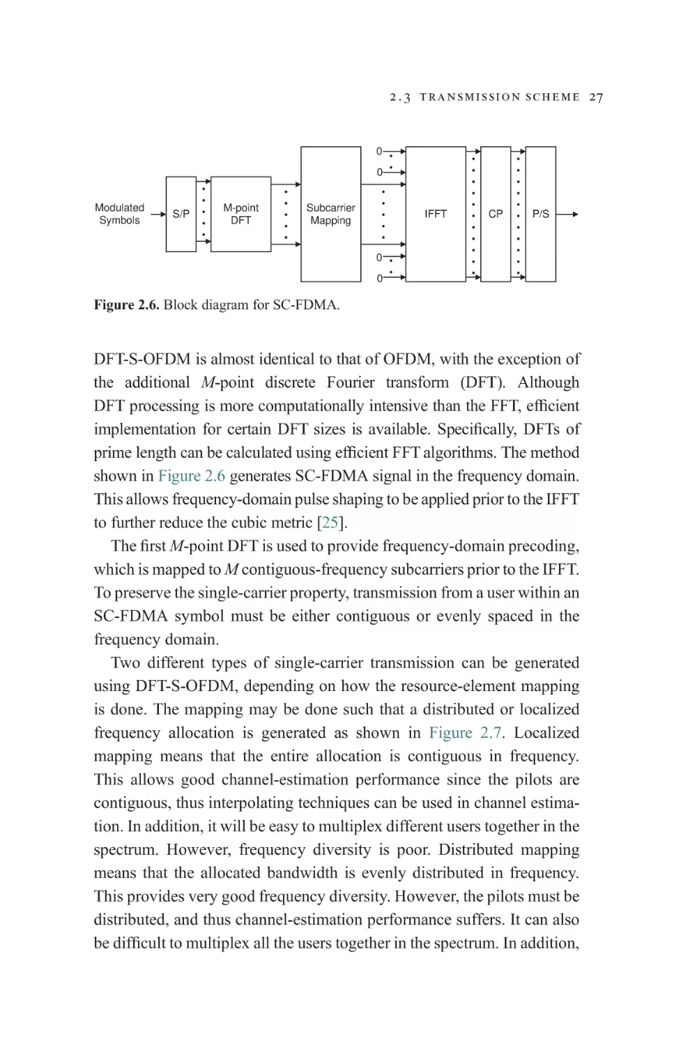
Figure 2.6. Block diagram for SC-FDMA.
DFT-S-OFDM is almost identical to that of OFDM, with the exception of
the additional M-point discrete Fourier transform (DFT). Although
DFT processing is more computationally intensive than the FFT, efficient
implementation for certain DFT sizes is available. Specifically, DFTs of
prime length can be calculated using efficient FFT algorithms. The method
shown in Figure 2.6 generates SC-FDMA signal in the frequency domain.
This allows frequency-domain pulse shaping to be applied prior to the IFFT
to further reduce the cubic metric [25].
The first M-point DFT is used to provide frequency-domain precoding,
which is mapped to M contiguous-frequency subcarriers prior to the IFFT.
To preserve the single-carrier property, transmission from a user within an
SC-FDMA symbol must be either contiguous or evenly spaced in the
frequency domain.
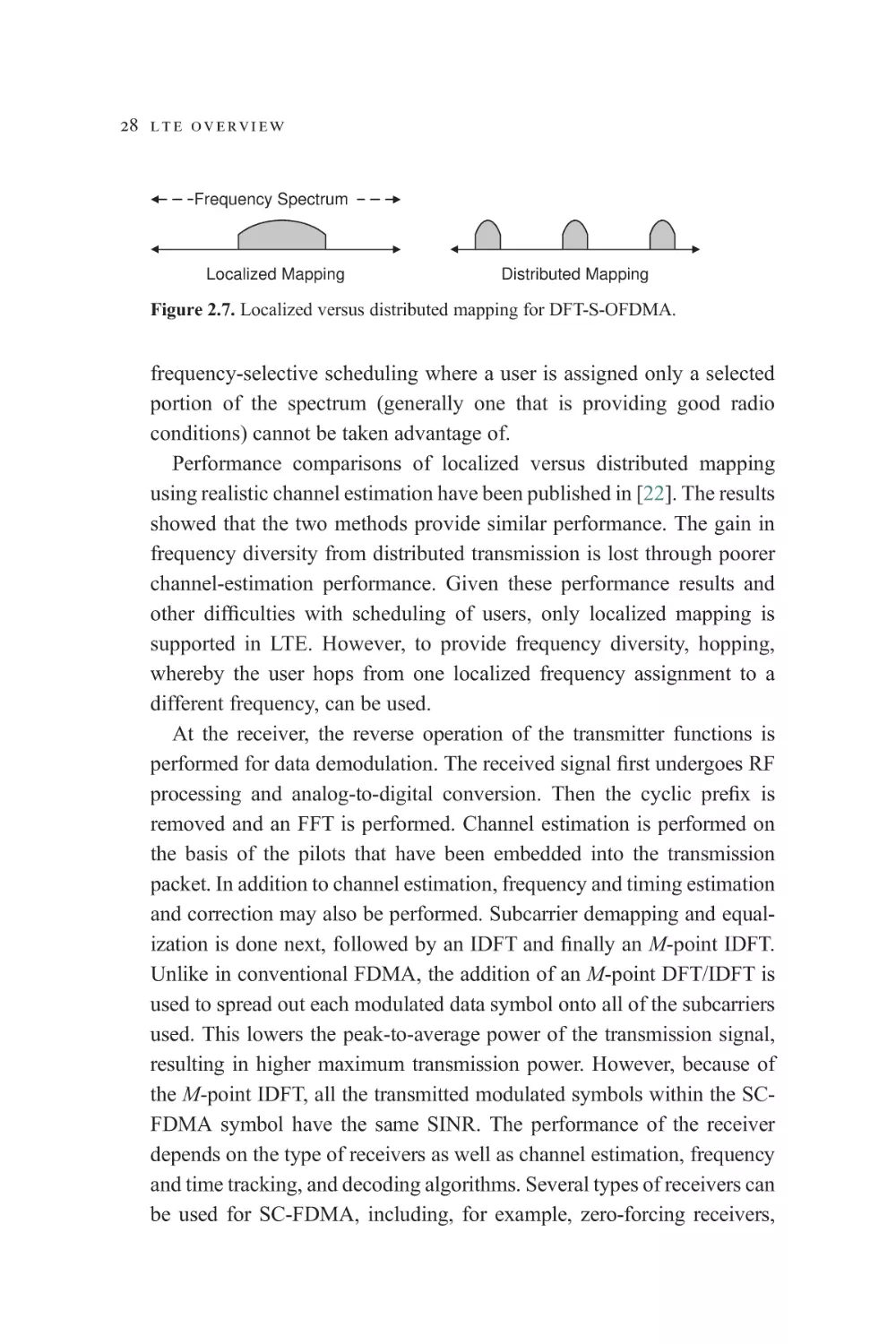
Two different types of single-carrier transmission can be generated
using DFT-S-OFDM, depending on how the resource-element mapping
is done. The mapping may be done such that a distributed or localized
frequency allocation is generated as shown in Figure 2.7. Localized
mapping means that the entire allocation is contiguous in frequency.
This allows good channel-estimation performance since the pilots are
contiguous, thus interpolating techniques can be used in channel estimation. In addition, it will be easy to multiplex different users together in the
spectrum. However, frequency diversity is poor. Distributed mapping
means that the allocated bandwidth is evenly distributed in frequency.
This provides very good frequency diversity. However, the pilots must be
distributed, and thus channel-estimation performance suffers. It can also
be difficult to multiplex all the users together in the spectrum. In addition,
28 l t e o v e r v i e w
Frequency Spectrum
Localized Mapping
Distributed Mapping
Figure 2.7. Localized versus distributed mapping for DFT-S-OFDMA.
frequency-selective scheduling where a user is assigned only a selected
portion of the spectrum (generally one that is providing good radio
conditions) cannot be taken advantage of.
Performance comparisons of localized versus distributed mapping
using realistic channel estimation have been published in [22]. The results
showed that the two methods provide similar performance. The gain in
frequency diversity from distributed transmission is lost through poorer
channel-estimation performance. Given these performance results and
other difficulties with scheduling of users, only localized mapping is
supported in LTE. However, to provide frequency diversity, hopping,
whereby the user hops from one localized frequency assignment to a
different frequency, can be used.
At the receiver, the reverse operation of the transmitter functions is
performed for data demodulation. The received signal first undergoes RF
processing and analog-to-digital conversion. Then the cyclic prefix is
removed and an FFT is performed. Channel estimation is performed on
the basis of the pilots that have been embedded into the transmission
packet. In addition to channel estimation, frequency and timing estimation
and correction may also be performed. Subcarrier demapping and equalization is done next, followed by an IDFT and finally an M-point IDFT.
Unlike in conventional FDMA, the addition of an M-point DFT/IDFT is
used to spread out each modulated data symbol onto all of the subcarriers
used. This lowers the peak-to-average power of the transmission signal,
resulting in higher maximum transmission power. However, because of
the M-point IDFT, all the transmitted modulated symbols within the SCFDMA symbol have the same SINR. The performance of the receiver
depends on the type of receivers as well as channel estimation, frequency
and time tracking, and decoding algorithms. Several types of receivers can
be used for SC-FDMA, including, for example, zero-forcing receivers,
2 . 3 t r a n s m i s s i o n s c h e m e 29
minimum-mean-squared-error receivers, interference-rejection combining
receivers, and turbo equalization receivers. Naturally, receiver performance is tied to complexity, with performance improving as complexity
grows. In practice, a minimum-mean-squared-error or interference-rejection
combining receiver is usually used because of its good performance and
manageable complexity.
In the uplink, the same issue with a DC subcarrier is present as in the
downlink. However, if the DC carrier is skipped in the uplink, then the
cubic metric can increase if the UE transmits on the resource block that
contains the DC subcarrier. This increase in cubic metric is on the order
of 0.5–0.7 dB, which will reduce the maximum transmit power by
12%–18%. As a result, a carrier shift of 7.5 kHz was introduced in the
uplink so that no carrier will be centered around DC. This leads to only
small performance degradation on the resource block that contains the
center frequency.
Transmitter characteristics and requirements for the UE can be found
in [26], including operating bands and radio-channel arrangement, transmit power, dynamic range, transmit signal quality, and output spectrum
emissions. Currently, only one UE power class is defined, with a maximum output power of 23 dBm and a tolerance of ±2 dB. The minimum
power output is −40 dBm. The actual UE transmit power, however, is
determined using a power-control formula and controlled by the eNB. To
allow for implementation margin, a tolerance band is provided. For
instance, if the UE has not had an uplink transmission within the last
20 ms, a tolerance of ±9 dB is allowed. That is, the actual transmit power
of the UE can be within 9 dB of the desired power. For UEs with uplink
transmission within the past 20 ms, a much smaller tolerance is allowed.
This tolerance is based on the difference between the required power and
the last transmit power. The larger the power difference, the larger the
allowable tolerance. In this case, the minimum tolerance band is ±2.5 dB
for a power difference of less than 2 dB, and the maximum tolerance
band is ±6 dB for a power difference of greater than or equal to 15 dB.
The UE also has the same EVM requirements for QPSK (17.5%) and 16QAM (12.5%) as the eNB. However, the EVM requirement for 64QAM has not been defined. Also similarly to the eNB, the UE has
30 l t e o v e r v i e w
requirements on out-of-band and spurious emissions that are intended to
limit the amount of interference with other UEs. The out-of-band emissions are limited by the spectrum mask and adjacent-channel leakage
ratio which the UE must satisfy. The spectrum-mask requirement limits
the maximum out-of-band power level, while the requirement regarding
the adjacent-channel leakage ratio limits the mean power on adjacent
channel frequencies. Limits on spurious emissions are also provided in
order to regulate how much interference can be generated by unwanted
transmitter effects at the UE.
References
[1] 3GPP TS 25.913, Requirements for Evolved UTRA (E-UTRA) and
Evolved UTRAN (E-UTRAN), v7.3.0, March 2006.
[2] 3GPP TS 25.912, Feasibility study for evolved Universal Terrestrial
Radio Access (UTRA) and Universal Terrestrial Radio Access Network
(UTRAN), v7.2.0, July 2006.
[3] 3GPP TS 36.300, E-UTRA and E-UTRAN overall description, v8.12.0,
March 2010.
[4] Larmo, A., Lindstrom, M., Meyer, M. et al., “The LTE link-layer
design,” IEEE Communications Magazine, vol. 47, no. 4, pp. 52–59,
April 2009.
[5] Dahlman, E., Ekstrom, H., Furuskar, A. et al., “The 3G Long-Term
Evolution – radio interface concepts and performance evaluation,”
IEEE 63rd Vehicular Technology Conference, vol. 1, pp. 137–141,
May 2006.
[6] Ekstrom, H., “QoS control in the 3GPP evolved packet system,” IEEE
Communications Magazine, vol. 47, no. 2, pp. 76–83, February 2009.
[7] Racz, A., Temesvary, A., Reider, N., “Handover performance in 3GPP
Long Term Evolution (LTE) systems,” 16th IST Mobile and Wireless
Communications Summit, July 2007.
[8] Bajzik, L., Horvath, P., Korossy, L., Vulkan, C., “Impact of intra-LTE
handover with forwarding on the user connections,” 16th IST Mobile and
Wireless Communications Summit, July 2007.
[9] Meng, W., Georgiades, M., Tafazolli, R., “Signaling cost evaluation of
mobility management schemes for different core network architectural
r e f e r e n c e s 31
[10]
[11]
[12]
[13]
[14]
[15]
[16]
[17]
[18]
[19]
[20]
[21]
[22]
arrangements in 3GPP LTE/SAE,” IEEE Vehicular Technology
Conference, pp. 2253–2258, May 2008.
3GPP TS 23.002, Network architecture, v10.0.0, September 2010.
3GPP TS 23.203, Policy and charging control architecture, v10.1.0,
September 2010.
3GPP TS 36.306, User equipment (UE) radio access capabilities,
v8.7.0, June 2010.
Weinstein, S., Ebert, P., “Data transmission by frequency-division
multiplexing using the discrete fourier transform,” IEEE Transactions
on Communication Technology, vol. 19, no. 5, pp. 628–634, October
1971.
Bingham, J. A. C., “Multicarrier modulation for data transmission: an
idea whose time has come,” IEEE Communications Magazine, vol. 28,
no. 5, pp. 5–14, May 1990.
Sari, H., Karam, G., Jeanclaude, I., “An analysis of orthogonal
frequency-division multiplexing for mobile radio applications,” IEEE
44th Vehicular Technology Conference, vol. 3, pp. 1635–1639, June
1994.
Taewon, H., Chenyang, Y., Gang, W., Shaoqian, L., Ye Li, G., “OFDM
and its wireless applications: a survey,” IEEE Transactions on
Vehicular Technology, vol. 58, no. 4, pp. 1673–1694, May 2009.
Ciochina, C., Sari, H., “A review of OFDMA and single-carrier
FDMA,” European Wireless Conference (EW), pp. 706–710, April
2010.
R1-050720, “Frequency selective scheduling resource block size for
EUTRA downlink,” Motorola, RAN1#42, San Diego, CA, October
2005.
Myung, H. G., Lim, J., Goodman, D. J., “Single carrier FDMA for
uplink wireless transmission,” IEEE Vehicular Technology Magazine,
vol. 1, no. 3, pp. 30–38, September 2006.
R1-060385, “Cubic metric in 3GPP-LTE”, Motorola, RAN1#44,
Denver, CO, February 2006.
R1-051088, “Coverage comparison between UL OFDMA and SCFDMA,” Nokia, RAN1#42, San Diego, CA, October 2005.
R1-051033, “Further topics on uplink DFT-S-OFDM for E-UTRA,”
Motorola, RAN1#42, San Diego, CA, October 2005.
32 l t e o v e r v i e w
[23] Fan, X., Li, Y., Li, M., Zhang, X., “Analysis and comparison of
different SC-FDMA schemes for 3GPP LTE,” International
Conference on Wireless Communications, Networking and Mobile
Computing, pp. 787–790, September 2007.
[24] Priyanto, B. E., Codina, H., Rene, S., Sorenson, T. B., Mogensen, P.,
“Initial performance evaluation of DFT-spread OFDM based
SC-FDMA for UTRA LTE uplink,” IEEE Vehicular Technology
Conference, April 2007.
[25] Mauritz, O., Popovic, B. M., “Optimum family of spectrum-shaping
functions for PAPR reduction of DFT-spread OFDM signals,” IEEE
64th Vehicular Technology Conference, September 2006.
[26] 3GPP TS 36.101, User equipment (UE) radio transmission and reception, v8.4.0, December 2008.
3
Downlink transmission and system
performance
3.1 Introduction
In this chapter the details of LTE downlink transmission are discussed.
The LTE downlink air interface uses the OFDM multiple-access technique described in Chapter 2. The use of OFDM transmission technology
provides significant advantages over other radio transmission techniques.
They include high spectral efficiency, support for broadband data transmission, the absence of intra-cell interference (i.e. multiple users in the
same cell can share the same subframe without interfering with each
other), resistance to inter-symbol interference arising from multipath
operation, natural support for MIMO schemes, a low-complexity
receiver, and support for frequency-domain techniques such as
frequency-selective scheduling, a single-frequency network, and soft
fractional frequency reuse. In addition to OFDM, LTE also utilizes
several other features to enhance system performance and user experience. They include short frame size to minimize latency, a singlefrequency network to provide high-data-rate broadcast services, VoIP
support to increase voice capacity, coverage for very large cells, and
coverage for high-speed users (up to 350 km/h) [1]–[2].
In LTE, both frequency-division duplex (FDD) and time-division
duplex (TDD) transmission are supported. Furthermore, the baseband
structure is common between FDD and TDD thus making LTE a very
flexible and efficient technology that can be deployed in either paired or
unpaired spectrum. In LTE, the differences between TDD and FDD are
mostly at the physical layer. As a result, identical network architecture can
be used to support both modes, thus reducing deployment costs and
complexity substantially. In the specifications, the two modes have been
designed to share as much functionality and as many features as possible,
33
34 d o w n l i n k a n d s y s t e m p e r f o r m a n c e
with the main design differences being the need to support various TDD
DL/UL allocations and provide co-existence with other TDD systems.
This chapter will cover an overview of E-UTRA downlink structure,
downlink reference signal structure, downlink control and other overhead
channels, and Multimedia Broadcast Multicast services. Aspects of the
performance of downlink shared and control channels for the single-input
multiple-output case are also included. Finally, a brief comparison
between LTE FDD and TDD systems is provided.
3.2 Mapping between transport and physical channels
The LTE physical layer provides four services to the MAC layer, namely
data-transfer services, signaling of Hybrid Automatic Repeat Request
(HARQ) feedback, signaling of scheduling request and measurement
reports (e.g. channel-quality information, received signal reference
power). The access to the data-transfer services is through the use of
transport channels. Six physical and four transport channels are defined
for LTE. The physical channels are the Physical Downlink Shared
Channel (PDSCH), Physical Broadcast Channel (PBCH), Physical
Multicast Channel (PMCH), Physical Control Format Indicator Channel
(PCFICH), Physical Downlink Control Channel (PDCCH), and Physical
HARQ Indicator Channel (PHICH). The four transport channels are the
Broadcast Channel (BCH), Paging Channel (PCH), Downlink Shared
Channel (DL-SCH), and Multicast Channel (MCH).
The PDSCH carries downlink data traffic and the PDSCH resources are
assigned using the downlink scheduling assignment carried on the
PDCCH. The PDSCH resources assigned to each user are orthogonal
(i.e. they are unique in time and frequency) except for in multi-user
MIMO (MU-MIMO), where multiple users are assigned overlapping
time–frequency resources. The PDCCH carries control information for
uplink and downlink as well as uplink power-control information, and is
assigned on a per-user basis, i.e. each control channel is individually
coded with its own error-detection information and can be power controlled. In addition, the PDCCH also carries uplink power-control information. The function of the PCFICH is to dynamically indicate the
3 . 3 l t e d o w n l i n k f r a m e s t r u c t u r e 35
number of control symbols used in a subframe. This feature is useful in
improving system capacity since the control-channel overhead can be
reduced on the basis of user loading in a cell. The PHICH is used to carry
acknowledgments associated with uplink data transmission. Finally, the
BCH is used to convey basic physical-layer system parameters necessary
to initiate access to the system.
The downlink also supports several types of signal, including the
synchronization signal, the cell-specific reference signal, and UE-specific
dedicated reference signals. The synchronization signal is used for cell
acquisition, detection of frame timing, and handover purposes. The cellspecific reference signal is used for demodulation of downlink data transmitted using open- and closed-loop spatial multiplexing schemes, for
estimating channel quality, and also for handoff measurements. The
UE-specific reference signal is used for demodulating downlink data
transmitted using beamforming, where the channel response is determined using a UE-specific reference signal. Table 3.1 summarizes the
different types of downlink physical channels and signals.
3.3 LTE downlink frame structure
In the downlink, OFDM is the multiple-access technique for E-UTRA
FDD and TDD systems. OFDM is well suited for high-data-rate systems
operating in multipath environments because of its robustness with
respect to delay spread. Multipath channels provide the potential to
improve the system performance by exploiting both the frequency diversity and the frequency selectivity of the channel. In OFDM, one data
symbol is transmitted per frequency subcarrier (called a resource element
in LTE). This exploits the frequency selectivity of the multipath channel
since the different symbols of the data packet are transmitted in different
frequency locations. In addition, because only one data symbol is transmitted per resource element, low-complexity receivers can be used. This
allows frequency-selective operation in addition to frequency-diverse
scheduling and one-cell reuse of the available bandwidth. Furthermore,
due to its frequency-domain nature, OFDM enables flexible-bandwidth
operation with low complexity. Smart antenna technologies are also
36 d o w n l i n k a n d s y s t e m p e r f o r m a n c e
Table 3.1. Summary of downlink channels and signals
Name
Description
Physical channels
Physical Downlink Shared
Channel (PDSCH)
Physical Downlink Control
Channel (PDCCH)
Shared data channel used for
transmission of scheduled user data
Control channel used for transmission of
control information, including
scheduling grants and power-control
information
Physical Control Format Indicator Used to dynamically indicate the number
Channel (PCFICH)
of OFDM symbols allocated for
control signaling in a subframe
Physical HARQ Indicator
Used to transmit downlink ACK/NACK
Channel (PHICH)
associated with uplink data
transmission.
Physical Broadcast Control
Used to transmit system information
Channel (PBCH)
necessary for system access
Paging Control Channel (PCH)
Used to transmit paging information
Physical signals
Cell-specific reference signal
UE-specific reference signal
Primary and secondary
synchronization signals (PSS
and SSS)
Common reference signal used for
demodulation of data and control
information, deriving CQI/PMI
information, and handoff
measurements
Dedicated reference signal dedicated to a
UE mainly used for RS-based
beamforming
Used for a variety of purposes, including
detection of frame timing, cell
acquisition, computing number of
antennas in BCH, and for handover
purposes
3 . 3 l t e d o w n l i n k f r a m e s t r u c t u r e 37
easier to support with OFDM, since each subcarrier becomes flat-faded
and the antenna weights can be optimized on a per-subcarrier (or block of
subcarriers) basis. Another significant advantage of OFDM is with
respect to broadcast services using a synchronized single-frequency network with appropriate cyclic-prefix design. Single-frequency network
transmission refers to simulcast transmission of the same content from
multiple cells, which, when combined over the air, significantly increases
the received signal power and supportable data rates for broadcast
services.
The downlink physical-layer resource grid is shown in Figure 3.1. The
DL RB
DL
Nsc subcarriers by Nsymb
total downlink resource grid has a size of NRB
DL
OFDM symbols, where NRB
is the number of available downlink
RB
resource blocks and Nsc is the number of subcarriers per resource
block. A resource element is equivalent to a subcarrier and can be
identified by the slot number and index (k, l), where k is the subcarrier
index and l is the OFDM symbol index.
Table 3.2 provides the downlink subframe parameters for different
spectrum allocations with subcarrier spacing 15 kHz. For MBMSdedicated cells, a subcarrier spacing of 7.5 kHz is also supported for very
DL
N symb
Resource
Element
RB
N sc
Resource
Block
Resource
Block Pair
Figure 3.1. Resource grid.
38 d o w n l i n k a n d s y s t e m p e r f o r m a n c e
Table 3.2. Parameters for downlink transmission scheme
Transmission bandwidth (MHz)
1.4
Subframe duration (ms)
Subcarrier spacing (kHz)
Sampling frequency (MHz)
FFT size
Number of resource blocks
Number of OFDM symbols per
subframe
CP length
Short
Extended
3
5
10
15
20
1.0 1.0 1.0 1.0
1.0
1.0
15 15 15 15
15
15
1.92 3.84 7.68 15.36 23.04 30.72
128 256 512 1024 1536 2048
6
15 25 50
75
100
14/12 (normal/extended cyclic prefix)
5.2 μs for l = 0, 4.7 μs for l = 1, . . ., 6
16.7 μs
large cells. Three different cyclic-prefix values are supported – normal
(~4.7 μs) and extended (16.6 μs) for subcarrier spacing 15 kHz and
extended (33 μs) for subcarrier spacing 7.5 kHz. In OFDM, a cyclic prefix
is used to guard against inter-symbol interference from previous OFDM
symbols. Inter-symbol interference degrades performance since the
received signal of the current symbol is distorted by signals from previous
symbols, and complicated signal-processing techniques are required in
order to mitigate this effect. In general, the longer the cyclic prefix, the
more robust the protection against inter-symbol interference. However, a
cyclic prefix is considered overhead since useful data cannot be carried on
the cyclic prefix. The normal cyclic prefix (~4.7 μs) provides a good
balance between overhead and supportable RMS delay spread, and is
suitable for most delay-spread environments where the RMS delay spread
is less than 5 μs which is typical for urban and suburban environments. The
extended cyclic prefix is mainly used for very large cells or cells supporting
MBMS using a single-frequency network.
The minimum quanta for scheduling downlink data are described by a
resource grid of subcarriers and OFDM symbols. The minimum scheduling quanta are defined as a pair of resource blocks (RBs) and described
3 . 3 l t e d o w n l i n k f r a m e s t r u c t u r e 39
Table 3.3. Physical resource-block definition
Cyclic-prefix type
Number of
subcarriers
Number of
symbols
Normal
Extended
12
12
7
6
SUBFRAME 0
SUBFRAME 1
SUBFRAME 5
Data
SUBFRAME 6
L1/L2 Control
L1/L2 Control
Data
L1/L2 Control
L1/L2 Control
P-BCH
L1/L2 Control
Radio Frame
Data
SUBFRAME 9
Figure 3.2. FDD downlink subframe structure.
in Table 3.3. The 12 subcarriers span 180 kHz and were chosen to optimize
the frequency-selectivity gain. As an example, for normal subframes a
resource block consists of 120–144 resource elements (REs). The
PDSCH supports QPSK, 16-QAM, and 64-QAM modulation, and is
coded using R = 1/3 mother turbo code. The turbo code used is the same
as Rel-6 UMTS turbo code except that the turbo code’s internal interleaver
is based on quadratic polynomial permutation (QPP) structure. The shared
channel also supports adaptive asynchronous HARQ, adaptive modulation
and coding, and MIMO/beamforming with scheduling done at the eNB.
Two frame structure types are supported in LTE – Type 1, which is
applicable to FDD deployment, and Type 2, which is applicable to TDD
deployment. Type 1 radio-frame structure (FDD) is shown in Figure 3.2.
A radio frame is comprised of 10 subframes, each of length 1 ms. This
subframe size was chosen to reduce the user-plane latency. The small
subframe size allows data to be delivered very quickly and any possible
retransmission to be sent soon after the initial transmission. Each
downlink subframe is further divided into two 0.5-ms slots to allow
interference-randomization techniques (e.g. cell-specific scrambling)
to be applied separately to each slot. Interference randomization is a
technique in which transmission of the signal from different eNBs is
40 d o w n l i n k a n d s y s t e m p e r f o r m a n c e
randomized to ensure that users do not always experience interference
from a particular eNB. Each slot is comprised of seven OFDM symbols
in the case of a normal cyclic prefix or six OFDM symbols in the case of an
extended cyclic prefix. Hence there is a loss in throughput due to the lower
number of symbols for an extended cyclic prefix. Within each slot, L1/L2
control regions comprising the PCFICH, PHICH, and PDCCH are located
in the first one to three OFDM symbols. The PBCH is transmitted in
subframe 0 using the central six resource blocks. Similarly, the synchronization signals are transmitted in subframes 0 and 5. In addition, cell-specific
reference signals are also transmitted throughout the subframe, allowing
a simple channel estimator to be used, like low-complexity MMSE-FIR
and IFFT-based channel estimators for demodulation of the downlink
shared channel. The cell-specific reference signals are also used for
computing channel quality, precoding matrix information, cell search/
acquisition, handover measurements etc.
Type 2 (TDD) frame structure is shown in Figure 3.3. Similarly to Type
1 structure, each radio frame spans 10 ms and consists of 10 1-ms subframes. Since the same spectrum is shared in a TDD deployment, a
subframe may be allocated to either downlink or uplink transmission
subject to certain constraints. First, subframes 0 and 5 are always downlink subframes, since they contain synchronization signals and broadcast
information necessary for users to connect and obtain information about
the system. In LTE, two switching-point periodicities are supported –
5 ms and 10 ms. Thus, each TDD uplink/downlink configuration pattern
will repeat itself every 5 ms or 10 ms. To provide a switching point
between downlink and uplink transmission, a special subframe is used.
SUBFRAME 0
SPECIAL
SUBFRAME
SUBFRAME 5
SPECIAL
SUBFRAME
Figure 3.3. TDD frame structure (TDD configuration 1).
L1/L2 Control
Data GP
UpPTS
L1/L2 Control
Data
P-BCH
L1/L2 Control
Data GP
UpPTS
L1/L2 Control
Data
P-BCH
L1/L2 Control
Radio Frame
Data
SUBFRAME 9
3 . 3 l t e d o w n l i n k f r a m e s t r u c t u r e 41
This special subframe contains three fields – the Downlink Pilot Time
Slot (DwPTS), Guard Period (GP), and Uplink Pilot Time Slot (UpPTS).
The DwPTS carries the downlink control and data, similarly to a normal
subframe, but with a reduced number of symbols. Thus the DwPTS can
be thought of as a shortened downlink subframe. On the other hand, the
UpPTS is only provisioned to carry PRACH format 4 (short RACH) and
sounding reference symbols. In other words, the UpPTS cannot be used to
transmit uplink data and control. The GP in the special subframe provides
the total switching period from downlink to uplink transmission and from
uplink to downlink transmission. Thus, there is no special subframe to
accommodate the switching period from uplink to downlink. Instead, an
appropriate timing advance at the UE will be employed to create the
necessary guard period for uplink to downlink transition.
For the 5-ms switching-point periodicity, subframes 1 and 6 are special
subframes. For the 10-ms switching-point periodicity, however, only
subframe 1 is a special subframe, while subframe 6 is a regular downlink
subframe. Figure 3.4 illustrates the seven possible DL/UL allocations,
Downlink
Special Subframe
TDD
Configuration
Uplink
0
D
S
U
U
U
D
S
U
U
U
1
D
S
U
U
D
D
S
U
U
D
2
D
S
U
D
D
D
S
U
D
D
3
D
S
U
U
U
D
D
D
D
D
4
D
S
U
U
D
D
D
D
D
D
5
D
S
U
D
D
D
D
D
D
D
6
D
S
U
U
U
D
S
U
U
D
Subframe (1 ms)
Radio frame (10 ms)
Figure 3.4. TDD DL/UL configurations for LTE.
42 d o w n l i n k a n d s y s t e m p e r f o r m a n c e
where D corresponds to a downlink subframe, S corresponds to a special
subframe, and U corresponds to an uplink subframe. For instance, DL/UL
configuration 1 provides approximately a 60:40 downlink-to-uplink split,
while configuration 4 provides approximately an 80:20 downlink-touplink time-division split. The choice of DL/UL configurations depends
upon the operator’s downlink-to-uplink traffic mix and co-existence with
other systems such as TD-CDMA or WiMAX. In general, an asymmetric
downlink-heavy split is used since many types of data traffic (e.g. web
browsing, streaming of video) are by nature directional in favor of the
downlink. Note that DL/UL configuration 5, where there is only one
uplink subframe, is intended for systems that provide mostly broadcast
services.
As illustrated in Figure 3.3, the total length of DwPTS, GP, and UpPTS
fields is 1 ms, which is the same as the length of a regular subframe.
However, within the special subframe the length of each field may vary
depending on the requirement for co-existence with legacy TDD systems,
supported cell size, and switching-time requirement. Eight different configurations are defined, providing a DwPTS of varying sizes from 3 to 10
OFDM symbols. For instance, configuration 3 provides a DwPTS:GP:
UpPTS of size 11:2:1 OFDM symbols. In this case, 11 OFDM symbols
are available for use by the DwPTS, while the UpPTS is of length 1
OFDM symbol. Certain configurations must be used when PRACH
format 4 needs to be supported since PRACH format 4 requires UpPTS
of size two symbols.
3.4 Data transmission
3.4.1 Shared data channel
Data transmission on the downlink is transmitted on the PDSCH. Users
are allocated resources within the PDSCH via a scheduling assignment
contained in the downlink control information. In LTE Rel-8, SU-MIMO
and MU-MIMO are both supported. In SU-MIMO, multiple data streams
are simultaneously transmitted to the same user using the same physical
resource blocks. In MU-MIMO, multiple data streams are simultaneously
3 . 4 d a t a t r a n s m i s s i o n 43
transmitted to different users using the same physical resource blocks.
SU-MIMO requires signaling to inform the users of the relevant transmission parameters, whereas MU-MIMO operation is transparent to the
users.
The transmitter chain can be summarized as follows. First, user data is
coded using turbo coding with the mother code rate of 1/3 and rate
matched to the coding rate assigned by the scheduler. For example, if
the user is assigned a coding rate of 1/2, the rate-matching procedure will
remove one of the three encoded bits generated using the mother code rate
of 1/3 to arrive at the assigned coding rate of 1/2. The encoded bits are
next scrambled on the basis of user and cell identities, modulated, precoded, and then mapped to resource elements. The asychronous HARQ
protocol is used in the downlink. This means that retransmission for a
specific HARQ process can occur anytime after a predefined delay. For
FDD, retransmission for an uplink packet transmitted at subframe n can
occur in any subframe after subframe n + 8. As a result, control signaling
is required for packet retransmission. In addition, packet retransmission
may be adaptive or non-adaptive. With non-adaptive retransmission, the
UE retransmits the packet using the same resource allocation as assigned
previously, with the option of changing only the redundancy version.
With adaptive retransmission, the UE may be assigned new downlink
resources, modulation and coding rate, and redundancy version, as long
as the transport block size is the same as the original.
3.4.1.1 Dynamic and semi-persistent scheduling
Downlink data transmission can be scheduled dynamically every subframe or semi-persistently until the resource is released. For dynamically
scheduled data transmission, the scheduling assignment is given via
downlink control information (DCI) format 1/1A/1B/2/2A/2B, where
the different formats refer to the different types of scheduling assignment.
The DCI is transmitted in the downlink control channel, the details of
which are provided in the next section.
In LTE, a stop-and-wait ARQ protocol is used to ensure that a data
packet is correctly received before a new packet is transmitted. In this
protocol, the sender waits for an acknowledgment subsequent to data
44 d o w n l i n k a n d s y s t e m p e r f o r m a n c e
transmission. If a positive acknowledgment (ACK) is received, new data
is then sent next. However, if a negative acknowledgment (NACK) is
received, the previous data packet is retransmitted. To continuously
supply the receiver with data, a multi-channel (N) stop-and-wait protocol
is used. This protocol parallelizes the stop-and-wait protocol, in effect
running N separate instantiations of the HARQ protocol. As a result, the
receiver is not stuck waiting for data, since multiple instances of the
algorithm send different data blocks on different HARQ process numbers.
In LTE the value of N in the case of FDD is set to 8, while for TDD it
depends on the TDD DL/UL split. After decoding the downlink data sent
in the Nth subframe by the eNB, the UE sends the ACK/NACK at N + 4
subframes, since the processing time at the UE is 3 ms. On receiving the
ACK/NACK, the eNB schedules retransmissions or new transmissions at
the subframes with numbers greater than or equal to N + 8.
In the downlink, asynchronous HARQ, in which the UE transmits
chase or incremental-redundancy versions of a packet on any HARQ
process until an ACK is received or the maximum number of retries
has been reached, is used. In the asynchronous HARQ stop-and-wait
protocol the UE can send retransmissions on any HARQ process in any
subframe, thus allowing greater scheduling flexibility [3]–[4]. For asynchronous HARQ to work, the following needs to be signaled using the
DCI format: explicit signaling of the HARQ process, an incrementalredundancy version, and a new data indicator.
Semi-persistent scheduling is suitable for users that have periodic data
assignment on the downlink. This mode is designed to save scarce downlink control-channel resources by periodically and persistently allocating
downlink resources to users with known periodic downlink data transmission such as VoIP or video conferencing [5]. In this mode a downlink
allocation is given and remains available to the user until the allocation is
released. As a result, a large number of users can be scheduled in this mode.
3.4.1.2 Resource allocation
Resource blocks are allocated in scheduling assignment grants using an
appropriate resource-allocation type (RAT). This assignment informs the
UE which resource blocks it has been assigned for data transmission.
3 . 4 d a t a t r a n s m i s s i o n 45
Three RATs are available – 0, 1, and 2. All three types can be used for
resource assignment in the downlink, but only RAT 2 can be used for
uplink assignment. Types 0 and 1 are implemented using bitmaps, where
each bit in the map specifies whether the corresponding resource block or
resource-block group is assigned to the user. This provides great flexibility as to which resource blocks can be assigned to a given user.
However, the disadvantage is that a large number of bits must to be sent
to the user, resulting in high control overhead. Figure 3.5 illustrates RAT 0
and 1 for a system bandwidth of 5 MHz. In the case of RAT 0, each bit in
the map signifies whether the resource-block group is assigned to the user.
The size of the resource-block group is dependent on the system bandwidth. For a system bandwidth of 5 MHz as shown in Figure 3.5, a
resource-block group comprises two resources blocks, thus resource can
be assigned in multiples of two resource blocks. When RAT 1 is used, an
individual resource block can be assigned. Four different RAT 1 patterns
can be generated, depending on how the P and shift (S) parameters are set.
This allows all different individual resource blocks to be addressed using
a reduced number of bits.
RAT 2 provides contiguous virtual or physical allocation of resource
blocks. This format requires only the starting resource-block number and
the number of assigned resource blocks to be sent to the users. The control
overhead with RAT 2 signaling is significantly lower than that for RAT
0/1 signaling. However, scheduling flexibility is lost insofar as only contiguous resource blocks can be assigned to a user. This is the only RAT
format that can be used in the uplink, since uplink assignment must be
contiguous in order to preserve the single-carrier property.
RB
0
RAT 0
1
2
0
3
4
1
5
6
2
7
8
3
9
10 11 12 13 14 15 16 17 18 19 20 21 22 23 24
4
5
6
7
8
9
10
12
11
RBG
0
1
2
0
3
1
4
2
5
3
6
4
7
5
8
6
9
7
10 11
8
9
12
RAT 1
0
0
1
1
2
3
2
3
4
4
5
5
6
Figure 3.5. Examples of resource-allocation types.
6
7
7
8
8
9
9
10
P = 0, S = 0
P = 1, S = 0
10 11
10
P = 0, S = 1
P = 1, S = 1
46 d o w n l i n k a n d s y s t e m p e r f o r m a n c e
3.4.1.3 Modulation and TBS allocation
Each PDSCH transmission to the UE contains an information set whose
size is given by the transport block size (TBS). In order to decode this data
packet, the UE needs to know the modulation type, the TBS, and the
coding rate. The modulation and TBS are jointly provided to the user in
the downlink scheduling assignment using the IMCS field. The coding rate
can be determined by the number of resource blocks once the modulation
and TBS are known. The possible values are contained in two lookup
tables and communicated to the user using the 5-bit MCS Index. The 5-bit
index provides 32 possible values, which provide sufficient granularity in
modulation and coding-rate assignment while maintaining low overhead.
A subset of the table is shown in Table 3.4, and the complete table can be
Table 3.4. A subset of the MCS index table [6]
MCS index
Modulation
TBS index
0
1
QPSK
QPSK
...
QPSK
QPSK
16-QAM
16-QAM
...
16-QAM
16-QAM
64-QAM
64-QAM
...
64-QAM
64-QAM
QPSK
16-QAM
64-QAM
0
1
8
9
10
11
15
16
17
18
27
28
29
30
31
8
9
9
10
14
15
15
16
25
26
Reserved
Reserved
Reserved
3 . 4 d a t a t r a n s m i s s i o n 47
found in [6]. The table has two entries corresponding to each index value,
namely the modulation order of the data packet and the TBS index. As an
example, consider an assignment to the user of IMCS = 10. From Table 3.4,
the user interprets this as stating that 16-QAM modulation will be used to
transmit the data, and the TBS of the data packet can be determined from
the TBS table using a TBS index of 9.
A subset of the TBS index table is shown in Table 3.5, and the complete
table can be found in [6]. Each row in the table provides the size of the
transport block in bits for a given TBS index and number of assigned
physical resource blocks. The table extends to 110 resource blocks, which
is the maximum number of resource blocks supported in LTE. The
number of assigned physical resource blocks is determined by the user
on the basis of the RAT discussed in Section 3.4.1.2. For instance, with a
TBS index of 9, and four assigned resource blocks, the size of the transport block is 616 bits according to Table 3.5. As a result, the user can
determine whether it is being scheduled to receive a downlink data packet
of size 616 bits (plus 24-bit CRC) that will be transmitted on four resource
blocks using 16-QAM modulation. The physical location of those
resource blocks is given by a separate resource-allocation field. Using
Table 3.5. A subset of the TBS index table [6]
Number of physical resource blocks
TBS index
1
2
3
4
5
6
7
8
0
1
2
16
24
32
32
56
72
56
88
144
120
176
208
152
208
256
176
224
296
208
256
328
9
10
136
144
296
328
456
504
776
872
936
1032
1096
1224
1256
1384
25
26
616
712
1256
1480
1864
2216
88
144
176
...
616
680
...
2536
2984
3112
3752
3752
4392
4392
5160
5160
5992
48 d o w n l i n k a n d s y s t e m p e r f o r m a n c e
this information, the user can also determine the coding rate of the data
packet to be sent.
This table is valid for FDD and regular subframes in TDD. For special
subframes in TDD, however, the TBS is scaled by 0.75 to account for the
reduced number of OFDM symbols. Note that a separate table is used for
two-layer spatial multiplexing, whereby two data streams are multiplexed
into the same transport block. In that case, the values of the entries are
approximately double those in the regular table.
3.4.2 Multimedia broadcast multicast service
Multimedia Broadcast Multicast Service (MBMS) will deliver highdata-rate multimedia services such as audio/video streaming, broadcast
data services, and advertising to LTE subscribers. The services are
delivered using broadcast or multicast mode. Examples of broadcast
services include television and radio broadcasts, service updates, and
location-based advertising. Multicast services in general require a subscription and can include, for example, personal communications,
financial data services, entertainment-related services, and others as
offered by the service provider. Because the service is broadcast, the
maximum data rate is limited by the signal quality received by the
worst user.
In LTE, MBMS is delivered via the PMCH using coordinated multicell transmission from a multimedia broadcast single-frequency network
(MBSFN) service area. In the MBSFN, the same signal is transmitted
from a cluster of neighboring cells belonging to the same MBSFN service
area so that the energy in each subcarrier from different cells participating
in the MBSFN operation is naturally combined over the air. This is
conceptually illustrated in Figure 3.6, where the same multicast channel
being transmitted from different cells is coherently combined by the user
at the cell edge. This provides a substantial improvement in the SNR at
the cell edge, which can increase the maximum supportable data rate
substantially. Using the MBSFN, spectral efficiencies at 95% cell coverage of approximately 1 bps and 3 bps can be achieved for large cells
(1732 m site-to-site) and small cells (500 m site-to-site), respectively. In
3 . 4 d a t a t r a n s m i s s i o n 49
MBSFN Service Area
P-MCH
eNB
P-MCH
P-MCH
eNB
eNB
P-MCH
eNB
UE
P-MCH
P-MCH
eNB
eNB
P-MCH
eNB
Figure 3.6. MBMS single-frequency network.
this case, data rates of 10–30 Mbps can be supported using a system
bandwidth of 10 MHz.
To support MBSFN operation, inter-site synchronization is required. In
addition, the cyclic-prefix duration should be long enough compared with
the time difference between the signals received from multiple cells.
Hence the MBSFN subframe is usually operated using the extended
cyclic prefix shown in Table 3.2. The subcarrier spacing of 7.5 kHz
using a cyclic-prefix duration of 33 μs is applicable only for standalone
MBMS operation using a separate carrier. The MBSFN (PMCH) and
unicast traffic (DL-SCH) can also be multiplexed in a TDM fashion with
the MBSFN subframe, preferably using an extended cyclic-prefix duration of 16.5 μs.
50 d o w n l i n k a n d s y s t e m p e r f o r m a n c e
3.5 Control signaling
3.5.1 Physical Downlink Control Channel
The PDCCH carries the DCI necessary to decode the PDSCH and
PUSCH. The design of the LTE PDCCH is very robust and flexible.
There are two principal types of control-channel design, namely the
broadcast common control channel and the per-user dedicated control
channel. In the case of a broadcast control channel, the common control
information required by all users is jointly coded. In this case, the code
rate used is designed to reach the worst-case user, and the control signals
could not be power-controlled or beamformed to a specific user. With a
per-user dedicated control channel, each user control channel is independently coded with an individual CRC. Using this structure, a user with
a good SINR will require less coding, whereas if a user is at the cell edge
the code rate can be lowered. Additionally, each user’s control channel
can be individually power-controlled as well as beamformed. Analysis
shows that with a per-user dedicated control channel the control overhead
is reduced and overall coverage and capacity are increased [7]–[8]. This
dedicated control structure is similar to that used in Rel-6 HSDPA [9]. In
LTE, the downlink control channel is designed on the basis of per-user
dedicated information for which the power and coding rate can be
individually controlled. Multiple control channels are used, and a user
monitors a number of control channels in order to find its dedicated
control information. Each channel carries information associated with a
radio-network temporary ID (RNTI), which is the identity assigned to a
UE by the network. For the control channel, convolutional code is used
due to its good performance for the small packet size typical of the control
information. Different code rates are supported through the use of different numbers of control-channel resource elements.
The PDCCH is located in the first n OFDM symbols of the subframe,
where n is dependent on the bandwidth, subframe, and service type [10].
In a typical FDD deployment, n is less than or equal to 3, and is
dynamically signaled to the users via the PCFICH. Data transmission
begins after n OFDM symbols, thus there is no mixing between data and
3 . 5 c o n t r o l s i g n a l i n g 51
control. Placing the control information in the first n symbols of the
subframe means that micro-sleep power-saving mode can be employed
by the users. In this mode, the receiver can wake up during transmission
of the control information and, if there is no assignment, go back to sleep
within one symbol, giving battery-life savings of approximately 64%.
There are 10 available DCI formats in LTE Rel-8. Within each DCI
format, several types of control information are sent – information related
to resource indication such as the resource-block size and duration of
assignment, information related to the transport format such as multiantenna information, modulation scheme, and payload size, and information related to HARQ support such as the process number, the redundancy
version, and a new data indicator. The available formats are briefly
described in Table 3.6.
The detailed bit allocation for some of the DCI formats used for
downlink scheduling assignment is shown in Tables 3.7–3.9. Details for
uplink scheduling assignment (DCI format 0) are discussed in
Section 4.3.1.
Table 3.6. DCI formats
Format Description
0
1
1A
1B
1C
1D
2
2A
3
3A
Uplink scheduling assignment
Downlink scheduling assignment for SIMO
Compact downlink scheduling assignment for SIMO
Based on format 1A with the addition of 2–4 bits for PMI, 2 bits for
two TX antennas and 4 bits for four TX antennas
Very compact downlink assignment for one codeword
Compact downlink assignment for scheduling of one PDSCH
codeword with precoding and power-offset information
Downlink scheduling assignment for SU-MIMO
Downlink scheduling assignment for open-loop spatial multiplexing
Transmission of TPC commands for PUCCH and PUSCH with 2-bit
power adjustments
Transmission of TPC commands for PUCCH and PUSCH with 1-bit
power adjustments
52 d o w n l i n k a n d s y s t e m p e r f o r m a n c e
Table 3.7. DCI format 1, downlink scheduling assignment for SIMO
Field
Number of bits
Resource allocation
header
RB assignment
MCS
HARQ process number
1
New data indicator
Redundancy version
DL
NRB =P
5
3 (FDD), 4
(TDD)
1
2
TPC for PUCCH
DL assignment index
CRC + UE ID
2
2
16
Description
DL resource-block assignment
Modulation and coding level
HARQ ID for asynchronous
N-channel stop-and-wait
HARQ based on incremental
redundancy
Applies to TDD only
The purpose of the multiple DCI formats is to scale the number of bits
for the PDCCH depending upon the UE and eNB features. As an example, if the downlink spatial multiplexing feature is not invoked in the eNB
there is no need for scheduling with the control-channel format for spatial
multiplexing (format 2), since this requires a greater number of controlchannel bits. There are four types of downlink assignment corresponding
to one codeword and two types of downlink assignment corresponding to
two codewords. There are two types of assignment – localized and
distributed. Distributed transmission is generally associated with
frequency-diverse scheduling, whereas localized transmission is associated with frequency-selective or frequency-non-selective scheduling.
The new data indicator (explicitly based on the NDI field) clears the
HARQ buffer and starts decoding the data according to the contents of
assignments when detected by the UE. After receiving a downlink scheduling assignment, the UE sets up the HARQ buffer on the basis of
the contents of the MCS and the resource-block assignment field.
Since the downlink HARQ transmission is based on an asynchronous
3 . 5 c o n t r o l s i g n a l i n g 53
Table 3.8. DCI format 1A, compact downlink scheduling assignment
for SIMO
Field
Number of bits
Format differential
flag
Localized/
distributed VRB
assignment flag
RB assignment
MCS
1
1
Description
Localized or distributed
resource-block
allocation
DL
DL
log2 ðNRB
ðNRB
þ 1Þ=2Þ
5
Modulation and coding
level
HARQ process
3 (FDD), 4 (TDD)
HARQ ID for
number
asynchronous Nchannel stop-and-wait
New data indicator 1
Redundancy version 2
HARQ based on
incremental
redundancy
TPC for PUCCH
2
DL assignment
2
Applies to TDD only
index
CRC + UE ID
16
stop-and-wait protocol, the HARQ process number field is needed for the
downlink, whereas it is not required for the uplink because of the use of
the synchronous stop-and-wait HARQ.
Each scheduling grant is defined on the basis of fixed-size controlchannel elements (CCEs), where a CCE is defined as a group of resource
elements. The CCEs can be combined in a predetermined manner to
achieve different coding rates. A CCE aggregation level of one, two,
four, or eight CCEs can be used to support one DCI transmission. Each
CCE is made of nine resource element groups, where each group contains
four resource elements. The resource elements used within the CCE are
distributed throughout the entire control-channel region, providing
54 d o w n l i n k a n d s y s t e m p e r f o r m a n c e
Table 3.9. DCI format 2, downlink scheduling assignment for MIMO
Field
Number of
bits
Resource-allocation header
RB assignment
TPC for PUCCH
DL assignment index
HARQ process number
1
DL
NRB =P
2
2
3 (FDD), 4
(TDD)
Transport block to codeword 1
swap flag
Transport block 1
MCS
5
New data indicator
1
Redundancy version
2
Transport block 2
MCS
New data indicator
Redundancy version
Precoding information
CRC + UE ID
5
1
2
Description
DL resource-block assignment
Applies to TDD only
HARQ based on incremental
redundancy
Modulation and coding level
HARQ based on incremental
redundancy
Modulation and coding level
HARQ based on incremental
redundancy
3 or 6
16
frequency-diversity gain and an interference-averaging effect. QPSK
modulation is always used. Because multiple CCEs can be combined to
effectively reduce the effective coding rate, a user control-channel assignment would then be based on channel-quality information reported. For
instance, with DCI format 1 the effective coding rate is 0.53 with one
CCE and 0.07 with eight CCEs.
The UE uses blind decoding to detect the PDCCH. To reduce the
number of blind detections, two search spaces are defined – the common
search space and the UE-specific search space. In the UE-specific search
space, the UE searches aggregation levels 1, 2, 4, and 8, whereas in the
3 . 5 c o n t r o l s i g n a l i n g 55
common search space the UE searches aggregation levels 4 and 8. The
common search space begins at CCE index 0. The UE determines the
starting CCE of the UE-specific search space using a hashing function
that is dependent on the MAC identity and subframe number.
3.5.2 Physical Control Format Indicator Channel
The PCFICH is used to dynamically indicate the number of OFDM
symbols used for control in a subframe. The possible values are dependent on the subframe type, structure, and system bandwidth. For system
bandwidth greater than 1.4 MHz, up to three OFDM symbols may be
reserved for control signaling. Further restriction is placed, however, on
MBSFN subframes to limit the maximum number of control symbols to
two. This restriction is enforced also for subframes 1 and 6 of the frame
structure of Type 2 (TDD) since the primary synchronization signal is
transmitted on the third OFDM symbol. For system bandwidth of
1.4 MHz, up to four symbols may be used for control signaling since
the bandwidth of the control region is very small. This will ensure that one
has a sufficiently large control region to schedule multiple uplink and
downlink users in the same subframe.
The PCFICH is transmitted in the first OFDM symbol of the subframe
and has three possible values. Because of the small number of information
bits carried by the control format indicator, possible coding options are
limited. As a result, predefined codewords based on (3,2) simplex coding
with repetition and systematic bits with minimum Hamming distance of
21 are used, as shown in Table 3.10. The selected codeword is mapped to
16 QPSK symbols, which are subsequently mapped to different resource
elements. To provide maximum frequency diversity, the PCFICH is
mapped onto four resource-element groups that are uniformly distributed
over the whole system bandwidth. The mapping ensures that each group
is separated by approximately a quarter of the system bandwidth, ensuring that the channel seen by each resource-element group is as uncorrelated as possible. Note that the PCFICH mapping to resource elements is
fixed and known from the cell identity. Transmit diversity is also supported using the same diversity scheme as the PDCCH. This combination
56 d o w n l i n k a n d s y s t e m p e r f o r m a n c e
Table 3.10. Control format indicator codeword
Value Codeword
1
2
3
0, 1, 1, 0, 1, 1, 0, 1, 1, 0, 1, 1, 0, 1, 1, 0, 1, 1, 0, 1, 1, 0, 1, 1, 0, 1, 1, 0, 1,
1, 0, 1
1, 0, 1, 1, 0, 1, 1, 0, 1, 1, 0, 1, 1, 0, 1, 1, 0, 1, 1, 0, 1, 1, 0, 1, 1, 0, 1, 1, 0,
1, 1, 0
1, 1, 0, 1, 1, 0, 1, 1, 0, 1, 1, 0, 1, 1, 0, 1, 1, 0, 1, 1, 0, 1, 1, 0, 1, 1, 0, 1, 1,
0, 1, 1
of frequency and transmit diversity allows the PCFICH to have good
performance and robustness against noise and interference. In a typical
urban propagation channel, the SNR requirement for PCFICH performance at 0.1% error rate is around − 2 dB. If the operating SNR at the cell
edge is below this threshold, power boosting (i.e. transmitting the subcarriers used for PCFICH at higher power than other subcarriers) can be
used to ensure good PCFICH performance. Because only 16 resource
elements are used for the PCFICH, power boosting of this channel can
easily be done if needed.
3.5.3 Physical HARQ Indicator Channel
The PHICH carries the acknowledgment response to uplink transmission
on the PUSCH by the UE. Subsequent to transmission of an uplink
transport block on the PUSCH, the UE will receive an acknowledgment
of the packet on a specific PHICH resource on the basis of a predefined
timing. The acknowledgment may be positive (ACK), meaning that the
data transport block was received and decoded correctly, or negative
(NACK), meaning that the packet was not decoded correctly. Upon
NACK reception, the UE can retransmit the data packet at a predefined
time. In the physical layer, the acknowledgment is transmitted on a
PHICH resource, which is defined by an index pair comprising the
PHICH group number ngroup
PHICH and the sequence number within the
3 . 5 c o n t r o l s i g n a l i n g 57
group nseq
PHICH . Each PHICH group contains eight different sequences, in
the case of a normal cyclic prefix, or four different sequences, in the case
of an extended cyclic prefix.
The UE determines the PHICH resource associated with its uplink
transmission by the lowest resource-block index for uplink allocation
and the 3-bit cyclic-shift parameter for the uplink reference signal given
in the grant. By using the lowest resource-block index for uplink allocation, the PHICH resource can be implicitly determined. This provides a
saving insofar as explicit PHICH resource assignment is not required.
However, to be able to handle spatial multiplexing where multiple users
can share the same lowest resource block, an explicit parameter, namely
the 3-bit cyclic-shift parameter for the DMRS, is also used. This ensures
that the PHICH resource assignment is free from contention. For instance,
for a user given an uplink assignment of four resource blocks PRB = 5, 6,
7, 8 and nDMRS ¼ 1, the corresponding PHICH resource is indicated by
seq
ngroup
PHICH ¼ 6 and nPHICH ¼ 2. If another user is scheduled on the same set
of resource blocks but with nDMRS ¼ 4, then that user’s PHICH resource
seq
is indicated by ngroup
PHICH ¼ 2 and nPHICH ¼ 4.
To allow control of the PHICH overhead, the number of PHICH groups
can be configured by the phich-Resource RRC parameter, which can take
on values of {1/6, 1/2, 1, 2}. The possible values specify the number of
PHICH resources as a multiple of the number of resource blocks. For
instance, a value of 1/2 means that approximately half the PHICH
resource exists as physical resource blocks, whereas a value of 2 means
that there is approximately twice as much PHICH resource as physical
resource blocks. By restricting the number of PHICH groups to a minimum, more resource elements are made available for the PDCCH to
transmit downlink control information. When there is less PHICH
resource than the number of physical resource blocks, the eNB is responsible for ensuring that there is no PHICH-resource contention among the
users. The eNB does this by checking for PHICH-resource contention
when scheduling a user. If no PHICH-resource is available, the eNB may
be prevented from scheduling a particular user. An example of the number
of PHICH resources for a subframe with a normal cyclic prefix is shown
in Table 3.11. From this table, it can be seen that, with phich-Resource set
58 d o w n l i n k a n d s y s t e m p e r f o r m a n c e
Table 3.11. Number of PHICH resources (normal cyclic prefix)
System bandwidth (MHz)
1/6
1/2
1
2
5
10
20
8
16
24
16
32
56
32
56
104
56
104
200
ACK/NACK
Coding
(Repetition)
BPSK
Modulation
Layer
Mapping
RE
Mapping
IFFT
Spreading
Figure 3.7. PHICH block diagram.
to 1/2, 56 unique PHICH-resource indices are available at 20 MHz. This
means that up to 56 uplink users can be simultaneously scheduled in the
same subframe.
An illustrative block diagram of the PHICH is shown in Figure 3.7.
Since Rel-8 of the specifications does not support spatial multiplexing
from the same user on the uplink, only one acknowledgment bit is to be
transmitted. The acknowledgment bit is first coded using repetition to
form a block of bits. These coded bits are then modulated using BPSK
modulation and spread by an orthogonal sequence. For a normal cyclic
prefix, eight orthogonal sequences are available using a spreading factor
of 4 together with I/Q multiplexing. For an extended cyclic prefix, four
orthogonal sequences are available using a spreading factor of 2 together
with I/Q multiplexing. This allows multiple acknowledgments to be codemultiplexed into the same PHICH group. Code-division multiplexing
increases the PHICH capacity, allows power control between acknowledgments for different users, and provides good interference averaging.
Subsequent to the spreading operation, layer mapping using transmit
diversity is performed on the basis of the number of transmit antennas
at the eNB.
3 . 5 c o n t r o l s i g n a l i n g 59
PHICH 1
0 Reference Signal – Ant Port 0
PHICH 2
1 Reference Signal – Ant Port 1
Time
Frequency
0
1
0
1
0
1
0
1
0
1
0
1
1
Figure 3.8. PHICH mapping (normal duration).
The mapping of PHICH in the time–frequency domain is illustrated in
Figure 3.8. Each PHICH group is comprised of three repeated segments
that are mapped to different frequency regions to provide frequency
diversity. In addition, the PHICH group can be mapped into one (normal
duration) or three (extended duration) OFDM symbols. Mapping into
three OFDM symbols allow more power to be allocated to the PHICH,
increasing the coverage and reliability of this channel.
For the PHICH, the performance requirement is usually specified as an
ACK-to-NACK error probability of 0.1%. Because each PHICH group
contains multiple acknowledgments, the power requirement depends on
the number of acknowledgments. When only a single acknowledgment is
present in the PHICH group, the SNR requirement is around − 2 dB in a
typical urban channel. This makes the PHICH a very robust channel
insofar as it can operate well at the SINR typically seen at the cell edge.
With multiple acknowledgments in a PHICH group, interference among
different acknowledgments can degrade performance somewhat.
However, the eNB can use intelligent scheduling management (e.g. by
limiting the number of acknowledgments within a PHICH group or
ensuring that all acknowledgments within a group are transmitted with
similar powers) to ensure minimal interference.
3.5.4 Physical Broadcast Channel
In LTE, system information necessary for system access is divided into
two parts – the MasterInformationBlock (MIB) and a number of
SystemInformationBlock (SIBs). The MIB contains basic physical-layer
system parameters necessary to demodulate downlink channels.
Subsequent to successful acquisition of the MIB information, the UE
60 d o w n l i n k a n d s y s t e m p e r f o r m a n c e
Table 3.12. Master-information-block fields
MIB field
Number of information bits
Downlink system bandwidth
PHICH configuration
System frame number
Spare
3
3
8
10
will be able to read the downlink control and data channels, which would
allow it to obtain additional control information contained in the SIBs that
is necessary in order to perform initial access into the system. These SIBs
are transmitted on the data channel. The MIB is transmitted on the PBCH
over four radio frames (40 ms period) with portions transmitted in subframe 0 of every radio frame. The MIB contains four fields as shown in
Table 3.12. The downlink system bandwidth gives the number of resource
blocks in the downlink with possible values of 6, 15, 25, 50, 75, and 100
(corresponding to system bandwidths of 1.4, 3, 5, 10, 15, and 20 MHz,
respectively). The PHICH configuration gives the amount of PHICH
resource and its duration. The system frame number (SFN) field provides
the most significant 8 bits of the 10-bit SFN. The last two bits are to be
determined blindly by users on the basis of the coding structure of the BCH.
A block diagram of the BCH transmission is shown in Figure 3.9. First,
a 16-bit CRC is appended to the BCH transport channel, forming an
information block of size 40 bits. Note that the CRC for this transport is
further masked by specific codewords denoting the number of transmit
antennas (1, 2, or 4) at the eNB. Thus, by decoding the BCH, the UE will
receive confirmation regarding the number of eNB transmit antennas.
Prior to this confirmation, the UE will need to blindly determine the
number of transmit antennas via the synchronization signals. The transport block is then coded using R = 1/3 tail-biting convolution coding.
Rate-matching is next performed to generate 1920 coded bits for a normal
cyclic prefix and 1728 coded bits for an extended cyclic prefix. This
provides a very low coding rate (e.g. a coding rate of 1/48 for a normal
cyclic prefix if all transmissions are considered), and as a result the BCH
3 . 5 c o n t r o l s i g n a l i n g 61
MIB
CRC
24
16
Coded & Rate-Matched Bits
1920
Segment 0
Segment 1
Segment 2
Segment 3
480
480
480
480
Scramble
Subframe 0
1
Radio Frame
SFN mod 4 = 0
9
0
1
Radio Frame
SFN mod 4 = 1
Scramble
Scramble
Scramble
9
0
1
Radio Frame
SFN mod 4 = 2
9
0
1
Radio Frame
SFN mod 4 = 3
Figure 3.9. Mapping of BCH into four 10-ms subframes (normal cyclic prefix).
enjoys robust performance even for low SNRs. The coded bits are then
scrambled and equally divided into four blocks and mapped into four
consecutive radio frames. This is illustrated in Figure 3.9. The scrambled
sequence is initialized by the cell ID every four radio frames, and therefore is different for each of the segments shown. The position of the
PBCH is always fixed in time to the first four OFDM symbols of slot 1,
subframe 0 of every radio frame, and in frequency to 72 subcarriers
centered around the DC subcarrier. QPSK modulation is always used.
When more than one transmit antenna is present at the eNB, transmit
diversity is used for antenna diversity. In FDD, the PBCH is placed next to
the synchronization signals in the transmission subframe. This is because
the UE will generally use channel estimation obtained from the synchronization signals to demodulate the PBCH since the downlink bandwidth
is not known. Therefore, by having the PBCH next to the synchronization
signals in time, good channel estimates can be ensured. In TDD, the
PBCH is placed slightly ahead in time of the synchronization signals. This
allows the user to be able to distinguish between FDD and TDD systems
during the cell-search stage.
Each of the four PBCH coded segments is self-decodable. However,
since each segment has a different scrambling sequence, the UE will have
62 d o w n l i n k a n d s y s t e m p e r f o r m a n c e
to try four decoding possibilities at each instance. This, however, allows
the UE to implicitly derive the last two bits of the SFN from which of the
hypotheses was successful. Note that, if the UE cannot decode the PBCH
in one reception, it can combine several subsequent transmissions to
increase the SNR. In a typical urban propagation channel, the SNR
requirement for PBCH performance of 1% BLER is around − 8 dB.
This makes the PBCH a very robust channel.
3.5.5 Paging Control Channel
The PCH is used either to transmit paging information to UEs in idle
mode or to inform both idle and connected UEs about a system information change or Earthquake and Tsunami Warning System (ETWS) notification. UEs that are in idle mode may be configured with a specific
discontinuous reception (DRX) cycle, and thus will wake up only intermittently to monitor the Paging Control Channel (PCH). DRX allows the
UE to turn off its electronics while in the discontinuous reception state,
providing battery-life saving. The paging message contains the following
fields – systemInfoModification field, to indicate a change in system
information, etws-Indication field, to indicate ETWS notification, and a
list of paging records. Each paging record contains the UE identity and
the originating domain for paging. Up to 16 paging records can be
grouped together in one paging message, thus 16 UEs can be addressed
at the same time.
The paging message is transmitted on the Paging Control Channel.
This is a logical channel that is transmitted onto the PDSCH using a
special identifier called the Paging Radio Network Temporary Identifier
(P-RNTI). Only one P-RNTI value is available and this is shared by all
users. In this case, the eNB transmits the paging message on the PDSCH
together with an associated downlink scheduling assignment using either
DCI format 1A or DCI format 1C. Because this is transmitted on the
PDSCH, the eNB has the flexibility to select the amount of resources
(modulation and coding, and number of resource blocks) sufficient to
reach the intended UEs. Because this message is normally addressed to
multiple UEs, ACK/NACK is not possible and therefore the eNB will
3 . 6 d o w n l i n k r e f e r e n c e s i g n a l 63
generally transmit this message with some performance margin to ensure
reception. UEs that have been configured for paging notification (i.e.
users that are in idle mode) will decode the control information and
then the paging message. If the systemInfoModification or etwsIndication is set, the UE will reacquire the system information and
perform the appropriate action. In the case of a match of its identity in
the paging record, it will forward this information to the upper layer in
preparation for the establishment of an RRC connection to receive an
incoming call.
3.6 Downlink reference signal
Downlink reference signals are provided to assist the users in performing
channel estimation and demodulation of control and data information,
and for channel information measurements such as channel quality information (CQI), rank, and precoding matrix indicator (PMI). Three types of
downlink reference signals are available – cell-specific reference signals,
MBSFN reference signals, and dedicated reference signals. Cell-specific
reference signals are common to all users, while UE-specific reference
signals are used only with dedicated reference-symbol-based beamforming. MBSFN reference signals are used in MBSFN transmission and are
common to all cells in the MBSFN service area. In LTE, a referencesignal pattern is specified per downlink antenna port, where an antenna
port is a logical entity that can be mapped to one or more physical
antennas. For cell-specific and MBSFN reference signals, one, two or
four antenna ports are available. As an example, an eNB with two
physical transmission antennas can be configured to use either one or
two antenna ports. If it is configured to support two antenna ports, different reference signal patterns are transmitted on the two available physical
antennas. If only one antenna port is used, then the same reference-signal
pattern is transmitted on both physical antennas. The number of cellspecific antenna ports must be first determined blindly by the UEs, and
then confirmed via the antennaPortsCount field of the radio resource
configuration message. For UE-specific reference signals, however, only
one antenna port (antenna port 5) is defined. In this case, only one
64 d o w n l i n k a n d s y s t e m p e r f o r m a n c e
reference-signal pattern is defined, which is then mapped to all available
physical antennas.
The downlink cell-specific reference-signal structure is shown in
Figure 3.10 for four antenna ports. Note that, for a smaller number of
antenna ports, the unused reference-signal symbols are available for
either data or control transmission. For instance, with one antenna port,
resource elements for reference signals R1, R2, and R3 are used for either
data or control transmission. The overhead consumed by the reference
signals is 4.8%, 9.5%, and 14.3% for one, two, and four antenna ports,
respectively. To provide good channel-estimation performance, cellspecific reference symbols are provided at regular time and frequency
intervals. From Figure 3.10, it can be seen that there is a frequency
separation between reference symbols of six resource elements. This
gives a coherence bandwidth of 90 kHz, which can support a propagation
channel with RMS delay spread of up to 2.2 μs. In the case of one or two
antenna ports, reference symbols are present in four OFDM symbols that
are distributed fairly evenly within the resource block. This temporal
separation provides a coherence time of approximately 0.3 ms and can
Resource
Element
Reference Symbol
(Ant Port 1)
Reference Symbol
(Ant Port 3)
3
0
1
3
0
0
2
1
0
2
1
Frequency
1
Slot
Slot
Subframe
Figure 3.10. Mapping of the cell-specific common downlink reference signals
(normal cyclic prefix).
3 . 6 d o w n l i n k r e f e r e n c e s i g n a l 65
therefore easily support channel estimation for UE with speed up to 350
km/h. In the case of four antenna ports, however, reference symbols are
present in only two OFDM symbols within the resource block in order to
reduce the overhead. In this case, channel estimation is good for UE speed
up to 120 km/h but merely functional at 350 km/h.
The cell-specific reference signals are generated using a pseudorandom sequence and mapped on all reference-symbol positions as
shown in Figure 3.10. The pseudo-random sequence is initialized with
the cell identity, slot and symbol number, and cyclic-prefix type. Thus, the
reference signal will be different in each OFDM symbol, providing a
measure of interference randomization across different cells. In addition,
the frequency-domain position of the cell-specific reference signals is
determined by the cell identity. Since the frequency separation between
reference-signal positions is six resource elements, up to six different
shifts are available. This allows, for example, support for six sectors or
cells per eNB, each with a unique frequency positioning of the reference
signals to minimize interference.
The reference-signal structure for MBSFN subframe using an extended
cyclic prefix is shown in Figure 3.11. Only one antenna port (antenna
port 4) is used, which means that only one reference-signal pattern is
defined and all physical transmit antennas will use this pattern. From
Resource
Element
Reference Symbol
(Ant Port 4)
Frequency
4
4
4
4
4
4
4
Slot
Slot
Subframe
Figure 3.11. Reference-signal structure for MBSFN subframes.
66 d o w n l i n k a n d s y s t e m p e r f o r m a n c e
Figure 3.11, it can be seen that the reference symbol density in both time
and frequency is much larger than that for the cell-specific reference
signals. This is because much finer frequency resolution is needed in
the case of MBSFN to provide good channel estimation due to the highly
frequency-selective nature of the MBSFN signals which are transmitted
from different cells within the MBSFN service area. High frequencyselectivity means that the channel changes quickly in the frequency
domain. Thus, finer frequency resolution of the reference signal is needed
in order to provide good channel estimation. The reference-signal overhead in this case is 12.5%. In the MBSFN subframe, up to two of the first
OFDM symbols can be reserved for non-MBSFN transmission and will
not be used for PMCH transmission. The first two symbols can be used for
uplink assignment and power control, measurement purposes such as
CQI, and channel tracking. It may be noted that PMCH is not transmitted
in subframes 0 and 5 on a carrier supporting a mix of PDSCH and PMCH
transmission. Similarly to the cell-specific reference-signal sequence, the
MBSFN reference-signal sequence is generated using a pseudo-random
sequence that is initialized by the OFDM symbol number and MBSFN
identity. There is, however, no cell-specific shift because signals from all
eNBs in the MBSFN service area must be coherently combined.
Finally, the UE-specific reference-signal structure for LTE Rel-8 is
shown in Figure 3.12. The user-specific reference signals are used for
UE-specific beamforming and consist of 12 dedicated symbols per resource
block (7.1% overhead). In addition, cell-specific reference signals are also
needed in order for the users to demodulate control information. For
instance, with two cell-specific antenna ports and UE-specific reference
signals, the overall overhead is 16.6%. As a result, the number of antenna
ports used for cell-specific reference signals should be reduced to one or
two in order to keep the overhead reasonable. In that case, control information can be transmitted using either transparent or standards-based transmitdiversity schemes. If a UE is transmitting in beamforming mode, both the
PDSCH and the dedicated reference signals are weighted by the same
beamforming weights computed at the eNB. Although only one pattern is
defined, different beamforming weights are applied to each antenna and
thus different signals are transmitted out over the physical antennas.
3 . 7 s y n c h r o n i z a t i o n s i g n a l s 67
Frequency
Resource
Element
Reference Symbol
(Ant Port 5)
5
5
5
5
Slot
Slot
Subframe
Figure 3.12. UE-specific reference-signal structure (normal cyclic prefix).
3.7 Synchronization signals
Downlink synchronization signals are used for a variety of purposes,
including detection of frame timing, initial and neighbor-cell acquisition,
computing the number of antennas in the BCH, and for handover purposes. It may also be noted that the neighbor-cell search is based on the
same downlink signals as for the initial cell search. Two synchronization
signals are available in LTE – the primary synchronization signal (PSS)
and the secondary synchronization signals (SSS). Both the PSS and the
SSS are transmitted on 72 active subcarriers located around the DC
subcarrier. For FDD, the PSS and SSS are transmitted on subframes 0
and 5 and occupy two symbols in a subframe as shown in Figure 3.2. For
the TDD frame structure, the SSS is transmitted on the last symbol of
subframe 0 as illustrated in Figure 3.3. The PSS is transmitted on the third
OFDM symbol in the DwPTS to allow the same reference-signal placement in the DwPTS as in other downlink subframes. This, however, will
result in a small degradation of the cell-search performance using coherence detection at very high vehicular speed due to channel variations,
since the PSS and SSS are not located next to each other.
The synchronization signals are tied to the physical-layer cell identity.
ð1Þ
Users first obtain the group identity NID ¼ ð0; . . . ; 167Þ from the
sequence index used for the PSS. Next, the identity within the group
68 d o w n l i n k a n d s y s t e m p e r f o r m a n c e
ð2Þ
NID ¼ ð0; 1; 2Þ is obtained from the sequence index used for the SSS.
Upon detection of the synchronization signals, users can determine the
physical-layer identity (also known as the cell identity) using the relationð1Þ
ð2Þ
cell
ship NID
¼ 3NID þ NID . Since there are 168 unique groups and 3 unique
identities within each group, 504 unique physical-layer identities are available [11]. This provides approximately the same number of physical-layer
identities as in UMTS systems. Through careful cell planning of physicallayer cell identity, it is possible to optimize initial and neighbor-cell search
performance by ensuring that neighboring cells employ synchronization
signals with minimum correlation. A common approach is for the sectors
within a cell to share the same group identity but with different cell
identities.
3.7.1 Cell search and synchronization sequences
Cell search in LTE is performed in a hierarchical procedure involving
detection of the two synchronization signals [12]. This two-step, hierarchical cell-search procedure was chosen due to its robust performance
in low-SNR environments. In the first step, acquisition of the symbol
timing necessary to align frequency processing is done on the basis of the
PSS. This is generally done through correlating the received signal with a
known set of PSSs. Subsequent to symbol-timing acquisition, radio frame
timing and cell identity are acquired from the SSSs. This is usually done
using more efficient frequency-domain correlation techniques.
The sequence used for the PSS is generated using a Zadoff–Chu
sequence with a different root sequence index. Zadoff–Chu sequences
have good auto-correlation and very low cross-correlation, thus minimizing interference. In addition, a Zadoff–Chu sequence has a constant
amplitude, which results in a low peak-to-average power ratio in the
transmitter, has low implementation complexity, and can provide a
phase reference that can be used to aid in the detection of the SSS.
Although the 72 central subcarriers are used for the synchronization
signal, the sequence is of length 63 since the length of the Zadoff–Chu
sequence should be a prime number for optimal performance. The
remaining nine subcarriers are nulled (i.e. there is no transmission on
3 . 8 p e r f o r m a n c e r e s u l t s 69
ð2Þ
those subcarriers). The parameter NID ¼ ð0; 1; 2Þ corresponds to using an
index of 25, 29, and 34, respectively. These indices were chosen because
they allow all three possible PSSs to be quickly processed together and
also because these sequences result in superior performance. The SSS
sequence is generated by concatenating two length-31 binary sequences.
The combination of these two sequences differs between subframe 0 and
subframe 5, which helps to detect radio frame timing and cell identity.
3.8 Performance results
3.8.1 Link-level performance
Table 3.13 provides an illustrative example of the typical operating
requirements and associated SNR for various downlink channels. For
example, for the PHICH, a typical operating point is for the false-alarm
Table 3.13. Downlink link-level channel performance (two transmit and
two receive antennas)
Physical channel
PCFICH
PHICH
PBCH
PDCCH
DCI format 0, eight CCEs
DCI format 2, two CCEs
PDSCH
VoIP, 12.2 AMR
FTP, 5.2 Mbps
FTP, 21.4 Mbps
FTP, 36.7 Mbps
Typical operating
requirements
Typical SNR operating
points (dB)
1% error
P(miss) < 0.1%
1% BLER
2.1
2.0
8.0
1% BLER
1% BLER
5.4
3.3
10% BLER for first
transmission
10% BLER for first
transmission
10% BLER for first
transmission
10% BLER for first
transmission
5.5
1.0
10.0
17.5
70 d o w n l i n k a n d s y s t e m p e r f o r m a n c e
and false-detection rate to be below 0.1%. For the data channel, the
operating point is usually set at 10% block error rate (BLER) for the initial
transmission, resulting in throughput of approximately 91% of the initial
data rate when HARQ is considered. In Table 3.13, the required SNR per
subcarrier is given for the typical urban (TU) propagation channel [3],
which is widely used in analysis of cellular networks due to its accurate
representation of an urban propagation environment. At the eNB, two
transmit antennas are used with transmit diversity. Two receive antennas
are present at the UE, providing receiver diversity as well as combining
gains. Additional link-level performance results may be found in [13].
3.8.2 System-level performance
In this section, the downlink system performance of LTE Rel-8 is provided as per the ITU scenarios using transmit diversity, with two transmit
antennas and two receive antennas at the eNB and UE, respectively, and
using a full-buffer-traffic model. It may be noted that the performance of
the downlink with various multi-antenna schemes is shown in Chapter 5.
The downlink system performance is provided for four distinct scenarios
defined in [14] – an indoor hotspot, an urban micro-cell, an urban macrocell, and a rural macro-cell. The baseline configuration parameters are
shown in Table 3.14.
Non-ideal channel estimation is assumed and the subband CQI is
reported every 5 ms. Localized allocation (using frequency-selective
scheduling) is simulated for 2 × 2 SFBC. The system performance for
10 UEs per sector for full buffer traffic using frequency-selective scheduling is summarized in Table 3.15 [15]. Full buffer traffic guarantees that
there will always be data available for each user. The corresponding
simulation assumptions are summarized in Table 8.1.
It may observed from Table 3.15 that, with 2 × 2 operation, the
E-UTRA downlink sector spectral efficiency is highest for an indoor
environment, while for the other environments it varies from 1.3 to 1.7
bps/Hz. This shows that the transmit diversity is quite robust with respect
to vehicle speed and different environments. Additional downlink system
performance results may be found in [16]–[19].
3 . 8 p e r f o r m a n c e r e s u l t s 71
Table 3.14. Simulation scenarios
Deployment scenario
for the evaluation Urban
process
macro-cell
Urban
micro-cell
Indoor
hotspot
Rural
macro-cell
Total eNB
transmit
power
46 dBm for
10 MHz,
49 dBm for
20 MHz
41 dBm for
10 MHz,
44 dBm for
20 MHz
24 dBm for
40 MHz,
21 dBm for
20 MHz
46 dBm for
10 MHz,
49 dBm
for 20 MHz
Inter-site
distance (m)
500
200
60
1732
User distribution,
randomly and
uniformly
distributed
over area
100% of
users
outdoors
in vehicles
50% of users –
outdoors
(pedestrian
users) and
50% of users
indoors
100% of
users
outdoors in
high-speed
vehicles
UT speeds
of interest (km/h)
30
3
3
120
BS noise figure
(dB)
5
5
5
5
UT noise figure
(dB)
7
7
7
7
Thermal-noise
level (dBm/Hz)
−174
−174
−174
−174
Carrier frequency
(GHz)
2
2.5
3.4
0.8
Number of eNB
antennas
Up to eight transmitters/receivers
Number of UE
antennas
Up to two transmitters/receivers
72 d o w n l i n k a n d s y s t e m p e r f o r m a n c e
Table 3.14. (cont.)
Deployment scenario
for the evaluation Urban
process
macro-cell
Urban
micro-cell
Indoor
hotspot
Rural
macro-cell
UE power class
(dBm)
24
24
21
24
Outdoor to in-car
penetration loss
(dB)
9 (LN,
σ = 5 dB)
–
–
9 (LN,
σ = 5 dB)
Table 3.15. System performance using 2 × 2 SFBC for full buffer traffic
Scenario
Sector spectral efficiency Cell-edge spectral efficiency
(bps/Hz)
(bps/Hz)
Indoor hotspot
Urban micro-cell
Urban macro-cell
Rural macro-cell
2.61
1.69
1.19
1.30
0.189
0.040
0.022
0.021
3.9 Rel-8 interference coordination schemes
Two types of downlink inter-cell interference coordination (ICIC)
schemes are supported in LTE Rel-8 – static and semi-static ICIC. In
the static ICIC scheme (also known as fractional frequency reuse (FFR)),
a portion of the bandwidth in each sector or eNB of the same physical site
is reserved for scheduling cell-edge UEs. As an example, each sector
reserves 18 resource blocks for scheduling of cell-edge users but uses
only 6 orthogonal resource blocks (corresponding to a reuse pattern of 3).
Since different cells use different sets of resource blocks, there is no
interference with cell-edge users from sectors within the same physical
sites. This can significantly improve the SINR of the cell-edge users at the
expense of resource blocks. There are various FFR schemes. In a variant
known as soft FFR, one can assign high-SINR UEs in the FFR zones used
by neighboring sectors but with the eNB using a lower power level to
3 . 9 r e l - 8 i n t e r f e r e n c e c o o r d i n a t i o n s c h e m e s 73
these UEs. The static ICIC scheme needs some level of system planning.
System simulations were run for full buffer traffic, for SU-MIMO with
four transmit and two receive antennas, using a wideband scheduler and
using an optimized FFR scheme. It was observed that the fifth-percentile
edge throughput improved by approximately 11% while the sector
throughput dropped by approximately 10%.
In semi-static ICIC, the amount of resources reserved for cell-edge
users is semi-statically changed using an event-triggered message over
the X2 interface. This reduces the system-planning impact. In LTE Rel-8,
the Relative Narrowband Transmit Power (RNTP) message is defined for
Table 3.16. Similarities and differences between LTE TDD and FDD
Features
LTE FDD
LTE TDD
Comments
Frame structure
1-ms subframe
1-ms subframe
1-ms special
subframe
consisting of
DwPTS,
UpPTS,
and GP
Switching points
–
eNB
synchronization
DL control
channel
5- and 10-ms
periodicity
Synchronous
Asynchronous/
synchronous
Can schedule one Can schedule
DL and one
one DL and
UL subframe
multiple UL
at a time
subframes
at a time
Single ACK/
ACK/NACK
NACK
bundling and
corresponding
multiple
to one DL
ACK/NACK
subframe
corresponding
to multiple DL
subframes
UL control
channel
74 d o w n l i n k a n d s y s t e m p e r f o r m a n c e
Table 3.16. (cont.)
Features
LTE FDD
LTE TDD
Comments
Random access
channel
Four PRACH
formats
Five PRACH
formats
Short RACH
transmitted
on UpPTS
Special slot usage
–
HARQ timing
N = 8 stop-andwait protocol
DwPTS: RS, data
and control
UpPTS: SRS and
short RACH
Dependent on
Affects
DL:UL split
performance
of real-time
services for
TDD
DL, downlink; UL, uplink.
this purpose. It is transmitted from each cell when the transmit power of a
set of resource blocks exceeds a specified threshold. The frequency of the
RNTP transmission is limited to no more than 200 ms in order to prevent
messaging overload.
3.10 LTE FDD vs. TDD comparison
As noted earlier in the chapter, there is very close alignment in the
physical-layer parameters and features between FDD and TDD. A short
summary of similarities and differences between LTE TDD and FDD is
outlined in Table 3.16.
References
[1] Classon, B., Baum, K., Nangia, V. et al., “Overview of UMTS airinterface evolution,” IEEE 64th Vehicular Technology Conference,
September 2006.
r e f e r e n c e s 75
[2] Furuskar, A., Jonsson, T., Lundevall, M., “The LTE radio interface – key
characteristics and performance,” IEEE 19th International Symposium
on Personal, Indoor and Mobile Radio Communications, September
2008.
[3] 3GPP TS 25.814, Physical layer aspects for evolved Universal
Terrestrial Radio Access (UTRA), v7.1.0, September 2006.
[4] Kian, C. B., Doufexi, A., Armour, S., “Performance evaluation of
hybrid ARQ schemes of 3GPP LTE OFDMA system,” IEEE 18th
International Symposium on Personal, Indoor and Mobile Radio
Communications, September 2007.
[5] Yong, F., Lunden, P., Kuusela, M., Valkama, M., “Efficient semipersistent scheduling for VoIP on EUTRA downlink,” IEEE 68th
Vehicular Technology Conference, September 2008.
[6] 3GPP TS 36.213, Physical layer procedures, v8.8.0, September 2009.
[7] Love, R., Kuchibhotla, R., Ghosh, A. et al., “Downlink control channel
design for 3GPP LTE,” IEEE Wireless Communications and
Networking Conference, pp. 813–818, April 2008.
[8] Liu, J., Love, R., Stewart, K., Buckley, M. E., “Design and analysis of
LTE physical downlink control channel,” IEEE 69th Vehicular
Technology Conference, April 2009.
[9] Ghosh, A., Ratasuk, R., Frank, C. et al., “Control channel design for
high speed downlink shared channel for 3GPP W-CDMA, Rel-5,”
IEEE 57th Vehicular Technology Conference, vol. 3, pp. 2085–2089,
April 2003.
[10] Hosein, P., “Resource allocation for the LTE Physical Downlink
Control Channel,” IEEE GLOBECOM Workshops, December 2009.
[11] Yang, Y., Che, W., Yan, N., Tan, X., Min, H., “Efficient implementation
of primary synchronisation signal detection in 3GPP LTE downlink,”
Electronics Letters, vol. 46, no. 5, pp. 376–377, March 2010.
[12] Yingming, T., Guodong, Z., Grieco, D., Ozluturk, F., “Cell search in
3GPP Long Term Evolution systems,” IEEE Vehicular Technology
Magazine, vol. 2, no. 2, pp. 23–29, June 2007.
[13] Sanchez, J. J., Morales-Jimenez, D., Gomez, G., Enbrambasaguas, J. T.,
“Physical layer performance of Long Term Evolution cellular
technology,” 16th IST Mobile and Wireless Communications
Summit, July 2007.
76 d o w n l i n k a n d s y s t e m p e r f o r m a n c e
[14] ITU-R M.2135, Guidelines for evaluation of radio interface technologies for IMT-Advanced, 2008.
[15] Yakun, S., Xiao, W., Love, R. et al., “Multi-user scheduling for OFDM
downlink with limited feedback for evolved UTRA,” IEEE 64th
Vehicular Technology Conference, September 2006.
[16] Farajidana, A., Chen, W., Damnjanovic, A. et al., “3GPP LTE downlink
system performance,” IEEE Global Telecommunications Conference,
November–December, 2009.
[17] Rinne, M., Kuusela, M., Tuomaala, E. et al., “A performance summary
of the evolved 3G (E-UTRA) for voice over Internet and best effort
traffic,” IEEE Transactions on Vehicular Technology, vol. 58, no. 7,
pp. 3661–3673, September 2009.
[18] Berkmann, J., Carbonelli, C., Dietrich, F., Drewes, C., Wen, X., “On 3G
LTE terminal implementation – standard, algorithms, complexities and
challenges,” International Wireless Communications and Mobile
Computing Conference, pp. 970–975, August 2008.
[19] Puttonen, J., Henttonen, T., Kolehmainen, N. et al., “Voice-over-IP
performance in UTRA Long Term Evolution downlink,” IEEE
Vehicular Technology Conference, pp. 2502–2506, May 2008.
4
Uplink transmission and system
performance
4.1 Introduction
LTE uplink provides an increase in capacity (both sector and cell-edge) by a
factor of 2–3 compared with previous UMTS high-speed uplink packet
access (HSUPA) systems at substantially less latency. This enables efficient
support of high-rate data services such as FTP, HDTV broadcast, and
HTTP as well as delay-sensitive services such as VoIP and video streaming.
In LTE, several technological enhancements have been introduced in the
uplink air interface to enable this improvement. They include orthogonal
uplink transmission from intra-cell users, frequency-selective scheduling,
shorter subframe size, support for 64-QAM modulation, multi-user spatial
multiplexing, subframe bundling, semi-persistent scheduling, fractional
power control, inter-cell interference control, and efficient control channels.
In this chapter, a detailed overview of LTE uplink structure, operations,
and performance is provided. First, a description of the uplink structure,
including the transmission scheme, frame structure, and physical channels,
is given. Then, data- and control-channel operations supporting various
uplink improvements such as orthogonal uplink transmission from intracell users, frequency-selective scheduling, subframe bundling, and semipersistent scheduling are described. This is followed by an explanation of
the reference signals, random access, and timing advance needed for uplink
operations. Power-control methods are next described. Finally, details of
the link- and system-level performance of the uplink are provided.
4.2 Transmission scheme and frame structure
The uplink physical layer provides three basic functions – data transport
from the UE to the eNB, channel-state and control information feedback,
and random access. In the uplink, three physical-layer channels are
77
78 u p l i n k a n d s y s t e m p e r f o r m a n c e
present – the Physical Uplink Shared Channel (PUSCH), Physical Uplink
Control Channel (PUCCH), and Physical Random Access Channel
(PRACH) – to support these functionalities. The PUSCH carries data
traffic and is assigned to users via the uplink scheduling assignment.
The PUCCH carries three types of control signaling – ACK/NACK for
downlink transmission, scheduling request indicators, and feedback of
downlink channel information, including the channel-quality indicator,
precoding-matrix indicator, and rank indicator. The precoding-matrix and
rank indicators provide information about the channel state needed for
downlink MIMO transmission. The PRACH carries the random-access
channel. Users may use this channel to request initial access, initiate
handoff procedures, and transition from the idle to the connected state.
In addition to the three physical-layer channels, two types of reference
signals are supported on the uplink – the demodulation reference signal
(DMRS), which is associated with transmission of uplink data or control,
and the sounding reference signal (SRS), which is used mainly to aid in
channel-dependent scheduling, timing maintenance, and UE-specific
beamforming. Table 4.1 summarizes the different types of uplink physical
channels and signals.
A graphical illustration of the uplink frame structure is shown in
Figure 4.1. The uplink subframe structure is the same as that for the
downlink and is 1 ms long and divided into two 0.5-ms slots. Each slot is
comprised of either seven SC-FDMA symbols, in the case of a normal
cyclic prefix, or six symbols, in the case of an extended cyclic prefix. Data
transmission occurs in the inner band resource blocks in order to reduce
out-of-band emission. Different users are assigned different resource
blocks, ensuring orthogonality among users in the same cell. Data transmission may hop at the slot boundary to provide frequency diversity.
Control resources are then placed at the edge of the carrier band, with
inter-slot hopping to provide frequency diversity. The reference signals
necessary for data demodulation are interspersed throughout the data and
control channels. The SRS can be scheduled by the base station to be
transmitted in the last symbol of a subframe.
UL
A physical resource block consists of Nsymb
NscRB resource elements,
RB
where Nsc ¼ 12 is the number of resource elements (or subcarriers) per
4 . 2 t r a n s m i s s i o n s c h e m e a n d f r a m e s t r u c t u r e 79
Table 4.1. Summary of uplink channels and signals
Name
Description
Physical channels
Physical Uplink Shared
Channel (PUSCH)
Physical Uplink Control
Channel (PUCCH)
Physical Random Access
Channel (PRACH)
Shared data channel used for transmission of
scheduled user data
Control channel used for transmission of
control information including
acknowledgments, scheduling requests, and
downlink channel reports (channel quality,
preferred precoding-matrix indicator, and
rank indication)
Random access used for transmission of
random-access preambles
Physical signals
Demodulation reference
signal (DMRS)
Sounding reference signal
(SRS)
Reference signal used for demodulation of
data and control information
Reference signal used for sounding of the
uplink channel response
Uplink System BW
PUCCH
PUCCH
UL
PRB N RB −1
PUSCH
PUSCH
PRACH
PUSCH
PUCCH
PUCCH
1-ms subframe
1-ms subframe
PRB 0
Figure 4.1. Uplink frame structure.
UL
SC-FDMA symbol and Nsymb
is the number of symbols in a slot. The
UL
parameter Nsymb equals 7 for a normal cyclic-prefix length and 6 for an
extended cyclic-prefix length. The resource blocks are numbered
UL
1 and mapped in the frequency domain as shown in
0; . . . ; NRB
Figure 4.1.
80 u p l i n k a n d s y s t e m p e r f o r m a n c e
4.3 Data channel
Data transmission occurs on the PUSCH. Users are allocated resources
within the PUSCH by the eNB via a scheduling assignment. The allocation is given in multiples of virtual resource blocks. Each virtual resource
block is mapped to two physical resource blocks. The size of each
physical resource block is 12 resource elements by 7 SC-FDMA symbols
for a normal cyclic prefix. However, one symbol per slot is used for the
reference signal. Thus, each virtual resource block can accommodate 144
data symbols. For an extended cyclic prefix, the size of each physical
resource block is 12 resource elements by 6 SC-FDMA symbols, resulting in 120 available data symbols after reference signals overhead. In LTE
Rel-8, SU-MIMO is not supported since terminals can only transmit using
one antenna. However, MU-MIMO is supported. With MU-MIMO,
several users may be assigned the same resource blocks simultaneously
on the same uplink subframe, and these overlapping resource blocks will
be separated at the eNB using signal-processing techniques.
The transmitter chain can be summarized as follows. First, user data is
coded and rate-matched to the assigned coding rate. The coded data is
next scrambled on the basis of user and cell identities, modulated, DFT
precoded, and then mapped to resource elements. For an efficient implementation of the DFT precoder, the number of assigned virtual resource
blocks must be equal to 2a 3b 5c where a, b, and c are non-negative
integers. This means that the number of assigned resource blocks must
be a multiple of 2, 3, or 5. To efficiently support small data transmission,
allocation of resource blocks of size 1 is also allowed. For instance, at
20 MHz, where 100 virtual resource blocks are available, only 34 different resource-block assignments (1, 2, 3, 4, 5, 6, 8, 9, 10, 12, 15, 16, 18, 20,
24, 25, 27, 30, 32, 36, 40, 45, 48, 50, 54, 60, 64, 72, 75, 80, 81, 90, 96,
100) are possible. Although the granularity of the resource-block assignment is significantly reduced, it was shown in [1] that this resulted in only
a small degradation (1%–2% capacity loss) of performance.
To preserve the single-carrier property in the uplink, only one physical
channel can be transmitted in one SC-FDMA symbol. As a result, when
data and control information coincide in the same subframe, control
4 . 3 d a t a c h a n n e l 81
Data
CQI/PMI
DMRS
ACK/NACK
PUSCH
RI
l =0
l =6
l =0
l =6
1-ms subframe
Figure 4.2. Data and control multiplexing on the PUSCH.
information must be multiplexed into unique positions in the PUSCH [2].
In this case, coded data is rate-matched or punctured to accommodate the
additional control information. This allows the shared data, CQI/PMI,
ACK/NACK, and rank indication (RI) to be transmitted in the same
subframe. Figure 4.2 illustrates the multiplexing of data and control
from the same user within one PUSCH data transmission. ACK/NACK
and RI control information are transmitted next to the reference signal to
provide the best channel-estimation performance. CQI is accommodated
within the PUSCH allocation by appropriate rate-matching (i.e. adjusting
the code rate) of the data.
Since different types of control information and data have different
performance requirements, the number of PUSCH symbols used for each
type of control may vary. As a result, users are configured with different
control-information offset values that allow the size of each control region
shown in Figure 4.2 to vary depending on the SNR requirements for each
type of control information.
A synchronous HARQ protocol is used in the uplink. This means that
retransmission for a specific HARQ process occurs on the basis of
predefined timing relationships. For FDD, retransmission for an uplink
82 u p l i n k a n d s y s t e m p e r f o r m a n c e
packet transmitted at subframe n occurs in subframes n + 8k, where k is a
positive integer. In addition, packet retransmission may be adaptive or
non-adaptive. With non-adaptive retransmission, the UE retransmits the
packet using the same frequency resource allocation as assigned previously. However, because incremental redundancy is used, the redundancy
version will change. The redundancy version is implicitly tied to the
transmission number and is given by 0, 2, 3, and 1. The pattern repeats
if more transmission is needed. The advantage of this method is that an
uplink scheduling grant is not required for retransmission, thus saving
significant PDCCH overhead. With adaptive retransmission, the UE may
be reassigned uplink frequency resources, modulation and coding rate,
and redundancy version via a new uplink scheduling grant. This allows
the eNB full flexibility in packet retransmission at a cost of additional
PDCCH overhead.
4.3.1 Dynamic uplink scheduling assignment
Uplink data transmission can be scheduled dynamically every subframe
or semi-persistently until the resource is released. For dynamically scheduled data transmission, the scheduling assignment is given via downlink
control information (DCI) format 0, which is transmitted in the downlink
control channel. In the uplink, synchronous HARQ is used and therefore
retransmission will occur with predefined timing. As a result, it is not
necessary to give another scheduling assignment for retransmission. In
the absence of a scheduling grant, the user will retransmit the data packet
using scheduling information obtained in the original assignment but with
a different redundancy version. The eNB, however, can provide a scheduling assignment for retransmission, allowing it to change resource
assignment, modulation and coding rate, and redundancy version.
Table 4.2 lists the fields contained in DCI format 0. To ensure that the
user can determine whether the DCI is decoded correctly, a 16-bit cyclic
redundancy check is added. In addition, since each DCI is directed to a
particular user, a 16-bit user identity given by the Radio Network
Temporary ID (RNTI) is also embedded. To reduce overhead, however,
the CRC is masked by the user identity and only one 16-bit field is
4 . 3 d a t a c h a n n e l 83
Table 4.2. Uplink scheduling assignment (DCI format 0)
Field
Size (bits)
Format differential flag
Hopping flag
Resource assignment
Modulation and coding scheme
New data indicator
Transmit power control
Reference signal cyclic-shift value
Uplink index
Downlink assignment index
CQI request
CRC + UE ID
1
1
UL
UL
ðNRB
þ 1Þ=2Þ
log2 ðNRB
5
1
2
3
2
2
1
16
required, saving approximately 25%. This masking operation, however,
results in a slight degradation in error-detection performance. Upon
successful reception and decoding of the DCI, the user will transmit
uplink data n ≥ 3 subframes later. In FDD, n = 3, but for TDD the value
of n is dependent on the TDD configuration and downlink subframe for
which the scheduling assignment was received.
In LTE, different formats are distinguished by the users through differences in the size of the control information. Users are configured to
receive several possible DCI formats depending on the desired transmission mode. Upon successful decoding of a control channel, the UE
will determine the appropriate DCI format through the size of the DCI.
However, DCI formats 0 and 1A have identical size to reduce blind
decoding attempts by the user. Therefore, a format differential flag is
present to allow the user to distinguish between these two formats. The
hopping flag informs the user whether PUSCH frequency hopping is to be
performed. When hopping is enabled, PUSCH transmission will hop
within a subframe on a slot basis to provide greater frequency diversity.
Two hopping modes are defined, and UEs are pre-configured in one of the
two hopping modes. In Type 1 hopping mode, PUSCH transmission will
hop according to information given in the scheduling assignment. This
84 u p l i n k a n d s y s t e m p e r f o r m a n c e
gives the eNB full flexibility in resource assignment to this particular user,
and allows the eNB to resolve any potential resource conflict (e.g. when
the PRACH is present). In Type 2 hopping mode, PUSCH transmission
will hop according to a predefined pattern. This allows simple application
of PUSCH frequency hopping at the loss of some scheduling flexibility.
The resource-assignment field provides resource-block allocation, and
its size is dependent on the uplink bandwidth. For example, for a system
bandwidth of 10 MHz, the length of this field is 11 bits, whereas, at
20 MHz, it is 13 bits. Since LTE requires assigned resource for a user to be
contiguous in order to preserve the single-carrier property, the resourceassignment field is comprised simply of a starting virtual resource block
number and length in number of contiguous resource blocks. When
frequency hopping is disabled, the actual physical resource blocks are
the same as the assigned virtual resource blocks. When frequency hopping is enabled, however, the physical resource blocks are mapped from
the assigned virtual resource blocks on the basis of a pre-configured
hopping mode and subframe number.
The modulation and coding scheme (MCS) field provides the modulation and coding rate to be used for uplink data packets. QPSK and
16-QAM are always available for all terminal categories, with 64-QAM
supported only by category-5 terminals. Only turbo coding is used for
data transmission, and coding rates of ~0.14 to ~0.84 can be supported
with rate lower than 1/3 obtained through repetition coding. This allows a
spectral efficiency per resource element of 0.28 to 5.0. In the uplink, the
redundancy version used for incremental redundancy is implicitly given
as 0, 2, 3, 1 depending on the retransmission number. That is, the first
transmission of a data packet is implicitly given a redundancy version
of 0. Retransmission will then follow the predefined pattern unless an
explicit scheduling assignment is given to change the redundancy version. The new data indicator field indicates whether this packet is a new
data packet or a retransmission of previous data packets. It is toggled
between 0 and 1 whenever a new data packet is transmitted by the user.
The transmit power control (TPC) command directs the user to adjust
the transmit power of the data packet on the basis of the assigned value.
This command is part of the closed-loop power-control operation, which
4 . 3 d a t a c h a n n e l 85
may be used for tracking fading conditions or to correct measurement
errors as necessary. The reference signal cyclic-shift field provides the
cyclic-shift value for the demodulation reference signal sequence. It can
be used to assigned unique sequences to users transmitting on the same
resource blocks as part of MU-MIMO operation or to manage PHICH
assignment. Eight possible values are available.
The uplink index and downlink assignment index fields are applicable only to TDD. In addition, the uplink index field is used only in TDD
uplink–downlink configuration 0. In this configuration, more uplink
than downlink subframes are available and this field is used to schedule
up to two uplink subframes via one scheduling assignment. In
downlink-heavy TDD configurations, the downlink assignment index
is used to inform the user of the number of scheduling assignments it
may receive. For example, in TDD configuration 2, four downlink
subframes are present for every uplink subframe. In this case, the UE
may receive up to four downlink scheduling assignments prior to
having to transmit an acknowledgment in the uplink. The downlink
assignment index can then be used to update the UE regarding the total
number of assignments to be expected within this scheduling window.
This allows the UE to possibly detect whether it has missed any assignment within the window and transmit the appropriate response. Finally,
the CQI request field is used to inform the user to also send CQI and
PMI reports in the allocated subframe. This allows the eNB to receive
full and fresh CQI reports, which may then be used to schedule upcoming downlink data.
4.3.2 Semi-persistent uplink scheduling assignment
In LTE, uplink scheduling assignment can be done dynamically or in a
semi-persistent manner. Dynamic scheduling assignment is valid only for
one subframe, whereas for semi-persistently scheduled data transmission
an uplink allocation is given and remains valid until the allocation is
released. For instance, using semi-persistent assignment, a user can be
scheduled to transmit uplink data every 20 ms until this assignment is
cancelled. This mode is designed to save control-channel resources by
86 u p l i n k a n d s y s t e m p e r f o r m a n c e
periodically and persistently allocating uplink resources to users with
known periodic uplink data transmission such as VoIP or video conferencing. Because the scheduling is given just once, this option is particularly useful for users in poor channel conditions who take up a
disproportionate amount of control-channel resources. As a result, significantly more users can be scheduled in a subframe than otherwise can
be accommodated using only dynamic scheduling assignment on the
downlink control channel. Configuration of semi-persistent allocation is
done via RRC and L1 PDCCH signaling. Two parameters are configured
by RRC signaling – the semi-persistent scheduling interval and the
number of empty transmissions before the resource is implicitly released.
Semi-persistent scheduling intervals of 10, 20, 32, 40, 64, 80, 128, 160,
320, and 640 ms are available. The number of empty transmissions before
the resource is implicitly released can be configured to be 2, 3, 4 or 8. In
addition, a user is also assigned a semi-persistent scheduling RNTI (SPS
C-RNTI) that will be used in conjunction with L1 PDCCH signaling via a
specially configured DCI format 0 to activate and release semi-persistent
scheduling assignment. For activation of semi-persistent scheduling, DCI
format 0 is used together with CRC that is masked by the SPS C-RNTI
instead of C-RNTI. In addition, some fields are set to known values to
provide enhanced error-checking capability and decrease CRC falsing
probability compared with using the SPS C-RNTI alone. In the case of
semi-persistent scheduling activation, the TPC field is set to 00, the
reference signal cyclic shift is set to 000, and the most significant bit of
the MCS field set to 0. The user can then obtain required parameters such
as resource assignment and MCS from the remaining fields of DCI format
0. Explicit release of semi-persistent allocation is performed in a similar
manner by the eNB by setting the TPC field to 00, the reference signal
cyclic-shift field to 000, the MCS field to 11111, and resource-block fields
to all ones.
Note that SPS assignment is valid only for initial transmission.
If retransmission of a packet is required, the eNB must issue an
explicit dynamic uplink scheduling assignment to handle the retransmission. In this case, the scheduling assignment is addressed to the SPS
CRNTI.
4 . 3 d a t a c h a n n e l 87
4.3.3 Subframe bundling
LTE system coverage is usually limited by the uplink since the transmission power of the UE is much smaller than that of the eNB. For delayinsensitive traffic, HARQ can be used to balance downlink and uplink
coverage. By increasing the maximum number of HARQ retransmissions
in the uplink, uplink coverage can be increased at the cost of a reduced
data rate. For delay-sensitive traffic, however, the maximum number of
HARQ retransmissions is limited to within the delay budget. This is
because packets that are received with delays exceeding the delay budget
are normally discarded. As a result, in the uplink, LTE allows a packet to
be transmitted over four consecutive uplink subframes via subframe
bundling. This allows increased coding as well as increased transmission
energy over multiple subframes. With subframe bundling, uplink coverage can be significantly increased [3]. Acknowledgment from the eNB is
sent after the last subframe of the bundle has been transmitted. If retransmission is required, the entire bundle is retransmitted. An example of
subframe-bundling operation is shown in Figure 4.3 for a 12.2-kbps
AMR VoIP service that is transmitted in one uplink resource block.
Compared with single-subframe operation, the total UE transmission
power is increased by a factor of 4. If four resource blocks are used, the
effective coding rate for the entire bundle is 0.15, compared with 0.6
when subframe bundling is not used.
Subframe-bundling mode is UE-specific, meaning that it can be configured on each UE individually, and can be enabled via the ttiBundling
flag using the RRC configuration. For TDD, subframe bundling can be
configured only for TDD configurations 0, 1, and 6, for which at least four
uplink subframes are available per radio frame.
4.3.4 HARQ processes
To minimize packet retransmission latency, the maximum number of
HARQ processes should be as small as possible. This is because retransmission must wait until all HARQ processes have been exhausted, so the
greater the number of HARQ processes, the larger the retransmission
88 u p l i n k a n d s y s t e m p e r f o r m a n c e
VoIP voice packet
CRC
328
24
Coded Bits (circular buffer)
1068
Segment 0
Segment 1
Segment 2
Segment 3
RV = 0
RV = 2
RV = 3
RV = 1
Subframe
0
1
2
3
Subframe Bundle
Figure 4.3. Example of subframe bundling operation.
delay. This number is therefore based on the maximum allowable processing time both at the eNB and at the UE. In LTE, this processing time
should be less than 3 ms on the basis of an estimation of hardware
capabilities. Using this processing time, Table 4.3 provides the maximum
number of HARQ processes in the uplink. From this table, it can be seen
that the retransmission latency is 7 ms for FDD and 9–10 ms for TDD.
This provides a very quick turnaround in order to support low-latency
services such as VoIP.
For FDD, a HARQ timing diagram for normal HARQ operation is
shown in Figure 4.4. It can be seen that, using a processing time of 3 ms
both at the eNB and at the UE, an uplink data transmission in subframe n
will be acknowledged in subframe n + 4, with earliest retransmission at
subframe n + 8. Because the retransmission can occur at the earliest on the
eighth subframe following initial transmission as shown in Figure 4.4,
eight different HARQ processes, each corresponding to a new data
packet, can be supported.
4 . 3 d a t a c h a n n e l 89
Table 4.3. Maximum number of uplink HARQ processes
Maximum number of HARQ
processes
Retransmission latency
(ms)
Frame structure
type
Normal
Subframe
bundling
Normal
Subframe
bundling
FDD
TDD 0
TDD 1
TDD 2
TDD 3
TDD 4
TDD 5
TDD 6
8
7
4
2
3
2
1
6
4
3
2
–
–
–
–
3
7
10
9
9
9
9
9
10
12
14
13
–
–
–
–
16
Radio Frame
eNB
0
1
2
3
4
5
6
7
8
eNB Processing
Time
UE
UE Processing
Time
0
1
2
0
1
2
Subframe
Number
UL Data
Retransmission
ACK/NACK
UL Data
Transmission
9
3
4
5
6
7
8
9
3
4
5
6
7
0
1
Uplink HARQ Processes
Figure 4.4. Uplink HARQ processes (FDD).
For TDD, the maximum number of HARQ process depends on the DL/
UL configuration. This is because the eNB or UE may have to wait until a
downlink or uplink subframe becomes available before transmission can
occur. Figure 4.5 provides the HARQ timing diagram under normal operation for TDD configuration 0. It is seen that seven HARQ processes are
available under normal operation and the packet retransmission latency is
10 ms. The values for other configurations are provided in Table 4.3.
90 u p l i n k a n d s y s t e m p e r f o r m a n c e
Radio Frame
UL
7
eNB
UL
8
UL
9
DL
0
S
1
UL
2
UL
3
UL
4
DL
5
S
6
UL
7
UL
8
UL
9
DL
0
S
1
eNB Processing
Time
UL Data
Transmission
UL Data
Retransmission
ACK/NACK
UE Processing
Time
UL
7
UE
UL
8
UL
9
0
1
DL
0
S
1
UL
2
UL
3
UL
4
2
3
4
DL
5
S
6
UL
7
UL
8
UL
9
5
6
0
DL
0
S
1
Uplink HARQ Processes
Figure 4.5. Uplink HARQ processes (TDD configuration 0).
Radio Frame
eNB
0
1
2
3
4
5
6
7
8
9
0
1
2
3
4
5
6
7
8
9
eNB Processing
Time
UL Data
Transmission
UL Data
Retransmission
ACK/NACK
Subframe
Bundle
UE
0
1
2
0
3
4
5
6
7
8
9
1
Subframe
Number
0
2
1
2
3
4
5
6
3
7
8
9
0
Uplink HARQ Processes
Figure 4.6. Uplink HARQ processes (FDD subframe bundling).
Under subframe-bundling operation, the maximum number of HARQ
processes is determined by the bundle size of four subframes. A timing
diagram for FDD is shown in Figure 4.6. In this example, four HARQ
processes are available, with a retransmission time between bundles
of 12 ms.
4.4 Control information
In the uplink, the following control information is conveyed by the
mobile – ACK/NACK, scheduling request (SR), channel-quality information (CQI), precoding-matrix indicator (PMI), and rank indicator (RI)
[4]. The ACK/NACK conveys packet acknowledgment and occurs in
response to scheduled downlink data transmission. The SR, CQI, PMI,
and RI are transmitted periodically in a predefined configuration by the
base station. Users are allocated specific resources for their transmission.
4 . 4 c o n t r o l i n f o r m a t i o n 91
For instance, a mobile may be instructed to report CQI information to the
base station every 10 ms.
The ACK/NACK and SR are carried on the PUCCH, while CQI/PMI/
RI reports are carried on either the PUCCH or the PUSCH. The PUCCH
is placed on the band edge to allow contiguous data resource blocks and
also to limit out-of-band emission from high-power data transmission. In
addition, each PUCCH transmission is mapped into two slots that are
located on opposite band edges to provide frequency diversity. An illustration of the PUCCH mapping to physical resource blocks is shown in
Figure 4.7.
To preserve the single-carrier property in the uplink, only one physical
channel can be transmitted in a subframe. As a result, when multiple items
of control information must be sent simultaneously on the PUCCH,
several formats are defined to handle different multiplexing options.
Table 4.4 lists the various PUCCH formats available. The CQI/PMI/RI
information is carried by PUCCH format 2/2a/2b while ACK/NACK and
SR are carried by PUCCH format 1/1a/1b. The PUCCH format 2/2a/2b is
mapped to the outermost control resource blocks (e.g. PUCCH 0 and 1 in
Figure 4.7), while format 1/1a/1b is mapped to the inner control resource
blocks (e.g. PUCCH 2 and 3 in Figure 4.7). This is because not all
resource blocks reserved for PUCCH format 1/1a/1b may be used, and
thus they can be reassigned to data transmission as they become available.
The two formats are mapped to different resource blocks, with one
transition resource block that may contain both PUCCH formats.
PUCCH 0
PUCCH 2
PUCCH 2
PUCCH 0
PUCCH 3
PUCCH 1
UL
N RB − 1
Uplink System BW
PUCCH 1
PUCCH 3
l =0
l =6
l =0
1-ms subframe
Figure 4.7. PUCCH mapping to physical resource blocks.
0
l =6
92 u p l i n k a n d s y s t e m p e r f o r m a n c e
Table 4.4. PUCCH formats
PUCCH
format
1
1a
1b
2
2a
2b
Field
Modulation
Scheduling request
1-bit ACK/NACK
2-bit ACK/NACK
CQI/PMI/RI
CQI/PMI/RI + 1-bit
ACK/NACK
CQI/PMI/RI + 2-bit
ACK/NACK
–
BPSK
QPSK
QPSK
QPSK +
BPSK
QPSK +
QPSK
Number of
information
bits
–
1
2
20
21
22
Table 4.5 summarizes the multiplexing options when different types of
control information are to be transmitted in the same subframe. In general,
ACK/NACK and SR are prioritized over CQI/PMI/RI transmission.
4.4.1 ACK/NACK and scheduling request
Acknowledgment and scheduling request information are carried on the
PUCCH formats 1/1a/1b. The PUCCH format 1 is used to convey SR
information, while formats 1a and 1b are used to convey 1-bit and 2-bit
ACK/NACK, respectively. The 2-bit ACK/NACK is used to convey two
acknowledgments, one per codeword, when SU-MIMO transmission on
the downlink with two codewords is used. The information is first
modulated and then multiplied by a cyclically shifted spreading sequence
of length 12 resource elements. For SR, ON/OFF keying is used and the
information is denoted by the presence or absence of the signal. For ACK/
NACK, BPSK and QPSK modulations are used for 1-bit and 2-bit ACK/
NACK, respectively. Subsequent to spreading by a cyclically shifted
sequence in the frequency domain, the signals are further spread blockwise over multiple OFDM symbols per slot in the time domain. Note that
the reference signal is also spread block-wise in the time domain. The
number of users that may be multiplexed into a resource blocks depends
4 . 4 c o n t r o l i n f o r m a t i o n 93
Table 4.5. PUCCH multiplexing options
Control information
CQI/
ACK/
PMI/RI NACK SR Multiplexing method
×
×
×
×
×
×
×
×
×
CQI is dropped, transmit only ACK/NACK + SR
If UE is configured to transmit ACK/NACK and
CQI simultaneously, use PUCCH format 2a or 2b
for a normal cyclic prefix, and PUCCH format 2
for an extended cyclic prefix; otherwise CQI is
dropped and only ACK/NACK is transmitted
CQI dropped, only SRI transmitted, as shown
above
With negative SR, the UE will transmit the using
the ACK/NACK resource; with positive SR, UE
will transmit ACK/NACK information using the
SRI resource
on the number of usable cyclic shifts and the block-wise spreading gain.
The number of frequency-domain users that can be multiplexed via cyclic
shifts is dependent on the channel delay spread, while the number of timedomain users is dependent on the Doppler spread. Resources in PUCCH
ð1Þ
formats 1/1a/1b are assigned using a PUCCH resource index nPUCCH .
This resource index can then be uniquely mapped to resource block
number, orthogonal sequence index, and cyclic shift.
Figure 4.8 provides a block diagram of the PUCCH formats 1/1a/1b for
a normal cyclic prefix. In the frequency domain, 12 different cyclic shifts
are available, while block-wise spreading in the time domain is limited to
3 due to the reference signal. This allows a maximum of 36 users to be
multiplexed in one resource block. In practice, however, the number of
usable cyclic shifts is limited due to channel delay spread.
Scheduling request reporting is configured by higher layers and users
are provided with periodic transmission opportunity during which to send
the SR. Users are configured via three RRC parameters – sr-PUCCHResourceIndex, sr-ConfigIndex, and dsr-TransMax. The parameter
94 u p l i n k a n d s y s t e m p e r f o r m a n c e
Cyclic
Shift
ACK/NACK or SR
PUCCH
DMRS
Sequence
Cyclic
Shift
w(0)
w(1)
w(1)
w(0)
w(2)
w(2)
w(3)
RE Mapping
RE Mapping
RE Mapping
RE Mapping
RE Mapping
RE Mapping
RE Mapping
IFFT
IFFT
IFFT
IFFT
IFFT
IFFT
IFFT
Reference Signal
1 slot
Figure 4.8. PUCCH formats 1/1a/1b channel structure.
sr-PUCCH-ResourceIndex provides the PUCCH resource index in which
to transmit the SR. The parameter sr-ConfigIndex configures the reporting
period and subframe offset for SR transmission. Valid periodicity values
include 5, 10, 20, 40, and 80 ms. Finally, the parameter dsr-TransMax
defines the maximum number of SR transmissions before the user will
abandon the request. If the user does not receive a response to the SR after
dsr-TransMax transmissions, it will assume loss of synchronization with
the eNB and will initiate a random-access procedure.
The ACK/NACK transmission, on the other hand, is done in response
to downlink data reception. In this case, a user selects the PUCCH
resource to transmit the ACK/NACK on the basis of the type of scheduling assignment associated with downlink data reception. In the case of
semi-persistently scheduled data, a user is pre-configured with four
PUCCH resource indices and told which of the four pre-configured
resource indices to use in the semi-persistent scheduling activation message. In the case of dynamically scheduled data, a user implicitly selects
the PUCCH resource index according to the transmission mode.
In FDD, a user selects the PUCCH resource index on the basis of the
index of the first CCE used in constructing the DCI and the number of
reserved PUCCH resource indices. For example, if 20 PUCCH resource
indices are reserved for RRC assignment (i.e. for SR and semipersistently scheduled data) and the user were given a downlink scheduling assignment on CCEs 4, 5, 6, and 7, then the user will use PUCCH
resource index 19 + 4 = 23 to transmit the ACK/NACK.
4 . 4 c o n t r o l i n f o r m a t i o n 95
ACK/NACK
DL Subframe
0
DL Subframe
1
DL Subframe
2
DL Subframe
3
Codeword 0
b(0)
b(0)
b(0)
b(0)
~
b ( 0)
Codeword 1
b(1)
b(1)
b(1)
b(1)
~
b (1)
Figure 4.9. ACK/NACK bundling for TDD.
In TDD, for asymmetric DL/UL allocation, acknowledgments from
multiple downlink subframes will have to be transmitted in one uplink
subframe. For instance, in TDD configuration 2, in every radio frame
eight downlink subframes are available versus two uplink subframes. As
a result, each uplink subframe must carry the acknowledgments for four
downlink subframes. As a result, two types of ACK/NACK feedback
modes are available in TDD: bundling and multiplexing. In bundling
mode, the user will bundle (i.e. perform a logical AND operation) all the
acknowledgments for each codeword across subframes as shown in
Figure 4.9. In essence, if any one of the data packets was not decoded
correctly, then all transmissions will have to be retransmitted. This mode
is useful when the UE is power-limited [5]. In this case, the user selects
the PUCCH resource index on the basis of the index of the first CCE used
in constructing the last correctly received DCI and the number of reserved
PUCCH resource indices.
The ACK/NACK multiplexing mode is illustrated in Figure 4.10. In
this mode, the number of feedback symbols is equivalent to the number of
associated downlink subframes. For subframes without data transmission, the UE reports a DTX up to the eNB. To reduce the number of
required feedback bits, spatial bundling across codewords is performed.
That is, within each subframe, acknowledgments for the two MIMO
codewords are bundled together to form one decision. For instance, in
downlink subframe 0, if one codeword was received correctly while the
other codeword was not, the decision for that subframe will be NACK. To
transmit all the multiplexed bits, PUCCH resource selection is used in
conjunction with a 2-bit feedback. The user selects the PUCCH resource
index on the basis of the index of the first CCE used in constructing the
96 u p l i n k a n d s y s t e m p e r f o r m a n c e
Table 4.6. ACK/NACK multiplexing for two downlink subframes [27]
Multiplexed ACK/NACK
PUCCH resource selection
Feedback bits
ACK, ACK
1
1, 1
ACK, NACK/DTX
0
0, 1
NACK/DTX, ACK
1
0, 0
NACK/DTX, NACK
1
1, 0
NACK, DTX
DTX, DTX
0
–
1, 0
–
ACK/NACK
DL Subframe
0
DL Subframe
1
DL Subframe
2
DL Subframe
3
Codeword 0
b(0)
b(0)
b(0)
b(0)
Codeword 1
b(1)
b(1)
b(1)
b(1)
~
b (0)
~
b (1)
~
b (2)
~
b (3)
Figure 4.10. ACK/NACK multiplexing for TDD.
DCI, the feedback bits, and the number of reserved PUCCH resource
indices.
An example of ACK/NACK multiplexing is shown in Table 4.6, where
acknowledgments from two downlink subframes are to be multiplexed.
By using PUCCH resource and symbol selection (i.e. how to set the
feedback bits), six different combinations are supported.
Although the ACK/NACK channel is generally robust and performs
well even for low SNR, the interference seen in this channel can be
significant, since multiple users may be multiplexed into the same
resource block. As a result, ACK/NACK repetition is supported in
order to provide increased uplink coverage. Users are configured via the
user-specific ackNackRepetition parameter. When ACK/NACK repetition is enabled, the user will transmit ACK/NACK with repetition factors
4 . 4 c o n t r o l i n f o r m a t i o n 97
NANRep of 2, 4, and 6. For example, with NANRep ¼ 4, the user will
transmit the same acknowledgment in four consecutive subframes.
4.4.2 Channel measurement report – CQI/PMI/RI
In LTE, users may be configured to transmit downlink channel measurement reports including CQI, PMI, and RI back to the eNB to aid in
scheduling, resource allocation, and link adaptation. The CQI report
provides a measure of the supportable spectral efficiency (that is, the
supportable modulation and coding rate) on the downlink shared data
channel for the corresponding reporting bandwidth. Such CQI measurement reports play an integral part in system performance and are used in
numerous system components such as scheduling, resource allocation,
link adaptation, and downlink power allocation for control information.
Similarly, the PMI report provides a preferred precoding codebook index
for the corresponding reporting bandwidth. The PMI is used when closedloop spatial multiplexing is used for downlink data transmission. The CQI
and PMI reports can be wideband or per subband, which is defined as a set
of contiguous resource blocks. The RI denotes the supported number of
transmission layers or data streams as determined by the mobile. For
instance, a rank indicator of two means that the mobile can support two
independent data streams using MIMO technique.
Table 4.7 provides the supported 4-bit CQI values and their corresponding spectral efficiencies. For each CQI report, the user selects and
reports the CQI index corresponding to the supportable modulation and
coding rate (i.e. spectral efficiency) that it can receive with a transportblock error probability of less than 10%. For instance, when a user reports
CQI index 8, it informs the eNB that, for the CQI bandwidth being
reported, it can support a transport block using 16-QAM modulation
and a coding rate of approximately 0.48 with a block error of less than
10%. Note that the CQI index is provided on the basis of the spectral
efficiency supported by the mobile so as to provide a feedback mechanism that is independent of the performance at the mobile. However, from
the observation that the supported spectral efficiency can be approximated by
98 u p l i n k a n d s y s t e m p e r f o r m a n c e
Table 4.7. The CQI table and reference SINR requirements [27]
CQI index
Modulation
Spectral efficiency
(bps/Hz)
Reference
SINR
(dB)
0
1
2
3
4
5
6
7
8
9
10
11
12
13
14
15
Out of range
QPSK
QPSK
QPSK
QPSK
QPSK
QPSK
16-QAM
16-QAM
16-QAM
64-QAM
64-QAM
64-QAM
64-QAM
64-QAM
64-QAM
0.15
0.23
0.38
0.60
0.88
1.18
1.48
1.91
2.41
2.73
3.32
3.90
4.52
5.12
5.55
6.7
4.7
2.3
0.2
2.4
4.3
5.9
8.1
10.3
11.7
14.1
16.3
18.7
21.0
22.7
MPR ¼
1
log2 ð1 þ l SINRÞ
Ks
the SINR required in order to support the assigned MPR is given by
SINR ¼ ð2MPRKs 1Þ=l with typical values of Ks ¼ 1:25 and l ¼ 0:66.
The approximate SINR corresponding to each CQI index is also provided
for reference in Table 4.7. These approximate SINR values are not shown
in the 3GPP specification, but are provided here for reference. Using this
approximation, it is seen that the CQI index is given in approximately
2-dB step size. This provides enough resolution to cover an SINR
dynamic range of approximately 30 dB.
The size of the CQI feedback depends on the reporting type as well as
on the report mode, with possible values given in Table 4.8.
4 . 4 c o n t r o l i n f o r m a t i o n 99
Table 4.8. Size of CQI field
Wideband CQI (bits)
Aperiodic subband differential CQI (bits)
Aperiodic subband differential CQI (bits)
4
2
3
Table 4.9. Size of PMI field
Number of eNB antenna ports
Rank
PMI size (bits)
2
2
4
1
2
2
1
≥1
4
The PMI feedback is used when a mobile is configured in closed-loop
spatial multiplexing mode, including single-layer spatial multiplexing
(MU-MIMO and precoding) and multiple-layer spatial multiplexing
(SU-MIMO). For other transmission modes, this reporting is not needed.
In this mode, users are configured to report the preferred precoding entry
from the relevant codebook using appropriate rank information. For
instance, when only one-layer transmission can be supported (RI = 1),
the user selects from codebook indices 0, 1, 2, and 3 when reporting the
preferred PMI value to the eNB. Several codebook-index-selection criteria are available, and selection is implementation-specific to the particular mobile. Some well-known selection criteria include selecting the
precoding entry that maximizes the SNR or capacity or minimizes the
trace of the mean-squared error. The possible sizes of the PMI feedback,
which is dependent on the number of transmit antenna ports at the eNB as
well as on rank, are given in Table 4.9.
The RI feedback is used to inform the eNB of the number of transmission
layers that can be supported by the mobile. This is usually determined by
the rank of the composite channel response over all transmit and receive
antennas, hence the name rank indicator. Rank determination can be done,
for example, by eigen-decomposition of the composite channel response.
100 u p l i n k a n d s y s t e m p e r f o r m a n c e
Table 4.10. Size of RI field
Number of eNB antenna ports
Maximum number
of layers
RI size (bits)
2
4
4
2
2
4
1
1
2
When a maximum of four transmission layers is supported, the 2-bit RI
field has possible values of 1, 2, 3, and 4. However, when a maximum of
two transmission layers is supported, the RI field is of size 1 bit with
possible values of 1 and 2. The maximum number of supported transmission layers is given by the supported antenna ports at the eNB and UE.
For example, to support four layers, four transmit antennas at the eNB and
four receive antennas at the UE are needed. The eNB may determine the
minimum number of receive antennas at the UE on the basis of UE
category information exchanged at call initiation. The possible sizes of
the RI feedback, which is dependent on the number of transmit antenna
ports at the eNB as well as on rank, are given in Table 4.10.
4.4.2.1 CQI/PMI/RI reporting modes
Two reporting modes are supported for the downlink channel measurements – aperiodic reporting which is done on the PUSCH, and periodic
reporting, which is done on the PUCCH. Aperiodic reporting is triggered
by setting the CQI request bit in the uplink allocation. The user then sends
the entire downlink channel report within the PUSCH allocation. This
includes, for example, the wideband CQI value plus the CQI and PMI
values for each subband, where a subband is defined as a set of contiguous
resource blocks, and rank indication. Under periodic CQI reporting, the
user is pre-configured via higher-layer signaling to transmit CQI reports
periodically on the PUCCH. The user transmits one subband CQI/PMI
report per reporting instance and cycles through the entire bandwidth.
Both of these modes are optional, so the user may be configured in one or
4 . 4 c o n t r o l i n f o r m a t i o n 101
both modes. Alternatively, feedback need not be configured at all if the
user can be supported without downlink channel state feedback.
In general, wideband feedback should be configured periodically to
provide basic information about the downlink channel information to the
eNB. In addition to this, narrowband feedback can be configured as
needed to support frequency-selective scheduling and spatial multiplexing. The choice of periodic versus aperiodic narrowband reporting
depends mostly on the downlink data traffic characteristics and overhead
considerations. Naturally, the reporting mode should match the expected
traffic pattern. For instance, if the mean time between downlink data
traffic is long, aperiodic reporting can be used to supplement wideband
feedback to reduce uplink overhead. On the other hand, for traffic with
periodic transmission such as video conferencing, periodic reporting
should be used.
Within each reporting mode, different types of reports can be configured as shown in Tables 4.11 and 4.12. For instance, in aperiodic reporting mode 1-2, the user will report one wideband CQI value and multiple
PMI values (one per subband) when instructed to do so by the eNB. In
aperiodic reporting, subband feedback may be UE-selected or higherlayer-configured. In the case of higher-layer-configured subband feedback, the user is configured to report feedback from a predetermined set
of subbands. With UE-selected subband feedback, the user provides
Table 4.11. CQI/PMI feedback types for aperiodic reporting [27]
Aperiodic reporting
mode
1-2
2-0
2-2
3-0
3-1
CQI
PMI
Wideband
UE-selected subband
UE-selected subband
Higher-layer configured
subband
Higher-layer configured
subband
Subband
None
UE-selected subband
None
Wideband
102 u p l i n k a n d s y s t e m p e r f o r m a n c e
Table 4.12. CQI/PMI feedback types for periodic reporting [27]
Periodic reporting mode
CQI
PMI
1-0
1-1
2-0
2-1
Wideband
Wideband
UE-selected subband
UE-selected subband
None
Wideband
None
UE-selected subband
Table 4.13. Supported feedback modes for PDSCH transmission mode [27]
Aperiodic
Transmission Description of downlink data reporting
mode
mode
transmission
Periodic
reporting
mode
1
2
3
2-0, 3-0
2-0, 3-0
2-0, 3-0
1-2, 2-0
1-2, 2-0
1-2, 2-0
1-2, 2-2, 3-1
1-1, 2-1
3-1
1-2, 2-2, 3-1
1-1, 2-1
1-1, 2-1
2-0, 3-0
1-2, 2-0
4
5
6
7
Single antenna
Transmit diversity
Transmit diversity if RI = 1,
large-delay CDD for RI > 1
Closed-loop spatial
multiplexing
Multi-user MIMO
Single-layer closed-loop
spatial multiplexing
Single antenna
feedback for a selected set of preferred subbands (for example, the best M
subbands) together with positions of the preferred subbands.
The different types of reports are needed in order to support a wide
range of downlink data transmission modes as shown in Table 4.13. For
instance, when a user is configured in transmission mode 2 (transmit
diversity), it may be configured to report downlink channel measurements
using aperiodic reporting mode 2-0 or 3-0 and periodic reporting mode
1-2 or 2-0. On the other hand, when a user is configured in transmission
mode 4 (closed-loop spatial multiplexing), PMI feedback is required. As a
4 . 4 c o n t r o l i n f o r m a t i o n 103
d(0)
d(1)
PUCCH
DMRS
Seq
Seq
d(2)
d(3)
PUCCH
DMRS
Seq
Seq
ACK/NACK (2a/2b)
d(4)
Seq
RE Mapping
RE Mapping
RE Mapping
RE Mapping
RE Mapping
RE Mapping
RE Mapping
IFFT
IFFT
IFFT
IFFT
IFFT
IFFT
IFFT
DMRS
DMRS
1 slot
Figure 4.11. PUCCH formats 2/2a/2b.
result, the user must select from one of the feedback modes that include
PMI feedback.
The block diagram for PUCCH formats 2/2a/2b used to carry periodic
CQI/PMI/RI is shown in Figure 4.11. Note that only one slot of the
subframe is shown. The CQI information bits (4–11 bits, depending on
the reporting type) are encoded using Reed–Muller code into 20 coded bits.
The coded bits are then mapped into 10 QPSK modulation symbols, and
subsequently each modulation symbol is spread using a length-12 orthogonal sequence using the pre-configured cyclic shift. Twelve different cyclic
shifts are available, leading to a CQI multiplexing capacity of 12 users per
resource block. In practice, however, the maximum number of CQI reports
per resource block is significantly smaller (e.g. 4–6) due to orthogonality
and other cell interference. In formats 2a/2b, the second reference signal
may be modulated by 1-bit or 2-bit acknowledgment when both items of
control information are to be transmitted in the same subframe.
4.4.2.1.1 Aperiodic CQI/PMI/RI reporting
In aperiodic reporting, the feedback mode for a user is first configured via a
higher layer according to Table 4.11. When downlink channel state information is needed at the eNB, it triggers the report by setting the CQI request
flag in the uplink scheduling assignment. The user then transmits the
downlink channel state information back to the eNB on the assigned
PUSCH data resource. From Table 4.11, it can be seen that, for all
modes, CQI or PMI feedback per subband is reported. The number of
104 u p l i n k a n d s y s t e m p e r f o r m a n c e
Table 4.14. Subband size for higher-layer-configured aperiodic reporting
Higher-layerconfigured
UE-selected
System
Number Subband Number Subband
bandwidth of
size
of
size
(MHz)
resource (resource subbands (resource
blocks blocks)
blocks)
1.4
3
5
10
15
20
–
4
4
6
8
8
6
15
25
50
75
100
–
2
2
3
4
4
1
4
7
9
10
13
Number
of
preferred
subbands
Number
of
subbands
1
3
5
5
6
6
1
8
13
17
19
25
Wideband
0
UE-selected subband
1
3
0
Higher-layerconfigured subband
Resource block
2
0
1
4
1
2
3
4
5
5
2
6
7
8
6
7
3
8
9
4
10
11
5
12
6
9 10 11 12 13 14 15 16 17 18 19 20 21 22 23 24
Subband
Figure 4.12. Wideband and subband size for aperiodic reporting.
subband-specific feedback reports depends on the subband size, which may
be UE-selected or higher-layer-configured. In the case of higher-layerconfigured subband feedback, the user is configured to report feedback
from a predetermined set of subbands. With UE-selected subband feedback, the user provides feedback for a selected set of preferred subbands
(for example, the best M subbands) together with positions of the preferred
subbands. The subband size and number for each channel bandwidth are
shown in Table 4.14. An illustration of how the channel is divided into
subbands for UE-selected and higher-layer-configured subband reporting is
shown in Figure 4.12 for a channel bandwidth of 5 MHz. In this case, for
higher-layer-configured subband reporting, each subband is comprised of
4 . 4 c o n t r o l i n f o r m a t i o n 105
four contiguous resource blocks, with the exception of the last subband in
the set, which is of size one resource block. Seven different subbands are
available. Note that the wideband report is based on measurements over the
entire channel bandwidth.
The following CQI/PMI reports are transmitted in each mode.
*
*
Mode 1-2: wideband CQI, subband PMI. One preferred PMI for each
subband using higher-layer-configured subband size. One wideband
CQI report per codeword calculated using the preferred PMI in each
subband. The user will transmit four (wideband CQI) bits per codeword. One codeword is assumed when the rank is 1 and two codewords
are assumed when the rank is greater than 1. The size of the wideband
PMI report is dependent both on the rank and on the number of antenna
ports at the eNB due to the different codebook sizes. When four
antenna ports are present at the eNB, the PMI report is 4 bits regardless
of rank. However, when two antenna ports are present at the eNB, the
PMI report is 2 bits for rank 1 and 1 bit for rank 2. In this case, the user
will transmit N PMI reports, where N is the number of subbands. Using
the example in Figure 4.12, in this mode a rank-2 user will transmit two
wideband reports (one per codeword) and seven subband PMI reports.
Mode 2-0: UE-selected subband CQI, no PMI. One wideband CQI
report, one UE-selected subband CQI report, and the position of the
selected subbands. The wideband report is calculated on the basis of
the first codeword. The UE selects M preferred subbands from the set,
where M is given in Table 4.14, and reports the CQI on the basis of
transmission over the selected subbands, calculated on the basis of the
first codeword. The UE-selected subband CQI is differentially encoded
with respect to the wideband index. The valid offset values for the 2-bit
differential field are ≤ 1, 2, 3, and ≥ 4. The position of the M preferred
subbands is given by an L-bit index, where
N
L ¼ log2
M
and N is the number of subbands. For instance, using the example in
Figure 4.12, the UE will report one wideband report (4 bits), one UEselected differential subband report (2 bits), and the position of the
106 u p l i n k a n d s y s t e m p e r f o r m a n c e
*
*
*
selected subbands (L = 11 bits with N = 13 and M = 5 from Table 4.14).
Thus, the user will transmit a total of 17 bits in this example.
Mode 2-2: UE-selected subband CQI, UE-selected subband PMI. One
wideband CQI report per codeword, one UE-selected subband CQI
report per codeword, one wideband PMI report, one UE-selected subband PMI report, and the position of the selected subbands. Similarly to
mode 2-1, UE selects M preferred subbands from the set, where M is
given in Table 4.14, and reports the position of the M preferred subbands
using an L-bit index. The UE-selected subband CQI is likewise differentially encoded with respect to the wideband index. For instance, using
the example in Figure 4.12 with four antenna ports and rank 1, the UE
will report one wideband CQI report (4 bits), one UE-selected differential subband CQI report (2 bits), one wideband PMI report (4 bits),
one UE-selected subband report (4 bits), and the position of the selected
subbands (L = 11 bits with N = 13 and M = 5 from Table 4.14). Thus, the
user will transmit a total of 25 bits in this example.
Mode 3-0: UE-selected subband CQI, no PMI. One wideband CQI
report and one differential CQI report per subband, calculated on the
basis of the first codeword. The differential CQI value is with respect to
the wideband index. The valid offset values for the 2-bit differential
field are 0, 1, ≥ 2, and ≤ −1. For instance, with a reported wideband
index of 7 and differential value ≥ 2, this subband can support transmission with CQI index ≥ 9. In general, the number of feedback bits for
this mode is given by 4 + 2N, where N is the number of subbands.
Using the example in Figure 4.12, in this mode the user will transmit
one wideband report (4 bits) and seven differential subband reports
(7 × 2 = 14 bits).
Mode 3-1: UE-selected subband CQI, wideband PMI. For each codeword, one wideband CQI report and one differential CQI report per
subband. In addition, a single wideband PMI is reported. Note that the
size of the CQI reports is dependent on the rank. The user will transmit
4 (wideband CQI) + 2N (differential subband CQI) bits per codeword.
One codeword is assumed when the rank is 1 and two codewords are
assumed when the rank is greater than 1. On the other hand, the size of
the wideband PMI report is dependent both on the rank and on the
number of antenna ports at the eNB due to the different codebook sizes.
4 . 4 c o n t r o l i n f o r m a t i o n 107
When four antenna ports are present at the eNB, the PMI report is 4 bits
regardless of rank. However, when two antenna ports are present at the
eNB, the PMI report is 2 bits for rank 1 and 1 bit for rank 2.
In addition to the above CQI/PMI reports, the RI is also reported if the
user is configured in transmission mode 3 or 4 (open-loop or closed-loop
SU-MIMO).
4.4.2.1.2 Periodic CQI/PMI/RI reporting
The following CQI/PMI reports are transmitted in each mode.
*
*
*
Mode 1-0: wideband CQI, no PMI. One wideband CQI report per
codeword calculated using the first codeword. For transmission mode 3
(open-loop spatial multiplexing), the rank is also reported, and the CQI
is calculated on the basis of the last reported rank. The size of the report
is 4 bits when the CQI is being reported. When the RI is being reported,
the size of the report is 1 or 2 bits.
Mode 1-1: wideband CQI, wideband PMI. One wideband PMI report,
one wideband CQI report for the first codeword calculated using the
wideband PMI report, and one 3-bit differential CQI report for the
second codeword if the rank is greater than 1. The possible 3-bit
differential CQI values are 0, 1, 2, ≥ 3, ≤ –4, −3, −2, and −1, and
represent the CQI offset level between values of the wideband CQI
index for the first and second codewords. The size of the CQI report is 4
bits (wideband CQI for the first codeword) when the rank is 1 and 7 bits
(wideband CQI for the first codeword, differential CQI for the second
codeword) when the rank is greater than 1. The size of the PMI report,
sent simultaneously with the CQI report, is given in Table 4.9. When
the RI is being reported, the size of the repot is 1 or 2 bits.
Mode 2-0: UE-selected subband CQI, no PMI. One wideband CQI
report or one UE-selected subband report. The two types of report are
sent depending on the configured reporting instance of each report. The
wideband CQI report is calculated using the first codeword. For a UEselected subband report, the UE selects one preferred subband in each of
the J bandwidth parts and reports a CQI calculated on the basis of
transmission in that subband alone. The user also reports the position of
the selected subband using an L-bit index. The user will cycle through all
108 u p l i n k a n d s y s t e m p e r f o r m a n c e
*
J bandwidth parts in successive reporting instances. In this mode, the
size of the CQI report is 4 bits when the wideband CQI is being reported
and 4 + L bits when the UE-selected CQI is being reported. When the RI
is being reported, the size of the report is 1 or 2 bits.
Mode 2-1: UE-selected subband CQI, wideband PMI. One wideband
PMI and one wideband CQI report in a subframe configured for wideband reporting, and one UE-selected CQI report in a subframe configured for UE-selected reporting. When wideband reporting is being done,
the UE reports one wideband PMI report, one wideband CQI report for
the first codeword calculated using the wideband PMI report, and one 3bit differential CQI report for the second codeword if the rank is greater
than 1. When UE-selected subband reporting is being done, the UE
selects one preferred subband in each of the J bandwidth parts and
reports a CQI calculated on the basis of transmission in that subband
alone. When the rank is greater than 1, the UE also reports an additional
3-bit differential CQI report for the second codeword. The user also
reports the position of the selected subband using an L-bit index. The
user will cycle through all J bandwidth parts in successive reporting
instances. When the RI is being reported, the size of the report is 1 or 2
bits. The size of the wideband CQI/PMI report is identical to that for
mode 1-1 reports, while the size of the UE-selected subband CQI report
is either 4 + L bits for rank 1 or 4 + L bits for rank greater than 1.
4.5 Reference signals
In the uplink, two types of uplink reference signals are present – the
demodulation reference signal used for demodulation of the uplink data
and control channels, and the sounding reference signal used for uplink
channel sounding. The demodulation reference signal spans the bandwidth of the transmitted signal, while the sounding reference signal
bandwidth is configurable. Both signals are constructed from the same
set of constant-amplitude zero-auto-correlation (CAZAC) sequences.
These CAZAC sequences exhibit the following important properties:
low cubic metric, low cross-correlation between different sequences
(either of the same length or of different lengths), large number of
available sequences, and low sequence generation complexity and
4 . 5 r e f e r e n c e s i g n a l s 109
storage requirement. These properties make them attractive for use as
reference signals. The reference signal sequence is given by
ðÞ
ru;v
¼ ejnru;v ðnÞ
where ru;v ðnÞ is the base sequence and α is the cyclic shift. The length of
the sequences is in multiple resource blocks. The base sequence is
uniquely identified by the group number u and the within-group number
v. There are 30 different groups (u = {0, 1, . . ., 29}). For sequences of
length five resource blocks or more, there are two member sequences
(v = {0, 1}) available within a group. Otherwise, only one member
sequence (v = {0}) is available within a group. For sequences of length
three resource blocks or more, extended Zadoff–Chu sequences, a
type of CAZAC sequence, are used. Zadoff–Chu sequences have very
nice properties, and can be generated via a formula that reduces the
storage requirement. For smaller sequences, however, only a few lowcubic-metric Zadoff–Chu sequences are available. As a result, computergenerated CAZAC sequences are used instead.
In LTE, 30 different base sequence groups are available for assignment
to different cells. This is limited by the number of available root Zadoff–
Chu sequences in the case of of three resource blocks allocation. Within
each cell, two different cell-specific interference-randomization techniques may be applied to the uplink reference signals – group and sequence
hopping. Both techniques are used to alleviate large cross-correlations
arising from Zadoff–Chu sequences of different lengths and ensure that
interference from uplink reference signals in other cells is minimized.
Group hopping entails random but coordinated selection of the group
number u among different cells in order to change the sequence group
number from slot to slot. This method can be used with simple cell
planning of the sequence group since the group number in each cell will
change with time. Alternatively, sequence hopping can be used instead
of group hopping. Sequence hopping, which is available for sequence
lengths larger than six resource blocks, randomly selects one of the two
available base sequences on a slot-by-slot basis. This method can be used
if a static sequence group associated with a cell is desired (e.g. due to cell
planning based on an interference pattern).
110 u p l i n k a n d s y s t e m p e r f o r m a n c e
4.5.1 Demodulation reference signal
The demodulation reference signal is used to demodulate the PUSCH and
PUCCH channels. The demodulation reference signal is defined using four
parameters – the sequence length, sequence group number, sequence
number within group, and cyclic shift. For the PUSCH, the length of the
signal is identical to the assigned bandwidth, while the sequence group
number and sequence number within group are assigned as described
in Section 4.5. There are 12 available cyclic shifts, which are configured
by three component parameters – the cell-specific cyclic shift, the UEspecific cyclic shift given in the uplink assignment grant, and the random
cyclic shift based on cell identity and slot number. Eight cell-specific
cyclic-shift values are available, requiring three-bit signaling. The values
are {0, 6, 3, 4, 2, 8, 10, 9} and are chosen for the minimum interference
among cyclic-shift values. This allows sequence planning whereby different cell-specific shifts are assigned in order to minimize possible interference. Additionally, to ensure that interference is randomized (that is, the
interference between two cells is random), a cell-specific random pattern is
also imposed. In addition, eight UE-specific cyclic-shift values, {0, 2, 3, 4,
6, 8, 9, 10}, are available and dynamically assigned via the uplink scheduling assignment. This allows the eNB to uniquely identify the demodulation sequences from multiple users via different cyclic shifts in support of
MU-MIMO where multiple users share the same resource blocks.
For the PUCCH, the demodulation reference signal spans only one
resource block and the cyclic-shift value is dependent on the PUCCH
format. The number of possible cyclic-shift values is configurable, with
12 as the maximum.
4.5.2 Sounding reference signal
The sounding reference signal (SRS) is used to sound the uplink channel,
which allows the eNB to measure the uplink channel response. This
allows the eNB to determine the channel-quality information in the uplink
direction, perform accurate link adaptation, and support frequencyselective scheduling. It may also be used to beamform downlink data
4 . 5 r e f e r e n c e s i g n a l s 111
transmission on the basis of, for example, the angle of arrival or channel
reciprocity property. In addition, the eNB may also use the timing information from the uplink channel response to maintain uplink synchronization. The sounding bandwidth, frequency position, periodicity, and
subframe offset are configured by the eNB via higher-layer signaling
on a cell-wide basis. Users are then configured on a per-user basis with
different sounding periodicities, bandwidths, and hopping patterns based
on the cell-wide configuration.
In LTE, the maximum sounding bandwidth is configured on a cell-wide
basis. Eight SRS configurations (CSRS ) are available, with a specific value
for each configuration dependent on the system bandwidth. The eight
configurations provide the maximum SRS bandwidth. For example, for a
system bandwidth of 10 MHz, SRS configurations of 16–48 resource
blocks are available. LTE provides multiple user-specific sounding bandwidths to support various sounding strategies, requirements, and power
limitations. This allows the operator to select the SRS bandwidth that is
appropriate to the amount of control overhead and sounding strategy. For
example, in interference-coordinated systems, users may be restricted to
transmitting only in a certain resource-block subset. As a result, the
sounding region can be configured to span only the resource blocks
used. As another example, VoIP users may be restricted to transmission
in certain groups of resource blocks, and thus do not require wideband
sounding. Power limitation may force some users to utilize the narrowband sounding mode. This is because, for power-limited users, the power
spectral density decreases as the transmission bandwidth increases. Thus,
to achieve the minimum received signal quality, the users need to restrict
transmission of the SRS in narrowband operation. This situation is
common for cell-edge users, who also suffer from high inter-cell interference in addition to possible power limitation.
Within each SRS bandwidth configuration, four different user-specific
assignments ðBSRS Þ on the basis of a tree structure are possible. This
allows efficient assignment of the SRS, especially when users with different sounding bandwidths are multiplexed together, because several codeassignment algorithms and strategies are available. Sequence planning
and allocation can also be performed efficiently. An example is shown in
112 u p l i n k a n d s y s t e m p e r f o r m a n c e
B
=0
B
=1
B
=2
B
=3
RB
48
24
24
12
4
4
12
4
4
4
12
4
4
4
12
4
4
4
4
0 1 2 3 4 5 6 7 8 9 10 11 12 13 14 15 16 17 18 19 20 21 22 23 24 25 26 27 28 28 30 31 32 33 34 35 36 37 38 39 40 41 42 43 44 45 46 47 48 49
Uplink BW
Figure 4.13. Sounding reference signal configuration example.
Figure 4.13 for CSRS ¼ 0 for 10 MHz. In this case, the sounding region
spans 48 resource blocks. The BSRS assignment provides the sounding
bandwidth for each sounding instance. For example, with BSRS ¼ 0, the
entire sounding region is sounded at once (wideband sounding). With
BSRS ¼ 3, only four resource blocks are sounded at a time (narrowband
sounding), and users can be configured to hop among different sounding
regions in each instance in order to eventually sound all 48 resource
blocks.
Within each sounding region, a transmission comb is used with the
sequence as given in Section 4.5 (i.e. the sequence used for the sounding
is the same as the sequence used for the reference signal). The length of
the sequence is determined by the sounding bandwidth. In LTE, a decimation factor of 2 is used, which means that only every other resource
element is sounded and two transmission combs are available. Thus, to
sound 4 resource blocks requires a sequence of length 24 resource
elements. In addition, within each transmission bandwidth, eight cyclic
shifts are available. Both FDM using a comb structure and CDM using
cyclic shifts are used in LTE to increase the number of supportable users
and provide orthogonality when different sounding bandwidths are used
in the same symbol. Using Figure 4.13 as an example, two sounding
bandwidths, say 48 and 4 resource blocks, can be configured in the same
symbols using frequency-division multiplexing. One frequency comb can
be configured to support an SRS transmission bandwidth of 48 resource
blocks while the other comb can be configured to support an SRS transmission bandwidth of 4 resource blocks. This provides orthogonality
among signals of different transmission bandwidths. In addition, within
each transmission bandwidth, up to eight users can be code-division
multiplexed via the use of different cyclic-shift values.
4 . 5 r e f e r e n c e s i g n a l s 113
Consequently, a maximum number of 16 users can be multiplexed into
one sounding region. However, this might not be achievable in practice
due to orthogonality and interference issues. For example, at the smallest
sounding bandwidth of four resource blocks, each cyclic shift provides
timing protection of approximately 4.2 μs. In propagation channels with
delay spread longer than this value, orthogonality is lost and a user will
experience interference from other users using adjacent cyclic shifts.
Additionally, with many users multiplexed into the same bandwidth, the
SINR of the desired users may be degraded significantly due to other cell
interference. As a result, a more realistic estimate of the number of
supportable users may be approximately six to eight users in each sounding transmission. For the example shown in Figure 4.13, 6–8 users can be
multiplexed into one sounding symbol with BSRS ¼ 0 and 72–96 users
can be multiplexed into one sounding symbol with BSRS ¼ 3. Additional
users may be time multiplexed on the basis of the required sounding
period, which can significantly increase the number of users that can be
supported. For instance, for low-mobility users, a sounding period in the
range of 40–80 ms may be sufficient because the propagation channel
changes slowly. This allows sounding to be efficiently supported even
when many users are active in the system.
In FDD, sounding is performed by transmitting the configured sounding
reference signal in the last SC-FDMA symbol of a subframe to provide the
shortest possible delay between transmission and application of the SRS.
As a result, users who are configured to transmit uplink data in a sounding
subframe must puncture their uplink data transmission to accommodate
sounding. In TDD, sounding can also be performed in the UpPTS in
addition to in the data subframes. In both cases, the eNB configures the
sounding period TSFC and subframe offset SFC on a cell-wide basis. The
possible numbers of sounding subframes for each 10-ms radio frame are
{1, 2, 4, 5, 7, 8, 10} for FDD and {2, 3, 4, 5, 6, 7, 8, 9} for TDD. Once cellwide sounding has been configured, the user-specific sounding period
TSRS and subframe offset Toffset can be individually configured. The
available user-specific sounding period is {2, 5, 10, 20, 40, 80, 160,
320} ms, with appropriate values of subframe offsets available depending
on the period. An example sounding subframe configuration is shown in
114 u p l i n k a n d s y s t e m p e r f o r m a n c e
UE 1, TSRS = 2, Τoffset = 0
0
2
UE 2, TSRS = 5, Τoffset = 3
4
6
8
3
UE 3, TSRS = 5, Τoffset = 0
0
Cell specific configuration
TSFC = 1, ΔSFC = 0
0
0
8
2
3
4
5
4
7
8
8
8
0
6
6
3
5
1
2
9
0
5
1
2
3
4
5
6
7
8
9
10-ms radio frame
Figure 4.14. Sounding subframe configuration example – FDD.
Figure 4.14. In this example, cell-wide sounding is configured in every
subframe and users are assigned different periods and offsets.
Note that the SRS transmission bandwidth does not extend into the
PUCCH control region, so control information is not punctured. However,
when a user has both control information and SRS to be transmitted in the
same subframe, the following rules apply.
*
*
SRS + PUCCH format 2/2a/2b. User will not transmit an SRS and
transmits only PUCCH format 2/2a/2b.
SRS + ACK/NACK or SR. User will transmit an SRS and transmit an
ACK/NACK or SR only if the higher-layer parameter SimultaneousAN-and-SRS is set to TRUE. In this case, a shortened PUCCH format is
used to transmit the ACK/NACK or SR in order to preserve the singlecarrier property. Otherwise, if the parameter Simultaneous-AN-andSRS is set to FALSE, the user will not transmit an SRS and transmits
only an ACK/NACK or SR.
In general, SRS has lower priority than other control signaling and as a
result will usually be dropped when SRS transmission coincides with
uplink control signals.
4.6 Random access
When the mobile is not time-synchronized to the base station in the
uplink, it must use a contention-based random-access channel to access
the network. It may use this channel to request initial access, initiate
handoff procedures, and transition from idle to connected state. To ensure
4 . 6 r a n d o m a c c e s s 115
Table 4.15. Random-access preamble formats
Cyclic-prefix
Preamble length TCP
format
(μs)
Preamble
sequence length
TPRE (μs)
Maximum sup- Subcarrier
ported cell size spacing
(km)
(kHz)
0
1
2
3
4 (TDD
only)
800
800
2 × 800
2 × 800
133.33
14.6
101.8
29.7
101.8
1.4
103.125
684.375
203.125
684.375
14.583
1.25
1.25
1.25
1.25
7.5
low latency, the random-access procedure must be designed such that a
control-plane latency requirement of less than 100 ms is achieved. In
LTE, five random-access formats are available, as shown in Table 4.15.
Each PRACH occupies a bandwidth of six physical resource blocks
(equivalent to a bandwidth of 1.08 MHz). In FDD mode, only one
PRACH is available per subframe. However, its periodicity can be configured from one PRACH every 20 ms to one every 1 ms in order to
provide sufficient random-access opportunities. The location and periodicity of the channels are signaled on the system information blocks.
In TDD mode, due to the reduction in the number of available uplink
subframes, multiple PRACHs may be defined in one subframe.
In LTE, random-access sequences (or preambles) must exhibit good
detection performance and robustness with respect to interference as well
as providing accurate timing estimation [6]–[7]. This is because, in
E-UTRA, uplink transmissions must be synchronized in order to prevent
interference. In addition, random access must be possible from the cell
edge, where the SINR may be very poor. As a result, to meet the coverage
requirement, only the preamble can be transmitted in the contention
channel. This means that the user is able only to transmit a sequence
but no additional data (e.g. user identity) for the initial random-access
attempt. Figure 4.15 illustrates the random-access burst, which consists
of a cyclic prefix, preamble sequence, and guard time. Table 4.15 lists the
116 u p l i n k a n d s y s t e m p e r f o r m a n c e
Random Access
TCP
TPRE
TRA
TGT
Time
Figure 4.15. Random access burst.
available preamble formats and supportable cell sizes. In LTE, random
access must be designed to support large cells of size up to 100 km. In this
case, repetition is used to extend the random-access burst to allow more
transmission energy. This requires appropriate adjustments to the cyclic
prefix and guard period. For instance, to support a cell of size 25 km, an
extended random-access burst of duration 2 ms is deployed as shown in
Table 4.15, where the 800-μs preamble is repeated with the cyclic prefix
length and guard interval each extended to 200 μs.
A cyclic prefix is added to aid in frequency-domain processing in order
to reduce the detection complexity. A guard interval is required in order to
prevent interference with other transmissions arising from timing misalignment due to different propagation delays. This timing misalignment
between mobiles in the cell is dependent on the cell size. For instance,
the guard interval 103.125 μs corresponds to a supportable cell radius of
approximately 14.6 km. After removing approximately 5 μs to account
for the propagation channel, the usable guard interval is approximately
(103.125 μs – 5 μs)/6.67 μs/km ≈ 14.6 km, where 6.67 μs/km accounts for
twice the propagation delay between the base station and the mobile.
Note that twice the propagation delay is accounted for because the mobile
synchronizes to a delayed transmission of the base station.
Naturally, preamble waveforms for random access should have a good
detection probability while maintaining a low false-alarm rate, allow
accurate timing estimation, and have low power de-rating. In this
case, a Zadoff–Chu sequence is used. A Zadoff–Chu sequence has the
zero-correlation-zone property, which means that it has zero periodic
4 . 6 r a n d o m a c c e s s 117
cross-correlation for a contiguous set of delays. In other words, within a
certain amount of delay, the cross-correlation of this sequence and its
delayed version is zero. The constant amplitude results in a low peak-toaverage power ratio in the transmitter. This is especially important in the
uplink, where the peak-to-average power ratio must be kept low due to
power-amplifier limitations. The Zadoff–Chu sequence of length NZC is
given by the expression
xu ðnÞ ¼ ejpunðnþ1Þ=NZC ;
0 n NZC 1
where u, the sequence index, is relatively prime to NZC (i.e. the only
common divisor for u and NZC is 1). For a fixed u, the Zadoff–Chu
sequence has ideal periodic auto-correlation property (i.e. the periodic
auto-correlation is zero for all time shifts other than zero). For different
values of u, Zadoff–Chu sequences are not orthogonal, but exhibit low
constant cross-correlation regardless of time shift. If the sequence length
N is selected as a prime number, there are NZC – 1 different available
sequences. The zero-correlation zone for the Zadoff–Chu sequence is
generated using the cyclic-shift version of the base carrier sequence as
shown in Figure 4.16. Note that each zero-correlation zone must be large
enough to accommodate the maximum timing misalignment between
mobiles in the cell, which is dependent on the cell size. Thus, the number
of zero-correlation zones that can be generated per sequence index u is
based on the sequence length NZC and the cell size. The maximum
available number of sequences available in the system is then (NZC –
1) × L, where L is the number of zones per sequence index.
In LTE, two preamble sets are available – regular and restricted. The
restricted set is used for high-speed cells where most users access the
cell in a high-mobility environment (e.g. in high-speed trains). At high
UE 1
UE 2
UE 3
cyclic-shift
length
Figure 4.16. Preamble sequence for random access.
UE k – 1
UE k
118 u p l i n k a n d s y s t e m p e r f o r m a n c e
velocity, frequency offset due to the Doppler shift causes spurious or
aliased peaks, resulting in high false-alarm rates. These spurious peaks
occur at known cyclic-shift values, and, as a result, some cyclic shifts are
restricted (i.e. not used) in the preamble set. This significantly improves
the detection performance in a high-mobility environment at the cost of
more Zadoff–Chu sequences being consumed in the construction of the
preamble set.
4.6.1 Random-access procedure
Figure 4.17 provides the random-access procedure. Four different messages are exchanged as part of the random-access procedure and contention resolution. They are random-access preamble transmission,
random-access response, L2/L3 message transmission such as connection
request, and RRC contention resolution [8].
In the first step, a mobile randomly selects a PRACH and a preamble
among the available preambles within the set. Two preamble groups
(A and B) are available to be selected depending on the size of the L2/L3
message and pathloss to be transmitted by the user. In general, a user
selects from group B if it has a large amount of data to transmit and is
operating under relatively good radio conditions as measured by the
UE
eBN
Random-Access Pream
ble
nse
Random-Access Respo
Configuration Message
Contention-Resolution
Message
Configuration Message
Response
Figure 4.17. Random access procedure.
4 . 7 t i m i n g a d v a n c e 119
pathloss. Otherwise it will select a preamble from group A. The mobile
then randomly selects a preamble from the group, determines the initial
power setting using open-loop power control, and transmits the preamble.
Upon reception of the random-access preamble, the base station can
send its response within a predefined timing window instead of at a
specific time. This allows some scheduling flexibility and load balancing.
This response is sent using a combination of L1/L2 control and downlink
shared data channels. The L1/L2 control channel points to the location
within the shared data channel where the actual random-access response
is contained. Note that multiple responses may be multiplexed into the
shared data channel. Each random-access response contains an uplink
scheduling grant for data transmission, timing advance information, and
an assignment of a temporary C-RNTI. Timing advance information is
used by the mobile to time-synchronize its uplink transmission. Note that
HARQ is not used for transmission of the random-access response due to
the possibility of contention (i.e. more than one mobile selecting the same
preamble sequence).
In the third step, the mobile transmits its message (e.g. an RRC connection request) in the uplink using its temporary C-RNTI. Included in this
message is its mobile identifier and whether it has already been assigned a
C-RNTI from a previous network access. This message is of dynamic size,
and HARQ can be used to ensure that it is successfully received at the base
station. The temporary C-RNTI will serve as its identity for contentionresolution purposes, which the base station would echo in the fourth
message. This would serve as an early indication if a collision occurred
during the previous transmission, and hence would allow the mobile to
re-initiate the random-access procedure as soon as possible. Otherwise,
the mobile will have to wait until the fifth message before contention is
resolved. This may incur significant delay since the response to the RRC
connection request has to come from the serving gateway.
4.7 Timing advance
In the uplink, transmission from users should be time-synchronized so
that orthogonality is maintained. During initial access, UEs can obtain
120 u p l i n k a n d s y s t e m p e r f o r m a n c e
Frequency
Receiver
Processing Window
UE 1
CP
UE 2
UE 3
CP
CP
Subframe n – 1
CP
Subframe n – 1
Subframe n – 1
CP
CP
Subframe n
CP
Subframe n
Subframe n
CP
CP
Subframe n + 1
Subframe n + 1
Subframe n + 1
Time
Figure 4.18. Uplink timing misalignment.
downlink timing and frequency synchronization on the basis of downlink
synchronization signals. However, uplink transmission is not synchronized, with timing misalignment due to propagation delay relative to the
eNB as well as channel profile characteristics. For example, a UE that
is 500 m away from the cell has a timing misalignment of 2 × 500/
(3 × 10⁸) = 3.33 μs, which must be corrected. Note that the round-trip
delay is used (hence the factor of 2) because the UE will lock onto the
downlink synchronization signals from the eNB, which accounts for half
of the round-trip delay. Once this initial access timing misalignment has
been corrected, timing drift can occur due to either user movement or
sudden changes in propagation channel. For example, a UE that is moving at 120 km/h will have a timing drift of around 1 μs per second.
Additionally, sudden changes in propagation channel, for example turning a corner in a dense urban area, can also cause large changes in
propagation channel leading to timing misalignment.
Without accurate timing synchronization, interference from different
users within the same subframe as well as from surrounding subframes
will degrade performance. To avoid such interference, signals from all
uplink users must arrive in the demodulation window within a fraction of
the cyclic prefix. The degree of performance degradation increases with
timing error but, in general, a timing error of ±1 μs is deemed acceptable.
An example of the timing misalignment among different users is shown
in Figure 4.18. In this case, the receiver window is aligned with UE 1. The
received signal from UE 2 is sufficiently time-aligned since it arrives
4 . 7 t i m i n g a d v a n c e 121
Channel Profile
Receiver Reference Timing
Timing
Adjustment
Time
Figure 4.19. Timing measurement and required adjustment.
within the cyclic prefix. However, UE 3 is misaligned with the receiver
window, and timing adjustment to delay the transmission from UE 3 is
needed.
The eNB is responsible for maintaining uplink timing synchronization
for the users. Thus, it must measure the uplink transmission timing and
provide appropriate timing adjustment when necessary. When the UE is
not synchronized, it must access the system using a random-access
procedure, and timing information is obtained from the random-access
preamble. Once the UE is synchronized and active in the system, the eNB
can measure the timing alignment on the basis of any uplink signal
transmission, including demodulation reference signals transmitted with
PUCCH or PUSCH and SRSs, which may be configured to be transmitted
periodically. On the basis of an uplink transmission, the eNB measures
the channel profile against the receiver reference timing as shown in
Figure 4.19. On the basis of this measurement, the eNB can issue an
appropriate timing adjustment command to the UE.
In LTE, timing adjustment is performed using the timing-advance (TA)
command, which is transmitted either as part of a random-access response
or as a MAC control element. Timing adjustment is done in multiples of
0.52 μs. When the TA command is transmitted as part of the randomaccess response, an 11-bit TA command with possible values of TA = 0, 1,
2, . . ., 1282 is used. This provides timing adjustment from 0 to 667 μs
in steps of 0.52 μs, equivalent to a maximum supportable cell radius of
100 km. The UE then advances its uplink transmission by the given
amount. This timing adjustment is used when the UE is completely
unsynchronized. When the UE is already synchronized and only fine
timing adjustment is necessary, the TA command is transmitted as part
122 u p l i n k a n d s y s t e m p e r f o r m a n c e
of a MAC control message. In this case, a 6-bit TA command with
possible values of TA = 0, 1, 2, . . ., 63 is used and the UE adjusts its
timing by NTA,old + (TA − 31) × 0.52 μs. In this case, a negative value
corresponds to delaying the uplink transmission.
4.8 Power control
In the uplink, power control refers to the setting of the uplink transmission
power such that the spectral density per resource block is set to the
appropriate level [9]–[11]. This is used to ensure that uplink transmission
is received at the right power level for demodulation and also to limit the
amount of interference with nearby cells. While the basic power-control
concepts apply to all uplink channels, variations in their application are
needed in order to deal with different characteristics and requirements.
4.8.1 Data channel
In the uplink, the UE transmit power is controlled by the eNB through
controlling the power spectral density (PSD) per resource block. This
power level is determined from several parameters given to the UE by the
eNB. They include the number of resource blocks assigned, target power,
pathloss and pathloss compensation factor, assigned modulation and
coding level, and closed-loop adjustment. Some parameters, such as the
target power and pathloss compensation factor, are cell-specific, meaning
that the same values apply to all users in the same cell. Other parameters
are UE-specific, meaning that different values may be assigned to different users. This is accomplished via the power-setting formula given by
PPUSCH ¼ minðPCMAX ; 10 log10 ðMPUSCH Þ þ PO
þ f ðiÞÞ ½dBm
PUSCH
þ PL þ TF
where PCMAX is the maximum configured UE transmit power and MPUSCH
is the number of PUSCH resource blocks used to scale the PSD per
resource block. Several components are present in the power-setting
formula – open-loop setting, closed-loop setting, and adjustment for the
4 . 8 p o w e r c o n t r o l 123
assigned transport format. The open-loop component includes the following parameters.
*
*
*
PO PUSCH is the sum of a cell-specific target power broadcast by the eNB
and a UE-specific parameter. This parameter can be thought of as the
required SINR plus thermal noise and interference over thermal noise (IoT)
term. UE-specific adjustment is used to correct any UE-specific errors
(e.g. due to inaccurate power setting). Broadcast values of 126 to 24 dBm
are allowed, with additional UE-specific adjustment of 8 to 7 dB.
PL is the downlink pathloss estimated by the user. In LTE, the
reference-signal transmit power is broadcast. This allows the pathloss
to be calculated using the reference-signal received power (RSRP)
measurement given in [12].
is a cell-specific fractional compensation factor,
2 f0:0; 0:4; 0:5; 0:6; 0:7; 0:8; 0:9; 1:0g.
The parameters PO PUSCH and are used to control the average SINR
at the eNB. In LTE, fractional pathloss compensation is available via
setting the parameter . Fractional pathloss compensation, whereby the
transmission power is set to compensate for only a portion of the pathloss,
is beneficial for cell-edge users who generally have large pathloss and
generate significant interference with neighboring cells. By limiting the
transmit power via fractional pathloss compensation, the IoT seen in
neighboring cells can be reduced significantly, providing improvements
both in cell average and in cell-edge user throughput. Furthermore, since
the UE transmit power consumption is correspondingly reduced, longer
battery life can be achieved.
The long-term average SINR may be given as SINR =
PPUSCH 10 log10 (MPUSCH) – PL – IoT – N, where N is the thermal
noise. If just the open-loop power-control terms are considered, this SINR is
given by SINR ¼ PO PUSCH þ ð 1Þ PL IoT N. It can be seen that
the SINR is therefore controlled through appropriate selection of PO PUSCH
and parameters. Note that the IoT is also dependent on PO PUSCH and ,
and therefore changes in these parameters will affect the IoT as well.
In addition to open-loop power setting, closed-loop adjustment is
available to compensate for fast fading, measurement errors, inaccuracies
124 u p l i n k a n d s y s t e m p e r f o r m a n c e
in mobile transmit power setting, varying interference level, etc. It also
allows the desired SINR target for each UE to be individually controlled
on the basis of, for example, quality-of-service requirements. The closedloop component is denoted as f ðiÞ.
*
f ðiÞ is a UE-specific correction value that is applied to the power
setting. Two modes are available to allow implementation-specific
adjustments on the basis of the required convergence speed and
power correction. Absolute adjustment is available in step sizes of
{4, 1, 1, 4} dB, but can be done only when an uplink scheduling
assignment is provided to the user. This mode provides fast power
correction and avoids TPC propagation error. Accumulated adjustment
can be done either via the uplink scheduling assignment or periodically
via the TPC command in step sizes of {1, 0, 1, 3} dB. The value of
f ðiÞis obtained from the transmit power-control command given periodically or together with an uplink scheduling grant. The parameter
f ðiÞ may be cumulative or absolute:
f ði 1Þ þ PUSCH ði KPUSCH Þ for cumulative mode
f ðiÞ ¼
PUSCH ði KPUSCH Þ for absolute mode
where PUSCH ði KPUSCH Þ is the transmit power-control command sent
to the user in subframe i KPUSCH , where KPUSCH denotes the corresponding delay.
Finally, the power level may be adjusted by the assigned transport
format given by TF.
*
TF is a UE-specific parameter that adjusts the power setting on the
basis of the assigned modulation and coding rate in order to arrive at
the appropriate SINR for the selected modulation and coding rate. The
parameter TF is given by
PUSCH
Þ; deltaMCS-Enabled on
10 log10 ðð2MPRKs 1Þoffset
TF ¼
0; deltaMCS-Enabled off
where deltaMCS-Enabled is a UE-specific parameter configured
by the RRC. With deltaMCS-Enabled off, power adjustment on the
basis of the MCS is turned off. Instead, MCS adjustment can be
4 . 8 p o w e r c o n t r o l 125
used for link adaptation. With deltaMCS-Enabled on, power is
adjusted using the formula above, with Ks ¼ 1:25. This adjustment
is based on the observation that the spectral efficiency supported can
be approximated by
1
log2 ð1 þ l SINRÞ
MPR ¼
Ks
Thus, the SINR required in order to support the assigned MPR is given
by SINR ¼ ð2MPRKs 1Þ=l . With the constant l incorporated into
the PO PUSCH setting, the adjustment on the basis of the assigned transport
format can be given by the formula above. The value of the parameter
Ks depends on the receiver performance, with a typical value being
Ks ¼ 1:25.
4.8.2 Control channels
Power control of the PUCCH is similarly determined through controlling
the PSD as given by the equation
PPUCCH ¼ minðPCMAX ; PO
þ F
PUCCH
PUCCH ðFÞ
þ PL þ hðnCQI ; nHARQ Þ
þ gðiÞÞ ½dBm
Fractional power compensation is not used since full compensation is
required in order to meet the target SINR represented by the PO PUCCH
parameter. However, because different PUCCH formats have different
SINR requirements, the following adjustment parameters are needed.
*
*
hðnCQI ; nHARQ Þ is an adjustment parameter based on the number of CQI
information bits being transmitted in the control channel. When only
HARQ acknowledgment bits are transmitted, this parameter is set to 0.
F PUCCH ðFÞ is a power-adjustment parameter based on the transmitted PUCCH format. The adjustment is relative to the required
power for PUCCH format 1a. For example, when PUCCH format 2 is
transmitted, the possible adjustment values are {2, 0, 1, 2}.
Similarly to power control for PUSCH, closed-loop adjustment is available. The closed-loop component is given by
*
gðiÞ, which is a UE-specific adjustment value given by TPC commands.
The value is accumulated from past TPC commands according to
126 u p l i n k a n d s y s t e m p e r f o r m a n c e
gðiÞ ¼ gði 1Þ þ
M
X
PUCCH ði km Þ
m¼0
where PUCCH is the transmit power control previously sent to the user.
4.8.3 Random-access channel
The random-access channel is used to transmit a random-access preamble. The preamble received target power is given by the higher layer, and
can be calculated using the initial received target power scaled to the
appropriate preamble format. The transmission power is incremented in
each subsequent transmission according to the power-ramping step size.
Power setting of the PRACH is given by the equation
PPUCCH ¼ minðPCMAX ; PREAMBLE RECEIVED TARGET POWER
þ PLÞ ½dBm
where the PRAMABLE_RECEIVED_TARGET_POWER is provided to
the user via higher-layer signaling.
4.8.4 Sounding reference signal
Power setting of the SRS closely follows that of the PUSCH and is given by
PSRS ¼ minðPCMAX ; PSRS
OFFSET
þ 10 log10 ðMSRS Þ þ PO
PUSCH
þ
PL þ f ðiÞÞ ½dBm
where MSRS is the SRS transmission bandwidth given in terms of the
number of resource blocks. The term PSRS OFFSET is a cell-specific parameter. The parameters PO PUSCH and f ðiÞ are given in Section 4.8.1.
4.9 Interference coordination schemes
In the uplink, several inter-cell interference coordination (ICIC) schemes
can be implemented. They include schemes based on fractional frequency
reuse and schemes based on fractional power control. In general, ICIC
schemes are used to improve cell-edge throughput. For fully loaded
4 . 9 i n t e r f e r e n c e c o o r d i n a t i o n s c h e m e s 127
systems, this improvement in cell-edge user throughput is usually obtained
at the expense of reduced overall cell throughput. However, for lightly
loaded systems, both cell-edge user throughput and cell throughput can
be improved. In addition, ICIC schemes can be used to improve system
capacity for delay-sensitive traffic such as VoIP or video streaming.
Uplink ICIC schemes based on fractional frequency reuse are similar to
the downlink schemes described in Section 3.9. In this case, eNBs reserve
a fraction of the bandwidth for use by the cell-edge users. This can be
done in a static or semi-static manner, but the main idea is that a different
reuse pattern is assigned to each eNB such that the interference in this
region is minimized. For example, in static ICIC with three eNBs belonging to the same physical site, each eNB is allowed to schedule users only
on a predefined third of the resource blocks. In semi-static ICIC, the reuse
pattern is allowed to vary on the basis of information exchanged among
eNBs. In Rel-8, the uplink high-interference indicator (HII) information
element is defined. The HII contains a bitmap of interference tolerance for
all the resource blocks, where each eNB indicates whether the resource
block can tolerate high interference or not. The HII information is shared
among eNBs via the X2 interface. On the basis of information from the
HII, each eNB can determine the optimal resource-block-reuse pattern for
its own cell.
A second approach to uplink ICIC is fractional power-control adaptation, whereby the transmit power of the users within the cell is adaptively
controlled to minimize the impact on the surrounding cells. In this case,
different eNBs will adapt their own power-control parameters (usually the
fractional power-control parameter α and the reference received power
target PO, PUSCH) on the basis of feedback from surrounding cells. In
Rel-8, the uplink overload indicator (OI) information element is defined
to assist in this power adaptation. The OI contains a bitmap of the
observed interference level for each physical resource block. Three
interference values are defined – high, medium, and low. Similarly to
the HII, the OI information is shared among eNBs via the X2 interface.
On the basis of information from the OI, each eNB can determine the
optimal power-control parameters for its own cell. For example, each
eNB can adapt its power-control parameters on the basis of how many
128 u p l i n k a n d s y s t e m p e r f o r m a n c e
high-interference OIs it received. The idea is to lower the interference
level if neighboring cells report lots of high-level interference on their
resource blocks. Performance results from [10] showed that this approach
can provide a significant gain (~150%) in the cell-edge user throughput at
the expense of a moderate loss (30%) of cell throughput in fully loaded
systems.
4.10 Performance results
4.10.1 Link-level performance
Table 4.16 provides an illustrative example of the typical operating
requirements as well as the SNR for various uplink channels [13]. For
example, for PUCCH format 1 (1-bit ACK/NACK), a typical operating
point is for the false-alarm and false-detection rate to be below 1%. For
the data channel, the operating point is usually set at 10% BLER for the
initial transmission, resulting in throughput of approximately 91% of the
initial data rate when HARQ is considered. In Table 4.16, the required
SNR per subcarrier is given for the typical urban (TU) propagation
channel [14], which is widely used in analysis of cellular networks due
to its accurate representation of an urban propagation environment [15].
Two receive antennas are present at the eNB, providing receiver diversity
as well as combining gains.
An example of an uplink link budget based on the SNR requirements in
Table 4.16 is shown in Table 4.17. The link budget provides the maximum allowable pathloss, which may then be mapped into cell-area
coverage. The numbers provided are examples based on typical hardware
performance and system conditions [16]. Note that the link performance
can be improved with more advanced receiver algorithms such as turbo
equalization [17]. From Table 4.17, it can be seen that coverage is balanced between the different control and random-access channels, and is
generally limited by the required data rate at the cell edge. In this case,
using VoIP service as the guideline, the maximum allowable pathloss is
approximately 124 dB, which translates into a supportable cell size of
4 . 1 0 p e r f o r m a n c e r e s u l t s 129
Table 4.16. Uplink link-level channel performance (two receive antennas)
Typical
Physical channel operating requirements
PRACH
Preamble
format 0
Preamble
format 2
Preamble
format 4
PUCCH
Format 1a
Format 2
PUSCH
VoIP, 12.2
AMR
P(FA) = 1%, P(MD) = 1%
Typical SNR operating
points (dB)
9.1
P(FA) = 1%, P(MD) = 1% 11.2
P(FA) = 1%, P(MD) = 1%
1.8
P(FA) = 1%
1% BLER
7.1
6.5
10% BLER for first
transmission
10% BLER for first
transmission
FTP, 5.2 Mbps 10% BLER for first
transmission
FTP, 21.4 Mbps 10% BLER for first
transmission
FTP, 36.7 Mbps 10% BLER for first
transmission
4.2
8.0 (Subframe bundling)
2.5
11.5
19.0
approximately 0.78 km for a carrier frequency of 2 GHz using the 3GPP
pathloss model [14]
L ¼ 128:1 þ 37:6 log10 ðrÞ
where r is given in kilometers. To provide a cell-edge data rate of
5.2 Mbps, however, the supportable cell size is reduced significantly, to
0.23 km. Similarly, a maximum cell radius of 0.08 km can be supported at
a cell-edge data rate of 36.7 Mbps. As can be seen from the link budget,
the supportable cell radius is limited by the desired uplink cell-edge data
rate and the corresponding pathloss.
1-bit
ACK/
NACK
17.0
3.0
5.0
174.0
9000
19.0
94.4
17.0
3.0
5.0
174.0
9000
11.5
101.9
17.0
3.0
5.0
174.0
9000
2.5
110.9
3.0
3.0
3.0
5.0
5.0
5.0
174.0 174.0 174.0
360
360
180
4.2
8.0
6.5
136.9 131.6 135.4
2.0
21.0
23
FTP
(36.7 Mbps)
17.0
17.0
17.0
23
FTP
(21.4 Mbps)
2.0
21.0
23
FTP
(5.2 Mbps)
2.0
21.0
2.0
21.0
2.0
21.0
23
VoIP
(Subframe
bundling)
PUSCH
2.0
21.0
23
VoIP
23
4-bit
CQI
PUCCH
UE EIRP
power (dBm)
23
23
Transmit antenna gain
2.0
2.0
(dBi)
EIRP (dBm)
21.0
21.0
Base-station sensitivity
Antenna gain
17.0
17.0
Transmission line loss
3.0
(dB)
3.0
5.0
BS noise figure (dB)
5.0
Thermal noise (kT)
174.0 174.0
(dBm/Hz)
1080
180
Bandwidth (kHz)
9.1
7.1
Required SNR (dB)
131.7 137.5
Base-station
sensitivity
Uplink channel
Format
0
PRACH PRACH
Table 4.17. Uplink link-budget example
Margins
Lognormal fade
margin
Interference margin
Penetration loss
MS body loss
Total system margin
Maximum allowable
pathloss
4.9
3.0
18.0
2.0
27.9
130.0
4.9
8.0
18.0
2.0
32.9
124.8 125.6
4.9
3.0
18.0
2.0
27.9
124.7
4.9
3.0
18.0
2.0
27.9
128.5
4.9
3.0
18.0
2.0
27.9
104.0
4.9
3.0
18.0
2.0
27.9
95.0
4.9
3.0
18.0
2.0
27.9
87.5
4.9
3.0
18.0
2.0
27.9
132 u p l i n k a n d s y s t e m p e r f o r m a n c e
4.10.2 System-level performance
In this section, the uplink system performance is provided for four distinct
scenarios defined in [18] – an indoor hotspot, an urban micro-cell, an
urban macro-cell, and a rural macro-cell. The micro-cell and macro-cell
scenarios are traditional 19-cell, 57-sector system setups, while only two
cells are present in the indoor hotspot scenario. The pathloss profiles
of the four scenarios are shown in Figure 4.20. From the profile, it can
be seen that the performance of the indoor hotspot will be limited by
interference, whereas the urban micro-cell and rural macro-cell are noiselimited. For the urban macro-cell, however, the performance is both
noise-limited and interference-limited.
Representative results for full-buffer traffic for the four scenarios are
shown in Table 4.18. The setup assumes a system bandwidth of 10 MHz
with two uncorrelated receive antennas at the eNB. The UE has only one
transmit antenna. The results show the sector and cell-edge (denoted as the
fifth-percentile user throughput) spectral efficiencies. So, for example, in
an FDD 10-MHz urban micro-cell system, an average aggregate throughput of 12.3 Mbps can be expected per sector. At the same time, 5% of the
users will experience throughput of 345 kbps or less. From the results, it
can be seen that the system throughput follows an expected pattern with the
respective scenarios. In general, the larger the cell size, the lower the sector
and cell-edge throughput. In addition, for delay-insensitive traffic, the
spectral efficiencies of FDD and TDD systems are similar. Additional
uplink system-level performance results may be found in [19]–[20]. In
comparison with HSUPA system-level results in [21], it is seen that LTE
provides an improvement by a factor of 2–3 in system performance.
Table 4.19 summarizes the uplink VoIP capacity for the systems considered since LTE VoIP capacity is limited by the uplink [22]–[24]. In this
case, performance is normalized to supportable VoIP users per MHz at 2%
outage, where an outage is defined as 2% or more of the packets being
lost or discarded. Thus, for example, when the capacity is given as 51 VoIP
users per MHz, 510 VoIP users can be supported in a 10-MHz system.
Results are provided both for FDD and for TDD configuration 1. It is seen
here that results for normalized TDD systems in some scenarios are
4 . 1 0 p e r f o r m a n c e r e s u l t s 133
Table 4.18. Uplink system-level performance (full-buffer traffic)
FDD
Scenario
Indoor
hotspot
Urban
micro-cell
Urban
macro-cell
Rural
macro-cell
TDD
Cell-edge
spectral
Sector
spectral efficiency efficiency
(bps/Hz)
(bps/Hz)
Sector
spectral
efficiency
(bps/Hz)
Cell-edge
spectral
efficiency
(bps/Hz)
2.24
0.140
2.21
0.136
1.32
0.035
1.21
0.030
0.91
0.025
0.88
0.022
0.87
0.021
0.86
0.019
1
0.9
0.8
0.7
Rural Macro-cell
CDF
0.6
0.5
Urban Macro-cell
0.4
Indoor Hotspot
0.3
Urban Micro-cell
0.2
0.1
0
–140 –130 –120
–110
–100 –90
–80
Pathloss (dB)
Figure 4.20. Pathloss of the scenarios considered.
–70
–60
–50
–40
134 u p l i n k a n d s y s t e m p e r f o r m a n c e
Table 4.19. Uplink system-level performance (VoIP)
Dynamic scheduling
(users/MHz)
Semi-persistent scheduling
(users/MHz)
Scenario
FDD
TDD
FDD
TDD
Indoor hotspot
Urban micro-cell
Urban macro-cell
Rural macro-cell
62
51
49
47
63
52
40
40
136
78
88
97
130
70
95
105
significantly poorer than for FDD systems. This is because of the additional
latency for retransmission that is incurred while waiting for an uplink
subframe to become available.
Results for both dynamic and semi-persistent scheduling are shown in
Table 4.19. Dynamic scheduling requires associated control information
with every packet. Thus, control-channel limitation can restrict the number of VoIP users that may be scheduled in one subframe [25]–[26]. With
semi-persistent scheduling, however, the VoIP capacity increases significantly. This is because semi-persistent scheduling can be used to assign
resources in a periodic manner on the basis of the VoIP traffic pattern.
Thus, for traffic types with regular data transmissions such as VoIP and
real-time video, semi-persistent scheduling is very beneficial.
Table 4.20 illustrates the system performance as a function of the
number of receive antennas at the eNB. Increasing the number of receive
antennas provides diversity and combining gain. It can be seen that both
sector and cell-edge performance can be improved significantly. For
instance, for the urban micro-cell scenario, the sector throughput is
increased by 41% and 81% when the number of receive antennas is
four and eight, respectively.
Figure 4.21 illustrates the throughput CDF for different cell sizes and
environments for urban micro-cell and rural macro-cell scenarios with
two and four receive antennas. Significant performance improvement
from additional receive antennas is apparent.
Sector
spectral
efficiency
(bps/Hz)
2.24
1.32
0.91
0.88
Scenario
Indoor hotspot
Urban micro-cell
Urban macro-cell
Rural macro-cell
0.140
0.035
0.025
0.021
Cell-edge
spectral
efficiency
(bps/Hz)
Two receive antennas
2.79
1.86
1.37
1.40
Sector
spectral
efficiency
(bps/Hz)
0.175
0.067
0.053
0.047
Cell-edge
spectral
efficiency
(bps/Hz)
Four receive antennas
Table 4.20. Uplink system-level performance (full-buffer traffic, FDD)
3.12
2.39
1.90
2.07
Sector
spectral
efficiency
(bps/Hz)
0.212
0.089
0.086
0.073
Cell-edge
spectral
efficiency
(bps/Hz)
Eight receive antennas
136 u p l i n k a n d s y s t e m p e r f o r m a n c e
Figure 4.21. Throughput CDF for urban micro-cell and rural macro-cell (nRx
indicates the number of receive antennas).
From the link- and system-level results shown in this section, several
observations may be made regarding uplink performance for LTE.
*
*
*
LTE provides very high uplink data capacity. With four receive
antennas at the eNB, a cell spectral efficiency of 1.4–2.8 bps/Hz can be
achieved depending on the deployment scenario.
LTE provides very high uplink voice capacity. With four receive
antennas at the eNB, a VoIP capacity of 80–140 users per MHz can be
achieved depending on the deployment scenario.
The performance of FDD and TDD systems is similar for delaynon-sensitive traffic. For delay-sensitive traffic such as VoIP,
however, the performance for TDD systems is worse due to
retransmission latency incurred while waiting for an uplink subframe to become available.
r e f e r e n c e s 137
References
[1] R1-070037, “DFT Restrictions and Impact on UL System
Performance”, Motorola, RAN1#47bis, Sorrento, Italy, January 2007.
[2] Classon, B., Baum, K., Nangia, V. et al., “Overview of UMTS air-interface
evolution,” IEEE 64th Vehicular Technology Conference, September 2006.
[3] Susitaival, R., Meyer, M., “LTE coverage improvement by TTI bundling,” IEEE 69th Vehicular Technology Conference, April 2009.
[4] Ghosh, A., Ratasuk, R., Xiao, W. et al., “Uplink control channel design
for 3GPP LTE,” IEEE 18th International Symposium on Personal,
Indoor and Mobile Radio Communications, September 2007.
[5] Rahman, M. I., Astely, D., “Link level investigation of ACK/NACK
bundling for LTE TDD,” IEEE 69th Vehicular Technology Conference,
April 2009.
[6] Kishiyama, Y., Higuchi, K., Sawahashi, M., “Investigations on random
access channel structure in Evolved UTRA uplink,” International
Symposium on Wireless Communication Systems, pp. 287–291,
September 2006.
[7] Popovic, B. M., Mauritz, O., “Random access preambles for Evolved
UTRA cellular system,” IEEE 9th International Symposium on Spread
Spectrum Techniques and Applications, pp. 488–492, August 2006.
[8] Ghosh, A., Ratasuk, R., Filipovich, I., Tan, J., Xiao, W., “Random
access design for UMTS air-interface evolution,” IEEE 65th Vehicular
Technology Conference, pp. 1041–1045, April 2007.
[9] Simonsson, A., Furuskar, A., “Uplink power control in LTE – overview and
performance,” IEEE 68th Vehicular Technology Conference, September 2008.
[10] Xiao, W., Ratasuk, R., Ghosh, A. et al., “Uplink power control, interference coordination and resource allocation for 3GPP E-UTRA,” IEEE
Vehicular Technology Conference, September 2006.
[11] Castellanos, C. U., Villa, D. L., Rosa, C. et al., “Performance of uplink
fractional power control in UTRAN LTE,” IEEE Vehicular Technology
Conference, pp. 2517–2521, May 2008.
[12] 3GPP TS 36.214, Physical layer – measurements, v8.6.0, March 2009.
[13] Dabbagh, A. D., Ratasuk, R., Ghosh, A., “On UMTS-LTE physical
uplink shared and control channels,” IEEE 68th Vehicular Technology
Conference, September 2008.
[14] 3GPP TS 25.814, Physical layer aspects for evolved Universal
Terrestrial Radio Access (UTRA), v7.1.0, September 2006.
138 u p l i n k a n d s y s t e m p e r f o r m a n c e
[15] Asplund, H., Larsson, K., Okvist, P., “How typical is the “Typical
Urban” channel model?,” IEEE Vehicular Technology Conference,
pp. 340–343, May 2008.
[16] Prasad, N., Shuangquan, W., Xiaodong, W., “Efficient receiver algorithms for DFT-spread OFDM systems,” IEEE Transactions on
Wireless Communications, vol. 8, no. 6, pp. 3216–3225, June 2009.
[17] Berardinelli, G., Priyanto, B. E., Sorensen, T. B., Mogensen, P., “Improving
SC-FDMA performance by turbo equalization in UTRA LTE uplink,”
IEEE Vehicular Technology Conference, pp. 2557–2561, May 2008.
[18] ITU-R M.2135, Guidelines for evaluation of radio interface technologies for IMT-Advanced, 2008.
[19] Lunttila, T., Lindholm, J., Pajukoski, K., Tiirola, E., Toskala, A.,
“EUTRAN uplink performance,” International Symposium on Wireless
Pervasive Computing, February 2007.
[20] Wong, I. C., Oteri, O., McCoy, W., “Optimal resource allocation in
uplink SC-FDMA systems,” IEEE Transactions on Wireless
Communications, vol. 8, no. 5, pp. 2161–2165, May 2009.
[21] Ghosh, A., Love, R., Whinnett, N. et al., “Overview of enhanced uplink
for 3GPP W-CDMA,” IEEE 59th Vehicular Technology Conference,
pp. 2261–2265, May 2004.
[22] Nory, R., Kuchibhotla, R., Love, R., Sun, Y., Xiao, W., “Uplink VoIP
support for 3GPP EUTRA,” IEEE 65th Vehicular Technology
Conference, pp. 710–714, April 2007.
[23] Haiming, W., Dajie, J., Tuomaala, E., “Uplink capacity of VoIP on LTE
system,” Asia–Pacific Conference on Communications, pp. 397–400,
October 2007.
[24] Jing, H., Haiming, W., “Principle and performance of TTI bundling for
VoIP in LTE FDD mode,” IEEE Wireless Communications and
Networking Conference, April 2009.
[25] Puttonen, J., Puupponen, H.-H., Aho, K., Henttonen, T., Moisio, M.,
“Impact of control channel limitations on the LTE VoIP capacity,” Ninth
International Conference on Networks (ICN), April 2010.
[26] Valkama, M., Anttila, L., Renfors, M., “Some radio implementation
challenges in 3G-LTE context,” IEEE 8th Workshop on Signal
Processing Advances in Wireless Communications, June 2007.
[27] 3GPP TS 36.213, Physical layer procedures, v8,8,0, September 2009.
5
MIMO
5.1 Introduction
OFDM systems naturally benefit from the use of multi-antenna systems
(MASs), which improves the capacity and coverage of the LTE system
significantly. In the downlink, four different multi-antenna transmission
techniques are supported – transmit diversity, closed-loop spatial multiplexing using precoding codebooks, open-loop spatial multiplexing,
and user-specific reference-symbol-based beamforming [1]–[3]. Spatial
multiplexing can be used to support single-user MIMO (SU-MIMO),
whereby multiple data streams (or spatial layers in LTE terminology) are
transmitted to the same user simultaneously in the same time–frequency
resource, or multi-user MIMO (MU-MIMO), whereby multiple data
streams (or layers) are transmitted to different users simultaneously using
the same time–frequency resource. A significant gain in system capacity
can be achieved with MIMO [4]. In the uplink, SU-MIMO is not possible
since the UE can only transmit on one antenna. However, MU-MIMO can
be supported in the uplink. In this chapter, a comprehensive description
of various multi-antenna technologies for Rel-8 downlink and uplink is
presented, together with details of their performance.
5.2 Downlink multi-antenna techniques
In LTE, each multi-antenna transmission technique is denoted by a
transmission mode. There are seven transmission modes in downlink,
corresponding to transmit diversity, open-loop spatial multiplexing,
SU-MIMO closed-loop spatial multiplexing, MU-MIMO closed-loop
spatial multiplexing, and UE-specific reference-symbol-based beamforming. The different downlink multi-antenna schemes for the data
channel are summarized in Table 5.1.
139
UE-specific RS-based
beamforming
SISO
Open-loop
transmit diversity
Open-loop spatial
multiplexing
Closed-loop spatial
multiplexing
Multi-user MIMO
MAS
7
5
SU-MIMO
codebook
subset
None
Large-delay
CDD
SU-MIMO
3
4, 6
None
SFBC/FSTD
Precoding
1
2
Transmit
mode
4, 8
2, 4
2, 4
2, 4
1
2, 4
eNB
1, 2, 4
1, 2, 4
1, 2, 4
1, 2, 4
1, 2, 4
1, 2, 4
UE
Antenna
<60 km/h
<30 km/h
<30 km/h
>30 km/h
All
>30 km/h
Preferred
UE
velocity
Table 5.1. Summary of various downlink transmission modes for the PDSCH
Correlated
Correlated/
uncorrelated
Correlated
Uncorrelated
Uncorrelated
Uncorrelated
Antenna
geometry
UE-specific RS
CRS
CRS
CRS
CRS
CRS
Reference
symbols
5 . 2 d o w n l i n k m u l t i - a n t e n n a t e c h n i q u e s 141
There are generally three classes of multi-antenna transmission techniques that are used for the data channel, namely open-loop schemes
using common reference symbols (CRSs) and a precoder, closed-loop
schemes based on CRSs and a precoder, and a closed-loop scheme based
on dedicated reference symbols (DRSs), which is mainly applicable for
LTE-TDD. It may be noted that the CRSs and DRSs are used for channel
estimation and demodulation of the downlink shared channel. The use
of CRSs is limited to a maximum of four antennas in LTE since the
overhead becomes excessive (>15%) if more than four CRSs are to be
supported. All the Rel-8 transmission modes use CRSs, except for transmission mode 7, which uses UE-specific DRSs. However, DRSs will be
used for advanced multiple-antenna schemes in LTE-A in order to further
improve the performance of the downlink shared channel and also for
overhead reduction. This is discussed in detail in Chapter 6. For the
control and broadcast channels, the only technique supported is transmit
diversity (using space frequency block code). The baseband signal
generation for the data channel uses the following steps.
1. Scrambling of code bits in each codeword. A maximum of two codewords is supported.
2. Modulation of scrambled bits to generate complex-valued modulation
symbols.
3. Mapping of the modulation symbols onto one or several transmission
layers. A maximum of four layers is supported in LTE Rel-8.
4. Precoding of the modulation symbols on each layer for transmission
on the antenna ports.
5. Mapping of the modulation symbols for each antenna port to resource
elements.
6. Generation of a time-domain OFDM signal for each antenna port.
In LTE, different UEs in a cell are allowed to have different transmission
modes, with the ability to do mode switching. As an example, a UE
moving at slow speed starts with a default transmission mode 4 but, when
it moves to the cell edge, the eNB scheduler has the ability to switch it to
transmission mode 3 if the PMI feedback becomes unreliable. Next, the
various downlink multi-antenna schemes are discussed in detail.
142 m i m o
5.2.1 Transmission mode 2: transmit diversity
The SFBC operation, also called precoding for transmit diversity, is
defined for two and four transmit antennas and used for rank-1 (singlestream) transmission. It is the default multi-antenna scheme for the
common downlink control channels and is also used by the data channel.
The SFBC scheme can be used with up to four antennas and uses common
reference symbols. For the simple case of two antennas, the symbols are
grouped into pairs as shown below and transmitted from the two antennas
using two adjacent subcarriers S1 and S2 as given by the following
equation:
A11
A21
A12
A22
1 1
¼ pffiffiffi
2 1
S
1
1
S2
1
1 S þ S2
¼ pffiffiffi 1
2 S1 S2
S2
S1
S2 þ S1
S2 S1
where A11 and A12 are the symbols transmitted from the first and second
antennas on the first subcarrier and A21 and A22 are the symbols transmitted from the first and second antennas on the second subcarrier. The
scheme is easily extended to four antennas. It may be noted that, with
four-antenna SFBC, four common reference signals are used for demodulation of data symbols. Finally, eight-antenna SFBC is not possible in
LTE Rel-8 since the number of CRSs is limited to four. In order to support
transmit diversity with eight antennas, low-delay CSD with a delay of
several samples between antenna pairs is used, followed by the LTE
SFBC on the four antennas.
5.2.2 Transmission mode 3: precoder-based open-loop
spatial multiplexing
The term open loop indicates that there is no feedback related to the
precoding-matrix indicator (PMI) from the UE. Precoder-based openloop spatial multiplexing with up to four layers is implemented using a
linear precoding matrix, which is applied at the transmitter via large-delay
cyclic delay diversity (CDD) operation. This feature is generally useful at
5 . 2 d o w n l i n k m u l t i - a n t e n n a t e c h n i q u e s 143
relatively high vehicle speeds, at which PMI feedback is unreliable. For
the case when two codewords S1 and S2 are spatially multiplexed using
two transmit antennas the large-delay CDD operation is given by
A11
A12
1
1 1 0
¼ pffiffiffi
0
2 0 1
ðS1 þ S2 Þ
1
¼
2 ðS1 þ S2 ejp Þ
0
j2p=2
e
1
1 1
pffiffiffi
j2p=2
2 1 e
S1
S2
where A11 and A12 are the symbols transmitted from the first and second
antennas on the first subcarrier. The first term in the equation is the
precoding matrix for two-layer spatial multiplexing and the combination
of the second and third terms is the large-delay cyclic diversity matrix. In
the case of four transmit antennas, the number of layers can vary from one
to four and eNB cyclically assigns different precoding matrices on the
basis of the number of layers taken from a fixed-size codebook. Finally, it
may be noted that the codeword-to-layer mapping is fixed for both openand closed-loop spatial multiplexing. The scheme can easily be extended
to more than two antennas, as defined in [5].
5.2.3 Transmission modes 4 and 6: closed-loop spatial
multiplexing (single-user MIMO)
The conceptual diagram of a precoder-based SU-MIMO scheme is illustrated in Figure 5.1. In this scheme, the UE estimates the propagation
channel from the common reference signals and computes the PMI
from the codebook configured at the eNB and the UE. The codebook
index and the associated rank indicator are then transmitted to the eNB
using the uplink channel. The rank indicator indicates the number of
layers and there is a fixed mapping between the number of layers and
codewords.
The eNB then uses the corresponding codebook entry to precode the
transmission. As an example, if the codebook index transmitted by the UE
is 1 and the corresponding rank indicator is 2, the precoding for spatial
multiplexing is defined as follows for two-codeword transmission:
144 m i m o
Base station
Mobile station
z1(k)
s 1(k)
channel
Precoder
Receiver
s 2(k)
z2(k)
PMI feedback (codebook)
Figure 5.1. Illustration of the SU-MIMO scheme.
A11
A12
¼
1 1
2 1
1
1
S1
S2
¼
1 ðS1 þ S2 Þ
2 ðS1 S2 Þ
where A11 and A12 are the symbols transmitted from the first and second
antennas on the first subcarrier. However, the eNB can override the PMI
feedback from the UE and replace it by its own PMI, which is indicated to
the UE using the downlink control channel.
LTE supports 2 2, 4 2, and 4 4 downlink precoder-based SUMIMO configurations with rank adaptation using up to four CRSs. The
maximum numbers of layers and codewords supported are four and two,
respectively. Transmission mode 6 is a special case of transmission mode
4 where the rank is constrained to 1, i.e. single-codeword transmission.
The SU-MIMO scheme works very well at low to medium vehicle speeds
using uncorrelated antennas, but is not useful at high vehicle speeds
because of the unreliability of PMI feedback at high speeds. Interference,
however, is a concern that can limit the multiplexing gain [6].
5.2.4 Transmission mode 5: multi-user MIMO
The MU-MIMO scheme in LTE Rel-8 is sub-optimal in nature and uses a
subset of the SU-MIMO codebook. In this transmission mode, multiple
UEs use the same time–frequency resource using rank-1 transmission.
5 . 2 d o w n l i n k m u l t i - a n t e n n a t e c h n i q u e s 145
Mobile station
Receiver
z1(k)
Base station
s 1(k)
Precoder
Mobile station
s 2(k)
Receiver
z2(k)
PMI feedback
Figure 5.2. Illustration of the MU-MIMO scheme.
The CQI/PMI/RI feedback is the same as in the SU-MIMO scheme,
and uses a 4-bit codebook-based feedback. The scheme is illustrated in
Figure 5.2, where pairs of users feed back the codebook index and the
eNB chooses the best user pair, predicts the MCS, and precodes the
transmission using the codebook based on the transmitted PMI.
To achieve the maximum gain with MU-MIMO transmission, the eNB
antennas need to be correlated. At the UE, there is no suppression of cross
talk between the paired users. As will be shown later in this chapter, there
is no performance advantage of this sub-optimal transmission mode
compared with the SU-MIMO scheme (transmission modes 4 and 6).
An advanced MU-MIMO scheme will be available in Rel-9 and Rel-10 of
LTE, which will be described in Chapter 6.
5.2.5 Transmission mode 7: UE-specific reference-symbol-based
beamforming
This mode is generally useful for LTE TDD (especially in LTE Rel-8) if
the number of transmit antennas is greater than or equal to four. The eNB
can semi-statically configure a UE to use the UE-specific reference signal,
146 m i m o
v 1(k)
w 1(k)
v 2(k)
z(k)
s(k)
v 3(k)
w 1(k)
v 4(k)
Figure 5.3. Baseband representation of transmission mode 7.
which acts as a phase reference for data demodulation of a single codeword (i.e. single-layer transmission) at the UE. At the eNB transmitter, a
single set of transmit weights is computed, and these weights are applied
to each subcarrier within a desired band. A covariance matrix of the
channel is first computed over the band of interest, and the transmit
antenna weights (denoted by vector vi(k) in Figure 5.3) are computed by
taking the largest eigenvector of this covariance matrix, and applying it to
all the data and UE-specific dedicated reference-symbol subcarriers
within the band. Since the same weight is applied to the data and to the
reference signal at the eNB, the UE is not required to have knowledge of
the transmit weights for decoding the data. In TDD mode, the reciprocity
principle allows the transmit weights to be computed on the basis of
the uplink sounding reference signal. The baseband representation of
transmission mode 7 is shown in Figure 5.3. The number of UE-specific
reference symbols per PRB is 12 and their locations are shown in
Figure 3.12.
In this mode, antenna-array calibration is required by the transmit
antenna array in order to account for the variations in the gain and
phase responses of the transmit and receive hardware across the multiple
antennas. A separate calibration antenna circuitry is used at the eNB,
which uses the following basic procedure for calibration.
1. The uplink and downlink channel responses between the calibrating
antenna and each antenna of the base array are measured.
5 . 2 d o w n l i n k m u l t i - a n t e n n a t e c h n i q u e s 147
Table 5.2. System simulation scenarios
Simulation case
Inter-site
distance (m)
Penetration
loss (dB)
Speed
(km/h)
3GPP case 1
3GPP case 3
Urban micro-cell
Urban macro-cell
Rural macro-cell
Indoor hotspot
500
1732
200
500
1732
–
20
20
20
20
10
0
3
3
3
30
120
–
2. Dividing the downlink channel response by the uplink channel
response cancels out the reciprocal portions of the channel response,
leaving the gain and phase differences between the transmit and
receive hardware.
3. These gain and phase differences are then incorporated into the
downlink closed-loop transmission strategy to account for the nonreciprocity of the antenna-array hardware.
5.2.6 System performance of LTE Rel-8 multiple-antenna schemes
In this section, aspects of the performance of various multiple-antenna
schemes are compared via system simulations. The simulation cases are
summarized in Table 5.2.
The performance details of the various MIMO modes are first compared for 3GPP case 1 for correlated and uncorrelated antennas with
respect to sector and edge throughputs at various vehicle speeds as
shown in Tables 5.3 and 5.4. Both 2 × 2 and 4 × 2 MIMO configurations
are considered in the performance comparison for full-buffer traffic.
From Tables 5.3 and 5.4, the following observations are made.
1. The performance of 4 × 2 SU-MIMO (transmission mode 4) is
approximately 25% better than that of 2 × 2 SU-MIMO (transmission
mode 4), while the performance of 8 × 2 single-layer beamforming
(transmission mode 7) is 25% better than that of 4 × 2 SU-MIMO.
148 m i m o
Table 5.3. Throughput comparison for downlink MAS with correlated
0.5λ-spacing antennas
Sector throughput
(kbps)
MIMO configuration 3
30
120
EBF (four
transmitters)
EBF (eight
transmitters)
SU-MIMO
(rank-1 only)
SU-MIMO
(rank-1
and rank-2)
OL-MIMO
(four transmitters)
OL-MIMO
(two transmitters)
SU-MIMO
(two transmitters)
19 908
17 136
16 222
22 438
20 100
19 816
Cell-edge throughput
(kbps)
3
30
120
831.2
555.9
488.7
19 285
1073.8
681.7
600.5
17 017
16 066
823.4
573.2
498.5
21 139
17 339
16 110
802.9
571.2
499.9
14 880
11 475
10 389
331.4
239.7
193.6
14 254
10 823
9 750
328.0
226.6
179.9
17 255
13 418
12 308
563.4
356.3
300.6
2. With a correlated antenna array, closed-loop MIMO outperforms
open-loop MIMO in terms of both sector throughput and cell-edge
throughput at all speeds. This is due to the fact that, with a correlated
antenna array, there is very little transmit diversity or spatial multiplexing gain to be exploited by open-loop MIMO.
3. With UE-specific reference-signal-based beamforming (transmission
mode 7), there is approximately 10% improvement in sector
throughput and 25% improvement in edge throughput as the
number of antennas at the eNB increases from four to eight. Finally,
the degradation seen at high speeds is mainly from outdated
CQI information, which affects both closed-loop and open-loop
MIMO.
5 . 2 d o w n l i n k m u l t i - a n t e n n a t e c h n i q u e s 149
Table 5.4. Throughput comparison for downlink MAS with large-spacing
antennas
Sector throughput
(kbps)
Cell-edge throughput
(kbps)
MIMO configuration 3
30
120
3
30
120
EBF (four
transmitters)
EBF (eight
transmitters)
SU-MIMO
(rank-1 only)
SU-MIMO
(rank-1
and rank-2)
OL-MIMO (four
transmitters)
OL-MIMO (two
transmitters)
SU-MIMO (two
transmitters)
15 037
10 841
9 578
457.4
231.4
219.1
16 579
12 069
10 515
587.5
331.4
255.3
15 499
10 079
8 089
485.0
283.1
207.3
18 968
11 115
8 904
433.7
263.6
189.1
16 380
13 072
11 963
173.6
187.5
173.6
17 233
12 340
11 258
228.8
226.7
216.1
17 157
10 779
9 194
390.7
247.7
193.2
4. For uncorrelated antennas, the open-loop MIMO sector throughput is
better than that for closed-loop MIMO except for the 4 × 2 configuration at low speeds.
5. With uncorrelated antennas, SU-MIMO outperforms open-loop MIMO
for cell-edge throughput due to beamforming gain, though the difference
disappears with increasing speed. In addition, for n ≥ 4 transmit antennas,
the sector throughput is always lower than for the correlated-antenna case.
Next the details of the performance of transmission modes 4 and 7 are
compared for ITU environments for 2 × 2, 4 × 2, and 8 × 2 (transmission
mode 7 only) cross-pole and uniform linear array (ULA) antenna configurations, respectively, and TDD configuration 1. The results are summarized in Tables 5.5–5.7.
150 m i m o
Table 5.5. 2 × 2 SU-MIMO with cross-poles: TDD configuration 1
Scenario
Cell spectral efficiency
(bps/Hz)
Cell-edge user spectral
efficiency
(bps/Hz)
Indoor hotspot
Urban micro-cell
Urban macro-cell
Rural macro-cell
4.42
2.09
1.09
1.38
0.158
0.062
0.020
0.029
Table 5.6. 4 × 2 SU-MIMO using a pair of cross-poles with 0.5λ spacing:
TDD configuration 1
Antenna configuration
Pair of cross-poles
with 0.5λ spacing
Uniform linear array
with 0.5λ spacing
Scenario
Cell SE
(bps/Hz)
Cell-edge
user SE
(bps/Hz)
Cell SE
(bps/Hz)
Cell-edge user
SE (bps/Hz)
Urban micro-cell
Urban macro-cell
Rural macro-cell
2.47
1.48
1.78
0.073
0.030
0.042
2.20
1.54
1.91
0.072
0.036
0.049
SE, spectral efficiency.
The following observations are made from Tables 5.5–5.7.
*
The sector throughput performance of 2 × 2 and 4 × 2 transmission
mode 4 (SU-MIMO) is superior to that of transmission mode 7 with
any antenna configuration. This is due to the fact that transmission
mode 7 supports only one stream, as opposed to two streams in the case
of transmission mode 4.
5 . 2 d o w n l i n k m u l t i - a n t e n n a t e c h n i q u e s 151
Table 5.7. UE-specific reference-signal beamforming performance
(transmission mode 7) for various antenna configurations for the urban
micro-cell scenario: TDD configuration 1
Antenna configuration
Cell spectral
efficiency (bps/Hz)
Cell-edge user spectral
efficiency
(bps/Hz)
2 2 Cross-pole
4 2 ULA
4 2 Cross-pole
8 2 Cross-pole
1.63
2.00
1.90
2.19
0.055
0.083
0.072
0.098
Table 5.8. Performance at 0.5λ and 10λ antenna spacing (two transmit
antennas, MIMO), FDD, case 1
Antenna spacing 0.5λ
Antenna spacing 10λ
MIMO
configuration
Cell SE Cell-edge user Cell SE Cell-edge user
(bps/Hz) SE (bps/Hz)
(bps/Hz) SE (bps/Hz)
Rank 1 BF
SU-MIMO with
MMSE
SU-MIMO with
MMSE + SIC
MU-MIMO
1.94
1.96
0.074
0.075
1.60
1.83
0.051
0.052
2.01
0.075
1.94
0.048
2.00
0.074
1.60
0.049
SE, spectral efficiency.
*
A cross-pole antenna is superior to a ULA for transmission mode 4,
whereas in the case of beamforming (transmission mode 7) a ULA is
superior.
Finally, the performance of closed-loop spatial multiplexing schemes and
MU-MIMO (transmission mode 5) is compared for cross-pole and ULA
cases with two and four transmit antennas. The results are summarized
in Table 5.8. From the results shown, it can be seen that MU-MIMO
works well only with correlated antennas, while SU-MIMO with rank
152 m i m o
adaptation works well both for uncorrelated and for correlated antennas.
For rank-1 beamforming, correlated antennas provide better performance
than do uncorrelated antennas. Additional performance analysis of downlink MIMO in LTE may be found in [7]–[17].
5.3 Uplink multi-antenna techniques
In LTE Rel-8, although multiple receive antennas are present at the UEs,
only one transmit antenna is available. This is because only one power
amplifier and transmitter chain is used in order to minimize cost and
simplify the hardware design. Antenna selection, whereby the UE selects
which of the antennas it will use for transmission, however, is enabled in the
standards. In this mode, either the eNB can inform the UE of the preferred
antenna for transmission, or the UE can autonomously select the transmit
antenna. In either case, the UE will not transmit on more than one antenna at
the same time. As a result, multi-antenna transmission techniques such as
transmit diversity and precoding are not applicable to the uplink LTE. In
LTE-A, however, multi-antenna transmission by the UEs will be supported.
At the eNB, however, multiple receive antennas (generally two,
four, or eight) are present, and can be used to improve performance via
receive diversity or multi-user spatial multiplexing. Receive diversity
can improve performance by providing several independent radiopropagation channels (where a channel is from the transmit antenna to
one of the receive antennas) for the transmitted signal. For instance, when
one channel is experiencing severe fading, another channel may be in
good condition. As a result, there is less fluctuation in the received signal
and quality is improved. Performance improvement with multiple receive
antennas is discussed in Section 3.8.2. Multi-user spatial multiplexing, on
the other hand, is used to multiplex different users onto the same time and
frequency resources in the spatial domain. This technique is commonly
referred to as spatial division multiple access (SDMA). In LTE, however,
the spatial multiplexing mode is also referred to as multi-user multipleinput multiple-output (MU-MIMO). MU-MIMO can also be viewed as
a virtual MIMO system where, instead of multiple data streams being
transmitted by a single user, the multiple data streams are coming from
5 . 3 u p l i n k m u l t i - a n t e n n a t e c h n i q u e s 153
UE
UE
MU-MIMO pair
UE
UE
eNB
MU-MIMO pair
UE
UE
MU-MIMO pair
Figure 5.4. Uplink MU-MIMO in LTE.
different users [18]. For instance, two users may be scheduled to transmit
on the same set of resource blocks in the same subframe. Sophisticated
signal-processing techniques are then used at the eNB to separate out the
signals and decode the two data packets from the two users [19]. As a
result, spatial multiplexing can increase system throughput beyond what
can be achieved with receive diversity alone.
A diagram illustrating uplink MU-MIMO is shown in Figure 5.4. In
this example, two users are paired together to form a MU-MIMO
pair. Each user within the MU-MIMO pair is then scheduled for uplink
transmission to the eNB in the same subframe using the same resource
blocks. Different MU-MIMO pairs can be scheduled simultaneously,
depending on the number of resource blocks available. The pairing is
also done dynamically and can change from subframe to subframe. Note
154 m i m o
that, although in the example two users are paired together, referencesignal design in LTE allows up to eight users to share the same resources.
In theory, the maximum possible number of users sharing the same
resources depends on the number of receive antennas at the eNB. For
instance, with four receive antennas, up to four users can be multiplexed
together. In practice, though, the multiplexing capability is much lower
due to implementation constraints such as limited feedback information
and eNB processing capabilities.
Uplink MU-MIMO is implemented in LTE standards in a manner that is
transparent to the users. Each user is independently controlled by the
eNB through scheduling assignment using DCI format 0 as described
in Section 4.3.1 and does not know that MU-MIMO is being used.
The transport block size, modulation, and coding rates are controlled
independently, allowing separate link adaptation for each scheduled
user. Furthermore, the resources assigned among MU-MIMO user pairs
need not be the same because resource blocks can overlap among the
different multiplexed users. When the multiplexed users share the same
resource blocks, the reference signals are orthogonal, thus providing good
channel-estimation performance. To ensure that the reference signals from
the multiplexed users can be separated by the eNB, different cyclic shifts of
the reference signal can be assigned to different users. With partially overlapping assignment, however, the reference signals are no longer orthogonal. However, since the reference signals in LTE have low cross-correlation,
sufficiently good channel-estimation performance can still be expected.
At the eNB, various user-pairing techniques may be used. They
include, for example, random pairing, capacity pairing, orthogonal pairing, cross-correlation paring, bit-error-rate paring, and error-variance
pairing [20]. In general, the more uncorrelated the transmissions from
the paired users, the better the performance. Cross-correlation pairing, for
instance, requires knowledge of the channel cross-correlation in order to
pair users with orthogonal channels together. This minimizes performance degradation arising from interference among the multiplexed users.
This method, however, requires estimates of the cross-correlation, and
also a sufficient number of users must be available for scheduling so that a
good match can be found. Similarly, orthogonal pairing selects users with
5 . 3 u p l i n k m u l t i - a n t e n n a t e c h n i q u e s 155
orthogonal radio channels in order to eliminate interference. This requires
channel knowledge that can be estimated using the sounding reference
signals, which will incur overhead. In practice, user pairing is a function
of the scheduler and thus is performed at the MAC layer. As a result,
channel state information may be stale by the time the scheduler is
ready to do the pairing. Random pairing, on the other hand, selects
users for multiplexing randomly and does not require knowledge of the
user channel statistics. Random pairing is simplest to implement and can
provide a reasonable performance gain.
In conjunction with user pairing, a strategy for power allocation or
sharing is crucial in uplink MU-MIMO. This is because the users in
general will interfere with each other, and interference management
via power allocation is important for throughput improvement. In
general, interference is controlled by limiting the total power output
from all users that are multiplexed onto the same resource blocks. This
requires that these users are allocated power subject to the sum not
exceeding a limit. Without proper power allocation, MU-MIMO can
lead to a significant increase in interference, negating or even reversing
the benefits of MU-MIMO. Several power-allocation techniques are
possible – uniform, maximum capacity, and minimum sum error rate
[21]–[22]. For instance, with uniform power allocation, power is
shared equally among the multiplexed users subject to the sum of all
powers being smaller than a predetermined limit. This simple strategy
does not take into account the channel qualities of different users or
whether one user can more efficiently use the power than can another.
A different strategy is the maximum-capacity approach, whereby power
is allocated in a manner that will maximize the sum throughput (given by
the sum of all the individual data rates). In this case, power is divided
unequally, with most of the power being given to users in good channel
conditions.
At the eNB, data transmissions from the multiplexed users are treated
as independent spatially multiplexed streams. The eNB can use a conventional receiver such as the minimum mean-squared error (MMSE)
receiver to try to decode each data stream separately, or it can employ
more advanced receivers such as an interference rejection combining
156 m i m o
Table 5.9. Uplink system-level performance (full-buffer traffic, FDD, four
receive antennas)
1×4
1 × 4 + MU-MIMO
Scenario
Sector
spectral
efficiency
(bps/Hz)
Cell-edge
spectral
efficiency
(bps/Hz)
Sector
spectral
efficiency
(bps/Hz)
Cell-edge
spectral
efficiency
(bps/Hz)
Indoor hotspot
Urban micro-cell
Urban macro-cell
Rural macro-cell
2.8
1.9
1.4
1.4
0.17
0.07
0.05
0.05
3.8
2.3
1.6
1.6
0.25
0.08
0.06
0.05
(IRC) receiver or a successive interference canceller (SIC) receiver. The
SIC receiver decodes different data streams successively while attempting
to cancel out interference using information that had been decoded during
previous attempts. Even more advanced receivers such as the maximum
likelihood detector (MLD) are also possible, and implementation is
limited solely by the processing capability of the eNB.
Uplink system performance is shown in Table 5.9 for four distinct
scenarios (indoor hotspot, urban micro-cell, urban macro-cell, and rural
macro-cell) as defined in Section 3.8.2. Up to two users may be multiplexed on the same resource blocks and power is shared equally between
the multiplexed MU-MIMO users. In this case, a simple random user
pairing is used, and the eNB uses a SIC receiver capable of performing
interference cancellation. The users are power-controlled to limit the IoT
to approximately 10 dB or less, depending on the deployment scenario. A
typical cellular layout with 57 cells (19 sites with 3 cells per site) is used,
with 10 active users per cell doing full-buffer transfer. The system
bandwidth is 10 MHz and a frequency-reuse factor of 1 (full frequency
reuse) is employed. Four receive antennas with antenna separation of
10 wavelengths (corresponding to uncorrelated antennas) are used at the
eNB. Both sector and cell-edge spectral efficiencies are shown in
Table 5.9.
r e f e r e n c e s 157
From the results, it can be seen that MU-MIMO can increase both
sector and cell-edge performance, with the amount of improvement being
dependent on the deployment scenario. For instance, in an indoor hotspot,
the sector throughput increases by 38% while the cell-edge throughput
increases by 41%. In the urban micro-cell deployment scenario, the sector
throughput increases by 24% while the cell-edge throughput increases by
19%. Also, even though MU-MIMO does not improve the signal strength
of the users, there is a performance improvement also for users at the cell
edge because more transmission opportunities are available. Furthermore,
from the results shown in Table 5.9, it can be seen that the performance
improvement for MU-MIMO is generally greater for scenarios in which
users experience good channel conditions. This is because greater
improvement can be obtained for users in good channel conditions due
to the lower transmission power (and therefore less interference generated) and better channel-estimation performance. Note that additional
performance gain may possibly be achieved by employing more
sophisticated user-pairing and power-allocation strategies. In addition,
MU-MIMO performance improves with the number of receive antennas
at the eNB since the additional degrees of freedom minimize interference
among the multiplexed users. Thus, performance can be significantly
improved if eight receive antennas are used.
References
[1] Ghosh, A., Xiao, W., Ratasuk, R., Rottinghaus, A., Classon, B., “Multiantenna system design for 3GPP LTE,” IEEE International Symposium
on Wireless Communication Systems, pp. 478–482, October 2008.
[2] Ghosh, A., Ratasuk, R., “Multi-antenna systems for LTE eNodeB,” IEEE
70th Vehicular Technology Conference, September 2009.
[3] Qinghua, L., Guangjie, L., Wookbong, L. et al., “MIMO techniques in
WiMAX and LTE: a feature overview,” IEEE Communications
Magazine, vol. 48, no. 5, pp. 86–92, May 2010.
[4] Zihuai, L., Vucetic, B., Jian, M., “Ergodic capacity of LTE downlink
multiuser MIMO systems,” IEEE International Conference on
Communications, 2008, pp. 3345–3349, May 2008.
158 m i m o
[5] 3GPP TS 36.211, Physical Channels and Modulation, v8.7.0, May 2009.
[6] Andrews, J. G., Wan, C., Heath, R. W., “Overcoming interference in
spatial multiplexing MIMO cellular networks,” IEEE Wireless
Communications, vol. 14, no. 6, pp. 95–104, December 2007.
[7] Ketonen, J., Juntti, M., Cavallaro, J. R., “Performance–complexity comparison of receivers for a LTE MIMO–OFDM system,” IEEE Transactions
on Signal Processing, vol. 58, no. 6, pp. 3360–3372, June 2010.
[8] Na, W., Pokhariyal, A., Sorensen, T. B., Kolding, T., Mogensen, P.,
“Performance of spatial division multiplexing MIMO with frequency
domain packet scheduling: from theory to practice,” IEEE Journal on
Selected Areas in Communications, vol. 26, no. 6, pp. 890–900,
August 2008.
[9] Hojin, K., Jianjun, L., Yongxing, Z., Kim, J. S., “On the performance
of limited feedback single-/multi-user MIMO in 3GPP LTE systems,”
3rd International Symposium on Wireless Communication Systems,
pp. 684–688, September 2006.
[10] Virtej, E., Kuusela, M., Tuomaala, E., “System performance of
single-user MIMO in LTE downlink,” IEEE 19th International
Symposium on Personal, Indoor and Mobile Radio Communications,
September 2008.
[11] Zihuai, L., Pei, X., Vucetic, B., “SINR distribution for LTE downlink
multiuser MIMO systems,” IEEE International Conference on Acoustics,
Speech and Signal Processing, 2009, pp. 2833–2836, April 2009.
[12] Kian, C. B., Doufexi, A., Armour, S., “On the performance of
SU-MIMO and MU-MIMO in 3GPP LTE downlink,” IEEE 20th
International Symposium on Personal, Indoor and Mobile Radio
Communications, pp. 1482–1486, September 2009.
[13] Xiao, P., Lin, Z., Cowan, C., “Analysis of channel capacity for LTE
downlink multiuser MIMO systems,” IEEE 72nd Vehicular Technology
Conference, September 2010.
[14] Wang, J., Wu, M., Zheng, F., “The codebook design for MIMO
precoding systems in LTE and LTE-A,” 6th International Conference
on Wireless Communications Networking and Mobile Computing,
September 2010.
[15] Werner, K., Furuskog, J., Riback, M., Hagerman, B., “Antenna
configurations for 4 × 4 MIMO in LTE – field measurements,” IEEE
71st Vehicular Technology Conference, May 2010.
r e f e r e n c e s 159
[16] Simonsson, A., Qian, Y., Ostergaard, J., “LTE downlink 2 × 2 MIMO
with realistic CSI: overview and performance evaluation,” IEEE
Wireless Communications and Networking Conference, April 2010.
[17] Talukdar, A., Mondal, B., Cudak, M., Ghosh, A., Fan W., “Streaming
video capacity comparisons of multi-antenna LTE systems,” IEEE
Vehicular Technology Conference, May 2010.
[18] Hanguang, W., Haustein, T., “Sum rate analysis of SDMA transmission
in single carrier FDMA system,” 11th IEEE Singapore International
Conference on Communication Systems, pp. 846–850, November
2008.
[19] Meili, Z., Bin, J., Ting, L., Wen, Z., Xiqi, G., “DCT-based channel
estimation techniques for LTE uplink,” IEEE 20th International
Symposium on Personal, Indoor and Mobile Radio Communications,
pp. 1034–1038, September 2009.
[20] Ruder, M. A., Dang, U. L., Gerstacker, W. H., “User pairing for
multiuser SC-FDMA transmission over virtual MIMO ISI channels,”
IEEE Global Communications Conference, 2009.
[21] Haipeng, L., Xiaoqiang, L., “System level study of LTE uplink
employing SC-FDMA and virtual MU-MIMO,” IEEE International
Conference on Communications Technology and Applications,
pp. 152–156, October 2009.
[22] Hanguang, W., Haustein, T., “Sum rate analysis of SDMA transmission
in single carrier FDMA system,” 11th IEEE Singapore International
Conference on Communication Systems, pp. 846–850, November
2008.
6
LTE-Advanced
6.1 Introduction
Rel-8 LTE delivers improved system capacity and coverage, improved user
experience through higher data rates, reduced-latency deployment, and
reduced operating costs, and seamless integration with existing systems.
Further enhanced requirements, however, were approved in 2008 to allow
LTE to be approved as a radio technology for International Mobile
Telecommunications-Advanced (IMT-Advanced). IMT-Advanced requirements are defined by the International Telecommunication Union, which is
an organization that provides globally accepted standards for telecommunications. This further advancement for LTE is known as LTE-Advanced
(LTE-A). The LTE-A requirements are shown in Table 6.1 and focus mainly
on improvements in system performance and latency reduction. From
Table 6.1, it can be seen that the target cell and user spectral efficiencies
have increased significantly. Peak data rates of 1 Gbps in the downlink and
500 Mbps in the uplink must be supported. Target latencies have been
significantly reduced as well. In addition to advancements in system performance, deployment and operating-cost-related goals were also introduced. They include support for cost-efficient multi-vendor deployment,
power efficiency, efficient backhaul, open interfaces, and minimized
maintenance tasks. A comprehensive list of LTE-A requirements can be
found in [1].
To achieve these LTE-A requirements related to system performance,
numerous physical-layer enhancements have been introduced in LTE-A
[2]–[3]. They include carrier aggregation, enhanced downlink spatial
multiplexing, uplink spatial multiplexing, and support for heterogeneous
networks. Carrier aggregation allows multiple carriers to be aggregated to
provide bandwidth extension up to 100 MHz. This provides a significant
increase in the peak data rates, allows efficient interference management,
160
6 . 2 c a r r i e r a g g r e g a t i o n 161
Table 6.1. LTE-A requirements
Feature
Requirements
Peak data rate
Downlink – 1 Gbps
Uplink – 500 Mbps
Downlink – 30 bps/Hz (8 × 8)
Uplink – 15 bps/Hz (4 × 4)
Downlink – 3.7 bps/Hz (4 × 4)
Uplink – 2.0 bps/Hz (2 × 4)
Downlink – 0.12 bps/Hz (4 × 4)
Uplink – 0.07 bps/Hz (2 × 4)
50 ms from camped to active state
10 ms from dormant to active state
Reduced compared with Rel-8
Peak spectral efficiency
Average cell spectrum efficiency
Cell-edge user spectral efficiency
C-plane latency
U-plane latency
and supports heterogeneous deployment. Enhanced downlink spatial
multiplexing extends the number of simultaneous data streams from
four to eight, and allows coordinated data transmissions among eNBs.
Uplink spatial multiplexing introduces SU-MIMO in the uplink and will
allow four simultaneous data streams to be transmitted from a user.
Heterogeneous networks consist of a traditional macro-cell-based network augmented with various types of low-power network nodes that
address the capacity and coverage challenges resulting from the growth of
data services. In this chapter, an overview of each of these LTE-A features
is provided.
6.2 Carrier aggregation
Carrier aggregation is a feature in LTE-A to enable bandwidth extension
to support deployment bandwidths of up to 100 MHz. This is done by
aggregating several carriers to provide a larger system bandwidth [4]–[5].
It will allow LTE-A target peak data rates in excess of 1 Gbps in the
downlink and 500 Mbps in the uplink to be achieved [1]. In addition to the
increased peak data rates, carrier aggregation also allows advanced features
162 l t e - a d v a n c e d
such as multi-carrier scheduling, carrier load balancing, quality-of-service
(QoS) differentiation, interference coordination, and heterogeneous deployment to be used to further increase the spectral efficiency of the system. For
instance, with QoS differentiation, different subscription classes can be
created whereby users are assigned a bandwidth and a preferred carrier on
the basis of their level-of-service agreement. Multi-carrier scheduling can
also be used to schedule users in a carrier that is experiencing less interference, thus improving throughput. Similarly, carrier aggregation can be used
with inter-cell interference coordination techniques to ensure that users are
scheduled in a manner that will generate less interference with surrounding
cells. This is beneficial in a heterogeneous deployment where cells of
different power levels and coverage areas are supported. For example,
different carriers can be assigned to different coverage areas via soft reuse
of the carriers. In addition, different eNB types (e.g. macro-cell, pico-cell,
and femto-cell) may be assigned different carriers to avoid interference.
Naturally, carrier aggregation is designed to be backward compatible
and will allow the operator to provide additional capacity without adverse
impact on legacy LTE users. An operator can combine existing LTE
spectrum that may be fragmented to provide larger bandwidth, thus
extending the lives of their legacy networks. In addition, any new spectrum subsequently acquired or obtained through re-mining (i.e. reuse of
spectrum when cellular systems are decommissioned) can also be added.
Existing LTE users can access the system using one of the legacy LTE
carriers. LTE-A users, on the other hand, will be able to access multiple
carriers simultaneously and thereby take advantage of the wider bandwidth. In LTE-A Rel-11, a new carrier type, called an extension carrier,
may be supported in addition to LTE Rel-8 carriers. An extension carrier,
as the name implies, operates as an extension of another carrier, and users
can access this type of carrier only as part of a carrier-aggregation set. An
extension carrier may, but need not, have its own control signaling. In the
case that it doesn’t, control signaling is provided through the primary or
anchor carrier. The main use of the extension carrier is to provide service
in an environment with strong interference.
Three aggregation scenarios are possible, depending on the spectrum
availability of the operators – contiguous spectrum aggregation in a single
6 . 2 c a r r i e r a g g r e g a t i o n 163
Occupied
BW
Occupied
BW
Occupied
BW
Occupied
BW
DL
UL
DL
UL
20 MHz
20 MHz
20 MHz
20 MHz
1.8-GHz Band
2.1-GHz Band
Figure 6.1. Example of carrier aggregation.
radio band, non-contiguous spectrum aggregation in a single radio band,
and non-contiguous spectrum aggregation in multiple radio bands. A
radio band is a part of the radio spectrum that has been reserved for a
specific purpose (i.e. cellular service, public safety, etc.). For example,
LTE operating band 1 is reserved for FDD mode with uplink carriers in
the frequency range 1920–1980 MHz and downlink carriers in the frequency range 2110–2170 MHz [6]. Operators may have been allocated
multiple carriers within the same band or across multiple bands, which
can then be aggregated together. In addition, within the same band, the
carriers to be aggregated may be contiguous or non-contiguous. Contiguous
spectrum aggregation refers to carriers that are adjacent to each other in the
frequency spectrum. An example of an FDD system with an aggregated
bandwidth of 40 MHz constructed using two 20 MHz carriers is shown in
Figure 6.1.
In [7], prioritized deployment scenarios for LTE-A were proposed for
the aggregation possibilities outlined in the previous paragraph. These
deployment scenarios were prioritized by several cellular operators to
enable a co-existence and feasibility study of the carrier-aggregation
feature. Some representative examples of the proposed scenarios are
listed in Table 6.2 (adapted from [7]). As shown in Table 6.2, for FDD
asymmetric carrier aggregation (e.g. larger bandwidth in the downlink
than in the uplink) is possible. In TDD, however, the aggregation must be
symmetric because the same carriers are used both for the downlink and
for the uplink in a time-division-multiplexed manner. However, TDD
allows asymmetric bandwidth usage through the use of different downlink–uplink time splits. Table 6.2 shows examples where existing LTE
bands are aggregated (e.g. band 3 (1.8 GHz) + band 1 (2.1 GHz)) on the
164 l t e - a d v a n c e d
Table 6.2. Examples of LTE-A deployment scenarios for carrier
aggregation
Deployment
scenario
Duplexing Aggregated
mode
bandwidth
Contiguous
single band
Non-contiguous
multiple bands
FDD
Contiguous
single band
TDD
FDD
UL: 40 MHz
DL: 80 MHz
UL: 30 MHz
DL: 30 MHz
100 MHz
Carrier aggregation
UL: 2 × 20 MHz (3.5 GHz)
DL: 4 × 20 MHz (3.5 GHz)
UL: 15 MHz (1.8 GHz) +
15 MHz (2.1 GHz)
DL: 15 MHz (1.8 GHz) +
15 MHz (2.1 GHz)
5 × 20 MHz (2.3 GHz)
UL, uplink; DL, downlink.
basis of the spectrum available to the operators. In addition, new radio
bands (e.g. 3.5 GHz) are also planned, which will allow very large and
contiguous aggregation. From an implementation perspective, noncontiguous carrier aggregation in different radio bands can be quite
challenging since hardware configurations (e.g. antenna size, power
amplifier, filters) might not be compatible among the different radio
bands. In general, aggregated carriers should be in similar frequency
ranges as shown in Table 6.2 in order to minimize hardware variations.
As a result, contiguous carrier aggregation is the least challenging in
terms of hardware implementation.
Note that Table 6.2 defines the carrier-aggregation scenario from a
system perspective, i.e. the scenarios are system-wide. However, an
individual UE may be assigned a different aggregation configuration
that is a subset of the system-wide configuration. For instance, consider
a system-wide aggregation of two 20-MHz carriers in the uplink and four
20-MHz carriers in the downlink. Some users may be assigned one
20-MHz carrier in the uplink and two 20-MHz carriers in the downlink,
6 . 2 c a r r i e r a g g r e g a t i o n 165
while other users may be assigned two 20-MHz carriers in the uplink and
two 20-MHz carriers in the downlink. User-specific configurations allow
advanced features such as load-balancing, interference coordination, and
QoS management to be efficiently supported in the network. In addition,
UEs of different capability classes can also be defined (e.g. some UEs can
support only a maximum of 20 MHz in the uplink). In 3GPP, allowable
system-wide and user-specific carrier-aggregation configurations will be
defined by the 3GPP Radio Access Network Working Group 4 (RAN4)
which is in charge of radio performance. In Rel-10, the number of
configured uplink component carriers is always smaller than or equal to
the number of downlink component carriers. As a result, uplink-heavy
carrier aggregation will not be supported.
To efficiently support carrier aggregation, the concept of a primary cell
and associated primary component carriers has been introduced. When a
UE first establishes an RRC connection with the network, it is attached to
only one cell which is referred to as the primary cell (PCell). The uplink
and downlink carriers associated with this PCell are called the downlink
primary component carrier (DL PCC) and the uplink primary component
carrier (UL PCC), respectively. Additional secondary component carriers
can be included, depending on the desired carrier-aggregation configuration and UE capability. The uplink primary component carrier will carry
data and all control channels and information needed to support data
transmission using carrier aggregation. Uplink secondary carriers will be
used only for data transmission. In addition, semi-persistent scheduling
can be done only on the primary downlink and uplink component carriers.
In Rel-8, the peak data rate is 299.6 Mbps in the downlink with fourlayer spatial multiplexing and 75.4 Mbps in the uplink, achieved using a
system bandwidth of 20 MHz. With carrier aggregation, these peak rates
will increase with the aggregated bandwidth. Thus, using four 20-MHz
downlink carriers, a peak data rate in excess of 1 Gbps can be achieved
using carrier aggregation alone. In the uplink, however, a peak data rate in
excess of 500 Mbps cannot be achieved even at an aggregated bandwidth
of 100 MHz using just carrier aggregation. In this case, LTE-A uplink
spatial multiplexing can be used in conjunction with carrier aggregation
to increase the peak data rate beyond 500 Mbps.
166 l t e - a d v a n c e d
As part of the feasibility study for carrier aggregation, co-existence
analysis must be performed to ensure that carrier aggregation will not
adversely impact the performance of other wireless systems located
nearby in the spectrum. The study is done using the LTE-A system as
an aggressor and another cellular system as the victim. The performance
of the victim system is then evaluated to ensure that any degradation is
within an acceptable limit. This analysis is to be undertaken by RAN 4,
with the final results captured in a study report. For LTE, the methodology
for a co-existence study is defined in [8]. For LTE-A, an initial
co-existence study using an LTE-A system with carrier aggregation as
the aggressor (i.e. the system generating the interference) and a legacy
LTE system as the victim (i.e. the system experiencing interference) is
under way. Both downlink and uplink co-existence studies are being
performed. In the downlink, the interference of an LTE-A eNB with
other base stations interference is being studied, while in the uplink the
interference of an LTE-A UE with other mobile stations is being studied.
Summary results for the co-existence performance analysis can be found
in [9]. An example of a downlink co-existence scenario is illustrated in
Figure 6.2, where an LTE-A system involving two 20-MHz carriers is
located next to a legacy 10-MHz LTE system. The performance degradation of the victim is analyzed in terms of the adjacent-channel interference
ratio (ACIR), which is the fraction of the total transmit power of the
aggressor system that is experienced by the victim [9]. Analysis is done
for different ACIR to gauge the performance degradation in terms of the
level of interference.
DL
DL
DL
20 MHz
20 MHz
10 MHz
LTE-A aggressor system
Figure 6.2. Example of LTE-A to LTE co-existence scenario.
LTE victim system
6 . 2 c a r r i e r a g g r e g a t i o n 167
Preliminary results have been presented in [9] both for the downlink
and for the uplink. The system studied consists of five 20-MHz LTE-A
carriers as the aggressor and a 10-MHz LTE carrier as the victim. For the
downlink, cell throughput loss was between 5% and 14%, depending on
the ACIR (the higher the ACIR, the lower the throughput loss), while
cell-edge users suffer performance loss between 5% and 9%. For the
uplink, both cell throughput and cell-edge throughput losses were less
than 2% for all ACIR considered. Note that performance degradation is
much less severe in the uplink due to the much smaller UE transmission
power. From the results shown, co-existence of LTE-A with adjacent LTE
is feasible for this case. Note, however, that the results are preliminary and
did not consider all supported aggregation scenarios. It may be that
different aggregation scenarios result in worse degradation, requiring
some restriction on the aggregation scenarios that can be supported.
6.2.1 Data transmission
In LTE, data is encapsulated in a medium-access control (MAC) packet
data unit (PDU) and forwarded to the physical (PHY) layer for transmission over the air. The size of the supportable transmission packet is
given by the transport-block-size (TBS) table using the procedure
described in Section 3.4.1.3. With carrier aggregation, however, the
supportable data packet size will increase significantly. Instead of expanding the TBS table, LTE-A adopted the approach shown in Figure 6.3,
whereby the physical layer remains the same as in LTE Rel-8. The MAC
PDU is instead segmented into multiple packet data units such that each
data packet will fit into one carrier. This interface requires minimal
changes to the physical-layer specifications, and also allows individual
control for the transmission of data on each of the carriers. However,
separate HARQ processing and associated control signaling is required
for each of the component carriers. Separate HARQ is advantageous
because, if one of the segmented packets is received in error, only that
packet need be retransmitted, not the entire MAC PDU. In addition,
separate physical-layer processing allows individual link adaptation and
MIMO support for each carrier. This can improve throughput since the
168 l t e - a d v a n c e d
PHY
DL
20 MHz
MAC PDU
PDU
Segment
PHY
DL
20 MHz
PHY
DL
20 MHz
Figure 6.3. Data transmission for carrier aggregation.
amount of data transmitted on each carrier can be independently matched
to the channel conditions on each carrier. However, an increase in overhead is expected due to the segmentation process. Thus, this method is
not efficient for small packet size, and therefore smaller packets should
not be transmitted on multiple carriers. For large packet size, however,
this increased overhead is expected to be only a small fraction of the
packet size.
The data transmission chain in Figure 6.3 is valid both for the downlink
and for the uplink. In the downlink, OFDM is used and multiple transmitter chains will be required for non-contiguous aggregation. With contiguous aggregation, a single transmitter chain with one IFFT may be used.
In the uplink, carrier aggregation is supported using N-SC-FDMA transmission. With carrier aggregation, the single-carrier property in the uplink
is no longer preserved when transmitting on multiple carriers. As a result,
the cubic metric increases, which requires larger back-off in the power
amplifier, thereby reducing the maximum transmit power at the UE. For
instance, when transmitting on two simultaneous carriers, the peak output
power of the user is reduced by approximately 1–2 dB. As a result, there
6 . 2 c a r r i e r a g g r e g a t i o n 169
may be a loss of coverage of LTE-A users transmitting on multiple
carriers simultaneously. This can be compensated for by smart scheduling,
whereby users with poor channel conditions will be restricted to transmitting in just a single carrier.
6.2.2 Control signaling
To enable carrier aggregation, control-signaling design must be extended
to provide individual control information for each carrier. In the downlink, control signaling serves several purposes – to inform the user about
the size of the control region, to provide acknowledgments for uplink
packet transmission, and to provide scheduling assignment in both downlink and uplink subframes. In the uplink, control signaling is used to
provide feedback to the eNB, including acknowledgment for downlink
packet transmission, channel-quality reports, and the rank indicator (RI),
precoding-matrix indicator (PMI), and scheduling-request indicator. This
control signaling must now be extended in an efficient manner to work
across multiple carriers. In Rel-10, PUCCH will be transmitted only from
the primary uplink component carrier.
Several challenges, however, are present in the redesign of control
signaling to support multi-carrier transmission. First, carrier-aggregation
configurations are user-specific and are subsets of the system-wide configuration. As a result, many different configurations must be supported
simultaneously in the system, including the typical case of asymmetric
aggregation where some carriers are missing their counterpart. In this
case, reuse of the Rel-8 design might not be possible. Second, UE transmission is limited in the uplink and thus care must be taken to ensure that
coverage is not reduced as a result of carrier aggregation. Third, some
advanced features such as interference coordination may require that
control be sent on a different carrier than data. While this complicates
the design and introduces additional overhead, it is necessary to do so to
support the use of extension carriers. Finally, overhead must be minimized in order to derive the maximum benefits. This is especially
crucial in the uplink, since most of the feedback is sent on the uplink
170 l t e - a d v a n c e d
(e.g. feedback such as channel-quality reports must be sent for every
configured downlink carrier).
For carrier aggregation, more changes will be required in the design of
uplink control signaling than for the downlink. This is because of the
transmission power limitation at the UE and the need to support userspecific aggregation configurations. In general, these configurations will
be downlink-heavy (i.e. they will have more downlink carriers than
uplink carriers) because typically significantly more data is consumed
than generated by the UE. To support these data transmissions, feedback
such as channel-quality reports and acknowledgments must be generated
and transmitted by the UE. Consider the most asymmetric case of five
downlink carriers and one uplink carrier. In this case, feedback information for five downlink carriers must be transmitted on just one uplink
carrier. This requires the design to be highly flexible in order to address
the many possible configurations and highly efficient in order to minimize
power usage at the UE.
Several approaches have been offered for transmission of uplink
acknowledgments (i.e. ACK/NACK transmission in response to downlink data). In LTE, this acknowledgment conveys one of three possible
states per codeword – ACK, NACK, or DTX. With SU-MIMO, an
acknowledgment is required for each codeword, thus increasing the
number of states to five for two codewords. In carrier aggregation, the
number of possibilities increases exponentially with the number of
downlink carriers. For FDD, with five downlink carriers, 3125 different
states are possible. This will require the equivalent of 12 information
bits to transmit. Without explicit DTX support, the maximum number
of acknowledgment bits can be reduced to 10. For TDD, typically
4DL:1UL is the most asymmetric configuration that will be supported
in practice since 9DL:1UL will be generally used for broadcast transmission. In addition, at most five downlink carriers can be used in
carrier aggregation. Thus, ACK/NACK multiplexing for TDD should
be designed to carry acknowledgments from at most five downlink
carriers in 4DL:1UL configuration. In this case, 40 bits will be required,
given two codewords and five downlink carriers. To efficiently transmit
this information, several approaches were studied. They include
6 . 2 c a r r i e r a g g r e g a t i o n 171
bundling, multi-code transmission, code selection, multi-code transmission, spreading-factor reduction, and higher-order modulation. Bundling
reuses the TDD concept whereby all the acknowledgments are bundled
or combined together. This requires the least power, but may be very
inefficient since only one bundled acknowledgment is received for all
downlink transmissions. In TDD, transmission errors are correlated
(i.e. if one packet is in error, the other is also usually in error) since
the radio conditions are similar among all transmissions, so bundling is
a good approach. However, in multi-carrier transmission, radio conditions can be quite different across carriers. Thus, errors are unlikely to
be correlated and bundling across carriers can degrade performance
significantly. Multi-code transmission allows the UE to transmit using
multiple codes simultaneously. This allows acknowledgments to be
multiplexed together in the code domain at the expense of higher
transmission power. Code selection allows the UE to select one of
multiple reserved codes to convey the information. This method uses
less power, but requires a large overhead since a large number of codes
(analogous to a large number of uplink resource blocks) will have to be
reserved. Thus, code selection works well when the number of ACK/
NACK transmissions is small, but requires substantial resources for a
large number of bits. It may also be possible to reuse the Rel-8 PUCCH
format 2 (used for CQI/PMI/RI transmission) for acknowledgments.
Unfortunately, no single method is universally superior. As a result,
different methods have been defined according to the number of
acknowledgments to be transmitted.
For FDD, a maximum of 10 bits can be used to transmit acknowledgments for carrier aggregation, depending on the configuration. Two different PUCCH formats will be used. For up to four acknowledgment bits,
PUCCH format 1b with channel selection will be used. This is similar to
the scheme used for TDD in Rel-8 (see Section 4.4.1). For 5 to 10
acknowledgment bits, however, a new PUCCH format, namely format
3, which is based on DFT-S-OFDM, will be used. A detailed description
is shown in Figure 6.4. With this format, the acknowledgment bits are first
encoded into 48 encoded bits. The encoded bits are next scrambled and
then mapped to 24 QPSK modulation symbols. The modulation symbols
172 l t e - a d v a n c e d
d(0),…,d(N–1)
w(1)
w(0)
w(3)
w(2)
w(4)
DFT
DFT
DFT
DFT
DFT
IFFT
IFFT
IFFT
IFFT
IFFT
DMRS
DMRS
1 slot
Figure 6.4. PUCCH format 3.
then undergo orthogonal spreading and then transform coding before
mapping to the resource elements.
From Figure 6.4, it can be seen that this format is similar to PUCCH
format 2, with the main differences being the coding rate and the number of
users supported. For example, with 10 acknowledgment bits, PUCCH
format 2 provides a coding rate of 0.5, while PUCCH format 3 provides a
coding rate of 0.21. This reduced coding rate results in a performance gain
of approximately 2 dB, which was the main reason why this new format
was introduced. However, a maximum of five users can be supported in this
format, compared with a maximum of eight users using PUCCH format 2.
When PUCCH format 1b with channel selection is used, resource
selection can be done implicitly as in Rel-8. However, with PUCCH
format 3, implicit resource selection is no longer viable due to the large
overhead associated with format 3. In this case, a UE will select a
PUCCH resource to transmit its acknowledgment on the basis of an
RRC-configured resource and a new field called the ACK/NACK
resource indicator (ARI) given in the downlink scheduling assignment.
The combination of these two fields allows low overhead while providing
some scheduling flexibility in resource assignment. In this case, a UE is
assigned a specific PUCCH resource via RRC signaling. However, some
limited adjustment to the final resource selection can be made dynamically via the ARI. This allows the same resource to be assigned to
multiple users, thus minimizing overhead. In cases of conflict where
6 . 2 c a r r i e r a g g r e g a t i o n 173
users with the same PUCCH resource are scheduled in the same
subframe, the ARI can be used to avoid this contention.
For TDD, a maximum of 20 bits can be used to transmit acknowledgments for carrier aggregation, even though 40 bits are needed to support
the most severe configuration. Spatial bundling across codewords will be
done. That is, within each subframe, acknowledgments for the two codewords are bundled together to form one decision. For up to four acknowledgment bits, PUCCH format 1b with channel selection will be used.
For from 5 to 20 acknowledgment bits, however, PUCCH format 3 will
be used.
In addition to the uplink acknowledgments, channel state information
such as channel-quality reports, rank reports, and PMI reports must also
be transmitted. In LTE-A, this information can be sent periodically or
upon request by the eNB. In Rel-10, the PUCCH will be transmitted only
from a single uplink component carrier. As a result, the CQI/PMI/RI
reports from up to five downlink carriers will need to be transmitted
from just one uplink carrier. Currently, an independent CQI/PMI/RI
configuration for each component carrier (i.e. cycling through each carrier) is supported as a baseline. To provide maximum configurability,
additional restrictions such as a minimum reporting period should not be
imposed, and therefore it is up to the eNB to manage the reporting
configuration to avoid collisions. For carrier aggregation, a set of such
reports will be required for each of the configured downlink carriers. This
may be done, for instance, periodically in a time-division-multiplexed
manner whereby reports for different carriers are sent at different times.
Different carriers may be configured with different reporting periods and
types to save overhead. For instance, subband CQI reporting may be
configured on the primary downlink carrier with only wideband reporting
configured for secondary carriers. The eNB may also rely mostly on
aperiodic CQI reports that require only infrequent periodic wideband
reports. With an independent CQI/PMI/RI configuration for each carrier,
it is possible that collisions between reports from different carriers may
occur. Although the eNB can try to avoid collisions, this is not always
practical, especially in TDD systems, where the number of uplink subframes may be restricted. In addition, with concurrent SRS transmission,
174 l t e - a d v a n c e d
finding a configuration that completely avoids collisions can be quite
complicated. In the case of collision, only the report with the highest
priority is sent. The other reports are dropped. This allows greater flexibility in the configuration of each carrier, especially in selecting the
periodicity of the CQI/PMI/RI reports.
In the downlink, the main design challenge for control signaling is the
transmission of scheduling assignments to the UE. For carrier aggregation, separate scheduling assignment grants, such that each grant provides
information about data transmission in one carrier, have been adopted.
Thus, if a user is scheduled to receive data on two carriers, two downlink
scheduling grants will be given. Similarly, if a user is scheduled to transmit on two carriers, two uplink scheduling grants will be provided. Using
separate grants means that the eNB has the ability to perform dynamic
grant load balancing and interference coordination among the component
carriers on a subframe basis. To allow scheduling flexibility, cross-carrier
scheduling such that a grant for data transmission in one carrier is given in
another carrier is allowed. Thus, a new field called the carrier indication
field (CIF) will be added to the scheduling grant to inform the UE of the
carrier index the grant applies to.
In the downlink, the size of the control-channel region (given in terms
of the number of OFDM symbols) can be dynamically changed on a
subframe basis. This information is conveyed in the PCFICH, and
users must detect this information on all of the carriers. However, an
error situation may arise with cross-carrier scheduling when the user
correctly received a grant in one carrier but cannot successfully decode
the PCFICH of the target carrier. Several proposals were put forward
regarding the size of the control region across the multiple carriers. One
proposal was to fix the size of the control region to be the same across all
carriers. This facilitates cross-carrier scheduling since users are aware of
the size of the control region in all carriers. A counter-proposal was to
independently set the size of the control region per carrier. This allows
more optimal tuning of resources per carrier at the expense of having
the user independently decode the PCFICH in all carriers. This approach
was adopted since it allows the most flexibility and can result in the
lowest overhead. However, to eliminate potential error when cross-carrier
6 . 2 c a r r i e r a g g r e g a t i o n 175
scheduling is used, the user will also be informed of the size of the control
region in the other carriers that it is scheduled.
The downlink acknowledgment channel structure for carrier aggregation is based on Rel-8 design. The PHICH is transmitted on the same
downlink carrier as the uplink scheduling assignment. In general,
resource-index selection should reuse LTE Rel-8 design as much as
possible to avoid introducing a new method [10]. For the PHICH, Rel-8
design can be extended to efficiently support system and UE-specific
carrier-aggregation configurations. Two main issues were considered –
which downlink carrier to send the PHICH on, and how to select the
PHICH resource in that carrier. For PHICH carrier association, two
approaches have been considered so far. The first is to explicitly define
the downlink–uplink pair. For asymmetric carrier aggregation, several
uplink carriers can be paired with one downlink carrier. The second
approach is to transmit acknowledgment on the same downlink carrier
as the uplink scheduling assignment. This solves the issue with uplinkheavy aggregation and also does not require an explicit pairing relationship
to be defined. Owing to the potential need to support many simultaneous
UE-specific configurations, the second approach was adopted due to the
decoupling of aggregation configuration with the PHICH. As for the
problem of PHICH resource selection, in Rel-8 the number of PHICH
indices is configurable, with the maximum number equal to roughly twice
the number of downlink resource blocks. In most cases this is sufficient
even when MU-MIMO and uplink-heavy aggregation is considered. For
instance, in a 20-MHz system, 200 unique PHICH resources are available.
This means that potentially up to 200 transmissions can be acknowledged
in one downlink carrier. In general, the system is unlikely to be fully loaded
and the number of scheduled users is limited by the size of the control
channel. Thus, the number of unique PHICH resources required per subframe is likely to be significantly less than the PHICH capacity. Thus, it
is seen that current Rel-8 PHICH provisioning should provide enough
capacity to support carrier aggregation.
Since in Rel-10 uplink-heavy carrier aggregation will not be supported,
PHICH resource collision can occur only as a result of cross-carrier
scheduling. For dynamically scheduled transmission, the DMRS
176 l t e - a d v a n c e d
cyclic-shift mechanism can be used by the eNB to avoid collisions.
Nonetheless, for semi-persistent scheduling, collision remains a possibility. However, it was agreed that, for Rel-10, SPS can be done only
on the primary component carriers. As a result, cross-carrier SPS will
not be supported. Thus, PHICH collision is no longer an issue and no
additional standardized mechanism is needed for Rel-10 for PHICH
resource selection.
6.3 Downlink multi-antenna transmission
In LTE Rel-8, downlink data transmission using a maximum of four data
layers (a data layer is equivalent to a data stream) to the same user (4 × 4
SU-MIMO) is supported. A summary of downlink transmission modes
supported in Rel-8 is outlined in Table 5.1. Four different multi-antenna
transmission techniques are supported – transmit diversity (transmission
mode 2), closed-loop spatial multiplexing using precoding vectors (transmission modes 4, 5, and 6), open-loop spatial multiplexing (transmission
mode 3), and user-specific beamforming (transmission mode 7). Closed
and open-loop spatial multiplexing requires the use of common reference
signals (CRSs). The number of required CRS sets grows linearly with
the number of antenna ports. Thus, for four-layer transmission (transmission mode 4), four sets of CRSs are needed, which can result in high
overhead. User-specific beamforming, on the other hand, uses a fixed
number of dedicated reference signals regardless of the number of antennas. However, in Rel-8, only one data layer can be transmitted using
user-specific beamforming transmission mode 7.
In LTE Rel-9, a new downlink transmission mode (transmission
mode 8) is introduced, wherein the dedicated reference-signal (DRS)based beamforming is extended to a maximum of two data layers.
Transmission modes 7 and 8 have been optimized for TDD, and are
being deployed by major TDD operators around the world. In Rel-10
LTE, the downlink spatial multiplexing is extended to support eight
data layers (8 × 8 MIMO), thus increasing the peak data rate by a
factor of 2 over LTE Rel-8 for single-carrier transmission. In Rel-10, a
new PDSCH transmission mode (transmission mode 9) that has
6 . 3 d o w n l i n k m u l t i - a n t e n n a t r a n s m i s s i o n 177
been optimized for both FDD and TDD is introduced. If a CRS is used
to support this, the overhead will increase substantially. To avoid this, a
DRS has been adopted for this new mode. In the following section,
the details of LTE Rel-9 and Rel-10 downlink spatial multiplexing (transmission modes 8 and 9) are described together with the performance
results.
6.3.1 LTE Rel-9 downlink spatial multiplexing
The downlink spatial multiplexing scheme in Rel-9 is mainly geared
towards TDD since the spatial channel information is obtained at the
base station through a sounding reference signal (SRS) using the principle
of channel reciprocity. The user-specific reference-signal-based singlelayer beamforming scheme in Rel-8 is extended in Rel-9 to provide either
one or two streams (layers) of data to a single UE using DRS (SU-MIMO)
or two layers of data to two UEs (one layer each) using the same time–
frequency resource (MU-MIMO). In summary, the Rel-9 downlink
spatial multiplexing scheme supports a single transmission mode for
SU-MIMO (ranks 1 and 2) and MU-MIMO with dynamic transition
between SU-MIMO rank 1, SU-MIMO rank 2, and MU-MIMO. It is
also possible to extend MU-MIMO to four streams with a non-orthogonal
DRS. The new MU-MIMO implementation in Rel-9 provides a significant enhancement compared with Rel-8 MU-MIMO (transmission
mode 5). This is because Rel-8 MU-MIMO does not provide any performance gains compared with SU-MIMO or single-layer beamforming
since it is limited by coarse quantization (due to the use of a codebook)
and the lack of interference suppression at the UE.
In order to support dual-layer beamforming transmission, two layers of
user-specific reference symbols need to be used to demodulate the two
streams of data to a single user or a single stream of data to two separate
users using the same time–frequency allocation. The user-specific
reference-signal structure is shown in Figure 6.5, where it occupies
12 resource elements per resource block, amounting to 8.3% overhead.
The two layers of user-specific reference signals are overlaid on top of
178 l t e - a d v a n c e d
Reference Symbol
(Ant Port 0)
UE-Specific
Reference Symbol
Resource
Element
2
1
0
2
1
1
3
0
1
3
0
Frequency
0
Slot
Slot
Subframe
Figure 6.5. UE-specific reference signal for transmission-mode 8 dual-layer
beamforming.
each other and are separated by a length-2 orthogonal cover code. The
UE, after subtracting out its channel estimate, may estimate a covariance
matrix representing the combined interference from a co-scheduled UE
and other cell transmissions. This feature can be used by a receiver to
significantly suppress the interference due to MU-MIMO. It may also
be noted that the UE is not explicitly informed of the presence of a
co-scheduled UE, either for purposes of feedback or for demodulation
when in MU-MIMO mode. In this mode, the UE feeds back the CQI on
the basis of transmit diversity. The modulation, coding, and rank for
transmission to the UE are determined at the base station. As indicated
before, this mode is suitable for LTE TDD where SRS is used to estimate
the covariance matrix at the base station. The transmit weights are then
derived from the covariance matrix. For an FDD system, the translation
of uplink covariance matrix to downlink covariance matrix is possible
under some channel conditions. However, this results in approximately
15%–20% degradation in system performance.
Since both SU-MIMO and MU-MIMO can be supported in transmission mode 8, the scheduler algorithm needs to be modified to
6 . 3 d o w n l i n k m u l t i - a n t e n n a t r a n s m i s s i o n 179
include a selection criterion between the two techniques. A typical
scheduler criterion based on a proportionally fair scheduling metric is as
follows.
Let Si be the estimated throughput for user i using SU-MIMO, let (Mk,
Mj) be the estimated throughput for user pair (k, j) using MU-MIMO, let
Ri be the average rate for user i using SU-MIMO up to that frame, and let
(Rk, Rj) be the average rate for user k and j using MU-MIMO up to that
frame. If the metric
Si
Mk Mj
þ
Ri
Rk
Rj
then the scheduler decides to implement SU-MIMO on that frame with user
i (and the associated number of streams) that maximizes the SU-MIMO
throughput metric, otherwise MU-MIMO is used with the user pair (k, j)
which gives the highest MU-MIMO throughput metric.
Next, the system performance of transmission mode 8 is compared
with that of transmission mode 7 for two, four, and eight antennas with
various numbers of transmit antennas and polarizations (uniform linear
array (ULA) and cross-poles) using the urban micro-cell spatial channel
model at 3 km/h, wideband CQI, and transmit weights derived from
wideband SRS as summarized in Table 6.3.
The following conclusions can be drawn from Table 6.3. In transmission mode 7, an improvement in sector throughput of the order of
10% for cross-polarized antennas can be achieved when the number of
cross-polarized antennas is increased from four to eight. Similarly, the
fifth-percentile cell-edge throughput exhibits an improvement of approximately 19%. With four transmit antennas, transmission mode 8 performs
approximately 25% better in sector throughput than transmission mode 7
using ULA antennas, while it is 15% better using cross-pole antennas.
However, with eight cross-pole transmit antennas, transmission mode 8
provides 33% greater sector throughput than transmission mode 7, while
the edge throughput is 8% better. In summary, the performance of Rel-9
transmission mode 8 is superior to that of Rel-8 transmission mode 7, and
the improvement is more pronounced as the number of transmit antennas
is increased.
180 l t e - a d v a n c e d
Table 6.3. PDSCH performance for various antenna configurations at the
eNB (10-MHz TDD, configuration 1)
Transmission mode 7
Transmission mode 8
Number of
antennas and
configuration
Sector
spectral
efficiency
(bps/Hz
per sector)
Edge
spectral
efficiency
(bps/Hz
per sector)
Sector
spectral
efficiency
(bps/Hz
per sector)
Edge
spectral
efficiency
(bps/Hz
per sector)
2, cross-poles
4, ULA
4, cross-poles
8, ULA
8, cross-poles
1.6
2.0
1.9
2.2
2.1
0.05
0.08
0.07
0.10
0.09
1.7
2.5
2.1
3.2
2.8
0.05
0.08
0.07
0.11
0.09
6.3.2 LTE Rel-10 downlink spatial multiplexing
In LTE Rel-10, the downlink spatial multiplexing scheme is extended to
support up to eight streams, thus enabling 8 × 8 MIMO. Similarly to LTE
Rel-9, the scheme is based on dedicated reference signals but is optimized
for both FDD and TDD. Hence, eight layers of user-specific reference
signals are introduced. As discussed earlier, the overhead due to supporting eight layers of user-specific reference signals is much lower than that
for using eight layers of CRSs since the user-specific reference signals
are more easily adaptable to the number of layers of data transmission and
the size of the resource allocation. Furthermore, to support CQI and to
compute channel spatial information for up to eight layers, an additional
reference signal called the channel state information reference signal
(CSI-RS) was introduced. The CSI-RS is transmitted sparsely and the
overhead is around 0.5% considering all eight antenna ports. The maximum number of codewords or transport blocks transmitted over eight
layers will remain two, with support for separate modulation and coding
schemes and separate HARQ acknowledgments on each codeword.
The CSI-RS is designed such that it satisfies the following properties: it is
scalable up to eight antennas, the total overhead is less than 0.5% and it is
6 . 3 d o w n l i n k m u l t i - a n t e n n a t r a n s m i s s i o n 181
transmitted sparsely (e.g. once per radio frame), and there is good inter-cell
interference rejection which means that at least three cells have orthogonal
or quasi-orthogonal CSI-RSs. The inter-cell orthogonality is beneficial
since it allows better CSI estimates at the UE. In addition, the CSI-RS
should not be transmitted on OFDM symbols with control information or
on OFDM symbols with LTE Rel-8 CRS. The CSI-RS port multiplexing for
each pair of CSI-RS ports is based on CDM. With 2, 4, and 8 antenna ports,
the CSI-RS can be transmitted in reuse patterns of 20, 8, and 5, respectively,
thus providing CSI-RS orthogonality across five cells. This will enable a
UE at the cell edge to measure CSI-RSs transmitted from adjacent cells for
coordinated multi-point transmission support.
In Rel-10, the UE-specific reference-signal design is extended to
support up to eight streams, which is an extension from two-stream
UE-specific reference signals for Rel-9. The UE-specific reference signal
also supports four users for MU-MIMO using orthogonal code cover of
size four. Ideally, a covariance-matrix estimate of the downlink channel
provides the best multi-rank precoder information to the eNB. This
provides the eNB with the flexibility to decide the rank, MCS, and
MU/SU transmission for a UE. This kind of information also maximizes
the benefit of UE-specific reference signals where the eNB has the freedom to choose transmit weightings. Computing the covariance matrix
at the eNB is natural for an LTE TDD system where such a matrix is
calculated from the SRS utilizing reciprocity.
In Rel-10, the rank-2 and rank-4 precoding codebooks are based on the
Rel-8 rank-2 and rank-4 codebooks, respectively. For eight transmit antennas, a double codebook structure for ranks 1 to 8 is introduced. This is
given by W = W1W2, where W1 is block-diagonal and contains wideband/
long-term spatial channel information, and W2 contains subband spatial
channel information. The key idea is to provide two different feedback
overheads and rates for the long-term and short-term components while at
the same time reducing the overhead. The block-diagonal structure of W1
is matched to the covariance structure of a cross-polarized transmit antenna
array. The rank-8 precoding codebook details are described in [11]. For
rank-2 and rank-4 transmission, the Rel-8 codebooks are retained. For
rank-8 transmission, the Rel-8 PMI reporting using PUCCH and PUSCH
182 l t e - a d v a n c e d
Table 6.4. Rel-10 PUSCH CQI modes
CQI/PMI mode
CQI
1-2
Wideband CQI
Single W1: one Subband PMI W2
for entire system
for the entire
bandwidth
system
bandwidth
(wideband)
Wideband CQI for Single W1: one Wideband PMI W2
the entire system
for the entire
+ “M-preferred”
bandwidth +
system
PMI W2 (for
“M-preferred”
bandwidth
UE-selected
CQI (for UE(wideband)
subbands)
selected bands)
Subband CQI
Single W1: one Wideband PMI W2
for the entire
system
bandwidth
(wideband)
2-2
3-1
W1
W2
is extended to signal W1 and W2. As an example for PUCCH reporting
mode 1-1, W is determined from two subframe reports conditioned upon
the latest rank-indication (RI) report. In the first report, the RI and W1 are
jointly coded, whereas in the second report the wideband CQI and wideband W2 are jointly coded. Similarly, the Rel-8 PUSCH CQI modes are
extended to support Rel-10 CQI modes as shown in Table 6.4.
In Rel-10, downlink data transmission can be sent on eight antenna
ports using a user-specific reference signal. However, related items of
control information (e.g. PDCCH, PHICH, PCFICH) are still transmitted
on just four antenna ports using CRSs. This is because the overhead
required to support eight-antenna-port transmission for control information is prohibitive. As a result, an antenna-mapping technique must
be used to map the control signals coming out of the four antenna
ports to the available eight physical transmit antennas. This technique
must be transparent to the user to allow proper decoding. Examples of
6 . 3 d o w n l i n k m u l t i - a n t e n n a t r a n s m i s s i o n 183
available techniques include cyclic-delay diversity and precoding-vector
switching.
6.3.3 Coordinated multi-point transmission
The motivation of the coordinated multi-point transmission (CoMP) feature
is to provide air-interface support to enable cooperation among eNBs that
may, but need not, be co-located (for CoMP an eNB may be a different
sector within one physical eNB or may be completely different eNBs
that are widely separated). Multiple eNBs may cooperate to determine the
scheduling, transmission parameters, and transmit antenna weights for a
particular UE. This cooperation will depend on a high-capacity backhaul
link between eNBs. Closed-loop beamforming or precoding-based transmissions will be supported in CoMP. This framework is depicted in
Figure 6.5, where three eNBs may coordinate to create a multi-point transmission to UE1 (served by eNB1) and UE2 (served by eNB2). The objective
eNB2
UE2
eNB1
UE1
eNB3
Figure 6.6. A CoMP framework for downlink transmission where eNB1, eNB2, and
eNB3 can coordinate and create a multi-point transmission to UE1 and UE2.
184 l t e - a d v a n c e d
of CoMP is to reduce interference for the UEs in the network which are
close to multiple eNBs and therefore experience an interference-limited
environment. The interference experienced by these UEs may be reduced
and can be predicted if there is some coordination between the interfering
eNBs and the serving eNB. The control overhead, feedback methods, and
scheduling restrictions necessary to enable CoMP are currently being
studied in 3GPP. Within the timeframe of Rel-10 a standardized interface
of direct communication between two eNBs will not be re-defined and no
additional features will be defined to support inter-site CoMP. Therefore,
the coordination needed for CoMP will depend on proprietary interfaces
that may easily be produced for co-located inter-sector coordination.
CoMP operation can be divided into two classes – coordinated scheduling/beamforming (CS/CB) and joint processing (JP). With CS/CB, data is
transmitted from the serving eNB but the transmit weights, MCS selection
for the UEs etc. are based on coordination from multiple eNBs. In the JP
scheme, data is transmitted from multiple eNBs to a single UE so as to
improve the received signal quality and cancel out the interference from
other UEs. It is similar to the MBSFN concept, except that the weights,
MCS, and resource allocation are derived jointly on the basis of feedback
from the UE, which in turn is computed from multiple base stations.
From the system study of inter-sector CoMP (both co-located and nonco-located sites are assumed to cooperate) using CS/CB for macro-only
deployments, there is a reasonable improvement in sector and edge throughput
as outlined in Table 6.5. However, for HetNet environments inter-site CoMP
may provide significant performance advantages (e.g. pico-cell clusters).
6.4 Uplink multi-antenna transmission
In LTE, the UE is equipped with just one power amplifier and RF transmitter chain. This means that the UE can transmit on just one antenna,
although multiple antennas may be available. The eNB has the ability to
direct the UE regarding which antenna to use for uplink transmission.
This feature is called antenna selection, and can be used to provide some
gain in transmit diversity due to the property that transmission signals
from different antennas experience different radio channels. The UE can
6 . 4 u p l i n k m u l t i - a n t e n n a t r a n s m i s s i o n 185
Table 6.5. Performance comparison of Rel-9 vs. CS/CB for a 4 × 2 system
ULA 0.5λ at eNB and UE XPOL 0.5λ at eNB and UE
Scenario
Gain in cellaverage SE
Rel-9 SU-MIMO 0 (baseline)
(sounding)
Rel-9 MU-MIMO +30.18%
(sounding)
SU-MIMO + CS/
+5.73%
CB (sounding)
MU-MIMO + CS/ +33.73%
CB (sounding)
Gain in
cell-edge
SE
Gain in cellaverage SE
Gain in
cell-edge
SE
0 (baseline) 0 (baseline)
0 (baseline)
+23.41%
+16.74%
+13.29%
+11.31%
+4.94%
+11.15%
+34.10%
+19.10%
+21.73%
SE, spectral efficiency.
also autonomously select which of the transmit antennas to use. For
LTE-A, up to four power amplifiers and RF transmitter chains will be
supported. Thus, the UE can transmit simultaneously on up to four
transmit antennas. Similarly to the downlink, several multi-antenna transmission modes will be supported, depending on deployment scenarios,
control or data transmission, and user configurations. However, several
additional challenges must be overcome for multi-antenna transmission at
the UE. First, the UE is more limited in transmission power and processing capabilities, thus power consumption and algorithm complexity must
be carefully managed. For example, if the UE in LTE-A is limited to the
current allowable maximum transmit power of 23 dBm, power must be
shared across all the amplifiers. First, this means that, per antenna, some
receiver functions such as channel estimation and frequency tracking
will degrade due to there being less power per antenna. Second, due to
the small size of the UE, high transmit antenna correlation, which limits
diversity gain, may be the norm in some cases. So the techniques must
work well with various antenna correlations. Furthermore, a power
186 l t e - a d v a n c e d
IDFT
Digital
Gain
D/A
Filters
Mixer
PA
IDFT
Digital
Gain
D/A
Filters
Mixer
PA
Mapper
Figure 6.7. Example architecture of UE with two transmit antennas.
imbalance between different transmit antennas may be present due to UE
orientation or how the handset is held [12]. This can reduce both the
transmit power and the diversity gain.
With the introduction of multiple transmit antennas, changes in UE
architecture will be required, including multiple radio-frequency transmitter chains and power amplifiers. This is a matter of implementation,
but an illustrative example for a UE with two transmit antennas is shown
in Figure 6.7. However, from a specification point of view, it is important
to know the general architecture in order to intelligently design multiantenna schemes. Examples of the proposed architectures for UE with
two transmit antennas include two at 20 dBm (i.e. two power amplifiers
each capable of delivering 20 dBm of transmit power), two at 23 dB, and
23 dBm + 20 dBm. Currently, two at 20 dBm is the baseline architecture
for UE with two transmit antennas. This means that the user is capable of
delivering 23 dBm total power when transmitting on two antennas, but
only 20 dBm when just one of the antennas is used.
In general, different multi-antenna techniques are available for control
and data transmissions. This is because of the different requirements and
transmission modes for the two types of transmission. Generally, multiantenna transmission for control is done to increase the reliability of the
signal. For data, however, it can be used to increase either the signal
reliability or the data rate. This section discusses the different transmission modes expected to be supported in the uplink for LTE-A.
6.4.1 Control channels
Transmit diversity can be used for the control channels to improve the
received signal quality of these channels. Improving the performance of
6 . 4 u p l i n k m u l t i - a n t e n n a t r a n s m i s s i o n 187
the control channels can result in an increased coverage area for the same
transmit power or in the same coverage area for a reduced transmit power.
Reducing the transmit power will lower the interference with other cells,
thus improving their performance. In LTE, two different control-channel
formats are used – format 1/1a/1b, which is used to transmit acknowledgments and scheduling-request indicators (see Section 4.4.1), and
format 2/2a/2b, which is used to transmit channel-state information (see
Section 4.4.2). Frequency diversity is already supported for control transmissions through the use of slot-hopping. Several requirements were
defined for the design of transmit-diversity techniques. First, with the
introduction of multiple transmit antennas, it is desirable to maintain the
same cubic metric as for Rel-8 transmission if possible, or to select a
method that results in a low cubic metric in order to ensure that the
coverage is not severely impacted. Second, the technique must provide
good diversity gain, work well with correlated antennas, and be robust
against implementation non-idealities and channel variations. Third, the
increase in eNB and UE complexity should be minimized. Fourth, backward compatibility is greatly desired so that LTE-A and LTE users can
share the same time–frequency resources. In addition, the technique
should be applicable to both two and four transmit antennas. Several
techniques were investigated, including the following.
*
Cyclic delay diversity (CDD). With CDD, transmissions from different
antennas are delayed in time in order to introduce temporal diversity
gain. This method has a low cubic metric similar to that for singlecarrier transmission. In addition, it can be used without any need for
orthogonal reference signals on each antenna. Because of this, CDD
can be implemented in a manner transparent to the eNB, and the eNB
is not required to know the number of transmit antennas being used at
the UE. This allows, for example, the UE to autonomously change
the number of transmit antennas without having to inform the eNB.
This method can be used for all control formats as well as for data,
and provides reasonable diversity gain. However, CDD performance
degrades under high transmit antenna correlation. In addition,
the incremental gain becomes limited as more transmit antennas
are used.
188 l t e - a d v a n c e d
*
*
*
*
Space orthogonal-resource transmit diversity (SORTD). In this technique, users spread the information using different orthogonal resources across antennas. It can be used for all control-channel formats and
provides large diversity gain. In addition, with this technique, legacy
LTE users can also be multiplexed into the same time–frequency
resource. Thus, it can provide backward compatibility as well.
However, SORTD requires an orthogonal reference signal on each
antenna, which will significantly increase the reference-signal overhead. For instance, two different cyclic shifts of the reference signals
are required with two transmit antennas, thus doubling the overhead.
Precoding-vector switching (PVS). In PVS, different precoding
vectors are applied at different times to provide diversity gain. This
technique is currently used on the downlink to provide transmit
diversity for the synchronization signals. Similarly to CDD, this technique does not require orthogonal reference signals on each antenna
and provides a low cubic metric. However, the diversity gain achieved
using this technique is low, and it is not generally competitive with
other techniques.
Space frequency block code (SFBC). Several flavors of SFBC are
available, including some that provide a similar cubic metric to that of
LTE. SFBC is currently used to provide transmit diversity on the
downlink control channels, and the basic concept is described in
Section 5.2.1. This method provides a large diversity gain and has
minimal complexity. However, it is not backward compatible, and thus
LTE-A and LTE users cannot be multiplexed together on the same
time–frequency resources.
Space time block code (STBC). STBC is similar to SFBC with the
exception that the block coding is performed across SC-FDMA symbols instead of across frequencies. This method requires an even
number of SC-FDMA symbols in order to form pairs. However, for a
normal cyclic prefix, seven SC-FDMA symbols are available in each
slot. Hence, a different method must be used for the last SC-FDMA
symbol of the slot, which reduces the diversity gain. In addition, STBC
performance degrades under high Doppler shift due to the rapid
changes in the propagation conditions. Finally, not all control-channel
formats can use this technique.
6 . 4 u p l i n k m u l t i - a n t e n n a t r a n s m i s s i o n 189
*
Frequency switch transmit diversity (FSTD). FSTD provides diversity
by transmitting different groups of resource elements on different
antennas. It doesn’t require an orthogonal reference signal on each
antenna, thus there is no increase in reference-signal overhead.
A moderate performance gain can be expected with this technique.
However, the increase in the cubic metric may be high, and the method
is not completely backward compatible.
In LTE-A, SORTD has been selected for PUCCH format 1/1a/1b using
two transmission antennas. This technique was selected due to its good
performance and backward compatibility. When four antennas are available, the antennas are divided into two sets of two antennas, and SORTD
is separately applied on each of the two sets. For PUCCH format 2/2a/2b,
the analysis is still ongoing due to the large reference-signal overhead
required for SORTD and also the desire to support a larger payload size in
format 2/2a/2b for LTE-A. However, as shown in [13], different techniques provide the best performance for different payload sizes, and no
technique is superior in all cases.
6.4.2 Random-access channel
Users initiate access to the system by transmitting a preamble on the
PRACH. Since this is the first transmission by the UE, the eNB has no
knowledge of the UE class or capabilities. As a result, any transmitdiversity scheme used by the UE must be transparent to the eNB (i.e. the
eNB does not need to know which scheme and how many transmit
antennas the UE used). Otherwise the eNB must perform blind detection
of the number of UE transmit antennas, which can be difficult for cell-edge
users under low-SINR conditions. Of the techniques discussed in
Section 6.4.1, CDD and PVS are multi-antenna techniques that can be
implemented in a manner that is transparent to the eNB. In PVS, the UE
selects a precoding vector and applies it to the preamble to generate signals
over multiple antennas. Since the UE has no knowledge of which precoding vector will give the best performance, the precoding vector is generally
selected in a random manner or based on a predefined pattern. Subsequent
preamble transmissions then use different precoding vectors to increase the
190 l t e - a d v a n c e d
diversity gain. Although the gain from PVS is small, random-access transmission is very robust in general and PVS may be sufficient.
Cyclic delay diversity, on the other hand, provides a better diversity
gain and can also be made transparent to the eNB if the delays introduced
on different transmit antennas are kept to within the cyclic prefix. CDD
works by introducing multiple paths through the delays, thus increasing
the frequency diversity. However, the timing-estimation accuracy is
degraded because the transmit power is spread among the different
paths. Thus, it is not clear whether the additional diversity gain will be
sufficient to overcome this loss.
As shown in Section 4.10.1, PRACH is the most robust channel with
the lowest SINR requirements among all uplink channels. While multiantenna transmission can increase the reliability of the preamble transmission, it might not result in increased reliability or coverage of the cell.
Hence, multi-antenna techniques for the PRACH may remain undefined
in the specification and instead be left to implementation. This is the same
approach as in multi-antenna transmission of downlink synchronization
signals in LTE.
6.4.3 Data channel
For data transmission on the PUSCH, two types of multi-antenna transmission technologies are being considered. The first involves techniques
that will improve the performance and reliability of PUSCH transmission
by improving the received SINR. They include transmit diversity and
beamforming via precoding. The second involves techniques that will
increase the data throughput of PUSCH transmission using the spatial
multiplexing principle. In the downlink of LTE, these different techniques
are associated with a transmission mode that is configurable on a per-user
basis. For example, transmission mode 2 refers to transmit diversity,
transmission mode 3 is open-loop spatial multiplexing, transmission
mode 4 is closed-loop spatial multiplexing, and transmission mode 7 is
beamforming with a user-specific reference signal.
The first type of multi-antenna transmission technique is used to
improve the received signal quality of the PUSCH. In LTE-A, two
6 . 4 u p l i n k m u l t i - a n t e n n a t r a n s m i s s i o n 191
techniques were investigated – open-loop transmit diversity and closedloop precoding. Open-loop transmit diversity does not require knowledge
of the channel state information. The available techniques are similar to
those described in Section 6.4.1 for the PUCCH, namely CDD, PVS,
STBC, and SFBC. Closed-loop precoding requires the eNB to estimate
uplink channel state information, normally through the use of an SRS.
Closed-loop precoding can be based either on the short-term channel state
information or on long-term channel statistics [13]. Precoding based on
short-term information is applicable for low-mobility users, for which
such information can be applied before it becomes obsolete due to the
varying channel, whereas precoding based on long-term information is
applicable for high-mobility users and users that are semi-persistently
scheduled. This technique is robust with respect to antenna correlation
and antenna imbalance, and is applicable to both two and four transmit
antennas.
An illustration of the closed-loop precoding technique is shown in
Figure 6.8. The transmitted data is precoded using a precoding matrix
that is selected by the eNB, and given to the UE via the scheduling grant.
This precoding is based on predefined codebooks similar to those defined
for the downlink. The eNB selects the best PMI from the codebooks on
the basis of channel state information and informs the UE of its selection
(e.g. through control signaling or RRC configuration). In this case, SRSs
must be transmitted from both antennas so that the eNB can estimate the
Transmit
Data
IDFT
RF
Transmitter
IDFT
RF
Transmitter
Precoder
eNB
Precoding-Matrix-Indicator Feedback
Figure 6.8. Uplink closed-loop precoding for LTE-A.
192 l t e - a d v a n c e d
full spatial channel either on a short-term or on a long-term basis. This
introduces a performance loss from uplink overhead that will have to be
overcome through a precoding gain. In addition, the precoding can be
done on a wideband basis (i.e. one precoding matrix applied to the entire
bandwidth) or on a subband basis (i.e. different precoding matrices can be
applied to different portions of the bandwidth). Subband-based precoding
is more beneficial, but is more complicated and will require more control
signaling. Performance analysis and complexity tradeoffs between openloop transmit diversity and closed-loop techniques have been investigated
in [13]–[14]. The general consensus is that closed-loop precoding provides better performance than does open-loop transmit diversity. This is
because higher gain can be achieved with closed-loop precoding due to
the ability to direct the transmitter beam from the users. However, closedloop precoding is more complicated and requires additional overhead
compared with open-loop transmit diversity.
The second type of multi-antenna transmission technique is used to
increase the data throughput of the PUSCH. This is done through spatial
multiplexing whereby different data streams are multiplexed into different
spatial layers. In LTE, this technique is known as single-user multiple-input
multiple-output (SU-MIMO). Up to four spatial layers will be supported in
the uplink of LTE-A. This will increase the peak data rate for a 20-MHz
carrier from 75.4 Mbps in LTE to 149.8 Mbps in LTE-A. Note that this peak
rate is per carrier. When carrier aggregation is considered, the maximum
peak rate will increase to 748.9 Mbps when five uplink 20-MHz carriers are
used, thus exceeding the LTE-A requirement of 500 Mbps. The basic
design for uplink SU-MIMO is the same as for downlink SU-MIMO. In
this design, at most two codewords are supported using the same layer
mapping as for the downlink. This is illustrated in Figure 6.9 for four-layer
multiplexing. In this case, two of the layers are multiplexed into the same
codeword. Note that different layer-mapping and multiplexing procedures
are performed for layers 1, 2, 3, and 4.
In Figure 6.9, each codeword goes through the physical-layer processing chain, including coding and rate matching, scrambling, and mapping
to symbol modulations. The codewords are then mapped to the different
layers and undergo DFT-precoding. In LTE-A, layer shifting was studied
6 . 4 u p l i n k m u l t i - a n t e n n a t r a n s m i s s i o n 193
Codeword 1
Codeword 2
Coding
and
Mod
Coding
and
Mod
DFT
RF
DFT
RF
DFT
RF
DFT
RF
S/P
Mapping–
Codeword to
Layer
Precoder
S/P
Figure 6.9. Example of four-layer spatial multiplexing.
as a method to equalize performance among the different data layers.
Layer shifting is a technique in which different layers coming out from the
codeword to the layer-mapping block are mixed together. This allows all
the layers to be transmitted on all the antennas, thus providing similar
performance across layers. This mixing can be done, for example, on an
SC-FDMA symbol-by-symbol basis. In this case, different layers are
mapped to different antennas in different SC-FDMA symbols. For
instance, in the first SC-FDMA symbol, layers 1, 2, 3, and 4 can be mapped
to transmit antennas 1, 2, 3, and 4, respectively. In the next SC-FDMA
symbols, layers 1, 2, 3, and 4 can be mapped to transmit antennas 2, 4, 3,
and 1, respectively. In the downlink, layer shifting is not done, and each
layer experiences a different performance. System simulation results demonstrated that this layer differentiation results in higher overall data
throughput than when layer shifting is used. As a result, layer shifting
was not included in uplink MIMO. Next, precoding is applied, and the
symbols are then mapped into different RF transmitter chains and transmit
antennas.
The performance of uplink SU-MIMO depends on the design of the
codebooks. Codebook design for the uplink is different than that for the
downlink due to the use of the single-carrier transmission scheme. This
means that the codebook should have a cubic-metric-preserving property
(i.e. the cubic metric should not increase with SU-MIMO transmission).
A lower cubic metric allows higher transmission power, which can
enhance coverage or provide higher throughput. However, the disadvantage of this requirement is that the best-performing codebooks might
not be cubic-metric-preserving ones. In addition to the cubic-metricpreserving property, high transmit-antenna correlation must be considered,
194 l t e - a d v a n c e d
so the entries in the codebook must have good separation from each other.
In addition, equal transmission power per layer is required so that power
balancing can be achieved. Naturally, the number of entries in each codebook should be small in order to keep the signaling overhead low.
Different codebooks are required for different numbers of transmit
antennas and ranks (or spatial layers) because the size and entries of the
codebooks need to be optimized individually. For example, with two
transmit antennas, two codebooks – one for rank-1 transmission and
one for rank-2 transmission – are needed. Similarly to the case for the
downlink, codebooks will need to be defined for two and four transmit
antennas. In LTE-A, codebook design for two transmit antennas has been
finalized. In this case, rank-1 transmission uses the same codebook as for
the downlink, whereas rank-2 transmission uses the identity matrix. The
baseline codebook design for rank-1, rank-2, and rank-4 transmission for
four transmit antennas has been finalized. The rank-1 codebook has
24 constant entries with 16 entries and 8 entries supporting antenna-pair
turn-off. The antenna-pair turn-off entries are used to allow transmission
on only one pair of the transmit antennas. This allows two of the four
available antennas to be selected for transmission in the case of severe
antenna imbalance. The rank-2 codebook has 16 entries consisting of
cubic-metric-preserving matrices. The codebook for rank-4 transmission
is the identity matrix. Note that the identity matrix is used for full-rank
transmission for both two and four antennas. This means that each layer is
transmitted on one antenna. This is the same as for MU-MIMO in LTE,
where each of the users is considered a virtual MIMO user. The eNB can
then use the same receiver as the one it uses for MU-MIMO to process
full-rank SU-MIMO transmission. The rank-3 codebook design is still
under study due to the non-negligible performance loss when a codebook
with the cubic-metric-preserving property is used. Note that each element
of the precoding matrix consists of a limited number of values in order to
limit the complexity.
To support uplink spatial multiplexing, unique reference signals must
be sent on each transmit antenna to enable the eNB to perform channel
estimation on each transmit antenna separately. In the uplink, reference
signals are user-specific (i.e. unique to each user rather than being shared).
6 . 4 u p l i n k m u l t i - a n t e n n a t r a n s m i s s i o n 195
As a result, they can be precoded (by applying the precoding matrix) in
the same manner as the data. Using precoded reference signals helps save
overhead since the required number of unique reference signals is based
on the rank rather than on the number of antennas. For example, with four
transmit antennas, only two unique reference signals are required for
rank-2 transmission. If the reference signals were not precoded, then
four unique reference signals, one for each antenna, would be required.
Similarly to reference-signal support in MU-MIMO LTE, the unique
reference signals can be generated by using different cyclic shifts.
Although 12 different cyclic shifts are available per sequence, in practice
only about 4 can be used in order to maintain orthogonality between the
different signals.
6.4.4 Coordinated multi-point reception
Coordinated multi-point (CoMP) processing is a technique for coordination among different eNBs that can be used to improve system and user
performance. Uplink CoMP is a network feature, and in most cases can be
done in a manner transparent to the users. In WCDMA, coordinated
reception in the form of soft handover is supported. There, information
from different base stations is combined at the radio network controller.
However, LTE architecture is a flat architecture that is based on the
Internet Protocol, and therefore no radio network controller is present.
As a result, either coordination techniques will have to be implemented in
a distributed manner at participating eNBs or a centralized coordinating
entity will have to be introduced. Although some techniques by which to
extend CoMP to control signaling have been proposed, the main focus is
on improving data throughput since control signaling is considered to be
quite robust in LTE. As the name implies, CoMP requires cooperation
among different eNBs that form a cooperation set. In general, the more
eNBs in the cooperation set, the better the performance improvement.
However, the complexity increases exponentially with the number of
eNBs to coordinate. In the uplink, three different CoMP approaches are
available – coordinated scheduling, coordinated beamforming, and joint
processing. Coordinated scheduling requires the eNBs in the cooperation
196 l t e - a d v a n c e d
set to coordinate their scheduling decisions such that interference is
limited or eliminated. For example, users in different eNBs can be
scheduled on different resource blocks in order to avoid interference.
Coordinated beamforming refers to coordination of the transmitted
signals by the users such that either the users do not interfere with each
other or the interference is minimized. Joint reception refers to joint
detection of the uplink signals by multiple eNBs in order to improve
detection quality. Joint reception can be used to serve a single user or
multiple users simultaneously using MIMO techniques.
The cooperating eNBs themselves can be made up exclusively of
eNBs at the same site (e.g. eNBs that make up the sectors of a site) or of
eNBs across different sites as shown in Figure 6.10. In either scenario,
the UE is still attached to just one cell, and thus is controlled by just one
eNB (called the serving eNB). Same-site coordination is much easier,
since the sectors are served by the same equipment, and generally does
not require data transfer on an external backhaul. In addition, it can be
done in a proprietary manner without standards support. However, only
limited gain can be expected, especially for users that are on the cell
borders with other sites. Multi-site coordination requires standardized
signaling support in order for it to work across equipment from
8
7
Cell ID
2
9
Multi-site
Coordination
1
UE
3
5
4
Same-site
Coordination
6
Figure 6.10. Uplink eNB coordination.
6 . 4 u p l i n k m u l t i - a n t e n n a t r a n s m i s s i o n 197
multiple vendors, large backhaul capability for data transfer, and
possibly the addition of a centralized entity to perform the coordination.
Significantly larger gain, however, is possible with multi-site coordination,
albeit at the expense of additional complexity and backhaul costs.
Coordinated scheduling requires different eNBs to coordinate their
scheduling decisions in such a way as to optimize certain performance
metrics (e.g. cell throughput or average user throughput). The goal is
normally to coordinate scheduling decisions such that interference is
minimized. This means that scheduling decisions must be either coordinated among different eNBs in a distributed manner or obtained from a
centralized entity. In general, a centralized architecture is not preferred due
to the additional delay incurred and the need to introduce a coordinating
entity. However, it can be done in certain scenarios, such as same-site
coordination. In LTE, inter-cell interference coordination techniques can
already be supported using the high-interference indicator (HII) and the
overload indicator (OI). The HII provides an indication of which resource
blocks in the reporting eNB will generate high interference with the
neighboring eNBs, while the OI indicates which resource blocks are
experiencing high interference at the reporting eNB. Through the exchange
of this information, neighboring eNBs can coordinate their scheduling
decisions such that interference is minimized. For instance, in lightly
loaded systems, the eNBs can avoid assigning resource blocks that will
contribute large interference with neighboring cells on the basis of their
reported overload indicators. Another potential scheme is cooperative
silencing, whereby the dominant interferer is not allowed to transmit (or
allowed to transmit only at reduced power) on some set of resource blocks
or in some subframes. This scheme has been shown to be beneficial in a
heterogeneous deployment scenario where a low-power eNB is added into
a macro-cell in order to increase coverage and performance [15]. Another
example of coordinated scheduling involves user pairing where the pairing
may be done across eNBs [16]–[17]. In this scheme, the eNBs have
knowledge of the channel response from all users in the system and thus
can pick users that are orthogonal in the spatial domain. The users are then
scheduled using the same time–frequency resource with the expectation
that they will create minimum interference with each others.
198 l t e - a d v a n c e d
The main concerns with coordinated scheduling are the amount of
information that must be exchanged over the backhaul and the performance and complexity of the distributed algorithm. In general, the distributed algorithm is run in an adaptive manner and may require several
iterations before convergence to a good solution occurs. This increases
the complexity, introduces delay, and requires scheduling decisions to be
exchanged multiple times. This exchange of information is done through
the backhaul, which may have high latency and limited capacity. In
addition, the complexity and delay can increase substantially as the
number of cooperating eNBs grows. Increasing the delay reduces the
benefits since the gains from the scheduling strategies (e.g. scheduling
users only when they have a good channel) may be lost due to information becoming out of date. In addition, scheduling decisions are
implementation-specific and not standardized across equipment vendors.
Thus, in a system that is served by multiple vendors, coordinated scheduling might not be feasible.
Joint reception (also known as macro-diversity reception) can be performed with various degrees of cooperation and using different techniques.
For example, multiple eNBs may receive the same data packet from the
UE, with each eNB decoding the data packet independently. The eNB
that correctly decodes the packet will then forward the data to the serving
eNB. Alternatively, all eNBs can forward quantized received signals to the
serving eNB for final decoding. The different multiple received signals at
different eNBs can then be combined at the serving eNB. This can be
thought of as the serving eNB having virtual antennas made up of the
physical antennas of all the eNBs. The second approach results in a greater
improvement than does the first, because more sophisticated detection and
interference-suppression techniques can be used, but requires significantly
more information transfer between eNBs. As noted previously, coordination can be performed within the same site or across multiple sites. Since
joint reception relies on receive diversity across the eNBs to improve
performance, especially for cell-edge users, same-site joint reception does
not provide a significant gain, due to the similar channel conditions. This is
unfortunate, since same-site joint reception can be implemented very
simply. Joint reception across multiple sites, however, has been shown to
6 . 4 u p l i n k m u l t i - a n t e n n a t r a n s m i s s i o n 199
significantly improve performance [18]. Another example of joint reception involves the cancelling out of uplink interfering transmissions from the
other cells. In this case, the eNB has some knowledge of the interfering
uplink users from other cells (e.g. modulation and coding level, reference
signals). It can then use this information to regenerate and cancel out the
interference from the desired signal. In this scenario, each eNB must try to
decode all interfering data packets. Alternatively, each eNB may first
decode its own packet and, if successful, forward the decoded packet to
neighboring eNBs for use in interference cancellation.
One difficulty with joint reception is the timing difference of the uplink
signals arriving at all the eNBs in the cooperation set. With SC-FDMA,
the uplink transmission must arrive at the eNB within a predefined timing
window given by the cyclic-prefix length as discussed in Section 4.7.
Otherwise, the performance of any uplink transmission that arrives outside of this window will degrade severely. The propagation time of the
signal depends on the distance to the eNBs, and with multiple eNBs
different propagation times will be observed. However, as long as the
difference in delays is smaller than the cyclic prefix, the performance is
good. Two approaches can be used to address the timing issue. The first
approach is to limit the eNBs in the cooperating set to those with delays
that are within the cyclic prefix. This limits the number of potential eNBs
that can form the set. Different timing-advance-adjustment schemes have
been presented in [19], which address this problem. The second approach
is to use an extended cyclic prefix. This will allow the signals to be
received by more eNBs, thus improving performance. However, using
an extended cyclic prefix will reduce the number of SC-FDMA symbols
per subframe by two and thus reduce throughput by approximately 14%.
Coordinated beamforming refers to coordination of the transmitted
signals by the users such that the interference arising from different users
is minimized. This could be implemented, for example, through the selection of proper precoding matrices (i.e. the beamforming weights) for the
users to be scheduled in different cells. Alternatively, this can be done
through proper user selection (i.e. selection of users that will transmit in the
uplink) by the scheduler in different cells such that they create minimum
interference with each other. The received signal can be decoded by the
200 l t e - a d v a n c e d
serving cell only, or jointly across multiple cells. In the case of joint
reception, all the receive antennas at the different eNBs can be viewed as
virtual antennas of the serving eNB. For joint reception, soft decisions must
be forwarded through the backhaul to the serving eNB. In the case of
reception in just the serving cell, scheduling decisions and channel state
information (either short-term or long-term) must be exchanged between
cells. This process can be implemented in an iterative manner. For instance,
an eNB selects the user and beamforming weights and then informs the
neighbors of this information. Neighboring eNBs then select their users and
beamforming weights, and report this information back. The process is then
iterated until an optimal set of users and weights has been found. The
drawbacks of coordinated beamforming are similar to those for coordinated
scheduling, namely complexity, delay, and backhaul cost.
6.5 Heterogeneous network
Traditional cellular network architecture was mainly designed for voice,
and is more than two decades old. It is estimated that 64% of all mobile IP
traffic will be video by 2013 [20], so it will be the single largest component of mobile data usage. The streaming video rates supported will be of
the order of 600 kbps to 1.5 Mbps and will be used in mainly hotspot and
indoor applications for downlink and for public-safety applications
(e.g. streaming video from the scene of an incident) and/or high-speed
machine-to-machine communications (e.g. video surveillance) in the
uplink direction. It will be difficult to support high edge data rates and
usage in an LTE macro-cellular system even with advanced multi-antenna
schemes employing four transmit and receive antennas at the eNB.
Recently, the concept of heterogeneous networks has been defined in
the 3GPP standards. Heterogeneous networks consist of a traditional
macro-cell-based network augmented with various types of low-power
network nodes that address the capacity and coverage challenges resulting from the growth of data services. The traditional macro network is
deployed to provide umbrella coverage and the augmenting component
provides an underlay network that could consist of a new type of network
node (pico, relay, remote radio head, femto and distributed antenna
6 . 5 h e t e r o g e n e o u s n e t w o r k 201
system) or be a complementary technology like Wi-Fi. In this section, the
various low-power nodes and their performance in various deployment
scenarios are discussed. Finally, various inter-cell interference
coordination (ICIC) techniques for heterogeneous deployments are summarized. These ICIC techniques can be used to further enhance the
performance of heterogeneous deployments.
6.5.1 Heterogeneous network overview
A heterogeneous network consists of low-power nodes underlain in a
macro-cell network. The characteristics of the various types of heterogeneous nodes are summarized in Table 6.6.
An example of a traditional macro-cellular network augmented
by different types of heterogeneous network nodes is shown in
Figure 6.11. This figure shows a heterogeneous network consisting of
below-rooftop and in-building deployments underlying a macro-cell network. The deployment of low-power pico nodes below the roof top will
Table 6.6. Characteristics of heterogeneous nodes
Type
of node
Placement
Transmit
power (W)
Micro-cell
Outdoors
1–5
RRH node
Indoors or
outdoors
Indoors or
outdoors
1–5
Relay
Pico-cell
Femto-cell
Indoors or
outdoors
Indoors
T, transmit; R, receive.
1–5
0.2–1
0.1
Number
of
antennas
Backhaul
characteristics
2T + 2R,
Dedicated
4T + 4R
wireline
2T + 2R,
Dedicated
4T + 4R
wireline
2T + 2R,
Wireless
4T + 4R
out-of-band
or in-band
2T + 2R,
Dedicated
4T + 4R
wireline
2T + 2R,
Residential
4T + 4R
broadband
202 l t e - a d v a n c e d
Today –Traditional
Future – Heterogeneous
Coverage
Macro
Macro
Capacity
Macro
k
4G Network
Dense Urban
Urban/Suburban
Rural
Figure 6.11. Macro-cell network with various types of heterogeneous nodes underlay.
allow more street-level coverage and increase the spectrum efficiency of
the overall system by enabling an increased use of a higher-level modulation and coding scheme. The in-building coverage can be achieved
using a remote radio head, a distributed antenna system, or Wi-Fi offload.
The deployment of heterogeneous nodes is challenged by the availability of backhaul and its physical size. As outlined in Table 6.6, the
heterogeneous node will need to be much smaller in terms of both size and
power. Further, there will be additional complexities with heterogeneousnetwork deployment, such as the significant increase in the number of
nodes to be managed (by a factor of 4–25) and the increase in effort for
system configuration and operation across nodes within an overlay/underlay. In the following sections, the various types of heterogeneous-network
deployment are discussed in detail.
6.5.2 Indoor distributed-antenna system
Indoor passive distributed-antenna systems (DASs) using coaxial cables
are being used by many operators throughout the world to provide LTE
6 . 5 h e t e r o g e n e o u s n e t w o r k 203
coverage in buildings and pavilions prewired with DASs, in high-security
areas, and where disruption of equipment maintenance should be kept to a
minimum. For an indoor passive DAS, an eNB can be deployed with a
DAS (where the radio-frequency connection between the low-power
remote radio heads (RRHs) and the baseband processing unit can be
over coaxial cables). The advantage of a passive DAS is that signals
with nearly uniform powers can be delivered to UEs, which would translate into nearly uniform user data rates across the coverage area. In
contrast, if standalone RRHs are deployed, this will result in stronger
signals (and higher rates) close to the eNB and weaker signals (and lower
rates) at the edge of the coverage area.
An example of an indoor DAS and RRH deployment is shown in
Figure 6.12. Next, the performance of the DAS system is simulated for
a large hall with approximate dimensions of 200 m by 120 m and compared with an indoor deployment with two RRHs mounted in the ceiling.
Two frequency plans are studied. In the first, the same 20-MHz channel is
used in both cells (1 × 20 MHz), whereas in the second, two separate
10-MHz channels (2 × 10 MHz) are used in a reuse-2 fashion.
Figure 6.12. Example of indoor
DAS and RRH deployment.
eNB 1
(DAS)
eNB 1
eNB 2
(DAS)
eNB 2
DAS
RRH
204 l t e - a d v a n c e d
Table 6.7. Downlink DAS performance
Frequency plan
Performance metric (bps/Hz)
DAS
RRH
1 × 20 MHz
Cell spectral efficiency
Cell-edge UE spectral efficiency
Cell spectral efficiency
Cell-edge UE spectral efficiency
2.670
0.065
2.685
0.084
4.321
0.062
2.685
0.087
2 × 10 MHz
Table 6.8. Uplink DAS performance
Frequency plan Performance metric (bps/Hz)
DAS RRH
1 × 20 MHz
1.02
1.65
0.027 0.033
9.77 10.02
1.04
1.05
0.025 0.026
2 × 10 MHz
Cell spectral efficiency
Cell-edge UE spectral efficiency
IoT (dB)
Cell spectral efficiency
Fifth-percentile edge UE spectral efficiency
Table 6.7 shows the TDD (configuration 1) downlink performance
results. It is observed that the traditional RRH deployment yields significantly better cell spectral efficiency than does the indoor DAS with a
1 × 20-MHz frequency plan. Furthermore, with a 2 × 10-MHz frequency
plan the cell spectral efficiency of the DAS deployment is not significantly different, whereas that of the traditional deployment becomes
similar to that of the DAS. The cell-edge spectral-efficiency performance
of the two deployments is similar for both frequency plans.
In the uplink, the performance trends are similar to those observed for
the downlink: the cell spectral efficiency and cell-edge spectral efficiency
with a 1 × 20-MHz frequency plan and an RRH deployment are substantially better than those for the 2 × 10-MHz scheme. Furthermore, the
values of the interference-power-over-thermal-noise-power ratio (IoT)
for the two deployments are comparable. The uplink throughput results
are summarized in Table 6.8.
6 . 5 h e t e r o g e n e o u s n e t w o r k 205
6.5.3 In-band relays
Relays are used to improve the overall sector throughput performance and
the coverage of the LTE system. In other words, relays can provide better
user experience for UEs situated in poor-geometry locations. Repeaters
can also offer enhanced coverage for eNBs by amplifying and forwarding
received waveforms, but suffer from the following disadvantages:
they can’t distinguish between signals and interference/noise, and
radio-frequency isolation is very problematic, resulting in interference
issues. The LTE system will mainly utilize in-band relays, for which the
eNB-to-relay link shares the same band with direct eNB-to-UE links
within the cell. Out-of-band relays, for which the eNB-to-relay link
does not share the same band with direct eNB-to-UE links, can also be
used, but they consume valuable spectrum resources. Relays can either
be deployed outdoors or indoors. The use cases for outdoor relays are
hotspots and deadspot mitigation. Outdoor relays can be deployed above
rooftops, below rooftops, and on street poles. Both omni-directional and
directional donor antennas can be used for outdoor relays. The directional
donor antenna enhances the in-band backhaul capability, as will be
shown later in the chapter. The use of indoor relays is likely to be
prevalent in urban as well as rural environments since most of the data
traffic is generated indoors. Indoor relays consist of two units: a donor
unit, which is generally placed outside the building, and a coverage unit,
which is placed inside. The donor and coverage units are connected by a
cable or out-of-band wireless link when they are not co-located. The relay
donor antenna can be placed on a rooftop so that it has a line of sight to the
donor eNB.
The type of relay node which is being standardized in 3GPP is also
known as type-1 relays. Type-1 relays have the following characteristics.
First, the relay cell has its own physical cell ID, transmits its own
synchronization channels, reference symbols, etc., and will be distinct
from the donor cell. Second, the UE should receive scheduling information and HARQ feedback directly from the relay node (RN) and send its
control channels (SR/CQI/ACK) to the RN. Third, the RN appears as a
Rel-8 eNB to Rel-8 UEs. The relay access is split as shown in Figure 6.13.
206 l t e - a d v a n c e d
F1 – DL
F2 – UL
F2 – UL
T/R
F1 – DL
T/R
Donor
eNB
T/R
R
UE
T/R
F1 – DL
T/R
Relay
Node
F2 – UL
R
T/R
UE
Figure 6.13. Relay access split.
As this figure illustrates, for FDD the eNB-to-RN transmission occurs in
the downlink frequency, whereas the RN-to-eNB transmission occurs in
the uplink frequency. The maximum number of transmit antennas supported for eNB–RN and RN–eNB links is limited to four.
The design of a robust and efficient in-band backhaul link is essential
for efficient in-band relay operation. The backhaul traffic is transmitted by
creating gaps in the RN-to-UE transmission in order to avoid simultaneous transmission and reception on the same carrier frequency. Thus the
eNB-to-RN and RN-to-UE links are multiplexed in time, and similarly
UE-to-RN and RN-to-eNB links are also multiplexed in time. Ideally
these gaps can be created by introducing the concept of almost blank
subframes (ABSs). However, in the current LTE standard, blank subframes are achieved by configuring certain subframes as MBSFN subframes in the relay cell. It may be noted that MBSFN subframes are not
completely blank subframes but contain two control symbols. The concept is illustrated in Figure 6.14, where the utilization of subframes at
eNBs, RNs, macro-cell UEs (UE1), and relay-cell UEs (UE2) is shown.
The arrows show the direction of transmission for radio links in each
subframe. Thus, subframes are normally used for access links, i.e. downlink transmission from an eNB or RN to its UEs, except during the
MBSFN subframes, when UEs in the relay cell do not receive data,
whereas eNBs may transmit downlink traffic both to RNs (i.e. backhaul
6 . 5 h e t e r o g e n e o u s n e t w o r k 207
UE1
eNB
RN
radio link
UE2
MBSFN
MBSFN
subframe
Figure 6.14. Transmission of backhaul traffic by creating gaps in RN to UE
transmission.
traffic) and to macro-cell UEs (access traffic). The set of ABSs that can be
configured for downlink eNB–RN transmission and uplink RN–eNB
transmission for both frame structure type 1 and frame structure type 2
is given in [21]. The set of such downlink backhaul subframes is semistatically assigned, whereas the set of uplink backhaul subframes is either
semi-statically assigned or implicitly derived from the downlink backhaul
subframes using the HARQ timing relationship.
A new physical control channel, the Relay-PDCCH (R-PDCCH), is
defined for the eNB to assign backhaul resources to the RN. One requirement for the R-PDCCH is the increased flexibility in multiplexing (eNBto-RN and eNB-to-UE traffic). For example, when the RN serves no UEs
or has no backhaul traffic, then it should be possible to assign the resource
blocks used for the R-PDCCH to the Rel-8 UEs. The R-PDCCH also
facilitates sending backhaul control information for an LTE TDD system
without which the operation of the TDD system would have been complex. The R-PDCCH has the following characteristics. First, it supports
both common reference symbols and dedicated reference symbols.
Second, the downlink scheduling assignments are always transmitted in
the first slot of a subframe. If a scheduling assignment is transmitted in
the first PRB of a given PRB pair, then an uplink scheduling assignment may be transmitted in the second PRB of the PRB pair. Third,
the R-PDCCH is multiplexed in a TDM + FDM fashion. Finally, the
R-PHICH is not supported and HARQ feedback is included in the
208 l t e - a d v a n c e d
R-PDCCH. The R-PDCCH transmission format can be either without
cross-interleaving or with cross-interleaving. In the cross-interleaved
mode, the R-PDCCHs for different relay nodes are multiplexed within
the same PRB, whereas for the non-interleaved case the R-PDCCHs for
different relay nodes are not multiplexed within the same PRB. It may be
noted that the search-space design for detecting R-PDCCHs is different
for these two formats.
For RN–eNB transmission, the PUCCH is used to send the HARQ
acknowledgments corresponding to decoding of the PDSCH and the
scheduling request message is transmitted only in the uplink subframes
that have been configured for RN–eNB transmission.
Next, the performance of outdoor relays with in-band backhaul is
shown and compared with that of relays with out-of-band backhaul.
Four models are considered for the in-band backhaul link when simulating outdoor relays, as described below. The models to be used for
pathloss, antennas, and lognormal shadowing on the access and backhaul
links are described in [22].
1. Backhaul A: non-optimized relay-site planning with a single, omnidirectional antenna set at the RN.
2. Backhaul B: the backhaul model for optimized relay-site planning
(bonus pathloss of 5 dB) with a single, omni-directional antenna set.
3. Backhaul C: backhaul A with a directional antenna for the backhaul
link and an omni-directional antenna set for the relay-access links.
4. Backhaul D: backhaul B with a directional antenna for the backhaul
link and an omni-directional antenna set for the relay-access links.
A two-ring, 19-macro-cell, three-sectored site hexagonal grid system
layout is simulated with dual-port UE receiver operation and assuming
TU channels using cell wrap-around for two systems, each operating in a
10-MHz bandwidth, corresponding to a deployment scenario with intersite distance 1.732 km. In this simulation 1425 UEs are randomly dropped
with uniform spatial probability density over the entire 57-cell network.
For the results presented here, a deployment with 228 relays is considered. The relays are dropped randomly over the entire network with a
uniform spatial distribution.
6 . 5 h e t e r o g e n e o u s n e t w o r k 209
Figure 6.15. Average sector throughput performance of macro-cell plus outdoor
relays.
By controlling the number of backhaul subframes per frame, the size of
the backhaul pipe can be controlled (at the expense of the resources
available for the macro-cell access links). Note that this is the total
number of subframes shared by all backhaul links in the sector. For
in-band backhaul, the scheduler of each RN is constrained to allocate
resources to its UEs only when the amount of data that it has transferred
to the UEs does not exceed the amount of data the RN has received from
the donor eNB. This constraint ensures that the relay-cell throughput does
not exceed the corresponding backhaul throughput. For out-of-band
(OOB) backhaul simulations, it is assumed that the backhaul is ideal
and unconstrained.
In Figure 6.15, the aggregate sector throughput is shown as the sum of
its two components: that due to the macro-cell and that due to all RNs
(when present) associated with a donor macro-cell. Clearly, ideal OOB
backhaul yields the best throughput performance since unlimited backhaul capacity is assumed to be freely available. With in-band backhaul,
backhaul D performs best, being aided by both optimized relay-site
planning and a directional antenna. On the basis of the simulation results,
in-band relays will mainly be used to fill coverage holes where wired or
OOB wireless backhaul will be difficult to deploy.
210 l t e - a d v a n c e d
6.5.4 Pico- and femto-cell underlay
The LTE pico or femto system is a low-power access solution that is
intended for deployment as an underlay in a macro network. Its primary
purpose is to provide enhanced capacity for busy outdoor areas and
improved coverage for indoor areas for an existing macro network. The
deployment of low-power pico nodes below the rooftop will allow more
street-level coverage and increase the spectrum efficiency of the overall
system. Simulation results for low-power pico nodes deployed within a
macro-cell both for the downlink and for the uplink are shown in this
section. The simulations are performed as per [22]. The key simulation
assumptions can be summarized as follows. A 19-cell, three-sector
macro-cell system with wrap-around is defined and 2, 4, and 10 picocells are randomly dropped within each macro-cell coverage area. The
macro-cell transmission power is 40 W while the pico-cell transmission
power is 1 W. Users attach either to the macro-cell or to the pico-cell
depending on the strength of the received reference-signal power measurement. Owing to the large power difference, cell attachment is biased in
favor of the macro-cell. For instance, with one macro-cell and one picocell in the coverage area, 92% of the users will attach to the macro-cell.
Overall downlink performance results when pico-cells are added into
the macro-cell coverage area are shown in Table 6.9. Both user and
sector throughput results within the macro-cell coverage area
are shown. For the user throughput, the 50th-percentile results are
Table 6.9. Downlink performance with pico-cells
Number of
pico-cells per
macro-cell
0
1
2
4
10
50th-Percentile user
throughput (bps)
Macro-cell
5
5.0 × 10
5.3 × 10⁵
5.8 × 10⁵
6.7 × 10⁵
9.4 × 10⁵
Pico-cell
Total
sector
throughput
–
3.2 × 10⁶
3.6 × 10⁶
3.8 × 10⁶
5.0 × 10⁶
1.6 × 10⁷
2.5 × 10⁷
3.4 × 10⁷
5.2 × 10⁷
9.5 × 10⁷
Fraction of UEs
associated with
pico-cells (%)
–
7.9
14.7
26.3
44.4
6 . 5 h e t e r o g e n e o u s n e t w o r k 211
shown. The percentages of users associated with pico-cells are also
shown in Table 6.9. It can be observed that, due to the large difference
in transmission power and antenna gain between macro-cell and pico-cell
eNBs, even UEs dropped in the vicinity of a pico-cell (within 40 m of the
pico-cell) can be associated with a macro-cell instead of the pico-cell.
However, user throughput over the cell area in a pico-cell is approximately six times better than that in a macro-cell. It may be noted that the
macro and pico nodes use the same carrier frequency and that no
interference-mitigation techniques are used. As the number of pico
nodes per sector increases, the macro-cell user experience improves
since only the good-geometry users are connected to macro-cells and
more traffic is offloaded to the pico-cells. For example, with one pico-cell
per sector, 2 UEs are served by the pico-cell and 28 by the macro-cell.
With four pico-cells per sector, 8 UEs are served by the pico-cells and 22
by the macro-cell. So the macro-cell UE performance improves because
there are fewer UEs to serve. The overall UE throughput improves
because more pico-cells are present.
Overall uplink performance results when pico-cells are added into the
macro-cell coverage area are shown in Table 6.10. From the results, it can
be seen that uplink user performance is significantly improved with the
Table 6.10. Uplink performance with pico-cells
50th-Percentile user
throughput (bps)
Number of
pico-cells per
macro-cell
Macro-cell Pico-cell
0
1
2
4
10
2.0 × 10⁵
2.1 × 10⁵
2.3 × 10⁵
2.7 × 10⁵
3.6 × 10⁵
–
4.31 × 10⁶
4.12 × 10⁶
4.01 × 10⁶
4.05 × 10⁶
Total
sector
throughput
Fraction
of UEs
associated
with picocells (%)
IoT
(dB)
8.8 × 10⁶
1.9 × 10⁷
2.8 × 10⁷
4.3 × 10⁷
7.3 × 10⁷
–
7.9
14.7
26.3
44.4
9.7
9.9
10.3
10.4
10.5
212 l t e - a d v a n c e d
addition of pico-cells. For instance, without pico-cells, the median user
throughput is 200 kbps. With one pico-cell added, this improves to 210
kbps. With 10 pico-cells added, the average user throughput increases to
360 kbps. The improvement increases with the number of pico-cells per
sector as traffic is offloaded onto the pico-cells. The total sector throughput is also seen to increase significantly with the addition of pico-cells.
For instance, the overall throughput improves by 117% when 1 pico-cell
is added, and by 725% when 10 pico-cells are added into the macro-cell
coverage area.
Some system statistics are also presented in Table 6.10. It can be seen
that the fraction of UEs associated with the pico-cells is 15%, 26%, and
44%, respectively, for 2, 4, and 10 pico-cells per macro-cell. Although
there is a large difference in transmission power and antenna gain
between macro-cell and pico-cell eNBs, in general an acceptable percentage of UEs is attached to the pico-cells. Note that biased cell selection is
not used in this study. Such a technique can be used to further increase the
association percentage if so desired. Also note that the IoT is kept to
approximately 10 dB using appropriate power-control settings regardless
of the deployment scenario. In this case, it is seen that the rise in uplink
IoT is small even when more UEs are transmitting simultaneously.
6.5.5 Interference-management techniques for heterogeneous
network
The results presented in the previous section were achieved without
using any ICIC techniques. Since the interference scenario in heterogeneous network deployments is different from that in macro-cell-only
deployments, effective ICIC techniques will further enhance the performance of the heterogeneous network system. An example of the
interference scenario is depicted in Figure 6.16, wherein a UE connected
to the macro-cell may experience interference from the femto-cells or
the pico-cells on the downlink and may also cause interference with
heterogeneous network nodes in the uplink direction. If a UE that is not
part of the femto-cell closed subscriber group (CSG) is in the vicinity of
the pico-cell coverage, it will experience interference in the downlink
6 . 5 h e t e r o g e n e o u s n e t w o r k 213
Downlink
Uplink
Femto-cell
Femto-cell
Femto UE
Macro UE
Macro-cell
Desired Signal
Macro UE
Macro-cell
Interference Signal
Figure 6.16. Heterogeneous network interference scenarios.
direction from the femto-cell downlink. In the uplink direction, the nonCSG UE will be connected to a macro-cell and will be transmitting at
close to full power, thus creating interference with the femto-cell uplink.
In another example, if a macro-cell wants to offload its users to picocells, a cell-range-extension technique (e.g. biasing) is required, which
will require interference mitigation since the users might not be connected to the best serving cell. Hence, ICIC techniques will be beneficial
for the effective performance of the heterogeneous network underlaid in
a macro-cell network.
The ICIC techniques for heterogeneous networks can be classified
under three main categories, namely Rel-8/9-based schemes, Rel-10based schemes without carrier aggregation, and Rel-10 schemes based
on carrier aggregation. The ICIC techniques generally require synchronization between the macro and heterogeneous network nodes.
6.5.5.1 Rel-8/9-based schemes
One of the simplest ICIC schemes involves using different carrier frequencies for different cell layers. As an example, carrier frequencies
f1 and f2 are used for the overlay macro-cell, with carrier f2 being transmitted at a lower power from the macro-cell and carrier f2 being used in
the underlay pico-cell. Standard Rel-8/9 semi-static ICIC schemes
whereby RNTP can be exchanged between a pico node and a macrocell over the X2 interface can also be used. Preliminary simulation results
214 l t e - a d v a n c e d
show that the user experience can be improved significantly when two
separate carriers are used for macro- and pico-cells. In the uplink, optimization of fractional power-control schemes on the basis of X2 overload
control can mitigate the inter-cell interference and the rise in noise at the
macro- and pico-cells.
6.5.5.2 Rel-10 non-carrier-aggregation-based schemes
Several concepts are currently being discussed in the 3GPP standards.
These are based on both frequency- and time-domain techniques and are
applicable both for the data channels and for the control channels. In the
time-domain scheme for the PDSCH and PDCCH, the data from the
macro-cell is transmitted, for example, on alternate subframes. The gaps
in downlink data transmission are created using almost blank subframes
(i.e. MBSFN subframes) in the macro-cell. Data is transmitted from the
pico-cell during all the subframes. In other words, the low-power picocell uses all its resources while the macro-cell uses a fraction of its
resources. A bitmap is used to indicate the almost blank subframe pattern
of the macro-cell, which is transmitted to pico-cells using X2 signaling.
The pattern period can be between 40 ms and 70 ms (using FDD or TDD)
and is semi-statically configured. Additionally, the RRC signaling is
modified to provide resource-specific RLM/RRM measurements both
for the serving cell and for the neighbor cell.
Additionally, Rel-8 interference-management techniques using backhaul can be used to further improve the performance of the data channel.
In the frequency-domain scheme, part of the time-frequency resources
may be reserved in the macro-cell, where the PDSCH is not transmitted
while the PDSCH is transmitted over the whole time-frequency resource
in the pico-cell. For the control channel, different parts of the carrier
bandwidth can be used to transmit the PDCCH in different cell layers.
Both these techniques extend the coverage of the low-power node and
improve the reliability of the control and data transmission.
6.5.5.3 Rel-10 carrier-aggregation-based schemes
For Rel-10 UEs connected to the macro-cell and pico-cell the control
can be sent on carrier f1 and carrier f2, respectively, so that there is no
6 . 5 h e t e r o g e n e o u s n e t w o r k 215
Overall Cell-Edge UE Performance Gain with HetNet over Macro only
400
350
f1-f2 without ICIC
300
Gain (%)
250
f1-f1 with Rel-10 ICIC
200
150
f1-f1 without ICIC
100
50
0
0
2
4
6
8
10
12
14
16
18
20
Bias (dB)
Figure 6.17. Performance of Rel-10 ICIC scheme with one and two carriers.
control-channel interference. On the other hand, data for Rel-10 UEs can
be scheduled on multiple component carriers (in this case f1 and/or f2)
using carrier aggregation with cross-carrier scheduling. Using carrieraggregation techniques, each grant contains a carrier-indication field
(CIF) to indicate which carrier the grant applies to, thus allowing reuse
of existing LTE scheduling grant formats with only the addition of the
CIF. Additionally, for the data part, downlink interference-coordination
techniques can be used.
The cell-edge and average UE throughput can be significantly
improved by modifying the cell-attachment procedure. By biasing cell
selection, the UEs in the vicinity of pico-cells can be attached to picocells, resulting in traffic offload from the macro-cells to the pico-cells.
This in turn maximizes the performance gain provided by the addition of
these pico-cells to the network. Range expansion is typically characterized by associations where the serving cell does not correspond to the cell
with the best downlink geometry for a given user; instead, the serving cell
216 l t e - a d v a n c e d
Table 6.11. Additional user equipment category for LTE Rel-10
Maximum number
of bits in a subframe
UE category
6
7
8
Downlink
301 504
301 504
2 998 560
Uplink
51 024
102 048
1 497 760
Maximum number
of downlink MIMO layers
2 or 4
2 or 4
8
corresponds to, for example, the cell with lowest pathloss to the UE.
Figure 6.17 shows (i) improvement in overall edge-user throughput with
an almost blank subframe as the bias is increased and (ii) improvement in
overall edge-user throughput when the macro and pico overlays are
supported on two different carriers.
6.6 Miscellaneous
In addition to the major enhancements described earlier, several other
miscellaneous physical-layer enhancements have also been introduced in
LTE-A. They include non-contiguous uplink transmission and aperiodic
sounding reference signals. Further, additional UE categories as shown in
Table 6.11 were defined in order to support higher throughputs in LTE-A.
6.6.1 Non-contiguous uplink transmission
In LTE, uplink data allocation must be contiguous in order to preserve a
low cubic metric. Two drawbacks of this requirement are limited
frequency-selective scheduling gain and resource fragmentation. The
gain from frequency-selective scheduling is limited because the preferred
resource blocks cannot be assigned to the user unless they are contiguous.
In addition, the frequency resource can be fragmented because retransmissions generally occupy the same bandwidth as initial transmissions.
Thus, these retransmissions leave holes in the frequency blocks that might
not be completely filled, leading to less than 100% resource utilization.
These two drawbacks can be addressed with non-contiguous uplink
6 . 6 m i s c e l l a n e o u s 217
Non-contiguous PUSCH
allocation to UE2
PUCCH
UE2
UE3
UE2
Uplink System BW
PUSCH
UE1
PUCCH
1-ms subframe
Figure 6.18. Example of non-contiguous uplink data transmission.
transmission, where a user is allowed to transmit on two non-contiguous
blocks simultaneously. However, with the introduction of non-contiguous
uplink transmission, the UE and system complexity will increase. In addition, the loss in terms of the cubic metric will negate some of the system gain.
In LTE-A, UE can be scheduled to transmit two PUSCH clusters simultaneously as illustrated in Figure 6.18. The main advantage of non-contiguous
resource allocation within one component carrier is the frequency-selective
scheduling gain. In [23], gains from non-contiguous resource allocation were
analyzed. From the results shown, it can be seen that there is a gain of
approximately 12%–15% in sector throughput and a gain of 17%–25% in
cell-edge throughput. However, in these analyses, ideal channel knowledge
and channel estimation were usually assumed. For realistic scenarios, the
sector throughput gain reduces to approximately 4%–5%.
In addition, with non-contiguous resource allocation, PUSCH resource
fragmentation can be eliminated or greatly reduced. Resource fragmentation occurs when certain resource blocks cannot be assigned due to the
single-carrier requirement. As a result, a loss of spectral efficiency can
occur. In [24], a 6.5% improvement in bandwidth utilization was
observed when non-contiguous allocation was used. In general, this
problem becomes less severe as the number of available users in the
218 l t e - a d v a n c e d
system increases, since more users can be scheduled to fill in the resource
gap. Thus, in a typical deployment with a large number of users in a cell,
the loss of spectral efficiency is expected to be very small. However, it
should be noted that, even with a sufficient number of users, controlchannel limitations may prevent a large number of users being scheduled
in one subframe. Thus, it may still be beneficial to use non-contiguous
allocation. With non-contiguous resource allocation, the issue of PUSCH
resource holes can be greatly reduced or even eliminated while keeping
the control overhead small.
6.6.2 Aperiodic SRS
Dynamic aperiodic SRS will be supported in Rel-10 in order to increase
SRS capacity and provide sounding capability as needed by the eNB.
Similarly to aperiodic CQI in LTE Rel-8, users will be triggered to transmit aperiodic SRSs. This will be done using control signaling via an
uplink scheduling grant. In this case, the underlying assumption is that
SRS triggering occurs at the same time as a PUSCH allocation. This
makes sense insofar as SRS can be used to support uplink datatransmission techniques such as frequency-selective scheduling and
uplink MIMO. However, SRSs may be transmitted on a different subframe than data transmission. In this case, an SRS-request bit similar to
the aperiodic CQI request bit will be added. When triggered, a user will
transmit an SRS using a predefined configuration. Note that a user may be
configured for both periodic and aperiodic SRS transmission. For
instance, periodic SRS transmission with a very long period may be
configured for the UE in order to provide long-term channel statistics.
When uplink data is available, the eNB can then trigger the UE to transmit
an aperiodic SRS prior to uplink data scheduling.
References
[1] 3GPP TS 36.913, Requirements for further advancements for Evolved
Universal Terrestrial Radio Access (E-UTRA) – (LTE-Advanced),
v9.0.0, December 2009.
r e f e r e n c e s 219
[2] Ghosh, A., Ratasuk, R., Mondal, B., Mangalvedhe, N., Thomas, T.,
“LTE-advanced: next-generation wireless broadband technology,”
IEEE Wireless Communications, vol. 17, no. 3, pp. 10–22, June 2010.
[3] Osseiran, A., Hardouin, E., Gouraud, A. et al., “The road to
IMT-advanced communication systems: state-of-the-art and innovation
areas addressed by the WINNER + project,” IEEE Communications
Magazine, vol. 47, no. 6, pp. 38–47, June 2009.
[4] Iwamura, M., Etemad, K., Mo-Han, F., Nory, R., Love, R., “Carrier
aggregation framework in 3GPP LTE-advanced,” IEEE
Communications Magazine, vol. 48, no. 8, pp. 60–67, August 2010.
[5] R1-082468, “Carrier aggregation in LTE-Advanced,” Ericsson,
RAN1#53bis, Warsaw, June 2008.
[6] 3GPP TS 36.104, Base station (BS) radio transmission and reception,
v9.1.0, September 2009.
[7] R4-090963, “Prioritized deployment scenarios for LTE-Advanced
studies,” NTT DoCoMo et al., RAN4#50, Athens, February 2009.
[8] 3GPP TS 36.942, Radio frequency (RF) system scenarios, v8.2.0, May
2009.
[9] R4-091749, “Co-existence studies of contiguous aggregation
deployment scenarios for LTE-A”, Motorola, RAN4#51, San
Francisco, CA, May 2009.
[10] R1-101467, “PHICH for carrier aggregation,” Motorola, RAN1#60,
San Francisco, CA, February 2010.
[11] R1-105096, “36.211 Draft CR (Rel-10, B) Introduction of Rel-10
LTE-Advanced features,” Ericsson, RAN1#62, Madrid, August 2010.
[12] R1-090795, “UL-MIMO with antenna gain imbalance,” Motorola,
RAN1#56, Athens, February 2009.
[13] R1-093327, “Tx diversity for LTE-Advanced PUSCH,” Nokia Siemens
Networks, Nokia, RAN1#58, Shenzhen, China, August 2009.
[14] R1-100506, “Further investigation on necessity of PUSCH Tx diversity
for LTE-Advanced,” NTT DoCoMo, NEC Group, RAN1#59bis,
Valencia, January 2010.
[15] R1-090865, “CoMP cooperative silencing hotzone DL performance,”
Qualcomm Europe, RAN1#56, Athens, February 2009.
[16] Li, Q., Fang, S., Yang, Y., Pan, Z., “User pairing transmission scheme in
uplink coordinated multi-point reception,” 2nd International
Conference on Future Computer and Communication, May 2010.
220 l t e - a d v a n c e d
[17] Venkatesan, S., “Coordinating base stations for greater uplink spectral
efficiency in a cellular network,” IEEE 18th International Symposium
on Personal, Indoor and Mobile Radio Communications, September
2007.
[18] Falconetti, L., Hoymann, C., Gupta, R., “Distributed uplink macro
diversity for cooperating base stations,” IEEE International Conference
on Communications Workshops, June 2009.
[19] R1-090823, “Discussion on timing advance issue in CoMP & text
proposal,” Huawei, RITT, Texas Instruments, CMCC, RAN1#56,
Athens, February 2009.
[20] Cisco, “Cisco visual networking index: forecast and methodology,
2009–2013,” June, 2010.
[21] 3GPP TS 36.216, “Physical layer for relaying operation,” v10.0.0,
October 2010.
[22] 3GPP TS 36.814, “Further advancements for E-UTRA physical layer
aspects,” v9.0.0, March 2010.
[23] R1-084582, “System performance of uplink non-contiguous resource
allocation,” Panasonic, RAN1#55, Prague, November 2008.
[24] R1-084398, “Analyses comparing different UL transmission schemes
for LTE-A,” Qualcomm Europe, RAN1#55, Prague, November 2008.
Additional reading
[1] Loa, K., Chih-Chiang, W., Shiann-Tsong, S. et al., “IMT-advanced relay
standards,” IEEE Communications Magazine, vol. 48, no. 8, pp. 40–48,
August 2010.
[2] Yu, C., Hua, C., “Cooperative broadcasting schemes for LTE-A,” 2009
IEEE 20th International Symposium on Personal, Indoor and Mobile
Radio Communications, pp. 1487–1491, September 2009.
[3] Minghai, F., Xiaoming, S., Lan, C., Kishiyama, Y., “Enhanced dynamic
cell selection with muting scheme for DL CoMP in LTE-A,” IEEE 71st
Vehicular Technology Conference, May 2010.
[4] Young-Han, N., Lingjia, L., Yan, W. et al., “Cooperative communication
technologies for LTE-advanced,” IEEE International Conference on
Acoustics Speech and Signal Processing (ICASSP), pp. 5610–5613,
March 2010.
a d d i t i o n a l r e a d i n g 221
[5] Xiaolin, H., Zhan, Z., Kayama, H., “Adaptive multi-Tx multi-Rx MIMO
transmission scheme for LTE-Advanced downlink,” IEEE Global
Telecommunications Conference, December 2009.
[6] Jialing, L., Love, R., Nimbalker, A., “Recent results on relaying for LTEAdvanced,” IEEE 70th Vehicular Technology Conference, September
2009.
[7] Sawahashi, M., Kishiyama, Y., Morimoto, A., Nishikawa, D., Tanno, M.,
“Coordinated multi-point transmission/reception techniques for LTEadvanced,” IEEE Wireless Communications, vol. 17, no. 3, pp. 26–34,
June 2010.
7
Comparison of broadband
technologies
7.1 Introduction
LTE Rel-8 and WiMAX are the two main wireless broadband technologies
based on OFDM which are currently being commercialized. Both of these
technologies are being enhanced (LTE-Advanced and 802.16m) so as to
support higher peak rates, higher throughput and coverage, and lower latencies, resulting in a better user experience. Further, both LTE-Advanced and
802.16m were approved by the ITU as IMT-Advanced technology. Also
several operators are considering deploying both these technologies or
migrating their existing WiMAX system to LTE or 802.16m. In this chapter,
these two main broadband technologies are compared with respect to their
features and system performance. Also, WiMAX and LTE co-existence and
migration scenarios are briefly discussed.
7.2 Feature comparison of wireless broadband technologies
The primary competing wireless broadband technology to 3GPP LTE is a
family of standards developed by the Institute of Electrical and Electronic
Engineers (IEEE) called 802.16. WiMAX is an industry forum promoting
802.16 that also defines a subset of features (called profiles) based on
802.16 specifications. Since the IEEE 802.16 family of standards contains
many optional features that need not be implemented by vendors and
operators, the task of the WiMAX forum is to decide on an agreed profile
by reducing the number of options in the 802.16 specifications and to
promote inter-operability among equipment vendors and system operators.
The 802.16-2004 standard (known as 802.16d) uses OFDM access both for
the downlink and for the uplink, and is used for fixed applications. Scalable
bandwidth operation (i.e. with the symbol duration and inter-subcarrier
spacing constant irrespective of the bandwidth) and mobility enhancements
222
7 . 2 f e a t u r e c o m p a r i s o n 223
were provided in the next-generation 802.16e standards. The 802.16e
standard was first published in early 2006, two years prior to LTE Rel-8.
The WiMAX Rel-1 profile supports TDD transmission, various frequencypermutation schemes, and multi-antenna technology. Although there are
quite a lot of similarities in features, there are some major differences
between the WiMAX Rel-1 profile and LTE Rel-8. The primary physicallayer differences between these two technologies are as follows.
Uplink transmission schemes. LTE uses single-carrier FDMA (SCFDMA), whereas OFDMA is used for WiMAX. As discussed in
Section 2.3.2, SC-FDMA requires lower amplifier power back-off, thus
improving the cell-edge performance of the system compared with
OFDMA. For the same maximum transmit power, an LTE user is capable
of transmitting using approximately 2 dB higher power on the cell edge
due to the use of SC-FDMA. This results in LTE providing either greater
cell coverage or a higher data rate for the same coverage. However, the
link performance of SC-FDMA is inferior to that of an OFDMA receiver,
especially for higher-order modulations. Thus, cell-center users may
experience slight performance loss under LTE. Finally, the control-channel
design of an SC-FDMA system has to become somewhat complex in order to
maintain the single-carrier property of the system. In Rel-10, carrier aggregation is supported and the single-carrier property of SC-FDMA is no longer
preserved, so there is a reduction in coverage when carrier aggregation is
used. In 802.16m, since the transmission scheme is based on OFDMA, there
is no effect on coverage when carriers are aggregated.
Downlink control-channel design. A requirement for the downlink
control-channel design is that the control information should be reliably
decoded at the cell edge without the aid of HARQ. As indicated in
Section 3.5, there are two principles for control-channel design, namely
a broadcast common control channel and a per-user dedicated control
channel. In the case of a broadcast control channel, the control signals for
multiple users are jointly coded. The code rate is designed to decode the
worst-geometry user, and therefore the control signals cannot be
individually power-controlled or beamformed. In WiMAX Rel-1, the
control-channel design is based on a broadcast control channel, whereas
in LTE it is based on a per-user control-channel design. It may also be
224 c o m p a r i s o n o f b r o a d b a n d t e c h n o l o g i e s
noted that in a WiMAX system coverage is limited by the control channel
in the downlink and by the data channel in the uplink. In 802.16m, the
control-channel design was modified to accommodate a per-user control
channel. A new MAP called Advanced-MAP that carries resourceallocation information both for the downlink and for the uplink every
subframe was defined.
Multi-antenna support. IEEE 802.16e supports a host of multipleantenna-system (MAS) technologies, but the downlink multi-antenna technologies supported by the WiMAX profile can be generally classified into
open-loop MIMO schemes that include space–time block coding (STBC or
MIMO-A), open-loop spatial multiplexing (MIMO-B) with adaptive mode
selection between the two, and UE-specific reference-symbol-based beamforming. The transmitter using open-loop MIMO does not require explicit
knowledge of the fading channel. The downlink multi-antenna transmission
modes for LTE Rel-8 have been discussed in Section 5.2. In LTE Rel-8 up to
five principal multiple-antenna modes are supported in the downlink, namely
transmit diversity, open-loop spatial multiplexing (OLSM), closed-loop spatial multiplexing (CLSM or single-user MIMO (SU-MIMO)), multi-user
MIMO (MU-MIMO), and UE-specific reference-symbol-based beamforming. Both WiMAX and LTE can support up to eight transmit antennas at the
base station and four receive antennas at the UE. In the uplink, both WiMAX
and LTE Rel-8 support one transmit and up to eight receive antennas, and the
only multi-antenna scheme supported on the uplink for both of these technologies is MU-MIMO. In LTE Rel-10, the downlink spatial multiplexing
scheme was extended to support 8 × 8 MIMO and enhanced MU-MIMO
based on dedicated reference symbols. Similar enhancements have been
made to 802.16m. Table 7.1 shows the similarities/differences in MAS
schemes between LTE Rel-10 and 802.16m. In LTE Rel-10 and 802.16m,
uplink spatial multiplexing supporting up to four streams is introduced.
Hence the peak data rate supported on the uplink is quadrupled. Also,
transmit diversity is supported for the LTE Rel-10 control channel.
Frame structure. There is a difference in transmission parameters and
frame structure between WiMAX and LTE. With respect to transmission
parameters, the subcarrier spacings for WiMAX and LTE are 11 and
15 kHz, respectively, which difference does not have a major impact on
Matrix A (STC zone) MIMO mode 0 (SFBC with
RP), MIMO mode 5 (CDR)
Open-loop transmit
diversity
Transmit mode 9 [up to
rank 8 & SM]
MIMO mode 3 (fixed
precoding)
No equivalent
version
Open-loop MUMIMO
No equivalent
version
No equivalent
version
Transmit modes 8 & 9
MIMO mode 4 (codebook &
sounding-based)
Not in profile
Closed-loop MUMIMO
Transmit mode 5
(codebook-based
only)
Transmit modes 8 & 9 (up
to rank 2 for mode 8 and
rank 8 for mode 9)
Closed-loop SUMIMO (A & B) + BF MIMO mode 2 (Rank 1 & SM Transmit mode 7
MIMO (UL sounding- (STC zone with
with AP)
(UE-specific BF
based)
dedicated pilots)
(rank 1 only))
MIMO mode 2 (rank 1 & SM Transmit modes
with AP)
4 & 6 (rank 1 &
SM)
Closed-loop SUMIMO (codebookbased)
Not in profile
Transmit mode 3 (SM with
large-delay
CDD)
Transmit mode 2 (SFBC
with FSTD)
Transmit mode 1
LTE-Rel-10
Open-loop SU-MIMO Matrix B (STC zone) MIMO mode 1 (rank 1 & SM Transmit mode 3
with RP)
(SM with largedelay CDD)
Transmit mode 2
(SFBC with
FSTD)
Single transmit zone No explicit SISO/SIMO mode Transmit mode 1
(SISO/SIMO or
(minimum number of BS
CSTD)
transmit antennas is 2)
LTE-Rel-8
SISO/SIMO
IEEE 802.16m
(WiMAX R2)
IEEE 802.16e
(WiMAX R1)
MIMO technology
Table 7.1. Comparison of MIMO modes for WiMAX and LTE
226 c o m p a r i s o n o f b r o a d b a n d t e c h n o l o g i e s
performance. The TDD frame size in WiMAX is 5 ms while the subframe
size in LTE is 1 ms, thus allowing LTE to have lower user-plane latency
and lower HARQ turnaround time. Finally, both WiMAX and LTE
support cyclic-prefix lengths that are comparable and have been designed
to combat multipath fading in different environments. The subframe
structure in 802.16m is similar to that in LTE. There are eight subframes
of size 0.617 ms per 802.16e frame. Hence the user-plane latency of
802.16m is comparable to that of LTE.
Downlink and uplink sub-channelization. Both WiMAX and LTE support various sub-channelization schemes. In the downlink, the subchannelization schemes for both these technologies are based on distributed
or localized allocation. In WiMAX terminology, distributed transmission is
known as partial usage of sub-channels (PUSC), whereas localized transmission is known as adaptive modulation and coding (AMC) mode. In the
LTE Rel-8 uplink, both localized and distributed (via PUSCH hopping)
allocations are supported. Similarly, the uplink of WiMAX supports both
PUSC and AMC sub-channelization schemes.
Downlink and uplink pilot structure. The downlink pilot structure in
WiMAX is based on frequency-division multiplexing, and supports both
common and dedicated reference symbols, while the uplink pilots are
based on a frequency-division-multiplexing/time-division-multiplexing
structure. The Rel-8 LTE also supports both common and dedicated
reference signals, and the pilot structure is based on frequency-division
multiplexing/time-division multiplexing both for the downlink and for
the uplink. In LTE Rel-10, the dedicated reference signal is extended to
support up to eight streams.
Uplink power control. WiMAX uses open-loop power control with
closed-loop corrections on the uplink, whereas LTE Rel-8 uses fractional
intra-cell plus X2-based inter-cell power control with closed-loop corrections. The LTE fractional power control is described in Section 4.8. The
sector and edge throughput performance of an LTE system as well as the
interference rise over thermal are improved significantly using uplink
fractional power control.
Hybrid ARQ (HARQ). Both WiMAX and LTE support an N-channel
HARQ stop-and-wait protocol, but the total HARQ processing time
7 . 3 p e r f o r m a n c e c o m p a r i s o n 227
differs for these two technologies. In LTE FDD Rel-8 and WiMAX Rel-1,
the values N = 8 and N = 3 result in total HARQ processing times of 8 ms
and 15 ms, respectively. For LTE TDD, the HARQ processing time is
dependent on the downlink/uplink split, and is as shown in Section 4.3.4.
Also LTE and 802.16m support HARQ on the basis of a Chase and
incremental-redundancy combining scheme, whereas WiMAX profile 1
supports Chase combining only.
Modulation and channel coding. Both LTE Rel-8 and WiMAX Rel-1
support QPSK, 16-QAM, and 64-QAM modulation on the downlink, and
QPSK and 16-QAM modulation on the uplink. In addition, LTE Rel-8
supports 64-QAM modulation on the uplink for the highest UE category.
Both these technologies support some variant of turbo code, convolutional
code, and block codes. However, the granularity of modulation and coding
levels supported in LTE is much higher than that in WiMAX Rel-1.
Overhead. Because of the broadcast nature of the control channel
in WiMAX, the total downlink overhead varies between 43% and
50% and is inversely proportional to the bandwidth. For LTE, the
total overhead is on the order of 30%–32%. The downlink overhead in
LTE-A and 802.16m can be reduced to below 30% by using UE-specific
reference signals and by reducing the set of common reference signals.
A feature comparison between these technologies is summarized in
Table 7.2. It may be observed from this table that similar features are
supported for both LTE and 802.16m.
Finally, both LTE-A and 802.16m are designed to be fully backward
compatible with LTE and WiMAX Rel-1, respectively. Since the frame
size in 802.16m was made smaller than that in WiMAX Rel-1, the
WiMAX and 802.16m frames are TDM multiplexed in the downlink
and TDM/FDM multiplexed in the uplink.
7.3 Performance comparison of LTE/LTE-A and WiMAX/
802.16m
The peak data rates supported by WiMAX and LTE are summarized in
Tables 7.3 and 7.4, respectively. Although the peak rates do not have true
values with respect to system performance, they are of significant value
Mobility
3.5, 5, 7, 8.75, & 10 MHz Supports of up to
40 MHz of bandwidth
Licensed & unlicensed 2.3, 2.5, 3.5 & 5.8 GHz
Spectrum
Scalable OFDMA in
uplink & downlink
Channel
bandwidth
Access technology Scalable OFDMA in
uplink & downlink
Mobile IP with targeted
mobility < 120 km/h
Network
architecture
Very-flat, IP-based eNB
+ S-GW
LTE Rel-8
Additionally supports up
to 100 MHz for downlink
and 40 MHz for uplink
with carrier aggregation
Same as for LTE Rel-8.
Single-carrier property is
not preserved for SCFDMA uplink
Full 3GPP mobility with
target up to 500 km/h, 2G/
3G handover and global
roaming
Same as for LTE Rel-8.
For heterogeneous
network architecture may
be different
LTE Rel-10
Licensed IMT-2000 bands
1.4, 1.6, 3, 5, 10, 15, &
20 MHz
Downlink: scalable
OFDMA
Uplink: scalable SCFDMA
Mobile IP with targeted Full 3GPP mobility with
mobility < 120 km/h
target up to 500 km/h,
2G/3G handover with
global roaming
Flat, IP-based, BS + ASN Flat, IP-based, BS +
GW
ASN GW
Feature
IEEE 802.16m
(WiMAX R2)
IEEE 802.16e
(WiMAX R1)
Table 7.2. Comparison of WiMAX and LTE
One codeword, one
composite CQI, and
ACK/NACK
PUSC/band AMC
TDM/FDM
Data and control
transmitted together
Number of
codewords, CQI
and ACK/NACK
for downlink
Downlink subchannelization
Uplink pilot
structure
Uplink control
channel
Data and control
transmitted together
TDM/FDM
Contiguous and
distributed, additional
FFR zone
One codeword, one
composite CQI, and
ACK/NACK
FDM, common and
FDM, common, and
dedicated pilots, supports dedicated pilots
up to two streams
Downlink pilot
structure
0.617-ms subframes,
11 kHz subcarrier
spacing, six symbols
per subframe
5-ms TDD frame
Framing TTI
Same as for LTE Rel-8,
differences due to carrier
aggregation
Dedicated pilot support of
up to eight streams, CSIRS support for eight
antennas
FDM, data and control
are not transmitted
together
TDM
Data and control can be
transmitted together
TDM
Localized and distributed Localized and distributed
allocation
allocation
Two codewords, per
stream CQI and ACK/
NACK
TDM, common, and
dedicated pilots
Fixed two 0.5-ms slots = Fixed two 0.5-ms slots =
1-ms subframes, 14
1-ms subframes, 14
symbols per subframe
symbols per subframe
Inversely proportional to
bandwidth; for 10 MHz,
downlink overhead
~43%–46%
Total overhead
Downlink overhead
< 30%
IR supported, N = 7
Chase only, N = 3
HARQ
Same as for LTE Rel-8,
modifications to support
carrier aggregation
Highly granular
LTE Rel-10
Downlink overhead
~31%–33%
Downlink overhead
25%–28%
Chase and IR, N = 8 for FDD, N varies for TDD
Fractional OL PC with
closed-loop correction,
inter-cell interference
mitigation using X2
interface
Open-loop power control Open-loop power
with closed-loop
control with closedcorrections
loop corrections
LTE Rel-8
Uplink power
control
IEEE 802.16m
(WiMAX R2)
Limited and less granular 16 MCSs, larger packet Highly granular
and encoder block size
IEEE 802.16e
(WiMAX R1)
MCS tables
Feature
Table 7.2. (cont.)
7 . 3 p e r f o r m a n c e c o m p a r i s o n 231
Table 7.3. WiMAX peak data rate (29:18 TDD ratio)
Link type
Bandwidth
WiMAX
Peak rate (Mbps)
Downlink
10 MHz
10 MHz
10 MHz
10 MHz
20 MHz
20 MHz
20 MHz
10 MHz
10 MHz
10 MHz
10 MHz
20 MHz
20 MHz
20 MHz
IEEE 802.16e
IEEE 802.16m, 2 × 2
IEEE 802.16m, 4 × 4
IEEE 802.16m, 8 × 8
IEEE 802.16m, 2 × 2
IEEE 802.16m, 4 × 4
IEEE 802.16m, 8 × 8
IEEE 802.16e
IEEE 802.16m, 1 × 2
IEEE 802.16m, 2 × 2
IEEE 802.16m, 4 × 4
IEEE 802.16m, 1 × 2
IEEE 802.16m, 2 × 2
IEEE 802.16m, 4 × 4
31.7
37.2
71.0
142.0
79.4
151.5
303.0
5.0
13.1
24.2
46.4
27.5
51.8
99.4
Uplink
Table 7.4. LTE peak data rate (TDD configuration 1)
Link type
Bandwidth
LTE and LTE-A
Peak rate (Mbps)
Downlink
20 MHz
20 MHz
20 MHz
40 MHz
40 MHz
40 MHz
20 MHz
20 MHz
20 MHz
40 MHz
40 MHz
40 MHz
2 × 2 SU-MIMO
4 × 4 SU-MIMO
8 × 8 SU-MIMO (Rel-10)
2 × 2 SU-MIMO (Rel-10)
4 × 4 SU-MIMO (Rel-10)
8 × 8 SU-MIMO (Rel-10)
1 × 2 SIMO
2 × 2 SU-MIMO (Rel-10)
4 × 4 SU-MIMO (Rel-10)
1 × 2 SIMO (Rel-10)
2 × 2 SU-MIMO (Rel-10)
4 × 4 SU-MIMO (Rel-10)
82.9
164.8
329.5
165.8
329.6
659.0
30.2
60.3
119.8
60.4
120.6
239.6
Uplink
232 c o m p a r i s o n o f b r o a d b a n d t e c h n o l o g i e s
from a marketing point of view. Note that the significant increase in
uplink peak data rate on going from 802.16e (5 Mbps) to 802.16m
(13.1 Mbps) is due to the availability of 64-QAM modulation in 802.16m.
Aspects of the system performance of WiMAX-and LTE-based technologies for a TDD system for two transmit antennas, two transmit/four
receive antennas, two receive antennas downlink and one transmit/two
receive antennas uplink are summarized in Tables 7.5 and 7.6 respectively. A 19-cell, three-sector system with full-buffer traffic using one cell
reuse and three cell reuses is simulated. The notation (1× 3× 1) refers to
single cell reuse, with one cell having three sectors and a single frequency
being reused in all the sectors. The notation (1 × 3 × 3) refers to three-cell
reuse with one cell having three sectors and three distinct carrier frequencies being used in each of the three sectors.
The following observations can be made from the comparison charts in
the above tables.
*
*
*
*
The performance of WiMAX Rel-1 is significantly inferior to that of
LTE Rel-8.
The performance of the 1 × 3 × 3 reuse system using 30 MHz of bandwidth is approximately 2–2.5 times better than that of the 1 × 3 × 1
reuse system using 10 MHz of bandwidth.
The performance of 802.16m will be comparable to that of LTE Rel-8
for 2 × 2 downlink and 1 × 2 uplink and 4 × 2 LTE-A downlink.
There is a significant improvement in performance with LTE-A
downlink using MU/SU-MIMO (transmission mode 8/9) compared
with LTE Rel-8 using 4 × 2 SU-MIMO (transmission mode 4) and
single-layer beamforming (transmission mode 7).
The performance shown above is for a full-buffer traffic model using a
specific channel model. The relative performance of LTE and WiMAX
technologies is dependent upon the type of traffic, channel model, multiantenna scheme, scheduler algorithm etc.
7.4 Migration and co-existence scenarios
WiMAX Rel-1 technology has been widely deployed around the world.
Currently, 3GPP operators are doing trials and deploying Rel-8 LTE
5.8
0.11
1.0
0.018
5
1.5
0.39
DL sector throughput (Mbps) DL
5% throughput (Mbps)
DL SE (bps/Hz per sector)
DL 5% SE (bps/Hz per sector)
UL peak rate (Mbps) (sustained)
UL sector throughput (Mbps)
UL SE (bps/Hz per sector)
SE, spectral efficiency.
32
DL 2 × 2
UL 1 × 2
10 TDD
60/40
DL/UL
DL peak rate (Mbps) (sustained)
Antenna configuration
(transmit × receive)
Spectrum
usage (MHz)
Parameter
0.29
3.3
5
0.85
0.021
15.3
0.39
32
2×2
1×2
3 × 10
TDD
60/40
DL/UL
0.75
2.9
26
1.59
0.037
9.9
0.23
44
2×2
1×2
10 TDD
60/40
DL/UL
0.41
4.8
26
1.16
0.032
21.7
0.61
44
2×2
1×2
3 × 10
TDD
60/40
DL/UL
LTE (Rel-8)
(1 × 3 × 3)
0.76
3
14.6
1.67
0.0427
9.5
0.244
41.8
2×2
1×2
0.41
4.8
14.6
1.18
0.034
20.2
0.597
41.8
2×2
1×2
0.76
3
29.2
1.67
0.0427
9.5
0.244
41.8
2×2
1×2
0.41
4.8
29.2
1.18
0.034
20.2
0.597
41.8
2×2
1×2
3 × 10 TDD
configuration 1
LTE-A (Rel-10) LTE-A (Rel-10)
(1 × 3 × 1)
(1 × 3 × 3)
10 TDD
3 × 10
10 TDD
configuration 1 TDD
configuration 1
configuration 1
WiMAX WiMAX 802.16m 802.16m LTE (Rel-8)
(1 × 3 × 1) (1 × 3 × 3) (1 × 3 × 1) (1 × 3 × 3) (1 × 3 × 1)
Table 7.5. WiMAX vs. LTE comparison for 2 × 2 downlink (DL) and 1 × 2 uplink (UL) TDD system at 10 MHz
0.539
32
7.4
0.143
DL peak rate
(Mbps) (sustained)
DL sector
throughput (Mbps)
DL 5% throughput
(Mbps)
DL sector SE (bps/ 1.24
Hz per sector)
0.024
DL 5% SE (bps/Hz (MIMO)
per sector)
17.6
DL 4 × 2
UL 1 × 4
Antenna
configuration
(transmit/receive)
0.98
0.03
(MIMO)
32
4×2
1×4
3 × 10
(TDD,
60/40 DL/
UL)
10 (TDD,
60/40 DL/
UL)
Spectrum
usage
(MHz)
WiMAX
(1 × 3 × 3)
WiMAX
(1 × 3 × 1)
Parameter
2.4
0.065
(MU-MIMO)
0.406
15
44
4×2
2×4
10 (TDD, 60/
40 DL/UL)
802.16m
(1 × 3 × 1)
1.58
0.049
(SU-MIMO)
0.928
29.7
44
4×2
2×4
3 × 10 (TDD,
60/40 DL/UL)
802.16m
(1 × 3 × 3)
1.56
0.03
(SU-MIMO)
0.172
8.94
41.8
4×2
1×4
1.10
0.03
(SU-MIMO)
0.48
18.2
41.8
4×2
1×4
LTE-A
(Rel-10)
(1 × 3 × 3)
2.43
0.062
(MU-MIMO)
0.356
13.87
41.8
4×2
2×4
1.27
0.042
(MU-MIMO)
0.727
21.9
41.8
4×2
2×4
10 (TDD,
3 × 10 (TDD,
configuration 1) configuration 1)
LTELTE
(Rel-8) (1 × 3 × 3) (Rel-10)
(1 × 3 × 1)
10 (TDD,
3 × 10 (TDD,
configuration 1) configuration 1)
LTE
(Rel-8)
(1 × 3 × 1)
Table 7.6. WiMAX vs. LTE comparison for 4 × 2 downlink (DL) TDD system at 10 MHz
7 . 4 m i g r a t i o n a n d c o - e x i s t e n c e s c e n a r i o s 235
FDD- and TDD-based technology. The large-scale commercial deployment
of LTE Rel-8 technology will occur in the 2011–2012 timeframe, with
deployment of LTE-A in the 2013–2015 timeframe. Operators are also
exploring the migration path of their WiMAX network. Two migration
scenarios are being considered – concurrent deployment of WiMAX and
LTE-TDD technology and migration of WiMAX to LTE-TDD or 802.16m.
Under concurrent deployment of WiMAX and LTE-TDD, LTE-TDD
will co-exist with an adjacent WiMAX carrier. WiMAX Rel-1 has been
deployed in a 1 × 3 × 3, 1 × 4 × 2 or 1 × 4 × 4 reuse pattern. Deployment of
WiMAX in a 1 × 3 × 1 pattern using fractional frequency reuse and inter-cell
interference-coordination schemes is being considered. For this scenario to
be feasible, the downlink/uplink split for these two technologies should be
similar in order to prevent adjacent-carrier interference between LTE-TDD
and WiMAX. The most common downlink/uplink ratio for WiMAX Rel-1
using a bandwidth of 10 MHz is the 60:40 configuration, meaning that 29
OFDMA symbols are allocated to downlink transmission and 18 OFDMA
symbols are allocated to uplink transmission out of a total of 47 symbols.
The 29 downlink symbols consist of 1 preamble symbol and 14 PUSC data
slots, which occupy 2 OFDMA symbols each. In the uplink, the 18 symbols
typically consist of 3 control symbols carrying the random-access channel
and feedback channels and 5 PUSC data slots. Unlike in the downlink, the
uplink PUSC data slots occupy three OFDMA symbols. The TD-LTE frame
structure and the available downlink/uplink are given in Section 3.3. In
order to time-align an LTE-TDD with WiMAX, the LTE-TDD system
should use a switching period of 5 ms (LTE-TDD configurations 0, 1, 2,
and 6) as well as a similar downlink and uplink transmission period. Of the
available downlink/uplink LTE-TDD configurations, configuration 1 has
similar transmission periods to WiMAX with a downlink/uplink ratio of
60:40. The LTE-TDD special subframe format 4 is used to provide an
approximate match to the WiMAX 60:40 frame with only a 2% overlap
between BS and MS transmission periods. Figure 7.1 illustrates the compatible LTE-TDD and WiMAX frame structures. Note that the LTE-TDD
radio frame starts 1 ms later than the WiMAX frame. The simplest solution
to eliminate the remaining 2% overlap between the downlink transmission
period of WiMAX and the uplink transmission period of LTE-TDD is to
236 c o m p a r i s o n o f b r o a d b a n d t e c h n o l o g i e s
Downlink Transmission
Uplink Transmission
29 symbols
18 symbols
WiMAX
TD-LTE
SUBFRAME 9
SUBFRAME 0
1 ms
DwPTS
GP UpPTS
SUBFRAME 2
SUBFRAME 3
SUBFRAME 1
5 ms
Figure 7.1. LTE-TDD and WiMAX frame structures for concurrent operation.
drop two downlink WiMAX symbols. This results in a reduction in maximum throughput of 7% (=2/29) to the WiMAX downlink with no loss to
the LTE-TDD system. For deployment in this mode, a UE should be capable
of supporting both LTE-TDD and WiMAX technology including single- or
dual-mode devices.
When migrating from WiMAX to LTE-TDD, the network supports
only LTE-TDD-capable devices and the radio access network is fully
converted into an LTE-TDD network. Only LTE-TDD-capable UE or
dual-mode devices can be supported. The migration from WiMAX Rel-1
to 802.16m is more natural, since 802.16m is fully backward compatible
with respect to WiMAX Rel-1.
Additional reading
[1] Chang, M. J., Abichar, Z., Chau-Yun, H., “WiMAX or LTE: who will
lead the broadband mobile internet?,” IT Professional, vol. 12, no. 3,
pp. 26–32, May–June 2010.
[2] Ball, C., Hindelang, T., Kambourov, I., Eder, S., “Spectral efficiency
assessment and radio performance comparison between LTE and
WiMAX,” IEEE 19th International Symposium on Personal, Indoor and
Mobile Radio Communications, September 2008.
[3] Krapichler, C., “LTE, HSPA and mobile WiMAX: a comparison of
technical performance,” Institution of Engineering and Technology Hot
Topics Forum: LTE vs WiMAX and Next Generation Internet, September
2007.
a d d i t i o n a l r e a d i n g 237
[4] Srikanth, S., Pandian, P. A. M., “Orthogonal frequency division multiple access in WiMAX and LTE – a comparison,” National Conference
on Communications (NCC), January 2010.
[5] Zhijie, W., Yafeng, W., Fei, W., “Comparison of VoIP capacity between
3G-LTE and IEEE 802.16m,” IEEE 20th International Symposium on
Personal, Indoor and Mobile Radio Communications, pp. 2192–2196,
September 2009.
[6] Lowe, S., “LTE vs WiMAX,” Institution of Engineering and
Technology Hot Topics Forum: LTE vs WiMAX and Next Generation
Internet, September 2007.
[7] Pulley, D., “Infrastructure implementation challenges for LTE and
WiMAX air interfaces,” Institution of Engineering and Technology Hot
Topics Forum: LTE vs WiMAX and Next Generation Internet,
September 2007.
[8] Report ITU-R M. 2135, “Guidelines for evaluation of radio interface
technologies for IMT-Advanced,” 2008.
[9] Report ITU-R M. 2134, “Requirements related to technical performance for IMT-Advanced radio interface(s),” 2008.
[10] 3G Americas, 3GPP Mobile Broadband Innovation Path to 4G:
Release 9/10 and Beyond, February 2010.
[11] Rysavy Research, HSPA to LTE-Advanced: 3GPP Broadband
Evolution to IMT-Advanced, September 2009.
[12] WiMAX Forum, Mobile WiMAX–Part I/II: A Technical Overview and
Performance Evaluation, February 2006.
Appendix
A.1 System analysis and performance metrics
In this book, system-level performance results based on comprehensive
system simulations of cellular networks are provided. An example of the
cellular layout used for system simulation is shown in Figure A.1. This is a
typical 19-site, 57-cell system using a hexagonal grid. In this case, a cell is
viewed as a sector of the physical site. However, in LTE each cell is treated
as an independent eNB. The spacing between each site and the next is
dependent on the deployment scenario. For example, in urban micro-cell
deployment, the inter-site distance is 200 m. Users are dropped randomly
into the simulation space. For instance, in urban micro-cell deployment,
570 users are randomly dropped. After the users have been dropped, longterm radio characteristics such as pathloss and shadowing are calculated.
Users are then assigned to the cell using the minimum pathloss as the
cell-selection criterion. For the urban micro-cell example, on average,
approximately 10 users will be associated with each cell.
Next, system analysis is performed as the system operates according to
the standards. The basic analysis steps include scheduling, transmissionmode selection and resource allocation, mapping to the physical layer,
transmission, link-error prediction, and HARQ. The simulations are run
for a fixed number of user drops and time. Afterwards, the following
physical-layer performance metrics are collected and reported.
*
*
Cell/sector throughput, defined as the total number of over-the-air
(i.e. over-the-physical-layer) information bits that were successfully
delivered to or from the cell within the simulation time. This number is
averaged over all the cells in the system.
User throughput, defined as the total number of over-the-air information bits that were successfully delivered within the transmission time
for a user. This statistic is determined for all the users in the system.
238
a . 1 s y s t e m a n a l y s i s a n d p e r f o r m a n c e m e t r i c s 239
26
23
25
27
29
24
5
28
30
32
33
18
10
38
16
14
12
UE
49
Site
46
48
44
40
42
Cell ID
51
13
41
x
xx x
x 50
x xx
x
47
15
37
39
17
3
34
52
54
1
11
36
19
2
9
Cell or eNB
53
21
7
35
57
4
8
55
20
6
31
56
22
43
45
Figure A.1. Cellular layout for system simulation.
*
*
The 95th-percentile user throughput, defined as the user throughput at
the 95th percentile of the sorted user throughput distribution. For
example, in a 57-cell system with 570 users and 10 simulation drops,
there are 5700 user throughput data points. These values are first
sorted into ascending order and the 95th-percentile throughput is
given by the throughput of the 5415th user within the sorted user
distribution. This metric is also sometimes referred to as cell-center
user throughput.
Cell-edge user throughput (5th-percentile throughput), defined as the
user throughput at the 5th percentile of the sorted user throughput
distribution. Using the above example, the cell-edge throughput is given
by the throughput of the 285th user within the sorted user distribution.
The unit for the above performance metrics is bits per second (bps).
To provide an easy basis for comparison between systems with different bandwidths, these results are usually normalized by the system bandwidth to give spectral efficiencies. For instance, if the cell throughput is
240 a p p e n d i x
11 Mbps and the system bandwidth is 10 MHz, the cell spectral efficiency
is 1.1 bits per second per Hz (bps/Hz).
Scheduling refers to the selection of users that will be assigned time–
frequency resources in the next subframe. Several scheduling methods are
available. Typical scheduling methods include round-robin, maximum
SINR, and proportional fairness. In round-robin scheduling, users take
turns being scheduled. This type of scheduling has a high degree of
fairness insofar as all users are equally scheduled regardless of their
channel conditions. As a result, the cell-edge user throughput is high
but system performance with round-robin scheduling is poor. On the other
hand, in maximum-SINR scheduling, users are ranked according to their
current channel conditions, and only users with good channel conditions
are scheduled. In this case, the level of fairness is poor since users in bad
channel conditions might not be assigned any resources at all. MaximumSINR scheduling results in very high system throughput but very poor
cell-edge throughput. Proportional fair scheduling attempts to balance
fairness and throughput by limiting how often good users are scheduled
on the basis of fairness to all users. In this case, each user is assigned a
metric called the proportional fair (PF) metric. In every subframe, users
are sorted according to this metric and the user with the highest value is
the first to be given resources. The components of the PF metric include
average achieved throughput, possible throughput if scheduled, fairness
factors, and a weight factor. Average throughput refers to the actual data rate
this user is experiencing, while possible throughput refers to the possible
data rate that can be achieved by this user in this subframe. In addition, two
fairness factors can be used to adjust the priority to be assigned to each of
these components. Finally, an additional weight factor can be used to
modify the priority depending on other criteria independent of throughput
(e.g. packet delay or service type). For example, VoIP traffic may be given
higher priority than HTTP through the use of this weight factor.
Resource allocation determines how many resource blocks can be
assigned to this user, what kind of MIMO scheme to use, the transportblock size, the power level, and the modulation and coding rate. Together
with scheduling, resource allocation is paramount to achieving good
performance. In general, resource allocation is done using a greedy
a . 2 a b b r e v i a t i o n s 241
Table A.1. System simulation parameters
Parameter
Assumption
Cellular layout
Antenna pattern
Hexagonal grid, 19 sites, 3 cells per site
Directional antenna with beam-width 70° and
maximum attenuation 20 dB
IMT channel model
IR with stop-and-wait HARQ protocol
Proportional fair
Channel model
HARQ
User-selection
metric
Link-errorprediction method
Other cell
interference
Control channels
CQI mode
CQI delay
Channel estimation
Exponential effective SIR mapping (EESM)
Explicitly modeled
Explicitly modeled
Periodic, modes 1–1 and 2–1
5 ms
Non-ideal
approach. For example, in the uplink, once a user has been selected for
scheduling, he is allowed to take as many resource blocks as possible
subject to a power constraint. This is also true in the downlink when
frequency-non-selective scheduling is used.
Table A.1 list pertinent system simulation parameters used to generate
the results in this book. They include items of information related to the
channel model, antenna pattern, link-error-prediction method, overhead
assumptions, and implementation details. For example, Table A.1 shows
the CQI mode and associated delay assumed when evaluating downlink
system performance.
A.2 Abbreviations
ABS
ACK
Almost blank subframes
Acknowledgment
242 a p p e n d i x
AMC
ARQ
AS
BCCH
BCH
BSR
CA
CAZAC
CCE
CDD
CFI
CIF
CP
C-plane
CQI
CRC
C-RNTI
CSG
CSI-RS
DAI
DAS
DCCH
DCI
DFT
DFT-S-OFDM
DL
DL-SCH
DRX
DTCH
DTX
DwPTS
eNB
EPC
EPRE
E-UTRA
Adaptive modulation and coding
Automatic repeat request
Access stratum
Broadcast Control Channel
Broadcast Channel
Buffer status report
Carrier aggregation
Constant-amplitude zero auto-correlation
Control-channel element
Cyclic-delay diversity
Control-format indicator
Carrier-indicator field
Cyclic prefix
Control plane
Channel quality indicator
Cyclic redundancy check
Cell RNTI
Closed subscriber group
Channel state information RS
Downlink assignment index
Distributed antenna system
Dedicated Control Channel
Downlink control information
Discrete Fourier transform
DFT spread OFDM
Downlink
Downlink shared channel
Discontinuous reception
Dedicated Traffic Channel
Discontinuous transmission
Downlink pilot time slot
E-UTRAN node B
Evolved packet core
Energy per resource element
Evolved UTRA
a . 2 a b b r e v i a t i o n s 243
E-UTRAN
FDD
FFT
FDM
HARQ
HI
HO
HSDPA
ICIC
IoT
IP
IR
LTE
LTE-A
MAC
MBMS
MCH
MCS
MIB
MIMO
MME
MU-MIMO
NACK
NAS
OFDM
OFDMA
PA
PAPR
PBCH
PCCH
PCFICH
PCH
PCI
PDCCH
PDCP
Evolved UMTS terrestrial radio access network
Frequency-division duplexing
Fast Fourier transform
Frequency-division multiplexing
Hybrid ARQ
HARQ indicator
Handover
High-speed downlink packet access
Inter-cell interference coordination
Interference over thermal
Internet Protocol
Incremental redundancy
Long Term Evolution
LTE-Advanced
Medium-access control
Multimedia broadcast multicast service
Multicast channel
Modulation and coding scheme
Master information block
Multiple-input multiple-output
Mobility management entity
Multi-user MIMO
Negative acknowledgment
Non-access stratum
Orthogonal frequency-division multiplexing
Orthogonal frequency-division multiple access
Power amplifier
Peak-to-average power ratio
Physical Broadcast Channel
Paging Control Channel
Physical Control Format Indicator Channel
Paging Channel
Physical cell identifier
Physical Downlink Control Channel
Packet Data Convergence Protocol
244 a p p e n d i x
PDSCH
PDU
P-GW
PHICH
PHR
PHY
PMCH
PMI
PRACH
PRB
P-RNTI
PSS
PUCCH
PUSCH
QAM
QCI
QoS
RACH
RA-RNTI
RAT
RAT
RB
RBG
RE
RF
RI
RLC
RN
RNC
RNTI
ROHC
RPF
RRC
RRH
RRM
Physical Downlink Shared Channel
Protocol data unit
PDN gateway
Physical Hybrid ARQ Indicator Channel
Power headroom report
Physical layer
Physical Multicast Channel
Precoding-matrix indicator
Physical Random Access Channel
Physical resource block
Paging RNTI
Primary synchronization signal
Physical Uplink Control Channel
Physical Uplink Shared Channel
Quadrature amplitude modulation
QoS class identifier
Quality of service
Random Access Channel
Random-access RNTI
Radio access technology
Resource-allocation type
Resource block
Resource-block group
Resource element
Radio frequency
Rank indication
Radio link control
Relay node
Radio network controller
Radio network temporary identifier
Robust header compression
Repetition factor
Radio resource control
Remote radio head
Radio resource management
a . 2 a b b r e v i a t i o n s 245
RS
RSCP
RSRP
RSRQ
RSSI
S1-MME
S1-U
SAE
SC-FDMA
SCH
SDMA
SDU
SFBC
SFN
SFN
S-GW
SI
SIB
SIMO
SINR
SIR
SI-RNTI
SPS
SPS C-RNTI
SR
SRS
SSS
SU-MIMO
TA
TB
TBS
TCP
TDD
TPC
TPMI
Reference signal
Received signal code power
Reference-signal received power
Reference-signal received quality
Received-signal strength indicator
S1 for the control plane
S1 for the user plane
System architecture evolution
Single-carrier–frequency-division multiple access
Synchronization channel
Spatial-division multiple access
Service data unit
Space frequency block code
Single-frequency network
System frame number
Serving gateway
System information
System-information block
Single-input multiple-output
Signal-to-interference-plus-noise ratio
Signal-to-interference ratio
System-information RNTI
Semi-persistent-scheduling
Semi-persistent scheduling C-RNTI
Scheduling request
Sounding reference symbols
Secondary synchronization signal
Single-user MIMO
Time alignment
Transport block
Transport-block size
Transmission control protocol
Time-division duplexing
Transmit power control
Transmitted precoding-matrix indicator
246 a p p e n d i x
TTI
UCI
UE
UL
UL-SCH
UMTS
U-plane
UpPTS
UTRA
UTRAN
VRB
WCDMA
Transmission time interval
Uplink control information
User equipment
Uplink
Uplink shared channel
Universal Mobile Telecommunication System
User plane
Uplink pilot time slot
Universal Terrestrial Radio Access
Universal Terrestrial Radio Access Network
Virtual resource block
Wideband code-division multiple access
Index
acknowledgment (ACK/NACK) 92–97
bundling 95
multiplexing 95
adjacent-channel interference ratio
(ACIR) 166
almost-blank subframe (ABS) 206
antenna array calibration 146
antenna port 63
antenna selection 152
carrier aggregation 161–175
co-existence analysis 165
contiguous spectrum aggregation 162–163
non-contiguous spectrum aggregation
163–164
carrier indication field (CIF) 174
cell-edge spectral efficiency 156
cell search 68
channel quality indicator (CQI) 97–108
aperiodic 103
reporting modes 101, 102
table 98
channel state information reference symbol
(CSI-RS) 180–181
closed subscriber group (CSG) 212
co-existence 232
constant-amplitude zero auto-correlation
(CAZAC) 108
control plane 12
coordinated multi-point transmission (CoMP)
183–184
coordinated scheduling 195
coordinated scheduling/beamforming
(CS-CB) 184
covariance matrix 146
cross-carrier scheduling 174
cross-pole antennas 149
cubic metric 25, 26
cyclic prefix 23–24, 38
DFT-spread OFDM 26
discontinuous reception (DRX) 62
distributed antenna system (DAS) 200–204
downlink control information (DCI) 51–53
format 0 83
format 1 52
format 1A 53
format 2 54
downlink pilot time slot (DwPTS) 41
dual-layer beamforming 177
eNodeB (eNB) 12
error-vector magnitude 24, 29
E-UTRA operating bands 7, 8
evolved packet core (EPC) 12, 16–18
Evolved Universal Terrestrial Radio Access
Network (E-UTRAN) 12, 14–16
extension carrier 162
femto-cell 200
frame structure 39–42
FDD 39
TDD 40
frequency division duplex (FDD) 39, 73, 74
guard period (GP) 41
heterogeneous network 200–201
high-interference indicator (HII) 62, 127
home subscriber server (HSS) 16, 17
hybrid automatic repeat request (HARQ) 43
process number 87–90
IEEE 802.16 222
in-band backhaul 206
indoor hotspot 156
inter-cell interference coordination
downlink 72–74
uplink 126–128
interference rejection combining (IRC) 155
International Mobile Telecommunications –
Advanced (IMT-A) 160
joint processing 184
layer shifting 193
link budget 130
link-level performance 69–70, 128–129
downlink 69
uplink 129
247
248 i n d e x
logical channels 14
low-power nodes 201
LTE-Advanced 160
macro-cell 200
master information block (MIB) 59, 60
maximum likelihood detector (MLD) 156
medium access control (MAC) 14–15
micro-cell
migration 232–235
minimum mean-squared error (MMSE) 155
mobility management entity (MME) 16, 17
mode switching 141
multi-antenna system (MAS) 139
multi-carrier transmission 169
multimedia broadcast multicast service
(MBMS) 48–49
multimedia broadcast single-frequency
network (MBSFN) 48–49, 65–66
multi-user MIMO (MU-MIMO) 139
orthogonal frequency-division multiple access
(OFDMA) 20–25
overhead 227
overload indicator (OI) 50, 127
Packet Data Convergence Protocol (PDCP) 14
Packet Data Network Gateway (P-GW) 16, 17
Paging Control Channel (PCH) 62–63
peak-to-average power ratio 25
per-user dedicated control channel 223
Physical Broadcast Channel (PBCH) 60–62
Physical Control Format Indicator Channel
(PCFICH) 55–56
Physical Downlink Control Channel
(PDCCH) 50–55
Physical Downlink Shared Data Channel
(PDSCH) 42–48
Physical HARQ Indicator Channel (PHICH)
55–59
physical layer (PHY) 14, 16
Physical Multicast Channel (PMCH) 48
Physical Random Access Channel (PRACH)
115–119
preamble 115–118
procedure 118–119
Physical Uplink Control Channel (PUCCH)
91–108
format 1/1a/1b 93
format 2/2a/2b 103
multiplexing options 93
Physical Uplink Shared Channel (PUSCH)
80–90
pico-cell 200
policy control and charging rules functions
(PCRFs) 16, 17
power control 122–126
PRACH 126
PUCCH 125
PUSCH 122
SRS 126
precoding codebook 181
precoding-matrix indicator (PMI) 97
primary cell 165
QoS class identifier (QCI) 18
radio link control (RLC) 14
radio network temporary identifier (RNTI)
50, 62, 86, 127
radio spectrum 6–9
rank indicator (RI) 97
reciprocity 146
reference signal
cell-specific 63–65
sounding 110–114
user-specific 66, 110
relative narrowband transmit power 73
relay 200
Relay-PDCCH (R-PDCCH) 207–208
remote radio head (RRH) node 200
resource-allocation type 44
resource block 38
resource element 37
reuse pattern 235
rural macro-cell 156
S1 interface 13
scheduling
downlink assignment index 85
dynamic 82–85
semi-persistent 85–86
uplink index 85
scheduling request (SR) 93
sector spectral efficiency 156
serving gateway (S-GW) 16, 17
single-carrier frequency-division multiple
access (SC-FDMA) 25–30
single-user MIMO (SU-MIMO) 139
spatial multiplexing
closed-loop 139
open-loop 139
subcarrier spacing 22
subframe bundling 87
successive interference canceller (SIC) 156
synchronization signals 67–68
system information block (SIB) 59
system-level performance 70, 71,
132–136
downlink 72, 147–152, 180, 184,
204, 210
uplink 135, 156, 204, 211
i n d e x 249
time-division duplex (TDD) 40–42, 61, 67,
73, 74, 89
timing advance 119–122
transmission mode 2 142
transmission mode 3 142
transmission mode 4 and 6 143
transmission mode 5 144
transmission mode 8 176–179
transmission mode 9 176
transmission mode 7 145
transmit diversity 139
cyclic delay diversity (CDD) 142
frequency-switched transmit diversity
(FSTD) 189
precoding vector switching (PVS) 188
space frequency block code (SFBC) 142, 188
space-orthogonal resource transmit
diversity (SORTD) 188
space time block code (STBC) 188
transport-block size 46
transport channels 15, 34
uniform linear array 149
uplink pilot time slot (UpPTS) 41
urban macro-cell 156
urban micro-cell 156
user equipment (UE) 18–20, 216
user plane 12
user-specific beamforming 139, 145
VoIP capacity 132–134
WiMAX 222–236
wireless broadband technology 1
comparison 222–227
genesis 1–3
key drivers 4–6
peak rates 4
X2 interface 13
Zadoff–Chu sequence 68, 109,
116–117