o

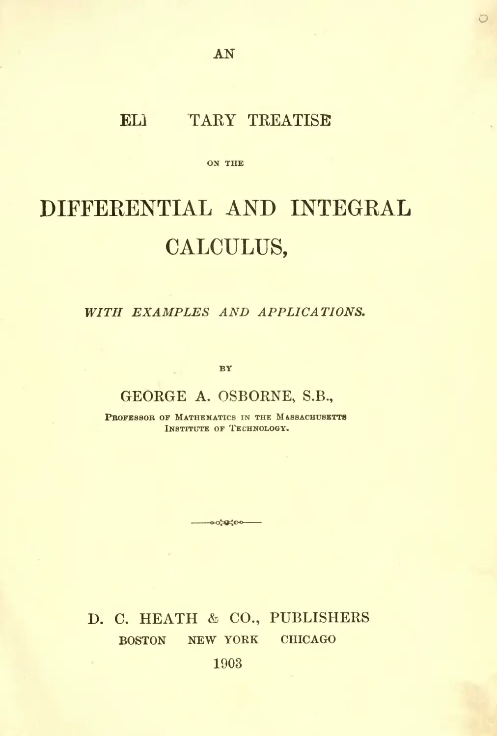
AN



ELI TARY TREATISE



ON THE



DIFFERENTIAL AND INTEGRAL
CALCULUS,

WITH EXAMPLES AND APPLICATIONS.



BY



GEORGE A. OSBORNE, S.B.,

PROFESSOR OF MATHEMATICS IN THE MASSACHUSETTS
INSTITUTE OF TECHNOLOGY.



D. C. HEATH & CO., PUBLISHERS

BOSTON NEW YORK CHICAGO

1903




COPTKIGHT, 1891,
BY GEORGE A. OSBORNE

:
PEEFACE.
THIS work, intended as a text-book for colleges and scien
tific schools, is based on the method of limits, as the most
rigorqus and most intelligible form of presenting the first
principles of the subject. The method of limits has also the
important advantage of being a familiar method; for it is
now so generally introduced in the study of the more ele
mentary branches of mathematics, that the student may be
assumed to be fully conversant with it on beginning the
Differential Calculus.
The rules or formulae for differentiation in Chapter III.
differ in one respect from those in similar text-books, in being
expressed in terms of u instead of x, u being any function
of x. They are thus directly applicable to all expressions,
without the aid of the usual theorem concerning a function of
a function.
After acquiring the processes of differentiation, the student
in Chapter V. is introduced to the differential notation, as a
convenient abbreviation of the corresponding expressions by
differential coefficients. This notation has manifest advan
tages in the study of the Integral Calculus and in its
applications.
In Chapter IX. and subsequent pages I have introduced for
Partial Differentiation the notation , which has recently
ox
come into such general use.

IV PREFACE.
The chapters on Maxima and Minima have been placed
after the applications to curves, as the consideration of that
subject is much simplified by representing the function by
the ordinate of a curve. Maxima and Minima may be taken,
if desired, with equal advantage immediately after Chapter
XIII.
In Chapter X., Integral Calculus, I have taken the problem
of finding the Moment of Inertia of a plane area, as a better
illustration of double integration than that of finding the
area itself. The student more readily comprehends the inde
pendent variation of x and y in the double integral,
J J (x 2 + y*)dxdy, than in C Cdxdy.
A few pages of Chapter XII., Integral Calculus, are devoted
to a description of the Hyperbolic Functions together with
their differentials, and a comparison is made with the cor
responding Circular Functions.
G. A. OSBORNE.
BOSTON, 1895.

CONTENTS.
DIFFERENTIAL CALCULUS.
CHAPTER I.
AETS . FUNCTIONS. P AGES .
1-4. Definition and Classification of Functions 1, 2
5. Notation of Functions. Examples 3, 4
CHAPTER II.
DIFFERENTIAL COEFFICIENT.
6, 7. Limit. Increment . . . . 5
8-10. Differential Coefficient. Examples 6-9
CHAPTER III.
DIFFERENTIATION.
11-13. Differentiation of Algebraic Functions. Examples 10-21
14-16. Differentiation of Logarithmic and Exponential Functions.
Examples 21-27
17,18. Differentiation of Trigonometric Functions. Examples.. 27-32
19, 20. Differentiation of Inverse Trigonometric Functions. Ex
amples 32-37
21,22. Differentiation of Inverse Function and Function of a
Function. Examples 37-40
CHAPTER IV.
SUCCESSIVE DIFFERENTIATION.
23, 24. Definition and Notation 41
25. The nth Differential Coefficient. Examples 42-45
26. Leibnitz s Theorem. Examples 45-47
v

VI CONTENTS.
CHAPTER V.
ARTS. DIFFERENTIALS. pAGEg
27. Differentials as related to Differential Coefficients 48, 49
28. Differentiation by Differentials 49
29. Successive Differentials. Examples 50, 51
CHAPTER VI.
IMPLICIT FUNCTIONS.
30. Differentiation of Implicit Functions. Examples 52-54
CHAPTER VII.
EXPANSION OF FUNCTIONS.
32-36. Maclaurin s Theorem. Examples 55-60
37-41. Taylor s Theorem. Examples 60-63
42-45. Rigorous Proof of Taylor s Theorem 64, 65
46-49. Remainder in Taylor s and Maclaurin s Theorems 66-68
CHAPTER VIII.
INDETERMINATE FORMS.
50, 51. Limiting Value of a Fraction 69
52, 53. Evaluation of x Examples 70-73
54-57. Evaluation of ^, oo, oo oo. Examples 73-76
58. Evaluation of Exponential Forms. Examples 76-78
CHAPTER IX.
PARTIAL DIFFERENTIATION.
59,60. Partial Differential Coefficients of First Order. Exam
ples 79, 80
61-63. Partial Differential Coefficients of Higher Orders. Exam
ples 80-82
64,65. Total Differential of Functions of Several Variables.
Examples 82-84
66. Condition for an Exact Differential. Examples 85
67. Differentiation of Implicit Functions 86
68, 69. Taylor s Theorem for Several Variables 87, 88

CONTENTS. VU
CHAPTER X.
CHANGE OF VARIABLES IN DIFFERENTIAL
COEFFICIENTS. PAGES
rs.
70. Changing from x to y
72. Changing from y to z
73. Changing from x to z. Examples 90-92
CHAPTER XI.
REPRESENTATION OF VARIOUS CURVES.
74-85. Rectangular Co-ordinates
86-93. Polar Co-ordinates 98-102
CHAPTER XII.
DIRECTION OF CURVE. TANGENT AND NORMAL.
ASYMPTOTES.
94-97. Direction of Curve. Subtangent and Subnormal.
Examples 103-108
98, 98. Differential Coefficient of the Arc 108,109
99. Equation of the Tangent and Normal. Examples . . . 109-112
100-106. Asymptotes. Examples 112-116
CHAPTER XIII.
DIRECTION OF CURVATURE. POINTS OF INFLEXION.
107-109. Direction of Curvature 117
110. Points of Inflexion. Examples . . . 118, 119
CHAPTER XIV.
CURVATURE. CIRCLE OF CURVATURE. EVOLUTE
AND INVOLUTE.
111-113. Definition of Curvature ; Uniform and Variable 120, 121
114, 115. Radius of Curvature. Examples 121-124
116. Centre of Curvature 124, 125
117-121. Evolute and Involute. Examples 125-128

Vlll CONTENTS.
CHAPTER XV.
ORDER OF CONTACT. OSCULATING CIRCLE.
ARTS. PAGES.
122, 123. Consecutive Common Points 129, 130
124, 125. Osculating Curves 130, 131
126-128. Analytical Conditions for Contact 131-133
129, 130. Osculating Circle. Examples 133-136
f
CHAPTER XVI.
ENVELOPES.
131-133. Series of Curves. Definition of Envelope 137, 138
134-136. Equation of Envelope 138-140
137. Evolute, the Envelope of Normals. Examples 140-144
CHAPTER XVII.
SINGULAR POINTS OF CURVES.
138-141. Multiple Points 145-148
142, 143. Points of Osculation. Cusps 149, 150
144. Conjugate Points. Examples 150-152
CHAPTER XVIII.
MAXIMA AND MINIMA OF FUNCTIONS OF ONE
INDEPENDENT VARIABLE.
145-149. Definition. Conditions for Maxima and Minima de
rived from Curves 153-157
150, 151. Conditions for Maxima and Minima by Taylor s
Theorem. Examples 157-162
Problems in Maxima and Minima 162-164
CHAPTER XIX.
MAXIMA AND MINIMA OF FUNCTIONS OF SEVERAL
INDEPENDENT VARIABLES.
152-155. Definition. Conditions for Maxima and Minima by
Taylor s Theorem. Examples 165-171

CONTENTS.
INTEGRAL CALCULUS.
CHAPTER I.
ELEMENTARY FORMS OF INTEGRATION. PAGES<
ARTS.
1, 2. Definition of Integration. Elementary Principles ..... 173, 174
3. Fundamental Integrals ............................. 175, 176
4-7. Derivation and Application of Fundamental Formulae.
Examples ....................................... 176-187
CHAPTER II.
INTEGRATION OF RATIONAL FRACTIONS.
8, 9. Preliminary Operation. Factors of Denominator ..... 188, 189
10. Case I. Examples ................................. 189-191
11. Case II. Examples ................................ 191,192
12. Case III. Examples ...............................
13. Case IV. Examples ............................... 195-198
CHAPTER III.
INTEGRATION BY RATIONALIZATION.
14-16. Fractional Powers of x and of a + bx. Examples ---- 199-201
17. Fractional Powers of a + 6a 2 . Examples ............ 201, 202
18, 19. Expressions containing V tf + ax + b. Examples . . . 202-204
20. Integration by Substitution. Examples .............. 204, 205
CHAPTER IV.
INTEGRATION BY PARTS. INTEGRATION BY SUCCESSIVE
REDUCTION.
21. Integration by Parts. Examples .................... 206-208
22-24. Formulae of Reduction. Examples .................. 208-214
CHAPTER V.
TRIGONOMETRIC INTEGRALS.
25-27. Integration of tan w xdx; of seczcfo; of tanx sec n x dx.
Examples ......................... ............. 215-218
28, 29. Integration of sin m x cos n x dx. Examples ............. 219-222

X CONTENTS.
ABTS. PAGES.
30. Trigonometric, transformed into Algebraic, Integrals.
Examples 222-224
31, 32. Trigonometric Formulae of Reduction. Examples 224-226
33-35. Integration of dx . and dx
a + b sin x a+b cos x
of e ax sin nx dx and e"* cos nx dx.
Examples 226-229
CHAPTER VI.
INTEGRALS FOR REFERENCE.
36. Integrals containing Vd z x 2 ; Va? a 1 ax 2 + bx -f c. 230-235
CHAPTER VII.
INTEGRATION AS A SUMMATION. DEFINITE INTEGRALS.
37-40. Integration, the Summation of an Infinite Series 236-^240
41-43. Definition of Definite Integral. Examples 240-244
CHAPTER VIII.
APPLICATION OF INTEGRATION TO PLANE CURVES.
APPLICATION TO CERTAIN VOLUMES.
44-47. Areas of Curves. Examples 245-249
48, 49. Lengths of Curves. Examples 249-252
50, 51. Surfaces of Revolution. Examples 252-255
52. Other Volumes. Examples 255-257
CHAPTER IX.
SUCCESSIVE INTEGRATION.
53-56. Double and Triple Integrals. Examples 258-260
CHAPTER X.
DOUBLE INTEGRATION APPLIED TO PLANE AREAS
AND MOMENT OF INERTIA.
57-60. Double Integration. Rectangular Co-ordinates. Ex
amples 261-264
61-03. Double Integration. Polar Co-ordinates. Examples . . 264-266

CONTENTS.
CHAPTER XI.
SUKFACE AND VOLUME OF ANY SOLID.
ARTS,
64, 65. Area of any Surface. Examples 267-270
66, 67. Volume of any Solid. Examples 270-273
CHAPTER XII.
HYPERBOLIC FUNCTIONS. CYCLOID, EPICYCLOID, AND
HYPOCYCLOID. INTRINSIC EQUATION OF A CURVE.
69-71. Definitions of Hyperbolic, and Inverse Hyperbolic,
Functions 274-276
72, 73. Differentiation of Hyperbolic Functions. Inverse Hyper
bolic Functions as Integrals 276, 277
74, 75. Hyperbolic Functions and the Hyperbola. Exercises . . 278-280
76-82. Equation and Properties of the Cycloid 280-284
83-89. Equations and Properties of the Epicycloid, and Hypo-
cycloid 284-288
90-93. Intrinsic Equation of a Curve and of its Evolute.
Examples 289-292

DIFFERENTIAL CALCULUS.
CHAPTER I.
FUNCTIONS.
1. Definition of a Function. When the value of one variable
quantity so depends upon that of another, that any change
in the latter produces a corresponding change in the former,
the former is said to be a function of the latter.
For example, the area of a square is a function of its side ;
the volume of a sphere is a function of its radius ; the sine,
cosine, and tangent are functions of the angle ; the expressions
x>, log (or 2 + 1), V O + 1),
are functions of x.
A quantity may be a function of two or more variables.
For example, the area of a rectangle is a function of two
adjacent sides ; either side of a right triangle is a function of
the two other sides; the volume of a rectangular parallele
piped is a function of its three dimensions.
The expressions
) > a * +y >
are functions of x and y.
The expressions
xy + yz+zx, \~> log (z 2 + ?/ - z),
are functions of x, y, and z.
2. Dependent and Independent Variables. If y is a function
of x, as in the equations
y = aj 2 , y = tan 4 a;, y = e x ,

2 DIFFERENTIAL CALCULUS.
x is called the independent variable, and y the dependent
variable.
It is evident that whenever y is a function of x, x may be
also regarded as a function of y, and the positions of dependent
and independent variables reversed. Thus from the preceding
equations,
x=-\/y, x = tan- 1 y, x = log e y.
In equations involving more than two variables, as
z -\-x y = 0, w -}- wz -{- zx + y = Q,
one must be regarded as the dependent variable, and the
others as independent variables.
3. Explicit and Implicit Functions. When one quantity is
expressed directly in terms of another, the former is said to
be an explicit function of the latter.
For example, y is an explicit function of x in the equations,
y = x 2 + 2x, y = Vx 2 + 1.
When the relation between y and x is given by an equation
containing these quantities, but not solved with reference to y,
y is said to be an implicit function of x, as in the equations,
2xy + y 2 = x 2 + 1, 2/4- logy =
Sometimes, as in the first of these equations, we can solve
the equation with reference to y, and thus change the function
from implicit to explicit. Thus we find from this equation,
4. Algebraic and Transcendental Functions. An algebraic
function is one that involves only the operations of addition,
subtraction, multiplication, division, involution and evolution
with constant exponents. All other functions are called tran
scendental functions, including logarithmic, exponential, trigo
nometric, and inverse trigonometric, functions.
.

FUNCTIONS.
5. Notation of Functions. The symbols J^(aj), /(), <(,
\}/(x), and the like, are used to denote functions of x. Thus
instead of " y is a function of x," we may write
y=f(x) or y = <j>(x).
A functional symbol occurring more than once in the same
problem or discussion is understood to denote the same func
tion or operation, although applied to different quantities.
Thus, if
........ (1)
then /(?/):= 2/ 2 + 5, /(a) = a 2 + 5,
f(a + 1) = (a + I) 2 + 5 = a 2 + 2 a + 6,
9, /(I) = 6 .
In all these expressions /( ) denotes the same operation as
denned by (1) ; that is, the operation of squaring the quantity
-and adding 5 to the result.
The following examples will further illustrate the notation
of functions.
EXAMPLES.
1. If f(x) = 2a?-a?-7x + 6, show that
/(3) = 30, /(2) = 4, /(0) = 6, /(1) = 0,
/(-2) = 0, /(f) = 0, f(x-2) = 2tf-l3x 2 + 21x,
f(x + h) = 2^ + (67i - 1) a? + (6/i 2 - 27i - 7) x + 27i 3
2. Given /i(2/) = 22/ 4 -2/ 3 +l ? / 2 (y) = 7^-6y+l; show that
3. If /(a) = 5L=, show that
Cl -j -L

4. If
DIFFERENTIAL CALCULUS.
(m + l)m(w-l)(m-2), show that
= <(- 2),
m
5. If
m 2
= (z-a)(o;-&)(a;-c), show that
[<KO)]
6. If <w =
, show that
v ) = <f>(2u)
, show that
1 -fa;
, show that
7. If
8. If ^ =
9. Given \j/(x) = cos cc + V^ since ; show that
<K2a) = [^()] 2 , A(a + 6) = K0
10. If /(a;, y, z) = & -h f + z> - 3xyz, show that
/(*, y, )/(/>, g, )=/( A Jf, JV),
where i = px + qy + rz,
M=py + qz +rx,
N=pz+qx + ry* t -L M + tf v L M - M M~L ty
/! + /lVn alMW =(L + w + ^g*/*Jv
<ix n n)-^f^ v -n-fr r)e AV
^r-- 3>Vr)C** 4 ? 3f f - 3 *^" )
I

CHAPTER II.
DIFFERENTIAL COEFFICIENT.
6. Limit. The limit of a variable quantity is a fixed value
or condition, from which it can be made to differ as little as
we please.
The student is supposed to be already familiar with the
meaning of this term, of which the following illustrations
may be mentioned.
The limit of the value of the recurring decimal .3333 >
as the number of decimal places is indefinitely increased, is J.
The limit of the sum of the series 1 + ^H-J + |-H ---- , as
the number of terms is indefinitely increased, is 2.
The circle is the limit of a regular polygon, as the number
of sides is indefinitely increased.
The tangent to a curve is the limit of a secant, as the points
of intersection approach coincidence.
The limit of the fraction, , as approaches zero, is 1,
u
provided is expressed in circular measure.
7. Increments. An increment of a variable quantity is any
addition to its value, and is denoted by the symbol A written
before this quantity. Thus Aa; denotes an increment of x,
A?/ an increment of y.
For example, if we have given
and assume x = 10, then if we increase the value of x by 2,
the value of y is increased from 100 to 144, that is, by 44.
In other words, if we assume the increment of x to be A# =2,
we shall find the increment of y to be Ay = 44.

6 DIFFERENTIAL CALCULUS.
A negative increment is a decrement; that is, a decrease in.
value.
For example, calling x = 10, as before, in y = or 2 .
if AOJ = 2, then Ay = - 36.
a Differential Coefficient. In the equation y = x*, if we
suppose x to vary, y will vary also. To fix the attention upon
a definite value of x, let us suppose x = 10 and therefore
y = 100, and let us inquire what addition or increment will
be produced in y by a certain increment assigned to x. Cal
culating the values of Ay corresponding to different values of
A#, we find results as in the following table :
If Aaj =
then Ay =
i A V
and =
Aa;
3.
69.
23.
2.
44.
22.
1.
21.
21.
0.1
2.01
20.1
0.01
0.2001
20.01
0.001
0.020001
20.001
h.
207i + ^ 2 .
20 + 7i.
The third column gives the value of the ratio between the
increments of x and of y.
It appears from the table that, as A# diminishes and
approaches zero, Ay also diminishes and approaches zero.
The ratio - diminishes, but instead of approaching zero, ap
proaches 20 as its limit.
Ay
This limit of is called the differential coefficient of y with

DIFFERENTIAL COEFFICIENT.
respect to x, and is denoted by _^. In this case, when x = 10,
, dx
^ = 20.
dx
It is to be noticed that -7- is not here defined as a fraction,
dx
but as a single symbol denoting the limit of the fraction
. The student will find as he advances that -/ has many
A# dx
of the properties of an ordinary fraction, and Chapter V. shows
how it may be regarded as such.
9. Without restricting ourselves to any one numerical value,
we may obtain ~ from the equation y = x 2 thus :
dx
Having y = x 2 , let Aa; = h, and let the new value of y be
denoted by
therefore
Ay = y - y = (x + h) 2 - x 2 = 2xh + h 2 .
Dividing by A# == 7i, gives
The limit of this, when h approaches zero, is 2x. Hence
dx
In the same way the differential coefficients of other given
functions may be found.
For example, find ~ from the equation,
dx
Let Az = 7i,
then f =2

8 DIFFERENTIAL CALCULUS.
Dividing by Aa; = ft gives
?7
The limit of ~ is 6 a; 2 , as h approaches zero.
nx
-**
dx
Take for another example
y = Va?. Aic =
= a; -f ft a?.
A?/ _ Va; + ft V^
Ax~~ 7i
The limit of this takes the indeterminate form But by
rationalizing the numerator, we have
A h 1
ft + V*
The limit of ^ = -^ ;
that is, ~
10. General Definition of Differential Coefficient.
In general, if y = <f>(x),
Aa;
^ = limit of * n- , as /t approaches zero.
da; &
The differential coefficient of a function may then be defined

DIFFERENTIAL COEFFICIENT. 9
as the limiting value of the ratio of the increment of the function
to the increment of the variable, as these increments approach
zero. That is, the differential coefficient of the function <f>(x)
with respect to x, is
the limit of *( + >)-*&,
h
as h is indefinitely diminished.
The differential coefficient is sometimes called the derivative.
NOTE. In Art. 94 will be found a geometrical illustration
of the differential coefficient.
EXAMPLES.
Following the process of Art. 9, derive the following dif
ferential coefficients :
10. .= x.

CHAPTER III.
DIFFERENTIATION.
11. The process of finding the differential coefficient of a
given function is called differentiation. The examples in the
preceding chapter are introduced to illustrate the meaning
of the differential coefficient, but this elementary method of
differentiation is too tedious for general use.
Differentiation is more readily performed by the application
of certain general rules, which may be expressed by formulae.
In these formulae u and v will denote variable quantities, func
tions of x ; and c and n, constant quantities.
It is frequently convenient to write the differential co
efficient of a quantity
d . T du
u, instead ot
dx dx
Thus the differential coefficient of (u -\-v) is more con
veniently written
(u + v), rather than
dx dx
12. Formulae for Differentiation of Algebraic Functions.
dx
II. =
dx
III. -(n + v)= + .
dx ^ dx dx
TTT d / N du . dv
IY. ~-(uv) = v + u
dx dx dx

DIFFERENTIATION.
V. -f(c) = V
dx dx
^
VII. *.(u") = nu- 1 ^.
dx^ dx
These formulae express the following general rules of dif
ferentiation :
I. The differential coefficient of a variable with respect to itself
is unity.
II. The differential coefficient of a constant is zero.
III. The differential coefficient of the sum of two variables is
the sum of their differential coefficients.
IV. The differential coefficient of the product of two variables
is the sum of the products of each variable by the differential
coefficient of the other.
V. The differential coefficient of the product of a constant and
a variable is the product of the constant and the differential co
efficient of the variable.
VI. The differential coefficient of a fraction is the differential
coefficient of the numerator multiplied by the denominator minus
the differential coefficient of the denominator multiplied by the
numerator, this difference being divided by the square of the
denominator.
VII. The differential coefficient of any power of a variable is
the product of the exponent, the power with exponent diminished
by I, and the differential coefficient of the variable.
13. Derivation of Formulae.
Proof of I. This follows immediately from the definition of
a differential coefficient. For since - = 1, its limit T^ 1
Aa; ax
Proof of II. A constant is a quantity whose value does
not vary. Hence

** DIFFERENTIAL CALCULUS.
Ac = and = ;
Aa;
therefore its limit ~ =
dx
Proof of III. Let y = u + v, and suppose that when x is
changed into x + h, y, u, and v become y , u , and v ; then
y =u +v ;
therefore y y = u u + v v
that is ? Ay = Aw -f- Av.
Divide by Aa;; then
Ay Aw Aw
Ax Aa; Aa;
Now suppose Aa; to diminish and approach zero, and we
have, for the limits of these fractions,
dx dx dx
If in this we substitute for y, u -f v, we have
dx dx dx
It is evident that the same proof would apply to any
number of variables connected by plus or minus signs. We
should then have
.
dx^ dx dx dx
Proof of IV. Let y = uv; then
y =u v ,
and y y = u v uv = (u u)v -}- u(v v) ;
that is, Ay = v A-M + wAi?.

DIFFERENTIATION. 13
Divide by A#; then
Aw i Ait , Aw
_^. /y -- 1- ^ - .
Ax Ao; Aa;
Now suppose As? to approach zero, and, noticing that the
limit of v is v, we have
& = + *.
dx dx dx
that is, *. (uv ) = v *> + u%L
dx dx dx
This formula may be extended to the product of three or
more variables. Thus we have
d , ^ d , ^ / \ , dw
(uvw) = (uv w) = w (uv) -\-uv-
dx^ dx^ dx^ dx
f du , dv\ , dw
= w (v + u) +uv~
\ dx dxj dx
du , dv . dw
= vw -- \-uw -- \-uv --
dx dx dx
Similarly, for the product of four functions, we have
d , du , dv , dw , dz
(uvwz} = vwz -- h wzu -- h zuv -- h uvw
dx dx dx dx dx
A similar relation holds for the product of any number of
variables.
Proof of V. This is a special case of IV., being zero.
But we may derive it independently thus :
y = cu,
y =cu ,
Ay = cAw,
Ay _ Ait
Ace Ao;

14 DIFFERENTIAL CALCULUS.
= c, or cu = c.
ax ax ax ax
Proof of VI. Let y = -,
.,
then
w u w v uv 1 (u u}v u (V v)
therefore y y = -r -- = -- - -- =^ - - r 5

, , , .
that is, Ay =
Au Av
v u
Ay _ Ace Ax
Now suppose Ax to diminish towards zero, and, noticing
that the limit of v is v, we have
du dv
V U
dy dx dx
dx ~ v 2
Or we may derive VI. from IV. thus :
Since y = >
therefore yv = u.
dy , dv du
By IV., /y ^r + #;r = :r>
J dx dx dx
dy _ du u dv m
dy dx dx
therefore ^ = =
dx v 2

DIFFEEEN TIA TION.
Proof of VII. First, suppose n to be a positive integer.
Let y = u n ,
and, y = u n ,
= (u -u) (u n - l +u n
that is, Ay = AwO* - 1 + u n ~ 2 u + u -*u* + w"- 1 ),
Now let Az diminish ; then, u being the limit of u , each
of the n terms within the parenthesis becomes u n ~ l ; therefore
Second, suppose n to be a positive fraction, -
p
Let y = w,
then 2/ ? =^;
therefore A(^) = A(V).
ax aic
But we have already shown VII. to be true when the ex
ponent is a positive integer ; hence we may apply it to each
member of this equation. This gives
therefore ;/_^
cfce qy q ~ l dx
Substituting for y, w, gives
which shows VII. to be true in this case also. Hence that
formula applies to any positive value of n, whether integral
or fractional.

16 DIFFERENTIAL CALCULUS.
Third, suppose n to be negative and equal to m.
Let y = u~ m = :
u m
~<L(u m ) - mu m ~ l ~
*
by VI =
7
dx M S " u 2m dx
Hence VII. is universally true.
EXAMPLES.
Differentiate the following functions :
If two quantities are equal, their differential coefficients
must be equal. Hence
dx dx
If we apply VII., substituting u = x and n = 4, we have
(x 4 ) = 40J 8 = 4oj, by I.
dx dx
2. / =
dx dx
by III., making u = 3x 4 and v = 4 or 3 .
Similarly, (4^) = 4 (a?) = 4 . 3^=
dec ao;
O\

DIFFERENTIATION. 17
3. y = x%+2.
^ = -f(**)+;f(2).
dx dx^ dx
A(*I ) = |x*, by VII.
dx
-f(2) = 0, by II.
dx
... U?**.
da; 2
4. 2/ = 3Va ?z- + i + a.
Va; &
^ = A (3 ^)_A ( 2*-l) + A^ 3 ) + f*
da; da; V da; v dx^ dx
dx dx\x 2 +3j
Applying VI., making
u = x + 3 and v = x 2 + 3, we have
d fx_3\
(x 2 +3)

18 DIFFERENTIAL CALCULUS.
;
If we apply VII., making
o
u= x 2 H- 2 and n = -, we have
3
dy _
dx
J 7. ?/ =
If we apply IV., making
and i? = (af 3 a)^, we have
dx" dx
A(x*- X y=:l(x*-X)^ (x>--x) = --(x>-X
dx 2 dx 2
dx 2
-a)

DIFFERENTIATION. 19
dx
9 y = ; - = c -
x dx x 2
10 . =
_
* **
12. Given
(a + x) 5 = a 5 + 5 a 4 fl? + 10 a 3 x 2 + 10 aV+ 5
derive by differentiation the expansion of (a + x)\
^
13. Given l +
derive the sum of the series 1 + 2# + 3x 2
Ans.
- . _
:> "
c?y __ nx n ~ l
da;
16.
1 ff y __ /-jL O,v^ I /v.4\ /1 j_ ^2\3 (ty

20
18.
19.
20.
21.
DIFFERENTIAL CALCULUS.
&? (a + 8 *)"(<* -
%t
U.X
dx
I
da;
23.
24. y =
1-a;
3 -far 1
25.
26.
27.
x+ Vl-f x 9
x
-I- Va
a a;
29. y
)+ n(a+a;)] (aH-^
a?) -f- n (a + a?)
(l+ar 8 )*
da;
dx
da;
a 2 4- a Va 2 -

DIFFEEEN TIA TION.
21
da?
(3 -a)
gy__2/
rfa; a 8 \ V
14. Formula for Differentiation of Logarithmic and Expo
nential Functions.
du
VIII. |log.=Aog..
x. - aM=loa . aM .
XL e = e .
dx dx
XII. ^ = ^-^
daj dx
dx
15. Before deriving these formulae it is necessary to find
the limit of the expression
fjjj as z approaches infinity.
By the Binomial Theorem
which may be written

22 DIFFERENTIAL CALCULUS.
Now when z increases indefinitely, we have
limit of
This quantity is usually denoted by e, so that
The value of e can be easily calculated to any desired
number of decimals by computing the values of the successive
terms of this series. For seven decimal places the calculation
is as follows,
1.
1.
.5
.166666667
.041666667
.008333333
.001388889
.000198413
.000024802
.000002756
.000000276
.000000025
.000000002
6 = 2.7182818
By calculating the value of (l+|)" for different valueft of *
we may verify its limit. Thus
(!+!) 2.25
(!+) = 2.48832
(1+A) 10 = 2.59374
(1.01) 100 = 2.70481
(1.001) 1000 = 2.71692
(1.0001) 10890 =2.71815
(1.00001) 100000 = 2.71827
(1.000001) 1000000 = 2.71828

DIFFERENTIATION. 23
16. Derivation of Formulae.
Proof of VIII. Let y = log a w,
then y=log a (w-f Aw),
Ay = log a (w + Aw) log a w = log a
Dividing by
i t .
- = 101 + - _.
Now if A# approach zero, Aw at the same time approaches
zero ; then the limit of ( 1 H -- * ) "is the same as the limit
/ IV \ U J
of ( i _{. _ ) as z increases indefinitely. But in Art. 15 we
\ /
have already found the latter limit to be e. Hence we have
, du
dy , dx
Proof of IX. This is a special case of VIII., when a = e.
In this case -
NOTE. Logarithms to base e are called Napierian loga
rithms. Hereafter, when no base is specified, Napierian
logarithms are to be understood.
That is log u = log e w.
Proof of X.
Let y = a".
Taking the logarithm of each member, we have
logi/=wloga;
dy
therefore by IX., ^ = loga .


24 DIFFERENTIAL CALCULUS.
Multiplying by y = a u , we have
dx dx
Proof of XL This is a special case of X., where a = e.
Proof of XII. Let y = u\
Taking the logarithm of each member, we have
dy v du
therefore by IX, *5. JS
y u dx
Multiplying by y = u v , we have
ft. *-!*! + log*.**.
dx dx dx
EXAMPLES.
dy 6
.
2. , =
3. , =
_ . dy _ __x
4. /^logVl-a 2 . - _
5 . f .
6. y= V^
7. =
e 2 " 1
8. / =

DIFFERENTIATION. 25
9. = o;-3e
dx
Att
10. v = lo<
where Jf= - = Iog 10 e = .434294
log. 10
11. y
log 5 = 1.609440
12 y-*"
~
What is the result of differentiating both members of each
of the three following equations?
13.
Ans.
1+a?
16. y =
17. ^
18. j, = logV^V?. ^ = / V"
& ^/ a _ y X dx (a x)

26
DIFFERENTIAL CALCULUS.
19. f-Jgf + fc.d-*
20. y = e^*(x%
21. y=4 4
dy _ log a?
dx~~ (lx)
22. 2 /=far J -^ + ^-\
\ a a 2 a 3 /
23. y = log a; log (log a;) log a;.
24. y =
25. y = mlog ( ^a; + Va; -f- m) -f
da;
I. y = log

DIFFERENTIATION. 27
L 33. y = (ex)*. | = (e^(2 +lo g x).
34. y.
35. y = x
36. y = x
37. 2/ = e
38. 2/ = e
39. 2/ = a
17. Formulae for Differentiation of Trigonometric Functions.
In the following formulae the angle u is supposed to be ex
pressed in circular measure.
XTTI sinw = cosw
dx dx
XIV.
dx ax
XV. tanct=sec 2 u^.
dx dx
XVI.
dx dx
XVII. secw = sec it tanw-^-
*dx dx
XVIII. cosec u = cosec u cot u -^
da; ^
XIX. versi^ = sinw^.
dx da;

28 DIFFERENTIAL CALCULUS.
18. Derivation of Formulae.
Proof of XIII. Let y = sin w,
then y = sin(w 4- Aw) ;
therefore A?/ = sin (u +- Aw) sin u.
But from Trigonometry,
sin J. sin B = 2 sini(J[ - J3)
i
If we substitute A = u-i- Ait and B = u,
we have A?/ = 2 cos [ w + -~ ) sin
\ * /
sin
TT
Hence
Aa;
/ . Aw\ Aw
= cos [ u -\ --- ) ---
V 2 y Aw Aa
Now when Ax approaches zero, Aw likewise approaches
zero, and as Aw is in circular measure, the limit of
is unity.
Aw
~2~
Hence
dx dx
Proof of XIV. This may be derived by substituting in
XIII. for w, - w.
Then -- =

or
DIFFER EN TIA TION. 29
d f du\ du
- cosw = smw f ) = smifc
dx \ dxj dx
Proof of XV. Since tan u = Sm U
cosu
d . d
cos u sin u sin u cos u
u -YTT d . dx dx
by VI., tanu =
dx cos*u
o du , o c?w du
co$ 2 u hsin 2 ^
dx dx dx
o du
= sec 2 w
dx
Proof of XVI. This may be derived from XV. by substitut
ing - u for u.
Proof of XVII. Since sec it = ,
cosw
cosu sinw
, TTT d dx dx
by VI., --secw = =
dx cos u cos j u
= secw tanit
dx
Proof of XVIII. This may be derived from XVII. by sub
stituting ^ u for u.
Proof of XIX. This is readily obtained from XIV. by the
relation
versw = 1 cosu.

30 DIFFERENTIAL CALCULUS.
EXAMPLES.
1. y = sin 2 x cos x. -^ = 2 cos 2 x cos a; sin 2 a; sin 05
da;
2. y tan*5x. _J^= 1 tan 5 x sec 8 5 a;.
da;
3. w=: tana; a;. -^
da;
4. y = sin (wa; + m) -^
(IX
5.
sec a; da;
6. y = sin 8 a; cos a;. -^ = sin 1 x (3 cos* a; sin 8 a;).
ax
7. y = sin (a; -fa) cos (a; a) . -^ = cos 2 a?.
8 sin(a-a;) t ^ =
sin (a -fa;) dx
9. 7/ = tan 2 a;-log(sec 2 a;). ^=
CtiC
10. y = tan 4 a; 2 tan 2 a; + log (sec 4 a;)
^>
da;
11. y (a sin 2 x + 6 cos 2 a;) n .
^ = n(a - 6) sin2a;(a sin 2 a;
da;
12. 2/ = logsina;. -^=cota;.
13. v = log tana;. 3 -= .
da; sm2a;
14. y = ig sec as. -^ = tana?.

DIFFERENTIATION.
31
15. =
dx
17. y-*-.
18. v=smna;sin n a;.
ax
19
"
sin
ty __ mn sin m " 1 rta; cos(m n) x
lacosx bsmx dy_ __ _ ab _ ^
\acosoj + bsiux dx ~ a 2 cos 2 a; 6 2 sin 2 a;
24.
sec 4 a;
dx
In each of the following pairs of equations derive by differen
tiation each of the two equations from the other :
25. sin 2 x= 2 sin x cos a?,
cos 2 x = cos 2 a; sin 2 a;.
2 tan a;
sin 2 a; =
cos 2 x =
l + tan 2 a;
1 tan 2 a;
14- tan 2 x

32 DIFFERENTIAL CALCULUS.
27. sin3# = 3sm# 4sin 3 #,
cos 3 x = 4 cos 3 x 3 cos x.
28. sin4o; = 4 since cos 3 a? 4 cos # sin 3 a;,
cos 4 a; = 1 8sin 2 a cos 2 x.
29. sin(m -\- n)x = sinmcc cos nx -f cos mx sin 910;,
cos (m + n) x = cos mz cos nx sin mx sin nx.
30. sin = *-+- + ...
31. sino;:=- - -^ ,
19. Formulae for Differentiation of Inverse Trigonometric
Functions.
du
d . , dx
sin" 1 u =
dx Vl - u 2
du
d dx
du
XXII. tan" 1 u q
dx 1-M
<
XXIII. COt" 1 It:
dx 1
du
dx u Vu 2 ^1

DIFFEEEN TIA TION. 33
XXV. -
dx
XXVI. .. .
dec y 2 u u 2
20. Derivation of Formulas.
Proof of XX. Let y = sin" 1 ?* ;
therefore
sin?/ = u.
By XIII.,
dy du
cos?/-^ = -;
dx dx
du
therefore
dy dx
dx cos?/
But
cos?/ = VI
sic 2 ?/
therefore
Proof of XXI. This may be derived like XX., or from
the relation
-- sm" 1 ^ ;
2 du
whence -cos l u =
d d . dx
l = - - - 1 = --
dec dec Vl M 2
*
Proof ofXXlI. Let T/^tan- 1 ^;
therefore tany = w.
^2-S
dw
dv cto
therefore -~ = "
dx sec 2 ?/

34 DIFFERENTIAL CALCULUS.
But sec 2 ?/ = 1 + tan 2 ?/ = 1 + u 2 ;
du
therefore
dy dx
dx 1 +
Proof of XXIII. This may be derived like XXII., or from
the relation
cot" 1 ^ = - tan" 1 ?*.
Proof of XXIV. Let y = sec" 1 ?* ;
therefore sec?/ = u.
,rTTTT dy du
By XVII., sec y tan y~ = ;
dx dx
du
therefore
dy dx
dx sec y tan y
But sec?/ tan?/ = secy Vsec 2 ?/ 1 = u V^ 2 1 ;
du
therefore = - .
da? u-Vu*-l
Proof of XXY. This may be derived like XXIV., or from
the relation
cosec" 1 u = - sec" 1 u.
Proo/o/XXVI. Let 2/ =
therefore u = vers y = 1 cos y.
therefore = .
dx smy
But sin?/ = Vl cos 2 ?/ = Vl (1 u) 2 = V2
therefore

DIFFEREN TIA TION.
EXAMPLES.
2. 2/ = sin~ 1 (3a; 1).
1805
3. y j "*- 1
35
8.
9.
10.
9
if * 1 /Q
ax vi
-i 2 a; dy__ 2
0. y= an 1 _ o* fa
6.
do; e*+ e-
dy n
7. w = tan 1 (n tan a/) . -7- = 5 ; a . 8 "
y ^ dx cos 3 x + w 2 sm sl *
^^ dv 2
cZaj V9^
dy 2
daj = ~7~
dv 2
dx 1+x 2
ie *--e~* ^ 2
11. y = tan- g da; - e s +e-
i 1 dy 2
12. y = cosec- 1 ^ - ~
2 ar 1 da;
13. y = sec ^ ZI - da^a^ + l

36
H _i
. y 2= sin
DIFFERENT
V2
15. y = tan" 1
16 v cos" 1
4sinx
3 4-5cosx
n-, cin- 1
o + 3cosx
1+x 2
18. y = cosec
rl l
2x
tt^-u.-
1 ox
20. y = sin- 1
21. y = tan"~ J
22. ycstan- 1
9.5 11 , nrkf- 1
Vsinx.
\l + cosx
1 Vax
, w l^ 1 ^
24.
25.
c?x
dx 5 + 3 cos x
dx 5 + 3cosx
dy^ -2
dx 1+x 2 *
dy = _2_
dx 1+x 2
dx 1+x 2
dx 2
dx 2
cosecos.
dx
2 ax 2
dx x 4 a 4
d?/ Vl x 2 x
dy_-2
"~
27. y = (x+a)tan~\ Vax.
dx 2Vl-x*
dx

DIFFEREN TIA TION. 37
28. y =
29. y = si]
01 ,3x-x 3
1 1 ?/ T T n n
32. 2/ = tan -1 -
33. ?/ = tan~ 1
34. v = lc
dx
21. To express _J? in, terms of If v is a function of x.
dx dy
fchen (Art. 2) x may be regarded as a function of y. Prom
the former relation we have , and from the latter,
dx dy
These differential coefficients are connected by a simple relation.
It is evident that ^ = ,
Ax Ao;
however small the values of Ax and Ay. As these quantities
approach zero, we have, for the limits of the members of this
equation,
^ = J_ .......... (1)
dx dx
Ty
That is, the relation between JL and is the same as if they
,. P dx dy
were ordinary fractions.

38 DIFFEEENTIAL CALCULUS.
For example, suppose
-- rr (2)
2/ + 1
Differentiating with respect to y, we have
dx =
dy
" y by (2).
This is the same result that we get by solving (2) with
reference to y, giving
and differentiating this with reference to x.
22 To express ^ in terms of ^ and . If y is a given
dx dz dx
function of z, and z a given function of a?, it follows that
y is a function of a?. This relation may be obtained by
eliminating z between the two given equations, but -1 can be
found without such elimination.
By differentiating the two given equations, we find -^ and
, and from these differential coefficients, -/- may be obtained
dx dx
by a relation which may be derived as follows :
Aw Aw Az
It is evident that -^ = - -,
Aic Az Ax
however small Ax, Ay, and Az. As these quantities approach
zero, we have for the limits of the members of this equation,
dy _ dy dz /-j\
cto ~~ dz dx
That is, the relation is the same as if the differential coeffi
cients were ordinary fractions.

DIFFERENTIATION. 39
For example, suppose
= a 2 or. )
Differentiating these equations, the first with reference to z,
and the second with reference to x, we have
32 = 5*-, *z = -2x.
dz dx
By (1), = 5 2 4 (-2x) = -10x(a 2 -x 2 ) 4 , by (2).
The same result might have been obtained by eliminating z
between (2), giving
2, = (a 2 -a 2 ) 5 ,
and differentiating this with reference to x.
EXAMPLES.
In the following seven examples find by differentiation - ,
and then ^ by (1) Art. 21.
2y l*\ *" dy (y I) 2 2
1. x =
y-l dx 2 (0 2)
2. z=V~ * "* A 2 1
3. 0;= Vl + siny. % = 2Vl + sin2/ = 2
dx cosy V2 - 2
4. x =
dx
y dy(i+iogy) 2
1 + logy ^ logy icy
6. ?-l og ey +^ /e2y - 4 dy = Ve-4 = ^--l_

40
DIFFERENTIAL CALCULUS.
2 Ve y - 2 d V
r y - 4
In the following examples find by differentiation J? and *
c?w rt2;
and then ~- by (1) Art. 22.
dx
8. y=,
2z
3z-
z =
2x-l
9. ==
10. / =
dy
d
dy
11. / =
z = e*.
V3
da; xz (1 + a)

CHAPTER IV.
SUCCESSIVE DIFFERENTIATION.
23. Definition. A single differentiation performed on
y =f(x) gives the differential coefficient, -*- This result
ctx
being generally also a function of x, may be again differen
tiated, and we thus obtain what is called the second differential
coefficient; the result of three successive differentiations is
the third differential coefficient; and so on.
For example, if y x 4 ,
dxdx
_^A^
dx dx dx
24. Notation. The second differential coefficient of y with
respect to x, is denoted by *
Co 33"
That is,
d?y d dy
dx 2 dxdx
Similarly,
d s y __ d d dy
dx 3 dxdxdx
d d~y
~~dx~dx 2
d*y __ d d d dy _ d d 3 y
dx* dxdx dxdx dxdx 3
d n y _ d d n ~ l y
dx n ~dxdx n ~ 1

42 DIFFERENTIAL CALCULUS.
Thus, if y = x\
^ = 4*3,
dx
The successive differential coefficients are sometimes called
the first, second, third, derivatives.
If the original function of x is denoted by f(x), its suc
cessive differential coefficients are often denoted by
25. The nth Differential Coefficient. It is possible to express
the nth. differential coefficient of some functions.
For example,
(a). From y =e x , we have
(6) . From y = e *, we have
(c) . From y = log a;, we have
da;
dhy (-l) ft ->-l
a n

SUCCESSIVE DIFFERENTIATION. 43
(d). From y = sinax, we have
- = a cos ax = a sin [ ax -f - ],
dx \ 2J
= a 3 cos ax + = a 3 si
EXAM PLES.
2. r .rf. =
3. 2/ = (o;-3)e aB +4a;e a: +^ =
cZx 2
4 < d 2 y =
F m dx*
5. = o;lox. =

44 DIFFERENTIAL CALCULUS.
,r78/,.
8. v = (a*-G
aar
o a 3 A 5\ d z y
9. 2/ = ^log*--| ^ =
10. y = log sin*. * 9cosa
dar* sin 3 x
11. .
12. 2/ = e~ x cosa;. ^ = 4e~*cosic.
da; 4
13. 2/ = tana;. ^ = 6sec 4 a; 4sec 2 a;.
dor
Decompose the fraction before differentiating.
15. y =
16. y =
17. ^-
9 27 dtf
18. t/ = tan 2 a; + 8 log cos x + 3 a; 2 .
aar
19. = ar ! -
20. y^
21. y =
22. 2/ = sin(msin- 1 a;). (l- 2 ) -oj + m?y = 0.

SUCCESSIVE DIFFERENTIATION. 45
23. y = a cos (log a?) -H & sin (log a?), x 2 ?, + -f y = 0.
o/i 1 d n ?/ ( 1)"^
24. ?/ = - A
dx n (x + 2)
f 1
25. S = U-,. f^ =
dx n
26. y=a*. ^ = (loga) n a x .
dx n
27. y = cosax. ^ == a 71 cos [ ax -f
cfcc n V 2
28 = 1 ~ a; . ^l/ = 2 (~ 1 ) n t! 1
1 -f- dx n ~~ (
o
Reduce the fraction to a mixed quantity, 1 H , before
differentiating.
29. v = -
26. Leibnitz s Theorem. This is a formula for the ?ith
differential coefficient of the product of two variables in terms
of the successive differential coefficients of those variables.
A special case of Leibnitz s Theorem, when n = 1, is formula
IV.,
d , ^_du dv x.j,
dx dx dx
For convenience let us use the following abridged notation :
_dv _ d 2 v _ d n v
dx dx* dx n
du d 2 u d n u
HI = , u 2 = , u n =
dx dx 2 dx n
Then (1) becomes
d ,
(2)

46 D1FFEEENTIAL CALCULUS.
Differentiating (2),
. (uv) = u 2 v -\- ^1^1+ w^H- uv 2 = u 2 v + 2u 1 v 1 -\- uv 2 .
dx 2
d 3
(uv) = u 3 v -f u 2 v 1 -{- 2 u 2 V!-}- 2 u ] v 2 + WiV 2 -f- uv s
doc?
= u s v + 3 ufl-L + 3 u^v 2 + wy 3 .
We shall find this law of the terms to apply, however far
we continue the differentiation, the coefficients being those of
the Binomial Theorem.
In general
n _
1 +wv B ........ (3)
This may be proved by induction, by showing that if true for
(uv), it is also true for -(uv). This exercise is left for
dx n ^ dx n+
the student.
In the ordinary notation (3) becomes
d n , ^ d n u d n ~ l udv . n(n l)d n
[2
For example, let us find by Leibnitz s Theorem (e ax x).
CL3&
Here u=e ax , u^ae, u n = a n e ax .
Substituting in (3), we have
(xe^) =a n e a *x + na n ~ l e ax = a n ~ l e ax (ax + n)
dx n

SUCCESSIVE DIFFERENTIATION. 47
EXAMPLES.
Find by Leibnitz s Theorem the following differential co
efficients :
2 .
3 v=sa j ..

CHAPTER V.
DIFFERENTIALS .
27. The differential coefficient _ ^ has been defined, not as a
dx
fraction having a numerator and denominator, but as a single
symbol representing the limiting value of , as A# and A?/
approach zero. But there are some advantages in regarding
the differential -coefficient as an actual fraction, dx and dy
being infinitely small increments of x and y, and called differ
entials of x and y. That is, dx is an infinitely small Ax, and
dy an infinitely small Ay.
For instance, if we differentiate y = x 2 , we obtain
.
dx
Using differentials, this result might be written
dy = 2xdx.
These are two forms of expressing the same relation.^ Ac
cording to the first,
The limit of the ratio of the increment of y to that of x, as
these increments approach zero, is 2x.
According to the second,
An infinitely small increment of y is 2 x times the corresponding
infinitely small increment of x.
We have the same two forms of expressing other relations
in mathematics.
For instance, we may say,
" The limit of the ratio, _^-, as these quantities approach
., chord
zero, is unity.

DIFFERENTIALS. 49
Or,-
" An infinitely small arc is equal to its chord."
The equation dy = 2xdx may thus be used as a convenient
substitute for ,
dx
We see also why or 2 x is called the differential coefficient,
dx
for it is the coeffici&nt of dx in the equation dy = 2xdx.
* 28. The formulae for differentiation may be expressed in
the form of differentials by omitting the dx in each member.
Thus, IV. becomes
d(uv) = vdu + udv ;
and XXIL, " - 1 du
and the others may be similarly expressed.
Differentiation by the new formulae is substantially the
same as by the old, differing only in using the symbol d
instead of
dx
For example, take Ex. 5, p. 17.
, , x + 3
+ 3)dx-(x + 3) 2xdx
(x 2 +3) 2
Dividing by dx gives
dx

50 DIFFERENTIAL CALCULUS.
29. Successive Differentials. Successive differential coeffi
cients. 4, ^, , which have been denned as single symbols,
dx 2 dy?
may also be interpreted as fractions, the numerators, d 2 y, d s y,
", denoting d(dy), d[d(dy)~\, , and called the second,
third, , differentials of y, while the denominators are (dx) 2 ,
(dxy, ....
This will be better understood from an example.
Let y = x\
then dy = 4 y? dx.
As 4:%?dx is a variable, dy is a variable, and may be
again differentiated. Now, x being the independent variable,
its increment dx may be supposed the same infinitely small
quantity for all values of x ; that is, we may regard dx as
constant in the preceding equation. Thus we obtain
d(dy) = 12x 2 dx . dx =
Denoting d(dy) by d 2 y,
Differentiating again, and still regarding dx as constant,
d(d 2 y) = 2xdx(dx) 2 = 24 a; (die) 3 ,
or d? = 24
From these equations, by dividing by the power of dx in the
second members, we find
a y __ 94 a
(dxY
The independent variable a?, whose differential is supposed
constant, is sometimes called the equicrescent variable.

DIFFERENTIALS. 51
EXAMPLES.
Differentiate the following, using differentials in the process:
2. 2/=V
3. y = (e x
4. / =
6. 2/=sin m ajcos n o;. dy = sin m ~ 1 iccos w ~ 1 c(mcos 2 ^ nsm 2 x)dx.
7. y = taii 3 & + tana?. dy = sec 4 xdx.
3
dx
8. y = tan 1 log a?. dy=

CHAPTER VI.
IMPLICIT FUNCTIONS. (See also Art. 67.)
30. Hitherto, in finding ^, , ^, , y has been an explicit
ax ax- dx?
function of x. When the relation between y and x is given by
an equation containing these quantities but not solved with
reference to ?/, y is said to be an implicit function of x.
If the equation can be solved with reference to y, we
may find its differential coefficients by the methods already
given. But this solution is not necessary for the differentiation,
for by the use of the formulae of differentiation we may derive
dy d?y d 3 y ^ directly from the given equation.
dx dx- dx 5
31. For example, suppose the relation between y and x to
be given by the equation
a~y 2 -}- b 2 x*= a?b 2 .
Differentiating with respect to x,
(ay + 6V) = 0,
dx
dx
dy __ tfx
dx a 2 y
Having thus obtained the first differential coefficient, we
may, by differentiating again, derive the second differential
coefficient.

IMPLICIT FUNCTIONS. 53
Substituting now for -j- its value,
dx 2 ay ay
By differentiating again we may obtain
d?y = 3bx
dx* ~ ay
The first differentiation may be conveniently performed by
differentials instead of differential coefficients. Thus we should
have from the equation
giving ^ = -~, as before.
dx a?y
In deriving^, ^. , it is better to use differential co-
dx 2 dx*
efficients rather than differentials.
rt .
2. si
EXAMPLES.
dy 2 a d 2 y 4 a 2
- = -= -- *
.
dx xcos(xy)
3 05*=^ ^y __ f- gy logy = y C 1 -
die o^ xylogx 0^(1 logy)
4. z 2x = a?.
dy __ y <Py _ a 2 d^ _ 3a 2 a?
dto ~ y-x dx*~ (y-xY" dtf~ (y-v

54 DIFFERENTIAL CALCULUS.
5. = sina?
dy_ cos(x + y) d 2 y _ _ y
dx 1 cos (x + y) d^ [1 cos(#
e ^= w =
da;
7. sec^cos^m. ^ = *f?, gg tan y - t
aaj tany aor tan- 3 ?/
8. .
y 2 ax
9. a; = a b cos 0, y = a 6 4- 6 sin 0,
the variables being as, y, and 0.
dy _ a + 6 cos 6 (Py^ _ _ b -\-acos
dx~ bain 6 d^~ 6 2 sin 3 <9

CHAPTER VII.
EXPANSION OF FUNCTIONS.
32. The student is probably already familiar with methods
of expanding certain functions into series. Thus, by ordinary
division,
by the Binomial Theorem,
(a + x} n = a n + na r
But these methods are limited in their application to certain
forms of functions. We are now about to consider a method
of expansion applicable to all functions, and including as
special cases the expansions just referred to.
These methods are known as Taylor s Theorem and Mac-
laurin s Theorem. These two theorems are so connected that
either may be regarded as involving the other. We shall first
consider Maclaurhrs Theorem as the simpler in expression
and derivation.
33. Madaurin s Theorem. This is a theorem by which any
function of x may be expanded into a series of terms arranged
according to the ascending integral powers of x. It may be
expressed as follows :
f(x) =/(0) +/ (0)
l
in which f(x) is the given function to be expanded, and f (x),
f"(x), / "(), , its successive differential coefficients.

56 DIFFERENTIAL CALCULUS.
TVinf IQ f f fv\ f ( ff\
JLildlj lb, J I JC1 ~^TJ \ X))
> / () /"()> > as tne notation implies, denote the
values of /(a;), / (a;), /"(a;), , when a; = 0.
34. Derivation of Madaurin s Theorem. This may be de
rived by the method of Indeterminate Coefficients by assuming
f(x) = A + Bx+Ca*+Da?+Etf+ ...... (1)
where A, B, C, are supposed to be constant coefficients.
Differentiating successively, and using the notation just de
fined, we have
(2)
(3)
(4)
(5)
Now since equation (1), and consequently (2), (3), are
supposed true for all values of a?, they will be true when x = 0.
Substituting zero for x in these equations, we have
from (1), f(0) = A, or A =/(0),
(2), / (0) = J5, or
(3), /"(0) = 2C7, or C

EXPANSION OF FUNCTIONS. 57
/tu /f\\
WM*^J,J VV/ *-t/^, Ui. ^- ^-,
li
Substituting these values of A, B, C, in (1), we have
0)+ ...... (6)
If [
35. As an example in the application of Maclaurin s Theo
rem, let it be required to expand log (1 -f x) into a series.
/() = log (1 -f a?), /(0) = logl 0.
~
aj) = 2(1 + )-*, / f "(0) = 2.
a?) = - [3(1+ *)-*, / iv (0) - [3.
Substituting in (6) Art. 34, we have
or
36. If, in the application of Maclaurin s Theorem to a given
function, any of the quantities /(O), / (O), /"(O), are
infinite, this function is not capable of being expanded in the
proposed series. This is the case with logcc, a?*, cot a?.

58 DIFFERENTIAL CALCULUS.
EXAMPLES.
Derive the following by Maclaurin s Theorem
or* . jc 5 & 7
+ .-=- .-=
L! U> II
2.
3. ^
4. (a + x) n = a
Li
7. tan
Here
f(x) = -2x + 4 a 3 -
* 8. Bin- z-x + -

EXPANSION OF FUNCTIONS. 59
Here /O) = sin 1 a;,
Expanding by the Binomial Theorem,
1 1.3 1-3-5
where a = -, 6 = , , = , ,
/"(a?) = 2ax
9.
10. lo w cosx==- Jf(^ + ^ + ^ + --4 where -fcf=.4342945.
11.
12. From Ex. 7 derive
Also, since tan- 1 ! = tan" 1 - + tan" 1 -,
2 o
4 2 32
= .4636476 ... + .3217506 ... = .785398 ....
,MT = 3.141592....

60 DIFFEEENTIAL CALCULUS.
The computation includes 10 terms of the first series and
7 of the second.
13. From Ex. 3 show that
= cos x + V 1 sin x, by Exs. 1, 2.
Similarly, show that
e -w-i _ cos x _ ^/ _ ^ g ^ n ^
From these two equations derive the exponential values of
the sine and cosine,
37. Taylor s Theorem. This is a theorem for expanding
any function of the sum of two quantities in a series arranged
according to the powers of one of these quantities.
As the Binomial Theorem expands (x + h) n in a series
arranged according to the powers of h, so Taylor s Theorem
expands any function of (x + h) in a similar series. It may
be expressed as follows :
f(x + h) = f(x) +f (x)h +/"(*) jl + / "(*) ~ +
38. The proof of Taylor s Theorem depends upon the fol
lowing principle :
If we differentiate f(x + h) with reference to x, regarding k
constant, the result is the same as if we differentiate it with
reference to 7i, regarding x constant.

EXPANSION OF FUNCTIONS. 61
That is, /(* + h) = ~f(x + h).
For, let z = x + h,
then by (1) Art. 22,
I- 1 - and I- 1
therefore ^-/(a; + h) = 4/O + 7
dx dh
39. Derivation of Taylor s Theorem. With the aid of the
preceding article we can now derive Taylor s Theorem by the
method of Indeterminate Coefficients. Assume
f(x + K)=A+Bh+Ch*+DJi* + ... (1)
where A, B, C, are supposed to be functions of x but not
of h.
Differentiating (1), first with reference to cc, then with refer
ence to h,
dx dx dx dx dx
dh
By Art. 38, the first members of these two equations are
equal to each other, therefore
&A + <H*h + ^h 2 + ... =B + 2Ch
dx dx dx

62 DIFFERENTIAL CALCULUS.
Equating the coefficients of like powers of h according to the
principle of Indeterminate Coefficients, we have
~dx~~ ~~dx
dx 2 dx 2
dx [3 dx 3
The coefficient A may be found from (1) by putting h = 0,
as the equation must hold for this value among others.
Then A=f(x).
Hence JB = ^ =/ ().
Substituting these expressions for A, B, C, in (1), we
have
x) + ---. . (2)
40. Maclaurin s Theorem may be obtained from Taylor s
Theorem by substituting x = 0. We then have
f(h) =/(0) +/ (0)ft +/"(0)| +/ "(0) | + .-.
This is Maclaurin s Theorem expressed in terms of h in
stead of x.

EXPANSION OF FUNCTIONS. 63
41. As an example in the application of Taylor s Theorem,
let it be required to expand sin (a? + h) into a series.
f(x) = siux,
f (x) = COS 07,
f"(x) = sin a;,
f "(x) = cos a;,
Substituting these expressions in (2) Art. 39, we find
h 2 h s 7^ 4
sin(a + h) = sinx + hcosx- sinx - cosx + -sin a; -f
l l L*
EXAMPLES.
Derive the following by Taylor s Theorem :
2. (x + hY = x n + nx n ~ l h
15
7i 2 h 3
3. cos (# -f ft) = cos & hsiux - cosx+ smoH .
4. tan (a; + h) = tan x + h sec 2 x + 7i 2 sec 2 x tan x
+ - 3 secXl + 3tanV) + .
3
/ /j, 2 /^ 3 \
. A s cosa;
6.
^
o sin x

64 DIFFERENTIAL CALCULUS.
7. log sec (x + h) = log sec x -f h tan x -f ~ sec 2 x
+ secXl + 3 tanV) -{- ....
42. The preceding proofs of Taylor s and Maclaurin s
Theorems by the method of Indeterminate Coefficients are not
altogether satisfactory, inasmuch as the possibility of develop
ment in the proposed form is assumed.
Any rigorous proof of Taylor s Theorem, independent of
Indeterminate Coefficients, is comparatively difficult. We give
the following as presenting the least difficulties to the student.
43. Continuous Functions. A function is said to be con
tinuous between certain values of the independent variable,
when it changes gradually while the variable passes from one
value to the other. In other words, a continuous function is
one that can be represented by a continuous curve.
44. If a given function <(#) is zero when x = a and when
x = 6, and is finite and continuous between those values, as
well as its differential co
efficient </> (#) ; then < (#)
must be zero for some
value of x between a and 6.
Let the function be rep
resented by the curve
y = 4>(x). Let OA = a,
_ OB = b. Then according
/^ B ^\ ^ ^ ^ e n ypthesis, y ==
when x=a, and when x=b.
Since the curve is continuous between A and 13, there must
be some point P between them, where the tangent is parallel
to OX, and consequently < (#) = 0. (See Art. 94.) Hence the
proposition is established.
y. ~ o-
-X
A- A
*. o

EXPANSION OF FUNCTIONS. 65
With the aid of this proposition. Taylor s Theorem can now
be derived without the use of Indeterminate Coefficients.
45. Proof of Taylor s Theorem. Suppose f(x) and its suc
cessive n + 1 differential coefficients to be finite and continuous
between x= a and x = a + h. Let
here
It is to be noticed that R is independent of x.
It is evident that <f>(x) = Q when x = and when x = h.
Hence by Art. 44, <j> (x) = Q for some value of x between
and h. Suppose h this value. Then
-^ = 0. when a; = ft .
[n
But < (a) = when a=0; hence <^"(a;) = for some value
of x between and h .
Continuing this process to n -f 1 differentiations, we find
<t>+\x) =f n+l (a + x)-R = Q
for some value of x between and h. Let this value of x
be Oh, where < 1.
Then f n + l (a + 6h) = K.
Equating this value of J with that given above, we have

66 DIFFERENTIAL CALCULUS.
We may now substitute x for a, since a may have any value,
and we have
[2 [n
46. Remainder in Taylor s Theorem. The last term
7,n+l
is called the remainder after n + 1 terms. When the form of
the function f(x) is such that by taking n sufficiently large,
this remainder can be made indefinitely small, then Taylor s
Theorem gives a convergent series.
47. Failure of Taylor s Theorem. When f(x) or any of its
successive differential coefficients are infinite or discontinuous
between x and x -f- h, the preceding demonstration no longer
holds good, and for such a function Taylor s Theorem is said
to fail.
48. Remainder in Madaurin s Theorem. If we let x = in
the preceding equation, we have
Or, substituting x for h,
When the remainder, , -f n+l (0x), by taking n sufficiently
n 1
large, can be made indefinitely small, the series is convergent.

EXPANSION OF FUNCTIONS. 67
49. Remainder in certain series. Let us apply the general
expression for the remainder, -- f n+l (0x), to the develop
ment of e*. . Here
R- e**
J-tl - O .
I 71 + 1
The fraction - can be made as small as we please by
n-fl
taking n sufficiently large, whatever may be the value of x.
Moreover, e ex is finite j hence R approaches zero.
Hence the series
is convergent for all values of x.
/v.n+1
It is evident that -- f n+l (0x) will have zero for its limit,
whenever f(x) is of such a form that all of its successive dif
ferential coefficients are finite. This is the case with since and
cos x. Hence these expansions
-+-
are convergent for all values of x.
If f(x) = log(l + B)> ^ nen ^ ne remainder is
This may be expressed as
-fl
If x is positive and equal to, or less than, unity, R has a
limit of zero.

68 DIFFERENTIAL CALCULUS.
Hence the expansion
is convergent for positive values of x, when x = 1 or x< 1, but
divergent, when x > 1.

CHAPTER VIII.
INDETERMINATE FORMS.
50. The value of a fraction is, in general, the value of the
numerator divided by that of the denominator. When, how
ever, the numerator and denominator being variable have, one
or both, the value zero or infinity, the above definition is no
longer applicable, and must be amended or enlarged.
The expression, value of the fraction, must be understood to
mean, under these circumstances, that value which the fraction
approaches as its limit, tuhen the numerator and denominator
approach the assigned values. We shall use it in this sense in
the present chapter.
It is to be noticed that this new definition of the value of
a fraction is not necessarily confined to the cases mentioned
above, where the ordinary definition fails, but is of general
application, since any value of a variable fraction may be
regarded as a limiting value.
51. A fraction may take either of the three forms, -, -, -,
a
(where a is a finite quantity) , according as the numerator or
denominator becomes zero, or both become zero.
In the first case, - = ; that is, if the numerator approach
zero, and the denominator a finite quantity, the fraction ap
proaches zero as its limit.
In the second case, - = oo ; that is, when the numerator ap
proaches a finite quantity, and the denominator zero, the frac
tion is increasing beyond any finite limit.
In the third case, - is called indeterminate, for the reason that
when both numerator and denominator approach zero, this
alone is not sufficient to determine the limit of the fraction,
which can only be found from the general form of the fraction.

70 DIFFEEENTIAL CALCULUS.
For instance, consider the fraction *~
When a; = 2, the fraction takes the form - = 0.
o
When x = 1, the fraction takes the form - = oo.
When x = 1, the fraction takes the form -, which is indeter
minate.
52. To evaluate a fraction that takes the indeterminate form -
Frequently an algebraic transformation in the given fraction
will determine the value. If the fraction in the preceding
article be reduced to lower terms, its value, which was before
indeterminate when x = 1, will be found to be -
2
As another illustration, consider the fraction _ x ~
Vs-1-1
When x 2, this takes the form -. But by rationalizing the
denominator, we transform the fraction into
which becomes 2, when x = 2.
53. The Differential Calculus furnishes the following method
applicable to all cases.
Substitute for the numerator and denominator, respectively,
their differential coefficients. The value of this new fraction for
the assigned value of x will be the value required.
To prove this, suppose the fraction ^-^iz = " ? w hen x = a ;
fjc
that is, <(a) = 0, and ^(a) = 0.
By Art. 50, the required value of the fraction is the limit of
7i)
A as h approaches zero.

INDETERMINATE FORMS. 71
By Taylor s Theorem,
l l
Substituting a for a;, and remembering that
a) = 0, we have
<t>(a + h) _ _ |J _ 13
>
therefore, as h approaches zero,
the limit of iilLlA) - M.
If < (a) = 0, and ^ f (a) = 0, we have similarly from (1),
as h approaches zero,
j i i i f* CD ( Cb ~T~ it } CD ( r// 1
the limit 01 -^ ! - = ^ \ j
that is, the process must be repeated, and as often as may
be necessary to obtain a result which is not indeterminate..
For example, let us find the value of the fraction in Art. 51,
,
= -, when x 1.
^ (a?) x- 1
Hence *M = 2-3 = _ 1 whenx==L
^ (a;) 2o; 2
For another example, let us find the value of
-* 2 ,
== -, when x = 0.
<// (x) 1 cos x
<ft f (.x) _ e*_ e x _
$ (x) s mx
when x = 0.

72
DIFFEEENTIAL CALCULUS.
EXAM PLES.
Find the values of the following fractions
1.
1^., when a =1.
Ans. 1.
ce 1
x ~ when r 2
1
.
(a,_l)__;f
n

ez ~ e " z a? = 0,
-4n. 2.
o .
since
4
ce since r _n
-4ns. 0.
Tt
a; 2 sin ce
K
log(2ce 2 1) JP=I,
^4?is. 4.
tl.
tan(cc-l)
6.
tan ce cc ce
- ^
Ans. 2.
ce since
7.
log sin x v "*
-4n. -|-
(K-2xf 2
e x_ e -x_ 2a; ^_
^L?is. 2.
.
cc since
9.
aj*-2a? + 2aj-l aj-]
-4ns. T
a* -15 ^ + 240? -10
10
in
2 tan ce sin 2 cc / = n.
Ans. 2.
Jlvl.
sin 3 ce
11.
e lUe -f" /p J
Ans. ^-
e 4x _ g e 2x+2 _j_ g gX+3 _ 3 g4
12.
sec 2 ce 2tance r -
-4w*. *
1 + cos 4 ce
is
O x -e 2 ) 3 ^=2.
udns. 6e 4 .

INDETERMINATE FORMS. 73
54. A fraction may take either of the forms, , , .
a oo oo
By regarding the value of a fraction as a limit, it is evident
that in the first two cases, = oo, and = 0.
a oo
The form is indeterminate, for the reason that, if the
GO
numerator and denominator both increase beyond any finite
limit, this alone is not sufficient to determine the limit of the
fraction.
1
55. To evaluate a fraction that takes the form
oo
Suppose _ when x = a :

that is, <(a) = oo, and \f/(a) = oo.
By taking the reciprocals of <j>(x) and ^(a?), we have
1
<j(x) \f;(x)
~-r = ^ = -, when a; = a.
$(x) 1 o
*()
Hence by Art. 53,
the limiting value of lf!l, when a; = a, is the value of
wnen * . a.
That is, ^; ...... (1)
^r(a) <#> (a)L^(a)J
hence i == A!MiM j or *M = 4^0. . . ( 2 )
f

74 DIFFERENTIAL CALCULUS.
In deriving (2), we have divided (1) by ri^X If, however,
$W
^W _ o or ^ ? equation (2) does not logically follow from
<K0
(1). Nevertheless, it may be shown that (2) is true in these
cases also.
Suppose iLk^l = o ? and n a finite quantity,
if, (a)
then
To this last fraction, (2) evidently applies,
theref ore
thatis, + , = + n, or
^(o) f(a)
If iM = o, then
\l/(a) <>a
and we have the preceding case.
Thus the form ^ is evaluated in the same way as the form -
For example, find the value of
log ft
cotu;
. when x = 0.
Here * (fl?) = 1^ = -, when x = 0.
\l/(x) cotic oo
1
56. To evaluate a function that takes the form O-GO.
The product <t>(x)-ij/(x) becomes indeterminate when one
factor = 0, and the other = GO.

INDETERMINATE FOEMS. 75
By taking the reciprocal of one of the factors, the expression
iy be made to take the form - or
J oo
For example, find the value of
(TT 2x) tanx,
This takes the form -co. But
(?r 2 x) tan x, when x = -
The value is found by Art. 53 to be 2.
57. To evaluate a function that takes the form oo oo.
Transform the expression into a fraction, which will assume
either the form - or
OD
For example, find the value of
log a; x 1
This takes the form oo oo. But
a; -l-lo a
, when x = 1 .
log x xl (x 1 ) log x
The value is found by Art. 53 to be --
2
EXAMPLES.
Find the values of the following :
i
logfaj--
1. _ v _ 1L when = - Ana. 0.
tan x
2. sec 3 x cos 7 x, x = Ans. -
3. secx

76 DIFFERENTIAL CALCULUS.
i
4. ( a x !);&, aj=oo. Ans. log a.
c loo; cot a? * n
5. ^ , # = 0. Ans. U.
log (0-
coseca;
6. cosec 2 a; ,
x 2 o
7. -2 1_, *=i. ^w. -1.
e* e x 1 2
8. (1 tana;) 86023;, a5 = 7
7TX
sec
9. : ^1-., *=1-
TTX 4 a 2
10. (ft 2 ar) tan 7 x = a. Ans.
2 ft 7T
u> log tan 2 a; x = 7r > ^^ _ ^
log tan x 2
12. _JL _J , a. = o. Ans.-
sin 2 a; 1 cos a; ^
13. 2 a? tan a; TT sec a;, X:= i ^ ns * ~~ 2
tanfj
14. L4 j^ a;=1> ^ ns< 2 .
7TX
tan-
15.
58. To evaluate a function that takes either of the forms,
0, 00, I 00 .
Take the logarithm of the given function, which will assume
the form O-oo, and can be evaluated by Art. 56. From this
the value of the given function can be found.

INDETERMINATE FORMS. 77
For example, find the value of
i
(l+o;)* when x = 0.
This takes the form 1 .
i
Let 3( = (l+aO*;
then logy = - log (1 +05) =3o-0, when = 0.
The value of logy is found to be 1. Hence the value of
y is e.
EXAMPLES.
Find the value of the following :
1.
(i + * 2 r,
when a?= 0.
^Iws. 1.
2.
(+!)%
,\
X= CO.
Ans. e.
i
3.
(cos2cc) z2 ,
aj=0.
Ans. -
i
\
4.
a? 1 -*,
a;=l.
e
5.
(log*)"",
aj = l.
Ans. 1.
6.
(l+Jf,
X = GO.
Ans. e a .
7.
(cot )"*",
a? = 0.
Ans. 1.
8.
(sinx) tanz ,
a
r- 72 ".
~2
Ans. 1 .
9.
(x-l) logsin7r %
= 1.
Ans. e a .
10.
f tan - ] 2
= 1.
Ans. -.
V *)
e

78 DIFFERENTIAL CALCULUS.
A wajN*"""*
11. [tan , x=l. Ans. 1.
jfll- ,1
12. (2-^r*, * = . ^n*. e l.
13. (cot#) logl , o? = 0. Ans. _.
^
i i
14. RoffCe + )!, aj = 0. ^ns. e e o
15. (log a;)*, i=0. Ans. 1.
16. (e x -\-xY- x=Q. Ans. e 2 .

CHAPTER IX.
PARTIAL DIFFERENTIATION.
59. Functions of several Independent Variables. In the pre
ceding chapters differentiation has been applied only to func
tions of a single independent variable. We shall now consider
functions of two or more independent variables.
60. Partial Differential Coefficients. Representing by u a
function of the two independent variables x and y,
u=f(x,y) ......... ()
If we differentiate (a), supposing x to vary and y to . lin
T , . du
constant, we obtain -
dx
If we differentiate (a), supposing y to vary and x to remain
, , . du
constant, we obtain -
Cblj
The differential coefficients, ^, ^, thus derived, are called
dx d y du du
partial differential coefficients and are denoted by ^ Qy
For example, if u = y? + 3 x*y - f,
= 3 y? -f 6 xy, regarding y as constant.
dx
= 3x* 3y 2 , regarding x as constant.
dy
In general, whatever the number of independent variables,
the partial differential coefficients are obtained by supposing
only one to vary at a time.
79

80 DIFFERENTIAL CALCULUS.
EXAMPLES.
N
1. If u = a?y 2 -2xy* + 3tfy 3 ,
show that a? + y^ = 5%.
dx dy
2. u = (y-)(z-x)(x-9), ^ + ^ + ^ = 0.
dx dy dz
3. -
dx dy dz x -f y
4e xy du , du
u==
5. M =
dx dy
6. w = e x sin ?/ + e y sin a;,
7. w = log (tana; + tan y -f- tans:) ,
sin2^+sin22/^
dx dy dz
61. Partial Differential Coefficients of Higher Orders. By
successive differentiation, regarding the independent variables
as varying only one at a time, we may obtain
cPu d^u cPu d^u
dx* dy* dx* dy*
If we differentiate u with respect to a?, then this result with
respect to y, we obtain [ Y which is written .
dy\dxj dydx
C$11
Similarly. is the result of three successive differentia-
dydx 2
tions, two with respect to x, and one with respect to y. It will
now be shown that this result is independent of the order of
these differentiations.

PARTIAL DIFFERENTIATION. 81
Th d * u ^ U U d * U d * U
1S dydx dxdy dydx 2 dxdydx da?dy
62. Given u =f(x, y) ........ (a)
,7 , d fdu\ d fdu\
to prove that __=.
dy\dxj dx\dy J
Supposing x alone to change in (a),
A x + ^ x >y) -f( x > y)
AOJ Ax
Now supposing ?/ alone to change in (6),
a^ y)
Reversing the above order, we find
At* = /Q, y + A .y) -/fo
A?/ Ay
and
Ax Ay
A A>" A
Hence -
This being true, however small Ace and Ay may be ? we have
for the limits of the above
_a_/au\ _a_/^
dy\dx) dx\dy
or
dydx dxdy
63. This principle, that the order of differentiation is immor
terial, may be extended to any number of differentiations.
Thus B * u = -^-(\ = -^-{^] = d * u
dydx 2 dydx\dxj dxdy\dxj dxdydx
dx\dydxj dx\dxdyj dxrdy
It is evident that the principle applies also to functions of
three or more variables.

82 DIFFERENTIAL CALCULUS.
EXAMPLES.
Yerify - - = , in each of the four following equations :
dydx dxdy
1. u = y log (1 + xy). 3. u = sin (xif).
2. -*. 4. u = a ^3>.
ay ox
ypv 2 , ji 3 2 M , d 2 u f)du
5. If u = -, show that a? + y -- = 2-
# + 2/ "Or dxdy ox
9x4- o 9^ , o 9 2 n . 6w A
6 . w = (a- + ^, 3aJ + 3^ + - =
7. , = e -
8. u =
9. w = sin (?/ + z) sin (2 + a?) sin (a; + 2/) ?
dxdydz
64. Total Differential If u is a function of two or more
variables, and all vary at the same time, the change in u is
called the total increment, and if infinitely small, the total dif
ferential of u.
This total differential of u may be obtained by the usual
formulae of differentiation, using differentials as in Art. 28.
For example, suppose
Differentiating, regarding both x and y variable,
= ar% + 3 tfydx - 6 tfydy - 6 xifdx
- (3 afy _ 6 xy*)dx

TOTAL DIFFERENTIAL. 83
But 3afy-6a^ = , and a?-
Hence du = dx + dy ...... (1)
dx By
This expression for the total differential holds for any func
tion -of two variables, u=f(x, y).
For, if we differentiate this equation, using differentials as
in the preceding example, we may arrange the terms in two
groups containing dx and dy respectively, so that the result
will be of the form
du = Pdx + Qdy ....... (2)
Now if x alone varies, y being constant, (2) becomes
d x u = Pdx, giving -^ = P.
dx
If y alone varies, x being constant, (2) becomes
d y u = Qdy, giving ~ == Q.
Substituting in (2) these expressions for P and Q, we have
...... (3)
dy
Similarly, if u =f(x, y, z), it may be shown that
dz . ... (4)
dx dy
65. The result of the preceding article may be reached also
in the following way. The total differential of a function of
several independent variables is the sum of its partial differen
tials arising from the separate variation of the variables.
Let AM, du, denote the total increment, and differential of u.
A X M, \u, d x u, d y u, the partial increments and differentials,
when x and y vary separately.
Let u =f(x, y),

84 DIFFERENTIAL CALCULUS.
Then
Hence Aw = A^w + AX*
Now if Ax, Ay, and consequently A x w, AX, Aw, become infi
nitely small, we have
du d x u + d y u,
since the limit of u is w.
*\
We may write d x u = dx. d v u = cfy,
cte dy *
du -, du -,
giving du dx H dy.
dx dy "
The process above may be extended to functions of three or
more variables.
EXAM PLES.
Find as in Art. 64 the total differential of u in each of the
following, and show that it agrees with (3), Art. 64.
1. u = ax 2 + 2 bxy -f cy 2 , du = 2 (ax + by) dx + 2(bx + cy) dy.
.2. u = x^, d^tttocte + fe
3. u = log x ~y -f- 2 tan" 1 -, d?t = .-^ A (ydx xdy}.
x + y y x 4 -y 4
Find the total differential of u in each of the following, and
show that it agrees with (4), Art. 64.
4. u = ax 2 -f by 2 + cz 2 -f- 2fyz -f 2 gzx -f- 2 ftccy,
dw == 2(ax+hy+gz)dx+2(hx+by+fz)dy+2 (gx+fy + cz)dz,
5. w = a?*, dw = ic^" 1 (yzdx + zx log o?dy + xy lo^
6. w = tan 2 a;tan 2 2/tan 2 ^ .
1 sin 2 a; sin 2 y sin 2 zj

PARTIAL DIFFERENTIATION. 85
66. Condition for an Exact Differential.
The expression Pdx+ Qdy is called an exact differential, when
it is the total differential of some function of x and y.
For example, ydx + xdy is an exact differential,
because it is the differential of xy.
But 2 ydx + xdy is not an exact differential,
because it is not the differential of any function of x and y.
The general expression Pdx -f- Qdy is an exact differential
only when P and Q satisfy a certain condition, which we will
now derive.
Suppose this expression to be the differential of some func
tion u, of x and y.
Then du = Pdx + Qdy.
But from (3) Art. 64, du = dx + dy.
dx dy "
Hence P =^, Q = ^.
dx dy
Differentiating the first of these equations with respect to y,
and the second with respect to x, we have
aPa d d 2 u
dy dydx dx dxdy
Hence |?=|2 (1)
dy dx
which is the condition that Pdx -f Qdy may be an exact differ
ential.
Similarly, it may be shown that Pdx -f Qdy -f Rdz is an
exact differential, when
~dy~~dx ~dz = ~fy dx = ~dz

86 DIFFEEENTIAL CALCULUS.
EXAMPLES.
By means of (1) determine which of the following expres
sions are exact differentials :
2.
3. (xy-tf + 1) dx + (x 2 - xy - 1) dy.
4.
Show that condition (1) is satisfied by the answers to Ex
amples 1, 3, Art. 65; and conditions (2) by the answers to
Examples 4, 5, Art. 65.
67. Differentiation of an Implicit Function. The differential
coefficient of an implicit function may be expressed in terms
of partial differential coefficients.
Suppose y and x connected by the equation < (a;, y) 0. Let
u represent the first member of this equation. That is,
u = 4>(x,y) = ....... (1)
Prom (3) Art. 64, we have for the total differential of u,
dy
But by (1), u is always zero, that is, a constant ; and there
fore its total differential du must be zero. Hence
dx dy
du
(2)
dx du
dy
For example, suppose, as in Art. 31,
a 2 ?/ 2 + 6V a 2 6 2 =

PARTIAL DIFFERENTIATION. 87
Here u = a 2 ?/ 2 + 6V - a 2 6 2 ,
and ^
dx
Hence by (2), K
dx 2 a?y a?y
Derive by (2) the expressions for -^ in the examples in
Art. 31.
68. Extension of Taylor s Theorem to functions of two inde
pendent variables. If we apply Taylor s Theorem to
regarding x as the only variable, we have
f(x + h, y + k) = f(x, y + fc) + h f(
Now expanding f(x, y + k), regarding y as the only variable,
f(x, y + k) =f(x, y) + kj-f(x, y) +|J/fe y) + "-
Substituting this in (1),
f(x + h,y + k) =f(x, y) H- h ~f(x, y)+1c jf(x, y)
This may be expressed in the symbolic form thus :
f(x + h,y + k) =f(x, y) +fe + k-f(x, y)

88 DIFFERENTIAL CALCULUS.
where fh+k--\ is to be expanded by the Binomial Theorem,
as if h and 7c-~ were the two terms of the binomial, and the
resulting terms applied separately to f(x, y).
69. Taylor s Theorem applied to functions of any number of
independent variables. By a method similar to that of the pre
ceding article we shall find
f(x+h, y+Jc, z+l)=f(x, y, ) + /fc + fcA + ^W y, z)
y uX oy ozj
This expansion may be extended to any number of variables.

CHAPTER X.
CHANGE OF THE VARIABLES IN DIFFERENTIAL
COEFFICIENTS.
dn d 2 v d?y * dx d 2 x d s x
70. To express |, -J, J, ... ^n terns of ~, -, ^ -.
This is called changing the independent variable from x to y.
By (1) Art. 21, ^ = -L ()
dx dx
dy
/x
From (a),
Similarly,
From (6) ,
__
fdx\
\dy)
-
Z "" dy dx
dy
cPx
_ dy*
~~ fdx\ 3
. W
_ , t
dx*~~dxdx 2 dy dy? dx
d d*y_\df) dydf
dy dx 2
iy)
dxd s x

90 DIFFERENTIAL CALCULUS.
71. It is sometimes necessary in the differential coefficients,
dy dfy d B y
dx dx 2 dF
to introduce a new variable 2? in place of x or y,z being a given
function of the variable removed.
There are two cases, according as z replaces y or x.
72. First. To express $>, * ** ... , tema 0/ *,
da; dx 2 dx* J dx
d 2 z d s z .
~flTtf ^~a " w iere y ls a gwen function of z.
For example, suppose y = z 3 .
Then S/=3z 2 ^.
da; do;
j
dz
Similarly, -J|, _^, ..., may be expressed in terms of z
and a;.
It is to be noticed that in this case there is no change of the
independent variable, which remains x.
73. Second. To express ^, ** *H ... in terms of *>,
dx dx 2 dx 3 dz
d 2 y d s y
- 2 , -r4, , where x is a given function ofz.
dz d&
This is called changing the independent variable from x to z.
For example, suppose x = z*.
By (1) Art. 22,
dx dz dx

CHANGE OF VAEIABLE.
* 0,2 _
But dz~ * dx" 3
(a)
d d dz
ddy
From (a), - ~
27
EXAMPLES.
Change the independent variable from a; to y in the two fol
lowing equations :
.
Ans. = + a -T

DIFFERENTIAL CALCULUS.
Change the variable from y to z in the two following equa
tions :
tfy - , 2(l+v} AZ?A 2
O. ""^"t J^ .
MS. d z
4. r
Change the independent variable from x to 2 in the following
equations :
7 -
dx

APPLICATION TO PLANE CURVES.
CHAPTER XL
CERTAIN CURVES IN THE FOLLOWING CHAPTERS.
74. We give in this chapter representations and descrip
tions of some of the curves used as examples in the following
chapters.
RECTANGULAR CO-ORDINATES.
M
75. The Cissoid,
Za x
This curve may be constructed
from the circle ORA (radius,
a) by drawing any oblique
line OM, and making
-X MP=OR.
The equation above may be
easily obtained from this con
struction. The line AM par
allel to Y is an asymptote.

94
DIFFERENTIAL CALCULUS.
76. The Witch,
This curve may be constructed from the circle ORA
(radius, a) by drawing any abscissa MR, and extending it
to P by the contruction shown in the figure.
The equation above may be derived from this construction.
The axis of X is an asymptote.
77. The Curve, a?y = -ax 2 -\-2 a 3 .
o

REPRESENTATION OF CURVES.
Y
95
78. The Catenary,
y-f
This is the curve of a cord or
chain suspended freely between.
two points.
79. The Parabola referred to Tangents at the Extremities of
the Latus Rectum, x^ + y* = a*.
a L
The line LL is the latus rectum ; its middle point F, the
focus ; OFM is the axis of the parabola ; the middle point of
OF, A, is the vertex.

96
DIFFERENTIAL CALCULUS.
80. The Hypocycloid of Four Cusps,
*-.*
This is the curve
described by a
point P in the
circumference of
the circle PR, as
it rolls within the
circumference of
the fixed circle
A x ABA , whose ra
dius, a, is four
times that of the
former.
The equation is that of the ellipse
with the second exponent changed from 2 to f.

REPRESENTATION OF CURVES.
82. The Curve,
97
83. The Curve,
~ l x n
(1)
where one co-ordinate is proportional to the nth power of the
other, is frequently called the parabola of the nth degree.
84. If 7i = 3 in (1) Art. 83, we have
The Cubical Parabola, a?y = tf.
Y


98 DIFFERENTIAL CALCULUS.
85. If n = f, in (1) Art. 83, we have
The Semi-Cubical Parabola,
Y
or ay 2 = a?.
POLAR CO-ORDINATES.
86. The Circle, r = a sin 6.
The circle is OPA (diameter, a) tangent to the initial line
OX at the pole, 0.
A
87. The Spiral of Archimedes, r = a6.
In this curve r is proportional to 0. Assuming r = (X4,
when 6 = 2 TT, then

REPRESENTATION OF CURVES.
99
The dotted part of the curve corresponds to negative values
of 0.
88. The Logarithmic Spiral, r =
Starting from A, where
= and r = l, r increases
with 0-, but if we sup
pose negative, r de
creases as numerically
increases. Since r =
only when = oo, it
follows that an infinite
number, of retrograde
revolutions from A is
required to reach the
pole 0.
A property of this
spiral is that the radii vectores OP, OP 1? OP 2) , make a
constant angle with the curve.

100
DIFFERENTIAL CALCULUS.
89. The Parabola,
r = asec -
2i
The initial line OX is the axis of the parabola ; the pole
is the focus ; LL , the latus rectum.
90. The Lemniscate, r* = a 2 cos 2 0.
This is a curve of two loops like the figure eight.
It may be defined in connection with the equilateral hyper
bola, as the locus of P, the foot of a perpendicular from O on
PQ, any tangent to the hyperbola.
The loops are limited by the asymptotes of the hyperbola,
making
TOX =T OX= 45. OA = a.
The lemniscate has the following property :
If two points, F and F 1 , be taken on the axis, such that
OF=OF = ,
V2
then the product of the distances P F, P F , of any point of
the curve from these fixed points, is constant, and equal to the
square of OF.

REPRESENTATION OF CURVES.
101
The points F and F 1 are called the foci of the lemniscate,
and this property may be used as a definition of the curve.
T
91. The Curve,
3

102
DIFFERENTIAL CALCULUS.
92. The Cardioid, r = a (1 - cos 0) .
This is the curve described by a point P in the circumfer
ence of a circle PA (diameter, a) as it rolls upon an equal
fixed circle OA.
Q
Or it may be constructed by drawing through O, any line OR
in the circle OA, and producing OR to Q and Q , making
The given equation follows directly from this construction.
93. The Curve, r = a sin 2 6.

CHAPTER XII.
Q/
DIRECTION OF CURVE. TANGENT AND NORMAL.
ASYMPTOTES.
94. Direction of Curve. When the equation of the curve is
given in rectangular co-ordinates, its direction at any point
is determined by the angle made by its tangent at that point
with the axis of X. We shall
denote this angle by <.
Let P be a point in a curve
whose equation is y=f(x), its
co-ordinates being x = OM, and
y = PM. Draw the tangent
PT, and PR parallel to OX..
Then TPR = <j>.
Now give to x the increment
Aa;=a JOT; then y will receive
the increment &y = QR, and we have another point Q in the
curve. Draw PQ.
r\T>T> QR Ay f ^
Then tan QPR = -* = ^ W
Now if Ace be supposed to diminish and approach zero, A#
will approach zero, the point Q will move along the curve
towards P, and PQ will approach in direction PT as its limit.
Taking the limits of the two members of equation (a), we
have
limit of QPR = TPR = 4,
and
limit of = , by definition.
Ace dx
dy
tan <f> = -
dx

104 DIFFERENTIAL CALCULUS.
For example, find the direction at any point of the parabola
2/ 2 = 4 ax.
dy _ la t
dx~
At the vertex 0, where x = 0,
tan< = oo, < = 90.
At L, where x = a,
tan < = 1, < = 45.
For that part of the curve
beyond L, as x increases, tan<
and (j> decrease. Thus the par
abola is more nearly parallel to
OX, the further it extends from O.
95. Subtangent and Subnormal Let PT be the tangent,
f and PN the normal, to a
curve at the point P, whose
ordinate is y = PM. Then
MTis called the subtangent,
and JOT the subnormal, cor
responding to the point P.
To find expressions for
these quantities :
O T
M
Subtangent =MT= PMcoi PTM=
dx
Subnormal = MN= PM tan MPN= ytzn<j> = y-^
The length PNis sometimes called the normal It is evident
that PN=PMsec<j> =

DIRECTION OF CURVE. 105
EXAMPLES.
1. The equation of a curve is a?y = ax>+ 2 a 3 .
o
(a). Find < when x = and x = a. Ans. < = and 135.
(6). Find the points where the curve is parallel to X.
Ans. x = and x = 2 a.
(c). Find the points where < = 45. Ans. x = (1 V2)a.
(d). Find the point where the direction is the same as that
at x =. 3 a. ^ws. x = a.
2. Where is the curve y(x 1) (a* 2) = x 3 parallel to
X ? Ans. x = 3 V2.
3. Show that the ellipse ~ -f | = 1, and the hyperbola
18 o
x 2 =y 2 -\-5, intersect at right angles.
4. At what angle does the circle x 2 -f y*= Sax intersect the
cissoid v 2 =
2a x
Ans. At the origin, 90; at the two other points, 45.
5. At what angle does the parabola a 2 =4 a?/ intersect the
y = 8a ? Ans. tan- 1 3 = 71 33 54".
22
6. Find the subtangent and subnormal of the parabola
y 2 =ax. A*> 2 x and 2 a.
7. Find the subtangent and subnormal of the parabola of the
nth degree y n =a n ~ 1 x. Ans. nx and ^
nx
8. Find the subtangent of the cissoid ?/ 2 = ^
Ct ~"~~ *v
Ans.
x _x_
9. Fina the normal of the catenary y = - (e a + e ) .
J **

106
DIFFERENTIAL CALCULUS.
96. Direction of Curve. Polar Co-ordinates. By means of
the equations
x = r cos 0, ?/ = r sin 0,
we may express tan < in terms of r and 6. Thus
,A.- d y
dy
dO
_
ax
fir
r cos + sin
d
-rsin0-f cos0
dO
(a)
The angle OPT between the tangent and the radius vector
may also be ex
pressed. Denote
this angle by \l/.
Let r, 0, be the
co-ordinates of P;
r + Ar, + A0,
the co-ordinates
of Q. Describe
the arc PR about
as a centre.
Then
If we suppose Q to approach P, the figure PHQ will approach
more and more nearly a right triangle, E being the right angle.
We have at the limit
RP _rA0
EQ~ A/
or tan $ = =- < (b)
We also have
PTX=OPT+POX,
or <j> = ^ H- . . .

DIRECTION OF CURVE.
107
97. Polar Subtangent and
Subnormal. N
If through 0, NT be drawn
perpendicular to OP, OT is
called the polar subtangent, and
ON the polar subnormal, cor
responding to the point P.
OT= OP tan OPT; that is,
Polar subtangent = r tan <A = *
= OPcotPM) ; that is,
Polar subnormal = rcoti/^ =
Of C7
EXAMPLES.
1. In the circle r asin0, find \l/ and <.
Ans. \l/ 0, and < = 2 0.
2. In the logarithmic spiral r = e ae , show that \j/ is constant.
3. In the spiral of Archimedes, r = aO, show that tan^ = ;
thence find the values of if/ when = 2 IT and 4?r.
^n. 80 57 and 85 27 .
Also show that the polar subnormal is constant.
4. The equation of the lemniscate referred to a tangent at its
centre is r 2 = a 2 sin 20. Find ^, <, and the polar sub-
tangent.
Ans. ^ = 20; < = 30; subtangent = a tan 2 Vsin 2 0.
/a
5. Given the equation of a curve r = asin 8 -; show that
o
6. In the parabola r = a sec 2 -, show that < -f ^ = *.

108
DIFFERENTIAL CALCULUS.
7. In the cardioid r = a (I - cos 6), find <, ^ and the polar
subtangent.
Ans. < = TT; ^ = ^J subtangent =2 atan- sin 2 -.
8. Find the area of the circumscribed square of the preceding
cardioid, formed by tangents inclined 45 to the axis.
Ans.
9. Derive equation (a) from equations (6) and (c), of Art. 96.
98. Differential Coefficient of the Arc. Rectangular Co-ordi
nates. In the figure of Art. 94, let s denote the length of the
arc of the curve measured from any fixed point of it.
Then s = arc AP, As = arc PQ.
We have sec QPR = ^Q.
PR
Now suppose A* to approach zero, and the point Q to
approach P.
Then limit sec QPR = sec TPR = sec
limit = limit
Hence sec <#> = ;
da?
therefore =
It is evident also that
dx
da ds
It may be noticed that these re-
dy lations (1) and (2) are correctly rep
resented by a right triangle, whose
hypothenuse is ds, sides dx and dy,
and angle at the base <.
Here ds = ^/ (dx) 2 + (dy) 2 ,
Tor *-A/l+75?-
dx \ \dx)

TANGENT AND NORMAL.
109
98J. Differential Coefficient of the Arc. Polar Co-ordinates.
From the figure of Art. 96, by considering the limiting triangle
of PRQ, we have.
limit sec PQE = limit ^ = limit,
Ar
or
oeu w
dr
w
J o
/ r] Q\ 2
Hence = Vl + tai
dr
1+
"%)
(2)
ds
d^
dsdr
drd0
=V^(I) 2
It may be noticed that these
relations (1), (2), and (3), are cor
rectly represented by a right tri
angle, whose hypothenuse is ds,
sides dr and rdO, and angle be
tween dr and ds, if/.
Here
and thence
--V:
dr \
ds
or =
99. Equations of the Tangent and Normal. Having given
the equation of a curve y =/(aj), let it be required to find the
equation of a straight line tangent to it at a given point.
Let (V, ?/ ) be the given point of contact. Then the equation
of a straight line through this point is
in which x and ?/ are the variable co-ordinates of any point in
the straight line ; and m, the tangent of its inclination to the
axis of X. But since the line is to be tangent to the given
curve, we must have, by (1) Art. 94,
= ^/,
dx

110 DIFFERENTIAL CALCULUS.
being derived from the equation of the given curve y =/(#),
dx
and applied to the point of contact (x\ y ) .
If we denote this by -^-, we have, substituting m = -^- in
t x dx dx
equation (a),
y-y = ^(x-x ) ........ (1)
for the equation of the required tangent.
Since the normal is a line through (# , y ) perpendicular to the
tangent, we have for its equation
*-f < *> g( o- <>
dx
For example, find the equations of the tangent and normal to
the circle ar> + 2/ 2 =a 2 at the point (x ,y ).
Here, by differentiating or 2 + / = a 2 , we find
4 = -2, from which ^o*
dx 2/ dic y
Substituting in (1), we have
as the equation of the required tangent.
It may be simplified as follows :
yy -y 2 =-X
The equation of the normal to the circle is found from (2)
to be
which reduces to

TANGENT AND NORMAL. Ill
EXAMPLES.
Find the equations of the tangent and normal to each of the
three following curves at the point (# , y ) :
1. The parabola y 2 =
Ans. yy =2a(x + x ), 2 a (y -y ) + y (x-x ) = 0.
2. The ellipse + =
3. The equilateral hyperbola 2xy = a 2 .
Ans. xy +yx = a?, y (y-y ) = x (x-
4. Show that in the preceding curve the area of the triangle
formed by a tangent and the co-ordinate axes is constant
and equal to a 2 .
5. In the cissoid y 2 = - , find the equations of the tan-
2a x
gent and normal at the points whose abscissa is a.
Ans.At(a,a), y=2x-a, 2y + x=3a.
At (a, a), y + 2x = a, 2y = x 3a.
6. In the witch y = , find the equations of the tangent
2
and normal at the point whose abscissa is 2 a.
Ans. +2/ = 4a, = 2x 3a.
7. In the curve -+( = l, find the equation of the
W w
tangent at the point (# , y ). Ans. ~ + y \ [ = 1.
a 35^2/ 3
8. In the ellipse x 2 + 2?/ 2 2xy x = 0, find the equations of
the tangent and normal at the points whose abscissa is 1.
Ans. At (1,0), 2y = s-l, y + 2x=2.
At (1,1), 2y

112 DIFFERENTIAL CALCULUS.
9. In the parabola x% -f if = a*, find the equation of the tan*
gent at the point (x , y ) . Ans , xx r-} + yy ,-} = ^.
10. Show that in the preceding curve the sum of the intercepts
of the tangent on the co-ordinate axes is constant and
equal to a.
11. In the hypocycloid aj* + y* = a*, find the equation of the
tangent at the point ( , y ). AnSt xx ,~k + ^r* = a f
12. Show that in the preceding curve the part of the tangent
intercepted between the co-ordinate axes is constant and
equal to a.
100. Asymptotes. Rectangular Co-ordinates. When the
tangent to a curve approaches a limiting position, as the dis
tance of the point of contact from the origin is indefinitely
increased, this limiting position is called an asymptote. In
other words, an asymptote is a tangent which passes within a
finite distance of the origin, although its point of contact is at
an infinite distance.
101. From the equation of the tangent (1) Art. 99, we
find for its intercepts on the co-ordinate axes,
Intercept on X x y ,
dy
Intercept on Y= y -V^ -
If either of these intercepts is finite for x 1 = <x>, or y ( = oo,
the corresponding tangent will be an asymptote.
The equation of this asymptote may be obtained from its
two intercepts, or from one intercept and the limiting value
f dy 1
of -/-.
dx 1

ASYMPTOTES. 113
102. Omitting the accents in Art. 101 as no longer neces
sary, let us investigate the conic sections with reference to
asymptotes.
(1) . The parabola, f = 4 ax.
dy 2a
Here -f- =
dx y
Intercept on X=x y~- = x ^- = x,
dy 2 a
^ dy 2 ax y
Intercept on Y= y x-f- = y = ^
dx y 2
When x = oo, y = oo, and both intercepts are also infinite.
Hence the parabola has no asymptote.
(2) . The hyperbola, 2 - ^ = 1.
Here ^ = ^L
dx a 2 y
a 2
Intercept on X = ,
Intercept on Y=
y
These intercepts are both zero when x = oo, and there is an
asymptote passing through the origin. To find its equation,
it is necessary to find the value of -&, when x = oo.
Hence ^ = -, when a; = oo.
dx a

DIFFERENTIAL CALCULUS.
There are then two asymptotes, whose equations are
y=^x.
a
(3). The ellipse, having no infinite branches, can have no
asymptote.
103. Asymptotes Parallel to the Co-ordinate Axes. When, in
the equation of the curve, x = oo gives a finite value of y, as
y = a, then y = a is the equation of an asymptote parallel to X.
And when y = co gives x = a, then x=a is an asymptote
parallel to T.
104. Asymptotes by Expansion. Frequently an asymptote
may be determined by solving the equation of the curve for x
or y and expanding the second member.
For example, to find the asymptotes of the hyperbola
b 2
As x increases indefinitely, the curve approaches the lines
y= , the asymptotes.
105. Asymptotes. Polar Co-ordinates. From the figure of
Art. 97, it is evident that for an asymptote, the polar subtan-
gent OT has a finite limit, as OP is indefinitely increased.
rift
That is, when r 2 has a finite limit for r = oo, there is an
ar
asymptote at that distance from the pole, and parallel to r.
If the distance r 2 is positive, it is to the right, and if
negative, to the left, of the pole, looking in the direction of
the infinite r.

ASYMPTOTES.
115
106. For example, find the
asymptotes of the curve
r = a tan 9.
Here

dO
= asec 2 <9,
and the subtansrent = r 2
dr
= a sin 2 6.
When = |,
we have r = oo,
and the subtangent = a.
There are two asymptotes perpendicular to OX, at the distance
a from the pole, on each side of it.
EXAM PLES.
Investigate the following curves with reference to asymp
totes :
x 3
Asymptote, y = x.
Asymptote, x + y = 2.
3
. Asymptote, x = 2 a.
Asymptote, x -f- y = 0.
5. (a; 2 a)?/ 2 = x 3 a 3 . Asymptotes, x = 2 a, x + a = y.
6. ar J + ?/ 3 =
"- 3. The cissoid 2/ 2 =
4.
+ T/ 3 = 3 axy^^M . Asymptote, a; + y + a = 0.
%^v IX
(Substitute y = ME in the given equation and in the
expressions for the intercepts.)
7. The reciprocal spiral r = ^-
6
Asymptote parallel to OX, at the distance a above.

DIFFERENTIAL CALCULUS.
8. r = asec20.
There are four asymptotes at the same distance - from the
pole, and inclined 45 with OX,
9. The parabola r = - - -. There is no asymptote.
1 cos &
There is an asymptote parallel to OX, at the distance b
above.
11. r = a(sec20 + tan20).
There are two asymptotes parallel to = -, at the distance
a on each side of the pole.

CHAPTER XIII.
DIRECTION OF CURVATURE. POINTS OF INFLEXION.
107. A curve is either concave upward or concave downward.
It will now be shown that when the equation of the curve is in
rectangular co-ordiuates, the curve is concave upward or down
ward, according as - 2 is positive or negative.
ax
108. Lemma. If u is a function of x which increases as x
increases, then - > ; but if u decreases as x increases, < 0.
dx dx
For, in the former case Au and A a? have the same sign, and
therefore > 0, and consequently > 0.
A a; dx
In the latter case, Aw and Ax have different signs, and there-
fore ^ < 0, and ^
Acc dx
X X
109. By inspection of the first of the two figures above, we
see that when the curve is concave upward, <j> increases as x
increases, and consequently tan</> increases as x increases.
d tan (f> ~ m
dx
Hence, by Art. 108,
that is,
dxdx

118
DIFFERENTIAL CALCULUS.
From the second figure, we see that when the curve is con
cave downward, tan < decreases as x increases, and therefore
d tan <fr
- ; - <* u ,
do;
that is,
<
110. A Point of Inflexion of a curve is a point P, where the
curvature changes, the curve on one side of this point being
concave upward, and on
the other, concave down
ward. Hence, by Art. 109,
at a point of inflexion, ^
changes sign ; that is,
= or oo .
dx*
It is evident that the tan
gent at a point of inflexion intersects the curve at that point.
Find the point of inflexion of the curve y = (x I) 3 , and the
direction of curvature on each side of it.
Here ^ = 6(oj-l).
tix
Putting this equal to zero, we have for the required point of
inflexion, x=l. If X <1, ^<0; and if x>l, ^ > 0.
dx 2 dx 2
Hence the curve is concave downward on the left, and con
cave upward on the right, of the point of inflexion.
EXAMPLES.
Find the points of inflexion, and the direction of curvature,
of the three following curves :
1. The curve d l y = -- ax 2 + 2 a 3 .
o
Ans. (a, --); concave downward on the left of this
V 3 /
point, concave upward on the right.

POINTS OF INFLEXION. 119
o 3
2. The witch y= 2 2
Ans. I -, j ; concave downward between, these
V V3 2;
points, concave upward outside of them.
or 5
3. The curve y =

Ans. -3a, - (0,0), sa, , concave up-
ward on the left of first point, downward between
first and second, upward between second and
third, and downward on the right of third point.
4. Find the points of inflexion of the curve [ - ] + ( - ] = 1.
\aj \bj
Ans. x= ~
V2
5. Find the points of inflexion of the curve a 4 y 2 = a 2 x 4 x fi .
Ans. a= - \27-3V33.
6

CHAPTER XIV.
CURVATURE.
RADIUS OF CURVATURE.
AND INVOLUTE.
EVOLUTE
111. Definition of Curvature. If a point moves in a straight
line, the direction of its motion is the same at every point of its
course ; but if its path is a curved line, there is a continual
change of direction as it moves along the curve. This change
of direction is called curvature.
The direction at any point being the same as that of the tan
gent at that point, the curvature maybe determined by compar
ing the linear motion of the point with the simultaneous angular
motion of the tangent. The curvature is either uniform or
variable.
112. Uniform Curvature. The curvature is uniform when, as
the point moves over equal arcs, the tangent turns through equal
angles. It is then measured by the angle described by the tan
gent while the point describes a unit of arc.
Suppose the point P to move in the curve AQ. Let s = AP
denote its distance along the curve from any fixed point ^4, and
let <}> = PTX, the angle made
by the tangent PT with the Y
fixed line OX. Then as the
point describes the arc PQ,
which is denoted by As, the
tangent turns through the
angle QRK or A<. Then, if
the curvature is uniform, it
is equal to ^
As
The circle is the only curve of uniform curvature. Supposing
APQ an arc of a circle, if we draw the radii OP and CQ, and
let r denote the length of the radius, then the angle PCQ
=k<t>; but arc PQ = CP X angle PCQ , that is, As = rA<.

EADIUS OF CUEVATUEE. 121
Hence r = ; that is, the radius of a circle is the reciprocal of
A<
its curvature.
113. Variable Curvature. In this case the tangent does not
turn through equal angles as the point describes equal arcs.
Here ^ is the mean curvature throughout the arc As. The
As
curvature at the beginning of this arc is more nearly equal to
^ the shorter we take As. Hence the curvature at any point
As
is the limit of ^, that is, 4.
As ds
114. Radius of Curvature. A circle tangent to a curve at
any point, and having the same curvature as that of the curve
at that point, is called the circle of curvature; its radius, the
radius of curvature; and its centre, the centre of curvature.
The curvature of this circle being that of the given curve, is
equal to ^- If we denote the radius of curvature by p, then
ds
.12, P = ^ . W
To obtain p in terms of x and ?/, we have from (1), Art. 98,
Prom (1), Art. 94, tan< = ^, <#> = ^^
*}L
dx 2
Differentiating, ^- =
dy\ 3
dy_
\dx,
,dx/ I /o\
Hence P = ^ = 7JI = - ^ U - ^
a<p a<p
dx

122 DIFFERENTIAL CALCULUS.
Also, by interchanging x and y, we have
ffix
,r7^2
Which is sometimes the more convenient expression.
As an example, find the radius of curvature of the semi-
cubical parr-bola ay 2 = x 3 .
Differentiating, %L = i^!, ^H = _ 3
Substituting in (3), we find
/=* (4o 6 + 9 * )1 .
EXAMPLES.
Find the radius of curvature of the following curves :
1. The parabola y 2 =4ax. Ans. P = ?-fci! 2 a
1 . o
2. The equilateral hyperbola
S. The ellipse ^ + ^=1.
y-*2 Z,.2
sin
What are the values of p at the extremities of the maior
and minor axes ? MS
^,. ^and^L.
a b
4. The curve + = i, at the point (0, b).
Ans. =
3b
5. The curve y = log sec x. Ans> p = sec
6. The parabola x% + y% = a%. Ans = 2 ^ + .V)

RADIUS OF CURVATUBE. 123
- .V 2
7. The catenary y = * (e + e ) . Ans P = ~
8. The hypocycloid oj* + i/ = a. -4ns. p =
9. The curve a 4 / = 2 x 4 - a 6 , at the points (0, 0) and (a, 0).
Ans. p = and p = a.
10. The cissoid f =
115. JBadiMS of Curvature in Polar Co-ordinates. Resuming
(1) Art. 114, p = , let us express p in terms of r and 0.
From (8) Art. 98*, ^ = \i* + (-)-
From (c) Art. 96,
From (6) Art. 96
;<MJ r do 2
Differentiating, -J =
dO f 2 +( -
Substituting,
Hence P ==
/dry_rr
+ u ; ^

124
DIFFERENTIAL CALCULUS.
Ans. P = 2.
P 2
EXAMPLES.
Find the radius of curvature of the following curves :
1 . The circle r = a sin 0.
2. The logarithmic spiral r = e ad . Ans. p = r Vl + a 2 .
Q
3. The spiral of Archimedes r = aO. Ans. p ==
4. The cardioid r = a (1 cos 0) .
5. The curve r = asin 3 --
6. The parabola r = asec 2 --
7. The lemniscate r 2 = a 2 cos 2 0.
Ans. P 2 = -ar.
9
Ans. p = -asin 2
4 3

.d.7is. p = 2asec 3
2
^Ins. p = .
116. Co-ordinates of the Centre of Curvature. Let a, y be the
co-ordinates of P, any
point of the curve AB,
and (7 the corresponding
centre of curvature. CP
is then the radius of
curvature, and is normal
to the curve.
Draw also the tangent
PT.
Then <7P= P ;
angle PCR = PTX=<j>.
Let a, /?, be the co-ordinates of C.
OL=OM-RP, LC
that is, a = a p sin<, j3 = y + p cos(f> . . . (1)
To express a and /? in terms of x and y, we have, by (2) Art.
98, and (1), (2), Art. 114,

EVOLUTE AND INVOLUTE.
125
3*|l + f:3
ds dy dy dy dx u&
dcj) dx dcf>
;) ]
,_ds dx _ dx _
pCOS<- ^- - tfy
d(f> ds
Hence
a = X
dy
dx*
dy?
P =
(2)
dx*
117. Evolute and Involute.
Every point of a curve AB has a
corresponding centre of
curvature. Thus, Pj, P 2 ,
P 3 , etc., have for their
respective centres of
curvature Ci, O 2 , O 3 , etc.
The curve HK, which
is the locus of the cen
tres of curvature, is
called the evolute of AB.
0~
To express the inverse relation, AB is called the involute of HK
118. To find the equation of the evolute of a given curve.
By (2) Art. 116, a and /?, the co-ordinates of any point of the
required evolute, may be expressed in terms of x and y, the
co-ordinates of any point of the given curve. These two equa
tions, together with that of the given curve, furnish three
equations between a, 0, a, and y, from which, if x and y are
eliminated, we obtain a relation between a and /?, which is the
equation of the required evolute.
For example, find the equation of the evolute of the parabola
2 = 4 ax.

126 DIFFERENTIAL CALCULUS.
Substituting in (2) Art. 116, we have
Eliminating jc, we have for
the equation of the evolute,
a/3 2 = (a -2 a) 3 .
27 v
This curve is the semi-
cubical parabola. The figure
shows its form and position.
F is the focus of the given
parabola.
OC=2a=2 x OF.
119. Properties of the Invo
lute and Evolute. Let us return
to the equations, (1) Art. 116,
(3 = y + p cos <f>.
Differentiating with reference to s, and by (2) Art. 98, and
(1) Art. 114, we have
da dx dp . , , d<f> dp
ds ds ds ds ds
ds ds ds
Dividing (6) by (a),
ds ds
(a)
(b)
If < denote the angle made with the axis of X by the tan
gent to the evolute, then, by (1) Art. 94,
- n<. .<--< -
That is, the tangent to the evolute is perpendicular to the
corresponding tangent to the involute. In other words, a tan
gent to the evolute at any point Ci (Fig. Art 117), is CiPu the
normal to the involute at P la

EVOLUTE AND INVOLUTE. 127
120. Again, from (a) and (&), Art. 119,
where s denotes the length of the arc of the evolute measured
from a fixed point. Hence,
/ 4- .A.
^1 = ^ a nd therefore As = Ap. ^Jt^
ds ds
That is, the difference between any two radii of curvature
PA, P*C is equal to the corresponding included arc of the
evolute C&.
121. From the two properties of Arts. 119 and 120, it fol
lows that the involute AB may be described by the end of a
string unwound from the evolute HK. From this property the
word evolute is derived.
It will be noticed that a curve has only one evolute, but an
infinite number of involutes, as may be seen by varying the
length of the string which is unwound. Such curves are called
parallel curves.
EXAMPLES.
Find the co-ordinates of the centre of curvature of the
cubical parabola f - rfto. ^ R __a*y-
~~" " ~
2. Find the co-ordinates of the centre of curvature of the
X X
catenary y= %(e+e~").
A
Ans. a^-^V/^, = 2y.
3. Find the co-ordinates of the centre of curvature, and the
equation of the evolute, of the ellipse -4-^= 1.
( a 2_&*)a? n (a 2
Ans. a= ft-

128 DIFFERENTIAL CALCULUS.
4. Show that in the parabola x* + y* = a? we have the rela
tion a + ft = 3 (x -f y) .
5. Find the co-ordinates of the centre of curvature, and the
equation of the evolute, of the hypocycloid a^-f-y* = <A
Ans. a =
6. Given the equation of the equilateral hyperbola 2xy = a 2
show that
a + /J = toL , a-^^Il
Thence derive the equation of the evolute

CHAPTER XV.
ORDER OF CONTACT. OSCULATING CIRCLE.
122. Definition. Suppose two curves to have two common
points
and P 2 . If one
Fig. 1.
of these points, as P 2 , be sup
posed to approach to coinci
dence with P D the limiting
position is called a contact
of the first order. Thus two
curves are said to have contact
of the first order when they
have two consecutive common
points.
Again, suppose the two
curves, having at P a con
tact of the first order, to have
a third common point P 3 . Now
when P 3 moves up to coinci
dence with P, we have ulti
mately a contact of the second
order, which thus denotes three
consecutive common points.
Similarly, suppose the two
curves to have three common
consecutive points at P, form
ing a contact of the second
order, and a fourth common
point P 4 . By supposing P 4
to move up to P, we have a contact of the third order, contain
ing/our consecutive common points.
In general, a contact of the nth order includes n + 1 consecu
tive common points.
Fig. 3.

DIFFERENTIAL CALCULUS.
123. When the order of contact is even, the curves cross at
the point of contact; but when the order is odd, they do not
cross.
For a contact of the first order, it is evident from Fig. 1,
Art. 122, that outside of P l and P 2 , the dotted curve is on^the
same side of the other curve. Hence, when the two points
coincide to form the point of contact, the curves do not cross
at that point.
For a contact of the second order, it is evident from Fig. 2,
Art. 122, that when P s coincides with P, the curves cross at
the point of contact.
For a contact of the third order, Fig. 3, Art. 122 shows that
the curves do not cross at the point of contact.
Similarly it is evident that the proposition is generally true.
124. Osculating Curves. As a straight line can be made to
pass through only two points, the tangent has generally a
contact of only the first order with a curve.
The circle having the closest contact with a curve at a given
point is called the osculating circle. As a circle can be made
to pass through only three points, the osculating circle has
generally contact of the second order.
The parabola of closest contact is likewise called the oscu
lating parabola. As a parabola can be made to pass through
four points, the osculating parabola has contact of the third
order.
The conic of closest contact is called the osculating conic.
As a conic can be made to pass through five points, the
osculating conic has contact of the fourth order.
It is^ evident from Art. 123 that the osculating circle and
osculating conic cross the curve at the point of contact, while
the tangent and osculating parabola do not.
125. Exceptional Points. Although the tangent has gener
ally contact of the first order, it may at exceptional points of
a curve have a contact of a higher order.
~t /3-tjJ* 4- C v vj -f D V 4 fc- 7
/^>WV(;

ORDER OF CONTACT.
131
For example, since the tangent at a point of inflexion crosses
the curve, it follows from Art. 123, that the order of contact
must be even. Hence at a point of inflexion the tangent has
contact of at least the second order.
The osculating circle, which has generally contact of the
second order, has a higher order of contact at points of maxi
mum or minimum curvature, as, for example, the vertices of
an ellipse. It is evident from the symmetry of the ellipse
with reference to its vertices, that no circle tangent at these
points would cross the curve at the point of contact. Hence,
by Art. 123, the order of contact is odd, at least the third.
126. Analytical Conditions for Contact.
Let y = <j>(x), and y = ^(x),
be the equations of two curves having two common points
P and Q.
Y
O M N
Let OM = a, MN= h.
Then <(a) = ^(a), and <f>(a + h) = {{/(a -f ^).
Expanding each member of this equation by Taylor s
Theorem,
2 a J3

132 DIFFERENTIAL CALCULUS.
Since <(a)=^(a), we have from (1) after dividing by h,
When Q approaches P, li approaches zero, and we have at
the limit ,, , ,, x
< (a) = i//(a).
Hence the conditions for a contact of the first order at the
point x = a, are
127. Again, suppose the two curves have a contact of the
first order at P and another common point Q.
M NX
As before, let OM = a, MN= h.
Since <(a) = t//(a), and < (a) = if/ (a),
we have from (1) Art. 126, after dividing by A 2 ,
When Q approaches P, we have at the limit, when h = 0,
Hence the conditions for a contact of the second order at the
point x = a, are

OSCULATING CIRCLE. 133
128. Conditions for contact of the nth order. The same
process may be extended to contacts of higher orders, every
additional point in the contact adding one to the series of
equalities at the end of the preceding article.
In general, the conditions for a contact of the nth order at
the point x = a, are
In other words, for x = a,
fy. ^y. d n y
y ~dx dx* dx n
must all have the same values, respectively, taken from the
equations of both curves.
129. To find the co-ordinates of the centre, and radius, of the
osculating circle at any point of a given curve.
Let the equation of the given curve be
The general equation of a circle with centre (a,b) and
radius r, is
1>=i* ....... (1)
Differentiating twice successively, we have
6) =0, ...... (2)
From (3), ,-& =
dor 2
(2\ a ax ^ ^ /J (5)
(4 ft x a -j- \ >

134 DIFFERENTIAL CALCULUS.
Substituting (4) and (5) in (1),
r 2 ^
Hence g = x-^ L v / j ? & = 2/ + _
dry ury
dx 2 dx 2
(6)
and r = L ^v_j_ (g)
tfy
dx 2
In these expressions, a, ?/, -^, ?, refer to (1), the equa-
d# dx 2
tion of the circle ; but since the osculating circle by definition
has contact of the second order with the given curve, these
quantities will have the same values if derived from the
equation y =f(x), at the point of contact.
By comparing (7) and (8) with the expressions for a, ft,
and p, in Arts. 114, 116, it is evident that the osculating
circle is the same as the circle of curvature.
130. At a point of maximum or minimum curvature, the
osculating circle has contact of the third order.
Tf we regard equation (8) in the preceding article as re
ferring to the given curve, y =f(x), we have as a condition
for a maximum or minimum value of r,
= 0. (See Art. 146.)
We thus obtain from (8),
dyd*y\>
~

OSCULATING CIRCLE. 135
from which
\d
Again, if we regard (8) as referring to the osculating circle
we shall also have = 0,
dx
since r is constant for all points on the circle.
Thus we obtain, both for the curve and the circle, the same
expression (1) for ^, and since -^ and ^ in the second
dx? dx dx 2
member of (1) have, at the point of contact, the same values
for both curves, it follows that - has likewise the same
dor 5
value. Hence the contact is of the third order.
EXAMPLES.
1. Find the order of contact of the two curves,
y = x* : and y = 3x 2 3 a? -f 1-
By combining the two equations, the point, x = 1, y = 1,
is found to be common to both curves.
Differentiating the two given equations,
y = X s , y = 3x 2 -
dx dx
dor*

136 . DIFFERENTIAL CALCULUS.
When x = 1. - - = 3. in both curves :
dx
when x = 1. - = 6. in both curves :
dx*
but < ^- has different values in the two curves.
dx 3
Hence the contact is of the second order.
2. Find the order of contact of the parabola 4?/ = ar 2 , and
the straight line y = x l. Ans. First order.
3. Find the order of contact of
9y = x*3x z +27, and 9y + 3x = 2S.
Ans. Second order.
4. Find the order of contact of
y = log(x l), and x 2 - 6 a; + 2y + 8 = 0,
at the common point (2, 0). Ans. Second order.
5. Find the order of contact of the parabola 4y = x 2 4, and
the circle x*+y*2y = 3. Ans. Third order.
6. What must be the value of a, in order that the parabola
may have contact of the second order with the hyperbola
xy = 3x l? Ans. a 1.
7. Find the order of contact of the parabola
(x-2ay+(y-2a) 2 =2xy,
and the hyperbola xy = a 2 . Ans. Third order.

CHAPTER XVI.
ENVELOPES.
131. /Series of Curves. When, in the equation of a curve,
different values are assigned to one of its constants, the result
ing equations represent a series of curves, differing in position,
but all of the same kind or family.
For example, if we give different values to a in the equation
of the parabola y* = 4 ax, we obtain a series of parabolas, all
having a common vertex and axis, but different focal dis
tances.
Again, take the equation of the circle (x a)*+(y 6) 2 =c 2 .
By giving different values to a, we have a series of equal
circles whose centres are on the line y=b.
The quantity a which remains constant for any one curve
of the series, but varies as we pass from one curve to another,
is called the parameter of the series.
Sometimes two parameters are supposed to vary simultane
ously, so as to satisfy a given relation between them.
Thus, in the equation of the circle (x - a) 2 + (y - 6) 2 = c 2 ,
we may suppose a and b to vary, subject to the condition,
We then have a series of equal circles, whose centres are on
another circle described about the origin with radius k.
132. Definition of Envelope. The intersection of any two
curves of a series will approach a certain limit, as the two
curves approach coincidence. Now, if we suppose the param
eter to vary by infinitesimal increments, the locus of the ulti
mate intersections of consecutive curves is called the envelope
of the series.

138
DIFFERENTIAL CALCULUS.
133. The envelope of a series of carves is tangent to every
curve of the series.
P Q
Suppose , M t N to be any three curves of the series. P is
the intersection of M with the preceding curve L, and Q its
intersection with the following curve N.
As the curves approach coincidence, P and Q will ultimately
be two consecutive points of the envelope, and of the curve M.
Hence the envelope touches M.
Similarly, it may be shown that the envelope touches any
other curve of the series.
134. To find the equation of the envelope of a given series of
curves.
Before considering the gen
eral problem let us take the
following special example.
Eequired the envelope of
the series of straight lines
represented by
, m
x a being the variable param
eter.
Let the equations of any
two of these lines be
and
a + h
(1)
(2)

ENVELOPES. 139
From (1) and (2) as simultaneous equations, we can find
the intersection of the two lines. Subtracting (1) from (2),
hm
a (a -f- h)
r\ Wl /O\
or = a 77-77 ( 6 )
a(a +
From (3) and (1), we have
m (2a + h}m . . . (4)
which are the co-ordinates of the intersection.
Now if we suppose h to approach zero in (4), we have for
the ultimate intersection of consecutive lines
m 2m
- 2 , y =
or a
By eliminating a between these equations we have
y 2 = 4 mx,
which, being independent of a, is the equation of the locus of
the intersection of any two consecutive lines ; that is, the equa
tion of the required envelope.
The figure shows the straight lines, and the envelope which
is a parabola.
135. We will now give the general solution.
Let the given equation be
f(x, y, a) = 0,
which, by varying the parameter a, represents the series of
curves.
To find the intersection of any two curves of the series, we
combine
/y N rt /"I \
and f(x, y, a + 7t) = (2)

140 DIFFEEENTIAL CALCULUS.
From (1) and (2), we have
_ _
h = u, . . . . (3)
and it is evident that the intersection may be found by com,
bming (1) and (3), instead of (1) and (2).
When the two curves approach coincidence, h approaches
zero, and we have, by Art. 10, for the limit of equation (3),
Thus equations (1) and (4) determine the intersection of
two consecutive curves. By eliminating a between (1) and
(4) we shall obtain the equation of the locus of these ultimate
intersections, which is the equation of the envelope.
136. Applying this method to the preceding example,
V = ax + ,
a
we differentiate with reference to a, and obtain for (4) Art. 135,
Eliminating a between these equations gives the equation
of the envelope,
?/ 2 = 4ma, as before.
137. The evolute of a given curve is the envelope of its
normals.
This is indicated by the figure of Art. 117, and the proposi
tion may be proved by the method of Art. 135, as follows :
The general equation of the normal at the poifct (x y ) is
by (2) Art. 99,
-tf + -jfr-fO-a ...... (i)

ENVELOPES. 141
dy
in which the variable parameter is x , the quantities y , -,
being functions of x . Differentiating (1) with reference to
x , we have
From (1) and (2) we find for the intersection of consecu
tive normals,
cte 2
As these expressions are identical with the co-ordinates of
the centre of curvature in Art. 116, it follows that the envelope
of the normals coincides with the evolute.
&r
EXAMPLES.
1. Find the envelope of the series of straight lines repre
sented by y = 2mx + m 4 , m being the variable param
eter.
Differentiating the given equation with reference to m,
Eliminating m between the two equations, we have for
the envelope,
2. Find the envelope of the series of parabolas y 2 =a(x a),
a being the variable parameter. ^ ns . 4i/ 2 = ar 2 .

142 DIFFERENTIAL CALCULUS.
3. Find the envelope of a series of circles whose centres are
on the axis of X, and radii proportional to (m times)
eir distance from the origin. Ans f=
4. Find the evolute of the parabola y* = ax according to
Art. 137, taking the equation of the normal in the form
y = m (x - 2 a) - am 3 . Ans. 27ay*= 4 (x - 2 a) 3 .
5. Find the evolute of the ellipse ~ + ^=l, taking the
equation of the normal in the form
by = ax tan < (a 2 b 2 ) sin 0,
where < is the eccentric angle.
Ans. (ax)* -f (by)%= (a 2 - ft 8 )*
6. Find the envelope of the straight lines represented by
a cos 3 6 + 7/sin3 <9 = a(cos 2 0)1,
being the variable parameter.
Ans. (v* + y*?=d*(v*f), the lemniscate.
7. Find the envelope of the series of ellipses, whose axes
coincide and whose area is constant.
The equation of the ellipses is
a and b being variable parameters, subject to the con
dition ab = k 2 , ........... (2)
calling the constant area irk 2 .
Substituting in (1) the value of b from (2),
x 2 a
in which a is the only variable parameter. Differen
tiating (3) with reference to a, we have

ENVELOPES. 143
_2^2 = ....... 4
a 3 k 4
Eliminating a between (3) and (4), we have
Second Solution. Differentiate (1), regarding both a and
b as variable.
(5)
cr o
Differentiating (2) also, we have
From (5) and (6), we have
5=1* w
From (7) and (1),
x 2 _y 2 _1 /o\
a 2 ~#~~2
Substituting (8) in (2),
8. Find the envelope of the circles whose diameters are the
double ordinates of the parabola y 2 = 4a#.
Ans. 2
9. Find the envelope of the straight lines - + 1 = 1,
when a n + b n = k n . JL _^
Ans.
10. Find the envelope of the ellipses + f = 1,
or tr
when a + b = k. Ans.

144 DIFFERENTIAL CALCULUS.
11. Find the envelope of the circles passing through the
origin, whose centres are on the parabola y 2 = 4 ax.
Ans. + 2a)2/ 2 +z 3 :=0.
12. Find the envelope of circles described on the central radii
of an ellipse as diameters, the equation of the ellipse
being + =1. Ans. (x 2 +y*) 2 = a?x 2 + tfy\
13. Find the envelope of the ellipses whose axes coincide, and
such that the distance between the extremities of the
major and minor axes is constant and equal to k.
Ans. A square whose sides are (x y) 2 = k 2 .

CHAPTER XVII.
SINGULAR POINTS OP CURVES.
138. The term singular points is applied to points of a curve
having some peculiar property independent of the position
of the co-ordinate axes.
We proceed to consider the different varieties of singular
points.
Points of Inflexion. These have already been considered
in Art. 110.
Multiple Points. These are points through which several
branches of a curve pass. The figures show a double point
and a triple point.
139. To find the multiple points of a curve. It is evident
that at such a point there are several tangents, and therefore
-^ has more than one value.
dx
Suppose the equation of the curve, free from radicals, to be
Then by (2) Art. 67, we have
du
8 where =
dy

146 DIFFEEENTIAL CALCULUS.
Since u contains no radicals, this expression for ^ can
dx
have but one value at any given point, unless it takes the
form - ; that is,
<fo = , and ^ = (1)
dx dy
These are therefore the conditions for a multiple point.
If values of x and y which satisfy (1) also satisfy the
equation of the curve f( , _ n
J( x ) y) v>
we have for any such point
dy = ()
dx 0*
This indeterminate form can be evaluated by the method
of Art. 53.
The result of the process of evaluation will be an equation
of the second, or higher, degree with respect to -^, thus
Gt*
determining several values of that quantity. This will be
apparent from an example.
140. Let us examine for multiple points the lemniscate
(x*+y 2 ) 2 =a\x 2 -y 2 ).
Here u = (x 2 + y*)* + a*(f - x*) = 0.
Putting = 0, and -^ = 0,
dx dy
we find x = 0, y = 0, or x = -^, # = 0.

SINGULAR POINTS.
147
Of these values of x and y, x = 0, y = 0, alone satisfy the
equation of the given curve. Let us find the value of
dx
for this point.
dy dx 2x 3 +2xy 2 -a?x
~ = = = pr~9 - rr~^ - ^r = - 1 when x = 0. y = 0.
dx du 2x 2
Evaluating by Art. 53,
da;
= , when x = 0, y = 0.
Hence
(!->
dx dx
or =
dx
The origin is a double point, the two tangents being inclined
45 to X.
141. Again, take the curve whose equation is
u = x 4 +2 ax 2 y ay*= 0.
= 4X 3
, - 2ax 2 - 3a?/ 2 .

148
DIFFERENTIAL CALCULUS.
Putting = 0, and = 0, we find x = 0, y = 0, to be the
dx dy
only point of the curve satisfying these conditions.
In finding the values of -^,
dx
let
_dy
[ ~dx

3 ay 2 2 ax 2
Evaluating by Art. 53,
4 ax
Evaluating again,
and
~dx*
Say,
? wnenx==0; 2/ =
Hence
and therefore 2/i=0, or 2/i=V2.
Hence the origin is a triple point as shown in the figure.

SINGULAR POINTS.
149
142. Points of Osculation. A multiple point is called a
point of osculation when the branches of the curve passing
through it are tangent to each other.
In this case ^ will have two or more equal values at the
dx
point.
For example, consider the curve
Here
u = a 4 /- aV+ X G = 0.
Evaluating by Art. 53,
MW-W* = _0_ whenx== o, y =
" l O^4 , *>^,4., ? *
Hence 2a 4 2/! 2 =0, giving two values of 2/j= 0. The origin
is a point of osculation.

150
DIFFERENTIAL CALCULUS.
143. Cusps. When the branches of the curve are only on
one side of the point of osculation, this point is called a cusp,
as P! or P 2 .
The conditions for a cusp are the same as those for a point
of osculation, with the additional condition of imaginary
points of the curve on one side of this point.
For example, take the semicubical
parabola
Here
2/ 2 =^.
When x = 0, = 0.
dx
There are then two coincident
tangents at the origin. But since
y is imaginary for negative values
of a;, there are no points on the left
of the origin. Hence the origin is
a cusp.
144. Conjugate Points. If, in determining a multiple point,
the values of -^ are imaginary, we then have a point of the
curve through which no branches pass ; that is, an isolated
point. Such a point is called a conjugate point.

SINGULAR POINTS.
151
For example, the curve
ay 2 x 3 -j- bx 2 = 0, gives
dy 3x 2 -2bx
= -, when x = 0, y = 0.
Hence the origin is a con
jugate point. This appears
directly from the given equa
tion
""
from which it is evident that
besides the origin, there are
no points of the curve when
x<b.
EXAMPLES.
1. Show that the curve
has a multiple point at the origin.
2. Show that the curve
has a multiple point at the origin.

152 DIFFERENTIAL CALCULUS.
3. Show that the cissoid
2 a?
ni* - _
" - O
2a x
has a cusp at the origin.
4. Show that the curve
or 3 + 2x 2 + 2a?y - f + 5x - 2y = 0,
has a cusp at the point ( 1, 2).
5. Show that the curve
has a conjugate point at the origin.
6. Show that the curve
ay 2 = (x a) 2 (x 5), at the point (a, 0)r
has a conjugate point, if a < b ;
a double point, if a > b ;
and a cusp, if a = &

CHAPTER XVIII.
MAXIMA AND MINIMA OF FUNCTIONS OF ONE
INDEPENDENT VARIABLE.
?, ^2> .
145. Definition. A maximum value of a function is a value
greater than those immediately preceding or immediately following.
A minimum value of a function is a value less than those
immediately preceding or immediately following.
If the function is represented by the curve y=f(x), then
PM represents a
maximum value of
y or of f(x) , and
QN represents a
minimum value.
146. To find
the conditions for
a maximum or a
minimum.
M N X It is evident that
at botji P and Q the tangent is parallel to the axis of X, and
therefore we have as a condition for both maxima and minima,
dx
(a)
Again, at P the curve is concave downward, and at Q, con
cave upward.
Hence, by Art. 109,
for a maximum value, ^< 0,
dx*
for a minimum value, - > 0.
dx 2
For example, find the maximum and minimum value of
Put

154
D1FFEREN TIAL CALCUL US.
Then = r>- ,
dx dx 2
By (a), z 2 - 4^ + 3 = 0.
Solving this equation,
x = l or 3.
To apply (b), we substitute both x = 1 and # = 3 in
and find
,
dx 2
when x = 1, ? < 0,
da; 2
when a = 3, ^ 2
Hence when x = 1, y is a maximum ;
when x = 3, y is a minimum.
The maximum value of y is 21, and the minimum value, 1.
147. In exceptional cases it may happen that the value of
x given by (a) makes ^ = 0, so that neither of the con
ditions (b) is satisfied. This
would be the case for a point
of inflexion R, whose tangent
is parallel to OX. Here the
ordinate RL is neither a
maximum nor a minimum.
But there may be a maxi
mum or minimum value of
-y y. even when ^ = 0. This
\j L. A */ * (iT
is more fully considered in Art. 150. The method of the
following article is also applicable to such cases.
148. Second Method of determining Maxima and Minima.
Referring to the figure of Art. 145, and supposing x to

MAXIMA AND MINIMA FOB ONE VARIABLE. 155
increase, we see that as we approach P, y increases, and on
leaving P, y decreases. Hence, by Art. 108, ^ is positive on
the left, and negative on the right, of P. That is, when y
is a maximum, -^ changes from -f to .
dx
Similarly, it may be shown that when, as at Q, y is a
minimum, -^ changes from to +
dx
These relations may also be obtained by noticing that tan <,
which is equal to ^, changes sign at P and Q.
Let us apply these conditions to the example in Art. 146,
where
^ = x 2 4x + 3 = (x 1) (aj 3) .
dx
Here ^ can change sign only when x = 1 or x = 3.
dx
By supposing x to be first slightly less, and then slightly
greater, than 1, we find that x - 1 changes from - to + ;
but since x - 3 is then negative, it follows that -^ changes from
4- to -, when aj= 1, and denotes a maximum. In the same
way, we find that ^ changes from - to -f , when x = 3, and
dx
denotes a minimum.
Again, consider the function y = (x - 4) 5 (z + 2) 4 .
Here = 3(3x - 2) (a? - 4) 4 (z + 2) 3 .
When a? = ?, changes from to + ;
3 dx
when x = - 2, ^ changes from + to - ;
when x = 4, ^ does not change sign,
da;
since (x 4) 4 cannot be negative.

156
DIFFERENTIAL CALCULUS.
Hence we conclude that y is a minimum when x = - a max-
3
imum when x = 2; but neither a maximum nor minimum
when x = 4.
As this method does not require -r^, it is preferable to that
of Art. 146, when the second differentiation of y involves much
work.
149. Case where -/= co. It is to be noticed that ^ some-
da; dx
times changes sign by passing through infinity instead of zero.
Hence if - = oo,
for a finite value of , this value should be examined, as well
i
as those given by
For example, suppose
jO
y = a b(x c) f .
Then &= 2b .:
= 0.
dx
hence we have
da?
= GO, when a;
It is evident that when
x = c, -& changes from -f
ax
to , indicating a maximum
value of y, which is a.
The figure shows the max
imum ordinate PM, corre
sponding to a cusp at P.

MAXIMA AND MINIMA FOE ONE VARIABLE. 157
On the other hand, suppose y = a b(x e)*.
Then
dx
3(x-c
= oo, when x c.
But as -^ does not change sign when x = c, there is no
dx
maximum nor minimum. The corresponding curve is shown
in the figure.
Y
150. Conditions for Maxima and Minima by Taylor s
Theorem. Suppose the function f(x) to be a maximum when
x = a. Then, by the definition in Art. 145,
and also
f(a)>f(a-h),
where h is any small but finite quantity. Now, by the sub
stitution of a for x in Taylor s Theorem, we have
By the hypothesis /(a + ft) -/(a) < 0,
and also f(a - h) -/(a) < 0.
(2)

158 DIFFERENTIAL CALCULUS.
Hence the second members of both (1) and (2) must be
negative.
By taking li sufficiently small, the first term can be made
numerically greater than the sum of all the others, involving
h 2 , h s , etc. Thus the sign of the entire second member will
be that of the first term. As these have different signs in (1)
and (2), the second members cannot both be negative unless
/ (a) = 0.
Equations (1) and (2) then become
f(a + h) -f(a) = -|/>) + /" () + -
f(a - h) -/(a) = g/(a) - / + -.
l l
The term containing h 2 now determines the sign of the
second members. That these may be negative, we must have
/"(a)<0.
If then / ( a ) = and /"()< >
/(a) is a maximum.
Similarly, it may be shown that if
/ (a) = and /"(a)>0,
f(o) will be a minimum.
If / ()=<> and /"(a) = 0,
similar reasoning will show that for a maximum we must also
have / "(a) = and / iv ()<0;
and for a minimum
/ "(a) = and / iv (a)>0.
151. The conditions may be generalized as follows :
Suppose

MAXIMA AND MINIMA FOR ONE VARIABLE. 159
Then if n is even, /(a) is neither a maximum nor a
minimum.
If n is odd, /(a) will be a maximum or minimum, according
aS /^fttWO or
EXAMPLES.
tt 2 a
1. Find the maximum value of ax x 2 . Ans. --, when x = --
4 J
2. Find the maximum and minimum values of
2 x 3 9 cc 2 + 12 a; 3. ^4ns. a; = 1 gives a maximum, 2 ;
x = 2 gives a minimum, 1.
3. Find the maximum and minimum values of
or 5 3a 2 9# -f- 5. Ans. x = 1 gives a maximum, 10 ;
x = 3 gives a minimum, 22.
4. Show that X s 3 x 2 + Co; has neither a maximum nor min
imum value.
5. Show that ax + , is a minimum, when ax = - = V&.
6. Show that the least value of -^- + -^ is (a + 6) 2 .
siirfl cos-0
Investigate the following functions for maxima or minima :
x* lx-\-> Ans. x = 4 gives a maximum value of y ;
x 10 x = 16 gives a minimum value of y.
Ans. A minimum when x = e.
logo;
9. (a; - a) (b x)
x 2
Ans. x = gives a maximum value, ^ a ~~
a + b 4a6
10. = 2 tan # tan 2 #. Ans. A maximum when * =

160 DIFFERENTIAL CALCULUS.
11. y = sina;(l + cosa;). Ans. A maximum when x = "
3
12. y =: tana; + Scot x. Ans. A minimum when x = -
3
13. 2/ = sina;cos(x-a). Ans. A maximum when # = - + -,
2^4 V
a minimum when # = - -,
2 4
14. ^-O-*)
15. i
o -- A minimum when x = - k
^x
. A maximum when x = - ~ ; a minimum when a; = 1 j
neither when a; = 2.
16. 2/ = (a-2) 5 (2a; + l) 4 .
Ans. A maximum when a; = - ^ ; a minimum when x = ;
neither when a; = 2. ^-^
17. ^(s + l^z-S) 2 .
^Iws. A minimum when x = 5 ; a maximum when a; = - ;
a minimum when a; = 1.
18. y = (2x-a)$(x-a)$
Ans. A maximum when x == ~ ; a minimum when a? = a.
o
PROBLEMS IN MAXIMA AND MINIMA.
1. Divide 10 into two such parts that the product of the
square of one and the cube of the other may be the greatest
possible.
Let x and 10 - x be the parts. Then x\lQ-x) 5 is to be a
maximum. Letting u = x 2 (10 x) 3 , we find
from which we find that u is a maximum when x = 4. Hence
the required parts are 4 and 6.

MAXIMA AND MINIMA FOE ONE VARIABLE. 161
2. A square piece of pasteboard whose side is a, has a small
square cut out at each corner ; find the side of this square that
the remainder may form a box of maximum contents.
Let x = the side of the small square. Then the contents of
the box will be (a 2x) 2 x. Eepresenting this by u, we find
that u is a maximum when x = -, which is the required answer.
6
3. Find the greatest right cylinder that can be inscribed in
a given right cone.
Suppose the figure to be a section
through the axis AD.
Let AD = a, DC=b.
Let x = DQ, the radius of the base
of the cylinder, and y = PQ, its alti
tude.
From the similar triangles ADC,
PQC, we find
b-x
= or y = -(o
The volume of the cylinder is
This will be a maximum when u = bx 2 x 3 is a maximum.
This is found to be when x = |6, the radius of the base of the
required cylinder.
From this, y = -, the altitude of the cylinder.
o
4. Determine the right cylinder of the greatest convex
surface that can be inscribed in a given sphere.
Suppose the figure (page 162) to be a section through the
axis of the cylinder, AB.
Let r = OP, the radius of the sphere.
Let x = OR, the radius of the base of the cylinder,
and y =Pfi, one-half its altitude.
M.

162 DIFFERENTIAL CALCULUS.
From the right triangle OPR we have
(a)
The convex surface of the cylinder
is
This will be a maximum when
u = r 2 x 2 x 4 is a maximum.
This is found to be when x = r ,
V2
the radius of the base of the required
cylinder.
From this, y = . Hence the altitude of the cylinder is
rV2.
Another solution of the problem is the following :
Since the convex surface is 4 vxy, put u = xy, to be a maximum.
dx
But from (a),
Eliminating -2 from (6) and (c), we have a; = y, which,
Cv35
combined with (a), gives the same result as before.
5. A rectangular piece of pasteboard 30 inches long and 14
inches wide has a square cut out at each corner; find the side
of this square so that the remainder may form a box of maxi
mum contents. Ans. 3 inches.
6. Divide a into two parts such that the product of the mth
power of one and the nth power of the other may be a maxi
mum. Ans. The required parts are proportional to ra and n.
7. A person being in a boat 3 miles from the nearest point
of the beach, wishes to reach in the shortest time a place 5 miles

MAXIMA AND MINIMA FOR ONE VARIABLE. 163
from that point along the shore ; supposing he can walk 5 miles
an hour, but row only at the rate of 4 miles an hour, required
the place he must land.
Ans. One mile from the place to be reached.
8. The top of a pedestal which sustains a statue 11 feet high
is 25 feet above the level of a man s eye ; find his horizontal
distance from the base of the pedestal when he sees the statue
subtending the greatest angle. Ans. 30 feet.
9. Through a point (a, 6), referred to rectangular axes, a
straight line is to be drawn, forming with the axes a triangle
of the least area. Show that its intercepts on the axes are 2 a
and 26.
10. Through the point (a, b) a line is drawn such that the
part intercepted between the axes is a minimum. Show that its
length is (a* + & f ) f .
11. Given the slant height a of a right cone ; find its altitude
when the volume is a maximum. ^ ns <*> m
V3
12. Given a point on the axis of the parabola f = 4 ax, at
the distance h from the vertex ; find the abscissa of the point
of the curve nearest to it. Ans. x = h 2a.
13. Find the maximum rectangle that can be inscribed in an
ellipse whose semi-axes are a and b.
Ans. The sides are aV2 and &V2 ; the area, 2ab.
14. A rectangular box, open at the top, with a square base,
is to be constructed to contain 108 cubic inches. What must
be its dimensions to require the least material ?
Ans. Altitude, 3 inches ; side of base, 6 inches,
15. Find the altitude of the right cylinder of greatest volume
inscribed in a sphere whose radius is r. ^ ns %r .
V3

164 DIFFERENTIAL CALCULUS.
16. Find the altitude of the right cylinder inscribed in a
sphere whose radius is r, when its entire surface is a maximum.
Ans. (2 }r.
\ V5/
17. Find the altitude of the right cone of greatest volume
inscribed in a sphere whose radius is r. Ans. %r.
18. Find the altitude of the right cone of maximum entire
surface inscribed in a sphere whose radius is r.
Ans. (23 - Vl7) ~
19. Find the altitude of the right cone of least volume cir
cumscribed about a sphere whose radius is r.
Ans. Its altitude is 4r, and its volume is twice that of the
sphere.
20. Find the altitude of the least isosceles triangle cir
cumscribed about an ellipse whose semi-axes are a and 6, the
base of the triangle being parallel to the major axis.
Ans. 3b.
21. A tangent is drawn to the ellipse whose semi-axes are a
and 6, such that the part intercepted by the axes is a minimum.
Show that its length is a + b.
22. The lower corner of a leaf, whose width is a, is folded
over so as just to reach the inner edge of the page. Find the
width of the part folded over, when the length of the crease is
a minimum. Ans. fa.
23. In the preceding example, find when the area of the tri
angle folded over is a minimum.
Ans. When the width folded is a.
C^" f ^ ^ ) " v 1 ""
jjh toAfiitii -

CHAPTER XIX.
MAXIMA AND MINIMA OF FUNCTIONS OF TWO OR
MORE INDEPENDENT VARIABLES.
152. Definition. A function, f(x, y), of two independent
variables has a maximum value, when
for all small values of h and fc, positive or negative ; and a
minimum value, when
/fo y) </(*+&> y-ffc).
153. Conditions for Maxima or Minima.
Letting u =/(, y\
we have from Art. 68,
/(* + h, y + *) -f(x, y) = ftg + fc
+ (1)
dy 2 J
In order that w may be a maximum, the second member of
(1) must be negative for small values of h and k, positive or
negative. By similar reasoning to that in Art. 150, it is
evident that the sign of (1) is determined by the terms con
taining the lowest powers of h and k ; that is, by
dx dy
Hence, in order that (1) may not change sign with h and k,
we must have
ft a a =(X
dx dy

DIFFERENTIAL CALCULUS.
As h and Je are independent of each other, this is equivalent to
Equation (1) then becomes
f(x + h,y + Jc) -f(x, y)=l (Ah 2 + 2Bhk
where A = --^- - d * u
But AK
^
In order that (3) may preserve the same sign for all small
values of h and fc, it is necessary that AC - B 2 should be
positive ; for if negative, the numerator of (3) will be positive
when AJ= 0, and negative when Ah + Bk = 0. Hence we have
as an additional condition for a maximum,
B?<AC. ....... (4)
The sign of (3) then depends upon that of the denominator
A. Hence for a maximum we must have
A<0.
Similarly it may be shown that for a minimum value of w,
we must have (2) and (4), together with
A>0.
It may be noticed that (4) requires that A and C should
have the same sign. Hence if A is positive, C will be also.
The exceptional cases, where
or where A = 0, B = 0, (7=0,
require further investigation. We shall not consider them
here.

MAXIMA AND MINIMA FOR TWO VARIABLES. 167
154. The conditions for a maximum or minimum value of
u =f(x, y)j may be restated as follows :
For either a maximum or minimum,
| = 0, and g-0 8 (1)
also
/ d 2 u \ 2 d 2 u d 2 u
\dydx) dx 2 dy 2
For a maximum, - < 0, and
. . . (3)
For a minimum,
and
. . . . (4)
f
155. Functions of Three Variables. A similar investigation
to that in Art. 153, gives as the conditions of a maximum or
minimum vulue of u =f(x, y, z):
For either a maximum or minimum,
d^_ A du_r\ dit_ A
and
dxdy) dx 2 dy 2
For a maximum. < 0, and A < ;
ox?
for a minimum, - ^ > 0, and A > ;
-. .
where A =
dx 2 dxdy dxdz
d 2 u d-u d 2 u
dxdy
dydz
dxdz dydz dz 2
4

168 DIFFERENTIAL CALCULUS.
EXAMPLES.
1. Find the maximum value of
u = 3 axy ce 3 y 3 .
Here =3ay-3x>, <=3ax-
dx dy
Also f 6*, j = -6y,
die 2 d?/ 2
Applying (1) Art. 154, we have
ay x* = 0, and ax 2/ 2 = ;
whence x = 0, y = ; or x = a, y = a.
The values x = 0, y = 0, give
which do not satisfy (2) Art. 154.
Hence they do not give a maximum or minimum.
The values x = a, y = a, give
which satisfy both (2) and (3), Art. 154.
Hence they give a maximum value of u which is a 3 .
2. Find the maximum value of xyz, subject to the condition
+ + ^ = 1. . . . (1)
a 2+ 6 2 c 2
5-2 T 2 ?/ 2
From(l), J.l-J-Js
and as xyz is numerically a maximum when a? 2 ?/ 2 * 2 is a
maximum, we put

MAXIMA AND MINIMA FOR TWO VARIABLES. 169
S
From = and = 0, we find, as the only values
dx dy
satisfying (2) Art. 154,
x = -^z, 2/ = > which give
V3 V3
__ =_
a^~ "T" a?/ 2 ~ " 9
As these values satisfy (2) and (3), Art. 154, it follows
that xyz is a maximum when
B= ^ ^ = v * = ^
The maximum value of xyz is
3V3
3. Find the values of a?, y, 2, that render
a minimum.
4. Find the maximum value of
.3
(a x) (a y) (x + y a). Ans. >
5. Find the minimum value of
Ans. (ab-tf-
o

170 DIFFERENTIAL CALCULUS.
6. Find the values of x and y that render
sin a; + siny + cos (x + y)
a maximum or minimum.
Ans. A minimum, when x = y = ;
2
a maximum, when x = y = -
7. Find the maximum value of
8. Find the maximum value of or 2 ?/ 3 *; 4 , subject to the condition
9. Divide a into three parts such that their continued
product may be the greatest possible.
Let the parts be JB, y, and a x y.
Then u = xy(a x y), to be a maximum.
5 1L C^ll
m . fi^t i O w^t __ oi ^ C\ ^r /yo* . /v2 n _ O rf\i C\
dx dy
These equations give x y = --
o
Hence a is divided into equal parts.
NOTE. When, from the nature of the problem, it is
evident that there is a maximum or minimum, it is
often unnecessary to consider the second differential
coefficients.
10. Divide a into three parts, x, y, z, such that x m y n z p may
be a maximum. x y z a
m n p m + n +p

MAXIMA AND MINIMA FOR TWO VARIABLES. 171
11 Divide 30 into four parts such that the continued prod
uct of the first, the square of the second, the cube
the third, and the fourth power of the fourth, may
be a maximum. An S . 3 ? 6, 9, 12.
12. Given the volume a 3 of a rectangular parallelepiped; find
when the surface is a minimum.
Ans. When the parallelepiped is a cube.
13. An open vessel is to be constructed in the form of a
rectangular parallelepiped, capable of containing 108
cubic inches of water. What must be its dimensions to
require the least material in construction ?
Ans. Length and width, 6 in.; height, 3 in.
14. Find the co-ordinates of a point, the sum of the squares
of whose distances from three given points,
is a minimum. t
3
the centre of gravity of the triangle joining the given
points.
15. Find the volume of the greatest rectangular parallelepiped
that can be inscribed in the ellipsoid
~2 ,,2 2 8a6c
El4_2r _ i. Ans. --
a^ c 2 3V3

INTEGRAL CALCULUS.
CHAPTER I.
ELEMENTARY FORMS OF INTEGRATION.
1. Definition of Integration. The inverse operation of dif
ferentiation is called integration. By differentiation we find
the differential of a given function, and by integration we find
the function corresponding to a given differential. This func
tion is called the integral of the differential.
For instance,
since 2xdx is the differential of x 2 ,
therefore x* is the integral of 2xdx.
The symbol j is used to denote the integral of the expres
sion following it.
Thus the foregoing relations would be written,
C
2xdx=x 2 .
It is evidently the same thing whether we consider this
integral, as the function whose differential is 2xdx, or the
function whose differential coefficient is 2x.
As a matter of notation, however, it is not customary to
write
J 2 x = or 2 , but always I2xdx = x 2 .
Integration is not like differentiation a direct operation, but
consists in recognizing the given expression as the differential

INTEGRAL CALCULUS.
of a known function, or in reducing it to a form where such
recognition is possible. All functions can be differentiated,
but all cannot be integrated; that is, their integrals cannot
be expressed in terms of known functions.
2. Elementary Principles.
(a). It is evident that we have
j*2xdx = x* + 2, or (*2xdx = x 2 -5,
as well as C2xdx = x 2 -
since x 2 + 2 and x 2 - 5 are functions, each of whose differen
tials is 2xdx.
In general f 2 x dx = x 2 + c,
where c denotes an arbitrary constant called the constant of
integration.
Every integral in its most general form includes this term,
-f c. We shall omit this constant of integration in the follow
ing integrals, as it can readily be added when necessary.
(6). Since d(u v iv) = du dv dw,
it follows that
J (du dv dw) = Cdu Cdv Cdw.
That is, we integrate a polynomial by integrating the sepa
rate terms, and retaining the signs.
(c). Since d(au) = adu,
it follows that Ca du = a Cdu.
That is, a constant factor may be transferred from one side
of the symbol J to the other, without affecting the integral.

ELEMENTARY INTEGRALS. 175
3. Fundamental Integrals. We shall now give a list of
formulae, which may be regarded as fundamental, and to
which all integrals must ultimately be reduced. We shall
then consider in this chapter such examples as are integrable
by these formulae, either directly, or after some simple trans
formation.
/,/n+l
u n du = -
n -fi
ll. f^ = logu.
J u
III. radM==
J log a
IV. Ce u du = e u .
V. J cosudu = sinw.
VI. j sin udu cos ^.
VII. J sec 2 udu tan w.
VIII. I cosec 2 wdit = coin.
IX. j sec w tan udu = sec w.
X. J cosec u cot it du cosec w.
XL J
XII. J
XIII. CsQGudu = log (sec w + tan u) = log tan Q + ^\
XIV. r cosec wc?^ = log (cosec w cot w) = log tan--

176 INTEGRAL CALCULUS.
XV. f__fc It-." or =-lcot-.
J u 2 + a 2 a a a a
XVI. - o or =
XVII. _ = sn - or = -
XVIII
. f j^_ = sin -i"
^ Va 2 w a a
. f- ^ =
^ Vu 2 a 2
^* ^ 1 iW 1
. = = -secr 1 -, or = -
J u^/ u i _ tt 2 a a a
. f dM =vers-^.
^ V2 aw u 2 a
cosec"-.
a
XX
4. Proo/ o/ I. and II.
To derive I.,
since d (u n+l ) = (n -f- 1 ) w M dX
therefore
Hence
/* o/w+i
| w n dw = -.
J 71-1-1
Formula II. follows directly from
du
dlogu =
u
It is to be noticed that I. applies to all values of n except
n = 1. For this value, it gives
r w - i d?*=-=oo.
*/
Formula II. provides for this failing case of I.

ELEMENTARY INTEGRALS. 177
EXAMPLES
FOR FORMULAE I. AND II.
Integrate the following expressions :
1 Cx*dx = , by I., where u = x, and n = 4.
J 5
2. C
If we apply I., calling u = tf + l, and n = -; then
.
We must then introduce a factor 2 before the ado;, and
consequently its reciprocal - on the left of J .
JV + l)*xdx = | J(^ 2 + 1>* 2 o?(to, by (c) Art. 2.
_1 {+!)* ^
~2 3
2
f(a? > -a 2 )(to == l r(3a^-
J a^-Sa 2 ^ 3J a^-
= log( 3 -
3
By introducing the factor 3, we make the numerator the
differential of the denominator, and then apply II.
. C

INTEGRAL CALCULUS.
10

11. f (a 2 -
J
12.
13.
Integrate also, after expanding (a? + 1) 2 . How are the two
results reconciled ?
14.
16.
Integrate also, after multiplying x 2 - 2x + 2 by a? - 1, and
compare the two results.
16.
= (3ax 2 -
17 /"
17 J
Integrate also, after multiplying numerator and denominator
by 2, and compare the two results.
(nx)

ELEMENTARY INTEGRALS. 179
21. r 2a? -*-(te = s-
y 2i x -p o
22.
6
23. f da? _ t _ =
J Va + V)V
25.
05 + 1
26.
27. r(x3 + l)(x 3 + 5)idx = ^(x 3 + 5)t
Suggestion, (a? + 1) (^ + 5)* = (^ + 5x*)*(aft +
f
J
28
Suggestion. Multiply numerator and denominator by a?"- 1 .
The following integrals may be evaluated by I., after mul
tiplying the binomial under the radical sign by or 2 .
= - J- f (a, 2 or 2 - 1)-* ( -
2av
orx

INTEGRAL CALCULUS.
a 2 ~x 2 dx (V-ar^f
33. J "*-_:= 2 ^_
35. r _ _eto __ _
" x V2 aa; or*
36. f ____ ^^ _ = _
^ 2a-ajt a
38. f da; = x ~ a
J (2ax- a?)t a 2 V2^
This may be obtained from Ex. 33 by substituting x-a
for x.
5. Proof of III. and IV. These are evidently obtained
directly from the corresponding formula) of differentiation.
EXAMPLES
FOR FORMULA III. AND IV.
loga
2.
3.

ELEMENTARY INTEGRALS. 181
. f (<* + e -*)*dx = I (e 2 * - e~ 2ac ) + 2 s
8. dx = log(e z + 1) 2 - x.
9. Ca*e x dx =
1 H-loga
10. -
a z 6 z log a log 6
6. Proof of V. XIV. It is evident that V. X. are obtained
directly from the corresponding formulae of differentiation.
To derive XI. and XII.,
Aan u du = \ smM M = log cos w = log sec u.
J J cos u
sinw
To derive XIII. and XIV.,
/* , _ /*secM(tanit + secu)c?^_ /^sec ^ tan ^ du -f sec 2 ^ dM
J J see -f-tanw J
= log (sec u -h tan w) .
//~cosec w C cot w 4- cosec w) dtt
cosecwc?w= I - * - *
J cosec u cot u
= log (cosec u cotu).

INTEGRAL CALCULUS.
By Trigonometry,
2 sin 2
u
sm% , . u u 2
2 sin -cos -
2 2
If we substitute in this - + u f or u,
we have sec u + tan w = tanfc + H\
\4 2y
Hence we obtain the second forms of XIII. and XIV.
EXAMPLES
FOR FORMULA V.-XIV.
1. J (sin2#-f cos 2 a;) da? = - (sin 2 a; cos2x).
2. f(cos| sin Sx)dx = 3sin- + -cos3z.
Jo 33
3.
A /^sin3^c7a; 1
4. I - = -sec3.
J cos 2 3a; 3
5 / sec f( sec ^ + tan f)^ = 2 (tan| + sec|\
/> /*! cosao; 7 l x
o . I - ax = - (cosec ax cot ax} .
J sin 2 ax a
7. J (tana; -f- cot x) 2 dx tana; cot x.
5. ( (seca; tan x) 2 da; = 2 (tana; sec a;) x.
Q C sinxdx 1
* I
*/ a
10. (* tana:r?a; _ log ( cos 2 a; + 5 sin 2 a;) t
J a + 6tan 2 a; 2(6 a)

ELEMENTARY INTEGRALS. 183
11. I (tan2a; I) 2 cfce = -tan2a; + logcos2a?.
J 2
12. f (sec2a; + l) 2 dx = itan2a; + Iog(sec2a; + tan2a?) + x.
13. j (coseca; l)(cota;+l)c?a; = x coseca; log(l + cosa;).
14. J (sec a; -|- coseca;) 2 da; = tana; cot x + 2 log tan a;.
15. fsm 2 a;cfa = - - isin2o;.
16. fcos^dz = - H- -sin 2 x.
J 24
17. C l + smx dx = 2(seca; + tana;) - x.
J 1 since
10 /"cot a; + tana; 7 IT fir , \
18. do; = -logtan[ - + x }.
J cot x tan a; 2 V 4 y
19.
tana
/^
sec a; sec (x -f- a) da; = log
sin a
cos (x + a)
7. Proof o/ XV.-XX.
To derive XV.,
f ** J: f-^^ 1 f-AS^.ito^t
J w 2 + a 2 a J ^ ? a ^ 1 + (^-V a a
To derive XVII.,
du
du
/du / a . jtt
V<?^2~~J /" ^~" a

184 INTEGEAL CALCULUS.
To derive XIX.,
C d " I C a 1
= = - I - ^-
J Wu 2 a 2 <*>J u u 2 <*>
Since tan- 11 * = * -cot- 1 -,
a 2 a
it is evident that dtan- 1 - = d( cot 1
a \ a
Hence either expression may be used as the integral in XV.
In the same way we obtain the second forms of XVII. and
XIX.
The formulae XVI. and XVIII. are inserted in the list of
integrals, because they are of similar form to XV. and XVII.,
respectively, with different signs.
To derive XVI.,
1 = 1/1 1 \ .
u 2 a? 2 a\u a u + a) y
hence
C du = 1 rf du du \
J u 2 a 2 2 aJ \u a u + a)
^ct 2a u + a
Or we may integrate thus :
C du __ 1 Cf du du \
J u 2 -d 2 ~2aJ \a u a + u)
a - u) - log(a

ELEMENTARY INTEGRALS.
To derive XVIII.,
assume Vw 2 a? = z } a new variable.
Then u 2 a 2 = z*,
2udu=2zdz- t
du dz du -f dz
185
therefore
Hence
that is,
u u + z
f_f^ = =iog(+V^rf;
J -\/u 2 a 2
EXAM PLES
FOR FORMULAE XV. XX.
6 2
-2
3. C dx ^Isin-^x.
- Vl-4a 2 2
da; ilog(2 a ,+-

INTEGRAL CALCULUS.
. f * = lver S - gg
/ -V/W _ T^ 2 ^ 2 6 a
13 __ | Q 6a; a _ 1 ^ bx +
~ g ~ S
-log(3x 2 + 2)- tan 1 ^-.
3 V6 V6
15.
2V6
The same formulae may be applied to expressions involving
x 2 -f- ax + 6 or x 2 + ax 4- 6, by completing the square
with the terms containing x. Thus,
dx
C dx - 1 tan- 1 ^ + 1
-J (iC + l)^ + 4-2 tan ~~
17. J v _Jg__,=
V9-(2x-l) :
= sin
20 i ^ i._2a; + 3-V5

ELEMENTARY INTEGRALS. 187
22 f -
j
dx
V5 2 -4o; + ia
*" = sec a tan- 1 (a; sec a tan a) .
26 f 2fe = llog 3 * 4 - 1 .
Jirf + lOa + S 4 g * + 3
27 f d?_ = | = -tan--^L,
J ax 2 + 6x + c V4ac 6 2 V4ac 6 2
__
=
V6 2 + 4 ac

CHAPTER II.
INTEGRATION OF RATIONAL FRACTIONS.
8. Preliminary Operation. If the degree of the numerator
is equal to, or greater than, that of the denominator, the frac
tion should be reduced to a mixed quantity, by dividing the
numerator by the denominator.
For example,
x 2
= o 3
The degree of the numerator of this new fraction will be
less than that of the denominator. Such fractions only will
be considered in the following articles.
9. Factors of the Denominator. A rational fraction is inte
grated by decomposing it into partial fractions, whose denomi
nators are the factors of the original denominator.
Now it is shown by the Theory of Equations, that a poly
nomial of the nth degree with respect to x, may be resolved
into n factors of the first degree,
(a; - O (x - a 2 )(x a 3 )~-(x a n ).
These factors are real or imaginary, but the imaginary fac
tors will occur in pairs, of the form
x a-f-ftV 1, and x a &V 1,
whose product is (x a) 2 + 6 2 , a real factor of the second
degree.

RATIONAL FRACTIONS. 189
It follows, then, that any polynomial may be resolved into
real factors of the first or second degree, and only such factors
will be considered in the denominators of fractions.
There are four cases to be considered.
First. Where the denominator contains factors of the first
degree only, each of which occurs but once.
Second. Where the denominator contains factors of the first
degree only, some of which are repeated.
Third. Where the denominator contains factors of the sec
ond degree, each of which occurs but once.
Fourth. Where the denominator contains factors of the sec
ond degree, some of which are repeated.
10. CASE I. Factors of the denominator all of the first degree,
and none repeated.
The given fraction may be decomposed into partial frac
tions, as shown by the following example,
dx.
Assume
_A JB_
x x-2
where A, B, C, are unknown constants.
Clearing (1) of fractions,
^+6-8=^(a;-2)(a;+2)+Ba(aj+2) + Ca;(a;-2) . . (2)
= (A + B + C)x* + 2(3 - C)x - 4 A.
Equating the coefficients of like powers of x in the two
members of the equation, according to the method of Indeter
minate Coefficients, we have
-4 + 5 + = 1,
2(3-0) = 6,
-A= -8;
whence -4 = 2, J3 = 1, C = - 2.

\
rCi
\j
190 INTEGRAL CALCULUS.
Hence <f + 6x-8 = 2 _1_ 2
a? -ix x x-2 x + 2
and
A shorter method of finding A, B, C, is the following :
If in (2) we let x = 0, B and C will disappear from the
equation, and we shall have
-8 = -A, or A = 2.
Similarly, If x = 2, 8 = 8 J3 ; or 5 = 1.
If oj=-2, -16 = 8(7, or O = -2.
EXAMPLES.
3 r^ 2 4-2x cos 2 q ^ __ ^ Seca l - ^ + 1 +cosa
J x 2 4-2cc-|-sm 2 a 2 ic-f-1 cos a
5- f XdX
y X
- 2 - V3) - ~ log (a; - 2 + V3)
2V3 2V3

RATIONAL FRACTIONS. 191
f 6(*-f3)cte j
* J ^"sST+I^"
11. CASE II. Factors of the denominator all of the first degree,
and some repeated.
Here the method of decomposition of Case I. requires modi
fication. Suppose, for example, we have
01)^-
If we follow the method of the preceding case, we should
write a 3 -f-1 A B C D
TT~7 == 1 T H T
x x-1 x-l x-l
But since the common denominator of the fractions in the
second member of this equation is x(xl), their sum cannot
be equal to the given fraction with the denominator x(x I) 3 .
To meet this objection, we assume
A B C D .
Clearing of fractions,
x 3 + 1 = A(x - I) 3 + Bx + Cx(x - 1)+ Dx(x - I) 2
+ -B - C+ D)x - A.
Hence A + D = 1,
Whence

INTEGRAL CALCULUS.
Therefore _+. = _ 1 + __^_ _ + _ _J_ , _1_
*(o;-l) 3 a; (a;- I) 8 ^ (a? -!)*- 1
Hence
x-l
1 \2
EXAMPLES.
5.
6 f9(-a?+4s+2)da; = 2^-5 2o;+l g -2
J aj_aj-2 8 ^-2) 2 " t "2(x4-l) 2 g a;+l
108aj-61
=
12. CASE III. Denominator containing factors of the second
degree, but none repeated.
The form of decomposition will appear from the following
example, r , 10
I t) JC "T~ J_A
J^TIT da; -

NATIONAL FRACTIONS. 193
2 A , Bx + C
We assume - = + -j ,
a;a! 2 4 x or + 4
and in general for every partial fraction in this case, whose
denominator is of the second degree, we must assume a numer-
rator of the form Bx + C.
For it is evident that each additional fraction of this kind
increases by two the degree of the equation, when cleared of
fractions, and consequently increases by two the number of
equations for determining A, B, 0, .
Hence its numerator should add two to the number of these
unknown quantities.
Clearing (1) of fractions,
5x -f 12 = (A-}- B)x* + Cx -f 4 A.
A + B = Q, 0-5, 44 = 12.
Whence 4 = 3, B = - 3, O=5;
5x 12 3 -3x + 5
f
J
Hence
Take for another example,
2x 2 -3x-3}dx
r (2
J (aj-
This fraction is decomposed as follows :
z -x-3
a; -
-\

194
C(3x
J x*-
INTEGRAL CALCULUS.
}dx_ C(3x-3)dx , r dx
2 2
=1
2 r
J (
EXAMPLES.
__
~ g
3

ST
J \x
. f
J

r
J

RATIONAL FRACTIONS. 195
10. r4*5L = -Ll<
J x 4 + 1 V2
V2
/_gcos2a + l ^
J a 4 + 2x 2 cos2a + l
_sina 1 a; 2 + 2 a; sin a + 1
~"
13. CASE IV. Denominator containing factors of the second
degree, some of which are repeated.
This case bears the same relation to Case III., that Case II.
bears to Case I., and requires a similar modification of the
partial fractions.
For illustration take
.T-f 3
2 -dx.
We assume
J.z + 1? _,
A = -l, B = 3, 0=2, JD = 0.
Therefore 2a?+* + 3.. -s + 3
/ oj + 3, f da? . Q T ^a;
priy^ = "J^Ti7 +3 J(^i?
c?x
fel5+f
To integrate the last fraction, we use the following formula
of reduction,
C dx _ L__r_-*-_W2n-
J (ST^r~2(n-i)a 2 L(^-h 2 r 1

196 INTEGRAL CALCULUS.
This formula will be derived in Chapter IV., but the
student can now verify it by differentiating both members
It enables us to integrate the expression peculiar to
^ depend
By successive applications the given integral is made to depend
ultimately upon f-r^-> which is itan~
2
To apply this formula toj* |* we make a=l and n=2.
We then have
As another example in the integration of a partial fraction
in Case IV., consider
13 f d.
2 J ~tf-3x 2
r \ 2J _3 r* (2x-3)dx __
J (x 2 -3x + 3) 2 2J (x*-3x + 3) 2 ~ 2(^-
f dz
"
o
where z = x ^.

RATIONAL FRACTIONS.
Applying the formula of reduction,
_ 2 /_L. C dz \- 2 z
o\ > of Q I Q I -{ Q,
O \ O I o . O / .o , O t , U
197
r+-
Va
Or substituting 2 = x -,
Jj
V3
hence
r (3x
J ^_
+ 2)dx __ 3 13(2 a; -3)
3)
3V3 V3
13a;-24 26
3(^-30? + 3) 3V3 V3
EXAM PLES.
V3 V3

198 INTEGRAL CALCULUS.
2 V5
e pta^s-l)^ 2(3?- 1) (a, -1)

vs 3
,a ,
4 "

CHAPTER III.
INTEGRATION BY RATIONALIZATION. INTEGRATION
BY SUBSTITUTION.
14. As the preceding chapter provides for the integration
of rational fractions, it follows that any rational algebraic
function is integrable.
Some irrational expressions may be integrated by substitut
ing a new variable, so related to the old, that the new expres
sion shall be rational.
15. Expressions involving only fractional powers of x. Such
forms may be rationalized by assuming x = z n , where n is the
least common multiple of the denominators of the several
fractional exponents.
dx
Take for example, J -
J
+ x*
Assume 03 = z 6 , dx = 6 z?dz ;
then o^ = z 3 , o^ = z 2 .
dx
Substituting in this, z SB*, we have
J xt + x*** 2 *

200
INTEGRAL CALCULUS.
16. Expressions involving only fractional powers of (a + bx),
may be rationalized by the method of the preceding article.
Take for exa
mple, f
J (x -
2)* + (x - 2
Assume x 2 = Z Q , dx = 6z 5 dz.
dx r 6z 5 dz
= 6[>-log(z
Substituting z = (x 2)^, we have
f
J
zdz
EXAMPLES.
2 .
3.
x* -
a; + 1
a; Vic + 1
f
J
7.
f - ^ -
J 1 4.^ + 1

INTEGRATION BY RATIONALIZATION. 201
. f *_ *(
J (x^ + af 3
10. f
^ (
/
17. Expressions of the form f(x-)-xdx, involving fractional
powers of (a + 6x 2 ), may also be rationalized by the method
of Art. 15.
/r 3 r7r
-
vr^
Assume 1 x z = z 2 , x* = lz 2 , xdx = zdz.
C^dx = _ r ( i-z* } zdz = _ C (l _ z * )dz
J vi"^r^ J 2 J v
EXAMPLES.
1 I J m jc * ^ ^ ~r " _/o a-2 _j_ -i
/ JLO^
dx 1 T
3.

202 INTEGRAL CALCULUS
4
3-^-3).
18. Expressions containing V& 2 + ax -\- b.
If we assume, as in the preceding articles,
ax + b = z, x 2 + ax + b = z 2 ,
the expression for x, and consequently that of dx, in terms of
2, will involve radicals. To meet this objection we assume
2z + a (22 + a) 2
Thus VV + ao; + 6, x, and da are expressed rationally in
terms of z.
for example, f - dx
J x^/x 2 -x + 2
Take
Assume V^ 2 05 + 2 = 2 a;, a; + 2 = 2 2
- 2 + 2
22-1
/
2 V2 2+V2
Substituting 2 = vV x + 2 + x,
: ^ lc

INTEGRATION BY NATIONALIZATION. 203
19. Expressions containing V x 2 -f- ax + b.
To rationalize in this case, it is necessary to resolve b+ax ce 3
into two factors. These factors will be real, unless the given
radical ~Vb + ax x* is imaginary for all values of x. For
These factors are real unless a 2 + 4 b is negative, but then
b -j-ax x 2 is negative for all values of #, and consequently
"Vb -\-ax-x 21 is imaginary.
Eepresent the two factors thus,
b + az - y? = (a - x) ((3 + x).
Now assume
V& + ax - x 2 = V(a o;)(/3 + a;) = (a - a) 2 ;
then
Thus x is expressed rationally in terms of z.
Take for example, | --
*/ fl
Assume V2 + x x 2 = V(2 a?) (1 + a) = (2 #)z.
V2 -f x - x 2 =(2-x)z =
Therefore,
C
J
2dz
-l V2

204
INTEGRAL CALCULUS.
Substituting z = \/
x
EXAMPLES.
,= 2tan- 1 (a + -Vx* + 2x 1).
s. J^^r
da;
-1
> f
or =
log(ce
or =_
or =
x-1
20. Integration by Substitution. This method is used for
rationalization, as shown in the preceding articles, but in other
cases the introduction of a new variable often simplifies

INTEGRATION BY SUBSTITUTION.
205
the given expression, and renders it directly integrable. This
is illustrated by the following examples.
EXAMPLES.
*
Assume
, J_^_=li
xVa 2 -x 2
x*dx 3
Assume x =
z
Assume x =
z
5 r
/
6. r__sm^d^_ =
J sin (a + a)
7 ^ r
^
e* x dx
Assume
a ) C osa - sinalog sin(a + a).
Assume
Assume
Q f
J
9. f
*^
10
Assume
Assume a; + -
Assume

CHAPTER IV.
INTEGRATION BY PARTS. INTEGRATION BY
CESSIVE REDUCTION.
21. Integration by Parts. From the equation
d(uv) = udv + vdu,
we obtain, by integrating both members,
uv=j udv+C vdu.
Hence J udv = uv Cvdu. .......
The use of (1) is called integration by parts.
Let us apply it, for example, to
| xlogxdx.
then dv = xdx;
whence du = ^, and v = -.
x 2
Substituting in (1), we have
JW*-to-lflg-~ f^.^2 . ... (2)
X 2 , X 2
= 2 loga; -T
The student should carefully notice how the factors u, dv,
v, du, occur in the process, so as to be able to apply it without
such a formal substitution as in the preceding example.
On referring to the equation (2), we see that, after selecting
for u a certain factor of the given integral, as logo;, we obtain
the first term in the second member, by integrating as if this

INTEGRATION BY PARTS. 207
factor were constant j also that the expression following the
second f , is the same as the preceding term, with the factor
logo; replaced by its differential.
Take for another example
j x cos x dx.
Assuming u = cos a?, we find
Jx cos x dx = cos x -^- I ^-( sinxdx).
L *) &
But as the new integral is no simpler than the given one,
we gain nothing by this application of the process.
If, however, we let u = x, we find
J xcosxdx = xsmx j sinxcfce
> 7.
EXAMPLES.
. C
3. r xsinxdx = xcosaj + sinx.
)
4.
5.
N 6. fo;tan- 1 a;daj = ^4 : ^tan- 1 a;-^
/ J ^
7. fsin- 1 a; doj = x sin" 1 ic + Vl # 2 -
8. f

208 INTEGRAL CALCULUS.
9. / O yi^ = 2V+l[lo 8 (s + 1) - 2].
10. f log(1 + ; V * )(to = 2(1 + V5)log(l + VS) -2V*.
^
11. ftan-
13.
In each of the following examples integration by parts must
be applied successively.
14. Cx 2 e x dx
15. f
J
a a a a
16.
22. Formulas of Reduction. These are formulae by which
the integral, _
\x m (a + bx n )*>dx,
may be made to depend upon a similar integral with either m
or p numerically diminished. There are four such formulae,
as follows,
Cx m (a + bx n ydx
"*H-i ~
(+ } ; ( }

FOEMUL^E OF BEDUCTION. 209
Cx m (a + b
= fa( a+ tor)*-*dx, . . . (B)
np+m + l np+m+U
Cx m (a
J ((7)
l) (m+a
(V(
l C^ a+ ^p+^dx. (D)
a J
Formula (A) changes m into m n.
Formula (B) changes p into p 1.
Formula (0) changes m into m + n.
Formula (D) changes p into p + 1.
Formulae (C) and (D) are used when m or p is negative,
requiring an algebraic increase.
23. Derivation of Formulae (A) and (C). Let us put for
convenience
n , dz = nbx n l dx.
Then
Integrating by parts, with u = x m n+ \
(1)
. (2)

210 INTEGRAL CALCULUS.
Substituting (2) in (1), and transposing, we have
(np+m + 1)6 Cx m z p dx
... (3)
Dividing by (np + m + 1)6, we have (A).
If in (3) we substitute
and transpose, we have
- ( np + m + n + l)bCx m + n z*>dx.
Omitting the accents, and dividing by (m + l)a, we have (C).
24. Derivation of Formula (B) and (D). If we integrate
by parts Jx m z p dx, calling u = z p } we have
(m + 1) Cx m z p dx = x m+l z p - nbp Cx m + n z p ~ l dx. ... (1)
J oj m ^d!a; = j (a + b^oFz^dx
= aCx m z p - l dx + bCx m+n z p - 1 dx. . . . . (2)
Eliminating from (1) and (2), CscT^^^dXf we have,
(np -f- m -f 1) Cx m z"dx = M+ V + npa Ctf*0- l dx. . . (3)
Dividing by np + m + 1, we have (

FOEMUL^E OF REDUCTION. 211
If in (3) we substitute
and transpose, we have
w(p +l)a Cx m z p dx = - ar+V +1 + (np +n+m+l)
Omitting the accents, and dividing by n(p+l)a, we have
Formulae (X) and (5) fail, when np + m + 1 = 0.
Formula (C) fails, when m + 1 = 0.
Formula (D) fails, when p + 1 = 0.
EXAMPLES.
f^f^L-^-^vsrr^ + ^sin-^.
J v^^ 2 2 a
Here
Apply (-4), making
m = 2, w = 2, P = a = a *> b =
2. fVa 2
Apply (-B), making
= 0, n = 2, P = o a = a2 ? 6
3 f _^__ = _y
J a^Va 2 ^^ 2

INTEGRAL CALCULUS.
Apply (C), making
Ex. 4, p. 205, gives
jV (a 2 - ^)-^
Substituting, we obtain the complete integral.
4.
Apply (D), making
_ = _ _
3 a 2 ^3 2 ( X)
Ex. 33, p. 180, gives
= C
J
(a 8 -ar>)f aVa^T
Substituting this, we have
dx x 2x
-.+
5.

FORMULA OF REDUCTION.
213
f(x 2 +a 2 ) l ^=|
s o
fVa 2 - x*dx = - Va 2 -^ + -sin" 1 -
*/ 2 2 a
fVrTT^ = V <> ~ *> ( b + *> + ( a + &)sm-V- ^-
*/OH~aj \tt-j-o
Substitute 6 4- a; = z 2 , and the integral takes the form of
Ex. 7.
x + b
dx
= V(a? + a) (a + 6) + (a - &)log(Va? + a -f V
Substitute x + 6 = z 2 , and the integral takes the form
of Ex. 2.
2 ax -Mx = ^l^V2a^ - x 2 + ^vers- 1 -.
2 2 a
11.
12.
13.
14
C^/2aM-tfdx = jVa 2 -(a;-a
which is in the form of Ex. 7.
fx 2 Va 2 - a^cto = - (2a^ - a 2 ) Va 2 -a^ + -"sin" 1 -.
^ 8 8 a
f(a 2 - ^tcte = f (5 a 2 - 2 a; 2 ) V^^ + ^sin- 1 ^.
/ 8 S a
da
2(
n - l)a 2 L(^ -fa 2 )- 1 + (2% 3) J (a^a 2 )- 1

214
16.
dx
INTEGRAL CALCULUS.
60^ 4ic
V2
17 f^T-&
18. J__^ = = -
- a?.
/o 9 . i
= -\2ax- x* -\- avers" 1 -.
/* &C&E _ /* a; ? (%g
Here
Apply (-4) ? and the integral is reduced to
^aaj-ic 2
21
/^ dec
. I =-
/x m dx
V2 ax x 2
m
/
(2w-3)aa; TO (2m -3)

25.
CHAPTER V.
TRIGONOMETRIC INTEGRALS.
Required I tsm n xdx, or j cot n xdx.
These forms can be readily integrated when n is an integer,
positive or negative.
Cten*xdx = f tan n - 2 x(sec 2 # - 1) dx
= \ ta,u n - 2 xsec 2 xdx \ tan n ~ 2 a;cfce
tan 71 - 1 ^ (*. _ 2 ,
= I tan n ~ 2 ic dx.
n 1 J
Thus J taifxdx is made to depend upon Cta,n n - 2 xdx, and
ultimately, by successive reductions, upon C t&axdx or Cdx.
When n is negative, the integral takes the form
I cot n xdx,
which can be integrated in a similar manner.
For example, required J tarfxdx.
Ct&rfxdx = Jtan 3 aj(sec 2 a; l)dx
//
tan 3 #efce= I tan#(sec 2 o;
= log sec x.
S* i~~4,,,
Hence

216 INTEGRAL CALCULUS.
26. Required \ see n xdx, or J cosec n xdx.
These forms can be readily integrated, when n is an even
positive integer.
J sec n xdx = J sec n ~ 2 #sec 2 o;daj
/-2
(tan 2 z + l) 2 setfxdx.
If 7i is even, n ~~ will be a whole number, and the first
2i
factor can be expanded by the Binomial Theorem, and the
terms integrated directly.
The following example will illustrate the process.
J sec?xdx= \ sec*
= f (tan 2 z + 1) 2 sec 2 x dx = f(tan 4 a + 2 tan 2 o; + 1) sec a dx
2tan 3 o; .
+ tan x.
27. Required Jtan m icsec n a;(ia;, or J cot m o;cosec n a;dic.
These forms may be readily integrated when n is a positive
even number, or when m is a positive odd number.
When n is even, the method of Art. 26 is applicable.
This is illustrated by the following example :
//
J*
= f (tan 8 # + tan 6 a)sec 2 o;cto = -^~ + *r^
When m is odd, proceed as follows :
r tan m # sec n # dx = J tan"*" 1 ^ sec"" 1 ^ sec xtanxdx
/m-l
(sec 2 ic 1) 8 sec^ajsecatanajcfce.

TRIGONOMETRIC INTEGRALS. 217
Since m is odd, m ~ will be a whole number, and the first
factor can then be expanded, and the terms integrated
separately.
The following example illustrates the process.
Jtan 5 a; sec 3 # dx = j tan 4 o; sec 2 # sec x tan x dx
= J (sec 2 # I) 2 sec 2
= J (sec 6 ic 2sec 4 a;
sec 7 a; _ 2 secfo sec 3 a;
7 5 3
EXAMPLES.
.
. f
J
x.
3. Ccot 4 ~dx = - cot 3 ! + 3 cot | +
*/ 3 GO
/X X
n 4 n 4"
e C j.7 ^ cot 6 a; , cot 4 cc cot 2 o; n
5. I coficdce = 1 log smas.
J 6 4 J
6. When n is even,
-, tan n x tan x . tan x
tan w #aa; = H
n 1 n o n o
5!
+ (-1) 2 (tana; -a),

218 INTEGRAL CALCULUS.
7. When n is odd,
/^dTi** i/y* f QTi** 3/> 4"ri-r\n 5/vt
k a ^ M ^7^. Ld/I1 x ran i ^an x
n-1 n-3 n-5
8.
5
9.
10
10. /1
jj rsec 6 a;dx ^ _!._ cot 3 a;
12 /
9
J C< ~6~~ ~8~"
u - -* - T T
15. f cotfscoseo sds = - COSec9a? + 2cosec7a; - cosec X
J 975
16.
17. f( tan x + cot #) 3 dx = - ( tan 2 ic eot 2 #) + log tan 2 a;.
/ 2
1ft fsec% + l , _tan 7 a; t 2tan 5 a? , 2tan 3 a ,
1O. I - dX -- -- - -- -- -- 1- X.
J sec 2 o;-hl 75 3
/Q
(sec x + tan x) 4 dx = - (sec 3 ic 4- tan 3 ic) 4 sec x + x.
o
01

TRIGONOMETRIC INTEGRALS. 219
28.
Hequired \ sm m xcos n xdx.
This is readily integrated when m or n is a positive odd
number, or when m + n is a negative even number.
Suppose n to be odd and positive.
r r
I sin w #cos n a;cfa; = I sin m a;(l sin 2 a;) 2 cos a; da;.
As n "~ is a positive integer, the second factor can be
a
expanded, and the terms integrated separately.
For example,
f sin 2 a; cos 5 # dx = f sin 2 # (1 sin 2 a;) 2 cos x dx
= ("(sin 6 ;*; 2 sin 4 # + sin 2 ic) cos xdx
_ sirfx 2 sin 5 a;
~~ ~~
A similar process may be used, when m is odd and positive.
For example,
j sin 3 x cos 2 # dx = J cos 2 # (1 cos 2 ic) sin x dx
= j (cos 2
When m + n is a negative even number, the form can be
integrated by expressing it in terms of secoj and tana;. Thus
fsm wl a;cos n a;cfo= D^ cos*** da?
J J cos m x
= Ct&n m xsec- m - n xd

220 INTEGRAL CALCULUS.
Since m n is positive and even, the method of Art. 27
is applicable.
For example, consider ( sma? c?a?.
J cos 4 a;
Here ra = 2, w = 4, ra + n = 2.
cosa
EXAMPLES.
1. fsi
J
2.
3.
4. fcos 5 - dx = sin 5 - - sin 3 - + 5 sin -
/ 5 535 5
e /^cos 5 a?da; sin 3 ic . 1
5. I = --- 2smz-^ --
J sm 2 ic 3 since
6. Cs^x^^dx=-3^^( c -
J \ 4 5 16
7 Ccos 4 xdx _ _
J sin 6 #
8. f dx =
J sin 2 a;cos 4 a; 3
C
. I -
/ si

9
dx tan 4 a; 3tan 2 a;
T
4
3 tan^ a;
rsi
J c
11.
Vsin 3 a?cos 5 o;

TRIGONOMETRIC INTEGRALS. 221
/* Q
12. J (sin x + cos x) 5 dx = sin a; cos x + - (sin 3 a; cos 3 x)
-- (sin 5 ic cos s ic).
5
13. (Y --- i Ycto=i -(tan 3 o; - cot 3 x) - 2(tan 2 z - cot 2 a;)
J \sinoj cosxj
-f- 7 (tan x cot x) 8 log tan x.
cos n+3 a;
n _l n -2
29. Integration by Multiple Angles. By means of the proper
formulae of trigonometry, sm m x cos n x, when ra and n are pos
itive integers, can be expressed in a series of terms of the
first degree, involving sines and cosines of multiples of x.
If we use the method of Art. 28 for integrating terms with
odd exponents, occurring during the process, the following
formulas for the double angle will be sufficient for the trans
formation of the terms with even exponents.
2 sin x cos x = sin 2 x,
2 sin 2 # = 1 cos 2 x,
2cos-^ = 1 -f- cos 2 a;.
For example, required
f
sin*xcos 2 xdx.
sin 4 #cos 2 a; = (sinajcosa;) 2 sin 2 aj = - sin 2 2 a? (1 cos2ic)
8
= - sin 2 2xcos2x + -=- (1 cos4#).
Hence sin<*cos^ = - - + -

222 INTEGRAL CALCULUS.
EXAMPLES.
2.
3. fsin^cos 2 ^^ = fx - sin4a; Y
J s^ 4
4
3 4
5.
16 \ 3 4
6. "
7. "
. I sin 8 a? da;
= ^r ~ 4sin2a! + l a S2x + -
io\ o c> 8 64 y
30. Integration of Trigonometric Functions by Transforma
tion into Algebraic Functions.
If in the integral j sm n xcos n xdx, we assume sino; = z ; we
have also
aj = sin~ 1 dx= dz
Hence fsin wl a;cos w a;da;= f^d
J J
dz
^
D1

TRIGONOMETRIC INTEGRALS. 223
By means of the formulae of reduction, this form is inte-
grable for all integral values of m and n, positive or negative.
In the preceding transformation we might have assumed
cos x = z, instead of sin x = z.
Any expression containing sin x and cos x, free from radicals,
can thus be integrated, either by a formula of reduction or by
rationalization. Moreover, since the other trigonometric func
tions can be expressed rationally in terms of the sine and
cosine, it follows that any rational trigonometric expression
can be integrated.
EXAMPLES
/ /,
Assume cos x == z f sin 2 a; = 1 z 2 , dx =
J sin 2 a? cos 4 a; dec = J 2 4 (1
By the formulae of reduction,
Substituting z = cos x, we have the integral required.
2. CsQc 3 xdx = seca;tana; + 1 log (sec a; + tana;).
Assume sec x = z, x = sec" 1 z, dx = z
Csec*xdx= C z * dz =-Vs g -
J J -y/^ 2 1 2
fj/y* /v
= - + logtan-
sin x cos 2 x cos a;

224 INTEGRAL CALCULUS.
A r dx sinx 1 , 3,
* I -7 - r- = - 5 --- : -- h-
J sin 2 x cos 3 x 2cos 2 # sm# 2
t- rcos*xdx cosx S-i x
0- I r-= = pr-r-s -- cos cc ^ log tan-.
J sin 8 * 2sin s aj 2 2
/~sin 2 #cfo; sin 3 x sinx 1, ,
b - - = 7- r + 5~ ; -- - log (sec o? + tana;).
J cos 5 a 4 cos 4 a 8 cos 2 a; 8
Assume tan x = z.
7. f *> l]ogW;_E\_-
J tan 2 x-l 4 \ 4y 2
Q rtan(aj + a)da; , , .
8. J - v ^ ^ =x tan a log (cot a tana).
a C d bx a -, x .
9- - 7 = ~^ r; + ~; -log(asma; + 6cosa;).
J atanaj + 6 a 2 + 6 2 a 2 + 6 2
31. Trigonometric Formulce of Reduction.
By means of the following formulae, \ sm m xcos n xdx may be
obtained for all integral values of m and n, by successive re
duction.
J sin TO
sin m ~ 1 a;cos n+1 aj . m 1
-- 1
m + n m -j-
1 /* . _
I sm m - 2 iecos n a;da;. . (1)
n/
Jcos n a;da;_ cos n+1 a? mn2 rcos n xdx ,o\
sin m a? (m l)sin m ~ 1 a; m 1 J sin w ~ 2 a;
I sin m iccos n fl3da;
n 1 C n
- I sm m a;cos w ~ 2 a;(Za;. . . (3)
m + nj
m + n
/sin" 1 x dx _ sin m+1 # nm2 rsin m xdx f .^
cos n a; ~ (n l)cos n - 1 o; n 1 J cos n ~ 2 ic
+ ^^1 Csin^xdx. . (5)
m*/

TEIGONOMETEIC 1NTEGBALS. 225
dx ,
/dx __ __ cos a; __ . m 2 C
sin m x~~ (m-l)sin m - 1 ic ra - 1 J si
f cos .^ = M22 + ^ cos-^cZ* ..... (7)
J n n J
/dx _ sing? _^_ n 2 C dx ^ . . (8)
cos n x~ (n l)cos n - l x n iJ cos n - 2
32. Derivation of the Formulas in the preceding article.
To derive (1), we integrate by parts with u = sin"*-^.
fs
J
Csin m ~ 2 xcos n+2 xdx= Csm m ~ 2 xcos n xdx ( sm m xcos n xdx.
Substituting this in the preceding equation, we have
(ra + n) I sin^ajcos^da;
x + (m 1) J sin w ~ 2 a;cos n a;(ix,
which gives (1).
To derive (2), substitute in (1)
m 2 = m , m = 2 m ,
afterwards omitting the accents and transposing.
To derive (3), integrate by parts with w = cos n ~ 1 a; ; and pro*
ceed as in the derivation of (1).
To derive (4), substitute in (3)
n - 2 = - n , n = 2-n ,
afterwards omitting the accents and transposing.
To derive (5) and (6), make n = in (1) and (2), respectively.
To derive (7) and (8), make m = in (3) and (4), respectively.

226 INTEGRAL CALCULUS.
EXAMPLES.
2. cosec 5 a;cfo = --l_ .3 V 3
3. sece=:-.-_ ___ ,
2cos 2 #\ v 3cos 4 a; 12cos 2 cc
+ ~ log (sec x + tan x) .
^+|co8%+|co8a,+|co8)+g.
+
4.
5. = _
2 V 3 12
/ cosx = -r- ^?^ (cos 4 x + sin 2 a; cos 2 # + - sm z x]
sin^x sma;^ 2 J 2
7 f ^ 1/^1 5 5. \
J sin 4 * cos 3 x cos 2 x 1^3 sin 3 x "*" 3 sin a; 2 S1 L ^
5
2
33. Required f
J a + 6sinoj
-008-.
22
f as
J /

TRIGONOMETRIC INTEGRALS.
If a>b, numerically,
C dx = 2
J a + 6sino; -^/tf
227
tam
a tan - -h &
^
If a<6, numerically,
/
V- &
(6 2 a 2 )
:log :
;log
-a 2 atan- + 6+V& 2 -a 2
34
. Required C-
dx
bcosx
f. dx = C
J a + bcosx J t
sec 2 -
If we put tan | = 2
r
J
a + 6 + a 6)2! 2 a
a
If a > b, numerically,
dx 2
a + 6 cos x a b ^ a
2
tan

228 INTEGEAL CALCULUS.
If a < bj numerically,
C dx _ __ 2__ r
J a + b cos x 6 aJ "
dz
6-a
2 a 2 2 V& a -f V& 4- a
V& 2 -a V&^tan|-V&+^
35. Required Ce ax smnxdx, and Ce ax cosnxdx.
Integrating by parts, with u e ax ,
J n nj
Integrating the same, with u = sin nx,
/ . e* x smnx n C
e ax smnxdx = - \ e" cos nx dx. . . (2)
a aj \ J
Eliminating from (1) and (2) Ce^cosnxdx, we have
(a 2 -f- n 2 ) Ce sin nx dx = e ax (a sin nx n cos nx) ;
" hence fesinnscte = e<lx ( as nx ~ ncosnx)^
*/ o? -\- ri*
Substituting this in (1) and transposing, gives
hence jVcos nxdx = eM ^ n sin nx + a cos na; >
*s Ct -J- 71

TEIGONOMETRIC INTEGRALS. 229
EXAMPLES.
tan- - 2
--l
. f
J
5-h4sin2a? 3
3.
r
*/
3 + o cos a; 4
. f
J 5 3 cos x 2 \ 2/
- (%
J 5
o
4cos2* 3
6. fe 2 "cos-da; = e" 2 fsin- + cos-V
x 2 ^ 2 2/
w S*sinxdx_ sin x-}- cos x
J e^~ 2e z
8.
9.
10.
ct
11. fe 3z (sin2a;-cos2a;)^ = (sin2a;-5cos2a;)
/ 13
n

CHAPTER VI.
INTEGRALS FOR REFERENCE.
36. We give for reference a list of some of the integrals of
the preceding chapters.
2. f*i = log*.
J X
3. f_^_ = ltan-^
J x 2 + a 2 a a
4 f <*s -JL.iog 3 *-
* J a^-a 2 2a 8 + a*
EXPONENTIAL INTEGRALS.
5. fafdaj^-^-
J log a
6. Ce e dx = e x .
TRIGONOMETRIC INTEGRALS.
7. I sin x dx = cos x.
8. J cos x dx = sin a?.
9. Ttan x dx = log sec x.
10. Tcot x dx = log sin a;.

INTEGRALS FOR REFERENCE. 231
11. I sec x dx = log (sec x-\- tan a;)
12. J cosec a; da; = log (cosec a; cot a>)
= log tan-.
2
13. | sec 2 a; da; = tana;.
14. j cosec 2 x dx = cot x.
15. I sec a; tan a; do? = sec a;.
16. I cosec x cot a; da? = cosec x.
17. f sin 2 a;da; = ^ - isin2a;.
/ 24
18.
24
INTEGRALS CONTAINING Va 2 aj 2 .
19
20
21.
. f ^ =gin -.g.
^ Va 2 x 2
. f ^^ = -gyg^? + ^ g in--S.
/ Va 2 ic 2 2 2 a
f
*>
dx
23
f.

INTEGRAL CALCULUS.
232
24.
25. far* Vtf=tfdx = | (2 x 2 - a 2 ) V^=^ + ^sin- 1 *.
8 a
26. f _ dx = _ E^
J (a 2 -x 2 )t aVa -aj 8
27. J(a 2 -
INTEGRALS CONTAINING Var + a 2 .
28. f
^
a; 2 da?
+
30. J_^_ = llog-
/+ ,1 _ l~.
32 -J;
33.
34.
./.
36. T(a; 2 +a 2 )^da;=-
/ 8

INTEGRALS FOR REFERENCE.
INTEGRALS CONTAINING
a .
/rf ,
u = log(a? + Vo 2 - a 2 ).
V# 2 c* 2
/" # 2 (icc x / a 2
I / n ^ O ~o" o
./ V^^ _ a 2 J J
*^ x Vcc 2 a 2 a a
*/;
37
38
39
da?
a
ax
41. f
J
42. fV^^a" 2 ^ = f --JW^tf - -log(a;
/ ^2
43.
45.
a 2 - -log(a?
8
cte
46.
47.
/:
8 V 8
INTEGRALS CONTAINING \/2axx 2 .
dx = yers-^.
V2aa;-a; 2
cte
V2 ax x 2
ax
49
. C^2ax-
233

234
INTEGRAL CALCULUS.
50.
K0

(2oa;-aj 2 )* aV2aa?
54 . r ^
^ 2 * V 2 ax
55 -/;
56.
/:
_
(2 ace a 2 )* V 2 ax or
INTEGRALS CONTAINING ax 2 -}-bx
dx
or
dx
V4ac-6 2 V4ac~6 2
_ 4 ac 2 ace + 6 + V^ 2 4 ac
Vaa 2 4- to + c
= J_log (2 ax + b + 2 vWcuc 2 + 60; + c),
58.
59
. f
J V- a^ + bx + c Va V6 2 + 4ac
60. | V aic 2 + 6x + ccfce

INTEGRALS FOR REFERENCE.
235
OTHER INTEGRALS.
ei. A r~
b+x
x) +- (a
= V(a ~ * X6+Z) + (a + 6)sin ""

CHAPTER VII.
INTEGRATION AS A SUMMATION. DEFINITE
INTEGRALS.
37. The process of integration may be regarded as the
summation of an infinite series of infinitely small terms.
As an illustration, consider the following problem.
S 38. To find the area
PABQ included between
a given curve OS, the
axis of X, and the ordi-
nates AP and BQ.
Let y = a?* be the equa
tion of the given curve.
Let OA = a, OB = b.
Suppose AB divided
into n equal parts (in the
figure, n = 6), and let Ao;
denote one of the equal parts, as AA 1} A^, ....
Then AB = b-a = n&x.
At AU A 2 , ..-, draw the ordiiiates A&, A 2 P 2 , ..., and com
plete the rectangles PA^ P^A 2 , ....
From the equation of the curve, y = x%,
PA = a?, P,A, = (a + Aa?)*, P 2 A 2 =(a + 2 Aa?)*, ... QB = b\
Area of rectangle PA l = PA x AA l =
Area of rectangle P,A 2 = P^ x A^4 2 = (a +
Area of rectangle P 2 A 3 = P 2 A 2 x A 2 A 3 = (a + 2
236

INTEGRATION AS A SUMMATION. 237
The sum of all the n rectangles is
o?kx + (a + Ax) 2- Ax + (a + 2 Ax)* Ax -\ \- (b - Ax)* Ax,
which may be represented by ^V*Ax,
where x^Ax represents each term of the series, x taking in suc
cession the values a, a -f Ax, a -}- 2 Ax, , b Ax.
It is evident that the area PABQ is the limit of the sum of
the rectangles, as n increases, and Ax decreases.
When Ax in the preceding series is changed into the infini
tesimal dx, the symbol ^ is replaced by I , an abbreviation
of the word " sum."
Thus
Cx^dx = cfidx +(a + dxfidx + (a + 2 dxfidx -\ \-(bdx)^dx
= area PABQ (1)
/*& ^
The expression I x*<ix, as defined by (1), denotes the sum of an
Jo.
infinite number of terms, each of which is represented by x^dx,
x taking in succession the values a, a -f dx, a + 2 dx, , b dx.
Or the definition may be more precisely expressed by
= Limit of ^x^Ax, as Ax approaches zero.
/
Jo,
It is to be noticed that a new meaning is thus given to the
symbol | , which has been defined heretofore as the inverse of
differentiation. It will now be shown that the two definitions
are consistent.
39. Value of ( x^dx. To find the area PABQ we must find
/*& i
the sum of the series (1), Art. 38, that is, the value of I x 2 dx.
Now
But the differential of a function of x is the increment of
that function when x receives the increment dx.

238 INTEGRAL CALCULUS.
That is, d (I xf] = \ (x + dx)* - | oA
V> / *3 u
Hence, a&fo = | ( + dte)* - | a?*
Substituting for a;, a, a + da, a -f- 2 da;, , 6
we have afrdx = - (a + <&)* - a *
O O
(a + dxfax = \ (a + 2 dx)% - | (a
o o
(a + 2 dxfax = ? (a + 3 cto) 1 - 1 (a + 2 cZ)*,
Adding and cancelling terms in second member, we have
.
That is, as x varies from a to 6, the sum of the successive
increments of the function |x ! is equal to its entire increment.
o
Thus f*oAto = 1 6 1 - | o* = area PABQ.
J * 3 o
We have thus shown that the sum of the infinite series repre
sented by Cx^dx is found by substituting for , b and a in
?aj*, the integral of a&fc;, and subtracting the latter result from
3
the former.
The expression f aj^cto is called a d^lnfte m^m/, and the
process of evaluating it is called integrating between limits, the
initial value a of the variable being the inferior limit, and the
final value b the superior limit.
In contradistinction * is called the iwde/Sntte wtegraZ of

INTEGRATION AS A SUMMATION. 239
40. The relation of the terms of the series I x*dx to the
%y d
integral -a may be made clearer to the student by consider-
o
ing the following series of numbers :
1 3
4 5
9 ,
16 9
25 n
36
The numbers in the second column are the differences be
tween consecutive numbers in the first, and it is evident that
the sum of the second column of numbers is the difference
between the first and last, in the first column. That is,
7 9 + 11 = 36-1.
The terms of f x^dx may be similarly arranged, as follows :
*/u
f
(a + dx)?dx,
(a + 2 dx)%,
(a + 2 daj)*da?,
| (6 -(to)*,
(6 - dx) i<to.
I"-

240 INTEGRAL CALCULUS.
Since x^dx is the differential of |a, the terms in the second
o
column are the infinitesimal differences between the consecu
tive terms in the first, and therefore
aklx + (a + dx)*dx + (a + 2 dx)*+ ... + (b-dxfidx = - F - - a?-,
3 3
that is, \ x^dx = - b% ^ eft.
Jo. 3 3
41. General Definition of a Definite Integral.
In general, if <j> (x) denote any given function of x, which is
finite and continuous from x = a to x = b, J </> (x)dx is the
%/ Q>
definite integral representing the sum of an infinite series of
terms, obtained from </>(V)dx, by supposing x to vary from
a to b.
If J </> (x)dx = \f/(x) } the indefinite integral,
/&
then I <f>(x)dx = ij/(b)if/(a).
This may be illustrated by an area as in Art. 38, by suppos
ing y = < (x) to be the equation of the curve OS, and the proof
of Art. 39 may be similarly modified, by substituting </> (x) for
i 2s
x*, and $ (x) for - x*.
3
42. We add in this article the proof of the relation between
the definite and indefinite integrals, expressed in the form of
limits instead of infinitesimals as in Art. 39.
We shall use the expression " Limit Ax==0 " to denote the words
" The limit, as Aa? approaches zero, of."
Given <j>(x) = ^ (x), and
dx
a < 0*0 Ao; = 0(a) Aa + </>(a + Aa?) Aa; + <f>(a + 2 A) Aa;

DEFINITE INTEGRALS. 241
the function <(x) being finite :.^d continuous from x a to
x = b; to prove that
Limit Aa;==
From the definition of j(a?), in Ar t- 10, Dif. Cal.,
dx
*(*) = -f ^(a) = LimiW.,^* + A *) - *().
da? Ax
Hence (* + A ^~ ("> = ^( 8 ) + c .
where e is a quantity that vanishes with A#. Hence,
\f/(x + Ax) ^r(a;) = <f>(x) Aa; + cAa;.
Substituting in this equation for x,
a, a + Aa;, a + 2 Ao?, 6 Aa;,
we have
I/A (a 4- Ace) ^(a)= <(a)Aaj-f- ejAa;,
^(a + 2 Aa;) ^(a + Ax) = <#>(a -f Ax) Ax + c 2 Ax,
/r(a + 3 Ax) \l/(a + 2 Ax) = <(a + 2 Ax) Ax + c 3 Ax,
= </>(6 Ax)Ax + e n Ax.
Adding and cancelling terms in first member, we find
(1)
Now if e t is the greatest of the quantities cj, c 2 , c n , it fol
lows that
that is,

242 INTEGRAL CALCULUS.
Hence V b eA# vanishes with e k , that is, with Aa;.
Taking the limit of (1), we have
vu C b
-oX <j>(x)kx= I <f>(x)dx.
/a
43. It is to be noticed that the arbitrary constant c, in the
indefinite integral, disappears from the definite integral.
/&
Thus, if in evaluating I x*dx, we call the indefinite integral
3,4
h c, we have
4
paftto = + c-( + cT-T. as before.
Ja 4 \4 ) 4 4
/&
Or if in evaluating I <^(aj)daj, we call the indefinite inte
gral \}/(x)+c, we have
as before.
EXAMPLES.
Evaluate the following definite integrals :
64 1
2. f 6 ^ = loga?r= loge - logl = 1.
Jl C ll
7T W
3. ( $mxdx = cosx =0 (!) = !.
Jo 3
/
4. I
\s Q
5.

DEFINITE INTEGEAL8. 243
ft f 3 jcfo^_
J 2 1 + x 2 "
7 r 8 8<te
* Jo af + 4a 2
ir
8. f 4 sec 4 0d0 = f
Jo 3
9. r
Ji
10.
6
dx TT a
2sin<x
/ /i
12
Jo (a 2
2ab(a
2n
14. C 2 fa _
Jo 2 + cos x
13. JV
3V3
Derive the following by (5) and (7), Art. 31:
15. If n is even,
/a . /2 1.3.5. >.(n l)y
J o s:aaj^=j o c( 24.6-n 2*
16. If w is odd,
2.4.6- ..(n-1)
/. r
I sm n a;da;= I
Jo Jo

244 INTEGRAL CALCULUS.
43J. Change of Limits. When a new variable is used in
obtaining the indefinite integral, we may avoid the restoration
of the original variable, by changing the limits to correspond
with the new variable.
For example, to evaluate
- , assume Va; = K.
Jo l+Va
Then we have dx
Now when x = 4, z = 2 ; and when x = 0, z = 0.
Hence f -*L_ . C***L = 2 [2 _ log(1 + ,%
Jo 1+Vz J 1 + * ;J
= 4-21og3.
EXAMPLES.
a
= 6. Assume x = -
Z
/log5 pX-L/a* _ 1
3. ( -da? = 4--. Assume ^-l = a.
Jo e 1 + 3
4. r!___^___ = _J_iog (sec a + tana).
JQ ye 2 * _j_ tan 2 a
Assume e 2 * 4- tan 2 a = z 2 .
T^ (sin 6 + cos 0) d0 log 3
" Jo 3 + sin2g 4
=

CHAPTER VIII.
APPLICATION OP INTEGRATION TO PLANE CURVES.
APPLICATION TO CERTAIN VOLUMES.
44. Areas of Curves. Rectangular Co-ordinates. The sim
plest application of integration to curves is in determining the
areas defined by them. We have already used this problem in
Arts. 38, 39, as an illustration of a definite integral. We shall
now consider it in a more general form, and derive the expres
sion for the area included by any curve, in rectangular co
ordinates.
45. To find the area between a given curve PQ, the axis of
X, and two given ordinates, AP and BQ.
Let OA = a, OB = b.
Let x and y be the co
ordinates of any point
P 2 of the curve ; then
x + kx, y + &y,
will be the co-ordinates
of Pg-
The area of the rec
tangle P 2 A 2 A 3 is
P 2 A 2 X A 2 A 3 = 2/Ajc. A A x A 2 A 3 A 4 B
The sum of all the rectangles PAA^ P^A^A^ P 2 A 2 A 3J ,
may be represented by ^S/Ao;.
The required area PQBA is the limit of the sum of the rec
tangles, as A# is indefinitely diminished. That is
r e
=J.

246 INTEGEAL CALCULUS.
We may also regard the required area as generated, by the
ordinate AP moving from left to right, and varying in length
according to the equation of the given curve. Eegarding y as
constant while moving the distance dx, it generates the rec
tangle ydx. Then the general formula for the required area is
C b
= I ydx, as before;
/
the inferior limit a OA, denoting the initial position of the
moving ordinate, and the superior limit b = OB, its final posi
tion.
Similarly the area between the given curve, the axis of Y,
and two given abscissas, is
A=Cxdy,
the limits of integration being the limiting values of y.
EXAMPLES.
1. Find the area between the parabola y 2 = kax and the axis
of X, from the origin to the ordinate at the point (h, k).
Here A= \ ydx \ 2a^x^dx
*/o Jo
Since 1& -.
2
.*. A == -lik, two-thirds the circumscribed rectangle.
3
2- Find the entire area of the ellipse |- - = 1. Ans. -nab.
a 2 Ir
3. Show that the area of a sector of the equilateral hyper
bola x 2 y 2 = a 2 , included between the axis of X and a
diameter through the point (x, y) of the curve, is
4. Find the entire area between the witch y--
2 a
- -5,
and the axis of X.
Ans.

AREAS OF CURVES.
247
5. Find the area intercepted between the co-ordinate axes by
the parabola a;* -+- y* = a*.
6. Find the entire area within the curve [ -
7. Find the entire area within the hypocycloid X s + y* = a
8. Find the entire area between the cissoid 2/ 2 = 7>"
and the line x = 2 a, its asymptote.
Ans.
The area between two curves is the sum, or the difference,
of the areas between the curves and one of the co-ordi
nate axes, the limits being determined by the points of
intersection.
9. Find the area included between the parabola a 2 = 4 a?/,
/ A \
and the witch y = ^ ^ A Ans. ( 2 IT - -J a 2 .
Q
46. Areas of Curves.
Polar Co-ordinates. To find
the area POQ, included be
tween a given curve PQ, and
tivo given radii vectores, OP
and OQ. Let
Let r and be the co-or
dinates of any point P 2 of
the curve, then
will be the co-ordinates
of P..

248 INTEGRAL CALCULUS.
The area of the circular sector P 2 OR 2 is
i OP 2 X PA = * r - r ^ = \i ^-
The sum of the sectors POR, PiOB 1} P 2 OR 2 , , may be rep
resented by p
The required area POQ is the limit of the sum of the sectors,
as A0 approaches zero. That is,
A = -
47. We may also regard the area POQ as generated, by the
radius vector revolving from OP to OQ, and varying in length
according to the equation of the given curve.
Regarding r as constant while describing the angle dO, it
generates the sector whose area is -
2
1 C$
Hence A - \ r 2 dO, as before ;
the inferior limit a denoting the initial, and the superior limit
/?, the final position, of the moving radius vector.
EXAMPLES.
1 . Find the area described by the radius vector in one entire
revolution of the spiral of Archimedes r = aO.
1
Here A = " | rdB = - ,
Jc/O A O
2-
2. Find the area described by the radius vector in the loga
rithmic spiral r e ae , from = to =

LENGTHS OF CURVES.
249
3. Find the entire area of the circle r = asin0. Ans.
4. Find the area of one loop of the curve r = a sin 20.
Ans. ?
5. Find the entire area of the cardioid r = a(l cos 0).
-, or six times the area of the generating circle.
6. Find the area described by the radius vector in the parab
ola r = asec 2 -, from = to = |-
A 4cr
Ans.

7. Find the area below OX within the curve r = a sin 3 -, p j Q
Ans. 107r
r> " 48. Lengths of Curves. Rectangular Co-ordinates. To find
the length of the arc PQ between two given points P and Q.
Let OA = a, OB = b.
Denoting the required length
of arc by s, we have
ds = \ l + (^
therefore
(1) Art. 98, Dif. Cal.
A B
the limits of integration being the limiting values of x.
Or we may evidently use the formula
the limits being the limiting values of y.

250 INTEGRAL CALCULUS.
EXAMPLES.
1. Find the length of the arc of the parabola y 2 = 4 ax, from
the vertex to the extremity of the latus rectum.
TT dy a^
Here -^ = ,
dx x ?
J.-L C*f+ V 7 rva-ha^i
therefore s= I \l+-}dx= I ( ~ ) dx.
Jo ^ X J J* \ x J
This may be integrated by 9, p. 213, making 6 = 0.
i-hVa).
= a [V2 + log (1 + V2)]= 2.29558 a.
2. Find the length of the arc of the semi-cubical parabola
ay 2 = X s , from the origin to x = 5 a. * 335 a
27
3. Find the length of the arc of the curve 9 ay 2 = x(x 3 a) 2 ,
from x = to x = 3 a. Ans. 2 a V3.
X X
4. Find the length of the arc of the catenary y = | (e a + e a ),
from x = to the point (a;, y) .
X X
Ans. - (e a e a ) .
5. Find the entire length of the arc of the hypocycloid
x % -f- 1/3 _ a i m Ans. 6 a.
49. Lengths of Curves. Polar Co-ordinates. To find the
length of the arc PQ between two given points P and Q.
Let POX=a,

LENGTHS OF CURVES.
We have
therefore
(3) Art. 98i, Dif. Cal.
the limits being the limiting values
of (9.
/ X
Or we have ds = f~l + r 2 (f!Y7<^ 5 ( 2 ) Art 98 i> Dif CaL
therefore s = f T 1 + r 2 ( |- ) r dr, (2)
/ I \CLTJ I
the limits being the limiting values of r. That is, OP=a,
EXAMPLES.
1. Find the length of the arc of the spiral of Archimedes
r = aO, from the pole to the end of the first revolution.
Here
s =
2. Find the entire length of the cardioid r = a (1 cos 0) .
A.ns. 8 a.
3. Find the length of the logarithmic spiral r = e ae , from the
pole to the point (r, 0). Use formula (2).
Ans.
a

252
INTEGEAL CALCULUS.
4. Find the entire length of the curve r = a sin 3 --
3
Ans.
3-n-a
*t
5. The equation of the epicycloid, the radius of the fixed
circle being a, and that of the rolling circle -, is
sin 2 9 = \y- 4 j - Find the length of one loop.
From the above equation
:j then use Formula (2). Ans. 6 a.
50. Surfaces of Revolution. Volume. To find the volume
generated, by revolving about OX the plane area APQB.
Let OA = a, OB = b.
Let x and y be the
co-ordinates of any point
P z of the given curve.
It is evident that the
rectangle P 2 A 2 A 3 will
generate a right cylin
der, whose volume is
The sum of all these
cylinders may be repre
sented by 7r^>\ b y 2 Ax.
^"^ a
The required volume is the limit of the sum of the cylinders,
as Ao; approaches zero. That is,
V =
y 2 dx.
Or we may regard the required volume as generated by the
area of a circle, which moves with its plane always perpendicu
lar to the axis of X, its centre moving along this axis, and its
radius being the ordinate of the given curve.

SURFACES OF REVOLUTION. 253
Since y is the radius of this moving circle, its area is 7r?/ 2 ,
and regarding y as constant while it moves over the distance
dx, we have for the volume of an elementary cylinder,
dV=-rry-dx.
Hence
= TT Cy 2 dx, ....... (1)
the limits being the limiting values of x.
Similarly, if F is the axis of revolution,
the limits being the limiting values of y.
51. Surfaces of Revolution. Area. To find the area of the
surface generated, by revolving about OX the arc PQ.
In the figure of Art. 50, let P 2 P 3 be an element of the given
curve.
This will generate the convex surface of the frustum of a
right cone. Hence we have by geometry, for an element of
the required surface,
dS = 2^ P ^ +
where 2/=P 2 4y and y 1 = P 3 A 3 .
But since the limit of y is ?/, we have
hence 8 =
By (1) Art. 98, Dif. Cal.,

Similarly if OF is the axis of revolution,

254 INTEGRAL CALCULUS.
EXAMPLES.
1. Find the volume and surface of the prolate spheroid
obtained, by revolving a
From (1) Art. 50, we have
obtained, by revolving about X the ellipse + = 1.
a 2 6 2
3
From (1) Art. 51,
= 7T&[& +
V -Va 2 - b 2
COS"
->
aj
V ^a 2 - b 2
2. Find the volume and surface generated, by revolving about
X. the parabola y 2 = 4 ax, from the origin to x = a.
Ans. 2ira s and 8 (V 8 ~ 1) 7r a 2 .
3. Find the volume and convex surface of the right cone
generated, by revolving about X the line joining the
origin and the point (a. b). A nab 2 , , / , , 9
v ; Ans. and Trbva 2 + b 2 .
3
4. Find the entire volume and surface generated, by revolving
about X the hypocycloid aj 3 + ?/ cA
105

OTHER VOLUMES. 255
5. Find the entire volume generated by revolving the witch
y = about X, its asymptote. Ans. 47r 2 a 3 .
6. Find the volum e generated by revolving about X, the part
of the parabola x^+y^ = a?, intercepted by the co-ordi
nate axes. A Tra 3
15
7. Find the volume and surface of the torus generated by
revolving about X, the circle x* + (y b) 2 = a 2 .
Ans. 27r 2 a?b and
about Y, the catenary y = - (e a +e a ), from x=0 to x=a.
8. Find the volume and surface generated by revolving
T 2
^L ( e + 5 c -i _ 4) and 27ra 2 (l - e~ l ).
*>k
52. Other Volumes. The method of finding the volume of
a solid of revolution in Art. 50, by considering it generated
by a moving circle of varying radius, may be extended to any
solid, where the area of a section can be expressed as a
function of its perpendicular distance from a fixed point.
If we denote this distance by x, and the area of the section
by X, we have for the volume,
V= Cxdx. . (1)

256
INTEGEAL CALCULUS.
EXAMPLES.
Find the volume of a pyramid or cone having any base
whatever.
Let A be the area of the base, and h the altitude.
Let x denote the perpendicular distance from the vertex,
of a section parallel to the base. Calling the area of
this section X, as in (1), we have by solid geometry,
Substituting in (1),
2. Find the volume of a right conoid with circular base, the
radius of base being a, and altitude h.
The section RTQ, perpendicular to
OA, is an isosceles triangle.
Let x = OP; then
Substituting in (1), we have
V= h I A/2 ax x*dx =
This is one-half the cylinder of the same base and
altitude.
3. A rectangle moves from a fixed point, one side varying
as the distance from this point, and the other as the
square of this distance. At the distance of 2 feet,
the rectangle becomes a square of 3 feet. What is
the volume then generated ? Ans. 4 cubic feet.
lit-

OTHER VOLUMES. 257
4. On the double ordinates of the ellipse |- %- = 1. and in
a 2 b 2
planes perpendicular to that of the ellipse, isosceles
triangles of vertical angle 2 a are described. Find the
volume of the surface thus constructed.
A 4acr
Ans. -
3 tan a
5. Given a right cylinder, altitude li, and radius of base a.
Through a diameter of the upper base two planes are
passed, touching the lower base on opposite sides. Find
the volume included between the planes.
Ans. fir ]a 2 h.
\ 3J
6. Two cylinders of equal altitude h have a circle of radius a,
for their common upper base. Their lower bases are
tangent to each other. Find the volume common to
the two cylinders.
Ans.

CHAPTER IX.
SUCCESSIVE INTEGRATION.
53. Double Integral. If we reverse the operations repre-
wh
u
sented by - -- , we have what is called a double inteqral.
dxdy
For example, suppose
dxdy
then u= i Cx-y s dydx,
which indicates two successive integrations, the first with
reference to x, regarding y as a constant, and the second
with reference to y, regarding a; as a constant. Thus
omitting the constants of integration.
54. Definite Double Integral. Here the integrations are
between given limits.
For example,
s*2o sa s*2b / n<S\a
I I (a-x)y 2 dydx= I (ax---}y 2 dy
/& /0 /6 V ^yO
/26.^2
c/5 2
6
/26 xa
In the above I I (a x)y 2 dydx, the right integral sign
\J b +J
with the limits and a, is to be used with the variable x, and
the left with the limits b and 2 6, with the variable y ; that is,
the integral signs with their limits are to be taken in the same
order as the differentials dy, dx, at the end, and from right to
left.

SUCCESSIVE INTEGRATION. 259
55. Sometimes the limits of the first integration are func
tions of the variable of the second.
For example,
24
As another example,
56. ZVipfe Integrals. A similar notation is used for three
successive integrations. Thus
EXAMPLES.
Evaluate the following definite integrals :
2. ^sintfdrc^ = 2-=- (cos^ - cos a)

260 INTEGRAL CALCULUS.
5 - JT
Jo Jo
e. r r
/0 ^/i
7.
8.
84

CHAPTER X.
DOUBLE INTEGRATION APPLIED TO PLANE AREAS
AND MOMENT OP INERTIA.
57. Moment of Inertia. As an illustration of double inte
gration, we shall consider the problem of finding the moment
of inertia of a given plane area.
Definition. The moment of inertia of a given plane area
about a given point in the plane, is the sum of the products
obtained, by multiplying the area of each infinitesimal portion
by the square of its distance from the given point.
58. Double Integration. Rectangular Co-ordinates. To find
the moment of inertia of the rectangle OACB about 0.
Let OA = a,
OB = b.
Suppose the rec
tangle divided into
rectangular elements
by lines parallel to
the co-ordinate axes.
Let x, y, which are to
be regarded as independent variables, be the co-ordinates of
any point of intersection as P, and x -+- dx, y -f- dy, the co-ordi
nates of Q. Then the area of the element PQ is dxdy.
Moment of PQ = OP 2 , dxdy = (x 2 + y 2 )dxdy.
The moment of the entire rectangle OACB is the sum of all
the terms obtained from (x 2 -f y 2 )dxdy, by varying x from to
a, and y from to b.
If we suppose x to be constant, while y varies from to 6, we
shall have the terms that constitute a vertical strip MNN M .
Y
M
N
c
!
I
] 1

f
1 i
P
1
1 I
1 1

f-
j
f
iztz
N

262 INTEGRAL CALCULUS.
Hence
Moment of MNN M = dx C (x> + y 2 )dy
\
Having thus found the moment of a vertical strip, we may
sum all these strips, by supposing x in this result to vary from
to a. That is,
Moment of OACB =
dx =
But the preceding operations are the same as those repre
sented by the double integral,
+ y 2 )dxdy.
(See Art. 54.)
If we first collect all the elements in a horizontal strip, and
then sum these horizontal strips, we have
Moment of OACB = C f V + f)dydx =
*/o Jo
a * b
59. To find the moment
of inertia of the right tri
angle OA C about O.
Let OA = a, AC=b.
The equation of OC is
This differs from the preceding problem only in the limits
of the first integration. In collecting the elements in a vertical
strip MN, y varies from to MN. But MN is no longer a
constant as in Art. 58, but varies with OM f according to the
equation of 0(7, y = -x. Hence the limits of y are and -x.
In collecting all the vertical strips by the second integration,
x varies from to a, as in Art. 58.

APPLICATION OF DOUBLE INTEGRATION.
263
. . Moment of OAC
(x 2 + y 2 )dxdy
= a &f + X
\^4 12y
By supposing the triangle composed of horizontal strips as
HK, we shall find
Moment of OAC
= r/
*/0 Jay
H
AX
60. Plane Area as a Double Integral. If in Art. 58 we omit
the factor (# 2 + 2/ 2 ), we shall have instead of the moment, the
area, of the given surface.
That is, Area = C Cdx dy = C C dy dx,
the limits being determined as before.
EXAMPLES.
1 . Find the moment of inertia about the origin, of the right
triangle formed by the co-ordinate axes and the line
joining the points (a, 0), (0, b).
l(a-x)
Ans. I f (cc 2 -f- y^dxdy = i
Jo Jo ^2
2. Find the moment of inertia about the origin, of the circle
f a? _ #2 ,,.^4
3. Find also the area of the preceding circle by Art. 60.
Ans. Tra 2 .
4. Find by Art. 60, the area between a straight line and a
parabola, each of which joins the origin and the point
(a, 6), the axis of X being the axis of the parabola.
/ r^l - ay
Ans. I I
Jo Jt>r,
Ans.
O ay2
6

264 INTEGRAL CALCULUS.
5. Find the moment of inertia of the preceding area about
the origin. . ab/a? V\
4 U 5/
6. Find the moment of inertia about the origin, of the area
included within the parabola 2/ 2 =4a#, the line x+y=3a,
and the axis of X.
ni<J~ax /*3a /3a-z
(x? + y")dxdy+j^ J[ (x>
35
61. Double Integration. Polar Co-ordinates. To find the
area of the quadrant of a circle AOB, whose radius is a.
In rectangular co-ordinates,
Art. 58, the lines of division
consist of two systems, for one
of which x is constant, and for
the other, y is constant.
So in polar co-ordinates, we
have one system of straight lines
, through the pole, for each of
which is constant, and another
system of circles about the pole as centre, for each of which r
is constant.
Let r, 0, which are to be regarded as independent variables,
be the co-ordinates of any point of intersection as P, and
r -\- dr, -f- dO, the co-ordinates of Q. Then the area of PQ is
If we first integrate regarding 6 constant, while r varies
from to a, we collect all the elements in any sector MOM 1 .
The second integration sums all the sectors, by varying
from to ^-
4
if
Hence Area BOA = C CrdOdr =
Jo Jo 4

APPLICATION OF DOUBLE INTEGRATION. 265
If we reverse the order of integration, integrating first with,
reference to 0, and afterwards with reference to r, we collect
all the elements in a circular strip NLL N , and sum all these
strips. This is written
Area B OA
= ff
Jo Jo
rdrdO.
62. If the moment of inertia about is required, we have
for the moment of PQ, r^-rdOdr. Hence,
77 T
Moment of BOA = C fVd0dr= f C i*drdO = ^
c/O Jo /0 */0 O
63. To find by a double integration the area of the semi
circle OB A with radius 0(7 = a,
the pole being on the circumfer
ence.
The polar equation of the cir
cle is r = 2acos0. If we inte
grate first with reference to r, then
with reference to 6, we shall have
Area 0.8^1
= C f
Jo JQ
2acos#
Here, in collecting the elements in a radial strip OM, r
varies from to OM. But OM varies with 9, according to the
equation of the circle r = 2 a cos 0. Hence the limits are and
2 a cos 0.
In collecting all these radial
strips for the second integration,
varies from to
2
By supposing the area composed
of concentric circular strips about o
O as LK, we find
/2a /"cos" 1 !^-
Area OBA = I |
Jo Jo

266 INTEGRAL CALCULUS.
EXAMPLES.
1. Find the moment of inertia about of the area of the
semicircle in Art. 63.
4
2. Find the moment of inertia about the pole, of the area
f\
included by the parabola r = a sec 2 -, the initial line OX,
2
and a line at right angles to it through the pole.
I 1 5 7/1 -I 48 ft
Ans.
, ff
Jo Jo
3. Find the moment of inertia about its centre, of the area
of one loop of the lemniscate r 2 = a 2 cos 2 0. ^ ng ira 4 t ^
4. Find by double integration the entire area of the cardioid
r a(l cos0).
2
5. Find the moment of inertia about the pole, of the area of
the preceding cardioid. ^ ns 357rft 4
16

CHAPTER XL
SURFACE AND VOLUME OF ANY SOLID.
64. To find the area of any surface, whose equation is given
between three rectangular co-ordinates, x, y, z.
Let this equation be
z=/O> 2/)-
Suppose the given surface to be divided into elements by
two series of planes, parallel respectively to XZ and YZ.
These planes will also divide the plane XY into elementary
M
rectangles, one of which is PQ, the projection upon the plane
XYof the corresponding element of the surface P Q .
Let x, y, z, be the co-ordinates of P , and x + dx, y + dy,
z + dz, of Q.

268 INTEGRAL CALCULUS.
Since PQ is the projection of P Q , the area of PQ is equal
to that of P Q , multiplied by the cosine of the inclination of
P Q to the plane XY. This angle is evidently that made by
the tangent plane at P with the plane XY. Denoting this
angle by y,
Area PQ = Area P Q . cos y,
Area P Q = Area PQ - sec y.
We see from the figure that
Area PQ = dx dy.
Also from analytical geometry of three dimensions,
where and are partial differential coefficients, taken from
dx dy
the equation of the given surface z f(x, y).
Hence Area P Q = |~1 + ( Y+ ( Y~j *fa dy.
If JS denote the required surface,
*=//[ + (!) + (1)7** <
the limits of the integration depending upon the projection, on
the plane XY, of the surface required.
65. For example, suppose the surface ABC to be one-eighth
of the surface of a sphere whose equation is
Here
dx z dy

SURFACE OF ANY SOLID. 269
Substituting in (1) Art. 64, we have
Integrating first with reference to y, we collect all the ele
ments in a strip M N KL, y varying from zero to ML, that is,
between the limits and Va 2 x 2 .
Integrating afterwards with reference to x, we sum all the
strips, to obtain the required surface ABC, x varying from
Hence fl = qf f 58 ^ ^ - = ^.
J) J<> ^2 _ yS. _ y2 2
&-
EXAMPLES.
1 . The axes of two equal right circular cylinders, a being the
radius of base, intersect at right angles ; find the sur
face of one intercepted by the other.
Take for the equations of the cylinders,
=a?, and
Ans. 8a = 8* -
2. The centre of a sphere, whose radius is a, is on the sur
face of a right circular cylinder, the radius of whose
base is - Find the surface of the sphere intercepted
by the cylinder.
Take for the equations of the sphere and cylinder,
3? 4- y 2 + z 2 = 2 ?
3. In the preceding example, find the surface of the cylinder
intercepted by the sphere.
/ /V^"55 ciMz
2a I I - =4a 2 .
Jo Jo ^/ax x 2
H

270 INTEGRAL CALCULUS.
4. Find the area of that part of the surface
= a 2
which is situated in the positive compartment of co
ordinates.
The surface is a right circular cylinder, whose axis is the
line 2 = 0,
and radius of base a.
Ans.
Sin a COS a
5. A diameter of a sphere, whose radius is a, is the axis of a
right prism with a square base, 2 b being the side of the
square. Find the surface of the sphere intercepted by
the prism. , ,
Ans. 8a[26sin- 1 -a sin- 1
66. To find the volume of any solid bounded by a surface,
whose equation is given between three rectangular co-ordinates,
v, y, z-
As a plane area, by dividing it into elementary rectangles,
is
so any solid may be supposed to be divided, by planes parallel
to the co-ordinate planes, into elementary rectangular parallele
pipeds. The volume of one of these parallelepipeds is dxdydz,
and the volume of the entire solid is
the limits of the integration depending upon the equation
of the bounding surface.

VOLUME OF ANY SOLID.
271
67. For example, let us find the volume of one-eighth of
the ellipsoid, whose equation is
PQ represents one of the elementary parallelepipeds whose
volume is dxdydz.
If we integrate with reference to z, we collect all the
elements in the column MN , z varying from zero to MM ;
a? v*
1 ~~ <? ~~ &*"
Integrating next with reference to y, we collect all the
columns in the slice KLN H, y varying from zero to KL\
\ 2?
that is, from to y = & x 1 -
X
This value of y is taken from the equation of the curve ALB,

272 INTEGRAL CALCULUS.
Finally, we integrate with reference to x, to collect all the
slices in the entire solid ABC. Here x varies from zero to
A ; that is, from to a.
Hence we have
/<* /&V/1-- /c\/l_ - V -
V= C C V * 2 f V 2 *dxdydz.
Jo Jo Jo
Evaluating this integral, we find
6
For the entire ellipsoid,
V-
EXAMPLES.
1. Find the volume of one of the wedges cut from the cylin
der, x*+y 2 = a 2 , by the planes
z = and z = cctan a.
2 a 3 tan a
/a /v 2 # 2 /a;tana
^ws. 21 dxdydz =
Jo Jo Jo
3
2. Find the volume of the solid contained between the
paraboloid of revolution
the cylinder x 2 + 1/ 2 = 2 aa,
and the plane z = 0.
O O
3. Find the volume bounded by the surface
and by the positive sides of the three co-ordinate planes.
abc
90

VOLUME OF ANY SOLID. 273
4. The centre of a sphere of radius a, is on the surface of a
right circular cylinder, the radius of whose base is
-. Find the volume of the part of the cylinder inter-
2
cepted by the sphere. (See Ex. 2, Art. 65.)
Ans. rf-
d \
5. Find the entire volume bounded by the surface, whose
equation is x* + y*+z = a .p,- Ans.
35
n


CHAPTER XII.
HYPERBOLIC FUNCTIONS. EQUATIONS AND PROPER^
TIES OF CYCLOID, EPICYCLOID, AND HYPOCYCLOID.
INTRINSIC EQUATION OF A CURVE.
68. We have reserved for this chapter certain miscellaneous
subjects, for the treatment of which, both the Differential, and
Integral, Calculus are required.
HYPERBOLIC FUNCTIONS.
69. Definitions. By analogy with the exponential values of
the sine and cosine, on page 60,
cos
the real functions
e* e~* , e* + e~*
-, and - ,
are called the hyperbolic sine, and hyperbolic cosine, of a?, and
written
6 Z 6~ z f x t *>"*
sinhic = -, cosh x = .
2 2
By substituting x V 1 for # in (1), we find
: Sm ^ * cosh a; = cos (x V 1).
It is evident also that
sinhO = 0, cosh = 1,
sinh ( x) = sinh x, cosh ( x) = cosh x.

HYPERBOLIC FUNCTIONS. 275
The functions, sinh a?, cosh a?, for real values of a?, are not
periodic functions like sin#, cos a;, but increase with x to
infinity.
The other hyperbolic functions are
sinh x e x e~*
tanh x =
sech x =
cosh x e x + e~ z
1 = e x + e~ x
tanh a; e x er j
1 2
cosh x e x + e~*
1 2
cosech x
sinh x e x e~ x
70. From these definitions we find
cosh 2 a; sinh 2 a; = 1,
tanh 2 a; + sech 2 a; = 1,
coth 2 a? cosech 2 a; = 1,
sinh 2 x = 2 sinh # cosh a?,
cosh 2 a; = cosh 2 a; + sinh 2 a?,
sinh (a; y) = sinh a? cosh y cosh a? sinh y,
cosh (a; y) = cosh a? cosh y sinh a; sinh y,
1 tanh a; tanh?/
71. Inverse Hyperbolic Functions.
If aj=sinh2/ 5 ........ (1)
then 2/ = sinh" 1 a?.
But from (1),
_-*
2

276 INTEGEAL CALCULUS.
Solving this with reference to y,
Hence sinh" 1 ^ = log(oj+
Similarly, -cosh" 1 a; = log (a; + Vic 2 1).
= tanh- 1 - = ll og *l,
x 2 x l
sech- 1 a; = cosh- 1 - = Iog 1+Vl ~ a;2 ?
a? a;
cosech- 1 x = sinh- 1 1 = log 1+A/1+a;2 .
72. Differentiation of Hyperbolic Functions. From the defi
nitions we have
sinha; = cosh a;,
dx
cosh a; = sinha;.
dx
tanh x = sech 2 x.
dx
cothx = cosech 2 a?.
dx
sech x = sech x tanh x,
dx
cosech a? = cosech ajcoth x.
To differentiate the inverse function
y = sinh" 1 x }
we have x -
dx

HYPERBOLIC FUNCTIONS. 277
dy_ 1
Hence sinh x =
Similarly, . cosh # = i
* Vaj-l
c? _ 1
dx anj ^ ~~ 1 - x 2
dx
- sech x=
dx aVT^a?
d_
dx
-cosech x =
73. Inverse Circular, and Inverse Hyperbolic, Functions as
Integrals. A comparison of the integrals involving the inverse
circular functions, with those involving the inverse hyperbolic
functions, shows the close analogy between them.
Va 2 -ar> a + a a
,# /^ C?iC , *X
or = cos- 1 -- = cosh~ 1 -.
J -* 2
f_*L. ^itant-i-
J a 2 x 2 a a
or =_cot-. or =
a a a a
a a wa a a
or
-l C osec-^. f rr: = - ioOflech-2.
a a ^ xva 2 + x? <*> a

278
INTEGRAL CALCULUS.
74. Circular and Hyperbolic Functions, as related to the Circle
and Equilateral Hyperbola. To show the origin of the term
hyperbolic functions, let us first
consider the circle
O MAX
Hence OM = x = a cos ,
If we let
= angle POA,
u = sectorial area POA,
we have
. a?0
x acos0,
and
. 2u
= asm
a 2
(1)
We shall now show that if "cos" and "sin" in (1)
are replaced by " cosh " and
" sinh," then (1) will apply
to the equilateral hyper
bola
022 /9\
ar y = a. . \^)
Here the sectorial area
POA is
:. 3, p. 246.)
(3)

HYPERBOLIC FUNCTIONS. 279
Hence
and
Hence OJf = a? = a cosh ^,
a 2
o,.
and PJf = y = a sinh .
a 2
which are similar expressions to (1).
If = angle PCM, in the hyperbola,
hence u = tanh -1 tan ;
whereas in the circle,
-_ =_tan
75. Exercises in Hyperbolic Functions.
l+o 8
2.
3 . tanh" 1 sin a? = sech" 1 cos x.
4. tan" 1 sinh x = sec" 1 cosh x.
5 . 2 tan" 1 tanh x = tan" 1 sinh 2 #.
6. 2 tanh" 1 tan x = tanh" 1 sin 2 x.
7. 2 cosh" 1 cos x = cosh" 1 cos 2 x.
8. 2 cos" 1 cosh x = cos" 1 cosh 2 x.
I

280 INTEGEAL CALCULUS.
9. y = tan^a^H- tanh" 1 ^. ^_ ~
da; 1-a; 4
10. y = tan-Hanbo;. ^
11. y sinh^tanaj. ^
da;
. ,. Ay
12. y = sin~ 1 Vsin2a; smh~ 1 Vsin2a;. -^
13. y tan^Vtanh^ + tanh^Vtanha;. -^
da;
xv.3 5
[ -
l. 12.
15. cosha; = l + | 2 + |
16.
o o
a - ~-
17. Express the equation of the catenary y = -(e a -}-e "),
2
and also the length of the arc from the vertex, in
hyperbolic functions.
Ans. y = a cosh -, and s = a sinh
a a
EQUATION AND PROPERTIES OF THE CYCLOID.
76. Definition. The cycloid is the curve described by a
point in the circumference of a circle, as it rolls along a straight
line.
Let OX be the straight line. As the circle NPT, with
radius a, rolls along this line, the point P describes the cycloid
OBO .

CYCLOID.
281
Let the angle through which the circle has rolled from 0,
PCN= 6 ;
and let x, y, be the co-ordinates of P.
O M
X
As P is supposed to have been in contact at 0, it follows
that
Then
= OM= ON-MN=aO-asinO,
(i)
or
If we eliminate between these equations, we have
x = a cos" 1 V2 ay y 2
a
x = avers" 1 -\/2ay y 2
(2)
This is the equation of the cycloid, but equations (1) are
generally more useful than (2).
77. The point B is called the vertex of the curve. If the
origin is transferred from to B with parallel axes, we have,
x 1 , y } being the new co-ordinates,
y = y + 2 a, x = x + T&.

282 INTEGRAL CALCULUS.
Substituting these in (1), we obtain
x = a(0 TT) asin0,
y = a acosfl.
Letting Tr = , the angle through which the circle has
rolled from A, and omitting the accents on x 1 and y , we have
x = aO + a sin ,
the equation of the cycloid referred to its vertex.
78. Tangent and Normal From (1) Art. 76, we have
= 2asin|cos|;
therefore -^= tan<f> = cot- (9,\
dx 9, v /
dx
Hence
f\
But since PTN=-, the angle made by PT with the axis
z
_e
the normal.
of X is - - ; hence PT is the tangent to the curve, and PN
79. Radius of Curvature. From (1) and (2) of the preced
ing article, we find
<py ,MM_ i
^

CYCLOID.
283
Substituting in the expression for the radius of curvature,
we have
Hence if we produce PN to Q, making NQ = PN, Q will
be the centre of curvature for the point P.
80. Evolute. Produce the diameter TN, making NR = TN,
and on NR as diameter describe the circle NR. This circle
will pass through Q, since NQ = PN.
The arc NQ = arc PN= ON,
and axcNQR=OA;
therefore arc QR = OA - ON= RK.
Hence Q is a point in an equal cycloid, generated by rolling
the circle NQR from K along the straight line KR.
Hence the evolute of the cycloid OBO is composed of the
two semi-cycloids OK and KO .

284 INTEGRAL CALCULUS.
81. Length of Arc. To find the length of the arc OP (Fie
of Art. 76) we substitute in
= cot|, and dx = 2asm 2 -
We thus obtain
s = 2a
- cos-X
2J
If = 2**, we have for the entire arc, OBO = 8 a.
This result is also evident from the property of the evolute
from which
82. Area. To find the area between the curve and the axis
of X 9 we substitute in
y = a(l- cosO), dx = a(l - cosO)dO.
Thus we have for the entire area OBO A,
A = a2 jf ^C 1 ~ cos 0) 2 dO = 3 Tra 2 .
Hence this area is three times that of the generating circle.
EPICYCLOID AND HYPOCYCLOID.
83. Equation of Epicycloid. The epicycloid is the curve
described by a point in the circumference of a circle, which
rolls outside of a fixed circle.
Suppose the circle BPS rolls on the fixed circle ADA, the
point P describing the epicycloid APA.
Let OB = a, BC=b,

EPICYCLOID AND HTPOCYCLOID. 285
Since the arcs BA and BP are equal, we have
a<f> = bij/.
x=OM=ON+RP
= (a + b)cos<f>
y=PM=CN-CR
= (a + 6)sin< 6cosh/> (- <\ |
(2)
Substituting in (1) and (2), ^ =
(a + 6) cos < b cos
+
y = (a
6 sin
(3)
84. Equation of Hypocydoid. The hypocycloid is the curve
described by a point in the circumference of a circle, which
rolls inside of a fixed circle.

286 INTEGRAL CALCULUS.
If in equations (3) Art. 83, we change 6 into b, we have
the equations of the hypocycloid,
x = (a b) cos <t> + b cos a ~ <,
y = (a 6)sin< 6 sin-
85. When, in the epicycloid or hypocycloid, the ratio between
a and b is given, we can eliminate <f> between the two equations,
and obtain a single algebraic equation between x and ?/.
For example, consider the hypocycloid where a = 4 b. Then
equations (1) Art. 84, become
< = acos 3 <f>.
4 4
~ sin< -
4 4
222
Whence a;* -f- 3r = ft , as given on page 96.
86. Radius of Curvature of Epicycloid. By differentiating
(3) Art. 83, we have
(1)
( 2 )
(3)
(4)
Therefore
dx 26

EPICYCLOID AND HYPOCYCLOID. 287
Whence
sec
>, d> a + 26 26
9 -r~ =
^~ 26 26
Substituting in the formula for the radius of curvature, we find
a + 26 26 a + 26 2
If a = oo, the epicycloid becomes the cycloid, and
a + 26
Hence p = 46sin^, as in Art. 79.
87. Radius of Curvature of Hypocycloid. By changing b
into - 6 in (5) Art. 86, we have for the radius of curvature
of the hypocycloid, numerically,
-ST2& "2
88. Length of Arc. From (2) and (4), Art. 86, we have
<bv /*?y + /&y =4(a
Hence for the entire loop ^Pu4 (Fig. Art. 83), we have
27T&
For the hypocycloid, the length of one loop is
8(a-6)&

288 INTEGRAL CALCULUS.
89. Area betweeen Curve and Fixed Circle. To find the area
APA BA (Fig. Art. 83), it is better to use polar co-ordinates,
r, 0. The formula,
A =
will give the area APA OA, and this, less the area of the sec
tor A OA, will be the required area.
Differentiating | = tan 0,
we have
xdy -ydx = x*SQc 2 0dO = r*dO.
From (3) Art. 83, and (1), (3), Art. 86, we find
xdy - y dx = (a + b) (a + 2 6) /I - cos -
Therefore
J> d0 = (a + 6) (a + 2 6) J7l - cos -
27T&
^ = ^(a + 6)(a + 26) f Vl-cos^
/ o
Subtracting the area of the sector
tve have
Am APA BA =
a
The corresponding area for the hypocycloid is
n ^(3a
J a

INTRINSIC EQUATION OF A CURVE. 289
INTRINSIC EQUATION OF A CURVE.
90. Definition. In considering the subject of curvature in
Art. Ill, page 120, the linear motion of a point along a curve
is compared with the corresponding change of direction.
An equation expressing the relation between these quantities
is called the intrinsic equation of the curve. It may be more
precisely defined as follows :
The intrinsic equation of a curve is the relation between the
length of the arc measured from some fixed point, and the
angle by which its tangent deviates from the original direction
at the fixed point.
It is called the intrinsic equation, because it is independent
of any co-ordinate axes, or any external points or lines of
reference.
Suppose to be the
point of the curve from
which the arc is meas
ured, and let OT be the
tangent at 0. Taking P
as any point of the curve,
and letting
s = arc OP,
and 4 = PM T,
the intrinsic equation will be of the form
=/(*).
The intrinsic equation of the circle whose radius is a is
evidently = a<.
91. To find the intrinsic equation of a curve whose equation
is given in rectangular or polar co-ordinates, it is only necessary
to find the general expressions for s and <, and eliminate the
other variables.

290 INTEGRAL CALCULUS.
For example, let us find the intrinsic equation of the cycloid.
Taking the vertex as origin, we use equations (1) Art. 77,
reversing the direction of the axis of Y. We then have,
omitting accents,
y = a(l cos0).
Differentiating these equations, we obtain
fo _ , dy sin0 Q
tan < = -f. = - = tan -
dx 1 + cos B 2
Hence =
Hence
= 2a J cos-e?^ = 4asin-. ... (2)
Eliminating between (1) and (2), we have
s = 4 a sin <,
which is the intrinsic equation of the cycloid, referred to its
vertex.
92. Intrinsic Equation of the Evolute.
If we differentiate the intrinsic equation of the curve
*=/(*),
we have, by (1) Art. 114, Dif. Cal., the radius of curvature,
Let , P , be the centres of curvature for 0, P, respectively,
and O P, the evolute of OP.
Let s=OP, $
and s =0 P ,

INTRINSIC EQUATION OF TEE E VOLUTE. 291
Since tangents to O P are normals to OP,
Also
s = P =PP - 00 .
IT
But from (1) PP =/ (4>),
consequently O0 =/ (0).
Hence * =/ (*) -/ (O) = / (* ) -/ (O).
Omitting the accents on s and <, as no longer necessary,
we have, for the intrinsic equation of the evolute,
93. For example, from the intrinsic equation of the cycloid
= 4a cos <j>,
we have
and
Hence the equation of the evolute is
s = 4a(cos< 1),
5 being negative, as the radius of curvature is decreasing,

292 INTEGRAL CALCULUS.
EXAMPLES.
Find the intrinsic equations of the following curves, and
of their evolutes.
n - -
e ~ a . Ans. s=atan< and s =
JL
^=ai Ans. s = sin 2 ^, and s =
2 2
3. r = a(l cosd). Ans. s = 4avers, and s = -sin-
o o o

APPENDIX.
ANGLES MADE WITH THE CO-ORDINATE PLANES BY THE
TANGENT PLANE OF A SURFACE.
94. The expression for sec y on page 268 may be derived as
follows :
Let P, a point of the given surface, be the point of contact.
Through P draw PX , PY 1 , PZ , parallel to the co-ordinate
axes.
Let the curve PQ be the section of the surface by the plane
X Z , and PM tangent to it ; also PR the section by the plane
Y<Z , and PJST tangent to it.
293

294 INTEGRAL CALCULUS.
Since y is constant for points in the plane X Z , it is evi
dent that the tangent of the angle M PX is the partial
differential coefficient of z with respect to x ; that is,
tanJf PX =
dx
Similarly, tan N PT 1 = -
dy
As the tangent plane at P contains the two tangent lines
PM and PN , the plane HFPN 1 is the tangent plane.
Pass a plane parallel to X Y at the distance h above it,
intersecting the tangent lines in the points M , N , whose
projections are M, N.
Draw MN 9 and PT perpendicular to it, and erect the plane
PTT perpendicular to X Y .
Then T PT= 7)
the angle made by the tangent plane M PN 1 with X Y .
Let PM= a, PN= b.
By similar triangles
PT:a = b: MN = 6 :
ab
PT ab
ten 2 T PT = 4- - = tan 2 M PM + tan 2 N PN.
a 2 b 2
that is, tan 2 y =( ) +( ,,

TANGENT PLANE. 295
95. Another Method.
Let a, 13, y, be the angles made by the normal to the
surface at P with PX , PY , PZ .
Let angles M PM= A, N PN=B.
The direction cosines of PM are cos A, 0, sin A ;
ofPN , 0, cosJS, sinJ5.
Since the normal is perpendicular to both PM and PN , we
must have cos a cos A + cos y sin A = 0,
and . cos (3 cos B -+- cos y sin B = 0,
from which cos a = tan A cos y,
cos (3 = tan J5 cos y.
Substituting these expressions in
cos 2 a + cos 2 ft + cos 2 y = 1,
we have cos 2 y (tan 2 ^4 + tan 2 B + 1) = 1,
sec 2 y = 1 + tan 2 A + tan 2 5 = 1 + f Y + (^ V
\dxj \dyj
tan 2 .B

ADVERTISEMENTS.

ANALYTIC GEOMETRY
PLANE AND SOLID.
BY E. W. NICHOLS,
Professor of Mathematics in the Virginia Military Institute.
The aim of the author has been to prepare a work for be
ginners, and at the same time to make it sufficiently compre
hensive for the requirements of the usual undergraduate course.
For the methods of development of the various principles he has
drawn largely upon his experience in the classroom. In the
preparation of the work, all authors, home and foreign, whose
works were available, have been freely consulted.
In the first few chapters elementary examples follow the dis
cussion of each principle. In the subsequent chapters, sets of
examples appear at intervals throughout each chapter, and are
so arranged as to partake both of the nature of a review and an
extension of the preceding principles. At the end of each
chapter general examples, involving a more extended application
of the principles deduced, are placed for the benefit of those
who may desire a higher course in the subject.
Nichols s Analytic Geometry is in use as the regular text in
the greater number of the larger colleges and universities, and
has proved itself adapted to the needs of institutions with the
most varied requirements.
Cloth. Pages xii + 275. Introduction price, $1.25.
D. C. HEATH & CO., Publishers, Boston, New York, Chicago

NUMBER AND ITS ALGEBRA
BY ARTHUR LEFEVRE, C.E.
Instructor in Pure Mathematics in the University of Texas.
In the form of a syllabus of lectures on the theory of number
and its algebra, introductory to a collegiate course in algebra,
this monograph presents a thorough exposition of number as
conceived and used in mathematics, in form comprehensible by
those not already thoroughly versed in the science. It is no
mere psychological discussion of mental processes antecedent to
the primary concept of number, but the self-consistent development
of the concept through phases undreamed of by the man whose
sole notion of number is his abstraction from a flock of sheep or
pile of coins, the whole being a body of knowledge essential to
right teaching at any stage of systematic mathematical instruction.
Among the universities that have adopted this work are Har
vard and the universities of Pennsylvania and Virginia.
Cloth. Pages, iv-\-2^o. Price, $1.25.
THE NUMBER SYSTEM
OF ALGEBRA
Treated Theoretically and Historically
BY HENRY B. FINE, PH.D.
Professor of Mathematics in Princeton University
The theoretical part of this book is an elementary exposition,
of the nature of the number concept, of the positive integer, and
of the four artificial forms of number, which, with the positive in
teger, constitute the " number system " of algebra, viz., the nega
tive, the fraction, the irrational, and the imaginary.
The historical part presents a resume of the history of the
most important parts of elementary arithmetic and algebra.
Cloth. Pages, x -f- 131. Price, $1.00.
D. C, HEATH & CO., Publishers, Boston, New York, Chicago

THEORY OF EQUATIONS
BY SAMUEL MARX BARTON, PH.D.,
Professor of Mathematics in the University of the South.
In this treatise the author aims to give the elements of Deter
minants and the Theory of Equations in a form suitable, both in
amount and quality of matter, for use in undergraduate courses.
The work is readily intelligible to the average student who has be
come proficient in algebra and the elements of trigonometry.
The use of the calculus has been purposely avoided. While the
presentation of the subject has necessarily been condensed to
suit the requirements of college courses, great pains has been
taken not to sacrifice clearness to brevity. It is a short treatise,
but not a syllabus.
Part I treats of Determinants. The chapters give the funda
mental theorems, with examples for illustration ; applications and
special forms of determinants, followed by a collection of care
fully selected examples.
Part II treats of the Theory of Equations proper, with chapters
upon complex numbers, properties of polynomials, general
properties of equations, relations between roots and coefficients,
symmetric functions, transformation of equations, limits of the
roots of an equation, separation of roots, elimination, solution of
numerical equations. Almost every theorem is elucidated by
the complete solution of one or more representative examples.
Cloth. Tages, x+ 198. Introduction price, $7.50.
D. C. HEATH & CO., Publishers, Boston, New York, Chicago

COLLEGE ALGEBRA

BY EDWARD A. BOWSER, LL.D.

Professor of Mathematics and Engineering in Rutgers College.



This work is designed for academies, colleges and scientific
schools. It begins with the elements, and the full treatment of
the earlier parts renders it unnecessary that students who use
it shall have previously studied a more elementary algebra.

Among its points of superiority are the following :

1. Completeness of treatment combined with simplicity.

2. Avoidance of the abstruse and the elaborate in treating the
more difficult parts of the subject.

3. Definiteness of statement the steps and processes are
generally formulated in plain rules.

4. Careful consideration and clear presentation of material for
the student.

5. Systematic arrangement of material under each subject.

6. Full notes of explanation, direction, and information, use
ful to student and teacher.

7. Numerous examples are distributed throughout the text in
immediate connection with the principles they illustrate.



Half leather. Pages, xviii -540. Introduction price, $1.50.

Bowser s Academic Algebra, $1.12.

Bowser s Plane and Solid Geometry, $1.25.

Bowser s Elements of Place and Spherical Trigonometry, 90 cents.

With tables, $1.40.

Bowser s Five Place Logarithmic and Trigonometric Tables, 50 cents.
Bowser s Treatise on Trigonometry, $1.50.



D. C. HEATH CO., Publishers, Boston, New York, Chicago




COLLEGE ALGEBRA

BY WEBSTER WELLS, S.B.,

Professor of Mathematics in the Massachusetts Institute
of Technology.



The first eighteen chapters have been arranged with reference
to the needs of those who wish to make a review of that portion
of Algebra preceding Quadratics. While complete as regards
the theoretical parts of the subject, only enough examples are
given to furnish a rapid review in the classroom.

Attention is invited to the following particulars on account of
which the book may justly claim superior merit :

The proofs of the five fundamental laws of Algebra the Com
mutative and Associative Laws for Addition and Multiplication, and
the Distributive Law for Multiplication for positive or negative
integers, and positive or negative fractions ; the proofs of the
fundamental laws of Algebra for irrational numbers ; the proof of
the Binomial Theorem for positive integral exponents and for
fractional and negative exponents ; the proof of Descartes s Rule
of Signs for Positive Roots, for incomplete as well as complete
equations ; the Graphical Representation of Functions ; the so
lution of Cubic and Biquadratic Equations.

In Appendix I will be found graphical demonstrations of the
fundamental laws of Algebra for pure imaginary and complex
numbers ; and in Appendix II, Cauchy s proof that every equa
tion has a root.



Half leather. Pages, vi + 578. Introduction price, $7.50.
Part II, beginning with Quadratics. 341 pages. Introduction price, $1.32.

D. C. HEATH & CO., Publishers, Boston, New York, Chicago




TREATISE ON TRIGONOMETRY

AND ITS APPLICATIONS TO

ASTRONOMY AND GEODESY

BY EDWARD A. BOWSER, LL.D.
Professor of Mathematics and Engineering in Rutgers College

The aim of the author has been to present in as concise a
form as is consistent with clearness, the fullest course in Trigo
nometry which is given in the best technical schools and in
advanced courses in colleges.

The examples are very numerous and are carefully selected.
Among these are some of the most elegant theorems in Plane and
Spherical Trigonometry. The numerical solution of triangles
has received much attention, each case being treated in detail.

The chapters on De Moivre s Theorem, and Astronomy,
Geodesy, and Polyhedrons will serve to introduce the students to
some of the higher applications of Trigonometry, rarely found in
American text-books.

American Mathematical Monthly : Excepting one, this is the most complete
Treatise on Trigonometry published in America, and in point of excellence is superior
to that work. In the method of treatment, arrangement, typographical execution,
and numerous and well-selected exercises, it has no superior. The definitions of the
functions are given " once for all " and need not be restated and modified when ob
tuse and reflex angles are considered.

In the development of the theoretical part of the subject, the work is especially
interesting and clear. From the beginning the student is carried along with enthu
siasm and with the assurance that he is mastering the subject. The unusually large
and well-chosen collection of problems are suited to every requirement, and by
solving these the student learns to do by doing.

The treatment of Trigonometric Elimination, De Moivre s Theorem, Summation
of Series, etc., is more complete than is usually given in text-books.

These observations have been gathered by using the book in the class-room.
Half leather. Pages, xiv -\- 368. Introduction price, $1.50.



Bowser s Five Place Logarithmic and Trigonometric Tables, 50 cents.
Bowser s Elements of Plane and Spherical Trigonometry, 90 cents.

With tables, $1.40.

Bowser s Plane and Solid Geometry, $1.25.
Bowser s Academic Algebra, $1.12.
Bowser s College Algebra, $1.50.

D. C. HEATH & CO., Publishers, Boston, New York, Chicago




SURVEYING AND NAVIGATION

AN ELEMENTARY TREATISE
BY ARTHUR G. ROBBINS, S.B.,

Assistant Professor of Civil Engineering, Massachusetts Institute of Technology

This brief work on Surveying and Navigation is intended for
those students who desire to supplement the study of Trigo
nometry with a brief course in its applications to those subjects.
Although the subjects are treated in an elementary way, the
work is correct and accurate as far as it goes.

Paper. Pages, m + 61. Price, 50 cents.

Bound with Wells s New Plane and Spherical Trigonometry, with
tables,



PLANE AND SPHERICAL
TRIGONOMETRY

BY E. MILLER, A.M.

Professor of Mathematics and Astronomy in the University of Kansas.



The work is arranged in a clear and logical order. It brings
the principles of the subject face to face with operations, and
thus not only satisfies the student of the mutual dependence
of the two, but tends to carry him back to a clear apprehension
of what he had probably failed to appreciate in the subordinate
sciences. It has been remarked by many who have used the work
as a text, that it contains the best exposition and development
of Spherical Trigonometry ever published.

Cloth. Pages, vi -f- 114. With tables, $1.40.



D. C. HEATH & CO., Publishers, Boston, New York, Chicago




DESCRIPTIVE GEOMETRY

BY CLARENCE A. WALDO, PH.D.

Professor of Mathematics in Purdue University

The special features of this work are : The method of develop
ing the subject by problems systematically arranged, and supple
mented by suggestions when needed; the large number of
problems given ; the method of stating the problems, which, in
connection with the notation adopted, makes every lettered
drawing entirely self-explanatory; the introduction of several
subjects of considerable descriptive value, such as the axis of
affinity, axonometry, Pascal s and Brianchon s hexagons; the
early discussion of the cone and cylinder of revolution and the
sphere, in order that from the beginning these surfaces may be
used as auxiliary ; the omission of all plates except a few of a
generic character.

Cloth, Pages, xii -f- 77. Price, 80 cents.



GEOMETRICAL TREATMENT
OF CURVES

Which are isogonal conjugate to a straight line with respect to a triangle

BY ISAAC J. SCHWATT, PH.D.

Assistant Professor of Mathematics in the University of Pennsylvania

The discussion includes the hyperbola and several aspects of
the ellipse. Three large folding plates illustrate the application
of principles.

Paper. Octavo. Pages, iv -f- 45. Price, $1.00.



CONIC SECTIONS

BY RUFUS B. HOWLAND, B.C.E.

Professor of Mathematics in Wyoming Seminary, Kingston, Pa.

This manual presents the elements of Conic Sections in
form suited to the capacity of advanced classes in Geometry.

Cloth. Pages, iv -j- 60. Price, 75 cents.



D. C. HEATH & CO., Publishers, Boston, New York, Chicago




Science*



Ballard S World Of Matter. A guide to mineralogy and chemistry. $1.00.
Benton S Guide to General Chemistry. A manual for the laboratory. 35 cents.
Boyer S Laboratory Manual in Biology. An elementary guide to the laboratory study of

animals and plants. 80 cents.

Boynton, Morse and Watson s Laboratory Manual in Chemistry. 50 cents.
Chute s Physical Laboratory Manual. A well-balanced course in laboratory physics, re
quiring inexpensive apparatus. Illustrated. 80 cents.
Chute s Practical Physics. For high scnools and colleges. #1.12.
Clark s Methods in Microscopy. Detailed descriptions of successful methods. $1.60.
Coit S Chemical Arithmetic. With a short system of analysis. 50 cents.
Colton s Physiology : Experimental and Descriptive. For high schools and colleges.

Illustrated. #1.12.
Colton s Physiology: Briefer Course. For earlier years in high schools. Illustrated.

90 cents.

Colton s Practical Zoology. Gives careful study to typical animals. 60 cents.
Grabfield and Burns s Chemical Problems. For review and drill. Paper. 25 cents.
Hyatt s Insecta. A practical manual for students and teachers. Illustrated. $1.25.
Ne well s Experimental Chemistry. A modern text-book in chemistry for high schools

and colleges. $1.10.
Orndorff s Laboratory Manual . Contains directions for a course of experiments in Organic

Chemistry, arranged to accompany Remsen s Chemistry. Boards. 35 cents.
Pepoon , Mitchell and Maxwell s Plant Life . A laboratory guide. 50 cents.
Remsen s Organic Chemistry. An introduction to the study of the compounds of carbon.

For students of the pure science, or its application to arts. $1.20.
Roberts S Stereo-Chemistry. Its development and present aspects, i.oo.
Sanford S Experimental Psychology. Parti. Sensation and Perception. $1.50.
Shaler s First Book in Geology. Cloth, 60 cents. Boards, 45 cents.
Shepard s Inorganic Chemistry. Descriptive and qualitative ; experimental and inductive ;

leads the student to observe and think. For high schools and colleges. $1.12.
Shepard s Brief er Course in Chemistry, with chapter on Organic Chemistry. For schools
giving a half year or less to the subject, and schools limited in laboratory facilities. 80 cents.
Shepard s Laboratory Note-Book. Blanks for experiments; tables for the reactions of

metallic salts. Can be used with any chemistry. Boards. 35 cents.
Spalding S Botany. Practical exercises in the study of plants. 80 cents.
Stevens S Chemistry Note-Book. Laboratory sheets and covers. 50 cents.
Venable S Short History of Chemistry. For students and the general reader. $1.00.
Walter, Whitney and Lucas s Animal Life. A laboratory guide. 50 cents.
Whiting s Physical Measurement. I. Density, Heat, Light, and Sound. II. Dynamics,
Mafnetism, Electricity. III. Principles and Methods of Physical Measurement, Phys,-
cal Laws and Principles, and Tables. Parts I-IV, in one volume, #3.75-
Whiting s Mathematical and Physical Tables . Paper. 50 cents.
Williams s Modern Petrography. Paper. 25 cents.

For elementary works see our list of
books in Elementary Science.

D.C. HEATH & CO., Publishers, Boston, New York, Chicago




Mathematics



Barton s Theory Of Equations. A treatise for college classes. $1.50.

Bowser s Academic Algebra. For secondary schools. $1.12.

Bowser s College Algebra. A full treatment of elementary and advanced topics . $1.50,

Bowser s Plane and Solid Geometry. $1.25. PLANE, bound separately. 75 cts.

Bowser s Elements of Plane and Spherical Trigonometry. 90 cts.; with tables, $1.40.

Bowser s Treatise on Plane and Spherical Trigonometry. An advanced work for col
leges and technical schools. $1.50.

Bowser s Five-Place Logarithmic Tables. 50 cts.

Fine s Number System in Algebra. Theoretical and historical. $1.00.

Gilbert s Algebra Lessons. Three numbers: No. i, to Fractional Equations; No. 2.
through Quadratic Equations; No. 3, Higher Algebra. Each number, per dozen, $1.44.

Hopkins S Plane Geometry. Follows the inductive method. 75 cts.

Howland s Elements of the Conic Sections. 75 cts.

Lefevre S Number and its Algebra. Introductory to college courses in algebra. $1.23.

Lyman s Geometry Exercises. Supplementary work for drill. Per dozen, $1.60.

McCurdy s Exercise Book in Algebra. A thorough drill book. 60 cts.

Miller s Plane and Spherical Trigonometry. For colleges and technical schools. $1.15-
With six-place tables, $1.40.

Nichol 8 Analytic Geometry. A treatise for college courses. $1.25.

Nichols s Calculus. Differential and Integral. $2.00.

Osborne s Differential and Integral Calculus. $2.00.

Peterson and Baldwin s Problems in Algebra. For texts and reviews. 30 cts.

Robbins S Surveying and Navigation. A brief and practical treatise. 50 cts.

Schwatt s Geometrical Treatment of Curves. $1.00.

Waldo s Descriptive Geometry. A large number of problems systematically arranged and
with suggestions. 80 cts.

Wells s Academic Arithmetic. With or without answers. $1.00.

Wells S Essentials Of Algebra. For secondary schools. $1.10.

Wells S Academic Algebra. With or without answers. $1.08.

Wells s New Higher Algebra. For schools and colleges. $1.32.

Wells s Higher Algebra. $1.32.

Wells s University Algebra. Octavo. $1.50.

Wells s College Algebra. $1.50. Part II, beginning with quadratics. $1.32.

Wells s Essentials of Geometry. (1899.) $1.25. PLANE, 75 cts. SOLID, 75 cts.

Wells s Elements of Geometry. Revised. (1894.) $1.25. PLANE, 75 cts.; SOLID, 75 cts.

Wells s New Plane and Spherical Trigonometry. For colleges and technical schools,
$1.00. With six place tables, $1.25. With Robbins s Surveying and Navigation, $1.50.

Wells S Complete Trigonometry. Plane and Spherical. 90 cts. With tables, $1. 08.
PLANE, bound separately, 75 cts.

Wells s New Six-Place Logarithmic Tables. 60 cts.

Wells s Four-Place Tables. 25 cts.

For Arithmetics see aur list of books in Elemtntary Mathematics.

D.C. HEATH & CO. ..Publishers, Boston, New York, Chicago