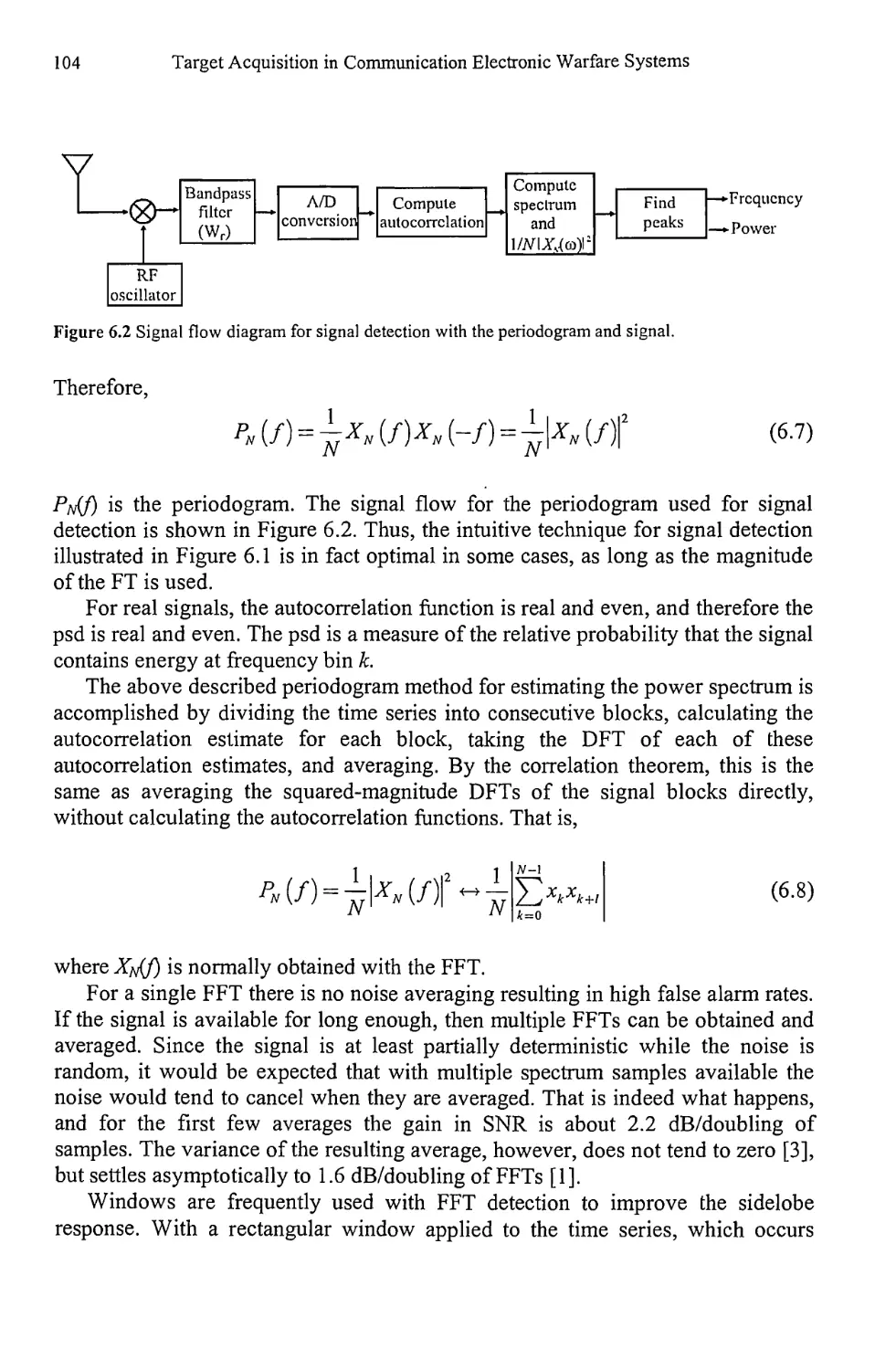
/


Text
Richard A. Poisel
For a listing of recent titles in the Artech House Information Warfare Library,
turn to the back of this book.
Target Acquisition in Communication
Electronic Warfare Systems
Richard A. Poisel
Artech House
Boston • London
www. artechhouse. com
Library of Congress Cataloging-in-Publication Data
A catalog record for this book is available from the Library of Congress.
British Library Cataloguing in Publication Data
Poisel, Richard
Target acquisition in communication electronic warfare systems
1. Military telecommunication 2. Electronics in military engineering
3. Target acquisition
I. Title
623’.043
ISBN 1-58053-913-0
Cover design by Gary Ragaglia
© 2004 ARTECH HOUSE, INC.
685 Canton Street
Norwood, MA 02062
All rights reserved. Printed and bound in the United States of America. No part of this book
may be reproduced or utilized in any form or by any means, electronic or mechanical, including
photocopying, recording, or by any information storage and retrieval system, without permission
in writing from the publisher. All terms mentioned in this book that are known to be trademarks
or service marks have been appropriately capitalized. Artech House cannot attest to the accuracy
of this information. Use of a term in this book should not be regarded as affecting the validity of
any trademark or service mark.
International Standard Book Number: 1-58053-913-0
10 98765432 1
To my parents: my earliest and best teachers
Contents
Preface xi
Chapter 1 Introduction 1
1.1 Electronic Warfare 1
1.2 Communications and EW 2
1.3 Signal Detection 4
1.4 Signal Searching 9
1.5 Notation 10
1.6 Concluding Remarks 10
References 11
Chapter 2 Deterministic and Stochastic Processes 13
2.1 The Fourier Transform 13
2.1.1 Important Fourier Transforms 15
2.2 Deterministic Signals 22
2.2.1 Energy and Power in Deterministic Signals 24
2.3 Stochastic Processes 25
2.3.1 Ensembles 25
2.3.2 Power Spectral Densities 27
2.3.3 Mean, Autocorrelation, and Autocovariance Functions 28
2.3.4 Stationary and Wide-Sense Stationary Processes 29
2.3.5 Ergodic Processes 3 0
2.3.6 Cyclostationary Processes 30
2.4 Stochastic Signals 31
2.5 White Noise 39
2.5.1 Signals in Noise 40
2.6 Concluding Remarks 41
References 41
Chapter 3 Target Search Methods 43
3.1 General Search 45
3.2 Directed Search 49
3.3 Concluding Remarks 49
vii
viii
Target Acquisition in Communication Electronic Warfare Systems
References 50
Chapter 4 Hypothesis Testing for Signal Detection 51
4.1 Hypothesis Testing 51
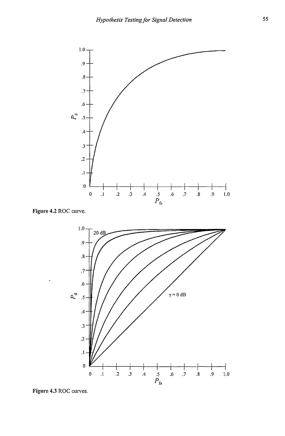
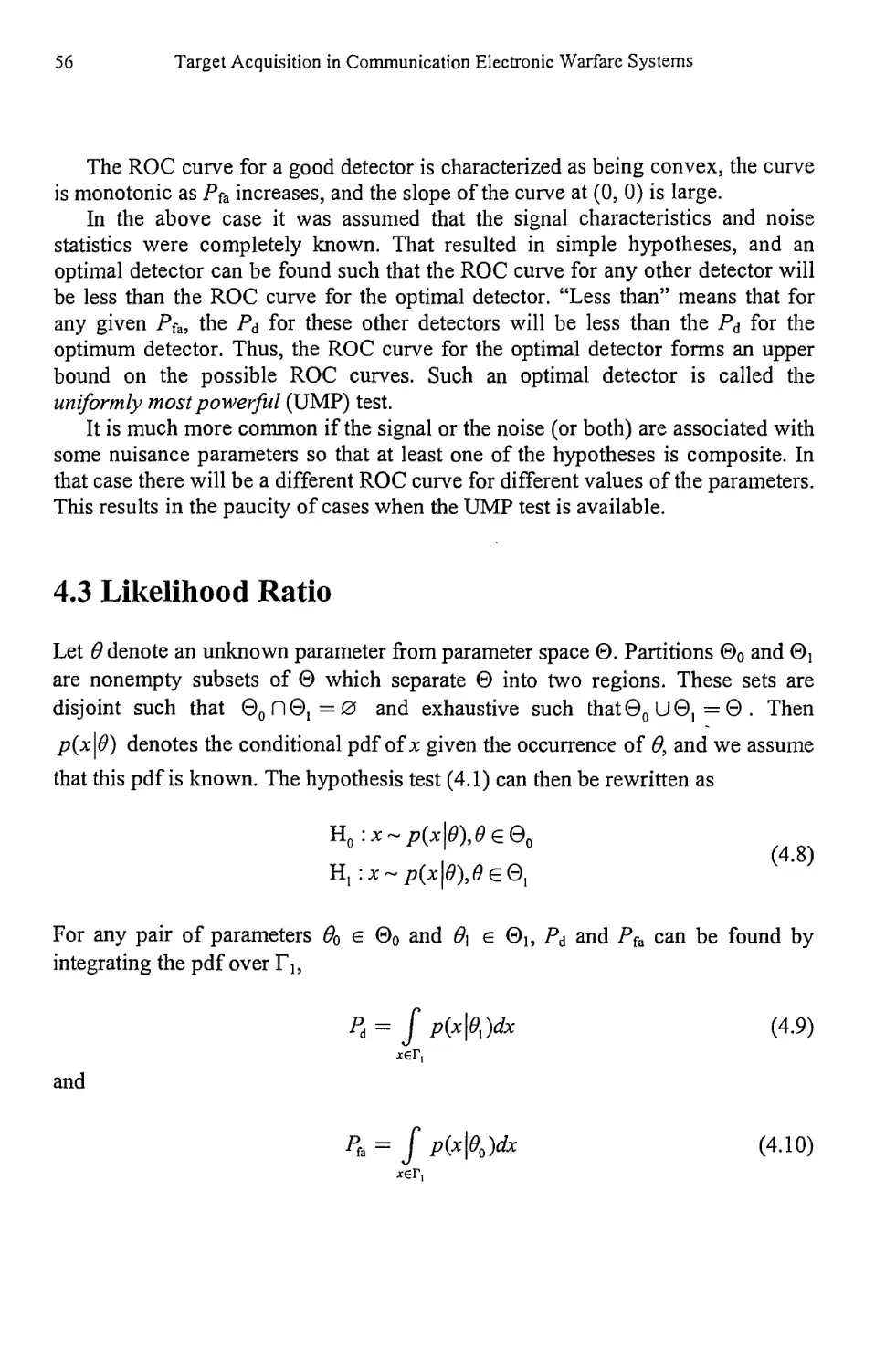
4.2 Receiver Operating Characteristics 54
4.3 Likelihood Ratio 56
4.4 Hypothesis Tests 57
4.4.1 Bayes Criterion 59
4.4.2 Minimax Criterion 64
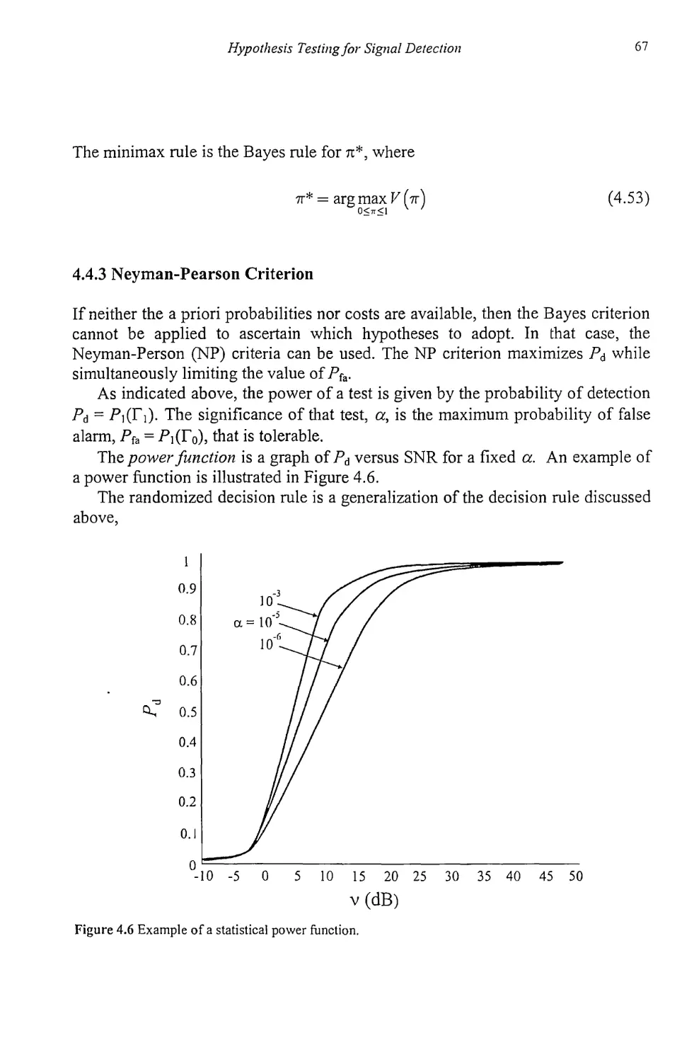
4.4.3 Neyman-Pearson Criterion 67
4.5 Multiple Measurements 68
4.6 Multiple Hypotheses 69
4.7 Concluding Remarks 69
References 70
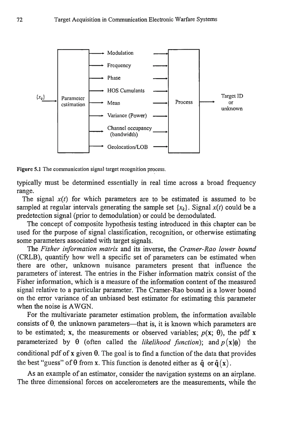
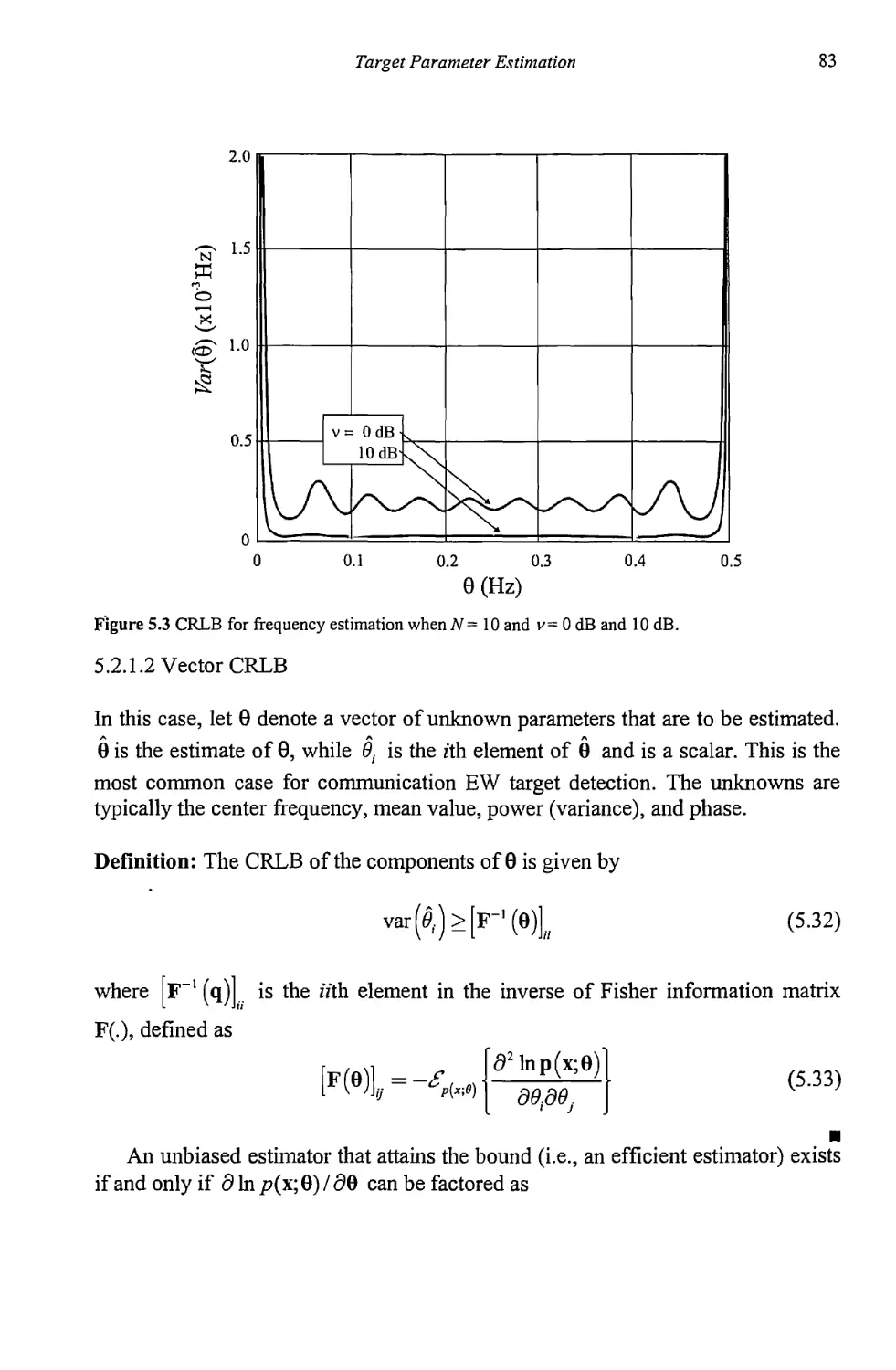
Chapter 5 Target Parameter Estimation 71
5.1 Signal Parameter Estimation 71
5.2 The Cramer-Rao Bound 73
5.2.1 CRLB for Signals in AWGN 77
5.3 Maximum Likelihood Estimation 88
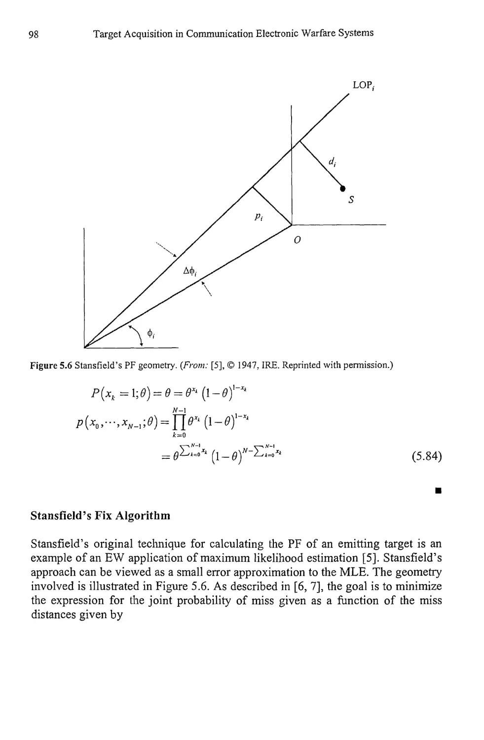
5.4 Concluding Remarks 99
References 99
Chapter 6 Spectrum Estimation 101
6.1 Spectrum Estimation with the Periodogram 101
6.1.1 Averaged Periodogram 105
6.2 Blackman-Tukey Spectrum Estimation 108
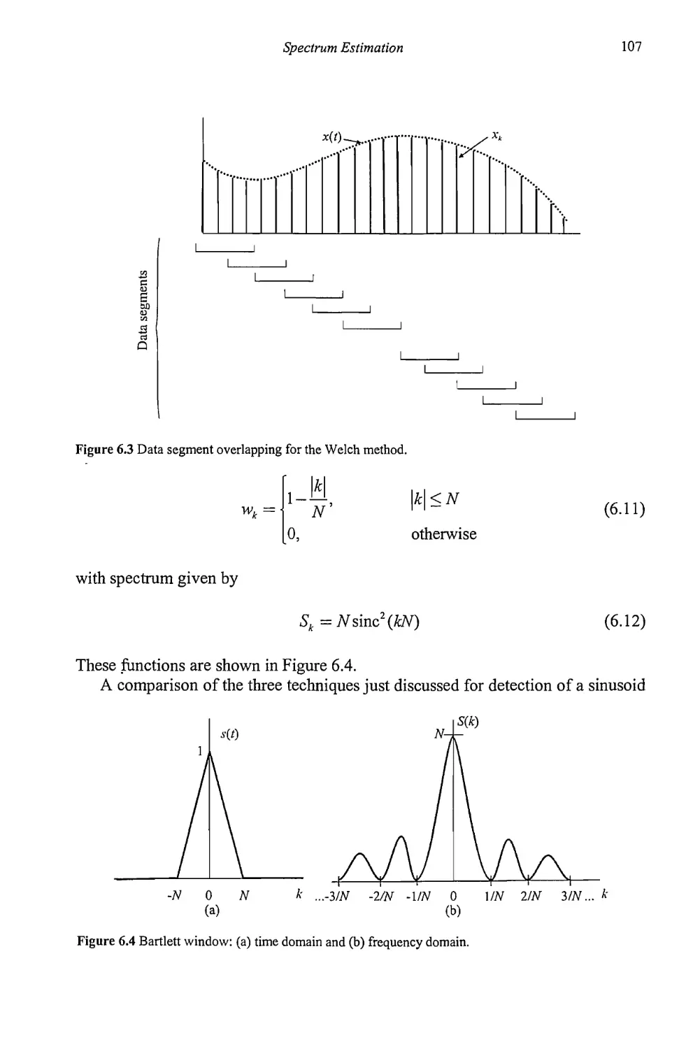
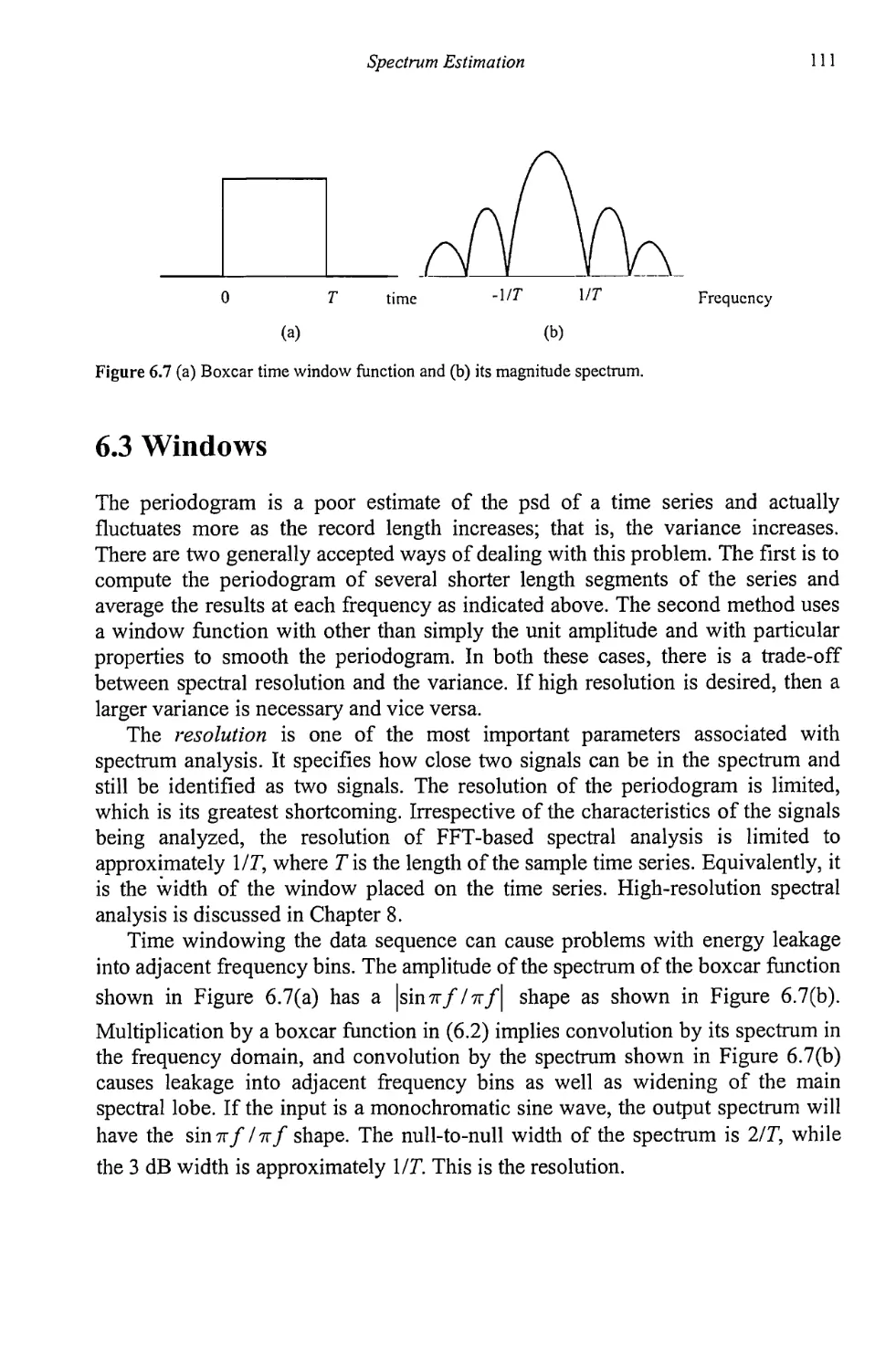
6.3 Windows 111
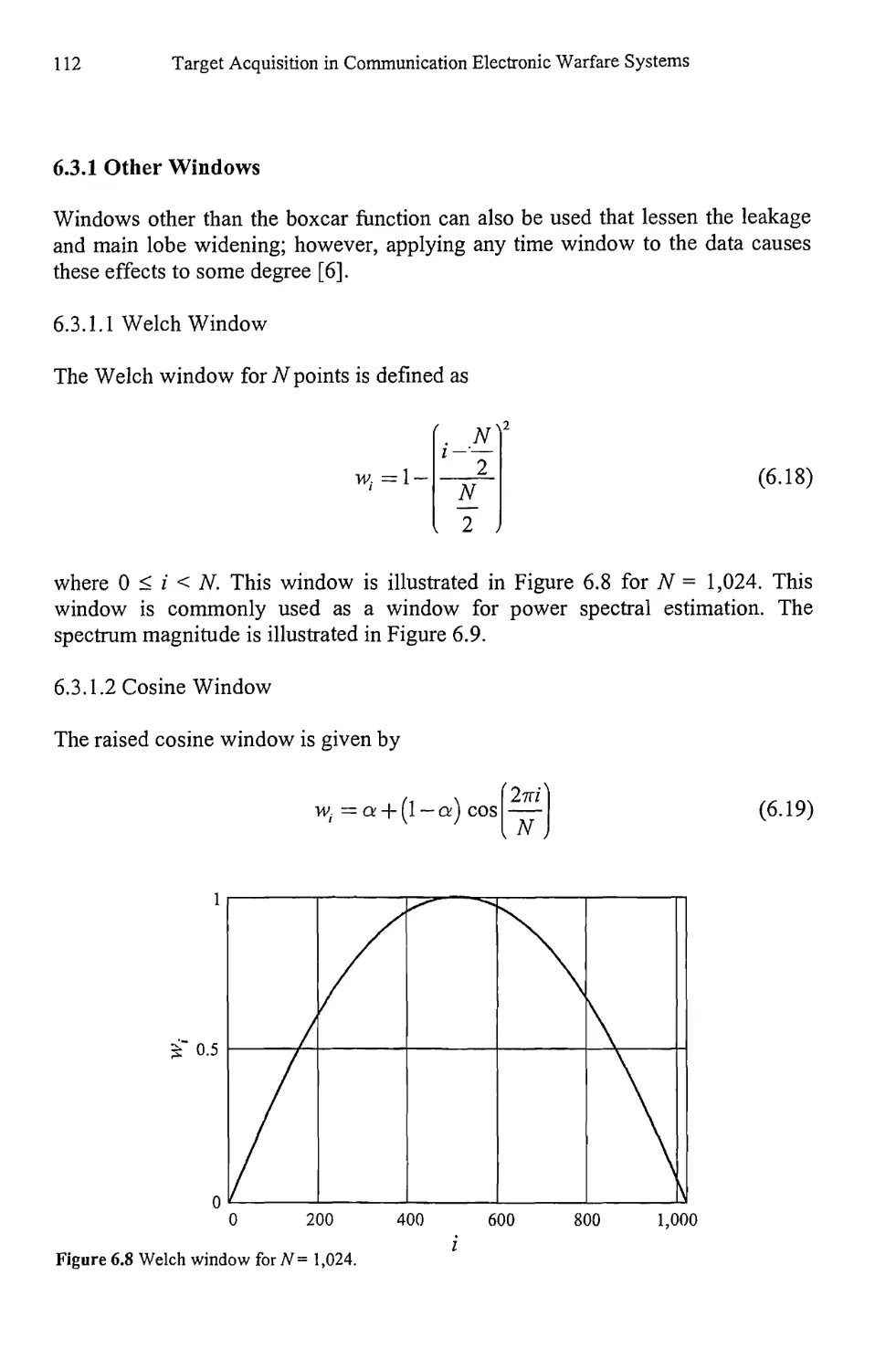
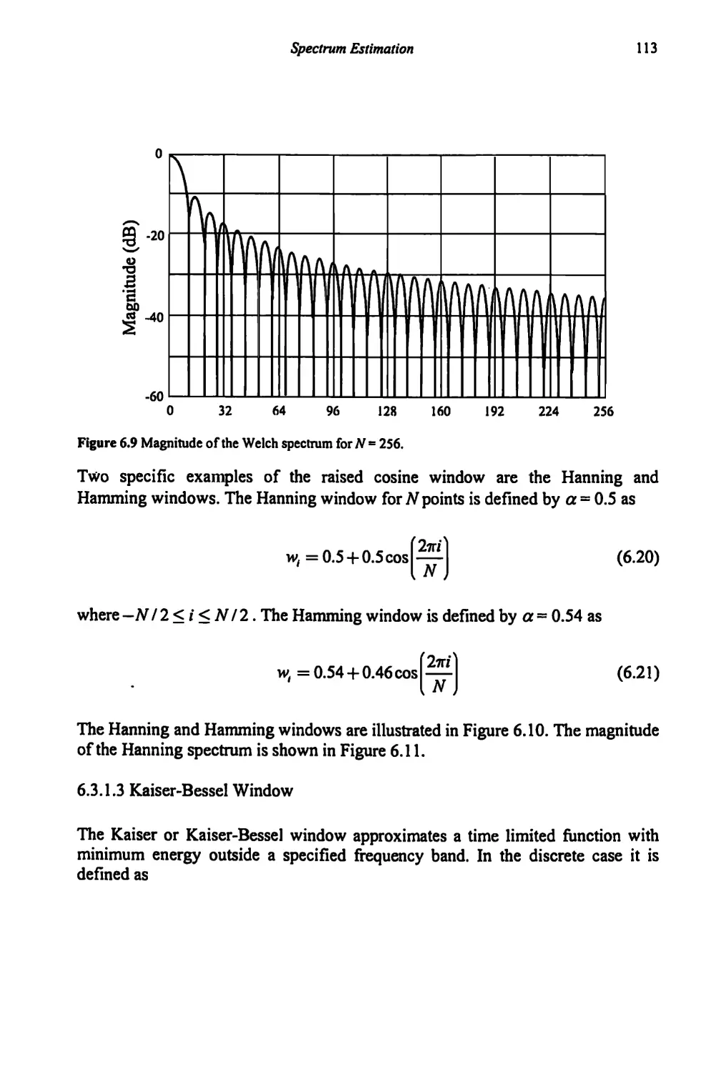
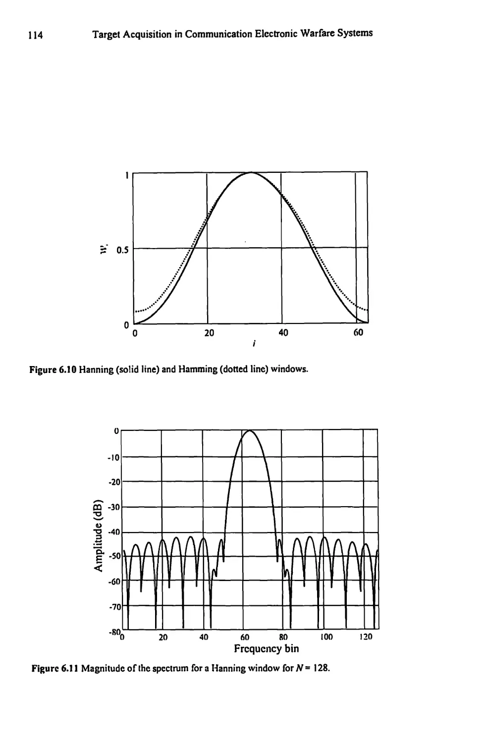
6.3.1 Other Windows 112
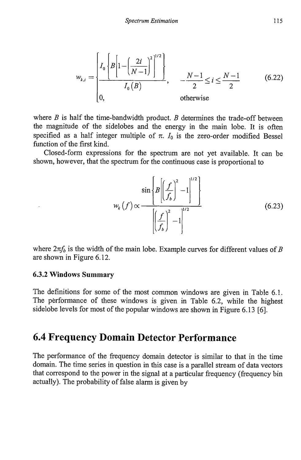
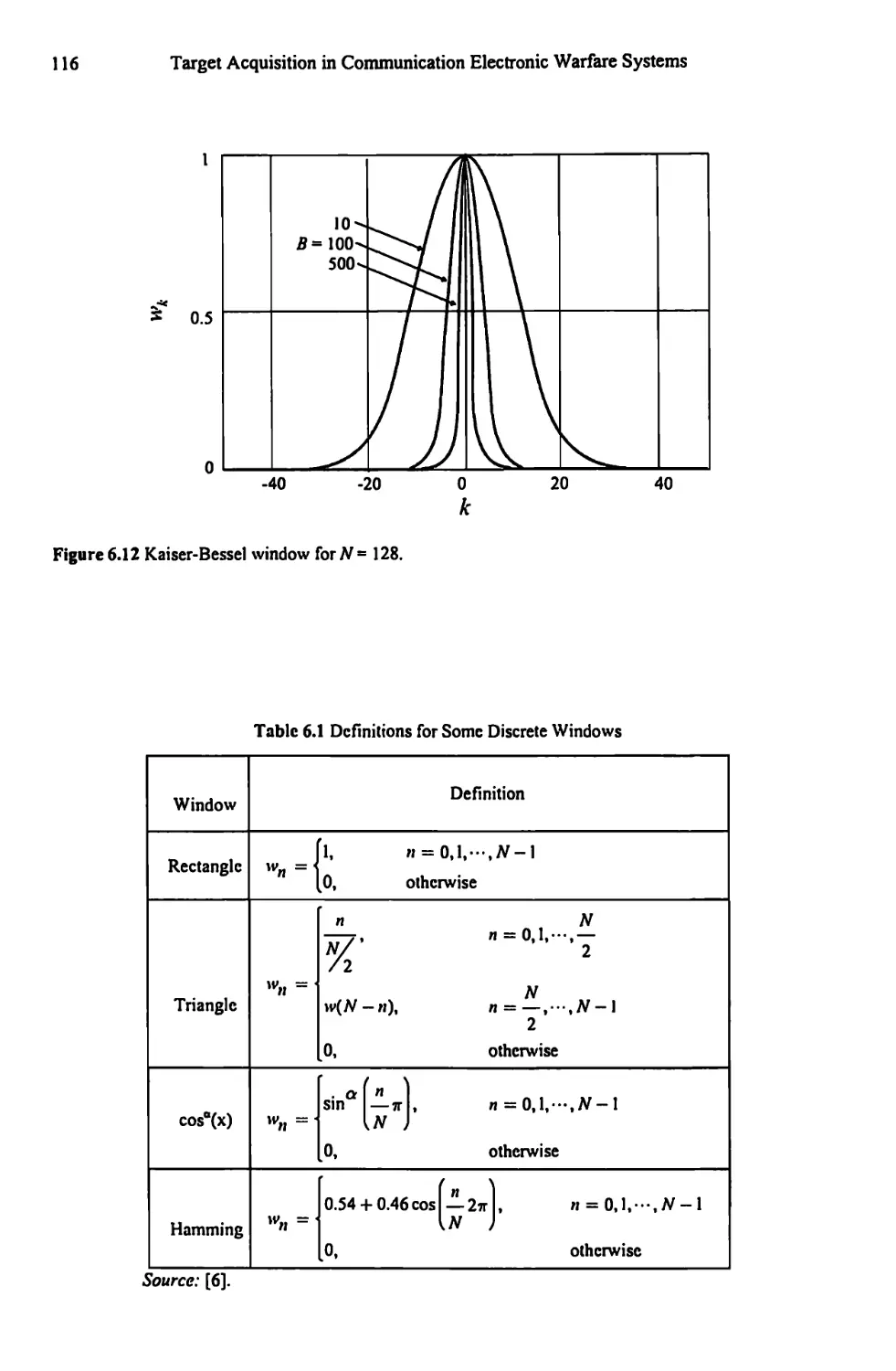
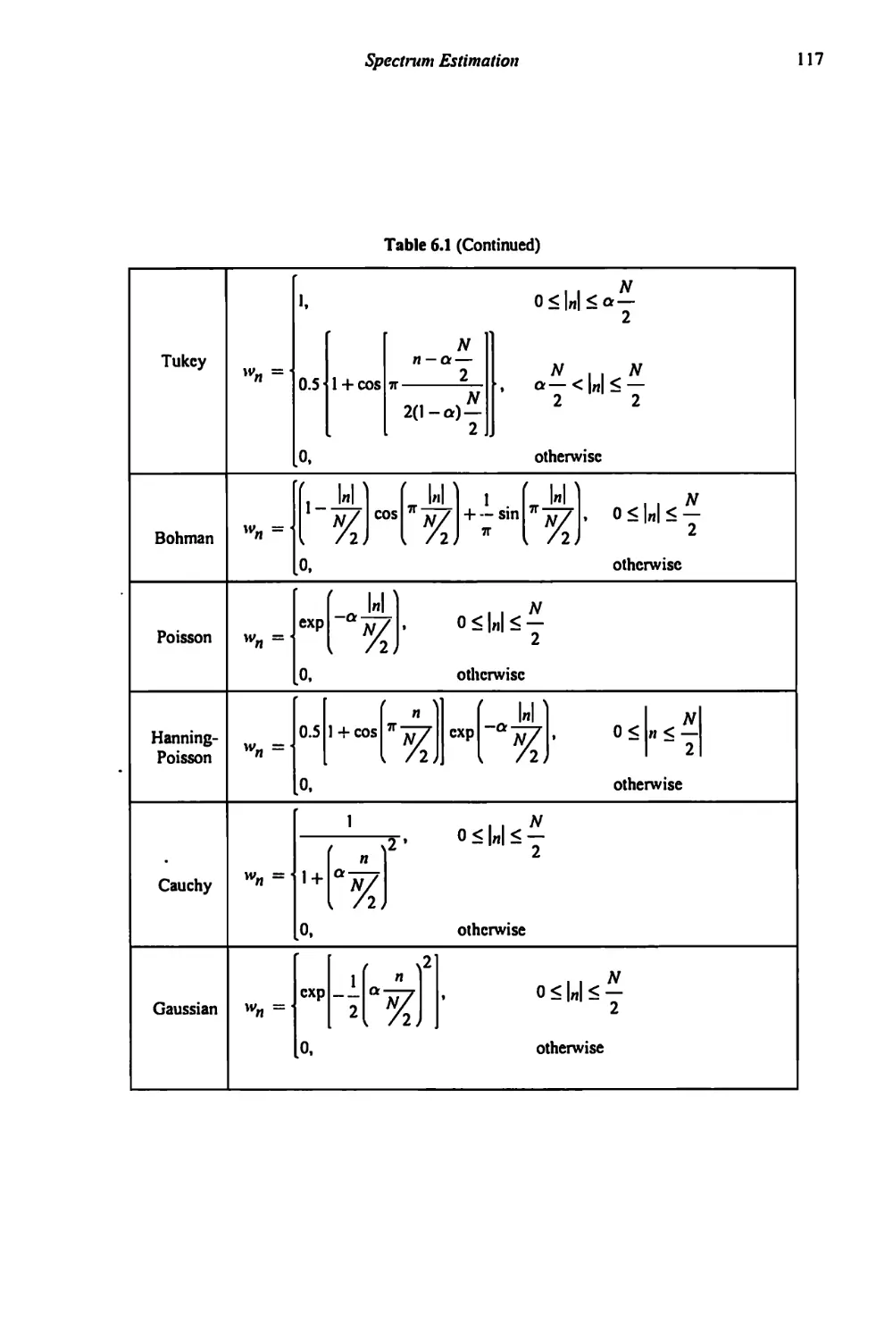
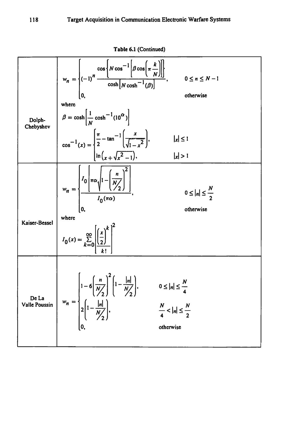
6.3.2 Windows Summary 115
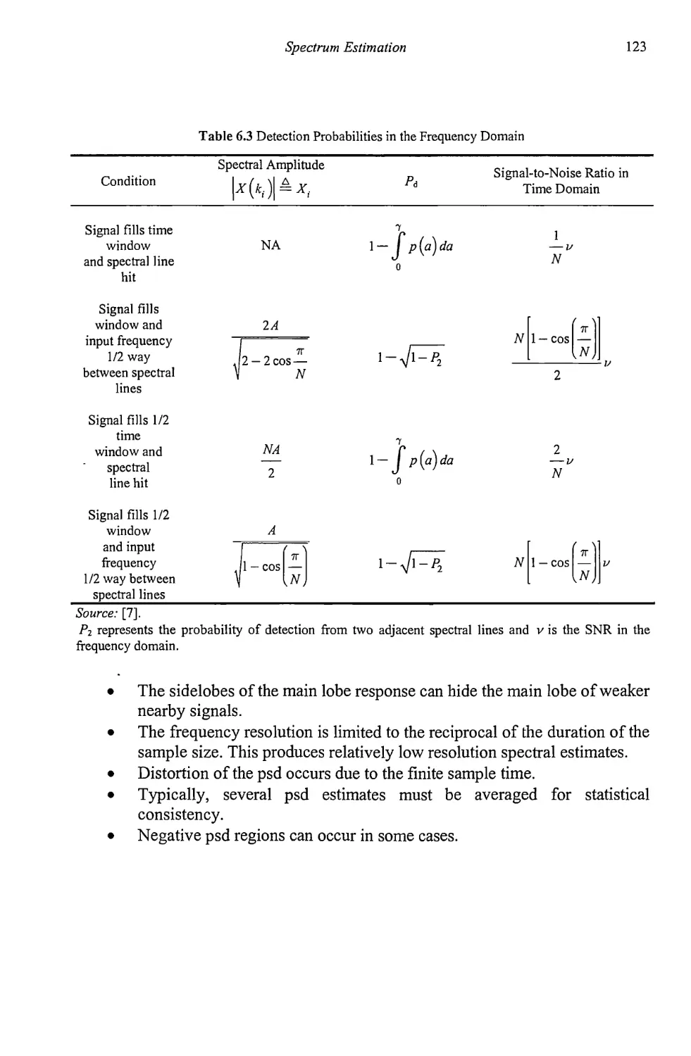
6.4 Frequency Domain Detector Performance 115
6.5 Concluding Remarks 122
References 124
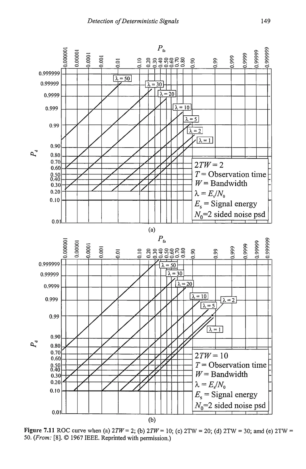
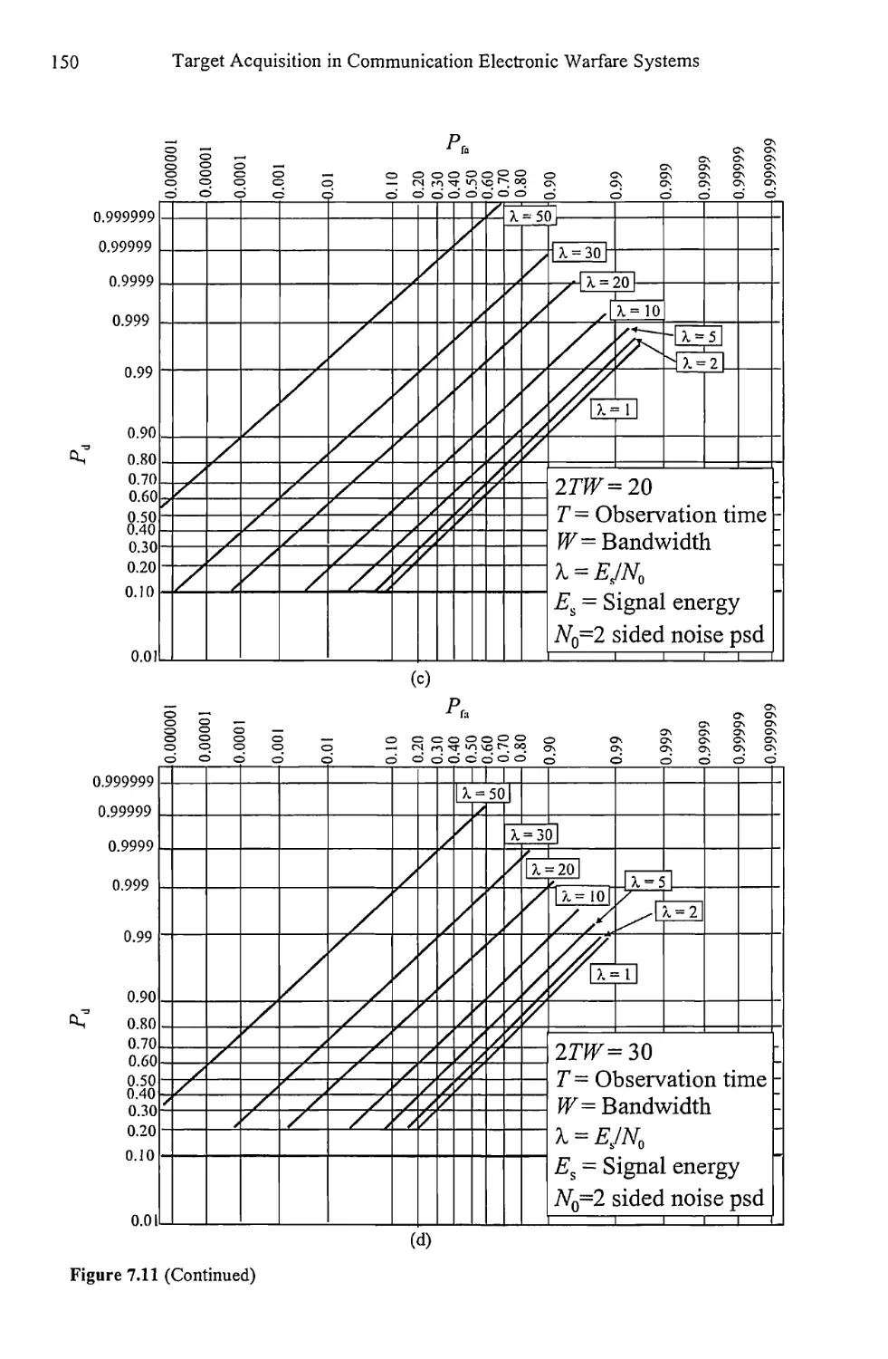
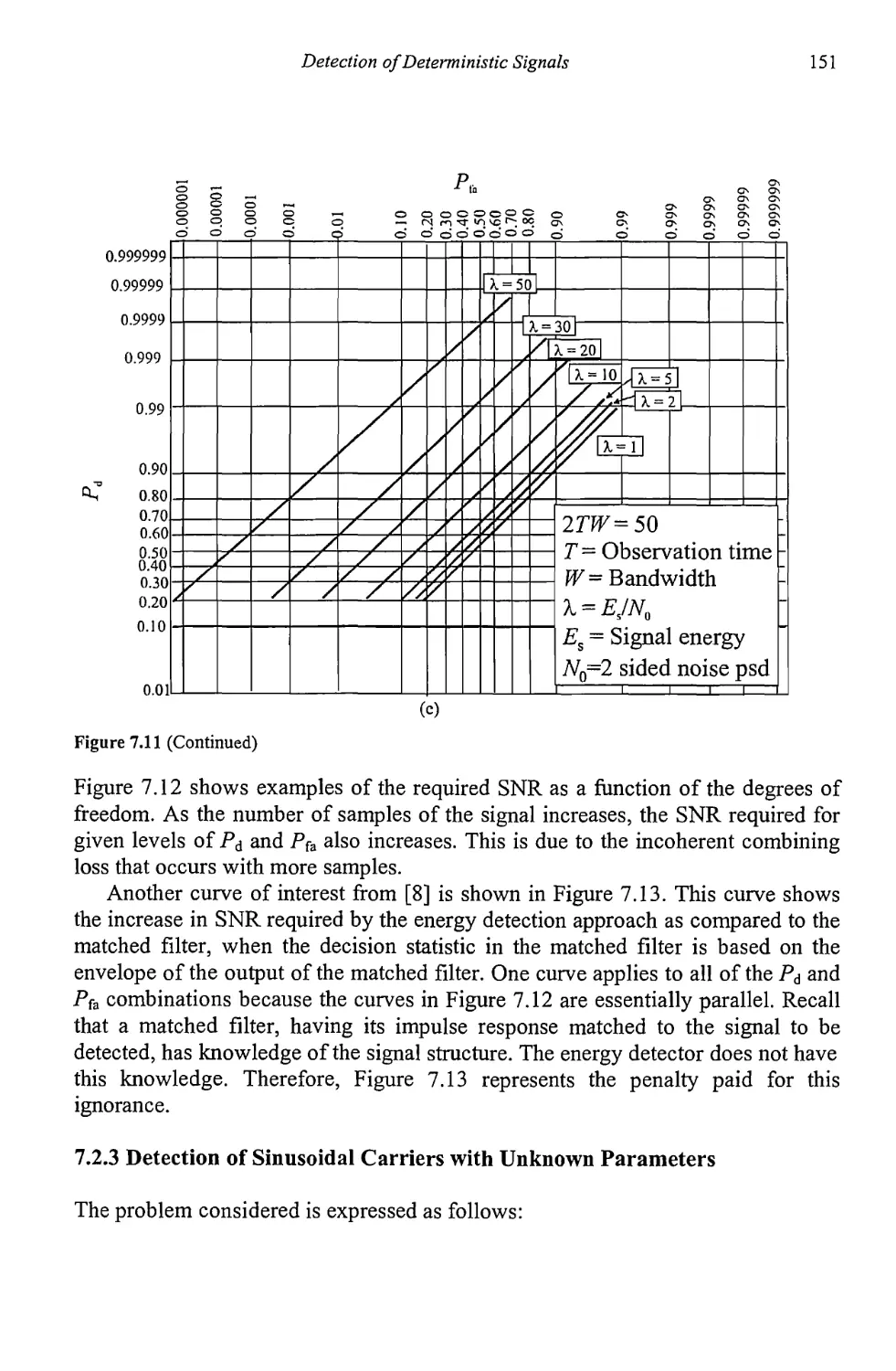
Chapter 7 Detection of Determinisitc Signals 125
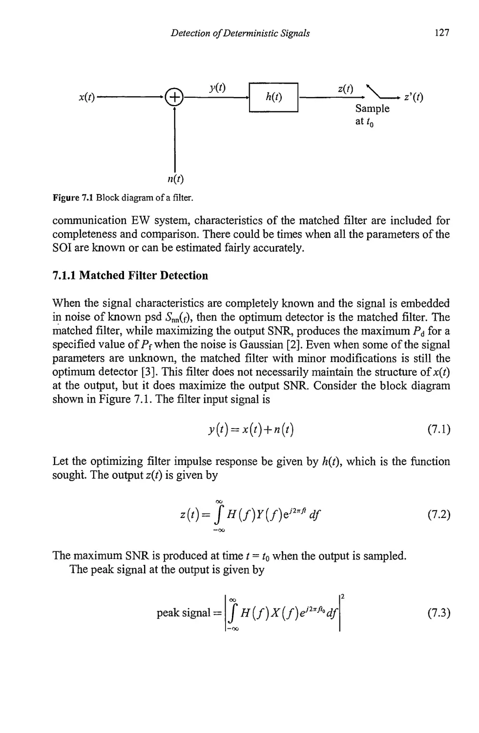
7.1 Detection of Deterministic Signals with Known Parameters 126
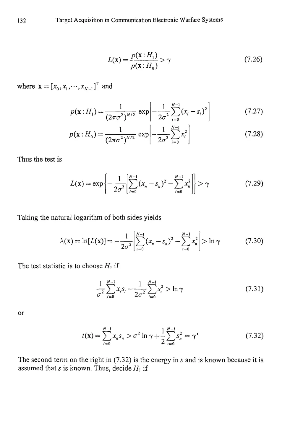
7.1.1 Matched Filter Detection 127
7.1.2 Matched Filter Performance 131
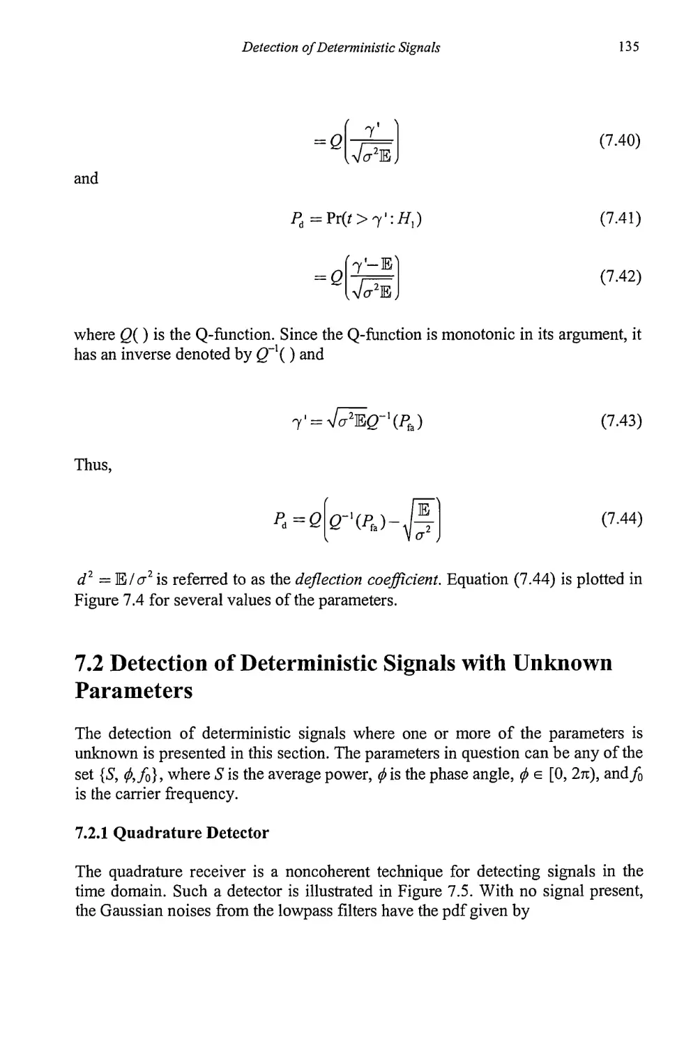
7.2 Detection of Deterministic Signals with Unknown Parameters 135
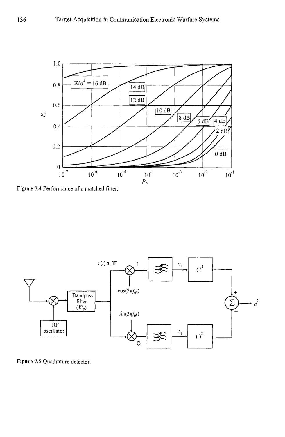
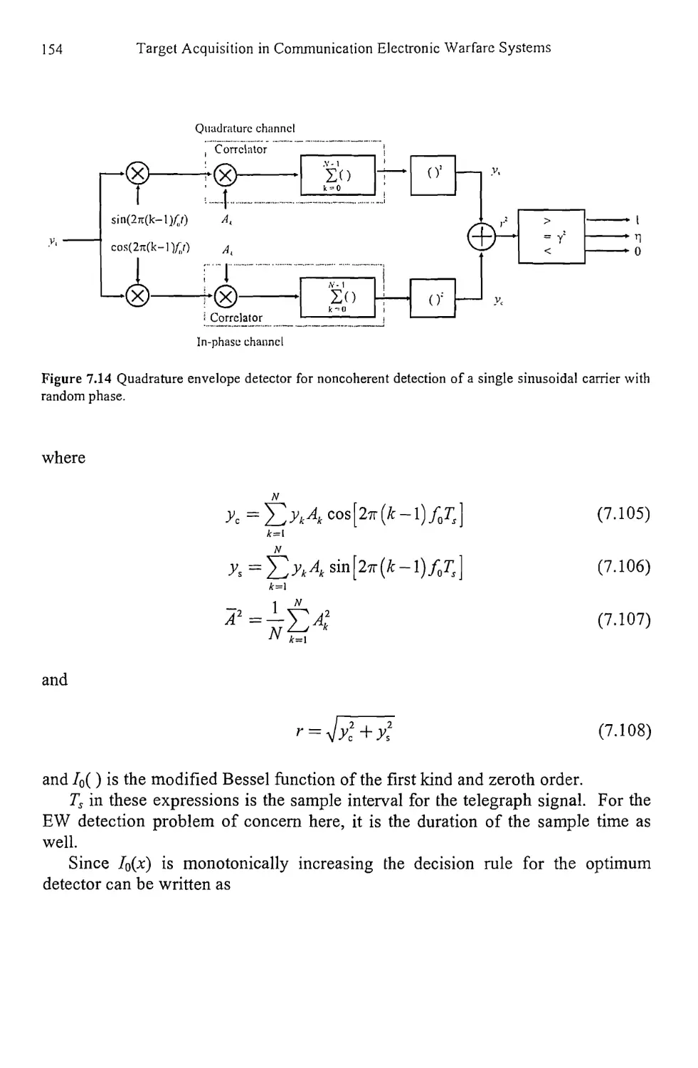
7.2.1 Quadrature Detector 135
7.2.2 GLRT Detection 141
Contents ix
7.2.3 Detection of Sinusoidal Carriers with
Unknown Parameters 151
7.2.4 Locally Optimum Test for Weak Signal Detection 157
7.2.5 Bayes Linear Model 174
7.2.6 MLE of the Unknown Parameters of
Sinusoids in AWGN 179
7.2.7 Optimum Detection of Deterministic Signals with
Unknown Parameters in Impulsive Noise 184
7.3 Concluding Remarks 187
References 189
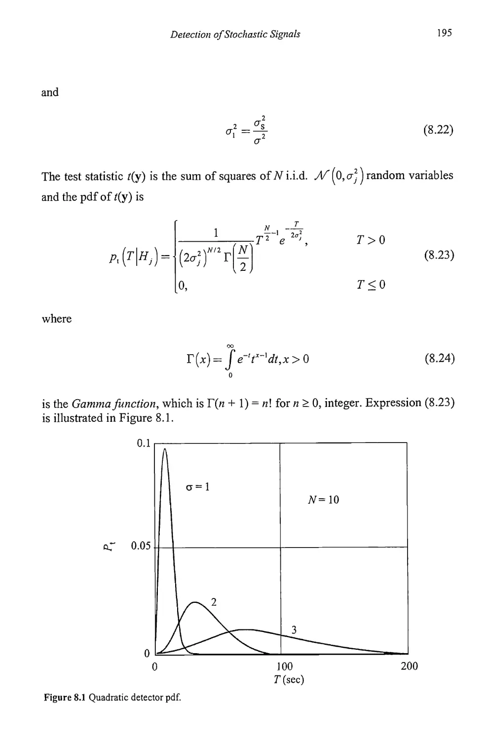
Chapter 8 Detection of Stochastic Signals 191
8.1 Detection of Random Signals with Unknown Parameters 191
8.1.1 GLRT Detection of Stochastic Signals 191
8.1.2 Locally Optimum Detection of Stochastic Signals 197
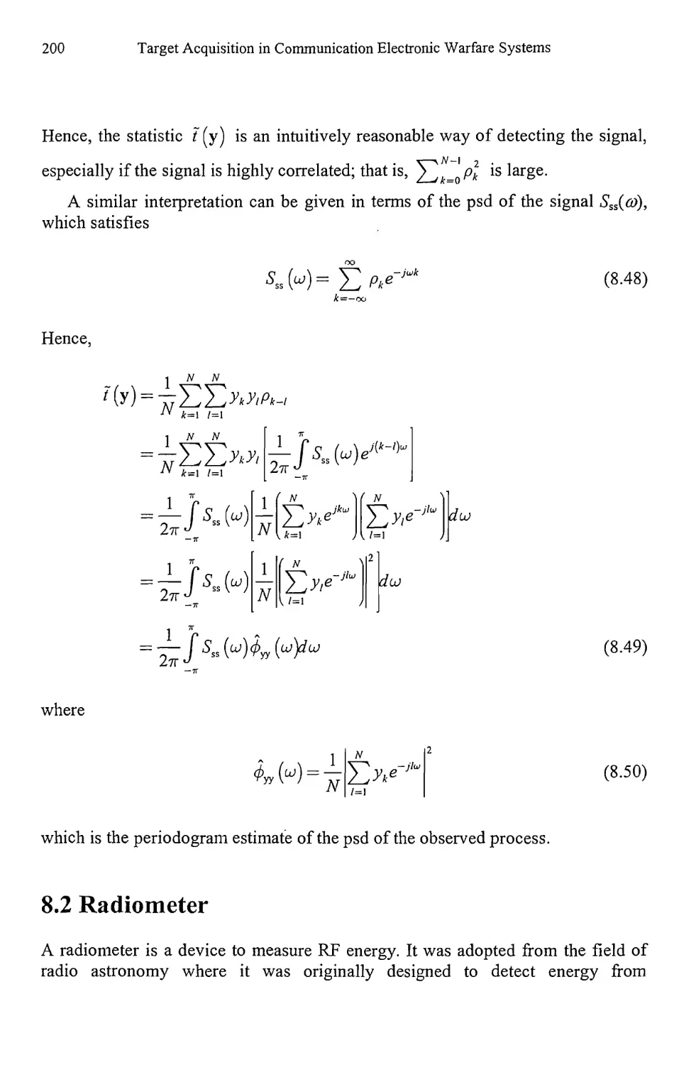
8.2 Radiometer 200
8.2.1 Radiometer 201
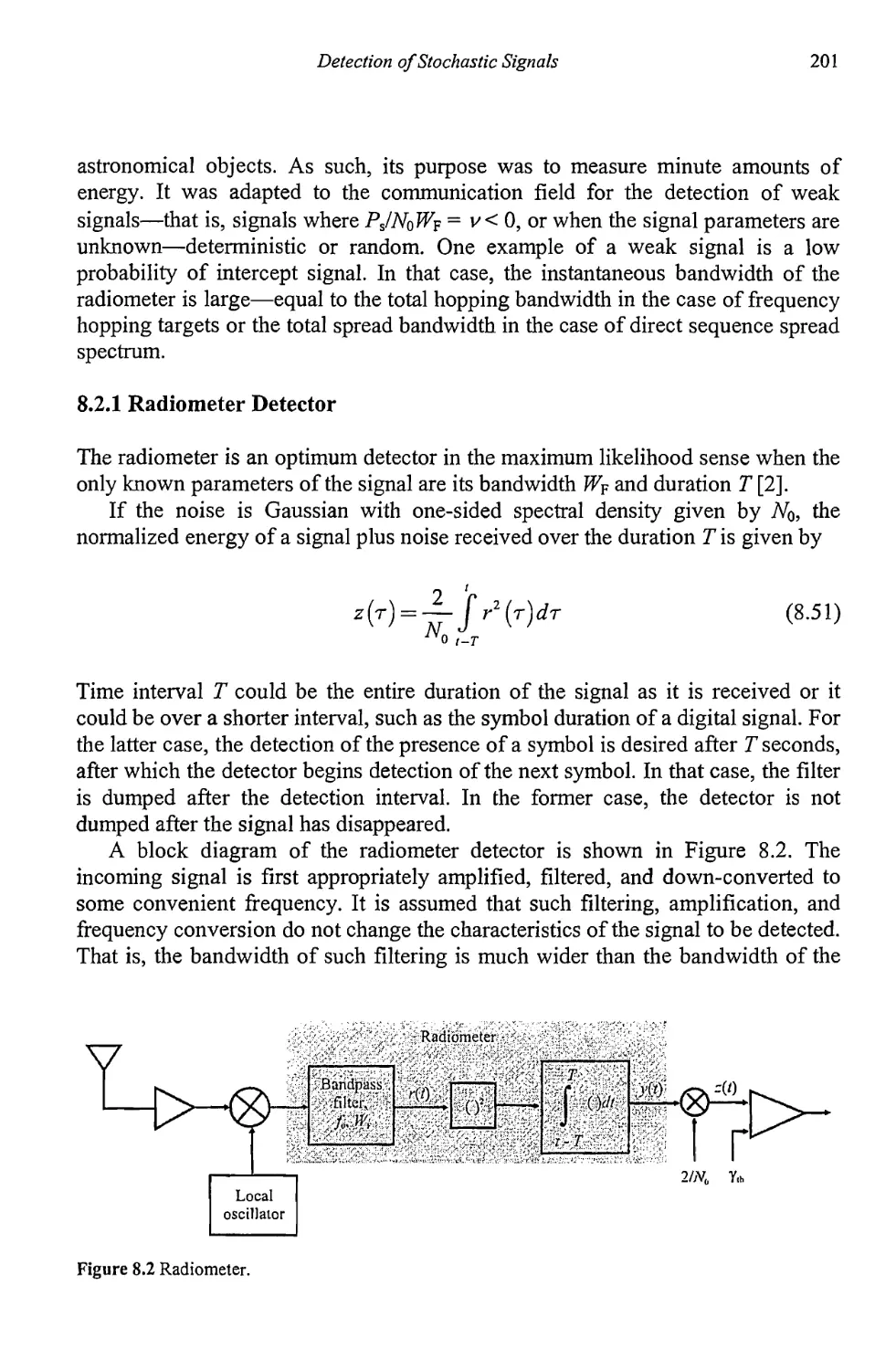
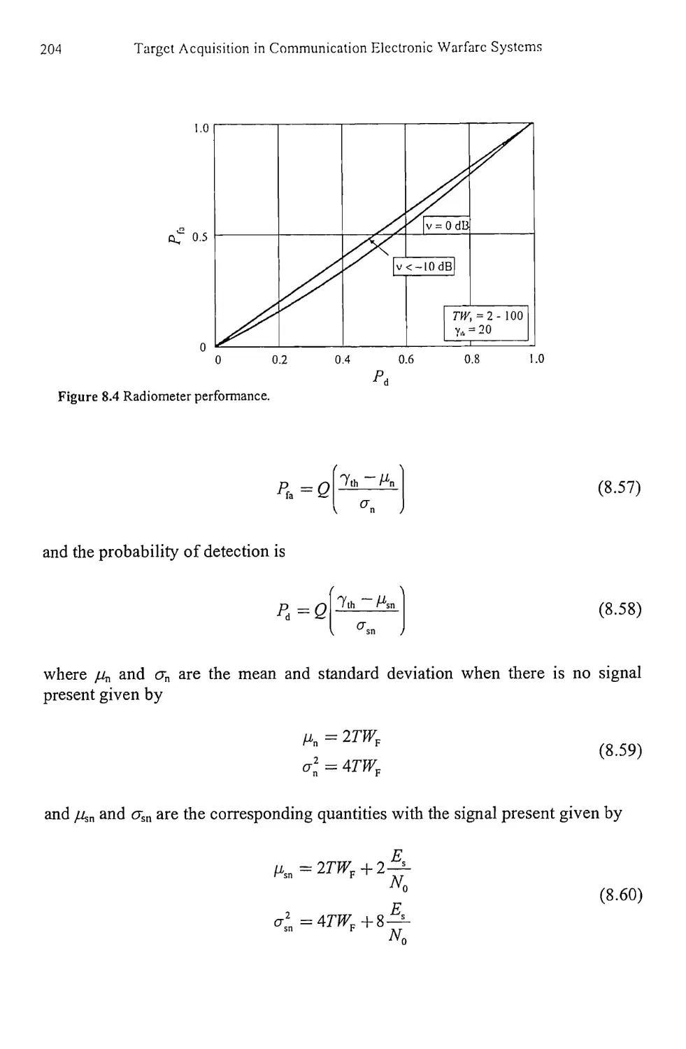
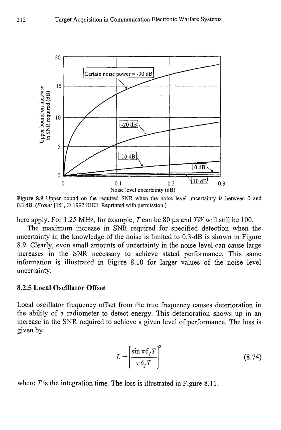
8.2.2 Radiometer Performance 202
8.2.3 Radiometer Models 203
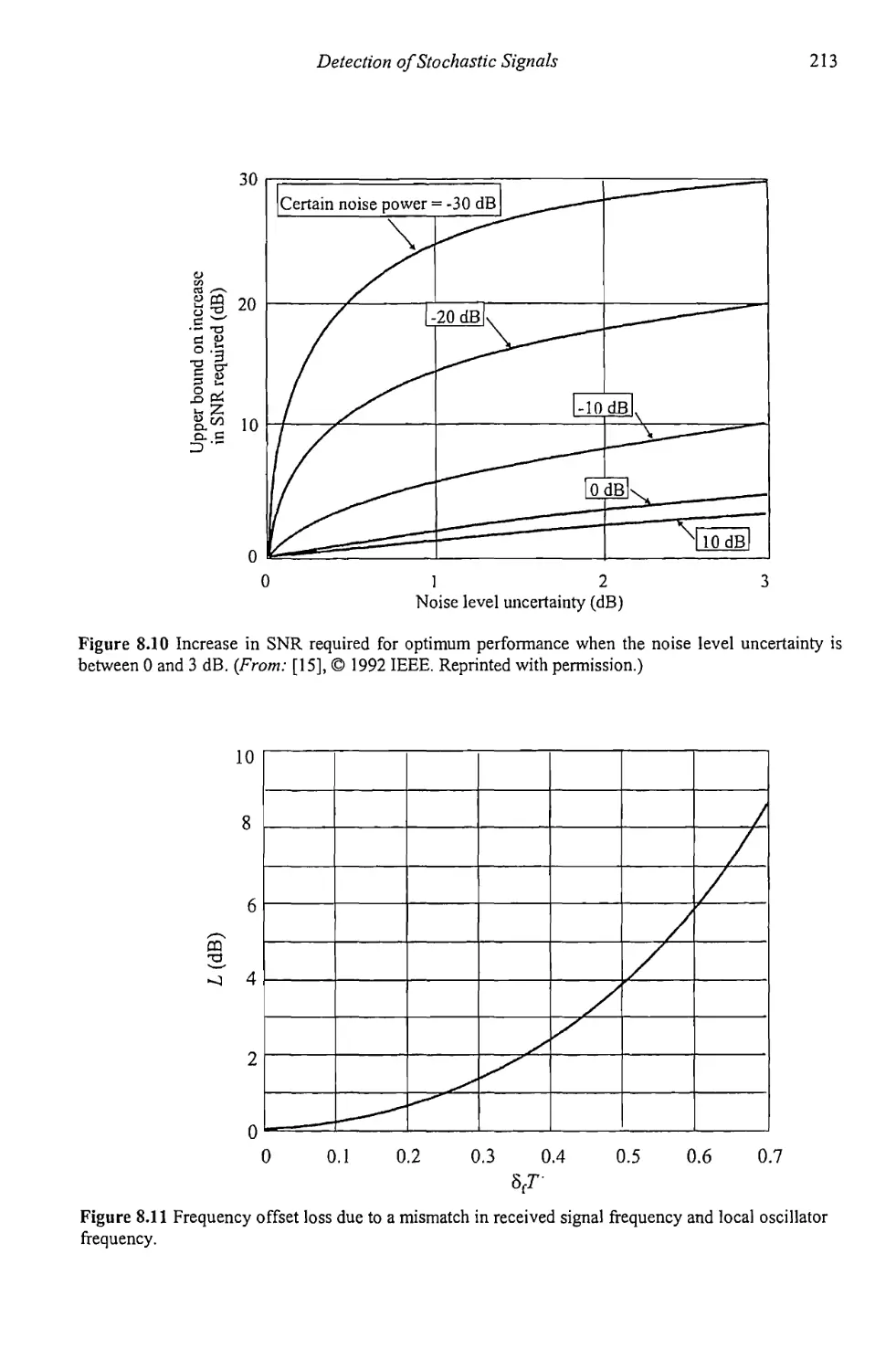
8.2.4 Uncertain Noise Power 210
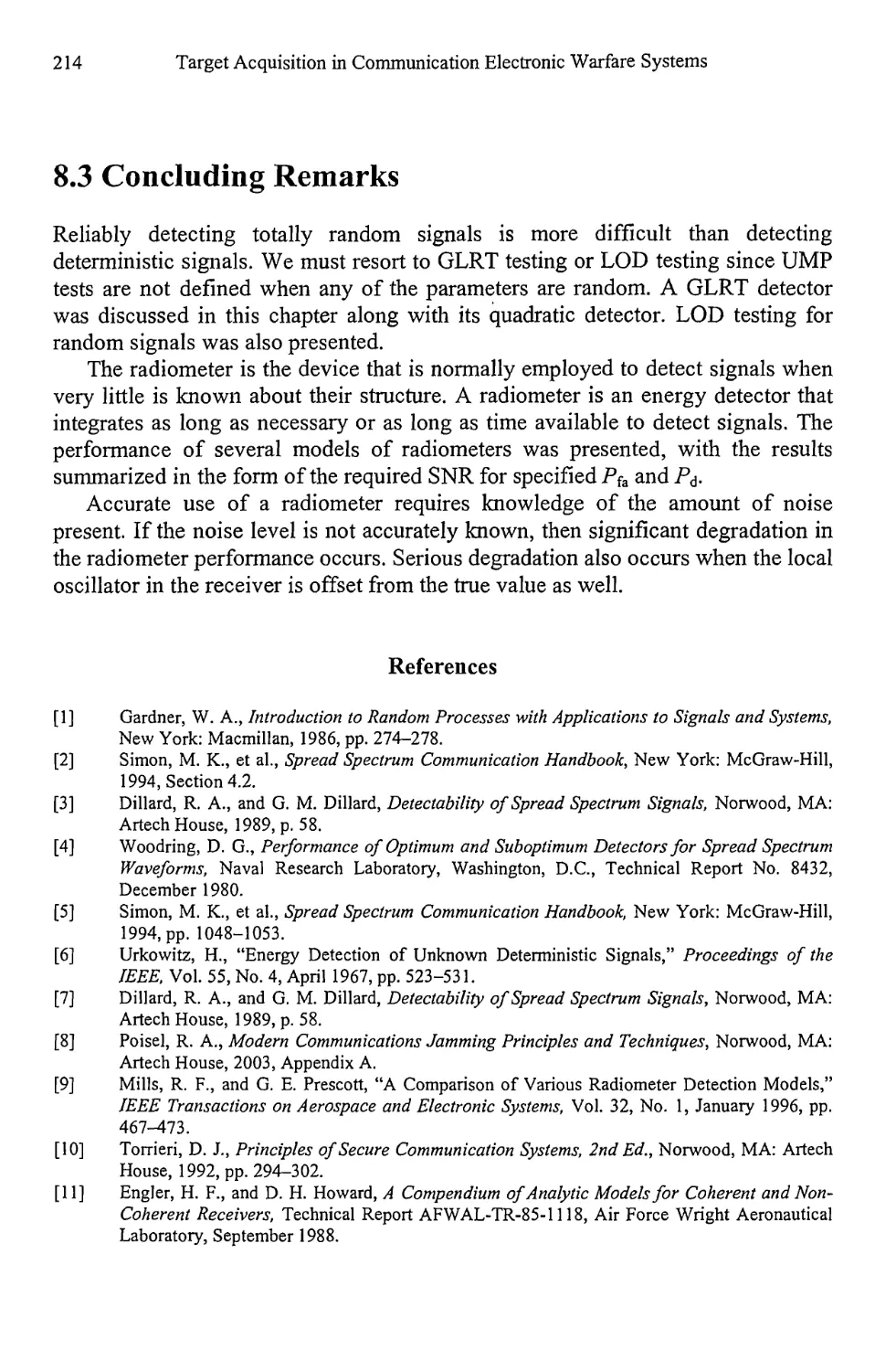
8.2.5 Local Oscillator Offset 212
8.3 Concluding Remarks 214
References 214
Chapter 9 High-Resolution Spectrum Estimation 217
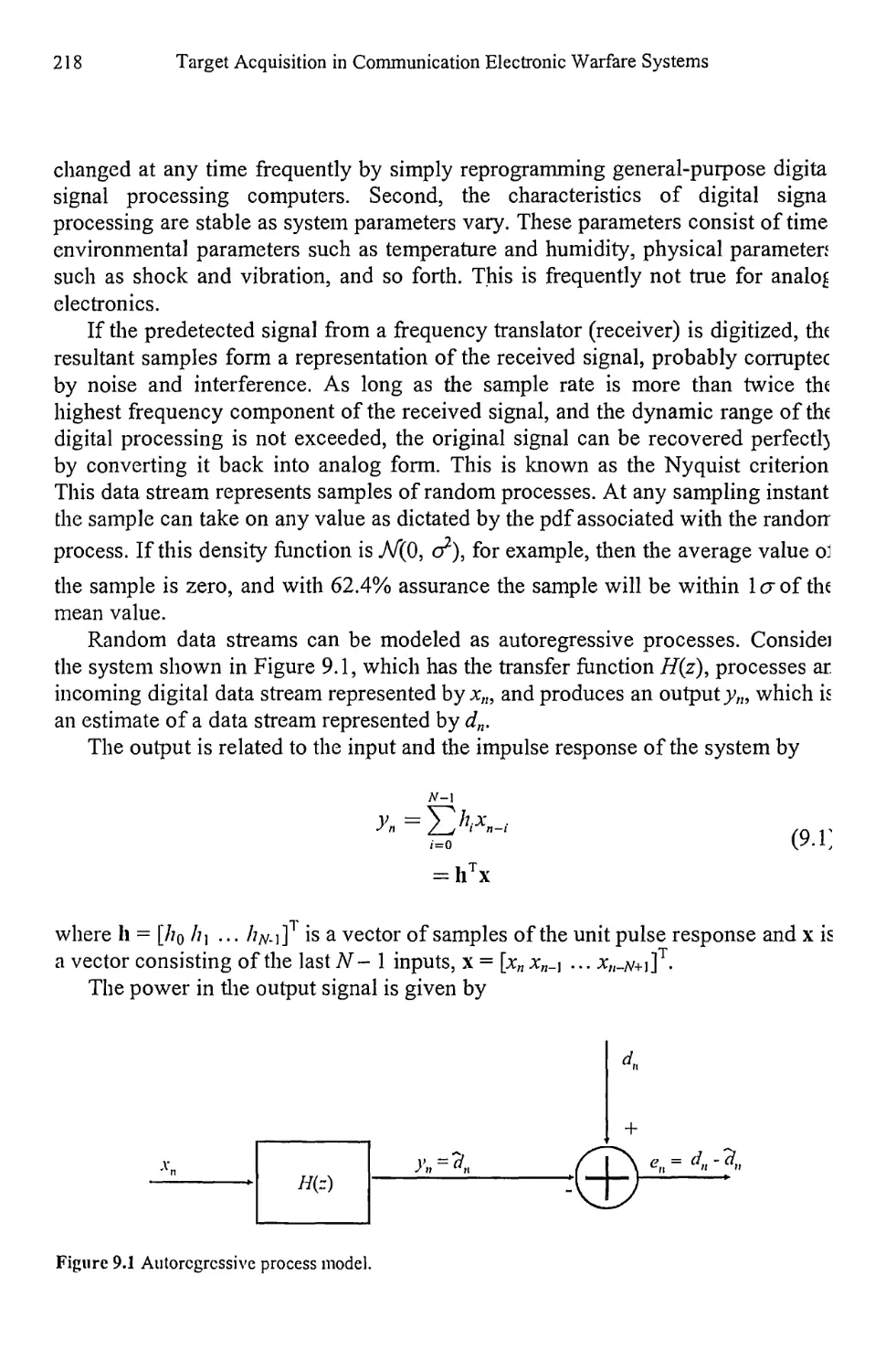
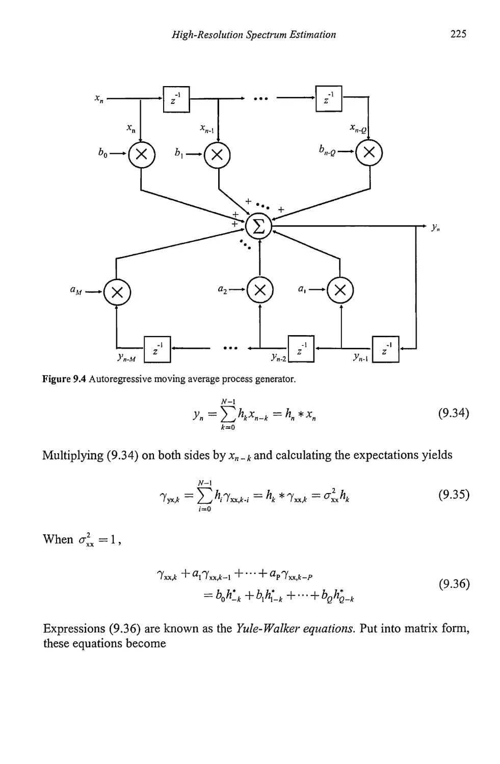
9.1 Autoregressive Moving Average Modeling 217
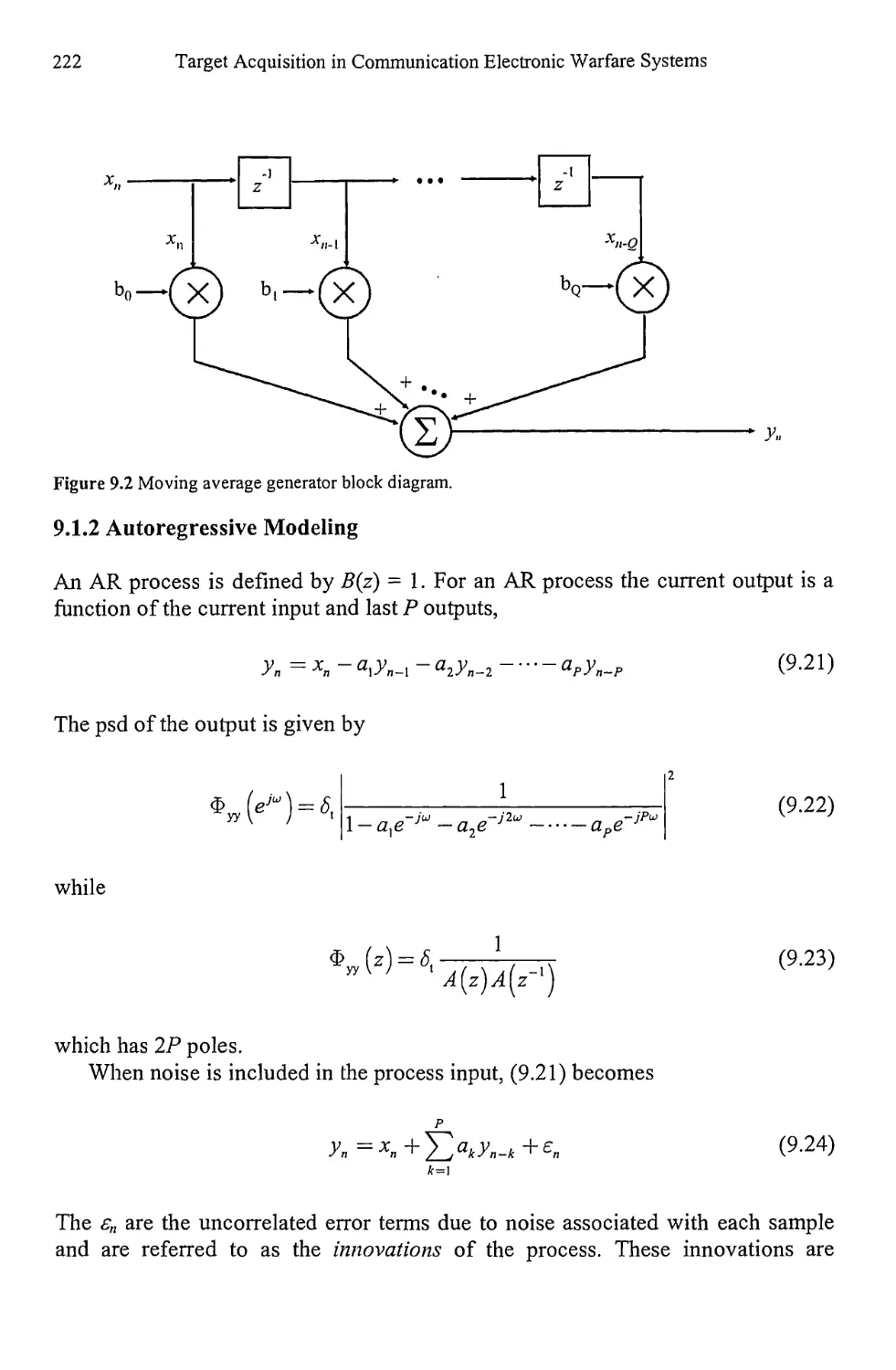
9.1.1 Moving Average Modeling 221
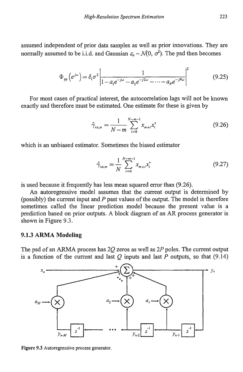
9.1.2 Autoregressive Modeling 222
9.1.3 ARMA Modeling 223
9.1.4 Maximum Entropy Spectral Estimation 231
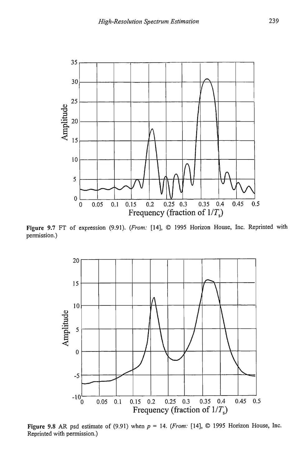
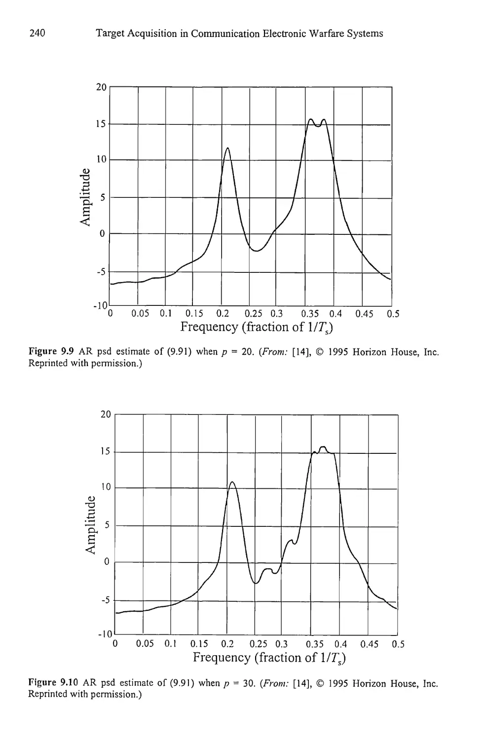
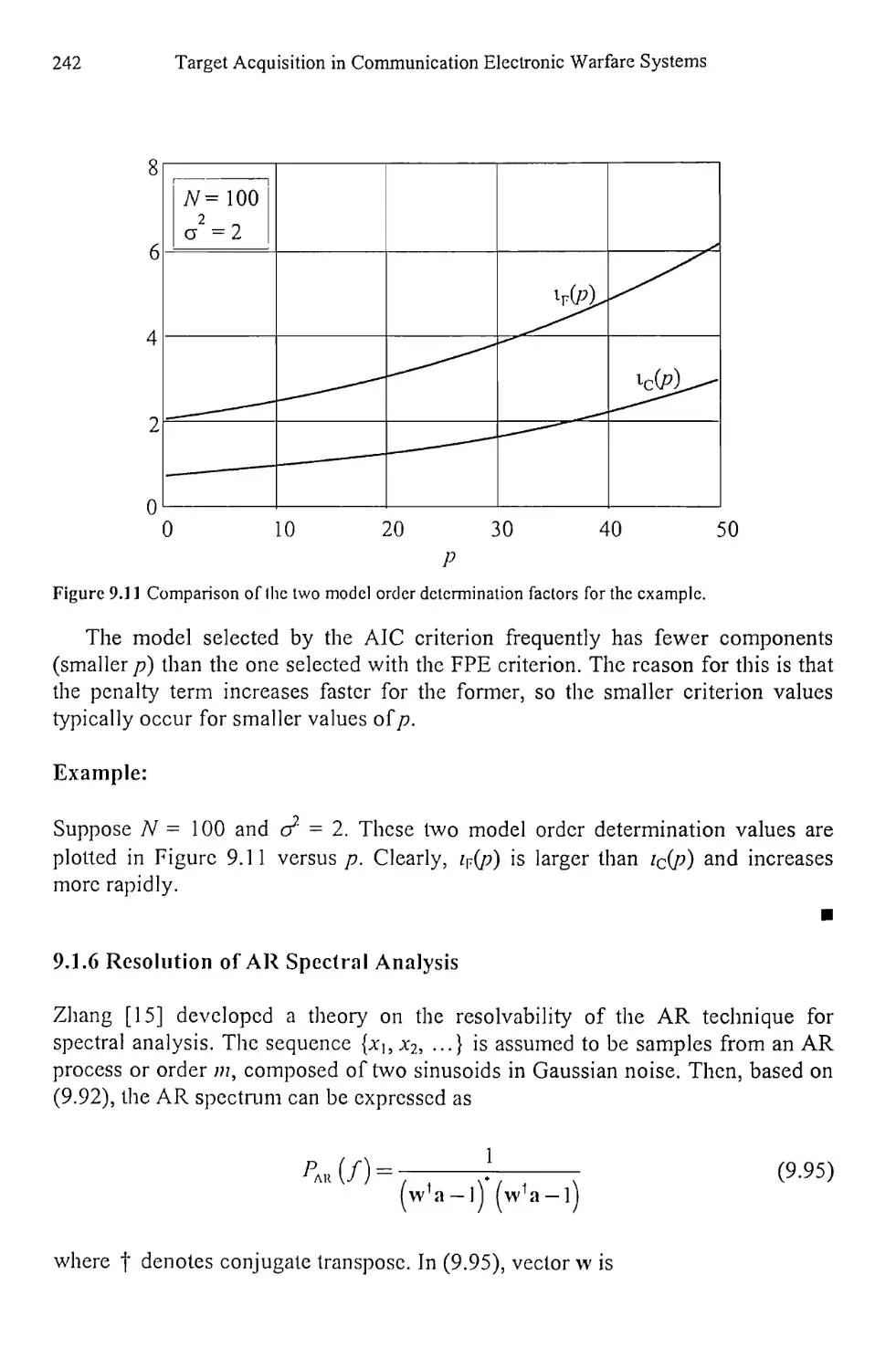
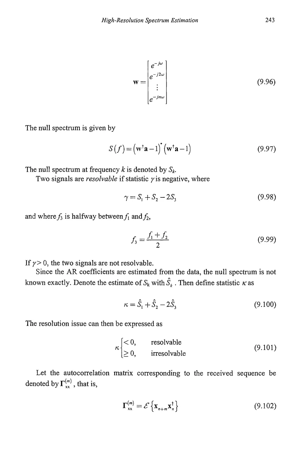
9.1.5 Model Order Determination 238
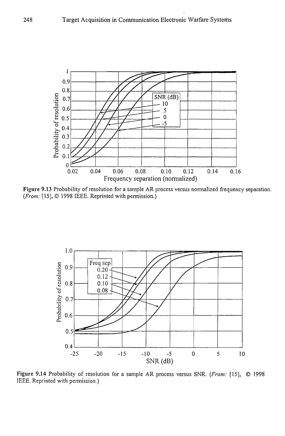
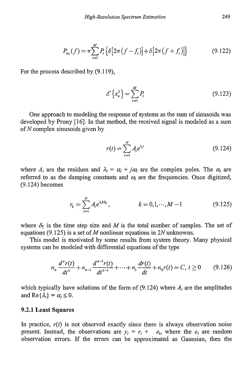
9.1.6 Resolution of AR Spectral Analysis 242
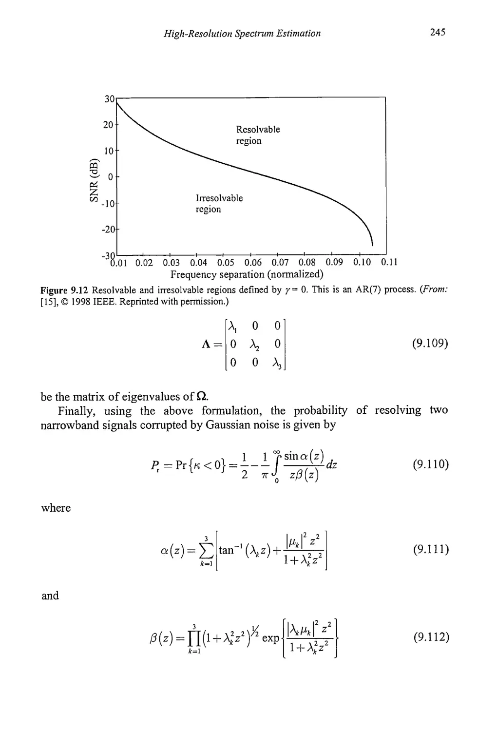
9.2 Line Spectra 247
9.2.1 Least Squares 249
9.2.2 Prony’s Method 250
9.2.3 Modified Prony Methods 251
9.3 Signal Subspace Techniques 251
9.3.1 Pisarenko Method 258
9.3.2 Root Pisarenko 263
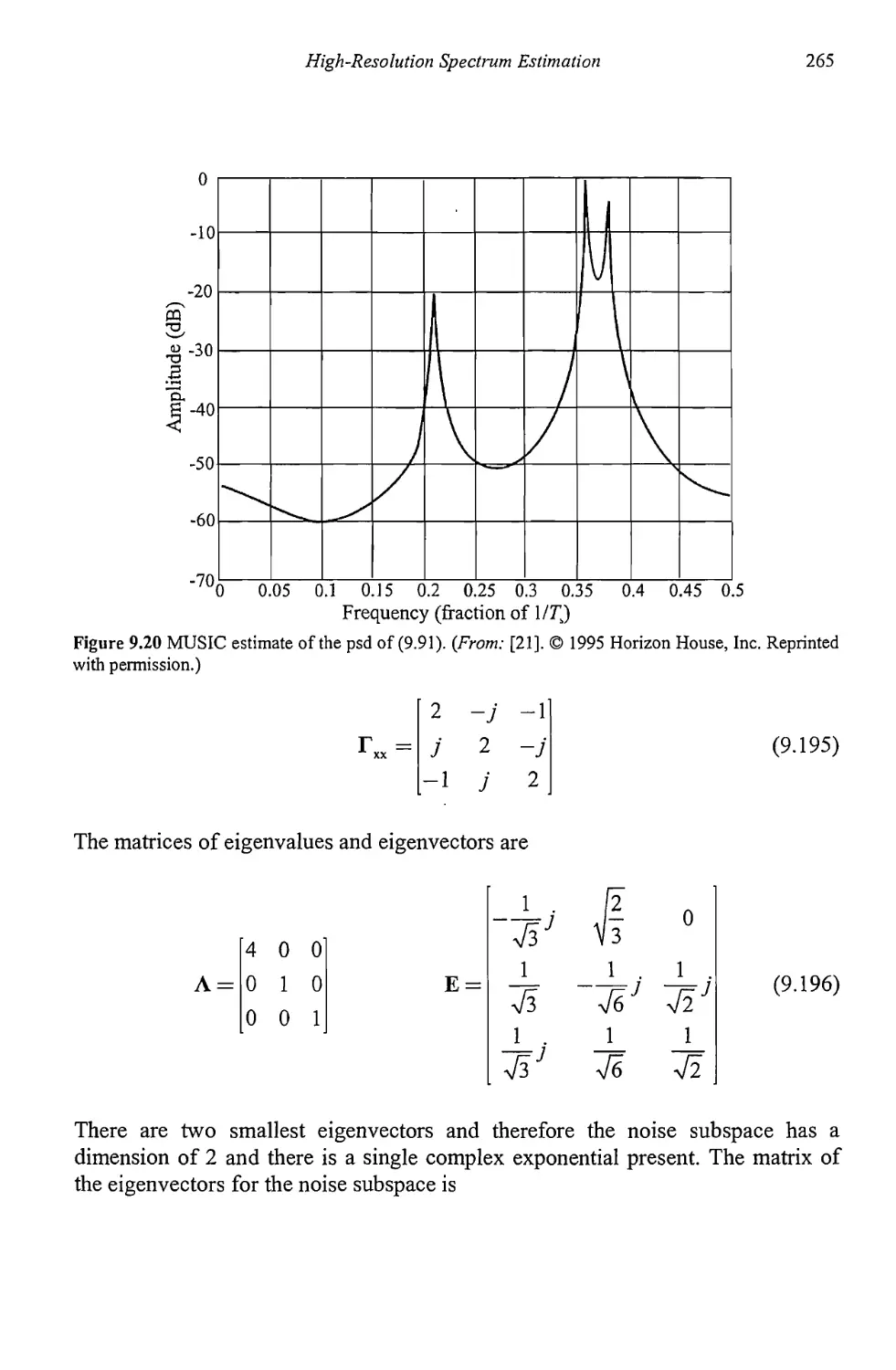
9.3.3 MUSIC 264
9.3.4 Minimum Norm 266
X
Target Acquisition in Communication Electronic Warfare Systems
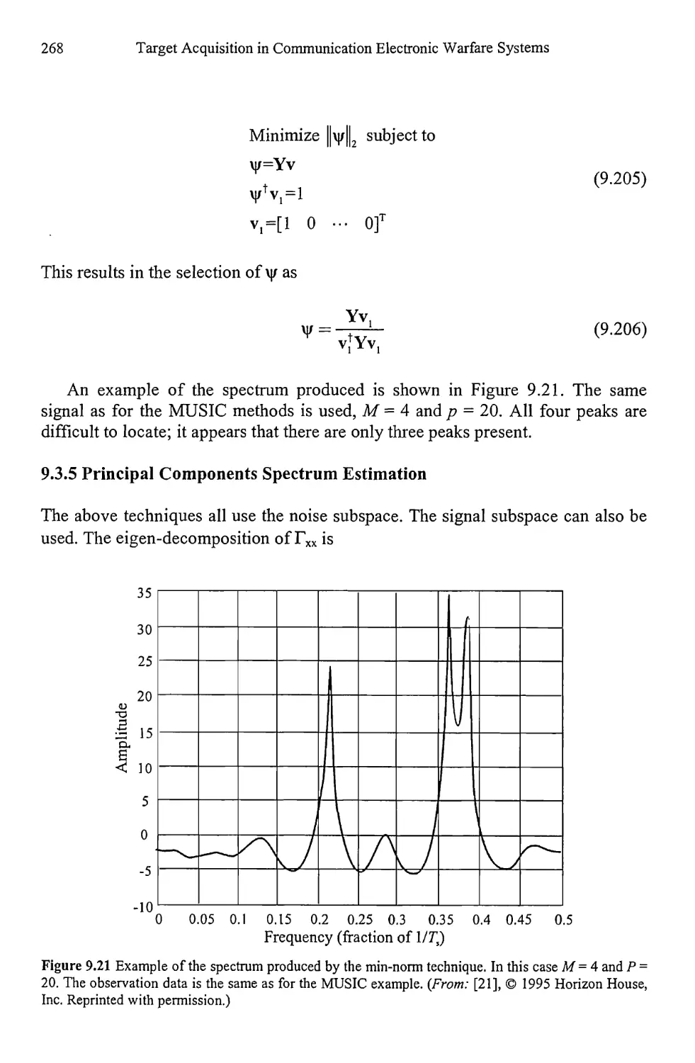
9.3.5 Principal Components Spectrum Estimation 268
9.4 Maximum Likelihood 269
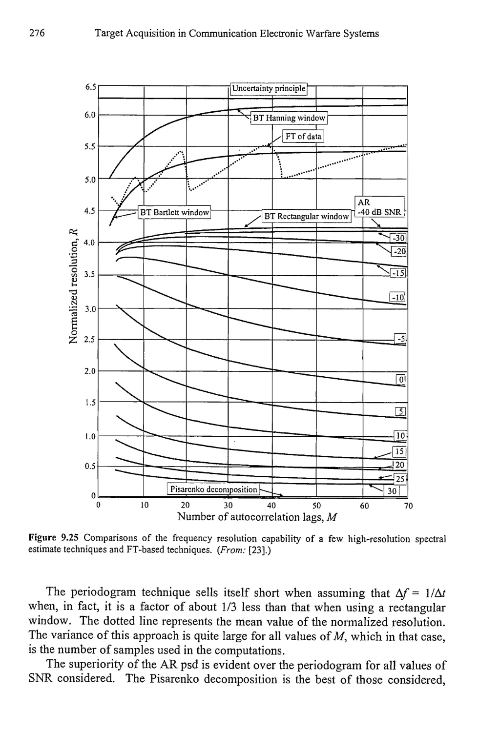
9.5 Resolution Comparison 270
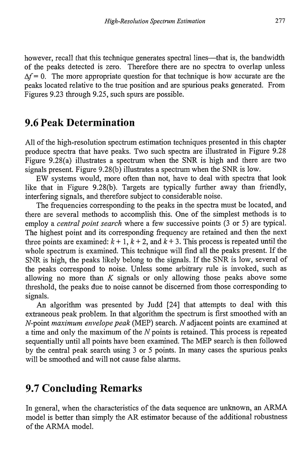
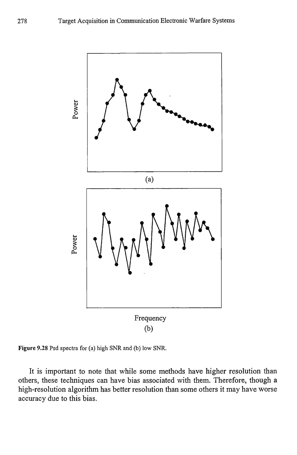
9.6 Peak Determination 277
9.7 Concluding Remarks 277
References 283
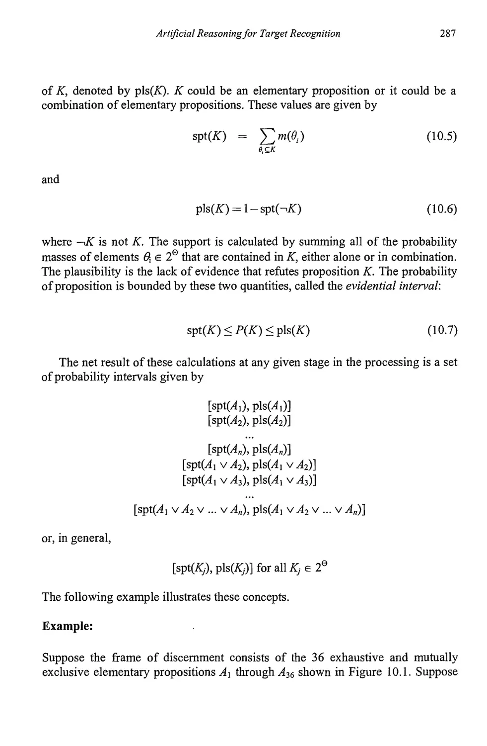
Chapter 10 Artificial Reasoning for Target Identification 285
10.1 Evidential Reasoning 285
10.1.1 Rules of Combination 289
10.1.2 Limitations of the Dempster-Shafer Method 295
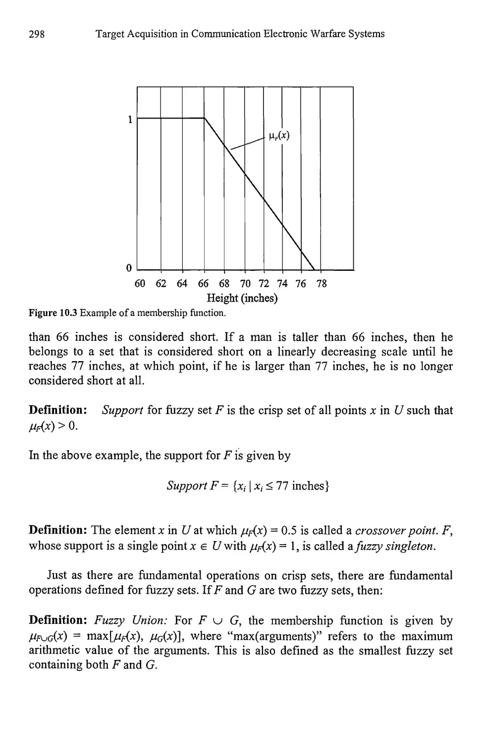
10.2 Fuzzy Logic 296
10.2.1 Fuzzy and Crisp Sets 296
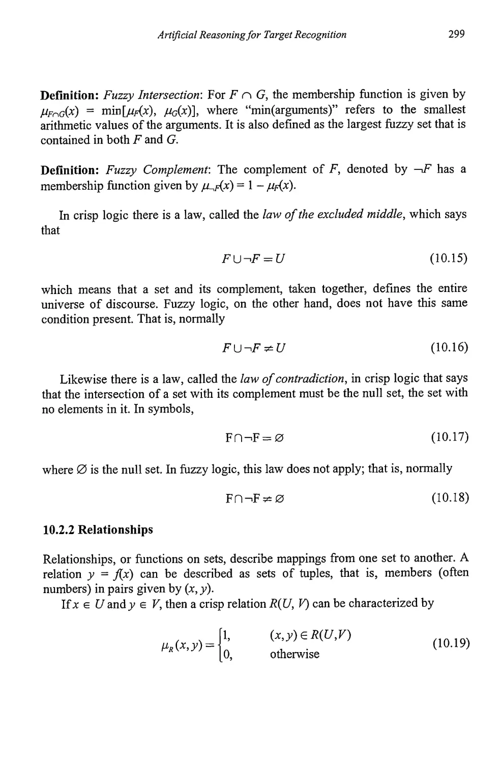
10.2.2 Relationships 299
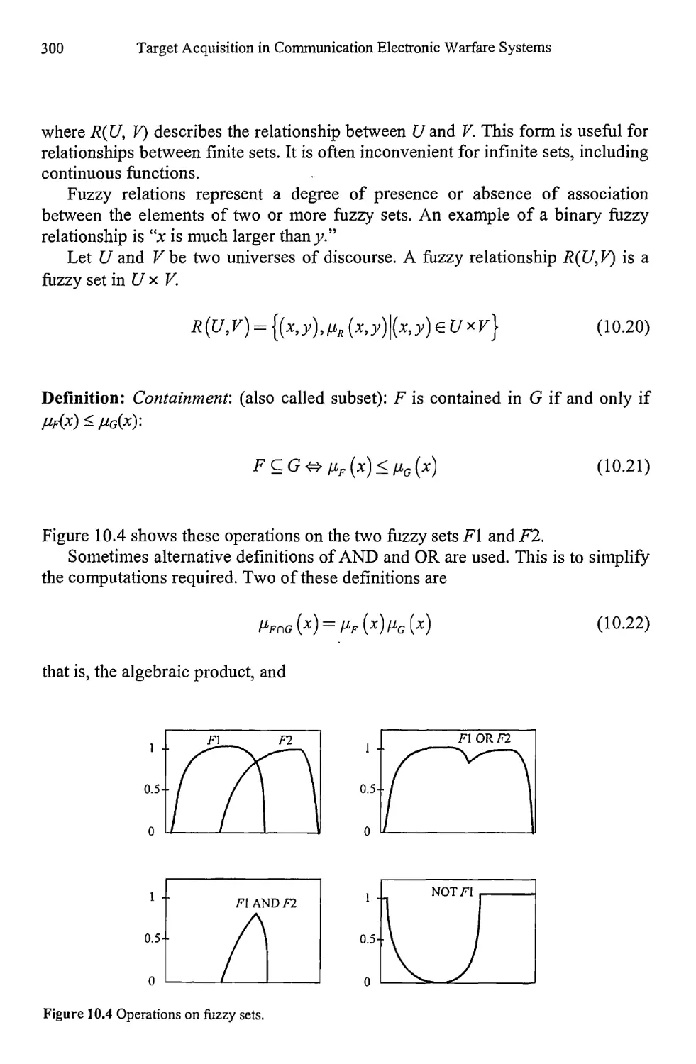
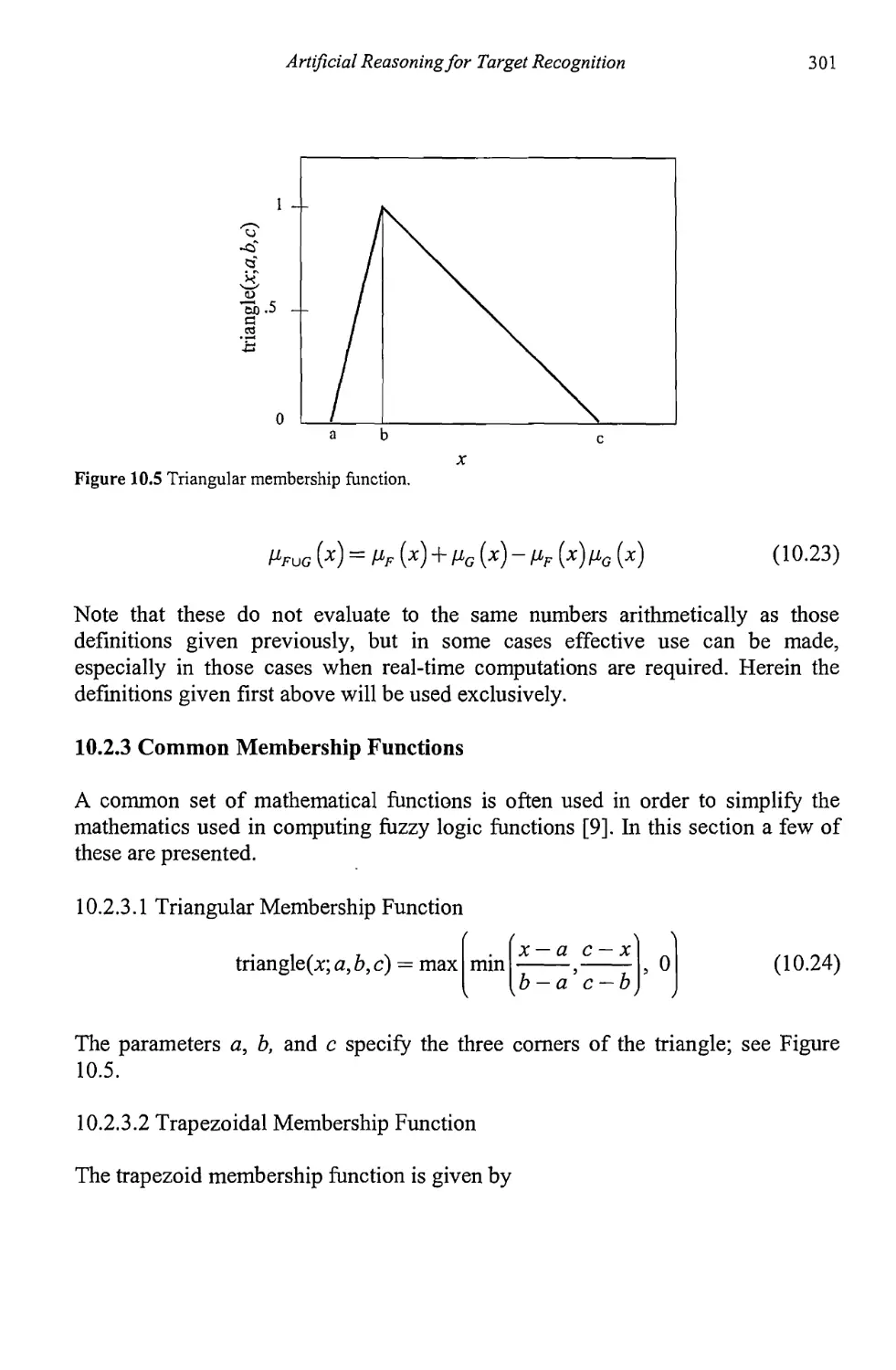
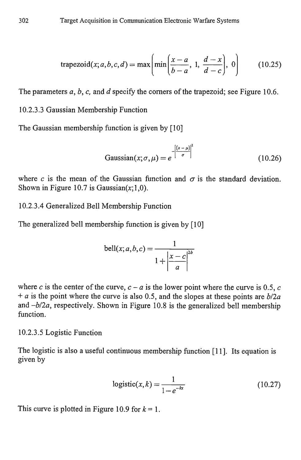
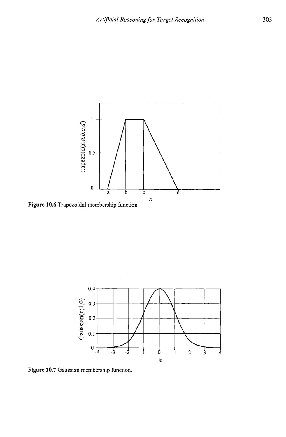
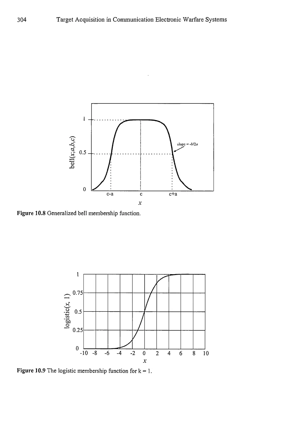
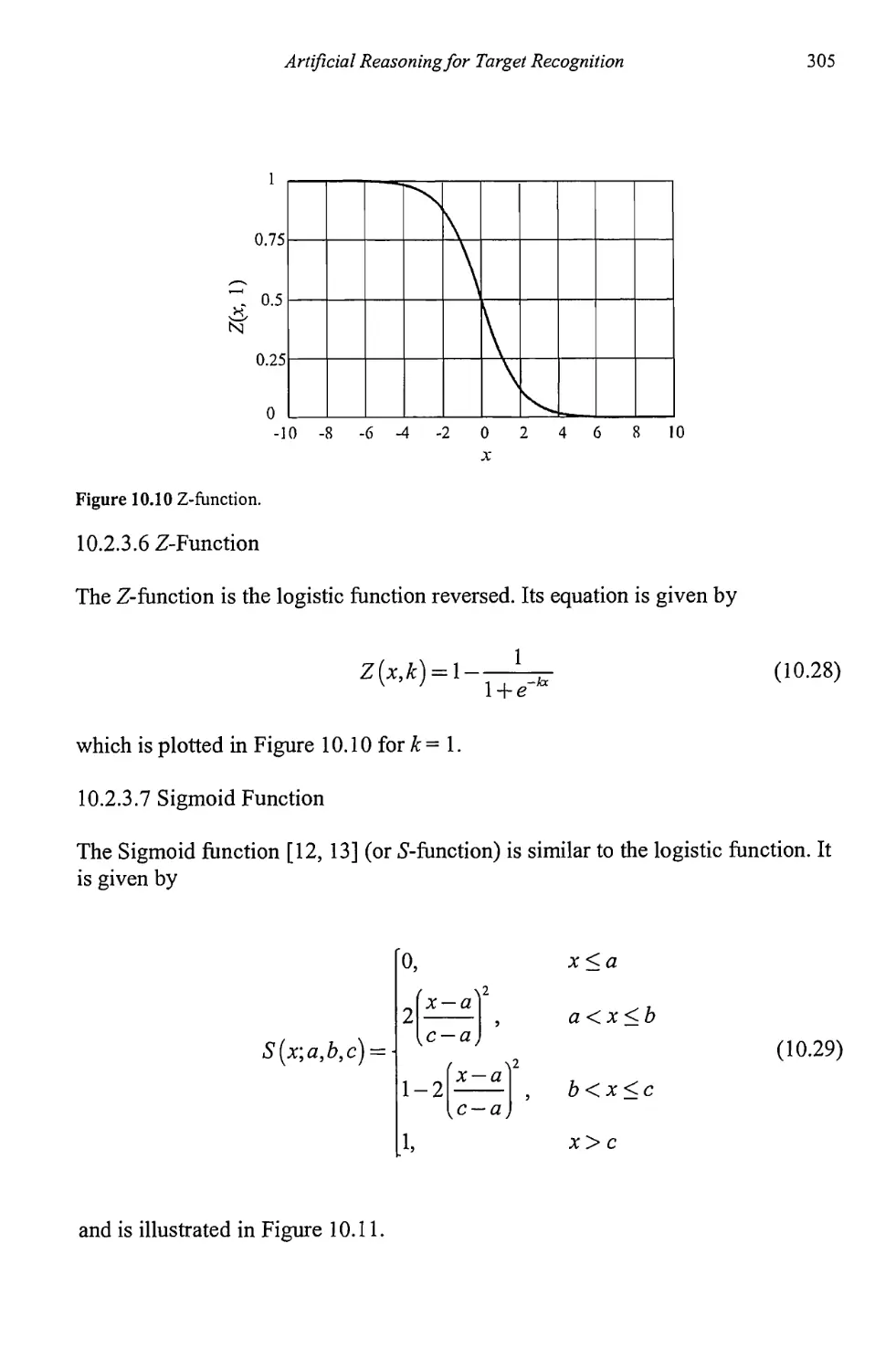
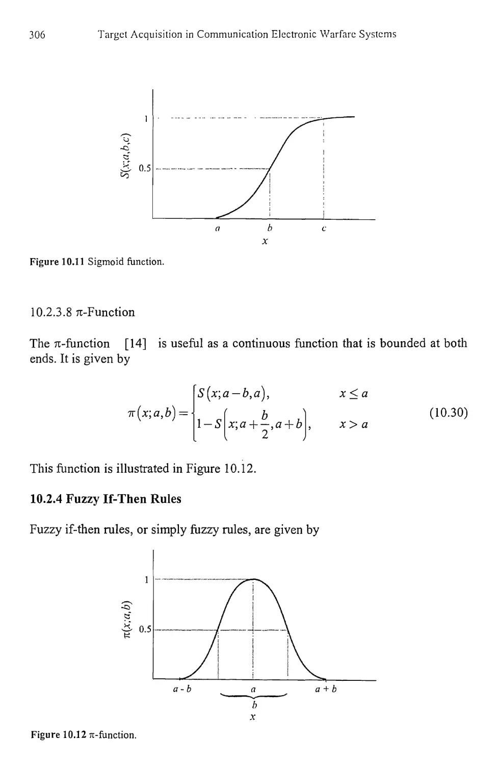
10.2.3 Common Membership Functions 301
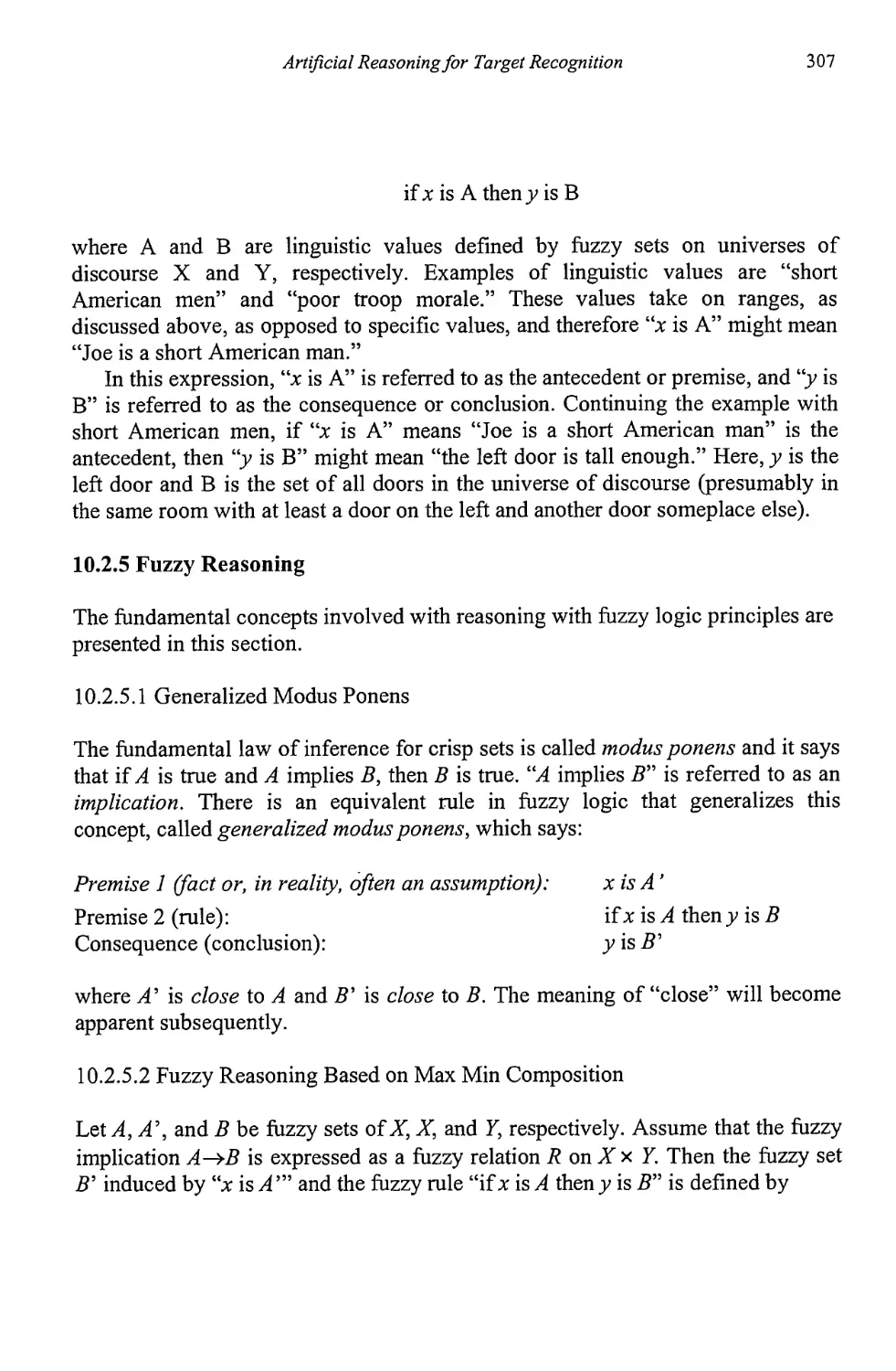
10.2.4 Fuzzy If-Then Rules 306
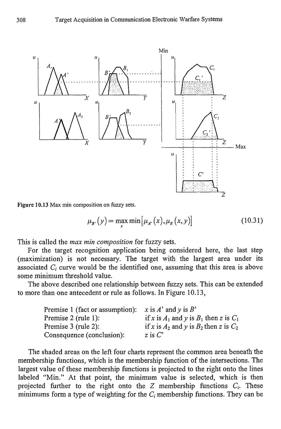
10.2.5 Fuzzy Reasoning 307
10.3 Concluding Remarks 316
References 319
Chapter 11 Resource Allocation 321
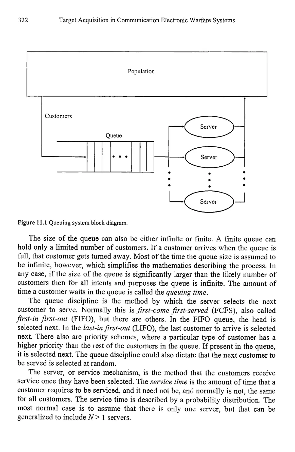
11.1 Queues 321
11.1.1 Statistics for Queuing Theory 323
11.1.2 Kendall-Lee Notation 325
11.1.3 Queue Relationships 326
11.1.4 M/M/1 Model 327
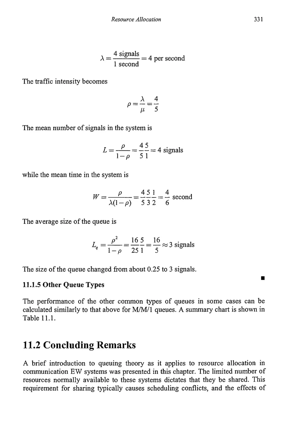
11.1.5 Other Queue Types 331
11.2 Concluding Remarks 331
References 332
Appendix A Lagrange Multipliers 335
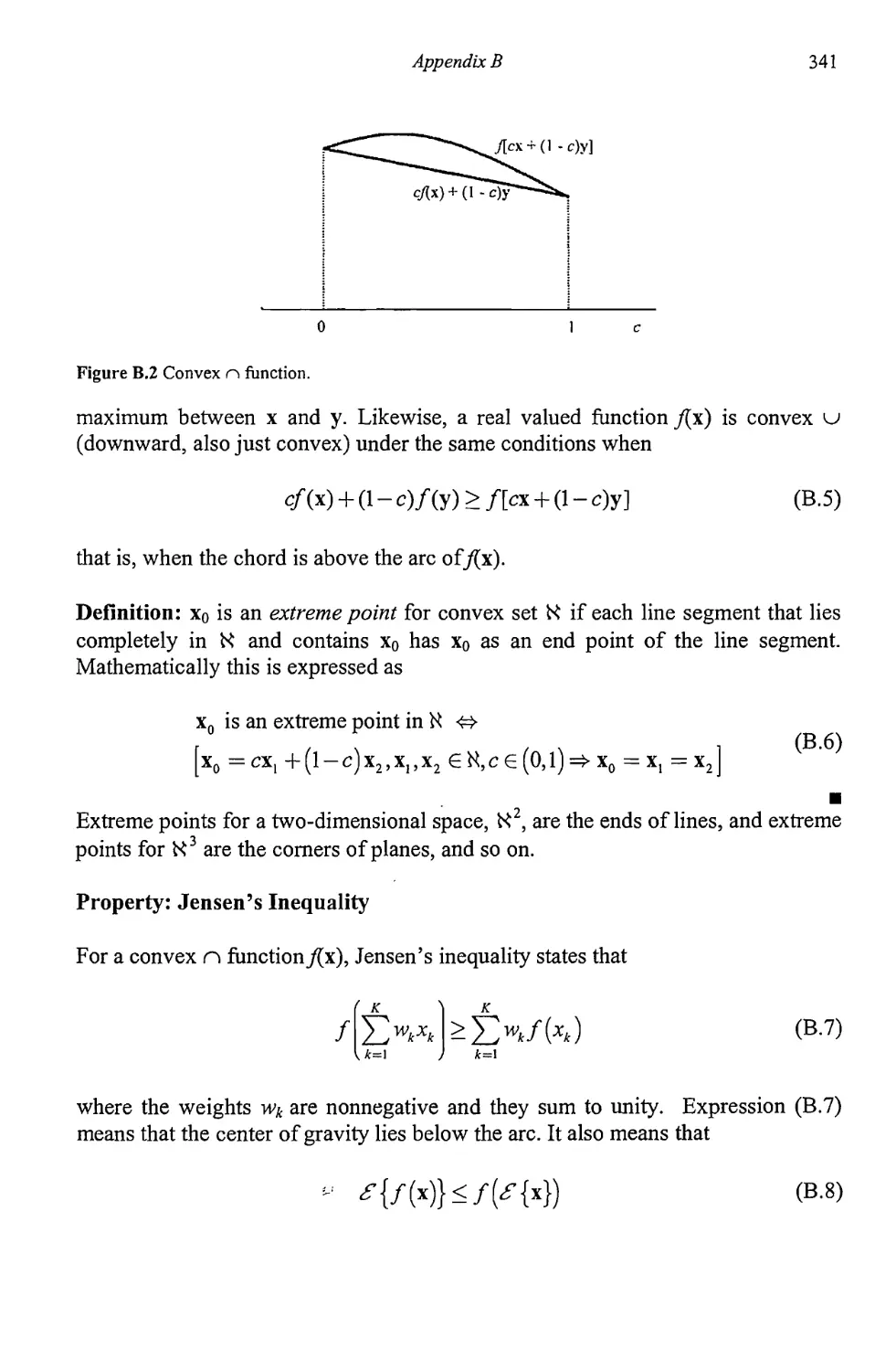
Appendix В Convex Functions 339
Reference 343
List of Acronyms 345
About the Author 349
Index
351
Preface
Target acquisiton in communication electronic warfare (EW) systems is a requisite
function for proper system functioning. In general it consists of determining the
presence of signals at particular frequencies and whether those signals are targets
or not. Measurements of signal parameters are required so such determination can
be accomplished. These measurements are automated to the maximum extent
possible.
This book is intended for technical practitioners, such as engineers and
scientists, who are interested in learning the basics of how to acquire target signals
in communication EW systems. The educational level required is that of a
baccalaureate degree in an appropriate technical discipline. The material is
suitable for one new to the EW field and contains references to additional, more
advanced material for those motivated to pursue such investigations.
Chapter 1 provides a brief introduction to the tagret acquisition problem. The
communication system model is introduced as well as what is meant by electronic
warfare in a communication system setting.
There are two generalized classifications for signals: random and nonrandom.
The latter is usually termed deterministic in the sense that if the value of the signal
is known at any point in time, then its future (and past) values can be determined.
In the former, one or more parameters associated with the signal are random, and
therefore knowing the signal’s value does not allow for ascertaining its value at
other times. These signals are called stochastic. Such signals can only be
described in probabilistic terms.
Chapter 2 presents background material on statistical processes and contrasts
deterministic versus stochastic processes. For the most part, the signals of concern
for communication EW systems are determinsistic with one or more random
parameters. The theory of communications has developed along certain paths, and
the design of modem communication systems utilizes these concepts. For
example, the oscillators used to transform signals from one frequency regime to
another (frequency conversion) are sinusoidal. The characteristics of sinusoids are
well known, and except perhaps for unknown (and maybe random) amplitude and
phase, they are deterministic. A review of Fourier transforms is presented to
remind the reader of the fundamental principles involved. A thorough coverage of
such transforms is certainly beyond the scope of this book, however.
xii
Target Acquisition in Communication Electronic Warfare Systems
Chapter 3 provides a brief introduction to radio frequency (RF) spectrum
search techniques. Searching the RF spectrum is required when the targets of
interest do not necessarily occupy the same frequency all the time. For static
situations, the targets remain fixed and searching is simple. In fact, searching may
not be necessary at all—-just tune receivers to the known frequencies where the
targets of interest are located and leave them there. In most cases of interest,
however, this will not be true and some form of searching is required. This is
dictated by the limited resources available compared to the number of targets of
concern.
Chapter 4 introduces the reader to the notion of hypothesis testing applied to
target detection. Hypothesis testing is a statistical technique used to ascertain
whether particular conditions are true or not in an optimal way.
Estimation of target parameters is important so that determination of whether
the signal is one of interest or not can be made. The fundamentals of this area as
they apply to EW target acquisition are introduced in Chapter 5. The target
parameters of interest extend beyond just the frequency of active signals. They
include signal modulation type and power levels, to mention just a few.
Perhaps the most important parameters of interest are the frequencies of target
signals. The methods for estimating the spectrum of a target are introduced in
Chapter 6. The methods discussed produce relatively low frequency resolution,
however. Resolution in this sense is the ability to distinguish two signals that are
closely spaced in frequency. In many practical scenarios where EW systems are
applied, the RF spectrum is very crowded and many signals are present. The
ability to separate signals in those cases becomes very important.
Chapter 7 introduces the reader to methods for detection of deterministic
signals. As mentioned, for the most part a considerable amount is known about the
signals of interest from communication targets. Typically one or more parameters
are random in nature, but for the most part the signals are a sinusoid of some type.
Therefore, detection methods for deterministic signals are important.
Chapter 8 is the counterpart to Chapter 7 for detection techniques for stochastic
signals. Normally, the less that is known about the signal to be detected, the poorer
the detection performance. When the signal is completely known the best
technique for detection is the matched filter. Such filters can be designed to detect
known signals in an optimum sense; what is meant by optimality is described in
Chapter 7. When one or more parameters about the signal are not known, then the
matched filter is no longer optimal and some other methods must be employed for
detection.
As mentioned above, classical methods for signal detection lead to relatively
low resoluton in signal separation, which can be detrimental in crowded RF
environments. High-resolution techniques have been devised to deal with this
problem, and such methods are introduced in Chapter 9. Two methods are
Preface
xiii
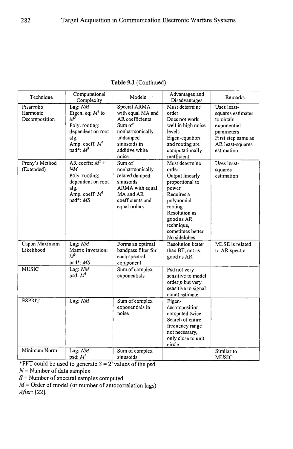
described in detail to give the reader a flavor of what is involved. Other techniques
are discussed in general terms and a table is presented that compares most of the
known methods of high-resolution spectrum estimation.
Chapter 10 introduces two artificial intelligence methods for automation or
partial automation of the signal identification process. The chapter is not intended
to provide a comprehensive treatise on the subject, but instead to provide a few
techniques as an introduction to the subject, providing an existence proof for such
techniques.
The process of conducting electronic warfare in any real situation is extremely
complicated, and there are never enough resources to thoroughly cover all targets.
Chapter 11 contains an introduction to methods for resource allocation and
techniques for evaluating system performance when there are limited resources.
This book is not intended to be a textbook on target acquisition for electronic
warfare, but rather a reference that can be consulted on specific topics as they arise
in system design. It can also serve as a reference for short courses on the subject.
I would like to acknowledge two colleagues at I2WD. The efforts of John
Kosinski who read the manuscript in detail are appreciated. I would also like to
note the actions of Maria Wright to get the timely security release.
Chapter 1
Introduction
Electronic warfare (EW) is one of the tools available to force commanders
conducting military operations. It is similar to artillery fire in the sense that it is an
indirect method for application of its effects. It is indirect because direct line of
site with a target is not required for its use. All that is required is that the target be
within radio line of sight, the range of which is often much longer than visual line
of sight.
The direct effects of the application of EW are temporary—they go away when
the EW energy is removed. This is not to say that the overall effects are temporary.
Indeed, the application of EW techniques and methods can have significant impact
on the outcome of hostile activities.
This chapter serves as a general introduction to EW and its main components.
The remainder of the book focuses on a specific aspect of communication EW that
is important enough to deserve such extensive coverage.
1.1 Electronic Warfare
The appellation EW applies to any attempt to conduct adverse actions on
electronic equipment. It consists of three main components: electronic support
(ES), electronic attack (EA), and electronic protect (ЕР) [1]. The contents of this
book apply primarily to one of the components of ES: target detection.
ES is a supporting function for EA. It consists of extracting information about
relevant signals to be attacked, so that the attack will be more effective. The four
main functions performed for ES are all passive and are:
• Searching for signals;
• Intercepting and categorizing signals of interest (SOI);
• Direction finding/emitter location;
1
2
Target Acquisition in Communication Electronic Warfare Systems
• Analysis of the ensuing information.
This information consists of technical information, such as frequency and
modulation, as well as operational information, such as enemy intent and high-
value target determination. Herein, communication ES will be the focus.
EA refers to attacking an electronic device in some fashion short of physical
destruction. It generally refers to emitting energy into receiving components so
that such receivers will not correctly decode an intended signal. Such signals can
be communication, radar, or telemetry signals, or any other radiated energy, man-
made or natural. The principal EA activity is active, which is jamming.
EP consists of those activities conducted to prevent adversaries from being
effective at EA and ES of our own electronic devices, and is, in a sense, the
counterpart to EA and ES. EP can be either active or passive. Examples of passive
EP are:
• Physical siting of the EW system;
• Shielding of the electronic emissions in the direction of hostile EW
systems;
• Emission control (EMCON), which controls when friendly
communications occur;
• Directional antennas that transmit and receive signals in perferred
direcions;
• Frequency management;
• Deception.
Examples of active EP are:
• Encryption;
• Low probability of intercept (LPI) modulations;
• Antijam (AJ) communications.
Nothing more will be said of EP herein except to the extent that the EA and ES
topics discussed can be used for friendly EP.
1.2 Communications and EW
Communication is the exchange of information between two or more entities. It
could be physical, as in the case of a transmitter and receiver in separate locations,
or it can be temporal, as in the storage of informaiton on a tape recorder, for
Introduction
3
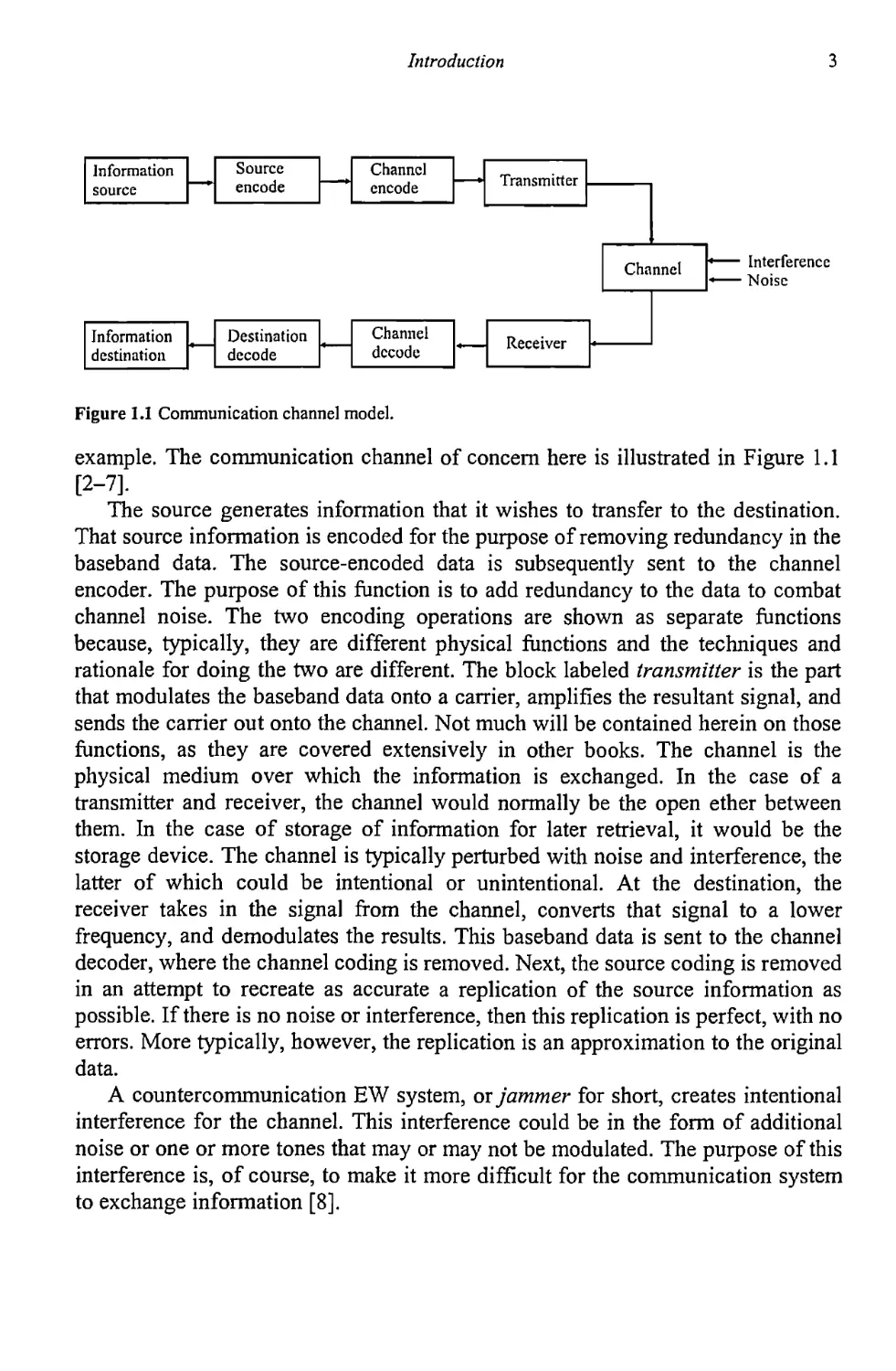
Figure 1.1 Communication channel model.
example. The communication channel of concern here is illustrated in Figure 1.1
[2-7].
The source generates information that it wishes to transfer to the destination.
That source information is encoded for the purpose of removing redundancy in the
baseband data. The source-encoded data is subsequently sent to the channel
encoder. The purpose of this function is to add redundancy to the data to combat
channel noise. The two encoding operations are shown as separate functions
because, typically, they are different physical functions and the techniques and
rationale for doing the two are different. The block labeled transmitter is the part
that modulates the baseband data onto a carrier, amplifies the resultant signal, and
sends the carrier out onto the channel. Not much will be contained herein on those
functions, as they are covered extensively in other books. The channel is the
physical medium over which the information is exchanged. In the case of a
transmitter and receiver, the channel would normally be the open ether between
them. In the case of storage of information for later retrieval, it would be the
storage device. The channel is typically perturbed with noise and interference, the
latter of which could be intentional or unintentional. At the destination, the
receiver takes in the signal from the channel, converts that signal to a lower
frequency, and demodulates the results. This baseband data is sent to the channel
decoder, where the channel coding is removed. Next, the source coding is removed
in an attempt to recreate as accurate a replication of the source information as
possible. If there is no noise or interference, then this replication is perfect, with no
errors. More typically, however, the replication is an approximation to the original
data.
A countercommunication EW system, or jammer for short, creates intentional
interference for the channel. This interference could be in the form of additional
noise or one or more tones that may or may not be modulated. The purpose of this
interference is, of course, to make it more difficult for the communication system
to exchange information [8].
4
Target Acquisition in Communication Electronic Warfare Systems
Although there are many types of channels, the one of primary interest herein
is the additive white Gaussian noise (AWGN) channel. In such a channel the noise
present, generated by thermal and galactic sources, is added to the signal. That is
the case whether the noise is background noise or jammer noise [9-12].
One type of channel that is particularly important for wireless communications,
the type of communications of interest here, is the fading channel [13-16]. There
are several sources of fading, but probably the one most relevant for wireless
communications is multipath reflection. As a transmitter or receiver moves, or
obstacles enter the path between them, the signal strength of multipath reflections
changes, thus causing fading. Although fading is important for analysis of
communication effectiveness, as well as analysis of jamming effectiveness in
fading situations, nothing more will be mentioned here.
1.3 Signal Detection
The first step in signal processing in communication EW systems is to determine
the presence of the signal. Herein that is known as the signal detection problem.
To determine if a detected signal is a signal of interest, further processing of the
signal is frequently required to determine or estimate parameters associated with
the signal.
Detecting the presence of a signal is a different problem from estimating
the value of some parameter. Detecting presence is a binary problem, or at least a
problem of limited dimension—detecting the presence of one of m types of
signals, for example. The variate takes on only certain values and there is a finite
number of them. In parameter estimation, on the other hand, the variate can, in
general, take on any value from a range of values—an uncountably infinite
number of possibilities.
The target set for communication EW systems consists of all types of
communication systems of interest to the users of the EW system. It is frequently
not known ahead of time what all those signals will be, so the signals arriving at
the receiver belonging to the EW system likely have an unknown form until they
are processed further [17]. Known-signal searching is the most applicable
approximation for searching for signals in communication EW systems because
the processing to make the determination if the signal is present is usually
performed prior to demodulating the signal. For most modulating schemes, there is
a substantial carrier component to the signal. That carrier originates from an
oscillator at the transmitter that generates sinusoidal waves in most cases of
interest here. Therefore, the signal being sought is a sinusoidal signal with some
form of modulation on it. The form of the carrier is therefore known.
Introduction
5
Typically, in the spectrum of interest to an EW system, there will be several
signals present. These signals may be close together—indeed they can be in the
same frequency channel. This leads to the question of how well two (or more)
signals can be separated when they are close together and what the impacts are of
signal amplitude on this resolvability. Chapter 5 presents what are more traditional
methods of signal detection, couched in the terminology of spectral estimation.
Spectral estimation is determining (estimating) the parameters of a signal such as
its frequency and amplitudes (or power levels). These techniques typically have
low resolution compared with some other techniques.
Reliably detecting the presence of a signal at a frequency when little or nothing
is known about that signal is a difficult and challenging problem. When the radio
frequency (RF) environment is composed of many communication networks, there
can be many signals to sort through, especially when many of these signals belong
to friendly forces and are therefore normally of little interest. In such environments
the resolution provided by simple search schemes may not be fine enough.
Techniques have been devised to increase this resolution, and some of these
techniques are presented in Chapter 8.
Cochannel interference [18] is also a significant problem in crowded
environments. There is only so much RF spectrum available to all sides in an
adversarial relationship. What is available must be shared, and between hostile
parties this sharing is not cooperative. The same frequencies are used by all sides.
Cochannel interference results where two (or more) signals use the same
frequency channel at the same time. This certainly affects the communication
systems if a comunication receiver hears both transmitters. It also significantly
affects the ability of an EW system to intercept the signals.
The most straightforward way to do spectral analysis of a signal is to present
the signal to a bank of narrowband filters, either analog or digital. This
configuration produces an approximation to the short-term Fourier transform
(STFT) of the signal. The characteristics of such an approach are limited only by
the practicality of its implementation.
The resolution of such an approach is limited to the number of practical filters,
which, by implication, determines the bandwidth of each filter. In addition, the
time the signal must be present at the input to the filter bank is proportional to the
bandwidth of the filters—for finer resolution (narrow bandwidth) the signal must
be present for a longer duration, and vice versa, for low-frequency resolution, the
signal need only be present for a short period.
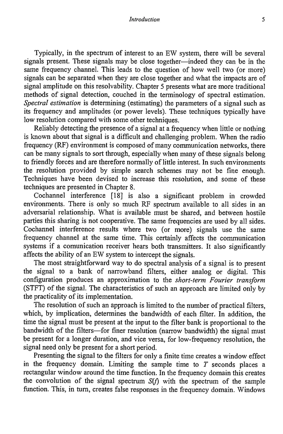
Presenting the signal to the filters for only a finite time creates a window effect
in the frequency domain. Limiting the sample time to T seconds places a
rectangular window around the time function. In the frequency domain this creates
the convolution of the signal spectrum S(f) with the spectrum of the sample
function. This, in turn, creates false responses in the frequency domain. Windows
6
Target Acquisition in Communication Electronic Warfare Systems
Signal
present
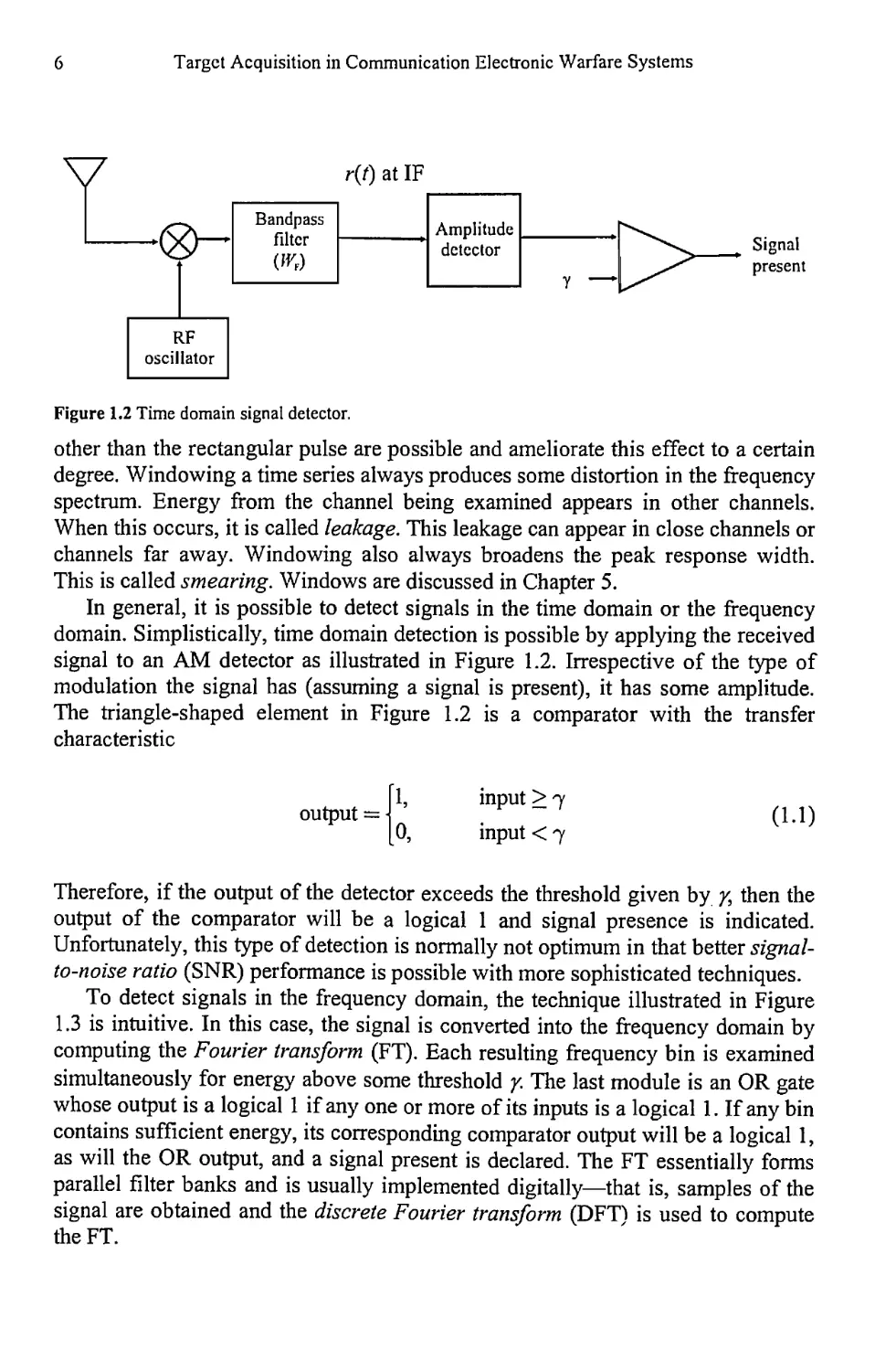
Figure 1.2 Time domain signal detector.
other than the rectangular pulse are possible and ameliorate this effect to a certain
degree. Windowing a time series always produces some distortion in the frequency
spectrum. Energy from the channel being examined appears in other channels.
When this occurs, it is called leakage. This leakage can appear in close channels or
channels far away. Windowing also always broadens the peak response width.
This is called smearing. Windows are discussed in Chapter 5.
In general, it is possible to detect signals in the time domain or the frequency
domain. Simplistically, time domain detection is possible by applying the received
signal to an AM detector as illustrated in Figure 1.2. Irrespective of the type of
modulation the signal has (assuming a signal is present), it has some amplitude.
The triangle-shaped element in Figure
characteristic
1.2 is a comparator with the transfer
output =
1,
0,
input > 7
input < 7
(1.1)
Therefore, if the output of the detector exceeds the threshold given by /, then the
output of the comparator will be a logical 1 and signal presence is indicated.
Unfortunately, this type of detection is normally not optimum in that better signal-
to-noise ratio (SNR) performance is possible with more sophisticated techniques.
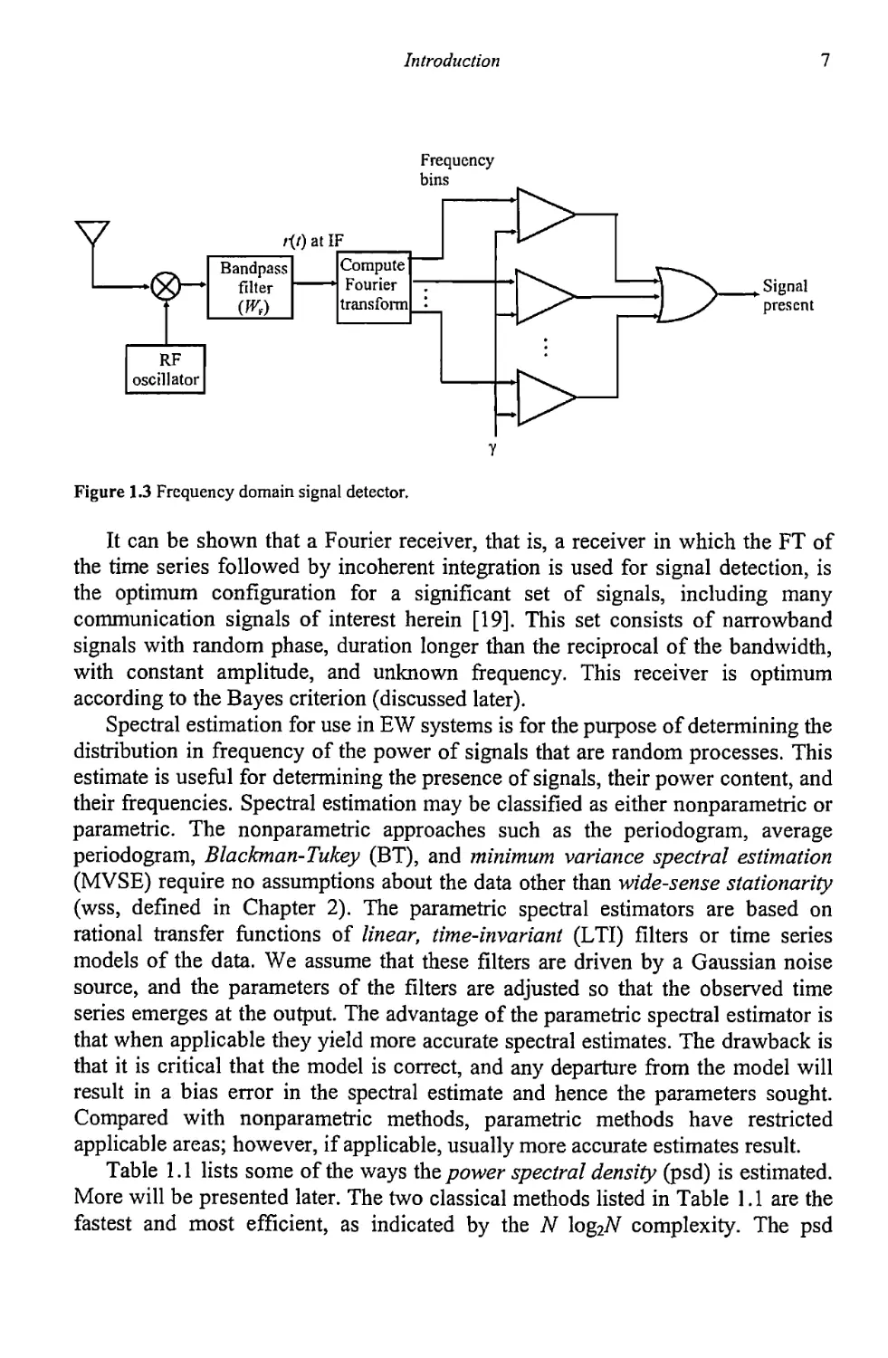
To detect signals in the frequency domain, the technique illustrated in Figure
1.3 is intuitive. In this case, the signal is converted into the frequency domain by
computing the Fourier transform (FT). Each resulting frequency bin is examined
simultaneously for energy above some threshold y. The last module is an OR gate
whose output is a logical 1 if any one or more of its inputs is a logical 1. If any bin
contains sufficient energy, its corresponding comparator output will be a logical 1,
as will the OR output, and a signal present is declared. The FT essentially forms
parallel filter banks and is usually implemented digitally—that is, samples of the
signal are obtained and the discrete Fourier transform (DFT1 is used to compute
the FT.
Introduction
7
Figure 1.3 Frequency domain signal detector.
It can be shown that a Fourier receiver, that is, a receiver in which the FT of
the time series followed by incoherent integration is used for signal detection, is
the optimum configuration for a significant set of signals, including many
communication signals of interest herein [19]. This set consists of narrowband
signals with random phase, duration longer than the reciprocal of the bandwidth,
with constant amplitude, and unknown frequency. This receiver is optimum
according to the Bayes criterion (discussed later).
Spectral estimation for use in EW systems is for the purpose of determining the
distribution in frequency of the power of signals that are random processes. This
estimate is useful for determining the presence of signals, their power content, and
their frequencies. Spectral estimation may be classified as either nonparametric or
parametric. The nonparametric approaches such as the periodogram, average
periodogram, Blackman-Tukey (ВТ), and minimum variance spectral estimation
(MVSE) require no assumptions about the data other than wide-sense stationarity
(wss, defined in Chapter 2). The parametric spectral estimators are based on
rational transfer functions of linear, time-invariant (LTI) filters or time series
models of the data. We assume that these filters are driven by a Gaussian noise
source, and the parameters of the filters are adjusted so that the observed time
series emerges at the output. The advantage of the parametric spectral estimator is
that when applicable they yield more accurate spectral estimates. The drawback is
that it is critical that the model is correct, and any departure from the model will
result in a bias error in the spectral estimate and hence the parameters sought.
Compared with nonparametric methods, parametric methods have restricted
applicable areas; however, if applicable, usually more accurate estimates result.
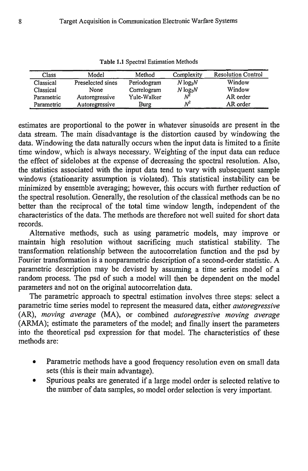
Table 1.1 lists some of the ways the power spectral density (psd) is estimated.
More will be presented later. The two classical methods listed in Table 1.1 are the
fastest and most efficient, as indicated by the N log2W complexity. The psd
8
Target Acquisition in Communication Electronic Warfare Systems
Table 1.1 Spectral Estimation Methods
Class Model Method Complexity Resolution Control
Classical Preselected sines Periodogram N log2W Window
Classical None Correlogram N log2W Window
Parametric Autoregressive Yule-Walker N2 AR order
Parametric Autoregressive Burg N2 AR order
estimates are proportional to the power in whatever sinusoids are present in the
data stream. The main disadvantage is the distortion caused by windowing the
data. Windowing the data naturally occurs when the input data is limited to a finite
time window, which is always necessary. Weighting of the input data can reduce
the effect of sidelobes at the expense of decreasing the spectral resolution. Also,
the statistics associated with the input data tend to vary with subsequent sample
windows (stationarity assumption is violated). This statistical instability can be
minimized by ensemble averaging; however, this occurs with further reduction of
the spectral resolution. Generally, the resolution of the classical methods can be no
better than the reciprocal of the total time window length, independent of the
characteristics of the data. The methods are therefore not well suited for short data
records.
Alternative methods, such as using parametric models, may improve or
maintain high resolution without sacrificing much statistical stability. The
transformation relationship between the autocorrelation function and the psd by
Fourier transformation is a nonparametric description of a second-order statistic. A
parametric description may be devised by assuming a time series model of a
random process. The psd of such a model will then be dependent on the model
parameters and not on the original autocorrelation data.
The parametric approach to spectral estimation involves three steps: select a
parametric time series model to represent the measured data, either autoregressive
(AR), moving average (MA), or combined autoregressive moving average
(ARMA); estimate the parameters of the model; and finally insert the parameters
into the theoretical psd expression for that model. The characteristics of these
methods are:
• Parametric methods have a good frequency resolution even on small data
sets (this is their main advantage).
• Spurious peaks are generated if a large model order is selected relative to
the number of data samples, so model order selection is very important.
Introduction
9
The nonlinear relationship of spectral power to actual power exhibited by most
parametric methods makes absolute power measurements meaningless, so only
relative power measurements are possible.
There are several factors that need to be taken into consideration in detection
theory. Roberts [20] points out the following:
• If available, increased observation time will almost always
be useful, assuming that the signal persists.
• Another point of view, another location, even another
system might improve the situation. For example, in
antisubmarine warfare, is it better to listen for submarines
on dry land, from hydrophones near shore, or from
hydrophones at sea with telephone lines to shore, or is it
better to fly airplanes or sail ships to the submarines’
operating areas and provide ways for them to listen?
• Signal processing exists to exploit differences in the nature
of signals and noise. If differences exist, signal processing
can transform both to some appropriate domain (e.g.,
frequency domain) where they are orthogonal and where
they may be separated more distinctly. But signal
processing cannot create what is not there; it cannot increase
the information content. (This is a manifestation of the data
processing theorem from the field of information theory
[21].)
• To utilize signal processing, engineering knowledge of
signals and noise is necessary. Noise measurements can
come from ordinary engineering experiments, but if the
signal source is uncooperative (such as is the case for
communication EW systems) then information relating to it
will need to come from uncontrolled available
measurements and subsequent deductions and calculations.
• With consideration of the consequence, it is important to
evaluate how good or bad the decision will be, once made,
in some average sense. Such evaluation might, for example,
indicate the need for more equipment, or operators, or
training.
1.4 Signal Searching
Typically a communication EW system operates in an RF environment that is
hostile and noncooperative. Sometimes some of the parameters of the signals of
10
Target Acquisition in Communication Electronic Warfare Systems
interest, such as frequency and modulation type, are available, but often not
entirely. These parameters must be detemined when they are unavailable.
Searching for signals of interest can be accomplished in several ways, such as
rapidly tuning a receiver through the spectrum. When little or nothing is known
about the target environment, the problem is different from when most of the
targets have been identified. The former requires searching over a region of the
spectrum in a continuous and contiguous fashion, looking for energy
corresponding to unknown (a priori) frequencies. In the latter, the frequency
locations of target signals are generally known—the problem is to find out if such
signals are either still at that location or have moved, presumably because it is
known that they stopped transmitting for some period. These search problems are
discussed in Chapter 3.
1.5 Notation
Herein, scalars are denoted as italic plain text letters, while small bold letters
denote vectors, and large bold letters denote matrices. Thus, 0is a scalar while 0 is
a vector and 0 is a matrix. A vector 0 normally consists of scalars but could also
consist of other vectors or matrices. Thus, normally, 0 = вг • • Bn ] .
At various points throughout the presentation, sections are cordoned off with
the title “Scholium.” This refers to material that is important and interesting, but is
not central to the development being presented.
The end of a section describing a singular thought, a theorem and its proof, for
example, is delineated by the symbol so that the reader knows the preceding
discussion has been concluded.
1.6 Concluding Remarks
The literature on signal detection and estimation is vast. Perhaps one of the most
cited references is the series of books by Van Trees [22-24]. Another early source
is due to Helstrom [25]. An excellent overview of the history of the development
of the field is given in [26]. A very readable introduction to the theory of signal
detection in noise for both communication and radar signals is presented in [27].
Root provides an introduction to the theory of signal detection in noise [28].
The topics covered in this work are certainly focused on a narrow field—
communication EW system theory. It will be established, however, that there are
fundamental principles involved with this topic, and the operation of these systems
is based on sound first principles.
Introduction
11
References
[1] Poisel, R. A., Introduction to Communication Electronic Warfare Systems, Norwood, MA:
Artech House, 2002, p. 3.
[2] Ziemer, R. E., and W. H. Tranter, Principles of Communications Systems Modulation and
Noise, 5th Ed., New York: John Wiley & Sons, 2002.
[3] Ziemer, R. E., and R. L. Peterson, Introduction to Digital Communication, 2nd Ed., Upper
Saddle River, NJ: Prentice Hall, 2001.
[4] Gagliardi, R. M., Introduction to Communications Engineering, 2nd Ed., New York: John
Wiley & Sons, 1988.
[5] Proakis, J. G., Digital Communications, 3rd Ed., New York: McGraw-Hill, 1995.
[6] Simon, M. K., S. M. Hinedi, and W. C. Lindsey, Digital Communication Techniques: Signal
Design and Detection, Upper Saddle River, NJ: Prentice Hall, 1995.
[7] Das, J., S. K. Mullick, and P. K. Chatterlee, Principles of Digital Communication: Signal
Representation, Detection, Estimation, and Information Coding, New York: John Wiley &
Sons, 1986.
[8] Poisel, R. A., Introduction to Communication Electronic Warfare Systems, Norwood, MA:
Artech House, 2002, Ch. 7.
[9] Root, W. L., “Communication Through Unspecified Additive Noise,” Information and
Control, Vol. 4, 1961, pp. 15-29.
[10] Gagliardi, R. M., Introduction to Communications Engineering, 2nd Ed., New York: John
Wiley & Sons, 1988, pp. 148-154.
[11] Ziemer, R. E., and W. H. Tranter, Principles of Communications: Systems, Modulation, and
Noise, 5th Ed., New York: John Wiley & Sons, 2002, pp. 270-275.
[12] Reference Data for Radio Engineers, 6th Ed., Indianapolis: Howard W. Sams & Co., Inc.,
1975, Ch. 29.
[13] Simon, M. K., and M. S. Alouini, Digital Communication over Fading Channels, New York:
John Wiley & Sons, Inc., 2000.
[14] McGuffin, B. F., “Distributed Jammer Performance in Rayleigh Fading,” Proceedings IEEE
MILCOM 2002, Anaheim, CA, October 7-11, 2002.
[15] Ericson, T., “A Gaussian Channel with Slow Fading,” IEEE Transactions on Information
Theory, May 1970, pp. 353-355.
[16] Biglieri, E., J. Proakis, and S. Shamai, “Fading Channels: Information-Theoretic and
Communication Aspects,” IEEE Transactions on Information Theory, Vol. 44, No. 6, October
1998, pp. 2619-2692.
[17] McNicol, D., A Primer of Signal Detection Theory, Sydney: George Australian Publishing
Company, 1972.
[18] Spooner, С. M., “Classification of Co-channel Communication Signals Using Cyclic
Cumulants,” Proceedings of ASILOMAR-29, 1996, pp. 531-536.
[19] Williams, J. R., and G. G. Ricker, “Signal Detectability Performance of Optimum Fourier
Receivers,” IEEE Transactions on Audio and Electroacoustics, Vol. AU-20, No. 4, October
1972, pp. 264-270.
[20] Roberts, L. R., Signal Processing Techniques, Anaheim, CA: Interstate Electronics
Corporation, 1981, p. 7-2.
[21] Gallager, R. G., Information Theory and Reliable Communication, New York: John Wiley &
Sons, 1968, p. 80.
12 Target Acquisition in Communication Electronic Warfare Systems
[22] Van Trees, H. L., Detection, Estimation, and Modulation Theory, Part I: Detection,
Estimation, and Linear Modulation Theory, New York: John Wiley & Sons, 1968.
[23] Van Trees, H. L., Detection, Estimation, and Modulation Theory, Part II: Nonlinear
Modulation Theory, New York: John Wiley & Sons, 1971.
[24] Van Trees, H. L., Detection, Estimation, and Modulation Theory, Part III: Radar-Sonar
Signal Processing and Gaussian Signals in Noise, New York: John Wiley & Sons, 1971.
[25] Helstrom, C. W., Statistical Theory of Signal Detection, New York: Pergamon Press, 1960.
[26] Kailath, T., and H. V. Poor, “Detection of Stochastic Processes,” IEEE Transactions on
Information Theory, Vol. 44, No. 6, October 1998, pp. 2230-2259.
[27] DiFranco, J. V., and W. L. Rubin, Radar Detection, Dedham, MA: Artech House, 1980, Chs.
5-8.
[28] Root, W. L., “An Introduction to the Theory of the Detection of Signals in Noise,”
Proceedings of the IEEE, Vol. 58, No. 5, May 1970, pp. 610-623.
Chapter 2
Deterministic and Stochastic Processes
A signal or function is deterministic if its future value can be predicted when the
current value is known. A signal or function is random, or stochastic, if its future
value can only be described statistically; the precise future value cannot be
determined even if the current value is known.
Communication signals in noise can be considered as exemplars of stochastic
processes. Sometimes the signals themselves, without the noise, are modeled as
stochastic processes. An example of this is general searching (defined in Chapter
3), where little or nothing is known about the signals received except, perhaps, that
there is energy at some frequency. Such signals can be modeled as random,
stochastic processes. In general, stochastic processes can be scalar- or vector-
valued quantities that vary with time. Thus, if two samples of the process were
measured at the same time, the measured value would likely be different.
Spectral analysis is a commonly used tool for analysis of signals, to include
communication signals of interest for EW systems. The mathematical foundations
of spectral analysis date back to the French mathematician Jean-Baptiste Fourier
(1768-1830) who discovered the relationship between a deterministic time domain
function s(t) and its unique representation in the frequency domain, commonly
referred to as its spectrum, or Fourier spectrum in honor of the mathematician.
2.1 The Fourier Transform
If s(t) is a signal in the time domain then its FT, denoted by S(J), in the frequency
domain is given by
oo
?(/) = f
"OO
Similarly, if S(f) is the FT of a signal s(f), then s(f) is given by
(2.1)
13
14
Target Acquisition in Communication Electronic Warfare Systems
(2.2)
This relationship is denoted by
(23)
In general, the FT is a complex function, with a real part denoted by Re{5(/)} and
an imaginary part denoted by Im {£(/)}. Equivalently, S(j) has a magnitude
(argument)
|S(/)| = +
(2.4)
and phase angle
It is usually the magnitude of the FT that is called the spectrum of the signal. As
will be discussed at length later in this section, the FT does not exist for all
functions.
Scholium
Notice that
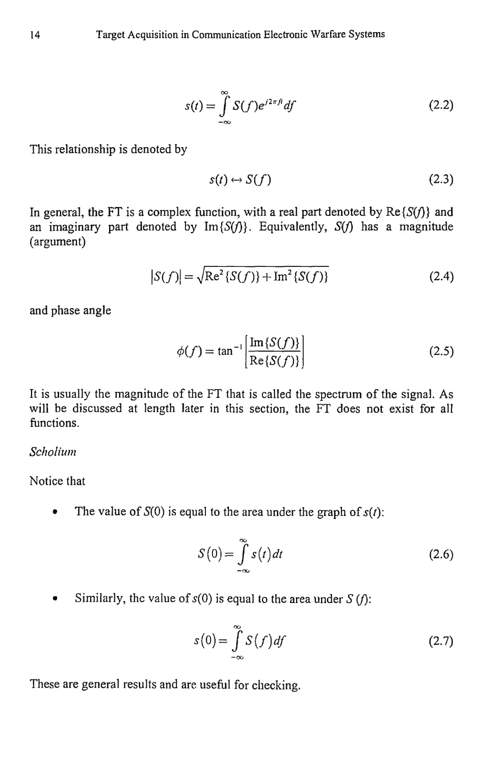
• The value of 5(0) is equal to the area under the graph of s(t)\
5(0)= J s(T)dl
(2.6)
Similarly, the value of 5(0) is equal to the area under 5 (/):
s(0) = Js(/)<
(2-7)
These are general results and are useful for checking.
Deterministic and Stochastic Processes
15
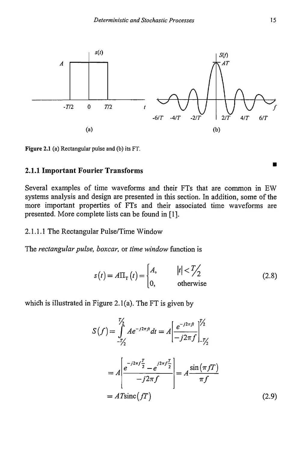
Figure 2.1 (a) Rectangular pulse and (b) its FT.
2.1.1 Important Fourier Transforms
Several examples of time waveforms and their FTs that are common in EW
systems analysis and design are presented in this section. In addition, some of the
more important properties of FTs and their associated time waveforms are
presented. More complete lists can be found in [1].
2.1.1.1 The Rectangular Pulse/Time Window
The rectangular pulse, boxcar, or time window function is
^) = ЖТт(/) =
A,
0,
otherwise
(2.8)
which is illustrated in Figure 2.1(a). The FT is given by
7г
S(f) = f Ae~i2’!f'dt = A
-Т/
/1
e j2”f2 — ej2nf2 sin(7r/r)
-jlltf 7Г/
= ^7sinc(/r)
(2-9)
16
Target Acquisition in Communication Electronic Warfare Systems
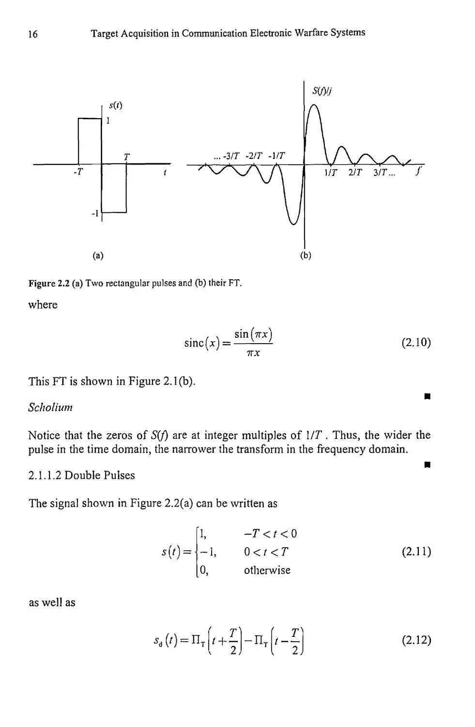
Figure 2.2 (a) Two rectangular pulses and (b) their FT.
where
. . sin (tex)
sinc(x) =--------—~
7ГХ
(2.Ю)
This FT is shown in Figure 2.1(b).
Scholium
Notice that the zeros of S(f) are at integer multiples of MT. Thus, the wider the
pulse in the time domain, the narrower the transform in the frequency domain.
2.1.1.2 Double Pulses
The signal shown in Figure 2.2(a) can be written as
s(r) =
1,
-1,
0,
-T < t < 0
0</ <T
otherwise
(2.П)
as well as
5d
(r) - Пт p +
(2.12)
Deterministic and Stochastic Processes
17
Using linearity, the shifting theorem, and the FT of the pulse (2.9),
S (/) = Te2'f > sine (/Г) - Tei2’f~z sine (/7)
= sin2 (тт/Г) (2.13)
7Г/
This FT is shown in Figure 2.2(b).
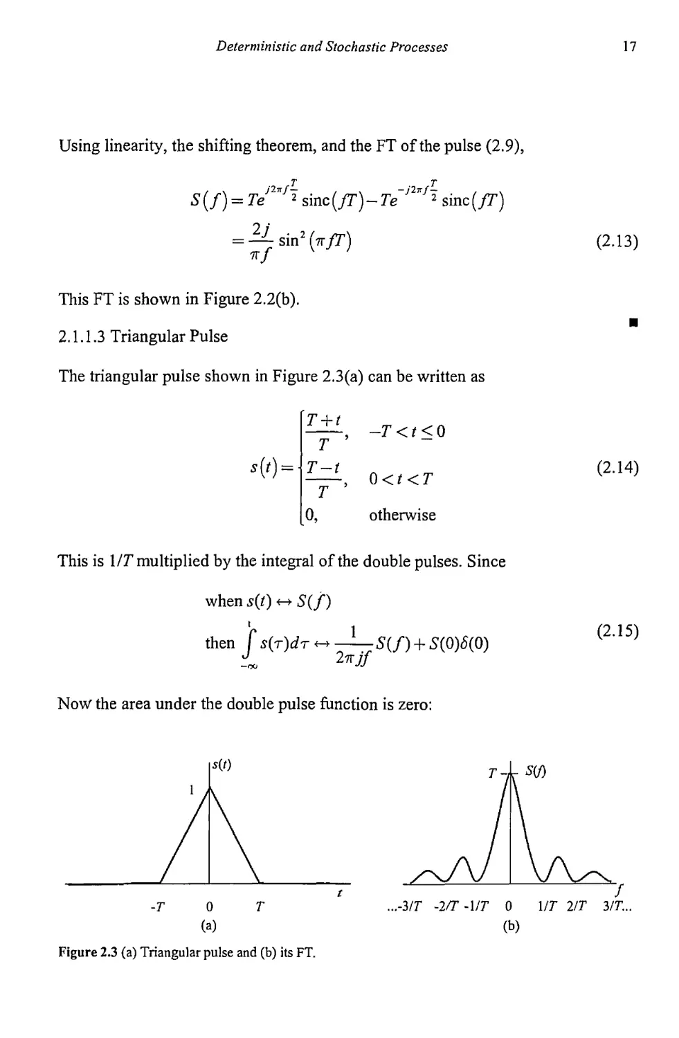
2.1.1.3 Triangular Pulse
The triangular pulse shown in Figure 2.3(a) can be written as
T + r
T '
T-t
T ’
o,
—T < t < 0
0<Z <T
otherwise
(2-14)
This is MT multiplied by the integral of the double pulses. Since
when s(t} S(f)
then S(/) + S(0)<5(0)
—co 2?rj/
Now the area under the double pulse function is zero:
Figure 2.3 (a) Triangular pulse and (b) its FT.
...-3/T ~2/T -\/T 0 1/7 2/T 3/T...
(b)
18
Target Acquisition in Communication Electronic Warfare Systems
J ^W=o
(2.16)
Using (2.6) and (2.13), it can be concluded that
S’(/) = i-T7^sin2^#j + 0«0)
T jlirf 7Г/
sin2 (тг/Г)
= T sine2 (/Г)
(2.17)
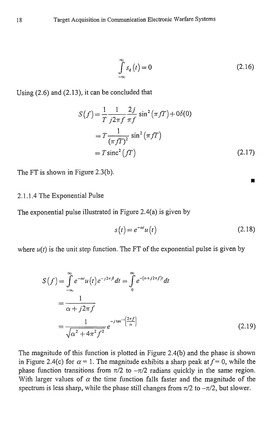
The FT is shown in Figure 2.3(b).
2.1.1.4 The Exponential Pulse
The exponential pulse illustrated in Figure 2.4(a) is given by
s(/) = e-Q'tz(/) (2.18)
where w(Z) is the unit step function. The FT of the exponential pulse is given by
S(/) = f e-alu(t}e-'2'fldt = f e'^'^'dl
-OU 0
1
a + j2tt f
yja2 +47Г2/2
(2-19)
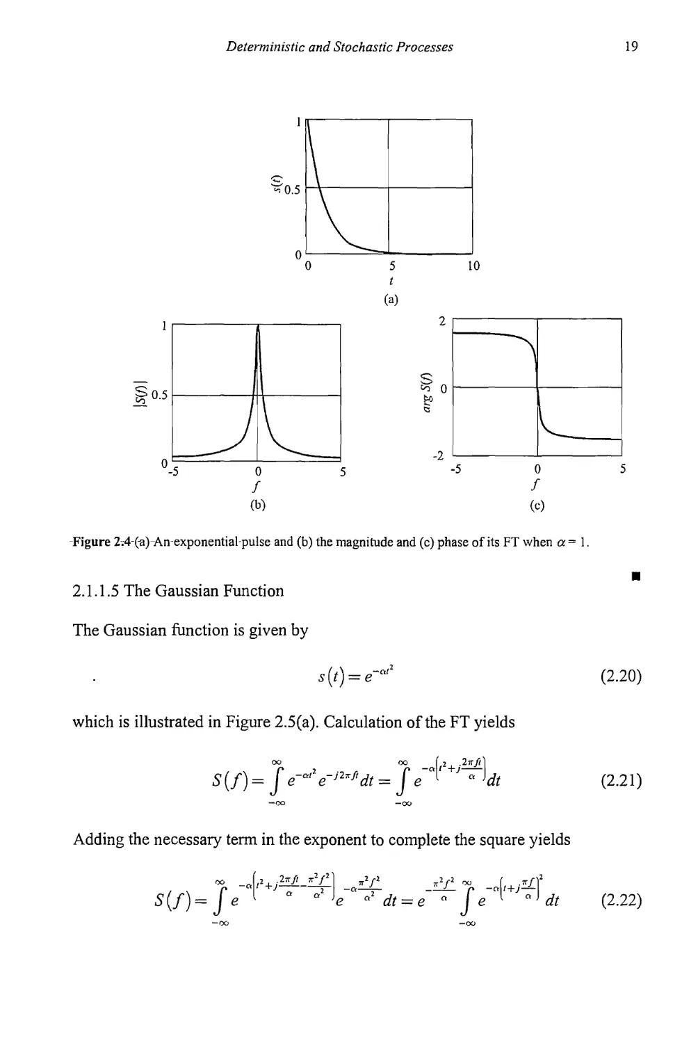
The magnitude of this function is plotted in Figure 2.4(b) and the phase is shown
in Figure 2.4(c) for a = 1. The magnitude exhibits a sharp peak at/= 0, while the
phase function transitions from tc/2 to -тг/2 radians quickly in the same region.
With larger values of a the time function falls faster and the magnitude of the
spectrum is less sharp, while the phase still changes from тг/2 to -тг/2, but slower.
Deterministic and Stochastic Processes
19
Figure 2^4 (a) An exponential-pulse and (b) the magnitude and (c) phase of its FT when a = 1.
2.1.1.5 The Gaussian Function
The Gaussian function is given by
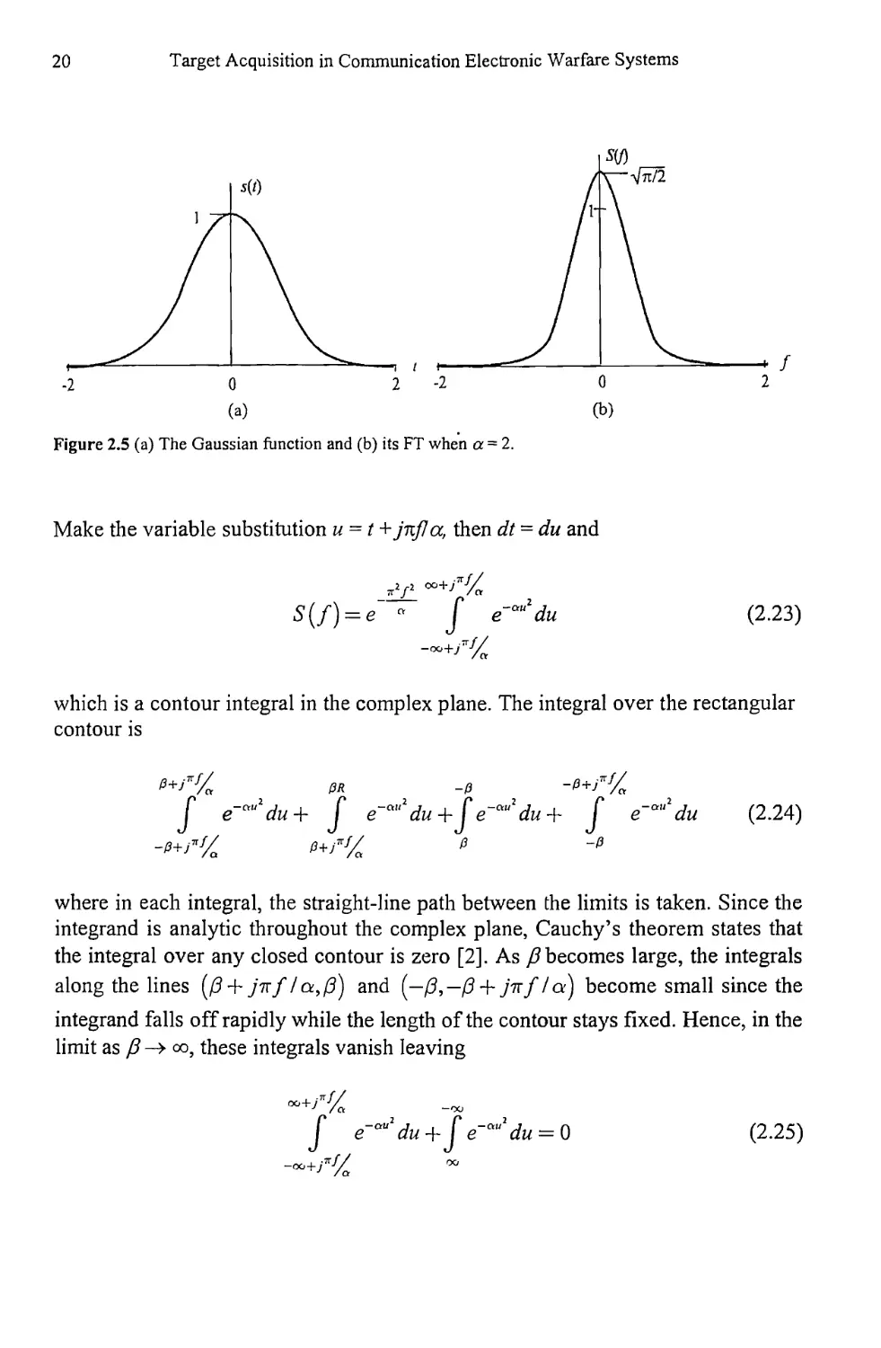
s(t) = e~a'2 (2.20)
which is illustrated in Figure 2.5(a). Calculation of the FT yields
5(/)= Je~a,2e-j2*f,dt = f e~“" '~’dt (2.21)
-oo -OO
Adding the necessary term in the exponent to complete the square yields
OO
e [ ° ° °2 dt =
(2.22)
20
Target Acquisition in Communication Electronic Warfare Systems
Figure 2.5 (a) The Gaussian function and (b) its FT when a = 2.
Make the variable substitution и = t + jitfla, then dt = du and
S(/) = e‘ "
(2.23)
which is a contour integral in the complex plane. The integral over the rectangular
contour is
p+^f/a PR -P
J e~c,“‘du + j' e-‘"‘,du+fe-a",du+ f e'°"'du (2.24)
where in each integral, the straight-line path between the limits is taken. Since the
integrand is analytic throughout the complex plane, Cauchy’s theorem states that
the integral over any closed contour is zero [2]. As /3 becomes large, the integrals
along the lines (/3 + jirf /t*,/3) and (-/3,-/3 + jtt/la) become small since the
integrand falls off rapidly while the length of the contour stays fixed. Hence, in the
limit as /3 —> oo, these integrals vanish leaving
oo+>7r^ -oo
J e-“'du+^ e~m'du = 0
(2-25)
Deterministic and Stochastic Processes
21
0Г
(2.26)
Therefore,
S(f) = J^e~^ (2.27)
v a
which is shown in Figure 2.5(b). In general, as the width of the pulse in the time
domain broadens, the width of that in the frequency domain narrows, and vice
versa.
Property: Shannon/Nyquist Sampling Theorem [3, 4]
Letx(r) be a signal with FT X(f) such that X(f) - 0 for |/| > fc. Then
x(r)= £ x(kTs) sinc[2Tr/e(г-и;)] (2.28)
A=-oo
where fs = 2/c and Ts = l/fs.
Thus, the time function that is band limited to a finite frequency region has infinite
extent in the time domain. Furthermore, that time function can be exactly
reproduced with appropriately scaled sine functions.
Property: Cosine Function
If
x(0 = A cos(2tt fQt) (2.29)
then
л л
W) = y5(/-A)+f^(/ + /0) (2.30)
22
Target Acquisition in Communication Electronic Warfare Systems
The FT of a cosine function of infinite extent consists of two positive Dirac delta
functions located at the positive and negative frequencies of the function.
Property: Sine Function
If
x(t) = A sin(27r fot) (2.31)
then
A A
W) = J--+ Л) - Jf Kf - f0) (2.32)
The FT of an infinite sine function consists of two Dirac delta functions located at
the positive and negative frequencies of the function shifted in phase. The positive
delta function is shifted +ti/2 radians and the negative delta function is shifted -тг/2
radians.
2.2 Deterministic Signals
As mentioned, a deterministic signal is known for all time given its value at a
single time. Examples of deterministic signals are the cos( ) and sin( ) functions.
Such functions are, of course, useful for system analysis. Many practical signals of
interest in communications EW analysis and design are, however, stochastic or at
least have some parameters associated with them that are stochastic. These signals
will be considered in the next section.
Parseval’s relationship says that if
•Ф)~£(Л (2.33)
then the energy, <?(/), in the time domain is related to that in the frequency domain
as
oo oo
£/ = 1/'И)Гл=/|5(Л|2^ (2.34)
“00
Deterministic and Stochastic Processes
23
This simply says that the total energy in a signal s(0 is equal to the area under the
square of the magnitude of its FT.1 |S(/)|2 is typically called the energy density, or
energy spectral density function, and |5(/)|2 df describes the density of signal
energy contained in the differential frequency band from ftof+df
Scholium
The average power in electronic circuits is given by P = i2R or P = v2/R. As is
commonly assumed, when considering the analysis of signals it will here be
assumed that this resistive value is unity, allowing the power to be expressed
simply as s2(f) = v2(Z) or = i2(t). This allows units of power to be expressed as the
square of the signal amplitudes and the units of energy measured as volts2-second
(amperes2-second).
The average power, Pavg, over a time interval Z2 to ti is obtained by integrating
s\t) from /1 to t2 and then dividing the result by T = t2 -or
(2.35)
1 0
where T is the period of the signal. Total energy can thus be expressed in terms of
power, p{t),
oo
E = J s2(t)dt
-oo
1 Recall the electrical energy storage elements (assuming zero initial energy):
• Inductor
v(t) = Ldi(t) I dt
т r T
e(t) = J v(t)i(t)dt = J = z(t)dz(t) = |lz2(T)
0 0 0
• Capacitor
z(t) = Cdv(t) / dt
т т r
e(t) = § v(t)i(t)dt = J dt = C J v(t)dv(i) = ^Cv2(T")
oo о
24
Target Acquisition in Communication Electronic Warfare Systems
(2.36)
In general, the quantities discussed here are complex and therefore have both real
parts and imaginary parts, or amplitudes and phase functions.
2.2.1 Energy and Power in Deterministic Signals
2.2.1.1 Finite Energy Signals
All deterministic signals can be divided into finite energy signals or infinite energy
signals. Most real signals exist for only a finite amount of time and, generally,
have a limited frequency range of interest. Theoretically, no signal can have both
finite duration and finite frequency extent, however.
The total energy in the signal s(t) is given by (2.34). Signals such that Ef<co
are called finite energy signals and are also referred to as £? functions. If s(fi is a
finite energy signal, then lim s(t\ = 0 .
t—*±oo
If s(t) is passed through an ideal bandpass filter of bandwidth B, with transfer
function H(f) given by
W) =
1,
°,
(2.37)
otherwise
producing y(f) at the output, then the energy in y(t) is given by
-oo —oo
-%
(2.38)
2.2.1.2 Finite Power Signals
Not all signals have finite energy, that is, there is an infinite amount of energy in
them. Typical examples are the sin and cos functions, as well as impulse functions.
Deterministic and Stochastic Processes
25
For this type of function, the power is the important parameter. The average power
in s(f) is given by
! %
-TA
(2.39)
and functions for which P; < °o are called finite power functions.
2.3 Stochastic Processes
This section introduces the basic notions behind stochastic processes.
2.3.1 Ensembles
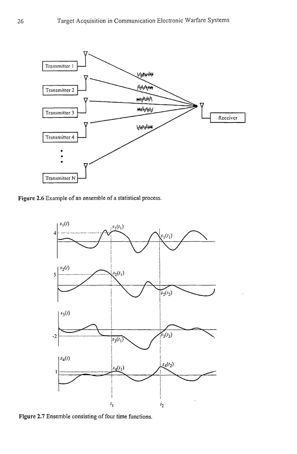
Consider the hypothetical communication system shown in Figure 2.6. All of the
transmitters are perfectly collocated and are identical. They all transmit the exact
same signal to the single receiver at exactly the same time. Noise is added to each
of these signals, which causes the signals arriving at the receiver to be different,
even though the transmitted signals were the same. At any specific instant in time,
say t = 5, the amplitude of any given one of these received signals will have some
value, but this amplitude is unpredictable. This collection of signals is called an
ensemble. The statistical descriptions for stochastic processes always refer to such
an ensemble of waveforms. Any one of these waveforms is referred to as a
realization of the stochastic process.
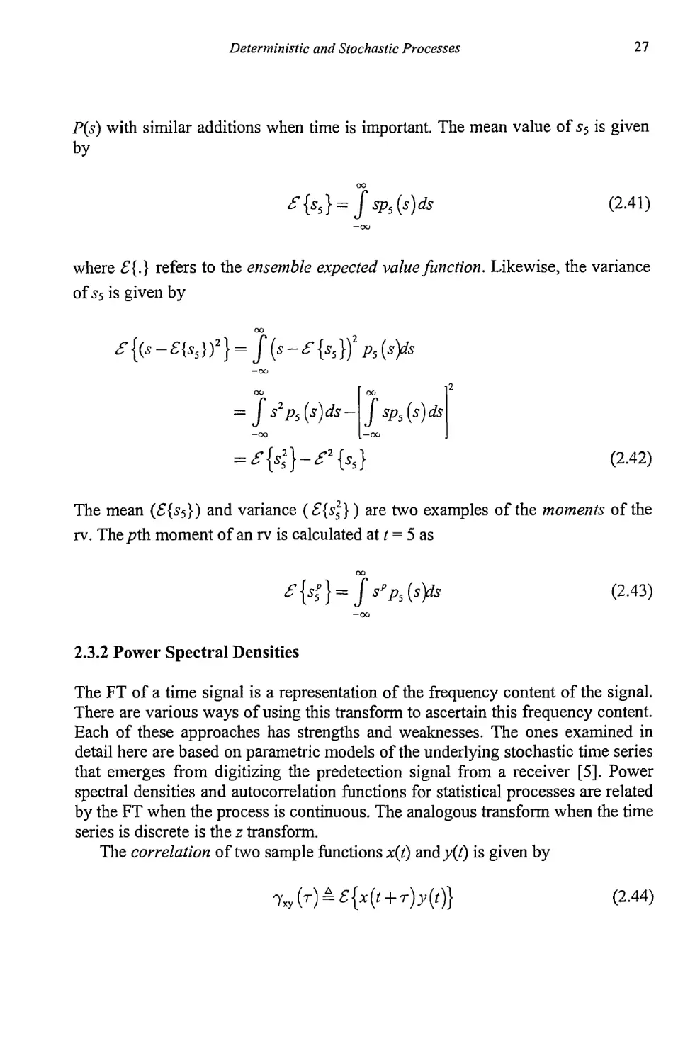
A specific example of an ensemble of time functions consisting of four
elements is shown in Figure 2.7. The statistics of this random process are
calculated across ensemble elements. Thus the average value at t = /] is
^(«,) = |[^(O+^(«1)+^tt)+^(<1)] = 2 (2.40)
An ensemble represents the complete and exhaustive set of possible
waveforms that can be received. The value actually received in one experiment
with this system at a particular time, say x5, is thus a random variable (rv) with,
for example, an associated probability density function (pdf), cumulative
probability distribution function, mean value, variance, and standard deviation.
Here, the pdf will be denoted by p(s), and when a particular time is important, say
t = 5, then ps(s). The cumulative probability density function, cdf, will be denoted
26
Target Acquisition in Communication Electronic Warfare Systems
Figure 2.6 Example of an ensemble of a statistical process.
Figure 2.7 Ensemble consisting of four time functions.
Deterministic and Stochastic Processes
27
P(s) with similar additions when time is important. The mean value of s5 is given
by
= J sp5(s)ds
(2-41)
where £{.} refers to the ensemble expected value function. Likewise, the variance
of 55 is given by
S {(s - £{s5 } )2} = J (s - £ {s5 })2 p5 (s)&
J J sp.^ds
= £&}-£> {ss}
(2.42)
The mean (£{55}) and variance (£{55}) are two examples of the moments of the
rv. The 72th moment of an rv is calculated at t = 5 as
= JsPP5(s>
(2.43)
2.3.2 Power Spectral Densities
The FT of a time signal is a representation of the frequency content of the signal.
There are various ways of using this transform to ascertain this frequency content.
Each of these approaches has strengths and weaknesses. The ones examined in
detail here are based on parametric models of the underlying stochastic time series
that emerges from digitizing the predetection signal from a receiver [5]. Power
spectral densities and autocorrelation functions for statistical processes are related
by the FT when the process is continuous. The analogous transform when the time
series is discrete is the z transform.
The correlation of two sample functions x(t) and y(0 is given by
(2.44)
28
Target Acquisition in Communication Electronic Warfare Systems
If x(f) <-> %(/), the Wiener-Khinchin theorem states that the autocorrelation
function of x(/) is related to its FT, X(f), as
(2.45)
where т is time delay and/is frequency. Thus, the absolute value of the FT of the
autocorrelation function is the psd of that function.
For discrete time processes xn and yn, where n is a running index such that the
sample times are tn = nT when T is the time between samples (assumed constant),
the correlation function is given by
7xy,„ =£{w.} (2-46)
This value is to be estimated using N values of the functions as xQ, xh ..., xN_i and
Уо,Уь
One estimate of the autocorrelation function is given by
(2-47)
which is called the sample autocorrelation function. The expected value of the
sample autocorrelation function is given by
(2-48)
n=0 ‘V
so the expected value of the sample is not equal to the actual expected value of the
series. When this occurs, the estimate is said to be biased.
The calculation of an estimate is consistent if the estimate converges to the true
value as N approaches infinity. This will be true if the bias as well as the variance
both converge to zero as N approaches infinity. This is true for yNim as well as the
variance when xn ~ //(0, o2).
2.3.3 Mean, Autocorrelation, and Autocovariance Functions
Correlation functions of a stochastic process can be defined that, in general,
indicate how well the rv in one realization from the ensemble at a point in time is
similar to another realization. The mean of the process is defined as
Deterministic and Stochastic Processes
29
Ms (/) = 4^ W} = f sPt {s)ds (2-49)
-oo
It is worth pointing out again that there is a mean value for each t, since the
averaging taking place is over the ensemble at each /, as opposed to over time.
The similarity of the stochastic process at two distinct times is given by the
autocorrelation function defined as
Tss (A ’ ^2 ) — (^1 — J J 51 S2p(si>tl’s2’t2)dsids2 (2.50)
-oo -oo
while the autocovariance function at two different times is an indication of the
spread of the rv around the mean value. It is given by
«„ (*1,*2 ) = ^ {[$' (<1 ) - Ms (<l)] [s(<2 ) - Ms )]} (2-51)
These definitions can be extended to two distinct sample functions si and s2 from
the random process as 7 and к , respectively.
There is no limit on the number of times that can be included in these statistics,
so the joint moment at n time instants is given by
(2-52)
= f f-f rts2-s,p(s„tt;s2,t2;-;sa,ta)ds,ds2-dsn (2.53)
—oo -oo -oo
2.3.4 Stationary and Wide-Sense Stationary Processes
There are two important definitions of stationarity for stochastic processes. Both
imply characteristics of the behavior of the process with time.
2.3.4.1 Strict-Sense Stationarity
If the statistics of a stochastic process are independent of the choice of the time
origin, the process is said to be strict-sense stationary. Therefore, instead of
30
Target Acquisition in Communication Electronic Warfare Systems
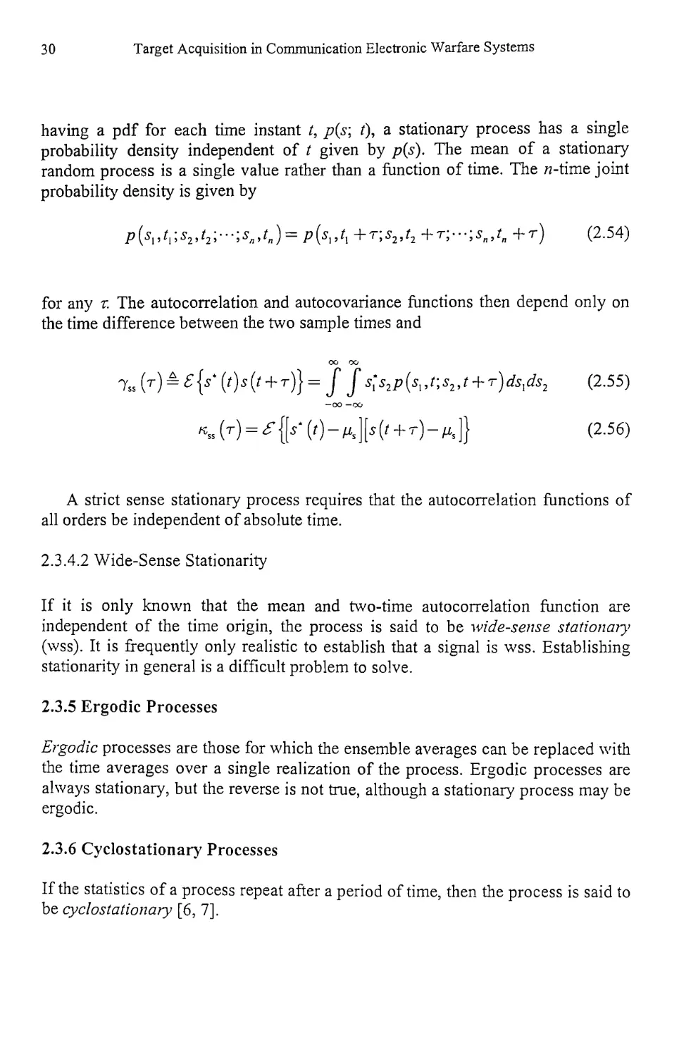
having a pdf for each time instant t, p(s\ t), a stationary process has a single
probability density independent of t given by p(s). The mean of a stationary
random process is a single value rather than a function of time. The л-time joint
probability density is given by
= +r) (2.54)
for any t. The autocorrelation and autocovariance functions then depend only on
the time difference between the two sample times and
OO oo
Tss('r)-£p;‘(rMz + T)} = J" f s;s2p(sl,t;s2,t + r')ds,^s2 (2.55)
-oo -oo
K„ (T) = £ fl5' (0 - M, ]P G + T) - Ms ]} (2-56)
A strict sense stationary process requires that the autocorrelation functions of
all orders be independent of absolute time.
2.3.4.2 Wide-Sense Stationarity
If it is only known that the mean and two-time autocorrelation function are
independent of the time origin, the process is said to be vdde-sense stationary’
(wss). It is frequently only realistic to establish that a signal is wss. Establishing
stationarity in general is a difficult problem to solve.
2.3.5 Ergodic Processes
Ergodic processes are those for which the ensemble averages can be replaced with
the time averages over a single realization of the process. Ergodic processes are
always stationary, but the reverse is not true, although a stationary process may be
ergodic.
2.3.6 Cyclostationary Processes
If the statistics of a process repeat after a period of time, then the process is said to
be cyclostationary [6, 7].
Deterministic and Stochastic Processes
31
2.4 Stochastic Signals
The discussion in Section 2.2 on deterministic signals does not apply directly
when the signals under consideration are stochastic. There are two reasons for this.
First, S(f) is a random variable, since, for any fixed / each sample would be
represented by a different value of the ensemble of possible sample functions.
Hence, it is not a frequency representation of the process but only of one member
of the process. The second reason for not using the S(f) of (2.1) is that, for
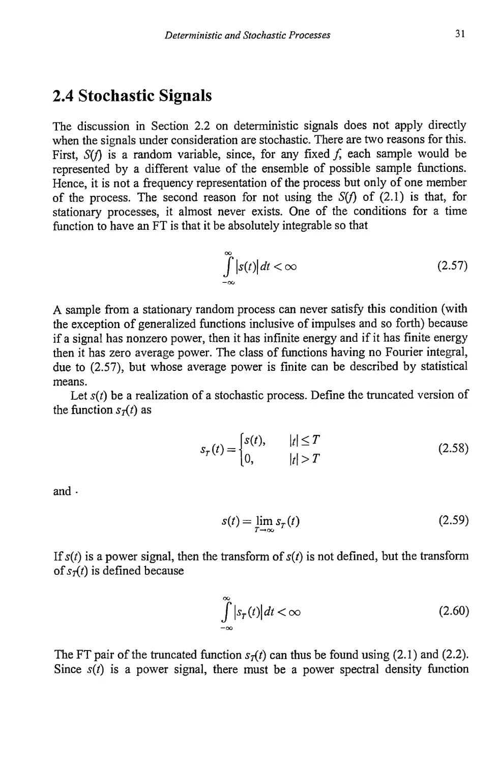
stationary processes, it almost never exists. One of the conditions for a time
function to have an FT is that it be absolutely integrable so that
J'|s,(/)|^ < oo
-oo
(2.57)
A sample from a stationary random process can never satisfy this condition (with
the exception of generalized functions inclusive of impulses and so forth) because
if a signal has nonzero power, then it has infinite energy and if it has finite energy
then it has zero average power. The class of functions having no Fourier integral,
due to (2.57), but whose average power is finite can be described by statistical
means.
Let s(t) be a realization of a stochastic process. Define the truncated version of
the function Sj(t) as
ST (0 —
И<Г
M>r
(2.58)
and
s(t) = lim sT(t)
T-*ao
(2.59)
If s(f) is a power signal, then the transform of s(f) is not defined, but the transform
of s^t) is defined because
OO
jMOl^Coo
-oo
(2.60)
The FT pair of the truncated function Sjif) can thus be found using (2.1) and (2.2).
Since s(t) is a power signal, there must be a power spectral density function
32
Target Acquisition in Communication Electronic Warfare Systems
associated with it and the total area under this density must be the average power
despite the fact that s(t) is non-Fourier transformable.
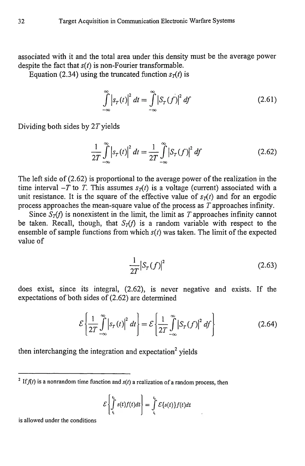
Equation (2.34) using the truncated function s-^f) is
OO OO
Дю|’й = 1/'|5,.(/)|2# (2.61)
—oo -oo
Dividing both sides by 2Tyields
1 °° i °°
—/Рг(0|2Л = —J|Sr(/)|2# (2.62)
-OO -oo
The left side of (2.62) is proportional to the average power of the realization in the
time interval -T to T. This assumes s-ft) is a voltage (current) associated with a
unit resistance. It is the square of the effective value of Sj(t) and for an ergodic
process approaches the mean-square value of the process as T approaches infinity.
Since Sff) is nonexistent in the limit, the limit as T approaches infinity cannot
be taken. Recall, though, that Sff) is a random variable with respect to the
ensemble of sample functions from which s(t) was taken. The limit of the expected
value of
^г(/)Г (2-63)
does exist, since its integral, (2.62), is never negative and exists. If the
expectations of both sides of (2.62) are determined
(2.64)
then interchanging the integration and expectation2 yields
2 If ft) is a nonrandom time function and s(t) a realization of a random process, then
E J s(t)f(t)dt = J E{s(t)}f(t)dt
is allowed under the conditions
Deterministic and Stochastic Processes
33
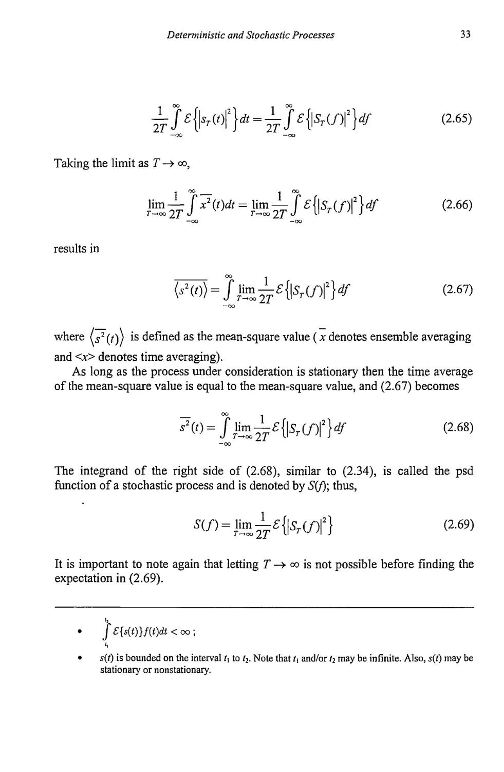
1 00 Г x 1 0°
J = J фг(Лф/ (2.65)
—oo —00
Taking the limit as T -+ co,
Фмк <2-66)
-00 -00
results in
М = /^Фг(Л|2И (2-67)
where ^2(r)) is defined as the mean-square value (x denotes ensemble averaging
and <x> denotes time averaging).
As long as the process under consideration is stationary then the time average
of the mean-square value is equal to the mean-square value, and (2.67) becomes
<2-68>
-00
The integrand of the right side of (2.68), similar to (2.34), is called the psd
function of a stochastic process and is denoted by S(f); thus,
W = (2'69’
It is important to note again that letting T -+ co is not possible before finding the
expectation in (2.69).
< 00 ;
<!
• s(f) is bounded on the interval Л to t2. Note that Л and/or t2 may be infinite. Also, s(t) may be
stationary or nonstationary.
34
Target Acquisition in Communication Electronic Warfare Systems
If s(t) is a voltage (current) associated with а Ю resistance, s2(t) is the average
power dissipated in that resistor and S(f) is the average power associated with a
bandwidth of 1 Hz centered at/Hz.
S(f) has the units volts2-second and its integral, (2.68), leads to the mean-
square value, hence,
___ oo
“OO
(2.70)
Since Sj(/) is the FT of assuming a nonstationary process, from (2.69),
- oo oo
5(/)=lim—£ fCsT(t2)e'2^dt2
T—+ oo 2,1 'J 'J
(2.71)
The subscripts of t\ and t2 have been introduced to keep the variables of integration
distinct. So,
= lim —
T-.0O 2T
- oo oo
= }™^f dt>f
(2.72)
The expectation £{б,7.(/|)57.(г2)} is the autocorrelation function, /SS(Z], h ), of the
truncated process where
£ {sy (Zj )sT (Z2)} — 7SS (^ > G )>
k,l>k2|<r
(2.73)
Substituting
G ~T
dt2 = dr
(2.74)
(2.72) becomes
Deterministic and Stochastic Processes
35
T-*oo
- oo oo
-Lf f dr f 7ss(r,,Z, +T)e-^dtl
21 \J J
L-OO -oo
or
(2.75)
5(/) = f lim — Гy„(tl,tl +r)dt,\e-^dr (2.76)
Thus, the spectral density is the FT of the time average of the autocorrelation
function. The relationship of (2.76) is valid even for nonstationary processes.
For the stationary process, the autocorrelation function is independent of time
origin, and therefore
bsJ'id, +т)) = 7„(т)
(2.77)
It has just been shown that for a stationary random process the autocorrelation
function is the inverse FT of the spectral density function. This cannot be said for
nonstationary processes, however.
The FT of the autocorrelation function is called the psd, or the power spectrum
of s(t}, denoted by S(f):
OO
$(/) = f y„(r)e-'2’"d/ (2.78)
-oo
and
OO
7„(t) = $ Skfye^df (2.79)
-oo
The average power of a stationary stochastic process is defined as
p,=^{И')Г]
(2.80)
Likewise, the autocorrelation of s(t) is given by
36
Target Acquisition in Communication Electronic Warfare Systems
7„И = <Г-р(ф'(/ + т)} (2.81)
and the cross-correlation function of s(f) and x(i) is given by
7OH = 4'((>H (2.82)
If a stationary stochastic process s(t) is input to an LTI filter with impulse
response /?(Z) producing output y(t) = (s* h)(t\ the cross-correlation of the input
and output is
7sy (Л,Л) = ^{s’ (',№)}
= S s' (t,)f h(v)s(t1-v)dv
-OO
=J/!M7SSg2-'i-''>
-oo
= f h(Vy{S’(t>}S(l2-V)}dV
(2.83)
Thus, ysy(.) is not a function of time but a function of only the time difference
T = Z2 - t], so
7.y('r) = (7ss*/')(T)
(2.84)
By a derivation similar to (2.83),
7„ (T) = (xy * ii) (t) = (7ss * 11 * ii) (r) (2.85)
where h (z) = h' (—z). Note that the psd is an even function of frequency.
The autocorrelation and cross-correlation functions are defined for finite power
stochastic functions as
Deterministic and Stochastic Processes
37
7S, = lim^ J's‘(t')s(t + T)dt (2.86)
-%
and
1T/1
7Vi = I™ 7 f s? (Фг (t+rjdt (2.87)
~ -%
respectively. When t= 0,
i % , TA
(°)= 11® T f S* = f ^dt
1 _T/ 1 _T/
/2 /2
= Ps (2.88)
By derivations similar to that leading up to (2.84), it can be shown that the
autocorrelation of the output of an ideal LTI filter is given by
7w(4 = (7„*^(t)
(2.89)
with corresponding FT
^(/)=^1яИ2 <2-9°)
If a finite power signal is passed through an ideal bandpass filter of bandwidth
B, the average power of the output, calculated in a similar manner to the above, is
7„(°) =
(2.91)
which justifies calling 5SS (/) the psd of s(f).
The cross-correlation function of the input and output is similarly given by
38
Target Acquisition in Communication Electronic Warfare Systems
%у('г) = (х!*А)('г) <2-92)
with corresponding FT
= (2.93)
Assuming that у is wss, the psd Ф^ (e'^can be shown to be as
follows.
M<7r
= E £{у^У1}е-^
m=-<*>
= 4л E л+^’'Ч
I m = -OQ J
= X' {е'-')х(е^)
= £{У;е^Х^)}
= И'“)Г
(2-94)
(2.95)
where Фуу is the psd of у and ф^фп) is the autocorrelation sequence ofy.
Equation (2.94) is true by the time shifting property of the FT. This is known as
the Weiner-Khinchin theorem.
If y(k) represents a specific instance of the wss ergodic random process Y^, a
finite-length sequence can be defined as
yN(k) =
[Ж1,
—N < к < N
otherwise
(2.96)
From this an estimate r^im) of the autocorrelation of у can be generated as
1 N
(m> = п м; i E у к +т}у'н w
IIN -b 1 k=_N
(2.97)
Deterministic and Stochastic Processes
39
Thus,
k=—N
. Eд'«('я+ВД('я)е“',‘“
Z/V 4-1 m=_N
1 N
—------ 3+(m)
2W + 1„E/"
N
12 уЛк+т~}
i
277 + 1
N
M+ E
m=-N
(2.98)
(2.99)
Again, (2.98) is possible due to the time shifting property of the FT.
The true psd is the expected value of Ф (eyw) as 77-> co:
= lim £
1
277 + 1
N
E y^-ita
k=-N
(2.100)
2.5 White Noise
If the psd of a stationary stochastic process x(r) is a constant value with frequency
it is said to be white (see Figure 2.8). This corresponds to the naturally occurring
thermal noise in the atmosphere as well as all electronic devices. The psd can be
specified either over the entire frequency spectrum of -co <f< co, when it is given
by No I 2 W/Hz, or equivalently, over just the positive frequency range of 0 <f<
co, where it is specified by No W/Hz.
40
Target Acquisition in Communication Electronic Warfare Systems
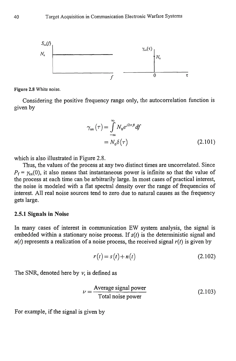
SM(f)
Ym('v)
Figure 2.8 White noise.
Considering the positive frequency range only, the autocorrelation function is
given by
= W)
(2.101)
which is also illustrated in Figure 2.8.
Thus, the values of the process at any two distinct times are uncorrelated. Since
Pf= 7xx(0), it also means that instantaneous power is infinite so that the value of
the process at each time can be arbitrarily large. In most cases of practical interest,
the noise is modeled with a flat spectral density over the range of frequencies of
interest. All real noise sources tend to zero due to natural causes as the frequency
gets large.
2.5.1 Signals in Noise
In many cases of interest in communication EW system analysis, the signal is
embedded within a stationary noise process. If s(t) is the deterministic signal and
n(t) represents a realization of a noise process, the received signal r(Z) is given by
r(r) = s(/) + n(/)
(2.102)
The SNR, denoted here by v, is defined as
Average signal power
Total noise power
(2.103)
For example, if the signal is given by
Deterministic and Stochastic Processes
41
5 (/) = JlS sin (2тгft)
(2.104)
where S is the average power in the signal, the noise is specified as No W/Hz, and
the total noise power in a double-sided bandwidth В is PN = BNq, then the SNR is
S _ S
BN. ~ BN0
(2.105)
2.6 Concluding Remarks
The fundamental properties of deterministic and stochastic processes were
presented in this chapter. Processes in the context important here are signals and
the mechanisms that generate them.
Deterministic signals are idealizations of realistic signals. Most signals of
importance to communications EW are stochastic in some sense. There are one or
more parameters about them that are random, and therefore these signals can only
be described by probability functions and the resulting statistical properties.
References
[1 ] Bracewell, R., The Fourier Transform and Its Applications, New York: McGraw-Hill, 1965.
[2] Kaplan, W., Introduction to Analytic Functions, Reading, MA: Addison-Wesley, 1966, p. 42.
[3] Tretter, S. A., Introduction to Discrete-Time Signal Processing, New York: John Wiley &
Sons, 1976, pp. 14-15.
[4] Cover, T. M., and J. A. Thomas, Elements of Information Theory, New York: John Wiley &
' Sons, 1991, pp. 248-249.
[5] Tretter, S. A., Introduction to Discrete-Time Signal Processing, New York: John Wiley &
Sons, 1976, Chapter 11.
[6] Gardner, W. A., Statistical Spectral Analysis: A Nonprobabilistic Theory, Englewood Cliffs,
NJ: Prentice Hall, 1988, Part II.
[7] Gardner, W. A., Introduction to Random Processes with Applications to Signals and Systems,
New York: Macmillan, 1986, Chapter 12.
Chapter 3
Target Search Methods
In communication EW problems, signal detection refers to establishing the
presence or absence of a signal at a frequency by searching the frequency
spectrum [1]. There are three distinct types of such searching: general search
(GS), directed search (DS), and signal verification. This last category is not
searching in the same sense as the other two—it consists of verifying that the
target signal is still present at the frequency channel that is being jammed [2].
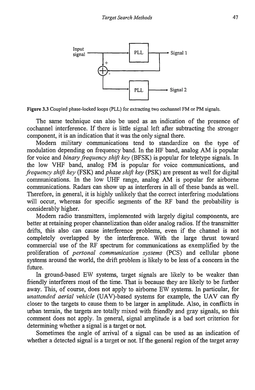
Characteristics of these search schemes are examined in this chapter [3].
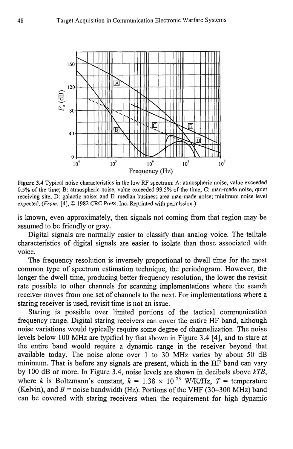
GS is the type of search when little or nothing is known about the signal
environment and the frequencies of the active targets must be established—this is
an ES function. The search receiver scans the frequency spectrum from some start
frequency to some stop frequency (or multiple bands of these) and measures the
energy present at each channel. If energy is detected, then that frequency is tagged
as active and the receiver moves on. Alternatively, other actions can occur upon
detection of an active channel, such as notifying an operator or automated
processing equipment to begin making measurements on the signal.
In GS searching, the target types, in general, are unknown, although there can be
exceptions to this. Therefore it is best assumed that the signals have at least some
random parameters. These parameters are the signal’s amplitude, time of
detection, and phase of the carrier. The frequency is known because it is either
assumed to be the center of the channel being searched, or it can be measured as
the position of the centroid of the spectrum or the highest peak of the spectrum.
The two types of signals of interest then are:
• Targets with random amplitude and phase at known frequency;
• Modulated sinusoid with known frequency, random modulation, random
amplitude, and random phase.
43
44
Target Acquisition in Communication Electronic Warfare Systems
Figure 3.1 Wideband receiver for signal searching.
DS assumes that most or all of the frequencies of the targets of interest are
known. In addition, other characteristics of the signals may be known, such as the
modulation type. The search receiver tunes to each discrete channel, the priorities
of which can be taken into account. The search only covers those frequencies that
are known active at some point in the recent past. In addition, if an operator or
automation has determined that the signal at a particular frequency is a high-
priority target, that channel could be revisited more often than some other channels
that may be of just general interest. With DS searching, there is a much higher
probability of knowing the target type associated with the frequency. Thus,
specific targets can be modeled as:
• Random targets at known frequency with known amplitude, known
modulation, and unknown phase;
• Modulated sinusoidal target with known frequency, known modulation,
known amplitude, and random phase.
Combinations of GS and DS are also possible. This scenario would be used
when the target environment is partially known (DS), but a significant portion is
not (GS).
As mentioned, verification is ensuring that the target being jammed at a
frequency is still active at that frequency. This is also called look-through. During
the look-though period, the jamming signal must be blanked to not damage the
sensitive ES equipment. In this case, the signal type is known, including all the
relevant parameters. In that case, the hypothesis testing approach for signal
detection, discussed later, is probably not required. The high-resolution signal
detection capabilities are required, which is true of all of the search strategies
discussed here.
Searching is typically accomplished by converting the signal output of a
relatively wideband receiver into the frequency domain and determining the
frequencies where the peaks occur, as illustrated in Figure 3.1. There are two
fundamental types of spectral estimation methods that can be used for signal
detection. The first is called the traditional method and is used when relatively low
resolution is adequate with resolution defined as indicated in Figure 3.2. Two
equal amplitude signals are resolved when their peak levels are separated by a
Target Search Methods
45
Figure 3.2 Frequency resolution. The signals are just resolvable when the dip between two signals is 3
dB below the peak levels. This frequency separation is approximately l/T for low-resolution spectrum
estimation. An alternate definition is used in Chapter 9 that allows for differing power levels of the
signals.
frequency span defined by the 3-dB drop from the peaks values. In Figure 3.2, this
span is given by^ - j\. When this amount of resolution is not adequate, the second
technique provides for higher resolution signal detection at the expense of a higher
computational burden. Two traditional techniques are presented in Chapter 4: the
periodogram and the Blackman-Tukey method. The higher resolution methods are
presented in Chapter 8.
All spectral estimation techniques are imperfect in that false detections occur
and detections are sometimes missed, as discussed in this chapter.
3.1 General Search
As indicated in Chapter 1, general searching for signals of interest is used to
establish where signals are located in the RF environment. The signal environment
in GS is assumed to consist of deterministic signals with random parameters, as
well as random signals with unknown parameters as the most general case. The
background noise is assumed here to consist of AWGN.
When little or nothing is known about the signal being detected, the optimum
detector is the radiometer. The radiometer estimates the amount of energy and
noise present in the signal. Detailed discussions about the radiometer are presented
in Chapter 5.
46
Target Acquisition in Communication Electronic Warfare Systems
The parameters for GS must be provided by tasking prior to a mission. The
most general tasking for GS is to search a single frequency band from start to
finish, repetitively. The frequency band list, of course, can be modified during a
mission. Once a signal is detected, system assets are tasked to determine as much
about the signal as possible for subsequent use in DS or for other purposes, such as
tasking set-on receivers. Databases could also exist that are provided by external
sources or determined on prior missions as to frequencies in use by SOIs.
When energy is detected, signal detection is declared. Rarely is this sufficient
to declare the signal as being associated with a target, even though the frequency is
the same. Further processing is almost always required for target declaration. This
further processing could be determining the type of modulation present (if any)
Another possibility is to obtain a line of bearing (LOB) on the target and/or
task other EW systems to do the same. An LOB is the direction from which the
signal arrives at the EW system. The resultant data could then be used to calculate
a position fix (PF). A signal classifier could be tuned to the frequency where the
energy is detected, making appropriate measurements to ascertain the modulation
of the signal. A set-on receiver could be tuned to the frequency so that the signal
can be intercepted. These are but a few of the possibilities, but they all start with
the fundamental requirement to measure the energy to detect the presence of
signals.
Two or more signals can be occupying the same frequency channel. In general
these signals can be targets, friendly interferes, or gray interferes. Based on the
detected energy alone, the distinction is difficult to ascertain. Other means must
then be employed to determine the status of the signals. This assumes that it is
possible to determine the presence of more than one signal, which is a dubious
assumption at best. In the tactical military communication frequency bands, the
channelization is fairly narrow—10 kHz in the HF band, 25 kHz in the low VHF
band (30-90 MHz), and 50 kHz in the low UHF band (110-400 MHz). If a signal
is using a channel in one of these bands, it will likely use the whole channel, and if
two or more signals are present, they will almost assuredly substantially overlap in
frequency content.
In some cases it is possible to remove one (or more) of the interfering signals
when cochannel interference occurs. The system shown in Figure 3.3 is one such
technique for FM signals. The first PLL locks onto the stronger of the signals at
the input and forms an identical signal that is n radians out of phase with it (as
indicated by the negative sign at the adder in Figure 3.3). That signal is then added
to the incoming signal that effectively removes the stronger signal. The resultant
signal is the weaker of the signals at the input. This could be repeated a number of
times.
Target Search Methods
47
Figure 3.3 Coupled phase-locked loops (PLL) for extracting two cochannel FM or PM signals.
The same technique can also be used as an indication of the presence of
cochannel interference. If there is little signal left after subtracting the stronger
component, it is an indication that it was the only signal there.
Modem military communications tend to standardize on the type of
modulation depending on frequency band. In the HF band, analog AM is popular
for voice and binary frequency shift key (BFSK) is popular for teletype signals. In
the low VHF band, analog FM is popular for voice communications, and
frequency shift key (FSK) and phase shift key (PSK) are present as well for digital
communications. In the low UHF range, analog AM is popular for airborne
communications. Radars can show up as interferers in all of these bands as well.
Therefore, in general, it is highly unlikely that the correct interfering modulations
will occur, whereas for specific segments of the RF band the probability is
considerably higher.
Modem radio transmitters, implemented with largely digital components, are
better at retaining proper channelization than older analog radios. If the transmitter
drifts, this also can cause interference problems, even if the channel is not
completely overlapped by the interference. With the large thrust toward
commercial use of the RF spectrum for communications as exemplified by the
proliferation of personal communication systems (PCS) and cellular phone
systems around the world, the drift problem is likely to be less of a concern in the
future.
In ground-based EW systems, target signals are likely to be weaker than
friendly interferers most of the time. That is because they are likely to be further
away. This, of course, does not apply to airborne EW systems. In particular, for
unattended aerial vehicle (UAV)-based systems for example, the UAV can fly
closer to the targets to cause them to be larger in amplitude. Also, in conflicts in
urban terrain, the targets are totally mixed with friendly and gray signals, so this
comment does not apply. In general, signal amplitude is a bad sort criterion for
determining whether a signal is a target or not.
Sometimes the angle of arrival of a signal can be used as an indication of
whether a detected signal is a target or not. If the general region of the target array
48
Target Acquisition in Communication Electronic Warfare Systems
Figure 3.4 Typical noise characteristics in the low RF spectrum: A: atmospheric noise, value exceeded
0.5% of the time; B: atmospheric noise, value exceeded 99.5% of the time; C: man-made noise, quiet
receiving site; D: galactic noise; and E: median business area man-made noise; minimum noise level
expected. (From: [4], © 1982 CRC Press, Inc. Reprinted with permission.)
is known, even approximately, then signals not coming from that region may be
assumed to be friendly or gray.
Digital signals are normally easier to classify than analog voice. The telltale
characteristics of digital signals are easier to isolate than those associated with
voice.
The frequency resolution is inversely proportional to dwell time for the most
common type of spectrum estimation technique, the periodogram. However, the
longer the dwell time, producing better frequency resolution, the lower the revisit
rate possible to other channels for scanning implementations where the search
receiver moves from one set of channels to the next. For implementations where a
staring receiver is used, revisit time is not an issue.
Staring is possible over limited portions of the tactical communication
frequency range. Digital staring receivers can cover the entire HF band, although
noise variations would typically require some degree of channelization. The noise
levels below 100 MHz are typified by that shown in Figure 3.4 [4], and to stare at
the entire band would require a dynamic range in the receiver beyond that
available today. The noise alone over 1 to 30 MHz varies by about 50 dB
minimum. That is before any signals are present, which in the HF band can vary
by 100 dB or more. In Figure 3.4, noise levels are shown in decibels above kTB,
where к is Boltzmann’s constant, к = 1.38 x 10⁻²³ W/K/Hz, T = temperature
(Kelvin), and В = noise bandwidth (Hz). Portions of the VHF (30-300 MHz) band
can be covered with staring receivers when the requirement for high dynamic
Target Search Methods
49
range is considered. The same is true for the UHF band, although the important
PCS bands can be covered with adequate dynamic range, typically 15 MHz around
400 MHz, 70 MHz around 900 MHz, and 140 MHz around 1.9 GHz (1.850-1.990
GHz).
The results of GS are a list of signals with their parameters. These parameters
could be:
• Frequency;
• Power level;
• Modulation type;
• Geolocation/LOB.
and other, more detailed information.
3.2 Directed Search
Directed search is used when most of the parameters associated with the targets
are known. Most importantly, it is known that the signal at a DS frequency is a
true, or at least suspected, target. The DS frequencies are known, and the EW
system moves from one frequency to the next, measuring the energy at each
frequency channel to determine the presence or absence of a signal. Just as for GS,
if energy is detected, several subsequent actions are possible, and whether any of
them are executed depends on the particular mission and the signal.
The data required for directed searching, such as frequencies, signal types,
amplitudes, and so forth, are provided for directed search. This information could
be provided by other sources, prior to or during the mission, or it could be the
result of GS discussed in Section 3.1. The more information that is provided, of
course, the higher the probability is that a detected signal is a SOI.
For scanning implementations, the time it takes to revisit a DS frequency
impacts on the probability of detecting that target on its next transmission, which
may be important for some missions.
3.3 Concluding Remarks
Determining the presence or absence of signals is the purpose of spectral
searching. If little is known about the target environment then, GS is implemented
to establish where the signals are and to determine as much about them as
50
Target Acquisition in Communication Electronic Warfare Systems
possible. If the target environment is fairly well known, then DS can be used. In
DS, the frequencies are known, as are several other threat signal parameters.
The result of GS is a list of frequencies where potential threat signals may be
located. These results are used for subsequent DS when targets are further
exploited.
In practice, both GS and DS are conducted simultaneously. With limited
system assets, the two search methods might share the same receiver, alternating
between the two search types with that receiver. In larger systems, separate
subsystems can be used for the two search modes. GS can be running separately,
categorizing the target environment, while DS is used to keep track of known
targets.
References
[1] Frater, M. R., and M. Ryan, Electronic Warfare for the Digitized Battlefield, Norwood, MA:
Artech House, 2001, pp. 100-112.
[2] Poisel, R. A., Introduction to Communication Electronic Warfare Systems, Norwood, MA:
Artech House, 2002, Chapter 14.
[3] Adamy, D., EW101: A First Course in Electronic Warfare, Norwood, MA: Artech House,
2001, p. 110.
[4] Volland, H., ed., Handbook of Atmospherics, Volume 1, Boca Raton, FL: CRC Press, 1982,
pp. 295-296.
Chapter 4
Hypothesis Testing for Signal Detection
There is a firm theoretical background for optimal detection of signals in noise
available with hypothesis testing [1-3]. Hypothesis testing is one method used to
optimally or suboptimally determine whether a signal is present or not [2, 4-8].
4.1 Hypothesis Testing
The simplest case to consider is when all of the parameters of a deterministic
signal are known and the channel provides AWGN, whether the signal is present
or not. Suppose that the receiver in the EW system outputs a predetection (not
demodulated) waveform x = {x(0 : t e [0, T|} over the observation time interval
[0, 7]. This signal may have been produced by noise alone or by a received signal
of known form plus noise. These two hypotheses can be expressed as
Ho: x = noise;
H1:x = signal + noise
(4.1)
Stated another way, there are two possible hypotheses:
Ho: there is no signal and the time series consists of noise only ~ pQ
H]'. the time series consists of the sum of the signal and noise ~ p}
That is, hypothesis Ho has a priori probability distribution pQ and has a
priori probability distribution px. The noise associated with the reception of a
signal causes this to be a stochastic problem, and even though the characteristics
of the signal are completely known, the received signal can only be described
statistically. The observation upon which the decision as to which hypothesis is to
51
52
Target Acquisition in Communication Electronic Warfare Systems
be selected is denoted by Y. Hq is referred to as the null hypothesis and is called
the alternative hypothesis. Hq and Hi are called simple hypotheses when the pdf of
x under Ho and Hi does not depend on any unknown parameters such as signal
amplitude or phase. When such unknown parameters are involved, these
hypotheses are called composite hypotheses. The unknown parameters are called
nuisance parameters. Their values are uninteresting with regard to the problem at
hand, yet their presence influences the ability to correctly decide the presence or
absence of a signal.
An example of a simple (binary) hypothesis test is
Hq. Y= Yq
Hi-.Y-Yi
where there are only two possible outcomes and they are completely specified. An
example of a composite hypothesis test is
Hq. Y= Yq
Hi: Y* Yq
so that in Hi, more than one outcome is possible.
Consider Table 4.1. Ignoring the first row in Table 4.1, the remaining table
entries are denoted by dij j =1,2. This table indicates, for each condition of having
the signal present or absent, the possible outcomes of making a decision, and each
of these outcomes has an associated probability. Since one of the decisions must
be made, the sum of the probabilities for any one column must total to unity. For
decision (1, 1), (decide the signal is present when it is present), denoted by du, the
outcome of the decision is the correct one. The probability in this case is called the
probability of detection, denoted by Pd. For tZ2i, the signal is there but it was not
detected. The corresponding probability for this decision is called the probability
of miss, and denoted by Pm. Thus,
(4-2)
For di2, the detector thought the signal was there and it actually was not. This is
known as a false alarm, with the probability denoted by Pfa. Lastly, for d22, the
Table 4.1 Possible Decisions
Signal Present___________Signal Absent
Decide signal present Decide signal present
Decide signal absent Decide signal absent
Hypothesis Testing for Signal Detection
53
signal was declared absent when it actually was not there. This is a correct
decision, but its probability does not carry a particular designation; this particular
event is of little direct interest.
To estimate which hypothesis is true, the signal can be compared to a threshold
and declared true only if the signal is larger than the threshold. The higher the
threshold value, the lower the chance that a signal will be declared present when it
is not present. On the other hand, the lower the threshold value, the lower the
chance that a signal will be missed if it is in fact present. Thus, there are two types
of errors possible: (1) the error of declaring the signal present when it is absent
(declare when Ho is true), and (2) the error of missing the signal when it is
present (declare Ho when is true). The first of these is called a Type I error as
well as a false alarm. The second of these is called a Type II error as well as a
missed detection. In all realistic cases of signal detection, then, there is a trade-off
between setting the threshold high to lower Pfa and setting the threshold low to
lower Pm. To ascertain the quantitative effects of this trade-off, it is necessary to
specify the pdf for x in (4.1) under each of the hypotheses Ho and .
Depending on the situation, one of the error types can be more important than
the other. False alarms corresponding to type I errors task system resources
unnecessarily and thereby slow down system throughput. If there are enough
system resources to adequately handle the signal environment with significant
false alarms, then this is not a significant problem. On the other hand, rejecting the
presence of a signal when in fact there is one present (missed detection) can cause
critical signals to be missed.
A decision rule (or hypothesis test) 5 partitions the observation space Г into
two regions given by Гi and Го such that if Y g Го, hypothesis Ho is chosen and if
Y g rb hypothesis Hi is chosen. The set Г1 is referred to as the rejection region
and the set Го is called the acceptance region. Such a decision rule is illustrated in
Figure 4.1 for arbitrary probability densities. The decision rule, 5, is thus defined
as a function of the observation Y as
УеГ,
Уего
(4.3)
Figure 4.1 Decision regions for decision rule 5.
54
Target Acquisition in Communication Electronic Warfare Systems
In statistics, Г1 is known as the critical region because it is in this region
within which the null hypothesis is rejected. Alternatively, if the observed value is
not in the critical region (that is, it is in Го), the conclusion is to not reject the null
hypothesis. The critical value for a hypothesis test is a threshold that determines
whether the null hypothesis is rejected. In addition, in statistics, the significance
level is the probability of false alarm—that is, the probability of incorrectly
rejecting the null hypothesis. The power of a statistical hypothesis test is the
probability of detection—that is, the probability of correctly rejecting the null
hypothesis.
4.2 Receiver Operating Characteristic
The threshold for x is denoted by /. The critical region, denoted by 7£c, is that
range for x for which x(t) > /. That is,
тгс = {x: x(t) > 7}
(4-4)
This region then specifies the conditions on x for which the detector declares the
signal to be present. Based on the critical region, then, the probability of detection,
Pd, is given by
Pd=P(^|ff,)
^=р(7гЯ1|я0)
and
P = I-P
m a
(4.5)
(4.6)
(4.7)
where P(A |Z?) denotes the probability of event A given hypothesis B.
The two-dimensional graph of Pd(y) versus Pfa(y) specifies the error
performance of the detector for various values of Pd(y) and Pfa(y), an example of
which is shown in Figure 4.2 for a particular value of /. When the plots are
included so that — 00 < 7 < 00 are contained on the graph, or some limited range
for /of interest, it is referred to as the receiver operating characteristic (ROC), an
example of which for /> 1 is shown in Figure 4.3.
Hypothesis Testing for Signal Detection
55
Figure 4.3 ROC curves.
56
Target Acquisition in Communication Electronic Warfare Systems
The ROC curve for a good detector is characterized as being convex, the curve
is monotonic as Pfa increases, and the slope of the curve at (0, 0) is large.
In the above case it was assumed that the signal characteristics and noise
statistics were completely known. That resulted in simple hypotheses, and an
optimal detector can be found such that the ROC curve for any other detector will
be less than the ROC curve for the optimal detector. “Less than” means that for
any given Pfa, the Pd for these other detectors will be less than the Pd for the
optimum detector. Thus, the ROC curve for the optimal detector forms an upper
bound on the possible ROC curves. Such an optimal detector is called the
uniformly most powerful (UMP) test.
It is much more common if the signal or the noise (or both) are associated with
some nuisance parameters so that at least one of the hypotheses is composite. In
that case there will be a different ROC curve for different values of the parameters.
This results in the paucity of cases when the UMP test is available.
4.3 Likelihood Ratio
Let 0 denote an unknown parameter from parameter space 0. Partitions 0O and 0j
are nonempty subsets of 0 which separate 0 into two regions. These sets are
disjoint such that ОоП0,=0 and exhaustive such thatOgUOj^O. Then
denotes the conditional pdf of x given the occurrence of 0, and we assume
that this pdf is known. The hypothesis test (4.1) can then be rewritten as
Ho :x~ p(x\6),6 eQ0
Hi : x ~ p(x |0), в G 0j
(4.8)
For any pair of parameters 0Q e 0o and 0\ e 0b Pd and Pfa can be found by
integrating the pdf over Гb
Pd = f p(x^)dx
and
pr. = f P^lejdx
(4.9)
(4.Ю)
Hypothesis Testing for Signal Detection
57
If the two hypotheses as expressed by (4.8) are simple (not composite),
then© = {00,0,}. In that case, O0 = {0O} and©, = {0,}, each consisting of a single
element. The Neyman-Pearson theorem [8] states that in this case there exists a
UMP test such that Pd is maximized subject to a set level of Pfa; that is, Pfa < a.
The UMP test is called the likelihood ratio test and is given by
A(x)4
Х*|0о)яо7
(4.И)
where у is a threshold value determined by a = Pfa. The value of у is determined
by
oo
« = J рСЖМу
7
(4.12)
where /?(^|0) is the pdf of the likelihood ratio statistic Л(х).
When one of the hypotheses is composite, then the Neyman-Pearson theorem
does not apply. In that case the generalized LRT (GLRT) is often used. This is an
ad hoc extension to the LRT and is given by
max /?(х|0,) н,
тмр(х0о)<
(4.13)
That is, the GLRT replaces the unknown parameters with their maximum
likelihood estimates in the pdfs. There is no underlying theory that guarantees that
the GLRT will yield optimum results, but it generally produces good results in
practice.
4.4 Hypothesis Tests
In general, the specific parameter of interest may not be measurable directly. In
that case, one or more quantities related to the parameter of interest are measured
instead. Such measurements and the ensuing judgments are called tests. Two of
the more common types of tests are the aforementioned UMP test and the locally
most powerful (LMP) test. Formally,
58
Target Acquisition in Communication Electronic Warfare Systems
Definition. Let w,(k) be the pdf for к for hypothesis H,. Then
Р,(у\Н,) = fpK(y)w/(K)dK (4-14)
The UMP test criterion, given
Ho : P for к, G Го
° K ° (4.15)
Я, : PK for к e Г,
is
max Pd (<5, к,) Vк, G ?! (4.16)
subject to
V«er0 (4.17)
Hence, UMP tests are independent of the particular к.
Definition. Given that
Ho : PK for к, = к0
: P. for к, G ?! = (rc0,oo)
the LMP test is
max — P. (6, к,
<5 дк, d k '
subject to Pfa (<5) < a
(4.19)
so the likelihood ratio becomes
*W =---M
PoW
(4.20)
Hypothesis Testing for Signal Detection
59
For the generalized likelihood ratio test, the likelihood ratio is
(4.21)
4.4.1 Bayes Criterion
Given the observation У, how is the hypothesis selected? One approach assigns
cost functions to each of the possible decisions. These costs are denoted by COo,
Con Oo, and Oi corresponding to d00, dQi, dw, and dn, respectively. These cost
functions, denoted by Cy, are defined as
Cy = cost of chosing when H. is true (4.22)
This approach was first investigated by Thomas Bayes (1702-1761), and
carries his name. The costs are referred to as Bayesian costs. The Bayes rule is
used to minimize Bayesian costs. Let Tij denote the a priori probability that Hj is
true.
Let
Pj (Г,.) = probability of choosing H( given that is true (4.23)
then the conditional risk is given by
'•>('5) = c.Z(r1) + CoZ>(ro) (4-24)
Let the pdfs of and be denoted bypo(Y) andpi(Y), respectively. Then the
probabilities of error are given by
oo
Ро(Г,) = ро(И^ (4-25)
7
and
/?(г0)=f ?1(tyr
(4.26)
60
Target Acquisition in Communication Electronic Warfare Systems
For example, if У is a normal random variable, then
and
АЛЛ = 7=ехР
Л/2-7ГСГ
c-^.)2
2<r2
(4.27)
Pi (У) = -7==ехР
у/2тта2
T-M,)2
o~2
(4-28)
The Bayes (average) risk or cost is given by
г((5) = 7гого(г) + тг]?;(г)
= 77 о [C00P0 (Г,) + C]0P0 (Г,)]
+’г,[ад(г0)+с„/’(г1)]
= тг0{с00[1-р0(г0)]+ад(г1)}
+^,{с01[1-^(г1)]+ад(г,)}
= ^o [c„„ — с<л T)+c,x (r,)]
+7г1[С01-С0|7’(Г,) + С||^(Г|)]
~ то [Coo 4" Ti) (c,o — Coo )j
4'lri [Coi (r,)(c„ — c„,)|
~ ’’Tm 4" (C10 — C00 )P0 (Г))
Cqi 4- 7Г| (C,, — C01) (Г,)
= 7T0C00 + 7T0 (C10 -c„)f pQ (y)M(dy)
r' „ (4.29)
4-?Г1С0| + я-, (C„ -C0l) J p, (y)p(dy)
The optimal decision rule is known as the Bayes rule and is determined by
choosing set to minimize r(£). Thus, choose fi to be
Hypothesis Testing for Signal Detection
61
r,=
x 6 Г| 7r0 (Go Go) Po (x)
4-7Г1 (Сц — C01 )/?i (x) < 0
x^^'|7ri(Gi G.) /J, (x)
— (Go — Go) Po (x)
(4.30)
It is normally the case that the costs of the mistakes are larger than the cost
associated with making a right decision. Therefore, Cn < COi and Coo < Сю, so Г1
can be written as
where
Г1={У6Г|р,(У)/А(У)>7в}
(4.31)
_ ^o (Go Go)
(Gi— Gi)
(4.32)
The Bayes rule is given by the likelihood test
A (y) = Pl I> 7b choose
А (У) l< Tb choose Яо
(4.33)
and
A(X)>7b
A O') < 7b
(4.34)
Note that the region defined by |y G Г|р, (У) = 7B/?0 (У)} does not contribute to
the risk, so therefore it can be deleted or only part of it retained. Therefore, 5B is
not necessarily uniquely defined.
The conditional probability that Hj is true, given that the observation X takes
on the value x, is given by
62
Target Acquisition in Communication Electronic Warfare Systems
тгу (X) = Р(Н. true|y = y) = =
Po^Y^+p^Y)^
(4.35)
The probabilities 7t0(T) and rc^T) are called the a posteriori probabilities of the
hypotheses. The Bayes decision rule can be written in terms of the a posteriori
probabilities as
4>(r) =
1,
o,
%,(/)< MH
(4.36)
Thus, the minimum probability of error decision rule chooses the hypothesis with
the maximum a posteriori probability of occurrence, given that Y = y. A decision
rule such as this is referred to as a maximum a posteriori (MAP) decision rule.
Suppose the hypothesis in question is given by
where д and are two fixed numbers with px > The likelihood ratio for this
test is given by
(4.37)
with the corresponding Bayes test
0,
otherwise
(4.38)
Hypothesis Testing for Signal Detection
63
Since the log is a monotonically increasing function of its argument, the test
parameter can be put into a different form as
1, ^[x-^]>log7B
0, otherwise
—. 1, , Mi + Mo
Л, xw6 /B | Mi Mo 2 (4.39)
0, otherwise
If the priors are equal and the costs are uniform, then
Y> , М,+Мо
2
otherwise
(4.40)
which is illustrated in Figure 4.4.
In this case, Р0(Г J = Р1(Г0), so
'•(М=-^(Го)+^о(г1)=ро(г1)
= J p0(Y)dY
Mi+Mo
2
oo y2
f e~dY
Po+Mi „
~~2--
Figure 4.4 Binary hypothesis test with normal pdfs, uniform costs, and equal priors.
64
Target Acquisition in Communication Electronic Warfare Systems
Figure 4.5 Bayes cost for normal pdfs, uniform costs, and equal priors.
I 2<z )
where Ф is the distribution function for the standard normal random variable
Л/"(0,1) and
i/ = (4.42)
a2
is the SNR. The Bayes risk in this case as a function of the SNR is illustrated in
Figure 4.5.
4.4.2 Minimax Criterion
In many practical cases of interest, the a priori probabilities are not known or,
perhaps, not knowable. The minimax criterion is useful in this case. The minimax
risk is given by
r (%, 6) = irr0 (5) + (1 - тг) Г, (5)
(4-43)
Hypothesis Testing for Signal Detection
65
When 5 is fixed, г(тс, 5) is an affine function1 of тс, so
max г (тг, 5) = max {r0 (5), i\ (<5)} (4.44)
The goal is to find the decision rule S* * that minimizes (4.43); that is,
тахг(тг,<5*) = min max г(-тг, 5) (4.45)
0<7Г<1 V ' 6 0<7Г<1 4 '
In order to fmd this decision rule, assuming it exists, we assume that there is an
associated probability 7c* such that
тахг(тг,<5*) < г(тг*,^*) < ттг(тг*,<5) (4.46)
0<7Г<1 4 ' 4 ' 6 4 '
Such а тс* is the least favorable probability for 5*, while 5* is a Bayes rule for тс*.
Now, for any pair (тг, 5) it is necessarily true that
min г (тг*, 6) < г (тг*, 6 *) < max r (тг, 8 *) (4.47)
Therefore, for the pair that satisfies (4.46),
max r (тг, 8 *) = г (тг*, 6 *) = min г (тг*, 8} (4.48)
0<7T<] 4 ' 4 ’ 6 4 '
Therefore,
< max ттг(тг,<5)
0<7Г<1 6 4 '
1 An affine function or transformation is one that is invariant to a linear transformation followed by a
translation. In one dimension, an affine function is of the form у = ax + b\ that is, it is composed of a
linear function plus a constant and the graph of у is a straight line. In two dimensions it is of the form z
= ax + by + c, and the graph is still a straight line. This can be extended to any number of dimensions.
The properties of such a function are:
• If three points are on a straight line before the transformation, they will still be on the line
after the transformation;
• Parallel lines remain parallel;
• The ratio of the length of line segments remains constant after the transformation;
• Quadratic functions remain the same after the transformation—that is, parabolas remain
parabolas, ellipses remain ellipses.
66
Target Acquisition in Communication Electronic Warfare Systems
< minmaxr(7r,<5)
<5 0<7г<1 4 '
< max г (тг, 8 *) = г (тг*, 8 *)
or
тахг(тг,<5*) = г(тг*,<5*) = minmaxrM) (4.49)
0<7T<l \ \ > 5 0<7Г<| V '
which means that 8* is a minimax rule. In addition,
тахгпшг(тг,<5) = ттг(тг*,5) (4.50)
which states that л* is a least favorable probability distribution in terms of the
minimum Bayes risk.
Property: Minimax
If 7t* is a least favorable distribution associated with 8*, and one of the following
conditions is true:
(1) r0(8*) = r,(8*)
(2) 7t* = 0 and r0(8*) < 8*
(3) 7t* = 1 and r0(S*) >'i($*)
then 8* is a minimax rule.
Let
Г (тг) = тш7'(тг,(5) = minimum Bayes risk for тг (4.51)
L(tt) is a concave and continuous function and, given that Q > C,7 for i j, L(0) =
Ci] and L(l) = Coo-
The minimax rule is then given by
TO#» (6).,; (6)] = rnin max г (тг, 5)
= max ттг(тг,<5) = maxLfvr)
0<7Г<1 6 4 ' 0<7Г<1 4 '
Hypothesis Testing for Signal Detection
67
The minimax rule is the Bayes rule for л*, where
тг* = arg max И (тг
0<7Г<1 4
(4.53)
4.4.3 Neyman-Pearson Criterion
If neither the a priori probabilities nor costs are available, then the Bayes criterion
cannot be applied to ascertain which hypotheses to adopt. In that case, the
Neyman-Person (NP) criteria can be used. The NP criterion maximizes while
simultaneously limiting the value of P&.
As indicated above, the power of a test is given by the probability of detection
PA = Р](Г1). The significance of that test, a, is the maximum probability of false
alarm, Pfa = Р1(Г0), that is tolerable.
The power function is a graph of PA versus SNR for a fixed a. An example of
a power function is illustrated in Figure 4.6.
The randomized decision rule is a generalization of the decision rule discussed
above,
Figure 4.6 Example of a statistical power function.
68
Target Acquisition in Communication Electronic Warfare Systems
1 if A(t)>7
77 if A(t) = 7
0 if A(t)<7
(4.54)
Then
•f}. (г) = ^0 {^(r)} = f 6(y)p0 (y)p(dy)
Г
= Р0[Л(Г)>7]+7?Р0[Л(У) = 7] (4-55)
and
Pd(6) = £,{5(У)} = f6(y)p,(y)p(dy'}
Г
= /;[а(у)>7]+^[а(у) = 7] (4.56)
The NP rule is a likelihood ratio test where the threshold /0 and the randomization
r/o are chosen such that Pfa = a. That is, the false alarm probability is fixed at some
desired value. Such testing is also called constant false alarm rate (CFAR) testing.
4.5 Multiple Measurements
The more usual case is when there are several measurements that can be combined
and used in some fashion to make the decision. For a time series of samples, for
example, perhaps 64 sequential samples of the signal are available.
For example, given that H\ is true, let D, be a 1 if the detector correctly detects
the signal present during test i and 0 if the detector detects incorrectly during test i.
Then, if there are M frames of data,
л 1 M
P*=^D> (4.57)
is an estimate of the probability of detection. Generating an estimate for the
probability of false alarm, Pfa is done in the same way. Let D, = 1 if the detector
incorrectly detects the signal during test i and 0 if the detector correctly rejects the
signal during test i. Then, for the M frames of data
Hypothesis Testing for Signal Detection
69
i м
M i^l
(4.58)
4.6 Multiple Hypotheses
The notions introduced in prior sections assumed that there was only one unknown
parameter and that parameter could assume only one value. With testing of
multiple hypotheses, that parameter can take on many values, with a hypothesis
associated with each one. In that case, there is more than one hypothesis associated
with each decision region. Symbolically,
не A, (4.59)
That is, hypothesis Hiilc has distribution PK, where к parameterizes the distribution
and к is drawn from set Az.
4.7 Concluding Remarks
Hypothesis testing for signal detection is the process of making guesses
(hypotheses) about whether a signal is present based on the data series received. A
threshold is established based on whichever technique is being used. If some
aspect of the data series exceeds that threshold, signal presence is declared. If it
does not exceed that threshold, then signal absence is declared.
There are two types of errors that can occur in this process: declaring that a
signal is not present when it is (missed detection) and declaring that a signal is
present when it is not (false alarm).
Optimal signal detectors can be designed based on the criteria presented in this
chapter. The definition of optimum depends on the type of detection technique
used. The Bayes criterion minimizes the overall cost (risk) in the detection
process. The Bayes technique, however, requires that the a priori probabilities are
known or can be estimated. When that is not the case, the minimax criterion can be
applied. The NP detection criteria assures that the probability of detection is
maximized while keeping the probability of false alarm below a prescribed level.
70
Target Acquisition in Communication Electronic Warfare Systems
References
[1] Whalen, A. D.( Detection of Signals in Noise, New York: Academic Press, 1971, Chapters 5-
9.
[2] Roberts, L. R., Signal Processing Techniques, Anaheim, CA: Interstate Electronics
Corporation, 1981, Chapter 4.
[3] Van Trees, H. L., Detection, Estimation, and Modulation Theory, Part I, New York: John
Wiley & Sons, 1968, Chapter 2.
[4] Neyman, J., and E. Pearson, “On the Problem of the Most Efficient Tests of Statistical
Hypotheses,” Philadelphia Transactions of the Royal Society, Series A, 231, 1933, pp. 289-
337.
[5] Helstrom, C. W., Statistical Theory of Signal Detection, New York: Pergamon Press, 1960,
Chapter 4.
[6] Whalen, A. D., Detection of Signals in Noise, New York: Academic Press, 1971, Chapter 4.
[7] Johnson, D. H., and D. E. Dudgeon, Array Signal Processing Concepts and Techniques,
Upper Saddle River, NJ: Prentice-Hall, 1993, Chapter 4.
[8] Hoel, P. G., S. C. Port, and C. J. Stone, Introduction to Statistical Theory, New York:
Houghton Mifflin, 1971, pp. 56-67.
Chapter 5
Target Parameter Estimation
The process of recognizing targets in communication EW systems generally
consists of two steps:
1. Extract parameters (also called features) from the intercepted signal by
measurement;
2. Process these parameters by using some applicable technique to ascertain
whether the signal is one of interest, referred to as an SOI.
This process is illustrated in Figure 5.1, which also lists some of the parameters
used when recognizing communication EW targets.
5.1 Signal Parameter Estimation
Parameter estimation is the process of recovering an estimate of some feature of a
signal by measurements of some sort. Signals are typically corrupted by noise, and
any measurements are therefore corrupted. As opposed to the signal detection
problem discussed in Chapters 7 and 8, where the results of the detection process
result in a finite number of answers (in the binary case, for example, the answer
takes on only two values), the parameters of interest can take on an infinite
number of values. These values, however, are normally confined to a certain range
[1-3].
Parameter estimation is important in EW systems for several reasons.
Parameters of interest include the angle of arrival of the signal, or the time of
arrival for the purpose of establishing the geolocation of a target. The modulation
type is also of interest so that signal sorting based on targets of interest can be
performed. The phase angle of a signal can be important as well. The amplitude, or
equivalently, the power of a signal, is important. These and other parameters
71
72
Target Acquisition in Communication Electronic Warfare Systems
Figure 5.1 The communication signal target recognition process.
typically must be determined essentially in real time across a broad frequency
range.
The signal x(f) for which parameters are to be estimated is assumed to be
sampled at regular intervals generating the sample set {x*}. Signal x(r) could be a
predetection signal (prior to demodulation) or could be demodulated.
The concept of composite hypothesis testing introduced in this chapter can be
used for the purpose of signal classification, recognition, or otherwise estimating
some parameters associated with target signals.
The Fisher information matrix and its inverse, the Cramer-Rao lower bound
(CRLB), quantify how well a specific set of parameters can be estimated when
there are other, unknown nuisance parameters present that influence the
parameters of interest. The entries in the Fisher information matrix consist of the
Fisher information, which is a measure of the information content of the measured
signal relative to a particular parameter. The Cramer-Rao bound is a lower bound
on the error variance of an unbiased best estimator for estimating this parameter
when the noise is AWGN.
For the multivariate parameter estimation problem, the information available
consists of 9, the unknown parameters—that is, it is known which parameters are
to be estimated; x, the measurements or observed variables; /?(x; 9), the pdf x
parameterized by 9 (often called the likelihood function); and/?(x|o) the
conditional pdf of x given 9. The goal is to find a function of the data that provides
the best “guess” of 9 from x. This function is denoted either as q or q (x).
As an example of an estimator, consider the navigation systems on an airplane.
The three dimensional forces on accelerometers are the measurements, while the
Target Parameter Estimation
73
parameters to be estimated are the three dimensional location of the aircraft. By
Newton’s second law of mechanics, F = тиа, where F are the forces, m is the mass
of the accelerometer, and a is the acceleration vector. Since the velocity is the time
integral of the acceleration, it can be estimated by measuring these forces.
Likewise, the location is given by the time integral of the velocity, so it too can be
estimated.
As in detection theory, there are several approaches to estimation. Bayesian
estimation is in common use, where the underlying first principle is the Bayes
theorem from probability theory. In Bayesian estimation, it is assumed that 0
consists of random variables whose pdfs, />(0), are known; the conditional
densities /?(x|q) are also known. Bayesian estimation also requires cost
functions C(0,0), which are the costs, or penalties incurred, for estimating 0
with q. Usually (but not always), these cost functions are the squared error in the
estimate. When the cost functions are the squared error, the optimal Bayesian
estimates are £{#|x|, the conditional means of the unknown parameters given the
observed data.
Minimum mean square error estimation (MMSE) leads to the Weiner and
Kalman filters, which optimally estimate (in a mean square error sense) signal
parameters. In MMSE the performance measure that is optimized is the mean
square error of the estimate from the true value of the parameter.
Discussed in detail here is maximum likelihood estimation (MLE). In MLE, it
is assumed that 0 is unknown and nonrandom. The likelihood function is the pdf
of x parameterized by 0.
5.2 The Cramer-Rao Bound
The Cramer-Rao lower bound (CRLB) provides a lower bound on the variance of
an unbiased estimator. It takes on different forms depending on whether there is
one or more than one unknown parameter to be estimated. In the former case, the
CRLB is a scalar, and in the latter, the CRLB is a vector.
An estimator is called efficient if it achieves the CRLB. An estimator is
consistent if the estimate# approaches #in some probabilistic sense. The bias of
an estimator is defined as£{q}. 0 is an unbiased estimator if its bias is
zero: £{#} - 0 = 0 , or £{9} = 0 .
The estimate variance of G is
74
Target Acquisition in Communication Electronic Warfare Systems
<72=£{02}-<f2{<?}
(5.1)
Example:
The estimate variance of the sample mean
xk
(5.2)
is found as follows. The mean square value is
N-\ N—\
=J_E^2}+EE^k}^}
TV2 / = 1 1=0 7=0
J
I=o 7=0
= lf{x2} + M2
7V-1
N
(5-3)
where (лх is the mean value of x,-, assumed the same for all i. Thus, the estimate
variance is
2 =S{e2}-£2{ex}
= —£{x2} + £ ^—1 - ? {§ }
= ^K2}-m.2]
= -^
N
(5.4)
This example illustrates the fact that as the number of observations, N,
increases, the variance of the sample mean decreases. Since the bias is zero, the
sample mean is a consistent estimator.
Target Parameter Estimation
75
Example:
Suppose the mean value, 0, is known and the variance is to be estimated. Then
(5-5)
N i=0
which is a consistent estimator.
Example:
Suppose that both the mean value and the variance are to be estimated. Then
^2=-^E(x,-0)2 (5.6)
where 0 is the sample mean.
The only difference between (5.5) and (5.6) is that (5.5) uses the true mean value
while (5.6) uses the sample mean. The mean value of the variance estimate is
determined as
1 N-l
™ 1=0
= 7;EkU2}-2^}+f^2}
™ i=0 L
1 N-l 9
=—Еш2}—=5-
N2
E£Wf<E
;=o
N-l N-l N-l
Ef{*2>+E E£w^,}
/ = 0 1 = 0 j=0
76
Target Acquisition in Communication Electronic Warfare Systems
= T^{x,2} + w-l)02]
+-E[^{%2}+W-i)02]
N x :l N2 ' N
N2 N2
N N N
+—£{jc,2}+^~
N ' N
= — [AT - E{x2 }1 -—£{x2} - 1- e2
N[ ' J N ' N •
= ^{xi}_^le2
N ' N
= ^a2
N
(5-7)
Thus, the mean of the sample variance is biased away from the true variance by a
factor of (TV - 1 )/N. As N becomes large, however, this factor approaches unity,
and therefore the sample variance is asymptotically unbiased.
To determine whether this estimator is consistent, assume the mean is zero for
convenience. Let£ = a2. Then
and
i N—\ N-l
1V 1=0 ;=o
= Е-[Ж{/} + W-1)£2{x2}]
Target Parameter Estimation
77
= l[£{xn4} + ^-l)£2{x2}]
but
£&} = £&,}
SO
var(<z2) = £{C2} —£2{0
= 1[5{^}_£2{x2}] (5.8)
Therefore, based on (5.7) and (5.8), as Ngets large the sample variance produces a
consistent estimate.
5.2.1 CRLB for Signals in AWGN
5.2.1.1 Scalar CRLB
The scalar CRLB is an indication of how well a single parameter of a signal, such
as its amplitude, frequency, phase, or direction of arrival, can be estimated. The
signal is given by
xk= sok+nk’ к — 0, !,•••, N-l
(5.9)
where- в is unknown, n^ ~ A/(0, o2), and the xk are independent and identically
distributed (i.i.d.).
The scalar CRLB is given by the negative expected value of the inverse of the
second derivative of the natural logarithm of the pdf of the parameterized on
the parameter to be estimated. This falls out of the definition of Fisher
information. Denote the CRLB with var(0). Then
var(0) = — 8
d2 In p(x\&)
№
(5.Ю)
For a signal in AWGN, the CRLB is determined as follows.
78
Target Acquisition in Communication Electronic Warfare Systems
Now
but
p(x0,---,xN_l;e) =
1
(2тгГ2^
exp
1 w-i
k=o
S6k
)2
1ИP(x4>"-’xN-i>e') = -!n(2?r)'"2a" --sn)2
k = 0
dlnp(x„-,xll_l;6') _ 1 y-i, \dsm
do ~<x2h!: de
d _ 1 y4/ \d2sell (dsm I
de2 <z2fc?‘ ek’de2 I, do J
d2lnp(xo,-,x„,;0)
de2
1 N~x
f dsek Y
I. de J
£{xi<} = £{sk+ni:} = £{sil} + £{nk} = £{sl,} = (5.12)
and the last term in the summation in (5.11) is given by
(5.13)
so
d \np(^xQ,--• ,xN_}',6^
дё2
S0k
de2
и
Target Parameter Estimation
79
= _±vfM
de J
So the CRLB for signals in AWGN is
(5-14)
(5.15)
An unbiased estimator that is an efficient estimator exists if and only if:
= (5-16)
If this is true,
0 = g(x) (5.17)
Example:
Suppose the measurement sample is given by
хо=0 + ио (5-18)
where 0 is an unknown constant that is to be estimated and n0 ~ jV(0, a2). The
variance of the unbiased estimator with the smallest variance is found as
1
'2тта‘
exp --^-(xo-0)2
Zcr
г<72-|ут(*о-^)2
Zcr
d\nP(xQ-,e) = i
do a2 0 '
(5.19)
80
Target Acquisition in Communication Electronic Warfare Systems
d2 lnp(xo;0) _ 1
902
d2ln/?(xo;0) _ 1
so
de1
var > er2
(5.20)
The efficient estimator is determined from (5.16) and (5.19). If F(9) = l/o2 and
g(x0) = *o, then the estimator is
£ = (5.21)
Example:
Suppose there are N i.i.d. samples with an exponential density with parameter 0.
The CRLB for this parameter can be estimated as follows. The exponential density
is given by
,xt/_l;e) = eN exp
N-l
(5-22)
SO
N-l
In p(xo,‘--,xN_l;0) = N]n0 — 0^xk
5Inp(^xQ,-• • ,xN_l',0^ _ TV
90 ~~0~hXk
^2lnp(x0,--,x^,;^) = _N_
902 02
and finally
var($) > — 02
U- tv
(5-24)
Target Parameter Estimation
81
In this case, the CRLB depends on the value of the unknown в that is being
estimated. Also, (5.23) cannot be factored into F(0) and g(xQ), so the estimator
cannot be stated easily.
Example:
Suppose the signal is a cosine wave and that the amplitude is not known. Then
xk — 0cos(2tf/o£) + ha (5.25)
and 6 is to be estimated. In this case, the frequency f0 is known. The CRLB is
found as
% =0cos(27r/oft) ^- = cos(2Tr/04)
and var(0) > (5.26) Lcos2 (2,г/<л) A-=0
The denominator of (5.26) is plotted in Figure 5.2 for To = 0.1, 0.2, and 0.3. The
curves are virtually identical for all values of N considered. Furthermore, the
denominator is well approximated by N/2. Thus,
var(0)>^ (5.27) /2
Example:
In this case, the amplitude is known but the frequency is not. Then
xk = y[2S cos (2тг0k) + nk (5.28)
where 5 is the average power in the signal. In this case,
S2
Target Acquisition in Communication Electronic Warfare Systems
Figure 5.2 Denominator of the variance for cosine wave with unknown amplitude. The three curves are
for jo = 0.1, 0.2, and 0.3.
sek — y/2S cos(27T0A:) (5.29)
^- = j2S2vk sin (2~6k; (5.30)
and
vai-(0) > - a ----------------
Уду2£27г^ sin2 (2iv0k)
k=0
= 2S^-------------5--------- (5.31)
/а2 У^(2тг£)2 sin2 (2тгвк)
k=0
Note that this CRLB is a function of в. The CRLB is plotted in Figure 5.3 when v
= 25/O2 = 1 and 10 with N= 10 as a function of в.
Target Parameter Estimation
83
9 (Hz)
Figure 5.3 CRLB for frequency estimation when N= 10 and v= 0 dB and 10 dB.
5.2.1.2 Vector CRLB
In this case, let 0 denote a vector of unknown parameters that are to be estimated.
0 is the estimate of 0, while 0. is the zth element of 0 and is a scalar. This is the
most common case for communication EW target detection. The unknowns are
typically the center frequency, mean value, power (variance), and phase.
Definition: The CRLB of the components of 0 is given by
var(^>[F-'(e)]/;
(5.32)
where [f 1 (q)| is the z’zth element in the inverse of Fisher information matrix
F(.), defined as
d2 lnp(x;0)
(5.33)
An unbiased estimator that attains the bound (i.e., an efficient estimator) exists
if and only if d In />(x;0) /dQ can be factored as
84
Target Acquisition in Communication Electronic Warfare Systems
If this is true,
p.34)
(5-35)
The Fisher information matrix can be expressed as
Fe = <fe{WT} (5.36)
where
т
V=^lnp(x|0)
(7(7]
(5.37)
6=0ML
e=0ML
Under the Л/’(0,ст2) process assumption, (5.36) reduces to
F(q) = 4-GTG,
a
,T _ 9xT(9)
(5.38)
The matrix G is called a sensitivity matrix.
Assume that the parameter vector 0 is partitioned into two sets so that
0 = [0^ 0j ]T. The first set of these parameters 0^ will be those quantities to be
estimated. The other set 0j are nuisance parameters because they influence the
measured data but whose values are not desired. Most of the time, this second set
of parameters negatively impacts the estimation of the parameters in the first set.
By partitioning the matrix G of (5.38) according to the partitioning into 0i and
G = [G, G2], G,=^, g 3x(0) (5.39)
dq2
The inverse of the Fisher information matrix of (5.38) is given by
Target Parameter Estimation
85
where
F-1(q) = <72
[g^g,]"1 0
0 [gIq^g2]
(5.40)
Qg =i-g([g;g,.]"'g^
(5.41)
is a projection matrix projecting onto the space orthogonal to the space spanned by
the matrix G,. I is the identity matrix.
5.2.1.3 CRLB on the Modulation Parameters of Phase Shift Key Signals
PSK modulation is a common method for digital signaling. In particular, it is by
far the most popular modulation for direct sequence spread spectrum signals. In
PSK modulation, the phase of the carrier is changed to carry the selected symbol
during the time intervals. Binary PSK (BPSK) is also a popular modulation for
digital communications with low-speed modems. In BPSK, there are two possible
phase shifts, usually 0 and л or л and -тс radians, but others are possible.
Ho derived the CRLB on the modulation parameters of PSK signals [4]. The
signal model in quadrature form is given by
•Ф) = ckj (Г) cos(27r/0r) - sin(27r/0r)
(5-42)
where the a/s, i g (I, Q}, are the in-phase and quadrature amplitudes given by
(0 = $2 cos0ng(r-nTs)
(5.43)
and
“q w=L^sin ф-g^ -nTj
(5.44)
when the samples are indexed by n. Furthermore,
/0 = center frequency
Ts = symbol time
86
Target Acquisition in Communication Electronic Warfare Systems
-S’ = average power in each channel
(2тгт _ о м
[M
M = order of the modulation [BPSK, M = 2; quaternary phase shift key (QPSK),
M = 4; and so forth]
g(z) = pulse shaping function.
The signal intercepted by the EW system is corrupted by AWGN and so is
given by
0</<L
(5.45)
where n(7) The PSK signal parameters are given by 0 = >
for which the CRLB is to be determined.
Because n(t) is AWGN, the pdf for x is given by
with the natural log given by
1 L
In [p (* t, e)] = In К -—J [x(r) - s(r, 0)]2 dt
0
(5.47)
BPSK
For BPSK,
a,W = V25£<<6„g(/-KTs); aQ«) = 0
(5.48)
where dn& {+1, -1} with equal probability. The derived elements of the Fisher
information matrix are (see [4] for details)
4-7Г2$' r
Л1=——J <25т2(2тг/0г)У2г(?-и7;)2Л (5.49)
an 0 n
Target Parameter Estimation
87
f22 =4 f (5.50)
CT
no n
1 L
F„=—J cos2(27T/0/)£g(r-n7;)2* (5.51)
^n 0 n
Ftl =F2i =^-ftsin(47rf0t)EnS(t-’<Ts)g'(t-nTs)dt (5.52)
^n 0 "
— Is L
Лз =-^7- I lsin(4,r/0/)£g(/-n:rs)2<* (5.53)
ГГ
n о n
and
—J? L
Fa =F22 = Ц- f cos2(27r/0r)£ng(/-n7;)g'(/-n7’!)d/ (5.54)
an 0 n
where g'(/) is the time derivative ofg(/).
M-ary PSK
For higher forms of PSK, the amplitude modulations on the two channels are
given by
alW = V5£rfI.Ag(i-n7;), n , l 2тгт | a, = cos t M J (5.55)
and ' aq(t) = 4S^d^g(t-nTs), n , . f 2тгти) [ M ) (5.56)
where 0 < m < M-l, each with probability 1/M. In this case, the elements of the
Fisher information matrix are
^n 0 n
(5.57)
88
Target Acquisition in Communication Electronic Warfare Systems
^2=A)’E«2gV-«rs)2dr (5.58)
1(7 n 0 n
(5.59)
Л2=^.=Лз = ^.=0 (5-60)
and
Fn = FJ2 =^]^ё^-пТ^\1-пТ^ (5.61)
1<Jn 0 n
Clearly, the pulse shaping functions affect the accuracy with which these
parameters can be estimated. In [4], simulations were performed using typical
pulse shaping functions. The CRLB for 2м PSK, for all M > 2, are equivalent.
BPSK and 2м PSK are not the same, but very close. These results are illustrated in
Figure 5.4.
The CRLB for estimating the center frequency with a resistive/capacitive (RC)
shaping function is shown in Figure 5.4(a). This CRLB is quite low at about -38
dB, as is the CRLB for estimating the symbol time [Figure 5.4(b)]. Power
estimation is not as good, with the CRLB at about -6 dB. When using a lowpass
pulse shaping function, the CRLBs are somewhat larger than when using the RC
function. These are shown in Figure 5.4(d)-(f).
5.3 Maximum Likelihood Estimation
When the outcome of an experiment is observed and probabilities are calculated
based on these outcomes a model is implicitly assumed that generates the
experimental outcomes. For example, observing events such as the outcome of a
toss of a coin, a model is assumed that produces heads one-half the time and tails
the other times. In the case of a coin, the model would state that there is a fixed
probability for the particular outcomes. This model has one parameter, 3, the
probability of the coin landing on heads. If the coin is fair, then 3 = 0.5.
If the probability of an event x dependent on model parameter 3 is written
Target Parameter Estimation
89
Roll-off factor
(a)
(b)
Roll-off factor
(c)
Figure 5.4 CRLB for PSK signals: (a), (b), and (c) RC pulse shaping function; (d), (e), and (f) lowpass
pulse shaping function. The CRLB are normalized by the noise variance and expressed in decibels
relative to that value. (From: [4]. © 1999 IEEE. Reprinted with permission.)
(0
90
Target Acquisition in Communication Electronic Warfare Systems
Pr(x|(9)
then the corresponding likelihood is
A(0|x)
(5.62)
(5-63)
that is, the likelihood of the parameters given the data.
In most cases, certain values are more probable than others. The underlying
principle of maximum likelihood estimation is to find the parameter value(s) that
makes the observed data most likely. This is because the likelihood of the
parameters given the data is defined to be equal to the probability of the data given
the parameters.
When predicting outcomes based on a set of assumptions, then probabilities
are of interest—the probabilities of certain outcomes occurring or not occurring.
In the case of data analysis, however, the data are already available—there is no
randomness to it. Once the data have been observed, they are fixed, there is no
“probabilistic” part to them anymore. In this case, the likelihood of the model
parameters are of interest that underlie the fixed data.
The two approaches can be summarized as
Determining probabilities: The parameters are known, estimate the probabilities;
Determining likelihood: Having observed the data, estimate the parameters.
The MLE of 0 given x is
0 = argmaxp(x|0) (5.64)
The argmax function returns the value of 0 that maximizes p(x|0); 0 is the “most
likely” value for 0 given the observed values x. Normally, p(x |0) is thought of as
a function of x with 0 as a fixed parameter. In this context, p(x |0) is thought of as
a probability density. For MLE, p(x|0) is thought of as a function of 0 with x as a
fixed parameter. In this context, p(x|0) is thought of as a likelihood function.
For large sample sets, MLEs are asymptotically optimal. Also, for large N,
MLEs are asymptotically unbiased, normally distributed with minimum variance.
Target Parameter Estimation
91
0 is usually determined by the classical technique from elementary calculus of
differentiating the likelihood function (or the logarithm of the likelihood function
if such a logarithm is a nondecreasing function of the parameters) by 0, setting the
derivative to zero, and solving for 0 in terms of x.
Let the unknown parameters of a given system be denoted by the vector 0 as
O = [0, e2 ••• 0P]T (5.65)
where the noiseless measurement is some vector function of these parameters. All
actual measurement in any real circumstance will be corrupted by noise. Let the
noisy measurement be given byx(O). Assume the noise is A/(0, a2). The ability,
on the average, to estimate 0 is bounded by the Cramer-Rao bound discussed in
Section 5.1.
For a scalar, the likelihood equation is
Alogp(x|6) =0
(5.66)
If p(xp) is from an exponential family (defined below), then there is a unique
solution to the likelihood equation. However, in general, there may be one, many,
or no solutions. If 9 achieves the CRLB, then it is a solution to the likelihood
equation.
The MLE equation in vector form is
^-losHx|0)
Ovx
(5.67)
^-l°gp(x|0)
Example:
Suppose N = 1 and x0 ~ M#» °2), where в is unknown and o2 is known. The MLE
of 0 is found as
92
Target Acquisition in Communication Electronic Warfare Systems
In p (x0; 0) = —1пл/2тгсг2 — ——
2<j
Therefore,
xo=0 (5.69)
Example:
Suppose N = 1, x0 is drawn from an exponential density with parameter в
illustrated in Figure 5.5:
P
x0 >0
x0 <0
(5.70)
The MLE of 0 in terms of x0 is determined as follows. For x0 < 0,0 = 0 . For x0 -
0,
Figure 5.5 Example of exponential density when N = 1.
Target Parameter Estimation
93
In p (x0; 0) = In 0 + In e 6x° = In 0 — 6x0
dtnp(x„-,e) l
de e ’
(5.71)
Example:
Suppose observations x0 through xN_{ are i.i.d. exponential with parameter в. The
MLE of 0 in terms of x0 through xN_ ] is determined by
p(x,>xt,---,xN_t;e) = e!/ exp
N-l
k=0 J
(5.72)
In p(x0, Xp"-, xN_};0) = TV In 0 +In exp —ру^хк
= N\nO-e^xk
-Llnp(xo,x1,--,x„_1;6') = ^-^xll = 0
(7С/ U k=0
(5-73)
Example:
Suppose x0 through хдг_ i are i.i.d. with xk~A/(6, o2). The MLE is found as
94
Target Acquisition in Communication Electronic Warfare Systems
1 JV-1
ex₽5-5-E(^-0)
,2cr k=0
1
2(7
P(XO^Xl’’"’XN-i’^) ~ I---~
у]2тга2
1п/?(х0,х|,---,хл,_1) = -11п2тггт2+Ьехр -
2 k=0
1 1 w-1
= --1п2тг(Т2-—
2 2cr k=0
1 1
= --1п2тг<72—-У'х2-2х1е+е2
2 2<z2^ *
— inp{xa,x„-,xN_l) = ^-T^-2xte + 2e = 0
ou za k=0
so
1 w-1
0ML = ^E
W k=0
(5-74)
Now
|0)Л
1 N-l 4.
= ^E J
^=0 -oo
1 W-l
= ^E^NP}
fc=0
Because of the i.i.d. assumption,
N-l
and, thus,
(5.75)
Target Parameter Estimation
95
Therefore, this is an unbiased estimator.
An unbiased estimator is minimum variance unbiased (MVUB) if the error
variance o2 cannot be made smaller by any other unbiased estimator of 0. t(x) is a
sufficient statistic for 0 if the pdf of x given t(x) is independent of в. This is true if
and only if the pdf of x factors as a(x)bft); a(x) cannot depend on в and bft)
cannot depend on x except through t. A sufficient statistic is a minimal sufficient
statistic for в if it is a function of every other sufficient statistic for 0.
Two characteristics of sufficient statistics are:
• A sufficient statistic summarizes all of the information about 0 in x.
• If a sufficient statistic for 0 exists, the maximum likelihood estimate 0 is
a function of the sufficient statistic.
Two characteristics of MVUB estimators are:
• Every efficient estimator is MVUB;
• An estimator may be MVUB but not achieve the CRLB.
Property: Rao-Blackwell
Given that g(x)is an unbiased estimator of g(0) and that T(x) is a sufficient
statistic for 0, define
g(x) = <fe{g(X)|r(X) = r(x)} (5.76)
then
(a) g (x) is also unbiased.
(b) var, {g (x)} < var, {g (x)} .
(c) with equality if and only if Pe [g (X) = g (X)] = 1.
Definition: The family {P& 0 e 0} is said to be complete if
<f,{/(X)} = OV0ee^Pe[/(^) = O] = l (5.77)
96
Target Acquisition in Communication Electronic Warfare Systems
If the family {P& 0 g 0} is complete, then there is no nontrivial sufficient statistic
for 0, that is, the x and all sufficient statistics are 1:1.
Suppose 7{x) is sufficient for {Pq, 0 g 0} and let Qg be the distribution for
T(x) if X ~ Pg. If {Qg, 0 g 0} is a complete family, then T(x) is a complete
sufficient statistic. Any unbiased estimator that is a function of a complete
sufficient statistic is unique and thus is a MVUB.
A class of distributions is said to be an exponential family if there exist the
real-valued functions C, Qi, ..., Qnii ..., Tm, and h such that
m Л2О
л(х) = С(9)Л(х)ехр£0(в)7;(х) VxeG.eee^V (5-78)
1=1 tJU
These T, are complete sufficient statistics if 0 contains an m-dimensional
rectangle.
Example:
Given that xo through x^-i are i.i.d. Gaussian with unknown mean 0 and known
variance o2, a sufficient statistic for 0 is found as
exP -fl)
2<? *=0
1
(2тг)лг,2аАГ
1
M \NI2 N
*=o
вф-Лй-2^+’’
. 2a *e0
i N-l
exp
2a д=ж0
xexP -ут|-20Ёх* + N02
I *=o
so
1 [1х"1
(5.79)
and
Target Parameter Estimation
97
bt(f)=exp - Д- -2^xt +N02
(5.80)
The sufficient statistic is
(5.81)
Note that the MLE of 0 is a function of this statistic.
Example:
Given that x0 through xN_} are i.i.d. exponential with unknown parameter 0, a
sufficient statistic for 0 is found as follows:
The sufficient statistic is
r = exp x„
(5.83)
Note that the maximum likelihood (ML) estimator of 0 is a function of this
statistic.
Example:
Given that x0 through x^ are i.i.d. binomial with unknown probability 0, a
sufficient statistic is found as:
P(x„ = О;б) = 1-0 = 0" (1-0)1’
98
Target Acquisition in Communication Electronic Warfare Systems
Figure 5.6 Stansfield’s PF geometry. (From: [5], © 1947. IRE. Reprinted with permission.)
Pixt =\-0'! = e = 0x‘ (1-0)'"''
(5.84)
Stansfield’s Fix Algorithm
Stansfield’s original technique for calculating the PF of an emitting target is an
example of an EW application of maximum likelihood estimation [5]. Stansfield’s
approach can be viewed as a small error approximation to the MLE. The geometry
involved is illustrated in Figure 5.6. As described in [6, 7], the goal is to minimize
the expression for the joint probability of miss given as a function of the miss
distances given by
Target Parameter Estimation
99
1 1 N d1'
P(d„d2,-,d„) =-------4-----exp -?E-b (5.85)
1=1
This expression is minimized when the summation in the argument of exp is
maximized. The result is the PF that is the most likely location of the target.
5.4 Concluding Remarks
Some of the more salient aspects of extracting parameters from emitting
communication EW targets were presented in this chapter. In general, target
recognition proceeds in two steps:
(1) Signal parameter estimation;
(2) Target recognition based on those parameters.
The parameters chosen to estimate depend on the SOIs, and some fairly general
ones were discussed. The power level was one of these, and it could be expected to
remain much the same from one transmission to the next, as long as the transmitter
and receiver are not moving rapidly and the target is stationary in frequency.
MLE was the method presented in the chapter to estimate the parameters.
There are other techniques, each with their strong points and weak points. The best
technique to estimate parameters depends on the particular application.
References
[1] Whalen, A. D., Detection of Signals in Noise, New York: Academic Press, 1971, Chapter 10.
[2] Helstrom, C. W., Statistical Theory of Signal Detection, New York: Pergamon Press, 1960,
Ch. 7 and 5.
[3] Van Trees, H. L., Detection, Estimation, and Modulation Theory, New York: John Wiley &
Sons, 1965.
[4] Но, К. C., “Modified CRLB on the Modulation Parameters of a PSK Signal,” Proceedings
IEEE MILCOM, 99, Paper 2.2.
[5] Stansfield, R. G., “Statistical Theory of DF Fixing,” Journal of the Institute of Electrical
Engineers, Vol. 94, Part Illa, 1947, pp. 762-770.
[6] Poisel, R. A., Introduction to Communication Electronic Warfare Systems, Norwood, MA:
Artech House, 2002, pp. 381-383.
[7] Gething, P. J. D., Radio Direction Finding and Resolution of Multicomponent Wave-Fields,
London: Peter Peregrinus, Ltd., 1978, pp. 271-275.
Chapter 6
Spectrum Estimation
Detecting targets in communication EW systems consists of determining if energy
at a frequency is present and, if it is, subsequently processing the signal to
establish whether it is an SOI or not. This is normally accomplished by computing
the psd of the signal and finding where the peaks occur. Therefore, even though
this process is usually referred to as spectrum estimation, it is not the spectrum that
is of primary interest—it is some parameters associated with the spectrum that are
of interest for target acquisition.
In this chapter, two basic methods of power spectrum estimation are presented.
These are relatively low resolution processes (the meaning of resolution will
subsequently become clear). Higher resolution methods, which may be necessary
as the spectrum crowding increases, are presented in Chapter 8.
The two methods presented in this chapter are the periodogram and Blackman-
Tukey estimation. The former applies when the signal environment is
deterministic or almost so, while the latter assumes that the SOIs are stochastic.
6.1 Spectrum Estimation with the Periodogram
Because the FFT of a signal is a representation of the signal in the frequency
domain, and the power at each frequency is the information contained therein,
searching for the peaks in the FFT can be used for signal detection while
simultaneously providing estimates of the location of those signals in the
frequency domain [1, 2]. The FFT is a filter bank and is illustrated in Figure 6.1.
This is the notion behind the periodogram.
The periodogram is the classical nonparametric spectral estimation method.
The periodogram assumes that the process being analyzed consists of several
harmonically related sinusoids with additive noise. It estimates the psd by forming
101
10.1
Target Acquisition in Communication Electronic Warfare Systems
Figure 6.1 Structure for an FFT detector.
Spectrum Estimation
103
a bank of narrowband filters with sin x/x-like response. The periodogram is an
unbiased estimator, but the variance does not decrease with an increase in N,
which is usually an undesirable characteristic. Even though the periodogram is not
a good estimator for all types of problems, it is still widely used. It can be shown
that the discrete periodogram spectral estimate computes a least squares fit of a
harmonically related set of complex sinusoids to the data [3].
When x(n) is a wss random process with autocorrelation function /хх(ти) and
sample psd,
OO
m=— oo
(6.1)
create the windowed process from x(ri) as
XN,n = “Л
where an are the time samples of the window. This window has the property that an
~ 0 for n < 0 and n>N. The z-transform of xn is
oo 7V-1
*,W=Ew"=Ew' <6-3)
n=—oo n=0
Let
= (6.4)
The sample autocorrelation function for the windowed sequence is
1 oo |
^N.n = У? XN,k+nXN,k =~^XN,n *XN,-n (6-5)
™ k=-<*> W
Because of the window, however, yN n = 0 for |w| > N. The z-transform of is
given by
OO 1
(6.6)
n=-(XJ
104
Target Acquisition in Communication Electronic Warfare Systems
Figure 6.2 Signal flow diagram for signal detection with the periodogram and signal.
Therefore,
рЛ/)=Тхд/)^(-/)=1|%д/)|2 (6.7)
P^f) is the periodogram. The signal flow for the periodogram used for signal
detection is shown in Figure 6.2. Thus, the intuitive technique for signal detection
illustrated in Figure 6.1 is in fact optimal in some cases, as long as the magnitude
of the FT is used.
For real signals, the autocorrelation function is real and even, and therefore the
psd is real and even. The psd is a measure of the relative probability that the signal
contains energy at frequency bin k.
The above described periodogram method for estimating the power spectrum is
accomplished by dividing the time series into consecutive blocks, calculating the
autocorrelation estimate for each block, taking the DFT of each of these
autocorrelation estimates, and averaging. By the correlation theorem, this is the
same as averaging the squared-magnitude DFTs of the signal blocks directly,
without calculating the autocorrelation functions. That is,
(6-8)
where X1V(f) is normally obtained with the FFT.
For a single FFT there is no noise averaging resulting in high false alarm rates.
If the signal is available for long enough, then multiple FFTs can be obtained and
averaged. Since the signal is at least partially deterministic while the noise is
random, it would be expected that with multiple spectrum samples available the
noise would tend to cancel when they are averaged. That is indeed what happens,
and for the first few averages the gain in SNR is about 2.2 dB/doubling of
samples. The variance of the resulting average, however, does not tend to zero [3],
but settles asymptotically to 1.6 dB/doubling of FFTs [1].
Windows are frequently used with FFT detection to improve the sidelobe
response. With a rectangular window applied to the time series, which occurs
Spectrum Estimation
105
simply by sampling the signal over a finite period, the peak sidelobe response,
which occurs in the adjacent channel, is only 13 dB less than the main peak
response. With more sophisticated windows applied to the time series, this
response can be substantially reduced, but at the expense of increasing the width
of the main lobe.
6.1.1 Averaged Periodogram
The periodogram is a random variable itself with a standard deviation on the same
order of magnitude as its mean. Any individual periodogram can deviate
significantly from the true spectrum estimate. This can be addressed by averaging
several sample periodograms, which reduces the variance of the spectral estimate
at the expense of lower resolution. Such averaging in the frequency domain
corresponds to windowing in the time domain. This is the basis of Bartlett’s
method for estimating the psd of a time series.
One concern with this technique is the number of periodograms averaged. In
order for the periodogram approach to work, the signal being analyzed must be
stationary. The more individual periodograms are used for the averaging, the
longer the signal must be stationary. In the RF environments typified by EW
system employments, the stationary assumption may be short lived.
This method segments the data into К nonoverlapping blocks of length L, and
computes the periodogram on each block. The results are then averaged to obtain
the psd. This method can reduce the variance in proportion to К if those blocks are
uncorrelated. Since the data are usually continuous, they are rarely totally
uncorrelated; thus, the variance reduction factor will be less than K.
Given a fixed-length data set, the block length, L, cannot be made arbitrarily
short. The rectangular window function generates a bias in the estimation, and
when the window length is too short, distortion is introduced. To avoid excessive
smearing effects, the block length L must be large enough so that the narrowest
peak in the psd can still be resolved. Therefore, when averaging the blocked
periodograms, there is a trade-off between the variance and the bias.
In both the periodogram method and the averaged periodogram methods, the
higher lags of the estimated correlation produce poorer estimates, since they
involve fewer lag products. One way to avoid this problem is to weight the higher
lags less using appropriately structured windowing functions.
Definition: Bartlett’s Method
Let the Zth sample in the Ath segment of the nonoverlapped random time series x be
given by Xk,i, where I = 0, 1, ..., L - 1 and к = 0, 1, ..., К- 1, and К is the number
of frames. The periodogram of the Ath block is then
106
Target Acquisition in Communication Electronic Warfare Systems
Pt(Z) = ||nFT(x,)|2 =1 Ev y2’”%
(6-9)
and the Bartlett estimate of the psd is
A a-=0
(6.10)
Finding the periodogram via the Bartlett method by averaging К individual
periodograms based on К nonoverlapping segments of the time series reduces the
variance of the periodogram by a factor of K. However, since the frequency
resolution is given by 1/T, where T is the length of the time window, and each
individual sample set has length T/K, the frequency resolution is reduced by the
factor of K. A modification to the Bartlett method is given by the Welch method.
Definition: Welch Method
In the Welch method of spectral estimation, the time series segments are
overlapped and windowed prior to computation of the DFT. Such overlapping is
illustrated in Figure 6.3, where the overlap is 50%. The resulting time series is
then w^x^i where 1 = 0, 1, ..., L-l and к = 0, 1, ..., K-l, and where is the
window function. Such overlapping recovers some of the lost frequency resolution
while maintaining the advantage of reducing the variance.
Note that |Xxx | x»x is a circular autocorrelation. This can be converted into
a linear correlation with zero padding of the time series; that is, {xj is replaced by
{xi, 0, 0,..., 0}. Estimator (6.10) is biased, however, in that the true autocorrelation
is weighted by N — |Z| ,6 which can be removed by division. It is common to leave
it in, however, since it is equivalent to smoothing the power spectrum with a sine2
kernel by multiplying the autocorrelation function with a triangular window, called
the Bartlett window. This smoothing puts less weight in the large-lag estimates
that are less reliable. The Bartlett window is given by
Spectrum Estimation
107
Figure 6.3 Data segment overlapping for the Welch method.
™k =
№
°,
\k\<N
otherwise
(6.11)
with spectrum given by
Sk = TV sine2 (W)
(6.12)
These functions are shown in Figure 6.4.
A comparison of the three techniques just discussed for detection of a sinusoid
-NON к -2/N -UN 0 UN 2/N 3/N... к
(a) (b)
Figure 6.4 Bartlett window: (a) time domain and (b) frequency domain.
108
Target Acquisition in Communication Electronic Warfare Systems
and frequency estimation in AWGN was conducted by So et al. [4]. When the
frequency was f0 - 0.25 (in other words, precisely at a DFT point), the ROC for
the normal periodogram and that computed with the Bartlett method (4 segments)
are shown in Figure 6.5. For these curves, N= 256, so there are 64 data points per
segment. The regular periodogram has better Pa versus Pfa performance, as
expected since the periodogram is the optimum ML detector. The variance of the
lower curves, however, is smaller by a factor of 6.
The CRLB for estimating the frequency with the periodogram is given by [4]
3
тг^(№-1)г/
(6.13)
where v is the SNR. When SNR is above a threshold, y, this bound is achieved. If
v< y, however, the frequency estimation performance, as measured by the mean
square frequency error (MSFE) deviates substantially from this value. Examples
are shown in Figure 6.6 when f0 = 0.26. Again, the normal periodogram achieves
the CRLB at the lowest SNR. The Welch method with 50% overlap and
rectangular window is next for low SNRs but remains high after about v= -5 dB.
Next is the Bartlett method, which also remains higher for larger SNRs. The
worst performance is for the Welch method with no overlap and the Hanning
window.
6.2 Blackman-Tukey Spectral Estimation
If the time sequence is stochastic, then, as discussed in Chapter 2, the FT of the
time sequence does not exist and some other technique must be used to determine
the frequency content.
In 1958, Blackman and Tukey published a short book that presented an
implementation of Wiener’s autocorrelation to the power spectral estimation
method [5]. First, the autocorrelation lags of the time sequence are determined.
This sequence is then windowed with an appropriate window that tapers to small
values at the edges. The FFT of this sequence is then obtained to obtain the psd
estimate [3]. Thus, the autocorrelation function of s(t) is denoted by
Tss(T) = ^W+'r>*(0}
(6.14)
The psd is obtained by taking the FT of yss(z) due to the Wiener-Khinchin
theorem,
Spectrum Estimation
109
(a)
Figure 6.5 Signal detection performance when Jo = 0.25 for (a) normal periodogram and (b) Bartlett
method with 4 segments. (From: [4], © 1999 IEEE. Reprinted with permission.)
110
Target Acquisition in Communication Electronic Warfare Systems
Figure 6.6 MSFE performance comparison for the three techniques to compute the periodogram when
= 0.26. (From: [4], © 1999 IEEE. Reprinted with permission.)
OO
S(J) = f 7ss(r) exp(-j2jrfr)dT
(6.15)
When s(t) is ergotic, which in practice it almost always is, then the time statistics
are equal to the ensemble statistics, and the autocorrelation function can be
obtained by averaging over time as opposed to over the ensemble. In that case,
7„ (T) = lim 77 Гs(«+T)s* (t)dt (6.16)
r-*o° 2T J
and the psd is obtained as
T
2
5(/) = lim 8
~ f exp(-j2itft)dt
(6-17)
-T
The psd determined with the ВТ process can produce negative regions, which
leads to complications in interpreting the spectrum function as a psd, since the
power cannot be negative in such processes.
Spectrum Estimation
111
гТ[\У\
О T time -1^ Frequency
(a) (b)
Figure 6.7 (a) Boxcar time window function and (b) its magnitude spectrum.
6.3 Windows
The periodogram is a poor estimate of the psd of a time series and actually
fluctuates more as the record length increases; that is, the variance increases.
There are two generally accepted ways of dealing with this problem. The first is to
compute the periodogram of several shorter length segments of the series and
average the results at each frequency as indicated above. The second method uses
a window function with other than simply the unit amplitude and with particular
properties to smooth the periodogram. In both these cases, there is a trade-off
between spectral resolution and the variance. If high resolution is desired, then a
larger variance is necessary and vice versa.
The resolution is one of the most important parameters associated with
spectrum analysis. It specifies how close two signals can be in the spectrum and
still be identified as two signals. The resolution of the periodogram is limited,
which is its greatest shortcoming. Irrespective of the characteristics of the signals
being analyzed, the resolution of FFT-based spectral analysis is limited to
approximately 1/T, where T is the length of the sample time series. Equivalently, it
is the width of the window placed on the time series. High-resolution spectral
analysis is discussed in Chapter 8.
Time windowing the data sequence can cause problems with energy leakage
into adjacent frequency bins. The amplitude of the spectrum of the boxcar function
shown in Figure 6.7(a) has a |sin тг/ / тг/| shape as shown in Figure 6.7(b).
Multiplication by a boxcar function in (6.2) implies convolution by its spectrum in
the frequency domain, and convolution by the spectrum shown in Figure 6.7(b)
causes leakage into adjacent frequency bins as well as widening of the main
spectral lobe. If the input is a monochromatic sine wave, the output spectrum will
have the sinTr/ Inf shape. The null-to-null width of the spectrum is 2/77, while
the 3 dB width is approximately 1/T. This is the resolution.
112
Target Acquisition in Communication Electronic Warfare Systems
6.3.1 Other Windows
Windows other than the boxcar function can also be used that lessen the leakage
and main lobe widening; however, applying any time window to the data causes
these effects to some degree [6].
6.3.1.1 Welch Window
The Welch window for N points is defined as
(6.18)
where 0 < i < N. This window is illustrated in Figure 6.8 for N = 1,024. This
window is commonly used as a window for power spectral estimation. The
spectrum magnitude is illustrated in Figure 6.9.
6.3.1.2 Cosine Window
The raised cosine window is given by
(6.19)
Figure 6.8 Welch window for N= 1,024.
Spectrum Estimation
113
Figure 6.9 Magnitude of the Welch spectrum for N = 256.
Two specific examples of the raised cosine window are the Hanning and
Hamming windows. The Hanning window for N points is defined by a = 0.5 as
wt = 0.5 4- 0.5 cos j (6.20)
where —N !2<i<N 12. The Hamming window is defined by a = 0.54 as
w, = 0.54 + 0.46 cos (6.21)
The Hanning and Hamming windows are illustrated in Figure 6.10. The magnitude
of the Hanning spectrum is shown in Figure 6.11.
6.3.1.3 Kaiser-Bessel Window
The Kaiser or Kaiser-Bessel window approximates a time limited function with
minimum energy outside a specified frequency band. In the discrete case it is
defined as
114
Target Acquisition in Communication Electronic Warfare Systems
Figure 6.10 Hanning (solid line) and Hamming (dotted line) windows.
Figure 6.11 Magnitude of the spectrum for a Hanning window for N = 128.
Spectrum Estimation
115
otherwise
У-l . w-i
----< i <---
2 ~ ~ 2
(6.22)
where В is half the time-bandwidth product. В determines the trade-off between
the magnitude of the sidelobes and the energy in the main lobe. It is often
specified as a half integer multiple of n. Zo is the zero-order modified Bessel
function of the first kind.
Closed-form expressions for the spectrum are not yet available. It can be
shown, however, that the spectrum for the continuous case is proportional to
w*(/)
(6.23)
where 2nfb is the width of the main lobe. Example curves for different values of В
are shown in Figure 6.12.
6.3.2 Windows Summary
The definitions for some of the most common windows are given in Table 6.1.
The performance of these windows is given in Table 6.2, while the highest
sidelobe levels for most of the popular windows are shown in Figure 6.13 [6].
6.4 Frequency Domain Detector Performance
The performance of the frequency domain detector is similar to that in the time
domain. The time series in question in this case is a parallel stream of data vectors
that correspond to the power in the signal at a particular frequency (frequency bin
actually). The probability of false alarm is given by
116
Target Acquisition in Communication Electronic Warfare Systems
Figure 6.12 Kaiser-Bessel window forW = 128.
к
Tabic 6.1 Definitions for Some Discrete Windows
Window Definition
Rectangle wn =' 1, n = 0,1,•••,#-1 0, otherwise
Triangle wn = n N —7» я = 0,!,•••,— NA N w(N -и), n = —, - 2 0, otherwise
cosa(x) w„ = sinQ ^Trj, и = 0,1, •••,#-! 0, otherwise
Hamming w„ = 0.54 + 0.46 cos (A 27t j, и = 0,1, • • •, Af -1 0, otherwise
Source: [6].
Spectrum Estimation
117
Table 6.1 (Continued)
Tukcy wn = i i N 1, 0<|n|<a — 2
0.5 1 +COS N 11 n~Q— Kl „ 7 ** i । N ЧГ £_ . Z> L. <
2(I-O)* 2 2 2 JJ
0, otherwise
Bohman wn = ft I”’ N 0, [ M li f M 11 w cos| %hs,n| otherwise
Poisson wn =' exp .°’ Ml I W °-|n|-7 otherwise
Hanning- Poisson wn = 0.5 0. 1 + cos n 7 ( „ I»1 ] N “₽ %' os"s7 otherwise
Cauchy wn = 1 i i N o <l»l <- 2 otherwise
1 + 0, n qn/ /2, 2’
Gaussian wn = exp 0, 4| \2 n "dl 1 1 W o< 1» <- 2 otherwise
118
Target Acquisition in Communication Electronic Warfare Systems
Spectrum Estimation
119
Table 6.1 (Continued)
Barcilon- Temes wn = where (-1 A cos[y(n)] + В \n • г f м sin[y(n)] C । । N L S' n LJ
(C + —1 +1 2 c J
0, otherwise
A = sinh(C) = V В = cosh(C) = 1 C = cosh-1 (10° (3 = cosh j io2a-i oa )
y(n) = N cos 1 f «1 /?cos 7Г — I N)
Blackman =- 2V/2 e (-i; m=0 0, m f mn 1 ) am cos — 27Г L n = 0,1,..., N / 2 I ) otherwise
Rieman sin t °’ « | < v > r , . |2n — = sine In } о.ыЛ otherwise
Reisz = 1- 0, n n7 /2 2 } 1 0<|n| < — 2 otherwise
120
Target Acquisition in Communication Electronic Warfare Systems
Table 6.2 Window Performance
Window High SL Level (dB) SL Fall-off (dB/oct) Coh Gain Equiv Noise BW (bins) 3 dB BW (bins) Scallop Loss (dB) Worst Case Process Loss (dB) 6dB BW (bins) Overlap Corr (%)
75% OL 50% OL
Rectangle -13 —^5 1.00 1.00 0.89 3.92 3.92 1.21 76.0 50.0
Triangle -27 -12 0.50 1.33 1.28 1.82 3.0 1.78 71.9 26.0
cosa(x)
a= 1 -23 -12 0.64 1.23 1.20 2.10 3.01 1.65 76.5 31.8
a = 2 (Hanning) -32 -18 0.50 1.50 1.44 1.42 3.18 2.00 66.9 16.7
a = 3 -24 -24 0.42 1.73 1.66 1.08 3.47 2.32 56.7 8.5
a = 4 -30 -30 0.38 1.94 1.86 0.86 3.75 2.59 48.6 6.3
Hamming -43 —6 0.54 1.36 1.30 1.78 3.10 1.81 70.7 23.5
Reisz -21 -12 0.67 1.20 1.16 2.22 3.01 1.59 76.5 36.4
Rieman -26 -12 0.59 1.30 1.26 1.89 3.03 1.74 73.4 27.4
De La Valle Poussin -53 -24 0.38 1.92 1.82 0.90 3.72 2.55 49.3 6.0
Tukey a = 0.25 -14 -18 0.88 1.10 1.01 2.96 3.39 1.38 76.1 46.4
a = 0.50 -15 -18 0.75 1.22 1.15 2.24 3.11 1.57 72.7 36.4
a = 0.75 -19 -18 0.63 1.36 1.31 1.73 3.07 1.80 70.5 26.1
Bohman -46 -24 0.41 1.79 1.71 1.02 3.54 2.38 56.5 7.4
Poisson a = 2 -19 -6 0.44 1.30 1.21 2.09 3.23 1.69 69.9 27.8
a = 3 -24 -6 0.32 1.65 1.45 1.46 3.64 2.08 56.8 16.1
a = 4 -31 -6 0.25 2.08 1.75 1.03 6.21 2.58 40.4 7.4
Hanning-Poisson a = 0.5 -35 -18 0 43 1.61 1.54 1.26 3.33 2.14 61.3 12.6
a= 1.0 -39 -18 0.38 1.73 1.64 1.11 3.50 2.30 56.0 9.2
a = 2.0 None -18 0.29 2.02 1.87 0.87 3.94 2.65 46.6 6.7
Cauchy a = 3 -31 -6 0.42 1.48 1.34 1.71 3.40 1.90 61.6 20.2
a = 4 -35 -6 0.33 1.76 1.50 1.36 3.83 2.20 48.8 13.2
a = 5 -30 -6 0.28 2.06 1.68 1.13 6.28 2.53 38.3 9.0
Gaussian a = 2.5 -42 -6 0.51 1.39 1.33 1.69 3.14 1.86 67.7 20.0
a = 3.0 -55 -6 0.43 1.64 1.55 1.25 3.40 2.18 57.5 10.6
a = 3.5 -69 -6 0.37 1.90 1.79 0.94 3.73 2.52 47.2 6.9
Dolph-Chebyshev a = 2.5 -50 0 0.53 1.39 1.33 1.70 3.12 1.85 69.6 22.3
a = 3.0 -60 0 0.48 1.51 1.44 1.44 3.23 2.01 66.7 16.3
a = 3.5 -70 0 0.45 1.62 1.55 1.25 3.35 2.17 60.2 11.9
a = 6.0 -80 0 0.42 1.73 1.65 1.10 3.48 2.31 56.9 8.7
Kaiser-Bessel a = 2.5 -46 -6 0.49 1.50 1.43 1.46 3.20 1.99 66.7 16.9
a = 3.0 -57 -6 0.44 1.65 1.57 1.20 3.38 2.20 59.5 11.2
a = 3.5 -69 —6 0.40 1.80 1.71 1.02 3.56 2.39 53.9 7.4
a = 6.0 -82 -6 0.37 1.93 1.83 0.89 3.74 2.57 48.8 6.8
Barcilon-Temcs a = 3.0 -53 -6 0.47 1.56 1.49 1.34 3.27 2.07 63.0 16.2
a = 3.5 -58 -6 0.43 1.67 1.59 1.18 3.40 2.23 58.6 10.4
a = 6.0 -68 -6 0.41 1.77 1.69 1.05 3.52 2.36 56.4 7.6
Exact Blackman -51 -6 0.46 1.57 1.52 1.33 3.29 2.13 62.7 16.0
Blackman -58 -18 0.42 1.73 1.68 1.10 3.47 2.35 56.7 9.0
Minimum 3-Sample Blackman- Harris (B-H) -67 -6 0.42 1.71 1.66 1.13 3.45 1.81 57.2 9.6
Minimum 4-Sample B-H -92 -6 0.36 2.00 1.90 0.83 3.85 2.72 46.0 3.8
61 dB 3-Sample B-H -61 -6 0.45 1.61 1.56 1.27 3.34 2.19 61.0 12.6
74 dB 4-Sample B-H -74 -6 0.40 1.79 1.74 1.03 3.56 2.44 53.9 7.4
4-Samplc a = 3 Kaiscr-Bcswsel -69 -6 0.40 1.80 1.74 1.02 3.56 2.44 53.9 7.4
SL: Sidelobe, Coh: Coherent, BW: Bandwidth, Corr: Correlation, OL: Overlap
Source: [6].
Spectrum Estimation
121
Worst case processing loss (dB)
Figure 6.13 Levels of the highest sidelobes for many window types. (From: [6], © 1978 IEEE.
Reprinted with permission.)
122
Target Acquisition in Communication Electronic Warfare Systems
oo oo a 7
pa = f P(a)da = Jda = e 2nV
(6.24)
where o2 is the variance of an individual data vector, assumed to be the same, and
N represents the number of points used in the detection—the length of the FFT if
that is the technique used [7].
The detection performance depends on the frequency of the input signal(s)
relative to the placement of the frequency bins in the FFT and the length of the
signal sample included in the FFT computation [7]. The variance in the detection
performance is also Nc?, however.
The amplitude pdf in this case is
(6.25)
The results are summarized in Table 6.3. The first row in Table 6.3 represents the
best-case detection performance while that in the fourth row represents the worst-
case conditions. For conditions other than those in Table 6.3, the detection
performance falls between these two.
6.5 Concluding Remarks
The periodogram assumes that the data values, be they sampled from the original
sequence or autocorrelation lags, outside the sample window are zero. This
typically is an unrealistic assumption. This leads to distortion of the psd due to
smearing and leakage into other frequency bins. Some of the high-resolution
spectral estimation techniques discussed in Chapter 8 address this concern.
The advantages to using the FT or periodogram approach for spectrum
estimation are:
• They are computationally efficient for small data sets.
• For sinusoidal processes, the peaks of psd are proportional to the power
of the signal at that frequency.
• For sinusoids in noise, they provide optimal estimates.
The disadvantages are:
Spectrum Estimation
123
Table 6.3 Detection Probabilities in the Frequency Domain
Condition Spectral Amplitude Pd Signal-to-Noise Ratio in Time Domain
Signal fills time window and spectral line hit NA p(a)da 0 1 — и N
Signal fills window and input frequency 1/2 way 2A N l 7Г ] 1 - COS —
1 7Г , 2 —2 cos — V N 1-д/1-Р2
between spectral lines 2
Signal fills 1/2 time window and spectral line hit NA 2 t- f p(a)da 0 2 V N
Signal fills 1/2 window A
and input frequency 1/2 way between spectral lines [ (7r'l ,1 - cos — 1 - д/1 - P2 N ( 7Г 1 1 - COS — V
Source: [7].
Pi represents the probability of detection from two adjacent spectral lines and v is the SNR in the
frequency domain.
• The sidelobes of the main lobe response can hide the main lobe of weaker
nearby signals.
• The frequency resolution is limited to the reciprocal of the duration of the
sample size. This produces relatively low resolution spectral estimates.
• Distortion of the psd occurs due to the finite sample time.
• Typically, several psd estimates must be averaged for statistical
consistency.
• Negative psd regions can occur in some cases.
124
Target Acquisition in Communication Electronic Warfare Systems
References
[1] Roberts, L. R., Signal Processing Techniques, Anaheim, CA: Interstate Electronics
Corporation, 1981, pp. 7-31-7-33.
[2] Tsui, J., Digital Techniques for Wideband Receivers, Norwood, MA: Artech House, 1995. .
[3] Kay, S. M., and S. L. Marple, “Spectrum Analysis—A Modem Perspective,” Proceedings of
the IEEE, Vol. 69, No. 11, November 1981, pp. 1380-1419.
[4] So, H. C., et al., “Comparison of Various Periodograms for Sinusoid Detection and Frequency
Estimation,” IEEE Transactions on Aerospace and Electronic Systems, Vol. 35, No. 3, July
1999, pp. 945-952.
[5] Blackman, R. B., and J. W. Tukey, The Measurement of Power Spectra from the Point of View
of Communications Engineering, New York: Dover, 1958.
[6] Harris, F. J., “On the Use of Windows for Harmonic Analysis with the Discrete FT,”
Proceedings of the IEEE, Vol. 66, No. 1, January 1978, pp. 51-83.
[7] Tsui, J., Digital Techniques for Wideband Receivers, Norwood, MA: Artech House, 1995, pp.
293-297.
Chapter 7
Detection of Deterministic Signals
The target set for communication EW systems consists of all types of
communication systems of interest to the users of the EW system. It is frequently
not known ahead of time what all those signals will be, so the signals arriving at
the receiver belonging to the EW system likely have an unknown form until they
are further processed [1].
The first step in such processing is to determine the presence of the signal at
all. Herein that is known as the signal detection problem. To determine if a
detected signal is a signal of interest, further processing of the signal is frequently
required to determine or estimate parameters associated with the signal. A brief
introduction to the theory of signal detection and, in particular, its application to
communication EW problems is presented in this chapter.
Typically, in the spectrum of interest to an EW system there will be several
signals present. These signals may be close together—indeed they can be in the
same frequency channel. This leads to the question of how well can two (or more)
signals be separated when they are close together and what are the impacts of
signal amplitude on this resolvability. This chapter presents what are more
traditional methods of signal detection, couched in terminology of spectral
estimation. Spectral estimation, as discussed in Chapter 5, is determining
(estimating) the frequency of signals and their amplitudes (or power levels). These
techniques typically have low resolution compared to some other techniques.
These latter methods are known, appropriately, as high or super resolution
techniques for spectral estimation. Such approaches are presented in Chapter 8.
Detecting the presence of a signal is a different problem from estimating the
value of some parameter. Detecting presence is a binary problem, or at least a
problem of limited dimension—detecting the presence of one of m types of
signals, for example. The variate takes on only certain values and there are a finite
number of them. In parameter estimation, on the other hand, the variate can, in
general, take on any value from a range of values—an infinite number of
possibilities.
125
126
Target Acquisition in Communication Electronic Warfare Systems
The communication EW problem is characterized by its noncooperative nature.
Two communication nodes, trying to exchange information, know a considerable
amount about the other node—that is, they cooperate with one another. The
intercept of the signals exchanged between these nodes by a casual interloper is
considerably more difficult. Frequently, very little is known by the EW system
about the nodes or the signals they pass.
The parameters of signals can be deterministic or random. These parameters
are the signal’s amplitude, modulation, time of arrival, and phase of the carrier.
The frequency may be known because it is either assumed to be the center of the
channel being searched, or it can be measured as the position of the centroid of the
spectrum or the highest peak of the spectrum.
Therefore, for the signal detection problem in communication EW systems,
there are two cases of most interest. The signals are either:
• Deterministic except for one or more unknown parameters. That is,
modulated deterministic sinusoidal with unknown frequency,
amplitude, time of arrival, and phase.
• Completely random specified only by known (or assumed) statistical
distributions.
The noise vector is assumed to be independent of both types of signal vectors.
Coherent detection of signals is possible when the phase of the carrier is
known. For coherent detection, the receiver recovers the carrier phase and locks to
it, thereby allowing for better detection performance. Coherent detection typically
produces 3 dB (SNR) improved performance over incoherent detection. However,
the phases of the signals in the pass band of the receiver in an EW system will
almost never be known, at least at this stage of signal processing. Therefore,
coherent detection is precluded—only incoherent detection will be considered.
Detection of deterministic signals with known as well as unknown parameters
is discussed in this chapter. Detection of random signals is presented in Chapter 8.
7.1 Detection of Deterministic Signals with Known
Parameters
When all the parameters associated with the signal to be detected are known,
except for the delay, and the noise is AWGN, the optimum detector is the matched
filter. This filter maximizes the SNR at its output; although it is not necessarily
true that maximization of the output SNR is optimum. This will be shown in this
section. While this is not the normal problem being addressed by the
Detection of Deterministic Signals
127
x(f)
y(t)
h(t)
Sample
/г(г)
Figure 7.1 Block diagram of a filter.
communication EW system, characteristics of the matched filter are included for
completeness and comparison. There could be times when all the parameters of the
SOI are known or can be estimated fairly accurately.
7.1.1 Matched Filter Detection
When the signal characteristics are completely known and the signal is embedded
in noise of known psd 5nn(f)5 then the optimum detector is the matched filter. The
matched filter, while maximizing the output SNR, produces the maximum Pd for a
specified value of Pf when the noise is Gaussian [2]. Even when some of the signal
parameters are unknown, the matched filter with minor modifications is still the
optimum detector [3]. This filter does not necessarily maintain the structure of x(f)
at the output, but it does maximize the output SNR. Consider the block diagram
shown in Figure 7.1. The filter input signal is
Дг) = х(/) + п(1)
(7.1)
Let the optimizing filter impulse response be given by h(t), which is the function
sought. The output z(t) is given by
(7.2)
The maximum SNR is produced at time t = t0 when the output is sampled.
The peak signal at the output is given by
peak signal =
(7.3)
128
Target Acquisition in Communication Electronic Warfare Systems
From Chapter 2, the psd of the noise at the output is Фпп (/)|7/(/)| and the total
noise at the output is given by
oo
total noise power = J Фпп (/)\H (/)|2 df (7.4)
-ГХ;
Therefore, the SNR to be maximized is given by
(7.5)
In a Euclidean vector space, for any two vectors a and b, the Cauchy-Schwartz
inequality states that [4]
HI<HM
(7.6)
where ||x|| = (x,x)'/2 is the norm of x. The norm of x in a Euclidean vector space
consisting of vectors a, p, and p and constant c is any function over that vector
space that obeys the following properties [5]:
(a,₽) = (P,a)
(a + p, p) = (a, p) + (p, p)
(ca,p) = c(a,p)
(a, a) > 0 unless a = 0
(7.7)
(7-8)
(7.9)
(7.Ю)
and a*b is the dot product of vectors a and b. Equality holds if and only if the
vectors are collinear; that is, a = ЛЬ* for some к E R. In this case, the vectors are
functions U(f) and V{f) with inner product given by
oo
(a,b) = J U(f)V(f)df
(7.И)
— OO
Detection of Deterministic Signals
129
By direct substitution it can be shown that (7.11) satisfies (7.7) through (7.10).
Thus,
OO CO OO
f U(f)V(f)df < j>(/)|2dfJT(/)|2 df
(7-12)
We can make the following associations in (7.5)
^(/) = X (/)"(/) П-13)
and
r(7)=
(7.14)
The Cauchy-Schwartz inequality yields
df
< —OO__________________—OO______nn V-' /________
(7.15)
since |е?27г/'° | = 1, and where v is the SNR. Therefore, the maximum SNR is
independent of H(f). The maximum SNR is achieved when equality holds so that
130
Target Acquisition in Communication Electronic Warfare Systems
X(/)e'2’A
(7.16)
and the optimum filter transfer function that ensues is
(7.17)
The filter response is “matched” to the conjugate of the psd of the signal, thus the
appellation “matched filter.” The resulting maximum SNR is then
- £•_(/)
(7-18)
Calculation of (7.17) requires knowledge of the noise psd, both in the design of the
filter and in operation, since the noise environment in which EW systems operate
varies with time and location in the frequency spectrum.
When
(7.19)
which corresponds to AWGN, this filter is
(7.20)
and
;7max
(7.21)
The filter impulse response is
Detection of Deterministic Signals
131
h(t) = J
— DO
= J—X’ (f)e~J2’,/'°eJ2,'J>df
-oo^O
J V Л
и —oo
= 7F J
2k
N„
(7.22)
Therefore, the filter impulse response is equivalent to the signal conjugated,
reversed in time, and delayed by to.
The output signal has the form
(x * h) W = ^[x W * x' ('o -')] = (t -1,) (7.23)
Therefore, matched filter detection when searching for known signals in noise will
perform best when the signal has a large and peaked autocorrelation
function 7^ (t —10).
7.1.2 Matched Filter Performance
Given that the signal is given by sample vector x, the detection problem is given
by the two hypotheses
Н0:х, =nt i = — 1 (7.24)
77, :x,. =5, +w. i = l,2,...,N-l (7.25)
where s, are samples of the known signal and n, are samples of the noise. The
Neyman-Pearson likelihood ratio test for detecting a known deterministic signal
with Gaussian noise of variance o2 is given by
132
Target Acquisition in Communication Electronic Warfare Systems
Z(x) =
(7.26)
Хх:Я0)
where x = [x0, X], • • ♦, xN_} ]T and
Thus the test is
XX:/Z') = (2^2r 1 7V-1 2CT ;=0
XX://»)=(2^2)-2 “P 1 JV-1 :=0
(7.27)
(7.28)
(7.29)
Taking the natural logarithm of both sides yields
A(x) = ln[i(x)] = - A- ^(xn - SJ2 -jE2
2*^ I=o i=o
> In 7
(7.30)
The test statistic is to choose if
i 7V-1 i TV-1
V 1=0 zcr ( = o
(7.31)
or
Г(х) = Ё*Л ><72ln7 + l^s2 =7’
(=o 2 ,=0
(7.32)
The second term on the right in (7.32) is the energy in s and is known because it is
assumed that 5 is known. Thus, decide if
Detection of Deterministic Signals
133
(b)
Figure 7.2 Neyman-Pearson detector for a deterministic signal in AWGN (a) correlator and (b)
matched filter.
JV-1
r(x) = J}xA>7'
i = 0
(7.33)
Two equivalent forms of the optimum detector employing the Neyman-Pearson
criterion for a known signal in AWGN are shown in Figure 7.2. The configuration
shown in Figure 7.2(a) is called a correlator, while that in Figure 7.2(b) is called a
matched filter.
Test Z(x) is a linear sum of Gaussian random variables and therefore is itself
Gaussian. Then
£{t(x)-.H0} = £
(N-l I
(5,.+«,>,. =E
1=0 J
(7.34)
(7-35)
where E is the energy in the signal. In addition
134
Target Acquisition in Communication Electronic Warfare Systems
Figure 7.3 Pdfs for the matched filter when the signal is completely known.
var[7(x): Яо] = var
N-l
— У? var(w. )s2
i=0
JV-1
= сг2у^52 = cr2E
1=0
(7.36)
Likewise, var[Z(x): H}] = ct2E . Therefore,
jV(0,cr2E) under Ho
jV(E,ct2E) under Я]
(7.37)
The pdfs corresponding to this test are illustrated in Figure 7.3.
This test statistic is often scaled by 1/Vct2E , which makes the test
Af (0,1) under HQ
Л7(л/е/<72,1) under
(7.38)
As discussed in Kay [6], this test statistic is equivalent to that of a matched filter
given by (7.33). Now
Pfa=Pr(/>7’:#0)
(7.39)
Detection of Deterministic Signals
135
and
= Q
7'
Pd =Рг(Г>71:Я1)
= Q
71— IE
(7.40)
(7.41)
(7.42)
where Q() is the Q-function. Since the Q-function is monotonic in its argument, it
has an inverse denoted by Q~\) and
7'=^e-'(pfa)
(7.43)
Thus,
^=2
(7.44)
d2 = E/cr2 is referred to as the deflection coefficient. Equation (7.44) is plotted in
Figure 7.4 for several values of the parameters.
7.2 Detection of Deterministic Signals with Unknown
Parameters
The detection of deterministic signals where one or more of the parameters is
unknown is presented in this section. The parameters in question can be any of the
set {5, ф,/о\, where S is the average power, ф is the phase angle, ф e [0, 2л), and f0
is the carrier frequency.
7.2.1 Quadrature Detector
The quadrature receiver is a noncoherent technique for detecting signals in the
time domain. Such a detector is illustrated in Figure 7.5. With no signal present,
the Gaussian noises from the lowpass filters have the pdf given by
136
Target Acquisition in Communication Electronic Warfare Systems
Figure 7.4 Performance of a matched filter.
Figure 7.5 Quadrature detector.
Detection of Deterministic Signals
137
and
(7.45)
(7.46)
where o2 is the variance of the stochastic noise process, assumed to be the same
for both channels. It is also the average power of the noise. Noise processes Vi and
vQ are assumed to be i.i.d., so therefore their joint pdf is given by
P(v,,vQ) = pWp(vq) (7.47)
The pdf of a is therefore given by
р(«) = fqp(vI)p(vQ)j^ = -iT fae 2°" d6 (JAS)
о 27ГСТ 0
which is
p(a) = Ae“^ (7.49)
where a = + Vq and 0 = tan ’(vq/vj). Expression (7.49) can be identified as
the Rayleigh pdf.
A false alarm occurs when there is no signal present but the detector indicates
that there is. The probability of this occurring is given by
oo OO q2 y2
P[a = Jp(a)da = J-^-e 2alda = e 2a2
7 7 67
(7.50)
Constant false alarm rate detection is accomplished by setting the probability of
false alarm, Pk = Р](Г0), to the maximum that is tolerable and making an estimate
of the noise power present as given by o2. The threshold / is then adjusted to
138
Target Acquisition in Communication Electronic Warfare Systems
maintain the false alarm rate. Note that if the noise level changes, new estimates
must be calculated. Changing noise levels are common in EW system operation.
When there is a signal present then
(7.51)
and
(7.52)
where v, and vQ are the average values of the voltages coming from the lowpass
filters. These values are given by
v, = A cos ф
(7-53)
and
vQ =: A sin ф
(7-54)
where ф is the initial phase of the input signal. Likewise,
V] = a cos 9
(7.55)
and
vQ - a sin 0
The joint amplitude and phase density function is
a2 + A2 -2a/i(cos$cos(?-t-sin$sin0)
= -^—e---------------------------------
2тгст2
(7-56)
Detection of Deterministic Signals
139
a
[а24-Л2-2аЛсо5(0-0)|
2?
(7-57)
The dependence on the phase can be removed by averaging over (0, 2л) as
2tt
р(Ф) = J р[а,е\ф)ао
0
(7.58)
which is recognized as the Ricean pdf. Notice that the expression on the right is
independent of ф.
Note that (7.50) and (7.58) are based on making a detection decision on a
single sample. Higher reliability in these decisions can be obtained by using more
than one sample. If at least M out of the N samples must indicate the
corresponding decision, then
(7.59)
and
where [x] indicates the integer part of x.
The block diagram of a near-optimum receiver where k noncoherent samples
are to be used for detection is shown in Figure 7.6. The square root function
provides for detection of the envelope of r(Z). Samples of this envelope are
integrated (summed) in the postdetection integrator, the output of which is
sampled after k samples are collected.
140
Target Acquisition in Communication Electronic Warfare Systems
Quadrature channel
In-phase channel
Figure 7.6 Quadrature envelope detector for detection of к noncoherent samples.
There is a noncoherent detection loss associated with the detector in Figure 7.6
compared with coherent detection (when the phase of r(t) is known). This loss is
tabulated in the chart shown in Figure 7.7 [7]. Thus, for example, when
v= 10 dB and к = 200, there is an additional approximately 8-dB loss due to non-
coherently adding the samples.
Until now it has been assumed that the local oscillator that generates the sin
and cos signals is perfectly tuned to the frequency of r(/). This is likely to be rare,
and there is an associated loss due to this offset. The loss can be expressed as
Figure 7.7 Noncoherent integration loss. The SNR in this chart is the postdetection signal power-to-
noise power ratio. (From: [7]. © 1988 Computer Science Press. Reprinted with permission.)
Detection of Deterministic Signals
141
5/
Figure 7.8 Frequency offset loss for quadratic detectors.
sin(7r6fr)2
(7-61)
where 8f is the frequency offset. This is plotted in Figure 7.8.
7.2.2 GLRT Detection
The development in this section follows that in Kay [6] fairly closely. Assume that
the observation samples are measured over a time window given by N samples.
The two hypotheses for this problem are given by
HQ \xi =nt, z = 0,l,...,A-l
Hx :xt = 5. i = 0,l,...,7V-l
where
sn = ^cos(2tt/o« + 0)
(7-63)
and A = л/25 when S is the average power in the signal. In this case, any or all of
the set {A,fQ, ф} are unknown. The noise is represented by samples nb ~ A/(0, o2).
140
Target Acquisition in Communication Electronic Warfare Systems
Quadrature channel
In-phase channel
Figure 7.6 Quadrature envelope detector for detection of к noncoherent samples.
There is a noncoherent detection loss associated with the detector in Figure 7.6
compared with coherent detection (when the phase of r(t) is known). This loss is
tabulated in the chart shown in Figure 7.7 [7]. Thus, for example, when
v= 10 dB and k- 200, there is an additional approximately 8-dB loss due to non-
coherently adding the samples.
Until now it has been assumed that the local oscillator that generates the sin
and cos signals is perfectly tuned to the frequency of r(t}. This is likely to be rare,
and there is an associated loss due to this offset. The loss can be expressed as
Figure 7.7 Noncoherent integration loss. The SNR in this chart is the postdetection signal power-to-
noise power ratio. (From: [7]. © 1988 Computer Science Press. Reprinted with permission.)
Detection of Deterministic Signals
141
8/
Figure 7.8 Frequency offset loss for quadratic detectors.
sin(Tr<5fz)
7Г(^
(7.61)
where <5f is the frequency offset. This is plotted in Figure 7.8.
7.2.2 GLRT Detection
The development in this section follows that in Kay [6] fairly closely. Assume that
the observation samples are measured over a time window given by N samples.
The two hypotheses for this problem are given by
Н0:х{ = n{, i = O,1,...,N — 1
= 5, -bn,., i = 0,1,...,N-l
where
s„ = A cos(2ttfQn + ф) (7.63)
and A = \/2S when S is the average power in the signal. In this case, any or all of
the set {A,f0, ф} are unknown. The noise is represented by samples nh ~ A/(0, o2).
142
Target Acquisition in Communication Electronic Warfare Systems
The optimal detector, that is, a UMP test, does not exist when any of the
parameters is unknown. The GLRT discussed in Chapter 3 produces a suboptimal
detector, but in most cases an acceptable one. The GLRT will decide H\ if
р(х:Л, <£,/„,#,)
(7.64)
where 2,^,and f0 are the MLE estimates of А, ф, and f0, respectively, which are
given by [6]
(7-65) (7.66)
ф = tan 1
where n V-l dos(2tt /oz) (7-67)
2 «2 =T7l2;v.sin(2’r7o N 1=0 (7.68)
and f0 is determined by computing the periodogram and finding the frequency
where the largest peak occurs. Denoting the periodogram evaluated at f0 as I(fo)
(7.69)
and using (7.64),
In
РМуЦад)>1П7
р(х:Я„) <7
(7.70)
Thus: for a deterministic signal when the amplitude, phase, and frequency are all
unknown, decide H\ if
/(/0)><72ln7
(7.71)
Detection of Deterministic Signals
143
Figure 7.9 Typical performance curves for the GLRT decision logic when the signal is deterministic
with unknown amplitude, phase, and frequency.
Therefore, the decision that a signal is present is made if the maximum value of
the periodogram exceeds a threshold. When it does, that peak is at the MLE of the
frequency.
The probability of detection is related to the other parameters through the
expression
where there are N observations and 6 MW=-22(^), (11. exp —x - 22(V^)+— У7Г i v > 1, v even v = \ (7-73) .. > —— , v > 2, V odd (2/c-l)!
is the right-tail probability for a /-square rv. The noncentral /-square rv with
noncentrality parameter £ is denoted by /J. Typical performance curves for this
GLRT detector are illustrated in Figure 7.9.
144
Target Acquisition in Communication Electronic Warfare Systems
Y’
Figure 7.10 GLRT detector when the signal is deterministic with unknown amplitude, phase, and
frequency.
The block diagram for the structure that implements this decision logic is
shown in Figure 7.10.
Urkowitz followed a similar line of reasoning to develop an approximation to
the optimal receiver for deterministic signals with unknown parameters [8]. He
based his development on the approximation that a signal uniformly sampled at a
rate of 2W, where W is the highest frequency component present, for T seconds
can be approximately recovered from these samples. The rationale for this
approximation is presented in the appendix of [8]. Thus, for any signal s(t),
where
2ТИ'
s(t) sinc(2fr7 — z)
(7.74)
s, — sJ2W
(7.75)
This decomposition is based on the orthogonal property of the sine function
oo
J' sinc(2fr7 - z) sinc(2fr7 — k)dt =
1/2W,
0,
i = к
i к
(7.76)
Detection of Deterministic Signals
145
Assuming that the signal is represented as a bandpass process, then the noise
can be expressed as
«(<) = Re[n(/)e-'2’/"']
where
»W = «i(0+j»Q(0
(7.77)
is known as the complex envelope while nff) and n^{f) are the real and imaginary
components. Thus,
72(0 = Re { [72, (0 + J7?q(0][cOS(2tt/00 + J sin(27r/oO] }
= Re[n,(0 cos(2tf/00 + jn^t) sin(2Tr/oO
+J72q(O COS(2tf/00-72q(0 sin(27r/oO]
= Re{[«i(0 cos(2tt/0/)-72q(0 sin(2TT/oO]
+j[72i(Z) sin(27r/oO + 7?Q(O cos(2tf/oO]}
= 72,(0 COS(27T/oO-72q(0 8т(2тг/оО
(7.78)
where is the frequency in the center of the pass band, tzi(z) is the in-phase
component of the noise, and 72Q(?) is the quadrature component. The noise energy
is
p 1
jT»,=-£X
0 '-1
(7.79)
where
at,=nJW
(7.80)
Define measures of SNR as
146
Target Acquisition in Communication Electronic Warfare Systems
> = 11 b = Qi
" j2№Wa Q' ^2WN0
(7.81)
where No is the band-limited (to width W) noise psd. WN0 is the total noise power
in either of the quadrature channels when No is the two-sided noise psd. Under Ho,
the test statistic is
1 r
чд
nr
= E^+^)
(7.82)
The variance of all of the by and by is unity, so the sum in the second line in
(7.82) has a /-square distribution with TW degrees of freedom.
Just as the noise can be represented in quadrature as in (7.78), the signal can be
represented in quadrature as well:
s(0 = cos(27f/0/)-5q(Z) sin(27r/0Z)
(7.83)
where 5j(f) and 5q(Z) are lowpass functions band-limited to |/| < W/2. These
components can be represented as
^(0 = ZX sinc(^-z)
i=i
ЛГ
•sqW = EO!Q'
(7.84)
where
ai/ —
aQ< =
(7.85)
The observed signal plus noise is thus given by
*(0 = [$1 (1) + »! (/)] cos(27r/0l) - [sQ (1) + (/)] sin(27r/0z)
= x,(l) cos(2t/00-xq(1) sin(2ir/oO (7.86)
Detection of Deterministic Signals
147
These components, in turn, can be represented as
1 TW
(0 = ’i W + «I (0 = — E (“11 + a« ) sinc(H7 - 0
,=1
I TW
(0 = Sq (0 + «q (0 = — E (“qi + aQi) sinc(^ - 0
(7.87)
Again, define SNR measures
n _ s\nw
(7.88)
Q'
The SNR is JV0 0 1=1 2V0 (7.89)
where Es is the signal energy.
Under hypothesis H\, where it is assumed that the signal is present, the total
energy in the observation is
° ; T (7.90)
= | f tf (0 + ", W+jf (0 + ]<*
0 0
which yields the test statistic
TW
V' = E№, + A,)2+(*Qi +VJ (7-91)
1=0
148
Target Acquisition in Communication Electronic Warfare Systems
This statistic has a noncentral /-square distribution with 2TW degrees of freedom
and noncentrality parameter
p
(7.92)
When the threshold is given by /, the probability of false alarm is given by
Pfa =Pr(F'>7|/<J) = Pr{X22ra. >7) (7.93)
and the probability of detection is given by
Pd =Рг(И'>7|Я,) = Рг[х%Д^)>7] (7.94)
where represents a noncentral /-square variate with noncentrality
parameter %, given by (7.92).
Urkowitz used an approximation to the noncentral /-square distribution based
on the central /-square distribution with modified threshold and degrees of
freedom. In particular, the modified threshold is given by
7 = 27W + 2( (7'95^
2TW + (
and the modified degrees of freedom is given by
In that case, the probability of detection is given approximately by
= Pfenr (0 > 7] = Pr(/52 > 7') (7.97)
The ROC curves in Figure 7.11 were computed using this approximation to the
noncentral /-square distribution. (Actually, Figure 7.11(a) was computed using a
different method, which is explained in [8].) As these charts indicate, as 2TW gets
larger for a given Pfa, Pd decreases.
Detection of Deterministic Signals
149
(a)
(b)
Figure 7.11 ROC curve when (a) 2TW = 2; (b) 2TW = 10; (c) 2TW = 20; (d) 2TW = 30; amd (e) 2TW =
50. {From: [8]. © 1967 IEEE. Reprinted with permission.)
150
Target Acquisition in Communication Electronic Warfare Systems
Figure 7.11 (Continued)
Detection of Deterministic Signals
151
Figure 7.11 (Continued)
Figure 7.12 shows examples of the required SNR as a function of the degrees of
freedom. As the number of samples of the signal increases, the SNR required for
given levels of Pd and also increases. This is due to the incoherent combining
loss that occurs with more samples.
Another curve of interest from [8] is shown in Figure 7.13. This curve shows
the increase in SNR required by the energy detection approach as compared to the
matched filter, when the decision statistic in the matched filter is based on the
envelope of the output of the matched filter. One curve applies to all of the Pd and
Pfa combinations because the curves in Figure 7.12 are essentially parallel. Recall
that a matched filter, having its impulse response matched to the signal to be
detected, has knowledge of the signal structure. The energy detector does not have
this knowledge. Therefore, Figure 7.13 represents the penalty paid for this
ignorance.
7.2.3 Detection of Sinusoidal Carriers with Unknown Parameters
The problem considered is expressed as follows:
152
Target Acquisition in Communication Electronic Warfare Systems
2TW
Figure 7.12 SNR required for the specified level of performance as a function of the degrees of freedom.
(From: [8], © 1967 IEEE. Reprinted with permission.)
Figure 7.13 Required SNR comparison of energy detector to the matched filter. (From: [8], © IEEE
1967. Reprinted with permission.)
Detection of Deterministic Signals
153
HQ-yk=sQk+nk, & = 0,l,•••,#-! (7.98)
Hx-.yk=sxk+nk, /c = 0,l,-,7V-l (7.99)
where у = (y0, yi9 ..., yv-i)T e 9^ is the vector of observation samples, n = (n0,
идн)т is a vector of noise samples and s0 = (5Oo3 soi3 s<w-i)T g 9^ and Si =
(5io, 5ц, ..., 51дг_])т e are vectors of samples of two signals.
7.2.3.1 Noncoherent Detection of a Single Modulated Sinusoidal Carrier with
Known Amplitude and Unknown Phase
If the signal amplitude is known, or can be estimated, then the hypotheses in this
case consist of
Ho :y = n
H} : у = s + n
(7.100)
(7.101)
where n ~ A/(0, o2!). The elements of s are
^(^) = 481п[(*-1)2тг/07;+^], k = \,2,-,N (7.102)
where A = (At, Az, An)t is the vector of the known amplitudes and each is
uniformly distributed over [0, 2 л]. The sample time is given by Ts and f0 is the
signal carrier frequency; these two satisfy
Nf0Ts=m
(7.103)
for some integer m.
This model is called the telegraph signal, where the signal is either present or
absent, corresponding to key down and key up events. When the key is down, the
sinusoid carrier with known amplitude and random phase is transmitted. To this is
added the random thermal noise. For the other case, only noise is present.
The likelihood function for this model is given by [9]
Л(у) = е
(7.104)
154
Target Acquisition in Communication Electronic Warfare Systems
Quadrature channel
In-phase channel
Figure 7.14 Quadrature envelope detector for noncoherent detection of a single sinusoidal carrier with
random phase.
where
N Ус = 12 Л-4 cos [2тг (* ~ ] *=l N Л =12л4 sin[27r(fc-1)/,?;] k=l - 1 N k (7.105) (7.106) (7.107)
and
' = Ле+Л
(7.108)
and 7o() is the modified Bessel function of the first kind and zeroth order.
Ts in these expressions is the sample interval for the telegraph signal. For the
EW detection problem of concern here, it is the duration of the sample time as
well.
Since 7o(x) is monotonically increasing the decision rule for the optimum
detector can be written as
Detection of Deterministic Signals
155
with
0,
1,
r<7
r = 7
r>7
(7.109)
$0 =
(7.110)
where threshold т depends on the definition of optimality for the test. For example,
the threshold for a -Pfa-level Neyman-Pearson test is given by
т = сгф-|(1_рГа) + Мо
(7.111)
where Ф is the cumulative distribution function for the standard normal Л/(0, 1)
random variable. The detector for this test is the envelope detector illustrated in
Figure 7.14.
7.2.3.2 Noncoherent Detection of Multiple Sinusoidal Signals with Known
Amplitude and Unknown Phase
The above can be extended to more that one signal present. Presented here is when
there are two signals possible. Extension to more than two signals is
straightforward. In this case the two hypotheses are
^0:y = s0+w (7.112)
versus
/f1:y = s1+w (7.113)
where
W = 4* sin[2w(4-l)/0T, + <h] (7.114)
for j = 0, 1. The likelihood ratio is found by assuming a third hypothesis which is
the noise-only hypothesis and comparing it to each of (7.112) and (7.113). Thus,
156
Target Acquisition in Communication Electronic Warfare Systems
where
NA,
Л(у) = Т^
e 4(721
(7-115)
1 N -'v k=l (7.116)
r,=M+yl (7.117)
= 12 4лcos [M* - 0/<4 ] k=\ (7.118)
yv = E AJtyk sin [2тг (* — 1) f0Ts ] (7.119)
k=\
Again, 7\ is the sample time for detection of the presence of the signals.
If 4 = 4 ’ with uniform costs and equal priors, then the optimal Bayes detector is
given by
4(у) =
0,
0 or 1,
1,
(7.120)
If it is further assumed that
E4*4 = °- j~!
k=\
(7.121)
and that
E 4 4sin i2”' (* ~ О Л7! + 4 ] = °
*=1
(7.122)
for all фк, then the error probability for this detector is
_NA%_
Pe=-e
2
(7.123)
Detection of Deterministic Signals
157
Figure 7.15 Probability of error for multiple signals optimal Bayes detection.
Recognizing thatz? = NA^ / o2, this function is plotted in Figure 7.15.
7.2.4 Locally Optimum Test for Weak Signal Detection
Hoh [10] reported on the analysis of a locally optimum detector (LOD) for weak
deterministic signals with unknown amplitude, random phase over [0, 2л) (not
necessarily uniform), in non-Gaussian noise and interference environments. The
hypotheses of the problem are
H0‘.xk =nk+ik, k = 0,l,...,N-l
:xk = sk + nk 4-^, k = 0,1,...,# —1
(7.124)
where nk are i.i.d. samples from a noise process independent of sk and ik, sk are
samples of the signal to be detected independent of nk and ik, and ik represents
samples from an interference process such as man-made noise, atmospheric noise,
or intentional jamming. The observed process X consists of complex samples
Xk ~' Xlk JXQk
(7.125)
158
Target Acquisition in Communication Electronic Warfare Systems
Figure 7.16 Quadrature channels.
The real and imaginary components of Xk are obtained by sampling the output of
the in-phase and quadrature channels as illustrated in Figure 7.16.
Expression (7.125) can be put into polar form as
xt=aK>e^‘ (7.126)
where
% =7*»+4 <7J27)
and
=tan-'^ (7.128)
xlk
with the obvious associations
=% sinA
Likewise, ik and Пк can be expressed in rectangular and polar form with the
components expressed as z^, iqk, a. , Ф1к and щк, пцк, ап*, фп*, respectively.
Detection of Deterministic Signals
159
The known signal with unknown amplitude is expressed as
Sk ~~ Л-Ск 3
A: = 1,2,...,7V —1
(7.130)
where A is the unknown amplitude and gn is the signal that has been normalized to
have an energy of one:
Есс=КГ=1
k=0
(7.131)
The components of (k are similarly defined in rectangular and polar coordinates as
|C|, and^(o.
Let zk = nk + ik, and Z = {zk}. Under Ho, the pdf for X is given by
px(jr|tf0) = pz(jr)
(7.132)
where Pzi,zq( ) is the joint pdf of the in-phase and quadrature phase total
interference components. This expression is true because each of the samples xk is
i.i.d. because the underlying noise process nk is i.i.d. Under H\, the pdf is
p*(X\HJ = pz(X-S)
(7.133)
k=Q
The test statistic used by the optimum receiver is given by the likelihood ratio
N—\
px (X | Я] ) П T’zi.ZQ “ Slk > XQk ~ SQk )
Е(Ж) =
N-\
(7.134)
or its logarithmic equivalent, yielding
П ^ZI^Q ’ XQA )
160
Target Acquisition in Communication Electronic Warfare Systems
w-i
/(%:Л) = £1п
k=0
Pzi,ZQ (*•!* Slk ’ XQk SQk )
(7.135)
Pzi.ZQ C*IA: > XQk )
and Яо is chosen if t(X\ A) < y, and H} is chosen in t(X: A) > y.
With so little known about the pdf, a UMP cannot be determined. An
alternative is to replace A with its MLE and the resulting detector is the well-
known GLRT detector. However, this technique performs poorly for small A and
small sample size. In addition, GLRT detectors are frequently complex to
implement. Another alternative determines locally optimum (LO) detectors for
which A can be unknown. In addition to simple implementation, LO detectors are
optimum for the case of vanishingly small SNR. For the weak signal LOD being
considered here, the appropriate structure maximizes the slope of the likelihood
ratio at A = 0 while keeping a fixed Ffa [see (4.19)]. According to the generalized
NP lemma and under mild regularity conditions [11], the LO test is
gp(*lg,)
а* я
АЖ)
(7.136)
It can be shown that this is the same as the threshold test with the test statistic
changed to [12]
t\X-.A) = 9t(X'A>>
dA
(7.137)
The Taylor series expansion ofy(*) around a point a is given by
f{x) = f(a) + (X - a)f '(a) + f “(a) + • • + - (7.138)
2! n\
where the notation fn(a) refers to the «th derivative of/fc) evaluated at point a. In
two dimensions this becomes
Detection of Deterministic Signals
161
f{a + h, b + k) = f(a, b) + [h + к f(x, y)|x=a
[ дх ду) ' у=ъ
1 L d
n\[ дх dy)
f(X,y)\x=a+--
y=b
(7.139)
where the bar and subscripts mean that after differentiation, x is replaced with a
and у is replaced with b. Also, in this notation,
p r
дх dy "
P + P'l J\x,y) = h
dx dy\
dx ' dy ’
+ 2ккдг/{Х>у) + k,df{x,y)
дх dxdy dy
Under the assumption that A is small, A « 0, the logarithm of the pdf can be
approximated by expanding it in a Taylor series yielding (ignoring other than the
first two terms)
Pzi.ZQ (.XUt ^Clk ’ XQk ^Qk ) ~ ^[Pzi.ZQ (Xlk ’ XQk )]
(7.mo)
^IA
л/. InlPzi.ZQ (Xlk ’ XQk )]
di
Using (7.140), (7.137) becomes
. 4 v Э ] T’zi.ZQ (-^lA -^ClA ’ XQk ^Qk)
I . А) у 1П
fc=o Pzi.ZQ (-^lA ’ XQk )
9 in Pzi.ZQ (*№ -^ClA > -^QA ^Cqa )
A=0 ЭЛ /’zi.ZQ C-^IA ’ XQk )
N-’ Q
= 7Г7 [ln -Pz’.ZQ ~ ’ XQk ~ ) — ln Pzi.ZQ
A=0 OA
162
Target Acquisition in Communication Electronic Warfare Systems
i г ( мл/-
In tPzi.ZQ (*!* ’ XQk )] ~ д
OX
Э1п[р }
d*Qk
__ d .. d ln[pZI Zq (xu., Xqk)] d ln[pZI 2Q (Хц., Xqk)]
'hdA[~ d^ d^k
_ ln[.Pzi,ZQ (*!* » XQk )] _ > ln[.Pzi,ZQ (Xlk ’ XQk )]
k=o UXQk A=n
so
Г(Л-:Л) = £т;(Х) (7.141)
k = 0
where
r,.OT = -
ln[.Pzi,ZQ (Xlk ’ XQk )] >. ^tPzi.ZQ (Xbt > XQk )]
Ъх H dx
UX\k UXQk
(7.142)
The pdf expressed in terms of aXt and фх can be determined from the pdf
expressed in terms of x^ and x^ using the pdf transformation theorem [13]. This
theorem states that
PzK ) = TT~^-------TTPzOWqJ (7.143)
where |</(xR, xQk )| is the absolute value of the Jacobian of the transformation
given by
J(x,y) =
dg(x,y)
dx
dh(xfy)
dx
dg(x,y)
dy
dh(x,y)
dy
(7.144)
Detection of Deterministic Signals
163
where g( ) and h{ ) are the equations of the transformation from
variables to another. In this case,
and
g(x, y) = g(xtt, xQt) =
й(х,у) = A(^,xQJ = tan
XQk
< XU< ,
one set of
(7.145)
(7.146)
Now, from (7.127)
dg(*,y)_da*. Хц
dx dxv л/4+xq*
and substituting (7.129) into this
da ax cos фх
___ ________*k_____________
COS2 (b +a2 sin</>
V xt Тх; X„
SO
9ax
= cos фх
Dx *
Likewise,
dg(x,y) _daXi xQt
9y dxQII
yielding
——= sin^>
Dx к
ил0к
(7.147)
(7.148)
164
Target Acquisition in Communication Electronic Warfare Systems
As for the second function in the Jacobian,
'Qk
X\k ,
d^-
dXvc
о 5 tan 1
dh(x,y) _ дфч
dx dX}k
1
2
l IA
-1
Qk
Qk
— sin ф7
sin2 ф*
COS (Д,
— Sin</>X;
%
ax* cos2 ф>
(7.149)
Likewise,
dh(x,y) __ дф*к
dy dxQk
= cos^
<9 tan 1
•^QA-
. X\k ,
^XQA-
(7.150)
Therefore,
sin^, sin фу
Жт) = ~sil4, cos фх
a4
Detection of Deterministic Signals
165
and, from (7.143),
where
cos2 Ф, sin2 <4,
______ x* _|_______22
a
x* x*
1
«v.
(7.151)
Pz (ax, > & J = Pz )
(7.152)
(7.153)
f^a*k ’Фхк) — Pzi.ZQ (XU- > XQk )
(7-154)
Using the total differential for the logarithm of the pdf and (7.147) through
(7.150) the terms in (7.142) can be determined. The total differential is
d In p7 (X., Xo.) d In p7 (X., XOk)
ainpz(Xu>XQ4) =--------f *’ Q<X +—/ "4
d(b
x*
but, from (7.147),
gQx, =003^9^
_ ^x, COS’/’x,
= — dxn
(7.155)
Likewise, from (7.149),
166
Target Acquisition in Communication Electronic Warfare Systems
sin </>
дФ^ =---------~дфц
a,,
а
-________— дх
— 2 иЛЫ
= (7.156)
%
Therefore,
O 1 ( Y Y \ ___ I*1 Pz ^[k ’ ^Qk Xlk д
din pz(Xlk,X(^k) — dxy.
dci ay
x* x<
51npz(Xu>^Qt)a sin<^
-------HI------------5---dx*
SO
91пр^Хи,Х^ x№ ЭЬРг(Хц,^)
Эх. a, da*
(7.157)
a>, sm<A gtopz(^K>-yQt)
In a similar manner it can be established that
91npzw(xtt,xQt) xQtain/(aX(,^) xuain/(aX(,^t)
------я----------=--------5 h~ HI- (/.158)
&q* ax, д^,-----------------------------------------дф^
Putting (7.157) and (7.158) into (7.141) yields
IW = E [Re(V: )ga (</x, > A) + Wt C )g, («x. > Ф^ )]
k = 0
= ЕКе[(^)С] (7.159)
k=0
where
Detection of Deterministic Signals
167
St Л,) (7.160)
with
d
1
a*t
(7.161)
(7.162)
The LOD structure corresponding to this analysis is shown in Figure 7.17.
A performance measure can be defined to determine the gain in detection
performance achieved by including the nonlinearity in the processing path. This
measure is the processing gain (PG), defined by the ratio of the signal-to-
interference ratio (SZR) at the output of the detector with the nonlinearity present
(SZR^f) to that without it, when the receiver is linear (SZR\f). Thus,
pG=SZR^
SZR,
(7.163)
Figure 7.17 LOD structure for known weak signal in arbitrary noise. (From: [10], © 1990 IEEE.
Reprinted with permission.)
168
Target Acquisition in Communication Electronic Warfare Systems
As determined by a similar analysis of Ingram and Houlse [14], with the
nonlinearity present,
(7.164)
where
rt(X) = Re[(xigi)C]
(7.165)
Without the nonlinearity
JV-l
cr
(7.166)
where o2 is the variance of x, which is also the power in x.
Using (7.140) and (7.142),
oo oo
£ {Tk (A)} — Pzi,ZQ (X[k ~ Л-Сцс ’ XQk ~ )^XQke^X]k
—oo —oo
A С C л ^[Pzi.ZQ (XU- ’ XQk)] z ^^[Pzi.ZQ^U’^Qjl)] J J Hirqx
= AJ J ----------+ ^--------------------AA (7.167)
-oo -oo U UXQk
while the variance of 77(A) is
oo oo
= f f [Т^Х)-£{Т^Х)]2 pz^xn- A^,xqt- A^dx^ (7.168)
—OO — oo
Using a Taylor series expansion of the argument in the integrals in (7.168), and
ignoring terms higher than the first two, this expression reduces to
Detection of Deterministic Signals
169
ln[.Pzi,ZQ (XI* > XQk )]
, ^ln[pziZQ(*U,.XQt)]
Q‘
U*Qk
Pzi,ZQ (Xlk ’ XQk )^XQk^Xlk (7.169)
Therefore,
£f2{Tt(X)}ff2
k=0_________
N-l N-l
E^ZEcx;
k=0 k=0
ln[Pzi,ZQ fol* » XQk )J
^-[Pzi.ZQ fol* > XQk )]
^XQ*
Pzi.ZQ fol* ’ XQ* )^Q* ^1*
<Э1пЖ,Л)
<Эях
x*
cos№t -^)
1 9 In/(а Ф )
_|------------i---i_
ax 9фх
x*
(7.170)
sin(</>Xi -^)
X/(ax, >^x, )ax/Arfat
Averaging over [0, 2rt) in (7.170) yields
д1п/(аХ)Д)
<Эя
x*
___1 ^h/(°„.A,)
ax, дфХ1
f(axi^t)ax^dat (7.171)
Inside the integrals the к subscript can be dropped because the variables are not
subject to the summation. Using (7.131) and (7.153), the performance gain can be
written
170
Target Acquisition in Communication Electronic Warfare Systems
(7.172)
The processing gain due to the amplitude processing is given by the first part
of the integrand in (7.172)
glnPz(«X.^x)
_____gX
dax
Рг(.(‘х,Фх')‘1фх<1ах (7.173)
while that due to the phase processing is given by the second part of the integrand
q jn Pz (gx > ^x)
1 ax
ax
Pz (ax ’ ^x )^^х^ах
(7.174)
and, from (7.172) the total processing gain is given by their sum
PG = PG&+PG^
(7.175)
As an example of a LOD detector for a weak signal, assume that the noise is
white Gaussian and that the interference is a continuous wave (CW) signal. Then
Pzi.ZQ (.Xlk ’ XQk ) Pnl.nQ (XIk ^\k ’ XQk ZQA- )
~ Pn\ — Z'tt )PnQ (*!* ’ XQk )
(7.176)
Detection of Deterministic Signals
171
since the two quadrature components of white noise are independent. Here,
and
P„l(xK-!tt) =------7r=eXP
стпл/2тг
~(xu -fl. cos<At):
2^n2
(7.177)
/ \ 1
PnQ(^-^)=-------/==CXP
СТпл/27Г
(7.178)
where cP is the variance (power) of the noise. Combining (7.153) and (7.176)
yields
/ j. x &X
Рг(ах^Фх) = ~-----г
27TCTn
pvn J + Qi2 “ 2aX«i C0S(</>X ~ <A )]
pl
(7.179)
Substituting (7.179) into (7.173) yields the processing gain due to the amplitude
processing as
oo 2tt
PG‘-Cff
о 0
flx [flj - 2flxflj cos(<£x - ф.) + fl2 cos2 (фх - ф-)]
fly^i / I I x
x exp cos(<px — ф{)
OO
= 2тгС J flx[flx/0(w)-2flxfliZ0,(W) + fli2f0,,(W)] exp
0
ax
2<72
where
c = -2-T
47ГО-6
exp
flxflj
(1фх(1ах
dax
(7.180)
(7.181)
I0(u) = modified Bessel function of zero order
(7.182)
(7.183)
(7.184)
2<r
172
Target Acquisition in Communication Electronic Warfare Systems
du
du
(7.185)
(7.186)
Expression (7.180) reduces to
a2
2?
PGa = —7 1 + exp--------!y
a 2<z2 F 2<z2
(7.187)
The interference power, denoted by Pi} is given by
2
(7.188)
and the noise power denoted by Pn is given by a2. The total nonsignal power is
given by
<72 =/>+/>„
(7.189)
The processing gain due to amplitude processing can be expressed in terms of
these powers as
PG. =-
a 2
1 + exp---L
(7.190)
The processing gain due to phase is derived as
f a2
exp --2y sin2(</>x -<Д) exp
о 0
OO X,
= 2тга2с f ax[I0(и)-/"(«)] exp da
d 2cr
о n
<72 f, <'
= —- 1 - exp---------4-
2crn2 2tTn2
a2
,2
axai
cos(</)x
(/J,) d([)xdax
0
Detection of Deterministic Signals
173
ISR (dB)
Figure 7.18 Processing gain for Gaussian noise and a CW interferer.
£
2
1-exp
(7.191)
where C, u, and the other factors are the same as for the amplitude processing.
The total processing gain, then, is given by
PG = PGaPG^
1 —exp
2
1 —exp
4-14- exp
P{
14-exp
A
(7.192)
Let Ps denote the power in the signal. Then
P
PG = \-f —
R
174
Target Acquisition in Communication Electronic Warfare Systems
V
(7.193)
The denominator in (7.193) is the output SZR of a linear detector with total
interference given by i + n of power P\ + Pn. The numerator is the SZR of the
output of a nonlinear detector that can totally suppress the interference i. This
function is plotted in Figure 7.18 for some representative values of SNR.
For a given SNR, the larger the level of the CW interference, the larger the
processing gain.
7.2.5 Bayes Linear Model
In the Bayes linear model for detecting deterministic signals with unknown
parameters, under H\ it is assumed that [15]
x = H0 4- n
(7.194)
where x is the vector of observations, H is a known N x p (N > p) observation
matrix of rank p, 0 is a p x 1 vector of model parameters (some of which are
unknown), and n is an N x 1 random noise vector n ~ Af(0, o2!), and it is assumed
that the noise variance o2 is known. The linear model asserts that either A0 = b,
where A is a known r x p (r < p) matrix of rank r and b is a known r x 1 vector, or
not. Thus the hypotheses are
HQ : A0 = b
Я, : A0 b
(7.195)
The GLRT for this model is given by the following property of the model.
Property: GLRT for Bayes Linear Model
With the GLRT for the hypothesis problem given by (7.195), then decide H\ if
Z(x) = 21nA0(x)
= -L(A0, -b)T[A(HTH)-'АтГ‘(А0, —b) > 7’
a
(7.196)
Detection of Deterministic Signals
175
where
0, =(HTH)-'HTx (7.197)
is the MLE of 0under Hi. The detection performance is given by
^=2^(7’) (7-198)
(7.199)
where the noncentrality parameter is
£ = Д-(А0, -b)T[A(HTH)-‘ AT]-'(A01 -b) (7.200)
a
7.2.5.1 Detection of a Deterministic Signal with Unknown Amplitude in Unknown
Interference
This problem occurs when there is more than one signal in the pass band of the
receiver filter. For processing the signal digitally, the interference is assumed to be
a tone at one of the DFT points. The interference could be intentional as with a
jammer, or it could be unintentional, as with cochannel interference. Cochannel
interference frequently occurs in dense RF environments because all sides share
the RF spectrum. If the receiver can hear two or more signals, then cochannel
interference will occur. This interference could be from friendly or adversarial
transmitters.
We denote the interfering signal with [16]
ik =B cos(2tt/^ + </>) + nk, к = — 1 (7.201)
The hypotheses are
Ho :хк = Вcos(2tf/& + </>) + nk, A: = 0,1,...,TV —1 (7.202)
H. :xk =Ask+ Вcos(2tf/A:4-ф) + пк, к = 0,1,...,А-1 (7.203)
where nk ~ Af(0, o2). It is assumed that В and ф are unknown but the frequency is
known. Then, expanding the cos () term in (7.201) using standard trigonometric
methods,
176
Target Acquisition in Communication Electronic Warfare Systems
В cos(2tt/^ + Ф) + nk = a, cos(2tt/&) + a2 sin(27r/^) (7.204)
then
X = 1 0 5] cos(2tf/) sin(27r/J) sN_x cos[2tt/:(77-1)] sin[27rT\ (77 — 1)] A +n (7.205) a2 . e
The hypotheses are now
Ho : A = 0
: A * 0
(7.206)
or (letting b = [0 0 0]T)
Ho : A0 = 0
Я, : A0 0
where A = [ 1 0 0]. Expression (7.196) then becomes
-t-0^AT[A(HTH)-1 AT]-1 A9, >7'
(7.207)
(7.208)
where 0, is given by (7.197). If J\ is near the edge of the filter, then amplitude
and/or phase distortion will change the characteristics of the interfering signal.
Therefore, assuming/^ is not near the edges of the pass band,
W-1 E7 *=0 w-i E^ k=0 cos(2tt f.k) 1V-1 E^ k=0 sin(27r/A:)
HTH« V-l E^ k=0 C0S(27t/&) N 2 0 (7.209)
N-l E^ . k=0 , sin(27r/A:) 0 N 2
Detection of Deterministic Signals
177
Let Sz = cos(2tt//c) and S, = sin(2Tr/fc) , then
1
(HTH)"' = w-i 9 9 s- -»s-s‘ 9 N-l Q s- i?;+«s;
ът N-l 2 k=0
(7.210)
and
Therefore,
and
A(HTH)“' =
HTx =
1
„2,-2
5= + 5s —xl^s’.
Z fc=O
* S.
2
Ss
(7.211)
7V-1
k=0
N—l
cos(2tvf{k)
k=0
Y^xk sin(2Tvf{k)
. k=0
A0, =A(HTH)~'HTx
-уЁхЛ + ^Ёл cos(2tt/*) + sin(2Tr/fc)
__ k=0 k=0 k=0
k=0
(7.212)
(7.213)
178
Target Acquisition in Communication Electronic Warfare Systems
_7V
A(HTH)-' AT =----------_
k=0
Define the FTs
ш)=Ел exp(->27rZ^)=sc - a
k=0
= Ёл ехРЛ7'2тг/А)
k=0
Then
Е>ЛRe[;r(/)S-(Z)]
AO, =
э W-l
—М+1У,
k=0
and
A(HTH)"'AT =
_N_
______2
1Ж)Г-у
JV-1
Then
Ф0 =
(2V—1 n
^Vt--Re[X(/)S*(Z)
k = 0 ™
W-l э
,k = 0 /v
(7.214)
(7.215)
(7.216)
(7.217)
(7.218)
(7.219)
The test statistic can also be expressed in terms of the DFT coefficients. Since
Detection of Deterministic Signals
179
jv-i I jv-i
Езд
k=0 7V k=0
(7.220)
where Xk and Sk are the DFT coefficients. Assume that the interference is at
frequency = UN. Then
(7.221)
From this,
k*l,N-l
Ф0 =
(7.222)
Therefore, decide H\ if
(7.223)
The detection logic for this detector is illustrated in Figure 7.19. This is the same
detector for detection of a deterministic signal with unknown amplitude, except
that the FFT bins that contain the interference are zeroed.
7.2.6 MLE of the Unknown Parameters of Sinusoids in AWGN
The detection of deterministic sinusoidal signals with unknown parameters is
discussed in this section. The sinusoids are deterministic since knowing the value
of the signals at any point in time allows the value of the signal to be predicted at
any future time. The parameters of interest in this case are the frequency of the
signal, its phase, and its amplitude. It is assumed that the number of signals
180
Target Acquisition in Communication Electronic Warfare Systems
HJHX
Figure 7.19 GLRT detector with interference. The sums are over all frequencies with the interference
frequency deleted.
present, denoted by q, is known or accurately estimated by the techniques
presented in Chapter 8.
The samples of the signal consisting of q complex sinusoids in complex
AWGN are given by
xt = Ae™"* + », (7.224)
k=\
where А к, фк, and fk are the amplitude, phase, and frequency of the Ath sinusoid,
respectively. Denoting Sk as the average power in signal k, then Sk = Ak /2 .
We should note that the results presented here apply to unmodulated sinusoids
and only approximate the case when the signals have modulation applied.
Applying these results to narrowband (but not zero bandwidth) signals may lead to
significant errors.
7.2.6.1 MLE of the Unknown Parameters of a Single Sinusoid in AWGN
Kay has shown [17] that estimation of the parameters of a single sinusoid is
possible. The frequency of a complex sinusoid in complex AWGN is given by the
peak of the periodogram of the signal. This yields the MLE of the frequency, f0.
The same result applies for a real sinusoid in real AWGN. If the estimate of the
frequency is known, the MLE of the amplitude and phase is given by
Detection of Deterministic Signals
181
and
(7.225)
ф = tan 1
(7.226)
It can be shown that the CRLB for the frequency estimate is given by [ 17]
var( f) >_____________-________=_____________-_________
1 A2N(N2 - 1)(2тг)2 ^(TV2 - 1)(2тг)2
where ь\= SJ a2 is the SNR for the signal. Similarly,
var(A.) > -^n-
’ 2A
(7.227)
(7.228)
and
var(0,) >
^(27^-1)
A2N(N + 1)
(27V — 1)
2v}N(N + l)
(7.229)
Expressions (7.227) and (7.229) are plotted in Figure 7.20 (log scale) versus
the SNR for a few typical values of N.
1..2.6.2 MLE of the Unknown Parameters of Multiple Sinusoids in AWGN
Determining the MLEs for the sinusoidal parameters when there is more than one
constituent sinusoid present is much more difficult. An example of the surface to
182
Target Acquisition in Communication Electronic Warfare Systems
Figure 7.20 CRLBs on the variance of frequency and phase MLEs as a function of SNR. Note that the
ordinate is plotted on a log scale.
Detection of Deterministic Signals
183
Figure 7.21 Surface to be searched for maximum.
be searched to determine the maximum is shown in Figure 7.21. The local maxima
and minima are clearly discernable, and if one of these local maximums is chosen,
then erroneous results ensue.
There are two cases, however, when two signals can be discerned. These are:
l ./i = k/N and /2 = MN where к and / are different integers over the
ranges
N_
2’2
for N even
and
TV-11 [TV-1
2 H 2
for N odd.
2 . |/;-/2|»i/n
(7.230)
The MLE estimates of the frequencies are determined from the two highest peaks
in the periodogram. This requires a one-dimensional search. The second case is
when the periodogram peaks are discernable, which requires wide separation in
frequency. It was this difficulty in estimating the parameters of two or more
sinusoids in AWGN that was largely responsible for motivating the development
of the high-resolution methods presented in Chapter 9.
184
Target Acquisition in Communication Electronic Warfare Systems
The CRLBs for multiple signals is difficult to calculate in closed form and
therefore must be determined numerically. As indicated in Kay [17], define
o=W 4 Ф, f> 4 Фг - /, 4 Ф,1 P-231)
The CR bounds are then
var(0,) >
О D2
(7.232)
where B, = At- if 0{ corresponds to a phase parameter, Bt = 1 if Oi corresponds to an
amplitude parameter, and Bi = 2л А,- if corresponds to a frequency parameter. M
is a 3q x 3q matrix and [M-1]„ corresponds to the nth element of its inverse. The
matrix is defined as
22^ cosAJ/J]
k=0
N-]
22*sinAt(7J]
k=Q
W-I
к cosAJi,;]
k=0
ЛГ-1
-^2*smAt[i(/]
k=0
N-l
22cos AD'J]
k=0
W-I
-^sinAJi.j]
k=0
N—\
22*cosAt[;,j]
jt=o
w-1
22 sin As[/,j]
k=0
W-l
22 cos A, [»,;]
k=0
(7.233)
and ДДг\у] = 2тг(/—/;)£ + (<Д. — </>y) . j , if all adjacent signal
pairs are such that|/—/J1/7V. This condition is the same as (7.230) and
implies that the peaks of the periodogram are discernable for all frequency pairs.
In such a situation, M is block diagonal and the CRLBs are the same as that for a
single sinusoid given by (7.227) through (7.229).
7.2.7 Optimum Detection of Deterministic Signals with Unknown Parameters
in Impulsive Noise
Tsihrintzis and Nikias examined the performance of signal detection when the
noise is modeled as impulsive [18]. The pdf for bivariate isotropic symmetric,
alpha-stable (BlSaS) impulsive noise is defined by the inverse FT given by
Detection of Deterministic Signals
185
„ „ {exp[j27r(/<5, + /2<S2)
P...,M(xl,x2) = f f -7(27r)2(f,2+f22y'2] dfxdf2 (7.234)
xexp[-y27r(x,/+x2/2)]}
Parameters a and у are known as the characteristic exponent and dispersion,
respectively. The other two parameters 8{ and 82 are location parameters and are
set equal to zero for this discussion.
Closed-form pdfs of (7.234) only exist for two cases: a = 1 and a = 2. The
former is known as the Cauchy pdf and the latter is the familiar Gaussian pdf.
These expressions are
А,Т(Л1>Х2) =
2X/+72)3'2’
1 H
----exp ——
4tf7 47,
(7.235)
These functions are shown in Figure 7.22.
The hypotheses model considered is given by
Figure 7.22 Comparison of the Gaussian pdf (a = 2) with the Cauchy (a = 1) and other pdfs (a = 0.5,
1.5), the latter three of which are used to model impulsive noise. For a = 0.5 and 1.5, the curves were
obtained with a series expansion.
186
Target Acquisition in Communication Electronic Warfare Systems
HQ :xk — nk, & = 0,l,...,7V-l
Hx :xk = eJ*sk +nk, к = 0,l,...,7V-l
(7.236)
where sk is the signal of interest, ф is a random phase angle on [0, 2л), and nk are
samples from BlSaS noise with dispersion y. It is assumed that either hypothesis
is equally likely, which is a marginal assumption for the signal search problem.
There is no reason to believe that the signal being sought will occur half the time
and not the other half. It does, however, provide a useful bound and serves to
illustrate the effects of impulsive noise considerations on detection.
The optimum receiver for this problem implements the test statistic given by
the likelihood ratio
1 y-' f, Pi,y(xk е^5кУ^^
4. = j —Г-;—W
(7.237)
which, by integrating over the range for ф, removes its random effects. This
expression is difficult to solve in closed form, so a suboptimum statistic for the
Cauchy receiver is used, which is given by
1*^ 2л J (a2-\-b cos ф-]-с sin ф)3'2
= 1
(Ы2+72)3'2
(7.238)
where
a2=l4+H+72
£> = -Re(xtst)
c = -2Im(x^*)
On the other hand, the test statistic for the optimum Gaussian receiver is
(7.239)
Detection of Deterministic Signals
187
Because only two closed-form expressions exist for the pdf, a Monte-Carlo
simulation was performed to provide detection performance for when a 1,2 .
Comparison of the two receivers in the form of ROC curves for a few values of a
in BlSaS (/=1) noise are shown in Figure 7.23. The Cauchy receiver is shown as
a solid line while the Gaussian results are shown as dotted lines. For all but a = 2,
where the Gaussian receiver is optimum, the Cauchy receiver has significantly
better performance. The Gaussian receiver is best when a = 2 because then the pdf
is normal and the Gaussian receiver is optimal in that case.
Performance of the individual receivers in the same type of noise are shown in
Figure 7.24. Again, the optimality of the Gaussian receiver when a = 2 is evident.
However, when а Ф 2, the Cauchy receiver outperforms the Gaussian receiver.
The conclusion of the analysis is that when the noise is known or suspected to
be other than Gaussian, the Cauchy receiver implementing the statistic given by
(7.238) will provide significantly better detection performance than the Gaussian
receiver.
7.3 Concluding Remarks
The fundamentals of detection of deterministic signals with known and unknown
parameters were presented in this chapter. Deterministic signals with unknown and
random parameters are perhaps the most prolific signal types of interest to
communication EW system designers. The signals are deterministic because they
are generated by oscillators in transmitters that produce sinusoidal signals. These
signals are used as high-frequency carriers for the information-bearing
modulations.
The matched filter is the optimum detector when everything is known about a
signal. This forms a comparison for other types of detection. When there are
nuisance parameters present, and in most real circumstances there are, then the
UMP test is not available and some less optimal test is required for signal
detection. Described in this chapter were two of these nonoptimal tests. The first
was the GLRT test where the variates are replaced with their MLE estimates. The
second was a LOD test for weak signals in AWGN.
Other forms of testing for deterministic signals were also presented. These
include the Bayes linear model and the quadrature detector.
Finally, the effects on optimal detection in other than AWGN were discussed.
In particular, the effects of impulsive noise, which occurs frequently in practice,
on optimum detection was discussed.
188
Target Acquisition in Communication Electronic Warfare Systems
Figure 7.23 Performance of a Cauchy receiver compared to Gaussian receiver in unit dispersion BlSaS
noise. (From: [18], © 1995 IEEE. Reprinted with permission.)
Figure 7.24 Comparison of Cauchy receiver with the Gaussian receiver in impulsive noise. (From:
[18], © 1995 IEEE. Reprinted with permission.)
Detection of Deterministic Signals
189
References
[1] McNicol, D., A Primer of Signal Detection Theory, Sydney: George Australian Publishing
Company, 1972.
[2] Kay, S. M., Fundamentals of Statistical Signal Processing Detection Theory, Upper Saddle
River, NJ: Prentice Hall, 1998, p. 65.
[3] Turin, G. L., “An Introduction to Matched Filters,” IRE Transactions on Information Theory,
June 1960, pp. 311-329.
[4] Indritz, J., Methods in Analysis, New York: Macmillan, 1964, p. 7.
[5] Indritz, J., Methods in Analysis, New York: Macmillan, 1964, p. 5.
[6] Kay, S. M., Fundamentals of Statistical Signal Processing Detection Theory, Upper Saddle
River, NJ: Prentice Hall, 1998, pp. 101-105.
[7] Nicholson, D. L., Spread Spectrum Signal Design LPE and AJ Systems, Rockville, MD:
Computer Science Press, 1988, p.144.
[8] Urkowitz, H., “Energy Detection of Unknown Deterministic Signals,” Proceedings of the
IEEE, Vol. 55, No., 4, April 1967, pp. 523-531.
[9] Whalen, A. D., Detection of Signals in Noise, New York: Academic Press, 1971, p. 199.
[10] Hoh, Y.-S., “Optimum Detection of Known Signals in a Non-Gaussian Interference
Environment,” Proceedings of IEEE MILCOM1990, pp. 642-657.
[11] Kassam, S. A., Signal Detection in Non-Gaussian Noise, New York: Springer-Verlag, 1988.
[12] Modestino, J., and A. Ningo, “Detection of Weak Signals in Narrowband Non-Gaussian
Noise,” IEEE Transactions on Communications, Vol. COM-25, September 1977, pp. 592-
600.
[13] Papoulis, A., Probability, Random Variables, and Stochastic Processes, New York: McGraw-
Hill, 1965, p. 201.
[14] Ingram, R., and R. Houlse, Performance of the Optimum and Several Suboptimum Receivers
for Threshold Detection of Known Signals in Additive, White, Non-Gaussian Noise, Naval
Underwater Systems Center, New London, CT, NUSC Tech. Report 6339, November 1980.
[15] Kay, S. M., Fundamentals of Statistical Signal Processing Detection Theory, Upper Saddle
River, NJ: Prentice Hall, 1998, pp. 272-275.
[16] Kay, S. M., Fundamentals of Statistical Signal Processing Detection Theory, Upper Saddle
River, NJ: Prentice Hall, 1998, pp. 284-289.
[17] Kay, S. M., Modern Spectral Estimation Theory and Applications, Upper Saddle River, NJ:
Prentice Hall, 1988, Chapter 13.
[18] Tsihrintzis, G. A., and C. L. Nikias, “Incoherent Receivers in Alpha-Stable Impulse Noise,”
IEEE Transactions on Signal Processing, Vol. 43, No. 9, September 1995, pp. 2225-2229.
Chapter 8
Detection of Stochastic Signals
As indicated at the beginning of Chapter 6, there are two types of signals of
primary interest to communication EW systems. The signals are either
deterministic with one or more unknown parameters or they are completely
random. Detection of deterministic signals was discussed in Chapter 7. Detection
of random signals is presented in this chapter.
8.1 Detection of Random Signals with Unknown
Parameters
When the medium through which the RF signal is propagating is scattering, a sine
wave may appear as though it is noise. A modulated sine wave communication
signal in this medium may look like noise with modulation on it. Therefore it is
necessary to analyze the detection performance of noise-like signals.
8.1.1 GLRT Detection of Stochastic Signals
When nothing is known about the signal being analyzed, it can be modeled as
completely random with unknown and random parameters. Let sk denote the Ath
sample of such a Gaussian random signal with zero mean and covariance matrix
Cs. Then, with observations x*, the hypotheses are
-Хк = nk>
'xk =sk+nk,
k = 0,l,...,A-l
k = 0,l,...,A-l
where nk ~ Af(0, o2). The covariance of sk is given by
(8.1)
191
192
Target Acquisition in Communication Electronic Warfare Systems
7SS, = £{V**+J
(8-2)
The covariance matrix for sn is given by
7ss,0 7ss,l • 7ss,A,-1
C = 7ss,l 7ss,o • 7ss,V—2
s 7ss,W-l 7ss^-2 •• 7ss,0 .
(8-3)
Let the covariance matrix for nk be denoted by Cn. Since nk are i.i.d. and
~ A/^OjtT2), then Cn = o2!. When the signal is present, the covariance matrix for xk
is given by Cs + Cn. The pdf under Я] is thus given by
Pt* 7„,0 > ] =-------1 1
27r7det(Cs + a2I)
exp -LT(CS + <z2I) 'x
(8-4)
This expression must be maximized over yss>0 in order to find the MLE to use in
the GLRT. By making the appropriate substitutions, the log likelihood ratio
becomes
in 7(x) = in 2^ -lS[(cn +C,)-1 -c;']sT
(8.5)
The likelihood test is based on the second term in (8.5), which is of the form sJsT
where, -J = (Cn + Cs)-1 -C"1 (ignoring the Yi factor has no impact on the
result). Thus, Hi should be chosen when
s(Cn+Csr1CsCn1sT>7'
(8.6)
Given that there are two random signals and the hypotheses are
Я.гу-Ж^.Е,)
(8-7)
(8.8)
Detection of Stochastic Signals
193
where Цо and pi are the vectors of means while Eo and Ei are the noise covariance
matrices. Eo and Ej are invertible, symmetric, and positive definite. Therefore, all
their eigenvalues {A*. are positive real numbers and the associated eigenvectors
{vA. can form an orthonormal basis for 9^. The spectral decomposition of these
matrices is given by
(8.9)
and similarly for
The log-likelihood ratio is given by
logZ(y) = |yT(L0-1-Lr’)y + (l*iSr1-|*Xl)y
(8.10)
4-Й
l2.l
If So = S] = E, the quadratic term disappears and the optimal test statistic is then
<(y) = (H,-|io)TS-1y (8.11)
which is a linear detector (matched filter). Alternatively, if po = Pi = p, then the
optimal test is
1(у) = (у-н)т(е-'-2Г'Ху-»*) <812)
When p = 0, then this statistic becomes
/(y) = yT(E-1-L-1)y (8.13)
Expression (8.13) corresponds to detecting zero-mean Gaussian signals in
Gaussian noise, according to the hypotheses
яо: у = n
(8.14)
194
Target Acquisition in Communication Electronic Warfare Systems
versus
:y = s rn
(8.15)
where n ~ A/(0, o2!), s ~ AA(0, Es), and n and s are independent.
When there are two Gaussian signals present, then the covariance matrices are
changed to
E0=t72I
(8.16)
and
(8-17)
The corresponding optimal detection statistic is given by
4 (y) =
7,
1,
yTQy <r'=2(logr-C)
yTQy = r’ = 2(logr-C)
уTQy > t'= 2(logt — C)
(8.18)
where
2
N
d" Ho So Ho Hi Si Pj
(8.19)
and
Q = <z"2I- (<72I + Lsf' =<7-25s(<72I + Ls)"‘ (8.20)
Expressions (8.18) throught (8.20) correspond to a quadratic detector.
If s = (5], s2, ..., sN)T and the samples {sA, }^=1 are i.i.d. and ~ Ж {o, a2}, then
Aj — Л2 = ... = = and
(8.21)
Detection of Stochastic Signals
195
and
(8.22)
The test statistic Z(y) is the sum of squares of N i.i.d. N (o, crj) random variables
and the pdf of /(y) is
*№) = • I (<tl T>Q (8.23)
0, T<0
where
Г(х) = Je ltx 'dt,x>0
о
(8.24)
is the Gamma function, which is Г(п + 1) = n\ for n > 0, integer. Expression (8.23)
is illustrated in Figure 8.1.
Figure 8.1 Quadratic detector pdf.
196
Target Acquisition in Communication Electronic Warfare Systems
The associated cumulative distribution function is given by
J > (8.25)
where
Г(^ = ^{е~Гу^У (8.26)
and if a2 = 1, this pdf is the chi-square density with N degrees of freedom,
discussed in Chapter 7.
For the Pfa-level NP test, the threshold r' is
^ = 2^or’'[pi-A] (8.27)
and
R (5) = 1 - г|— 1— ,1 - Pr, 1 2 CT] ^2 ) (8.28)
The hypotheses for detection of random signals in Gaussian noise are
[s(r) + n(/), signal present, . . T/ x(Z) = 1 q < -% ^n(Z), signal absent, z 2 (8.29)
with the detection statistic given by
Т/ Т/ /2 /2 y = J J k(u,v)x(u)x(y)dudv -Т/-Т/ /2 /2 (8.30)
where the weighting function, k(u,v), defines the characteristics of the quadratic
detector. The quantity to be maximized used by Gardner [1] for random signal
detection was the deflection, defined as
Detection of Stochastic Signals
197
present} - |ур(г) absent}|
var{y|.y(z) absent
(8.31)
The resulting test statistic is
7V0 -oo
(8.32)
where No is the one-sided noise spectral density, 5s(f) is the psd of the random
signal to be detected, and PT(/) is the periodogram of x(f) (discussed in Chapter 5)
given by
Л(/) = у|Л(/)Г (8.33)
where ^т(/) is a truncated version of X(t\.
TA
ХЛЛ= f x(t)e-^dt
-Т/
/2
(8.34)
It is a common when conducting GS in communication EW systems to assume
that the signals have a flat spectrum given by 50 W/Hz, with a finite bandwidth
specified by the frequency interval (-2?/2, B/2). In that case,
(fW
(8.35)
Note that this detector requires estimating the noise level TVq-
8.1.2 Locally Optimum Detection of Stochastic Signals
Suppose the hypotheses are given by
198
Target Acquisition in Communication Electronic Warfare Systems
Я0:у = п
H, :y = A
(8.36)
(8.37)
where в > 0 is an unknown constant multiplier, n ~ //(0, a2!), s ~ jV(0, Ss), and n
and s are independent. The optimal test statistic for these hypotheses is
/(y) = ^yT(l4-^J)"1y
(8.38)
The second <9 cannot be separated out, so no UMP test exists. An LMP test can be
found by differentiating /(y) wrt 0, which ultimately yields
*(y) = yTEsy (8.39)
The statistic does not lose its optimality if it is divided by N, so
l'(y) = -^yTEsy (8.40)
A zero mean signal is wss if the (k - Z)th element of Es, denoted by /Л-,/, depends
only on the difference (k - Z). Thus,
Pk,l — Pk-l,Q — Pk-l (8.41)
Therefore,
l(y) = TyTEsy (8.42)
P\,\ P\,2 P\,N Ух
= У г P2,\ Pl,2 P2,N У2
Pn,\ Pn,2 Pn,n у».
Detection of Stochastic Signals
199
Po
= ^[л У1 A'n]
Pn-i
Pl
Po
Pn-2
Pn-i
Pn-2
Po
У1
У2
Jn
Carrying out the matrix math and rearranging terms yield
2 N N N-l
t (y) = 77 E E y^iPx-i = AA + 2E ЛА
N k=l 1=1 k=l
(8.43)
where
1 х~л N — k 1 N~k
?k ~ ~N^y,yi+k N N-k^y'y'+k
(8.44)
{pk} can be regarded as a weighted estimate of the covariance £{yiyi+k} of the
observations for к = 0, 1, N-l. Hence, the test statistic can be regarded as a
weighted estimate of the covariance structure of the observations correlated with
the known covariance structure of the signal. Since
^<>{yly,+>}=
1, fc = 0
0, k = 0
(8.45)
and
X’f 1 — +
k = 0
к 0
(8.46)
it follows that, for reasonably accurate estimates {pk},
Po,
(N-l ''i
Po +2Upt)’
under 770
under Hx
(8-47)
200
Target Acquisition in Communication Electronic Warfare Systems
Hence, the statistic t (y) is an intuitively reasonable way of detecting the signal,
especially if the signal is highly correlated; that is, is large.
A similar interpretation can be given in terms of the psd of the signal 5ss(<d),
which satisfies
oo
*»= E
k=-rx>
Hence,
। N N
(8.48)
(8.49)
where
(8.50)
which is the periodogram estimate of the psd of the observed process.
8.2 Radiometer
A radiometer is a device to measure RF energy. It was adopted from the field of
radio astronomy where it was originally designed to detect energy from
Detection of Stochastic Signals
201
astronomical objects. As such, its purpose was to measure minute amounts of
energy. It was adapted to the communication field for the detection of weak
signals—that is, signals where PS/NOW? = v< 0, or when the signal parameters are
unknown—deterministic or random. One example of a weak signal is a low
probability of intercept signal. In that case, the instantaneous bandwidth of the
radiometer is large—equal to the total hopping bandwidth in the case of frequency
hopping targets or the total spread bandwidth in the case of direct sequence spread
spectrum.
8.2.1 Radiometer Detector
The radiometer is an optimum detector in the maximum likelihood sense when the
only known parameters of the signal are its bandwidth and duration T [2].
If the noise is Gaussian with one-sided spectral density given by Nq, the
normalized energy of a signal plus noise received over the duration T is given by
2 ‘r
z(r) = — J r2(r)dr (8.51)
l-T
Time interval T could be the entire duration of the signal as it is received or it
could be over a shorter interval, such as the symbol duration of a digital signal. For
the latter case, the detection of the presence of a symbol is desired after T seconds,
after which the detector begins detection of the next symbol. In that case, the filter
is dumped after the detection interval. In the former case, the detector is not
dumped after the signal has disappeared.
A block diagram of the radiometer detector is shown in Figure 8.2. The
incoming signal is first appropriately amplified, filtered, and down-converted to
some convenient frequency. It is assumed that such filtering, amplification, and
frequency conversion do not change the characteristics of the signal to be detected.
That is, the bandwidth of such filtering is much wider than the bandwidth of the
Figure 8.2 Radiometer.
202
Target Acquisition in Communication Electronic Warfare Systems
Figure 8.3 Filter bank combiner.
signal of interest. We assume that the filter center frequency fQ and bandwidth Wp
are matched to the signal. The center frequency is the IF frequency of the receiver,
while Wp is assumed to be known to match the signal. It is further assumed that Wp
is rectangular, with amplitude one. Thus, the noise that passes through Wp is flat of
bandwidth Wp.
Note that the normalized energy contains a multiplicative term that contains
the reciprocal of the noise spectral density. An estimate of this density is therefore
required for the radiometer to function properly. The performance of the
radiometer is relatively sensitive to this value, however, as discussed in Section
8.2.2.
It is also possible to implement channelized radiometers, as illustrated in
Figure 8.3. The bandwidth of each channel is matched to the instantaneous
bandwidth of the target channel, and there are enough channels to cover all or a
significant portion of the total bandwidth of interest. This is called the filter bank
combiner (FBC) [3,4]. It is not necessary to cover the entire bandwidth, in which
case it is called a partial band FBC [5].
8.2.2 Radiometer Performance
When the radiometer declares a signal present when there is only noise, a false
alarm has occurred. The probability of false alarm is therefore
^=Pr{z > 7th |no signal present}
(8.52)
Detection of Stochastic Signals
203
When the radiometer declares that there is a signal present when the signal is
there, detection has occurred. The probability of detection is thus
P„ = {z > 7,„ (signal present}
(8-53)
It is well known that under the assumptions above, test statistic z(t) has a
central chi-square distribution with 2TW? degrees of freedom with noise only and
noncentral chi-square distribution with 2TW? degrees of freedom and noncentrality
parameter Л = 2EJNq, where £s is the energy in the signal [6, 7]. The probability of
false alarm is given by [7]
(8.54)
where Г() is the gamma function. The probability of detection is given by [7]
where /e ( ) is the modified Bessel function of the first kind and order a.
Expression (8.55) reduces to the generalized ^-function [8] as
(8-56)
Expressions (8.54) and (8.56) are plotted in Figure 8.4 against each other as
TWy is varied between 2 and 100. For values of /th in the range of 10 to 50, these
curves do not vary much.
8.2.3 Radiometer Models
Mills and Prescott [9] compared five different mathematical models of
radiometers. The first was developed by Edell, and is described in Simon et al. [2],
where the Gaussian approximation to the chi-square distribution was used. The
probability of false alarm is
204
Target Acquisition in Communication Electronic Warfare Systems
Figure 8.4 Radiometer performance.
(8.57)
A = Q
and the probability of detection is
b=Q
(8.58)
where /4 and crn are the mean and standard deviation when there is no signal
present given by
(8.59)
and /4п and crsn are the corresponding quantities with the signal present given by
^=2TWf + 2^-
-^o
a’ =477Ff+8^-
^o
(8.60)
Detection of Stochastic Signals
205
Since Q() is a monotonically increasing function of its arguments, it is invertible.
Assuming that Ps//VofFF, which is the true signal power to noise power SNR, is
low—low enough so that it makes no difference whether the signal is present or
not—then crn = crsn, and a factor d can be determined by solving (8.57) and (8.58)
for yth and equating, yielding
(8.61)
Parameter d2 is a measure of the detector output SNR. The power in the signal is
given by S = Es/T. This yields the required SNR1 to achieve the specified levels of
Pfa and Pd given in Table 8.1. This expression does not apply when TW? is small
(TWp < 100), however. In that case, a factor tj is included, which is given by [9]
77 =
assuming %2 statistics
assuming Gaussian statistics
(8.62)
This factor is also available from the chart shown in Figure 8.5 for Pd = 0.9 [4].
The second model considered was one developed by Torrieri [10]. It also used
the Gaussian approximation to the /-square distribution and therefore is only
applicable for large TW products. The approximations are
7„,-МЖ'
(8.63)
and
P,=Q
fx20TWf+2N0Es
(8.64)
where the modified threshold is
1 Note that this is not the SNR defined previously, but actually Ps/jV0, which has the units of frequency
because W/W/Hz = Hz.
206
Target Acquisition in Communication Electronic Warfare Systems
Table 8.1 SNRrcq for Various Radiometer Models
EVGA
(equal
variance
Gaussian
assumption)
Edell
Torrieri
Engler
Park
'a
N
Dillard
+—
\ TWF pTWF
_ d2 + yjd4 +16TWFd2
~ AT
_ d2 +^4 +18 ATWFd2
” 4T
_______A.6WF_____
1 + 9.2TWF^^--1
N P
p = |[7-21n(/’a)-2-'(Pd)f
T| = correction factor obtained from curves
T= integration time (sec)
)TF = receiver bandwidth (Hz)
Source: [9].
Detection of Stochastic Signals
207
Figure 8.5 Woodring’s adjustment factor r] for small values of TW when Pj = 0.9. (From: [4].)
7,h- 2
(8.65)
Equation (8.64) is solved for Es/N0, again by inverting the error function. Equation
(8.63) is solved for 7,h /No, which is substituted into the solution for (8.64), using
Es = PST. Then letting TWF -> oo yields the expression in Table 8.1.
The next model analyzed was due to Engler [11]. This model can be used even
for small TWF, which is sometimes the case for frequency-hopping LPI targets.2
The derivation of this model was adopted from the theory of detection of radar
pulses originally developed by Barton [12]. In this model an equivalent SNR is
determined. A conversion is made between the SNR in a noncoherent receiver to
an equivalent SNR in a coherent receiver with TWF = 1 that yields the same
detection performance. The coherent SNR is given by d\ where d is given by
(8.61). The resulting equation for the SNR required is given in Table 8.1.
Parks model is also usable for all values of TWF. The basic model is given by
(8.66)
2
For example, if JV? = 1 kHz and hop rate = 1 khps (T= 1 ms), then TJVv = 1.
208
Target Acquisition in Communication Electronic Warfare Systems
In this case, however, the multiplicative constant g (as opposed to 77) is given by
_1 PHi [
~ 4yTWF + N
(8.67)
The last model analyzed is due to Dillard [13], which was also based on the
method in Barton as derived by Urkowitz [14]. In this model the loss incurred for
noncoherent integration of n samples is given by
where Dn is the required SNR for a single sample given the required Pd and Pfa.
This is also given by
(8.69)
where Cn is the detector loss when the SNR at the input is Dn. Equating (8.68) and
(8.69), and letting n - TWF, p - D}, and DTl^ = P3/NqWf, the expression in Table
8.1 ensues. The single sample SNR p is available from tables for single sample
noncoherent radar detection curves or can be approximated by the expression
given in Table 8.1 [15].3
Table 8.1 presents the required SNR in order to achieve the specified and
Pfa. In the first two instances, TWF > 100 is required in order to satisfy the
requirement that the chi-square distribution with 2TWF degrees of freedom can be
approximated by the Gaussian distribution due to the central limit theorem.
Comparison of the models is shown in Figure 8.6 and 8.7. Figure 8.6 compares
the required SNR deviation from the exact SNR required. The exact P{a is given by
рь = j p,. (x')dx
(8.70)
3 The values from the reference must be adjusted by 3 dB since the reference uses IEJNq.
Detection of Stochastic Signals
209
Figure 8.6 Radiometer model comparison. In this case the graphs show the deviation from the exact
SNR required to achieve Рй = 0.9 and Pfa = 10'8. {From: [9], © 1996 IEEE. Reprinted with permission.)
Figure 8.7 Radiometer model comparison. In this case the graphs show the deviation from the exact
SNR required to achieve Pfa = 10'3 with TW? = 103. {From: [9], © 1996 IEEE. Reprinted with
permission.)
210
Target Acquisition in Communication Electronic Warfare Systems
where pn(x) is the probability distribution when there is no signal present given by
[10]
p„ и =
1 m-i | x
exp[~2
(8-71)
The exact Pd is given by
OO
pd= f P^(x)dx
(8.72)
where /?sn(^) is the probability distribution with a signal present given by [10]
= 2 (8'73)
where Л = IEJNq and Im( ) is the modified Bessel function of the first kind and
order m.
As the TW product increases, the Torrieri, EVGA, and Engler models all
approach the exact required SNR. On the other hand, the Park and Dillard models
remain biased away from the exact value.
As Pa increases, as illustrated in Figure 8.7, the required SNR deviation
remains relatively constant. The Engler model varies the most.
8.2.4 Uncertain Noise Power
As mentioned, for a radiometer to function properly, a fairly accurate estimate of
the amount of noise is required. Sonnenschein and Fishman conducted an analysis
to determine what the impacts are of not having good knowledge of this noise
[15]. They used the model developed by Edell discussed above.
The required SNR for a radiometer for some typical values of parameters is
shown in Figure 8.8 with P{a and Pm = 1 - Pd as parameters, versus the time
bandwidth product. This is the theoretical required SNR assuming perfect
knowledge of the noise. This chart is correct assuming that TW » 1.
For typical signal detection systems in communication EW systems, in the low
VHF range, where the channels are 25 kHz wide, the filter bandwidth WF is
normally set at 25 kHz. In the low UHF range it is typically 50 kHz, while in the
HF range it is typically 3 kHz. Due to the requirement to detect modem LPI
Detection of Stochastic Signals
211
Figure 8.8 The required SNR for proper operation of a radiometer when the noise is perfectly known.
(From: [15], © 1992 IEEE. Reprinted with permission.)
targets, the sample time T is usually between 1 and 10 ms in the low VHF and low
UHF range. LPI targets in the HF range frequency hop at even slower rates. Thus,
the value of TW for the usual targets of communication EW systems are as given
in Table 8.2. It is best if TW > 100 or so. It can be argued that for some of these
values, TW is not much greater than 1, so care must be used in using these results.
In some cases, however, in particular for longer sample windows, this requirement
is easily met.
For direct sequence spread spectrum (DSSS) targets, which can occur
anywhere in the spectrum, but for practical reasons such as avoiding interference
from TVs and radio stations, are only found in specific places, W does not
correspond to the channels mentioned above. An example is the cellular
international standard IS 95, which is a DSSS signal where Wis 1.25 MHz. In the
DSSS case, since W is so wide, T can be correspondingly smaller and the results
Table 8.2 Time-Bandwidth Products
Frequency Range T (msec) IF (Hz) TW
HF 100 300 30
HF 100 3,00(p 300
Low VHF 1 25,000 25
Low VHF 10 25,000 250
Low UHF 1 50,000 50
Low UHF 10 50,000 500
212
Target Acquisition in Communication Electronic Warfare Systems
Figure 8.9 Upper bound on the required SNR when the noise level uncertainty is between 0 and
0.3 dB. (From: [15], © 1992 IEEE. Reprinted with permission.)
here apply. For 1.25 MHz, for example, T can be 80 ps and TW will still be 100.
The maximum increase in SNR required for specified detection when the
uncertainty in the knowledge of the noise is limited to 0.3-dB is shown in Figure
8.9. Clearly, even small amounts of uncertainty in the noise level can cause large
increases in the SNR necessary to achieve stated performance. This same
information is illustrated in Figure 8.10 for larger values of the noise level
uncertainty.
8.2.5 Local Oscillator Offset
Local oscillator frequency offset from the true frequency causes deterioration in
the ability of a radiometer to detect energy. This deterioration shows up in an
increase in the SNR required to achieve a given level of performance. The loss is
given by
sin F6fT
F5fT
(8.74)
where T is the integration time. The loss is illustrated in Figure 8.11.
Detection of Stochastic Signals
213
Figure 8.10 Increase in SNR required for optimum performance when the noise level uncertainty is
between 0 and 3 dB. (From: [15], © 1992 IEEE. Reprinted with permission.)
0 0.1 0.2 0.3 0.4 0.5 0.6 0.7
8f7
Figure 8.11 Frequency offset loss due to a mismatch in received signal frequency and local oscillator
frequency.
214
Target Acquisition in Communication Electronic Warfare Systems
8.3 Concluding Remarks
Reliably detecting totally random signals is more difficult than detecting
deterministic signals. We must resort to GLRT testing or LOD testing since UMP
tests are not defined when any of the parameters are random. A GLRT detector
was discussed in this chapter along with its quadratic detector. LOD testing for
random signals was also presented.
The radiometer is the device that is normally employed to detect signals when
very little is known about their structure. A radiometer is an energy detector that
integrates as long as necessary or as long as time available to detect signals. The
performance of several models of radiometers was presented, with the results
summarized in the form of the required SNR for specified Pfa and Pd.
Accurate use of a radiometer requires knowledge of the amount of noise
present. If the noise level is not accurately known, then significant degradation in
the radiometer performance occurs. Serious degradation also occurs when the local
oscillator in the receiver is offset from the true value as well.
References
[1] Gardner, W. A., Introduction to Random Processes with Applications to Signals and Systems,
New York: Macmillan, 1986, pp. 274-278.
[2] Simon, M. K., et al., Spread Spectrum Communication Handbook, New York: McGraw-Hill,
1994, Section 4.2.
[3] Dillard, R. A., and G. M. Dillard, Detectability of Spread Spectrum Signals, Norwood, MA:
Artech House, 1989, p. 58.
[4] Woodring, D. G., Performance of Optimum and Suboptimum Detectors for Spread Spectrum
Waveforms, Naval Research Laboratory, Washington, D.C., Technical Report No. 8432,
December 1980.
[5] Simon, M. K., et al., Spread Spectrum Communication Handbook, New York: McGraw-Hill,
1994, pp. 1048-1053.
[6] Urkowitz, H., “Energy Detection of Unknown Deterministic Signals,” Proceedings of the
IEEE, Vol. 55, No. 4, April 1967, pp. 523-531.
[7] Dillard, R. A., and G. M. Dillard, Detectability of Spread Spectrum Signals, Norwood, MA:
Artech House, 1989, p. 58.
[8] Poisel, R. A., Modern Communications Jamming Principles and Techniques, Norwood, MA:
Artech House, 2003, Appendix A.
[9] Mills, R. F., and G. E. Prescott, “A Comparison of Various Radiometer Detection Models,”
IEEE Transactions on Aerospace and Electronic Systems, Vol. 32, No. 1, January 1996, pp.
467-473.
[10] Torrieri, D. J., Principles of Secure Communication Systems, 2nd Ed., Norwood, MA: Artech
House, 1992, pp. 294-302.
[11] Engler, H. F., and D. H. Howard, A Compendium of Analytic Models for Coherent and Non-
coherent Receivers, Technical Report AFWAL-TR-85-1118, Air Force Wright Aeronautical
Laboratory, September 1988.
Detection of Stochastic Signals
215
[12] Barton, D. K., “Simple Procedures for Radar Detection Calculations,” IEEE Transactions on
Aerospace and Electronic Systems, Vol. AES-5, September 1969, pp. 837-846.
[13] Dillard, R. A., “Detectability of Spread Spectrum Signals,” IEEE Transactions on Aerospace
and Electronic Systems, Vol. AES-15, No. 3, July 1979, pp. 526-538.
[14] Urkowitz, H., “Closed-Form Expressions for Noncoherent Radar Integration Gain and
Collapsing Loss,” IEEE Transactions on Aerospace and Electronic Systems, Vol. AES-9,
September 1973, pp. 781-783.
[15] Sonnenschein, A., and P. M. Fishman, “Radiometric Detection of Spread-Spectrum Signals in
Noise of Uncertain Power,” IEEE Transactions on Aerospace and Electronic Systems, Vol.
28, No. 3, July 1992, pp. 654-660.
Chapter 9
High-Resolution Spectrum Estimation
The method of spectral estimation using the periodogram was discussed in Chapter
4, which included classical power spectral estimation methods. Estimating the psd
via the FT in the form of the periodogram is fast and efficient. There are
occasions, however, when there are two or more signals present and they are close
together; those techniques will generate a single peak for both signals. High
resolution methods have been developed to address this issue.
There is a group of methods that are model-based. These techniques attempt to
fit the time series data to models to compute the frequency spectrum directly,
without use of the FT [1, 2]. In those techniques, a random process is assumed to
be generated by a filter with an input that is noise-like. Characteristics of the
process are derived based on determining parameters of the filter. Therefore, these
methods are also referred to as parametric methods. The common parametric
methods of spectral estimation are described first in this chapter.
There is another group of algorithms for estimating the spectrum of a
stochastic process that is based on the eigen-analysis of the autocorrelation matrix
of the samples from the process. Perhaps the most well known of these is the
MUSIC algorithm discovered by Schmidt [3]. Some of these algorithms are
presented next in this chapter.
The last group discussed in this chapter is based on the maximum likelihood
technique, as analyzed by Capon [4].
High-resolution spectral estimation is applicable to both GS and DS. Its utility
shows up when the spectrum is crowded with many RF signals.
9.1 Autoregressive Moving Average Modeling
Most modem signal processing is done digitally whenever possible. There are
several reasons of this. First, digital signal processing is flexible. It can be
217
218
Target Acquisition in Communication Electronic Warfare Systems
changed at any time frequently by simply reprogramming general-purpose digita
signal processing computers. Second, the characteristics of digital signa
processing are stable as system parameters vary. These parameters consist of time
environmental parameters such as temperature and humidity, physical parameter!
such as shock and vibration, and so forth. This is frequently not true for analog
electronics.
If the predetected signal from a frequency translator (receiver) is digitized, the
resultant samples form a representation of the received signal, probably corruptee
by noise and interference. As long as the sample rate is more than twice the
highest frequency component of the received signal, and the dynamic range of the
digital processing is not exceeded, the original signal can be recovered perfectly
by converting it back into analog form. This is known as the Nyquist criterion
This data stream represents samples of random processes. At any sampling instant
the sample can take on any value as dictated by the pdf associated with the randorr
process. If this density function is A/fO, o2), for example, then the average value o:
the sample is zero, and with 62.4% assurance the sample will be within 1 a of the
mean value.
Random data streams can be modeled as autoregressive processes. Considei
the system shown in Figure 9.1, which has the transfer function H(z), processes ar.
incoming digital data stream represented by xn, and produces an output yn, which is
an estimate of a data stream represented by dn.
The output is related to the input and the impulse response of the system by
(9.i;
= hTx
where h = [Ло h} ... ] ]T is a vector of samples of the unit pulse response and x is
a vector consisting of the last A- 1 inputs, x = [x„ xn_} ... x„_yv+i]T.
The power in the output signal is given by
Figure 9.1 Autoregressive process model.
High-Resolution Spectrum Estimation
219
Р,=^{уг„} (9-2)
Now
У2п = УУГ = (ьтх)(ьтхУ = ЬтххгЬ (9.3)
when the hi are real, where ( denotes conjugate transposition. Then
Py=S {y2} = £ {hT xxf h } = h V {xxf} h
(9-4)
(9-5)
where Гхх is the autocorrelation matrix of x with entries given by
(9.6)
Suppose
l = hTh = E|^|2
A-=0
(9.7)
220
Target Acquisition in Communication Electronic Warfare Systems
Lagrange multipliers with (9.5) and (9.7) produce
L = |hTF„h + A(l-hTh) (9.8)
Now take the gradient with respect to h of L, VhL , and set it to zero to determine
the Lagrange multipliers. It can be shown that if a and b are two n x 1 nonzero
vectors and A is an n x n symmetric matrix, then
—aTb = a (9.9)
db
and
—aTAa = 2a (9.10)
Ja
Applying (9.9) and (9.10) to the gradient yields
VhL = Txxh - Ah = 0 (9.11)
Thus,
rxxh = Ah (9.12)
which is the eigenvalue decomposition of Гхх. Using (9.7),
hTrxxh = AhTh = A (9.13)
The unconstrained optimization of (9.8) leads to A = Amin by minimizing (9.13),
while Я = Атах is obtained by maximizing (9.13).
In general, an ARMA model assumes that a time series can be modeled as the
output of a pole and zero filter excited by AWGN as
p Q
У„ +^2ьЛ-к (914)
*=1 k=Q
High-Resolution Spectrum Estimation
221
where x, ~ A<(0, (7). The transfer function for this filter is given by
tf(z) =
^(z)
(9.15)
9.1.1 Moving Average Modeling
An MA process of order Q is defined by A(z) = 1, so that
tf(z) = 7?(z)
(9.16)
and the output is a function of the last Q inputs,
У, = M»+M»-)+-V-e
(9.17)
By the Weiner-Khinchin theorem (2.94), the psd ofy„ is given by
Ф„(е'“) = |г(е'“)|2 = £ |W|<% (9.18)
ni=-OO
Therefore, the psd for an MA process is given by
Q
EV
(9.19)
k=0
which has 2Q zeros. <5t is the sampling interval.
Substituting z = exp(ja>) into (9.19) yields
(9.20)
If bi = 1/Q Xfi, theny„ is the average of the last Q input values, hence the name
moving average. A block diagram of the technique for generating an MA process
is shown in Figure 9.2.
222
Target Acquisition in Communication Electronic Warfare Systems
9.1.2 Autoregressive Modeling
An AR process is defined by R(z) = 1. For an AR process the current output is a
function of the current input and last P outputs,
Уп = xn - ax Л-1 - агУп-2------арУп-р
(9.21)
The psd of the output is given by
while
фуу(г) = г. ,( A -1\
which has 2P poles.
When noise is included in the process input, (9.21) becomes
л =x„ +e-
k=l
(9.22)
(9.23)
(9.24)
The £n are the uncorrelated error terms due to noise associated with each sample
and are referred to as the innovations of the process. These innovations are
High-Resolution Spectrum Estimation
223
assumed independent of prior data samples as well as prior innovations. They are
normally assumed to be i.i.d. and Gaussian гп - Л/(0, о2). The psd then becomes
________________1_________________
\ — axe~ju>—a2e~jlu------аре~]Рш
(9.25)
For most cases of practical interest, the autocorrelation lags will not be known
exactly and therefore must be estimated. One estimate for these is given by
I N—m—1
7XX_ =--------- xm+ix* (9.26)
xx’m N_m m+l 1
which is an unbiased estimator. Sometimes the biased estimator
I N—m—l
(9.27)
is used because it frequently has less mean squared error than (9.26).
An autoregressive model assumes that the current output is determined by
(possibly) the current input and P past values of the output. The model is therefore
sometimes called the linear prediction model because the present value is a
prediction based on prior outputs. A block diagram of an AR process generator is
shown in Figure 9.3.
9.1.3 ARMA Modeling
The psd of an ARMA process has 2Q zeros as well as 2P poles. The current output
is a function of the current and last Q inputs and last P outputs, so that (9.14)
Figure 9.3 Autoregressive process generator.
224
Target Acquisition in Communication Electronic Warfare Systems
holds. The psd in an ARMA process is given by
b0+bie-Ja+b2e-Jlu+---bee-J^
— a2e~i2u-----ape~iP“
(9.28)
and
ф» (z) =
(9.29)
where <5t is the sample time interval.
For the ARMA(P, Q) data model,
P Q
Елл-*=ЕЧл-<->
k=Q k=Q
(9.30)
and in vector form is
«0 =1
aTy = bTx
(9.31)
A block diagram of an ARMA process generator is shown in Figure 9.4.
Multiplying both sides of (9.30) by yn^ and computing the expected value
yields
Txx.fc d’^lTxx.A—1 d ap7xx,k-p ~~
Mxm +-be'1^-e
The system transfer function is
OO
tf(z) = £V‘ (9.33)
k=0
and in the time domain, the output is the convolution of the unit pulse response
with the input:
High-Resolution Spectrum Estimation
225
Multiplying (9.34) on both sides by xn_k and calculating the expectations yields
ЛГ-1
= ht *7^ =
i=Q
When axx = 1,
7ххЛ + ^l^xx^-l btfp'Yxxfc-p
(9.35)
(9.36)
Expressions (9.36) are known as the Yule-Walker equations. Put into matrix form,
these equations become
226
Target Acquisition in Communication Electronic Warfare Systems
7xx 7xx,-l • 7xx,-p co
7xx,l 7xx 7xx,l-p 1 C1
7xx,g 7xx,2-1 7xx,2-P = CQ (9.37)
7xx,2+1 7XX,2 7xx,2-P+1 ap. 0
7xx,2+P 7xx,2+P-1 7xx,2 0
where
(9.38)
The right side of (9.37) has zeros at the bottom because for a causal system, Q = 0
for к > Q. In block matrix form, (9.37) can be written as
Г
Г
(9.39)
corresponding to the partitions
7xx Txx.-l
7xx,l 7xx
7xx,2 Txx.g-l
7XX,2+1 Txx.g
7xx,2+P 7xx,2+P-1
7xx,-P
7xx,l-P
7xx,2-P
7xx,g-p+l
a.
co
C1
CQ
0
(9.40)
Note that for an AR model (when Q = 0), (9.37) becomes
High-Resolution Spectrum Estimation
227
7xx 7xx,-l 7xx,-p 1
7xx,l 7xx • 7xx,-p+l = 0 (9.41)
7xx,P 7xx,P-l •• 7xx ap. 0
This equation for an MA model (P = 0) is
7xx co
7xx,l = cl (9.42)
7xx,6 CQ.
where
(9.43)
The * symbol between the factors in (9.43) indicates convolution, which means
that the coefficients with offsets of к are multiplied and summed.
The solution to these equations is found as follows. To find the AR parameters,
solve the linear equations from (9.39):
ГАа = 0 (9.44)
To find the MA parameters, use the other part of (9.39) as
Гва = с (9.45)
with
ct=bt*h^t (9.46)
Thus,
(9.47)
Now take the z-transform
228
Target Acquisition in Communication Electronic Warfare Systems
Figure 9.5 Autocorrelation function for the MA and ARMA examples.
A(z)Sx(z) = C(z) = B(z)H'(l/z’) = 5(Z)£^2 (9.48)
A (1/z )
To solve this equation the following must be factored
5y(z)-5(z)r(l/z*) (9.49)
where
5y(z) A A(z)SK(z)A‘(l/z‘) = C(z)A’(l/z") (9.50)
known
Example: (MA)
Suppose that a real random process with the autocorrelation function shown in
Figure 9.5 is to be fitted to a second-order (Q = 2) MA model. The Yule-Walker
equations are of the form 7ххЛ = bk* b*_k so
7o — bo + b\ + ^2
7i =bib0-}-b2bl =2
72 = bibo = 1
(9.51)
High-Resolution Spectrum Estimation
229
In general, these equations are difficult to solve because they are nonlinear. By
inspection, however, bQ - b} = b2 = 1 is one solution.
The spectral factorization approach is one way of solving (9.51). First the
complex spectral density function is computed as
Q
Sx (2) = £ 7xx..z’‘ = Z2 + 2z + 3 + 2Z-' + z-2 (9.52)
k=-Q
which can be factored as
5X (z) = (1 + z"1 + z"2) (1 + z + z2) (9.53)
5(z)
which shows again that b0 = b\ = b2 = 1. Normally such a factorization is not as
obvious as in this case and the roots must be numerically determined.
For this example there are double roots at each root location on the unit circle
so that
Sx(z) = (z-‘— e-,2’/3)(z-1-e-J'2’,3Xz-eJ2,r'3Xz-e-J'2’''3) (9.54)
B(z) is given by the product of the second two factors. The roots are shown in
Figure 9.6.
Example: (ARMA)
Suppose the ARMA model is first order with
я(г) = №‘ (9.55)
\ + a.z
This model is to be fit to the correlation function shown in Figure 9.5. The Yule-
Walker equations are of the form
3 2
2 3
co
C1
0
(9.56)
230
Target Acquisition in Communication Electronic Warfare Systems
Figure 9.6 Roots for for the MA example. There are two roots at each of ехр(/2л/3) and
exp(-j2n/3).
The lower part of (9.56) yields a single equation
1 + 2а,=0 (9.57)
so that ax = 1/2. Substituting this into the upper part of (9.56) yields the two
equations
cQ = 3 2
cj ^2 3
2
]_
2
The negative power terms in 5y(z) are obtained from
Sy(z) = C(z)A'(\/z‘) = 2+|z-' l-|z
(9.58)
(9.59)
High-Resolution Spectrum Estimation
231
7 1
= 1+1Z-' (9.60)
Because of symmetry, the entire function must be of the form
1 7 1
Sy(z) = ^z + - + -z-' (9.61)
The factors of (9.61) are
Sy (z) = (1.262 + 0.396z-1 )(1.262 + 0.396z) (9.62)
so that b0 - 1.262 and b[ = 0.396. Therefore,
1262±0396^
1 —0.5z"
The Yule-Walker equations can be efficiently calculated recursively [5]. That
process is simpler than solving the equations directly.
The Kolmogorov theorem states that any wss process can be modeled as an AR
process of infinite order, denoted by AR(oo) [6]. In theory, the resolution of an AR
spectral estimator can be improved by increasing the order of the model. In
practice, however, as the model order increases, so does the number of peaks,
irrespective of the spectral content of the time series.
9.1.4 Maximum Entropy Spectral Analysis
For Gaussian random processes and known (not estimated from the random
process) autocorrelation lags, the AR method is equivalent to the one-dimensional
maximum entropy (ME) technique analyzed by Burg [7]. The assumptions for the
lag values outside the time window are different, however. For the AR method
they are assumed to be zero, while for the ME technique they are selected such
that the entropy, or randomness, of the process is maximized but the first p
autocorrelation lags match that of the data. In practice, of course, the
autocorrelation lags must be estimated from the data. In that case (practical cases),
the maximum entropy is not really obtained due to the estimation of the
autocorrelation coefficients.
232
Target Acquisition in Communication Electronic Warfare Systems
9.1.4.1 Entropy
The occurrence of a random event provides a certain amount of information about
the underlying random process. The occurrence of an improbable event provides
much more information than if such an occurrence were highly likely. The amount
of information, denoted by Zz, corresponding to the realization of an event у,- e У,
where Y is an rv, should therefore be a decreasing function of its probability Pr(yz).
In fact, the formal definition of information was provided by Shannon [8] as
A =l°g2—-bits (9.64)
Pr(z)
(Of course, different bases for the logarithm can be used that yield different units
on I,. Here we will use base 2.)
Over time interval T, y, will occur, on average, 7Pr(yz) times. The total
information generated during this interval is then
/ = ^Pr(x)log2—E- (9.65)
Pr(z)
The entropy, H, of a discrete rv У is defined by [9]
Я(Г) = -Х;РгО’)1о82Рг(у) (9.66)
The entropy rate of stochastic process Y = {уь y2> ..., y^} is defined by [10]
Л(У)=ПтЯ(?|>Л,-,^) (9.67)
/v~*oo
In the case of a Gaussian process, the entropy rate is proportional to
1/2
h<x f log24ME (/)<// (9.68)
-1/2
where ФМЕ (/) is the psd estimated by the maximum entropy method, and f is the
frequency.
High-Resolution Spectrum Estimation
233
Maximum entropy is an AR process in that it employs parametric modeling
with all poles. The time series being analyzed is assumed to be an AR process, and
as such is generated with the structure shown in Figure 9.3, where xn = sn and a, <
0 Vz.
9.1.4.2 Spectral Estimate
The ME estimate is the psd, ФМЕ (/), that maximizes h while being consistent
with the known values of the autocorrelation coefficients. That is,
7,-л = J ^мАЛе-^df,
-K<k<K
(9.69)
where 7УД are the 2ЛГ+1 known autocorrelation lag values and 8t is the
autocorrelation lag interval. The solution can be found by using, for example, the
Lagrange multipliers technique described next, with constraints provided by (9.69)
that yield
4me(/) =
(9.70)
and
<z2 = £{ee’} (9.71)
The psd obtained by using the maximum entropy method is equivalent to the
psd of an AR process of order M. Different algorithms are available to estimate the
parameters ah i = 1,...,M The Yule-Walker technique [11] and the Burg method
[7] are two. The Marple method provides a good estimator and is described below
in Section 9.1.4.4.
The original maximum entropy technique, as discovered by Burg, has some
problems associated with it. First of all, as previously mentioned, the exact results
for the statistics for (9.70) are not available. Secondly, just as for the Yule-Walker
method for estimating the AR coefficients, the Burg technique causes spectral line
splitting, as discovered by Fourgere et al. [12]. Such line splitting is most likely to
occur when: (1) the SNR is high; (2) the initial phase of sinusoidal components is
an odd multiple of jc/4 radians; (3) the time duration of the data sequence is such
234
Target Acquisition in Communication Electronic Warfare Systems
that sinusoidal components have an odd number of quarter cycles; and (4) the
number of AR parameters estimated is a large percentage of the number of data
values used for the estimation [13]. The utility of the maximum entropy method is
limited by its dependence on the SNR. The resolution decreases as the SNR
decreases. Lastly, also shared with the Yule-Walker method, is the problem of
bias in the estimation of the location of the peaks with respect to the actual
location of those peaks. Considerable error is possible in this estimation.
9.1.4.3 The Lagrange Multipliers
The Lagrange multipliers aM-i correspond to the coefficients of an AR time series
Y(t) of order M according to
м
(9-72)
1=1
where w is residual white noise. We saw in Section 9.1 that the knowledge of the
coefficients directly gives an estimate of the power spectrum of the series.
These coefficients can be computed by solving a set of linear equations whose
coefficients form a symmetric Toeplitz matrix:
7o 7i 7м II 1
7i 7o ” 7л/-1 ам,о
Ум Ум-\ 7o ам,м
where
7(=£{хЛ+(} (9-74)
.2
0
(9.73)
0
is the autocorrelation function at lag i and, for a stationary process, 7* = 7_..
Expression (9.73) is known as the Yule-Walker normal equation.
9.1.4.4 The Marple Algorithm
The Marple algorithm is based on a least-squares procedure [13]. The parameters
of an AR process of order M can be estimated either with the linear forward or the
High-Resolution Spectrum Estimation
235
linear backwards procedures. These procedures have prediction errors and
given ЬУ
M
= У~}аМ.кУ1+М-к
k=0
\<i < N — M
(9.75)
and
M
e<M,t = У~^,ам.кУ1+к
k=0
(9.76)
where aM,k are the parameters of an AR process defined as
м
yi=-^aM,kyi-k+^i
k=l
(9.77)
where~ . Complex-valued data is assumed and aMfi is defined as
unity. Since stationarity is assumed, the backward coefficients are simply the
conjugate of the forward coefficients [13].
The least-squares estimate of the AR parameters is found by minimizing the
sum of the backward and forward prediction error energies eM defined as
W-m 10 N-m -
fc=l k=l
(9.78)
The minimum of eM is determined by setting its derivative with respect to all AR
parameters to zero
де л/
^ = 0 = 2VaMkcu(j,k)
aaM,j k=0
(9.79)
where
N-M
J,k = 0A.-,M (9.80)
1=1
The minimum prediction error energy is found to be
236
Target Acquisition in Communication Electronic Warfare Systems
м
et, — V а., .см(^,к)
/__________j M ,k м \ /
k=Q
(9-81)
Expressions (9.79) and (9.81) can be combined in a (M + 1) x (M+ 1) matrix
C,,A,, =
MM M
(9.82)
where
M»,0) - C„(0,jtf)
c„(l,0) - cu(\,M)
CM is not a Toeplitz matrix but it can be demonstrated that it is composed of the
sum of two Toeplitz data matrix products allowing a Levinson-//^ recursive
algorithm as follows.
c„ = y'y„+(y;)'y;
(9.83)
where
High-Resolution Spectrum Estimation
237
Ум+i Ум
Ум+2 Ум+\
z
У1
Ум Ум-\ “ Ум-м
is a (N - М) х (М + 1) Toeplitz data matrix and is the conjugate and reverse
version of Ym given by
M —
•• Ум Ум+1
У1 Ум+, Ум+2
Уы-м •• Ум-, УN .
In order to exploit this near Toeplitz form of Cm and give a Levinson-like
recursive algorithm for the AR parameters, it is necessary to introduce time-index-
shifted variants of (9.78). Define the time-shifted prediction error energies e'M and
4 as
N-m-l . N—m-l ,
4= E|4°i+,r+E|^r (9.84)
<-=l <-=l
and
M—m—1 _ M—tn—X -
4=Е|С|+ЕШ <9-85>
*=1 k=l
These can be minimized in a manner similar to that used for eM, yielding
and
C'A' =E' (9.86)
C"A"=E" (9.87)
МММ V a'
This structure enables a recursive algorithm that must satisfy the AR parameters
238
Target Acquisition in Communication Electronic Warfare Systems
aM,m =aM-\,m + aM ,м(аМ-\,М-т} (9.88)
eM,m\n =eM-\ + (9.89)
0 = + ам,мем-\ (9.90)
where
Дл, =[C„(M,0) c„(M,l) - сл,(М,М)]4
The least squares estimates of the AR parameters applied to the problem of
spectral estimation leads to better performance than the Burg estimate, especially
in the case of small amounts of data. This method does not produce spectral line
splitting, presents less sensitivity to initial phase, and reduces bias in the frequency
estimate.
9.1.5 Model Order Determination
Selecting the correct model order is critical for proper estimation by these
techniques. This is illustrated with an example [14].
Example: (AR Model Order Determination)
Suppose the input to an AR estimator is the sum of three sinusoids given by
xn = cos (2vrx 0.2 b?+ 0.1)+ 2 cos (2/ГХ 0.36л)+ 1.9 cos (2тгх 0.38/7) (9.91)
for /7 = 0, 1, ..., 31. The FT of this signal, after being zero-padded with 4,064
zeros, is shown in Figure 9.7. When an AR estimate of order p = 14 is made of
(9.91), the chart in Figure 9.8 ensues. The signal at 0.21 is evident, but the signals
at 0.36 and 0.38 have been combined into one. When the order is increased to p =
20, then the psd in Figure 9.9 results. In that case, all three signals are evident with
no spurious peaks that might indicate other signals. Further increasing the order to
p = 30 results in the psd shown in Figure 9.10. There are several spurious peaks in
this case, and the signals at 0.36 and 0.38 are again combined in some fashion.
This indicates that the order is set too high.
Thus, the selection of the model order is an important issue. If the order is not
large enough, the spectrum may be too smooth. On the other hand, if the order is
too high, superfluous peaks can occur.
High-Resolution Spectrum Estimation
239
Figure 9.7 FT of expression (9.91). {From: [14], © 1995 Horizon House, Inc. Reprinted with
permission.)
Figure 9.8 AR psd estimate of (9.91) when p = 14. {From: [14], © 1995 Horizon House, Inc.
Reprinted with permission.)
240
Target Acquisition in Communication Electronic Warfare Systems
Figure 9.9 AR psd estimate of (9.91) when p = 20. (From: [14], © 1995 Horizon House, Inc.
Reprinted with permission.)
Figure 9.10 AR psd estimate of (9.91) when p = 30. (From: [14], © 1995 Horizon House, Inc.
Reprinted with permission.)
High-Resolution Spectrum Estimation
241
There are several techniques for estimating the order of a process. Two of
them will be discussed here, called the final prediction error (FPE) criterion and
Akaike information criterion (AIC). Like the other minimization criteria, both of
these information criteria require evaluating the criterion for the various candidate
models and selecting the model that minimizes the criterion.
Assume that the sequence {xb x2i ...}, contains samples from an AR process of
order m. Then
x* =EXx*-p+£* (9-92)
P=1
where a = [alt a2, ..., am]T is the vector of AR coefficients, гк is the Ath sample
from an innovations process ~ Af (o, a*), and * denotes conjugation.
9.1.5.1 Final Prediction Error Criterion
Let zF(p) denote the value of the FPE criterion for a particular value of p given by
if(?) = <72^±£±1 (9.93)
‘ N-p-1
The rational term in this expression increases with p and constitutes a penalty term
designed to prevent the use of too many terms. For this FPE criterion to be used, it
is computed for every potential model of the process and the model with the
minimum criterion is selected as the best one.
9.1.5.2 Akaike Information Criterion
Let zA(p) denote the value of the AIC. The second method uses the AIC that
determines the order by minimizing
1д(р) = 1па)+1^±4 (9.94)
A — p — 5
Again, this criterion is computed for each potential model and the one with the
minimum criterion is selected. The second term in (9.94) is also a penalty term
that imposes a higher cost for larger values of p.
242
Target Acquisition in Communication Electronic Warfare Systems
Figure 9.11 Comparison of 1 he two model order determination factors for the example.
The model selected by the AIC criterion frequently has fewer components
(smaller p) than the one selected with the FPE criterion. The reason for this is that
the penalty term increases faster for the former, so the smaller criterion values
typically occur for smaller values ofp.
Example:
Suppose N = 100 and cr2 = 2. These two model order determination values are
plotted in Figure 9.11 versus p. Clearly, iv.(p) is larger than zc(p) and increases
more rapidly.
9.1.6 Resolution of AR Spectral Analysis
Zhang [15] developed a theory on the resolvability of the AR technique for
spectral analysis. The sequence {a'j, x2, ...} is assumed to be samples from an AR
process or order m, composed of two sinusoids in Gaussian noise. Then, based on
(9.92), the AR spectrum can be expressed as
^(/) =
________1________
(wta-l) (w1a-l)
where f denotes conjugate transpose. In (9.95), vector w is
(9.95)
High-Resolution Spectrum Estimation
243
w =
e~j“
e~JmuJ
(9-96)
The null spectrum is given by
5(/) = (wta-l) (wfa-l) (9.97)
The null spectrum at frequency к is denoted by S^.
Two signals are resolvable if statistic у is negative, where
7 — +52 — 2S3
(9.98)
and where f, is halfway between f and/^,
(9.99)
If y> 0, the two signals are not resolvable.
Since the AR coefficients are estimated from the data, the null spectrum is not
known exactly. Denote the estimate of 5k with Sk. Then define statistic к as
к = Sx+S2-2S3
(9.100)
The resolution issue can then be expressed as
к
<0,
> 0,
resolvable
irresolvable
(9.101)
Let the autocorrelation matrix corresponding to the received sequence be
denoted by , that is,
Г(”>
XX I Л + /П П J
(9.102)
244
Target Acquisition in Communication Electronic Warfare Systems
Note that the variance of the innovations process can be obtained from
, detr(m+1)
.2 _ xx
' ~ detr(”>
Let matrix Га be defined as
е2К»Г'
(9.103)
(9.104)
where N is the number of samples in the sequence.
Define covariance matrix Г as
w*raw,
Г =
wjr.w,
w?raw2
wjraw2
wTaw2
w*raw.
wjraw.
w3fraw;
(9.105)
and a mean vector Ц as
wja — 1
Wja~l
wja —1
(9.106)
The square root of Г, denoted by Q, is defined as
r = QQf
(9.107)
Let £2 = QfDQ, where
1
0
0
and let
0
0
-2
(9.108)
D =
0
1
0
High-Resolution Spectrum Estimation
245
Figure 9.12 Resolvable and irresolvable regions defined by /= 0. This is an AR(7) process. {From:
[15], © 1998 IEEE. Reprinted with permission.)
(9.109)
be the matrix of eigenvalues of Q.
Finally, using the above formulation, the probability of resolving two
narrowband signals corrupted by Gaussian noise is given by
rsin^z)^
(9.110)
where
«(z)=E
A=1
tan 1 (Atz) +
' ‘ 7 1 + A2z
(9.1П)
and
/3(z)=n(1+A*z2)/exP
k=\
z
14- A^z2
(9.112)
246
Target Acquisition in Communication Electronic Warfare Systems
The /лк are the entries from p.
The function у in (9.98) depends on the power in the signals and the noise
variance (power) through the SNR. Furthermore, it depends on the frequencies of
the two sinusoids through their frequency separation. Setting у = 0 separates the
parameter space composed of the SNR and frequency separation into two regions.
On one side of this curve, the signals are resolvable and on the other, they are not.
This is illustrated in Figure 9.12.
Example:
A numerical example is as follows. This example is from [15]. Suppose two
narrowband Gaussian signals and ^^are generated by the AR processes
Si,h — ClSi,h-l + £(,* (9.113)
where c, = 0.94e;2,/l (9.114)
and c2 = 0.96ej2^2 (9.И5)
The innovations process ецк ~ CA/XO,^). The correlation matrix of siyk is given
by
1 c(. •• <
c.,= c* 1
(O'71-1 • .. 1
(9.116)
where m = 9.
The observed sequence is given by
(9.117)
High-Resolution Spectrum Estimation
247
with covariance matrix
(9.118)
77 is used to control the SNR. Pr for this example is plotted in Figure 9.13 for
representative values of the SNR versus the normalized frequency separation. The
frequency separation is normalized to the mean value of the two frequencies. In
this case,/i = 0.15, f2 = 0.24, so /norm = 0.195. As can be seen, a frequency
separation of 0.10 or more produces a probability of resolution of 90% or better. PT
is plotted in Figure 9.14 versus SNR.
9.2 Line Spectra
In some cases a more appropriate model of the stochastic process is based on a
combination of sinusoids in noise. If it is known, for example, that this is the case
for the process under investigation, then this model may yield more accurate
results than the AR models discussed in Section 9.1.
In this model for stochastic processes the process is assumed to consist of a
linear combination of M sinusoidal signals with constant amplitudes and
frequencies and random phase 0uniformly distributed on [0, 2л). Thus,
M
cos ) (9.119)
1=1
The autocorrelation function for this random process is
м
7„,*=E^C0S(W) (9.120)
1=1
where
(9.121)
The psd of this process is the FT of (9.120) and is given by
248
Target Acquisition in Communication Electronic Warfare Systems
a
SNB L(dB)
— 10
— ( j )
5
/ / *
0.9
0.8
0.7
0.6
0.5
0.4
0.3
0.2
0.1
0
0.02 0.04 0.06 0.08 0.10 0.12 0.14 0.16
Frequency separation (normalized)
Figure 9.13 Probability of resolution for a sample AR process versus normalized frequency separation.
{From: [15], © 1998 IEEE. Reprinted with permission.)
Figure 9.14 Probability of resolution for a sample AR process versus SNR. {From: [15], © 1998
IEEE. Reprinted with permission.)
High-Resolution Spectrum Estimation
249
м
^х(П = ’г£^{'5[27г(/-/)] + г[27г(/ + Л)]} (9.122)
1=1
For the process described by (9.119),
м
^KhE*? <9-123>
1=1
One approach to modeling the response of systems as the sum of sinusoids was
developed by Prony [16]. In that method, the received signal is modeled as a sum
of N complex sinusoids given by
N
1=1
(9.124)
where Л, are the residues and Д- = + ja), are the complex poles. The are
referred to as the damping constants and со, are the frequencies. Once digitized,
(9.124) becomes
N
rt=^Aie>"'‘S'’ fc = 0,l,-,Af-l (9.125)
i=l
where <5r is the time step size and M is the total number of samples. The set of
equations (9.125) is a set of Mnonlinear equations in 2Nunknowns.
This model is motivated by some results from system theory. Many physical
systems can be modeled with differential equations of the type
£dr) d" l''(0+...+ ^V)+ (t) = c <>0 (9126)
” dt" dt"~' 1 dt 0
which typically have solutions of the form of (9.124) where At are the amplitudes
and Re{Az} = az < 0.
9.2.1 Least Squares
In practice, r(t) is not observed exactly since there is always observation noise
present. Instead, the observations are у,- = г,- + where the e, are random
observation errors. If the errors can be approximated as Gaussian, then the
250
Target Acquisition in Communication Electronic Warfare Systems
unknown parameters in the exponential signal are estimated by minimizing the
sum of squared errors given by
(9.127)
This is a nonlinear least squares problem in the unknown parameters Aj and
The Prony estimation approach is to represent the signal r(f) not in terms of the
Aj and but in terms of the coefficients of the differential equation (9.126).
Computing the eigenvectors of a suitably calculated covariance matrix identifies
the coefficients.
9.2.2 Prony’s Method
Prony’s method is a technique for extracting the signal parameters by solving a set
of linear equations for the coefficients of the recurrence equation that the signals
satisfy. It is closely related to Pisarenko’s method, discussed in Section 9.3.1,
which uses the smallest eigenvalue of an estimated covariance matrix.
In particular the rk in (9.125) must satisfy
N
£cv;+„=0, n = 0,1,-.4-1 (9.128)
1=0
where 77 = M-N. The roots zt of
N
^cr,z'=0 (9.129)
define the frequencies as
z,=e^, i = l,2,-,N (9.130)
Setting ац= 1, then the remainder of the damping coefficients can be obtained by
solving
jv-i
airi+n
’'n+d
(9.131)
High-Resolution Spectrum Estimation
251
When exactly 2N samples are used, then (9.131) can be solved exactly for the a’s.
It is normally the case, however, that more than 2N samples are available and
least-squares estimation of the a’s is used.
When the a’s are available, z, = ехр(Л,<5г) of (9.129) can be calculated with
x 1 1
Л = — In z.
(9.132)
After that, the A’s can be calculated using (9.125).
Prony’s method works well when there is no noise present. The addition of
noise to the model, however, causes significant problems. Noise tends to make the
damping parameters too large. Kahn et al. [17] showed that it is actually
inconsistent when noise is included. This has motivated the development of
modifications to the Prony method.
9.2.3 Modified Prony Methods
A modified Prony algorithm was developed by Osborne [18] that reacts to noise
better than Prony’s original technique. It was generalized by Smyth [19] and
Osborne and Smyth [20] to estimate any function that satisfies a difference
equation with coefficients that are linear and homogeneous in the parameters.
Osborne and Smyth considered rational function fitting and proved that the
algorithm is asymptotically stable in that case.
The algorithm for exponential fitting will estimate, for fixed /2, any function
r(t) that solves a constant coefficient differential equation (9.126). Perturbed
observations, y-} - r{ + e,, are made at equispaced times th i = 1, ..., n, where the e,
are independent and ~ W(0, о2). The solutions to (9.126) include complex
exponentials, damped and undamped sinusoids, and real exponentials, depending
on the roots of the polynomial with the zq as coefficients. This algorithm has the
practical advantage that it will estimate any of these functions according to which
best fits the available observations.
9.3 Signal Subspace Techniques
Because the RF channels are assumed to be linear, they admit to the superposition
principle, so it can be assumed that the received signal consists of a sum of M
complex sinusoids and noise as
252
Target Acquisition in Communication Electronic Warfare Systems
м
xt = +nt, k = 0,l,-,N-l (9.133)
1=1
where rik ~ Af{0, c?} represents a noise sample. The set of noise samples are
Gaussian and i.i.d. These complex amplitudes Л/have random phase
A'. = | Д. | (9.134)
and Ф, are uniformly distributed. The goal is to estimate the unknown frequencies
a>i and amplitudes | Д. |, or, equivalently, power P. = . The signal subspace
techniques use the eigen-decomposition of the estimated autocorrelation matrix of
the stochastic process. They are based on the notion that the signals si k = А^кш'
span a subspace of the vector space of observations given by (9.133). Throughout
this section it is assumed that
£{AfAkJ = £{4-ha*} = 0 whenz^Z: (9.135)
If there is only one signal present, then
xk = Ask (9.136)
with
sk=ejklJ° (9.137)
Л = |4р* (9.138)
which is illustrated in Figure 9.15.
In vector form, this is
x = As + n (9.139)
where x = [x0 Xj ... .Хдг_]]т. The autocorrelation matrix of x is given by
Гхх = £ | As( As)f} + £ {nn*} (9.140)
= Р088т+сто21 (9.141)
High-Resolution Spectrum Estimation
253
Фхх(^)
2яР0
------------------------------------------------------------аь
------1-----------------------------------------------1-----
-71 COo 7t CO
Figure 9.15 Spectrum for a single signal with noise.
where f denotes conjugate transpose and Po = £{|a|2} . Note that
rxxs = (P0ss*+<702l)s
= Р088Т8 + CTqS
= (tVP0+<z2)s (9.142)
so the signal vector is an eigenvector of Гхх with eigenvalue Л = NP0 + .
Denote the remaining eigenvalues of Гхх with ez. Then
Г„е. = ^ss4 +<^oe,
= <z02e, (9.143)
since sfe(. = 0. Thus, the eigenvalues associated with the remaining eigenvectors
are all equal to a} .
The solution to the single signal situation is therefore as follows:
• Find the autocorrelation matrix and its associated eigenvalues and
eigenvectors.
• Find the N- 1 smallest eigenvalues; they will all be equal to .
• Identify the remaining (largest) eigenvalue which is equal to NP0 + ;
knowing this and aj allows computation of Po.
254
Target Acquisition in Communication Electronic Warfare Systems
, ja\ :x(e ) 27iP1 litP, ~ a2
1 °0 1
-It (O0 71 Ci)
Figure 9.16 Two complex sinusoids with AWGN.
• The eigenvector corresponding to the largest eigenvalue is proportional to
s = [1 eJUJ° ej2lJ° • • • e7(/^-1)Wo ] . From this, co0 can be found.
Now suppose there are two complex sinusoids present, as illustrated in Figure
9.16. The observed sequence in this case is
(9.144)
where
s:t =eik“' A, =|4|e-* i = l,2 (9.145)
In vector form, this is
x = AjS, + A2s2 +n (9.146)
with autocorrelation matrix
r„=P,5,S; + PASt+cr02I (9.147)
where
P, = £-[|A,.|2} 1 = 1,2 (9.148)
There are N - 2 noise eigenvectors orthogonal to both S] and s2, and they all have
the eigenvalues equal to cTq because
High-Resolution Spectrum Estimation
255
Гххе. — PjSjSje,. + P2s2s2e(. + croe(.
= сг2е(. z = 3,4,...,N
(9.149)
because s|e. = s2e(. = 0. The remaining two largest eigenvectors are in the
subspace spanned by Si and s2, as illustrated in Figure 9.17, where for illustrative
purposes N= 3. The subspace containing the signals is called the signal subspace
and that containing the noise eigenvectors, orthogonal to the signal subspace, is
called the noise subspace.
Now consider the general case of M signals in AWGN. The observed sequence
is given by
м
(9.150)
1=1
or, in matrix form,
м
x = ^2a,.s(.+n (9.151)
The autocorrelation matrix is given by
Figure 9.17 Signal and noise subspaces illustrated for N= 3.
256
Target Acquisition in Communication Electronic Warfare Systems
Г„=£^+а021 (9.152)
1=1
which can be written using matrices as
rxx=SP(,St+<702I = r,+a02I (9.153)
where
S = [s, s2 - s„] (9.154)
is a matrix whose columns are the signal samples. Furthermore,
P0=diag[/] P2 - Pu] (9.155)
is a diagonal matrix of the signal powers. Гр is a rank p approximation to Гхх.
Thus, the M signal vectors, sb s2, ..., make up the signal subspace. The first
M eigenvectors of the autocorrelation matrix Гхх (which correspond to the largest
eigenvalues) span the signal subspace. These eigenvectors have eigenvalues
greater than a2. The remaining N - M eigenvalues define the noise subspace,
which is orthogonal to the signal subspace. These eigenvalues are all equal to a2.
Therefore, the first p eigenvalues of Гхх will be greater than a2 and the last M - p
eigenvalues will be equal to a2, so
\ =
Xst + a2 for some А/ > 0, 1 < i < p
ao i = p + l,---,M
(9.156)
This decomposes the set of eigenvalues and corresponding eigenvectors into two
classes. In the first class are those eigenvectors that span the signal subspace,
while the other class consists of those eigenvectors that span the noise subspace.
The corresponding eigen-decomposition of Гхх, also known as the singular value
decomposition, is given by
Л, X
P ,------. M rA
Гхх = £(V +^o)eM< + £ en.<e!.<
1=1 l=p+l
(9.157)
High-Resolution Spectrum Estimation
257
signal noise
component component
= Е,Л,Е<+еХЁ*' (9-158)
where
Es=[e, e2 - e,] (9.159)
E„=K+I - e«] (9-160)
ez- is the eigenvector for the /th eigenvalue of Гхх,
As = diag(Af + a2 A(+cr02 ... A;+<z2) (9.161)
and
An=o-02I (9.162)
The {e,} form an orthonormal basis set.
To estimate the frequency of the component signals, we take advantage of the
fact that the signal vectors are orthogonal to the noise subspace. That is,
Property: Orthogonality of Signal Subspace with Noise Subspace
s.e, =0,f = l,2,---,M; к = М + 1,М + 2,-,N (9.163)
Proof:
The ek are eigenvectors of Гхх and as such
r„et=<z02et (9.164)
but (9.153) is also true. Therefore,
(SPSt+a^e^aX (9.165)
and therefore, of necessity,
258
Target Acquisition in Communication Electronic Warfare Systems
SPS*et = 0 (9.166)
The frequency estimation function is formed as
F(“) = —-------!------- (9-167)
£ |«Ч^)е(|2
i=p+l
where
w(w) = [l eju (9.168)
The summation in the denominator of (9.167) may be different depending on the
method being discussed. F(co) will peak at the values of co corresponding to the
frequencies in the component signals co\, (Oi, ..., cop. In practice, weights are used
in the denominator function in (9.167). Also, typically in practice, the inverse of
(9.167) is used and the resulting function space is searched for minimums.
The solution of this general problem varies according to the particular
algorithm being discussed. The remainder of this section discusses some of these
techniques. The method included here in detail is the Pisarenko technique since
all of the subspace approaches are based on the same fundamental principles, and
the Pisarenko technique is one of the simplest. The other methods to be briefly
discussed are the root Pisarenko method, MUSIC algorithm, minimum norm
algorithm, and principle components algorithm. While all these techniques are
based on the same fundamental principal, their performance characteristics are
distinct.
9.3.1 Pisarenko Method
Assume that there are M signals at unknown frequencies co\, a>2, ..., coM for which
the frequencies and powers are to be found. Let N = M + 1. From the above
property, the single eigenvector in the noise subspace eN (corresponding to the
smallest eigenvector) is orthogonal to each signal vector s,-. Let
w = [l ...
(9.169)
while
High-Resolution Spectrum Estimation
259
Figure 9.18 Pisarenko frequency estimation function with two signals and noise present.
s,=[l e7"' e724 e7<"-|)“']T (9.170)
then clearly
w’eJ =0, i = (9.171)
Form the frequency estimation function
= --t ~t (9-172)
This function will therefore peak at the frequencies of the signals present similar to
that shown in Figure 9.18.
The power in the component signals is found as follows. Гхх is related to its
eigenvalues Д and signal space eigenvectors ez as
Гххе(. =A,.e,-> i = (9.173)
and since {ez} forms an orthonormal basis,
e]e,. =1 (9.174)
Then
260
Target Acquisition in Communication Electronic Warfare Systems
A, = ejr„e,
' M
+‘toi
< A-=l
e,’
(9.175)
The set of linear equations that results is given by
м
£/’|Ste,| = A,—<zj, i = (9.176)
11=1
For M = 2 for example, (9.176) is of the form
1А.Г
Iftl2
p,
Pi
(9.177)
where
ft =e?st
(9.178)
= ej
№
A-<7„2
which can be solved for P,.
One limitation of the Pisarenko method is that the number of signals, M, must
be known or somehow estimated. In addition, it assumes that the noise is AWGN.
Whereas Prony’s method is inconsistent when noise is considered, the Pisarenko
form of the method is consistent but inefficient for estimating sinusoid signals and
inconsistent for estimating damped sinusoids or exponential signals.
Example: (Pisarenko)
Suppose there is a single real sinusoidal signal in AWGN present and the
frequency and power of this signal are to be determined. The correlation matrix for
the data is
XX
3 0-2
0 3 0
-2 0 3
(9.179)
High-Resolution Spectrum Estimation
261
From Chapter 2, recall that a real sinusoid consists of two complex exponentials,
one at the positive frequency and one at the negative frequency. Therefore, M = 2
and a 3 x 3 autocorrelation matrix is required.
The eigenvalues and corresponding eigenvectors for Гхх are given by the
matrices
(9.180)
and
respectively. Therefore, the noise variance is
and the corresponding noise eigenvector is
ез
The frequency estimation function is
(9.181)
(9.182)
1
0
1
V2
^)=ГТ7
|wTe3|
This function peaks at to = ±тг/2, since
(9.183)
(9.184)
262
Target Acquisition in Communication Electronic Warfare Systems
1
e 2
1
±7
-1
(9.185)
and
wte3=[1 =FJ -1]
(9.186)
= 0
The power is found as follows. The signal vectors are
and
(9.187)
Hence,
P\\
(9.188)
-1/V2 0 1/V2
0-10
1
-j
-1
-V2 -T
. -J J
(9.189)
м k-02
Then
High-Resolution Spectrum Estimation
263
is
Figure 9.19 Frequency estimation function for the example of the Pisarenko technique.
2 2
1 1
7? _ 4
[Al R
(9.190)
so
/?=P2=1
Expression (9.184) is plotted in Figure 9.19.
9.3.2 Root Pisarenko
The eigen-filter for the root Pisarenko modification to the technique described in
Section 9.3.1 is defined as
(г) = eN,0 "b eN,lZ "b ’'' "b eN,N-lZ (9.191)
where the noise eigenvector is given by
eN ~ eN.\ ' * ’ eN,N-i ] (9-192)
Then
(9.193)
264
Target Acquisition in Communication Electronic Warfare Systems
which is zero at w = . Therefore, the M roots of E^z) occurring on
the unit circle correspond to the signal frequencies , w2,..., шм .
9.3.3 MUSIC
The MUSIC algorithm was discovered by Schmidt [3]. It is based on the eigen-
decomposition of the autocorrelation matrix and applies for both frequency
spectral estimation as well as spatial spectral estimation. The latter of these is
useful for determination of the angle of arrival of a signal.
The frequency estimation function for MUSIC is given by
Лииз,с(") = ПЙ—!----------- (9194)
L |w(u>)e,|2
i=p+l
Whereas for the Pisarenko method, the denominator of the frequency estimation
function is composed of a single eigenvector [the one corresponding to the
smallest eigenvalues (9.172)], the MUSIC function uses all the eigenvectors from
the noise subspace. (The signal subspace can also be used—that is the basis of the
principle component approach described below.) This essentially averages the
results over all the eigenvectors.
In theory, all of the functions in the form of (9.172) would work, withp + 1 < i
< M and with the component frequencies determined by the peaks. The true
frequency estimation function, however, is only supposed to exhibit peaks at the p
values of the true frequencies present. In practice, the remaining M- 1 -p zeros of
wf (w)e; might lie close to the unit circle that could produce spurious peaks. The
averaging of the denominator of the MUSIC function tends to ameliorate this
concern.
The MUSIC estimation of the psd is shown in Figure 9.20 for (9.91). All three
signals are evident at their correct locations, with substantial differences in the
power levels, so separation is facilitated.
It turns out that the selection of Mis not critical in the MUSIC algorithm [21].
The selection of p is critical, however. If p is too low, the psd will not show the
correct peaks, while if it is too large, spurious peaks occur.
Example: (MUSIC)
Let the correlation matrix of the complex exponentials in AWGN be given by
High-Resolution Spectrum Estimation
265
Figure 9.20 MUSIC estimate of the psd of (9.91). (From: [21]. © 1995 Horizon House, Inc. Reprinted
with permission.)
XX
2 —j -1
j -j
-1 J 2 _
(9.195)
The matrices of eigenvalues and eigenvectors are
A= 0 1 0
0 0 1
(9.196)
4 0 0
Г
There are two smallest eigenvectors and therefore the noise subspace has a
dimension of 2 and there is a single complex exponential present. The matrix of
the eigenvectors for the noise subspace is
266
Target Acquisition in Communication Electronic Warfare Systems
(9.197)
while
2 i . J.
3 з7 3
P =: E Ef - = = noise noise noise i . ~3J 2 3 1 . з7 (9.198)
1 . 2
3 ~3J 3
The frequency estimation function is
г — _ i (9.199)
x MUSIC ~ tn
which peaks at
1
w =
e
1
J
-1
(9.200)
Thus, the signal has frequency uj = -тг / 2.
9.3.4 Minimum Norm
The frequency estimation function for the minimum norm technique for frequency
estimation is given by
High-Resolution Spectrum Estimation
261
1
|wt(‘v)4'|
^MinNorm (^)
(9.201)
where w(co) is given by (9.168) and vector у is chosen according to the following
requirements:
1. i|7 is not zero.
2. i|7 lies in the noise subspace.
3. The effects of spurious peaks are minimized.
Criterion 1 is satisfied by making Vi = 1. Constraint 2 is enforced by setting =
Yv, where v is a variable vector and Y is the projection matrix that projects a
vector onto the noise subspace. Thus,
Y = EX (9.202)
where
E»=K+1 e,+2 ••• e„] (9.203)
contains the noise eigenvectors.
The peaks of F(cd) are determined by the zeros of the denominator in (9.201),
which can be written as
Л/-1
d(2) = ^v/kz-k
k=Q
signal spurious
frequencies peaks
p M-\
= П(1-Л-‘) П (1-г*И
k=l k=p+l
(9.204)
The spurious peaks are introduced by the zeros Zk that are close to the unit circle.
To minimize the effects of these peaks, it is desirable to choose \|/ such that these
zeros are well within the unit circle. This is accomplished by choosing that \|/ with
the minimum norm. Therefore, the problem becomes
268
Target Acquisition in Communication Electronic Warfare Systems
Minimize ||\|/||2 subject to
\|/=Yv
^¥,=1
v,=[l 0 0]T
This results in the selection of \|/ as
YV1
V = .
vfYv,
(9.205)
(9.206)
An example of the spectrum produced is shown in Figure 9.21. The same
signal as for the MUSIC methods is used, M = 4 and p = 20. All four peaks are
difficult to locate; it appears that there are only three peaks present.
9.3.5 Principal Components Spectrum Estimation
The above techniques all use the noise subspace. The signal subspace can also be
used. The eigen-decomposition of Гхх is
Figure 9.21 Example of the spectrum produced by the min-norm technique. In this case M= 4 and P =
20. The observation data is the same as for the MUSIC example. (From: [21], © 1995 Horizon House,
Inc. Reprinted with permission.)
High-Resolution Spectrum Estimation
269
signal noise
subspace subspace
M P M
rxx = £ A,e,e* = £A,e,e’ + £ А,.е,.е* (9.207)
1=1 1=1 l=p+l
where, without loss of generality, Aj > A2 > ... > Лр > Лр+i = Лр + 2 = ... = Лм, where
it has been assumed that the noise eigenvalues are all equal.
The principal component method uses the rank-/? approximation of Гхх given
byrsin (9.153),
(9.208)
Using the signal subspace has the effect of filtering the noise. This estimate for Гхх
is then used in any of the above spectral estimation methods.
9.4 Maximum Likelihood
The ML spectral estimate approach was developed by Capon [4] and is maximum
likelihood in name only. The technique here is similar to that for the periodogram
discussed in Chapter 4, with the difference being that the filter parameters are
adjusted according to the statistics of the stochastic process [22]. Thus, the
frequencies of the signals being analyzed need not be (and are normally not)
harmonically related. The filters are of the finite impulse response (FIR) type
shown in Figure 9.22, with tap weights given by
(9.209)
ML spectral estimates offer higher resolution than the periodogram spectral
estimates but less than the AR estimates. The weights are dynamically adjusted so
that the frequency response at the frequency under consideration (/~0) is unity and
the variance of the output is minimized. The output variance is given by
a2 = ^ГХД
(9.210)
and the gain constraint can be expressed as
W^ = l
(9.211)
270
Target Acquisition in Communication Electronic Warfare Systems
Figure 9.22 Finite impulse response filter.
where Гхх is the autocorrelation matrix ofx, and W is given by
W = [l eJid°6' ••• 1T
(9.212)
where $ is the sampling interval. The optimum weights are given by
r-1w
I _ XX
00 - Wtr-'W
(9.213)
and the minimum variance is
w^w
(9.214)
The ML frequency estimation function is then given by
4
(9.215)
9.5 Resolution Comparison
Computed spectra are illustrated in Figure 9.23 through 9.25 for several of the
spectral estimation techniques. The spectra are based on a 64-point real process
High-Resolution Spectrum Estimation
271
that consists of three sinusoids and a colored noise signal that has a broad
bandwidth reaching from/= 0.2/Ts to just short of/= 0.5/7"s, whose true spectrum
is shown in Figure 9.23(a). The sinusoids are located at f- 0.20/Ts, and
0.21/Ts with SNRs of 10, 30, and 30 dB, respectively. The noise process is
centered at/= 0.39/Ts.
The periodogram computed via the Blackman-Tukey approach is shown in
Figure 9.23(b). The two sinusoids around f = 0.2/Ts are combined into one and the
one at f = 0.1 ITS is not discernable at all due to masking by the sidelobes of the
signals at/= 0.2/Ts and 0.21/Ts. The broad signal centered at/= 0.35/Ts produces a
response as well; however, there is no discernable peak. The peaks that are present
in the region indicate that there is energy there, however.
The AR psd using the Yule-Walker equations described above is shown in
Figure 9.23(c). The signals around 0.2/Ts are detected, but they are combined. The
signal at f = 0.1/Ts also produces a small peak. The three peaks in the upper
frequency range would tend to indicate that there are at least two, if not three,
separate signals there rather than the single broadband one.
The psd for the Burg algorithm based on maximizing the information entropy
in the AR coefficients is illustrated in Figure 9.23(d) [22]. That approach can
Blackman-Tukey psd
_40l-------------------------------•------
0 0.1 0.2 0.3 0.4 0.5
Fraction of sampling frequency
Figure 9.23 The psd estimates for the true psd shown in (a) for (b) periodogram, (c) AR, and (d) AR
via the Burg algorithm. {From: [22], © 1981 IEEE. Reprinted with permission.)
(d)
272
Target Acquisition in Communication Electronic Warfare Systems
Moving average psd
-40 ------— ------— -------------•------
0 0.1 0.2 0.3 0.4 0.5
Fraction of sampling frequency
(c)
AR via least squares
0
s
S--10
£
B--20
> ’
•5-30
-40
0 0.1 0.2 0.3 0.4 0.5
Fraction of sampling frequency
(b)
ARMA psd via extended Yule-Walker
Figure 9.24 The psd estimates for the true psd shown in (a) for (b) AR via least squares, (c) MA, and
(d) ARMA via extended Yule-Walker equations. {From: [22], © 1981 IEEE. Reprinted with
permission.)
produce very sharp peaks at the signals of interest and is therefore useful when
signals are closely spaced. The two narrowband signals around 0.2/Ts are
separately detected with sharp peaks. The spurious peaks where the broadband
signal is located are misleading, indicating that three and perhaps more signals are
present there. It can be said, however, that the signal was not missed. The signal at
0.01/Ts was totally missed in this case, however. Viewing the time series as a
sequenced set of data rather than a time series, it is possible also to compute the
psd in reverse. Such an approach for the AR estimator yields the curve shown in
Figure 9.24(b). In this case, the narrowband signal at 0.1/Ts is detected, although it
is very weak. The two narrowband signals around 0.2/Ts are also detected and
resolved. The multiple peaks at the higher frequencies leads to false indications of
multiple signals, just as for the Burg algorithm.
The MA psd is shown in Figure 9.24(c). The only signal detected is a
combination of the two around 0.2/Ts. Discerning the other signals from the psd is
very difficult, even for a human examining the results.
The Yule-Walker equations can be solved to find the AR coefficients in an
ARMA process and then some technique devised to find the MA coefficients
High-Resolution Spectrum Estimation
273
Prony psd
0 ------------------
a
Pisarenko spectral line decomposition
Fraction of sampling frequency
3-10
Fraction of sampling frequency
(c)
(d)
Figure 9.25 The psd estimates for the true psd shown in (a) for (b) Pisarenko spectral line
decomposition, (c) Prony method, and (d) Capon method. {From: [22], © 1981 IEEE. Reprinted with
permission.)
separately. This leads to nonoptimal coefficients, however. Extending the Yule-
Walker equations is one such technique. The resulting psd is shown in Figure
9.24(d). The only signals found were the combination of the two narrowband
signals around 0.2/Ts.
The Fourier approach to spectral estimation assumes that the signals present
are harmonically related. The Pisarenko harmonic decomposition removes that
assumption. It does assume, however, that the signals present are tones in white
noise. The technique is a special case of the ARMA approach. It assumes that the
autocorrelation lags are perfectly known, even though the frequencies and the
order are not a priori known. These results are illustrated in Figure 9.25(b). The
narrowband signal at 0.1/Ts is found but the two around 0.2/Ts are combined.
Numerous spurious peaks result as well, including some in the upper frequency
ranges where the broadband signal is located. The observed data is clearly not a
combination of tones in white noise, however; so one would assume that this
model would not work well on this data set.
Prony’s technique is based on fitting a linear combination of exponentials to
the data. This fit was an exact fit of P exponentials. A more modem version
274
Target Acquisition in Communication Electronic Warfare Systems
assumes that an approximate fit of 2P < N exponentials is required, which use a
least-squares fitting procedure. This latter approach is called the extended Prony
method. The resulting psd is shown in Figure 9.25(c). The narrowband signal at
0.1/Ts and those around 0.2/Ts were found, albeit combined. Several spurious
signals emerge where the broadband signal is located, leading to false conclusions
about the number of signals present.
Lastly, the Capon method is based on a maximum likelihood approach. It
measures the out power in a parallel combination of narrowband filters. This is
similar to the periodogram. In the periodogram, however, the width of the filters is
fixed, while in the Capon approach the filter widths differ for each frequency and
in fact vary as the processing proceeds. Energy not close to the frequency bin of
interest is minimized through the filter in question. The output variance in each bin
is minimized subject to unity filter amplitude response. The resultant psd is shown
in Figure 9.25(d). At best, the two narrowband signals at 0.2/Ts were combined
and detected. There appears to be somewhat of a correct response to the wideband
signals at higher frequencies, however.
Marple performed an analysis of the resolution capability of two high-
resolution methods and compared those with the conventional methods of simply
taking the DFT of the time series directly as well as the periodogram [23]. As a
metric, the normalized resolution given by
R = 2irM/\t/\f
(9.216)
was used, where M is the number of correlation lags used, A? is the length of the
time series, and Л/ is the frequency separation of two signals at the point of just
being resolved. Two signals are resolved when
4—
(9.217)
That is, two sinusoids are resolved at that Д/ = |/— /2| at which the psd
evaluated at the center frequency S(fc), where fc = (/] 4-_/^)/2 is equal to the average
of the two separate psds evaluated at the two sinusoidal frequencies. This is
illustrated in Figure 9.26.
Resolution of several of the methods of spectrum estimation are illustrated in
Figure 9.27. As expected, the resolution limit for the periodogram and
straightforward FFT of the data is approximately
High-Resolution Spectrum Estimation
275
Frequency
(a)
Frequency
Frequency
(c)
(d)
Figure 9.26 Definition of frequency resolution. In (a) the two signals are completely resolved. In (b)
they are still resolvable but some of the energy from both signals is mixing. In (c) the two signals are
just resolvable, where the psd halfway between them is half their average power (they need not have
the same power). This is the definition of resolution. In (d) the signals are not resolvable at all.
A/ = —
J /St
(9.218)
which means that, for 1,
Л^27Г
(9.219)
The two high-resolution techniques considered were the AR spectrum as
calculated by the Berg method and the Pisarenko decomposition, while the two
FT-based techniques are simply transforming the time series directly and the
Blackman-Tukey periodogram with a few different windows. The results are
illustrated in Figure 9.27 for several combinations of the variables. The limit in
(9.219) is also plotted for comparison.
276
Target Acquisition in Communication Electronic Warfare Systems
Figure 9.25 Comparisons of the frequency resolution capability of a few high-resolution spectral
estimate techniques and FT-based techniques. {From: [23].)
The periodogram technique sells itself short when assuming that Д/ = 1/Д/
when, in fact, it is a factor of about 1/3 less than that when using a rectangular
window. The dotted line represents the mean value of the normalized resolution.
The variance of this approach is quite large for all values of M, which in that case,
is the number of samples used in the computations.
The superiority of the AR psd is evident over the periodogram for all values of
SNR considered. The Pisarenko decomposition is the best of those considered,
High-Resolution Spectrum Estimation
277
however, recall that this technique generates spectral lines—that is, the bandwidth
of the peaks detected is zero. Therefore there are no spectra to overlap unless
Д/ = 0. The more appropriate question for that technique is how accurate are the
peaks located relative to the true position and are spurious peaks generated. From
Figures 9.23 through 9.25, such spurs are possible.
9.6 Peak Determination
All of the high-resolution spectrum estimation techniques presented in this chapter
produce spectra that have peaks. Two such spectra are illustrated in Figure 9.28
Figure 9.28(a) illustrates a spectrum when the SNR is high and there are two
signals present. Figure 9.28(b) illustrates a spectrum when the SNR is low.
EW systems would, more often than not, have to deal with spectra that look
like that in Figure 9.28(b). Targets are typically further away than friendly,
interfering signals, and therefore subject to considerable noise.
The frequencies corresponding to the peaks in the spectra must be located, and
there are several methods to accomplish this. One of the simplest methods is to
employ a central point search where a few successive points (3 or 5) are typical.
The highest point and its corresponding frequency are retained and then the next
three points are examined: к + 1 ,k + 2, and к + 3. This process is repeated until the
whole spectrum is examined. This technique will find all the peaks present. If the
SNR is high, the peaks likely belong to the signals. If the SNR is low, several of
the peaks correspond to noise. Unless some arbitrary rule is invoked, such as
allowing no more than К signals or only allowing those peaks above some
threshold, the peaks due to noise cannot be discerned from those corresponding to
signals.
An algorithm was presented by Judd [24] that attempts to deal with this
extraneous peak problem. In that algorithm the spectrum is first smoothed with an
А-point maximum envelope peak (МЕР) search. N adjacent points are examined at
a time and only the maximum of the N points is retained. This process is repeated
sequentially until all points have been examined. The МЕР search is then followed
by the central peak search using 3 or 5 points. In many cases the spurious peaks
will be smoothed and will not cause false alarms.
9.7 Concluding Remarks
In general, when the characteristics of the data sequence are unknown, an ARMA
model is better than simply the AR estimator because of the additional robustness
of the ARMA model.
278
Target Acquisition in Communication Electronic Warfare Systems
(a)
Frequency
(b)
Figure 9.28 Psd spectra for (a) high SNR and (b) low SNR.
It is important to note that while some methods have higher resolution than
others, these techniques can have bias associated with them. Therefore, though a
high-resolution algorithm has better resolution than some others it may have worse
accuracy due to this bias.
High-Resolution Spectrum Estimation
279
Table 9.1 summarizes the various high-resolution spectrum estimation methods
discussed in this chapter and compares them to the two low-resolution techniques
from Chapter 4.
280
Target Acquisition in Communication Electronic Warfare Systems
Table 9.1 Spectral Estimation Techniques
Technique Computational Complexity Models Advantages and Disadvantages Remarks
Periodogram: TFT Version Mog2?/ Sum of harmonically related sinusoids Output directly proportional to power Most computationally efficient Resolution roughly the reciprocal of the observation interval Performance poor for short data records Leakage distorts spectrum and masks weak signals Harmonic least- squares fit Requires some type of frequency domain statistical averaging to stabilize spectrum Windowing can reduce sidelobes at expense of resolution
Periodogram: Blackman-Tukey Lag: NM psd*: MS Identical to MA with windowing of the lags Most computationally efficient ifM« N Resolution roughly the reciprocal of the observation interval Leakage distorts spectrum and masks weak signals Negative psd values in spectrum may result with some window weightings and autocorrelation estimates
AR Yule-Walker Version Lag: NM AR Coeff: M2 psd*: MS Autoregressive process Model order must be selected Better resolution than FFT or ВТ, but not as good as other AR methods Spectral line splitting occurs Implied windowing distorts spectrum No sidelobes Model applicable to seismic, speech,radar clutter data Minimum-phase linear prediction filter guaranteed if biased log estimates computed AR related to linear prediction analysis and adaptive filtering
High-Resolution Spectrum Estimation
281
Table 9.1 (Continued)
Technique Computational Complexity Models Advantages and Disadvantages Remarks
AR Burg Version Lag: NM + M psd*: MS Autoregressive process High resolution for low noise levels Good spectral fidelity for short data records Spectral line splitting can occur Bias in the frequency estimates of peaks No implied windowing No sidelobes Must determine order Stable linear prediction filter guaranteed Adaptive filtering applicable Uses constrained recursive least- squares approach
AR Least squares or forward backward linear prediction version AR coeff: MN+ M1 psd*: MS Autoregressive process Sharper response for narrowband processes than other AR estimates No spectral line splitting observed Bias reduced in the frequency estimates Must determine order No sidelobes Stable linear prediction filter not guaranteed, though stable filter results in most instances Based on exact recursive least squares solution with no constraint
MA MA coeff: nonlinear simul. Eq. set Lag: NM Psd*: MS Moving average process Broad spectral responses (low resolution) Must determine order Has sidelobes Generalized form of ВТ technique
ARMA (Yule Walker version) Lag Ests: NM Coeff: M3 psd*: MS ARMA process Must determine AR & MA orders Models all rational transfer function processes Requires accurate log estimates to obtain good results
282
Target Acquisition in Communication Electronic Warfare Systems
Table 9.1 (Continued)
Technique Computational Complexity Models Advantages and Disadvantages Remarks
Pisarenko Harmonic Decomposition Lag: NM Eigen, eq;M2 to M3 Poly, rooting: dependent on root alg. Amp. coeff: M3 psd*:M3 Special ARMA with equal MA and AR coefficients Sum of nonharmonically undamped sinusoids in additive white noise Must determine order Does not work well in high noise levels Eigen-equation and rooting are computationally inefficient Uses least- squares estimates to obtain exponential parameters First step same as AR least-squares estimation
Prony’s Method (Extended) AR coeffs: M2 + NM Poly, rooting: dependent on root alg. Amp. coeff: M3 psd*: MS Sum of nonharmonically related damped sinusoids ARMA with equal MA and AR coefficients and equal orders Must determine order Output linearly proportional to power Requires a polynomial rooting Resolution as good as AR technique, sometimes better No sidelobes Uses least- squares estimation
Capon Maximum Likelihood Lag: NM Matrix Inversion: M3 psd*: MS Forms an optimal bandpass filter for each spectral component Resolution better than ВТ, not as good as AR MLSE is related to AR spectra
MUSIC Lag: NM psd: Л/3 Sum of complex exponentials Psd not very sensitive to model order p but very sensitive to signal count estimate
ESPRIT Lag: NM Sum of complex exponentials in noise Eigen- decomposition computed twice Search of entire frequency range not necessary, only close to unit circle
Minimum Norm Lag: NM psd: M3 Sum of complex sinusoids Similar to MUSIC
*FFT could be used to generate S = 2V values of the psd
W= Number of data samples
S = Number of spectral samples computed
M= Order of model (or number of autocorrelation lags)
After: [22].
High-Resolution Spectrum Estimation
283
References
[1] Hardin, J. C., Introduction to Time Series Analysis, NASA Reference Publication 1145,
Hampton, VA: NASA, 1986, pp. 136-139.
[2] Gardner, W. A., Statistical Spectral Analysis: A Nonprobabilistic Theory, Englewood Cliffs,
NJ: Prentice Hall, 1988, pp. 266-329.
[3] Schmidt, R., “Multiple Emitter Location and Signal Parameter Estimation,” IEEE
Transactions on Antennas and Propagation, Vol. AP-34, March 1986, pp. 276-290.
[4] Capon, J., “High Resolution Frequency-Wave Number Spectrum Analysis,” Proceedings of
the IEEE, Vol. 57, No. 57, August 1969, pp. 1408-1418.
[5] Poisel, R. A., Modern Communications Jamming Principles and Techniques, Norwood, MA:
Artech House, 2003.
[6] Kay, S. M., Modern Spectral Estimation Theory and Applications, Upper Saddle River, NJ:
Prentice Hall, 1988, p. 174.
[7] Burg, J. P., “Maximum Entropy Spectral Analysis,” Proceedings of 37th Meeting of the
Society of Exploration Geophysics, Oklahoma City, Oklahoma, October 1967.
[8] Shannon, С. E., “The Mathematical Theory of Communication,” Bell System Technical
Journal, Vol. 27, 1948, pp. 379-423 and 623-659. Also available from http://cm.bell-
labs.com/cm/ms/what/shannonday/paper.html and in book form from The University of
Illinois Press, 1963.
[9] Cover, T. M., and J. A. Thomas, Elements of Information Theory, New York: John Wiley &
Sons, 1991, p. 13.
[10] Cover, T. M., and J. A. Thomas, Elements of Information Theory, New York: John Wiley &
Sons, 1991, p. 63.
[11] Ulrych, T. J., and T. N. Bishop, “Maximum Entropy Spectral Analysis and Autoregressive
Decomposition,” Rev. Geophys, Vol. 13, 1975, pp. 183-200.
[12] Fourgere, P. F., E. J. Zawaqlick, and H. R. Radoski, “Spontaneous Line Splitting in Maximum
Entropy Power Spectrum Analysis,” Physical Earth and Plane. International, Vol. 12, August
1976, pp. 201-209.
[13] Marple, S. L., Jr., “A New Autoregresssive Spectrum Analysis Algorithm,” IEEE
Transactions on Acoustics, Speech, and Signal Processing, Vol. ASSP28, August 1980, pp.
441-454.
[14] Tsui, J., Digital Techniques for Wideband Receivers, Norwood, MA: Artech House, 1995, pp.
386-390.
[15] Zhang, Q. T., “A Statistical Resolution Theory of the AR Method of Spectral Analysis,” IEEE
Transactions on Signal Processing, Vol. 46, No. 10, October 1998, pp. 2757-2769.
[16] Prony, R., “Essai Experimental et Analytique sur les Lois de la Dilatabilite de Fluides
Elastiques et sur Celles de la Force Expansive de la Vapeur de L’Alkool, A Differentes
Temperatures,” J. L’Ecole Polytech, (Paris), Vol. 1, No. 2, 1795, pp. 24-79.
[17] Kahn, M., et al., “On the Consistency of Prony’s Method and Related Algorithms,” Journal of
Computational and Graphical Statistics, Vol. 1, 1992, pp. 329-349.
[18] Osborne, M. R., “Some Special Nonlinear Least Squares Problems,” SIAM Journal of
Numerical Analysis, Vol. 12, 1975, pp. 571-592.
[19] Smyth, G. K., “Coupled and Nested Iterations in Nonlinear Estimation,”. Ph.D. thesis,
Australian National University, Canberra, 1985.
[20] Osborne, M. R. and G. K. Smyth, “A Modified Prony Algorithm for Fitting Functions Defined
by Difference Equations,” SIAM Journal of Scientific and Statistical Computing, Vol. 12,
1991, pp. 362-382.
[21] Tsui, J. P., Digital Techniques for Wideband Receivers, Norwood, MA: Artech House, 1995,
pp. 410-412.
284 Target Acquisition in Communication Electronic Warfare Systems
[22] Kay, S. M., and S. L. Marple, “Spectrum Analysis—A Modem Perspective,” Proceedings of
the IEEE, Vol. 69, No. 11, November 1981, pp. 1380-1419.
[23] Marple, L., “Frequency Resolution of High-Resolution Spectrum Analysis Techniques,”
Proceedings of the RADC Spectrum Estimation Workshop, May 24-26, 1978, pp. 19-39.
[24] Judd, M. D., “A Simple, Low-Computation Peak Detection Algorithm for the Angle-of
Arrival Spectrum for Signal Subspace Methods,” IEEE Transactions on Aerospace and
Electronic Systems, Vol. 28, No. 4, October 1992, pp. 1158-1163.
Chapter 10
Artificial Reasoning for Target
Recognition
As pointed out at the beginning of Chapter 9, the process of recognizing targets in
communication EW systems consists generally of two steps:
1. Extract parameters (also called features) from the intercepted signal by
measurement.
2. Process these parameters by some applicable technique to ascertain
whether the signal is one of interest.
This chapter presents two techniques applicable to the second step in this process.
They both are from the generic field of artificial intelligence, where computers are
programmed to rudimentarily mimic the way humans think. The techniques are
evidential reasoning and fuzzy logic.
10.1 Evidential Reasoning
A way to allow for some uncertainty in machine reasoning processes is to use the
evidential reasoning theory discovered by Dempster and Schafer and subsequently
documented by the latter [1]. Input data are allowed to support a proposition,
refute a proposition, or have no affect on a proposition.
A proposition is either a basic hypothesis, as in the Bayesian case, or a
combination of hypotheses. Although hypo theses cannot overlap, propositions can.
In fact, a proposition can consist of hypotheses that have conflicting elements.
Let 0 = {Ab A2, ..., A„} represent the complete and mutually exclusive set of
possible propositions, called the elemental propositions. 0 is called the frame of
285
286
Target Acquisition in Communication Electronic Warfare Systems
discernment. There are 2” - 1 general propositions that can be developed from 0,
which, in addition to the elemental propositions, consist of the disjunction of the
elements of 0. (Actually the power set usually includes the null subset 0, which
brings the number of elements to 2". That is not included here.) This is called the
power set of 0, and is usually denoted by 2®. Let A® denote the set of all of the
possible distinctions of these elementary propositions. That is,
Aq = {4 VA2,A]VA3,...,AlVA2V...VAn} (10.1)
and 2® = {0, Ae}. In this equation, v refers to the logical, or Boolean, OR
function.
Because the processing involved with evidential reasoning involves the power
set of propositions, usually problems that are solved using the technique are
limited in size. The power set quickly gets very large.
For each 0, e 2®, a probability mass, w($)> is assigned that represents the
amount of evidence associated with This mass is assigned such that
w (0i) < 1
(Ю.2)
and
Em(0,) = 1
7
(10.3)
From these probability masses, the probability of an elementary proposition A,
is given by
P(4)=E>(0,) (10-4)
0/C д
Thus, the probability of is given by summing all of the probability masses
associated with elements in 2® that are subsets of At. For example, if 0 = {rzb a2,
a3}, A® = {a}v a2, aY v д3, a2 v я3, ar v a2 v a3}, then P(ax \/ a3) = m(a}) + w(r?i v
я3) + m(a3).
The last element of 2®, that is, A}v A2 v A3 \/ ... v An is called the granular
proposition and represents the amount that is unknown, that is, the amount of
uncertainty.
Belief in a proposition К is given by an interval whose lower bound is the
support for K, denoted by spt(X) and whose upper limit is given by the plausibility
Artificial Reasoning for Target Recognition
287
of K, denoted by pls(7Q. К could be an elementary proposition or it could be a
combination of elementary propositions. These values are given by
spt(/Q = f m(e,)
(10.5)
0,CK
and
pls(TC) = 1 - spt(-iAT)
(10.6)
where —iK is not K. The support is calculated by summing all of the probability
masses of elements $ e 2® that are contained in K, either alone or in combination.
The plausibility is the lack of evidence that refutes proposition K. The probability
of proposition is bounded by these two quantities, called the evidential interval'.
spt(2C) < P(K) < pls(^)
(Ю.7)
The net result of these calculations at any given stage in the processing is a set
of probability intervals given by
[spt(/4j), plsQ^O]
[spt(^2), plsQ42)]
[spt(4„), pls(4„)]
[spt(^i v^2), pls(y4j v^2)]
[spt(y4i v43), plsG^j v^j)]
[spt(^i V Л2 V ... V An), pls(^! V Л2 V ... V Л„)]
or, in general,
[spt(/Q, pls(/Q] for all Kj e 2®
The following example illustrates these concepts.
Example:
Suppose the frame of discernment consists of the 36 exhaustive and mutually
exclusive elementary propositions Ai through A36 shown in Figure 10.1. Suppose
288
Target Acquisition in Communication Electronic Warfare Systems
that there are four propositions under consideration, through В 4, which are
composed of some of these elementary propositions, and there is a question about
proposition K, shown in the figure.
Here,
0 = {Ль Л2, Л3, ..., Л3б}
Л0={Л1 V Л2, А1 V А3, Л1 V Л2 V Л3 v Л4 V ... v Л36}
20= {А\, А2, А3, ..., Лзб,Л1 v А2, А} v Л3,..., А} v А2 v А3 v Л4 v ... v Л36}
Aj represents an elementary proposition about 0, which are exhaustive (complete)
and mutually exclusive. In symbology,
К — {Лц v Л17 v Лц v A22 v Л23 v Л24 v Л28 V Л29 V Л30}
В\ = {/44v А3 v Лб v Лю v Лц v А\2 v Л16V Л17 v Лю}
В2 — {А8 \/Ад \/ А\о v Лц v А\4 v Лц v Лц v Л17 v A2q v A2\ v A22 v A23 v Л2б v
Л27 v Л28 v Л29}
= М25 v ^26 V Л31 V Л32}
в4 - Цгз v ^24}
Suppose that probability masses have been established by some mechanism to be
Artificial Reasoning for Target Recognition
289
w(Bi) = 0.3
m(B2) = 0.2
m(Bf) = 0.4
w(B4) = 0.1
w(-) = 0 otherwise.
In this example, 0, e {2?b B2, B3, B^}, whereas in general, unless otherwise
eliminated from consideration for practical reasons, the 2?,’s would consist of most,
if not all, of 2®. Then
spt(^)=£m(ft) = m(54) = 0.1
OiQK
spt(^AT) = = m(Bf) = 0.4
pls(70 = 1 — spt(-i^) = 0.6
Thus, the evidential interval for К is [0.1, 0.6].
10.1.1 Rules of Combination
The probability intervals computed as above can be combined in order to compute
an overall probability of an event. The combinations must be based on evidence
from independent sources over the same frame of discernment 0 in order for the
theory to apply, however.
Dempster’s rule of combination can be viewed as a generalization of the
Bayesian rule of combination—they yield the same results in the same
circumstances. Let represent the new element of 2® that is represented by
combining 0] and 02.
Property: Dempster’s Rule of Combination
For all 0,, 02, ft e 2®
= A s (io-8)
where
290
Target Acquisition in Communication Electronic Warfare Systems
Modulation
(AM or FM)
Power
(0<^ <0.5
<0.5 < 1.0)
Process
Target ID
or
unknown
Figure 10.2 Simplified example of target recognition.
к = £ (Ю.9)
0|П02=0
In these equations, m](0]) refers to the probability mass assigned by logic system 1
for 0\ c 2®, while ти2(0]) refers to the probability mass assigned by logic system 2
for 0X e 2®. Obviously, 0 must be the same for the two logic systems.
Example:
As a simple example of target recognition using evidential reasoning, consider the
block diagram shown in Figure 10.2. The elementary events in this case are given
by the four two-tuples as:
A\t <modulation = AM, power = px>
A2: <modulation = AM, power = p2>
A3. <modulation = FM, power = px>
Л4: <modulation = FM, power = jp2>
There are 24 - 1 = 15 elements of 2®. Suppose that the following mass
functions have been assigned by some means.
0, = Ah mx(0x) = 0.10 , w2(00 = 0.09
02 = Аъ m\(0i) = 0.09, m2( 6^) = 0.09
0з = A3, = 0.03, m2(0i) = 0.04
04 = A4, т}(0А) = 0.01, m2(04) = 0.01
05 = Ax v A2, mx(05) = 0.15, w2(05) = 0.10
06 =AX vA3, mx(06) = 0.05, ra2(06) = 0.12
07 = Aj v Л4, тх{0т) = 0.04, mAQ) = 0.02
0& = A2 v A3, т}(0$) = 0.06, w2(08) = 0-06
0g = A2 \/ A4, mx(09) = 0.02, ти2(09) = 0.04
0io = A3 v A4, M](0]o) = 0.04, m2(0lQ) = 0.06
Artificial Reasoning for Target Recognition
291
0n =A] v A2 v A3, т](0ц) = 0-Ю, т2(0]i) = 0.07
012 = A] v A2 v A4, mx(0x2) = 0.06, m2(0x2) = 0.08
#13 = AX v A3 v A4, mx(0i3) = 0.02, яг2(#1з) = 0.04
#14 = A2 v A3 v A4, mx(0x4) = 0.09, ти2(0]4)= 0.02
015= A] vA2vA3 vA4, mi(0is) = 0.14, и?2(015)= 0.16
Scholium
Some of these compound sets have meaning as defined by the constituent events.
These events are:
05 = A ] v Л2, Is the modulation AM?
06 = A] v A3, Is the powerpf>
07 = A j v Л4, Is there any signal present?
0% = A2 v A3i Is there any signal present?
$ v Л4, Is the power pf!
0]Q = A3v A4, Is the modulation FM?
^15 = Лi v Л2 v Л3 v Л4, Is there any signal present?
Next, calculate the combined probability masses:
к = mx(0x)m2(0i) + wi(6>i)w2(03) + mx(0x)m2(04) + mx(0x)m2(0z) + mx(0x)m2(09) +
mx(0\)m2(0xo) + mx(0x)m2(0X4) + mi(^)m2(^) + тх(02}т2(0з') + mx( 02fin2(04) +
т\(02)т2(0б) + mi(#2>2(07) + mx(0f)m2(0XQ) + mx(02)m2(0\3) + тх(0з)т2(0х) +
т\(6з)т2(02) + Wi(6*3)w2(<94) + 7221(<9j)7222(/95) + m i (6*3) w2( 0j) + Wi(6*3>72(09) +
™i(<%>2(0i2) + mx(04)m2(0x) + mx(04)m2(02) + mi(04>2® + ^i(^4>2(<95) +
Wi(04>*2(06) + ^i(<94)w2(<98) + mx(04)m2(0xx) + + m i(<95)w2(<94) +
^i(05>2(0io) + ^1(<9б>2(6^) + mi(06)m2(04) + тх(0б)т2(09) + m^^W +
^i(^)^2(^) + m\(&i)m2(0%) + + т1(ЭДт2(04) + Wi(^)m2(^7) +
т\(6э)т2(0\) + wi(<99>2(6^) + Wi(<99)w2(<96) + т1(0^)т2(0х) + т1(0^)т2(01) +
^i(0io)w2(05) + mi(0n)m2(04) +1111(012^2(03) + mi(0i3')m2(02) + mi(0]4)m2(0])
= 0.1526
m3(0i) = [mi(0i)m2(0i) + mi(0])m2(05) + mi(0i)m2(06) + mi(0i)m2(0i) +
^1(<91)^2(<9ц) + mi(0i)m2(0\2) + mi(0i)m2(0i3) + т](01)т2(0\5У\ I (1 - 0.1526) =
0.0802
m№i) = Oi(#2>*2(#2) + mi(02)m2(05) + mi(0f)m2(0i) + mi(0f)m2(0)) +
ni\(&i)iii2(0\\) + т\(@2)т2(@\2) + ni\(O2)m2(0i4) + тх(#2)яг2(015)] / 0.8474 = 0.0658
292
Target Acquisition in Communication Electronic Warfare Systems
W3(^) = [^1((9з)7722((9з) + тх(0з)т2(06) + +
mi) + тх(0з)т2(Охз) + mx(ftym2(0}^ + тх{0з}т2{0х5}\ I 0.8474 = 0.0202
7и3(04) = + WiC^W^io) +
Wj(^4)7722(^12) + (^4)7222(^13) + w 1(^4)7722(^14) + ^i(#4)^2(015)] / 0.8474 = 0.0058
w3(05) = + wi(^5>2(^i) + mi(&5)m2(M + wi(6>5)7222(6>15)] / 0.8474
= 0.0549
7723(06) = [miWm2(06) + 722i(6>6)7722(6>ii) + 772i(06)7722(013) + И^А)] / 0.8474
= 0.0230
7723(6l7) = [W1(6J7)7222(617) + Wi( ^>2(^12) + mx(07)m2(0]3) + mx(6J7)7222(6>15)] / 0.8474
= 0.0142
7723(6k) = [772i(6>8)7222(6>8) + т^)т2{0п) + 772j(6>8)t222(0x4) + mx{0^m2(0xsy\ I 0.8474
= 0.0219
M<%) = [w1(6>9)7222(6>9) + W1(^M(^2) + ™1(й?>2(014) + ^1(^>2(6,15)] / 0.8474
= 0.0071
Wt3(^io) = [w1(6>1O)7722(6>io) + W1(6>1O)7222(6>13) + ШХ (0Ю)т2(014) + 7221(6>1o)7222(6>15)] /
0.8474 = 0.0132
7723(^1) = [m1(6>i1)7222(6,u) + mx(0xx)m2(0x5)] / 0.8474 = 0.0271
^3(^12) = ["21(^12^2(^12) + ^1(^12)W2(^15)] / 0.8474 = 0.0170
w3(^i3) = [т\(0\з)т2(0]3) + тпi(6>1з)7722(015)] / 0.8474 = 0.0047
™3(0J4) = [m\(0\4)m2(0\4) + W](6’14)W2(6,15)] / 0.8474 = 0.0191
m3(0]5) = 10.8474 = 0.0264
Now the evidential intervals will be calculated based on the combined mass
functions.
spt(<9j) = 7223(19!) = 0.0802
Artificial Reasoning for Target Recognition
293
pls(^i) = 1 - spt(—1 <?1) = 1 - [m-fOf) + 7723(^3) + + mfG&) + ти3(Я) + Юз(<?1о)
+ w3(6>14)] = 1 - [0.0658+ 0.0202+ 0.0058+ 0.0219 + 0.0071 + 0.0132 + 0.0191] =
0.8469
spt(#?) = ^з($г) = 0.0658
pls(^) = 1 - spt(-n^) = 1 - [т3(6>,) + 7723(<?з) + w3(04) + Мз(0б) + m3(07) + ^з(6>ю)
+ m3(013)] = 1 - [0.0802 + 0.0202 + 0.0058+ 0.0230 + 0.0142 + 0.0132 + 0.0047]
= 0.8387
spt(^) = 7723(6^) = 0.0202
pls(6*3) = 1 - spt(—,6*3) = 1 - [w3(6>!) + + m3(04) + w3(6>5) + + w3(6^) +
тизСО = 1 - [0.0802 + 0.0658 + 0.0058 + 0.0549 + 0.0142 + 0.0071+ 0.0170] =
0.7550
spt(04) = m3(04) = 0.0058
pls(6>4) = 1 - spt(—,04) = 1 - + m3(^z) + + ти3(06) + +
^з(0ц)] = 1 - [0.0802 + 0.0658 + 0.0202 + 0.0549 + 0.0230 + 0.0219 + 0.027] ] =
0.7069
spt(05) = m3(6>5) + m3(0i) + = 0.0549 + 0.0802 + .0658 = 0.2009
pls(05) = 1 - spt(-,05) = 1 - + m3(6>4) + m3(0io)] = 1 - [0.0202 + 0.0058 +
0.0132] = 0.961
spt( 6>6) = ти3(06) + тзСЯ) + т3(Ъ) = 0.0230 + 0.0802 + 0.0202 = 0.1234
pls(<96) = 1 - spt(-,06) = 1 - \m3(&f) + m3(6»4) + w3(6^)] = 1 - [0.0658 + 0.0058 +
0.0071] = 0.9213
sptC^) = 7723(6^) + m3(0!) + ти3(04) + ти3(08) = 0.0142 + 0.0802 + 0.0058 = 0.1002
plsC^) = 1 - spt(-,^) = 1 - [m3(Gf) + w3(^) + 7723(6>4) + m3(6>8)] = 1 - [0-0658 +
0.0202+ 0.0219] = 0.8921
spt(6>8) = ти3(08) + 7?73( <9г) + w3(0j) = 0.0219 + 0.0658 + 0.0202 = 0.1079
294
Target Acquisition in Communication Electronic Warfare Systems
pls(08) = 1 - spt(-,08) = 1 - [m3(0!) + m3(6>4) + m3(07)] = 1 - [0.0802 + 0.0058 +
0.0142] = 0.8998
spt(6b) = w3(6>9) + m3(6>!) + т3(@з) = 0.0071 + 0.0802 + 0.0202 = 0.0893
pls(09) = 1 - spt(-109) = 1 - [и?3(0]) + w3(^) + ra3(06)] = 1 - [0.0802 + 0.0202 +
0.0230] = 0.8766
spt(6>10) = m3(6>10) + т3(0з) + m3(6>4) = 0.0132 + 0.0202 + 0.0058 = 0.0392
pls(^o) = 1 - sptC-n^o) = 1 - [w3(^i) + w3(^) + ra3(05)] = 1 - [0.0802 + 0.0658 +
0.0549] = 0.7791
spt(6>u) = m3(0n) + w3(6>j) + w3(^) + w3(0j) = 0.0271 + 0.0802 + 0.0658 + 0.0202
= 0.1933
pls(6>n) = 1 - sptC-ntfjj) = 1 - m3(6>4) = 1 - 0.0058 = 0.9942
spt(012) = m3(012) + w3(6>i) + m3(69 + w3(04) = 0.0170 + 0.0802 + 0.0658 + 0.0058
= 0.1688
pls(012) = 1 - spt(—. 6>12) = 1 - m3(03) = 1 - 0.0202 = 0.9798
spt(013) = m3(6*13) + w3(^) + т3(вз) + ти3(04) = 0.0047+ 0.0802 + 0.0202 + 0.0058
= 0.1109
pls(6\3) = 1 - spt(-n 6>13) = 1 - 7223(6*2) = 1 - 0.0658 = 0.9342
spt(014) = ти3(014) + w3(^) + ти3(ед + w3(04) = 0.0191 + 0.0658 + 0.0202 + 0.0058
= 0.1109
pls(014) = 1 - spt(—1014) = 1 - 7223(6*!) = 1 - 0.0802 = 0.9198
spt(6*15) = 7723(6*15) + m3(0}) + w3(^) + т3(0з) + w3(04) = 0.0264 + 0.0802 + 0.0658
+ 0.0202 + 0.0058 = 0.1984
pls(0i5)= 1 — spt(—n 6>! 5) = 1
The results of these calculations are summarized in Table 10.1 for convenience.
Artificial Reasoning for Target Recognition
295
Table 10.1 Support and Plausibility Summary
Support Plausibility
0i 0.0802 0.8469
02 0.0658 0.8387
0з 0.0202 0.7550
04 0.0058 0.7069
05 0.2009 0.9610
06 0.1234 0.9213
©7 0.1002 0.8921
08 0.1079 0.8998
09 0.0893 0.8766
010 0.0392 0.7791
0.1 0.1933 0.9942
012 0.1688 0.9798
©13 0.1109 0.9342
014 0.1109 0.9198
015 0.1984 1.0000
Note that the support for the combined individual propositions is less than the
initial probability masses, whereas support for all but one combination (0ю) is
larger. This indicates that in this situation there is considerable uncertainty as to
which target is present—an indication that additional data need to be collected
before a firm prediction can be made. This is further confirmed by the support for
the granular proposition, 0]5, which has one of the largest values of support so far.
The only one that is larger is в$ = A i v Л2, indicating that there is considerable lack
of knowledge if the signal is AM or not. There is also considerable support for 0\ i
= Л1 v A2 v A3i which would tend to indicate that the signal is probably not FM
with power p2.
The computations shown above are both associative and communitative.
Therefore, it matters not in which order they are computed. The computations can
therefore be optimized for the hardware available.
10.1.2 Limitations of the Dempster-Shafer Method
In general, a probability mass needs to be associated with every element of 2®,
whereas for the Bayesian system, probabilities are only necessary for elements of
®. This adds substantially to the amount of calculations necessary, going from a
set on the order of n to one on the order of 2й. As illustrated in the last example,
the number of combinations explodes. For realistic problems, this is a significant
concern, typically limiting the algorithm to relatively small problem sets.
296
Target Acquisition in Communication Electronic Warfare Systems
When combining probability masses, both bodies of evidence to be combined
need to be independent and the errors restricted to measurement errors. This is
difficult to ensure.
Determining the mass functions can be a problem and is perhaps one of the
more difficult issues in using this approach. In some cases, for example, when raw
sensor data is being combined, the mass functions are relatively easy to assign. In
others, such as the examples used here, it might be much more difficult.
10.2 Fuzzy Logic
The utility of fuzzy logic arises because of its ability to mimic the way humans
reason. A human often does not require all the data necessary to make a decision
or to otherwise take an action. Normal computer logic does require all the data,
every time, and if false data is provided a computer will come to a false
conclusion. As with evidential reasoning, fuzzy logic allows for some degree of
tolerance for not knowing everything [2-7].
The material in the first part of this section was derived principally from the
excellent tutorial paper by Mendel [8].
10.2.1 Fuzzy and Crisp Sets
To understand fuzzy logic, it is convenient to begin with the definitions of
(normal, nonfuzzy, crisp) sets and operations on those sets. These notions will then
be extended to fuzzy sets and fuzzy logic.
A set is any collection of objects, such as the members of a baseball team or
the actors in a play. A crisp set is a set whose membership can be distinctly
delineated, such as those sets just given, or the numbers between 0 and 100 that
are evenly divisible by 31 (= {0, 31, 62, 93}). Crisp set C can be characterized by
a membership function such that
where e means “is a member of’ and £ means “is not a member of.” If C is the set
just defined, then = 1, /^c(31) = 1, /^с(62) = 1, /^с(93) = 1, and p<fxi) = 0 for
all other %,• e U = {0, 1, 2, 3, ...,100}. Thus membership functions for crisp sets
consist of the values 1 and 0.
A universe of discourse U is the totality of elements at issue for a particular
problem. For the example given above, U= {0, 1, 2, 3,..., 100}. The cross product
Artificial Reasoning for Target Recognition
297
of two such universes U and V, denoted by U x V, is the complete set of 2-tuples
(u, v), where и e U and v e V. That is, it’s simply the ordered pairing of elements
of the universes taking one element at a time from each of the universes. A single
“element” of U x К is (w, v). That is, (w, v) e U x V.
The operations of union, intersection, and complement are defined in the usual
way. For crisp sets C] and C2 consisting of elements x, selected from the universe
of discourse U, their crisp union is given by
Cj U C2 = {x; € t/|x; € Ct or x,. € C2 or both}
(10.11)
For those unfamiliar with this notation, this expression should be read: Ci u C2 is
the set consisting of those elements that are in C] or are in C2 or both.
Their crisp intersection is given by
П C2 = {x(. € U |x(. € С, and x, € C2}
(10.12)
The crisp complement of Cj is given by
1 Ct ----- {%; € d |x(. C| }
(10.13)
Membership functions exist for both crisp and fuzzy sets. The membership
functions for fuzzy sets, can, and normally do, consist of more than just 0 and 1,
however. Let X describe a universe of discourse, which even for fuzzy sets is not
fuzzy itself, and let F a X be a fuzzy set on X. pifx) denotes its membership
function. This function describes the degree of similarity of x to the fuzzy set F
and is normally a connected curve, although not necessarily continuous nor
smooth, describing this similarity. Its values normally range from 0 to 1, where
//Дх,) = 0 means there is no similarity between x,- and the set F and f/fxj) = 1
means there is total similarity between x,- and F. Values in between 0 and 1 for
Ptfx) are allowed; PifXi) = 0.6, for example, would indicate that x,- is more similar
to F than it is dissimilar.
Therefore, a fuzzy set is totally defined by the variables in the set and the
membership function. The notation for a fuzzy set is
F = {х,^(х)|х;. EX]
(10.14)
As an example of a fuzzy set, suppose F is the set “short American men.” Its
membership function might be as shown in Figure 10.3. Any American man less
298
Target Acquisition in Communication Electronic Warfare Systems
Figure 10.3 Example of a membership function.
than 66 inches is considered short. If a man is taller than 66 inches, then he
belongs to a set that is considered short on a linearly decreasing scale until he
reaches 77 inches, at which point, if he is larger than 77 inches, he is no longer
considered short at all.
Definition: Support for fuzzy set F is the crisp set of all points x in U such that
> 0.
In the above example, the support for F is given by
Support F = {Xj | xt < 77 inches}
Definition: The element x in U at which //Дх) = 0.5 is called a crossover point. F,
whose support is a single point x e U with pjfx) = 1, is called a fuzzy singleton.
Just as there are fundamental operations on crisp sets, there are fundamental
operations defined for fuzzy sets. If F and G are two fuzzy sets, then:
Definition: Fuzzy Union: For F u G, the membership function is given by
= тах[//Дх), //G(x)], where “max(arguments)” refers to the maximum
arithmetic value of the arguments. This is also defined as the smallest fuzzy set
containing both F and G.
Artificial Reasoning for Target Recognition
299
Definition: Fuzzy Intersection'. For F n G, the membership function is given by
fiFr>G(x) = min[//Xх), Fg(x)\, where “min(arguments)” refers to the smallest
arithmetic values of the arguments. It is also defined as the largest fuzzy set that is
contained in both F and G.
Definition: Fuzzy Complement'. The complement of F, denoted by —F has a
membership function given by = 1 - pFx).
In crisp logic there is a law, called the law of the excluded middle, which says
that
FC^F— U (10.15)
which means that a set and its complement, taken together, defines the entire
universe of discourse. Fuzzy logic, on the other hand, does not have this same
condition present. That is, normally
FC^F^U (10.16)
Likewise there is a law, called the law of contradiction, in crisp logic that says
that the intersection of a set with its complement must be the null set, the set with
no elements in it. In symbols,
Fn-F-0 (10.17)
where 0 is the null set. In fuzzy logic, this law does not apply; that is, normally
Fn-F^0 (10.18)
10.2.2 Relationships
Relationships, or functions on sets, describe mappings from one set to another. A
relation у = fix) can be described as sets of tuples, that is, members (often
numbers) in pairs given by (x, y).
If x g U and у g V, then a crisp relation R(U, V) can be characterized by
fl, (x,y)eR(U,V)
1Ч(Х’У)= „ (10.19)
[0, otherwise
300
Target Acquisition in Communication Electronic Warfare Systems
where R(U, V) describes the relationship between U and V. This form is useful for
relationships between finite sets. It is often inconvenient for infinite sets, including
continuous functions.
Fuzzy relations represent a degree of presence or absence of association
between the elements of two or more fuzzy sets. An example of a binary fuzzy
relationship is “x is much larger thany.”
Let U and J7 be two universes of discourse. A fuzzy relationship F(L/,F) is a
fuzzy set in U x V.
R(U,V) = {(x.y),^ e iw)
(10.20)
Definition: Containment: (also called subset): F is contained in G if and only if
F C G (x) < (x)
(10.21)
Figure 10.4 shows these operations on the two fuzzy sets Fl and F2.
Sometimes alternative definitions of AND and OR are used. This is to simplify
the computations required. Two of these definitions are
^FOG (X) — Ff (X)
(10.22)
that is, the algebraic product, and
Figure 10.4 Operations on fuzzy sets.
Fl OR F2
Artificial Reasoning for Target Recognition
301
Figure 10.5 Triangular membership function.
Mfug W = (x) + (x) - (x)jzG (x) (10.23)
Note that these do not evaluate to the same numbers arithmetically as those
definitions given previously, but in some cases effective use can be made,
especially in those cases when real-time computations are required. Herein the
definitions given first above will be used exclusively.
10.2.3 Common Membership Functions
A common set of mathematical functions is often used in order to simplify the
mathematics used in computing fuzzy logic functions [9]. In this section a few of
these are presented.
10.2.3.1 Triangular Membership Function
triangle(x; a, b, c) = max min
b- a’ c — b
(10.24)
, 0
The parameters a, b, and c specify the three comers of the triangle; see Figure
10.5.
10.2.3.2 Trapezoidal Membership Function
The trapezoid membership function is given by
302
Target Acquisition in Communication Electronic Warfare Systems
trapezoid(x; a, b, c, d) = max min
b — a’ d — c ,
(10.25)
The parameters a, b, c, and d specify the comers of the trapezoid; see Figure 10.6.
10.2.3.3 Gaussian Membership Function
The Gaussian membership function is given by [10]
Ы2
Gaussian (x; ci, ju) = e
(10.26)
where c is the mean of the Gaussian function and cr is the standard deviation.
Shown in Figure 10.7 is Gaussian(x;l,0).
10.2.3.4 Generalized Bell Membership Function
The generalized bell membership function is given by [10]
bell(x; а,Ь,с) =
1 +
x — c
where c is the center of the curve, c - a is the lower point where the curve is 0.5, c
+ a is the point where the curve is also 0.5, and the slopes at these points are b!2a
and -b/2a, respectively. Shown in Figure 10.8 is the generalized bell membership
function.
10.2.3.5 Logistic Function
The logistic is also a useful continuous membership function [11]. Its equation is
given by
logistic(x, k) =
(10.27)
This curve is plotted in Figure 10.9 for k= 1.
Artificial Reasoning for Target Recognition
303
Figure 10.6 Trapezoidal membership function.
Figure 10.7 Gaussian membership function.
304
Target Acquisition in Communication Electronic Warfare Systems
Figure 10.8 Generalized bell membership function.
Figure 10.9 The logistic membership function fork = 1.
Artificial Reasoning for Target Recognition
305
Figure 10.10 Z-function.
10.2.3.6 Z-Function
The Z-function is the logistic function reversed. Its equation is given by
ZM = 1—(10.28)
1 + e
which is plotted in Figure 10.10 for к = 1.
10.2.3.7 Sigmoid Function
The Sigmoid function [12, 13] (or 5-function) is similar to the logistic function. It
is given by
0, / _ \ \ C ( S(x;a,b,c) = 1, x < a \2 Я 7, - , a < x < b 7 1 ’ г (Ю.29) c — a] , b < x < c : — a) x> c
and is illustrated in Figure 10.11.
306
Target Acquisition in Communication Electronic Warfare Systems
Figure 10.11 Sigmoid function.
10.2.3.8 я-Function
The 7i-function [14] is useful as a continuous function that is bounded at both
ends. It is given by
Tv[x\a,b] =
S(x;a-b,a),
l-s|x;a +—,a + b
x < a
x> a
(10.30)
This function is illustrated in Figure 10.12.
10.2.4 Fuzzy If-Then Rules
Fuzzy if-then rules, or simply fuzzy rules, are given by
x
Figure 10.12 rc-function.
Artificial Reasoning for Target Recognition
307
if x is A then у is В
where A and В are linguistic values defined by fuzzy sets on universes of
discourse X and Y, respectively. Examples of linguistic values are “short
American men” and “poor troop morale.” These values take on ranges, as
discussed above, as opposed to specific values, and therefore “x is A” might mean
“Joe is a short American man.”
In this expression, “x is A” is referred to as the antecedent or premise, and “y is
B” is referred to as the consequence or conclusion. Continuing the example with
short American men, if “x is A” means “Joe is a short American man” is the
antecedent, then “y is B” might mean “the left door is tall enough.” Here, у is the
left door and В is the set of all doors in the universe of discourse (presumably in
the same room with at least a door on the left and another door someplace else).
10.2.5 Fuzzy Reasoning
The fundamental concepts involved with reasoning with fuzzy logic principles are
presented in this section.
10.2.5.1 Generalized Modus Ponens
The fundamental law of inference for crisp sets is called modus ponens and it says
that if A is true and A implies B, then В is true. “A implies B” is referred to as an
implication. There is an equivalent rule in fuzzy logic that generalizes this
concept, called generalized modusponens, which says:
Premise 1 (fact or, in reality, often an assumption): xisA’
Premise 2 (rule): if x is A then у is В
Consequence (conclusion): у is B'
where A’ is close to A and B' is close to B. The meaning of “close” will become
apparent subsequently.
10.2.5.2 Fuzzy Reasoning Based on Max Min Composition
Let A, A\ and В be fuzzy sets of X, X, and Y, respectively. Assume that the fuzzy
implication A—>B is expressed as a fuzzy relation R on X x Y. Then the fuzzy set
B' induced by “x is A and the fuzzy rule “if x is A then у is 5” is defined by
308
Target Acquisition in Communication Electronic Warfare Systems
Min
и и и
Figure 10.13 Max min composition on fuzzy sets.
Vb' W = maxminj^. (х),^л (x,y)] (10.31)
This is called the max min composition for fuzzy sets.
For the target recognition application being considered here, the last step
(maximization) is not necessary. The target with the largest area under its
associated С,- curve would be the identified one, assuming that this area is above
some minimum threshold value.
The above described one relationship between fuzzy sets. This can be extended
to more than one antecedent or rule as follows. In Figure 10.13,
Premise 1 (fact or assumption):
Premise 2 (rule 1):
Premise 3 (rule 2):
Consequence (conclusion):
x is A’ and у is B’
ifx is A] and у is thenz is C]
if x is A2 and у is B2 then z is C2
z is C”
The shaded areas on the left four charts represent the common area beneath the
membership functions, which is the membership function of the intersections. The
largest value of these membership functions is projected to the right onto the lines
labeled “Min.” At that point, the minimum value is selected, which is then
projected further to the right onto the Z membership functions C,-. These
minimums form a type of weighting for the C, membership functions. They can be
Artificial Reasoning for Target Recognition
309
thought of as the amount of weight given to their respective C, in computing the
max min composition. The minimums of the Q thus selected are projected
downward to the line labeled “Max” where the maximum, or union, function is
performed. The resultant membership function is the maximum of each of the
individual weighted membership functions.
The question still remains: What is the significance of the last statement “z is
C”? This will be addressed below, after an example is given to illustrate the
points just covered.
Example: (Fuzzy Logic)
For a specific example of the use of fuzzy logic to recognize targets, suppose there
are six signal parameters necessary given by:
(1) Signal bandwidth expressed as a fraction of the channel width;
(2) Signal power (variance), normalized to a maximum value so the range is
(0, I);
(3) Line of bearing;
(4) Amount of power from an AM demodulator, normalized to a maximum
value of 1;
(5) Amount of power from an FM discriminator, normalized to a maximum
value of 1;
(6) SNR of the predetected signal.
Membership functions for the bandwidth as a fraction of the channel width is
shown in Figure 10.14, where low, moderate, and high spectral occupancy form
the categories. There is nothing magic about these curves. They are best estimates
of what might be good functions to use to categorize channel occupancy. These
functions have been linearized for simplicity in presentation.
These membership functions are given by
Mlowbw (x) — trapezoid(x;0,0,0.15,0.25)
= trapezoid(x; 0.20,0.40,0.60,0.70)
^HighBw (x) — trapezoid(x; 0.50,0.70,1.0,1.0)
The membership functions for the amount of power in the predetected signal
are shown in Figure 10.15. These relationships are given by the following:
310
Target Acquisition in Communication Electronic Warfare Systems
Fraction of channel
Figure 10.14 Membership function for signal bandwidth expressed as a fraction of the channel width
for the example.
Figure 10.15 Membership function for signal power.
Artificial Reasoning for Target Recognition
311
0.8
0.6
0.4
0.2
0
О О О О С5 OOoOOOoqOOOOcO
— — — — — ГМСЧСЧГ'1 ГЧг'1'*>1ч1гл
Line of bearing (degrees)
Figure 10.16 Membership functions for the line of bearing.
^LowPowerW = trapezoid(x; 0,0,0.30,0.70)
^ModeratePowerW = triangle(x; 0.25,0.50,0.75)
^HighPower W = trapezoid(x; 0.60,0.70,1.0,1.0)
The membership functions for the line of bearing (LOB) are shown in Figure
10.16. There is a membership function defined for every 10° increment in azimuth
that is 20° wide at the bottom. The zth function is given by
A^lob, (x) = triangle(x; i -10, z, i +10)
The amount of AM on a signal, whether intended or unintended, can be a
sorting parameter. Unintentional AM on an FM signal, for example, can be caused
by a malfunctioning power supply in the transmitter, which would tend to identify
that particular transmitter until the power supply is fixed. The AM modulation
membership functions are shown in Figure 10.17. Thus,
312
Target Acquisition in Communication Electronic Warfare Systems
Figure 10.17 Membership function for AM.
Mlowam(x) - trapezoid(x; 0,0,0.20,0.70)
^ModeratcANiW = trapezoid(x; 0.20,0.40,0.50,0.70)
^Н|Бьлм(х) ~ trapezoid(x; 0.20,0.70,1.0,1.0)
Unintentional FM on an AM or PM signal can also be a sorting parameter.
Such FM on an AM signal, for example, could be caused by a local oscillator that
is unstable and varying in frequency. This also would tend to stay with that
transmitter until it is fixed. Therefore,
^lowfm W = trapezoid(x; 0,0,0.25,1.0)
A^ModerateFM (x) = trapezoid(x; 0.25,040,0.70,1.0)
MHighFM(x) = triangle(x; 0.25,1.0,1.0)
These membership functions are shown in Figure 10.18.
The last membership functions, pertaining to the SNR of the predetected
signal, are shown in Figure 10.19. The higher the SNR, in general, the better signal
recognition results ensue, and it is important to factor that into the process. A high
SNR is also an indication of the proximity of the transmitter to the EW system.
The membership functions are given by
^lowsnrM = trapezoid(x;0,0,10,30)
= trapezoid(x; —2,10,15,30)
MmgbsNRW = trapezoid(x; —2,27,45,45)
Artificial Reasoning for Target Recognition
313
Figure 10.18 Membership function for FM.
Figure 10.19 Membership function for predetection SNR.
314
Target Acquisition in Communication Electronic Warfare Systems
(a)
(b)
(C)
Figure 10.20 Premises for the example.
Given these fuzzy sets of membership functions, we will now proceed to
establish the logical inferences of the problem. Premise 1 is given by
a is Ab is B\ c is C’, d is D’, e is E' and/is F'
where A’, B’, C\ D\ E\ and F' are as shown in Figure 10.20. These premises are
the estimates of the parameters established with the techniques described in
Artificial Reasoning for Target Recognition
315
Chapter 9. The estimation procedure can provide a measure of the confidence in
the estimate, and that confidence measure can be used to define the membership
functions.
In this example, the estimate of the bandwidth is fairly low—between 0 and
20% of the channel width, with the average at 10%, as seen in Figure 10.20(a).
The power in the signal is significant, being close to the maximum as seen in
Figure 10.20(b). The estimated LOB, whose membership function is shown in
Figure 10.20(c), is 118°, with an associated estimate of the possible error in that
value. The membership function for the estimate of the amount of AM
modulation in the signal is shown in Figure 10.20(d). There is about 25% of the
maximum amount of such modulation in this case. Likewise for the FM
modulation, except the membership function is somewhat wider, as shown in
Figure 10.20(e). Finally, the predetection SNR membership function, shown in
Figure 10.20(e), indicates that the SNR is about 20 dB, with variability of ±10 dB.
The next step is to apply the logical if-then statements, or simply rules. For
illustration purposes, the following two will be used:
Rule 1:
If the fraction of the channel occupied is (low or moderate);
and the power is (moderate or high);
and the LOB is (120°);
and the AM modulation is (> 10%);
and the FM modulation is (moderate or high);
and the predetection SNR is (moderate or high);
Then the target is T\.
Rule 2:
If the fraction of the channel occupied is (low);
and the power is (moderate);
and the LOB is (110°);
and the AM modulation is (moderate or high);
and the FM modulation is (high);
and the predetection SNR is (moderate or high);
Then the target is T2.
In these rules, the parentheses indicate that the logical function contained therein
should be evaluated first—the so-called order of precedence in mathematics.
The first of these rules with the premise overlaid is shown in Figure 10.21.
Notice the graph of where the OR functions have been computed which represent
316
Target Acquisition in Communication Electronic Warfare Systems
the max values of each of the individual curves involved. The shaded regions
comprise the common areas of the membership functions and the premise—it is
the highest point on these membership curves that is used for the max min
composition. These points are carried to the right in the figure by the dotted lines.
The 45° lines on the right simply reflect the values onto a common line so that the
overall minimum can be obtained; they do not change the values. These lines are
necessary only to fit all of the parts of the figure on one page. The depiction of the
second rule is shown in Figure 10.22, where the same layout applies.
The minimum values from these curves are selected to determine the
magnitude of the conclusion sets, as shown in Figure 10.23.
Output
The center of mass of the calculated minimum functions can be calculated with
7.
(10.32)
for continuous //(c) and
(10.33)
if the membership function is discrete. This is a measure of the center of the
membership function, and, if c were a random variable and //(c) were its
probability density function, this is the equation of the mean. In this example, the
target is identified as T\ since the area under its curve is larger.
10.3 Concluding Remarks
This chapter presented two methods for computer reasoning with the estimates
made from measured data in a communication EW system. The estimates arc
obtained with the methods presented in Chapter 9, and the meanings of the
estimates arc derived with the methods presented in this chapter.
Artificial Reasoning for Target Recognition
AM modulation
Figure 10.22 Min max diagrams for rule 2.
00
Target Acquisition in Communication Electronic Warfare Systems
Artificial Reasoning for Target Recognition
319
Z (fraction)
Figure 10.23 Conclusion sets.
The two techniques discussed, evidential reasoning and fuzzy logic, are
certainly not the only ones available for computer reasoning. They are, however,
relatively straightforward and easy to understand. Both are readily implemented on
general purpose computers.
References
[1] Shafer, G., A Mathematical Theory of Evidence, Princeton, NJ: Princeton University Press,
1976.
[2] Kosko, B., Fuzzy Engineering, Upper Saddle River, NJ: Prentice Hall, 1991.
[3] Kosko, B. The Fuzzy Future, New York: Harmony Books, 1999.
[4] Zadeh, L., K.-S. Fu, K. Tanaka, and M. Shimura, eds., Fuzzy Sets and Their Application to
Cognitive and Decision Processes, Boston: Academic Press, 1975.
[5] McNeill, F. M., and R. R. Yager, Fuzzy Logic: A Practical Approach, Boston: Academic
Press, 1994.
[6] Dubois, D., and H. Prade, Fuzzy Sets and Systems: Theory and Applications, Boston:
Academic Press, 1980.
320 Target Acquisition in Communication Electronic Warfare Systems
[7] Cox, E., The Fuzzy System Handbook: A Practitioner's Guide to Building, Using, and
Maintaining Fuzzy Systems, Boston: Academic Press, 1994.
[8] Mendel, J. M., “Fuzzy Logic Systems for Engineering: A Tutorial,” Proceedings of the IEEE,
Vol. 83, No. 3, March 1995, pp. 345-3710.
[9] Jang, J. R. and C. Sun, “Neuro-Fuzzy Modeling and Control,” Proceedings of the IEEE, Vol.
83, No. 3, March 1995, pp. 378^105.
[10] Cox, E., The Fuzzy System Handbook: A Practitioner’s Guide to Building, Using, and
Maintaining Fuzzy Systems, Boston: Academic Press, 1994, pp. 705-710.
[11] McNeill, F. M., and R. R. Yager, Fuzzy Logic: A Practical Approach, Boston: Academic
Press, p. 34.
[12] Zadeh, L., et al. (eds.), Fuzzy Sets and Their Application to Cognitive and Decision Processes,
Boston: Academic Press, 1975, p. 30.
[13] Cox, E., The Fuzzy System Handbook: A Practitioner’s Guide to Building, Using, and
Maintaining Fuzzy Systems, Boston: Academic Press, 1994, pp. 52-62.
[14] Cox, E., The Fuzzy System Handbook: A Practitioner’s Guide to Building, Using, and
Maintaining Fuzzy Systems, Boston: Academic Press, 1994, pp. 605-610.
Chapter 11
Resource Allocation
When a signal is detected by some mechanism, in order to determine if it’s an SOI,
further processing is normally required. Signal processors typically perform this
processing in the system, and the number of them is normally limited. Thus,
conflicts arise with their utilization. The effects of limiting the number of signal
processors, or other system resources, are discussed in this chapter.
11.1 Queues
Queuing theory proves useful for the analysis of such conflicts. This theory was
first investigated by A. K. Erlang (1878-1929), a Dutch mathematician, for the
study of blocking and waiting times in telephone systems [1]. Allen presented an
excellent introduction to queuing theory in designing telephone systems [2]. His
particular emphasis was on communication and computing system applications,
but the results are applicable to communication EW systems as well.
Queuing theory is the study of waiting lines, or queues [3]. The principal
components are an input source (population), the queue, the queue discipline, and
one or more servers. A block diagram of a notional queuing system is shown in
Figure 11.1.
The input source produces customers. These customers are generated
according to a statistical distribution that describes their interarrival time at the
queue input. These customers join the queue, waiting for their turn to use a server.
The servers will select the next customer to service according to the queue
discipline. The head of the queue is the customer that arrived first. The tail of the
queue can mean two things: either all of the whole queue except the head, or the
last customer in the queue. Which meaning applies depends on the context. The
size of the population can be finite or infinite—most of the time it is assumed to be
infinite.
321
322
Target Acquisition in Communication Electronic Warfare Systems
Figure 11.1 Queuing system block diagram.
The size of the queue can also be either infinite or finite. A finite queue can
hold only a limited number of customers. If a customer arrives when the queue is
full, that customer gets turned away. Most of the time the queue size is assumed to
be infinite, however, which simplifies the mathematics describing the process. In
any case, if the size of the queue is significantly larger than the likely number of
customers then for all intents and purposes the queue is infinite. The amount of
time a customer waits in the queue is called the queuing time.
The queue discipline is the method by which the server selects the next
customer to serve. Normally this is first-come first-served (FCFS), also called
first-in first-out (FIFO), but there are others. In the FIFO queue, the head is
selected next. In the last-in first-out (LIFO), the last customer to arrive is selected
next. There also are priority schemes, where a particular type of customer has a
higher priority than the rest of the customers in the queue. If present in the queue,
it is selected next. The queue discipline could also dictate that the next customer to
be served is selected at random.
The server, or service mechanism, is the method that the customers receive
service once they have been selected. The service time is the amount of time that a
customer requires to be serviced, and it need not be, and normally is not, the same
for all customers. The service time is described by a probability distribution. The
most normal case is to assume that there is only one server, but that can be
generalized to include N > 1 servers.
Resource Allocation
323
When the system is in steady state, it has been in operation for a considerable
time. When a queuing system is just started and has not yet achieved steady state,
it is in transition. Steady state is normally defined as that point at which the state
of the system has become independent of the initial state and the total elapsed
time.
11.1.1 Statistics for Queuing Theory
There are four generally accepted statistical distributions encountered in queuing
theory: the degenerate distribution, the exponential distribution, the Erlang
distribution, and the general distribution.
In a degenerate distribution, the variable is a constant value. This would be the
case if the variable does not change, so that the distance, velocity, production rate,
and so forth are constant. In fact, this distribution is not really a statistical
distribution at all—the variable is deterministic.
The time between arrivals T, is a Poisson process which has an exponential
distribution with the pdf
/ ч 1 “
p(x) = -e »,
a
where Л = 1! a. Note that
0 < x < oo,
(11.1)
a > 0
A
(И.2)
and
var(T) = A.
A
(11-3)
An example of this distribution is shown in Figure 11.2.
The number of arrivals in a fixed time interval T\ is also Poisson distributed
with parameter m = XI\. For this distribution the number of customers that arrive
in interval T\ is a discrete rv, denoted by X such that
Pr(X = x) = — e-Ar'
x!
£{X} = m
(11-4)
(И-5)
324
Target Acquisition in Communication Electronic Warfare Systems
and
Figure 11.2 Exponential distribution when 2= 1/20.
var(x) = m
(11-6)
The exponential distribution is a special case of the Erlang pdf, which is given by
pW=
/3i+1x‘
k\
0 < x < oo,
/3 > 0
(11-7)
So the exponential distribution is the Erlang distribution with к = 1 and a= 1/Д
The general distribution actually does not specify a distribution. The results
apply to all distributions. When a specific pdf is applied to the problem, further
restrictions are applied.
The arrival rate of radar pulses in a dense target environment at an electronic
intelligence (ELINT) EW system has been analyzed to be approximately
exponential [4]. This was verified by analysis and simulation by El-Ayadi et al.
[5]. This is basically the same as the arrival of pulses at a communication EW
system in a moderate frequency-hopping target environment. The target
environment considered in the latter reference was over the range of 30,000 to
60,000 pulses per second. A tactical communication EW system would probably
have to deal with about this amount as well. At this pulse rate, if the targets are
hopping at 100 hps, there would be about 300 to 500 active emitters at a time.
Since, typically, tactical push-to-talk (PTT) communication networks use their
communication systems at a duty cycle of about 10% on average, that would
imply that there are a total of 3,000 to 6,000 total targets that the EW system
would have to deal with within its hearing range.
Resource Allocation
325
11.1.2 Kendall-Lee Notation
D. G. Kendall (1918 -) proposed a standard notation for queue types [6]. Lee later
extended that notation [7]. The standard is given by
AIBIS\(dlCIP) (11.8)
where
A = Distribution of interarrival times of customers;
В = Distribution of service times;
S = Number of servers;
d = The queue discipline;
C = Maximum total number of customers that can be accommodated in the
system;
P = Calling population size.
The two distributions, A and B, can be any one of the following distributions:
M= Markovian distribution (exponential);
D = Degenerate (or deterministic) distribution;
Ек = Erlang distribution (k = shape parameter);
G = General distribution.
Kendall introduced the first three notations while Lee added the latter three.
As mentioned, S is normally 1 or a variable to be determined. C is normally
either infinite or a variable to be determined, as is P. If C and P are infinite they
are usually omitted. If C is infinite but P is not, then the infinity symbol is needed
for C. When only the first three symbols are used, the last three are assumed to be
FIFO/oo/oo,
For example, EkIEil\ describes a queuing system that has an Erlang distribution
with shape parameter к for the interarrival times of the customers, an Erlang
distribution with shape parameter I for the service time distribution, and a single
server.
The symbol Л denotes the mean arrival rate when P is infinite and Д, denotes
the mean arrival rate when P is not infinite and there are n customers in the
system. Likewise, /лп denotes the mean service rate when there are n customers in
the system and when the mean service rate is constant for all servers, /j, denotes the
mean service rate. When there are multiple servers, /j, and /4 represent the total
326
Target Acquisition in Communication Electronic Warfare Systems
rate of all the servers in the system. In steady state, the arrivals are random and
form a Poisson process at a constant average rate.
Some notation in queuing theory is:
Pi = Probability of exactly i customers in the queuing system;
L = Expected number of customers in the queuing system;
Lq = Expected queue length and includes customers currently being served;
ш = Waiting time in the system, including service time, for each customer;
W = £{ш} ;
wq = Waiting time in queue, excluding service time, for each customer;
=£{%)
11.1.3 Queue Relationships
For all queues the following applies:
Expected interarrival time = —
Expected service time = —
P
Property: Little’s Law
Little’s law states that for a steady state system,
L = XW
as well as
4 =
? я
(П-9)
(11.10)
(U-И)
(11.12)
If the arrival rate of customers is dependent on the size of the queue, then A in
(11.11) and (11.12) must be replaced with the average arrival rate A . In addition,
w = w+~
p
(11-13)
Since A is the constant average arrival rate and jj, is the maximum service rate
when the system is busy, when in steady state A < [i or else the queue would
Resource Allocation
327
continue to expand. Also, in steady state the average output rate must equal the
average input rate.
The system vacillates back and forth between two states: busy and idle. When
busy, the system produces an average output rate of p. In an idle period there are
no customers and no output. If Pq denotes the proportion of time the system is idle,
then the utilization of the system, which is defined as the proportion of time the
system is busy and denoted by p, is given by 1 - Po. p is also called the traffic
intensity. Thus, in steady state the arrival rate = departure rate = X and
A = OPo+/i(l-Po)
which yields the utilization
p = -
P
(И.14)
In steady state with a single server, p < 1.
11.1.4 M/M/1 Model
In the M/M/1 model, the customer arrival time is exponential, as is the service
time. Assuming the system is in steady state, let/(0 denote the pdf of the customer
arrival rate and g(t) the pdf of the service time. Then
/W = A^' (ИЛ5)
gW =
Thus, from (11.14) the server utilization is
P = -
P
(И.16)
328
Target Acquisition in Communication Electronic Warfare Systems
Figure 11.3 Mean number of customers in the system.
The probability that there are n customers in the queue and being serviced at any
given time in a steady state system is
p„=(l-p)p"
(11-17)
With this probability, the average number of customers in the system can be found
as
oo oo
л = £(») = £«/>„=£,1(1-p)p"
n-0 n=0
(11.18)
This simple expression is shown in Figure 11.3, which illustrates that as the traffic
intensity approaches 1, the average number of customers in the system explodes.
For numbers below about 0.6 the mean number is reasonably small.
The average time in the system is calculated as follows. By Little’s law,
L = XW
so
Resource Allocation
329
W = ^ = -P—
A A(l-p)
(И-19)
The average time in the queue before being served is given by
W=W-~
... p2
A(l-p)
(11.20)
The average length of the queue is easily calculated.
Lq = 8{n} — ^{number in service}
where
£ {number in service) = 0 x Pr0 +1 x Pr(> 0)
= OPro + l(l —Pr0)
= 1-Pr„
= P
(H-21)
Therefore,
L,=£{n}-p
p1
1-p
(11.22)
Example: (M/M/1 Queue)
A signal classification subsystem is tasked by the spectrum search subsystem
when there is a signal detected at a frequency. The frequency is the only parameter
that is passed to the signal classification system. The classification system has its
own receiver that is tuned to the tasked frequency, if available, so that the
spectrum search system can move on to new frequencies. On average, a signal is
330
Target Acquisition in Communication Electronic Warfare Systems
detected every 500 ms and it takes the classification system an average of 200 ms
to obtain an answer.
How busy is the classifier?
. 1 signal
A =----------= 2 per second
500 ms
The mean service rate is
1 signal
ii =--------= 5 per second
200 ms
while the traffic intensity is
The mean number of signals in the system is
r P 2 5 2 .
L —----= — = — signals
\-p 53 3
while the mean time in the system is
ш P 2511 A
W =-------=------= — second
A(l —p) 5 3 2 3
The average size of the queue is
, P1 4 5 4 ,
L =-------=------= — & 0.25 signals
9 1-p 25 3 15
If this same processor were used in a denser target environment where the signal
detection rate is 4 signals per second how would the performance be impacted?
Resource Allocation
331
4 signals .
A =----------= 4 per second
1 second
The traffic intensity becomes
Л 4
P M 5
The mean number of signals in the system is
r P 45 л • 1
L = —— = — = 4 signals
1-p 5 1
while the mean time in the system is
и/ P 45 1 4 ,
W = —-------=-------= — second
Л(1 — p) 5 3 2 6
The average size of the queue is
, P2 16 5 16 . .
L =---------=----= — 3 signals
q 1-p 25 1 5
The size of the queue changed from about 0.25 to 3 signals.
11.1.5 Other Queue Types
The performance of the other common types of queues in some cases can be
calculated similarly to that above for M/M/1 queues. A summary chart is shown in
Table 11.1.
11.2 Concluding Remarks
A brief introduction to queuing theory as it applies to resource allocation in
communication EW systems was presented in this chapter. The limited number of
resources normally available to these systems dictates that they be shared. This
requirement for sharing typically causes scheduling conflicts, and the effects of
332
Target Acquisition in Communication Electronic Warfare Systems
Table 11.1 Types of Queues and Their Characteristics
Server Utilization Average Customer Average Length of
(p) Wait Time (J7q) Queue (£q)
A P p2
M/M/1 P = —
P> A(l-p) 1-p
p p pN P/n
m/m/jv NA Гп T U 1 r I / / \ Z
~N
L p2
M/D/1 NA 4
A 2(1-P)
MJD/N No simple formulas
/1 l + £ A 1 + fc A2
M/EV 1 2k p,(p, — X) 2k p,(p, — X)
M/Ek/V No simple formulas
L X2a2+p2
M/G/l NA 4
A 2(1-P)
o2 is the variance of the general distribution and Mp is its mean.
such sharing can be analyzed with the assistance of queuing theory, as devised by
Erlang at the beginning of the twentieth century.
The most common type of queue is the M/M/1 queue, where the population
arrival rate is described by a Markov process, as is the server time distribution.
The M/M/1 queuing system has one server. Details of the statistical behavior of
the M/M/1 queue were presented.
References
[1] Erlang, A. K., “Solution of Some Problems in the Theory of Probabilities of Significance in
Automatic Telephone Exchanges,” Elektrotkeknikeren, Vol. 13, 1917.
[2] Allen A. O., “Elements of Queuing Theory for System Design,” Bell System Technical
Journal, No. 2, 1975, pp. 161-187.
[3] Bunday, D., Basic Queuing Theory, London, England: Arnold, 1986.
Resource Allocation
333
[4] Bussgang, J. J., and T. L. Fine, “Interpulse Interval Distribution in the Environment of N
Periodic Pulse Radars,” IEEE Transactions on Radio Frequency Interference, Vol. RFI-5,
1963, pp. 7-10.
[5] El-Ayadi, M. H., K. El-Barbary, and H. E. Abou-Badr, “Analysis of Queuing Behavior of
Automatic ESM Systems,” IEEE Transactions on Aerospace and Electronic Systems, Vol. 37,
No. 3, July 2001, pp. 1010-1021.
[6] Kendall, D. G., “Stochastic Processes Occurring in the Theory of Queues and Their Analysis
by the Method of Imbedded Markov Chains,” Annals of Mathematical Statistics, Vol. 24,
1953, pp. 339-354.
[7] Lee, A. M., Applied Queueing Theory, London, England: Macmillan, 1966.
Appendix A
Lagrange Multipliers
There are two ways to find the maximum (or minimum) of a function fix, y) (such
maximum or minimum is called a stationary point) with two unknowns which is
subject to a second, constraint, function g(x, y) = c. The first way solves for one
variable in the first function in terms of the other variable. This, then, is substituted
into the second function to create a single function in one unknown. The derivative
of this function is then found and set to zero which is then solved for the variable.
This variable is then substituted into the first function to find the second variable.
Attempting to solve such problems this way often leads to unwieldy expressions
that cannot be simplified.
The second way is based on Lagrange multipliers. In this approach, the
constraint function is restructured to equal zero, that is,
A(x,y) = g(x,y)-c = 0
(A.1)
This new function, equaling zero, is added to the first function after multiplication
by a constant Л, called a Lagrange multiplier,
L - f(x,y)+Xh(x,y)
(A.2)
and the maximum is found by setting the partial derivatives of L equal to zero,
dx
dy
^=o
9X
(A.3)
This generates three equations in three unknowns that can be solved for the three
variables, although normally the value of Л is only of interest for solving for the x
and у values, where flx,y) is maximum.
335
336
Target Acquisition in Communication Electronic Warfare Systems
Example:
Suppose the maximum and minimum values of
/(x,y) = x + 2^-5y
are to be found subject to the constraint
-x + у = 4
Then
h{x,y) = — x + y — 4
and
L = x + 2xy — 5 у + A(—x + у — 4)
Now
dL
dx
— = 2x —A—5=0
2y + A + l = 0
dL
— = -x +у
dx
-4 = 0
Eliminating Л from (A.8) and (A.9) yields
2x + 2y
-4 = 0
Using (A.l 1) and (A. 10) generates
4y —8 = 0
y = 2
(A.4)
(A.5)
(A.6)
(A.7)
(A.8)
(A.9)
(A. 10)
(A. 11)
(A. 12)
Substituting this into (A.8) yields
Appendix A
337
4+A+l=0
A = -5
(A.13)
Finally, using this in (A.9) yields
2x + 5-5 = 0
x = 0
(A. 14)
So the maximum of/(x,y) occurs at (0, 2).
The Lagrange multiplier technique for finding the stationary points of functions
is more general than the substitution technique in that it can be applied in more
cases.
Appendix В
Convex Functions
In general, higher order functions have many local minima and maxima.
Therefore, it is necessary to determine whether a maximum or minimum found is
the global one or one of the local ones. The concept of convex functions is useful
for this purpose.
Definition: Suppose ЛГ-dimensional vectors x = and
У — (У1’У2’"'’Ук') consisting of real numbers x* and yk exist in domain R. R is
convex if V x, у e R and for any positive constant c < 1
ex + (1 — c)y € Я (B.l)
The meaning of this is evident from Figure B.l, which shows some examples
of convex and nonconvex regions. All such lines between any two vectors in R
must lie within R for the region to be convex.
Definition: A vector x = (x,, x2, • • •, xK) is a probability vector if the elements x,
are all nonnegative and
E^=l (B-2)
k=\
The set of probability vectors associated with symbol sources is a convex domain.
To see this, suppose pi and p2 are probability vectors. Their components pk are
nonnegative and the sum ofpk in each vector equals unity. The components of
339
340
Target Acquisition in Communications Electronic Warfare Systems
The segment between
x and у is included within R.
Nonconvcx regions
Figure B.l Example of convex and nonconvex regions R. The domain is convex if all lines, such as the
one between x and y, are within R.
p = cp,+(l-c)p2,
C<1
(B.3)
are nonnegative and their sum is also unity. Therefore, p is a probability vector
and the domain of probability vectors is convex.
Functions can be convex as well.
Definition: A real valued function fix) in convex n (upward) in a convex domain
of a vector space R, if Vx € R ,fix) and Ду) satisfies [1]
c/(x) + (1 - c)/(y) < /[ex + (1 - c)y] (B.4)
Geometrically, this requirement is shown in Figure B.2. In this case, the chord
expressed in the left of (B.4) must lie below the curve for the function to have a
Appendix В
341
Figure B.2 Convex n function.
maximum between x and y. Likewise, a real valued function /(x) is convex u
(downward, also just convex) under the same conditions when
c/(x) + (1 - c)/(y) > f[cx + (1 - c)y] (B.5)
that is, when the chord is above the arc ofy(x).
Definition: x0 is an extreme point for convex set К if each line segment that lies
completely in К and contains x0 has x0 as an end point of the line segment.
Mathematically this is expressed as
x0 is an extreme point in К о
Г / \ / \ 1 (В. 6)
[x0 =cx, Н-Ц-с^х^х^Хз 6K,c€(0,l)=^ x0 = x, = x2]
Extreme points for a two-dimensional space, K2, are the ends of lines, and extreme
points for K3 are the comers of planes, and so on.
Property: Jensen’s Inequality
For a convex n function^*), Jensen’s inequality states that
' К X-
f Ёлл (b-7)
a=i *=i
where the weights are nonnegative and they sum to unity. Expression (B.7)
means that the center of gravity lies below the arc. It also means that
- /•{/«} (B.8)
342
Target Acquisition in Communications Electronic Warfare Systems
since the wk define a probability space (defined below). Likewise, for a convex u
function/(x),
( к
fE
k=\
™kxk
k=\
(B.9)
which says that the center of gravity lies above the arc.
Let vector x = [х^х2,---,хк] in a convex n domain. When [p^p2,'-',pK] are
probabilities that sum to unity, then from Jensen’s inequality,
This means that
(B.ll)
where £{.} denotes expectation.
It can be shown that if/!(х),^(х), ...,Д(Х) are convex n functions and cb c2,
..., cK are positive real numbers, then the sum
к
S = EaA(*) (B.12)
k=\
is also convex n.
For a one-dimensional vector x,flx) is convex n at x whenever
0
dx1
(B.13)
Likewisey(x) is convex u at x whenever
d2f(x) ; p
dx2
(B.14)
If
(B.10)
Appendix В
343
d2f(x) Q
dx2
(B.l 5)
at x, then x is an inflection point, changing from convex n to convex u or vice
versa. Expressions (B.13) and (B.14) are simply the requirements learned in
elementary calculus for a minimum and maximum, respectively, of a function at a
stationary point.
Reference
[1] Gallager, R. G., Information Theory and Reliable Communication, New York: John Wiley &
Sons, 1968, p. 84.
List of Acronyms
AIC Al AM AR ARMA AWGN Akaike information criteria artificial intelligence amplitude modulation autoregressive autoregressive moving average additive white Gaussian noise
BFSK BlSaS BPSK ВТ binary frequency shift key bivariate isotropic symmetric alpha-stable binary phase shift key Blackman-Tukey
cdf CFAR CRLB cw cumulative density function constant false alarm rate Cramer-Rao lower bound continuous wave
dB DF DFT DS DSSS decibel direction finding discrete Fourier transform directed search direct sequence spread spectrum
EA ELINT EMCON EP electronic attack electronic intelligence emission control electronic protect
345
346
Target Acquisition in Communication Electronic Warfare Systems
ES EVGA EW electronic support equal variance Gaussian assumption electronic warfare
FBC FCFS FFT FIFO FM FPE FSK FT filter bank combiner first-come first-served fast Fourier transform first-in first-out frequency modulation final prediction error criterion frequency shift key Fourier transform
GHz GLRT GS gigahertz generalized likelihood test general search
HF i.i.d. high frequency independent and identically distributed
IEE IEEE IF IRE Institute of Electrical Engineers Institute of Electrical and Electronic Engineers intermediate frequency Institute of Radio Engineers
kHz kilohertz
LIFO LMP LO LOB LOD LPI LRT LTI last-in first-out locally most powerful locally optimum line of bearing locally optimum detector low probability of intercept likelihood test linear time invariant
List of Acronyms
347
MA MAP ME МЕР MHz MLE ML MMSE MSFE MUSIC MVSE MVUB moving average maximum a posteriori maximum entropy maximum envelope peak megahertz maximum likelihood estimate maximum likelihood minimum mean square error mean square frequency error multiple signal classification minimum variance spectral estimation minimum variance unbiased
NP Neyman-Pearson
PBFBC PCS pdf PF PG PLL psd PSK PTT partial band filter bank combiner personal communication system probability density function position fix processing gain phase lock loop power spectral density phase shift key push to talk
QPSK quaternary phase shift key
RF ROC rv radio frequency receiver operating characteristic random variable
SNR SOI sss STFT SVD signal-to-noise ratio signal of interest strict-sense stationary short-term Fourier transform singular value decomposition
348
Target Acquisition in Communication Electronic Warfare Systems
SZE signal-to-interference ratio
TW time bandwidth product
UAV UHF UMP unmanned aerial vehicle ultra high frequency universally most powerful
VHF very high frequency
wss wide-sense stationary
About the Author
Richard A Poisel received a B.S. in electrical engineering from the Milwaukee
School of Engineering in 1969 and an M.S. in the same discipline from Purdue
University in 1971. He spent 3 years in the military service from 1971 to 1973.
After his service he attended the University of Wisconsin, where he received a
Ph.D. in electrical and computer engineering in 1977. From 1977 to 2004 he was
with the same government organization, which has had several different names
and is currently known as the U.S. Army Research, Development, and Engineering
Command, Intelligence and Information Warfare Laboratory. During the 1993—
1994 academic year, Dr. Poisel attended the MIT Sloan School of Management as
a Sloan Fellow, receiving an M.B.A. Initially a research engineer, Dr. Poisel
eventually rose to the role of the director of the laboratory on an acting basis from
1997 to 1999. He was appointed chief scientist in 1999 and was relocated to the
Army’s Intelligence Center at Ft. Huachuca, Arizona, where he served as a
technical advisor to the command group. He is currently employed by Raytheon
Missile Systems as a senior engineering fellow.
349
Index
Acceptance region, 53
Additive white Gaussian noise (AWGN), 4
Akaike information criterion, 241
Alternative hypothesis, 52
Amplitude modulation, 47
AR modeling, 222
Autocorrelation, 35
Autoregressive moving average (ARMA), 8, 223
Autoregressive, 8, 222
Average power, 25, 35
Bartlett window, 106
Bartlett’s Method, 105
Bayes criterion, 7, 59
Bayes linear model, 174
Bell membership function, 302
Biased, 28
Binary frequency shift key (BFSK), 47
Bivariate isotropic symmetric alpha-stable, 184
Blackman-Tukey, 7, 108
Central point search, 277
Characteristic exponent, 185
/-square, 148
Circular autocorrelation, 106
Cochannel interference, 5
Composite hypothesis, 52
Constant false alarm rate (CFAR), 68
Containment, 300
Convex functions, 339
Correlation, 27
Cosine function, 22
Cosine window, 112
Consistent estimate, 28
Cramer-Rao lower bound (CRLB), 72, 73, 83
Crisp intersection, 297
Crisp set, 296
Crisp union, 297
Critical region, 54
Critical value, 54
Cross correlation function, 36
Cross product, 296
Crossover point, 298
Cumulative probability density function (dcpf), 25
Cumulative probability distribution (cdf), 25
Cyclostationary processes, 30
Decision rule, 53
Dempster’s rule of combination, 289
Deterministic processes, 13
Deterministic signals, 13, 22, 125
Directed search, 43, 49
Discrete Fourier transform (DFT), 6
Dispersion, 185
351
352
Target Acquisition in Communication Electronic Warfare Systems
Double pulses, 16
Efficient estimator, 73
Electronic attack (EA), 1
Electronic protect (ЕР), 1
Electronic support (ES), 1
Electronic warfare (EW), 1
ELINT, 324
Emission control (EMCON), 2
Energy density, 23
Energy spectral density, 23
Ensembles, 25
Ensemble expected value function, 27
Entropy, 232
Ergodic processes, 30
Estimate variance, 73
Evidential interval, 287
Evidential reasoning, 285
Exponential family, 91, 96
Exponential pulse, 18
Fading channel, 4
False alarm, 52
Filter bank combiner, 202
Final prediction error, 241
Finite energy signals, 24
Finite power signals, 24
First-come first-served, 322
Fisher information matrix, 72, 83
Fourier spectrum, 13
Fourier transform 6, 13
Frequency modulation, 47
Frequency estimation function, 258
Frequency shift key (FSK), 47
Fuzzy complement, 299
Fuzzy intersection, 299
Fuzzy logic, 296
Fuzzy reasoning, 307
Fuzzy singleton, 298
Fuzzy union, 298
Gamma function, 195
Gaussian membership function, 302
Gaussian function, 19
General search, 43, 45
Generalized LRT, 57, 191
Generalized modus ponens, 307
GLRT detection 141
Granular proposition, 286
High frequency (HF), 46
Hypothesis testing, 51
Independent and identically distributed (i.i.d.), 77
Jensen’s inequality, 341
Kaiser-Bessel window, 113
Kendall-Lee notation, 325
Lagrange multipliers, 234, 335
Last-in first-out (LIFO), 322
Law of excluded middle, 299
Leakage, 6
Least favorable probability, 65
Least-square, 249
Likelihood function, 72
Likelihood ratio, 56
Likelihood ratio test (LRT), 57
Line of bearing (LOB), 46
Linear time invariant (LTI), 7, 36
Little’s law, 326
Index
353
Locally most powerful (LMP) test, 57
Locally optimum detector, 157
Logistic function, 302
Look-through, 44
MA modeling, 221
Marple, 234
Matched filter detection, 127, 193
Matched filter performance, 131
Maximum a posteriori (MAP), 62
Maximum entropy, 231
Maximum envelope peak (МЕР), 277
Maximum likelihood estimation (MLE), 73, 88
Maximum likelihood, 97, 181, 268
Mean square frequency error (MSFE), 108
Membership function, 296
Minimal sufficient statistic, 95
Minimax, 64
Minimum mean square error (MMSE), 73
Minimum variance spectral estimation (MVSE), 7
Minimum variance unbiased (MVUB), 95
Minimum norm, 266
Model order, 238
Moments, 27
Moving average, 8, 221
MUSIC, 263
Neyman-Pearson (NP) criterion, 67
Noise, 48
Noise subspace, 255
Nuisance parameters, 52
Null hypothesis 52
Partial band filter bank combiner, 202
Pdf transformation theorem, 162
Periodogram, 101
Periodogram, averaged, 105
Personal communication systems (PCS) 47
Phase lock loop (PLL), 46
Phase shift key (PSK), 47, 85
Pi-function, 306
Pisarenko method, 258
Position fix (PF), 46, 97
Power (of a test), 54
Power spectral density (psd), 7, 27
Power spectrum, 35
Principal components, 268
Probability density function (pdf), 27
Probability of detection, 52
Probability of miss, 52
Processing gain, 167
Prony’s method, 250
PTT, 324
Quadrature detector, 136, 194
Queues, 321
Radiometer, 200
Random variable, 25
Rao-Blackwell, 95
Receiver operating characteristic (ROC), 54
Rectangular pulse, 15
Rejection region, 53
Riceanpdf, 139
Root Pisarenko, 263
Sample autocorrelation function, 28
Sensitivity matrix, 84
Service time, 322
Shannon/Nyquist sampling theorem, 21
Short-term Fourier transform (STFT), 5
Sigmoid-function, 305
354
Target Acquisition in Communication Electronic Warfare Systems
Signal of interest (SOI), 1,49, 71
Signal subspace, 251
Signal-to-noise ratio, 6, 40
Signal verification, 43
Sine function, 22
Singular value decomposition, 256
Smearing, 6
Spectral decomposition, 193
Spectral estimation, 5
Spectrum estimation, 101
Stationary processes, 29
Stochastic processes, 13, 25
Stochastic signals, 13,31
Strict-sense stationary (sss), 29
Sufficient statistic, 95
Support, 298
Trapezoidal membership function, 301
Triangular pulse, 17
Triangular membership function, 301
Type I error, 53
Type II error, 53
Ultra high frequency (UHF), 46
Unattended aerial vehicle (UAV), 47
Unbiased estimator, 73
Uncertain noise power, 210
Uniformly most powerful (UMP) test, 56
Universe of discourse, 296
Very high frequency (VHF), 46
Welch method, 106
Welch window, 112
White noise, 39
Wide-sense stationary (wss), 7, 30
Windows, 110
Weiner-Khinchin theorem, 28, 38,108
Yule-Walker equations, 225
Z-function, 305
The Artech House Information Warfare Library
Electronic Intelligence: The Analysis of Radar Signals, Second
Edition, Richard G. Wiley
Electronic Warfare for the Digitized Battlefield, Michael R. Frater
and Michael Ryan
Electronic Warfare in the Information Age, D. Curtis Schleher
EW 101: A First Course in Electronic Warfare, David Adamy
Information Warfare Principles and Operations, Edward Waltz
Introduction to Communication Electronic Warfare Systems,
Richard A. Poisel
Knowledge Management in the Intelligence Enterprise,
Edward Waltz .ii
Mathematical Techniques in Multisensor Data Fusion, Second
Edition, David L Hall and Sonya A. H. McMullen
Modern Communications Jamming Principles and Techniques,
Richard A. Poisel
Principles of Data Fusion Automation, Richard T. Antony
Tactical Communications for the Digitized Battlefield, Michael Ryan
and Michael R. Frater
Target Acquisition in Communication Electronic Warfare Systems,
Richard A. Poisel
For further information on these and other Artech House titles,
including previously considered out-of-print books now available
through our In-Print-Forever® (IPF®) program, contact:
Artech House
Artech House
685 Canton Street
Norwood, MA 02062
Phone: 781-769-9750
46 Gillingham Street
London SW1V1AH UK
Fax: 781-769-6334
e-mail: artech@artechhouse.com
Phone: +44 (0)20-7596-8750
Fax: +44 (0)20-7630-0166
e-mail: artech-uk@artechhouse.com
Find us on the World Wide Web at: www.artechhouse.com