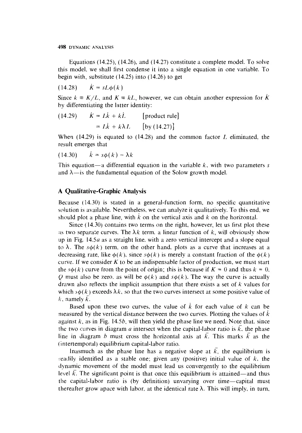
/


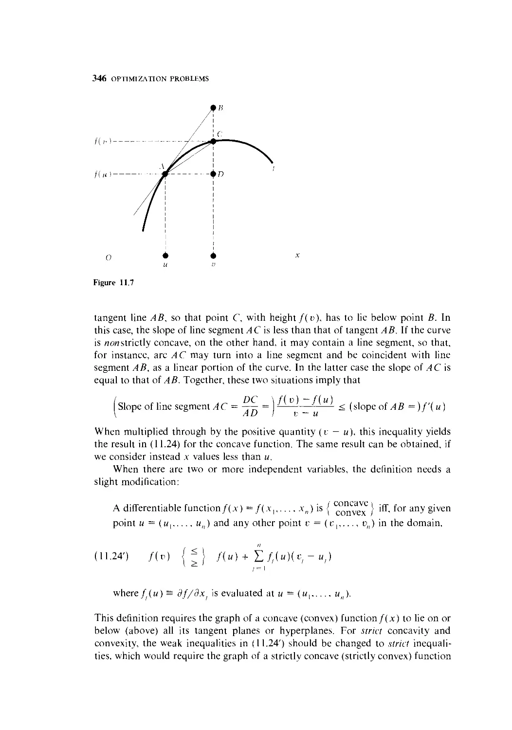
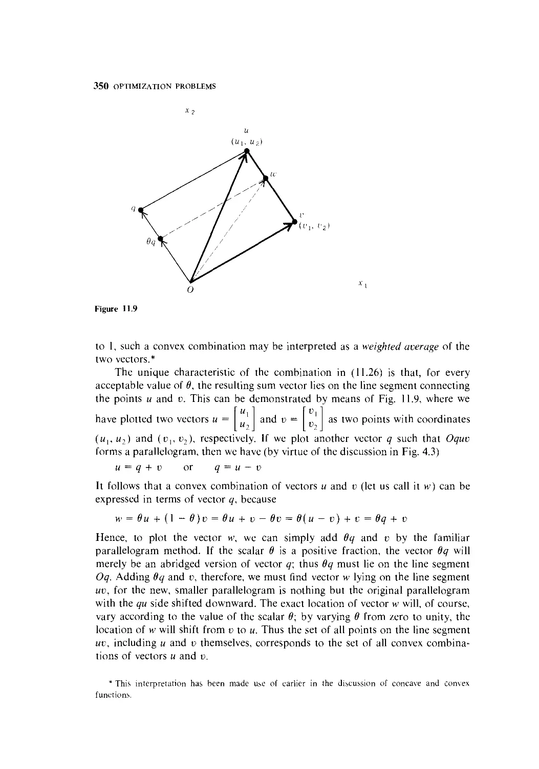


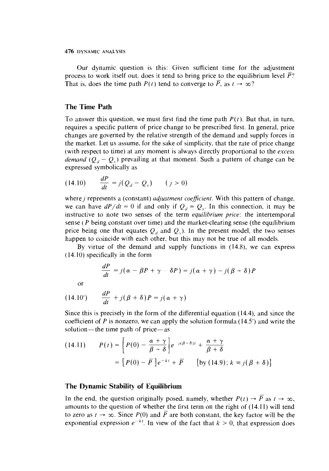


Text
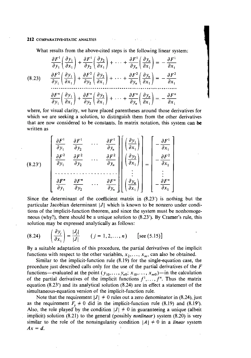
FUNDAMENTAL METHODS OF
MATHEMATICAL ECONOMICS
Alpha C. Chiang
FUNDAMENTAL
METHODS OF
MATHEMATICAL
ECONOMICS
Third Edition
Alpha C. Chiang
Professor of Economics
The University of Connecticut
McGraw-Hill, Inc.
New York St. Louis San Francisco Auckland Bogota
Caracas Lisbon London Madrid Mexico City Milan
Montreal New Delhi San Juan Singapore
Sydney Tokyo Toronto
This book was set in Times Roman b\ Science T\pographers, Inc.
The editors were Patricia A. Mitchell and Gail Ga\ert.
the production supervisor was Leroy A. Young
The cover was designed by Carla Bauer.
FUNDAMENTAL METHODS OF MATHEMATICAL ECONOMICS
Copyright '<-: 1984, 1974, 1967 by McGraw-Hill, Inc All rights reserved.
Printed in the United States of America. Except as permitted under the
United States Copyright Act of 1976. no pan of this publication may be
reproduced or distributed in any form or b\ an\ means, or stored in a data
base or retrieval system, without the prior written permission of the
publisher.
21 22 23 24 25 26 27 28 29 30 FGRFGR 9 9
ISBN 0-07-010513-7
Library of Congress Cataloging in Publication Data
Chiang, Alpha C, date
Fundamental methods of mathematical economics.
Bibliography: p.
Includes index.
1. Economics, Mathematical. 1. Titk.
HB135.C47 1984 33O'.O1'51 83-19609
ISBN 0-07-010813-7
This book is printed on acid-free paper.
CONTENTS
Preface
Part 1 Introduction
1 The Nature of Mathematical Economics 3
1.1 Mathematical versus Nonmathematical Economics 3
1.2 Mathematical Economics versus Econometrics 5
2 Economic Models 7
2.1 Ingredients of a Mathematical Model 7
2.2 The Real-Number System 10
2.3 The Concept of Sets 11
2.4 Relations and Functions 17
2.5 Types of Function 23
2.6 Functions of Two or More Independent Variables 29
2.7 Levels of Generality 31
Part 2 Static (or Equilibrium) Analysis
3 Equilibrium Analysis in Economics 35
3.1 The Meaning of Equilibrium 35
3.2 Partial Market Equilibrium—A Linear Model 36
VI CONTENTS
3.3 Partial Market Equilibrium—A Nonlinear Model 40
3.4 General Market Equilibrium 46
3.5 Equilibrium in National-Income Analysis 52
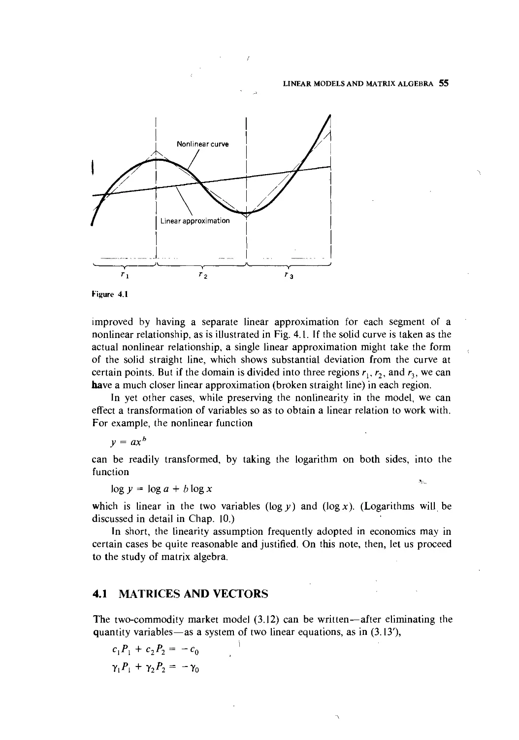
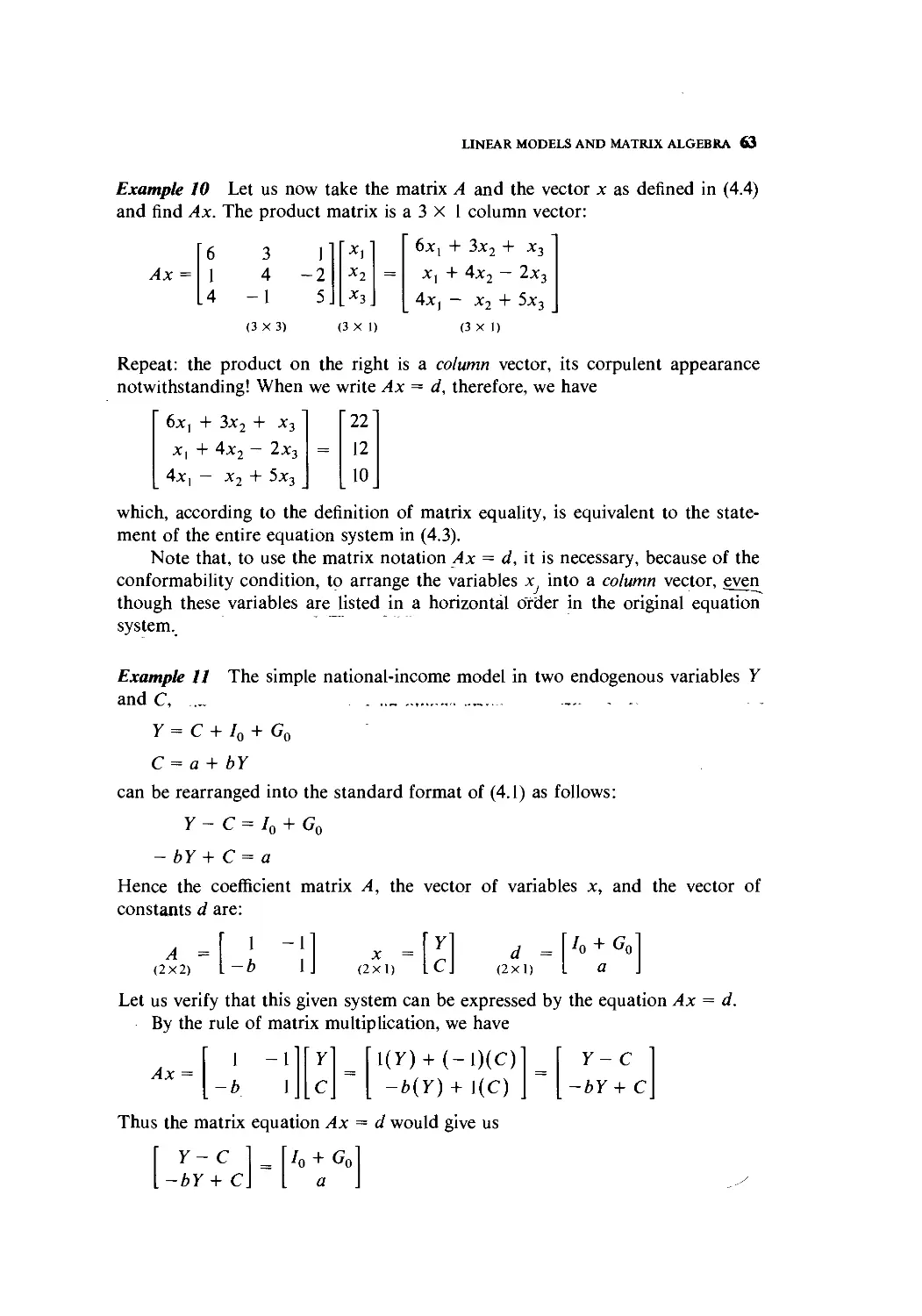
4 Linear Models and Matrix Algebra 54
4.1 Matrices and Vectors 55
4.2 Matrix Operations 58
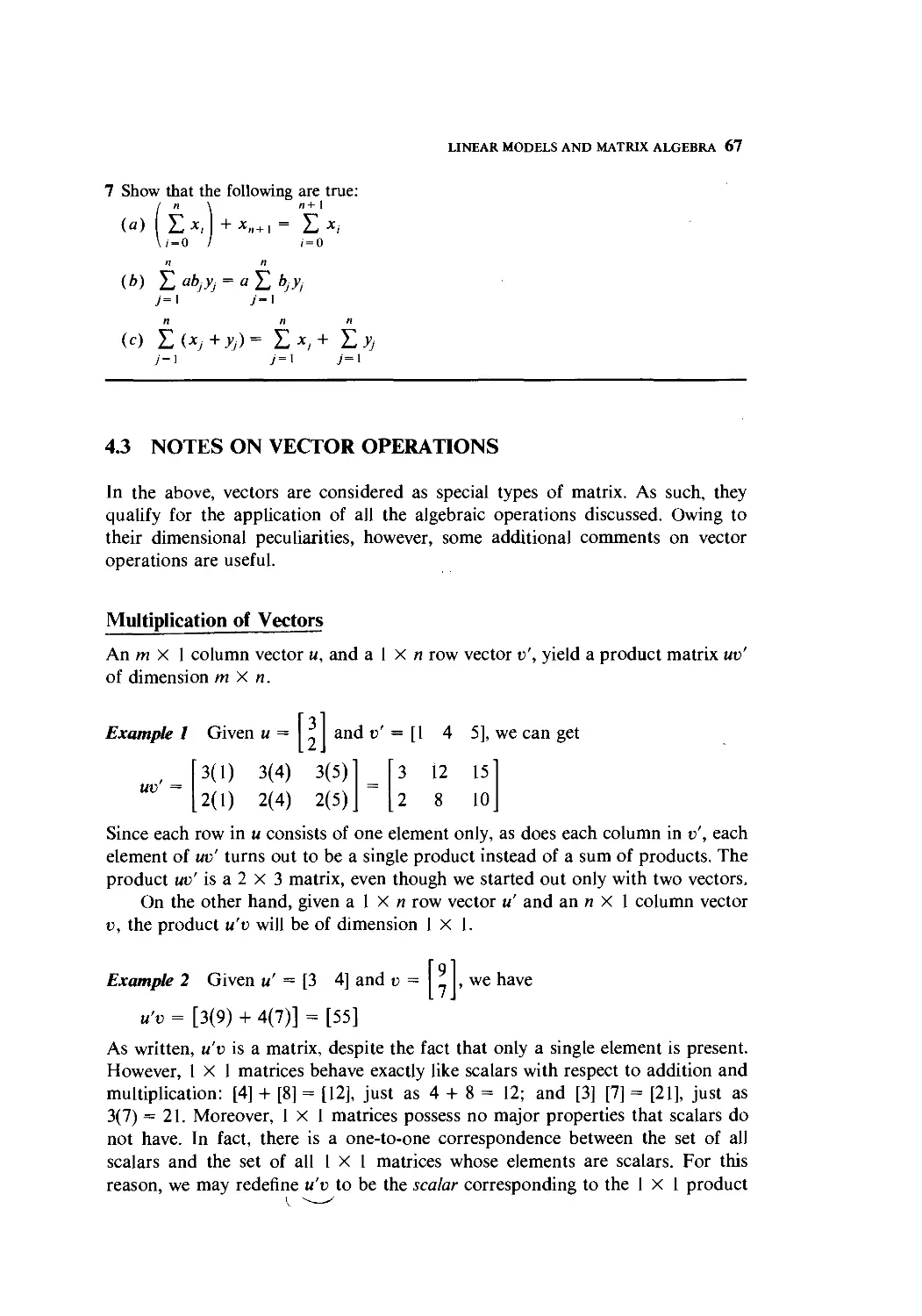
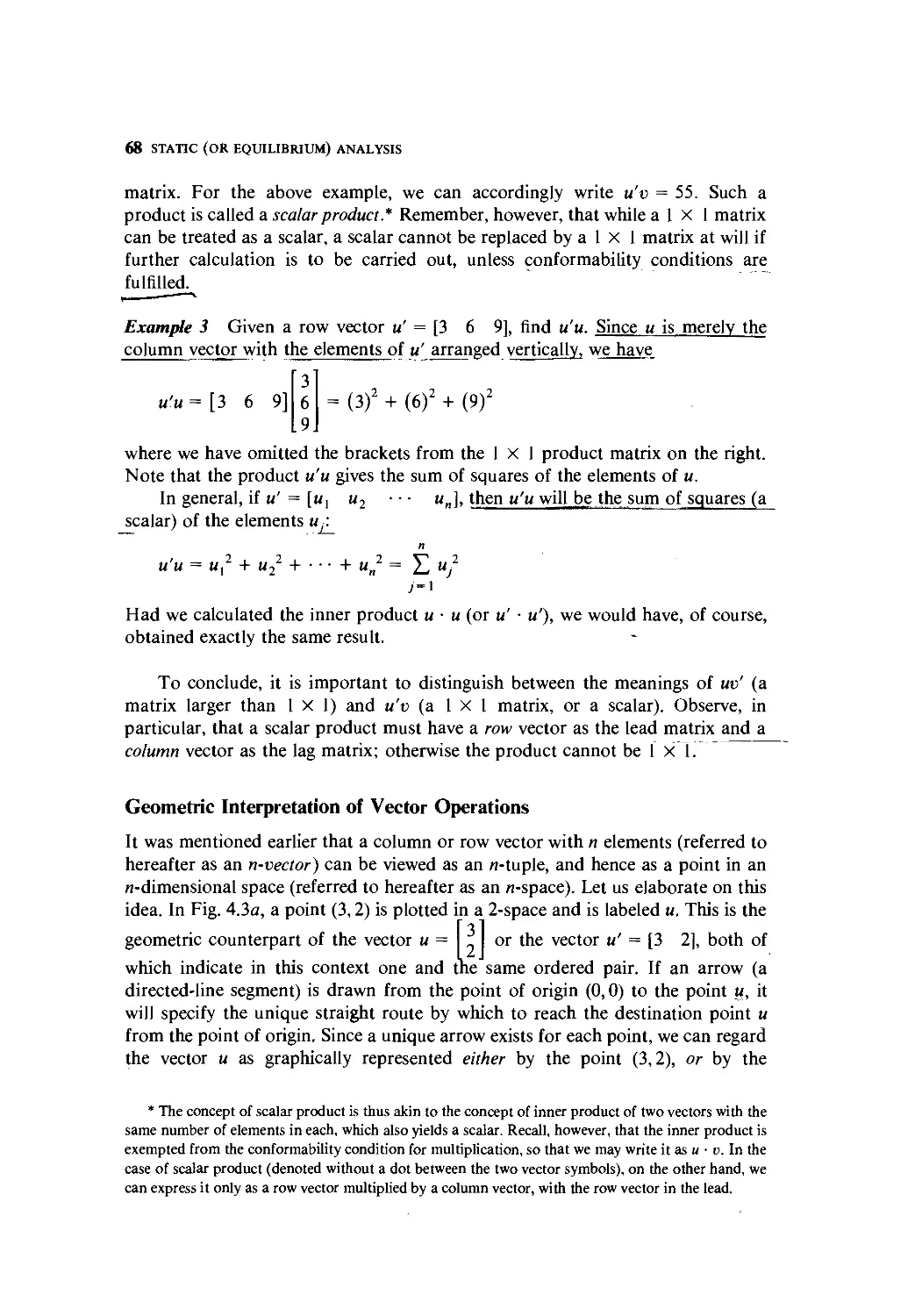
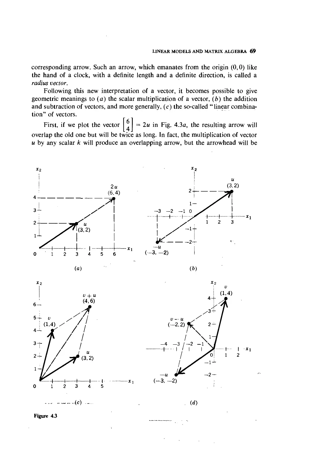
4.3 Notes on Vector Operations 67
4.4 Commutative, Associative, and Distributive Laws 76
4.5 Identity Matrices and Null Matrices 79
4.6 Transposes and Inverses 82
5 Linear Models and Matrix Algebra (Continued) 88
5.1 Conditions for Nonsingularity of a Matrix 88
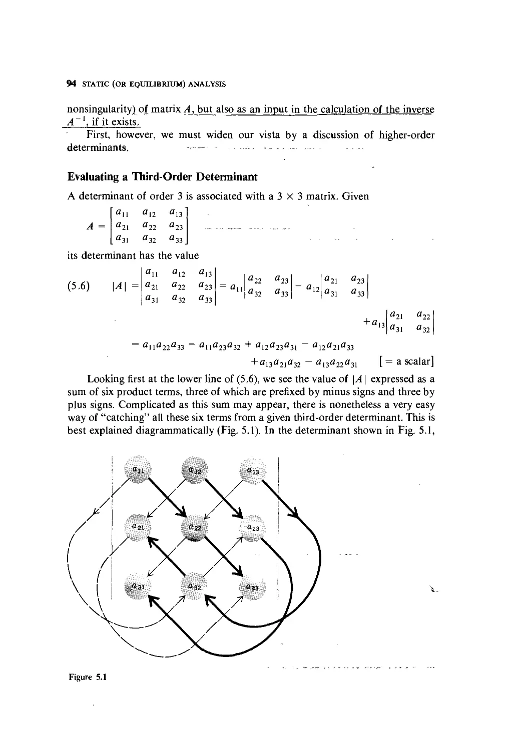
5.2 Test of Nonsingularity by Use of Determinant 92
5.3 Basic Properties of Determinants 98
5.4 Finding the Inverse Matrix 103
5.5 Cramer's Rule 107
5.6 Application to Market and National-Income Models 112
5.7 Leontief Input-Output Models 115
5.8 Limitations of Static Analysis 124
Part 3 Comparative-Static Analysis
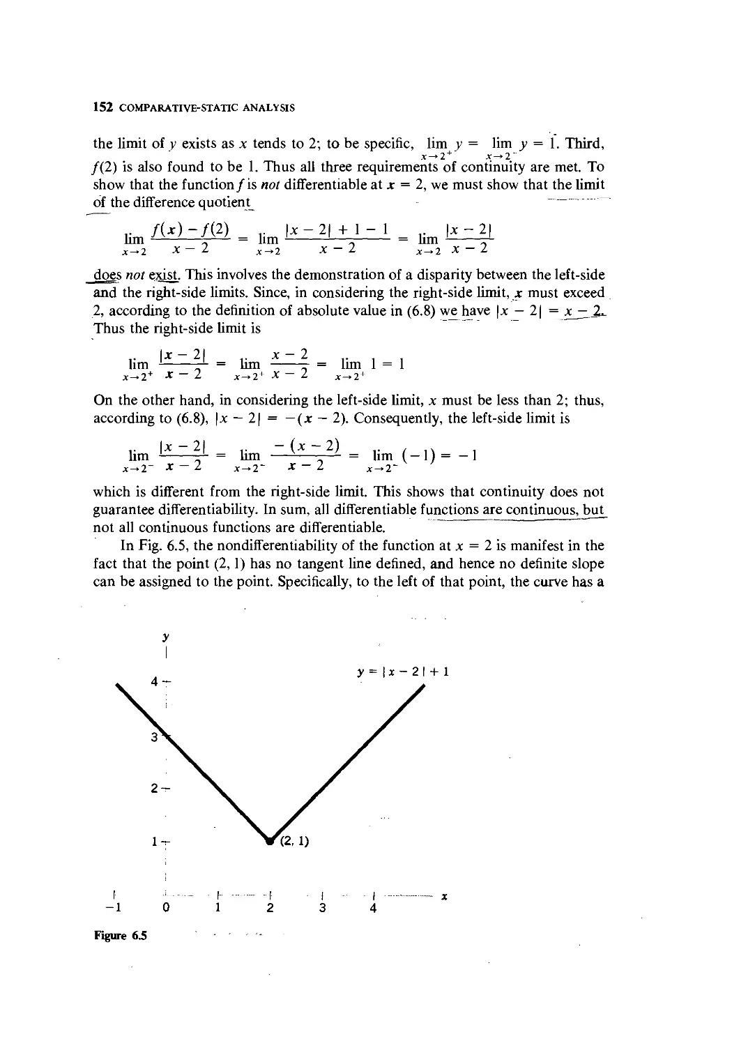
6 Comparative Statics and the Concept
of Derivative 127
6.1 The Nature of Comparative Statics 127
6.2 Rate of Change and the Derivative 128
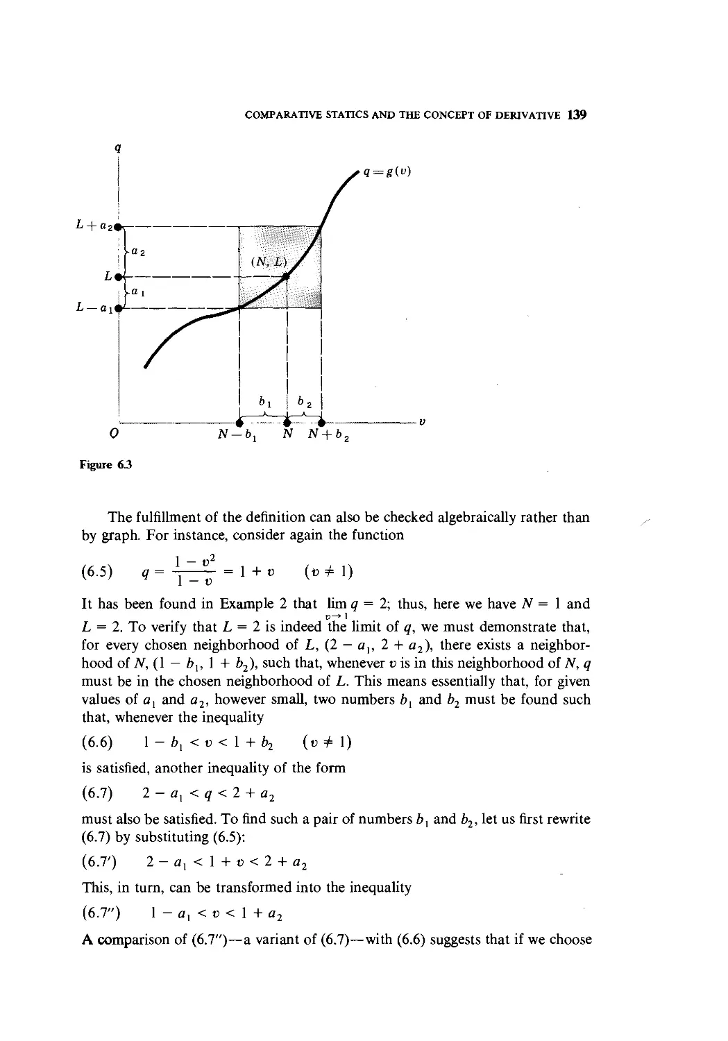
6.3 The Derivative and the Slope of a Curve 131
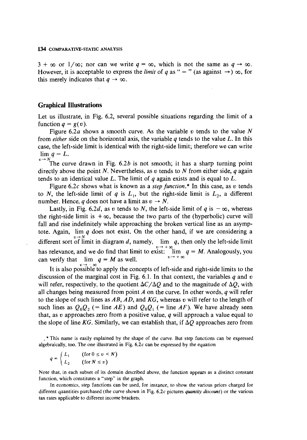
6.4 The Concept of Limit 132
6.5 Digression on Inequalities and Absolute Values 141
6.6 Limit Theorems 145
6.7 Continuity and Differentiability of a Function 147
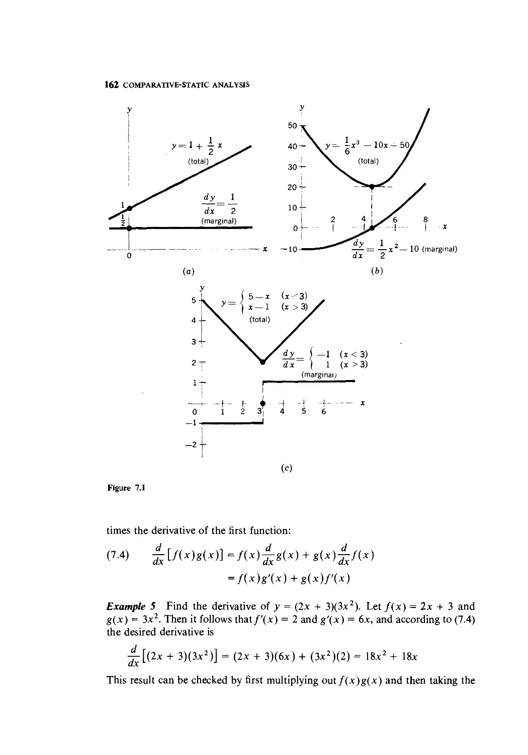
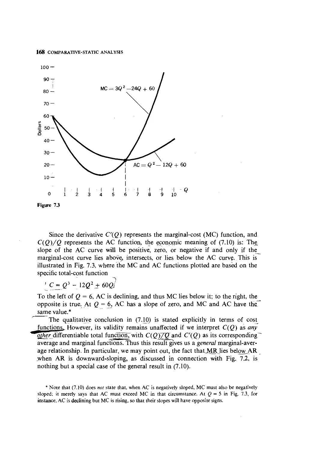
7 Rules of Differentiation and Their Use
in Comparative Statics 155
7.1 Rules of Differentiation for a Function of One Variable 155
7.2 Rules of Differentiation Involving Two or More
Functions of the Same Variable 159
7.3 Rules of Differentiation Involving Functions of
Different Variables 169
7.4 Partial Differentiation 174
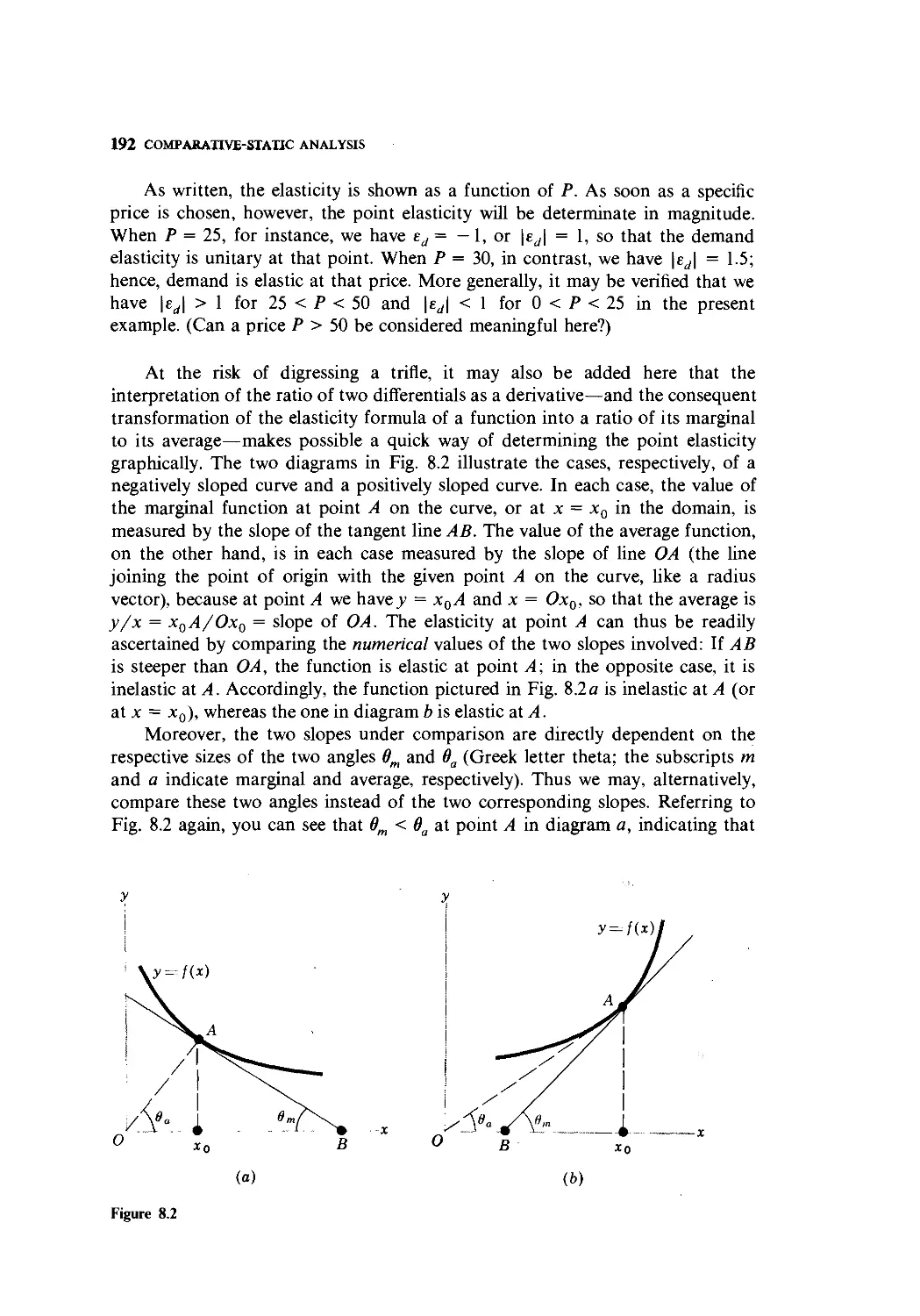
7.5 Applications to Comparative-Static Analysis 178
7.6 Note on Jacobian Determinants 184
CONTENTS Vll
8 Comparative-Static Analysis of
General-Function Models 187
8.1 Differentials 188
8.2 Total Differentials 194
8.3 Rules of Differentials 196
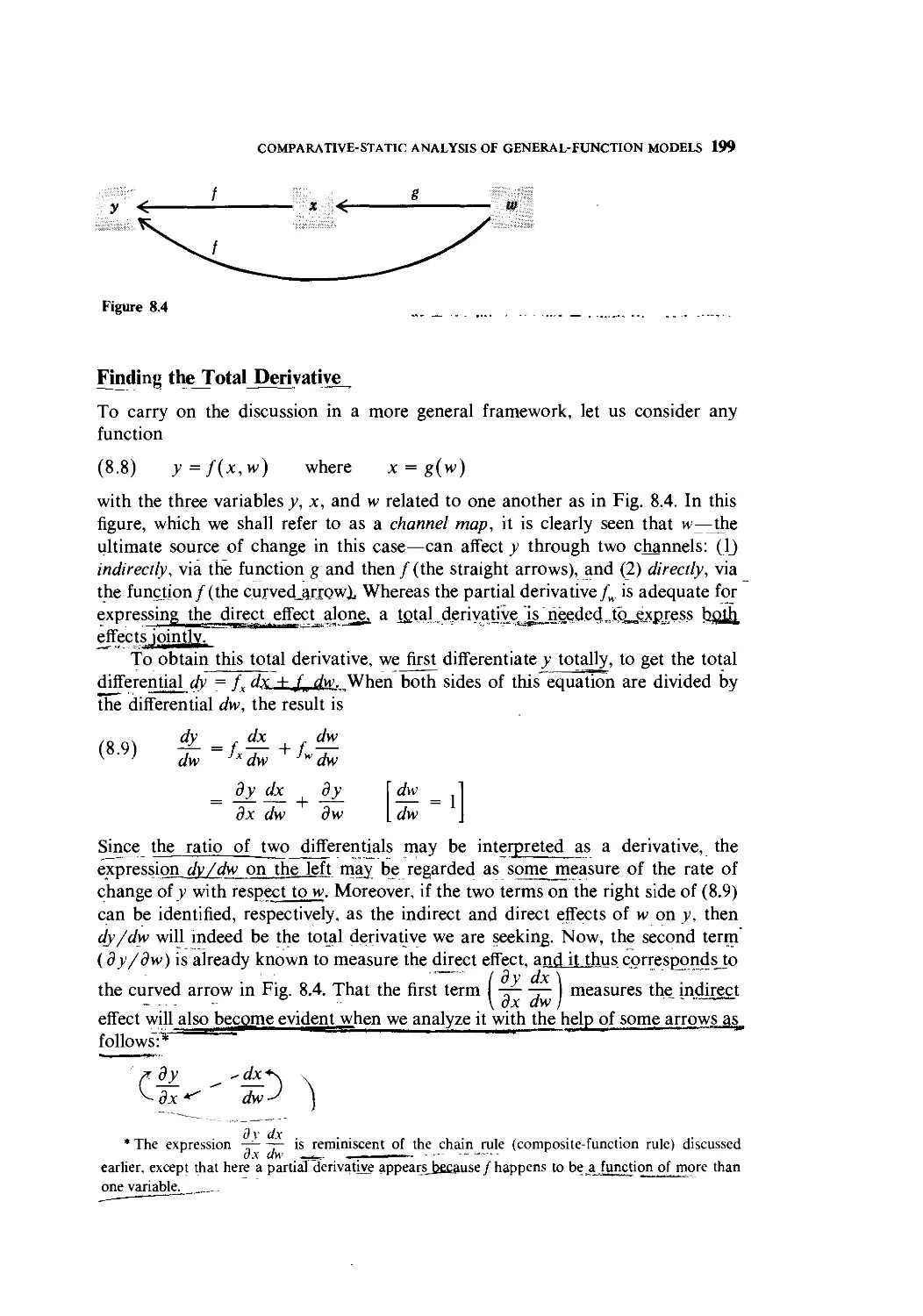
8.4 Total Derivatives 198
8.5 Derivatives of Implicit Functions 204
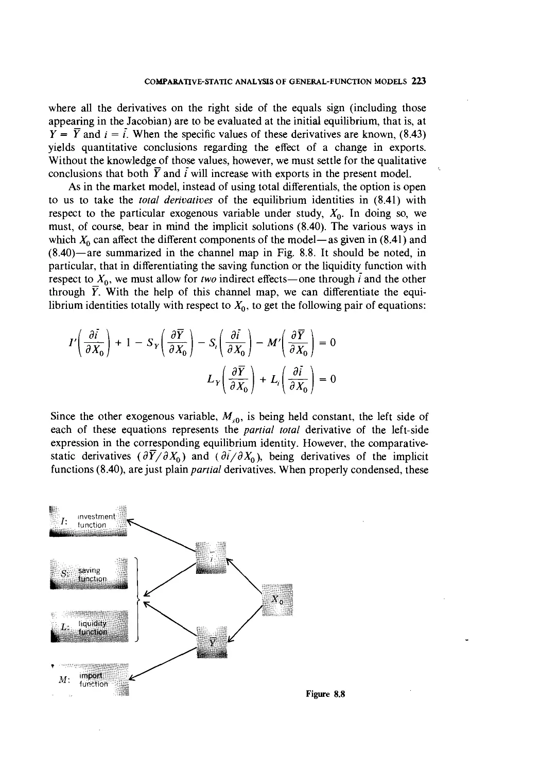
8.6 Comparative Statics of General-Function Models 215
8.7 Limitations of Comparative Statics 226
Part 4 Optimization Problems
9 Optimization: A Special Variety of
Equilibrium Analysis 231
9.1 Optimum Values and Extreme Values 232
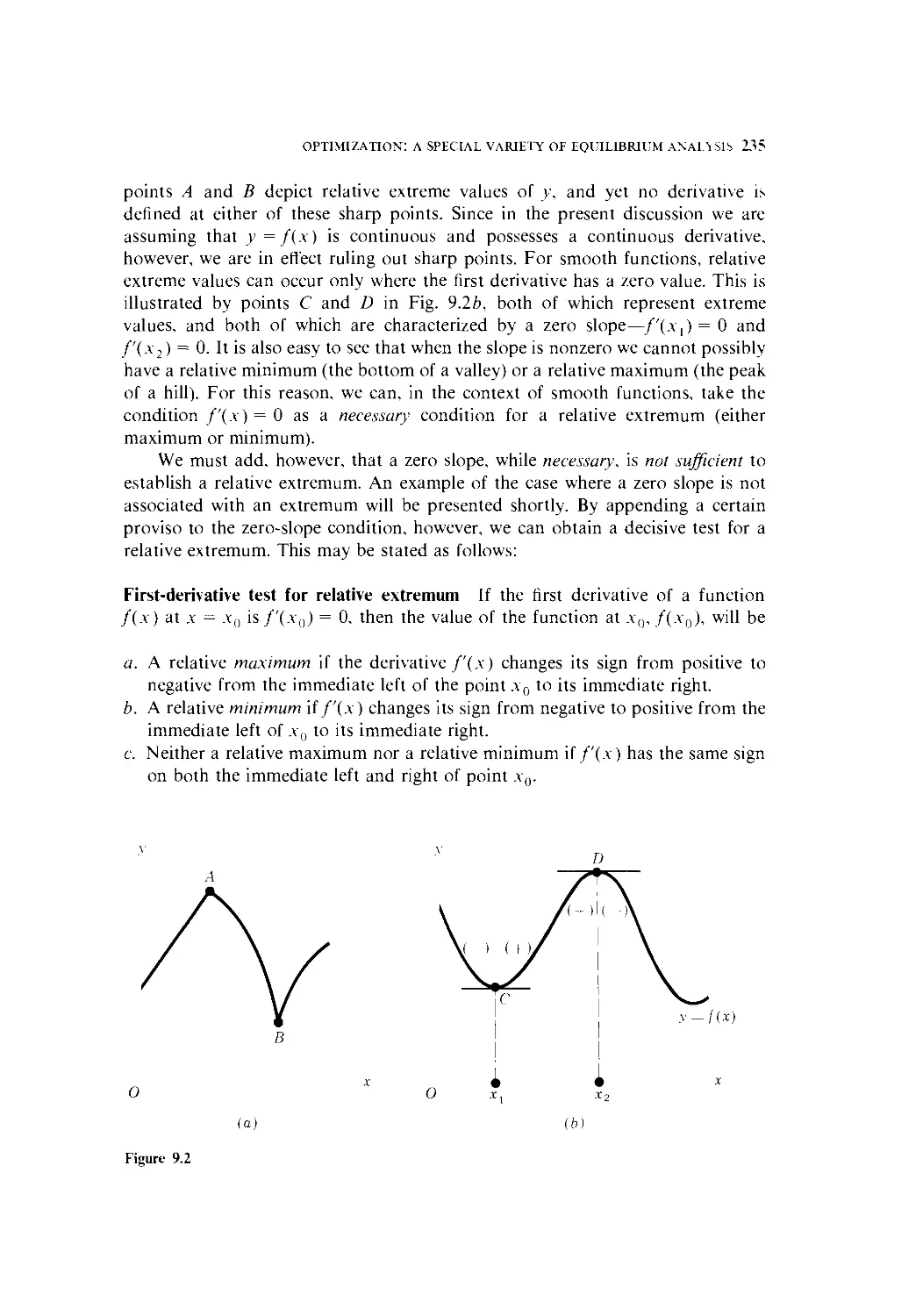
9.2 Relative Maximum and Minimum; First-Derivative Test 233
9.3 Second and Higher Derivatives 239
9.4 Second-Derivative Test 245
9.5 Digression on Maclaurin and Taylor Series 254
9.6 N th-Derivative Test for Relative Extremum of a
Function of One Variable 263
10 Exponential and Logarithmic Functions 268
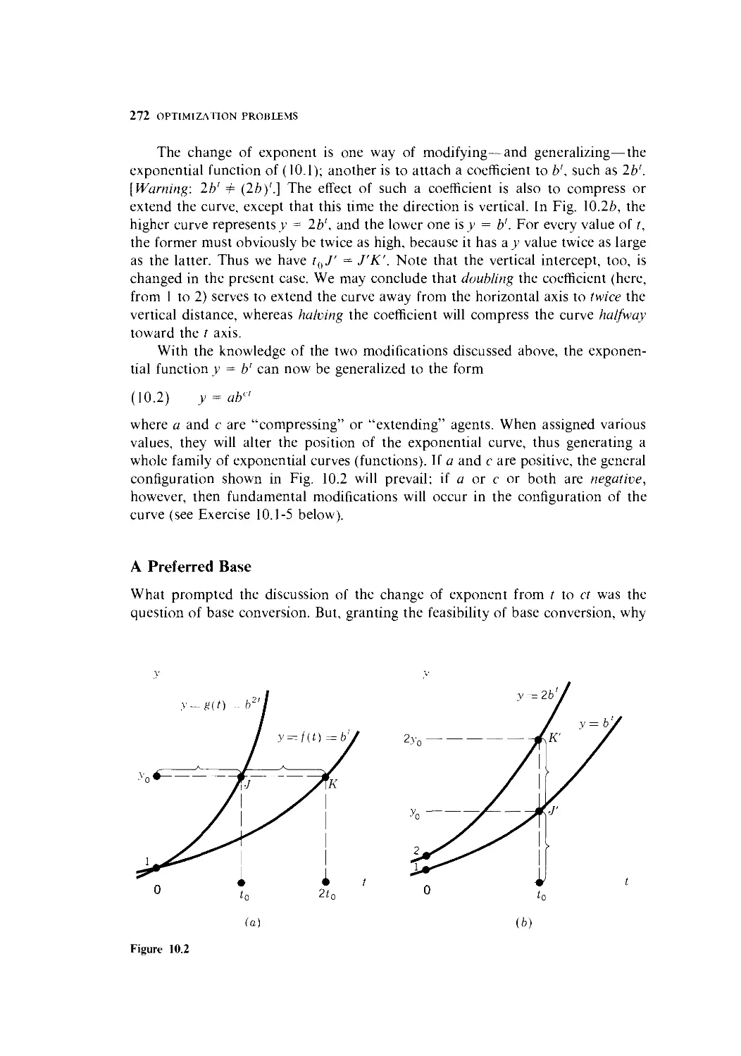
10.1 The Nature of Exponential Functions 269
10.2 Natural Exponential Functions and the Problem
of Growth 274
10.3 Logarithms 282
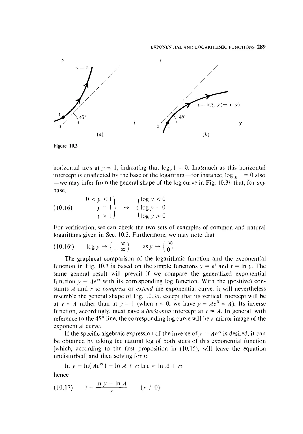
10.4 Logarithmic Functions 287
10.5 Derivatives of Exponential and Logarithmic Functions 292
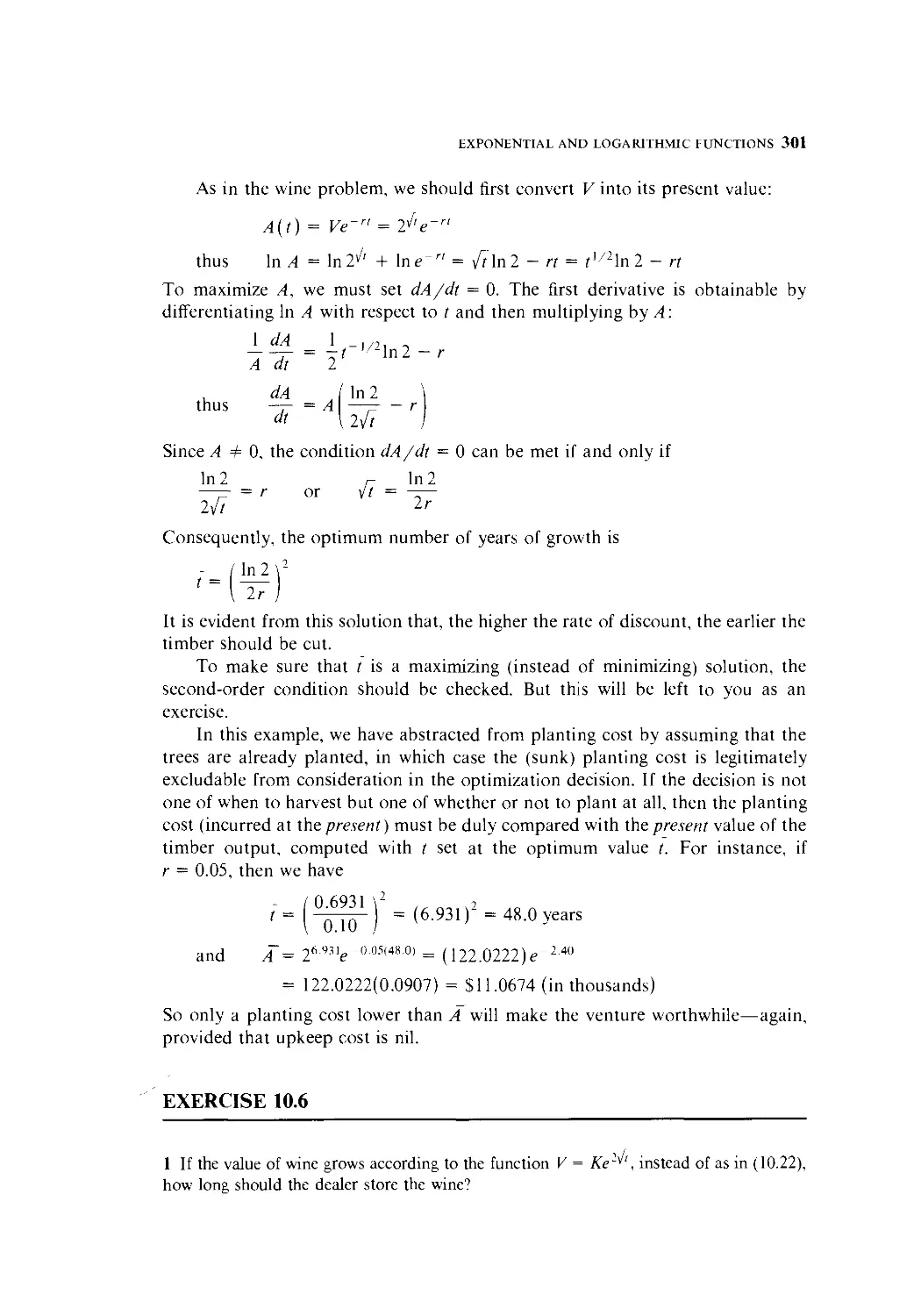
10.6 Optimal Timing 298
10.7 Further Applications of Exponential and
Logarithmic Derivatives 302
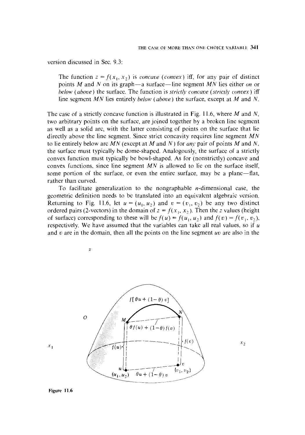
11 The Case of More than One Choice Variable 307
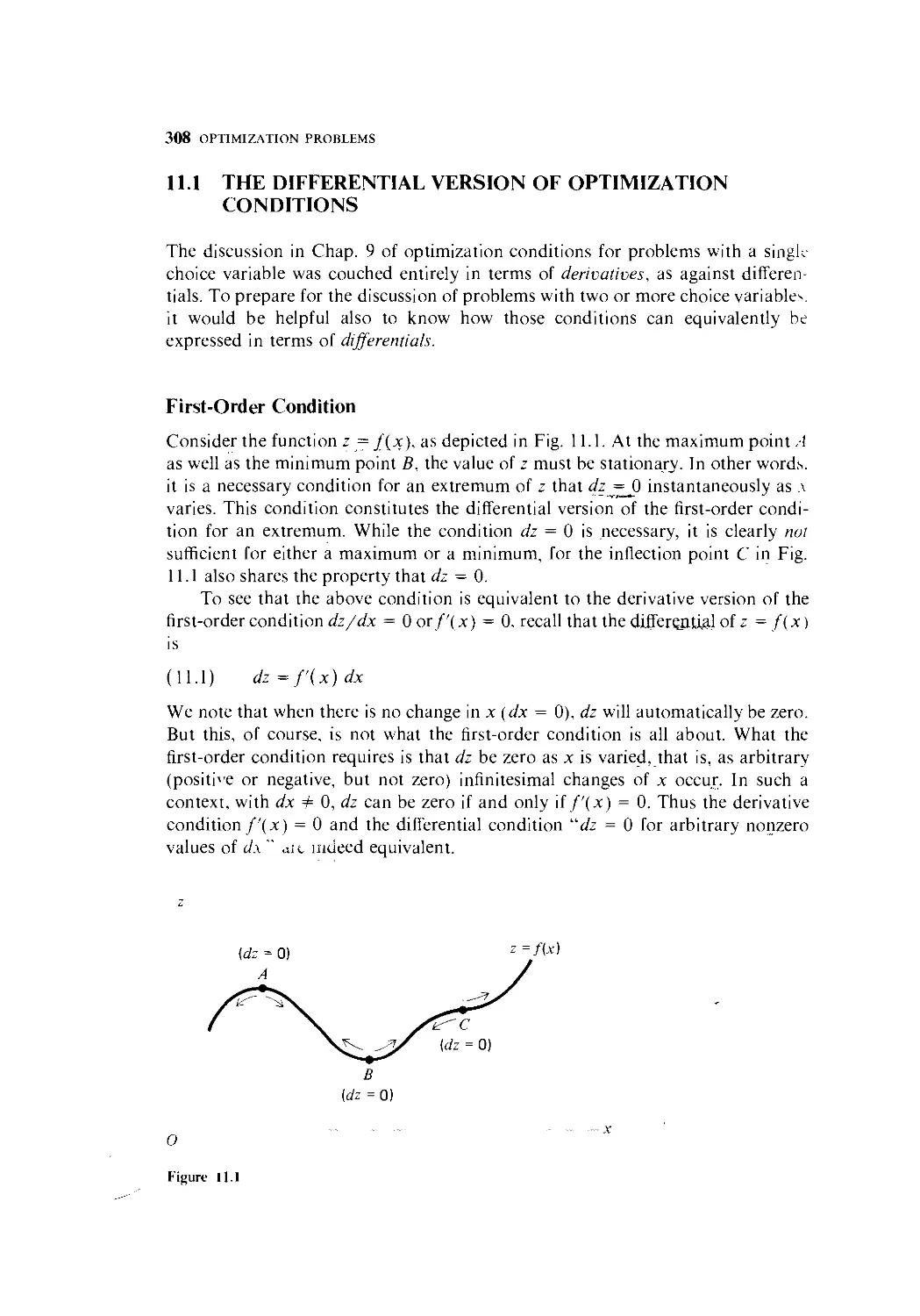
11.1 The Differential Version of Optimization Conditions 308
11.2 Extreme Values of a Function of Two Variables 310
11.3 Quadratic Forms—An Excursion 319
11.4 Objective Functions with More than Two Variables 332
11.5 Second-Order Conditions in Relation to Concavity and Convexity 337
11.6 Economic Applications 353
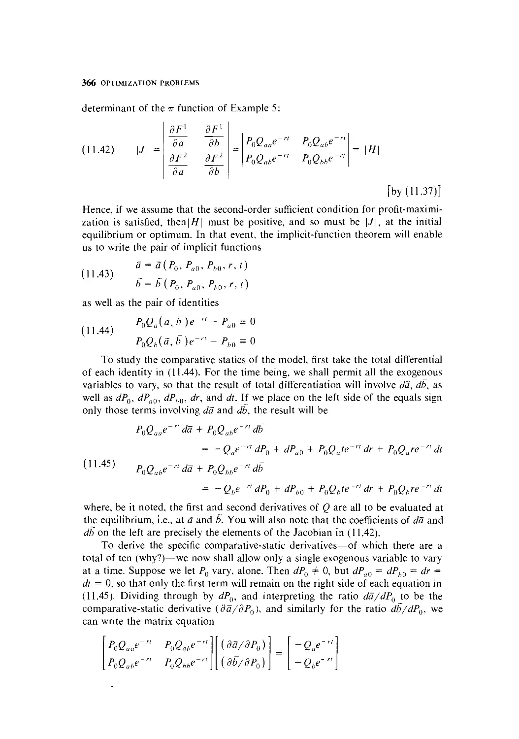
11.7 Comparative-Static Aspects of Optimization 364
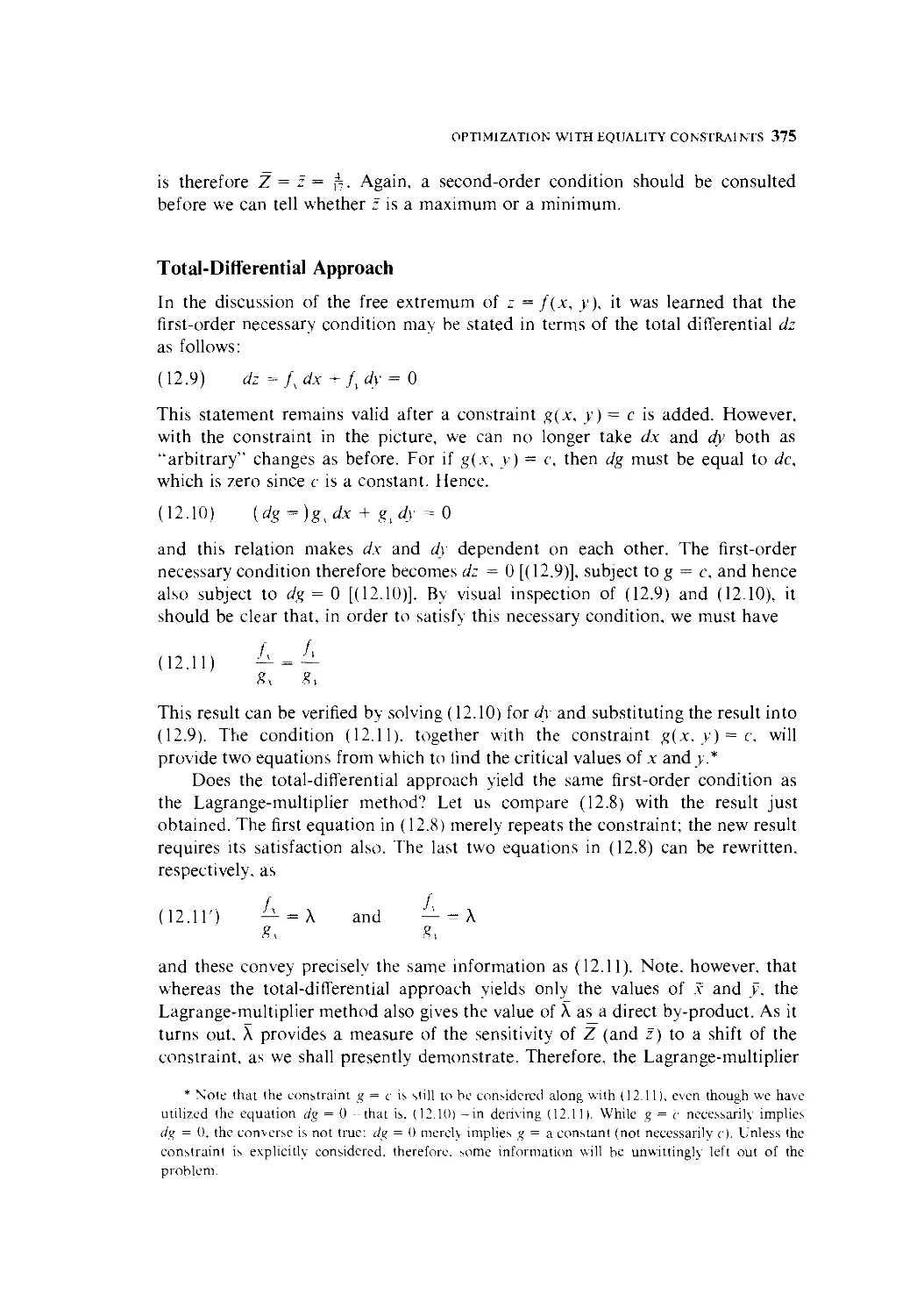
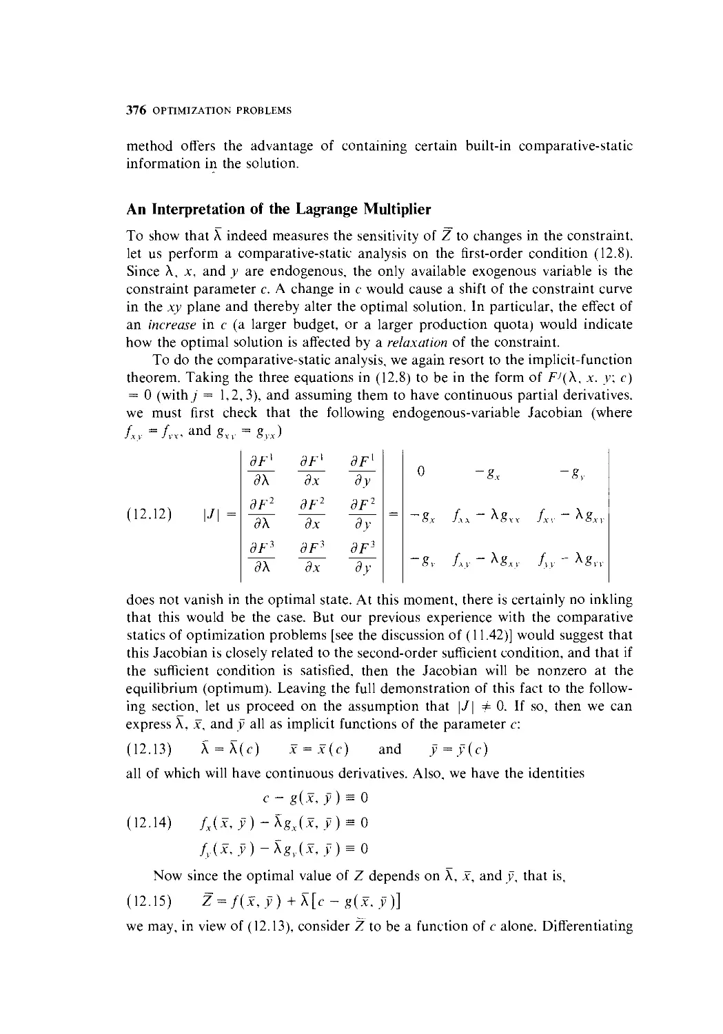
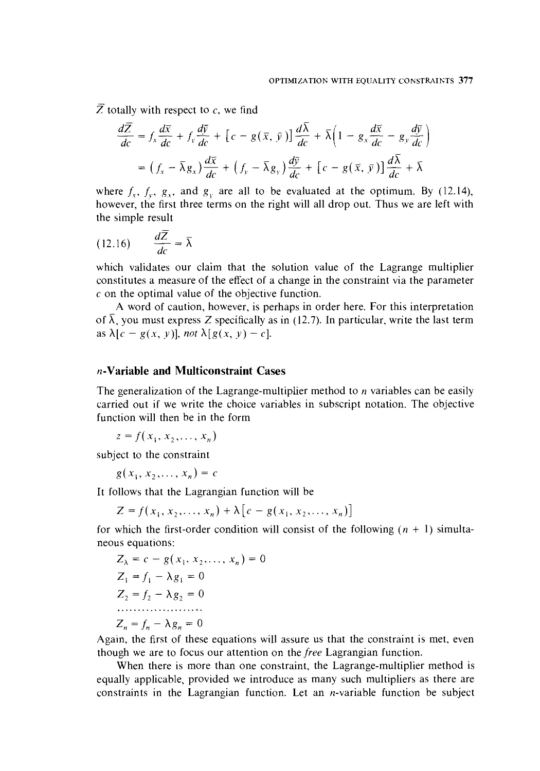
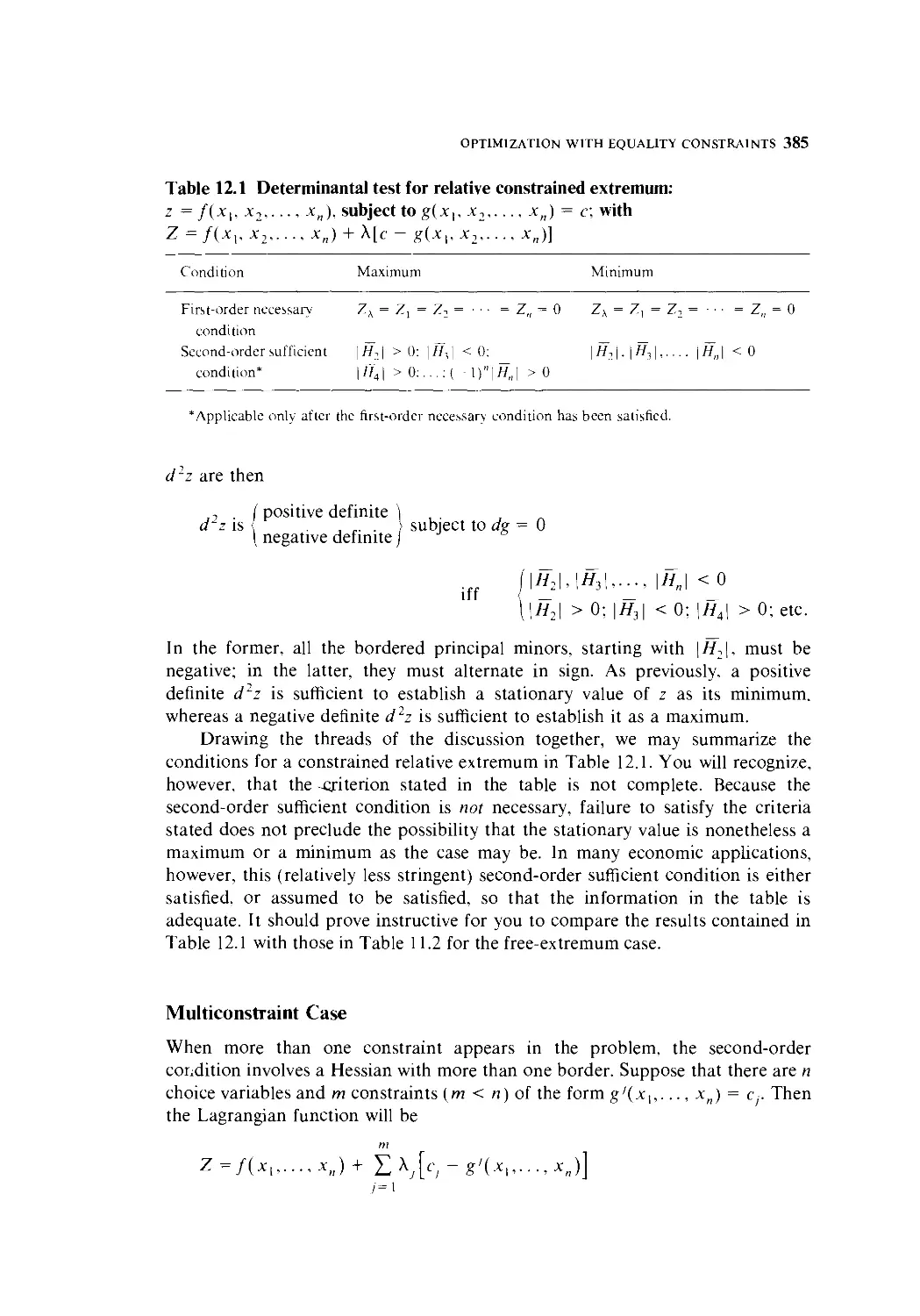
12 Optimization with Equality Constraints 369
12.1 Effects of a Constraint 370
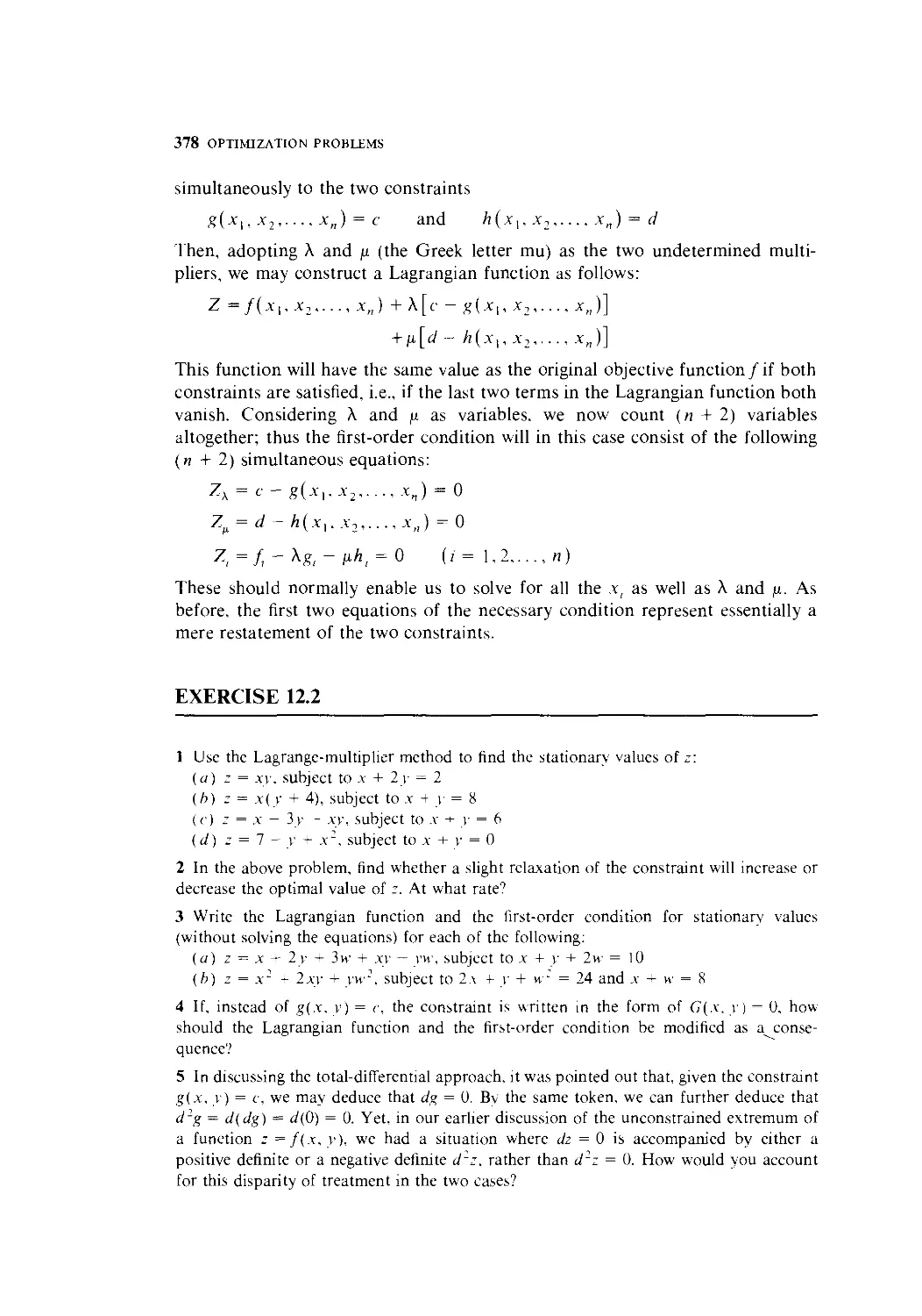
12.2 Finding the Stationary Values 372
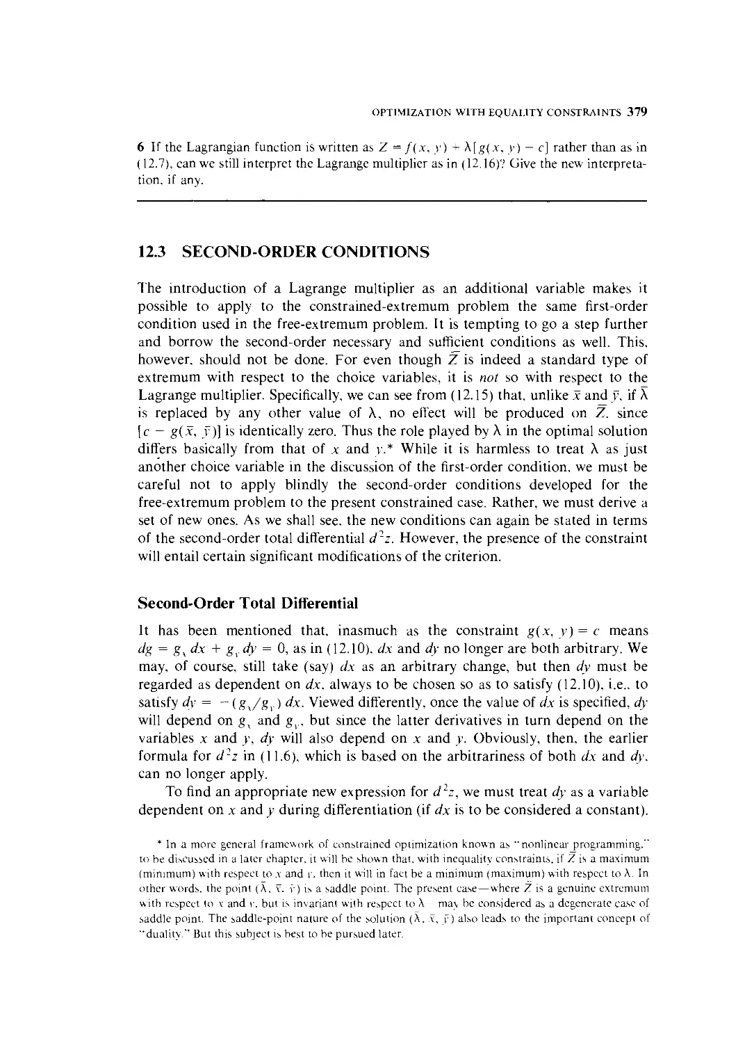
12.3 Second-Order Conditions 379
Vlll CONTENTS
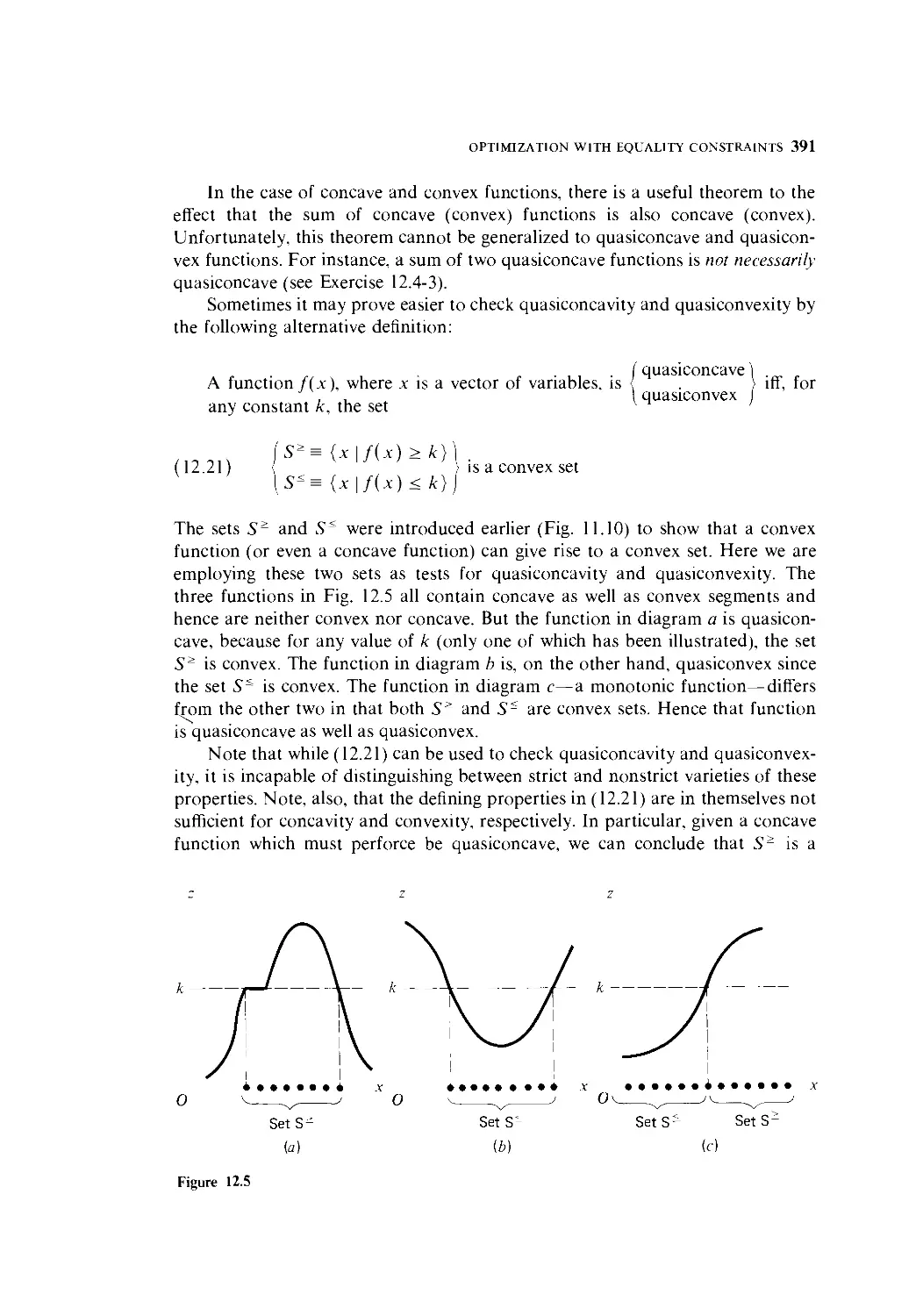
12.4 Quasiconcavity and Quasiconvexity 387
12.5 Utility Maximization and Consumer Demand 400
12.6 Homogeneous Functions 410
12.7 Least-Cost Combination of Inputs 418
12.8 Some Concluding Remarks 431
Part 5 Dynamic Analysis
13 Economic Dynamics and Integral Calculus 435
13.1 Dynamics and Integration 436
13.2 Indefinite Integrals 437
13.3 Definite Integrals 447
13.4 Improper Integrals 454
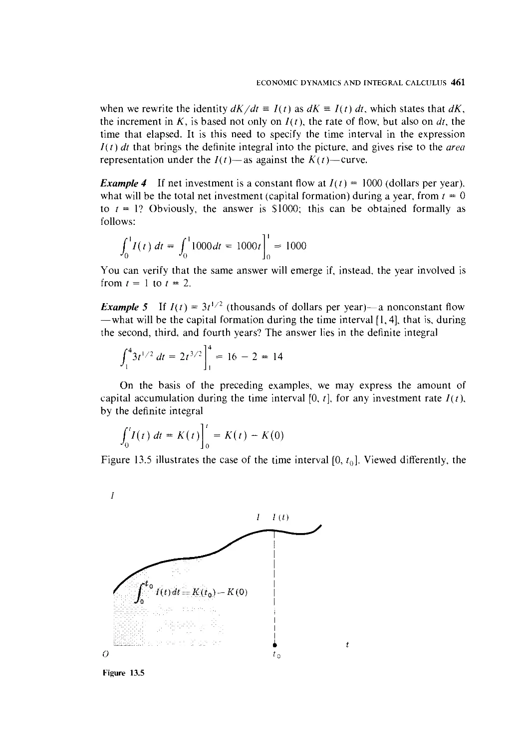
13.5 Some Economic Applications of Integrals 458
13.6 Domar Growth Model 465
14 Continuous Time: First-Order
Differential Equations 470
14.1 First-Order Linear Differential Equations with Constant
Coefficient and Constant Term 470
14.2 Dynamics of Market Price 475
14.3 Variable Coefficient and Variable Term 480
14.4 Exact Differential Equations 483
14.5 Nonlinear Differential Equations of the First Order
and First Degree 489
14.6 The Qualitative-Graphic Approach 493
14.7 Solow Growth Model 496
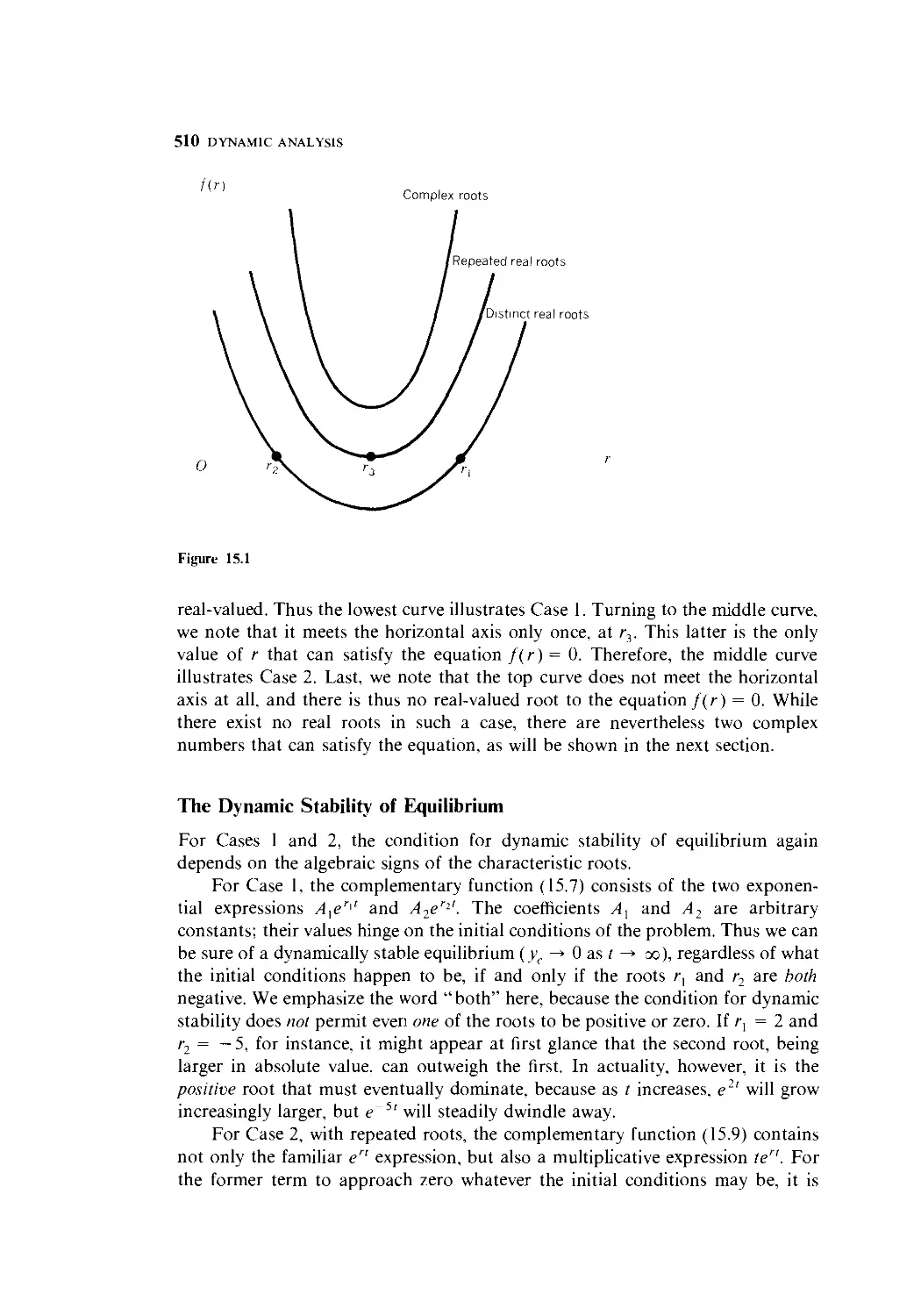
15 Higher-Order Differential Equations 502
15-1 Second-Order Linear Differential Equations with
Constant Coefficients and Constant Term 503
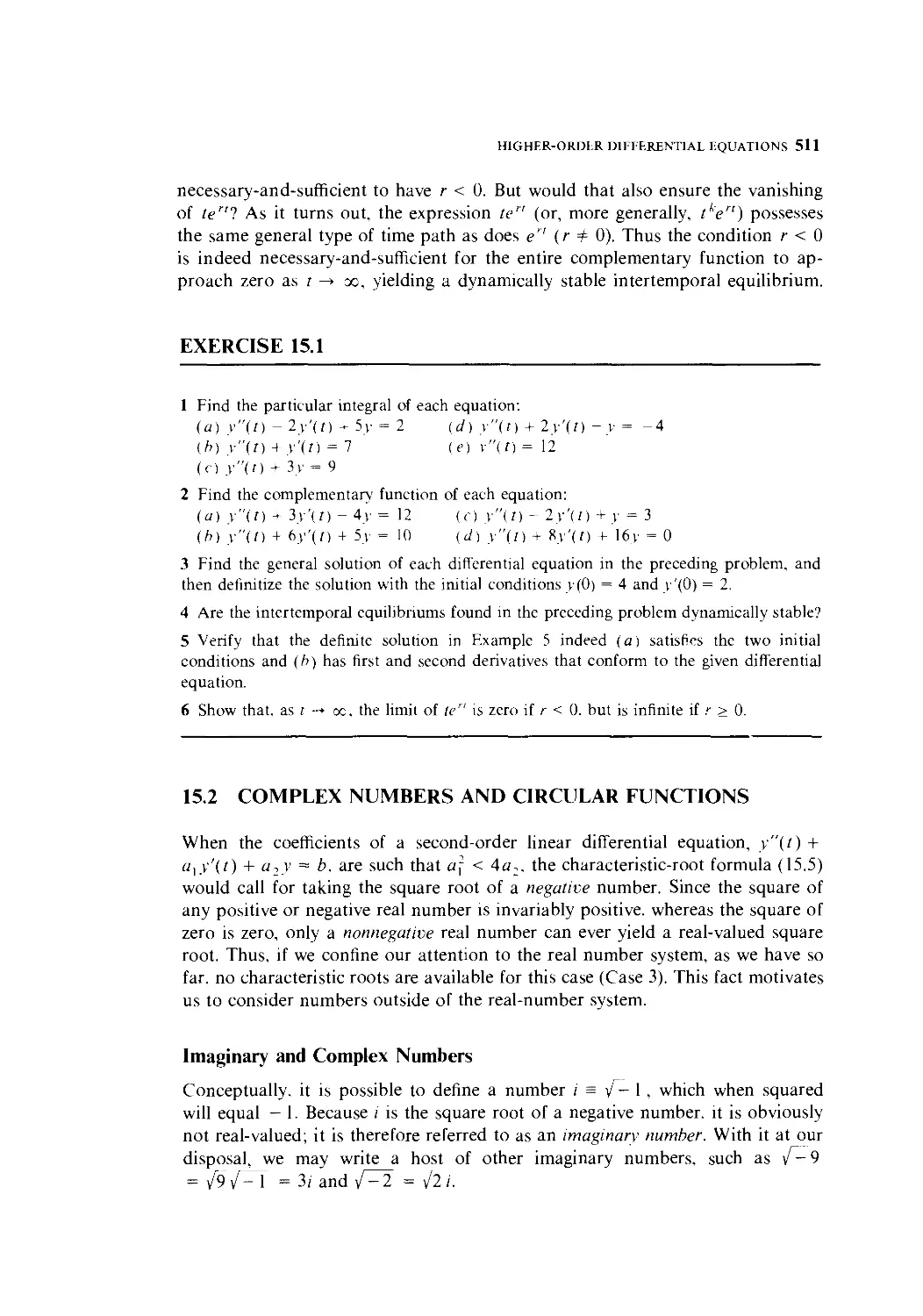
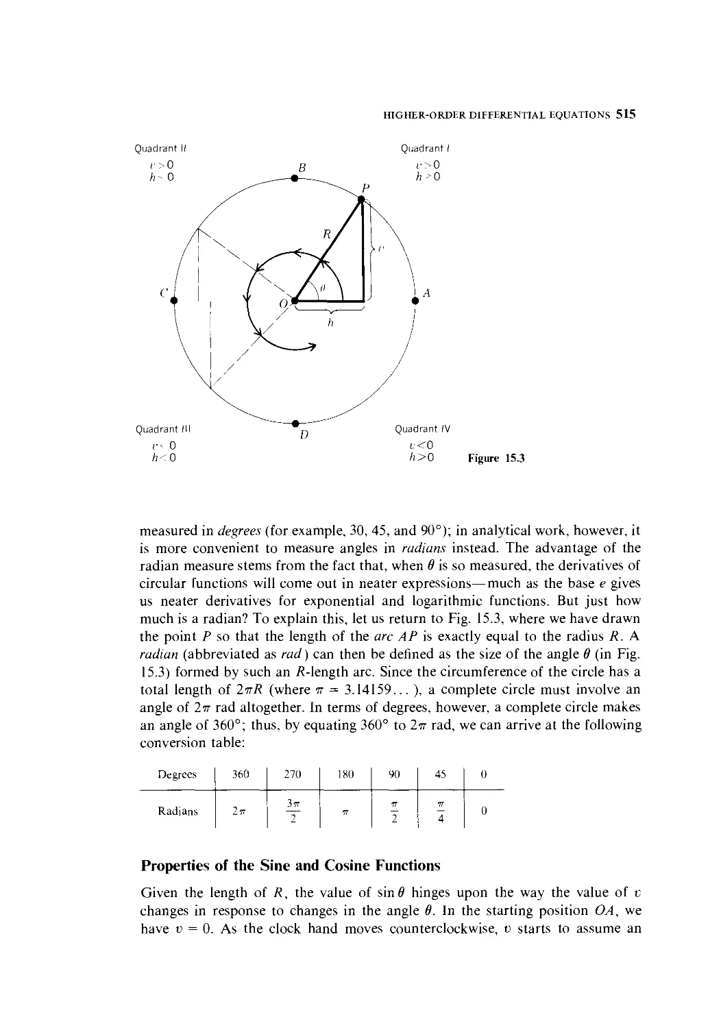
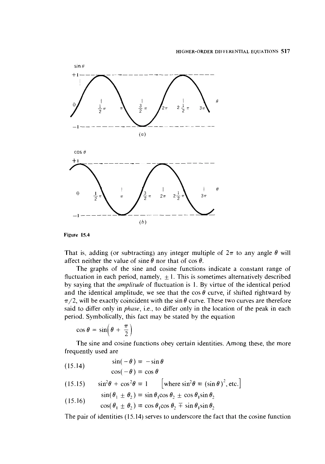
15.2 Complex Numbers and Circular Functions 511
15.3 Analysis of the Complex-Root Case 523
15.4 A Market Model with Price Expectations 529
15.5 The Interaction of Inflation and Unemployment 535
15.6 Differential Equations with a Variable Term 541
15.7 Higher-Order Linear Differential Equations 544
16 Discrete Time: First-Order Difference Equations 549
16.1 Discrete Time, Differences, and Difference Equations 550
16.2 Solving a First-Order Difference Equation 551
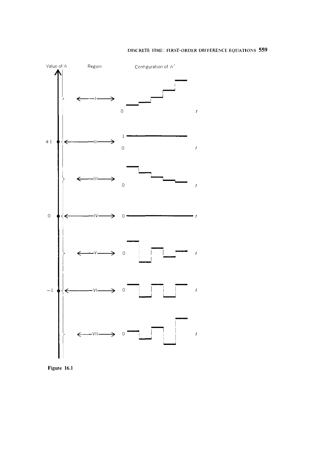
16.3 The Dynamic Stability of Equilibrium 557
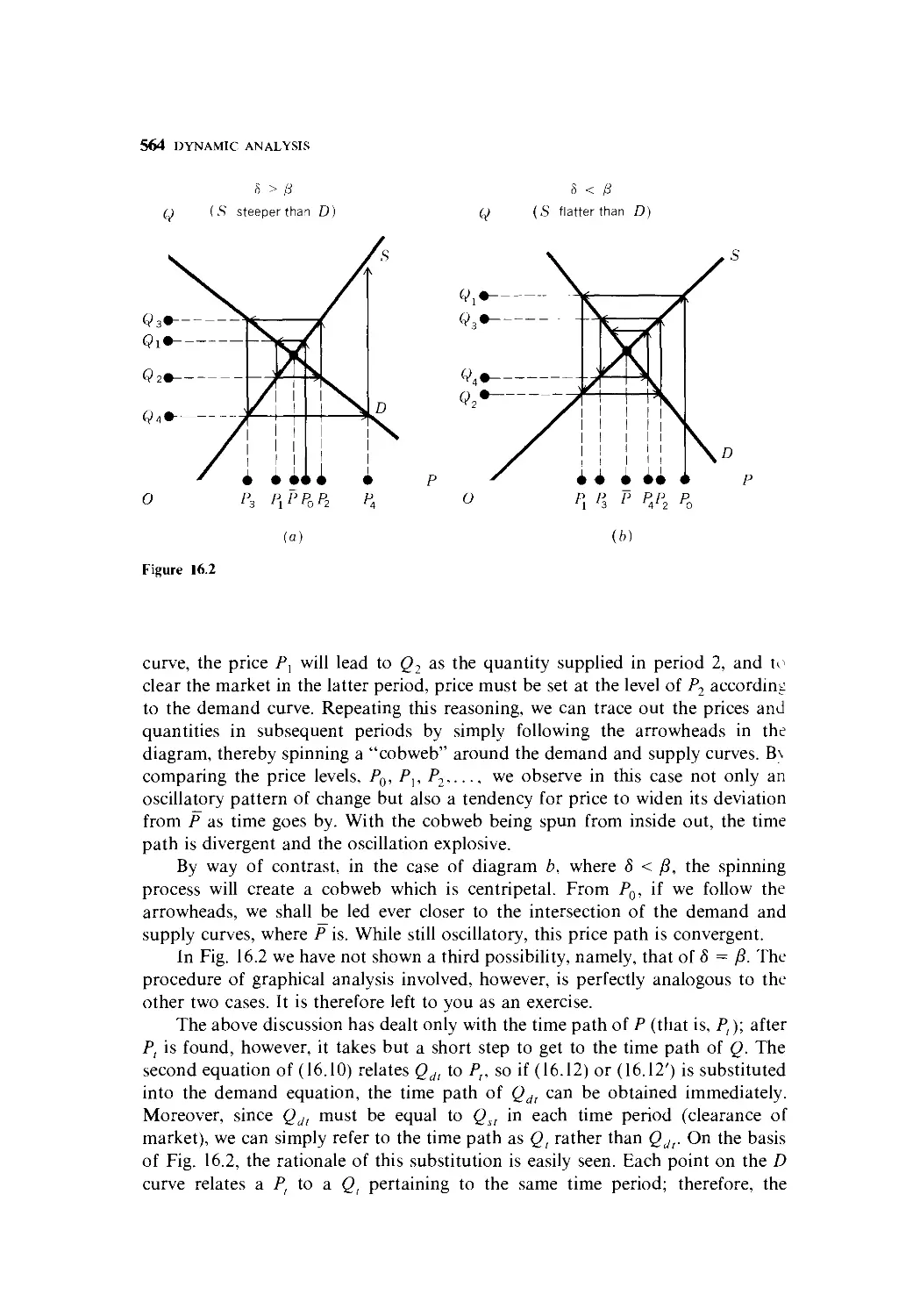
16.4 The Cobweb Model 561
16.5 A Market Model with Inventory 566
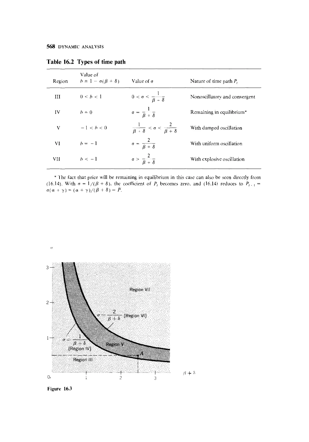
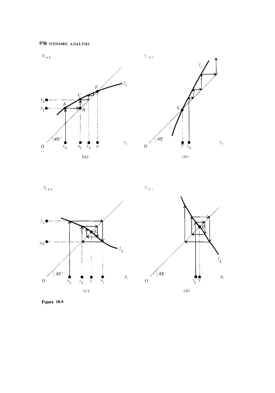
16.6 Nonlinear Difference Equations—The Qualitative-Graphic Approach 569
CONTENTS IX
17 Higher-Order Difference Equations 576
17.1 Second-Order Linear Difference Equations with Constant
Coefficients and Constant Term 577
17.2 Samuelson Multiplier-Acceleration Interaction Model 585
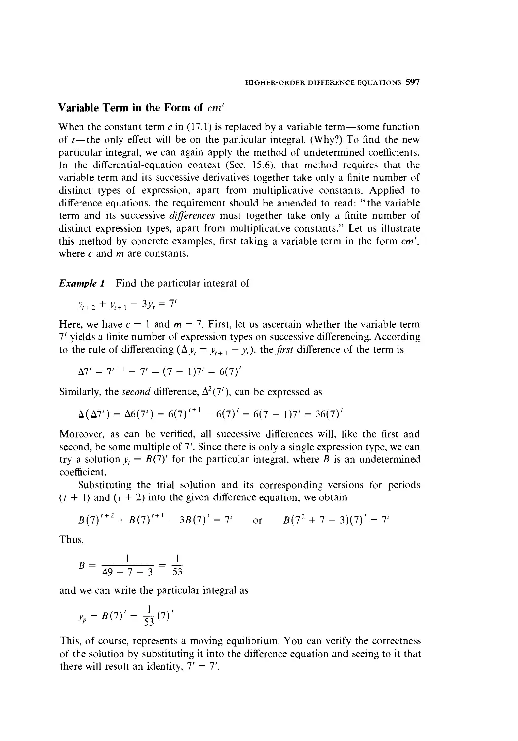
17.3 Inflation and Unemployment in Discrete Time 591
17.4 Generalizations to Variable-Term and Higher-Order Equations 596
18 Simultaneous Differential Equations and
Difference Equations 605
18.1 The Genesis of Dynamic Systems 605
18.2 Solving Simultaneous Dynamic Equations 608
18.3 Dynamic Input-Output Models 616
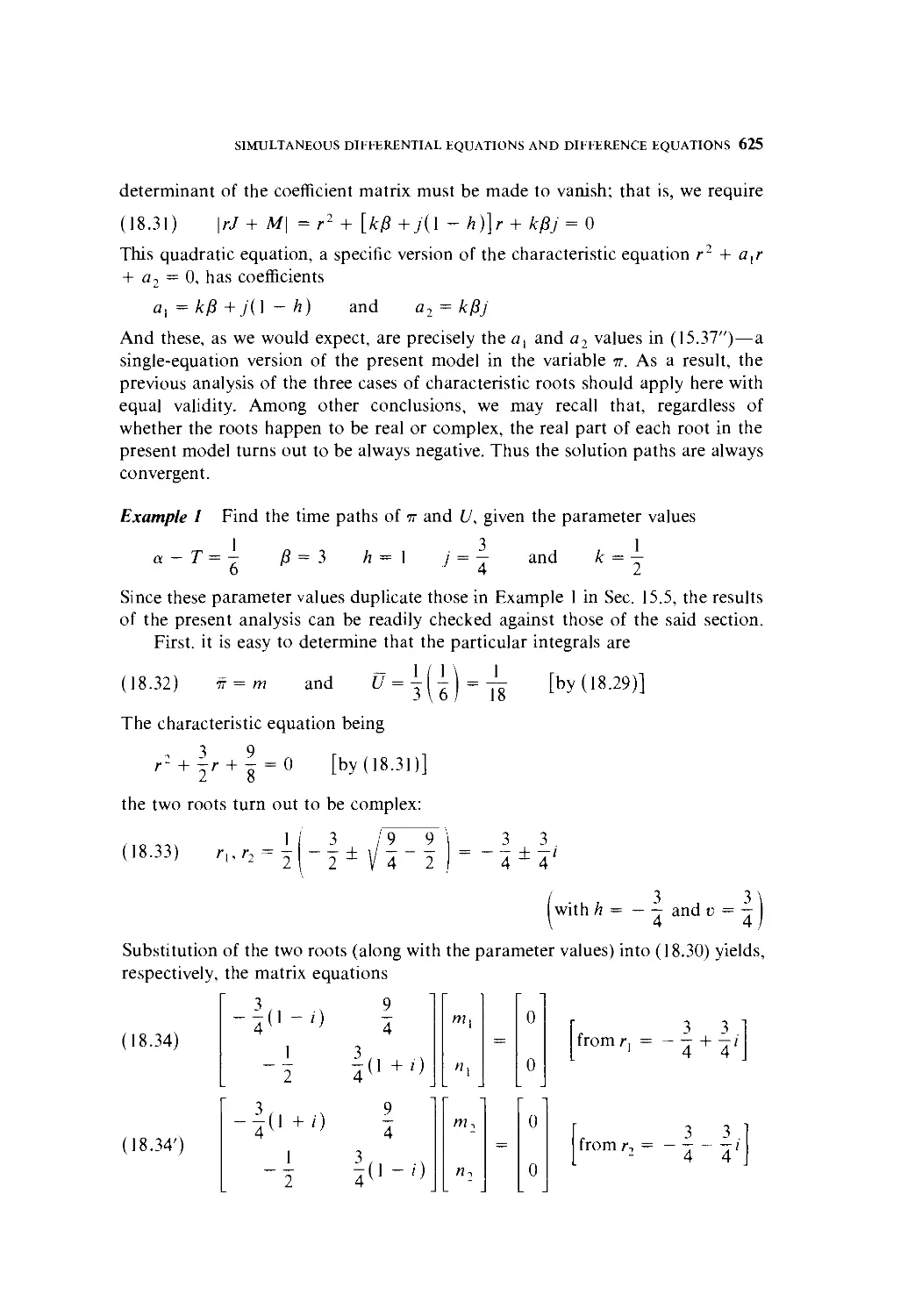
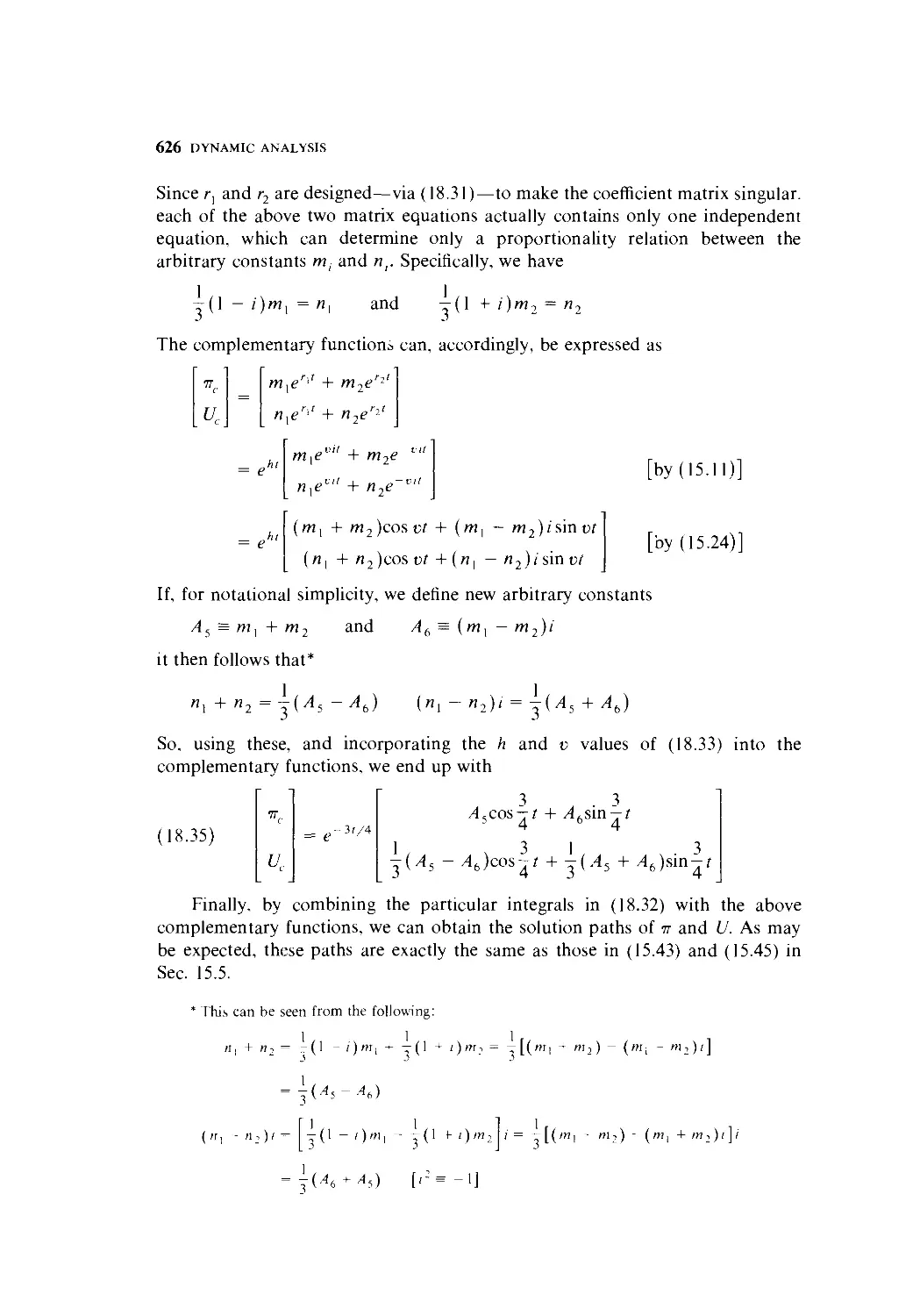
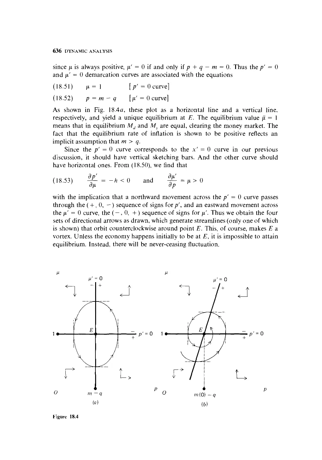
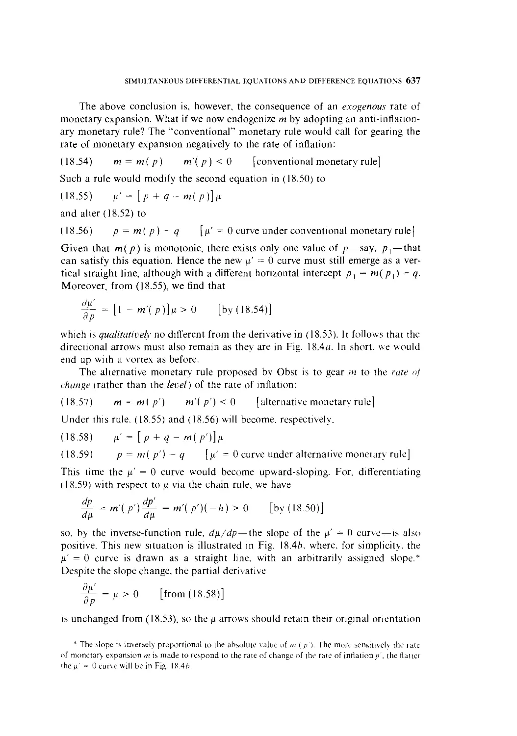
18.4 The Inflation-Unemployment Model Once More 623
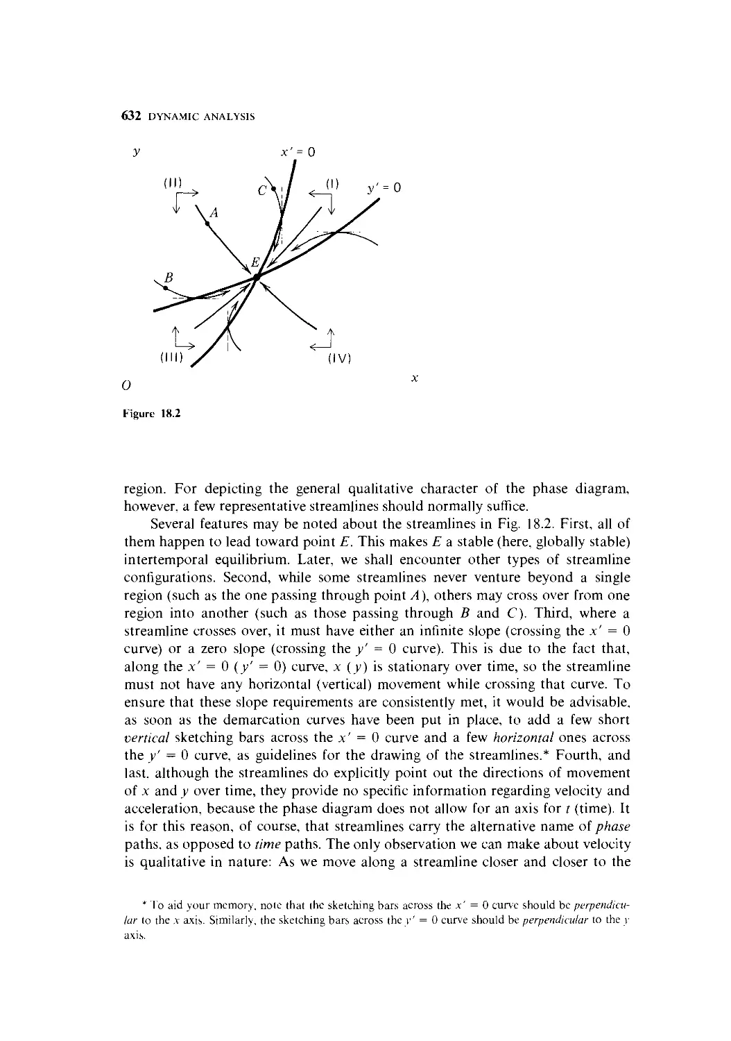
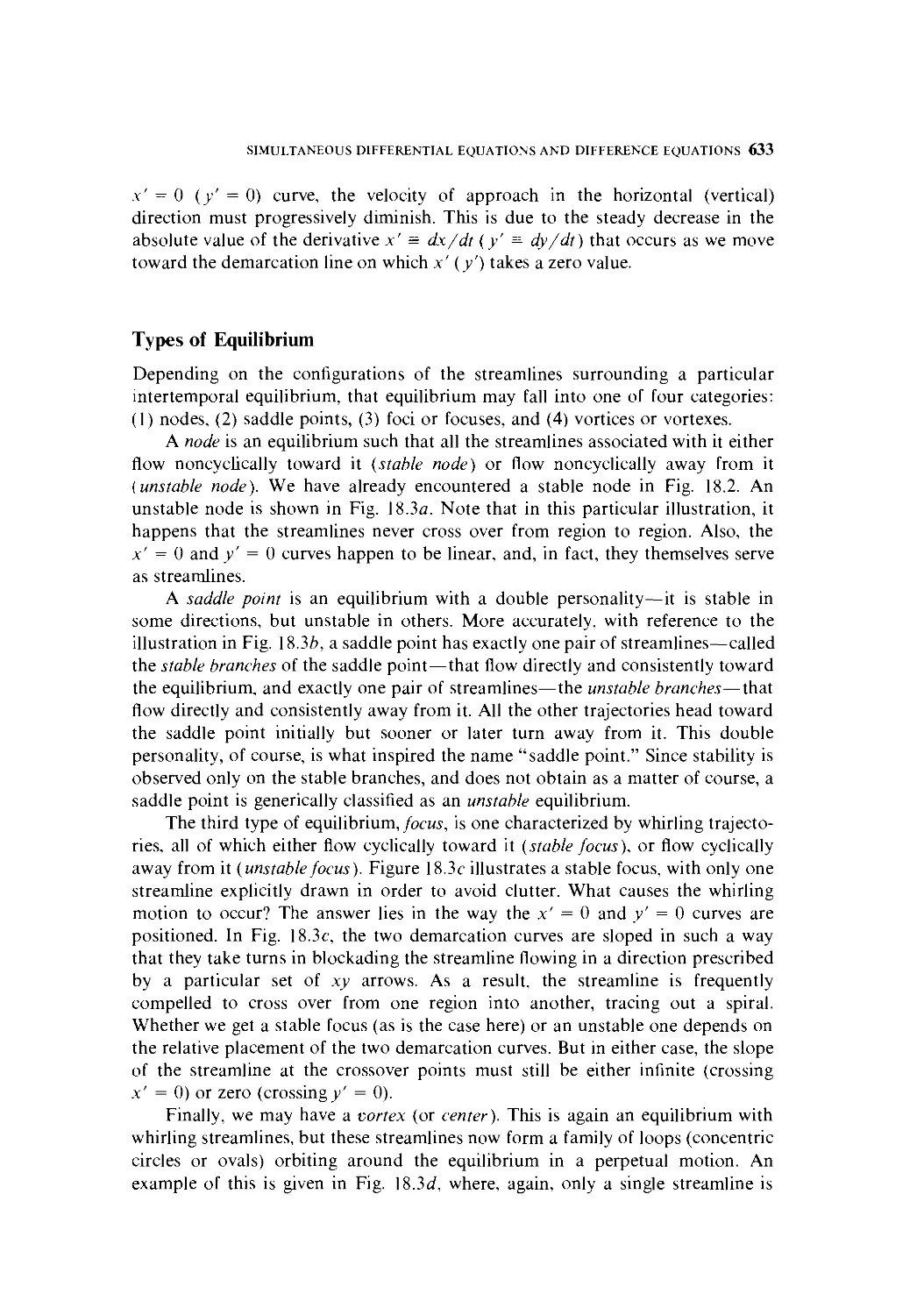
18.5 Two-Variable Phase Diagrams 628
18.6 Linearization of a Nonlinear Differential-Equation System 638
18.7 Limitations of Dynamic Analysis 646
Part 6 Mathematical Programming
19 Linear Programming 651
19.1 Simple Examples of Linear Programming 652
19.2 General Formulation of Linear Programs 661
19.3 Convex Sets and Linear Programming 665
19.4 Simplex Method: Finding the Extreme Points 671
19.5 Simplex Method; Finding the Optimal Extreme Point 676
19.6 Further Notes on the Simplex Method 682
20 Linear Programming (Continued) 688
20.1 Duality 688
20.2 Economic Interpretation of a Dual 696
20.3 Activity Analysis: Micro Level 700
20.4 Activity Analysis: Macro Level 709
21 Nonlinear Programming 716
21.1 The Nature of Nonlinear Programming 716
21.2 Kuhn-Tucker Conditions 722
21.3 The Constraint Qualification 731
21.4 Kuhn-Tucker Sufficiency Theorem; Concave Programming 738
21.5 Arrow-Enthoven Sufficiency Theorem: Quasiconcave Programming 744
21.6 Economic Applications 747
21.7 Limitations of Mathematical Programming 754
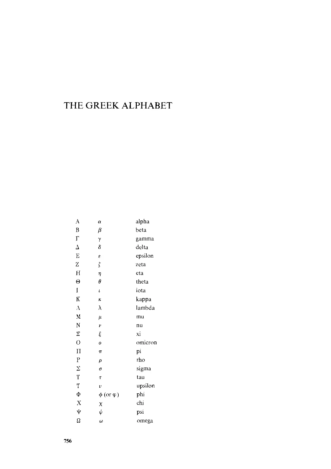
The Greek Alphabet 756
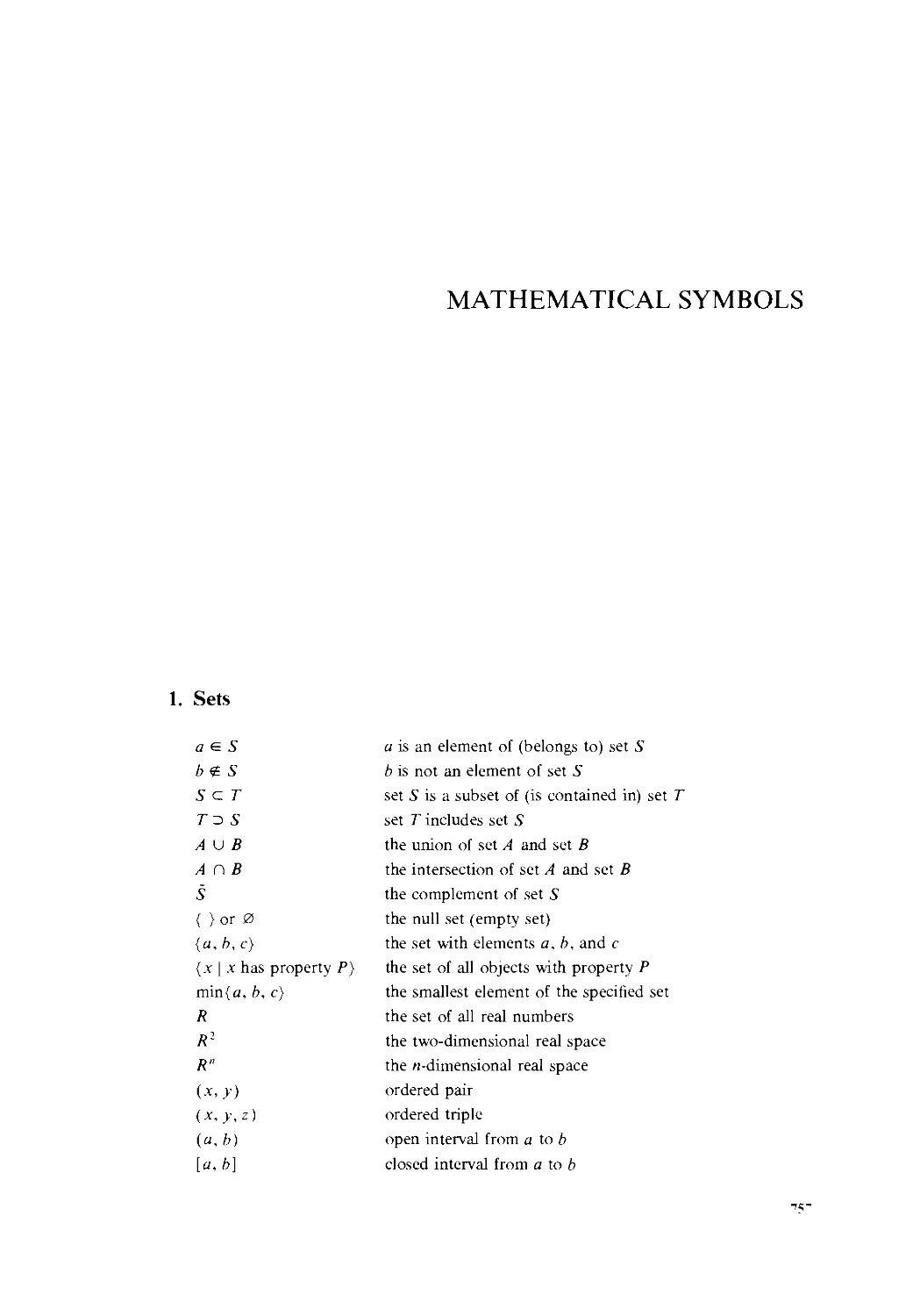
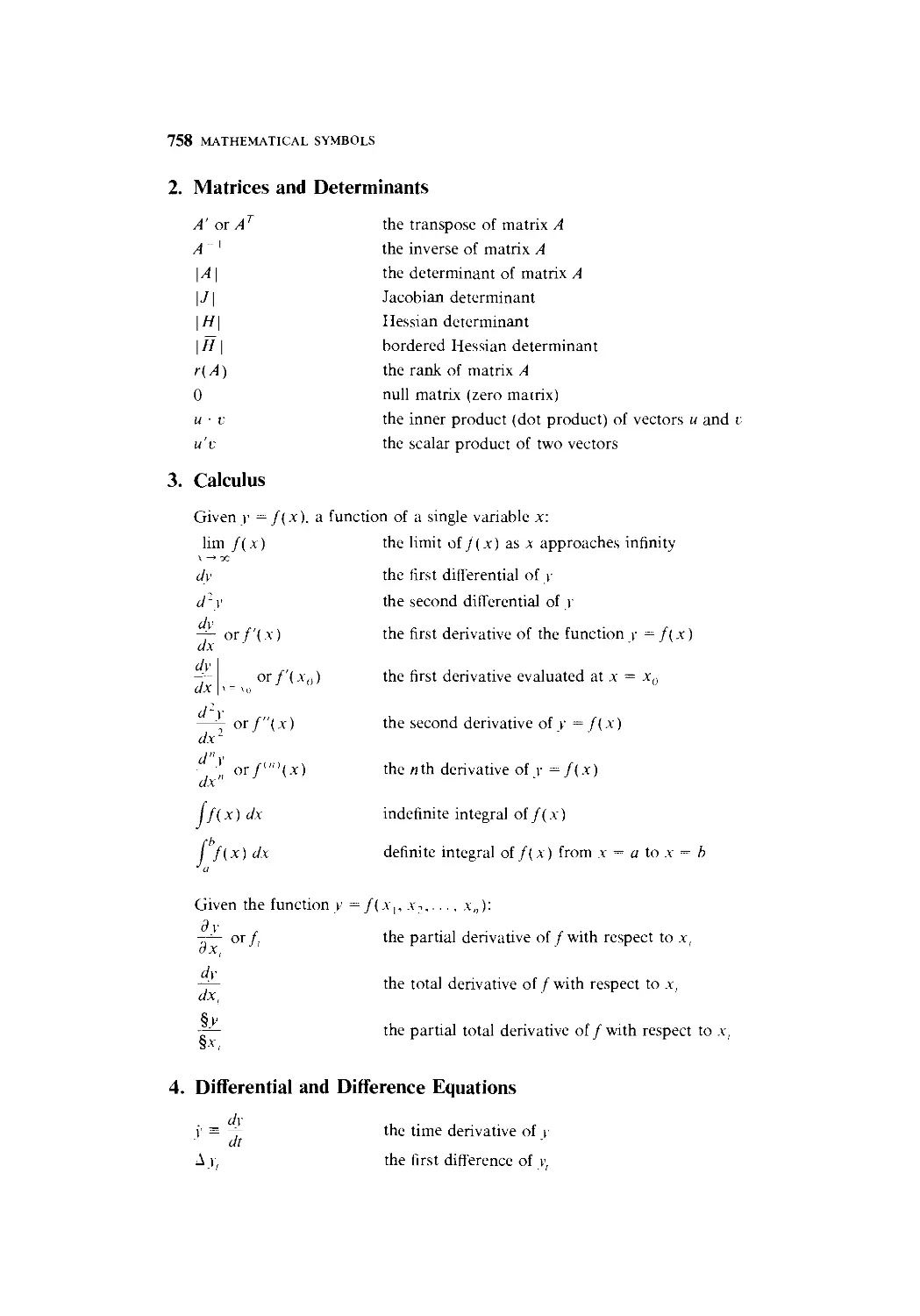
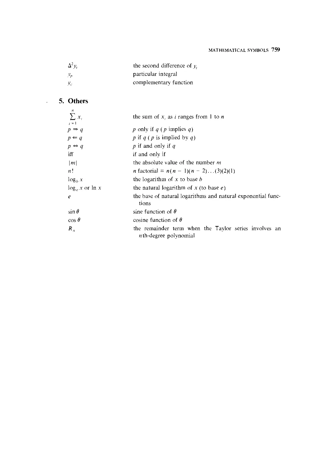
Mathematical Symbols 757
A Short Reading List 760
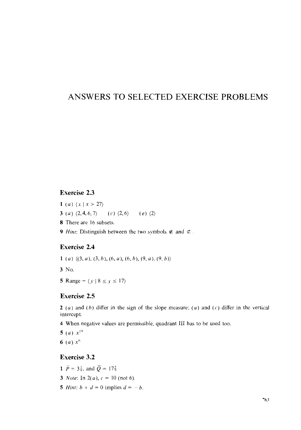
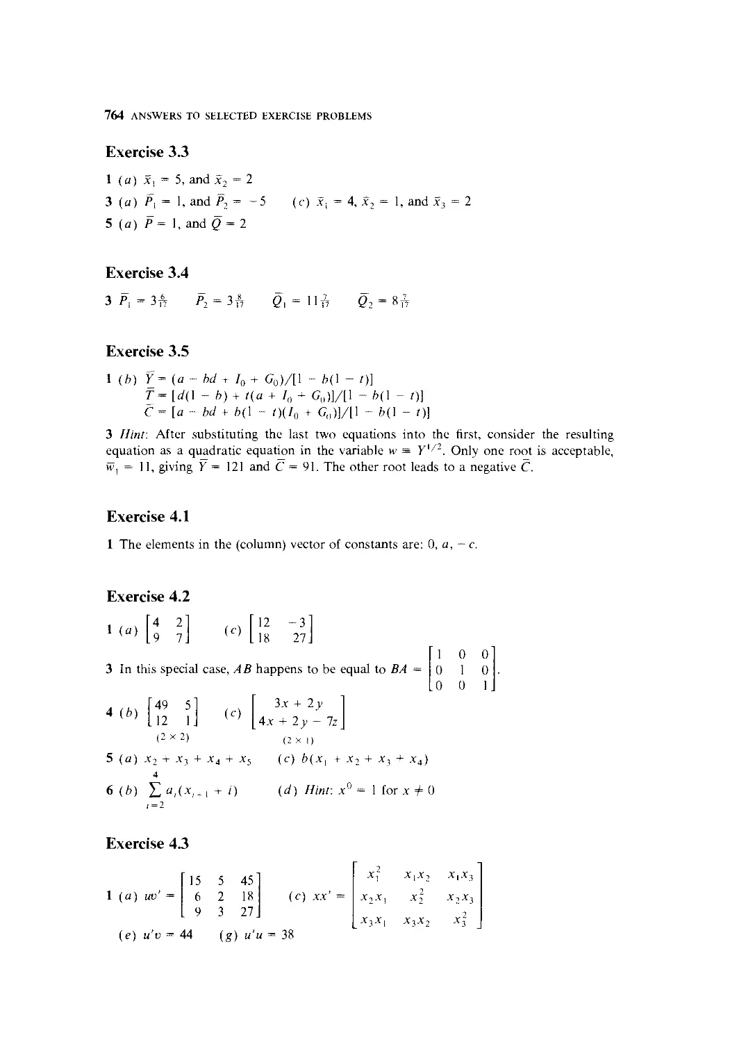
Answers to Selected Exercise Problems 763
Index 781
PART
ONE
INTRODUCTION
CHAPTER
ONE
THE NATURE OF MATHEMATICAL ECONOMICS
Mathematical economics is not a distinct branch of economics in the sense that
public finance or international trade is. Rather, it is an approach to economic
analysis, in which the economist makes use of mathematical symbols in the
statement of the problem and also draws upon known mathematical theorems to
aid in reasoning. As far as the specific subject matter of analysis goes, it can be
micro- or macroeconomic theory, public finance, urban economics, or what not.
Using the term mathematical economics in the broadest possible sense, one
may very well say that every elementary textbook of economics today exemplifies
mathematical economics insofar as geometrical methods are frequently utilized to
derive theoretical results. Conventionally, however, mathematical economics is
reserved to describe cases employing mathematical techniques beyond simple
geometry, such as matrix algebra, differential and integral calculus, differential
equations, difference equations, etc. It is the purpose of this book to introduce the
reader to the most fundamental aspects of these mathematical methods—those
encountered daily in the current economic literature.
1.1 MATHEMATICAL VERSUS NONMATHEMAT1CAL
ECONOMICS
Since mathematical economics is merely an approach to economic analysis, it
should not and does not differ from the nonmathematical approach to economic
analysis in any fundamental way. The purpose of any theoretical analysis,
regardless of the approach, is always to derive a set of conclusions or theorems
from a given set of assumptions or postulates via a process of reasoning. The
major difference between "mathematical economics" and "literary economics"
4 INTRODUCTION
lies principally in the fact that, in the former, the assumptions and conclusions are
stated in mathematical symbols rather than words and in equations rather than
sentences; moreover, in place of literary logic, use is made of mathematical
theorems—of which there exists an abundance to draw upon—in the reasoning
process. Inasmuch as symbols and words are really equivalents (witness the fact
that symbols are usually defined in words), it matters little which is chosen over
the other. But it is perhaps beyond dispute that symbols are more convenient to
use in deductive reasoning, and certainly are more conducive to conciseness and
preciseness of statement.
The choice between literary logic and mathematical logic, again, is a matter of
little import, but mathematics has the advantage of forcing analysts to make their
assumptions explicit at every stage of reasoning. This is because mathematical
theorems are usually stated in the "if-then" form, so that in order to tap the
"then" (result) part of the theorem for their use, they must first make sure that
the "if" (condition) part does conform to the explicit assumptions adopted.
Granting these points, though, one may still ask why it is necessary to go
beyond geometric methods. The answer is that while geometric analysis has the
important advantage of being visual, it also suffers from a serious dimensional
limitation. In the usual graphical discussion of indifference curves, for instance,
the standard assumption is that only two commodities are available to the
consumer. Such a simplifying assumption is not willingly adopted but is forced
upon us because the task of drawing a three-dimensional graph is exceedingly
difficult and the construction of a four- (or higher) dimensional graph is actually a
physical impossibility. To deal with the more general case of 3, 4, or n goods, we
must instead resort to the more flexible tool of equations. This reason alone
should provide sufficient motivation for the study of mathematical methods
beyond geometry.
In short, we see that the mathematical approach has claim to the following
advantages: A) The "language" used is more concise and precise; B) there exists
a wealth of mathematical theorems at our service; C) in forcing us to state
explicitly all our assumptions as a prerequisite to the use of the mathematical
theorems, it keeps us from the pitfall of an unintentional adoption of unwanted
implicit assumptions; and D) it allows us to treat the general ^-variable case.
Against these advantages, one sometimes hears the criticism that a mathe-
mathematically derived theory is inevitably unrealistic. However, this criticism is not
valid. In fact, the epithet " unrealistic" cannot even be used in criticizing eco-
economic theory in general, whether or not the approach is mathematical. Theory is
by its very nature an abstraction from the real world. It is a device for singling
out only the most essential factors and relationships so that we can study the crux
of the problem at hand, free from the many complications that do exist in the
actual world. Thus the statement "theory lacks realism" is merely a truism that
cannot be accepted as a valid criticism of theory. It then follows logically that it is
quite meaningless to pick out any one approach to theory as "unrealistic." For
example, the theory of firm under pure competition is unrealistic, as is the theory
THE NATURE OF MATHEMATICAL ECONOMICS 5
of firm under imperfect competition, but whether these theories are derived
mathematically or not is irrelevant and immaterial.
In sum, we might liken the mathematical approach to a "mode of transporta-
transportation" that can take us from a set of postulates (point of departure) to a set of
conclusions (destination) at a good speed. Common sense would tell us that, if
you intend to go to a place 2 miles away, you will very likely prefer driving to
walking, unless you have time to kill or want to exercise your legs. Similarly, as a
theorist who wishes to get to your conclusions more rapidly, you will find it
convenient to "drive" the vehicle of mathematical techniques appropriate for your
particular purpose. You will, of course, have to take "driving lessons" first; but
since the skill thus acquired tends to be of service for a long, long while, the time
and effort required would normally be well spent indeed.
For a serious "driver"—to continue with the metaphor—some solid lessons
in mathematics are imperative. It is obviously impossible to introduce all the
mathematical tools used by economists in a single volume. Instead, we shall
concentrate on only those that are mathematically the most fundamental and
economically the most relevant. Even so, if you work through this book conscien-
conscientiously, you should at least become proficient enough to comprehend most of the
professional articles you will come across in such periodicals as the American
Economic Review, Quarterly Journal of Economics, Journal of Political Economy,
Review of Economics and Statistics, and Economic Journal. Those of you who,
through this exposure, develop a serious interest in mathematical economics can
then proceed to a more rigorous and advanced study of mathematics.
1.2 MATHEMATICAL ECONOMICS VERSUS ECONOMETRICS
The term "mathematical economics" is sometimes confused with a related term,
"econometrics." As the "metric" part of the latter term implies, econometrics is
concerned mainly with the measurement of economic data. Hence it deals with
the study of empirical observations using statistical methods of estimation and
hypothesis testing. Mathematical economics, on the other hand, refers to the
application of mathematics to the purely theoretical aspects of economic analysis,
with little or no concern about such statistical problems as the errors of measure-
measurement of the variables under study.
In the present volume, we shall confine ourselves to mathematical economics.
That is, we shall concentrate on the application of mathematics to deductive
reasoning rather than inductive study, and as a result we shall be dealing
primarily with theoretical rather than empirical material. This is, of course, solely
a matter of choice of the scope of discussion, and it is by no means implied that
econometrics is less important.
Indeed, empirical studies and theoretical analyses are often complementary
and mutually reinforcing. On the one hand, theories must be tested against
empirical data for validity before they can be applied with confidence. On the
6 INTRODUCTION
other, statistical work needs economic theory as a guide, in order to determine
the most relevant and fruitful direction of research. A classic illustration of the
complementary nature of theoretical and empirical studies is found in the study
of the aggregate consumption function. The theoretical work of Keynes on the
consumption function led to the statistical estimation of the propensity to
consume, but the statistical findings of Kuznets and Goldsmith regarding the
relative long-run constancy of the propensity to consume (in contradiction to
what might be expected from the Keynesian theory), in turn, stimulated the
refinement of aggregate consumption theory by Duesenberry, Friedman, and
others.*
In one sense, however, mathematical economics may be considered as the
more basic of the two: for, to have a meaningful statistical and econometric
study, a good theoretical framework—preferably in a mathematical formulation
—is indispensable. Hence the subject matter of the present volume should be
useful not only for those interested in theoretical economics, but also for those
seeking a foundation for the pursuit of econometric studies.
* John M. Keynes, The General Theory of Employment, Interest and Money, Harcourt, Brace and
Company, Inc., New York, 1936, Book III: Simon Kuznets, National Income: A Summon of Findings.
National Bureau of Economic Research, 1946, p. 53; Raymond Goldsmith, A Study of Saving in the
United States, vol. I, Princeton University Press, Princeton, N.J., 1955, chap. 3; James S. Duesenberry,
Income, Saving, and the Theory of Consumer Behavior, Harvard University Press, Cambridge, Mass.,
1949; Milton Friedman, A Theory of the Consumption Function, National Bureau of Economic
Research. Princeton University Press, Princeton, N.J., 1957.
CHAPTER
TWO
ECONOMIC MODELS
As mentioned before, any economic theory is necessarily an abstraction from the
real world. For one thing, the immense complexity of the real economy makes it
impossible for us to understand all the interrelationships at once; nor, for that
matter, are all these interrelationships of equal importance for the understanding
of the particular economic phenomenon under study. The sensible procedure is,
therefore, to pick out what appeal to our reason to be the primary factors and
relationships relevant to our problem and to focus our attention on these alone.
Such a deliberately simplified analytical framework is called an economic model,
since it is only a skeletal and rough representation of the actual economy.
2.1 INGREDIENTS OF A MATHEMATICAL MODEL
An economic model is merely a theoretical framework, and there is no inherent
reason why it must be mathematical. If the model is mathematical, however, it
will usually consist of a set of equations designed to describe the structure of the
model. By relating a number of variables to one another in certain ways, these
equations give mathematical form to the set of analytical assumptions adopted.
Then, through application of the relevant mathematical operations to these
equations, we may seek to derive a set of conclusions which logically follow from
those assumptions.
8 INTRODUCTION
Variables, Constants, and Parameters
A variable is something whose magnitude can change, i.e., something that can
take on different values. Variables frequently used in economics include price,
profit, revenue, cost, national income, consumption, investment, imports, exports,
and so on. Since each variable can assume various values, it must be represented
by a symbol instead of a specific number. For example, we may represent price by
P, profit by tt, revenue by R, cost by C, national income by Y, and so forth.
When we write P = 3 or C = 18, however, we are "freezing" these variables at
specific values (in appropriately chosen units).
Properly constructed, an economic model can be solved to give us the solution
values of a certain set of variables, such as the market-clearing level of price, or
the profit-maximizing level of output. Such variables, whose solution values we
seek from the model, are known as endogenous variables (originating from within).
However, the model may also contain variables which are assumed to be
determined by forces external to the model, and whose magnitudes are accepted
as given data only; such variables are called exogenous variables (originating from
without). It should be noted that a variable that is endogenous to one model may
very well be exogenous to another. In an analysis of the market determination of
wheat price (P), for instance, the variable P should definitely be endogenous; but
in the framework of a theory of consumer expenditure, P would become instead a
datum to the individual consumer, and must therefore be considered exogenous.
Variables frequently appear in combination with fixed numbers or constants,
such as in the expressions IP or 0.5/?. A constant is a magnitude that does not
change and is therefore the antithesis of a variable. When a constant is joined to a
variable, it is often referred to as the coefficient of that variable. However, a
coefficient may be symbolic rather than numerical. We can, for instance, let the
symbol a stand for a given constant and use the expression aP in lieu of IP in a
model, in order to attain a higher level of generality (see Sec. 2.7). This symbol a
is a rather peculiar case—it is supposed to represent a given constant, and yet,
since we have not assigned to it a specific number, it can take virtually any value.
In short, it is a constant that is variablel To identify its special status, we give it
the distinctive name parametric constant (or simply parameter).
It must be duly emphasized that, although different values can be assigned to
a parameter, it is nevertheless to be regarded as a datum in the model. It is for
this reason that people sometimes simply say "constant" even when the constant
is parametric. In this respect, parameters closely resemble exogenous variables,
for both are to be treated as "givens" in a model. This explains why many writers,
for simplicity, refer to both collectively with the single designation " parameters."
As a matter of convention, parametric constants are normally represented by
the symbols a, b, c, or their counterparts in the Greek alphabet: a, /3, and y. But
other symbols naturally are also permissible. As for exogenous variables, in order
that they can be visually distinguished from their endogenous cousins, we shall
follow the practice of attaching a subscript 0 to the chosen symbol. For example,
if P symbolizes price, then Plt signifies an exogenously determined price.
ECONOMIC MODELS 9
Equations and Identities
Variables may exist independently, but they do not really become interesting until
they are related to one another by equations or by inequalities. At this juncture
we shall discuss equations only.
In economic applications we may distinguish between three types of equa-
equation: definitional equations, behavioral equations, and equilibrium conditions.
A definitional equation sets up an identity between two alternate expressions
that have exactly the same meaning. For such an equation, the identical-equality
sign = (read: "is identically equal to") is often employed in place of the regular
equals sign = , although the latter is also acceptable. As an example, total profit is
defined as the excess of total revenue over total cost; we can therefore write
77 = R - C
A behavioral equation, on the other hand, specifies the manner in which a
variable behaves in response to changes in other variables. This may involve
either human behavior (such as the aggregate consumption pattern in relation to
national income) or nonhuman behavior (such as how total cost of a firm reacts to
output changes). Broadly defined, behavioral equations can be used to describe
the general institutional setting of a model, including the technological (e.g.,
production function) and legal (e.g., tax structure) aspects. Before a behavioral
equation can be written, however, it is always necessary to adopt definite
assumptions regarding the behavior pattern of the variable in question. Consider
the two cost functions
B.1) C = 75 + 100
B.2) C = 110 + Q2
where Q denotes the quantity of output. Since the two equations have different
forms, the production condition assumed in each is obviously different from the
other. In B.1), the fixed cost (the value of C when Q = 0) is 75, whereas in B.2) it
is 110. The variation in cost is also different. In B.1), for each unit increase in Q,
there is a constant increase of 10 in C. But in B.2), as Q increases unit after unit,
C will increase by progressively larger amounts. Clearly, it is primarily through
the specification of the form of the behavioral equations that we give mathemati-
mathematical expression to the assumptions adopted for a model.
The third type of equations, equilibrium conditions, have relevance only if our
model involves the notion of equilibrium. If so, the equilibrium condition is an
equation that describes the prerequisite for the attainment of equilibrium. Two of
the most familiar equilibrium conditions in economics are
Qd = Qs [quantity demanded = quantity supplied]
and S = I [intended saving = intended investment]
which pertain, respectively, to the equilibrium of a market model and the
equilibrium of the national-income model in its simplest form. Because equations
10 INTRODUCTION
of this type are neither definitional nor behavioral, they constitute a class by
themselves.
2.2 THE REAL-NUMBER SYSTEM
Equations and variables are the essential ingredients of a mathematical model.
But since the values that an economic variable takes are usually numerical, a few
words should be said about the number system. Here, we shall deal only with
so-called "real numbers."
Whole numbers such as 1,2. 3. ... are called positive integers; these are the
numbers most frequently used in counting. Their negative counterparts
— 1, — 2, — 3. ... are called negative integers; these can be employed, for example,
to indicate subzero temperatures (in degrees). The number 0 (zero), on the other
hand, is neither positive nor negative, and is in that sense unique. Let us lump all
the positive and negative integers and the number zero into a single category,
referring to them collectively as the set of all integers.
Integers, of course, do not exhaust all the possible numbers, for we have
fractions, such as 1. 4. and ,', which—if placed on a ruler—would fall between
the integers. Also, we have negative fractions, such as - I and - t. Together,
these make up the set of all fractions.
The common property of all fractional numbers is that each is expressible as
a ratio of two integers; thus fractions qualify for the designation rational numbers
(in this usage, rational means ratio-m\). But integers are also rational, because
any integer n can be considered as the ratio n/\. The set of all integers and the set
of all fractions together form the set of all rational numbers.
Once the notion of rational numbers is used, however, there naturally arises
the concept of irrational numbers—numbers that cannot be expressed as ratios of
a pair of integers. One example is the number /2 = 1.4142.... which is a
nonrepeating, nonterminating decimal. Another is the special constant tt =
3.1415... (representing the ratio of the circumference of any circle to its diame-
diameter), which is again a nonrepeating, nonterminating decimal, as is characteristic of
all irrational numbers.
Each irrational number, if placed on a ruler, would fall between two rational
numbers, so that, just as the fractions fill in the gaps between the integers on a
ruler, the irrational numbers fill in the gaps between rational numbers. The result
of this filling-in process is a continuum of numbers, all of which are so-called
"real numbers." This continuum constitutes the set of all real numbers, which is
often denoted bv the symbol R. When the set R is displayed on a straight line (an
extended ruler), we refer to the line as the real line.
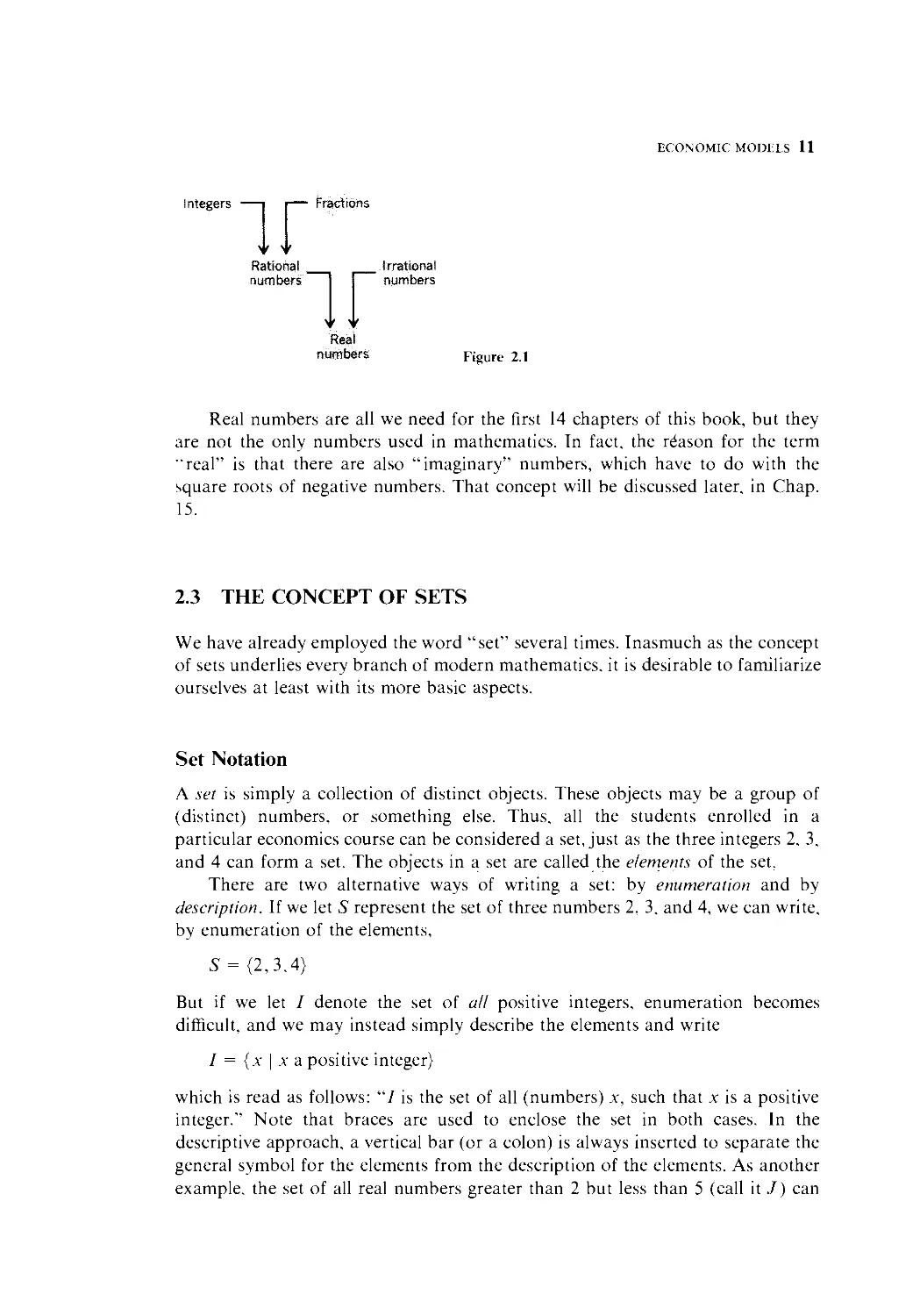
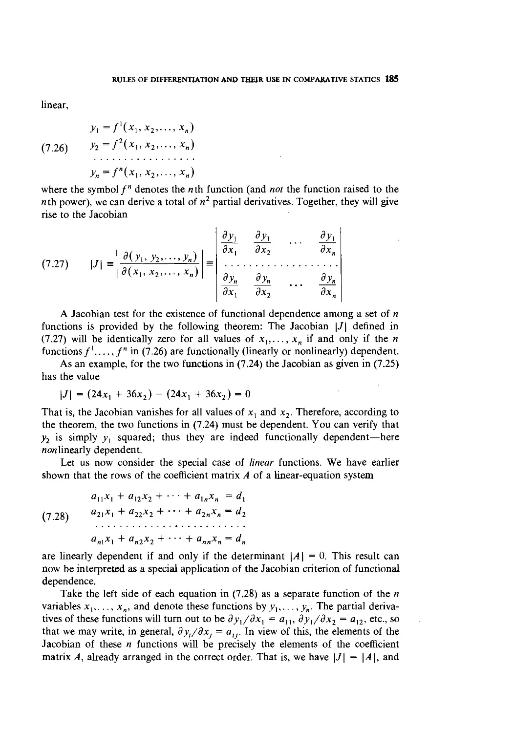
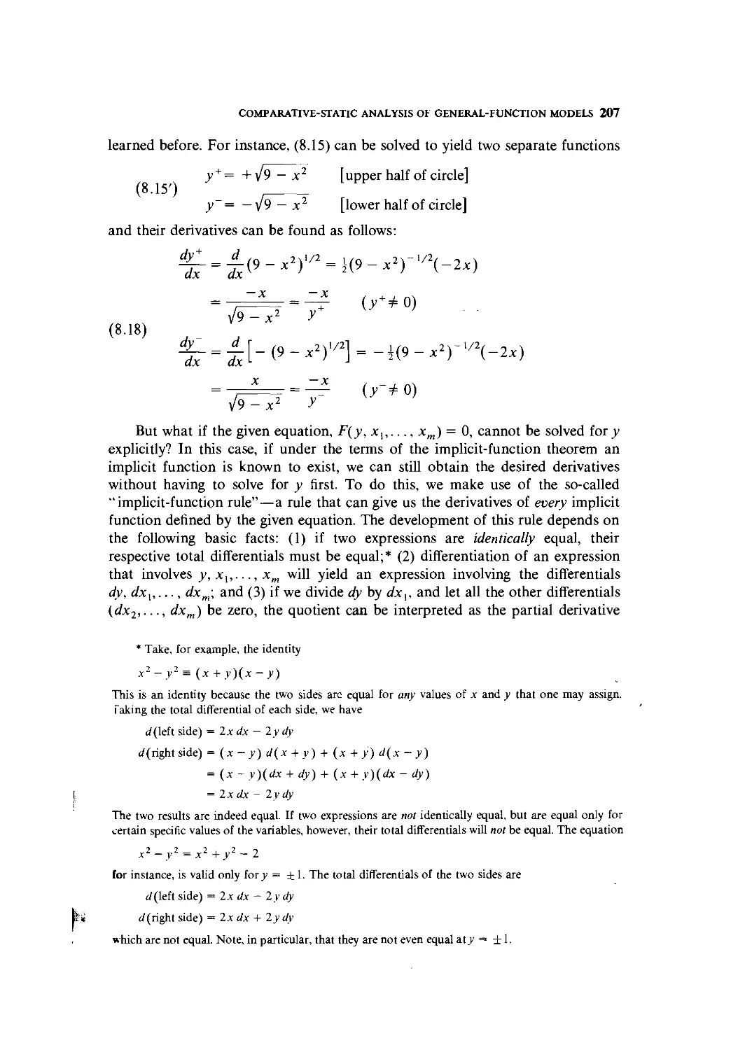
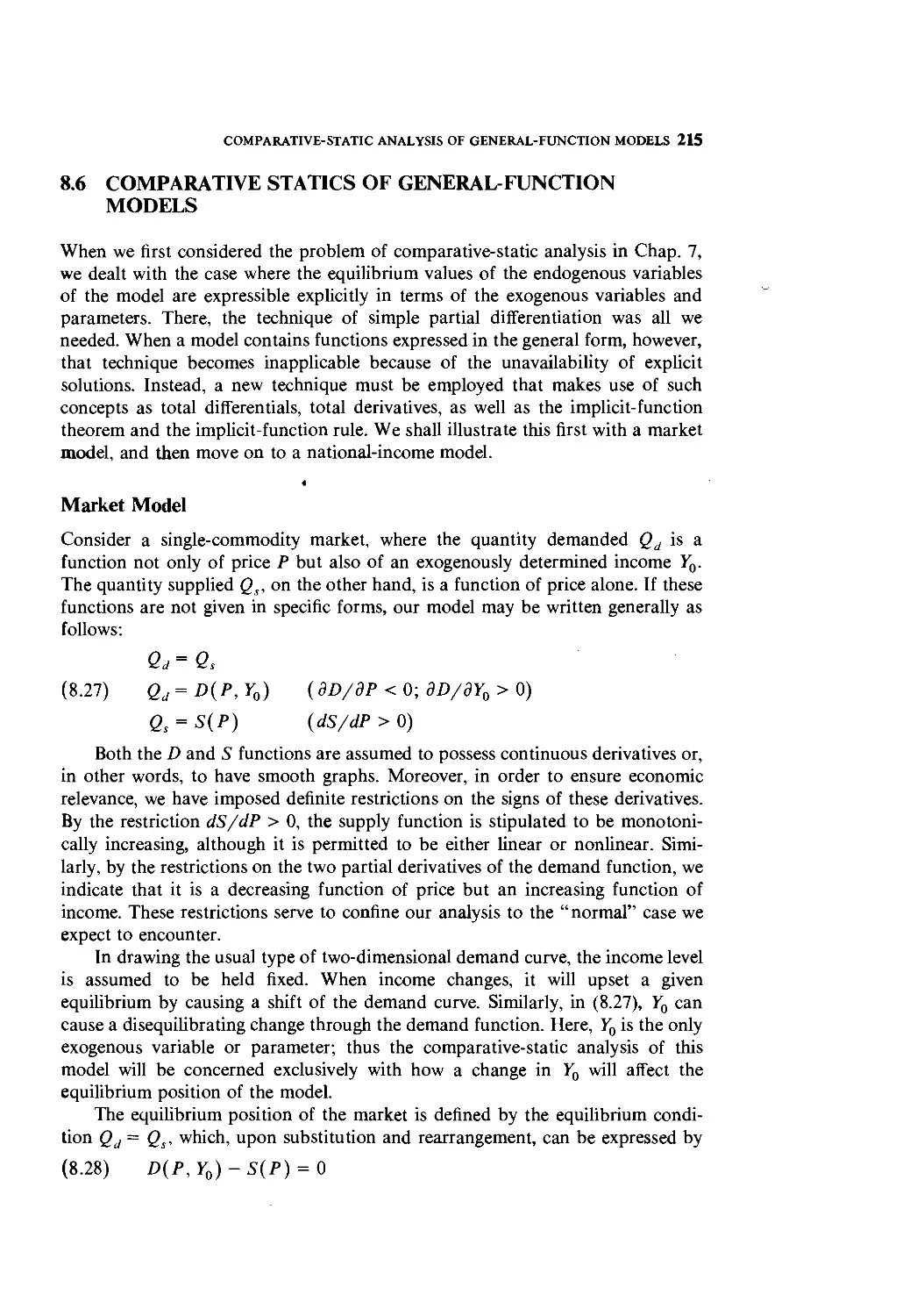
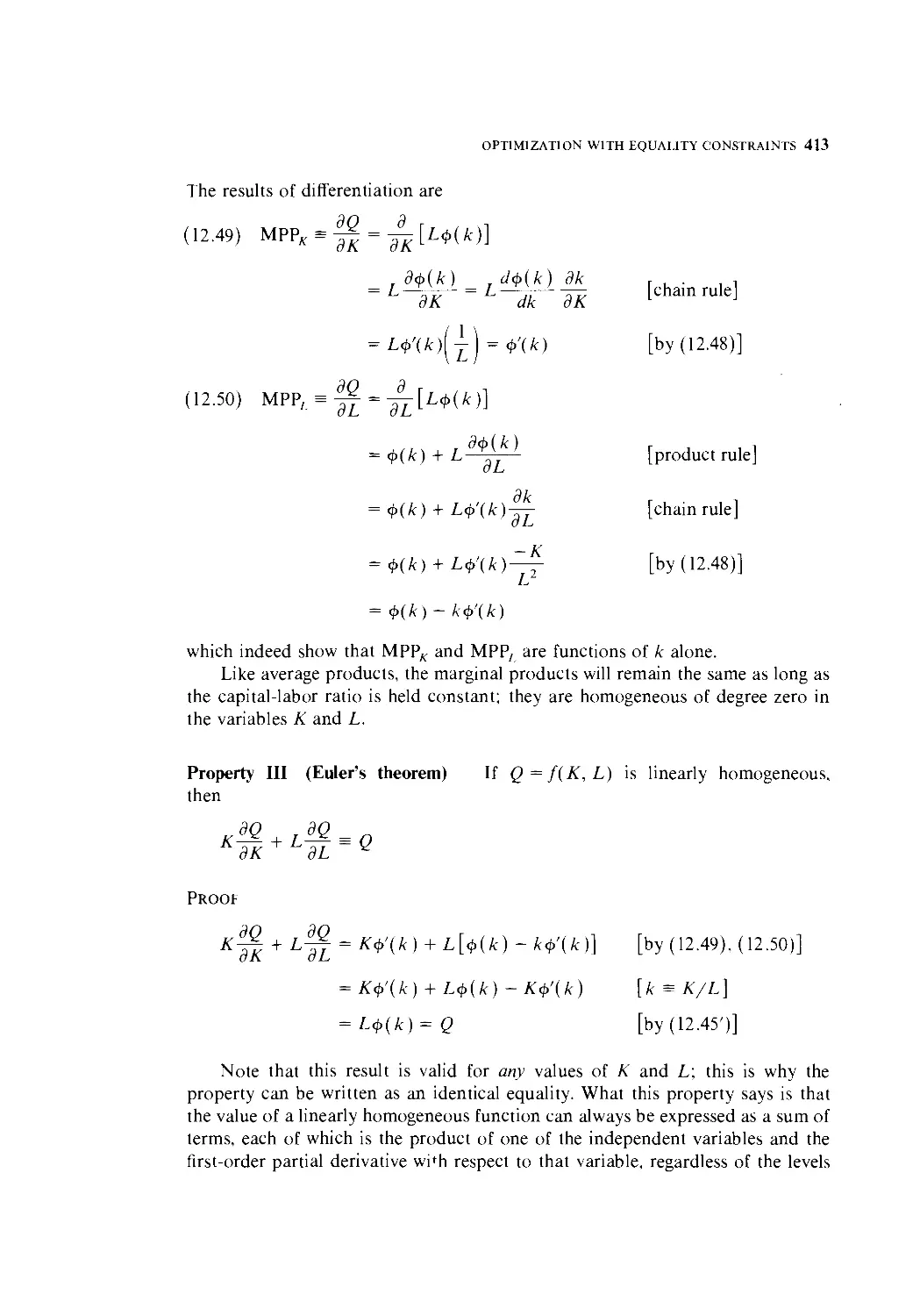
In Fig. 2.1 are listed (in the order discussed) all the number sets, arranged in
relationship to one another. If we read from bottom to top, however, we find in
effect a clas.MficatOry scheme in which the set of real numbers is broken down into
its component and subcomponent number sets. This figure therefore is a summary
of the structure of the real-number system.
ECONOMIC MODELS 11
Integers ——i r— Fractions
ir
Rational __^ Irrational
numbers I I numbers
Real
numbers Figure 2.1
Real numbers are all we need for the first 14 chapters of this book, but they
are not the only numbers used in mathematics. In fact, the reason for the term
■"real" is that there are also "imaginary" numbers, which have to do with the
square roots of negative numbers. That concept will be discussed later, in Chap.
15.
2.3 THE CONCEPT OF SETS
We have already employed the word "set" several times. Inasmuch as the concept
of sets underlies every branch of modern mathematics, it is desirable to familiarize
ourselves at least with its more basic aspects.
Set Notation
A set is simply a collection of distinct objects. These objects may be a group of
(distinct) numbers, or something else. Thus, all the students enrolled in a
particular economics course can be considered a set, just as the three integers 2, 3,
and 4 can form a set. The objects in a set are called the elements of the set.
There are two alternative ways of writing a set: by enumeration and by
description. If we let 5" represent the set of three numbers 2, 3, and 4, we can write,
by enumeration of the elements,
S = {2,3,4}
But if we let / denote the set of all positive integers, enumeration becomes
difficult, and we may instead simply describe the elements and write
/ = {x | x a positive integer}
which is read as follows: "/ is the set of all (numbers) x, such that x is a positive
integer." Note that braces are used to enclose the set in both cases. In the
descriptive approach, a vertical bar (or a colon) is always inserted to separate the
general symbol for the elements from the description of the elements. As another
example, the set of all real numbers greater than 2 but less than 5 (call it /) can
12 INTRODUCTION
be expressed symbolically as
J = {x | 2 < x < 5}
Here, even the descriptive statement is symbolically expressed.
A set with a finite number of elements, exemplified by set 5" above, is called a
finite set. Set / and set J, each with an infinite number of elements, are, on the
other hand, examples of an infinite set. Finite sets are always denumerable (or
countable), i.e., their elements can be counted one by one in the sequence
1.2,3 Infinite sets may, however, be either denumerable (set / above), or
nondenumerable (set J above). In the latter case, there is no way to associate the
elements of the set with the natural counting numbers 1,2, 3, and thus the set
is not countable.
Membership in a set is indicated by the symbol g (a variant of the Greek
letter epsilon e for "element"), which is read: "is an element of." Thus, for the
two sets 5 and / defined above, we may write
2G5 3g5 8e/ 9 g / (etc.)
but obviously 8 £ S" (read: "8 is not an element of set 5"). If we use the symbol
R to denote the set of all real numbers, then the statement "x is some real
number" can be simply expressed by
x g R
Relationships between Sets
When two sets are compared with each other, several possible kinds of relation-
relationship may be observed. If two sets 5, and S2 happen to contain identical elements,
5, = {2,7,a,/} and S2 = {2, a,7, /}
then 5, and S2 are said to be equal E, = S2). Note that the order of appearance
of the elements in a set is immaterial. Whenever even one element is different,
however, two sets are not equal.
Another kind of relationship is that one set may be a subset of another set. If
we have two sets
5 = {1,3,5,7,9} and T = {3,1}
then T is a subset of 5, because every element of T is also an element of 5. A
more formal statement of this is: T is a subset of 5 if and only if "x g T " implies
"x g S." Using the set inclusion symbols c (is contained in) and d (includes),
we may then write
T a S or 5 3 T
It is possible that two given sets happen to be subsets of each other. When this
occurs, however, we can be sure that these two sets are equal. To state this
formally: we can have 5, c S2 and S2 c S, if and only if 5", = S2.
ECONOMIC MODELS 13
Note that, whereas the e symbol relates an individual element to a set, the c
symbol relates a subset to a set. As an application of this idea, we may state on the
basis of Fig. 2.1 that the set of all integers is a subset of the set of all rational
numbers. Similarly, the set of all rational numbers is a subset of the set of all real
numbers.
How many subsets can be formed from the five elements in the set 5" =
{1,3,5,7,9}? First of all, each individual element of 5 can count as a distinct
subset of 5, such as {1}, {3}, etc. But so can any pair, triple, or quadruple of these
elements, such as {1,3}, {1,5}, {3,7,9}, etc. For that matter, the set 5 itself
(with all its five elements) can be considered as one of its own subsets—every
element of 5 is an element of 5, and thus the set 5 itself fulfills the definition of a
subset. This is, of course, a limiting case, that from which we get the "largest"
possible subset of 5, namely, 5 itself.
At the other extreme, the "smallest" possible subset of 5 is a set that contains
no element at all. Such a set is called the null set, or empty set, denoted by the
symbol 0 or { }. The reason for considering the null set as a subset of 5 is quite
interesting: If the null set is not a subset of 5 @ <t S), then 0 must contain at
least one element x such that x £ S. But since by definition the null set has no
element whatsoever, we cannot say that 0 <t S; hence the null set is a subset of
S.
Counting all the subsets of 5, including the two limiting cases 5 and 0. we
find a total of 25 = 32 subsets. In general, if a set has n elements, a total of 2"
subsets can be formed from those elements.*
It is extremely important to distinguish the symbol 0 or { } clearly from the
notation {0}; the former is devoid of elements, but the latter does contain an
element, zero. The null set is unique; there is only one such set in the whole
world, and it is considered a subset of any set that can be conceived.
As a third possible type of relationship, two sets may have no elements in
common at all. In that case, the two sets are said to be disjoint. For example, the
set of all positive integers and the set of all negative integers are disjoint sets. A
fourth type of relationship occurs when two sets have some elements in common
but some elements peculiar to each. In that event, the two sets are neither equal
nor disjoint; also, neither set is a subset of the other.
Operations on Sets
When we add, subtract, multiply, divide, or take the square root of some
numbers, we are performing mathematical operations. Sets are different from
* Given a set with /; elements (a, b. c n) we may first classify its subsets into two categories:
one with the clement a in it, and one without. Each of these two can be further classified into two
subcategories: one with the clement h in it, and one without. Note that by considering the second
clement h. we double the number of categories in the classification from 2 to 4 ( = 22). Bv the same
token, the consideration of the element ( will increase the total number of categories to 8 (= 21).
When all n elements are considered, the total number of categories will become the total number of
subsets, and that number is 2".
14 INTRODUCTION
numbers, but one can similarly perform certain mathematical operations on them.
Three principal operations to be discussed here involve the union, intersection,
and complement of sets.
To take the union of two sets A and B means to form a new set containing
those elements (and only those elements) belonging to A, or to B, or to both A
and B. The union set is symbolized by A U B (read: "A union B").
Example 1 If A = {3, 5, 7} and B = {2, 3,4, 8}, then
A u B = {2,3.4,5,7,8}
This example illustrates the case in which two sets A and B are neither equal nor
disjoint and in which neither is a subset of the other.
Example 2 Again referring to Fig. 2.1. we see that the union of the set of all
integers and the set of all fractions is the set of all rational numbers. Similarly, the
union of the rational-number set and the irrational-number set yields the set of all
real numbers.
The intersection of two sets A and B, on the other hand, is a new set which
contains those elements (and only those elements) belonging to both A and B. The
intersection set is symbolized by A n B (read: "A intersection B").
Example 3 From the sets A and B in Example 1, we can write
A n B = {3}
Example 4 If A = {- 3, 6, 10} and B = {9,2.7,4}, then A n B = 0. Set A and
set B are disjoint; therefore their intersection is the empty set—no element is
common to A and B.
It is obvious that intersection is a more restrictive concept than union. In the
former, only the elements common to A and B are acceptable, whereas in
the latter, membership in either A or B is sufficient to establish membership in the
union set. The operator symbols n and U —which, incidentally, have the same
kind of general status as the symbols /~, +. + , etc. — therefore have the
connotations "and" and "or," respectively. This point can be better appreciated
by comparing the following formal definitions of intersection and union:
Intersection: AnB = {x\xeA and x e B)
Union: A u B = {x \ x e A or x e B}
Before explaining the complement of a set, let us first introduce the concept of
universal set. In a particular context of discussion, if the only numbers used are
the set of the first seven positive integers, we may refer to it as the universal set,
U. Then, with a given set, say, A = {3,6,7}, we can define another set A (read:
"the complement of A") as the set that contains all the numbers in the universal
ECONOMIC MODELS 15
set U which are not in the set A. That is.
A = {x | a- g L-'and.v <£ A) = {1.2.4.5}
Note that, whereas the symbol U has the connotation "or" and the symbol n
means "and." the complement symbol ~ carries the implication of "not."
Example 5 If U = {5, 6, 7. 8. 9} and A = {5. 6}. then A = {7. 8. 9}.
Example 6 What is the complement of Ul Since every object (number) under
consideration is included in the universal set, the complement of U must be
empty. Thus 0=0.
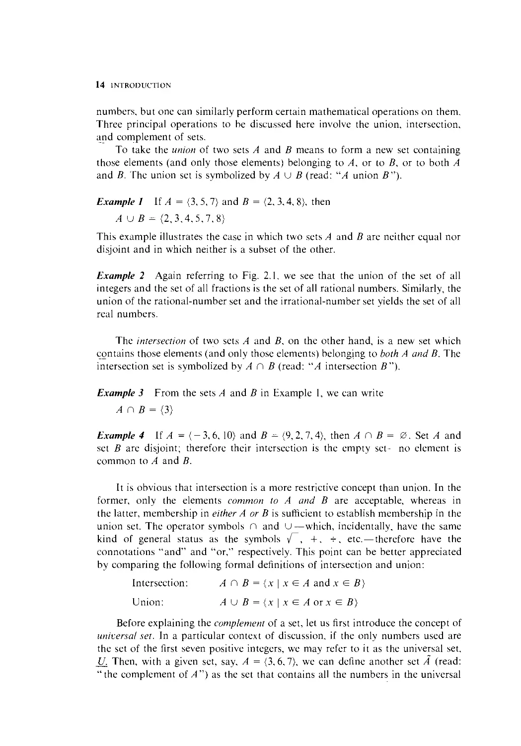
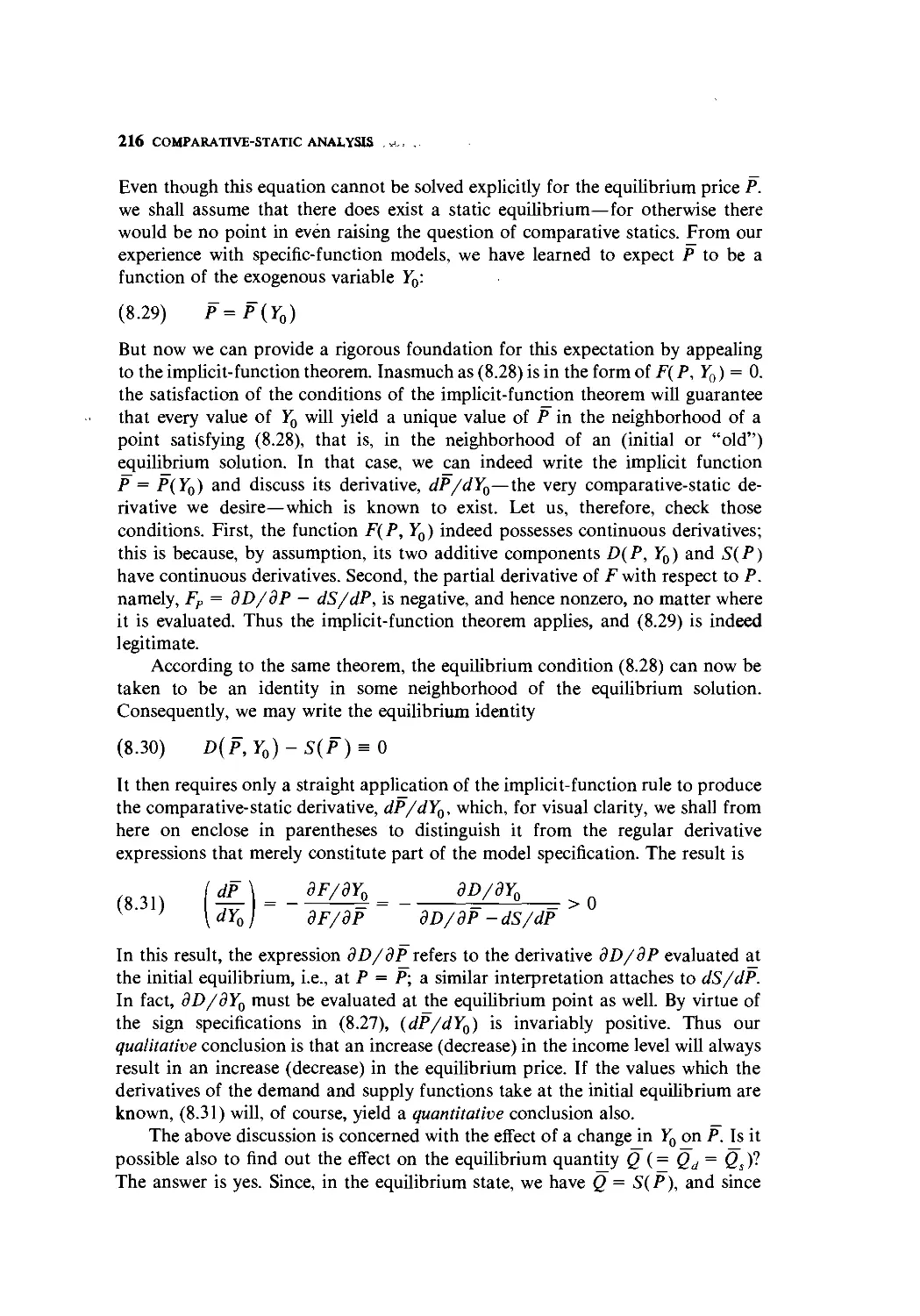
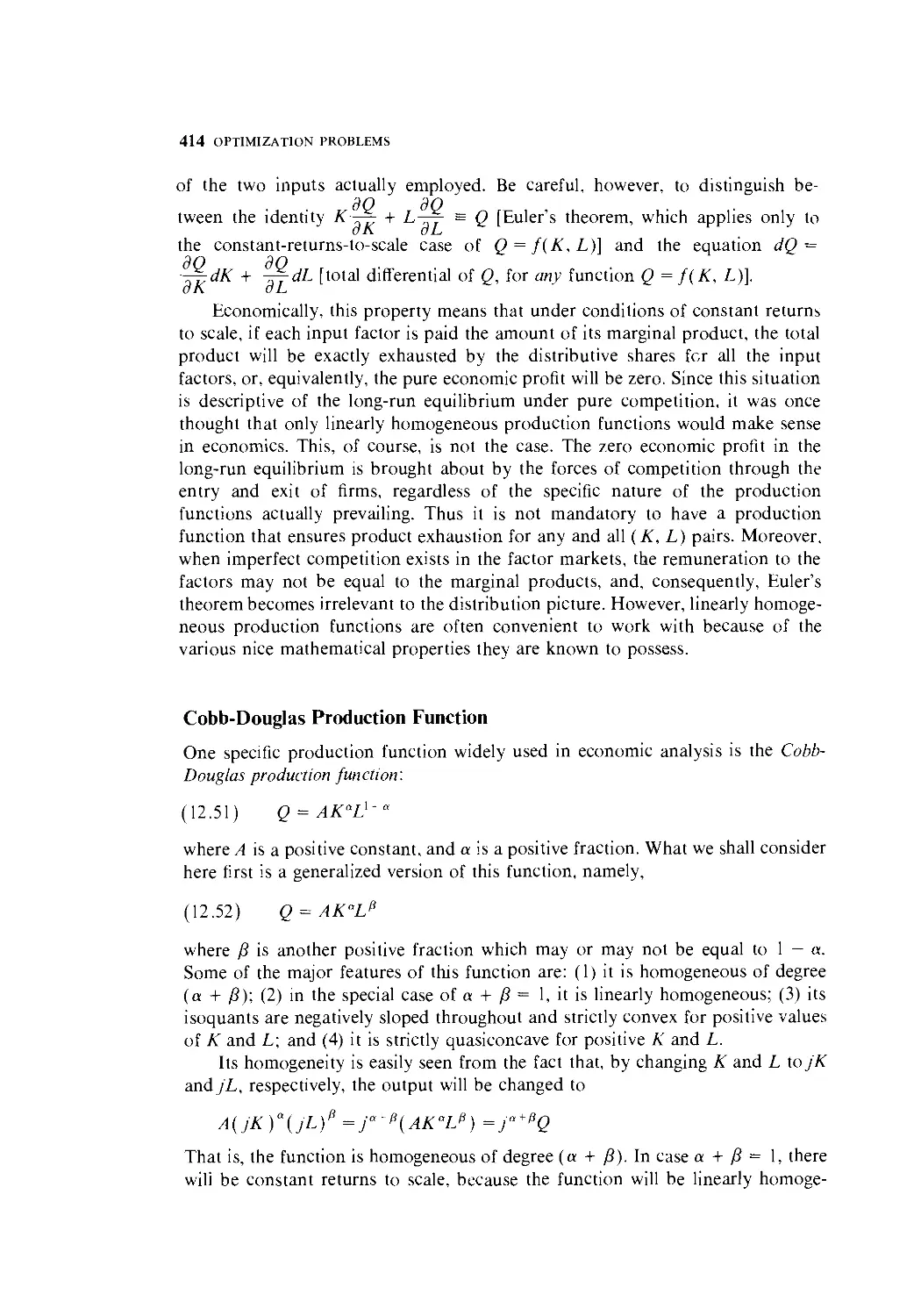
The three types of set operation can be visualized in the three diagrams of
Fig. 2.2. known as Venn diagrams. In diagram a, the points in the upper circle
form a set A, and the points in the lower circle form a set B. The union of A and
B then consists of the shaded area covering both circles. In diagram b are shown
the same two sets (circles). Since their intersection should comprise only the
points common to both sets, only the (shaded) overlapping portion of the two
circles satisfies the definition. In diagram c. let the points in the rectangle be the
universal set and let A be the set of points in the circle; then the complement set
A will be the (shaded) area outside the circle.
Laws of Set Operations
From Fig. 2.2. it may be noted that the shaded area in diagram a represents not
only A U B but also B U A. Analogously, in diagram b the small shaded area is
the visual representation not only of A n B but also of B n A. When formalized.
Complement
A
(e)
Figure 2.2
16 INTRODUCTION
this result is known as the commutative law (of unions and intersections):
A U B = B U A A n B = B n A
These relations are very similar to the algebraic laws a + b = b + a and a X b =
b X a.
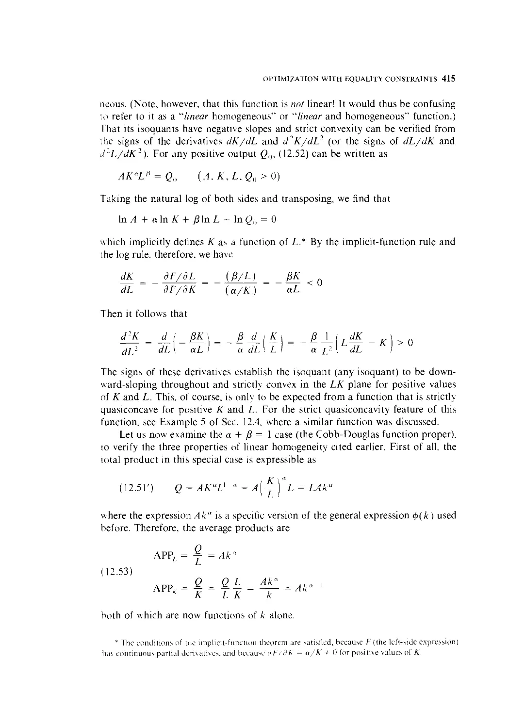
To take the union of three sets A, B, and C, we first take the union of any two
sets and then "union" the resulting set with the third; a similar procedure is
applicable to the intersection operation. The results of such operations are
illustrated in Fig. 2.3. It is interesting that the order in which the sets are selected
for the operation is immaterial. This fact gives rise to the associative law (of
unions and intersections):
A U (B U C) = (A u B) u C
A n {B n c) = {A n B) nc
These equations are strongly reminiscent of the algebraic laws a + (b + c) = (a
+ b) + c and a X (b X c) = (a X b) X c.
There is also a law of operation that applies when unions and intersections
are used in combination. This is the distributive law (of unions and intersections):
These resemble the algebraic law a X (b + c) = (a X b) + (a X c).
Example 7 Verify the distributive law, given A = D, 5}, B = C, 6, 7}, and C =
B,3}. To verify the first part of the law, we find the left- and right-hand
expressions separately:
Left: A U (B n C) = {4,5}U{3} = {3,4,5}
Right: (A U B) n (A U C) = C,4,5,6,7} n B,3,4, 5} = {3,4,5}
.4 U B U C
A n H n C
(a)
(b)
Figure 2.3
ECONOMIC MODELS 17
Since the two sides yield the same result, the law is verified. Repeating the
procedure for the second part of the law, we have
Left: A n (B U C) = D,5}n{2, 3,6,7}= 0
Right: (A n B) U (A n C) = 0 U 0 = 0
Thus the law is again verified.
EXERCISE 2.3
1 Write the following in set notation:
(a) The set of all real numbers greater than 27.
(ft) The set of all real numbers greater than 8 but less than 73.
2 Given the sets S, = {2,4,6}, S2 = {7,2,6}, S, = {4,2,6}, and S4 = {2,4}, which of the
following statements are true?
(a) S, = S2 (d) 3 € S2 (g) S, d S4
(ft) S, = R ■ (e) 4 <£ S4 (h) 0 c S2
(c) 5 e S2 (/) S4 c R (/) S, d{1,2>
3 Referring to the four sets given in the preceding problem, find:
{a) S, u S2 {c) S2 n Si (<?) S4 n S2 n S,
(ft) S, u S, (i/) S2 n S4 (/) s, u S, u 54
4 Which of the following statements are valid?
(a) A \J A = A (e) A n 0 = 0
(ft) /I n /I = /I (/) /I n 61 = /I
(c) /IU0 =/l (g) The complement of A is /I.
(</)^U(/=(/
5 Given A = {4,5,6}. B = {3,4,6,7}. and C = {2,3,6}, verify the distributive law.
6 Verify the distributive law by means of Venn diagrams, with different orders of
successive shading.
7 Enumerate all the subsets of the set {a, ft, c}.
8 Enumerate all the subsets of the set S = {1,3,5,7}. How many subsets are there
altogether?
9 Example 6 shows that 0 is the complement of U. But since the null set is a subset of
any set, 0 must be a subset of U. Inasmuch as the term "complement of G" implies the
notion of being not in U, whereas the term " subset of U " implies the notion of being in U.
it seems paradoxical for 0 to be both of these. How do you resolve this paradox?
2.4 RELATIONS AND FUNCTIONS
Our discussion of sets was prompted by the usage of that term in connection with
the various kinds of numbers in our number system. However, sets can refer as
well to objects other than numbers. In particular, we can speak of sets of
18 INTRODUCTION
"ordered pairs" — to be defined presently—which will lead us to the important
concepts of relations and functions.
Ordered Pairs
In writing a set {a, b), we do not care about the order in which the elements a and
b appear, because by definition {a, b) = {b, a). The pair of elements a and b is in
this case an unordered pair. When the ordering of a and b does carry a
significance, however, we can write two different ordered pairs denoted by (a, b)
and (b, a), which have the property that (a, b) =h (b, a) unless a = b. Similar
concepts apply to a set with more than two elements, in which case we can
distinguish between ordered and unordered triples, quadruples, quintuples, and so
forth. Ordered pairs, triples, etc., collectively can be called ordered sets.
Example 1 To show the age and weight of each student in a class, we can form
ordered pairs (a, r>), in which the first element indicates the age (in years) and the
second element indicates the weight (in pounds). Then A9,127) and A27,19)
would obviously mean different things. Moreover, the latter ordered pair would
hardly fit any student anywhere.
Example 2 When we speak of the set of the five finalists in a contest, the order in
which they are listed is of no consequence and we have an unordered quintuple.
But after they are judged, respectively, as the winner, first runner-up, etc., the list
becomes an ordered quintuple.
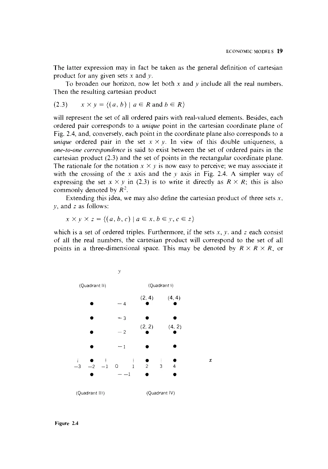
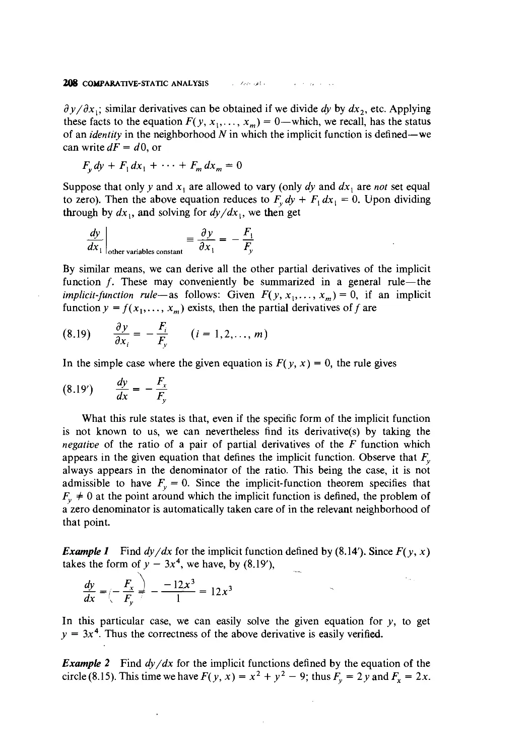
Ordered pairs, like other objects, can be elements of a set. Consider the
rectangular (cartesian) coordinate plane in Fig. 2.4, where an x axis and a y axis
cross each other at a right angle, dividing the plane into four quadrants. This xy
plane is an infinite set of points, each of which represents an ordered pair whose
first element is an x value and the second element a y value. Clearly, the point
labeled D,2) is different from the point B,4); thus ordering is significant here.
With this visual understanding, we are ready to consider the process of
generation of ordered pairs. Suppose, from two given sets, x = {1,2} and>' = C,4},
we wish to form all the possible ordered pairs with the first element taken from
set x and the second element taken from set y. The result will, of course, be the set
of four ordered pairs A,3), A,4), B,3), and B,4). This set is called the cartesian
product (named after Descartes), or direct product, of the sets x and y and is
denoted by x X y (read: "x cross _>•"). It is important to remember that, while x
and y are sets of numbers, the cartesian product turns out to be a set of ordered
pairs. By enumeration, or by description, we may express the cartesian product
alternatively as
or x X y = {(a, b) \ a <= x and b e y)
ECONOMIC MODELS 19
The latter expression may in fact be taken as the general definition of cartesian
product for any given sets x and y.
To broaden our horizon, now let both x and y include all the real numbers.
Then the resulting cartesian product
B.3) x X y = {{a, b) \ a e R and b e R)
will represent the set of all ordered pairs with real-valued elements. Besides, each
ordered pair corresponds to a unique point in the cartesian coordinate plane of
Fig. 2.4, and, conversely, each point in the coordinate plane also corresponds to a
unique ordered pair in the set x X y. In view of this double uniqueness, a
one-to-one correspondence is said to exist between the set of ordered pairs in the
cartesian product B.3) and the set of points in the rectangular coordinate plane.
The rationale for the notation x X y is now easy to perceive; we may associate it
with the crossing of the x axis and the y axis in Fig. 2.4. A simpler way of
expressing the set x X y in B.3) is to write it directly as R X R; this is also
commonly denoted by R2.
Extending this idea, we may also define the cartesian product of three sets x,
y, and z as follows:
x X y X z = {(a, b, c) \ a e x, b e y, c e z)
which is a set of ordered triples. Furthermore, if the sets x, y, and z each consist
of all the real numbers, the cartesian product will correspond to the set of all
points in a three-dimensional space. This may be denoted by R X R X R, or
(Quadrant II) (Quadrant I)
B,4) D,4)
• -4 • •
• -3 • •
B, 2) D, 2)
• - 2 • •
• -1 • •
1*1 I • I •
-3-2-10 12 3 4
• 1 • •
(Quadrant III) (Quadrant IV)
Figure 2.4
20 INTRODUCTION
more simply, R3. In the following development, all the variables are taken to be
real-valued; thus the framework of our discussion will generally be R2, or R3,
or R".
Relations and Functions
Since any ordered pair associates a y value with an x value, any collection of
ordered pairs—any subset of the cartesian product B.3)—will constitute a
relation between y and x. Given an x value, one or morej values will be specified
by that relation. For convenience, we shall now write the elements of x X y
generally as (x, y)—rather than as (a, b), as was done in B.3)—where both x
and y are variables.
Example 3 The set {(x, y)\y = 2x) is a set of ordered pairs including, for
example, A,2), @,0), and (—1,-2). It constitutes a relation, and its graphical
counterpart is the set of points lying on the straight line y = 2x, as seen in Fig.
2.5.
Example 4 The set {(x, y) \y <, x), which consists of such ordered pairs as
A,0), A,1), and A,-4), constitutes another relation. In Fig. 2.5, this set
corresponds to the set of all points in the shaded area which satisfy the inequality
y <, x.
y = 2x
' y -
Figure 2.5
ECONOMIC MODELS 21
Observe that, when the x value is given, it may not always be possible to
determine a unique y value from a relation. In Example 4, the three exemplary
ordered pairs show that if x = 1, v can take various values, such as 0, 1, or —4.
and yet in each case satisfy the stated relation. Graphically, two or more points of
a relation may fall on a single vertical line in the xy plane. This is exemplified in
Fig. 2.5, where many points in the shaded area (representing the relation y < x)
fall on the broken vertical line labeled x = a.
As a special case, however, a relation may be such that for each x value there
exists only one corresponding y value. The relation in Example 3 is a case in
point. In that case, y is said to be a function of x, and this is denoted by v = /(x),
which is read:"_y equals/of x." [Note: f(x) does not mean/ times x.] A function is
therefore a set of ordered pairs with the property that any x value uniquely
determines ay value.* It should be clear that a function must be a relation, but a
relation may not be a function.
Although the definition of a function stipulates a unique y for each x. the
converse is not required. In other words, more than one x value may legitimately
be associated with the same y value. This possibility is illustrated in Fig. 2.6.
where the values x] and x2 in the x set are both associated with the same value
(y0) in the>> set by the functiony = f(x).
A function is also called a mapping, or transformation; both words connote
the action of associating one thing with another. In the statement y = f(x). the
functional notation / may thus be interpreted to mean a rule by which the set x is
" mapped" (" transformed") into the set y. Thus we may write
* This definition of "function" corresponds to what would be called a single-valued function in the
older terminology. What was formerly called a multivalued function is now referred to as a relation.
22 INTRODUCTION
//
Xl X2
(Domain)
w :
>'i y2
(Range)
i
4
,
V ■ 1
>U2, >'2>
i I
o
(a)
F)
Figure 2.7
where the arrow indicates mapping, and the letter/symbolically specifies a rule of
mapping. Since / represents a particular rule of mapping, a different functional
notation must be employed to denote another function that may appear in the
same model. The customary symbols (besides/) used for this purpose are g, F, G,
the Greek letters <j> (phi) and ip (psi), and their capitals, $ and ^. For instance,
two variables y and z may both be functions of x, but if one function is written as
y = f(x), the other should be written as z = g(x), or z = 4>(x). It is also
permissible, however, to write v = y(x) and z = z(x), thereby dispensing with the
symbols/ and g entirely.
In the functiony = f(x), x is referred to as the argument of the function, and
v is called the value of the function. We shall also alternatively refer to x as the
independent variable and y as the dependent variable. The set of all permissible
values that x can take in a given context is known as the domain of the function,
which may be a subset of the set of all real numbers. The y value into which an x
value is mapped is called the image of that x value. The set of all images is called
the range of the function, which is the set of all values that the y variable will
take. Thus the domain pertains to the independent variable x, and the range has
to do with the dependent variable y.
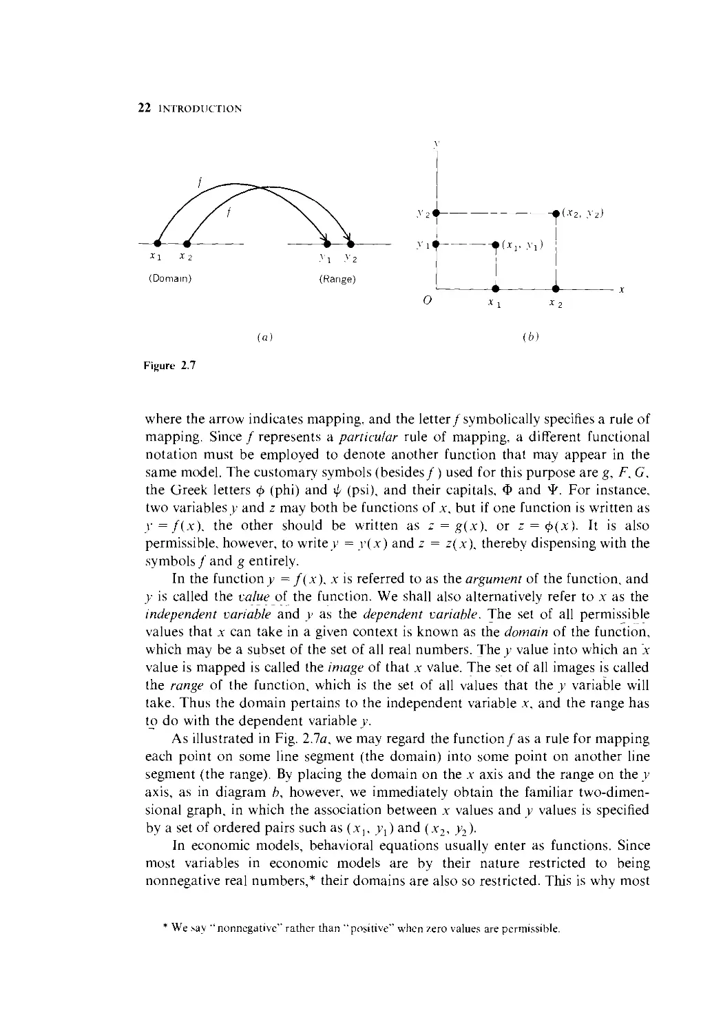
As illustrated in Fig. 2.7a, we may regard the function/as a rule for mapping
each point on some line segment (the domain) into some point on another line
segment (the range). By placing the domain on the x axis and the range on the y
axis, as in diagram b, however, we immediately obtain the familiar two-dimen-
two-dimensional graph, in which the association between x values and y values is specified
by a set of ordered pairs such as (x,,>>,) and (x2, y2)-
In economic models, behavioral equations usually enter as functions. Since
most variables in economic models are by their nature restricted to being
nonnegative real numbers,* their domains are also so restricted. This is why most
* We .say "nonnegative" rather than "positive" when zero values are permissible.
ECONOMIC MODELS 23
geometric representations in economics are drawn only in the first quadrant. In
general, we shall not bother to specify the domain of every function in every
economic model. When no specification is given, it is to be understood that the
domain (and the range) will only include numbers for which a function makes
economic sense.
Example 5 The total cost C of a firm per day is a function of its daily output Q:
C = 150 + 1Q. The firm has a capacity limit of 100 units of output per day. What
are the domain and the range of the cost function? Inasmuch as Q can vary only
between 0 and 100, the domain is the set of values 0 < Q < 100; or more
formally,
Domain = {Q | 0 < Q < 100}
As for the range, since the function plots as a straight line, with the minimum C
value at 150 (when Q = 0) and the maximum C value at 850 (when Q = 100), we
have
Range = (C | 150 < C < 850}
Beware, however, that the extreme values of the range may not always occur
where the extreme values of the domain are attained.
EXERCISE 2.4
1 Given St = {3,6,9}, S2 = {a, b}, and S3 = (m, «}, find the cartesian products:
(a) S, X S2 (b) S2 X S3 (c) S, X S,
2 From the information in the preceding problem, find the cartesian product S, X S2 X S-,.
3 In general, is it true that S, X Si = Si X S{1 Under what conditions will these two
cartesian products be equal?
4 Does each of the following, drawn in a rectangular coordinate plane, represent a
function?
(a) A circle ■ (b) A triangle (c) A rectangle
5 If the domain of the function v = 5 + 3.x is the set (x \ ! < x < 4}, find the range of the
function and express it as a set.
6 For the function v = -x2\ if the domain is the set of all nonnegative real numbers,
what will its range be?
2.5 TYPES OF FUNCTION
The expression y = f(x) is a general statement to the effect that a mapping is
possible, but the actual rule of mapping is not thereby made explicit. Now let us
consider several specific types of function, each representing a different rule of
mapping.
24 INTRODUCTION
Constant Functions
A function whose range consists of only one element is called a constant function.
As an example, we cite the function
y=f(x) = 7
which is alternatively expressible as y = 7 or f(x) = 7, whose value stays the
same regardless of the value of x. In the coordinate plane, such a function will
appear as a horizontal straight line. In national-income models, when investment
(/) is exogenously determined, we may have an investment function of the form
/ = $100 million, or / = /0, which exemplifies the constant function.
Polynomial Functions
The constant function is actually a "degenerate" case of what are known as
polynomial functions. The word "polynomial" means "multiterm," and a poly-
polynomial function of a single variable x has the general form
B.4) y = a0 + axx + a2x2 + • ■ • + anx"
in which each term contains a coefficient as well as a nonnegative-integer power
of the variable x. (As will be explained later in this section, we can write x1 = x
and x° = 1 in general; thus the first two terms may be taken to be aox° and atx{,
respectively.) Note that, instead of the symbols a, b,c,..., we have employed the
subscripted symbols a0, ax,..., an for the coefficients. This is motivated by two
considerations: A) we can economize on symbols, since only the letter a is "used
up" in this way; and B) the subscript helps to pinpoint the location of a
particular coefficient in the entire equation. For instance, in B.4), a2 is the
coefficient of x2, and so forth.
Depending on the value of the integer n (which specifies the highest power of
x), we have several subclasses of polynomial function:
Case of n = 0: y = a0 [constant function]
Case of n = 1: y = a0 + a{x [linear function]
Case of n = 2: y = a0 + a{x + a2x2 [quadratic function]
Case of n = 3: y = a0 + axx + a2x2 + a3x3 [cubic function]
and so forth. The superscript indicators of the powers of x are called exponents.
The highest power involved, i.e., the value of n, is often called the degree of the
polynomial function; a quadratic function, for instance, is a second-degree
polynomial, and a cubic function is a third-degree polynomial.* The order in
which the several terms appear to the right of the equals sign is inconsequential;
* In the several equations just cited, the last coefficient (un) is always assumed to be nonzero:
otherwise the function would degenerate into a lower-degree polynomial.
ECONOMIC MODELS 25
they may be arranged in descending order of power instead. Also, even though we
have put the symboly on the left, it is also acceptable to write f(x) in its place.
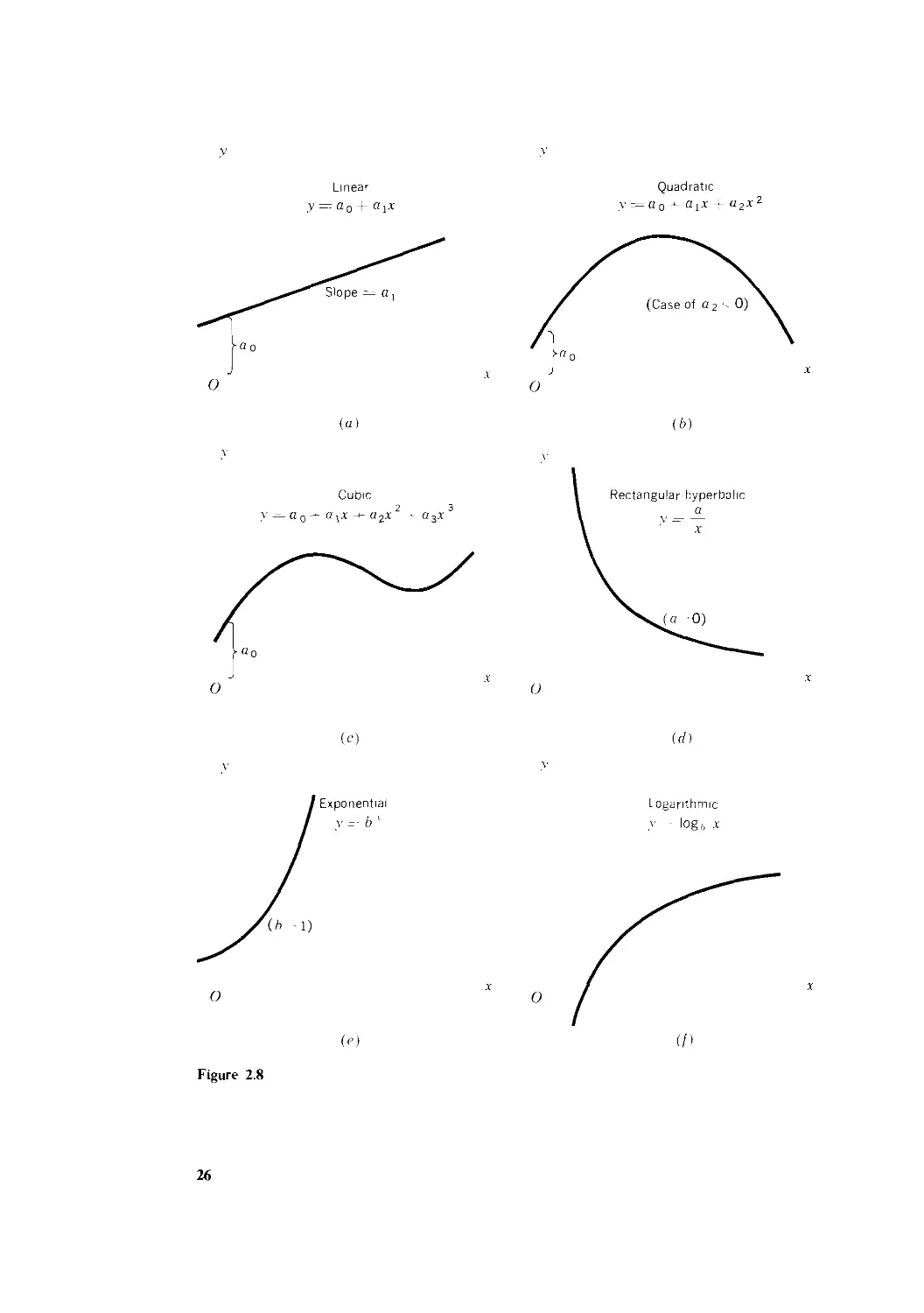
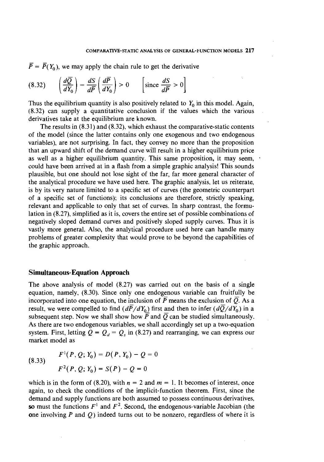
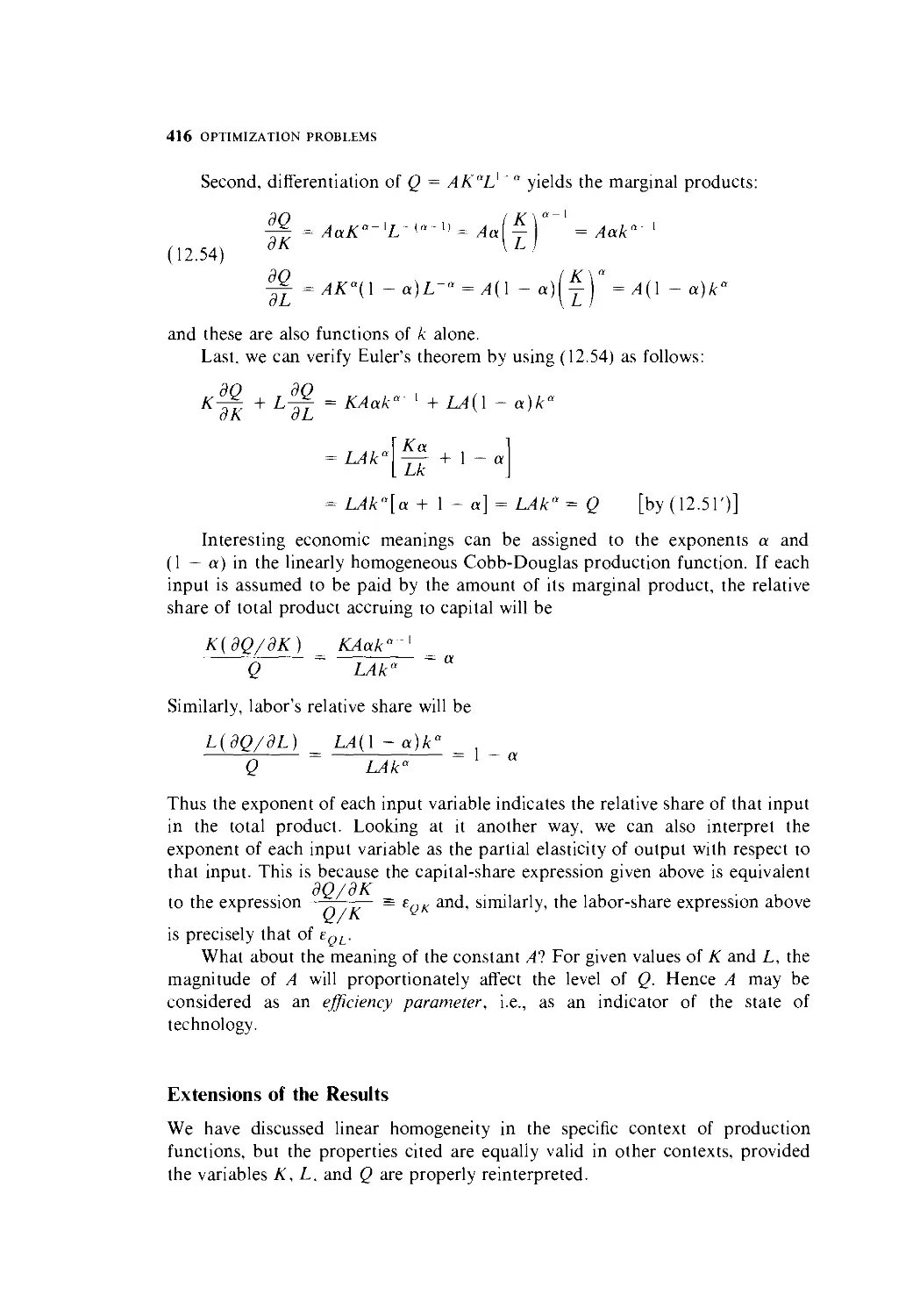
When plotted in the coordinate plane, a linear function will appear as a
straight line, as illustrated in Fig. 2.8a. When x = 0, the linear function yields
y = a0; thus the ordered pair @, a0) is on the line. This gives us the so-called "y
intercept" (or vertical intercept), because it is at this point that the vertical axis
intersects the line. The other coefficient, a,, measures the slope (the steepness of
incline) of our line. This means that a unit increase in x will result in an increment
in v in the amount of a,. What Fig. 2.8a illustrates is the case of a, > 0, involving
a positive slope and thus an upward-sloping line; if a, < 0, the line will be
downward-sloping.
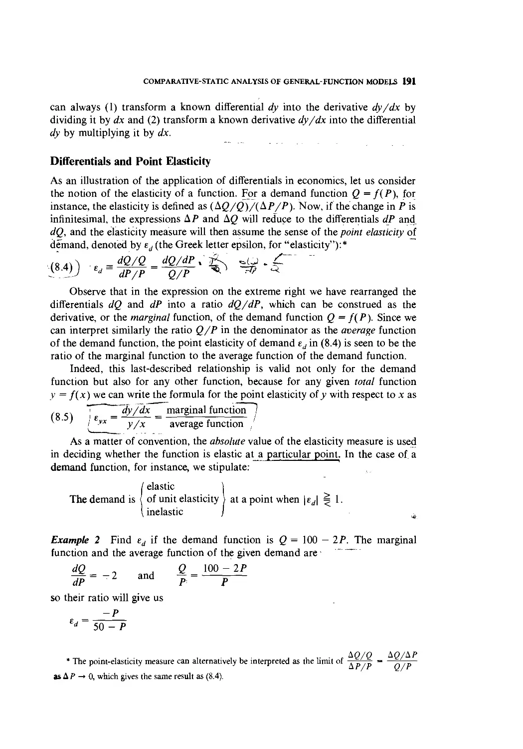
A quadratic function, on the other hand, plots as a parabola—roughly, a
curve with a single built-in bump or wiggle. The particular illustration in Fig. 2.86
implies a negative a2; in the case of a2 > 0, the curve will "open" the other way,
displaying a valley rather than a hill. The graph of a cubic function will, in
general, manifest two wiggles, as illustrated in Fig. 2.8c. These functions will be
used quite frequently in the economic models discussed below.
Rational Functions
A function such as
x - 1
>' =
x1 + 2x + 4
in which y is expressed as a ratio of two polynomials in the variable x, is known
as a rational function (again, meaning ra?/o-nal). According to this definition, any
polynomial function must itself be a rational function, because it can always be
expressed as a ratio to 1, which is a constant function.
A special rational function that has interesting applications in economics is
the function
a
V = — or xy = a
x
which plots as a rectangular hyperbola, as in Fig. 2.8<i. Since the product of the
two variables is always a fixed constant in this case, this function may be used to
represent that special demand curve—with price P and quantity Q on the two
axes—for which the total expenditure PQ is constant at all levels of price. (Such a
demand curve is the one with a unitary elasticity at each point on the curve.)
Another application is to the average fixed cost (AFC) curve. With AFC on one
axis and output Q on the other, the AFC curve must be rectangular-hyperbolic
because AFC X Q(= total fixed cost) is a fixed constant.
The rectangular hyperbola drawn from xy = a never meets the axes, even if
extended indefinitely upward and to the right. Rather, the curve approaches the
axes asymptotically, as y becomes very large, the curve will come ever closer to the
Linear
,y —- a 0 + a x
Slope — a,
Quadratic
(a)
(b)
Cubic
y — a 0 — a !
Rectangular-hyperbolic
(c)
(d)
' Exponential
v=- b'
Logarithmic
,v ■ log/, x
O
o
Figure 2.8
26
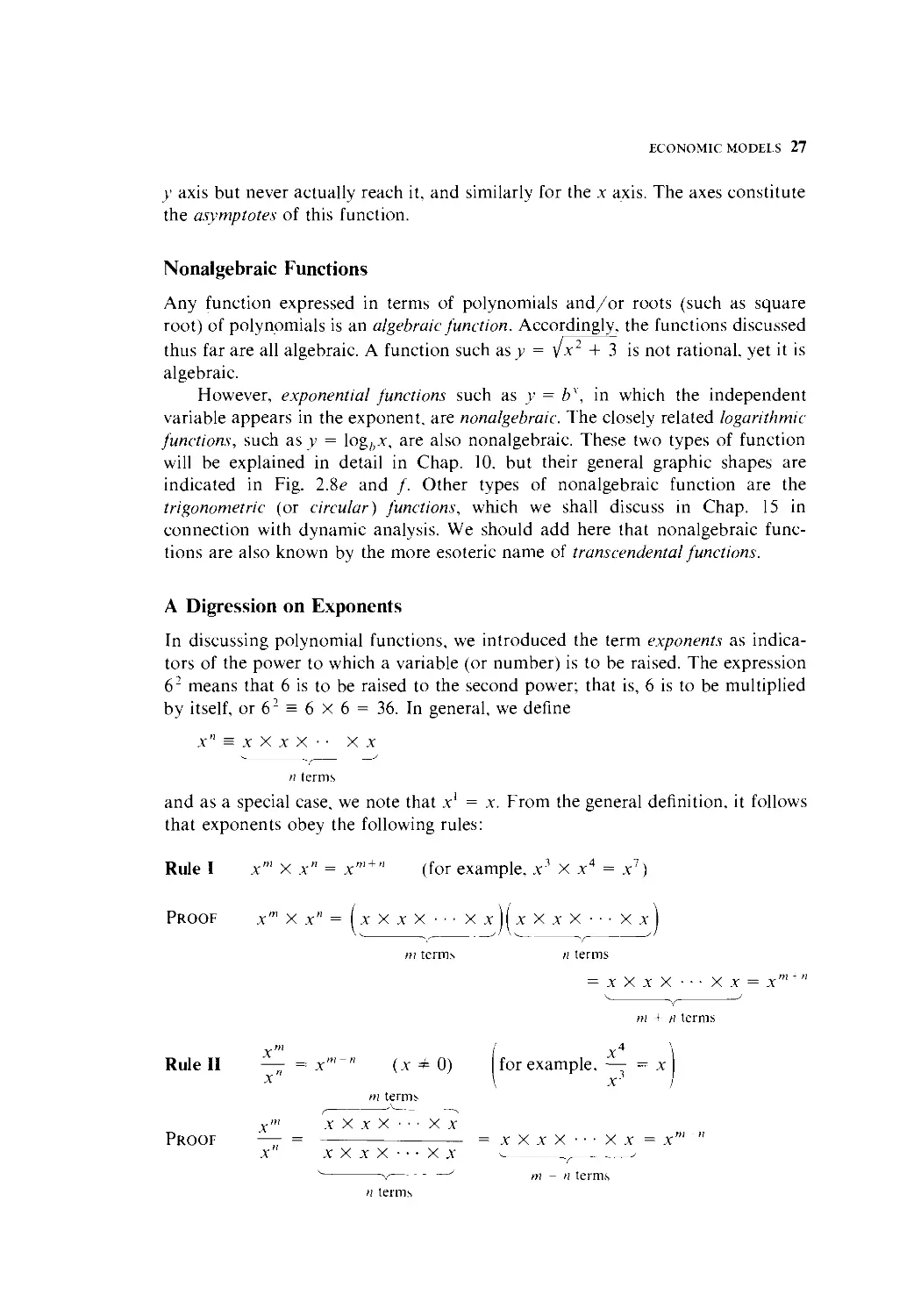
ECONOMIC MODELS 27
y axis but never actually reach it, and similarly for the x axis. The axes constitute
the asymptotes of this function.
Nonalgebraic Functions
Any function expressed in terms of polynomials and/or roots (such as square
root) of polynomials is an algebraic function. Accordingly, the functions discussed
thus far are all algebraic. A function such as y = \x2 + 3 is not rational, yet it is
algebraic.
However, exponential functions such as y = bx, in which the independent
variable appears in the exponent, are nonalgebraic. The closely related logarithmic
functions, such as y = logfcx, are also nonalgebraic. These two types of function
will be explained in detail in Chap. 10, but their general graphic shapes are
indicated in Fig. 2.8<? and /. Other types of nonalgebraic function are the
trigonometric (or circular) functions, which we shall discuss in Chap. 15 in
connection with dynamic analysis. We should add here that nonalgebraic func-
functions are also known by the more esoteric name of transcendental functions.
A Digression on Exponents
In discussing polynomial functions, we introduced the term exponents as indica-
indicators of the power to which a variable (or number) is to be raised. The expression
62 means that 6 is to be raised to the second power; that is, 6 is to be multiplied
by itself, or 62 = 6 X 6 = 36. In general, we define
x" = x X x X
X x
n terms
and as a special case, we note that x1 = x. From the general definition, it follows
that exponents obey the following rules:
Rule I
Proof
xm X X" = X
n _ vm+n
(for example, x3 X x4 = x1)
xm X x" = [ x X x X
X x \\ x X x X
X x
m terms
n terms
= X X X X
X X = x"
Rule II —- = x"
Proof
xm
x"
f
X
X
X
X
X
X
11
X ■ ■ ■
X ■ ■ ■
terms
X
X
X
X
m + n terms
/' x4
(x ± 0) for example, — = x
\ x-
m terms
X x
= X X X X ■ ■ ■ X X = Xm "
m - n terms
28 INTRODUCTION
because the n terms in the denominator cancel out n of the m terms in the
numerator. Note that the case of x = 0 is ruled out in the statement of this rule.
This is because when x = 0, the expression xn'/x" would involve division by zero,
which is undefined.
What if m < n: say, m = 2 and n = 5? In that case we get, according to Rule
II, xm " = x~3, a negative power of x. What does this mean? The answer is
actually supplied by Rule II itself: When m = 2 and n = 5, we have
xr_ x X x 1 _ _^
xi~xXxXxXxXx x X x X x x3
Thus a' = 1/x3, and this may be generalized into another rule:
Rule III x~" = -^ (x * 0)
A
To raise a (nonzero) number to a power of minus n is to take the reciprocal of its
nth power.
Another special case in the application of Rule II is when m = n, which
yi'eWs the expression xm~" = xm"m = x°. To interpret the meaning of raising a
number x to the zeroth power, we can write out the term xm ~m in accordance
with Rule II above, with the result that x'"/x'" = 1. Thus we may conclude that
any (nonzero) number raised to the zeroth power is equal to 1. (The expression 0°
is undefined.) This may be expressed as another rule:
Rule IV -x0 =1 (x * 0)
As long as we are concerned only with polynomial functions, only (nonnega-
tive) integer powers are required. In exponential functions, however, the exponent
is a variable that can take noninteger values as well. In order to interpret a
number such as x)/2, let us consider the fact that, by Rule I above, we have
Since xwl multiplied by itself is x. x]/1 must be the square root of x. Similarly,
x''3 can be shown to be the cube root of x. In general, therefore, we can state the
following rule:
ti, -
Rule V x'/n = ix
Two other rules obeyed by exponents are:
Rule VI (x"')" = x'""
Rule VII xm X v"' = (xv)'"
ECONOMIC MODELS 29
EXERCISE 2.5
1 Graph the functions
(a) v = 8 + 3* (b) v = 8 - 3.x (c) v = 3x + 12
(In each case, consider the domain as consisting of nonnegative real numbers only.)
2 What is the major difference between (a) and (b) above? How is this difference reflected
in the graphs? What is the major difference between (a) and (c)? How do their graphs
reflect it?
3 Graph the functions
(a) y = -x2 + 5x ~ 2 (b) v = x2 + 5x ~ 2
with the set of values - 5 < x < 5 as the domain. It is well known that the sign of the
coefficient of the x2 term determines whether the graph of a quadratic function will have a
"hill" or a "valley." On the basis of the present problem, which sign is associated with the
hill? Supply an intuitive explanation for this.
4 Graph the function y = 36/x, assuming that x and v can take positive values only.
Next, suppose that both variables can take negative values as well; how must the graph be
modified to reflect this change in assumption?
5 Condense the following expressions:
(a) x4 X x15 (b) x" X xh X x' (c) x3 X >■' X z1
6 Find: (a) x3/x~- (b) (x1'2 X x1 -)/x2>'
n, in,— \n\
7 Show that x" = ixm = \ix ) . Specify the rules applied in each step.
8 Prove Rule VI and Rule VII.
2.6 FUNCTIONS OF TWO OR MORE INDEPENDENT
VARIABLES
Thus far, we have considered only functions of a single independent variable,
y = /(x). But the concept of a function can be readily extended to the case of two
or more independent variables. Given a function
z = g(x, v)
a given pair of x and y values will uniquely determine a value of the dependent
variable z. Such a function is exemplified by
z = ax + by or z = a0 + axx + a2x2 + b{ v + b2 V2
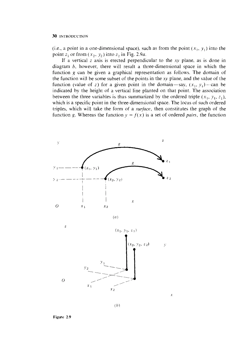
Just as the functiony - f(x) maps a point in the domain into a point in the
range, the function g will do precisely the same. However, the domain is in this
case no longer a set of numbers but a set of ordered pairs (x, y), because we can
determine z only when both x and y are specified. The function g is thus a
mapping from a point in a two-dimensional space into a point on a line segment
30 INTRODUCTION
(i.e., a point in a one-dimensional space), such as from the point (x,, _>>,) into the
point z, or from (x2, >>2) into z2 in Fig. 2.9a.
If a vertical z axis is erected perpendicular to the xy plane, as is done in
diagram b, however, there will result a three-dimensional space in which the
function g can be given a graphical representation as follows. The domain of
the function will be some subset of the points in the xy plane, and the value of the
function (value of z) for a given point in the domain — say, (x,, >•,)—can be
indicated by the height of a vertical line planted on that point. The association
between the three variables is thus summarized by the ordered triple (x,, >,, z,),
which is a specific point in the three-dimensional space. The locus of such ordered
triples, which will take the form of a surface, then constitutes the graph of the
function g. Whereas the function y = f(x) is a set of ordered pairs, the function
♦(*!
o
(a)
(x2, y2, z2) y
o
X2
(b)
Figure 2.9
ECONOMIC MODELS 31
z = g(x, y) will be a set of ordered triples. We shall have many occasions to use
functions of this type in economic models. One ready application is in the area of
production functions. Suppose that output is determined by the amounts of
capital (K) and labor (L) employed; then we can write a production function in
the general form Q = Q(K, L).
The possibility of further extension to the cases of three or more independent
variables is now self-evident. With the function y = h(u,v, r>), for example, we
can map a point in the three-dimensional space, (ul? u^vv,), into a point in a
one-dimensional space (j,). Such a function might be used to indicate that a
consumer's utility is a function of his consumption of three different commodities,
and the mapping is from a three-dimensional commodity space into a one-dimen-
one-dimensional utility space. But this time it will be physically impossible to graph the
function, because for that task a four-dimensional diagram is needed to picture
the ordered quadruples, but the world in which we live is only three-dimensional.
Nonetheless, in view of the intuitive appeal of geometric analogy, we can continue
to refer to an ordered quadruple («,, t;,, h,, yx) as a "point" in the four-dimen-
four-dimensional space. The locus of such points will give the (nongraphable) graph of the
function y = h(u, v, w), which is called a hypersurface. These terms, viz., point
and hypersurface, are also carried over to the general case of the ^-dimensional
space.
Functions of more than one variable can be classified into various types, too.
For instance, a function of the form
y = alxl + a2x2 + ■ ■ ■ + anxn
is a linear function, whose characteristic is that every variable is raised to the first
power only. A quadratic function, on the other hand, involves first and second
powers of one or more independent variables, but the sum of exponents of the
variables appearing in any single term must not exceed two.
Note that instead of denoting the independent variables by x, u, v, r>, etc., we
have switched to the symbols jc,. x2 xn. The latter notation, like the system
of subscripted coefficients, has the merit of economy of alphabet, as well as of an
easier accounting of the number of variables involved in a function.
2.7 LEVELS OF GENERALITY
In discussing the various types of function, we have without explicit notice
introduced examples of functions that pertain to varying levels of generality. In
certain instances, we have written functions in the form
V = 7 y = 6x + 4 y = x2 - 3x + 1 (etc.)
Not only are these expressed in terms of numerical coefficients, but they also
indicate specifically whether each function is constant, linear, or quadratic. In
terms of graphs, each such function will give rise to a well-defined unique curve.
In view of the numerical nature of these functions, the solutions of the model
32 INTRODUCTION
based on them will emerge as numerical values also. The drawback is that, if we
wish to know how our analytical conclusion will change when a different set of
numerical coefficients comes into effect, we must go through the reasoning process
afresh each time. Thus, the results obtained from specific functions have very little
generality.
On a more general level of discussion and analysis, there are functions in the
form
y = a y = a + bx y = a + bx + ex1 (etc.)
Since parameters are used, each function represents not a single curve but a whole
family of curves. The function y = a, for instance, encompasses not only the
specific cases y = 0, y = 1, and y = 2 but also y = \, y = - 5,..., ad infinitum.
With parametric functions, the outcome of mathematical operations will also be
in terms of parameters. These results are more general in the sense that, by
assigning various values to the parameters appearing in the solution of the model,
a whole family of specific answers may be obtained without having to repeat the
reasoning process anew.
In order to attain an even higher level of generality, we may resort to the
general function statement y = f(x), or z = g(x, y). When expressed in this
form, the function is not restricted to being either linear, quadratic, exponential,
or trigonometric—all of which are subsumed under the notation. The analytical
result based on such a general formulation will therefore have the most general
applicability. As will be found below, however, in order to obtain economically
meaningful results, it is often necessary to impose certain qualitative restrictions
on the general functions built into a model, such as the restriction that a demand
function have a negatively sloped graph or that a consumption function have a
graph with a positive slope of less than 1.
To sum up the present chapter, the structure of a mathematical economic
model is now clear. In general, it will consist of a system of equations, which may
be definitional, behavioral, or in the nature of equilibrium conditions.* The
behavioral equations are usually in the form of functions, which may be linear or
nonlinear, numerical or parametric, and with one independent variable or many.
It is through these that the analytical assumptions adopted in the model are given
mathematical expression.
In attacking an analytical problem, therefore, the first step is to select the
appropriate variables—exogenous as well as endogenous—for inclusion in the
model. Next, we must translate into equations the set of chosen analytical
assumptions regarding the human, institutional, technological, legal, and other
behavioral aspects of the environment affecting the working of the variables. Only
then can an attempt be made to derive a set of conclusions through relevant
mathematical operations and manipulations and to give them appropriate eco-
economic interpretations.
* Inequalities may also enter as an important ingredient of a model, but we shall not worry about
them for the time being.
PART
TWO
STATIC (OR EQUILIBRIUM) ANALYSIS
CHAPTER
THREE
EQUILIBRIUM ANALYSIS IN ECONOMICS
The analytical procedure outlined in the preceding chapter will first be applied to
what is known as static analysis, or equilibrium analysis. For this purpose, it is
imperative first to have a clear understanding of what "'equilibrium" means.
3.1 THE MEANING OF EQUILIBRIUM
Like any economic term, equilibrium can be defined in various ways. According to
one definition, an equilibrium is "a constellation of selected interrelated variables
so adjusted to one another that no inherent tendency to change prevails in the
model which they constitute."* Several words in this definition deserve special
attention. First, the word "selected" underscores the fact that there do exist
variables which, by the analyst's choice, have not been included in the model.
Hence the equilibrium under discussion can have relevance only in the context of
the particular set of variables chosen, and if the model is enlarged to include
additional variables, the equilibrium state pertaining to the smaller model will no
longer apply.
Second, the word "interrelated" suggests that, in order for equilibrium to
obtain, all variables in the model must simultaneously be in a state of rest.
Moreover, the state of rest of each variable must be compatible with that of every
* Fritz Machlup, ''Equilibrium and Disequilibrium: Misplaced Concreteness and Disguised
Politics." Economic Journal, March 1958. p. 9. (Reprinted in F. Machlup, Essays on Economic
Semantics, Prentice-Hall, Inc., Englcwood Cliffs. N.J.. 1963.)
35
36 STATIC (OR EQUILIBRIUM) ANALYSIS
other variable; otherwise some variable(s) will be changing, thereby also causing
the others to change in a chain reaction, and no equilibrium can be said to exist.
Third, the word "inherent" implies that, in defining an equilibrium, the state
of rest involved is based only on the balancing of the internal forces of the model,
while the external factors are assumed fixed. Operationally, this means that
parameters and exogenous variables are treated as constants. When the external
factors do actually change, there may result a new equilibrium defined on the
basis of the new parameter values, but in defining the new equilibrium, the new
parameter values are again assumed to persist and stay unchanged.
In essence, an equilibrium for a specified model is a situation that is
characterized by a lack of tendency to change. It is for this reason that the
analysis of equilibrium (more specifically, the study of what the equilibrium state
is like) is referred to as statics. The fact that an equilibrium implies no tendency
to change may tempt one to conclude that an equilibrium necessarily constitutes a
desirable or ideal state of affairs, on the ground that only in the ideal state would
there be a lack of motivation for change. Such a conclusion is unwarranted. Even
though a certain equilibrium position may represent a desirable state and some-
something to be striven for—such as a profit-maximizing situation, from the firm's
point of view—another equilibrium position may be quite undesirable and
therefore something to be avoided, such as an underemployment equilibrium level
of national income. The only warranted interpretation is that an equilibrium is a
situation which, if attained, would tend to perpetuate itself, barring any changes
in the external forces.
The desirable variety of equilibrium, which we shall refer to as goal equi-
equilibrium, will be treated later in Parts 4 and 6 as optimization problems. In the
present chapter, the discussion will be confined to the nongoal type of equilibrium,
resulting not from any conscious aiming at a particular objective but from an
impersonal or suprapersonal process of interaction and adjustment of economic
forces. Examples of this are the equilibrium attained by a market under given
demand and supply conditions and the equilibrium of national income under
given conditions of consumption and investment patterns.
3.2 PARTIAL MARKET EQUILIBRIUM—A LINEAR MODEL
In a static-equilibrium model, the standard problem is that of finding the set of
values of the endogenous variables which will satisfy the equilibrium condition of
the model. This is because once we have identified those values, we have in effect
identified the equilibrium state. Let us illustrate with a so-called "partial-equi-
"partial-equilibrium market model," i.e., a model of price determination in an isolated market.
Constructing the Model
Since only one commodity is being considered, it is necessary to include only
three variables in the model: the quantity demanded of the commodity (Qd), the
EQUILIBRIUM ANALYSIS IN ECONOMICS 37
quantity supplied of the commodity (Q,), and its price (P). The quantity is
measured, say, in pounds per week, and the price in dollars. Having chosen the
variables, our next order of business is to make certain assumptions regarding the
working of the market. First, we must specify an equilibrium condition—some-
condition—something indispensable in an equilibrium model. The standard assumption is that
equilibrium obtains in the market if and only if the excess demand is zero
(Q<j ~ Qs = 0), that is, if and only if the market is cleared. But this immediately
raises the question of how Qd and Qs themselves are determined. To answer this,
we assume that Qd is a decreasing linear function of P (as P increases, Qd
decreases). On the other hand, Qs is postulated to be an increasing linear function
of P (as P increases, so does Qs), with the proviso that no quantity is supplied
unless the price exceeds a particular positive level. In all, then, the model will
contain one equilibrium condition plus two behavioral equations which govern
the demand and supply sides of the market, respectively.
Translated into mathematical statements, the model can be written as:
Qa = Q,
C.1) Qd=a-bP (a,b>0)
Qs = -c + dP (c,d> 0)
Four parameters, a, b, c, and d, appear in the two linear functions, and all of
them are specified to be positive. When the demand function is graphed, as in Fig.
3.1, its vertical intercept is at a and its slope is — b, which is negative, as required.
The supply function also has the required type of slope, d being positive, but its
Figure 3.1
38 STATIC (OR EQUILIBRIUM) ANALYSIS
vertical intercept is seen to be negative, at — c. Why did we want to specify such a
negative vertical intercept? The answer is that, in so doing, we force the supply
curve to have a positive horizontal intercept at Pj% thereby satisfying the proviso
stated earlier that supply will not be forthcoming unless the price is positive and
sufficiently high.
The reader should observe that, contrary to the usual practice, quantity rather
than price has been plotted vertically in Fig. 3.1. This, however, is in line with the
mathematical convention of placing the dependent variable on the vertical axis. In
a difFerent context below, in which the demand curve is viewed from the
standpoint of a business firm as describing the average-revenue curve, AR = P =
f(Qj)- we shall reverse the axes and plot P vertically.
With the model thus constructed, the next step is to solve it. i.e., to obtain the
solution values of the three endogenous variables, Qd. £>5, and P. The solution
values, to be denoted Qd, QK, and P, are those values that satisfy the three
equations in C.1) simultaneously, i.e., they are the values which, when substituted
into the three equations, make the latter a set of true statements. In the context of
an equilibrium model, those values may also be referred to as the equilibrium
values of the said variables. Since Qit = QK, however, they can be replaced by a
single symbol Q. Hence, an equilibrium solution of the model may simply be
denoted by an ordered pair (P,Q). In case the solution is not unique, several
ordered pairs may each satisfy the system of simultaneous equations; there will
then be a solution set with more than one element in it. However, the multiple-
equilibrium situation cannot arise in a linear model such as the present one.
Solution by Elimination of Variables
One way of finding a solution to an equation system is by successive elimination
of variables and equations through substitution. In C.1). the model contains three
equations in three variables. However, in view of the equating of Qd and Qs by
the equilibrium condition, we can let Q = Qit = Qs and rewrite the model
equivalently as follows:
Q = a - bP
C.2)
Q = -c + dP
thereby reducing the model to two equations in two variables. Moreover, by
substituting the first equation into the second in C.2), the model can be further
reduced to a single equation in a single variable:
a - bP = -c + dP
or, after subtracting (a + dP) from both sides of the equation and multiplying
through by - 1.
C.3) (b + d)P = a + c
EQUILIBRIUM ANALYSIS IN ECONOMICS 39
This result is also obtainable directly from C.1) by substituting the second and
third equations into the first.
Since b + d + 0, it is permissible to divide both sides of C.3) by (b + d). The
result is the solution value of P:
Note that P is—as all solution values should be—expressed entirely in terms of
the parameters, which represent given data for the model. Thus P is a determinate
value, as it ought to be. Also note that P is positive—as a price should
be—because all the four parameters are positive by model specification.
To find the equilibrium quantity Q (= Qd = £?>) that corresponds to the
value P, simply substitute C.4) into either equation of C.2), and then solve the
resulting equation. Substituting C.4) into the demand function, for instance, we
can get
., e. =■ b(a + c) a(b + d) - b(a + c) ad - be
C.5) Q = a--^- = ^ = TTT
which is again an expression in terms of parameters only. Since the denominator
(b + d) is positive, the positivity of Q requires that the numerator (ad — be) be
positive as well. Hence, to be economically meaningful, the present model should
contain the additional restriction that ad > be.
The meaning of this restriction can be seen in Fig. 3.1. It is well known that
the P and Q of a market model may be determined graphically at the intersection
of the demand and supply curves. To have Q > 0 is to require the intersection
point to be located above the horizontal axis in Fig. 3.1, which in turn requires
the slopes and vertical intercepts of the two curves to fulfill a certain restriction
on their relative magnitudes. That restriction, according to C.5), is ad > be, given
that both b and d are positive.
The intersection of the demand and supply curves in Fig. 3.1, incidentally, is
in concept no different from the intersection shown in the Venn diagram of Fig.
2.2b. There is one difference only: instead of the points lying within two circles,
the present case involves the points that lie on two lines. Let the set of points on
the demand and supply curves be denoted, respectively, by D and S. Then, by
utilizing the symbol Q (= Qd = £?v), the two sets and their intersection can be
written
S = {(P,Q)\Q= -c
and D n S = {P, Q)
The intersection set contains in this instance only a single element, the ordered
pair (P, Q). The market equilibrium is unique.
40 STATIC (OR EQUILIBRIUM) ANALYSIS
EXERCISE 3.2
1 Given the market model
Qa = Qs
Qt/ = 24-2P
Q- = + IP
find P and Q by (a) elimination of variables and (b) using formulas C.4) and C.5). (Use
fractions rather than decimals.)
2 Let the demand and supply functions be as follows:
(a) Qd=S\- 3P (b) Qd= 30 -IP
q = 6P - 10 Qs = -6 + 5P
find P and 0 by elimination of variables. (Use fractions rather than decimals.)
3 According to C.5), for Q to be positive, it is necessary that the expression (ad - be)
have the same algebraic sign as (b + d). Verify that this condition is indeed satisfied in the
models of the preceding two problems.
4 \l (b + d) = Q m the linear market model, can an equilibrium solution be found by
using C.4) and C.5)? Why or why not?
5 If (b + d) = 0 in the linear market model, what can you conclude regarding the
positions of the demand and supply curves in Fig. 3.1? What can you conclude, then,
regarding the equilibrium solution?
3.3 PARTIAL MARKET EQUILIBRIUM—A NONLINEAR MODEL
Let the linear demand in the isolated market model be replaced by a quadratic
demand function, while the supply function remains linear. Then, if numerical
coefficients are employed rather than parameters, a model such as the following
may emerge:
Qa=Qs
C-6) Qd=4-P2
Qs = 4P ~ ]
As previously, this system of three equations can be reduced to a single equation
by elimination of variables (by substitution):
4 - P2 = 4P - 1
or
C.7) P2 + 4P - 5 = 0
This is a quadratic equation because the left-hand expression is a quadratic
function of variable P. The major difference between a quadratic equation and a
linear one is that, in general, the former will yield two solution values.
EQUILIBRIUM ANALYSIS IN ECONOMICS 41
Quadratic Equation versus Quadratic Function
Before discussing the method of solution, a clear distinction should be made
between the two terms quadratic equation and quadratic function. According to the
earlier discussion, the expression P2 + 4P - 5 constitutes a quadratic function.
say, f(P). Hence we may write
C.8) f(P) = P2 + AP- 5
a
- 6 - 5 - 4l - 3 | - 2 | - 1
What C.8) does is to specify a rule of mapping from P to f(P), such as
0
f(P)
0
-5
-8
-9 -8
-5
0
Although we have listed only nine P values in this table, actually all the P values
in the domain of the function are eligible for listing. It is perhaps for this reason
that we rarely speak of "solving" the equation f(P) = P2 + 4P - 5, because we
normally expect "solution values" to be few in number, but here all P values can
get involved. Nevertheless, one may legitimately consider each ordered pair in the
table above—such as (- 6,7) and (- 5,0)—as a solution of C.8), since each such
ordered pair indeed satisfies that equation. Inasmuch as an infinite number of
such ordered pairs can be written, one for each P value, there is an infinite
number of solutions to C.8). When plotted as a curve, these ordered pairs
together yield the parabola in Fig. 3.2.
f(P)
-6 -5\ —
Figure 3.2
42 STATIC (OR EQUILIBRIUM) ANALYSIS
In C.7). where we set the quadratic function/(.P) equal to zero, the situation
is fundamentally changed. Since the variable f(P) now disappears (having been
assigned a zero value), the result is a quadratic equation in the single variable P.*
Now that/(.P) is restricted to a zero value, only a select number of P values can
satisfy C.7) and qualify as its solution values, namely, those P values at which the
parabola in Fig. 3.2 intersects the horizontal axis—on which f(P) is zero. Note
that this time the solution values are just P values, not ordered pairs. The solution
P values are often referred to as the roots of the quadratic equation f(P) = 0, or,
alternatively, as the zeros of the quadratic function f(P).
There are two such intersection points in Fig. 3.2, namely, A,0) and (-5,0).
As required, the second element of each of these ordered pairs (the ordinate of the
corresponding point) shows f{P) = 0 in both cases. The first element of each
ordered pair (the abscissa of the point), on the other hand, gives the solution value
of P. Here we get two solutions,
P, = 1 and P2 = - 5
but only the first is economically admissible, as negative prices are ruled out.
The Quadratic Formula
Equation C.7) has been solved graphically, but an algebraic method is also
available. In general, given a quadratic equation in the form
C.9) ax2 + bx + c = 0 (a ± 0)
its two roots can be obtained from the quadratic formula:
-b + (b2 - 4ac)>/2
C.10) jc,,jc,=
la
where the + part of the + sign yields x, and the - part yields x2.
This widely used formula is derived by means of a process known as
"completing the square." First, dividing each term of C.9) by a results in the
equation
Subtracting c/a from, and adding b1 /4a2 to, both sides of the equation, we get
, b b2 b2 c
x' + - x + —- = —
a 4a 4a a
* The distinction between quadratic function and quadratic equation just discussed can be
extended also to cases of polynomials other than quadratic. Thus, a cubic equation results when a
cubic function is set equal to zero.
EQUILIBRIUM ANALYSIS IN ECONOMICS 43
The left side is now a "perfect square," and thus the equation can be expressed as
b \2 b2 - 4ac
or, after taking the square root on both sides,
b , (b2-4ac)l/2
x + — = +
la la
Finally, by subtracting b/la from both sides, the result in C.10) is evolved.
Applying the formula to C.7), where a = 1, b = 4, c = -5, and x = P, the
roots are found to be
p -- -4+ A6+ 20)
1/2
-4 + 6
= 1, -5
which check with the graphical solutions in Fig. 3.2. Again, we reject P2~ ~5 on
economic grounds and, after omitting the subscript 1. write simply P = 1.
With this information in hand, the equilibrium quantity Q can readily be
found from either the second or the third equation of C.6) to be Q = 3.
Another Graphical Solution
One method of graphical solution of the present model has been presented in Fig.
3.2. However, since the quantity variable has been eliminated in deriving the
quadratic equation, only P can be found from that figure. If we are interested in
1-2
Figure 3.3
44 STATIC (OR EQUILIBRIUM) ANALYSIS
finding P and Q simultaneously from a graph, we must instead use a diagram
with Q on one axis and P on the other, similar in construction to Fig. 3.1. This is
illustrated in Fig. 3.3. Our problem is of course again to find the intersection of
two sets of points, namely,
D = {(P,Q)\Q = 4- P2}
and 5 = {(P,Q) \ Q = 4P - 1}
If no restriction is placed on the domain and the range, the intersection set will
contain two elements, namely,
Dn S = {A.3),(-5,-21)}
The former is located in quadrant I, and the latter (not drawn) in quadrant III. If
the domain and range are restricted to being nonnegative, however, only the first
ordered pair A,3) can be accepted. Then the equilibrium is again unique.
Higher-Degree Polynomial Equations
If a system of simultaneous equations reduces not to a linear equation such as
C.3)* or to a quadratic equation such as C.7) but to a cubic (third-degree
polynomial) equation or quartic (fourth-degree polynomial) equation, the roots
will be more difficult to find. One useful method which may work is that of
factoring the function. For example, the expression x3 - x2 - 4x + 4 can be
written as the product of three factors (x — 1), (x + 2), and (x — 2). Thus the
cubic equation
x3 - x2 ~ 4x + 4 = 0
can be written after factoring as
(x~ \)(x + 2)(x -2) = 0
In order for the left-hand product to be zero, at least one of the three terms in the
product must be zero. Setting each term equal to zero in turn, we get
* _ 1 = 0 or .x + 2 = 0 or .x - 2 = 0
These three equations will supply the three roots of the cubic equation, namely,
x, = 1 x2= —2 and x3 = 2
The trick is, of course, to discover the appropriate way of factoring. Unfor-
Unfortunately, no general rule exists, and it must therefore remain a matter of trial and
error. Generally speaking, however, given an «th-degree polynomial equation
f(x) = 0, we can expect exactly n roots, which may be found as follows. First, try
to find a constant c, such that f(x) is divisible by (x + c,). The quotient
f(x)/(x + c,) will be a polynomial function of a lesser—(n - l)st—degree; let
* Equation C.3) can be viewed as the result of setting the linear function (b 4- d)P - (a + c)
equal to zero.
EQUILIBRIUM ANALYSIS IN ECONOMICS 45
us call it g(x). It then follows that
f(x)= (x + c,)g(x)
Now, try to find a constant c, such that g(x) is divisible by (x + c-,). The
quotient g(x)/(x + c2) will again be a polynomial function of a lesser—this time
(n - 2)nd—degree, say, h(x). Since g(x) = (x + c2)h(x), it follows that
f{x) = (x + c,)g(x) = (x + c,)(.v + c2)h(x)
By repeating the process, it will be possible to reduce the original «th-degree
polynomial f{x) to a product of exactly n terms:
/(*)= (x + c,)(x + c-2)--- (-v + cn)
which, when set equal to zero, will yield n roots. Setting the first factor equal to
zero, for example, one gets 3c, = -c,. Similarly, the other factors will yield
3c2 = — c2, 3c3 = — c3, etc. These results can be more succinctly expressed by
employing an index subscript i:
x,= -c, (/=1,2 n)
Even though only one equation is written, the fact that the subscript / can take n
different values means that in all there are n equations involved. Thus the index
subscript provides a very concise way of statement.
EXERCISE 3.3
1 Find the zeros of the following functions graphically:
(a) f(x) = x2 - Ix + 10 (b) g(x) = 2x2 - 4x - 16
2 Solve the preceding problem by the quadratic formula.
3 Solve the following polynomial equations by factoring:
(a) P2 + 4P - 5 = 0 [see C.7)] (c) x1 - Ix2 + 14* - 8 = 0
(b) x3 + 2x2 - 4x - 8 = 0 (d) x} - 3x2 - 4x = 0
4 Find a cubic function with roots 7, - 2, and 5.
5 Find the equilibrium solution for each of the following models:
£>s = 6P - 4 2s = pl ~ 2
6 The market equilibrium condition, Qtl=Qs, is often expressed in an equivalent
alternative form, Q(l — Qs = 0, which has the economic interpretation "excess demand is
zero." Does C.7) represent this latter version of the equilibrium condition? If not, supply
an appropriate economic interpretation for C.7).
46 STATIC (OR EQUILIBRIUM) ANALYSIS
3.4 GENERAL MARKET EQUILIBRIUM
The last two sections dealt with models of an isolated market, wherein the Qd and
Qs of a commodity are functions of the price of that commodity alone. In the
actual world, though, no commodity ever enjoys (or suffers) such a hermitic
existence; for every commodity, there would normally exist many substitutes and
complementary goods. Thus a more realistic depiction of the demand function of
a commodity should take into account the effect not only of the price of the
commodity itself but also of the prices of most, if not all, of the related
commodities. The same also holds true for the supply function. Once the prices of
other commodities are brought into the picture, however, the structure of the
model itself must be broadened so as to be able to yield the equilibrium values of
these other prices as well. As a result, the price and quantity variables of multiple
commodities must enter endogenously into the model en masse.
In an isolated-market model, the equilibrium condition consists of only one
equation, Qd = Qf, or E = Qd — Qs = 0, where E stands for excess demand.
When several interdependent commodities are simultaneously considered, equi-
equilibrium would require the absence of excess demand for each and every commod-
commodity included in the model, for if so much as one commodity is faced with an excess
demand, the price adjustment of that commodity will necessarily affect the
quantities demanded and quantities supplied of the remaining commodities,
thereby causing price changes all around. Consequently, the equilibrium condi-
condition of an ^-commodity market model will involve n equations, one for each
commodity, in the form
C.11) E,= Qdl-Qsl = 0 (/= 1,2,...,«)
If a solution exists, there will be a set of prices P, and corresponding quantities Qt
such that all the n equations in the equilibrium condition will be simultaneously
satisfied.
Two-Commodity Market Model
To illustrate the problem, let us discuss a simple model in which only two
commodities are related to each other. For simplicity, the demand and supply
functions of both commodities are assumed to be linear. In parametric terms,
such a model can be written as
Qd\ = a0 + a\P\ + ^2^2
Qai ~ Qa = 0
Qdl = «0 + al^l + ^2
EQUILIBRIUM ANALYSIS IN ECONOMICS 47
where the a and b coefficients pertain to the demand and supply functions of the
first commodity, and the a and f$ coefficients are assigned to those of the second.
We have not bothered to specify the signs of the coefficients, but in the course of
analysis certain restrictions will emerge as a prerequisite to economically sensible
results. Also, in a subsequent numerical example, some comments will be made
on the specific signs to be given the coefficients.
As a first step toward the solution of this model, we can again resort to
elimination of variables. By substituting the second and third equations into the
first (for the first commodity) and the fifth and sixth equations into the fourth (for
the second commodity), the model is reduced to two equations in two variables:
C.13) K-*o)+ («> ~bx)Px + (a2-b2)P2 = 0
(ao-)8o) + (a, -j8,)P, + (a2- )82)P2 = 0
These represent the two-commodity version of C.11). after the demand and
supply functions have been substituted into the two equilibrium-condition equa-
equations.
Although this is a simple system of only two equations, as many as 12
parameters are involved, and algebraic manipulations will prove unwieldy unless
some sort of shorthand is introduced. Let us therefore define the shorthand
symbols
''*"'-*' (, = 0,1.2)
y,s «, - ft
Then C.13) becomes—after transposing the c0 and y0 terms to the right-hand side
of the equals sign:
which may be solved by further elimination of variables. From the first equation,
it can be found that P2 = — (c0 + c\P^)/c2. Substituting this into the second
equation and solving, we get
C.14)
Note that />, is entirely expressed, as a solution value should be, in terms of the
data (parameters) of the model. By a similar process, the equilibrium price of the
second commodity is found to be
C.15)
For these two values to make sense, however, certain restrictions shouiJ be
imposed on the model. First, since division by zero is undefined, we must require
the common denominator of C.14) and C.15) to be nonzero, that is, c]y2 + c-nv
Second, to assure positivity, the numerator must have the same sign as the
denominator.
48 STATIC (OR EQUILIBRIUM) ANALYSIS
The equilibrium prices having been found, the equilibrium quantities £>i ar>d
Q-, can readily be calculated by substituting C.14) and C.15) into the second (or
third) equation and the fifth (or sixth) equation of C.12). These solution values
will naturally also be expressed in terms of the parameters. (Their actual calcula-
calculation is left to you as an exercise.)
Numerical Example
Suppose that the demand and supply functions are numerically as follows:
QdX = 10 - 2/>, + P2
C.16) Vs] '
Qd2 = 15+ />,- P2
e.l2=-l +2P2
What will be the equilibrium solution?
Before answering the question, let us take a look at the numerical coefficients.
For each commodity, Qsi is seen to depend on Pl alone, but Qdl is shown as a
function of both prices. Note that while P{ has a negative coefficient in Qdx, as we
would expect, the coefficient of P2 is positive. The fact that a rise in P2 tends to
raise Qdl suggests that the two commodities are substitutes for each other. The
role of P{ in the Qd2 function has a similar interpretation.
With these coefficients, the shorthand symbols c, and y, will take the following
values:
c0 = 10 - (-2) =12 c, = -2 - 3 = -5 c2 = 1 - 0 = 1
Y0= 15-(-l)= 16 y, = 1-0=1 Y2=-l-2=-3
By direct substitution of these into C.14) and C.15), we obtain
P, = % = 3f and P2 = n = (>i
And the further substitution of P{ and P2 into C.16) will yield
Bi = T = 9y and Q2 = ^ = \2\
Thus all the equilibrium values turn out positive, as required. In order to preserve
the exact values of P{ and P2 to be used in the further calculation of £>i and Q2, it
is advisable to express them as fractions rather than decimals.
Could we have obtained the equilibrium prices graphically? The answer is
yes. From C.13), it is clear that a two-commodity model can be summarized by
two equations in two variables P, and P2. With known numerical coefficients,
both equations can be plotted in the PiP2 coordinate plane, and the intersection
of the two curves will then pinpoint /", and P2.
EQUILIBRIUM ANALYSIS IN ECONOMICS 49
^-Commodity Case
The above discussion of the multicommodity market has been limited to the case
of two commodities, but it should be apparent that we are already moving from
partial-equilibrium analysis in the direction of general-equilibrium analysis. As
more commodities enter into a model, there will be more variables and more
equations, and the equations will get longer and more complicated. If all the
commodities in an economy are included in a comprehensive market model, the
result will be a Walrasian type of general-equilibrium model, in which the excess
demand for every commodity is considered to be a function of the prices of all the
commodities in the economy.
Some of the prices may, of course, carry zero coefficients when they play no
role in the determination of the excess demand of a particular commodity; e.g., in
the excess-demand function of pianos the price of popcorn may well have a zero
coefficient. In general, however, with n commodities in all, we may express the
demand and supply functions as follows (using Qdl and QSI as function symbols
in place of / and g):
C 17) (' = 1,2,..., n)
( } Qil=QjPl,P2,-:Pn)
In view of the index subscript, these two equations represent the totality of the In
functions which the model contains. (These functions are not necessarily linear.)
Moreover, the equilibrium condition is itself composed of a set of n equations,
C.18) Qdl-Qsl = 0 (/=l,2,..../i)
When C.18) is added to C.17), the model becomes complete. You should
therefore count a total of 3n equations.
Upon substitution of C.17) into C.18), however, the model can be reduced to
a set of n simultaneous equations only:
Qj,(P^P2 Pn)-Qsl(P,.P2 Pn) = 0 (/= 1,2,..., n)
Besides, inasmuch as Et = Qdl - Qu, where £, is necessarily also a function of all
the n prices, the above set of equations may be written alternatively as
E,(Pl,P2,...,Pn) = 0 (/= l,2,...,/i)
Solved simultaneously, these n equations will determine the n equilibrium prices
Pt — if a solution does indeed exist. And then the Q-t may be derived from the
demand or supply functions.
Solution of a General-Equation System
If a model comes equipped with numerical coefficients, as in C.16), the equi-
equilibrium values of the variables will be in numerical terms, too. On a more general
level, if a model is expressed in terms of parametric constants, as in C.12), the
equilibrium values will also involve parameters and will hence appear as "for-
50 STATIC (OR EQUILIBRIUM) ANALYSIS
mulas," as exemplified by C.14) and C.15). If, for greater generality, even the
function forms are left unspecified in a model, however, as in C.17), the manner
of expressing the solution values will of necessity be exceedingly general as well.
Drawing upon our experience in parametric models, we know that a solution
value is always an expression in terms of the parameters. For a general-function
model containing, say, a total of m parameters (a,, a2,..., am)—where m is not
necessarily equal to n—the n equilibrium prices can therefore be expected to take
the general analytical form of
C.19) Pl = P,(ai,a2 aj (/ = 1, 2,..., n)
This is a symbolic statement to the effect that the solution value of each variable
(here, price) is a function of the set of all parameters of the model. As this is a
very general statement, it really does not give much detailed information about
the solution. But in the general analytical treatment of some types of problem,
even this seemingly uninformative way of expressing a solution will prove of use,
as will be seen in a later chapter.
Writing such a solution is an easy task. But an important catch exists: the
expression in C.19) can be justified if and only if a unique solution does indeed
exist, for then and only then can we map the ordered w-tuple (a,, a2, am)
into a determinate value for each price Pr Yet, unfortunately for us, there is no a
priori reason to presume that every model will automatically yield a unique
solution. In this connection, it needs to be emphasized that the process of
"counting equations and unknowns'' does not suffice as a test. Some very simple
examples should convince us that an equal number of equations and unknowns
(endogenous variables) does not necessarily guarantee the existence of a unique
solution.
Consider the three simultaneous-equation systems
C.20) x+ y = %
x + y = 9
2x + v = 12
2x + 3y = 58
C.22) y = 18
x + y = 20
In C.20), despite the fact that two unknowns are linked together by exactly two
equations, there is nevertheless no solution. These two equations happen to be
inconsistent, for if the sum of x and y is 8, it cannot possibly be 9 at the same
time. In C.21), another case of two equations in two variables, the two equations
are functionally dependent, which means that one can be derived from (and is
implied by) the other. (Here, the second equation is equal to two times the first
equation). Consequently, one equation is redundant and may be dropped from
the system, leaving in effect only one equation in two unknowns. The solution will
EQUILIBRIUM ANALYSIS IN ECONOMICS 51
then be the equation y = 12 — 2x, which yields not a unique ordered pair (x, y)
but an infinite number of them, including @, 12), A, 10), B,8), etc., all of which
satisfy that equation. Lastly, the case of C.22) involves more equations than
unknowns, yet the ordered pair B, 18) does constitute the unique solution to it.
The reason is that, in view of the existence of functional dependence among the
equations (the first is equal to the second plus twice the third), we have in effect
only two independent, consistent equations in two variables.
These simple examples should suffice to convey the importance of consistency
and functional independence as the two prerequisites for application of the process
of counting equations and unknowns. In general, in order to apply that process,
make sure that A) the satisfaction of any one equation in the model will not
preclude the satisfaction of another and B) no equation is redundant. In C.17),
for example, the n demand and n supply functions may safely be assumed to be
independent of one another, each being derived from a different source—each
demand from the decisions of a group of consumers, and each supply from the
decisions of a group of firms. Thus each function serves to describe one facet of
the market situation, and none is redundant. Mutual consistency may perhaps
also be assumed. In addition, the equilibrium-condition equations in C.18) are
also independent and presumably consistent. Therefore the analytical solution as
written in C.19) can in general be considered justifiable.*
For simultaneous-equation models, there exist systematic methods of testing
the existence of a unique (or determinate) solution. These would involve, for
linear models, an application of the concept of determinants, to be introduced in
Chap. 5. In the case of nonlinear models, such a test would also require a
knowledge of so-called "partial derivatives" and a special type of determinant
called the Jacobian determinant, which will be discussed in Chaps. 7 and 8.
EXERCISE 3.4
1 Work out the step-by-step solution of C.13'), thereby verifying the results in C.14) and
C.15).
2 Rewrite C.14) and C.15) in terms of the original parameters of the model in C.12).
3 The demand and supply functions of a two-commodity market model are as follows:
Q,n = 18 - 3P, + P2 Qil2 = 12 + />, - 2P2
Q,]=-2+4Pl Q~2 = -2 + 3p]
Find P, and Q, (i = 1,2). (Use fractions rather than decimals.)
* This is essentially the wav that Leon Walras approached the problem of the existence of a
general market equilibrium. In the modern literature, there can be found a number of sophisticated
mathematical proofs of the existence of a competitive market equilibrium under certain postulated
economic conditions. But the mathematics used is advanced. The easiest one to understand is perhaps
the proof given in Robert Dorfman. Paul A. Samuelson. and Robert M. Solow, Linear Programming
and Economic Analysis, McGraw-Hill Book Company. New York. 1958, chapter 13, which you should
read after having studied Part 6 of the present volume.
52 STATIC (OR EQUILIBRIUM) ANALYSIS
3.5 EQUILIBRIUM IN NATIONAL-INCOME ANALYSIS
Even though the discussion of static analysis has hitherto been restricted to
market models in various guises—linear and nonlinear, one-commodity and
multicommodity, specific and general—it, of course, has applications in other
areas of economics also. As a simple example, we may cite the familiar Keynesian
national-income model,
C 23) y=C + /o+Go (a>Q. 0<b<\)
C = a + bY
where Y and C stand for the endogenous variables national income and consump-
consumption expenditure, respectively, and /0 and Go represent the exogenously de-
determined investment and government expenditures. The first equation is an
equilibrium condition (national income = total expenditure). The second, the
consumption function, is behavioral. The two parameters in the consumption
function, a and b, stand for the autonomous consumption expenditure and the
marginal propensity to consume, respectively.
It is quite clear that these two equations in two endogenous variables are
neither functionally dependent upon, nor inconsistent with, each other. Thus we
would be able to find the equilibrium values of income and consumption
expenditure, Y and C, in terms of the parameters a and b and the exogenous
variables /0 and Go.
Substitution of the second equation into the first will reduce C.23) to a single
equation in one variable, Y:
Y = a + bY + Io + Go
or A - b)Y = a + /„ + Go
Thus the solution value of Y (equilibrium national income) is
— a + /n + Gn
C.24) y = pr^
which, it should be noted, is expressed entirely in terms of the parameters and
exogenous variables, the given data of the model. Putting C.24) into the second
equation of C.23) will then yield the equilibrium level of consumption expendi-
expenditure:
- - b(a + In + Gn)
C.25) C = a + bY=a + — —5- ^-
1 — b
a{\ - b) + b(a + IQ + Go) _ a + b(I0 + Go)
1 - b \ - b
which is again expressed entirely in terms of the given data.
Both Y and C have the expression A - b) in the denominator; thus a
restriction b + 1 is necessary, to avoid division by zero. Since b, the marginal
propensity to consume, has been assumed to be a positive fraction, this restriction
is automatically satisfied. For Y and C to be positive, moreover, the numerators in
EQUILIBRIUM ANALYSIS IN ECONOMICS 53
C.24) and C.25) must be positive. Since the exogenous expenditures /,, and Go are
normally positive, as is the parameter a (the vertical intercept of the consumption
function), the sign of the numerator expressions will work out, too.
As a check on our calculation, we can add the C expression in C.25) to
(/0 + Go) and see whether the sum is equal to the Y expression in C.24). If so,
the C and Y values do satisfy the equilibrium condition, and the solution is valid.
This model is obviously one of extreme simplicity and crudity, but other
models of national-income determination, in varying degrees of complexity and
sophistication, can be constructed as well. In each case, however, the principles
involved in the construction and analysis of the model are identical with those
already discussed. For this reason, we shall not go into further illustrations here.
A more comprehensive national-income model, involving the simultaneous equi-
equilibrium of the money market and the goods market, will be discussed in Sec. 8.6
below.
EXERCISE 3.5
1 Given the following model:
Y = C + /„ + Co
C = a + b(Y - T) (a > 0, 0 < b < 1) [T: taxes]
T = d + tY (d > 0, 0 < / < 1) [/: income tax rate]
(a) How many endogenous variables are there?
(b) Find f, f, and C.
2 Let the national-income model be:
Y = C + /(, + C
C = a + 6G- r0) (a>0, 0<fc<l)
C = g7 @ < g < 1)
(a) Identify the endogenous variables.
(b) Give the economic meaning of the parameter g.
(c) Find the equilibrium national income.
(d) What restriction on the parameters is needed for a solution to exist?
3 Find Y and C from the following:
Y=C+ /„ + Co
C = 25 + 6Y!/2
/0 = 16
Cn = 14
CHAPTER
FOUR
LINEAR MODELS AND MATRIX ALGEBRA
For the one-commodity model C.1), the solutions P and Q as expressed in C.4)
and C.5) are relatively simple, even though a number of parameters are involved.
As more and more commodities are incorporated into the model, such solution
formulas quickly become cumbersome and unwieldy. That was why we had to
resort to a little shorthand, even for the two-commodity case—in order that the
solutions C.14) and C.15) can still be written in a relatively concise fashion. We
did not attempt to tackle any three- or four-commodity models, even in the linear
version, primarily because we did not yet have at our disposal a method suitable
for handling a large system of simultaneous equations. Such a method is found in
matrix algebra, the subject of this chapter and the next.
Matrix algebra can enable us to do many things. In the first place, it provides
a compact way of writing an equation system, even an extremely large one.
Second, it leads to a way of testing the existence of a solution by evaluation of a
determinant—a concept closely related to that of a matrix. Third, it gives a
method of finding that solution (if it exists). Since equation systems are encoun-
encountered not only in static analysis but also in comparative-static and dynamic
analyses and in optimization problems, you will find ample application of matrix
algebra in almost every chapter that is to follow.
However, one slight "catch" should be mentioned at the outset. Matrix
algebra is applicable only to //wear-equation systems. How realistically linear
equations can describe actual economic relationships depends, of course, on the
nature of the relationships in question. In many cases, even if some sacrifice of
realism is entailed by the assumption of linearity, an assumed linear relationship
can produce a sufficiently close approximation to an actual nonlinear relationship
to warrant its use. In other cases, the closeness of approximation may also be
54
LINEAR MODELS AND MATRIX ALGEBRA 55
Figure 4.1
improved by having a separate linear approximation for each segment of a
nonlinear relationship, as is illustrated in Fig. 4.1. If the solid curve is taken as the
actual nonlinear relationship, a single linear approximation might take the form
of the solid straight line, which shows substantial deviation from the curve at
certain points. But if the domain is divided into three regions /-,, r2, and r3, we can
have a much closer linear approximation (broken straight line) in each region.
In yet other cases, while preserving the nonlinearity in the model, we can
effect a transformation of variables so as to obtain a linear relation to work with.
For example, the nonlinear function
y = axh
can be readily transformed, by taking the logarithm on both sides, into the
function
log y = log a + b log x
which is linear in the two variables (logj>) and (logx). (Logarithms will be
discussed in detail in Chap. 10.)
In short, the linearity assumption frequently adopted in economics may in
certain cases be quite reasonable and justified. On this note, then, let us proceed
to the study of matrix algebra.
4.1 MATRICES AND VECTORS
The two-commodity market model C.12) can be written—after eliminating the
quantity variables—as a system of two linear equations, as in C.13'),
cxPx +c2P2= -c0 _ ]
+
56 STATIC (OR EQUILIBRIUM) ANALYSIS 5
where the parameters c0 and y0 appear to the right of the equals sign. In general, a
system of m linear equations in n variables (x,, x2,..., xn) can also be arranged
into such a format:
'12
D.1)
«21*1 +
'22
X, +
+ a,.xn =
*2nXn
1« •*« ~~
a-,nxn = d-,
m2x2
= dn
In D.1), the variable x, appears only within the leftmost column, and in general
the variable Xj appears only in theyth column on the left side of the equals sign.
The double-subscripted parameter symbol ati represents the coefficient appearing
in the /th equation and attached to the yth variable. For example, a2i is the
coefficient in the second equation, attached to the variable x,. The parameter dt
which is unattached to any variable, on the other hand, represents the constant
term in the /th equation. For instance, dx is the constant term in the first
equation. All subscripts are therefore keyed to the specific locations of the
variables and parameters in D.1).
Matrices as Arrays
There are essentially three types of ingredients in the equation system D.1). The
first is the set of coefficients a^; the second is the set of variables x,,..., xn; and
the last is the set of constant terms dx,..., dm. If we arrange the three sets as
three rectangular arrays and label them, respectively, as A, x, and d (without
subscripts), then we have
D.2) A =
l2\
'22
lm\
al«
a2«
X =
'V
x2
•
d =
d\
d2
d'm
As a simple example, given the linear-equation system
D.3)
6x, + 3x2 +
x, + 4x, -
x3 = 22
4x, -
5x3
= 12
= 10
we can write
D.4)
A =
3 r
4 -2
-1 5
x =
•V
x2
.X3.
d =
22"
12
10
Each of the three arrays in D.2) or D.4) constitutes a matrix.
A matrix is denned as a rectangular array of numbers, parameters, or
variables. The members of the array, referred to as the elements of the matrix, are
LINEAR MODELS AND MATRIX ALGEBRA 57
usually enclosed in brackets, as in D.2), or sometimes in parentheses or with
double vertical lines: || ||. Note that in matrix A (the coefficient matrix of the
equation system), the elements are separated not by commas but by blank spaces
only. As a shorthand device, the array in matrix A can be written more simply as
. , //= 1,2,...,/
^ = K1 (y = 1,2,...,
Inasmuch as the location of each element in a matrix is unequivocally fixed by the
subscript, every matrix is an ordered set.
Vectors as Special Matrices
The number of rows and the number of columns in a matrix together define the
dimension of the matrix. Since matrix A in D.2) contains m rows and n columns, it
is said to be of dimension m X n (read: "m by «"). It is important to remember
that the row number always precedes the column number; this is in line with the
way the two subscripts in a^ are ordered. In the special case where m = n, the
matrix js called a square matrix; thus the matrix A in D.4) is a 3 X 3 square
matrix.
Some matrices may contain only one column, such as x and d in D.2) or D.4).
Such matrices are given the special name column vectors. In D.2), the dimension
of x is n X 1, and that of d is m X 1; in D.4) both x and d are 3 X 1. If we
arranged the variables Xj in a horizontal array, though, there would result a 1 X n
matrix, which is called a row vector. For notation purposes, a row vector is often
distinguished from a column vector by the use of a primed symbol:
/x' = [xi x2 ••• xn]
You may observe that a vector (whether row or column) is merely an ordered
w-tuple, and as such it may be interpreted as a point in an ^-dimensional space. In
turn, the m X n matrix A can be interpreted as an ordered set of m row vectors or
as an ordered set of n column vectors. These ideas will be followed up later.
An issue of more immediate interest is how the matrix notation can enable us,
as promised, to express an equation system in a compact way. With the matrices
defined in D.4), we can express the equation system D.3) simply as
Ax = d v
In fact, if A, x, and d are given the meanings in D.2), then even the general-equa-
general-equation system in D.1) can be written as Ax — d. The compactness of this notationis
thus unmistakable.
~~ However, the equation Ax = d prompts at least two questions. How do we
multiply two matrices A and x? What is meant by the equality of Ax and d! Since
matrices involve whole blocks of numbers, the familiar algebraic operations
defined for single numbers are not directly applicable, and there is need for a new
set of operational rules.
58 STATIC (OR EQUILIBRIUM) ANALYSIS
EXERCISE 4.1
1 Rewrite the equation system C.1) in the format of D.1), and show that, if the three
variables are arranged in the order Qd, Qs, and P, the coefficient matrix will be
1 -
0
1 0
0 b
1 -d
How would you write the vector of constants?
2 Rewrite the equation system C.12) in the format of D.1) with the variables arranged in
the following order: QdU QsU QJ2, QS2> p\,
variable vector, and the constant vector.
Write out the coefficient matrix, the
4.2 MATRIX OPERATIONS
As a preliminary, let us first define the word equality. Two matrices A = [a,j] and
B = [bjj] are said to be equal if and only if they have the same dimension and
have identical elements in the corresponding locations in the arrax- In other
words, A = B if and only if atj = btj for all values of / andy. Thus, for example,
we find
As another example, if I y\ = , this will mean that x = 1 and y = 4.
Addition and Subtraction of Matrices
Two matrices can be added if and only if they have the same dimension. When
this dimensional requirement is met, the matrices are said to bo_conformable for
addition. In that case, the addition of A = [a,y] and B = [b^] is defined as the
addition of each pair of corresponding elements.
Example 1
4 9
2 1
4 + 2
2 + 0
9 + 0
1 + 7
Example 2
'21
12
22
32 _
+
bu bn
b2x b22
_b3\ b32_
=
= a-,
b2l
'12
'22
'12
u22
LINEAR MODELS AND MATRIX ALGEBRA 59
In general, we may state the rule thus:
k7] + [b,j] = [c,.j] where Clj = al} + biJ
Note that the sum matrix [c,-.] must have the same dimension as the component
matrices [a,j] and [b^].
The subtraction operation A — B can be similarly denned if and only if A
and B have the same dimension. The operation entails the result
[a,j] ~ [bij] = [dij] where dtJ = aij - btJ
Example 3
19 3l_[6 8] = f 19 — 6 3-8l[l3 -5
2 Oj Ll 3j L 2- 1 0-3J L 1 -3
The subtraction operation A — B may be considered alternatively as an addition
operation involving a matrix A and another matrix (-l)B. This, however, raises
the question of what is meant by the multiplication of a matrix by a single
number (here, — 1).
Scalar Multiplication
To multiply a matrix by a number—or in matrix-algebra terminology^ by a scalar
—is to multiply every element of that matrix by the given scalar.
Example 4
7f3 -11 21 -7
Lo 5j I 0 35
Example 5
l2\ 2
3^22
From these examples, the rationale of the name scalar should become clear,
for it "scales up (or down)" the matrix by a certain multiple. The scalar can, of
course, be a negative number as well.
Example 6
2l a22 d2\ [-a2l -a22 -d2
Note that if the matrix on the left represents the coefficients and the constant
60 STATIC (OR EQUILIBRIUM) ANALYSIS
terms in the simultaneous equations
021*1 + a22*2 = d2
then multiplication by the scalar - 1 will amount to multiplying both sides of
both equations by — 1, thereby changing the sign of every term in the system.
Multiplication of Matrices
Whereas a scalar can be used to multiply a matrix of any dimension, the
multiplication of two matrices is contingent upon the satisfaction of a different
dimensional requirement.
Suppose that, given two matrices A and B, we want to find the product AB.
The conformability condition for multiplication is that the column dimension of A_
(the "lead" matrix in the expression AB) must be equal to the row dimension of_
B (the "lag" matrix). For instance, if
D.5) A = [au a]2] -k B =
AX2) BX3)
the product AB then is defined, since A has two columns and B has two
rows—precisely the same number.* This can be checked at a glance by comparing
the second number in the dimension indicator for A, which is A X 2), with the
first number in the dimension indicator for B, B X 3). On the other hand, the
reverse product BA is not defined in this case, because B (now the lead matrix) has
three columns while A (the lag matrix) hasjmly onejow; hence the conformability
condition is violated.
In general, if A is of dimension m X n and B is of dimension p X q, the
matrix product AB will be defined if and only if n = p. If defined, moreover, the
product matrix AB will have the dimension m X q—the same number of rows as
the lead matrix A and the same number of columns as the lag matrix B. For the
matrices given in D.5), AB will be 1 X 3.
It remains to define the exact procedure of multiplication. For this purpose,
let us take the matrices A and B in D.5) for illustration. Since the product AB is
defined and is expected to be of dimension 1 X 3, we may write in general (using
the symbol C rather than c' for the row vector) that
AH - C - [Cn C|2 C|3J
Each element in the product matrix C, denoted by c,- •, is defined as a sum of
products, to be computed from the elements in the ith row of the lead matrix A,
and those in theyth column of the lag matrix B. To find cu, for instance, we
should take the first row in A (since / = 1) and the first column in B (since y = 1)
* The matrix A, being a row vector, would normally be denoted by a'. We use the symbol A here
to stress the fact that the multiplication rule being explained applies to matrices in general, not only to
the product of one vector and one matrix.
LINEAR MODELS AND MATRIX ALGEBRA 61
First pair
For cn:
First pair
Figure 4.2
—as shown in the top panel of Fig. 4.2—and then pair the elements together
sequentially, multiply out each pair, and take the sum of the resulting products, to
get
D.6) cu=aubu +a12b2]
Similarly, for ci2, we take the first row in A (since / = 1) and the second column in
B (since y = 2), and calculate the indicated sum of products—in accordance with
the lower panel of Fig. 4.2—as follows:
D.6') cn = anbn + al2b22
By the same token, we should also have
D.6") cl3 = anbl3 + anb23
It is the particular pairing requirement in this process which necessitates the
matching of the column dimension of the lead matrix and the row dimension of
the lag matrix before multiplication can be performed.
The multiplication procedure illustrated in Fig. 4.2 can also be described by
Using the concept of the inner product of two vectors. Given two vectors u and v
with n elements each, say, («,, u2,...,«„) and (vuv2,...,vn), arranged either as
two rows or as two columns or as one row and one column, their inner product,
written as u ■ v, is denned as
u ■ v
U2V
2V2
This is a sum of products of corresponding elements, and hence the inner product
of two vectors is a scalar. If, for instance, we prepare after a shopping trip a
vector of quantities purchased of n goods and a vector of their prices (listed in the
corresponding order), then their inner product will give the total purchase cost.
62 STATIC (OR EQUILIBRIUM) ANALYSIS
Note that the inner-product concept is exempted from the conformability condi-
condition, since the arrangement of the two vectors in rows or columns is immaterial.
Using this concept, we can describe the element c,y in the product matrix
C = AB simply as the inner product of the ith row of the lead matrix A and the
Jih column of the lag matrix B. By examining Fig. 4.2, we can easily verify the
validity of this description.
The rule of multiplication outlined above applies with equal validity when the
dimensions of A and B are other than those illustrated above; the only prere-
prerequisite is that the conformability condition be met.
Example 7 Given
A =
BX2)
and
B
BX2)
r-i oi
I 4 l\
find AB. The product AB is obviously denned, and will be 2 X 2:
AB
3(-l) +5D) 3@)+ 5G)
4(-l) + 6D) 4@)+ 6G)
17
20
35
42
Example 8 Given
A =
CX2)
1
2
4
3
8
0.
and
b =
BX1)
find Ab. This time the product matrix should be 3 X 1, that is, a column vector:
Ab =
1E) H
2E)-
4E)-
1-3(9)'
h8(9)
hO(9)_
=
2"
82
20
Example 9 Given
*3 -1
0
A
CX3)
1
0
and
B =
CX3)
0 -\
0
1
5
1
5
2
5
10
7
10
_ J_
10
find AB. The same rule of multiplication now yields a very special product
matrix:
AB =
0+1+0 -f-i + !
0 + 0 + 0 -i+ o + f
0 + 0 + 0 —f + 0 + f
T5
*+o-i =
+ 0-4
=
1
0
0
0
1
0
0
0
1
This last matrix—a square matrix with Is in its principal diagonal (the diagonal
running from northwest to southeast) and 0s everywhere else—exemplifies the
important type of matrix^known ^J^ntltvJ^pt(ix- This will be further discussed
below.
LINEAR MODELS AND MATRIX ALGEBRA 63
Example 10 Let us now take the matrix A and the vector x as denned in D.4)
and find Ax. The product matrix is a 3 X 1 column vector:
Ax =
3
4
1
1
-2
5.
•V
x2
x3
=
6x, + 3x
= x,
2 + x3
4x2 - 2x3
4x, -
x2
5x3
CX3)
C X 1)
C X 1)
Repeat: the product on the right is a column vector, its corpulent appearance
notwithstanding! When we write Ax = d, therefore, we have
6x,
X,
4x,
+ 3x2 +
+ 4x2-
- x2 +
x3
2x3
5x3_
=
2"
12
10
which, according to the definition of matrix equality, is equivalent to the state-
statement of the entire equation system in D.3).
Note that, to use the matrix notation Ax = d, it is necessary, because of the
conformability condition, to arrange the variables Xj into a column vector, even
though these variables are listed in a horizontal order in the original equation
system.
Example 11 The simple national-income model in two endogenous variables Y
and C, ... . ..„ „..
C = a + bY
can be rearranged into the standard format of D.1) as follows:
- bY + C= a
Hence the coefficient matrix A, the vector of variables x, and the vector of
constants d are:
A =\ { ~l
Bx2) L —b 1
Bx1) [C
d =
Bxi)
Let us verify that this given system can be expressed by the equation Ax = d.
By the rule of matrix multiplication, we have
-bY+C
Ax~--b ij[c
Thus the matrix equation Ax = d would give us
-bY + C
64 STATIC (OR EQUILIBRIUM) ANALYSIS
Since matrix equality means the equality between corresponding elements, it is
clear that the equation Ax = d does precisely represent the original equation
system, as expressed in the D.1) format above.
The Question of Division
While matrices, like numbers, can undergo the operations of addition, subtrac-
subtraction, and multiplication—subject to the conformability conditions—it is not
possible to divide one matrix by another. That is, we cannot write A/B.
For two numbers a and b, the quotient a/b (with b + 0) can be written
alternatively as ab~] or b'a, where b~' represents the inverse or reciprocal of b.
Since ab~] = b'a, the quotient expression a/b can be used to represent both
ab~' and b ]a. The case of matrices is different. Applying the concept of inverses
to matrices, we may in certain cases (discussed below) define a matrix B ' that is
the inverse of matrix B. But from the discussion of conformability condition it
follows that, if AB~' is denned, there can be no assurance that B~ U is also
denned. Even if AB~l and B~XA are indeed both denned, they still may not
represent the same product. Hence the expression A/B cannot be used without
ambiguity, and it must be avoided. Instead, you must specify whether you are
referring to AB~' or B~ U—provided that the inverse B~l does exist and that the
matrix product in question is denned. Inverse matrices will be further discussed
below.
Digression on L Notation
The use of subscripted symbols not only helps in designating the locations of
parameters and variables but also lends itself to a flexible shorthand for denoting
sums of terms, such as those which arose during the process of matrix multiplica-
multiplication.
The summation shorthand makes use of the Greek letter £ (sigma, for
"sum"). To express the sum of x1( x2, and x3, for instance, we may write
3
X, + X2 + X3 = £ Xj
y-i
which is read: "the sum of Xj as/ ranges from 1 to 3." The symbol/, called the
summation index, takes only integer values. The expression Xj represents the
summand (that which is to be summed), and it is in effect a function of/ Aside
from the letter/, summation indices are also commonly denoted by i or k, such as
7
£ x, = x3 + x4 + x5 + x6 + x-j
= x0 + xi + ■ ■ ■ + xn
LINEAR MODELS AND MATRIX ALGEBRA 65
The application of £ notation can be readily extended to cases in which the x
term is prefixed with a coefficient or in which each term in the sum is raised to
some integer power. For instance, we may write:
3 3
£ axj = axx + ax2 + ax3 = a(xx + x2 + x3) = a £ Xj
3
= a1x1 + a2x2 + a3x3
atx' = aox° + a,*1 + a2x2 + ■■■ + anx"
= a0 + axx + a2x2 + ■ • • + anx"
n
The last example, in particular, shows that the expression £ atx' can in fact be
i = 0
used as a shorthand form of the general polynomial function of B.4).
It may be mentioned in passing that, whenever the context of the discussion
leaves no ambiguity as to the range of summation, the symbol £ can be used
alone, without an index attached (such_as £*J. or with only the index letter
underneath (such as £ x,). """
Let us apply the £ shorthand to matrix multiplication. In D.6), D.6'), and
D.6"), each element of the product matrix C = AB is denned as a sum of terms,
which may now be rewritten as follows:
2
Cn = fln*ii + anbi\ = L a\kbk\
k=\
2
Cn = a\\bn + anb2i = L a\kbk2
2
C13 = flll*13 + fl12*23 = L alA^3
In each case, the first subscript of cX] is reflected in the first subscript of a]k, and
the second subscript of cXj is reflected in the second subscript of bj^ in the £
expression. The index k, on the other hand, is a "dummy" subscript; it serves to
indicate which particular pair of elements is being multiplied, but it does not
show up in the symbol cij.
Extending this to the multiplication of an m X n matrix A = [aik\ and an
n X p matrix B = [bkJ], we may now write the elements of the m X p product
matrix AB = C = [c,7] as
66 STATIC (OR EQUILIBRIUM) ANALYSIS
or more generally,
" //= l,2,.
c,j = L alkbkj
This last equation represents yet another way of stating the rule of multiplication
for the matrices denned above.
EXERCISE 4.2
(a) /f + fl
2 Given /f =
); C -
(c) 3/1
4fl + 2C
(a) Is /ffl defined? Calculate /ffl. Can you calculate BA1 Why?
(ft) Is BC defined? Calculate flC. Is Cfl defined? If so, calculate CB. Is it true that
BC = Cfl?
3 On the basis of the matrices given in Example 9, is the product BA defined? If so,
calculate the product. In this case do we have AB = BA1
4 Find the product matrices in the following (in each case, append beneath every matrix a
dimension indicator):
(*)
0
3
2
6
.3
1
0
3
5
0
0'
4
0
;]
8
0
.3
4
5
0
0
1
5
f
2
1.
[: i -?1
c]
7 0
0 2
1 4
5 Expand the following summation expressions:
5 4
(a)
1-1
6 Rewrite the following in E notation:
(a) *,(*, - 1) + 2x2(x2 - 1) + 3x
(ft) a2(x3 + 2) + a3(x4 + 3) + a4(
4)
J
x x2
X
}
s
LINEAR MODELS AND MATRIX ALGEBRA 67
7 Show that the following are true:
I \ n+\
i-0 I , = 0
(b) £ abjyj = a £ bjyj
j-i j-i
7-1 7=1 7-1
4.3 NOTES ON VECTOR OPERATIONS
In the above, vectors are considered as special types of matrix. As such, they
qualify for the application of all the algebraic operations discussed. Owing to
their dimensional peculiarities, however, some additional comments on vector
operations are useful.
Multiplication of Vectors
An m X 1 column vector u, and a 1 X n row vector v', yield a product matrix uv'
of dimension m X n.
r 31
Example 1 Given u = and v' = [1 4 5], we can get
,= 3A) 3D) 3EI= 3 12 15
UV 2A) 2D) 2E) J 2 8 10
Since each row in u consists of one element only, as does each column in v', each
element of uv' turns out to be a single product instead of a sum of products. The
product uv' is a 2 X 3 matrix, even though we started out only with two vectors.
On the other hand, given a 1 X n row vector u' and an n X 1 column vector
v, the product u'v will be of dimension 1 X 1.
To]
Example 2 Given u' = [3 4] and v = , we have
u'v = [3(9) + 4G)] = [55]
As written, u'v is a matrix, despite the fact that only a single element is present.
However, 1 X 1 matrices behave exactly like scalars with respect to addition and
multiplication: [4] + [8] = [12], just as 4 + 8 = 12; and [3] [7] = [21], just as
3G) =21. Moreover, 1 X 1 matrices possess no major properties that scalars do
not have. In fact, there is a one-to-one correspondence between the set of all
scalars and the set of all 1 X 1 matrices whose elements are scalars. For this
reason, we may redefine u'v to be the scalar corresponding to the 1 X 1 product
68 STATIC (OR EQUILIBRIUM) ANALYSIS
matrix. For the above example, we can accordingly write u'v = 55. Such a
product is called a scalar product.* Remember, however, that while a 1 X 1 matrix
can be treated as a scalar, a scalar cannot be replaced by a 1 X 1 matrix at will if
further calculation is to be carried out, unless conformability conditions are
fulfilled.
Example 3 Given a row vector u' = [3 6 9], find u'u. Since u is merely the
column vector with the elements of u' arranged vertically, we have
u'u = [3 6 9]
= CJ + FJ + (9J
L 9 J
where we have omitted the brackets from the 1 X 1 product matrix on the right.
Note that the product u'u gives the sum of squares of the elements of u.
In general, if u' = [«, u2 • • ■ «„], then u'u will be the sum of squares (a
scalar) of the elements u^
n
U'U = M,2 + U22 + ■ ■ ■ + Un2 = £ «/
7-1
Had we calculated the inner product u ■ u (or u' ■ «'), we would have, of course,
obtained exactly the same result.
To conclude, it is important to distinguish between the meanings of uv' (a
matrix larger than 1 X 1) and u'v (a 1 X 1 matrix, or a scalar). Observe, in
particular, that a scalar product must have a row vector as the lead matrix and a
column vector as the lag matrix; otherwise the product cannot be 1 X 1.
Geometric Interpretation of Vector Operations
It was mentioned earlier that a column or row vector with n elements (referred to
hereafter as an n-vector) can be viewed as an w-tuple, and hence as a point in an
^-dimensional space (referred to hereafter as an w-space). Let us elaborate on this
idea. In Fig. 4.3a, a point C,2) is plotted in a 2-space and is labeled u. This is the
geometric counterpart of the vector u = \A or the vector u' = [3 2], both of
which indicate in this context one and the same ordered pair. If an arrow (a
directed-line segment) is drawn from the point of origin @,0) to the point u, it
will specify the unique straight route by which to reach the destination point u
from the point of origin. Since a unique arrow exists for each point, we can regard
the vector u as graphically represented either by the point C,2), or by the
* The concept of scalar product is thus akin to the concept of inner product of two vectors with the
same number of elements in each, which also yields a scalar. Recall, however, that the inner product is
exempted from the conformability condition for multiplication, so that we may write it as u • v. In the
case of scalar product (denoted without a dot between the two vector symbols), on the other hand, we
can express it only as a row vector multiplied by a column vector, with the row vector in the lead.
LINEAR MODELS AND MATRIX ALGEBRA 69
corresponding arrow. Such an arrow, which emanates from the origin @,0) like
the hand of a clock, with a definite length and a definite direction, is called a
radius vector.
Following this new interpretation of a vector, it becomes possible to give
geometric meanings to (a) the scalar multiplication of a vector, (b) the addition
and subtraction of vectors, and more generally, (c) the so-called "linear combina-
combination" of vectors.
First, if we plot the vector = 2m in Fig. 4.3a, the resulting arrow will
overlap the old one but will be twice as long. In fact, the multiplication of vector
u by any scalar k will produce an overlapping arrow, but the arrowhead will be
(a)
(b)
(d)
Figure
70 STATIC (OR EQUILIBRIUM) ANALYSIS
relocated, unless k = 1. If the scalar multiplier is k > 1, the arrow will be
extended out (scaled up); if 0 < k < 1, the arrow will be shortened (scaled
down); if k = 0, the arrow will shrink into the point of origin—which represents
a null vector, . A negative scalar multiplier will even reverse the direction of
the arrow. If the vector u is multiplied by - 1, for instance, we get -u = ,
and this plots in Fig. A3b as an arrow of the same length as u but diametrically
opposite in direction.
Next, consider the addition of two vectors, v = and u = . The sum
[4l
can be directly plotted as the broken arrow in Fig. 4.3c. If we
construct a parallelogram with the two vectors u and v (solid arrows) as two of its
sides, however, the diagonal of the parallelogram will turn out exactly to be the
arrow representing the vector sum v + u. In general, a vector sum can be
obtained geometrically from a parallelogram. Moreover, this method can also give
us the vector difference v - u, since the latter is equivalent to the sum of v and
(— \)u. In Fig. 4.3d, we first reproduce the vector v and the negative vector -m
from diagrams c and b, respectively, and then construct a parallelogram. The
resulting diagonal represents the vector difference v - u.
It takes only a simple extension of the above results to interpret geometrically
a linear combination (i.e., a linear sum or difference) of vectors. Consider the
simple case of
The scalar multiplication aspect of this operation involves the relocation of the
respective arrowheads of the two vectors v and u, and the addition aspect calls for
the construction of a parallelogram. Beyond these two basic graphical operations,
there is nothing new in a linear combination of vectors. This is true even if there
are more terms in the linear combination, as in
£ kivi = /c,u, + k2v2 + ■■■ + knvn
where kt are a set of scalars but the subscripted symbols u, now denote a set of
vectors. To form this sum, the first two terms may be added first, and then the
resulting sum is added to the third, and so forth, till all terms are included.
Linear Dependence '
A set of vectors vu..., vn is said to be linearly dependent if (and only if) any one_
of them can be expressed as a linear combination of the remaining vectors;
otherwise they are linearly independent.
LINEAR MODELS AND MATRIX ALGEBRA 71
Example 4 The three vectors ui=7<u2=o> and v3 = ^ are linearly
dependent because v3 is a linear combination of u, and v^
6 -f 2l = f4
21J 16j 5
3c, - 2»2= _, I - I -i = I _i =e3
Note that this last equation is alternatively expressible as
3t>, - 2t>2 — t>3 = 0
where 0 = represents a null vector (also called zero vector).
Example 5 The two row vectors v\ = [5 12] and v'2 = [10 24] are linearly
dependent because
2v\ = 2[5 12] = [10 24] = v2
The fact that one vector is a multiple of another vector illustrates the simplest
case of linear combination. Note again that this last equation may be written
equivalently as
where 0' represents the null row vector [0 0].
With the introduction of null vectors, linear dependence may be redefined as
follows. A set of m-vectors u,,..., vn is linearly dependent if and only if there
exists a seTof scalars k\,...',""&„'(not all zero) such that
£*•■».■= 0
;=, (mXl)
If this equation can be satisfied only when kt = 0 for all i, on the other hand, these
vectors are linearly independent.
The concept of linear dependence admits of an easy geometric interpretation
also. Two vectors u and 2m—one being a multiple of the other—are obviously
dependent. Geometrically, in Fig. 4.3a, their arrows lie on a single straight line.
The same is true of the two dependent vectors u and - u in Fig. 4.36. In contrast,
the two vectors u and v of Fig. 4.3c are linearly independent, because it is
impossible to express one as a multiple of the other. Geometrically, their arrows
do not lie on a single straight line.
When more than two vectors in the 2-space are considered, there emerges this
significant conclusion: once we have found two linearly independent vectors in the
2-space (say, u and v), all the other vectors in that space will be expressible as a
linear combination of these (u and v). In Fig. 4.3c and d, it has already been
illustrated how the two simple linear combinations v + u and v - u can be found.
Furthermore, by extending, shortening, and reversing the given vectors u and v
and then combining these into various parallelograms, we can generate an infinite
number of new vectors, which will exhaust the set of all 2-vectors. Because of this,
72 STATIC (OR EQUILIBRIUM) ANALYSIS
any set of three or more 2-vectors (three or more vectors in a 2-space) must be
linearly dependent. Two of them can be independent, but then the third must be a
linear combination of the first two.
Vector Space
The totality of the 2-vectors generated by the various linear combinations of two
independent vectors u and v constitutes the two-dimensional vector space. Since
we are dealing only, with vectors with real-valued elements, this vector space is
none other than R2, the 2-space we have been referring to all along. The 2-space
cannot be generated by a single 2-vector, because "linear combinations" of the
latter can only give rise to the set of vectors lying on a single straight line. Nor
does the generation of the 2-space require more than two linearly independent
2-vectors—at any rate, it would be impossible to find more than two.
The two linearly independent vectors u and v are said to span the 2-space.
They are also said to constitute a basis for the 2-space. JNote_that we said a basis,
not the basis, because any pair of 2-vectors can serve in that capacity as long as
they are linearly independent. In particular, consider the two vectors [1 0] and
[0 1], which are called unit vectors. The first one plots as an arrow lying along
the horizontal axis, and the second, an arrow lying along the vertical axis. Because
they are linearly independent, they can serve as a basis for the 2-space, and we do
in fact ordinarily think of the 2-space as spanned by its two axes, which are
nothing but the extended versions of the two unit vectors.
By analogy, the three-dimensional vector space is the totality of 3-vectors,
and it must be spanned by exactly three linearly independent 3-vectors. As an
illustration, consider the set of three unit vectors
D.7)
where each e{ is a vector with J_as its ith element and with zeros elsewhere. These
three vectors are obviously linearly independent; in fact, their arrows lie on the
three axes of the 3-space in Fig. 4.4. Thus they span the 3-space, which implies
that the entire 3-space (i?3, in our framework) can be generated from these unit
[l]
vectors. F^or example, the vector 2 can be considered as the linear combination
"" L 2 J
e, + 2e2 + 2e3. Geometrically, we can first add the vectors e, and 2e2 in Fig. 4-4
by the parallelogram method, in order to get the vector represented by the point
A,2,0) in the x,x2 plane, and then add the latter vector to 2e3—via the
parallelogram constructed in the shaded vertical plane—to obtain the desired
final result, at the point A,2,2).
The further extension to w-space should be obvious. The w-space can be
denned as the totality of n-vectors. Though nongraphable, we can still think of the
rc-space as being spanned by a total of n (^-element) unit vectors thatfare all
1
0
0.
e2 =
0
1
.0.
0
0
1.
LINEAR MODELS AND MATRIX ALGEBRA 73
2e3
@,0,2)
Figure 4.4
linearly independent. Each w-vector, being an ordered w-tuple, represents a point
in the w-space, or an arrow extending from the point of origin (i.e., the ^-element
null vector) to the said point. And any given set of n linearly independent
^-vectors is, in fact, capable of generating the entire w-space. Since, in our
discussion, each element of the w-vector is restricted to be a real number, this
rc-space is in fact R".
The rc-space referred to above is sometimes more specifically called the
euclidean n-space (named after Euclid). To explain this latter concept, we must
first comment briefly on the concept of distance between two vector points. For
any pair of vector points u and v in a given space, the distance from u to v is some
real-valued function
d = d(u,v)
with the following properties: A) when u and v coincide, the distance is zero; B)
when the two points are distinct, the distance from u to v and the distance from v
to u are represented by an identical positive real number; and C) the distance
between u and v is never longer than the distance from u to w (a point distinct
fromj^and t>) plus the distance from w to v. Expressed symbolically,
d(u, v) = 0 (for u = v)
d(u,v) = d(v,u) > 0
d(u, v) < d(u, w) + d(w, v)
(for u + v)
(for w + u, v)
74 STATIC (OR EQUILIBRIUM) ANALYSIS
The last property is known as the triangular inequality, because the three points u,
v, and w together will usually define a triangle.
When a vector space has a distance function defined that fulfills the above
three properties it is called a metric space. However, note that the distance d(u, v)
has been discussed above only in general terms. Depending on the specific form
assigned to the d function, there may result a variety of metric spaces. The
so-called "euclidean space" is one specific type of metric space, with a distance
function defined as follows. Let point u be thew-tuple(a{, a2,..., an) and point v
be the w-tuple (b{, b2,..., bn); then the euclidean distance function is
d{u, v) =
where the square root is taken to be positive. As can be easily verified, this specific
distance function satisfies all three properties enumerated above. Applied to the
two-dimensional space in Fig. 4.3a, the distance between the two points F,4) and
C,2) is found to be
This result is seen to be consistent with Pythagoras' theorem, which states that the
length of the hypotenuse of a right-angled triangle is equal to the (positive) square
root of the sum of the squares of the lengths of the other two sides. For if we take
F,4) and C,2) to be u and v, and plot a new point w at F,2), we shall indeed
have a right-angled triangle with the lengths of its horizontal and vertical sides
equal to 3 and 2, respectively, and the length of the hypotenuse (the distance
between u and v) equal to v32 + 22 = \f\3 .
The euclidean distance function can also be expressed in terms of the square
root of a scalar product of two vectors. Since u and v denote the two w-tuples
(ay,..., an) and (by,..., bn), we can write a column vector u — v, with elements
al — bx, a2 — b2,..., an — bn. What goes under the square-root sign in the
euclidean distance function is, of course, simply the sum of squares of these n
elements, which, in view of Example 3 above, can be written as the scalar product
(u — v)'(u — v). Hence we have
d(u,v) = /(«- v)'{u -v)
EXERCISE 4.3
1 Given u' = [5 2 3], v' = [3 1 9], w' = [7 5 8], and x' = [xx x2 x3], write
out the column vectors, u, v, w, and x, and find
(a) uv' (c) xx' (e) u'v (g) u'u
(b) uw' (d)v'u (f)w'x (h) x'x
LINEAR MODELS AND MATRIX ALGEBRA 75
2 Given w =
xlVy
, and z
(a) Which of the following are defined: w'x, x'y', xy', y'y, zz', yw', x • y?
(b) Find all the products that are defined.
3 Having bought n items of merchandise at quantities Qu..., Qn and prices Pu..., Pn,
how would you express the total cost of purchase in (a) L notation and (b) vector
notation?
4 Given two nonzero vectors w, and w2, the angle 6 @° < 6 < 180°) they form is related
to the scalar product w[w2 (= w'2wx) as follows:
i acute \ i > \
0 is a(n) / right \ angle if and only if w[w21 = >0
I obtuse I \ < I
Verify this by computing the scalar product for each of the following pair of vectors (see
Figs. 4.3 and 4.4):
(a) w{ •
(d) w, =
(e) w, =
1
0
0
r
2
2
,W2 =
,w2 =
0
2
.0
1
2
0
5 Given u = and v = , find the following graphically:
(a) 2v
(b) u + v
(c) u — v
(d) v - u
2u + 3v
4u — 2v
6 Since the 3-space is spanned by the three unit vectors defined in D.7), any other 3-vector
should be expressible as a linear combination of e,, e2, and e3. Show that the following
3-vectors can be so expressed:
4
7
0.
(b)
15
-2
1
(c)
— 1
3
9
(d)
2
0
8
7 In the three-dimensional euclidean space, what is the distance between the following
points?
(a) C,2,8) and @,-1,5) (b) (9,0,4) and B,0, -4)
8 The triangular inequality is written with the weak inequality sign < , rather than the
strict inequality sign < . Under what circumstances would the " = " part of the inequality
apply?
9 Express the length of a radius vector v in the euclidean n-space (i.e., the distance from
the origin to point v) in terms of:
(a) scalars (b) a scalar product (c) an inner product
76 STATIC (OR EQUILIBRIUM) ANALYSIS
4.4 COMMUTATIVE, ASSOCIATIVE, AND DISTRIBUTIVE LAWS
In ordinary scalar algebra, the additive and multiplicative operations obey the
commutative, associative, and distributive laws as follows:
Commutative law of addition: a + b = b + a
Commutative law of multiplication: ab = ba
Associative law of addition: (a + b) + c = a + (b + c)
Associative law of multiplication: (ab)c = a(bc)
Distributive law: a(b + c) = ab + ac
These have been referred to during the discussion of the similarly named laws
applicable to the union and intersection of sets. Most, but not all, of these laws
also apply to matrix operations—the significant exception being the commutative
law of multiplication.
Matrix Addition
Matrix addition is commutative as well as associative. This follows from the fact
that matrix addition calls only for the addition of the corresponding elements of
two matrices, and that the order in which each pair of corresponding elements is
added is immaterial. In this context, incidentally, the subtraction operation
A — B can simply be regarded as the addition operation A + (-B), and thus no
separate discussion is necessary.
The commutative and associative laws can be stated as follows:
Commutative law A + B = B + A
Proof A + B = [au] + [bu] = [atJ + bu] = [btj + au] = B + A
Example 1 Given A = H* \ and B = !? 2 , we find that /
Associative law (A + B) + C = A + (B + C)
Proof (A + B) + C= [a,., + btJ] + [ctJ] = [au + btj + cu]
= K,] + [b,j + c,j] = A + (B + C)
r 3 "I [q] To]
Example 2 Given vl = , v2 = , and t>3 = , we find that
LINEAR MODELS AND MATRIX ALGEBRA 77
which is equal to
•■♦<*-•»■ [JH-IH10.]
Applied to the linear combination of vectors kxv{ + • • • + knvn, this law
permits us to select any pair of terms for addition (or subtraction) first, instead of
having to follow the sequence in which the n terms are listed.
Matrix Multiplication
Matrix multiplication is not commutative, that is,
AB + BA
As explained previously, even when AB is denned, BA may not be; but even if
both products are defined, the general rule is still AB + BA.
Example 3 Let A = f * 2] and B = \Q X
AB =
1@)+ 2F) 1(- 1) + 2G)
3@)+ 4F) 3(-l) + 4G)
[0A) - 1C) 0B)- 1DI
bUt ^ = [6A)+ 7C) ^6B)+ 7D)] =
then
12 13
24 25
-3 -4
27 40
Example 4 Let u' be 1 X 3 (a row vector); then the corresponding column vector
u must be 3 X 1. The product u'u will be 1 X 1, but the product uu' will j?e 3 X 3.
Thus, obviously,j/ajLMM'.
In view of the general rule AB 4= BA, the terms premultiply and postmultiply
are often used to specify the order of multiplication. In the product AB, the
matrix B is said to be /^multiplied by A, and A to be post multiplied by B.
There do exist interesting exceptions to the rule AB 4= BA, however. One such
case is when A is a square matrix and B is an identity matrix. Another is when A
is the inverse of B, that is, when A = B~'. Both of these will be taken up again
later. It should also be remarked here that the scalar ^
does obey the commutative law; thiis_
kA = Ak
if A: is a scalar.
Although it is not in general commutative, matrix multiplication is associa-
associative. *
Associative law (AB)C = A(BC) = ABC
In forming the product ABC, the conformability condition must naturally be
satisfied by each adjacent pair of matrices. If A is m X n and if C is p X q, then
78 STATIC (OR EQUILIBRIUM) ANALYSIS
conformability requires that B be n X p:
ABC
(mXn) (nXp) (pXq)
Note the dual appearance of n and p in the dimension indicators. If the
conformability condition is met, the associative law states that any adjacent pair
of matrices may be multiplied out first, provided that the product is duly inserted
in the exact place of the original pair.
[x 1 \ a 0
' and A = '' I, then
X2\ [ 0 a22l
r n.. v, i
x'Ax = x'{Ax) = [xl x
which is a "weighted" sum of squares, in contrast to the simple sum of squares
given by x'x. Exactly the same result comes from
(x'A)x = [anXl a22x2]\x\ = anxf + a22x\
Matrix multiplication is also distributive.
Distributive law A(B + C) = AB + AC [premultiplication by A]
(B + C)A = BA + CA [postmultiplication by A]
In each case, the conformability conditions for addition as well as for multiplica-
multiplication must, of course, be observed.
EXERCISE 4.4
j],andC-[j \], verify that
lGiven/l = [ j],«[J j
(a) (A + B) + C = A + (B + C)
(b) (A + B)-C = A + (B - C)
2 The subtraction of a matrix B may be considered as the addition of the^fnatrix (— \)B.
Does the commutative law of addition permit us to state that A — B =yB — A"]\i not, how
would you correct the statement? /
3 Test the associative law of multiplication with the following matrices:
5 3] fl_f-8 0 7]
5j B-[ 1 3 2j
1 0
0 3
.7 1
4 Prove that for any two scalars g and k
(a) k(A + B) = kA + kB
(b) (g + k)A = gA + kA
LINEAR MODELS AND MATRIX ALGEBRA 79
5 Prove that (A + B)(C + D) = AC + AD + BC + BD.
6 If the matrix A in Example 5 had all its four elements nonzero, would x'Ax still give a
weighted sum of squares? Would the associative law still apply?
4.5 IDENTITY MATRICES AND NULL MATRICES
Identity Matrices
Reference has been made earlier to the term identity matrix. Such a matrix is
denned as a square (repeat: square) matrix with Is in its principal diagonal and 0s_
everywhere else. It is denoted by the symbol /, or /„, in which the subscript n
serves to indicate its row (as well as column) dimension. Thus,
1 0
0 1
1 0 0
0 1 0
0 0 1
But both of these can also be denoted by /.
The importance of this special type of matrix lies in the fact that it plays a
role similar to that of the number 1 in scalar algebra. For any number a, we have
l(a) = a(l) = a. Similarly, for any matrix A, we have
Example 1 Let A = \ \ \ \\, then
I A =
AI =
1 Oil 1
0 1JL2
2
0
2
2
0
1
0
0
0
31
3J
0
1
0
3.
0
0
1
1 2 3
2 0 3
= A
2
0
= A
Because A is 2 X 3, premultiplication and postmultiplication of A by / would call
for identity matrices of different dimensions, namely, I2 and /3, respectively. But
in case A is n X n, then the same identity matrix ln can be used, so that D.8)
becomes InA = AIn, thus illustrating an exception to the rule that matrix multi-
multiplication is not commutative.
The special nature of identity matrices makesil possible, during the rrmjtiplU,
cation process, to insert or delete an identity matrix without affecting^tfiejnatrix
product. This follows directly from D.8). Recalling the associative law, we have,
for instance,
A I B =(AI)B= A B
(mXn) (nXn) (nXp) (mXn) (nXp)
which shows that the presence or absence of / does not affect the product.
80 STATIC (OR EQUILIBRIUM) ANALYSIS
Observe that dimension conformability is preserved whether or not / appears in
the product.
An interesting case of D.8) occurs when A = /„, for then we have
AIn=(lnf = In
which states that an identity matrix squared is equal to itself. A generalization of
this result is that
(/„)* = /„ (*=1,2,...)
An identity matrix remains unchanged when it is multiplied by itself any number
of times. Any matrix with such a property (namely, AA = A) is referred to as an
idempotent matrix. ~~—' =—
Null Matrices
Just as an identity matrix / plays the role of the number 1, a null matrix—or zero
matrix—denoted by 0, plays the role of the number J). A null matrix is simply a
matrix whose elements are all zero. Unlike /, the zero matrix is not restricted tcT
being square. Thus it is possible to write
] - Aril
o] - Aril
and so forth. A square null matrix is idempotent, but a nonsquare one is not.
(Why?)
As the counterpart of the number 0, null matrices obey the following rules of
operation (subject to conformability) with regard to addition and multiplication:
^4 + 0 = 0 + ^ = ^4
(mXn) (mXn) (mXn) (mXn) (mXn)
A 0 = 0 and 0,4 = 0
(mXn) (nXp) (mxp) (qXm) (mXn) (qXn)
Note that, in multiplication, the null matrix to the left of the equals sign and the
one to the right may be of different dimensions.
Example 2
0
Example 3
72l a22\ [0 0i I «21 u22
,,
[
a21 a22 a23
n
Bxl)
To the left, the null matrix is a 3 X 1 null vector; to the right, it is a 2 X 1 null
vector.
LINEAR MODELS AND MATRIX ALGEBRA 81
Idiosyncracies of Matrix Algebra
Despite the apparent similarities between matrix algebra and scalar algebra, the
case of matrices does display certain idiosyncracies that serve to warn us not to
" borrow" from scalar algebra too unquestioningly. We have already seen that, in
general, AB + BA in matrix algebra. Let us look at two more such idiosyncracies
of matrix algebra.
For one thing, in the case of scalars, the equation ab = 0 always implies that
either a or b is zero, but this is not so in matrix multiplication. Thus, we have
l\n -
although neither A nor B is itself a zero matrix.
As another illustration, for scalars, the equation cd = ce (with c 4= 0) implies
that d = e. The same does not hold for matrices. Thus, given
1} D-[\ J
we find that
8
24
even though D + E.
These strange results actually pertain only to the special class of matrices
known as singular matrices, of which the matrices A, B, and C are examples.
(Roughly, these matrices contain a row which is a multiple of another row.)
Nevertheless, such examples do reveal the pitfalls of unwarranted extension of
algebraic theorems to matrix operations.
EXERCISE 4.5
Givers =
_\
J],
and
1 Calculate: (a) AI (b) IA (c) Ix (d) x'l
Indicate the dimension of the identity matrix used in each case.
2 Calculate: (a) Ab (b) Alb (c) x'IA (d) x'A
Does the insertion of I in (b) affect the result in (a)? Does the deletion of / in (d) affect
the result in (c)?
3 What is the dimension of the null matrix resulting from each of the following?
(a) Premultiply A by a 4 X 2 null matrix.
(b) Postmultiply A by a 3 X 6 null matrix.
(c) Premultiply b by a 4 X 3 null matrix.
(d) Postmultiply a; by a 1 X 5 null matrix.
82 STATIC (OR EQUILIBRIUM) ANALYSIS
4 Show that a diagonal matrix, i.e., a matrix of the form
0
0
0
a 22
0
0
0
• • • a,,,
can be idempotent only if each diagonal element is either 1 or 0. How many different
numerical idempotent diagonal matrices of dimension n X n can be constructed altogether
from the matrix above?
4.6 TRANSPOSES AND INVERSES
When the rows and columns of a matrix A are interchanged—so that its first row
becomes the first column, and vice versa—we obtain the_transpose of A, which is
denoted by A' or AT. The prime symbol is by no means new to us; it was used
earlier to distinguish a row vector from a column vector. In the newly introduced
terminology, a row vector x' constitutes the transpose of the column vector x. The
superscript ^in the alternative symbol is obviously shorthand for the word
transpose.
Example 1 Given A = I 3. *?
Bx3) LI 0
change the rows and columns and write
and B =
BX2)
we can inter-
A' =
CX2)
-9
and
B' =
BX2)
By definition, if a matrix A is m X n, then its transpose A' must be n X m. An
n X n square matrix, however, possesses a transpose with the same dimension.
Example 2 If C = Y* l and D
C =
9
-1
and
D' =
1
0
4
1
0
4
0
3
7
0
3
7
4
7
2
A
1
2
, then
Here, the dimension of each transpose is identical with that of the original matrix.
In D', we also note the remarkable result that D' inherits not only the
dimension of D but also the original array of elements! The fact that D' = D is
the_ result of the symmetry of the elements with reference to the principal
diagonal.^ Considering the principal diagonal in D as a mirror, the elements
LINEAR MODELS AND MATRIX ALGEBRA 83
located to its northeast are exact images of the elements to its southwest; hence
the first row reads identically with the first column, and so forth. The matrix D
exemplifies the special class of square matrices known as symmetric matrices.
Another example of such a matrix is the identity matrix /, which, as a symmetric
matrix, has the transpose /' = /.
Properties of Transposes
The following properties characterize transposes:
D.9) {A')' = A
D.10) (A + B)'=A' + Br
D.11) (AB)' = B'A'
The first says that the transpose of the transpose is the original matrix—a
rather self-evident conclusion.
The second property may be verbally stated thus: the transpose of a sum is
the sum of the transposes.
Example 3 If A = [* ^] and B = [^ °j, then
■?
A-'
The third property is that the transpose of a product is the product of the
transposes in reverse order. To appreciate the necessity for the reversed order, let
us examine the dimension conformability of the two products on the two sides of
D.11). If we let A be m X n and B be n X p, then AB will be m X p, and {AB)'
will be p X m. For equality to hold, it is necessary that the right-hand expression
B'A' be of the identical dimension. Since B' isp X n and A' is n X m, the product
B'A' is indeed p X m, as required. The dimension of B'A' thus works out. Note
that, on the other hand, the product A'B' is not even defined unless m = p.
A
Example 4 Given A = [ J * j and B = JO - 1 j^ we haye ^ ^ ^
and ,„.-[ 0 6lfl 3l_f.2 » '^
and «^-[, 7J[2 4]-[13 25
,„.-[ 0 6lf
«^-[_, 7J[
This verifies the property.
84 STATIC (OR EQUILIBRIUM) ANALYSIS
Inverses and Their Properties
For a given matrix,4, the transposed' is always derivable. On the other hand, its
inverse matrix—another type of "derived" matrix—may or may not exist. The
inverse of matrix A, denoted by A~l, is denned only if A is a square matrix, in
which case the inverse is the matrix that satisfies the condition
D.12) AA~[ = A~lA = I
That is, whether A is pre- or postmultiplied by A~[, the product will be the same
identity matrix. This is another exception to the rule that matrix multiplication is
not commutative.
The following points are worth noting:
1. Not every square matrix has an inverse—squareness is a necessary condition,
but not a sufficient condition, for the existence of an inverse. If a square matrix
AJaas an inverse, A is said to be nonsingular; if A possesses no inverse, it is
called a singular matrix.
2. If A ~' does exist, then the matrix A can be regarded as the inverse of A ~ ', just
as A~l is the inverse of A. In short, A and A'1 are inverses of each other.
3. If A is n X n, then A'1 must also be n X n; otherwise it cannot be conform-
conformable for both pre- and postmultiplication. The identity matrix produced by the
multiplication will also be n X n.
4. If an inverse exists, then it is unique. To prove its uniqueness, let us suppose
that B has been found to be an inverse for A, so that
AB = BA = I
Now assume that there is another matrix C such that AC = CA = I. By
premultiplying both sides of AB = I by C, we find that r
CAB = CI(=C) [by D.8)]
Since CA = I by assumption, the preceding equation is reducible to
IB = C or B = C
That is, B and C must be one and the same inverse matrix. For this reason, we
can speak of the (as against an) inverse of A.
5. The two parts of condition D.12)—namely, AA~' = / and A~lA = /—actually
imply each other, so that satisfying either equation is sufficient to establish the
inverse relationship between A and A ~~'. To prove this, we should show that if
AA~l = I, and if there is a matrix B such that BA = I, then B = A~' (so that
BA = I must in effect be the equation A~lA = I). Let us postmultiply both
sides of the given equation BA = I by A~'; then
(BA)A~l = IA~l
B(AA~l) = IA~l [associative law]
BI = IA~l [AA~' = / by assumption]
LINEAR MODELS AND MATRIX ALGEBRA 85
Therefore, as required,
B = A~l [by D.8)]
Analogously, it can be demonstrated that, if A ~ lA = I, then the only matrix C
which yields CA ~l = I is C = A.
Example 5 Let A = _ „ and B = — _ ; then, since the scalar
LUZJ oLU 51
multiplier (|) in B can be moved to the rear (commutative law), we can write
3 ll[2 -lll_[6. Oil _ [1 01
AB~[0 2JL0 3J6 LO 6J6 LO 1
This establishes B as the inverse of A, and vice versa. The reverse multiplication,
as expected, also yields the same identity matrix:
BA=-\2 ~l}\3 l} = -\6 °l = f1 °1
The following three properties of inverse matrices are of interest. If A and B
are nonsingular matrices with dimension n X n, then:
^D.13) (A~'Ly'i=A
D.14) (AB)~l = B~lA~l
D.15) (A')-l = {A-1)'
The first says that the inverse of an inverse is the original matrix. The second
states that the inverse of a product is the product of the inverses in reverse order.
And the last one means that the inverse of the transpose is the transpose of the
inverse. Note that in these statements the existence of the inverses and the
satisfaction of the conformability condition are presupposed.
The validity of D.13) is fairly obvious, but let us prove D.14) and D.15).
Given the product AB, let us find its inverse—calHt C. From D.12) we know that
CAB = I; thus, postmultiplication of both sides by BlA~l will yield
D.16) CABB~[A~[ = IB~lA~l (= B~[A~l) C^C^f'^'z 7 h ^'
But the left side is reducible to C z & "fi "
CA{BB-[)A-[ = CAIA~l [by D.12)]
= CAA'1 = CI = C [by D.12) and D.8)]
Substitution of this into D.16) then tells us that C = B~lA~l or, in other words,
that the inverse of AB is equal to B~ lA~l, as alleged. In this proof, the equation
AA~' = A~[A = I was utilized twice. Note that the application of this equation
is permissible if and only if a matrix and its inverse are strictly adjacent to each
other in a product. We may write AA~lB = IB = B, but never ABA~l = B.
The proof of D.15) is as follows. Given A', let us find its inverse—call it £>.,
By definition, we then have DA' = I. But we know that
86 STATIC (OR EQUILIBRIUM) ANALYSIS
produces the same identity matrix. Thus we may write
= (A-l)'A' [by D.11)]
Postmultiplying both sides by (A')~', we obtain
DA'(A'yl = (A-l)'A'(ATl
or D = (A-1)' [by D.12)]
Thus, the inverse of A' is equal to (A~1)', as alleged.
In the proofs just presented, mathematical operations were performed on
whole blocks of numbers. If those blocks of numbers had not been treated as
mathematical entities (matrices), the same operations would have been much
more lengthy and involved. The beauty of matrix algebra lies precisely in its
simplification of such operations.
Inverse Matrix and Solution of Linear-Equation System
The application of the concept of inverse matrix to the solution of a simulta-
simultaneous-equation system is immediate and direct. Referring to the equation system
in D.3), we pointed out earlier that it can be written in matrix notation as
D.17) A x = d
CX3) CX1) CX1)
where A, x, and d are as denned in D.4). Now if the inverse matrix A ~' exists, the
premultiplication of both sides of the equation D.17) by A~' will yield
A-[Ax=A~[d
or \
D.18) x = A~l d r
CX1) CX3) CX1)
The left side of D.18) is a column vector of variables, whereas the right-hand
product is a column vector of certain known numbers. Thus, by definition of the
equality of matrices or vectors, D.18) shows the set of values of the variables that
satisfy the equation system, i.e., the solution values. Furthermore, since A'1 is
unique if it exists, A ~~ ld must be a unique vector of solution values. We shall
therefore write the x vector in D.18) as x, to indicate its status as a (unique)
solution.
Methods of testing the existence of the inverse and of its calculation will be
discussed in the next chapter. It may be stated here, however, that the inverse of
the matrix A in D.4) is
! f 18 -16 -10
A'1 = jr -13 26 13
L —17 18 21
LINEAR MODELS AND MATRIX ALGEBRA 87
Thus D.18) will turn out to be
18 -16
-13 26
-17 18
x.
X-,
J_
52
-10
13
21
22
12
10
=
2
3
1
which gives the solution: xl = 2, x2 = 3, and x3 = 1.
The upshot is that, as one way of finding the solution of a linear-equation
system Ax = d, where the coefficient matrix A is nonsingular, we can first find the
inverse A~l, and then postmultiply A~l by the constant vector d. The product
A ~ ld will then give the solution values of the variables.
H.
EXERCISE 4.6
1 Given A =
2 Use the matrices given in the preceding problem to verify that
(a) (A + B)'= A'+ B' (b)(AC)' = C'A'
3 Generalize the result D.11) to the case of a product of three matrices by proving that,
for any conformable matrices A, B, and C, the equation (ABC)' = C'B'A' holds.
4 Given the following four matrices, test whether any one of them is the inverse of
another:
»-[* ■?]
-;
'-
-;
1
5 Generalize the result D.14) by proving that, for any conformable nonsingular matrices
A, B, and C, the equation (ABCy ' = C~ XB~ lA ~ '.
6 Let A = I - X(X'Xy]X'.
(a) Must A be square? Must (X'X) be square? Must Xbe square?
(b) Show that matrix A is idempotent. [Note: If X' and X are not square, it is
inappropriate to apply D.14).]
CHAPTER
FIVE
LINEAR MODELS AND MATRIX ALGEBRA
(CONTINUED)
In Chap. 4, it was shown that a linear-equation system, however large, may be
written in a compact matrix notation. Furthermore, such an equation system can
be solved by finding the inverse of the coefficient matrix, provided the inverse
exists. Now we must address ourselves to the questions of how to test for the
existence of the inverse and how to find that inverse. Only after we have answered
these questions will it be possible to apply matrix algebra meaningfully to
economic models.
5.1 CONDITIONS FOR NONSINGULARITY OF A MATRIX
A given coefficient matrix A can have an inverse (i.e^can be "nonsingular") only
if it is square. As was pointed out earlier, however, the squareness condition is
necessary but not sufficient for the existence of the inverse A~l. A matrix can be
square, but singular (without an inverse) nonetheless.
Necessary versus Sufficient Conditions
The concepts of "necessary condition" and "sufficient condition" are used
frequently in economics. It is important that we understand their precise mean-
meanings before proceeding further.
LINEAR MODELS AND MATRIX ALGEBRA (CONTINUED) 89
A necessary condition is in the nature of a prerequisite: suppose that a
statement p is true only if another statement q is true: then q constitutes a
necessary condition of/?. Symbolically, we express this as follows:
E.1) p~q
which is read: "/? only if q" or alternatively, "if/?, then q." It is also logically
correct to interpret E.1) to mean "/? implies q." It may happen, of course, that we
also have /? => w at the same time. Then both q and w are necessary conditions
for/?.
Example 1 If we let /? be the statement "a person is a father" and q be the
statement "a person is male," then the logical statement/? => q applies. A person
is a father only if he is male, and to be male is a necessary condition for
fatherhood. Note, however, that the converse is not true: fatherhood is not a
necessary condition for maleness.
A different type of situation is that in which a statement /? is true if q is true,
but /? can also be true when q is not true. In this case, q is said to be a sufficient
condition for/?. The truth of q suffices for the establishment of the truth of/?, but
it is not a necessary condition for /?. This case is expressed symbolically by
E.2) p~q
which is read: "/? if q" (without the word "only")—or alternatively, "if q, then
/?," as if reading E.2) backwards. It can also be interpreted to mean "q implies/?."
Example 2 If we let /? be the statement "one can get to Europe" and q be the
statement "one takes a plane to Europe," then /? <= q. Flying can serve to get one
to Europe, but since ocean transportation is also feasible, flying is not a
prerequisite. We can write /? <= q, but not /? => q.
In a third possible situation, q is both necessary and sufficient for/?. In such^
an event, we write
E.3) _p ~q
which is read: "/? if and only if q" (also written as "/? iff <y "). The double-headed
arrow is really a combination of the two types of arrow in E.1) and E.2); hence
the joint use of the two terms "if and "only if." Note that E.3) states not only
that p implie£.4_biiLalso that q implies
Example 3 If we let /? be the statement " there are less than 30 days in the
month" and q be the statement " it is the month of February," then /? <=> q. To
have less than 30 days in the month, it is necessary that it be February.
Conversely, the specification of February is sufficient to establish that there are
less than 30 days in the month. Thus <jris_a_necessary-and-sufficient condition
for p.
90 STATIC (OR EQUILIBRIUM) ANALYSIS
In order to prove/? => q, it needs to be shown that q follows logically from/?.
Similarly, to prove /? <= q requires a demonstration that /? follows logically from q.
But to prove /? <=» q necessitates a demonstration that /? and q follow from each
other.
Conditions for Nonsingularity
When the squareness condition isjalready met, a sufficient condition for the
nonsingularity of a matrix is that its rows be linearly independent (or, what
amounts to the same thing, that its columns be linearly independent). When the
dual mnHitiqns_of_sgiiareness and linear independence are taken together, they
constitute the necessary-and-sufficient conditionjor nonsingularitv (nonsingular-
ity .«* squarenessjgi^ linear independence).
An n X: n coefficient matrix A can be considered as an ordered set of row
vectors, i.e., as a column vector whose elements are themselves row vectors:
A =
'22
'In
l2n
ln2
where v't = [an ar
n
■ <*;»\i = 1,2,..., n. For the rows (row vectors) to be
linearly independent, none must be a linear combination of the rest. More
formally, as was mentioned in Sec. 4.3, linear row independence requires that the
only set of scalars /c, which can satisfy the vector equation
E.4)
*,0|'= 0
(IXn)
be k, = 0 for all i.
3
0
6
4
1
8
5"
2
10
=
v'2
Example 4 If the coefficient matrix is
A =
then, since [6 8 10] = 2[3 4 5], we have v'3 = 2v\ = 2v\ + 0v'2. Thus the
third row is expressible as a linear combination of the first two, and the rows are
not linearly independent. Alternatively, we may write the above equation as
2v\ + 0v'2 -v'3 = [6 8 10] + [0 0 0] - [6 8 10] = [0 0 0]
Inasmuch as the set of scalars that led to the zero vector of E.4) is not kt = 0 for
all i, it follows that the rows are linearly dependent.
LINEAR. MODELS AND MATRIX ALGEBRA (CONTINUED) 91
Unlike the squareness condition, the linear-independence condition cannot
normally be ascertained at a glance. Thus a method of testing linear independence
among rows (or columns) needs to be developed. Before we concern ourselves
with that task, however, it would strengthen our motivation first to have an
intuitive understanding of why the linear-independence condition is heaped
together with the squareness condition at all. From the discussion of counting
equations and unknowns in Sec. 3.4, we recall the general conclusion that, for a_
system_of equations to possess a unique solutjon^it is not sufficient_lo_JiaveJJie_
same number of equations as unknowns. In addition, the equations must be
consistent with and functionally independent (meaning, in the present context of
lineju^systems^/wear/y independent) of one another. There is a fairly obvious
tie-in between the "same number of equations as unknowns" criterion and the
squareness (same number of rows and columns) of the coefficient matrix. What
the " linear independence among the rows" requirement does is to preclude the_
inconsistency and the linear dependence among the equations as well. Taken
together, therefore, the dual requirement of squareness and row independence in
the coefficient matrix is tantamount to the conditions for the existence of a unique
solution enunciated in Sec. 3.4.
Let us illustrate how the linear dependence among the rows of the coefficient
matrix can cause inconsistency or linear dependence among the equations them-
themselves. Let the equation system Ax = d take the form
10
5 2\[x2\ [d2
where the coefficient matrix/l contains linearly dependent rows: v\ = 2v'2. (Note
that its columns are also dependent, the first being \ of the second.) We have not
specified the values of the constant terms dl and d2, but there are only two
distinct possibilities regarding their relative values: A) dl = 2d2 and B) dl + 2d2.
Under the first—with, say, d{ = 12 and d2 = 6—the two equations are consistent
but linearly dependent (just as the two rows of matrix A are), for the first equation
is merely the second equation times 2. One equation is then redundant, and the
system reduces in effect to a single equation, 5x{ + 2x2 = 6, with an infinite
number of solutions. For the second possibility—with, say, dl = 12 but d2 =
0—the two equations are inconsistent, because if the first equation (\0xl + 4x2 =
12) is true, then, by halving each term, we can deduce that 5x{ + 2x2 = 6;
consequently the second equation Exl + 2x2 = 0) cannot possibly ,be true also.
Thus no solution exists.
The upshot is that no unique solution will be available (under either possibil-
possibility) so long as the rows in the coefficient matrix A are linearly dependent. In fact,
the only way to have a unique solution is to have linearly independent rows (or
columns) in the coefficient matrix. In that case, matrix A will be nonsingular,
which means that the inverse A ~' does exist, and that a unique solution x = A " ld
can be found.
92 STATIC (OR EQUILIBRIUM) ANALYSIS
Rank of a Matrix
Even though the concept of row independence has been discussed only with
regard to square matrices, it is equally applicable to any m X n rectangular
matrix. If the maximum number of linearly independent rows that can be found
in such a matrix is r. the matrix is said to be of rank r. (The rank also tells us the
maximum number of linearly independent columns in the said matrix.) The rank
of an m X n matrix can be at most m or n, whichever is smaller.
.By definition, an n X n nonsingular matrix A has n linearly independent rows
(or columns); consequently it must be of rank n. Conversely, an n X n matrix
having rank n must be nonsingular.
EXERCISE 5.1
1 In the following paired statements, let/? be the first statement and q the second. Indicate
for each case whether E.1) or E.2) or E.3) applies.
(a) It is a holiday; it is Thanksgiving Day.
(b) A geometric figure has four sides; it is a rectangle.
(c) Two ordered pairs (a, b) and (b, a) are equal; a is equal to b.
(d) A number is rational; it can be expressed as a ratio of two integers.
(e) A 4 X 4 matrix is nonsingular; the rank of the matrix is 4.
(/) The gasoline tank in my car is empty; I cannot start my car. ? ^. $
(g) The letter is returned to the sender for insufficient postage: the sender forgot to put
a stamp on the envelope.
2 Let p be the statement "a geometric figure is a square," and let q be as follows:
(a) It has four sides. ? => v
(£>) It has four equal sides. f}<£- ^
(c) It has four equal sides each perpendicular to the adjacent one.
Which is true for each case: p => q, p <= q, or p <=» ql
3 Are the rows linearly independent in each of the following?
[
4 Check whether the columns of each matrix in the preceding problem are also linearly
independent. Do you get the same answer as for row independence?
5.2 TEST OF NONSINGULARITY BY USE OF DETERMINANT
To ascertain whether a square matrix is nonsingular, we can make use of the
concept of determinant.
LINEAR MODELS AND MATRIX ALGEBRA (CONTINUED) 93
Determinants and Nonsingularity
The determinant of a square matrix A, denoted by \A\, is_a_uniquely defined
scalar (number) associated with that matrix. Determinants are defined only for
Ta{
sguare matrices. For a 2 X 2 matrix A = \ a
to be the sum of two terms as follows:
122
its determinant is defined
E.5) \A\ =
'21
= ana22 -a2lan [= a scalar]
which is obtained by multiplying the two elements in the principal diagonal of A
and then subtracting the product of the two remaining elements. In view of the
dimension of matrix A, \A | as defined in E.5) is called a second-order determinant.
Example 1 Given A =
10
8
and B =
5
-1
their determinants are:
and
\B\
10
8
= 10E) - 8D) = 18
0 -1
= 3(-l)-0E)= -3
While a determinant (enclosed by two vertical bars rather than brackets) is by
definition a scalar, a matrix as such does not have a numerical value. In other
words, a determinant is reducible to a number, but a matrix is, in contrast, a
whole block of numbers. It should also be emphasized that a determinant is
defined only for a square matrix, whereas a matrix as such does not have to be
square. ~~~
Even at this early stage of discussion, it is possible to have an inkling of the
relationship between the linear dependence of the rows in a matrix A, on the one
hand, and its determinant \A\, on the other. The two matrices
C =
8
and
D =
6
24
r
both have linearly dependent rows, because c[ = c'2 and d'2 = 4d[. Both of their
determinants also turn out to be equal to zero:
\C\ =
\D\ =
8 24
= 3(8) - 3(8) = 0
= 2B4) - 8F) = 0
This result strongly suggests that a "vanishing" determinant (a zero-value de-
determinant) may have something to do with linear dependence. We shall see that
this is indeed the case. Furthermore, the value of a determinant \A | can serve not
only as a criterion for testing the linear independence of the rows (hence the
94 STATIC (OR EQUILIBRIUM) ANALYSIS
nonsingularity) of matrix A, but also as an input in the calculation of the inverse
A~l, if it exists.
First, however, we must widen our vista by a discussion of higher-order
determinants. - - • —
Evaluating a Third-Order Determinant
A determinant of order 3 is associated with a 3 X 3 matrix. Given
A =
i
a
a?
'12
22
a
a-.
32 3
its determinant has the value
a,, a,-, a
E.6) \A\ =
'ii
21
31
'12
22
32
a
13
23
33
= a
n
a
a
22
32
a
a
23
33
— Q
12
a
a
21
31
a
a
23
33
+ a
13
a2l
a
a
22
32
= ana22a33 - ana23a32 + al2a23a3l - al2a2la33
+ al3a2la32 - al3a22a3l [ = a scalar]
Looking first at the lower line of E.6), we see the value of |^41 expressed as a
sum of six product terms, three of which are prefixed by minus signs and three by
plus signs. Complicated as this sum may appear, there is nonetheless a very easy
way of "catching" all these six terms from a given third-order determinant. This is
best explained diagrammatically (Fig. 5.1). In the determinant shown in Fig. 5.1,
Figure 5.1
LINEAR MODELS AND MATRIX ALGEBRA (CONTINUED) 95
each element in the top row has been linked with two other elements via two solid
arrows as follows: an -* a22 -* a33, al2 -> a23 -* a3l, and al3 -* a32
a2l. Each
triplet of elements so linked can be multiplied out, and their product be taken as
one of the six product terms in E.6). The solid-arrow product terms are to be
prefixed with plus signs.
On the other hand, each top-row element has also been connected with two
other elements via two broken arrows as follows: an —» a32 —» a23, al2 —» a2l —»
a33, and al3 -* a22 -* a3l. Each triplet of elements so connected can also be
multiplied out, and their product taken as one of the six terms in E.6). Such
products are prefixed by minus signs. The sum of all the six products will then be
the value of the determinant. ■ ■ -
Example 2
■2'
4
7
1
5
8
3
6
9
Example 3
' I / ' '■'
-7 0 3
9 1 4
0 6 5
= 295
This method of cross-diagonal multiplication provides a handy way of
evaluating a third-order determinant, but unfortunately it is not applicable to
determinants of orders higher than 3. For the latter, we must resort to the
so-called "Laplace expansion" of the determinant.
Evaluating an nth-Order Determinant by Laplace Expansion
Let us first explain the Laplace-expansion process for a third-order determinant.
Returning to the first line of E.6), we see that the value of \A | can also be
regarded as a sum of three terms, each of which is a product of a first-row element
an(l a particular second-order determinant. This latter process of evaluating"
\A\—by means of certain lower-order determinants—illustrates the Laplace
expansion of the determinant.
The three second-order determinants in E.6) are not arbitrarily determined,
a22 a23
but are specified by means of a definite rule. The first one,
32
'33
is a
sub determinant of \A | obtained by deleting theory/ row and first column of \A |.
This is called the minorj>X the element_gxi (the element at the intersection of the
deleted row and column) and is denoted by | M,, |. In general, the symbol | A/^j
can be used to represejit the minor obtained by ^deleting the i th row and j th
96 STATIC (OR EQUILIBRIUM) ANALYSIS
column of a given determinant. Since a minor is itself a determinant, it has a
value. As the reader can verify, the other two second-order determinants in E.6)
are, respectively, the minors |Afl2| and |Ml3|; that is,
\MU\ s
122
\Ml2\ s
'21
A concept closely related to the minor is that of the cofactor. A cofactor,
denoted by |C, |, is a minor with a prescribed algebraic sign attached to it.* The
rule of sign is as follows. If the sum of the two subscripts / andy in the minor
\M,j\ is even, then the cofactor takes the same sign as the minor; that is,
| ctj\ = | Af,-.|. If it is odd, then the cofactor takes the opposite sign_to the minor;
that is, | Cjj | = — | MtJ \. In short, we have
where it is obvious that the expression (- \)'+J can be positive if and only if
(/ + j) is even. The fact that a cofactor has a specific sign is of extreme
importance and should always be borne in mind.
Example 4 In the determinant
the minor of the element 8 is
\Mn\ =
= -6
but the cofactor of the same element is
|C12| = -\Ma\ =6
because i + j = 1 + 2 = 3 is odd. Similarly, the cofactor of the element 4 is
I \\-<
Using these new concepts, we can express a third-order determinant as
E.7) \A\ = au\Mn\ -al2\Ml2\ + al3\Ml3\
= an\Cu\ +fll2|Cl2| + al3|C13| = E*,;|C.,I
7=1
i.e., as a sum of three terms, each of which is the product of a first-row element
and its corresponding cofactor. Note the difference in the signs of the a,2|Ml2|
and al21Cl21 terms in E.7). This is because 1 + 2 gives an odd number.
The Laplace expansion of a third-order determinant serves to reduce the
evaluation problem to one of evaluating only certain second-order determinants.
* Many writers use the symbols Mtj and CtJ (without the vertical bars) for minors and cofactors.
We add the vertical bars to give visual emphasis to the fact that minors and cofactors are in the nature
of determinants and, as such, have scalar values.
LINEAR MODELS AND MATRIX ALGEBRA (CONTINUED) 97
A similar reduction is achieved in the Laplace expansion of higher-order determi-
determinants. In a fourth-order determinant \B\, for instance, the top row will contain
four elements, bu... bu; thus, in the spirit of E.7), we may write
where the cofactors \CXJ\ are of order 3. Each third-order cofactor can then be
evaluated as in E.6). In general, the Laplace expansion of an wth-order determi-
determinant will reduce the problem to one of evaluating n cofactors, each of which is of
the (n — l)st order, and the repeated application of the process will methodically
lead to lower and lower orders of determinants, eventually culminating in the
basic second-order determinants as defined in E.5). Then the value of the original
determinant can be easily calculated.
Although the process of Laplace expansion has been couched in terms of the
cofactors of the first-row elements, it is also feasible to expand a determinant by
the cofactor of any row or, for that matter, of any column. For instance, if the
first column of a third-order determinant \A\ consists of the elements au, a2],
and a31, expansion by the cofactors of these elements will also yield the value of
\A\ =au\Cn\ +fl2,|C21|
Example 5 Given \A\ =
the result
\A\ =5
1/
6
3
-3
1
0
0
3
_ o
0
0
— ft
o
2
7
0
0
2
7
3
-3
, expansion by the first row produces
= 0 + 0 - 27 = -27
But expansion by the first column yields the identical answer:
\A\ =5
3 0
-3 0
- 2
6 1
-3 0
+ 7
6 1
3 0
= 0- 6 - 21 = -27
Insofar as numerical calculation is concerned, this fact affords us an oppor-
opportunity to choose some "easy" row or column for expansion. A row or column with
the largest number of 0s or Is is always preferable for this purpose, because a 0
times its cofactor is simply 0, so that the term will drop out, and a 1 times its
cofactor is simply the cofactor itself, so that at least one multiplication step can
be saved. In Example 5, the easiest way to expand the determinant is by the third
column, which consists of the elements 1, 0, and 0. We could therefore have
evaluated it thus:
2 3
7 -3
-0 + 0- -27
98 STATIC (OR EQUILIBRIUM) ANALYSIS
To sum up, the value of a determinant |^41 of order n can be found by the
Laplace expansion of any row or any column as follows:
E.8) \A\ =
[expansion by the /th row]
[expansion by they'th column]
EXERCISE 5.2
1 Evaluate the following determinants:
8
4
6
1
4
3
1
0
0
2
7
6
3
1
3
3
5
9
(c)
4
6
8
1
8
0
0
0
2
1
11
4
2
3
3
(e)
4
-2
7
(/)
a
ft
c
3
9
ft
c
a
c
a
ft
5
-1
0
2
8
2 Determine the signs to be attached to the relevant minors in order to get the following
cofactors of a determinant: |C13|, |C23|, |C33|, |C41|,and |C34|.
3 Given
a
d
8
b
e
h
c
f
i
, find the minors and cofactors of the elements a, b, and/.
4 Evaluate the following determinants:
1 2
2 3
(a)
1 6
0 -5
0,
4
0
0
(9,
6
-1
8
(*)
2
5
0
1
7
6
0
-3
0
4
9
1
1
8
0
4
5 In the first determinant of the preceding problem, find the value of the cofactor of the
element 9.
5.3 BASIC PROPERTIES OF DETERMINANTS
We can now discuss some properties of determinants which will enable us to
"discover" the connection between linear dependence among the rows of a square
matrix and the vanishing of the determinant of that matrix.
Five basic properties will be discussed here. These are properties common to
determinants of all orders, although we shall illustrate mostly with second-order
determinants:
Property I The interchange of rows and columns does not affect the value of a
determinant. In other words, the determinant of a matrix A has the same value as
that of its transpose A',.that is, \A\= \A'\.
LINEAR MODELS AND MATRIX ALGEBRA (CONTINUED) 99
Example 1
Example 2
4
5
a
c
3
6
b
d
4
3
a
b
5
6
c
d
= 9
= ad — be
Property II The interchange of any two rows (or any two columns) will alter the
sign, but not the numerical value2 of the determinant.
Example 3
c d
a b
Example 4
umns yields
a b
c d
= ad — be, but the interchange of the two rows yields
= cb - ad = — (ad - be)
ft. -Hf- "
= -26, but the interchange of the first and third col-
ii f' . -
= 26.
0
2
3
3
7
1
1
5
0
1
5
0
3
7
1
0
2
3
Property III The multiplication of any one row (or one column) by a scalar k
will change the value of the determinant /c-fold.
Example 5
get
By multiplying the top row of the determinant in Example 3 by k, we
ka kb
= kad - kbc = k(ad - be) = k
It is important to distinguish between the two expressions kA and k\A\. In
multiplying a matrix A by a scalar k, all the elements in A are to be multiplied by
k. But, if we read the equation in the present example from right to left, it should
be clear that, in multiplying a determinant \A | by k, only a single row (or column)
should be multiplied by k. This equation, therefore, in effect gives us a rule for
factoring a determinant: whenever any single row or column contains a common
divisor, it may be factored out of the determinant.
Example 6 Factoring the first column and the second row in turn, we have
= 6Ead - I4bc)
The direct evaluation of the original determinant will, of course, produce the same
answer.
15a
12c
1b
Id
5a
4c
1b
Id
= 3B)
5a
2c
1b
d
100 STATIC (OR EQUILIBRIUM) ANAJLYSS <
In contrast, the factoring of a matrix requires the presence of a common
divisor for all its elements, as in
ka
kc
kb
kd
= k
Property IV The addition (subtraction) of a multiple of any row to (from)
another row will leave the value of the determinant unaltered. The same holds
true if we replace the word row by column in the above statement.
Example 7 Adding k times the top row of the determinant in Example 3 to its
second row, we end up with the original determinant:
a
c + ka
b
d + kb
= a(d + kb) - b(c + ka) = ad - be =
Property V If one row (or column) is a multiple of another row (or column), the
value of the determinant will be zero. As a special case of this, when two rows (or
two columns) are identical, the determinant will vanish.
= lab -2ab =
= cd- cd = 0
Example 8
2a 2b
a b
Additional examples of this type of "vanishing" determinants can be found in
Exercise 5.2-1.
This important property is, in fact, a logical consequence of Property IV. To
understand this, let us apply Property IV to the two determinants in Example 8
and watch the outcome. For the first one, try to subtract twice the second row
from the top row, for the second determinant, subtract the second column from
the first column. Since these operations do not alter the values of the determi-
determinants, we can write " '
2a
a
2b
b
0
a
0
b
c
d
c
d
0
0
c
d
The new (reduced) determinants now contain, respectively, a row and a column of
zeros; thus their Laplace expansion must yield a value of zero in both cases. In
general, when one row (column) is a multiple of another row (column), the
application of Property IV can always reduce all elements of that row (column) to
zero, and Property V therefore follows.
The basic properties just discussed are useful in several ways. For one thing,
they can be of great help in simplifying the task of evaluating determinants. By
subtracting multiples of one row (or column) from another, for instance, the
elements of the determinant may be reduced to much smaller and simpler
numbers. Factoring, if feasible, can also accomplish the same. If we can indeed
LINEAR MODELS AND MATRIX ALGEBRA (CONTINUED) 101
apply these properties to transform some row or column into a form containing
mostly Os or Is, Laplace expansion of the determinant will become a much more
manageable task.
Determinantal Criterion for Nonsingularity
Our present concern, however, is primarily to link the linear dependence of rows
with the vanishing of a determinant. For this purpose, Property V can be invoked.
Consider an equation system Ax = d:
3
15
4
4
20
0
2
10
1
x\
x2
=
'dx'
d2
4
5
1
1
2
0
2
1
1
=
v>2
V3
This system can have a unique solution if and only if the rows in the coefficient
matrix A are linearly independent, so that A is nonsingular. But the second row is
five times the first; the rows are indeed dependent, and hence no unique solution
exists. The detection of this row dependence was by visual inspection, but by
virtue of Property V we could also have discovered it through the fact that
\A\ =0.
The row dependence in a matrix may, of course, assume a more intricate and
secretive pattern. For instance, in the matrix
B =
there exists row dependence because 2v\ - v'2 - 3t>3 = 0; yet this fact defies
visual detection. Even in this case, however, Property V will give us a vanishing
determinant, \B\ =0, since by adding three times v'3 to v'2 and subtracting twice
v\ from it, the second row can be reduced to a zero vector. In general, any pattern
of linear dependence among rows will be reflected in a vanishing
determinant—and herein lies the beauty of Property V! Conversely, if the rows
are linearly independent, the determinant must have a nonzero value.
We have, in the above, tied the nonsingularity of a matrix principally to the
linear independence among rows. But, on occasion, we have made the claim that,
for a square matrix A, row independence <=> column independence. We are now
equipped to prove that claim:
According to Property I, we know that \A\ = \A'\. Since row independence
in A <=» \A\ + 0, we may also state that row independence m A ** \A'\ + 0.
But \A'\ =/= 0 <=» row independence in the transpose A' <=» column indepen-
independence in A (rows of A' are by definition the columns of A). Therefore, row
independence in A <=» column independence in A.
102 STATIC (OR EQUILIBRIUM) ANALYSIS
Our discussion of the test of nonsingularity can now be summarized. Given a
linear-equation system Ax = d, where A is an n X n coefficient matrix,
\A | =£0 <=» there is row (column) independence in matrix A
<=» A is nonsingular
<=» A "' exists
<=> a unique solution x = A ~ xd exists
Thus the value of the determinant of the coefficient matrix, \A\, provides a
convenient criterion for testing the nonsingularity of matrix A and the existence
of a unique solution to the equation system Ax = d. Note, however, that the
determinantal criterion says nothing about the algebraic signs of the solution
values, i.e., even though we are assured of a unique solution when \A\ =h 0, we
may sometimes get negative solution values that are economically inadmissible.
Example 9 Does the equation system
7x, — 3x2 — 3x3 = 7
2x, + 4x2 + x3 = 0
— 2x2 — x3 = 2
possess a unique solution? The determinant \A \ is
7 -3 -3
2 4 1
0 -2 -1
Therefore a unique solution does exist.
Rank of a Matrix Redefined
The rank of a matrix A was earlier defined to be the maximum number of linearly
independent rows in A. In view of the link between row independence and the
nonvanishing of the determinant, we can redefine the rank of an m X n matrix as
the maximum order of a nonvanishing determinant that can be constructed from
the rows and columns of that matrix. The rank of any matrix is a unique number.
Obviously, the rank can at most be m or n, whichever is smaller, because a
determinant is defined only for a square matrix, and from a matrix of dimension,
say, 3x5, the largest possible determinants (vanishing or not) will be of order 3.
Symbolically, this fact may be expressed as follows:
r(A) <. min {m, n)
which is read: "The rank of A is less than or equal to the minimum of the set of
two numbers m and «." The rank of an n X n nonsingular matrix A must be n\ in
that case, we may write r(A) = n.
LINEAR MODELS AND MATRIX ALGEBRA (CONTINUED) 103
Sometimes, one may be interested in the rank of the product of two matrices.
In that case, the following rule is of use:
r(AB) < min {r(A), r{B))
EXERCISE 5.3
1 Use the determinant
to verify the first four properties of determinants.
2 0-1
1 1 7
3 3 9
2 Show that, when all the elements of an nth-order determinant \A | are multiplied by a
number k, the result will be k"\A |.
3 Which properties of determinants enable us to write the following?
9 18
27 56
=
9 18
0 2
9 27
4 2
= 18
1 3
2 1
4
19
5
4
-5
7
0
1
4
1
3
7
-2
6
0
r
0
3.
(c)
7
1
13
7
3
10
—
-
9
0
8
1
1
3
5
1
6
o'
4
-4.
4 Test whether the following matrices are nonsingular:
(*)
5 What can you conclude about the rank of each matrix in the preceding problem?
6 Can any set of 3-vectors below span the 3-space? Why or why not?
(a) [1 2 0] [2 3 1] [3 4 2]
(b) [8 13] [12 8] [-7 1 5]
7 Rewrite the simple national-income model C.23) in the Ax — d format (with 7 as the
first variable in the vector x), and then test whether the coefficient matrix A is nonsingular.
5.4 FINDING THE INVERSE MATRIX
If_the matrix A in the linear-equation system Ax = d is nonsingular, then A ~'
exists, and the solution of the system will be x = A " xd. We have learned to test
the nonsingularity of A by the criterion \A\ + 0. The next question is: How can
we find the inverse A ~' if A does pass that test?
Expansion of a Determinant by Alien Cofactors
Before answering this query, let us discuss another important property of determi-
determinants.
Property VI The expansion of a determinant by alien cofactors (the cofactors of
a "wrong" row or column) always yields a value of zero.
104 STATIC (OR EQUILIBRIUM) ANALYSIS
Example 1 If we expand the determinant
1 0 3
elements but the cofactors of the second-row elements
4 1 2
5 2 1
by using its first-row^
= -3
4 2
1 3
= 10 |C23| = -
= 1
+a]2\C22\ +al3|C23| =4(-3)+ 1A0) + 2A) = 0.
More generally, applying the same type of expansion by alien cofactors as
described in Example 1 to the determinant \A \ =
zero sum of products as follows:
3
-2
'32
'33
will yield a
E.9)
al2\C22\ +al3\C23\
i= 1
= -a.
+ a
12
31
— a
13
31
= -aual2a33 + aual3a32 + aual2a33 - a]2a]3a3]
-anal3a32
a[2al3a3l = 0
determinant \A*\ =
, which differs from \A\ only in its second
The reason for this outcome lies in the fact that the sum of products in E.9) can
be considered as the result of the regular expansion by the second row of another
311 fll2
23\ a32 3
row and whose first two rows are identical. As an exercise, write out the cofactors
of the second rows of \A*\ and verify that these are precisely the cofactors which
appeared in E.9)—and with the correct signs. Since \A*\ = 0, because of its two
identical rows, the expansion by alien cofactors shown in E.9) will of necessity
yield a value of zero also.
Property VI is valid for determinants of all orders and applies when a
determinant is expanded by the alien cofactors of any row or any column. Thus
we may state, in general, that for a determinant of order n the following holds:
E.10)
£ aiJ\ Crj\ =0 (/=/= /') [expansion by z'th row and
7=1 cofactors of j'th row]
n
£ a)■\Ciy\ =0 (j =£/) [expansion byy'th column and
'=' cofactors of/th column]
Carefully compare E.10) with E.8). In the latter (regular Laplace expansion), the
subscripts of ai} and of |C .| must be identical in each product term in the sum.
In the expansion by alien cofactors, such as in E.10), on the other hand, one of
the two subscripts (a chosen value of i' or j') is inevitably "out of place."
LINEAR MODELS AND MATRIX ALGEBRA (CONTINUED) 105
Matrix Inversion
Property VI, as summarized in E.10), is of direct help in developing a method of
matrix inversion, i.e., of finding the inverse of a matrix.
Assume that an n X n nonsingular matrix A is given:
E.11)
A =
(nXn)
l2\
'\2
122
l2n
n2
(Ml ±0)
Since each element of A has a cofactor | Ctj |, it is possible to form a matrix of
cofactors by replacing each element atj in E.11) with its cofactor |Ciy-|. Such a
cofactor matrix, denoted by C = [|Cjy|], must also be n X n. For our present
purposes, however, the transrjpse,|of C is of more interest This transpose C" is
commonly referred to as the adioint of A and is symbolized hjiarij A. Written out,
the adjoint takes the form
E.12) C = adj,4 =
(nXn)
|C21|
|C22|
\cn2\
c.j IQJ ••• IQJJ
The matrices A and C" are conformable for multiplication, and their product
AC is another n X n matrix in which each element is a sum of products. By
utilizing the formula for Laplace expansion as well as Property VI of determi-
determinants, the product AC may be expressed as follows:
AC =
(nXn)
E a\
E.
7-1
La2j\cv\ E
7=1
7=1
7-1
= Ml
0 0
1 p
0 1
7=1
0
0
• Ml
• 0
• 0
-2j\
[by E.8) and E.10)]
0 0
= \A\In [factoring]
106 STATIC (OR EQUILIBRIUM) ANALYSIS
As the determinant \A\ is a nonzero scalar, it is permissible to divide both
sides of the equation AC = \A \I by \A |. The result is
AC
\A\
= I
C
or
= /
Premultiplying both sides of the last equation by A ', and using the result that
C
A~]A = I, we can get -j- = A~\ or
E.13)
= —adjA [by E.12)]
Now, we have found a way to invert the matrix A!
The general procedure for finding the inverse of a square matrix A thus
involves the following steps: A) find \A | [we need to proceed with the subsequent
steps if and only if \A\ + 0, for if \A\ =0, the inverse in E.13) will be
undefined]; B) find the cof actors of all the elements of A, and arrange them as a
cofactor matrix C = [|C,y|]; C) take the transpose of C to get adj A; and D)
divide adj A by the determinant \A\. The result will be the desired inverse A~\
r3 ?]
Example 2 Find the inverse of A = . Since \A\ = -2 + 0, the inverse
_ i >■ - ^. J
A exists. The cofactor of each element is in this case a 1 X 1 determinant,
which is simply defined as the scalar element of that determinant itself (that is,
\a,j\ = aiJ). Thus, we have rj/ - t I
[ 0 -
C =
|C22|
-2
Observe the minus signs attached to 1 and 2, as required for cof actors. Transpos-
Transposing the cofactor matrix yields
0 -2"
-1 3.
so the inverse A ~' can be written as
ad) A =
0 -2
-1 3
Example 3 Find the inverse of B =
1
3
0
inverse B also exists. The cofactor matrix is
. Since \B\ = 99 + 0, the
3
0
1
0
1
3
2
7
-1
7
-1
2
0
3
4
3
4
0
2
7
-1
7
-1
2
0
3
4
3
4
0
3
0
1
0
1
3
21
-7
5
6
31
-8
-9
3
12
LINEAR MODELS AND MATRIX ALGEBRA (CONTINUED) 107
Therefore,
adj
and the
B~
B =
21
6
-9
-7
31 -
3
6
8
12
desired inverse matrix is
y
= 7177 adj
1
B = —
99
21
6
9
-7
31
3
5
-8
12
You can check that the results in the above two examples do satisfy
AA~' = A ~ ]A = I and BB~' = B~lB = I, respectively.
EXERCISE 5.4
1 Suppose that we expand a fourth-order determinant by its third column and the
cofactors of the second-column elements. How would you write ~the~Tesulting sum of
products in L notation? What will be the sum of products in L notation if \*fe expand it by
the second row and the cofactors of the fourth-row elements? C o
2 Find the inverse of each of the following matrices:
wA = [l ?] ^C=[l -]} £ ^*'/cV<
1 0] , n = \l 6] S--i
.9 2\ ( ' [0 31
3 (a) Drawing on your answers to the preceding problem, formulate a two-step rule for
finding the adjoint of a given 2x2 matrix A: In the first step, indicate what should be
done to the two diagonal elements of A in order to get the diagonal elements of adj A; in
the second step, indicate what should be done to the two off-diagonal elements of A.
[ Warning: This rule applies only to 2 X 2 matrices.]
(b) Add a third step which, in conjunction with the previous two steps, yields the 2 X 2
inverse matrix A'].
4 Find the inverse of each of the following matrices:
(a) E =
F =
5 Is it possible for a matrix to be its own inverse?
4
7
2
1
1
4
-2
3
0
-1
0
0
1
3
1
2
3
2
(c) C-
(d) H =
1
0
0
1
0
0
0
0
1
0
1
0
0'
1
0.
0
0
1
5.5 CRAMER'S RULE
The method of matrix inversion just discussed enables us to derive a convenient,
practical way of solving a linear-equation system, known as Cramer's rule.
108 STATIC (OR EQUILIBRIUM) ANALYSIS
Derivation of the Rule
Given an equation system Ax = d, where A is n X «, the solution can be written
as
x = A~ld= ^(adM)* [by E.13)]
provided A is nonsingular. According to E.12), this means that
'rf,
1
Ml
,,| |C21|
|C22|
.J |C2J
IQJ.
</2|C2l|
</2|C22|
i= 1
I- I
1= I
Equating the corresponding elements on the two sides of the equation, we obtain
the solution values
E.14) xt = -rji £ d,\Cn
= mT,?/'|C'21 (etc°
The E terms in E.14) look unfamiliar. What do they mean? From E.8), we
see that the Laplace expansion of a determinant \A | by its first column can be
n
expressed in the form £ aA|C(l|. If we replace the first column of \A\ by the
(=i
column vector d but keep all the other columns intact, then a new determinant
will result, which we can call Mil—the subscript 1 indicating that the first
column has been replaced by d. The expansion of \At\ by its first column (the d
n
column) will yield the expression £ dt \Cn\, because the elements dt now take the
LINEAR MODELS AND MATRIX ALGEBRA (CONTINUED) 109
place of the elements an. Returning to E.14), we see therefore that
Similarly, if we replace the second column of \A\ by the column vector d, while
retaining all the other columns, the expansion of the new determinant \A2\ by its
n
second column (the d column) will result in the expression £ dt | Ci21. When
_/- 1
divided by \A\, this latter sum will give us the solution value x2; and so on.
This procedure can now be generalized. To find the solution value of they th
variable jf., we can merely replace theyth column of the determinant \A\ by the
constant terms dl ■ ■ ■ dn to get a new determinant \A^\ and then divide \A^\ by
the original determinant \A\. Thus, the solution of the system Ax = d can be
expressed as
E.15)
The result in E.15) is the statement of Cramer's rule. Note that, whereas the
matrix inversion method yields the solution values of all the endogenous variables
at once (f is a vector), Cramer's rule can give us the solution value of only a
single endogenous variable at a time (xy is a scalar).
Example 1 Find the solution of the equation system
5x, + 3x2 = 30
6x, - 2x2 = 8
The coefficients and the constant terms give the following determinants:
\AJ
\A
1
\A
a\i
a2l
\
ax2 ■
a22 ■
'•
an2 •
•• dx ■■■
■■ d2 ■■■
■■ dn •••
(j th column replaced by d)
"in
a2n
\
ann
\A\ =
6 -2
= -28
30
8 -2
30
= -84
= -140
Therefore, by virtue of E.15), we can immediately write
x, =
-84
-28
= 3
and
x-, =
\A.
\A\
-140
-28
= 5
Example 2 Find the solution of the equation system
7x, — x2 — x3 = 0
10x, - 2x2
x3 = 8
6x, + 3x2 - 2*3 = 7
110 STATIC (OR EQUILIBRIUM) ANALYSIS
The relevant determinants \A\ and \A-\ are found to be
\A\ =
I-42I =
10
10
-1
-2
3
0
8
7
-1
1
-2
-1
1
-2
= -61
= -183
I-43I =
0
8
7
7
10
6
-1
-2
3
-1
-2
3
-1
1
-2
0
8
7
= -61
= -244
thus the solution values of the variables are
-61
-61
= 1
I-42I . -183
\A\ -61
l-43
-244
-61
= 4
Notice that in each of these examples we find \A\ + 0. This is a necessary
condition for the application of Cramer's rule, as it is for the existence of the
inverse A~\ Cramer's rule is, after all, based upon the concept of the inverse
matrix, even though in practice it bypasses the process of matrix inversion.
Note on Homogeneous-Equation Systems
The equation systems Ax = d considered above can have any constants in the
vector d. If d = 0, that is, if dx = d2 = • • ■ = dn = 0, however, the equation
system will become
Ax = 0
where 0 is a zero vector. This special case is referred to as a homogeneous-equation
system.*
If the matrix A is nonsingular, a homogeneous-equation system can yield only
a "trivial solution," namely, x, = x2 = • • • — xn = 0. This follows from the fact
that the solution x = A ~ ]d will in this case become
x = A~] 0 = 0
(nXl) ( n X n ) ( n X I) (nXl)
Alternatively, this outcome can be derived from Cramer's rule. The fact that
d = 0 implies that \Aj\, for ally, must contain a whole column of zeros, and thus
the solution will turn out to be
1-4,1
0
= ~\A\=° U=U2,...,n)
Curiously enough, the only way to get a non trivial solution from a homoge-
homogeneous-equation system is to have \A\ =0, that is, to have a singular coefficient
* The word "homogeneous" describes the property that when all the variables x,,..., xn are
multiplied by the same number, the equation system will remain valid. This is possible only if the
constant terms (those unattached to any xl) are all zero.
LINEAR MODELS AND MATRIX ALGEBRA (CONTINUED) 111
matrix A\ In that event, we have
_ \Ai\ 0
0
*'• \A\
where the 0/0 expression is not equal to zero but is, rather, something undefined.
Consequently, Cramer's rule is not applicable. This does not mean that we cannot
obtain solutions; it means only that we cannot get a unique solution.
Consider the homogeneous-equation system
E.16)
a2lxt
a22x2 = 0
It is self-evident that x, = x2 = 0 is a solution, but that solution is trivial. Now,
assume that the coefficient matrix A is singular, so that \A\ =0. This implies that
the row vector [a,, a]2] is a multiple of the row vector [a2l a22]', consequently,
one of the two equations is redundant. By deleting, say, the second equation from
E.16), we end up with one (the first) equation in two variables, the solution of
which is x, = (~O\2/ci]])x2. This solution is nontrivial and well defined if
au + 0, but it really represents an infinite number of solutions because, for every
possible value of x2, there is a corresponding value x, such that the pair
constitutes a solution. Thus no unique nontrivial solution exists for this homoge-
homogeneous-equation system. This last statement is also generally valid for the w-vari-
able case.
Solution Outcomes for a Linear-Equation System
Our discussion of the several variants of the linear-equation system Ax = d
reveals that as many as four different types of solution outcome are possible. For
a better overall view of these variants, we list them in tabular form in Table 5.1.
Table 5.1 Solution outcomes for a linear-equation system Ax = d
^~~~~~-—~~-^_^^ Vector d
Determinant | A \~~~——~~^____^^
\A\ +0
(matrix A nonsingular)
\A\ = 0
(matrix A
singular)
Equations
dependent
Equations
inconsistent
dj= 0
(nonhomogeneous system)
There exists a unique, non-
trivial solution x =f= 0
There exist an infinite num-
number of solutions (not in-
including the trivial one)
No solution exists
d=0
(homogeneous system)
There exists a unique, trivial
solution x — 0
There exist an infinite num-
number of solutions (inclu-
(including the trivial one)
[Not applicable]
112 STATIC (OR EQUILIBRIUM) ANALYSIS
As a first possibility, the system may yield a unique, nontrivial solution. This
type of outcome can arise only when we have a nonhomogeneous system with a
nonsingular coefficient matrix A. The second possible outcome is a unique, trivial
solution, and this is associated with a homogeneous system with a nonsingular
matrix A. As a third possibility, we may have an infinite number of solutions.
This eventuality is linked exclusively to a system in which the equations are
dependent (i.e., in which there are redundant equations). Depending on whether
the system is homogeneous, the trivial solution may or may not be included in the
set of infinite number of solutions. Finally, in the case of an inconsistent equation
system, there exists no solution at all. From the point of view of a model builder,
the most useful and desirable outcome is, of course, that of a unique, nontrivial
solution x =/= 0.
EXERCISE 5.5
1 Use Cramer's rule to solve the following equation systems:
(a) 3.x,-2x2 =11 (c)8x,-7x2 6
2x\ + x2 = 12 A:, + x2 = 3
(b) -x, + 3x2 = -3 (d) 6.x, + 9x2 = 15
4*1 — x2 = 12 7*1 — 3x2 = 4
2 For each of the equation systems in the preceding problem, find the inverse of the
coefficient matrix, and get the solution by the formula x = A ~ ]d.
3 Use Cramer's rule to solve the following equation systems:
(a)
(b)
8x, -
2x,
-x, 4
X,
4 Show that
x2
X2 +
+
-3x2
5x2
5x3 =
3x3 =
+ 2x
+ X
— x
Cramer's
= 15
= 1
= 4
3 ""
3 -
3 =
rule
24
6
8
can
@
(d)
4x +
x +
3x
— x
X
X
be derived
y
+ y
- y
+ y
-2z = 7
= 5
+ z = 4
+ z = a
+ z = b
— z = c
alternatively by the following procedure.
Multiply both sides of the first equation in the system Ax = d by the cofactor |C!y|, and
then multiply both sides of the second equation by the cofactor \C2j\, etc. Add all the
newly obtained equations. Then assign the values 1,2,..., n to the indexy, successively, to
get the solution values xu x2,..., xn as shown in E.14).
5.6 APPLICATION TO MARKET AND NATIONAL-INCOME
MODELS
Simple equilibrium models such as those discussed in Chap. 3 can be solved with
ease by Cramer's rule or by matrix inversion.
LINEAR MODELS AND MATRIX ALGEBRA (CONTINUED) 113
Market Model
The two-commodity model described in C.12) can be written (after eliminating
the quantity variables) as a system of two linear equations, as in C.13'):
-c0
The three determinants needed— \A |, \AX |, and \A2\—have the following values:
Ml =
cl
Yi
-
—
c0
To
C2
Y2
C2
Y2
Y,
coY,
Therefore the equilibrium prices must be
p- _ l^i I _ C2Y0 ~ CqY2 — 1^2!
1 ~~ TTT ~~ 7~v — r v 2 ~ I j I
II ^/2 2<1 II
which are precisely those obtained in C.14) and C.15). The equilibrium quantities
can be found, as before, by setting Pl = P, and P2 = P2 in the demand or supply
functions.
National-Income Model
The simple national-income model cited in C.23) can also be solved by the use of
Cramer's rule. As written in C.23), the model consists of the following two
simultaneous equations:
C = a + bY {a > 0, 0 < b < 1)
These can be rearranged into the form
Y - C = /0 + Go
-bY+C=a
so that the endogenous variables Y and C appear only on the left of the equals
signs, whereas the exogenous variables and the unattached parameter appear only
on the right. The coefficient matrix now takes the form , and the
column vector of constants (data), ° ° . Note that the sum /0 + Go is
considered as a single entity, i.e., a single element in the constant vector.
114 STATIC (OR EQUILIBRIUM) ANALYSIS
Cramer's rule now leads immediately to the following solution:
Y =
a
1
+
+
1 -1
-b 1
1 -b
C =
1
-b
Co
1
-b
+
a
—
C
'o)
1
1
a + b(l0 + Go)
1 -b
You should check that the solution values just obtained are identical with those
shown in C.24) and C.25).
Let us now try to solve this model by inverting the coefficient matrix. Since
the coefficient matrix is A = \ , its cofactor matrix will be . , ,
L-b 1J L1 1J
and we therefore have adj A = I . It follows that the inverse matrix is
\_b 1J
1 1
\A\ J 1 - b[b 1
We know that, for the equation system Ax = d, the solution is expressible as
x = A~xd. Applied to the present model, this means that
1
1
1 -b
1
1
1 -b
b(I0 + G0)
It is easy to see that this is again the same solution as obtained before.
Matrix Algebra versus Elimination of Variables
The two economic models used for illustration here both involve two equations
only, and thus only second-order determinants need to be evaluated. For large
equation systems, higher-order determinants will appear, and their evaluation
may prove to be no simple task. Nor is the inversion of large matrices exactly
child's play. From the computational point of view, in fact, matrix inversion and
Cramer's rule are not necessarily more efficient than the method of successive
elimination of variables.
If so, one may ask, why use the matrix methods at all? As we have seen from
the preceding pages, matrix algebra has given us a compact notation for any
linear-equation system, and also furnishes a determinantal criterion for testing the
existence of a unique solution. These are advantages not otherwise available. In
addition to these, it may be mentioned that, unlike the elimination-of-variable
method, which affords no means of analytically expressing the solution, the
matrix-inversion method and Cramer's rule do provide the handy solution expres-
expressions x = A~xd and Xj = \Aj\/\A\. Such analytical expressions of the solution
LINEAR MODELS AND MATRIX ALGEBRA (CONTINUED) 115
are useful not only because they are in themselves a summary statement of the
actual solution procedure, but also because they make possible the performance
of further mathematical operations on the solution as written, if called for.
Under certain circumstances, matrix methods can even claim a computational
advantage, such as when the task is to solve at the same time several equation
systems having an identical coefficient matrix A but different constant-term
vectors. In such cases, the elimination-of-variable method would require that the
computational procedure be repeated each time a new equation system is consid-
considered. With the matrix-inversion method, however, we are required to find the
common inverse matrix A'1 only once; then the same inverse can be used to
premultiply all the constant-term vectors pertaining to the various equation
systems involved, in order to obtain their respective solutions. This particular
computational advantage will take on great practical significance when we con-
consider the solution of the Leontief input-output models in the next section.
EXERCISE 5.6
1 Solve the national-income model in Exercise 3.5-1:
(a) by matrix inversion (b) by Cramer's rule
(List the variables in the order Y, C, T.)
2 Solve the national-income model in Exercise 3.5-2:
(a) by matrix inversion (b) by Cramer's rule
(List the variables in the order 7, C, G.)
5.7 LEONTIEF INPUT-OUTPUT MODELS
In its " static" version, Professor Leontief s input-output analysis* deals with this
particular question: "What level of output should each of the n industries in an
economy produce, in order that it will just be sufficient to satisfy the total demand
for that product?"
The rationale for the term input-output analysis is quite plain to see. The
output of any industry (say, the steel industry) is needed as an input in many
other industries, or even for that industry itself; therefore the "correct" (i.e.,
shortage-free as well as surplus-free) level of steel output will depend on the input
requirements of all the n industries. In turn, the output of many other industries
will enter into the steel industry as inputs, and consequently the "correct" levels
of the other products will in turn depend partly upon the input requirements of
the steel industry. In view of this interindustry dependence, any set of "correct"
* Wassily W. Leontief, The Structure of American Economy 1919-1939, 2d ed., Oxford University
Press, Fair Lawn, N.J., 1951.
116 STATIC (OR EQUILIBRIUM) ANALYSIS ...Kii,... -j.i
output levels for the n industries must be one that is consistent with all the input
requirements in the economy, so that no bottlenecks will arise anywhere. In this
light, it is clear that input-output analysis should be of great use in production
planning, such as in planning for the economic development of a country or for a
program of national defense.
Strictly speaking, input-output analysis is not a form of the general equi-
equilibrium analysis as discussed in Chap. 3. Although the interdependence of the
various industries is emphasized, the "correct" output levels envisaged are those
which satisfy technical input-output relationships rather than market equilibrium
conditions. Nevertheless, the problem posed in input-output analysis also boils
down to one of solving a system of simultaneous equations, and matrix algebra
can again be of service.
Structure of an Input-Output Model
Since an input-output model normally encompasses a large number of industries,
its framework is of necessity rather involved. To simplify the problem, the
following assumptions are as a rule adopted: A) each industry produces only one
homogeneous commodity (broadly interpreted, this does permit the case of two or
more jointly produced commodities, provided they are produced in a fixed
proportion to one another); B) each industry uses a fixed input ratio (or factor
combination) for the production of its output; and C) production in every
industry is subject to constant returns to scale, so that a fc-fold change in every
input will result in an exactly fc-fold change in the output. These assumptions are,
of course, unrealistic. A saving grace is that, if an industry produces two different
commodities or uses two different possible factor combinations, then that in-
industry may—at least conceptually—be broken down into two separate industries.
From these assumptions we see that, in order to produce each unit of the^th
commodity, the input need for the zth commodity must be a fixed amount, which
we shall denote by a,y. Specifically, the production of each unit of the j\h
commodity will require aXj (amount) of the first commodity, a2j of the second
commodity,..., and anj of the nth commodity. (The order of the subscripts in atj
is easy to remember: the first subscript refers to the input, and the second to the
output, so that atj indicates how much of the z'th commodity is used for the
production of each unit of the^th commodity.) For our purposes, we may assume
prices to be given and, thus, adopt "a dollar's worth" of each commodity as its
unit. Then the statement a32 = 0.35 will mean that 35 cents' worth of the third
commodity is required as an input for producing a dollar's worth of the second
commodity. The atJ symbol will be referred to as an input coefficient.
For an n-industry economy, the input coefficients can be arranged into a
matrix A = [atJ], as in Table 5.2, in which each column specifies the input
requirements for the production of one unit of the output of a particular industry.
The second column, for example, states that to produce a unit (a dollar's worth)
of commodity II, the inputs needed are: a12 units of commodity I, a22 units of
LINEAR MODELS AND MATRIX ALGEBRA (CONTINUED) 117
Table 5.2 Input-coefficient matrix
Input
I
II
III
N
I
~"n
"i\
"T,\
II
"n
a 22
"n
"m
Output
III
*» ■■■
"it, • • •
3 • • •
N
"in
"m
"in
"nn_
commodity II, etc. If no industry uses its own product as an input, then the
elements in the principal diagonal of matrix A will all be zero.
The Open Model
If, besides the n industries, the model also contains an "open" sector (say,
households) which exogenously determines a. final demand (noninput demand) for
the product of each industry and which supplies a primary input (say, labor
service) not produced by the n industries themselves, the model is an open model.
In view of the presence of the open sector, the sum of the elements in each
column of the input-coefficient matrix A (or input matrix A, for short) must be
less than 1. Each column sum represents the partial input cost (not including the
cost of the primary input) incurred in producing a dollar's worth of some
commodity; if this sum is greater than or equal to $1, therefore, production will
not be economically justifiable. Symbolically, this fact may be stated thus:
n
£fll7<l G= 1,2 n)
where the summation is over /, that is, over the elements appearing in the various
rows of a specific column j. Carrying this line of thought a step further, it may
also be stated that, since the value of output ($1) must be fully absorbed by the
payments to all factors of production, the amount by which the column sum falls
short of $ 1 must represent the payment to the primary input of the open sector.
Thus the value of the primary input needed in producing a unit of the yth
n
commodity should be 1 - X atj-
If industry I is to produce an output just sufficient to meet the input
requirements of the n industries as well as the final demand of the open sector, its
output level xx must satisfy the following equation:
a\ixi
d]
or
- au)xi - anx2 aXnxn = dx
118 STATIC (OR EQUILIBRIUM) ANALYSIS i iyfe i
where dx denotes the final demand for its output and aXjXj represents the input
demand from the yth industry.* Note that, aside from the first coefficient,
A - a,,), the remaining coefficients in the last equation are transplanted directly
from the first row of Table 5.2, except that they are now all prefixed with minus
signs. Similarly, the corresponding equation for industry II will have the same
coefficients as in the second row of Table 5.1 (again with minus signs added),
except that the variable x2 will have the coefficient A - a22) instead of - a22. For
the entire set of n industries, the "correct" output levels can therefore be
summarized by the following system of n linear equations:
- au)xx -
E.17)
anx2
- a22)x2
ai»x» =
= d2
an2X2 -
In matrix notation, this may be written as
E.17)
— a
21
-an
A - 022)
-a,
— a
2n
-a
n2
d-O
If the Is in the principal diagonal of the matrix on the left are ignored, the
matrix is simply — A = [-atj]. As it is, on the other hand, the matrix is the sum
of the identity matrix In (with Is in its principal diagonal and with Os everywhere
else) and the matrix —A. Thus E.17') can also be written as
E.17") (I-A)x = d
where x and d are, respectively, the variable vector and the final-demand
(constant-term) vector. The matrix (/ - A) is called the technology matrix, and we
may denote it by T. Thus the system can also be written as
E.17'") Tx = d
As long as T is nonsingular—and there is no a priori reason why it should not be
—we shall be able to find its inverse T~l, and obtain the unique solution of the
system from the equation
E.18) x=T~xd={l - A)~Xd
* Do not ever add up the input coefficients across a row; such a sum—say, au + a]2 + ■ ■ ■ + au,
—is devoid of economic meaning. The sum of the products anx{ + anx2 + ■ ■ ■ + a]rlxn, on the
other hand, does have an economic meaning; it represents the total amount of x{ needed as input for
all the n industries.
LINEAR MODELS AND MATRIX ALGEBRA (CONTINUED) 119
0.2
0.4
0.1
0
0
0
.3
.1
.3
0.2
0.2
0.2
A Numerical Example
For purposes of illustration, suppose that there are only three industries in the
economy and that the input-coefficient matrix is as follows (let us use decimal
values this time):
aU «12 «13~
E.19) A = 02i 022 023
031 032 033.
Note that in A each column sum is less than 1, as it should be. Further, if we
denote by aOj the dollar amount of the primary input used in producing a dollar's
worth of theyth commodity, we can write [by subtracting each column sum in
E.19) from 1]:
E.20) a01 = 0.3 a02 = 0.3 and a03 = 0.4
With the matrix A above, the open input-output system can be expressed in
the form Tx — (I — A)x = d as follows:
E.21)
0.8 -0.3 -0.2
-0.4 0.9 -0.2
-0.1 -0.3 0.8
x2
X-,
Here we have deliberately not given specific values to the final demands dx, d2,
and d3. In this way, by keeping the vector d in parametric form, our solution will
appear as a "formula" into which we can feed various specific d vectors to obtain
various corresponding specific solutions.
By inverting the 3 X 3 technology matrix T, the solution of E.21) can be
found, approximately (because of rounding of decimal figures), to be:
1
0.384
0.66
0.34
0.21
0.30
0.62
0.27
0.24
0.24
0.60
If the specific final-demand vector (say, the final-output target of a development
'10
program) happens to be d =
in billions of dollars, then the following
specific solution values will emerge (again in billions of dollars):
x, =
1
0.384
and similarly,
7.94
0.384
[0.66A0) + 0.30E) + 0.24F)] =
9.54
0.384
= 24.84
x, =
20.68
and
7.05
0.384
= 18.36
An important question now arises. The production of the output mix xu x2,
and x3 must entail a definite required amount of the primary input. Would the
amount required be consistent with what is available in the economy? On the basis
120 STATIC (OR EQUILIBRIUM) ANALYSI& ) ■■,..,:»
of E.20), the required primary input may be calculated as follows:
3
£ aQJXj = 0.3B4.84) + 0.3B0.68) + 0.4A8.36) = $21.00 billion
./='
[10]
Therefore, the specific final demand d = 5 will be feasible if and only if the
L 6\
available amount of the primary input is at least $21 billion. If the amount
available falls short, then that particular production target will, of course, have to
be revised downward accordingly.
One important feature of the above analysis is that, as long as the input
coefficients remain the same, the inverse T x = (I — A)~x will not change;
therefore only one matrix inversion needs to be performed, even if we are to
consider a hundred or a thousand different final-demand vectors—such as a
spectrum of alternative development targets. This can mean considerable savings
in computational effort as compared with the elimination-of-variable method,
especially if large equation systems are involved. Note that this advantage is not
shared by Cramer's rule. By the latter rule, the solution will be calculated
according to the formula Xj = |7J|/|r|, but each time a different final-demand
vector d is used, we must reevaluate the determinants |7J|. This would be more
time-consuming than the multiplication of a known T~' by a new vector d.
Finding the Inverse by Approximation
For large equation systems, the task of inverting a matrix can be exceedingly
lengthy and tedious. Even though computers can aid us, simpler computational
schemes would still be desirable. For the input-output models under considera-
consideration, there does exist a method of finding an approximation to the inverse
T x = (I — A) x to any desired degree of accuracy; thus it is possible to avoid
the process of matrix inversion entirely.
Let us first consider the following matrix multiplication (m = a positive
integer):
(I-A)(I + A + A2 + ■■■ + Am)
= 1A + A + A2 + ■ ■ ■ + Am) - A(I + A + A2 + ■ ■ ■ + Am)
= (I + A + A2 + ■ ■ ■ + Am) - (A + A2 + ■ ■ ■ + Am +Am+X)
= I-Am+X
Had the result of the multiplication been the identity matrix 7 alone, we could
have taken the matrix sum (I + A + A2 + • • • + Am) as the inverse of G - A).
It is the presence of the —Am + X term that spoils things! Fortunately, though,
there remains for us a second-best course, for if the matrix Am+X can be made to
approach an n X n null matrix, then I — Am+X will approach 7, and accordingly
the said sum matrix (I + A + A2 + ••• + Am) will approach the desired inverse
LINEAR MODELS AND MATRIX ALGEBRA (CONTINUED) 121
(/ - Ay'. By making Am+' approach a null matrix, therefore, we can obtain an
approximation inverse by adding the matrices /, A, A2,..., Am.
But can we make Am+X approach a null matrix? And if so, how? The answer
to the first question is yes if—as is true of the input-output models under
consideration—the elements in each column of matrix A are nonnegative num-
numbers adding up to less than 1, such as illustrated in E.19). For such cases, Am+X
can be made to approach a null matrix by making the power m sufficiently large,
i.e., by a long-enough process of repeated self-multiplication of matrix A. We
shall sketch the proof for this statement presently, but if for now its validity is
granted, the procedure of computing the approximation inverse becomes very
clear: we can simply calculate the successive matrices A2, A1,..., until there
emerges a matrix Am+X whose elements are, by a preselected standard, all of a
negligible order of magnitude ("approaching zero"). When that happens, we can
terminate the multiplication process and add up all the matrices already obtained,
to form the approximation inverse (I + A + A2 + ■ ■ ■ + Am).*
Note that, when the matrix A is such that Am+' approaches the null matrix as
m is increased indefinitely, the approximation inverse (I + A + A2 + ■ ■ ■ + Am)
will also have the property that all its elements are nonnegative. The first two
terms in the sum, / and A, obviously contain nonnegative elements only. But so
do all powers of A, because the self-multiplication of A involves nothing other
than the multiplication and addition of the nonnegative elements of A itself.
Inasmuch as the final-demand vector d also contains only nonnegative elements, it
should be clear from E.18) that the solution output levels must also be nonnega-
nonnegative. This, of course, is precisely what we wanted them to be.
Let us now sketch the proof for the assertion that, given a nonnegative
input-coefficient matrix A = [au] whose column sums are each less than 1, the
matrix Am+X will approach a null matrix as m is increased indefinitely.! For this
purpose, we shall need the concept of the norm of a matrix A, which is defined as
the largest column sum in A and is denoted by N(A). In the matrix of E.19), for
instance, we have N(A) = 0.7; this is the first column sum, which happens also to
be equal to the second column sum. It is immediately clear that no element in a
matrix can ever exceed the value of the norm; that is,
atj<N(A) (for all/,y)
In the input-output context, we have JV(.<4) < 1, and all atj < 1. Actually, the
* The approximation of(/- A)'1 by (/ + A + A2 + ••• + A"') is analogous to the approxima-
approximation of the infinite series
A - /•)"' = YZ~r= 1 +r + r2 + ••• @ < r < 1)
by the sum A + r + r2 + ■ ■ ■ + r"). Since the subsequent terms in the series become progressively
smaller, we can approximate A - r)~' to any desired degree of accuracy by an appropriate choice of
the number n.
t For a more detailed discussion, see Frederick V. Waugh, "Inversion of the Leontief Matrix by
Power Series," Econometrica, April, 1950, pp. 142-154.
122 STATIC (OR EQUILIBRIUM) ANALYSIS
matrix A being nonnegative, we must have
0 <N(A) < 1
Regarding norms of matrices, there is a theorem stating that, given any two
(conformable) matrices A and B, the norm of the product matrix AB can never
exceed the product of N(A) and N(B):
E.22) N(AB)<N(A)N(B)
In the special case of A = B, where the matrix is square, this result means that
E.23) N{A2) < [N{A)]2
When B = A2, E.22) and E.23) together imply that
N(A3) < N(A)N(A2) < N(A)[N(A)]2 = [N(A)f
The generalized version of the last result is
E.24) N(Am) < [N(A)]m
It is in this light that the fact 0 < N(A) < 1 acquires significance, for as m
becomes infinite, [N(A)]m must approach zero if N( ,4) is a positive fraction. By
E.24), this means that N(Am) must also approach zero, since N(Am) is at most as
large as [N(A)]m. If so, however, the elements in the matrix Am must approach
zero also when m is increased indefinitely, because no element in the latter matrix
can exceed the value of the norm N(Am). Thus, by making m sufficiently large,
the matrix Am+X can be made to approach a null matrix, when the condition
0 < N(A) < 1 is satisfied.
The Closed Model
If the exogenous sector of the open input-output model is absorbed into the
system as just another industry, the model will become a closed model. In such a
model, final demand and primary input do not appear; in their place will be the
input requirements and the output of the newly conceived industry. All goods will
now be intermediate in nature, because everything that is produced is produced
only for the sake of satisfying the input requirements of the (n + 1) industries in
the model.
At first glance, the conversion of the open sector into an additional industry
would not seem to create any significant change in the analysis. Actually,
however, since the new industry is assumed to have a fixed input ratio as does any
other industry, the supply of what used to be the primary input must now bear a
fixed proportion to what used to be called the final demand. More concretely, this
may mean, for example, that households will consume each commodity in a fixed
proportion to the labor service they supply. This certainly constitutes a significant
change in the analytical framework involved.
Mathematically, the disappearance of the final demands means that we will
now have a homogeneous-equation system. Assuming four industries only (includ-
LINEAR MODELS AND MATRIX ALGEBRA (CONTINUED) 123
ing the new one, designated by the subscript 0), the "correct" output levels will,
by analogy to E.17'), be those which satisfy the equation system:
0 - «oo)
~a
o\
~a
02
-fl
io
-"
20
A - a,,) -a12
-a2l A - a22)
-am
-a13
-a23
A -«33>.
JCj
*2
X3
o"
0
0
0
Because this equation system is homogeneous, it can have a nontrivial solution if
and only if the 4 X 4 technology matrix (I — A) has a vanishing determinant.
The latter condition is indeed always satisfied: In a closed model, there is no more
primary input; hence each column sum in the input-coefficient matrix A must
now be exactly equal to (rather than less than) 1; that is, aOj + aXj + a2j + a}j =
1, or
a0j = 1 - a\j - a2j - alj
But this implies that, in every column of the matrix (I — A) above, the top
element is always equal to the negative of the sum of the other three elements.
Consequently, the four rows are linearly dependent, and we must find 11 — A | =0.
This guarantees that the system does possess nontrivial solutions; in fact, as
indicated in Table 5.1, it has an infinite number of them. This means that in a
closed model, with a homogeneous-equation system, no unique "correct" output
mix exists. We can determine the output levels jc,,..., x4 in proportion to one
another, but cannot fix their absolute levels unless additional restrictions are
imposed on the model.
EXERCISE 5.7
1 On the basis of the model in E.21), if the final demands are dx = 30, d2 = 15, and
d] = 10 (all in billions of dollars), what will be the solution output levels for the three
industries? (Round off answers to two decimal places.)
2 Using the information in E.20), calculate the total amount of primary input required to
produce the solution output levels of the preceding problem.
3 In a two-industry economy, it is known that industry I uses 10 cents of its own product
and 60 cents of commodity II to produce a dollar's worth of commodity I; industry II uses
none of its own product but uses 50 cents of commodity I in producing a dollar's worth of
commodity II; and the open sector demands $1000 billion of commodity I and $2000
billion of commodity II.
(a) Write out the input matrix, the technology matrix, and the specific input-output
matrix equation for this economy,
(fc) Find the solution output levels by Cramer's rule.
124 STATIC (OR EQUILIBRIUM) ANALYSIS
4 Given the input matrix and the final-demand vector
A =
0.05
0.33
0.19
0.25
0.10
0.38
0
0
0
.34
.12
d =
1800
200
900
(a) Explain the economic meaning of the elements 0.33, 0, and 200.
(fc) Explain the economic meaning (if any) of the third-column sum.
(c) Explain the economic meaning (if any) of the third-row sum.
(d) Write out the specific input-output matrix equation for this model.
5 Find the solution output levels of the three industries in the preceding problem by
Cramer's rule. (Round off answers to two decimal places.)
5.8 LIMITATIONS OF STATIC ANALYSIS
In the discussion of static equilibrium in the market or in the national income,
our primary concern has been to find the equilibrium values of the endogenous
variables in the model. A fundamental point that was ignored in such an analysis
is the actual process of adjustments and readjustments of the variables ultimately
leading to the equilibrium state (if it is at all attainable). We asked only about
where we shall arrive but did not question when or what may happen along the
way.
The static type of analysis fails, therefore, to take into account two problems
of importance. One is that, since the adjustment process may take a long time to
complete, an equilibrium state as determined within a particular frame of static
analysis may have lost its relevance before it is even attained, if the exogenous
forces in the model have undergone some changes in the meantime. This is the
problem of shifts of the equilibrium state. The second is that, even if the
adjustment process is allowed to run its course undisturbed, the equilibrium state
envisaged in a static analysis may be altogether unattainable. This would be the
case of a so-called " unstable equilibrium," which is characterized by the fact that
the adjustment process will drive the variables further away from, rather than
progressively closer to, that equilibrium state. To disregard the adjustment
process, therefore, is to assume away the problem of attainability of equilibrium.
The shifts of the equilibrium state (in response to exogenous changes) pertain
to a type of analysis called comparative statics, and the question of attainability
and stability of equilibrium falls within the realm of dynamic analysis. Each of
these clearly serves to fill a significant gap in the static analysis, and it is thus
imperative to inquire into those areas of analysis also. We shall leave the study of
dynamic analysis to Part 5 of the book and shall next turn our attention to the
problem of comparative statics.
PART
THREE
COMPARATIVE-STATIC ANALYSIS
CHAPTER
SIX
COMPARATIVE STATICS
AND THE CONCEPT OF DERIVATIVE
The present and the two following chapters will be devoted to the methods of
comparative-static analysis.
6.1 THE NATURE OF COMPARATIVE STATICS
Comparative statics, as the name suggests, is concerned with the comparison of
different equilibrium states that are associated with different sets of values of
parameters and exogenous variables. For purposes of such a comparison, we
always start by assuming a given initial equilibrium state. In the isolated-market
model, for example, such an initial equilibrium will be represented by a de-
determinate price P and a corresponding quantity Q. Similarly, in the simple
national-income model of C.23), the initial equilibrium will be specified by a
determinate Y and a corresponding C. Now if we let a disequilibrating change
occur in the model—in the form of a variation in the value of some parameter or
exogenous variable—the initial equilibrium will, of course, be upset. As a result,
the various endogenous variables must undergo certain adjustments. If it is
assumed that a new equilibrium state relevant to the new values of the data can
be defined and attained, the question posed in the comparative-static analysis is:
How would the new equilibrium compare with the old?
It should be noted that in comparative statics we again disregard the process
of adjustment of the variables; we merely compare the initial (prechange)
127
128 COMPARATIVE-STATIC ANALYSIS
equilibrium state with the final (postchange) equilibrium state. Also, we again
preclude the possibility of instability of equilibrium, for we assume the new
equilibrium to be attainable, just as we do for the old.
A comparative-static analysis can be either qualitative or quantitative in
nature. If we are interested only in the question of, say, whether an increase in
investment /0 will increase or decrease the equilibrium income Y, the analysis will
be qualitative because the direction of change is the only matter considered. But if
we are concerned with the magnitude of the change in Y resulting from a given
change in /0 (that is, the size of the investment multiplier), the analysis will
obviously be quantitative. By obtaining a quantitative answer, however, we can
automatically tell the direction of change from its algebraic sign. Hence the
quantitative analysis always embraces the qualitative.
It should be clear that the problem under consideration is essentially onej)f_
finding a rate of change: the rate of change of the equilibrium value of an
endogenous variable with respect to the change in a particular parameter or
exogenous variable. For this reason, the mathematical concept of derivative takes
on preponderant significance in comparative statics, because that concept—the
most fundamental one in the branch of mathematics known as differential calculus
— is directly concerned with the notion of rate of change! Later on, moreover, we
shall find the concept of derivative to be of extreme importance for optimization
problems as well.
6.2 RATE OF CHANGE AND THE DERIVATIVE
Even though our present context is concerned only with the rates of change of the
equilibrium values of the variables in a model, we may carry on the discussion in
a more general manner by considering the rate of change of any variable y in
response to a change in another variable x, where the two variables are related to
each other by the function
Applied in the comparative-static context, the variable y will represent the
equilibrium value of an endogenous variable, and x will be some parameter. Note
that, for a start, we are restricting ourselves to the simple case where there is only
a single parameter or exogenous variable in the model. Once we have mastered
this simplified case, however, the extension to the case of more parameters will
prove relatively easy.
The Difference Quotient
Since the notion of "change" figures prominently in the present context, a special
symbol is needed to represent it. When the variable x changes from the value x0
to a new value xv the change is measured by the difference xi — x0. Hence, using
the symbol A (the Greek capital delta, for "difference") to denote the change, we
COMPARATIVE STATICS AND THE CONCEPT OF DERIVATIVE 129
write Ax = x, — x0. Also needed is a way of denoting the value of the function
f(x) at various values of x. The standard practice is to use the notation/(*,) to
represent the value of f(x) when x = x,. Thus, for the function f(x) = 5 + x2,
we have/@) = 5 + 02 = 5; and similarly, /B) = 5 + 22 = 9, etc.
When x changes from an initial value x0 to a new value (x0 + Ax), the value
of the function^ = f(x) changes from/(x0) to f(x0 + Ax). The change iny per
unit of change in x can be represented by the difference quotient
This quotient, which measures the average rate of change of y, can be calculated if
we know the initial value of x, or x0, and the magnitude of change in x, or Ax.
That is, Ay/Ax is a function of x0 and Ax.
Example 1 Given y = f(x) = 3x2 — 4, we can write: .- f (*) — & X *■ ■* ■&>
/(x0) = 3(x0J - 4 /(x0 + Ax) = 3(x0 + AxJ - 4 ~~
Therefore, the difference quotients
(ft0, ' Ay _ 3(x0 + AxJ - 4 - Cx2 - 4) _ 6x0Ax + 3(AxJ^) % /^
K ' J* Ax Ax J
= 6xo + 3Ax
which can be evaluated if we are given x0 and Ax. Let x0 = 3 and Ax = 4; then
the average rate of change of y will be 6C) + 3D) = 30. This means that, on the
average, as x changes from 3 to 7, the change in y is 30 units per unit change in x.
The Derivative
Frequently, we are interested in the rate of change of y when Ax is very small. In
such a case, it is possible to obtain an approximation of Ay/Ax by dropping all
the terms in the difference quotient involving the expression Ax. In F.2), for
instance, if Ax is very small, we may simply take the term 6x0 on the right as an
approximation of Ay/Ax. The smaller the value of Ax, of course, the closer is the
approximation to the true value of Ay/Ax.
As Ax approaches zero (meaning that it gets closer and closer to, but never
actually reaches, zero), Fx0 + 3 Ax) will approach the value 6x0, and by the
same token, Ay/Ax will approach 6x0 also. Symbolically, this fact is expressed
either by the statement Ay/Ax -* 6x0 as Ax -» O,jor_byjthe_ equation
F.3) lim ~ = lim Fx0 + 3Ax) = 6jcJ>)
Ax->0 AX Ax->0 J
where the symbol lim is read: "The limit of... as Ax approaches 0." If, as
Ax->0
Ax -» 0, the limit of the difference quotient Ay/Ax exists, that limit is identified
as the derivative of the function y = /(x).
130 COMPARATIVE-STATIC ANALYSIS
Several points should be noted about the derivative. First, a derivative is a
function; in fact, in this usage the word derivative really means a derived function.
The original function y = f(x) is a primitive function, and the derivative is
another function derived from it. Whereas the difference quotient is a function of
x0 and Ax, you should observe—from F.3), for instance—that the derivative is a
function of x0 only. This is because Ax is already compelled to approach zero,
and therefore it should not be regarded as another variable in the function. Let us
also add that so far we have used the subscripted symbol x0 only in order to stress
the fact that a change in x must start from some specific value of x. Now that this
is understood, we may delete the subscript and simply state that the derivative,
like the primitive function, is itself a function of the independent variable x. That
is, for each value of x, there is a unique corresponding value for the derivative
function.
Second, since the derivative is merely a limit of the difference quotient, which
measures a rate of change of y, the derivative must of necessity also be a measure
of some rate of change. In view of the fact that the change in x envisaged in the
derivative concept is infinitesimal (that is, Ax -» 0), however, the rate measured
by the derivative is in the nature of an instantaneous rate of change.
Third, there is the matter of notation. Derivative functions are commonly
denoted in two ways. Given a primitive function^ = f(x), one way of denoting
its derivative (if it exists) is to use the symbol f'{x), or simply/'; this notation is
attributed to the mathematician Lagrange. The other common notation is dy/dx,
devised by the mathematician Leibniz. [Actually there is a third notation, Dy, or
Df(x), but we shall not use it in the following discussion.] The notation/'(x),
which resembles the notation for the primitive function/(x), has the advantage of
conveying the idea that the derivative is itself a function of x. The reason for
expressing it as/'(*)—rather than, say, <j>(x)—is to emphasize that the function
/' is derived from the primitive function/. The alternative notation, dy/dx, serves
instead to emphasize that the value of a derivative measures a rate of change. The
letter d is the counterpart of the Greek A, and dy/dx differs from Ay/Ax chiefly
in that the former is the limit of the latter as Ax approaches zero. In the
subsequent discussion, we shall use both of these notations, depending on which
seems the more convenient in a particular context.
Using these two notations, we may define the derivative of a given function
y = f(x) as follows:
Example 2 Referring to the function y = 3x2 — 4 again, we have shown its
difference quotient to be F.2), and the limit of that quotient to be F.3). On the
basis of the latter, we may now write (replacing x0 with x):
^- = 6x or /'(*) = 6x
Note that different values of x will give the derivative correspondingly different
COMPARATIVE STATICS AND THE CONCEPT OF DERIVATIVE 131
values. For instance, when x = 3, we have/'(*) = 6C) = 18; but when x = 4, we
find that/'D) = 6D) = 24.
EXERCISE 6.2
1 Given the function^ = 4x2 + 9:
(a) Find the difference quotient as a function of x and Ax. (Use x in lieu of x0).
(b) Find the derivative dy/dx.
(c) Find/'C) and/'D).
2 Given the function^ = 5x2 — Ax:
(a) Find the difference quotient as a function of x and Ax.
(b) Find the derivative dy/dx.
(c) Find/'B) and/'C).
3 Given the function v = 5x — 2:
(a) Find the difference quotient A_y/Ax. What type of function is it?
(b) Since the expression Ax does not appear in the function A_y/Ax above, does it
make any difference to the value of A_y/Ax whether Ax is large or small? Consequently,
what is the limit of the difference quotient as Ax approaches zero?
6.3 THE DERIVATIVE AND THE SLOPE OF A CURVE
Elementary economics tells us that, given a total-cost function C = f(Q), where C
denotes total cost and Q the output, the marginal cost (MC) is denned as the
change in total cost resulting from a unit increase in output; that is, MC =
AC/A(X It is understood that AQ is an extremely small change. For the case of a
product that has discrete units (integers only), a change of one unit is the smallest
change possible; but for the case of a product whose quantity is a continuous
variable, AQ will refer to an infinitesimal change. In this latter case, jt is well
known that the marginal cost can be measured by the slope of the total-cost
curve. But the slope of the total-cost curve is nothing but the limit of the ratio
AC/AQ, when AQ approaches zero. Thus the concept of the slope of a curve is
merely the geometric counterpart of the concept of the derivative. Both have to do
with the " marginal" notion so extensively used in economics.
In Fig. 6.1, we have drawn a total-cost curve C, which is the graph of the
(primitive) function C = f(Q). Suppose that we consider Qo as the initial output
level from which an increase in output is measured, then the relevant point on the
cost curve will be A. If output is to be raised to Qo + AQ = Q2, the total cost wiU_
be increased from Co to Co + AC^J^,; thus AC/AQ = (C, - C0)/(Q2- Qo).
Geometrically, this is the ratio of two line segments, EB/AE, or the slope of the
lin^iB_Jrhis_rjaniailarraJio_ineasures an average rate of change—the average
132 COMPARATIVE-STATIC ANALYSIS
C
° Oi ~t\ H
marginal cost for the particular AQ pictured—and represents a difference quo-
quotient. As such, it is a function of the initial value Qo and the amount of change
What happens when we vary the magnitude of AQ1 If a smaller output
increment is contemplated (say, from Qo to Qx only), then the average marginal
cost will be measured by the slope of the line AD instead. Moreover, as we reduce
the output increment further and further, flatter and flatter lines will result until,
in the limit (as AQ -» 0), we obtain the line KG (which is the tangent line to the
cost curve at point A) as the relevant line. The slope of KG(= HG/KH)
measures the slope of the total-cost curve at point A and represents the limit of
AC/AQ, as AQ -* 0, when initial output is at Q = Qo. Therefore, in terms of the
derivative, the slope of the C = f(Q) curve at point A corresponds to the
particular derivative value f'(Q0).
What if the initial output level is changed from Qo to, say, Q2? In that case,
point B on the curve will replace point A as the relevant point, and the slope of
the curve at the new point B will give us the derivative value f'(Q2). Analogous
results are obtainable for alternative initial output levels. In general, the derivative
f'(Q)—a function of Q—will vary as Q changes.
6.4 THE CONCEPT OF LIMIT
The derivative dy/dx has been defined as the limit of the difference quotient
Ay/Ax as Ax -* 0. If we adopt the shorthand symbols q = Ay/Ax (q for
COMPARATIVE STATICS AND THE CONCEPT OF DERIVATIVE 133
quotient) and v = Ax (v for variation), we have
dy Ay ■
-j- = lim -r*- = limg
ax a*^o Ax 0->o
In view of the fact that the derivative concept relies heavily on the notion of limit,
it is imperative that we get a clear idea about that notion.
Left-Side Limit and Right-Side Limit
The concept of limit is concerned with the question: "What value does one
variable (say, q) approach as another variable (say, v) approaches a specific value
(say, zero)?" In order for this question to make sense, q must, of course, be a
function of v; say, q = g(v). Our immediate interest is in finding the limit of q as
v -» 0, but we may just as easily explore the more general case ofv-*N, where N
is any finite real number. Then, lim q will be merely a special case of lim q
i)->0 o-»/V
where N = 0. In the course of the discussion, we shall actually also consider the
limit of q as v —* +00 (plus infinity) or as v —* — 00 (minus infinity).
When we say v -* N, the variable v can approach the number N either from
values greater than N, or from values less than N. If, as v -» N from the left side
(from values less than N), q approaches a finite number L, we call L the leftside
limit of q. On the other hand, if L is the number that q tends to as v -» N from
the right side (from values greater than N), we call LjhejjghtrsideJimiLQLq, The
left- and right-side limits may or may not be equal.
The left-side limit of q is symbolized by lim q (the minus sign signifies from
o-»/V"
values less than N), and the right-side limit is written as lim q. When—and
v->N+
only when—the two limits have a common finite value (say, L), we consider the
limit of q to exist and write it as lim q = L. Note that L must be a finite number.
If we have the situation of lim q = 00 (or — 00), we shall consider q to possess no
limit, because lim q = 00 means that q -* 00 as v -» N, and if q will assume
ever-increasing values as v tends to N, it would be contradictory to say that q has
a limit. As a convenient way of expressing the fact that q -* 00 as v -* N,
however, people do indeed write lim q = 00 and speak of q as having an
_"infinite limit.", "-"
In certain cases, only the limit of one side needs to be considered. In taking
the limit of q as v -* + 00, for instance, only the left-side limit of q is relevant,
because v can approach + 00 only from the left. Similarly, for the case of
v -* — 00, only the right-side limit is relevant. Whether the limit of q exists in
these cases will depend only on whether q approaches a finite value as v -* +00,
or as v —* — 00.
It is important to realize that the symbol 00 (infinity) is not a number, and
therefore it cannot be subjected to the usual algebraic operations. We cannot have
134 COMPARATIVE-STATIC ANALYSIS
3 + oo or l/oo; nor can we write q = oo, which is not the same as q -* oo.
However, it is acceptable to express the limit of q as " = " (as against -») oo, for
this merely indicates that q -* oo.
Graphical Illustrations
Let us illustrate, in Fig. 6.2, several possible situations regarding the limit of a
function q = g(v).
Figure 6.2a shows a smooth curve. As the variable v tends to the value N
from either side on the horizontal axis, the variable q tends to the value L. In this
case, the left-side limit is identical with the right-side limit; therefore we can write
lim q = L.
o-»/V
The curve drawn in Fig. 6.2b is not smooth; it has a sharp turning point
directly above the point N. Nevertheless, as v tends to N from either side, q again
tends to an identical value L. The limit of q again exists and is equal to L.
Figure 6.2c shows what is known as a step function.* In this case, as v tends
to N, the left-side limit of q is L,, but the right-side limit is L2, a different
number. Hence, q does not have a limit as v -» N.
Lastly, in Fig. 6.2d, as v tends to N, the left-side limit of q is — oo, whereas
the right-side limit is + oo, because the two parts of the (hyperbolic) curve will
fall and rise indefinitely while approaching the broken vertical line as an asymp-
asymptote. Again, lim q does not exist. On the other hand, if we are considering a
v—N
different sort of limit in diagram d, namely, lim q, then only the left-side limit
o-» + oo
has relevance, and we do find that limit to exist: lim q = M. Analogously, you
can verify that lim q = M as well. u-> + oo
o-» — oo
It is also possible to apply the concepts of left-side and right-side limits to the
discussion of the marginal cost in Fig. 6.1. In that context, the variables q and v
will refer, respectively, to the quotient AC/AQ and to the magnitude of AQ, with
all changes being measured from point A on the curve. In other words, q will refer
to the slope of such lines as AB,AD, and KG, whereas v will refer to the length of
such lines as Q0Q2 (= line AE) and Q0Qi (= line AF). We have already seen
that, as v approaches zero from a positive value, q will approach a value equal to
the slope of line KG. Similarly, we can establish that, if AQ approaches zero from
. * This name is easily explained by the shape of the curve. But step functions can be expressed
algebraically, too. The one illustrated in Fig. 6.2c can be expressed by the equation
_ ( L, (forO< v <N)
q~ \L2 (for AT <v)
Note that, in each subset of its domain described above, the function appears as a distinct constant
function, which constitutes a "step" in the graph.
In economics, step functions can be used, for instance, to show the various prices charged for
different quantities purchased (the curve shown in Fig. 6.2c pictures quantity discount) or the various
tax rates applicable to different income brackets.
COMPARATIVE STATICS AND THE CONCEPT OF DERIVATIVE 135
q
(a)
(b)
Li-
L2\ _
o
Figure 6.2
N
(c)
a negative value (i.e., as the decrease in output becomes less and less), the quotient
AC/AQ, as measured by the slope of such lines as RA (not drawn), will also
approach a value equal to the slope of line KG. Indeed, the situation here is very
much akin to that illustrated in Fig. 6.2a. Thus the slope of KG in Fig. 6.1 (the
counterpart of L in Fig. 6.2) is indeed the limit of the quotient q as v tends to
zero, and as such it gives us the marginal cost at the output level Q = Qo.
136 COMPARATIVE-STATIC ANALYSIS
Evaluation of a Limit
Let us now illustrate the algebraic evaluation of a limit of a given function
q = g(«)-
Example 1 Given q = 2 + v2, find lim q. To take the left-side limit, we sub-
D->0
stitute the series of negative values — 1, — jo, — loo,. • • (in that order) for v and
find that B + v2) will decrease steadily and approach 2 (because v2 will gradually
approach 0). Next, for the right-side limit, we substitute the series of positive
values 1, "rt »Too»- - - (in that order) for v and find the same limit as before.
Inasmuch as the two limits are identical, we consider the limit of q to exist and
write lim q = 2.
u->0
It is tempting to regard the answer just obtained as the outcome of setting
v = 0 in the equation q = 2 + v2, but this temptation should in general be
resisted. In evaluating lim q, we only let v tend to N but, as a rule, do not let
v = N. Indeed, we can quite legitimately speak of the limit of q as v -* N, even if
N is not in the domain of the function q = g(v). In this latter case, if we try to set
v = N, q will clearly be undefined.
Example 2 Given q = A — v2)/(l — v), find lim q. Here, N = 1 is not in the
domain of the function, and we cannot set v = 1 because that would involve
division by zero. Moreover, even the limit-evaluation procedure of letting v -» 1,
as used in Example 1, will cause difficulty, for the denominator A — v) will
approach zero when v -* 1, and we will still have no way of performing the
division in the limit.
One way out of this difficulty is to try to transform the given ratio to a form
in which v will not appear in the denominator. Since v -» 1 implies that v =h 1, so
that A — v) is nonzero, it is legitimate to divide the expression A — v2) by
A — v), and write*
' The division can be performed, as in the case of numbers, in the following manner:
1 +v
i - v [i ^"^
1 - v
Alternatively, we may resort to factoring as follows:
1 - v \ - v v '
COMPARATIVE STATICS AND THE CONCEPT OF DERIVATIVE 137
In this new expression for q, there is no longer a denominator with v in it. Since
A +u)-»2ast>-» 1 from either side, we may then conclude that lim q = 2.
Example 3 Given q = Bv + 5)/(v + 1), find lim q. The variable v again
v—* + oo
appears in both the numerator and the denominator. If we let v -* + oo in both,
the result will be a ratio between two infinitely large numbers, which does not
have a clear meaning. To get out of the difficulty, we try this time to transform
the given ratio to a form in which the variable v will not appear in the
numerator.* This, again, can be accomplished by dividing out the given ratio.
Since Bv + 5) is not evenly divisible by (v + 1), however, the result will contain
a remainder term as follows:
2« + 5 3
But, at any rate, this new expression for q no longer has a numerator with v in it.
Noting that the remainder 3/(u + 1) -» 0 as v -* + oo, we can then conclude
that lim q = 2.
o-» + oo
There also exist several useful theorems on the evaluation of limits. These will
be discussed in Sec. 6.6.
Formal View of the Limit Concept
The above discussion should have conveyed some general ideas about the concept
of limit. Let us now give it a more precise definition. Since such a definition will
make use of the concept of neighborhood of a point on a line (in particular, a
specific number as a point on the line of real numbers), we shall first explain the
latter term.
For a given number L, there can always be found a number (L— ax) < L
and another number (L + a2) > L, where a, and a2 are some arbitrary positive
numbers. The set of all numbers falling between (L — ax) and (L + a2) is called
the interval between those two numbers. If the numbers (L — a,) and (L + a2)
are included in the set, the set is a closed interval; if they are excluded, the set is
an open interval. A closed interval between (L— a,) and (L + a2) is denoted by
the bracketed expression
[L - ax, L + a2] = {q | L - ax < q < L + a2)
and the corresponding open interval is denoted with parentheses:
F.4) {L-ax,L + a2) = {q\L- ax<q<L+ a2)
* Note that, unlike the t; -» 0 case, where we want to take t; out of the denominator in order to
avoid division by zero, the t; -» oo case is better served by taking t; out of the numerator. As t; -» oo,
an expression containing t; in the numerator will become infinite but an expression with t; in the
denominator will, more conveniently for us, approach zero and quietly vanish from the scene.
138 COMPARATIVE-STATIC ANALYSIS
Thus, [ ] relate to the weak inequality sign < , whereas ( ) relate to the strict
inequality sign < . But in both types of intervals, the smaller number (L — a,) is
always listed first. Later on, we shall also have occasion to refer to half-open and
half-closed intervals such as C,5] and [6, oo), which have the following meanings:
C,5] = {x | 3 < x < 5} [6, oo) = {x | 6 < x < oo}
Now we may define a neighborhood of L to be an open interval as defined in
F.4), which is an interval "covering" the number L* Depending on the magni-
magnitudes of the arbitrary numbers a, and a2, it is possible to construct various
neighborhoods for the given number L. Using the concept of neighborhood, the
limit of a function may then be defined as follows:
As v approaches a number N, the limit of q = g(v) is the number L, if, for
every neighborhood of L that can be chosen, however small, there can be
found a corresponding neighborhood of N (excluding the point v = N) in the
domain of the function such that, for every value of v in that iV-neighbor-
hood, its image lies in the chosen L-neighborhood.
This statement can be clarified with the help of Fig. 6.3, which resembles Fig.
6.2 a. From what was learned about the latter figure, we know that lim q = L in
v—N
Fig. 6.3. Let us show that L does indeed fulfill the new definition of a limit. As the
first step, select an arbitrary small neighborhood of L, say, (L - ax, L + a2).
(This should have been made even smaller, but we are keeping it relatively large
to facilitate exposition.) Now construct a neighborhood of N, say, (N - bx,
N + b2), such that the two neighborhoods (when extended into quadrant I) will
together define a rectangle (shaded in diagram) with two of its corners lying on
the given curve. It can then be verified that, for every value of v in this
neighborhood of N (not counting v = N), the corresponding value of q = g(v)
lies in the chosen neighborhood of L. In fact, no matter how small an L-neighbor-
L-neighborhood we choose, a (correspondingly small) JV-neighborhood can be found with the
property just cited. Thus L fulfills the definition of a limit, as was to be
demonstrated.
We can also apply the above definition to the step function of Fig. 6.2c in
order to show that neither L, nor L2 qualifies as lim q. If we choose a very small
v->N
neighborhood of L,—say, just a hair's width on each side of L,—then, no matter
what neighborhood we pick for N, the rectangle associated with the two neighbor-
neighborhoods cannot possibly enclose the lower step of the function. Consequently, for
any value of v > N, the corresponding value of q (located on the lower step) will
not be in the neighborhood of L,, and thus Lx fails the test for a limit. By similar
reasoning, L2 must also be dismissed as a candidate for lim q. In fact, in this
case no limit exists for q as v -* N. V~*N
* The identification of an open interval as the neighborhood of a point is valid only when we are
considering a point on a line (one-dimensional space). In the case of a point in a plane (two-dimen-
(two-dimensional space), its neighborhood must be thought of as an area, say, a circular area around the point.
COMPARATIVE STATICS AND THE CONCEPT OF DERIVATIVE 139
= g(v)
The fulfillment of the definition can also be checked algebraically rather than
by graph. For instance, consider again the function
F.5) q=l^ = l+v (to*i)
It has been found in Example 2 that lim q = 2; thus, here we have N = 1 and
o-» 1
L = 2. To verify that L = 2 is indeed the limit of q, we must demonstrate that,
for every chosen neighborhood of L, B — ax, 2 + a2), there exists a neighbor-
neighborhood of N, A — bx, 1 + b2), such that, whenever v is in this neighborhood of N, q
must be in the chosen neighborhood of L. This means essentially that, for given
values of a, and a2, however small, two numbers bx and b2 must be found such
that, whenever the inequality
F.6) 1 - bx < v < 1 + b2 (v * 1)
is satisfied, another inequality of the form
F.7) 2-ax<q<2 + a2
must also be satisfied. To find such a pair of numbers bx and b2, let us first rewrite
F.7) by substituting F.5):
F.7') 2-ax<\+v<2 + a2
This, in turn, can be transformed into the inequality
F.7") 1 - ax < v < 1 + a2
A comparison of F.7")—a variant of F.7)—with F.6) suggests that if we choose
140 COMPARATIVE-STATIC ANALYSIS
the two numbers bx and b2 to be bx = a, and b2 = a2, the two inequalities F.6)
and F.7) will always be satisfied simultaneously. Thus the neighborhood of N,
A — bu 1 + b2), as required in the definition of a limit, can indeed be found for
the case of L = 2, and this establishes L = 2 as the limit.
Let us now utilize the definition of a limit in the opposite way, to show that
another value (say, 3) cannot qualify as lim q for the function in F.5). If 3 were
K-» i
that limit, it would have to be true that, for every chosen neighborhood of 3,
C - a,, 3 + a2), there exists a neighborhood of 1, A — bx, 1 + b2), such that,
whenever v is in the latter neighborhood, q must be in the former neighborhood.
That is, whenever the inequality
l-bi<v<l+b2
is satisfied, another inequality of the form
3 — ai<l+v<3 + a2
or 2 — a, < v < 2 + a2
must also be satisfied. The only way to achieve this result is to choose bi = ai — 1
and b2 = a2 + 1. This would imply that the neighborhood of 1 is to be the open
interval B — ax, 2 + a2). According to the definition of a limit, however, ax and
a2 can be made arbitrarily small, say, a, = a2 = 0.1. In that case, the last-men-
last-mentioned interval will turn out to be A.9, 2.1) which lies entirely to the right of the
point v = 1 on the horizontal axis and, hence, does not even qualify as a
neighborhood of 1. Thus the definition of a limit cannot be satisfied by the
number 3. A similar procedure can be employed to show that any number other
than 2 will contradict the definition of a limit in the present case.
In general, if one number satisfies the definition of a limit of q as v -* N, then
no other number can. If a limit exists, it will be unique.
EXERCISE 6.4
1 Given the function q = (v2 + v - 56)/(t> - 7), (v ± 7), find the left-side limit and the
right-side limit of q as v approaches 7. Can we conclude from these answers that q has a
limit as v approaches 7?
2 Given q = [(v + 2K - 8]/c, (v + 0), find:
(a) lim q (b) lim q (c) lim q
v—*0 v—*2 v—*a
3 Given q = 5 — \/v, (v 4° 0), find:
(a) lim q (b) lim q
v—* + oo v—* — oo
4 Use Fig. 6.3 to show that we cannot consider the number (L + a2) as the limit of q as v
tends to N.
COMPARATIVE STATICS AND THE CONCEPT OF DERIVATIVE 141
6.5 DIGRESSION ON INEQUALITIES AND ABSOLUTE VALUES
We have encountered inequality signs many times before. In the discussion of the
last section, we also applied mathematical operations to inequalities. In trans-
transforming F.7') into F.7"), for example, we subtracted 1 from each side of the
inequality. What rules of operations apply to inequalities (as opposed to equa-
equations)?
Rules of Inequalities
To begin with, let us state an important property of inequalities: inequalities are
transitive. This means that, if a > b and if b > c, then a > c. Since equalities
(equations) are also transitive, the transitivity property should apply to "weak"
inequalities (> or <) as well as to "strict" ones (> or <). Thus we have
/a > b, b > c => a > c
( a > b,b > c => a > c
This property is what makes possible the writing of a continued inequality, such as
3 < a < b < 8 or 7 < x < 24. (In writing a continued inequality, the inequality
signs are as a rule arranged in the same direction, usually with the smallest
number on the left.)
The most important rules of inequalities are those governing the addition
(subtraction) of a number to (from) an inequality, the multiplication or division
of an inequality by a number, and the squaring of an inequality. Specifically,
these rules are as follows.
Rule I (addition and subtraction) a > b => a ± k > b ±k
An inequality will continue to hold if an equal quantity is added to or subtracted
from each side. This rule may be generalized thus: If a > b >_c, then_a ± k >
b± k> cj±X___
Rule II (multiplication and division)
ka>kb {k>0)
ka<kb (*<0)
The multiplication of both sides by & positive number preserves the inequality, but
a negative multiplier will cause the sense (or direction) of_thg_inequality, to be.
reversed^
Example 1 Since 6 > 5, multiplication by 3 will yield 3F) > 3E), or 18 > 15;
but multiplication by -3 will result in (-3N < (-3M, or - 18 < - 15.
Division of an inequality by a number n is equivalent to multiplication by the
number 1/n; therefore the rule on division is subsumed under the rule on
multiplication.
142 COMPARATIVE-STATIC ANALYSIS
Rule III (squaring) ( a > b, (b > 0) => a2 > b21
If its two sides are both nonnegative, the inequality will continue to hold when
both sides are squared.
Example 2 Since 4 > 3 and since both sides are positive, we have 42 > 32, or
16 > 9. Similarly, since 2 > 0, it follows that 22 > 02, or 4 > 0.
The above three rules have been stated in terms of strict inequalities, but their
validity is unaffected if the > signs are replaced by > signs.^
Absolute Values and Inequalities
When the domain of a variable x is an open interval (a, b), the domain may be
denoted by the set {x \ a < x < b) or, more simply, by the inequality a < x_< b.
Similarly, if it is a closed interval [a, b], it may be expressed by the weak
inequality a < x < b. In the special case of an interval of the form (— a, a)—say,
(- 10,10)—it may be represented either by the inequality -10 < x < 10 or,
alternatively, by the inequality
|;c| < 10
where the symbol \x\ denotes the absolute value (or numerical value) of x.
Tor any real number n, the absolute value of n is denned as follows:*
/ n (if n > 0)
F.8) \n\ = ! -n (ifn < 0)
( 0 (if n = 0)
Note that, if n = 15, then 1151 = 15; but if n = - 15, we find .
| -15| = -(-15) =15
also. In effect, therefore, the absolute value of any real number is simply its
numerical value after the sign is removed. For this reason, we always have_
| n | = | — n |. The absolute value of n is also called the modulus ofjz.
Given the expression \x\ = 10, we may conclude from F.8) that x must be
either 10 or —10. By the same token, the expression \x\ < 10 means that A) if
x > 0, then x = \x\ < 10, so tha^x must be less thanj(); but also B) if x < 0,
then according to F.8) we have -x = \x\ < 10, or x > - 10, so that x must be
greater than — 10. Hence, by combining the two parts of this result, we see that x
must lie within the open interval (— 10,10). In general, we can write "■■ - -
F.9) \x\ < n <=» -n < x < n (n > 0)
* The absolute-value notation is similar to that of a first-order determinant, but these two concepts
are entirely different. The definition of a first-order determinant is \atj\ = atJ, regardless of the sign
of a,j. In the definition of the absolute value |«|, the sign of n will make a difference. The context of
the discussion would normally make it clear whether an absolute value or a first-order determinant is
under consideration.
COMPARATIVE STATICS AND THE CONCEPT OF DERIVATIVE 143
which can also be extended to weak inequalities as follows:
F.10) (\x\ < n » -n<,x<rT) (n > 0)
Because they are themselves numbers, the absolute values of two numbers m
and n can be added, subtracted, multiplied, and divided. The following properties
characterize absolute values:
\m\ + \n\ > \m + n\
\m\ ■ \n\ = \m ■ n\
\jn\_ =
The first of these, interestingly, involves an inequality rather than an equation.
The reason for this is easily seen: whereas the left-hand expression \m\ + \n\ is
definitely a sum of two numerical values (both taken as positive), the expression
| m + n | is the numerical value of either a sum (if m and n are, say, both positive)
or a difference (if m and n have opposite signs). Thus the left side may exceed the
right side.
Example 3 If m = 5 and n = 3, then \m\ + |n| = \m + n\ = 8. But if m = 5
and n = — 3, then \m\ + \n\ =5 + 3 = 8, whereas
\m + n\ = |5 - 3| = 2
is a smaller number.
In the other two properties, on the other hand, it makes no difference whether
m and n have identical or opposite signs, since, in taking the absolute value of the
product or quotient on the right-hand side, the sign of the latter term will be
removed in any case.
Example 4 If m = 1 and n = 8, then \m\ • \n\ = \m ■ n\ = 7(8) - 56. But even
if m = — 7 and n = 8 (opposite signs), we still get the same result from
\*n\ ■ \n\ = | -7| ■ |8| = 7(8) = 56
and \m- n\ = | - 7(8)| = 7(8) = 56
Solution of an Inequality
Like an equation, an inequality containing a variable (say, x) may have a
solution; the solution, if it exists, is a set of values of x which make the inequality
a true statement. Such a solution will itself usually be in the form of an inequality.
Example 5 Find the solution of the inequality
3x - 3 > x + 1
As in solving an equation, the variable terms should first be collected on one side
144 COMPARATIVE-STATIC ANALYSIS
of the inequality. By adding C — x) to both sides, we obtain
3x-3 + 3-x>x+l + 3-x
or 2x > 4
Multiplying both sides by y (which does not reverse the sense of the inequality,
because \ > 0) will then yield the solution
x>2
which is itself an inequality. This solution is not a single number, but a set of
numbers. Therefore we may also express the solution as the set {x \ x > 2} or as
the open interval B, oo).
Example 6 Solve the inequality 11 - x \ < 3. First, let us get rid of the absolute-
value notation by utilizing F.10). The given inequality is equivalent to the
statement that
-3 < 1 - x < 3
or, after subtracting 1 from each side,
-4 < -x<2
Multiplying each side by (— 1), we then get
4 > x > -2
where the sense of inequality has been duly reversed. Writing the smaller number
first, we may express the solution in the form of the inequality
-2 < x < 4
or in the form of the set {x \ - 2 < x < 4} or the closed interval [ - 2,4].
Sometimes, a problem may call for the satisfaction of several inequalities in
several variables simultaneously; then we must solve a system of simultaneous
inequalities. This problem arises, for example, in mathematical programming,
which will be discussed in the final part of the book.
EXERCISE 6.5
1 Solve the following inequalities:
(a) 3x - 1 < Ix + 2 (c) 5x + 1 < x + 3
(b) 2x + 5 < x - 4 (d) 2x - 1 < 6x + 5
2 If Ix - 3 < 0 and Ix > 0, express these in a continued inequality and find its solution.
3 Solve the following:
(a)|x+l|<6 (fc)|4-3x|<2 (c)|2x + 3|<5
COMPARATIVE STATICS AND THE CONCEPT OF DERIVATIVE 145
6.6 LIMIT THEOREMS
Our interest in rates of change led us to the consideration of the concept of
derivative, which, being in the nature of the limit of a difference quotient, in turn
prompted us to study questions of the existence and evaluation of a limit. The
basic process of limit evaluation, as illustrated in Sec. 6.4, involves letting the
variable v approach a particular number (say, N) and observing the value which q
approaches. When actually evaluating the limit of a function, however, we may
draw upon certain established limit theorems, which can materially simplify the
task, especially for complicated functions.
Theorems Involving a Single Function
When a single function q = g(v) is involved, the following theorems are applica-
applicable.
Theorem I If q = av + b, then lim q = aN + b (a and b are constants).
Example 1 Given q = 5v + 7, we have lim q = 5B) + 7 = 17. Similarly, lim q
= 5@) + 7 = 7.
Theorem II If q = g(v) = b, then lim q = b.
v->N
This theorem, which says that the limit of a constant function is.the_constant in
that function, is merely a special case of Theorem I, with a = 0. (You have
already encountered an example of this case in Exercise 6.2-3.)
Theorem HI If q = v, then lim q = N.
v->N
Uq = vk, then Urn q = Nk.
Example 2 Given q = v3, we have lim q = BK = 8.
You may have noted that, in the above three theorems, what is done to find
the limit of q as v -* N is indeed to let v = N. But these are special cases, and
they do not vitiate the general rule that "t> -» N " does not mean "v = N."
Theorems Involving Two Functions
If we have two functions of the same independent variable_t^^, = %(v) and
q2 = h(v), and if both functions possessjimits as follows:
lim <7, = L, lim q2 = L2
where L, and L2 are two finite numbers, the following theorems are applicable.
146 COMPARATIVE-STATIC ANALYSIS
Theorem IV (sum-difference limit theorem)
lim (qx ± q2) = LX±L2
The limit of a sum (difference) of two functions is the sum (difference) of their
respective limits.
In particular, we note that
lim 2qx = lim (qx + qx) = L, + L, = 2L,
v-'N o-» N
which is in line with Theorem I.
Theorem V (product limit theorem)
lim {qxq2) = LXL2
v—>N
The limit of a product of two functions is the product of their limits.
Applied to the square of a function, this gives
v-> N
which is in line with Theorem III.
Theorem VI (quotient limit theorem)
The limit of a quotient of two functions is the quotient of their limits. Naturally,
the limit L2 is restricted to be nonzero; otherwise the quotient is undefined.
Example 3 Find lim A + v)/B + v). Since we have here lim A + v) f= 1 and
lim B + v) = 2, the desired limit is \. --,
Remember that L, and L2 represent finite numbers; otherwise these thecveins
do not apply. In the case of Theorem VI, furthermore, L2 must be nonzero as
well. If these restrictions are not satisfied, we must fall back on the method of
limit evaluation illustrated in Examples 2 and 3 in Sec. 6.4, which relate to the
cases, respectively, of L2 being zero and of Lz being infinite.
Limit of a Polynomial Function
With the above limit theorems at our disposal, we can easily evaluate the limit of
any polynomial function
F.11) q = g(v) = ao + axv + a2v2 + ■■■ + anv"
as v tends to the number N. Since the limits of the separate terms are,
COMPARATIVE STATICS AND THE CONCEPT OF DERIVATIVE 147
respectively,
lim a0 = a0 lim axv = axN lim a2v2 = a2N2 (etc.)
the limit of the polynomial function is (by the sum limit theorem)
F.12) lim q = ao + axN + a2N2 + ■■■ + anN" "
This limit is also, we note, actually equal to g( N), that is, equal to the value of the
function in F.11) when v = N. This particular result will prove important in.
discussing the concept of continuity of the polynomial function.
EXERCISE 6.6
1 Find the limits of the function q = 8 — 9t> + v2:
(a)Ast>->0 (fc)Aso-»3 (c)Ast>->-l
2 Find the limits of q = (v + 2)(v - 3):
(a) As v —* — 1 (b) As v —* 0 (c) As v —* 4
3 Find the limits of q = Cv + 5)/(o + 2):
(a) As v -> 0 (b) As v -> 5 (c) As c -> - 1
6.7 CONTINUITY AND DIFFERENTIABILITY OF A FUNCTION
The preceding discussion of the concept of limit and its evaluation can now be
used to define the continuity and differentiability of a function. These notions
bear directly on the derivative of the function, which is what interests us.
Continuity of a Function
When a function q = g(v) possesses a limit as v tends to the point N in the
domain, and when this limit is also equal to g(N)—that is, equal to the value of
the function at v = N—the function is said to be continuous at N. As stated
above, the term continuity involves no less than three requirements: A) the point
N must be in the domain of the function; i.e., g(N) is denned; B) the function
must have a limit as v -* N; i.e., lim g(v) exists; and C) that limit must be equal
v->N
in value to g(N); i.e., lim g(v) = g(N).
It is important to note that while—in discussing the limit of the curve in Fig.
6.3—the point (./V, L) was excluded from consideration, we are no longer
excluding it in the present context. Rather, as the third requirement specifically
states, the point (N, L) must be on the graph of the function before the function
can be considered as continuous at point N.
Let us check whether the functions shown in Fig. 6.2 are continuous. In
diagram a, all three requirements are met at point N. Point N is in the domain; q
148 COMPARATIVE-STATIC ANALYSIS ■ . i., ... ,
has the limit L as v -* N; and the limit L happens also to be the value of the
function at N. Thus, the function represented by that curve is continuous at N.
The same is true of the function depicted in Fig. 6.2b, since L is the limit of the
function as v approaches the value N in the domain, and since L is also the value
of the function at N. This last graphic example should suffice to establish that the
continuity of a function at point N does not necessarily imply that the graph of
the function is "smooth" at v = N, for the point (N, L) in Fig. 6.2b is actually a
"sharp" point and yet the function is continuous at that value of v.
When a function q = g(v) is continuous at all values of v in the interval
(a, b), it is said to be continuous in that interval. If the function is continuous at
all points in a subset S of the domain (where the subset S may be the union of
several disjoint intervals), it is said to be continuous in S. And, finally, if the
function is continuous at all points in its domain, we say that it is continuous in
its domain. Even in this latter case, however, the graph of the function may
nevertheless show a discontinuity (a gap) at some value of v, say, at v = 5, if that
value of v is not in its domain.
Again referring to Fig. 6.2, we see that in diagram c the function is
discontinuous at N because a limit does not exist at that point, in violation of the
second requirement of continuity. Nevertheless, the function does satisfy
the requirements of continuity in the interval @, N) of the domain, as well as in
the interval [N, oo). Diagram d obviously is also discontinuous at v = N. This
time, discontinuity emanates from the fact that N is excluded from the domain, in
violation of the first requirement of continuity.
On the basis of the graphs in Fig. 6.2, it appears that sharp points are
consistent with continuity, as in diagram b, but that gaps are taboo, as in
diagrams c and d. This is indeed the case. Roughly speaking, therefore, a function
that is continuous in a particular interval is one whose graph can be drawn for the
said interval without lifting the pencil or pen from the paper—a feat which is
possible even if there are sharp points, but impossible when gaps occur.
Polynomial and Rational Functions
Let us now consider the continuity of certain frequently encountered functions.
For any polynomial function, such as q = g(v) in F.11), we have found from
F.12) that lim q exists and is equal to the value of the function at N. Since TV is a
point (any point) in the domain of the function, we can conclude that any
polynomial function is continuous in its domain. This is a very useful piece of
information, because polynomial functions will be encountered very often.
What about rational functions? Regarding continuity, there exists an interest-
interesting theorem (the continuity theorem) which states that the sum, difference,
product, and quotient of any finite number of functions that are continuous in the
domain are, respectively, also continuous in the domain. As a result, any rational
function (a quotient of two polynomial functions) must also be continuous in its
domain.
COMPARATIVE STATICS AND THE CONCEPT OF DERIVATIVE 149
Example 1 The rational function
is defined for all finite real numbers; thus its domain consists of the interval
(—00, oo). For any number N in the domain, the limit of q is (by the quotient
limit theorem)
lim q =
n lim (v2 +1) N2 + 1
which is equal to g(N). Thus the three requirements of continuity are all met at
N. Moreover, we note that N can represent any point in the domain of this
function; consequently, this function is continuous in its domain.
Example 2 The rational function j-i) .( '
t + t! — 4v — 4 r ——yiii/fi) -~
9 v2-4 '■
is not defined at v = 2 and at v = —2. Since those two values of v are not in the
domain, the function is discontinuous at v = — 2 and v = 2, despite the fact that
a limit of q exists as v -» —2 or 2. Graphically, this function will display a gap at
each of these two values of v. But for other values of v (those which are in the
domain), this function is continuous.
Differentiability of a Function^
The previous discussion has provided us with the tools for ascertaining whether
any function has a limit as its independent variable approaches some specific
value. Thus we can try to take the limit of any function y = f(x) as x approaches
some chosen value, say, x0. However, we can also apply the "limit" concept at a
different level and take the limit of the difference quotient of that function,
Ay/Ax, as Ax approaches zero. The outcomes of limit-taking at these two
different levels relate to two different, though related, properties of the function /.
Taking the limit of the function y = f(x) itself, we can, in line with the
discussion of the preceding subsection, examine whether the function/is continu-
continuous at x = x0. The conditions for continuity are A) x = x0 must be in the domain
of the function/, B) y must have a limit as x -* x0, and C) the said limit must be
equal to/(x0). When these are satisfied, we can write
F.13) , lim f(x) = f{x0) [continuity condition] 1
When the "limit" concept is applied to the difference quotient Ay/Ax as
Ax -* 0, on the other hand, we deal instead with the question of whether the
function/is differentiable at x = x0, i.e., whether the derivative dy/dx exists at
150 COMPARATIVE-STATIC ANALYSIS
x = x0, or whether f'(x0) exists. The term "differentiable" is used here because
the process of obtaining the derivative dy/dx is known as differentiation (also
called derivation). Since f'(x0) exists if and only if the limit of Aj/Ax exists at
x =jcQas Ax -» 0, the symbolic expression of the differentiability of/is
F.14) f'(x0) = lim ^
A0 &X
= lim
/(xo + Ax)-/(xo)
[differentiability condition]
These two properties, continuity and differentiability, are very intimately
related to each other—the continuity of / is a necessary condition for_its
differentiability (although, as we shall see later, this condition is not sufficient).
What this means is that, to be differentiable at x = x0, the function must first
pass the test of being continuous at x — x0. To prove this, we shall demonstrate
that, given a functiony = f(x), its continuity at x = x0 follows from its differen-
differentiability at x = x0, i.e., condition F.13) follows from condition F.14). Before
doing this, however, let us simplify the notation somewhat by A) replacing x0
with the symbol N and B) replacing (x0 + Ax) with the symbol x. The latter is
justifiable because the postchange value of x can be any number (depending on
the magnitude of the change) and hence is a variable denotable by x. The
equivalence of the two notation systems is shown in Fig. 6.4, where the old
notations appear (in brackets) alongside the new. Note that, with the notational
change, Ax now becomes (x — N), so that the expression "Ax -» 0" becomes
[/(XO+AX)]
My
O
= /(*)
I
N ? x
I>o] [x0 + Ax]
Figure 6.4
COMPARATIVE STATICS AND THE CONCEPT OF DERIVATIVE 151
"x -* N," which is analogous to the expression v -* N used before in connection
with the function q = g(v). Accordingly, F.13) and F.14) can now be rewritten,
respectively, as
F-13') ton^x) = f(.N)
x — N X — N
What we want to show is, therefore, that the continuity condition F.13')
follows from the differentiability condition F.14'). First, since the notation
x —* N implies that x 4= N, so that x — N is a nonzero number, it is permissible to
write the following identity:
F.15) f(x)-f(N) = JX XJ* '(x ~ N)
Taking the limit of each side of F.15) as x -» N yields the following results:
Left side = lim f(x)— lim f(N) [difference limit theorem]
x—N x—N
= \im f(x)-f(N) [/(A^) is a constant]
x — N " "
Right side = lim ^—^—^—- lim (x - N) [product limit theorem]
x—N X—N x — N
= f'(N)( lim x - lim n) [by F.140 and difference
^x—N x—N ' '
limit theorem]
= f'(N)(N - N) = 0
Note that we could not have written these results, if condition F.14') had not
been granted, for if f'(N) did not exist, then the right-side expression (and hence
also the left-side expression) in F.15) would not possess a limit. If f'(N) does
exist, however, the two sides will have limits as shown above. Moreover, when the
left-side result and the right-side result are equated, we get lim f(x) — f(N)= 0,
x — N
which is identical with F.13'). Thus we have proved that continuity, as shown in
F.13'), follows from differentiability, as shown in F.14'). In general, if a function
is differentiable at every point in its domain, we may conclude that it must be
continuous in its domain.
Although differentiability implies continuity, the converse is not true. That is,
continuity is a necessary, but not a sufficient, condition for differentiability. To
demonstrate this, we merely have to produce a counterexample. Let us consider
the function
F.16) y = f(x)= \x-2\ + 1
which is graphed in Fig. 6.5. As can be readily shown, this function is not
differentiable, though continuous, when x = 2. That the function is continuous at
x = 2 is easy to establish. First, x = 2 is in the domain of the function. Second,
152 COMPARATIVE-STATIC ANALYSIS
the limit of y exists as x tends to 2; to be specific, lim y = lim y = 1. Third,
/B) is also found to be 1. Thus all three requirements of continuity are met. To
show that the function/is not differentiable at x = 2, we must show that the limit
of the difference quotient^
lim
x - 2
,. \x - 2| + 1-1 \x
= lim ■—r = km =
x^2 X-2 x^2 X-2
2|
does not exist. This involves the demonstration of a disparity between the left-side
and the right-side limits. Since, in considering the right-side limit, x must exceed
2, according to the definition of absolute value in F.8) we have \x — 2| = xj^J2^
Thus the right-side limit is
On the other hand, in considering the left-side limit, x must be less than 2; thus,
according to F.8), \x - 2| = -(jc - 2). Consequently, the left-side limit is
lim —
x^2" X
-2
x-2
= Urn (-1)= -1
which is different from the right-side limit. This shows that continuity does not
guarantee differentiability. In sum, all differentiable functions are continuous,_but
not all continuous functions are differentiable.
In Fig. 6.5, the nondifferentiability of the function at x = 2 is manifest in the
fact that the point B,1) has no tangent line defined, and hence no definite slope
can be assigned to the point. Specifically, to the left of that point, the curve has a
l
-1
Figure 6.S
I
COMPARATIVE STATICS AND THE CONCEPT OF DERIVATIVE 153
slope of — 1, but to the right it has a slope of + 1, and the slopes on the two sides
display no tendency to approach a common magnitude at x = 2. The point B,1)
is, of course, a special point; it is the only sharp point on the curve. At other
points on the curve, the derivative is defined and the function is differentiable.
More specifically, the function in X6-.16) can be divided into two linear functions
as follows:
Left part: y=-(x-2) + l = 3-x (x < 2)
Right part: y = (x - 2) + 1 = x - 1 (x > 2) -
The left part is differentiable in the interval ( —oo,2), and the right part is
differentiable in the interval B, oo) in the domain.
In general, differentiability is a more restrictive condition than continuity,
because it requires something beyond continuity. Continuity at a point only rules
out the presence of a gap, whereas differentiability rules out " sharpness" as well.
Therefore, differentiability calls for "smoothness" of the function (curve) as well
as its continuity. Most of the specific functions employed in economics have the
property that they are differentiable everywhere. When general functions are used,
moreover, they are often assumed to be everywhere diffgrgntiable^as we shall do,
in the subsequent discussion.
EXERCISE 6.7
1 A function y = f(x) is discontinuous at x = x0 when any of the three requirements for
continuity is violated at x = x0. Construct three graphs to illustrate the violation of each
of those requirements.
2 Taking the set of all finite real numbers as the domain of the function q = g(v) = v2 —
Iv- 3:
(a) Find the limit of q as v tends to N (a finite real number).
(b) Check whether this limit is equal to g(N).
(c) Check whether the function is continuous at N and continuous in its domain.
3 Given the function q = g(v) = — :
v +2
(a) Use the limit theorems to find lim q, N being a finite real number.
v—*N
(b) Check whether this limit is equal to g(N).
(c) Check the continuity of the function g(t>) at N and in its domain (- oo, oo).
. „. ,, , x2 + x - 20
4 Given y — f(x) — -^-i :
(a) Is it possible to apply the quotient limit theorem to find the limit of this function as
x->4?
( b) Is this function continuous at x — 4? Why?
(c) Find a function which, for x 4° 4, is equivalent to the above function, and obtain
from the equivalent function the limit of y as x —* 4.
154 COMPARATIVE-STAHC ANALYSIS
5 In the rational function in Example 2, the numerator is evenly divisible by the
denominator, and the quotient is v + 1. Can we for that reason replace that function
outright by q = v + 1? Why or why not?
6 On the basis of the graphs of the six functions in Fig. 2.8, would you conclude that each
such function is differentiable at every point in its domain? Explain.
CHAPTER
SEVEN
RULES OF DIFFERENTIATION AND THEIR USE
IN COMPARATIVE STATICS
The central problem of comparative-static analysis, that of finding a rate of
change, can be identified with the problem of finding the derivative of some
function y — f(x), provided only a small change in x is being considered. Even
though the derivative dy/dx is defined as the limit of the difference quotient
<7 = g(v) as i) -> 0, it is by no means necessary to undertake the process of
limit-taking each time the derivative of a function is sought, for there exist various
rules of differentiation (derivation) that will enable us to obtain the desired
derivatives directly. Instead of going into comparative-static models immediately,
therefore, let us begin by learning some rules of differentiation.
7.1 RULES OF DIFFERENTIATION FOR A FUNCTION OF
ONE VARIABLE
First, let us discuss three rules that apply, respectively, to the following types of
function of a single independent variable: y = k (constant function), y = x", and
y = ex" (power functions). All these have smooth, continuous graphs and are
therefore differentiable everywhere.
Constant-FunctionJRule _
The derivative of a constant function y = f(x) = k is identically zero, i.e., is zero
for all values of x. Symbolically, this may be expressed variously as
±=0 or ^=0 or f'{x) = 0
dx dx
155
156 COMPARATIVE-STATIC ANALYSIS
In fact, we may also write these in the form
d d dk=Q
dx dx ax
where the derivative symbol has been separated into two parts, d/dx on the one
hand, and y [or/(x) or A:] on the other. The first part, d/dx, may be taken as an
operator symbol, which instructs us to perform a particular mathematical opera-
operation. Just as the operator symbol -j instructs us to take a square root, the symbol
d/dx represents an instruction to take the derivative of, or to differentiate, (some
function) with respect to the variable x. The function to be operated on (to be
differentiated) is indicated in the second part; here it is y = f(x) = k.
The proof of the rule is as follows. Given f(x) = k, we have f(N) = kfor
any value of N. Thus the value of f'(N)—the value of the derivative at
x = N—as defined in F.13) will be
f'{N)= lim
n
Um Um0 0
xn x-N x^Nx-N X^N
Moreover, since N represents any value of x at all, the result f'(N) = 0 can be
immediately generalized to f'(x) = 0. This proves the rule.
It is important to distinguish clearly between the statement/'(x) = 0 and the
similar-looking but different statement f'(x0) = 0. By f'{x) = 0, we mean that the
derivative function/' has a zero value for all values of x; in writing f'(x0) = 0, on
the other hand, we are merely associating the zero value of the derivative with a
particular value of x, namely, x = x0.
As discussed before, the derivative of a function has its geometric counterpart
in the slope of the curve. The graph of a constant function, say, a fixed-cost
function CF = f(Q) = $1200, is a horizontal straight line with a zero slope
throughout. Correspondingly, the derivative must also be zero for all values of Q:
C
Power-Function Rule
The derivative of a power function y = f(x) = x" is nx"~\ Symbolically, this is
expressed as
G.1) j^xn = nx"'x or f'(x) = nxn'x
Example 1 The derivative of v = x3 is -r- = ~rxl = 3x2.
dx dx
Example 2 The derivative of y = x9 is ~rx9 = 9xs.
This rule is valid for any real-valued power of x; that is, the exponent can be
any real number. But we shall prove it only for the case where n is some positive
RULES OF DIFFERENTIATION AND THEIR USE IN COMPARATIVE STATICS 157
integer. In the simplest case, that of n=\, the function is f(x) = x, and
according to the rule, the derivative is
/'(*)= ^x=l(x°)=l
The proof of this result follows easily from the definition of f'(N) in F.14').
Given/(x) = x, the derivative value at any value of x, say, x = N, is
f(N)= lim^'W- Hm^4= lim 1 = 1
x^n x-N x^Nx-N X^N
Since N represents any value of x, it is permissible to write/'(x) = 1. This proves
the rule for the case of n = 1. As the graphical counterpart of this result, we see
that the function y = f(x) = x plots as a 45° line, and it has a slope of +1
throughout.
For the cases of larger integers, n = 2,3,..., let us first note the following
identities:
x2 — N2
= x + N [2 terms on the right]
x-N
x3 - AT3
x-N
= x2 + Nx + N2 [3 terms on the right]
G.2) X"x_^" =x"~' + Nx"'2 + N2x"-3 + ■■■ +N"-'
[n terms on the right]
On the basis of G.2), we can express the derivative of a power function/(x) = x"
at x = N as follows:
G.3)
Hm^lim^
x^n x-N X^N x-N
= lim (x"'x + Nx"~2 + ••• + AT"-) [by G.2)]
= limx""^1+ lim Nx"~2 + • • • + lim N"'1
x^N x->AT x->/V
[sum limit theorem]
-AT + N"'] + ••• + N"~] [a total of n terms]
= nNn'x
Again, N is any value of x; thus this last result can be generalized to
which proves the rule for n, any positive integer.
As mentioned above, this rule applies even when the exponent n in the power
expression x" is not a positive integer. The following examples serve to illustrate
its application to the latter cases.
158 COMPARATIVE-STATIC ANALYSIS
Example 3 Find the derivative of y = x°. Applying G.1), we find
Jj-x° = 0{x~') = 0
ax
Example 4 Find the derivative of y = \/x3. This involves the reciprocal of a
power, but by rewriting the function asy = x~3, we can again apply G.1) to get
the derivative:
Example 5 Find the derivative of y = 4x . A square root is involved in this case,
but since -fx = xx/2, the derivative can be found as follows:
Derivatives are themselves functions of the independent variable x. In
Example 1, for instance, the derivative is dy/dx = 3x2, or f'(x) = 3x2, so that a
different value of x will result in a different value of the derivative, such as
/'(I) = 3AJ = 3 /'B) = 3BJ = 12
These specific values of the derivative can be expressed alternatively as
= 12
dx
= 3 t
dx
x=2
but the notations /'(I) and /'B) are obviously preferable because of their
simplicity.
It is of the utmost importance to realize that, to find the derivative values
/'(I), /'B), etc., we mustyzm differentiate the function f(x), in order to get the
derivative function f\x), and then let x assume specific values in f'(x). To
substitute specific values of x into the primitive function/(x) prior to differentia-
differentiation is definitely not permissible. As an illustration, if we let x = 1 in the function
of Example 1 before differentiation, the function will degenerate into y = x = 1
—a constant function—which will yield a zero derivative rather than the correct
answer of f'(x) = 3x2.
Power-Function Rule Generalized
When a multiplicative constant c appears in the power function, so that f(x) =
ex", its derivative is
-^cx" = cnx"'] or /'(*) = cnx"-]
This result shows that, in differentiating ex", we can simply retain the multiplica-
multiplicative constant c intact and then differentiate the term x" according to G.1).
RULES OF DIFFERENTIATION AND THEIR USE IN COMPARATIVE STATICS 159
Example 6 Given y = 2x, we have dy/dx = 2x° = 2.
Example 7 Given/(x) = Ax1, the derivative is f'(x) = 12.x2.
Example 8 The derivative of /(x) = 3x ' 2 is /'(x) = - 6x '3.
For a proof of this new rule, consider the fact that for any value of x, say,
x = N, the value of the derivative of f(x) = ex" is
)) y CXn - CN" Ix"-Nn
= km ^— = lim c
N
— 11111
= lim c
= c lim
= cnN"~
X
lim
x" -
x-
1
- N
xn-
x —
• N"
- N
N"
N
^ lim c
N x-N X^N \ x-N
[product limit theorem]
flimit of a constantl
[from G.3)]
In view that N is any value of x, this last result can be generalized immediately to
f'(x) = cnx"~\ which proves the rule.
EXERCISE 7.1
1 Find the derivative of each of the following functions:
(a) y = x13 (c) y = 7x6 (<?) w = -4«l/2
(fc) >> = 63 (^/) w = 3m^'
2 Find the following:
3 Find/'(I) and/'B) from the following functions:
(a)y=f(x)=\Sx (c) /(x)= -5x^2 (<?) /'(w) = 6w'/3
4 Graph a function/(x) that gives rise to the derivative function/'(x) = 0. Then graph a
function g(x) characterized by/'(x0) = 0.
7.2 RULES OF DIFFERENTIATION INVOLVING TWO OR MORE
FUNCTIONS OF THE SAME VARIABLE
The three rules presented in the preceding section are each concerned with a
single given function/(x). Now suppose that we have two differentiable functions
of the same variable x, say, f(x) and g(x), and we want to differentiate the sum,
160 COMPARATIVE-STATIC ANALYSIS
difference, product, or quotient formed with these two functions. In such circum-
circumstances, are there appropriate rules that apply? More concretely, given two
functions—say, f(x) = 3.x2 and g(x) = 9.x12—how do we get the derivative of,
say, 3.x2 + 9.x12, or the derivative of Cx2)(9.x12)?
Sum-Difference Rule
The derivative of a sum (difference) of two functions is the sum (difference) of the
derivatives of the two functions:
f[/(*) ± *(*)] = -j-f(x) ± -£g(x) -f'{x) ± g'{x)
The proof of this again involves the application of the definition of a derivative
and of the various limit theorems. We shall omit the proof and, instead, merely
verify its validity and illustrate its application.
Example 1 From the function y = 14.x3, we can obtain the derivative dy/dx =
42.x2. But 14.x3 = 5.x3 + 9.x3, so that y may be regarded as the sum of two
functions/(.x) = 5.x3 and g(x) - 9.x3. According to the sum rule, we then have
&- = -fLEx3 + 9x3) = -^5x3 + ^-9x3 = 15*2 + 27x2 = Alx2
dx dx ' dx dx
which is identical with our earlier result.
This rule, stated above in terms of two functions, can easily be extended to
more functions. Thus, it is also valid to write
£;[/(*) ± 8(x) ±h(x)] = f{x) ± g'(x) ± h'(x)
Example 2 The function cited in Example 1, y = 14.x3, can be written as
y = 2x3 + 13.x3 - x3. The derivative of the latter, according to the sum-difference
rule, is
4jr = ^-Bx3 + 13x3 - x3) = 6x2 + 39.x2 - 3x2 = 42x2
dx dx '
which again checks with the previous answer.
This rule is of great practical importance. With it at our disposal, it is now
possible to find the derivative of any polynomial function, since the latter is
nothing but a sum of power functions.
Example 3 —(ax2 + bx + c) = lax + b
RULES OF DIFFERENTIATION AND THEIR USE IN COMPARATIVE STATICS 161
Example 4
-^-Gx4 + 2x3 - 3x + 37) = 28x3 + 6x2 - 3 + 0 = 28x3 + 6x2 - 3
dxv '
Note that in the last two examples the constants c and 37 do not really
produce any effect on the derivative, because the derivative of a constant term is
zero. In contrast to the multiplicative constant, which is retained during differenti-
differentiation, the additive constant drops out. This fact provides the mathematical
explanation of the well-known economic principle that the fixed cost of a firm
does not affect its marginal cost. Given a short-run total-cost function
C = Q3 - 4Q2 + 10Q + 75
the marginal-cost function (for infinitesimal output change) is the limit of the
quotient AC/AQ, or the derivative of the C function:
whereas the fixed cost is represented by the additive constant 75. Since the latter
drops out during the process of deriving dC/dQ, the magnitude of the fixed cost
obviously cannot affect the marginal cost.
In general, if a primitive function y = f(x) represents a total function, then
the derivative function dy/dx is its marginal function. Both functions can, of
course, be plotted against the variable x graphically; and because of the corre-
correspondence between the derivative of a function and the slope of its curve, for each
value of x the marginal function should show the slope of the total function at
that value of x. In Fig. 7. la, a linear (constant-slope) total function is seen to
have a constant marginal function. On the other hand, the nonlinear (varying-
slope) total function in Fig. lAb gives rise to a curved marginal function, which
lies below (above) the horizontal axis when the total function is negatively
(positively) sloped. And, finally, the reader may note from Fig. 7.1c (cf. Fig. 6.5)
that " nonsmoothness" of a total function will result in a gap (discontinuity) in
the marginal or derivative function. This is in sharp contrast to the everywhere-
smooth total function in Fig. lAb which gives rise to a continuous marginal
function. For this reason, the smoothness of a primitive function can be linked to
the continuity of its derivative function. In particular, instead of saying that a
certain function is smooth (and differentiable) everywhere, we may alternatively
characterize it as a function with a continuous derivative function, and refer to it
as a continuously differentiable function.
Product Rule
The derivative of the product of two (differentiable) functions is equal to the first
function times the derivative of the second function plus the second function
162 COMPARATIVE-STATIC ANALYSIS
3
(total)^*^
^"^ dy 1
"dx"~T
(marginal)
- ■
(a)
y
4t\
si \
2 —
i-r
I
_ , „ 1
0 1
E-x
(total)
\ y
|
* at
1
50 x
40 - \ y =
30 -i- Ny
20 f
lot
0L. f
of- t
-10^ ^
(x-3)
(x > 3) /
/
Tx= \ 1 (
(marginal
-4 1 ■-!-
4 5 6
U3-10x
(total)
1
"^dy 1
dx"=TX
(b)
x < 3)
x > 3)
/
f 50/
7
6 8
1 1 . r
1 !
2— 10 (marginal)
(c)
Figure 7.1
times the derivative of the first function:
= f(x)g'(x)+g(x)f'(x)
Example 5 Find the derivative of y = Bx + 3)Cx2). Let f(x) = 2x + 3 and
g(x) = 3x2. Then it follows that/'(.x) = 2 and g'(x) = 6x, and according to G.4)
the desired derivative is
This result can be checked by first multiplying out f(x)g(x) and then taking the
RULES OF DIFFERENTIATION AND THEIR USE IN COMPARATIVE STATICS 163
derivative of the product polynomial. The product polynomial is in this case
f(x)g(x) = Bx + 3)Cx2) = 6.x3 + 9x2, and direct differentiation does yield the
same derivative, 18.x2 + 18.x.
The important point to remember is that the derivative of a product of two
functions is not the simple product of the two separate derivatives. Since this
differs from what intuitive generalization leads one to expect, let us produce a
proof for G.4). According to F.13), the value of the derivative of f(x)g(x) when
x = N should be
d
G-5) -j-[f(x)g(xj\
dx
lim
x->N
f(x)g(x)-f(N)g(N)
x - N
But, by adding and subtracting f(x)g(N) in the numerator (thereby leaving the
original magnitude unchanged), we can transform the quotient on the right of
G.5) as follows:
f(x)g(x) -f(x)g(N) + f(x)g(N) -f(N)g(N)
x- N
Substituting this for the quotient on the right of G.5) and taking its limit, we then
get
= lim fix) lim
/V N
g(x)-g(N)
x- N
G.50 i\
The four limit expressions in G.5') are easily evaluated. The first one is f(N), and
the third is g(N) (limit of a constant). The remaining two are, according to F.13),
respectively, g'(N) and f'(N). Thus G.5') reduces to
G-5") £1
= f{N)g'{N)+g{N)f'(N)
And, since N represents any value of x, G.5") remains valid if we replace every N
symbol by x. This proves the rule.
As an extension of the rule to the case of three functions, we have
G-6) -^[f(x)g(x)h(x)] =f'(x)g(x)h(x) +f(x)g'(x)h(x)
+f(x)g(x)h'(x)
In words, the derivative of the product of three functions is equal to the product
of the second and third functions times the derivative of the first, plus the prod-
product of the first and third functions times the derivative of the second, plus the
164 COMPARATIVE-STATIC ANALYSIS
product of the first and second functions times the derivative of the third. This
result can be derived by the repeated application of G.4). First treat the product
g(x)h(x) as a single function, say, <f>(x), so that the original product of three
functions will become a product of two functions, f(x)<f>(x). To this, G.4) is
applicable. After the derivative of f(x)<f>(x) is obtained, we may reapply G.4) to
the product g(x)h(x) = <j>(x) to get <j>'(x). Then G.6) will follow. The details are
left to you as an exercise.
The validity of a rule is one thing; its serviceability is something else. Why do
we need the product rule when we can resort to the alternative procedure of
multiplying out the two functions/(x) and g(x) and then taking the derivative of
the product directly? One answer to that question is that the alternative procedure
is applicable only to specific (numerical or parametric) functions, whereas the
product rule is applicable even when the functions are given in the general form.
Let us illustrate with an economic example.
Finding Marginal-Revenue Function from Average-Revenue Function
If we are given an average-revenue (AR) function in specific form,
AR = 15 - Q)
the marginal-revenue (MR) function can be found by first multiplying AR by Q
to get the total-revenue (R) function:
R = AR • Q = A5 - Q)Q = \5Q - Q2"
and then differentiating R:
But if the AR function is given in the general form AR = f(Q), then the
total-revenue function will also be in a general form:
R = AR-Q=f(Q)-Q
and therefore the "multiply out" approach will be to no avail. However, because
R is a product of two functions of Q, namely,/(Q) and Q itself, the product rule
may be put to work. Thus we can differentiate R to get the MR function as
follows:
G.7) MR ^ ^ = f(Q) • 1 + Q f'(Q)=f{Q) + Qf'{Q)
However, can such a general result tell us anything significant about the MR?
Indeed it can. Recalling that f(Q) denotes the ARJunction, let us rearrange G.7)
and write
G.7') MR - AR = MR - f(Q) = Qf'(Q)
This gives us an important relationship between MR and AR: namely, they
always differ by the amount Qf'(Q).
RULES OF DIFFERENTIATION AND THEIR USE IN COMPARATIVE STATICS 165
It remains to examine the expression Qf'(Q). Its first component Q denotes
output and is always nonnegative. The other component, f'(Q), represents the
slope of the AR curve plotted against Q. Since "average revenue" and "price*rare
but different names for the same thing:
the AR curve can also be regarded as a curve relating price P to output Q:
P = f(Q). Viewed in this light, the AR curve is simply the inverse of the demand
curve for the product of the firm, i.e., the demand curve plotted after the P and Q
axes are reversed. Under pure competition, the AR curve is a horizontal straight
line, so that/'(Q) = 0 and, from G.7'), MR - AR = 0 for all possible values of
Q. Thus the MR curve and the AR curve must coincide. Under imperfect
"competition, on the other hand, the AR curve is normally downward-sloping, as
in Fig. 7.2, so that f'(Q) < 0 and, from G.7'), MR - AR < 0 for all positive
levels of output. In this case, the MR curve must lie below the AR curve.
The conclusion just stated is qualitative in nature; it concerns only the relative
positions of the two curves. But G.7') also furnishes the quantitative information
that the MR curve will fall short of the AR curve at any output level Q by
precisely the amount Qf'(Q). Let us look at Fig. 7.2 again and consider the
particular output level N. For that output, the expression Qf'(Q) specifically
becomes Nf'(N); if we can find the magnitude of Nf'(N) in the diagram, we shall
know how far below the average-revenue point G the corresponding marginal-
revenue point must lie.
The magnitude of N is already specified. And f'(N) is simply the slope of the
AR curve at point G (where Q = N), that is, the slope of the tangent line JM_
measured b>; the ratio of two distances OJ/OM. However, we see that OJ/OM =
0
Figure 7.2
Q
166 COMPARATIVE-STATIC ANALYSIS
HJ/HG; besides, distance HG is precisely the amount of output under considera-
consideration, N. Thus the distance Nf'(N), by which the MR curve must lie below the AR
curve at output N, is
Nf'(N) = i/G|| = HJ
Accordingly, if we mark a vertical distance KG = HJ directly below point_G, then
point K must be a point on the MR curve. (A simple way of accurately plotting
KG is to draw a straight line passing through point H and parallel to JG; point K
is where that line intersects the vertical line NG.)
The same procedure can be used to locate other points on the MR curve. All
we must do, for any chosen point G' on the curve, is first to draw a tangent to the
AR curve at G' that will meet the vertical axis at some point J'. Then draw a
horizontal line from G' to the vertical axis, and label the intersection with the axis
as H'. If we mark a vertical distance K'G' = H'J' directly below point G', then
the point K' will be a point on the MR curve. This is the graphical way of
deriving an MR curve from a given AR curve. Strictly speaking, the accurate
drawing of a tangent line requires a knowledge of the value of the derivative at
the relevant output, that is, f'(N); hence the graphical method just outlined
cannot quite exist by itself. An important exception is the case of a linear AR
curve, where the tangent to any point on the curve is simply the given line itself,
so that there is in effect no need to draw any tangent at all. Then the above
graphical method will apply in a straightforward way.
Quotient Rule
The derivative of the quotient of two functions, f(x)/g(x), is
d f(x) _ f'(x)g(x)-f{x)g'(x)
dx g(x) g2(x)
In the numerator of the right-hand expression, we find two product terms, each
involving the derivative of only one of the two original functions. Note thatf'(x)
appears in the positive term, and g'(x) in the negative term. The denominator
consists of the square of the function g(x); that is, g2(x) = [g(x)]2.
Example 6
d Bx- 3\ = 2(x_
d I 5x \ 5{x2+ l)-5xBx)
Example 7 — ' -
Examples ^
dx
(x2+lf
2«x(cx) - (ox'
CX ) (
_ c(ax2 - b) ax2 - b
(exJ ex2
RULES OF DIFFERENTIATION AND THEIR USE IN COMPARATIVE STATICS 167
This rule can be proved as follows. For any value of x = N, we have
= km /(*)/&(*)-/W/gW
G-8) iz
x = N
x->N
x - N
The quotient expression following the limit sign can be rewritten in the form
f(x)g(N)-f(N)g(x) 1
g(x)g(N)
x-N
By adding and subtracting f(N)g(N) in the numerator and rearranging, we can
further transform the expression to
1 \f(x)g(N) -f(N)g(N) +f(N)g(N) -f(N)g(x)
g(x)g(N)[ x-N
1
g(x)g(N)[c>K ' x-N J^ ' x-N
Substituting this result into G.8) and taking the limit, we then have
d /(*)
dx g(x)
X-N ^g(x)g{N)
[g(N)f'(N)-f(N)g'(N)] [by F.13)]
which can be generalized by replacing the symbol N with x, because N represents
any value of x. This proves the quotient rule.
Relationship Between Marginal-Cost and Average-Cost Functions
As an economic application of the quotient rule, let us consider the rate of change
of average cost when output varies.
Given a total-cost function CrljCXfiltne average-cost (AC) function will be.
a_quotienU)f two functions^of Q, since AC = C(Q)/Q, defined as long as Q > 0.
Therefore, the rate of change of AC with respect to Q can be found by
differentiating AC:
G.9) d C(g) -
dQ Q Q
From this it follows that, for Q > 0,
l
" Q[C{Q) Q
c<e)ic(e)
168 COMPARATIVE-STATIC ANALYSIS
Figure 73
Since the derivative C'(Q) represents the marginal-cost (MC) function, and
C(Q)/Q represents the AC function, the economic meaning of G.10) is: The.
slope of the AC curve will be positive, zero, or negative if and only if the_
marginal-cost curve lies above, intersects, or lies below the AC curve. This is
illustrated in Fig. 7.3, where the MC and AC functions plotted are based on the
specific total-cost function
' C-=Q3 - 12Q2 + 600/
To the left of Q = 6, AC is declining, and thus MC lies below it; to the right, the
opposite is true. At Q = 6, AC has a slope of zero, and MC and AC have the"
same value.*
The qualitative conclusion in G.10) is stated explicitly in terms of cost^
functions^. However, its validity remains unaffected if we interpret C(Q) as any
other; differentiable total function7with C{QJ/J2&aA C'(Q) as its corresponding~
average and marginal functions. Thus this result gives us a general marginal-aver-
marginal-average relationship. In particular, we may point out, the fact thatJ.1R lies below_AR
.when AR is downward-sloping, as discussed in connection with Fig. 7.2, is
nothing but a special case of the general result in G.10).
* Note that G.10) does not state that, when AC is negatively sloped, MC must also be negatively
sloped; it merely says that AC must exceed MC in that circumstance. At Q = 5 in Fig. 7.3, for
instance, AC is declining but MC is rising, so that their slopes will have opposite signs.
RULES OF DIFFERENTIATION AND THEIR USE IN COMPARATIVE STATICS 169
EXERCISE 7.2
1 Given the total-cost function C = Q3 — 5Q2 + \AQ + 75, write out a variable-cost
(VC) function. Find the derivative of the VC function, and interpret the economic
meaning of that derivative.
2 Given the average-cost function AC = Q2 - AQ + 214, find the MC function. Is the
given function more appropriate as a long-run or a short-run function? Why?
3 Differentiate the following by using the product rule:
(a) (9x2 - 2)Cx + 1) (d) (ax - b)(cx2)
(b) Cx + \\)Fx2 - 5x) (e) B - 3x)(l + x)(x + 2)
/ 4 (a) Given AR = 60 — 3Q, plot the average-revenue curve, and then find the MR curve
by the method used in Fig. 7.2.
(b) Find the total-revenue function and the marginal-revenue function mathematically
from the given AR function.-
(c) Does the graphically derived MR curve in (a) check with the mathematically
derived MR function in (£>)?
(d) Comparing the AR and MR functions, what can you conclude about their relative
slopes?
5 Provide a mathematical proof for the general result that, given a linear average curve,
the corresponding marginal curve must have the same vertical intercept but will be twice
as steep as the average curve.
r6 Prove the result in G.6) by first treating g(x)h(x) asasingle function, g(x)h(x) = <j>(x),
and then applying the product rule G.4).
7 Find the derivatives of:
(a) (x2 + 3)/x (c) Ax/(x + 5)
(b) (x + l)/x (d) (ax2 + b)/(cx + d)
8 Given the function/(x) = ax + b, find the derivatives of:
(a) f(x) (b) xf(x) (c) l//(x) (d) f(x)/x
7.3 RULES OF DIFFERENTIATION INVOLVING FUNCTIONS OF
DIFFERENT VARIABLES
In the preceding section, we discussed the rules of differentiation of a sum,
difference, product, or quotient of two (or more) differentiable functions of the
same variable. Now we shall consider cases where there are two or more
differentiable functions, each of which has a distinct independent variable.
Chain Rule
If we have a function z = f(y), where y is in turn a function of another variable
x, say, y = g(x), then the derivative of z with respect to x is equal to the
170 COMPARATIVE-STATIC ANALYSIS
derivative of z with respect to y, times the derivative of y with respect to x.
Expressed symbolically,
This rule, known as the chain rule, appeals easily to intuition. Given a Ax, there
must result a corresponding Aj via the function^ = g(x), but this Aj> will in turn
bring about a Az via the function z = f(y). Thus there is a "chain reaction"_as
follows:
viag via/
Ax -» ky -* Az
The two links in this chain entail two difference quotients, Aj>/Ax and Az/Aj>,
but when they are multiplied, the Ay will cancel itself out, and we end up with
Az Ay ^z \^
Ay Ax Ax y
a difference quotient that relates Az to Ax. If we take the limit of these difference
quotients as Ax -^_0_(which implies Ay -» 0), each difference quotient will turn
into a derivative; i.e., we shall have (dz/dy)(dy/dx) = dz/dx. This is precisely
_the result in G.11).
In view of the function y = g(x), we can express the function z = f(y) as
z = f[g(x)], where the contiguous appearance of the two function symbols/ and
g indicates that this is a composite function (function of a function). It is for this
reason that the chain rule is also referred to as the composite-function rule or
function-of-a-function rule.
The extension of the chain rule to three or more functions is straightforward.
If we have z = f(y), y = g(x), and x = h{w), then
dz dz dy dx
dw dy dx dw
and similarly for cases in which more functions are involved.
Example 1 If z = 3y2, wherey = 2x + 5, then
dx dy dx
Example 2 If z = y — 3, where y = x3, then
*L = lCx2) = 3x2
dx
Example 3 The usefulness of this rule can best be appreciated when we must
differentiate a function such as z = (x2 + 3x - 2)'7. Without the chain rule at
our disposal, dz/dx can be found only via the laborious route of first multiplying
out the 17th-power expression. With the chain rule, however, we can take a
RULES OF DIFFERENTIATION AND THEIR USE IN COMPARATIVE STATICS 171
shortcut by defining a new, intermediate variable^ = x2 + 3x — 2, so that we get
in effect two functions linked in a chain:
z = y" and y = x2 + 3x - 2
The derivative dz/dx can then be found as follows:
*L = &&. = ny^2x + 3) = I7(x2 + 3x- 2)'6Bx + 3)
dx dy dx J v ' v v '
Example 4 Given a total-revenue function of a firm ./? = f(Q), where output Q_
is a function ofjabor input L^or^ Q = g(L), find dR/dL. By the chain rule, we
have _..
dL dQ dL
Translated, into .economic terms^ dR/dQ is the MR func^fift and dQ /dL i
marginal-physicajUprpduct<)f;labor (MPPL) function. Similarly, dR/dL has
the connotation of the marginal-revenue-product-of-labor (MRP^j function. Thus
the result shown above constitutes the mathematical statement of the well-known
result in economics that MRPX = MR • MPPL.
Inverse-Function Rule •• (
If the function y = f(x) represents a one-to-one mapping, i.e., if the function is
such that a different value of x will always yield a different value of y, the
function/will have an inverse function x = f~\y) (read: "x is an inverse function
of y "). Here, the symbol f~' is a function symbol which, like the derivative-func-
derivative-function symbol/', signifies a function related to the function/; it does no/jnean thg
reciprocal of the function f(x).
What the existence of an inverse function essentially means is that, in this
case, not only will a given value of x yield a unique value of y [that is, y = f(x)],
but also a given value of y will yield a unique value of x. To take a nonnumerical
instance, we may exemplify the one-to-one mapping by the mapping from the set
of all husbands to the set of all wives in a monogamous society. Each husband
has a unique wife, and each wife has a unique husband. In contrast, the mapping
from the set of all fathers to the set of all sons is not one-to-one, because a father
may have more than one son, albeit each son has a unique father.
When x and y refer specifically to numbers, the property of one-to-one
mapping is seen to be unique to the class of functions known as monotonic
functions. Given a function/(x), if successively larger values of the independent
variable x always lead to successively larger values of f(x), that is, if
*i>*2 =* f(xi)>f{x2)
then the function / is said to be an increasing (or monotonically increasing)
172 COMPARATIVE-STATIC ANALYSIS
function.* If successive increases in x always lead to successive decreases inf(x),
that is, if ~^ "" ~~
xi > x2 => /(*,) <f(x2)
on the other hand, the function is said to be a decreasing (or monotonicaljy
decreasing) function. In either of these cases, an inverse function f~' exists.
A practical way of ascertaining the monotonicity of a given function^ = f(x)
is to check whether the derivative/'(x) always adheres to the same algebraic sign
(not zero) for all values of x. Geometrically, this means that its slope is either
always upward or always downward. Thus a firm's demand curve Q = f(P) that
has a negative slope throughout is monotonic. As such, it has an inverse function
P = f~\Q), which, as mentioned previously, gives the average-revenue curve of
the firm, since P = AR.
Example 5 The function
9 = 5x + if}
has the derivative dy/dx = 5, which is positive regardless of the value of x; thus
the function is monotonic. (In this case it is increasing, because the derivative is
positive.) It follows that an inverse function exists. In the present case, the inverse
function is easily found by solving the given equation, y = 5x + 25 for x. The
result is the function . S^^ ~- ^ —I s~
x = jy-$ X : I # -T
It is interesting to note that this inverse function is also monotonic, and
increasing, because dx/dy = \ > 0 for all values of y.
Generally speaking, if an inverse function exists, the original and the inverse
functions must both be monotonic. Moreover, if / ' is the inverse function of /,
then / must be the inverse function of f~'; that is, / and /~' must \k_ inverse^
functions of each other.
It is easy to verify that the graph of y = f(x) and that of x = f~ \y) are one__
and the same, only with the axes reversed. If one lays the x axis of the / ' graph
over the x axis of the / graph (and similarly for the y axis), the two curves will
coincide. On the other hand, if the x axis of the/~1 graph is laid over the j> axis of
* Some writers prefer to define an increasing function as a function with the property that
*, > x2 =» f(x{)>f(x2) [with a weak inequality]
and then reserve the term strictly increasing function for the case where
x\ > X2 =* f(x\)>f(xi) [with a strict inequality]
Under this usage, an ascending step function qualifies as an increasing (though not strictly increasing)
function, despite the fact that its graph contains horizontal segments. We shall not follow this usage in
the present book. Instead, we shall consider an ascending step function to be, not an increasing
function, but a nondecreasing one. By the same token, we shall regard a descending step function not
as a decreasing function, but as a nonincreasing one.
RULES OF DIFFERENTIATION AND THEIR USE IN COMPARATIVE STATICS 173
the / graph (and vice versa), the two curves will become mirror images of each
other with reference to the 45^ line drawn through the origin. This mirror-image
relationship provides us with an easy way of graphing the inverse function £_|,
once the graph of the original function / is given. (You should try this with the
two functions in Example 5.)
For inverse functions, the rule of differentiation is
dy dy/dx '
This means that the derivative of the inverse function is the reciprocal of the
derivative of the original function; as such, dx/dy must take the same sign as
dy/dx, so that if /is increasing (decreasing), then so must be/.
As a verification of this rule, we can refer back to Example 5, where dy/dx
was found to be 5, and dx/dy equal to ^. These two derivatives are indeed
reciprocal to each other and have the same sign.
In that simple example, the inverse function is relatively easy to obtain, so
that its derivative dx/dy can be found directly from the inverse function. As the
next example shows, however, the inverse function is sometimes difficult to
express explicitly, and thus direct differentiation may not be practicable. The
usefulness of the inverse-function rule then becomes more fully apparent.
Example 6 Given y = x5 + x, find dx/dy. First of all, since
' ' '
for any value of x, the given function is monotonically increasing, and an inverse
function exists. To solve the given equation for x may not be such an easy task,
but the derivative of the inverse function caj^ nevertheless /be found quickly by use
of the inverse-function rule:
dx 1 1
dy dy/dx 5x4 + 1
The inverse-function rule is, strictly speaking, applicable only when the
function involved is a one-to-one mapping. In fact, however, we do have some
leeway. For instance, when dealing with a U-shaped curve (not monotonic), we
may consider the downward- and the upward-sloping segments of the curve as
representing two separate functions, each with a restricted domain, and each
being monotonic in the restricted domain. To each of these, the inverse-function
rule can then again be applied.
EXERCISE 7.3
1 Given y = u3 + 1, where u = 5 — x2, find dy/dx by the chain rule.
2 Given w = ay2 and y = bx2 + ex, find dw/dx by the chain rule.
174 COMPARATIVE-STATIC ANALYSIS , .;■.. . .
3 Use the chain rule to find dy/dx for the following:
(a)^ = Cx2- 13K (b) y = (%x3 - 5)9 (c) y = (ax + fcL
4 Given _y = (I6x + 3)~2, use the chain rule to find dy/dx. Then rewrite the function as
y = l/(l6x + 3J and find dy/dx by the quotient rule. Are the answers identical?
5 Given y = Ix + 21, find its inverse function. Then find dy/dx and dx/dy, and verify the
inverse-function rule. Also verify that the graphs of the two functions bear a mirror-image
relationship to each other.
6 Are the following functions monotonic?
(a) y xb + 5 (x > 0) (b) y = 4x5 + x3 + 3x
For each monotonic function, find dx/dy by the inverse-function rule.
7.4 PARTIAL DIFFERENTIATION
Hitherto, we have considered only the derivatives of functions of a single
independent variable. In comparative-static analysis, however, we are likely to
encounter the situation in which several parameters appear in a model, so that the
equilibrium value of each endogenous variable may be a function of more than
one parameter. Therefore, as a final preparation for the application of the concept
of derivative to comparative statics, we must learn how to find the derivative of a
function of more than one variable.
Partial Derivatives
Let us consider a function
G.12) y=f(xux2,...,xn)
where the variables xt (i' = 1,2,..., n) are^all independent of one another, so that
each can vary by itself without affecting the others. If the variable x, undergoes a
change Ax, while x2,..., xn all remain fixed, there will be a corresponding change
inj>, namely, Aj\ The difference quotient in this case can be expressed as
13\ (/Ay _
_
Ajc, Ax,
If we take the limit of A^/Ax, as Ax, -» 0, that limit will constitute a derivative.
We call it the partial derivative of y with respect to xA, to indicate that all the
other independent variables in the function are held constant when taking this
particular derivative. Similar partial derivatives can be defined for infinitesimal
changes in the other independent variables. The process of taking partial deriva-
derivatives is called partial differentiation.
Partial derivatives are assigned distinctive symbols. In lieu of the letter d (as
in dy/dx), we employ the symbol^ which is a variant of the Greek 8 (lower case
delta). Thus we shall now write dy/dx^ which is read: "the partial derivative of y
RULES OF DIFFERENTIATION AND THEIR USE IN COMPARATIVE STATICS 175
with respect to xt." The partial-derivative symbol sometimes is also written as
■»—y; in that case, its d/dxt part can be regarded as an operator symbol
instructing us to take the partial derivative of (some function) with respect to the
variable xt. Since the function involved here is denoted in G.12) by/, it is also
permissible to write df/dxL.
Is there also a partial-derivative counterpart for the symbol f'(x) that we
used before? The answer is yes. Instead of/', however, we now use/,,/2, etc.,
where the subscript indicates which independent variable (alone) is being allowed
to vary. If the function in G.12) happens to be written in terms of unsubscripted
variables, such asx_^_/(MJ_t5i_w), then thejpartial deriyativesjnay be denoted by
/„,/„, and fw ratherjhan /,, f2, and /,.
In line with these notations, and on the basis of G.12) and G.13), we can now
define
, dy ,. Ay
dxx a^-oAx,
as the first in the set of n partial derivatives of the function /.
Techniques of Partial Differentiation
Partial differentiation differs from the previously discussed differentiation pri-
primarily in that we must hold (n — 1) independent variables constant while allow-
allowing one variable to vary. Inasmuch as we have learned how to handle constants in
differentiation, the actual differentiation should pose little problem.
Example 1 Given y = f{xx, x2) = 3xf + xxx2 + 4x\, find the partial deriva-
derivatives. When finding dy/dxx (or/,), we must bear in mind that x2 is to be treated
as a constant during differentiation. As such, x2 will drop out in the process if it is
an additive constant (such as the term 4x\) but will be retained if it is a
multiplicative constant (such asJn^thejteruiXfX^). Thus we have _
Similarly, by treating xx as a constant, we find that
Note that, like the primitive function /, bothjjartial derivatives are them-
themselves functions of the variables xx and x2. That is, we may write them as two
derived functions ^
/,=/,(*,, x2) and f2=f2(xl,x2)
For the point (x,, x2) = A,3) in the domain of the function/, for example, the
partial derivatives will take the following specific values:
and ^ /2A,3) = 1 + 8C) = 25 >>
176 COMPARATIVE-STATIC ANALYSIS
Example 2 Giveny = f(u, v)= (u + 4)Cm + 2v), the partial derivatives can be
found by use of the product rule. By holding v constant, we have
/„=(« + 4)C) + 1Cm + 2v) = 2Cm + v + 6)
Similarly, by holding u constant, we find that
/„ = (« + 4)B) + 0Cm + 2v) = 2(m + 4)
When u = 2 and v = 1, these derivatives will take the following values:
fuB,1) = 2A3) = 26 and /oB,1) = 2F) = 12
Example 3 Given y = Cm — 2u)/(m2 + 3u), the partial derivatives can be
found by use of the quotient rule: —_
dy __ 3(m2 + 3v) - 2mCm - 2v) _ -3m2 + 4uv + 9v
du (u2 + 3vJ (u2 + 3vf
dy -2(m2 + 3v) -3Cm- 2v) _ -mBm + 9)
Geometric Interpretation of Partial Derivatives
As a special type of derivative, a partial derivative is a measure of the instanta-
instantaneous rates of change of some variable, and in that capacity it again has a
geometric counterpart in the slope of a particular curve.
Let us consider a production function Q = Q(K, L), where Q, K, and L
denote output, capital input, and labor input, respectively. This function is a
particular two-variable version of G.12), with n = 2. We can therefore define two
partial derivatives dQ/dK (or QK) and dQ/dL (or QL). The partial derivative
QK relates to the rates of change in output with respect to infinitesimal changes in
capital, while labor input is held constant. Thus QK symbolizes the marginal-
physical-product-of-capital (MPP^) function. Similarly, the partial derivative QL
is the mathematical representation of the MPPL function.
Geometrically, the production function Q = Q(K, L) can be depicted by a
production surface in a 3-space, such as is shown in Fig. 7.4. The variable Q is
plotted vertically, so that for any point (K, L)in the base plane (AX plane), the
height of the surface will indicate the output Q. The domain of the function
should consist of the entire nonnegative quadrant of the base plane, but for our
purposes it is sufficient to consider a subset of it, the rectangle OK0BL0. As a
consequence, only a small portion of the production surface is shown in the
figure.
Let us now hold capital fixed at the level Ko and consider only variations in
the input L. By setting K = KQ, all points in our (curtailed) domain become
irrelevant except those on the line segment K0B. By the same token, only the
curve K0CDA (a cross section of the production surface) will be germane to the
present discussion. This curve represents a total-physical-product-of-labor (TPPL)
RULES OF DIFFERENTIATION AND THEIR USE IN COMPARATIVE STATICS 177
curve for a fixed amount of capital K = Ko; thus we may read from its slope the
rate of change of Q with respect to changes in L while K is held constant. It is
clear, therefore, that the slope of a curve such as K0CDA represents the geometric
counterpart of the partial derivative QL. Once again, we note that the slope of a
total (TPPL) curve is its corresponding marginal (MPPL = QL) curve.
It was mentioned earlier that a partial derivative is a function of all the
independent variables of the primitive function. That QL is a function of L is
immediately obvious from the K0CDA curve itself. When L = L,, the value of QL
is equal to the slope of the curve at point C; but when L = L2, the relevant slope
is the one at point D. Why is QL also a function of A"? The answer is that K can
be fixed at various levels, and for each fixed level of K, there will result a different
TPPL curve (a different cross section of the production surface), with inevitable
repercussions on the derivative QL. Hence QL is also a function of K.
An analogous interpretation can be given to the partial derivative QK. If the
labor input is held constant instead of K (say, at the level of Lo), the line segment
L0B will be the relevant subset of the domain, and the curve L0A will indicate the
relevant subset of the production surface. The partial derivative QK can then be
interpreted as the slope of the curve L0A—bearing in mind that the K axis
extends from southeast to northwest in Fig. 7.4. It should be noted that QK is
again a function of both the variables L and K.
EXERCISE 7.4
1 Find dy/dxx and dy/dx2 for each of the following functions:
(a) y = 2x\ - \\x\x2 + 3xf (c) y = Bx, + 3)(x2 - 2)
(b)y = lxx + 5x,xf - 9x32 (d) y = Dx, + 3)/(x2 - 2)
178 COMPARATIVE-STATIC ANALYSIS
2 Find/X and/v from the following:
(a) f(x, y) = x2 + 5xy - y3 (c) f(x, y) -
- 2) (rf) /(x, j) ^
xy
3 From the answers to the preceding problem, find /x(l,2)—the value of the partial
derivative fx when x = 1 and y = 2—for each function.
4 Given the production function Q = 96A"O3L07, find the MPP*- and MPPL functions. Is
MPPj. a function of K alone, or of both K and LI What about MPPL?
5 If the utility function of an individual takes the form
t/=t/(x,,x2)=(x, + 2J(x2 + 3K
where U is total utility, and x, and x2 are the quantities of two commodities consumed:
(a) Find the marginal-utility function of each of the two commodities.
(b) Find the value of the marginal utility of the first commodity when 3 units of each
commodity are consumed.
7.5 APPLICATIONS TO COMPARATIVE-STATIC ANALYSIS
Equipped with the knowledge of the various rules of differentiation, we can at last
tackle the problem posed in comparative-static analysis: namely, how the equi-
equilibrium value of an endogenous variable will change when there is a change in any
of the exogenous variables or parameters.
Market Model
First let us consider again the simple one-commodity market model of C.1). That
model can be written in the form of two equations:
Q = a- bP (a, b > 0) [demand]
Q = -c + dP (c,d>0) [supply]
with solutions
These solutions will be referred to as being in the reduced form: the two
endogenous variables have been reduced to explicit expressions of the four
mutually independent parameters a, b, c, and d.
To find how an infinitesimal change in one of the parameters will affect the
value of P, one has only to differentiate G.14) partially with respect to each of the
parameters. If the sign of a partial derivative, say, dP/da, can be determined
RULES OF DIFFERENTIATION AND THEIR USE IN COMPARATIVE STATICS 179
from the given information about the parameters, we shall know the direction in
which P will move when the parameter a changes; this constitutes a qualitative
conclusion. If the magnitude of dP/da can be ascertained, it will constitute a
quantitative conclusion.
Similarly, we can draw qualitative or quantitative conclusions from the
partial derivatives of Q with respect to each parameter, such as dQ/da. To avoid
misunderstanding, however, a clear distinction should be made between the two
derivatives dQ/da and dQ/da. The latter derivative is a concept appropriate to
the demand function taken alone, and without regard to the supply function. The
derivative dQ/da pertains, on the other hand, to the equilibrium quantity in
G.15) which, being in the nature of a solution of the model, takes into account the
interaction of demand and supply together. To emphasize this distinction, we
shall refer to the partial derivatives of P and Q with respect to the parameters as
comparative-static derivatives.
Concentrating on P for the time being, we can get the following four partial
derivatives from G.14):
~z— = -, ; parameter a has the coefficient ;
da b + d L b + d\
dP 0(b + d) - \(a + c) -(a + c) r . ,,
= -i '- \ '- = —i /■ [quotient rule]
db (b + dJ (b + dJ
dP \ I dP
dc b + d\ da
dP 0(b+ d) - \(a + c) _ -(a + c) I dP
u (b + df (b + dJ \ db
Since all the parameters are restricted to being positive in the present model, we
can conclude that
, .,,. dP dP n , dP dP n
G.16) ^- = ^->0 and ^r = ^T<0
v ' da dc db dd
For a fuller appreciation of the results in G.16), let us look at Fig. 7.5, where
each diagram shows a change in one of the parameters. As before, we are plotting
Q (rather than P) on the vertical axis.
Figure 7.5a pictures an increase in the parameter a (to a'). This means a
higher vertical intercept for the demand curve, and inasmuch as the parameter b
(the slope parameter) is unchanged, the increase in a results in a parallel upward
shift of the demand curve from D to D'. The intersection of D' and the supply
curve S determines an equilibrium price P', which is greater than the old
equilibrium price P. This corroborates the result that dP/da > 0, although for
the sake of exposition we have shown in Fig. 7.5a a much larger change in the
parameter a than what the concept of derivative implies.
The situation in Fig. 7.5c has a similar interpretation; but since the increase
takes place in the parameter c, the result is a parallel shift of the supply curve
180 COMPARATIVE-STATIC ANALYSIS :», ,i;.. , ... ,
instead. Note that this shift is downward because the supply curve has a vertical
intercept of — c; thus an increase in c would mean a change in the intercept, say,
from —2 to — 4. The graphical comparative-static result, that P' exceeds P, again
conforms to what the positive sign of the derivative dP/dc would lead us to
expect.
Figures 7.5b and 7.5d illustrate the effects of changes in the slope parameters
b and d of the two functions in the model. An increase in b means that the slope
of the demand curve will assume a larger numerical (absolute) value; i.e., it will
become steeper. In accordance with the result dP/db < 0, we find a decrease in P
in this diagram. The increase in d that makes the supply curve steeper also results
in a decrease in the equilibrium price. This is, of course, again in line with the
negative sign of the comparative-static derivative dP/dd.
Thus far, all the results in G.16) seem to have been obtainable graphically. If
so, why should we bother to learn differentiation at all? The answer is that the
differentiation approach has at least two major advantages. First, the graphical
technique is subject to a dimensional restriction, but differentiation is not. Even
Q
Q
(Increase in a)
O
Q
(a)
(increase in b)
D
— P
id)
Figure 7.5
RULES OF DIFFERENTIATION AND THEIR USE IN COMPARATIVE STATICS 181
when the number of endogenous variables and parameters is such that the
equilibrium state cannot be shown graphically, we can nevertheless apply the
differentiation techniques to the problem. Second, the differentiation method can
yield results that are on a higher level of generality. The results in G.16) will
remain valid, regardless of the specific values that the parameters a, b, c, and d
take, as long as they satisfy the sign restrictions. So the comparative-static
conclusions of this model are, in effect, applicable to an infinite number of
combinations of (linear) demand and supply functions. In contrast, the graphical
approach deals only with some specific members of the family of demand and
supply curves, and the analytical result derived therefrom is applicable, strictly
speaking, only to the specific functions depicted.
The above serves to illustrate the application of partial differentiation to
comparative-static analysis of the simple market model, but only half of the task
has actually been accomplished, for we can also find the comparative-static
derivatives pertaining to Q. This we shall leave to you as an exercise.
National-Income Model
In place of the simple national-income model discussed in Chap. 3, let us study a
slightly enlarged model with three endogenous variables, Y (national income), C
(consumption), and T (taxes):
Y = C + 70 + Go
G.17) C = a + B(Y- T) (a > 0; 0 < 0 < 1)
T = y + 8Y (y > 0; 0 <8 < 1)
The first equation in this system gives the equilibrium condition for national
income, while the second and third equations show, respectively, how C and T are
determined in the model.
The restrictions on the values of the parameters a, B, y, and 8 can be
explained thus: a is positive because consumption is positive even if disposable
income (Y — T) is zero; B is a positive fraction because it represents the marginal
propensity to consume; y is positive because even if Y is zero the government will
still have a positive tax revenue (from tax bases other than income); and finally, 8
is a positive fraction because it represents an income tax rate, and as such it
cannot exceed 100 percent. The exogenous variables 70 (investment) and Go
(government expenditure) are, of course, nonnegative. All the parameters and
exogenous variables are assumed to be independent of one another, so that any
one of them can be assigned a new value without affecting the others.
This model can be solved for Y by substituting the third equation of G.17)
into the second and then substituting the resulting equation into the first. The
equilibrium income (in reduced form) is
- a - By + 7n + Gn
182 COMPARATIVE-STATIC ANALYSIS
Similar equilibrium values can also be found for the endogenous variables C and
T, but we shall concentrate on the equilibrium income.
From G.18), there can be obtained six comparative-static derivatives. Among
these, the following three have special policy significance:
l
G.20)
dG
3Y
8y
dY
1-/8 +
-P
1 - P +
-pu-
-pups
ps
py
>0
<0
Go)
-0Y
1 - p + PS
<0
[by G.18)]
The partial derivative in G.19) gives us the government-expenditure multiplier. It
has a positive sign here because P is less than 1, and PS is greater than zero. If
numerical values are given for the parameters P and 8, we can also find the
numerical value of this multiplier from G.19). The derivative in G.20) may be
called the nonincome-tax multiplier, because it shows how a change in y, the
government revenue from nonincome-tax sources, will affect the equilibrium
income. This multiplier is negative in the present model because the denominator
in G.20) is positive and the numerator is negative. Lastly, the partial derivative in
G.21) represents an income-tax-rate multiplier. For any positive equilibrium
income, this multiplier is also negative in the model.
Again, note the difference between the two derivatives dY/dG0 and dY/dG0.
The former is derived from G.18), the expression for the equilibrium income. The
latter, obtainable from the first equation in G.17), is dY/dG0 = 1, which is
altogether different in magnitude and in concept.
Input-Output Model
The solution of an open input-output model appears as a matrix equation
x = (I - A)~]d. If we denote the inverse matrix (/ - A)~x by B = [btj], then,
for instance, the solution for a three-industry economy can be written as x = Bd,
or
G.22)
12
b22
'13
J23
J33
d,
d2
What will be the rates of change of the solution values Xj with respect to the
exogenous final demands dx, d2, and d3l The general answer is that
TT = bik 0,*= 1,2,3)
RULES OF DIFFERENTIATION AND THEIR USE IN COMPARATIVE STATICS 183
To see this, let us multiply out Bd in G.22) and express the solution as
b2id]
b22d2
bnd2
b23d3
In this system of three equations, each one gives a particular solution value as a
function of the exogenous final demands. Partial differentiation of these will
produce a total of nine comparative-static derivatives:
XT = fen ~~xT = bu ~~xT = fei3
3d,
HI
dd,
(n 23') —-1= h —1 = h —-
V'ZJ/ aj 1 2J °22 aj ""
3£.
dx-.
Jd:
= b
33
This is simply the expanded version of G.23).
Reading G.23') as three distinct columns, we may combine the three deriva-
derivatives in each column into a matrix (vector) derivative:
(i 23") ^L = -JL
G-23 } ddx ~ ddx
b2x
dx
3d-,
bn
b22
dx
Since the three column vectors in G.23") are merely the columns of the matrix B,
by further consolidation we can summarize the nine derivatives in a single matrix
derivative dx/dd. Given x = Bd, we can simply write
3d
bu
L/2,
'13
J22
= B
This is a compact way of denoting all the comparative-static derivatives of our
open input-output model. Obviously, this matrix derivative can easily be extended
from the present three-industry model to the general n-industry case.
Comparative-static derivatives of the input-output model are useful as tools
of economic planning, for they provide the answer to the question: If the
planning targets, as reflected in (dx,d2,...,dn), are revised, and if we wish to
take care of all direct and indirect requirements in the economy so as to be
completely free of bottlenecks, how must we change the output goals of the n
industries?
184 COMPARATIVE-STATIC ANALYSIS
EXERCISE 7.5
1 Examine the comparative-static properties of the equilibrium quantity in G.15), and
check your results by graphic analysis.
2 On the basis of G.18), find the partial derivatives df/dlo, df/da, and f
Interpret their meanings and determine their signs.
3 The numerical input-output model E.21) was solved in Sec. 5.7.
(a) How many comparative-static derivatives can be derived?
(b) Write out these derivatives in the form of G.23') and G.23").
7.6 NOTE ON JACOBIAN DETERMINANTS
The study of partial derivatives above was motivated solely by comparative-static
considerations. But partial derivatives also provide a means of testing whether
there exists functional (linear or nonlinear) dependence among a set of n func-
functions in n variables. This is related to the notion of Jacobian determinants (named
after Jacobi).
Consider the two functions
G.24)
>>, = 2.x, + 3x2
y2 = 4.x? + 12.x,;
If we get all the four partial derivatives
9xj
-p- = 2 -r^-= 3 -PL =
and arrange them into a square matrix in a prescribed order, called a Jacobian
matrix and denoted by J, and then take its determinant, the result will be what is
known as a Jacobian determinant (or a Jacobian, for short), denoted by \J\:
G.25)
dxx dx2
(8.x,
A2.x,
dxx dx2
For economy of space, this Jacobian is sometimes also expressed as
d{xx,x2)
More generally, if we have n differentiable functions in n variables, not necessarily
linear,
G.26)
RULES OF DIFFERENTIATION AND THEIR USE IN COMPARATIVE STATICS 185
y\ =f\xx,x2,...,xn)
y2=f2{xx,x2,...,xn)
where the symbol/" denotes the nth function (and not the function raised to the
nth power), we can derive a total of n2 partial derivatives. Together, they will give
rise to the Jacobian
G.27)
d(*,,*2,...,*J
dxx dx2
dx.
A Jacobian test for the existence of functional dependence among a set of n
functions is provided by the following theorem: The Jacobian \J\ defined in
G.27) will be identically zero for all values of *,,..., xn if and only if the n
functions/1,..., /" in G.26) are functionally (linearly or nonlinearly) dependent.
As an example, for the two functions in G.24) the Jacobian as given in G.25)
has the value
|/| = B4*, + 36x2) - B4*, + 36x2) = 0
That is, the Jacobian vanishes for all values of *, and x2. Therefore, according to
the theorem, the two functions in G.24) must be dependent. You can verify that
y2 is simply yx squared; thus they are indeed functionally dependent—here
nonlinearly dependent.
Let us now consider the special case of linear functions. We have earlier
shown that the rows of the coefficient matrix A of a linear-equation system
axxx
aX2x2
G.28)
+
+
a2nXn =
+
+ annXn =
are linearly dependent if and only if the determinant \A\ =0. This result can
now be interpreted as a special application of the Jacobian criterion of functional
dependence.
Take the left side of each equation in G.28) as a separate function of the n
variables *,,...,*„, and denote these functions by yx,..., yn. The partial deriva-
derivatives of these functions will turn out to be dyx/dxx = axx, dyx/dx2 = ax2, etc., so
that we may write, in general, dyydxj = a/y. In view of this, the elements of the
Jacobian of these n functions will be precisely the elements of the coefficient
matrix A, already arranged in the correct order. That is, we have \J\ = \A\, and
186 COMPARATIVE-STATIC ANALYSIS
thus the Jacobian criterion of functional dependence among yx,..., yn—or, what
amounts to the same thing, functional dependence among the rows of the
coefficient matrix A—is equivalent to the criterion \A\ = 0 in the present linear
case.
In the above, the Jacobian was discussed in the context of a system of n
functions in n variables. It should be pointed out, however, that the Jacobian in
G.27) is defined even if each function in G.26) contains more than n variables,
say, n + 2 variables:
.tt =/''(*i.---. *«.*«+i.*«+2) (' = 1.2,..., n)
In such a case, if we hold any two of the variables (say, xn+, and xn+2) constant,
or treat them as parameters, we will again have n functions in exactly n variables
and can form a Jacobian. Moreover, by holding a different pair of the x variables
constant, we can form a different Jacobian. Such a situation will indeed be
encountered in Chap. 8 in connection with the discussion of the implicit-function
theorem.
EXERCISE 7.6
1 Use Jacobian determinants to test the existence of functional dependence between the
functions paired below:
(a) yx = 3xj + x2 (b) yx = 3xf + 2x\
y2 = 9xf + 6xf(x2 + 4) + x2(x2 + 8) + 12 y2 = 5x, + 1
2 Consider G.22) as a set of three functions x, = f'{du d2, d2) (with i = 1,2,3).
(a) Write out the 3 X 3 Jacobian. Does it have some relation to G.23')? Can we write
\J\ = \B\1
(b) Since B = (I — A) ', can we conclude that \B\ 4s 0? What can we infer from this
about the three equations in G.22)?
CHAPTER
EIGHT
COMPARATIVE-STATIC ANALYSIS OF
GENERAL-FUNCTION MODELS
The study of partial derivatives has enabled us, in the preceding chapter, to
handle the simpler type of comparative-static problems, in which the equilibrium
solution of the model can be explicitly stated in the reduced form. In that case,
partial differentiation of the solution will directly yield the desired comparative-
static information. You will recall that the definition of the partial derivative
requires the absence of any functional relationship among the independent
variables (say, *,), so that jc, can vary without affecting the values ofx2,x3,...,xn.
As applied to comparative-static analysis, this means that the parameters and /or
exogenous variables which appear in the reduced-form solution must be mutually
independent. Since these are indeed defined as predetermined data for purposes
of the model, the possibility of their mutually affecting one another is inherently
ruled out. The procedure of partial differentiation adopted in the last chapter is
therefore fully justifiable.
However, no such expediency should be expected when, owing to the inclu-
inclusion of general functions in a model, no explicit reduced-form solution can be
obtained. In such cases, we will have to find the comparative-static derivatives
directly from the originally given equations in the model. Take, for instance, a
simple national-income model with two endogenous variables Y and C:
Y=C + I0 + G0
C = C(Y,T0) [To: exogenous taxes]
187
188 COMPARATIVE-STATIC ANALYSIS
which is reducible to a single equation (an equilibrium condition)
to be solved for Y. Because of the general form of the C function, however, no
explicit solution is available. We must, therefore, find the comparative-static
derivatives directly from this equation. How might we approach the problem?
What special difficulty might we encounter?
Let us suppose that an equilibrium solution Y does exist. Then, under certain
rather general conditions (to be discussed later), we may take Y to be a
differentiable function of the exogenous variables /0, Go, and To. Hence we may
write the equation
Y = Y(I0,G0,T0)
even though we are unable to determine explicitly the form which this function
takes. Furthermore, in some neighborhood of the equilibrium value Y, the
following identical equality will hold:
Y=C(Y,T0)+I0+G0
This type of identity will be referred to as an equilibrium identity because it is
nothing but the equilibrium condition with the Y variable replaced by its
equilibrium value Y. Now that Y has entered into the picture, it may seem at first
blush that simple partial differentiation of this identity will yield any desired
comparative-static derivative, say, dY/dT0. This, unfortunately, is not the case.
Since Y is a function of To, the two arguments of the C function are not
independent. Specifically, To can in this case affect C not only directly, but also
indirectly via Y. Consequently, partial differentiation is no longer appropriate for
our purposes. How, then, do we tackle this situation?
The answer is that we must resort to total differentiation (as against partial
differentiation). Based on the notion of total differentials, the process of total
differentiation can lead us to the related concept of total derivative, which
measures the rate of change of a function such as C(Y, To) with respect to the
argument To, when To also affects the other argument, Y. Thus, once we become
familiar with these concepts, we shall be able to deal with functions whose
arguments are not all independent, and that would remove the major stumbling
block we have so far encountered in our study of the comparative statics of a
general-function model. As a prelude to the discussion of these concepts, how-
however, we should first introduce the notion of differentials.
8.1 DIFFERENTIALS
The symbol dy/dx, for the derivative of the function y = f(x), has hitherto been
regarded as a single entity. We shall now reinterpret it as a ratio of two quantities,
dy and dx.
COMPARATIVE-STATIC ANALYSIS OF GENERAL-FUNCTION MODELS 189
Differentials and Derivatives
Given a function y = f(x), a specific Ax will call forth a corresponding Ay, and
we can use the difference quotient A >>/AjcJo represent the rate of change of y
with respect to x. Since it is true that
the magnitude of Ay can be found, once the rate of change Ay/Ax and the
variation in x are known.
When Ax is infinitesimal, Ay will also be infinitesimal, and the difference
quotient Ay/Ax will turn into the derivative dy/dx. Then, if we denote the
infinitesimal changes in x and y, respectively, by dx and dy (in place of Ax and
Ay), the identity (8.1) will become
(8.2) dy^[^dx) or ^Jy = f'(x)dx
The symbols dy and dx are called the differentials of y and x, respectively.
Dividing the two identities in (8.2) throughout by dx, we have
<•■*> $■(£) -
This result shows that the derivative (dy/dx) = f'(x) may be interpreted as the
quotient of two separate differentials dy and dx.
On the basis of (8.2), once we are given the derivative of a functiony = f(x),
dy can immediately be written as f'(x) dx. The derivative f'(x) may thus be
viewed as a "converter" that serves to convert an infinitesimal change dx into a
corresponding change dy.
Example 1 Given y = 3x2 + Ix — 5, find dy. The derivative of the function is
dy/dx = 6x + 7; thus the desired differential is
(8.3) dy = Fx + 7) dx ,
This result can be used to calculate the change in y resulting from a given
change in x. It should be remembered, however, that the differentials dy and dx
refer to infinitesimal changes only; hence, if we put an x change of substantial
magnitude (Ax) into (8.3), the resulting dy can only serve as an approximation to
the exact value of the corresponding y change {Ay). Let us calculate dy from
(8.3), assuming that x is to change from 5 to 5.01. To do this, we set x = 5 and
dx = 0.01 and substitute these into (8.3). The result is dy = 37@.01) = 0.37. How
does this figure compare with the actual change in y*\ When x = 5 (before
change), we can compute from the given function that y = 105, but when
x = 5.01 (after change), we get y = 105.3703. The true change in y is therefore
Ay = 0.3703, for which our answer dy = 0.37 constitutes an approximation with
an error of 0.0003.
190 COMPARATIVE-STATIC ANALYSIS
The source of error in the approximation can be illustrated in general by
means of Fig. 8.1. For the given Ax depicted in the figure (distance AC), the true
change in y, or Ay, is the distance CB. Had we used the slope of line AB
(= Ay/Ax = CB/AC) as the relevant rate of change and applied (8.1) to find
Ay, we would have obtained the correct answer: ._
J \Ax
Ax =
AC
= CB
But, in using (8.3)—a specific version of (8.2)—we actually employed the
derivative dy/dx in lieu of Ay/Ax; that is, we used the slope of the tangent line
AD (= CD/AC) instead of the slope of line AB in the calculation. Thus we
obtained the answer
which differs from the true change CB by an error of DB. This error can, of
course, be expected to become smaller, the smaller is the Ax, that is, the closer the
point B moves toward point A.
The process of finding the differential dy is called differentiation. Recall that
we have been using this term as a synonym for derivation, without having given
an adequate explanation. In the light of our interpretation of a derivative as a
quotient of two differentials, however, the rationale of the term becomes self-evi-
self-evident. It is still somewhat ambiguous, though, to use the single term "differentia-
"differentiation" to refer to the process of finding the differential dy as well as to that of
finding the derivative dy/dx. To avoid confusion, the usual practice is to qualify
the word "differentiation" with the phrase "with respect to x" when we take the
derivative dy/dx. It should be clear from (8.2) that, given a function^ = f(x), we
= /(*)
COMPARATIVE-STATIC ANALYSIS OF GENERAL-FUNCTION MODELS 191
can always A) transform a known differential dy into the derivative dy/dx by
dividing it by dx and B) transform a known derivative dy/dx into the differential
dy by multiplying it by dx.
Differentials and Point Elasticity
As an illustration of the application of differentials in economics, let us consider
the notion of the elasticity of a function. For a demand function Q = f(P), for
instance, the elasticity is defined as (AQ/Q)/(AP/P). Now, if the change in P is
infinitesimal, the expressions AP and AQ will reduce to the differentials dP and^
dQ, and the elasticity measure will then assume the sense of the point elasticity of
demand, denoted by ed (the Greek letter epsilon, for "elasticity"):*
Observe that in the expression on the extreme right we have rearranged the
differentials dQ and dP into a ratio dQ/dP, which can be construed as the
derivative, or the marginal function, of the demand function Q = f(P). Since we
can interpret similarly the ratio Q/P in the denominator as the average function
of the demand function, the point elasticity of demand ed in (8.4) is seen to be the
ratio of the marginal function to the average function of the demand function.
Indeed, this last-described relationship is valid not only for the demand
function but also for any other function, because for any given total function
V = f(x) we can write the formula for the point elasticity of y with respect to x as
, . ! dy/dx marginal function ,
(8.5 I I £,,„ — ; — ; : /
' l-v y/x average function l
As a matter of convention, the absolute value of the elasticity measure is used
in deciding whether the function is elastic at a particular point. In the case of a
demand function, for instance, we stipulate:
/ elastic \
The demand is I of unit elasticity > at a point when \ed\ = 1.
\ inelastic / ^
Example 2 Find ed if the demand function is Q = 100 — 2 P. The marginal
function and the average function of the given demand are
dQ „ . Q 100 - 2P
-^=-2 and — = j
so their ratio will give us
-P
Ed ~ 50 - P
AQ/Q AQ/AP
* The point-elasticity measure can alternatively be interpreted as the limit of . = —
as A P -» 0, which gives the same result as (8.4).
192 COMPARATIVE-SIAIIC ANALYSIS
As written, the elasticity is shown as a function of P. As soon as a specific
price is chosen, however, the point elasticity will be determinate in magnitude.
When P = 25, for instance, we have ed = — 1, or \ed\ = 1, so that the demand
elasticity is unitary at that point. When P = 30, in contrast, we have \ed\ = 1.5;
hence, demand is elastic at that price. More generally, it may be verified that we
have \ed\ > 1 for 25 < P < 50 and \ed\ < 1 for 0 < P < 25 in the present
example. (Can a price P > 50 be considered meaningful here?)
At the risk of digressing a trifle, it may also be added here that the
interpretation of the ratio of two differentials as a derivative—and the consequent
transformation of the elasticity formula of a function into a ratio of its marginal
to its average—makes possible a quick way of determining the point elasticity
graphically. The two diagrams in Fig. 8.2 illustrate the cases, respectively, of a
negatively sloped curve and a positively sloped curve. In each case, the value of
the marginal function at point A on the curve, or at x = x0 in the domain, is
measured by the slope of the tangent line AB. The value of the average function,
on the other hand, is in each case measured by the slope of line OA (the line
joining the point of origin with the given point A on the curve, like a radius
vector), because at point A we have^ = x0A and x = Ox0, so that the average is
y/x = x0A/Ox0 = slope of OA. The elasticity at point A can thus be readily
ascertained by comparing the numerical values of the two slopes involved: If AB
is steeper than OA, the function is elastic at point A; in the opposite case, it is
inelastic at A. Accordingly, the function pictured in Fig. 8.2a is inelastic at A (or
at x = x0), whereas the one in diagram b is elastic at A.
Moreover, the two slopes under comparison are directly dependent on the
respective sizes of the two angles 0m and 0a (Greek letter theta; the subscripts m
and a indicate marginal and average, respectively). Thus we may, alternatively,
compare these two angles instead of the two corresponding slopes. Referring to
Fig. 8.2 again, you can see that dm < 0a at point A in diagram a, indicating that
' = /(*)
(a)
(b)
Figure 8.2
COMPARATIVE-STATIC ANALYSIS OF GENERAL-FUNCTION MODELS 193
y
/ = /(x) y = /(*)j
(b)
the marginal falls short of the average in numerical value; thus the function is
inelastic at point A. The exact opposite is true in diagram b.
Sometimes, we are interested in locating a point of unitary elasticity on a
given curve. This can now be done easily. If the curve is negatively sloped, as in
Fig. 8.3a, we should find a point C such that the line OC and the tangent BC will
make the same-sized angle with the x axis, though in the opposite direction. In the
case of a positively sloped curve, as in Fig. 8.3fe, one has only to find a point C
such that the tangent line at C, when properly extended, passes through the point
of origin.
We must warn you that the graphical method just described is based on the
assumption that the function^ = f(x) is plotted with the dependent variable^ on
the vertical axis. In particular, in applying the method to a demand curve, we
should make sure that Q is on the vertical axis. (Suppose that Q is actually plotted
on the horizontal axis. How should our method of reading the point elasticity be
modified?)
EXERCISE 8.1
1 Find the differential dy, given:
(a) y - -x(x2 + 3) (ft) y = (x - 8)Gx + 5) (c) y
x2+ 1
2 Given the import function M = /(Y), where M is imports and Y is national income,
express the income elasticity of imports eMY in terms of the propensities to import.
3 Given the consumption function C = a + bY (with a > 0; 0 < b < 1):
(a) Find its marginal function and its average function.
(b) Find the income elasticity of consumption eCY, and determine its sign, assuming
Y > 0. —"
(c) Show that this consumption function is inelastic at all positive income levels.
194 COMPARATIVE-STATIC ANALYSIS
4 Find the point elasticity of demand, given Q = k/P", where k and n are positive
constants.
(a) Does the elasticity depend on the price in this case?
(/>) In the special case where n — 1, what is the shape of the demand curve? What is the
point elasticity of demand?
8.2 TOTAL DIFFERENTIALS
The concept of differentials can easily be extended to a function of two or more
independent variables. Consider a saving function
(8.6) S = S(Y, i)
where S is savings, Y is national income, and / is interest rate. This function is
assumed—as all the functions we shall use here will be assumed—to be continu-
continuous and to possess continuous (partial) derivatives, which is another way of
saying that it is smooth and differentiable everywhere. We know that the partiaL
derivative dS/dY (or SY) measures the rate of change of S with respect to an
infinitesimal change in Y or, in short, that it signifies the marginal propensity to
save. As a result, the change in S due to that change in Y may be representecTBy
the expression (dS/dY) dY, which is comparable to the right-hand expression in
(8.2). By the same token, the change in S resulting from an infinitesimal change in
/ can_be_denoted_as (dS/di) di. The total changeiflj>_ will then be eauaTJo
/,„ dS ,v dS ,
dS = —dY+—di
01 01
or, in an alternative notation,
'dS =_Sy dY_+_Sidi__J
Note that the two partial derivatives SY and S, again play the role of "converters"
that serve to convert the infinitesimal changes dY and di, respectively, into a
corresponding change dS. The expression dS, being the sum of the changes from_
both sources, isja)led the total differential of the saving function. And the process
of finding such a total ^differential i£ called total differentiation.
It is possible, of course, that Frnay change while / remains constant. In that
case, di = 0, and the total differential will reduce to a partial differential-
dSj= (dS/dY) dY. Dividing both sides by dY, we get ~ " *
"~i dS_ _ (dS_\ " >
dY \ dY ) , constant \
Thus it is clear that the partial derivative dS/dY can also be interpreted as the
ratio of two differentials dS and dY, with the proviso that /, the other independent
variable in the function, is held constant. In a wholly analogous manner, we can
form another partial differential dS = (8S/di)di when dY = 0, and can then
interpret the partial derivative dS/di as the ratio of the differential dS (with Y
COMPARATIVE-STATIC ANALYSIS OF GENERAL-FUNCTION MODELS 195
held constant) to the differential di. Note that although dS and di can now each
stand alone as a differential, the expression dS/di remains as a single entity.
The more general case of a function of n independent variables can be
exemplified by, say, a utility function in the general form
(8.7) U=U{xx,x2,...,xn)
The total differential of this function can be written as
dU , dll dU
dU = -t—dx, + -2—dx-, + • • • + ——dx
ox, ox-, z ox»
or dU= Uxdxx + U2dx2 + ••• + Undxn =
in which each term on the right side indicates the amount of change in U resulting
from an infinitesimal change in one of the independent variables. Economically,
the first term, T7, dx~^, means the marginal utility of the first commodity times the
increment in consumption of that commodity, and similarly for the other terms.
The sum of these thus represents the total change in utility originating from all
possible sources of change.
Like any other function, the_saying^ function (8.6) and the utility function
(8.7) can both be expectedJojgye rise to elasticity measures similar to that
defined in (8.5). But each^elasticity_measure must in these instances be defined in
terms qfjhe change in one of the independent variables only; there will thus be
two such elasticitylneasures to the saving function^ and n of them to the utility
function. These_are^apcordingly called partial elasticities. For the saving function,
~" ' ' elasticities may be written as
For the utility function, the n partial elasticities can be concisely denoted as
follows:
e -*^ (/=12 „)
1 OX: U
EXERCISE 8.2
1 Find the total differential, given:
(a) z = 3x2 + xy - 2y3 (b) U = 2xx + 9xxx2 + x\
2 Find the total differential, given:
(a) y r— (b) y = *'*2
X, + X2 ' X, + X2
3 The supply function of a certain commodity is:
Q = a + bP2 + Rx/2 (a<0, b > 0) [R: rainfall]
Find the price elasticity of supply eQP, and the rainfall elasticity of supply eQR.
196 COMPARATIVE-STATIC ANALYSIS
4 How do the two partial elasticities in the last problem vary with P and S? In a
monotonk fashion (assuming positive P and RJ!
5 The foreign demand for our exports X depends on the foreign income Yf and our price
level P: X = Y//2 + P~2. Find the partial elasticity of foreign demand for our exports
with respect to our price level.
8.3 RULES OF DIFFERENTIALS
A straightforward way of finding the total differential dy, given a function
y = f(xx,x2)
is to find the partial derivatives /, and f2 and substitute these into the equation
dy=fxdxx +f2dx2
But sometimes it may be more convenient to apply certain rules of differentials
which, in view of their striking resemblance to the derivative formulas studied
before, are exceedingly easy to remember.
Let k be a constant and u and v be two functions of the variables xx and x2.
Then the following rules are valid:*
Rule I dk = 0 (cf. constant-function rule)
Rule II d(cu") = cnu"~x du (cf. power-function rule)
Rule HI d(u + v) = du ± dv (cf. sum-difference rule)
Rule IV d(uv) = v du + u dv (cf. product rule)
Rule V d( - ] = — (v du - u dv) (cf. quotient rule)
Instead of proving these rules here, we shall merely illustrate their practical
application.
Example 1 Find the total differential dy of the function
y = 5x1; + 3x2
The straightfoward method calls for the evaluation of the partial derivatives
/, = 10x, and/2 = 3, which will then enable us to write
dy = fxdxx + f2 dx2 = lCbc, dxx + 3 dx2
* All the rules of differentials discussed in this section are also applicable when u and v are
themselves the independent variables (rather than functions of some other variables xx and x2).
COMPARATIVE-STATIC ANALYSIS OF GENERAL-FUNCTION MODELS 197
We may, however, let u = 5.x f and v = 3x2 and apply the above-mentioned rules
to get the identical answer as follows:
dy = dEx2x) + dCx2) [by Rule III]
= l0xxdxx + 3dx2 [by Rule II]
Example 2 Find the total differential of the function
y = 3.x? + xxx\
Since/, = 6.x, + x\ and/2 = 2xxx2, the desired differential is ,
dy = F.x, + x\) dxx + 2xxx2dx2
By applying the given rules, the same result can be arrived at thus:
dy = d{3x2x) + d{xxx22) [by Rule III] f
- 6.x, dxx + x\ dxx + xx d{x\) [by Rules II and IV]
= Fxx + x\) dxx + 2xxx2dx2 [by Rule II]
Example 3 Find the total differential of the function
2
= xi + x2 f U/ ClcJ _ /cvjW ^ ^
2x\
In view of the fact that the partial derivatives in this case are
/, = ■— — and f2 = —-
71 2x\ n 2x\
(check these as an exercise), the desired differential is
dy = -_(xx + 2x2) A , 1 Jm
However, the same result may also be obtained by application of the rules as
follows:
dy= -^[2x2xd{xx+x2)-(xx+x2)dBx2x)] [by Rule V]
4.X,
= — [lx\2(dxx + dx2) - (xx + x2Lxx dxx] [by Rules III and II]
4.x,
= —-[-2xx(xx + 2x2) dxx + 2x2dx2]
-(xx + 2x2)
2x\
198 COMPARATIVE-STATIC ANALYSIS
These rules can naturally be extended to cases where more than two functions
of jc, and x2 are involved. In particular, we can add the following two rules to the
previous collection:
Rule VI d(u ± v ± w) = du ± dv ± dw
Rule VII d(uvw) = vwdu + uwdv + uv dw
To derive Rule VII, we can employ the familiar trick of first letting z = vw^
so that
d(uvw) = d(uz) = z du + u dz [by Rule IV]
Then, by applying Rule IV again to dz, we get the intermediate result
dz = d(vw) = wdv + v dw
which, when substituted into the preceding equation, will yield
d(uvw) = vw du + u{w dv + v dw) = vw du + uw dv + uv dw
as the desired final result. A similar procedure can be employed to derive Rule VL
EXERCISE 8.3
1 Use the rules of differentials to find (a) dz from z = 3x2 + xy — 2y3 and (b) dU from
U = 2x, + 9x,x2 + x\. Check your answers against those obtained for Exercise 8.2-1.
2 Use the rules of differentials to find dy from the following functions:
(a) y ^— (b) y ^~
x\ + x2 xt + x2
Check your answers against those obtained for Exercise 8.2-2.
3 Giveny = 3x,Bx2 - l)(x3 + 5)
(a) Find dy by Rule VII.
(b) Find the partial differential of y, if dx2 = dx3 — 0.
(c) Derive from the above result the partial derivative dy/dxx.
4 Prove Rules II, III, IV, and V, assuming u and v to be the independent variables (rather
than functions of some other variables).
TOTAL DERIVATIVES
With the notion of differentials at our disposal, we are now equipped to answer
the question posed at the beginning of the chapter, namely, how we find the rate
of change of the function C(Y, To) with respect to To, when Y and TQ are related.
As previously mentioned, the answer lies in the concept of total derivative. Unlike
a partial derivative, a total derivative does not require the argument Y to remain
constant as TQ varies, and can thus allow for the postulated relationship between
the two arguments^ ~ ~~~~~~
COMPARATIVE-STATIC ANALYSIS OF GENERAL-FUNCTION MODELS 199
/ 8
Figure 8.4
Finding the Total Derivative
To carry on the discussion in a more general framework, let us consider any
function
(8.8) y = f(x,w) where x = g(w)
with the three variables^, x, and w related to one another as in Fig. 8.4. In this
figure, which we shall refer to as a channel map, it is clearly seen that w—the
ultimate source of change in this case—can affect y through two channels: Q)
indirectly, via the function g and then/(the straight arrows), and B) directly, via
the function/(the curved_arrowX Whereas the partial derivative fw is adequate for
expressing the direct effect alongj a totaLderiyativejsjnee.ded.j£LJxp.ress ho|ji
effects jointly.
To obtain this total derivative, we first differentiate y totally, to get the total
differential dy = fx dx + /tl dw. When both sides of this equation are divided by
the differential dw, the result is
_ dy dx_ dy_ \ dw _
dx dw dw [ dw
Since the ratio of two differentials may be interpreted as a derivative, the
expression, dy/dw on thgjgft may be regarded as somejneasure of the rate of
change of y with respect to w. Moreover, if the two terms on the right side of (8.9)
can be identified, respectively, as the indirect and direct effects of w on y, then
dy/dw will indeed be the total derivative we are seeking. Now, the second term
(dy/dw) is already known to measure the direct effect, and it thus correspondsjto
the curved arrow in Fig. 8.4. That the first term -z—r- measures the indirect
- .. . - \ dx dw) ~~
effect will also become evident when we analyze it with the help of some arrows^as.
follows?*
' p dy_ ^-dx_*\ \
^- fa *" dw J )
* The expression -^—j- is reminiscent of the chain rule (composite-function rule) discussed
dx dw _5_. ___—- - ■-- —
earlier, except that here a partiaTderivative appearsj2£cause / happens to be a functionjof more than
one variable.
200 COMPARATIVE-STATIC ANALYSIS
The change in w (namely, dw) is in the first instance transmitted to the variable x,
and through the resulting change in x (namely, dx) it is relayed to the variable>\
But this is precisely the indirect effect, as depicted by the sequence of straight
arrows in Fig. 8.4. Hence, the expression in (8.9) does indeed represent the desired
total derivative. The process of finding the total derivative dy/dw is referred to as
total differentiation of y with respect to w.
Example 1 Find the total derivative dy/dw, given the function
y = f(x, w) = 3x - w2 where x — g(w) = 2w2 + w + 4
By virtue of (8.9), the total derivative should be ~J ^ 4u> *-/
•srk
$L = 3Dw + 1) + (-2w) = lOw + 3
As a check, we may substitute the function g into the function /, to get
y = 3Bw2 + w + 4) - w2 = 5w2 + 3w + 12
which is now a function of w alone. The derivative dy/dw is then easily found to
be 10 w + 3, the identical answer.
Example 2 If we have a utility function U = £/(c, s), where c is the amount of
coffee consumed and s is the amount of sugar consumed, and another function
'5 = g(c) indicating the complementarity between these two goods, then we can
simply write _ -
from which it follows that
\ dU <W dU .:
dc 8c dg{c)g}y
1
A Variation on the_Theme_
The situation is only slightly more complicated when we have
= g(w)
(8.10) y=f(x],x2,w) where __
^*2 — n\w)
The channel map will now appear as in Fig. 8.5. This time, the variable w can
affect .y through three channels: A) indirectly, via the function g and then/, B)
again indirectly, via the function h and then /, and C) directly via /. From our
previous experience, these three effects are expected to be expressible, respec-
dy dx] dy dx2 dy
tively, as — —, — —, and -r—. This expectation is indeed correct, for
cbc, dw ax2 dw dw
when we take the total differential of y, and then divide both sides by dw, we do
COMPARATIVE-STATIC ANALYSIS OF GENERAL-FUNCTION MODELS 201
W
Figure 8.5 ~
get
(8.11) 4L =/,-?"+ h -T1 + /,T
aw aw aw aw
= dj^dx^ + J^^ + dy_
dxi dw dx2 dw dw
which is comparable to (8.9) above.
Example 3 Let the production function be
Q=Q(K,L,t)
where, aside from the two inputs K and L, there is a third argument t, denoting
time. The presence of the t argument indicates that the production function can
shift over time in reflection of technological changes. Thus this is a dynamic
rather than a static production function. Since capital and labor, too, can change
over time, we may write
K=K{t) and L = L{t)
Then the rate of change of output with respect to time can be expressed, in line
with the total-derivative formula (8.11), as
dt
dK^ dQdL BQ_
dt dL dt dt
or, in an alternative symbolism,
Another Variation on the Theme
When the ultimate source of change, w in (8.10), is replaced by two coexisting
sources, u and v, the situation becomes the following:
(8.12) y = f(xi,x2,u,v) where
xi = g(u,v)
x2 = h(u,v)
202 COMPARATIVE-STATIC ANALYSIS
While the channel map will now contain more arrows, the principle of its
construction remains the same; we shall, therefore, leave it to you to draw. To
find the total derivative of y with respect to u (while v is held constant), we may
once again resort to taking the total differential of y, and then dividing through
by the differential du, with the result:
dy _ dy dx] dy dx2 dy du dy dv
du dxi du dx2 du du du dv du
dy dxt dy dx2 dy \ dv n . . , ,, 1
= -5 j 1- -5 j 1- -~ -7- = 0 since v is held constant
dxx du dx2 du du \_du J
In view of the fact that we are varying u while holding v constant (as a single
derivative cannot handle changes in u and v both), however, the above result must
be modified in two ways: A) the derivatives dxx/du and dx2/du on the right
should be rewritten with the partial sign as dx^/du and dx2/du, which is in line
with the functions g and h in (8.12); and B) the ratio dy/du on the left should
also be interpreted as a partial derivative, even though—being derived through
the process of total differentiation of y—it is actually in the nature of a total
derivative. For this reason, we shall refer to it by the explicit name of partial total
derivative, and denote it by §y/§u (with § rather than d), in order to distinguish
it from the simple partial derivative dy/du which, as the above result shows, is
but one of three component terms that add up to the partial total derivative.*
With these modifications, our result becomes
(813) §Z = i>L^L + i>L^2 + ^Z ■--•
§m <bc 1 du dx2 du du
which is comparable to (8.11). Note the appearance of the symbol dy/du on the
right, which necessitates the adoption of the new symbol §y/§u on the left to
indicate the broader concept of a partial total derivative. In a perfectly analogous
manner, we can derive the other partial total derivative, §.y/§t5. Inasmuch as the
roles of u and v are symmetrical in (8.12), however, a simpler alternative is
available to us. All we have to do to obtain §>>/§« is to replace the symbol u in
(8.13) by the symbol v throughout.
The use of the new symbols §y/§u and §.y/§t5 for the partial total deriva-
derivatives, if unconventional, serves the good purpose of avoiding confusion with the
simple partial derivatives dy/du and dy/dv that can arise from the function /
alone in (8.12). However, in the special case where the/function takes the form of
y=f{xvx2) without the arguments u and v, the simple partial derivatives
dy/du and dy/dv are not defined. Hence, it may not be inappropriate in such a
* An alternative way of denoting this partial total derivative is:
dv dy
~T or "T
COMPARATIVE-STATIC ANALYSIS OF GENERAL-FUNCTION MODELS 203
case to use the latter symbols for the partial total derivatives of y with respect to u
and v, since no confusion is likely to arise. Even in that event, though, the use of a
special symbol is advisable for the sake of greater clarity.
Some General Remarks
To conclude this section, we offer three general remarks regarding total derivative
and total differentiation:
1. In the cases we have discussed, the situation involves without exception a
variable that is functionally dependent on a second variable, which is in turn
dependent functionally on a third variable. As a consequence, the notion of a
chain inevitably enters the picture, as evidenced by the appearance of
a product (or products) of two derivative expressions as the component(s) of
a total derivative. For this reason, the total-derivative formulas in (8.9),
(8.11), and (8.13) can also be regarded as expressions of the chain rule, or the
composite-function rule—a more sophisticated version of the chain rule
introduced in Sec. 7.3.
2. The chain of derivatives does not have to be limited to only two "links" (two
derivatives being multiplied); the concept of total derivative should be
extendible to cases where there are three or more links in the composite
function.
3. In all cases discussed, total derivatives—including those which have been
called partial total derivatives—measure rates of change with respect to some
ultimate variables in the chain or, in other words, with respect to certain
variables which are in a sense exogenous and which are not expressed as
functions of some other variables. The essence of the total derivative and of
the process of total differentiation is to make due allowance for all the
channels, indirect as well as direct, through which the effects of a change in
an ultimate variable can possibly be carried to the particular dependent
variable under study.
EXERCISE 8.4
1 Find the total derivative dz/dy, given:
(a) z =f(x, y) = 2x + xy - y1, where x = g(y) = 3y2
(b) z = 6x2 - 3xy + 2y2, where x = \/y
(c) z = (x + y)(x — 2y), where x = 2 — ly
2 Find the total derivative dz/dt, given:
(a) z = x2 — &xy — y3, where x = 3/ and y = \ — t
(b) z = 3u + vt, where u = It2 and v = t + 1
(c) z = f(x, y, t), where x = a + bt and y = c + dt
204 COMPARATIVE-STATIC ANALYSIS
3 Find the rate of change of output with respect to time, if the production function u
Q = A(t)KaLp, where A(t) is an increasing function of /, and K = Ko + at, and
L = Lo + bt.
4 Find the partial total derivatives §W/§u and §W/§v if:
(a) W = ax2 + bxy + cu, where x = au + fiv and y = yu
(b) W = /(*,, x2), where x, = 5«2 + 3v and x2 = u - 4v3
5 Draw a channel map appropriate to the case of (8.12).
6 Derive the expression for §y/§v formally from (8.12) by taking the total differential of >■
and then dividing through by do.
DERIVATIVES OF IMPLICIT FUNCTIONS
The concept of total differentials can also enable us to find the derivatives of
so-called "implicit functions."
Implicit Functions
A function given in the form of y = f(x), say,
(8.14) ly^rM^^
is called an explicit function, because the variable y is explicitly expressed as a
function of x. If this function is written alternatively in the equivalent form
(8.14') y-3x4 = 0_
however, we no longer have an explicit function. Rather, the function (8.14) is
then only implicitly defined by the equation (8.14'). When we are (only) given an
equation in the form of (8.14'), therefore, the function^ = f(x) which it implies,
and whose specific form may not even be known to us, is referred to as an implicit
Junction.
An equation in the form of (8.14') can be denoted in general by F(y, x) = 0,
because itsjeft side is a function of the two variables y and x. Note that we are
using the capital letter fTiere to distinguish it from the function/; the function F,
representing the left-side expression in (8.14'), has two arguments, y and"*,
whereas the function /, representing the implicit function, has only one argument,
x. There may, of course, be more than two arguments in the F function. For
instance, we may encounter an equation F(y, x,,..., xm) = 0. Such an equation
may also define an implicit functiony = f{xv..., xm).
The equivocal word "may" in the last sentence was used advisedly. For,
whereas an explicit function, say, y = f(x), can always be transformed into an
equation F(y, x) = 0 by simply transposing ihef(x) expression to the left side of
COMPARATIVE-STATIC ANALYSIS OF GENERAL-FUNCTION MODELS 205
the equals sign, the reverse transformation is not always possible. Indeed, in
certain cases, a given equation in the form of F(y, x) = 0 may not implicitly
define a function y = f(x). For instance, the equation x2 + y2 = 0 is satisfied
only at the point of origin @,0), and hence yields no meaningful function to
speak of. As another example, the equation
(8.15)
implies not a function, but a relation, because (8.15) plots as a circle, as shown in
Fig. 8.6, so that no unique_yalue of y corresponds to each value of x. Note,
however, that if we restrict y to nonnegative values, then we will have the upper
half of the circle only, and that does constitute a function, namely, y =
+ \9 — x2. Similarly, the lower half of the circle, with y values nonpositive,
constitutes another function, y = — \9 — x2. In contrast, neither the left half
nor the right half of the circle can qualify as a function.
In view of this uncertainty, it becomes of interest to ask whether there are
known general conditions under which we can be sure that a given equation in the
form of
(8.16) F(y,xi,...,xm) = 0
does indeed define an implicit function
(8.17) y=f(x,,...,xm)
The answer to this lies in the so-called "implicit-function theorem," which states
-31 -2-10 1 2
(lower half)
-3
Figure 8.6
206 COMPARATIVE-STATIC ANALYSIS
that:
Given (8.16), if (a) the function F has continuous partial derivatives
Fy, Fu..., Fm, and if (b) at a point (y0, xw,..., xm0) satisfying the equation
(8.16), FY is nonzero, then there exists an w-dimensional neighborhood of
(xw,..., xm0), N, in whichy is an implicitly defined function of the variables
xx,...,xm, in the form of (8.17). This implicit function satisfies y0 =
f(xi0,..., xm0). It also satisfies the equation (8.16) for every w-tuple (x,,
xm) in the neighborhood N—thereby giving (8.16) the status of an identity in
that neighborhood. Moreover, the implicit function / is continuous, and has
continuous partial derivatives/,,..., fm.
Let us apply this theorem to the equation of the circle, (8.15), which contains
only one x variable. First, we can duly verify that Fv = 2y and Fx — 2x are
continuous, as required. Then we note that Fy is nonzero except when y = 0, that
is, except at the leftmost point (— 3,0) and the rightmost point C,0) on the circle.
Thus, around any point on the circle except (— 3,0) and C,0), we can construct a
neighborhood in which the equation (8.15) defines an implicit function^ = f(x).
This is easily verifiable in Fig. 8.6, where it is indeed possible to draw, say, a
rectangle around any point on the circle—except ( — 3,0) and C,0)—such that
the portion of the circle enclosed therein will constitute the graph of a function,
with a unique y value for each value of x in that rectangle.
Several things should be noted about the implicit-function theorem. First, the
conditions cited in the theorem are in the nature of sufficient (but not necessary)
conditions. This means that if we happen to find F = 0 at a point satisfying
(8.16), we cannot use the theorem to deny the existence of an implicit function
around that point. For such a function may in fact exist (see Exercise 8.5-4).*
Second, even if an implicit function/is assured to exist, the theorem gives no clue
as to the specific form the function/ takes. Nor, for that matter, does it tell us the
exact size of the neighborhood N in which the implicit function is defined.
However, despite these limitations, this theorem is one of great importance. For
whenever the conditions of the theorem are satisfied, it now becomes meaningful
to talk about and make use of a function such as (8.17), even if our model may
contain an equation (8.16) which is difficult or impossible to solve explicitly ior y
in terms of the x variables. Moreover, since the theorem also guarantees the
existence of the partial derivatives /,,. ..,/m, it is now also meaningful to talk
about these derivatives of the implicit function.
Derivatives of Implicit Functions
If the equation F(y, x,,..., xm) = 0 can be solved for y, we can explicitly write
out the function y = f(x,,..., xm), and find its derivatives by the methods
* On the other hand, if F = 0 in an entire neighborhood, then it can be concluded that no implicit
function is defined in that neighborhood. By the same token if Fy = 0 identically, then no implicit
function exists anywhere.
COMPARATIVE-STATIC ANALYSIS OF GENERAL-FUNCTION MODELS 207
learned before. For instance, (8.15) can be solved to yield two separate functions
v + = +v9 — x2 [upper half of circlel
(8.15')
y~= — v9 — x2 [lower half of circle]
and their derivatives can be found as follows:
— X
(8.18)
dx dx
x —x
But what if the given equation, F(y, x,,..., xm) = 0, cannot be solved for y
explicitly? In this case, if under the terms of the implicit-function theorem an
implicit function is known to exist, we can still obtain the desired derivatives
without having to solve for y first. To do this, we make use of the so-called
"implicit-function rule"—a rule that can give us the derivatives of every implicit
function denned by the given equation. The development of this rule depends on
the following basic facts: A) if two expressions are identically equal, their
respective total differentials must be equal;* B) differentiation of an expression
that involves y, x,,..., xm will yield an expression involving the differentials
dy,dxu..., dxm; and C) if we divide dy by dxv and let all the other differentials
(dx2,..., dxm) be zero, the quotient can be interpreted as the partial derivative
* Take, for example, the identity
x2-y2 = (x + y)(x-y)
This is an identity because the two sides are equal for any values of x and y that one may assign.
Faking the total differential of each side, we have
(/(left side) = 2xdx -2ydy
(/(right side) = (x - y) d(x + y) + (x + y) d(x - y)
= (x - y)(dx + dy) + (x + y)(dx - dy)
= 2x dx - 2y dy
The two results are indeed equal. If two expressions are not identically equal, but are equal only for
certain specific values of the variables, however, their total differentials will not be equal. The equation
,*-/-**+/-2
for instance, is valid only (or y = ±1. The total differentials of the two sides are
(/(left side) = 2x dx - 2y dy
(/(right side) = 2x dx + 2y dy
which are not equal. Note, in particular, that they are not even equal at y = ±1.
208 COMPARATIVE-STATIC ANALYSIS /,,-,,.( , ,
dy/dxx; similar derivatives can be obtained if we divide dy by dx2, etc. Applying
these facts to the equation F(y, x,,..., xm) = 0—which, we recall, has the status
of an identity in the neighborhood N in which the implicit function is defined—we
can write dF = dO, or
Suppose that only y and jc, are allowed to vary (only dy and dxx are not set equal
to zero). Then the above equation reduces to Fydy + Fx dxi = 0. Upon dividing
through by dxv and solving for dy/dxu we then get
dy
dx,
= dy _ _ F\
= Ihc ~ F^
other variables constant ' y
By similar means, we can derive all the other partial derivatives of the implicit
function /. These may conveniently be summarized in a general rule—the
implicit-function rule—as follows: Given F(y, x,,..., xm) = 0, if an implicit
functiony = f(xl,..., xm) exists, then the partial derivatives of /are
(8.19) j^=-y (i=l,2,...,m)
In the simple case where the given equation is F(y, x) = 0, the rule gives
(8.190 £-"£
y ' dx Fy
What this rule states is that, even if the specific form of the implicit function
is not known to us, we can nevertheless find its derivative(s) by taking the
negative of the ratio of a pair of partial derivatives of the F function which
appears in the given equation that defines the implicit function. Observe that Fy
always appears in the denominator of the ratio. This being the case, it is not
admissible to have F = 0. Since the implicit-function theorem specifies that
Fy + 0 at the point around which the implicit function is defined, the problem of
a zero denominator is automatically taken care of in the relevant neighborhood of
that point.
Example 1 Find dy/dx for the implicit function defined by (8.14'). Since F(y, x)
takes the form of y — 3x4, we have, by (8.19'),
_,) _ 12,3
dx \ Fy 1
In this particular case, we can easily solve the given equation for y, to get
y = 3x4. Thus the correctness of the above derivative is easily verified.
Example 2 Find dy/dx for the implicit functions defined by the equation of the
circle (8.15). This time we have F(y, x) = x2 + y2 - 9; thusi^, = 2y&ndFx = 2x.
COMPARATIVE-STATIC ANALYSIS OF GENERAL-FUNCTION MODELS 209
By (8.19'), the desired derivative is
dx 2y y ^Tyi>
Earlier, it was asserted that the implicit-function rule gives us the derivative of
every implicit function defined by a given equation. Let us verify this with the two
functions in (8.15') and their derivatives in (8.18). If we substitute >>+ for^ in the
implicit-function-rule result dy/dx = — x/y, we will indeed obtain the derivative
dy+/dx as shown in (8.18); similarly, the substitution of y~ for y will yield the
other derivative in (8.18). Thus our earlier assertion is duly verified.
Example 3 Find dy/dx for any implicit function(s) that may be defined by the
equation F(y, x, w) = y3x2 + w3 + yxw — 3 = 0. This equation is not easily
solved for y. But since Fy, Fx, and Fv are all obviously continuous, and since
Fy = 3y2x2 + xw is indeed nonzero at a point such as A,1,1) which satisfies the
given equation, an implicit function y=f(x,w) assuredly exists around that
point at least. It is thus meaningful to talk about the derivative dy/dx. By (8.19),
moreover, we can immediately write
dy Fx 2y*x + yw
dx Fy 3y2x2 + xw
At the point A,1,1), this derivative has the value — f.
Example 4 Assume that the equation F(Q, K, L) = 0 implicitly defines a pro-
production function Q = f(K, L). Let us find a way of expressing the marginal
physical products MPP^ and MPPL in relation to the function F. Since the
marginalproducts are simply the partial derivatives dQ/dK and dQ/dL, we can
apply the implicit-function rule and write
mpp,-H —if and M??^§=-jr
K dK FQ dL FQ
Aside from these, we can obtain yet another partial derivative,
dK_= _F^
8L~ FK
from the equation F(Q, K, L) = 0. What is the economic meaning of dK/dUl
The partial sign implies that the other variable, Q, is being held constant; it
follows that the changes in K and L described by this derivative are in the nature
of "compensatory" changes designed to keep the output Q constant at a specified
level. These are therefore the type of changes pertaining to movements along a
production isoquant. As a matter of fact, the derivative dK/dL is the measure of
the slope of such an isoquant, which is negative in the normal case. The absolute
* The restriction y j= 0 is of course perfectly consistent with our earlier discussion of the equation
(8.15) that follows the statement of the implicit-function theorem.
210 COMPARATIVE-STATIC ANALYSIS
value of dK/dL, on the other hand, is the measure of the marginal rate of
technical substitution between the two inputs.
Extension to the Simultaneous-Equation Case
The implicit-function theorem also comes in a more general and powerful version
that deals with the conditions under which a set of simultaneous equations
F\yx,.. .,yn;xx,...,xm) =
(8.20)
F"(yx,...,yn;xx,...,xm) = 0
will assuredly define a set of implicit functions*
yx = fx{xx,...,xm)
(8.21) >'2=/2(*1>---.*J
yn =/"(•*!>■ ■■>*m)
The generalized version of the theorem states that:
Given the equation system (8.20), if (a) the functions F\..., F" all have
continuous partial derivatives with respect to all the y and x variables, and if
(b) at a point (yw,...,yn0; xw,...,xm0) satisfying (8.20), the following
Jacobian determinant is nonzero:
d{F\...,F")
d(y\>--->yn)
dyx
dF2
dyx
dF"
dF2
dy2
dF"
dF2
dy"
dF"
dyx dy2 dy
then there exists an w-dimensional neighborhood of (xx0,..., xm0), N, in
which the variablesyx,...,yn are functions of the variables x,,..., xm in the
form of (8.21). These implicit functions satisfy
v = f\( x \
S\0 J VA10>" ■ ■ ' mO/
ynO = fn\X\0i- ■ ■■> Xm0)
* To view it another way, what these conditions serve to do is to assure us that the n equations in
(8.20) can in principle be solved for the n variables—yx,..., yn—even if we may not be able to obtain
the solution (8.21) in an explicit form.
COMPARATIVE-STATIC ANALYSIS OF GENERAL-FUNCTION MODELS 211
They also satisfy (8.20) for every w-tuple (*,,..., xm) in the neighborhood N
— thereby giving (8.20) the status of a set of identities as far as this
neighborhood is concerned. Moreover, the implicit functions/',...,/" are
continuous and have continuous partial derivatives with respect to all the x
variables.
As in the single-equation case, it is possible to find the partial derivatives of
the implicit functions directly from the n equations in (8.20), without having to
solve them for the y variables. Taking advantage of the fact that, in the
neighborhood N, (8.20) has the status of identities, we can take the total
differential of each of these, and write dFJ = 0 (j = 1,2,...,«). The result is a
set of equations involving the differentials dyx,..., dyn and dxx,..., dxm. Specifi-
Specifically, after transposing the dxt terms to the right of the equals signs, we have
dF dF dF
——ay, + -z—dv, + • • • + ——dv
dyx yx dy2 yi dyn y"
dxx dx
dF2 dF2 dF2
(8.22) "Vl ^
dyx "" dy2 "y2 dyn "y"
dF"
Since all the partial derivatives appearing in (8.22) will take specific (constant)
values when evaluated at the point (yl0,..., yn0; xiQ,..., xm0)— the point around
which the implicit functions (8.21) are defined—we have here a system of n linear
equations, in which the differentials dyj (considered to be endogenous) are
expressed in terms of the differentials dxt (considered to be exogenous).
Now, suppose that we let all the differentials dxt be zero except dxx (that is, only
.*, is allowed to vary); then all the terms involving dx2,. ■ ■, dxm will drop out of
the system. Suppose, further, that we divide each remaining term by dxx\ then
there will emerge the expressions dyx/dxx,..., dyn/dxx. These, however, should be
interpreted as partial derivatives of (8.21) because all the x variables have been
held constant except xx. Thus, by taking the steps just described, we are led to the
desired partial derivatives of the implicit functions. Note that, in fact, we can
obtain in one fell swoop a total of n of these (here, they are dyx/dx,,..., dyn/dx,).
212 COMPARATIVE-STATIC ANALYSIS
What results from the above-cited steps is the following linear system:
,_dF^(9y2\ . . dF'
dxx
(8.23)
dyx \ dxx j dy2 \ dxx
dF2 (dyx\ | dF2 I dy2
dyx \ dxx ) dy2 \ dxx
dx.
dxx
dyn dx
3F2
dx.
dF"
dyx \ dx
dF"
dy2
dy,
dx.
dF"
dyn \ dx
dF"
dx,
where, for visual clarity, we have placed parentheses around those derivatives for
which we are seeking a solution, to distinguish them from the other derivatives
that are now considered to be constants. In matrix notation, this system can be
written as
dF'
(8.23')
dF^
dyx
dy2
dF2
dF2
dF"
dF"
dF"
dyx dy2
(9yA
\dxx]
[dyA
\dxx)
ldy»\
=
dF'
dxx
dF2
dxx
dF"
dxx
Since the determinant of the coefficient matrix in (8.23') is nothing but the
particular Jacobian determinant \J\ which is known to be nonzero under condi-
conditions of the implicit-function theorem, and since the system must be nonhomoge-
neous (why?), there should be a unique solution to (8.23'). By Cramer's rule, this
solution may be expressed analytically as follows:
(8.24)
^)=|4 (;=l,2,...,n) [see E.15)]
By a suitable adaptation of this procedure, the partial derivatives of the implicit
functions with respect to the other variables, x2,..., xm, can also be obtained.
Similar to the implicit-function rule (8.19) for the single-equation case, the
procedure just described calls only for the use of the partial derivatives of the F
functions—evaluated at the point (yx0,..., yn0; xx0,..., xm0)—in the calculation
of the partial derivatives of the implicit functions/',...,/". Thus the matrix
equation (8.23') and its analytical solution (8.24) are in effect a statement of the
simultaneous-equation version of the implicit-function rule.
Note that the requirement \J\ =/= 0 rules out a zero denominator in (8.24), just
as the requirement Fy =/= 0 did in the implicit-function rule (8.19) and (8.19').
Also, the role played'by the condition \J\ =/= 0 in guaranteeing a unique (albeit
implicit) solution (8.21) to the general (possibly nonlinear) system (8.20) is very
similar to the role of the nonsingularity condition \A\ =/= 0 in a linear system
Ax = d. '
COMPARATIVE-STATIC ANALYSIS OF GENERAL-FUNCTION MODELS 213
Example 5 Let the national-income model G.17) be rewritten in the form
Y-C-I0-G0 = 0
(8.25) C - a- P(Y- T) = 0
T- y - 8Y = 0
If we take the endogenous variables (Y, C, T) to be (yu y2, y^), and take the
exogenous variables and parameters (I0,G0,a, fi,y, 8) to be (*,, x2,. ■■, x6),
then the left-side expression in each equation can be regarded as a specific F
function, in the form of FJ(Y, C, T; Io, Go, a, /?, y, 8). Thus (8.25) is a specific
case of (8.20), with n = 3 and m = 6. Since the functions F\ F2, and F3 do have
continuous partial derivatives, and since the relevant Jacobian determinant (the
one involving only the endogenous variables),
(8.26)
dF]
dY
dF2
dY
dF3
dF]
dc
dF2
dc
dF]
dT
dF2
dT
by dc
dr
1
p
8
-1
1
0
0
p
1
= 1-/8H
h 08
is always nonzero (both /? and 8 being restricted to be positive fractions), we can
take Y, C and T to be implicit functions of (/0, Go, a, fi,y,8) at and around any
point that satisfies (8.25). But a point that satisfies (8.25) would be an equilibrium
solution, relating to Y, C and T. Hence, what the implicit-function theorem tells
us is that we are justified in writing
Y = fi{Io,Go,a,P,y,8)
C = f2(Io,Go,a,P,y,8)
T = f3{Io,Go,a,/3,y,8)
indicating that the equilibrium values of the endogenous variables are implicit
functions of the exogenous variables and the parameters.
The partial derivatives of the implicit functions, such as dY/dI0 and dY/dG0,
are in the nature of comparative-static derivatives. To find these, we need only the
partial derivatives of the F functions, evaluated at the equilibrium state of the
model. Moreover, since n = 3, three of these can be found in one operation.
Suppose we now hold all exogenous variables and parameters fixed except Go.
Then, by adapting the result in (8.23'), we may write the equation
1
p
8
-1
1
0
o"
P
1
dY/dG0
dC/dG0
df/dG0
=
1
0
0
from which three comparative-static derivatives (all with respect to Go) can be
calculated. The first one, representing the government-expenditure multiplier, will
214 COMPARATIVE-STATIC ANALYSIS
for instance come out to be
1
0
0
-1
1
0
0
1
8Y 0 0 1 1 ru ,-_,
Wo = jTj = i-p + pi [by (8-26)]
This is, of course, nothing but the result obtained earlier in G.19). Note, however,
that in the present approach we have worked only with implicit functions, and
have completely bypassed the step of solving the system (8.25) explicitly for Y, C.
and T. It is this particular feature of the method that will now enable us to tackle
the comparative statics of general-function models which, by their very nature,
can yield no explicit solution.
EXERCISE 8.5
1 Assuming that the equation F(U, x,, x2>..., xn) = 0 implicitly defines a utility function
f/ = /(x,,x2,...,xB):
(a) Find the expressions for dU/dx2, dU/dxn, dx3/dx2, and dxA/dxn.
(b) Interpret their respective economic meanings.
2 Given the equation F(y,^c) = 0 shown below, is an implicit function y = f(x) defined
around the point (y =? 3, x =OJ?
(a) x3 - 2x2/+ Ixy1 - 22 = 0
(b) 2x2 + 4xy - y4 + 67 = 0
If your answer is affirmative, find dy/dx by the implicit-function rule, and evaluate it at
the said point.
3 Given x2 + 3xy + 2yz + y2 + z2 - 11 = 0, is an implicit function z = f(x, y) defined
around the point (x = 1, y = 2, z = 0I If so, find dz/dx and dz/dy by the implicit-func-
implicit-function rule, and evaluate them at that point.
4 By considering the equation F(y, x) = (x - yK = 0 in a neighborhood around the
point of origin, prove that the conditions cited in the implicit-function theorem are not in
the nature of necessary conditions.
5 If the equation F(x, y, z) = 0 implicitly defines each of the three variables as a function
of the other two variables, and if all the derivatives in question exist, find the value of
dz dx dy_ . t
JxTyJi' '
6 Justify the assertion in the text that the equation system (8.23') must be nonhomoge-
neous.
7 From the national-income model (8.25), find the nonincome-tax multiplier and the
income-tax-rate multiplier by the implicit-function rule. Check your results against G.20)
and G.21).
COMPARATIVE-STATIC ANALYSIS OF GENERAL-FUNCTION MODELS 215
8.6 COMPARATIVE STATICS OF GENERAL-FUNCTION
MODELS
When we first considered the problem of comparative-static analysis in Chap. 7,
we dealt with the case where the equilibrium values of the endogenous variables
of the model are expressible explicitly in terms of the exogenous variables and
parameters. There, the technique of simple partial differentiation was all we
needed. When a model contains functions expressed in the general form, however,
that technique becomes inapplicable because of the unavailability of explicit
solutions. Instead, a new technique must be employed that makes use of such
concepts as total differentials, total derivatives, as well as the implicit-function
theorem and the implicit-function rule. We shall illustrate this first with a market
model, and then move on to a national-income model.
4
Market Model
Consider a single-commodity market, where the quantity demanded Qd is a
function not only of price P but also of an exogenously determined income Yo.
The quantity supplied Qs, on the other hand, is a function of price alone. If these
functions are not given in specific forms, our model may be written generally as
follows:
(8.27) Qd=D(P,Y0) {dD/dP<0;dD/dY0>0)
Qs = S(P) (dS/dP > 0)
Both the D and S functions are assumed to possess continuous derivatives or,
in other words, to have smooth graphs. Moreover, in order to ensure economic
relevance, we have imposed definite restrictions on the signs of these derivatives.
By the restriction dS/dP > 0, the supply function is stipulated to be monotoni-
cally increasing, although it is permitted to be either linear or nonlinear. Simi-
Similarly, by the restrictions on the two partial derivatives of the demand function, we
indicate that it is a decreasing function of price but an increasing function of
income. These restrictions serve to confine our analysis to the "normal" case we
expect to encounter.
In drawing the usual type of two-dimensional demand curve, the income level
is assumed to be held fixed. When income changes, it will upset a given
equilibrium by causing a shift of the demand curve. Similarly, in (8.27), Yo can
cause a disequilibrating change through the demand function. Here, Yo is the only
exogenous variable or parameter; thus the comparative-static analysis of this
model will be concerned exclusively with how a change in Yo will affect the
equilibrium position of the model.
The equilibrium position of the market is defined by the equilibrium condi-
condition Qd = Qs, which, upon substitution and rearrangement, can be expressed by
(8.28) D{P,Y0)-S{P) = 0
216 COMPARATIVE-STATIC ANALYSIS .,, ..
Even though this equation cannot be solved explicitly for the equilibrium price P.
we shall assume that there does exist a static equilibrium—for otherwise there
would be no point in even raising the question of comparative statics. From our
experience with specific-function models, we have learned to expect P to be a
function of the exogenous variable Yo:
(8.29) P = P{Y0)
But now we can provide a rigorous foundation for this expectation by appealing
to the implicit-function theorem. Inasmuch as (8.28) is in the form of F( P,YQ) = 0.
the satisfaction of the conditions of the implicit-function theorem will guarantee
that every value of Yo will yield a unique value of P in the neighborhood of a
point satisfying (8.28), that is, in the neighborhood of an (initial or "old")
equilibrium solution. In that case, we can indeed write the implicit function
P = P(Y0) and discuss its derivative, dP/dY0—the very comparative-static de-
derivative we desire—which is known to exist. Let us, therefore, check those
conditions. First, the function F(P, Yo) indeed possesses continuous derivatives;
this is because, by assumption, its two additive components D( P, Yo) and S( P)
have continuous derivatives. Second, the partial derivative of F with respect to P.
namely, FP = dD/dP — dS/dP, is negative, and hence nonzero, no matter where
it is evaluated. Thus the implicit-function theorem applies, and (8.29) is indeed
legitimate.
According to the same theorem, the equilibrium condition (8.28) can now be
taken to be an identity in some neighborhood of the equilibrium solution.
Consequently, we may write the equilibrium identity
(8.30) D(F,Y0)-S{P) = 0
It then requires only a straight application of the implicit-function rule to produce
the comparative-static derivative, dP/dY0, which, for visual clarity, we shall from
here on enclose in parentheses to distinguish it from the regular derivative
expressions that merely constitute part of the model specification. The result is
dp \ _ dF/dY0 _ dD/dY0^ > o
dY0J 8F/8P dD/dP-dS/dP
In this result, the expression dD/dP refers to the derivative dD/dP evaluated at
the initial equilibrium, i.e., at P = P; a similar interpretation attaches to dS/dP.
In fact, dD/dY0 must be evaluated at the equilibrium point as well. By virtue of
the sign specifications in (8.27), (dP/dY0) is invariably positive. Thus our
qualitative conclusion is that an increase (decrease) in the income level will always
result in an increase (decrease) in the equilibrium price. If the values which the
derivatives of the demand and supply functions take at the initial equilibrium are
known, (8.31) will, of course, yield a quantitative conclusion also.
The above discussion is concerned with the effect of a change in Yo on P. Is it
possible also to find out the effect on the equilibrium quantity Q (= Qd = Qs)?
The answer is yes. Since, in the equilibrium state, we have Q = S( P), and since
COMPARATIVE-STATIC ANALYSIS OF GENERAL-FUNCTION MODELS 217
P = P(Y0), we may apply the chain rule to get the derivative
/o ^ ldQ\ dS ( dP\ _ [ . dS n
(8.32) -%- = —= -=- > 0 since —= > 0
V ' \dY0J dP\dY0J [ dP
Thus the equilibrium quantity is also positively related to Yo in this model. Again,
(8.32) can supply a quantitative conclusion if the values which the various
derivatives take at the equilibrium are known.
The results in (8.31) and (8.32), which exhaust the comparative-static contents
of the model (since the latter contains only one exogenous and two endogenous
variables), are not surprising. In fact, they convey no more than the proposition
that an upward shift of the demand curve will result in a higher equilibrium price
as well as a higher equilibrium quantity. This same proposition, it may seem,
could have been arrived at in a flash from a simple graphic analysis! This sounds
plausible, but one should not lose sight of the far, far more general character of
the analytical procedure we have used here. The graphic analysis, let us reiterate,
is by its very nature limited to a specific set of curves (the geometric counterpart
of a specific set of functions); its conclusions are therefore, strictly speaking,
relevant and applicable to only that set of curves. In sharp contrast, the formu-
formulation in (8.27), simplified as it is, covers the entire set of possible combinations of
negatively sloped demand curves and positively sloped supply curves. Thus it is
vastly more general. Also, the analytical procedure used here can handle many
problems of greater complexity that would prove to be beyond the capabilities of
the graphic approach.
Simultaneous-Equation Approach
The above analysis of model (8.27) was carried out on the basis of a single
equation, namely, (8.30). Since only one endogenous variable can fruitfully be
incorporated into one equation, the inclusion of P means the exclusion of Q. As a
result, we were compelled to find (dP/dY0) first and then to infer (dQ/dY0) in a
subsequent step. Now we shall show how P and Q can be studied simultaneously.
As there are two endogenous variables, we shall accordingly set up a two-equation
system. First, letting Q = Qd = Qs in (8.27) and rearranging, we can express our
market model as
F\P,Q;Yo)
F2{P,Q;Y0) =
which is in the form of (8.20), with n = 2 and m = 1. It becomes of interest, once
again, to check the conditions of the implicit-function theorem. First, since the
demand and supply functions are both assumed to possess continuous derivatives,
so must the functions Fx and F2. Second, the endogenous-variable Jacobian (the
one involving P and Q) indeed turns out to be nonzero, regardless of where it is
218 COMPARATIVE-STATIC ANALYSIS
evaluated, because
(8.34)
8P
3F2
8P
dF2
dQ
-1
-^ -1
_
dp
dP
dS 3D
Hence, if an equilibrium solution (P,Q) exists (as we must assume in order to
make it meaningful to talk about comparative statics), the implicit-function
theorem tells us that we can write the implicit functions
(8.35)
= P(Y0) and Q = Q (Yo)
even though we cannot solve for P and Q explicitly. These functions are known to
have continuous derivatives. Moreover, (8.33) will have the status of a pair of
identities in some neighborhood of the equilibrium state, so that we may also
write
D(P,Y0)-Q = 0
(8.36)
From these, (dP/dY0) and (dQ/dY0) can be found simultaneously.
These two derivatives have as their ingredients the differentials dP, dQ, and
dY0. To bring these differential expressions into the picture, we differentiate each
identity in (8.36) in turn. The result, upon rearrangement, is a linear system in dP
LdPdQ 0
dP *
This system is linear because dP and dQ (the variables) both appear in the first
degree, and the coefficient derivatives (all to be evaluated at the initial equi-
equilibrium) and dY0 (an arbitrary, nonzero change in the exogenous variable) all
represent specific constants. Upon dividing through by dY0 and interpreting the
quotient of two differentials as a derivative, we have the matrix equation*
3D
8P
dP
= -1
dP_
dY0
dQ_
dYn
3D
8Y0
0
* Without going through the steps of total differentiation and division by dY0, the same matrix
equation can be obtained from an adaptation of the implicit-function rule (8.23').
COMPARATIVE-STATIC ANALYSIS OF GENERAL-JUNCTION MODELS 219
By Cramer's rule, and using (8.34), we then find the solution to be
dP
dYn
3D
dYn
-1
-1
\J\
(8.37)
dYn
3D
8P
dS
dP
3D
,dY0
0
\J\
3D
\J\
dS 3D
dP dY0
\J\
where all the derivatives of the demand and supply functions (including those
appearing in the Jacobian) are to be evaluated at the initial equilibrium. You can
check that the results just obtained are identical with those obtained earlier in
(8.31) and (8.32), by means of the single-equation approach.
Use of Total Derivatives
Both the single-equation and the simultaneous-equation approaches illustrated
above have one feature in common: we take the total differentials of both sides of
an equilibrium identity and then equate the two results. Instead of taking the total
differentials, however, it is possible to take, and equate, the total derivatives of the
two sides of the equilibrium identity with respect to a particular exogenous
variable or parameter.
In the single-equation approach, for instance, the equilibrium identity is
D(P,Y0)-S(P) = 0
where P = P(Y0)
[from (8.30)]
[from (8.29)]
Taking the total derivative of the equilibrium identity with respect to Yo—which
takes into account the indirect as well as the direct effects of a change in Yo—will
therefore give us the equation
3D ( dP
3D
dYn
dS ( dP
dP \ dY0
= 0
(indirect effect \ / direct effect \ / indirect effect \
of y0 on D J \ of y0 on D j \ of Yo on S J
When this is solved for (dP/dY0), the result is identical with the one in (8.31).
220 COMPARATIVE-STATIC ANALYSIS
U 1 unction
A" function
Figure 8.7
In the simultaneous-equation approach, on the other hand, there is a pair of
equilibrium identities:
D(P,Y0)-Q = 0
S(p)-Q = 0 [from (8.36)]
where P = P(Y0) Q = Q(Y0) [from (8.35)]
The various effects of Yo are now harder to keep track of, but with the help of the
channel map in Fig. 8.7, the pattern should become clear. This channel map tells
us, for instance, that when differentiating the D function with respect to Yo, we
must allow for the indirect effect of Yo upon D through P, as well as the direct
effect of Yo (curved arrow). In differentiating the S function with respect to Yo, on
the other hand, there is only the indirect effect (through P) to be taken into
account. Thus the result of totally differentiating the two identities with respect to
y0 is, upon rearrangement, the following pair of equations:
dD_[dP_\ _ ldQ_\ = 9D
dp \dY0] { dY0 j ~ 3Y0
dP\dY0] [dY
These are, of course, identical with the equations obtained by the total-differential
method, and they lead again to the comparative-static derivatives in (8.37).
National-Income Model
The procedure just illustrated will now be applied to a national-income model,
also to be formulated in terms of general functions. This time, for the sake of
variety, let us abstract from government expenditures and taxes and, instead, add
foreign trade relations into the model. Furthermore, let us include the money
market along with the market for goods.
More specifically, the goods market will be assumed to be characterized by the
following four functions:
1. Investment expenditure / is a decreasing function of interest rate /:
/ = /(/) G'<0)
where /' = dl/di is the derivative of the investment function.
COMPARATIVE-STATIC ANALYSIS OF GENERAL-FUNCTION MODELS 221
2. Saving S is an increasing function of national income Y as well as interest
rate i, with the marginal propensity to save being a positive fraction:
5 = S(Y,i) @< SY< 1; 5, > 0)
where SY = SS/dY (marginal propensity to save) and Sj = dS/di are the
partial derivatives.
3. The expenditure on imports M is a function of national income, with the
marginal propensity to import being another positive fraction:
M = M(Y) @ < M' < 1)
4. The level of exports X is exogenously determined:
X=X0
In the money market, we have two more functions as follows:
5. The quantity demanded of money Md is an increasing function of national
income {transactions demand) but a decreasing function of interest rate
{speculative demand):
Md=L{Y,i) (Ly>0; Z, < 0)
The function symbol L is employed here because the money demand
function is customarily referred to as the liquidity function. The symbol Md,
representing money demand, should be carefully distinguished from the
symbol M, for imports.
6. The money supply is exogenously determined, as a matter of monetary policy:
Note that /, S, M, and X, representing flow concepts, are all measured per period
of time, as is Y. On the other hand, Md and Ms are stock concepts, and they
indicate quantities in existence at some specific point of time. Whether stock or
flow, all the above functions are assumed to have continuous derivatives.
The attainment of equilibrium in this model requires the simultaneous
satisfaction of the equilibrium condition of the goods market (injections =
leakages, or I + X = S + M) as well as that of the money market (demand for
money = supply of money, or Md = Ms). On the basis of the general functions
cited above, the equilibrium state may be described by the following pair of
conditions:
(8 38)
Since the symbols /, S, M, and L can be viewed as function symbols, we have in
effect only two endogenous variables, income Y and interest rate i, plus two
exogenous variables, exports Xo (based on foreign decisions) and Ms0 (determined
by the monetary authorities). Thus (8.38) can be expressed in the form of (8.20),
222 COMPARATIVE-STATIC ANALYSIS
with n = m = 2:
/"(y, i; *„. ^so) = /@ + *o - s(y, i) - M(y) = o
E.38 )
F2(Y i-X M \ = L(Yi\-M =0
This system satisfies the conditions of the implicit-function theorem, because A)
f1 and F2 have continuous derivatives (since all the component functions therein
have continuous derivatives by assumption) and B) the endogenous-variable
Jacobian is nonzero when evaluated at the initial equilibrium (which we assume to
exist) as well as elsewhere:
(8.39)
-Sv- M'
I' - S,
L,
0
dFx/3Y 8F]/c
dF2/dY dF2/di
= ~L,(Sy+M')-Ly(I'-
Hence the implicit functions
(8.40) Y=Y(X0,Ms0) and i = i{X0,Ms0)
can be written, even though we are unable to solve for Y and / explicitly.
Furthermore, we may take (8.38') to be a pair of identities in some neighborhood
of the equilibrium, so that we may also write
(8.4i) ;</)+*o~s(^'F),r"<p:°
From these equilibrium identities, a total of four comparative-static derivatives
will emerge, two relating to Xo and the other two relating to Ms0. But we shall
derive here only the former two, leaving the other two to be derived by you as an
exercise.
Accordingly, after taking the total differential of each identity in (8.41), we
set dMs0 equal to zero, so that dX0 will be the sole disequilibrating factor. Next,
dividing through by dX0, and interpreting each quotient of two differentials as a
partial derivative (partial, because the other exogenous variable Ms0 is being held
constant), we arrive at the matrix equation
(8.42)
The solution is, by Cramer's rule and using (8.39),
- 1 /' - S,
-Sy~
Ly
M'
r
-s-
(dY/dx0)
(di/dx0)
-l
o
8Y
0
\J\
-L,
\J\
> 0
(8.43)
dXn
-1
COMPARATIVE-STATIC ANALYSIS OF GENERAL-FUNCTION MODELS 223
where all the derivatives on the right side of the equals sign (including those
appearing in the Jacobian) are to be evaluated at the initial equilibrium, that is, at
Y = Y and i = /. When the specific values of these derivatives are known, (8.43)
yields quantitative conclusions regarding the effect of a change in exports.
Without the knowledge of those values, however, we must settle for the qualitative
conclusions that both Y and i will increase with exports in the present model.
As in the market model, instead of using total differentials, the option is open
to us to take the total derivatives of the equilibrium identities in (8.41) with
respect to the particular exogenous variable under study, Xo. In doing so, we
must, of course, bear in mind the implicit solutions (8.40). The various ways in
which Xo can affect the different components of the model—as given in (8.41) and
(8.40)—are summarized in the channel map in Fig. 8.8. It should be noted, in
particular, that in differentiating the saving function or the liquidity function with
respect to Xo, we must allow for two indirect effects—one through i and the other
through Y. With the help of this channel map, we can differentiate the equi-
equilibrium identities totally with respect to Xo, to get the following pair of equations:
dXn
dx0
di
dXn
= o
Since the other exogenous variable, Ms0, is being held constant, the left side of
each of these equations represents the partial total derivative of the left-side
expression in the corresponding equilibrium identity. However, the comparative-
static derivatives (dY/dX0) and (di/dX0), being derivatives of the implicit
functions (8.40), are just plain partial derivatives. When properly condensed, these
investment
function
<j. saving
k ' ' functioi
i. liquidity
function
w. import
* ' function
V-.
Figure 8.8
224 COMPARATIVE-STATIC ANALYSIS
two equations reduce exactly to (8.42). So the total-differential method and ux
total-derivative method yield identical results.
You will observe that (dY/dX0) is in the nature of an export multiplie-
Since the export-induced increase in the equilibrium income will, by virtue of the
import function M = M(Y), cause imports to rise as well, we can again apply the
chain rule to find the (auxiliary) comparative-static derivative:
_ ldY\ -M'L,
( =
\dXQJ M\dX0J \J\
The sign of this derivative is positive because M' > 0. By a perfectly analogous
procedure, we can also find the other auxiliary comparative-static derivatives,
such as (dI/dX0) and (dS/dX0).
Summary of the Procedure
In the analysis of the general-function market model and national-income model,
it is not possible to obtain explicit solution values of the endogenous variables.
Instead, we rely on the implicit-function theorem to enable us to write the implicit
solutions such as
P = P(Y0) and i = i(X0,Ms0)
Our subsequent search for the comparative-static derivatives such as (dP/dY0)
and (di/dX0) then rests for its meaningfulness upon the known fact—thanks
again to the implicit-function theorem—that the P and / functions do possess
continuous derivatives.
To facilitate the application of that theorem, we make it a standard practice
to write the equilibrium condition(s) of the model in the form of (8.16) or (8.20).
We then check whether A) the F function(s) have continuous derivatives and B)
the value of Fy or the endogenous-variable Jacobian determinant (as the case may
be) is nonzero at the initial equilibrium of the model. However, as long as the
individual functions in the model have continuous derivatives—an assumption
which is often adopted as a matter of course in general-function models—the first
condition above is automatically satisfied. As a practical matter, therefore, it is
needed only to check the value of Fy or the endogenous-variable Jacobian. And if
it is nonzero at the equilibrium, we may proceed at once to the task of finding the
comparative-static derivatives.
To that end, the implicit-function rule is of help. For the single-equation case,
simply set the endogenous variables equal to its equilibrium value (e.g., set
P = P) in the equilibrium condition, and then apply the rule as stated in (8.19) to
the resulting equilibrium identity. For the simultaneous-equation case, we must
also first set all endogenous variables equal to their respective equilibrium values
in the equilibrium conditions. Then we can either apply the implicit-function rule
as illustrated in (8.24) to the resulting equilibrium identities, or carry out the
COMPARATIVE-STATIC ANALYSIS OF GENERALrJUNCTION MODELS Z25
several steps outlined below:
1. Take the total differential of each equilibrium identity in turn.
2. Select one, and only one, exogenous variable (say, Xo) as the sole disequi-
librating factor, and set the differentials of all other exogenous variables equal
to zero. Then divide all remaining terms in each identity by dX0, and
interpret each quotient of two differentials as a comparative-static derivative
—a partial one if the model contains two or more exogenous variables.*
3. Solve the resulting equation system for the comparative-static derivatives
appearing therein, and interpret their economic implications. In this step, if
Cramer's rule is used, we can take advantage of the fact that, earlier, in
checking the condition \J\ ± 0, we have in fact already calculated the
determinant of the coefficient matrix of the equation system now being
solved.
4. For the analysis of another disequilibrating factor (another exogenous vari-
variable), if any, repeat steps 2 and 3. Although a different group of
comparative-static derivatives will emerge in the new equation system, the
coefficient matrix will be the same as before, and thus the known value of \J\
can again be put to use.
Given a model with m exogenous variables, it will take exactly m applications of
the above-described procedure to catch all the comparative-static derivatives there
are.
EXERCISE 8.6
1 Let the equilibrium condition for national income be
S(Y) + T(Y) = I(Y) + G0 (S',T',I'> 0; S' + V > I')
where S, Y, T, I, and G stand for saving, national income, taxes, investment, and
government expenditure, respectively. All derivatives are continuous.
(a) Interpret the economic meanings of the derivatives S', T', and /'.
(b) Check whether the conditions of the implicit-function theorem are satisfied. If so,
write the equilibrium identity.
(c) Find (dY/dG0) and discuss its economic implications.
2 Let the demand and supply functions for a commodity be
Qd = D(P,Y0) (Dp<0; DYo > 0)
Qs = S(P,T0) (Sp>0; STo<O)
* Instead of taking steps 1 and 2, we may equivalently resort to the total-derivative method by
differentiating (both sides of) each equilibrium identity totally with respect to the selected exogenous
variable. In so doing, a channel map will prove to be of help.
226 COMPARATIVE-STATIC ANALYSIS
where Yo is income and To is the tax on the commodity. All derivatives are continuous.
(a) Write the equilibrium condition in a single equation.
(b) Check whether the implicit-function theorem is applicable. If so, write the equi-
equilibrium identity.
(c) Find (dP/dY0) and (dP/dT0), and discuss their economic implications.
(d) Using a procedure similar to (8.32), find (dQ/dY0) from the supply function and
(dQ/dT0) from the demand function. (Why not use the demand function for the former,
and the supply function for the latter?)
3 Solve the preceding problem by the simultaneous-equation approach.
4 Let the demand and supply functions for a commodity be
Qd-D(P,t0) (|f<0; |^>o) and Q, = Q,o
where t0 is consumers' taste for the commodity, and where both partial derivatives are
continuous.
(a) Write the equilibrium condition as a single equation.
(b) Is the implicit-function theorem applicable?
(c) How would the equilibrium price vary with consumers' taste?
5 From the national-income model in (8.38), find (dY/dMs0) and (di/dMs0), and
interpret their economic meanings. Use both the total-differential method and the total-
derivative method, and verify that the end results are the same.
6 Consider the following national-income model (with taxes ignored):
Y- C{Y) -/(/)- Go = 0 @< C'< l;/'<0)
kY + L(i) - Ms0 = 0 (k = positive constant; U < 0)
(a) Is the first equation in the nature of an equilibrium condition?
(b) What is the total quantity demanded for money in this model?
(c) Analyze the comparative statics of the model when money supply changes (mone-
(monetary policy) and when government expenditure changes (fiscal policy).
8.7 LIMITATIONS OF COMPARATIVE STATICS
Comparative statics is a useful area of study, because in economics we are often
interested in finding out how a disequilibrating change in a parameter will affect
the equilibrium state of a model. It is important to realize, however, that by its
very nature comparative statics ignores the process of adjustment from the old
equilibrium to the new and also neglects the time element involved in that
adjustment process. As a consequence, it must of necessity also disregard the
possibility that, because of the inherent instability of the model, the new equi-
equilibrium may not be attainable ever. The study of the process of adjustment per se
belongs to the field of economic dynamics. When we come to that, particular
attention will be directed toward the manner in which a variable will change over
COMPARATIVE-STATIC ANALYSIS OF GENERAL-FUNCTION MODELS 227
time, and explicit consideration will be given to the question of stability of
equilibrium.
The important topic of dynamics, however, must wait its turn. Meanwhile, in
the next part of the book, we shall undertake to study the problem of optimiza-
optimization , an exceedingly important special variety of equilibrium analysis with atten-
attendant comparative-static implications (and complications) of its own.
PART
FOUR
OPTIMIZATION PROBLEMS
CHAPTER
NINE
OPTIMIZATION: A SPECIAL VARIETY
OF EQUILIBRIUM ANALYSIS
When we first introduced the term equilibrium in Chap. 3, we made a broad
distinction between goal and nongoal equilibrium. In the latter type, exemplified
by our study of market and national-income models, the interplay of certain
opposing forces in the model—e.g., the forces of demand and supply in the
market models and the forces of leakages and injections in the income
models—dictates an equilibrium state, if any, in which these opposing forces are
just balanced against each other, thus obviating any further tendency to change.
The attainment of this type of equilibrium is the outcome of the impersonal
balancing of these forces and does not require the conscious effort on the part of
anyone to accomplish a specified goal. True, the consuming households behind
the forces of demand and the firms behind the forces of supply are each striving
for an optimal position under the given circumstances, but as far as the market
itself is concerned, no one is aiming at any particular equilibrium price or
equilibrium quantity (unless, of course, the government happens to be trying to
peg the price). Similarly, in national-income determination, the impersonal bal-
balancing of leakages and injections is what brings about an equilibrium state, and
no conscious effort at reaching any particular goal (such as an attempt to alter an
undesirable income level by means of monetary or fiscal policies) needs to be
involved at all.
231
232 OPTIMIZATION PROBLEMS
In the present part of the book, however, our attention will be turned to the
study of goal equilibrium, in which the equilibrium state is defined as the optimum
position for a given economic unit (a household, a business firm, or even an entire
economy) and in which the said economic unit will be deliberately striving for
attainment of that equilibrium. As a result, in this context—but only in this
context—our earlier warning that equilibrium does not imply desirability will
become irrelevant and immaterial. In this part of the book, our primary focus will
be on the classical techniques for locating optimum positions—those using
differential calculus. More modern developments, known as mathematical pro-
programming, will be discussed later.
9.1 OPTIMUM VALUES AND EXTREME VALUES
Economics is by and large a science of choice. When an economic project is to be
carried out, such as the production of a specified level of output, there are
normally a number of alternative ways of accomplishing it. One (or more) of
these alternatives will, however, be more desirable than others from the stand-
standpoint of some criterion, and it is the essence of the optimization problem to
choose, on the basis of that specified criterion, the best alternative available.
The most common criterion of choice among alternatives in economics is the
goal of maximizing something (such as maximizing a firm's profit, a consumer's
utility, or the rate of growth of a firm or of a country's economy) or of minimizing
something (such as minimizing the cost of producing a given output). Economi-
Economically, we may categorize such maximization and minimization problems under the
general heading of optimization, meaning "the quest for the best." From a purely
mathematical point of view, however, the terms "maximum" and "minimum" do
not carry with them any connotation of optimality. Therefore, the collective term
for maximum and minimum, as mathematical concepts, is the more matter-of-fact
designation extremum, meaning an extreme value.
In formulating an optimization problem, the first order of business is to
delineate an objective function in which the dependent variable represents the
object of maximization or minimization and in which the set of independent
variables indicates the objects whose magnitudes the economic unit in question
can pick and choose, with a view to optimizing. We shall therefore refer to the
independent variables as choice variables.* The essence of the optimization
process is simply to find the set of values of the choice variables that will yield the
desired extremum of the objective function.
For example, a business firm may seek to maximize profit 77, that is, to
maximize the difference between total revenue R and total cost C. Since, within
the framework of a given state of technology and a given market demand for the
firm's product, R and C are both functions of the output level Q, it follows that 77
* They can also be called decision variables, or policy variables.
optimization: a special variety of equilibrium analysis 233
is also expressible as a function of Q:
HQ) = *(Q) ~ C(Q)
This equation constitutes the relevant objective function, with 77 as the object of
maximization and Q as the (only) choice variable. The optimization problem is
then that of choosing the level of Q such that 77 will be a maximum. Note that the
optimal level of 77 is by definition its maximal level, but the optimal level of the
choice variable Q is itself not required to be either a maximum or a minimum.
To cast the problem into a more general mold for further discussion (though
still confining ourselves to objective functions of one variable only), let us
consider the general function
y=f(*)
and attempt to develop a procedure for rinding the level of x that will maximize
or minimize the value of y. It will be assumed in this discussion that the function/
is continuously differentiable.
9.2 RELATIVE MAXIMUM AND MINIMUM:
FIRST-DERIVATIVE TEST
Since the objective function y = f(x) is stated in the general form, there is no
restriction as to whether it is linear or nonlinear or whether it is monotonic or
contains both increasing and decreasing parts. From among the many possible
types of function compatible with the above objective-function form, we have
selected three specific cases to be depicted in Fig. 9.1. Simple as they may be, the
graphs in Fig. 9.1 should give us valuable insight into the problem of locating the
maximum or minimum value of the function}' = f(x).
Relative versus Absolute Extremum
If the objective function is a constant function, as in Fig. 9.1a, all values of the
choice variable x will result in the same value of y, and the height of each point
0 X 0
(a) (b) (e)
Figure 9.1
234 OPTIMIZATION PROBLEMS
on the graph of the function (such as A or B or C) may be considered a maximum
or, for that matter, a minimum—or, indeed, neither. In this case, there is in effect
no significant choice to be made regarding the value of x for the maximization or
minimization of v.
In Fig. 9Ab. the function is monotonically increasing, and there is no finite
maximum if the set of nonnegative real numbers is taken to be its domain.
However, we may consider the end point D on the left (the y intercept) as
representing a minimum; in fact, it is in this case the absolute (or global)
minimum in the range of the function.
The points E and F in Fig. 9.1c, on the other hand, are examples of a relative
(or local) extremum, in the sense that each of these points represents an
extremum in the immediate neighborhood of the point only. The fact that point F
is a relative minimum is, of course, no guarantee that it is also the global
minimum of the function, although this may happen to be the case. Similarly, a
relative maximum point such as E may or may not be a global maximum. Note
also that a function can very well have several relative extrema. some of which
may be maxima while others are minima.
In most economic problems that we shall be dealing with, our primary, if not
exclusive, concern will be with extreme values other than end-point values, for
with most such problems the domain of the objective function is restricted to be
the set of nonnegative numbers, and thus an end point (on the left) will represent
the zero level of the choice variable, which is often of no practical interest.
Actually, the type of function most frequently encountered in economic analysis
is that shown in Fig. 9.1c, or some variant thereof which contains only a single
bend in the curve. We shall therefore continue our discussion mainly with
reference to the search for relative extrema such as points E and F. This will,
however, by no means foreclose the knowledge of an absolute maximum if we
want it, because an absolute maximum must be either a relative maximum or one
of the end points of the function. Thus if we know all the relative maxima, it is
necessary only to select the largest of these and compare it with the end points in
order to determine the absolute maximum. The absolute minimum of a function
can be found analogously. Hereafter, the extreme values considered will be
relative or local ones, unless indicated otherwise.
First-Derivative Test
As a matter of terminology, from now on we shall refer to the derivative of a
function alternatively as its first derivative (short for first-order derivative). The
reason for this will become apparent shortly.
Given a function y = f{x), the first derivative/'(a ) plays a major role in our
search for its extreme values. This is due to the fact that, if a relative extremum of
the function occurs at x = .x0, then either A) we have/'(.x0) = 0, or B)/'(.x0)
does not exist. The second eventuality is illustrated in Fig. 9.2a, where both
optimization: a special variety of equilibrium analysis 235
points A and B depict relative extreme values of y, and yet no derivative is
defined at either of these sharp points. Since in the present discussion we are
assuming that y = f(x) is continuous and possesses a continuous derivative,
however, we are in effect ruling out sharp points. For smooth functions, relative
extreme values can occur only where the first derivative has a zero value. This is
illustrated by points C and D in Fig. 9.2b, both of which represent extreme
values, and both of which are characterized by a zero slope—/'(*,) = 0 and
f'(x2) = 0. It is also easy to see that when the slope is nonzero we cannot possibly
have a relative minimum (the bottom of a valley) or a relative maximum (the peak
of a hill). For this reason, we can, in the context of smooth functions, take the
condition f'(x) = 0 as a necessary condition for a relative extremum (either
maximum or minimum).
We must add, however, that a zero slope, while necessary, is not sufficient to
establish a relative extremum. An example of the case where a zero slope is not
associated with an extremum will be presented shortly. By appending a certain
proviso to the zero-slope condition, however, we can obtain a decisive test for a
relative extremum. This may be stated as follows:
First-derivative test for relative extremum If the first derivative of a function
f(x) at x = xQ is /'(*()) = 0, then the value of the function at ,x0, /(.v0), will be
a. A relative maximum if the derivative/'(x) changes its sign from positive to
negative from the immediate left of the point x0 to its immediate right.
b. A relative minimum if f'(x) changes its sign from negative to positive from the
immediate left of ,x0 to its immediate right.
c. Neither a relative maximum nor a relative minimum if f'(x) has the same sign
on both the immediate left and right of point x0.
y-l(x)
(a)
(b)
Figure 9.2
236 OPTIMIZATION PROBLEMS
Let us call the value x0 a critical value of x iff'(x0) = 0, and refer to/(.x0) as
a stationary value of y (or of the function/). The point with coordinates x0 and
f(x0) can, accordingly, be called a stationary point. (The rationale for the word
"stationary" should be self-evident—wherever the slope is zero, the point in
question is never situated on an upward or downward incline, but is rather at a
standstill position.) Then, graphically, the first possibility listed in this test will
establish the stationary point as the peak of a hill, such as point D in Fig. 9.2b,
whereas the second possibility will establish the stationary point as the bottom of
a valley, such as point C in the same diagram. Note, however, that in view of the
existence of a third possibility, yet to be discussed, we are unable to regard the
condition/'(v) = 0 as a sufficient condition for a relative extremum. But we now
see that, // the necessary condition f'(x) = 0 is satisfied, then the change-of-
derivative-sign proviso can serve as a sufficient condition for a relative maximum
or minimum, depending on the direction of the sign change.
Let us now explain the third possibility. In Fig. 9.3a, the function/is shown
to attain a zero slope at point J (when x = j). Even though/'(j) is zero—which
makes /(j) a stationary value—the derivative does not change its sign from one
side of x = j to the other; therefore, according to the test above, point J gives
neither a maximum nor a minimum, as is duly confirmed by the graph of the
function. Rather, it exemplifies what is known as an inflection point.
-r-=-«'(*)
(a')
(&')
Figure 9.3
optimization: a special variety of equilibrium analysis 237
The characteristic feature of an inflection point is that, at that point, the
derivative (as against the primitive) function reaches an extreme value. Since this
extreme value can be either a maximum or a minimum, we have two types of
inflection points. In Fig. 9.3a', where we have plotted the derivative/'(a), we see
that its value is zero when a = j (see point /') but is positive on both sides of
point /'; this makes J' a minimum point of the derivative function/'(a).
The other type of inflection point is portrayed in Fig 93b, where the slope of
the function g(x) increases till the point k is reached and decreases thereafter.
Consequently, the graph of the derivative function g'(x) will assume the shape
shown in diagram b\ where point K' gives a maximum value of the derivative
function g'(x).*
To sum up: A relative extremum must be a stationary value, but a stationary
value may be associated with either a relative extremum or an inflection point. To
find the relative maximum or minimum of a given function, therefore, the
procedure should be first to find the stationary values of the function where
/'(a) = 0 and then to apply the first-derivative test to determine whether each of
the stationary values is a relative maximum, a relative minimum, or neither.
Example 1 Find the relative extrema of the function
y =f(x) = x3 - 12a2 + 36a + 8
First, we find the derivative function to be
/'(a) = 3a2 - 24a + 36
To get the critical values, i.e., the values of a satisfying the condition/'(a) = 0,
we set the quadratic derivative function equal to zero and get the quadratic
equation
3a2 - 24a + 36 = 0
By factoring the polynomial or by applying the quadratic formula, we then obtain
the following pair of roots (solutions):
a, = 2 [at which we have/'B) = 0 and/B) = 40]
a2 = 6 [at which we have/'F) = 0 and/F) = 8]
Since f'B) = f'F) = 0, these two values of a are the critical values we desire.
It is easy to verify that /'(a) > 0 for x < 2, and /'(a) < 0 for a > 2, in the
immediate neighborhood of a = 2; thus, the corresponding value of the function
/B) = 40 is established as a relative maximum. Similarly, since /'(a) < 0 for
a < 6, and f\x) > 0 for a > 6, in the immediate neighborhood of a = 6, the
value of the function /F) = 8 must be a relaive minimum.
* Note that a zero derivative value, while a necessary condition for a relative extremum. is not
required for an inflection point; for the derivative g'(x) has a positive value at x = k, and yet point K
is an inflection point.
238 OPTIMIZATION PROBLEMS
50-
40 —
30 —
20-
1/012 3 456 78 9
Figure 9.4
The graph of the function of this example is shown in Fig. 9.4. Such a graph
may be used to verify the location of extreme values obtained through use of the
first-derivative test. But, in reality, in most cases "helpfulness" flows in the
opposite direction—the mathematically derived extreme values will help in plot-
plotting the graph. The accurate plotting of a graph ideally requires knowledge of the
value of the function at every point in the domain; but as a matter of actual
practice, only a few points in the domain are selected for purposes of plotting,
and the rest of the points typically are filled in by interpolation. The pitfall of this
practice is that, unless we hit upon the stationary point(s) by coincidence, we shall
miss the exact location of the turning point(s) in the curve. Now, with the
first-derivative test at our disposal, it becomes possible to determine these turning
points precisely.
Example 2 Find the relative extremum of the average-cost function
AC = f(Q) = Q2 - 5Q + 8
The derivative here is f'(Q) = 2Q - 5, a linear function. Setting f'(Q) equal to
zero, we get the linear equation 2Q —5 = 0, which has the single root Q = 2.5.
This is the only critical value in this case. To apply the first-derivative test, let us
find the values of the derivative at, say, Q = 2.4 and Q = 2.6, respectively. Since
/'B.4) = - 0.2 < 0 whereas f'B.6) = 0.2 > 0, we can conclude that the sta-
stationary value AC =/B.5) = 1.75 represents a relative minimum. The graph of
the function of this example is actually a U-shaped curve, so that the relative
minimum already found will also be the absolute minimum. Our knowledge of the
exact location of this point should be of great help in plotting the AC curve.
OPTIMIZATION: A SPECIAL VARIETY OF EQU11 IBRirM ANAI \sb 239
EXERCISE 9.2
1 Find the stationary values of the following (check whether relative maxima or minima or
inflection points), assuming the domain to be the set of all real numbers:
(a) y = -2.x1 + 4.x +9 (c) y = x2 + 3
(b) y = 5x- + x (d) y = 3a : - 6a + 2
2 Find the stationary values of the following (check whether relative maxima or minima or
inflection points), assuming the domain to be the interval [0, oo):
(a) y = x* - 3a- + 5
(b) y = 1a' - a-2 + .x + 10
(c) v = --x1 + 4.5.x: - 6.x + 6
3 Show that the function y = a + I/a (with x ± 0) has two relative extrema, one a
maximum and the other a minimum. Is the "minimum" larger or smaller than the
"maximum"? How is this paradoxical result possible?
4 Let T = <f>(A) be a total function (e.g.. total product or total cost):
(a) Write out the expressions for the marginal function M and the average function A.
(b) Show that, when A reaches a relative extremum, M and A must have the same
value.
(c) What general principle does this suggest for the drawing of a marginal curve and an
average curve in the same diagram?
(d) What can you conclude about the elasticity of the total function T at the point
where A reaches an extreme value?
9.3 SECOND AND HIGHER DERIVATIVES
Hitherto we have considered only the first derivative/'(v) of a function v = /( v);
now let us introduce the concept of second derivative (short for second-order
derivative), and derivatives of even higher orders. These will enable us to develop
alternative criteria for locating the relative extrema of a function.
Derivative of a Derivative
Since the first derivative f\x) is itself a function of .x, it, too, should be
differentiable with respect to x, provided that it is continuous and smooth. The
result of this differentiation, known as the second derivative of the function/, is
denoted by
/"(a) where the double prime indicates that/(x) has been differentiated
with respect to x twice, and where the expression (x) following the
double prime suggests that the second derivative is again a func-
function of x
240 OPTIMIZATION PROBLEMS
or
—- where the notation stems from the consideration that the second
derivative means, in fact, —r-\ ~r I; hence the d2 in the numerator
dx \dx )
and dx2 in the denominator of this symbol
If the second derivative/"(a) exists for all x values in the domain, the function
f(x) is said to be twice differentiate; if, in addition, f"(x) is continuous, the
function/(x) is said to be twice continuously differentiate.*
As a function of x the second derivative can be differentiated with respect to
x again to produce a third derivative, which in turn can be the source of a fourth
derivative, and so on ad infinitum, as long as the differentiability condition is met.
These higher-order derivatives are symbolized along the same line as the second
derivative:
/"'(•x), /D)(.x) , /('"(x) [with superscripts enclosed in ( )]
d3y dAy d"y
or
dx3' dx4'"" dx"
The last of these can also be written as £y, where the f- part serves as an
dx dx
operator symbol instructing us to take the «th derivative of (some function) with
respect to x.
Almost all the specific functions we shall be working with possess continuous
derivatives up to any order we desire; i.e., they are continuously differentiable any
number of times. Whenever a general function is used, such as f(x), we always
assume that it has derivatives up to any order we need.
Example 1 Find the first through the fifth derivatives of the function
y = f(x) = 4.X-4 - X3 + \lx2 + 3.X- - 1
The desired derivatives are as follows:
f'{x) = 16x3 - 3x2 + 34.x- + 3
f"{x) = 48.x2 - 6.x -t 34
f'"{x) = 96x - 6
/D)(.x) = 96
/E)(x) = 0
* The following notations arc often used to denote continuity and differentiability of a function:
fee' or / e C: /is a continuous function
/sC(" or feC': /is continuously differentiable
/e Cl2): /is twice continuously differentiable
The symbol C'"} denotes the set of all functions that possess «th-order derivatives which are
continuous in the domain.
optimization: a special variety of equilibrium analysis 241
In this particular (polynomial-function) example, each successive derivative
emerges as a simpler expression than the one before, until we reach a fifth
derivative, which is identically zero. This is not generally true, however, of all
types of function, as the next example will show. It should be stressed here that
the statement "the fifth derivative is zero" is not the same as the statement "the
fifth derivative does not exist," which describes an altogether different situation.
Note, also, that/E)(x) = 0 (zero at all values of x) is not the same as/E)(x0) = 0
(zero at x0 only).
Example 2 Find the first four derivatives of the rational function
These derivatives can be found either by use of the quotient rule, or. after
rewriting the function as>' = x(l + x)~', by the product rule:
g'(x) = A +x)~
g"(x) = -2A +
g'"(x) = 6(l + x)
gD)(*) = -24A +
-4
1)
In this case, repeated derivation evidently does not tend to simplify the subse-
subsequent derivative expressions.
Note that, like the primitive function g(x), all the successive derivatives
obtained are themselves functions of x. Given specific values of x, these derivative
functions will then take specific values. When x = 2, for instance, the second
derivative in Example 2 can be evaluated as
g"B)= -2C) = ^
and similarly for other values of x. It is of the utmost importance to realize that to
evaluate this second derivative g"(x) at x = 2, as we did, we must first obtain
g"(x) from g'(x) and then substitute x = 2 into the equation for g"(x). It is
incorrect to substitute x = 2 into g(x) or g'(x) prior to the differentiation process
leading to g"(x).
Interpretation of the Second Derivative
The derivative function f'(x) measures the rate of change of the function /. By
the same token, the second-derivative function /" is the measure of the rate of
change of the first derivative /': in other words, the second derivative measures
the rate of change of the rate of change of the original function /. To put it
differently, with a given infinitesimal increase in the independent variable x from
a point x = x(),
s>/°\ n means that the value of the function tends to / increase
f(xQ)<0j J J \ decrease
242 OPTIMIZATION PROBLEMS
whereas, with regard to the second derivative,
tnt °\ n / means that the slope of the curve tends to { \
/"(x()) < 0/ F J \ decrease
Thus a positive first derivative coupled with a positive second derivative at
x = x0 implies that the slope of the curve at that point is positive and
increasing—the value of the function is increasing at an increasing rate. Likewise,
a positive first derivative with a negative second derivative indicates that the slope
of the curve is positive but decreasing—the value of the function is increasing at a
decreasing rate. The case of a negative first derivative can be interpreted analo-
analogously, but a warning should accompany this case: When/'(x0) < 0 and/"(x0)
> 0, the slope of the curve is negative and increasing, but this does not mean that
the slope is changing, say, from (—10) to (— 11); on the contrary, the change
should be from (—11), a smaller number, to (—10), a larger number. In other
words, the negative slope must tend to be less steep as x increases. Lastly, when
/'(■*o) < 0 ar>d f"(xo) K 0' l^e slope of the curve must be negative and decreas-
decreasing. This refers to a negative slope that tends to become steeper as x increases.
Since we have been talking about slopes, it may be useful to continue the
discussion with a graphical illustration. In Fig. 9.5 we have marked out six points
(A, B, C, D, E, and F) on the two parabolas shown; each of these points
illustrates a different combination of first- and second-derivative signs, as follows:
If at the derivative signs are we can illustrate it by
A = A,
A = AS
V = A,
A = A4
A = A 5
X" = V6
/'l
/''
/''
g'
g'
g
l*i) >
{*})<
(-V4)<
(.v5) =
U6)>
0
0
0
0
0
0
/'
/'
/'
g'
g'
g'
'(■x,)<
'(A2) -
'(-X3)<
'(x4) :
'(v5):
: 0
c 0
; 0
> 0
> 0
> 0
point
point
point
point
point
point
A
B
C
D
E
F
From this, we see that a negative second derivative (the first three cases) is
consistently reflected in an inverse U-shaped curve, or a portion thereof, because
the curve in question is required to have a smaller and smaller slope as x
increases. In contrast, a positive second derivative (the last three cases) con-
consistently points to a U-shaped curve, or a portion thereof, since the curve in
question must display a larger and larger slope as x increases. Viewing the two
curves in Fig. 9.5 from the standpoint of the horizontal axis, we find the one in
diagram a to be concave throughout, whereas the one in diagram b is convex
throughout. Since concavity and convexity are descriptions of how the curve
"bends," we may now expect the second derivative of a function to inform us
about the curvature of its graph, just as the first derivative tells us about its slope.
Although the words "concave" and "convex" adequately convey the differing
curvature of the two curves in Fig. 9.5, writers today would more specifically label
them as strictly concave and strictly convex, respectively. In line with this terminol-
optimization: a special variety of equilibrium analysis 243
O
Figure 9.5
(a)
(b)
ogy, a function whose graph is strictly concave (strictly convex) is called a strictly
concave (strictly convex) function. The precise geometric characterization of a
strictly concave function is as follows. If we pick any pair of points M and N on
its curve and join them by a straight line, the line segment MN must lie entirely
below the curve, except at points M and N. The characterization of a strictly
convex function can be obtained by substituting the word "above" for the word
"below" in the last statement. Try this out in Fig. 9.5. If the characterizing
condition is relaxed somewhat, so that the line segment MN is allowed to lie either
below the curve, or along (coinciding with) the curve, then we will be describing
instead a concave function, without the adverb "strictly," Similarly, if the line
segment MN either lies above, or lies along the curve, then the function is convex,
again without the adverb "strictly." Note that, since the line segment MN may
coincide with a (nonstrictly) concave or convex curve, the latter may very well
contain a linear segment. In contrast, a strictly concave or convex curve can never
contain a linear segment anywhere. It follows that while a strictly concave
(convex) function is automatically a concave (convex) function, the converse is
not true.*
From our earlier discussion of the second derivative, we may now infer that if
the second derivative/"(x) is negative for all x, then the primitive function/(x)
must be a strictly concave function. Similarly, f(x) must be strictly convex, if
f"(x) is positive for all x. Despite this, it is not valid to reverse the above
inference and say that, if f(x) is strictly concave (strictly convex), then f"(x)
must be negative (positive) for all x. This is because, in certain exceptional cases,
the second derivative may have a zero value at a stationary point on such a curve.
An example of this can be found in the function y = f(x) = x4, which plots as a
strictly convex curve, but whose derivatives
f'(x) = 4x3 f"(x)=\2x2
* We shall discuss these concepts further in Sec. 11.5 below.
244 OPTIMIZATION PROBLEMS
indicate that, at the stationary point where x — 0. the value of the second
derivative is /"@) = 0. Note, however, that at any other point, with x =j= 0, the
second derivative of this function does have the (expected) positive sign. Aside
from the possibility of a zero value at a stationary point, therefore, the second
derivative of a strictly concave or convex function may be expected in general to
adhere to a single algebraic sign.
For other types of function, the second derivative may take both positive and
negative values, depending on the value of x. In Fig. 9.3a and b, for instance,
both f(x) and g(x) undergo a sign change in the second derivative at their
respective inflection points J and K. According to Fig. 9,3a', the slope of
f'(x)—that is, the value off"(x)—changes from negative to positive at x = j; the
exact opposite occurs with the slope of g'(x)—that is, the value of g"(x)—on the
basis of Fig. 9.3b'. Translated into curvature terms, this means that the graph of
f(x) turns from concave to convex at point J, whereas the graph of g(x) has the
reverse change at point K. Consequently, instead of characterizing an inflection
point as a point where the first derivative reaches an extreme value, we may
alternatively characterize it as a point where the function undergoes a change in
curvature or a change in the sign of its second derivative.
An Application
The two curves in Fig. 9.5 exemplify the graphs of quadratic functions, which
may be expressed generally in the form
y = ax2 + bx + c (a + 0)
From our discussion of the second derivative, we can now derive a convenient
way of determining whether a given quadratic function will have a strictly convex
(U-shaped) or a strictly concave (inverse U-shaped) graph.
Since the second derivative of the quadratic function cited i.s d2y/dx2 = 2a,
this derivative will always have the same algebraic sign as the coefficient a.
Recalling that a positive second derivative implies a strictly convex curve, we can
infer that a positive coefficient a in the above quadratic function gives rise to a
U-shaped graph. In contrast, a negative coefficient a leads to a strictly concave
curve, shaped like an inverted U.
As intimated at the end of Sec. 9.2, the relative extremum of this function will
also prove to be its absolute extremum, because in a quadratic function there can
be found only a single valley or peak, evident in a U or inverted U, respectively.
EXERCISE 9.3
1 Find the second and third derivatives of the following functions:
(a) ax2 + bx + c (c) ~r~- (x + 1)
(bN434 (^) (+\)
OPTIMIZATION: A SPECIAL VARIETY OF EQUILIBRIUM ANALYSIS 245
2 Which of the following quadratic functions are strictly convex?
(a) y = 9x2 - Ax + 2 (c) u = 9 - x2
(b) w = -3x2 +39 (d) v = 8 - 3x + x:
3 Draw (a) a concave curve which is not strictly concave, and (b) a curve which qualifies
simultaneously as a concave curve and a convex curve.
4 Given the function j = a — (a, b, c > 0; x > 0), determine the general shape of
its graph by examining (a) its first and second derivatives, (b) its vertical intercept, and
(c) the limit of y as x tends to infinity. If this function is to be used as a consumption
function, how should the parameters be restricted in order to make it economically
sensible?
5 Draw the graph of a function/(x) such that/'(x) = 0, and the graph of a function g(x)
such that g'C) = 0. Summarize in one sentence the essential difference between/(x) and
g(x) in terms of the concept of stationary point.
9.4 SECOND-DERIVATIVE TEST
Returning to the pair of extreme points B and E in Fig. 9.5 and remembering the
newly established relationship between the second derivative and the curvature of
a curve, we should be able to see the validity of the following criterion for a
relative extremum:
Second-derivative test for relative extremum If the first derivative of a function/
at x = xQ is f'(x0) = 0, then the value of the function at x0, /(x0), will be
a. A relative maximum if the second-derivative value at x0 isf"(x0) < 0.
b. A relative minimum if the second-derivative value at x0 is/"(x0) > 0.
This test is in general more convenient to use than the first-derivative test,
because it does not require us to check the derivative sign to both the left and the
right of xQ. But it has the drawback that no unequivocal conclusion can be drawn
in the event that/"(^0) = 0- F°r tnen the stationary value f(x0) can be either a
relative maximum, or a relative minimum, or even an inflectional value.* When
the situation of f"(x0) = 0 is encountered, we must either revert to the first-
derivative test, or resort to another test, to be developed in Sec. 9.6, that involves
* To see that an inflection point is possible when f"(xu) = 0, let us refer back to Fig. 9.3a and
9.3a'. Point J in the upper diagram is an inflection point, with ,v — j as its critical value. Since the
f'(x) curve in the lower diagram attains a minimum at x = j, the slope of f'(x) [i.e., /"(-*)] must be
zero at the critical value x = j. Thus point J illustrates an inflection point occurring when/"(^o) = 0.
To see that a relative extremum is also consistent with/"(.x0) = 0, consider the function v = x4.
This function plots as a U-shaped curve and has a minimum, v = 0, attained at the critical value
x = 0. Since the second derivative of this function is f"(x) = \2x2, we again obtain a zero value for
this derivative at the critical value x = 0. Thus this function illustrates a relative extremum occurring
when/"(x0) = 0.
246 OPTIMIZATION PROBLEMS
the third or even higher derivatives. For most problems in economics, however,
the second-derivative test should prove to be adequate for determining a relative
maximum or minimum.
Example 1 Find the relative extremum of the function
v = f(x) = 4x2 - x
The first and second derivatives are
f'(x) = 8x - 1 and f"(x) = 8
Setting/'(x) equal to zero and solving the resulting equation, we find the (only)
critical value to be x = £, which yields the (only) stationary value /(«) = — jg.
Because the second derivative is positive (in this case it is indeed positive for any
value of x), the extremum is established as a minimum. Indeed, since the given
function plots as a U-shaped curve, the relative minimum is also the absolute
minimum.
Example 2 Find the relative extrema of the function
y = g(x) = x3 -3x2 + 2
The first two derivatives of this function are
g'(x) = 3.x2 - 6x and g"(x) = 6x - 6
Setting g'(x) equal to zero and solving the resulting quadratic equation, 3x2 — 6x
= 0. we obtain the critical values x, = 0 and x2 = 2, which in turn yield the two
stationary values:
g@) = 2 [a maximum because g"@) = — 6 < 0]
gB) = -2 [a minimum because g"B) = 6 > 0]
Necessary versus Sufficient Conditions
As was the case with the first-derivative test, the zero-slope condition/'(x) = 0
plays the role of a necessary condition in the second-derivative test. Since this
condition is based on the first-order derivative, it is often referred to as the
first-order condition. Once we find the first-order condition satisfied at x = x0, the
negative (positive) sign of/"(x0) is sufficient to establish the stationary value in
question as a relative maximum (minimum). These sufficient conditions, which are
based on the second-order derivative, are often referred to as second-order
conditions.
It bears repeating that the first-order condition is necessary, but not sufficient,
for a relative maximum or minimum. (Remember inflection points?) In sharp
contrast, while the second-order condition that/"(x) be negative (positive) at the
critical value x0 is sufficient for a relative maximum (minimum), it is not necessary.
[Remember the relative extremum that occurs when/"(x0) = 0?] For this reason,
one should carefully guard against the following line of argument: "Since the
OPTIMIZATION: A SPECIAL VARIETY OF EQUILIBRIUM ANALYSIS 247
stationary value /(.v0) is already known to be a minimum, we must have
f"(x0) > 0." The reasoning here is faulty because it incorrectly treats the positive
sign of/"(x0) as a necessary condition for/(.x0) to be a minimum.
This is not to say that second-order derivatives can never be used in stating
necessary conditions for relative extrema. Indeed they can. But care must then be
taken to allow for the fact that a relative maximum (minimum) can occur not only
when f"(x0) is negative (positive), but also when/"(x0) is zero. Consequently,
second-order necessary conditions must be couched in terms of weak inequalities:
r ■ i t, * l. i • / maximum! • . ,
for a stationary value f(xn) to be a relative . . }, it is necessary that
I minimum I
f"( x i/ — \o
/ 1*) u
Conditions for Profit Maximization
We shall now present some economic examples of extreme-value problems, i.e.,
problems of optimization.
One of the first things that a student of economics learns is that, in order to
maximize profit, a firm must equate marginal cost and marginal revenue. Let us
show the mathematical derivation of this condition. To keep the analysis on a
general level, we shall work with the total-revenue function R = R(Q) and
total-cost function C = C(Q), both of which are functions of a single variable Q.
From these it follows that a profit function (the objective function) may also be
formulated in terms of Q (the choice variable):
(9.1) v = ir(Q) = R(Q)-C(Q)
To find the profit-maximizing output level, we must satisfy the first-order
necessary condition for a maximum: dv/dQ = 0. Accordingly, let us differentiate
(9.1) with respect to Q and set the resulting derivative equal to zero. The result is
u. 77
(9.2) -JQ=n'(Q) = R'(Q)-C(Q)
= 0 iff R'(Q) = C'(Q)
Thus the optimum output (equilibrium output) Q must satisfy the equation
R\Q) = C'(Q), or MR = MC. This condition constitutes the first-order condi-
condition for profit maximization.
However, the first-order condition may lead to a minimum rather than a
maximum; thus we must check the second-order condition next. We can obtain
the second derivative by differentiating the first derivative in (9.2) with respect to
Q-
< 0 iff R"{Q) < C"(Q)
For an output level Q such that R'(Q) = C'(Q), the satisfaction of the second-
248 OPTIMIZATION PROBLEMS
order condition R"(Q) < C"(Q) is sufficient to establish it as a profit-maximizing
output. Economically, this would mean that, if the rate of change of MR is less
than the rate of change of MC at the output where MC = MR, then that output
will maximize profit.
These conditions are illustrated in Fig. 9.6. In diagram a we have drawn a
total-revenue and a total-cost curve, which are seen to intersect twice, at output
levels of Q2 and Q4. In the open interval (Q2, Q4), total revenue R exceeds total
cost C, and thus m is positive. But in the intervals [0, Q2) and (Q4, Q5], where (?s
represents the upper limit of the firm's productive capacity, 77 is negative. This
fact is reflected in diagram b, where the profit curve—obtained by plotting the
vertical distance between the R and C curves for each level of output—lies above
the horizontal axis only in the interval (Q2, (?4).
When we set dn/dQ = 0, in line with the first-order condition, it is our
intention to locate the peak point K on the profit curve, at output Q3, where the
slope of the curve is zero. However, the relative-minimum point M (output (?,)
will also offer itself as a candidate, because it, too, meets the zero-slope require-
requirement. We shall later resort to the second-order condition to eliminate the
"wrong" kind of extremum.
The first-order condition dir/dQ = 0 is equivalent to the condition R'(Q) =
C'(Q). In Fig. 9.6a, the output level Q3 satisfies this, because the R and C curves
do have the same slope at Q3 (the tangent lines drawn to the two curves at H and
J are parallel to each other). The same is true for output Qv Since the equality of
the slopes of R and C means the equality of MR and MC, outputs Q3 and Q]
must obviously be where the MR and MC curves intersect, as illustrated in Fig.
9.6c.
How does the second-order condition enter into the picture? Let us first look
at Fig. 9.6b. At point K, the second derivative of the it function will (barring the
exceptional zero-value case) have a negative value, tt"(Q3) < 0, because the curve
is inverse U-shaped around K; this means that Q3 will maximize profit. At point
M, on the other hand, we would expect that ir"(Qi) > 0; thus Q] provides a
relative minimum for w instead. The second-order sufficient condition for a
maximum can, of course, be stated alternatively as R"(Q) < C"{Q), that is, that
the slope of the MR curve be less than the slope of the MC curve. From Fig. 9.6c,
it is immediately apparent that output Q2 satisfies this condition, since the slope
of MR is negative while that of MC is positive at point L. But output Qx violates
this condition because both MC and MR have negative slopes, and that of MR is
numerically smaller than that of MC at point N, which implies that R"(Q\) is
greater than C"{QX) instead. In fact, therefore, output Ql also violates the
second-order necessary condition for a relative maximum, but satisfies the
second-order sufficient condition for a relative minimum.
Example 3 Let the R(Q) and C(Q) functions be
R(Q) = 12000 - 2Q2
C(Q) = Q3 - 61.25Q2 + 1528.50 + 2000
OPTIMIZATION: A SPECIAL VARIETY OF EQUILIBRIUM ANALYSIS 249
R,C
K- R(Q)
Figure 9.6
250 OPTIMIZATION PROBLEMS
Then the profit function is
"■((?) = ~£3 + 59.25Q2 - 32S.5Q - 2000
where .R, C, and 77 are all in dollar units and Q is in units of (say) tons per week.
This profit function has two critical values, Q = 3 and Q = 36.5, because
^ = -3Q2 + 118.5g - 328.5 = 0 when Q = | ^ 5
But since the second derivative is
d2^ _ , „ [>0 when B= 3
^2 - 6^+118.5 • <Q when Q = 36.5
the profit-maximizing output is Q = 36.5 (tons per week). (The other output
minimizes profit.) By substituting Q into the profit function, we can find the
maximized profit to be 77 = 77C6.5) = 16,318.44 (dollars per week).
As an alternative approach to the above, we can first find the MR and MC
functions and then equate the two, i.e.. find their intersection. Since
R'(Q) = 1200 - AQ
C'(Q) = 3Q2 - \22.5Q + 1528.5
equating the two functions will result in a quadratic equation identical with
dir/dQ = 0 which has yielded the two critical values of Q cited above.
Coefficients of a Cubic Total-Cost Function
In Example 3 above, a cubic function is used to represent the total-cost function.
The traditional total-cost curve C = C(Q), as illustrated in Fig. 9.6a, is supposed
to contain two wiggles that form a concave segment (decreasing marginal cost)
and a subsequent convex segment (increasing marginal cost). Since the graph of a
cubic function always contains exactly two wiggles, as illustrated in Fig. 9.4, it
should suit that role well. However, Fig. 9.4 immediately alerts us to a problem:
the cubic function can possibly produce a downward-sloping segment in its
graph, whereas the total-cost function, to make economic sense, should be
upward-sloping everywhere (a larger output always entails a higher total cost). If
we wish to use a cubic total-cost function such as
(9.3) C = C(Q) = ag3 + bQ2 + cQ + d ^
therefore, it is essential to place appropriate restrictions on the parameters so as
to prevent the C curve from ever bending downward.
An equivalent way of stating this requirement is that the MC function should
be positive throughout, and this can be ensured only if the absolute minimum of
the MC function turns out to be positive. Differentiating (9.3) with respect to Q,
we obtain the MC function
(9.4) MC = C'(Q) = 3aQ2 + 2bQ + c
OPTIMIZATION: A SPECIAL VARIETY Ot EQUILIBRIUM ANALYSIS 251
which, because it is a quadratic, plots as a parabola as in Fig. 9.6c. In order for
the MC curve to stay positive (above the horizontal axis) everywhere, it is
necessary that the parabola be U-shaped (otherwise, with an inverse U, the curve
is bound to extend itself into the second quadrant). Hence the coefficient of the
Q1 term in (9.4) has to be positive; i.e., we must impose the restriction a > 0. This
restriction, however, is by no means sufficient, because the minimum value of a
U-shaped MC curve—call it MCmm (a relative minimum which also happens to
be an absolute minimum)—may still occur below the horizontal axis. Thus we
must next find MCmin and ascertain the parameter restrictions that would make it
positive.
According to our knowledge of relative extremum, the minimum of MC will
occur where
-^MC = 6aQ + 2b = 0
The output level that satisfies this first-order condition is
-2b -b
<2* =
6a 3a
This minimizes (rather than maximizes) MC because the second derivative
d2(MC)/dQ2 = 6a is assuredly positive in view of the restriction a > 0. The
knowledge of Q* now enables us to calculate MCmin, but we may first infer the
sign of coefficient b from it. Inasmuch as negative output levels are ruled out, we
see that b can never be positive (given a > 0). Moreover, since the law of
diminishing returns is assumed to set in at a positive output level (that is, MC is
assumed to have an initial declining segment), Q* should be positive (rather than
zero). Consequently, we must impose the restriction b < 0.
It is a simple matter now to substitute the MC-minimizing output Q* into
(9.4) to find that
, it ~b , lac - b2
+ 2b +
c =
3a / 3a 3a
Thus, to guarantee the positivity of MCmm, we must impose the restriction*
b2 < 3ac. This last restriction, we may add, in effect also implies the restriction
c > 0. (Why?)
* This restriction may also be obtained by the method of completing the square. The MC function
can be successively transformed as follows:
MC = 3aQ2 + 2bQ + c
3a
Since the squared expression can possibly be zero, the positivity of MC will be ensured—on the
knowledge that a > 0—only if b2 < 3ac.
252 OPTIMIZATION PROBLEMS
The above discussion has involved the three parameters a, b, and c. What
about the other parameter, dl The answer is that there is need for a restriction on
d also, but that has nothing to do with the problem of keeping the MC positive. If
we let Q = 0 in (9.3), we find that C@) = d. The role of d is thus to determine
the vertical intercept of the C curve only, with no bearing on its slope. Since the
economic meaning of d is the fixed cost of a firm, the appropriate restriction (in
the short-run context) would be d > 0.
In sum, the coefficients of the total-cost function (9.3) should be restricted as
follows (assuming the short-run context):
(9.5) a.c, d>0 b<0 b2 < 3ac
As you can readily verify, the C(Q) function in Example 3 does satisfy (9.5).
Upward-Sloping Marginal-Revenue Curve
The marginal-revenue curve in Fig. 9.6c is shown to be downward-sloping
throughout. This, of course, is how the MR curve is traditionally drawn for a firm
under imperfect competition. However, the possibility of the MR curve being
partially, or even wholly, upward-sloping can by no means be ruled out a priori.*
Given an average-revenue function AR = /((?), the marginal-revenue func-
function can be expressed by
MR =f(Q) + Qf'(Q) [from G.7)]
The slope of the MR curve can thus be ascertained from the derivative
^MR =f'(Q) +f'(Q) + Qf"(Q) = 2f'(Q) + Qf'(Q)
As long as the AR curve is downward-sloping (as it would be under imperfect
competition), the 2f'(Q) term is assuredly negative. But the Qf"(Q) term can be
either negative, zero, or positive, depending on the sign of the second derivative of
the AR function, i.e., depending on whether the AR curve is strictly concave,
linear, or strictly convex. If the AR curve is strictly convex either in its entirety (as
illustrated in Fig. 7.2) or along a specific segment, the possibility will exist that the
(positive) Qf"(Q) term may dominate the (negative) 2f'(Q) term, thereby causing
the MR curve to be wholly or partially upward-sloping.
Example 4 Let the average-revenue function be
AR =/(£>) = 8000 - 230+ \.\Q2 - O.O1803 v
As can be verified (see Exercise 9.4-7), this function gives rise to a downward-
sloping AR curve, as is appropriate for a firm under imperfect competition. Since
MR =/(£>) + Qf'(Q) = 8000 - 46Q + 3.3Q2 - 0.072Q3
* This point is emphatically brought out in John P. Formby, Stephen Layson, and W. Jame.s Smith.
"The Law of Demand, Positive Sloping Marginal Revenue, and Multiple Profit Equilibria." Economic
Inquiry, April 1982. pp. 303-311.
OPTIMIZATION: A SPECIAL VARIETY OF EQUILIBRIUM ANALYSIS 253
it follows that the slope of MR is
^MR = -46 + 6.6Q - 0.216Q2
Because this is a quadratic function and since the coefficient of Q2 is negative,
dMR/dQ must plot as an inverse-U-shaped curve against Q, such as shown in
Fig. 9.5a. If a segment of this curve happens to lie above the horizontal axis,
therefore, the slope of MR will take positive values.
Setting dMR/dQ = 0, and applying the quadratic formula, we find the two
zeros of the quadratic function to be Q] = 10.76 and Q2 = 19.79 (approximately).
This means that, for values of Q in the open interval ((?,, Q2), the dMR/dQ
curve does lie above the horizontal axis. Thus the marginal-revenue curve indeed
is positively sloped for output levels between Qx and Q2.
The presence of a positively sloped segment on the MR curve has interesting
implications. With more bends in its configuration, such an MR curve may
produce more than one intersection with the MC curve satisfying the second-order
sufficient condition for profit maximization. While all such intersections con-
constitute local optima, however, only one of them is the global optimum that the
firm is seeking.
EXERCISE 9.4
1 Find the relative maxima and minima of y by the second-derivative test:
(a) v = -2.r2 + 8.x + 25 (c) y = -x' - 3x2 + 5x + 3
(b) y = x- + 6.x2 + 7 (J)V=7~^T
2 Mr. Greenthumb wishes to mark out a rectangular flower bed along the side wall of his
house. The other three sides are to be marked by wire netting, of which he has only 32 ft
available. What are the length L and width W of the rectangle that would give him the
largest possible planting area? How do you make sure that your answer gives the largest,
not the smallest area?
3 A firm has the following total-cost and demand functions:
C= W - V2 + 111^+ 50
Q = 100 - P
(a) Does the total-cost function satisfy the coefficient restrictions of (9.5)?
(b) Write out the total-revenue function R in terms of Q. \
(c) Formulate the total-profit function 77 in terms of Q.
( d) Find the profit-maximizing level of output Q.
(e) What is the maximum profit?
4 If coefficient b in (9.3) were to take a zero value, what would happen to the marginal-cost
and total-cost curves?
254 OPTIMIZATION PROBLEMS
5 A quadratic profit function t(Q) = hQ2 + jQ + k is to be used to reflect the following
assumptions:
(a) If nothing is produced, the profit will be negative (because of fixed costs).
(b) The profit function is strictly concave.
(c) The maximum profit occurs at a positive output level Q.
What parameter restrictions are called for?
6 A purely competitive firm has a single variable input L (labor), with the wage rate H
per period. Its fixed inputs cost the firm a total of F dollars per period. The price of the
product is />„.
(a) Write the production function, revenue function, cost function, and profit function
of the firm.
(b) What is the first-order condition for profit maximization? Interpret the condition
economically.
(c) What economic circumstances would ensure that profit is maximized rather than
minimized?
7 Use the following procedure to verify that the AR curve in Example 4 is negativeK
sloped:
(a) Denote the slope of AR by S. Write an expression for S.
(b) Find the maximum value of S, Smax, by using the second-derivative test.
(c) Then deduce from the value of Smax that the AR curve is negatively sloped.
9.5 DIGRESSION ON MACLAURIN AND TAYLOR SERIES
The time has now come for us to develop a test for relative extrema that can
apply even when the second derivative turns out to have a zero value at the
stationary point. Before we can do that, however, it will first be necessary to
discuss the so-called "expansion" of a function y = /(x) into what are known,
respectively, as a Maclaurin series (expansion around the point x = 0) and a
Taylor series (expansion around any point x = x0).
To expand a function y = f(x) around a point x0 means, in the present
context, to transform that function into a polynomial form, in which the coefficients
of the various terms are expressed in terms of the derivative values/'(xo),/"(xo),
etc. — all evaluated at the point of expansion x0. In the Maclaurin series, these
will be evaluated at x = 0; thus we have/'@), /"@), etc., in the coefficients. The
result of expansion may be referred to as a power series because, being a
polynomial, it consists of a sum of power functions.
Maclaurin Series of a Polynomial Function
Let us consider first the expansion of a polynomial function of the nth degree, x
(9.6) /(x) = a0 + axx + a2x2 + a3x3 + a4x4 + • ■ • + anx"
Since this involves the transformation of one polynomial into another, it may
seem a sterile and purposeless exercise, but actually it will serve to shed much
light on the whole idea of expansion.
OPTIMIZATION: A SPECIAL VARIETY OF EQUILIBRIUM ANALYSIS 255
Since the power series after expansion will involve the derivatives of various
orders of the function /, let us first find these. By successive differentiation of
(9.6), we can get the derivatives as follows:
f'(x) = a] + 2a2x + 3a}x2 + 4a4.vJ + • • • + nanx"~l
f"(x) = 2a2 + 3B)a,.v + 4C)a4x2 + • • • + n(n - \)anx"~2
f'"{x) = 3B)a3 + 4C)B)a4.v + ■■■ +n(n- l)(n- 2)anxn^
/D>(x) = 4C)B)a4 + 5D)C)B)a,A- + • • •
+ n(n - \)(n - 2)(n -
f")(x) = n(n- \)(n-2)(n- 3) • • •
Note that each successive differentiation reduces the number of terms by one—the
additive constant in front drops out—until, in the nth derivative, we are left with
a single constant term (a product term). These derivatives can be evaluated at
various values of x\ here we shall evaluate them at x = 0, with the result that all
terms involving x will drop out. We are then left with the following exceptionally
neat derivative values:
(9.7) /'@) = a, /"@)=2a: r'@) = 3B)a3 /D|@) = 4C)B)a4
/(B)@) = «(n- \)(n-2)(n- 3) • • • C)B)(l)afl
If we now adopt a shorthand symbol n\ (read: "n factorial"), defined as
n\ = n(n — l)(/7 — 2) ••• C)B)A) (« = a positive integer)
so that, for example, 2! = 2 X 1 = 2 and 3! = 3 X 2 X 1 = 6, etc. (with 0!
defined as equal to 1), then the result in (9.7) can be rewritten as
/'(o) _ /"(Q) .no) _ /<4>(o)
Ux ~ 1! °2 ~ 2! a- ~ 3! ~ 4!
Substituting these into (9.6) and utilizing the obvious fact that/(O) = a{), we can
now express the given function /( a ) as a new polynomial in which the coefficients
are expressed in terms of derivatives evaluated at x = 0:*
This new polynomial, the Maclaurin series of the polynomial function /(x),
represents the expansion of the function f(x) around zero (x =0).
* Since 0! = 1 and 1! = I. the first two terms on the right of the equals sign in (9.8) can be written
more simply as f@). and/'@).x. respectively We have included the denominators 0! and l! here to
call attention to the symmetry among the various terms in the expansion.
256 OPTIMIZATION PROBLEMS
Example 1 Find the Maclaurin series for the function
(9.9) f(x) = 2 + 4x + 3x2
This function has the derivatives
/'(*) = 4 + 6* f/'@) =
so that {
/"(*) = 6
Thus the Maclaurin series is
= 2 + Ax + 3x2
This verifies that the Maclaurin series does indeed correctly represent the given
function.
Taylor Series of a Polynomial Function
More generally, the polynomial function in (9.6) can be expanded around any
point x0, not necessarily zero. In the interest of simplicity, we shall explain this by
means of the specific quadratic function in (9.9) and generalize the result later.
For the purpose of expansion around a specific point x0, we may first
interpret any given value of x as a deviation from x0. More specifically, we shall
let x = x0 + 8, where 8 represents the deviation from the value x0. Upon such
interpretation, the given function (9.9) and its derivatives will now become
(9.10) f(x) = 4 + 6(xo + 8)
/"(*) = 6
We know that the expression (xo + S)=xisa variable in the function, but since
x0 in the present context is a fixed number, only 8 can be properly regarded as a
variable in (9.10). Consequently, f(x) is in fact a function of 8, say, g(8):
with derivatives
g"(8) = 6 [=/"(*)]
We already know how to expand g(8) around zero (8 = 0). According to
(9.8), such an expansion will yield the following Maclaurin series:
+ ,+
optimization: a special variety of equilibrium analysis 257
But since we have let x = xn + 8. the fact that 8 = 0 will imply that x = x{);
hence, on the basis of the identity g( 8) = f{ x), we can write for the case of 8 = 0:
g@)=/(.v()) g'@)=/'(.v()) g"(O) =/"(*„)
Upon substituting these into (9.11). we find the result to represent the expansion
of f(x) around the point x(), because the coefficients involve the derivatives
f'(x{)). /"(*()), etc.. all evaluated at x = x0:
(9.12) /(,)[ = *(«)] = ^ + ^-(x - .v0) + ^% - x0J
You should compare this result—a Taylor series of f(x)—with the Maclaurin
series of g(8) in (9.11).
Since for the specific function under consideration, namely, (9.9). we have
/(*„) = 2+ 4xo+ 3.x2 /'(.vo) = 4 + 6xo f"(x0) = 6
the Taylor-series formula (9.12) will yield
f{x) = 2 + 4x0 + 3XJ; + D + 6.v())(.v - *„) + $(x - a-()J
= 2 + 4.v + 3.x2
This verifies that the Taylor series does correctly represent the given function.
The expansion formula in (9.12) can be generalized to apply to the nth-degree
polynomial of (9.6). The generalized Taylor-series formula is
This differs from the Maclaurin series of (9.8) only in the replacement of zero by
x0 as the point of expansion and in the replacement of x by the expression
(x - .v()). What (9.13) tells us is that, given an nth-degree polynomial/(x), if we
let x = 7 (say) in the terms on the right of (9.13). select an arbitrary number x0,
then evaluate and add these terms, we will end up exactly with/G)—the value of
fix) at x = 1.
Example 2 Taking x0 = 3 as the point of expansion, we can rewrite (9.6)
equivalently as
f(x) = /C) +/'C)(x - 3) + ^(.v - 3)- + ■ • • + L^1(x - 3)"
Expansion of an Arbitrary Function
Heretofore, we have shown how an nth-degree polynomial function can be
expressed in another nth-degree polynomial form. As it turns out, it is also
258 OPTIMIZATION PROBLEMS
possible to express any arbitrary function <t>(x)—one that is not even necessarih
a polynomial—in a polynomial form similar to (9.13). provided <t>(x) has finite,
continuous derivatives up to the desired order at the expansion point x0.
According to a mathematical proposition known as Taylor's theorem, given
an arbitrary function <f>(x), if we know the value of the function at x = .x0 [that is.
4>(x())] and the values of its derivatives at x0 [that is. <t>'(xo),<t>"{x{)), etc.], then
this function can be expanded around the point
positive integer arbitrarily chosen):
(9.14)
as follows (n = a fixed
0!
'(*„)
2!
= P., + R.
x - x0)
R.
where Pn represents the (bracketed) nth-degree polynomial [the first (n + 1) terms
on the right], and Rn denotes a remainder, to be explained below.* The presence
of Rn distinguishes (9.14) from (9.13), and for this reason (9.14) is called a Taylor
series with remainder. The form of the polynomial Pn and the size of the
remainder Rn will depend on the value of n we choose. The larger the n, the more
terms there will be in Pn\ accordingly. Rn will in general assume a different value
for each different n. This fact explains the need for the subscript n in these two
symbols. As a memory aid, we can identify n as the order of the highest derivative
in Pn. (In the special case of n = 0. no derivative will appear in Pn at all.)
The appearance of Rn in (9.14) is due to the fact that we are here dealing with
an arbitrary function <f> which cannot always be transformed exactly into the
polynomial form shown in (9.13). Therefore, a remainder term is included as a
supplement to the Pn part, in order to represent the difference between 4>(x) and
the polynomial Pn. Looked at differently, Pn may be considered a polynomial
approximation to <t>(x), with the term /(„ as a measure of the error of approxima-
approximation. If we choose n = 1, for example, we have
4>(x) =
>'(xo)(x - x0)]
R,
where P, consists of n + 1 = 2 terms and constitutes a linear approximation to
4>(x). If we choose n = 2, a second-power term will appear, so that
where P2, consisting of n + 1
4>(x). And so forth.
, = P. + R-,
= 3 terms, will be a quadratic approximation to
* The symbol Rn (remainder) is not to be confused with the symbol R" («-space).
optimization: a special variety of equilibrium analysis 259
We should mention, in passing, that the arbitrary function <t>(x) could
obviously encompass the nth-degree polynomial of (9.6) as a special case. For this
latter case, if the expansion is into another nth-degree polynomial, the result of
(9.13) will exactly apply; or in other words, we can use the result in (9.14), with
RtI = 0. However, if the given nth-degree polynomial/(x) is to be expanded into
a polynomial of a lesser degree, then the latter can only be considered an
approximation to f(x), and a remainder will appear; accordingly, the result in
(9.14) can be applied with a nonzero remainder. Thus the Taylor series in the
form of (9.14) is perfectly general.
Example 3 Expand the nonpolynomial function
around the point x0 = 1, with n = 4. We shall need the first four derivatives of
4>(x), which are
4>'(x) = -A + x)~2 so that <f>'(l) = -BY2 = —7-
4
4>"'(x)= -6A + xy4 4>"V)= -6B) 4 = —
<t>i4)(x) = 24A + x)~5 4>D)O) = 24B) = -
Also, we see that <£(l) = -j. Thus, setting x0 = 1 in (9.14) and utilizing the
information derived above, we obtain the following Taylor series with remainder:
2 4 8 16 32 4
= 11 _ 11 x + lx2 _ J_X3 + ±X4 + R
It is possible, of course, to choose x0 — 0 as the point of expansion here, too.
In that case, with x0 set equal to zero in (9.14), the expansion will result in a
Maclaurin series with remainder.
Example 4 Expand the quadratic function
4>(x) = 5 + 2x + x2
around x0 = 1, with n = 1. This function is, like (9.9) in Example 1, a second-
degree polynomial. But since our assigned task is to expand it into a first-degree
polynomial (n = 1)—i.e., to find a linear approximation to the given quadratic
260 OPTIMIZATION PROBLEMS
function—a remainder term is bound to appear. For this reason, 4>(x) is viewed
as an "arbitrary" function for the purpose of the Taylor expansion.
To carry out this expansion, we need only the first derivative <t>'(x) = 2 + 2x.
Evaluated at x0 = 1, the given function and its derivative yield
Thus the Taylor series with remainder is
4>{x) = 4>{x0) +4>'(xo)(x - x0) + Rt
= 8 + 4(x - 1) + #, = 4 + 4x + /?,
where the D + 4x) term is a linear approximation and the Rl term represents the
error of approximation.
In Fig. 9.7, <t>(x) plots as a parabola, and its linear approximation, a straight
line tangent to the 4>(x) curve at the point A,8). The occurrence of the point of
tangency at x = 1 is not a matter of coincidence; rather, it is the direct
consequence of the fact that the point of expansion is set at that particular value
of x. This suggests that, when an arbitrary function 4>(x) is approximated by a
polynomial, the latter will give the exact value of 4>(x) at (but only at) the point
of expansion, with zero error of approximation (Rt =0). Elsewhere, /?, is strictly
nonzero and, in fact, shows increasingly larger errors of approximation as we try
to approximate 4>(x) for x values farther and farther away from the point of
expansion x0.
4jc
-4 -3 -2 -1
O
Figure 9.7
optimization: a special variety of equilibrium analysis 261
Lagrange Form of the Remainder
Now we must comment further on the remainder term. According to the
Lagrange form of the remainder, we can express R „ as
(9.15) Rn =
\P)
1)!
where p is some number between x (the point where we wish to evaluate the
arbitrary function <f>) and x0 (the point where we expand the function <£). Note
that this expression closely resembles the term which should logically follow the
last term in Pn in (9.14), except that the derivative involved is here to be evaluated
at a pointp instead of x0. Since the point/? is not otherwise specified, this formula
does not really enable us to calculate Rn; nevertheless, it does have great
analytical significance. Let us therefore illustrate its meaning graphically, al-
although we shall do it only for the simple case of n = 0.
When n = 0, no derivatives whatever will appear in the polynomial part Po;
therefore (9.14) reduces to
- x0)
or 4>(x) - <t>(x0) =
- x0)
This result, a simple version of the mean-value theorem, states that the difference
between the value of the function 4> at x0 and at any other x value can be
expressed as the product of the difference (x - x0) and the derivative <£' evaluated
at p (with/? being some point between x and x0). Let us look at Fig. 9.8, where
the function 4>(x) is shown as a continuous curve with derivative values defined at
all points. Let x0 be the chosen point of expansion, and let x be any point on the
horizontal axis. If we try to approximate <t>(x), or distance xB, by <f>(x0), or
distance x0A, it will involve an error equal to 4>(x) — 4>(x0), or the distance CB.
O
Figure 9.8
262 OPTIMIZATION PROBLEMS
What the mean-value theorem says is that the error CB—which constitutes the
value of the remainder term Ro in the expansion—can be expressed as <£'(p)(x -
x0), where p is some point between x and x0. First we locate, on the curve
between points A and B, a point D such that the tangent line at D is parallel to
line AB; such a point D must exist, since the curve passes from A to B in a
continuous and smooth manner. Then, the remainder will be
cr
R{) = CB = ~AC = (slope of AB) AC
= (slope of tangent at D) -AC
= (slope of curve at x = p) • AC = <j>'(p)(x - x0)
where the point p is between x and x0, as required. This demonstrates the
rationale of the Lagrange form of the remainder for the case n = 0. We can
always express Ro as <j>'(p)(x - x0) because, even though/? cannot be assigned a
specific value, we can be sure that such a point exists.
Equation (9.15) provides a way of expressing the remainder term Rn, but it
does not eliminate Rn as a source of discrepancy between 4>(x) and the poly-
polynomial Pn. However, if it happens that
R „ -> 0 as n -> oo so that Pn -> <f> (x) as n -> oo
then it will be possible to make Pn as accurate an approximation to <t>(x) as we
desire by choosing a large enough value for n, that is, by including a large enough
number of terms in the polynomial Pn.* In this (convenient) event, the Taylor
series is said to be convergent to <t>(x) at the point of expansion. An example of
this will be discussed in Sec. 10.2 below.
EXERCISE 9.5
1 Find the value of the following factorial expressions:
4' 6! (n + 2)!
(a) 5! (b) 7! (c) ^y (d) ^ (e) V n[ '
2 Find the first five terms of the Maclaurin series (i.e., choose n = 4 and let x0 = 0) for:
(a) 4>(x) = -j-37 (b)*(>
3 Find the Taylor series, with n = 4 and x0 = — 2, for the two functions in the preceding
problem.
4 On the basis of the Taylor series with the Lagrange form of the remainder [see (9.14)
and (9.15)], show that at the point of expansion (x = x()) the Taylor series will always give
exactly the value of the function at that point, <#>(x0), not merely an approximation.
* This should be reminiscent of the method of finding the inverse matrix by approximation,
di.scu.s.sed in Sec. 5.7.
optimization: a special variety of equilibrium analysis 263
9.6 N TH-DERIVATIVE TEST FOR RELATIVE EXTREMUM OF
A FUNCTION OF ONE VARIABLE
The expansion of a function into a Taylor (or Maclaurin) series is useful as an
approximation device in the circumstance that Rn -> 0 as n -> oo, but our present
concern is with its application in the development of a general test for a relative
extremum.
Taylor Expansion and Relative Extremum
As a preparatory step for that task, let us redefine a relative extremum as follows:
A function f(x) attains a relative maximum (minimum) value at x0 if
f(x) - f(x0) is negative (positive) for values of x in the immediate neighbor-
neighborhood of ,v0, both to its left and to its right.
This can be made clear by reference to Fig. 9.9, where x, is a value of x to the left
of x0, and x2 is a value of x to the right of x(). In diagram a, f(x0) is a relative
maximum; thus f(x0) exceeds both/(x,) and f(x2). In short, f(x) —f(x0) is
negative for any value of x in the immediate neighborhood of x0. The opposite is
true of diagram b, where f(x0) is a relative minimum, and thus/(x) - f(x0) > 0.
Assuming/(x) to have finite, continuous derivatives up to the desired order
at the point x = xQ, the function f(x)—not necessarily polynomial—can be
expanded around the point x0 as a Taylor series. On the basis of (9.14) (after duly
changing <f> to/), and using the Lagrange form of the remainder, we can write
(9.16)
2!
- x,
n\
1)!
- xoy
/(*!>
o
1 i 1
Xq
(a)
(b)
Figure 9.9
264 OPTIMIZATION PROBLEMS
If we can determine the sign of the expression/(x) - f(x0) for values of x to the
immediate left and right of x0, we can readily come to a conclusion as to whether
f(x0) is an extremum, and if so, whether it is a maximum or a minimum. For this,
it is necessary to examine the right-hand sum of (9.16). Altogether, there are
(n + 1) terms in this sum—n terms from Pn, plus the remainder—and thus the
actual number of terms is indefinite, being dependent upon the value of n we
choose. However, by properly choosing n, we can always make sure that there will
exist only a single term on the right, thereby drastically simplifying the task of
evaluating the sign of f(x) — f(x0) and ascertaining whether f(x0) is an ex-
extremum. and if so, which kind.
Some Specific Cases
This will become clearer through some specific illustrations.
Case 1 f'(xo)+O
If the first derivative at x0 is nonzero, let us choose n - 0; then there will be
only n + 1 = 1 term on the right side, implying that only the remainder Ro will
be there. That is, we have
where p is some number between xQ and a value of x in the immediate
neighborhood of x0. Note that p must accordingly be very, very close to x0.
What is the sign of the expression on the right? Because of the continuity of
the derivative, f'(p) will have the same sign as/'(x0) since, as mentioned above,
p is very, very close to x0. In the present case, /'(p) must be nonzero; in fact, it
must be a specific positive or negative number. But what about the (x - x0) part?
When we go from the left of x0 to its right, x shifts from a magnitude x, < x0 to a
magnitude x2 > x0 (see Fig. 9.9). Consequently, the expression (x - x0) must
turn from negative to positive as we move, and f(x) - f(x0) = f'(p){x - x0)
must also change sign from the left of x0 to its right. However, this violates our
new definition of a relative extremum; accordingly, there cannot exist a relative
extremum at/(x0) when/'(.x0) + 0—a fact that is already well known to us.
Case 2 f'(x0) = 0: f"(x0) + 0
In this case, choose n = 1, so that initially there will be n + 1 = 2 terms on
the right. But one of these terms will vanish because f'(xQ) = 0, and we shall
again be left with only one term to evaluate:
j v o / v o' 91 v 0 /
= ]if"(p)(x - x()f [because/'(x0) = 0]
optimization: a special variety of equilibrium analysis 265
As before, /"(p) will have the same sign as/"(x0), a sign that is specified and
unvarying; whereas the (x - x0J part, being a square, is invariably positive.
Thus the expression f(x) — f(x0) must take the same sign as /"(x0) and,
according to the above definition of relative extremum, will specify
A relative maximum off(x) if/"(x0) < 0
|with/'(x0) = Oj
A relative minimum off{x) if/"(x0) > 0
You will recognize this as the second-derivative test introduced earlier.
Case 3 /'(x0) = /"(*„) = 0, but/'"(x0) + 0
Here we are encountering a situation that the second-derivative test is
incapable of handling, for/"(x0) is now zero. With the help of the Taylor series,
however, a conclusive result can be established without difficulty.
Let us choose n = 2; then three terms will initially appear on the right. But
two of these will drop out because f'(x0) = /"(x0) = 0, so that we again have
only one term to evaluate:
fix) -f(x0) = /'(*„)(* - x0) + \f"(xo)(x - xof + ^f'"(p)(x - x0K
As previously, the sign of/'"(/?) is identical with that of f'"(x0) because of the
continuity of the derivative and because p is very close to x0. But the (x - x()K
part has a varying sign. Specifically, since (x — x0) is negative to the left of x0, so
also will be (x - x()K; yet, to the right of xQ, the (x - x0K part will be positive.
Again there is a change in the sign of f(x) - f(xQ) as we pass through x0, which
violates the definition of a relative extremum. However, we know that x0 is a
critical value [f'(x0) = 0], and thus it must give an inflection point, inasmuch as
it does not give a relative extremum.
Case4 /'(*„) = /"(*„) =••• = /<* - "(X()) = 0, but /(V)U()) + 0
This is a very general case, and we can therefore derive a general result from
it. Note that here all the derivative values are zero until we arrive at the Mh one.
Analogously to the preceding three cases, the Taylor series for Case 4 will
reduce to
Again, fiN)(p) takes the same sign as/(M(x0), which is unvarying. The sign of
the (x - xQ)N part, on the other hand, will vary if N is odd (cf. Cases 1 and 3)
and will remain unchanged (positive) if N is even (cf. Case 2). When N is odd,
accordingly, f(x) — f(x0) will change sign as we pass through the point x0.
thereby violating the definition of a relative extremum (which means that x0 must
266 OPTIMIZATION PROBLEMS
give us an inflection point). But when A' is even,/(a) - f(x0) will not change sign
from the left of ,x0 to its right, and this will establish the stationary value f(x0) as
a relative maximum or minimum, depending on whether /(V)(x0) is negative or
positive.
/Vth-Derivative Test
At last. then, we may state the following general test.
A'th-Derivative test for relative extremum of a function of one variable If the first
derivative of a function/(.v) at .x() is/'(.v()) = 0 and if the first nonzero derivative
value at a() encountered in successive derivation is that of the /V'th derivative.
/' v'(Ai)) * 0, then the stationary value/(.v()) will be
a. A relative maximum if A' is an even number and/( V)(.x()) < 0.
b. A relative minimum if N is an even number but /(v \x0) > 0.
(. An inflection point if N is odd.
It should be clear from the above statement that the Nth-derivative test can
work if and only if the function /(a) is capable of yielding, sooner or later, a
nonzero derivative value at the critical value .vA. While there do exist exceptional
functions that fail to satisfy this condition, most of the functions we are likely to
encounter will indeed produce nonzero/'v'(.v()) in successive differentiation.*
Thus the test should prove serviceable in most instances.
Example 1 Examine the function v = G — v L for its relative extremum. Since
f'{-\) = —4G — .v) is zero when a = 7. we take x = 7 as the critical value for
testing, with r = 0 as the stationary value of the function. By successive deriva-
derivation (continued until we encounter a nonzero derivative value at the point x = 7).
^ If /( \) is a constant function, for instance, then obviously /'(.\ ) = /"( \ ) = ■ • • = 0. so that no
nonzero derivative \alue can c\er be found This, however, is a trivial case, since a constant function
requires no test for extreinum anyway. As a nontnvial example, consider the function
i —
I e ' '' (for \ * 0)
1 0 (for x = 0)
where the function i■ — e ' ' is an exponential function, vet to be introduced (Chap. 10). Bv itself,
i — f ' is discontinuous at \ = 0. because \ = 0 is not in the domain (division bv zero is
undefined). However, since lim r = 0, we can. bv appending the stipulation that r = 0 for v = 0, lill
the gap in the domain and thereby obtain a continuous function. The graph of this function shows
that it attains a minimum at \ = 0. But it turns out that, at \ = 0. all the derivatives (up to any order)
have zero values. Thus we are unable to applv the A th-derivative test to confirm the graphically
ascertainable fact that the function has a minimum at \ = 0. For further discussion of this exceptional
case, see R. Couraut. Differential ami Integral Calculus (translated by E. J. McShane), Interscience.
New York. vol. I, 2d ed., 1937. pp. 1%. 197, and 336.
optimization: a special variety of equilibrium analysis 267
we get
f"(x) = 12G - xI so that f"(l) = 0
f'"(x)= -24G - x) f"V) = 0
f{A)(x) = 24 /D)G) = 24
Since 4 is an even number and since/D)G) is positive, we conclude that the point
G,0) represents a relative minimum.
As is easily verified, this function plots as a strictly convex curve. Inasmuch
as the second derivative at x = 7 is zero (rather than positive), this example serves
to illustrate our earlier statement regarding the second derivative and the curva-
curvature of a curve (Sec. 9.3) to the effect that, while a positive/"(x) for all x does
imply a strictly convex/(x), a strictly convex/(.x) does not imply a positive/"(x)
for all x. More importantly, it also serves to illustrate the fact that, given a strictly
convex (strictly concave) curve, the extremum found on that curve must be a
minimum (maximum), because such an extremum will either satisfy the second-
order sufficient condition, or, failing that, satisfy another (higher-order) sufficient
condition for a minimum (maximum).
EXERCISE 9.6
1 Find the stationary values of:
(a)V = .x3 (b)y=-x4 (c) y = .v6 + 5
Determine by the Nth-derivative test whether they represent relative maxima, relative
minima, or inflection points.
2 Find the stationary values of the following functions:
(a) y = (.x - II + 16 (b) v = (x - 2L (c) r = C - x)b + 1
Use the A'th-derivative test to determine the exact nature of these stationary values.
CHAPTER
TEN
EXPONENTIAL AND LOGARITHMIC FUNCTIONS
The Nth-derivative test developed in the preceding chapter equips us for the task
of locating the extreme values of any objective function, as long as it involves
only one choice variable, possesses derivatives to the desired order, and sooner or
later yields a nonzero derivative value at the critical value x0. In the examples
cited in Chap. 9, however, we made use only of polynomial and rational
functions, for which we know how to obtain the necessary derivatives. Suppose
that our objective function happened to be an exponential one, such as
y = 8A"^X
Then we are still helpless in applying the derivative criterion, because we have yet
to learn how to differentiate such a function. This is what we shall do in the
present chapter.
Exponential functions, as well as the closely related logarithmic functions,
have important applications in economics, especially in connection with growth
problems, and in economic dynamics in general. The particular application
relevant to the present part of the book, however, involves a class of optimization
problems in which the choice variable is time. For example, a certain wine dealer
may have a stock of wine, the market value of which, owing to its vintage year, is
known to increase with time in some prescribed fashion. The problem is to
determine the best time to sell that stock on the basis of the wine-value function,
after taking into account the interest cost involved in having the money capital
tied up in that stock. Exponential functions may enter into such a problem in two
268
EXPONENTIAL AND LOGARITHMIC FUNCTIONS 269
ways. In the first place, the value of the wine may increase with time according to
some exponential law of growth. In that event, we would have an exponential
wine-value function. This is only a possibility, of course, and not a certainty.
When we give consideration to the interest cost, however, a sure entry is provided
for an exponential function because of the fact of interest compounding, which
will be explained presently. Thus we must study the nature of exponential
functions before we can discuss this type of optimization problem.
Since our primary purpose is to deal with time as a choice variable, let us now
switch to the symbol t—in lieu of x — to indicate the independent variable in the
subsequent discussion. (However, this same symbol t can very well represent
variables other than time also.)
10.1 THE NATURE OF EXPONENTIAL FUNCTIONS
As introduced in connection with polynomial functions, the term exponent means
an indicator of the power to which a variable is to be raised. In power expressions
such as x3 or x5, the exponents are constants; but there is no reason why we
cannot also have a variable exponent, such as in 3x or 3', where the number 3 is to
be raised to varying powers (various values of x). A function whose independent
variable appears in the role of an exponent is called an exponential function.
Simple Exponential Function
In its simple version, the exponential function may be represented in the form
A0.1) y =/(?) = b' (b > 1)
where y and t are the dependent and independent variables, respectively, and b
denotes a fixed base of the exponent. The domain of such a function is the set of
all real numbers. Thus, unlike the exponents in a polynomial function, the
variable exponent t in A0.1) is not limited to positive integers—unless we wish to
impose such a restriction.
But why the restriction of b > 1? The explanation is as follows. In view of the
fact that the domain of the function in A0.1) consists of the set of all real
numbers, it is possible for t to take a value such as k. If b is allowed to be
negative, the half power of b will involve taking the square root of a negative
number. While this is not an impossible task, we would certainly prefer to take
the easy way out by restricting b to be positive. Once we adopt the restriction
b > 0, however, we might as well go all the way to the restriction b > 1: The
restriction b > 1 differs from b > 0 only in the further exclusion of the cases of
A) 0 < b < 1 and B) b = 1; but as will be shown, the first case can be subsumed
under the restriction b > 1, whereas the second case can be dismissed outright.
Consider the first case. If b = \, then we have
M' 1 ,_,
270 OPTIMIZATION PROBLEMS
This shows that a function with a fractional base can easily be rewritten into one
with a base greater than 1. As for the second case, the fact that b — 1 will give us
the function^ = 1' = 1, so that the exponential function actually degenerates into
a constant function; it may therefore be disqualified as a member of the
exponential family.
Graphical Form
The graph of the exponential function in A0.1) takes the general shape of the
curve in Fig. 10.1. The curve drawn is based on the value b = 2; but even for
other values of b, the same general configuration will prevail.
Several salient features of this type of exponential curve may be noted. First,
it is continuous and smooth everywhere; thus the function should be everywhere
differentiable. As a matter of fact, it is continuously differentiable any number of
times. Second, it is monotonically increasing, and in fact y increases at an
increasing rate throughout. Consequently, both the first and second derivatives of
the function y = b' should be positive—a fact we should be able to confirm after
we have developed the relevant differentiation formulas. Third, we note that, even
though the domain of the function contains negative as well as positive numbers,
the range of the function is limited to the open interval @, oo). That is, the
dependent variable y is invariably positive, regardless of the sign of the indepen-
independent variable t.
EXPONENTIAL AND LOGARITHMIC FUNCTIONS 271
The monotonicity of the exponential function entails at least two interesting
and significant implications. First, we may infer that the exponential function
must have an inverse function, which is itself monotonic. This inverse function,
we shall find, turns out to be a logarithmic function. Second, since monotonicity
means that there is a unique value of t for a given value of y and since the range
of the exponential function is the interval @, oo), it follows that we should be able
to express any positive number as a unique power of a base b > 1. This can be
seen from Fig. 10.1, where the curve of v = 2' covers all the positive values of v in
its range; therefore any positive value of y must be expressible as some unique
power of the number 2. Actually, even if the base is changed to some other real
number greater than 1, the same range holds, so that it is possible to express any
positive number v as a power of any base b > 1.
Generalized Exponential Function
This last point deserves closer scrutiny. If a positive y can indeed be expressed as
powers of various alternative bases, then there must exist a general procedure of
base conversion. In the case of the function y = 9', for instance, we can readily
transform it into y = C2)' = 32'. thereby converting the base from 9 to 3.
provided the exponent is duly altered from i to 2r. This change in exponent,
necessitated by the base conversion, does not create any new type of function, for.
if we let w = 2?, then v = 32' = 3M is still in the form of A0.1). From the point of
view of the base 3. however, the exponent is now 2r rather than t. What is the
effect of adding a numerical coefficient (here. 2) to the exponent r?
The answer is to be found in Fig. 10.2a. where two curves are drawn -one
for the function v = f(t) = b' and one for another function v = g{t) = bZl. Since
the exponent in the latter is exactly twice that of the former, and since the
identical base is adopted for the two functions, the assignment of an arbitrary
value r = r0 in the function g and r = 2rt) in the function / must yield the same
value:
Thus the distancey()j will be half of v0A'. By similar reasoning, for any value of y.
the function g should be exactly halfway between the function / and the vertical
axis. It may be concluded, therefore, that the doubling of the exponent has the
effect of compressing the exponential curve halfway toward the v axis, whereas
halving the exponent will extend the curve away from the v axis to twice the
horizontal distance.
It is of interest that both functions share the same vertical intercept
/@) = g@) = b° = 1
The change of the exponent r to It, or to any other multiple of t, will leave the
vertical intercept unaffected. In terms of compressing, this is because compressing
a zero horizontal distance will still yield a zero distance.
272 OPTIMIZATION PROBLEMS
The change of exponent is one way of modifying—and generalizing—the
exponential function of A0.1); another is to attach a coefficient to b', such as 2b'.
[Warning: 2b' =/= Bb)'.] The effect of such a coefficient is also to compress or
extend the curve, except that this time the direction is vertical. In Fig. 10.2b, the
higher curve represents y = 2b', and the lower one is y = b'. For every value of t,
the former must obviously be twice as high, because it has a y value twice as large
as the latter. Thus we have t()j' = J'K'. Note that the vertical intercept, too, is
changed in the present case. We may conclude that doubling the coefficient (here,
from 1 to 2) serves to extend the curve away from the horizontal axis to twice the
vertical distance, whereas halving the coefficient will compress the curve halfway
toward the t axis.
With the knowledge of the two modifications discussed above, the exponen-
exponential function y = b' can now be generalized to the form
A0.2)
y = abcl
where a and c are "compressing" or "extending" agents. When assigned various
values, they will alter the position of the exponential curve, thus generating a
whole family of exponential curves (functions). If a and c are positive, the general
configuration shown in Fig. 10.2 will prevail; if a or c or both are negative,
however, then fundamental modifications will occur in the configuration of the
curve (see Exercise 10.1-5 below).
A Preferred Base
What prompted the discussion of the change of exponent from t to ct was the
question of base conversion. But, granting the feasibility of base conversion, why
(a)
(b)
Figure 10.2
EXPONENTIAL AND LOGARITHMIC FUNCTIONS 273
would one want to do it anyhow? One answer is that some bases are more
convenient than others as far as mathematical manipulations are concerned.
Curiously enough, in calculus, the preferred base happens to be a certain
irrational number denoted by the symbol e:
e = 2.71828...
When this base e is used in an exponential function, it is referred to as a natural
exponential function, examples of which are
y = e' y = e3' y = Aert
These illustrative functions can also be expressed by the alternative notations
y = exp( t) y = expC?) y = A exp( rt)
where the abbreviation exp (for exponential) indicates that e is to have as its
exponent the expression in parentheses.
The choice of such an outlandish number as e = 2.71828... as the preferred
base will no doubt seem bewildering. But there is an excellent reason for this
choice, for the function e' possesses the remarkable property of being its own
derivative! That is,
d
—
dt
a fact which will reduce the work of differentiation to practically no work at all.
Moreover, armed with this differentiation rule—to be proved later in this chapter
—it will also be easy to find the derivative of a more complicated natural
exponential function such as y = Aen. To do this, first let w = rt, so that the
function becomes
y = Ae* where w = rt, and A, r are constants
Then, by the chain rule, we can write
dy dy dw
~T = ~r~T = Ae*(r) = rAert
dt dw dt y '
That is,
A0.3) jAen = rAen
The mathematical convenience of the base e should thus be amply clear.
EXERCISE 10.1
1 Plot in a single diagram the graphs of the exponential functions y = 3' and y = 32'.
(a) Do the two graphs display the same general positional relationship as shown in Fig.
10.2a?
(b) Do these two curves share the same y intercept? Why?
(c) Sketch the graph of the function y = 33' in the same diagram.
274 OPTIMIZATION PROBLEMS
2 Plot in a single diagram the graphs of the exponential functions y = 4' and y = 3D').
(a) Do the two graphs display the general positional relationship suggested in Fig.
10.26?
(b) Do the two curves have the same v intercept? Why?
(c) Sketch the graph of the functiony = jD') in the same diagram.
3 Taking for granted that e' is its own derivative, use the chain rule to find dy/dt for the
following:
(a)y = eil (b) y = 4e3' (c) y = 6e 2t
4 In view of our discussion about A0.1), do you expect the function y = e' to be
monotonically increasing at an increasing rate? Verify your answer by determining the
signs of the first and second derivatives of this function. In doing so, remember that the
domain of this function is the set of all real numbers, i.e., the interval (— x, oc).
5 In A0.2), if negative values are assigned to a and c, the general shape of the curves in
Fig. 10.2 will no longer prevail. Examine the change in curve configuration by contrasting
(a) the case of a = — 1 against the case of a = 1, and (b) the case of c = — 1 against the
case of c = 1.
10.2 NATURAL EXPONENTIAL FUNCTIONS
AND THE PROBLEM OF GROWTH
The pertinent questions still unanswered are: How is the number e defined? Does
it have any economic meaning in addition to its mathematical significance as a
convenient base? And, in what ways do natural exponential functions apply to
economic analysis?
The Number e
Let us consider the following function:
A0.4) /(m)
If larger and larger values are assigned to m, then/(w) will also assume larger
values; specifically, we find that
/(!)=(!+ !)' =2
/B)= A + I)' = 2-25
/C) = A + jK = 2.37037...
/D) = A + iL = 2.44141...
Moreover, if m is increased indefinitely, then/(w) will converge to the number
EXPONENTIAL AND LOGARITHMIC FUNCTIONS 275
2.71828... = e\ thus e may be defined as the limit of A0.4) as m -> oo:
A0.5) e = lim f(m) = lim (l + —^
That the approximate value of e is 2.71828 can be verified by finding the
Maclaurin series of the function <t>(x) = ex—with x used here to facilitate the
application of the expansion formula (9.14). Such a series will give us a poly-
polynomial approximation to ex, and thus the value of e (= e]) may be approximated
by setting x = 1 in that polynomial. If the remainder term Rn approaches zero as
the number of terms in the series is increased indefinitely, i.e., if the series is
convergent to 4>(x), then we can indeed approximate the value of e to any desired
degree of accuracy by making the number of included terms sufficiently large.
To this end, we need to have derivatives of various orders for the function.
Accepting the fact that the first derivative of ex is ex itself, we can see that the
derivative of <j>(x) is simply ev and. similarly, that the second, third, or any
higher-order derivatives must be ex as well. Hence, when we evaluate all the
derivatives at the expansion point (x0 = 0), we have the gratifyingly neat result
4>'@) = «>"@) = ■•■ = 4><">@) = e° = 1
Consequently, by setting x0 = 0 in (9.14). the Maclaurin series of ex is
n\
= 1 + X + — X +^X+---+—[X + Kn
The remainder term Rn, according to (9.15), can be written as
R" = (n + 1)! X = (n + \)\X
Inasmuch as the factorial expression (n + 1)! will increase in value more rapidly
than the power expression x"^] (for a finite x) as n increases, it follows that
/?n->0asrt->oo. Thus the Maclaurin series converges, and the value of ex may,
as a result, be expressed as an infinite series—an expression involving an infinite
number (n -> oo) of additive terms which follow a consistent, recognizable
pattern of formation, and in which the remainder term Rn disappears (Rn —> 0):
A0.6) ex=\+x + ^x2 + ^*3 + 1^4 + ^5 + . ..
276 OPTIMIZATION PROBLEMS
As a special case, for x = 1, we find that
= 2 + 0.5 + 0.1666667 + 0.0416667 + 0.0083333 + 0.0013889
+ 0.0001984 + 0.0000248 + 0.0000028 + 0.0000003 + ■ ■ •
= 2.7182819
Thus, if we want a figure accurate to five decimal places, we can write e = 2.71828.
Note that we need not worry about the subsequent terms in the infinite series,
because they will be of negligible magnitude if we are concerned only with five
decimal places.
An Economic Interpretation of e
Mathematically, the number e is the limit expression in A0.5). But does it also
possess some economic meaning? The answer is that it can be interpreted as the
result of a special process of interest compounding.
Suppose that, starting out with a principal (or capital) of $1, we find a
hypothetical banker to offer us the unusual interest rate of 100 percent per annum
($1 interest per year). If interest is to be compounded once a year, the value of
our asset at the end of the year will be $2; we shall denote this value by F(l),
where the number in parentheses indicates the frequency of compounding within
1 year:
V( 1) = initial principal A + interest rate)
= 1A + 100%) = A + I)' = 2
If interest is compounded semiannually, however, an interest amounting to 50
percent (half of 100 percent) of principal will accrue at the end of 6 months. We
shall therefore have $1.50 as the new principal during the second 6-month period,
in which interest will be calculated at 50 percent of $1.50. Thus our year-end asset
value will be 1.50A + 50%); that is,
VB) = A + 50%)(l + 50%) = A + AJ
By analogous reasoning, we can write FC) = A + j)\ VD) = A + |L, etc.; or,
in general,
A0.7) V{m) = (l + —
where m represents the frequency of compounding in 1 year.
In the limiting case, when interest is compounded continuously during the
year, i.e., when m becomes infinite, the value of the asset will grow in a
"snowballing" fashion, becoming at the end of 1 year
lim F(w)= lim (l + —) = e(dollars) [by A0.5)]
EXPONENTIAL AND LOGARITHMIC FUNCTIONS 277
Thus, the number e = 2.71828 can be interpreted as the year-end value to which a
principal of $1 will grow if interest at the rate of 100 percent per annum is
compounded continuously.
Note that the interest rate of 100 percent is only a nominal interest rate, for if
$1 becomes $e = $2,718 after 1 year, the effective interest rate is in this case
approximately 172 percent per annum.
Interest Compounding and the Function Ae"
The continuous interest-compounding process just discussed can be generalized in
three directions, to allow for: A) more years of compounding, B) a principal
other than $1, and C) a nominal interest rate other than 100 percent.
If a principal of $1 becomes $e after 1 year of continuous compounding and
if we let %e be the new principal in the second year (during which every dollar will
again grow into $e), our asset value at the end of 2 years will obviously become
$e(e) = $ e2. By the same token, it will become $e3 at the end of 3 years or, more
generally, will become $e' after t years.
Next, let us change the principal from $1 to an unspecified amount, $A. This
change is easily taken care of: if $1 will grow into $e' after t years of continuous
compounding at the nominal rate of 100 percent per annum, it stands to reason
that $A will grow into %Ae'.
How about a nominal interest rate of other than 100 percent, for instance,
r = 0.05 (= 5 percent)? The effect of this rate change is to alter the expression Ae'
to Ae", as can be verified from the following. With an initial principal of %A, to
be invested for t years at a nominal interest rate r, the compound-interest formula
A0.7) must be modified to the form
A0.8) V(m) = a(\ + —
The insertion of the coefficient A reflects the change of principal from the
previous level of $1. The quotient expression r/m means that, in each of the m
compounding periods in a year, only \/m of the nominal rate r will actually be
applicable. Finally, the exponent mt tells us that, since interest is to be com-
compounded m times a year, there should be a total of mt compoundings in t years.
The formula A0.8) can be transformed into an alternative form
A0.8') K(W)^[(l+^
= A I 1 + — I where w = —
[\ w I \ r
As the frequency of compounding m is increased, the newly created variable w
must increase pari passu; thus, as m -> oo, we have w -> oo, and the bracketed
expression in A0.8'), by virtue of A0.5), tends to the number e. Consequently, we
278 OPTIMIZATION PROBLEMS
find the asset value in the generalized continuous-compounding process to be
A0.8") V= lim V{m) = Ae"
m->x.
as anticipated above.
Note that, in A0.8), t is a discrete (as against a continuous) variable: it can
only take values that are integral multiplies of I/in. For example, if m = 4
(compounding on a quarterly basis), then t can only take the values of \, {, f, 1,
etc., indicating that V(m) will assume a new value only at the end of each new
quarter. When m -> oo, as in A0.8"), however, 1/w will become infinitesimal,
and accordingly the variable t will become continuous. In that case, it becomes
legitimate to speak of fractions of a year and to let t be, say, 1.2 or 2.35.
The upshot is that the expressions e, e', Ae', and Ae" can all be interpreted
economically in connection with continuous interest compounding, as sum-
summarized in Table 10.1.
Instantaneous Rate of Growth
It should be pointed out, however, that interest compounding is an illustrative,
but not exclusive, interpretation of the natural exponential function Ae". Interest
compounding merely exemplifies the general process of exponential growth (here,
the growth of a sum of money capital over time), and we can apply the function
equally well to the growth of population, wealth, or real capital.
Applied to some context other than interest compounding, the coefficient r in
Ae" no longer denotes the nominal interest rate. What economic meaning does it
then take? The answer is that r can be reinterpreted as the instantaneous rate of
growth of the function Ae". (In fact, this is why we have adopted the symbol r,
for rate of growth, in the first place.) Given the function V = Ae", which gives
the value of V at each point of time t, the rate of change of V is to be found in the
derivative
^ = rAe" = rV [see A0.3)]
But the rate of growth of V is simply the rate of change in V expressed in relative
(percentage) terms, i.e., expressed as a ratio to the value of V itself. Thus, for any
Table 10.1 Continuous interest compounding
Years of
Nominal continuous Asset value, at the end of
Principal, $ interest rate compounding compounding process, $
1
1
A
A
100* (= 1)
100%
100%
r
1
t
t
t
e
e'
Ae'
Ae'
EXPONENTIAL AND LOGARITHMIC FUNCTIONS 279
given point of time, we have
A0.9) Rate of growth of V = ^^ = ~ = r
as was stated above.
Several observations should be made about this rate of growth. But, first, let
us clarify a fundamental point regarding the concept of time, namely, the
distinction between a point of time and a period of time. The variable V (denoting
a sum of money, or the size of population, etc.) is a stock concept, which is
concerned with the question: How much of it exists at a given moment? As such,
V is related to the point concept of time; at each point of time, V takes a unique
value. The change in V, on the other hand, represents a flow, which involves the
question: How much of it takes place during a given time span? Hence a change
in V and, by the same token, the rate of change of V must have reference to some
specified period of time, say, per year.
With this understanding, let us return to A0.9) for some comments:
1. The rate of growth defined in A0.9) is an instantaneous rate of growth. Since
the derivative dV/dt = rAe" takes a different value at a different point of ?,
as will V = Aerl, their ratio must also have reference to a specific point (or
instant) of t. In this sense, the rate of growth is instantaneous.
2. In the present case, however, the instantaneous rate of growth happens to be
a constant r, with the rate of growth thus remaining uniform at all points of
time. This many not, of course, be true of all growth situations actually
encountered.
3. Even though the rate of growth r is measured instantaneously, as of a
particular point of time, its magnitude nevertheless has the connotation of so
many percent per unit of time, say, per year (if t is measured in year units).
Growth, by its very nature, can occur only over a time interval. This is why a
single still picture (recording the situation at one instant) could never portray,
say, the growth of a child, whereas two still pictures taken at different times
— say, a year apart—can accomplish this. To say that V has a rate of growth
of r at the instant t = ?(), therefore, really means that, if the rate r prevailing
at t = tQ is allowed to continue undisturbed for one whole unit of time (I
year), then V will have grown by the amount rV at the end of the year.
4. For the exponential function V = Ae", the percentage rate of growth is
constant at all points of t, but the absolute amount of increment of V increases
as time goes on, because the percentage rate will be calculated on larger and
larger bases.
Upon interpreting r as the instantaneous rate of growth, it is clear that little
effort will henceforth be required to find the rate of growth of a natural
exponential function of the form y = Ae", provided r is a constant. Given a
functiony = 75e002'. for instance, we can immediately read off the rate of growth
of v as 0.02 or 2 percent per period.
280 OPTIMIZATION PROBLEMS
Continuous versus Discrete Growth
The above discussion, though analytically interesting, is still open to question
insofar as economic relevance is concerned, because in actuality growth does not
always take place on a continuous basis—not even in interest compounding.
Fortunately, however, even for cases of discrete growth, where changes occur only
once per period rather than from instant to instant, the continuous exponential
growth function can be justifiably used.
For one thing, in cases where the frequency of compounding is relatively
high, though not infinite, the continuous pattern of growth may be regarded as an
approximation to the true growth pattern. But, more importantly, we can show
that a problem of discrete or discontinuous growth can always be transformed
into an equivalent continuous version.
Suppose that we have a geometric pattern of growth (say, the discrete
compounding of interest) as shown by the following sequence:
A, A{\ + /), A{\ + if, A(\ + i)\...
where the effective interest rate per period is denoted by / and where the exponent
of the expression A + /') denotes the number of periods covered in the com-
compounding. If we consider A + /) to be the base b in an exponential expression,
then the above sequence may be summarized by the exponential function
Ab'—except that, because of the discrete nature of the problem, t is restricted to
integer values only. Moreover, b = 1 + / is a positive number (positive even if / is
a negative interest rate, say, -0.04), so that it can always be expressed as a power
of any real number greater than 1, including e. This means that there must exist a
number r such that*
1 +/ = /> = er
Thus we can transform Ab' into a natural exponential function:
A(\ + /)' = Ab' = Aen
For any given value of t—in this context, integer values of t—the function
Ae" will, of course, yield exactly the same value as 4A + /')', such as A(\ + i) =
AerandA(\ + iJ = Ae2r. Consequently, even though a discrete case A{\ + /)'is
being considered, we may still work with the continuous natural exponential
function Ae". This explains why natural exponential functions are extensively
applied in economic analysis despite the fact that not all growth patterns may
actually be continuous.
Discounting and Negative Growth
Let us now turn briefly from interest compounding to the closely related concept
of discounting. In a compound-interest problem, we seek to compute the future
value V (principal plus interest) from a given present value A (initial principal).
* The method of finding the number t. given a specific value of b. will be discussed in Sec. 10.4.
EXPONENTIAL AND LOGARITHMIC FUNCTIONS 281
The problem of discounting is the opposite one of finding the present value A of a
given sum V which is to be available t years from now.
Let us take the discrete case first. If the amount of principal A will grow into
the future value of A{\ + i)' after t years of annual compounding at the interest
rate / per annum, i.e., if
F= 4A + /)'
then, by dividing both sides of the equation by the nonzero expression A + /)',
we can get the discounting formula:
A0.10) A = —= V(\ + i) '
A +/)'
which involves a negative exponent. It should be realized that in this formula the
roles of V and A have been reversed: V is now a given, whereas A is the unknown,
to be computed from / (the rate of discount) and t (the number of years), as well
as V.
Similarly, for the continuous case, if the principal A will grow into Ae" after t
years of continuous compounding at the rate r in accordance with the formula
V = Ae"
then we can derive the corresponding continuous-discounting formula simply by
dividing both sides of the last equation by en:
A0.11) A =-^= Ve "
Here again, we have A (rather than V) as the unknown, to be computed from the
given future value V, the nominal rate of discount r, and the number of years t.
Taking A0.11) as an exponential growth function, we can immediately read
— r as the instantaneous rate of growth of A. Being negative, this rate is
sometimes referred to as a rate of decay. Just as interest compounding exemplifies
the process of growth, discounting illustrates negative growth.
EXERCISE 10.2
1 Use the infinite-series form of ex in A0.6) to find the approximate value of:
(a) e2 (b) \[e (= e1'2)
(Round off your calculation of each term to 3 decimal places, and continue with the series
till you get a term 0.000.)
2 Given the function <p(x) = e2t:
(a) Write the polynomial part Pn of its Maclaurin series.
(b) Write the Lagrange form of the remainder RH. Determine whether /?„ -» 0 as
n —> oo, that is, whether the series is convergent to <p(x).
(c) If convergent, so that <t>(x) may be expressed as an infinite series, write out this
series.
282 OPTIMIZATION PROBLEMS
3 Write an exponential expression for the value:
(a) $10, compounded continuously at the interest rate of 5% for 3 years
(b) $690, compounded continuously at the interest rate of 4% for 2 years
(These interest rates are nominal rates per annum.)
4 What is the instantaneous rate of growth of y in each of the following?
(a) y = e007' (c) v = Ae02'
(b) y = I2e003' (d) v = 0.03e'
5 Show that the two functions y, = Ae" (interest compounding) and y2 = Ae " (dis-
(discounting) are mirror images of each other with reference to the y axis [cf. Exercise 10.1-5.
part (/>)].
10.3 LOGARITHMS
Exponential functions are closely related to logarithmic functions (log functions.
for short). Before we can discuss log functions, we must first understand the
meaning of the term logarithm.
The Meaning of Logarithm
When we have two numbers such as 4 and 16, which can be related to each other
by the equation 42 = 16, we define the exponent 2 to be the logarithm of 16 to the
base of 4, and write
log416 = 2
It should be clear from this example that the logarithm is nothing but the power
to which a base D) must be raised to attain a particular number A6). In general,
we may state that
A0.12) y = b' « ? = log,,y
which indicates that the log of y to the base b (denoted by \oghy) is the power to
which the base b must be raised in order to attain the valuey. For this reason, it is
correct, though tautological, to write
fc log* V = y
In the discussion of exponential functions, we emphasized that the function
y = b' (with b > 1) is monotonically increasing. This means that, for any positive
value of y, there is a unique exponent t (not necessarily positive) such that y = b'\
moreover, the larger the value of y, the larger must be ?, as can be seen from Fig.
10.2. Translated into logarithms, the monotonicity of the exponential function
implies that any positive number y must possess a unique logarithm t to a base
b > 1 such that the larger the y, the larger its logarithm. As Figs. 10.1 and 10.2
EXPONENTIAL AND LOGARITHMIC FUNCTIONS 283.
show, y is necessarily positive in the exponential function y = b'\ consequently, a
negative number or zero cannot possess a logarithm.
Common Log and Natural Log
The base of the logarithm, b > I, does not have to be restricted to any particular
number, but in actual log applications two numbers are widely chosen as
bases—the number 10 and the number e. When 10 is the base, the logarithm is
known as common logarithm, symbolized by log,() (or if the context is clear,
simply by log). With e as the base, on the other hand, the logarithm is referred to
as natural logarithm and is denoted either by logt, or by In (for natural log). We
may also use the symbol log (without subscript e) if it is not ambiguous in the
particular context.
Common logarithms, used frequently in computational work, are exemplified
by the following:
log1() 1000 = 3 [because 103 = 1000]
log10100 = 2 [because 102 = 100]
log1010 = 1 [because 101 = 10]
log10l = 0 [because 10° = l]
Iog100.1 =-1 [because 10" ' = 0.1 ]
Iog100.01 =-2 [because 10 = 0.01]
Observe the close relation between the set of numbers immediately to the left of
the equals signs and the set of numbers immediately to the right. From these, it
should be apparent that the common logarithm of a number between 10 and 100
must be between 1 and 2 and that the common logarithm of a number between 1
and 10 must be a positive fraction, etc. The exact logarithms can easily be
obtained from a table of common logarithms or electronic calculators with log
capabilities.*
In analytical work, however, natural logarithms prove vastly more convenient
to use than common logarithms. Since, by the definition of logarithm, we have the
relationship
A0.13) y = e' « t = \ogey{oxt = \ny)
it is easy to see that the analytical convenience of e in exponential functions will
automatically extend into the realm of logarithms with e as the base.
* More fundamentally, the value of a logarithm, like the value of e. can be calculated (or
approximated) by resorting to a Maclaurin-series expansion of a log function, in a manner similar to
that outlined in A0.6). However, we shall not venture into this matter here.
284 OPTIMIZATION PROBLEMS
The following examples will serve to illustrate natural logarithms:
Ine3 = loge e3 = 3
Ine2 = log,, e2 = 2
Ine1 = logf ex = I
lnl =log£,e° = 0
In- = logf e = - 1
The general principle emerging from these examples is that, given an expression
e", where n is any real number, we can automatically read the exponent n as the
natural log of e". In general, therefore, we have the result that In e" = n*
Common log and natural log are convertible into each other; i.e., the base of
a logarithm can be changed, just as the base of an exponential expression can. A
pair of conversion formulas will be developed after we have studied the basic
rules of logarithms.
Rules of Logarithms
Logarithms are in the nature of exponents; therefore, they obey certain rules
closely related to the rules of exponents introduced in Sec. 2.5. These can be of
great help in simplifying mathematical operations. The first three rules are stated
only in terms of natural log, but they are also valid when the symbol In is
replaced by log,,.
Rule I (log of a product) In(wu) = In u + \nv (u, v > 0)
Example 1 ln(e6e4) = lne6 + In e4 = 6 + 4 = 10
Example 2 \niAe1) = In A + lne7 = In A + 7
Proof By definition, In u is the power to which e must be raised to attain the
value of «; thus e[nu = w.j Similarly, we have einv = v and eln<"c) = uv. The latter
is an exponential expression for uv. However, another expression of uv is
obtainable by direct multiplication of u and v:
uv _ £\nu£\nv _ ^lnu + lntj
Thus, by equating the two expressions for uv, we find
ein(«f)= ein« + int- or ln(wu) = In w + Inu
* As a mnemonic device, observe that when the symbol In (or logp) is placed at the left of the
expression e", the symbol In seems to cancel out the symbol e, leaving n as the answer.
t Note that when e is raised to the power In », the symbol e and the symbol In again seem to
cancel out, leaving u as the answer.
EXPONENTIAL AND LOGARITHMIC FUNCTIONS 285
Rule II (log of a quotient) ln(w/u) = In u - In v («, v > 0)
Example 3 In(e2/c) = In e2 - In c = 2 - In c
Example 4 \n{e2/e5)= In e2 - lne5 = 2 - 5 = - 3
The proof of this rule is very similar to that of Rule I and is therefore left to you
as an exercise.
Rule III (log of a power) lnw" = alnw (u > 0)
Examples lne15 = 151ne= 15
Example 6 In A3 — 3 In A
Proof By definition, eln"=«; and similarly, einu" = u". However, another
expression for u" can be formed as follows:
M«= (elnu)a = ealnu
By equating the exponents in the two expressions for ua, we obtain the desired
result, In u" — a In u.
These three rules are useful devices for simplifying the mathematical opera-
operations in certain types of problems. Rule I serves to convert, via logarithms, a
multiplicative operation (uv) into an additive one (In u + lnu); Rule II turns a
division (u/v) into a subtraction (In u - lnu); and Rule III enables us to reduce
a power to a multiplicative constant. Moreover, these rules can be used in
combination.
Example 7 ln(wu") = In u + In va = In u + a In v
You are warned, however, that when we have additive expressions to begin
with, logarithms may be of no help at all. In particular, it should be remembered
that
ln(u + v) =/= In u + In v
Let us now introduce two additional rules concerned with changes in the base
of a logarithm.
Rule IV (conversion of log base) log,, u = (logfc e)(logf u) (u > 0)
This rule, which resembles the chain rule in spirit (witness the "chain"
h /e \e /"), enables us to derive a logarithm logf u (to base e) from the
logarithm log,, u (to base b), or vice versa.
286 OPTIMIZATION PROBLEMS
Proof Let u = e'\ so that/? = logt, u. Then it follows that
log,,« = log,,?'' = p\oghe = {\ogeu){\oghe)
Rule IV can readily be generalized to
log,, u = (log,, c)(logt u)
where c is some base other than b.
i
Rule V (inversion of log base) log,, e
log,/'
This rule, which resembles the inverse-function rule of differentiation, enables
us to obtain the log of b to the base e immediately upon being given the log of e
to the base />, and vice versa. (This rule can also be generalized to the form
\oghc = l/\ogcb).
Proof As an application of Rule IV. let u = b\ then we have
log,,/; = (\oghe)(\ogeb)
But the left-side expression is log,,/; = 1; therefore log,, e and \ogeb must be
reciprocal to each other, as Rule V asserts.
From the last two rules, it is easy to derive the following pair of conversion
formulas between common log and natural log:
log10iV=(log10e)(log^) = 0.4343 log, tf
A0.14)
lN (l10)(ltf) 2.3026 log10^
for N a positive real number. The first equals sign in each formula is easily
justified by Rule IV. In the first formula, the value 0.4343 (the common log of
2.71828) can be found from a table of common logarithms or an electronic
calculator; in the second, the value 2.3026 (the natural log of 10) is merely the
reciprocal of 0.4343, so calculated because of Rule V.
Example 8 log, 100 = 2.3026(log10 100) = 2.3026B) = 4.6052. Conversely, we
have log10 100 = 0.4343(loge 100) = 0.4343D.6052) = 2.
An Application
The above rules of logarithms enable us to solve with ease certain simple
exponential equations (exponential functions set equal to zero). For instance, if we
seek to find the value of x that satisfies the equation
ab*-c = 0 (a,b,c>0)
we can first try to transform this exponential equation, by the use of logarithms,
into a linear equation and then solve it as such. For this purpose, the c term
EXPONENTIAL AND LOGARITHMIC FUNCTIONS 287
should first be transposed to the right side:
abx = c
Whereas we do not have a simple log expression for the additive expression
(abx — c), we do have convenient log expressions for the multiplicative term abx
and for c individually. Thus, after the transposition of c and upon taking the log
(say. to base 10) of both sides, we have
log a + x log b = log c
which is a linear equation in the variable x, with the solution
log c - log a
log/)
EXERCISE 10.3
1 What are the values of the following logarithms?
(a) log,() 10.000 (c) log, 81
(b) log|{H.0001 (d) log, 3125
2 Evaluate the following:
(a) \ne2 (c) ln(l/e3) (e) (e>ni)\
(b) log,, e 4 (d)\ogL,(\/e2) (/)lnex-elnx
3 Evaluate the following by application of the rules of logarithms:
(a) log,()A00I4 (d) \nAez
(b) logloT^ (e) \nABe 4
(c) lnC/B) (/) (log4e)(logt,64)
4 Which of the following are valid?
(a) In u — 2 = In — (c) In u +■ In t; — In w = In —
(b) 3 + \nv = In— (d) In 3 + In 5 = In 8
5 Prove that ln( u/v) = In u - In v.
10.4 LOGARITHMIC FUNCTIONS
When a variable is expressed as a function of the logarithm of another variable,
the function is referred to as a logarithmic function. We have already seen two
versions of this type of function in A0.12) and A0.13), namely,
t = logfc v and t = logt, y (= In y)
which differ from each other only in regard to the base of the logarithm.
288 OPTIMIZATION PROBLEMS
Log Functions and Exponential Functions
As we stated earlier, log functions are inverse functions of certain exponential
functions. An examination of the above two log functions will confirm that they
are indeed the respective inverse functions of the exponential functions
y = b' and y = e'
because the log functions cited are the results of reversing the roles of the
dependent and independent variables of the corresponding exponential functions.
You should realize, of course, that the symbol t is being used here as a general
symbol, and it does not necessarily stand for time. Even when it does, its
appearance as a dependent variable does not mean that time is determined by
some variable y\ it means only that a given value of y is associated with a unique
point of time.
As inverse functions of monotonically increasing (exponential) functions,
logarithmic functions must also be monotonically increasing, which is consistent
with our earlier statement that the larger a number, the larger is its logarithm to
any given base. This property may be expressed symbolically in terms of the
following two propositions: For two positive values of y (yx and jy2),
do.,5) in"=;n» ~ *-*
In yx > In y2 » _>', > y2
These propositions are also valid, of course, if we replace In by logfc.
The Graphical Form
The monotonicity and other general properties of logarithmic functions can be
clearly observed from their graphs. Given the graph of the exponential function
y = e', we can obtain the graph of the corresponding log function by replotting
the original graph with the two axes transposed. The result of such replotting is
illustrated in Fig. 10.3. Note that if diagram b were laid over diagram a, with y
axis on y axis and t axis on t axis, the two curves should coincide exactly. As they
actually appear in Fig. 10.3—with interchanged axes—on the other hand, the two
curves are seen to be mirror images of each other (as the graphs of any pair of
inverse functions must be) with reference to the 45° line drawn through the
origin.
This mirror-image relationship has several noteworthy implications. For one,
although both are monotonically increasing, the log curve increases at a decreas-
decreasing rate (second derivative negative), in contradistinction to the exponential curve,
which increases at an increasing rate. Another interesting contrast is that, while
the exponential function has a positive range, the log function has a positive
domain instead. (This latter restriction on the domain of the log function is, of
course, merely another way of stating that only positive numbers possess loga-
logarithms.) A third consequence of the mirror-image relationship is that, just as
y = e' has a vertical intercept at 1, the log function t = \oge y must cross the
EXPONENTIAL AND LOGARITHMIC FUNCTIONS 289
t
Figure 10.3
horizontal axis at y = 1, indicating that log^ I = 0. Inasmuch as this horizontal
intercept is unaffected by the base of the logarithm—for instance, log10 1 = 0 also
— we may infer from the general shape of the log curve in Fig. 10.3/; that, for any
base,
0 < y < \\ /log v < 0
A0.16) v= 1 > « l\ogy = 0
y > 11 \ log y > 0
For verification, we can check the two sets of examples of common and natural
logarithms given in Sec. 10.3. Furthermore, we may note that
A0.16') \ogy^{^} asr^{*
The graphical comparison of the logarithmic function and the exponential
function in Fig. 10.3 is based on the simple functions y = e' and t = In y. The
same general result will prevail if we compare the generalized exponential
function y = Ae" with its corresponding log function. With the (positive) con-
constants A and r to compress or extend the exponential curve, it will nevertheless
resemble the general shape of Fig. 10.3a. except that its vertical intercept will be
at y = A rather than at y = 1 (when t — 0, we have y = Ae° = A). Its inverse
function, accordingly, must have a horizontal intercept at y = A. In general, with
reference to the 45° line, the corresponding log curve will be a mirror image of the
exponential curve.
If the specific algebraic expression of the inverse of y = Ae" is desired, it can
be obtained by taking the natural log of both sides of this exponential function
[which, according to the first proposition in A0.15), will leave the equation
undisturbed] and then solving for t:
In >• = ln( Ae") = In A + rt In e = In A + rt
hence
A0.17) t^^l^LA (r + 0)
290 OPTIMIZATION PROBLEMS
This result, a log function, constitutes the inverse of the exponential function
y = Ae". As claimed earlier, the function in A0.17) has a horizontal intercept at
y = A, because when y = A, we have In y = In A, and therefore t = 0.
Base Conversion
In Sec. 10.2, it was stated that the exponential function y = Ab' can always be
converted into a natural exponential function y = Ae". We are now ready to
derive a conversion formula. Instead of Ab', however, let us consider the conver-
conversion of the more general expression Ab1' into Ae". Since the essence of the
problem is to find an r from given values of b and c such that
er = bc
all that is necessary is to express r as a function of b and c. Such a task is easily
accomplished by taking the natural log of both sides of the last equation:
\ner = \nbc
The left side can immediately be read as equal to r, so that the desired function
(conversion formula) emerges as
A0.18) r = \nbc = c\nb
This indicates that the function v = Ab1' can always be rewritten in the natural-
base form, y = Ae{c'Xnh)l
Example I Convert y = 2' to a natural exponential function. Here, we have
A — 1, b = 2, and c = I. Hence r = cln b = In 2, and the desired exponential
function is
If we like, we can also calculate the numerical value of (In 2) by use of A0.14) and
a table of common logarithms as follows:
A0.19) In 2 = 2.3026 logUJ = 2.3026@.3010) = 0.6931
Then we may express the earlier result alternatively as y = e0693".
Example 2 Convert y = 3EJ' to a natural exponential function. In this exam-
example, A = 3, b = 5. and c = 2, and formula A0.18) gives us r = 2 In 5. Therefore
the desired function is
y = Ae" = 3eB1n5"
Again, if we like, we can calculate that
2 In 5 = In 25 = 2.3026 log,,, 25 = 2.3026A.3979) = 3.2188
so the earlier result can be alternatively expressed as v = 3e3*218X'
It is also possible, of course, to convert log functions of the form t = log,, v
into equivalent natural log functions. To that end, it is sufficient to apply Rule IV
EXPONENTIAL AND LOGARITHMIC FUNCTIONS 291
of logarithms, which may be expressed as
\oghy = (\oghe)(\ogey)
The direct substitution of this result into the given log function will immediately
give us the desired natural log function:
t = log,, y = (logfte)(logf v)
1
\ogeb
In v
loge v [by Rule V of logarithms]
In ft
By the same procedure, we can transform the more general log function t =
a\ogh{cy) into the equivalent form
t = a(\oghe){\ogecy) = ^T^log,(cv') = ]^ln(c'v)
Example 3 Convert the function t = log2 y into the natural log form. Since in
this example we have b = 2 and a = t■ = I, the desired function is
t = —-In v
In 2
By A0.19), however, we may also express it as t = (l/0.6931)ln y.
Example 4 Convert the function t = 7 log10 2 r into a natural logarithmic func-
function. The values of the constants are in this case a = 7. ft = 10. and c = 2;
consequently, the desired function is
l2
But since In 10 = 2.3026, as A0.14) indicates, the above function can be rewritten
as t = G/2.3026)ln2>- = 3.0400 In2y.
In the above discussion, we have followed the practice of expressing t as a
function of v when the function is logarithmic. The only reason for doing so is our
desire to stress the inverse-function relationship between the exponential and
logarithmic functions. When a log function is studied bv itself, we shall write
v = In t (rather than t = In y\ as is customary. Naturally, nothing in the analyti-
analytical aspect of the discussion will be affected by such an interchange of symbols.
EXERCISE 10.4
1 The form of the inverse function of y = Ae" in A0.17) requires r to be nonzero. What i.s
the meaning of this requirement when viewed in reference to the original exponential
function v = Aer"l
292 OPTIMIZATION PROBLEMS
2 (a) Sketch a graph of the exponential function y = Aer'\ indicate the value of the
vertical intercept.
(b) Then sketch the graph of the log function / = — , and indicate the value
of the horizontal intercept.
3 Find the inverse function of y = ab".
4 Transform the following functions to their natural exponential forms:
(a) v = 83' (c) v = 5E)'
(/>)>• = 2GJ' (d)y = 2(\5L'
5 Transform the following functions to their natural logarithmic forms:
(a) i = log7v (c) t = 31ogls9v
(b) i = logs3y (d) t = 21og10 y
6 Find the continuous-compounding nominal interest rate per annum (r) that is equiva-
equivalent to a discrete-compounding interest rate (/) of
(a) 5 percent per annum, compounded annually
(b) 5 percent per annum, compounded semiannually
(f) 6 percent per annum, compounded semiannually
(d) 6 percent per annum, compounded quarterly
10.5 DERIVATIVES OF EXPONENTIAL AND LOGARITHMIC
FUNCTIONS
Earlier it was claimed that the function e' is its own derivative. As it turns out, the
natural log function, In ?, possesses a rather convenient derivative also, namely,
d(\n t)/dt = \/t. This fact reinforces our preference for the base e. Let us now
prove the validity of these two derivative formulas, and then we shall deduce the
derivative formulas for certain variants of the exponential and log expressions e'
and In t.
Log-Function Rule
The derivative of the log function y = In t is
— In t = -
dt t
To prove this, we recall that, by definition, the derivative of y — f(t) = In t has
the following value at t = N:
txu\ v /(fWW ,• In r - In Af ,. \n(t/N)
f (N ) = hm = hm r^— = hm —^——-
Jy ' ,^v t-N ,^v t-N ,^.v t-N
[by Rule II of logarithms]
N . '
Now let us introduce a shorthand symbol m = rr.Then we can write
t - N t-N
EXPONENTIAL AND LOGARITHMIC FUNCTIONS 293
—, and also — = 1 H -— = 1 H . Thus the expression to the right of the
N N N m
limit sign above can be converted to the form
t - N N N \ m) N \ m
[by Rule III of logarithms]
Note that, when t tends to N, m will tend to infinity. Thus, to find the desired
derivative value, we may take the limit of the last expression above asm-> oo:
+ ±)"-±lne-± [by A0.5)]
Since N can be any number for which a logarithm is defined, however, we can
generalize this result, and write /'(?) = d(\nt)/dt = \/t. This proves the log-
function rule.
Exponential-Function Rule
The derivative of the function y = e' is
d
This result follows easily from the log-function rule. We know that the inverse
function of the function y = e' is t = In y, with derivative dt/dy = \/y. Thus, by
the inverse-function rule, we may write immediately
d , dy 1 1
— e = — = = — v = e
dt dt dt/dy \/y
The Rules Generalized
The above two rules can be generalized to cases where the variable t in the
expression e' and In t is replaced by some function of ?, say, /(?)• The generalized
versions of the two rules are
e r{t)e \0e e
dt J ' [ dt dt
A0.20)
^, ^ , f'U)
The proofs for A0.20) involve nothing more than the straightforward applica-
application of the chain rule. Given a function^ = e-^('\ we can first let u = f(t), so that
y = e". Then, by the chain rule, the derivative emerges as
dt dt£ due dt dt
Similarly, given a function y = ln/(f), we can first let v =/(?), so as to form a
294 OPTIMIZATION PROBLEMS
chain: y = In c, where v =/(?)• Then, by the chain rule, we have
d . ti \ d d dv \ dv 1 ,
-7-\nf(t) = —lnu= — n»— = - -j- = ——-f(t)
dt J ' dt dv dt v dt f(t)
Note that the only real modification introduced in A0.20) beyond the simpler
rules de'' /dt = e' and ^(ln t)/dt = \/t is the multiplicative factor/'(?)•
Example 1 Find the derivative of the function y = erl. Here, the exponent is
rt = f(t), with/'(?) = r; thus
dt dt
Example 2 Find dy/dt from the function y = e~'. In this case, /(?) = — ?, so
that/'(?) = - 1. As a result,
dl = A
dt dt'
Example 3 Find dy/dt from the function y = In at. Since in this case/(?) = at,
with/'(?) = a, the derivative is
d, a \
— In at = — = -
dt at t
which is, interestingly enough, identical with the derivative of y = In t.
This example illustrates the fact that a multiplicative constant for t within a
log expression drops out in the process of derivation. But note that, for a constant
A:, we have
d , , , d . k
— A: In t = A: —In t = —
dt dt t
thus a multiplicative constant without the log expression is still retained in
derivation.
Example 4 Find the derivative of the function y = In tc. With /(?) = tc and
/'(?) = ctl~\ the formula in A0.20) yields
d , L ctc~] c
— In?' = —— = -
dt tl t
Example 5 Find dy/dt from y = t3\n t2. Because this function is a product of
two terms t3 and In ?2, the product rule should be used:
dv i d -, id-,
-f = r-rIn ?2 + In t2~yt3
dt dt dt
= 2?2 + 3?2B1n?) [Rule III of logarithms]
= 2?2A + 3 In?)
EXPONENTIAL AND LOGARITHMIC FUNCTIONS 295
The Case of Base b
For exponential and log functions with base b, the derivatives are
4~b' = b'\nb {Warning: 4~b' + tb'-]]
A0.21) dt Y dt \
d . 1
Note that in the special case of base e (when b = e), we have In b = In e = 1, so
that these two derivatives will reduce to (d/dt)e' = e' and (d/dt)\n t = \/t,
respectively.
The proofs for A0.21) are not difficult. For the case of b', the proof is based
on the identity b = elnh, which enables us to write
(We write t In b, instead of In b ?, in order to emphasize that (is not a part of the
log expression.) Hence
4-b' = Jte'[nb = (In b)(e'lnb) [by A0.20)]
= (\nb)(bl) = b'lnb
To prove the second part of A0.21), on the other hand, we rely on the basic log
property that
which leads us to the derivative
d. d( 1 \ Id. 1/1
— logh t = — -—r In t = -—r -r- n ? =
^ bh dt\\nb I \nb dt
r In t r r n ? = r
dt\\nb I \nb dt In b \ t
The more general versions of these two formulas are
Again, it is seen that if b = e, then In b = 1, and these formulas will reduce to
A0.20).
Example 6 Find the derivative of the functiony — 12'~'. Here, b = 12,/(?) = 1
- ?. and/'(?) = - 1; thus
f =
296 OPTIMIZATION PROBLEMS
Higher Derivatives
Higher derivatives of exponential and log functions, like those of other types of
functions, are merely the results of repeated differentiation.
Example 7 Find the second derivative of y = b' (with b > 1). The first derivative,
by A0.21), is y\t) = b'\nb (where In b is, of course, a constant); thus, by
differentiating once more with respect to t, we have
y"^ = liy'^ = [jtb')lnb== (Z?'lnZ?)lnZ? = b'(\nbf
Note that y = b' is always positive and In b (for b > 1) is also positive [by
A0.16)]; thus >'(?) = b'\n b must be positive. And y"(t), being a product of b'
and a squared number, is also positive. These facts confirm our previous state-
statement that the exponential function y = b' increases monotonically at an increas-
increasing rate.
Example 8 Find the second derivative of v = In t. The first derivative is >•' = \/t
= /"'; hence, the second derivative is
Inasmuch as the domain of this function consists of the open interval @, oo),
y' = \/t must be a positive number. On the other hand, y" is always negative.
Together, these conclusions serve to confirm our earlier allegation that the log
function y = In t increases monotonically at a decreasing rate.
An Application
One of the prime virtues of the logarithm is its ability to convert a multiplication
into an addition, and a division into a subtraction. This property can be exploited
when we are differentiating a complicated product or quotient of any type of
functions (not necessarily exponential or logarithmic).
Example 9 Find dy/dx from
y (x + 3)Bjc + 1)
Instead of applying the product and quotient rules, we may first take the natural
log of both sides of the equation to reduce the function to the form
In y = In x2 - \n(x + 3) - lnBx + 1)
According to A0.20), the derivative of the left side with respect to x is
-f (left side) = I f
dx v dx
EXPONENTIAL AND LOGARITHMIC FUNCTIONS 297
whereas the right side gives
d ,.,.,, 2x 1 2 7jc + 6
— (right side) =
dx y 6 ' X2 x + 3 2x + 1 x(x + 3)Bjc + 1)
When the two results are equated and both sides are multiplied by y, we get the
desired derivative as follows:
dy Ix + 6
~dx ~ x(x + 3)Bjc + \)y
Ix + 6 x2 x(lx + 6)
x(x + 3)Bx +\)(x + 3)Bx +1) {
Example 10 Find dy/dx from y = x"ekx c. Taking the natural log of both sides,
we have
In y = a In x + In ekx~c = a In x + kx — c
Differentiating both sides with respect to x, and using A0.20), we then get
y dx x
and ± = l<L+k) (<L+k)xaek*-c
dx \x I \x )
EXERCISE 10.5
1 Find the derivatives of:
(a)y = e2t+4 (e) y
(d)y = 2e2-'2 (h) y = axehx*l
2 (a) Verify the derivative in Example 3 by utilizing the equation In at = In a + In /.
(b) Verify the result in Example 4 by utilizing the equation In /' = cln /.
3 Find the derivatives of:
(a)_V = ln8/5 (e) y = In x - ln(l + x)
(b) y = In atc (/) y = ln[x(l - x)8]
(d) y = 51n(/ + IJ (/i) v = 5x4ln x2
4 Find the derivatives of:
(a)y=i' (d) y = \ogllx2
{b) y = Iog2(/ + 1) (e) _y = log,(8x2 + 3)
(c)v=132' + 3 (/) v = .x2log3x
298 OPTIMIZATION PROBLEMS
5 Prove the two formulas in A0.21').
6 Show that the function V = Ae" (with A, r > 0) and the function A = Ve " (with
V, r > 0) are both monotonic, but in opposite directions, and that they are both strieth
convex in shape (cf. Exercise 10.2-5).
7 Find the derivatives of the following by first taking the natural log of both sides:
10.6 OPTIMAL TIMING
What we have learned about exponential and log functions can now be applied to
some simple problems of optimal timing.
A Problem of Wine Storage
Suppose that a certain wine dealer is in possession of a particular quantity (say, a
case) of wine, which he can either sell at the present time (t = 0) for a sum of $K
or else store for a variable length of time and then sell at a higher value. The
growing value (V) of the wine is known to be the following function of time:
A0.22) V=KeJl [= /Cexp(?l/2)]
so that if t = 0 (sell now), then V = K. The problem is to ascertain when he
should sell it in order to maximize profit, assuming the storage cost to be nil.*
Since the cost of wine is a "sunk" cost—the wine is already paid for by the
dealer—and since storage cost is assumed to be nonexistent, to maximize profit is
the same as maximizing the sales revenue, or the value of V. There is one catch,
however. Each value of V corresponding to a specific point of t represents a dollar
sum receivable at a different date and, because of the interest element involved, is
not directly comparable with the V value of another date. The way out of this
difficulty is to discount each V figure to its present-value equivalent (the value at
time t = 0), for then all the V values will be on a comparable footing.
Let us assume that the interest rate on the continuous-compounding basis is
at the level of r. Then, according to A0.11), the present value of V can be
expressed as
A0.22') A(t)= Ve-rl = Ke^'e " = Ke^' ~"
where A, denoting the present value of V, is itself a function of t. Therefore our
problem amounts to finding the value of t that maximizes A.
* The consideration of storage cost will entail a difficultv we are not yet equipped to handle. Later,
in Chap. 13, we shall return to this problem.
EXPONENTIAL AND LOGARITHMIC FUNCTIONS 299
Maximization Conditions
The first-order condition for maximizing A is to have dA/dt = 0. To find this
derivative, we can either differentiate A0.22') directly with respect to t, or do it
indirectly by first taking the natural log of both sides of A0.22') and then
differentiating with respect to t. Let us illustrate the latter procedure.
First, we obtain from A0.22') the equation
In 4@ = In K + In/ "" = In K + (?1/2 - rt)
Upon differentiating both sides with respect to t, we then get
1 dA _ 1-1/2 .
A dt " V
dA I \ in
or — = A\ -t [/~ - r
dt \ 2
Since A 4= 0, the condition dA/dt = 0 can be satisfied if and only if
1 ,/-, 1 \ r
-t '- = r or —— = r or — = y7
2 lit 2r
This implies that the optimum length of storage time is
\2 1
)
If r = 0.10, for instance, then t = 25, and the dealer should store the case of wine
for 25 years. Note that the higher the rate of interest (rate of discount) is, the
shorter the optimum storage period will be.
The first-order condition, 1/B/?) = r, admits of an easy economic interpre-
interpretation. The left-hand expression merely represents the rate of growth of wine
value V, because from A0.22)
,11/ A J
= K— exp(?1/2) [A'constant]
/2) [by A0.20)]
[by A0.22)]
so that the rate of growth of V is indeed the left-hand expression in the first-order
condition:
= dV/dt __ l_ 1/7 _ _1_
ry ~ ^ ~ 2' ~ ~ 2ft
The right-hand expression r is. in contrast, the rate of interest or the rate of
compound-interest growth of the cash fund receivable // the wine is sold right
away—an opportunity-cost aspect of storing the wine. Thus, the equating of the
two instantaneous rates, as illustrated in Fig. 10.4, is an attempt to hold onto the
300 OPTIMIZATION PROBLEMS
rate
—— (rate of growth of wine value)
r (rate of interest on sales receipts)
O t
Figure 10.4
wine until the advantage of storage is completely wiped out, i.e., to wait till
the moment when the (declining) rate of growth of wine value is just matched by
the (constant) interest rate on cash sales receipts.
The next order of business is to check whether the value of t satisfies the
second-order condition for maximization of A. The second derivative of A is
d2A d 1 \ l/2 \ d I \ l/2 \ /I l/2 \dA
= -rA -?"l/2 - r = A— -r l/2 - r + kr l/2 - r ■
dt1 dt\2' j "<//U j ' U ■ I dt
But, since the final term drops out when we evaluate it at the equilibrium
(optimum) point, where dA/dt = 0, we are left with
d2A d ( 1 __J/2 \ ./ 1 _3/2\ -A
= A -r \-1 ]/2 - r\ = A\--t 3/1
dt2 dt\2' ) 14
In view that A > 0, this second derivative is negative when evaluated at t > 0,
thereby ensuring that the solution value t is indeed profit-maximizing.
A Problem of Timber Cutting
A similar problem, which involves a choice of the best time to take action, is that
of timber cutting.
Suppose the value of timber (already planted on some given land) is the
following increasing function of time:
expressed in units of $1000. Assuming a discount rate of r (on the continuous
basis) and also assuming zero upkeep cost during the period of timber growth,
what is the optimal time to cut the timber for sale?
EXPONENTIAL AND LOGARITHMIC FUNCTIONS 301
As in the wine problem, we should first convert V into its present value:
A(t) = Ve-rl = 2^'e-rl
thus In A = In 2^' + \ne~rl = /7In2 - r? = ?J/2ln2 - rt
To maximize ,4, we must set dA/dt = 0. The first derivative is obtainable by
differentiating In A with respect to t and then multiplying by A:
1 dA 1 _]/2] .
t- = -? J/Vln2 - r
A dt 2
dA I In 2
thus —r- = ^ r
«? \ 1st
Since ^ ¥= 0, the condition dA/dt = 0 can be met if and only if
In 2 r In 2
2// ~ r °r 2r
Consequently, the optimum number of years of growth is
i2^2
It is evident from this solution that, the higher the rate of discount, the earlier the
timber should be cut.
To make sure that t is a maximizing (instead of minimizing) solution, the
second-order condition should be checked. But this will be left to you as an
exercise.
In this example, we have abstracted from planting cost by assuming that the
trees are already planted, in which case the (sunk) planting cost is legitimately
excludable from consideration in the optimization decision. If the decision is not
one of when to harvest but one of whether or not to plant at all, then the planting
cost (incurred at the present) must be duly compared with the present value of the
timber output, computed with t set at the optimum value t. For instance, if
r = 0.05, then we have
and A = 26-931e-°-05<48-0' = A22.0222) e40
= 122.0222@.0907) = $11.0674 (in thousands)
So only a planting cost lower than A will make the venture worthwhile—again,
provided that upkeep cost is nil.
EXERCISE 10.6
1 If the value of wine grows according to the function V = Ke1'1, instead of as in A0.22),
how long should the dealer store the wine?
302 OPTIMIZATION PROBLEMS
2 Check the second-order condition for the timber-cutting problem.
3 As a generalization of the optimization problem illustrated in the present section, show
that:
(a) With any value function V =/(') and a given continuous rate of discount r, the
first-order condition for the present value A of V to reach a maximum is that the rate of
growth of V be equal to r.
(b) The second-order sufficient condition for maximum really amounts to the stipula-
stipulation that the rate of growth of V be decreasing with time.
10.7 FURTHER APPLICATIONS OF EXPONENTIAL AND
LOGARITHMIC DERIVATIVES
Aside from their use in optimization problems, the derivative formulas of Sec.
10.5 have further useful economic applications.
Finding the Rate of Growth
When a variable y is a function of time, y = /(?), its instantaneous rate of growth
is defined as*
= dy/dt = f'(t) = marginal function
( ' ry~ y f(t) total function
But, from A0.20), we see that this ratio is precisely the derivative of In/(?) = In y.
Thus, to find the instantaneous rate of growth of a function of time/(?), we can
—instead of differentiating it with respect to t, and then dividing by/(?)—simply
take its natural log and then differentiate ln/(?) with respect to time.j This
alternative method may turn out to be the simpler approach, if f(t) is a
multiplicative or divisional expression which, upon logarithm-taking, will reduce
to a sum or difference of additive terms.
Example 1 Find the rate of growth of V = Aerl, where t denotes time. It is
already known to us that the rate of growth of V is r, but let us check it by finding
the derivative of In V:
In V = In A + rtIn e = In A + rt [A constant]
Therefore,
rr= ^-lnK=0 + ^rrt = r
1 dt dt
as was to be demonstrated.
* If the variable t does not denote lime, the expression (dy/dt)/y is referred to as the proportional
rule of'ihange of r with respect to t.
t If we plot the natural log of a function f(t) against t in a two-dimensional diagram, the slope of
the curve, accordingly, will tell us the rate of growth of f(t). This provides the rationale for the
.so-called "semilog scale" charts.
EXPONENTIAL AND LOGARITHMIC FUNCTIONS 303
Example 2 Find the rate of growth of v = 4'. In this case, we have
In y = In 4' = ?ln4
Hence r = — In v = In 4
1 dt 7
This is as it should be, because e]n4 = 4, and consequently, y = 4' can be
rewritten as y = e°n4)l, which would immediately enable us to read (In4) as the
rate of growth of y.
Rate of Growth of a Combination of Functions
To carry this discussion a step further, let us examine the instantaneous rate of
growth of a product of two functions of time:
u /«=/(<)
v = uv where
Taking the natural log of v, we obtain
In v = In u + In v
Thus the desired rate of growth is
d . d , d .
r = —In v = —In u H—pin c
1 dt 7 dt dt
But the two terms on the right side are the rates of growth of u and c,
respectively. Thus we have the rule
A0.24) rlur) = ru + rr
Expressed in words, the instantaneous rate of growth of a product is the sum of
the instantaneous rates of growth of the components.
By a similar procedure, the rate of growth of a quotient can be shown to be
the difference between the rates of growth of the components (see Exercise
10.7-4):
A0.25) rlu/l)-ru-rr
Example 3 If consumption C is growing at the rate a, and if population H (for
"heads") is growing at the rate /?, what is the rate of growth of per capita
consumption? Since per capita consumption is equal to C/H, its rate of growth
should be
Now consider the instantaneous rate of growth of a sum of two functions of
time:
z = u + v where
304 OPTIMIZATION PROBLEMS
This time, the natural log will be
lnz = ln(«+u) [=Mn«
Thus
— ^(W + ») [by A0.20)]
u + v
But from A0.23) we have ru = f'(t)/f(t), so that/'(O = f(t)ru = uru. Similarly,
we have g'(t) = vrv. As a result, we can write the rule
A0.26) ,=-?-,.„■ v
U + V U + V V
which states that the rate of growth of a sum is a weighted average of the rates of
growth of the components.
By the same token, we have (see Exercise 10.7.5)
<10-27> '<-"-^ "^
Example 4 The exports of goods of a country, G = G(t), has a growth rate of
a/t, and its exports of services, S = S(t), has a growth rate of b/t. What is the
growth rate of its total exports? Since total exports is X(t) = G(t) + S(t), a sum,
its rate of growth should be
= g s;
_ G / £ \ 5" / M _ Ga + Sfr
A" W / * I t ) Xt
Finding the Point Elasticity
We have seen that, given y =/(?), the derivative of In y measures the instanta-
instantaneous rate of growth of y. Now let us see what happens when, given a function
y = f(x), we differentiate (In y) with respect to (In x), rather than to x.
To begin with, let us define u = In y and v = In x. Then we can observe a
chain of relationship linking u to y, and thence to x and v as follows:
u = In y y = /(x) x = eJn v = e""'
Accordingly, the derivative of (In y) with respect to (In x) is
d(ln
d(\n
y)
x)
du
dv
( d
\dy
du
dy
>ji
dx dv
[dy\l
\dx){
d A
dvL )
1
V
dy „
l
v
EXPONENTIAL AND LOGARITHMIC FUNCTIONS 305
But this expression is precisely that of the point elasticity of the function. Hence
we have established the general principle that, for a function^ = f(x), the point
elasticity of v with respect to x is
A0.28)
d(\nx)
It should be noted that the subscript yx in this symbol is an indicator that>' and x
are the two variables involved and does not imply the multiplication of y and x.
This is unlike the case of r(m,, where the subscript does denote a product. Again,
we now have an alternative way of finding the point elasticity of a function by use
of logarithms, which may often prove to be an easier approach, if the given
function comes in the form of a multiplicative or divisional expression.
Example 5 Find the point elasticity of demand, given that Q = k/P, where A: is
a positive constant. This is the equation of a rectangular hyperbola (see Fig.
2.8t/); and, as is well known, a demand function of this form has a unitary point
elasticity at all points. To show this, we shall apply A0.28). Since the natural log
of the demand function is
In Q = In k - In P
the elasticity of demand (Q with respect to P) is indeed
The result in A0.28) was derived by use of the chain rule of derivatives. It is
of interest that a similar chain rule holds for elasticities; i.e., given a function
y = g(w). where w = h(x), we have
A0.29) £„ = £,.„£„.,
The proof is as follows:
dy w\l dw x \ dy dw w x dy x _
dw y J\ dx w I dw dx y w dx y vx
EXERCISE 10.7
1 Find the instantaneous rate of growth:
(a) y = 3t2 (c) y = ab' (e) y = t/V
(b)y = atl (d)y = 2'(r)
2 If population grows according to the function H — H{)B)'" and consumption by the
—function C = Coe"', find the rates of growth of population, of consumption, and of per
capita consumption by using natural log.
3 If v is related to i by v = xk, how will the rates of growth r, and rx be related?
306 OPTIMIZATION PROBLEMS
4 Prove that if y = u/v, where u = f(t) and v = g(t), then the rate of growth of y will be
r = ru - rv, as shown in A0.25).
5 Prove the rate-of-growth rule A0.27).
6 Given the demand function Qd = k/P", where k and n are positive constants, find the
point elasticity of demand ed by using A0.28) (cf. Exercise 8.1-5).
1 (a) Given y = wz, where w = g(x) and z = h(x), establish that
(b) Given^ = u/v, where u = G(\) and v = H(x), establish that
8 Given y = fix), show that the derivative d(\oghy)/d(loghx)—log to base b rather than
e—also measures the point elasticity e1(.
9 Show that, if the demand for money Md is a function of the national income Y = Y(t)
and the interest rate /' = /'(/), the rate of growth of Md can be expressed as a weighted sum
of ry and r,,
where the weights are the elasticities of Md with respect to Y and /, respectively.
10 Given the production function Q = F(K, L), find a general expression for the rate of
growth of Q in terms of the rates of growth of K and L.
CHAPTER
ELEVEN
THE CASE OF MORE
THAN ONE CHOICE VARIABLE
The problem of optimization was discussed in Chap. 9 within the framework of
an objective function with a single choice variable. In the last chapter, the
discussion was extended to exponential objective functions, but we still dealt with
one choice variable only. Now we must develop a way of finding the extreme
values of an objective function that involves two or more choice variables. Only
then will we be able to tackle the type of problem confronting, say, a multiprod-
uct firm, where the profit-maximizing decision consists of the choice of optimal
output levels for several commodities and the optimal combination of several
different inputs.
We shall discuss first the case of an objective function of two choice variables,
z = /(*, >), in order to take advantage of its graphability. Later the analytical
results can be generalized to the nongraphable ^-variable case. Regardless of the
number of variables, however, we shall assume in general that, when written in a
general form, our objective function possesses continuous partial derivatives to
any desired order. This will ensure the smoothness and differentiability of the
objective function as well as its partial derivatives.
For functions of several variables, extreme values are again of two kinds: A)
absolute or global and B) relative or local. As before, our attention will be
focused heavily on relative extrema, and for this reason we shall often drop the
adjective "relative," with the understanding that, unless otherwise specified, the
extrema referred to are relative. However, in Sec. 11.5, conditions for absolute
extrema will be given due consideration.
307
308 OPTIMIZATION PROBLEMS
11.1 THE DIFFERENTIAL VERSION OF OPTIMIZATION
CONDITIONS
The discussion in Chap. 9 of optimization conditions for problems with a single
choice variable was couched entirely in terms of derivatives, as against differen-
differentials. To prepare for the discussion of problems with two or more choice variables,
it would be helpful also to know how those conditions can equivalently be
expressed in terms of differentials.
First-Order Condition
Consider the function z = /(.*), as depicted in Fig. 11.1. At the maximum point A
as well as the minimum point B, the value of z must be stationary. In other words,
it is a necessary condition for an extremum of z that dzj=J) instantaneously as x
varies. This condition constitutes the differential version of the first-order condi-
condition for an extremum. While the condition dz = 0 is necessary, it is clearly not
sufficient for either a maximum or a minimum, for the inflection point C in Fig.
11.1 also shares the property that dz = 0.
To see that the above condition is equivalent to the derivative version of the
first-order condition dz/dx = 0 or/'(x) = 0. recall that the differentia! of z = f(x)
is
A1.1) dz=f'(x)dx
We note that when there is no change in x (dx = 0), dz will automatically be zero.
But this, of course, is not what the first-order condition is all about. What the
first-order condition requires is that dz be zero as x is varied, that is, as arbitrary
(positive or negative, but not zero) infinitesimal changes of x occur. In such a
context, with dx =/= 0, dz can be zero if and only iff'(x) = 0. Thus the derivative
condition/'(x) = 0 and the differential condition "dz = 0 for arbitrary nonzero
values of dx " ait indeed equivalent.
z=f(x)
(dz = 0)
o
Figure ll.l
THE CASE OF MORE THAN ONE CHOICE VARIABLE 309
Second-Order Condition
A maximum point, such as point A in Fig. 11.1, has the graphical property that as
we slide along the curve infinitesimally toward the left (dx < 0) and the right
(dx > 0) of A, we are descending in both directions. A sufficient condition for
achieving this is that dz < 0 on both sides of A in the immediate neighborhood of
that point.* The fact that dz = 0 at point A, but dz < 0 at points on the two sides
of A, means that dz is invariably decreasing as we move away from A in either
direction. In other words, the condition amounts to d(dz) < 0—or, in a simpler
notation, d2z < 0—for arbitrary nonzero values of dx. The symbol d2z = d(dz),
denoting the differential of a differential, is known as the second-order differential
of z. And the above condition on d2z constitutes the differential version of the
second-order sufficient condition for a maximum.
Note that the negativity of d2z is sufficient, but not necessary, for a maximum
of z. The reason is that, in certain cases, d2z may happen to be zero (rather than
negative) at a maximum of z. This possibility is, of course, strongly reminiscent of
the cases under the Nth-derivative test where a maximum may be characterized
by a zero second-derivative value. Indeed, in the case of a function of a single
variable, there exists a very close relationship between the sign of the second-order
differential d2z and that of the second-order derivative d2z/dx2 or f"(x), as we
shall presently show.
Given that dz = f'(x) dx, we can obtain d2z merely by further differentiation
of dz. In so doing, however, we should bear in mind that dx, representing in this
context an arbitrary or given nonzero change in x, is to be treated as a constant
during differentiation. Consequently, dz can vary only with/'(x), but since f'(x)
is in turn a functionjj! x, dz can in the final analysis vary only with x. In view of
this, we have
A1.2) d2z^d(dz) = d[f'(x)dx] [by A1.1)]
= [<#"'(*)] dx [dx is constant]
= [f"(x)dx]dx=f"(x)dx1
Note that the exponent 2 appears in A1.2) in two fundamentally different ways.
In the symbol d2z, the exponent 2 indicates the second-order differential of z; but
in the symbol dx2 = (dxJ, the exponent 2 denotes the squaring of the first-order
differential dx. The result in A1.2) provides a direct link between d2z and/"(*).
Inasmuch as we are considering nonzero values of dx only, the dx2 term is always
positive; thus d2z andf'(x) must take the same algebraic sign.
This fact serves to confirm our earlier claim that the differential condition
"d2z < 0 for arbitrary nonzero values of dx" is equivalent to the derivative
condition /"(■*) < 0 as a sufficient condition for a maximum of z. But, turning to
* This can be clarified by referring to A1.1). Let dz < 0 on both sides of point A. Then/'( x) and
dx must be opposite in sign. This means that to the left of point A (letting dx < 0), /'(a) must be
positive, so the/ curve must be upward-sloping. Similarly, to the right of A (letting dx > 0), f'(.x)
must be negative, so the/curve must be downward-sloping. Hence, point A is the peak of a hill.
310 OPTIMIZATION PROBLEMS
the case of a minimum of z, we can also see from A1.2) that the sufficient
derivative condition/"(x) > 0 can be equivalently stated as "d2z > 0 for arbi-
arbitrary nonzero values of dx." Finally, we may infer from A1.2) that the second-order
necessary conditions
For maximum of z: f"(x) < 0
For minimum of z: f"(x)^0
can be translated, respectively, into
For maximum of z: d2z < 0
for arbitrary nonzero values of dx
For minimum of z: d2z > 0
Differential Conditions versus Derivative Conditions
Now that we have demonstrated the possibility of expressing the derivative
version of first- and second-order conditions in terms of dz and d2z, you may very
well ask why we bothered to develop a new set of differential conditions when
derivative conditions were already available. The answer is that differential
conditions—but not derivative conditions—are stated in forms that can be
directly generalized from the one-variable case to cases with two or more choice
variables. To be more specific, the first-order condition (zero value for dz) and the
second-order condition (negativity or positivity for d2z) are applicable with equal
validity to all cases, provided the phrase "for arbitrary nonzero values of dx" is
duly modified to reflect the change in the number of choice variables.
This does not mean, however, that derivative conditions will have no further
role to play. To the contrary, since derivative conditions are operationally more
convenient to apply, we shall—after the generalization process is carried out by
means of the differential conditions to cases with more choice variables —still
attempt to develop and make use of derivative conditions appropriate to those
cases.
11.2 EXTREME VALUES OF A FUNCTION OF TWO VARIABLES
For a function of one choice variable, an extreme value is represented graphically
by the peak of a hill or the bottom of a valley in a two-dimensional graph. With
two choice variables, the graph of the function—z = f(x, y) — becomes a surface
in a 3-space, and while the extreme values are still to be associated with peaks and
bottoms, these "hills" and "valleys" themselves now take on a three-dimensional
character. They will, in this new context, be shaped like domes and bowls,
respectively. The two diagrams in Fig. 11.2 serve to illustrate. Point A in diagram
a, the peak of a dome, constitutes a maximum; the value of z at this point is
larger than at any other point in its immediate neighborhood. Similarly, point B
in diagram b, the bottom of a bowl, represents a minimum; everywhere in its
immediate neighborhood the value of the function exceeds that at point B.
THE CASE OF MORE THAN ONE CHOICE VARIABLE 311
(a)
Figure 11.2
First-Order Condition
For the function
tz='f(x,y)
the first-order necessary condition for an extremum (either maximum or mini-
minimum) again involves dz = 0. But since there are two independent variables here,
dz is now a total differential; thus the first-order condition should be modified to
the form
A1.3) dz = 0 for arbitrary values of dx and dy, not both zero
The rationale behind A1.3) is similar to the explanation of the condition dz = 0
for the one-variable case: an extremum goint must be a stationary point, and at a
stationary point, z must be constant for arbitrary infinitesimal changes of the two
variables x andj.
In the present two-variable case, the total differential js
A1.4) dz = fx dx + /,. dy
In order to satisfy condition A1.3), it is necessary-and-sufficient that the two
partial derivatives fx and/, be simultaneously equal to zero. Thus the equivalent
derivative version of the first-order condition A1.3) is
A1.5) /,=/, =0
or
dz_
dx
dv
= 0
There is a simple graphical interpretation of this condition. With reference to
point A in Fig. 11.2a, to have/A = 0 at that point means that the tangent line Tx,
drawn through A and parallel to the xz plane (holding v constant), must have a
zero slope. By the same token, to have fi = 0 at point A means that the tangent
line 7j., drawn through A and parallel to thejyz plane (holding x constant), must
also have a zero slope. You can readily verify that these tangent-line requirements
312 OPTIMIZATION PROBLEMS
(a)
(b)
Figure 11.3
actually also apply to the minimum point B in Fig. 11.2ft. This is because
condition A1.5), like condition A1.3), is a necessary condition for both a maxi-
maximum and a minimum.
As in the earlier discussion, the first-order condition is necessary, but not
sufficient. That it is not sufficient to establish an extremum can be seen from the
two diagrams in Fig. 11.3. At point C in diagram a, both Tx and Tv have zero
slopes, but this point does not qualify as an extremum: Whereas it is a minimum
when viewed against the background of the yz plane, it turns out to be a
maximum when looked at against the xz plane! A point with such a "dual
personality" is referred to, for graphical reasons, as a saddle point. Similarly, point
D in Fig. 11.3ft, while characterized by flat Tx and Ty, is no extremum. either; its
location on the twisted surface makes it an inflection point, whether viewed against
the xz or the yz plane. These counterexamples decidedly rule out the first-order
condition as a sufficient condition for an extremum.
To develop a sufficient condition, we must look to the second-order total
differential, which is related to second-order partial derivatives.
Second-Order Partial Derivatives
The function z = f(x, y) can give rise to two first-order partial derivatives,
dz
= -7— and
dx
dv
Since fx is itself a function of x (as well as of y), we can measure the rate of
change of fx with respect to x, whiles remains fixed, by a particular second-order
(or second) partial derivative denoted by either fxx or d2z/dx2:
d2z d 1 dz
dx2 ~ dx \ dx
or
The notation/x> has a double subscript signifying that the primitive function/has
THE CASE OF MORE THAN ONE CHOICE VARIABLE 313
been differentiated partially with respect to x twice, whereas the notation d2z/dx2
resembles that of d2z/dx2 except for the use of the partial symbol. In a perfectly
analogous manner, we can use the second partial derivative
d , , , d2z
dz
to denote the rate of change of/,, with respect to>\ while x is held constant.
Recall, however, that /v is also a function of y and that/,, is also a function of
.v. Hence, there can be written two more second partial derivatives:
A v ~
dxdy dx
dydx dy\dx
These are called cross (or mixed) partial derivatives because each measures the
rate of change of one first-order partial derivative with respect to the "other"
variable.
It bears repeating that the second-order partial derivatives of z = f(x, y), like
z and the first derivatives fx and /,, are also functions of the variables x and y.
When that fact requires emphasis, we can write fxx as fxx(x, y), and fXY as
fxy(x, y), etc. And, along the same line, we can use the notation/,.v( 1,2) to
denote the value of/,.v evaluated at x = I and>' = 2, etc.
Even though/V1 and/,v have been separately defined, they will —according to
a proposition known as Young's theorem—be identical with each other, as long as
the two cross partial derivatives are both continuous. In that case, the sequential
order in which partial differentiation is undertaken becomes immaterial, because
Ay =/,v F°r tne ordinary types of specific functions with which we work, this
continuity condition is usually met; for general functions, as mentioned earlier,
we always assume the continuity condition to hold. Hence, we may in general
expect to find identical cross partial derivatives. In fact, the theorem applies also
to functions of three or more variables. Given z = g(u, v,w), for instance, the
mixed partial derivatives will be characterized by gUE = gvu, gvw — gwl, etc.,
provided these partial derivatives are all continuous.
Example 1 Find the four second-order partial derivatives of
z = x3 + 5xy - y2
The first partial derivatives of this function are
/, = 3x2 + 5y and /,. = 5x - 2 v
Therefore, upon further differentiation, we get
A, = 6* fyx = 5 /X1. = 5 /„ =-2
As expected,/.^ and/u. are identical.
Example 2 Find all the second partial derivatives of z = x2e l. In this case, the
first partial derivatives are
~\/v = 2xe l and /,. = -x2e~y
314 OPTIMIZATION PROBLEMS
Thus we have
/„ = 2e > /„ = -2xe ' /x, = -2.ve" > /, = .v2e '
Again, we see that /vx = /x,.
Note that the second partial derivatives are all functions of the origins
variables x and y. This fact is clear enough in Example 2. but it is true even t\'i
Example I. although some second partial derivatives happen to be const an:
functions in that case.
Second-Order Total Differential
Given the total differential dz in A1.4). and with the concept of second-order
partial derivatives at our command, we can derive an expression for the second-
order total diflerential d2z by further differentiation of dz. In so doing, we should
remember that in the equation dz = j\ dx + ft dy. the symbols dx and dy repre-
represent arbitrary or given changes in x and y: so they must be treated as constants
during differentiation. As a result, dz depends only on/, and/v, and since fx and
/,. are themselves functions of .v and y. dz. like z itself, is a function of x and y.
To obtain d2z. we merely apply the definition of a diflerential — as shown in
A1.4)—to dz itself. Thus.
A1.6) d2z^d{dz) = ^^dx+3^-dv [cf. A1.4)]
= j^(f,dx+ /, dy ) dx + -fv ( A dx + /, dy) dy
= ( /„ dx + A, dy )dx + ( /, x dx + ./;,. dy ) dy
= fx x dx2 + fx, dy dx + /, x d.x dy + /,, dy2
= j\xdx2 + 2j\tdxdy + f]tdy: [j\r = /M]
Note, again, that the exponent 2 appears in A1.6) in two different ways. In the
symbol d2z. the exponent 2 indicates the second-order total diflerential of z; but in
the symbol dx2 = {dxJ. the exponent denotes the squaring of the first-order
differential dx.
The result in A1.6) shows the magnitude of d2z (the change in dz) in terms of
given values of dx and dy. measured from some point {x{). y{)) in the domain. In
order to calculate d2z. however, we also need to know the second-order partial
derivatives /xx. /M,. and /u. all evaluated at (.v(). v{))—just as we need the
first-order partial derivatives to calculate dz from A1.4).
Example 3 Given z = xl + 5xy - y2. find dz and d2z. This function is the same
as +he one in Example 1. Thus, substituting the various derivatives already
THE CASE Oh MORE THAN ONE CHOICE VARIABLE 315
obtained there into A1.4) and A1.6). we find*
dz = C.x2 + 5y) dx + Ex - 2y) dy
and
d2z = 6xdx2 + \0dxdy - 2dy2
At the point x = 1 and v = 2, for instance, we have
dz = \Mx + dy and d2z = 6dx2 + \0dx dy - 2dy2
And for given dx and dy from the point x = 1 and y = 2 in the domain, the sign
of dz tells the direction of change of z, whereas the sign of d2z reveals whether dz
is increasing (d2z > 0) or decreasing (d2z < 0).
Second-Order Condition
Using the concept of d2z, we can state the second-order sufficient condition for a
maximum of z = f(x, y) as follows:
A1.7) d2z < 0 for arbitrary values of dx and dy, not both zero
The rationale behind A1.7) is very similar to that of the d2z condition for the
one-variable case, and it can be explained by means of Fig. 11.4, which depicts
the bird's-eye view of a surface. Let point A on the surface—the point lying
directly above the point (x0, yQ) in the domain—satisfy the first-order condition
A1.3). Then point A is a prospective candidate for a maximum. Whether it in fact
qualifies depends on the surface configuration in the neighborhood of A. If an
infinitesimal movement away from A in any direction along the surface (see the
arrows in Fig. 11.4) invariably results in a decrease in z — that is, if dz < 0 for
arbitrary values of dx and dy, not both zero—A is a peak of a dome. Given that
dz — 0 at point A, however, the condition dz < 0 at other points in the neighbor-
neighborhood of A amounts to the stipulation that dz is decreasing, that is, d2z = d(dz) <
0, for arbitrary values of dx and dy, not both zero. Thus A1.7) constitutes a
sufficient condition for identifying a stationary value as a maximum of z.
Analogous reasoning would show that a counterpart second-order sufficient
condition for identifying a stationary value as a minimum of z = f(x, y) is
A1.8) d2z > 0 for arbitrary values of dx and dy, not both zero
* An alternative wav of reaching these results is by direct differentiation of the function:
dz = <J( x') + dE\y) J(r-)
= 3\; d\ + 5ytl\ + 5_v dy -- 2 y dy
Further differentiation of dz (bearing in mind that dx and dy are constants) will then yield
dzz = dCx1) dx ->- dEv) dx - dE.x) dy - dB y) dy
= F \ dx) dx + Edy) dx -<- (idx ) dv Bdy ) dy
- tx dx1 + \()dx dy - 2d\ :
316 OPTIMIZATION PROBLEMS
The reason why A1.7) and A1.8) are only sufficient, but not necessary,
conditions is that it is again possible for d2z to take a zero value at a maximum or
a minimum. For this reason, second-order necessary conditions must be stated
with weak inequalities as follows:
11.9)
For maximum of z: d2z < 0 \ for arbitrary values of dx and dy.
For minimum of z: d2z > 0 I not both zero
In the following, however, we shall pay more attention to the second-order
sufficient conditions.
For operational convenience, second-order differential conditions can be
translated into equivalent conditions on second-order derivatives. In the two-vari-
two-variable case, A1.6) shows that this would entail restrictions on the signs of the
second-order partial derivatives/^, /xi, and fvv. The actual translation would
require a knowledge of quadratic forms, which will be discussed in the next
section. But we may first introduce the main result here: For any values of dx and
dv, not both zero.
d2z<
Note that the sign of d2z hinges not only on/xx and/.,., which have to do with the
surface configuration around point A (Fig. 11.4) in the two basic directions shown
by Tx (east-west) and T (north-south), but also on the cross partial derivative/vv.
The role played by this latter partial derivative is to ensure that the surface in
question will yield (two-dimensional) cross sections with the same type of
0
0
iff
iff
A,
Ax
< 0: /
> 0; /
,, < 0;
,, > 0;
and
and
/„/,
/„/,,
, > A2
> f2
T-,
(dx
[dy
(d*
\dy
-.0\
:O)
\
/■■
■0\
■o)
(dx - 0\
\dy .0)
/
/
' A "^
\
\
\
\
(dx ■■■ O\
\dy - o;
O
Figure 11.4
x0
I HI: CASt OF MORE THAN ONE CHOICE VARIABLE 317
Table 11.1 Conditions for relative extremum: z = /(.*. y)
Condition Maximum Minimum
First-order necessary condition l\ = /,=() f\ = /",=()
Second-order sufficient
condition* />,-',, <0 />>•/,, >(>
and and
'Applicable only after the lirst-order nccessar\ condition has been satisfied.
configuration (hill or valley, as the case may be) not only in the two basic
directions (east-west and north-south), but in all other possible directions (such as
northeast-southwest) as well.
The above result, together with the first-order condition A1.5), enables us to
construct Table 11.1. It should be understood that all the second partial deriva-
derivatives therein are to be evaluated at the stationary point where fx = f\ — 0. It
should also be stressed that the second-order sufficient condition is not necessary
for an extremum. In particular, if a stationary value is characterized by fx x fV) = f~t
in violation of that condition, that stationary value may nevertheless turn out to
be an extremum. On the other hand, in the case of another type of violation, with
a stationary point characterized by fxxf\y < /x2, we can identify that point as a
saddle point, because the sign of dlz will in that case be indefinite (positive for
some values of dx and dy, but negative for others).
Example 4 Find the extreme value(s) of z = 8.v3 + 2.vy - 3.v2 + y2 + 1. First
let us find all the first and second partial derivatives:
fx = 24x2 + 2y - 6x /, = 2x + 2y
/vv = 48.v-6 /,., =2 /M=2
The first-order condition calls for satisfaction of the simultaneous equations
fx = 0 and /, = 0; that is,
24x2 + 2y - 6.v = 0
2y + 2x = 0
The second equation implies that y — — ,\\ and when this information is sub-
substituted into the first equation, we get 24.\-2 - 8.x = 0, which yields the pair of
solutions
.v, = 0 [implyingy, = -.v, = 0]
x2 = \ [implyingy, = - \]
To apply the second-order condition, we note that, when
x, = v, - 0
318 OPTIMIZATION PROBLEMS
/xv turns out to be -6, while/.,, is 2, so that/vv/n, is negative and is necessarily
less than a squared value/x2,. This fails the second-order condition. The fact that
fxx and/,,, have opposite signs suggests, of course, that the surface in question will
curl upward in one direction but downward in another, thereby giving rise to a
saddle point.
What about the other solution? When evaluated at x2 = j, we find that
fxx = 10, which, together with the fact that/,, =/vl. = 2, meets all three parts of
the second-order sufficient condition for a minimum. Therefore, by setting x = \
and y = - \ in the given function, we can obtain as a minimum of z the value
z = Vj. In the present example, there thus exists only one relative extremum (a
minimum), which can be represented by the ordered triple
-1 23
Example 5 Find the extreme value(s) of z = x + ley - ex - e2v. The relevant
derivatives of this function are
A=l-e* fv = 2e-2e2'
To satisfy the necessary condition, we must have
1 - ex = 0
2e- 2e2v = 0
which has only one solution, namely, x = 0 andy = k. To ascertain the status of
the value of z corresponding to this solution (the stationary value), we evaluate
the second-order derivatives at x = 0 and y = \, and find that fxx = - 1, /,, =
— 4e, and fxv = 0. Since /vv and /, are both negative and since, in addition,
(- l)(-4e) > 0, we may conclude that the z value in question, namely,
z = 0 + e - <?° - e1 = - 1
is a maximum value of the function. This maximum point on the given surface
can be denoted by the ordered triple (x, >", z) = @, \, - 1).
Again, note that, to evaluate the second partial derivatives at x and y,
differentiation must be undertaken first, and then the specific values of x and y
are to be substituted into the derivatives as the final step.
EXERCISE 11.2
Use Table 11.1 to find the extreme value(s) of each of the following four functions, and
determine whether they are maxima or minima:
1 z = x1 + xy + 2_r2 + 3
2 z = - x2 + x\- - r2 + 2x + v
1HE CASE OF MORE THAN ONE CHOICE VARIABLE 319
3 z = ax2 + by2 + c; consider each of the three subcases:
(a) a > 0, b > 0 (b) a < 0, b < 0 (c) a and b opposite in sign
4 z = e2x -2x + 2_r: + 3
5 Consider the function z = (x - 2L + (y - 3L.
(a) Establish by intuitive reasoning that z attains a minimum (z = 0) at x = 2 and
y = 3.
(b) Is the first-order necessary condition in Table 11.1 satisfied?
(c) Is the second-order sufficient condition in Table 11.1 satisfied?
(d) Find the value of d2z. Does it satisfy the second-order necessary condition for a
minimum in A1.9)?
11.3 QUADRATIC FORMS—AN EXCURSION
The expression for d2z on the last line of A1.6) exemplifies what are known as
quadratic forms, for which there exist established criteria for determining whether
their signs are always positive, negative, nonpositive, or nonnegative, for arbitrary
values of dx and dy, not both zero. Since the second-order condition for
extremum hinges directly on the sign of d2:. those criteria are of direct interest.
To begin with, we define a form as a polynomial expression in which each
component term has a uniform degree. Our earlier encounter with polynomials
was confined to the case of a single variable: a{) + axx + ■ ■ ■ + a,,x". When more
variables are involved, each term of a polynomial may contain either one variable
or several variables, each raised to a nonnegative integer power, such as 3x +
4x2y? — lyz. In the special case where each term has a uniform degree—i.e.,
where the sum of exponents in each term is uniform—the polynomial is called a
form. For example. Ax — 9v + z is a linear form in three variables, because each
of its terms is of the first degree. On the other hand, the polynomial 4x2 — xy +
3v2, in which each term is of the second degree (sum of integer exponents = 2),
constitutes a quadratic form in two variables. We may also encounter quadratic
forms in three variables, such as x2 + 2xy - yw + 7vv2, or indeed in n variables.
Second-Order Total Differential as a Quadratic Form
If we consider the differentials dx and dy in A1.6) as variables and the partial
derivatives as coefficients, i.e., if we let
u = dx v = dy
A1J01 «./„ »-/;. *-/.,[-/..]
then the second-order total differential
d2z =fx,dx2 + 2/x, dx dy + /,, dy2
can easily be identified as a quadratic form q in the two variables u and t;:
A1.6') q = au1 + 2huv + bt2
320 OPTIMIZATION PROBLEMS
Note that, in this quadratic form, dx = u and dy = v are cast in the role of
variables, whereas the second partial derivatives are treated as constants—the
exact opposite of the situation when we were differentiating dz to get d2z. The
reason for this reversal lies in the changed nature of the problem we are now
dealing with. The second-order sufficient condition for extremum stipulates d2z to
be definitely positive (for a minimum) and definitely negative (for a maximum),
regardless of the values that dx and dy may take (so long as they are not both
zero). It is obvious, therefore, that in the present context dx and dy must be
considered as variables. The second partial derivatives, on the other hand, will
assume specific values at the points we are examining as possible extremum
points, and thus may be regarded as constants.
The major question becomes, then: What restrictions must be placed upon a,
b, and h in A1.6'), when u and v are allowed to take any values, in order to ensure
a definite sign for ql
Positive and Negative Definiteness
As a matter of terminology, let us remark that a quadratic form q is said to be
positive definite \ ['positive (> 0)
positive semidefinite I
, , > if a is invariably
negative semidefinite (
negative definite
regardless of the values of the variables in the quadratic form, not all zero. If q
changes signs when the variables assume different values, on the other hand, q is
said to be indefinite. Clearly, the cases of positive and negative definiteness of
q = d2z are related to the second-order sufficient conditions for a minimum and a
maximum, respectively. The cases of sem/definiteness, on the other hand, relate to
second-order necessary conditions. When q = d2z is indefinite, we have the
symptom of a saddle point.
Determinantal Test for Sign Definiteness
A widely used test for the sign definiteness of q calls for the examination of the
signs of certain determinants. This test happens to be more easily applicable to
positive and negative definiteness (as against semidefiniteness); that is, it applies
more easily to second-order sufficient (as against necessary) conditions. We shall
confine our discussion here to the sufficient conditions only.*
For the two-variable case, determinantal conditions for the sign definiteness
of q are relatively easy to derive. In the first place, we see that the signs of the first
and third terms in A1.6') are independent of the values of the variables u and v,
* For a discussion of determinantal test for second-order necessary conditions, see Akira Takayama,
Mathematical Economics. The Dryden Press. Hinsdale, IL, 1974. pp. 118-120.
nonnegative
nonpositive
negative
(>0)
(<0)
(<0)
THE CASE OF MORE THAN ONE CHOICE VARIABLE 321
because these variables appear in squares. Thus it is easy to specify the condition
for the positive or negative definiteness of these terms alone, by restricting the
signs of a and b. The trouble spot lies in the middle term. But if we can convert
the entire polynomial into an expression such that the variables u and v appear
only in some squares, the definiteness of the sign of q will again become tractable.
The device that will do the trick is that of completing the square. By adding
h2v2/a to, and subtracting the same quantity from, the right side of A1.6'), we
can rewrite the quadratic form as follows:
q = au2 + Ihuv H v2 + bv2 v2
v a a
= a
= a
w
u -
+ -
h
h -
a
Ih
a
\
V
uv H -V
a"
b
h2
ab - h2
Now that the variables u and v appear only in squares, we can predicate the sign
of q entirely on the values of the coefficients a, b, and h as follows:
is
(positive definite '
\ negative definite;
iff
( a > 0)
\ a < 0 /
and ab — h1 > 0
Note that A) ab — h2 should be positive in both cases and B) as a prerequisite for
the positivity of ab - h1, the product ab must be positive (since it must exceed the
squared term h1); hence, the above condition automatically implies that a and b
must take the identical algebraic sign.
The condition just derived may be stated more succinctly by the use of
determinants. We observe first that the quadratic form in A1.6') can be re-
rearranged into the following square, symmetric format:
q = a(uz) + h(uv)
+ h{vu) +b{v2)
with the squared terms placed on the diagonal and with the 2huv term split into
two equal parts and placed off the diagonal. The coefficients now form a
symmetric matrix, with a and b on the principal diagonal and h off the diagonal.
Viewed in this light, the quadratic form is also easily seen to be the 1 X 1 matrix
(a scalar) resulting from the following matrix multiplication:
q=[u v]
a h
h b
— which is referred to as
The determinant of the 2 X 2 coefficient matrix,
the discriminant of the quadratic form q, and which we shall therefore denote by
\D\—supplies the clue to the criterion in A1.11), for the latter can be alterna-
322 OPTIMIZATION PROBLEMS
tively expressed as:
(positive definite '
\ negative definite
[11-11')
iff
f\a\
\\a\
and
> 0
The determinant |a| = a is a subdeterminant of \D\ that consists of the first
element on the principal diagonal; thus it is called the first principal[minor of \D
ah
The determinant " ',' can also be considered a subdeterminant of IDl; since it
h b ' '
involves the first and second elements on the principal diagonal, it is called the
second principal minor of \D\. In the present case, there are only two principal
minors available, and their signs will serve to determine the positive or negative
definiteness of q.
When A1.11') is translated, via A1.10), into terms of the second-order total
differential d2z, we have
2 . /positive definite \
d2zh
\ negative definite j
iff
and
/vx
A,
A,
Recalling that the last inequality above implies that /vv and /n are required to
take the same sign, we see that this is precisely the second-order sufficient
condition presented in Table 11.1.
In general, the discriminant of a quadratic form
Ihuv + bv1
h
q = au
is the symmetric determinant
. In the particular case of the quadratic form
d2z=fxydx2 + 2fxvdxdy+fn,dy2
the discriminant is a determinant with the second-order partial derivatives as its
elements. Such a determinant is called a Hessian determinant (or simply a
Hessian). In the two-variable case, the Hessian is
\H\ =
A,- A,
which, in view of Young's theorem (/M =/,,x), is symmetric—as a discriminant
should be. You should carefully distinguish the Hessian determinant from the
Jacobian determinant discussed in Sec. 7.6.
discriminant of q is
5 > 0 and
Example 1 Is q = 5w2 + 3uv + 2v2 either positive or negative definite? The
5 1.5
1.5 2
5 1.5
1.5 2
Therefore q is positive definite.
, with principal minors
= 7.75 > 0
THE CASE 01- MORE THAN ONE CHOICE VARIABLE 323
Example 2 Given /xx = - 2, /x| = 1, and /j, = -1 at a certain point on a
function z = f(x, v), does d2z have a definite sign at that point regardless of the
values of dx and dyl The discriminant of the quadratic form d2: is in this case
— "> 1
, with principal minors
1 -1
-2 < 0
and
-2
= 1 > 0
Thus dzz is negative definite.
Three-Variable Quadratic Forms
Can similar conditions be obtained for a quadratic form in three variables?
A quadratic form with three variables «,, «-,, and w, may be generally
represented as
l\ui)
dv[u\
d,lu,ul
where the double-E (double-sum) notation means that both the index / and the
index / are allowed to take the values 1, 2, and 3; and thus the double-sum
expression is equivalent to the 3x3 array shown above. Such a square array of
the quadratic form is, incidentally, always to be considered a symmetric one, even
though we have written the pair of coefficients (t/P, d2\) or (c/21, dr) as if the
two members of each pair were different. For if the term in the quadratic form
involving the variables m, and u2 happens to be. say, 12w,w2, we always let
dv = (/-,, = 6, so that dx2uxu2 = d2Xunux, and a similar procedure may be applied
to make the other off-diagonal elements symmetrical.
Actually, this three-variable quadratic form is again expressible as a product
of three matrices:
11.1 2) ?(«,.M2, «,) = [«,
d2i
d}2
= u'Du
As in the two-variable case, the first matrix (a row vector) and the third matrix (a
column vector) merely list the variables, and the middle one (D) is a symmetric
coefficient matrix from the square-array version of the quadratic form in A1.12).
This time, however, a total of three principal minors can be formed from its
324 OPTIMIZATION PROBLEMS
discriminant,
|D,f = d
namely,
11 Di =
1 i 1 i.
1 2
|O3| -
^11
^21
</31
dn
dn
d32
dl3
dn
d33
where \D,\ denotes the /th principal minor of the discriminant \D\* It turns out
that the conditions for positive or negative definiteness can again be stated in
terms of certain sign restrictions on these principal minors.
By the now-familiar device of completing the square, the quadratic form in
A1.12) can be converted into an expression in which the three variables appear
only as components of some squares. Specifically, recalling that al2 = a2u etc., we
have
U\ + ~A~U2
1
dndv -
dud22- d\2
dnd22d33 -
2dl2dl3d23
<*11«22 ~ «12
This sum of squares will be positive (negative) for any values of «,, u2, and w3,
not all zero, if and only if the coefficients of the three squared expressions are all
positive (negative). But the three coefficients (in the order given) can be expressed
in terms of the three principal minors as follows:
\D2\ \D3\
D,
\D2\
Hence, fox positive definiteness, the necessary-and-sufficient condition is threefold:
> 0
\D2
D,
> 0
> 0
[given that |D,| > 0 already]
[given that \D2\ > 0 already]
ln^other words, the three principal minors must all be positive. For negative
definiteness, on the other hand, the necessary-and-sufficient condition becomes:
|D,| < 0
\D2\ > 0 [given that |D,| < 0 already]
|D,| < 0 [given that \D2\ > 0 already]
That is, the three principal minors must alternate in sign in the specified manner.
* We have so far viewed the / th principal minor | /), | as a subdeterminant formed by retaining the
first / principal-diagonal elements of \D\. Since the notion of a minor implies the deletion of something
from the original determinant, however, you may prefer to view the /th principal minor alternatively
a.s a subdeterminant formed by deleting the last ( n - i) rows and columns of \D\.
THt CASE OE MORE THAN ONE CHOICE VARIABLE 325
Example 3 Determine whether q = u2 + 6u] + 3uj - 2ulu2 - 4w2w, is either
positive or negative definite. The discriminant of q is
I -I 0
-I 6-2
0 -2 3
with principal minors as follows:
1 -1
> 0
= 5 > 0
and
1
1
0
-1
6
-2
0
- 2
3
= 11 > 0
-1 6
Therefore, the quadratic form is positive definite.
Example 4 Determine whether q = 2u2 + 3v2 - w2 + 6uv - 8iw — 2vw is
either positive or negative definite. The discriminant may be written as
2 3-4
3 3 - 1 , and we find its first principal minor to be 2 > 0. but the
-4 -1 -1
second principal minor is
2 3
3 3
= — 3 < 0. This violates the condition for both
positive and negative definiteness; thus q is neither positive nor negative definite.
^-Variable Quadratic Forms
As an extension of the above result to the n-variable case, we shall state without
proof that, for the quadratic form
<7("i-w2
"») =
[where d,t = d;i]
= u' D u [cf. A1.12')]
( 1 X /;) ( n X n ) |/p> 1 )
the necessary-and-sufficient condition for positive definiteness is that the principal
minors of \D\, namely.
= d
\D2
2
^22
dll2
d2,
d.
all be positive. The corresponding necessary-and-sufficient condition for negative
definiteness is that the principal minors alternate in sign as follows:
|D,| < 0 \D2\ > 0 |Z>31 < 0 (etc.)
so that all the <%W-numbered principal minors are negative and all et~en-numbered
326 OPTIMIZATION PROBLEMS
ones are positive. The nth principal minor, |DJ = \D\, should be positive if n is
even, but negative if n is odd. This can be expressed succinctly by the inequality
Characteristic-Root Test for Sign Definiteness
Aside from the above determinantal test for the sign definiteness of a quadratic
form u'Du, there is an alternative test that utilizes the concept of the so-called
"characteristic roots" of the matrix D. This concept arises in a problem of the
following nature. Given an n X n matrix D, can we find a scalar r. and an n X I
vector x + 0, such that the matrix equation
1.13)
D
x = r x
( » X n ) ( k X 1 )
is satisfied? If so, the scalar r is referred to as a characteristic root of matrix D and
x as a characteristic vector of that matrix.*
The matrix equation Dx = rx can be rewritten as Dx - rlx = 0, or
1.13') (D-rI)x =
where 0 is n XI
This, of course, represents a system of n homogeneous linear equations. Since we
want a nontrivial solution for .v. the coefficient matrix (D - rl)—called the
characteristic matrix of D—is required to be singular. In other words, its determi-
determinant must be made to vanish:
A1.14)
D - rl\=
du - r
dl2
l2
- r
d.
</.... - r
= 0
Equation A1.14) is called the characteristic equation of matrix D. Since the
determinant \D — rl\ will yield, upon Laplace expansion, an nth-degree poly-
polynomial in the variable r, A1.14) is in fact an nth-degree polynomial equation.
There will thus be a total of n roots, (r, rH), each of which qualifies as a
characteristic root. If D is symmetric, as is the case in the quadratic-form context,
the characteristic roots will always turn out to be real numbers, but they can take
either algebraic sign, or be zero.
Inasmuch as these values of r will all make the determinant \D — rl\ vanish,
the substitution of any of these (say, r,) into the equation system A1.13') will
produce a corresponding vector x\r_r. More accurately, the system being homo-
homogeneous, it will yield an infinite number of vectors corresponding to the root rr
We shall, however, apply a process of normalization (to be explained below) and
* Characteristic roots are also known by the alternative names, of latent roots, or eigenvalues.
Characteristic vectors arc also called eigenvectors.
THE CASE OF MORE THAN ONE CHOICE VARIABLE 327
select a particular member of that infinite set as the characteristic vector corre-
corresponding to r,; this vector will be denoted by vr With a total of n characteristic
roots, there should be a total of n such corresponding characteristic vectors.
Example 5 Find the characteristic roots and vectors of the matrix .By
substituting the given matrix for D in A1.14), we get the equation
2 -
-1 - r
= r2 - r- 6 = 0
with roots r, = 3 and r2 = -2. When the first root is used, the matrix equation
A1.13') takes the form of
'2-3 2 irx,i r-i 2ir.Y,i rcr
-1-3
2 -4 x
The two rows of the coefficient matrix being linearly dependent, as we would
expect in view of A1.14), there is an infinite number of solutions, which can be
expressed by the equation x] = 2.x-,. To force out a unique solution, we normalize
the solution by imposing the restriction x2 + x\ = 1.* Then, since
x\ =
x2 + x\ = Bx2
we can obtain (by taking the positive square root) x2 = 1/ /5 , and also xt = 2.x2
= 2/ /5 . Thus the first characteristic vector is
v, =
1//5
Similarly, by using the second root r2 = -2 in A1.13'), we get the equation
x2
4 2
2 1
*i
Xn
0
0
which has the solution .x, = - {x2. Upon normalization, we find
x1 + x\ = {-{x2y + x\ = Ixj = 1
which yields x2 = 2/ {*> and x, = - 1/ /5 • Thus the second characteristic vector
-1//5
2//5
The set of characteristic vectors obtained in this manner possesses two
* More generally, for the H-variable case, we require thai ^ .v,2 =
/ = 1
328 OPTIMIZATION PROBLEMS
important properties: First, the scalar product v'lvl (i = 1,2, n) must be equal
to unity, since
normalization]
Second, the scalar product c,'^ (where / + j) can always be taken to be zero.* In
sum, therefore, we may write that
A1.15) v'tv, = 1 and u,'r; = 0 (/ + j)
These properties will prove useful below. As a matter of terminology, when two
vectors yield a zero-valued scalar product, the vectors are said to be orthogonal
(perpendicular) to each other.f Hence each pair of characteristic vectors of matrix
D must be orthogonal. The other property, v'lvl = 1, is indicative of normaliza-
normalization. Together, these two properties account for the fact that the characteristic-
vectors (v | u,) are said to be a set of orthonormal vectors. You should try to
verify the orthonormality of the two characteristic vectors found in Example 5.
Now we are ready to explain how the characteristic roots and characteristic
vectors of matrix D can be of service in determining the sign deflniteness of the
quadratic form u'Du. In essence, the idea is again to transform u'Du (which
involves not only squared terms u\ , u\, but also cross-product terms such as
«i«2 and u2u3) into a form that contains only squared terms. Thus the approach
is similar in intent to the completing-the-square process used in deriving the
determinantal test above. However, in the present case, the transformation
possesses the additional feature that each squared term has as its coefficient one
of the characteristic roots, so that the signs of the n roots will provide sufficient
information for determining the sign deflniteness of the quadratic form.
* To demonstrate this, we note that, by A1.13). we may write Dvl = r/v/. and Dv: = r:vr By
premultiplying both sides of each of these equations by an appropriate row veetor, we have
r,'/)t;; — v'lrlv/ = f^'\v. [ r is a sealar]
— r;V,v, — r,
Sinee v'lDtl and v'lDvl are both lxl. and sinee they are transposes of eaeh other (recall that D' = D
because D is symmetric), they must represent the same scalar. It follows that the extreme-right
expressions in these two equations are equal; hence, by .subtracting, we have
Now if r =/= r, (distinct roots), then v'lvl has to be zero in order for the equation to hold, and this
establishes our claim. If rt — r, (repeated roots), moreover, it will always be possible, as it turns out. to
find two linearly independent normalized vectors .satisfying r':v/ = 0. Thus, we may state in general
that t,'t'; = 0. whenever/ =f= j. r 1 r
t As a simple illustration of this, think of the two unit vectors of a 2-spacc, el = and t': —
These vectors lie, respectively, on the two axes, and are thus perpendicular. At the same time, we do
lind that e\e2 = t'U'i = "•
THE CASE OF MORE THAN ONE CHOICE VARIABLE 329
The transformation that will do the trick is as follows. Let the characteristic
vectors «,,,,., vn constitute the columns of a matrix T:
T =[„,
•>„]
(n X n )
and then apply the transformation
u'Du;
u = T v to the quadratic form
( k X 1) (n X n ) ( n X 1)
u'Du= (Ty)'D(Ty)= y'T'DTy [by D.11)]
= y'Ry where R = T'DT
As a result, the original quadratic form in the variables w, is now turned into
another quadratic form in the variables >',, Since the w, variables and the \\
variables take the same range of values, the transformation does not affect the
sign definiteness of the quadratic form. Thus we may now just as well consider the
sign of the quadratic form y'Ry instead. What makes this latter quadratic form
intriguing is that the matrix R will turn out to be a diagonal one, with the roots
r,,,,,, /•„ of matrix D displayed along its diagonal, and with zeros everywhere else,
so that we have in fact
A1.16) u'Du = y'Ry = [j, y2
r, 0
0 r,
0 0
r,,yn
which is an expression involving squared terms only. The transformation R =
T'DT provides us, therefore, with a procedure for diagonalizing the symmetric
matrix D into the special diagonal matrix R,
Example 6 Verify that the matrix given in Example 5 can be
r, 0 [3 ol
diagonalized into the matrix = . On the basis of the char-
U r2 IU — 2 J
acteristic vectors found in Example 5, the transformation matrix T should be
2/Z5 -1//5
1/75 2/75
Thus we may write
R = T'DT =
~> —
3 0
0 -2
which duly verifies the diagonalization process.
330 OPTIMIZATION PROBLEMS
To prove the diagonalization result in A1.16), let us (partially) write out the
matrix R as follows:
R = T'DT =
We may easily verify that D[rt v2 ••• rH] can be rewritten as [Dvt Di\
Dvtl]. Besides, by A1.13), we can further rewrite this as [rtvt /%i\
/•„(■„]. Hence, we see that
R =
r2v-
r.X\, =
r,,v'2vl}
r, 0
0 r2
0 0
[by A1.15)]
which is precisely what we intended to show.
In view of the result in A1.16), we may formally stale the characteristic-root
test for the sign definiteness of a quadratic form as follows:
a q = u'Du is positive (negative) definite, if and only if every characteris-
characteristic root of D is positive (negative)
b q — u'Du is positive (negative) semidefinite, if and only if all character-
characteristic roots of D are nonnegative (nonpositive)
c q = u'Du is indefinite, if and only if some of the characteristic roots of
D are positive and some are negative
Note that, in applying this test, all we need are the characteristic roots; the
characteristic vectors are not required unless we wish to find the transformation
matrix T. Note, also, that this test, unlike the determinantal test outlined above,
permits us to check the second-order necessary conditions (part b above) simulta-
simultaneously with the sufficient conditions (part a). However, it does have a drawback.
When the matrix D is of a high dimension, the polynomial equation A1.14) may
not be easily solvable for the characteristic roots needed for the test. In such
cases, the determinantal test might yet be preferable.
THE CASE OE MORE THAN ONE CHOICE VARIABLE 331
EXERCISE 11.3
1 By direct matrix multiplication, express each matrix product below as a quadratic form:
[ w [][]
2 In parts /> and c of the preceding problem, the coefficient matrices are not symmetric
with respect to the principal diagonal. Verify that by averaging the off-diagonal elements
and thus converting them, respectively, into - . and we will get the
same quadratic forms as before.
3 On the basis of their coefficient matrices (the symmetric versions;, determine by the
determinantal test whether the quadratic forms in Exercise 11.3-1 a, b, and c are either
positive definite or negative definite.
4 Express each quadratic form below as a matrix product involving a symmetric coefficient
matrix:
(a) q = 3w: — 4uv + lv2
(b) q = u2 + luv + 3tr
(c) q = %uv - u2 - 3lu2
(d) q = 6xv — 5v" — 2x~
(e) q = 3u2 — 2u|«2 + 4U|U3 + 5ul + 4u^ — 2m:«,
(/) q = —u2 + 4uv — 6uw — 4v2 — lw2
5 From the discriminants obtained from the symmetric coefficient matrices of the preced-
preceding problem, ascertain by the determinantal test which of the quadratic forms are positive
definite and which are negative definite.
6 Find the characteristic roots of each of the following matrices:
What can you conclude about the signs of the quadratic forms u'Du, u'Eu, and u'Ful
(Check your results against Exercise 11.3-3.)
'4 2
7 Find the characteristic vectors of the matrix .
8 Given a quadratic form u'Du, where D is 2 X 2, the characteristic equation of D can be
written as
\ i — r d \ -j
= 0 (dv = </,,)
d2l d12- r '
Expand the determinant; express the roots of this equation by use of the quadratic
formula; and deduce the following:
(a) No imaginary number (a number involving \/ — 1 ) can occur in r, and r2.
(b) To have repeated roots, matrix D must be in the form of K
(c) To have either positive or negative semidefiniteness, the discriminant of the quadratic
form may vanish, that is, |D| = 0 is possible.
332 OPTIMIZATION PROBLEMS
11.4 OBJECTIVE FUNCTIONS WITH MORE THAN TWO
VARIABLES
When there appear in an objective function n > 2 choice variables, it is no longer
possible to graph the function, although we can still speak of a hypersurface in an
(n + l)-dimensional space. On such a (nongraphable) hypersurface, there again
may exist (n + l)-dimensional analogs of peaks of domes and bottoms of bowls.
How do we identify them?
First-Order Condition for Extremum
Let us specifically consider a function of three choice variables,
z =/(*,, x2, x3)
with first partial derivatives /,, /2, and f3 and second partial derivatives ftj
(= d2z/dxldx), with i, j = 1,2,3. By virtue of Young's theorem, we have
/„=/,,
Our earlier discussion suggests that, to have a maximum or a minimum of z,
it is necessary that dz = 0 for arbitrary values of dxt, dx2, and dx3, not all zero.
Since the value of dz is now
A1.17) dz = fxdxx+ f2 dx2 + /3 dx3
and since dxx, dx2, and dx3 are arbitrary (infinitesimal) changes in the indepen-
independent variables, not all zero, the only way to guarantee a zero dz is to have
/, = /2 = f3 = 0. Thus, again, the necessary condition for extremum is that all the
first-order partial derivatives be zero, the same as for the two-variable case.*
Second-Order Condition
The satisfaction of the first-order condition earmarks certain values of z as the
stationary values of the objective function. If at a stationary value of z we find
that d2z is positive definite, this will suffice to establish that value of z as a
minimum. Analogously, the negative definiteness of d2z is a sufficient condition
for the stationary value to be a maximum. This raises the questions of how to
express d2z when there are three variables in the function and how to determine
its positive or negative definiteness.
* As a special case, note thai if we happen to be working with a function z = f(xh x2- a,)
implicitly defined by an equation F(z. a,. x2, a,) - 0, where
d- -i)F/dxl
then the first-order condition/| = f2 - ft - 0 will amount to the condition
OF i)F _ dF
a x [ dx-, a x,
.since the value of the denominator <)F/dz f 0 makes no difference.
THE CASE OF MORE THAN ONE CHOICE VARIABLE 333
The expression for d2z can be obtained by differentiating dz in A1,17), In
such a process, as in A1.6), we should treat the derivatives/, as variables and the
differentials dx, as constants. Thus we have
A1.18)
2z = d(dz) =
dxx
d
dX2 GX3
+ f2dx2 + f3dx3)dxx
*r fidx2 + f3dx3)dx2
f2 dx2 + f3 dx3)dx3
= fudx2
, dx3
fndx,dx2+ fl3dx,dx3
f22 dx\ + f23 dx2 dx3
f32 dx3 dx2 + f33 dx\
which is a quadratic form similar to A1.12). Consequently, the criteria for positive
and negative definiteness we learned earlier are directly applicable here.
In determining the positive or negative definiteness of d2z, we must again, as
we did in A1.6'), regard dx, as variables that can take any values (though not all
zero), while considering the derivatives / as coefficients upon which to impose
certain restrictions. The coefficients in A1.18) give rise to the symmetric Hessian
determinant
H\ =
hi fn
hi /33
whose successive principal minors may be denoted by
fu hi
=/„
H7\ =
fix hi
H3\ = \H\
Thus, on the basis of the determinantal criteria for positive and negative definite-
definiteness, we may state the second-order sufficient condition for an extremum of z as
follows:
A1.19) zisafmaximum)
\ minimum j
if
< 0; \H2\ > 0; \H3\ < 0 (d2z negative definite)
> 0; \H2\ > 0; |//3| > 0 (d2z positive definite)
In using this condition, we must evaluate all the principal minors at the stationary
point where /, = f2 = f3 = 0.
334 OPTIMIZATION PROBLEMS
We may, of course, also apply the characteristic-root test and associate the
positive definiteness (negative definiteness) of d2z with the positivity (negativity)
/11 /12 y 13
of all the characteristic roots of the Hessian matrix
fn f:
2?
In fact.
fix
./3. hi
instead of saying that the second-order total differential d2z is positive (negative)
definite, it is also acceptable to state that the Hessian matrix H (to be dis-
distinguished from the Hessian determinant \H\) is positive (negative) definite. In
this usage, however, note that the sign definiteness of H refers to the sign of the
quadratic form d2z with which H is associated, not to the signs of the elements of
H per se.
Example 1 Find the extreme value(s) of
7 =: "J V -t- Y V -t- A. V -t- V Y -I- V ~ -I- /
^- ^* .A i i ,\ i .A 'j i ^^\ ^ i ^\ I v\ ^ i ^\ -\ i ^«
The first-order condition for extremum involves the simultaneous satisfaction of
the following three equations:
(/2=) *i
(/3=) ^
Because this is a homogeneous linear-equation system, in which all the three
equations are independent (the determinant of the coefficient matrix does not
vanish), there exists only the single solution x, = x2 = x3 = 0. This means that
there is only one stationary value, z = 2.
The Hessian determinant of this function is
x2 -
8x2
f x3
+ 2x3
= 0
= 0
= 0
\H\ =
fix
hx
fxi
fll
hi
/l3
fll
hi
=
4
1
1
1
8
0
1
0
2
the principal minors of which are all positive:
=4
//, = 31
H3\ =54
Thus we can conclude, by A1.9), that z = 2 is a minimum.
Example 2 Find the extreme value(s) of
z = -x3t + 3x,x3 + 2x2 - x\ - 3x3
The first partial derivatives are found to be
/, = -3x2 + 3x, f2 = 2 - 2x2 f3 = 3x, - 6x3
By setting all/ equal to zero, we get three simultaneous equations, one nonlinear
THE CASE OF MORE THAN ONE CHOICE VARIABLE 335
and two linear:
-3x2 +3jc3 = O
-2x, = -2
3x,
-6x3 = 0
Since the second equation gives x2 = 1 and the third equation implies x, = 2x3,
substitution of these into the first equation yields two solutions:
|@, 1,0), implying z = 1
'" 2" 3 \D, 1, i), implying 1= \i
The second-order partial derivatives, properly arranged, give us the Hessian
-6x, 0 3
\H\ =
-2 0
0 -6
in which the first element ( — 6x,) reduces to 0 under the first solution (with
x, = 0) and to —3 under the second (with X, = 4). It is immediately obvious that
the first solution does not satisfy the second-order sufficient condition, since
| //, | =0. We may, however, resort to the characteristic-root test for further
information. For this purpose, we apply the characteristic equation A1.14). Since
the quadratic form being tested is d2z, whose discriminant is the Hessian
determinant, we should, of course, substitute the elements of the Hessian for the
d,t elements in that equation. Hence the characteristic equation is (for the first
solution)
-r 0 3
0 - 2 - r 0
3 0 -6-r
= 0
which, upon expansion, becomes the cubic equation
r3 + 8r2 + 3r - 18 = 0
By trial and error, we are able to factor the cubic function and rewrite the above
equation as
(r + 2)(r2 + 6r- 9) = 0
It is clear from the (r + 2) term that one of the characteristic roots is r, = -2.
The other two roots can be found by applying the quadratic formula to the other
term; they are r2 = - 3 + \/l2 , and ry = - 3 - 4/72 . Inasmuch as -, and r3 are
negative but r, is positive, the quadratic form d2z is indefinite, thereby violating
the second-order necessary conditions for both a maximum and a minimum z.
Thus the first solution A = 1) is not an extremum at all, but an inflection point.
As for the second solution, the situation is simpler. Since the successive
principal minors
= -3
H,\ =6
and
H3\ = -18
336 OPTIMIZATION PROBLEMS
duly alternate in sign, the determinantal test is conclusive. According to A1.19),
the solution z = Is is a maximum.
^-Variable Case
When there are n choice variables, the objective function may be expressed as
z =/(*,,x2,...,*„)
The total differential will then be
dz = /, dxx + f2 dx2 + ■ ■ ■ + /„ dxn
so that the necessary condition for extremum (dz = 0 for arbitrary dxt) means
that ajl the n first-order partial derivatives are required to be zero.
The second-order differential d2z will again be a quadratic form, derivable
analogously to A1.18) and expressible by an n X n array. The coefficients of that
array, properly arranged, will now give the (symmetric) Hessian
\H\ =
/.. /.2 ■■■ /.„
/2. hi ■■■ fin
Jn\ Jtil inn
with principal minors |//,|, |//2| ■. |//„|, as defined before. The second-order
sufficient condition for extremum is, as before, that all the n principal minors be
positive (for a minimum in z) and that they duly alternate in sign (for a maximum
in z), the first one being negative.
In summary, then—if we concentrate on the determinantal test—we have the
criteria as listed in Table 11.2, which is valid for an objective function of any
number of choice variables. As special cases, we can have n = 1 or n — 2. When
n = 1, the objective function is z =/(x), and the conditions for maximization,
/, = 0 and |//| | < 0, reduce to/'(x) = 0 and/"(x) < 0, exactly as we learned in
Sec. 9.4. Similarly, when n = 2, the objective function is z = f(xu x2). so that the
first-order condition for maximum is f\=f2 — 0, whereas the second-order
Table 11.2 Determinantal test for relative extremum:z=/(xbx2,...,xn)
Condition Maximum Minimum
First-order necessary condition f\ = A = • ■ • ~ /„ = 0 f\=fj='''=fi, = ^
Second-order sufficient condition* |//|j < 0; |//-,| > 0;
|//,| <0: •■•"■;<-1H//J >0 l"il-ll I""! >0
* Applicable only after the first-order necessary condition has been satisfied.
THE CASE OF MORE THAN ONE CHOICE VARIABLE 337
sufficient condition becomes
, „ . iw f\i
/, i < 0 and
h1 hi
which is merely a restatement of the information presented in Table 11.1.
EXERCISE 11.4
Find the extreme values, if any, of the following five functions. Check whether they are
maxima or minima by the determinantal test.
1 : = x\ + 3xj, - 3*1X2 + 4-XiX-, + 6x2
2 z = 29 - (x\ + x\ + x2)
3 Z = X|X, + X\ — X2 + X2X} + XJ, + 3.V^
4 z = e" + e' + e"~ - 2e" - (.v -+■ v)
5 z = e2' + e ' + e"~ - Bx + 2e" - y)
Then answer the~ following questions regarding Hessian matrices and their characteristic
roots:
6 (a) Which of the above five problems yield diagonal Hessian matrices? In each such
case, do the diagonal elements possess a uniform sign?
(b) What can you conclude about the characteristic roots of each diagonal Hessian
matrix found? About the sign definiteness of d:zl
(c) Do the results of the characteristic-root test check with those of the determinantal
test'?
1 (a) Find the characteristic roots of the Hessian matrix for problem 3.
(b) What can you conclude from your results?
(c) Is your answer to (b) consistent with the result of the determinantal test for
problem 3 above?
11.5 SECOND-ORDER CONDITIONS IN RELATION TO
CONCAVITY AND CONVEXITY
Second-order conditions—whether stated in terms of the principal minors of the
Hessian determinant or the characteristic roots of the Hessian matrix—are always
concerned with the question of whether a stationary point is the peak of a hill or
the bottom of a valley. In other words, they relate to how a curve, surface, or
hypersurface (as the case may be) bends itself around a stationary point. In the
single-choice-variable case, with z =/(x), the hill (valley) configuration is mani-
manifest in an inverse U-shaped (U-shaped) curve. For the two-variable function
z=/(x, >), the hill (valley) configuration takes the form of a dome-shaped
(bowl-shaped) surface, as illustrated in Fig. 11.2a (Fig. 11.2b). When three or
338 OPTIMIZATION PROBLEMS
more choice variables are present, the hills and valleys are no longer graphable,
but we may nevertheless think of "hills" and "valleys" on hypersurfaces.
A function that gives rise to a hill (valley) over the entire domain is said to be
a concave {convex) function.* For the present discussion, we shall take the
domain to be the entire R", where n is the number of choice variables. Inasmuch
as the hill and valley characterizations refer to the entire domain, concavity and
convexity are, of course, global concepts. For a finer classification, we may also
distinguish between concavity and convexity on the one hand, and strict concavity
and strict convexity on the other hand. In the nonstnct case, the hill or valley is
allowed to contain one or more flat (as against curved) portions, such as line
segments (on a curve) or line segments and plane segments (on a surface). The
presence of the word "strict," however, rules out such line or plane segments. The
two surfaces shown in Fig. 11.2 illustrate strictly concave and strictly convex
functions, respectively. The curve in Fig. 6.5, on the other hand, is convex (it
shows a valley) but not strictly convex (it contains line segments). A strictly
concave (strictly convex) function must be concave (convex), but the converse is
not true.
In view of the association of concavity and strict concavity with a global hill
configuration, an extremum of a concave function must be a peak—a maximum
(as against minimum). Moreover, that maximum must be an absolute maximum
(as against relative maximum), since the hill covers the entire domain. However,
that absolute maximum may not be unique, because multiple maxima may occur
if the hill contains a flat horizontal top. The latter possibility can be dismissed
only when we specify strict concavity. For only then will the peak consist of a
single point and the absolute maximum be unique. A unique (nonunique) absolute
maximum is also referred to as a strong (weak) absolute maximum.
By analogous reasoning, an extremum of a convex function must be an
absolute (or global) minimum, which may not be unique. But an extremum of a
strictly convex function must be a unique absolute minimum.
In the preceding paragraphs, the properties of concavity and convexity are
taken to be global in scope. If they are valid only for a portion of the curve or
surface (only in a subset S of the domain), then the associated maximum and
minimum are relative (or local) to that subset of the domain, since we cannot be
certain of the situation outside of subset S. In our earlier discussion of the sign
definiteness of d2z (or of the Hessian matrix //), we evaluated the principal
minors of the Hessian determinant only at the stationary point. By thus limiting
the verification of the hill or valley configuration to a small neighborhood of the
stationary point, we could discuss only relative maxima and minima. But it may
happen that d2z has a definite sign everywhere, regardless of where the principal
minors are evaluated. In that event, the hill or valley would cover the entire
domain, and the maximum or minimum found would be absolute in nature. More
specifically, if d2z is everywhere negative (positive) semidefinite, the function
* If the hill (valley) pertains only to a subset S of the domain, the function is said to be concave
(convex) on S.
THE CASE OF MORE THAN ONE CHOICE VARIABLE 339
z = /(*,, x2 xn) must be concave (convex), and if d2z is everywhere negative
(positive) definite, the function / must be strictly concave (strictly convex).
The preceding discussion is summarized in Fig. 11.5 for a twice continuously
differentiable function z =/(*,, x2,..., xn). For clarity, we concentrate exclu-
exclusively on concavity and maximum; however, the relationships depicted will
remain valid if the words "concave," "negative," and "maximum" are replaced,
respectively, by "convex," "positive," and "minimum." To read Fig. 11.5, recall
that the => symbol (here elongated and even bent) means "implies." When that
symbol extends from one enclosure (say, a rectangle) to another (say, an oval), it
2=/U, Xn)
is a stationary point
[first-order condition]
d2z is negative
definite at z
[second-order sufficient
condition]
/is
concave
d2z
is
everywhere
negative
semidefinite
d2z is negative
semidefinite at z
[second-order
necessary condition]
z isa
relative maximum
/is
strictly
concave
z is an
absolute maximum
z is a unique
absolute maximum
d2z
is
everywhere
negative
definite
Figure 11.5
340 OPTIMIZATION PROBLEMS
means that the former implies (is sufficient for) the latter; it also means that the
latter is necessary for the former. And when the => symbol extends from one
enclosure through a second to a third, it means that the first enclosure, when
accompanied by the second, implies the third.
In this light, the middle column in Fig. 11.5, read from top to bottom, states
that the first-order condition is necessary for z to be a relative maximum, and the
relative-maximum status of z is, in turn, necessary for z to be an absolute
maximum, and so on. Alternatively, reading that column from bottom to top, we
see that the fact that z is a unique absolute maximum is sufficient to establish z as
an absolute maximum, and the absolute-maximum status of z is, in turn, sufficient
for z to be a relative maximum, and so forth. The three ovals at the top have to do
with the first- and second-order conditions at the stationary point z. Hence they
relate only to a relative maximum. The diamonds and triangles in the lower part,
on the other hand, describe global properties that enable us to draw conclusions
about an absolute maximum. Note that while our earlier discussion indicated only
that the everywhere negative semidefiniteness of d2z is sufficient for the concavity
of function/, we have added in Fig. 11.5 the information that the condition is
necessary, too. In contrast, the stronger property of everywhere negative definite-
ness of d2z is sufficient, but not necessary, for the strict concavity of/—because
strict concavity of/ is compatible with a zero value of d2z at a stationary point.
The most important message conveyed by Fig. 11.5, however, lies in the two
extended => symbols passing through the two diamonds. The one on the left
states that, given a concave objective function, any stationary point can im-
immediately be identified as an absolute maximum. Proceeding a step further, we
see that the one on the right indicates that if the objective function is strictly
concave, the stationary point must in fact be a unique absolute maximum. In
either case, once the first-order condition is met, concavity or strict concavity
effectively replaces the second-order condition as a sufficient condition for maxi-
maximum—nay, for an absolute maximum. The powerfulness of this new sufficient
condition becomes clear when we recall that d2z can happen to be zero at a peak,
causing the second-order sufficient condition to fail. Concavity or strict concavity,
however, can take care of even such troublesome peaks, because it guarantees that
a higher-order sufficient condition is satisfied even if the second-order one is not.
It is for this reason that concavity is often assumed from the very outset when a
maximization model is to be formulated with a general objective function (and,
similarly, convexity is often assumed for a minimization model). For then all one
needs to do is to apply the first-order condition. Note, however, that if a specific
objective function is used, the property of concavity or convexity can no longer
simply be assumed. Rather, it must be checked.
Checking Concavity and Convexity
Concavity and convexity, strict or nonstrict, can be defined (and checked) in
several ways. We shall first introduce a geometric definition of concavity and
convexity for a two-variable function z = f{xx, x2), similar to the one-variable
THE CASE OF MORE THAN ONE CHOICE VARIABLE 341
version discussed in Sec. 9.3:
The function z = f(x{, x-,) is concave (convex) iff, for any pair of distinct
points M and N on its graph—a surface—line segment MN lies either on or
below (above) the surface. The function is strictly concave (strictly convex) iff
line segment MN lies entirely below (above) the surface, except at M and N.
The case of a strictly concave function is illustrated in Fig. 11.6, where M and N,
two arbitrary points on the surface, are joined together by a broken line segment
as well as a solid arc, with the latter consisting of points on the surface that lie
directly above the line segment. Since strict concavity requires line segment MN
to lie entirely below arc MN (except at M and N) for any pair of points M and N,
the surface must typically be dome-shaped. Analogously, the surface of a strictly
convex function must typically be bowl-shaped. As for (nonstrictly) concave and
convex functions, since line segment MN is allowed to lie on the surface itself,
some portion of the surface, or even the entire surface, may be a plane—flat,
rather than curved.
To facilitate generalization to the nongraphable ^-dimensional case, the
geometric definition needs to be translated into an equivalent algebraic version.
Returning to Fig. 11.6, let u = («,, u2) and v = (u,, v2) be any two distinct
ordered pairs B-vectors) in the domain of z — f(xt, x2). Then the z values (height
of surface) corresponding to these will be/(w) =/(«,, u2) and/(u) =/(u,. v2),
respectively. We have assumed that the variables can take all real values, so if u
and v are in the domain, then all the points on the line segment uv are also in the
Figure 11.6
342 OPTIMIZATION PROBLEMS
domain. Now each point on the said line segment is in the nature of a "weighted
average" of u and v. Thus we can denote this line segment by 8u + A - 8)v.
where 9 (the Greek letter theta)—unlike u and v — is a (variable) scalar with the
range of values 0 < 6 < 1.* By the same token, line segment MN, representing
the set of all weighted averages of /(«) and f(v), can be expressed by #/(«) +
A - d)f(v), with 6 again varying from 0 to 1. What about arc MN along the
surface? Since that arc shows the values of the function/evaluated at the various
points on line segment uv, it can be written simply as f[6u + A - 8)v]. Using
these expressions, we may now state the following algebraic definition:
A function / is | convex^} '^" ^or an^ Pa'r °^ distinct points " and v m tne
domain of/, and for 0 < 6 < 1,
A1.20) 8f(u) + (l-8)f(v) (J\ f[8u+(l-8)v]
height of line segment height of arc
Note that, in order to exclude the two end points M and N from the height
comparison, we have restricted 6 to the open interval @, 1) only.
This definition is easily adaptable to strict concavity and convexity by
changing the weak inequalities < and > to the strict inequalities < and > ,
respectively. The advantage of the algebraic definition is that it can be applied to
a function of any number of variables, for the vectors u and v in the definition
can very well be interpreted as ^-vectors instead of 2-vectors.
From A1.20), the following three theorems on concavity and convexity can
be deduced fairly easily. These will be stated in terms of functions/(x) and g(x),
but x can be interpreted as a vector of variables; that is, the theorems are valid
for functions of any number of variables.
Theorem I (linear function) If f(x) is a linear function, then it is a concave
function as well as a convex function, but not strictly so.
Theorem II (negative of a function) If f(x) is a concave function, then
—f(x) is a convex function, and vice versa. Similarly, if f(x) is a strictly concave
function, then —f(x) is a strictly convex function, and vice versa.
Theorem III (sum of functions) If f(x) and g(x) are both concave (convex)
functions, then/(x) + g(x) is also a concave (convex) function. If f(x) and g(x)
* The weighted-average expression 6u -i- A - 6)v, for any specific value of 6 between 0 and 1, is
technically known as a convex combination of the two vectors u and v. Leaving a more detailed
explanation of this to a later point of this section, we may note here that when 6 = 0, the given
expression reduces to vector v and similarly that when 6 = 1, the expression reduces to vector u. An
intermediate value of 6, on the other hand, gives us an average of the two vectors u and v.
THE CASE OF MORE THAN ONE CHOICE VARIABLE 343
are both concave (convex) and, in addition, either one or both of them are strictly
concave (strictly convex), then/(jc) + g(x) is strictly concave (strictly convex).
Theorem I follows from the fact that a linear function plots as a straight line,
plane, or hyperplane, so that "line segment MN" always coincides with "arc
MN." Consequently, the equality part of the two weak inequalities in A1.20) are
simultaneously satisfied, making the function qualify as both concave and convex.
However, since it fails the strict-inequality part of the definition, the linear
function is neither strictly concave nor strictly convex.
Underlying Theorem II is the fact that the definitions of concavity and
convexity differ only in the sense of inequality. Suppose that/(x) is concave; then
6f(u) + (l -6)f(v)<f[6u+(\ -6)v]
Multiplying through by - 1, and duly reversing the sense of the inequality, we get
6[-f(u)] + A - 0)[-f(v)] > -f[6u + A - 8)v]
This, however, is precisely the condition for —f(x) to be convex. Thus the
theorem is proved for the concave/(x) case. The geometric interpretation of this
result is very simple: the mirror image of a hill with reference to the base plane or
hyperplane is a valley. The other cases can be proved similarly.
To see the reason behind Theorem III, suppose that/(x) and g(x) are both
concave. Then the following two inequalities hold:
A1.21) 8f(u) + A - 6)f(v)<f[6u + A - 6)v]
A1.22) 6g(u) + A - 6)g(v) <g[6u + A - 6)v]
Adding these, we obtain a new inequality
A1.23) e[f(u)+g(u)] + A - 8)[f(v) + g(v)]
<f[6u+ A -6)v] + g[6u+(l - 6)v]
But this is precisely the condition for [f(x) + g(x)] to be concave. Thus the
theorem is proved for the concave case. The proof for the convex case is similar.
Moving to the second part of Theorem III, let/(x) be strictly concave. Then
A1.21) becomes a strict inequality:
A1.21') 6f(u) + A - 6)f(v)<f[6u + A - 6)v]
Adding this to A1.22), we find the sum of the left-side expressions in these two
inequalities to be strictly less than the sum of the right-side expressions, regardless
of whether the < sign or the = sign holds in A1.22). This means that A1.23) now
becomes a strict inequality, too, thereby making [f(x) + g(x)] strictly concave.
Besides, the same conclusion emerges a fortiori, if g(x) is made strictly concave
along with/(x), that is, if A1.22) is converted into a strict inequality along with
A1.21). This proves the second part of the theorem for the concave case. The
proof for the convex case is similar.
344 OPTIMIZATION PROBLEMS
This theorem, which is also valid for a sum of more than two concave
(convex) functions, may prove useful sometimes because it makes possible the
compartmentalization of the task of checking concavity or convexity of a function
that consists of additive terms. If the additive terms are found to be individually
concave (convex), that would be sufficient for the sum function to be concave
(convex).
Example 1 Check z — x\ + x\ for concavity or convexity. To apply A1.20), let
u = (I/,, u2) and v = (u,, v2) be any two distinct points in the domain. Then we
have
/(«) = /(«,, u2) = u\ + u\
f(v) =/(U|, V2) = v] + vj
and f[6u + A - 6)v] = /[<?«, + A - 8)vl,8u2 + A - 8)v2\
value of .V, value of v;
= [6u{ + A - 8)v[f + [6u2 + A - 6)v2]2
Substituting these into A1.20), subtracting the right-side expression from the
left-side one, and collecting terms, we find their difference to be
6»A - 6)(u] + u\) + 0A - 8)(v2 + v22) -26»A - 0)(u,o, + u2v2)
= 0A - *)[(«, - u,J + (u2 - v2f]
Since 0 is a positive fraction, 0A — 0) must be positive. Moreover, since («,, u2)
and (ub u2) are distinct points, so that either w, =/= u, or u2 i= v2 (or both), the
bracketed expression must also be positive. Thus the strict > inequality holds in
A1.20), and z = x\ + x\ is strictly convex.
Alternatively, we may check the x\ and x\ terms separately. Since each of
them is individually strictly convex, their sum is also strictly convex.
Because this function is strictly convex, it possesses a unique absolute
minimum. It is easy to verify that the said minimum is z = 0, attained at
JC| = x2 = 0, and that it is indeed absolute and unique because any ordered pair
(*,, x2) + @,0) yields a z value greater than zero.
Example 2 Check z = —x\ — x\ for concavity or convexity. This function is the
negative of the function in Example 1. Thus, by Theorem II, it is strictly concave.
Example 3 Check z = (x + yJ for concavity or convexity. Even though the
variables are denoted by x and y instead of x, and x2, we can still let u = (u,, u2)
and v = (ub v2) denote two distinct points in the domain, with the subscript /
THE CASE OF MORE THAN ONE CHOICE VARIABLE 345
referring to the /th variable. Then we have
/(«) = /(«,, u2) = («, + u2f
f(v) =/(t>,, t>2) = (t>, + u2J
and f[6u + A - 6»)u] = [0W| + A - 0)t>, + 6»w2 +A - d)v2f
= [0(«, + u2) + {\ -6)(V[ + v2)]2
Substituting these into A1.20), subtracting the right-side expression from the
left-side one, and simplifying, we find their difference to be
6»A - 0)(W| + u2f - 26»A - 0)(W| + u2)(v[ + v2) + 0A - 0)(c, + c2J
As in Example 1, 0A - 0) is positive. The square of the bracketed expression is
nonnegative (zero cannot be ruled out this time). Thus the > inequality holds in
A1.20), and the function (x + yJ is convex, though not strictly so.
Accordingly, this function has an absolute minimum that may not be unique.
It is easy to verify that the absolute minimum is z = 0, attained whenever
x + y = 0. That this is an absolute minimum is clear from the fact that whenever
x + y + 0, z will be greater than z — 0. That it is not unique follows from the fact
that an infinite number of (jc, y) pairs can satisfy the condition x + y = 0.
Differentiable Functions
As stated in A1.20), the definition of concavity and convexity uses no derivatives
and thus does not require differentiability. If the function is differentiable,
however, concavity and convexity can also be defined in terms of its first
derivatives. In the one-variable case, the definition is:
A differentiable function/(x) is j ^^^f } iff, for any given point u and any
other point v in the domain,
A1.24) /(„) (J} f{u) + f'(u)(v - u)
Concavity and convexity will be strict, if the weak inequalities in A1.24) are
replaced by the strict inequalities < and > , respectively. Interpreted geometri-
geometrically, this definition depicts a concave (convex) curve as one that lies on or below
(above) all its tangent lines. To qualify as a strictly concave (strictly convex)
curve, on the other hand, the curve must lie strictly below (above) all the tangent
lines, except at the points of tangency.
In Fig. 11.7, let point A be any given point on the curve, with height/(w) and
with tangent line AB. Let x increase from the value u. Then a strictly concave
curve (as drawn) must, in order to form a hill, curl progressively away from the
346 OPTIMIZATION PROBLEMS
Figure 11.7
tangent line AB, so that point C, with height/(u), has to lie below point B. In
this case, the slope of line segment AC is less than that of tangent AB. If the curve
is non strictly concave, on the other hand, it may contain a line segment, so that,
for instance, arc AC may turn into a line segment and be coincident with line
segment AB, as a linear portion of the curve. In the latter case the slope of AC is
equal to that of AB. Together, these two situations imply that
Slope of line segment AC = ~ =\li^LzIl!iL < (slOpeof^B = )/'(«)
AD I v u
When multiplied through by the positive quantity (t: - u), this inequality yields
the result in A1.24) for the concave function. The same result can be obtained, if
we consider instead x values less than u.
When there are two or more independent variables, the definition needs a
slight modification:
A differentiable function /(x) = /(x,,..., xn) is { ^^f } iff, for any given
point u = (u| un) and any other point c = (v,,..., vn) in the domain.
A1.24') f(v
where/;(w) = df/dx/ is evaluated at u = («, un).
This definition requires the graph of a concave (convex) function/(x) to lie on or
below (above) all its tangent planes or hyperplanes. For strict concavity and
convexity, the weak inequalities in A1.24') should be changed to strict inequali-
inequalities, which would require the graph of a strictly concave (strictly convex) function
THE CASE OF MORE THAN ONE CHOICE VARIABLE 347
to lie strictly below (above) all its tangent planes or hyperplanes, except at the
points of tangency.
Finally, consider a function z — f(x,,..., xn) which is twice continuously
differentiable. For such a function, second-order partial derivatives exist, and thus
d2z is defined. Concavity and convexity can then be checked by the sign of d2z:
A1.25)
A twice continuously differentiable function z = /(*,,..., xn) is
(IlGScltlVG ^
. . > semidefinite. The said function
positive j
is strictly !C°Ii':aPVYe} if (but not only if) d2z is everywhere |negdtlve\
J \ convex / J \ positive j
definite.
You will recall that the concave and strictly concave aspects of A1.25) have
already been incorporated into Fig. 11.5.
Example 4 Check z = — x4 for concavity or convexity by the derivative condi-
conditions. We first apply A1.24). The left- and right-side expressions in that inequality
are in the present case -v4 and —uA~ 4«3(u - «), respectively. Subtracting the
latter from the former, we find their difference to be
/' v4 - u4 \
-v4 + u4 + 4u3(v - u) = (v - u)\ — + 4w3 [factoring]
= (v - u)[-(v3 + v2u + vu2 + u3) + 4u3]
[by G.2)]
It would be nice if the bracketed expression turned out to be divisible by (v — «),
for then we could again factor out (v — u) and obtain a squared term (v - uJ to
facilitate the evaluation of sign. As it turns out, this is indeed the case. Thus the
difference cited above can be written as
- (o - uf[c2 + 2vu + 3w2] = - (v - uf[(v + uf + 2u2}
Given that v + w, the sign of this expression must be negative. With the strict <
inequality holding in A1.24), the function z = —x4 is strictly concave. This
means that it has a unique absolute maximum. As can be easily verified, that
maximum is I = 0, attained at x — 0.
Because this function is twice continuously differentiable, we may also apply
A1.25). Since there is only one variable, A1.25) gives us
d2z = f"(x) dx2 = -\2x2dx2 [by A1.2)]
We know that dx2 is positive (only nonzero changes in x are being considered):
but - \2x2 can be either negative or zero. Thus the best we can do is to conclude
that d2z is everywhere negative sew/definite, and that z = -x4 is (nonstrictly)
348 OPTIMIZATION PROBLEMS
concave. This conclusion from A1.25) is obviously weaker than the one obtained
earlier from A1.24); namely, z = -x4 is strictly concave. What limits us to the
weaker conclusion in this case is the same culprit that causes the second-deriva-
second-derivative test to fail on occasions—the fact that d2z may take a zero value at a
stationary point of a function known to be strictly concave, or strictly convex.
This is why, of course, the negative (positive) definiteness of d2z is presented in
A1.25) as only a sufficient, but not necessary, condition for strict concavity (strict
convexity).
Example 5 Check z = x\ + x\ for concavity or convexity by the derivative
conditions. This time we have to use A1.24') instead of A1.24). With u = («,, u2)
and v = (u,, v2) as any two points in the domain, the two sides of A1.24') are
Left side = v\ + vj
Right side = u2 + u2 + 2ul(vl — «,) + 2u2(v2 — u2)
Subtracting the latter from the former, and simplifying, we can express their
difference as
v] - 2vtut + u\ + v\ — 2v2u2 + u\ = (t), - «,) + (v2 - u2)
Given that (u,, v2) + («,, u2), this difference is always positive. Thus the strict >
inequality holds in A1.24'), and z = x\ + x\ is strictly convex. Note that the
present result merely reaffirms what we have previously found in Example 1.
As for the use of A1.25), since/, = 2xt, and/2 = 2x2, we have
/,, = 2 > 0 and
/.. fa
fix hi
2 0
0 2
= 4 > 0
regardless of where the second-order partial derivatives are evaluated. Thus d2z is
everywhere positive definite, which duly satisfies the sufficient condition for strict
convexity. In the present example, therefore, A1.24') and A1.25) do yield the
same conclusion.
Convex Functions versus Convex Sets
Having clarified the meaning of the adjective "convex" as applied to a function,
we must hasten to explain its meaning when used to describe a set. Although
convex sets and convex functions are not unrelated, they are distinct concepts,
and it is important not to confuse them.
For easier intuitive grasp, let us begin with the geometric characterization of a
convex set. Let S be a set of points in a 2-space or 3-space. If, for any two points
in set S, the line segment connecting these two points lies entirely in S, then S is
said to be a convex set. It should be obvious that a straight line satisfies this
definition and constitutes a convex set. By convention, a set consisting of a single
point is also considered as a convex set, and so is the null set (with no point). For
additional examples, let us look at Fig. 11.8. The disk—namely, the "solid" circle,
THE CASE OF MORE THAN ONE CHOICE VARIABLE 349
a circle plus all the points within it—is a convex set, because a line joining any
two points in the disk lies entirely in the disk, as exemplified by ab (linking two
boundary points) and cd (linking two interior points). Note, however, that a
(hollow) circle is not in itself a convex set. Similarly, a triangle, or a pentagon, is
not in itself a convex set, but its solid version is. The remaining two solid figures
in Fig. 11.8 are not convex sets. The palette-shaped figure is reentrant (indented);
thus a line segment such as gh does not lie entirely in the set. In the key-shaped
figure, moreover, we find not only the feature of reentrance, but also the presence
of a hole, which is yet another cause of nonconvexity. Generally speaking, to
qualify as a convex set, the set of points must contain no holes, and its boundary
must not be indented anywhere.
The geometric definition of convexity also applies readily to point sets in a
3-space. For instance, a solid cube is a convex set, whereas a hollow cylinder is
not. When a 4-space or a space of higher dimension is involved, however, the
geometric interpretation becomes less obvious. We then need to turn to the
algebraic definition of convex sets.
To this end, it is useful to introduce the concept of convex combination of
vectors (points), which is a special type of linear combination. A linear combina-
combination of two vectors u and v can be written as
ktu
k2v
where A:, and k2 are two scalars. When these two scalars both lie in the closed
interval [0, 1] and add up to unity, the linear combination is said to be a convex
combination, and can be expressed as
A1.26) Ou + A -6)v @ < 6 < 1)
As an illustration, the combination — + — is a convex combination. In
view of the fact that these two scalar multipliers are positive fractions adding up
Figure 11.8
350 OPTIMIZATION PROBLEMS
Figure 11.9
to 1, such a convex combination may be interpreted as a weighted average of the
two vectors.*
The unique characteristic of the combination in A1.26) is that, for every
acceptable value of d, the resulting sum vector lies on the line segment connecting
the points u and v. This can be demonstrated by means of Fig. 11.9, where we
rW|] ru,]
have plotted two vectors u = and v = „ as two points with coordinates
L 2 J L 2 J
(«,, u2) and (Up v2), respectively. If we plot another vector q such that Oquv
forms a parallelogram, then we have (by virtue of the discussion in Fig. 4.3)
u = q + v or q = u - v
It follows that a convex combination of vectors u and v (let us call it w) can be
expressed in terms of vector q, because
w = du + A - d)v = du + v - 6v = 6{u - v) + v = dq + v
Hence, to plot the vector w, we can simply add dq and v by the familiar
parallelogram method. If the scalar 6 is a positive fraction, the vector dq will
merely be an abridged version of vector q; thus dq must lie on the line segment
Oq. Adding dq and v, therefore, we must find vector w lying on the line segment
uv, for the new, smaller parallelogram is nothing but the original parallelogram
with the qu side shifted downward. The exact location of vector w will, of course,
vary according to the value of the scalar d; by varying d from zero to unity, the
location of w will shift from v to u. Thus the set of all points on the line segment
uv, including u and v themselves, corresponds to the set of all convex combina-
combinations of vectors u and v.
* This interpretation has been made use of earlier in the discussion of concave and convex
functions.
1HI. CASE OF MORE THAN ONE CHOICE VARIABLE 351
In view of the above, a convex set may now be redefined as follows: A set S is
convex if and only if. for any two points u e S and v e S. and for every scalar
6 g [0, 1], it is true that w = du + A - 6)c e S. Because this definition is
algebraic, it is applicable regardless of the dimension of the space in which the
vectors u and v are located. Comparing this definition of a convex set with that of
a convex function in A1.20), we see that even though the same adjective "convex"
is used in both, the meaning of this word changes radically from one context to
the other. In describing a function, the word "convex" specifies how a curve or
surface bends itself—it must form a valley. But in describing a set, the word
specifies how the points in the set are "packed" together—they must not allow
any holes to arise, and the boundary must not be indented. Thus convex functions
and convex sets are clearly distinct mathematical entities.
Yet convex functions and convex sets are not unrelated. For one thing, in
defining a convex function, we need a convex set for the domain. This is because
the definition A1.20) requires that, for any two points u and v in the domain, all
the convex combinations of u and r — specifically, du + (I — 0)v, 0 < 0 <
1 — must also be in the domain, which is, of course, just another way of saying
that the domain must be a convex set. To satisfy this requirement, we adopted
earlier the rather strong assumption that the domain consists of the entire «-space
(where n is the number of choice variables), which is indeed a convex set.
However, with the concept of convex sets at our disposal, we can now substan-
substantially weaken that assumption. For all we need to assume is that the domain is a
convex subset of R", rather than R" itself.
There is yet another way in which convex functions are related to convex sets.
If f{x) is a convex function, then for any constant A:, it can give rise to a convex
set
A1.27) S^ = {.v | /(x )<k) [/(x) convex]
This is illustrated in Fig. 11.10a for the one-variable case. The set S~ consists of
all the x values associated with the segment of the/(x) curve lying on or below
the broken horizontal line. Hence it is the line segment on the horizontal axis
marked by the heavy dots, which is a convex set. Note that if the k value is
changed, the S" set will become a different line segment on the horizontal axis,
but it will still be a convex set.
Going a step further, we may observe that even a concave function is related
to convex sets in ways similar. First, the definition of a concave function in
A1.20) is, like the convex-function case, predicated upon a domain that is a
convex set. Moreover, even a concave function—say, g(x)—can generate an
associated convex set, given some constant A:. That convex set is
A1.28) S^{x\g(x)>k) [g(x) concave]
in which the > sign appears instead of < . Geometrically, as shown in Fig.
11.10/) for the one-variable case, the set S- contains all the x values correspond-
corresponding to the segment of the g(x) curve lying on or above the broken horizontal line.
Thus it is again a line segment on the horizontal axis—a convex set.
352 OPTIMIZATION PROBLEMS
(*)
Figure 11.10
Although Fig. 11.10 specifically illustrates the one-variable case, the defini-
definitions of S~ and S~ in A1.27) and A1.28) are not limited to functions of a single
variable. They are equally valid if we interpret x to be a vector, i.e., let
x = (jc1 ,..., xn). In that case, however, A1.27) and A1.28) will define convex sets
in the rc-space instead. It is important to remember that while a convex function
implies A1.27), and a concave function implies A1.28), the converse is not
true—for A1.27) can also be satisfied by a nonconvex function and A1.28) by a
nonconcave function. This is discussed further in Sec. 12.4.
EXERCISE 11.5
1 Use A1.20) to check whether the following functions are concave, convex, strictly
concave, strictly convex, or neither:
(a) z = x2 (b) z = x2 + 2x\ (c) z = 2x2 - xy + y2
2 Use A1.24) or A1.24') to check whether the following functions are concave, convex,
strictly concave, strictly convex, or neither:
(a)z=-x2 (b) z = (x, + x2J (c)_'=-xv
3 In view of your answer to problem 2c above, could you have made use of Theorem III
of this section to compartmentalize the task of checking the function z = 2x2 - xy + y2
in problem k? Explain your answer.
4 Do the following constitute convex sets in the 3-space?
(a) A doughnut (b) A bowling pin (c) A perfect marble
5 The equation x2 + y2 = 4 represents a circle with center at @,0) and with a radius of 2.
(a) Interpret geometrically the set {(.x, y) | .x2 + y2 < 4).
(b) Is this set convex?
THE CASE OF MORE THAN ONE CHOICE VARIABLE 353
6 Graph each of the following sets, and indicate whether it is convex:
(a) {(x, v) \y = e1) (c) {(x,y) | >• < 13 - x2}
(b) {(x, y) | v > e") (d) {(.x, >■) | xy > l;.x > 0, y > 0}
7 Given u = and v = , which of the following are convex combinations of u
L 6 J L o J
d '!
and v'!
[] Kl [Si
8 Given two vectors w and t; in the 2-space, find and sketch:
(a) The set of all linear combinations of u and v
(b) The set of all nonnegative linear combinations of u and v
(c) The set of all convex combinations of u and v
9 (a) Rewrite A1.27) and A1.28) specifically for the cases where the / and g functions
have n independent variables.
(b) Let n = 2, and let the function / be shaped like a (vertically held) ice-cream cone
whereas the function g is shaped like a pyramid. Describe the sets S£ and S - .
11.6 ECONOMIC APPLICATIONS
At the beginning of this chapter, the case of a multiproduct firm was cited as an
illustration of the general problem of optimization with more than one choice
variable. We are now equipped to handle that problem and others of a similar
nature.
Problem of a Multiproduct Firm
Example 1 Let us first postulate a two-product firm under circumstances of pure
competition. Since with pure competition the prices of both commodities must be
taken as exogenous, these will be denoted by Plo and P20, respectively. Accord-
Accordingly, the firm's revenue function will be
K ~ "\0V\ ~r ■" 2OV2
where Q, represents the output level of the /th product per unit of time. The firm's
cost function is assumed to be
Note that dC/dQx = AQX + Q2 (the marginal cost of the first product) is a
function not only of Qi but also of Q2. Similarly, the marginal cost of the second
product also depends, in part, on the output level of the first product. Thus,
according to the assumed cost function, the two commodities are seen to be
technically related in production.
The profit function of this hypothetical firm can now be written readily as
m = R-C = PWQX + P20Q2 - 20? - QXQ2 - 2Q\
354 OPTIMIZATION PROBLEMS
a function of two choice variables (£>, and Q2) and two price parameters. It is our
task to find the levels of Qt and Q2 which, in combination, will maximize 77. For
this purpose, we first find the first-order partial derivatives of the profit function:
A1.29)
Setting these both equal to zero, to satisfy the necessary condition for maximum,
we get the two simultaneous equations
4Gi + Q2 = ^10
01 + 402 = ^20
which yield the unique solution
and O ~ 4Pl° " f 10
Thus, if Pl0 = 12 and P20 = 18, for example, we have Qt = 2 and Q2 = 4,
implying an optimal profit 77 = 48 per unit of time.
To be sure that this does represent a maximum profit, let us check the
second-order condition. The second partial derivatives, obtainable by partial
differentiation of A1.29), give us the following Hessian:
\H\ =
77,,
-4 -1
-1 -4
Since \HX \ = -4 < 0 and \H2\ = 15 > 0, the Hessian matrix (or d2z) is negative
definite, and the solution does maximize the profit. In fact, since the signs of the
principal minors do not depend on where they are evaluated, d2z is in this case
everywhere negative definite. Thus, according to A1.25), the objective function
must be strictly concave, and the maximum profit found above is actually a
unique absolute maximum.
Example 2 Let us now transplant the problem of Example 1 into the setting of a
monopolistic market. By virtue of this new market-structure assumption, the
revenue function must be modified to reflect the fact that the prices of the two
products will now vary with their output levels (which are assumed to be identical
with their sales levels, no inventory accumulation being contemplated in the
model). The exact manner in which prices will vary with output levels is, of
course, to be found in the demand functions for the firm's two products.
Suppose that the demands facing the monopolist firm are as follows:
0, = 40 - 2P, + P2
A1.30)
Q2 = 15 + P, - P2
These equations reveal that the two commodities are related in consumption;
THE CASE OF MORE THAN ONE CHOICE VARIABLE 355
specifically, they are substitute goods, because an increase in the price of one will
raise the demand for the other. As given. A1.30) expresses the quantities de-
demanded 0, and 02 as functions of prices, but for our present purposes it will be
more convenient to have prices Px and P2 expressed in terms of the sales volumes
0, and 02, that is, to have average-revenue functions for the two products. Since
A1.30) can be rewritten as
-IP, + />2 = e,-4o
p\ - pi = Qi - I5
we may (considering 0, and 07 as parameters) apply Cramer's rule to solve for Px
and P2 as follows:
A1.30') ^55-2.- &
P2 = 10-Q]- 2Q2
These constitute the desired average-revenue functions, since Px = AR, and
P2 = AR2.
Consequently, the firm's total-revenue function can be written as
R = ^,0, + P2Q2
= E5 - 0, - Q2)QX + G0 - 0, - 2Q1)Q1 [by A1.30')]
= 550, + 7O02 - 2QXQ2 - 0? - 2Qj
If we again assume the total-cost function to be
C = Q\ + 0,02 + 0i
then the profit function will be
A1.31) m = R- C = 550, + 7O02 - 30,02 - 20? - 30^
which is an objective function with two choice variables. Once the profit-maximiz-
profit-maximizing output levels 0, and 02 are found, however, the optimal prices Px and P2 are
easy enough to find from A1.30').
The objective function yields the following first and second partial deriva-
derivatives:
77, = 55 - 302 - 40, 77-, = 70 - 30, - 602
77,, = —4 77,2 = 1 = ~3 7727 = — 6
To satisfy the first-order condition for a maximum of 77, we must have 77, = 772 = 0;
that is,
40, + 302 = 55
30, + 602 = 70
Thus the solution output levels (per unit of time) are
@l.02) = (8,7t)
Upon substitution of this result into A1.30') and A1.31), respectively, we find
356 OPTIMIZATION PROBLEMS
that
P, = 39^ P2 = 461 and 77 = 488y (per unit of time)
— 4 —3
. , , we have
— 3 —0
= -4 < 0 and H7\ = 15 > 0
Inasmuch as the Hessian is
so that the value of m does represent the maximum profit. Here, the signs of the
principal minors are again independent of where they are evaluated. Thus the
Hessian matrix is everywhere negative definite, implying that the objective
function is strictly concave and that it has a unique absolute maximum.
Price Discrimination
Even in a single-product firm, there can arise an optimization problem involving
two or more choice variables. Such would be the case, for instance, when a
monopolistic firm sells a single product in two or more separate markets (e.g.,
domestic and foreign) and therefore must decide upon the quantities (£>,, Q2,
etc.) to be supplied to the respective markets in order to maximize profit. The
several markets will, in general, have different demand conditions, and if demand
elasticities differ in the various markets, profit maximization will entail the
practice of price discrimination. Let us derive this familiar conclusion mathemati-
mathematically.
Example 3 For a change of pace, this time let us use three choice variables, i.e.,
assume three separate markets. Also, let us work with general rather than
numerical functions. Accordingly, our monopolistic firm will simply be assumed
to have total-revenue and total-cost functions as follows:
C=C(Q) where Q = Q] + Q2 + Q3
Note that the symbol R: represents here the revenue function of the /th
market, rather than a derivative in the sense of /,. Each such revenue function
naturally implies a particular demand structure, which will generally be different
from those prevailing in the other two markets. On the cost side, on the other
hand, only one cost function is postulated, since a single firm is producing for all
three markets. In view of the fact that Q = £>, + Q2 + Q3, total cost C is also
basically a function of Qx, Q2, and Q3, which constitute the choice variables of
the model. We can, of course, rewrite C(Q) as C(£>, + Q2 + Q3). It should be
noted, however, that even though the latter version contains three independent
variables, the function should nevertheless be considered as having a single
argument only, because the sum of Qt is really a single entity. In contrast, if the
function appears in the form C(Q],Q2,Q3), then there can be counted as many
arguments as independent variables.
THE CASE OF MORE THAN ONE CHOICE VARIABLE 357
Now the profit function is
* = R^Q,) + R2(Q2) + R3(Q3) - C(Q)
with first partial derivatives 77, = dm / dQt (for / = 1,2,3) as follows:"
77, = R\(QX) - C'
A1.32) ir2 = R'2(Q2)-C
773 = R'3{Q3) - C'
dQ
= R\(QX)-C'(Q)
= R'3(Q3) - C'(Q)
since j^- = 1
dQ ,
since -—- = 1
dQ
since -tt^- =
Setting these equal to zero simultaneously will give us
That is,
MC = MR, = MR2 = MR3
Thus the levels of Qt, Q2, and Q3 should be chosen such that the marginal
revenue in each market is equated to the marginal cost of the total output Q.
To see the implications of this condition with regard to price discrimination,
let us first find out how the MR in any market is specifically related to the price in
that market. Since the revenue in each market is R, = P,Qh it follows that the
marginal revenue must be
dR, dQ, dP
— [by (8.4)]
where edj, the point elasticity of demand in the /th market, is normally negative.
Consequently, the relationship between MR, and Pt can be expressed alternatively
by the equation
1
A1.33)
Recall that \edl\ is, in general, a function of Pn so that when Qj is chosen, and Pt
thus specified, \edl\ will also assume a specific value, which can be either greater
than, or less than, or equal to one. But if \edl\ < 1 (demand being inelastic at a
point), then its reciprocal will exceed one, and the parenthesized expression in
A1.33) will be negative, thereby implying a negative value for MR,. Similarly, if
* Note that, to find dC/dQ,, the chain rule is used;
dC _ dC dQ
dQ, ~ dQ dQ,
358 OPTIMIZATION PROBLEMS
edi\ = 1 (unitary elasticity), then MR, will take a zero value. Inasmuch as a firm's
MC is positive, the first-order condition MC = MR, requires the firm to operate
at a positive level of MR,. Hence the firm's chosen sales levels Qi must be such
that the corresponding point elasticity of demand in each market is greater than
one.
The first-order condition MR, = MR2 = MR3 can now be translated, via
A1.33), into the following:
PAl-
= P2\\-
From this it can readily be inferred that the smaller the value of \ed\ (at the
chosen level of output) in a particular market, the higher the price charged in that
market must be—hence, price discrimination—if profit is to be maximized.
To ensure maximization, let us examine the second-order condition. From
A1.32), the second partial derivatives are found to be
- c"(Q)
j§~2
h)-C"(Q)
S)-C"{Q)
and
"■|2 ~~ ml\ ~ m\~i ~ m~i\ ~ 3 ~ 7732 ~ ~C"(Q)
since
= 1
so that we have (after shortening the second-derivative notation)
R\' - C" - C" - C"
\H\ =
-C"
-C"
r2 - C"
-C"
R'i - C"
The second-order sufficient condition will thus be duly satisfied, provided we
have:
1.
2.
3.
\H{\ = R" - C" < 0; that is, the slope of MR, is less than the slope of MC
of the entire output [cf. the situation of point L in Fig. 9.6c]. (Since any of the
three markets can be taken as the "first" market, this in effect also implies
Rr2 - C" < 0 and R^ - C" < 0.)
\H2\ = (R'{ - C"){Rl - C") - (C"J > 0; or, R'{R'^ - (R'{ + R'^C" > 0
\H3\ = R'{R';R'i - (R\'R'2' + R'{R'i + R'{R'i)C" < 0
The last two parts of this condition are not as easy to interpret economically as
the first. Note that had we assumed that the general /?,((?,) functions are all
concave and the general C(Q) function is convex, so that —C(Q) is concave, then
the profit function—the sum of concave functions—could have been taken to be
concave, thereby obviating the need to check the second-order condition.
THE CASE OF MORE THAN ONE CHOICE VARIABLE 359
Example 4 To make the above example more concrete, let us now give a
numerical version. Suppose that our monopolistic firm has the specific average-
revenue functions
P, = 63 - 40, so that Rx = P,0, = 630, - AQ\
P2 = 105 - 502 R2 = P2Q2 = 1O502 - 5Q22
P3 = 75 - 603 R3 = P,Q3 = 7503 - 6032
and that the total-cost function is
C = 20 + 150
Then the marginal functions will be
R\ = 63 - 80, R'2 = 105 - 1O02 R'3 = 75 - 1203 C = 15
When each marginal revenue R\ is set equal to the marginal cost C of the total
output, the equilibrium quantities are found to be
0, = 6 02 = 9 and 03 = 5
3
Thus 0 = £ 0, = 20
/= i
Substituting these solutions into the revenue a id cost equations, we get 77 = 679
as the total profit from the triple-market business operation.
Because this is a specific model, we do have to check the second-order
condition (or the concavity of the objective function). Since the second derivatives
are
R'{ = -8 R'2' = - 10 R'; = - 12 C" = 0
all three parts of the second-order sufficient conditions given in Example 3 are
duly satisfied.
It is easy to see from the average-revenue functions that the firm should
charge the discriminatory prices P] = 39, P2 = 60, and P3 = 45 in the three
markets. As you can readily verify, the point elasticity of demand is lowest in the
second market, in which the highest price is charged.
Input Decisions of a Firm
Instead of output levels 0,, the choice variables of a firm may also appear in the
guise of input levels.
Example 5 Let us assume the following circumstances: A) Two inputs a and b
are used in the production of a single product 0 of a hypothetical firm. B) The
prices of both inputs, Pa and Ph, are beyond the control of the firm, as is the
output price P; hence we shall denote them by Pa0, Ph0, and Po, respectively. C)
The production process takes t0 years (t0 being some positive constant) to
complete; thus the revenue from sales should be duly discounted before it can be
360 OPTIMIZATION PROBLEMS
properly compared with the cost of production incurred at the present time. The
rate of discount, on a continuous basis, is assumed to be given at r0.
Upon assumption 1, we can write a general production function Q = Q(a, b),
with marginal physical products Qa and Qh. Assumption 2 enables us to express
the total cost as
C = aPa0 + bPh0
and the total revenue as
R = P0Q(a,b)
To write the profit function, however, we must first discount the revenue by
multiplying it by the constant e~r"'"—which, to avoid complicated superscripts
with subscripts, we shall write as e n. Thus, the profit function is
77 = P0Q(a,b)e-" - aPa0 - bPh0
in which a and b are the only choice variables.
To maximize profit, it is necessary that the first partial derivatives
,,34,
both be zero. This means that
A1.35) P0Qae-rt = Pa0 and PQQhe-" = PhQ
Since P0Qa (the price of the product times the marginal product of input a)
represents the value of marginal product of input a (VMPU), the first equation
merely says that the present value of VMPU should be equated to the given price
of input a. The second equation is the same prerequisite applied to input b.
Note that, to satisfy A1.35), the marginal physical products Qa and Qh must
both be positive, because Po, Pa0, Ph0, and e~rt all have positive values. This has
an important interpretation in terms of an isoquant, defined as the locus of input
combinations that yield the same output level. When plotted in the ab plane,
isoquants will generally appear like those drawn in Fig. 11.11. Inasmuch as each
of them pertains to a fixed output level, along any isoquant we must have
dQ = Qada+ Qhdb = 0
which implies that the slope of an isoquant is expressible as
A1.36)
da Qh MPP,
1 h
Thus, to have Qa and Qh both positive is to confine the firm's input choice to
the negatively sloped segments of the isoquants only. In Fig. 11.11, the relevant
region of operation is accordingly restricted to the shaded area defined by the two
so-called "ridge lines." Outside the shaded area, where the isoquants are char-
characterized by positive slopes, the marginal product of one input must be negative.
THE CASE OF MORE THAN ONE CHOICE VARIABLE 361
Isoquants
N
The movement from the input combination at M to the one at N, for instance,
indicates that with input b held constant the increase in input a leads us to a lower
isoquant (a smaller output); thus, Qa must be negative. Similarly, a movement
from M' to N' illustrates the negativity of Qh. Note that when we confine our
attention to the shaded area, each isoquant can be taken as a function of the form
b = <$>(a), because for every admissible value of a, the isoquant determines a
unique value of b.
The second-order condition revolves around the second partial derivatives of
77, obtainable from A1.34). Bearing in mind that Qa and Qh, being derivatives, are
themselves functions of the variables a and b, we can find maa, mah = mha, and <nhh,
and arrange them into a Hessian:
A1.37) \H\ =
"ah
"bb
P0Q
hhe
For a stationary value of m to be a maximum, it is sufficient that
H{ I < 0
H2\ =
[that is, iraa < 0, which can obtain iff Qaa < 0]
H\ > 0 [that is, TTaamhh > 7^, which can obtain iff QaaQhh > Q2ah\
Thus, we note, the second-order condition can be tested either with the it,-f
derivatives or the QtJ derivatives, whichever are more convenient.
The symbol Qaa denotes the rate of change of Qa (= MPPU) as input a
changes while input b is fixed; similarly, Qhh denotes the rate of change of Qh
(= MPPfc) as input b changes alone. So the second-order sufficient condition
362 OPTIMIZATION PROBLEMS
stipulates, in part, that the MPP of both inputs be diminishing at the chosen input
levels a and b. Observe, however, that diminishing MPPa and MPPfc do not
guarantee the satisfaction of the second-order condition, because the latter
condition also involves the magnitude of Qah = Qha, which measures the rate of
change of MPP of one input as the amount of the other input varies.
Upon further examination it emerges that, just as the first-order condition
specifies the isoquant to be negatively sloped at the chosen input combination (as
shown in the shaded area of Fig. 11.11), the second-order sufficient condition
serves to specify that same isoquant to be strictly convex at the chosen input
combination. The curvature of the isoquant is associated with the sign of the
second derivative d2b/da2. To obtain the latter, A1.36) must be differentiated
totally with respect to a, bearing in mind that Qa and Qh are both derivative
functions of a and b and yet. on an isoquant, b is itself a function of a; that is.
Qa = Qa(a* b) Qh = Qh{a, b) and b = 4>(a)
The total differentiation thus proceeds as follows:
d_
da
A1.38)
da2
dQ dQ
da
da
Since b is a function of a on the isoquant, the total-derivative formula (8.9) gives
us
A1.39)
da
da
db da da
db da da
a da
db,
hd
After substituting A1.36) into A1.39) and then substituting the latter into A1.38),
we can rewrite the second derivative as
A1.40)
1
da2
Ql
QaaQh - QhaQa ~ QahQa + QhhQl
-2Qllh(Qa)(Qh) + Qhh(QaJ]
It is to be noted that the expression in brackets (last line) is a quadratic form in
the two variables Qa and Qh. If the second-order sufficient condition is satisfied,
so that
Qua < 0 and
Qua -
hh
> 0
then, by virtue of A1.11'), the said quadratic form must be negative definite. This
will in turn make d2b/da2 positive, because Qh has been constrained to be
positive by the first-order condition. Thus the satisfaction of the second-order
sufficient condition means that the relevant (negatively sloped) isoquant is strictly
convex at the chosen input combination, as was asserted.
THE CASE OF MORE THAN ONE CHOICE VARIABLE 363
The concept of strict convexity, as applied to an isoquant b = <j>(a), which is
drawn in the two-dimensional ab plane, should be carefully distinguished from
the same concept as applied to the production function Q(a, b) itself, which is
drawn in the three-dimensional abQ space. Note, in particular, that if we are to
apply the concept of strict concavity or convexity to the production function in
the present context, then, to produce the desired isoquant shape, the appropriate
stipulation is that Q(a, b) be strictly concave in the 3-space (be dome-shaped),
which is in sharp contradistinction to the stipulation that the relevant isoquant be
strictly convex in the 2-space (be U-shaped, or shaped like a part of a U).
Example 6 Next, suppose that interest is compounded quarterly instead, at a
given interest rate of ;0 per quarter. Also suppose that the production process
takes exactly a quarter of a year. The profit function then becomes
m = P0Q(a, b)(\ +io)'] -aPa0- bPh0
The first-order condition is now found to be
with an analytical interpretation entirely the same as in Example 5, except for the
different manner of discounting.
You can readily see that the same sufficient condition derived in the preced-
preceding example must apply here as well.
EXERCISE 11.6
1 If the competitive firm of Example 1 has the cost function C = 2Q\ + 2Q\ instead,
then:
(a) Will the production of the two goods still be technically related?
(b) What will be the new optimal levels of Q, and Q21
(c) What, is the value of 7rl2? What does this imply economically?
2 A two-product firm faces the demand and cost functions below.
0, = 40 - IF, - P2 Q2 = 35 - P, - P2 C = Q\ + 1Q\ + 10
(a) Find the output levels that satisfy the first-order condition for maximum profit.
(Use fractions.)
(b) Check the second-order sufficient condition. Can you conclude that this problem
possesses a unique absolute maximum?
(c) What is the maximal profit?
3 On the basis of the equilibrium price and quantity in Example 4, calculate the point
elasticity of demand \edl\ (for i = 1,2,3). Which market has the highest and the lowest
demand elasticities?
364 OPTIMIZATION PROBLEMS
4 If the cost function of Example 4 is changed to C = 20 + 15Q + Q2:
(a) Find the new marginal-cost function.
(b) Find the new equilibrium quantities. (Use fractions).
(c) Find the new equilibrium prices.
(d) Verify that the second-order sufficient condition is met.
5 In Example 6, how would you rewrite the profit function if the following conditions
hold?
(a) Interest is compounded semiannually at an interest rate of i0 per annum, and the
production process takes 1 year.
(b) Interest is compounded quarterly at an interest rate of i0 per annum, and the
production process takes 9 months.
6 Given Q = Q{a, b), how would you express algebraically the isoquant for the output
level of, say, 260?
11.7 COMPARATIVE-STATIC ASPECTS OF OPTIMIZATION
Optimization, which is a special variety of static equilibrium analysis, is naturally
also subject to investigations of the comparative-static sort. The idea is, again, to
find out how a change in any parameter will affect the equilibrium position of the
model, which in the present context refers to the optimal values of the choice
variables (and the optimal value of the objective function). Since no new
technique is involved beyond those discussed in Part 3, we may proceed directly
with some illustrations, based on the examples introduced in the preceding
section.
Reduced-Form Solutions
Example 1 of Sec. 11.6 contains two parameters (or exogenous variables), Plo and
P20; it is not surprising, therefore, that the optimal output levels of this two-prod-
two-product firm are expressed strictly in terms of these parameters:
4P10 ~ P 4f " P
g, - 4P10 Pl° and Q2 =
and Q2
These are reduced-form solutions, and simple partial differentiation alone is
sufficient to tell us all the comparative-static properties of the model, namely,
dPw 15 dP20 15 8Pl0 15 dP20 15
For maximum profit, each product of the firm should be produced in a larger
quantity if its market price rises or if the market price of the other product falls.
Of course, these conclusions follow only from the particular assumptions of
the model in question. We may point out, in particular, that the effects of a
change in Plo on Q2 and of P20 on Q{, are consequences of the assumed technical
THE CASE OF MORE THAN ONE CHOICE VARIABLE 365
relation on the production side of these two commodities, and that in the absence
of such a relation we shall have
Moving on to Example 2, we note that the optimal output levels are there
stated, numerically, as Q{ = 8 and Q2 = 7§—no parameters appear. In fact, all
the constants in the equations of the model are numerical rather than parametric,
so that by the time we reach the solution stage those constants have all lost their
respective identities through the process of arithmetic manipulation. What this
serves to underscore is the fundamental lack of generality in the use of numerical
constants and the consequent lack of comparative-static content in the equi-
equilibrium solution.
On the other hand, the non use of numerical constants is no guarantee that a
problem will automatically become amenable to comparative-static analysis. The
price-discrimination problem (Example 3), for instance, was primarily set up for
the study of the equilibrium (profit-maximization) condition, and no parameter
was introduced at all. Accordingly, even though stated in terms of general
functions, a reformulation will be necessary if a comparative-static study is
contemplated.
General-Function Models
The input-decision problem of Example 5 illustrates the case where a general-
function formulation does embrace several parameters—in fact, no less than five
(Po, Pa0, Pb0, r, and t), where we have, as before, omitted the 0 subscripts from
the exogenous variables r0 and t0. How do we derive the comparative-static
properties of this model?
The answer lies again in the application of the implicit-function theorem. But,
unlike the cases of nongoal-equilibrium models of the market or of national-
income determination, where we worked with the equilibrium conditions of the
model, the present context of goal equilibrium dictates that we work with the
first-order conditions of optimization. For Example 5, these conditions are stated
in A1.35). Collecting all terms in A1.35) to the left of the equals signs, and
making explicit that Qa and Qh are both functions of the endogenous (choice)
variables a and b, we can rewrite the first-order conditions in the format of (8.20)
as follows:
F\a, b; Po, Pa0, Ph0, r, t) = P0Qa(a, b)e-r< - Pa0 = 0
F2(a, b; Po, Pa0, Ph0, r, t) = P0Qh(a, b)e~" - Ph0 = 0
The functions Fx and F2 are assumed to possess continuous derivatives. Thus it
would be possible to apply the implicit-function theorem, provided the Jacobian
of this system with respect to the endogenous variables a and b does not vanish at
the initial equilibrium. The said Jacobian turns out to be nothing but the Hessian
366 OPTIMIZATION PROBLEMS
determinant of the 77 function of Example 5:
A1.42) \J\ =
dF1
la
dF2
da
dF1
db
dF2
db
; 11.43)
[by A1.37)]
Hence, if we assume that the second-order sufficient condition for profit-maximi-
profit-maximization is satisfied, then|//| must be positive, and so must be |/|, at the initial
equilibrium or optimum. In that event, the implicit-function theorem will enable
us to write the pair of implicit functions
a = a(PQ,PaQ,PhQ,r,t)
b = b(P0,Pa0,Ph0,r,t)
as well as the pair of identities
(,,.44) "f-^.l'f'l
To study the comparative statics of the model, first take the total differential
of each identity in A1.44). For the time being, we shall permit all the exogenous
variables to vary, so that the result of total differentiation will involve da, db, as
well as dP0, dPa0, dPh0, dr, and dt. If we place on the left side of the equals sign
only those terms involving da and db, the result will be
= -Qae--"dP0 + dPa0 + P0Qate-r'dr + P0Qare-" dt
; 11.45)
-Qhe-"dP0 + dPh0 + P0Qhte-"dr
< dt
where, be it noted, the first and second derivatives of Q are all to be evaluated at
the equilibrium, i.e., at a and b. You will also note that the coefficients of da and
db on the left are precisely the elements of the Jacobian in A1.42).
To derive the specific comparative-static derivatives—of which there are a
total of ten (why?)—we now shall allow only a single exogenous variable to vary
at a time. Suppose we let Po vary, alone. Then dP0 + 0, but dPa0 = dPh0 = dr =
dt = 0, so that only the first term will remain on the right side of each equation in
A1.45). Dividing through by dP0, and interpreting the ratio da/dP0 to be the
comparative-static derivative (da/dPQ), and similarly for the ratio db/dP0, we
can write the matrix equation
(da/dP0)
(db/dP0)
THE CASE OF MORE THAN ONE CHOICE VARIABLE 367
The solution, by Cramer's rule, is found to be
da\ (QhQah-QaQhh)Pne'2rt
x Jol \J\
A1.46)
db\ (QQQ
\J\
If you prefer, an alternative method is available for obtaining these results: You
may simply differentiate the two identities in A1.44) totally with respect to Po
(while holding the other four exogenous variables fixed), bearing in mind that Po
can affect a and b via A1.43).
Let us now analyze the signs of the comparative-static derivatives in A1.46).
On the assumption that the second-order sufficient condition is satisfied, the
Jacobian in the denominator must be positive. The second-order condition also
implies that Qaa and Qhh are negative, just as the first-order condition implies that
Qa and Qh are positive. Moreover, the expression Poe~2rl is certainly positive.
Thus, if Qah > 0 (if increasing one input will raise the MPP of the other input),
we can conclude that both (da/dP0) and (db/dP0) will be positive, implying that
an increase in the product price will result in increased employment of both
inputs in equilibrium. If Qah < 0, on the other hand, the sign of each derivative in
A1.46) will depend on the relative strength of the negative force and the positive
force in the parenthetical expression on the right.
Next, let the exogenous variable r vary, alone. Then all the terms on the right
of A1.45) will vanish except those involving dr. Dividing through by dr + 0, we
now obtain the following matrix equation
aae"' P0Qahe-rl
(da/dr)
(db/dr)
with the solution
da\ t(QaQhh-QhQah){P()e "\
dr I \J\
: 11-47)
db_\ = t(QhQaa-QaQah)(Poe ")'
dr j \J\
Both of these comparative-static derivatives will be negative if Qah is positive, but
indeterminate in sign if Qah is negative.
By a similar procedure, we may find the effects of changes in the remaining
parameters. Actually, in view of the symmetry between r and t in A1.44) it is
immediately obvious that both (da/dt) and (db/dt) must be similar in ap-
appearance to A1.47).
The effects of changes in Pa0 and PM) are left to you to analyze. As you will
find, the sign restriction of the second-order sufficient condition will again be
useful in evaluating the comparative-static derivatives, because it can tell us the
368 OPTIMIZATION PROBLEMS
signs of Qaa and Qhb as well as the Jacobian |/| at the initial equilibrium
(optimum). Thus, aside from distinguishing between maximum and minimum, the
second-order condition also has a vital role to play in the study of shifts in
equilibrium positions as well.
EXERCISE 11.7
For the following three problems, assume that Qah > 0.
1 On the basis of the model described in A1.41) through A1.44), find the comparative-static
derivatives (da/dPa0) and (db/dPa0). Interpret the economic meaning of the result. Then
analyze the effects on a and b o( a change in Ph0.
2 For the problem of Example 6 in Sec. 11.6:
(a) How many parameters are there? Enumerate them.
(b) Following the procedure described in A1.41) through A1.46), and assuming that the
second-order sufficient condition is satisfied, find the comparative-static derivatives
(da/dP0) and (db/dP0). Evaluate their signs and interpret their economic meanings.
(c) Find (da/di0) and (db/di0), evaluate their signs, and interpret their economic
meanings.
3 Show that the results in A1.46) can be obtained alternatively by differentiating the two
identities in A1.44) totally with respect to Po, while holding the other exogenous variables
fixed. Bear in mind that Po can affect a and bby virtue of A1.43).
4 A Jacobian determinant, as defined in G.27), is made up of first-order partial deriva-
derivatives. On the other hand, a Hessian determinant, as defined in Sees. 11.3 and 11.4, has as
its elements second-order partial derivatives. How, then, can it turn out that |/| = \H\, as
in A1.42)?
CHAPTER
TWELVE
OPTIMIZATION WITH EQUALITY CONSTRAINTS
The last chapter presented a general method for finding the relative extrema of an
objective function of two or more choice variables. One important feature of that
discussion is that all the choice variables are independent of one another, in the
sense that the decision made regarding one variable does not impinge upon the
choices of the remaining variables. For instance, a two-product firm can choose
any value for Qx and any value for Q2 it wishes, without the two choices limiting
each other.
If the said firm is somehow required to observe a restriction (such as a
production quota) in the form of Qx + Q2 = 950, however, the independence
between the choice variables will be lost. In that event, the firm's profit-maximiz-
profit-maximizing output levels Qx and Q2 will be not only simultaneous but also dependent,
because the higher Qx is, the lower Q2 must correspondingly be, in order to stay
within the combined quota of 950. The new optimum satisfying the production
quota constitutes a constrained optimum, which, in general, may be expected to
differ from the free optimum discussed in the preceding chapter.
A restriction, such as the production quota mentioned above, establishes a
relationship between the two variables in their roles as choice variables, but this
should be distinguished from other types of relationships that may link the
variables together. For instance, in Example 2 of Sec. 11.6, the two products of
the firm are related in consumption (substitutes) as well as in production (as is
reflected in the cost function), but that fact does not qualify the problem as one of
constrained optimization, since the two output variables are still independent as
369
370 OPTIMIZATION PROBLEMS
choice variables. Only the dependence of the variables qua choice variables gives
rise to a constrained optimum.
In the present chapter, we shall consider equality constraints only, such as
Qi + Q2 = 950. Our primary concern will be with relative constrained extrema,
although absolute ones will also be discussed in Sec. 12.4.
12.1 EFFECTS OF A CONSTRAINT
The primary purpose of imposing a constraint is to give due cognizance to certain
limiting factors present in the optimization problem under discussion.
We have already seen the limitation on output choices that result from a
production quota. For further illustration, let us consider a consumer with the
simple utility (index) function
A2.1) U= xxx2 + 2x{
Since the marginal utilities—the partial derivatives £/, = dll/dxl and U2 =
dU/dx2—are positive for all positive levels of x{ and x2 here, to have U
maximized without any constraint, the consumer should purchase an infinite
amount of both goods, a solution that obviously has little practical relevance. To
render the optimization problem meaningful, the purchasing power of the con-
consumer must also be taken into account; i.e., a budget constraint should be
incorporated into the problem. If the consumer intends to spend a given sum, say,
$60, on the two goods and if the current prices are P10 = 4 and P20 = 2, then the
budget constraint can be expressed by the linear equation
A2.2) 4.x, + 2x2 = 60
Such a constraint, like the production quota referred to earlier, renders the
choices of x{ and x2 mutually dependent.
The problem now is to maximize A2.1), subject to the constraint stated in
A2.2). Mathematically, what the constraint (variously called restraint, side rela-
relation , or subsidiary condition) does is to narrow the domain, and hence the range of
the objective function. The domain of A2.1) would normally be the set
{(*,, x2)\xx > 0, x2 > 0}. Graphically, the domain is represented by the nonnega-
tive quadrant of the x{x2 plane in Fig. 12.1a. After the budget constraint A2.2) is
added, however, we can admit only those values of the variables which satisfy this
latter equation, so that the domain is immediately reduced to the set of points
lying on the budget line. This will automatically affect the range of the objective
function, too; only that subset of the utility surface lying directly above the
budget-constraint line will now be relevant. The said subset (a cross section of the
surface) may look like the curve in Fig. 12.16, where U is plotted on the vertical
axis, with the budget line of diagram a placed on the horizontal axis. Our interest,
then, is only in locating the maximum on the curve in diagram b.
In general, for a function z = f(x, y), the difference between a constrained
extremum and a free extremum may be illustrated in the three-dimensional graph
OPTIMIZATION WITH EQUALITY CONSTRAINTS 371
--- 60
(a)
(b)
Figure 12.1
of Fig. 12.2. The free extremum in this particular graph is the peak point of the
entire dome, but the constrained extremum is at the peak of the inverse U-shaped
curve situated on top of (i.e., lying directly above) the constraint line. In general,
a constrained maximum can be expected to have a lower value than the free
maximum, although, by coincidence, the two maxima may happen to have the
same value. But the constrained maximum can never exceed the free maximum.
It is interesting to note that, had we added another constraint intersecting the
first constraint at a single point in the xy plane, the two constraints together
would have restricted the domain to that single point. Then the locating of the
Free maximum
Figure 12.2
372 OPTIMIZATION PROBLEMS
extremum would become a trivial matter. In a meaningful problem, the number
and the nature of the constraints should be such as to restrict, but not eliminate,
the possibility of choice. Generally, the number of constraints should be less than
the number of choice variables.
12.2 FINDING THE STATIONARY VALUES
Even without any new technique of solution, the constrained maximum in the
simple example defined by A2.1) and A2.2) can easily be found. Since the
constraint A2.2) implies
A2.2') x2 = 6°~ 4X[ = 30- 2xx
we can combine the constraint with the objective function by substituting A2.2')
into A2.1). The result is an objective function in one variable only:
U= jc,C0- 2x{) + 2jc, = 32.x, - 2x\
which can be handled with the method already learned. By setting dU/dxl =
32 - 4xi equal to zero, we get the solution x] = 8, which by virtue of A2.2')
immediately leads to x2 = 30 - 2(8) = 14. From A2.1), we can then find the
stationary value U = 128; and since the second derivative is d2U/dxf = -4 < 0,
that stationary value constitutes a (constrained) maximum of U*
When the constraint is itself a complicated function, or when there are several
constraints to consider, however, the technique of substitution and elimination of
variables could become a burdensome task. More importantly, when the con-
constraint comes in a form such that we cannot solve it to express one variable (x2)
as an explicit function of the other (*,), the elimination method would in fact be
of no avail—even if x2 were known to be an implicit function of xx, that is, even
if the conditions of the implicit-function theorem were satisfied. In such cases, we
may resort to a method known as the method of Lagrange (undetermined)
multiplier, which, as we shall see, has distinct analytical advantages.
Lagrange-Multiplier Method
The essence of the Lagrange-multiplier method is to convert a constrained-
extremum problem into a form such that the first-order condition of the free-
extremum problem can still be applied.
Given the problem of maximizing U = xtx2 + 2.x,, subject to the constraint
4.x, + 2x2 = 60 [from A2.1) and A2.2)], let us write what is referred to as the
Lagrangian function, which is a modified version of the objective function that
* You may recall that for the flower-bed problem of Exercise 9.4-2 the same technique of
substitution was applied to find the maximum area, using a constraint (the available quantity of wire
netting) to eliminate one of the two variables (the length or the width of the flower bed).
OPTIMIZATION WITH EQUALITY CONSTRAINTS 373
incorporates the constraint as follows:
A2.3) Z = xxx2 + 2xx + AF0 - 4jc, - 2x2)
The symbol A (the Greek letter lambda), representing some as yet undetermined
number, is called a Lagrange (undetermined) multiplier. If we can somehow be
assured that 4x{ + 2x2 = 60, so that the constraint will be satisfied, then the last
term in A2.3) will vanish regardless of the value of A. In that event, Z will be
identical with U. Moreover, with the constraint out of the way, we only have to
seek the free maximum of Z, in lieu of the constrained maximum of U, with
respect to the two variables x{ and x2. The question is: How can we make the
parenthetical expression in A2.3) vanish?
The tactic that will accomplish this is simply to treat A as an additional
variable in A2.3), i.e., to consider Z= Z(A, „*,, x2). For then the first-order
condition for free extremum will consist of the set of simultaneous equations
Zx(= dZ/dX ) = 60 - 4x, - 2x2 = 0
A2.4) Z,(= dZ/dxx ) = x2 + 2 - 4A = 0
Z2(= dZ/dx2) = jc, - 2A = 0
and the first equation will automatically guarantee the satisfaction of the con-
constraint. Thus, by incorporating the constraint into the Lagrangian function Z and
by treating the Lagrange multiplier as an extra variable, we can obtain the
constrained extremum U (two choice variables) simply by screening the stationary
values of Z, taken as a free function of three choice variables.
Solving A2.4) for the critical values of the variables, we find x{ = 8, x2 = 14
(and A = 4). As expected, the values of x{ and x2 check with the answers already
obtained by the substitution method. Furthermore, it is clear from A2.3) that
Z = 128; this is identical with the value of U found earlier, as it should be.
In general, given an objective function
A2.5) z=f(x,y)
subject to the constraint
A2.6) g(x,y) = c
where c is a constant,* we can write the Lagrangian function as
A2.7) Z=f(x,y) + \[c-g(x,y)]
For stationary values of Z, regarded as a function of the three variables A, x, and
* It is also possible to subsume the constant c under the contraint function so that A2.6) appears
instead as G(x, v) = 0, where G(.\. v) = g(x, r) - c. In that case, A2.7) should be changed to
Z =/(.*, r) + A[0 - G(x, v)] =/(.*. v) - AG( v. r). The version in A2.6) is chosen because it
facilitates the study of the comparative-static effect of a change in the constraint constant later [see
A2.16)].
374 OPTIMIZATION PROBLEMS
y, the necessary condition is
A2.8) Zx=fx-\gx = 0
Zv=/v.-Ag,. = 0
Since the first equation in A2.8) is simply a restatement of A2.6), the stationary
values of the Lagrangian function Z will automatically satisfy the constraint of
the original function z. And since the expression X[c — g(x, y)] is now assuredly
zero, the stationary values of Z in A2.7) must be identical with those of A2.5),
subject to A2.6).
Let us illustrate the method with two more examples.
Example 1 Find the extremum of
z = xy subject to x + y = 6
The first step is to write the Lagrangian function
Z = xy + AF - x- y)
For a stationary value of Z, it is necessary that
Zx = 6-x-y = 0\ i x +y = 6
Zx = y - A = 0 \ or { ~ ^ + >> = 0
Zv. = x-X = 0 I \-A + jc =0
Thus, by Cramer's rule or some other method, we can find
A = 3 x= 3 y = 3
The stationary value is Z = z = 9, which needs to be tested against a second-order
condition before we can tell whether it is a maximum or minimum (or neither).
That will be taken up later.
Example 2 Find the extremum of
z = x\ + x\ subject to xx + 4x2 = 2
The Lagrangian function is
Z = xx + x\ + AB - xx - 4x2)
for which the necessary condition for a stationary value is
ZA = 2 - xx - 4x2 = 0\ I xx + 4x2 = 2
Z, = 2xx - A = 0 \ or / -A + 2jc, =0
Z2 = 2x2 - 4A = 0 j \-4A + 2jc2 = 0
The stationary value of Z, defined by the solution
A — -f7 Xj— -pj -X2~T7
OPTIMIZATION WITH EQUALITY CONSTRAINTS 375
is therefore Z = z = p,. Again, a second-order condition should be consulted
before we can tell whether z is a maximum or a minimum.
Total-Differential Approach
In the discussion of the free extremum of z = f(x, >), it was learned that the
first-order necessary condition may be stated in terms of the total differential dz
as follows:
A2.9) dz=fxdx+f%dy = O
This statement remains valid after a constraint g(x, y) = c is added. However,
with the constraint in the picture, we can no longer take dx and dy both as
"arbitrary" changes as before. For if g(x, v) = c, then dg must be equal to dc,
which is zero since c is a constant. Hence.
A2.10) (dg=)gxdx + g^dy = 0
and this relation makes dx and dy dependent on each other. The first-order
necessary condition therefore becomes dz = 0 [A2.9)], subject to g — c, and hence
also subject to dg = 0 [A2.10)]. By visual inspection of A2.9) and A2.10), it
should be clear that, in order to satisfy this necessary condition, we must have
A2.11) ^^^
This result can be verified by solving A2.10) for dy and substituting the result into
A2.9). The condition A2.11), together with the constraint g{x, v) = e, will
provide two equations from which to find the critical values of x and y*
Does the total-differential approach yield the same first-order condition as
the Lagrange-multiplier method? Let us compare A2.8) with the result just
obtained. The first equation in A2.8) merely repeats the constraint; the new result
requires its satisfaction also. The last two equations in A2.8) can be rewritten,
respectively, as
A2.11') — = A and — = X
and these convey precisely the same information as A2.11). Note, however, that
whereas the total-differential approach yields only the values of x and y, the
Lagrange-multiplier method also gives the value of A as a direct by-product. As it
turns out. A provides a measure of the sensitivity of Z (and z) to a shift of the
constraint, as we shall presently demonstrate. Therefore, the Lagrange-multiplier
* Note that the constraint g = c is still to be considered along with A2.11), even though we have
utilized the equation dg = 0 -that is. A2.10) -in deriving A2.11). While g = c necessarily implies
dg — 0. the converse is not true: dg — 0 mereK implies g — a constant (not necessarily c). Unless the
constraint is explicitly considered, therefore, some information will be unwittingly left out of the
problem.
376 OPTIMIZATION PROBLEMS
method offers the advantage of containing certain built-in comparative-static
information in the solution.
An Interpretation of the Lagrange Multiplier
To show that A indeed measures the sensitivity of Z to changes in the constraint,
let us perform a comparative-static analysis on the first-order condition A2.8).
Since A, x, and y are endogenous, the only available exogenous variable is the
constraint parameter c. A change in c would cause a shift of the constraint curve
in the xy plane and thereby alter the optimal solution. In particular, the effect of
an increase in c (a larger budget, or a larger production quota) would indicate
how the optimal solution is affected by a relaxation of the constraint.
To do the comparative-static analysis, we again resort to the implicit-function
theorem. Taking the three equations in A2.8) to be in the form of FJ(X, x. y; c)
= 0 (with j = 1,2,3), and assuming them to have continuous partial derivatives,
we must first check that the following endogenous-variable Jacobian (where
112.12) \J\ =
dF1 dF1
dX
dF2
dX
dx
dF2
dx
dF3
dx
dF1
dy
dF2
dy
dF3
dy
0
-gx
= ~gX Ax -
Av -
~8v Ay ~ X8xv fyy -
does not vanish in the optimal state. At this moment, there is certainly no inkling
that this would be the case. But our previous experience with the comparative
statics of optimization problems [see the discussion of A1.42)] would suggest that
this Jacobian is closely related to the second-order sufficient condition, and that if
the sufficient condition is satisfied, then the Jacobian will be nonzero at the
equilibrium (optimum). Leaving the full demonstration of this fact to the follow-
following section, let us proceed on the assumption that |/| =/= 0. If so, then we can
express A, x, and y all as implicit functions of the parameter c:
A2.13) A = A(c) Jc = x(c) and y=y(c)
all of which will have continuous derivatives. Also, we have the identities
c- g(x,y) s 0
A2.14) fx(x,y)-Xgx(x,y)S0
fv(x,y)-Xgy(x,y)^0
Now since the optimal value of Z depends on A, x, and y, that is,
A2.15) Z=f(x,y)+\[c-g(x.y)]
we may, in view of A2.13), consider Z to be a function of c alone. Differentiating
OPTIMIZATION WITH EQUALITY CONSTRAINTS 377
Z totally with respect to c, we find
dZ . dx . dy r
where /x, /v, gx, and gv are all to be evaluated at the optimum. By A2.14),
however, the first three terms on the right will all drop out. Thus we are left with
the simple result
A2.16) f-X
which validates our claim that the solution value of the Lagrange multiplier
constitutes a measure of the effect of a change in the constraint via the parameter
c on the optimal value of the objective function.
A word of caution, however, is perhaps in order here. For this interpretation
of X, you must express Z specifically as in A2.7). In particular, write the last term
as X[c - g(x, y)], not X[g(x, y) - c].
n -Variable and Multiconstraint Cases
The generalization of the Lagrange-multiplier method to n variables can be easily
carried out if we write the choice variables in subscript notation. The objective
function will then be in the form
z = /(*,, x2,...,*„)
subject to the constraint
g(xl,x2,...,xn) = c
It follows that the Lagrangian function will be
Z = /(*,, x2,..., xn) + X[c - g(xux2,..., xn)]
for which the first-order condition will consist of the following (n + 1) simulta-
simultaneous equations:
ZA = c - g(x{,x2,..., xn) = 0
2 = 0
zn = /„ - xgn = o
Again, the first of these equations will assure us that the constraint is met, even
though we are to focus our attention on the free Lagrangian function.
When there is more than one constraint, the Lagrange-multiplier method is
equally applicable, provided we introduce as many such multipliers as there are
constraints in the Lagrangian function. Let an ^-variable function be subject
378 OPTIMIZATION PROBLEMS
simultaneously to the two constraints
g(xu x2,..., xn) = c and h{xx, x2,.... xn) = d
Then, adopting A and ju (the Greek letter mu) as the two undetermined multi-
multipliers, we may construct a Lagrangian function as follows:
Z = f(x{,x2 xn) + X[c - z(x{,x2 xj]
+ li[d - h(x{,x2,..., xj]
This function will have the same value as the original objective function/if both
constraints are satisfied, i.e., if the last two terms in the Lagrangian function both
vanish. Considering A and fi as variables, we now count (n + 2) variables
altogether; thus the first-order condition will in this case consist of the following
(n + 2) simultaneous equations:
Z\ = f - g(x].x2,..., xn) = 0
n)
These should normally enable us to solve for all the .x, as well as A and ft. As
before, the first two equations of the necessary condition represent essentially a
mere restatement of the two constraints.
EXERCISE 12.2
1 Use the Lagrange-multiplier method to find the stationary values of z:
(a) z = xv, subject to x + 2 y = 2
(b) z = x(y + 4), subject to x + y = 8
(c) z = x - 3v - xy, subject to x ■+■ y = 6
(d) z = 1 — v + x2, subject to x + v = 0
2 In the above problem, find whether a slight relaxation of the constraint will increase or
decrease the optimal value of z. At what rate?
3 Write the Lagrangian function and the first-order condition for stationary values
(without solving the equations) for each of the following:
(a) z — x + 2 v + 3w + at — vh', subject to x + v + 2w = 10
(b) z = x2 + 2xy + vh'2, subject to 2a + y + h-: = 24 and x + w = 8
4 If, instead of g(x, v) = c, the constraint is written in the form of G(x, y) = 0, how
should the Lagrangian function and the first-order condition be modified as a conse-
consequence?
5 In discussing the total-differential approach, it was pointed out that, given the constraint
g( a, y) = c, we may deduce that dg = 0. By the same token, we can further deduce that
d2g = d(dg) = d{0) = 0. Yet, in our earlier discussion of the unconstrained extremum of
a function z =/(a, v), we had a situation where dz = 0 is accompanied by either a
positive definite or a negative definite d2z, rather than d2z = 0. How would you account
for this disparity of treatment in the two cases?
OPTIMIZATION WITH EQUALITY CONSTRAINTS 379
6 If the Lagrangian function is written as Z = f(x, y) + X[g(x, y) - c] rather than as in
A2.7), can we still interpret the Lagrange multiplier as in A2.16)? Give the new interpreta-
interpretation, if any.
12.3 SECOND-ORDER CONDITIONS
The introduction of a Lagrange multiplier as an additional variable makes it
possible to apply to the constrained-extremum problem the same first-order
condition used in the free-extremum problem. It is tempting to go a step further
and borrow the second-order necessary and sufficient conditions as well. This,
however, should not be done. For even though Z is indeed a standard type of
extremum with respect to the choice variables, it is not so with respect to the
Lagrange multiplier. Specifically, we can see from A2.15) that, unlike x andj, if X
is replaced by any other value of A, no effect will be produced on Z. since
[c — g(x, v)] is identically zero. Thus the role played by A in the optimal solution
differs basically from that of x and y* While it is harmless to treat A as just
another choice variable in the discussion of the first-order condition, we must be
careful not to apply blindly the second-order conditions developed for the
free-extremum problem to the present constrained case. Rather, we must derive a
set of new ones. As we shall see. the new conditions can again be stated in terms
of the second-order total differential d2z. However, the presence of the constraint
will entail certain significant modifications of the criterion.
Second-Order Total Differential
It has been mentioned that, inasmuch as the constraint g(x, y) = c means
dg = gxdx + gvdy = 0, as in A2.10), dx and dy no longer are both arbitrary. We
may, of course, still take (say) dx as an arbitrary change, but then dy must be
regarded as dependent on dx, always to be chosen so as to satisfy A2.10), i.e., to
satisfy dy = — (gx/gr) dx. Viewed differently, once the value of dx is specified, dy
will depend on gx and gv, but since the latter derivatives in turn depend on the
variables x and y, dy will also depend on x and y. Obviously, then, the earlier
formula for d2z in A1.6), which is based on the arbitrariness of both dx and dy,
can no longer apply.
To find an appropriate new expression for d2z, we must treat dy as a variable
dependent on x and y during differentiation (if dx is to be considered a constant).
* In a more general framework of constrained optimization known as "nonlinear programming."
to be discussed in a later chapter, it will be shown that, with inequality constraints, if Z is a maximum
(minimum) with respect to .v and y. then it will in fact be a minimum (maximum) with respect to X. In
other words, the point (X, v. y) is a saddle point. The present case—where Z is a genuine extremum
with respect to \ and y. but is invariant with respect to X— mav be considered as a degenerate case of
saddle point. The saddle-point nature of the solution (X. x, y) also leads to the important concept of
"duality." But this subject is best to be pursued later.
380 OPTIMIZATION PROBLEMS
Thus,
= -^{fxdx +fvdy)dx + jj{fxdx +fvdy) dy
dx+[fvxdX + {fvvdy + f&)] dy
= L, dx2 + /„, dy dx + fy-^-dx + fvx dx dy + fyy dy
Since the third and the sixth terms can be reduced to
d(dy) ,.. , d(dy)
fy
-dx +
= fvd(dy)=fYd2y
dx dy
the desired expression for d2z is
A2.17) d2z =fxxdx2 + 2fxydxdy+fyydy2 + fvd2y
which differs from A1.6) only by the last term,/\.d2y.
It should be noted that this last term is in the first degree [d2y is not the same
as (dyJ]; thus its presence in A2.17) disqualifies d2z as a quadratic form.
However, d2z can be transformed into a quadratic form by virtue of the
constraint g(x, y) = c. Since the constraint implies dg = 0 and also d2g = d(dg)
= 0, so by the procedure used in obtaining A2.17) we can get
{d2g =)gxxdx2 + 2gxvdxdy + g>vdy2 + gyd2y = 0
Solving this last equation for d2y and substituting the result in A2.17), we are
able to eliminate the first-degree expression d2y and write d2z as the following
quadratic form:
Z Jxx „ Sx\
Because of A2.11'), the first parenthetical coefficient is reducible to (fxx — Xgxx),
and similarly for the other terms. However, by partially differentiating the
derivatives in A2.8), you will find that the following second derivatives
A2.18) ZXY=fxr-\gx> = ZYJ(
Zvy = fvv ~Xgvv
are precisely equal to these parenthetical coefficients. Hence, by making use of the
Lagrangian function, we can finally express d2z more neatly as follows:
A2.17') d2z = Zxxdx2 +Zxydxdy
+ Zvxdydx +Zyydy2
OPTIMIZATION WITH EQUALITY CONSTRAINTS 381
The coefficients of A2.17') are simply the second partial derivatives of Z with
respect to the choice variables x and y; together, therefore, they can give rise to a
Hessian determinant.
Second-Order^Conditions.
For a constrained extremum of z = f(x, >•), subject to g(x, y) = c, the second-
order necessary and sufficient conditions still revolve around the algebraic sign of
the second-order total differential d2z, evaluated at a stationary point. However,
there is one important change. In the present context, we are concerned with the
sign definiteness or semidefiniteness of d2z. not for all possible values of dx and
dy (not both zero), but only for those dx and dy values (not both zero) satisfying
the linear constraint A2.10), gx dx + gydy = 0. Thus the second-order necessary
conditions are:
For maximum of z: d2z negative semidefinite, subject to dg = 0
For minimum of z: d2z positive semidefinite, subject to dg = 0
and the second-order sufficient conditions are:
For maximum of z: d2z negative definite, subject to dg = 0
For minimum of z: d2z positive definite, subject to dg = 0
In the following, we shall concentrate on the second-order sufficient conditions.
Inasmuch as the (dx, dy) pairs satisfying the constraint gxdx + g dy = 0
constitute merely a subset of the set of all possible dx and dy, the constrained sign
definiteness is less stringent—that is, easier to satisfy—than the unconstrained
sign definiteness discussed in the preceding chapter. In other words, the second-
order sufficient condition for a constrained extremum problem is a weaker
condition than that for a free extremum problem. This is welcome news because,
unlike necessary conditions which must be stringent in order to serve as effective
screening devices, sufficient conditions should be weak to be truly serviceable.*
The Bordered Hessian
As in the case of free extremum, it is possible to express the second-order
sufficient condition in determinantal form. In place of the Hessian determinant
\H\, however, in the constrained-extremum case we shall encounter what is
known as a bordered Hessian.
In preparation for the development of this idea, let us first analyze the
conditions for the sign definiteness of a two-variable quadratic form, subject to a
* "A million-dollar bank deposit" is clearly a sufficient condition for "being able to afford a steak
dinner." But the extremely limited applicability of that condition renders it practically useless. A more
meaningful sufficient condition might be something like "twenty dollars in one's wallet," which is a
much less stringent financial requirement.
382 OPTIMIZATION PROBLEMS
linear constraint, say,
q = au2 + 2huv + bv2 subject to au + jiv = 0
Since the constraint implies v = - {a/fi)u, we can rewrite q as a function of one
variable only:
= au2 - 2h-p.u
b—-u2
2
(aji2 - 2haji + ba2)^
It is obvious that q is positive (negative) definite if and only if the expression in
parentheses is positive (negative). Now, it so happens that the following symmet-
symmetric determinant
a
h
= 2haji - aji2 - ba2
is exactly the negative of the said parenthetical expression. Consequently, we can
state that
q is
I positive definite \
\ negative definite /
subject to au + jiv = 0
iff
0
a
J8
a
a
h
h
b
<0
>o
It is noteworthy that the determinant used in this criterion is nothing but the
a h
discriminant of the original quadratic form
h b
, with a border placed on top
and a similar border on theleft. Furthermore, the border is merely composed of
the two coefficients a and /? from the constraint, plus a zero in the principal
diagonal. This bordered discriminant is symmetric.
Example 1 Determine whether q = 4u2 + 4uv + 3d2, subject to u - 2v = 0, is
either positive or negative definite. We first form the bordered discriminant
0 1 -2
1 4 2 , which is made symmetric by splitting the coefficient of uv into
2 2 3
two equal parts for insertion into the determinant. Inasmuch as the determinant
has a negative value (- 27), q must be positive definite.
When applied to the quadratic form d2z in A2.17'), the variables u and v
become dx and dy, respectively, and the (plain) discriminant consists of the
Hessian . Moreover, the constraint to the quadratic form being
gx dx + gv dy = 0, we have a = gx and /? = gv. Thus, for values of dx and dy that
satisfy the said constraint, we now have the following determinantal criterion for
OPTIMIZATION WITH EQUALITY CONSTRAINTS 383
the sign definiteness of d2z:
d~z is I
positive definite
negative definite
subject to dg = 0
iff
o g, gv
/. <o
\ > 0
The determinant to the right, often referred to as a bordered Hessian, shall be
denoted by \H |, where the bar on top symbolizes the border. On the basis of tjxis,
we may conclude that, given a stationary value of z = f(x, y) or of Z = f(x, y)
+ X[c - g{x, y)], a positive \H | is sufficient to establish it as a relative maxi-
maximum of z; similarly, a negative \H \ is sufficient to establish it as a minimum—all
the derivatives involved in \H | being evaluated at the critical values of x and y.
Now that we have derived the second-order sufficient condition, it is an easy
matter to verify that, as earlier claimed, the satisfaction of this condition will
guarantee that the endogenous-variable Jacobian A2.12) does not vanish in the
optimal state. Substituting A2.18) into A2.12), and multiplying both the first
column and the first row of the Jacobian by - 1 (which will leave the value of the
determinant unaltered), we see that
A2.19) \J\ =
0
z.
z.
That is, the endogenous-variable Jacobian is identical with the bordered Hessian
— a result similar to A1.42) where it was shown that, in the free-extremum
context, the endogenous-variable Jacobian is identical with the plain Hessian. If,
in fulfillment of the sufficient condition, we have \H \ + 0 at the optimum, then
|/| must also be nonzero. Consequently, in applying the implicit-function theo-
theorem to the present context, it would not be amiss to substitute the condition
\H | + 0 for the usual condition |/| =*= 0. This practice will be followed when we
analyze the comparative statics of constrained-optimization problems below.
Example 2 Let us now return to Example 1 of Sec. 12.2 and ascertain whether
the stationary value found there gives a maximum or a minimum. Since Zx = y - X
and Zv = x — X. the second-order partial derivatives are Zxx = 0, ZAv. = Zvx = 1,
and ZVI = 0. The border elements we need are gx = 1 and gv = 1. Thus we find
that
\H\ =
0
1
1
1
0
1
1
1
0
= 2 >0
which establishes the value z = 9 as a maximum.
384 OPTIMIZATION PROBLEMS
Example 3 Continuing on to Example 2 of Sec. 12.2, we see that Z^ = 2jc, - A
and Z2 = 2x2 - 4A. These yield Zn =2, Zl2 = Z2I = 0, and Z22 = 2. From the
constraint _x, + 4*2 = 2, we obtain g, = 1 and g2 = 4. It follows that the
bordered Hessian is
= - 34 < 0
and the value z = -A is a minimum.
// =
0
1
4
1
2
0
4
0
2
n -Variable Case
When the objective function takes the form
z =f(xux2,...,xn) subjectto g(xu x2,..., xn) = c
the second-order condition still hinges on the sign of d2z. Since the latter is a
constrained quadratic form in the variables dxu dx2,..., dxn, subject to the
relation
(dg=)g{dx, + g2dx2
+gndxn =
the conditions for the positive or negative definiteness of d2z again involve a
bordered Hessian. But this time these conditions must be expressed in terms of
the bordered principal minors of the Hessian.
Given a bordered Hessian
\H\ =
0
8\
Si
g\
its successive bordered principal minors can be defined as
\H2\ =
Si
zll
7
z,2|
<?2
zl2
1 L
n
\H\ =
3
u
^2
^3
Zu
Z2I
z3,
^2
zl2
z22
Z32
^3
Z,3
Z23
Z33
(etc.)
with the last one being \H
H
In the newly introduced symbols, the
horizontal bar above H again means bordered, and the subscript indicates
the order of the principal minor being bordered. For instance, \H2\ involves the
second principal minor of the (plain) Hessian, bordered with 0, g,, and g2; and
similarly for the others. The conditions for positive and negative definiteness of
OPTIMIZATION WITH EQUALITY CONSTRAINTS 385
Table 12.1 Determinantal test for relative constrained extremum:
z =/O|, x2,..., *„), subject to gO,, x2,..., xn) = c; with
Z= f{x{,x2,..., xn) + X[c - g(x,, *,,..., xn)]
Condition Maximum Minimum
First-order necessary 7A = 7, = Z2 = ■ ■ ■ = 7,, = 0 Zx = 7, = Z2 = ■ ■ ■ = 7,, = 0
condition
Second-order sufficient | H2\ > 0; | /7,| < 0; \H2\.\H3\ \H,,\ < 0
condition* | /T41 > 0;...; ( -\)"\H,,\ > 0
'Applicable only after the first-order necessary condition has been satisfied.
d z are then
, ( positive definite \
d~z is { . , .. . subiect to ae = 0
{negative definite j
,ff j\H2\,\H,\,...,\Hn\<0
\\H2\ > 0; |/73| <0; \H4\ > 0; etc.
In the former, all the bordered principal minors, starting with \H2\, must be
negative; in the latter, they must alternate in sign. As previously, a positive
definite d2z is sufficient to establish a stationary value of z as its minimum,
whereas a negative definite d2z is sufficient to establish it as a maximum.
Drawing the threads of the discussion together, we may summarize the
conditions for a constrained relative extremum in Table 12.1. You will recognize,
however, that the -criterion stated in the table is not complete. Because the
second-order sufficient condition is not necessary, failure to satisfy the criteria
stated does not preclude the possibility that the stationary value is nonetheless a
maximum or a minimum as the case may be. In many economic applications,
however, this (relatively less stringent) second-order sufficient condition is either
satisfied, or assumed to be satisfied, so that the information in the table is
adequate. It should prove instructive for you to compare the results contained in
Table 12.1 with those in Table 11.2 for the free-extremum case.
Multiconstraint Case
When more than one constraint appears in the problem, the second-order
condition involves a Hessian with more than one border. Suppose that there are n
choice variables and m constraints (m < n) of the form g'(xt,..., xn) = cr Then
the Lagrangian function will be
7=1
386 OPTIMIZATION PROBLEMS
and the bordered Hessian will appear as
\H
0
0
0
g\
g\
gl
0
0
0
2
gi
gl ■
0
0
0
• ■ gr
■ ■ gT
■ ■ g'n"
g\ g'l
g\ gl
gr g
ii c
Z,n Zn2
■■ gl
gl
■ ■ ■ g"n'
■■■ zXn
■■ z2n
■ ■ ■ Znn
where gj = dg1 /dxt are the partial derivatives of the constraint functions, and
the double-subscripted Z symbols denote, as before, the second-order partial
derivatives of the Lagrangian function. Note that we have partitioned the
bordered Hessian into four areas for visual clarity. The upper-left area consists of
zeros only, and the lower-right area is simply the plain Hessian. The other two
areas, containing the g{ derivatives, bear a mirror-image relationship to each
other with reference to the principal diagonal, thereby resulting in a symmetric
array of elements in the entire bordered Hessian.
Various bordered principal minors can be formed from \H \. The one that
contains Z22 as the last element of its principal diagonal may be denoted by | H2 \.
as before. By including one more row and one more column, so that Z33 enters
into the scene, we will have |//3|, and so forth. With this symbolism, we can state
the second-order sufficient condition in terms of the signs of the following
(n - m) bordered principal minors:
Hm+\\, \Hm + 1\T---, \Hn\(= \H \)
For a maximum of z, a sufficient condition is that these bordered principal minors
alternate in sign, the sign of \Hm +, j being that of (- I)"'. For a minimum of z,
a sufficient condition is that these bordered principal minors all take the same
sign, namely, that of (- l)m.
Note that it makes an important difference whether we have an odd or even
number of constraints, because (-1) raised to an odd power will yield the
opposite sign to the case of an even power. Note, also, that when m = 1, the
condition just stated reduces tothat presented in Table 12.1.
EXERCISE 12.3
1 Use the bordered Hessian to determine whether the stationary value of z obtained in
each part of Exercise 12.2-1 is a maximum or a minimum.
2 In stating the second-order sufficient conditions for constrained maximum and mini-
minimum, we specified the algebraic signs of |H11, |//,|, \H4\, etc., but not of |H] \. Write out
an appropriate expression for | H] \, and verify that it invariably takes the negative sign.
OPTIMIZATION WITH EQUALITY CONSTRAINTS 387
3 Recalling Property II of determinants (Sec. 5.3), show that:
(a) By appropriately interchanging two rows and/or two columns of \H2\ and duly
altering the sign of the determinant after each interchange, it can be transformed into
ii Z12 8\
ix Z22 gi
(b) By a similar procedure, |/7-,| can be transformed into
7-n z\2 Zn g\
72i Z22 Z2, g2
Z,, Zn Z,3
Si Ki Si
What alternative way of "bordering" the principal minors of the Hessian do these results
suggest?
4 Write out the bordered Hessian for a constrained optimization problem with four choice
variables and two constraints. Then state specifically the second-order sufficient condition
for a maximum and for a minimum of z, respectively.
12.4 QUASICONCAVITY AND QUASICONVEXITY
In Sec. 11.5 it was shown that, for a problem of free extremum, a knowledge of
the concavity or convexity of the objective function obviates the need to check the
second-order condition. In the context of constrained optimization, it is again
possible to dispense with the second-order condition if the surface or hyper-
surface has the appropriate type of configuration. But this time the desired
configuration is quasiconcavity (rather than concavity) for a maximum, and
quasiconvexity (rather than convexity) for a minimum. As we shall demonstrate,
quasiconcavity (quasiconvexity) is a weaker condition than concavity (convexity).
This is only to be expected, since the second-order sufficient condition to be
dispensed with is also weaker for the constrained optimization problem (d2z
definite in sign only for those dx, satisfying dg = 0) than for the free one (d2z
definite in sign for all dx,).
Geometric Characterization
Quasiconcavity and quasiconvexity, like concavity and convexity, can be either
strict or nonstrict. We shall first present the geometric characterization of these
concepts:
Let u and v be any two distinct points in the domain (a convex set) of a
function /, and let line segment uv in the domain give rise to arc MN on the
graph of the function, such that point N is higher than or equal in height to
388 OPTIMIZATION PROBLEMS
point M. Then function/is said to be quasiconcave (quasiconvex) if all points
on arc MN other than M and N are higher than or equal in height to point M
(lower than or equal in height to point N). The function/is said to be strictly
quasiconcave (strictly quasiconvex) if all the points on arc MN other than M
and N are strictly higher than point M (strictly lower than point N).
It should be clear from this that any strictly quasiconcave (strictly quasiconvex)
function is quasiconcave (quasiconvex), but the converse is not true.
For a better grasp, let us examine the illustrations in Fig. 12.3, all drawn for
the one-variable case. In diagram a, line segment uv in the domain gives rise to
arc MN on the curve such that N is higher than M. Since all the points between M
and N on the said arc are strictly higher than M, this particular arc satisfies the
condition for strict quasiconcavity. For the curve to qualify as strictly quasicon-
quasiconcave, however, all possible (w, v) pairs must have arcs that satisfy the same
condition. This is indeed the case for the function in diagram a. Note that this
function also satisfies the condition for (nonstrict) quasiconcavity. But it fails the
condition for quasiconvexity, because some points on arc MN are higher than N,
which is forbidden for a quasiconvex function. The function in diagram b has the
opposite configuration. All the points on arc M'N' are lower than A", the higher
of the two ends, and the same is true of all arcs that can be drawn. Thus the
function in diagram b is strictly quasiconvex. As you can verify, it also satisfies
the condition for (nonstrict) quasiconvexity, but fails the condition for quasicon-
quasiconcavity. What distinguishes diagram c is the presence of a horizontal line segment
M"N", where all the points have the same height. As a result, that line
segment—and hence the entire curve—can only meet the condition for quasicon-
quasiconcavity, but not strict quasiconcavity.
Generally speaking, a quasiconcave function that is not also concave has a
graph roughly shaped \ike a bell, or a portion thereof, and a quasiconvex function
has a graph shaped like an inverted bell, or a portion thereof. On the bell, it is
admissible (though not required) to have both concave and convex segments. This
more permissive nature of the characterization makes quasiconcavity (quasicon-
N
M
O
O
(c)
Figure 12.3
OPTIMIZATION WITH EQUALITY CONSTRAINTS 389
Figure 12.4
vexity) a weaker condition than concavity (convexity). In Fig. 12.4, we contrast
strict concavity against strict quasiconcavity for the two-variable case. As drawn,
both surfaces depict increasing functions, as they contain only the ascending
portions of a dome and a bell, respectively. The surface in diagram a is strictly
concave, but the one in diagram b is certainly not, since it contains convex
portions near the base of the bell. Yet it is strictly quasiconcave; all the arcs on
the surface, exemplified by MN and M'N', satisfy the condition that all the points
on each arc between the two end points are higher than the lower end point.
Returning to diagram^, we should note that the surface therein is also strictly
quasiconcave. Although we have not drawn any illustrative arcs MN and M'N' in
diagram a, it is not difficult to check that all possible arcs do indeed satisfy the
condition for strict quasiconcavity. In general, a strictly concave function must be
strictly quasiconcave, although the converse is not true. We shall demonstrate this
more formally in the paragraphs that follow.
Algebraic Definition
The geometric characterization above can be translated into an algebraic defini-
definition for easier generalization to higher-dimensional cases:
(quasiconcave \
A function /'is . iff, for any pair of distinct points u and v in
(quasiconvex /
the (convex) domain of/, and for 0 < 0 < 1,
A2.20) f(v)>f(u) -
390 OPTIMIZATION PROBLEMS
To adapt this definition to strict quasiconcavity and quasiconvexity, the two weak
inequalities on the right should be changed into strict inequalities < . N >.
You may find it instructive to compare A2.20) with A1.20).
From this definition, the following three theorems readily follow. These will
be stated in terms of a function/(*), where x can be interpreted as a vector of
variables, x = (*,,..., xn).
Theorem I (negative of a function) If f(x) is quasiconcave (strictly quasicon-
quasiconcave), then -f(x) is quasiconvex (strictly quasiconvex).
Theorem II (concavity versus quasiconcavity) Any concave (convex) function
is quasiconcave (quasiconvex), but the converse is not true. Similarly, any strictly
concave (strictly convex) function is strictly quasiconcave (strictly quasiconvex),
but the converse is not true.
Theorem III (linear function) If f(x) is a linear function, then it is quasicon-
quasiconcave as well as quasiconvex.
Theorem I follows from the fact that multiplying an inequality by - 1
reverses the sense of inequality. Let f(x) be quasiconcave, with f(v) > f(u).
Then, by A2.20), f[0u + A - 8)v] > f(u). As far as the function -f(x) is
concerned, however, we have (after multiplying the two inequalities through by
- 1) -/(«) > -/(u) and -f[6u + A - 6)v] < -f(u). Interpreting -f(u) as
the height of point N, and —f(v) the height of M, we see that the function -f(x)
satisfies the condition for quasiconvexity in A2.20). This proves one of the four
cases cited in Theorem I; the proofs for the other three are similar.
For Theorem II, we shall only prove that concavity implies quasiconcavity.
Let/(;c) be concave. Then, by A1.20),
f[du+ A -d)v] >df(u) + {l -B)f(v)
Now assume that f(v)>f(u); then any weighted average of f(v) and f(u)
cannot possibly be less than/(w), i.e.,
6f(u) + (l -6)f(v)>f(u)
Combining the above two results, we find that
f[9u+(\-9)v]>f(u) for f(v)>f{u)
which satisfies the definition of quasiconcavity in A2.20). Note, however, that the
condition for quasiconcavity cannot guarantee concavity.
Once Theorem II is established, Theorem III follows immediately. We
already know that a linear function is both concave and convex, though not
strictly so. In view of Theorem II, a linear function must also be both quasicon-
quasiconcave and quasiconvex, though not strictly so.
OPTIMIZATION WITH EQUALITY CONSTRAINTS 391
In the case of concave and convex functions, there is a useful theorem to the
effect that the sum of concave (convex) functions is also concave (convex).
Unfortunately, this theorem cannot be generalized to quasiconcave and quasicon-
quasiconvex functions. For instance, a sum of two quasiconcave functions is not necessarily
quasiconcave (see Exercise 12.4-3).
Sometimes it may prove easier to check quasiconcavity and quasiconvexity by
the following alternative definition:
I quasiconcave "I
A function fix), where x is a vector of variables, is { . iff, for
, , quasiconvex
any constant Ac, the set v ;
I S-= {x \f(x) > k}\
12.21) is a convex set
\S^{x\f(x)<k)j
The sets 5- and S~ were introduced earlier (Fig. 11.10) to show that a convex
function (or even a concave function) can give rise to a convex set. Here we are
employing these two sets as tests for quasiconcavity and quasiconvexity. The
three functions in Fig. 12.5 all contain concave as well as convex segments and
hence are neither convex nor concave. But the function in diagram a is quasicon-
quasiconcave, because for any value of k (only one of which has been illustrated), the set
S~ is convex. The function in diagram b is, on the other hand, quasiconvex since
the set Ss is convex. The function in diagram c—a monotonic function—differs
from the other two in that both 5- and S- are convex sets. Hence that function
is quasiconcave as well as quasiconvex.
Note that while A2.21) can be used to check quasiconcavity and quasiconvex-
quasiconvexity, it is incapable of distinguishing between strict and nonstrict varieties of these
properties. Note, also, that the defining properties in A2.21) are in themselves not
sufficient for concavity and convexity, respectively. In particular, given a concave
function which must perforce be quasiconcave, we can conclude that 5- is a
Figure 12.5
392 OPTIMIZATION PROBLEMS
convex set; but given that S5" is a convex set, we can conclude only that the
function / is quasiconcave (but not necessarily concave).
Example 1 Check z = x2 (x > 0) for quasiconcavity and quasiconvexity. This
function is easily verified geometrically to be convex, in fact strictly so. Hence it is
quasiconvex. Interestingly, it is also quasiconcave. For its graph—the right half of
a U-shaped curve, initiating from the point of origin and increasing at an
increasing rate—is, similarly to Fig. 12.5c, capable of generating a convex S~ as
well as a convex S~ .
If we wish to apply A2.20) instead, we first let u and v be any two distinct
nonnegative values of x. Then
f(u) = u2 f(v) = v2 and f[0u + A - 9)v] = [Ou + A - 0)v]2
Suppose that/(u) > f(u), that is, v2 > u2; then v > u, or more specifically, v > u
(since u and v are distinct). Inasmuch as the weighted average [Ou + A - 0)v]
must lie between u and t\ we may write the continuous inequality
v2 > [Ou + A - 0)v]2 > u2 forO < 0 < 1
or f(v) > f[6u + A - 0)v] >f(u) for 0 < 0 < 1
By A2.20), this result makes the function / both quasiconcave and
quasiconvex—indeed strictly so.
Example 2 Show that z = f(x, v) = xy (x, y > 0) is quasiconcave. We shall use
th> criterion in A2.21) and establish that the set 5- = {(x, y) | xy > k} is convex
for any k. For this purpose, we set xy = k to obtain an isovalue curve for each
value of k. Like x and y, k should be nonnegative. In case k > 0, the isovalue
curve is a rectangular hyperbola in the first quadrant of the xy plane. The set 5- ,
consisting of all the points on or above a rectangular hyperbola, is a convex set.
In the other case, with k = 0, the isovalue curve as defined by xy = 0 is L-shaped,
with the L coinciding with the nonnegative segments of the x and y axes. The set
S> , consisting this time of the entire nonnegative quadrant, is again a convex set.
Thus, by A2.21), the function z = xy (x, y > 0) is quasiconcave.
You should be careful not to confuse the shape of the isovalue curves xv = k
(which is defined in the xy plane) with the shape of the surface z = xy (which is
defined in the xyz space). The characteristic of the z surface (quasiconcave in
3-space) is what we wish to ascertain; the shape of the isovalue curves (convex in
2-space for positive k) is of interest here only as a means to delineate the sets S'
in order to apply the criterion in A2.21).
Example 3 Show that z = f(x, y) = (x - aJ + ( v - bJ is quasiconvex. Let us
again apply A2.21). Setting (x - aJ + ( v - bI = k, we see that k must be
nonnegative. For each k, the isovalue curve is a circle in the xy plane with its
center at (a, b) and with radius A . Since S~ = {(x, y) \ (x ~ aJ + ( y - bJ <
k) is, the set of all points on or inside a circle, it constitutes a convex set. This is
OPTIMIZATION WITH EQUALITY CONSTRAINTS 393
true even when k = 0—when the circle degenerates into a single point,
{a, b)—since by convention a single point is considered as a convex set. Thus the
given function is quasiconvex.
Differentiable Functions
The definitions A2.20) and A2.21) do not require differentiability of the function
/. If / is differentiable, however, quasiconcavity and quasiconvexity can alterna-
alternatively be defined in terms of its first derivatives:
A differentiable function of one variable, fix), is < . } iff, for any
, ,■ ■ ■ , . , , . quasiconvex
pair of distinct points u and v in the domain, v '
A2.22) /(«)>/(«)
/
\f'(v)(v-u)
Quasiconcavity and quasiconvexity will be strict, if the weak inequality on the
right is changed to the strict inequality > 0. When there are two or more
independent variables, the definition is to be modified as follows:
A differentiable function fix, , xn) is . > iff, for any two
1 " \ quasiconvex j J
distinct points u = (m,, un) and v = (u,,..., vn) in the domain,
A2.22') f(v)>f(u)
I/»(»,-«,
^ > 0
where ff = df/dxp to be evaluated at u or v as the case may be.
Again, for strict quasiconcavity and quasiconvexity, the weak inequality on the
right should be changed to the strict inequality > 0.
Finally, if a function z =/(x,, xn) is twice continuously differentiable,
quasiconcavity and quasiconvexity can be checked by means of the first and
second partial derivatives of the function, arranged into the bordered determinant
A2.23) \B\ =
0 /, h
/, /„ /l2
h flX f*2
fn fit I fit 2
fn
Un
kn
Jnn
394 OPTIMIZATION PROBLEMS
This bordered determinant resembles the bordered Hessian | H | introduced in the
preceding section. But unlike the latter, the border in \B\ is composed of the first
derivatives of the function / rather than an extraneous constraint function g. It is
because \B\ depends exclusively on the derivatives of function/itself that we can
use \B\. along with its successive principal minors
A2.24)
BA =
/,
/,
o /, A I
/, /,, fn
A A. hi
\B,,\ = \B\
to characterize the configuration of that function.
We shall state here two conditions; one is necessary, and the other is
sufficient. Both relate to quasiconcavity and quasiconvexity on a domain consist-
consisting only of the nonnegative orthant (the ^-dimensional analog of the nonnegative
quadrant), that is, with xi xn > 0.*
For z = /(*,,..., xn) to be quasiconcave on the nonnegative orthant, it is
necessary that
.12.25)
< 0, \B2\ > 0,
B
l( ^
o if « is
/ odd
I even
wherever the partial derivatives are evaluated in the nonnegative orthant. For
quasiconvexity, it is necessary that
; 12.25')
< 0, \B2\ < 0,
\BH\ <0
A sufficient condition for/to be quasiconcave on the nonnegative orthant is
that
; 12.26)
< 0, \B2\ > 0.
B,
"' I >
0 if « is
( odd
\ even
wherever the partial derivatives are evaluated in the nonnegative orthant. For
quasiconvexity, the corresponding sufficient condition is that
A2.26')
0, \B2\
0.
\Bn\
Note that the condition \BX\ < 0 in A2.25) and A2.25') is automatically satisfied
* Whereas concavitv (convexitv) of a function on a convex domain can always be extended to
concavity (convexitv) over the entire .space, quasiconcavity and quasiconvexity cannot. For instance,
our conclusions in Examples I and 2 above will not hold if the variables are allowed to take negative
values. The two conditions given here are based on Kenneth J. Arrow and Alain C. Enthoven.
"Quasi-Concave Programming." Eeonometrtcu. October 1961. p. 797. (Theorem 5). Their attention is
confined to quasiconcave functions; our extension to quasiconvex functions makes use of the fact that
the negative of a quasiconcave function is quasiconvex.
OPTIMIZATION WITH EQUALITY CONSTRAINTS 395
because \Bl | = —f}\ it is listed here only for the sake of symmetry. In contrast,
the condition \BX\ < 0 in A2.26) and A2.26') is not automatically satisfied.
Example 4 The function z = f(xx, x2) = xxx2 (xx, x2 > 0) is quasiconcave (cf.
Example 2 above). We shall now check this by A2.22'). Let u = (ux, u2) and
v = («,, v2) be any two points in the domain. Then/(w) = u]u2 and/(u) = vxv2.
Assume that
A2.27) f(v)>f(u) or vxv2>uxu2 (vx,v2,ux,u2>0)
Since the partial derivatives of/are/, = x2 and/2 = xx, A2.22') amounts to the
condition that
fx(u)(vx - ux) + f2(u)(v2 - u2) = u2{vx - ux) + ux(v2 - u2) > 0
or, upon rearrangement,
A2.28) u2(vx - w,) > u](u2 - v2)
We need to consider four possibilities regarding the values of ux and u2. First,
if ux = u2 = 0, then A2.28) is trivially satisfied. Second, if ux = 0 but u2 > 0,
then A2.28) reduces to the condition u2vx > 0, which is again satisfied since u2
and vx are both nonnegative. Third, if w, > 0 and u2 = 0, then A2.28) reduces to
the condition 0 > - uxv2, which is still satisfied. Fourth and last, suppose that ux
and u2 are both positive, so that vx and v2 are also positive. Subtracting v1ux from
both sides of A2.27), we obtain
A2.29) v2(vx-ux)>ux(u2-v2)
Three subpossibilities now present themselves:
1. If u2 = v2, then vx > ux. In fact, we should have vx > ux since (w,, u2) and
(vx, v2) are distinct points. The fact that u2 = v2 and vx > ux implies that
condition A2.28) is satisfied.
2. If u2 > v2, then we must also have vx > ux by A2.29). Multiplying both sides
of A2.29) by u2/v2, we get
A2.30) u2{vx - ux) > —ux(u2 - v2)
> ux(u2 - u2) since — > 1
L U2
Thus A2.28) is again satisfied.
3. The final subpossibility is that u2 < v2, implying that u2/v2 is a positive
fraction. In this case, the first line of A2.30) still holds. The second line also
holds, but now for a different reason: a fraction (u2/v2) of a negative number
(w2 - v2) is greater than the latter number itself.
Inasmuch A2.28) is satisfied in every possible situation that can arise, the
function z = xxx2 (xx, x2 > 0) is quasiconcave. Therefore, the necessary condi-
396 OPTIMIZATION PROBLEMS
tion A2.25) should hold. Because the partial derivatives of/are
/l=*2 /2=*1 /ll=/22 = 0 /,2=/2, = 1
the relevant principal minors turn out to be
0 x2
x2 0
= ~x22<0 \B2\ =
0 x2 jc,
x2 0 1
x, 1 0
Thus A2.25) is indeed satisfied. Note, however, that the sufficient condition
A2.26) is satisfied only over the positive orthant.
Example 5 Show that z = f(x, y) = xayh (x, y > 0; 0 < a, b < 1) is quasicon-
cave. The partial derivatives of this function are
fxx = a(a - \)x"-2yh /,,.=/„ = obx"-^"'1 fvy = b(b - l)xayh~2
Thus the principal minors of \B\ have the following signs:
0
\B2
A A
o A A
A /« A,
= - (axa"'j'') < 0
= [2a2Z>2 - a(a- \)b2
-a2b(b-
0
This satisfies the sufficient condition for quasiconcavity in A2.26). The given
function is in fact strictly quasiconcave, although the criterion in A2.26) is
incapable of confirming that.
A Further Look at the Bordered Hessian
The bordered determinant \B\, as defined in A2.23), differs from the bordered
Hessian
\H\ =
0 g,
^1 Zll ^12
^2 Z21
z,
z.
■\n
«„ zBl
in two ways: A) the border elements in \B\ are the first-order partial derivatives
OPTIMIZATION WITH EQUALITY CONSTRAINTS 397
of function / rather than g; and B) the remaining elements in \B\ are the
second-order partial derivatives of / rather than the Lagrangian function Z.
However, in the special case of a linear constraint equation, g(jc,,..., xn) = axxx
+ ■ ■ ■ + anxn = c—a case frequently encountered in economics (see Sees. 12.5
and 12.7)—Ztj reduces io ftJ. For then the Lagrangian function is
Z =/(*,,..., xn) + X[c - axxx - ■■■ - a,,xn]
so that
Zl=fJ-\al and Z.j^f,,
Turning to the borders, we note that the linear constraint function yields the
first derivative g — a . Moreover, when the first-order condition is satisfied, we
have Zj= f: — Xaj = 0, so that /; = Xar or /; = Xgr Thus the border in \B\ is
simply that of \H \ multiplied by a positive scalar X. By factoring out X
successively from the horizontal and vertical borders of \H \ (see Sec. 5.3,
Example 5), we have
\B\ = X2\H\
Consequently, in the linear-constraint case, the two bordered determinants always
possess the same sign at the stationary point of Z. By the same token, the
principal minors \Bt\ and \H,\ (/ = \,...,n) must also share the same sign at
that point. It then follows that if the bordered determinant \B\ satisfies the
sufficient condition for quasiconcavity in A2.26), the bordered Hessian \H | must
then satisfy the second-order sufficient condition for constrained maximization in
Table 12.1. A similar link exists between quasiconvexity and the second-order
condition for minimization subject to a linear constraint.
Absolute versus Relative Extrema
A more comprehensive picture of the relationship between quasiconcavity and
second-order conditions is presented in Fig. 12.6. (A suitable modification will
adapt the figure for quasiconvexity.) Constructed in the same spirit—and to be
read in the same manner—as Fig. 11.5, this figure relates quasiconcavity to
absolute as well as relative constrained maxima. The three ovals in the upper part
summarize the first- and second-order conditions for a relative constrained
maximum. And the rectangles in the middle column, like those in Fig. 11.5, tie the
concepts of relative maximum, absolute maximum, and unique absolute maxi-
maximum to one another.
But the really interesting information can be found in the two diamonds and
the elongated => symbols passing through them. The one on the left tells us that,
once the first-order condition is satisfied, and if the two provisos listed in the
diamond are also satisfied, we have a sufficient condition for an absolute
constrained maximum. The first proviso is that the function / be explicitly
quasiconcave—a new term which we must hasten to define.
398 OPTIMIZATION PROBLEMS
z=/U, ,xn)
is a stationary point
subject to
g(x,, xn)= c
[first-order condition]
d2z is negative
definite at z
subject to dg = 0.
[second-order
sufficient condition)
/is
explicitly
quasiconcave,
and the constraint
set is
convex
d2z is negative
semidef inite at z
subject to dg = 0
[second-order
necessary condition]
z is a relative
constrained
maximum
■ is an absolute
constrained
maximum
2 is a unique
absolute
constrained
maximum
/is
strictly
quasiconcave,
and the constraint
set is
convex
Figure 12.6
A function / is explicitly quasiconcave iff
/(«)>/(«) - f[9u+(\ -9)v]>f(u)
This defining property means that whenever a point on the surface, /(u), is higher
than another, f(u), then all the intermediate points—the points on the surface
lying directly above line segment uv in the domain—must also be higher than
OPTIMIZATION WITH EQUALITY CONSTRAINTS 399
/(u). What such a stipulation does is to rule out any horizontal plane segments on
the surface.* Note that the condition for explicit quasiconcavity is not as strong as
the condition for strict quasiconcavity, since the latter requires f[6u + A - 6)v]
> f(u) even for /(«) = f(u), implying that nan horizontal plane segments are
ruled out, too.j The other proviso in the left-side diamond is that the sel
{(.x,,.. ■, xn) | g(X\ xn) = c) be convex. If an equality constraint is specified,
as in our present context, however, the said set can be convex if and only if the
constraint function g is linear (e.g., a straight line in a two-dimensional domain).
Thus, in the present context, the second proviso simply means a linear constraint
equation. When both provisos are met, we shall be dealing with that portion of a
bell-shaped, horizontal-segment-free surface (or hypersurface) lying directly above
a line (or plane or hyperplane) in the domain, A local maximum found on such a
subset of the surface must be an absolute constrained maximum.
The diamond on the right in Fig. 12.6 involves the stronger condition of strict
quasiconcavity. A strictly quasiconcave function must be explicitly quasiconcave,
although the converse is not true. Hence, when strict quasiconcavity replaces
explicit quasiconcavity, an absolute constrained maximum is still ensured. But
this time that absolute constrained maximum must also be unique, since the
absence of any plane segment anywhere on the surface decidedly precludes the
possibility of multiple constrained maxima.
EXERCISE 12.4
1 Draw a strictly quasiconcave curve : = / ( v) which is
(a ) also quasiconvex (d ) not concave
(b) not quasiconvex (e) neither concave nor convex
(c) not convex (/) both concave and convex
2 Are the following functions quasiconcave? Strictly so? First check graphically then
algebraically by A2.20). Assume that .v > 0.
(a)f(x) = a (b) f(x) = a -t- bx (b > 0) (c) f(x) = a + ex1 (c < 0)
3 (a) Let z = f(x) plot as a negatively sloped curve shaped like the right half of a bell m
the first quadrant, passing through the points @,5), B,4), C,2), and E, 1). Let ; =-- ?( \)
plot as a positively sloped 45° line. Are/(a) and g(x) quasiconcave?
(b) Now plot the sum/(a) + ,?(a). Is the sum function quasiconcave?
4 By examining their graphs, and using A2.21), check whether the following functions are
quasiconcave, quasiconvex, both, or neither:
{a) f(x) = .V1 - 2x (b) /U|, a:) = 6a, - 9x2 (c) /( a,, a- ) = x: - In a
* Let the surface contain a horizontal plane segment P such that /(») e P and l(v) £ I'. Then
those intermediate points that are located on P will be of equal height to /(«), thereb\ violating the
tirst proviso.
t Let the surface contain a slanted plane segment P' such that /'(it) = f( i ) are both located on P'
Then all the intermediate points will also be on !'' and be of equal height to f( u), thereby violating the
cited requirement for strict quasiconcavitv
400 OPTIMIZATION PROBLEMS
5 (a) Verify that a cubic function z = ax} + bx2 + ex + dls in general neither quasicon-
cave nor quasiconvex,
(b) Is it possible to impose restrictions on the parameters such that the function
becomes both quasiconcave and quasiconvex for x > 0?
6 Use A2,22) to check z = x2 (x S 0) for quasiconcavity and quasiconvexity.
7 Show that z = xy (x, y > 0) is not quasiconvex.
8 Use bordered determinants to check the following functions for quasiconcavity and
quasiconvexity;
(a) z = -x1 -y2 (x, v > 0) (b) z = -(x + IJ - (y + 2J (x, y > 0)
12.5 UTILITY MAXIMIZATION AND CONSUMER DEMAND
The maximization of a utility function was cited earlier as an example of
constrained optimization. Let us now reexamine this problem in more detail. For
simplicity, we shall still allow our hypothetical consumer the choice of only two
goods, both of which have continuous, positive marginal-utility functions. The
prices of both goods are market-determined, hence exogenous, although in this
section we shall omit the zero subscript from the price symbols. If the purchasing
power of the consumer is a given amount B (for budget), the problem posed will
be that of maximizing a smooth utility (index) function
l/= U(x,y) (Vx,Vr> 0)
subject to
xPx + yPy = B
First-Order Condition
The Lagrangian function of this optimization model is
Z = U(x, y) + X(B - xPx - yPr)
As the first-order condition, we have the following set of simultaneous equations:
ZA = B - xPx - yPy = 0
A2.31) Zx=Vx-\Px = 0
Zv = Ut. - XPy = 0
Since the last two equations are equivalent to
A2,31') ~ = ~ = X
the first-order condition in effect calls for the satisfaction of A2,31'), subject
to the budget constraint—the first equation in A2,31), What A2.31') states is
OPTIMIZATION WITH EQUALITY CONSTRAINTS 401
merely the familiar proposition in classical consumer theory that, in order to
maximize utility, consumers must allocate their budgets so as to equalize the ratio
of marginal utility to price for every commodity. Specifically, in the equilibrium
or optimum, these ratios should have the common value X, As we learned earlier,
, JX measures the comparative-static effect of the constraint constant on the optimal
Lvalue of the objective function. Hence, we have in the present context X =
(dll/dB); that is, the optimal value of the Lagrange multiplier can be interpreted
as the marginal utility of money (budget money) when the consumer's utility is
maximized.
If we restate the condition in A2,31') in the form
A2.31") -^
the first-order condition can be given an alternative interpretation, in terms of
indifference curves.
An indifference curve is defined as the locus of the combinations of x and y
that will yield a constant level of U, This means that on an indifference curve we
must find
dU= Uxdx + Uydy = 0
with the implication that dy/dx = - UJ U, Accordingly, if we plot an
indifference curve in the xy plane, as in Fig, 12,7, its slope, dy/dx, must be equal
to the negative of the marginal-utility ratio Ux/Uv, (Since we assume Ux, Uv > 0,
the slope of the indifference curve must be negative.) Conversely, since Ux/Uv is
the negative of the indifference-curve slope, it must represent the marginal rate of
substitution between the two goods.
What about the meaning of Px/Pyl As we shall presently see, this ratio
represents the negative of the slope of the graph of the budget constraint. The
O
y __
Budget line
dy Pr
(slope = y-= —K)
I d P,.
-Indifference
curves
O
Budget
line
(a)
(b)
Figure 12.7
402 OPTIMIZATION PROBLEMS
budget constraint, xPx + yPy, = B, can be written alternatively as
so that, when plotted in the xy plane as in Fig. 12.7, it emerges as a straight line
with slope -PX/PY (and vertical intercept B/Py).
In this light, the new version of the first-order condition—A2.31") plus the
budget constraint—discloses that, to maximize utility, a consumer must allocate
the budget such that the slope of the budget line (on which the consumer must
remain) is equal to the slope of some indifference curve. This condition is met at
point E in Fig. 12.7a, where the budget line is tangent to an indifference curve.
Second-Order Condition
If the bordered Hessian in the present problem is positive, i.e., if
0 Px Pv
;i2.32) \H
px uxx ux
P, Uvr U.
= 2PxPyUXY -
(with all the derivatives evaluated at the critical values x and y), then the
stationary value of U will assuredly be a maximum. The presence of the
derivatives Uxx, UVY, and Uxv in A2.32) clearly suggests that meeting this
condition would entail certain restrictions on the utility function and, hence, on
the shape of the indifference curves. What are these restrictions?
Considering first the shape of the indifference curves, we can show that a
positive \H | means the strict convexity of the (downward-sloping) indifference
curve at the point of tangency E. Just as the downward slope of an indifference
curve is guaranteed by a negative dy/dx( = — Ux/Uv), its strict convexity would
be ensured by a positive d2y/dx2. To get the expression for d2y/dx2, we can
differentiate - UX/UY with respect to x; but in doing so, we should bear in mind
not only that both Ux and UY (being derivatives) are functions of x and y but also
that, along a given indifference curve, y is itself a function of x. Accordingly, Ux
and UY can both be considered as functions of x alone; therefore, we can get a
total derivative
Since x can affect Ux and UY not only directly but also indirectly, via the
intermediary of y, we have
A2.34) ^ = Uxx + Ux^~ -r1 = Uxr + UYY^~
dx dx dx ' - dx
where dy/dx refers to the slope of the indifference curve. Now, at the point of
OPTIMIZATION WITH EQUALITY CONSTRAINTS 403
tangency E—the only point relevant to the discussion of the second-order
condition—this slope is identical with that of the budget constraint; that is,
dy/dx = —PX/PY. Thus we can rewrite A2.34) as
dU P dU,. P
A2.34') -£=Uxx-Uyx-± -±=Uxy-Uyy^
Substituting A2.34') into A2.33) and utilizing the information that
l/, = -p [from A2.31")]
and then factoring out Ux./P2, we can finally transform A2.33) into
A v l IIP2- 11 Pz
ax uvfy uiry
It is clear that when the second-order sufficient condition A2.32) is satisfied,
the second derivative in A2.33') is positive, and the relevant indifference curve is
strictly convex at the point of tangency. In the present context, it is also true that
the strict convexity of the indifference curve at the tangency implies the satisfac-
satisfaction of the sufficient condition A2.32). This is because, given that the indifference
curves are negatively sloped, with no stationary points anywhere, the possibility
of a zero d2y/dx2 value on a strictly convex curve is ruled out. Thus strict
convexity can now result only in a positive d2y/dx2, and hence a positive \H |,
by A2.33').
Recall, however, that the derivatives in \H\ are to be evaluated at the critical
values x and y only. Thus the strict convexity of the indifference curve, as a
sufficient condition, pertains only to the point of tangency, and it is not incon-
inconceivable for the curve to contain a concave segment away from point E, as
illustrated by the broken curve segment in Fig. 12.7a. On the other hand, if the
utility function is known to be a smooth, increasing, strictly quasiconcave
function, then every indifference curve will be everywhere strictly convex. Such a
utility function has a surface like the one in Fig. 12.46. When such a surface is cut
with a plane parallel to the xy plane, we obtain for each of such cuts a cross
section which, when projected onto the xy plane, becomes a strictly convex,
downward-sloping indifference curve. In that event, no matter where the point of
tangency may occur, the second-order sufficient condition will always be satisfied.
Besides, there can exist only one point of tangency, one that yields the unique
absolute maximum level of utility attainable on the given linear budget. This
result, of course, conforms perfectly to what the diamond on the right of Fig. 12.6
states.
You have been repeatedly reminded that the second-order sufficient condition
is not necessary. Let us illustrate here the maximization of utility while A2.32)
fails to hold. Suppose that, as illustrated in Fig. 12.76, the relevant indifference
curve contains a linear segment that coincides with a portion of the budget line.
Then clearly we have multiple maxima, since the first-order condition Ux/Ur =
404 OPTIMIZATION PROBLEMS
PX/PY is now satisfied at every point on the linear segment of the indifference
curve, including £,, £2, and £3. In fact, these are absolute constrained maxima.
But since on a line segment d2y/dx2 is zero, we have \H \ = 0 by A2.33'). Thus
maximization is achieved in this case even though the second-order sufficient
condition A2.32) is violated.
The fact that a linear segment appears on the indifference curve suggests the
presence of a slanted plane segment on the utility surface. This occurs when the
utility function is explicitly quasiconcave rather than strictly quasiconcave. As
Fig. \2.1b shows, points £b £2, and £,, all of which are located on the same
(highest attainable) indifference curve, yield the same absolute maximum utility
under the given linear budget constraint. Referring to Fig. 12.6 again, we note
that this result is perfectly consistent with the message conveyed by the diamond
on the left.
Comparative-Static Analysis
In our consumer model, the prices Px and Pv are exogenous, as is the amount of
the budget, B. If we assume the satisfaction of the second-order sufficient
condition, we can analyze the comparative-static properties of the model on the
basis of the first-order condition A2.31). viewed as a set of equations FJ = 0
G= 1,2,3), where each F1 function has continuous partial derivatives. As
pointed out in A2.19), the endogenous-variable Jacobian of this set of equations
must have the same value as the bordered Hessian; that is, |/| = \H \. Thus,
when the second-order condition A2.32) is met, |/| must be positive and it does
not vanish at the initial optimum. Consequently, the implicit-function theorem is
applicable, and we may express the optimal values of the endogenous variables as
implicit functions of the exogenous variables:
A2.35) x = x(Px,Py,B)
y=y{Px,Pr,B)
These are known to possess continuous derivatives that give comparative-static
information. In particular, the derivatives of the last two functions x and y, which
are descriptive of the consumer's demand behavior, can tell us how the consumer
will react to changes in prices and in the budget. To find these derivatives,
however, we must first convert A2.31) into a set of equilibrium identities as
follows:
B - xPx~ yPy = 0
A2.36) f/xCc, y) -\PX = 0
U,(x, y)-\PY = 0
OPTIMIZATION WITH EQUALITY CONSTRAINTS 405
By taking the total differential of each identity in turn (allowing every variable to
change), and noting that Uxv = UYX, we then arrive at the linear system
-Px dx - Pt dy = x dPx + ydPY - dB
A2.37) ~Pxd\ + Uxxdx + Uxvdy = XdPx
- Pv dX + Uyx dx + UYY dy = X dPv
To study the effect of a change in the budget size (also referred to as the
income of the consumer), let dPx = dPv = 0, but keep dB + 0. Then, after
dividing A2.37) through by dB, and interpreting each ratio of differentials as a
partial derivative, we can write the matrix equation*
12.38)
0
-P,
-p,
uxx
uvx
{dX/dB)'
(dx/dB)
(dy/dB)
=
' -f
0
0
As you can verify, the array of elements in the coefficient matrix is exactly the
same as what would appear in the Jacobian |/|, which has the same value as the
bordered Hessian \H \ although the latter has Px and Py. (rather than —Px and
— PY) in the first row and the first column. By Cramer's rule, we can solve for all
three comparative-static derivatives, but we shall confine our attention to the
following two:
A2.39)
dB
1
\J\
12-40) ^ =^
dB
0 -1 -PY
-Px 0 UXY
P, 0 UYY
0 -Px -1
■px vxx o
-p. u,r o
I/,.
-1
~PX
By the second-order condition, |/| = \H \ is positive, as are Px and Pv. Unfor-
Unfortunately, in the absence of additional information about the relative magnitudes
of Px, Py, and the £/ ., we are still unable to ascertain the signs of these two
comparative-static derivatives. This means that, as the consumer's budget (or
income) increases, his optimal purchases x and y may either increase or decrease.
In case, say, x decreases as B increases, product x is referred to as an inferior good
as against a normal good.
* The matrix equation A2.38) can also be obtained by totally differentiating A2.36) with respect to
B. while bearing in mind the implicit solutions in A2.35).
406 OPTIMIZATION PROBLEMS
Next, we may analyze the effect of a change in Px. Letting dPv = dB = 0 this
time, but keeping dPx + 0, and then dividing A2.37) through by dPx, we obtain
another matrix equation
12.41)
0
-P
-P.
I/..
(d\/dPK)
(dx/8Px)
From this, the following comparative-static derivatives emerge:
A2.42)
dx
Ox-,
-px
\J\
-P
-p
X
0
UYV
\J\
0 -Pv
[T, means the /th term]
0 -P
u.
x
X
0
_x_
\J\
o -i
How do we interpret these two results? The first one, (dx/dPx), tells how a
change in Px affects the optimal purchase of x; it thus provides the basis for the
study of our consumer's demand function for x. There are two component terms
in this effect. The first term, Tx, can be rewritten, by usingA2.39), as —(dx/8B)x.
In this light, Ti seems to be a measure of the effect of a change in B (budget, or
income) upon the optimal purchase x, with x itself serving as a weighting factor.
However, since this derivative obviously is concerned with a price change, T{
must be interpreted as the income effect of a price change. As Px rises, the decline
in the consumer's real income will produce an effect on x similar to that of an
actual decrease in B; hence the use of the term -(dx/dB). Understandably, the
more prominent the place of commodity x in the total budget, the greater this
income effect will be—and hence the appearance of the weighting factor x in 7",.
This interpretation can be demonstrated more formally by expressing the con-
OPTIMIZATION WITH EQUALITY CONSTRAINTS 407
sumer's effectual income loss by the differential dB = — x dPx. Then we have
dB
; 12.44)
and
x = —
T = _
1
dP.
dB
which shows T} to be the measure of the effect of dPx on x via B, that is, the
income effect.
If we now compensate the consumer for the effectual income loss by a cash
payment numerically equal to dB. then, because of the neutralization of the
income effect, the remaining component in the comparative-static derivative
(dx/dPx), namely, T2, will measure the change in x due entirely to price-induced
substitution of one commodity for another, i.e., the substitution effect of the
change in Px. To see this more clearly, let us return to A2.37), and see how the
income compensation will modify the situation. When studying the effect of dPx
only (with dPv = dB = 0), the first equation in A2.37) can be written as -Pxdx
- Pydy = x dPx. Since the indication of the effectual income loss to the consumer
lies in the expression x dPx (which, incidentally, appears only in the first equation),
to compensate the consumer means to set this term equal to zero. If so, the vector
of constants in A2.41) must be changed from
pensated version of the derivative (dx/dPx) will be
X
X
.0.
to
0
X
0
, and the income-com-
dx \
dP,
:ompensated
0 0 -Pv
Px X LJXV
P 0 U...
0 -Pv
■pt- I/....
= r,
Hence, we may express A2.42) in the form
dx
12.42')
dP.
I dx
compensated
income effect
substitution effect
This result, which decomposes the comparative-static derivative (8x/dPx) into
two components, an income effect and a substitution effect, is the two-good
version of the so-called "Slutsky equation."
What can we say about the sign of {dx/dPxI The substitution effect T-, is
clearly negative, because |/| > 0 and X > 0 [see A2.31')]. The income effect Tt,
on the other hand, is indeterminate in sign according to A2.39). Should it be
negative, it would reinforce T2\ in that event, an increase in Px must decrease the
purchase of x, and the demand curve of the utility-maximizing consumer would
be negatively sloped. Should it be positive, but relatively small in magnitude, it
would dilute the substitution effect, though the overall result would still be a
408 OPTIMIZATION PROBLEMS
downward-sloping demand curve. But in case 7", is positive and dominates 7^
(such as when x is a significant item in the consumer budget, thus providing an
overwhelming weighting factor), then a rise in Px will actually lead to a larger
purchase of x, a special demand situation characteristic of what are called Giffen
goods. Normally, of course, we would expect (dx/dPx) to be negative.
Finally, let us examine the comparative-static derivative in A2.43), (dy/dPx)
= T3 + TA, which has to do with the cross effect of a change in the price of x on
the optimal purchase of y. The term T3 bears a striking resemblance to term T]
and again has the interpretation of an income effect.* Note that the weighting
factor here is again x (rather than v); this is because we are studying the effect of
a change in Px on effectual income, which depends for its magnitude upon the
relative importance of x (noty) in the consumer budget. Naturally, the remaining
term, TA, is again a measure of the substitution effect.
The sign of T3 is, according to A2.40), dependent on such factors as Uxx, Uvx,
etc., and is indeterminate without further restrictions on the model. However, the
substitution effect TA will surely be positive in our model, since X, Px, Pt and |/|
are all positive. This means that, unless more than offset by a negative income
effect, an increase in the price of x will always increase the purchase of y in our
two-commodity model. In other words, in the context of the present model, where
the consumer can choose only between two goods, these goods must bear a
relationship to each other as substitutes.
Even though the above analysis relates to the effects of a change in Px, our
results are readily adaptable to the case of a change in Pv. Our model happens to
be such that the positions occupied by the variables x and y are perfectly
symmetrical. Thus, to infer the effects of a change in Pv, all that it takes is to
interchange the roles of x and y in the results already obtained above.
Proportionate Changes in Prices and Income
It is also of interest to ask how x and y will be affected when all three parameters
Px, PY, and B are changed in the same proportion. Such a question still lies within
the realm of comparative statics, but unlike the preceding analysis, the present
inquiry now involves the simultaneous change of all the parameters.
When both prices are raised, along with income, by the same multiple^, every
term in the budget constraint will increase>fold, to become
JB-jxPx-jyPY = 0
* If you need a stronger dose of assurance that 7, represents the income effect, you can use A2.40)
and A2.44) to write
d_L\-_ ( dx \dB
l)BjX~ \dBJdPx
Thus 7", is the effect of a change in /\ on y via the income faetor B.
OPTIMIZATION WITH EQUALITY CONSTRAINTS 409
Inasmuch as the common factor j can be canceled out, however, this new
constraint is in fact identical with the old. The utility function, moreover, is
independent of these parameters. Consequently, the old equilibrium levels of x
and y will continue to prevail; that is, the consumer equilibrium position in our
model is invariant to equal proportionate changes in all the prices and in the
income. Thus, in the present model, the consumer is seen to be free from any
"money illusion."
Symbolically, this situation can be described by the equations
The functions x and y\ with the invariance property just cited, are no ordinary
functions; they are examples of a special class of function known as homogeneous
functions, which have interesting economic applications. We shall therefore ex-
examine these in the next section.
EXERCISE 12.5
1 Given U = (x + 2)(y + 1) and Pl = 4, P, = 6, and B = 130:
(a) Write the Lagrangian function.
(b) Find the optimal levels of purchase x and y.
(c) Is the second-order sufficient condition for maximum satisfied?
(d) Does the answer in (b) give any comparative-static information?
2 Assume that U — (x + 2)( y + 1), but this time assign no specific numerical values to
the price and income parameters.
(a) Write the Lagrangian function.
(b) Find x, y, and X in terms of the parameters Px, P,, and B.
(c) Check the second-order sufficient condition for maximum.
(d) By setting Px = 4, P, = 6, and B = 130, check the validity of your answer to the
preceding problem.
3 Can your solution (x and p) in Exercise 12.5-2 yield any comparative-static informa-
information? Find all the comparative-static derivatives you can, evaluate their signs, and interpret
their economic meanings.
4 From the utility function U = (x + 2)( y + 1) and the constraint xPx + yPt = B of
Exercise 12.5-2, we have already found the Un and \H |, as well as x and X. Moreover, we
recall that |/| = \fl\.
(a) Substitute these into A2.39) and A2.40) to find (dx/dB) and (dy/dB).
(b) Substitute into A2.42) and A2.43) to find (dx/dPx) and (dy/dPx).
Do these results check with those obtained in Exercise 12.5-3?
5 Comment on the validity of the statement "If the derivate (dx/dPx) is negative, then x
cannot possibly represent an inferior good."
410 OPTIMIZATION PROBLEMS
6 When studying the effect of dPx alone, the first equation in A2.37) reduces to —/\ dx -
Pt dy = x dPx, and when we compensate for the consumer's effectual income loss by
dropping the term x dPx, the equation becomes — Px dx — P, dy = 0. Show that this last
result can be obtained alternatively from a compensation procedure whereby we try to
keep the consumer's optimal utility level U (rather than effectual income) unchanged, so
that the term T2 can alternatively be interpreted as ( dx/dPx )<7,conslam. [Hint: Make use
of A2.31").]
7 (a) Does the assumption of diminishing marginal utility to goods x and y imply strictly
convex indifference curves?
(b) Does the assumption of strict convexity in the indifference curves imply diminishing
marginal utility to goods x and y?
12.6 HOMOGENEOUS FUNCTIONS
A function is said to be homogeneous of degree r, if multiplication of each of its
independent variables by a constant / will alter the value of the function by the
proportion jr, that is, if
f(jX],...,jxn) = jrf{xx vj
In general, j can take any value. However, in order for the above equation to
make sense, (jxt,... ,jxn) must not lie outside the domain of the function/. For
this reason, in economic applications the constant^ is usually taken to be positive,
as most economic variables do not admit negative values.
Example 1 Given the function/(x. y,w) = x/y + 2w/3x, if we multiply each
variable by j, we get
In this particular example, the value of the function will not be affected at all by
equal proportionate changes in all the independent variables; or, one might say.
the value of the function is changed by a multiple of/' (= 1). This makes the
function/ a homogeneous function of degree zero.
You will observe that the functions x and y cited at the end of the preceding
section are both homogeneous of degree zero.
Example 2 When we multiply each variable in the function
g(x, y,w) =
x2
OPTIMIZATION WITH EQUALITY CONSTRAINTS 411
by 7, we get
The function g is homogeneous of degree one (or, of the first degree); multiplica-
multiplication of each variable by7 will alter the value of the function exactlyy-fold as well.
Example 3 Now, consider the function h(x, v, w) = 2x2 + 3yw - w2. A similar
multiplication this time will give us
h(M, jy, jw) = 2(jxJ + 3(jy)(jw) - (jw? =j2h(x, y,w)
Thus the function h is homogeneous of degree two; in this case, a doubling of all
variables, for example, will quadruple the value of the function.
Linear Homogeneity
In the discussion of production functions, wide use is made of homogeneous
functions of the first degree. These are often referred to as linearly homogeneous
functions, the adverb "linearly" modifying the adjective "homogeneous." Some
writers, however, seem to prefer the somewhat misleading terminology linear
homogeneous functions, or even linear and homogeneous functions, which tends
to convey, wrongly, the impression that the functions themselves are linear. On
the basis of the function g in Example 2 above, we know that a function which is
homogeneous of the first degree is not necessarily linear in itself. Hence you
should avoid using the terms "linear homogeneous functions" and "linear and
homogeneous functions" unless, of course, the functions in question are indeed
linear. Note, however, that it is not incorrect to speak of "linear homogeneity,"
meaning homogeneity of degree one, because to modify a noun (homogeneity)
does call for the use of an adjective (linear).
Since the primary field of application of linearly homogeneous functions is in
the theory of production, let us adopt as the framework of our discussion a
production function in the form, say,
A2.45) Q=f(K,L)
Whether applied at the micro or the macro level, the mathematical assumption of
linear homogeneity would amount to the economic assumption of constant
returns to scale, because linear homogeneity means that raising all inputs (inde-
(independent variables) 7-fold will always raise the output (value of the function)
exactly 7-fold also.
What unique properties characterize this linearly homogeneous production
function?
412 OPTIMIZATION PROBLEMS
Property I Given the linearly homogeneous production function Q = f{K, L),
the average physical product of labor (APP7) and of capital (APP^) can be
expressed as functions of the capital-labor ratio, k = K/L, alone.
To prove this, we multiply each independent variable in A2.45) by a factor
j = \/L. By virtue of linear homogeneity, this will change the output from Q to
jQ = Q/L- The right side of A2.45) will correspondingly become
Since the variables K and L in the original function are to be replaced (whenever
they appear) by k and 1, respectively, the right side in effect becomes a function
of the capital-labor ratio k alone, say, <$>(k), which is a function with a single
argument, k, even though two independent variables K and L are actually
involved in that argument. Equating the two sides, we have
A2.46) APP, =j- = </>(£)
The expression for APP^ is then found to be
0 0 L 4>(k)
A2.47) aPPk = ¥=¥t; = ^V^
A L A K
Since both average products depend on k alone, linear homogeneity implies
that, as long as the K/L ratio is kept constant (whatever the absolute levels of K
and L), the average products will be constant, too. Therefore, while the produc-
production function is homogeneous of degree one, both APP£ and APPA- are homoge-
homogeneous of degree zero in the variables K and L, since equal proportionate changes
in K and L (maintaining a constant k) will not alter the magnitudes of the
average products.
Property II Given the linearly homogeneous production function Q = f(K, L),
the marginal physical products MPP£ and MPP^ can be expressed as functions of
k alone.
To find the marginal products, we first write the total product as
A2.45') Q = L<t>(k) [by A2.46)]
and then differentiate Q with respect to K and L. For this purpose, we shall find
the following two preliminary results to be of service:
A2 48) IK = JL( *£) = !. dk = d (K\ ~K
*■ ' ' dK dK\LJ~ L dL~ dL\L
OPTIMIZATION WITH EQUALITY CONSTRAINTS 413
The results of differentiation are
A2.49) MPP^H = ^[L<^)]
. d<t>(k) dk r 1
= L~dirJK [chain rule]
= L<t>'(k)[j;) = <*>'( k) [by A2.48)]
A2.50)
= <f>(k) + L }T [product rule]
oL
= <f>(k) + L<j>'(k)^rj- [chain rule]
oL
L<t>'(k)^ [by A2.48)]
which indeed show that MPP^ and MPP7 are functions of k alone.
Like average products, the marginal products will remain the same as long as
the capital-labor ratio is held constant; they are homogeneous of degree zero in
the variables K and L.
Property III (Euler's theorem) If Q = f(K, L) is linearly homogeneous,
then
Proof
*|§ + lJJ = K<t>'(k) + L[<t>(k) - k<f>'(k)] [by A2.49), A2.50)]
= K<f>'(k) + L<j>(k) - K<j>'(k) [k = K/L]
= L<t>(k)=Q [by A2.45')]
Note that this result is valid for any values of K and L; this is why the
property can be written as an identical equality. What this property says is that
the value of a linearly homogeneous function can always be expressed as a sum of
terms, each of which is the product of one of the independent variables and the
first-order partial derivative wifh respect to that variable, regardless of the levels
414 OPTIMIZATION PROBLEMS
of the two inputs actually employed. Be careful, however, to distinguish be-
between the identity K~— + L-— = Q [Euler's theorem, which applies only to
the constant-returns-to-scale case of Q = f(K, L)] and the equation dQ —
~dK + -£dL [total differential of Q, for any function Q = f(K, L)\
o K o L
Economically, this property means that under conditions of constant returns
to scale, if each input factor is paid the amount of its marginal product, the total
product will be exactly exhausted by the distributive shares fcr all the input
factors, or, equivalently, the pure economic profit will be zero. Since this situation
is descriptive of the long-run equilibrium under pure competition, it was once
thought that only linearly homogeneous production functions would make sense
in economics. This, of course, is not the case. The zero economic profit in the
long-run equilibrium is brought about by the forces of competition through the
entry and exit of firms, regardless of the specific nature of the production
functions actually prevailing. Thus it is not mandatory to have a production
function that ensures product exhaustion for any and all (K, L) pairs. Moreover,
when imperfect competition exists in the factor markets, the remuneration to the
factors may not be equal to the marginal products, and, consequently, Euler's
theorem becomes irrelevant to the distribution picture. However, linearly homoge-
homogeneous production functions are often convenient to work with because of the
various nice mathematical properties they are known to possess.
Cobb-Douglas Production Function
One specific production function widely used in economic analysis is the Cobb-
Douglas production function:
A2.51) Q = AKaLla
where A is a positive constant, and « is a positive fraction. What we shall consider
here first is a generalized version of this function, namely,
A2.52) Q = AKaLp
where /? is another positive fraction which may or may not be equal to 1 — «.
Some of the major features of this function are: A) it is homogeneous of degree
(« + /?); B) in the special case of a + /? = 1, it is linearly homogeneous; C) its
isoquants are negatively sloped throughout and strictly convex for positive values
of K and L\ and D) it is strictly quasiconcave for positive K and L.
Its homogeneity is easily seen from the fact that, by changing K and L to j'K
and JL, respectively, the output will be changed to
A(jK)a(jL)P =ja^(AKaLfj) =]aHiQ
That is, the function is homogeneous of degree (« + /?). In case a + /? = 1, there
wili be constant returns to scale, because the function will be linearly homoge-
OPTIMIZATION WITH EQUALITY CONSTRAINTS 415
neous. (Note, however, that this function is not linear! It would thus be confusing
to refer to it as a "linear homogeneous" or "linear and homogeneous" function.)
That its isoquants have negative slopes and strict convexity can be verified from
the signs of the derivatives dK/dL and d2K/dL2 (or the signs of dL/dK and
J2L/dK2). For any positive output Qo, A2.52) can be written as
AKaLp = Q{) (A. K,L.Qt)> 0)
Taking the natural log of both sides and transposing, we find that
In A + a In K + /?ln L - In Q{) = 0
which implicitly defines A" as a function of L* By the implicit-function rule and
the log rule, therefore, we have
dK _ dF/dL _ (P/L) PK
dL ~ dF/dK ~ (a/K) ~ aL
Then it follows that
d2K _ jd_l _ PK_\ _ _ P _d_ K_\ _ P \ I dK \ >
dL2 dl\ aL! all L ) ~ ~~ a [A dL l>
The signs of these derivatives establish the isoquant (any isoquant) to be down-
downward-sloping throughout and strictly convex in the LK plane for positive values
of K and L. This, of course, is only to be expected from a function that is strictly
quasiconcave for positive K and L. For the strict quasiconcavity feature of this
function, see Example 5 of Sec. 12.4. where a similar function was discussed.
Let us now examine the a + p = 1 case (the Cobb-Douglas function proper),
to verify the three properties of linear homogeneity cited earlier. First of all. the
total product in this special case is expressible as
; 12.51') Q = AK"V " = A
^ L = LAk"
where the expression Ak" is a specific version of the general expression <t>(k) used
before. Therefore, the average products are
APP, = ^ = Aka
A2.53)
K L K k
both of which are now functions of k alone.
* The conditions of tuc implicit-function theorem are satisfied, because F(the left-side expression)
has continuous partial derivatives, and because <)F/dK = a/K * 0 for positive values of K.
416 OPTIMIZATION PROBLEMS
Second, differentiation of Q = AKaLl~ a yields the marginal products:
A2.54) dK [L>
|J = AKa(\ -a)L-" = A(\ - a)(jY = A(\ - a)ka
and these are also functions of k alone.
Last, we can verify Euler's theorem by using A2.54) as follows:
4i + L^f KAak ' + LA(\ - a)ka
oK a L
Lk
= LAka[a + 1 - «] = LAka = Q [by A2.51')]
Interesting economic meanings can be assigned to the exponents « and
A - «) in the linearly homogeneous Cobb-Douglas production function. If each
input is assumed to be paid by the amount of its marginal product, the relative
share of total product accruing to capital will be
K(dQ/dK) _ KAaka~[ _
a
Q LAka a
Similarly, labor's relative share will be
L(dQ/dL) LA(\ - a)ka
Q LAka
= 1 - a
Thus the exponent of each input variable indicates the relative share of that input
in the total product. Looking at it another way, we can also interpret the
exponent of each input variable as the partial elasticity of output with respect to
that input. This is because the capital-share expression given above is equivalent
to the expression = eqk and, similarly, the labor-share expression above
is precisely that of EqL.
What about the meaning of the constant A? For given values of K and L, the
magnitude of A will proportionately affect the level of Q. Hence A may be
considered as an efficiency parameter, i.e., as an indicator of the state of
technology.
Extensions of the Results
We have discussed linear homogeneity in the specific context of production
functions, but the properties cited are equally valid in other contexts, provided
the variables K, L, and Q are properly reinterpreted.
OPTIMIZATION WITH EQUALITY CONSTRAINTS 417
Furthermore it is possible to extend our results to the case of more than two
variables. With a linearly homogeneous function
y =f(x[,x2,...,xn)
we can again divide each variable by xt (that is, multiply by 1/x,) and get the
result
y = x^l — , — ,...,— [homogeneity of degree 1]
which is comparable to A2.45'). Moreover, Euler's theorem is easily extended to
the form
xlfl = y [Euler's theorem]
/= i
where the partial derivatives of the original function / (namely, /,) are again
homogeneous of degree zero in the variables xn as in the two-variable case.
The above extensions can, in fact, also be generalized with relative ease to a
homogeneous function of degree r. In the first place, by definition of homogene-
homogeneity, we can in the present case write
y = x[<j>\ —, — , — [homogeneity of degree r]
\ x\ x\ x\ I
The modified version of Euler's theorem will now appear in the form
n
Y, x,f, = >y [Euler's theorem]
where a multiplicative constant r has been attached to the dependent variable v
on the right. And, finally, the partial derivatives of the original function/, the/,
will all be homogeneous of degree (r - 1) in the variables xr You can thus see
that the linear-homogeneity case is merely a special case thereof, in which r = 1.
EXERCISE 12.6
1 Determine whether the following functions are homogeneous. If so, of what degree?
(a) f(x, y) = {xy (d) f(x,y) = 2x + y + 3/x^
(b) f(x,y) = (x1 -_y2I/2 (e) f(x,y,w) = ^- + 2xw
w
(c) f(x, y) = x3 - xy + y3 (/) f(x, y, w) = x4 - 5yw3
2 Show that the function A2.45) can be expressed alternatively as Q = K\p\ — instead of
418 OPTIMIZATION PROBLEMS
3 Deduce from Euler's theorem that, with constant returns to scale:
(a) When MPPA = 0, APP, is equal to MPP,.
(b) When MPP, = 0, APPA is equal to MPPA.
4 On the basis of A2.46) through A2.50), check whether the following are true under
conditions of constant returns to scale;
(a) An APP, curve can be plotted against k (= K/L) as the independent variable (on
the horizontal axis).
(b) MPPA is measured by the slope of that APP, curve.
(c) APPA is measured by the slope of the radius vector to the APP7 curve.
(d) MPP, = APP, - A(MPPA ) = APP, - k (slope of APP,).
5 Use A2.53) and A2.54) to verify that the relations described in parts b, c, and d of the
preceding problem are obeyed by the Cobb-Douglas production function.
6 Given the production function Q = AKaLl\ show that:
(a) a + (i > 1 implies increasing returns to scale.
(b) a + (i < 1 implies decreasing returns to scale.
(c) a and fi are, respectively, the partial elasticities of output with respect to the capital
and labor inputs.
7 Let output be a function of three inputs: Q = AK"LhNl.
(a) Is this function homogeneous? If so, of what degree?
(b) Under what condition would there be constant returns to scale? Increasing returns
to scale?
(c) Find the share of product for input N, if it is paid by the amount of its marginal
product.
8 Let the production function Q = g(K, /,) be homogeneous of degree 2.
(a) Write an equation to express the second-degree homogeneity property of this
function.
(b) Find an expression for Q in terms of <t>(k), in the vein of A2.45').
(c) Find the MPPA function. Is MPP^ still a function of k alone, as in the linear-ho-
linear-homogeneity case?
(d) Is the MPPA function homogeneous in K and L? If so, of what degree?
12.7 LEAST-COST COMBINATION OF INPUTS
As another example of constrained optimization, let us discuss the problem of
finding the least-cost input combination for the production of a specified level of
output Qo representing, say, a customer's special order. Here we shall work with a
general production function; later on, however, reference will be made to homo-
homogeneous production functions.
First-Order Condition
Assuming a smooth production function with two variable inputs, Q— Q(a, b),
where Qa, Qh > 0, and assuming both input prices to be exogenous (though again
omitting the zero subscript), we may formulate the problem as one of minimizing
OPTIMIZATION WITH EQUALITY CONSTRAINTS 419
the cost
C = aPa + bPh
subject to the output constraint
Q(a,b)=Qa
Hence, the Lagrangian function is
Z = aPa + bPh + n[Q0 - Q(a,b)]
To satisfy the first-order condition for a minimum C, the input levels (the
choice variables) must satisfy the following simultaneous equations:
Zll=QQ-Q(a.b) = 0
za = Pa -vQa = o
Zh = Ph -tiQh = O
The first equation in this set is merely the constraint restated, and the last two
imply the condition
(.2.55) £-£-,
At the point of optimal input combination, the input-price-marginal-product
ratio must be the same for each input. Since this ratio measures the amount of
outlay per unit of marginal product of the input in question, the Lagrange
multiplier can be given the interpretation of the marginal cost of production in
the optimum state. This interpretation is, of course, entirely consistent with our
earlier discovery in A2.16) that the optimal value of the Lagrange multiplier
measures the comparative-static effect of the constraint constant on the optimal
value of the objective function, that is, jl = (§C/§£>0), where the § symbol
indicates that this is a partial total derivative.
Equation A2.55) can be alternatively written in the form
A2 55') -± = Ql
1 ' P O
which you should compare with A2.31"). Presented in this form, the first-order
condition can be explained in terms of isoquants and isocosts. As we learned in
A1.36), the Qa/Qh ratio is the negative of the slope of an isoquant; that is, it is a
measure of the marginal rate of technical substitution of a for b (MRTSufc). In the
present model, the output level is specified at Qo; thus only one isoquant is
involved, as shown in Fig. 12.8. with a negative slope.
The PJPh ratio, on the other hand, represents the negative of the slope of
isocosts (a notion comparable with the budget line in consumer theory). An
isocost, defined as the locus of the input combinations that entail the same total
cost, is expressible by the equation
C0 = aPa + bPh or b = ^-^a
420 OPTIMIZATION PROBLEMS
where Co stands for a (parametric) cost figure. When plotted in the ab plane, as in
Fig. 12.8, therefore, it yields a family of straight lines with (negative) slope
-Pa/Ph (and vertical intercept C0/Ph). The equality of the two ratios therefore
amounts to the equality of the slopes of the isoquant and a selected isocost. Since
we are compelled to stay on the given isoquant, this condition leads us to the
point of tangency £ and the input combination (a, b).
Second-Order Condition
To ensure a minimum cost, it is sufficient (after the first-order condition is met) to
have a negative bordered Hessian, i.e., to have
\H
0 i
Qa 'I
Qh -\
' ah
Ibb
= »{QaaQl-2QahQaQh+QhhQl)<0
Since the optimal value of ju (marginal cost) is positive, this reduces to the
condition that the expression in parentheses is negative when evaluated at £.
From A1.40), we recall that the curvature of an isoquant is represented by
the second derivative
QhhQl
in which the same parenthetical expression appears. Inasmuch as Qh is positive,
the satisfaction of the second-order sufficient condition would imply that d2b/da2
db -Pa
slope = =
da P
OPTIMIZATION WITH EQUALITY CONSTRAINTS 421
is positive—that is, the isoquant is strictly convex—at the point of tangency. In
the present context, the strict convexity of the isoquant would also imply the
satisfaction of the second-order sufficient condition. For, since the isoquant is
negatively sloped, strict convexity can mean only a positive d2b/da2 (zero
d2b/da2 is possible only at a stationary point on the isoquant), which would in
turn ensure that \H | < 0. However, it should again be borne in mind that the
sufficient condition \H \ < 0 (and hence the strict convexity of the isoquant) at
the tangency is, per se, not necessary for the minimization of C. Specifically, C
can be minimized even when the isoquant is (nonstrictly) convex, in a multiple-
minimum situation analogous to Fig. 12.76, with d2b/da2 = 0 and \H | = 0 at
each minimum.
In discussing the utility-maximization model (Sec. 12.5), it was pointed out
that a smooth, increasing, strictly quasiconcave utility function U — U(x, y) gives
rise to everywhere strictly convex, downward-sloping indifference curves in the xy
plane. Since the notion of isoquants is almost identical with that of indifference
curves,* we can reason by analogy that a smooth, increasing, strictly quasiconcave
production function Q — Q(a, b) can generate everywhere strictly convex, down-
downward-sloping isoquants in the ab plane. If such a production function is assumed,
then obviously the second-order sufficient condition will always be satisfied.
Moreover, it should be clear that the resulting C will be a unique absolute
constrained minimum.
The Expansion Path
Let us now turn to one of the comparative-static aspects of this model. Assuming
fixed input prices, let us postulate successive increases of Qo (ascent to higher and
higher isoquants) and trace the effect on the least-cost combination b/a. Each
shift of the isoquant, of course, will result in a new point of tangency, with a
higher isocost. The locus of such points of tangency, known as the expansion path
of the firm, serves to describe the least-cost combinations required to produce
varying levels of Qo. Two possible shapes of the expansion path are shown in Fig.
12.9.
If we assume the strict convexity of the isoquants (hence, satisfaction of the
second-order condition), the expansion path will be derivable directly from the
first-order condition A2.55'). Let us illustrate this for the generalized version of
the Cobb-Douglas production function.
The condition A2.55') requires the equality of the input-price ratio and the
marginal-product ratio. For the function Q = Aaab(i. this means that each point
on the expansion path must satisfy
M7^ p» Q" Aaa" Xf>p ab
* Both are in the nature of "isovalue" curves. They differ only in the field of application:
indifference curves arc used in models of consumption and isoquants, in models of production.
422 OPTIMIZATION PROBLEMS
implying that the optimal input ratio should be
A2.57) 4 =
a
4 ^f
a aP
= a constant
since «, /?, and the input prices are all constant. As a result, all points on the
expansion path must show the same fixed input ratio; i.e., the expansion path
must be a straight line emanating from the point of origin. This is illustrated in
Fig. 12.%, where the input ratios at the various points of tangency (AE/OA.
A'E'/OA' and A"E"/OA") are all equal.
The linearity of expansion path is characteristic of the generalized Cobb-
Douglas function whether or not a + /? = 1, because the derivation of the result
in A2.57) does not rely on the assumption a + /? = 1. As a matter of fact, any
homogeneous production function (not necessarily the Cobb-Douglas) will give
rise to a linear expansion path for each set of input prices, because of the
following reason: if it is homogeneous of (say) degree r, the marginal-product
functions Qa and Qh must both be homogeneous of degree (r — 1) in the inputs a
and b; thus a 7-fold increase in both inputs will produce ajr~ '-fold change in the
values of both Qa and Qh, which will leave the Qa/Qh ratio intact. Therefore, if
the first-order condition Pa/Ph = Qa/Qh is satisfied at given input prices by a
particular input combination (a0, b0), it must also be satisfied by a combination
(ja0, jb0)—precisely as is depicted by the linear expansion path in Fig. 12.9b.
Although any homogeneous production function can give rise to a linear
expansion path, the specific degree of homogeneity does make a significant
difference in the interpretation of the expansion path. In Fig. 12.%, we have
drawn the distance OE equal to that of ££', so that point £' involves a doubling
of the scale of point £. Now if the production function is homogeneous of degree
one, the output at £' must be twice B1 = 2) that of £. But if the degree of
a O
Expansion path
A A' A"
(a)
(b)
Figure 12.9
OPTIMIZATION WITH EQUALITY CONSTRAINTS 423
homogeneity is two, the output at £' will be four times B2 = 4) that of £. Thus,
the spacing of the isoquants for Q = 1, Q = 2,..., will be widely different for
different degrees of homogeneity.
Homothetic Functions
We have explained that, given a set of input prices, homogeneity (of any degree)
of the production function produces a linear expansion path. But linear expansion
paths are not unique to homogeneous production functions; for a more general
class of functions, known as homothetic functions, can produce them, too.
A homothetic function is a composite function in the form
A2.58) H=h[Q(a,b)] [h'(Q) + 0}
where Q(a, b) is homogeneous of degree r. Although derived from a homoge-
homogeneous function, the function H = H(a, b) is in general not homogeneous in the
variables a and b. Nonetheless, the expansion paths of H(a, b), like those of
Q{a, b), are linear. The key to this result is that, at any given point in the ab
plane, the H isoquant shares the same slope as the Q isoquant:
= h iQ)Qu
A2.59) Slope of H isoquant = -
h\V)Vb
= - —- = slope of Q isoquant
Vb
Now the linearity of the expansion paths of Q{a, b) implies, and is implied by,
the condition
— —r- = constant for any given —
Vb a
In view of A2.59), however, we immediately have
IT I
A2.60) —-f- = constant for any given -
"h a
as well. And this establishes that H(a, b) also produces linear expansion paths.
The concept of homotheticity is more general than that of homogeneity. In
fact, every homogeneous function is automatically a member of the homothetic
family, but a homothetic function may be a function outside the homogeneous
family. The fact that a homogeneous function is always homothetic can be seen
from A2.58), where if we let the function H = h(Q) take the specific form H = Q
—with h'(Q) = dH/dQ = 1 — then the function Q, being identical with the
function H itself, is obviously homothetic. That a homothetic function may not be
homogeneous will be illustrated in Example 2 below.
In defining the homothetic function H, we specified in A2.58) that h'(Q) + 0.
This enables us to avoid division by zero in A2.59). While the specification
h'(Q) + 0 is the only requirement from the mathematical standpoint, economic
424 OPTIMIZATION PROBLEMS
considerations would suggest the stronger restriction h'(Q) > 0. For if H(a, b) iv
like Q(a, b). to serve as a production function, that is, if H is to denote output,
then Ha and Hh should, respectively, be made to go in the same direction as Q
and Qh in the Q(a, b) function. Thus H(a, b) needs to be restricted to be a
monotonically increasing transformation of Q(a, b).
Homothetic production functions (including the special case of homogeneous
ones) possess the interesting property that the (partial) elasticity of optimal input
level with respect to the output level is uniform for all inputs. To see this, recall
that the linearity of expansion paths of homothetic functions means that the
optimal input ratio b/a is unaffected by a change in the exogenous output level
Ho. Thus d(b/a)/dH0 = 0 or
1
_ db ,- da i r . ,
a -j—— b -TTT- = 0 [quotient rule]
dH0 dH0 i
a
Multiplying through by a2H0, and rearranging, we then get
_da_ #o _ db_ H^
dH0 a ~ dH0 b °X E""° ~ Eh"']
which is what we asserted above.
Example 1 Let H = Q2, where Q = Aaabfi. Since Q(a, b) is homogeneous and
h'(Q) = 1Q is positive for positive output, H(a, b) is homothetic for Q > 0. We
shall verify that it satisfies A2.60). First, by substitution, we have
H = Q2 = (Aaabtsf = A2a2abip
Thus the slope of the isoquants of H is expressed by
Ha _ A22aa2iy'lb2fi = ab
( ' ' Hh ' A2a2a2fib2^x ' fa
This result satisfies A2.60) and implies linear expansion paths. A comparison of
A2.61) with A2.56) also shows that the function H satisfies A2.59).
In this example, Q(a, b) is homogeneous of degree (« + ft). As it turns out.
H(a, b) is also homogeneous, but of degree 2(« + /?). As a rule, however, a
homothetic function is not necessarily homogeneous.
Example 2 Let H = eQ, where Q = Aaab^. Since Q(a, b) is homogeneous and
h'(Q) = eQ is positive, H(a, b) is homothetic. From this function,
it is easily found that
[pp ab
This result is, of course, identical with A2.61) in Example 1.
OPTIMIZATION WITH EQUALITY CONSTRAINTS 425
This time, however, the homothetic function is not homogeneous, because
H(ja, jb) = exp[A(ja)"(jb) J = e\p(Aa"b^ja 'fi)
= [exp(Aaabfi')]'""= [H(a,b)]r" */H(a,b)
Elasticity of Substitution
Another aspect of comparative statics has to do with the effect of a change in the
Pa/Ph ratio upon the least-cost input combination ~b/a for producing the same
given output Qo (that is, while we stay on the same isoquant).
When the (exogenous) input-price ratio PJPh rises, we can normally expect
the optimal input ratio ~b/a also to rise, because input b (now relatively cheaper)
will tend to be substituted for input a. The direction of substitution is clear, but
what about its extent"] The extent of input substitution can be measured by the
following point-elasticity expression, called the elasticity of substitution and de-
denoted by 0 (lower-case Greek letter sigma, for "substitution"):
relative change in (~b/a)
A2.62) o = -
relative change in (Pa/Ph)
d(b/a) d(b/a)
b/a d(PJPh)
d(Pa/Ph)
The value of 0 can be anywhere between 0 and oc; the larger the 0, the greater
the substitutability between the two inputs. The limiting case of 0 = 0 is where
the two inputs must be used in a fixed proportion as complements to each other.
The other limiting case, with 0 infinite, is where the two inputs are perfect
substitutes for each other. Note that, if (b/a) is considered as a function of
(Pa/Ph), then the elasticity 0 will again be the ratio of a marginal function to an
average function.*
For illustration, let us calculate the elasticity of substitution for the gener-
generalized Cobb-Douglas production function. We learned earlier that, for this case.
*There is an alternative way of expressing a. Since, at the point of tangency. we always have
— = — = MRTS,,/;
the elasticity of substitution can be defined equivalently as
d(b/a) d(l/a)
relative change in (b/a ) lWa ^(Qa/Qi.)
A2.62') a =
relative change in MRTS(,;, d(Qa/Qh) b/a
~Qu/Qh Qu/Q
426 OPTIMIZATION PROBLEMS
the least-cost input combination is specified by
[from A2.57)]
This equation is in the form r = ax, for which dy/dx (the marginal) andy/x (the
average) are both equal to the constant a. That is,
d(b/a) _§_ md b/a _ §_
d{PJPh) «
Substituting these values into A2.62), we immediately find that 0=1; that is, the
generalized Cobb-Douglas production function is characterized by a constant,
unitary elasticity of substitution. Note that the derivation of this result in no way
relies upon the assumption that a + /? = 1. Thus the elasticity of substitution of
the production function Q = Aa"bfi will be unitary even if « + ji + 1.
CES Production Function
More recently, there has come into common use another form of production
function which, while still characterized by a constant elasticity of substitution
(CHS), can yield a a with a (constant) value other than 1.* The equation of this
function, known as the CES production function, is
A2.63) Q - A[8K " + A - 8)L p] '"'
(A > 0;0 <8 < \; -\ < p±0)
where A and L represent two factors of production, and A, 8, and p (lowercase
Greek letter rho) are three parameters. The parameter A (the efficiency' parameter)
plays the same role as the coefficient A in the Cobb-Douglas function; it serves as
an indicator of the state of technology. The parameter 8 (the distribution parame-
parameter), like the « in the Cobb-Douglas function, has to do with the relative factor
shares in the product. And the parameter p (the substitution parameter)—which
has no counterpart in the Cobb-Douglas function—is what determines the value
of the (constant) elasticity of substitution, as will be shown later.
First, however, let us observe that this function is homogeneous of degree
one. If we replace K and L byjK and jL, respectively, the output will change from
Q to
A[8(jK) p+(\-8)(jL) "] ' " = A{j"[8K " + A -«)/,-"]}" l/p
= G■"") ]'"Q=jQ
Consequently, the CES function, like all linearly homogeneous production func-
functions, displays constant returns to scale, qualifies for the application of Euler's
theorem, and possesses average products and marginal products that are homoge-
homogeneous of degree zero in the variables K and L.
* K. J. Arrow. H. B. Chenerv, B. S. Minhas, and R. M. Solovv. "Capital-Labor Substitution and
Economic Efficiency." Review of Economics and Statistics. August 1961. pp. 225-250.
OPTIMIZATION WITH EQUALITY CONSTRAINTS 427
We may also note that the isoquants generated by the CES production
function are always negatively sloped and strictly convex for positive values of K
and L. To show this, let us first find the expressions for the marginal products Q,
and QK. Using the notation [ • • • ] as a shorthand for [8K~P + A - 8)L "], we
have
A2.64)
t-p)/p I - (I +p)
-o-*>V
1-r/J
0 [by A2.63)]
and similarly,
> 0
which are defined for positive values of K and L. Thus the slope of isoquants
(with K plotted vertically and L horizontally) is
It can then be easily checked that d2K/dL2 > 0 (which we leave to you as an
exercise), implying that the isoquants are strictly convex for positive K and L.
It can also be shown that the CES production function is quasiconcave for
positive K and L. Further differentiation of A2.64) and A2.65) shows that the
second derivatives of the function have the following signs:
Qu. - dLQl -
\L
[Q, L - Q < 0, by Euler's theorem]
\K
[Qkk - C < 0, by Euler's theorem]
\ L
These derivative signs, valid for positive K and L, enable us to check the sufficient
condition for quasiconcavity A2.26). As you can verify,
and
= -Q2K<0
B2\= 2QKQLQKl - Q\QLL - QJQKK > 0
Thus the CES function is quasiconcave for positive K and L.
428 OPTIMIZATION PROBLEMS
Last, we shall use the marginal products in A2.64) and A2.65) to find the
elasticity of substitution of the CES function. To satisfy the least-cost combina-
combination condition QL/QK = PL/PK, where PL and PK denote the prices of labor
service (wage rate) and capital service (rental charge for capital goods), respec-
respectively, we must have
jf\'4p p
x) -T, I-"
Thus the optimal input ratio is (introducing a shorthand symbol c)
i/d+p)
Taking (K/L) to be a function of (Pl/Pk)* we find tne associated marginal and
average functions to be
w • 1f f- d(K/L) V/^
Marginal function =
d{PL/PK) 1 4
Average function =
Therefore the elasticity of substitution is*
, . Marginal function 1
A2.66) 0 = — : = -—;
Average function 1 + p
What this shows is that a is a constant whose magnitude depends on the
value of the parameter p as follows:
- 1 < p < 0\ / 0 > 1
P = 0\ - |o= 1
0 < p < oc j \a < \
Cobb-Douglas Function as a Special Case of the CES Function
In this last result, the middle case of p = 0 leads to a unitary elasticity of
substitution which, as we know, is characteristic of the Cobb-Douglas function.
This suggests that the (linearly homogeneous) Cobb-Douglas function is a special
* Of course, we could also have obtained the same result by first taking the logarithms of both
sides of A2.67):
and then applying the formula for elasticity in A0.28). to get
d(\nP,/PK)
OPTIMIZATION WITH EQUALITY CONSTRAINTS 429
case of the (linearly homogeneous) CES function. The difficulty is that the CES
function, as given in A2.63), is undefined when p = 0, because division by zero is
not possible. Nevertheless, we can demonstrate that, as p -> 0, the CES function
approaches the Cobb-Douglas function.
For this demonstration, we shall rely on a technique known as VHopitaVs
rule. This rule has to do with the evaluation of the limit of a function fix) = —\——
n(x)
as x —> a (where a can be either finite or infinite), when the numerator m(x) and
the denominator n{x) either A) both tend to zero as x -> a, thus resulting in an
expression of the 0/0 form, or B) both tend to + oo as x -> a, thus resulting in
an expression in the form of oo/oo (or oo/- oo, or — oc/oo, or -oo/- oc).
Even though the limit of/(*) cannot be evaluated as the expression stands under
these two circumstances, its value can nevertheless be found by using the formula
A2.69) lim ^^= lim ^T [L'Hopital's rule]
x^a n(x) x^a n'(x)
Example 3 Find the limit of A — x2)/(\ — x) as x —> 1. Here, both m(x) and
n{x) approach zero as x approaches unity, thus exemplifying circumstance A).
Since m'{x) = —2x and n'(x) = - 1, we can write
1 - x2 — 2x
lim = lim — = lim 2jc = 2
x -> 1 1 - X v _ l - 1 v _ i
This answer is identical with that obtained by another method in Example 2 of
Sec. 6.4.
Example 4 Find the limit of Bx + 5)/(x + 1) as x -> oc. When x becomes
infinite, both m{x) and n(x) become infinite in the present case; thus we have
here an example of circumstance B). Since m'(x) = 2 and n'(x) = 1, we can write
lim — = lim — = 2
V -» 3C X + 1 J^x 1
Again, this answer is identical with that obtained by another method in Example
3 of Sec. 6.4.
It may turn out that the right-side expression in A2.69) again falls into the
0/0 or the oo/oo format, same as the left-side expression. In such an event, we
may reapply L'Hopital's rule, i.e., we may look for the limit of m"(x)/n"(x) as
x -> a, and take that limit as our answer. It may also turn out that even though
the given function/(jc), whose limit we wish to evaluate, is originally not in the
form of m(x)/n(x) that falls into the 0/0 or the oc/oc format upon limit-taking,
a suitable transformation will make f(x) amenable to the application of the rule
in A2.69). This latter possibility can be illustrated by the problem of finding the
limit of the CES function A2.63)—now viewed as a function Q(p)—as p —> 0.
As given, Q(p) is not in the form of m(p)/n(p). Dividing both sides of
A2.63) by A, and taking the natural log, however, we do get an expression in that
430 OPTIMIZATION PROBLEMS
form, namely,
A2.70) ln£
A p n{p)
Moreover, as p -> 0, we find that m(p) -> -ln[<5 + 1 - 5] = -In 1 = 0. and
n(p) -> 0, too. Thus L'Hopital's rule can be used to find the limit of \n(Q/A).
Once that is done, the limit of Q can also be found: since Q/A = eln{Q/A\ so that
q = Aeyn(Q/A\ it follows that
A2.71) lime = lim/4eln(y/'4) = Aebmln(Q'/A)
From A2.70), let us first find m'(p) and «'(p), as required by L'Hopital's rule.
The latter is simply n'(p) = 1. The former is
m'(p) =7 P* T-^-[8K-p + A - 8)L-p] [chain rule]
K ' [8KP + A - 8)L-»] dp1 v ; j l j
By L'Hopital's rule, therefore, we have
lim ln^ = lim ^f4 = ^^
4 '()
In view of this result, when e is raised to the power of lim \n(Q/A), the outcome
p — 0
is simply KSL] ~s. Hence, by A2.71), we finally arrive at the result
limg = AKsLl s
showing that, as p -> 0, the CES function indeed tends to the Cobb-Douglas
function.
EXERCISE 12.7
1 Suppose that the isoquants in Fig. 12.96 are derived from a particular homogeneous
production function Q = Q(a,b). Noting that OF. = EE' = E'E", what must be the
ratios between the output levels represented by the three isoquants if the function Q is
homogeneous
( a) of degree one? (b) of degree two?
2 For the generalized Cobb-Douglas case, if we plot the ratio b/a against the ratio Pa/Ph,
what type of curve will result? Does this result depend on the assumption that a + (i = 1?
Read the elasticity of substitution graphically from this curve.
3 Is the CES production function characterized by diminishing returns to each input for
all positive levels of input?
4 Show that, on an isoquant of the CES function, dzK/dl} > 0.
OPTIMIZATION WITH EQUALITY CONSTRAINTS 431
5 (a) For the CES function, if each factor of production is paid according to its marginal
product, what is the ratio of labor's share of product to capital's share of product? Would
a larger value of S mean a larger relative share for capital'?
(b) For the Cobb-Douglas function, is the ratio of labor's share to capital's share
dependent on the K/L ratio? Does the same answer apply to the CES function?
6 (a) The CES production function rules out p = — 1. If p = — 1, however, what would
be the general shape of the isoquant.s for positive K and L')
(b) Is a defined for p = - 1? What is the limit of o as p -> - 1?
(c) Interpret economically the above results.
7 Show that by writing the CES function as Q = A[8K~" + A - S)L "] ' p, where
r > 0 is a new parameter, we can introduce increasing returns to scale and decreasing
returns to scale.
8 Evaluate the following:
(a) lim (c) lim
x-4 ^ X - 4 w0 X
(b) lim (d) lim —:-
\ —*() X x —> -f X
9 By use of L'HopitaJ's rule, show that
(a) lim ^- = 0 (b) lim xln.v = 0 (c) lim .vv = 1
12.8 SOME CONCLUDING REMARKS
In the present part of the book, we have covered the basic techniques of
optimization. The somewhat arduous journey has taken us A) from the case of a
single choice variable to the more general ^-variable case, B) from the polynomial
objective function to the exponential and logarithmic, and C) from the uncon-
unconstrained to the constrained variety of extremum.
Most of this discussion consists of the "classical" methods of optimization,
with differential calculus as the mainstay, and derivatives of various orders as the
primary tools. One weakness of the calculus approach to optimization is its
essentially myopic nature. While the first- and second-order conditions in terms
of derivatives or differentials can normally locate relative or local extrema without
difficulty, additional information or further investigation is often required for
identification of absolute or global extrema. Our detailed discussion of concavity,
convexity, quasiconcavity, and quasiconvexity is intended as a useful stepping
stone from the realm of relative extrema to that of absolute ones.
A more serious limitation of the calculus approach is its inability to cope with
constraints in the inequality form. For this reason, the budget constraint in the
utility-maximization model, for instance, is stated in the form that the total
expenditure be exactly equal to (and not "less than or equal to") a specified sum.
In other words, the limitation of the calculus approach makes it necessary to deny
the consumer the option of saving part of the available funds. And it is for
precisely the same reason that we have not explicitly constrained the choice
432 OPTIMIZATION PROBLEMS
variables to be nonnegative, as economic common sense may dictate. In fact, we
have only been able to use inequalities as model specifications (such as Qa > 0
and Qaa < 0). These play a role in evaluating the signs of mathematical solutions
but are not objects of mathematical operations themselves.
We shall deal with the matter of inequality constraints when we study
mathematical programming (linear and nonlinear programming), which repre-
represents the " nonclassical" approach to optimization. That topic, however, is re-
reserved for Part 6 of the book. Meanwhile, so that you can develop an appreciation
of the full sweep of categories of economic analysis—statics —> comparative
statics -> dynamics—we shall introduce in Part 5 methods of dynamic analysis.
This is also pedagogically preferable, since the mathematical techniques of
dynamic analysis are closely related to methods of differential calculus which we
have just learned.
For those of you who are anxious to turn to mathematical programming,
however, it is perfectly feasible to skip Part 5 and proceed directly to Part 6. No
methodological difficulties should arise.
PART
FIVE
DYNAMIC ANALYSIS
CHAPTER
THIRTEEN
ECONOMIC DYNAMICS
AND INTEGRAL CALCULUS
The term dynamics, as applied to economic analysis, has had different meanings
at different times and for different economists.* In standard usage today, how-
however, the term refers to the type of analysis in which the object is either to trace
and study the specific time paths of the variables or to determine whether, given
sufficient time, these variables will tend to converge to certain (equilibrium)
values. This type of information is important because it fills a serious gap that
marred our study of statics and comparative statics. In the latter, we always make
the arbitrary assumption that the process of economic adjustment inevitably leads
to an equilibrium. In a dynamic analysis, the question of "attainability" is to be
squarely faced, rather than assumed away.
One salient feature of dynamic analysis is the dating of the variables, which
introduces the explicit consideration of time into the picture. This can be done in
two ways: time can be considered either as a continuous variable or as a discrete
variable. In the former case, something is happening to the variable at each point
of time (such as in continuous interest compounding); whereas in the latter, the
variable undergoes a change only once within a period of time (e.g., interest is
* Fritz Machlup, "Statics and Dynamics: Kaleidoscopic Words," Southern Economic Journal,
October, 1959, pp. 91-110; reprinted in Machlup, Essays on Economic Semantics, Prentice-Hall, Inc.,
Englewood Cliffs, N.J.. 1963, pp. 9-42.
435
436 DYNAMIC ANALYSIS
added only at the end of every 6 months). One of these time concepts may be
more appropriate than the other in certain contexts.
We shall discuss first the continuous-time case, to which the mathematical
techniques of integral calculus and differential equations are pertinent. Later, in
Chaps. 16 and 17, we shall turn to the discrete-time case, which utilizes the
methods of difference equations.
13.1 DYNAMICS AND INTEGRATION
In a static model, generally speaking, the problem is to find the values of the
endogenous variables that satisfy some specified equilibrium condition(s). Ap-
Applied to the context of optimization models, the task becomes one of finding the
values of the choice variables that maximize (or minimize) a specific objective
function—with the first-order condition serving as the equilibrium condition. In a
dynamic model, by contrast, the problem involves instead the delineation of the
time path of some variable, on the basis of a known pattern of change (say, a
given instantaneous rate of change).
An example should make this clear. Suppose that population size H is known
to change over time at the rate
• 13.,) f-r">
We then try to find what time path(s) of population H = H(t) can yield the rate
of change in A3.1).
You will recognize that, if we know the function H = H(t) to begin with, the
derivative dH/dt can be found by differentiation. But in the problem now
confronting us, the shoe is on the other foot: we are called upon to uncover the
primitive function from a given derived function, rather than the reverse. Mathe-
Mathematically, we now need the exact opposite of the method of differentiation, or of
differential calculus.
The relevant method, known as integration, or integral calculus, will be
studied below. For the time being, let us be content with the observation that the
function H{t) = 2?l//2 does indeed have a derivative of the form in A3.1), thus
apparently qualifying as a solution to our problem. The trouble is that there also
exist similar functions, such as H(t) = 2tl/2 + 15 or H(t) = 2ti/2 + 99 or, more
generally,
A3.2) H(t) = 2ti/2 + c (c = an arbitrary constant)
which all possess exactly the same derivative A3.1). No unique time path can be
determined, therefore, unless the value of the constant c can somehow be made
definite. To accomplish this, additional information must be introduced into the
model, usually in the form of what is known as an initial condition or boundary
condition.
If we have knowledge of the initial population H@) — that is, the value of H
at t = 0, let us say, H@) = 100—then the value of the constant c can be made
ECONOMIC DYNAMICS AND INTEGRAL CALCULUS 437
determinate. Setting t = 0 in A3.2), we get
H@) = 2@)'/2 + c = c
But if H@) = 100, then c = 100, and A3.2) becomes
A3.2') H(t) = 2?'/2 + 100
where the constant is no longer arbitrary. More generally, for any given initial
population H@), the time path will be
A3.2") H(t) = 2?'/2 + H@)
Thus the population size H at any point of time will, in the present example,
consist of the sum of the initial population H@) and another term involving the
time variable t. Such a time path indeed charts the complete itinerary of the
variable H over time, and thus it truly constitutes the solution to our dynamic
model. [Equation A3.1) is also a function of t. Why can't it be considered a
solution as well?]
Simple as it is, this population example illustrates the quintessence of the
problems of economic dynamics. Given the pattern of behavior of a variable over
time, we seek to find a function that describes the time path of the variable. In the
process, we shall encounter one or more arbitrary constants, but if we possess
sufficient additional information in the form of initial conditions, it will be
possible to definitize these arbitrary constants.
In the simpler types of problem, such as the one cited above, the solution can
be found by the method of integral calculus, which deals with the process of
tracing a given derivative function back to its primitive function. In more
complicated cases, we can also resort to the known techniques of the closely
related branch of mathematics known as differential equations. Since a differential
equation is defined as any equation containing differential or derivative expres-
expressions, A3.1) surely qualifies as one; consequently, by finding its solution, we have
in fact already solved a differential equation, albeit an exceedingly simple one.
Let us now proceed to the study of the basic concepts of integral calculus.
Since we discussed differential calculus with x (rather than t) as the independent
variable, for the sake of symmetry we shall use x here, too. For convenience,
however, we shall in the present discussion denote the primitive and derived
functions by F(x) and/(x), respectively, rather than distinguish them by the use
of a prime.
13.2 INDEFINITE INTEGRALS
The Nature of Integrals
It has been mentioned that integration is the reverse of differentiation. If
differentiation of a given primitive function F(x) yields the derivative/(.x). we
can "integrate" f(x) to find F(x), provided appropriate information is available
438 DYNAMIC ANALYSIS
to definitize the arbitrary constant which will arise in the process of integration
The function F(x) is referred to as an integral (or antiderivative) of the function
f(x). These two types of process may thus be likened to two ways of studying a
family tree: integration involves the tracing of the parentage of the function/(a ).
whereas differentiation seeks out the progeny of the function F(x). But note this
difference—while the (differentiable) primitive function F(x) invariably produces
a lone offspring, namely, a unique derivative/(jc), the derived function/(.x) is
traceable to an infinite number of possible parents through integration, because if
F(x) is an integral of/(.x), then so also must be F(x) plus any constant, as we
saw in A3.2).
We need a special notation to denote the required integration of f(x) with
respect to x. The standard one is
ff(x)dx
The symbol on the left—an elongated S (with the connotation of sum, to be
explained later)—is called the integral sign, whereas the/(x) part is known as the
integrand (the function to be integrated), and the dx part—similar to the dx in the
differentiation operator d/dx—reminds us that the operation is to be performed
with respect to the variable x. However, you may also take/(;c) dx as a single
entity and interpret it as the differential of the primitive function F(x) [that is,
dF(x) = f(x) dx]. Then, the integral sign in front can be viewed as an instruction
to reverse the differentiation process that gave rise to the differential. With this
new notation, we can write that
A3.3) -£f(x)=/(x) =* ff(x)dx = F(x)+c
where the presence of c, an arbitrary constant of integration, serves to indicate the
multiple parentage of the integrand.
The integral ff(x) dx is, more specifically, known as the indefinite integral of
f(x) (as against the definite integral to be discussed in the next section), because it
has no definite numerical value. Because it is equal to F(x) + c, its value will in
general vary with the value of x (even if c is definitized). Thus, like a derivative,
an indefinite integral is itself a function of the variable x.
Basic Rules of Integration
Just as there are rules of derivation, we can also develop certain rules of
integration. As may be expected, the latter are heavily dependent on the rules of
derivation with which we are already familiar. From the following derivative
formula for a power function,
dx \ n + 1
for instance, we see that the expression x" + l/(n + 1) is the primitive function for
ECONOMIC DYNAMICS AND INTEGRAL CALCULUS 439
the derivative function*"; thus, by substituting these for F(x) and/(x) in A3.3),
we may state the result as a rule of integration.
Rule I (the power rule)
Example 1 Find fx3 dx. Here, we have n = 3, and therefore
(x3 dx = -x4 + c
Example 2 Find fx dx. Since n ~ 1. we have
f , 1 2
j x dx = — x + c
Example 3 What is /1 dxi To find this integral, we recall that x° = 1; so we can
let n = 0 in the power rule and get
j 1 dx = x + c
[/I dx is sometimes written simply as f dx, since 1 dx = dx.]
Example 4 Find fvx3 dx. Since yx3 = x3/2, we have n = |; therefore,
x5/2 2
C = — h C = — V X5 + C
Example 5 Find f — dx, (x =£ 0). Since 1/jc4 = x 4, we have n = -4. Thus
the integral is
-4+ 1
1
+ c = + c
Note that the correctness of the results of integration can always be checked
by differentiation; if the integration is correct, the derivative of the integral must
be equal to the integrand.
The derivative formulas for simple exponential and logarithmic functions
have been shown to be
—-ex = ex and — In x = — (x > 0)
dx dx x
From these, two other basic rules of integration emerge.
Rule II (the exponential rule)
fexdx = ex + c
440 DYNAMIC ANALYSIS
Rule HI (the logarithmic rule)
f — dx = In x + c (x > 0)
J x
It is of interest that the integrand involved in Rule III is l/x = x~', which is
a special form of the power function x" with n = - 1. This particular integrand is
inadmissible under the power rule, but now is duly taken care of by the
logarithmic rule.
As stated, the logarithmic rule is placed under the restriction x > 0, because
logarithms do not exist for nonpositive values of x. A more general formulation of
the rule, which can take care of negative values of x, is
f -dx = In |jc| + c (x + 0)
J X,
which also implies that (d/dx)\n\x\ = l/x, just as (d/dx)\n x = l/x. You
should convince yourself that the replacement of x (with the restriction x > 0) by
x | (with the restriction x 4= 0) does not vitiate the formula in any way.
Also, as a matter of notation, it should be pointed out that the integral
I —dx is sometimes also written as / —.
J x J x
As variants of Rules II and III, we also have the following two rules.
Rule Ila
jf'(x)ef{x) dx = ef{x) + c
Rule Ilia
or ln|/(x)|+c [/(*)*0]
The bases for these two rules can be found in the derivative rules in A0.20).
Rules of Operation
The three rules given above amply illustrate the spirit underlying all rules of
integration. Each rule always corresponds to a certain derivative formula. Also,
an arbitrary constant is always appended at the end (even though it is to be
definitized later by using a given boundary condition) to indicate that a whole
family of primitive functions can give rise to the given integrand.
To be able to deal with more complicated integrands, however, we shall also
find the following two rules of operation with regard to integrals helpful.
ECONOMIC DYNAMICS AND INTEGRAL CALCULUS 441
Rule IV (the integral of a sum) The integral of the sum of a finite number of
functions is the sum of the integrals of those functions. For the two-function case,
this means that
f[f(x) + g(x)] dx = ff(x) dx + fg(x) dx
This rule is a natural consequence of the fact that
j-x[F{x) + G{x)] =
j-xG(x) = f(x)+g(x
A B
Inasmuch as A = C, on the basis of A3.3) we can write
A3.4) f[f(x) + g(x)] dx = F(x) + G(x) + c
But, from the fact that B = C, it follows that
jf(x)dx = F(x) + c, and jg(x) dx = G(x) + c2
Thus we can obtain (by addition)
A3.5) Jf(x) dx + jg(x) dx = F(x) + G(x) + c, + c2
Since the constants c, c,, and c2 are arbitrary in value, we can let c = ct + c2.
Then the right sides of A3.4) and A3.5) become equal, and as a consequence,
their left sides must be equal also. This proves Rule IV.
Example 6 Find f(x3 + x + 1) dx. By Rule IV, this integral can be expressed as
a sum of three integrals: jx3 dx + fx dx + /I dx. Since the values of these three
integrals have previously been found in Examples 1, 2, and 3, we can simply
combine those results to get
/(
x3+x+
x \ ,
+ — + c2 + (x + c
x4 x2
= T + T +x
In the final answer, we have lumped together the three subscripted constants into
a single constant c.
As a general practice, all the additive arbitrary constants of integration that
emerge during the process can always be combined into a single arbitrary
constant in the final answer.
// 14.x \
\2e2x H \dx. By Rule IV, we can integrate the two
I 7jc2 + 5 /
additive terms in the integrand separately, and then sum the results. Since the
442 DYNAMIC ANALYSIS
2e2x term is in the format of f'(x)ef(X) in Rule Ha, with/(;c) = 2x, the integral is
e2x + c,. Similarly, the other term, 14x/Gjc2 + 5), takes the form off'(x)/f(x),
with f(x) = 7x2 + 5 > 0. Thus, by Rule Ilia, the integral is lnGx2 + 5) + c2.
Hence we can write
2e2x + \4X j dx = e2x + lnGx2 + 5) + c
where we have combined c, and c2 into one arbitrary constant c.
Rule V (the integral of a multiple) The integral of k times an integrand (k
being a constant) is k times the integral of that integrand. In symbols,
jkf(x)dx = kjf(x)dx
What this rule amounts to, operationally, is that a multiplicative constant can
be "factored out" of the integral sign. (Warning: A variable term cannot be
factored out in this fashion!) To prove this rule, we recall that k times/(.x) merely
means adding/(jc) k times; therefore, by Rule IV,
/*/(*) dx = f[f(x) +f(x) + ■ ■ ■ + f(x)\dx
k terms
= ff(x) dx + jf(x)dx + ■■■ + jf(x) dx = kjf(x) dx
k terms
Example 8 Find / - f(x) dx. Here k = - 1, and thus
f -f(x)dx= - jf(x)dx
That is, the integral of the negative of a function is the negative of the integral of
that function.
Example 9 Find jlx2 dx. Factoring out the 2 and applying Rule I, we have
^ 2 3
= -^x + c
jlx2 dx = 2 jx2 dx = 2 y + c
Example 10 Find f3x2 dx. In this case, factoring out the multiplicative constant
yields
J3x2dx = 3Jx2dx = 3(y
Note that, in contrast to the preceding example, the term x3 in the final answer
does not have any fractional expression attached to it. This neat result is due to
the fact that 3 (the multiplicative constant of the integrand) happens to be
ECONOMIC DYNAMICS AND INTEGRAL CALCULUS 443
precisely equal to 2 (the power of the function) plus 1. Referring to the power rule
(Rule I), we see that the multiplicative constant (n + 1) will in such a case cancel
out the fraction \/(n + 1), thereby yielding (xn+l + c) as the answer.
In general, whenever we have an expression (n + \)x" as the integrand, there
is really no need to factor out the constant (n + 1) and then integrate x"; instead,
we may write x"+' + c as the answer right away.
Example 11 Find I \5ex - x~2 H \dx, (x + 0). This example illustrates both
J \ x I
Rules IV and V; actually, it illustrates the first three rules as well:
fUex - \ + ^j dx = 5Jexdx - j x'1 dx + 3 j'^dx
[by Rules IV and V]
/ x-1 \
= Eex + c,) - — + c2 + C1n |jc| + c3)
= 5ex + - + 3 In x + c
x
The correctness of the result can again be verified by differentiation.
Rules Involving Substitution
Now we shall introduce two more rules of integration which seek to simplify the
process of integration, when the circumstances are appropriate, by a substitution
of the original variable of integration. Whenever the newly introduced variable of
integration makes the integration process easier than under the old, these rules
will become of service.
Rule VI (the substitution rule) The integral of f(u)(du/dx) with respect to
the variable x is the integral of/(«) with respect to the variable u:
du
u)-£dx = jf(u)du =
where the operation f du has been substituted for the operation f dx.
This rule, the integral-calculus counterpart of the chain rule, may be proved
by means of the chain rule itself. Given a function F(u), where u = u(x), the
chain rule states that
d rf \ d rt \du cf \du ft \ du
— F(u) = -j-riu)— = t \u) — =/(«) —
dx du ' dx dx ' dx
Since f(u)(du/dx) is the derivative of F(u), it follows from A3.3) that the
integral (antiderivative) of the former must be
(u) — dx = F( u) + c
444 DYNAMIC ANALYSIS
You may note that this result, in fact, follows also from the canceling of the two
dx expressions on the left.
Example 12 Find f2x(x2 + 1) dx. The answer to this can be obtained by first
multiplying out the integrand:
t r x4
J2x(x2 + 1) dx = jBx3 + 2x) dx = — + x2 + c
but let us now do it by the substitution rule. Let u = x2 + 1; then du/dx = 2x,
or dx = du/2x. Substitution of du/2x for dx will yield
j 2
J2x(x2 + 1) dx = J2xu~ = judu = y
dw
= Judu = y H
1
Ux + 2x2 + 1) + C, = )rX4 + X2 + C
where c = 4 + c,. The same answer can also be obtained by substituting du/dx
for 2x (instead of du/2x for dx).
Example 13 Find J6x2(x3 + 2)"dx. The integrand of this example is not easily
multiplied out, and thus the substitution rule now has a better opportunity to
display its effectiveness. Let u = x3 + 2; then du/dx = 3x2, so that
du
lc It 3 , TV99 j f 1 "U \ 99 J (~,
I 6jc (jc +2) t/jc = / 2-7- w dx = / 2m
J J \ dx J
99 dM
1 , , ,x
Example 14 Find /8e2v + 3 rfx. Let m = 2jc + 3; then du/dx = 2, or <fe =
Hence,
2 /"y = * j e" du = Ae" + c = 4e2v + 3 + c
As these examples show, this rule is of help whenever we can—by the
judicious choice of a function u = u(x)—express the integrand (a function of x)
as the product of /(«) (a function of u) and du/dx (the derivative of the u
function which we have chosen). However, as illustrated by the last two examples,
this rule can be used also when the original integrand is transformable into a
constant multiple off{u)(du/dx). This would not affect the applicability because
the constant multiplier can be factored out of the integral sign, which would then
leave an integrand of the form/(«)(</«/dx), as required in the substitution rule.
When the substitution of variables results in a variable multiple of f(u)(du/dx),
say, x times the latter, however, factoring is not permissible, and this rule will be
ECONOMIC DYNAMICS AND INTEGRAL CALCULUS 445
of no help. In fact, there exists no general formula giving the integral of a product
of two functions in terms of the separate integrals of those functions; nor do we
have a general formula giving the integral of a quotient of two functions in terms
of their separate integrals. Herein lies the reason why integration, on the whole, is
more difficult than differentiation and why, with complicated integrands, it is
more convenient to look up the answer in prepared tables of integration formulas
rather than to undertake the integration by oneself.
Rule VII (integration by parts) The integral of v with respect to u is equal to
uv less the integral of u with respect to v:
I v du = uv — I udv
The essence of this rule is to replace the operation j du by the operation j dv.
The rationale behind this result is relatively simple. First, the product rule of
differentials gives us
d (uv) = v du + u dv
If we integrate both sides of the equation (i.e., integrate each differential), we get a
new equation
jd(uv)= jvdu+ I udv
or uv = fvdu+ fu dv [no constant is needed on the left (why?)]
Then, by subtracting fu dv from both sides, the result stated above emerges.
Example 15 Find fx(x + l)l/2 dx. Unlike Examples 12 and 13, the present
example is not amenable to the type of substitution used in Rule VI. (Why?)
However, we may consider the given integral to be in the form of jv du, and
apply Rule VII. To this end, we shall let v = x, implying dv = dx, and also let
u = f(* + 1K//2, so that du = (x + l)l//2 dx. Then we can find the integral to be
jx(x+ 1) dx = fvdu = uv- ju
dv
-V2- fhx+ \K/2dx
3
= \{x+ lK/2.r-
Example 16 Find / In x dx, (x > 0). We cannot apply the logarithmic rule here,
because that rule deals with the integrand \/x, not In x. Nor can we use Rule VI.
But if we let v = In x, implying dv = (\/x) dx, and also let u = x, so that
446 DYNAMIC ANALYSIS
du = dx, then the integration can be performed as follows:
/ In x dx = I v du = uv — I udv
= x In x - fdx = x In x - x + c = x(\n x - l)+c
Example 17 Find fxex dx. In this case, we shall simply let v = x, and u = <?\ so
that du = rfx and du = ex dx. Applying Rule VII, we then have
I xex dx = fvdu=uv- ju dv
= exx - fexdx = exx - ex + c = ex(x - 1) + c
The validity of this result, like those of the preceding examples, can of course be
readily checked by differentiation.
EXERCISE 13.2
1 Find the following:
(a) j\6x~*dx (x =h 0) (d) J2e~2^dx
r r 4x
(b) J9x"dx (e) I —; dx
(c) /"(x5 - 3x) dx (/) fBax + b)(ax2 + bxfdx
2 Find:
(a) f\3exdx (d) J3e Bx + 7) dx
(b) fhex + -\dx (x > 0) (e
(c) f\5e' + ~)dx (x=f=0) (/
3 Find:
/— (**0) (c)
J x
2x
dx
x ■> x + 3
(ft) f-^T (*=M) (d) f-^-dx
J x - L J 2x~ + 5
4 Find:
(a) f(x + 3)(x + \)i/2dx (b) fx\nxdx (x > 0)
5 Given n constants k, (with i — 1,2,..., n) and n functions/,(x), deduce from Rules IV
and V that
/-I ;=1
tCONOMIC DYNAMICS AND INTEGRAL CALCULUS 447
13.3 DEFINITE INTEGRALS
Meaning of Definite Integrals
All the integrals cited in the preceding section are of the indefinite variety: each is
a function of a variable and, hence, possesses no definite numerical value. Now,
for a given indefinite integral of a continuous function/(x),
ff(x) dx = F(x) + c
if we choose two values of x in the domain, say, a and b (a < b), substitute them
successively into the right side of the equation, and form the difference
[F(b)+c]- [F(a) + c] = F(b) - F(a)
we get a specific numerical value, free of the variable x as well as the arbitrary
constant c. This value is called the definite integral off(x) from a to b. We refer to
a as the lower limit of integration and to b as the upper limit of integration.
In order to indicate the limits of integration, we now modify the integral sign
/■h
. The evaluation of the definite integral is then symbolized in the
a
following steps:
A3.6) [hf(x)dx = F(x)Y = F(b)-F(a)
" la
where the symbol ]ha (also written \ha or [ • • • ]ha) is an instruction to substitute b
and a, successively, for x in the result of integration to get F(b) and F(a), and
then take their difference, as indicated on the right of A3.6). As the first step,
however, we must find the indefinite integral, although we may omit the constant
c, since the latter will drop out in the process of difference-taking anyway.
Example 1 Evaluate / 3x2 dx. Since the indefinite integral is x3 + c, this
definite integral has the value
E3x2dx = xA = EK - (I) = 125 - 1 = 124
J\ Ji
/h
kex dx. Here, the limits of integration are given in
a
symbols; consequently, the result of integration is also in terms of those symbols:
h
h
1
= kex\ =k(eh-ea)
J
448 DYNAMIC ANALYSIS
Example 3 Evaluate j - h 2x \dx, (x + - 1). The indefinite integral is
Jq \ 1 + X /
In 11 + x\ + x2 + c; thus the answer is
H- + 2x\dx = In 1 + x + x2\
Jo\\ + x ) [ Jo
+ x
= (In5 + 16) - (lnl + 0)
= In 5 + 16 [since lnl = 0]
It is important to realize that the limits of integration a and b both refer to
values of the variable x. Were we to use the substitution-of-variables technique
(Rules VI and VII) during integration and introduce a variable, u, care should be
taken not to consider a and b as the limits of u. The next example will illustrate
this point.
Example 4 Evaluate C{2x3 - \JFx2)dx. Let u = 2x3 - 1; then du/dx =
6.x2, or du = 6x2 dx. Now notice that, when x = 1, u will be 1 but that, when
x = 2, u will be 15; in other words, the limits of integration in terms of the
variable u should be 1 (lower) and 15 (upper). Rewriting the given integral in u
will therefore give us not / u2 du but
•M
15 1 l5
2 J ' 1
u du = — u
= 1124|
Alternatively, we may first convert u back to x and then use the original limits of
1 and 2 to get the identical answer:
1 '" ' -Njl = ^A53- 13)= 1124|
= i 3
A Definite Integral as an Area Under a Curve
Every definite integral has a definite value. That value may be interpreted
geometrically to be a particular area under a given curve.
The graph of a continuous functiony = f(x) is drawn in Fig. 13.1. If we seek
to measure the (shaded) area A enclosed by the curve and the x axis between the
two points a and b in the domain, we may proceed in the following manner. First,
we divide the interval [a, b] into n subintervals (not necessarily equal in length).
Four of these are drawn in diagram a—that is, n = 4—the first being [jc,, x2] and
the last, [x4, xs]. Since each of these represents a change in x, we may refer to
them as Ax{,..., Ax4, respectively. Now, on the subintervals let us construct four
rectangular blocks such that the height of each block is equal to the highest value
of the function attained in that block (which happens to occur at the left-side
boundary of each rectangle here). The first block thus has the height/(jc,) and the
width Ax{, and, in general, the /th block has the height /(jc,) and the width Axr
ECONOMIC DYNAMICS AND INTEGRAL CALCULUS 449
The total area A* of this set of blocks is the sum
n
^•=L/(*.)A*« (n = 4 in Fig. 13.1a)
This, though, is obviously not the area under the curve we seek, but only a very
rough approximation thereof.
What makes A* deviate from the true value of A is the unshaded portion of
the rectangular blocks; these make A* an overestimate of A. If the unshaded
portion can be shrunk in size and be made to approach zero, however, the
approximation value A* will correspondingly approach the true value A. This
result will materialize when we try a finer and finer segmentation of the interval
[a, b], so that n is increased and Axt is shortened indefinitely. Then the blocks will
become more slender (if more numerous), and the protrusion beyond the curve
will diminish, as can be seen in diagram b. Carried to the limit, this "slenderizing"
O
O
Figure 13.1
(=a)
450 DYNAMIC ANALYSIS
operation yields
n
A3.7) lim YLf{xi)^xi~ lim /I* = area/I
n —* so t n —* oc
provided this limit exists. (It does in the present case.) This equation, indeed,
constitutes the formal definition of an area under a curve.
n
The summation expression in A3.7), ^ f(x,) Axt, bears a certain resem-
resemblance to the definite integral expression I f(x) dx. Indeed, the latter is based on
Ja
the former. When the change Ax, is infinitesimal, we may replace it with the
symbol dxr Moreover, the subscript / may be dropped because each of these
infinitesimal changes can be equally well represented by the symbol dx. Thus we
n
may rewrite f(x:) Ax: into f(x) dx. What about the summation sign? The Y
notation represents the sum of a finite number of terms. When we let n -> oo, and
take the limit of that sum, the regular notation for such an operation is rather
/■h
, where the
a
elongated S symbol also indicates a sum, and where a and b (just as i' = 1 and n)
serve to specify the lower and upper limits of this sum. In short the definite
integral is a shorthand for the limit-of-a-sum expression in A3.7). That is,
f(x)dx= lim Y, f(x,) Axl = area/I
Thus the said definite integral (referred to as a Riemann integral) now has an area
/h
is the continuous counter-
a
n
part of the discrete concept of £ .
In Fig. 13.1, we attempted to approximate area A by systematically reducing
an overestimate A* by finer segmentation of the interval [a, b]. The resulting limit
of the sum of block areas is called the upper integral—an approximation from
above. We could also have approximated area A from below by forming rectangu-
rectangular blocks inscribed by the curve rather than protruding beyond it (see Exercise
13.3-3). The total area A** of this new set of blocks will ?W<?restimate /I, but as
the segmentation of [a, b] becomes finer and finer, we shall again find lim A**
n —* oc
= A. The last-cited limit of the sum of block areas is called the lower integral. If.
and only if, the upper integral and lower integral are equal in value, then the
Riemann integral I f(x)dx is defined, and the function/(x) is said to be
Riemann integrable. There exist theorems specifying the conditions under which a
function/(jc) is integrable. According to the fundamental theorem of calculus, a
function is integrable in [a, b] if it is continuous in that interval. As long as we
ECONOMIC DYNAMICS AND INTEGRAL CALCULUS 451
"/(*)
Figure 13.2
are working with continuous functions, therefore, we should have no worries in
this regard.
Another point may be noted. Although the area A in Fig 13.1 happens to lie
entirely under a decreasing portion of the curvey = f(x), the conceptual equating
of a definite integral with an area is valid also for upward-sloping portions of the
curve. In fact, both types of slope may be present simultaneously; e.g., we can
calculate I f(x) dx as the area under the curve in Fig. 13.1 above the line Ob.
Jo
Note that, if we calculate the area B in Fig. 13.2 by the definite integral
I f(x)dx, the answer will come out negative, because the height of each
a
rectangular block involved in this area is negative. This gives rise to the notion of
a negative area, an area that lies below the x axis and above a given curve. In case
we are interested in the numerical rather than the algebraic value of such an area,
therefore, we should take the absolute value of the relevant definite integral. The
f A
area C = / f(x) dx, on the other hand, has a positive sign even though it lies in
the negative region of the x axis; this is because each rectangular block has a
positive height as well as a positive width when we are moving from c to d. From
this, the implication is clear that interchange of the two limits of integration
would, by reversing the direction of movement, alter the sign of Ax, and of the
definite integral. Applied to area B, we see that the definite integral / f(x) dx
(from b to a) will give the negative of the area B; this will measure the numerical
value of this area.
Some Properties of Definite Integrals
The discussion in the preceding paragraph leads us to the following property of
definite integrals.
452 DYNAMIC ANALYSIS
Property I The interchange of the limits of integration changes the sign of the
definite integral:
ff(x)dx= - fhf(x)dx
This can be proved as follows:
f'f(x)dx = F(a)-F(b)= - [F(b)-F(a)]= -("f{x)dx
Jh Ja
Definite integrals also possess some other interesting properties.
Property II A definite integral has a value of zero when the two limits of
integration are identical:
ff(x)dx = F(a)-F(a)=O
Under the "area" interpretation, this means that the area (under a curve)
above any single point in the domain is nil. This is as it should be, because on top
of a point on the x axis, we can draw only a (one-dimensional) line, never a
(two-dimensional) area.
Property HI A definite integral can be expressed as a sum of a finite number
of definite subintegrals as follows:
ff(x) dx = (hf(x) dx + ff(x) dx + fdf(x) dx (a<b<c < d)
Ja Ja Jb Jc
Only three subintegrals are shown in this equation, but the extension to the
case of n subintegrals is also valid. This property is sometimes described as the
additivity property.
In terms of area, this means that the area (under the curve) lying above the
interval [a, d] on the x axis can be obtained by summing the areas lying above
the subintervals in the set {[a, b], [b, c], [c, d]}. Note that, since we are dealing
with closed intervals, the border points b and c have each been included in two
areas. Is this not double counting? It indeed is. But fortunately no damage is
done, because by Property II the area above a single point is zero, so that the
double counting produces no effect on the calculation. But, needless to say, the
double counting of any interval is never permitted.
Earlier, it was mentioned that all continuous functions are Riemann integra-
ble. Now, by Property III, we can also find the definite integrals (areas) of certain
discontinuous functions. Consider the step function in Fig. 13.3a. In spite of the
discontinuity at point b in the interval [a, c], we can find the shaded area from the
sum
fhf(x)dx+ ff(x)dx
Ja Jb
The same also applies to the curve in diagram b.
ECONOMIC DYNAMICS AND INTEGRAL CALCULUS 453
(a)
Figure 13.3
Property IV
/" -f(x)dx
J a
Property V
(b)
dx
Property VI
("[f(x) + g(x)] dx = fhf(x)dx+ fhg(x)dx
Property VII (integration by parts) Given u{x) and v(x),
j v du = uv
rx = b
— j udv
x- a x= a
These last four properties, all borrowed from the rules of indefinite integration,
should require no further explanation.
Another Look at the Indefinite Integral
We introduced the definite integral by way of attaching two limits of integration
to an indefinite integral. Now that we know the meaning of the definite integral,
let us see how we can revert from the latter to the indefinite integral.
Suppose that, instead of fixing the upper limit of integration at b, we allow it
to be a variable, designated simply as x. Then the integral will take the form
ff(x)dx = F(x)-F(a)
which, now being a function of x, denotes a variable area under the curve of f(x).
But since the last term on the right is a constant, this integral must be a member
of the family of primitive functions of/(;c), which we denoted earlier as F(x) + c.
If we set c = —F(a), then the above integral becomes exactly the indefinite
integral jf(x) dx.
454 DYNAMIC ANALYSIS
From this point of view, therefore, we may consider the / symbol to mean the
same as I , provided it is understood that in the latter version of the symbol the
Ja
lower limit of integration is related to the constant of integration by the equation
c= -
EXERCISE 13.3
1 Evaluate the following:
(a) C-x2dx (d) D(x? - 6x2) dx
J\ 2 J2
2'
el , . /"I
(b) Cx(x2 + 6)dx (e) /"' (ax2 + bx + c) dx
A) •'-l
(c) C3jxdx (/) Bx2(\x3 + \)dx
2 Evaluate the following:
(a) j2e~2'dx (c) j\e2' + e") dx
3 In Fig. 13.1a, take the lowest value of the function attained in each subinterval as the
height of the rectangular block, i.e., take f(x2) instead of/(x,) as the height of the first
block, though still retaining Ax, as its width, and do likewise for the other blocks.
(a) Write a summation expression for the total area A** of the new rectangles.
(b) Does A** overestimate or underestimate the desired area A1
(c) Would A** tend to approach or to deviate further from A if a finer segmentation of
[a, b] were introduced? (Hint: Try a diagram.)
(d) In the limit, when the number n of subintervals approaches oo, would the ap-
approximation value A** approach the true value A, just as the approximation value A* did?
(e) What can you conclude from the above about the Riemann integrability of the
function/(x) in the figure?
4 The definite integral / f(x) dx is said to represent an area under a curve. Does this
a
curve refer to the graph of the integrand /(x), or of the primitive function F(x)l If we
plot the graph of the F(x) function, how can we show the above definite integral on
it—by an area, a line segment, or a point?
5 Verify that a constant c can be equivalently expressed as a definite integral:
(a) c = f {dx (b) c = f \dt
13.4 IMPROPER INTEGRALS
Certain integrals are said to be "improper." We shall briefly discuss two varieties
thereof.
ECONOMIC DYNAMICS AND INTEGRAL CALCULUS 455
Infinite Limits of Integration
When we have definite integrals of the form
f°°f(x)dx and (* f(x)dx
Ja J - x
with one limit of integration being infinite, we refer to them as improper integrals.
In these cases, it is not possible to evaluate the integrals as, respectively,
F(co) - F(a) and F(b)-F(-ao)
because oo is not a number, and therefore it cannot be substituted for x in the
function F(x). Instead, we must resort once more to the concept of limits.
The first improper integral cited above can be defined to be the limit of
another (proper) integral as the latter's upper limit of integration tends to oo; that
is.
A3.8) fXf(x)dx= lim fhf(x)
dx
If this limit exists, the improper integral is said to be convergent (or to converge),
and the limiting process will yield the value of the integral. If the limit does not
exist, the improper integral is said to be divergent and is in fact meaningless. By
the same token, we can define
A3.8') (* f(x)dx= lim fhf(x)dx
J - x a-> - x Ja
with the same criterion of convergence and divergence.
Example 1 Evaluate / —-. First we note that
fhdx
fhax _
b
Hence, in line with A3.8), the desired integral is
fxdx ,. fhdx ( -I \
/ — = hm / — = hm -r- + 1=1
•M X h^-xJ\ X h^x\ b j
This improper integral does converge, and it has a value of 1.
Since the limit expression is cumbersome to write, some people prefer to omit
the "lim" notation and write simply
dx
=0+1=1
Even when written in this form, however, the improper integral should neverthe-
nevertheless be interpreted with the limit concept in mind.
Graphically, this improper integral still has the connotation of an area. But
since the upper limit of integration is allowed to take on increasingly larger values
in this case, the right-side boundary must be extended eastward indefinitely, as
456 DYNAMIC ANALYSIS
(b)
Figure 13.4
shown in Fig. 13.4a. Despite this, we are able to consider the area to have the
definite (limit) value of 1.
Example 2 Evaluate / — .As before, we first find
( — = In x = In b - In 1 = In b
When we let b —> oo, by A0.16') we have In b —> oo. Thus the given improper
integral is divergent.
Figure 13.4Z> shows the graph of the function \/x, as well as the area
corresponding to the given integral. The indefinite eastward extension of the
right-side boundary will result this time in an infinite area, even though the shape
of the graph displays a superficial similarity to that of diagram a.
What if both limits of integration are infinite? A direct extension of A3.8)
and A3.8') would suggest the definition
A3.8") jX f{x)dx= lim jhf{x)dx
Again, this improper integral is said to converge if and only if the limit in
question exists.
Infinite Integrand
Even with finite limits of integration, an integral can still be improper if the
integrand becomes infinite somewhere in the interval of integration [a, b]. To
evaluate such an integral, we must again rely upon the concept of a limit.
Example 3 Evaluate / —dx. This integral is improper because, as Fig. 13.4Z>
Jo x
shows, the integrand is infinite at the lower limit of integration (I/a: —> oo as
ECONOMIC DYNAMICS AND INTEGRAL CALCULUS 457
= In 1 - In a = - In a [for a > 0]
0+). Therefore we should first find the integral
"'I
x
and then evaluate its limit as a -> 0+:
•i 1 , ,. f\ 1
/ — dx = In x
J,, x
I —dx = lim I —dx = lim ( - In a)
Since this limit does not exist (as a -> 0+, In a -> - oo), the given integral is
divergent.
Example 4 Evaluate / Jt~i/7 dx. When x —» 0+, the integrand l//x becomes
o
infinite; the integral is improper. Again, we can first find
/ x~x/2dx = 2jc1/2 =6-2^
The limit of this expression as a —> 0+ is 6 — 0 = 6. Thus the given integral is
convergent (to 6).
The situation where the integrand becomes infinite at the upper limit of
integration is perfectly similar. It is an altogether different proposition, however,
when an infinite value of the integrand occurs in the open interval (a, b) rather
than at a or b. In this eventuality, it is necessary to take advantage of the
additivity of definite integrals and first decompose the given integral into subin-
tegrals. Assume that/(x) -> oo as x -> p, wherep is a point in the interval (a, b);
then, by the additivity property, we have
(hf(x)dx= (Pf(x)dx+ (hf(x)dx
Ja Ja J p
The given integral on the left can be considered as convergent if and only if each
subintegral has a limit.
Example 5 Evaluate / —dx. The integrand tends to infinity when x ap-
J - i x
proaches zero; thus we must write the given integral as the sum
f x3dx= f x~3 dx + f x3 dx (say, =/,+/2)
— 1 — 1 0
The integral /, is divergent, because
lim f x~3 dx = lim ~^~x~2 = lim + -
b^O •>-] b^O L I \-\ b^O \ 2b l
Thus, we can conclude immediately, without having to evaluate 72, that the given
integral is divergent.
458 DYNAMIC ANALYSIS
EXERCISE 13.4
1 Check the definite integrals given in Exercises 13.3-1 and 13.3-2 to determine whether
any of them is improper. If improper, indicate which variety of improper integral each
one is.
2 Which of the following integrals are improper, and why?
(a) Ce-"dt (c) \\ 2'd.x (e) ^
() \ () fr
A) A} J\ x - i
6dx
(b) (V dx (d) fn e" dt (/) (* 6
J2 J - -x J - 3
3 Evaluate all the improper integrals in the preceding problem.
4 Evaluate the integral F2 of Example 5, and show that it is also divergent.
5 (a) Graph the function y = ce ' for nonnegative t, (c > 0), and shade the area under
the curve.
(b) Write a mathematical expression for this area, and determine whether it is a finite
area.
13.5 SOME ECONOMIC APPLICATIONS OF INTEGRALS
Integrals are used in economic analysis in various ways. We shall illustrate a few
simple applications in the present section and then show the application to the
Domar growth model in the next.
From a Marginal Function to a Total Function
Given a total function (e.g., a total-cost function), the process of differentiation
can yield the marginal function (e.g., the marginal-cost function). Because the
process of integration is the opposite of differentiation, it should enable us,
conversely, to infer the total function from a given marginal function.
Example 1 If the marginal cost (MC) of a firm is the following function of
output, C'(Q)= 2e02Q, and if the fixed cost is CF = 90, find the total-cost
function C(Q). By integrating C'(Q) with respect to Q, we find that
A3.9) Jle^dQ = 2-^e°-2V + c = \0e02^ + c
This result may be taken as the desired C(Q) function except that, in view of the
arbitrary constant c, the answer appears indeterminate. Fortunately, the informa-
information that CF = 90 can be used as an initial condition to definitize the constant.
When Q = 0, total cost C will consist solely of CF. Setting Q = 0 in the result of
A3.9), therefore, we should get a value of 90; that is, 10<?° + c = 90. But this
would imply that c = 90 - 10 = 80. Hence, the total-cost function is
C{Q) = 10e02e + 80
ECONOMIC DYNAMICS AND INTEGRAL CALCULUS 459
Note that, unlike the case of A3.2), where the arbitrary constant c has the same
value as the initial value of the variable //@), in the present example we have
c = 80 but C@) = CF = 90, so that the two take different values. In general, it
should not be assumed that the arbitrary constant c will always be equal to the
initial value of the total function.
Example 2 If the marginal propensity to save (MPS) is the following function of
income, S'(Y) = 0.3 - O.iy~1/2, and if the aggregate savings S is nil when
income Y is 81, find the saving function S(Y). As the MPS is the derivative of the
S function, the problem now calls for the integration of S'(Y):
S(Y) = j@.3 - O.\Y-l/2)dY= 0.3Y -
The specific value of the constant c can be found from the fact that S = 0 when
Y = 81. Even though, strictly speaking, this is not an initial condition (not
relating to Y = 0), substitution of this information into the above integral will
nevertheless serve to definitize c. Since
0 = 0.3(81) -0.2(9) +c =* c=-22.5
the desired saving function is
S(Y) = 03Y - 0.2Y]/2 - 22.5
The technique illustrated in the above two examples can be extended directly
to other problems involving the search for total functions (such as total revenue,
total consumption) from given marginal functions. It may also be reiterated that
in problems of this type the validity of the answer (an integral) can always be
checked by differentiation.
Investment and Capital Formation
Capital formation is the process of adding to a given stock of capital. Regarding
this process as continuous over time, we may express capital stock as a function
of time, K(t), and use the derivative dK/dt to denote the rate of capital
formation.* But the rate of capital formation at time t is identical with the rate of
net investment flow at time t, denoted by /(?). Thus, capital stock K and net
investment / are related by the following two equations:
£■'<»
and K(t) = Jl(t)dt= j^dt = J
dK
* As a matter of notation, the derivative of a variable with respect to time often is also denoted b>
a dot placed over the vanable, such as K = dK/dt. In dynamic analysis, where derivatives with respect
to time occur in abundance, this more concise symbol can contribute substantially to notational
simplicity. However, a dot. being such a tiny mark, is easily lost sight of or misplaced; thus, great care
is required in using this symbol.
460 DYNAMIC ANALYSIS
The first equation above is an identity; it shows the synonymity between net
investment and the increment of capital. Since I(t) is the derivative of K(t), it
stands to reason that K(t) is the integral or antiderivative of /(?), as shown in the
second equation. The transformation of the integrand in the latter equation is also
easy to comprehend: The switch from / to dK/dt is by definition, and the next
transformation is by cancellation of two identical differentials, i.e., by the
substitution rule.
Sometimes the concept of gross investment is used together with that of net
investment in a model. Denoting gross investment by Ig and net investment by /,
we can relate them to each other by the equation
where S represents the rate of depreciation of capital and 8K, the rate of
replacement investment.
Example 3 Suppose that the net investment flow is described by the equation
I(t) = 3?1/2 and that the initial capital stock, at time t = 0, is K@). What is the
time path of capital Kl By integrating I(t) with respect to t, we obtain
K(t) = fl(
t)dt=
Next, letting t = 0 in the leftmost and rightmost expressions, we find K@) = c.
Therefore, the time path of K is
A3.10) K(t) = 2t3/2 + K@)
Observe the basic similarity between the results in A3.10) and in A3.2").
The concept of definite integral enters into the picture when one desires to
find the amount of capital formation during some interval of time (rather than the
time path of K). Since jl(t) dt = K(t), we may write the definite integral
fhI(t)dt = K(t)\ =K(b)-K(a)
I
to indicate the total capital accumulation during the time interval [a, b]. Of
course, this also represents an area under the I(t) curve. It should be noted,
however, that in the graph of the K(t) function, this definite integral would
appear instead as a vertical distance—more specifically, as the difference between
the two vertical distances K(b) and K(a). (cf. Exercise 13.3-4.)
To appreciate this distinction between K(t) and I(t) more fully, let us
emphasize that capital A" is a stock concept, whereas investment / is a flow
concept. Accordingly, while K(t) tells us the amount of K existing at each point of
time, I{t) gives us the information about the rate of (net) investment per year (or
per period of time) which is prevailing at each point of time. Thus, in order to
calculate the amount of net investment undertaken (capital accumulation), we
must first specify the length of the interval involved. This fact can also be seen
ECONOMIC DYNAMICS AND INTEGRAL CALCULUS 461
when we rewrite the identity dK/dt = l{t) as dK = l{t) dt, which states that dK,
the increment in K, is based not only on /(?), the rate of flow, but also on dt, the
time that elapsed. It is this need to specify the time interval in the expression
I(t) dt that brings the definite integral into the picture, and gives rise to the area
representation under the /(?)—as against the K(t)—curve.
Example 4 If net investment is a constant flow at I(t) = 1000 (dollars per year),
what will be the total net investment (capital formation) during a year, from t = 0
to t = 1? Obviously, the answer is $1000; this can be obtained formally as
follows:
Cl{t)dt= ClOOOdt = 1000? =1000
•'o A) Jo
You can verify that the same answer will emerge if, instead, the year involved is
from t = 1 to t = 2.
Example 5 If I(t) = 3?l/2 (thousands of dollars per year)—a nonconstant flow
—what will be the capital formation during the time interval [1,4], that is, during
the second, third, and fourth years? The answer lies in the definite integral
= 2/V2 =
= 2/
= 16 -2= 14
On the basis of the preceding examples, we may express the amount of
capital accumulation during the time interval [0, t], for any investment rate I(t),
by the definite integral
('l(t)dt = K(t)\ =K(t)-K@)
Jo Jo
Figure 13.5 illustrates the case of the time interval [0, tQ]. Viewed differently, the
o
Figure 13.5
462 DYNAMIC ANALYSIS
above equation yields the following expression for the time path K(t):
K(t) = k(o)
The amount of K at any time t is the initial capital plus the total capital
accumulation that has occurred since.
Present Value of a Cash Flow
Our earlier discussion of discounting and present value, limited to the case of a
single future value V, led us to the discounting formulas
A = V{ 1 + /) [ discrete case]
and A = Ve~rl [continuous case]
Now suppose that we have a stream or flow of future values—a series of revenues
receivable at various times or of cost outlays payable at various times. How do we
compute the present value of the entire cash stream, or cash flow?
In the discrete case, if we assume three future revenue figures R: (t = 1,2, 3)
available at the end of the ?th year and also assume an interest rate of / per
annum, the present values of Rt will be, respectively,
/J,(l+/)~' R2(\ + if2 R3(\ + i)~3
It follows that the total present value is the sum
3
(i3.il) n= £*,(i + o '
(IT is the upper-case Greek letter pi, here signifying present.) This differs from the
single-value formula only in the replacement of F by R, and in the insertion of
the £ sign.
The idea of the sum readily carries over to the case of a continuous cash flow,
but in the latter context the £ symbol must give way, of course, to the definite
integral sign. Consider a continuous revenue stream at the rate of R(t) dollars per
year. This means that at t = ?, the rate of flow is R(tt) dollars per year, but at
another point of time t = t2 the rate will be R(t2) dollars per year—with t taken
as a continuous variable. If at any point of time t we allow an infinitesimal time
interval dt to pass, the amount of revenue during the interval [t, t + dt] can be
written as R(t) dt [cf. the previous discussion of dK = I(t) dt]. When continu-
continuously discounted at the rate of r per year, its present value should be R(t)erl dt.
If we let our problem be that of finding the total present value of a three-year
stream, our answer is to be found in the following definite integral:
A3.11') n = fR{t)e-r'dt
This expression, the continuous version of the sum in A3.11), differs from the
ECONOMIC DYNAMICS AND INTEGRAL CALCULUS 463
single-value formula only in the replacement of V by R(t) and in the appending
of the definite integral sign.*
Example 6 What is the present value of a continuous revenue flow lasting for y
years at the constant rate of D dollars per year and discounted at the rate of r per
year? According to A3.11'). we have
A3.12) n= (>De-"dt = Dfe "dt = ~X
Thus, IT depends on D, r and y. If D = $3000, r = 0.06. and y = 2, for instance,
we have
n = tStO - e~°A2) = 50.000A - 0.8869) = $5655 [approximately]
0.06
The value of II naturally is always positive; this follows from the positivity of D
and r, as well as A - e~ry). (The number e raised to any negative power will
always give a positive fractional value, as can be seen from the second quadrant
of Fig. 10.3a.)
Example 7 In the wine-storage problem of Sec. 10.6, we assumed zero storage
cost. That simplifying assumption was necessitated by our ignorance of a way to
compute the present value of a cost flow. With this ignorance behind us, we are
now ready to permit the wine dealer to incur storage costs.
Let the purchase cost of the case of wine be an amount C, incurred at the
present time. Its (future) sale value, which varies with time, may be generally
denoted as V(t)—its present value being V(t)e~rl. Whereas the sale value
represents a single future value (there can be only one sale transaction on this
case of wine), the storage cost is a stream. Assuming this cost to be a constant
stream at the rate of s dollars per year, the total present value of the storage cost
incurred in a total of t years will amount to
1,
se
rtdt = -A - e~") [cf. A3.12)]
Thus the net present value—what the dealer would seek to maximize—can be
expressed as
N(t) = V{t)e-" - -f(\ - e rt) - C = \v{t) + -^ |V" - -f - C
which is an objective function in a single choice variable t.
* It mav be noted that, whereas the upper summation index and the upper limit of integration are
identical at 3. the lower summation index 1 differs from the lower limit of integration 0. This is
because the first revenue in the discrete stream, by assumption, will not be forthcoming until t = 1
(end of first year), but the revenue flow in the continuous case is assumed to commence immediately
after t = 0.
464 DYNAMIC ANALYSIS
To maximize N(t), the value of t must be chosen such that N\t) = 0. This
first derivative is
A"(?)= V'(t)e-" - r\v{t) + ^U"" [product rule]
= [V(t) -rV{t) -s]e~rl
and it will be zero if and only if
V'(t) = rV{t) + s
Thus, this last equation may be taken as the necessary optimization condition for
the choice of the time of sale t.
The economic interpretation of this condition appeals easily to intuitive
reasoning: V'(t) represents the rate of change of the sale value, or the increment
in V, if sale is postponed for a year, while the two terms on the right indicate,
respectively, the increments in the interest cost and the storage cost entailed by
such a postponement of sale (revenue and cost are both reckoned at time t). So,
the idea of the equating of the two sides is to us just some "old wine in a new
bottle," for it is nothing but the same MC = MR condition in a different guise!
Present Value of a Perpetual Flow
If a cash flow were to persist forever—a situation exemplified by the interest from
a perpetual bond or the revenue from an indestructible capital asset such as land
—the present value of the flow would be
n = (XR(t)e-r'dt
which is an improper integral.
Example 8 Find the present value of a perpetual income stream flowing at the
uniform rate of D dollars per year, if the continuous rate of discount is r. Since, in
evaluating an improper integral, we simply take the limit of a proper integral, the
result in A3.12) can still be of help. Specifically, we can write
n = C Der< dt = lim f Derl dt = lim —A - e~ry) = —
•'o v -»oc •'o v■ -♦ °c r r
Note that the y parameter (number of years) has disappeared from the final
answer. This is as it should be, for here we are dealing with & perpetual flow. You
may also observe that our result (present value = rate of revenue -h rate of
discount) corresponds precisely to the familiar formula for the so-called "capitali-
"capitalization" of an asset with a perpetual yield.
EXERCISE 13.5
1 Given the following marginal-revenue functions:
a) R'(Q) = 28Q - e0^ (b) R'(Q) = 10A + Q) 2
hnd in each case the total-revenue function R(Q). What initial condition can you
introduce to definitize the constant of integration?
ECONOMIC DYNAMICS AND INTEGRAL CALCULUS 465
2 (a) Given the marginal propensity to import M'(Y) = 0.1 and the information that
M = 20 when 7=0, find the import function M(Y).
(b) Given the marginal propensity to consume C'(Y) = 0.8 + 0.1Y~'/2 and the infor-
information that C = Y when Y = 100, find the consumption function C(Y).
3 Assume that the rate of investment is described by the function I(t) = 12/l/3 and that
K@) = 25:
(a) Find the time path of capital stock K.
(b) Find the amount of capital accumulation during the time intervals [0,1] and [1,3],
respectively.
4 Given a continuous income stream at the constant rate of $1000 per year:
(a) What will be the present value n if the income stream lasts for 2 years and the
continuous discount rate is 0.05 per year?
(b) What will be the present value n if the income stream terminates after exactly 3
years and the discount rate is 0.04?
5 What is the present value of a perpetual cash flow of:
(a) $1450 per year, discounted at r = 5%?
(b) $2460 per year, discounted at r = 8%?
13.6 DOMAR GROWTH MODEL
In the population-growth problem of A3.1) and A3.2) and the capital-formation
problem of A3.10), the common objective is to delineate a time path on the basis
of some given pattern of change of a variable. In the classic growth model of
Professor Domar,* on the other hand, the idea is to stipulate the type of time path
required to prevail if a certain equilibrium condition of the economy is to be
satisfied.
The Framework
The basic premises of the Domar model are as follows:
1. Any change in the rate of investment flow per year I(t) will produce a dual
effect: it will affect the aggregate demand as well as the productive capacity of
the economy.
2. The demand effect of a change in I(t) operates through the multiplier
process, assumed to work instantaneously. Thus an increase in I(t) will raise
the rate of income flow per year Y(t) by a multiple of the increment in /(?).
The multiplier is k = \/s, where s stands for the given (constant) marginal
propensity to save. On the assumption that I(t) is the only (parametric)
expenditure flow that influences the rate of income flow, we can then state
* Evsey D. Domar. "Capital Expansion. Rate of Growth, and Employment," Econometnca. April.
1946, pp. 137-147; reprinted in Domar. Essays in the Theory of Economic Growth. Oxford University
Press. Fair Lawn. N.J.. 1957. pp. 70-82.
466 DYNAMIC ANALYSIS
that
A3.13) £-£!
K ' dt dt s
3. The capacity effect of investment is to be measured by the change in the rate
of potential output the economy is capable of producing. Assuming a constant
capacity-capital ratio, we can write
— = p ( = a constant)
where k (the Greek letter kappa) stands for capacity or potential output flow
per year, and p (the Greek letter rho) denotes the given capacity-capital ratio.
This implies, of course, that with a capital stock K(t) the economy is
potentially capable of producing an annual product, or income, amounting to
k = pK dollars. Note that, from k = pK (the production function), it follows
that dK = p dK, and
/n ,.v dK dK
A314) /
In Domar's model, equilibrium is defined to be a situation in which produc-
productive capacity is fully utilized. To have equilibrium is, therefore, to require the
aggregate demand to be exactly equal to the potential output producible in a
year; that is, Y = k. If we start initially from an equilibrium situation, however,
the requirement will reduce to the balancing of the respective changes in capacity
and in aggregate demand; that is,
A3 15) ^ = *L
(l3-'5) dt dt
What kind of time path of investment I(t) can satisfy this equilibrium condition
at all times?
Finding the Solution
To answer this question, we first substitute A3.13) and A3.14) into the equi-
equilibrium condition A3.15). The result is the following differential equation:
ni i*\ dI l X dl
A3.16) --=pl or 7-= Ps
Since A3.16) specifies a definite pattern of change for /, we should be able to find
the equilibrium (or required) investment path from it.
In this simple case, the solution is obtainable by directly integrating both
sides of the second equation in A3.16) with respect to t. The fact that the two
sides are identical in equilibrium assures the equality of their integrals. Thus,
1 dl
fj-dt-Jps*
ECONOMIC DYNAMICS AND INTEGRAL CALCULUS 467
7@)
O
Figure 13.6
By the substitution rule and the log rule, the left side gives us
/y=ln|/|+c, G^0)
whereas the right side yields (ps being a constant)
I ps dt = pst + c2
Equating the two results and combining the two constants, we have
A3.17) ln|/| = pst + c
To obtain |/| from In |/|, we perform an operation known as "taking the antilog
of In |/|," which utilizes the fact that elnx = x. Thus, letting each side of A3.17)
become the exponent of the constant e, we obtain
or |/| = eps'ec = Aepsl where A = ec
If we take investment to be positive, then |/| = /, so that the above result
becomes I(t) = Aepsl, where A is arbitrary. To get rid of this arbitrary constant,
we set t = 0 in the equation I(t) = Aepsl, to get 7@) = Ae° = A. This definitizes
the constant A, and enables us to express the solution—the required investment
path—as
A3.18) /(?) = I@)eps<
where 7@) denotes the initial rate of investment.*
This result has a disquieting economic meaning. In order to maintain the
balance between capacity and demand over time, the rate of investment flow must
grow precisely at the exponential rate of ps, along a path such as illustrated in
Fig. 13.6. Obviously, the larger will be the required rate of growth of investment,
* The solution A3.18) will remain valid even if we let investment be negative in the result
I/I = Aepsl. See Exercise 13.6-3.
468 DYNAMIC ANALYSIS
the larger the capacity-capital ratio and the marginal propensity to save happen
to be. But at any rate, once the values of p and s are known, the required growth
path of investment becomes very rigidly set.
The Razor's Edge
It now becomes relevant to ask what will happen if the actual rate of growth of
investment—call that rate r—differs from the required rate ps.
Domar's approach is to define a coefficient of utilization
Y(t)
u = lim ——— [ u = 1 means full utilization of capacity]
r^oo K(t)
t-
and show that u = r/ps, so that u ^ 1 as r ^ ps. In other words, if there is a
discrepancy between the actual and required rates (r + ps), we will find in the
end (as t —> oo) either a shortage of capacity (u > 1) or a surplus of capacity
(u < 1), depending on whether r is greater or less than ps.
We can show, however, that the conclusion about capacity shortage and
surplus really applies at any time t, not only as t -> oo. For a growth rate of r
implies that
/(?) = I@)ert and ^ = rI@)er<
Therefore, by A3.13) and A3.14), we have
dt s dt
P/(O
The ratio between these two derivatives,
dY/dt _ r_
dn/dt ps
should tell us the relative magnitudes of the demand-creating effect and the
capacity-generating effect of investment at any time t, under the actual growth
rate of r. If r (the actual rate) exceeds ps (the required rate), then dY/dt > dn/dt,
and the demand effect will outstrip the capacity effect, causing a shortage of
capacity. Conversely, if r < ps, there will be a deficiency in aggregate demand
and, hence, a surplus of capacity.
The curious thing about this conclusion is that if investment actually grows at
a faster rate than required (r > ps), the end result will be a shortage rather than a
surplus of capacity. It is equally curious that if the actual growth of investment
lags behind the required rate (r < ps), we will encounter a capacity surplus rather
than a shortage. Indeed, because of such paradoxical results, if we now allow the
entrepreneurs to adjust the actual growth rate r (hitherto taken to be a constant)
according to the prevailing capacity situation, they will most certainly make the
ECONOMIC DYNAMICS AND INTEGRAL CALCULUS 469
"wrong" kind of adjustment. In the case of r > ps, for instance, the emergent
capacity shortage will motivate an even faster rate of investment. But this would
mean an increase in r, instead of the reduction called for under the circumstances.
Consequently, the discrepancy between the two rates of growth would be
intensified rather than reduced.
The upshot is that, given the parametric constants p and s, the only way to
avoid both shortage and surplus of productive capacity is to guide the investment
flow ever so carefully along the equilibrium path with a growth rate r = ps. And,
as we have shown, any deviation from such a "razor's edge" time path will bring
about a persistent failure to satisfy the norm of full utilization which Domar
envisaged in this model. This is perhaps not too cheerful a prospect to contem-
contemplate. Fortunately, more flexible results become possible when certain assump-
assumptions of the Domar model are modified, as we shall see from the growth model of
Professor Solow, to be discussed in the next chapter.
EXERCISE 13.6
1 How many factors of production are explicitly considered in the Domar model? What
does this fact imply with regard to the capital-labor ratio in production?
2 We learned in Sec. 10.2 that the constant r in the exponential function Ae" represents
the rate of growth of the function. Apply this to A3.16), and deduce A3.18) without going
through integration.
3 Show that even if we let investment be negative in the equation |/| = Aepu, upon
definitizing the arbitrary constant A we will still end up with the solution A3.18).
4 Show that the result in A3.18) can be obtained alternatively by finding—and equating
— the definite integrals of both sides of A3.16),
1 dl
ldi=ps
with respect to the variable /, with limits of integration t = 0 and t = t. Remember that
when we change the variable of integration from t to /, the limits of integration will change
from t = 0 and t = t, respectively, to / = 7@) and / = /(?)•
CHAPTER
FOURTEEN
CONTINUOUS TIME: FIRST-ORDER
DIFFERENTIAL EQUATIONS
In the Domar growth model, we have solved a simple differential equation by
direct integration. For more complicated differential equations, there are various
established methods of solution. Even in the latter cases, however, the fundamen-
fundamental idea underlying the methods of solution is still the techniques of integral
calculus. For this reason, the solution to a differential equation is often referred to
as the integral of that equation.
Only first-order differential equations will be discussed in the present chapter.
In this context, the word order refers to the highest order of the derivatives (or
differentials) appearing in the differential equation; thus a first-order differential
equation can contain only the first derivative, say, dy/dt.
14.1 FIRST-ORDER LINEAR DIFFERENTIAL EQUATIONS WITH
CONSTANT COEFFICIENT AND CONSTANT TERM
The first derivative dy/dt is the only one that can appear in a first-order
differential equation, but it may enter in various powers: dy/dt, (dy/dtJ, or
(dy/dtK. The highest power attained by the derivative in the equation is referred
to as the degree of the differential equation. In case the derivative dy/dt appears
470
continuous time: first-order differential equations 471
only in the first degree, and so does the dependent variable v, and furthermore, no
product of the formy(dy/dt) occurs, then the equation is said to be linear. Thus a
first-order linear differential equation will generally take the form*
A4.1) ^ + u(t)y = w(t)
where u and w are two functions of t. as is v. In contrast to dy/dt and>\ however,
no restriction whatsoever is placed on the independent variable t. Thus the
function u and w may very well represent such expressions as t1 and e' or some
more complicated functions of t\ on the other hand, u and w may also be
constants.
This last point leads us to a further classification. When the function u (the
coefficient of the dependent variable v) is a constant, and when the function w is a
constant additive term, A4.1) reduces to the special case of a first-order linear
differential equation with constant coefficient and constant term. In this section, we
shall deal only with this simple variety of differential equations.
The Homogeneous Case
If u and w are constant functions and if w happens to be identically zero, A4.1)
will become
A4.2) f| + av = 0
where a is some constant. This differential equation is said to be homogeneous, on
account of the zero constant term (compare with homogeneous-equation systems).
More accurately, this equation is homogeneous because every term therein is
uniformly in the first degree in terms of y and dy/dt\ in particular, the constant 0
— unlike any other constant—can be regarded as in the first degree in terms of y
because 0 v = 0.
Equation A4.2) can be written alternatively as
04 r, 14.-.
But you will recognize that the differential equation A3.16) we met in the Domar
model is precisely of this form. Therefore, by analogy, we should be able to write
the solution of A4.2) or A4.2') immediately as follows:
A4.3) y(t) = Ae~ "' [general solution]
or
A4.3') y(t) = y@)e-a' [definite solution]
In A4.3), there appears an arbitrary constant A; therefore it is a general solution.
* Note that the derivative term dv/dt in A4.1) has a unit coefficient. This is not to imply that it can
never actually have a coefficient other than one, but when such a coefficient appears, we can always
" normalize" the equation by dividing each term by the sajd coefficient. For this reason, the form given
in A4.1) mav nonetheless be regarded as a general representation.
472 DYNAMIC ANALYSIS
When any particular value is substituted for A, the solution becomes a particular
solution of A4.2). There is an infinite number of particular solutions, one for each
possible value of A, including the value y@). This latter value, however, has a
special significance: y@) is the only value that can make the solution satisfy the
initial condition. Since this represents the result of definitizing the arbitrary
constant, we shall refer to A4.3') as the definite solution of the differential
equation A4.2) or A4.2').
You should observe two things about the solution of a differential equation:
A) the solution is not a numerical value, but rather a functiony(t)—a time path
if t symbolizes time; and B) the solution y(t) is free of any derivative or
differential expressions, so that as soon as a specific value of t is substituted into
it, a corresponding value of y can be calculated directly.
The Nonhomogeneous Case
When a nonzero constant takes the place of the zero in A4.2), we have a
nonhomogeneous linear differential equation
A4.4) Cjt + «y = b
The solution of this equation will consist of the sum of two terms, one of which is
called the complementary function (which we shall denote by yc), and the other
known as the particular integral (to be denoted by yp). As will be shown, each of
these has a significant economic interpretation. Here, we shall present only the
method of solution; its rationale will become clear later.
Even though our objective is to solve the nonhomogeneous equation A4.4),
frequently we shall have to refer to its homogeneous version, as shown in A4.2).
For convenient reference, we call the latter the reduced equation of A4.4). The
nonhomogeneous equation A4.4) itself can accordingly be referred to as the
complete equation. It turns out that the complementary function^ is nothing but
the general solution of the reduced equation, whereas the particular integral yp is
simply any particular solution of the complete equation.
Our discussion of the homogeneous case has already given us the general
solution of the reduced equation, and we may therefore write
yc = Ae-at [by A4.3)]
What about the particular integral? Since the particular integral is any particular
solution of the complete equation, we can first try the simplest possible type of
solution, namely,^ being some constant (y = k). Uy is a constant, then it follows
that dy/dt = 0, and A4.4) will become ay = b, with the solution y = b/a.
Therefore, the constant solution will work as long as a + 0. In that case, we have
The sum of the complementary function and the particular integral then con-
CONTINUOUS TIME: FIRST-ORDER DIFFERENTIAL EQUATIONS 473
stitutes the general solution of the complete equation A4.4):
A4.5) y(t) = yc + yp = Ae~al H— [general solution, case of a =h 0]
What makes this a general solution is the presence of the arbitrary constant
A. We may, of course, definitize this constant by means of an initial condition.
Let us say thaty takes the value>@) when t = 0. Then, by setting t = 0 in A4.5).
we find that
y@)=A+- and A = y{0) --
a a
Thus we can rewrite A4.5) into
A4.5') y(t) = |>'@) --L-"' + - [definite solution, case of a * 0]
It should be noted that the use of the initial condition to definitize the arbitrary
constant is—and should be—undertaken as the final step, after we have found
the general solution to the complete equation. Since the values of both y\. and yp
are related to the value of y@), both of these must be taken into account in
definitizing the constant A.
Example 1 Solve the equation dy/dt + 2y = 6, with the initial condition y@) =
10. Here, we have a = 2 and b = 6; thus, by A4.5'), the solution is
y(t) = [10 - 3]e-2' + 3 = 7e~2' + 3
Example 2 Solve the equation dy/dt + Ay — 0, with the initial condition y@) =
1. Since a = 4 and b = 0, we have
^@ = [1 - 0]e~4' + 0 = e-M
The same answer could have been obtained from A4.3'), the formula for the
homogeneous case. The homogeneous equation A4.2) is merely a special case of
the nonhomogeneous equation A4.4) when b = 0. Consequently, the formula
A4.3') is also a special case of formula A4.5') under the circumstance that b = 0.
What if a = 0, so that the solution in A4.5') is undefined? In that case, the
differential equation is of the extremely simple form
A46) £-»
By straight integration, its general solution can be readily found to be
A4.7) y(t) = bt + c
where c is an arbitrary constant. The two component terms in A4.7) can, in fact,
again be identified as the complementary function and the particular integral of
the given differential equation, respectively. Since a = 0, the complementary
function can be expressed simply as
y = Ae~at = Ae0 = A (A = an arbitrary constant)
474 DYNAMIC ANALYSIS
As to the particular integral, the fact that the constant solution y = k fails to
work in the present case of a = 0 suggests that we should try instead a noncon-
stant solution. Let us consider the simplest possible type of the latter, namely.
y = kt. Uy = kt, then dy/dt = k, and the complete equation A4.6) will reduce to
k — b, so that we may write
yp = bt (a = 0)
Our new trial solution indeed works! The general solution of A4.6) is therefore
A4.7') y(t) — y\ + yp — A + bt [general solution, case of a — 0]
which is identical with the result in A4.7), because c and A are but alternative
notations for an arbitrary constant. Note, however, that in the present case, yc is a
constant whereas yp is a function of time—the exact opposite of the situation in
A4.5).
By definitizing the arbitrary constant, we find the definite solution to be
A4.7") y(t) = y@) + bt [definite solution, case of a = 0]
Example 3 Solve the equation dy/dt = 2, with the initial condition _y@) = 5.
The solution is, by A4.7"),
y(t) = 5 + 2t
Verification of the Solution
It is true of all solutions of differential equations that their validity can always be
checked by differentiation.
If we try that on the solution A4.5'), we can obtain the derivative
-~a\e
When this expression for dy/dt and the expression for_y(f) as shown in A4.5') are
substituted into the left side of the differential equation A4.4), that side should
reduce exactly to the value of the constant term b on the right side of A4.4) if the
solution is correct. Performing this substitution, we indeed find that
Thus our solution is correct, provided it also satisfies the initial condition. To
check the latter, let us set t = 0 in the solution A4.5'). Since the result
v@) = |y@) --]+- = y@)
is an identity, the initial condition is indeed satisfied.
It is recommended that, as a final step in the process of solving a differential
equation, you make it a habit to check the validity of your answer by making sure
A) that the derivative of the time path y(t) is consistent with the given differential
equation and B) that the definite solution satisfies the initial condition.
CONTINUOUS TIME: FIRST-ORDER DIFFERENTIAL EQUATIONS 475
EXERCISE 14.1
1 Find y(, yp, the general solution, and the definite solution, given:
(a) -y- + 4v = 12; y@) = 2 (c) -f + lOy = 15; y@) = 0
ar " dt
(b) -f - 2v = 0; y@) = 9 (a1) 2-f + 4y = 6: y@) = H
ar ar
2 Check the validity of your answers to the preceding problem.
3 Find the solution of each of the following by using an appropriate formula developed in
the text:
(a) -f + V = 4; v@) = 0 (d) -^ + 3v = 2; y@) = 4
dt dt '
(b) ^ = 23; y@) =1 (e) ^ - 7y = 7; y@) = 7
(f) -f - 5y = 0; y@) = 6 (/) 3-f + 6v = 5; y@) = 0
ar dt
4 Check the validity of your answers to the preceding problem.
14.2 DYNAMICS OF MARKET PRICE
In the (macro) Domar growth model, we found an application of the homogeneous
case of linear differential equations of the first order. To illustrate the nonhomoge-
neous case, let us present a (micro) dynamic model of the market.
The Framework
Suppose that, for a particular commodity, the demand and supply functions are
as follows:
A4.8) Q< = «-ep ^>0)
Q,= -y + 8P (y,8>0)
Then, according to C.4), the equilibrium price should be*
— (X ~l~ "V
A4.9) P = — (= some positive constant)
If it happens that the initial price .P(O) is precisely at the level of P, the market
will clearly be in equilibrium already, and no dynamic analysis will be needed. In
the more interesting case of ,P@) + P, however, P is attainable (if ever) only after
a due process of adjustment, during which not only will price change over time
but Qd and £>s, being functions of P, must change over time as well. In this light,
then, the price and quantity variables can all be taken as functions of time.
• We have switched from the symbols (a, b, c, d) of C.4) to (a, fi.y.S) here to avoid any possible
confusion with the use of a and b as parameters in the differential equation A4.4) which we shall
presently apply to the market model.
476 DYNAMIC ANALYSIS
Our dynamic question is this: Given sufficient time for the adjustment
process to work itself out. does it tend to bring price to the equilibrium level P?
That is, does the time path P(t) tend to converge to P, as t -> oo?
The Time Path
To answer this question, we must first find the time path P(t). But that, in turn,
requires a specific pattern of price change to be prescribed first. In general, price
changes are governed by the relative strength of the demand and supply forces in
the market. Let us assume, for the sake of simplicity, that the rate of price change
(with respect to time) at any moment is always directly proportional to the excess
demand (Qd — Qs) prevailing at that moment. Such a pattern of change can be
expressed symbolically as
A4.10) ~=j(Qd-Qs) (j>0)
where 7 represents a (constant) adjustment coefficient. With this pattern of change,
we can have dP/dt = 0 if and only if Qd = Qs. In this connection, it may be
instructive to note two senses of the term equilibrium price: the intertemporal
sense (P being constant over time) and the market-clearing sense (the equilibrium
price being one that equates Qd and Qs). In the present model, the two senses
happen to coincide with each other, but this may not be true of all models.
By virtue of the demand and supply functions in A4.8), we can express
A4.10) specifically in the form
~ =j(a - pp + y - 8P)=j(a + y) -j(/3 + 8)P
or
dP
A4.10') — +/(/? + 8)P = jia + y)
dt
Since this is precisely in the form of the differential equation A4.4), and since the
coefficient of P is nonzero, we can apply the solution formula A4.5') and write the
solution—the time path of price—as
A4.11) P(t) =
P + 8
= [P(O) - P]e-kt + P [by A4.9); k =j(P + 8)]
The Dynamic Stability of Equilibrium
In the end, the question originally posed, namely, whether P(t) -> P as t -> oo,
amounts to the question of whether the first term on the right of A4.11) will tend
to zero as t -> oo. Since P@) and P are both constant, the key factor will be the
exponential expression e"kt. In view of the fact that k > 0, that expression does
CONTINUOUS TIME: FIRST-ORDER DIFFERENTIAL EQUATIONS 477
tend to zero as t -> oo. Consequently, on the assumptions of our model, the time
path will indeed lead the price toward the equilibrium position. In a situation of
this sort, where the time path of the relevant variable P(t) converges to the level P
—interpreted here in its role as the intertemporal (rather than market-clearing)
equilibrium—the equilibrium is said to be dynamically stable.
The concept of dynamic stability is an important one. Let us examine it
further by a more detailed analysis of A4.11). Depending on the relative magni-
magnitudes of P@) and P, the solution A4.11) really encompasses three possible cases.
The first is P@) = P, which implies P(t) = P. In that event, the time path of
price can be drawn as the horizontal straight line in Fig. 14.1. As mentioned
earlier, the attainment of equilibrium is in this case a fait accompli. Second, we
may have P@) > P. In this case, the first term on the right of A4.11) is positive,
but it will decrease as the increase in t lowers the value of e~kt. Thus the time
path will approach the equilibrium level P from above, as illustrated by the top
curve in Fig. 14.1. Third, in the opposite case of P@) < P, the equilibrium level P
will be approached from below, as illustrated by the bottom curve in the same
figure. In general, to have dynamic stability, the deviation of the time path from
equilibrium must either be identically zero (as in case 1) or steadily decrease with
time (as in cases 2 and 3).
A comparison of A4.11) with A4.5') tells us that the P term, the counterpart
of b/a, is nothing but the particular integral y , whereas the exponential term is
the (definitized) complementary function yc. Thus, we now have an economic
interpretation for yc and yp\ yp represents the intertemporal equilibrium level of the
relevant variable, and yc is the deviation from equilibrium. Dynamic stability
requires the asymptotic vanishing of the complementary function as t becomes
infinite.
In this model, the particular integral is a constant, so we have a stationary
equilibrium in the intertemporal sense, represented by P. If the particular integral
is nonconstant, as in A4.7'), on the other hand, we may interpret it as a moving
equilibrium.
P(t)
P@)(
P(f):caseof P @) P
P(f):caseof P@) - P
P@)<
0
Figure 14.1
478 DYNAMIC ANALYSIS
An Alternative Use of the Model
What we have done above is to analyze the dynamic stability of equilibrium (the
convergence of the time path), given certain sign specifications for the parameters.
An alternative type of inquiry is: In order to ensure dynamic stability, what
specific restrictions must be imposed upon the parameters?
The answer to that is contained in the solution A4.11). If we allow P@) =/= P,
we see that the first (yc) term in A4.11) will tend to zero as t -> oo if and only if
k > 0—that is, if and only if
Thus, we can take this last inequality as the required restriction on the parameters
j (the adjustment coefficient of price), fi (the negative of the slope of the demand
curve, plotted with Q on the vertical axis), and 8 (the slope of the supply curve,
plotted similarly).
In case the price adjustment is of the "normal" type, withy > 0, so that
excess demand drives price up rather than down, then this restriction becomes
merely (fi + 8) > 0 or, equivalently,
8> -0
To have dynamic stability in that event, the slope of the supply must exceed the
slope of the demand. When both demand and supply are normally sloped
(- fi < 0, 8 > 0), as in A4.8), this requirement is obviously met. But even if one
of the curves is sloped "perversely," the condition may still be fulfilled, such as
when 8 = 1 and — fi = 1/2 (positively sloped demand). The latter situation is
illustrated in Fig. 14.2, where the equilibrium price P is, as usual, determined by
Figure 14.2
CONTINUOUS TIME: 11RST-ORDER DIFFERENTIAL EQUATIONS 479
the point of intersection of the two curves. If the initial price happens to be at />,,
then Qd (distance Pfi) will exceed Qs (distance P^F), and the excess demand
(FG) will drive price up. On the other hand, if price is initially at P2, then there
will be a negative excess demand MN. which will drive the price down. As the two
arrows in the figure show, therefore, the price adjustment in this case will be
toward the equilibrium, no matter which side of P we start from. We should
emphasize, however, that while these arrows can display the direction, they are
incapable of indicating the magnitude of change. Thus Fig. 14.2 is basically static,
not dynamic, in nature, and can serve only to illustrate, not to replace, the
dynamic analysis presented above.
EXERCISE 14.2
1 If both the demand and supply in Fig. 14.2 are negatively sloped instead, which curve
should be steeper in order to have dynamic stability? Does your answer conform to the
criterion 8 > -/J?
2 Show that A4.10') can be rewritten as dP/dt + k(P - P) = 0. If we let P - P' = A
(signifying deviation), so that d\/di = dP/dr, the differential equation can be further
rewritten as
dt
Find the time path A(r), and discuss the condition for dynamic stability.
3 The dynamic market model discussed in this section is closely patterned after the static
one in Sec. 3.2. What specific new feature is responsible for transforming the static model
into a dynamic one?
4 Let the demand and supply be
Qd~a~pP + a~T Q-, ^ -y + 8P (a, p, y, 8 > 0)
(a) Assuming that the rate of change of price over time is directly proportional to the
excess demand, find the time path P{t) (general solution).
(b) What is the intertemporal equilibrium price? What is the market-clearing equi-
equilibrium price?
(c) What restriction on the parameter a would ensure dynamic stability?
5 Let the demand and supply be
dP
' dt
(a) Assuming that the market is cleared at every point of time, find the time path P(t)
(general solution).
(b) Does this market have a dynamically stable intertemporal equilibrium price?
(c) The assumption of the present model that Qd = Q^ for all t is identical with that of
the static market model in Sec. 3.2. Nevertheless, we still have a dynamic model here. How
come?
480 DYNAMIC ANALYSIS
14.3 VARIABLE COEFFICIENT AND VARIABLE TERM
In the more general case of a first-order linear differential equation
A4.12) !jt + u(')y = w(r)
u(t) and w(t) represent a variable coefficient and a variable term, respectively.
How do we find the time path y(t) in this case?
The Homogeneous Case
For the homogeneous case, where w(t) = 0, the solution is still easy to obtain.
Since the differential equation is in the form
A4.13) Cj+u(t)y = 0 or -^ = -u(t)
we have, by integrating both sides in turn with respect to t,
Left side = I ——dt = j — = In y + c (assuming^ > 0)
J y dt J y
Right side = j - u(t) dt = ~ ju(/) dt
In the latter, the integration process cannot be carried further because u(t) has
not been given a specific form; thus we have to settle for just a general integral
expression. When the two sides are equated, the result is
In .y = — c — \u\
t)dt
Then the desired y path can be obtained by taking the antilog of In y:
A4.14) y(t) = eXn> = e-le-lu{l)d'= Ae-Su{t)dl where/l^e'
This is the general solution of the differential equation A4.13).
To highlight the variable nature of the coefficient u(t), we have so far
explicitly written out the argument t. For notational simplicity, however, we shall
from here on omit the argument and shorten u(t) to u.
As compared with the general solution A4.3) for the constant-coefficient case,
the only modification in A4.14) is the replacement of the e~at expression by the
more complicated expression e~lud'. The rationale behind this change can be
better understood if we interpret the at term in e~"' as an integral: jadt = at
(plus a constant which can be absorbed into the A term, since e raised to a
constant power is again a constant). In this light, the difference between the two
general solutions in fact turns into a similarity. For in both cases we are taking
the coefficient of the y term in the differential equation—a constant term a in one
case, and a variable term u in the other—and integrating that with respect to t,
and then taking the negative of the resulting integral as the exponent of e.
Once the general solution is obtained, it is a relatively simple matter to get
the definite solution with the help of an appropriate initial condition.
continuous time: first-order differential equations 481
Example 1 Find the general solution of the equation — + 3t2y = 0. Here we
have u = 3t2, and ju dt = }3t2 dt = r3 + c. Therefore, by A4.14), we may write
the solution as
y(t) = Ae-{'l + c) = Ae~<\~< = Be '' whereB = Ae'1
Observe that if we had omitted the constant of integration c, we would have lost
no information, because then we would have obtained y(t) — Ae~'\ which is
really the identical solution since A and B both represent arbitrary constants. In
other words, the expression e ', where the constant c makes its only appearance,
can always be subsumed under the other constant A.
The Nonhomogeneous Case
For the nonhomogeneous case, where w(t) =h 0, the solution is not as easy to
obtain. We shall try to find that solution via the concept of exact differential
equations, to be discussed in the next section. It does no harm, however, to state
the result here first: Given the differential equation A4.12), the general solution is
A4.15)
y(t) =
jweludl
dt
where A is an arbitrary constant that can be definitized if we have an appropriate
initial condition.
It is of interest that this general solution, like the solution in the constant-
coefficient constant-term case, again consists of two additive components. Fur-
Furthermore, one of these two, Ae~lud\ is nothing but the general solution of the
reduced (homogeneous) equation, derived earlier in A4.14), and is therefore in the
nature of a complementary function.
Example 2 Find the general solution of the equation — + 2ty = t. Here we
have
u = 2t w = t and
Thus, by A4.15). we have
y(t) — e~ u' + k) A+ jte'+kdt
= e ne k\ A + ekjte''dt
= t2 + k (k arbitrary)
= Ae~ke
= (Ae k -
= Be'2 +
2 + e
f c)e
1
r- y
-,- !
where
H
B = Ae
[e
~k +
-kek
c is
= 1]
arbitrary
482 DYNAMIC ANALYSIS
The validity of this solution can again be checked by differentiation.
It is interesting to note that, in this example, we could again have omitted the
constant of integration k, as well as the constant of integration c, without
affecting the final outcome. This is because both k and c may be subsumed under
the arbitrary constant B in the final solution. You are urged to try out the simpler
process of applying A4.15) without using the constants k and c, and verify that
the same solution will obtain.
Example 3 Solve the equation — + Aty = At. This time we shall omit the
constants of integration. Since
u = At w = At and fudt = 2t2 [constant omitted]
the general solution is, by A4.15),
y(t) = e~2'2 A + ) Ate2'2 dt\ = e~2r(A + e2'2) [constant omitted]
= Ae~2' + 1
As may be expected, the omission of the constants of integration serves to
simplify the procedure substantially.
The differential equation -j- + uy = w in A4.12) is more general than the
dy
equation -j- + ay = b in A4.4), since u and w are not necessarily constant, as are
a and b. Accordingly, solution formula A4.15) is also more general than solution
formula A4.5). In fact, when we set u = a and w = b, A4.15) should reduce to
A4.5). This is indeed the case. For when we have
u = a w = b and j udt = at [constant omitted]
then A4.15) becomes
y(t) = e-"'(A + jbe"'dt\ = e'^A + ~ea'\ [constant omitted]
a
which is identical with A4.5).
EXERCISE 14.3
Solve the following first-order linear differential equations; if an initial condition is given,
definitize the arbitrary constant:
1 £+5v=15
dt
2 di +2tv = 0
dt
CONTINUOUS TIME: FIRST-ORDER DIFFERENTIAL EQUATIONS 483
3 f|+2rv =
4 ^ + t2y = 5r2; y@) = 6
* dv
6 -j- + y = r
14.4 EXACT DIFFERENTIAL EQUATIONS
We shall now introduce the concept of exact differential equations and use the
solution method pertaining thereto to obtain the solution formula A4.15) cited
above for the differential equation A4.12). Even though our immediate purpose is
to use it to solve a linear differential equation, an exact differential equation can
be either linear or nonlinear by itself.
Exact Differential Equations
Given a function of two variables F(y, t), its total differential is
dF(y,t)= irdy+ — dt
ay at
When this differential is set equal to zero, the resulting equation
— dv + -irdt = 0
dy ' dt
is known as an exact differential equation, because its left side is exactly the
differential of the function F( v, t). For instance, giver
F(y\ t) = y2t + k (k a constant)
the total differential is
dF = lytdy + y1 dt
thus the differential equation
A4.16) 2ytdy+y2dt = 0 or ^ + ^— = 0
is exact.
In general, a differential equation
A4.17) Mdy + Ndt = 0
is exact if and only if there exists a function F(y, t) such that M = dF/dy and
N = dF/dt. By Young's theorem, which states that 82F/dt dy = 32F/dydt,
484 DYNAMIC ANALYSIS
however, we can also state that A4.17) is exact if and only if
This last equation gives us a simple test for the exactness of a differential
equation. Applied to A4.16), where M = 2yt and N = y2, this test yields dM/dt
= 2y = dN/dy; thus the exactness of the said differential equation is duly
verified.
Note that no restrictions have been placed on the terms M and N with regard
to the manner in which the variable y occurs. Thus an exact differential equation
may very well be nonlinear (in y). Nevertheless, it will always be of the first order
and the first degree.
Being exact, the differential equation merely says
dF(y,t) = 0
Thus its general solution should clearly be in the form
F(y,t) = c
To solve an exact differential equation is basically, therefore, to search for the
(primitive) function F(y, t) and to set it equal to an arbitrary constant. Let us
outline a method of finding this for the equation M dy + N dt = 0.
Method of Solution
To begin with, since M = dF/dy, the function F must contain the integral of M
with respect to the variable^; hence we can write out a preliminary result—in a
yet indeterminate form—as follows:
A4.19) F(y,t) = JMdy
Here M, a partial derivative, is to be integrated with respect to y only; that is, t is
to be treated as a constant in the integration process, just as it was treated as a
constant in the partial differentiation of F(y, t) that resulted in M = dF/dy.*
Since, in differentiating F(y, t) partially with respect to y, any additive term
containing only the variable t and/or some constants (but with no y) would drop
out, we must now take care to reinstate such terms in the integration process. This
explains why we have introduced in A4.19) a general term \p(t), which, though
not exactly the same as a constant of integration, has a precisely identical role to
play as the latter. It is relatively easy to get jM dy; but how do we pin down the
exact form of this \p(t) term?
The trick is to utilize the fact that A' = dF/dt. But the procedure is best
explained with the help of specific examples.
* Some writers employ the operator symbol (( ■ ■ ■ ) dy to emphasize that the integration is with
respect to y only. We shall still use the symbol [( ■ ■ ■ ) dy here, since there is little possibility of
confusion.
CONTINUOUS TIME: FIRST-ORDER DIFFERENTIAL EQUATIONS 485
Example 1 Solve the exact differential equation
lytdy + y1 dt = 0 [reproduced from A4.16)]
In this equation, we have
M = 2yt and N = y2
Step i By A4.19), we can first write the preliminary result
F(y, t) = f lytdy + $(t) = y2t + «M0
Note that we have omitted the constant of integration, because it can automati-
automatically be merged into the expression ip(t).
Step ii If we differentiate the above result partially with respect to r, we can
obtain
But since N = dF/dt, we can equate N = y2 and dF/dt = y2 + yp'(t), to get
Step iii Integration of the last result gives us
and now we have a specific form of >H0- It happens in the present case that
is simply a constant; more generally, it can be a nonconstant function of t.
Step iv The results of Steps i and iii can be combined to yield
F(y, t)=y2t + k
The solution of the exact differential equation should then be F(y, t) = c. But
since the constant k can be merged into c, we may write the solution simply as
y2t = c or y(t) = ct'1/2
where c is arbitrary.
Example 2 Solve the equation (t + ly) dy + (y + 3t2) dt = 0. First let us
check whether this is an exact differential equation. Setting M — t + 2y and
N = y + 3t2, we find that dM/dt = 1 = dN/dy. Thus the equation passes the
exactness test. To find its solution, we again follow the procedure outlined in
Example 1.
486 DYNAMIC ANALYSIS
Stkp i Apply A4.19) and write
F(y,t)= f(t + 2y)dy + +(t) = yt + y2 + +(t)
[constant merged into i^@]
Stkp ii Differentiate this result with respect to t, to get
£-,♦♦•(-)
Then, equating this to N = y + 3t2, we find that
+'(t) = 3t2
Stkp iii Integrate this last result to get
ip(t)= \3t2dt = ti [constant may be omitted]
Step iv Combine the results of Steps i and iii to get the complete form of the
function F(y, t):
F(y\t) = yt + y2 + t3
which implies that the solution of the given differential equation is
yt + v2 + r3 = c
You should verify that setting the total differential of this equation equal to zero
will indeed produce the given differential equation.
This four-step procedure can be used to solve any exact differential equation.
Interestingly, it may even be applicable when the given equation is not exact. To
see this, however, we must first introduce the concept of integrating factor.
Integrating Factor
Sometimes an inexact differential equation can be made exact by multiplying
every term of the equation by a particular common factor. Such a factor is called
an integrating factor.
Example 3 The differential equation
ltdy + ydt = 0
is not exact, because it does not satisfy A4.18):
However, if we multiply each term by y, the given equation will turn into A4.16),
continuous time: hrst-order differential equations 487
which has been established to be exact. Thus y is an integrating factor for the
differential equation in the present example.
When an integrating factor can be found for an inexact differential equation,
it is always possible to render it exact, and then the four-step solution procedure
can be readily put to use.
Solution of First-Order Linear Differential Equations
The general first-order linear differential equation
dy
—- + uv = w
dt
which, in the format of A4.17), can be expressed as
A4.20) dy+(uy-w)dt = 0
has the integrating factor
eludl = exp
judt
This integrating factor, whose form is by no means intuitively obvious, can be
"discovered" as follows. Let / be the (yet unknown) integrating factor. Multipli-
Multiplication of A4.20) through by / should convert it into an exact differential equation
A4.20') / dy + I(uy - w)dt = 0
The exactness test dictates that dM/dt = dN/dy. Visual inspection of the M and
N expressions suggests that, since M consists of / only, and since u and vv are
functions of t alone, the exactness test will reduce to a very simple condition if / is
also a function of t alone. For then the test becomes
dl , dl/dt
— = Iu or —;— = u
dt I
Thus the special form I = I(t) can indeed work, provided it has a rate of growth
equal to w, or more explicitly, u(t). Accordingly, I(t) should take the specific
form
I(t) = Ae'udl [cf. A4.13) and A4.14)]
As can be easily verified, however, the constant A can be set equal to 1 without
affecting the ability of I(t) to meet the exactness test. Thus we can use the simpler
form e-udl as the integrating factor.
Substitution of this integrating factor into A4.20') yields the exact differential
equation
A4.20") e]udl dy + e'ud'(uy - vv) dt = 0
which can then be solved by the four-step procedure.
488 DYNAMIC ANALYSIS
Step i First, we apply A4.19) to obtain
F(y,t) = fef"dldy ++(t) = ye'udl
The result of integration emerges in this simple form because the integrand is
independent of the variable y.
Step ii Next, we differentiate the above result with respect to t, to get
-^ = yue'u dt + i'( t) [chain rule]
And, since this can be equated to N = efud'(uy — w), we have
V(t) = -weSudl
Step iii Straight integration now yields
i(t) = - (weludtdt
Inasmuch as the functions u = u(t) and w = w(t) have not been given specific
forms, nothing further can be done about this integral, and we must be contented
with this rather general expression for \p(t).
Step iv Substituting this ^(t) expression into the result of Step i, we find that
F(y,t) =yeludl - jweIud'dt
So the general solution of the exact differential equation A4.20")—and of the
equivalent, though inexact, first-order linear differential equation A4.20)—is
ye-'udl - jweIud'dt
= c
Upon rearrangement and substitution of the (arbitrary constant) symbol c by A,
this can be written as
A4.21) y(t) = e-Juc"\A + fwelud'dt
which is exactly the result given earlier in A4.15).
EXERCISE 14.4
1 Verify that each of the following differential equations is exact, and solve by the
four-step procedure:
(a) lyt^dy + 3y2t2 dt = 0
(b) 3y2t dy + (y3 + It) dt = 0
(c) /(I + 2_v) dy + y(\ + y) dt = 0
(d) -j- + ———— = 0 [Hint: First convert to the form of A4.17).]
at Ay t
continuous time: first-order differential equations 489
2 Are the following differential equations exact? If not, try t, y, and y2 as possible
integrating factors.
(a) 2(t3 + \)dy + 3yt2 dt = 0
(b) Ay^tdy + (lyA + 3t) dt = 0
3 By applying the four-step procedure to the general exact differential equation M dy +
N dt = 0, derive the following formula for the general solution of an exact differential
equation:
JMdy + JNdt- fly JMdy
d
dt
14.5 NONLINEAR DIFFERENTIAL EQUATIONS OF THE FIRST
ORDER AND FIRST DEGREE
In a linear differential equation, we restrict to the first degree not only the
derivative dy/dt, but also the dependent variable y, and we do not allow the
product y(dy/dt) to appear. When y appears in a power higher than one,
the equation becomes nonlinear even if it only contains the derivative dy/dt in the
first degree. In general, an equation in the form
A4.22) f(y,t)dy + g(y,t)dt = 0
or
A4.22') ^=h(y,t)
where there is no restriction on the powers of y and t, constitutes a first-order
first-degree nonlinear differential equation. Certain varieties of such equations can
be solved with relative ease by more or less routine procedures. We shall briefly
discuss three cases.
Exact Differential Equations
The first is the now-familiar case of exact differential equations. As was pointed
out earlier, the y variable can appear in an exact equation in a high power, as in
A4.16)—lytdy + y2 dt = 0—which you should compare with A4.22). True, the
cancellation of the common factor y from both terms on the left will reduce the
equation to a linear form, but the exactness property will be lost in that event. As
an exact differential equation, therefore, it must be regarded as nonlinear.
Since the solution method for exact differential equations has already been
discussed, no further comment is necessary here.
Separable Variables
The differential equation in A4.22)
f(y,t)dy + g(y,t)dt = O
J3y2dy = jtdt or v3 + c, = -t2 + c2
490 DYNAMIC ANALYSIS
may happen to possess the convenient property that the function / is in the
variable y alone, while the function g involves only the variable t, so that the
equation reduces to the special form
A4.23) f(y)dy + g(t)dt = O
In such an event, the variables are said to be separable, because the terms
involving y—consolidated into/( y)—can be mathematically separated from the
terms involving t, which are collected under g(t). To solve this special type of
equation, only simple integration techniques are required.
Example 1 Solve the equation 3 v2 dy - t dt = 0. First let us rewrite the equation
as
3y2dy = tdt
Integrating the two sides (each of which is a differential) and equating the results,
we get
\_ 1
2'
Thus the general solution can be written as
i /1 V '3
y~ = -t2 + c or y(t) = \-t2 + c)
The notable point here is that the integration of each term is performed with
respect to a different variable; it is this which makes the separable-variable
equation comparatively easy to handle.
Example 2 Solve the equation It dy + y dt = 0. At first glance, this differential
equation does not seem to belong in this spot, because it fails to conform to the
general form of A4.23). To be specific, the coefficients of dy and dt are seen to
involve the "wrong" variables. However, a simple transformation—dividing
through by lyt (=/= 0) — will reduce the equation to the separable-variable form
-dy + —dt = O
y It
From our experience with Example 1, we can work toward the solution (without
first transposing a term) as follows:*
dt = c
j it
so In y + -In t = c or In (_yr1/2) = c
* In the integration result, we should, strictly speaking, have written In \y\ and \ In | r|. If v and r
can be assumed to be positive, as is appropriate in the majority of economic contexts, then the result
given in the text will obtain.
CONTINUOUS TIME: E1RST-ORDER DIFFERENTIAL EQUATIONS 491
Thus the solution is
>t'/2 = e'=A or y(t) = kt-l/2
where k is an arbitrary constant, just as the symbols c and A employed elsewhere.
Note that, instead of solving the equation in Example 2 as we did, we could
also have transformed it first into an exact differential equation (by the integrat-
integrating factor v) and then solved it as such. The solution, already given in Example 1
of Sec. 14.4, must of course be identical with the one just obtained by separation
of variables. The point is that a given differential equation can often be solvable
in more than one way, and therefore one may have a choice of the method to be
used. In other cases, a differential equation that is not amenable to a particular
method may nonetheless become so after an appropriate transformation.
Equations Reducible to the Linear Form
If the differential equation dy /dt = h( y, t) happens to take the specific nonlinear
form
A4.24) -^ + Ry = Tym
dt
where R and T are two functions of t. and m is any number other than 0 and 1
(what if m = 0 or m = 1?), then the equation—referred to as a Bernoulli equation
— can always be reduced to a linear differential equation and solved as such.
The reduction procedure is relatively simple. First, we can divide A4.24) by
}'"', to get
y n,dl + R \-m = J
dt y
If we adopt a shorthand variable z as follows:
. dz dz dv ,, . _ „, c,
so that — = ——t- = A — m) y -
dt dy dt c
then the preceding equation can be written as
1 ^+Rz=T
1 - m dt
Moreover, after multiplying through by A — m) dt and rearranging, we can
transform the equation into
A4.24') dz + [A - m)Rz - A - m)T] dt = 0
This is seen to be a first-order linear differential equation of the form A4.20), in
which the variable z has taken the place of y.
Clearly, we can apply formula A4.21) to find its solution z(t). Then, as a final
step, we can translate z back to y by reverse substitution.
Example 3 Solve the equation dy/dt + tv = 3ty2. This is a Bernoulli equation,
with m = 2 (giving us z = >•'""' = y~'), R = t. and T = 3t. Thus, by A4.24'), we
492 DYNAMIC ANALYSIS
can write the linearized differential equation as
dz + (- tz + 3t) dt = 0
By applying formula A4.21), the solution can be found to be
z(t) = Aexp({t2) + 3
(As an exercise, trace out the steps leading to this solution.)
Since our primary interest lies in the solution y(t) rather than z(t), we must
perform a reverse transformation using the equation z = y~], or y = z~*. By
taking the reciprocal of z(t), therefore, we get
, ^ 1
as the desired solution. This is a general solution, because an arbitrary constant A
is present.
Example 4 Solve the equation dy/dt + (\/t)y = y3. Here, we have m = 3 (thus
z = y~2), R = \/t, and r = 1; thus the equation can be linearized into the form
dz + (~z + 2J dt = 0
As you can verify, by the use of formula A4.21), the solution of this differential
equation is
z(t) = At1 + It
It then follows, by the reverse transformation^ = z~l/2, that the general solution
in the original variable is to be written as
y(t) = {At1 + 2tyi/2
As an exercise, check the validity of the solutions of these last two examples
by differentiation.
EXERCISE 14.5
1 Determine, for each of the following, A) whether the variables are separable and B)
whether the equation is linear or else can be linearized:
(a) ltdv+ 2\'dt = Q (c) f
d> + dt = Q (d)
dt y
^ JTtd> + TTt
2 Solve (a) and (b) in Exercise 14.5-1 by separation of variables, taking y and t to be
positive. Check your answers by differentiation.
3 Solve (c) in Exercise 14.5-1 as a separable-variable equation and, also, as a Bernoulli
equation.
CONTINUOUS TIME: FIRST-ORDER DIFFERENTIAL EQUATIONS 493
4 Solve (d) in Exercise 14.5-1 as a separable-variable equation and, also, as a Bernoulli
equation.
5 Verify the correctness of the intermediate solution z(t) = At1 + It in Example 4 by
showing that its derivative dz/dt is consistent with the linearized differential equation.
14.6 THE QUALITATIVE-GRAPHIC APPROACH
The several cases of nonlinear differential equations previously discussed (exact
differential equations, separable-variable equations, and Bernoulli equations) have
all been solved quantitatively. That is, we have in every case sought and found a
time path y(t) which, for each value of t, tells the specific corresponding value of
the variable y.
At times, we may not be able to find a quantitative solution from a given
differential equation. Yet, in such cases, it may nonetheless be possible to
ascertain the qualitative properties of the time path—primarily, whether y(t)
converges—by directly observing the differential equation itself or by analyzing
its graph. Even when quantitative solutions are available, moreover, we may still
employ the techniques of qualitative analysis if the qualitative aspect of the time
path is our principal or exclusive concern.
The Phase Diagram
Given a first-order differential equation in the general form
f ither linear or nonlinear in the variable y, we can plot dy/dt against y as in Fig.
14.3. Such a geometric representation, feasible whenever dy/dt is a function of y
alone, is called a phase diagram, and the graph representing the function /, a
dt
O
Figure 14.3
494 DYNAMIC ANALYSIS
phase line. (A differential equation of this form—in which the time variable t does
not appear as a separate argument of the function/—is said to be an autonomous
differential equation.) Once a phase line is known, its configuration will impart
significant qualitative information regarding the time path y(t). The clue to this
lies in the following two general remarks:
1. Anywhere above the horizontal axis (where dy/dt > 0), y must be increasing
over time and, as far as the y axis is concerned, must be moving from left to
right. By analogous reasoning, any point below the horizontal axis must be
associated with a leftward movement in the variable y, because the negativity
of dy/dt means that y decreases over time. These directional tendencies
explain why the arrowheads on the illustrative phase lines in Fig. 14.3 are
drawn as they are. Above the horizontal axis, the arrows are uniformly
pointed toward the right—toward the northeast or southeast or due east, as
the case may be. The opposite is true below the y axis. Moreover, these results
are independent of the algebraic sign of y; even if phase line A (or any other)
is transplanted to the left of the vertical axis, the direction of the arrows will
not be affected.
2. An equilibrium level of y—in the intertemporal sense of the term—if it exists,
can occur only on the horizontal axis, where dy/dt = 0 (y stationary over
time). To find an equilibrium, therefore, it is necessary only to consider the
intersection of the phase line with the y axis.* To test the dynamic stability of
equilibrium, on the other hand, we should also check whether, regardless of
the initial position of y, the phase line will always guide it toward the
equilibrium position at the said intersection.
Types of Time Path
On the basis of the above general remarks, we may observe three different types
of time path from the illustrative phase lines in Fig. 14.3.
Phase line A has an equilibrium at point ya; but above as well as below that
point, the arrowheads consistently lead away from equilibrium. Thus, although
equilibrium can be attained if it happens that >@) = ya, the more usual case of
y@) =/= ya will result in y being ever-increasing [if y@) > ya] or ever-decreasing [if
y@) < ya]. Besides, in this case the deviation of y from ya tends to grow at an
increasing pace because, as we follow the arrowheads on the phase line, we
deviate farther from the y axis, thereby encountering ever-increasing numerical
values of dy/dt as well. The time path y(t) implied by phase line A can therefore
be represented by the curves shown in Fig. 14.4a, where y is plotted against t
(rather than dy/dt against y). The equilibriumya is dynamically unstable.
In contrast, phase line B implies a stable equilibrium at yh. If >'@) = yh,
equilibrium prevails at once. But the important feature of phase line B is that.
* However, not all intersections represent equilibrium positions. We shall see this when we discuss
phase line C in Fig. 14.3.
CONTINUOUS TIME: FIRST-ORDER DIFFERENTIAL EQUATIONS 495
y(f) y(O v(f)
(c)
even if >@) =/= yh, the movement along the phase line will guidey toward the level
of yh. The time path y(t) corresponding to this type of phase line should therefore
be of the form shown in Fig. 14.4ft, which is reminiscent of the dynamic market
model.
The above discussion suggests that, in general, it is the slope of the phase line
at its intersection point which holds the key to the dynamic stability of equi-
equilibrium or the convergence of the time path. A (finite) positive slope, such as at
point ya, makes for dynamic instability; whereas a (finite) negative slope, such as
at yh, implies dynamic stability.
This generalization can help us to draw qualitative inferences about given
differential equations without even plotting their phase lines. Take the linear
differential equation in A4.4). for instance:
dy , dy ,
-T- + ay = b or -^- = — ay + b
dt J dt
Since the phase line will obviously have the (constant) slope -a. here assumed
nonzero, we may immediately infer (without drawing the line) that
I converges to \
« ^ 0 « y (t) [ diverges from) equilibrium
As we may expect, this result coincides perfectly with what the quantitative
solution of this equation tells us:
v@ = [>'@) - ~ e-'" + ~a [from A4.5')]
We have learned that, starting from a nonequilibrium position, the convergence of
y(t) hinges on the prospect that e "' —> 0 as t -» oo. This can happen if and only
if a > 0; if a < 0, then e""' -» cc as r -» oo, and \>(t) cannot converge. Thus, our
conclusion is one and the same, whether it is arrived at quantitatively or
qualitatively.
It remains to discuss phase line C. which, being a closed loop sitting across
the horizontal axis, does not qualify as a function but shows instead a relation
between dy /dt and y* The interesting new element that emerges in this case is the
* This can arise from a second-degree differential equation {dy/dt)z = f( v).
496 DYNAMIC ANALYSIS
possibility of a periodically fluctuating time path. The way that phase line C is
drawn, we shall find y fluctuating between the two values yc and y'c in a perpetual
motion. In order to generate the periodic fluctuation, the loop must, of course,
straddle the horizontal axis in such a manner that dy/dt can alternately be
positive and negative. Besides, at the two intersection points yc and y'c, the phase
line should have an infinite slope; otherwise the intersection will resemble either
ya or yh, neither of which permits a continual flow of arrowheads. The type of
time pathj^r) corresponding to this looped phase line is illustrated in Fig. 14.4c.
Note that, whenevery(t) hits the upper boundy'c or the lower bound yc, we have
dy/dt = 0 (local extrema); but these values certainly do not represent equilibrium
values of y. In terms of Fig. 14.3, this means that not all intersections between a
phase line and the^ axis are equilibrium positions.
In sum, for the study of the dynamic stability of equilibrium (or the
convergence of the time path), one has the alternative either of finding the time
path itself or else of simply drawing the inference from its phase line. We shall
illustrate the application of the latter approach with the Solow growth model.
EXERCISE 146
1 Plot the phase line for each of the following, and discuss its qualitative implications:
2 Plot the phase line for each of the following and interpret:
(a) J = (y + IJ - 16 (y>0)
dy 1
{h) dt = ~iy~y~ (y ~0)
3 Given dy/dt = (y - 3)(j> - 5) = y2 - 8y + 15:
(a) Deduce that there are two possible equilibrium levels of y, one at y = 3 and the
other at y = 5.
(b) Find the sign of — I -^- I at y = 3 and y = 5, respectively. What can you infer from
these?
14.7 SOLOW GROWTH MODEL
The growth model of Professor Solow* is purported to show, among other things,
that the razor's-edge growth path of the Domar model is primarily a result of the
* Robert M. Solow, "A Contribution to the Theory of Economic Growth," Quarterly Journal of
Economics, February, 1956, pp. 65-94.
CONTINUOUS TIME: FIRST-ORDER DIFFERENTIAL EQUATIONS 497
particular production-function assumption adopted therein and that, under alter-
alternative circumstances, the need for delicate balancing may not arise.
The Framework
In the Domar model, output is explicitly stated as a function of capital alone:
k = pK (the productive capacity, or potential output, is a constant multiple of the
stock of capital). The absence of a labor input in the production function carries
the implication that labor is always combined with capital in a fixed proportion,
so that it is feasible to consider explicitly only one of these factors of production.
Solow, in contrast, seeks to analyze the case where capital and labor can be
combined in varying proportions. Thus his production function appears in the
form
Q=f{K,L) (K,L>0)
where Q is output (net of depreciation), K is capital, and L is labor—all being
used in the macro sense. It is assumed that fK and fI are positive (positive
marginal products), and fKK and flL are negative (diminishing returns to each
input). Furthermore, the production function / is taken to be linearly homoge-
homogeneous (constant returns to scale). Consequently, it is possible to write
A4.25) Q = Lf(~,\) = L<j>(k) whereAr^y
In view of the assumed signs of fK and fKK, the newly introduced <f> function
(which, be it noted, has only a single argument, k) must be characterized by a
positive first derivative and a negative second derivative. To verify this claim, we
first recall from A2.49) that
hence fK > 0 automatically means <j>'(k) > 0. Then, since
the assumption fKK < 0 leads directly to the result </>"(&) < 0. Thus the </> function
—which, according to A2.46), gives the APPL for every capital-labor ratio—is
one that increases with k at a decreasing rate.
Given that Q depends on K and L, it is necessary now to stipulate how the
latter two variables themselves are determined. Solow's assumptions are:
A4.26) An s —— = sQ [constant proportion of Q is invested]
A4.27) y = —-— = A (A > 0) [labor force grows exponentially]
The symbol s represents a (constant) marginal propensity to save, and A, a
(constant) rate of growth of labor. Note the dynamic nature of these assumptions;
they specify not how the levels of K and L are determined, but how their rates of
change are.
498 DYNAMIC ANALYSIS
Equations A4.25), A4.26), and A4.27) constitute a complete model. To solve
this model, we shall first condense it into a single equation in one variable. To
begin with, substitute A4.25) into A4.26) to get
A4.28) K = sL<j>(k)
Since A; = K/L, and K = kL, however, we can obtain another expression for K
by differentiating the latter identity:
A4.29) K = Lk + kL [product rule]
= Lk + kXL [by A4.27)]
When A4.29) is equated to A4.28) and the common factor L eliminated, the
result emerges that
A4.30) k = s<j>(k)-\k
This equation—a differential equation in the variable k, with two parameters s
and A—is the fundamental equation of the Solow growth model.
A Qualitative-Graphic Analysis
Because A4.30) is stated in a general-function form, no specific quantitative
solution is available. Nevertheless, we can analyze it qualitatively. To this end, we
should plot a phase line, with k on the vertical axis and k on the horizontal.
Since A4.30) contains two terms on the right, however, let us first plot these
as two separate curves. The \k term, a linear function of k, will obviously show
up in Fig. 14.5a as a straight line, with a zero vertical intercept and a slope equal
to A. The s§(k) term, on the other hand, plots as a curve that increases at a
decreasing rate, like <f>(k), since s<t>(k) is merely a constant fraction of the <t>(k)
curve. If we consider K to be an indispensable factor of production, we must start
the s<f>(k) curve from the point of origin; this is because if K — 0 and thus k = 0,
Q must also be zero, as will be <$>(k) and s§(k). The way the curve is actually
drawn also reflects the implicit assumption that there exists a set of A: values for
which s(j>(k) exceeds AA;, so that the two curves intersect at some positive value of
A\ namely k.
Based upon these two curves, the value of k for each value of k can be
measured by the vertical distance between the two curves. Plotting the values of k
against A:, as in Fig. 14.5ft, will then yield the phase line we need. Note that, since
the two curves in diagram a intersect when the capital-labor ratio is k, the phase
line in diagram b must cross the horizontal axis at k. This marks k as the
(intertemporal) equilibrium capital-labor ratio.
Inasmuch as the phase line has a negative slope at k, the equilibrium is
readily identified as a stable one; given any (positive) initial value of A:, the
dynamic movement of the model must lead us convergently to the equilibrium
level k. The significant point is that once this equilibrium is attained—and thus
the capital-labor ratio is (by definition) unvarying over time—capital must
thereafter grow apace with labor, at the identical rate A. This will imply, in turn.
continuous time: first-order differential equations 499
k(=
dt'
k=s4>(k) -
(b)
Figure 14.5
that net investment must grow at the rate A (see Exercise 14.7-2). Note, however,
that the word "must" is used here not in the sense of requirement, but with the
implication of automaticity. Thus, what the Solow model serves to show is that,
given a rate of growth of labor A, the economy by itself, and without the delicate
balancing a la Domar, can eventually reach a state of steady growth in which
investment will grow at the rate A, the same as K and L. Moreover, in order to
satisfy A4.25), Q must grow at the same rate as well because <f>(k) is a constant
when the capital-labor ratio remains unvarying at the level k. Such a situation, in
which the relevant variables all grow at an identical rate, is called a steady
state—a generalization of the concept of stationary state (in which the relevant
variables all remain constant, or in other words all grow at the zero rate).
Note that, in the above analysis, the production function is assumed for
convenience to be invariant over time. If the state of technology is allowed to
improve, on the other hand, the production function will have to be duly
modified. For instance, it may be written instead in the form
Q=T(t)f(K,L)
dT
dt
> 0
where T, some measure of technology, is an increasing function of time. Because
of the increasing multiplicative term T(t), a fixed amount of K and L will turn
out a larger output at a future date than at present. In this event, the s${k) curve
in Fig. 14.5 will be subject to a secular upward shift, resulting in successively
higher intersections with the \k ray and also in larger values of k. With
500 DYNAMIC ANALYSIS
technological improvement, therefore, it will become possible, in a succession of
steady states, to have a larger and larger amount of capital equipment available to
each representative worker in the economy, with a concomitant rise in productiv-
productivity.
A Quantitative Illustration
The above analysis had to be qualitative, owing to the presence of a general
function 4>(k) in the model. But if we specify the production function to be a
linearly homogeneous Cobb-Douglas function, for instance, then a quantitative
solution can be found as well.
Let us write the production function as
Q = KaL]a = lIj-Y = Lka
so that cf>(k) = ka. Then A4.30) becomes
k = ska - \k or 'k + \k = ska
which is a Bernoulli equation in the variable k [see A4.24)], with R = A, T = s,
and m = a. Letting z = Ar'"a, we obtain its linearized version
dz + [A - a)\z - A - a)s] dt = 0
or — + A - a)\z = A - a)s
a b
This is a linear differential equation with a constant coefficient a and a constant
term b. Thus, by formula A4.5'), we have
z{t) =
L
The substitution of z = kl ~a will then yield the final solution
:l~a= [/c@) - -|e
'-a _ l]a-o-")X, + £
where k@) is the initial value of the capital-labor ratio k.
This solution is what determines the time path of k. Recalling that A - a)
and A are both positive, we see that as t —> oo the exponential expression will
approach zero; consequently,
s , s s l/(l-a)
kl~a -^ -r or k -> hr as t -> oo
A \ A /
Therefore, the capital-labor ratio will approach a constant as its equilibrium
value. This equilibrium or steady-state value, (s/X)]/(l ~a\ varies directly with the
propensity to save s, and inversely with the rate of growth of labor A.
EXERCISE 14.7
1 Divide A4.30) through by k, and interpret the resulting equation in terms of the growth
rates of A:, K, and L.
continuous time: first-order differential equations 501
2 Show that, if capital is growing at the rate A (that is, K = Aex'), net investment / must
also be growing at the rate A.
3 If the production function in the Solow model is Q = T(t)f(K, L), with the function/
being linearly homogeneous, T(i) growing at the rate p, and L growing at the rate A, what
must be the rate of growth of Q in the steady state?
4 The original input variables of the Solow model are K and L, but the fundamental
equation A4.30) focuses on the capital-labor ratio k instead. What assumption(s) in the
model is(are) responsible for (and make possible) this shift of focus? Explain.
5 Draw a phase diagram for each of the following, and discuss the qualitative aspects of
the time pathy(t):
(a) y = 3 - v - In y (b) y = e> - (>■ + 2)
CHAPTER
FIFTEEN
HIGHER-ORDER DIFFERENTIAL EQUATIONS
In the last chapter, we discussed the methods of solving a first-order differential
equation, one in which there appears no derivative (or differential) of orders
higher than 1. At times, however, the specification of a model may involve the
second derivative or a derivative of an even higher order. We may, for instance,
be given a function describing "the rate of change of the rate of change" of the
income variable Y, say,
dt2
from which we are supposed to find the time path of Y. In this event, the given
function constitutes a second-order differential equation, and the task of finding
the time path Y(t) is that of solving the second-order differential equation. The
present chapter is concerned with the methods of solution and the economic
applications of such higher-order differential equations, but we shall confine our
discussion to the linear case only.
A simple variety of linear differential equations of order n is of the following
form:
502
H1GHER-0RDHR DIFFERENTIAL EQUATIONS 503
or, in an alternative notation,
A5.1') .v""@ + a,v(n-1)(O +•••+«„ ,v'(r) + fl,,.v = i
This equation is of order n, because the «th derivative (the first term on the left) is
the highest derivative present. It is linear, since all the derivatives, as well as the
dependent variable y, appear only in the first degree, and moreover, no product
term occurs in which y and any of its derivatives are multiplied together. You will
note, in addition, that this differential equation is characterized by constant
coefficients (the a's) and a constant term (b). The constancy of the coefficients is
an assumption we shall retain throughout this chapter. The constant term b, on
the other hand, is adopted here as a first approach; later, in Sec. 15.5, we shall
drop it in favor of a variable term.
15.1 SECOND-ORDER LINEAR DIFFERENTIAL EQUATIONS
WITH CONSTANT COEFFICIENTS AND CONSTANT TERM
For pedagogic reasons, let us discuss first the method of solution for the
second-order case (n = 2). The relevant differential equation is then the simple
one
A5.2) y"(t) + a, v'(r) + a2y = b
where a,, a2, and b are all constants. If the term b is identically zero, we have a
homogeneous equation, but if b is a nonzero constant, the equation is nonhomoge-
neous. Our discussion will proceed on the assumption that A5.2) is nonhomoge-
neous; in solving the nonhomogeneous version of A5.2), the solution of the
homogeneous version will emerge automatically as a by-product.
In this connection, we recall a proposition introduced in Sec. 14.1 which is
equally applicable here: If v; is the complementary function, i.e., the general
solution (with arbitrary constants) of the reduced equation of A5.2) and if y is
the particular integral, i.e., any particular solution (with no arbitrary constants) of
the complete equation A5.2). then y(t) = yt + yp will be the general solution
of the complete equation. As was explained previously, the y component provides
us with the equilibrium value of the variable v in the intertemporal sense of the
term, whereas the y\ component reveals, for each point of time, the deviation of
the time pathy(t) from the equilibrium.
The Particular Integral
For the case of constant coefficients and constant term, the particular integral is
relatively easy to find. Since the particular integral can be any solution of A5.2),
i.e., any value of y that satisfies this nonhomogeneous equation, we should always
try the simplest possible type: namely, v = a constant. It y = a constant, it
follows that
y'(t)=y"(t) = Q
504 DYNAMIC ANALYSIS
so that A5.2) in effect becomes a2y = b, with the solution y = b/a2. Thus, the
desired particular integral is
A5.3) yp = ± (a2±0)
Since the process of finding the value of yp involves the condition y'(t) = 0, the
rationale for considering that value as an intertemporal equilibrium becomes
self-evident.
Example 1 Find the particular integral of the equation
y"(t) +y'{t) -2y = -10
The relevant coefficients here are a2 = — 2 and b = — 10. Therefore, the particu-
particular integral isyp= - 10/(-2) = 5.
What if a2 = 0—so that the expression b/a2 is not defined? In such a
situation, since the constant solution for yp fails to work, we must try some
nonconstant form of solution. Taking the simplest possibility, we may try y = kt.
Since a2 = 0, the differential equation is now
y"(t) + a^'it) = b
but if y = kt, which implies y'(t) = k and y"(t) = 0, this equation reduces to
a^k = b. This determines the value of k as b/a]t thereby giving us the particular
integral
A5.3') yp = —t (a2 = 0;a]±0)
"i
Inasmuch asyp is in this case a nonconstant function of time, we shall regard it as
a moving equilibrium.
Example 2 Find the yp of the equation y"(t) + y'(t) = -10. Here, we have
a2 = 0, a, = 1, and b = — 10. Thus, by A5.3'), we can write
yp=- 10r
If it happens that a, is also zero, then the solution form of y = kt will also
break down, because the expression bt/a] will now be undefined. We ought, then,
to try a solution of the formj' = kt2. With a] = a2 = 0, the differential equation
now reduces to the extremely simple form
y"(t) = b
and ifj' = kt2, which implies y'(t) = 2kt andj^"(r) = 2k, the differential equa-
equation can be written as 2k = b. Thus, we find k = b/2, and the particular inte-
integral is
A5.3")
a,=a2 =
The equilibrium represented by this particular integral is again a moving equi-
equilibrium.
HIGHER-ORDER DIFFERENTIAL EQUATIONS 505
Example 3 Find the yp of the equation y"(t) = - 10. Since the coefficients are
a] = a2 = 0 and b = — 10, formula A5.3") is applicable. The desired answer is
The Complementary Function
The complementary function of A5.2) is defined to be the general solution of its
reduced (homogeneous) equation
A5.4) y"(t) +a]y'(t) + a2y = 0
This is why we stated that the solution of a homogeneous equation will always be
a by-product in the process of solving a complete equation.
Even though we have never tackled such an equation before, our experience
with the complementary function of the first-order differential equations can
supply us with a useful hint. From the solutions A4.3), A4.3'), A4.5), and A4.5'),
it is clear that exponential expressions of the form Aert figure very prominently in
the complementary functions of first-order differential equations with constant
coefficients. Then why not try a solution of the iormy = Aert in the second-order
equation, too?
If we adopt the trial solution y = Aerl, we must also accept
y'(t) = rAe" and y"(t) = r2AerI
as the derivatives of y. On the basis of these expressions for y,y'(t), andj/'(r), the
differential equation A5.4) can be transformed into
A5.4') Aer'(r2 + a,r + a2) = 0
As long as we choose those values of A and r that satisfy A5.4'), the trial solution
y = AerI should work. This means that we must either let A = 0 or see to it that r
satisfies the equation
A5.4") r2 + axr + a2 = 0
Since the value of the (arbitrary) constant A is to be definitized by use of the
initial conditions of the problem, however, we cannot simply set A = 0 at will.
Therefore, it is essential to look for values of r that satisfy A5.4").
Equation A5.4") is known as the characteristic equation (or auxiliary equa-
equation) of the homogeneous equation A5.4), or of the complete equation A5.2).
Because it is a quadratic equation in r, it yields two roots (solutions), referred to
in the present context as characteristic roots, as follows:*
-a, + pf ~ 4a2
These two roots bear a simple but interesting relationship to each other, which
* Note that the quadratic equation A5.4") is in the normalized form; the coefficient of the r1 term
is 1. In applying formula A5.5) to find the characteristic roots of a differential equation, we must first
make sure that the characteristic equation is indeed in the normalized form.
506 DYNAMIC ANALYSIS
can serve as a convenient means of checking our calculation: The sum of the two
roots is always equal to —a,, and their product is always equal to a2- The proof of
this statement is straightforward:
r-, =
(-a
a\
,J
2
-
-
v«.2-
2
4a
4a
2
2)
A5.6) , -".-V«r-^ _ -2a,
4a2
r/2 = _ = _ = a2
The values of these two roots are the only values we may assign to r in the
solution y = Aert. But this means that, in effect, there are two solutions which will
work, namely,
j, = A]er>' and y2 = A2er?'
where A] and A2 are two arbitrary constants, and r] and r2 are the characteristic
roots found from A5.5). Since we want only one general solution, however, there
seems to be one too many. Two alternatives are now open to us: A) pick either y,
or y2 at random, or B) combine them in some fashion.
The first alternative, though simpler, is unacceptable. There is only one
arbitrary constant iny] or y2, but to qualify as a general solution of a second-order
differential equation, the expression must contain two arbitrary constants. This
requirement stems from the fact that, in proceeding from a function y(t) to its
second derivative y"(t), we "lose" two constants during the two rounds of
differentiation; therefore, to revert from a second-order differential equation to
the primitive function y(t), two constants should be reinstated. That leaves us
only the alternative of combining y, and y2, so as to include both constants /I,
and A2. As it turns out, we can simply take their sum, y, + y2, as the general
solution of A5.4). Let us demonstrate that, if y, and y2, respectively, satisfy A5.4),
then the sum (_y, + y2) will also do so. If y, and y2 are indeed solutions of A5.4),
then by substituting each of these into A5.4), we must find that the following two
equations hold:
0 +^2y] = 0
y2(t) + a,y2'(t) + a2y2 = 0
By adding these equations, however, we find that
[y'\'(t) +^'@2+ «i [>'i'@ +>2'@] + M
( V, + Vi) -T
dt1 ~ d<
Thus, like _y, or y2, the sum (y, + y2) satisfies the equation A5.4) as well.
Accordingly, the general solution of the homogeneous equation A5.4) or the
HIGHER-ORDER DIFFERENTIAL EQUATIONS 507
complementary function of the complete equation A5.2) can, in general, be
written as y\. = y] + y2.
A more careful examination of the characteristic-root formula A5.5) indi-
indicates, however, that as far as the values of r, and r2 are concerned, three possible
cases can arise, some of which may necessitate a modification of our result
Case 1 (distinct real roots) When a] > 4a2, the square root in A5.5) is a real
number, and the two roots r, and r2 will take distinct real values, because the
square root is added to -a, for /-,, but subtracted from -a] for r2. In this case,
we can indeed write
A5.7) y =>-, + y2 = /f,e'l' + A2er>' (r, * r2)
Because the two roots are distinct, the two exponential expressions must be
linearly independent (neither is a multiple of the other); consequently, A^ and A2
will always remain as separate entities and provide us with two constants, as
required.
Example 4 Solve the differential equation
y"(t)+y'(t)-2y = -10
The particular integral of this equation has already been found to be y = 5, in
Example 1. Let us find the complementary function. Since the coefficients of the
equation are ax = 1 and a2 = — 2, the characteristic roots are, by A5.5),
-1 ± /TT¥ -1 + 3
'..'i2^-1.-2
(Check: r, + r2 = - 1 = -a,; r,r2 = -2 = a2.) Since the roots are distinct real
numbers, the complementary function is v< = Ale' + A2e~2'. Therefore, the gen-
general solution can be written as
A5.8) y(t)=y. +yp = A1e' + A^1' + 5
In order to definitize the constants Ai and A2, there is need now for two
initial conditions. Let these conditions be ^@) = 12 and v'@) = —2. That is,
when t = 0,y(t) andj^'(r) are, respectively, 12 and -2. Setting t = 0 in A5.8), we
find that
y@) = A] + A2 + 5
Differentiating A5.8) with respect to t and then setting t = 0 in the derivative, we
find that
y'(t) = Axe' - 2A2e~2' and /@) = /I, - 2A2
To satisfy the two initial conditions, therefore, we must set y@) = 12 and
y'@) = — 2, which results in the following pair of simultaneous equations:
A] + A2 = l
Ax - 2A2 = -2
508 DYNAMIC ANALYSIS
with solutions A] = 4 and A2 = 3. Thus the definite solution of the differential
equation is
A5.8') y(t) = 4el + 3e-2'+ 5
As before, we can check the validity of this solution by differentiation. The
first and second derivatives of A5.8') are
y'(t) = 4e'- 6e-2' and y"{t) = 4e' + \2e~2'
When these are substituted into the given differential equation along with A5.8'),
the result is an identity - 10 = - 10. Thus the solution is correct. As you can
easily verify, A5.8') also satisfies both of the initial conditions.
Case 2 (repeated real roots) When the coefficients in the differential equation are
such that a2 = 4a2, the square root in A5.5) will vanish, and the two characteris-
characteristic roots take an identical value:
r{=rx =r2) = -y
Such roots are known as repeated roots, or multiple (here, double) roots.
If we attempt to write the complementary function as yc = yl + y2, the sum
will in this case collapse into a single expression
yc = Axert + A2en = (A + Ai)e"
leaving us with only one constant. This is not sufficient to lead us from a
second-order differential equation back to its primitive function. The only way
out is to find another eligible component term for the sum—a term which satisfies
A5.4) and yet which is linearly independent of the term A3ert, so as to preclude
such "collapsing."
An expression that will satisfy these requirements is A4tert. Since the variable
t has entered into it multiplicatively, this component term is obviously linearly
independent of the A3ert term; thus it will enable us to introduce another
constant, A4. But does A4ten qualify as a solution of A5.4)? If we try y = A4ter!,
then, by the product rule, we can find its first and second derivatives to be
y'(t) = (rt + \)A4ert and y"(t) = (r2t + 2r)A4er<
Substituting these expressions of v, _>•', and y" into the left side of A5.4), we get
the expression
[(r2t + 2r) + ax{rt+ 1) + a2t]A4ert
Inasmuch as, in the present context, we have a2 = 4a2 and r = — a,/2, this last
expression vanishes identically and thus is always equal to the right side of A5.4);
this shows that A4tert does indeed qualify as a solution.
Hence, the complementary function of the double-root case can be written as
A5.9) yc = A3erl + A4ter<
HIGHER-ORDER DIFFERENTIAL EQUATIONS 509
Example 5 Solve the differential equation
y"(t) +6y'(t) + 9y = 27
Here, the coefficients are a] = 6 and a2 = 9; since a\ = 4a2, the roots will be
repeated. According to formula A5.5), we have r = —a,/2 = -3. Thus, in line
with the result in A5.9), the complementary function may be written as
yc = A3e-3' + A4te~3'
The general solution of the given differential equation is now also readily
obtainable. Trying a constant solution for the particular integral, we getj = 3. It
follows that the general solution of the complete equation is
The two arbitrary constants can again be definitized with two initial condi-
conditions. Suppose that the initial conditions are y@) — 5 and_y'@) = —5. By setting
t = 0 in the above general solution, we should find y@) = 5; that is,
y@) = A, + 3 = 5
This yields A3 = 2. Next, by differentiating the general solution and then setting
t = 0 and also A3 = 2, we must have y'@) = - 5. That is,
y'(t) = -3A3e~3' - 3AAte~3t + AAe^<
and y'@) = -6 + AA= -5
This yields AA = 1. Thus we can finally write the definite solution of the given
equation as
y(t) = 2e'3' + te-3' + 3
Case 3 (complex roots) There remains a third possibility regarding the relative
magnitude of the coefficients a, and a2, namely, a\ < 4a2. When this eventuality
occurs, formula A5.5) will involve the square root of a negative number, which
cannot be handled before we are properly introduced to the concepts of imaginary
and complex numbers. For the time being, therefore, we shall be content with the
mere cataloging of this case and shall leave the full discussion of it to the next two
sections.
The three cases cited above can be illustrated by the three curves in Fig. 15.1,
each of which represents a different version of the quadratic function/(r) = r2 +
axr + a2. As we learned earlier, when such a function is set equal to zero, the
result is a quadratic equation f(r) = 0, and to solve the latter equation is merely
to "find the zeros of the quadratic function." Graphically, this means that the
roots of the equation are to be found on the horizontal axis, where/(r) = 0.
The position of the lowest curve in Fig. 15.1, is such that the curve intersects
the horizontal axis twice; thus we can find two distinct roots r, and r2, both of
which satisfy the quadratic equation/(r) = 0 and both of which, of course, are
510 DYNAMIC ANALYSIS
f(r)
Complex roots
Repeated real roots
real roots
Figure 15.1
real-valued. Thus the lowest curve illustrates Case 1. Turning to the middle curve,
we note that it meets the horizontal axis only once, at r3. This latter is the only
value of r that can satisfy the equation /(/")= 0. Therefore, the middle curve
illustrates Case 2. Last, we note that the top curve does not meet the horizontal
axis at all, and there is thus no real-valued root to the equation/(r) = 0. While
there exist no real roots in such a case, there are nevertheless two complex
numbers that can satisfy the equation, as will be shown in the next section.
The Dynamic Stability of Equilibrium
For Cases 1 and 2, the condition for dynamic stability of equilibrium again
depends on the algebraic signs of the characteristic roots.
For Case 1, the complementary function A5.7) consists of the two exponen-
exponential expressions A^er'' and A2er2'. The coefficients Ax and A2 are arbitrary
constants; their values hinge on the initial conditions of the problem. Thus we can
be sure of a dynamically stable equilibrium (yc -> 0 as t -> oo), regardless of what
the initial conditions happen to be, if and only if the roots r, and r2 are both
negative. We emphasize the word "both" here, because the condition for dynamic
stability does not permit even one of the roots to be positive or zero. If r, =2 and
r2 = — 5, for instance, it might appear at first glance that the second root, being
larger in absolute value, can outweigh the first. In actuality, however, it is the
positive root that must eventually dominate, because as t increases, e2' will grow
increasingly larger, but e~5' will steadily dwindle away.
For Case 2, with repeated roots, the complementary function A5.9) contains
not only the familiar ert expression, but also a multiplicative expression ten. For
the former term to approach zero whatever the initial conditions may be, it is
HIGHER-ORDtR DIFFERENTIAL EQUATIONS 511
necessary-and-sufficient to have r < 0. But would that also ensure the vanishing
of ter"l As it turns out, the expression tert (or, more generally, tkert) possesses
the same general type of time path as does e" (/"=/= 0). Thus the condition r < 0
is indeed necessary-and-sufficient for the entire complementary function to ap-
approach zero as t -> oo, yielding a dynamically stable intertemporal equilibrium.
EXERCISE 15.1
1 Find the particular integral of each equation:
(a) y"(t) - 2y'(t) + 5y = 2 (d) y"(t) + 2y'(t) - y = -4
(b) y"(t) + y'(t) = 7 (e) v"(t) = 12
(c) y"(t) + 3v = 9
2 Find the complementary function of each equation:
(a) y"(t) + 3y'(t) - 4y = 12 (c) y"(t) - 2y'(t) + y = 3
(b) y"(t) + by'(t) + 5v = 10 (d) y"(t) + 8v'(O + 16.v = 0
3 Find the general solution of each differential equation in the preceding problem, and
then definitize the solution with the initial conditions >@) = 4 and y'@) = 2.
4 Are the intertemporal equilibriums found in the preceding problem dynamically stable?
5 Verify that the definite solution in Example 5 indeed (a) satisfies the two initial
conditions and (b) has first and second derivatives that conform to the given differential
equation.
6 Show that, as t -> oo, the limit of te" is zero if r < 0, but is infinite if r > 0.
15.2 COMPLEX NUMBERS AND CIRCULAR FUNCTIONS
When the coefficients of a second-order linear differential equation, y"(t) +
a]y'(t) + a2y — b, are such that a\ < 4a^, the characteristic-root formula A5.5)
would call for taking the square root of a negative number. Since the square of
any positive or negative real number is invariably positive, whereas the square of
zero is zero, only a nonnegative real number can ever yield a real-valued square
root. Thus, if we confine our attention to the real number system, as we have so
far, no characteristic roots are available for this case (Case 3). This fact motivates
us to consider numbers outside of the real-number system.
Imaginary and Complex Numbers
Conceptually, it is possible to define a number ( = /— 1 , which when squared
will equal - 1. Because i is the square root of a negative number, it is obviously
not real-valued; it is therefore referred to as an imaginary number. With it at our
disposal, we may write a host of other imaginary numbers, such as /-9
/ / = 3( and {^1 = /2 i.
512 DYNAMIC ANALYSIS
Imaginary
axis
C(h.r)
Real
axis
Figure 15.2
Extending its application a step further, we may construct yet another type of
number—one that contains a real part as well as an imaginary part, such as
(8 + /) and C + 5/). Known as complex numbers, these can be represented
generally in the form (h + vi), where h and v are two real numbers.* Of course,
in case v = 0, the complex number will reduce to a real number, whereas if h = 0,
it will become an imaginary number. Thus the set of all real numbers (call it R)
constitutes a subset of the set of all complex numbers (call it C). Similarly, the set
of all imaginary numbers (call it I) also constitutes a subset of C. That is, R c C,
and I c C. Furthermore, since the terms real and imaginary are mutually exclu-
exclusive, the sets R and I must be disjoint; that is R n I = 0.
A complex number (h + vi) can be represented graphically in what is called
an Argand diagram, as illustrated in Fig. 15.2. By plotting h horizontally on the
real axis and v vertically on the imaginary axis, the number (h + vi) can be
specified by the point (h, v), which we have alternatively labeled C. The values of
h and v are algebraically signed, of course, so that if h < 0, the point C will be to
the left of the point of origin; similarly, a negative v will mean a location below
the horizontal axis.
Given the values of h and v, we can also calculate the length of the line OC
by applying Pythagoras' theorem, which states that the square of the hypotenuse
of a right-angled triangle is the sum of the squares of the other two sides.
Denoting the length of OC by R (for radius vector), we have
15.10) R2 = h2
and
R = ]/h:
+
* We employ the symbols h (for horizontal) and v (for vertical) in the general complex-number
notation, because we shall presently plot the values of h and c, respectively, on the horizontal and
vertical axes of a two-dimensional diagram.
HIGHER-ORDER DIFFERENTIAL EQUATIONS 513
where the square root is always taken to be positive. The value of R is sometimes
called the absolute value, or modulus, of the complex number (h + vi). (Note that
changing the signs of h and v will produce no effect on the absolute value of the
complex number, R.) Like h and v, then, R is real-valued, but unlike these other
values, R is always positive. We shall find the number R to be of great importance
in the ensuing discussion.
Complex Roots
Meanwhile, let us return to formula A5.5) and examine the case of complex
characteristic roots. When the coefficients of a second-order differential equation
are such that a\ < 4a2, the square-root expression in A5.5) can be written as
• 2 a a 2 / r 'a 2
yaf — 4a2 = y4a2 ~ ai V — 1 = y4a2 — a\,
Hence, if we adopt the shorthand
h = —~- and t; =
2 2
the two roots can be denoted by a pair of conjugate complex numbers:
/"i, r2 = h ± vi
These two complex roots are said to be "conjugate" because they always appear
together, one being the sum of h and vi, and the other being the difference
between h and vi. Note that they share the same absolute value R.
Example 1 Find the roots of the characteristic equation r2 + r + 4 = 0. Apply-
Applying the familiar formula, we have
2 2^2
which constitute a pair of conjugate complex numbers.
As before, we can use A5.6) to check our calculations. If correct, we should
have r, + r2 = -a, (= - 1) and /-,/•-, = a2 (= 4). Since we do find
-1
'i ■ -2 I 2 ' 2
-1 -1
2 2
= -1
, -l /i5/\/ -l
and /-,/-,= | — + ——
2 / \ 2
our calculation is indeed validated.
514 DYNAMIC ANALYSIS
Even in the complex-root case (Case 3), we may express the complementary
function of a differential equation according to A5.7); that is,
A5.11) yc = A^h^vl)t + A2e(h' vl)l = eht{A^ev" + A^"')
But a new feature has been introduced: the number / now appears in the
exponents of the two expressions in parentheses. How do we interpret such
imaginary exponential functions?
To facilitate their interpretation, it will prove helpful first to transform these
expressions into equivalent circular-junction forms. As we shall presently see, the
latter functions characteristically involve periodic fluctuations of a variable.
Consequently, the complementary function A5.11), being translatable into cir-
circular-function forms, can also be expected to generate a cyclical type of time
path.
Circular Functions
Consider a circle with its center at the point of origin and with a radius of length
R, as shown in Fig. 15.3. Let the radius, like the hand of a clock, rotate in the
counterclockwise direction. Starting from the position OA, it will gradually move
into the position OP, followed successively by such positions as OB, OC, and
OD; and at the end of a cycle, it will return to OA. Thereafter, the cycle will
simply repeat itself.
When in a specific position—say, OP—the clock hand will make a definite
angle 6 with line OA, and the tip of the hand (P) will determine a vertical
distance v and a horizontal distance h. As the angle 6 changes during the process
of rotation, v and h will vary, although R will not. Thus the ratios v/R and h/R
must change with 6; that is, these two ratios are both functions of the angle 0.
Specifically, v/R and h/R are called, respectively, the sine (function) of 0 and the
cosine (function) of 6:
A5.12) sin<?= ~
K
A5.13) cos0= ~
In view of their connection with a circle, these functions are referred to as circular
functions. Since they are also associated with a triangle, however, they are
alternatively called trigonometric functions. Another (and fancier) name for them
is sinusoidal functions. The sine and cosine functions are not the only circular
functions; another frequently encountered one is the tangent function, denned as
cost/ h
Our major concern here, however, will be with the sine and cosine functions.
The independent variable in a circular function is the angle 6, so the mapping
involved here is from an angle to a ratio of two distances. Usually, angles are
HIGHER-ORDER DIFFERENTIAL EQUATIONS 515
Quadrant IV
h>0 Figure 15.3
measured in degrees (for example, 30, 45, and 90°); in analytical work, however, it
is more convenient to measure angles in radians instead. The advantage of the
radian measure stems from the fact that, when 6 is so measured, the derivatives of
circular functions will come out in neater expressions—much as the base e gives
us neater derivatives for exponential and logarithmic functions. But just how
much is a radian? To explain this, let us return to Fig. 15.3, where we have drawn
the point P so that the length of the arc AP is exactly equal to the radius R. A
radian (abbreviated as rad) can then be defined as the size of the angle 0 (in Fig.
15.3) formed by such an /^-length arc. Since the circumference of the circle has a
total length of IttR (where 77 = 3.14159... ), a complete circle must involve an
angle of 277 rad altogether. In terms of degrees, however, a complete circle makes
an angle of 360°; thus, by equating 360° to 277 rad, we can arrive at the following
conversion table:
Degrees
Radians
360
270
3tt
180
IT
90
7T
2
45
■n
0
0
Properties of the Sine and Cosine Functions
Given the length of R, the value of sin# hinges upon the way the value of v
changes in response to changes in the angle 6. In the starting position OA, we
have v = 0. As the clock hand moves counterclockwise, v starts to assume an
516 DYNAMIC ANALYSIS
increasing positive value, culminating in the maximum value of v = R when the
hand coincides with OB, that is, when 6 = 77/2 rad (= 90°). Further movement
will gradually shorten v, until its value becomes zero when the hand is in the
position OC—when 8 = 77 rad (= 180°). As the hand enters the third quadrant, v
begins to assume negative values; in the position OD, we have v = — R. In the
fourth quadrant, v is still negative, but it will increase from the value of — R
toward the value of v = 0, which is attained when the hand returns to OA—that
is, when 6 = 277rad (= 360°). The cycle then repeats itself.
When these illustrative values of v are substituted into A5.12), we can obtain
the results shown in the "sin#" row of Table 15.1. For a more complete
description of the sine function, however, see the graph in Fig. 15.4a, where the
values of sin 0 are plotted against those of 6 (expressed in radians).
The value of cos 6, in contrast, depends instead upon the way that h changes
in response to changes in 0. In the starting position OA, we have h = R. Then h
gradually shrinks, till h = 0 when 6 = 77/2 (position OB). In the second quadrant,
h turns negative, and when 0 = 77 (position OC), h = —R. The value of h
gradually increases from —R to zero in the third quadrant, and when 0 = 377/2
(position OD), we find that h = 0. In the fourth quadrant, h turns positive again,
and when the hand returns to position OA F = 2tt), we again have h = R. The
cycle then repeats itself.
The substitution of these illustrative values of h into A5.13) yields the results
in the bottom row of Table 15.1, but Fig. 15.4ft gives a more complete depiction
of the cosine function.
The sin 6 and cos 6 functions share the same domain, namely, the set of all
real numbers (radian measures of 6). In this connection, it may be pointed out
that a negative angle simply refers to the reverse rotation of the clock hand; for
instance, a clockwise movement from OA to OD in Fig. 15.3 generates an angle of
-77/2 rad (= -90°). There is also a common range for the two functions,
namely, the closed interval [- 1, 1]. For this reason, the graphs of sin# and cos 6
are, in Fig. 15.4, confined to a definite horizontal band.
A major distinguishing property of the sine and cosine functions is that both
are periodic; their values will repeat themselves for every 2 77 rad (a complete
circle) the angle 6 travels through. Each function is therefore said to have a period
of 277. In view of this periodicity feature, the following equations hold (for n any
integer):
2^77) = sin# cos(# + Imr) = cos#
Table 15.1
9
sine
cos e
0
0
1
1
1
0
17
0
-1
3
- 1
0
0
1
HIGHER-ORDER DIFFERENTIAL EQUATIONS 517
(a)
Figure 15.4
That is, adding (or subtracting) any integer multiple of 277 to any angle 0 will
affect neither the value of sine 6 nor that of cos 6.
The graphs of the sine and cosine functions indicate a constant range of
fluctuation in each period, namely, ± 1. This is sometimes alternatively described
by saying that the amplitude of fluctuation is 1. By virtue of the identical period
and the identical amplitude, we see that the cos 6 curve, if shifted rightward by
77/2, will be exactly coincident with the sin 6 curve. These two curves are therefore
said to differ only in phase, i.e., to differ only in the location of the peak in each
period. Symbolically, this fact may be stated by the equation
cos 8 = sin 0 + —
The sine and cosine functions obey certain identities. Among these, the more
frequently used are
A5.14) sm(-tf)S-sintf
cos(-#) = cos 0
A5.15) sin20 + cos20 = 1 [where sin20 = (sin 6 )\ etc.]
sinF, ± 0^) = sin#,cos#9 ±
A51M
cos(#| + 62) = cos^cos^ + 2
The pair of identities A5.14) serves to underscore the fact that the cosine function
518 DYNAMIC ANALYSIS
is symmetrical with respect to the vertical axis (that is, 8 and — 8 always yield the
same cosine value), while the sine function is not. Shown in A5.15) is the fact
that, for any magnitude of 6, the sum of the squares of its sine and cosine is
always unity. And the set of identities in A5.16) gives the sine and cosine of the
sum and difference of two angles 8X and 82. These identities will prove useful in
the subsequent discussion.
Finally, a word about derivatives. Being continuous and smooth, both sin 8
and cos# are differentiable. The derivatives, d(sin8)/d8 and d(cos8)/d8, are
obtainable by taking the limits, respectively, of the difference quotients
A(sin#)/A0 and A(cos#)/A0 as A8 -> 0. The results, stated here without proof,
are
A5.17) -^sintf = costf
do
A5.18) cos0 = -sintf
do
It should be emphasized, however, that these derivative formulas are valid only
when 8 is measured in radians; if measured in degrees, for instance, A5.17) will
become d(s'm8)/d8 = (it/180) cos 8 instead. It is for the sake of getting rid of
the factor G7/180) that radian measures are preferred to degree measures in
analytical work.
Example 2 Find the slope of the sine 8 curve at 8 = 77/2. The slope of the sine
curve is given by its derivative (= cos 8). Thus, at 8 = tt/2, the slope should be
cos (it/2) — 0. You may refer to Fig. 15.4 for verification of this result.
Example 3 Find the second derivative of sin#. From A5.17), we know that the
first derivative of sin 8 is cos 8, therefore the desired second derivative is
12 1
sin 8 = -T77 cos 8 = — sin 8
dO2
Euler Relations
In Sec. 9.5, it was shown that any function which has finite, continuous deriva-
derivatives up to the desired order can be expanded into a polynomial function.
Moreover, if the remainder term Rn in the resulting Taylor series (expansion at
any point jc0) or Maclaurin series (expansion at x0 = 0) happens to approach
zero as the number of terms n becomes infinite, the polynomial may be written as
an infinite series. We shall now expand the sine and cosine functions and then
attempt to show how the imaginary exponential expressions encountered in
A5.11) can be transformed into circular functions having equivalent expansions.
HIGHER-ORDER DIFFERENTIAL EQUATIONS 519
For the sine function, write <#>(#) = sin#; it then follows that <#>@) = sinO = 0.
By successive derivation, we can get
<#>'(#) = cos#
<t>"@) = -sin 8
<t>'"@) = -cos0
4>D)@) = sintf
<>E)@) = costf
<#>'@) = cosO = 1
<#>"@)= -sinO = 0
<#>'"@) = -cosO = -1
<#>D)@) = sinO = 0
<#>E)@) = cosO = 1
When substituted into (9.14), where 0 now replaces x, these will give us the
following Maclaurin series with remainder:
sin 8 = 0 + 8
5!
■ +
»
1)!
Now, the expression <f>("+])(p) in the last (remainder) term, which represents the
(n + l)st derivative evaluated at 8 = /?, can only take the form of +cos p or
+ sin p and, as such, can only take a value in the interval [— 1, 1], regardless of
how large n is. On the other hand, (n + 1)! will grow rapidly as n -> oo—in fact,
much more rapidly than 8"+l as n increases. Hence, the remainder term will
approach zero as n -> oo, and we can therefore express the Maclaurin series as an
infinite series:
A5.19) sin0 = 0-|l + ^--l. + ...
Similarly, if we write \p(8) = cos 8, then t//@) = cosO = 1, and the successive
derivatives will be
<//@) = -sinO = 0
= — cos # \p"@)— — cosO = —1
>//"@) = sinO = 0
= cos 0 ^D)@) = cosO = 1
^E)@) = -sinO = 0
On the basis of these derivatives, we can expand cos 0 as follows:
ft ft
cos0=l+O- °- +0+ -^
2! 4!
+
(n + 1)!
Since the remainder term will again tend toward zero as n —> oo. the cosine
520 DYNAMIC ANALYSIS
function is also expressible as an infinite series, as follows:
nl o4 nb
A5.20) cos0= !-_ + _-_ + ...
You must have noticed that, with A5.19) and A5.20) at hand, we are now
capable of constructing a table of sine and cosine values for all possible values of
6 (in radians). However, our immediate interest lies in finding the relationship
between imaginary exponential expressions and circular functions. To this end, let
us now expand the two exponential expressions e'e and e~'e. The reader will
recognize that these are but special cases of the expression ex, which has
previously been shown, in A0.6), to have the expansion
ex = 1 + x + —x2 + -^jx3 + ~x4 + ■■■
Letting x = id, therefore, we can immediately obtain
2! 3! 4! 5!
~2\ 3! 4! 5!
32 a4
+
-M
0 - 1T7
3! 5!
Similarly, by setting x = — id, the following result will emerge:
e -l-
2! 4! / \ 3! 5!
By substituting A5.19) and A5.20) into the above two results, the following pair
of identities—known as the Euler relations—can readily be established:
A5.21)
A5.21')
These will enable us to translate any imaginary exponential function into an
equivalent linear combination of sine and cosine functions, and vice versa.
Example 4 Find the value of e. First let us convert this expression into a
trigonometric expression. By setting 6 = 77 in A5.21), it is found that el7T = cos 77
+ / sin 77. Since cos 77 = - 1 and sin 77 = 0, it follows that el7T = — 1.
Example 5 Show that e~W2 = -i. Setting 6 = w/2 in A5.21'), we have
-l77/2 __ * _ ■ • £_n_V|\- _■
e — cos (sin — u i\i) — 1
HIGHER-ORDER DIFFERENTIAL EQUATIONS 521
Alternative Representations of Complex Numbers
So far, we have represented a pair of conjugate complex numbers in the general
form (h ± vi). Since h and v refer to the abscissa and ordinate in the cartesian
coordinate system of an Argand diagram, the expression (h ± vi) represents the
cartesian form of a pair of conjugate complex numbers. As a by-product of the
discussion of circular functions and Euler relations, we can now express (h ± vi)
in two other ways.
Referring to Fig. 15.2, we see that as soon as h and v are specified, the angle 0
and the value of R also become determinate. Since a given 0 and a given R can
together identify a unique point in the Argand diagram, we may employ 6 and R
to specify the particular pair of complex numbers. By rewriting the definitions of
the sine and cosine functions in A5.12) and A5.13) as
A5.22) v = Rs\nd and h = RcosO
the conjugate complex numbers (h ± vi) can be transformed as follows:
h ± vi = R cos 0 ± Ri sin 6 = R (cos 0 ± i sin 6)
In so doing, we have in effect switched from the cartesian coordinates of the
complex numbers (h and v) to what are called their polar coordinates (R and 6).
The right-hand expression in the above equation, accordingly, exemplifies the
polar form of a pair of conjugate complex numbers.
Furthermore, in view of the Euler relations, the polar form may also be
rewritten into the exponential form as follows: R(cos8 ± isinO) = Re±>e. Hence,
we have a total of three alternative representations of the conjugate complex
numbers:
A5.23) h ± vi = R(cos9 ± isinO) = Re±ie
If we are given the values of R and 0, the transformation to h and v is
straightforward: we use the two equations in A5.22). What about the reverse
transformation? With given values of h and v, no difficulty arises in finding the
corresponding value of R, which is equal to \h2 + v2. But a slight complication
arises in regard to 8: the desired value of 6 (in radians) is that which satisfies the
two conditions cos 6 = h/R and sin# = v/R; but for given values of h and v, 6 is
not unique! (Why?) Fortunately, the problem is not serious, for by confining our
attention to the interval [0,277) in the domain, the indeterminancy is quickly
resolved.
Example 6 Find the cartesian form of the complex number 5e3'"/2. Here we
have R = 5 and 8 = lir/l; hence, by A5.22) and Table 15.1,
h = 5 cos — = 0 and v = 5 sin — = - 5
The cartesian form is thus simply h + vi = —5/.
Example 7 Find the polar and exponential forms of A + /3 i). In this case, we
have h = 1 and v = ]/3; thus R = \/l + 3 = 2. Table 15.1 is of no use in locating
522 DYNAMIC ANALYSIS
Table 15.2
■a ' ' I V2 \ V3 1
v/2 \ 1
v/2"
the value of 0 this time, but Table 15.2. which lists some additional selected values
of sin# and cos#, will help. Specifically, we are seeking the value of 6 such thai
cos# = h/R = 1/2 and sin<? = v/R = /3 /2. The value 6 = tt/3 meets the
requirements. Thus, according to A5.23), the desired transformation is
1 + ]f3i = 2(cos^ ' -~:- ^^ -"r/3
3 " 'sin3) = "e
Before leaving this topic, let us note an important extension of the result in
A5.23). Supposing that we have the nth power of a complex number—say.
(h + vi)"—how do we write its polar and exponential forms? The exponential
form is the easier to derive. Since h + vi = Re'e, it follows that
(h + vi)" = (Re'6)" = R"e'"e
Similarly, we can write
(h -vi)" = (Re-'6)" = R"e '""
Note that the power n has brought about two changes: A) R now becomes R",
and B) 6 now becomes nO. When these two changes are inserted into the polar
form in A5.23), we find that
A5.23') (h + vi)" = R"(cosn8 ± isinnd)
That is,
[R(cosO ± isind)]" = R"(cos nd ± isinnB)
Known as De Moivre's theorem, this result indicates that, to raise a complex
number to the «th power, one must simply modify its polar coordinates by raising
R to the «th power and multiplying 6 by n.
EXERCISE 15.2
1 Find the roots of the following quadratic equations:
(a) r2 - 3r + 9 = 0 (c) 2x2 + .*• + 8 = 0
(b) r2 + 2r + 17 = 0 (d) 2xz - x + 1 = 0
2 (a) How many degrees are there in a radian'.'
(b) How many radians are there in a degree'.'
HIGHER-ORDER DIFFERENTIAL EQUATIONS 523
3 With reference to Fig. 15.3, and by using Pythagoras' theorem, prove that
77 77 1
(a) sirrd + cos'8 = 1 (b) sin— = cos-- = —=r
4 4 y2
4 By means of the identities A5.14), A5.15), and A5.16), show that:
(a) sin20 = 2sin0cos0
(b) cos20 = 1 - 2sin:0
(c) sin@, + 62) + sin@, - 62) = 2sin0,cos0:
(d) 1 + tan:0 = —
(e) sinfy - 6j = cos 6
(/) cos(| - 6j = sin0
5 By applying the chain rule:
(a) Write out the derivative formulas for -7rsin/@) and —^cosf(8), wheref(8) is a
uu do
function of 6.
(b) Find the derivatives of cos#\ sin@2 + 3^), cose9, and sin(l/0).
6 From the Euler relations, deduce that:
.. /2
(a) e m= -1 (c) e'"/4= ~-(\ + /)
177/1 = -n + i/vi ^) ' 3"'/4 = - — n + ;)
7 Find the cartesian form of each complex number:
(a) 2(cos^ + (sin^n (b) 4e:7 (c) /le"'^4
8 Find the polar and exponential forms of the following complex numbers:
+
(a) - + —j-i (b) 4(^ + i)
15.3 ANALYSIS OF THE COMPLEX-ROOT CASE
With the concepts of complex numbers and circular functions at our disposal, we
are now prepared to approach the complex-root case (Case 3), referred to in Sec.
15.1. You will recall that the classification of the three cases, according to the
nature of the characteristic roots, is concerned only with the complementary
function of a differential equation. Thus, we can continue to focus our attention
on the reduced equation
>■"(/) + axy'{t) + a2y — 0 [reproduced from A5.4)]
The Complementary Function
When the values of the coefficients a{ and a2 are such that a\ < 4a2, the
characteristic roots will be the pair of conjugate complex numbers
/-,, r2 = h ± vi
where h = - —a, and c = — y4a2 - af
524 DYNAMIC ANALYSIS
The complementary function, as was already previewed, will thus be in the form
yc = eh'{Axev" + A2e~v") [reproduced from A5.11)]
Let us first transform the imaginary exponential expressions in the parenthe-
parentheses into equivalent trigonometric expressions, so that we may interpret the
complementary function as a circular function. This may be accomplished by
using the Euler relations. Letting 8 = vt in A5.21) and A5.21'), we find that
ev" = cos vt + /sin vt and e~v" = cos vt — /sin vt
From these, it follows that the complementary function in A5.11) can be
rewritten as
A5.24) yc = eh'[A](cos vt + /sin vt) + A2(cos vt - /sin vt)]
= eh'[(Al + A2)cos vt + (Al - A2)isin vt]
Furthermore, if we employ the shorthand symbols
A5 = At + A2 and A6 = (Al - A2)i
it is possible to simplify A5.24) into*
A5.24') yc = eh'(A5cosvt + A6sinvt)
where the new arbitrary constants A5 and A6 are later to be definitized.
If you are meticulous, you may feel somewhat uneasy about the substitution
of 0 by vt in the foregoing procedure. The variable 0 measures an angle, but vt is a
magnitude in units of t (in our context, time). Therefore, how can we make the
substitution 0 = vt? The answer to this question can best be explained with
reference to the unit circle (a circle with radius R = 1) in Fig. 15.5. True, we have
been using 8 to designate an angle; but since the angle is measured in radian
units, the value of 6 is always the ratio of the length of arcAB to the radius R.
When R = 1, we have specifically
arc AB arc AB
0 = —-— = —: = arc AB
R 1
In other words, 6 is not only the radian measure of the angle, but also the length
of the 2lkAB, which is a number rather than an angle. If the passing of time is
charted on the circumference of the unit circle (counterclockwise), rather than on
a straight line as we do in plotting a time series, it really makes no difference
whatsoever whether we consider the lapse of time as an increase in the radian
measure of the angle 0 or as a lengthening of the sltcAB. Even if R j= 1,
moreover, the same line of reasoning can apply, except that in that case 8 will be
* The fact that in defining A6, we include in it the imaginary number i is by no means an attempt
to "sweep the dirt under the rug." Because A6 is an arbitrary constant, it can take an imaginary as well
as a real value. Nor is it true that, as defined, Ah will necessarily turn out to be imaginary. Actually, if
/4i and A2 are a pair of conjugate complex numbers, say, m + ni, then /M and Ab will both be real:
A5 = A] + A2 = (m 4- ni) + (m - m) = 2m, and A6 = (/I, - A2)i = [(m + ni) - (m - ni)]i =
(lni)i = ~2n.
HIGHER-ORDER DIFFERENTIAL EQUATIONS 525
Arc AB — ft
Figure 15.5
equal to (arc AB)/R instead; i.e., the angle 6 and the arc AB will bear a fixed
proportion to each other, instead of being equal. Thus, the substitution 6 = vt is
indeed legitimate.
An Example of Solution
Let us find the solution of the differential equation
y"(t) + 2y'(t)+ 17y = 34
with the initial conditions y@) = 3 and y'@) =11.
Since a, = 2, a2 = 17, and b = 34, we can immediately find the particular
integral to be
>,-Tr%-2 [by(l5JI
Moreover, since a] = 4 < 4a 2 = 68, the characteristic roots will be the pair of
conjugate complex numbers (h ± vi), where
h= -\ax= -1
and
= i;]l4a1 - a: = -/64 = 4
Hence, by A5.24'), the complementary function is
yc = e~'(Ascos4t + A6sin4t)
Combining^ andypi the general solution can be expressed as
y{t) = e^'(/l5cos4/ + A6sm4t) + 2
526 DYNAMIC ANALYSIS
To definitize the constants A5 and Ab, we utilize the two initial conditions.
First, by setting / = 0 in the general solution, we find that
y@) = e°(Aicos0 + ,46sin0) + 2
= (A5 + 0) + 2 = A5 + 2 [cos0 = 1; sin0 = 0]
By the initial condition y@) = 3, we can thus specify A5—\. Next, let us
differentiate the general solution with respect to /—using the product rule and the
derivative formulas A5.17) and A5.18) while bearing in mind the chain rule
[Exercise 15.2-5] —to And y'(t) and then/@):
y'(t) = -e~'(A5cos4t + A6s'm4t) + e~'[A5(-4sin4t) + 4A6cos4t]
so that
y'@) = - (/l5cos0 +yl6sin0) + (-4A5sin0 + 4/l6cos0)
= - (A5 + 0)+@ + 4A6) =4A6-A5
By the second initial condition _y'@) = 11, and in view that A5 = 1, it then
becomes clear that A6 = 3.* The definite solution is, therefore,
A5.25) y(t) = e~'(cos4/ + 3sin4?) + 2
As before, the y component (= 2) can be interpreted as the intertemporal
equilibrium level of y, whereas the yc component represents the deviation from
equilibrium. Because of the presence of circular functions in y(, the time path
A5.25) may be expected to exhibit a fluctuating pattern. But what specific pattern
will it involve?
The Time Path
We are familiar with the paths of a simple sine or cosine function, as shown in
Fig. 15.4. Now we must study the paths of certain variants and combinations of
sine and cosine functions so that we can interpret, in general, the complementary
function A5.24')
yc = ^'(^cos vt + A6sin vt)
and, in particular, the_yf component of A5.25).
Let us first examine the term (^45cos vt). By itself, the expression (cos vt) is a
circular function of (vt), with period 277 (= 6.2832) and amplitude 1. The period
of 277 means that the graph will repeat its configuration every time that (vt)
increases by 277. When / alone is taken as the independent variable, however,
repetition will occur every time t increases by 277/u, so that with reference to
/—as is appropriate in dynamic economic analysis—we shall consider the period
of (cost)/) to be 2it/v. (The amplitude, however, remains at 1.) Now, when a
multiplicative constant A5 is attached to (cos vt), it causes the range of fluctuation
* Note that, here, A6 indeed turns out to be a real number, even though we have included the
imaginary number / in its definition.
HIGHER-ORDER DIFFERENTIAL EQUATIONS 527
to change from +1 to ±A5. Thus the amplitude now becomes A5, though the
period is unaffected by this constant. In short, (Ascos vt) is a cosine function of t,
with period 2it/v and amplitude A5. By the same token, (Ahsinvt) is a sine
function of t, with period 2it/v and amplitude Ab.
There being a common period, the sum (A5cosvt + Abs\nvt) will also
display a repeating cycle every time t increases by 2-n/v. To show this more
rigorously, let us note that for given values of A5 and Ah we can always find two
constants A and e, such that
A5 = A cos e and Ah = -A sin e
Thus we may express the said sum as
Ascos vt + A6sin vt = A cos e cos vt - A sin e sin vt
= A (cos vt cos e - sin u/ sin e)
= Acos(vt + e) [by A5.16)]
This is a modified cosine function of t, with amplitude A and period 2w/u,
because every time that / increases by 2w/t\ (vt + e) will increase by 277, which
will complete a cycle on the cosine curve.
Had y\ consisted only of the expression (y45cost>/ + Absinvt), the implica-
implication would have been that the time path of y would be a never-ending, constant-
amplitude fluctuation around the equilibrium value of y, as represented by yp. But
there is, in fact, also the multiplicative term e1" to consider. This latter term is of
major importance, for, as we shall see. it holds the key to the question of whether
the time path will converge.
If h > 0, the value of e1" will increase continually as / increases. This will
produce a magnifying effect on the amplitude of M5cos vt + A6s\n ct) and cause
ever-greater deviations from the equilibrium in each successive cvcle. As il-
illustrated in Fig. 15.6a, the time path will in this case be characterized by
explosive fluctuation. If h = 0, on the other hand, then e1" = 1. and the comple-
complementary function will simply be (A^cosvt + A6s\nvt), which has been shown to
have a constant amplitude. In this second case, each cycle will display a uniform
pattern of deviation from the equilibrium as illustrated by the time path in Fig.
15.6ft. This is a time path with uniform fluctuation. Last, if h < 0, the term eht will
continually decrease as / increases, and each successive cycle will have a smaller
amplitude than the preceding one, much as the way a ripple dies down. This case
is illustrated in Fig. 15.6c, where the time path is characterized by damped
fluctuation. The solution in A5.25), with h = - 1, exemplifies this last case. It
should be clear that only the case of damped fluctuation can produce a convergent
time path; in the other two cases, the time path is nonconvergent or divergent.*
In all three diagrams of Fig. 15.6, the intertemporal equilibrium is assumed to
be stationary. If it is a moving one, the three types of time path depicted will still
fluctuate around it, but since a moving equilibrium generally plots as a curve
* We shall use the two words nomvnvergent and divergent interchangeably, although the latter is
more strictly applicable to the explosive than to the uniform variety of nonconvergencc.
528 DYNAMIC ANALYSIS
y(t)
h>
Equilibrium
level
O
v@
(a)
h--0
(b)
h- 0
rather than a horizontal straight line, the fluctuation will take on the nature of,
say, a series of business cycles around a secular trend.
The Dynamic Stability of Equilibrium
The concept of convergence of the time path of a variable is inextricably tied to
the concept of dynamic stability of the intertemporal equilibrium of that variable.
Specifically, the equilibrium is dynamically stable if, and only if, the time path is
convergent. The condition for convergence of the_y(/) path, namely, h < 0 (Fig.
15.6c), is therefore also the condition for dynamic stability of the equilibrium
of y.
You will recall that, for Cases 1 and 2 where the characteristic roots are real,
the condition for dynamic stability of equilibrium is that every characteristic root
be negative. In the present case (Case 3), with complex roots, the condition seems
to be more specialized; it stipulates only that the real part (h) of the complex
roots (h ± vi) be negative. However, it is possible to unify all three cases and
HIGHER-ORDER DIFFERENTIAL EQUATIONS 529
consolidate the seemingly different conditions into a single, generally applicable
one. Just interpret any real root r as a complex root whose imaginary part is zero
(v = 0). Then the condition "the real part of every characteristic root be
negative" clearly becomes applicable to all three cases and emerges as the only
condition we need.
EXERCISE 15.3
Find the yp and the yt, the general solution, and the definite solution of each of the
following:
1 y"(t) - 4/@ + 8j> = 0; y@) = 3,.y'@) = 7
2 y"(t) + 4y'(t) + 8_v = 2; y@) = 2\, y'@) = 4
3 y"(t) + 3y'(t) + 4y = 12; y@) = 2, _y'@) = 2
4 y"(/)-2y'(/) + lOy = 5; >'@) = 6,/@) = 8^
5 >>"(/)+ 9y = 3;y@)= l,j>'@) = 3
6 2y"(/) - \2y'(t) + 20y = 40; >>@) = 4,_y'@) = 5
7 Which of the above six differential equations yield time paths with (a) damped
fluctuation; (b) uniform fluctuation; (c) explosive fluctuation?
15.4 A MARKET MODEL WITH PRICE EXPECTATIONS
In the earlier formulation of the dynamic market model, both Qd and Qs are
taken to be functions of the current price P alone. But sometimes buyers and
sellers may base their market behavior not only on the current price but also on
the price trend prevailing at the time. For the price trend is likely to lead them to
certain expectations regarding the price level in the future, and these expectations
can, in turn, influence their demand and supply decisions.
Price Trend and Price Expectations
In the continuous-time context, the price-trend information is to be found
primarily in the two derivatives dP/dt (whether price is rising) and d2P/dt2
(whether increasing at an increasing rate). To take the price trend into account, let
us now include these derivatives as additional arguments in the demand and
supply functions:
Qd=D[P(t),P'(t),P"(t)]
Qs = S[P(t),P'(t),P"(t)]
If we confine ourselves to the linear version of these functions and simplify the
530 DYNAMIC ANALYSIS
notation for the independent variables to P, P', and P", we can write
Qd = a - /IP + mP' + nP" (a, /? > 0)
X ' Qs= -y + 8P + uP' + wP" (y,8>0)
where the parameters a, /?, 7, and 8 are merely carryovers from the previous
market models, but m, n, u, and w are new.
The four new parameters, whose signs have not been restricted, embody the
buyers' and sellers' price expectations. If m > 0, for instance, a rising price will
cause Qd to increase. This would suggest that buyers expect the rising price to
continue to rise and, hence, prefer to increase their purchases now, when the price
is still relatively low. The opposite sign for m would, on the other hand, signify
the expectation of a prompt reversal of the price trend, so the buyers would prefer
to cut back current purchases and wait for a lower price to materialize later. The
inclusion of the parameter n makes the buyers' behavior depend also on the rate
of change of dP/dt. Thus the new parameters m and n inject a substantial
element of price speculation into the model. The parameters u and w carry a
similar implication on the sellers' side of the picture.
A Simplified Model
For simplicity, we shall assume that only the demand function contains price
expectations. Specifically, we let m and n be nonzero, but let u = w = 0 in
A5.26). Further assume that the market is cleared at every point of time. Then we
may equate the demand and supply functions to obtain (after normalizing) the
differential equation
(I5.27) p..+ HLp.-£±±p=-!L±y.
n n n
This equation is in the form of A5.2) with the following substitutions:
m /? + 8 a + y
y = P a, = — a7 = b =
n n n
Since this pattern of change of P involves the second derivative P" as well as the
first derivative P', the present model is certainly distinct from the dynamic market
model presented in Sec. 14.2.
Note, however, that the present model differs from the previous model in yet
another way. In Sec. 14.2, a dynamic adjustment mechanism, dP/dt = j(Qd - Qs)
is present. Since that equation implies that dP/dt = 0 if and only if Qd = Qs, the
intertemporal sense and the market-clearing sense of equilibrium are coincident in
that model. In contrast, the present model assumes market clearance at every
moment of time. Thus every price attained in the market is an equilibrium price
in the market-clearing sense, although it may not qualify as the intertemporal
equilibrium price. In other words, the two senses of equilibrium are now dis-
disparate. Note, also, that the adjustment mechanism dP/dt = j(Qd - Qs), contain-
containing a derivative, is what makes the previous market model dynamic. In the
HIGHER-ORDER DIFFERENTIAL EQUATIONS 531
present model, with no adjustment mechanism, the dynamic nature of the model
emanates instead from the expectation terms mP' and nP"
The Time Path of Price
The intertemporal equilibrium price of this model—the particular integral Pp
(formerly^)— is easily found by using A5.3). It is
b_ = a + y
p a2 fi + 8
Because this is a (positive) constant, it represents a stationary equilibrium.
As for the complementary function Pc (formerly yc), there are three possible
cases.
Case 1 (distinct real roots)
n I \ n
The complementary function of this case is, by A5.7),
Pc = A^' + A2eri'
where
m (m\2 A( P + 8
+ l/ — + 4' M
A5.28) /•,,/•, = -
Accordingly, the general solution is
A5.29) P(t) = Pc + Pp = Aler"
Case 2 (double real roots)
n I \ n
In this case, the characteristic roots take the single value
m
thus, by A5.9), the general solution may be written as
A5.29') P(t) =A^e~m'/ln +A4te~""/2n a + Y
8 + 8
Case 3 (complex roots)
n I \ n
In this third and last case, the characteristic roots are the pair of conjugate
532 DYNAMIC ANALYSIS
complex numbers
rx, r2 = h ± vi
where
, m , 1 / //? + 8)
/?=-—- and «=-i/-4' '
In 2 V \ n / U
Therefore, by A5.24'), we have the general solution
A5.29") P{t) = e-m'/2n{Ascosvt + A^invt) + -
A couple of general conclusions can be deduced from these results. First, if
n > 0, then — 4(/S + 8)/n must be negative and hence less than (m/nJ. Hence
Cases 2 and 3 can immediately be ruled out. Moreover, with n positive (as are fi
and 8), the expression under the square-root sign in A5.28) necessarily exceeds
(m/nJ, and thus the square root must be greater than \m/n\. The + sign in
A5.28) would then produce one positive root (r,) and one negative root (r2).
Consequently, the intertemporal equilibrium is dynamically unstable, unless the
definitized value of the constant A] happens to be zero in A5.29).
Second, if n < 0, then all three cases become feasible. Under Case 1, we can
be sure that both roots will be negative if m is negative. (Why?) Interestingly, the
repeated root of Case 2 will also be negative if m is negative. Moreover, since /?,
the real part of the complex roots in Case 3, takes the same value as the repeated
root r in Case 2, the negativity of m will also guarantee that h is negative. In short,
for all three cases, the dynamic stability of equilibrium is ensured when the
parameters m and n are both negative.
Example 1 Let the demand and supply functions be
Qd = 42 - 4P - 4P' + P"
Qs= - 6 + SP
with initial conditions P@) = 6 and P'@) = 4. Assuming market clearance at
every point of time, find the time path P(t).
In this example, the parameter values are
a = 42 /3 = 4 7 = 6 5 = 8 m=-4 n= \
Since n is positive, our previous discussion suggests that only Case 1 can arise,
and that the two (real) roots r, and r2 will take opposite signs. Substitution of the
parameter values into A5.28) indeed confirms this, for
2'
The general solution is, then, by A5.29),
P(t) = Axeu + A2e-2' + 4
HIGHER-ORDER DIFFERENTIAL EQUATIONS 533
By taking the initial conditions into account, moreover, we find that A] = A2 = 1,
so the definite solution is
P(t) = e6' + e~2' + 4
In view of the positive root r, = 6, the intertemporal equilibrium (Pp = 4) is
dynamically unstable.
The above solution is found by use of formulas A5,28) and A5,29), Alterna-
Alternatively, we can first equate the given demand and supply functions to obtain the
differential equation
P" - 4P' - 12P = -48
and then solve this equation as a specific case of A5,2).
Example 2 Given the demand and supply functions
Qd= 40 - IP - IP' - P"
Qs= -5 + 3P
with P@) = 12 and P'@) = 1, find P(t) on the assumption that the market is
always cleared.
Here the parameters m and n are both negative. According to our previous
general discussion, therefore, the intertemporal equilibrium should be dynami-
dynamically stable. To find the specific solution, we may first equate Qd and Qs to obtain
the differential equation (after multiplying through by - 1)
P" + IP' + 5P = 45
The intertemporal equilibrium is given by the particular integral
P -il-9
r"~ 5 ~y
From the characteristic equation of the differential equation,
r2 + 2r + 5 = 0
we find that the roots are complex:
This means that h = - 1 and v = 2, so the general solution is
P(t) = e~'(A5cos2t + A6sm2t) + 9
To definitize the arbitrary constants A5 and A6, we set t = 0 in the general
solution, to get
P@) = e°(/l5cos0 + /l6sin0) + 9 = A5 + 9 [cos0=l; sinO = 0]
534 DYNAMIC ANALYSIS
Moreover, by differentiating the general solution and then setting t = 0, we find
that
P'(t) = -e~'(/l5cos2r + A6s\n2t) + e~'(-2A5sm2t + 2A6cos2t)
[product rule and chain rule]
and P'@) = -e°(/l5cos0 + ,46sin0) + e°(-2/l5sin0 + 2/l6cos0)
= - (A5 + 0) + @ + 2A6) = -A5 + 2A6
Thus, by virtue of the initial conditions P@) = 12 and P'@) = 1, we have A5 = 3
and A6 = 2. Consequently, the definite solution is
P(t) = e 'Ccos2r + 2sin2r) + 9
This time path is obviously one with periodic fluctuation: the period is
2tt/v = tt. That is, there is a complete cycle every time that t increases by
77 = 3.14159.... In view of the multiplicative term e ', the fluctuation is damped.
The time path, which starts from the initial price P@) = 12, converges to the
intertemporal equilibrium price Pp = 9 in a cyclical fashion.
EXERCISE 15.4
1 Let the parameters m, n, u, and w in A5.26) be all nonzero.
(a) Assuming market clearance at every point of time, write the new differential
equation of the model.
(h) Find the intertemporal equilibrium price.
(c) Under what circumstances can periodic fluctuation be ruled out?
2 Let the demand and supply functions be as in A5.26), but with u = w = 0 as in the text
discussion.
(a) If the market is not always cleared, but adjusts according to
%=j(Qj-Q>) 0>o)
write the appropriate new differential equation.
(b) Find the intertemporal equilibrium price and the market-clearing equilibrium price.
(c) State the condition for having a fluctuating price path. Can fluctuation occur if
n > 0?
3 Let the demand and supply be
Qd = 9 - P + P' + 3P" Qs = - 1 + 4P - P' + 5P"
with P@) = 4 and P'@) = 4.
(a) Find the price path, assuming market clearance at every point of time.
(b) Is the time path convergent? With fluctuation?
HIGHER-ORDER DIFFERENTIAL EQUATIONS 535
15.5 THE INTERACTION OF INFLATION AND
UNEMPLOYMENT
In this section, we illustrate the use of a second-order differential equation with a
macro model dealing with the problem of inflation and unemployment.
The Phillips Relation
The most widely used concept in the modern analysis of the problem of inflation
and unemployment is the Phillips relation.* In its original formulation, this
relation depicts an empirically based negative relation between the rate of growth
of money wage and the rate of unemployment:
A5.30) w =/(£/) [/'(£/) <0]
where the lowercase letter w denotes the rate of growth of money wage W (i.e.,
u> = W/W) and U is the rate of unemployment. It thus pertains only to the labor
market. Later usage, however, has adapted the Phillips relation into a function
that links the rate of inflation (instead of w) to the rate of unemployment. This
adaptation may be justified by arguing that mark-up pricing is in wide use, so that
a positive w, reflecting growing money-wage cost, would necessarily carry infla-
inflationary implications. And this makes the rate of inflation, like w, a function of U.
The inflationary pressure of a positive w can, however, be offset by an increase in
labor productivity, assumed to be exogeneous, and denoted here by T. Specifically,
the inflationary effect can materialize only to the extent that money wage grows
faster than productivity. Denoting the rate of inflation—that is, the rate of
growth of the price level P—by the lowercase letter/?, (p = P/P), we may thus
write
A5.31) p = w - T
Combining A5.30) and A5.31), and adopting the linear version of the function
f(U). we then get an adapted Phillips relation
A5.32) p = a-T~fiU (a, /? > 0)
The Expectations-Augmented Phillips Relation
More recently, economists have preferred to use the expectations-augmented
version of the Phillips relation
A5.30') w = /(£/) +/?77 @ < h < 1)
where it denotes the expected rate of inflation. The underlying idea of A5.30'), as
* A. W. Phillips, "The Relationship Between Unemployment and the Rate of Change of Money
Wage Rates in the United Kingdom, 1861-1957," Economtca, November 1958, pp. 283-299.
536 DYNAMIC ANALYSIS
propounded by Professor Friedman,* is that if an inflationary trend has been in
effect long enough, people are apt to form certain inflation expectations which
they then attempt to incorporate into their money-wage demands. Thus w should
be an increasing function of m. Carried over to A5.32), this idea results in the
equation
A5.33) p = a - T- /3U+ h-n @ < h < 1)
With the introduction of a new variable to denote the expected rate of
inflation, it becomes necessary to hypothesize how inflation expectations are
specifically formed.f Here we adopt the adaptive expectations hypothesis
A5.34) ^=j(p-v) @<7<l)
Note that, rather than explain the absolute magnitude of 77, this equation
describes instead its pattern of change over time. If the actual rate of inflation p
turns out to exceed the expected rate 77, the latter, having now been proven to be
too low, is revised upward (dir/dt > 0). Conversely, if p falls short of w, then -n is
revised in the downward direction. In format, A5.34) closely resembles the
adjustment mechanism dP/dt = j(Qd - Qs) of the market model. But here the
driving force behind the adjustment is the discrepancy between the actual and
expected rates of inflation, rather than Qd and Qs.
The Feedback from Inflation to Unemployment
It is possible to consider A5.33) and A5.34) as constituting a complete model.
Since there are three variables in a two-equation system, however, one of the
variables has to be taken as exogenous. If m and p are considered endogenous, for
instance, then U must be treated as exogenous. A more satisfying alternative is to
introduce a third equation to explain the variable U, so that the model will be
richer in behavioral characteristics. More significantly, this will provide us with an
opportunity to take into account the feedback effect of inflation on unemploy-
unemployment. Equation A5.33) tells us how U affects p—largely from the supply side of
the economy. But p surely can affect U in return. For example, the rate of
inflation may influence the consumption-saving decisions of the public, hence the
aggregate demand for domestic production, and the latter will, in turn, affect the
rate of unemployment. Even in the conduct of government policies of demand
management, the rate of inflation can make a difference in their effectiveness.
Depending on the rate of inflation, a given level of money expenditure (fiscal
policy) could translate into varying levels of real expenditure, and similarly, a
given rate of nominal-money expansion (monetary policy) could mean varying
* Milton Friedman, "The Role of Monetary Policy," American Economic Review. March. 1968.
pp. 1-17.
t This is in contrast to the last section, where price expectations were discussed without introduc-
introducing a new variable to represent the expected pnee. As a result, the assumptions regarding the
formation of expectations were only implicitly embedded in the parameters m. n, u. and w in A5.26).
HIGHER-ORDER DIFFERENTIAL EQUATIONS 537
rates of real-money expansion. And these, in turn, would imply differing effects
on output and unemployment.
For simplicity, we shall only take into consideration the feedback through the
conduct of monetary policy. Denoting the nominal money balance by M and its
rate of growth by m = M/M, let us postulate that*
A5.35) *±L = -k{m-p) (k>0)
Recalling A0.25), and applying it backward, we see that the expression (m — p)
represents the rate of growth of real money:
Thus A5.35) stipulates that dU/dt is negatively related to the rate of growth of
real-money balance. Inasmuch as the variable/? now enters into the determination
of dU/dt, the model now contains a feedback from inflation to unemployment.
The Time Path of it
Together, A5.33), A5.34), and A5.35) constitute a closed model in the three
variables w, p, and U. By eliminating two of the three variables, however, we can
condense the model into a single differential equation in a single variable.
Suppose that we let that single variable be 77. Then we may first substitute A5.33)
into A5.34) to get
(ITT
A5.36) —=j(a-T-pu)-j(l-h)w
Had this equation contained the expression dU/dt instead of U, we could have
substituted A5.35) directly. But as A5.36) stands, we must first deliberately create
a dU/dt term by differentiating A5.36) with respect to t, with the result
,.<. ,n, d2m dU dv
A5-37) ~^ = ~jp-df~Al-h)lf
Substitution of A5.35) into this then yields
A5.37') ^ =Jf3km -jfikp -j(\ - h)^
There is still a p variable to be eliminated. To achieve that, we note that A5.34)
implies
Using this result in A5.37'), and simplifying, we finally obtain the desired
* In an earlier discussion, we denoted the money supply by A/s, to distinguish it from the demand
for money Md. Here, we can simply use the unsubscripted letter M, since there is no fear of confusion.
538 DYNAMIC ANALYSIS
differential equation in the variable 77 alone:
d2ir
A5.37")
The particular integral of this equation is simply
b
= m
a-,
Thus the intertemporal equilibrium value of the expected rate of inflation hinges
exclusively on the rate of growth of nominal money.
For the complementary function, the two roots are, as before,
A5.39) r,,r2 = ^(""i ± Vfl? ~ 4a
where, as may be noted from A5.37"), both ax and a2 are positive. On a priori
grounds, it is not possible to determine whether a\ would exceed, equal, or be less
than 4a2. Thus all three cases of characteristic roots—distinct real roots, repeated
real roots, or complex roots—can conceivably arise. Whichever case presents
itself, however, the intertemporal equilibrium will prove dynamically stable in the
present model. This can be explained as follows: Suppose, first, that Case 1
prevails, with a] > 4a2. Then the square root in A5.39) yields a real number.
Since a2 is positive, \ia2 - Aa2 is necessarily less than yap = a,. It follows that r,
is negative, as is r2, implying a dynamically stable equilibrium. What if af = 4a^
(Case 2)? In that event, the square root is zero, so that r, = r2 = — a,/2 < 0. And
the negativity of the repeated roots again implies dynamic stability. Finally, for
Case 3, the real part of the complex roots is h = — «,/2. Since this has the same
value as the repeated roots under Case 2. the identical conclusion regarding
dynamic stability applies.
Although we have only studied the time path of it, the model can certainly
yield information on the other variables, too. To find the time path of. say, the U
variable, we can either start off by condensing the model into a differential
equation in U rather than w (see Exercise 15.5-2) or deduce the U path from the m
path already found (see Example 1).
Example I Let the three equations of the model take the specific forms
A5.40) p = - - 36' + 77
A5.41) ^ = !(,-„)
A5.42) ^ = -\(m-P)
Then we have the parameter values /? = 3, h = 1, j: = \, and k = {; thus, with
HIGHER-ORDER DIFFERENTIAL EQUATIONS 539
reference to A5.37"), we find
,3 9 9
ax = fik +y(l — h) = — a2 = jflk = -z and b = jfikm = —m
A ~ O O
The particular integral is b/a-, = m. With a] < 4a7, the characteristic roots are
complex:
1/3 / 9 9
r.,r, = - - - + i/ - - -
2 2 -1" V 4 2
1/3 3 \ 3 3
21 2 ""- 2 / 4 4
That is, h = — \ and v = f. Consequently, the general solution for the expected
rate of inflation is
A5.43) ir(t) = e 3r/4{A5coa-t + A^in-tj + m
which depicts a time path with damped fluctuation around the equilibrium
value m.
From this, we can also deduce the time paths for the p and U variables.
According to A5.41), p can be expressed in terms of 77 and dm/dt by the equation
4 dm
The 77 path in the general solution A5.43) implies the derivative
dm 3 _1f/4/ 3.3
—— = —-e ' \ A,cos —t + A<$m —t
dt 4 \ 5 4 6 4
+ e~ 3'/41 — — A5sin — t + — A6cos —1\ [product rule and chain rule]
Using the solution A5.43) and its derivative, we thus have
A5.44) p{t) = e 3l/A\yAbcos-t- A^xn-t
Like the expected rate of inflation 77, the actual rate of inflation p also has a
fluctuating time path converging to the equilibrium value m.
As for the U variable, A5.40) tells us that it can be expressed in terms of 77
and p as follows:
1 1
U= 3U-/O + -jg
By virtue of the solutions A5.43) and A5.44), therefore, we can write the time
path of the rate of unemployment as
A5.45) U(t)=y"'
This path is, again, one with damped fluctuation, with -^ as the dynamically
stable intertemporal equilibrium value of U.
Because the intertemporal equilibrium values of 77 and p are both equal to the
monetary-policy parameter m, the value of m—the rate of growth of nominal
540 DYNAMIC ANALYSIS
money—provides the axis around which the time paths of m and p fluctuate. If a
change occurs in m, a new equilibrium value of 77 and p will immediately replace
the old one, and whatever values the 77 and p variables happen to take at the
moment of the monetary-policy change will become the initial values from which
the new w and p paths emanate.
In contrast, the intertemporal equilibrium value of U does not depend on m.
According to A5.45), U converges to the constant -^ regardless of the rate
of growth of nominal money, and hence regardless of the equilibrium rate of
inflation. This constant equilibrium value of U is referred to as the natural rate ot
unemployment. The fact that the natural rate of unemployment is consistent with
any equilibrium rate of inflation can be represented in the Up space by a vertical
straight line parallel to the/? axis. That vertical line relating the equilibrium values
of U and p to each other, is known as the long-run Phillips curve. The vertical
shape of this curve, however, is contingent upon a special parameter value
assumed in this example. When that value is altered, as in Exercise 15.5-4, the
long-run Phillips curve may no longer be vertical.
EXERCISE 15.5
1 In the inflation-unemployment model, retain A5.33) and A5.34) but delete A5.35) and
let U be exogenous instead.
(a) What kind of differential equation will now arise?
(b) How many characteristic roots can you obtain? Is it possible now to have periodic
fluctuation in the complementary function?
2 In the text discussion, we condensed the inflation-unemployment model into a differen-
differential equation in the variable 77. Show that the model can alternatively be condensed into a
second-order differential equation in the variable U, with the same a] and a2 coefficients as
in A5.37"), but a different constant term b = kj[a — T — A — h)m\.
3 Let the adaptive expectations hypothesis A5.34) be replaced by the so-called "perfect
foresight" hypothesis 77 = p, but retain A5.33) and A5.35).
(a) Derive a differential equation in the variable p.
(b) Derive a differential equation in the variable U.
(c) How do these equations differ fundamentally from the one we obtained under the
adaptive expectations hypothesis?
(d) What change in parameter restriction is now necessary to make the new differential
equations meaningful?
4 In Example 1, retain A5.41) and A5.42) but replace A5.40) by
(a) Find/>(/), 7r(/), and £/(/).
(b) Are the time paths still fluctuating? Still convergent?
HIGHER-ORDER DIFFERENTIAL EQUATIONS 541
(c) What are p and U, the intertemporal equilibrium values of p and Ul
(d) Is it still true that U is functionally unrelated to pi If we now link these two
equilibrium values to each other in a long-run Phillips curve, can we still get a vertical
curve? What assumption in Example 1 is thus crucial for deriving a vertical long-run
Phillips curve?
15.6 DIFFERENTIAL EQUATIONS WITH A VARIABLE TERM
In the differential equations considered above,
y"(t) + a,/@ + a2y = b
the right-hand term b is a constant. What if, instead of b, we have on the right a
variable term: i.e., some function of t such as bt2, ehr, or b sin ti The answer is
that we must then modify our particular integral^. Fortunately, the complemen-
complementary function is not affected by the presence of a variable term, because yc deals
only with the reduced equation, whose right side is always zero.
Method of Undetermined Coefficients
We shall explain a method of finding yp, known as the method of undetermined
coefficients, which is applicable to constant-coefficient variable-term differential
equations, as long as the variable term and its successive derivatives together
contain only a finite number of distinct types of expression (apart from multi-
multiplicative constants). The explanation of this method can best be carried out with a
concrete illustration.
Example 1 Find the particular integral of
A5.46) y"(t) + 5/@ +3y = 6r2 - t- 1
By definition, the particular integral is a value of y satisfying the given equation,
i.e., a value of y that will make the left side identically equal to the right side
regardless of the value of t. Since the left side contains the function y(t) and the
derivatives y'(t) and y"(t)—whereas the right side contains multiples of the
expressions t2, t, and a constant—we ask: What general function form of y(t),
along with its first and second derivatives, will give us the three types of
expression t2, t, and a constant? The obvious answer is a function of the form
Bft2 + B2t + B3 (where Bt are coefficients yet to be determined), for if we write
the particular integral as
y(t) = Bxt2 + B2t + B3
we can derive
A5.47) /@ = 2fl,r + B2 and y"(t) = 2B]
542 DYNAMIC ANALYSIS
and these three equations are indeed composed of the said types of expression.
Substituting these into A5.46) and collecting terms, we get
Left side = C5,)r2 + A05, + 352)r + B5, + 552 + 353)
And when this is equated term-by-term to the right side, we can determine the
coefficients Bj as follows:
35, =6 | ffl,=2
105, + 352 = -1 I => \ B2 = -7
25, + 552 + 353 = -1 j [ 53 = 10
Thus the desired particular integral can be written as
yp = 2r2 - It + 10
This method can work only when the number of expression types is finite.
(See Exercise 15.6-1.) In general, when this prerequisite is met, the particular
integral may be taken as being in the form of a linear combination of all the
distinct expression types contained in the given variable term, as well as in all its
derivatives. Note, in particular, that a constant expression should be included in
the particular integral, if the original variable term or any of its successive
derivatives contains a constant term.
Example 2 As a further illustration, let us find the general form for the
particular integral suitable for the variable term (b sin t). Repeated differentiation
yields, in this case, the successive derivatives (boost), ( — bsint), (-boost),
(bsint), etc., which involve only two distinct types of expression. We may
therefore try a particular integral of the form E,sin t + B2cost).
A Modification
In certain cases, a complication arises in applying the method. When the
coefficient of the y term in the given differential equation is zero, such as in
y"(t) 4-5/@ = 6r2 - t- 1
the previously used trial form for the yp, namely, 5,r2 + 52Z + 53, will fail to
work. The cause of this failure is that, since the y(t) term is out of the picture and
since only derivatives/(O and y"(t) as shown in A5.47) will be substituted into
the left side, no 5,r2 term will ever appear on the left to be equated to the 6r2
term on the right. The way out of this kind of difficulty is to use instead the trial
solution t(Bit2 + B2t + 53); or if this too fails, to use t2(B]t2 + B2t + B3), and
so on.
Indeed, the same trick may be employed in yet another difficult circumstance,
as is illustrated in the next example.
HIGHER-ORDER DIFFERENTIAL EQUATIONS 543
Example 3 Find the particular integral of
A5.48) y"{t) + 3y'(t) -Ay = 2e~4'
Here, the variable term is in the form of e 4', but all of its successive derivatives
(namely, -8e~4', 32e~4', - 128e 4', etc.) take the same form as well. If we try
the solution
y{t) = Be' [with >■'(?) = -4Be~4'<indy"(t) = \6Be-4']
and substitute these into A5.48), we obtain the inauspicious result that
A5.49) Left side = A6 - 12 - 4)Be1 = 0
which obviously cannot be equated to the right-side term 2e~4'.
What causes this to happen is the fact that the exponential coefficient in the
variable term (— 4) happens to be equal to one of the roots of the characteristic
equation of A5.48):
r2 + 3r - 4 = 0 (roots r,, r2 = 1,-4)
The characteristic equation, it will be recalled, is obtained through a process of
differentiation;* but the expression A6 - 12 - 4) in A5.49) is derived through
the same process. Not surprisingly, therefore, A6 - 12 - 4) is merely a specific
version of (r2 + 3r — 4) with r set equal to —4. Since —4 happens to be a
characteristic root, the quadratic expression
r2 + 3r - 4 = 16 - 12 - 4
must of necessity be identically zero.
To cope with this situation, let us try instead the solution
>■(*) = Bte4'
with derivatives
>•'(?) = A - 4t)Be~4' and y"{t) = (-8 + \6t)Be 4l
Substituting these into A5.48) will now yield: left side = ~5Be4'. When this is
equated to the right side, we determine the coefficient to be B = -2/5. Conse-
Consequently, the desired particular integral of A5.48) can be written as
EXERCISE 15.6
1 Show that the method of undetermined coefficients is inapplicable to the differential
equation v"@ + ay'(t) + by = t '.
* See the text discussion leading to A5.4").
544 DYNAMIC ANALYSIS
2 Find the particular integral of each of the following equations by the method of
undetermined coefficients:
(a) y"(t) + 2y'(t)+y = t
(b) y"(t) + 4y'(t)+y = It1
(c) y"(t)+y'(t) + 2y = e'
(d) y"(t) + y'(t) + 3j> = sin/
15.7 HIGHER-ORDER LINEAR DIFFERENTIAL EQUATIONS
The methods of solution introduced above are readily extended to an «th-order
linear differential equation. With constant coefficients and a constant term, such
an equation can be written generally as
A5.50) /")@+a,/""I)@+ ■■■ + an-]y'(t) + any = b
Finding the Solution
In this case of constant coefficients and constant term, the presence of the higher
derivatives does not materially affect the method of finding the particular integral
discussed earlier.
If we try the simplest possible type of solution,^ = k, we can see that all the
derivatives fromy'(t) lo y(n)(t) will be zero; hence A5.50) will reduce to ank = b,
and we can write
yp = k=± (an + Q) [cf.A5.3)]
In case an = 0, however, we must try a solution of the form y = kt. Then, since
y'(t)= k, but all the higher derivatives will vanish, A5.50) can be reduced to
an^\k = b, thereby yielding the particular integral
y=kt=-^-t (an = Q-an_x + Q) [cf. A5.3')]
If it happens that an = an_x — 0, then this last solution will fail, too; instead, a
solution of the formj' = kt2 must be tried. Further adaptations of this procedure
should be obvious.
As for the complementary function, inclusion of the higher-order derivatives
in the differential equation has the effect of raising the degree of the characteristic
equation. The complementary function is defined as the general solution of the
reduced equation
HIGHER-ORDER DIFFERENTIAL EQUATIONS 545
Tryingj' = Ae" (=h 0) as a solution and utilizing the knowledge that this implies
y'(t) = rAe",y"(t) = r2Aer\..., y(n)(t) = r"Aen, we can rewrite A5.51) as
Aer'(r" + axrn~x + • • • + a,, . {r + an) = 0
This equation is satisfied by any value of r which satisfies the following («th-
degree polynomial) characteristic equation
A5.51') r" + axrn~x + ••• + an_,r+ an = 0
There will, of course, be n roots to this polynomial, and each of these should be
included in the general solution of A5.51). Thus our complementary function
should in general be in the form
As before, however, some modifications must be made in case the n roots are
not all real and distinct. First, suppose that there are repeated roots, say,
r, = r2 = r3. Then, to avoid "collapsing," we must write the first three terms of
the solution as Axer*' + A2ter>' + A3t2er'' [cf. A5.9)]. In case we have r4 = r, as
well, the fourth term must be altered to A4t3er'', etc.
Second, suppose that two of the roots are complex, say,
rs, r6 = h + vi
then the fifth and sixth terms in the above solution should be combined into the
following expression:
eh'(A5cosvt + A6sinvt) [cf. A5.24')]
By the same token, if two distinct pairs of complex roots are found, there must be
two such trigonometric expressions (with a different set of values of h, v, and two
arbitrary constants for each).* As a further possibility, if there happen to be two
pairs of repeated complex roots, then we should use eht as the multiplicative term
for one but use te1" for the other. Also, even though h and v have identical values
in the repeated complex roots, a different pair of arbitrary constants must now be
assigned to each.
Once yp and y\ are found, the general solution of the complete equation
A5.50) follows easily. As before, it is simply the sum of the complementary
function and the particular integral: y(t) = yc + yp. In this general solution, we
can count a total of n arbitrary constants. Thus, to definitize the solution, as many
as n initial conditions will be required.
Example 1 Find the general solution of
vD|@ + 6/"(?) + 14v"@ + 16/@ + 8>' = 24
* It is of interest to note that, inasmuch as complex roots always come in conjugate pairs, we can
be sure of having at least one real root when the differential equation is of an odd order, i.e., when n is
an odd number.
546 DYNAMIC ANALYSIS
The particular integral of this fourth-order equation is simply
v -
8
Its characteristic equation is, by A5.51'),
r4 + 6r3 + 14r2 + 16r + 8 = 0
which can be factored into the form
(r+ 2)(r + 2)(r2 + 2r + 2) = 0
From the first two parenthetical expressions, we can obtain the double roots
r{ = r2 = — 2, but the last (quadratic) expression yields the pair of complex roots
r3, r4 = - 1 + /, with /? = - 1 and v = 1. Consequently, the complementary
function is
2 2 e~'(A3cost + A4sin t)
= Ale'2'
A2te~2'
A4sln t)
and the general solution is
y(t) = Ate~2t + A2te~2' + e '(A3cost
The four constants^,, A2, A3, and AA can be definitized, of course, if we are given
four initial conditions.
Note that all the characteristic roots in this example either are real and
negative or are complex and with a negative real part. The time path must
therefore be convergent, and the intertemporal equilibrium is dynamically stable.
Convergence and the Routh Theorem
The solution of a high-degree characteristic equation is not always an easy task.
For this reason, it should be of tremendous help if we can find a way of
ascertaining the convergence or divergence of a time path without having to solve
for the characteristic roots. Fortunately, there does exist such a method, which
can provide a qualitative (though nongraphic) analysis of a differential equation.
This method is to be found in the Routh theorem* which states that:
The real parts of all of the roots of the «th-degree polynomial equation
are negative if and only if the first n of the following sequence of determi-
determinants
are all positive.
0
* For a discussion of this theorem, and a sketch of its proof, see Paul A. Samuelson, Foundations of
Economic Analysis, Harvard University Press, 1947, pp. 429-435, and the references there cited.
HIGHER-ORDER DIFFERENTIAL EQUATIONS 547
In applying this theorem, it should be remembered that \ax | = a,. Further, it is to
be understood that we should take am = 0 for all m > n. For example, given a
third-degree polynomial equation (n = 3), we need to examine the signs of the
first three determinants above; for that purpose, we should set aA = as = 0.
The relevance of this theorem to the convergence problem should become
self-evident when we recall that, in order for the time path y(t) to converge
regardless of what the initial conditions happen to be, all the characteristic roots
of the differential equation must have negative real parts. Since the characteristic
equation A5.51') is an «th-degree polynomial equation, with a0 = 1, the Routh
theorem can be of direct help in the testing of convergence. In fact, we note that
the coefficients of the characteristic equation A5.51') are wholly identical with
those of the given differential equation A5.51), so it is perfectly acceptable to
substitute the coefficients of A5.51) directly into the sequence of determinants
shown above for testing, provided that we always take a0 = 1. Inasmuch as the
condition cited in the theorem is given on the "if and only if" basis, it obviously
constitutes a necessary-and-sufficient condition.
Example 2 Test by the Routh theorem whether the differential equation of
Example 1 above has a convergent time path. This equation is of the fourth order,
so that n — 4. The coefficients are a0 = 1, a, = 6, a2 — 14, a3 = 16, a4 = 8, and
a5 = a6 = a7 = 0. Substituting these into the first four determinants, we find
their values to be 6, 68, 800, and 6400, respectively. Because they are all positive,
we can conclude that the time path is convergent.
EXERCISE 15.7
1 Find the particular integral of each of the following:
(a) y'"(t) + 2y"(t) + y'(t) + 2V = 8
(b) y'"(t) +y"(t) + 3/(/)= 1
(c) 3y'"t) + 9/'@= 1
(d) yW(t)+y"(t) = 4
2 Find the yp and the \\ (and hence the general solution) of:
(a) y'"(t) - 2>•"(/) ->•'(/) + 2_v = 4
[Hint: r} - 2r2 - r + 2 = (r ~ \)(r + \)(r - 2)]
(b) y'"(t) + ly"(t) + 15/@ + 9v = 0
[Hint: P + lr2 + \5r + 9 = (r + \)(r2 + 6r + 9)]
(c) /"(O + 6/'@ + 10/@ + 8>' = 8
[Hint: r + 6r2 + 10r + 8 = (r + 4)(r2 + 2r + 2)]
3 On the basis of the signs of the characteristic roots obtained in the preceding problem,
analyze the dynamic stability of equilibrium. Then check your answer by the Routh
theorem.
548 DYNAMIC ANALYSIS
4 Without finding their characteristic roots, determine whether the following differential
equations will give rise to convergent time paths:
(a) >•'"(/) - \0y"(t) + Tly'(t) - \%y = 3
(b) >•'"(/) + 1 \y"(t) + 34/@ + 24>> = 5
(c) y'"@ + 4.v"@ + 5/@ - 2y = -2
5 Deduce from the Routh theorem that, for the second-order linear differential equation
>'"(/) + aty'(t) + a2y = b, the solution path will be convergent regardless of initial
conditions if and only if the coefficients a, and a2 are both positive.
CHAPTER
SIXTEEN
DISCRETE TIME: FIRST-ORDER
DIFFERENCE EQUATIONS
In the continuous-time context, the pattern of change of a variable y is embodied
in the derivativesy'(t),y"(t), etc. The time change involved in these is infinitesi-
infinitesimal in magnitude. When time is, instead, taken to be a discrete variable, so that
the variable t is allowed to take only integer values, the concept of the derivative
obviously will no longer be appropriate. Then, as we shall see, the pattern of
change of the variable y must be described by so-called "differences," rather than
by derivatives or differentials, of y(t). Accordingly, the techniques of differential
equations will give way to those of difference equations.
When we are dealing with discrete time, the value of variable y will change
only when the variable t changes from one integer value to the next, such as from
t = 1 to t = 2. Meanwhile, nothing is supposed to happen to y. In this light, it
becomes more convenient to interpret the values of t as referring to periods—rather
than points—of time, with t = 1 denoting period 1 and t = 2 denoting period 2,
and so forth. Then we may simply regard y as having one unique value in each
time period. In view of this interpretation, the discrete-time version of economic
dynamics is often referred to as period analysis. It should be emphasized, however,
that "period" is being used here not in the calendar sense but in the analytical
sense. Hence, a period may involve one extent of calendar time in a particular
economic model, but an altogether different one in another. Even in the same
model, moreover, each successive period should not necessarily be construed as
549
550 DYNAMIC ANALYSIS
meaning equal calendar time. In the analytical sense, a period is merely a length
of time that elapses before the variable y undergoes a change.
16.1 DISCRETE TIME, DIFFERENCES, AND DIFFERENCE
EQUATIONS
The change from continuous time to discrete time produces no effect on the
fundamental nature of dynamic analysis, although the formulation of the problem
must be altered. Basically, our dynamic problem is still to find a time path from
some given pattern of change of a variable y over time. But the pattern of change
should now be represented by the difference quotient Ay/At, which is the
discrete-time counterpart of the derivative dy/dt. Recall, however, that t can now
take only integer values; thus, when we are comparing the values of y in two
consecutive periods, we must have At = 1. For this reason, the difference quotient
Ay/At can be simplified to the expression Ay; this is called theirs; difference of
y. The symbol A, meaning difference, can accordingly be interpreted as a directive
to take the first difference of (y). As such, it constitutes the discrete-time
counterpart of the operator symbol d/dt.
The expression Ay can take various values, of course, depending on which
two consecutive time periods are involved in the difference-taking (or "differenc-
"differencing"). To avoid ambiguity, let us add a time subscript to y and define the first
difference more specifically, as follows:
A6.1) ^y, = yl+]-y,
where yt means the value of y in the rth period, and^,+, is its value in the period
immediately following the rth period. With this symbolism, we may describe the
pattern of change of y by an equation such as
A6.2) Ay,= 2
or
A6.3) Ay, = -O.ly,
Equations of this type are called difference equations. Note the striking resem-
resemblance between the last two equations, on the one hand, and the differential
equations dy/dt = 2 and dy/dt = — 0.1 v on the other.
Even though difference equations derive their name from difference expres-
expressions such as Ayr there are alternate equivalent forms of such equations which
are completely free of A expressions and which are more convenient to use. By
virtue of A6.1), we can rewrite A6.2) as
A6.2') yt+l-yt=2
or
A6.2") y,^=y, + 2
DISCRETE TIME: FIRST-ORDER DIFFERENCE EQUATIONS 551
For A6.3), the corresponding alternate equivalent forms are
A6.3') V|-0.9y, = 0
or
A6.3") .V, = 0.9>'
The double-prime-numbered versions will prove convenient when we are calculat-
calculating a y value from a known y value of the preceding period. In later discussions,
however, we shall employ mostly the single-prime-numbered versions, i.e., those
of A6.2') and A6.3').
It is important to note that the choice of time subscripts in a difference
equation is somewhat arbitrary. For instance, without any change in meaning,
A6.2') can be rewritten as_y, — yt_x = 2, where (t — 1) refers to the period which
immediately precedes the rth. Or, we may express it equivalently as
yt+2-yl+\ = 2-
Also, it may be pointed out that, although we have consistently used
subscripted y symbols, it is also acceptable to use y(t), v(t + 1), and y(t — 1) in
their stead. In order to avoid using the notation y(t) for both continuous-time
and discrete-time cases, however, in the discussion of period analysis we shall
adhere to the subscript device.
Analogous to differential equations, difference equations can be either linear
or nonlinear, homogeneous or nonhomogeneous, and of the first or second (or
higher) orders. Take A6.2') for instance. It can be classified as: A) linear, for no y
term (of any period) is raised to the second (or higher) power of is multiplied by a
y term of another period; B) nonhomogeneous, since the right-hand side (where
there is no y term) is nonzero; and C) of the first order, because there exists only
a first difference Ayr involving a one-period time lag only. (In contrast, a
second-order difference equation, to be discussed in Chap. 17, involves a two-
period lag and thus entails three y terms: yt + 2, Vt+ \, as well asyr)
Actually, A6.2') can also be characterized as having constant coefficients and
a constant term (= 2). Since the constant-coefficient case is the only one we shall
consider, this characterization will henceforth be implicitly assumed. Throughout
the present chapter, the constant-term feature will also be retained, although a
method of dealing with the variable-term case will be discussed in Chap. 17.
Check that the equation A6.3') is also linear and of the first order; but unlike
A6.2'), it is homogeneous.
16.2 SOLVING A FIRST-ORDER DIFFERENCE EQUATION
In solving a differential equation, our objective was to find a time path y(t). As
we know, such a time path is a function of time which is totally free from any
derivative (or differential) expressions and which is perfectly consistent with the
given differential equation as well as with its initial conditions. The time path we
seek from a difference equation is similar in nature. Again, it should be a function
552 DYNAMIC ANALYSIS
of t—a formula defining the values of y in every time period—which is consistent
with the given difference equation as well as with its initial conditions. Besides, it
must not contain any difference expressions such as Ayt (or expressions like
Solving differential equations is, in the final analysis, a matter of integration.
How do we solve a difference equation?
Iterative Method
Before developing a general method of attack, let us first explain a relatively
pedestrian method, the iterative method—which, though crude, will prove im-
immensely revealing of the essential nature of a so-called "solution."
In this chapter we are concerned only with the first-order case; thus the,
difference equation describes the pattern of change of y between two consecutive
periods only. Once such a pattern is specified, such as by A6.2"), and once we are
given an initial value _y0, it is no problem to find yt from the equation. Similarly,
once yx is found, y2 will be immediately obtainable, and so forth, by repeated
application (iteration) of the pattern of change specified in the difference equa-
equation. The results of iteration will then permit us to infer a time path.
Example 1 Find the solution of the difference equation A6.2), assuming an
initial value of y0 = 15. To carry out the iterative process, it is more convenient to
use the alternative form of the difference equation A6.2"), namely, yt+, = yt + 2,
withj^0 =15. From this equation, we can deduce step-by-step that
y\ = yo + 2
2B)]
and, in general, for any period /,
A6.4) yt=y0 + tB)= 15 + 2t
This last equation indicates the y value of any time period (including the initial
period t = 0); it therefore constitutes the solution of A6.2).
The process of iteration is crude—it corresponds roughly to solving simple
differential equations by straight integration—but it serves to point out clearly
the manner in which a time path is generated. In general, the value of yt will
depend in a specified way on the value of y in the immediately preceding period
(y,-\); thus a given initial value y0 will successively lead to _y,, y2,..., via the
prescribed pattern of change.
Example 2 Solve the difference equation A6.3); this time, let the initial value be
unspecified and denoted simply by y0. Again it is more convenient to work with
DISCRETE TIME: FIRST-ORDER DIFFERENCE EQUATIONS 553
the alternative version in A6.3"), namely, yt+] = 0.9yr By iteration, we have
yx = 0.9y0
^2 = 0.9^, = O.9(O.9.yo) = @.9) Vo
y3 = 0.9y2 = 0.9@.9Jj;0 = @.9K>b
These can be summarized into the solution
A6.5) y,= @.9)'y0
To heighten interest, we can lend some economic content to this example. In
the simple multiplier analysis, a single investment expenditure in period 0 will call
forth successive rounds of spending, which in turn will bring about varying
amounts of income increment in succeeding time periods. Using y to denote
income increment, we have y0 = the amount of investment in period 0; but the
subsequent income increments will depend on the marginal propensity to con-
consume (MPC). If MPC = 0.9 and if the income of each period is consumed only in
the next period, then 90 percent of y0 will be consumed in period 1, resulting in an
income increment in period 1 of yt = 0.9^0. By similar reasoning, we can find
y2 = 0.9^|, etc. These, we see, are precisely the results of the iterative process cited
above. In other words, the multiplier process of income generation can be
described by a difference equation such as A6.3"), and a solution like A6.5) will
tell us what the magnitude of income increment is to be in any time period t.
Example 3 Solve the homogeneous difference equation
"IV, +1 ~ IV, = 0
Upon normalizing and transposing, this may be written as
/ n
yt+i = \
which is the same as A6.3") in Example 2 except for the replacement of 0.9 by
n/m. Hence, by analogy, the solution should be
I n \'
Watch the term — . It is through this term that various values of t will lead
\m )
to their corresponding values of y. It therefore corresponds to the expression ert in
the solutions to differential equations. If we write it more generally as b' (b for
base) and attach the more general multiplicative constant A (instead of y0), we see
that the solution of the general homogeneous difference equation of Example 3
will be in the form
y, = Ab'
We shall find that this expression Ab' will play the same important role in
554 DYNAMIC ANALYSIS
difference equations as the expression Aert did in differential equations.* How-
However, even though both are exponential expressions, the former is to the base b.
whereas the latter is to the base e. It stands to reason that, just as the type of the
continuous-time path y(t) depends heavily on the value of r, the discrete-time
path};, hinges principally on the value of b.
General Method
By this time, you must have become quite impressed with the various similarities
between differential and difference equations. As might be conjectured, the
general method of solution presently to be explained will parallel that for
differential equations.
Suppose that we are seeking the solution to the first-order difference equation
A6.6) yt+] + ayt = c
where a and c are two constants. The general solution will consist of the sum of
two components: a particular integral y^ which is any solution of the complete
nonhomogeneous equation A6.6), and a complementary function yc, which is the
general solution of the reduced equation of A6.6):
A6.7) yi+]+ay, = 0
The yp component again represents the intertemporal equilibrium level of y, and
the yc component, the deviations of the time path from that equilibrium. The sum
of y\ and y constitutes the general solution, because of the presence of an
arbitrary constant. As before, in order to definitize the solution, an initial
condition is needed.
Let us first deal with the complementary function. Our experience with
Example 3 suggests that we may try a solution of the form^ = Ab' (with Ab' + 0.
for otherwise yt will turn out simply to be a horizontal straight line lying on the t
axis); in that case, we also have yt + \ = Ab'*]. If these values of yt and yt+, hold,
the homogeneous equation A6.7) will become
Ab'^] + aAb' = 0
which, upon canceling the nonzero common factor Ab', yields
b + a = 0 or b = -a
This means that, for the trial solution to work, we must set b = -a; thus the
complementary function should be written as
Now let us search for the particular integral, which has to do with the
complete equation A6.6). In this regard, Example 3 is of no help at all, because
* You may object to this statement by pointing out that the solution A6.4) in Example 1 does not
contain a term in the form of Ab'. This latter fact, however, arises only because in Example 1 we have
b = n/m = 1/1 = 1, -so that the term Ab' reduces to a constant.
t We are borrowing this term from differential equations, even though no "integral" is involved
here. Some writers call it a. particular solution.
DISCRETE TIME: FIRST-ORDER DIFFERENCE EQUATIONS 555
that example relates only to a homogeneous equation. However, we note that for
yp we can choose any solution of A6.6); thus if a trial solution of the simplest
form yt = k (a constant) can work out, no real difficulty will be encountered.
Now, if yt = k, then y will maintain the same constant value over time, and we
must haveyt+] = k also. Substitution of these values into A6.6) yields
k + ak = c and k =
1 + a
Since this particular k value satisfies the equation, the particular integral can be
written as
This being a constant, a stationary equilibrium is indicated in this case.
If it happens that a = — 1, as in Example 1, however, the particular integral
c/(\ + a) is not defined, and some other solution of the nonhomogeneous
equation A6.6) must be sought. In this event, we employ the now-familiar trick of
trying a solution of the form^ = kt. This implies, of course, that>,+, = k(t + 1).
Substituting these into A6.6), we find
k(t + 1) + akt = c and k = = c [because a = - l]
thus yp{=kt) = ct
This form of the particular integral is a nonconstant function of t; it therefore
represents a moving equilibrium.
Adding v( and yp together, we may now write the general solution in one of
the two following forms:
A6.8) yt = A( — a)' + -. [general solution, case of a + - l]
A6.9) yt = A(-a)' + ct = A + ct [general solution, case of a = — 1]
Neither of these is completely determinate, in view of the arbitrary constant A. To
eliminate this arbitrary constant, we resort to the initial condition that yt = >0
when t = 0. Letting t — 0 in A6.8), we have
}'» = A + TT-a and ^ = V»-TT^
Consequently, the definite version of A6.8) is
A6.8') *
\+a
[definite solution, case of a =/= — l]
Letting t = 0 in A6.9), on the other hand, we find yQ = A, so the definite version
of A6.9) is
A6.9') yt = v0 + ct [definite solution, case of a = — l]
556 DYNAMIC ANALYSIS
If this last result is applied to Example 1 above, the solution that emerges is
exactly the same as the iterative solution A6.4).
You can check the validity of each of these solutions by the following two
steps. First, by letting t = 0 in A6.8'), see that the latter equation reduces to the
identity y0 = y0, signifying the satisfaction of the initial condition. Second, by
substituting the yt formula A6.8') and a similar yt^x formula—obtained by
replacing t with (t + 1) in A6.8')—into A6.6), see that the latter reduces to the
identity c = c, signifying that the time path is consistent with the given difference
equation. The check on the validity of solution A6.9') is analogous.
Example 4 Solve the first-order difference equation
Following the procedure used in deriving A6.8'), we can find yc by trying a
solution yt = Ab' (which implies >',_,_, = Ab'+]). Substituting these values into the
homogeneous version yl+] - 5yt = 0 and canceling the common factor Ab', we
get b = 5. Thus
To findj^,, try the solution^, = k, which impliesyt+ , = k. Substituting these into
the complete difference equation, we find k = - 5. Hence
It follows that the general solution is
Letting t = 0 here and utilizing the initial condition yo= 5, we obtain A = 2.
Thus the definite solution may finally be written as
Since the given difference equation of this example is a special case of A6.6),
with a = — 5, c = 1, and y0 = }, and since A6.8') is the solution "formula" for
this type of difference equation, we could have found our solution by inserting the
specific parameter values into A6.8'), with the result that
which checks perfectly with the earlier answer.
Note that the yt+] term in A6.6) has a unit coefficient. If a given difference
equation has a nonunit coefficient for this term, it must be normalized before
using the solution formula A6.8').
DISCRETE TIME: FIRST-ORDER DIFFERENCE EQUATIONS 557
EXERCISE 16.2
1 Convert the following difference equations into the form of A6.2"):
(a) Ay, = 7 (b) Ay, = 0.3y, (c) Ay, = 2y - 9
2 Solve the following difference equations by iteration:
(") y,~\ =y, + i (vb= 10)
(b) y,+ | = ay, (y0 = /?)
(c) >',+ i ~ ay, ~ P ( V, = yo when / = 0)
3 Rewrite the equations in the preceding problem in the form of A6.6), and solve by
applying formula A6.8') or A6.9'), whichever is appropriate. Do your answers check with
those obtained by the iterative method?
4 For each of the following difference equations, use the procedure illustrated in the
derivation of A6.8') and A6.9') to findy, yp, and the definite solution:
(a)
(b)
@
y,.
iy,
y
i + 3y, =
-; - y, =
i = 0.2 y,
4
6
+
4
(J-0
(y0
(v0
= 4)
= 7)
= 4)
16.3 THE DYNAMIC STABILITY OF EQUILIBRIUM
In the continuous-time case, the dynamic stability of equilibrium depends on the
Aert term in the complementary function. In period analysis, the corresponding
role is played by the Ab' term in the complementary function. Since its interpreta-
interpretation is somewhat more complicated than Aer\ let us try to clarify it before
proceeding further.
The Significance of b
Whether the equilibrium is dynamically stable is a question of whether or not the
complementary function will tend to zero as t -»_jx_. Basically, we must analyze
the path of the term Ab' as t is increased indefinitely. Obviously, the value of b
(the base of this exponential term) is of crucial importance in this regard. Let us
first consider its significance alone, by disregarding the coefficient A (by assuming
A = 1).
For analytical purposes, we can divide the range of possible values of b,
(-oo, + oo), into seven distinct regions, as set forth in the first two columns of
Table 16.1, arranged in descending order of magnitude of b^ These regions are
also marked off in Fig. 16.1 on a vertical b scale, with the points +1, 0, and — 1
as the demarcation points. In fact, these latter three points in themselves
constitute the regions II, IV, and VI. Regions III and V, on the other hand,
correspond to the set of all positive fractions and the set of all negative fractions,
respectively. The remaining two regions, I and VII, are where the numerical value
of b exceeds unity.
558 DYNAMIC ANALYSIS
Table 16.1 A classification of the values of b
Region
I
II
III
IV
V
VI
VII
Value of ft
ft > 1
ft = 1
0 < ft < 1
ft = 0
-1 <ft<0
ft = - 1
ft < -1
A*1 > 1)
A*1= 1)
A*1 < 1)
A*1 = 0)
A*1 < 1)
A*1= 1)
A*1 > 1)
Value of ft'
e.g.. B)'
A)'
c.g..(i)'
@)'
e.g..(-:)'
( -1)'
e.g.. ( - 2)'
Value
r = 0 t-
1
1
1
0
1
1
1 -
of ft'
= 1
1
\
0
;
i
in different
r = 2 r
4
1
1
4
0
\
1
4
time periods
= 3
8
1
1
s
0
i
X
-1
-8
t = 4
16
1
0
h
1
16
In each region, the exponential expression b' generates a different type of
time path. These are exemplified in Table 16.1 and illustrated in Fig. 16.1. In
region I (where b > 1), b' must increase with t at an increasing pace. The general
configuration of the time path will therefore assume the shape of the top graph in
Fig. 16.1. Note that this graph is shown as a step function rather than as a smooth
curve; this is because we are dealing with period analysis. In region II (b = 1), b'
will remain at unity for all values of t. Its graph will thus be a horizontal straight
line. Next, in region III, b' represents a positive fraction raised to integer powers.
As the power is increased, b' must decrease, though it will always remain positive.
The next case, that of ft = 0 in region IV, is quite similar to the case of b = 1; but
here we have b' = 0 rather than b' = 1. so its graph will coincide with the
horizontal axis. However, this case is of peripheral interest only, since we have
earlier adopted the assumption that Ab' =t= 0, which implies b =/= 0.
When we move into the negative regions, an interesting new phenomenon
occurs: The value of b' will alternate between positive and negative values from
period to period! This fact is clearly brought out in the last three rows of Table
16.1 and in the last three graphs of Fig. 16.1. In region V, where b is a negative
fraction, the alternating time path tends to get closer and closer to the horizontal
axis (cf. the positive-fraction region, III). In contrast, when b = - 1 (region VI), a
perpetual alternation between + 1 and - 1 results. And finally, when b < - 1
(region VII), the alternating time path will deviate farther and farther from the
horizontal axis.
What is striking is that, whereas the phenomenon of a fluctuating time path
cannot possibly arise from a single Aert term (the complex-root case of the
second-order differential equation requires a pair of complex roots), fluctuation
can be generated by a single b' (or Ab') term. Note, however, that the character of
the fluctuation is somewhat different; unlike the circular-function pattern, the
fluctuation depicted in Fig. 16.1 is nonsmooth. For this reason, we shall employ
the word oscillation to denote the new. nonsmooth type of fluctuation, even
though many writers do use the terms fluctuation and oscillation interchangeably.
Value of b Region
+ 1
-1
Figure 16.1
DISCRETE TIME: FIRST-ORDER DIFFERENCE EQUATIONS 559
Configuration of b1
-IV > 0'
-VI ^ 0
-VII > 0
560 DYNAMIC ANALYSIS
The essence of the above discussion can be conveyed in the following general
statement: The time path of b' (b + 0) will be
Nonoscillatory | I b > 0
Oscillatory / ' \ b < 0
Divergent \ (\b\ > 1
Convergent/ \\b\ < 1
It is important to note that, whereas the convergence of the expression e"
depends on the sign of r, the convergence of the b' expression hinges, instead, on
the absolute value of b.
The Role of A
So far we have deliberately left out the multiplicative constant A. But its
effects—of which there are two—are relatively easy to take into account. First,
the magnitude of A can serve to "blow up" (if, say, A = 3) or "pare down"
(if, say, A = j) the values of b'. That is, it can produce a scale effect without
changing the basic configuration of the time path. The sign of A, on the other
hand, does materially affect the shape of the path because, if b' is multiplied by
A = — 1, then each time path shown in Fig. 16.1 will be replaced by its own
mirror image with reference to the horizontal axis. Thus, a negative A can
produce a mirror effect as well as a scale effect.
Convergence to Equilibrium
The above discussion presents the interpretation of the Ab' term in the comple-
complementary function, which, as we recall, represents the deviations from some
intertemporal equilibrium level. If a term (say) y = 5 is added to the Ab' term,
the time path must be shifted up vertically by a constant value of 5. This will in
no way affect the convergence or divergence of the time path, but it will alter the
level with reference to which convergence or divergence is gauged. What Fig. 16.1
pictures is the convergence (or lack of it) of the Ab' expression to zero. When the
yp is included, it becomes a question of the convergence of the time path
y, = yc. + yp to the equilibrium level yp.
In this connection, let us add a word of explanation for the special case of
b = 1 (region II). A time path such as
yt = A(l)' +yp = A +yp
gives the impression that it converges, because the multiplicative term A)' = 1
produces no explosive effect. Observe, however, that yt will now take the value
(A + yp) rather than the equilibrium valueyp; in fact, it can never reachyp (unless
A = 0). As an illustration of this type of situation, we can cite the time path in
A6.9), in which a moving equilibrium y = ct is involved. This time path is to be
considered divergent, not because of the appearance of t in the particular integral
but because, with a nonzero A, there will be a constant deviation from the moving
DISCRETE TIME! FIRST-ORDER DIFFERENCE EQUATIONS 561
equilibrium. Thus, in stipulating the condition for convergence of time path yt to
the equilibrium y , we must rule out the case of b = 1.
In sum, the solution
y, = Ab' + yp
is a convergent path if and only if \b\ < 1.
Example 1 What kind of time path is represented by y, = 2( — §)' + 9? Since
b = - f < 0, the time path is oscillatory. But since \b\ = f < 1, the oscillation is
damped, and the time path converges to the equilibrium level of 9.
You should exercise care not to confuse 2( — f)' with — 2(f)'; they represent
entirely different time-path configurations.
Example 2 How do you characterize the time path yt = 3B)' + 4? Since b = 2
> 0, no oscillation will occur. But since \b\ = 2 > 1, the time path will diverge
from the equilibrium level of 4.
EXERCISE 16.3
1 Discuss the nature of the following time paths:
(a)y, = y+\ (e)>>, = 5(-■&)' +3
(b)y, = 2(\I (d)y, = -3(|)'+ 2
2 What is the nature of the time path obtained from each of the difference equations in
Exercise 16.2-4?
3 Find the solutions of the following, and determine whether the time paths are oscillatory
and convergent:
(a) >',+ \ ~ iy, = 6 ( Vo = 1)
(b) j>,+ 1 + 2y, = 9 (.Vo = 4)
16.4 THE COBWEB MODEL
To illustrate the use of first-order difference equations in economic analysis, we
shall cite two variants of the market model for a single commodity. The first
variant, known as the cobweb model, differs from our earlier market models in
that it treats Qs as a function not of the current price but of the price of the
preceding time period.
The Model
Consider a situation in which the producer's output decision must be made one
period in advance of the actual sale—such as in agricultural production, where
562 DYNAMIC ANALYSIS
planting must precede by an appreciable length of time the harvesting and sale of
the output. Let us assume that the output decision in period t is based on the
then-prevailing price Pt. Since this output will not be available for the sale until
period (t + 1), however, Pt will determine not Qsn but Qst+l. Thus we now have
a "lagged" supply function*
or, equivalently, by shifting back the time subscripts by one period,
e« = 5(p,_,)
When such a supply function interacts with a demand function of the form
Qdt=D(P,)
interesting dynamic price patterns will result.
Taking the linear versions of these (lagged) supply and (unlagged) demand
functions, and assuming that in each time period the market price is always set at
a level which clears the market, we have a market model with the following three
equations:
Qd, = Qs,
A6.10) Qd,= a~pP, (a,P>0)
Qsl=-y + 8P,_l (y,8>0)
By substituting the last two equations into the first, however, the model can be
reduced to a single first-order difference equation as follows:
PP, + 8P,_l = a + y
In order to solve this equation, it is desirable first to normalize it and shift the
time subscripts ahead by one period [alter t to (t + 1), etc.]. The result,
A6.11) P^ + ^P>=SLJ1
will then be a replica of A6.6), with the substitutions
D 8 a + 7
y = P a = — and c = —-p.—
P P
Inasmuch as 8 and P are both positive, it follows that a =£ — 1. Consequently, we
can apply formula A6.8'), to get the time path
A6-12) *' r° p + s)\ p] i p + s
where Po represents the initial price.
* We are making the implicit assumption here that the entire output of a period will be placed on
the market, with no part of it held in storage. Such an assumption is appropriate when the commodity
in question is perishable or when no inventory is ever kept. A model with inventory will be considered
in the next section.
DISCRETE TIME: FIRST-ORDER DIFFERENCE EQUATIONS 563
The Cobwebs
Three points may be observed in regard to this time path. In the first place, the
expression (a + y)/(fi + 8), which constitutes the particular integral of
the difference equation, can be taken as the intertemporal equilibrium price of the
model:*
- a + y
P + 8
Because this is a constant, it is a stationary equilibrium. Substituting P into our
solution, we can express the time path Pt alternatively in the form
A6.12') P,= (P0-P)(-|) +P
This leads us to the second point, namely, the significance of the expression
(Po - P). Since this corresponds to the constant A in the Ab' term, its sign will
bear on the question of whether the time path will commence above or below the
equilibrium (mirror effect), whereas its magnitude will decide how far above or
below (scale effect). Lastly, there is the expression ( — 8/0), which corresponds to
the b component of Ab'. From our model specification that 0, 8 > 0, we can
deduce an oscillatory time path. It is this fact which gives rise to the cobweb
phenomenon, as we shall presently see. There can, of course, arise three possible
varieties of oscillation patterns in the model. According to Table 16.1 or Fig. 16.1,
the oscillation will be
Explosive \
Uniform if 8 = 0
Damped /
where the term "uniform oscillation" refers to the type of path in region VI.
In order to visualize the cobwebs, let us depict the model A6.10) in Fig. 16.2.
The second equation of A6.10) plots as a downward-sloping linear demand curve,
with its slope numerically equal to 0. Similarly, a linear supply curve with a slope
equal to 8 can be drawn from the third equation, if we let the Q axis represent in
this instance a lagged quantity supplied. The case of 8 > 0 (S steeper than D)
and the case of 8 < 0 (S flatter than D) are illustrated in diagrams a and b,
respectively. In either case, however, the intersection of D and S will yield the
intertemporal equilibrium price P.
When 8 > 0, as in diagram a, the interaction of demand and supply will
produce an explosive oscillation as follows. Given an initial price Po (here
assumed above P), we can follow the arrowhead and read off on the S curve that
the quantity supplied in the next period (period 1) will be Q,. In order to clear the
market, the quantity demanded in period 1 must also be Q{, which is possible if
and only if price is set at the level of Pi (see downward arrow). Now, via the S
* As far as the market-clearing sense of equilibrium is concerned, the price reached in each period
is an equilibrium price, because we have assumed that Qdl = Qu for every t.
564 DYNAMIC ANALYSIS
8 > fi
Q (S steeper than D)
Q
(S flatter than D)
Q,
o
(a)
(b)
Figure 16.2
curve, the price />, will lead to Q2 as the quantity supplied in period 2, and to
clear the market in the latter period, price must be set at the level of P2 according
to the demand curve. Repeating this reasoning, we can trace out the prices and
quantities in subsequent periods by simply following the arrowheads in the
diagram, thereby spinning a "cobweb" around the demand and supply curves. B\
comparing the price levels, Po, .P,, P2, we observe in this case not only an
oscillatory pattern of change but also a tendency for price to widen its deviation
from P as time goes by. With the cobweb being spun from inside out, the time
path is divergent and the oscillation explosive.
By way of contrast, in the case of diagram b, where 8 < fi, the spinning
process will create a cobweb which is centripetal. From Po, if we follow the
arrowheads, we shall be led ever closer to the intersection of the demand and
supply curves, where P is. While still oscillatory, this price path is convergent.
In Fig. 16.2 we have not shown a third possibility, namely, that of 8 = /?. The
procedure of graphical analysis involved, however, is perfectly analogous to the
other two cases. It is therefore left to you as an exercise.
The above discussion has dealt only with the time path of P (that is, Pt); after
Pt is found, however, it takes but a short step to get to the time path of Q. The
second equation of A6.10) relates Qdt to Pr so if A6.12) or A6.12') is substituted
into the demand equation, the time path of Qdt can be obtained immediately.
Moreover, since Qdt must be equal to Qst in each time period (clearance of
market), we can simply refer to the time path as Q, rather than Qdr On the basis
of Fig. 16.2, the rationale of this substitution is easily seen. Each point on the D
curve relates a Pt to a Qt pertaining to the same time period; therefore, the
DISCRETE TIME: FIRST-ORDER DIFFERENCE EQUATIONS 565
demand function can serve to map the time path of price into the time path of
quantity.
You should note that the graphical technique of Fig. 16.2 is applicable even
when the D and S curves are nonlinear.
EXERCISE 16.4
1 On the basis of A6.10), find the time path of Q, and analyze the condition for its
convergence.
2 Draw a diagram similar to those of Fig. 16.2 to show that, for the case of S = /?, the
price will oscillate uniformly with neither damping nor explosion,
3 Given demand and supply for the cobweb model as follows, find the intertemporal
equilibrium price, and determine whether the equilibrium is stable:
(a) Qdl= 18-3P, gt, = -3+4/>,.l
(b) Qd,= 22-3P, Qs,= -2 + />_,
(c) Qd<= 19-6P, Q,, = 6P,^ - 5
4 In model A6.10), let the Qdl = Qsl condition and the demand function remain as they
are, but change the supply function to
Qu=-y + 8P,*
where P* denotes the expected price for period r. Furthermore, suppose that sellers have
the "adaptive" type of price expectation:*
/>,* = />,*_, +!,(/>. ,-/>,*_,) @ < TJ < 1 )
where t) (the Greek letter eta) is an expectation-adjustment coefficient.
(a) Give an economic interpretation to the above equation. In what respects is it similar
to, and different from, the adaptive expectations equation A5.34)?
(b) What happens if t) takes its maximum value? Can we consider the cobweb model as
a special case of the present model?
(c) Show that the new model can be represented by the first-order difference equation
(Hint: Solve the supply function for P*, and then use the information that Qu = Qd, =
a - pp,.)
(d) Find the time path of price. Is this path necessarily oscillatory? Can it be
oscillatory? Under what circumstances?
(e) Show that the time path P,, if oscillatory, will converge only if 1 - 2/tj < - S//8.
As compared with the cobweb solution A6.12) or A6.12'), does the new model have a
wider or narrower range for the stability-inducing values of — S//8?
5 The cobweb model, like the previously encountered dynamic market models, is essen-
essentially based on the static market model presented in Sec. 3.2. What economic assumption
is the dynamizing agent in the present case? Explain.
* See Marc Nerlove, "Adaptive Expectations and Cobweb Phenomena." Quarterly Journal of
Economics, May, 1958, pp. 227-240.
566 DYNAMIC ANALYSIS
16.5 A MARKET MODEL WITH INVENTORY
In the preceding model, price is assumed to be set in such a way as to clear the
current output of every time period. The implication of that assumption is either
that the commodity is a perishable which cannot be stocked or that, though it i-
stockable, no inventory is ever kept. Now we shall construct a model in which
sellers do keep an inventory of the commodity.
The Model
Let us assume the following:
1. Both the quantity demanded, Qdl, and the quantity currently produced, Qs..
are unlagged linear functions of price P,.
2. The adjustment of price is effected not through market clearance in ever\
period, but through a process of price-setting by the sellers: at the beginning
of each period, the sellers set a price for that period after taking into
consideration the inventory situation. If, as a result of the preceding-period
price, inventory accumulated, the current-period price is set at a lower level
than before; but if inventory decumulated instead, the current price is set
higher than before.
3. The price adjustment made from period to period is inversely proportional
to the observed change in the inventory (stock).
With these assumptions, we can write the following equations:
Qdl = a-pP, (a.P>0)
A6.13) Qst = -y + 8P, (y,8 > 0)
Pt+l=P,-a(Qsl-Qdl) (o>0)
where a denotes the stock-induced-price-adjustment coefficient. Note that A6.13) is
really nothing but the discrete-time counterpart of the market model of Sec. 14.2,
although we have now couched the price-adjustment process in terms of inventory
(Qst ~ Qdt) rather than excess demand (Qdt - Qst). Nevertheless, the analytical
results will turn out to be much different; for one thing, with discrete time, we
may encounter the phenomenon of oscillations. Let us derive and analyze the
time path Pt.
The Time Path
By substituting the first two equations into the third, the model can be condensed
into a single difference equation:
A6.14) Pl+i - [l - a(P + 8)]Pt = o(a + y)
DISCRETE TIME: FIRST-ORDER DIFFERENCE EQUATIONS 567
and its solution is given by A6.8'):
A6.15) P, =
= (P0-P)[l -o(P + 8)]' + P
Obviously, therefore, the dynamic stability of the model will hinge on the
expression 1 — a(/2 + 8); for convenience, let us refer to this expression as b.
With reference to Table 16.1, we see that, in analyzing the exponential
expression b', seven distinct regions of b values may be denned. However, since
our model specifications (a, ft, 8 > 0) have effectually ruled out the first two
regions, there remain only five possible cases, as listed in Table 16.2. For each of
these regions, the b specification of the second column can be translated into an
equivalent a specification, as shown in the third column. For instance, for region
III, the b specification is 0 < b < \: therefore, we can write
0 < 1 - a(ft + 8) < 1
-1 < ~o(ft + 8)<0 [subtracting 1 from all three parts]
and -r—- > a > 0 [dividing through by - (ft + 8)]
This last gives us the desired equivalent a specification for region III. The
translation for the other regions may be carried out analogously. Since the type of
time path pertaining to each region is already known from Fig. 16.1, the a
specification enables us to tell from given values of a, ft, and 8 the general nature
of the time path Pn as outlined in the last column of Table 16.2.
Example I If the sellers in our model always increase (decrease) the price by 10
percent of the amount of the decrease (increase) in inventory, and if the demand
curve has a slope of — 1 and the supply curve a slope of 15 (both slopes with
respect to the price axis), what type of time path P, shall we find?
Here, we have a = 0.1, ft = 1, and 8 = 15. Since l/(ft + 8) = t{ and
2/(fl + 3) - I, the value of a (= ,'„) lies between the former two values; it is
thus a case of region V. The time path Pt will be characterized by damped
oscillation.
Graphical Summary of the Results
The substance of Table 16.2, which contains as many as five different possible
cases of a specification, can be made much easier to grasp if the results are
presented graphically. Inasmuch as the a specification involves essentially a
comparison of the relative magnitudes of the parameters a and (/? + 8), let us
plot a against (/? + 8), as in Fig. 16.3. Note that we need only concern ourselves
with the positive quadrant because, by model specification, a and (/? + 8) are
both positive. From Table 16.2, it is clear that regions IV and VI are specified by
the equations a = !/(/? + 5) and a = 2/(/? + 8), respectively. Since each of
568 DYNAMIC ANALYSIS
Table 16.2 Types of time path
Value of
Region b = 1 - o(/S + S)
Value of a
Nature of time path P,
Ill
IV
VI
VII
0 < b < 1
b = 0
-1 < b < 0
b= -
0 < o <
1 2
^ < a < —
Nonoscillatory and convergent
Remaining in equilibrium*
With damped oscillation
With uniform oscillation
With explosive oscillation
* The fact that price will be remaining in equilibrium in this case can also be seen directly from
A6.14). With a = l/(/S + S), the coefficient of P, becomes zero, and A6.14) reduces to P,^, =
a(a + y) = (a + y)/@ + 8) - P.
Region Vtl
DISCRETE TIME: FIRST-ORDER DIFFERENCE EQUATIONS 569
these plots as a rectangular hyperbola, the two regions are graphically represented
by the two hyperbolic curves in Fig. 16.3. Once we have the two hyperbolas,
moreover, the other three regions immediately fall into place. Region III, for
instance, is merely the set of points lying below the lower hyperbola, where we
have a less than l/(/S + S). Similarly, region V is represented by the set of points
falling between the two hyperbolas, whereas all the points located above the
higher hyperbola pertain to region VII.
Example 2 If a = -j, /? = 1, and S = \, will our model A6.13) yield a convergent
time path Ptl The given parametric values correspond to point A in Fig. 16.3.
Since it falls within region V, the time path is convergent, though oscillatory.
You will note that, in the two models just presented, our analytical results are
in each instance stated as a set of alternative possible cases—three types of
oscillatory path for the cobwebs, and five types of time path in the inventory
model. This richness of analytical results stems, of course, from the parametric
formulation of the models. The fact that our result cannot be stated in a single
unequivocal answer is, of course, a merit rather than a weakness.
EXERCISE 16.5
1 In solving A6.14), why should formula A6.8') be used instead of A6.9')?
2 On the basis of Table 16.2, check the validity of the translation from the b specification
to the a specification for regions IV through VII.
3 If model A6.13) has the following numerical form:
Qdt-21-2P,
find the time path P, and determine whether it is convergent.
4 Suppose that, in model A6.13), the supply in each period is a fixed quantity, say,
Qu = k, instead of a function of price. Analyze the behavior of price over time. What
restriction should be imposed on k to make the solution economically meaningful?
16.6 NONLINEAR DIFFERENCE EQUATIONS—
THE QUALITATIVE-GRAPHIC APPROACH
Thus far we have only utilized linear difference equations in our models; but the
facts of economic life may not always acquiesce to the convenience of linearity.
Fortunately, when nonlinearity occurs in the case of first-order difference-equa-
570 DYNAMIC ANALYSIS
O
\
(d)
Figure 16.4
DISCRETE TIME: FIRST-ORDER DIFFERENCE EQUATIONS 571
tion models, there exists an easy method of analysis that is applicable under fairly
general conditions. This method, graphic in nature, closely resembles that of the
qualitative analysis of first-order differential equations presented in Sec. 14.6.
Phase Diagram
Nonlinear difference equations in which only the variables y,+ 1 and y, appear,
such as
yMl + y,3 = 5 or >',+ i + sin v, — In y, = 3
can be categorically represented by the equation
A6.16) y,,, = /(y,)
where/can be a function of any degree of complexity, as long as it is a function
of y, alone. When the two variables y,+, and y, are plotted against each other in a
cartesian coordinate plane, the resulting diagram constitutes a. phase diagram, and
the curve corresponding to / is a phase line. From these, it is possible to analyze
the time path of the variable by the process of iteration.
The terms phase diagram and phase line are used here in analogy to the
differential-equation case; but note one dissimilarity in the construction of the
diagram. In the differential-equation case, we plotted dy/dt against y as in Fig.
14.3, so that, in order to be perfectly analogous in the present case, we should
have Ay, on the vertical axis and y, on the horizontal. This is not impossible to do,
but it is much more convenient to place y, +1 on the vertical axis instead, as we
have done in Fig. 16.4. Note the presence of a 45° line in each diagram of Fig.
16.4; this line will prove to be of great service in carrying out our graphic analysis.
Let us illustrate the procedure involved by means of Fig. 16.4a, where we
have drawn a phase line (labeled /,) representing a specific difference equation
y'l-i-] = /i(>()- ^ we are giyen an initial valuey0 (plotted on the horizontal axis), by
iteration we can trace out all the subsequent values of y as follows. First, since the
phase line/, maps the initial valuey0 intoy, according to the equation
we can go straight up fromy0 to the phase line, hit point A, and read its height on
the vertical axis as the value of y,. Next, we seek to map y, into y2 according to
the equation
For this purpose, we must first plot y, on the horizontal axis—similarly to y0
during the first mapping. This required transplotting of y, from the vertical axis to
the horizontal is most easily accomplished by the use of the 45° line, which,
having a slope of + 1, is the locus of points with identical abscissa and ordinate,
such as B,2) and E,5). Thus, to transploty, from the vertical axis, we can simply
go across to the 45° line, hit point B, and then turn straight down to the
horizontal axis to locate the pointy']. By repeating this process, we can map y, to
y2 via point C on the phase line, and then use the 45° line for transplotting y2, etc.
572 DYNAMIC ANALYSIS
Now that the nature of the iteration is clear, we may observe that the desired
iteration can be achieved simply by following the arrowheads from y0 to A (on the
phase line), to B (on the 45° line), to C (on the phase line), etc.—always
alternating between the two lines—without it ever being necessary to resort to the
axes again.
Types of Time Path
The graphic iterations just outlined are, of course, equally applicable to the other
three diagrams in Fig. 16.4. Actually, these four diagrams serve to illustrate four
basic varieties of phase lines, each implying a different type of time path. The first
two phase lines, /, and /2, are characterized by positive slopes, with one slope
being less than unity and the other one greater than unity:
0<f{(y,) < 1 and fi(y,) > 1
The remaining two, on the other hand, are negatively sloped; specifically, we have
-K/3'U)<0 and /4'U)<-1
In each diagram of Fig. 16.4, the intertemporal equilibrium value of y
(namelyy) is located at the intersection between the phase line and the 45° line,
which we have labeled E. This is so because the point E on the phase line, being
simultaneously a point on the 45° line, will map a yt into a yl +, of identical value;
and when yl+] = yn by definition y must be in equilibrium intertemporally. Our
principal task is to determine whether, given an initial value y0 =/= y, the pattern of
change implied by the phase line will lead us consistently toward y (convergent)
or away from it (divergent).
For the phase line/,, the iterative process leads from^ toy in a steady path,
without oscillation. You can verify that, if v0 is placed to the right of y, there will
also be a steady movement toward y, although it will be in the leftward direction.
These time paths are convergent to equilibrium, and their general configurations
would be of the same type as shown in region III of Fig, 16.1.
Given the phase line/2, whose slope exceeds unity, however, a divergent time
path emerges. From an initial value y0 greater than y, the arrowheads lead steadily
away from the equilibrium to higher and higher y values. As you can verify, an
initial value lower than y gives rise to a similar steady divergent movement,
though in the opposite direction.
When the phase line is negatively inclined, as in f3 and /4, the steady
movement gives way to oscillation, and there appears now the phenomenon of
overshooting the equilibrium mark. In diagram c, y0 leads to _yb which exceeds y,
only to be followed by _y2, which falls short of y, etc. The convergence of the time
path will, in such cases, depend on the slope of the phase line being less than 1 in
its absolute value. This is the case of the phase line /3, where the extent of
overshooting tends to diminish in successive periods. For the phase line/4, whose
slope exceeds 1 numerically, on the other hand, the opposite tendency prevails,
resulting in a divergent time path.
DISCRETE TIME: FIRST-ORDER DIFFERENCE EQUATIONS 573
The oscillatory time paths generated by phase lines /•, and /4 are reminiscent
of the cobwebs in Fig. 16.2. In Fig. 16.4c or d. however, the cobweb is spun
around a phase line (which contains a lag) and the 45° line, instead of around a
demand curve and a (lagged) supply curve. Here, a 45° line is used as a
mechanical aid for transplotting a value of v. whereas in Fig. 16.2, the D curve
(which plays a role similar to that of the 45° line in Fig. 16.4) is an integral part
of the model itself. Specifically, once Qst is determined on the supply curve, we let
the arrowheads hit the D curve for the purpose of finding a price that will "clear
the market," as was the rule of the game in the cobweb model. Consequently,
there is a basic difference in the labeling of the axes: in Fig. 16.2 there are two
entirely different variables, P and Q. but in Fig. 16.4 the axes represent the values
of the same variable y in two consecutive periods. Note however, that if we
analyze the graph of the difference equation A6.11) which summarizes the
cobweb model, rather than the separate demand and supply functions in A6.10),
then the resulting diagram will be a phase line such as shown in Fig. 16.4. In other
words, there really exist two alternative ways of graphically analyzing the cobweb
model, which will yield the identical result.
The basic rule emerging from the above consideration of the phase line is that
the algebraic sign of its slope determines whether there will be oscillation, and the
absolute value of its slope governs the question of convergence. If the phase line
happens to contain both positively and negatively sloped segments, and if the
absolute value of its slope is at some points greater, and elsewhere less, than 1, the
time path will naturally become more complicated. However, even in such cases,
the graphic-iterative analysis can be employed with equal ease. Of course, an
initial value must be given to us before the iteration can be duly started. Indeed,
in these more complicated cases, a different initial value can lead to a time path of
an altogether different breed (see Exercises 16.6-2 and 16.6-3 below).
A Market with a Price Ceiling
We shall now cite an economic example of a nonlinear difference equation. In
Fig. 16.4, the four nonlinear phase lines all happen to be of the smooth variety; in
the present example, we shall show a nonsmooth phase line.
As a point of departure, let us take the linear difference equation A6.11) of
the cobweb model and rewrite it as
A6.17) />/+,= £±I-l/>, (j>
This is in the format of P,^, = /(/>,), with/'(/>,) = -S//3 < 0. We have plotted
this linear phase line in Fig. 16.5 on the assumption that the slope is greater than
1 in absolute value, implying explosive oscillation.
Now let there be imposed a legal price ceiling P (read: "P caret" or, less
formally, "P hat"). This can be shown in Fig. 16.5 as a horizontal straight line
because, irrespective of the level of Pt, Pt r, is now forbidden to exceed the level of
P. What this does is to invalidate that part of the phase line lying above P or, to
574 DYNAMIC ANALYSIS
P,
Figure 16.5
view it differently, to bend down the upper part of the phase line to the level of P,
thus resulting in a kinked phase line.* In view of the kink, the new (heavy) phase
line is not only nonlinear but nonsmooth as well. Like a step function, this kinked
line will require more than one equation to express it algebraically:
16.17')
(forP, < k]
(for Pt>k\
where k denotes the value of Pt at the kink.
Assuming an initial price Po, let us trace out the time path of price iteratively.
During the first stage of iteration, when the downward-sloping segment of the
phase line is in effect, the explosive oscillatory tendency clearly manifests itself.
After a few periods, however, the arrowheads begin to hit the ceiling price, and
thereafter the time path will develop into a perpetual cyclical movement between
P and an effectual price floor P (read: "P tilde" or, less formally, "P wiggle").
Thus, by virtue of the price ceiling, the intrinsic explosive tendency of the model
is effectively contained, and the ever-widening oscillation is now tamed into a
uniform oscillation.
What is significant about this result is that, whereas in the case of a linear
phase line a uniformly oscillatory path can be produced if and only if the slope of
* Strictly speaking, we .should also "bend" that part of the phase line lying to the right of the point
P on the horizontal axis. But it does no harm to leave it as it is, as long as the other end has already
been bent, because the transplotting of P,. ] to the horizontal axis will carry the upper limit of P o\er
to the P, axis automatically.
DISCRETE TIME; FIRST-ORDER DIFFERENCE EQUATIONS 575
the phase line is — 1, now after the introduction of nonlinearity the same
analytical result can arise even when the phase line has a slope other than - 1.
The economic implication of this is of considerable import. If one observes a
more or less uniform oscillation in the actual time path of a variable and attempts
to explain it by means of a linear model, one will be forced to rely on the rather
special—and implausible—model specification that the phase-line slope is exactly
— 1. But if nonlinearity is introduced, in either the smooth or the nonsmooth
variety, then a host of more reasonable assumptions can be used, each of which
can equally account for the observed feature of uniform oscillation.
EXERCISE 16.6
1 In difference-equation models, the variable r can only take integer values. Does this
imply that in the phase diagrams of Fig. 16,4 the variables y, and _y,+ j must be considered
as discrete variables?
2 As a phase line, use the left half of an inverse U-shaped curve, and let it intersect the
45° line at two points L (left) and R (right).
(a) Is this a case of multiple equilibria?
(b) If the initial value yQ lies to the left of L, what kind of time path will be obtained?
(c) What if the initial value lies between L and R?
(d) What if the initial value lies to the right of Rl
(e) What can you conclude about the dynamic stability of equilibrium at L and at R,
respectively?
3 As a phase line, use an inverse U-shaped curve. Let its upward-sloping segment intersect
the 45° line at point L, and let its downward-sloping segment intersect the 45° line at
point R. Answer the same five questions raised in the preceding problem, (Note: Your
answer will depend on the particular way the phase line is drawn; explore various
possibilities,)
4 In Fig. 16.5, rescind the legal price ceiling and impose a minimum price Pm instead.
(a) How will the phase line change?
(b) Will it be kinked? Nonlinear?
(c) Will there also develop a uniformly oscillatory movement in price?
5 With reference to A6.17') and Fig. 16,5, show that the constant k can be expressed as
CHAPTER
SEVENTEEN
HIGHER-ORDER DIFFERENCE EQUATIONS
The economic models in the preceding chapter involve difference equations that
relate Pt and Pt_, to each other. As the P value in one period can uniquely
determine the P value in the next, the time path of P becomes fully determinate
once an initial value Po is specified. It may happen, however, that the value of an
economic variable in period t (say, yt) depends not only on yt_, but also on yt_2.
Such a situation will give rise to a difference equation of the second order.
Strictly speaking, a second-order difference equation is one that involves an
expression A2yt, called the second difference of yt, but contains no differences of
order higher than 2. The symbol A2, the discrete-time counterpart of the symbol
d2/dt2, is an instruction to "take the second difference" as follows:
A2yt = A(Ayt) = A(yl+l - yt) [by A6.1)]
= U + 2 ~ y,+ \)~ U+i ~ y,) [again by A6.1)]*
= y,+2 - 2^+i + y,
Thus a second difference of yt is transformable into a sum of terms involving a
* That is, we first move the subscripts in the ( v,* i ~~ }',) expression forward by one period, to get a
new expression (yl + 2 - y,+ i). and then we subtract from the latter the original expression. Note that,
since the resulting difference may be written as Ay,+ 1 - Ay,, we may infer the following rule of
operation:
A(.n+i -k) = a»m - A>;
This is reminiscent of the rule applicable to the derivative of a sum or difference.
576
HIGHER-ORDER DIFFERENCE EQUATIONS 577
two-period time lag. Since expressions like A2_y, and Ay, are quite cumbersome to
work with, we shall simply redefine a second-order difference equation as one
involving a two-period time lag in the variable. Similarly, a third-order difference
equation is one that involves a three-period time lag, etc.
Let us first concentrate on the method of solving a second-order difference
equation, leaving the generalization to higher-order equations for a later section.
To keep the scope of discussion manageable, we shall only deal with linear
difference equations with constant coefficients in the present chapter. However,
both the constant-term and variable-term varieties will be examined below.
17.1 SECOND-ORDER LINEAR DIFFERENCE EQUATIONS WITH
CONSTANT COEFFICIENTS AND CONSTANT TERM
A simple variety of second-order difference equations takes the form
A7.1) V, + 2 + "i^+i + a2yt = c
You will recognize this equation to be linear, nonhomogeneous, and with constant
coefficients (a,, a2) and constant term c.
Particular Integral
As before, the solution of A7.1) may be expected to have two components: a
particular integralj^ representing the intertemporal equilibrium level of y, and a
complementary function yc specifying, for every time period, the deviation from
the equilibrium. The particular integral, defined as any solution of the complete
equation, can sometimes be found simply by trying a solution of the form y, = k.
Substituting this constant value of y into A7.1), we obtain
k + a,k + a^k = c and k =
1 2
1 + a, + a2
Thus, so long as A + a, + a2) =/= 0, the particular integral is
A7.2) yp(=k)= C (case of a, + a, * - l)
1 I U | T U 2
Example 1 Find the particular integral of yt + 2 - 3yt+ , + 4_v, = 6. Here we have
a, = -3, a2 = 4, and c = 6. Since a, + a2 =/= - 1, the particular integral can be
obtained from A7.2) as follows:
yp 1-3 + 4 3
In j^ase at +_Oj_ = — 1, then the trial solution y, = k breaks down, and we
must try yt = kt instead. Substituting the latter into A7.1) and-bearing in mind
578 DYNAMIC ANALYSIS
that we now have yt + , = k(t + 1) and yl + 2 = k(t + 2), we find that
k(t + 2) + alk(t + 1) + a2kt = c
c c
and k = — = [since a, + a1 = - 1]
A + a] + a2)t + a, + 2 a, + 2 '
Thus we can write the particular integral as
A7.2') >•(= kt) = —C—^t (case of a, + a2 = - 1; a, + - 2)
Example 2 Find the particular integral of y, + 2 + >', f, — 2y, = 12. Here, a, = 1,
a2 = ~2, and c = 12. Obviously, formula A7.2) is not applicable, but A7.2') is.
Thus,
This particular integral represents a moving equilibrium.
If a, + a2 = - 1, but at the same time a, = -2 (that is, if ai = -2 and
a2 = 1), then we can adopt a trial solution of the form yt = kt2, which implies
>',_,_, =/:(r+ IJ, etc. As you may verify, in this case the particular integral turns
out to be
A7.2") yp = kt2=C-t2 (case of a, = -2; a2 = 1)
However, since this formula applies only to the unique case of the difference
equation yt+ 2 — 2yl+ , + y, = c, its usefulness is rather limited.
Complementary Function
To find the complementary function, we must concentrate on the reduced
equation
A7.3) yt+2 + axyt+x + a2y, = 0
Our experience with first-order difference equations has taught us that the
expression Ab' plays a prominent role in the general solution of such an equation.
Let us therefore try a solution of the form y, = Ab', which naturally implies that
y, f, = Ab<Jr', and so on. It is our task now to determine the values of A and b.
Upon substitution of the trial solution into A7.3), the equation becomes
Ab'*2 + axAb'*x + a2Ab' = 0
or, after canceling the (nonzero) common factor Ab\
A7.3') b2 + a{b + a2 = 0
This quadratic equation—the characteristic equation of A7.3) or of A7.1)—which
is comparable to A5.4"), possesses the two charqcteristic_rogts
A7.4)
ja] - 4a2
HIGHER-ORDER DIFFERENCE EQUATIONS 579
each of which is acceptable in the solution Ab'. In fact, both bx and b2 should
appear in the general solution of the homogeneous difference equation A7.3)
because, just as in the case of differential equations, this general solution must
consist of two linearly independent parts, each with its own multiplicative arbitrary
constant.
Three possible situations may be encountered in regard to the characteristic
roots, depending on the square-root expression in A7.4). You will find these
parallel very closely the analysis of second-order differential equations in Sec.
15.1.
Case 1 (distinct real roots) When a\ > 4a2, the square root in A7.4) is a real
number, and ft, and bz are real and distinct. In that event, b\ and b'2 are linearly
independent, and the complementary function can simply be written as a linear
combination of these expressions; that is,
A7.5) yc = Aib\ + A2b'2
You should compare this with A5.7).
Example 3 Find the solution of _y,+ 2 + >',+ i ~ 2j, = 12. This equation has the
coefficients a, = 1 and a2 = -2; from A7.4), the characteristic roots can be
found to be bu b2 = 1,-2. Thus, the complementary function is
yc = Ax(\)' + A2(-2)' = Ax +A1(-2)'
Since, in Example 2, the particular integral of the given difference equation has
already been found to be yp = 4r, we can write the general solution as
y, = y< +yP = Ai +A2(-2)' + 4t
There are still two arbitrary constants Ax and A2 to be definitized; to
accomplish this, two initial conditions are necessary. Suppose that we are given
y0 = 4 and _y, = 5. Then, since by letting t = 0 and t = 1 successively in the
general solution we find
y0 = Ax + A2 (= 4 by the first initial condition)
>', = Al - 2A2 + 4 (= 5 by the second initial condition)
the arbitrary constants can be definitized to Ax = 3 and A2= \. The definite
solution then can finally be written as
Case 2 (repeated real roots) When a\ = 4a2, the square root in A7.4) vanishes,
and the characteristic roots are repeated:
b(=bl =bx)= -^
Now, if we express the complementary function in the form of-A7.5), the two
580 DYNAMIC ANALYSIS
components will collapse into a single term:
AX + A2b<2 = (Ax + A2)b' = A3b'
This will not do, because we are now short of one constant.
To supply the missing component—which, we recall, should be linearly
independent of the term A3b'—the old trick of multiplying b' by the variable t
will again work. The new component term is therefore to take the form A4tb'.
That this is linearly independent of A3b' should be obvious, for we can never
obtain the expression A4tb' by attaching a constant coefficient to A3b'. That A4tb'
does indeed qualify as a solution of the homogeneous equation A7.3), just as A3b'
does, can easily be verified by substituting^, = A4tb' [andyt+x = A4(t + l)b'+i,
etc.] into A7.3)* and seeing that the latter will reduce to an identity 0 = 0.
The complementary function for the repeated-root case is therefore
A7.6) yc = A3b'+ A4tb'
which you should compare with A5.9).
Example 4 Find the complementary function of yt + 2 + 6yt+x + 9y, = 4. The
coefficients being a, = 6 and a2 = 9, the characteristic roots are found to be
bx = b2 = -3. We therefore have
If we proceed a step further, we can easily findj^ = ^, so the general solution
of the given difference equation is
Given two initial conditions, A3 and A4 can again be assigned definite values.
Case 3 (complex roots) Under the remaining possibility of a] < 4a2, the char-
characteristic roots are conjugate complex. Specifically, they will be in the form
bu b7 = h + vi
where
- a,
A7.7) h = - y and v =
The complementary function itself thus becomes
yc = AX + A2b<2 = Ax(h + vi)' + A2(h - vi)'
As it stands, yc is not easily interpreted. But fortunately, thanks to De Moivre's
theorem, given in A5.23'), this complementary function can easily be transformed
into trigonometric terms, which we have learned to interpret.
* In this substitution it should be kept in mind that we have in the present case a,2 = 4a2 and
HIGHER-ORDER DIFFERENCE EQUATIONS 581
According to the said theorem, we can write
(h ± vi)' = R'(cos8t ± isinOt)
where the value of R (always taken to be positive) is, by A5.10),
A7.8) - - ' .«.+4fl,-fll
and 0 is the radian measure of the angle in the interval [0.2 77). which satisfies the
conditions
A7.9) cos6 = ^ = ~^ and sin0 = ^= '■ "'
Therefore, the complementary function can be transformed as follows:
A7.10) yc = AxR'(cos0t + isin8t) + A2R'(cos8t - isinOt)
= R'[(Al + A2)cos8t + {Ax - A2)is,m0t\
= R'(A,cos0t + A^sinBt)
where we have adopted the shorthand symbols
A5=Al+A2 and A6 = (Al-A2)i
The complementary function A7.10) differs from its differential-equation
counterpart A5.24') in two important respects. First, the expressions cos#r and
sin Ot have replaced the previously used cos vt and sin vt. Second, the multiplica-
multiplicative factor R' (an exponential with base R) has replaced the natural exponential
expression ehl. In short, we have switched from the cartesian coordinates (h and
v) of the complex roots to their polar coordinates (R and 6). The values of R and
0 can be determined from A7.8) and A7.9) once h and v become known. It is also
possible to calculate R and 0 directly from the parameter values a^ and a2 via
A7.8) and A7.9), provided we first make certain that a\ < 4a2 and that the roots
are indeed complex.
Example 5 Find the general solution of yt + 2 + \yt = 5. With coefficients a, = 0
and a2 = \, this constitutes an illustration of the complex-root case of a\ < 4a2.
By A7.7), the real and imaginary parts of the roots are h = 0 and v - j. It
follows from A7.8) that
Since the value of 0 is that which can satisfy the two equations
cos 8 = — =0 and sin 0 = — = 1
R R
582 DYNAMIC ANALYSIS
it may be concluded from Table 15.1 that
Consequently, the complementary function is
( \
yL = {2
To findj , let us try a constant solution^, = k in the complete equation. This
yields k = 4; thus, y = 4, and the general solution can be written as
A7.11) y,= (
Example 6 Find the general solution of yl + 2 — 4yl+l + 16 y, = 0. In the first
place, the particular integral is easily found to be yp = 0. This means that the
general solutionyt(= yc + yp) will be identical with_yc. To find the latter, we note
that the coefficients a, = — 4 and a2 = 16 do produce complex roots. Thus we
may substitute the al and a2 values directly into A7.8) and A7.9) to obtain
R = /16" = 4
cos 6 = -—- = ^ and sin 6 = 1/ 1 - /
242 V
^ and sin 6 1/ 1 1 / 7 ^
2-42 V 4-16 V 4 2
The last two equations enable us to find from Table 15.2 that
It follows that the complementary function—which also serves as the general
solution here—is
A7.12) yc( = yl) =
The Convergence of the Time Path
As in the case of first-order difference equations, the convergence of the time path
yt hinges solely on whether_yc tends toward zero as t —> 00. What we learned about
the various configurations of the expression b', in Fig. 16.1, is therefore still
applicable, although in the present context we shall have to consider two char-
characteristic roots rather than one.
Consider first the case of distinct real roots: bx =/= b2. If \bx\ > 1 and
\b21 > 1, then both component terms in the complementary function A7.5)—A{b\
and A2b2—will be explosive, and thusj^. must be divergent. In the opposite case
of I ft, I < 1 and |ft21 < 1, both terms in yc will converge toward zero as t is
indefinitely increased, as will yc also. What if \bx\ > 1 but \b2\ < 1? In this
intermediate case, it is evident that the A2b2 term tends to "die down," while the
other term tends to deviate farther from zero. It follows that the Axb\ term must
eventually dominate the scene and render the path divergent.
HIGHER-ORDER DIFFERENCE EQUATIONS 583
Let us call the root with the higher absolute value the dominant root. Then it
appears that it is the dominant root ft, which really sets the tone of the time path,
at least with regard to its ultimate convergence or divergence. Such is indeed the
case. We may state, thus, that a time path will be convergent—whatever the initial
conditions may be—if and only if the dominant root is less than 1 in absolute value.
You can verify that this statement is valid for the cases where both roots are
greater than or less than 1 in absolute value (discussed above), and where one
root has an absolute value of 1 exactly (not discussed above). Note, however, that
even though the eventual convergence depends on the dominant root alone, the
«o«dominant root will exert a definite influence on the time path, too, at least in
the beginning periods. Therefore, the exact configuration of y, is still dependent
on both roots.
Turning to the repeated-root case, we find the complementary function to
consist of the terms A3b' and A4tb', as shown in A7.6). The former is already
familiar to us, but a word of explanation is still needed for the latter, which
involves a multiplicative t. If \b\ > 1, the b' term will be explosive, and the
multiplicative t will simply serve to intensify the explosiveness as t increases. If
\b\ < 1, on the other hand, the b' part (which tends to zero as t increases) and the
t part will run counter to each other; i.e., the value of t will offset rather than
reinforce b'. Which force will prove the stronger? The answer is that the damping
force of b' will always win over the exploding force of t. For this reason, the basic
requirement for convergence in the repeated-root case is still that the root be less
than 1 in absolute value.
Example 7 Analyze the convergence of the solutions in Examples 3 and 4 above.
For Example 3, the solution is
v, = 3 + (-2)' + 4r
where the roots are 1 and -2, respectively [3A)' = 3], and where there is a
moving equilibrium At. The dominant root being —2, the time path is divergent.
For Example 4, where the solution is
y, = A2(~3)' + A4t(-3)' + \
and where \b\ = 3, we also have divergence.
Let us now consider the complex-root case. From the general form of the
complementary function in A7.10),
y\ = R'(A5cos6t + Absin6t)
it is clear that the parenthetical expression, like the one in A5.24'), will produce a
fluctuating pattern of a periodic nature. However, since the variable t can only
take integer values 0, 1,2,... in the present context, we shall catch and utilize
only a subset of the points on the graph of a circular function. The>> value at each
such point will always prevail for a whole period, till the next relevant point is
584 DYNAMIC ANALYSIS
I I I I I I
0 12 3 4 5 6
Figure 17.1
reached. As illustrated in Fig. 17.1, the resulting path is neither the usual
oscillatory type (not alternating between values above and below yp in consecutive
periods), nor the usual fluctuating type (not smooth); rather, it displays a sort of
stepped fluctuation. As far as convergence is concerned, though, the decisive
factor is really the R' term, which, like the eht term in A5.24'), will dictate
whether the stepped fluctuation is to be intensified or mitigated as t increases. In
the present case, the fluctuation can be gradually narrowed down if and only if
R < 1. Since R is by definition the absolute value of the conjugate complex roots
(h + vi), the condition for convergence is again that the characteristic roots be
less than unity in absolute value.
To summarize: For all three cases of characteristic roots, the time path will
converge to a (stationary or moving) intertemporal equilibrium—regardless of
what the initial conditions may happen to be—if and only if the absolute value of
every root is less than 1.
Example 8 Are the time paths A7.11) and A7.12) convergent? In A7.11) we
have R = \\ therefore the time path will converge to the stationary equilibrium
(= 4). In A7.12), on the other hand, we have R = 4, so the time path will not
converge to the equilibrium (= 0).
EXERCISE 17.1
1 Write out the characteristic equation for each of the following, and find the characteris-
characteristic roots:
(«)>',- 2 - >',+ i + 2y' = 2 (c) >'<+2 + 2y'~* ~ 2y' = 5
(b) yl + 1-4y,^ +4y,= 7 (d)yl+2-2y,.i + 3>>, = 4
2 For each of the difference equations in the preceding problem, state on the basis of its
characteristic roots whether the time path involves oscillation or stepped fluctuation, and
whether it is explosive.
HIGHER-ORDER DIFFERENCE EQUATIONS 585
3 Find the particular integrals of the equations in Exercise 17.1-1 above. Do these
represent stationary or moving equilibria?
4 Solve the following difference equations:
(a) v,+ 2 + 3v,+ 1 - -y, = 9 (>■„ = 6; y, = 3)
(b) >-,t2 - 2>-,., + 2y, = 1 ( v0 = 3; y, = 4)
( c) >',+ 2 - .V,* i + 4.V, = 2 (>■„ - 4; y, = 7)
5 Analyze the time paths obtained in the preceding problem.
17.2 SAMUELSON MULTIPLIER-ACCELERATION
INTERACTION MODEL
As an illustration of the use of second-order difference equations in economics, let
us cite Professor Samuelson's classic interaction model, which seeks to explore the
dynamic process of income determination when the acceleration principle is in
operation along with the Keynesian multiplier.* Among other things, that model
serves to demonstrate that the mere interaction of the multiplier and the accelera-
accelerator is capable of generating cyclical fluctuations endogenously.
The Framework
Suppose that national income Yt is made up of three component expenditure
streams: consumption, C); investment, /,; and government expenditure, Gr Con-
Consumption is envisaged as a function not of current income but of the income of
the prior period, ¥",_,; for simplicity, it is assumed that C, is strictly proportional
to y,_,. Investment, which is of the "induced" variety, is a function of the
prevailing trend of consumer spending. It is through this induced investment, of
course, that the acceleration principle enters into the model. Specifically, we shall
assume /, to bear a fixed ratio to the consumption increment AC,_, = Ct - C) ,.
The third component, Gr on the other hand, is taken to be exogenous; in fact, we
shall assume it to be a constant and simply denote it by Go.
These assumptions can be translated into the following set of equations:
Y, = Ct + /, + Go
A7.13) C, = 7r,__, @ < y < 1)
/,= a(C,-C,_,) (a>0)
where y (the Greek letter gamma) represents the marginal propensity to consume,
and a stands for the accelerator (short for acceleration coefficient). Note that, if
* Paul A. Samuelson, "Interactions between the Multiplier Analysis and the Principle of Accelera-
Acceleration," Revtew of Economic Statistics, May, 1939, pp. 75-78; reprinted in American Economic
Association, Readings in Business Cycle Theory, Richard D. lrwin, Inc.. Homewood, 111.. 1944. pp.
261-269.
586 DYNAMIC ANALYSIS
induced investment is expunged from the model, we are left with a first-order
difference equation which embodies the dynamic multiplier process (cf. Example
2 of Sec. 16.2). With induced investment included, however, we have a second-
order difference equation that depicts the interaction of the multiplier and the
accelerator.
By virtue of the second equation, we can express /, in terms of income as
follows:
/, = a{yY,_i -yY, 2) = ay(Yt , - Yt _2)
Upon substituting this and the C, equation into the first equation in A7.13) and
rearranging, the model can be condensed into the single equation
Y,-y(l+ a)Y,^ + ayY,^2 = Go
or, equivalently (after shifting the subscripts forward by two periods),
A7.14) Y,,2-y(l + a)Kr+l + ayY, = Go
Because this is a second-order linear difference equation with constant coefficients
and constant term, it can be solved by the method just learned.
The Solution
As the particular integral, we have, by A7.2),
p 1 - 7A + a) + 07 1 - 7
It may be noted that the expression 1/A - 7) is merely the multiplier that would
prevail in the absence of induced investment. Thus <7()/(l - 7)—the exogeneous
expenditure item times the multiplier—should give us the equilibrium income in
the sense that this income level satisfies the equilibrium condition "national
income = total expenditure" [cf. C.24)]. Being the particular integral of the
model, however, it also gives us the intertemporal equilibrium income.
With regard to the complementary function, there are three possible cases.
Case 1 (a2 > 4a2), in the present context, is characterized by
72A + a)" > 4a7 or 7A + a)" > 4a
or
A+aJ
Similarly, to characterize Cases 2 and 3, we only need to change the > sign in the
last inequality to = and < , respectively. In Fig. 17.2, we have drawn the graph
of the equation 7 = 4a/(l + aJ. According to the above discussion, the (a, 7)
pairs that are located exactly on this curve pertain to Case 2. On the other hand,
the (a, 7) pairs lying above this curve (involving higher 7 values) have to do with
Case 1, and those lying below the curve with Case 3.
HIGHtR-ORDER DIFFERENCE EQUATIONS 587
1C
2C
Stable; no cycles ID [\^
Stable; no cycles 2D **"
Damped stepped fluctuation 3D [e\
3D
Unstable: no cycles
Unstable; no cycles
Explosive stepped fluctuation
Uniform stepped fluctuation
4a
a (accelerator)
Figure 17.2
This tripartite classification, with its graphical representation in Fig. 17.2, is
of interest because it reveals clearly the conditions under which cyclical fluctua-
fluctuations can emerge endogenously from the interaction of the multiplier and the
accelerator. But this tells nothing about the convergence or divergence of the time
path of Y. It remains, therefore, for us to distinguish, under each case, between
the damped and the explosive subcases. We could, of course, take the easy way out
by simply illustrating such subcases by citing specific numerical examples. But let
us attempt the more rewarding, if also more arduous, task of delineating the
general conditions under which convergence and divergence will prevail.
Convergence versus Divergence
The difference equation A7.14) has the characteristic equation
b2 - 7A + a)b + ay = 0
which yields the two roots
y(l + a) + vrO + aJ
Since the question of convergence versus divergence depends on the values of ft,
and b-,, and since ft, and b-,, in turn, depend on the values of the parameters a and
y, the conditions for convergence and divergence should be expressible in terms
of the values of a and y. To do this, we can make use of the fact that—by A5.6)
588 DYNAMIC ANALYSIS
— the two characteristic roots are always related to each other by the following
two equations:
A7.15) b] + b2 = 7A + a)
A7.15') b]b2 = ay
On the basis of these two equations, we may observe that
A7.16) A - 6,)A - b2) = 1 - (b] + b2) + b^b2
= 1 - 7A + a) + cry = 1 - 7
In view of the model specification that 0 < 7 < 1, it becomes necessary to impose
on the two roots the condition
A7.17) 0 < A -6,)A ~ b2)<\
Let us now examine the question of convergence under Case 1, where the
roots are real and distinct. Since, by assumption, a and 7 are both positive,
A7.15') tells us that b]b2 > 0, which implies that b] and b2 possess the same
algebraic sign. Furthermore, since 7A + a) > 0, A7.15) indicates that both b]
and b2 must be positive. Hence, the time path Yt cannot have oscillations in
Case 1.
Even though the signs of b] and b2 are now known, there actually exist under
Case 1 as many as five possible combinations of (b],b2) values, each with its own
implication regarding the corresponding values for a and 7:
@
("■)
(Hi)
(IV)
(V)
0
0
0
1
1
<ft2<
<ft2<
<ft2<
= ft2<
<b, <
:ft, < 1 =>
:ft, = 1 =*
- I "^ U i —^
:ft, =>
:ft, =>
0 < 7 < 1; a7 < 1
7= 1
7 > 1
7= 1
0 < 7 < 1; a7 > 1
Possibility i, where both b] and b2 are positive fractions, duly satisfies condition
A7.17) and hence conforms to the model specification 0 < 7 < 1. The product of
the two roots must also be a positive fraction under this possibility, and this, by
A7.15'), implies that 07 < 1. In contrast, the next three possibilities all violate
condition A7.17) and result in inadmissible 7 values (see Exercise 17.2-3). Hence
they must be ruled out. But Possibility v is again acceptable. With both bt and b2
greater than one, A7.17) is again satisfied, although this time we have 07 > 1
(rather than < 1) from A7.15'). The upshot is that there are only two admissible
subcases under Case 1. The first—Possibility /—involves fractional roots ft, and
b2, and therefore yields a convergent time path of Y. The other subcase—Possibil-
subcase—Possibility v—features roots greater than one, and thus produces a divergent time path.
As far as the values of a and 7 are concerned, however, the question of
convergence and divergence only hinges on whether 07 < 1 or 07 > 1. This
HIGHER-ORDER DIFFERENCE EQUATIONS 589
information is summarized in the top part of Table 17.1, where the convergent
subcase is labeled 1C, and the divergent subcase ID.
The analysis of Case 2, with repeated roots, is similar in nature. The roots are
now b = y(\ + a)/2, with a positive sign because a and y are positive. Thus,
there is again no oscillation. This time we may classify the value of b into three
possibilities only:
(vi) 0 < b < 1 => y < 1; ay < 1
(vii) b = 1
(viii) b > 1
y= 1
y < 1; ay > 1
Under Possibility vi, b (= bx = b2) is a positive fraction, thus the implications
regarding a and y are entirely identical with those of Possibility / under Case 1. In
an analogous manner, Possibility viii, with b (= bx = b2) greater than one, yields
the same results as Possibility v. On the other hand, Possibility vii violates A7.17)
and must be ruled out. Thus there are again only two admissible subcases. The
first—Possibility vi—yields a convergent time path, whereas the other—Possibil-
other—Possibility viii—gives a divergent one. In terms of a and y, the convergent and divergent
subcases are again associated, respectively, with ay < 1 and ay > 1. These results
are listed in the middle part of Table 17.1, where the two subcases are labeled 2C
(convergent) and 2D (divergent).
Finally, in Case 3, with complex roots, we have stepped fluctuation, and
hence endogenous business cycles. In this case, we should look to the absolute
value R = y'a2 [see A7.8)] for the clue to convergence and divergence, where a2 is
the coefficient of the yt term in the difference equation A7.1). In the present
Table 17.1 Cases and subcases of the Samuelson model
Case
1 Distinct real roots
4a
1 -1 -,
(i +ay
2 Repeated real roots
4a
(\+aJ
3 Complex roots
4a
i - .,
(i +ay
Subcase
1C: 0 <
ID: 1 <
2C: 0 <
2D: b >
3C:« <
3D: R >
b2 < b\ < 1
b2 < b,
b < 1
1
1
1
Values of
a and y
ay < 1
ay > 1
ay < 1
ay > 1
ay < 1
ay > 1
Time path Y,
Nonoscillatory and
nonfluctuating
Nonoscillatorv and
nonfluctuating
With stepped
fluctuation
590 DYNAMIC ANALYSIS
model, we have R = y/ay , which gives rise to the following three possibilities:
(ix) R < \ =* ay < 1
(x) R = 1 =» ay = 1
(xi) R > \ =* ay > 1
Even though all of these happen to be admissible (see Exercise 17.2-4), only the
R < 1 possibility entails a convergent time path and qualifies as Subcase 3C in
Table 17.1. The other two are thus collectively labeled as Subcase 3D.
In sum, we may conclude from Table 17.1 that a convergent time path can
obtain if and only if ay < 1.
A Graphical Summary
The above analysis has resulted in a somewhat complex classification of cases and
subcases. It would help to have a visual representation of the classificatory
scheme. This is supplied in Fig. 17.2.
The set of all admissible (a,y) pairs in the model is shown in Fig. 17.2 by the
variously shaded rectangular area. Since the values of y = 0 and 7=1 are
excluded, as is the value a = 0, the shaded area is a sort of rectangle without
sides. We have already graphed the equation y = 4«/(l + aJ to mark off the
three major cases of Table 17.1: The points on that curve pertain to Case 2; the
points lying to the north of the curve (representing higher y values) belong to
Case 1; those lying to the south (with lower y values) are of Case 3. To distinguish
between the convergent and divergent subcases, we now add the graph of ay = 1
(a rectangular hyperbola) as another demarcation line. The points lying to the
north of this rectangular hyperbola satisfy the inequality ay > 1. whereas those
located below it correspond to ay < 1. It is then possible to mark off the subcases
easily. Under Case 1, the broken-line shaded region, being below the hyperbola,
corresponds to Subcase 1C, but the solid-line shaded region is associated with
Subcase ID. Under Case 2, which relates to the points lying on the curve
y = 4«/(l + aJ. Subcase 2C covers the upward-sloping portion of that curve,
and Subcase 2D, the downward-sloping portion. Finally, for Case 3, the rectangu-
rectangular hyperbola serves to separate the dot-shaded region (Subcase 3C) from the
pebble-shaded region (Subcase 3D). The latter, you should note, also includes the
points located on the rectangular hyperbola itself, because of the weak inequality
in the specification ay > 1.
Since Fig. 17.2 is the repository of all the qualitative conclusions of the
model, given any ordered pair (a.y). we can always find the correct subcase
graphically by plotting the ordered pair in the diagram.
Example I If the accelerator is 0.8 and the marginal propensity to consume is
0.7, what kind of interaction time path will result? The ordered pair @.8,0.7) is
located in the dot-shaded region, Subcase 3C; thus the time path is characterized
by damped stepped fluctuation.
HIGHER-ORDER DIFFERENCE EQUATIONS 591
Example 2 What kind of interaction is implied by a = 2 and y = 0.5? The
ordered pair B,0.5) lies exactly on the rectangular hyperbola, under Subcase 3D.
The time path of Y will again display stepped fluctuation, but it will be neither
explosive nor damped. By analogy to the cases of uniform oscillation and uniform
fluctuation, we may term this situation as " uniform stepped fluctuation." How-
However, the uniformity feature in this latter case cannot in general be expected to be
a perfect one, because, similarly to what was done in Fig. 17.1, we can only accept
those points on a sine or cosine curve that correspond to integer values of t, but
these values of t may hit an entirely different set of points on the curve in each
period of fluctuation.
EXERCISE 17.2
1 By consulting Fig. 17.2, find the subcases to which the following sets of values of a and
y pertain, and describe the interaction time path qualitatively.
(a) a = 3.5; y = 0.8 (c) a = 0.2; y = 0.9
(b) a = 2; y = 0.7 (d) a = 1.5; y = 0.6
2 From the values of a and y given in parts (a) and (c) of the preceding problem, find the
numerical values of the characteristic roots in each instance, and analyze the nature of the
time path. Do your results check with those obtained earlier?
3 Verify that Possibilities ii, Hi, and iv in Case 1 imply inadmissible values of y.
4 Show that in Case 3 we can never encounter y > 1.
17.3 INFLATION AND UNEMPLOYMENT IN DISCRETE TIME
The interaction of inflation and unemployment, discussed earlier in the continu-
continuous-time framework, can also be couched in discrete time. Using essentially the
same economic assumptions, we shall illustrate in this section how that model can
be reformulated as a difference-equation model.
The Model
The earlier continuous-time formulation (Sec. 15.5) consisted of three differential
equations:
A5.33) p = a - T — fiU + hm [expectations-augmented
Phillips relation]
A5.34) —j-=j(p — ir) [adaptive expectations]
A5.35) —- = —k(m - p) [monetary policy]
592 DYNAMIC ANALYSIS
Three endogenous variables are present: p (actual rate of inflation), 77 (expected
rate of inflation), and U (rate of unemployment). As many as six parameters
appear in the model; among these, the parameter m—the rate of growth of
nominal money (or, the rate of monetary expansion)—differs from the others in
that its magnitude is set as a policy decision.
When cast into the period-analysis mold, the Phillips relation A5.33) simply
becomes
A7.18) p, = a- T-PU, +hir, («,/?> 0; 0 < h < 1)
In the adaptive-expectations equation, the derivative must be replaced by a
difference expression:
A7.19) v,+ i-T,=j(pt-v,) @<j<\)
By the same token, the monetary-policy equation should be changed to*
A7.20) Ut+]- Ut= -k(m-pt+]) (k>0)
These three equations constitute the new version of the inflation-unemployment
model.
The Difference Equation in p
As the first step in the analysis of this new model, we again try to condense the
model into a single equation in a single variable. Let that variable be p.
Accordingly, we shall focus our attention on A7.18). However, since A7.18)—un-
A7.18)—unlike the other two equations—does not by itself describe a pattern of change, it is
up to us to create such a pattern. This is accomplished by differencing pt, i.e., by
taking the first difference of pn according to the definition
^P, = Pt+\ ~ Pt
Two steps are involved in this. First, we shift the time subscripts in A7.18)
forward one period, to get
A7.18') pt+l=a-T-pUt+i+hv,+ i
Then we subtract A7.18) from A7.18'), to obtain the first difference of pt that
gives the desired pattern of change:
A7.21) pl+l -p,= -)8(l/,+ 1- Ut) +*(*„,-*,)
= 0k(m -Pt+X)+ hj(p, - 77,) [by A7.20) and A7.19)]
Note that, on the second line of A7.21), the patterns of change of the other two
variables as given in A7.19) and A7.20) have been incorporated into the pattern
of change of the/? variable. Thus A7.21) now embodies all the information in the
present model.
* We have assumed that the change in U, depends on (m - pl + ,), the rate of growth of real money
in period (t + 1). As an alternative, it is possible to make it depend on the rate of growth of real
money in period t, (m — p,) (see Exercise 17.3-4).
HIGHER-ORDER DIFFERENCE EQUATIONS 593
However, the ■jt1 term is extraneous to the study of p and needs to be
eliminated from the above equation. To that end, we make use of the fact that
A7.22) hir, = pt-(a-T)+!3Ut [by A7.18)]
Substituting this into A7.21) and collecting terms, we obtain
A7.23) A +/3k)pl+l- [1 - j(l - h)] p, + tfU, = Hkm + j{a - T)
But there now appears a Ut term to be eliminated. To do that, we difference
A7.23) to get a (L/,+ 1 - Ut) term and then use A7.20) to eliminate the latter. Only
after this rather lengthy process of substitutions do we get the desired difference
equation in the p variable alone, which, when duly normalized, takes the form
(,7 24) p l+hj+{l-j){l+Pk) \-j(\-h) jfikm
A7-24) Pl+2 \+$k P'+] + \+/3k P>~\+f3k
The Time Path of p
The intertemporal equilibrium value of p, given by the particular integral of
A7.24), is
'-tt^-W" [by(l72I
As in the continuous-time model, therefore, the equilibrium rate of inflation is
exactly equal to the rate of monetary expansion.
As to the complementary function, there may arise either distinct real roots
(Case 1), or repeated real roots (Case 2), or complex roots (Case 3), depending on
the relative magnitudes of a2 and 4a2. In the present model,
A7.25) a2^4a2 iff [1 +hj + A -j){\ +/3k)]2
|4[i-y(i -h)](\+mc)
If h = \,j = -j and fik = 5, for instance, then a2 = E^J whereas 4a2 = 20; thus
Case 1 results. But if h = j = 1, then a2 = 4 while 4a2 = 4A + fik) > 4, and we
have Case 3 instead. In view of the larger number of parameters in the present
model, however, it is not feasible to construct a classificatory graph like Fig. 17.2
in the Samuelson model.
Nevertheless, the analysis of convergence can still proceed along the same line
as in the last section. Specifically, we recall from A5.6) that the two characteristic
roots b] and b2 must satisfy the following two relations
A7.26) bl+b2= -at = j^ + \-j>0
[see A7.24)]
A7.26') blb2 = a2= 1~J|1j8fcA) £(°J)
594 DYNAMIC ANALYSIS
Furthermore, we have in the present model
A7.27) A - 6,)A -b2)=l- (b, + b2) + bxb2 = y^~ > 0
Now consider Case 1, where the two roots bt and b2 are real and distinct.
Since their product blb2 is positive, bt and b2 must take the same sign. Because
their sum is positive, moreover, bx and b2 must both be positive, implying that no
oscillation can occur. From A7.27), we can infer that neither bx nor b1 can be
equal to one; for otherwise A - bt)(\ — b2) would be zero, in violation of the
indicated inequality. This means that, in terms of the various possibilities of
(/>,, b2) combinations enumerated in the Samuelson model, Possibilities ii and iv
cannot arise here. It is also unacceptable to have one root greater, and the other
root less, than one; for otherwise A — ft,)(l — b2) would be negative. Thus
Possibility Hi is ruled out as well. It follows that bt and b2 must be either both
greater than one. or both less than one. If bx > 1 and b2 > 1 (Possibility v).
however, A7.26') would be violated. Hence the only viable eventuality is Possibil-
Possibility /, with b] and b2 both being positive fractions, so that the time path of p is
convergent.
The analysis of Case 2 is basically not much different. By practically identical
reasoning, we can conclude that the repeated root b can only turn out to be a
positive fraction in this model; that is. Possibility vi is feasible, but not Possibili-
Possibilities vii and viii. The time path of p in Case 2 is again nonoscillatory and
convergent.
For Case 3. convergence requires that R (the absolute value of the complex
roots) be less than one. By A7.8), R = \ti2. Inasmuch as a2 is a positive fraction
[see A7.26')]. we do have R < 1. Thus the time path of p in Case 3 is also
divergent, although this time there will be stepped fluctuation.
The Analysis of U
If we wish to analyze instead the time path of the rate of unemployment, we may
take A7.20) as the point of departure. To get rid of the/? term in that equation,
we first substitute A7.18') to get
A7.28) A + fik)Ut+] - U, = k(a - T - m) + khirt¥]
Next, to prepare for the substitution of the other equation. A7.19), we difference
A7.28) to find that
A7.29) A +Pk)U,+ 2-{2 + Pk)Ut+l + U, = kh(w,,2-wt+i)
In view of the presence of a difference expression in 77 on the right, we can
substitute for it a forward-shifted version of the adaptive-expectations equation.
The result of this.
A7.30) A +0k)U,+ 2-B + Pk)Unl+ Ut = khj{Pt+x-TTt+x)
is the embodiment of all the information in the model.
HIGHER-ORDER DIFFERENCE EQUATIONS 595
However, we must eliminate the p and 77 variables before a proper difference
equation in U will emerge. For this purpose, we note from A7.20) that
A7.31) kpt+l=Ut+i-Ut + km
Moreover, by multiplying A7.22) through by ( — kj) and shifting the time sub-
subscripts, we can write
A7.32) -kjhirt+, = -kjpt+l+kj{a-T)- /3kjUl+,
= -j(Ul+l - U, + km) + kj(a -T)- /3kjUl+]
[by A7.31)]
= -j(\ + 0k)Ut+l +JU, + kj(a - T- m)
These two results express pt+l and irt+x in terms of the U variable and can thus
enable us, on substitution into A7.30), to obtain—at long last! — the desired
difference equation in the U variable alone:
A733) u _ LtMliLJXLLMlu , i-;Q-*)L,
A7-33) Ul + 2 x+fik Ul+l+ x+fik U,
= kj[a- T-(\ - h)m]
1 + j8fc
It is noteworthy that the two constant coefficients on the left (a, and a2) are
identical with those in the difference equation for/? [i.e., A7.24)]. As a result, the
earlier analysis of the complementary function of the p path should be equally
applicable to the present context. But the constant term on the right of A7.33)
does differ from that of A7.24). Consequently, the particular integrals in the two
situations will be different. This is as it should be, for, coincidence aside, there is
no inherent reason to expect the intertemporal equilibrium rate of unemployment
to be the same as the equilibrium rate of inflation.
The Long-Run Phillips Relation
It is readily verified that the intertemporal equilibrium rate of unemployment is
U= ^[a- T- A - h)m]
But since the equilibrium rate of inflation has been found to be p = m, we can
link U to p by the equation
A7.34) U=±[a-T-(\-h)p]
Because this equation is concerned only with the equilibrium rates of unemploy-
unemployment and inflation, it is said to depict the long-run Phillips relation.
A special case of A7.34) has received a great deal of attention among
economists: the case of h = 1. If h = 1, the/? term will have a zero coefficient and
thus drop out of the picture. In other words, U will become a constant function of
596 DYNAMIC ANALYSIS
p. In the standard Phillips diagram, where the rate of unemployment is plotted on
the horizontal axis, this outcome gives rise to a vertical long-run Phillips curve.
The U value in this case, referred to as the natural rate of unemployment, is then
consistent with any equilibrium rate of inflation, with the notable policy implica-
implication that, in the long run, there is no trade-off between the twin evils of inflation
and unemployment as exists in the short run.
But what if h < 1? In that event, the coefficient/? in A7.34) will be negative.
Then the long-run Phillips curve will turn out to be downward-sloping, thereby
still providing a trade-off relation between inflation and unemployment. Whether
the long-run Phillips curve is vertical or negatively sloped is, therefore, critically
dependent on the value of the h parameter, which, according to the expectations-
augmented Phillips relation, measures the extent to which the expected rate of
inflation can work its way into the wage structure and the actual rate of inflation.
All of this may sound familiar to you. This is because we discussed the topic in
Example 1 in Sec. 15.5, and you have also worked on it in Exercise 15.5-4.
EXERCISE 17.3
1 Supply the intermediate steps leading from A7.23) to A7.24).
2 Show that if the model discussed in this section is condensed into a difference equation
in the variable w, the result will be the same as A7.24) except for the substitution of it
for p.
3 The time paths of p and U in the model discussed in this section have been found to be
consistently convergent. Can divergent time paths arise if we drop the assumption that
h < 1? If yes, which divergent "possibilities" in Cases 1, 2, and 3 will now become
feasible?
4 Retain equations A7.18) and A7.19), but change A7.20) to
LU - U, = -k(m-p.)
(a) Derive a new difference equation in the variable/?.
(b) Does the new difference equation yield a different/T?
(c) Assume that j = h - 1. Find the conditions under which the characteristic roots
will fall under Cases 1, 2, and 3, respectively.
(d) Let j = h — 1. Describe the time path of p (including convergence or divergence)
when fik — 3, 4, and 5, respectively.
17.4 GENERALIZATIONS TO VARIABLE-TERM AND
HIGHER-ORDER EQUATIONS
We are now ready to extend our methods in two directions, to the variable-term
case, and to difference equations of higher orders.
HIGHER-ORDER DIFFERENCE EQUATIONS 597
Variable Term in the Form of cm'
When the constant term c in A7.1) is replaced by a variable term—some function
of t—the only effect will be on the particular integral. (Why?) To find the new
particular integral, we can again apply the method of undetermined coefficients.
In the differential-equation context (Sec. 15.6), that method requires that the
variable term and its successive derivatives together take only a finite number of
distinct types of expression, apart from multiplicative constants. Applied to
difference equations, the requirement should be amended to read: "the variable
term and its successive differences must together take only a finite number of
distinct expression types, apart from multiplicative constants." Let us illustrate
this method by concrete examples, first taking a variable term in the form cm',
where c and m are constants.
Example 1 Find the particular integral of
-Vr + 2 + y,+ \~ 3-Vr= 7'
Here, we have c = 1 and m = 1. First, let us ascertain whether the variable term
7' yields a finite number of expression types on successive differencing. According
to the rule of differencing (A_y, = yt+, - yt), the first difference of the term is
A7' = 7r+l - T = G - 1O'= 6G)'
Similarly, the second difference, A2G'), can be expressed as
A(A7r) = A6Gr) = 6G)'+l - 6G)' = 6G - lOr = 36G)'
Moreover, as can be verified, all successive differences will, like the first and
second, be some multiple of T. Since there is only a single expression type, we can
try a solution yt = B{1)' for the particular integral, where B is an undetermined
coefficient.
Substituting the trial solution and its corresponding versions for periods
(t + 1) and (t + 2) into the given difference equation, we obtain
B{1)' + 1 + B{l)'+X -35G)'= 7' or B(l2 + 1 - 3)G)' = 1'
Thus,
R= ' L
49 + 7-3 53
and we can write the particular integral as
This, of course, represents a moving equilibrium. You can verify the correctness
of the solution by substituting it into the difference equation and seeing to it that
there will result an identity, T = T.
598 DYNAMIC ANALYSIS
The result reached in Example 1 can be easily generalized from the variable
term 7' to that of cm'. From our experience, we expect all the successive
differences of cm' to take the same form of expression: namely, Bm', where B is
some multiplicative constant. Hence we can try a solution yt = Bm' for the
particular integral, when given the difference equation
A7.35) yt + 2 + axyt+x + a2y, = cm'
Using the trial solution y, = Bm', which implies yr+l = Bm'+\ etc., we can
rewrite equation A7.35) as
Bm' + 2 + axBm'+l + a2Bm' = cm'
or B(m2 + axm + a2)m' = cm'
Hence the coefficient B in the trial solution should be
*=-;—~
m + axm + a2
and the desired particular integral of A7.35) can be written as
A7.36) y = Bm' = — m' (m2 + axm + a2 + 0)
m + axm + a2
Note that the denominator of B is not allowed to be zero. If it happens to
be,* we must then use the trial solution v, = Btm' instead; or, if that too fails.
v, = Bt2m'.
Variable Term in the Form of ct"
Let us now consider variable terms in the form ct", where c is any constant, and n
is a positive integer.
Example 2 Find the particular integral of
.v,+2 + 5vMl + 2y, = t2
The first three differences of t2 (a special case of ct" with c = 1 and n = 2) are
found as follows:f
A?2 = (t + IJ - t2 = It + 1
A2?2 = A(A?2) = AB/ + 1) = A2? + Al
= 2(t + 1) - It + 0 = 2 [A constant = 0]
A3?2 = A(A2?2) = A2 = 0
* Analogous to the situation in Example 3 of Sec. 15.6. this eventuality will materialize when the
constant m happens to be equal to a characteristic root of the difference equation. The characteristic
roots of the difference equation above are the values of b that satisfy the equation b1 + axb + a1 = 0.
If one root happens to have the value m, then it must follow that m2 + axm + a2 = 0.
t These results should be compared with the first three derivatives of t2:
and —r = 0
dp
d 2
dt'
It
d- 2
dp
= 2
HIGHER-ORDER DIFFERENCE EQUATIONS 599
Since further differencing will only yield zero, there are altogether three distinct
types of expression: t2 (from the variable term itself), t, and a constant (from the
successive differences).
Let us therefore try the solution
yt = Bo + Bxt + B2t2
for the particular integral, with undetermined coefficients Bo, Bx, and B2. Note
that this solution implies
yr+, = Bo + Bx{t+ \) + B2(t+ IJ
= (Bo + 5, + B2) + E, + 2B2)t + B2t2
yl + 2 = Bo + Bt(t + 2) + B2(t + 2f
= (BQ+ 25, + 4B2) + E, + 4B2)t + B2t2
When these are substituted into the difference equation, we obtain
(850 + 75, + 9B2) + (85, + \4B2)t + %B2t2 = t2
Equating the two sides term by term, we see that the undetermined coefficients
are required to satisfy the following simultaneous equations:
75, -\
85, ^
- 952
- 1452
852
= 0
= 0
= 1
Thus, their values must be 50 = ^i, 5, = - ^, and B2 = |, giving us the
particular integral
13 7 1,2
7p 256 32 8
Our experience with the variable term t2 should enable us to generalize the
method to the case of ct". In the new trial solution, there should obviously be a
term Bnt", to correspond to the given variable term. Furthermore, since successive
differencing of the term yields the distinct expressions t"~\ t"~2,..., t, and 50
(constant), the new trial solution for the case of the variable term ct" should be
written as
v, = 5() + B]t + B2t2 + ■■■ + Bnt"
But the rest of the procedure is entirely the same.
It must be added that such a trial solution may also fail to work. In that
event, the trick—already employed on countless other occasions—is again to
multiply the original trial solution by a sufficiently high power of t. That is, we
can instead try v, = t(B() + Bxt + B2t2 + ■ ■ • + Bnt"). etc.
600 DYNAMIC ANALYSIS
Higher-Order Linear Difference Equations
The order of a difference equation indicates the highest-order difference present in
the equation; but it also indicates the maximum number of periods of time lag
involved. An «th-order linear difference equation (with constant coefficients and
constant term) may thus be written in general as
A7-37) y, + n + axyt + n_x + ■■■ + an_xy, + l + any, = c
The method of finding the particular integral of this does not differ in any
substantive way. As a starter, we can still try y, = k (the case of stationary
intertemporal equilibrium). Should this fail, we then try y, = kt or yt = kt2, etc.,
in that order.
In the search for the complementary function, however, we shall now be
confronted with a characteristic equation which is an «th-degree polynomial
equation:
A7.38) bn + axb"-x + ■■■ + an_xb + an = 0
There will now be n characteristic roots b, (i = 1,2,..., n), all of which should
enter into the complementary function thus:
A7.39) yc=t^b',
provided, of course, that the roots are all real and distinct. In case there are
repeated real roots (say, bx = b2 = b3), then the first three terms in the sum in
A7.39) must be modified to
Axb\ + A2tb\ + A3t2b\ [cf. A7.6)]
Moreover, if there is a pair of conjugate complex roots—say, bn_x, bn—then the
last two terms in the sum in A7.39) are to be combined into the expression
R'(An_xcosdt + Ansmdt)
A similar expression can also be assigned to any other pair of complex roots. In
case of two repeated pairs, however, one of the two must be given a multiplicative
factor of tR' instead of R'.
After yp and ^c are both found, the general solution of the complete difference
equation A7.37) is again obtained by summing; that is,
But since there will be a total of n arbitrary constants in this solution, no less than
n initial conditions will be required to definitize it.
HIGHER-ORDER DIFFERENCE EQUATIONS 601
Example 3 Find the general solution of the third-order difference equation
7 1 1
O O jl
By trying the solution yt = k, the particular integral is easily found to be yp = 32.
As for the complementary function, since the cubic characteristic equation
can be factored into the form
the roots are b] = b2 = \ and b3 = — ■£. This enables us to write
Note that the second term contains a multiplicative t; this is due to the presence
of repeated roots. The general solution of the given difference equation is then
simply the sum of yc and yp.
In this example, all three characteristic roots happen to be less than 1 in their
absolute values. We can therefore conclude that the solution obtained represents a
time path which converges to the stationary equilibrium level 32.
Convergence and the Schur Theorem
When we have a high-order difference equation that is not easily solved, we can
nonetheless determine the convergence of the relevant time path qualitatively
without having to struggle with its actual quantitative solution. You will recall
that the time path can converge if and only if every root of the characteristic
equation is less than 1 in absolute value. In view of this, the following
theorem—known as the Schur theorem*—becomes directly applicable:
The roots of the «th-degree polynomial equation
aQb" + alb"~] + ■ ■■ + an_ ,6 + an = 0
will all be less than unity in absolute value if and only if the following n
* For a discussion of this theorem and its history, see John S. Chipman, The Theory of
Inter-Sectoral Money Flows and Income Formation, The Johns Hopkins Press, Baltimore, 1951, pp.
119-120.
602 DYNAMIC ANALYSIS
determinants
A, =
A, =
a\
a»
a,,- i
0 '
I
aO !
0 '
an 1
an
o
0
an 1
ai
A =
are all positive.
Note that, since the condition in the theorem is given on the "if and only if"
basis, it is a necessary-and-sufRcient condition. Thus the Schur theorem is a
perfect difference-equation counterpart of the Routh theorem introduced earlier
in the differential-equation framework.
The construction of these determinants is based on a simple procedure. This
is best explained with the aid of the dashed lines which partition each determi-
determinant into four areas. Each area of the Arth determinant, Ak, always consists of a
k X k subdeterminant. The upper-left area has a0 alone in the diagonal, zeros
above the diagonal, and progressively larger subscripts for the successive coeffi-
coefficients in each column below the diagonal elements. When we transpose the
elements of the upper-left area, we obtain the lower-right area. Turning to the
upper-right area, we now place the an coefficient alone in the diagonal, with zeros
below the diagonal, and progressively smaller subscripts for the successive coeffi-
coefficients as we go up each column from the diagonal. When the elements of this area
are transposed, we get the lower-left area.
The application of this theorem is straightforward. Since the coefficients of
the characteristic equation are the same as those appearing on the left side of the
original difference equation, we can introduce them directly into the determinant
cited. Note that, in our context, we always have a0 = 1.
Example 4 Does the time path of the equation y,+ 2 + 3vrM + 2y, = 12 con-
converge? Here we have n = 2, and the coefficients are a0 = 1, a] — 3, and a2 = 2.
Thus we get
A, =
a2
1 2
2 1
= -3 < 0
HIGHER-ORDER DIFFERENCE EQUATIONS 603
Since this already violates the convergence condition, there is no need to proceed
to A2.
Actually, the characteristic roots of the given difference equation are easily
found to be bt, b2 = -1,-2, which indeed imply a divergent time path.
Example 5 Test the convergence of the path of ytr2 + iyl+l - \y, = 2 by the
Schur theorem. Here the coefficients are a0 = 1, «, = ■£, a2 = — \ (with n = 2).
Thus we have
A, =
A, =
0 a2
a, a.
0 a-,
0 a.
a, a1
0 a,.
1
6
35
~ 36
1
1
6
1
6
i
6
>
0
1
0
1
0
1
6
0
1
0
1
6
1
6
1
1
1176
1296
> 0
These do satisfy the necessary-and-sufficient condition for convergence.
EXERCISE 17.4
1 Apply the definition of the "differencing" symbol A, to find:
(a) \t (h) \2t (c) &t*
Compare the results of differencing with those of differentiation.
2 Find the particular integral of each of the following:
(a) v,., + 2v,»i + v, = 3'
(/>) y, + 2 - 5 v,. , - 6v, = 2F)'
(c) 3.v,,: + 9v, = 3D)'
3 Find the particular integrals of:
(a) y,, 2 - 2 v,. i + 5_v, = t
(h) v,-: - 2vM, + 5.v, = 4 + It
(c) y,,2 + 5v,. i + 2 v, = 18 + 6t + 8r
4 Would you expect that, when the variable term takes the form m' + t", the trial solution
should be B(m)' + (B{) + Btt + ■ ■ ■ + Bnt")l Why?
5 Find the characteristic roots and the complementary function of:
(a) >',-■> - iv,i2 - y,-\ + i.V, = 0
(h) ytri - 2v,.2 + ivMi - b; = 1
[ Hint: Try factoring out ( b — \) in both characteristic equations.]
604 DYNAMIC ANALYSIS
6 Test the convergence of the solutions of the following difference equations by the Schur
theorem:
(«) y,*2 + b,+ \ - iy, = 3
(b) y, + 2- b,= 1
7 In the case of a third-order difference equation
y,+i + a\y,+2 + aiy,+ ) + a^y, = c
what are the exact forms of the determinants required by the Schur theorem?
CHAPTER
EIGHTEEN
SIMULTANEOUS DIFFERENTIAL EQUATIONS
AND DIFFERENCE EQUATIONS
Heretofore, our discussion of economic dynamics has been confined to the
analysis of a single dynamic (differential or difference) equation. In the present
chapter, methods for analyzing a system of simultaneous dynamic equations are
introduced. Because this would entail the handling of several variables at the
same time, you might anticipate a great deal of new complications. But the truth
is that much of what we have already learned about single dynamic equations can
be readily extended to systems of simultaneous dynamic equations. For instance,
the solution of a dynamic system would still consist of a set of particular integrals
(intertemporal equilibrium values of the various variables) and complementary
functions (deviations from equilibriums). The complementary functions would
still be based on the reduced equations, i.e., the homogeneous versions of the
equations in the system. And the dynamic stability of the system would still
depend on the signs (if differential equations system) or the absolute values (if
difference equation system) of the characteristic roots in the complementary
functions. Thus the problem of a dynamic system is only slightly more com-
complicated than that of a single dynamic equation.
18.1 THE GENESIS OF DYNAMIC SYSTEMS
There are two general ways in which a dynamic system can come into being. It
may emanate from a given set of interacting patterns of change. Or it may be
605
606 DYNAMIC ANALYSIS
derived from a single given pattern of change, provided the latter consists of a
dynamic equation of the second (or higher) order.
Interacting Patterns of Change
The most obvious case of a given set of interacting patterns of change is that of a
multisector model where each sector, as described by a dynamic equation,
impinges on at least one of the other sectors. A dynamic version of the input-
output model, for example, could involve n industries whose output changes
produce dynamic repercussions on the other industries. Thus it constitutes a
dynamic system. Similarly, a dynamic general-equilibrium market model would
involve n commodities that are interrelated in their price adjustments. Thus, there
is again a dynamic system.
However, interacting patterns of change can be found even in a single-sector
model. The various variables in such a model represent, not different sectors or
different commodities, but different aspects of an economy. Nonetheless, they can
affect one another in their dynamic behavior, so as to provide a network of
interactions.* A concrete example of this has in fact been encountered in Chap.
17. In the inflation-unemployment model, the expected rate of inflation 77 follows
a pattern of change, A7.19), that depends not only on 77, but also on the rate of
unemployment U (through the actual rate of inflation p). Reciprocally, the
pattern of change of U, A7.20), is dependent on 77 (again through p). Thus the
dynamics of 77 and U must be simultaneously determined. In retrospect, therefore,
the inflation-unemployment model could have been treated as a simultaneous-
equation dynamic model. And that would have obviated the long sequence of
substitutions and eliminations that were undertaken to condense the model into a
single equation in one variable. Below, in Sec. 18.4, we shall indeed rework that
model, viewed as a dynamic system. Meanwhile, the notion that the same model
can be analyzed either as a single equation or as an equation system supplies a
natural cue to the discussion of the second way to have a dynamic system.
The Transformation of a High-Order Dynamic Equation
Suppose that we are given an «th-order differential (or difference) equation in one
variable. Then, as will be shown, it is always possible to transform that equation
into a mathematically equivalent system of n simultaneous first-order differential
(or difference) equations in n variables. In particular, a second-order differential
equation can be rewritten as two simultaneous first-order differential equations in
two variables.-}- Thus, even if we happen to start out with only one (high-order)
* Note that if we have two dynamic equations in the two variables ij and y2 such that the pattern
of change of i-j depends exclusively on r> itself, and similarly for v2, we really do not have a
simultaneous-equation system. Instead, we have merely two separate dynamic equations, each of
which can be analysed by itself, with no requirement of "simultaneity."
tConverseh, two first-order differential (or difference) equations in two \uriables can be consoli-
consolidated into a single second-order equation in one variable.
SIMULTANEOUS DIFFERENTIAL EQUATIONS AND DIFFERENCE EQUATIONS 607
dynamic equation, a dynamic system can nevertheless be derived through the
artifice of mathematical transformation. This fact, incidentally, has an important
implication: In the ensuing discussion of dynamic systems, we need only be
concerned with systems of first-order equations. For if a higher-order equation is
present, we can always transform it first into a set of first-order equations. This
will result in a larger number of equations in the system, but the order will then
be lowered to the minimum.
To illustrate the transformation procedure, let us consider the single difference
equation
A8.1) yl+2 + a,vr+1 + a2y, = c
If we concoct an artificial new variable v,, defined by
x,=yt,\ (implyingxt¥X = v, f2)
we can then express the original second-order equation by means of two first-order
(one-period lag) simultaneous equations as follows:
Xt+\ + a\x, +«2>', = C
A8-r) v r - 0
It is easily seen that, as long as the second equation (which defines the variable xt)
is satisfied, the first is identical with the original given equation. By a similar
procedure, and using more artificial variables, we can similarly transform a
higher-order single equation into an equivalent system of simultaneous first-order
equations. You can verify, for instance, that the third-order equation
A8.2) >'M3+^ + 2-3.yr+1 +2v, = 0
can be expressed as
wt+] + w, - 3xt + 2y,= 0
A8.2') jc|+1 -H, =0
where x, = yl+, (so that xn , = >', + 2) and w, = x,+, (so that wl+, = xl + 2 = J,+ 3)-
By a perfectly similar procedure, we can also transform an «th-order differen-
differential equation into a system of n first-order equations. Given the second-order
differential equation
A8.3) y"(t) + axy'(t) + a2y(t) = 0
for instance, we can introduce a new variable x(t), defined by
x(t) =y'(t) [implying x '(t) = y"(t)]
Then A8.3) can be rewritten as the following system of two first-order equations:
x'(t) + a^x(t) +a2 v(O = 0
A8.3')
y'(t) - x(t) = 0
where, you may note, the second equation performs the function of defining the
608 DYNAMIC ANALYSIS
newly introduced x variable, as did the second equation in A8.1')- Essentially the
same procedure can also be used to transform a higher-order differential equa-
equation. The only modification is that we must introduce a correspondingly larger
number of new variables.
18.2 SOLVING SIMULTANEOUS DYNAMIC EQUATIONS
The methods for solving simultaneous differential equations and simultaneous
difference equations are quite similar. We shall thus discuss them together in this
section. For our present purposes, we shall confine the discussion to linear
equations with constant coefficients only.
Simultaneous Difference Equations
Suppose that we are given the following system of linear difference equations:
*,+ i +6x,+9y,= 4
A8.4)
y,+1 - xt = °
How do we find the time paths of x and y such that both equations in this system
will be satisfied? Essentially, our task is again to seek the particular integrals and
complementary functions, and sum these to obtain the desired time paths of the
two variables.
Since particular integrals represent intertemporal equilibrium values, let us
denote them by x and y. As before, it is advisable first to try constant solutions,
namely, xt+, = xt = x and yl+, = y, = y. This will indeed work in the present
case, for upon substituting these trial solutions into A8.4) we get
,.,. lx + 9y = 4\ _ _ 1
A8.5) _ n) ^ x=y = J
— x + y = 0 j 4
(In case such constant solutions fail to work, however, we must then try solutions
of the form x, = ktt, yt = k2t, etc.)
For the complementary functions, we should, drawing on our previous
experience, adopt trial solutions of the form
A8.6) xt=mb' and y, = nb'
where m and n are arbitrary constants and the base b represents the characteristic
root. It is then automatically implied that
A8.7) xt+] = mb'+l and y,+ l = nb'+l
Note that, to simplify matters, we are employing the same base b =/= 0 for both
variables, although their coefficients are allowed to differ. It is our aim to find the
values of b, m, and n that can make the trial solutions A8.6) satisfy the reduced
(homogeneous) version of A8.4).
SIMULTANEOUS DIFFERENTIAL EQUATIONS AND DIFFERENCE EQUATIONS 609
Upon substituting the trial solutions into the reduced version of A8.4) and
canceling the common factor b' =/= 0, we obtain the two equations
(b + 6)m + 9n = 0
A8.8)
- m + bn = 0
This can be considered as a linear homogeneous-equation system in the two
variables m and n—if we are willing to consider b as a parameter for the time
being. Because the system A8.8) is homogeneous, it can yield only the trivial
solution m = n = 0 if its coefficient matrix is nonsingular (see Table 5.1 in Sec.
5.5). In that event, the complementary functions in A8.6) will both be identically
zero, signifying that x and y never deviate from their intertemporal equilibrium
values x and y. Since that would be an uninteresting special case, we shall try to
rule out that trivial solution by requiring the coefficient matrix of the system to be
singular. That is, we shall require the determinant of that matrix to vanish:
>+,6 I = b2 + 6b + 9 = 0
— 1 b
From this quadratic equation, we find that b ( = bx = b2) = -3 is the only value
which can prevent m and n from both being zero in A8.8). We shall therefore only
use this value of b. Equation A8.9) is called the characteristic equation, and its
roots the characteristic roots, of the given simultaneous difference-equation sys-
system.
Once we have a specific value of b. A8.8) gives us the corresponding solution
values of m and n. The system being homogeneous, however, there will actually
emerge an infinite number of solutions for (m. n), expressible in the form of an
equation m = kn, where A: is a constant. In fact, for each root b,. there will in
general be a distinct solution equation ml = klnl. But in the present case of
repeated roots, b = -3, we only obtain a single equation, m = —3n.
If we now let n = A3 (A3 being an arbitrary constant), so that m = —3/1,.
then—recalling that b= -3 — the trial solutions A8.6) will take the specific
forms
x, = -3A3(-3)' and y, = A,(- 3)'
and the complementary functions should be written as
y _ 2/1 ( 3)c 3/1 (t ~\- \\( 3\l
A8.10) ' 4 [by A7.6)]
where, to satisfy the condition x, = yt+1 in A8.4), a multiplicative term (t + 1) is
used in lieu of t in the second term of xc. The general solution then follows easily
by combining the particular integrals in A8.5) with the complementary functions
just found.
One significant feature of the above solution is that, since both time paths
have identical b' expressions in them, they must either both converge or both
diverge. This makes sense because, in a model with dynamically interdependent
610 DYNAMIC ANALYSIS
variables, a general intertemporal equilibrium cannot obtain unless no dynamic
motion is present anywhere in the system. In the present case, with repeated roots
b = -3, the time paths of x and y will both display explosive oscillation.
Matrix Notation
In order to bring out the basic parallelism between the methods of solving a single
equation and an equation system, the above exposition was carried out without
the benefit of matrix notation. Let us now see how the latter can be utilized here.
Even though it may seem pointless to apply matrix notation to a simple system of
only two equations, the possibility of extending that notation to the ^-equation
case should make it a worthwhile exercise.
First of all, the given system A8.4) may be expressed as
<-) [i !][£:]♦[-! J][i']-[Ji
or, more succinctly, as
A8.4") lu + Kv = d
where / is the 2 X 2 identity matrix; K is the 2 X 2 matrix of the coefficients of
the xt and yt terms; and u, v, and d are column vectors defined as follows;*
u =
vr+l
V —
The reader may find one feature puzzling: Since we know Iu = u, why not drop
the 11 The answer is that, even though it seems redundant now, the identity
matrix will be needed in subsequent operations, and therefore we shall retain it as
in A8.4").
When we try constant solutions xlv, = x, = x and y,+ ] = y\ = y for the
particular integrals, we are in effect setting u = p = ^ ; this will reduce A8.4")
to
y _
If the inverse (/ + K)~] exists, we can express the particular integrals as
A8.5')
This is of course a general formula, for it is valid for any matrix K and vector d as
long as (/ + K)~' exists. Applied to our numerical example, we have
(/ + K
7
-1
Therefore, x = y = \, which checks with A8.5).
* The symbol i; here denotes a vector. Do not confuse it with the i; in the complex-number
notation h + vi, where it represents a scalar.
SIMULTANEOUS DIFFERENTIAL EQUATIONS AND DIFFERENCE EQUATIONS 611
Turning to the complementary functions, we see that the trial solutions A8.6)
and A8.7) give the u and v vectors the specific forms
mbl+]
nbt+]
u =
- [n\b
and
v =
mb'
nb'
When substituted into the reduced equation Iu + Kv = 0, these trial solutions
will transform the latter into
I\'Z\b'+1 + K[y]b' = O
m
or, after multiplying through by b ' (a scalar) and factoring,
A8.8') (bI + K
bl =
where 0 is a zero vector. It is from this homogeneous-equation system that we are
to find the appropriate values of b, m, and n to be used in the trial solutions in
order to make the latter determinate.
To avoid trivial solutions for m and n, it is necessary that
A8.9') \bl + K\ = 0
And this is the characteristic equation which will give us the characteristic roots
br You can verify that if we substitute
i
into this equation, the result will precisely be A8.9), yielding the repeated roots
b = -3.
In general, each root b, will elicit from A8.8') a particular set of infinite
number of solution values of m and n which are tied to each other by the equation
ml = ktnr It is therefore possible to write, for each value of b,,
nl = Al and m, = klAl
where A: are arbitrary constants to be definitized later. When substituted into the
trial solutions, these expressions for nt and m, along with the values b, will lead to
specific forms of complementary functions. If all roots are distinct real numbers,
we may apply A7.5) and write
Xc
>'c
M
Lk,
E/
A,
i
b\
\
With repeated roots, however, we must apply A7.6) instead and, as a result, the
complementary functions will contain terms such as A3b' and A4tb', as in the
result A8.10) for our present numerical example. Finally, in the complex-root
case, the complementary functions should be written with A7.10) as their proto-
prototype.
Finally, to get the general solution, we can simply form the sum
' x
Then it remains only to definitize the arbitrary constants A,.
612 DYNAMIC ANALYSIS
The extension of this procedure to the ^-equation system should be self-
evident. When n is large, however, the characteristic equation—an «th-degree
polynomial equation—may not be easy to solve quantitatively. In that event, we
may again find the Schur theorem to be of help in yielding certain qualitative
conclusions about the time paths of the variables in the system. All these
variables, we recall, are assigned the same base b in the trial solutions, so they
must end up with the same b\ expressions in the complementary functions and
share the same convergence properties. Thus a single application of the Schur
theorem will enable us to determine the convergence or divergence of the time
path of every variable in the system.
Simultaneous Differential Equations
The method of solution just described can also be applied to a first-order linear
differential-equation system. About the only major modification needed is to
change the trial solutions to
and
= ne'
A8.11) x(t) = me"
which imply that
A8.12) x'(t) = rme" and y'{t) = me"
In line with our notational convention, the characteristic roots are now denoted
by r instead of b.
Suppose that we are given the following equation system:
A8.13
First,
A8.13
where
/
)
xV)
+
et us rewrite
') Ju + i
the matrices
=
1 2
0 1
2/@ + 2/0 +
yV)+ x(t) +
5/0
it in matrix notation as
4x> = g
are
u =
x'(t)
y'O)
M
=
'2
1
= 6
7
1
5
4
v =
..y@
77
61
Note, that, in view of the appearance of the 2/@ term in the first equation of
A8.13), we have to use the matrix/ in place of the identity matrix /, as in A8.4").
Of course, if / is nonsingular (so that /"' exists), then we can in a sense normalize
A8.13') by premultiplying every term therein by/, to get
A8.13") J'Ju+J-'Mv =Jlg or Iu + Kv = d
This new format is an exact duplicate of A8.4"), although it must be remembered
that the vectors u and v have altogether different meanings in the two different
contexts. In the ensuing development, we shall adhere to the Ju + Mv = g
formulation given in A8.13').
SIMULTANEOUS DIFFERENTIAL EQUATIONS AND DIFFERENCE EQUATIONS 613
To find the particular integrals, let us try constant solutions x(t) = x and
v(f) = y—which imply that x'(t) = y'{t) = 0. If these solutions hold, the vectors
v and u will become v =
- I and u =
, and A8.13') will reduce to Mv = g.
Thus the solution for x and y can be written as
x
[18.14)
which you should compare with A8.5'). In numerical terms, our present problem
yields the following particular integrals:
77
61
Next, let us look for the complementary functions. Using the trial solutions
suggested in A8.11) and A8.12), the vectors u and v become
[ml „ , \ml rt
u=[n\rer and «=[„]*'
Substitution of these into the reduced equation
Ju + Mv = 0
yields the result
and factoring,
You should compare this with A8.8'). Since our objective is to find nontrivial
solutions of m and n (so that our trial solutions will also be nontrivial), it is
necessary that
A8.16) \rJ + M\ =0
The analog of A8.9'), this last equation—the characteristic equation of the given
equation system—will yield the roots r, that we need. Then, we can find the
corresponding (nontrivial) values of mi and «,-.
In our present example, the characteristic equation is
or, after multiplying through by the scalar e
A8.15) (r/
A8.16') \rJ + M\ =
/• + 2 2r + 5
= r2 + 4r + 3 = 0
1 /• + 4
with roots r, = — 1, r2 = -3. Substituting these into A8.15), we get
1 3"
1 3
= 0
-1 -1
1 1
m2
n-,
= 0
(forr, = -1)
(forr2 = -3)
614 DYNAMIC ANALYSIS
It follows that w, = -3h, and m2 = -n2, which we may also express as
= 3A, and m-, = A-,
mx
n, = -A,
n2 = —A2
Now that r,, m,, and «, have all been found, the complementary functions can
be written as the following linear combinations of exponential expressions:
xc
Y.ner''
[distinct real roots]
And the general solution will emerge in the form
x{t)
y(t)
In our present example, the solution is
x{t)
A2e
'3'
-Axe-'-
15
Moreover, if we are given the initial conditions x@) = 6 and y@) = 12, the
arbitrary constants can be found to be At = 1 and A2 = 2. These will serve to
definitize the above solution.
Once more we may observe that, since the er'' expressions are shared by both
time paths x(t) and j'(f), the latter must either both converge or both diverge.
The roots being - 1 and - 3 in the present case, both time paths converge to their
respective equilibria, namely, x = 1 and y = 15.
Even though our example consists of a two-equation system only, the method
certainly extends to the general ^-equation system. When n is large, quantitative
solutions may again be difficult, but once the characteristic equation is found, a
qualitative analysis will always be possible by resorting to the Routh theorem.
Further Comments on the Characteristic Equation
The term "characteristic equation" has now been encountered in three separate
contexts: In Sec. 11.3, we spoke of the characteristic equation of a matrix; in Sec.
15.1 and Sec. 17.1, the term was applied to a single linear differential equation
and difference equation; now, in this section, we have just introduced the
characteristic equation of a system of linear difference or differential equations. Is
there a connection between the three?
There indeed is, and the connection is a close one. In the first place, given a
single equation and an equivalent equation system—as exemplified by the equa-
equation A8.1) and the system A8.1'), or the equation A8.3) and the system
A8.3')—their characteristic equations must be identical. For illustration, consider
the difference equation A8.1), y,+ 2 + aty,^_, + a2y, = c. We have earlier learned
to write its characteristic equation by directly transplanting its constant coefficients
SIMULTANEOUS DIFFERENTIAL EQUATIONS AND DIFFERENCE EQUATIONS 615
into a quadratic equation:
b2 + axb + a2 = 0
What about the equivalent system A8.1')? Taking that system to be in the form of
lu + Kv = d, as
istic equation is
a, a2
lu + Kv = d, as in A8.4"), we have the matrix K = | I. So the character-
; 18.17) \bl + K\ =
b + ax a2
-1 b
[by A8.9')]
wich is precisely the same as the one obtained from the single equation as was
asserted. Naturally, the same type of result holds also in the differential-equation
framework, the only difference being that we would, in accordance with our
convention, replace the symbol b by the symbol r in the latter framework.
It is also possible to link the characteristic equation of a difference- (or
differential-) equation system to that of a particular square matrix, which we shall
call D. Referring to the definition in A1.14), but using the symbol b (instead of r)
for the difference-equation framework, we can write the characteristic equation of
matrix D as follows:
A8.18) \D - bl\ = 0
In general, if we multiply every element of the determinant \D - bl\ by - 1, the
value of the determinant will be unchanged if matrix D contains an even number
of rows (or columns), and will change its sign if D contains an odd number of
rows. In the present case, however, since \D — bl\ is to be set equal to zero,
multiplying every element by - 1 will not matter, regardless of the dimension of
matrix D. But to multiply every element of the determinant \D — bl\ by - 1 is
tantamount to multiplying the matrix (D — bl) by — 1 (see Example 6 of Sec.
5.3) before taking its determinant. Thus, A8.18) can be rewritten as
A8.18') \bl - D\ =0
When this is equated to A8.17), it becomes clear that if we pick the matrix
D = — K, then its characteristic equation will be identical with that of the system
A8.1'). This matrix, — K, has a special meaning: If we take the reduced version of
the system, lu + Kv = 0, and express it in the form of lu = —Kv, or simply
\xt\
u = —Kv, we see that —K is the matrix that can transform the vector v =
\ 1
into the vector u = '+ in that particular equation.
L^'+i J
Again, the same reasoning can be adapted to the differential-equation system
A8.3'). However, in the case of a system such as A8.13'), Ju + Mv = g,
where—unlike in the system A8.3')—the first term is Ju rather than lu, we
should not take D = - M. Rather, it is necessary first to normalize the equation
Ju + Mv = g into the form of A8.13"), and then take D = -K = -J lM.
In sum, given A) a single difference or differential equation, and B) an
equivalent equation system, from which we can also obtain C) an appropriate
616 DYNAMIC ANALYSIS
matrix D, if we try to find the characteristic equations of all three of these, the
results must be one and the same.
EXERCISE 18.2
1 Verify that the difference-equation system A8.4) is equivalent to the single equation
>'( + 2 + 6.v,+ i + 9y, = 4, which was solved earlier as Example 4 in Sec. 17.1. How do the
solutions obtained by the two different methods compare?
2 Show that the characteristic equation of the difference equation A8.2) is identical with
that of the equivalent system A8.2').
3 Solve the following two difference-equation systems:
(a) x^{ + x, + 2y,= 24
yl+i + 2x, -2y,= 9 (with x0 = 10 and y0 = 9)
(b) Xl + l - X,- |y(= -1
xt+ i + >W i ~ iyt = 83 (with x0 = 5 and y{) = 4)
4 Solve the following two differential-equation systems:
(a) x'(t) - x(t) - I2y(t) = -60
y'(t) + x(t) + 6y(t) = 36 [with x(Q) = 13 and ^@) = 4]
(b) x'{t) -2x(t)+ 3y(t)= 10
y'(t)- x(t)+ 2y(t)= 9 [withx@)= 8 andj;@) = 5]
5 On the basis of the differential-equation system A8.13), find the matrix D whose
characteristic equation is identical with that of the system. Check that the characteristic
equations of the two are indeed the same.
18.3 DYNAMIC INPUT-OUTPUT MODELS
Our first encounter with input-output analysis was concerned with the question:
How much should be produced in each industry so that the input requirements of
all industries, as well as the final demand (open system), will be exactly satisfied?
The context was static, and the problem was to solve a simultaneous-equation
system for the equilibrium output levels of all industries. When certain additional
economic considerations are incorporated into the model, the input-output system
can take on a dynamic character, and there will then result a difference- or
differential-equation system of the type discussed in the preceding section.
Three such dynamizing considerations will be considered here. To keep the
exposition simple, however, we shall illustrate with two-industry open systems
only. Nevertheless, since we shall employ matrix notation, the generalization to
the ^-industry case should not prove difficult, for it can be accomplished simply
by duly changing the dimensions of the matrices involved. For purposes of such
generalization, it will prove advisable to denote the variables not by xt and y, but
by xx , and x2 „ so that we can extend the notation to xn , when needed. You will
SIMULTANEOUS DIFFERENTIAL EQUATIONS AND DIFFERENCE EQUATIONS 617
recall that,, in the input-output context, xt represents the output (measured in
dollars) of the ith industry; the new subscript t will now add a time dimension to
it. The input-coefficient symbol atJ will still mean the dollar worth of the /th
commodity required in the production of a dollar's worth of thej'th commodity,
and d, will again indicate the final demand for the /th commodity.
Time Lag in Production
In a static two-industry open system, the output of industry I should be set at the
level of demand as follows:
aux
ux2
dx
Now assume a one-period lag in production, so that the amount demanded in
period t determines not the current output but the output of period (t + 1). To
depict this new situation, we must modify the above equation to the form
A8.19) x, ,+ l = anxx , + anx2<t + dx ,
Similarly, we can write for industry II:
A8.19') x2>(+1 = a2XxUt + a22x2_, + d2 ,
Thus we now have a system of simultaneous difference equations; this constitutes
a dynamic version of the input-output model.
In matrix notation, the system consists of the equation
A8.20) xt+x-Ax, =
where
M, t+ I
X.
A =
d, =
Clearly, A8.20) is in the form of A8.4"), with only two exceptions. First, unlike
vector u, vector xt+, does not have an identity matrix / as its "coefficient."
However, as explained earlier, this really makes no analytical difference. The
second, and more substantive, point is that the vector dt, with a time subscript,
implies that the final-demand vector is being viewed as a function of time. If this
function is nonconstant, a modification will be required in the method of finding
the particular integrals, although the complementary functions will remain
unaffected. The following example will illustrate the modified procedure.
Example 1 Given the exponential final-demand vector
d.=
(8 = a positive scalar)
find the particular integrals of the dynamic input-output model A8.20). In line
with the method of undetermined coefficients introduced in Sec. 17.4, we should
try solutions of the form xUt = /8,5' and x2 t = f528\ where /?, and fi2 are
618 DYNAMIC ANALYSIS
undetermined coefficients. That is, we should try
ft8'"
A8.21) a, = '
[ftS'
which implies*
x,+ i =
If the indicated trial solutions hold, then the system A8.20) will become
ftS'+l
ftS'+l
>,8
ftS
<S' =
5 0
0 5
ft"
ft
8 0
0 8
8' -
8' =
8'
or, on canceling the common scalar multiplier 8' =/= 0,
18.22)
8 — a,
-a-,
Assuming the coefficient matrix on the extreme left to be nonsingular, we can
readily find ft and ft (by Cramer's rule) to be
8 — a,, + a,, 8 — a,, + a,,
A8.22') ft = -. and ft = -. -
where 1 = (8 - an)(8 - a22) — ava2l. Since ft and ft are now expressed
entirely in the known values of the parameters, we only need to insert them into
the trial solution A8.21) to get the definite expressions for the particular integrals.
A more general version of the type of final-demand vector discussed here is
given in Exercise 18.3-1.
The procedure for finding the complementary functions of A8.20) is no
different from that presented in the preceding section. Since the homogeneous
version of the equation system is x, 4 , - Ax, = 0, the characteristic equation
should be
\bl - A
b — a,
-a-,
-a.
b — a-,-.
= 0
[cf. A8.9')]
From this we can find the characteristic roots bx and b2 and thence proceed to the
remaining steps of the solution process.
* You will note that the vector I | can be rewritten in several equivalent forms:
I 0 \\fi
0 I
P:
S 0/3,
0 S U
We choose the third alternative here because in a subsequent step we shall want to add
another 2x2 matrix. The first two alternative forms will entail problems of dimension conformabil-
itv.
0 S
SIMULTANEOUS D1EEEREN11AI LQIJA 11ONS AND DIFFERENCE EQUATIONS 619
Excess Demand and Output Adjustment
The model formulation in A8.20) can also arise from a different economic
assumption. Consider the situation in which the excess demand for each product
always tends to induce an output increment equal to the excess demand. Since the
excess demand for the first product in period t amounts to
auxx , + aux2 , + d^ - a-,,
(demanded) (supplied)
the output adjustment (increment) Ax, , is to be set exactly equal to that level:
A*l.,(= X\,t, I ~ *1,() = aUX\., + «\2x2.t + d\.t ~ x\.t
However, if we add x, , to both sides of this equation, the result will become
identical with A8.19). Similarly, our output-adjustment assumption will give an
equation the same as A8.19') for the second industry. In short, the same
mathematical model can result from altogether different economic assumptions.
So far, the input-output system has been viewed only in the discrete-time
framework. For comparison purposes, let us now cast the output-adjustment
process in the continuous-time mold.
In the main, this would call for use of the symbol x;(r) in lieu of x, ,, and of
the derivative x,'(r) in lieu of the difference Ax, r With these changes, our
output-adjustment assumption will manifest itself in the following pair of
differential equations:
x[(t) = anxl(t) + anx2(i) + dt(t) - x,(r)
x'2{t) = a2Xxx{t) + a22x2(t) + d2(t) - x2(t)
At any instant of time t = r0, the symbol xt(t0) tells us the rate of output flow per
unit of time (say, per month) that prevails at the said instant, and dt(t0) indicates
the final demand per month prevailing at that instant. Hence the right-hand sum
in each equation indicates the rate of excess demand per month, measured at
t = t{). The derivative x,'(f0) at the left, on the other hand, represents the rate of
output adjustment per month called forth by the excess demand at t = t0. This
adjustment will eradicate the excess demand (and bring about equilibrium) in a
month's time, but only if the excess demand and the output adjustment both stay
unchanged at the current rates. In actuality, the excess demand will vary with
time, as will the induced output adjustment, thus resulting in a cat-and-mouse
game of chase. The solution of the system, consisting of the time paths of the
output xr supplies a chronicle of this chase. If the solution is convergent, the cat
(output adjustment) will eventually be able to catch the mouse (excess demand),
asymptotically (as t -> oo).
After proper rearrangement, this system of differential equations can be
written in the format of A8.13') as follows:
A8.23) lx' + (/ - A)x = d
where
X
X
1@
2@.
X —
x\
X2
@
@.
A =
d =
d{{t)
620 DYNAMIC ANALYSIS
(the prime denoting derivative, not transpose). The complementary functions can
be found by the method discussed earlier. In particular, the characteristic roots
are to be found from the equation
\rI+(l-A)\ =
- a,
-a.
-a-,
1 - a,.
= 0
[cf. A8.16)]
As for the particular integrals, if the final-demand vector contains noncon-
stant functions of time d}(t) and d2(t) as its elements, a modification will be
needed in the method of solution. Let us illustrate with a simple example.
Example 2 Given the final-demand vector
A,
d =
\2e<"
where A, and p are constants, find the particular integrals of the dynamic model
A8.23). Using the method of undetermined coefficients, we can try solutions of
the form x,(t) = /8,ep', which imply, of course, that x[{t) = pfi^1". In matrix
notation, these can be written as
A8.24)
and
x'=p
0 p
A
[cf. last footnote]
Upon substituting into A8.23) and canceling the common (nonzero) scalar
multiplier ept, we obtain
p 0
0 p
or
A8.25)
1 - a,,
-fl2i
p + 1 - al
— a
12
- a
22
-an
p + 1 - a22
If the leftmost matrix is nonsingular, we can apply Cramer's rule and determine
the values of the coefficients /?, to be
A|(p + 1 - a22) + \2al2
A8.25')
0,=
Pi ~
A2(p
A
where A = (p + 1 - an)(p + 1 - a22) - al2a2l. The undetermined coeffi-
coefficients having thus been determined, we can introduce these values into the trial
solution A8.24) to obtain the desired particular integrals.
SIMULTANEOUS DIFFERENTIAL EQUATIONS AND DIFFERENCE EQUATIONS 621
Capital Formation
Another economic consideration that can give rise to a dynamic input-output
system is capital formation, including the accumulation of inventory.
In the static discussion, we only considered the output level of each product
needed to satisfy current demand. The needs for inventory accumulation or
capital formation were either ignored, or subsumed under the final-demand
vector. To bring capital formation into the open, let us now consider—along with
an input-coefficient matrix A = [atJ]—a capital-coefficient matrix
where c, ■ denotes the dollar worth of the /th commodity needed by the yth
industry as new capital (either equipment or inventory, depending on the nature
of the /th commodity) as a result of an output increment of $1 in thejth industry.
For example, if an increase of $1 in the output of the soft-drink (jth) industry
induces it to add $2 worth of bottling equipment (/th commodity), then ctJ = 2.
Such a capital coefficient thus reveals a marginal capital-output ratio of sorts, the
ratio being limited to one type of capital (the /th commodity) only. Like the input
coefficients atJ, the capital coefficients are assumed to be fixed. The idea is for the
economy to produce each commodity in such quantity as to satisfy not only the
input-requirement demand plus the final demand, but also the capital-require-
capital-requirement demand for it.
If time is continuous, output increment is indicated by the derivatives x]{t)\
thus the output of each industry should be set at
= auX](t) + aux2(t)
cl2x'2(t)
x2(t) = a2lx](t) + a22x2(t) + c2Xx\(t) + c22x'2(t) + d2(t)
input requirement
capita! requirement
In matrix notation, this is expressible by the equation
Ix = Ax + Cx' + d
or
A8.26) Cx' + (A - l)x = -d
If time is discrete, the capital requirement in period t will be based on the
output increment xl t - xt t_ , (= Ax, ,_ ,); thus the output levels should be set at
M.r
a22
Hi c!2
c2x c22
x2 - x
2, j- I
input requirement
capita! requirement
final
demand
or lx{ = Axt + C(xt — xt_{) + dt
By shifting the time subscripts forward one period, and collecting terms, however,
622 DYNAMIC ANALYSIS
we can write the equation in the form
A8.27) (I-A-C)xt^-+Cx, = Jltl
The differential-equation system A8.26) and the difference-equation system
A8.27) can again be solved, of course, by the method of the preceding section. It
also goes without saying that these two matrix equations are both extendible to
the ^-industry case simply by an appropriate redefinition of the matrices and a
corresponding change in the dimensions thereof.
In the above, we have discussed how a dynamic input-output model can arise
from such considerations as time lags and adjustment mechanisms. When similar
considerations are applied to general-equilibrium market models, the latter will
tend to become dynamic in much the same way. But. since the formulation of
such models is analogous in spirit to input-output models, we shall dispense with
a formal discussion thereof and merely refer you to the illustrative cases in
Exercises 18.3-6 and 18.3-7.
EXERCISE 18.3
X,S'
1 In Example 1. if the final-demand vector is changed to d,— ' , what will the
particular integrals be? After rinding your answers show that the answers in Example 1 are
merely a special case of these, with A, = X, = 1.
2 (a) Show that A8.22) can be written more concisely as
(8/ - A)fi = u
(h) Of the five symbols used, which are scalars? Vectors? Matrices?
(c) Write the solution for (i in matrix form, assuming (SI — A) to be nonsingular.
3 (a) Show that A8.25) can be written more concisely as
(pi + I - A)p = \
(h) Which of the five symbols represent scalars. vectors, and matrices, respectively9
(c) Write the solution for /? in matrix form, assuming (pi + I — A) lobe nonsingular.
4 Given A =
and d, =
for the discrete-time production-lag input-
output model described in A8.20). find (a) the particular integrals; (b) the complementary
functions; and (c) the definite time paths, assuming initial outputs jc, 0 = '*£ ar)d ,t, (l = -p.
(Use fractions, not decimals, in all calculations.)
5 Given A —
and d =
for the continuous-time output-adjustment
input-output model described in A8.23), find (a) the particular integrals; (b) the comple-
complementary functions; and ( c) the definite time paths, assuming initial conditions xx(Q) = ^
and a,@) = r. (Use fractions, not decimals, in all calculations.)
6 In an //-commodity market, all Qlh and Qs (with i' — 1,2 n) can be considered as
functions of the n prices Pi Pn, and so can the excess demand for each commodity
SIMULTANEOUS DIFFERENTIAL EQUATIONS AND DIFFERENCE EQUATIONS 623
E, = QJ: - BW- Assuming linearity, we can write
E] = aut + auP[ + al2P2 + ■ ■ ■ + uu,Pn
A\ = a2f) + a2lPl + a22P2 + ■■■ + alt,Pn
t-n = «,,o + unlP, + a,,2P2 + ■■■ + a,,nPn
or, in matrix notation,
E = a + AP
(a) What do these last four symbols stand for —scalars, vectors, or matrices? What are
their respective dimensions?
(b) Consider all prices to be functions of time, and assume that dPJdt — alEl (i —
1,2,.... n). What is the economic interpretation of this last set of equations?
(c) Write out the differential equations showing each dPJdt to be a linear function of
the n prices.
(d) Show that, if we let P' denote the n X 1 column vector of the derivatives dPt/dt,
and if we let a denote an n X n diagonal matrix, with a,, a-,,.... aH (in that order) in the
principal diagonal and zeros elsewhere, we can write the above differential-equation
system in matrix notation as P' - aAP = aa.
1 For the ^-commodity market of the preceding problem, the discrete-time version would
consist of a set of difference equations A P, , = a, E: , (; = 1,2 n), where £, , = a,{) +
a,,PL, + a,2P2,,+ ••• + «,„?„.,.
(a) Write out the excess-demand equation system, and show that it can be expressed in
matrix notation as £, = a + APr
(b) Show that the price adjustment equations can be written as P, , , - P, = «£,, where
a is the n X n diagonal matrix defined in the preceding problem.
(c) Show that the difference-equation system of the present discrete-time model can be
expressed in the form P,, , — (/ + aA)P, — aa.
18.4 THE INFLATION-UNEMPLOYMENT MODEL ONCE MORE
Having illustrated the multisector type of dynamic systems with input-output
models, we shall now provide an economic example of simultaneous dynamic
equations in the one-sector setting. For this purpose, the inflation-unemployment
model, already encountered twice before in two different guises, can be called
back into service once again.
Simultaneous Differential Equations
In Sec. 15.5 the inflation-unemployment model was presented in the continuous-
time framework via the following three equations:
A5.33) p = a-T-/3U+hTT («,/?> 0; 0 <h< 1)
A5.34) ^=j(p-tt) @ <j < 1)
A5.35) ~=-k(m-p) (k>0)
624 DYNAMIC ANALYSIS
Not yet equipped at that time to deal with simultaneous dynamic equations, we
approached the problem by condensing the model into a single equation in one
variable. That necessitated a quite laborious process of substitutions and elimina-
eliminations. Now, in view of the coexistence of two given patterns of change in the
model for 77 and U, we shall treat the model as one of two simultaneous
differential equations.
When A5.33) is substituted into the other two equations, and the derivatives
dm/dt = 77\t) and dU/dt = U'(t) written more simply as 77' and U', the model
assumes the form
18.28)
+ 7A -h)ir+j0U =j(a - T)
U' - khir + kfiU = k(a - T - m)
or. in matrix notation,
18.28')
7A ~h
-kh
kfi
k(a — T — m)
From this system, the time paths of 77 and U can be found simultaneously. Then,
if desired, we can derive the p path by using A5.33).
Solution Paths
To find the particular integrals, we can simply set 77' = U' = 0 (to make 77 and U
stationary over time) in A8.28') and solve for 77 and U. In our earlier discussion,
in A8.14), such solutions were obtained through matrix inversion, but Cramer's
rule can certainly be used, too. Either way, we can find that
A8.29)
77 = m
and
U = ^ [a - T - A - h)m]
The result that 77 = m (the equilibrium expected rate of inflation equals the rate
of monetary expansion) coincides with that reached in Sec. 15.5. As to the rate of
unemployment U, we made no attempt to find its equilibrium level in that section.
If we did (on the basis of the differential equation in U given in Exercise 15.5-2),
however, the answer would be no different from the U solution in A8.29).
Turning to the complementary functions, which are based on the trial
solutions mert and nert, we can determine w, n, and r from the reduced matrix
equation
(rj + M)[™\ = 0 [from A8.15)]
which, in the present context, takes the form
A8.30)
'■+7A ~ h)
-kh
r + kfi
m
To avoid trivial solutions for m and n from this homogeneous system, the
SIMULTANEOUS DIFFERENTIAL EQUATIONS AND DIFFERENCE EQUATIONS 625
determinant of the coefficient matrix must be made to vanish; that is, we require
A8.31) \rJ + M\ = r1 + [jfcjS + j{\ - h)]r + kfij = 0
This quadratic equation, a specific version of the characteristic equation r1 + axr
+ a2 = 0, has coefficients
a, = kfi +j(\ - h) and a2 = kPj
And these, as we would expect, are precisely the at and a2 values in A5.37")—a
single-equation version of the present model in the variable 77. As a result, the
previous analysis of the three cases of characteristic roots should apply here with
equal validity. Among other conclusions, we may recall that, regardless of
whether the roots happen to be real or complex, the real part of each root in the
present model turns out to be always negative. Thus the solution paths are always
convergent.
Example 1 Find the time paths of 77 and U, given the parameter values
0=3
h = 1
= j and
Since these parameter values duplicate those in Example 1 in Sec. 15.5, the results
of the present analysis can be readily checked against those of the said section.
First, it is easy to determine that the particular integrals are
A8.32)
and
3\ 6
= _L [by A8.29)]
The characteristic equation being
r2 + y + l = ° [by A8.31)]
the two roots turn out to be complex:
A8-33) ,,,,2 = I ~\±^\~\
3 3
3 . 3
with n = —- and v = —
4 4
Substitution of the two roots (along with the parameter values) into A8.30) yields,
respectively, the matrix equations
A8.34)
; 18.34')
9
4
9
4
m,
m-,
from r, = - -7 + -r
1 4 4
3 3-
fromr2= -4-4'
626 DYNAMIC ANALYSIS
Since r, and r2 are designed—via A8.31)—to make the coefficient matrix singular,
each of the above two matrix equations actually contains only one independent
equation, which can determine only a proportionality relation between the
arbitrary constants mi and nr Specifically, we have
and
—A -I- i)m2 = n2
3 " Owi = "i
The complementary functions can, accordingly, be expressed as
n,e
= e
hi
= e
hi
mxemt + m2e v"
[by A5.11)]
(m,
w2)cosu? + (m, — w2)/sint3?
[by A5.24)]
If, for notational simplicity, we define new arbitrary constants
A* = in, + m -y and Ah = (m, — m~,)i
it then follows that*
n2 = (^5 " Ab)
( "
So, using these, and incorporating the h and v values of A8.33) into the
complementary functions, we end up with
18.35)
3
. 3
45cos-r + Absin-t
I , A ,3 1 / x . 3
3"(^5 ~ ^6)cos^r + -^(A5 + Ab)sm-t
Finally, by combining the particular integrals in A8.32) with the above
complementary functions, we can obtain the solution paths of 77 and U. As may
be expected, these paths are exactly the same as those in A5.43) and A5.45) in
Sec. 15.5.
* This can be seen from the following:
n, + iii = tA - j)mi + tA ^
~ "'2)']
(
'' = y[(mi - "'2) " (mi
SIMULTANEOUS DIFFERENTIAL EQUATIONS AND DIFFERENCE EQUATIONS 627
Simultaneous Difference Equations
The simultaneous-equation treatment of the inflation-unemployment model in
discrete time is similar in spirit to the preceding continuous-time discussion. We
shall thus merely give the highlights.
The model in question, as given in Sec. 17.3, consists of three equations, two
of which describe the patterns of change of 77 and £/, respectively:
A7.18) p, = a - T - /3U, + hir,
A7.19) 77r+, - 77, =j{p, ~ 77,)
A7.20) Ut+1 - Ut = -k{m-Pt+x)
Eliminating p, and collecting terms, we can rewrite the model as the difference-
equation system
18.36)
0
-kh
/3k
"r+1
j
k(a - T - m)
Solution Paths
If stationary equilibriums exist, the particular integrals of A8.36) can be ex-
expressed as 77 = 77, = 77r+, and U = Ut = Ut+l. Substituting 77 and U into A8.36),
and solving the system (by matrix inversion or Cramer's rule), we obtain
A8.37)
and U = - [a - T - A - h)m]
The U value is the same as what was found in Sec. 17.3. Although we did not find
77 in the latter section, the information in Exercise 17.3-2 indicates that 77 = w,
which agrees with A8.37). In fact, you may note, the results in A8.37) are also
identical with the intertemporal equilibrium values obtained in the continuous-time
framework in A8.29).
The search for the complementary functions, based this time on the trial
solutions mb' and nb', involves the reduced matrix equation
(bJ+K)[™]=0
or, in view of A8.36),
A8.38)
m
b-(\-j+jh) j/3
-bkh b{\ + /3k) - \
In order to avoid trivial solutions from this homogeneous system, we require
A8.39) \bJ + K\ = A + /3k)b2 - [l + hj + A -j)(\ + fik)]b
628 DYNAMIC ANALYSIS
The normalized version of this quadratic equation is the characteristic equation
b2 + axb + a2 = 0, with the same ax and a2 coefficients as in A7.24) and A7.33)
in Sec. 17.3. Consequently, the analysis of the three cases of characteristic roots
undertaken in that section should equally apply here.
For each root, b,, A8.38) supplies us with a specific proportionality relation
between the arbitrary constants m: and nn and these enable us to link the
arbitrary constants in the complementary function for U to those in the comple-
complementary function for 77. Then, by combining the complementary functions and
the particular integrals, we can get the time paths of 77 and U.
EXERCISE 18.4
1 Verify A8.29) by using Cramer's rule.
2 Verify that the same proportionality relation between m] and n, emerges whether we use
the first or the second equation in the system A8.34).
3 Find the time paths (general solutions) of 77 and £/, given:
(a) p = ~-2U + ir (b) /> = ^ - 2<y + j77
77' = -(/> -77) m' = -(/> - 77)
1
U' = -{m - p) U' = - -(m - p)
4 Find the time paths (general solutions) of 77 and U, given:
(- I
1
~ mi = 4 (Pi ~ W() ^
- U, = -(m -/»,+ ,) t/,+ , - (/, (/m -/»,.,)
18.5 TWO-VARIABLE PHASE DIAGRAMS
The preceding sections have dealt with the quantitative solutions of linear dy-
dynamic systems. In the present section, we shall discuss the qualitative-graphic
(phase-diagram) analysis of a nonlinear differential-equation system. More specifi-
specifically, our attention will be focused on the first-order differential-equation system
in two variables, in the general form of
x'(t) = f(x, y)
)•'(') = g(x,y)
Note that the time derivatives x'(t) and j•'(?) depend only on x andy and that the
variable t does not enter into the / and g functions as a separate argument. This
feature, which makes the system an autonomous system, is a prerequisite for the
application of the phase-diagram technique.
SIMULTANEOUS DIFFERENTIAL EQUATIONS AND DIFFERENCE EQUATIONS 629
The two-variable phase diagram, like the one-variable version introduced
earlier in Sec. 14.6, is limited in that it can answer only qualitative
questions—those concerning the location and the dynamic stability of the in-
tertemporal equilibrium(s). But, again like the one-variable version, it has the
compensating advantages of being able to handle nonlinear systems as comfort-
comfortably as linear ones and to address problems couched in terms of general functions
as readily as those in terms of specific ones.
The Phase Space
When constructing the one-variable phase diagram (Fig. 14.3) for the (autono-
(autonomous) differential equation dy/dt = f(y), we simply plotted dy/dt against y on
the two axes in a two-dimensional phase space. Now that the number of variables
is doubled, however, how can we manage to meet the apparent need for more
axes? The answer, fortunately, is that the 2-space is all we need.
To see why this is feasible, observe that the most crucial task of phase-dia-
phase-diagram construction is to determine the direction of movement of the variable(s)
over time. It is this information, as embodied in the arrowheads in Fig. 14.3, that
enables us to derive the final qualitative inferences. For the drawing of the said
arrowheads, only two things are required: A) a demarcation line—call it the
"dy/dt = 0" line—that provides the locale for any prospective equilibrium(s)
and, more importantly, separates the phase space into two regions, one char-
characterized by dy/dt > 0 and the other by dy/dt < 0 and B) a real line on which
the increases and decreases of y that are implied by any nonzero values of dy/dt
can be indicated. In Fig. 14.3, the demarcation line cited in item 1 (above) is
found in the horizontal axis. But that axis actually also serves as the real line cited
in item 2. This means that the vertical axis, for dy/dt, can actually be given up
without loss, provided we take care to distinguish between the dy/dt > 0 region
from the dy/dt < 0 region—say, by labeling the former with a plus sign, and the
latter with a minus sign. This dispensability of one axis is what makes feasible the
placement of a two-variable phase diagram in the 2-space. We now need two real
lines instead of one. But this is automatically taken care of by the standard x and
y axes of a two-dimensional diagram. We now also need two demarcation lines (or
curves), one for dx/dt = 0 and the other for dy/dt = 0. But these are both
graphable in a two-dimensional phase space. And once these are drawn, it would
not be difficult to decide which sides of these lines or curves should be marked
with plus and minus signs, respectively.
The Demarcation Curves
Given the following autonomous differential-equation system
A8.40) *'='<*•')
J1' = g{x,y)
where x' and y' are short for the time derivatives x'(t) and y'(t), respectively, the
630 DYNAMIC ANALYSIS
two demarcation curves—to be denoted by x' = 0 and y' = 0 — represent the
graphs of the two equations
A8.41) /(x,.y) = 0 [x'= 0 curve]
A8.42) g(x,y) = 0 [.v' = 0 curve]
If the specific form of the/function is known, A8.41) can be solved for y in terms
of x and the solution plotted in the xy plane as the x' = 0 curve. Even if not,
however, we can nonetheless resort to the implicit-function rule and ascertain the
slope of the x' = 0 curve to be
A8.43) f = _|£|£ = _£ (/*0)
dx (- = () of/ay /
As long as the signs of the partial derivatives /x and /( (+ 0) are known, a
qualitative clue to the slope of the x' = 0 curve is available from A8.43). By the
same token, the slope of the>' = 0 curve can be inferred from the derivative
A8.44) fx
For a more concrete illustration, let us assume that
A8.45) fx < 0 / > 0 gx > 0 and gv<0
Then the x' = 0 and y' ~ 0 curves will both be positively sloped. If we further
assume that
- -j > L [x'=0 curve steeper than y' = 0 curve]
then we may encounter a situation such as that shown in Fig. 18.1. Note that the
demarcation lines are now possibly curved. Note, also, that they are now no
longer required to coincide with the axes.
The two demarcation curves, intersecting at point E, divide the phase space
into four distinct regions, labeled I through IV. Point £, where x and y are both
stationary (x' = y' — 0), represents the intertemporal equilibrium of the system.
At any other point, however, either x or y (or both) would be changing over time,
in directions dictated by the signs of the time derivatives x' and y' at that point.
In the present instance, we happen to have x' > 0 (x' < 0) to the left (right) of
the x' = 0 curve; hence the plus (minus) signs on the left (right) of that curve.
These signs are based on the fact that
A8.46) ~f^==^<0 [by A8.40) and A8.45)]
which implies that, as we move continually from west to east in the phase space
(as x increases), x' undergoes a steady decrease, so that the sign of x' must pass
through three stages, in the order +,0, - . Analogously, the derivative
A8.47) -1- = gt < 0 [by A8.40) and A8.45)]
SIMULTANEOUS DIFFERENTIAL EQUATIONS AND DIFFERENCE EQUATIONS 631
implies that, as we move continually from south to north (as y increases), y'
steadily decreases, so that the sign of j■' must pass through three stages, in the
order +, 0, -. Thus we are led to append the plus signs below, and the minus
signs above, they' = 0 curve in Fig. 18.1.
On the basis of these plus and minus signs, a set of directional arrows can
now be drawn to indicate the intertemporal movement of x and y. For any point
in region I, x' and j' are both negative. Hence x and y must both decrease over
time, producing a westward movement for x, and a southward movement for y. As
indicated by the two arrows in region I, given an initial point located in region I,
the intertemporal movement must be in the general southwestward direction. The
exact opposite is true in region III, where x' and y' are both positive, so that both
the x and y variables must increase over time. In contrast, x' and y' have different
signs in region II. With x' positive and y' negative, x should move eastward and y
southward. And region IV displays a tendency exactly opposite to region II.
Streamlines
For a better grasp of the implications of the directional arrows, we can sketch a
series of streamlines in the phase diagram. Also referred to as phase trajectories (or
trajectories for short) or phase paths, these streamlines serve to map out the
dynamic movement of the system from any conceivable initial point. A few of
these are illustrated in Fig. 18.2, which reproduces the x' = 0 and y' = 0 curves in
Fig 18.1. Since every point in the phase space must be located on one streamline
or another, there should exist an infinite number of streamlines, all of which
conform to the directional requirements imposed by the xy arrows in every
O
Figure 18.1
y' =
(IV)
region. For depicting the general qualitative character of the phase diagram,
however, a few representative streamlines should normally suffice.
Several features may be noted about the streamlines in Fig. 18.2. First, all of
them happen to lead toward point E. This makes E a stable (here, globally stable)
intertemporal equilibrium. Later, we shall encounter other types of streamline
configurations. Second, while some streamlines never venture beyond a single
region (such as the one passing through point A), others may cross over from one
region into another (such as those passing through B and C). Third, where a
streamline crosses over, it must have either an infinite slope (crossing the x' = 0
curve) or a zero slope (crossing the y' = 0 curve). This is due to the fact that,
along the x' = 0 (y' = 0) curve, x (y) is stationary over time, so the streamline
must not have any horizontal (vertical) movement while crossing that curve. To
ensure that these slope requirements are consistently met, it would be advisable,
as soon as the demarcation curves have been put in place, to add a few short
vertical sketching bars across the x' = 0 curve and a few horizontal ones across
the y' = 0 curve, as guidelines for the drawing of the streamlines.* Fourth, and
last, although the streamlines do explicitly point out the directions of movement
of x and y over time, they provide no specific information regarding velocity and
acceleration, because the phase diagram does not allow for an axis for t (time). It
is for this reason, of course, that streamlines carry the alternative name of phase
paths, as opposed to time paths. The only observation we can make about velocity
is qualitative in nature: As we move along a streamline closer and closer to the
* To aid your memory, note that the sketching bars across the x' = 0 curve should be perpendicu-
perpendicular to the x axis. Similarly, the sketching bars across the v' = 0 curve should be perpendicular to the y
axis.
SIMULTANEOUS DIFFERENTIAL EQUATIONS AND DIFFERENCE EQUATIONS 633
.v' = 0 (>' = 0) curve, the velocity of approach in the horizontal (vertical)
direction must progressively diminish. This is due to the steady decrease in the
absolute value of the derivative x' = dx/dt (>■' = dy/dt) that occurs as we move
toward the demarcation line on which x' (y') takes a zero value.
Types of Equilibrium
Depending on the configurations of the streamlines surrounding a particular
intertemporal equilibrium, that equilibrium may fall into one of four categories:
A) nodes, B) saddle points, C) foci or focuses, and D) vortices or vortexes.
A node is an equilibrium such that all the streamlines associated with it either
flow noncyclically toward it (stable node) or flow noncyclically away from it
(unstable node). We have already encountered a stable node in Fig. 18.2. An
unstable node is shown in Fig. 18.3a. Note that in this particular illustration, it
happens that the streamlines never cross over from region to region. Also, the
x' = 0 and y' = 0 curves happen to be linear, and, in fact, they themselves serve
as streamlines.
A saddle point is an equilibrium with a double personality—it is stable in
some directions, but unstable in others. More accurately, with reference to the
illustration in Fig. 18.3ft, a saddle point has exactly one pair of streamlines—called
the stable branches of the saddle point—that flow directly and consistently toward
the equilibrium, and exactly one pair of streamlines—the unstable branches—that
flow directly and consistently away from it. All the other trajectories head toward
the saddle point initially but sooner or later turn away from it. This double
personality, of course, is what inspired the name "saddle point." Since stability is
observed only on the stable branches, and does not obtain as a matter of course, a
saddle point is generically classified as an unstable equilibrium.
The third type of equilibrium, focus, is one characterized by whirling trajecto-
trajectories, all of which either flow cyclically toward it (stable focus), or flow cyclically
away from it (unstable focus). Figure 18.3c illustrates a stable focus, with only one
streamline explicitly drawn in order to avoid clutter. What causes the whirling
motion to occur? The answer lies in the way the x' = 0 and y' = 0 curves are
positioned. In Fig. 18.3c, the two demarcation curves are sloped in such a way
that they take turns in blockading the streamline flowing in a direction prescribed
by a particular set of xy arrows. As a result, the streamline is frequently
compelled to cross over from one region into another, tracing out a spiral.
Whether we get a stable focus (as is the case here) or an unstable one depends on
the relative placement of the two demarcation curves. But in either case, the slope
of the streamline at the crossover points must still be either infinite (crossing
x' = 0) or zero (crossing^' = 0).
Finally, we may have a vortex (or center). This is again an equilibrium with
whirling streamlines, but these streamlines now form a family of loops (concentric
circles or ovals) orbiting around the equilibrium in a perpetual motion. An
example of this is given in Fig. 18.3J, where, again, only a single streamline is
634 DYNAMIC ANALYSIS
\
A
<—i
x'
f
= 0
f
u
y
^ +
x\"
r
I—>
o
la)
O
(b)
x'=0
U +
f .
= 0
r
}
<—i
O
Figure 18.3
(c)
0
(rf)
shown. Inasmuch as this type of equilibrium is unattainable from any initial
position away from point E, a vortex is automatically classified as an unstable
equilibrium.
All the illustrations in Fig. 18.3 display a unique equilibrium. When sufficient
nonlinearity exists, however, the two demarcation curves may intersect more than
once, thereby producing multiple equilibria. In that event, a combination of the
above-cited types of intertemporal equilibrium may exist in the same phase
diagram. Although there will then be more than four regions to contend with, the
underlying principle of phase-diagram analysis will remain basically the same.
SIMULTANEOUS DIFFERENTIAL EQUATIONS AND DIFFERENCE EQUATIONS 635
Inflation and Monetary Rule a la Obst
As an economic illustration of the two-variable phase diagram, we shall present a
model by Professor Obst,* which purports to show the ineffectiveness of the
conventional (hence the need for a new) type of countercyclical monetary-policy
rule, when an "inflation adjustment mechanism" is at work. Such a model
contrasts with our earlier discussion of inflation in that, instead of studying the
implications of a given rate of monetary expansion, it looks further into the
efficacy of two different monetary rules, each prescribing a different set of
monetary actions to be pursued in the face of various inflationary conditions.
A crucial assumption of the model is the inflation adjustment mechanism
no aq\ ^P _
which shows that the effect of an excess supply of money (Ms > Md) is to raise
the rate of inflation p, rather than the price level P. The clearance of the money
market would thus imply not price stability, but only a stable rate of inflation. To
facilitate the analysis, the second equality in A8.48) serves to shift the focus from
the excess supply of money to the demand-supply ratio of money, Md/M^ which
we shall denote by ju. On the assumption that Md is directly proportional to the
nominal national product PQ, we can write
The rates of growth of the several variables are then related by
- da/dt j d?/dt j dQ/dt dM*/dt
A8-49) ti ~ a + P + Q M5
[by A0.24) and A0.25)]
= p + q - m [a = a constant]
where the lowercase letters p, q, and m denote, respectively, the rate of inflation,
the (exogenous) rate of growth of the real national product, and the rate of
monetary expansion.
Equations A8.48) and A8.49), a set of two differential equations, can jointly
determine the time paths of p and ju, if, for the time being, m is taken to be
exogenous. Using the symbols/?' and ju' to represent the time derivativesp'(t) and
ju'(?), we can express this system more concisely as
p' = h{\ - n)
A8.50) P / *'
ju' = (p + q - m)n
Given that h is positive, we can have p' = 0 if and only if 1 - ju = 0. Similarly,
* Norman P. Obst, "Stabilization Policy with an Inflation Adjustment Mechanism." Quanerh
Journal of Economics. May 1978, pp. 355-359. No phase diagrams are given in the Obst paper, but
they can be readily constructed from the model.
636 DYNAMIC ANALYSIS
since ju is always positive, ju' = 0 if and only if p + q — m = 0. Thus the p' = 0
and jii' = 0 demarcation curves are associated with the equations
A8.51)
A8.52)
H= 1
p = m
[ p' = 0 curve]
[ jii' = 0 curve]
As shown in Fig. 18.4a, these plot as a horizontal line and a vertical line,
respectively, and yield a unique equilibrium at E. The equilibrium value jlx = 1
means that in equilibrium Md and Ms are equal, clearing the money market. The
fact that the equilibrium rate of inflation is shown to be positive reflects an
implicit assumption that m > q.
Since the p' = 0 curve corresponds to the x' = 0 curve in our previous
discussion, it should have vertical sketching bars. And the other curve should
have horizontal ones. From A8.50), we find that
A8.53)
= -h < 0
and -f- =
with the implication that a northward movement across the p' = 0 curve passes
through the (+, 0, -) sequence of signs for/?', and an eastward movement across
the ju' = 0 curve, the (—, 0, +) sequence of signs for ju'. Thus we obtain the four
sets of directional arrows as drawn, which generate streamlines (only one of which
is shown) that orbit counterclockwise around point E. This, of course, makes E a
vortex. Unless the economy happens initially to be at E, it is impossible to attain
equilibrium. Instead, there will be never-ceasing fluctuation.
■=0
Figure 18.4
SIMULTANEOUS DIFFERENTIAL EQUATIONS AND DIFFERENCE EQUATIONS 637
The above conclusion is, however, the consequence of an exogenous rate of
monetary expansion. What if we now endogenize m by adopting an anti-inflation-
anti-inflationary monetary rule? The "conventional" monetary rule would call for gearing the
rate of monetary expansion negatively to the rate of inflation:
A8.54) m — m{ p) m'( p) < 0 [conventional monetary rule]
Such a rule would modify the second equation in A8.50) to
A8.55) ii'=[p + q-m(p)]n
and alter A8.52) to
A8.56) p = m(p)-q [ju'= 0 curve under conventional, monetary rule]
Given that m(p) is monotonic, there exists only one value of p—say, px — that
can satisfy this equation. Hence the new \x' = 0 curve must still emerge as a ver-
vertical straight line, although with a different horizontal intercept /?, = m(px) — q.
Moreover, from A8.55), we find that
^- = [1 - m'(p)]ii> 0 [by A8.54)]
which is qualitatively no different from the derivative in A8.53). It follows that the
directional arrows must also remain as they are in Fig. 18.4«. In short, we would
end up with a vortex as before.
The alternative monetary rule proposed by Obst is to gear m to the rate of
change (rather than the level) of the rate of inflation:
A8.57) m = m( p') m'( p') < 0 [alternative monetary rule]
Under this rule. A8.55) and A8.56) will become, respectively.
A8.58) ii' = [p + q - m(p')]iJ.
A8.59) p — m( p') — q \\x' = 0 curve under alternative monetary rule]
This time the \x' = 0 curve would become upward-sloping. For, differentiating
A8.59) with respect to \i via the chain rule, we have
% =m'(p)% =m'(p')(-h)>0 [by A8.50)]
so, by the inverse-function rule, d\x/dp — the slope of the \i' = 0 curve—is also
positive. This new situation is illustrated in Fig. 18.4ft, where, for simplicity, the
\i' = 0 curve is drawn as a straight line, with an arbitrarily assigned slope.*
Despite the slope change, the partial derivative
Y~ = ii > 0 [from A8.58)]
is unchanged from A8.53), so the ^ arrows should retain their original orientation
* The .slope is inversely proportional to the absolute value of m'( p'). The more sen.sitivelv the rate
of monetary expansion m is made to respond to the rate of change of the rate of inflation//, the Hatter
the fi' = 0 curve will be in Fig. 18.4/).
638 DYNAMIC ANALYSIS
in Fig. 18.4a. The streamlines (only one of which is shown) will now twirl
inwardly toward the equilibrium at jl = 1 and p = w@) - q, where w@) denotes
m( p') evaluated at p' = 0. Thus the alternative monetary rule is seen to be
capable of converting a vortex into a stable focus, thereby making possible the
asymptotic elimination of the perpetual fluctuation in the rate of inflation.
Indeed, with a sufficiently flat \i' = 0 curve, it is even possible to turn the vortex
into a stable node.
EXERCISE 18.5
1 Show that the two-variable phase diagram can also be used, if the model consists of a
single second-order differential equation, y"(r)=/(y', r), instead of two first-order
equations.
2 The plus and minus signs appended to the two sides of the x' — 0 and y' = 0 curves in
Fig. 18.1 are based on the partial derivatives dx'/dx and dv'/dy, respectively. Can the
same conclusions be obtained from the derivatives dx'/dy and dy'/dxl
3 Using Fig. 18.2, verify that if a streamline does not have an infinite (zero) slope when
crossing the x' — 0 (y' = 0) curve, it will necessarily violate the directional restrictions
imposed by the xy arrows.
4 As special cases of the differential-equation system A8.40), assume that
(a) /v = 0 /, > 0 gx > 0 and g, = 0
(h) /v = 0 /, < 0 gv < 0 and g, = 0
For each case, construct an appropriate phase diagram, draw the streamlines, and
determine the nature of the equilibrium.
5 (a) Show that it is possible to produce either a stable node or a stable focus from the
differential-equation system A8.40), if
/v < 0 /, > 0 g( < 0 and g, < 0
(h) What special feature(s) in your phase-diagram construction are responsible for the
difference in the outcomes (node versus focus)?
6 With reference to the Obst model, verify that if the positively sloped /i' = 0 curve in Fig.
18.4/; is made sufficiently flat, the streamlines, although still characterized by crossovers,
will converge to the equilibrium in the manner of a node rather than a focus.
18.6 LINEARIZATION OF A NONLINEAR
DIFFERENTIAL-EQUATION SYSTEM
Another qualitative technique of analyzing a nonlinear differential-equation sys-
system is to draw inferences from the linear approximation to that system, to be
derived from the Taylor expansion of the given system around its equilibrium.*
* In the case of multiple equilibria, each equilibrium requires a separate linear approximation.
SIMULTANEOUS DIFFERENTIAL EQUATIONS AND DIFFERENCE EQUATIONS 639
We learned in Sec. 9.5 that a linear (or even a higher-order polynomial) ap-
approximation to an arbitrary function <f>(x) can give us the exact value of <t>(x) at
the point of expansion, but will entail progressively larger errors of approxima-
approximation as we move farther away from the point of expansion. The same is true of the
linear approximation to a nonlinear system. At the point of expansion—here, the
equilibrium point E—the linear approximation can pinpoint exactly the same
equilibrium as the original nonlinear system. And in a sufficiently small neighbor-
neighborhood of E, the linear approximation should have the same general streamline
configuration as the original system. As long as we are willing to confine our
stability inferences to the immediate neighborhood of the equilibrium, therefore,
the linear approximation could serve as an adequate source of information. Such
analysis, referred to as local stability analysis, can be used either by itself, or as a
supplement to the phase-diagram analysis. We shall deal with the two-variable
case only.
Taylor Expansion and Linearization
Given an arbitrary (successively differentiable) one-variable function </>(.*), the
Taylor expansion around a point x() gives the series
4>{x) = 4>{xQ) + 4>'(x())(x - xQ) + ^~^(x - xQf + ■■■
where a polynomial involving various powers of (x - x0) appears on the right. A
similar structure characterizes the Taylor expansion of a function of two variables
f(x, y) around any point (xQ, y0). With two variables in the picture, however, the
resulting polynomial would comprise various powers of (y — v()) as well as
(x — x0)—in fact, also the products of these two expressions:
A8.60) f(x,y) =f(xo,yo) + fx(x0, yo)(x - x0) + fr(x0, yo)(y - >•„)
x(y-yo)+fv.<* ■..K.v-.yoJ] + ••■ + «„
Note that the coefficients of the (x -■ ,,,) and (y - y0) expressions are now the
partial derivatives of/, all evaluated at the expansion point (x0, y0).
From the Taylor series of a function, the linear approximation—or lineariza-
linearization for short—is obtained by simply dropping all terms of order higher than one.
Thus, for the one-variable case, the linearization is the following linear function
of x:
<t>(xQ) + <p'(xn)(x - xQ)
Similarly, the linearization of A8.60) is the following linear function of x and r'.
640 DYNAMIC ANALYSIS
Besides, by substituting the function symbol g for/in this result, we can also get
the corresponding linearization of g(x, y). It follows that, given the nonlinear
system
18.61
x'=f(x,y)
y' = g(x, >■)
its linearization around the expansion point (xf), yQ) can be written as
x' =f(x0, >'o) +fAxo< ><>)(* - xo) +fv(xo- ro)( v - v()
18.62)
v' = g(x0, y0
x0, v0 )(x -
\\)
If the specific forms of the functions / and g are known, then f(xQ, v()),
A(*o. yo)>fy(xo< >'o) and trieir counterparts for the g function can all be assigned
specific values and the linear system A8.62) solved quantitatively. However, even
if the / and g functions are given in general forms, qualitative analysis is still
possible, provided only that the signs of/x, /,, gx, and #( are ascertainable.
The Reduced Linearization
For purposes of local stability analysis, the linearization A8.62) can be put into a
simpler form. First, since our point of expansion is to be the equilibrium point
(x, y), we should replace (x(), v()) by (x, y). More substantively, since at the
equilibrium point we have x' = v' = 0 by definition, it follows that
f(x,y)=g(x,y) = 0 [by A8.61)]
so the first term on the right side of each equation in A8.62) can be dropped.
Making these changes, then multiplying out the remaining terms on the right of
A8.62) and rearranging, we obtain another version of the linearization:
x' -fAx<y)x -fy(x-y)y = -fAx<y)x - fAx>y)y
A8.63) _N ' _ _ -x- -x-
y' ~ gx(x>y)x ~ £,(*■>■)>' = -£>(*■ >')* - gv(x,y)y
Note that, in A8.63), each term on the right of the equals signs represents a
constant. We took the trouble to separate out these constant terms so that we can
now drop them all, to get to the reduced equations of the linearization. The result,
which may be written in matrix notation as
A8.64)
constitutes the reduced linearization of A8.61). Inasmuch as qualitative analysis
depends exclusively on the knowledge of the characteristic roots, which, in turn,
hinge only on the reduced equations of a system, A8.64) is all we need for the
desired local stability analysis.
Going a step further, it may be observed that the only distinguishing property
of the reduced linearization lies in the matrix of partial derivatives—the Jacobian
matrix of the nonlinear system A8.61)—evaluated at the equilibrium (x, y).
x'\
A ~
( v , V )
X
V
0
0
SIMULTANEOUS DIFFERENTIAL EQUATIONS AND DIFFERENCE EQUATIONS 641
Hence, in the final analysis, the local stability or instability of the equilibrium is
predicated solely on the makeup of the said Jacobian. For notational convenience
in the ensuing discussion, we shall denote the Jacobian evaluated at the equi-
equilibrium by JE and its elements by a, b, e, and d:
; 18.65) JE =
fv
( X , V )
It will be assumed that the two differential equations are functionally indepen-
independent. Then we shall always have \JE
Exercise 18.6-4.)
0. (For some cases where \JE\ = 0, see
Local Stability Analysis
According to A8.16), and using A8.65), the characteristic equation of the reduced
linearization should be
r - a
— c
-b
■- d
= r2 - (a + d)r + (ad - be) = 0
It is clear that the characteristic roots depend critically on the expressions
(a + d) and (ad - be). The latter is merely the determinant of the Jacobian in
A8.65):
ad — be = \JE
And the former, representing the sum of the principal-diagonal elements of that
Jacobian, is called the trace of Jr, symbolized by tr JE:
a + d = tr JE
Accordingly, the characteristic roots can be expressed as
XrJF±
The relative magnitudes of (tr JEJ and 4\JE\ will determine whether the two roots
are real or complex, that is, whether the time paths of x and y are steady or
fluctuating. To check the dynamic stability of equilibrium, on the other hand, we
need to ascertain the algebraic signs of the two roots. For that purpose, the
following two relationships will prove to be most helpful:
A8.66) r, + r2 = \xJE
A8.67) rxr, = \JE
[cf. A5.5) and A5.6)]
Case 1 (tr7£.J > 4\JF\ In this case, the roots are real and distinct, and no
fluctuation is possible. Hence the equilibrium can be either a node or a saddle
point, but never a focus or vortex. In view that rx =/= r2, there exist three distinct
possibilities of sign combination: both roots negative, both roots positive, and
642 DYNAMIC ANALYSIS
two roots with opposite signs.* Taking into account the information in A8.66)
and A8.67), these three possibilities are characterized by:
(/) r, < 0, r2 < 0 => \JE\ > 0; irJE < 0
(//) r, > 0, r2 > 0 => \JE\ > 0; tr JE > 0
(//•/) r, > 0, r2 < 0 => |J£| < 0; tr^ | 0
Under Possibility /, with both roots negative, the complementary functions .v(. and
yc both tend to zero as t becomes infinite. The equilibrium is thus a stable node.
The opposite is true under Possibility //, which describes an unstable node. In
contrast, with two roots of opposite signs. Possibility /'/'/ yields a saddle point.
To see this last case more clearly, recall that the complementary functions of
the two variables under Case 1 take the general form
where the arbitrary constants Ax and A2 are to be determined from the initial
conditions. If the initial conditions are such that Ax = 0, the positive root r, will
drop out of the picture, leaving it to the negative root r2 to make the equilibrium
stable. Such initial conditions pertain to the points located on the stable branches
of the saddle point. On the other hand, if the initial conditions are such that
A2 = 0, the negative root r2 will vanish from the scene, leaving it to the positive
root r, to make the equilibrium unstable. Such initial conditions relate to the
points lying on the unstable branches. Inasmuch as all the other initial conditions
also involve Ax =f= 0, they must all give rise to divergent complementary functions,
too. Thus Possibility Hi yields a saddle point.
Case 2 (tr J£J = 4\JE\ As the roots are repeated in this case, only two possibili-
possibilities of sign combination can arise:
(iv) rx < 0, r2 < 0 => \JE\ > 0; tr^- < 0
(v) rx > 0, r2 > 0 => \JH\ > 0; tr/t > 0
These two possibilities are mere duplicates of Possibilities / and //. Thus they
point to a stable node and an unstable node, respectively.
Case 3 (tr JEJ < 4\JE\ This time, with complex roots h + vi, cyclical fluctua-
fluctuation is present, and we must encounter either a focus or a vortex. On the basis of
A8.66) and A8.67), we have in the present case
tr4: = r, + r2 = (h + vi) + (h - vi) = 2h
141 = r\r2 = (h + vi)(h - vi) = h2 + v2
Thus tr Jf has to take the same sign as h, whereas \JF\ is invariably positive.
* Since we have ruled out \Jt\ =0. no root can take a zero value.
SIMU1.1ANE0US DIFFERENTIAL EQUATIONS AND DIFFERENCE EQUATIONS 643
Consequently, there are three possible outcomes:
(vi) h < 0 => \JE\ > OArJ, < 0
(vii) h > 0 => |yA.| > O;try,_ > 0
(viii) h = 0 => \JE\> Q;trJr = 0
These are associated, respectively, with damped fluctuation, explosive fluctuation,
and uniform fluctuation. In other words. Possibility vi implies a stable focus;
Possibility vii, an unstable focus; and Possibility riii, a vortex.
The conclusions from the above discussion are summarized in Table 18.1 to
facilitate qualitative inferences from the signs of \J,,\ and tr Jb. Three features of
the table are especially noteworthy. First, a negative \JF\ is exclusively tied to the
saddle-point type of equilibrium. Thus we may take I^J < 0 to be a necessary-
and-sufficient condition for a saddle point. Second, a zero value for tr J, occurs
only under two circumstances—when there is a saddle point or a vortex. These
two circumstances are, however, distinguishable from each other by the sign of
\J, |. Accordingly, a zero tr./r coupled with a positive |,/r| is necessary-and-suffi-
cient for a vortex. Third, while a negative sign for tr./, is necessary for dynamic
stability, it is not sufficient, on account of the possibility of a saddle point.
Nevertheless, when a negative tr Jt is accompanied by a positive \J, |. we do have
a necessary-and-sufficient condition for dynamic stability.
The discussion leading to the summary in Table 18.1 has been conducted in
the context of a linear approximation to a nonlinear system. However, the
contents of that table are obviously applicable also to the qualitative analysis of a
system that is linear to begin with. In the latter case, the elements of the Jacobian
matrix will be a set of given constants, so there is no need to evaluate them at the
equilibrium. Since there is no approximation process involved, the stability
inferences will no longer be "local" in nature but will have global validity.
Table 18.1 Local stability analysis of a two-variable
nonlinear differential-equation system
Sign of Si fin of T\peof
Case \Ji | tr./, equilibrium
1 (try, ): -> 4|./, | - Stable node
+ • Unstable node
■ .0. Saddle point
2 (tr./, ): = 4|./, ! • Stable node
f * Unstable node
5 (tr./, ): < 4iy, | ■+■ Stable focu.s
^ t Unstable focus
(t \'orte\
644 DYNAMIC ANALYSIS
Example 1 Analyze the local stability of the nonlinear system
x' = f(x, y) = xy - 2
y =#(*. y) = 2x- y
First, setting x' = y' = 0, and noting the nonnegativity of x and y, we find a
single equilibrium E at (x, y) — A,2). Then, by taking the partial derivatives of
x' and>', and evaluating them at E, we obtain
J r-
JE
v )
2 -1
A.2)
2 1
2 -1
Since \Jf:\ = — 4 is negative, we can immediately conclude that the equilibrium is
locally a saddle point.
Note that while the first row of the Jacobian matrix originally contains the
variables y and x, the second row does not. The reason for the difference is that
the second equation in the given system is originally linear, and requires no
linearization.
Example 2 Given the nonlinear system
x' = x2 - y
/'= i -y
we can, by setting x' = y' = 0, find two equilibrium points: Ex = A,1) and
E2 = (- 1, 1). Thus we need two separate linearizations. Evaluating the Jacobian
* at the two equilibriums in turn, we obtain
The first of these has a negative determinant; thus Ex = A,1) is locally a saddle
point. From the second, we find that \JE21 = 2 and tr JF2 = - 3. Hence, by Table
18.1, E2 = (- 1,1) is locally a stable node under Case 1.
Example 3 Does the linear system
x' = x ~ y + 2
y' = x + y + 4
possess a stable equilibrium? To answer such a qualitative question, we can
simply concentrate on the reduced equations and ignore the constants 2 and 4
altogether. As may be expected from a linear system, the Jacobian has
as its elements four constants. Inasmuch as its determinant and trace are both
equal to 2, the equilibrium falls under Case 3 and is an unstable focus.'Note that
this conclusion is reached without having to solve for the equilibrium. Note, also,
that the conclusion is in this case globally valid.
SIMULTANEOUS DIFFERENTIAL EQUATIONS AND DIFFERENCE EQUATIONS 645
Example 4 Analyze the local stability of the Obst model A8.50),
p' = h{\ -ft)
ju,' = (p + q - w)ju
assuming that the rate of monetary expansion m is exogenous (no monetary rule
is followed). According to Fig. 18.4a, the equilibrium of this model occurs at
E = (p, fl) = (m - q, 1). The Jacobian matrix evaluated at E is
dp
dp
-h
0 -h
1 0
Since \JE\ = h > 0, and tr JE = 0, Table 18.1 indicates that the equilibrium is
locally a vortex. This conclusion is consistent with that of the phase-diagram
analysis in the preceding section.
Example 5 Analyze the local stability of the Obst model, assuming that the
alternative monetary rule is followed:
p' = h{\ - ju) [from A8.50)]
M' = [p + q - m(p')]n [from A8.58)]
Note that since// is a function of ju, the function m(p') is in the present model
also a function of ju. At the equilibrium E, where// = ju' = 0, we have /T = 1 and
p = w@) - q. The Jacobian evaluated at E is, therefore,
0 -h
ju p + q-m(p') -m'{p'){-h)n
0
-h
m'@)h
where w'@) is negative by A8.57). According to Table 18.1, with \JE\ = h > 0
and \rJE= m\Q)h < 0, we can have either a stable focus or a stable node,
depending on the relative magnitudes of (tr JEJ and 4|J£|. To be specific, the
larger the absolute value of the derivative w'@), the larger the absolute value of
tr/£ will be and the more likely (tr/£J will exceed 4\JE\, to produce a stable
node instead of a stable focus. This conclusion is again consistent with what we
learned from the phase-diagram analysis.
EXERCISE 18.6
1 Analyze the local stability of each of the following nonlinear systems:
(a) x' = ex ~ 1 (c) x' = 1 - e'
y' = yex y' = 5x ~ y
(b) x' = x + 2y (d) x' = x3 + 3x2y + y
/ = x2 + y y' = x(l + y2)
646 DYNAMIC ANALYSIS
2 Use Table 18.1 to determine the type of equilibrium a nonlinear system would have
locally, given that:
(a)
(b)
(c)
A
A
A
= 0
= 0
< 0
A-
> 0
c 0
> 0
g,:
gv ■
g, ■
> 0
< 0
< 0
and
and
and
e < 0
Are your results consistent with your answers to Exercises 18.5-4 and 18.5-5?
3 Analyze the local stability of the Obst model, assuming that the conventional monetary
rule is followed.
4 The following two systems both possess zero-valued Jacobians. Construct a phase
diagram for each, and deduce the locations of all the equilibriums that exist:
(a) x' = x + y (b) x' = 0
v' = -x - v v' = 0
18.7 LIMITATIONS OF DYNAMIC ANALYSIS
The static analysis presented in Part 2 of this volume dealt only with the question
of what the equilibrium position will be under certain given conditions of a
model. The major query was: What values of the variables, if attained, will tend to
perpetuate themselves? But the attainability of the equilibrium position was taken
for granted. When we proceeded to the realm of comparative statics, in Part 3, the
central question shifted to a more interesting problem: How will the equilibrium
position shift in response to a certain change in a parameter? But the attainability
aspect was again brushed aside. It was not until we reached the dynamic analysis
in part 5 that we looked the question of attainability squarely in the eye. Here we
specifically ask: If initially we are away from an equilibrium position—say.
because of a recent disequilibrating parameter change—will the various forces in
the model tend to steer us toward the new equilibrium position? Furthermore, in
a dynamic analysis, we also learn the particular character of the path (whether
steady, fluctuating, or oscillatory) the variable will follow on its way to the
equilibrium (if at all). The significance of dynamic analysis should therefore be
self-evident.
However, in concluding its discussion, we should also take cognizance of the
limitations of dynamic analysis. For one thing, to make the analysis manageable,
dynamic models are often formulated in terms of linear equations. While simplic-
simplicity may thereby be gained, the assumption of linearity will in many cases entail a
considerable sacrifice of realism, Since a time path which is germane to a linear
model may not always approximate that of a nonlinear counterpart, as we have
seen in the price-ceiling example in Sec. 16.6, care must be exercised in the
interpretation and application of the results of linear dynamic models. In this
connection, however, the qualitative-graphic approach may perform an extremely
valuable service, because under quite general conditions it can enable us to
SIMULTANEOUS DIFFERENTIAL EQUATIONS AND DIFFERENCE EQUATIONS 647
incorporate nonlinearity into a model without adding undue complexity to the
analysis.
Another shortcoming usually found in dynamic economic models is the use of
constant coefficients in differential or difference equations. Inasmuch as the
primary role of the coefficients is to specify the parameters of the model, the
constancy of coefficients—again assumed for the sake of mathematical manage-
manageability— essentially serves to "freeze" the economic environment of the problem
under investigation. In other words, it means that the endogenous adjustment of
the model is being studied in a sort of economic vacuum, such that no exogenous
factors are allowed to intrude. In certain cases, of course, this problem may not be
too serious, because many economic parameters do tend to stay relatively
constant over long periods of time. And in some other cases, we may be able to
undertake a comparative-dynamic type of analysis, to see how the time path of a
variable will be affected by a change in certain parameters. Nevertheless, when we
are interpreting a time path that extends into the distant future, we should always
be careful not to be overconfident about the validity of the path in its more
remote stretches, if simplifying assumptions of constancy have been made.
You realize, of course, that to point out its limitations as we have done here is
by no means intended to disparage dynamic analysis as such. Indeed, it will be
recalled that each type of analysis hitherto presented has been shown to have its
own brand of limitations. As long as it is duly interpreted and properly applied,
therefore, dynamic analysis—like any other type of analysis—can play an
important part in the study of economic phenomena.
THE GREEK ALPHABET
A
B
r
&
E
Z
H
0
I
K
A
M
N
0
n
p
V
T
T
X
a
P
y
s
e
f
(
K
A
0
77
P
a
r
V
</>(or<p)
X
alpha
beta
gamma
delta
epsilon
zeta
eta
theta
iota
kappa
lambda
mu
nu
xi
omicron
Pi
rho
sigma
tau
upsilon
phi
chi
psi
omega
756
MATHEMATICAL SYMBOLS
1. Sets
a e S a is an element of (belongs to) set S
b £ S b is not an element of set S
S c T set S is a subset of (is contained in) set T
F D S set T includes set S
A U B the union of set A and set B
A n B the intersection of set A and set B
S the complement of set S
{ } or 0 the null set (empty set)
{a,b, c) the set with elements a, b, and c
{x | x has property P) the set of all objects with property P
min{a, b, c} the smallest element of the specified set
R the set of all real numbers
R2 the two-dimensional real space
R" the ^-dimensional real space
(x, y) ordered pair
(x, y, z) ordered triple
(a, b) open interval from a to b
[a, b] closed interval from a to b
758 MATHEMATICAL SYMBOLS
2. Matrices and Determinants
A' or AT the transpose of matrix A
A ~ ' the inverse of matrix A
\A\ the determinant of matrix A
\J\ Jacobian determinant
\H\ Hessian determinant
H | bordered Hessian determinant
r( A) the rank of matrix A
0 null matrix (zero matrix)
u ■ v the inner product (dot product) of vectors u and t;
u'v the scalar product of two vectors
3. Calculus
Given r = /(x), a function of a single variable x:
lim f(x) the limit of f(x) as x approaches infinity
\ —* oc
dy the first differential of y
d2y the second differential of y
— or f'l x) the first derivative of the function y = f(x)
dx
or f'( x0) the first derivative evaluated at x = x0
dy
dx
—— or/"(x) the second derivative of v = f{x)
dx
—- or/""(x) the nth derivative of y =/(x)
dx"
if(x) dx indefinite integral of f(x)
I f(x) dx definite integral of /(x) from x = a to x = b
Given the function y = /( jc,, .v; , .v,,):
—— or/, the partial derivative of/with respect to x,
— the total derivative of / with respect to x,
■^- the partial total derivative of/with respect to .v,
4. Differential and Difference Equations
i' = -^- the time derivative of y
dt
A y, the first difference of y
MATHEMATICAL SYMBOLS 759
5. Others
p =
p*=
' Q
= <?
p<=> q
iff
m
n\
log
log
e
hx
ex or In x
sin0
cos
R,
e
the second difference of yr
particular integral
complementary function
the sum of xt as / ranges from 1 to n
p only if q (p implies q)
p if q (p is implied by q)
p if and only if q
if and only if
the absolute value of the number m
n factorial = n(n - 1)(« - 2).. .C)B)A)
the logarithm of x to base b
the natural logarithm of x (to base e)
the base of natural logarithms and natural exponential func-
functions
sine function of 8
cosine function of 6
the remainder term when the Taylor series involves an
«th-degree polynomial
ANSWERS TO SELECTED EXERCISE PROBLEMS
Exercise 2.3
1 {a) {x | x > 27}
3 (a) {2,4,6,7} (c) {2,6} (e) {2}
8 There are 16 subsets.
9 ///>»: Distinguish between the two symbols £ and <t .
Exercise 2.4
1 (a) {C, a), C, b), F, a), F, fe), (9, a), (9, £>)}
3 No.
5 Range = {.v | 8 < v < 17}
Exercise 2.5
2 (a) and (b) differ in the sign of the slope measure; (a) and (c) differ in the vertical
intercept.
4 When negative values are permissible, quadrant III has to be used too.
5 (a) x19
6 (a) jc6
Exercise 3.2
1 P = 3i and Q= 17|
3 Note: In 2(a), c = 10 (not 6).
5 ///«f: b + d = 0 implies d = -b.
764 ANSWERS TO SELECTED EXERCISE PROBLEMS
Exercise 3.3
1 (a) x] = 5, and x2 = 2
3 (a) P, = 1, and P2 = -5 (c) 3c, = 4, x2 = 1, and x3 = 2
5 (a) P= 1, and Q = 2
Exercise 3.4
Exercise 3.5
1 (b) ?= (a ~ bd + Io + Go)/[\ ~ b(\ - /)]
F= [rf(l - b) + t(a + /„ + C(,)]/[l ~ ft(l - 0]
C = [a - W + ft(l - /)(/0 + G())]/[l - fc(l - 0]
3 Hint: After substituting the last two equations into the first, consider the resulting
equation as a quadratic equation in the variable w = Y'/2. Only one root is acceptable,
w, = 11, giving Y = 121 and C = 91. The other root leads to a negative C.
Exercise 4.1
1 The elements in the (column) vector of constants are: 0, a, —c.
Exercise 4.2
3 In this special case, A B happens to be equal to BA =
9 5
1
0
0
0
1
0
0
0
1
BX2)
5 (a) x2 + x3 + x4 + )
4
6 (b) X «,(*,+i + ')
3x + 2y
4x + 2y~ Iz
BX1)
(c) b(x] + x2
xA)
(d)
: x° = 1 for x + 0
Exercise 4.3
I (a) uv' =
15 5 45
6 2 18
9 3 27
(c) xx' =
(e) «'u = 44 (g) «'« = 38
x
x{x2 xt*
x] x\ x2i
x{ x3x2 x]
ANSWERS TO SELECTED EXERCISE PROBLEMS 765
n
3 (a) Y.p,Q, (b) PQorP'QorQ'P
7 (a) d= fin
9 (c) d(v,0) = (v ■ v)'/2
Exercise 4.4
5 17
2 No; it should beA-B=-B + A.
4 (a) k(A + B) = k[au + btJ] = [*a,, + kb,,] = [*«„] + [kb.j]
/c/4 + /:fi (Can you justify each step?)
5 Hint: Use the two statements in the distributive law in succession.
Exercise 4.5
l(a)AI3=[~lQ J2 J] (c)I2x-
3 (a) 4 X 3 (c) 4 X 1
4 Hint: Multiply the given diagonal matrix by itself, and examine the resulting product
matrix for conditions for idempotency.
Exercise 4.6
3 //!«/: Define D = AB, and apply D.11).
5 //!«/: Define Z) = AB, and apply D.14).
Exercise 5.1
1 (a) E.2) (c) E.3)
3 (a) Yes. (d) No.
E-3)
Exercise 5.2
1 (a) -6 (c) 0 (e) 3abc - a3 - b3 ~ c3
3 \Mh
/
g
4 (a) Hint: Expand by the third column.
5 20 (not - 20)
766 ANSWERS TO SELECTED EXERCISE PROBLEMS
Exercise 5.3
3 (a) Property IV. (b) Property III (applied to both rows).
4 (a) Nonsingular. ( c) Singular.
5 (a) Rank = 3 (c) Rank < 3 (specifically, = 2)
7 A is nonsingular because \A\ = 1 - b =/= 0.
Exercise 5.4
4 4
1 L«,3K,2l L«2,IQ,I
;=1 /-I
3 (a) Interchange the two diagonal elements of A; multiply the two off-diagonal elements
of A by - 1.
(b) Divide by | A .
4 (a) E
3 2-9
-1 2-5
-6 - 4 26
(f)
1
0
.0
0
0
1
0
1
0.
Exercise 5.5
1 (a) x] =5, and x2 = 2 (c) x, = 1, and 3c, = 2
3 (a) x, = 2, x2 = 1, x3 = 0 (c) x = 0, v = 5, z = 4
4 ///«f: Apply E.8) and E.10).
Exercise
5.6
ib)
Y
C
f
A
— 1
1
h 4- ht
l
i
~b + bt
b{\
h(
.'(
1
f
1 -
h
t)
A)H
- o
+ <7
1
1
i 1 -
- C,, + a
('<>+ Co
b
b.
~ bd
) + «-
- i/(l -
=
\A2\ = a ~ bd + b(\ - t)(I0 + Go)
Co ~ bd + a
Exercise 5.7
1 3c | = 69.53, x2 - 57.03, and 3c3 - 42.58
3 (a) A =
[0.1
.10 0.50
i.60 0
(b) x, = 3333}, and x2 = 4000
; the matrix equation is
0.90
-0.60
-0.50][
i -oo J L
Fioool
ANSWERS TO SELECTED EXERCISE PROBLEMS 767
5 \A\ -0.62, \A,\ = 1916.16, \A,\ = 1015.70, and \A,\ = 1310.47. Thus (approxi-
(approximately): a-| = 3090.58, x2 = 1638.23, and x, = 2113.66 (answers may vary because of the
diflerent numbers of rounding operations used).
Exercise 6.2
I (a) ^y/^x = 8x + 4 Ax (b) dy/dx = 8x (c) /'C) = 24,/'D) = 32
3 (a) A v/Ax = 5; a constant function.
Exercise 6.4
1 Left-side limit = right-side limit = 15; the limit is 15.
3 (a) 5 (b) 5
Exercise 6.5
I {a) -3/4 < x (c) x < 1/2
3 (a) -7 < x < 5 (c) -4 < x < 1
Exercise 6.6
1 (a) 8 (c) 18
3 (a) 2\ (c) 2
Exercise 6.7
2 (a) A'2 - IN - 3 (fe) Yes. (c) Yes.
3 (a) (N + 2)/(N2 + 2) (b) Yes. (c) Continuous in the domain.
6 Yes; each function is continuous and smooth.
Exercise 7.1
1 (a) dy/dx = 13x12 (c) dy/dx = 42x5 (e) dw/du = ~2U-'/2
3 (a)/'(x)= 18;/'(l)=/'B)= 18 (c)/'(*)= 10a'3;/'(I) = 10,/'B) = 1 ±
Exercise 7.2
1 VC = g3 - 502 + 14Q; —^ = 3Q2 - 10g + 14 is the MC function.
3 (a) 3B7x2 + 6x ~ 2) (c) 12x(x + 1) (e) ~x(9x + 14)
4 (fc) MR = 60- 6g
7 (a) (x2 - 3)/x2 (<:■) 20/(x + 5J
8 (a) a (c) -a/(ax + fcJ
768 ANSWERS TO SELECTED EXERCISE PROBLEMS
Exercise 7.3
1 -6xE - x2J
3 (a) 18jcCjc2 - 13J (c) 4a(ax + bf
5 x = ^y - 3, dx/dy = j
Exercise 7.4
I (a) dy/dx] = 6x2 - 22jc,jc2, and dy/dx2 = ~ 1 \x2 + 6x2
(c) dy/dx] = 2(x2 - 2), and dy/dx2 = 2x] + 3
3 (a) 12 (c) 10/9
5 (a) U] = 2(x, + 2)(x2 + 3K, and U2 = 3(x, + 2J(x2 + 3J
Exercise 7.5
1 dQ/da = d/(b + d) > 0 dQ/db = -d(a + c)/(b + dI < 0
dQ/dc= ~b/(b + d) < 0 dQ/dd = b(a + c)/(b + dJ > 0
2 37/3/,, = df/da = 1/A - )8 + 08) > 0
Exercise 7.6
1 (a) |7| = 0; the functions are dependent.
(b) \J\ = —20x2; the functions are independent.
Exercise 8.1
1 (a) dy = -3(x2 + 1) dx (c) dy = [A - x2)/(x2 + IJ] dx
3 (a) dC/dY = b, and C/Y = (a + bY)/Y
Exercise 8.2
1 (a) dz = Fx + y) dx + (x - 6.y2) dV
2 (a) dy = [x2/(x, + x3J] dx] - [x]/(x] + x2J] dx2
3 eeP = 2bP2/(a + bP2 + Rl/2)
5 e^- -2/(y;/2P2+ 1)
Exercise 8.3
3 (a) dy = 3[Bx2 - l)(x3 + 5) ^x, + 2jt,(x3 + 5) dx2 + x]Bx2 - 1) dx3]
(c) dy/dx] = 3Bx2 - l)(x3 + 5)
4 Hint: Apply the definitions of differential and total differential.
Exercise 8.4
1 (a) dz/dy = x + \0y + 6y2 = lO.v + 9_v2
(c) i/z/^v = - 15x + 3v = 108>> - 30
ANSWERS TO SELECTED EXERCISE PROBLEMS 769
3 dQ/dt = [aaA/K + bfiA/L + A'(t)]KaLp
4 (b) §W/§u = 10«/, + /2 §HV§u = 3/, - 12tr/2
Exercise 8.5
2 (a) Defined; dy/dx = -Cx2 - 4xy + 3y2)/(-2x2 + 6xy) = -9/8
(fe) Defined; </y/rfx = -Dx + Ay)/(Ax - Ay3) = 2/13
4 The condition Fv + 0 is violated at @,0).
5 The product of partial derivatives is equal to — 1.
Exercise 8.6
1 (c) (df/dG{)) = 1/E' + r - /') > 0
3 CP/370) = DYo/(Sp- - DF) > 0 (dQ/dY0) = DYoS?/(Sf - Dp) > 0
(dP/dT0) = - 5r/E^- - Dp) > 0 Ee/5r0) = -SToDp/(Sp ~ Dp) < 0
0 (di/dM,0)= -(SY+ M')/\J] < 0
Exercise 9.2
1 (a) When x = 1, >> = 11 (a relative maximum),
(c) When x = 0, y = 3 (a relative minimum).
2 (a) The critical value x = - 1 lies outside the domain; the critical value x = 1 leads to
v = 3 (a relative minimum).
4 (d) The elasticity is one.
Exercise 9.3
1 (a) f"(x) = 2a,f'"(x) = 0 (c) f"(x) = 4A - x)-\f"'(x) = 12A - x)
3 (b) A straight line.
5 Every point on f(x) is a stationary point, but the only stationary point on g(x) we
know of is at x — 3.
Exercise 9.4
1 (a) fB) = 33 is a maximum.
(c) /(I) = 5y is a maximum; /E) = - 5j is a minimum.
2 Hint: First write an area function A in terms of one variable (either L or W) alone.
3 (d) Q = 11 (e) Maximum profit = 111 j
5 (a) k < 0 (b) h <0 (c) j > 0
7 (fc) 5 is maximized at the output level 20.37 (approximately).
770 ANSWERS TO SELECTED EXERCISE PROBLEMS
Exercise 9.5
1 (a) 120 (c) 4 (e) (n + 2)(n + 1)
2 (a) 1 + x + x1 + x3 + x4
3 (b) -63 - 98x - 62x2 - 18x3 - 2x'
M
Exercise 9.6
1 (a) /@) = 0 is an inflection point. (c) /@) = 5 is a relative minimum.
2 (b) /B) = 0 is a relative minimum.
Exercise 10.1
1 (a) Yes. (b) Yes.
3 (a) 5e5' (c) - 12e-2'
5 (a) The curve with a = — 1 is the mirror image of the curve with a = 1 with reference
to the horizontal axis.
Exercise 10.2
1 (a) 7.388 (b) 1.649
1 2 1 3
3 (a) $10e015 (b) $690e008
Exercise 10.3
1 (a) 4 (c) 4
2 (a) 2 (c) -3 (e) 6
3 (a) 28 (c) In3 - In fi (/) 3
Exercise 10.4
1 The requirement prevents the function from degenerating into a constant function.
3 Hint: Take log to base b.
4 (a) y = e"ln8" or.v = e62385' (c) y = 5e(ln5" or.v = 5e] 6(l95'
5 (a) / = (In.v)/(ln7)or / = 0.5139In v
(c) / = C1n9v)/(lnl5) or / = 1.1078 In 9y
6 (a) r = In 1.05 (c)r = 21nl.03
Exercise 10.5
1 (a) 2e2t + 4 (c) 2te'2"] (e) Bax + fc)e"x2*"x"
3 (a) 5// (c)l/(/ + 9) (e) \/[x(\ + x)]
ANSWERS TO SELECTED EXERCISE PROBLEMS 771
5 Hint: Use A0.21), and
7 (a) 3(8 -
Exercise
1 f= \/r
2 d2A/dt2
Exercise
1 (a) 2/t
3 rr = krx
6 e,,| - n
10 rQ = ee
Exercise
-*2)/[(*+2
10.6
= -/l(ln2)/<
10.7
(c) Info
„* + *<,,/,
11.2
apply the chain rule
J(X + 4J]
i\ftJ < 0
(e) 1//- In3
1 z = 3 is a minimum.
3 : = c, which is a minimum in case (a), a maximum in case (b), and a saddle point in
case (<:■)■
5 (a) Any pair (.v, v) other than B,3) yields a positive z value.
(b) Yes. (c) No. (rf) Yes (J2r = 0).
Exercise 11.3
1 (a) q = 4w2 + 4uv + 3v2 (c) q = 5x2 + bxy
3 (a) Positive definite. (c) Neither.
5 (a) Positive definite. (c) Negative definite. (e) Positive definite.
6 (a) ru r2 = 1G + \f\l)\ u'Du is positive definite.
(c) rh r2 = iE + \/6T); u'Fu is indefinite.
2/i5
Exercise 11.4
1 f=0 (minimum)
3 JF = — 11/40 (minimum)
5 2 = 2 — e (minimum), attained at (x, y, w) = @,0, 1)
6 (b) Hint: See A1.16).
7 (a) r] = 2 r2 = 4 + \/6 r, = 4 - v^
772 ANSWERS TO SELECTED EXERCISE PROBLEMS
Exercise 11.5
1 (a) Strictly convex. (c) Strictly convex.
2 (a) Strictly concave. (c) Neither.
3 No.
5 (a) Disk. (b) Yes.
7 (a) Convex combination, with 0 = 0.5. (b) Convex combination, with 0 = 0.2.
Exercise 11.6
1 (a) No. (b) Q, = P,0/4 and Q2 = P20/4
3 1^,1 = If \ed2\ = 1| |erf3| - li
5 (a) m = P0Q(a, b)(\ + \i0y2 - aPM - bPM
Exercise 11.7
1 (da/dPM) = P0Qhhe-"/\J\ < 0 (db/dPa0) = -P0Qahe-"/\J\ < 0
2 (a) Four. (fc) (da/dP0)= (QhQah- QaQhh)P0(\ +io)'2/\J\ >0
(c) (a«/a/0) = (QuQhh ~ QhQah)Pi(\ + /or7m < o
Exercise 12.2
1 (a) z = 1/2, attained when X_= 1/2, x = 1 andj^ = 1/2
(c) z = - 19, attained when X = —4,x= 1 and y = 5
4 Zx = - C(x, y) = 0 Zx=fx-\Gx = 0 Zy =fy- \Gy = 0
5 Hint: Distinguish between identical equality and conditional equality.
Exercise 12.3
1 (a) \H\ = 4; z is a maximum. (c) |// | = -2; z is a minimum.
Exercise 12.4
2 (a) Quasiconcave, but not strictly so. (c) Strictly quasiconcave.
4 (a) Neither. (c) Quasiconvex, but not quasiconcave.
5 Hint: Review Sec. 9.4.
7 Hint: Use either A2.21) or A2.25').
Exercise 12.5
1 (b) X = 3, x = 16, .y = 11 (c) \H\ = 48; condition is satisfied.
3 (dx/dB) = \/2Px > 0 (dx/dPx) = ~(B + PV)/2P2 < 0
(dx/dP' )= 1/2Pt > 0 etc.
ANSWERS TO SELECTED EXERCISE PROBLEMS 773
5 Not valid.
7 No to both (a) and (fo)—see A2.32) and A2.33').
Exercise 12.6
1 (a) Homogeneous of degree one. (c) Not homogeneous.
(e) Homogeneous of degree two.
4 They are true.
7 (a) Homogeneous of degree a + b + c.
8 (a) f'Q = g(jK, jL) (b) Hint: Lety = \/L.
(d) Homogeneous of degree one in K and L.
Exercise 12.7
1 (a) 1:2:3 (b) 1:4:9
2 Hint: Review Figs. 8.2 and 8.3.
4 Hint: This is a total derivative.
6 (a) Downward-sloping straight lines. (b) a -> oo as p -* ~
8 (a) 7 (c) In5 - 1
Exercise 13.2
1 (a) -8x + c, (x + 0) (c) ix6 - ix2 + c
2 (a) \3ex + c (c) 5ex - 3x"' + c, (x + 0)
3 (a) 3 In| jc| + c, (x + 0) (c) ln(x2 + 3) + c
4 (a) ^(x + lK/2(x + 3) - ^(x + IM'2 + c
Exercise 13.3
1 (a) 4} (b) H (e) 2(| + c)
2 (a) {(e-2 - e">) (c) e2(+e4 - \e2 + e - l)
3 (b) Underestimate. (e) f(x) is Riemann integrable.
Exercise 13.4
1 None.
2 (a), (c), (d)and(e)
3 (a), (c) and (;/) convergent; (e) divergent.
774 ANSWERS TO SELECTED EXERCISE PROBLEMS
Exercise 13.5
1 (a) R(Q) = \4Q2 - ^VIy + f (b) R(Q) = 100/A + (?)
3 (a) K(t) = 9t4'3 + 25
5 (a) 29,000
Exercise 13.6
1 Capital alone is considered. Since labor is normally necessary for production as well, the
underlying assumption is that K and L are always used in a fixed proportion.
3 Hint: Use F.8).
4 Hint: In m — In t; = In —
v
Exercise 14.1
1 (a) v@= ~e 4' + 3 (c)y(t)= 10 - e u")
3 (a) y(t) = 4A - e ') (c)y(t) = 6e-1 (e) y(t) = Se1'- \
Exercise 14.2
1 The D curve should be steeper.
3 The price adjustment mechanism generates a differential equation.
5 (a) P(t) = Aexp(-^—t\+ j^ (b) Yes.
Exercise 14.3
1 y{t) = Ae 5' + 3
3 y(t) = e '2 + [
Sy(t) = e '"- W
6 Hint: Review Sec. 13.2, Example 17.
Exercise 14.4
1 (a) y(t) = (c/f1I'2 (c) yt + y2t = c
Exercise 14.5
1 (a) Separable; linear when written as — + — y = 0
at f
{c) Separable; reducible to a Bernoulli equation.
3 y(t) = (A - rI 2
ANSWERS TO SELECTED EXERCISE PROBLEMS 775
Exercise 14.6
I {a) Upward-sloping phase bne; dynamically unstable equibbrium.
( c) Downward-sloping phase line; dynamically stable equibbrium.
3 The sign of the derivative measures the slope of the phase bne.
Exercise 14.7
1 h = rK - rL [cf. A0.25I
3 rQ = p + X
5 {a) Plot C — y) and In y as two separate curves, and then subtract. A single equi-
equilibrium exists (at a. y value between 1 and 3), and is dynamically stable.
Exercise 15.1
1 (a) yp = 2/5 (c) yp = 3 (e) yp = 6/2
3 (a) y(t) = be' + e 4' - 3 (c) y(t) = e' + te' + 3
6 Hint: Apply L'Hopital's rule.
Exercise 15.2
1 (a) f ± 1^/3 i (c) - j + Ifl i
3 (b) Hint: When 0 = -n/A, line OP is a 45° line.
1 (a) v^3~ + i (c) 1 - /
Exercise 15.3
1 v(/) = e2'Ccos2/ + j sin2/)
1(/, v/7 /7 -Jl
3y(t) = e x (-cos—/+ — sin-—-/) +3
5 v(/) = 2 cos3/ + sin3/ + 5
Exercise 15.4
n - w n - w n - w
= e'/2Bcos f/
3 {a) P(t) = e'/2Bcos f/ + 2sin \t) + 2
Exercise 15.5
(a) *— +y(l -h)=j(a - F
(fc) No complex roots; no fluctuation.
776 ANSWERS TO SELECTED EXERCISE PROBLKMS
3 (c) Both are first-order differential equations. (d) h j= 1
4 (a) TT(t) = e~'( A5cos —t + /i6sin —1\ + m (c) p = m\ U = — - -m
Exercise 15.6
2(a)yp=t-2 (c) yp = \e<
Exercise 15.7
1 («)>), = 4 (c-)^= iV'2
3 (a) Divergent. (c) Convergent.
Exercise 16.2
1 («).v,., =>',+ 7 (c)_y,+ l -3v,-9
3 (a) v, = 10 + / (<:■) .v, = .Vo«' ~ )8A + a + a2 +■■■+«'"')
Exercise 16.3
1 (a) Nonoscillatory; divergent. (c) Oscillatory; convergent.
3 (a) y, = -8A/3)' + 9 (c) y, = -2(-l/4)' + 4
Exercise 16.4
i q, = «-
3 (a) P = 3; explosive oscillation. (c) P = 2; uniform oscillation.
5 The lag in the supply function.
Exercise 16.5
1 a = -1
3 Pt = (Pa - 3)(- 1.4)' + 3, with explosive oscillation.
Exercise 16.6
1 No.
2 (b) Nonoscillatory, explosive downward movement.
(d) Damped, steady downward movement toward R.
4 (a) At first downward-sloping, then becoming horizontal.
ANSWERS TO SELECTED EXERCISE PROBLEMS 777
Exercise 17.1
1 (a) \ + 1' (<•) 2, "I
3 (a) 4 (stationary) (c) 5 (stationary)
4 (b) y, = V^'Bcos ^rt + sin ^H + 1
Exercise 17.2
I (a) Subcase ID (c) Subcase 1C
3 Hint: Use A7.16).
Exercise 17.3
3 Possibilities v, viii, x, and xi will become feasible.
4 (a) p, + 2 - [2-y(l - h)
(c) )8*|4
Exercise
1
3
5
(a) 1
(a) yp =
(«) 1/2,
Exercise
2
3
4
fc3 + b2 -
(«) ^,=
(a) x(t)
VIA
(c) 3r
(
— 1 and
18.2
- 3b +
-C)'
= 4e
2
+
It
c) yP =
l
= 0
4(-2)
- 3e
+ 3t+ 1
= 2 - / + /2
' + 7
3'+ 12
>•(/)= -
Exercise 18.3
2 (<:■) )8 = (S/-/T) '«
3 (c) fi = (pf+ I-A)
Exercise 18.4
3 (a)
A3e ' + A4te ' + m
778 ANSWERS TO SELECTED EXERCISE PROBLEMS
4 (a)
33 + /193 V
A,
23 - /l93
48
A,
64
23 + /193
33 - /T93 \'
64
m
— m
Exercise 18.5
1 The single equation can be rewritten as two first-order equations.
2 Yes.
4 (a) Saddle point.
Exercise 18.6
1 (a) | J, | = 1 and trj,. = 2; locally unstable node.
(c) | J, | = 5 and tr7A = — 1; locally stable focus.
2 (a) Locally a saddle point. (c) Locally stable node or stable focus.
4 (a) The x' = 0 and y' = 0 curves coincide, and provide a lineful of equilibrium points.
Exercise 19.1
1 (a) (x,.x2) = B,3) (Z>) (x,,x:)= B,0
3 (.V|,.v2) = @.4,0.6)
5 (a) The objective function will plot as a family of horizontal lines,
(c) They imply the equality constraint a.x] 4- fc.Vi = c.
1 No effect.
Exercise 19.2
1 Yes.
3 Hint: See Exercise 19.1-3, part (c).
Exercise 19.4
3 (a) @,0,4,3,8), @,3,4,0,2), B,3,2,0,0), D,2,0, 1,0), D,0,0,3,4)
5 (b), (c), (d) and (<?)
Exercise 19.5
1 G7, .V,, x:, j,, f:) = A4,2,2,0,0)
3 (w, .v,, x2, .y,, s,,.?,,.?%) = C4,4,0, 2,0,0, 5)
ANSWERS TO SELECTED EXERCISE PROBLEMS 779
Exercise 19.6
2 (C,x],x2,s],s2) = (8,8,0,0,12)
4 (C,xux2,s],s2,si)= D5,2,^,0,0, 1)
Exercise 20.1
4 (a) (y],y2,ti,'2<h) = B,3,2,0,0) and (x,, x2, x,, su s2) = @.1,2,0,0)
(Z>) C* = C = 19
5 (a) Yes. (c) Two.
6 (a) i, =0, 52= 12, C = 8 (c)>': = 0 (e)C* = C=8
7 (a) Hint: See Exercise 19.2-3. (b) Not necessarily. (c) Valid.
Exercise 20.2
1 77* measures the number of potential customers (in thousands or some other units); r
represents the imputed number of potential customers per advertising dollar spent; etc.
Exercise 20.3
2 No, it is dominated.
4 (a) 3-space. {b) Yes. (c) Pyramid.
6 (C?i. Qi- C?<. Qa) = D,0,0,0). Unlike AT,,, /,„ would not be fully employed.
Exercise 20.4
/-i
3 The cone consists of all the points lying on or below the ray \QU and on or above
the ray \Q -,.
4 (a) Hint: Review the discussion of isoquant construction for Fig. 20.3, and apply the
principle to Fig. 20.6b.
Exercise 21.1
1 (x,,x2) = E,5)
3 (x,,x2) = C,O)
5 A vertically held ice-cream cone.
780 ANSWERS TO SELECTED EXERCISE PROBLEMS
Exercise 21.2
3 The conditions xt(dZ/dXj) = 0 and the conditionsy:(dZ/dy:) = 0 can be condensed.
5 Consistent.
6 (b) dZ/dyt, dZ/dy2 and dZ/dy3 are all optimally negative; thus yx = y2 = y~i = 0.
(d) Yes.
Exercise 21.3
1 No qualifying arc can be found for a test vector such as (dxu dx2) = A,0).
3 (it,, x2) = @,0) is a cusp. The constraint qualification is satisfied (all test vectors are
horizontal and pointing eastward); the Kuhn-Tucker conditions are satisfied, too.
5 All the conditions can be satisfied by choosing y0 = 0 and yt > 0.
Exercise 21.4
1 (a) Maximize — C = — F(x), subject to —G'(x)<rl,(i= 1,..., w), and x > 0.
(c) F(x) convex, and G'(x) concave for all i, in the nonnegative orthant.
3 Replace weak inequalities by strict inequalities.
4 (a) Applicable.
Exercise 21.5
2 Sufficient, not necessary.
3 The function in (b) is acceptable; it is quasiconcave.
4 (a) Yes.
Exercise 21.6
1 WithZ= U(xu...,x,,) +y(B - P]x] ~ ■■■ - P,,xtl):
dZ/dxt = Ut- yP, < 0 dZ/dy = B - P,.v, - ■ ■ ■ - PHxn > 0
plus the nonnegativity and complementary-slackness conditions.
3 (b) R concave, C convex. (c) R quasiconcave, C(Q) + A - R(Q, A) quasiconvex.
4 (b) x, =x2=\
INDEX
Abscissa, 42
Absolute value. 142
of complex numbers, 513
Accelerator, 585
Activity analysis, 701, 709
Activity ray, 703
Activity vector, 701, 709-710
Adaptive expectations, 536, 565, 592
Additivity property, 452
Adjoint, 105
Amplitude, 517
Antiderivative. 438
Antilog, 467
Area under a curve, 448—450
Argand diagram, 512
Argument. 22
Arrow, K. J., 394o., 426o., 744, 746
Arrow-Enthoven sufficiency theorem, 745-746
applications of. 747. 749, 750
Associative law:
of matrix operations, 76-78
of set operations. 16
Asymptote. 27
Average cost in relation to marginal cost.
167-168
Average revenue:
in relation to demand, 354-355
in relation to marginal revenue. 164-166
Base:
of exponential function, 269-273
of logarithmic function, 282-284
Basic feasible solution, 674
Basis, 72, 674
Baumol, W. J.. 750o.
Bernoulli equation, 491, 500
Boundary condition, 436, 668
Boundary point, 668
Boundary solution, 723
Capital formation, 459-462, 621-622
Capitalization formula, 464
Cartesian coordinates, 18, 521
Cartesian product, 18, 19
CES production function, 426-428, 431
in relation to Cobb-Douglas production
function, 428-430
Chain rule, 169-170, 200
of elasticity, 305
Channel map, 199. 201, 220, 223
Characteristic equation, 614^-616
of difference equation, 578
of difference-equation system, 609. 611
of differential equation, 505
of differential-equation system, 613
of matrix, 326
Characteristic matrix, 326
Characteristic roots:
of difference equation, 578-581
of difference-equation system, 609
of differential equation, 505-510
of differential-equation system, 613
and dynamic stability of equilibrium,
510-511,528-529,582-584
of matrix, 326
and sign definiteness of quadratic form,
326-330
Characteristic vector, 326
Chenery, H. B., 426o.
Chipman, J. S., 601o.
Choice variable, 232
Circular function, 514
Cobb-Douglas production function, 414-416,
418
applications of, 421-423, 500
expansion path of, 422
in relation to CES production function,
428-430
Cobweb model, 561-565
Coefficient, 8
Coefficient matrix, 57
Cofactor, 96
alien, 103-104
Cofactor matrix, 105
Commutative law:
of matrix operations, 76, 77
of set operations, 16
Comparative-static derivative, 179
{See also Comparative statics)
Comparative statics, 127
of input-decision model, 365-368
of input-output model, 182-183
of least-cost-combination model, 421—426
of linear programming, 655-656
of market models, 178-181, 215-220
of multiproduct firm, 364-365
of national-income models, 181-182,
213-214, 220-224
of utility-maximization model, 404-409
Complement set, 14-15
Complementary function:
and dynamic stability of equilibrium, 477,
557
of first-order difference equation, 554
of first-order differential equation, 472—473
of higher-order difference equation,
578-581, 600-601
of higher-order differential equation,
505-509, 523-524, 544-545
of simultaneous difference equations.
608-609, 611
of simultaneous differential equations.
612-614
of variable-coefficient differential euuar.ii-.
481
"si
782 INDEX
Complementary slackness. 691. 726-729
Completing the square. 42-43, 251n.. 321, 324
Complex numbers. 511-513
alternative expressions for. 521
conjugate. 513
Composite-function rule. 170, 203
Concave functions, 242-244. 338-340
criteria for checking. 340-348
in nonlinear programming. 738-740
Concave programming. 740
Constant. 8
of integration. 438
parametric. 8
Constant function. 24
Constant-function rule. 155
Constant returns to scale, 116, 418. 701
and linear homogeneity. 411. 414-415. 426
Constrained extremum. 369
determinantal test for. 385
in relation to quasiconcavity and
quasiconvexity. 398
(See also Linear programming; Nonlinear
programming)
Constraint. 370
budget. 401-402
in linear programming, 661-662
in nonlinear programming. 716-717
Constraint borders. 653. 657
Constraint qualification. 734-738
Constraint-qualification test. 746
application of. 749-750
Consumption function. 52. 181. 585
Continuity. 147-148
in relation to differentiability. 149-153
Continuity theorem. 148
Continuous differentiability. 240
Continuous time. 435
Convergence:
of improper integral. 455—457
of series. 262, 275
of time path (.see Dynamic stability of
equilibrium)
Convex combination, 349-350. 705
Convex cone. 706
Convex function. 242-244. 338-340
versus convex set. 348-352
criteria for checking. 340-348
in nonlinear programming. 739-740
Convex polyhedral cone, 712. 713
Convex set.'348, 351
closed. 666
versus convex function, 348-352
and linear programming, 665-668
Cosine function. 514
derivative of. 518
properties of, 515-518
tables of values of, 516. 522
Cost, minimization of. 418-421. 749-750
Cost functions. 9
cubic, 250-252
relation between average and marginal.
167-168
relation between marginal and total.
131-132, 161
Counting equations and unknowns. 50-51,
67.V674
Courant, R.. 266«.
Cramer's rule. 107-110
Critical value. 236
CRTS (see Constant returns to scale)
Cubic function. 24. 250-252
versus cubic equation. 42n.
Cusp. 732. 733
Dantzig. G. B.. 669-670
Degeneracy. 686-687
Degree:
of differential equation. 470
of polynomial function, 24
Demand, 37. 40, 529-530
and average revenue, 355
elasticity of, 196, 357-358
excess (see Excess demand)
with price expectations, 529
De Moivre's theorem, 522, 580-581
Dependence:
among columns or rows of matrix, 90-91, 101
among equations. 50-51. 91
among functions. 184-186
linear. 70-72
Derivative. 129-131
comparative-static. 179
(See also Comparative statics)
continuity of. 161
first. 234'
and marginal function. 131. 161
partial (see Partial derivative)
partial total. 202. 223
rules of (see Differentiation rules)
second. 239. 241-244
and slope of curve. 131-132
total (see Total derivative)
Descartes. R.. 18
Determinant. 93, 94
factoring of, 99
Laplace expansion of, 95-98
properties of. 98-101. 103
vanishing. 93
Determinantal test:
for relative constrained extremum. 385
for relative extremum, 336
for sign definiteness of quadratic form,
320-322
Diagonal matrix. 82
Diagonalization of matrix. 329
Difference:
first. 550
second. 576
Difference equation. 550
classification of. 550-551. 576-577. 597. 600
definite versus general solution of. 554
particular solution of. 554rc.
phase-diagram analysis of. 569-573
(See also Complementary function;
Particular integral; Simultaneous
difference equations)
Difference quotient. 128-129
Differentiability. 149-153
twice. 240
Differential, 189
partial. 194
rules of, 196-198
total (see Total differential)
Differential calculus. 128
Differential equation, 437
autonomous, 494
classification of. 470-472, 480. 483. 489.
502-503. 541. 544
definite versus general solution of, \1\-\1~L
Differential equation (Cont.l:
exact. 483-487
particular solution of. 472
phase-diagram analysis of. 493—496
with separable variables. 489-491
(See also Complementary function;
Particular integral; Simultaneous
differential equations)
Differentiation. 150, 190
partial. 174-176
total. 194. 200
Differentiation rules:
chain rule. 169-170. 200. 203
composite-function rule. 170. 203
constant-function rule, 155
cosine-function rule. 518
exponential-function rule. 293, 295
implicit-function rule. 207-208, 212
inverse-function rule. 173
log-function rule. 292, 293. 295
power-function rule, 156, 158
product rule. 161-162
quotient rule. 166
sine-function rule. 518
sum-difference rule, 160
Diminishing returns, 251. 497
Direct product. 18
Discounting (see Present value)
Discrete time, 435^436, 549
Discriminant. 321
bordered. 382
Displacement quotient, 679
Distance. 73-74
Distribution parameter. 426
Distributive law;
of matrix operations. 78
of set operations. 16
Divergence {see Convergence)
Domain. 22
Domar. E. D., 465
Domination:
of characteristic roots. 582-583
of input combinations. 704
Dorfman. R. 51/7.
Dual program. 688
economic interpretation of. 696-700
in relation to primal program. 689-690. 693
Duality theorems. 690. 728
and'saddle point. 742-743
Duesenberry. J, S.. 6
Dummy variable. 672
Dynamic stability of equilibrium. 473—474
with continuous time. 473—474. 510-511.
526-529
with discrete time. 557-561, 582-584
local stability of nonlinear system. 639.
641-645
and phase diagram. 493-496. 571-573,
633-634
and Routh theorem. 546-547
and Schur theorem. 601-603
Dynamics. 435
of inflation and unemployment. 535-540.
591-596.623-628
of inflation and monetary rule. 635-638. 645
of input-output models. 616-622
of investment and capital. 465-469. 496-500
of market price, 475-479. 529-532. 561-565.
566-569. 573-575
of national income. 585-591
INDEX 783
e, the number. 274-277
Econometrics. 5
Economic model, 7-10
Efficiency parameter. 416, 426
Eigenvalue. 326n.
Eigenvector. 326n.
Elasticity, 196. 304-306
chain rule of. 305
of demand, 196. 357-358
graphical reading of. 192-193
of optimal input, 424
of output, 416
partial. 195
Elasticity of substitution, 425^426
of CES function, 428
of Cobb-Douglas function. 426
Elimination of variables, 38-39
versus matrix algebra, 114-115, 120
Enthoven, A. C. 394o.. 744, 746
Equation:
behavioral versus definitional. 9
characteristic (see Characteristic equation)
exponential. 286
quadratic. 42
Equation system:
consistency and independence, 50-51. 91
dynamic (see Simultaneous difference
equations; Simultaneous differential
equations)
homogeneous. 110-111, 123.609
linear, ?6. 86
Equilibrium. 35
dynamic stabilitv of (see Dynamic stability of
equilibrium')
general. 49
goal versus nongoal. 36
intertemporal. 476
moving versus stationary. 477
partial. 36
Equilibrium condition, 9
Equilibrium identity. 188. 216. 218. 222
Euclidean space. 73. 74
Euler relations, 520
Euler's theorem, 413-414. 417, 418
Exact differential equation. 483-487
Excess demand. 37. 46
and output adjustment. 619
and price adjustment, 476
in relation to inventory, 566
exp. 273
Expansion path. 421-424
Exponent. 24. 27-28
Exponential equation. 286
Exponential function. 269-273
base conversion of. 290-291
derivative of. 293. 295
and discounting. 280-281
and growth. 278-280. 282
and interest compounding. 277-278
natural. 273
Exponential-function rule:
of differentiation. 293. 295
of integration. 439^440
Extreme point. 654. 668
Extremuin. 232
absolute versus relative. 233-234. 3-1-
constrained versus free, 369
determinantal test for constrained ""'
determinantal test for free. 33^
global versus local. 233-234
784 INDEX
Extremum (Com.):
in relation to concavity and convexity, 339
in relation to quasiconcavity and
quasiconvexity. 398
strong versus weak, 338
Face. 712
Facet. 712
Factorial. 255
Factoring:
of determinant versus matrix, 99-100
of integrand. 442
of polynomial function, 44
Feasible region. 653
Final demand. 117
First-derivative test, 235
First-order condition, 246, 311, 332. 722
derivative versus differential form, 308
Flow concept, 221, 279. 460
Fluctuation. 527
(See also Time path)
Focus, 633, 642-643
Form, 319
Formby. J. P.. 252
45° line. 571
Fraction, 10
Friedman. M.. 6. 536
Function, 21-22
algebraic versus nonalgebraic. 27
concave versus convex. 242-244
continuous versus discontinuous. 147-148
decreasing versus increasing. 171-172
explicit versus implicit. 204
general versus specific, 31-32
graphical form of. 26, 517
quasiconcave versus quasiconvex. 387-395
Giffen good, 408
Globality theorem. 670
Goldsmith. R.. 6
Growth:
continuous versus discrete, 280
instantaneous rate of. 278-279, 302-304
negative. 280-281
Halfspace, 666
Hessian determinant. 322. 333
bordered, 381-386. 396-397
Hessian matrix, 334
Homogeneous-equation system. 110-111. 123.
609
Homogeneous function. 410-411. 417
linearly. 411-414. 417
Homothetic function. 423^4-25
Hyperplane. 665
supporting. 668-669
Hypersurface. 31. 332
/. the number. 511
Idempotent matrix. 80. 82, 87
Identity. 9
equilibrium. 188
Identity matrix, 79
Image, 22
mirror (see Mirror images)
Imaginary number. 511
Implicit function, 204
Implicit-function rule, 207-208. 212
applications of, 415, 630
Implicit-function theorem, 206. 210-211
application procedure, 224-225
applied to market model, 215-219
applied to national-income models, 213-214,
220-224
applied to optimization models, 365-368,
376-377, 404-405
Imputed value, 696. 698
Income effect. 406, 407
Independence (see Dependence)
Indifference curve. 401^404
Inequality, 141-142
solution of, 143-144
Inferior good. 405
Infinite series, 275, 518-520
Inflation, 535
and monetary rule. 635-638. 645
and unemployment, 535-540. 591-596,
623-628
Inflation expectations. 536, 540, 592
Inflection point, 236, 244, 265, 312
Initial condition. 436
Inner product. 61
Input coefficient. 116
Input-coefficient matrix. 117
Input-output model:
closed, 122-123
comparative statics of, 182-183
dynamic, 616-622
open. 117-120
in relation to linear programming, 709-711
static. 115-120
Integers. 10
Integral. 438. 470
definite, 447-454
lower versus upper. 450
improper. 454-457
indefinite. 437-446, 453-454
particular (see Particular integral)
Integral calculus, 436
Integrand, 438
Integrating factor. 486, 487
Integration. 436
constant of, 438
limits of. 447
by parts, 445, 453
Integration rules:
exponential rule, 439, 440
integration by parts. 445, 453
log rule, 440
power rule, 439
rules of operations. 441^443
substitution rule, 443^444
Intercept:
horizontal. 289
vertical, 25
Interest compounding, 276-278
Interior point, 668
Interior solution. 723
Intersection set, 14
Interval, closed versus open, 137-138
Inventory, 566
Inverse function. 171-173, 288
Inverse-function rule. 173
Inverse matrix, 84-86
approximation. 121
finding the. 103-106
Inverse matrix (Com.):
and solution of linear-equation svstem.
86-87
Investment. 220. 465-466
and capital formation. 459^462
gross. 460
induced. 585
net. 459
replacement. 460
Irrational number. 10
Isocost. 419. 655
Isolabor, 711. 714
Isoprofit. 659
Isoquant. 360-363. 420-421
in linear programming. 702-706
Iterative method:
for difference equation, 552-554
for linear programming, 676
Jacobi. K. G. J., 184
Jacobian determinant. 184-186
endogenous-variable, 213. 217-218. 222.
365-366. 376
in relation to bordered Hessian. 383
in relation to Hessian. 365-366
Keynes, J. M.. 6. 52. 585
Koopmans. T. C 670o.
Kuhn. H. W.. 722. 739
Kuhn-Tucker conditions. 726. 728-729
computational role of. 752-753
economic interpretation of, 726-728
Kuhn-Tucker sufficiency theorem, 739-742
applications of. 747, 749, 750
Kuznets. S., 6
Lag:
in consumption. 585
in production, 617
in supply. 562
Lagrange, J. L.. 130
Lagrange form of the remainder, 261, 275. 519
Lagrange multiplier, 373
and dual choice variable, 699-700
economic interpretation of, 376-377, 401.
419
Lagrangian function, 372-373, 377-378
in nonlinear programming, 726. 728
and saddle point. 742-743
Lancaster. K.. 663o.
Laplace expansion. 95-98
by alien cofactors, 103-104
Latent root. 326n.
Layson, S.. 252
Least-cost combination. 418-421, 749-750
Leibniz, G. W., 130
Leontief. W. W., 115
L'Hopital's rule, 429-430
Limit, 132-135, 137-138
evaluation of, 136-137
left-side versus right-side. 133
of polynomial function, 146-147
Limit theorems. 145-146
Linear approximation:
to a differential-equation system. 638-643
to a function, 258-260
Linear combination, 70
index 785
Linear dependence {see Dependence)
Linear-equation system. 56, 86
Linear function, 24-25. 31
Linear programming. 652-653. 656-657,
661-664
in relation to input-output model, 709-711
in relation to nonlinear programming,
720-721, 743
Linearization (see Linear approximation)
Liquidity function. 221
In, 283
Local stability analysis. 639-643
Log (see Logarithm)
Log-function rule:
of differentiation, 292, 293, 295
of integration, 440
Logarithm. 282
common versus natural. 283-284
conversion formulas. 286
and elasticity, 304-305
rules of. 284-286
Logarithmic function. 287-290
Machlup, F.. 35n., 435o.
Maclaurin series. 254-256
convergent, 275
of cosine function. 519-520
of exponential function. 275
with remainder, 259
of sine function. 519
McShane. E. J.. 266n.
Mapping, 21
Marginal cost:
in relation to average cost, 167-168
in relation to total cost, 131-132, 161,
458-459
Marginal physical product, 171, 176, 209
diminishing, 362, 497
Marginal propensity to consume, 52, 181, 553
Marginal propensity to import, 221
Marginal propensity to save, 221, 459
Marginal rate of substitution, 401
Marginal rate of technical substitution, 210,
419
and elasticity of substitution, 425o.
Marginal revenue:
in relation to average revenue, 164-166
upward-sloping, 252-253
Marginal revenue product, 171
Marginal utility, 195, 400
of money, 401
Market models, 36-43. 46-49, 113, 215
comparative statics of, 178-181, 215-220
dynamics of, 475-479, 529-532, 561-569,
573-575
Mathematical economics, 3, 5
Matrix, 56-57
addition and subtraction, 76-77
characteristic, 326
equality, 58
factoring of, 100
inversion, 105-107
laws of operations on, 76-78
lead versus lag, 60
multiplication, 60-62, 65-66. 7^->
nonsingular. 84, 90-91, 101-11J
scalar multiplication of, 59
singular, 81, 84
Maximand, 661
786 INDEX
Maximum {see Extremum)
Mean-value theorem. 261
Metric space, 74
Minhas. B. S., 426o.
Minimand. 662
Minimum {see Extremum)
Minor. 95
principal. 322, 324. 325. 333
bordered. 384-385
Mirror images:
in bordered Hessian. 386
in exponential and log functions, 288-289
in inverse functions. 173
in symmetric matrix. 82-83
in time paths, 560
Modulus, 142. 513
Monetary policy, 221. 537, 592
Money:
demand for, 221
illusion, 409
marginal utility of. 401
Monotonic function. 171-173
Multiplier:
export, 222
government-expenditure. 182
income-tax-rate. 182
interaction of. with accelerator. 585-590
Lagrange [see Lagrange multiplier)
nonincome-tax. 182
Multiproduct firm. 353-356. 364-365
n-spacc. 68. 73
A?-vector, 68
National-income models. 52-53. 113-114.
220-222
comparative statics of. 181-182. 213-214.
220-224
dynamics of. 585-591
Necessary condition. 89. 738-739
Necessary-and-sufficient condition. 89-90, 739
Negative definiteness. 320
conditions for. 325-326. 330
Negative semidefiniteness. 320
conditions for. 330
Neighborhood. 137. 138. 668a?.
Nerlove. M.. ?65a?
Neyman. J.. 722a?.
Node, 633, 642, 643
Nonlinear programming, 716-717
in relation to classical optimization. 717
in relation to linear programming, 720-721.
743
Nonnegativity restriction. 653. 722-724
Nonsatiation, 747-748
Nonsingularity. 84
conditions for. 90-91, 101-102
Norm. 121
Normalization:
of characteristic vector, 327
of differential equation. 471a?.
of differential-equation system. 612
.Vth-derivative test. 266
Null matrix, 80
Null set, 13
Null vector, 71
Objective function, 232, 652. 717
Obst, N. P., 635. 645
One-to-one correspondence. 19. 67. 171
Opportunity cost, 696
Optimal timing. 298-301
Optimization, 232
constrained {see Constrained extremum)
Ordered o-tuple. 57
Ordered pair. 18
Ordered triple, 19
Ordinate, 42
Orthant. 394
Orthogonal vectors, 328
Orthonormal vectors. 328
Oscillation, 558
{See also Time path)
Parabola. 25
Parallelogram. 70
Parameter, 8
Partial derivative, 174-176
cross (mixed), 313
economic interpretation of. 176
second-order, 312-313
Partial total derivative, 202. 223
Particular integral:
of first-order difference equation. 555
of first-order differential equation. 472—474
of hieher-order difference equation.
577-578. 600
of higher-order differential equation.
503-504. 544
and intertemporal equilibrium. 477, 503.
555.577
of simultaneous difference equations. 608.
610
of simultaneous differential equations.
612-613
of variable-term difference equation.
597-599
of variable-term differential equation.
541-543
Perfect foresight. 540
Period. 516
Period analysis. 549
Phase. 517 "
Phase diagram:
for difference equation. 569-573
applied. 573-O7?
for differential equation, 493—496
applied, 498-500
for differential-equation system, 628-634
applied. 635-638 "
Phase path, 631
Phase space. 629
Phillips, A. W.. 535/?.
Phillips relation, 535
expectations-augmented. 535-536. 592
long-run, 540. 595-596
Pivoting, 678-682
Point of contact. 655
Point of expansion. 254
Polar coordinates. 521
Polynomial function, 24
continuity of. 148
limit of, 146-147
Positive definiteness, 320
conditions for. 325-326. 330
Positive semidefiniteness. 320
conditions for. 330
Power function. 156
index 787
Power-function rule:
of differentiation, 156, 158
of integration, 439
Power series, 254
Present value, 280-281
of cash flow, 462^463
of perpetual flow, 464
Price ceiling, 573
Price discrimination, 356-359
Price expectations, 529-530, 565
Primal program, 688
in relation to dual program, 689-690
693
Primary input, 117
Primitive function, 130
Principal diagonal, 62
Principal minor, 322, 324, 325, 333
bordered, 384-385
Product rule, 161-162
Production function, 176
in linear programming, 702-706
linearly homogeneous, 411-414
(See also CES production function; Cobb-
Douglas production function)
Profit, maximization of, 247-250
Pythagoras' theorem, 74, 512
Quadratic equation, 42
Quadratic form, 319 323, 325
constrained, 381-382
sign definiteness of, 320
characteristic-root test, 326-330
determinantal test, 320-322
Quadratic formula, 42
Quadratic function, 24-25, 31
versus quadratic equation, 41^42
Qualifying arc, 735
Quasiconcave function, 387-396
CES function as a, 427
criteria for checking, 391-396
explicitly, 398-399, 404
in nonlinear programming, 744-746
Quasiconcave programming, 744
Quasiconvex function, 387-390
criteria for checking, 391-396
in nonlinear programming, 745-746
Quotient rule, 166
Radian, 515
Radius vector, 69
Range, 22
Rank, 92, 102-103
Rate of change, 128, 130
instantaneous, 130
proportional, 302o.
Rate of growth, 278-279, 302
of a combination of functions, 303-304
Rational function, 25
continuity of, 148-149
Rational number, 10
Razor's edge, 468-469
Real line, 10
Real number system, 10-11
Rectangular coordinate plane, 19
Rectangular hyperbola, 25, 569, 590
Reduced equation, 472
Reduced form, 178
Relation, 20
Remainder, 258
Lagrange form of the, 261. 5>
Requirement space, 674
Returns to scale:
constant (see Constant returr> to scale)
decreasing and increasing. -> -ol
Ridge lines, 360
Riemann integral, 450
Roots, 42
characteristic (see Characters.l roots)
complex versus real, 507-5'n. 513
of polynomial equation. 4J—i?. 545, 600
of quadratic equation, 42. 51'5-51)9
Routh theorem, 546-547
Saddle point:
and duality, 742-743
of dynamic system, 633
of function, 312, 317
stable and unstable branches of. 633, 642,
643
Sales-maximizing firm, 750—~52
Samuelson, P. A., 51n., 546a? . 585
Saving function, 194, 459
Scalar, 59, 67-68
Scalar multiplication, 59
Scalar product, 68
and angle between two vectors, 75
Schur theorem, 601-602
Second derivative, 239, 241-244
Second-derivative test, 245, 265
Second-order condition, 246. 315-318, 332-334
derivative versus differential form of, 309,
310
necessary versus sufficient, 247, 316, 381
in relation to concavity and convexity,
337-340
in relation to quasiconcavity and
quasiconvexity, 387-399
role of, in comparative statics, 367-368
Semilog scale, 302o.
Set(s), 11
complement of, 14—15
denumerable versus nondenumerable, 12
disjoint, 13
empty, 13
equality of, 12
finite versus infinite, 12
intersection of, 14
laws of operations on, 15-17
null, 13
union of, 14
universal, 14
Shadow price, 696, 121-12%
I notation, 64-66
Simplex, 670
Simplex method, 671-682
Simultaneous difference equations, 608-6:2
applied, 617-622, 627-628
Simultaneous differential equations, 612—r-'.-
applied, 619-621, 623-626
autonomous, 628
Sine function, 514
derivative of, 518
properties of, 515-518
tables of values of, 516, 522
Singular matrix, 81, 84
Sinusoidal function, 514
Slope, 25
788 INDEX
Slutsky equation, 407
Smith, W. J.,252
Solow, R. M., 51n., 426o., 496
Solution, 38
boundary versus interior 723
feasible, 653
optimal feasible, 655
outcomes for linear-equation system, 111
trivial, 110, 111
Solution space, 673
Square matrix, 57
Statics, 36
Stationary point, 236
Stationary state, 499
Stationary value, 236
Steady state, 499
Step function, 134, 558
Stock concept, 221, 279, 460
Streamlines, 631-633
Strictly concave function, 242-244, 338-340
applied to production function, 363
criteria for checking, 340-348
Strictly convex function, 242-244, 338-340
applied to indifference curves, 402^403
applied to isoquants, 362-363
criteria for checking, 340-348
Strictly quasiconcave function, 387-390
applied to production function, 421
applied to utility function, 403
Cobb-Douglas function as a, 414-415
criteria for checking, 391-396
Strictly quasiconvex function, 387-390
criteria forchecking, 391-396
Subset, 12 /
Substitutes, 48, 355, 408
Substitution effect, 407
Substitution parameter, 426
Substitution rule, 443-444
Sufficient condition, 89, 739
Sum of squares, 68
weighted, 78
Sum-difference rule, 160
Summand, 64
Summation sign, 64-66
Supply, 37, 40
lagged, 562
with price expectations, 529
Supporting hyperplane, 668-669
Surface, 30, 389
production, 176-177
utility, 403-404
Symmetric matrix, 83
Takayama, A., 320o.
Tangent function, 514
Taylor series, 256-257, 639
convergent, 262
and relative extremum, 263-266
with remainder, 258
Taylor's theorem, 258
Technology matrix, 118
Test vector, 734
Time path:
with fluctuation, 526-528, 537-539, 589
with oscillation, 557-560, 563-565, 567-568,
573-575
Time path (Con!.):
phase-diagram analysis of (see Phase
diagram)
steady, 476-477, 537-538, 557-560, 593
with stepped fluctuation, 584, 589, 591, 593
Total derivative, 198-203
applied to comparative statics, 219-220,
223-224
partial, 202, 223
Total differential, 194-195
second-order, 314, 379-381
Total differentiation, 194, 200
Trace, 641
Trajectory, 631
Transcendental function, 27
Transformation. 21
Transitivity, 141
Transpose matrix, 82-83
Triangular inequality, 74
Trigonometric function, 513
Tucker, A. W., 722, 739
Undetermined coefficients, method of,
541-543, 597-599
applied, 617-618, 620
Unemployment:
and inflation, 535-540, 591-596, 623-628
and monetary policy, 536-537
natural rate of, 540, 596
Union set. 14
Unit circle, 524
Unit vector, 72
Utility, maximization of, 400-408, 747-748
Value of function, 22
Value of marginal product, 360
Variable 8
artificial, 683, 686
choice, 232
continuous versus discrete, 435^36
dependent versus independent, 22
dummy, 672
endogenous versus exogenous, 8
slack versus surplus, 672
Vector, 57
addition, 70
geometric interpretation of, 68-72
multiplication, 67-68
Vector space, 72-74
Venn diagram, 15
Vortex, 633, 642-643
Walras, L., 49, 51n.
Waugh, F. V., 121n.
Weighted average, 350
Weighted sum of squares, 78
Young's theorem, 313
Zero matrix, 80
Zero vector, 71
Zeros of a function, 42