CRUSH CAPITALISM
ENJOY >:)
\

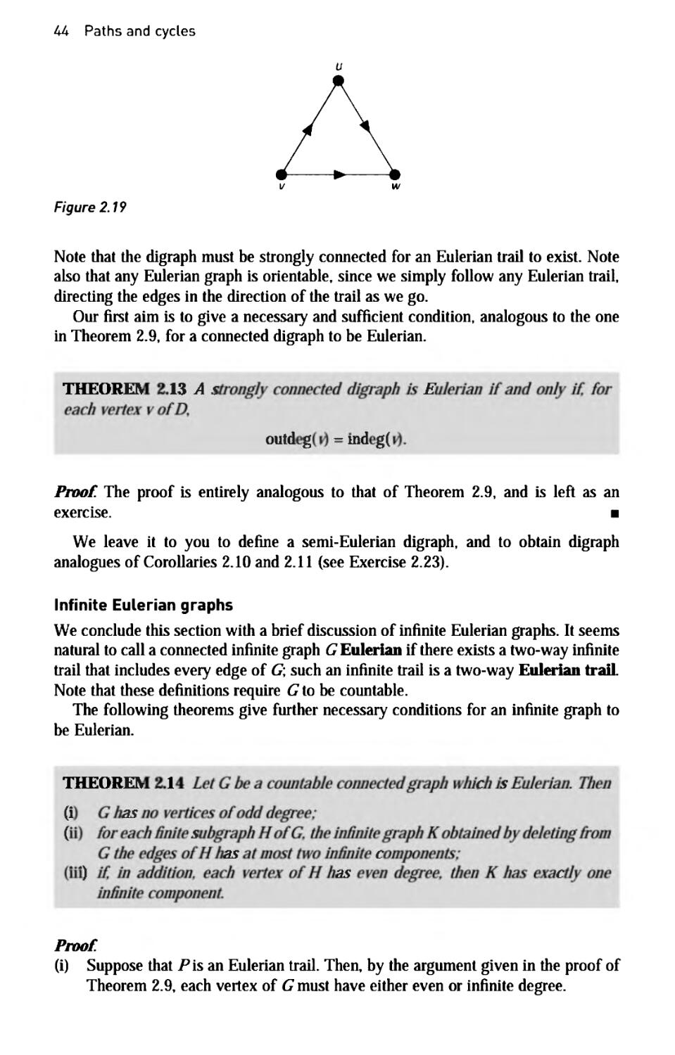
Introduction to Graph Theory

We work with leading authors to develop the strongest
educational materials in mathematics, bringing cutting-edge
thinking and best learning practice to a global market.
Under a range of well-known imprints, including Prentice Hall,
we craft high quality print and electronic publications which
help readers to understand and apply their content, whether
studying or at work.
To find out more about the complete range of our publishing,
please visit us on the World Wide Web at:
www.pearsoned.co.uk

Introduction to Graph Theory
Fifth Edition
Robin J. Wilson
Prentice Hall
is an imprint of
Harlow, England · London · New York · Boston · San Francisco · Toronto
Sydney · Tokyo · Singapore · Hong Kong · Seoul · Taipei ■ New Delhi
Cape Town · Madrid · Mexico City · Amsterdam · Munich · Paris · Milan

Pearson Education Limited
Edinburgh Gate
Harlow
Essex CM20 2JE
England
and Associated Companies throughout the world
Visit us on the World Wide Web at-
www.pearsoned.co.uk
First published by Oliver & Boyd 1972
Second edition published by Longman Group Ltd 1979
Third edition 1985
Fourth edition 1996
Fifth edition published 2010
©Robin Wilson 1972,2010
The right of Robin Wilson to be identified as author of this work has been asserted
by him in accordance with the Copyright, Designs and Patents Act 1988.
All rights reserved. No part of this publication may be reproduced, stored in a retrieval
system, or transmitted in any form or by any means, electronic, mechanical, photocopying,
recording or otherwise, without either the prior written permission of the publisher or a
licence permitting restricted copying in the United Kingdom issued by the Copyright
Licensing Agency Ltd. Saffron House. 6-10 Kirby Street, London EC1N 8TS.
ISBN: 978-0-273-72889-4
British Library Cataloguing-in-Publication Data
A catalogue record for this book is available from the British Library
Library of Congress Cataloging-in-Publication Data
Wilson. Robin J.
Introduction to graph theory / Robin J, Wilson. - 5th ed.
p. cm.
Includes bibliographical references and index.
ISBN 978-0-273-72889-4 (pbk.l
1. Graph theory, I. Title.
QA166.W55 2010
511'5-dc22
2010009905
10 987654321
U 13 12 11 10
Typeset in 10/12pt Times by 35
Printed and bound by Ashford Colour Press Ltd., Gosport. Hampshire.

Contents
Preface to the fifth edition vii
Introduction 1
Definitions and examples 8
1.1 Definitions 8
1.2 Examples 18
1.3 Variations on a theme 22
1.4 Three puzzles 26
Paths and cycles 32
2.1 Connectivity 32
2.2 Eulerian graphs and digraphs 40
2.3 Hamiltonian graphs and digraphs 47
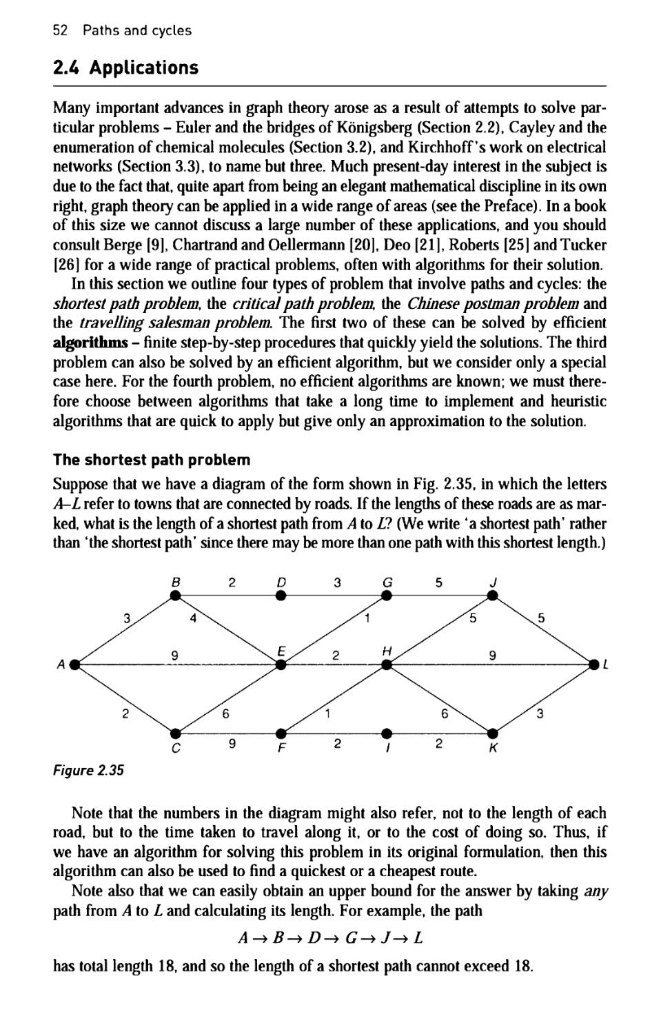
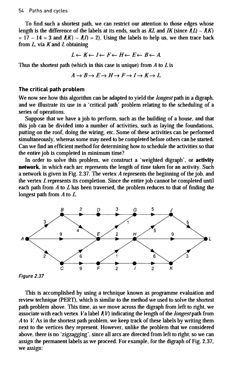
2.4 Applications 52
Trees 61
3.1 Properties of trees 61
3.2 Counting trees 65
3.3 More applications 70
Planarity 80
4.1 Planar graphs 80
4.2 Euler's formula 86
4.3 Dual graphs 91
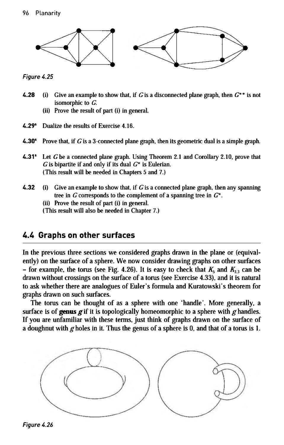
4.4 Graphs on other surfaces 96
Colouring graphs 101
5.1 Colouring vertices 101
5.2 Chromatic polynomials 107
5.3 Colouring maps 111
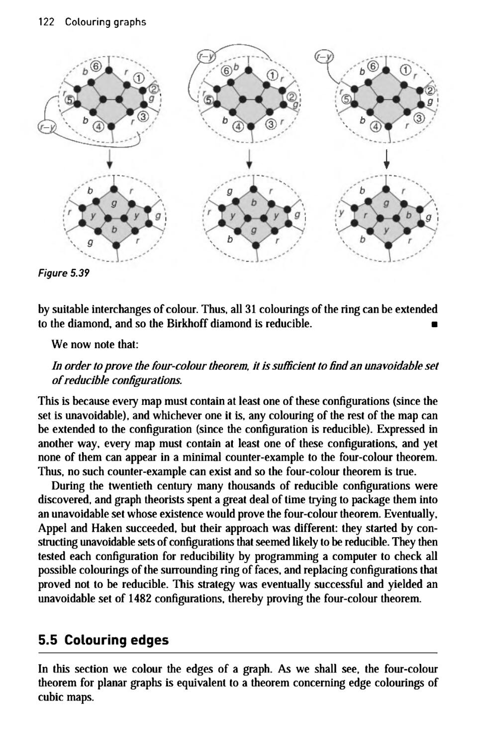
5.4 The four-colour theorem 117
5.5 Colouring edges 122

Contents
Matching, marriage and Menger's theorem 128
6.1 Hall's marriage'theorem 128
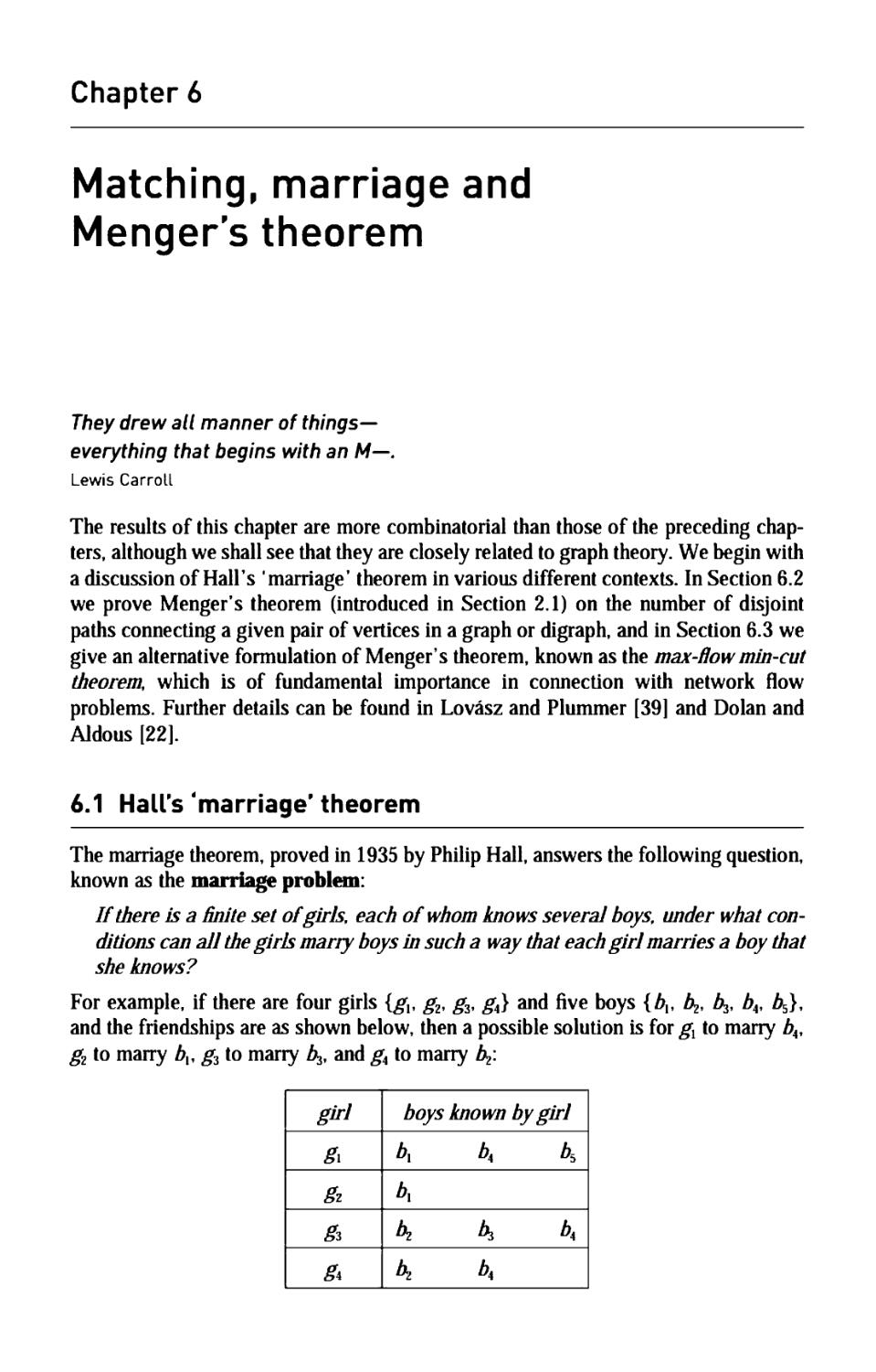
6.2 Mengers theorem 134
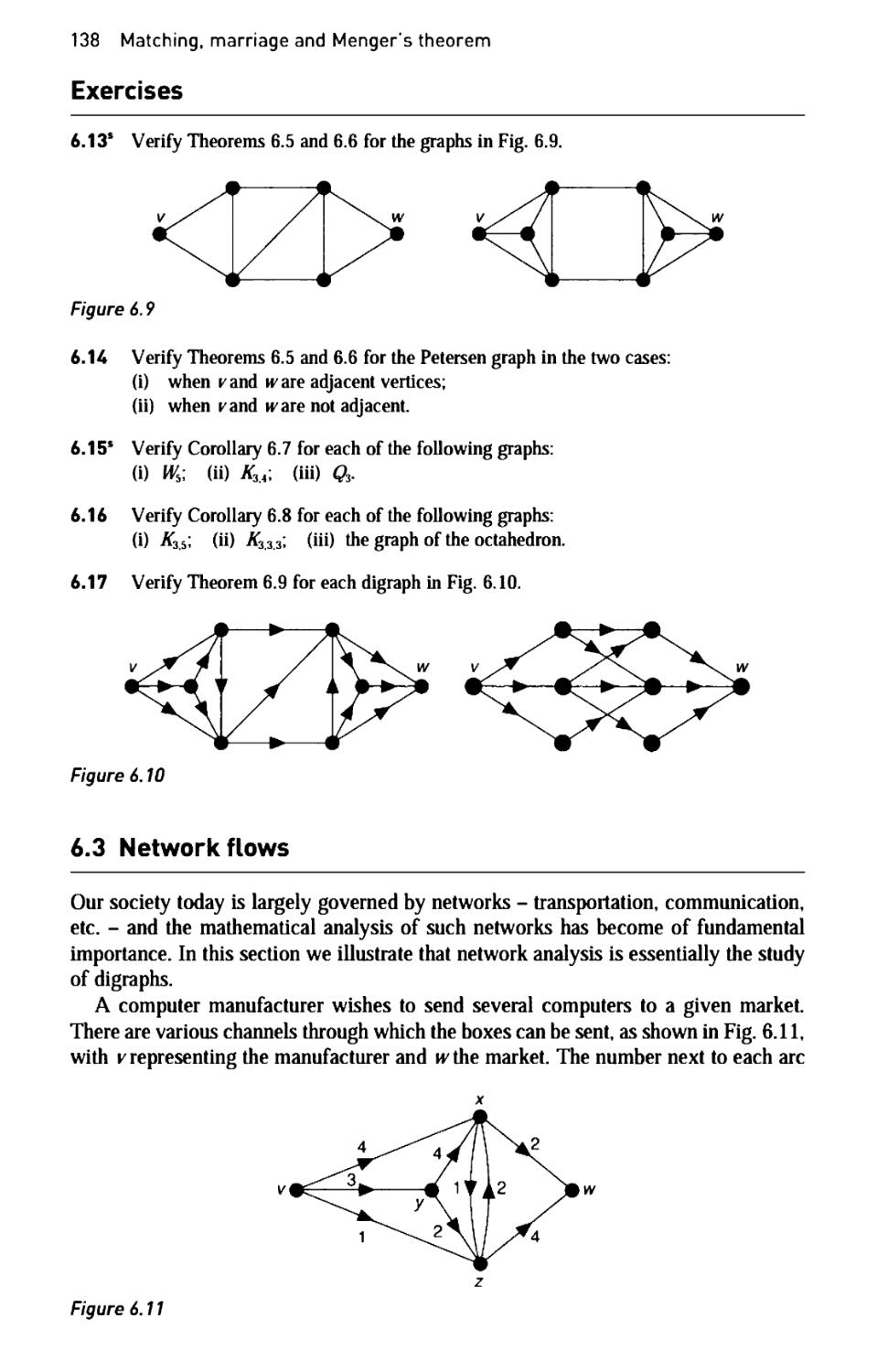
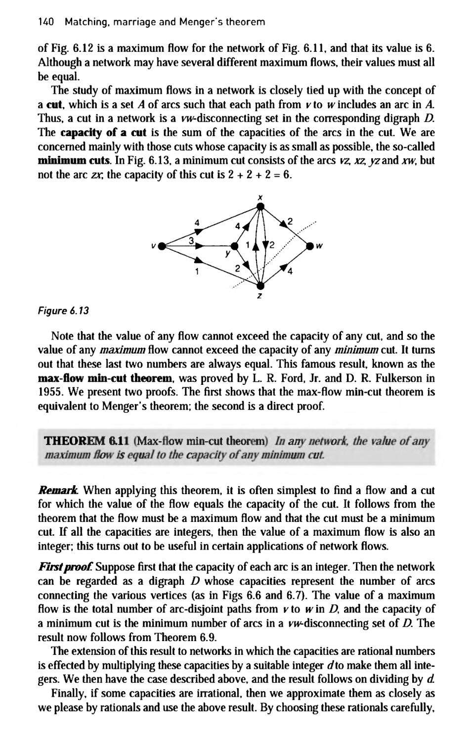
6.3 Network flows 138
Matroids U5
7.1 Introduction to matroids 145
7.2 Examples of matroids 149
7.3 Matroids and graphs 152
Appendix 1: Algorithms 158
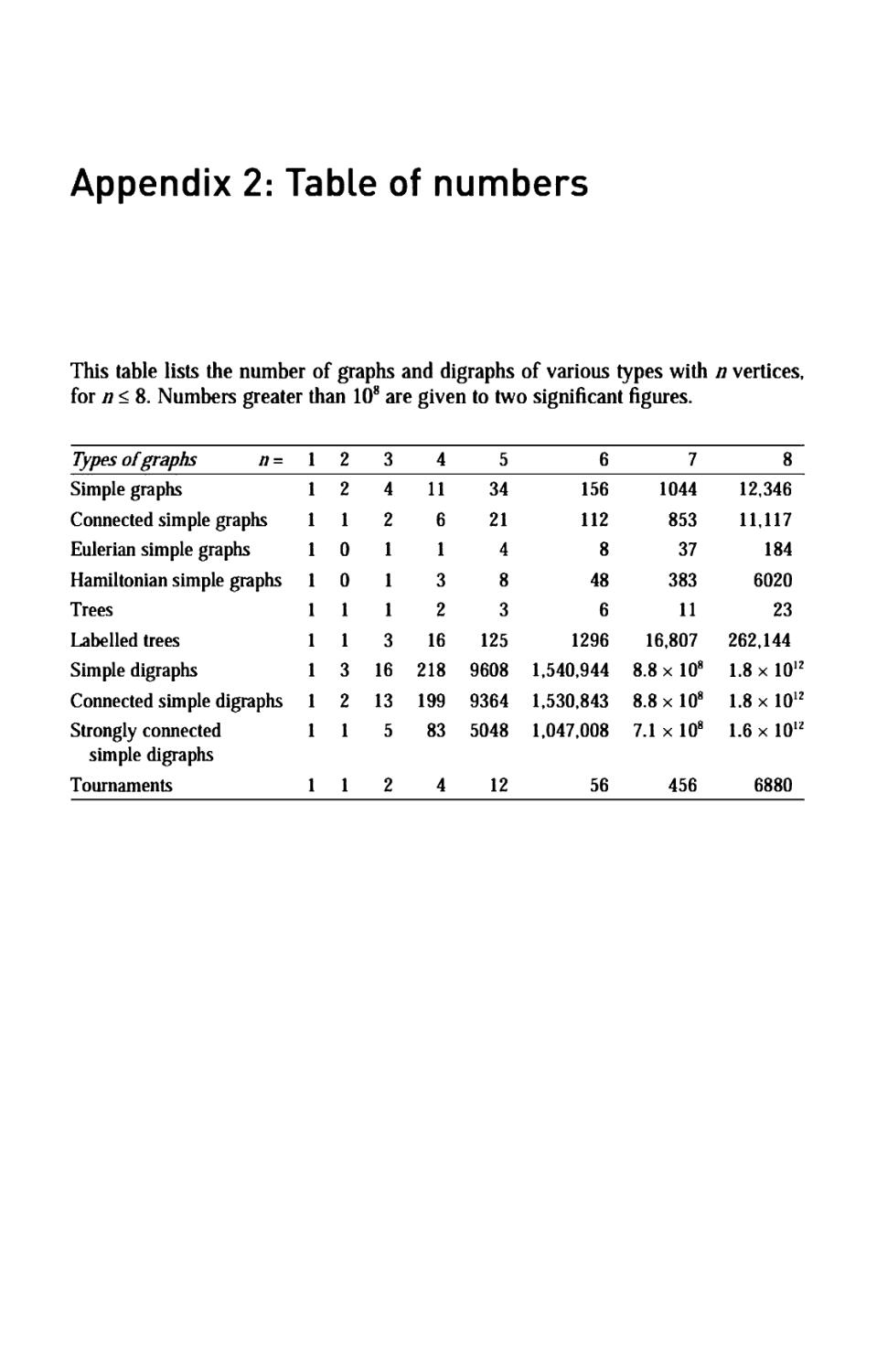
Appendix 2: Table of numbers 161
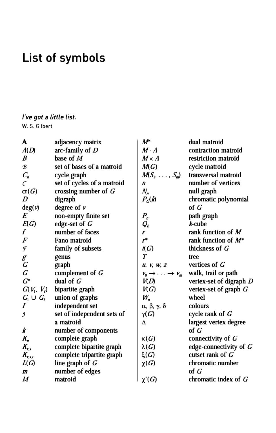
List of symbols 162
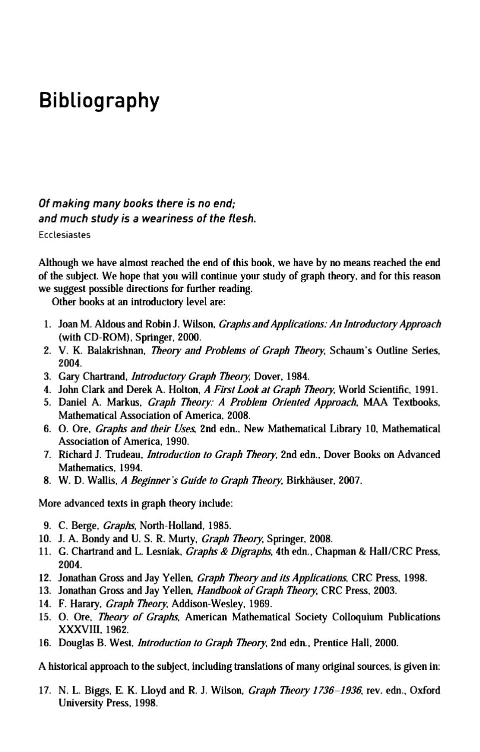
Bibliography 163
Solutions to selected exercises 166
Index 181
Go forth, my little book! pursue thy way!
Go forth, and please the gentle and the good.
William Wordsworth

Preface
In recent years, graph theory has established itself as an important mathematical tool
in a wide variety of subjects, ranging from operational research and chemistry to
genetics and linguistics, and from computer science and geography to sociology and
architecture. At the same time it has also emerged as a worthwhile mathematical
discipline in its own right.
In view of this, there has been a need for an inexpensive introductory text on
the subject, suitable both for mathematicians taking courses in graph theory and for
non-specialists wishing to learn the subject as quickly as possible. It is my hope
that this latest edition continues to go some way towards rilling this need. The only
prerequisites to reading it are a basic knowledge of elementary set theory and matrix
theory, although a further knowledge of abstract algebra and topology is needed for
a few of the more difficult exercises.
The contents of this book may be conveniently divided into four parts. The first of
these (Chapters 1-3) provides a basic foundation course, containing definitions and
examples of graphs and digraphs, connectedness, Eulerian and Hamiltonian paths
and cycles, and trees. This is followed by two chapters (Chapters 4 and 5) on planarity
and colouring, with special reference to the four-colour theorem. The third part
(Chapter 6) deals with transversal theory and connectivity, with applications to network
flows. The book ends with a chapter on matroids (Chapter 7), which ties together
material from the previous chapters and introduces some recent developments.
Throughout the book I have attempted to restrict the text to basic material. Of
the 300 exercises, many are routine examples designed to test understanding of the
text, while others will introduce you to new results and ideas. You should read each
exercise, whether or not you work through it in detail, as some are referred to later in
the book. Solutions are given for some of the exercises; these exercises are indicated
by the symbol s next to the exercise number. More difficult exercises (called
Challenge problems) appear at the end of each chapter.
I have used the symbol ■ to indicate the end of a proof, and bold-face type is used
for definitions. The number of elements in a set S is denoted by |5|, and the empty set
is denoted by 0.
A substantial number of changes have been made in this edition. The text has been
revised throughout and several sections have been rearranged and renumbered. Some
new material has been added - notably on the four-colour theorem and on algorithms
- and other material has been removed. Several further changes have arisen as a result
of comments by a number of people, and I should like to thank them for their helpful
remarks.

viii Preface to the fifth edition
Finally, I wish to express my thanks to my former students, but for whom this book
would have been completed earlier, to Mr William Shakespeare and others for their
apt and witty comments at the beginning of each chapter, and most of all to my wife
Joy for many things that have nothing to do with graph theory.
November 2009

Introduction
The last thing one discovers in writing a book is what to put first.
Blaise Pascal
In this Introduction we provide an intuitive background to the material that we present
more formally later on. Terms that appear here in bold-face type are to be thought of
as descriptions rather than as definitions; having met them here in an informal setting,
you should find them more familiar when you meet them later. So read this
Introduction quickly, and then forget all about it!
What is a graph?
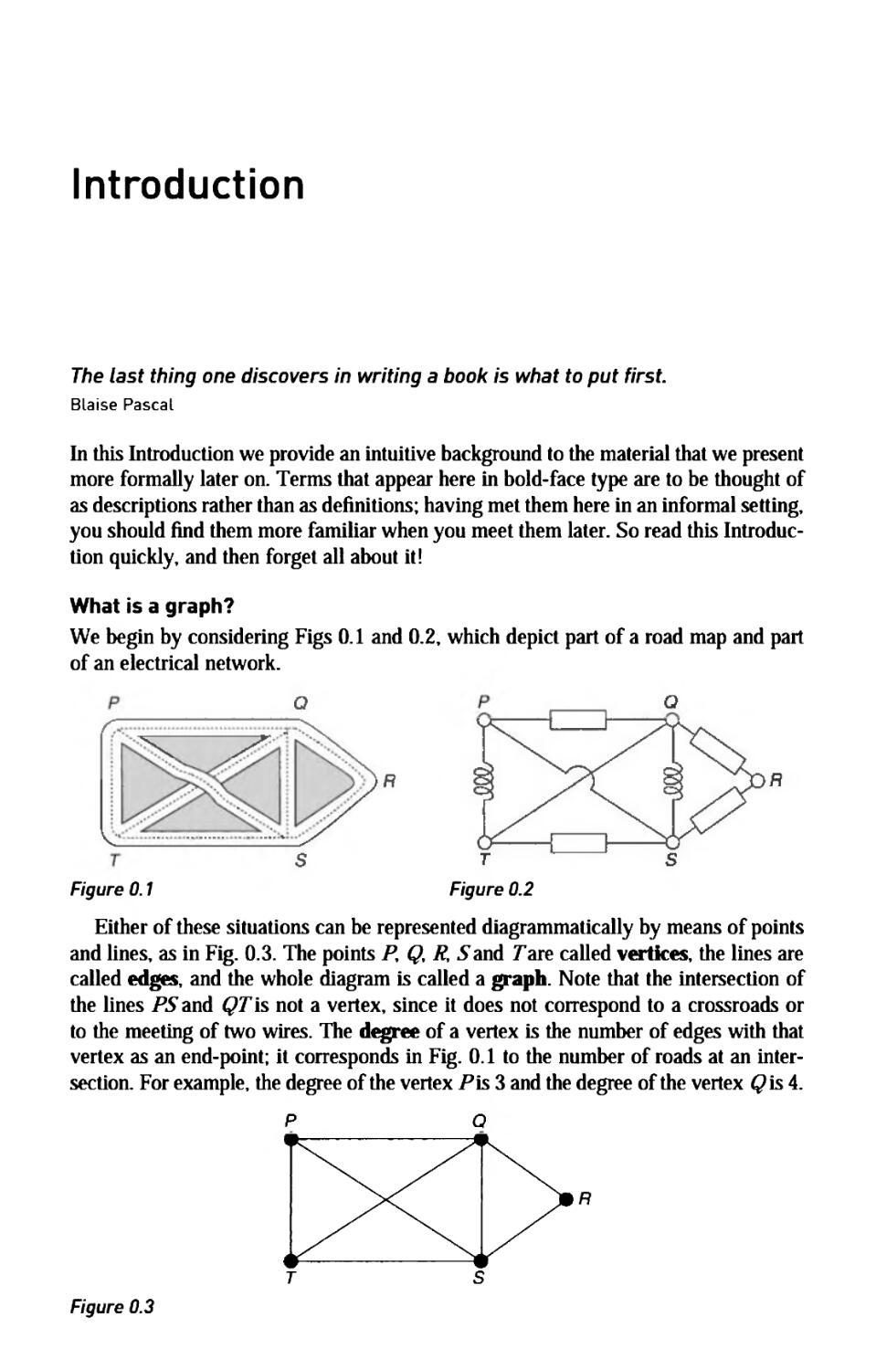
We begin by considering Figs 0.1 and 0.2, which depict part of a road map and part
of an electrical network.
τ s
Figure 0.1 Figure 0.2
Either of these situations can be represented diagrammatically by means of points
and lines, as in Fig. 0.3. The points Py Q, R, Sand Гаге called vertices, the lines are
called edges, and the whole diagram is called a graph. Note that the intersection of
the lines PS and QT is not a vertex, since it does not correspond to a crossroads or
to the meeting of two wires. The degree of a vertex is the number of edges with that
vertex as an end-point; it corresponds in Fig. 0.1 to the number of roads at an
intersection. For example, the degree of the vertex Pis 3 and the degree of the vertex Q is 4.
Ρ Q
R
Τ S
Figure 0.3

2 Introduction
The graph in Fig. 0.3 can also represent other situations. For example, if ΡΆ Q, fi,
Sand Γ represent football teams, then the existence of an edge might correspond to
the playing of a game between the teams at its end-points. Thus, in Fig. 0.3, team Ρ
has played against teams Q, 5 and T, but not against team R. In this representation,
the degree of a vertex is the number of games played by that team.
Another way of depicting these situations is to use the graph in Fig. 0.4. Here we
have removed the crossing' of the lines PS and QTby redrawing the line /^outside
the rectangle PQST. The resulting graph still tells us whether there is a direct road
from one intersection to another, how the electrical network is wired up, and which
football teams have played which. The only information we have lost concerns
* metrical' properties, such as the length of a road and the straightness of a wire.
Thus, a graph is a representation of a set of points and of how they are joined up,
and any metrical properties are irrelevant. From this point of view, any graphs that
represent the same situation, such as those of Figs 0.3 and 0.4, are regarded as the
same graph.
Figure 0.4
More generally, two graphs are the same if two vertices are joined by an edge in
one graph if and only if the corresponding vertices are joined by an edge in the other.
Another graph that is the same as those in Figs 0.3 and 0.4 is shown in Fig. 0.5. Here
all idea of space and distance has gone, but we can still tell at a glance which points
are joined by a road or a wire.
Figure 0.5
In this graph there is at most one edge joining each pair of vertices. Suppose now
that in Fig. 0.5 the roads joining ζ? and 5, and Sand Τ have too much traffic to carry.
Then we can ease the situation by building extra roads joining these points, and the
resulting diagram looks like Fig. 0.6. The edges joining ζ? and S, or Sand T, are called
multiple edges. If, in addition, we need a car park at P, then we indicate this by
drawing an edge from Ρίο itself, called a loop (see Fig. 0.7). In this book, graphs may

Introduction 3
S S
Figure 0.6 Figure 0.7
contain loops and multiple edges; graphs with no loops or multiple edges, such as the
graph in Fig. 0.5, are called simple graphs.
The study of directed graphs (or digraphs, as we abbreviate them) arises from
making the roads into one-way streets. An example of a digraph is given in Fig. 0.8,
with the directions of the one-way streets indicated by arrows; such a directed edge'
is called an arc. (In this example, there would be chaos at T, but that does not stop us
from studying such situations!)
-φ-
S
Figure 0.8
Much of graph theory is devoted to 'walks' of various kinds. A walk is a 'way of
getting from one vertex to another' in a graph or digraph, and consists of a sequence
of edges or arcs, one following after another. For example, in Fig. 0.5, P—» ζ? —» R
is a walk of length 2, and P-» S^> ζ?-> Τ7-» S^> J?is a walk of length 5. A walk
in which no vertex appears more than once is called a path; for example, P—» Γ—»
S—» 7? is a path. A walk of the form Q —» S^> Γ—» Q, in which no vertex appears
more than once, except for the beginning and end vertices which coincide, is called
a cycle.
In Chapter 2 we also consider walks with some extra property. In particular, we
discuss graphs and digraphs containing walks that include every edge exactly once
and end back at the initial vertex; such graphs and digraphs are called Eulerian. The
graph in Fig. 0.5 is not Eulerian, since any walk that includes each edge exactly once
(such as Ρ—» ζ?—» # —» S—» Γ—» P—» S—» ζ?—» Τ) must end at a vertex different
from the initial one. We also discuss graphs and digraphs containing cycles that pass
through every vertex; these are called Hamiltonian. For example, the graph in
Fig. 0.5 is Hamiltonian; a suitable cycle is Ρ—» ζ?—» У?—» S^> Г—» Р.
Some graphs or digraphs are in two or more parts. For example, consider the graph
whose vertices are the stations of the London Underground and the New York Subway,

A Introduction
and whose edges are the lines joining adjacent stations. It is clearly impossible to
travel from Trafalgar Square to Grand Central Station using only edges of this graph,
but if we confine our attention to the London Underground part only, then we can
travel from any station to any other. A graph or digraph that is 'in one piece', so that
any two vertices are connected by a path, is connected; a graph or digraph that is
in more than one piece is disconnected (see Fig. 0.9). We discuss connectedness in
Chapters 1, 2 and 6.
We are sometimes interested in connected graphs with only one path between each
pair of vertices. These graphs contain no cycles and are called trees (see Fig. 0.10).
They generalize the idea of a family tree, and are considered in Chapter 3.
Figure 0.9 Figure 0.10
Earlier we saw how the graph of Fig. 0.3 can be redrawn as in Figs 0.4 and 0.5 so
as to avoid crossings of edges. Any graph that can be redrawn without crossings in
this way is called a planar graph. In Chapter 4 we give several criteria for planarity.
Some of these involve the properties of particular 'subgraphs' of the graph in
question; others involve the fundamental notion of duality.
Planar graphs also play an important role in colouring problems. In our 'road-map'
graph, let us suppose that Shell, Esso, BP and Gulf wish to erect five garages between
them, and that for economic reasons no company wishes to erect two garages at
neighbouring corners. Then Shell can build at P, Esso can build at Q, BP can build at
S, and Gulf can build at T, leaving either Shell or Gulf to build at R (see Fig. 0.11).
However, if Gulf backs out of the agreement, then the other three companies cannot
erect their garages in the specified manner.
фШ) (Esso)
<Ш) СЮ
Figure 0.11

Introduction 5
We discuss such problems in Chapter 5, where we try to colour the vertices of
a simple graph with a given number of colours so that each edge of the graph joins
vertices of different colours. If the graph is planar, then we can always colour its
vertices in this way with only four colours - this is the celebrated four-colour
theorem. Another version of this theorem is that we can always colour the countries
of any map with four colours so that no two neighbouring countries share the same
colour (see Fig. 0.12).
Figure 0.12
In Chapter 6 we investigate the celebrated marriage problem, which asks under
what conditions a collection of girls, each of whom knows several boys, can be married
so that each girl marries a boy she knows. This problem can be expressed in the
language of a branch of set theory called * transversal theory', and is related to problems
of finding disjoint paths connecting two given vertices in a graph or digraph.
Chapter 6 concludes with a discussion of network flows and transportation
problems. Suppose that we have a transportation network such as in Fig. 0.13, in which
Pis a factory, Ris a market, and the edges of the graph are channels through which
goods can be sent. Each channel has a capacity, indicated by a number next to the
edge, representing the maximum amount of a commodity that can pass through that
channel. The problem is to determine how much of the commodity can be sent from
the factory to the market without exceeding the capacity of any channel.
Figure 0.13
We conclude with a chapter on matroids. This ties together the material of the
previous chapters, and follows the maxim 'be wise - generalize!' Matroid theory,
the study of sets with 'independence structures' defined on them, generalizes both
the linear independence of vectors and some results on graphs and transversals from
earlier in the book. However, matroid theory is far from being 'generalization for

6 Introduction
generalization's sake'. On the contrary, it gives us clearer insights into several
graphical results involving cycles and planar graphs, and provides simple proofs of results
on transversals that are awkward to prove by more traditional methods. Matroids have
played an important role in the development of combinatorial ideas in recent years.
We hope that this Introduction has been useful in setting the scene and describing
some of the treats that lie ahead. We now embark upon a formal treatment of the
subject.
Exercises
0.1* Write down the number of vertices, the number of edges and the degree of each
vertex in:
f
V-
0
'л
я
ч
.J
(i) the graph in Fig. 0.3;
(ii) the tree in Fig. 0.14.
а ь и
VA
D Ε F S Τ
Figure 0. Η Figure 0.15
0.2 Draw the graph representing the road system in Fig. 0.15, and write down the number
of vertices, the number of edges and the degree of each vertex.
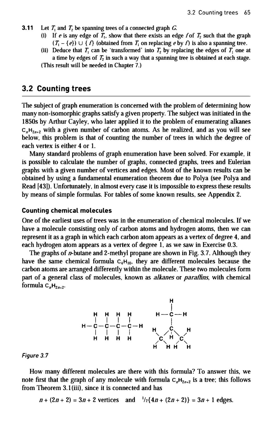
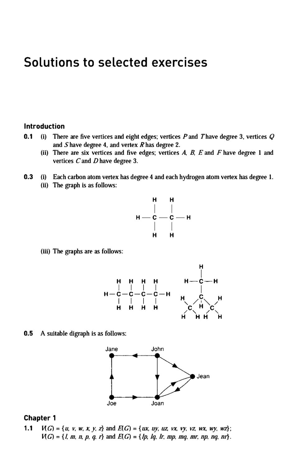
0.3s Figure 0.16 represents the chemical molecules of methane (CH4) and propane (C3H8).
(i) Regarding these diagrams as trees, what can you say about the vertices
representing carbon atoms (C) and hydrogen atoms (H)?
(ii) Draw a tree that represents the molecule with formula C2He (hexane).
(iii) There are two different chemical molecules with formula С4НШ. Draw trees that
represent these molecules.
Figure
0.4
0.16
Draw
a graph
that
Η
|
I
H —C —
Η
-Η Η
methane
represents
\
Joe
I
Jenny
the family I
John
Jean J.
I
Kenny
Η Η
I |
f I
I |
I I
Η Η
Η
I
I
I
I
Η
propane
tree in Fig.
I l
ane Jill
r
Bill
0.17.
1
Ben
Η
Figure 0.17

Introduction 7
0.5s John likes Joan, Jean and Jane; Joe likes Jane and Joan; Jean and Joan like each other.
Draw a digraph illustrating these relationships between John, Joan, Jean, Jane and Joe.
0.6 Snakes eat frogs and birds eat spiders; birds and spiders both eat insects; frogs eat
snails, spiders and insects. Draw a digraph representing this predatory behaviour.
0.7 Draw a graph with vertices А В,..., Μ that shows the various routes that one can take
when tracing the Hampton Court maze in Fig. 0.18.
Figure 0.18

Chapter 1
Definitions and examples
/ hate definitions!
Benjamin Disraeli
In this chapter, we lay the foundations for a proper study of graph theory. Section 1.1
formalizes some of the graph ideas in the Introduction, Section 1.2 provides a variety
of examples, and Section 1.3 presents two variations on the basic idea. In Section 1.4
we show how graphs can be used to represent and solve three problems from
recreational mathematics. More substantial applications are deferred until Chapters 2 and 3,
when we have more machinery at our disposal.
1.1 Definitions
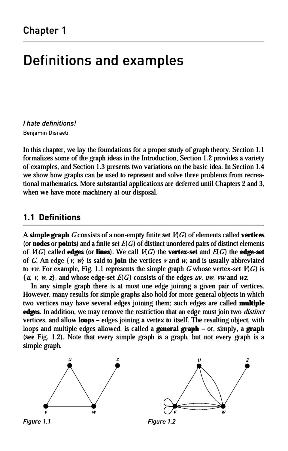
A simple graph <7 consists of a non-empty finite set V[ G) of elements called vertices
(or nodes or points) and a finite set E[G) of distinct unordered pairs of distinct elements
of \\G) called edges (or lines). We call V\G) the vertex-set and E[G) the edge-set
of G An edge { к w) is said to join the vertices у and w, and is usually abbreviated
to vw. For example, Fig. 1.1 represents the simple graph G whose vertex-set V[G) is
{u, v, w, z}, and whose edge-set Д<7) consists of the edges uv, uw, wand wz.
In any simple graph there is at most one edge joining a given pair of vertices.
However, many results for simple graphs also hold for more general objects in which
two vertices may have several edges joining them; such edges are called multiple
edges. In addition, we may remove the restriction that an edge must join two distinct
vertices, and allow loops - edges joining a vertex to itself. The resulting object, with
loops and multiple edges allowed, is called a general graph - or, simply, a graph
(see Fig. 1.2). Note that every simple graph is a graph, but not every graph is a
simple graph.
υ ζ и ζ
Figure 1.1
Figure 1.2

1.1 Definitions 9
Thus, a graph G consists of a non-empty finite set V[G) of elements called
vertices and a finite family ДС) of unordered pairs of (not necessarily distinct)
elements of \\G) called edges; the use of the word 'family' permits the existence of
multiple edges. We call V[ G) the vertex-set and Д G) the edge-family of G An edge
{ κ μ) is said to join the vertices ν and w, and is again abbreviated to vw. Thus in
Fig. 1.2, ИФ is the set {и, к и; ζ} and Д£) consists of the edges ι/κ ρτ (twice), w
(three times), ί/w (twice) and wz Note that each loop vvjoins the vertex ν to itself.
Although we sometimes need to restrict our attention to simple graphs, we shall prove
our results for general graphs whenever possible.
Remark. The language of graph theory is not standard - all authors have their own
terminology. Some use the term 'graph' for what we call a simple graph, while others
use it for graphs with directed edges, or for graphs with infinitely many vertices or
edges; we discuss these variations in Section 1.3. Any such definition is perfectly
valid, provided that it is used consistently. In this book:
All graphs are Unite and undirected, with loops and multiple edges allowed unless
specifically excluded.
Isomorphism
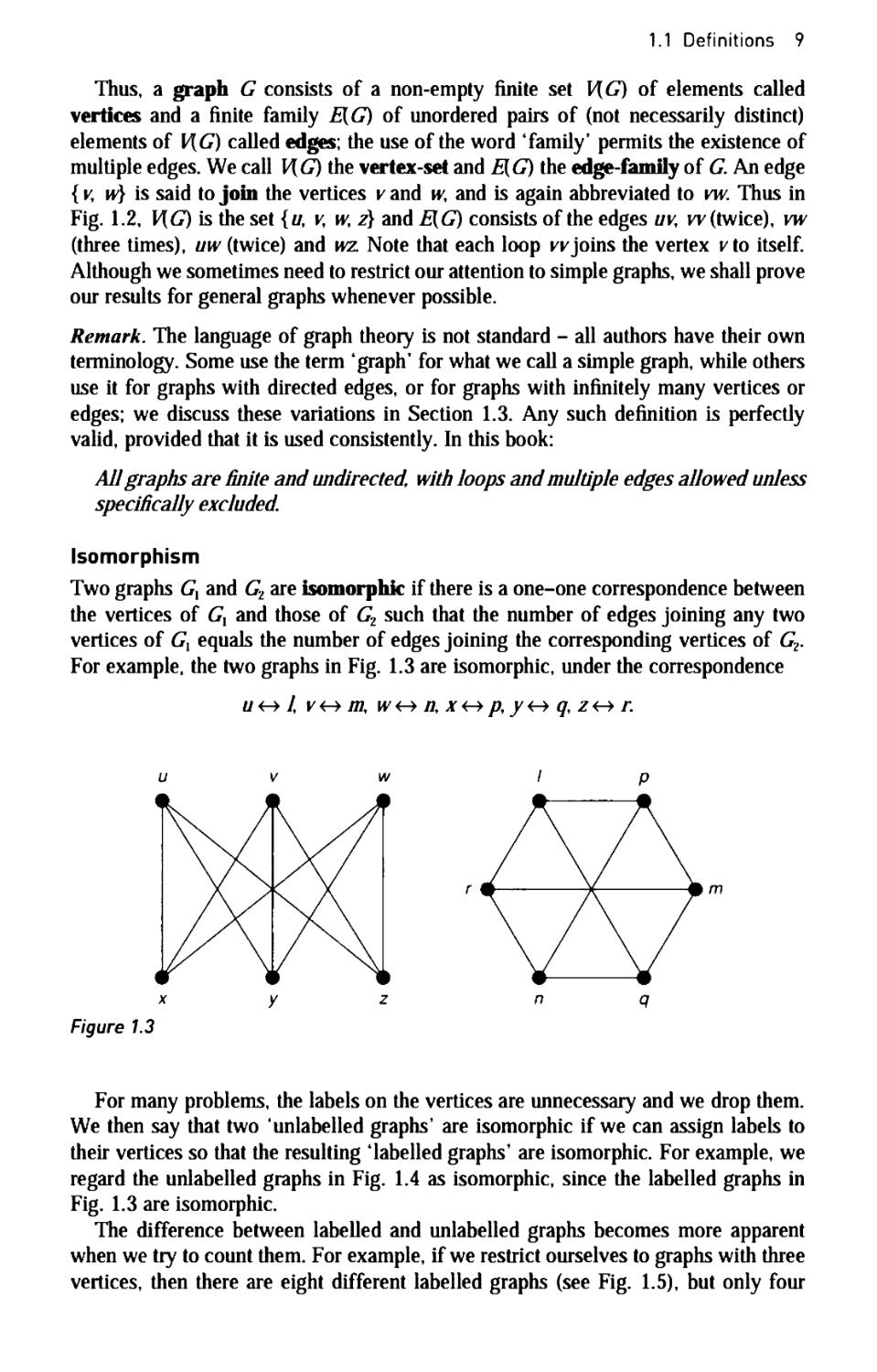
Two graphs Gx and GL are isomorphic if there is a one-one correspondence between
the vertices of Gx and those of GL such that the number of edges joining any two
vertices of Gx equals the number of edges joining the corresponding vertices of G2.
For example, the two graphs in Fig. 1.3 are isomorphic, under the correspondence
!/<-»/ V<r+ /П, W <-» A X<r+ /7, / <-» q, Z<r+ Г.
#-
χ у ζ η q
Figure 1.3
For many problems, the labels on the vertices are unnecessary and we drop them.
We then say that two unlabelled graphs' are isomorphic if we can assign labels to
their vertices so that the resulting 'labelled graphs' are isomorphic. For example, we
regard the unlabelled graphs in Fig. 1.4 as isomorphic, since the labelled graphs in
Fig. 1.3 are isomorphic.
The difference between labelled and unlabelled graphs becomes more apparent
when we try to count them. For example, if we restrict ourselves to graphs with three
vertices, then there are eight different labelled graphs (see Fig. 1.5), but only four

10 Definitions and examples
Figure 1.4
1111
# · · · · · · ·
3 2
3 2
3 2
3 2
1111
Λ Λ Δ Δ
3 2
3 2
3 2
3 2
Figure 1.5
ΛΔ
Figure 1.6
uniabelled ones (see Fig. 1.6). It is usually clear from the context whether we are
referring to labelled or uniabelled graphs.
Connected graphs
We can combine two graphs to make a larger graph. If the two graphs are Gx and GL
and their vertex-sets \\GX) and V[Gz) are disjoint, then their union C, U GL is the
graph with vertex-set \\G^ U И<72) and edge-family Д£,) U E[GZ) (see Fig. 1.7).
Most of the graphs discussed so far have been 'in one piece'. A graph is connected
if it cannot be expressed as a union of graphs, and disconnected otherwise. Clearly,
any disconnected graph <7can be expressed as the union of connected graphs, each of
which is called a component of G\ a disconnected graph with three components is
shown in Fig. 1.8.
a*
G,
Gi ^ G2
Figure 1.7

1.1 Definitions 11
# ·
Figure 1.8
When proving results about graphs in general, we can often obtain the
corresponding results for connected graphs and then apply them to each component separately.
A table of all the unlabelled connected simple graphs with up to five vertices is given
in Fig. 1.9.
"λ
□
и
"A
11
X
1
13
14
15
Χ ν?
16
A
17
18
19
20
21
X
22
23
24
25
A
26
й
27
28
ш
29
30
31
и
Figure 1.9

12 Definitions and examples
Adjacency and degrees
We say that two vertices ν and w of a graph are adjacent if there is an edge vw
joining them, and the vertices rand ware then incident with such an edge. We also
say that two distinct edges e and /are adjacent if they have a vertex in common
(see Fig. 1.10).
> « >-^*r
adjacent vertices adjacent edges
Figure 1.10
The degree of a vertex ν is the number of edges incident with к and is written
deg(0; when calculating the degree of κ we usually make the convention that a loop
at ν contributes 2 (rather than 1) to deg(0. A vertex of degree 0 is an isolated vertex
and a vertex of degree 1 is an end-vertex. Thus each of the two graphs in Fig. 1.11
has two end-vertices and three vertices of degree 2, while the graph in Fig. 1.12 has
one end-vertex, one vertex of degree 3, one of degree 6 and one of degree 8.
The degree sequence of a graph consists of the degrees written in increasing
order, with repeats where necessary. For example, the degree sequences of the graphs
in Figs 1.11 and 1.12 are (1, 1, 2, 2, 2) and (1, 3, 6, 8).
υ ζ
_ΔΙ
Figure 1.11 Figure 1.12
The earliest result on graph theory is essentially due to Leonhard Euler in 1735
(although he did not express it in the language of graphs). It is sometimes called
the handshaking lemma.
THEOR 1.1 ( andshakin 1 mm s
s
Proof. The sum of all the vertex-degrees is equal to twice the number of edges, since
each edge contributes exactly 2 to the sum. It is thus an even number. ■
The handshaking lemma is so called because it tells us that if several people shake
hands, then the total number of hands shaken must be even - this is precisely because
just two hands are involved in each handshake. A useful corollary of the
handshaking lemma is the following:
COROLLARY 1

1.1 Definitions 13
Proof. If the number of vertices of odd degree were odd, then the sum of the vertex-
degrees would also be odd, contradicting Theorem 1.1. So the number is even. ■
Subgraphs
A graph His a subgraph of a graph G if each of its vertices belongs to V( G) and each
of its edges belongs to E{G). Thus the graph in Fig. 1.13 is a subgraph of the graph
in Fig. 1.14, but is not a subgraph of the graph in Fig. 1.15, since the latter graph
contains no 'triangles'.
Figure 1.13
Figure 1.14 Figure 1.15
We can obtain subgraphs of a graph by deleting edges and vertices. If e is an edge
of a graph G, we denote by G - e the graph obtained from G by deleting the edge e4
more generally, if Fis any set of edges in G, we denote by G- Fthe graph obtained
by deleting the edges in F. Similarly, if ν is a vertex of G, we denote by G - ν the
graph obtained from <7by deleting the vertex ^together with the edges incident with
К more generally, if S is any set of vertices in <7, we denote by G - S the graph
obtained by deleting the vertices in S and all edges incident with any of them. An
example is shown in Fig. 1.16.
ν e w ν w w
Figure 1.16
We also denote by G\ e the graph obtained by taking an edge e and 'contracting'
it - that is, removing it and identifying its ends у and wso that the resulting vertex is
incident with all those edges (other than e) that were originally incident with ν or w.
An example is shown in Fig. 1.17.

14 Definitions and examples
G\e
Figure 1.17
The complement of a simple graph
If G is a simple graph with vertex-set V[G), its complement G is the simple graph
with vertex-set \\G) in which two vertices are adjacent if and only if they are not
adjacent in G\ Fig. 1.18 shows a graph and its complement. Note that the complement
of G is G
Figure 1.18
Matrix representations
Although it is convenient to represent a graph by a diagram of points joined by lines,
such a representation may be unsuitable if we wish to store a large graph in a
computer. One way of storing a simple graph is by listing the vertices adjacent to each
vertex of the graph. An example of this is given in Fig. 1.19.
Дс 1
и :
ν:
w
χ:
У'
v.y
ижу
кх,у
w,y
u,v,w,x
Figure 1.19
Other useful representations involve matrices. If G is a graph without loops, with
vertices labelled {1, 2,..., /ι}, its adjacency matrix A is the л х л matrix whose
ί/ύι entry is the number of edges joining vertex / and vertex/ If, in addition, the edges
are labelled {1, 2,. .., /n}, its incidence matrix Μ is the η χ m matrix whose 7/th
entry is 1 if vertex / is incident to edgey; and is 0 otherwise. Figure 1.20 shows
a labelled graph G with its adjacency and incidence matrices.

1.1 Definitions 15
Figure 1.20
Exercises
A =
Γ0 1 0 1 л
10 12
0 10 1
Ь 2 1 oj
м.
Ίοοιοο'
110 0 11
0 110 0 0
,0 0 1111,
1.1* Write down the vertex-set and edge-set of each graph in Fig. 1.3.
1.2 Write down the vertex-set and edge-family of the graph in Fig. 1.21.
Figure 1.21
1.3 Draw
(i) a simple graph,
(ii) a non-simple graph with no loops,
(iii) a non-simple graph with no multiple edges,
each with five vertices and eight edges.
1.4* By suitably labelling the vertices, show that the two graphs in Fig. 1.22 are isomorphic.
Figure 1.22
1.5* Explain why the two graphs in Fig. 1.23 are not isomorphic.
Figure 1.23

16 Definitions and examples
1.6 Are the graphs in Fig. 1.24 isomorphic?
Figure 1.24
1.7 Classify the following statements as true or false.
(i) any two isomorphic graphs have the same degree sequence;
(ii) any two graphs with the same degree sequence are isomorphic.
1.8* Locate each of the graphs in Fig. 1.25 in the table of Fig. 1.9.
(i)
Figure 1.25
1.9 Locate each of the graphs in Fig. 1.26 in the table of Fig. 1.9.
Figure 1.26
1.10 (i) Show that there are exactly 2"ia~m labelled simple graphs on η vertices,
(ii) How many of these have exactly m edges?
1.11s Write down the degree sequence of each graph with four vertices in Fig. 1.9, and
verify that the handshaking lemma holds for each graph.
1.12 Write down the degree sequence of each graph with five vertices in Fig. 1.9, and
verify that the handshaking lemma holds for each graph.
1.13 (i) Draw a graph on six vertices with degree sequence (3, 3, 5, 5, 5, 5); does there
exist a simple graph with these degrees?
(ii) How are your answers to part (i) changed if the degree sequence is (2, 3, 3, 4, 5, 5)?

1.1 Definitions 17
1.1 Λ (i) Let G be a graph with four vertices and degree sequence (1, 2, 3, 4). Write down
the number of edges of G, and construct such a graph,
(ii) Are there any simple graphs with four vertices and degree sequence (1, 2, 3, 4)?
1.15 If G is a simple graph with at least two vertices, prove that G must contain two or more
vertices of the same degree.
1.16s Which graphs in Fig. 1.27 are subgraphs of the graphs in Fig. 1.22?
Δ Π Ο Ο
Figure 1.27
1.17 Let G be the graph of Fig. 1.3 and let e be the edge их. Draw the graphs G - e and
G\e.
1.18 Let G be a graph with η vertices and in edges, and let ν be a vertex of G of degree
к and e be an edge of G How many vertices and edges have G - e, G- ν and G\e?
1.19 Draw the complements of the graphs in Figs. 1.13, 1.14 and 1.15.
1.20s Write down the adjacency and incidence matrices of the graph in Fig. 1.28.
Figure 1.28
1.21 Write down the adjacency and incidence matrices of the graph in Fig. 1.2.
1.22 Draw the graph whose adjacency matrix is given in Fig. 1.29.
Γθ 1 1 2 0Ί
10 0 0 1
10 0 11
2 0 10 0
to ι 1 о oj
Figure 1.29

18 Definitions and examples
1.23 Draw the graph whose incidence matrix is given in Fig. 1.30.
f0 0 1 1 1 1 1 0Λ
0 10 10 0 0 1
0 0 0 0 0 0 0 1
10 10 10 10
1^1 1 0 0 0 1 0 OJ
Figure 1.30
1.24 If G is a graph without loops, what can you say about the sum of the entries in
(i) any row or column of the adjacency matrix of G>
(ii) any row of the incidence matrix of G>
(iii) any column of the incidence matrix of G>
1.2 Examples
In this section we examine some important types of graphs. You should become
familiar with them, as they will appear frequently in examples and exercises.
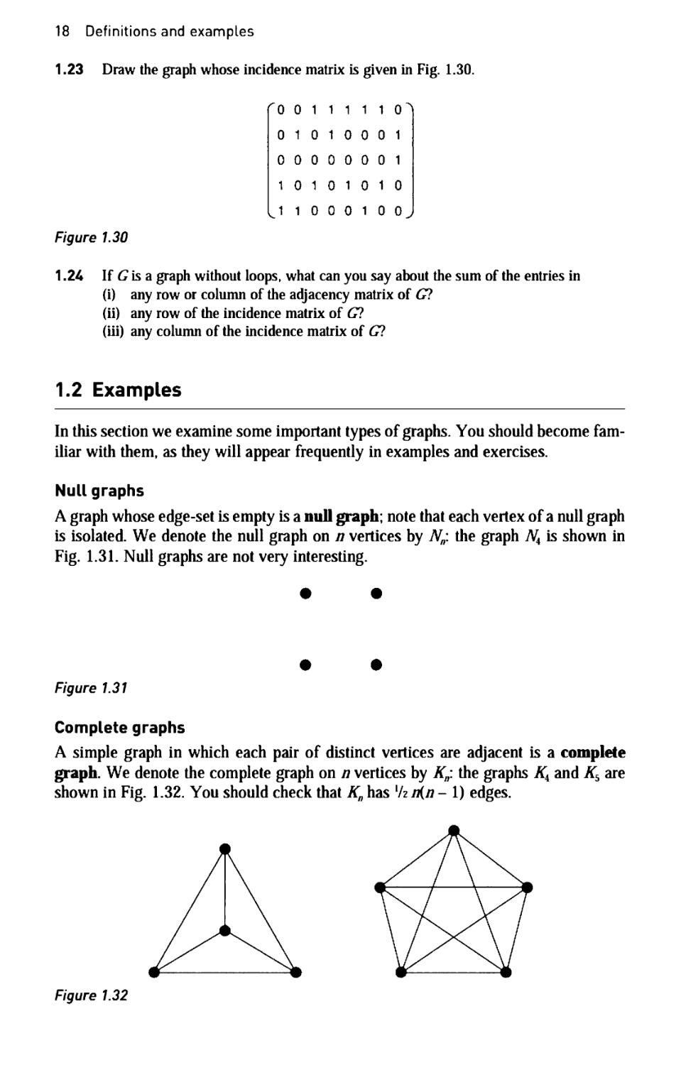
Null graphs
A graph whose edge-set is empty is a null graph; note that each vertex of a null graph
is isolated. We denote the null graph on η vertices by Nn: the graph NA is shown in
Fig. 1.31. Null graphs are not very interesting.
# ·
Figure 1.31
Complete graphs
A simple graph in which each pair of distinct vertices are adjacent is a complete
graph. We denote the complete graph on η vertices by Kn: the graphs K4 and Къ are
shown in Fig. 1.32. You should check that Kn has Vz/tf/i - 1) edges.
Figure 1.32

1.2 Examples 19
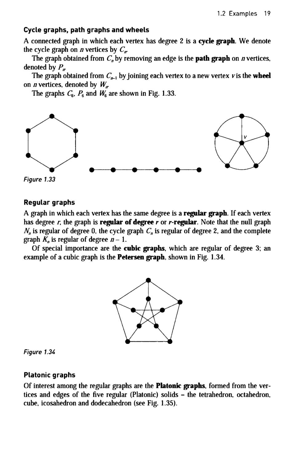
Cycle graphs, path graphs and wheels
A connected graph in which each vertex has degree 2 is a cycle graph. We denote
the cycle graph on η vertices by C„.
The graph obtained from Cn by removing an edge is the path graph on η vertices,
denoted by P„.
The graph obtained from C^ by joining each vertex to a new vertex vis the wheel
on η vertices, denoted by W^
The graphs Q, PB and W% are shown in Fig. 1.33.
Figure 1.33
Regular graphs
A graph in which each vertex has the same degree is a regular graph. If each vertex
has degree r, the graph is regular of degree r or r-regular. Note that the null graph
NB is regular of degree 0, the cycle graph Cn is regular of degree 2, and the complete
graph Kn is regular of degree η - 1.
Of special importance are the cubic graphs, which are regular of degree 3; an
example of a cubic graph is the Petersen graph, shown in Fig. 1.34.
Figure 1.34
Platonic graphs
Of interest among the regular graphs are the Platonic graphs, formed from the
vertices and edges of the five regular (Platonic) solids - the tetrahedron, octahedron,
cube, icosahedron and dodecahedron (see Fig. 1.35).

20 Definitions and examples
tetrahedron octahedron cube icosahedron dodecahedron
Figure 1.35
Bipartite graphs
If the vertex-set of a graph G can be split into two disjoint sets A and В so that
each edge of Gjoins a vertex of A and a vertex of Д then G is a bipartite graph (see
Fig. 1.36). Alternatively, a bipartite graph is one whose vertices can be coloured
black and white in such a way that each edge joins a black vertex (in A) and a white
vertex (in B\. We sometimes write G= G(A, Щ when we wish to specify the sets A
and B.
Μ
В
Figure 1.36
A complete bipartite graph is a bipartite graph in which each vertex in A is joined
to each vertex in В by just one edge. We denote the complete bipartite graph with r
black vertices and s white vertices by Krj the graphs Kl3, K12, K33 and Ku are shown
in Fig. 1.37. You should check that A^has /*+ ^vertices and /sedges.
^1 3 ^2,3 ^3,3 ^4,3
Figure 1.37

1.2 Examples 21
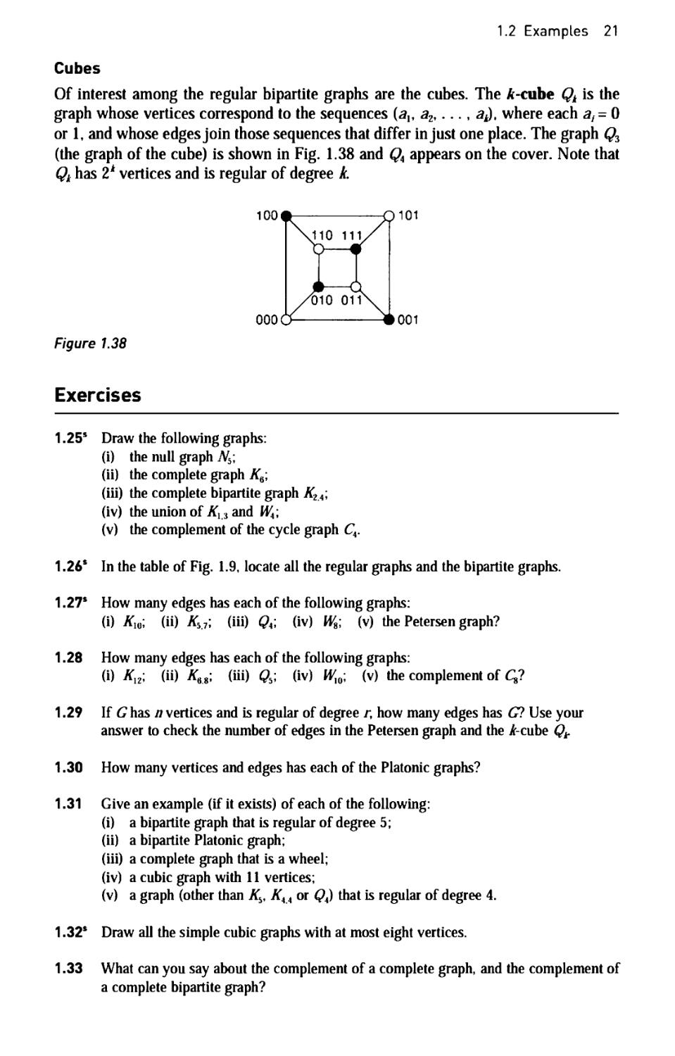
Cubes
Of interest among the regular bipartite graphs are the cubes. The A-cube Qk is the
graph whose vertices correspond to the sequences (а,, аъ ..., ak), where each af= 0
or 1, and whose edges join those sequences that differ in just one place. The graph Q3
(the graph of the cube) is shown in Fig. 1.38 and QA appears on the cover. Note that
Qk has 2k vertices and is regular of degree k.
100
000
Figure 1.38
Exercises
1.25s Draw the following graphs:
(i) the null graph N5;
(ii) the complete graph K6;
(iii) the complete bipartite graph K2A;
(iv) the union of Kl:i and WA\
(v) the complement of the cycle graph CA.
1.26s In the table of Fig. 1.9, locate all the regular graphs and the bipartite graphs.
1.27s How many edges has each of the following graphs:
(i) #10; (ii) КЪ7; (iii) ft; (iv) W6; (v) the Petersen graph?
1.28 How many edges has each of the following graphs:
(i) Kn\ (ii) K6S; (iii) Qb\ (iv) W10; (v) the complement of Q?
1.29 If G has η vertices and is regular of degree r, how many edges has C? Use your
answer to check the number of edges in the Petersen graph and the Лг-cube Qt
1.30 How many vertices and edges has each of the Platonic graphs?
1.31 Give an example (if it exists) of each of the following:
(i) a bipartite graph that is regular of degree 5;
(ii) a bipartite Platonic graph;
(iii) a complete graph that is a wheel;
(iv) a cubic graph with 11 vertices;
(v) a graph (other than Къ§ КАА or QA) that is regular of degree 4.
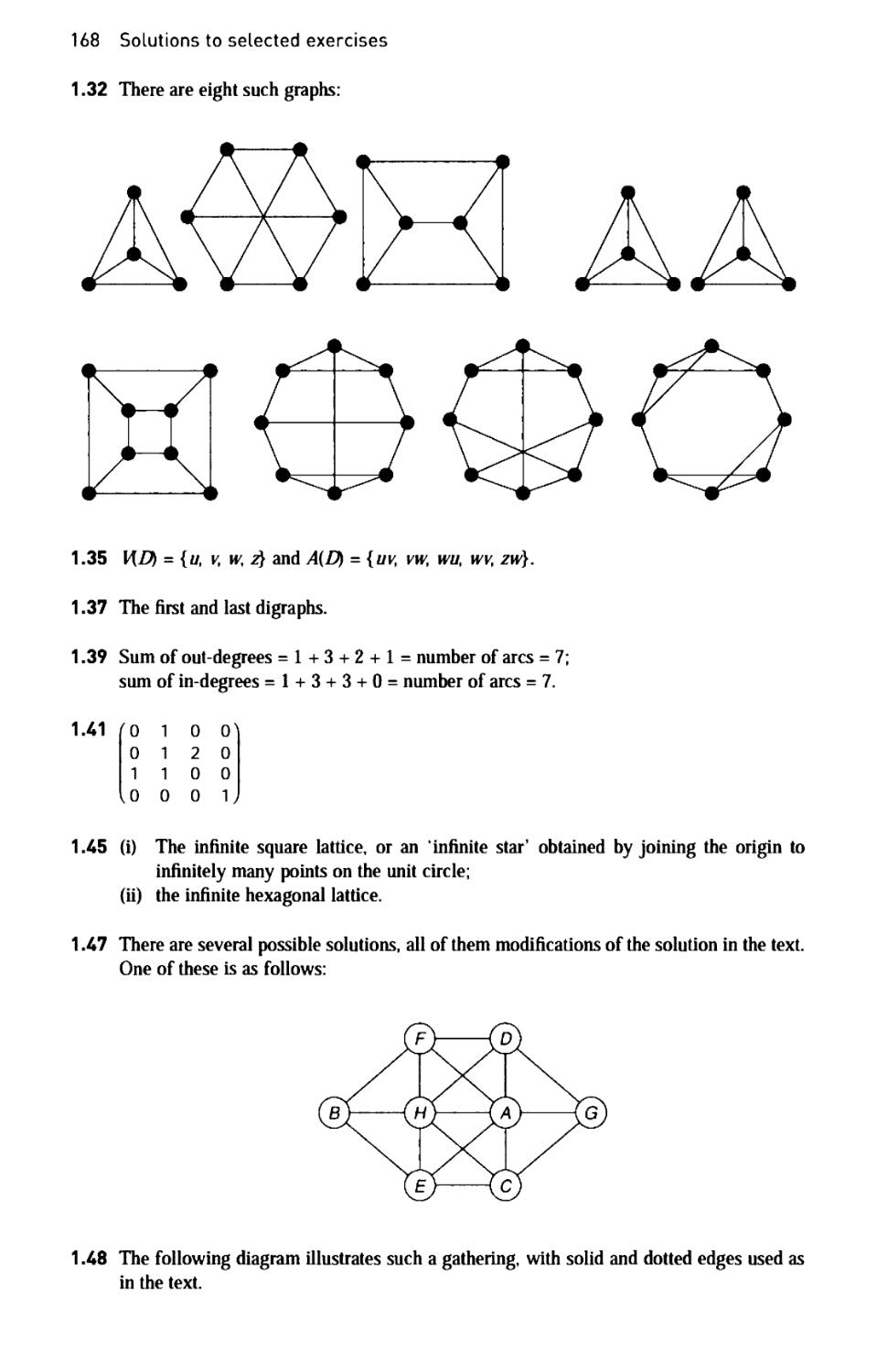
1.32s Draw all the simple cubic graphs with at most eight vertices.
1.33 What can you say about the complement of a complete graph, and the complement of
a complete bipartite graph?

22 Definitions and examples
1.34 The complete tripartite graph Kryt consists of three sets of vertices (of sizes r, s and
ή, with an edge joining two vertices if and only if they lie in different sets. Draw the
graphs Kll2 and KXVI and find the number of edges of Aii4i5.
1.3 Variations on a theme
In this section we consider two variations on the definition of a graph. In the first of
these, each edge is given a particular direction, as in a one-way street. In the second,
we allow our vertex-set and/or edge-set to be infinite.
Digraphs
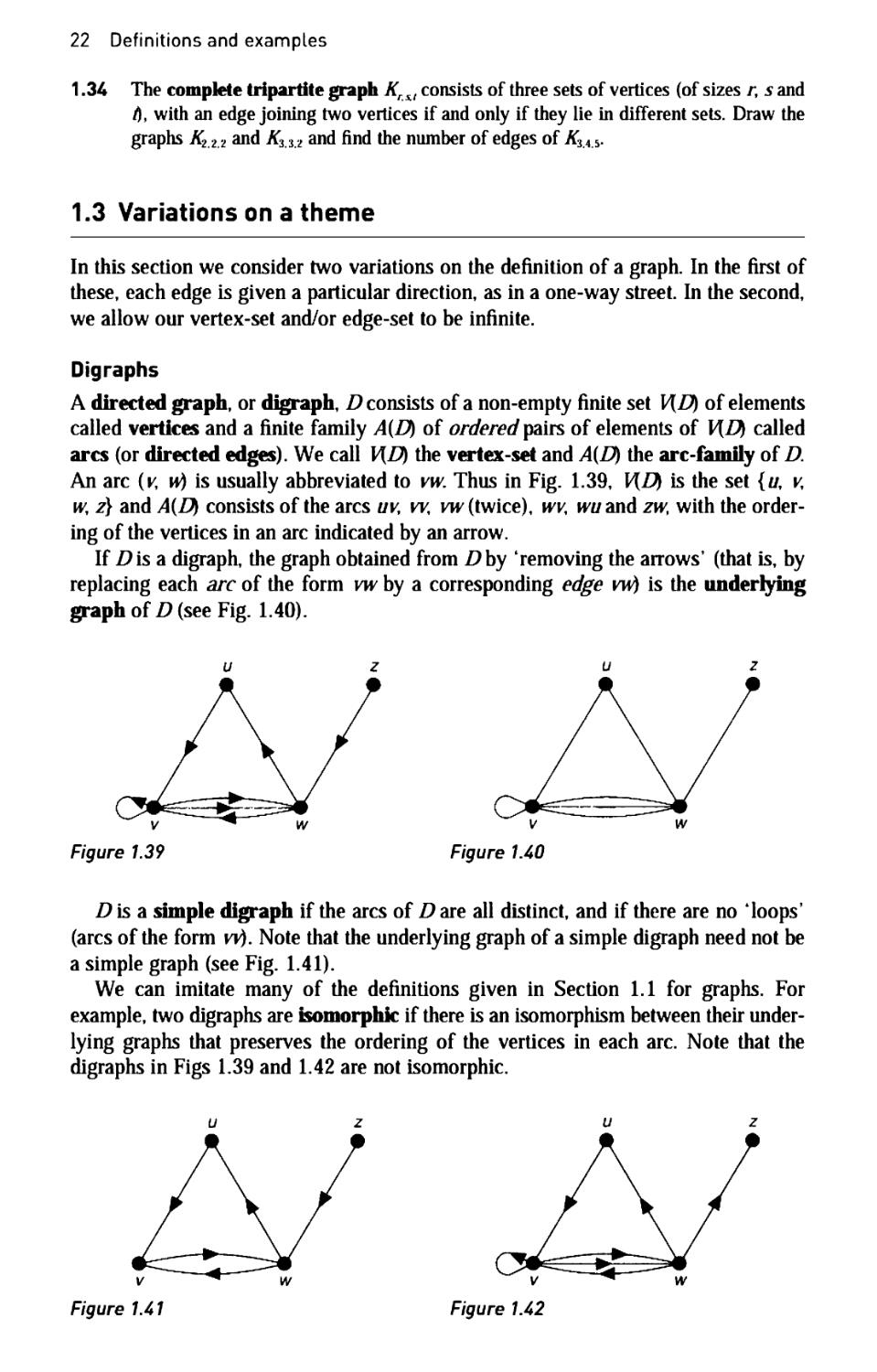
A directed graph, or digraph, Z) consists of a non-empty finite set V[D) of elements
called vertices and a finite family A(D) of ordered pairs of elements of V(Uj called
arcs (or directed edges). We call \\D) the vertex-set and A(D) the arc-family of D.
An arc (к n) is usually abbreviated to vw. Thus in Fig. 1.39, ]/(&} is the set {ί/, κ
w, z} and A{Uj consists of the arcs uv, w, vw (twice), wv, wu and zw, with the
ordering of the vertices in an arc indicated by an arrow.
If Dis a digraph, the graph obtained from Dby 'removing the arrows' (that is, by
replacing each arc of the form vw by a corresponding edge vW) is the underlying
graph of D (see Fig. 1.40).
и ζ υ ζ
ν ^ w
Figure 1.39 Figure 1.40
Ζ) is a simple digraph if the arcs of D are all distinct, and if there are no 'loops'
(arcs of the form vv). Note that the underlying graph of a simple digraph need not be
a simple graph (see Fig. 1.41).
We can imitate many of the definitions given in Section 1.1 for graphs. For
example, two digraphs are isomorphic if there is an isomorphism between their
underlying graphs that preserves the ordering of the vertices in each arc. Note that the
digraphs in Figs 1.39 and 1.42 are not isomorphic.
Δ/ A/
V ^ W V ^ W
Figure 1.41 Figure 1.42

1.3 Variations on a theme 23
We can also define connectedness. A digraph D is (weakly) connected if it cannot
be expressed as the union of two digraphs, defined in the obvious way. This is
equivalent to saying that the underlying graph of D is a connected graph. A stronger
definition of connectedness for digraphs will be given in Section 2.1.
Two vertices у and wof a digraph D are adjacent if there is an arc in A(D) of the
form vwor wv, and the vertices yand ware incident with such an arc
The out-degree of a vertex ν of D is the number of arcs of the form vwy and is
denoted by outdeg( v). Similarly, the in-degree of ν is the number of arcs of D of the
form wv, and is denoted by indeg(0.
There is a digraph version of Theorem 1.1, which we call, naturally enough, the
handshaking dilemma!
THEOREM 3 (Handshaking dil mma / sum и -
s s и о s
Proof. The sum of all the out-degrees is equal to the number of arcs, since each arc
contributes exactly 1 to the sum. Similarly, the sum of all the in-degrees is equal to
the number of arcs. ■
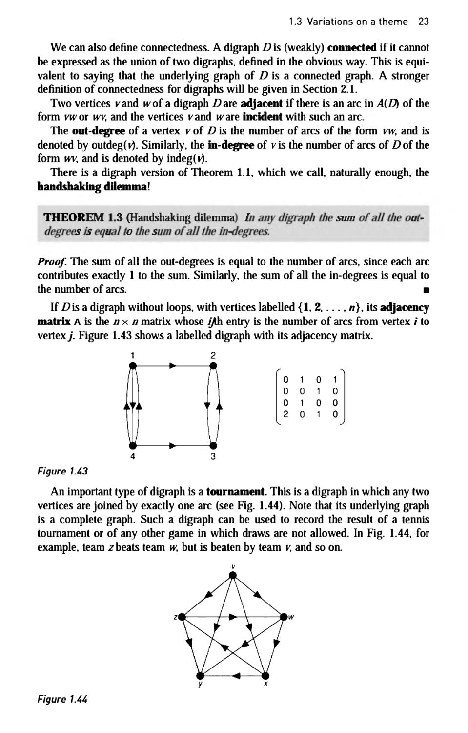
If Dis a digraph without loops, with vertices labelled {1, 2,..., л}, its adjacency
matrix A is the η χ η matrix whose ifiu entry is the number of arcs from vertex / to
vertex/ Figure 1.43 shows a labelled digraph with its adjacency matrix.
0 10 1
0 0 10
0 10 0
2 0 10
V. J
An important type of digraph is a tournament. This is a digraph in which any two
vertices are joined by exactly one arc (see Fig. 1.44). Note that its underlying graph
is a complete graph. Such a digraph can be used to record the result of a tennis
tournament or of any other game in which draws are not allowed. In Fig. 1.44, for
example, team ζ beats team w, but is beaten by team v, and so on.
Figure 1.44
1 2
/к—^~
4ti
L.
Figure 1.43

24 Definitions and examples
Infinite graphs
An infinite graph G consists of an infinite set V[ G) of elements called vertices and
an infinite family E(G) of unordered pairs of elements of V(G) called edges. If V(G)
and E(G) are both countably infinite (that is, they can be labelled 1, 2, 3,...), then
G is a countable graph. For convenience, we exclude the possibility of V[G) being
infinite but E(G) finite, as such objects are merely finite graphs together with
infinitely many isolated vertices, or of ДG) being infinite but V(G) finite, as such
objects are essentially finite graphs but with infinitely many loops or multiple edges.
Many of our earlier definitions extend immediately to infinite graphs. The degree
of a vertex νοί an infinite graph is the cardinality of the set of edges incident with к
and may be finite or infinite. An infinite graph is locally finite if each of its vertices
has finite degree; two important examples are the infinite square lattice and the
infinite triangular lattice, shown in Figs 1.45 and 1.46. We similarly define a locally
countable infinite graph to be one in which each vertex has countable degree.
Τ Τ Τ Τ
τ—τ—τ—τ
τ—τ—τ—τ
• · · ·
Figure 1.45
Figure 1.46
We can now prove the following simple, but fundamental, result.
THEOREM 1 Ε
Proof. Let pbe any vertex of such an infinite graph, and let Ax be the set of vertices
adjacent to к А2 be the set of all vertices adjacent to a vertex of Alt and so on. By
hypothesis, Ax is countable, and hence so are A2, A3 since the union of a
countable collection of countable sets is countable. Hence { v}, Ax Аъ ... is a sequence of
sets whose union is countable and contains every vertex of the infinite graph, by
connectedness. The result follows. ■
OROLLARY1 Ε
с

1.3 Variations on a theme 25
Exercises
1.35s Write down the vertex-set and arc-set of the digraph in Fig. 1.41.
1.36 Write down the vertex-set and arc-family of the graph in Fig. 1.42.
1.37s Two of the digraphs in Fig. 1.47 are isomorphic. Which two are they?
Figure 1.47
1.38 Two of the digraphs in Fig. 1.48 are isomorphic. Which two are they?
Figure 1.48
1.39s Verify the handshaking dilemma for the digraph of Fig. 1.39.
1 .40 Verify the handshaking dilemma for the tournament of Fig. 1.49.
Figure 1.49
1.41* Write down the adjacency matrix of the digraph in Fig. 1.39.
1.42 Write down the adjacency matrix of the tournament in Fig 1.44.
1.43 The converse Π of a digraph D is obtained from D by reversing the direction of each arc.
(i) Give an example of a digraph that is isomorphic to its converse.
(ii) What is the connection between the adjacency matrices of D and ΠΊ
1.44 Let Γ be a tournament on η vertices. If Σ denotes a summation over all the vertices of
T, prove that Σ outdeg(*)2 = Σ indeg(v)2.
1.45s Give an example of each of the following:
(i) an infinite bipartite graph;
(ii) an infinite connected cubic graph.

26 Definitions and examples
1 ЛЬ Give an example of each of the following:
(i) an infinite graph with infinitely many end-vertices;
(ii) an infinite graph with uncountably many vertices and edges.
1.4 Three puzzles
In this section we present three recreational puzzles that can be solved using ideas
relating to graphs. In each puzzle, notice how the use of a graph diagram makes the
problem much easier to understand and to solve.
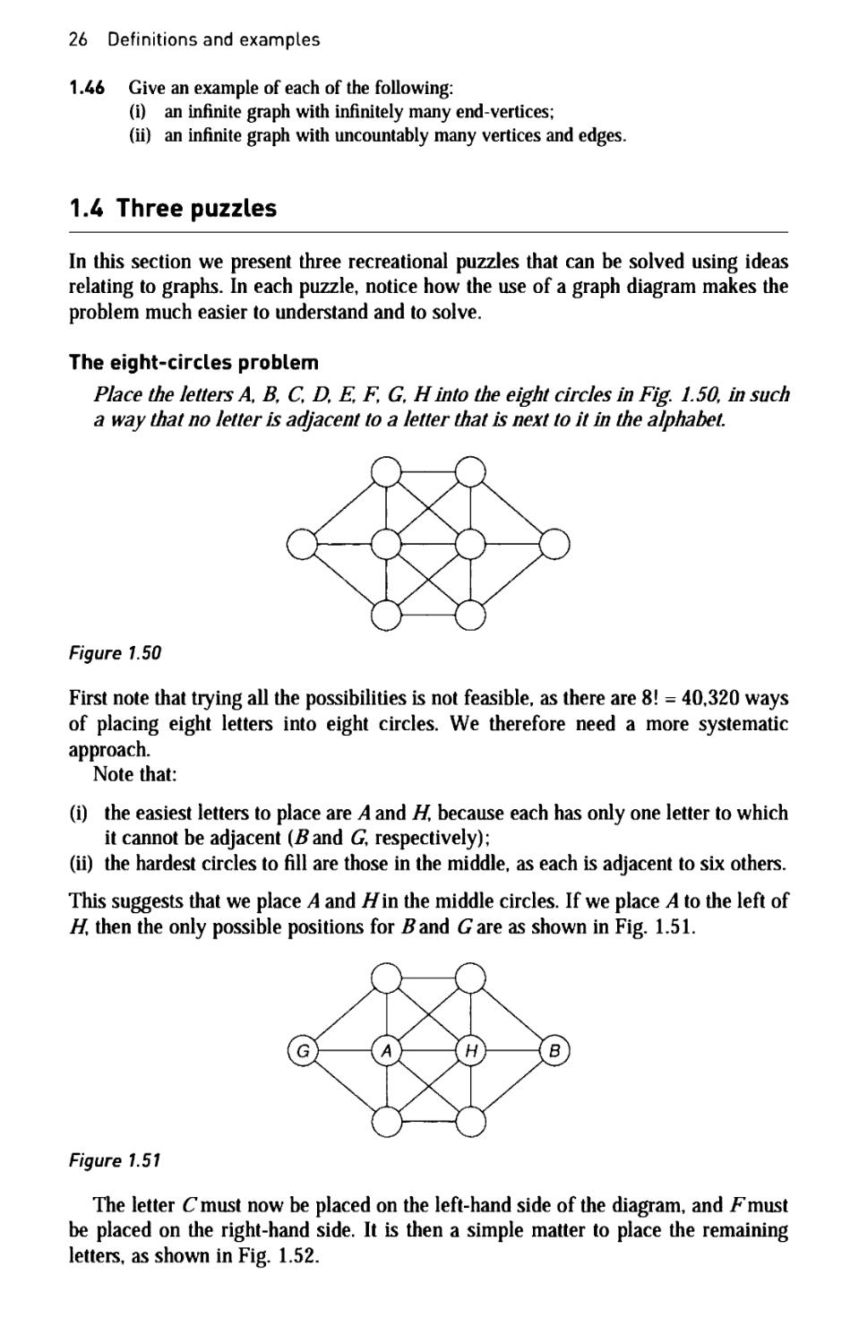
The eight-circles problem
Place the letters A, B, C, D, E, F, G, Η into the eight circles in Fig. 1.50, in such
a way that no letter is adjacent to a letter that is next to it in the alphabet.
Figure 1.50
First note that trying all the possibilities is not feasible, as there are 8! = 40,320 ways
of placing eight letters into eight circles. We therefore need a more systematic
approach.
Note that:
(i) the easiest letters to place are A and Я because each has only one letter to which
it cannot be adjacent (2?and G, respectively);
(ii) the hardest circles to fill are those in the middle, as each is adjacent to six others.
This suggests that we place A and Я in the middle circles. If we place A to the left of
Я then the only possible positions for 2? and G are as shown in Fig. 1.51.
Figure 1.51
The letter С must now be placed on the left-hand side of the diagram, and Fmust
be placed on the right-hand side. It is then a simple matter to place the remaining
letters, as shown in Fig. 1.52.

1.Д Three puzzles 27
Figure 1.52
Six people at a party
Show that, in any gathering of six people, there are either three people who all
know each other, or three people none of whom knows either of the other two.
To solve this, we draw a graph in which we represent each person by a vertex, and
join two vertices by a solid edge if the corresponding people know each other and by
a dotted edge if not. We must show that there is always a solid triangle or a dotted
triangle.
Let ν be any vertex. Then there must be exactly five edges incident with v, either
solid or dotted, and so at least three of these edges must be of the same type. Let us
assume that there are three solid edges (see Fig. 1.53); the case of at least three dotted
edges is similar.
Figure 1.53
If the people corresponding to the vertices w and χ know each other, then к w
and χ form a solid triangle, as required. Similarly, if the people corresponding to the
vertices w and /, or to the vertices χ and /, know each other, then we again obtain
a solid triangle. These three cases are shown in Fig. 1.54.
Figure 1.54

28 Definitions and examples
Finally, if no two of the people corresponding to the vertices w, χ and /know each
other, then w, χ and /form a dotted triangle, as required (see Fig. 1.55).
Figure 1.55
Since this exhausts all possibilities, the result follows.
The four-cubes problem
We conclude this section with a puzzle that has long been popular under the name of
Instant Insanity'.
Given four cubes whose faces are coloured red blue, green and yellow, as in
Fig. 1.56, can we pile them up so that all four colours appear on each side of the
resulting 4x1 stack?
R
R
Υ
R
G
В
R
R
Υ
Υ
в |g
В
G
В
G
R
Υ
G
В
Υ
Υ
R
G
cube 1
Figure 1.56
cube 2
cube 3
cube 4
cube 3
cube 2
cube 4 cube 1
Although these cubes can be stacked in thousands of different ways, there is
essentially only one way that gives a solution.
To solve this problem, we represent each cube by a graph with four vertices, R, B,
G and Y, one for each colour. In each of these graphs, two vertices are adjacent if and
only if the cube in question has the corresponding colours on opposite faces. The
graphs corresponding to the cubes of Fig. 1.56 are shown in Fig. 1.57.
i ί
ψ я
4 <
G ϊ
cube 1
3 R В
Vt W
1 · -%
/ G Υ
cube 2
R Ε
w
Ok ,
3 R В
9 я
Ь А
G Υ С
cube3
Ψ W
Ь йШ
W W
3 Υ
cube 4
Figure 1.57

1.4 Three puzzles 29
We next superimpose these graphs to form a new graph G (see Fig. 1.58).
s1 2
Figure 1.58
A solution of the puzzle is obtained by finding two subgraphs, Hx and Нъ of G
The subgraph Hx tells us which pair of colours appear on the front and back of each
cube, and the subgraph H2 tells us which pair of colours appear on the left and right.
To this end, the subgraphs Hx and H2 must have the following properties:
(a) Each subgraph contains exactly one edge from each cube: this ensures that each
cube has a front and back, and a left and right, and the subgraphs tell us which
pairs of colours appear on these faces.
(b) The subgraphs have no edges in common this ensures that the faces on the front
and back are different from those on the sides.
(c) Each subgraph is regular of degree 2: this tells us that each colour appears
exactly twice on the sides of the stack (once on each side) and exactly twice on
the front and back (once on the front and once on the back).
Using these observations, we can easily check that neither loop can be included in the
subgraphs. It then follows, after a little experimentation, that the subgraphs are as
shown in Fig. 1.59, and the solution can then be read from them, as in Fig. 1.60.
G * Υ
front and back
«1
left and right
H?
Figure 1.59
cube 4 -
. о
cube 1 -
► G
^ ν
fe- R
—>> R
left
R |
В
qI
Υ
front
Υ
В
R
G
r.ght
G |
R
В
back
Figure 1.60

30 Definitions and examples
Exercises
1MV Find another solution of the eight-circles problem.
1.48* Show that there is a gathering of five people in which there are no three people who all
know each other, and no three people none of whom knows either of the other two.
1.49* Find a solution of the four-cubes problem for the set of cubes in Fig. 1.61.
R
Υ
Υ
G
R
В
R
Υ
G
В
r|y|
R
Υ
G
Υ
В
R
l·
G
G
R
В | G |
cube 1 cube 2 cube 3 cube 4
Figure 1.61
1.50 Show that the four-cubes problem in Fig. 1.62 has no solution.
Υ
в
в
в
G
R
R
Υ
Υ
Υ
G
Β
G
Β
R
G
R
Υ
Υ
G
G
R
R
Β
cube 1 cube 2 cube 3 cube 4
Figure 1.62
Challenge problems
1.51 A simple graph that is isomorphic to its complement is self-complementary.
(i) Prove that, if G is self-complementary, then G has 4k or 4k + 1 vertices, where к
is an integer,
(ii) Find all self-complementary graphs with four and five vertices,
(iii) Find a self-complementary graph with eight vertices.
1.52 (For those who know linear algebra) If G is a simple graph with edge-set E(G), the
vector space of G is the vector space over the field Z2 = {0, 1} of integers modulo 2,
whose elements are subsets of E\G). The sum E+ Fof two such subsets iTand F\s the
set of edges in Ε от Fbut not both, and scalar multiplication is defined by \.E= Ε and
Q.E= 0. Show that this defines a vector space over Z2, and find a basis for it.
1.53 The line graph L(G) of a simple graph G is the graph whose vertices are in one-one
correspondence with the edges of G, with two vertices of L(G) being adjacent if and
only if the corresponding edges of G are adjacent.
(i) Show that K^ and Кхг have the same line graph.
(ii) Show that the line graph of the tetrahedron graph is the octahedron graph,
(iii) Prove that, if G is regular of degree 4 then L(G) is regular of degree 2k- 2.
(iv) Find an expression for the number of edges of L(G) in terms of the degrees of the
vertices of G.
(v) Show that L(K5) is the complement of the Petersen graph.

1.A Three puzzles 31
1.54 (For those who know group theory) An automorphism φ of a simple graph G is a
one-one mapping of the vertex-set of G onto itself with the property that <p(*) and y(u)
are adjacent whenever Hand (fare. The automorphism group Y(G) of G is the group
of automorphisms of G under composition.
(i) Prove that the groups Γ(G) and Y(G) are isomorphic,
(ii) Find the groups r(/Q, Y(KJ and r(Q.
(iii) Use the results of parts (i) and (ii) and of Exercise 1.53(v) to find the
automorphism group of the Petersen graph.
1.55 Show that an infinite graph Gcan be drawn in Euclidean 3-space if \\G) and Д G) can
each be put in one-one correspondence with a subset of the set of real numbers.
1.56 Prove that the solution of the four-cubes problem in the text is the only solution for that
set of cubes.

Chapter 2
Paths and cycles
So many paths that wind and wind,
While just the art of being kind
Is all the sad world needs.
Ella Wheeler Wilcox
Now that we have a reasonable armoury of graphs, we can look at their properties.
To do this, we need some definitions that describe ways of 'going from one vertex
to another', in both graphs and digraphs. We give these definitions in Section 2.1 and
present some results on connectivity. In Sections 2.2 and 2.3 we study two particular
types of graph and digraph: those with trails that include every edge, and those with
cycles that pass through every vertex. We conclude this chapter, in Section 2.4, with
some applications of paths and cycles.
2.1 Connectivity
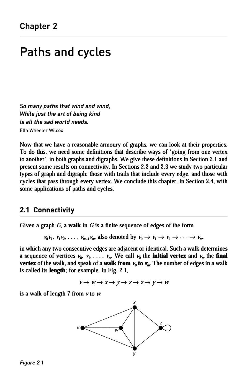
Given a graph <7, a walk in G is a finite sequence of edges of the form
v0vlt vx v2,..., уш_х vm also denoted by v0 -> vx -> v2 -> - · ■ -> vop
in which any two consecutive edges are adjacent or identical. Such a walk determines
a sequence of vertices v0, vx,. .., ν„ We call vQ the initial vertex and vm the final
vertex of the walk, and speak of a walk from r0 to vm The number of edges in a walk
is called its length; for example, in Fig. 2.1,
У—> W—>*—>/—>Z—>Z—>/—> W
is a walk of length 7 from ν to w.
Figure 2.1
У

2.1 Connectivity 33
The concept of a walk is usually too general for our purposes, so we impose some
restrictions. A walk in which all the edges are distinct is a trail If, in addition, the
vertices v0, vh ..., vm are distinct (except, possibly, v0= vj, then the trail is a path.
A walk, path or trail is closed if v0 = ут and a closed path with at least one edge is
a cycle. For example,
v—> w—» *—»/—» z—» z—» *is a trail,
v—> w—» *—»/—» zisa path,
v—> w—» *—»/—» z—» *—» v\s a closed trail,
and v—> w—» *—» /—» las a cycle.
Note that a loop is a cycle of length 1, and a pair of multiple edges is a cycle of
length 2. A cycle of length 3, such as
is called a triangle.
V W V W
connected disconnected
Figure 2.2
We observe that a graph is connected if and only if there is a path between each
pair of vertices (see Fig. 2.2). We can also prove the following results on bipartite
graphs:
THEOR as
Proof. => If <7is bipartite, we can split its vertex-set into two disjoint sets A and 2? so
that each edge of G joins a vertex of A and a vertex of B. Let
^o -> У ι -> - - - -> Уя -* ^o
be a cycle in G, and assume (without loss of generality) that v0 is in A. Then vx is
in Д yz is in A y3 is in Д and so on. Since vm must be in Д the cycle has even
length.
<= Conversely, assume that every cycle of G has even length. We may assume
that G is connected. Choose any vertex v, let A be the set of vertices w for which
the shortest path from Ио ^has even length, and let 2? be the set of vertices not in A
If any two vertices of A (or of B) were adjacent, then the shortest paths from these
vertices to ν would include a cycle of odd length. Thus each edge of G must join
a vertex of A and a vertex of Д so G is bipartite. ■

ЗД Paths and cycles
We next investigate bounds on the number of edges of a simple connected graph
with η vertices. Such a graph has fewest edges when it has no cycles, and has most
edges when it is a complete graph; this implies that the number of edges must lie
between /7-1 and lhn(n -1). In fact, we can prove a stronger result that includes this
as a special case.
THEOREM G sim a n s со η η
um G s
- -' < +1)
Proof. We prove the lower bound m> n- kby induction on the number of edges of
Gy the result being trivial if G is a null graph. If G contains as few edges as possible
(say щ), then the removal of any edge of G must increase the number of components
by 1, and the graph that remains has η vertices, к + 1 components and щ - 1 edges.
It follows from the induction hypothesis that mQ- 1 > n- (k+ 1), giving щ> n- k
as required.
To prove the upper bound, we can assume that each component of <7is a complete
graph. Suppose, then, that there are two components C^and ζ with /?y and /^vertices,
respectively, where п{> ц> 1. If we now replace C{ and Cj by complete graphs on
n{ + 1 and Uj - 1 vertices, then the total number of vertices remains unchanged, but
the number of edges is changed by
Чг{{п,+ 1)л,- лЦп,- 1)} - "ЛЦЦ- 1) - Ц- 1)Ц- 2)} = η,- nJ+ 1,
which is positive. It follows that, in order to attain the maximum number of edges,
<7must consist of a complete graph with n-k+1 vertices and k- 1 isolated vertices.
The result now follows. ■
We deduce the following corollary (see Exercise 2.4):
OROLLARY 3 l ( -1 ( )
Connectivity
Another approach used in the study of connected graphs is to ask 'how connected
is a given graph?'. Such questions have arisen in connection with the vulnerability
of certain networks, such as a rail or telecommunication network. One interpretation
of this is to ask how many edges (railway lines or telephone cables) or vertices
(stations or telephone exchanges) need to be out of action for the network to become
disconnected. We now introduce some terms that are useful when discussing such
questions.
A disconnecting set in a connected graph G is a set of edges whose deletion
disconnects G For example, in the graph of Fig. 2.3, the sets {elt e2, eb} and {e3, e6,
e7, eg} are disconnecting sets of G\ the disconnected graph left after deletion of the
second is shown in Fig. 2.4.

2.1 Connectivity 35
Figure 2.3 Figure 2Λ
We further define a cutset to be a minimal disconnecting set - that is, a
disconnecting set, no proper subset of which is a disconnecting set; in the above example,
only the second disconnecting set is a cutset. Note that the deletion of the edges in
a cutset always leaves a graph with exactly two components. If a cutset has only one
edge e, we call e a bridge (see Fig. 2.5).
Figure 2.5
These definitions can easily be extended to disconnected graphs. If G is any such
graph, a disconnecting set of G is a set of edges whose removal increases the
number of components of G, and a cutset of G is a minimal disconnecting set.
If G is connected, its edge-connectivity λ(<7) is the size of the smallest cutset in
G Thus X(G) is the smallest number of edges that we need to delete in order to
disconnect G For example, if <7is the graph of Fig. 2.3, then X(G) = 2, corresponding to
the cutset {e,, e2}. We also say that <7is Λ-edge-connected if X(G) > k. Thus the graph
of Fig. 2.3 is 1-edge-connected and 2-edge-connected, but is not 3-edge-connected.
It can be proved that a graph is 2-edge-connected if and only if any two distinct
vertices are joined by at least two paths with no edges in common (see Exercise 2.8(i));
for example, any two distinct vertices of Fig. 2.3 are joined by at least two such paths.
More generally we have the following celebrated theorem of K. Menger. It will be
proved in Chapter 6.
THEOREN f ng r 19 is -
dis с s as a
We can also define the analogous concepts for the removal of vertices. A
separating set in a connected graph G is a set of vertices whose deletion disconnects G\
recall that when we delete a vertex, we must also remove its incident edges. For
example, in the graph of Fig. 2.3, the sets { w, x} and { w, χ у} are separating sets of
G\ the disconnected graph left after removal of the first is shown in Fig. 2.6. If a
separating set contains only one vertex к we call ν Ά cut-vertex (see Fig. 2.7). These
definitions extend immediately to disconnected graphs, as above.

36 Paths and cycles
ν
Figure 2.6 Figure 2.7
If G is connected and not a complete graph, its (vertex) connectivity k(G) is the
size of the smallest separating set in G Thus к(G) is the smallest number of vertices
that we need to delete in order to disconnect G For example, if G is the graph of
Fig. 2.3, then k(G) = 2, corresponding to the separating set { w, x}. We also say
that G is Α-connected if к(<7) > k Thus the graph of Fig. 2.3 is 1-connected and
2-connected, but is not 3-connected.
It can be proved that a graph with at least three vertices is 2-connected if and only
if any two distinct vertices are joined by at least two paths with no other vertices
in common; for example, any two distinct vertices of Fig. 2.3 are joined by at least
two such paths (see Exercise 2.8(ii)). More generally, we have another theorem of
Menger, which will also be proved in Chapter 6.
THEOREV 5 19 ) + 1 $
-c s
с s
These concepts are not unrelated. For example, it can be proved that, if G is any
connected graph, then
k(G) < k(G) < 6(£),
where b(G) is the smallest vertex-degree in G
As we shall see, there are striking and unexpected similarities between the
properties of cycles and cutsets; for example, look at Exercises 2.46, 2.47, 2.48, 2.49 and
Theorem 3.2. The reasons for these similarities will become clear in Chapter 7.
Digraphs
There are also natural generalizations to digraphs of the above definitions. A walk in
a digraph D is a finite sequence of arcs of the form v0vlt vx v2,..., va}_x уш. We
sometimes write this sequence as
and speak of a walk from y0 to уж In an analogous way, we can define directed trails,
directed paths and directed cycles (or, simply, trails, paths and cycles, when there is
no possibility of confusion). Note that although a trail cannot contain a given arc vw
more than once, it can contain both nvand wv, for example, in Fig. 2.8,
is a trail.

2.1 Connectivity 37
υ ζ
Δ/
Figure 2.8
We can also define connectedness. The two most useful types of connected
digraph correspond to whether or not we take account of the directions of the arcs:
these definitions are the natural extensions to digraphs of the two descriptions of
connected graphs in Sections 1.2 and 2.1.
We have already defined a digraph D to be connected if it cannot be expressed
as the union of two digraphs; this is equivalent to saying that the underlying graph
of D is a connected graph. We also say that D is strongly connected if, for any two
vertices ν and wof Д there is a directed path from у to w. Every strongly connected
digraph is connected, but not all connected digraphs are strongly connected; for
example, the connected digraph of Fig. 2.8 is not strongly connected, since there is
no path from ν to ζ
The distinction between a connected digraph and a strongly connected one
becomes more evident if we consider the road map of a city, all of whose streets are
one way. If the road map is connected, then we can drive from any part of the city to
any other, ignoring the directions of the one-way streets as we go. However, if the
map is strongly connected, then we can drive from any part of the city to any other,
always going the 'right way' down the one-way streets.
Since every one-way system needs to be strongly connected, it is natural to ask
when we can impose a one-way system on a street map so that we can drive from
any part of the city to any other. This is not always possible: for example, if the city
consists of two parts connected by a single bridge, then we cannot impose such a
one-way system on the city, since whatever direction we give to the bridge, one part
of the city is cut off. But if there are no bridges, then we can always impose such
a one-way system. This result is stated below in Theorem 2.6.
For convenience, we define a graph G to be orientable if each edge of G can be
directed so that the resulting digraph is strongly connected; such a digraph is an
orientation of G For example, if G is the graph shown in Fig. 2.9, then G is
orientable; an orientation is shown in Fig. 2.10.
о о
Figure 2.9 Figure 2.10

38 Paths and cycles
The following theorem gives a necessary and sufficient condition (due to Η. Ε.
Robbins) for a graph to be orientable.
THEOREN 6 с Gis η
с
Proof. The necessity of the condition is clear.
To prove the sufficiency, we choose any cycle С and direct its edges cyclically.
If each edge of G is contained in С then the proof is complete. If not, we choose
any edge e that is not in С but which is adjacent to an edge of C. By hypothesis, e is
contained in some cycle С whose edges we may direct cyclically, except for those
edges that have already been directed - that is, those edges of С that also lie in C\
the situation is illustrated in Fig. 2.11, with dotted lines denoting edges of С We
proceed in this way, at each stage directing at least one new edge, until all edges have
been directed. Since the digraph must remain strongly connected at each stage of the
process, the result follows. ■
*
e/ V
Figure 2.11
Infinite graphs
We can also extend the concept of a walk to an infinite graph G. There are essentially
three different types of walk in G:
(i) a finite walk is defined exactly as above;
(ii) a one-way infinite walk with initial vertex v0 is an infinite sequence of edges of
the form
v0 —» vx —» v2 —> - - - ;
(iii) a two-way infinite walk is an infinite sequence of edges of the form
■ - · —» v_2 —» v_i —» v0 —» vx —» vz —»....
One-way and two-way infinite trails and paths are defined analogously.
The following result, known as Konig's lemma, tells us that infinite paths are not
difficult to come by; we shall use this result in Chapter 4.
7
THEOREN Koni 19

2.1 Connectivity 39
Proof. For each vertex ζ other than к there is a non-trivial path from Ио ζ It follows
that there are infinitely many paths in G with initial vertex v. Since the degree of ν
is finite, infinitely many of these paths must start with the same edge. If wx is such
an edge, then we can repeat this procedure for the vertex vx and thus obtain a new
vertex v2 and a corresponding edge vx v2. By carrying on in this way, we obtain the
one-way infinite path
ν ι -» v7
Exercises
2.1* In the Petersen graph, find
(i) a trail of length 5;
(ii) a path of length 9;
(iii) cycles of lengths 5, 6, 8 and 9;
(iv) cutsets with three, four and five edges.
2.2 In the dodecahedron graph, find
(i) a trail of length 5;
(ii) a path of length 10;
(iii) cycles of lengths 5, 8 and 9;
(iv) cutsets with three, four and five edges.
2.3* The girth of a graph is the length of its shortest cycle. Write down the girths of the
following graphs:
(i) A,; (ii) K5y, (Ш) Q; (iv) W8; (v) ft;
(vi) the Petersen graph; (vii) the graph of the dodecahedron.
2.4 Prove Corollary 2.3.
2.5* Prove that a simple graph and its complement cannot both be disconnected.
2.6* Write down k(G) and X(G) for each of the following graphs G:
(i) Q; (ii) Hi; (iii) K4y, (iv) ft.
2.7 (i) Show that, if С is a connected graph with minimum degree k then X(G) < к
(ii) Draw a graph G with minimum degree к for which k(l7) < X(G) < к
2.8 (i) Prove that a graph is 2-edge-connected if and only if any two distinct vertices are
joined by at least two paths with no edges in common,
(ii) Prove that a graph with at least three vertices is 2-connected if and only if any two
distinct vertices are joined by at least two paths with no other vertices in common.
2.9 In a connected graph, the distance d(vt w) between a vertex и and a vertex μ is the
length of the shortest path from ν to w.
(i) If d[v, \л)>2, show that there exists a vertex ζ such that
d(v, $ + d[z, u) = d(v, h).
(ii) In the Petersen graph, show that d(v, u) = 1 or 2, for any distinct vertices и and w.

ДО Paths and cycles
2.10 Show, by finding an orientation for each, that Kn (n > 3) and Kr5(r, s > 2) are
orientable.
2.11 Find orientations for the Petersen graph and the graph of the dodecahedron.
2.12 A tournament is transitive if the existence of arcs uv and vw implies the existence of
an arc uw.
(i) Give an example of a transitive tournament.
(ii) Show that in a transitive tournament the teams can be ranked so that each team
beats all the teams which follow it in the ranking,
(iii) Deduce that a transitive tournament with at least two vertices cannot be strongly
connected.
2.13 A tournament Г is irreducible if it is impossible to split the set of vertices of Τ into
two disjoint sets Vx and V2 so that each arc joining a vertex of Vx and a vertex of V2
is directed from Vx to V2.
(i) Give an example of an irreducible tournament.
(ii) Prove that a tournament is irreducible if and only if it is strongly connected.
2.1 4s Give an example to show that the conclusion of Konig's lemma is false if we omit the
condition that the infinite graph is locally finite.
2.2 EuLerian graphs and digraphs
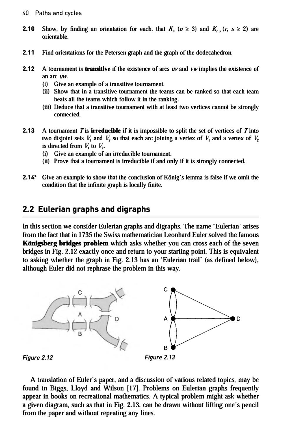
In this section we consider Eulerian graphs and digraphs. The name 'Eulerian' arises
from the fact that in 1735 the Swiss mathematician Leonhard Euler solved the famous
Konigsberg bridges problem which asks whether you can cross each of the seven
bridges in Fig. 2.12 exactly once and return to your starting point. This is equivalent
to asking whether the graph in Fig. 2.13 has an 'Eulerian trail· (as defined below),
although Euler did not rephrase the problem in this way.
Figure 2.12
A translation of Euler's paper, and a discussion of various related topics, may be
found in Biggs, Lloyd and Wilson [17]. Problems on Eulerian graphs frequently
appear in books on recreational mathematics. A typical problem might ask whether
a given diagram, such as that in Fig. 2.13, can be drawn without lifting one's pencil
from the paper and without repeating any lines.

2.2 Eulerian graphs and digraphs 41
EuLerian graphs
A connected graph G\s Eulerian if there exists a closed trail that includes every edge
of G; such a trail is an Eulerian trail. Note that this definition requires you to
traverse each edge once and once only, and to finish at your starting point. A non-
Eulerian graph G is semi-Eulerian if there exists a (non-closed) trail that includes
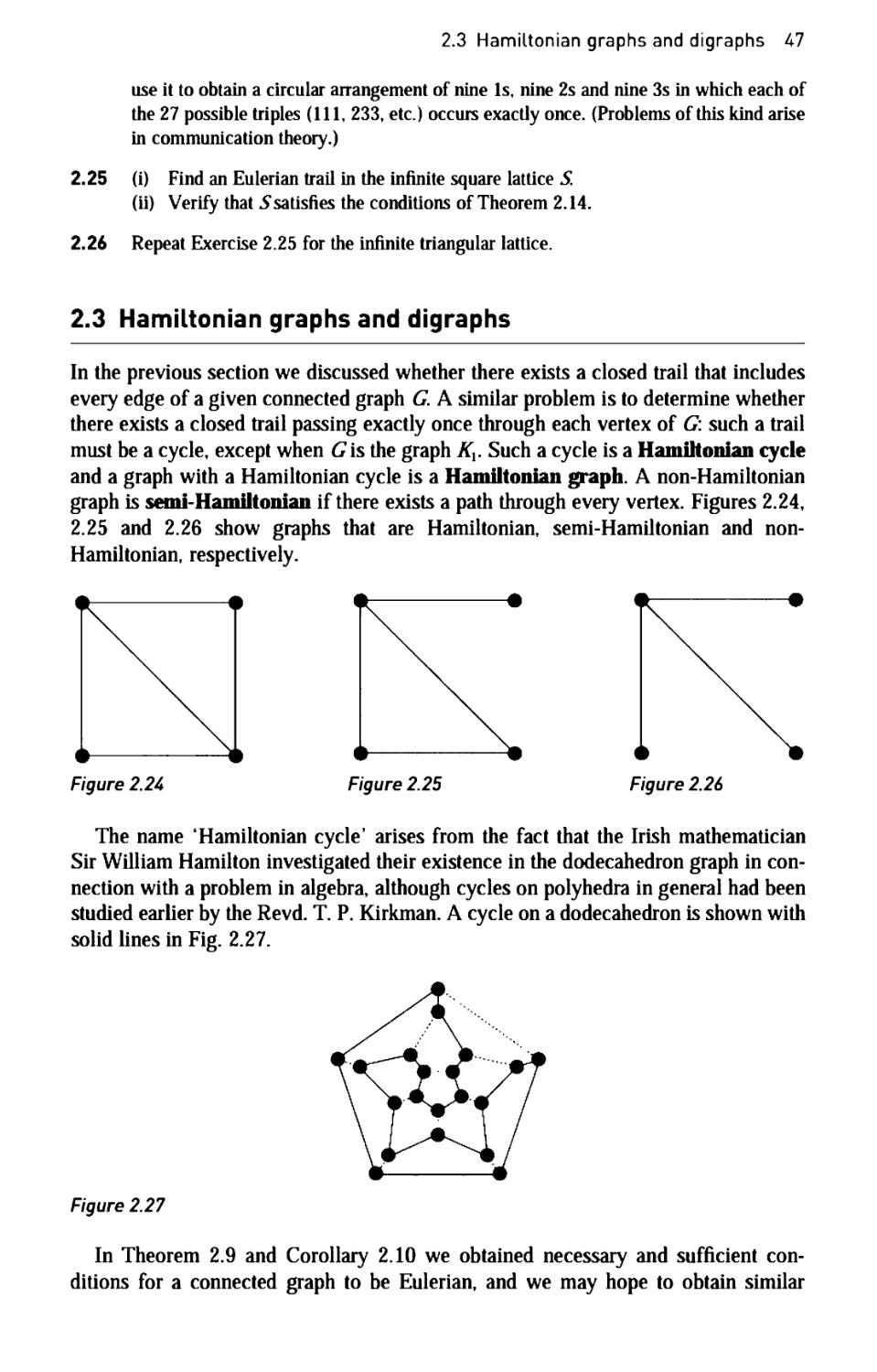
every edge of G Figures 2.14, 2.15 and 2.16 show graphs that are Eulerian, semi-
Eulerian and non-Eulerian, respectively.
Figure 2.14 Figure 2.15 Figure 2.16
One question that immediately arises is 'are there necessary and sufficient
conditions for a graph to be Eulerian?' Before answering this question in Theorem 2.9,
we prove a simple lemma.
LEMMA 8 is с as
с
Proof. If G has any loops or multiple edges, the result is trivial. We can therefore
suppose that G is a simple graph.
Let ν be any vertex of G We construct a walk
у —» vx —> yz -» · - -
inductively, by choosing vx to be any vertex adjacent to pand, for each /> 1,
choosing vM to be any vertex adjacent to vt except νμλ\ the existence of such a vertex
is guaranteed by our hypothesis. Since G has only finitely many vertices, we must
eventually choose a vertex that has been chosen before. If vk is the first such vertex,
then the part of the walk that lies between the two occurrences of vk is the required
cycle. ■
We come now to the main result of this section, which tells us that a given
connected graph is Eulerian if and only if all of its vertex-degrees are even. In terms of
the Konigsberg bridges problem, this corresponds to a city map in which the number
of bridges that emerge from each part of the city is even.
THEOREM 2.9 Eul r L 35) gra GisE a
о ас G
Proof. => Suppose that Ρ is an Eulerian trail of G Whenever Ρ passes through a
vertex, there is a contribution of 2 towards the degree of that vertex. Since each edge

Д2 Paths and cycles
occurs exactly once in P, the degree of each vertex must be a sum of 2s, and is thus
an even number.
<= The proof is by induction on the number of edges of G Suppose that the degree
of each vertex is even. Since <7is connected, each vertex has degree at least 2 and so,
by Lemma 2.8, <7 contains a cycle C.
If £7 contains every edge of Gy the proof is complete. If not, we remove from Gthe
edges of С to form a new (possibly disconnected) graph Я with fewer edges than G,
and in which each vertex still has even degree. By the induction hypothesis, each
component of //has an Eulerian trail. But each component of //has at least one
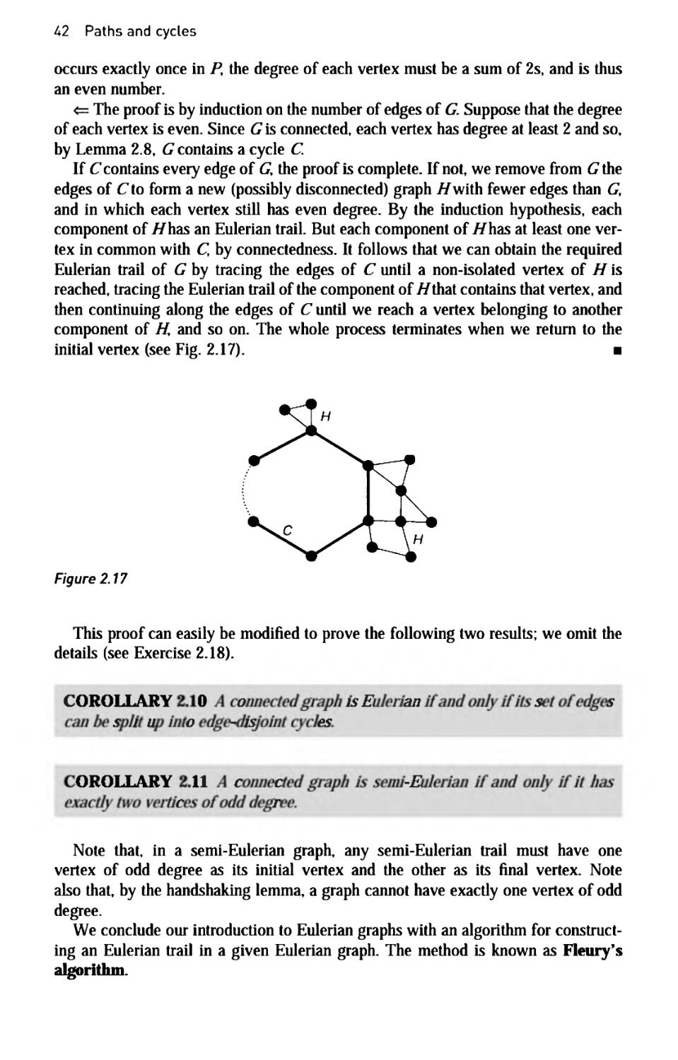
vertex in common with C, by connectedness. It follows that we can obtain the required
Eulerian trail of G by tracing the edges of С until a non-isolated vertex of Η is
reached, tracing the Eulerian trail of the component of #that contains that vertex, and
then continuing along the edges of С until we reach a vertex belonging to another
component of H, and so on. The whole process terminates when we return to the
initial vertex (see Fig. 2.17). ■
Figure 2.17
This proof can easily be modified to prove the following two results; we omit the
details (see Exercise 2.18).
COROLLARY 0 о is Ε an s s
s j и о -is es
OROLLARY 11 с с -Ε
с г
Note that, in a semi-Eulerian graph, any semi-Eulerian trail must have one
vertex of odd degree as its initial vertex and the other as its final vertex. Note
also that, by the handshaking lemma, a graph cannot have exactly one vertex of odd
degree.
We conclude our introduction to Eulerian graphs with an algorithm for
constructing an Eulerian trail in a given Eulerian graph. The method is known as Fleury's
algorithm.

2.2 Eulerian graphs and digraphs 43
THEOREM 1 Ε
Ε
S
s
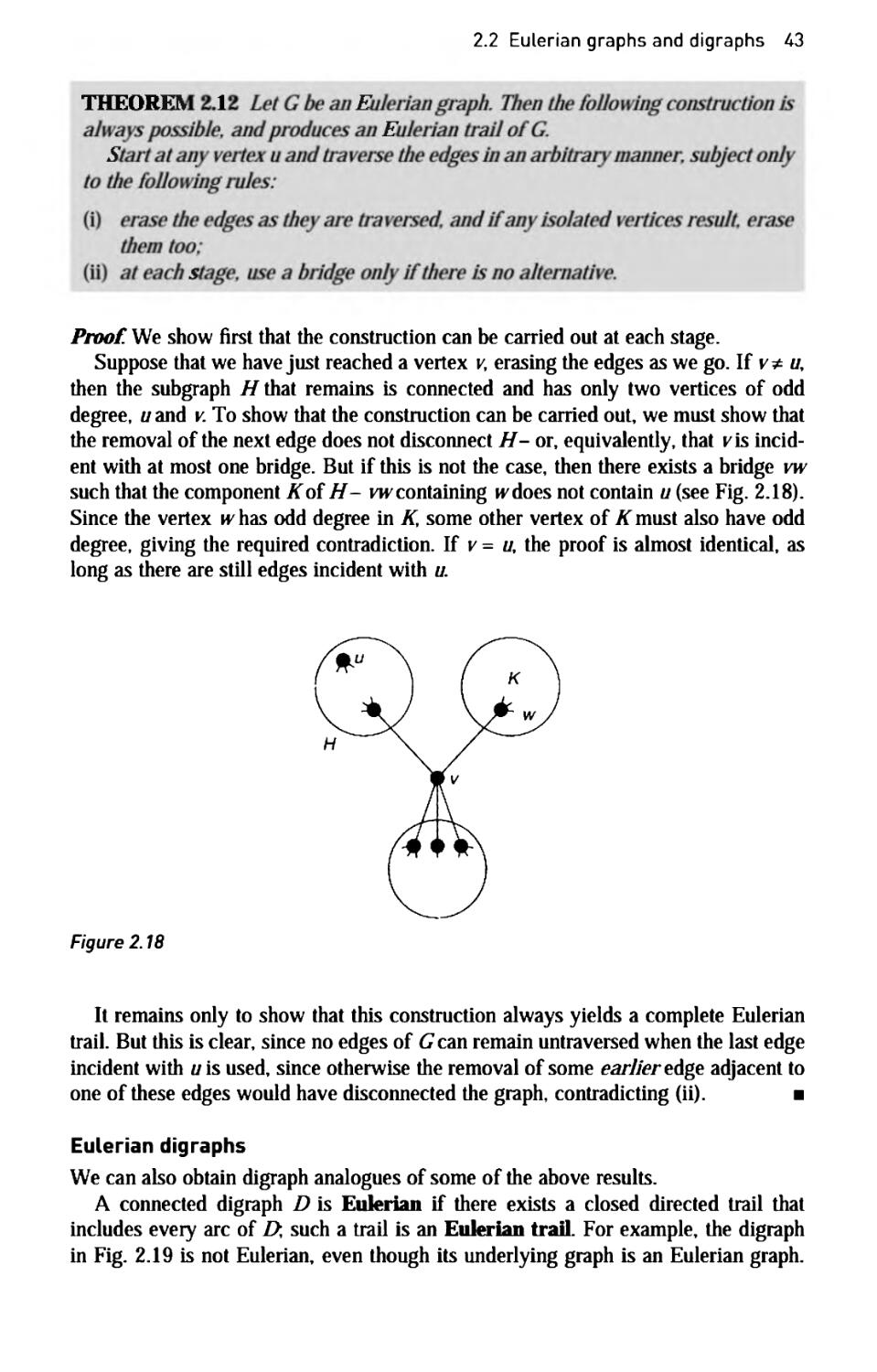
Proof. We show first that the construction can be carried out at each stage.
Suppose that we have just reached a vertex v, erasing the edges as we go. If уф иу
then the subgraph И that remains is connected and has only two vertices of odd
degree, и and v. To show that the construction can be carried out, we must show that
the removal of the next edge does not disconnect H- or, equivalently, that vis
incident with at most one bridge. But if this is not the case, then there exists a bridge vw
such that the component KoiH- vw containing wdoes not contain и (see Fig. 2.18).
Since the vertex whas odd degree in K, some other vertex of tfmust also have odd
degree, giving the required contradiction. If ν = и, the proof is almost identical, as
long as there are still edges incident with u.
Figure 2.18
It remains only to show that this construction always yields a complete Eulerian
trail. But this is clear, since no edges of <7can remain untraversed when the last edge
incident with и is used, since otherwise the removal of some earlier edge adjacent to
one of these edges would have disconnected the graph, contradicting (ii). ■
Eulerian digraphs
We can also obtain digraph analogues of some of the above results.
A connected digraph D is Eulerian if there exists a closed directed trail that
includes every arc of Д such a trail is an Eulerian trail. For example, the digraph
in Fig. 2.19 is not Eulerian, even though its underlying graph is an Eulerian graph.

44 Paths and cycles
Figure 2.19
Note that the digraph must be strongly connected for an Eulerian trail to exist. Note
also that any Eulerian graph is orientable, since we simply follow any Eulerian trail,
directing the edges in the direction of the trail as we go.
Our first aim is to give a necessary and sufficient condition, analogous to the one
in Theorem 2.9, for a connected digraph to be Eulerian.
THEOREM 13 Λ s Ε
outd g = md g(
Proof. The proof is entirely analogous to that of Theorem 2.9, and is left as an
exercise. ■
We leave it to you to define a semi-Eulerian digraph, and to obtain digraph
analogues of Corollaries 2.10 and 2.11 (see Exercise 2.23).
Infinite Eulerian graphs
We conclude this section with a brief discussion of infinite Eulerian graphs. It seems
natural to call a connected infinite graph G Eulerian if there exists a two-way infinite
trail that includes every edge of G\ such an infinite trail is a two-way Eulerian traiL
Note that these definitions require <7to be countable.
The following theorems give further necessary conditions for an infinite graph to
be Eulerian.
THEORE\ 1
с s
(i
(
as
as
as
Proof.
(i) Suppose that Pis an Eulerian trail. Then, by the argument given in the proof of
Theorem 2.9, each vertex of £must have either even or infinite degree.

2.2 Eulerian graphs and digraphs 45
(ii) Let Ρ be split up into three subtrails P_4 P0 and P+ in such a way that PQ is a finite
trail containing every edge of Η (and possibly other edges as well), and P_ and P.
are one-way infinite trails. Then the infinite graph formed by the edges of P_ and P+,
and the vertices incident with them, has at most two infinite components. Since
K\s obtained by adding only a finite set of edges to this graph, the result follows.
(iii) Let the initial and final vertices of P0 be ν and w. We wish to show that ν and
w are connected in К If ν = w, this is obvious. If not, then the result follows
when we apply Corollary 2.11 to the graph obtained by removing the edges of
//from PQy this graph having exactly two vertices (yand w) of odd degree, by
hypothesis. ■
The necessary conditions given in the previous theorem are also sufficient. We
state this result formally in the following theorem. Its proof may be found in Ore [15].
GisE an
THEOREM 2.15
en ns
Exercises
Gis с
с с un
Τ г
га
аг sa
2.15s Which of the following graphs are Eulerian or semi-Eulerian?
(i) the complete graph Къ;
(ii) the complete bipartite graph K2i;
(iii) the graph of the cube;
(iv) the graph of the octahedron;
(v) the Petersen graph.
2.16s In the table of Fig. 1.9, locate all the Eulerian and semi-Eulerian graphs.
2.17 (i) For which values of η is K„ Eulerian?
(ii) Which complete bipartite graphs are Eulerian?
(iii) Which Platonic graphs are Eulerian?
(iv) For which values of η is the wheel Wn Eulerian?
(v) For which values of k is the Лг-cube Qk Eulerian?
2.18 Prove Corollaries 2.10 and 2.11.
2.19s Let G be a connected graph with k (> 0) vertices of odd degree.
(i) Show that the minimum number of trails, that together include every edge of G
and that have no edges in common, is xhL
(ii) How many continuous pen-strokes are needed to draw the diagram in Fig. 2.20
without repeating any line?
Figure 2.20

Д6 Paths and cycles
2.20s Use Fleurys algorithm to produce an Eulerian trail for the graph in Fig. 2.21.
XI IK
Figure 2.21
2.21 An Eulerian graph is randomly traceable from a vertex ν if, whenever we start from
и and traverse the graph in an arbitrary way never using any edge twice, we eventually
obtain an Eulerian trail,
(i) Show that the graph in Fig. 2.22 is randomly traceable.
Figure 2.22
(ii) Give an example of an Eulerian graph that is not randomly traceable.
(iii) Why might a randomly traceable graph be suitable for the layout of an exhibition?
2.22s Find an Eulerian trail in the tournament of Fig. 2.23.
Figure 2.23
2.23 Prove Theorem 2.13 and the digraph analogues of Corollaries 2.10 and 2.11.
2.24 Let Dbe the digraph whose vertices are the pairs of integers 11, 12, 13, 21, 22, 23, 31,
32, 33, and whose arcs join if io kl if and only ify= L Find an Eulerian trail in Z)and

2.3 Hamiltonian graphs and digraphs 47
use it to obtain a circular arrangement of nine Is, nine 2s and nine 3s in which each of
the 27 possible triples (111, 233, etc.) occurs exactly once. (Problems of this kind arise
in communication theory.)
2.25 (i) Find an Eulerian trail in the infinite square lattice 5!
(ii) Verify that ^satisfies the conditions of Theorem 2.14.
2.26 Repeat Exercise 2.25 for the infinite triangular lattice.
2.3 Hamiltonian graphs and digraphs
In the previous section we discussed whether there exists a closed trail that includes
every edge of a given connected graph G A similar problem is to determine whether
there exists a closed trail passing exactly once through each vertex of G: such a trail
must be a cycle, except when Gis the graph Kx. Such a cycle is a Hamihonian cycle
and a graph with a Hamiltonian cycle is a Hamiltonian graph. A non-Hamiltonian
graph is semi-Hamiltonian if there exists a path through every vertex. Figures 2.24,
2.25 and 2.26 show graphs that are Hamiltonian, semi-Hamiltonian and non-
Hamiltonian, respectively.
Figure 2.24 Figure 2.25 Figure 2.26
The name 'Hamiltonian cycle' arises from the fact that the Irish mathematician
Sir William Hamilton investigated their existence in the dodecahedron graph in
connection with a problem in algebra, although cycles on polyhedra in general had been
studied earlier by the Revd. T. P. Kirkman. A cycle on a dodecahedron is shown with
solid lines in Fig. 2.27.
Figure 2.27
In Theorem 2.9 and Corollary 2.10 we obtained necessary and sufficient
conditions for a connected graph to be Eulerian, and we may hope to obtain similar

48 Paths and cycles
characterizations for Hamiltonian graphs - but no such characterization is known. In
fact, little is known in general about Hamiltonian graphs, and most results have the
form 'if Ghas enough edges, then <7is Hamiltonian'. Probably the most celebrated
of these is Dirac's theorem, due to G. A. Dirac (Corollary 2.17). We deduce it from
the following more general result of O. Ore.
THEOREM 6 Or 1960) is s a (_3 s
dgl g( -
a - ac ces G is ami m
Proof. We assume that the result is false, and derive a contradiction.
So let G be a non-Hamiltonian graph with η vertices, satisfying the given
condition on the vertex degrees. By adding extra edges if necessary, we may assume that G
is Only just' non-Hamiltonian, in the sense that the addition of any further edge gives
a Hamiltonian graph; note that adding an extra edge does not violate the condition on
the vertex degrees. It follows that G contains a path
vx -> v2 -> > vn
passing through every vertex. But since G is non-Hamiltonian, the vertices vx and vn
are not adjacent, and so deg(^) + deg(vj > n. It follows that there must be some
vertex Vj adjacent to vx with the property that v^x is adjacent to v„ (see Fig. 2.28).
Figure 2.28
But this gives us the required contradiction since
vx -> v2 ->. - - -> Vt_x -> vB -> vn.x -> · ·. -> vM -> v,-+ vx
is then a Hamiltonian cycle. ■
OROLLARY 1 (Dira 95 G (> 3)
deg( > с G
Proof. The result follows immediately from Theorem 2.16, since deg(0 + deg(w) > n
for each pair of vertices у and w, whether adjacent or not. ■
Hamiltonian digraphs
As we might expect, the study of Hamiltonian digraphs is less successful than that of
Eulerian digraphs. A digraph D is Hamiltonian if there is a directed cycle that includes
every vertex of D. A non-Hamiltonian digraph that contains a directed path through

2.3 Hamiltonian graphs and digraphs 49
every vertex is semi-Hamiltonian. Little is known about Hamiltonian digraphs, and
several theorems on Hamiltonian graphs do not generalize easily, if at all, to digraphs.
It is natural to ask whether there is a generalization to digraphs of Dirac's theorem
(Corollary 2.17). One such generalization is due to M. A. Ghouila-Houri; its proof is
more difficult than that of Dirac's theorem, and can be found in West [16].
THEOREM 18 D s c$
utd _ ind ( _
It seems that such results will not come easily, and so we consider instead which
types of digraph are Hamiltonian. In this respect, the tournaments are particularly
important, the results in this case taking a very simple form.
Because tournaments may have vertices with out-degree or in-degree 0, they are
not in general Hamiltonian. However, the following theorem, due to L. Redei and P.
Camion, shows that every tournament is 'nearly Hamiltonian'.
THEOREN 9
Ε
Ε s
Proof, (i) The statement is clearly true if the tournament has fewer than four vertices.
We prove the result by induction on the number of vertices, and assume that every
non-Hamiltonian tournament on η vertices is semi-Hamiltonian.
Let Γ be a non-Hamiltonian tournament on η + 1 vertices, and let Τ be the
tournament on η vertices obtained by removing from Га vertex ν and its incident arcs. By
the induction hypothesis, Τ has a semi-Hamiltonian path vx —» v2 —»... —» v„. There
are now three cases to consider:
■ if wx is an arc in T, then the required path is
■ if w, is not an arc in Γ (which means that vx vis), and if there exists an У such that
Wj is an arc in T, then choosing i to be the first such, we obtain the required path
(see Fig. 2.29)
Vx -> V2 -> - · - -> νμχ -> V^> !;.->. - · -> V„.
Figure 2.29

50 Paths and cycles
■ if there is no arc in Τ of the form wp then the required path is
(ii) We prove the stronger result that a strongly connected tournament Ton η vertices
contains cycles of length 3, 4,..., n.
To show that Γ contains a cycle of length 3, let у be any vertex of T, and let Wbe
the set of all vertices w such that vw is an arc in ΤΎ and Ζ be the set of all vertices ζ
such that zv is an arc. Since Γ is strongly connected, if and Ζ must both be
nonempty, and there must be an arc in Toi the form Wl, where W is in Wand У is in Ζ
(see Fig. 2.30). The required cycle of length 3 is then
ν —» W —» / -> v.
Figure 2.30
It remains only to show that, if there is a cycle of length ky where k<n, then there
is one of length к + 1. Let
be such a cycle. Suppose first that there exists a vertex к not contained in this cycle,
for which there exist arcs in Toi the form w,- and of the form VjV. Then there must
be a vertex vt such that both v^ ν and wf are arcs in T. The required cycle is then
(see Fig. 2.31)
V\ -* V2-> · . · -* Vi_x -* V -* Vf-* - . . -* Vk-* Vx.
If no vertex exists with the above-mentioned property, then the set of vertices not
contained in the cycle may be divided into two disjoint sets Wand Z, where Wis the
set of vertices wsuch that vgwis an arc for each д and Ζ is the set of vertices ζ such
4 w
Figure 2.31 Figure 2.32

2.3 Hamiltonian graphs and digraphs 51
that zv/is an arc for each / Since T\s strongly connected, Wand Zmust both be
nonempty, and there must be an arc in Tof the form Wl, where W is in Wand / is in Ζ
The required cycle is then (see Fig. 2.32)
vx —» W —» / —» v3 —». . ■ —» vk —» vx. m
Exercises
2.27s Which of the following graphs are Hamiltonian or semi-Hamiltonian?
(i) the complete graph K5\
(ii) the complete bipartite graph Kvi\
(iii) the graph of the octahedron;
(iv) the wheel W6\
(v) the 4-cube QK.
2.28s In the table of Fig. 1.9, locate all the Hamiltonian and semi-Hamiltonian graphs.
2.29 (i) For which values of η is Kn Hamiltonian?
(ii) Which complete bipartite graphs are Hamiltonian?
(iii) Which Platonic graphs are Hamiltonian?
(iv) For which values of η is the wheel Wa Hamiltonian?
(v) For which values of к is the Лг-cube Qk Hamiltonian?
2.30 Is the Grotzsch graph in Fig. 2.33 Hamiltonian?
Figure 2.33 Figure 2.34
2.31 (i) Prove that, if G is a bipartite graph with an odd number of vertices, then G is
non-Hamiltonian.
(ii) Deduce that the graph in Fig. 2.34 is non-Hamiltonian.
2.32 Use the result of Exercise 2.31 (i) to show that a knight cannot visit all the squares of
a5x5or7x7 chessboard exactly once by knight's moves and return to its starting
point. Can a knight visit all the squares of a 6 χ 6 chessboard?
2.33s Give an example to show that the condition 4deg(H ^ xltn , in the statement of Dirac's
theorem, cannot be replaced by 4deg(H > !/г(л- 1)'.
2.3Д (i) Let G be a graph with η vertices and {lh(n - l)(n - 2)} + 2 edges. Use Ore's
theorem to prove that G is Hamiltonian.
(ii) Find a non-Hamiltonian graph with η vertices and {7г(л - 1)(л - 2)} + 1 edges.
2.35s Find a Hamiltonian cycle in the tournament of Fig. 2.23.

52 Paths and cycles
2.6 Applications
Many important advances in graph theory arose as a result of attempts to solve
particular problems - Euler and the bridges of Konigsberg (Section 2.2), Cayley and the
enumeration of chemical molecules (Section 3.2), and Kirchhoff's work on electrical
networks (Section 3.3), to name but three. Much present-day interest in the subject is
due to the fact that, quite apart from being an elegant mathematical discipline in its own
right, graph theory can be applied in a wide range of areas (see the Preface). In a book
of this size we cannot discuss a large number of these applications, and you should
consult Berge [9], Chartrand and Oellermann [20], Deo [21], Roberts [25] and Tucker
[26] for a wide range of practical problems, often with algorithms for their solution.
In this section we outline four types of problem that involve paths and cycles: the
shortest path problem, the critical path problem, the Chinese postman problem and
the travelling salesman problem. The first two of these can be solved by efficient
algorithms - finite step-by-step procedures that quickly yield the solutions. The third
problem can also be solved by an efficient algorithm, but we consider only a special
case here. For the fourth problem, no efficient algorithms are known; we must
therefore choose between algorithms that take a long time to implement and heuristic
algorithms that are quick to apply but give only an approximation to the solution.
The shortest path problem
Suppose that we have a diagram of the form shown in Fig. 2.35, in which the letters
A-L refer to towns that are connected by roads. If the lengths of these roads are as
marked, what is the length of a shortest path from A to LI (We write 'a shortest path' rather
than 'the shortest path' since there may be more than one path with this shortest length.)
Figure 2.35
Note that the numbers in the diagram might also refer, not to the length of each
road, but to the time taken to travel along it, or to the cost of doing so. Thus, if
we have an algorithm for solving this problem in its original formulation, then this
algorithm can also be used to find a quickest or a cheapest route.
Note also that we can easily obtain an upper bound for the answer by taking any
path from A to L and calculating its length. For example, the path
has total length 18, and so the length of a shortest path cannot exceed 18.

2Λ Applications 53
In solving such problems, we regard our diagram as a connected graph in which
a non-negative number is assigned to each edge. Such a graph is called a weighted
graph, and the number assigned to each edge e is the weight of e, denoted by w(e).
The problem is to find a path from Л to Ζ with minimum total weight. Note that, if
we have a weighted graph in which each edge has weight 1, then the problem reduces
to that of finding the number of edges in a shortest path from A to L
There are several methods that we can use to solve this problem. One way is to
make a model of the map by knotting together pieces of string whose lengths are
proportional to the lengths of the roads. To find a shortest path, take hold of the knots
corresponding to A and L - and pull tight!
However, there is a more mathematical way of solving it. The idea is to move
across the map from left to right, labelling each vertex Fwith a number ДР0 that
indicates the shortest distance from A to V This means that, when we reach a vertex
such as Kin Fig. 2.35, then 1(K) is labelled either 1(H) + 6 or Д7) + 2, whichever is
the smaller. Our aim is to find J{L).
To apply the algorithm, we first assign A the label 0 and give Β, Ε and С the
temporary labels 1(A) + 3, 1(A) + 9 and ДЛ) + 2 - that is, 3, 9 and 2. We take the smallest
of these, and write ДО = 2. С L· now permanently labelled 2.
We next look at the vertices adjacent to this labelled vertex C. We assign Fthe
temporary label ДО + 9=11, and we can lower the temporary label at Eio ДО + 6
= 8. The smallest temporary label is now 3 (at B), so we write 1(B) = 3. В is now
permanently labelled 3.
Now we look at the vertices adjacent to B. We assign D the temporary label
/(B) + 2 = 5, and we can lower the temporary label at Eio 1(B) + 4 = 7. The smallest
temporary label is now 5 (at Z7), so we write 1(D) = 5. D is now permanently labelled
5.
Now we look at the vertices adjacent to D. The only one is G, and we assign it the
temporary label 1(D) + 3 = 8. The smallest temporary label is now 7 (at E), so we
write 1(E) = 7. Ε is now permanently labelled 7.
Continuing in this way, we successively obtain the permanent labels
KG) = 8, ДЯ) = 9, KF) = 10, Д7) = 12, Д/) = 13, AK) = 14, Д1) = 17;
these are shown on Fig. 2.36. It follows that the shortest path from A to L has
length 17.
Qg ©g 3 ®G 5
3 4 /1
®
9
Ε
О ® О
2 6 О 6 3
Figure 2.36

54 Paths and cycles
To find such a shortest path, we can restrict our attention to those edges whose
length is the difference of the labels at its ends, such as KL and IK (since J(L) - J(K)
= 17-14 = 3 and J(K) - J(I) = 2). Using the labels to help us, we then trace back
from Z, via К and I, obtaining
L <- K<r- I<r- F<r- H<r- E<r-B<r-A.
Thus the shortest path (which in this case is unique) from A to L is
A -*B^> E^> #-> F-> /-> K^> L
The critical path problem
We now see how this algorithm can be adapted to yield the longest path in a digraph,
and we illustrate its use in a 'critical path' problem relating to the scheduling of a
series of operations.
Suppose that we have a job to perform, such as the building of a house, and that
this job can be divided into a number of activities, such as laying the foundations,
putting on the roof, doing the wiring, etc. Some of these activities can be performed
simultaneously, whereas some may need to be completed before others can be started.
Can we find an efficient method for determining how to schedule the activities so that
the entire job is completed in minimum time?
In order to solve this problem, we construct a 'weighted digraph', or activity
network, in which each arc represents the length of time taken for an activity. Such
a network is given in Fig. 2.37. The vertex A represents the beginning of the job, and
the vertex L represents its completion. Since the entire job cannot be completed until
each path from Л to Ζ has been traversed, the problem reduces to that of finding the
longest path from A to L
Figure 2.37
This is accomplished by using a technique known as programme evaluation and
review technique (PERT), which is similar to the method we used to solve the shortest
path problem above. This time, as we move across the digraph from left to right, we
associate with each vertex Fa label Д V) indicating the length of the longest path from
A to К As in the shortest path problem, we keep track of these labels by writing them
next to the vertices they represent. However, unlike the problem that we considered
above, there is no 'zigzagging', since all arcs are directed from left to right, so we can
assign the permanent labels as we proceed. For example, for the digraph of Fig. 2.37,
we assign:

2.4 Applications 55
to vertex A the number 0;
to vertex Д the number /(A) + 3 - that is, 3;
to vertex С the number /(A) + 2 - that is, 2;
to vertex Д the number /(B) + 2 - that is, 5;
to vertex E, the largest of the numbers 1(A) + 9, /(B) + 4 and ДС) + 6 - that is, 9;
to vertex F the number ДО + 9 - that is, 11;
to vertex G, the larger of the numbers /(D) + 3 and /(E) + 1 - that is, 10;
to vertex H, the larger of the numbers /(E) + 2 and /(F) + 1 - that is, 12;
to vertex / the number /(F) + 2 - that is, 13;
to vertex J, the larger of the numbers Д G) + 5 and Д//) + 5 - that is, 17;
to vertex K, the larger of the numbers /(H) + 6 and Д7) + 2 - that is, 18;
to vertex L, the largest of the numbers ДЯ) + 9, ДУ) + 5 and Д/iQ + 33 - that is, 22.
These labels are shown in Fig. 2.38. It follows that a longest path has length 22,
and the job cannot therefore be completed until time 22.
Figure 2.38
To find the longest path, we trace back from L, as we did for the shortest path
problem. In this case, the unique longest path from A to L is
It is often called a critical path, since any delay in an activity on this path creates
a delay in the whole job. In scheduling a job, we therefore need to pay particular
attention to the critical paths.
We can also calculate the latest time by which any given operation must be
completed if the work is not to be delayed. Working back from L, we see that we must
reach
КЪу time 22 - 3 = 19,
7by time 22 - 5 = 17,
#by time min{17 - 5, 22 - 9 and 19 - 6} = 12,
and so on.
The Chinese postman problem
In this problem, discussed by the Chinese mathematician Meigu Guan, a postman
wishes to deliver his letters, covering the least possible total distance and returning to

56 Paths and cycles
his starting point. He must obviously traverse each road in his route at least once, but
should avoid covering too many roads more than once.
This problem can be reformulated in terms of a weighted graph, where the graph
corresponds to the network of roads, and the weight of each edge is the length of the
corresponding road. In this reformulation, the requirement is to find a closed walk of
minimum total weight that includes each edge at least once. If the graph is Eulerian,
then any Eulerian trail is a closed walk of the required type; such an Eulerian trail can
be found by Fleury's algorithm (see Section 2.2). If the graph is not Eulerian, then
the problem is much harder, although an efficient algorithm for its solution is known
(see Gibbons [23]).
To illustrate the ideas involved, we look at a special case, in which exactly two
vertices have odd degree (see Fig. 2.39).
Figure 2.39
Since vertices 2?and Fare the only vertices of odd degree, we can find a semi-
Eulerian trail from В to iT covering each edge exactly once. In order to return to the
starting point, covering the least possible distance, we now find the shortest path from
Flo В using the algorithm described above. The solution of the Chinese postman
problem is then obtained by combining this shortest path
F^F^A^B
with the original semi-Eulerian trail, giving a total distance of 13 + 64 = 77. Note that,
when we combine the shortest path and the semi-Eulerian trail, we get an Eulerian
graph (see Fig. 2.40).
В С
<п>
F Ε
Figure 2.40
The travelling salesman problem
In this problem, a travelling salesman wishes to visit several given cities and return
to his starting point, covering the least possible total distance. Such a route must be

2.4 Applications 57
Figure 2.41
a cycle. For example, if there are five cities A, B, C, Dand К and if the distances are
as given in Fig. 2.41, then two possible routes are the cycles
Л->Я-> C^D^F^A and A -> D^> B^> C^> E^> A,
with total distances of
2 + 7 + 9 + 5 + 6 = 29 and 4 + 3 + 7 + 8 + 6 = 28,
but neither is the shortest possible route. By inspection we find that the shortest route is
A^B^D^E^ C^>A4
with a total distance of 26.
This problem can also be reformulated in terms of weighted graphs. In this case,
the requirement is to find a Hamiltonian cycle of least possible total weight in a given
weighted complete graph. Note that, as in the shortest path problem, the numbers can
also refer to the times taken to travel between the cities, or the costs involved in doing
so. Thus, if we could find an efficient algorithm for solving the travelling salesman
problem in its original formulation, then we could apply the same algorithm to find
the quickest or the cheapest route.
One possible algorithm is to calculate the total distance for all possible
Hamiltonian cycles, but this is far too time consuming for more than about five cities.
For example, if there are 20 cities, then the number of possible cycles is Vz(19!),
which is about 6 χ 1016. Various other algorithms have been proposed, but they take
too long to apply - no efficient algorithm is known, and it is generally believed that
none exists. On the other hand, there are several heuristic methods that quickly tell us
approximately'what the shortest distance is. One of these is described in Section 3.3.
Exercises
2.36s Use the shortest path algorithm to find the shortest path from Λ to G in the weighted
graph of Fig. 2.42.

58 Paths and cycles
Figure 2.42
2.37 Use the shortest path algorithm to find the shortest path from L to A in Fig. 2.35, and
check that your answer agrees with that given in Fig. 2.36.
2.38 Find the shortest path from S to each other vertex in the weighted graph of Fig. 2.43.
Figure 2.43
2.39s In the critical path problem in the text, calculate the latest times at which we can reach
the vertices G, Ε ma B.
2.ДО Find the longest path from A to G in the network of Fig. 2.44.
0 40 Ε
С 10 F
Figure 2.44

2.4 Applications 59
2.41s Solve the Chinese postman problem for the weighted graph of Fig. 2.45.
D
Figure 2.45
2.42s Solve the travelling salesman problem for the weighted graph of Fig. 2.46.
Figure 2.46
2.43 Find the Hamiltonian cycle of greatest weight in the graph of Fig. 2.41.
Challenge problems
2.44 Let G be a simple graph on Ik vertices containing no triangles. Prove, by induction on
A, that G has at most № edges, and give an example of a graph for which this upper
bound is achieved. (This result is often called Turan s extremal theorem.)
2.45 Let С be a connected graph with vertex-set { vlt v2 vn}, m edges and /triangles.
(i) If A is the adjacency matrix of G, prove that the number of walks of length 2 from
Vj to Vj is the iflh entry of the matrix A2. Deduce that 1m - the sum of the
diagonal entries of A2,
(ii) Obtain a corresponding result for the number of walks of length 3 from vt to vf and
deduce that 6/= the sum of the diagonal entries of A3.
2.46 (i) Prove that, if two distinct cycles of a graph G each contain an edge e, then G has
a cycle that does not contain e.
(ii) Prove a similar result with 'cycles* replaced by 4cutsets'.
2.47 (i) Prove that, if С is a cycle and C* is a cutset of a connected graph G, then С and
C* have an even number of edges in common,
(ii) Prove that, if S is any set of edges of G with an even number of edges in common
with each cutset of G, then Scan be split into edge-disjoint cycles.

60 Paths and cycles
2.48 A set Ε οϊ edges of a graph G is independent if /Γ contains no cycle of G Prove that:
(i) any subset of an independent set is independent;
(ii) if /and J are independent sets of edges with | J\ > | /], then there is an edge e that
lies in У but not in /with the property that /U {e} is independent.
Prove also that (i) and (ii) still hold if we replace the word 'cycle' by 'cutset'.
2.49 Let Vbe the vector space of a graph G (see Exercise 1.52).
(i) Use Corollary 2.10 to show that, if С and D are cycles of G, then their sum C+ D
can be written as a union of edge-disjoint cycles,
(ii) Deduce that the set of such unions of cycles of С forms a subspace W of V
(the cycle subspace of G), and find its dimension,
(iii) Show that the set of unions of edge-disjoint cutsets of G forms a subspace W* of
I/(the cutset subspace of G), and find its dimension.
2.50 The line graph of a graph G was defined in Exercise 1.53.
(i) Show that the line graph of a simple Eulerian graph is Eulerian.
(ii) If the line graph of a simple graph G is Eulerian, must G be Eulerian?
2.51 Let Г be a tournament. The score of a vertex of Г is its out-degree, and the score
sequence of Г is the sequence formed by arranging the scores of its vertices in non-
decreasing order. Prove that, if (slt % s,) is the score-sequence of a tournament T,
then
(i) Si + ^ + . ■ ■ + sa = lkn{n - 1);
(ii) for each positive integer A<nt sl + s2 + · ■ ■ + si > lkk(k- 1), with strict inequality
for all к if and only if 74s strongly connected;
(iii) 7*is transitive (see Exercise 2.12) if and only if sk - k- 1 for each L
2.52 Prove that the Petersen graph is non-Hamiltonian.
2.53 Let G be a Hamiltonian graph and let S be any set of к vertices in G. Prove that the
graph G- S has at most it components.
2.54 (i) Find four Hamiltonian cycles in K(J, no two of which have an edge in common,
(ii) What is the maximum number of edge-disjoint Hamiltonian cycles in Kn+l?
2.55 Show that the infinite square lattice has both one-way and two-way infinite paths
passing exactly once through each vertex.

Chapter 3
Trees
A foot sees not the same tree that a wise man sees.
William Blake
We are all familiar with the idea of a family tree. In this chapter, we study trees in
general, with special reference to spanning trees in a connected graph and to Cayley's
celebrated result on the enumeration of labelled trees. The chapter concludes with
some further applications.
3.1 Properties of trees
A connected graph that has no cycles is a tree; Fig. 3.1 shows four trees.1 Note that
trees are simple graphs.
Figure 3.1
In many ways a tree is the simplest non-trivial type of graph. As we shall see,
it has several 'nice' properties, such as the fact that any two vertices are connected
by exactly one path. When trying to prove a general result for graphs, we sometimes
find it useful to start by trying to prove it for trees; in fact, there are several
conjectures that have not been proved for arbitrary graphs but are known to be true
for trees.
1 The last tree in Fig. 3.1 is particularly well known for its bark.

62 Trees
The following theorem lists some simple properties of trees.
s Τ
THEOR
(i Tis
li) Τ
и') Tis
f ) Tis
(v an
(v) Tc
Ъ 3.1
aws
Τ
s
as
Τ
es
g IS
a
с
Proof. If η = 1, all six results are trivial; we therefore assume that η > 2.
(i) =» (ii). Since Γ contains no cycles, the removal of any edge must disconnect
Τ into two graphs, each of which is a tree. It follows by induction that the
number of edges in each of these two trees is one fewer than the number of
vertices. Replacing the removed edge, we deduce that the total number of edges
of Tis η - 1.
(ii) => (Hi). If Γ is disconnected, then each component of Tis a connected graph
with no cycles and hence, by the previous part, the number of vertices in each
component exceeds the number of edges by 1. It follows that the total number of
vertices of Γ exceeds the total number of edges by at least 2, contradicting the
fact that Tbas η - 1 edges.
(iii) => (iv). The removal of any edge results in a graph with η vertices and η - 2
edges, which must be disconnected by Theorem 2.2.
(iv) => (v). Since T\s connected, each pair of vertices is connected by at least one
path. If a given pair of vertices is connected by two paths, then these paths
contain a cycle, contradicting the fact that each edge is a bridge.
(v) => (vi). If Γ contained a cycle, then any two vertices in the cycle would be
connected by at least two paths, contradicting statement (v). If an edge e is added
to T, then, since the vertices incident with e are already connected in T, a cycle is
created. The fact that only one cycle is obtained follows from Exercise 2.46Ц).
(vi) => (i). Suppose that Γ is disconnected. If we add to Γ any edge joining a vertex
of one component to a vertex in another, then no cycle is created. ■
Note that, by the handshaking lemma, the sum of the degrees of the η vertices of
a tree is equal to twice the number of edges (= 2/? - 2). It follows that:
If η > 2, any tree on η vertices has at least two end-vertices.
Given any connected graph £, we can choose a cycle (if there is one) and remove
any one of its edges, and the resulting graph remains connected. We repeat this
procedure with one of the remaining cycles, continuing until there are no cycles left. The
graph that remains is a tree that connects all the vertices of G It is called a spanning
tree of G. An example of a graph and one of its spanning trees appears in Fig. 3.2.
If we carry out the above procedure, the total number of edges removed is the cycle
rank of G, denoted by y(G). Note that γ(G) = m- η + 1, which is a non-negative
integer by Theorem 2.2. It is convenient also to define the cutset rank of G to be

3.1 Properties of trees 63
Figure 3.2
the number of edges in a spanning tree, denoted by ς(£7); thus, ξ(<7) = л - 1. Some
properties of the cutset rank are given in Exercise 3.33.
Before proceeding, we prove a couple of simple results concerning spanning trees.
In this theorem, the complement of a spanning tree Г of a (not necessarily simple)
connected graph G is the graph obtained from G by removing the edges of T.
THEOR
ι
G as
Proof.
(i) Let C* be a cutset of G, the removal of which splits a component of G into two
subgraphs Я and К Since Г is a spanning tree, Г must contain an edge joining
a vertex of //to a vertex of К and this edge is the required edge.
(ii) Let СЪе a cycle of <7 having no edge in common with the complement of T. Then
С must be contained in T, which is a contradiction. ■
Closely linked with the idea of a spanning tree Г of a connected graph G is that of
the fundamental set of cycles associated with 7! This is formed as follows: if we add
to Γ any edge of <7not contained in T, then by Theorem 3.1 (vi) we obtain a unique
cycle. The set of all cycles formed in this way, by adding separately each edge of G
not contained in T, is the fundamental set of cycles associated with T. Sometimes
we are not interested in the particular spanning tree chosen, and refer simply to a
fundamental set of cycles of G. Note that the number of cycles in any fundamental
set must equal the cycle rank of G Figure 3.3 shows the fundamental set of cycles of
the graph shown in Fig. 3.2 associated with the given spanning tree.
Figure 3.3
In the light of our remarks at the end of Section 2.1, we may hope to be able to
define a fundamental set of cutsets of a connected graph £ associated with a spanning
tree 7! This is indeed the case. By Theorem 3.1(iv), the removal of any edge of

64 Trees
Γ divides the vertex-set of Γ into two disjoint sets, Vx and Vz. The set of all edges
of £ joining a vertex of Vx to one of V2 is a cutset of G, and the set of all cutsets
obtained in this way, by removing separately each edge of T, is the fundamental set
of cutsets associated with T. Note that the number of cutsets in any fundamental
set must equal the cutset rank of G The fundamental set of cutsets of the graph in
Fig. 3.2 associated with the given spanning tree is {e,, e5}, {ez, es, e7, e8}, {e3, e6, e7,
ej and {e4, e6, <?J.
Exercises
3.1s In the table of Fig. 1.9, locate all the trees.
3.2s There are six trees on six vertices: draw them.
3.3 There are 11 trees on seven vertices: draw them.
3.4 (i) Prove that every tree is a bipartite graph,
(ii) Which trees are complete bipartite graphs?
3.5s Draw all the spanning trees in the graph of Fig. 3.4.
3.6 Draw all the spanning trees in the graph of Fig. 3.5.
Figure 3.4
Figure 3.5
Figure 3.6
3.7s
3.8
3.9s
3.10
Find the fundamental sets of cycles and cutsets of the graph in Fig. 3.6 associated with
the spanning tree shown.
Find the cycle and cutset ranks of
(i) K5: (ii) tf,3; (Ш) W5; (iv) jV5;
(v) the Petersen graph.
Let G be a connected graph. What can you say about
(i) an edge of G that appears in every spanning tree?
(ii) an edge of G that appears in no spanning tree?
If G is a connected graph, a centre of G is a vertex ν with the property that the
maximum of the distances between и and the other vertices of G is as small as possible. By
successively removing all the end-vertices, prove that every tree has either one centre
or two adjacent centres. Give an example of a tree of each type with seven vertices.

3.2 Counting trees 65
3.11 Let 7j and Тг be spanning trees of a connected graph G.
(i) If e is any edge of Tlt show that there exists an edge /of Тг such that the graph
(Tx - {e}) U { /} (obtained from T^ on replacing e by f) is also a spanning tree,
(ii) Deduce that Tx can be 'transformed' into Тг by replacing the edges of Tx one at
a time by edges of T2 in such a way that a spanning tree is obtained at each stage.
(This result will be needed in Chapter 7.)
3.2 Counting trees
The subject of graph enumeration is concerned with the problem of determining how
many non-isomorphic graphs satisfy a given property. The subject was initiated in the
1850s by Arthur Cayley, who later applied it to the problem of enumerating alkanes
c/»Hz/»*z with a given number of carbon atoms. As he realized, and as you will see
below, this problem is that of counting the number of trees in which the degree of
each vertex is either 4 or 1.
Many standard problems of graph enumeration have been solved. For example, it
is possible to calculate the number of graphs, connected graphs, trees and Eulerian
graphs with a given number of vertices and edges. Most of the known results can be
obtained by using a fundamental enumeration theorem due to Polya (see Polya and
Read [43]). Unfortunately, in almost every case it is impossible to express these results
by means of simple formulas. For tables of some known results, see Appendix 2.
Counting chemical molecules
One of the earliest uses of trees was in the enumeration of chemical molecules. If we
have a molecule consisting only of carbon atoms and hydrogen atoms, then we can
represent it as a graph in which each carbon atom appears as a vertex of degree 4, and
each hydrogen atom appears as a vertex of degree 1, as we saw in Exercise 0.3.
The graphs of л-butane and 2-methyl propane are shown in Fig. 3.7. Although they
have the same chemical formula C4H10, they are different molecules because the
carbon atoms are arranged differently within the molecule. These two molecules form
part of a general class of molecules, known as alkanes or paraffins, with chemical
formula слн2д+2.
Η Η
I I
Η —С —С
I I
Η Η
Figure 3.7
How many different molecules are there with this formula? To answer this, we
note first that the graph of any molecule with formula c„HZ/?+z is a tree; this follows
from Theorem 3.1 (iii), since it is connected and has
Η
I
с
I I
Η Η
н
I
с —н
Η
ι
С —Η
с н с
/ \ / \
Η Η Η Η
Η
η + (2л + 2) = Ъп + 2 vertices and l/?{An + (2л + 2)} = 3/? + 1 edges.

66 Trees
We note also that the alkane is determined completely once the carbon atoms are
arranged, since the hydrogen atoms can then be added in such a way as to bring
the degree of each carbon vertex up to 4. We can thus discard the hydrogen atoms,
as in Fig. 3.8, and the problem reduces to that of finding the number of trees with η
vertices, each of degree 4 or less.
„ A
Figure 3.8
This problem was solved by Cayley in 1875, by counting the number of ways in
which trees can be built up from their centre(s) (see Exercise 3.10); the details of this
argument are too complicated to describe here, but may be found in Biggs, Lloyd and
Wilson [17]. Much of Cayley's work was superseded by Polya and others, with the
result that several chemical series have now been enumerated by graph-theoretic
techniques.
Counting Labelled trees
This section is devoted primarily to two proofs of a famous result, usually attributed
to Cayley, on the number of labelledtrees with a given number of vertices.
To see what is involved, consider Fig. 3.9, which shows three ways of labelling
a path with four vertices. Since the second labelled tree is the reverse of the first one,
we regard them as the same. On the other hand, neither is isomorphic to the third
labelled tree, as you can see by comparing the degrees of the vertex labelled 3. Thus,
since the reverse of any labelled path does not result in a new one, the number of ways
of labelling the path is (4!)/2 = 12.
12344321 1243
Figure 3.9
Similarly, the number of ways of labelling the 'star' in Fig. 3.10 is 4, since the
central vertex can be labelled in four different ways, and each one determines the
labelling.
Figure 3.10

3.2 Counting trees 67
Since every tree with four vertices is either a path or a star, the total number of
non-isomorphic labelled trees on four vertices is 12 + 4 = 16.
We now prove Cayley's theorem, which generalizes this result to labelled trees
with η vertices. The following proofs are due to H. Prufer and L. E. Clarke; for other
proofs, see Moon [40].
THEOREMS. Cale 1889
First proof.We establish a one-one correspondence between the set of labelled trees
with η vertices and the set of sequences (a,, a2,..., a„_2)y where each «зу is an integer
satisfying 1 < a, < n. Since there are precisely if~2 such sequences, the result then
follows immediately. We assume that η > 3, since the result is trivial if η = 1 or 2.
In order to establish the required correspondence, we first let ГЬе a labelled tree
of order д and show how the sequence can be determined. If A, is the smallest label
assigned to an end-vertex, we let ax be the label of the vertex adjacent to the vertex
A,; for example, if T\s the labelled tree in Fig. 3.11, then bx = 2 and ax = 6. We then
remove the vertex bx and its incident edge, leaving a labelled tree of order /7-1. We
next let A2 be the smallest label assigned to an end-vertex of our new tree, and let a2
be the label of the vertex adjacent to the vertex A/, in this example, Ьг = 3 and a2 = 5.
We then remove the vertex At, and its incident edge, as before. We proceed in this way
until there are only two vertices left; the required sequence is then {ax, a2,..., а„_2);
in this example, Aj = 4 and аъ - 6, A4 = 6 and a4 = 5, A5 = 5 and аъ = 1, and the required
sequence is (6, 5, 6, 5, 1).
4 3
6
2 1
Figure 3.11
To obtain the reverse correspondence, we take a sequence (alt a2,..., an_2)t let A,
be the smallest number from 1 to η that does not appear in it, and join the vertices
ax and A,; for example, if the sequence is (6, 5, 6, 5, 1), then a, = 6, bx = 2 and the
first edge is 62. We then remove ax from the sequence and remove the number A,
from consideration, and proceed as before, building up the tree, edge by edge; in this
example, a2- 5, At, = 3 and the second edge is 53, a3= 6, Aj = 4 and the third edge is
64, a4= 5, A4 = 6 and the fourth edge is 56, and as= 1, h, = 5 and the fifth edge is 15.
We conclude by joining the last two vertices not yet crossed out - in this case, 1 and 7.
It can be checked that if we start with any labelled tree, find the corresponding
sequence, and then find the labelled tree corresponding to that sequence, we obtain
the tree we started from. We have therefore established the required correspondence,
and the result follows. ■

68 Trees
Second proof. Let 7\n, A) be the number of labelled trees on η vertices in which a
given vertex у has degree к We shall derive an expression for 1\n, A), and the result
follows on summing from k=\iok=n-\.
Let A be any labelled tree in which deg(0 = k-l. The removal from A of any edge
wz that is not incident with ν leaves two subtrees, one containing ν and either wov ζ
(w, say), and the other containing ζ If we now join the vertices у and z, we obtain a
labelled tree 2?in which deg(H = к (see Fig. 3.12). We call a pair (A, B) of labelled
trees a linkage if В can be obtained from A by the above construction. Our aim is to
count the possible linkages (A B).
Figure 3.12
Since A may be chosen in Дд к - 1) ways, and since В is uniquely defined by
the edge wz, which may be chosen in (/? - 1) - (k - 1) = η - к ways, the total number
of linkages (А Щ is (n - к) Дд к - 1).
On the other hand, let В be a labelled tree in which deg(H = k, and let Tu Tz,...,
7^ be the subtrees obtained from В by removing the vertex ν and each edge incident
with v. Then we obtain a labelled tree A with degM = к - 1 by removing from 2? just
one of these edges (vwt say, where tt^lies in 7^), and joining w, to any vertex и of any
other subtree Г (see Fig. 3.13). Note that the corresponding pair (А, Щ of labelled
trees is a linkage, and that all linkages may be obtained in this way.
Figure 3.13
Since В can be chosen in Дл, к) ways, and the number of ways of joining w, to
vertices in any other 7Jis (/?- 1) - nt where /7,1s the number of vertices of Th the total
number of linkages (А, Щ is
1\n, k) {(/?- 1 - nx) + (n- 1 - щ) + ■ ■ ■ + (/?- 1 - /7J},
which equals (n - l)(k- 1) Дд A), since /^ + щ + - - - + nk = л - 1.

3.2 Counting trees 69
We have thus shown that
(n- А) Дд1-1) = (л-1)(1-1) ДдА).
Iterating this result, and using the obvious fact that 7{n, η - 1) = 1, we find that
and on summing this over all possible values of A we deduce that the number 1{n) of
labelled trees on η vertices is given by
T(n) = § Т{пЛ = Σίί " f ) (л- 1Г1-1 = {(л- 1) + 1Г2 = л0"2 -
The above result can also be interpreted in terms of spanning trees of the complete
graph Kr
OROLLARY 3. Τ
Proof. To each labelled tree on η vertices there corresponds a unique spanning tree
of Kg. Conversely, each spanning tree of Kn gives rise to a unique labelled tree on
η vertices. ■
We conclude this section by stating a result that can be used to calculate the
number of spanning trees in any connected simple graph. It is called the matrix-tree
theorem and a proof may be found in Harary [14].
THEOREM 35 s s { t , .
= d a =-i
= 0 s
Exercises
3.12s Verify directly that there are exactly 125 labelled trees on five vertices
3.13 Draw all the trees corresponding to alkanes with formulae C5H12 and C6H14.
3.14s Show that, for each value of n, the graph associated with the alcohol СлН2д+1ОН is a
tree (the oxygen vertex has degree 2). Draw the tree corresponding to the molecule
C2H5OH.
3.15s In the first proof of Cayley's theorem, find:
(i) the labelled trees that correspond to the sequences (1, 2, 3, 4) and (3, 3, 3, 3);
(ii) the sequences that correspond to the labelled trees in Fig. 3.14.

70 Trees
5f
3 1
3+
Figure 3.14
3.16 In the first proof of Cay ley's theorem, find the labelled tree that corresponds to the
sequence (7, 6, 5, 4, 3, 2, 1).
3.17 (i) Find the number of trees on η vertices in which a given vertex is an end-vertex,
(ii) Deduce that, if η is large, then the probability that a given vertex of a tree with η
vertices is an end-vertex is approximately e~\
3.18s How many spanning trees has Kls?
3.19 Let x(G) be the number of spanning trees in a connected graph G.
(i) Prove that, for any edge e, x(G) = x(G- e) + τ(£\ e).
(ii) Use this result to calculate x(K2i).
3.3 More applications
In Section 2.4 we considered four problems that arise in operational research - the
shortest path problem, the critical path problem, the Chinese postman problem and
the travelling salesman problem. In this section we consider four applications that
involve the use of trees, taken from operational research, computer science, structural
engineering and electrical network theory.
The minimum connector problem
Suppose that we wish to build a railway network connecting η given cities in such
a way that a passenger can travel from any city to any other. If, for economic reasons,
the total amount of track must be a minimum, then the graph formed by taking the η
cities as vertices and the connecting rails as edges must be a tree. The problem is to
find an efficient algorithm for deciding which of the if~z possible trees connecting
these cities uses the least amount of track, assuming that all the distances between
pairs of cities are known. As before, we can reformulate the problem in terms of
weighted graphs. We denote the weight of the edge e by w(e), and our aim is to find
the spanning tree Γ with least possible total weight Щ T).
Unlike some of the problems we considered earlier, there is a simple algorithm that
provides the solution. It is known as a greedy algorithm, and involves being 'greedy'
at each stage, by choosing an edge of minimum weight in such a way that no cycle is
created. For example, if there are five cities, as shown in Fig. 3.15, then we start by
choosing the shortest edges AB (of weight 2) and BD (of weight 3). We cannot then
choose the edge AD (of weight 4), since it would create the cycle ABD, so instead

3.3 More applications 71
Figure 3.15 Figure 3.16
we choose the edge DE (of weight 5). We cannot then choose the edges AE or BE
(of weight 6), since each would create a cycle, so instead we choose the edge ВС
(of weight 7). This completes a tree (see Fig. 3.16), which turns out to be of minimum
total weight.
The algorithm is described in general in the following theorem.
THEOR 3. G с
s
{' sm s
h , с
US 5
s is s s ι
Proof. The fact that Г is a spanning tree of G follows immediately from Theorem
3.1(ii). We must show that the total weight of Г is a minimum.
In order to do so, suppose that Sis a spanning tree of G for which W[S) < ЩТ).
If ek is the first edge in the above sequence that does not lie in 5, then the subgraph of
<7 formed by adding ek to .£contains a unique cycle С that includes the edge et Since
С contains an edge e lying in 5but not in Tt the subgraph obtained from Son replacing
e by ek is a spanning tree У. But by the construction, w{et) < и{е), so И{У) < W[S)t
and У has one more edge in common with 74han S.
It follows on repeating this procedure that we can change S into T, one step at a
time, with the total weight decreasing at each stage. Hence ЩТ) < W{S), giving the
required contradiction. ■
We can also use the above algorithm to obtain a lower bound for the solution of
the travelling salesman problem (see Section 2.4). This is useful, since the greedy
algorithm is an efficient algorithm, whereas no efficient general algorithms are known
for the travelling salesman problem.

72 Trees
If we take any Hamiltonian cycle in a complete graph and remove any vertex к
then we obtain a semi-Hamiltonian path through the remaining vertices, and such
a path must be a spanning tree. So any solution of the travelling salesman problem
must consist of a spanning tree of this type, together with two edges incident with v.
It follows that if we take the weight of a minimum weight spanning tree through the
remaining vertices and add the two smallest weights of the edges incident with к then
we get a lower bound for the solution of the travelling salesman problem.
For example, if we take the weighted graph of Fig. 3.15 and remove the vertex Cy
then the remaining graph has the four vertices А, Д D and Ε The minimum weight
spanning tree joining these four vertices is the tree whose edges are AB, 2?/? and DE,
with total weight 10, and the two edges of minimum weight incident with Care CB
and CA (or CE) with total weight 15 (see Fig. 3.17). This gives 10 + 15 = 25 as the
resulting lower bound for the travelling salesman problem. Since the correct answer
is 26, we see that this approach to the travelling salesman problem can yield
surprisingly good results.
E Вт
9 D
Figure 3.17
"4f
Searching trees
In many applications, the trees that we consider have a hierarchical structure, with
one vertex at the top (inappropriately called the root), and the other vertices branching
down from it, as in Fig. 3.18. For example, a computer file or a library classification
system is often organized in this way, with information stored at the vertices.
If a particular piece of information is required, we need to be able to search the tree
in a systematic way. This often involves examining every part of the tree until the
\
Figure 3.18

3.3 More applications 73
desired vertex is found. We wish to find a search technique that eventually visits all
parts of the tree, but without visiting any vertex too often.
There are two well-known search procedures: depth-first search and breadth-
first search. Both methods visit all the vertices, but in a different order. No rule
can be given for which method should be used for a particular problem - each has
its advantages. For example, a breadth-first search is used in the shortest path
algorithm (Section 2.4), whereas a depth-first search is used for finding network flows
(Section 6.3).
In a breadth-first search, we fan out to as many vertices as possible, before
penetrating deeper into the tree. This means that we visit all the vertices adjacent to
the current vertex before proceeding to another vertex. For example, consider the tree
in Fig. 3.18. In order to perform a breadth-first search, we start at vertex a and visit
the vertices Λ and г that are adjacent to a. We then visit the vertices rfand e adjacent
to b, and the vertices f, gand h adjacent to с Finally we visit the vertices lj and к
adjacent to d and /adjacent to / This gives us the labelled tree in Fig. 3.19, where
the labels correspond to the order in which the vertices are visited.
Figure 3.19
In a depth-urst search, we penetrate as deeply as possible into a tree before
fanning out to other vertices. For example, consider again the tree in Fig. 3.18. In
order to perform a depth-first search, we start at vertex a and move down to b, rfand
/ Since we cannot penetrate further, we backtrack to d and then go down to j. We
must then backtrack again, and go to к We next backtrack via rfto b, from which we
can go down to e. Backtracking to a then takes us to c, /and / and eventually to
^and h before returning to a. This gives us the labelled tree in Fig. 3.20, where the
labels correspond to the order in which the vertices are visited.
Figure 3.20

74 Trees
Bracing rectangular frameworks
Many buildings and other rigid structures are supported by rectangular steel
frameworks, and such frameworks must remain rigid under heavy loads. For theoretical
purposes, however, such structures can often be treated as planar structures with
pin-joints (rather than rigid welds) holding the beams together.
Suppose that we have a rectangular framework consisting of rods linked by pin-
joints, forming a pattern of square cells, so that the whole structure can move in the
plane (see Fig. 3.21). We now brace three of the square cells with diagonal rods so
that no distortion is possible and the entire framework becomes rigid. (The diagonal
braces can go in either direction.)
τ—τ—τ
τ—τ—τ
1 1 i
distort
non-rigid
Figure 3.21
rigid
Further examples appear in Fig. 3.22. Framework (i) is not rigid, since it can be
distorted as shown. Framework (ii) is rigid, but is over-braced since several of the
diagonal braces can be removed without affecting the rigidity of the framework.
But is framework (iii) rigid? If so, can any braces be removed without affecting the
rigidity?
•—·—Φ--Φ
Figure 3.22
Ш
(iii)
In general, the more braces we add to a framework, the more rigid the structure
becomes, but it is often difficult to predict by looking at a given braced framework
whether it is rigid or not, and whether any of the braces can be removed without
affecting the rigidity of the entire framework.
The method we use is to draw a bipartite graph whose vertices correspond to the
rows and the columns of the framework, and whose edges join a row-vertex and a
column-vertex whenever there is a diagonal brace in the corresponding row and
column. For example, the bipartite graphs corresponding to the frameworks of Fig. 3.22
are as shown in Fig. 3.23; in each case there are three row-vertices rlt rz and r3 and
three column-vertices c,, c2 and c3, and there is an edge from r, to c, since there is
a diagonal brace in the rxcx square.

3.3 More applications 75
rows rt h r3 r, r2 r3 r. r2 rl
columns c, c2 c3 c, c2 c3 Cl °2 3
« (i") (i'i)
Figure 3.23
Note that the non-rigid framework (i) gives rise to a disconnected graph, whereas
the rigid framework (ii) gives rise to a connected graph. This is because each diagonal
brace forces the corresponding row and column to be at right angles. For example, in
the bipartite graph of framework (ii), the edges from r, and rz to c,, c2 and c3 show
that rows 1 and 2 are at right angles to all three columns, and similarly row 3 is at
right angles to columns 1 and 3; it follows that every row is at right angles to every
column, and thus the framework cannot be distorted. However, in the bipartite graph
of framework (i), the vertices r3 and c3 are not connected to the other vertices; thus,
row 3 and column 3 need not remain at right angles to the other rows and columns,
and the framework can be distorted.
These examples are instances of the following general rule, which shows that
framework (iii) is also rigid, since its graph is connected.
THEOREM &7 с L· 1
ISC
Note also that the graph of framework (ii) contains several cycles - for example,
r&fy cxrx. If we remove any edge from this cycle, the graph remains connected and
so the framework remains rigid. We can continue removing edges from the cycles in
the graph until there are no cycles left - for example, if we successively remove the
edges /|Clf rzc2 and r3clf the graph remains connected and the framework remains
rigid. The resulting graph is a tree passing through all the vertices - that is, a
spanning tree (see Fig. 3.24). The removal of any further edge would disconnect the tree,
and the framework would then cease to be rigid.
r\ h r3
Ci С? C3
Figure 3.24
Thus we have the following rule which shows that the frameworks in Fig. 3.22(iii)
and on the right of Fig. 3.21 have minimum bracings - that is, no further diagonal
braces can be removed without affecting the rigidity of the framework:
If the bipartite graph is a spanning tree, then the bracing is a minimum bracing.

76 Trees
Electrical networks
Suppose that we are given the electrical network in Fig. 3.25, and that we wish to find
the current in each wire.
Figure 3.25
To do this, we assign an arbitrary direction to the current in each wire, as in
Fig. 3.26, and apply Kirchhoff 4 laws:
(i) the algebraic sum of the currents at each vertex is 0;
(ii) the total voltage in each cycle is obtained by adding the products of the currents
ik and resistances Rk in that cycle.
Applying Kirchhoff s second law to the cycles VYXV, VWYV and VWYXV, we
obtain the equations
ixRx + i2RL = E\ i3R3 + i\RA - i2R2 = 0; /,/?, + J3R3 + i4R4 = К
But the last of these three equations is simply the sum of the first two, and gives us
no further information. Similarly, if we have the Kirchhoff equations for the cycles
WTyand WZVW, then we can deduce the equation for the cycle VWZYV.
It will save us work if we can find a set of cycles that gives us the information we
need without any redundancy, and this can be done by using a fundamental set of
cycles (see Section 3.1). In this example, taking the fundamental system of cycles in
Fig. 3.3, we obtain the following equations:
for the cycle VYXV,
for the cycle VYZV,
for the cycle VWZV,
for the cycle VYWZV,
ix Rx + I2R2 — E\
i2Rz + 1& + 1ъ^ = 0;
bSs + bus + h&r =0:
j2R2 - 14RA + 15RS + i7Rj = 0.
The equations arising from Kirchhoff s first law are:
for the vertex X
for the vertex V,
for the vertex W,
for the vertex Z,
■h + A
k-h
= 0
= 0
= 0
= 0
These eight equations can now be solved to give the eight currents J0, /,,..., 17.
For example, if E= 12, and if each wire has unit resistance (that is, Rt= 1 for each J),
then the solution is as given in Fig. 3.27.

3.3 More applications 77
V 2 W
Figure 3.27
Exercises
3.20s Use the greedy algorithm to find a minimum weight spanning tree in the graph in
Fig. 3.28.
3.21 Find a minimum weight spanning tree in the graph in Fig. 3.29.
3.22 Show that if each edge of a connected weighted graph G has the same weight, then the
greedy algorithm gives a method for constructing a spanning tree in G
3.23 (i) How would you adapt the greedy algorithm to find a maximum weight spanning tree?
(ii) Find a maximum weight spanning tree for each of the weighted graphs in
Figs 3.15 and 3.28.
3.24s When applying the greedy algorithm to the travelling salesman problem in the text,
what lower bounds do you get when you remove each of the vertices А Д Dana /Tin
turn, instead of CI
3.25s Perform a breadth-first search and a depth-first search on the tree in Fig. 3.30.
3.26 Perform a breadth-first search and a depth-first search on the tree in Fig. 3.31.
j к a b с d e f
Figure 3.30 Figure 3.31

78 Trees
3.27s By constructing the corresponding bipartite graph, determine whether the braced
framework in Fig. 3.32 is rigid. Is the bracing a minimum bracing?
τ—τ—у?—у?—τ
Τ—ут —τ—Τ—л
Figure 3.32
3.28 Determine whether the braced framework in Fig. 3.33 is rigid, and whether the bracing
is a minimum bracing.
ИТТ1
Τ Τ /ί—~7\ —Τ
I m-—m-—1 1
Figure 3.33
3.29 Determine whether each of the braced frameworks in Fig. 3.34 is rigid, and whether the
bracing is a minimum bracing.
Τ—T\ Τ—Τ—Τ
ψ—ψ ψ—4—ψ
Figure 3.34
3.30s Verify the currents in Fig. 3.27, by applying Kirchhoff's laws to the fundamental
cycles associated with the spanning tree with edges VX VW, WZ and YZ
3.31 Write down the Kirchhoff equations for the network of Fig. 3.35, in which the numbers
are resistances; use the spanning tree with edges VW, WZ, XV and WZ.

3.3 More applications 79
Figure 3.35
Challenge problems
3.32 (i) Let C* be a set of edges of a connected graph G Show that, if C* has an edge in
common with each spanning tree of G, then C* contains a cutset,
(ii) Obtain a corresponding result for cycles.
3.33 Show that if Я and К are subgraphs of a connected graph G, and if Я U К and Я П К
are defined in the obvious way, then the cutset rank ξ satisfies:
(i) 0 < ξ(Η) < | ДЯ) | (the number of edges of Я);
(ii) if His a subgraph of К then ξ(#) < ЦК)\
(iii) ξ^υ Κ) + ξ(ΗΠ К) < ξ(Η) + ξ(/Π.
З.ЗД Let Vbe the vector space associated with a simple connected graph G, and let Γ be
a spanning tree of G
(i) Show that the fundamental set of cycles associated with Γ forms a basis for the
cycle subspace W.
(ii) Obtain a corresponding result for the cutset subspace W*.
(iii) Deduce that the dimensions of Wand W* are y(G) and ξ(£), respectively.
3.35 Use the matrix-tree theorem to prove Cayley's theorem.
3.36 Let Дл) be the number of labelled trees on η vertices.
(i) By counting the number of ways of joining a labelled tree on k vertices and one
on η - k vertices, prove that
2(л-1)Лл)=х(5)кл-ЛЛ«Лл-«.
(ii) Deduce the identity
Σ^]^"(λ-«-^' = 2^-1)11^.
3.37 Using the results of Exercise 3.31, find the current in each wire of the network in
Fig. 3.35.

Chapter A
Planarity
Flattery will get you nowhere.
Popular saying
We now embark upon a study of topological graph theory, in which graphs become
tied up with topological notions such as planarity, genus, etc. In particular, we
investigate when a graph can be drawn in the plane and on other surfaces. In Section 4.1,
we discuss planar graphs, exhibit some graphs that are not planar, and state
Kuratowski's characterization of planar graphs. In Section 4.2, we prove Euler's
formula relating the numbers of vertices, edges and faces of a graph drawn in the
plane. In Section 4.3 we study the important topic of duality. In Section 4.4 we
generalize these ideas to graphs drawn on surfaces other than the plane.
4.1 Planar graphs
A planar graph is a graph that can be drawn in the plane without crossings - that is,
so that no two edges intersect geometrically except at a vertex with which both are
incident. Any such drawing is a plane drawing. For convenience, we often use the
abbreviation plane graph for a plane drawing of a planar graph. For example,
Fig. 4.1 shows three drawings of the planar graph KA, but only the second and third
drawings are plane graphs.
M0 A
Figure 4.1
The right-hand drawing in Fig. 4.1 leads us to ask whether every planar graph can
be drawn in the plane so that each edge is represented by a straight line. Although
loops or multiple edges cannot be drawn as straight lines, it was proved independently
by K. Wagner in 1936 and I. Fary in 1948 that:
Every simple planar graph can be dra wn with straight lines.

4.1 Planar graphs 81
See Chartrand and Lesniak [11] or West [16] for details.
Not all graphs are planar, as the following theorem shows.
THEOREN 1
Remark We give two proofs of this result. The first one, presented here, is
constructive. The second proof, which we give in Section 4.2, appears as a corollary of Euler's
formula.
Proof. Suppose first that K3 3 is planar. Since K33 has a cycle
of length 6, any plane drawing must contain this cycle drawn in the form of a
hexagon, as in Fig. 4.2.
У *
Figure 4.2 Figure 4.3
Now the edge wz must lie either wholly inside the hexagon or wholly outside it.
We deal with the case in which wzlies inside the hexagon - the other case is similar.
Since the edge их must not cross the edge wz, it must lie outside the hexagon; the
situation is now as in Fig. 4.3. It is then impossible to draw the edge vy, as it would
cross either их or wz. This gives the required contradiction.
Next, suppose that K5 is planar. Since Къ has a cycle
V^> W—» *—> /—» Z^> V
of length 5, any plane drawing must contain this cycle drawn in the form of a
pentagon, as in Fig. 4.4.
Figure 4.4

82 Planarity
Figure 4.5
Now the edge wz must lie either wholly inside the pentagon or wholly outside it.
We deal with the case in which w^lies inside the pentagon - the other case is similar.
Since the edges кг and vyAo not cross the edge wz, they must both lie outside the
pentagon; the situation is now as in Fig. 4.5. But the edge xz cannot cross the edge ijand
so must lie inside the pentagon; similarly the edge wy must lie inside the pentagon,
and the edges Myand Azmust then cross. This gives the required contradiction. ■
Note that, if we try to draw Къ or K3 3 on the plane, then there must be at least one
crossing of two edges, since these graphs are not planar. However, we do not need
more than one crossing (see Fig. 4.6), even when we require crossings to involve just
two edges.
Φ
Figure 4.6
More generally, the crossing number cr(<7) of a graph G is the smallest number
of crossings (of two edges) that can occur when <7is drawn in the plane. For example,
the crossing number of any planar graph is 0, and сг(,ЛГ5) = cr(K3J = 1. Unfortunately,
little is known about the crossing number of graphs in general. Even the crossing
numbers of most complete graphs and complete bipartite graphs are unknown.
Kuratowski's theorem
It is clear that every subgraph of a planar graph is planar, and that every graph with
a non-planar subgraph must be non-planar. It follows that any graph with K33 or Къ
as a subgraph is non-planar. In fact, as we shall see, these two graphs are the
'building blocks' for all non-planar graphs, in the sense that every non-planar graph must
'contain' at least one of them.

Д.1 Planar graphs 83
Figure 4.7
To make this statement more precise, we define two graphs to be homeomorphic
if both can be obtained from the same graph by inserting new vertices of degree 2 into
its edges. For example, any two cycle graphs are homeomorphic, as are the two
graphs of Fig. 4.7.
Note that the introduction of the term 'homeomorphic' is merely a technicality, as
the insertion or deletion of vertices of degree 2 is irrelevant to considerations of planarity.
However, it enables us to state the following important result, known as Kuratowski's
theorem, which gives a necessary and sufficient condition for a graph to be planar.
THEOREM uratowki 1930 is с ns
The proof of Kuratowski's theorem is long and involved, and we omit it; see
Chartrand and Lesniak [11] or West [16] for a proof. We shall, however, use
Kuratowski's theorem to obtain another criterion for planarity. To do so, we first
define a graph Η to be contractible to Къ or Къз if we can obtain Къ or K33 by
successively contracting edges of H. For example, the Petersen graph is contractible
to /ζ, as we can see by contracting the five 'spokes' joining the inner and outer
5-cycles (see Fig. 4.8).
#^
Figure 4.8
THEOREM 3 a s а о -
ас гК^.
Sketch of proof. <= Assume first that the graph <7is non-planar. Then, by Kuratowski's
theorem, G contains a subgraph Η homeomorphic to Къ or K33. On successively
contracting edges of Η that are incident to a vertex of degree 2, we see that Η is
contractible to Къ or K3 3.

84 Planarity
Figure 4.9
=> Now assume that <7 contains a subgraph #contractible to K33, and let the vertex
pof A33 arise from contracting the subgraph H% of Я (see Fig. 4.9).
The vertex у is incident in K33 with three edges elt e2 and e3. When regarded as
edges of H, these edges are incident with three (not necessarily distinct) vertices vb
v2 and v-i of Hr If vv v2 and v3 are distinct, then we can find a vertex wof Hv and three
paths from w to these vertices intersecting only at w. (There is a similar construction
if the vertices are not distinct, the paths degenerating in this case to single vertices.)
It follows that we can replace the subgraph Hv by a vertex w and three paths leading
out of it. If this construction is carried out for each vertex of Къ 3, and the resulting
paths joined up with the corresponding edges of Къъ, then the resulting subgraph is
homeomorphic to Къъ. It follows from Kuratowski's theorem that G is non-planar
(see Fig. 4.10).
Figure 4.10
A similar argument can be carried out if G contains a subgraph contractible to K5.
Here the details are more complicated, as the subgraph we obtain by the above process
can be homeomorphic to either Kb or /T3i3; see Chartrand and Lesniak [11]. ■
Infinite planar graphs
We conclude this section with a result on infinite planar graphs. Recall from
Section 2.1 that Konig's lemma allows us to deduce results about infinite graphs from the
corresponding results for finite graphs. The following theorem may be regarded as a
typical example.

4.1 Planar graphs 85
THEOR
Proof. Since G is countable, its vertices may be listed as vlt vZj v3,.... We now
construct a strictly increasing sequence Gx cz G2 a G3 a ... of subgraphs of G, by
taking Gk to be the subgraph whose vertices are vlt vz,..., vk and whose edges are
those edges of G joining two of these vertices. Since each G, can be drawn in the
plane in only a finite number m(i) of topologically different ways, we can construct
another infinite graph Я whose vertices wtJ (for /> 1 and 1 <j < /»(/)) correspond to
the various drawings of the graphs Gh and whose edges join the vertices w}J and wu
when к - i + 1 and the plane drawing corresponding to wu extends the drawing
corresponding to wif Since Я is clearly connected and locally finite, it follows from
Konig's lemma that Я contains a one-way infinite path. Since <7is countable, this
infinite path gives the required plane drawing of G m
Exercises
Д.1* Show how the graph of Fig. 4.11 can be drawn in the plane without crossings.
4.2 Show how the graph of Fig. 4.12 can be drawn in the plane without crossings.
Figure 4.11 Figure 4.12
4.3s Three unfriendly neighbours use the same water, oil and treacle wells. In order to avoid
meeting, they wish to build non-crossing paths from each of their houses to each of the
three wells. Can this be done?
4.4s Which complete graphs and complete bipartite graphs are planar?
4.5 (i) For which values of к is the Лг-cube Qk planar?
(ii) For which values of r, s and / is the complete tripartite graph Krst planar?
4.6* Show that KA 3 and the Petersen graph have crossing number 2.
4.7 Prove that the Petersen graph is non-planar
(i) by removing the two horizontal' edges and using Theorem 4.2;
(ii) by using Theorem 4.3.

86 Planarity
4.8* Give an example of
(i) a non-planar graph that is not homeomorphic to Kb or K33\
(ii) a non-planar graph that is not contractible to Къ or Ks 3.
Why does the existence of these graphs not contradict Theorems 4.2 and 4.3?
4.9 If two homeomorphic graphs have лу vertices and m, edges (/= 1, 2), show that
mx — /?! = тг — пг.
4.10 A planar graph G is outerplanar if G can be drawn in the plane so that all of its
vertices lie on the exterior boundary.
(i) Show that KA and Kl:s are not outerplanar.
(ii) Deduce that, if G is an outerplanar graph, then G contains no subgraph
homeomorphic or contractible to KA or K2i.
(The converse result also holds, yielding a Kuratowski-type criterion for a graph
to be outerplanar.)
4.11 By placing its vertices at the points (1, l2, l3), (2, 22, 23), (3, З2, 33) , prove that any
simple graph can be drawn without crossings in Euclidean three-dimensional space so
that each edge is represented by a straight line.
4.12 Give an example of each of the following:
(i) a countable planar graph;
(ii) a countable non-planar graph.
4.2 Euler's formula
If С is a planar graph, then any plane drawing of G divides the set of points of the
plane not lying on G into regions, called faces. For example, the plane graphs in
Figs 4.13 and 4.14 have eight faces and four faces, respectively. Note, in each case,
that the face f4 is unbounded; it is called the infinite face.
Figure 4.13 Figure 4.14
There is nothing special about the infinite face - in fact, any face can be selected
as the infinite face. To see this, we map the graph onto the surface of a sphere by
stereographic projection (see Fig. 4.15). We now rotate the sphere so that the point of
projection (the north pole) lies inside our selected infinite face, and then project the
graph down onto the plane tangent to the sphere at the south pole. The chosen face is
now the infinite face.

4.2 Euler's formula 87
Figure 4.15
Figure 4.16 shows a representation of the graph of Fig. 4.14 in which the infinite
face is f3.
Figure 4.16
We now state and prove Euler's formula that tells us that whatever plane
drawing of a planar graph we take, the number of faces is always the same and is given by
a simple formula.
THEOREM 5 (Eul r 1 0 с
U 5,
G
+ =
Remark An example of this theorem is given by Fig. 4.14, where n- 11, m= 13,
/= 4, and n- m+ f= 11 - 13 + 4 = 2.
Proof. The proof is by induction on the number of edges of G
If m= 0, then n- 1 (since <7is connected) and /= 1 (the infinite face). The theorem
is therefore true in this case.
Now suppose that the theorem holds for all plane graphs with at most m- 1 edges,
and let Gbe a plane graph with medges. If Gis a tree, then m= n-\ and /= 1, so that
η - m + /= 2, as required. If <7is not a tree, let e be an edge in some cycle of G Then

88 Planarity
G- e is a connected plane graph with η vertices, m - 1 edges and /- 1 faces, so that
η - (m - 1) + (/- 1) = 2, by the induction hypothesis. It follows that η - m + f= 2,
as required. ■
This result is often called 'Euler's polyhedron formula', since it relates the numbers
of vertices, edges and faces of a convex polyhedron. For example, for a cube we have
n= 8, /n = 12, /= 6, and n- m+ /= 8 - 12 + 6 = 2 (see Fig. 4.17).
Figure 4.17
To see the connection in general, project the polyhedron out onto its circumsphere,
and then use stereographic projection (as in Fig. 4.15) to project it down onto the
plane. The resulting graph is a 3-connected plane graph in which each face is bounded
by a polygon - such a graph is called a polyhedral graph (see Fig. 4.13). For
convenience, we restate Euler's formula for such graphs; an alternative proof is outlined
in Exercise 4.42.
COROLLARY
- + = .
Euler's formula can easily be extended to disconnected graphs:
OROLLARY s s
- + = +1
Proof. We obtain the result by applying Euler's formula to each component
separately, and remembering not to count the infinite face more than once. ■
All of the above results apply to arbitrary plane graphs. We now restrict ourselves
to simple graphs.
OROLLARY 8
(i
>3

4.2 Euler's formula 89
Proof.
(i) We can assume that we have a plane drawing of G Since each face is bounded
by at least three edges, it follows on counting up the edges around each face that
3/< 2m, the factor 2 appears since each edge bounds two faces (or the same face
twice) and is therefore counted twice. We obtain the required result by
combining this inequality with Euler's formula.
(ii) This part follows in a similar way, except that the above inequality 3/< 1m is
replaced by 4/< 2m. m
Using this corollary, we can give an alternative proof of Theorem 4.1.
COROLLARY 9
K,
Proof. If Къ were planar then, applying Corollary 4.8(i), we would obtain 10 < 9,
which is a contradiction. If Къъ were planar then, applying Corollary 4.8(H), we
would obtain 9 < 8, which is also a contradiction. ■
We can use a similar argument to prove the following theorem, which will be
useful when we study the colouring of graphs in Chapter 5.
THEOREM
5 5
10 Ε
Proof. Without loss of generality we can assume that <7is connected and has at least
three vertices. If each vertex has degree at least 6, then, with the above notation, we have
6/7 < 2/я, so 3/7 < m. It follows immediately from Corollary 4.8(i) that 3/7 < 3/7 - 6,
which is a contradiction. ■
We conclude this section with a few remarks on the 'thickness' of a graph, which
is another measure of how 'unplanar' a graph is. In electrical engineering, parts of
networks are sometimes printed on one side of a non-conducting plate, and are called
'printed circuits'. Since the wires are not insulated, they must not cross and the
corresponding graphs must be planar (see Fig. 4.18).
For a general network, we may need to know how many printed circuits are needed
to complete the entire network. To this end, we define the thickness 1(G) of a graph
99
So
So
0,—I
Ρ3 ,—g??
иг
Figure 4.18

90 Planarity
#
Figure 4.19
G to be the smallest number of planar graphs that can be superimposed to form G
For example, the thickness of a planar graph is 1, and of /ζ and Кзл is 2. Figure 4.19
shows that the thickness of K^ is 2.
As we shall see, a lower bound for the thickness of a graph is easily obtained
from Euler's formula. Surprisingly, this trivial lower bound frequently turns out to
be the correct value, as we can verify by direct construction. In deriving this lower
bound, we use the 'floor' and 'ceiling' symbols |_xl and \x\ to denote respectively
the largest integer not greater than χ and the smallest integer not less than x, for
example,
L3j = Γ31 = 3; UJ = 3; Μ = 4.
THEOREM \L sm _3) cs
с G) о s s in и
vG)-\ 3 61 _L( 3 3 6j
Proof. The first inequality is an immediate application of Corollary 4.4(i), with the
brackets arising from the fact that the thickness must be an integer. The second
inequality follows from the first by using the easily proved relation [a/b~] = \_(a + b - 1)/Zd
where a and b are positive integers. ■
Exercises
Л.13* Verify Eulerfs formula for
(i) the wheel W8;
(ii) the graph of the octahedron;
(iii) the graph of Fig. 4.13;
(iv) the complete bipartite graph K27.
Л. 1Л Redraw the graph of Fig. 4.14 with
(i) yj as the infinite face;
(ii) f2 as the infinite face.

4.3 Dual graphs 91
4.15s (i) Use Euler's formula to prove that, if G is a connected planar graph of girth 5 with
η vertices and m edges, then m < 5/з(л - 2). Deduce that the Petersen graph is
non-planar,
(ii) Obtain an inequality, generalizing that in part (i), for connected planar graphs of
girth r.
4.16 Let G be a polyhedron (or polyhedral graph), each of whose faces is bounded by a
pentagon or a hexagon.
(i) Use Euler's formula to show that G must have at least 12 pentagonal faces,
(ii) Prove, in addition, that if G is such a polyhedron with exactly three faces meeting
at each vertex (such as a football), then 6* has exactly 12 pentagonal faces.
4.17 Let G be a simple plane graph with fewer than 12 faces, in which each vertex has
degree at least 3.
(i) Use Euler's formula to prove that G has a face bounded by at most four edges,
(ii) Give an example to show that the result of part (i) is false if С has 12 faces.
4.18s (i) Let G be a simple connected cubic plane graph, and let Ck be the number of Лг-sided
faces. By counting the number of vertices and edges of G, prove that
3Q + 2CA + C3-C7-2Q-3Q = 12.
(ii) Use this result to deduce the result of Exercise 4.16Ш).
(in) Deduce also that G has at least one face bounded by at most five edges.
4.19 Let С be a simple graph with at least 11 vertices, and let G be its complement,
(i) Prove that G and G cannot both be planar.
(In fact, a similar result holds if 11 is replaced by 9, though this is difficult to prove.)
(ii) Find a graph G with eight vertices for which G and G are both planar.
4.20s Find the thickness of
(i) the Petersen graph;
(ii) the 4-cube QA.
4.21 (i) Show that the thickness of Ka satisfies t(KJ > |_7е(л + 7)J.
(ii) Use the results of Exercise 4.19 to prove that equality holds if η = 8, but not if
/?=9and 10.
(In fact, equality holds for all η other than 9 and 10.)
4.3 Dual graphs
In Theorems 4.2 and 4.3 we gave necessary and sufficient conditions for a graph to be
planar - namely, that it contains no subgraph homeomorphic or contractible to Къ or
K33. We now discuss conditions of a different kind, involving the concept of duality.
Given a plane drawing of a planar graph G, we construct another graph G*, called
the (geometric) dual of G. The construction is in two stages:
(i) inside each face /of G we choose a point y* - these points are the vertices of G*;
(ii) corresponding to each edge e of G we draw a line e* that crosses e (but no other
edge of G) and joins the vertices y* in the faces /adjoining e - these lines are the
edges of 67*.

92 Planarity
D-.
Figure 4.20
This procedure is illustrated in Fig. 4.20. The vertices v* of G* are represented by
small squares, the edges e of G by solid lines and the edges e* of G* by dotted lines.
Note that an end-vertex or a bridge of <7 gives rise to a loop of G*, and that if two
faces of G have more than one edge in common, then G* has multiple edges.
The geometrical idea of duality is very old. For example, the * fifteenth book of
Euclid', written about ad 500-600, observes that the dual of a cube is an octahedron,
and that the dual of a dodecahedron is an icosahedron (see Exercise 4.24). Note that
any two graphs formed from <7in this way must be isomorphic; this is why we called
G* '/Aedual of G instead of "a dual of G. On the other hand, if <7is isomorphic to
Д it does not necessarily follow that 67* is isomorphic to #*; an example that
demonstrates this is given in Exercise 4.27.
If G is both plane and connected, then G* is plane and connected, and there are
simple relations between the numbers of vertices, edges and faces of G and G*.
EMMA 1 L G а а с s
s, с υ G* с s
= = an =
Proof The first two relations are direct consequences of the definition of G*. The
third relation follows on substituting these two relations into Euler's formula, applied
to both G and G*. m
Since the dual G* of a plane graph <7is also a plane graph, we can repeat the above
construction to form the dual G** of G*. If <7is connected, then the relationship
between G** and <7is particularly simple, as we now show.
THEOREM 13
Proof. The result follows immediately, since the construction that gives rise to G*
from <7can be reversed to give <7from (7*; for example, in Fig. 4.20 the graph Gis
the dual of the graph G*. We need to check only that a face of G* cannot contain more
than one vertex of G (it certainly contains at least one), and this follows immediately
from the relations л** = /* = η, where л** is the number of vertices of (7**. ■

4.3 Dual graphs 93
If G is a planar graph, then a dual of G can be defined by taking any plane drawing
and forming its geometric dual, but uniqueness does not always hold. Since duals
have been defined only for planar graphs, it is trivially true to say that a graph is
planar if and only if it has a dual. On the other hand, we cannot tell from the above
whether a given graph is planar. It is obviously desirable to find a definition of duality
that generalizes the geometric dual and tells us in principle whether a given graph is
planar. One such definition exploits the relationship under duality between the cycles
and cutsets of a planar graph G We now describe this relationship and use it to obtain
the definition we seek. An alternative definition is given in Exercise 4.43.
THEOREM 1 G
s G s G с s
о и
Proof. We can assume that G\s a connected plane graph. If С is a cycle in G, then С
encloses one or more finite faces of <7, and thus contains in its interior a non-empty
set Sof vertices of G*. It follows immediately that those edges of G* that cross the
edges of С form a cutset of G* whose removal disconnects G* into two subgraphs,
one with vertex-set S and the other containing those vertices that do not lie in S
(see Fig. 4.21).
D
ΓΓΛα
s ·■-,
w =
d
Figure 4.21
The converse implication is similar, and is omitted.
OROLLARY 15
Proof. The result follows on applying Theorem 4.14 to G* and using Theorem
4.13. ■
Using Theorem 4.14 as motivation, we can now give an abstract definition of
duality. Note that this definition does not invoke any geometrical properties of planar
graphs, but concerns only the relationship between two graphs.

94 Planarity
We say that a graph G* is an abstract dual of a graph G if there is a one-one
correspondence between the edges of 6^ and those of G*, with the property that a set
of edges of G forms a cycle in G if and only if the corresponding set of edges of G*
forms a cutset in G*. For example, Fig. 4.22 shows a graph and its abstract dual, with
corresponding edges sharing the same letter.
Figure 4.22
It follows from Theorem 4.14 that the concept of an abstract dual generalizes that
of a geometric dual, in the sense that if G is a plane graph and G* is a geometric dual
of Gy then G* is an abstract dual of G We should like to obtain analogues for abstract
duals of our results on geometric duals. We present just one of these here - the
analogue for abstract duals of Theorem 4.13. In this theorem we do not require that
G should be connected.
THEOREM 6/(7 an s а о G Gisanabs о G
Proof.Let С be a cutset of G and let C* denote the corresponding set of edges of G*.
We show that C* is a cycle of G*. By the first part of Exercise 2.47, Chas an even
number of edges in common with any cycle of G, and so £7* has an even number of edges
in common with any cutset of G*. It follows from the second part of Exercise 2.47
that C* is either a cycle in G* or an edge-disjoint union of at least two cycles. But the
second possibility cannot occur, since we can show similarly that cycles in G*
correspond to edge-disjoint unions of cutsets in G, and so С would be an edge-disjoint
union of at least two cutsets, rather than a single cutset. The result follows. ■
Although our definition of an abstract dual may seem strange, it turns out to have
the properties required of it. We saw in Theorem 4.14 that a planar graph has an
abstract dual (for example, any geometric dual). We now show that the converse
result is true - that any graph with an abstract dual must be planar. This gives us an
abstract definition of duality that generalizes the geometric dual and characterizes
planar graphs. As we shall see in Section 7.3, the above definition of an abstract dual
is a natural consequence of duality in matroids.
THEOREM la as
Remark There are several proofs of this result. We outline a proof that uses
Kuratowski's theorem.

4.3 Dual graphs 95
Sketch of proof. As mentioned above, it is sufficient to prove that if <7is a graph with
an abstract dual G*, then <7is planar. The proof is in four steps.
(i) We note first that if an edge e is removed from G, then the abstract dual of the
remaining graph is obtained from 67* by contracting the corresponding edge e*.
On repeating this procedure, we deduce that, if G has an abstract dual, then so
does any subgraph of G.
(ii) We next observe that if G has an abstract dual, and if G is a graph that is homeo-
morphic to G, then G also has an abstract dual. This follows from the fact that
the insertion or removal in G of a vertex of degree 2 results in the addition or
deletion of a 'multiple edge' in G*.
(iii) The third step is to show that neither Къ nor K33 has an abstract dual. But K3 3
contains only cycles of length 4 or 6 and no cutsets with two edges. Thus, if G* were
a dual of K3 3, then G* would contain no multiple edges and each vertex of G* would
have degree at least 4. Hence G* would have at least five vertices, and thus at least
72(5 χ 4) = 10 edges, which is a contradiction. The argument for Къ is similar.
(iv) Suppose, now, that <7is a non-planar graph with an abstract dual G*. Then, by
Kuratowski's theorem, G has a subgraph Η homeomorphic to Къ or K33. It
follows from (i) and (ii) that Д and hence also Ks or K33, must have an abstract
dual, contradicting (iii). ■
Exercises
4.22s Find the dual of the graph in Fig. 4.23 and verify Lemma 4.12.
Figure 4.23 Figure 4.24
4.23 Find the dual of the graph in Fig. 4.24 and verify Lemma 4.12.
4.24 Show that the dual of the cube graph is the octahedron graph, and that the dual of the
dodecahedron graph is the icosahedron graph. What is the dual of the tetrahedron
graph?
4.25 Show that the dual of a wheel is a wheel.
4.26s Use duality to prove that there exists no plane graph with five faces, each pair of which
shares an edge in common.
4.27s Show that the graphs in Fig. 4.25 are isomorphic, but that their geometric duals are not
isomorphic.

96 Planarity
Figure 4.25
4.28 (i) Give an example to show that, if Gis a disconnected plane graph, then G** is not
isomorphic to G.
(ii) Prove the result of part (i) in general.
4.29s Dualize the results of Exercise 4.16.
4.30s Prove that, if G is a 3-connected plane graph, then its geometric dual is a simple graph.
4.31s Let G be a connected plane graph. Using Theorem 2.1 and Corollary 2.10, prove that
G is bipartite if and only if its dual G* is Eulerian.
(This result will be needed in Chapters 5 and 7.)
4.32 (i) Give an example to show that, if G is a connected plane graph, then any spanning
tree in G corresponds to the complement of a spanning tree in G*.
(ii) Prove the result of part (i) in general.
(This result will also be needed in Chapter 7.)
£.6 Graphs on other surfaces
In the previous three sections we considered graphs drawn in the plane or (equival-
ently) on the surface of a sphere. We now consider drawing graphs on other surfaces
- for example, the torus (see Fig. 4.26). It is easy to check that Къ and Къъ can be
drawn without crossings on the surface of a torus (see Exercise 4.33), and it is natural
to ask whether there are analogues of Euler's formula and Kuratowski's theorem for
graphs drawn on such surfaces.
The torus can be thought of as a sphere with one * handle'. More generally, a
surface is of genus gif it is topologically homeomorphic to a sphere with ^handles.
If you are unfamiliar with these terms, just think of graphs drawn on the surface of
a doughnut with g holes in it. Thus the genus of a sphere is 0, and that of a torus is 1.
Figure 4.26

UA Graphs on other surfaces 97
A graph that can be drawn without crossings on a surface of genus g but not on
one of genus g - 1, is a graph of genus g. Thus, Къ and Къъ are graphs of genus 1
(also called toroidal graphs).
The following result gives us an upper bound for the genus of a graph.
THEOREN 8 s ss и
Proof. We draw the graph on the surface of a sphere so that the number of crossings
is as small as possible, and is therefore equal to the crossing number с At each crossing,
we construct a 'bridge' (as in Fig. 0.1 of the Introduction) and run one edge over the
bridge and the other under it. Since each such bridge can be thought of as a handle,
we have drawn the graph on the surface of a sphere with с handles. It follows that the
genus does not exceed с. ш
There is currently no complete analogue of Kuratowski's theorem for surfaces of
genus g although Neil Robertson and Paul Seymour have proved that there exists a
finite collection of 'forbidden' subgraphs of genus g for each value of g
corresponding to the forbidden subgraphs Къ and Къз for graphs of genus 0. However, even
for the torus, there seem to be many hundreds of forbidden subgraphs.
In the case of Euler's formula we are more fortunate, since there is a natural
generalization for graphs of genus g In this generalization, a face of a graph of genus g
is defined in the obvious way.
THEOREM 419 L G с пп с cm
Τ
Sketch of proof. We outline the main steps in the proof, omitting the details.
Without loss of generality, we may assume that G is drawn on the surface of a
sphere with g handles. We can also assume that the curves A at which the handles
meet the sphere are cycles of G, by shrinking those cycles that contain these curves
in their interior.
We next disconnect each handle at one end, in such a way that the handle has
a free end iTand the sphere has a corresponding hole H. We may assume that the cycle
corresponding to the end of the handle appears at both the free end £*and at the other
end, since the additional vertices and edges required for this exactly balance each
other, leaving n- m + /unchanged (see Fig. 4.27).
Figure 4.27

98 Planarity
We complete the proof by telescoping each of these handles, leaving a sphere with
2g holes in it. This telescoping process does not change the value of η - m + f But
for a sphere, /? - л? + /= 2, and hence for a sphere with 2g holes in it,
η - m + f= 2 - Ig.
The result follows immediately. ■
COROLLARY ОТ s G > s
ss
ι -Γ ( -3 Π
Proof. Since each face is bounded by at least three edges, we have 3/< 2m (as in the
proof of Corollary 4.8(i)). The result follows on substituting this inequality into
Theorem 4.19, and using the fact that the genus of a graph is an integer. ■
As with the thickness, little is known about the genus of an arbitrary graph. The
usual approach is to use Corollary 4.20 to obtain a lower bound for the genus, and
then to try to obtain the required drawing by direct construction.
One case of particular historical importance is that of the genus of the complete
graphs. Corollary 4.20 tells us that the genus of KD satisfies
^jg^nM'Mu-D-s^ + il
or, after a little algebraic manipulation,
^A„)>r7iZ(/?-3)(/?-4)l.
Percy Heawood asserted in 1890 that the inequality just obtained is an equality, and
this was proved in 1968 by Gerhard Ringel and Ted Youngs after a long and difficult
struggle; see Ringel [44] for a discussion and proof of this theorem.
THEOREN (Rin 1 ndYuns 1968)
к =Pi( 3( - 1
Further results concerning the drawing of graphs on these surfaces, as well as on
*non-orientable' surfaces (such as the projective plane and the Mobius strip), can be
found in Beineke and Wilson 134] or Gross and Tucker [37].
Exercises
4.33s The surface of a torus can be regarded as a rectangle in which opposite edges are
identified (see Fig. 4.28). Using this representation, find drawings of Къ and KXJt on
the torus.

4.A Graphs on other surfaces 99
Figure 4.28
4.34 Using the representation in Exercise 4.33, show that the Petersen graph has genus 1.
4.35s (i) Calculate g(K7) and g(Kn).
(ii) Give an example of a complete graph of genus 2.
4.36 (i) Use Theorem 4.21 to prove that there is no value of л for which g(K} = 7.
(ii) What is the next integer that is not the genus of any complete graph?
4.37s (i) Give an example of a plane graph that is regular of degree 4 and in which each
face is a triangle,
(ii) Show that there is no graph of genus g> 1 with these properties.
4.38 (i) Obtain a lower bound, analogous to that of Corollary 4.20, for a graph containing
no triangles,
(ii) Deduce that g(Kr) > [Mr- 2)(s- 2)\
(Ringel has shown that this is an equality.)
Challenge problems
4.39 Let G be a planar graph with vertex-set { vu v2,..., vn}, and let p, рг pa be any
η distinct points in the plane. Give a heuristic argument to show that G can be drawn
in the plane in such a way that the point pi represents the vertex vfi for each /.
4.40 If rand s are both even, prove that
cr(KJ<lh6rs(r-2)(s-2),
and obtain corresponding results when r and/or s is odd
(Hint: place the r vertices along the >r-axis with lhr vertices on each side of the origin,
and the 5 vertices along the /axis in a similar way; then join up the vertices by straight-
line segments and count the crossings.)
4.41 (i) Use Corollary 4.8(ii) to prove that
i(KJ>[rs/(2r+2s-4)\
and verify that equality holds for t(KX3).
(ii) By splitting Krs into a number of copies of K2s, prove that, if r is even, then
t(Kr J < r, and deduce from part (i) that
KKJ = lhr if s> Чг(г-2)\
4.42 Let G be a polyhedral graph and let Wbe the cycle subspace of G
(i) Show that the polygons bounding the finite faces of G form a basis for W.
(ii) Deduce Corollary 4.6.

100
Planarity
4.43 A graph G* is a Whitney dual of G if there is a one-one correspondence between
E(G) and RG*) such that, for each subgraph Η of G with \\H) = И£), the
corresponding subgraph #* of G* satisfies
γ(#) + ξ(/?*) = ξ(67*),
where Я* is obtained from G* by deleting the edges of #*, and γ and ς are as defined
in Section 3.1.
(i) Show that this generalizes the idea of a geometric dual.
(ii) Prove that, if G* is a Whitney dual of G, then G is a Whitney dual of C*.
(In 1931, H. Whitney proved that a graph is planar if and only if it has such a dual.)
4.44 (i) Let G be a non-planar graph that can be drawn without crossings on a M obi us
strip. Prove that, with the usual notation, n- m + f- 1.
(ii) Show how Къ and KXi can be drawn without crossings on the surface of a M obi us
strip.

Chapter 5
Colouring graphs
With colours fairer painted their foul ends.
William Shakespeare [The Tempest]
In this chapter we investigate the colouring of graphs and maps, with special
reference to the celebrated four-colour theorem and related topics. In Section 5.1, we
colour the vertices of a graph so that each edge joins two vertices of different colours,
and in Section 5.2, on chromatic polynomials, we discuss in how many ways such an
assignment of colours can be made. Section 5.3 describes the connection between
these vertex colourings and the colouring of maps, and in Section 5.4 we discuss
the four-colour theorem. We conclude, in Section 5.5, by relating these ideas to the
colouring of the edges of a graph.
5.1 Colouring vertices
If G is a graph without loops, then G is /r-colotirable if we can assign one of к colours
to each vertex so that adjacent vertices have different colours. If G is it-colourable,
but is not (k - 1)-colourable, we say that G is /r-chromatk, or that the chromatic
number of G is k, and write x(G) = к For example, Fig. 5.1 shows a graph G
for which χ(G) = 4; the colours are denoted by Greek letters: it is thus A-colourable
if к > 4. We assume that all graphs here are simple, as multiple edges are irrelevant
to our discussion. We also assume, when necessary, that they are connected.
It is clear that х(Ю = η, and so there are graphs with arbitrarily high chromatic
number. At the other end of the scale, χ(<7) = 1 if and only if G is a null graph, and
x(G) = 2 if and only if G is a non-null bipartite graph. Note that every tree is
2-colourable, as is any cycle graph with an even number of vertices.
Figure 5.1
δ

102 Colouring graphs
It is not known which graphs are 3-chromatic, although it is easy to give examples
of such graphs. These examples include the cycle graphs or wheels with an odd
number of vertices and the Petersen graph. The wheels with an even number of
vertices are 4-chromatic.
There is little that we can say about the chromatic number of an arbitrary graph.
If the graph has η vertices, then its chromatic number cannot exceed /?, and if the
graph contains Kr as a subgraph, then its chromatic number cannot be less than r, but
such results do not usually take us very far. If, however, we know the degree of each
vertex, then we can make good progress.
THEOREM 5.1 G s a arg A
(Δ 1 - о иг
Proof. The proof is by induction on the number of vertices of G
Let <7be a simple graph with η vertices. If we delete any vertex pand its incident
edges, then the graph that remains is a simple graph with η - 1 vertices and largest
vertex-degree at most Δ (see Fig. 5.2). By our induction hypothesis, this graph is
(Δ + l)-colourable. Α (Δ + l)-colouring for G is then obtained by colouring ν with
a different colour from the (at most Δ) vertices adjacent to v. m
Figure 5.2
Brooks's theorem
By more careful treatment we can strengthen this theorem a little to give the
following result, known as Brooks's theorem. Its proof is lengthy and can be omitted if
desired.
THEOREM 5. (B ooks 19 1) is s onn is
a - G is A _ 3)
и
Proof. The proof is by induction on the number of vertices of G
Suppose that G has η vertices. If any vertex of G has degree less than Δ, then we
can complete the proof by imitating the proof of Theorem 5.1. We may thus suppose
that G is regular of degree Δ.
If we delete a vertex у and its incident edges, then the graph that remains has η - 1
vertices and the largest vertex degree is still at most Δ. By our induction hypothesis,
this graph is Δ-colourable. Our aim is now to colour у with one of the Δ colours We

5.1 Colouring vertices 103
can suppose that the vertices vlt v2,..., ул adjacent to у are arranged around у in
clockwise order, and that they are coloured with distinct colours c,f cz,..., сл, since
otherwise there would be a spare colour that could be used to colour y.
We now define H0 (l*j, 1 < i,j < Δ) to be the subgraph of G whose vertices are
those coloured q or Cj and whose edges are those joining a vertex coloured ct and
a vertex coloured cf If the vertices y, and ^ lie in different components of Hip then
we can interchange the colours of all the vertices in the component of H0 containing
yt (see Fig. 5.3). The result of this recolouring is that vt and Vj both have colour Cj,
enabling Ио be coloured ct We may thus assume that, given any i andy, ц and Vj
are connected by a path that lies entirely in Щ We denote the component of H9
containing ^-and Vjby Ср
Figure 5.3
If Vf is adjacent to more than one vertex with colour Cj, then there is a colour (other
than c) that is not assumed by any vertex adjacent to vt In this case, yf can be
recoloured using this colour, enabling Ио be coloured with colour ct If this does not
happen, then we can use a similar argument to show that every vertex of Cy (other
than yyand у) must have degree 2. For, if wis the first vertex of the path from ц to Vj
with degree greater than 2, then w can be recoloured with a colour different from ct
or Cj, thereby destroying the property that y} and Vj are connected by a path lying
entirely in CfJ (see Fig. 5.4). We can thus assume that, for any /andy, the component
Cy consists only of a path from yt to vf
{Cj) (Cj) W (Cj) (C) (Cj)
(Cj)
*(C;)
Figure 5.4
We can also assume that two paths of the form CtJ and C}1 (where i φ I) intersect
only at yj, since any other point of intersection χ can be recoloured with a colour
different from ch Cj or Cj (see Fig. 5.5), contradicting the fact that y{ and Vj are
connected by a path.
To complete the proof, we choose two vertices к and yj that are not adjacent, and
let / be the vertex with colour Cj that is adjacent to vt If Cu is a path (for some J*j),

104 Colouring graphs
*"»·
Cq (c() ψ (с,)
°l''^\v,
Figure 5.5
then we can interchange the colours of the vertices in this path without affecting the
colouring of the rest of the graph (see Fig. 5.6). But if we carry out this interchange,
then у would be a vertex common to the paths Cu and CJh which is a contradiction.
This contradiction establishes the theorem. ■
Both of these theorems are useful if all the vertex-degrees are approximately the
same. For example, by Theorem 5.1, every cubic graph is 4-colourable, and by
Theorem 5.2, every connected cubic graph, other than K4, is 3-colourable. On the
other hand, if the graph has a few vertices of large degree, then these theorems tell us
very little. This is well illustrated by the graph Kx^ Brooks's theorem tells us that it
is 5-colourable, but it is in fact 2-colourable for any s. There is no effective way of
avoiding this situation, although there are techniques that help a little.
Colouring planar graphs
This rather depressing situation does not arise if we restrict our attention to planar
graphs. In fact, we can easily prove the rather strong result that every simple planar
graph is 6-colourable.
THEOREM 5$E s а г sS-c oura
Proof.The proof is similar to that of Theorem 5.1. We prove the theorem by
induction on the number of vertices, the result being trivial for simple planar graphs with
at most six vertices.
Suppose then that G is a simple planar graph with η vertices, and that all simple
planar graphs with /7-1 vertices are 6-colourable. By Theorem 4.10, G contains
a vertex ν of degree at most 5. If we delete pand its incident edges, then the graph
that remains has /7-1 vertices and is thus 6-colourable (see Fig. 5.7). A 6-colouring
of G is then obtained by colouring ν with a colour different from the (at most five)
vertices adjacent to v. ш
Figure 5.7

5.1 Colouring vertices 105
As with Theorem 5.1, this result can be strengthened by more careful treatment.
The result is called the five-colour theorem.
THEOREN 5 Ε s a s -
Proof. The proof is similar to that of Theorem 5.3, although the details are more
complicated. We prove the theorem by induction on the number of vertices, the result
being trivial for simple planar graphs with fewer than six vertices. Suppose then
that G\s a simple planar graph with η vertices, and that all simple planar graphs with
η - 1 vertices are 5-colourable. By Theorem 4.10, <7 contains a vertex ν of degree
at most 5. As before, the deletion of ν leaves a graph with η - 1 vertices, which is
thus 5-colourable. Our aim is to colour ν with one of the five colours, so completing
the 5-colouring of G
If deg(0 < 5, then v can be coloured with any colour not assumed by the (at most
four) vertices adjacent to к completing the proof in this case. We thus suppose that
deg(v) = 5, and that the vertices vly v2, v3, v4J vs adjacent to rare arranged around у in
clockwise order as in Fig. 5.8. If these vertices vf are all mutually adjacent, then G
contains the non-planar graph Къ as a subgraph, which is impossible. So at least two
of them (say, vx and v3) are not adjacent.
^# to v3
Figure 5.8
We now contract the two edges щ and щ. The resulting graph is a planar graph
with fewer than η vertices, and is thus 5-colourable. We now reinstate the two edges,
giving both vx and v3 the colour originally assigned to v. A 5-colouring of G is then
obtained by colouring ν with a colour different from the (at most four) colours
assigned to the vertices vt ш
It is natural to ask whether this result can be strengthened further, and this leads
to what was formerly one of the most famous unsolved problems in mathematics -
the 'four-colour problem'. This problem, in its usual formulation for maps (see
Sections 5.3 and 5.4), was first posed in 1852, and was eventually settled by К Appel
and W. Haken in 1976.
THEOREN 5.5 Ap 1 and Hak n, 19 6) Ε

106 Colouring graphs
Their proof, which took them several years and a substantial amount of computer
time, ultimately depends on a complicated extension of the ideas in the above proof
of the five-colour theorem. We return to this topic in Section 5.4.
We conclude this section with a simple application of vertex colourings. Suppose
that a chemist wishes to store five chemicals a, b, c, rfand e in various areas of a
warehouse. Some of these chemicals react violently when in contact, and so must be kept
in separate areas. In the following table, an asterisk indicates those pairs of chemicals
that must be separated. How many areas are needed?
\ a b с d e
3. \ — ~~
A * _ * * *
c * * _ *
Η \ * * * _ *
e \ - * - *
To answer this, we draw the graph whose vertices correspond to the five
chemicals, with two vertices adjacent whenever the corresponding chemicals are to be kept
apart (see Fig. 5.9). If we now colour the vertices, as shown by the Greek letters, then
the colours correspond to the areas needed. In this case, the chromatic number is 4,
and so four areas are needed. For example, chemicals a and e can be stored in area a,
and chemicals b, rand rfcan be stored in areas β, γ and δ, respectively.
Figure 5.9
Exercises
5.1s Find the chromatic number of each graph in Fig. 5.10.
Figure 5.10

5.2 Chromatic polynomials 107
5.2 Find the chromatic number of each graph in Fig. 5.11.
Figure 5.11
5.3s In the table of Fig. 1.9, locate all the 2-chromatic, 3-chromatic and 4-chromatic graphs.
5.4 What is the chromatic number of
(i) each of the Platonic graphs?
(ii) the complete tripartite graph Kr^
(iii) the Лг-cube Qt?
5.5s Compare the upper bound for the chromatic number given by Brooks's theorem with
the correct value, for
(i) the Petersen graph;
(ii) the i-cube Qt
5.6 A lecture timetable is to be drawn up. Since some students wish to attend several
lectures, certain lectures must not coincide, as shown by asterisks in the following
table. How many periods are needed to timetable all seven lectures?
a
b
с
d
e
f
g
a
_
*
*
*
-
_
*
b
*
-
*
*
*
_
*
С
*
*
-
*
-
*
-
d
*
*
*
-
-
*
-
e
_
*
-
-
-
_
-
/
_
-
*
*
-
_
*
g
*
*
-
-
-
*
-
5.7s Let G be a simple graph with η vertices, which is regular of degree d. By considering
the number of vertices that can be assigned the same colour, prove that x(G) > n/(n - d).
5.8 Let С be a simple planar graph containing no triangles.
(i) Using Euler's formula, show that G contains a vertex of degree at most 3.
(ii) Use induction to deduce that G is 4-colourable.
(In fact, it can be proved that G is 3-colourable.)
5.2 Chromatic polynomials
In this section we continue our study of vertex colourings by associating with each
graph a function that tells us, among other things, whether or not the graph is
4-colourable. By investigating this function, we may hope to gain useful information

108 Colouring graphs
about the four-colour theorem. Without loss of generality, we restrict our attention to
simple graphs.
Let G be a simple graph, and let Pc(k) be the number of ways of colouring the
vertices of £with к colours so that no two adjacent vertices have the same colour. PG
is called (for the time being) the chromatic function of G For example, if G is the
tree shown in Fig. 5.12, then PG(k) = k(k- l)z, since the middle vertex can be coloured
in к ways, and then each end-vertex can be coloured in any of k- 1 ways. This result
can be extended to show that, if G is any tree with η vertices, then Pc{k) = k(k- l)*"1.
Similarly, if G\s the complete graph A3 in Fig. 5.13, then Pc(kj =k{k- l)(k- 2). This
can be extended to PG(k) = k(k- l)(k- 2) -. - (k- η + 1), if G\s the complete graph Κσ
CD
—+
Figure 5.12
Clearly, PG(k) = 0 lfk< χ(0. and Pc(k) >0ifk> x(G). Note also that the four-
colour theorem is equivalent to the statement:
If G Is a simple planar graph, then PC(A) > 0.
If we are given an arbitrary simple graph, it is usually difficult to obtain its
chromatic function by inspection. The following theorem and corollary give us a
systematic method for obtaining the chromatic function of a simple graph in terms of
the chromatic functions of null graphs.
THEOREM 5.6 G sun
( Ρ
G ra
Τ Ρ
For example, let G be the graph shown in Fig. 5.14. The corresponding graphs
G- e and G/e are shown in Fig. 5.15, and the theorem states that
Figure 5. Η
G-e(g)
Figure 5.15
G\e(g)

5.2 Chromatic polynomials 109
k(k- \){k- 2)U- 3) = {k(k- 1)U- 2)z} - {k(k- \)(k- 2)}.
Proof. Let e = vw. The number of ί-colourings of G - e in which ν and w have
different colours is unchanged if the edge e is drawn joining у and w, and is therefore
equal to Pc(k}. Similarly, the number of i-colourings of G - e in which ν and w
have the same colour is unchanged if ν and ware identified, and is therefore equal to
PcJM). The total number Pc_e(k) of i-colourings of G- eis therefore Pc(k) + Pae{k), as
required. ■
Using this result, we can prove that the chromatic function of any simple graph is
a polynomial.
COROLLARY 5 Τ chroma с sun ra is mi
Proof. We continue the above procedure by choosing an edge in G - e and an edge
in G \ e and deleting and contracting them. We then repeat the procedure for these
four new graphs, and so on. The process terminates when no edges remain - in other
words, when each remaining graph is a null graph. Since the chromatic function of
a null graph is a polynomial (= iA, where r is the number of vertices), it follows by
repeated application of Theorem 5.6 that the chromatic function of the graph <7must
be a sum of polynomials, and so must itself be a polynomial. ■
A worked example that illustrates this procedure is given later in the section.
In practice, we do not need to reduce each graph to a null graph. It is enough to
reduce each graph to graphs whose chromatic polynomials we already know, such
as trees.
In the light of Corollary 5.7, we can now call РСЩ the chromatic polynomial of
G Note from the above proof that, if G has η vertices, then Рс(§ is of degree n, since
no new vertices are introduced at any stage. Since the construction yields only one
null graph on η vertices, the coefficient of kn is 1. We can also prove by induction
(see Exercise 5.15) that the coefficients alternate in sign, and that the coefficient of
kn~l is -/n, where m is the number of edges of G Since we cannot colour a graph if
no colours are available, the constant term of any chromatic polynomial is 0.
We now give an example to illustrate the above ideas. We use Theorem 5.6 to find
the chromatic polynomial of the graph G of Fig. 5.16 and then verify that this
polynomial has the form
i5 - 7 k4 + ak3 - bk2 + ck
Figure 5.16

110 Colouring graphs
where a, b and с are positive constants, as predicted in the previous paragraph. It
is convenient at each stage to draw the graph itself, rather than write down its
chromatic polynomial. For example, instead of writing PG(K) = fc.e(k) - PcM, where
G, G- eand G I eare the graphs of Figs 5.14 and 5.15, we write down the 'equation'
in Fig. 5.17.
Figure 5.17
With this convention, and ignoring multiple edges as we proceed, we have
-(Л-И)-Ы-Л)-Д
Thus
PG(k) = k(k- l)4 - Щк- l)3 + 2k{k- l)z + k(k- l)(k- 2)
= k5 - lkK + lSk3 - 20kz + Sk
Note that this result has the required form k5 - lkA + ak2 - bk2 + ck where a, b and
care positive constants.
We conclude this section by recalling from Exercise 5.6 how vertex colourings can
be applied to timetabling problems. Suppose that we wish to arrange the times at
which certain lectures are to be given. Some pairs of lectures cannot be given at the
same time, since there may be students who wish to attend both. In order to construct
a timetable, we construct a graph whose vertices correspond to the lectures and whose
edges join pairs of lectures that cannot be scheduled at the same time. If we associate
a colour with each time available for lectures, then a colouring of the vertices
corresponds to a timetabling of the lectures. The chromatic number of the graph tells us the
number of lecture periods needed, and the chromatic polynomial tells us how many
ways there are of timetabling the lectures.

Exercises
5.3 Colouring maps 111
5.9* Write down the chromatic polynomials of
(i) the complete graph JQ;
(ii) the complete bipartite graph Klb.
In how many ways can these graphs be coloured with seven colours?
5.10 Write down the chromatic polynomials of
(i) the complete graph K7;
(ii) the complete bipartite graph KlA.
In how many ways can these graphs be coloured with ten colours?
5.11 (i) Find the chromatic polynomials of the six connected simple graphs on four vertices,
(ii) Verify that each of the polynomials in part (i) has the form
It* - mk3 + akl - bk,
where m is the number of edges, and a and b are positive constants.
5.12s Find the chromatic polynomials of
(i) the complete bipartite graph К2Ъ;
(ii) the cycle graph Q.
5.13 (i) Prove that the chromatic polynomial of K2s is
k(k-\)5+k(k-l)(k-2Y.
(ii) Prove that the chromatic polynomial of Cn is
(М)я+(-1№-1).
5.14 Prove that, if G is a disconnected simple graph, then its chromatic polynomial /&(A) is
the product of the chromatic polynomials of its components. What can you say about
the degree of the lowest non-vanishing term?
5.15 Let G be a simple graph with η vertices and m edges. Use induction on m, together with
Theorem 5.6, to prove that
(i) the coefficient of k°~l is -m,
(ii) the coefficients of Pc(k) alternate in sign.
5.16s (i) Use the results of Exercises 5.14 and 5.15 to prove that, if
PG(k) = k(k-\)°,
then G is a tree on η vertices,
(ii) Find three graphs with chromatic polynomial
k" - Ak* + 6*3 - Ak2 + k
5.3 Colouring maps
The four-colour problem arose historically in connection with the colouring of maps.
Given a map with several countries, we may ask how many colours are needed to
colour them so that no two countries with a common boundary line share the same

112 Colouring graphs
Figure 5.18
colour; for example, Fig. 5.18 shows a map that has been coloured with four colours.
Although it may seem that the more complicated a map becomes, the more colours
are needed to colour it, this is not the case. In fact:
Every map can be coloured with only four colours.
In order to make this statement precise, we must explain what we mean by a 'map'.
Since the two colours on either side of an edge must be different, we need to exclude
maps containing a bridge (see Fig. 5.19). We may also exclude vertices of degree 2,
as they can easily be eliminated (see Fig. 5.20). To cover these, and similar cases, we
define a map to be a 3-connected plane graph; thus a map contains no cutsets with
one or two edges, and in particular no vertices of degree 1 or 2. As we shall see, these
exclusions correspond to our exclusion of loops and multiple edges in Section 5.1.
Figure 5.19 Figure 5.20
We now define a map to be /r-colourable-(f) if its faces can be coloured with к
colours so that no two faces with a boundary edge in common have the same colour.
To avoid confusion, we use l-colourable-(v) to mean i-colourable in the usual sense.
For example, the map in Fig. 5.21 is 3-colourable-(f) and 4-colourable-(v). The four-
colour theorem for maps is thus the assertion that every map is 4-colourable-(f).
Figure 5.21
In Corollary 5.10 we prove the equivalence of the two forms of the four-colour
theorem. But first we investigate the condition under which a map can be coloured
with two colours This condition takes a particularly simple form.

5.3 Colouring maps 113
THEOREV 5.8 -( G Ε
First раюf. => For each vertex ν of G, the faces surrounding ν must be even in
number, since they can be coloured with two colours. It follows that each vertex has
even degree and so, by Theorem 2.9, <7is Eulerian.
<= If <7is Eulerian, we colour its faces in two colours as follows. Choose any face
Fand colour it red. Draw a curve from a point *in Fto a point in each other face,
passing through no vertex of G If such a curve crosses an even number of edges,
colour the face red; otherwise, colour it blue (see Fig. 5.22).
\
Figure 5.22
This colouring is well defined, as we can see by taking a 'cycle' of two such curves
and proving that it crosses an even number of edges of G, using the fact that each
vertex has an even number of edges incident with it. ■
A simpler proof of Theorem 5.8 involves translating the situation into one of
colouring the vertices of the dual graph. We first justify this procedure, and then
illustrate it by giving our alternative proof of Theorem 5.8 and by proving the equivalence
of the two forms of the four-colour theorem.
THEOREV 59 G G
5 -
Proof. => We can assume that G is simple and connected, so that G* is a map. If
we have a i-colouring of the vertices of <7, then we can ί-colour the faces of G*so
that each face inherits the colour of the unique vertex that it contains (see Fig. 5.23).
No two adjacent faces of <7*can have the same colour because the vertices of G that
they contain are adjacent in G and so must be differently coloured. Thus G* is
i-colourable-(f).
<= Suppose now that we have a ^-colouring of the faces of <7*. Then we can
i-colour the vertices of Gso that each vertex inherits the colour of the face
containing it. No two adjacent vertices of G have the same colour, by reasoning similar to
the above. Thus G\s i-colourable-(v). ■
It follows that we can dualize any theorem on the colouring of the vertices of a
planar graph to give a theorem on the colouring of the faces of a map, and conversely.
As an example of this, consider Theorem 5.8 again.

114 Colouring graphs
G'
Figure 5.23
THEOREM 5.8
is
is Ε
Second proof. By the result of Exercise 4.31, the dual of an Eulerian planar graph is
a bipartite planar graph, and conversely. It is therefore sufficient to observe that a
connected planar graph without loops is 2-colourable-(v) if and only if it is bipartite. ■
We can similarly prove the equivalence of the two forms of the four-colour
theorem.
COROLLARY 510
SIS
Proof. => We may assume that G is a simple connected plane graph. Then its
geometric dual <7*is a map and by assumption is 4-colourable-(f). It follows
immediately from Theorem 5.9 that <7is 4-colourable-(v).
<= Conversely, let G be a map and let G* be its geometric dual. Then G* is a
simple planar graph and by assumption is 4-colourable-(v). It follows immediately
from Theorem 5.9 that <7is 4-colourable-(f). ■
Duality can also be used to prove the following theorem.
THEOREM 5.11
С IS
G 3-
s.
Proof. => Given any face Fof G, the faces of G that surround Fmust alternate in
colour. So there must be an even number of them, and so each face is bounded by
an even number of edges (see Fig. 5.24).
<= We prove the dual result, that if G is a simple connected plane graph in which
each face is a triangle and each vertex has even degree (that is, G is Eulerian), then
Gis 3-colourable-(v). We shall denote the three colours by α, β and γ.
Since G is Eulerian, it follows from Theorem 5.8 that its faces can be coloured
with two colours, red and blue. The required 3-colouring of the vertices of G is then

5.3 Colouring maps 115
Figure 5.24 Figure 5.25
obtained by colouring the vertices of any red face so that the colours α, β and γ appear
in clockwise order, and colouring the vertices of any blue face so that these colours
appear in anti-clockwise order (see Fig. 5.25). This vertex colouring can be extended
to the whole graph, thus proving the theorem. ■
In the above theorem, we assumed that the map is cubic. This need not be a severe
restriction, as the following theorem shows.
THEOR 51 г - s
С IS - (
Proof. By Corollary 5.10, it is sufficient to prove that the 4-colourability of the faces
of every cubic map implies the 4-colourability of the faces of any map.
Let G be any map. If G has any vertices of degree 2, then we can remove them
without affecting the colouring. It remains only to eliminate vertices of degree 4 or
more. But if vis such a vertex, then we can stick a 'patch' over к as in Fig. 5.26.
Repeating this for all such vertices, we obtain a cubic map that is 4-colourable-(f) by
hypothesis. The required 4-colouring of the faces of G is then obtained by shrinking
each patch to a single vertex and reinstating each vertex of degree 2.
Figure 5.26

116 Colouring graphs
Exercises
5.17s How many colours are needed to colour the countries of the maps in Fig. 5.27?
Figure 5.27
5.18 How many colours are needed to colour the countries of the maps in Fig. 5.28?
Figure 5.28
5.19 Consider the map in Fig. 5.29, in which the countries are to be coloured red, blue, green
and yellow.
(i) Show that country Λ must be red.
(ii) What colour is country ER
Figure 5.29
5.20s Find the minimum number of colours needed to colour the faces of each of the Platonic
graphs, so that adjacent faces are coloured differently.
5.21s Give an example of a plane graph that is both 2-colourable-(f) and 2-colourable-(v).
5.22 The plane is divided into a finite number of regions by drawing infinite straight lines in
an arbitrary manner. Show that these regions can be 2-coloured.
5.23s By dualizing the proof of Theorem 5.3, prove the six-colour theorem for maps.
5.24 Let G be a simple plane graph with fewer than 12 faces, and suppose that each vertex
of G has degree at least 3.
(i) Use Exercise 4.17 to prove that С is 4-colourable-(v).
(ii) Dualize the result of part (i).

5.4 The four-colour theorem 117
5.6 The four-colour theorem
The four-colour problem was first posed in 1852 by a London student, Francis
Guthrie, who thought of it while colouring a map of the counties of England. The
problem remained dormant for several years until 1879, when Alfred Kempe, a
London barrister, produced a 'proof which for ten years was accepted as correct. But
in 1890, Percy Heawood of Durham pointed out Kempe's error, salvaged enough of
Kempe's argument to deduce the five-colour theorem, and generalized the problem to
other surfaces. Not until 1976 was the four-colour theorem proved, by Kenneth Appel
and Wolfgang Haken of the University of Illinois. Details of the proof can be found
in Wilson 146].
Although Kempe's argument was faulty, it contained two crucial ideas that
featured in the eventual proof: an unavoidable set of configurations and a reducible
configuration.
Unavoidable sets
In Exercise 4.18(iii) we saw that every cubic map must contain at least one face
bounded by three, four or five sides (see Fig. 5.30) - that is, a triangle, quadrilateral
or pentagon. We call such a collection of faces an unavoidable set of configurations,
because it cannot be avoided.
Figure 5.30
Another unavoidable set was obtained by Paul Wernicke in 1904, as shown in
Fig. 5.31. He showed that every map that contains no triangle or quadrilateral must
contain either two adjacent pentagons or a pentagon adjacent to a hexagon.
Figure 5.31
THEOREM 13 Τ со a ns F . una s
Proof.We assume that there exists a cubic map that contains none of these
configurations, and derive a contradiction. Since no pentagon can be adjacent to a triangle or
quadrilateral (because there are none), or to another pentagon or a hexagon, every
pentagon can be adjacent only to faces bounded by seven edges or more.

118 Colouring graphs
We now assign to each face a number which we can think of as an 'electrical
charge': to each face with к boundary edges, we assign a charge of 6 - k, so that each
pentagon receives a charge of 1, each hexagon receives zero charge, and each of the
other faces receives negative charge. Note that if the map has Съ pentagons, Q
hexagons, Q heptagons, and so on, then the total charge on the map is
(1 χ Q) + (0 χ Q + (-1 χ Q + (-2 χ Q -...
But, by the result of Exercise 4.18(i) with Q = C4 = 0,
Q-C7-2Q-3CS-... = 12.
Thus, the total charge on the map is 12.
We now redistribute the charges around the map in such a way that no charge is
created or destroyed. To do this, we transfer one-fifth of a unit of charge from each
pentagon to each of its five negatively charged neighbours: recall that each such
neighbour is bounded by seven edges or more. Then the total charge on the map remains
12, but each pentagon now has zero charge and each hexagon retains zero charge.
Note that if a heptagon (with initial charge -1) received enough contributions of
Vs to acquire positive charge, it would have at least six neighbouring pentagons - but
two of these pentagons would then have to be adjacent, which is disallowed. Thus,
after the redistribution, no heptagon can acquire positive charge. Similarly, if an
octagon (with initial charge -2) received enough contributions of Vs to acquire positive
charge, it would have at least eleven neighbouring pentagons, which is impossible.
Thus, after the redistribution, no octagon can acquire positive charge - and similarly,
nor can each nonagon, decagon,....
Thus, after the redistribution, no face can have positive charge, contradicting our
assertion that the total charge on the map is 12. This contradiction proves that every
cubic map must contain a triangle, a square, two adjacent pentagons, or a pentagon
adjoining a hexagon - and so these four configurations form an unavoidable set. ■
Reducible configurations
If the four-colour theorem were false, then there would exist cubic maps that require
five or more colours, and of these there would be at least one with a minimum number
of faces. Such a map Μ (sometimes called a minimal counter-example) would require
at least five colours, while any map with fewer faces than Μ could be face-coloured
with four colours.
We note that such a map Μ cannot contain a triangle T. For if it did, we could
remove a boundary edge from Γ and merge Γ with one of its former neighbours (see
Fig. 5.32), giving a map with fewer faces. By our assumption, we can face-colour this
new map with four colours.
b ■
N
colour original map
original map
Figure 5.32
obtain new map
colour new map

5.4 The four-colour theorem 119
We now reinstate Thy replacing the removed edge. Since the countries adjacent to
Tuse only three of the four available colours, there must be a spare colour for T. Thus,
we can colour Μ with four colours, which contradicts our assumption. This shows
that Μ cannot contain a triangle.
We next show similarly that Μ cannot contain a quadrilateral Q. For if it did, we
could remove a boundary edge and merge Q with one of its former neighbours (see
Fig. 5.33), giving a map with fewer faces. By our assumption, we can colour this new
map with four colours.
ч " , ч ~" \ ч " \ ч """ \
■—*■ Q Ί —> [ i —► : b i —*- \
■ Ч Ч - g \ ' \
original map obtain new map colour new map try to colour original map
Figure 5.33
We now reinstate Q by replacing the removed line. But in this case the countries
next to Q may already use all four colours, and so no spare colour is available for
colouring Q. Thus, the proof cannot proceed as before.
To overcome this difficulty, Kempe introduced a method now known as the
method of Kempe chains. In his method, we choose two of the colours surrounding
Q that are not adjacent - say, red and green - and consider only those faces that are
coloured with these colours. Each red or green face neighbouring Q is the starting
point for a red-green part of the map - that is, a part of the map consisting entirely of
countries coloured red or green. Two cases now arise, depending on whether these
two red-green parts are separate from each other, or link up (see Fig. 5.34).
Q
V 9
Case Case
Figure 5.34
Case 1. In the first case, the red and green faces above ζ? that can be reached from the
red neighbour of Q do not link up with the red and green faces below Q that can be
reached from the green neighbour of Q. We can therefore interchange the colours of
the red and green faces above Qy as shown in Fig. 5.35, without affecting the
colouring of those below Q. The quadrilateral Q is then surrounded only by the colours
green, blue and yellow, so that Q can be coloured red. This completes the colouring
of Μ in this case.
Case 2. The second case, where the red-green part above ζ? does link up with the red-
green part below Q, is a little more difficult, since nothing is gained by interchanging

120 Colouring graphs
ь 9
О V
ь я
Figure 5.35
the colours red and green: the red neighbour of Q becomes green and the green
neighbour of Q becomes red, and we are no better off than before.
In this case, we turn our attention to the blue-yellow parts of the map to the left
and right of Q. Here, the blue-yellow part on the right of Q is cut off from the blue-
yellow part on the left of Qt because the chain of red and green countries 'gets in the
way', as illustrated in Fig. 5.36. Thus, we can interchange the colours of the blue and
yellow faces on the right of Q without affecting the colouring of those on the left of
Q. The quadrilateral Q is then surrounded only by the colours yellow, red and green,
so that Q can be coloured blue. This completes the colouring of Μ in this case.
b b
Q b —* Q
g
9
Figure 5.36
Thus in each case we can colour Μ with four colours, which contradicts our
assumption. This shows that Μ cannot contain a quadrilateral.
We say that a configuration of faces is reducible if a 4-colouring of all the other
faces can be extended (directly or after interchanging colours) to include the
configuration; for example, as we have seen, a triangle and a quadrilateral are reducible
configurations. Note that no reducible configuration can appear in a minimal
counterexample to the four-colour theorem.
Another reducible configuration is the arrangement of four pentagons in Fig. 5.37.
It is known as the Birkhoff diamond, after the American mathematician George
Birkhoff. The following proof can be omitted if desired.
- ® Φ \
* О ®
Figure 5.37
b

5.4 The four-colour theorem 121
THEOR 5 В
Sketch of proof Suppose that we have a cubic map Μ that contains the Birkhoff
diamond D. Removing D yields a new map with fewer faces. We assume that this
new map can be face-coloured with four colours, and try to extend the colouring to
the pentagons in D.
If the faces in the outer ring surrounding D are numbered 1, 2, 3, 4, 5 and 6, as
shown in Fig. 5.37, then there are essentially 31 different ways in which they can be
coloured with the four colours red, green, blue and yellow. These colourings of the
six faces are as follows (the reason for the asterisks is given below):
rgrgrg rgrbrg* rgrbgy* rgbrgy rgbryb rgbgbg* rgbyrg rgbygy*
rgrgrb* rgrbrb rgrbyg* rgbrbg* rgbgrg* rgbgby rgbyrb rgbybg*
rgrgbg rgrbry rgrbyb* rgbrby rgbgrb* rgbgyg rgbyry* rgbyby*
rgrgby* rgrbgb* rgbrgb rgbryg rgbgry* rgbgyb rgbygb
Notice that we cannot include colourings such as rgygbr in which the two faces
coloured red appear together, and we have also omitted colourings such as rgrgry,
since it is essentially the same colouring as rgrgrb (on recolouring the final yellow
as blue).
Consider the colouring rgrgrb. This can be extended directly to Д as shown in
Fig. 5.38, and is called a 'good colouring'. In the same way, all the asterisked
colourings above are good colourings.
Figure 5.38
The colouring rgrbrb is not a good colouring, but by using Kempe-changes of
colour that interchange the colours red and yellow, or green and blue, we can convert
it into one of the good colourings rgrgrb, rgrbrg от rgrbyb. For example, if there is
a red-yellow chain connecting countries 3 and 5, then we can interchange the colours
in the blue-green chain from country 4 so as to recolour country 4 green. Similarly,
if there is a red-yellow chain connecting countries 1 and 5, then we can interchange
the colours in the blue-green chain from country 6 so as to recolour country 6 green.
But if there is no red-yellow chain connecting countries 3 and 5, or 1 and 5, then we
can interchange the colours in the red-yellow chain from country 5 so as to recolour
country 5 yellow. (These three situations are illustrated in Fig. 5.39.) Thus, the
colouring rgrbrb can be converted into a good colouring.
By using similar arguments, we can show that each of the 31 possible colourings of
the outer ring either is a good colouring, or can be converted into a good colouring

122 Colouring graphs
b g b
g
Ι ι g \
\ 9 \ b
Figure 5.39
by suitable interchanges of colour. Thus, all 31 colourings of the ring can be extended
to the diamond, and so the Birkhoff diamond is reducible. ■
We now note that:
In order to prove the four-colour theorem, it is sufficient to and an unavoidable set
of reducible configurations.
This is because every map must contain at least one of these configurations (since the
set is unavoidable), and whichever one it is, any colouring of the rest of the map can
be extended to the configuration (since the configuration is reducible). Expressed in
another way, every map must contain at least one of these configurations, and yet
none of them can appear in a minimal counter-example to the four-colour theorem.
Thus, no such counter-example can exist and so the four-colour theorem is true.
During the twentieth century many thousands of reducible configurations were
discovered, and graph theorists spent a great deal of time trying to package them into
an unavoidable set whose existence would prove the four-colour theorem. Eventually,
Appel and Haken succeeded, but their approach was different: they started by
constructing unavoidable sets of configurations that seemed likely to be reducible. They then
tested each configuration for reducibility by programming a computer to check all
possible colourings of the surrounding ring of faces, and replacing configurations that
proved not to be reducible. This strategy was eventually successful and yielded an
unavoidable set of 1482 configurations, thereby proving the four-colour theorem.
5.5 Colouring edges
In this section we colour the edges of a graph. As we shall see, the four-colour
theorem for planar graphs is equivalent to a theorem concerning edge colourings of
cubic maps.

5.5 Colouring edges 123
A graph G is /r-colourable-(e) (or ί-edge colourable) if its edges can be coloured
with к colours so that no two adjacent edges have the same colour. If G is k-
colourable-(e) but not (k- 1) -colourable- (e), we say that the chromatic index of <7is
k and write x(G) = k. For example, Fig. 5.40 shows a graph Gfor which x'(G) = 4.
Figure 5.40
Note that, if Δ is the largest vertex degree of G, then x(G) > Δ. The following
result, known as Vizing's theorem, gives very sharp bounds for the chromatic index
of a simple graph G Its proof can be found in West [16] or Fiorini and Wilson [35].
THEOR 5.15 (V 96 G $ -
A
- ( >-Δ
It is not known which graphs have chromatic index Δ and which have chromatic
index Δ + 1. However, the results for particular types of graphs can easily be found.
For example, x'(Q = 2 or 3, depending on whether η is even or odd, and x'(Wn) =
η - 1 if η > 4.
We now determine the corresponding results for complete graphs.
THEOREM 51 (K = is ( _3) )= -1
Proof. The result is trivial if η = 2. We therefore assume that η > 3.
If /7 is odd, then we can л-colour the edges of Kn by placing the vertices of Kn in
the form of a regular л-gon, colouring the edges around the boundary with a different
colour for each edge, and then colouring each remaining edge with the colour used
for the boundary edge parallel to it (see Fig. 5.41). The fact that Kn is not (n - 1)-
Figure 5.41

124 Colouring graphs
Figure 5.42
colourable-(e) follows by observing that the largest possible number of edges of the
same colour is l/z(n - 1), and so Kn has at most 7z(/? - 1) χ χ(Κ^ edges.
If η is even, then we first obtain Kn by joining the complete graph K^ to a single
vertex. If we now colour the edges of Kn_x as above, then there is one colour missing
at each vertex, and these missing colours are all different. We complete the edge
colouring of KD by colouring the remaining edges with these missing colours (see
Fig. 5.42). ■
We now show the connection between the four-colour theorem and the colouring
of the edges of a graph. This connection accounts for much of the interest in edge
colourings.
THEOREM 51 Τ -с is s
G) -3 с с G
Proof. => Suppose that we have a 4-colouring of the faces of G, where the colours
are denoted by α = (1, 0), β = (0, 1), γ = (1, 1) and δ = (0, 0). We can then construct
a 3-colouring of the edges of G by colouring each edge e with the colour obtained
by adding together (modulo 2) the colours of the two faces adjoining e, for example,
if e adjoins two faces coloured α and γ, then e is coloured β, since (1, 0) + (1, 1) =
(0, 1). Note that the colour δ cannot occur in this edge colouring, since the two faces
adjoining each edge must be distinct. Moreover, no two adjacent edges can share
the same colour. We thus have the required edge colouring with three colours (see
Fig. 5.43).
Figure 5.43

5.5 Colouring edges 125
<= Suppose now that we have a 3-colouring of the edges of G Then there is an
edge of each colour at each vertex. The subgraph determined by those edges coloured
α or β is regular of degree 2, and so, by an obvious extension of Theorem 5.8 to
disconnected graphs, we can colour its faces with two colours, 0 and 1. In a similar way,
we can colour the faces of the subgraph determined by those edges coloured α or
γ with the colours 0 and 1. Thus, we can assign to each face of G two coordinates
(л; β, where each of χ and /is 0 or 1. Since the coordinates assigned to two adjacent
faces of £must differ in at least one place, these coordinates (1, 0), (0, 1), (1, 1),
(0, 0) give the required 4-colouring of the faces of G. ■
Konig's theorem
We conclude this section with a theorem of Denes Konig on the chromatic index of
a bipartite graph. The method of proof is similar to that of Brooks's theorem in
Section 5.1 - we consider a two-coloured subgraph Щrand interchange the colours.
THEOREM 518 Konig 19 6 С s -
( "Δ
Proof. We use induction on the number of edges of G, and prove that if all but one
of the edges have been coloured with at most Δ colours, then there is a Δ-colouring
of the edges of G.
So suppose that each edge of G has been coloured, except for the edge vw. Then
there is at least one colour missing at the vertex v, and at least one colour missing at
the vertex w. If some colour is missing from both ν and w, then we colour the edge
vw with this colour. If this is not the case, then let α be a colour missing at v, and β
be a colour missing at w, and let Дф be the connected subgraph of G consisting of
the vertex rand those edges and vertices of G that can be reached from pby a path
consisting entirely of edges coloured α or β (see Fig. 5.44).
Figure 5.44
Since G is bipartite, the subgraph #„β cannot contain the vertex w, and so we can
interchange the colours α and β in this subgraph without affecting wor the rest of the
colouring. The edge vw can now be coloured β, thereby completing the colouring of
the edges of G m
COROLLARY 5. 9
(K =max(

126 Colouring graphs
Exercises
5.25s Find the chromatic index of the graph in Fig. 5.45.
5.26 Find the chromatic index of the graph in Fig. 5.46.
F'^re 5ЛБ Figure 5.46
5.27s In the table of Fig. 1.9, locate all the graphs with chromatic index 2 and 3.
5.28s Compare the lower and upper bounds for the chromatic index given by Vizing's
theorem with the correct value, for
(i) the cycle graph C1\
(ii) the complete graph Ai;
(iii) the complete bipartite graph KAA.
5.29 What is the chromatic index of each of the Platonic graphs?
5.30s By exhibiting an explicit colouring for the edges of Kri? give an alternative proof of
Corollary 5.19.
5.31s Prove that if G is a cubic Hamiltonian graph, then x'(G) = 3.
5.32 (i) By considering the possible 3-colourings of the outer 5-cycle, prove that the
Petersen graph has chromatic index 4.
(ii) Using part (i) and Exercise 5.31, deduce that the Petersen graph is non-
Hamiltonian.
Challenge problems
5.33 A graph G is A critical if χ( t7) = к and if the deletion of any vertex yields a graph with
smaller chromatic number.
(i) Find all 2-critical and 3-critical graphs,
(ii) Give an example of a 4-critical graph,
(iii) Prove that, if G is ^-critical, then
(a) every vertex of G has degree at least к - 1;
(b) G has no cut-vertices.
5.34 Generalize the results of Exercise 5.8 to the cases where
(i) G has girth r,
(ii) G has thickness /.
5.35 Try to prove the four-colour theorem by adapting the proof of the five-colour theorem
in Section 5.1. At what point does the proof fail?

5.5 Colouring edges 127
5.36 Let G be a countable graph, each finite subgraph of which is ^-colourable,
(i) Use Konig's lemma (Theorem 2.7) to prove that G is /--colourable,
(ii) Deduce that every countable planar graph is 4-colourable.
5.37 (i) Let G be a simple graph which is not a null graph. Prove that x(G) = χ(Ζ«7)),
where L(G) is the line graph of G
(ii) By combining part (i) with Brooks's theorem, prove Vizing's theorem in the case
Δ = 3.
5.38 By dualizing the proof of Theorem 5.4, prove the five-colour theorem for maps.
5.39 (i) Prove that, if a toroidal graph is embedded on the surface of a torus, then its faces
can be coloured with seven colours,
(ii) Find a toroidal graph whose faces cannot be coloured with six colours.
5.40 The map in Fig. 5.47 shown 16 countries numbered from 0 to 15. Each country other
than country 0 has been coloured red, blue, green or yellow.
(i) Write down the numbers of the countries in the blue-green and blue-yellow parts
of the map neighbouring country 0, and explain why interchanging the colours in
just one of these parts does not yield a 4-colouring of the map.
(ii) By interchanging the colours of countries 1 and 2 and recolouring countries 3 and
5, find a 4-colouring of the map.
1
6
0
5
9
1
13
Figure 5.47
5.41 Let б7 be a simple graph with an odd number of vertices. Prove that if б7 is regular of
degree Δ, then x'(G) = Δ + 1.

Chapter 6
Matching, marriage and
Menger's theorem
They drew ail manner of things—
everything that begins with an M—.
Lewis Carroll
The results of this chapter are more combinatorial than those of the preceding
chapters, although we shall see that they are closely related to graph theory. We begin with
a discussion of Hall's marriage' theorem in various different contexts. In Section 6.2
we prove Menger's theorem (introduced in Section 2.1) on the number of disjoint
paths connecting a given pair of vertices in a graph or digraph, and in Section 6.3 we
give an alternative formulation of Menger's theorem, known as the max-How min-cut
theorem, which is of fundamental importance in connection with network flow
problems. Further details can be found in Lovasz and Plummer [39] and Dolan and
Aldous [22].
6.1 Hall's'marriage'theorem
The marriage theorem, proved in 1935 by Philip Hall, answers the following question,
known as the marriage problem:
If there is a finite set of girls, each of whom knows several boys, under what
conditions can all the girls marry boys in such a way that each girl marries a boy that
she knows?
For example, if there are four girls {gx, gz, g2, g4} and five boys {/>,, /*,, Aj, b4, bb},
and the friendships are as shown below, then a possible solution is for g{ to marry Z>4,
g2 to marry />,, g3 to marry Aj, and g4 to marry /*,:
girl
g
gz
gz
g*
boys known by girl
A, bt Ьъ
bt
Ьг 4 *4
bt bt

6.1 Halls 'marriage' theorem 129
This problem can be represented graphically by taking G to be the bipartite graph
in which the vertex-set is divided into two disjoint sets Vx and Vz, corresponding to
the girls and the boys, with each edge joining a girl to a boy she knows. Figure 6.1
shows the graph G corresponding to the above situation.
Figure 6.1
More generally, a complete matching from Ц1о Vz in a bipartite graph G( Vv 10
is a one-one correspondence between the vertices in Ц and some of the vertices in
VZJ such that corresponding vertices are joined. The marriage problem can then be
expressed in graph-theoretic terms in the form:
IfG = G( Ц, Ц) is a bipartite graph, when does there exist a complete matching
from VxtoVzin G?
Returning to matrimonial language, we note that, in any solution of the marriage
problem:
Each set of к girls must know collectively at least к boys, for all integers к
satisfying 1 < k< m, where m is the total number of girls.
This condition is necessary because, if it failed for a given set of it girls, then we could
not marry the girls in that set, let alone the others. We refer to this condition as the
marriage condition.
Surprisingly, the marriage condition also turns out to be sufficient: this is the
content of Hall's 'marriage' theorem. Although this theorem is couched in the frivolous
terms of the marriage problem, it also applies to more serious problems. For example,
it gives a necessary and sufficient condition for the solution of a job assignment problem
in which applicants must be assigned to jobs for which they are variously qualified:
an example of such a problem is given in Exercise 6.2. Because of the importance of this
theorem, we give three proofs of it; the first is due to P. Halmos and H. E. Vaughan.
THEOREM 1 all 1935 s
1_ < .
Proof. As noted above, the condition is necessary.
To prove that it is sufficient, we use induction on m. The theorem is clearly true
when m- 1.

130 Matching, marriage and Menger's theorem
Suppose now that there are m girls and assume that the theorem is true if the
number of girls is less than m. There are two cases to consider:
(i) If every к girls (where к < m) collectively know at least к + 1 boys, so that the
condition is always true 'with one boy to spare\ then we take any girl and marry
her to any boy she knows. The original condition then remains true for the other
m - 1 girls, who can be married by induction, completing the proof in this case.
(ii) If now there is a set of к girls (k< m) who collectively know exactly к boys, then
these к girls can be married by induction to the iboys, leaving m - к girls still to
be married. But any collection of h of these m - к girls, for h < m - k, must know
at least h of the remaining boys, since otherwise these h girls, together with the
above collection of к girls, would collectively know fewer than h + к boys,
contrary to our assumption. It follows that the original condition applies to the m- к
girls. They can therefore be married by induction in such a way that everyone is
happy and the proof is complete. ■
We can also state Hall's theorem in the language of complete matchings in a
bipartite graph. Recall that the number of elements in a set Sis denoted by | S\.
COROLLARY a = ( ) chs A
ι ( s a as
A , is | |-|Φ(4|
su s Ц.
Proof. The proof of this corollary is a translation into graph terminology of the above
proof. ■
Transversal theory
We now present an alternative proof of Hall's theorem, given in the language of
transversal theory. We leave as an exercise the translation of this proof into matching
or marriage terminology.
Recall from our above example (see Fig. 6.1) that the sets of boys known by
the four girls are {/>,, A4, A5}, {AJ, {Z^, Z^t b4} and {/^ bA], and that a solution of the
marriage problem is obtained by finding four distinct As, one from each of these sets
of boys; such a solution is given in Fig. 6.2.
Figure 6.2

6.1 Halls 'marriage' theorem 131
In general, if Ε is a non-empty finite set, and if '/= (5,, *% 5J is a family of
(not necessarily distinct) non-empty subsets of E, then a transversal of Ψ is a set
of m distinct elements of E, one chosen from each set S/, thus, {Z>4, Ль Ь3, Д>} is
a transversal of the family
J= ({A. A4, A,}, (AK {^ A. bA), {A, AJ)
Now suppose that E= {1, 2, 3, 4, 5, 6}, and let
5i = ^ = {lI2},ii = i4 = {2,3}.^=a4>5.6}.
Then it is impossible to find five distinct elements of E, one from each subset 5;
in other words, the family ff = (Sly *%,..., &>) has no transversal. However, the
subfamily '/' = (5J, *%, *%, SJ has a transversal - for example, {1, 2, 3, 4}. We call
a transversal of a subfamily of 'fa partial transversal of '/. In this example, ^has
several partial transversals, such as {1, 2, 3, 6}, {2, 3, 6}, {1, 5} and 0. Note that any
subset of a partial transversal is a partial transversal.
It is natural to ask under what conditions a given family of subsets of a set has
a transversal. The connection between this problem and the marriage problem is
easily seen by taking Ε to be the set of boys, and St to be the set of boys known
by girl gt for 1 < i < m. A transversal in this case is then simply a set of m boys, one
corresponding to, and known by, each girl. It follows that Theorem 6.1 gives a
necessary and sufficient condition for a given family of sets to have a transversal.
We now restate Hall's theorem in this form, and give an alternative proof due to
R. Rado. The beauty of his proof lies in the fact that essentially only one step is
involved, in contrast to the Halmos-Vaughan proof which involves two separate
cases, but it is more awkward to express it in the intuitive and appealing language of
matrimony!
THEOREM a3 Ε - s = (Sl ^ ... S
о - suoE.Tnasnsrs urn
substsSc ns as _ _ .
Proof. The necessity of the condition is clear.
To prove the sufficiency, we show that if one of the subsets (5,, say) contains more
than one element, then we can remove an element from Sx without altering the
condition. By repeating this procedure, we eventually reduce the problem to the case in
which each subset contains only one element, and the proof is then trivial.
It remains only to show the validity of this 'reduction procedure'. So, suppose that
Sx contains elements *and/, the removal of either of which invalidates the condition.
Then there are subsets A and 2?of {2, 3,..., m) with the property that | P\ < \ A\ and
10| < | Д|, where
P={JsjU(Sl-{x}) and <?=LMu(Si-0«.
Then
\PUQ\ =
U SjUS] and \РП Q\>\ (J Sj
feAuB
feAT\B

132 Matching, marriage and Menger's theorem
The required contradiction now follows, since
\A\ + \B\>\P\ + \Q\ = \PU Q\ + \Pr\ Q\
21 (J 5yU5;| + | \J Si
> (| Л U B\ + 1) + IЛ П В\ (by Hall's condition)
Before proceeding to some applications of Hall's theorem, we state a corollary
that gives us a condition under which at least /girls can marry boys known to them.
COROLLARY a E
Sketch of proof. The result follows on applying Theorem 6.1 to the family
Г = (5, U Д ^ U Д ..., Sa U Д,
where Дis any set disjoint from iTand containing m- /elements. Note that ^Fhas
a partial transversal of size / if and only if fJ' has a transversal. ■
Exercises
6.1* Suppose that three boys a, b, с know four girls w, x,y, Z2& below:
boy
a
b
с
girls known by boy
w у ζ
χ ζ
* У
6.2
(i) Draw the bipartite graph corresponding to this table of relationships,
(ii) Find five different solutions of the corresponding marriage problem,
(iii) Check the marriage condition for this problem.
A building contractor advertises for a bricklayer, a carpenter, a plumber and a tool
maker, and receives five applicants - one for the job of bricklayer, one for carpenter,
one for bricklayer and plumber, and two for plumber and toolmaker.
(i) Draw the corresponding bipartite graph.
(ii) Check whether the marriage condition holds for this problem.
Can all of the jobs be filled by qualified people?
6.3s
Explain why the graph in Fig. 6.3 has no complete matching from Vx to Vt. Find a set
of vertices in Ц for which the marriage condition fails.

6.1 Halls 'marriage' theorem 133
Figure 6.3
6.4 (The 'harem problem') Let i?be a set of boys, and suppose that each boy in i? wishes
to marry more than one of his girl friends. Find a necessary and sufficient condition for
the harem problem to have a solution.
(Hint: replace each boy by several identical copies of himself, and then use Hall's
theorem.)
6.5 Prove that, if G- G{ Ц, Ц) is a bipartite graph in which the degree of each vertex in Vx
is not less than the degree of each vertex in Vt, then 67 has a complete matching.
6.6* Decide which of the following families of subsets of E- {1, 2, 3, 4, 5} have
transversals, find a transversal for those that have them, and list all the partial transversals
of those that have no transversal:
(i) ({1}, {2,3}, {1,2}, {1,3}, {1,4,5});
(ii) ({1,2}, {2,3}, {4,5}, {4,5});
(Ш) ({1,3}, {2,3}, {1,2}, {3});
(iv) ({1,3,4), {1,4, 5}, {2, 3,5}, {2, 4, 5}).
6.7 Repeat Exercise 6.6 for the set { 67, R, Д P, H, 5}:
(i) ({^{iaWfl.W/O.W^H;
(ii) ({R}. {R, 67}, {A, 67}, {Α, Λ»;
(iii) ({67, R}, {R, P, H), {67, 5}, {R, //});
(iv) ({R, Pi, {R, Pi, {R 67}, Ш).
6.8* Let Ebe the set of letters in the word MATROIDS. Show that the family
(STAR, ROAD, MOAT, RIOT, RIDS, DAMS, MIST)
of subsets of Ε has exactly eight transversals.
6.9* Let Ε be the set {1, 2 50}. How many different transversals has the family
({1,2}, {2,3}, {3,4} {50,1})?
6.10 Verify the statement of Corollary 6.4 when
E= {a, b, c, d, e} and J= ({a, c, e}, {b, d), {b, d), {b, d}).
6.11* Let E= {♦, V, 4, *, •} and <f= ({♦, V, 4}, {4, *), {*}, {*), {♦, Ψ, •}).
(i) List all the subfamilies of J for which the marriage condition is not satisfied,
(ii) Verify the statement of Corollary 6.4.
6.12 Rewrite
(i) the statement of Corollary 6.4 in marriage terminology;
(ii) the Halmos-Vaughan proof of Hall fs theorem in the language of transversal theory.

134 Matching, marriage and Menger's theorem
6.2 Menger's theorem
We now revisit a theorem that is closely related to Hall's theorem and has far-reaching
practical applications. This theorem, due to K. Menger, concerns the number of paths
connecting two given vertices ν and w in a graph G We may ask for the maximum
number of paths from Ио w, no two of which have an edge in common - such paths
are called edge-disjoint paths. Alternatively, we may ask for the maximum number
of paths from ν to w, no two of which have a vertex in common (apart from pand w)
- these are called vertex-disjoint paths. For example, in the graph of Fig. 6.4, there
are four edge-disjoint paths and two vertex-disjoint ones from ν to w.
r ζ
Figure 6.4
In order to investigate these problems, we need some further definitions. We
shall assume that Gis a connected graph and that rand ware distinct vertices of G
A nr-disconnecting set of G is a set Ε of edges of G such that each path from vlo w
includes an edge of E\ note that a ^^disconnecting set is a disconnecting set of G
Similarly, a m-separating set of <7is a set Sof vertices, other than vot w, such that
each path from Ио w passes through a vertex of S. In Fig. 6.4, the sets
Ελ = {ps, qs, ty4 tz] and Έ^ = {uw, xw, yw4 zw}
are ^^disconnecting sets, and
Vx = {5, /} and V2 = {p4 q, γ, ζ}
are t'w-separating sets.
In order to count the edge-disjoint paths from ν to w, we note first that, if Ε is
a иу-disconnecting set with к edges, then the number of edge-disjoint paths cannot
exceed k since otherwise some edge in Ε would be included in more than one path.
In fact, if Ε is a π^-disconnecting set of minimum possible size, then the number of
edge-disjoint paths is equal to k, and there is exactly one edge of iTin each such path.
This result is known as the edge form of Menger's theorem; it was first proved in
this form by L. R. Ford, Jr. and D. R. Fulkerson in 1955.
THEOREN is

6.2 Menger's theorem 135
Remark Our proof is non-constructive, in that it does not provide us with a
systematic way of obtaining к edge-disjoint paths, or even of finding the value of к An
algorithm that can do so is given in the next section.
Proof. As we have just pointed out, the maximum number of edge-disjoint paths
connecting у and w cannot exceed the minimum number of edges in a n^-disconnecting
set. We use induction on the number of edges of the graph G to prove that these
numbers are equal. The result is trivial if m = 1.
So, suppose that the number of edges of G is m, and that the theorem is true for all
graphs with fewer than m edges. There are two cases to consider:
(i) Suppose first that there exists a n^-disconnecting set iTof minimum size к, such
that not all of its edges are incident with v, and not all are incident with w, for
example, in Fig. 6.4, the above set £J is such a n^disconnecting set. The removal
from <7of the edges in Cleaves two disjoint subgraphs l^and ^containing rand
w, respectively.
We now define two new graphs <7, and G2 as follows: Gx is obtained from G
by contracting every edge of К (that is, by shrinking К down to \), and G2 is
obtained by similarly contracting every edge of W, the graphs Gx and G2 obtained
from Fig. 6.4 are shown in Fig. 6.5, with dotted lines denoting the edges of Εγ.
Since each of Gx and G2 has fewer edges than G, and since iTis a ^^disconnecting
set of minimum size for both Gx and G24 the induction hypothesis gives us к
edge-disjoint paths in Gx from ν to w, and similarly for G2. The required к edge-
disjoint paths in <7are obtained by combining these paths in the obvious way.
Ρ
Figure 6.5
(ii) Now suppose that each ^^disconnecting set of minimum size к consists only of
edges that are all incident to ν or all incident to w, for example, in Fig. 6.4, the
set 2ζ is such a ^^disconnecting set. We can assume without loss of generality that
each edge of G is contained in a ^^disconnecting set of size k since otherwise
its removal would not affect the value of к and we could use the induction
hypothesis to obtain к edge-disjoint paths. If Ρ is any path from ν to w, then Ρ
must consist of either one or two edges, and can thus contain at most one edge of
any ^^disconnecting set of size к By removing from <7the edges of P, we obtain
a graph with at least it - 1 edge-disjoint paths, by the induction hypothesis. These
paths, together with P, give the required к paths in G m
We turn now to the other problem mentioned at the beginning of the section - to
find the number of vertex-disjoint paths from ν to w. It was actually this problem that

136 Matching, marriage and Menger's theorem
Menger himself solved, although his name is usually given to both of Theorems 6.5
and 6.6. The proof of Theorem 6.5 goes through with only minor changes, mainly
involving the replacement of such terms as 'edge-disjoint' and 'incident' by 'vertex-
disjoint' and 'adjacent'. We now state the vertex form of Menger's theorem - its
proof is omitted.
THEOREM 6 (Μ η r 19 )
с s
s -s
Using Theorems 6.5 and 6.6, we can immediately deduce the conditions that we
met in Section 2.1 for a graph to be ^-connected and i-edge-connected:
COROLLARY& Gs - an dis
с с с as -diso aths
OROLLARY& G a + as is -
an is с s G conn с a as ν -dis in
The above discussion can be modified to give the number of arc-disjoint paths from
a vertex Ио a vertex win a digraph. The resulting theorem is similar to Theorem 6.5,
and its proof goes through almost word for word. Note that, in a digraph, a vw-
disconnecting set is a set Л of arcs such that each path from Ио w includes an arc in A
THEOR 6l9
For example, if the digraph is as shown in Fig. 6.6, then there are six arc-disjoint
paths from ν to w. A corresponding wy-disconnecting set consists of the arcs vz4 xz,
yz (twice) and xw (twice).
Figure 6.6

6.2 Menger's theorem 137
Clearly these diagrams will become very cumbersome as the number of arcs joining
pairs of vertices increases. To overcome this, we draw just one arc and write next to
it the number of arcs there should be (see Fig. 6.7). This seemingly innocent remark
is fundamental to the study of network flows, which we discuss in the next section.
Figure 6.7
We end this section by deducing Hall's theorem from Menger's theorem. We
prove the version of Hall's theorem that appears in Corollary 6.2.
THEOREM β. Ο
Proof. Let G = G( Vx, V2) be a bipartite graph. We must prove that, if | A \ < | φ (Α) | for
each subset Aof Vx, then there is a complete matching from Vx to V2.
To do this, we apply the vertex form of Menger's theorem (Theorem 6.6) to the
graph obtained by adjoining to G a vertex ν adjacent to every vertex in Vx (the girls)
and a vertex W adjacent to every vertex in V2 (the boys) (see Fig. 6.8).
Figure 6.8
Since a complete matching from Vx to V2 exists if and only if the number of
vertex-disjoint paths from Ио wis equal to the number of vertices in Vx (- k, say),
it is enough to show that every w^-separating set has at least к vertices. So, let She
a vw-separating set consisting of a subset A of Vx and a subset В of Vt. Since AU В
is a Kw-separating set, no edge can join a vertex of K, - A to a vertex of V2 - B, and
hence φ( Vx - А) с R It follows that
\Vl-A\<\<?(Vl-A)\<\B\,
and so 15| = | A\ + | B\ > \ Vx \ = к as required. ■

138 Matching, marriage and Menger's theorem
Exercises
6.13s Verify Theorems 6.5 and 6.6 for the graphs in Fig. 6.9.
<И> ;C3^
Figure 6.9
6.14 Verify Theorems 6.5 and 6.6 for the Petersen graph in the two cases:
(i) when у and ware adjacent vertices;
(ii) when f and (fare not adjacent.
6.15s Verify Corollary 6.7 for each of the following graphs:
(i) W5; (ii) KXA\ (iii) ft.
6.16 Verify Corollary 6.8 for each of the following graphs:
(i) Кхъ\ (ii) Кххъ\ (iii) the graph of the octahedron.
6.17 Verify Theorem 6.9 for each digraph in Fig. 6.10.
Figure 6.10
6.3 Network flows
Our society today is largely governed by networks - transportation, communication,
etc. - and the mathematical analysis of such networks has become of fundamental
importance. In this section we illustrate that network analysis is essentially the study
of digraphs.
A computer manufacturer wishes to send several computers to a given market.
There are various channels through which the boxes can be sent, as shown in Fig. 6.11,
with у representing the manufacturer and wthe market. The number next to each arc
Figure 6.11
ζ

6.3 Network flows 139
refers to the maximum load that can pass through the corresponding channel. The
manufacturer wishes to find the maximum number of boxes that can be sent through
the network without exceeding the permitted capacity of any channel.
Figure 6.11 can also describe other situations. For example, if each arc represents
a one-way street and the number next to each arc is the maximum possible flow of traffic
along that street, in vehicles per hour, then we may ask for the greatest possible
number of vehicles that can travel from ν to w in one hour. Alternatively, if the diagram
depicts an electrical network, we may ask for the maximum current that can safely be
passed through the network, given the currents at which individual wires burn out.
Using these examples as motivation, we define a network N to be a weighted
digraph - that is, a digraph to each arc a of which is assigned a non-negative real
number da) called its capacity. The out-degree outdeg(jr) of a vertex χ is the sum of
the capacities of the arcs of the form xz, and the in-degree indeg(A) is similarly
defined. For example, in the network of Fig. 6.11, outdeg(H = 8 and indeg(A) = 10.
Note that the handshaking dilemma now takes the form:
The sum of the out-degrees of the vertices of a network is equal to the sum of the
in-degrees.
A vertex with in-degree 0 is a source, and one with out-degree 0 is a sink; for
example, in Fig. 6.11 ν is the only source and wis the only sink. Usually we assume
that any network has exactly one source yand one sink w. The general case of several
sources and sinks, corresponding to more than one manufacturer and market, is
easily reduced to this special case (see Exercise 6.22).
A flow in a network is a function φ that assigns to each arc a a non-negative real
number φ (a), called the flow in a, in such a way that
(i) for each arc a, cp(a) < c(a);
(ii) the out-degree and in-degree of each vertex, other than yor w, are equal.
Thus, the flow in any arc cannot exceed its capacity and the 'total flow' into each
vertex, other than ν or w, is equal to the 'total flow' out of it. Figure 6.12 gives a
possible flow for the network of Fig. 6.11. Another flow is the zero flow in which
the flow in every arc is 0; any other flow is a non-zero flow. An arc a for which
cp(a) = c{a) is called saturated. In Fig. 6.12, the arcs vz, xz, yz, xwand zware
saturated, and the remaining arcs are unsaturated.
Figure 6.12
It follows from the handshaking dilemma that the sum of the flows in the arcs out
of vis equal to the sum of the flows in the arcs into и; this sum is called the value of
the flow. Prompted by our earlier examples, we are mainly interested in flows whose
value is as large as possible - the maximum flows. You can easily check that the flow

140 Matching, marriage and Menger's theorem
of Fig. 6.12 is a maximum flow for the network of Fig. 6.11, and that its value is 6.
Although a network may have several different maximum flows, their values must all
be equal.
The study of maximum flows in a network is closely tied up with the concept of
a cut, which is a set A of arcs such that each path from ν to w includes an arc in A.
Thus, a cut in a network is a ^-disconnecting set in the corresponding digraph D.
The capacity of a cut is the sum of the capacities of the arcs in the cut. We are
concerned mainly with those cuts whose capacity is as small as possible, the so-called
minimum cuts. In Fig. 6.13, a minimum cut consists of the arcs vzy xzy yzand xw, but
not the arc zr, the capacity of this cut is 2 + 2 + 2 = 6.
Figure 6.13
Note that the value of any flow cannot exceed the capacity of any cut, and so the
value of any maximum flow cannot exceed the capacity of any minimum cut. It turns
out that these last two numbers are always equal. This famous result, known as the
max-flow min-cut theorem, was proved by L. R. Ford, Jr. and D. R. Fulkerson in
1955. We present two proofs. The first shows that the max-flow min-cut theorem is
equivalent to Menger's theorem; the second is a direct proof.
THEOREM Gwl Max- ow min-cut theor m an о и
о s и с и и
Remark When applying this theorem, it is often simplest to find a flow and a cut
for which the value of the flow equals the capacity of the cut. It follows from the
theorem that the flow must be a maximum flow and that the cut must be a minimum
cut. If all the capacities are integers, then the value of a maximum flow is also an
integer; this turns out to be useful in certain applications of network flows.
First proof Suppose first that the capacity of each arc is an integer. Then the network
can be regarded as a digraph D whose capacities represent the number of arcs
connecting the various vertices (as in Figs 6.6 and 6.7). The value of a maximum
flow is the total number of arc-disjoint paths from ν to w in Д and the capacity of
a minimum cut is the minimum number of arcs in a ^^disconnecting set of D. The
result now follows from Theorem 6.9.
The extension of this result to networks in which the capacities are rational numbers
is effected by multiplying these capacities by a suitable integer rfto make them all
integers. We then have the case described above, and the result follows on dividing by d
Finally, if some capacities are irrational, then we approximate them as closely as
we please by rationals and use the above result. By choosing these rationals carefully,

6.3 Network flows 141
we can ensure that the value of any maximum flow and the capacity of any minimum
cut are altered by an amount that is as small as we wish. Note that, in practical
examples, irrational capacities rarely occur, since the capacities are usually given in
decimal form. ■
Second proof. Since the value of any maximum flow cannot exceed the capacity of
any minimum cut, it is sufficient to prove the existence of a cut whose capacity is
equal to the value of a given maximum flow.
Let φ be a maximum flow. We define two sets Kand Wo{ vertices in the network
as follows. If G is the underlying graph of the network, then a vertex ζ is in К if and
only if there exists in <7a path
in which each edge vp^ corresponds either to an unsaturated arc ν,·νΜ, or to an arc
vul Vj that carries a non-zero flow. The set ^consists of all those vertices that do not
lie in К For example, in Fig. 6.12, the set ^consists of the vertices ν, χ and/, and the
set ^consists of the vertices ζ and w.
Clearly, v\s contained in V. We now show that ^contains the vertex w. If this is
not so, then wlies in V, and hence there exists in <7a path
of the above type. We now choose a positive number ε that does not exceed the
amount needed to saturate any unsaturated arc vt-vul, and does not exceed the flow in
any arc vul v, that carries a non-zero flow. It is now easy to see that, if we increase by
ε the flow in all arcs of the first type and decrease by ε the flow in all arcs of the second
type, then we increase the value of the flow by ε, contradicting our assumption that φ
is a maximum flow. It follows that w lies in W.
To complete the argument, we let iTbe the set of all arcs of the form xz, where χ
is in К and ζ is in W. Clearly, iTis a cut. Moreover, each arc Azof Ε is saturated and
each arc zx carries a zero flow, since otherwise ζ would also be an element of V. It
follows that the capacity of iTmust equal the value of φ, and that iTis the required
minimum cut. ■
The max-flow min-cut theorem provides a useful check on the maximality or
otherwise of a given flow, as long as the network is fairly simple. In practice, the
networks we have to deal with are large and complicated, and it is usually difficult to
find a maximum flow by inspection. Most methods for finding a maximum flow
involve determining flow-augmenting paths from ν to w. These are paths that
consist entirely of unsaturated arcs Azand arcs zx carrying a non-zero flow. For example,
consider the network of Fig. 6.14.
Figure 6.14

142 Matching, marriage and Menger's theorem
Starting with the zero flow, we can construct the flow-augmenting paths
ν —» s —» t —» и; along which the value of the flow can be increased by 2,
v-* * —» z—» w, along which the value of the flow can be increased by 2,
and v-* £/ -> ζ —» * —» y-* w, along which the value of the flow can be increased
byl.
The resulting flow of value 5 is as shown in Fig. 6.15.
Since the network has a cut of capacity 5, this flow is a maximum flow and the cut
is a minimum cut.
2 t
Figure 6.1 Б
In this section we have been able only to scratch the surface of this very diverse
and important subject. If you wish to pursue these topics, see Lawler [24] or Dolan
and Aldous [22].
Exercises
6.18s Consider the network of Fig. 6.16.
(i) List all the cuts in this network, and find a minimum cut.
(ii) Find a maximum flow, and verify the max-flow min-cut theorem.
b 3 d
Figure 6.16
6.19 Repeat Exercise 6.18 for the network of Fig. 6.17.
a
Figure 6.17

6.3 Network flows 143
6.20s Verify the max-flow min-cut theorem for the network of Fig. 2.37.
6.21 Find a flow with value 20 in the network of Fig. 6.18. Is it a maximum flow?
6
Figure 6.18
6.22s (i) Consider a network with several sources and sinks. Show how the analysis of the
flows in this network can be reduced to the standard case by the addition of a new
'source vertex' and 'sink vertex',
(ii) Illustrate your answer to part (i) with reference to the network in Fig. 6.19.
Figure 6.19
Challenge problems
6.23 (i) Use the marriage condition to show that if each girl has r (> 1) boy friends and
each boy has rgirl friends, then the marriage problem has a solution,
(ii) Use the result of part (i) to prove that, if £ is a bipartite graph which is regular
of degree r, then G has a complete matching. Deduce that the chromatic index of
Gisr.
(This is a special case of Theorem 5.18.)
6.24 Suppose that the marriage condition is satisfied, and that each of the m girls knows at
least / boys. Show, by induction on m, that the marriages can be arranged in at least /!
ways if / < m, and in at least f.l(t - m)! ways if / > m.
6.25 Let /Tand f have their usual meanings, let Tx and Тг be transversals of ft and let лгЬе
an element of Tv Show that there exists an element /of T2 such that (71 - {x}) U {))
(the set obtained from 7J on replacing χ by β is also a transversal of {J. Compare this
result with Exercise 3.11.
(This result will be needed in Chapter 7.)

ид
Matching, marriage and Menger's theorem
6.26 Let if be a family consisting of m non-empty subsets of E, and let A be a subset of Ε
By applying Hall's theorem to the family consisting of J, together with \E\- m copies
of E- A, prove that there is a transversal of if containing A if and only if
(i) ^ has a transversal;
(ii) A is a partial transversal of J.
(A simpler proof, using matroids, is given in Chapter 7.)
6.27 The rank r(A) of a subset A of Ε is the number of elements in the largest partial
transversal of J contained in A. Show that
(i) 0<iiA)<\A[,
(ii) iiAQBQE,\heniiA)<iiB>;
(iii) if A, £c E, then t\A U Bj + r{A Π Β) < r{A) + r{Bj.
Compare these results with Exercise 3.33.
(This result will also be needed in Chapter 7.)
6.28 Let /The a countable set, and let '/= (Sv £2,...) be a countable family of non-empty
unite subsets of Ε
(i) Defining a transversal of ff in the natural way, show, by Konig's lemma (Theorem
2.7), that ^Thas a transversal if and only if the union of any it subsets 5) contains at
least к elements, for all finite k.
(ii) By considering
E= {1, 2, 3,... }, 51 = £ $ = {1}, £ = {2}, SA = {3}
show that the result of part (i) is false if not all of the SI are finite.
6.29 Prove Theorem 6.6 in detail
6.30 Show how the max-flow min-cut theorem can be used to prove Halls theorem.

Chapter 7
Matroids
The first of earthly blessings, independence.
Edward Gibbon
In this chapter we investigate an unexpected similarity between certain results in
graph theory and their analogues in transversal theory, as illustrated by Exercises 3.11
and 6.25, or Exercises 3.33 and 6.27. To do this, we introduce the idea of a matroid,
first studied in 1935 in a pioneering paper by Hassler Whitney. As we shall see,
a matroid is a set with an 'independence structure' defined on it, where the notion of
independence generalizes that of independence in graphs, as defined in Exercise 2.48,
and of linear independence in vector spaces. The link with transversal theory is
provided by Exercise 6.25.
In Section 7.3 we define duality in matroids in such a way as to explain the
similarity between the properties of cycles and cutsets in a graph. The unintuitive
definition of an abstract dual of a graph in Section 4.3 then arises as a natural
consequence of matroid duality. We also indicate how matroids can be used to give 'easy'
proofs of results in transversal theory, and we conclude with a matroid analogue of
Kuratowski's theorem. Throughout this chapter we state results without proof, where
convenient. The omitted proofs may be found in Oxley [42] or Welsh [45].
7.1 Introduction to matroids
In Section 3.1 we defined a spanning tree in a connected graph G to be a connected
subgraph of G that contains no cycles and includes every vertex of G Clearly a
spanning tree cannot contain another spanning tree as a proper subgraph. We also saw
in Exercise 3.11 that if Bx and B^ are spanning trees of G and e is an edge of Д, then
there is an edge /in B2 such that (Д - {*?}) U { f) (the graph obtained from B{ on
replacing e by f) is also a spanning tree of G
Analogous results hold in the theory of vector spaces and in transversal theory.
If V\s a vector space and if Bx and B^ are bases of К and e is an element of Blt then
we can find an element /of B2 such that (Д - {*?}) U { f) is also a basis of V. The
corresponding result in transversal theory appeared in Exercise 6.25.
Using these examples as motivation, we now give our first definition of a matroid:
A matroid Μ consists of a non-empty finite set Ε and a non-empty collection (3 of
subsets ofE, called'bases, satisfying the following properties:

U6 Matroids
<B{[) no base properly contains another base;
(B{ii) JfBl and Вг are bases and if e is any element ofBlt then there is an element
fofBl such that (Д - {e}) U { f) is also a base.
By repeatedly using property tf(ii), we can easily show that any two bases of a
matroid Μ have the same number of elements (see Exercise 7.5). This number is
called the rank of M.
As we indicated above, a matroid can be associated with any connected graph G
by letting iTbe the set of edges of G and taking as bases the edges of the spanning
trees of G For reasons that will appear later, this matroid is called the cycle matroid
of G, and is denoted by M(G). Similarly, if iTis a finite set of vectors in a vector space
К (such as R"), then we can define a matroid on iTby taking as bases all linearly
independent subsets of if that span the same subspace as £ A matroid obtained in this
way is called a vector matroid.
A subset of Ε is independent if it is contained in some base of the matroid M.
For a vector matroid, a subset of Eis independent whenever its elements are linearly
independent as vectors in the vector space. For the cycle matroid M[G) of a graph G,
the independent sets are those sets of edges of G that contain no cycle.
Since the bases of Μ are the maximal independent sets (that is, those independent
sets that are contained in no larger independent set), a matroid is uniquely defined
by specifying its independent sets. It is natural to ask whether there is a simple
definition of a matroid in terms of its independent sets. One such definition is as
follows. A proof of the equivalence of this definition and the one above is given in
Welsh [45]:
A matroid Μ consists of a non-empty finite set Ε and a non-empty collection 3 of
subsets of Ε (called independent sets), satisfying the following properties:
7(i) any subset of an independent set is independent;
7(ii) iff and J are independent sets with \J\>\f\, then there is an element e,
contained in J but not in I such that fu{e}is independent.
With this definition, a base is defined to be a maximal independent set. Property _7(ii)
can then be used repeatedly to extend any independent set to a base.
If Μ is a matroid defined in terms of its independent sets, then a subset of iTis
dependent if it is not independent, and a minimal dependent set is called a cycle.
If M(G) is the cycle matroid of a connected graph G, then the cycles of M[G) are
precisely the cycles of G Since a subset of iTis independent if and only if it contains
no cycles, a matroid can be defined in terms of its cycles. One such definition,
generalizing to matroids the result of Exercise 2.46(i), is as follows:
A matroid consists of a non-empty unite set Ε and a collection С of non-empty
subsets of Ε (called cycles) satisfying the following properties:
T(i) no cycle properly contains another cycle;
C(ii) ifCx and CL are two distinct cycles each containing an element e, then there
exists a cycle in Cx U Q that does not contain e.
Before proceeding to some examples, we give one further definition of a matroid.
This definition, in terms of a rank function r, is essentially the one given by Whitney.

7.1 Introduction to matroids 147
If Μ is a matroid defined in terms of its independent sets, and if A is a subset of E,
then its rank r{A) is the size of the largest independent set contained in A; note that
the previously defined rank of Μ is equal to r(E).
Since a subset A of Ε is independent if and only if r(A) = \A\, we can define a
matroid in terms of its rank function. The following theorem extends to matroids
the results of Exercises 3.33 and 6.27.
THEOREM ists s Ε
с s s s Ε, lis
ι 0 _ _ | | subs Ε
11 С Cf
ш) c£ и + ПВ)<
Proof. We assume first that M\s a matroid defined in terms of its independent sets,
and prove properties r(i), r(ii) and r(iii).
Properties r(i) and r(ii) are trivial. To prove r(iii), we let A^be a base (a maximal
independent subset) of Α Π Β. Since X is an independent subset of A, X can be
extended to a base У of A and then to a base Ζοΐ Au B. Since XU (Ζ- Υ) is an
independent subset of Д we have
r(£) > /tTu (Z- У)) = |A] + \Z\ - | K| = /t4 Π Д) + г[Л U Л) - #Ш
as required.
Conversely, let Μ be a matroid defined in terms of a rank function /; and define
a subset A of /Tto be independent if and only if r[A) = \ A\. It is then simple to prove
property j?(i). To prove β(η), let /and 7be independent sets with | J\ > \ 7], and suppose
that r(I\J { e}) = к for each element e that lies in /but not in /If e and /are two such
elements, then
fill) {e} U { /}) < /t/U M) + /</U { /}) - #</) = k
and so r(/U {e} U { /}) = к. We now continue this procedure, adding one new element
of J at a time. Since the rank is к at each stage, we conclude that r(/ U J) = к and
hence (by /<ii)) that r(J) < к, which is a contradiction. It follows that there exists
an element /that lies in У but not in I such that r(/U{/}) = i+l. ■
We conclude this section with some further definitions. A loop of a matroid Μ is
an element e of Ε satisfying r[{e}) = 0, and a pair of parallel dements of Л/аге
a pair {e, /} of elements of /Tthat satisfy r({e, /}) = 1 and are not loops. Note that,
if Μ is the cycle matroid of a graph <7, then the loops and parallel elements of Μ
correspond to loops and multiple edges of G.
We also need the concept of isomorphism. We call two matroids Mx and Mz
isomorphic if there is a one-one correspondence between their underlying sets £J
and /ζ that preserves independence: thus, a set of elements of Ex is independent in
Mx if and only if the corresponding set of elements of /ζ is independent in ML. For
example, the cycle matroids of the three graphs in Fig. 7.1 are all isomorphic. Note
that, although matroid isomorphism preserves cycles, cutsets and the number of edges
in a graph, it does not necessarily preserve connectedness, the number of vertices or
their degrees.

U8 Matroids
Я Я
Figure 7.1
Exercises
7.1* Let E- {a, ft c, d, e}. Find matroids on Ε for which
(i) Ε is the only base;
(ii) the empty set 0 is the only base;
(iii) the bases are those subsets of ΖΓ containing exactly three elements.
For each matroid, write down the independent sets, the cycles (if there are any) and the
rank function.
(This question is answered in the next section.)
7.2* Let Gx and G2 be the graphs shown in Fig. 7.2. Write down the bases, cycles and
independent sets of the cycle matroids M(GX) and M(G2).
Figure 7.2
7.3 Let Μ be the matroid on the set Ε-{a, ft c, d} whose bases are
{a, b}, {a, c}, {a, φ, {ft c}, {ft φ and {c, d}.
Write down the cycles of M, and deduce that there is no graph G with Μ as its cycle
matroid.
7.Д* Let E= {1, 2, 3, 4, 5, 6} and j= (Slt 52, £, SA, 55), where
S = £ = {1, 2}, £ = SA = {2, 3}, $ = {1, 4, 5, 6}.
(i) Write down the partial transversals of J and check that they form the independent
sets of a matroid on Ε
(ii) Write down the bases and cycles of this matroid.
7.5 Use properties 'H(i) and iB(ii) to prove that any two bases of a matroid on a set ufhave
the same number of elements.

7.2 Examples of matroids 1A9
7.6* (i) Use the result of Exercise 2.46(ii) to show that the cutsets of a graph satisfy
conditions C(i) and f(ii).
(ii) Write down the bases of the corresponding matroids for the graphs of Fig. 7.2.
7.7 Show how the definition of a fundamental system of cycles in a graph can be extended
to matroids.
7.2 Examples of matroids
In this section we examine several important types of matroid.
Trivial matroids
Given any non-empty finite set E, we can define on it a matroid whose only
independent set is the empty set 0. This matroid is the trivial matroid on E, and has rank 0.
Discrete matroids
At the other extreme is the discrete matroid on E, in which every subset of Ε is
independent. Note that the discrete matroid on iThas only one base, iTitself, and that
the rank of any subset A is the number of elements in A.
Uniform matroids
The previous examples are special cases of the Α-uniform matroid on E, whose
bases are those subsets of Ε with exactly к elements; the trivial matroid on Ε is
0-uniform and the discrete matroid is | £]-uniform. Note that the independent sets are
those subsets of iTwith at most к elements, and that the rank of any subset A is either
| A | or k, whichever is smaller.
Graphic matroids
As we saw in the previous section, we can define a matroid M(G) on the set of edges
of a connected graph <7by taking the cycles of £as the cycles of the matroid. M(G)
is the cycle matroid of G and its rank function is the cutset rank ξ.
It is natural to ask whether a given matroid Μ is the cycle matroid of some graph;
in other words, does there exist a graph £such that Μ is isomorphic to ЩС)? Such
matroids are called graphic matroids, and a characterization of them is given in the
next section. For example, the matroid Μ on the set {1, 2, 3} whose bases are {1, 2}
and {1, 3} is a graphic matroid isomorphic to the cycle matroid of the graph in
Fig. 7.3. An example of a non-graphic matroid is the 2-uniform matroid on a set of
four elements (see Exercise 7.3).
3
Figure 7.3

150 Matroids
Cographic matroids
Given a connected graph G, the cycle matroid M{G) is not the only matroid that can
be defined on the set of edges of G. Because of the similarity between the properties
of cycles and cutsets in a graph, we can construct a matroid by taking the cutsets of
G as cycles of the matroid. We saw in Exercise 7.6 that this construction defines a
matroid, and we call it the cutset matroid of G, denoted by M*{G). Note that a set
of edges of G is independent if and only if it contains no cutset of G
We call a matroid Μ cographic if there exists a graph G such that Λ/is isomorphic
to M*{G). The reason for the name 'cographic' is given in the next section.
Planar matroids
A matroid that is both graphic and cographic is a planar matroid. In the next
section, we investigate the connection between planar matroids and planar graphs.
Bipartite and Eulerian matroids
We can also define bipartite and Eulerian matroids. Since the usual definitions of
bipartite and Eulerian graphs, as given in Sections 1.2 and 2.2, are unsuitable for
matroid generalization, we must use alternative characterizations of these graphs.
In the case of bipartite graphs, we use Theorem 2.1 and define a bipartite matroid
to be a matroid in which each cycle has an even number of elements. For Eulerian
graphs we use Corollary 2.10 and define a matroid on a set Ε to be an Eulerian
matroid if iTcan be written as a union of disjoint cycles. In the next section we see
that Eulerian matroids and bipartite matroids are dual concepts (in a sense to be made
precise), as we might expect from Exercise 4.31.
RepresentabLe matroids
Since the definition of a matroid is partly motivated by the idea of linear
independence in a vector space (such as R"), it is of interest to investigate those matroids that
arise as vector matroids associated with some set of vectors in a vector space. Given
a matroid Μ on a set E, we say that Μ is representable over a field F if there
exist a vector space Kover Fand a map φ from Eio V, such that a subset A of Eis
independent in Μ if and only if φ is one-one on A and φ(Α) is linearly independent
in V. This amounts to saying that, if we ignore loops and parallel elements, then Μ is
isomorphic to a vector matroid defined in some vector space over F. We also say that
Mis a representable matroid if there exists some field Fsuch that Mis representable
over F
It turns out that some matroids are representable over every field (the regular
matroids), some are representable over no fields, and some are representable only
over a restricted class of fields. Of particular importance are the binary matroids,
which are representable over the field of integers {0, 1} modulo 2. For example, if G
is any graph, then its cycle matroid M[G) is a binary matroid. To see this, we associate
with each edge of G the corresponding row of the incidence matrix of G, regarded as
a vector with components 0 or 1. Note that, if a set of edges of G forms a cycle, then
the sum (modulo 2) of the corresponding vectors is 0.

7.2 Examples of matroids 151
An example of a binary matroid that is neither graphic nor cographic is the Fano
matroid, described below.
Transversal matroids
Our next example provides the link between matroids and transversal theory. Recall
from Exercises 6.25, 6.27 and 7.4 that, if iTis a non-empty finite set and if '/= (Slt
%,..., Sm) is a family of non-empty subsets of E, then the partial transversals of
ifcan be taken as the independent sets of a matroid on E, denoted by M('J) or Af[Slt
%,..., Sm). Any matroid obtained in this way (for suitable choices of iTand 'J) is
a transversal matroid. For example, the above graphic matroid Μ is a transversal
matroid on the set {1, 2, 3}, since its independent sets are the partial transversals of
the family (f= (Slt SJ, where Sx = {1} and ^ = {2, 3}. Note that the rank of a subset
A of Ε is the size of the largest partial transversal contained in A. An example of
a non-transversal matroid is given in Exercise 7.11.
As an example of the use of transversal matroids, recall from Exercise 6.26 that
a family 'Jq{ subsets of iThas a transversal containing a given subset A if and only if
(J has a transversal and A is a partial transversal of *f. Clearly these conditions are
necessary. To prove that they are sufficient, we observe that, since A is a partial
transversal of '/, A is an independent set in the transversal matroid Μ determined by
У, and so can be extended to a base of M. Since ifhas a transversal, every base of Μ
must be a transversal of % and the result follows immediately. If you have worked
through Exercise 6.26, you will realize how much simpler this argument is.
It can be proved that every transversal matroid is representable over some field, but
is binary if and only if it is graphic.
The Fano matroid
The Fano matroid Fis the matroid defined on the set E- {1, 2, 3, 4, 5, 6, 7}, whose
bases are all the subsets of iTwith three elements, except
{1, 2, 4}, {2, 3, 5}, {3, 4, 6}, {4, 5, 7}, {5, 6, 1}, {6, 7, 2} and {7, 1, 3}.
This matroid can be represented geometrically by Fig. 7.4; the bases are precisely
those sets of three elements that do not lie on a line. It can be shown that F\s binary
and Eulerian, but is not graphic, cographic, transversal or regular.
4 7 5
Figure 7.4

152 Matroids
Restrictions and contractions
In graph theory we often investigate the properties of a graph by looking at its
subgraphs, or by considering the graph obtained by contracting some of its edges. We
now define the corresponding notions for matroids.
If Μ is a matroid defined on a set E, and if Л is a subset of E, then the restriction
of Μ to A, denoted by Μ χ Д is the matroid whose cycles are precisely those cycles
of Μ that are contained in A. Similarly, the contraction of Μ to A, denoted by Μ A,
is the matroid whose cycles are the minimal members of the collection {Cj Π A},
where Cj is a cycle of M. (A simpler definition is given in Exercise 7.22.) You can
verify that these are indeed matroids, and that they correspond to the deletion and
contraction of edges in a graph.
A matroid obtained from Μ by restrictions and/or contractions is called a minor
of M. It can be proved that if Μ is graphic, cographic, binary and/or regular, then so
is any minor of Μ (see Exercise 7.26).
Exercises
7.8* Let E= {a, b}. Show that there are (up to isomorphism) exactly four matroids on E,
and list their bases, independent sets and cycles.
7.9 Let E= {a, b, c}. Show that there are (up to isomorphism) exactly eight matroids on К
and list their bases, independent sets and cycles.
7.10s Let Gx and G2 be the graphs of Fig. 7.2.
(i) Are M(G^ and M(G2) transversal matroids?
(ii) Are M*(G{) and M*(Q) transversal matroids?
7.11 Show that M(KA) is not a transversal matroid.
7.12s Show that every uniform matroid is a transversal matroid.
7.13 Show that the graphic matroids ЩК5) and ЩКХ^ are not cographic.
7.14s Describe the cycles of the Fano matroid.
7.15 Let Μ be a matroid on a set E, and let A Q i?Q Ε Prove that
(MxB)xA = MxA and (M- B\ · A = M- A.
7.3 Matroids and graphs
We now study duality in matroids. Our aim is to show how several of our earlier
results become more natural when looked at in this light. We shall see, for example,
that the rather artificial definition of an abstract dual of a planar graph in Section 4.3
arises as a direct consequence of the corresponding definition of a matroid dual.
Indeed, not only do concepts in matroid theory generalize their counterparts in graph
theory, but they sometimes simplify them as well.

7.3 Matroids and graphs 153
The dual of a matroid
Recall that we can form a matroid M*(G) on the set of edges of a connected graph
G by taking as cycles of M*(G) the cutsets of G In view of Theorem 4.14, it is
sensible to define a matroid dual so as to make this matroid the dual of the cycle
matroid M(G).
This is achieved as follows. If Μ is a matroid on a set E, defined in terms of its
rank function, we define the dual matroid M* of Μ to be the matroid on Ε whose
rank function r* is given by the expression
r*(A) = \A\ + r(E- A) - г(Е)у for Л с £
We must first verify that r* is the rank function of a matroid on Ε
THEORHV s
Proof. We verify the properties r(i) and r(iii) of Section 7.1 for the function r*: the
proof of r(ii) is equally straightforward (see Exercise 7.18).
To prove r(i), note that r(E- A) < r{E), and hence that r*(A) < \A\.
Also, by /tiii) applied to the function r, we have
r[E) + r(0) < r(A) + r[E- A)
and hence
r{E) - t\E- A) < r{A) <\A\.
It follows immediately that r*(A) > 0.
To prove /<iii), we have, for any A, B^ E,
г*Ии В) + г*(АГ) В)
= \AUB\ + \ADB\ + r{E- (A U В)) + ι\Ε- {АГ\В))~ 2г{Е)
= | А\ + | В\ + г{(Е- А) П (Е- В))+ г{(Е- A) U (Е- В)) - 2г{Е)
< | А\ + | В\ + г(Е- А) + г(Е- В) - 2r{E) (by r(iii), applied to ή
= r*(A)+r*(B),
as required. ■
Although the above definition seems contrived, it turns out that the bases of M*
can be described very simply in terms of those of M, as we now show; this result is
often used to define M*.
THEOREM 3 s
Proof. We show that, if B* is a base of Λ/*, then E- B* is a base of M, the converse
result is obtained by reversing the argument.
Since B* is independent in Af\ |2?*| = r*(B*) and hence r{E- B*) = r{E). It
remains only to prove that E- B* is independent in M. But this follows immediately
from the fact that r*(B*) = r*(E), on using the above expression for r*. m

154 Matroids
It follows from the above definition that, unlike the duality of planar graphs:
Every matroid has a dual and this dual is unique.
It also follows immediately from Theorem 7.3 that the double-dual Af** is equal to
Μ As we shall see, this trivial result is the natural generalization to matroids of the
non-trivial Theorems 4.13 and 4.16.
Cycles and cutsets
We next show that the cutset matroid M*(G) of a connected graph <7is the dual of
the cycle matroid ЩС).
THEOREM Gis с G) = { G)
Proof. Since the cycles of M*(G) are the cutsets of G we must check that C* is a
cycle of (Af(G))* if and only if C* is a cutset of G
Suppose first that C* is a cutset of G If C* is independent in (M(G))*, then C*
can be extended to a base B* of (M(G))*, and so С* П (Е- В*) is empty. This
contradicts the result of Theorem 3.2(i), since E- B* is a spanning tree of G Thus, C*
is a dependent set in (АД<7))*, and therefore contains a cycle of (M[G))*.
If, on the other hand, D* is a cycle of (AUG))*, then D* is not contained in any
base of (Ai(G))*. It follows that D* intersects every base of M(G) - that is, every
spanning tree of G Thus, by the result of Exercise 3.32(i), D* contains a cutset. The
result follows. ■
Before proceeding further, we introduce some more terminology. We say that
elements of a matroid Μ form a cocycle of Μ if they form a cycle of Af*. Note that,
in view of Theorem 7.4, the cocycles of the cycle matroid of a graph <7are precisely
the cutsets of G We similarly define a cobase of Μ to be a base of Af*, with
corresponding definitions for corank, co-independent set, etc. We also say that a matroid
Af is cographic if and only if its dual Af* is graphic. In view of Theorem 7.4, this
definition agrees with the one given in the previous section.
The reason for introducing this 'co-notation' is that we can now restrict ourselves
to a single matroid A£ without having to bring in Af*. To illustrate this, we prove the
analogue for matroids of Theorem 3.2(i).
THEOR 5
Proof. Let C* be a cocycle of a matroid M, and suppose that there exists a base 2? of
Af with the property that C* Π 2? is empty. Then C* is contained in Е- Д and so C*
is a cycle of Af* which is contained in a base of Af*. This contradiction establishes
the result. ■
COROLLARY 6 Ε с aw с
Proof. Apply the result of Theorem 7.5 to the matroid Af*. ■

7.3 Matroids and graphs 155
From a matroid point of view, the two results in Theorem 3.2 are dual forms of
a single result. Thus, instead of proving two results for graphs, as we had to in
Chapter 3, it is sufficient to prove a single result for matroids and then use duality.
This represents a saving of time and effort, and also gives us greater insight into
several results that we met earlier.
As a further example of these simplifications, let us return to Exercise 2.46. A
straightforward justification of these results involved two separate proofs - one for
cycles and a different one for cutsets. If, however, we prove the matroid analogue of
the result for cycles, as stated in Section 7.1, then we simply apply it to the matroid
M*{G) to deduce the corresponding result for cutsets. Conversely, we can use duality
to deduce the result for cycles from the result for cutsets.
Planar graphs
We now turn our attention to planar graphs, and show how the definitions of a
geometric dual and an abstract dual of a graph arise as consequences of matroid duality.
The Whitney dual of a graph, introduced in Exercise 4.43, is also a consequence of
matroid duality, since the equation given in that exercise is simply a restatement of
the expression for r* at the beginning of this section.
We start with the abstract dual.
THEOREM 5 )
Proof. Since G* is an abstract dual of <7, there is a one-one correspondence between
the edges of G and those of G* such that cycles in G correspond to cutsets in G*
and conversely. It follows immediately that the cycles of Af(G) correspond to the
cocycles of M{G*). Thus, by Theorem 7.4, M[G*) is isomorphic to M*(G). m
COROLLARY 8
)JS )
Proof. This follows immediately from Theorems 7.7 and 4.14. ■
As remarked earlier, a planar graph G can have several different duals, whereas
a matroid can have only one. The reason for this is that, if we have two (possibly
non-isomorphic) duals of G, then their cycle matroids are isomorphic matroids.
Graphic matroids
We conclude by answering the question 'under what conditions is a given matroid Μ
graphic?' It is not difficult to find necessary conditions. For example, it follows from
our discussion of representable matroids in Section 7.2 that such a matroid must
be binary. Furthermore, by our discussions of the Fano matroid Fand of minors, Μ
cannot contain as a minor any of the matroids M*(K)y M*(K33), For F*. It was
shown by W. T. Tutte that these necessary conditions are sufficient. The proof of this
result is too difficult to be given here (see Welsh [45]).

156 Matroids
THEOR (Tutt 19 8 a
)
On applying Theorem 7.9 to Λ/*, and noting that the dual of a binary matroid is
binary, we obtain necessary and sufficient conditions for a matroid to be cographic.
COROLLARY 10 is is -
с KJFrF*
Tutte also proved that:
A binary matroid is regular if and only if it contains no minor isomorphic to F
orF*.
By combining this result with those of Theorem 7.9 and Corollary 7.10, we
immediately deduce the following matroid analogue of Kuratowski's theorem (Theorem 4.2).
THEOREM la is s
)
Exercises
7.16s (i) Show that the dual of a discrete matroid is a trivial matroid.
(ii) What is the dual of the Α-uniform matroid on a set of η elements?
7.17 Find the duals of the eight matroids on the set E- {a, b, с }, obtained in Exercise 7.9.
7.18 Verify property r(ii) of Section 7.1 for the function r*.
7.19s Verify the result of Theorem 7.4 for the graph K*
7.20s What are the cocycles and cobases of
(i) the 3-uniform matroid on a set of nine elements?
(ii) the cycle matroids of the graphs in Fig. 7.2?
(iii) the cycle matroid of the graph in Fig. 7.3?
(iv) the Fano matroid?
7.21 Give an example to show that the dual of a transversal matroid need not be a
transversal matroid.
7.22 Show that the contraction matroid Μ ■ A is the matroid whose cocycles are precisely
those cocycles of Λ/that are contained in A
Challenge problems
7.23 Consider a matroid on a set R Use properties #(i) and ·Β(\ί) to prove that if А с Е, then
any two maximal independent subsets of A have the same number of elements

7.3 Matroids and graphs 157
7.24 State and prove a matroid analogue of the greedy algorithm (Theorem 3.6).
7.25 Let iTbe a set of η elements. Prove that, up to isomorphism,
(i) the number of matroids on iTis at most 22*;
(ii) the number of transversal matroids on iTis at most 2я*.
7.26 Prove that, if Mis graphic, cographic, binary and/or regular, then so is any minor of M.
7.27 Let Μ be a binary matroid on a set Ε
(i) Prove that, if Μ is an Eulerian matroid, then M* is bipartite.
(ii) Use induction on | E\ to prove the converse result.
(iii) By considering the 5-uniform matroid on a set of 11 elements, show that the word
binary' cannot be omitted.
(This result generalizes Exercise 4.31.)
7.28 If С is a cycle and C* is a cocycle in a matroid, prove that \СП С* \ φ Ι.
(This result generalizes the result of Exercise 2.47.)

Appendix 1: Algorithms
In this book we have encountered a number of problems, and have presented
systematic methods for solving them: these problems include the shortest path problem,
the critical path problem, the Chinese postman problem, the travelling salesman
problem, the minimum connector problem and the network How problem. Some of the
algorithms we presented were efficient, while for others we claimed that no efficient
algorithm is known. But what do we mean by the efficiency of an algorithm?
Algorithms
An algorithm is a finite step-by-step procedure for solving a problem. You can think
of it as a black box into which you input some data, turn the handle, and produce
an output that solves the problem. The word 'algorithm' derives from the name of
the ninth-century Persian mathematician al-Khwarizmi, who wrote an influential
arithmetic book on the Hindu-Arabic numerals. When this book was translated into
Latin, the opening words became Dixit algorismus and the word algorism came to be
used in the Middle Ages to mean arithmetic'.
In his famous 1798 Essay on population, Thomas Mai thus contrasted the steady
linear growth of food supplies with the exponential growth in population. He
concluded that however well one may cope in the short term, the exponential growth
would win in the long term, and there would be severe food shortages - a conclusion
that has been borne out in practice.
A similar distinction can be made for algorithms used to solve problems. Each
problem has an input size n, such as the number of cities in a network, and the
algorithm has a running time, which may be the time that a computer needs to carry
out all the necessary calculations, or the actual number of such calculations. Usually,
the running time depends on the size η of the input.
Particularly important, because they are the most efficient, are the polynomial-time
algorithms, in which the maximum running time is proportional to a power of the
input size - say, to if or if. The collection of all problems that can be solved by
a polynomial-time algorithm is called P.
In contrast, there are algorithms that are known not to take polynomial time, such
as the exponential-time algorithms in which the running time may grow like 2n or
faster. The collection of all problems that are known to have no polynomial algorithm
is called not-P.
To see the difference, consider the following table that compares the running
times for input sizes η = 10 and η = 50, for various types of polynomial-time and
exponential-time algorithms on a computer performing one million operations per

Appendix 1: Algorithms 159
second; note how rapidly the time taken for exponential-time algorithms increases
with л:
η
if
if
if
2n
3я
/7= 10
0.00001 seconds
0.0001 seconds
0.001 seconds
0.1 seconds
0.001 seconds
0.059 seconds
n=50
0.00005 seconds
0.0025 seconds
0.125 seconds
5.2 minutes
35.7 years
2.3 χ 1010 years
There are many polynomial-time algorithms around: their running time is at worst
some power of the input - usually the square or the cube. We say that the running time
of a graph algorithm is 0(if) if it is at most a constant multiple of if, where η is the input
size (usually the number of vertices of the graph). Examples include algorithms for:
■ the shortest path problem, with running time 0(if)\
■ the Chinese postman problem, with running time 0(if):
■ finding an Eulerian trail (Fleury s algorithm), with running time 0(m), where m
is the number of edges;
■ the minimal connector problem, with running time 0(if)',
■ the planar graph problem (is a given graph planar?), with running time 0(n).
So Ρ is the set of 'easy' problems that can be solved with a polynomial-time
algorithm. On the other hand, there are several problems for which no polynomial
algorithm has ever been found: these include the travelling salesman problem. But if
you suggest a possible route for the salesman, then you can check in polynomial time
whether it is a cyclical route and whether its length exceeds the minimum known.
In general, the collection of 'non-deterministic polynomial-time problems' - those
for which a solution, when given, can be checked in polynomial time - is called NP.
So the travelling salesman problem is in NP.
The Ρ = ΝΡΊ question
Clearly Ρ is contained in NP, since if a problem can be solved in polynomial time,
then the solution can certainly be checked in polynomial time - checking a solution
is far easier than finding it in the first place. But are they actually the same? Is P- NP?
It seems very unlikely - indeed, few people believe that they are the same - but it's
never been proved, and is one of the major unsolved problems in mathematics today
with a $1 million prize for its solution.
In 1971 Stephen Cook, of the University of Toronto, wrote a short but fundamental
paper, The complexity of theorem-proving procedures', in which he considered a
particular problem in NP called the satisfiability problem, and proved the amazing
result that any other problem in NP can be transformed into it in polynomial time.
This means that, going via the satisfiability problem:
Any problem in NP can be transformed to any other problem in NP in
polynomial time.
So if the satisfiability problem is in P, then so is everything in NP, and P= NP But if
the satisfiability problem is not in P, then Ρ φ NP. Thus the whole P= NP? question

160 Appendix 1: Algorithms
depends on whether we can find a polynomial algorithm for just one problem. But not
just one - there are thousands of such problems to choose from!
We say that a problem is NP-complete if i\s solution in polynomial time means that
every problem in NP can be solved in polynomial time. These include the satisfiability
problem, the travelling salesman problem and thousands of others. If you could find
a polynomial algorithm for just one of them, then polynomial algorithms would exist
for the whole lot, and Ρ would be the same as NP. On the other hand, if you could
prove that just one of them has no polynomial algorithm, then none of the others
could have a polynomial algorithm either, and Ρ would be different from NP
Examples of TViP-complete problems include the following:
■ the travelling salesman problem,
■ the isomorphism problem (are two given graphs isomorphic?);
■ the Hamiltonian cycle problem (does a given graph have a Hamiltonian cycle?);
■ the 3-colourability problem (is a given graph 3-colourable?).

Appendix 2: Table of numbers
This table lists the number of graphs and digraphs of various types with η vertices,
for η < 8. Numbers greater than 108 are given to two significant figures.
Types of graphs η =
Simple graphs
Connected simple graphs
Eulerian simple graphs
Hamiltonian simple graphs
Trees
Labelled trees
Simple digraphs
Connected simple digraphs
Strongly connected
simple digraphs
Tournaments
1
1
1
1
1
1
1
1
1
1
1
2
~2~~
1
0
0
1
1
3
2
1
1
3
4
2
1
1
1
3
16
13
5
2
4
11
6
1
3
2
16
218
199
83
4
5
34~
21
4
8
3
125
9608
9364
5048
12
6
156
112
8
48
6
1296
1,540,944
1,530,843
1,047,008
56
7
1044
853
37
383
11
16,807
8.8 χ 108
8.8 χ 108
7.1 χ 108
456
8
12,346
11,117
184
6020
23
262,144
1.8x10'
1.8xl0]
1.6x10'
6880

List of symbols
I've got a
little list
W. S. Gilbert
A
A(D)
В
'β
c„
с
cr«7)
D
deg(tf
Ε
ДО
f
F
J
g
G
G
G*
G(V„ Vz)
Gx U G2
I
3
к
Kn
Ks
Kj,s.t
UQ
m
Μ
adjacency matrix
arc-family of D
base of Μ
set of bases of a matroid
cycle graph
set of cycles of a matroid
crossing number of G
digraph
degree of ν
non-empty finite set
edge-set of G
number of faces
Fano matroid
family of subsets
genus
graph
complement of G
dual of G
bipartite graph
union of graphs
independent set
set of independent sets of
a matroid
number of components
complete graph
complete bipartite graph
complete tripartite graph
line graph of G
number of edges
matroid
M*
MA
MxA
M{G)
M{SX,..., SJ
η
Nn
ВД
Pn
Qk
r
r*
f{G)
Τ
и, к w, ζ
v0 -> ■ ■ ■ -> v„
WD)
no
wn
α, β, γ, δ
γ(0
Δ
к(С)
UG)
ξ(0
χίΟ
x(G)
dual matroid
contraction matroid
restriction matroid
cycle matroid
transversal matroid
number of vertices
null graph
chromatic polynomial
of G
path graph
it-cube
rank function of Μ
rank function of M*
thickness of G
tree
vertices of G
walk, trail or path
vertex-set of digraph D
vertex-set of graph G
wheel
colours
cycle rank of G
largest vertex degree
of G
connectivity of G
edge-connectivity of G
cutset rank of G
chromatic number
of G
chromatic index of G

Bibliography
Of making many books there is no end;
and much study is a weariness of the flesh.
Ecclesiastes
Although we have almost reached the end of this book, we have by no means reached the end
of the subject. We hope that you will continue your study of graph theory, and for this reason
we suggest possible directions for further reading.
Other books at an introductory level are:
1. Joan M. AJdous and Robin J. Wilson, Graphs and Applications: An Introductory Approach
(with CD-ROM), Springer, 2000.
2. V. K. Balakrishnan, Theory and Problems of Graph Theory, Schaum's Outline Series,
2004.
3. Gary Chartrand, Introductory Graph Theory, Dover, 1984.
4. John Clark and Derek A. Holton, A First Look at Graph Theory, World Scientific, 1991.
5. Daniel A. Markus, Graph Theory: A Problem Oriented Approach, MAA Textbooks,
Mathematical Association of America, 2008.
6. O. Ore, Graphs and tlieir Uses, 2nd edn., New Mathematical Library 10, Mathematical
Association of America, 1990.
7. Richard J. Trudeau, Introduction to Graph Theory, 2nd edn., Dover Books on Advanced
Mathematics, 1994.
8. W. D. Wallis, A Beginners Guide to Graph Theory, Birkhauser, 2007.
More advanced texts in graph theory include:
9. С Berge, Graphs, North-Holland, 1985.
10. J. A. Bondy and U. S. R. Murty, Graph Theory, Springer, 2008.
11. G. Chartrand and L. Lesniak, Graphs & Digraphs, 4th edn., Chapman & Hall/CRC Press,
2004.
12. Jonathan Gross and Jay Yellen, Graph Theory and its Applications, CRC Press, 1998.
13. Jonathan Gross and Jay Yellen, Handbook of Graph Theory, CRC Press, 2003.
14. F. Harary, Graph Theory, Addison-Wesley, 1969.
15. O. Ore, Theory of Graphs, American Mathematical Society Colloquium Publications
XXXVIII, 1962.
16. Douglas B. West, Introduction to Graph Theory, 2nd edn., Prentice Hall, 2000.
A historical approach to the subject, including translations of many original sources, is given in:
17. N. L. Biggs, E. K. Lloyd and R. J. Wilson, Graph Theory 1736-1936, rev. edn., Oxford
University Press, 1998.

16Д Bibliography
Pictures and tables of over 10,000 graphs can be found in:
18. R. С Read and R. J. Wilson, An Atlas ofGrapIis, Oxford University Press, 1998.
Applications of graph theory, and the use of algorithms, are discussed in:
19. L. W. Beineke and R. J. Wilson (eds), Graph Connections, Oxford University Press, 1997.
20. G. Chartrand and O. R. Oellermann, Applied and Algorithmic Graph Theory, McGraw-
Hill, 1993.
21. N. Deo, Graph Theory with Applications to Engineering and Computer Science, Pearson
Education, 2001.
22. A. K. Dolan and J. Aldous, NetworL· and Algorithms: An Introductory Approach, Wiley-
Interscience, 1993.
23. A. Gibbons, Algorithmic Graph Theory, Cambridge University Press, 1985.
24. E. L. Lawler, Combinatorial Optimization, NetworL· and Matroids, Dover, 2001.
25. F. S. Roberts, Discrete Mathematical Models, with Applications to Social, Biological and
Environmental Problems, Prentice Hall, 1976.
26. A. Tucker, Applied Combinatorics, 4th edn., Wiley, 2001.
Introductory books on combinatorics and transversal theory are:
27. I. Anderson, A First Course in Combinatorial Mathematics, 2nd edn., Oxford University
Press, 1989.
28. N. Biggs, Discrete Mathematics, 2nd edn., Oxford University Press, 2002.
29. Kenneth P. Bogart, Introductory Combinatorics, Brooks Cole, 2000.
30. V. Bryant, Aspects of Combinatorics, Cambridge University Press, 1993.
31. J. H. van Lint and R. M. Wilson, A Course in Combinatorics, 2nd edn., Cambridge
University Press, 2001.
Specialist texts on some of the topics in this book are:
32. Jorgen Bang-Jensen and Gregory Gutin, Digraphs: Theory, Algorithms and Applications,
2nd edn., Springer, 2008.
33. L. W. Beineke and R. J. Wilson (eds.), Selected Topics in Graph Theory 1, 2, 3, Academic
Press, 1978, 1983, 1987.
34. L. W. Beineke and R. J. Wilson (eds.), Topics in Topological Graph Theory, Cambridge
University Press, 2008.
35. S. Fiorini and R. J. Wilson, Edge-Colourings of Graphs, Research Notes in Mathematics
16, Pitman, 1977.
36. Ronald L. Graham, Martin Grotschel and Laszlo Lovasz (eds.), Handbook of
Combinatorics (2 vols.), MIT Press, 2003.
37. J. L. Gross and T. W. Tucker, Topological Graph Theory, Wiley-Interscience, 1987.
38. Tommy R. Jensen and Bjarne Toft, Graph Coloring Problems, Wiley-Interscience, 1995.
39. Lazslo Lovasz and Michael D. Plummer, Matching Theory, American Mathematical
Society, Vol. 367, Chelsea, 2009.
40. J. W. Moon, Counting Labelled Trees, Canadian Mathematical Congress, 1970.
41. J. W. Moon, Topics on Tournaments, Holt, Rinehart and Winston, 1968.
42. James G. Oxley, Matroid Theory, Oxford University Press, 1993.
43. George Polya and R. С Read, Combinatorial Enumeration of Groups, Graphs, and
Chemical Compounds, Springer, 1987.
44. G. Ringel, Map Color Theorem, Springer, 1974.
45. D. J. A. Welsh, Matroid Theory, Academic Press, 1976.
46. Robin Wilson, Four Colours Suffice, Allen Lane, 2002.

Bibliography 165
A unique book of mathematical reminiscences by one of the leaders in twentieth-century graph
theory is:
47. W. T. Tutte, Graph Theory as I have Known it, Oxford University Press, 1998.
Sooner or later, you may need to refer to mathematical journals rather than to books. Many
journals are devoted to graph theory and related fields, such as the Journal of Graph Theory,
the Journal of Combinatorial Theory, the European Journal of Combinatorics, Ars
Combinatoria and Discrete Matliematics.

Solutions to selected exercises
Introduction
0.1 (i) There are five vertices and eight edges; vertices /'and Thave degree 3, vertices Q
and S have degree 4, and vertex Rhas degree 2.
(ii) There are six vertices and five edges; vertices А Д iT and Fhave degree 1 and
vertices С and Z)have degree 3.
0.3 (i) Each carbon atom vertex has degree 4 and each hydrogen atom vertex has degree 1.
(ii) The graph is as follows:
Η
С
Η
Η
С
Η
(iii) The graphs are as follows:
Η Η Η Η
I I I I
h—c—c—c—c—η
I I I I
Η Μ Η Η
н — с—η
с н с
/ \ / \
Η Η Η Η
0.5 A suitable digraph is as follows:
Joe
Joan
Jean
Chapter 1
1.1 \\G) = {u, v, w, χ, γ, z) and E\G) = {их, иу, uz, vx, yy, vz, wx, wy, wz}\
\\G) = {/ m, n, p, q, r} and E[G) = {Jp, Jg, Ir, mp, mg, mr, np, ng, ηή.

Solutions to selected exercises 167
1Μ We can label the vertices as follows:
1.5 In the first graph, no vertices of degree 2 are adjacent; in the second graph they are
adjacent in pairs. Since isomorphism preserves adjacency of vertices, the graphs are not
isomorphic.
1.8 (i) graph 12; (ii) graph 27; (iii) graph 30.
1.11
graph 5
graph 6:
graph 7
graph 8
graph 9:
graph 10:
degree sequence (1, 1, 1, 3); sum of degrees = 6, number of edges = 3.
degree sequence (1, 1, 2, 2); sum of degrees = 6, number of edges = 3.
degree sequence (1, 2, 2, 3); sum of degrees = 8, number of edges = 4.
degree sequence (2, 2, 2, 2); sum of degrees = 8, number of edges = 4.
degree sequence (2, 2, 3, 3); sum of degrees = 10, number of edges = 5.
degree sequence (3, 3, 3, 3); sum of degrees = 12, number of edges = 6.
In each case, the sum of the degrees is twice the number of edges.
1.16 The cycles with five and six vertices.
1.20
A =
Ό
1
0
0
^1
1
0
1
0
1
0
1
0
2
0
0
0
2
0
1
1]
1
0
1
oj
. M =
Μ
0
0
0
li
1
1
0
0
0
0
1
0
0
1
0
0
0
1
1
0
1
1
0
0
0
0
1
1
0
°1
0
1
1
o)
1.25
1.26 Regular graphs: 1, 2, 4, 8, 10, 18, 31;
bipartite graphs: 2, 3, 5, 6, 8, 11, 12, 13, 17, 23.
1.27 (i) 45; (ii) 35; (iii) 32; (iv) 14; (v) 15.

168 Solutions to selected exercises
1.32 There are eight such graphs:
1.35 \\I7) - {и, ν, w, ζ) and A(Dj = {uv, vw, wu, wv, zw).
1.37 The first and last digraphs.
1.39 Sum of out-degrees = 1+3 + 2 + 1= number of arcs = 7;
sum of in-degrees =1 + 3 + 3 + 0 = number of arcs = 7.
1.41 (0 1 0 0\
0 12 0
110 0
\0 0 0 λ)
1.45 (i) The infinite square lattice, or an infinite star' obtained by joining the origin to
infinitely many points on the unit circle;
(ii) the infinite hexagonal lattice.
1.47 There are several possible solutions, all of them modifications of the solution in the text.
One of these is as follows:
1.48 The following diagram illustrates such a gathering, with solid and dotted edges used as
in the text.

Solutions to selected exercises 169
1.49 Using the method described in the text, we obtain the following graphs:
о 4
R В F
λ В
•
a
G Υ G Υ
cube 1 cube 2
R В R В
О · О ·
ш л ш т
W V V V
G Y G Υ
cube 3 cube 4
Ж'Ч^8
if 2 3 4
bQ^^^^U
2 1
the graph G
A pair of subgraphs Hx and H2 and a corresponding solution are as follows; there are
several other solutions.
F
л
\
1
|
1
С
λ Ε
Ь 4
r ^
к - - 4
* 4 Я
3 4 >
3
ρ
3
к
V
(
front and back
Chapter 2
2.1
F
I
2
I
С
1 1 B
1 Τ
\
1
* 3 #
3 J γ
left and right
"2
cube 4
cube3
cube 2
cube 1
a
—► В
^ V
w τ
fe Γι
lett
Υ
|
в
R I
G
front
Υ
G
R
В
right
G
Υ
В
R
back
There are many possibilities; for example:
(i) a^>b^>c^>d^>e —>/,
(ii) a—> Z>—> c^> */—> e—>j—> Л—» /—> /->g
(iii) a —> Z> —» г —> */—» e-> a;
a^> b^> c^> d^> /—> f^> a*,
a—> b —> c—> */—> e—>j—> Л^ /^ a;
a—» Z>—» c^ */—> e^j^>g^ /—> /"—> a;
(iv) {aft ae а/}, {аД a£ de, ς/}, {aft a/" a/, d£ ς/}.

170 Solutions to selected exercises
2.3 (i) 3; (ii) 4; (Ш) 8; (iv) 3; (v) 4; (vi) 5; (vii) 5.
2.5 Let G be disconnected, and let ν and w be vertices of G If ν and w lie in different
components of G, then they are adjacent in G. If ν and w lie in the same component of
G and ζ lies in another component, then ν —> ζ —> w is a path in G. In either case, any
two vertices can be connected by a path in G, and hence G is connected.
2.6 (i) κ = λ = 2; (ii) κ = λ = 3; (iii) κ = λ = 4; (iv) κ = λ = 4.
2.1 Λ Consider the infinite star of Exercise 1.45(i).
2.15 (i) Eulerian; (ii) semi-Eulerian; (iii) neither; (iv) Eulerian; (v) neither.
2.16 Eulerian graphs: 1, 4, 8, 18, 21, 25, 31;
semi-Eulerian graphs: 2, 3, 6, 7, 9, 13, 14, 16, 17, 19, 22, 23, 26, 28, 30.
2.19 (i) At least xhk trails are needed, so as to 'use up' all Λ: vertices of odd degree.
If we now add Чгк edges to G and join these vertices in pairs, then we obtain
an Eulerian graph G. We obtain the required Чгк trails by writing down an Eulerian
trail for G and then omitting the added edges,
(ii) Four.
2.20 There are many possible solutions; for example, traverse the edges in the order indicated
by the following diagram:
1 u 5 9
2.22 aedabdcbeca.
2.27 (i) Hamiltonian; (ii) semi-Hamiltonian; (iii) Hamiltonian; (iv) Hamiltonian;
(v) Hamiltonian.
2.28 Hamiltonian: 1, 4, 8, 9, 10, 18, 22, 26, 27, 28, 29, 30, 31;
semi-Hamiltonian: 2, 3, 6, 7, 13, 15, 16, 17, 19, 20, 21, 23, 24, 25.
2.33 The complete bipartite graph Κ{ά2)_ΙΛΜ)+ι if л is even, and Kin_mЛп+т if л is odd.
2.35 aecbda.
2.36 The permanent labels are, successively,
AA) = Q,№ = 30, AD) = 36, AQ = 48, ЛЛ = 58, AE) = 69, AG) = 77.
The shortest path, of length 77, is
A -> £-> Z>-> C-> F^> E^> G
2.39 G, 12; Д 10; Д 6.
2.Д1 Doubling the edges along the path B—> D^> E—> A-> С yields a solution with total
weight 24.
2.Д2 The required Hamiltonian cycle is A —> B—> C—> E^> Z>—> A, with total weight 14.

Solutions to selected exercises 171
Chapter 3
3.1 Trees: 1,2,3,5,6, 11, 12, 13.
3.2
·—·-
i
'k
3.5
a b a b a b a b
Π Π Π Π
d c d с d с d с
a b a b a b a b
ы к к ы
d с d с d с d с
3.7 Cycles: abcdea, abca, abcda, cdc,
cutsets: {ab, ac, ad, ae}, {ac, ad, ae, be}, {ad, ae, cd, cd), {ae, de}.
3.9 (i) It is a bridge; (ii) it is a loop.
3.12 There are three unlabelled trees on five vertices.
1
υ ν w
The first tree can be labelled in (5!)/2 = 60 ways; the second tree can be labelled in
5 χ 4 χ 3 = 60 ways, corresponding to the 60 possible choices for u, ν and w, the third
tree can be labelled in 5 ways, corresponding to the 5 possible choices for ζ The total
number is therefore 60 + 60 + 5 = 125.
3.14 The graph is a connected graph with
η + (2л + 1) + 1 + 1 = Зл + 3 vertices and 7г{4л + (2л + 1) + 2 + 1} edges,
and is therefore a tree, by Theorem 3.1(iii).
Η Η
Η — С — С — О — Η or
Η Η

172 Solutions to selected exercises
3.15 (i)
5 12 3 4 6
УС
(ii) (4, 4, 4, 1) and (4, 2, 2, 4).
3.18
Each spanning tree in K2s contains one of the two edges uv, and v,w, for each J, together
with one extra edge. The number of spanning trees is therefore 2s χ lhs = 52л_|.
3.20 We obtain either of the following weighted trees with total weight 13:
^6
3.24 vertex A: 15 + (2 + 4) = 21; vertex R 17 + (2 + 3) = 22;
vertex Z* 15 + (3 + 4) = 22; vertex E: 12 + (5 + 6) = 23.
3.25 We obtain the following labelled trees, where the labels correspond to the order in which
the vertices are visited:
10 11
breadth-first search
10 11
depth-first search
3.27
Co
c4
Since the bipartite graph is connected, the framework is rigid.
The graph contains a cycle, so the bracing is not a minimum bracing.

Solutions to selected exercises 173
3.30 The fundamental cycle equations are:
VWZYXV: /, + 4 - 4 + 4 = 12; VWZV. 4 + 4 + 4 = 0;
vwzyv. -4 + 4 - 4 + 4 = 0; mm. -4 - 4 + 4 = о.
The vertex equations are:
и 4 + 4 = 4 + 4; W· 4 = 4 + 4; x 4 = 4; ^ 4 + 4 = 4 + 4; 2 4 = 4 + 4-
These equations have the solution 4 = 4 = 8, 4 = 4, 4 = 4 = 2. 4 = 4 = -2* 4 = 0-
Chapter 4
4.1
4.3 No, since /ζ 3 is non-planar.
4.4 The complete graph Kn is planar if η < 4.
The complete bipartite graph Krs (r< s) is planar if r= 1 or 2, as shown by the following
plane drawings:
5 i 2
■:Ψ-
• · ·
кл
4.6 The following drawings show how the graphs can be drawn with two crossings. Some
experimentation should convince you that no drawing with just one crossing is possible.
Petersen graph
4.8 (i) and (ii)
or
Although these graphs are not homeomorphic or contractible to Къ or KVi, each contains
a subgraph homeomorphic or contractible to K^ or Kvy

17Д Solutions to selected exercises
4.13 (i) /7 = 8, /»= 14, /=8, and 8-14+ 8 = 2
(ii) η = 6, m= 12, /= 8, and 6- 12 + 8 = 2
(Ш) /7=9, /и = 15, /=8, and 9- 15 + 8 = 2
(iv) /7=9, /в = 14, /= 7, and 9 - 14 + 7 = 2.
4.15 (i)
(II)
Since G has girth 5, we have 5/< 2 m.
Combining this with Euler's formula η - m + /= 2 gives the required inequality.
If the Petersen graph were planar, then this inequality would be 15 < 40/з, which is
false. Thus, the Petersen graph is non-planar.
If G has girth r, then rf< 2m.
Combining this with Euler's formula gives the inequality m< i{n- 2)1 (r- 2).
4.18 (i) If G has η vertices, m edges and /faces, then
/= t?3 + CA + Съ + Q + ...,
2m = 3C3 + 4CA + ЪСЪ + 6C6 +...,
3/7= 3C3 + AQ + 5C5 + 6C6 +....
Substituting these expressions for ί m and η into Euler's formula yields the result.
(ii) Since Q = CK = C7 = C8 = ... = 0, we deduce that Q = 12.
(iii) If G has no face bounded by at most five edges, then Q = CA = Съ = О, and the left-
hand side is negative; this is a contradiction.
4.20 (i) Since the Petersen graph is non-planar, its thickness is at least 2. But the Petersen
graph can be obtained by superimposing two planar graphs, such as the outer
pentagon and the 'spokes', and the inner pentagon. So the Petersen graph has
thickness 2.
(ii) QA is not planar, as can be seen by applying Corollary 4.8(ii). So its thickness is
at least 2. But QK can be obtained by superimposing two planar graphs as follows.
So QA has thickness 2.
-# #-
4.22
if = /= 6, /77* = m = 10, /* = η = 6.
4.26 If such a plane graph existed, then its dual would be a plane graph with five mutually
adjacent vertices. Since Къ is non-planar, this is impossible.

Solutions to selected exercises 175
4.27
The above labelling shows that the given graphs are isomorphic. In the dual graphs the
vertex-degrees are all 3 or 5 on the left and 3 or 4 on the right, so these duals are not
isomorphic.
4.29 If С is a simple plane graph in which each vertex has degree 5 or 6, then G has at least
12 vertices of degree 5; if, in addition, each face is a triangle, then G has exactly 12
vertices of degree 5.
4.30 If G is 3-connected, then G has no vertices of degree 1 or 2, and hence G* has no loops
or multiple edges, and is therefore a simple graph.
4.31 If G is bipartite, then each cycle of G has even length, and thus each cutset of G* has an
even number of edges; in particular, each vertex of C* has even degree, and thus G* is
Eulerian. The reverse implication is obtained by reversing the argument.
4.33
н>
4.35 (i) g(K7) = [l/i2(7-3)(7- 4)1=1;
g(Kn) = Γ7ι2(11 - 3)(11 - 4)1 = Γ56/ι21 = 5.
(ii) KH, since g[KJ =Γ!/ΐ2(8 - 3)(8 - 4)1 = P%2l = 2.
4.37 (i) The octahedron graph.
(ii) For such a graph, 4n=2m= 3/ It follows from Theorem 4.19 that
Чгт- m + 2hw-2-2g,
and so/n=12(l-£), which is not positive.
This contradiction shows that no such graph can exist.
Chapter 5
5.1 2 and 4.
5.3 2-chromatic: 2, 3, 5, 6, 8, 11, 12, 13, 17, 23;
3-chromatic: 4, 7, 9, 14, 15, 16, 18, 19, 20, 21, 22, 25, 26, 27, 29;
4-chromatic: 10, 24, 28, 30.
5.5 (i) Upper bound = 3, chromatic number = 3;
(ii) upper bound = К chromatic number = 2.

176 Solutions to selected exercises
5.7 If c, is the number of vertices coloured / for 1 < /< χ(£), then c,< n- d
Thus, n<cl + c2 + '-- + cx(G) < x(G) x(n- d), and so x(G) > /У(л- d).
5.9 (i) k(A-l)(A-2)(A-3)(k-A)(A-5)\
(ii) k(k-l)\
JQ can be coloured with seven colours in 7x6x5x4x3x2 = 5040 ways;
K{ 5 can be coloured with seven colours in 7 x 65 = 54,432 ways.
-#»
If vertices a and b have the same colour, then there are k(k- l)5 colourings; if they have
different colours, then there are k(k- \)(k- 2)5 colourings. Thus,
£(« = Ki-l)s + Ki-l)(*-2)s.
(ii) We have, by Theorem 5.6,
ύ ύ-π
= k[k- Ι)4 - k(k- Щк2 - Зк+ 3) = k(k- 1)(F - 4F + U- 4).
5.16 (i) Since
k(k- 1Г1 = kB- (n- l)k°-1 + ... + (-I)""1*
С has л vertices, η - 1 edges and one component.
It follows from Theorem 3.1 (iii) that С is a tree on η vertices,
(ii) Since PG(k) = k(k - l)4, G must be a tree on five vertices - that is,
5.17 2 and 4.
5.20 Tetrahedron, 4; octahedron, 2; cube, 3; icosahedron, 3; dodecahedron, 4.
5.21 Any cycle graph with an even number of vertices; for example, CA.
5.23 We prove the result by induction on the number of countries, the result being trivial for
maps with at most six countries. Let С be a map with η countries, and assume that
all maps with η - 1 countries are 6-colourable-(f). By Euler's theorem, G contains a
country Fbounded by at most five edges. If we shrink Fto a point, then the remaining
graph has n- 1 countries, and is thus 6-colourable-(f). A 6-colouring of the countries of
G is then obtained by colouring F with a different colour from the (at most five) faces
surrounding F. Thus, G is 6-colourable-(f).

Solutions to selected exercises 177
5.25 Since the graph G contains vertices of degree 3, we have x'(G) > 3.
The following diagram illustrates a 3-edge-colouring of G, so x(G) - 3.
5.27 Chromatic index 2: 3, 6, 8, 13;
chromatic index 3: 4, 5, 7, 9, 10, 12, 15, 16, 17, 18, 20, 22, 23.
5.28 (i) Lower bound 2, upper bound 3, actual value 3;
(ii) lower bound 7, upper bound 8, actual value 7;
(iii) lower bound 6, upper bound 7, actual value 6.
5.30 Assume that r> s and that Kr5 is drawn as shown below, with the s vertices below the r
vertices. Now successively colour the edges using the colours
{1,2,.
{5,5+1 Г, 1,2 5-1}.
5.31 Since G is regular of degree 3, we have x'(G) > 3. To obtain a 3-colouring of the edges
of G, we colour the edges of a Hamiltonian cycle alternately red and blue, and then
colour the remaining edges green.
Chapter 6
6.1 (i)
(ii) aw, bx, су aw, bz, ex, aw, bz, cy, ay, bz, ex, az, bx, cy.
(iii)
A
\A\
\φ(Λ)
0 a b с ab ac be abc
0 1112 2 2 3
0322443 4
Thus | A\ < | q>(A) | for each subset A of {a, b, c}.
6.3 The first, third and fourth vertices in Vx are collectively joined to only two vertices of Vb
and hence the marriage condition fails.

178 Solutions to selected exercises
6.6 (i) No transversal.
The partial transversals are
0, 1, 2, 3, 4, 5, 12, 13, 14, 15, 23, 24, 25, 35, 123, 124, 125, 134, 135, 234, 235,
1234 and 1235.
(ii) Transversal - for example, {1, 2, 4, 5}.
(iii) No transversal.
The partial transversals are 0, 1, 2, 3, 12, 13, 23 and 123.
(iv) Transversal - for example, {1, 4, 2, 5}.
6.8 By inspection, we can find eight transversals, each omitting just one of the eight letters
in the word MATROIDS. For example, omitting M, we successively choose the letters S,
Rt O, ID, AT.
6.9 There is only one transversal - namely, {1, 2 50}.
6.11 (i) Let i/=(Sl S$). Then the marriage condition fails for {Sit SA} and {£, 5,, S4}.
(ii) The union of any к of the subsets contains at least one element if к = 1 or 2, at least
two elements if k- 3, at least four elements if k- 4, and five elements if k- 5, and
so contains at least к - 1 elements for any value of L
But /=4, /n = 5, sok+t-m = k-l,as required.
6.13 Edge form: the result is true with к = 2 for both graphs.
Vertex form: the result is true with к = 2 for both graphs.
6.15 The appropriate value of к is 3 for each graph.
6.18 (i) The cuts are
{ va, vb}, { va, ba, bd}, { va, ba, cd, dw}, { vb, ba, ac), { vb, ba, cd cw),
{ac, bd), {ac, cd dw), {bd, cd, cw} and {cw, dw}.
The unique minimum cut is {Ad cd, cw) with capacity 6.
(ii) A corresponding maximum flow with value 6 is as follows:
6.20 A cut with capacity 8 is {BD, EG, EH, EH, EI}.
A flow with value 8 is as follows:
В
D
2,
34
w
3
—►-
/*0
—►-
-"2
w
H,
-*-
0^
x^o
►
3
w
чЗ
ίΓ
К

Solutions to selected exercises 179
6.22 (i) Add a new source vertex v* joined to all the sources vi with arcs v* vt of infinite
capacity, and a new sink vertex w* joined to all the sinks w, with arcs w,w* of
infinite capacity.
(ii) a 1 "1
Chapter 7
7.1 (i) Take the matroid in which each subset of iTis independent, there are no cycles, and
r(A) - | A\ for each subset A of E\ this is the discrete matroid.
(ii) Take the matroid in which the only independent set is the empty set. The cycles are
{a}, {/>}, {с}, {а}, {e}, and the rank function is identically 0; this is the trivial
matroid.
(iii) Take the matroid in which the independent sets are those subsets of ZTwith zero,
one, two or three elements, the cycles are those subsets with four elements, and if A
is a subset of E, then r(A) = min {\A\, 3}; this is the 3-uniform matroid
7.2 M(GX) has bases abd, acdand bed,
just one cycle abc,
and independent sets 0, a, b, c, d, ab, ac, ad, be, bd, cd, abd, acdma bed.
M[Gi) has bases pqs, pqt prt, pst, qrs, qrt qstand prs,
cycles pqr, rst and pqst
and independent sets 0, p, q, r, s, t, pq, pr, ps, pt, qr, qs, qt rs, rt, st pqs, pqt, prt, pst,
qrs, qrt, qst and prs.
7.Д (i) The partial transversals are
0, 1, 2, 3, 4, 5, 6, 12, 13, 14, 15, 16, 23, 24, 25, 26, 34, 35, 36, 123, 124, 125,
126, 134, 135, 136, 234, 235 and 236.
These partial transversals are the independent sets of the matroid ЛД<7), where G is
the following graph:
0
(ii) The bases are 123, 124, 125, 126, 134, 135, 136, 234, 235 and 236;
the cycles are 1234, 1235, 1236, 45, 46 and 56.
7.6 (i) This follows immediately from the result of Exercise 2.46(ii) and the definition of
a cutset.

180 Solutions to selected exercises
(ii) graph £,: д b and c,
graph C2'. pc ps, pt, qr, qs, qt rs and rt.
7.8 Up to isomorphism, the four matroids on {a, b) are:
bases independent sets Ecycles
0
a
a, b
ab
0
0, a
0, a, b
0, a, b, ab
a, b
b
ab
-
7.10 (i) Yes: with the notation of Exercise 7.2t
ЛДС,) = M(ab, be, d) and M(Gd = Af(pq qrs, sh.
(ii) Yes: M*(GX) = ЩаЬс) and M*(G2) = M(pqr, /s/).
7.12 If Μ is a ^-uniform matroid on E, then М- Щ'}), where ^consists of Л: copies of Ε
7.1 4 The cycles of the Fano matroid are the lines, such as {lt 2, 4}t and the complements of
the lines, such as {1, 2, 3, 6}.
7.16 (i) The only base of a discrete matroid on ZTis ϋΓ itself, so the only base of its dual is
0; the dual matroid is thus the trivial matroid on Ε
(ii) The (n - A)-uniform matroid on the same set of η elements.
7.19 The bases of ЛД/Q are ab, яг and be, so the bases of (M(K.^)* are c, b and a.
Thus, ЩК*) is isomorphic to (M[K^)*.
j\ аф
7.20 (i) The cocycles are the subsets of cardinality 7; the cobases are the subsets of
cardinality 6.
(ii) M(C{) has cocycles ab, ac, be d, and cobases a, b, c.
M(G2) has cocycles pq, prs, prt, qrs, qrt st, and cobases pr, ps, pt qr, qs, qt rs, rt
(iii) The cocycles are 1 and 23, and the cobases are 2 and 3.
(iv) The cocycles are 1236, 1257, 1467, 1345, 2347, 2456 and 3567, and the cobases are
all subsets of four elements containing a line, such as 1247.

Index
Only a little more
I have to write,
Then I'll give o'er
And bid the world Goodnight.
Robert Herrick
abstract dual, 94
activity network, 54
adjacency matrix of digraph, 23
adjacency matrix of graph, 14
adjacent 12, 23
algorithm, 52, 158
alkane, 65
Appel, K., 105, 122
applications, 52, 70
arc, 22
arc-family, 22
assignment problem, 129
automorphism, 31
base of matroid, 145
binary matroid, 150
bipartite graph, 20
bipartite matroid, 150
BirkhofT diamond, 120
braced framework, 74
breadth-first search, 73
bridge, 35
Brooks1 s theorem, 102
Camion, P., 49
capacity of an arc, 139
capacity of a cut, 140
Cay ley, Α., 66
Cayley's theorem, 67
centre of a graph, 64
chemical molecule, 6, 65
Chinese postman problem, 55
chromatic function, 108
chromatic index, 123
chromatic number, 101
chromatic polynomial, 108
Clarke, L. E, 67
closed path, 33
cobase, 154
cocycle, 154
cographic matroid, 150, 154
со independent set, 154
coloured cubes, 28
colouring a graph, 101
colouring a map, 111
colouring edges, 123
colouring vertices, 101
complement of a graph, 14, 63
complete bipartite graph, 20
complete graph, 18
complete matching, 129
complete tripartite graph, 22
component, 10
connected digraph, 4, 23
connected graph, 4, 10, 37
connectivity, 36
contractible, 83
contracting an edge, 13
contraction matroid, 152
converse digraph, 25
Cook, S., 159
corank, 154
countable graph, 24
counting graphs, 65
critical graph, 126
critical path, 55
critical path analysis, 54
crossing number, 82

182 Index
cube, 20, 21, 28
cube graph, 21
cubic graph, 19
cut, 140
cutset, 35
cutset matroid, 150
cutset rank, 62
cutset subspace, 60
cut-vertex, 35
cycle, 3, 33
cycle graph, 19
cycle matroid, 146, 149
cycle of a digraph, 36
cycle of a graph, 33
cycle of a matroid, 146
cycle rank, 62
cycle subs pace, 60
degree of a vertex, 1, 12, 24
degree sequence, 12
deleting an edge, 13
dependent set, 146
depth-first search, 73
digraph, 3, 22
Dirac's theorem, 48
directed graph, 3, 22
disconnected graph, 4, 10
disconnecting set, 34, 35
discrete matroid, 149
disjoint paths, 35, 36, 134
distance in a graph, 39
dodecahedron graph, 20
doughnut, 96
dual graph, 91
dual matroid, 153
edge, 1, 8, 9, 24
edge-connectivity, 35
edge-contraction, 13
edge-deletion, 13
edge-disjoint paths, 134
edge-family, 9
edge-set, 8
efficiency of algorithm, 158
eight-circles problem, 26
electrical networks, 74
end-vertex, 12
enumeration, 65
Euclid, 92
Euler, L., 12, 40, 87
Eulerian digraph, 3, 43
Eulerian graph, 3, 41
Eulerian infinite graph, 44
Eulerian matroid, 150
Eulerian trail, 41, 43, 44
Euler's formula, 87
exponential growth, 158
extremal theorem, 59
face of a graph, 86, 97
family, 9
family of subsets, 131
family tree, 6
Fano matroid, 151
Fary, L, 80
final vertex, 32
finite walk, 38
five-colour theorem, 105
Fleury's algorithm, 42
flow in a network, 139
flow-augmenting path, 141
Ford, L. R., 134, 140
four-colour theorem, 5, 105, 114,
117
four-cubes problem, 28
framework, 74
Fulkerson, D. R, 134, 140
fundamental set of cutsets, 64
fundamental set of cycles, 63
general graph, 8
genus of a graph, 96
geometric dual, 91
Ghouila-Houri, Α., 49
girth, 39
graph, 1, 8, 9
graphic matroid, 149, 155
greedy algorithm, 70
Grotzsch graph, 51
group of a graph, 31
Haken, W., 105, 122
Hairs theorem, 129
Halmos, P. R, 129
Hamilton, W. R, 47
Hamiltonian cycle, 47
Hamiltonian digraph, 3, 48
Hamiltonian graph, 3, 47
handshaking dilemma, 23
handshaking lemma, 12
harem problem, 123
Heawood, P. J., 98, 117
homeomorphic graphs, 83
hydrocarbons, 6, 65
icosahedron graph, 20
incidence matrix, 14
incident, 12, 23

Index 183
in-degree, 23, 139
independent edges, 60
independent set, 146
index, chromatic, 123
infinite face, 86
infinite graph, 24, 38, 84
infinite square lattice, 24
infinite triangular lattice, 24
infinite walk, 38
initial vertex, 32
instant insanity, 28
irreducible tournament, 40
isolated vertex, 12
isomorphic digraphs, 22
isomorphic graphs, 9
isomorphic labelled graphs, 9
isomorphic matroids, 147
join, 8, 9
achromatic, 101
it colourable, 101
£colourable-(e), 123
^colourable-(f), 112
^-colourable-(v)t 112
^--connected, 36
^-critical, 126
*-cube, 21
^-edge-colourable, 123
Лг-edge-connected, 35
Kempe, А. В., 117
Kirchhoff's laws, 76
Kirkman, T. P., 47
Konigsberg bridges problem, 40
Konig's lemma, 38
Konig's theorem, 125
^-uniform matroid, 149
Kuratowski's theorem, 83
label, 9
labelled graph, 9, 66
labelling, 9
lattice, square, 24
length of a walk, 32
line graph, 30
linkage, 68
locally countable graph, 24
locally finite graph, 24
longest path problem, 54
loop, 2, 8
loop of a matroid, 147
map, 112
map colouring, 111
marriage problem, 5, 128
marriage theorem, 129
matching, 129
matrix of a graph, 14
matrix-tree theorem, 69
matroid, 145
matroid duality, 153
max-flow min-cut theorem, 140
maximum flow, 139
maze, 7
Meigu Guan, 55
Menger's theorem, 35, 36, 134
minimum connector problem, 70
minimum cut, 140
minor, 152
Mobius strip, 100
multiple edges, 2, 8
network, 139
network flow, 139
node, 8
NP, 159
null graph, 18
octahedron graph, 20
one-way infinite walk, 38
Ore's theorem, 48
orientable graph, 37
orientation, 37
out-degree, 23, 139
outerplanar graph, 86
P, 159
parallel elements, 147
partial transversal, 131
path, 3, 33
path graph, 19
personnel assignment problem, 129
PERT, 54
Petersen graph, 19
planar graph, 4, 80, 155
planar matroid, 150
plane drawing, 80
plane graph, 80
Platonic graphs, 19
Polya, G., 65
polyhedral graph, 88
polyhedron formula, 88
polynomial algorithm, 158
printed circuit, 89
problem of cubes, 28
program evaluation and review
technique, 54
Prufer, H., 67

18Д Index
Rado, R., 131
randomly traceable graph, 46
rank, 146, 147
rank function, 147
rank of a matroid, 146
rectangular framework, 74
Redei, L., 49
reducible configuration, 120
regular graph, 19
regular matroid, 150
representable matroid, 150
restriction matroid, 152
Ringel-Youngs' theorem, 98
Robbins, Η. Ε., 38
Robertson, N.. 97
root, 72
saturated arc, 139
score, 60
score sequence, 60
searching trees, 72
self-complementary graph, 30
semi-Eulerian graph, 41
semi Hamiltonian digraph, 49
semi Η a mil toman graph, 47
separating set, 35
Seymour, P., 97
shortest path problem, 52
simple digraph, 22
simple graph, 3
sink, 139
six people at a party, 27
six-colour theorem, 104
source, 139
spanning tree, 62
square lattice, 24
strongly-connected digraph, 37
subgraph, 13
table of graphs, 11
tetrahedron graph, 20
thickness, 89
timetabling problems, 110
topology, 96
toroidal graph, 97
torus, 96
tournament, 23, 49
trail, 33
transitive tournament, 40
transversal, 131
transversal matroid, 151
travelling salesman problem, 56
treacle, 85
tree, 4, 61
triangle, 33
triangular lattice, 24
trivial matroid, 149
Turan's extremal theorem, 59
Tutte's theorem, 156
two-way infinite walk, 38
unavoidable set, 117
underlying graph, 22
uniform matroid, 149
union of graphs, 10
unsaturated arc, 139
value of a flow, 139
Vaughan, H. E, 129
vector matroid, 146
vector space of a graph, 30
vertex, 1, 8, 9, 22, 24
vertex-connectivity, 36
vertex-disjoint paths, 134
vertex-set, 8, 9
Vizings theorem, 123
^^disconnecting set, 134
n^separating set, 134
Wagner, K., 80
walk, 3, 32, 36
weight of an edge, 53
weighted digraph, 54
weighted graph, 53
wheel, 19
Whitney, H., 100
Whitney dual, 100
Youngs, J. W. Т., 98
zero flow, 139
zero-one matrix, 14, 23
Here is my journey's end.
William Shakespeare (Macbeth)