/


Author: Bower I.G. Ray W. Albright Fletcher E.R. Clayton S. White
Tags: military affairs military equipment military training
Year: 1961


Text
AEC Category: PHYSICS
A MODEL DESIGNED TO PREDICT THE
MOTION OF OBJECTS TRANSLATED
BY CLASSICAL BLASTWAVES
I. Gerald Bowen, Ray W. Albright,
E. Royce Fletcher, and Clayton S. White
DISTRIBUTION STATEMENT A
Approved for Public Release
Distribution Unlimited
Issuance Date: June 29, 1961
Reproduced From
Best Available Copy
CIVIL EFFECTS TEST OPERATIONS
U.S. ATOMIC ENERGY COMMISSION
20011009 098
NOTICE
This report is published in the interest of providing information which may prove of
value to the reader in his study of effects data derived principally from nuclear weapons
tests.
This document is based on information available at the time of preparation which
may have subsequently been expanded and re-evaluated. Also, in preparing this report
for publication, some classified material may have been removed. Users are cautioned
to avoid interpretations and conclusions based on unknown or incomplete data.
PRINTED IN USA
Price $1.25. Available from the Office of
Technical Services, Department of Commerce,
Washington 25, D. C.
USAEC Office of Technical loformatlon Extension
Oak Ridge, Tennessee
A MODEL DESIGNED TO PREDICT THE
MOTION OF OBJECTS TRANSLATED
BY CLASSICAL BLAST WAVES
By
I. Gerald Bowen, Ray W. Albright,
E. Royce Fletcher, and Clayton S. White
Approved by: R. L. CORSBIE
Director
Civil Effects Test Operations
Lovelace Foundation for Medical Education and Research
Albuquerque, New Mexico
January 1961
ABSTRACT
A theoretical model was developed for the purpose of predicting the motion of objects
translated by winds associated with “classical” blast waves produced by explosions. Among
the factors omitted from the model for the sake of simplicity were gravity and the friction that
may occur between the displaced object and the surface upon which it initially rested. Numeri-
cal solutions were obtained (up to the time when maximum missile velocity occurs) in terms
of dimensionless quantities to facilitate application to specific blast situations. The results
were computed within arbitrarily chosen limits for blast waves with shock strengths from
0.068 to 1.7 atm (1 to 25 psi at sea level) for displaced objects with aerodynamic characteris-
tics ranging from those of a human being to those of 10-mg stones and for weapon yields at
least as small as 1 kt or as large as 20 Mt.
5
ACKNOWLEDGMENTS
The authors wish to acknowledge helpful discussions with Sandia Corporation personnel in
the Weapons Effects Department, especially in regard to the physics of the blast wave. Among
those giving consultation were Mr. L. J. Vortman, Dr. M. L. Merritt, Dr. T. B. Cook, and
Dr. C. D. Broyles.
Particular appreciation is expressed to Dr. Harold L. Brode of Rand Corporation for the
blast-wave data that he supplied to us in the form of empirical equations derived from results
computed from a point-source explosion model.
Computations necessary for the numerical solution of the equations of motion derived in
this report were made possible through the cooperation of the Systems Analysis Department
of Sandia Corporation. This department not only made available to us an electronic digital
computer but also assisted in the preparation of a suitable program to accomplish the neces-
sary computations. For this help we wish to thank Dr. W. W. Bledsoe, Dr. D. R. Morrison,
Mrs. Pauline Van Delinder, and Mr. W. W. Whisler.
Also, appreciation is expressed to Lovelace Foundation personnel who assisted in the
preparation of this report: Mr. Jerome Kleinfeld, Mr. Malcolm A. Osoff, and Mr. David W.
Roeder for preparation of data for charts and tables; Mr. Robert A. Smith, Mr. Roy D. Caton,
and Mr. George S. Bevil for preparation of illustrative material; Mrs. Isabell D. Benton,
Mrs. Martina B. Smith, Mrs. Joanna Upthegrove, and Mrs. Frances E. Moore for editorial
and secretarial assistance in preparation of the manuscript.
Lastly, the work reported here is a segment of that carried out on the biological effects
of blast from bombs made possible through support by the Division of Biology and Medicine
of the Atomic Energy Commission under contract with the Lovelace Foundation. The interest
and encouragement of Dr. C. L. Dunham, Mr. R. L. Corsbie, Dr. H. D. Bruner, and Dr. J. F.
Bonner, all of the Atomic Energy Commission, are gratefully acknowledged.
6
CONTENTS
ABSTRACT ACKNOWLEDGMENTS 5 6
CHAPTER 1 INTRODUCTION 11
1.1 Objectives .......... 11
1.2 Scope and Limitations ....... 11
CHAPTER 2 ANALYTICAL PROCEDURE ..... 13
2.1 Nomenclature ......... 13
2.2 Equations of Motion ........ 14
2.2.1 Fundamental Concepts ...... 14
2.2.2 Time Correction ....... 14
2.2.3 Dimensional Analysis ...... 15
2.2.4 Approximation Solution ...... 15
2.3 Evaluation of Blast-wave Variables ..... 16
2.3.1 General Remarks ....... 16
2.3.2 Dynamic Pressure and Wind Velocity 16
2.3.3 Overpressure vs. Time and Overpressure Impulse 17
2.3.4 Duration Concepts ....... 18
2.3.5 Velocity of Propagation of the Pressure Disturbance 18
CHAPTER 3 COMPUTATIONAL METHOD 22
3.1 Scope of Computational Effort ...... 22
3.2 General Planning ........ 22
3.3 Step Size 22
3.4 Machine Output ......... 24
3.5 Discussion of Error ........ 25
CHAPTER 4 RESULTS: COMPUTED MOTION PARAMETERS FOR OBJECTS
DISPLACED BY CLASSICAL BLAST WAVES 26
CHAPTER 5 INTERPRETATION OF RESULTS .... 33
5.1 General Remarks ........ 33
5.2 Acceleration Coefficients for Various Objects . 33
5.3 Weapon Yield as a Blast Parameter ..... 36
5.4 Maximum Velocity and Corresponding Displacement . 36
5.5 Estimation of Maximum Velocity from Total Displacement 43
5.6 Computed Velocity and Displacement for Particular Objects 43
5.6.1 Interpolation of Alpha and Overpressure. 43
5.6.2 Velocity and Displacement Predicted for Man and for
Glass Fragments ....... 43
7
CONTENTS (Continued)
5.6.3 Predicted Maximum Velocities and Corresponding
Displacements for 1-g Stones ......... 46
CHAPTER 6 DISCUSSION....................................................47
APPENDIX A APPROXIMATION METHODS TO SUPPLEMENT THE
COMPUTED RESULTS.......................................49
A.l General Remarks ............ 49
A. 2 Equations of Motion Applying for Short Times After Arrival of
the Blast Wave ............. 49
A.3 Equations of Motion for Objects with Small Acceleration
Coefficients ............. 50
A.4 Approximation Relations for Large Acceleration Coefficients .... 52
A. 5 Normalized Velocity vs. Distance for Missiles with Low
Acceleration Coefficients ........... 54
ILLUSTRATIONS
CHAPTER 2 ANALYTICAL PROCEDURE
2.1 Shock Overpressure as a Function of the Ratio of Overpressure
Impulse to Overpressure Duration ......... 19
2.2 Ratio of Duration of Wind to That of Overpressure as a Function of
Shock Overpressure ............ 20
CHAPTER 3 COMPUTATIONAL METHOD
3.1 Blast and Missile-motion Parameters vs. Time After Arrival of
Blast Wave ............. 23
CHAPTER 5 INTERPRETATION OF RESULTS
5.1 Anthropometric Dummy Translation History, Obtained from Full-scale
Weapon Test, Compared with That Predicted Using Various Values
of Acceleration Coefficient and Computed Data ....... 35
5.2 Predicted Maximum Velocity as a Function of Acceleration Coefficient
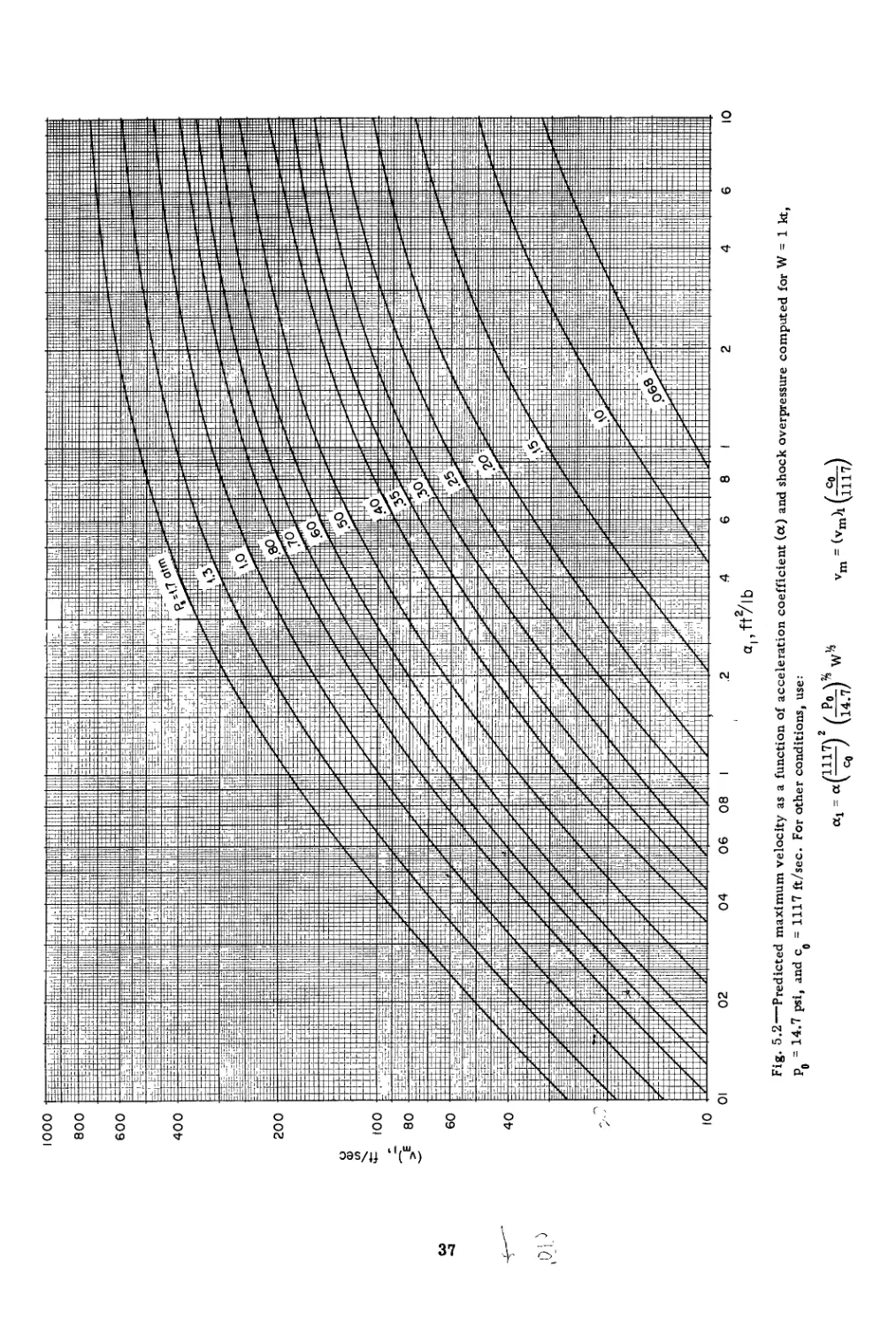
and Shock Overpressure (W = 1 kt) . . . . . . . . 37
5.3 Predicted Displacement at Maximum Velocity as a Function of
Acceleration Coefficient and Shock Overpressure (W = 1 kt) . . . . 38
5.4 Predicted Maximum Velocity as a Function of Acceleration Coefficient
and Shock Overpressure (W = 20 kt) . . . . . . . . . 39
5.5 Predicted Displacement at Maximum Velocity as a Function of
Acceleration Coefficient and Shock Overpressure (W = 20 kt) . . . . 40
5.6 Predicted Maximum Velocity as a Function of Acceleration Coefficient
and Shock Overpressure (W = 1000 kt) ........ 41
5.7 Predicted Displacement at Maximum Velocity as a Function of
Acceleration Coefficient and Shock Overpressure (W = 1000 kt) ... 42
5.8 Relation Between Velocity and Displacement as a Function of
Weapon Yield........................................44
5.9 Relation Between Shock Overpressure and Yield for Various Values
of Maximum Velocity and Displacement at Maximum Velocity . . . . 45
8
ILLUSTRATIONS (Continued)
APPENDIX A APPROXIMATION METHODS TO SUPPLEMENT THE
COMPUTED RESULTS
A.l Relation Between Velocity, Displacement, and Time After Arrival of
the Blast Wave ............. 51
A.2 Displacement at Maximum Velocity as a Function of Acceleration
Coefficient for Various Values of Shock Overpressure..................53
A.3 Normalized Velocity vs. Normalized Displacement for Various Values
of Acceleration Coefficient .......... 55
TABLES
CHAPTER 3 COMPUTATIONAL METHOD
3.1 Incremental Values of the Independent Variable and Parametric Values
for Which Computations Were Performed ........ 24
CHAPTER 4 RESULTS: COMPUTED MOTION PARAMETERS FOR OBJECTS
DISPLACED BY CLASSICAL BLAST WAVES
4.1 Computed Motion Parameters for Objects Displaced by Classical
Blast Waves ............. 27
CHAPTER 5 INTERPRETATION OF RESULTS
5.1 Typical Acceleration Coefficients ......... 34
9
Chapter 1
INTRODUCTION
1.1 OBJECTIVES
During the 1955 and 1957 Test Operations at the Nevada Test Site, the masses and veloci-
ties of over 20,000 objects (window-glass fragments, stones, spheres, sticks, etc.) which were
translated by nuclear-produced blast waves were experimentally determined,1-4 along with a
time-displacement history of an anthropometric dummy simulating man.5 The availability of
such a mass of data stimulated an analytical study calculated to arrive at a mathematical for-
mulation capable of predicting the translation of objects by blast, particularly since this data
offered an empirical fabric against which to test the success of the analytical effort.
The purpose of this report is to describe, step by step, the theoretical studies that have
resulted in a mathematical model capable of predicting the motion of objects utilizing selected
basic blast parameters. This model, however, is applicable only to those situations in which
♦classical wave forms exist.
1.2 SCOPE AND LIMITATIONS
The applicability of the model itself has no well-defined limits; however, the numerical
solutions that were obtained and are reported herein have been arbitrarily limited in scope. In
general, the aim was to compute velocity, displacement, and acceleration as a function of time
for objects ranging in size from a pea to man; these computations were to cover blast waves
with shock overpressures from 1 to 25 psi (14.7-psi ambient pressure) and weapon yields from
1 kt to 20 Mt.
Another class of limitations is invoked not by the scope of the computations, but by the
model itself. Formulation of a workable model was facilitated by the use of certain simplify-
ing assumptions. These assumptions, which are discussed below, have not, in general, caused
serious discrepancies between predicted velocities and those measured in the field operations,
particularly in those situations where the blast wave was classical.t
As a practical approach, it was assumed first that the effect of surface friction was neg-
ligible. It has been observed that fairly large objects tend to be lofted when subjected to blast
waves; the more intense the blast, the heavier the object that it is capable of lifting against
gravity. Nonspherical objects could develop either positive or negative lift depending on their
orientation to the wind. Thus, the validity of the no-friction assumption is dependent upon the
strength of the blast wave, the object under consideration, its random orientation, and the na-
ture of the surface over which translation occurs. It will be shown later that certain uses can
be made of the data even for situations in which surface friction is a significant factor.
♦The term “classical blast wave” is used in this report to mean the typical wave not ap-
preciably modified by terrain effects and possessing a well-defined shock front.
fA limited discussion of the agreement between predicted and measured velocities is.
made later in this report. A more complete treatment will be found in Ref. 3.
11
A second approximation made concerned the assumption that there was no gain or loss of
energy as a result of .the object’s moving with or against gravity. The kinetic energy that is
lost during lofting would be regained as the object fell to its original elevation, thus mitigating
somewhat the error in the predicted motion.
Third, only the propelling force of the wind was considered. Another force that might have
been included was that due to differences in overpressure between one side of the object and
the other during passage of the shock front (diffractive loading). Since the bodies being con-
sidered were relatively small (up to the size of man), the classical blast wave would engulf the
object very quickly and impart only a small momentum as a result of the overpressure itself.
Fourth, it was assumed that there was no change in the properties of an object which gov-
erned acceleration (area presented to the wind, drag coefficient, and mass) during the accel-
erative phase of displacement. For irregular, rigid objects that are nearly spherical, such as
stones, this is a reasonable assumption. For objects that are obviously nonspherical or de-
formable, prediction of a range of velocities taking into account both maximum and minimum
drag areas is often used. Another useful procedure is to employ the average drag area de-
rived from the concept of random orientation.6
Fifth, no allowance was made for the fact that a displaced object may be moved to a lower
overpressure region and thus be acted upon by correspondingly weaker blast winds. The re-
sults of the computations themselves seem to justify the neglection of this phenomenon. It
will be shown that displaced objects receive a large percentage of their velocities in a rela-
tively short distance over which the decay of the blast wave is small.
REFERENCES
1. I. Gerald Bowen, Allen F. Strehler, and Mead B. Wetherbe, Distribution and Density of Mis-
siles from Nuclear Explosions, Operation Teapot Report, WT-1168, March 1956.
2. I. Gerald Bowen, Donald R. Richmond, Mead B. Wetherbe, and Clayton S. White, Biological
Effects of Blast from Bombs. Glass Fragments as Penetrating Missiles and Some of the
Biological Implications of Glass Fragmented by Atomic Explosions, Report AECU-3350,
June 18, 1956.
3. I. Gerald Bowen et al., Secondary Missiles Generated by Nuclear-produced Blast Waves,
Operation Plumbbob Report, WT-1468 (in preparation).
4. V. C. Goldizen, D. R. Richmond, and T. L. Chiffelle, Missile Studies with a Biological Tar-
get, Operation Plumbbob Report, WT-1470, January 1961.
5. R. V. Taborelli, I. G. Bowen, and E. R. Fletcher, Tertiary Effects of Blast-Displacement,
Operation Plumbbob Report, WT-1469, May 22, 1959.
6. E. Royce Fletcher~et al., Determination of Aerodynamic Drag Parameters of Small Irregu-
lar Objects by Means of Drop Tests, Civil Effects Test Operations, Report CEX-59.14 (in
preparation).
12
Chapter 2
ANALYTICAL PROCEDURE
2.1 NOMENCLATURE
The terminology used in this study is defined in this section. A lower-case letter is used
to represent a quantity with dimensions. In general, the same letter is capitalized if the quan-
tity is made dimensionless by an appropriate factor or factors. Thus, the dimensionless term
is represented by its principle variable. The factors, or parameters, used to make quantities
dimensionless invariably are constants for any given blast situation.
a = acceleration coefficient = sC^/m
A = apotj/co
c0 = speed of sound in undisturbed air
Ca - drag coefficient of moving object
d = distance of travel of moving object
dm = distance of travel of moving object when maximum velocity is reached
D = d/(t+c0)
I = overpressure impulse = f p P dt
m = mass of moving object
p = overpressure or pressure in excess of p0
Po = pressure of undisturbed air
ps = maximum or shock overpressure
P = P/Po
Ps = ps/po, shock overpressure in atmospheres
q = dynamic pressure = (l/2)pu2
qs = dynamic pressure at the shock front
Q = q/Po
Qs = Vpo
p = air density
s = area presented to wind by moving object
t = time after arrival of blast wave
tp = duration of positive pressure phase of blast wave
tj = duration of winds in the direction of propagation of the blast wave
T = t/t+
u = velocity of the air
U = u/c0
v = velocity of the moving object
vm = maximum velocity of moving object
V = v/c0
v = acceleration of moving object
V = vt^/co
W = weapon yield in kilotons
x = velocity of propagation of the pressure disturbance
13
X = x/cq
Z = t/tj
NOTE: Any variable that is underlined indicates the average value taken over a particular
time interval.
2.2 EQUATIONS OF MOTION
2.2.1 Fundamental Concepts
Newton’s second law of motion can be stated as
_ dv
Force = m —
dt
and the drag force on a moving object is
Force =-^-p(u -v)2 sC(j
Ci
since the net wind moving past the object is (u — v). Combining the above equations and solving
for dv, we obtain
(2.1)
i m
It was convenient to isolate and label the physical parameters that involve the moving ob-
ject in Eq. 2.1.
^=a (2.2)
m
Now, a. can be called “acceleration coefficient” since it completely describes the object in so
far as the computation of velocity vs. time is concerned. Thus, two objects possessing the
same value of a, regardless of dissimilarity of shape, size, and mass, would experience the
same increase in velocity if exposed to the same or similar blast waves.
2.2.2 Time Correction
Since the moving object, or missile, travels along with the blast wave, the time during
which it is exposed to blast winds is longer the higher its velocity is in relation to the velocity
of propagation of the pressure disturbance and associated winds. Consider a small segment of
the blast wave of length dx where the air-particle density and velocity are approximately con-
stant. If this segment moves with a velocity x, then
dx = x dt
where dt is the time required for the segment dx to pass a fixed point. Similarly, the velocity
of propagation of a blast-wave segment past a missile that itself is moving at velocity v is
(x - v), and
dx = (x - v) dt'
where dt' is the time required for the blast segment to pass the missile. By eliminating dx
between the above equations, we obtain
dt'=dt-r-^~ (2.3)
X — V
14
Combining Eqs. 2.1 and 2.2 and substituting the corrected time dt' of Eq. 2.3 for dt, we obtain
dv = ypa(u - v)2
X
(x-v)
dt
(2.4)
It was more convenient to work with dynamic pressure, q = (1/2) pu2, than with air den-
sity. For this reason Eq. 2.4 was modified to
x dt
(x-v)
(2.5)
2.2.3 Dimensional Analysis
The blast-wave variables in Eq. 2.5 are determined as a function of time by four parame-
ters: (1) shock overpressure, ps; (2) ambient pressure, p0; (3) duration of the positive winds,
t+; and (4) speed of sound in the undisturbed air, c0. Computations were made for particular
values of shock overpressure in atmospheres, Ps = ps/po. The last three parameters, how-
ever, were used to make the variables in Eq. 2.5 dimensionless. The obvious advantage of this
procedure is that computed values of missile velocity, distance of travel, and acceleration can
be modified after the computations have been made to fit any blast situation defined by p0, tj,
and c0.
The variables of Eq. 2.5 were made dimensionless through the application of the following
algebratic operations: (1) both sides of the equation were divided by c0, (2) the numerators and
the denominators of the two fractions were divided by c0, (3) a was multiplied by p0 and q was
divided by p0, and (4) t was divided by tj and a was multiplied by tj.
After these operations have been performed, Eq. 2.5 becomes
= /A_\ /“PotuX [(u/cp) - (v/cp)'
\Co/ \Po} \ c0 /I u/c<>
x/Cp
(x/c0) - (v/c0)
(2.6)
and, after appropriate substitutions (see Sec. 2.1, Nomenclature)
dV = QA
ru-v\2
< и /
X
x-v
dZ
(2.7)
Two additional quantities are used in dimensionless form, distance of travel and accelera-
tion. Since both are functions of velocity and time, their dimensionless forms are determined
by dimensionless velocity and time. Thus
D = vZ = --^ = -^
Co tu cotu
(2.8'
and
V =
V
Z
Vtu
Co
(2.9)
2.2.4 Approximation Solution
The explicit expressions of Q, U, and X as a function of time for a particular blast wave
are very cumbersome. Added to this difficulty is the fact that the variable V cannot be sepa-
rated from the time-dependent variables (see Eq. 2.7). Hope for a complete mathematical so-
lution was soon abandoned.
A stepwise solution was then attempted which would permit the blast parameters to be
held constant for small increments of time but would allow the missile velocity to vary as a
nonlinear function of time. So that a simple mathematical integration can be accomplished, the
15
time-correction term, X/(X - V), was not included. Thus
«Vo+AV pZo+AZ'
J
V. ~ z,
(2.Ю)
where Vo and Zo are the velocity and time, respectively, at the beginning of the time period
and AV is the change in velocity in time AZ'. Underlined U and Q indicate average values over
the time AZ'.
Integration of Eq. 2.10 and substitution of limits yields
U-Vo —AV U - Vo -A AZZ
(2.11)
The average missile velocity during the time period AZ' is [Vo + (1/2)AV]. Thus the time-
correction term (see Eq. 2.3) expressed in dimensionless incremental form is
X
AZ' = AZ X-VO-(1/2)AV
(2.12)
Eliminating AZ' between Eqs. 2.11 and 2.12 and solving for AV, the following is obtained
A V — e + f — Ve2 + 2fg + f2
(2.13)
where e = X - Vo
f = AQ (U - V0)X (AZ/U2)
g = X-U
The velocity at the end of any step is the summation of the AV’s computed from the be-
ginning of the integration.
Incremental distance, AD, was computed by the following:
AD = [Vo + (1/2)AV] AZ' (2.14)
where Vo refers to the velocity at the beginning of the step. AZ' is defined in Eq. 2.12.
Evaluation of acceleration (V = dV/dZ) presented little difficulty since integration was not
involved. Furthermore, the time-correction term was not necessary because, by definition,
V is the instantaneous time rate of change in velocity. Thus, the following equation was formed
from Eq. 2.7:
2.3 EVALUATION OF BLAST-WAVE VARIABLES
2.3.1 General Remarks
A particular classical blast wave can be completely defined mathematically by the pa-
rameters of shock strength (ps/po), duration, and either the velocity of sound or the tempera-
ture for ambient conditions. Secondary-missile computations were made for selected values
of shock strength, each of which is applicable to any value of duration (and thus bomb yield) or
ambient sound velocity between wide limits.
2.3.2 Dynamic Pressure and Wind Velocity
Although dynamic pressure (from which wind may be computed) has been measured in ac-
16
tual blast situations, values computed from theoretical considerations were used in this study.
The reason for this was both the higher reliability and the greater facility for numerical treat-
ment of the computed parameters over the measured ones. Of the several studies made of the
blast wave, those made by Harold L. Brode of Rand Corporation1’2 were found to be most use-
ful for the present study. The equations3 listed below are empirical relations determined by
fitting curves to computed blast data. In terminology consistent with the present study, dy-
namic pressure as a function at shock overpressure and time is given by
Q = Qs (1 - Z) [Je-rz + Ke-6Z]
(2.16)
/2.5 P|\ /1 + 2 x 10⁻⁸ P4S\
where Qs (7 + pJ 1 + Ю-8 P4 )
J = 1.186 P^3 for Ps < 0.6
J = 1 for 0.6 Pss 1.0
J = (104 P^)/(104 + P2s) for Ps > 1
К = 1 - J
Y = (1/4) +3.6 Р‘/з
6 =(7 + 8 P^!) + 2 P|/(240 + Ps)
The relation for wind, or particle, velocity is
U = Us (1 - Z) e~ vZ
where Us = (Ps)/(1 + P^2)
v = P$ + 0.0032 P^2
(2.17)
2.3.3 Overpressure vs. Time and Overpressure Impulse
Overpressure as a function of time does not enter directly into the computation of
secondary-missile behavior; nevertheless, it seems appropriate to consider this relation since
it is the most commonly measured parameter of the real blast wave. Thus, overpressure-
time can be considered to be the bridge between secondary-missile field data and the com-
puted data resulting from the present study.
The following overpressure-time relation was obtained from Brode:1-3
P = Ps (1 - T) (ae-iT + be-jT)
(2-18)
2.282 (8 + Ps)
where a =----------------------------- + q 23
27.658 + Ps + 1.2 Pl + 0.007 Pl
b = 1 - a
i= ( ps , E5Pi
Vl + 0.1Ps 1500 + p3/i
j = 9 + 1.4 Ps
Pressure instrumentation used in field work often produces a more accurate measure-
ment of overpressure impulse than of shock overpressure. Indeed, an improved estimate of
shock overpressure can be made by making use of the impulse relation described below.
Overpressure impulse is defined as
I = fP dt
Jo
(2.19)
However, to facilitate integration of Eq. 2.18 in terms of normalized time, the following rela-
tion was used:
T = t/tj
(2.20)
17
thus,
dt = t£ dT
A combination of Eqs. 2.19 and 2.21 gives
I = tp/olpdT
(2.21)
(2.22)
Integration of Eq. 2.18 in the manner indicated by Eq. 2.22 yields the following:
I ~ Pstp
^(e'i + i-l) +^(e~i + j -1)
< $
Figure 2.1, a plot of Ps in atmospheres as a function of l/tp also in atmospheres, illus-
trates this relation graphically. This plot can be thought of as defining the “shape factor” of
(2.23)
the overpressure-time curve as a function of maximum overpressure. If impulse, I, and dura-
tion, tp, are measured by suitable instrumentation, then a value of shock overpressure can be
determined from the curve shown in this figure.
2.3.4 Duration Concepts
(a) Positive-overpressure Duration. To evaluate the computed motion parameters for a
particular yield, it is obviously necessary to know the duration of the blast wave (identified by
peak or shock overpressure) of interest. For this purpose the durations computed from theo-
retical considerations for free-air conditions, such as those by Brode, are of little value since
the complex effects of surface reflections are not considered. Thus, the semiempirical rela-
tions presented in Chap. 3 of The Effects of Nuclear Weapons1 were used to define overpres-
sure duration as a function of yield, overpressure, ambient pressure, and the speed of sound.
Using data for both the surface burst and the “typical air burst,” the following mathematical
expression was derived
log tp = 5.7995 + (1/3) log W - 0.2957 log ps - 0.0376 log p0 - log c0 (2.24)
where tp = duration of positive overpressure in milliseconds
W = yield in kilotons
ps = shock overpressure in pounds per square inch
Po = ambient pressure in pounds per square inch
Co = velocity of sound in the undisturbed air in feet per second
The above equation reflects data for the surface burst for shock overpressure (sea-level
conditions) from 1.68 to 36.7 psi and for the “typical air burst” from 1.86 to 19.7 psi.
(b) Overpressure vs. Wind Duration. Instrumentation used in past weapons tests was not
refined enough to establish a relation between overpressure and wind duration. However, the
theoretical work quoted above has established such a relation. Figure 2.2, derived from
Brode’s work,1,3 presents the ratio of the wind duration to the pressure duration for overpres-
pures up to 3 atm (44.1 psi at sea level). It is apparent from this chart that for the higher
overpressures air-particle inertia has the effect of sustaining positive winds for an appreci-
able time after the overpressure has become negative.
2.3.5 Velocity of Propagation of the Pressure Disturbance
It has been shown that it is necessary to know the velocity of propagation of the pressure
disturbance in order to compute the motion of objects displaced by blast waves. An easily
evaluated relation5 that was used for this purpose is:
(2.25)
18
C0
, atm
Fig. 2.1—Shock overpressure as a function of the ratio of overpressure impulse to overpressure duration.
М
о
1.0
18
17
16
15
14
13
12
II
2 4
10 12 14
22 24
26 28
Ps, atm
0
30
Fig- 2.2—Ratio of duration of wind to that of overpressure as a function of shock overpressure.
Two objections might be raised to the use of the above equation for the purposes of this
study. First, it applies strictly to the speed of propagation of the shock front, not to pressure
regions behind the front. Second, it was derived for nondivergent flow; whereas the present
study applies to divergent flow. In spite of these limitations, the relation was found to be in
reasonable agreement with work done by Brode1’2 as quoted in Sec. 2.3.2.
This, added to the fact that X appears only in the time-correction term (see Eq. 2.7),
whose effect on the computed value of dV is second order, probably justifies its use in the
present context.
REFERENCES
1. Harold L. Brode, Numerical Solutions of Spherical Blast Waves, J. Appl. Phys., 26: 766-775
(June 1955).
2. Harold L. Brode, Point Source Explosion in Air, Report AECU-3517, The Rand Corporation,
Dec. 3, 1956.
3. Harold L. Brode, personal communication.
4. Samuel Glasstone (Ed.), The Effects of Nuclear Weapons, Superintendent of Documents,
U. S. Government Printing Office, Washington, D. C., June 1957.
5. Ascher H. Shapiro, The Dynamics and Thermodynamics of Compressible Fluid Flow,
Vol. 2, p. 1001, Ronald Press Company, New York, 1954.
21
Chapter 3
COMPUTATIONAL METHOD
3.1 SCOPE OF COMPUTATIONAL EFFORT
Because computations were made in terms of dimensionless quantities, it was necessary
to use only two independent variables: (1) the acceleration-coefficient numeric* (A = apotj/co)
containing acceleration coefficient, ambient pressure, speed of sound, and duration of positive
winds (yield dependent) and (2) the shock-overpressure numeric (Ps = ps/po), which also in-
volves the ambient pressure. Thus, five independent variables, one describing the object dis-
placed and four describing the blast wave, were effectively reduced to two. It should be pointed
out thht the shock-overpressure numeric (along with the duration variable) represents or de-
fines three other blast variables that are actually used in the computations; namely, dynamic-
pressure numeric (Q), wind numeric (U), and propagation-velocity numeric (X), all of which
are functions of the time numeric (Z = t/tj).
Thus, for computational purposes, it was necessary to set limits only on A and Ps. Con-
sistent with the scope of the problem stated in Sec. 1.2, the limits arbitrarily set for A were
0.1 to 9000 and for Ps from 0.068 to 1.7 (1 psi to 25 psi for sea-level ambient pressure). Com-
putations were made for 15 values of Ps within the stated range, and associated with each of
these were 11 values of A (see Table 3.1, columns I and II), making a total of 165 complete
numerical integrations.
3.2 GENERAL PLANNING
Figure 3.1 illustrates some of the considerations in planning for numerical solutions of
the mathematical model. This plot shows the pertinent blast variables in dimensionless form
as functions of the time numeric (T = t/tp) for a 0.5-atm blast wave. Also shown on this plot
are velocity (V = v/c0) and displacement (D = d/tjcg) computed for an object with an accelera-
tion coefficient (A = «pot*/co) of 30. It should be noted that all plotted quantities change most
rapidly at early times. This means that a stepwise solution should be started using small time
increments, these to be lengthened as the solution progresses. Also of interest on this chart is
the U' curve, which represents the wind numeric at the position of the moving object rather
than at a fixed position. At T = 0.5, missile velocity was equal to that of the wind, and so the
integration was stopped. Sixty-two steps were taken to arrive at the solution shown here.
3.3 STEP SIZE
As shock overpressures increase, the rate of decay of the blast variables from shock
values also increases. For mean-v^lue assumptions (i.e., the assumption that the variable is
constant with a value equal to the mean over a specified time increment) to be equally valid for
♦Numeric is used here to designate a dimensionless quantity.
22
w
I, 10D, U,Q
0.50
1.5
dimensionless). Q, U, and X curves represent blast parameters as they would be measured at the point of origin of the missile. The U'
curve represents the wind isting at the location of the moving missile indicated by the displacement (D) curve.
TABLE 3.1—INCREMENTAL VALUES OF THE INDEPENDENT
VARIABLE AND PARAMETRIC VALUES FOR WHICH COMPUTATIONS WERE PERFORMED
I П III TV
Ps t+/t+ A AT* Tjt
0.068 0.900 0.1 0.0001 0.002
0.10 0.885 0.3 0.0002 0.004
0.15 0.875 1 0.0003 0.008
0.20 0.855 3 0.0004 0.015
0.25 0.840 10 0.001 0.030
0.30 0.835 30 0.002 0.060
0.35 0.805 100 0.003 0.120
0.40 0.793 300 0.005 0.250
0.50 0.760 1000 0.007 0.500
0.60 0.740 3000 0.010 0.750
0.70 0.720 9000 0.025 1.000
0.80 0.710 0.050 Final
1.00 0.675 0.100
1.30 0.635
1.70 0.585
♦Ten steps of each AT were used starting with AT = 0.001. See Sec. 3.3 for an explana-
tion of first four values of AT.
|Tj = times for which computed results were printed out.
high overpressures, the time increments should be correspondingly decreased. Noting that the
ratio of overpressure duration to wind duration decreases for increasing overpressures (see
Table 3.1, column I) suggested the use of a set of time increments in T constant for all solu-
tions. The AZ values computed for each overpressure (using AZ = tp/ty AT) then decrease as
desired for the higher overpressure blast waves.
The first computation in each integration series was made for a time increment, AT(
equal to 0.001. If the velocity V so computed was greater than 0.1, the solution was discarded;
then AT values of 0.0001, 0.0002, 0.0003, and 0.0004 were used, in turn, and T = 0.001 was
arrived at in four steps. Succeeding steps, gradually increasing in size, were then taken until
the end of the integration (see Table 3.1). If the initial step, AT = 0.001, yielded a velocity less
than 0.1, the integration proceeded from there without the use of the shorter steps.
The shortest integration, using the system described above, required 14 steps; this was
for Ps = 1.7, A = 9000. In general, the number of steps required increased as A decreased;
e.g., 75 steps were required for A = 3.0 and Ps = 0.068 and 81 steps were required for A = 0.1
and Ps = 1.7.
3.4 MACHINE OUTPUT* •
Since printing out results at the end of each step would have slowed the computation con-
siderably and also would have produced much more information than could have been utilized,
it was decided to limit the output of intermediate results to those necessary for the prepara-
tion of accurate plots. Because of the time-correction term (see Sec. 2.2.2), time at the end
of any particular step was different for each set of conditions. For simplicity in monitoring
results and ease of plotting time histories, it was convenient to program output at a set of
preselected time (see Table 3.1, column IV). Thus, it was necessary to program the com-
puter to interpolate (linearly) the computed results between time steps to the times selected
for print-out.
Special problems arose in the determination of the final values of the computed results;
i.e., the values occurring at the time when missile velocity and wind velocity were identical.
*The computer, a CRC-102A, was generously made available by Sandia Corporation.
24
Since missile velocity changes very slowly near the end of the accelerative phase, it was suf-
ficiently accurate to take final or maximum missile velocity to be that computed for the first
step where it equaled or exceeded the wind velocity. However, it was necessary to obtain the
time at which this occurred by interpolating the wind values to a time when they equaled maxi-
mum missile velocity. Making use of this time, displacement at maximum velocity could then
be computed. Final acceleration was always, of course, zero.
3.5 DISCUSSION OF ERROR
The usable word length of the computer was 36 binary digits or the equivalent of 9 decimal
digits of input or output. The fixed-point fractional mode of operation required careful scaling
of all magnitudes (primarily because of the large range of the parameter A) so that sufficient
significance be retained without the need for rescaling. Binary scaling proved adequately con-
servative in the attainment of this objective.
Approximations for square roots and cube roots were obtained with accuracy greater than
eight decimal places, and the exponential approximation is reported to be accurate to ±2 in the
seventh decimal place. (Cube roots were obtained by the Newton-Raphson method,1 and the ex-
ponential, by the rational polynomial approximation.2)
Blast-wave parameters were evaluated from empirical equations that were derived by
fitting curves to computed data obtained from a blast-wave model.3'4 Although Brode did not
make a definite statement regarding the over-all accuracy of the blast model, he did indicate
some deviation of the empirical equations from the computed data. From this it can be sur-
mised that computations involved in the present problem were carried out as accurately as
was warranted by the accuracy of the input blast data as well as by the probity of the missile
model itself (see Sec. 1.2).
It is noteworthy that computed missile velocity becomes stable by virtue of the number of
steps involved in each integration; i.e., if for some reason computed missile velocity at the end
of a particular step is too low, the net wind velocity (U - V) used in the next step will be cor-
respondingly high, thereby tending to compensate for the original error. As a consequence the
final solution is not extremely sensitive to the magnitude of the time increments so long as,
within any particular solution, the steps are sufficiently numerous for the compensatory ef-
fect to be realized before the computation ends.
REFERENCES
1. J. B. Scarborough, Numerical Mathematical Analysis, pp. 192-194, Johns Hopkins Press,
Baltimore, Md., 1955.
2. C. Hastings, Jr., Approximations for Digital Computers, Princeton University Press,
Princeton, N. J., 1955.
3. Harold L. Brode, Numerical Solutions of Spherical Blast Waves, J. Appl. Phys., 26: 766-775
(June 1955).
4. Harold L. Brode, Point-source Explosion in Air, Report AECU-3517, The Rand Corpora-
tion, Dec. 3, 1956.
25
Chapter 4
RESULTS: COMPUTED MOTION PARAMETERS FOR
OBJECTS DISPLACED BY CLASSICAL BLAST WAVES
The results of the 153 numerical integrations are presented in Table 4.1 in terms of the
dimensionless parameters. Each integration was made for a specific combination of over-
pressure (P) and acceleration coefficient (A). Values of missile velocity (V), distance of travel
(D), and missile acceleration (V) are given for 13 times during the accelerative phase of mis-
sile displacement. Numbers appearing in parenthesis after V, D, and V are scaling factors
indicating the number of places the decimal point has been moved to the right. Consider, for
example, the data tabulated for P = 0.10 and A = 1000 at T = 0.120. In this instance V(6) is read
as 55677, and thus V = 0.055677.
At T = 0, the time of arrival of the blast wave, velocity and displacement are zero, but
acceleration is maximum. “T = Final” is defined as the time after arrival of the blast wave
when missile velocity is maximum and acceleration is zero. The displacement (D) tabulated
under “Final” is defined as the total displacement of the object at the instant when the velocity
is maximum. The actual time when maximum velocity is attained appears in the last column
under “Tfinal.”
It should be noted that the time measurements used in this table are normalized with re-
spect to the duration of the positive pressure phase. Since the duration of positive winds is
longer than that of the positive pressure, T final values are sometimes greater than unity. The
exact value of Tfinal is, of course, the time when the missile velocity equals the wind velocity.
Examples of uses of the tabulated data along with various plots are given in Chap. 5.
26
TABLE 4 1—COMPUTED MOTION PARAMETERS FOR OBJECTS DISPLACED BY CLASSICAL BLAST WAVES
Nomenclature (Parameters can be evaluated in any consistent system of units);
a = sCD / m m = mass of moving object u ~ posi tiv e wind duration
A = «P„ u /c maximum ov erpressure T = 7lp+
Cq = velocity of sound in undisturbed an ₽o = pressure of undisturbed air v = velocity of moving object
CD = drag coefficient of moving object p = Pm / ₽o v (П) = V/Co x 10“
d = displacement of object s = area presented to wind by object V = accele ration of moving object
D (n) = d/ ( + c u о ) X 10n t+ = p positive overpressure duration V (n) = :tu / C X 0 10“
p A T: 0 . 002 . 004 . 008 . 015 . 030 . 060 . 120 .250 . 500 . 750 1. 000 Final T final
V (7) 0 88 175 345 635 12 18 2253 3912 6333 8820 9941 10296 10312
. 068 3 D (8) 0 1 3 12 44 169 641 2327 8439 25850 47142 70020 78517 1. 092
v (7) 49066 48500 47950 46860 45040 41460 35410 26640 16090 7350 2990 450 0
v (7) 0 293 582 1149 2109 4038 7433 12801 20435 27852 30821 31449
10 D (7) 0 1 4 14 56 212 766 2750 8303 14963 22561 1. 020
V (6) 16355 16155 15958 15573 14930 13670 11560 8541 4970 2080 693 0
v (7) 0 877 1741 3433 6278 11930 21674 36500 56161 72687 77374 77687
30 D (7) 0 1 3 12 43 167 625 2219 7761 22595 39619 49734 0. 895
V (6) 49066 48359 47666 46319 44085 39766 32709 22998 12132 3979 645 0
v (6) 0 291 576 1127 2037 3777 6578 10369 14477 16736 16896
100 D (7) 0 3 10 41 141 537 1952 6613 21514 57390 84057 0. 676
V (5) 16355 15998 15651 14987 13915 11942 8989 5442 2159 293 0
v (6) 0 864 1692 3245 5674 9907 15714 21879 26410 27340
300 D (7) 0 8 31 120 403 1468 4990 15361 442 52 94925 0. 458
v (5) 49066 46971 45000 41392 35994 27296 16832 7547 1650 0
V (6) 0 2776 5253 9478 15143 22942 30579 35809 37497 37500
1000 D (7) 0 25 98 366 1151 3772 11148 29385 72750 79332 0. 270
v (4) 16355 14546 13015 10583 7675 4336 1807 466 5 0
V (6) 0 7549 13179 20999 28954 36776 41926 43909 43993
3000 D (7) 0 71 259 884 2484 7005 17782 41155 56458 0. 159
V (4) 49066 35858 27310 17282 9279 3569 948 75 0
v (6) 0 17670 26508 35305 41625 46042 47903 48084
9000 D (7) 0 175 579 1712 4167 10150 22914 36728 0. 092
V (3) 14720 6565 3687 1618 62 1 164 20 0
v (7) 0 186 370 732 1346 2586 4797 8373 13662 19090 21447 22143 22172
. 10 3 D (7) 0 1 3 9 35 134 488 1780 5484 10009 14854 16451 1. 081
1/ v (6) 10563 10446 10331 10105 9727 8981 7720 5874 3592 1607 617 79 0
v (7) 0 619 1231 2433 4466 8550 15748 27142 43334 58605 64117 65030
10 D (7) 0 1 2 9 30 117 442 1596 5735 17274 30974 44789 0. 991
V (6) 352 1 1 34780 34357 33530 32151 29451 24934 18455 10662 4157 1159 0
v (6) 0 186 368 725 1324 2507 4527 7550 11421 14366 14980 14990
30 D (7) 0 2 7 26 90 345 1288 4545 15714 44931 77637 87959 0. 828
V (5) 10563 10400 10240 9930 9418 8437 6853 4713 2352 630 40 0
v (6) 0 615 1214 2364 4238 7745 13170 20056 26737 29507 29549
100 D (6) 0 1 2 9 29 109 391 1291 4051 10392 12684 0. 588
V (5) 3521 1 34274 33371 31661 28948 24111 17254 9631 3229 166 0
v (6) 0 1815 3527 6674 11421 19217 28969 38092 43502 44039
300 D (6) 0 2 6 25 81 287 940 2759 7546 12672 0. 382
V (4) 10563 9957 9398 8408 7002 4921 2717 1042 148 0
v (6) 0 5730 10604 18439 28080 39911 49951 55677 56779
1000 D (7) 0 52 197 717 2179 6786 18945 47387 97492 0. 220
v (4) 35211 29769 25479 19234 12654 6243 2219 430 0
v (6) 0 14926 24836 37145 48177 57 67 3 63035 64483 64485
3000 D (7) 0 140 496 1613 4298 11440 27641 61685 66790 0. 129
V (3) 10563 6740 4663 2596 1225 408 88 1 0
v (6) 0 32061 44935 56140 63298 67740 69201 69239
9000 D (7) 0 323 1015 2836 6574 15342 33599 42608 0. 075
V (3) 31690 10438 5105 1957 672 153 9 0
v (7) 0 137 273 540 994 19 16 3574 6298 10428 14752 16649 17259 17290
. 15 1 D (7) 0 2 7 26 98 360 1330 4146 7613 11338 13067 1. 114
V (7) 78671 77860 77070 75510 72890 67720 58890 45730 28730 13000 5130 970 0
v (7) 0 411 817 1617 2976 5727 10648 18654 30564 42539 47360 48571 48610
3 D (7) 0 1 6 ‘ 20 77 294 1072 3927 12 109 22033 32571 35280 1. 064
V (6) 23601 23347 23097 22607 21787 20168 17418 13352 8165 3461 1188 93 0
v (6) 0 137 272 537 985 1885 3466 5954 9430 12492 13406 13491
10 D (7) 0 1 5 19. 66 255 963 3469 12410 36978 65553 87180 0. 934
V (6) 78671 77685 76716 74829 71681 65535 55283 40583 22700 7722 1498 0
v (6) 0 409 812 1595 2903 5459 9741 15930 23339 28069 28614
30 D (6) 0 1 6 19 75 276 962 3251 9009 14907 0. 737
V (5) 23601 23188 22784 22005 20728 18311 14505 9531 4283 787 0
V (6) 0 1353 2659 5140 9097 16235 26597 38527 48331 50886
100 D (6) 0 1 5 18 62 230 802 2548 7610 18291 0.493
V (5) 78671 75942 73342 68503 61051 48440 32 022 15799 4053 0
V (6) 0 3959 7601 14071 23308 37233 52609 64838 70129 70248
300 D (6) 0 4 14 52 167 572 1776 4920 12715 16408 0. 310
V (4) 23601 21681 19979 17107 13344 8421 4021 1251 71 0
v (6) 0 12152 21747 35909 51461 68068 80049 85424 85866
1000 D (6) n 11 41 143 415 1215 3191 7580 11803 0. 176
V (4) 78671 61322 49088 33388 19384 8167 2417 287 0
27
TABLE 4. 1—COMPUTED MOTION PARAMETERS FOR OBJECTS DISPLACED BY CLASSICAL BLAST WAVES (Continued)
A T: 0 . 002 . 004 . 008 . 015 . 030 . 060 . 120 .250 . 500 .750 1. 000 Final T 1 final
v (6): 0 29712 46419 64522 78639 89205 94174 94913
3000 D (7): 0 281 957 2937 7384 18539 42794 78423 0. 103
V (3): 23601 12265 7478 3581 1471 422 67 0
V (5): 0 5724 7468 8791 9543 9952 10040
9000 D (7): 0 594 1768 4656 10315 23180 49210 0. 060
V (3): 70804 15437 6494 2178 671 124 0
V (8); 0 709 1412 2797 5159 9972 18694 33219 55666 79530 90144 93841 94326
. 3 D (8): 0 1 2 10 34 131 501 1847 6879 21660 39963 59715 75430 1. 195
V (7): 41667 41270 40880 40120 38830 36280 31870 25160 16130 7380 3000 750 0
V (7): 0 236 470 932 1718 3318 6211 11005 18345 25994 29258 30281 30336
1 D (7): 0 1 3 II 44 167 613 2275 7125 13085 19477 22777 1. 127
V (6): 13889 13754 13620 13360 12921 12050 10551 8277 5237 2321 886 169 0
V (7): 0 709 1410 2791 5140 9905 18458 32445 53308 73877 81694 83460 83509
3 D (7): 0 1 2 10 33 130 497 1818 6679 20600 37382 55103 59218 1. 058
V (6): 41667 41233 40806 39970 38568 35793 31048 23932 14589 5913 1872 108 0
V (6): 0 236 469 926 1699 3246 5958 10200 16013 20819 22032 22099
10 D (6): 0 1 3 11 43 162 582 2072 6108 10725 13452 0. 894
V (5): 13889 13711 13537 13198 12632 11527 9687 7043 3807 1145 156 0
V (6): 0 706 1397 2741 4971 9290 16389 26321 37483 43582 43974
30 D (6): 0 1 2 9 33 125 458 1573 5210 14074 20710 0. 677
V (5): 41667 40854 40063 38542 36066 31440 24313 15301 6234 784 0
V (6); 0 2324 4550 8730 15269 26672 4232 5 58939 70827 72901
100 D (6): 0 2 8 31 103 375 1277 3931 11310 22876 0. 437
V (4): 13889 13299 12743 11726 10203 7746 4781 2129 430 0
V (6): 0 6744 12803 23233 37417 57327 77289 91341 95988 95997
300 D (6): 0 6 23 85 268 888 2651 7054 17590 19256 0. 270
V (4): 41667 37336 33631 27665 20384 11787 5046 1336 14 0
V (5): 0 2017 3504 5549 7607 9598 10884 11356 11371
1000 D (6): 0 18 66 223 623 1747 4410 10160 13346 0. 153
V (3): 13889 10028 7569 4729 2501 946 245 16 0
V (5): 0 4669 6954 9200 10795 11887 12336 12373
3000 D (7): 0 441 1452 4268 10327 25025 56278 87144 0. 089
V (3): 41667 18053 9993 4311 1624 42 3 49 0
V (5): 0 8302 10362 11795 12545 12921 12976
9000 D (7); 0 867 2491 6329 13659 30061 54150 0. 052
V (2); 12500 1959 745 230 67 10 0
V (7): 0 108 215 427 788 1526 2869 5122 8633 12351 13974 14533 14611
. 3 D (7); 0 1 5 20 75 279 1044 3299 6089 9095 11534 1. 199
V (7): 64655 64070 63500 62370 60480 56690 50100 39890 25720 11590 4620 1170 0
V (7): 0 360 717 1422 2623 5074 9522 16940 28356 40143 45027 46504 46632
1 D (7): 0 1 5 17 65 250 925 3445 10810 19837 29489 34777 1. 135
V (6): 21552 21351 21154 20767 20114 18813 16556 13078 8287 3585 1321 244 0
V (6): 0 108 215 426 784 1513 2823 4971 8168 11245 12346 12566 12571
3 D (7): 0 1 4 14 50 195 745 2733 10052 30943 55942 82193 86992 1. 045
V (8): 64655 63999 63352 62086 59957 55734 48467 37432 22617 8734 2533 91 0
V (6): 0 360 715 1411 2586 4935 9034 15389 23897 30479 31872 31910
10 D (6): 0 1 5 17 64 242 866 3 061 8918 15513 18373 0. 857
V (5): 21552 21268 20990 20448 19546 17787 14861 10662 5542 1469 126 0
V (6): 0 1074 2126 4161 7520 13956 24332 38369 53178 60127 60345
30 D (6): 0 1 4 14 49 185 674 2284 7414 19566 26056 0. 628
V (5): 64655 63256 61899 59300 55100 47358 35710 21496 7949 638 0
V (6): 0 3528 6880 13102 22646 38751 59733 80440 93498 95022
100 D (6): 0 3 12 45 151 544 1809 5419 15118 26728 0. 396
V (4): 21552 20464 19452 17631 14981 10901 6316 2564 406 0
V (5): 0 1015 1906 3393 5326 7874 10230 11727 12110
300 D (6): 0 9 33 123 383 1231 3559 9182 21572 0. 243
V (4): 64655 56495 49759 39389 27546 14769 5777 1323 0
V (5): 0 2959 5005 7645 10121 12330 13642 14043 14045
1000 D (6): 0 26 94 310 841 2279 5591 12612 14590 0. 137
V (3): 21552 14433 10322 5995 2938 1026 238 6 0
V (5): 0 6521 9346 11921 13615 14711 15106 15123
3000 D (7): 0 617 1974 5614 132 07 31215 68967 94176 0. 080
V (3): 64655 23671 12102 4817 1713 409 32 0
V (5): 0 10886 13173 14661 15394 15735 15768
9000 D (7): 0 1144 3200 7928 16810 36491 58110 0. 046
V (2): 19397 2292 807 234 65 8 0
V (7): 0 152 302 600 1108 2150 4054 7268 12307 17623 19908 20690 208 04
. 3 D (7): 0 2 7 27 104 388 1457 4617 8524 12729 16174 1. 201
V (6): 9247 9168 9090 8937 8678 8160 7249 5814 3762 1673 657 170 0
V (7): 0 506 1008 1998 3690 7146 13443 23996 40294 56964 63694 65668 65841
1 D (7): 0 2 7 23 90 347 1283 4797 15073 27633 41028 48756 1. 142
V (6): 30822 30548 30277 29746 28849 27054 23912 18990 12031 5091 1819 328 0
V (6): 0 152 302 598 1103 2128 3975 7008 11505 15732 17162 17414
3 D (6): 0 2 7 27 103 378 1391 4272 7695 11771 1. 035
V (6): 92446 91547 90641 88868 85880 79935 69639 53809 32177 11873 3175 0
V (6): 0 505 1003 1980 3627 6911 12616 21374 32820 41136 42616 42633
10 D (6); 0 2 7 23 88 332 1186 4162 21986 20680 23309 0. 82 5
V (5): 30822 30404 29994 29196 27868 25283 20989 14847 7420 1741 84 0
28
TABLE 4. 1____COMPUTED MOTION PARAMETERS FOR OBJECTS DISPLACED BY CLASSICAL BLAST WAVES (Continued)
p A T: 0 . 002 . 004 . 008 . 015 . 030 . 060 . 120 .250 . 500 . 750 1. 000 Final T final
V (6) 0 1507 2979 5820 10481 19319 33295 51603 69808 772 10 77317
. 30 30 D (6) 0 1 5 20 67 253 913 3055 9739 25202 30955 0. 590
V (5) 92466 90267 88139 84084 77580 65751 48368 27908 9431 450 0
v (5) 0 493 959 1812 3097 5199 7811 10227 11592 11700
100 D (6) 0 4 16 62 205 726 2369 6931 18862 30043 0. 366
V (4) 30822 29024 27372 24446 20304 14203 7778 2916 362 0
V (5) 0 1408 2615 4574 7018 10069 12707 14243 14554
300 D (6) 0 12 45 165 505 1584 4456 11223 23530 0. 223
V (4) 92466 78821 67944 51892 34628 17406 6319 1269 0
V (5) 0 4007 6614 9801 12613 14977 16288 16622 16623
1000 D (6) 0 35 124 400 1057 2791 6701 14888 15638 0. 125
V (3) 30822 192 10 13089 7141 3298 1080 227 1 0
V (5) 0 8452 11745 14572 16324 17411 17755 17762
3000 D (6) 0 80 250 692 1593 3697 8066 10009 0. 073
V (3) 92466 29055 13911 5196 1770 393 19 0
V (5) 0 13411 15882 17400 18113 18421 18440
9000 D (7) 0 1523 3982 9527 19826 42498 61565 0. 043
V (2) 27740 2584 852 236 63 6 0
V (7) 0 200 399 79г 1465 2845 5380 9689 16489 23665 26730 27787 27954
. 35 . 3 D (7) 0 1 3 9 35 135 503 1898 6037 11155 16664 21476 1. 214
V (6) 12500 12399 12300 12104 11773 11105 9919 8014 5213 2304 9 02 244 0
v (7) 0 668 1330 2638 4874 9455 17828 31936 53819 76087 84941 87520 87766
1 D (7) 0 1 2 9 30 117 448 1662 6236 19633 35989 53412 64400 1. 156
V (6) 41667 41314 40965 40280 39119 36786 32661 26086 16555 6909 2433 451 0
v (6) 0 200 399 790 1456 2812 5259 9284 15239 20735 22522 22817
3 D (6) 0 1 3 9 35 133 488 1798 5512 9904 15059 1. 032
V (5) 12500 12379 12260 12026 11631 10842 9465 7321 4343 1549 392 0
V (6) 0 666 1323 2610 4778 9094 16560 27922 42468 52503 54045 54051
10 D (6) 0 1 2 8 29 114 426 1517 5291 15092 25877 28159 0. 802
V (5) 41667 41088 40520 39416 37577 34002 28070 19607 9475 2010 54 0
V (6) 0 1986 3922 7647 13727 25146 42895 65500 86877 94593 94626
30 D (6) 0 2 6 25 86 322 1156 3827 12011 30607 35439 0. 563
V (4) 12500 12178 11867 11278 10338 8651 6225 3462 1084 29 0
V (5) 0 648 1255 2356 3986 6582 9678 12393 13795 13873
100 D (6) 0 5 21 79 259 908 2912 8356 22309 32959 0. 345
V (4) 41667 38931 36446 32114 26131 17658 9221 3240 321 0
V (5) 0 1836 3376 5812 8748 12247 15113 16674 16934
300 D (6) 0 15 57 207 623 1917 5281 13059 25233 0.210
v (3) 12500 10412 8801 6512 4174 1991 683 123 0
v (5) 0 5110 8261 11945 15031 17522 18828 19114
1000 D (6) 0 44 153 485 1257 3251 7681 16550 0. 118
V (3) 41667 24324 15896 8237 3639 1133 220 0
V (5) 0 10385 14091 17125 18918 19993 20302 20305
3000 D (6) 0 97 298 809 1834 4200 9082 10523 0. 069
V (2) 12500 3439 1561 555 183 39 1 0
V (5) 0 15854 18478 20011 20716 20998 21011
9000 D (7) 0 1799 4610 10861 22381 47630 64499 0. 040
V (2) 37500 2863 897 242 61 5 0
/ V (7) 0 85 170 338 62 5 1216 2308 4176 7152 10315 11679 12169 12276
V . 40 . 1 D (8) 0 1 3 11 38 147 569 2 126 8072 25810 47818 71554 99719 1. 290
V (6) 5405 5365 5324 5245 5110 4837 4346 3542 2326 1035 413 124 0
V (7) 0 256 510 1013 1874 3646 6909 12481 21305 30570 34470 35803 36019
. 3 D (7) 0 1 3 11 44 170 636 2410 7679 14187 21181 27648 1. 227
V (6) 16216 16092 15969 15727 15315 14481 12986 10544 6866 2996 1157 314 0
V (6) 0 85 170 337 624 1211 2287 4107 6931 9775 10879 11191 11220
1 D (7) 0 1 3 11 37 147 565 2 102 7902 24880 45545 67506 81618 1. 159
V (6) 54054 53613 53177 52320 50864 47924 42680 34193 21638 8843 3026 542 0
V (6) 0 256 509 1009 1861 3596 6730 11882 19456 26282 28390 28705
3 D (6) 0 1 3 11 44 167 615 2265 6918 12385 18505 1. 020
V (5) 16216 16062 15909 15609 15102 14087 12304 9501 5565 1900 445 0
V (6) 0 851 1690 3332 6095 11580 21018 35224 52969 64529 66013 66017
10 D (6) 0 1 3 11 37 143 534 1893 6554 18495 31501 32888 0. 776
V (5) 54054 53278 52516 51035 48573 43790 35884 24677 11475 2164 17 0
V (5) 0 2 54 500 973 1740 3167 5343 8033 10449 11215 11216
30 D (6) 0 2 8 31 107 402 1429 4678 14454 36285 39581 0. 537
V (4) 16216 157 63 15327 14503 13201 10894 7656 4095 1183 13 0
V (5) 0 825 1591 2966 4966 8064 11617 14573 15964 16015
100 D (6) 0 7 26 99 321 1109 3499 9858 25862 35565 0. 326
V (4) 54054 50090 46531 40426 32208 21021 1047 8 3453 261 0
V (5) 0 2318 4220 7151 10567 14457 17496 19044 19255
300 D (6) 0 19 71 2 54 753 227 1 6139 14938 26743 0. 198
V (3) 16216 13187 10925 7832 4828 2196 713 114 0
V (5): 0 6310 9999 14135 17440 20014 21289 21529
1000 D (6)- 0 54 185 576 1465 3724 8678 17359 0. Ill
V (3). 54054 29529 18538 9154 3887 1155 2 07 0
v (5) 0 12379 16446 19635 21444 22492 22762 22763
3000 D (6) 0 116 349 930 2080 4709 10108 10979 0. 065
V (2) 16216 3921 1695 576 185 37 0
29
TABLE 4. 1—COMPUTED MOTION PARAMETERS FOR OBJECTS DISPLACED BY CLASSICAL BLAST WAVES (Continued)
p A T: 0 . 002 . 004 . 008 . 015 . 030 . 060 . 120 . 250 . 500 .750 1. 000 Final Т,- , final
v (5) 0 18272 21013 22542 2 32 32 23486 23493
. 40 9000 D (7) 0 2086 5253 12216 24965 52810 67114 0. 038
V (2) 48649 3081 919 243 59 3 0
V (7) 0 126 252 500 926 1808 3445 6279 10842 15700 17784 18546 18737
50 . 1 D (7) 0 2 5 21 81 305 1166 3750 6962 10427 14825 1. 310
V (6) 8333 8277 8222 8112 7925 7541 6835 5637 3733 1652 660 209 0
V (7) 0 379 755 1499 2777 5416 10310 18748 32238 46383 52281 54316 54742
. 3 D (7) 0 1 5 16 63 243 912 3477 11134 20596 30763 42156 1. 274
V (6) 25000 24828 24657 24321 23745 22564 20403 16744 10974 4744 1823 521 0
V (6) 0 126 251 499 924 1797 3407 6149 10422 14680 16291 167 39 16786
1 D (6) 0 2 5 21 81 301 1135 3582 6551 9701 11991 1. 180
V (6) 83333 82710 82092 80874 78794 74546 66825 53929 34108 13611 4542 837 0
V (6) 0 378 753 1492 2754 5325 9979 17633 28792 38517 41321 41691
3 D (6) 0 1 5 16 62 238 875 3219 9784 17431 25665 1. 010
V (5) 25000 24770 24543 24096 23338 21806 19081 14709 8459 2720 577 0
V (6) 0 1257 2495 4916 8978 17010 30702 50930 75199 89664 91114
10 D (6) 0 1 4 15 52 201 751 2643 9037 25084 41899 0. 744
V (5) 83333 82071 80833 78427 74431 66692 53969 36155 15816 2500 0
V (5) 0 374 736 1426 2536 4560 7550 11068 13977 14736
30 D (6) 0 3 11 44 150 559 1962 6299 18986 46961 0. 503
V (4) 25000 24203 23440 22011 19783 15935 10756 5400 1377 0
V (5) 0 12 10 2316 4266 7015 11082 15453 18806 20176 20198
100 D (6) 0 9 36 137 440 1491 4579 12540 32 074 40074 0. 302
V (4) 83333 76067 69685 59047 45357 27936 12931 3867 175 0
V (5) 0 3350 5992 9889 14180 18740 22055 23584 23731
300 D (6) 0 26 98 343 993 2907 7632 18145 29349 0. 182
v (3) 25000 19466 15572 10581 6127 2588 775 101 0
V (5) 0 8772 13461 18387 22041 24735 25977 26158
1000 D (6) 0 73 245 739 1829 4528 10350 18758 0. 102
V (3) 83333 40540 23831 10903 4371 1220 191 0
V (5) 0 16256 20959 24368 26234 27243 27462
3000 D (6) 0 156 445 1144 2500 5564 11778 0. 060
V (2) 25000 4890 1951 629 191 35 0
V (5) 0 22867 25819 27343 28009 28228 28230
9000 D (7) 0 2584 6340 14474 29240 61350 71606 0. 035
V (2) 75000 3527 973 249 57 2 0
V (7) 0 175 348 693 1285 2512 4805 8800 152 68 22113 25002 26050 26325
. 60 . 1 D (7) 0 1 2 7 28 110 415 1594 5139 9539 14279 20689 1. 330
V (6) 11842 11770 11699 11557 11314 10807 9858 8189 5434 2368 933 299 0
V (7) 0 524 1045 2077 3852 7525 14372 26250 45311 65121 732 08 75953 76552
. 3 D (7) 0 2 6 22 85 329 1239 4746 15223 28139 41990 58498 1. 292
V (6) 35526 35304 35082 34643 33888 32322 29394 24275 15905 6741 2536 724 0
V (6) 0 175 348 691 1280 2495 4741 8580 14555 20398 22528 23091 23148
1 D (6) 0 1 2 7 28 109 408 1543 4861 8868 13102 16217 1. 182
V (5) 11842 11759 11677 11514 11235 10659 9593 7763 4872 1879 600 104 0
V (6) 0 523 1042 2065 3812 7374 13817 24382 39565 52265 55616 55989
3 D (6) 0 2 6 21 84 321 1179 4325 13048 23Ю5 32969 0. 988
V (5) 35526 35205 34887 34260 33192 31022 27119 20772 11645 3485 649 0
V (5) 0 174 345 679 1238 2336 4187 6863 9934 11600 11724
10 D (6) 0 1 5 20 70 270 1002 3497 11793 32183 50288 0. 709
V (4) 11842 11651 11463 11098 10495 9331 7435 4832 1979 255 0
V (5) 0 516 1014 1957 3456 6138 9973 14261 17542 18240
30 D (6) 0 4 15 59 200 739 2558 8057 23730 53438 0. 472
V (4) 35526 34242 33021 30752 27269 21412 13869 6545 1468 0
V (5) 0 1661 3157 5741 9278 14280 19338 22955 24240 24247
100 D (6) 0 12 48 181 575 1907 5716 15274 38258 43920 0. 282
V (3) 11842 10641 9609 7939 5883 3430 1487 406 9 0
v (5) 0 4532 7966 12826 17890 22992 26456 27914 28011
300 D (6) 0 35 128 441 1250 3562 9130 21309 31570 0. 170
V (3) 35526 26463 20454 13213 7247 2864 801 84 0
V (5) 0 11430 17048 22631 26516 29252 30426 30558
1000 D (6) 0 94 308 907 2196 5324 11988 19952 0. 095
V (2) 11842 5146 2850 1219 466 123 17 0
V (5) 0 20161 25382 28914 30780 31741 31917
3000 D (6) 0 194 538 1353 2909 6393 12456 0. 056
V (2) 35526 5718 2124 656 192 32 0
V (5) 0 27313 30406 31899 32525 32714 32714
9000 D (7) 0 3083 7414 16684 33410 69669 75464 0. 032
V (1) 10658 384 99 25 5 0
V (7) 0 228 455 905 1678 3280 6264 11447 19774 28472 32092 33402 33790
70 . 1 D (7) 0 1 3 9 36 140 526 2014 6467 11968 17885 27204 1. 384
V (6) 15909 15810 15711 15516 15179 14481 13175 10889 7151 3065 1196 388 0
V (7) 0 685 1366 2714 5030 9821 18729 34116 58594 83649 93707 97100 97878
. 3 D (7) 0 2 8 27 108 418 1570 5992 19123 35233 5247 0 74779 1. 317
V (6) 47727 47418 47111 46502 45455 43288 39247 32221 20859 8669 3220 930 0
V (6) 0 228 455 903 1672 3254 6169 11118 18726 26006 28589 29257 29325
1 D (6) 0 1 3 9 36 138 515 1941 6073 11030 16253 20284 1. 191
V (5) 15909 15793 15677 15449 15057 14252 12767 10242 6318 2366 736 127 0
30
TABLE 4. 1____COMPUTED MOTION PARAMETERS FOR OBJECTS DISPLACED BY CLASSICAL BLAST WAVES (Continued)
p A T: 0 . 002 . 004 . 008 . 015 . 030 . 060 . 120 .2 50 . 500 .750 1. 000 Final T final
v (6) 0 684 1361 2696 4970 9593 17900 31353 50269 65532 69320 69708
. 70 3 D (6) 0 2 8 27 106 405 1483 5392 16090 28317 39757 0. 978
V (5) 47727 47265 46807 45907 44377 41283 35773 26965 14672 4164 718 0
v (5) 0 227 500 884 1607 3016 5352 8641 12259 14091 14200
10 D (6) 0 2 7 26 89 340 1254 4332 14375 38619 57995 0. 690
V (4) 15909 15624 15344 14805 13917 12228 9544 5997 2323 259 0
v (5) 0 673 1319 2534 4441 7786 12411 17350 20895 21555
30 D (6) 0 5 19 75 2 52 920 3142 9713 28030 59489 0. 454
V (4) 47727 45771 43925 40531 35415 27071 16841 7529 1538 0
v (5) 0 2154 4065 7302 11612 17452 23080 26882 28088 28091
100 D (6) 0 16 61 226 709 2309 6775 17747 43749 47593 0. 269
V (3) 159 09 14071 12528 10101 7237 4024 1650 420 4 0
v (5) 0 5796 10027 15800 21532 27050 30624 32019 32087
300 D (6) 0 44 159 537 1494 4166 10478 24117 33687 0. 161
V (3) 47727 34077 25521 15762 8262 3105 822 71 0
v (5) 0 14136 20600 26691 30787 33526 34651 34753
1000 D (6) 0 114 369 1064 2529 6035 13437 21070 0. 091
V (2) 159 09 6241 3284 1339 489 125 15 0
v (5) 0 23956 29627 33241 35085 36019 36162
3000 D (6) 0 230 624 1540 3271 7126 13080 0. 053
v (2) 47727 6498 2269 678 195 30 0
v (5) 0 31560 34768 36223 36821 36985
9000 D (7) 0 3537 8371 18637 37083 79003 0. 031
V (1) 14318 412 100 25 5 0
v (7) 0 290 579 1150 2132 4163 7939 14462 24841 35480 39802 41337 41793
V/. 80 . 1 D (7) 0 1 3 11 45 175 656 2505 7995 14738 21965 33526 1. 391
V (6) 205’3 20380 20248 19987 19538 18608 16872 13853 8970 3748 1429 458 0
v (6) 0 87 174 345 639 1246 2372 4306 7349 10399 11590 11982 12070
. 3 D (7) 0 1 2 10 34 135 522 1959 7443 23602 43295 64289 92126 1. 325
V (6) 61538 61124 60712 59896 58494 55596 50212 40913 26071 10530 3806 107 5 0
v (6) 0 290 578 1147 2122 4125 7801 13991 23363 32088 35065 35794 35862
1 D (6) 0 1 3 11 45 173 642 2402 7453 13464 19772 24478 1. 185
V (5) 20513 20355 20198 19889 19359 18271 16277 12921 7802 2810 835 133 0
v (6) 0 869 1730 3423 6303 12133 22531 39141 61924 79544 83588 83939
3 D (6) 0 1 2 10 34 133 505 1836 6612 19496 34073 46544 0.959
V (5) 61538 60897 60263 59017 56907 52663 45184 33452 17594 4678 714 0
v (5) 0 288 571 1120 2029 3784 6644 10560 14678 16607 16697
10 D (6) 0 2 8 32 111 423 1547 5281 17241 45592 65299 0. 666
V (4) 20513 20105 19708 18943 17694 15350 11719 7106 2594 242 0
v (5) 0 853 1668 3189 5547 9594 15004 20524 24235 24822
30 D (6) 0 6 24 93 312 1129 3798 11531 32641 65051 0. 435
V (4) 61538 58697 56037 51202 44050 32749 19558 8281 1524 0
v (5) 0 2716 5086 9024 14120 20743 26829 30720 31823
100 D (6) 0 20 75 278 860 2754 7921 20371 50915 0.256
« (3) 20513 17840 15650 12305 8522 4524 1762 418 0
v (5) 0 7202 12261 18922 25237 31069 34673 35976 36017
300 D (6) 0 54 194 645 1760 4812 11900 27053 35593 0. 153
V (3) 61538 42031 30491 18019 9051 3245 815 55 0
v (5) 0 16984 24234 30726 34938 37657 38709 38782
1000 D (6) 0 141 440 1235 2885 6784 14955 22077 U. U6b
V (2) 20513 7263 3636 1418 500 123 13 0
v (5) 0 27759 33804 37438 39233 40117 40233
3000 D (6) 0 268 715 1736 3651 7891 13640 0. 050
V (2) 61538 7122 2340 678 192 27 0
v (5) 0 35709 38955 40364 40940 41077
9000 D (7) 0 4015 9374 20681 40924 82115 0. 02
V (1) 18462 428 99 24 5 0
v (7) 0 42 0 838 1665 3085 6019 11460 20815 35558 50433 56385 58504 59207
1. 00 . 1 D (7) 0 1 5 16 62 240 900 3421 10863 19957 29685 47541 1.448
\J V (6) 31250 31041 30833 30421 29714 28251 25530 20826 13312 5454 2063 679 0
v (6) 0 126 251 499 924 1801 3422 6188 10491 14723 16345 16876 17013
. 3 D (6) 0 1 5 19 72 268 1015 3197 5842 8654 12941 1. 374
V (6) 93750 93091 92437 91141 88918 84333 75847 61310 38463 15169 5416 1571 0
v (6) 0 420 837 1660 3068 5953 11219 20000 33058 44873 48773 49711 49804
1 D (6) 0 1 5 16 62 236 876 3254 10002 17968 26300 33134 1. 203
v (5) 31250 30994 30740 30238 29381 27629 24443 19154 11289 3917 1133 185 0
v (5) 0 126 250 495 909 1743 3215 5520 8579 10830 11315 11352
3 D (6) 0 1 3 13 47 182 688 2482 8821 25618 44422 59773 0.950
V (5) 93750 92669 91602 89512 85987 78958 66779 48217 24295 6047 837 0
v (5) 0 417 824 1612 2905 5365 9265 14384 19458 21628 21702
10 D (6) 0 3 11 44 151 573 2075 6959 22201 57530 78883 0. 646
V (4) 31250 30529 29830 28495 26343 22397 16526 952 3 3219 244 0
v (5) 0 1230 2394 4540 7798 13202 20060 26600 30664 31195
30 D (6) 0 8 33 127 421 1499 4933 14586 40217 75037 0. 416
V (4) 93750 88601 83847 75368 63215 44977 25272 9954 1610 0
v (5) 0 3876 7170 12466 19001 27025 33893 37976 38982
100 D (6) 0 27 102 370 1124 3501 9784 24539 56771 0.243
V (3) 31250 26410 22601 17060 11219 5553 2014 437 0
31
TABLE 4. 1—COMPUTED MOTION PARAMETERS FOR OBJECTS DISPLACED BY CLASSICAL BLAST WAVES (Continued)
p A T: 0 . 002 . 004 . 008 .015 . 030 . 060 . 120 . 250 . 500 . 750 1. 000 Final TV , final
v (5) 0 10033 16653 24913 322 18 38567 42263 43476 43498
1. 00 300 D (6) 0 72 254 827 2198 5839 14111 31574 38927 0. 145
V (3) 93750 59448 40990 22619 10682 3599 846 39 0
v (5) 0 22441 31088 38257 42633 45389 46370 46418
1000 D (6) 0 182 551 1504 3435 7925 17252 23839 0. 081
V (2) 31250 9401 4355 1595 543 126 10 0
V (5) 0 34854 41589 45220 47022 47849 47935
3000 D (6) 0 331 857 2038 4227 9043 14623 0. 047
V (2) 93750 847 1 2 52 0 72 1 194 25 0
V (5) 0 43453 46703 48152 48703 48810
9000 D (7) 0 4754 10898 23754 46671 8771 1 0. 027
V (1) 28125 467 109 25 5 0
V (7) 0 644 1283 2545 4706 9143 17279 31000 52 02 3 72550 80561 83400 84435
1. 3 . 1 D (7) 0 2 6 23 89 342 1272 4768 14907 27164 4022 1 68159 1. 523
V (6) 50904 50500 50100 49312 47968 45231 40280 32103 19851 7861 2931 981 0
V (6) 0 193 385 763 1410 2735 5153 9199 15302 21098 23258 23963 24163
. 3 D (6) 0 2 7 27 102 379 1411 4374 7924 11684 18340 1. 435
V (5) 15271 15144 15017 14769 14345 13486 11940 9413 5699 2166 761 226 0
V (6) 0 643 1280 2536 4673 9018 16831 29538 47752 63543 68549 69768 69898
1 D (6) 0 2 6 23 88 336 1230 4492 13551 24115 35121 45333 1. 230
V (5) 50904 50404 49910 48940 47297 43997 38182 29020 16374 5421 1540 261 0
V (5) 0 193 382 754 1381 2 62 6 4774 8022 12117 14960 15538 15578
3 D (6) 0 1 5 19 67 259 970 3446 11967 33980 58322 78039 0. 949
v (4) 15271 15057 14847 14438 13757 12428 10219 7064 3353 781 101 0
V (5) 0 637 1256 2443 4367 7936 13367 20085 26277 28703 28770
10 D (6) 0 4 16 63 215 807 2867 9372 28995 73370 97398 0. 632
V (4) 50904 49455 48062 45435 41294 33999 23848 12837 3991 253 0
V (5) 0 1872 3618 6780 11439 18807 27541 35259 39647 40132
30 D (6) 0 12 47 180 588 2052 6556 18764 50225 88643 0.401
V (3) 15271 14232 13292 11664 9434 6324 3294 1194 170 0
v (5) 0 5816 10573 17897 26386 36110 43817 48061 48968
100 D (6) 0 38 143 510 1509 4547 12291 30002 64662 0. 232
V (3) 50904 41285 34139 24405 15046 6869 2306 455 0
v (5) 0 14564 23417 33709 42203 49042 52783 53889 53899
300 D (6) 0 99 345 1085 2797 7203 16988 37403 43367 0. 137
V (2) 15271 8748 5652 2880 1262 399 88 2 0
V (5) 0 30518 40988 48842 53364 56088 56984 57012
1000 D (6) 0 240 705 1863 4153 9398 20201 26147 0. 076
V (2) 50904 12461 5223 1787 583 128 8 0
V (5) 0 44930 52201 56004 57781 58541 58603
3000 D(6) 0 416 1044 2429 4966 10518 15899 0. 044
V (1) 15271 1017 285 76 20 2 0
V (5) 0 54258 57460 58925 59432 59514
9000 D(7) 0 5716 12862 27692 54027 94835 0. 026
V (1) 45813 504 117 25 4 0
V (6) 0 97 193 382 705 1364 2561 4546 7516 10345 11436 11827 11989
1. 7 . 1 D (7) 0 1 2 9 31 122 469 1731 6412 19799 35857 5292 1 97502 1. 638
V (6) 83046 82300 81562 80112 77653 72698 63917 49918 30033 11642 4342 1502 0
V (6) 0 290 577 1144 2110 4076 7628 13462 22037 29966 32887 33854 34170
. 3 D (6) 0 1 3 9 37 140 515 1893 5791 10424 15318 25785 1. 525
V (5) 24914 24677 24443 23984 23206 21645 18899 14575 8565 3181 1119 348 0
V (6) 0 966 1921 3800 6986 13412 24807 42926 68075 89200 95776 97464 97673
1 D (6) 0 1 2 9 31 121 459 1664 5981 17764 31384 45548 61411 1. 278
V (5) 83046 82106 81179 79366 76320 70283 59924 44304 24092 7753 2232 419 0
V (5) 0 289 573 1128 2056 3880 6958 11460 16885 20496 21221 21279
3 D (5) 0 1 3 9 35 132 460 1565 4361 7427 10100 0. 965
V (4) 24914 24503 24101 23324 22044 19599 15682 10413 4703 1062 145 0
V (5) 0 955 1877 3630 6431 11499 18903 27570 35083 37881 37957
10 D (5) 0 1 2 9 29 109 380 1213 3652 9067 11948 0. 630
V (4) 83046 80201 77493 72452 64688 51545 34415 17426 5090 305 0
V (5) 0 2792 5357 9908 16414 26200 37099 46108 50917 51407
30 D (5) 0 2 6 24 79 269 836 2324 6071 10426 0. 395
V (3) 24914 22860 2 1046 17997 14017 8867 4309 1461 193 0
v (5) 0 8537 15235 25108 35862 47424 55988 60447 61316
100 D (6, 0 52 192 672 1940 5667 14882 35525 73475 0. 226
V (3) 83046 64348 51304 34681 20100 8534 2695 498 0
V (5) 0 20626 32179 44690 54292 61727 65583 66639 66643
300 D (6) 0 134 449 1367 3424 8581 19838 43129 48278 0. 133
V (2) 24914 12805 7748 3670 1526 454 95 2 0
V (5) 0 40614 53232 61542 66335 69064 69913 69930
1000 D (6) 0 305 866 2225 4863 10833 23058 28706 0. 074
V (2) 83046 16580 6232 2076 643 137 7 0
V (5) 0 57276 64994 69046 70809 71537 71587
3000 D (6) 0 503 1230 2810 5681 11938 17324 0. 043
V (1) 249 14 1224 333 83 21 2 0
V (5) 0 67375 7052 5 71957 72458 72529
9000 D (6) 0 666 1476 3148 6108 10285 0. 025
V (1) 74741 543 126 27 4 0
32
Chapter 5
INTERPRETATION OF RESULTS
5.1 GENERAL REMARKS
The motion parameters of secondary missiles computed in the present study can be used
in many different ways. The purpose of this chapter is to point out a few analytical techniques
that have been found useful. Although the treatment is not exhaustive, such practical subjects
as weapon scaling, acceleration coefficients, and interpolation techniques are discussed. In
addition, samples of computed missile data are shown in graphic form.
5.2 ACCELERATION COEFFICIENTS FOR VARIOUS OBJECTS
Acceleration coefficient has been defined as the product of the area presented to the wind
by an object and its drag coefficient divided by its mass. To vivify the meaning of the com-
puted results, it is necessary to relate values of acceleration coefficient to real objects. For
this purpose Table 5.1 (based on Refs. 1—3) was prepared.
In regard to the acceleration coefficient for man, it is evident from these data that posi-
tion with respect to the wind is quite important. Change of position during translation, as well
as surface-friction effects, serves to complicate any attempt at an exact analysis. With re-
spect to this problem, it is useful to note the results of an experiment reported by Taborelli
et al.4 in which anthropometric dummies, weighing 169 lb dressed and having a height of 5 ft
9 in., were used in connection with full-scale weapons tests. In one instance a dummy was
placed on a concrete ramp standing with its back to the oncoming blast wave. The blast pa-
rameters at this location were: maximum overpressure 5.3 psi, ambient pressure 13.3 psi,
duration of positive pressure 0.964 sec, and the velocity of sound in the ambient air 1120
ft/sec. Partial results of the motion picture analysis shown in Fig. 5.1 indicate that the
dummy was accelerated to 21.4 ft/sec in 0.5 sec after having been displaced about 8 ft. By
this time the dummy’s position, which was initially vertical, had become horizontal with the
head toward the oncoming blast wave (see chart at top of Fig. 5.1). Also shown on this figure
are predicted velocity-time histories for various values of acceleration coefficient. It is in-
teresting to note that early in the displacement record, the dummy’s velocity corresponded
closely with that predicted for a man standing broadside to the wind (a = 0.052 ft2/lb, see
Table 5.1). At later times, because of rotation, the dummy’s increase in velocity with time
corresponded more closely with that predicted for a prone man aligned with the wind (see
lower curve on Fig. 5.1). It should be noted that the record obtained for the dummy was ter-
minated because dust obscured the test area; therefore, the latter part of the record was less
accurately determined than the initial portion. There was some indication that the dummy’s
velocity was increasing slightly at the termination of the record. However, if 21.4 ft/sec is
assumed to have been the maximum velocity attained, then it is possible to determine an ac-
celeration coefficient that would produce a predicted maximum velocity of the same value
(21.4 ft/sec) under the same blast conditions. The effective acceleration coefficient so de-
termined had a value of 0.0268 ft2/lb. This is remarkably close to 0.03 ft2/lb computed
33
TABLE 5.1 — TYPICAL ACCELERATION COEFFICIENTS (a)
a, ft2/lb Reference
168-lb man:
Standing facing wind 0.052 1
Standing sidewise to wind 0.022 1
Crouching facing wind 0.021 1
Crouching sidewise to wind 0.017 1
Prone aligned with wind 0.0063 1
Prone perpendicular to wind 0.022 1
Average value for tumbling man in
straight, rigid position 0.030 2
21-g mice, maximum presented area 0.38 2
180-g rats, maximum presented area 0.19 2
530-g guinea pigs, maximum presented
area 0.15 2
2100-g rabbits, maximum presented area 0.079 2
Typical stones:
0.1 g 0.67 2
1.0 g 0.32 2
10.0 g 0.15 2
Window-glass fragments, У8 in. thick:
0.1 g, all orientations 0.78 2
1.0 g, edgewise and broadside to wind 0.48-0.57 2
10.0 g, edgewise and broadside to
wind 0.34-0.72 2
Steel spheres:
l/s in. diameter 0.139 3
У4 in. diameter 0.0696 3
7/le in. diameter 0.0398 3
У2 in. diameter 0.0348 3
9/ie in. diameter 0.0310 3
for a tumbling man in a straight, rigid position (see Table 5.1). Using the latter value, a pre-
dicted maximum velocity of 23.4 ft/sec was obtained in a displacement of 19.5 ft (see plotted
point in Figure 5.1). The total displacement of the dummy, measured after the event, was
21.9 ft. This figure included, of course, the distance required for the dummy to come to a
stop after maximum velocity had been reached, and therefore it cannot be compared directly
with displacement predicted at the time of maximum velocity.
Other field studies5’6 have been made to evaluate the velocities of glass-fragment missiles
originating from windows facing the oncoming blast wave (the window frames were mounted in
the open and in houses). It was found in the case of the house-mounted windows that a con-
siderable portion of the missile sample from each window had velocities higher than could be
explained if acceleration coefficients noted in Table 5.1 were used in applying the results of
the present study to the blast situations encountered in the field operations. However, if one
computed on the basis of a reflected blast wave, the higher missile velocities were satisfac-
torily explained. Thus, it appears that the somewhat complicated hydrodynamic phenomena
occurring when a blast wave enters a house by way of a window or windows produces missile
results equivalent to a shock overpressure more than twice as great as the overpressure ac-
tually incident upon the house.
Acceleration coefficients for steel spheres have been included in Table 5.1 for compara-
tive purposes. For instance, the alphas for a tumbling man and a steel sphere 8/16 in. in di-
ameter are about the same. Similarly, % in. steel spheres and guinea pigs are approximately
equivalent in so far as translation by blast waves is concerned. Thus, in theory, an “equiva-
lent” sphere can be found for any irregular object. This concept has been used in weapon-
effects tests4,6 taking advantage of the fact that velocity can be experimentally determined
more readily for a sphere than for the object it represents.
34
Velocity, ft/sec Height above Surface, ft
°0
2
5
6
9
10
12
3
4
4
2
0
36
34
32
30
28
26
24
22
20
18
16
14
12
10
8
6
4
2
0
6
Time, sec
7 8
2
3
6
10
4
5
12
9
7 8
Time, sec
Fig. 5.1—Anthropometric dummy translation history, obtained from full-scale weapon test,4 com-
pared with that predicted using various values of acceleration coefficient (see Table 5.1) and the
computed data in Table 4.1. Numbers adjacent to plotted points indicate measured or computed dis-
placements. Blast parameters; ps= 5.3 psi, p^ = 13.3 psi, t* = 0.964 sec, cQ = 1120 ft/sec.
Dummy Displacement, ft Time, sec Velocity, ft/sec
05 0086 113
10 0125 150
20 0184 184
40 0284 207
60 0380 21.2
80 0472 21.4
100 0565 -
1 ID 0612 -
219 (final position)
35
5.3 WEAPON YIELD AS A BLAST PARAMETER
Although the motion parameters were evaluated without regard to yield, introduction of the
latter at this point is both interesting and useful. Employing the well-known weapon-scaling
law7,8 applying to given values of shock overpressures, the following relation can be written:
tp
(tp)i
(tu)l
W(Po)tp (Ср)!
WiPo Co
(5.1)
Quantities marked with the subscript “1” are considered to be constant and to have reference
or “standard” values. The parameters not so marked can take any set of appropriate values.
The next step is taken from the definitions of dimensionless acceleration coefficient (A)
and displacement (D). The subscript marking is similar to that for Eq. 5.1.
/«pptu\
\ Co A
qpptu
Cp
(5.2)
d
tuCo
(5.3)
Eliminating tj/(t^) j between Eq. 5.1 and Eqs. 5.2 and 5.3, in turn, the following is ob-
tained:
(5.4)
(5.5)
Thus, weapon yield replaces duration as parameter. The significance of this transforma-
tion will be demonstrated in Sec. 5.4.
5.4 MAXIMUM VELOCITY AND CORRESPONDING DISPLACEMENT
Data in Table 4.1, along with Eq. 2.24, were used to prepare Fig. 5.2, which shows the
maximum missile velocity as a function of acceleration coefficient and shock overpressure.
The tabulated data were made dimensional for a 1-kt burst where the ambient pressure and
speed of sound were 14.7 psi and 1117 ft/sec, respectively. By use of the transformation equa-
tion, Eq. 5.4, and the definition of dimensionless velocity, the data on this chart can be made to
apply to other conditions where W, p0, and c0 may be different from those used in the construc-
tion of the chart.
Consider the translation of a man whose average alpha is 0.03 ft2/lb. For a 1-kt burst
at a range where the shock overpressure is 1 atm, his maximum velocity is predicted to be
37 ft/sec (see Fig. 5.2). If the yield were 1000 kt, however, the adjusted alpha, a1; becomes
0.3. Entering this value for alpha on the same chart, again at the 1-atm curve, a maximum
velocity of 195 ft/sec is obtained.
Figure 5.3 shows, for a 1-kt burst, displacement at maximum velocity as a function of
alpha and shock overpressure, prepared for the same ambient conditions used for Fig. 5.2.
Continuing the example used above, the man would be displaced 9 ft when maximum velocity
was reached if the yield were 1 kt. However, if it were 1000 kt, his displacement would be
28 x 10001/3 = 280 ft (see Eqs. 5.4 and 5.5).
Figures 5.4 to 5.7 are similar to those described above except that the yields are 20 kt
and 1000 kt (1 Mt). The charts prepared for 1 kt could be used for all yields, except for limi-
tations in the range of the abscissa.
36
CO
,0i?
(v),, ft/sec
Fig. 5.2 Predicted maximum velocity as a function of acceleration coefficient (a) and shock overpressure computed for W = 1 kt,
Po = 14.7 psi, and c& = 1117 ft/sec. For other conditions, use:
cq = a
rm (vm>l
co
□0
U '( P)
Fig. 5.3“—Predicted displacement at maximum velocity as a function of acceleration coefficient (ot) and shock overpressure computed
for W = 1 kt. p = 14.7 psi. and c = 1117 ft/sec. For other conditions, use:
’ 0 r ’ о ’
CO
C0
(vj,. ft/sec
Fig. 5.4 Predicted maximum velocity as a function of acceleration coefficient (a) and shock overpressure computed for W = 20 kt,
Po ~ 14.7 psi, and co = 1117 ft/sec. For other conditions, use:
о
Fig. 5.5—Predicted displacement at maximum velocity as a function of acceleration coefficient (d) and shock overpressure computed
for W = 20 kt, p& = 14.7 psi, and cq " 1117 ft/sec. For other conditions, use:
2
% /W\^
dm = <dm*l
'14.7 W\^
' P.20 /
r0
(vm)„ ft/sec
Fig. 5.6—Predicted maximum velocity as a function of acceleration coefficient (a) and shock overpressure computed for W = 1000 kt
(1 Mt), p = 14.7 psi, and co - 1117 ft/sec. For other conditions, use:
0
cq = a
’1П7\2 ( p0 / W
ГсГ-' \14Л/ \1000/
m (Vm)1 1117
to
Fig. 5.7"“Predicted displacement at maximum velocity as
for W = 1000 kt (1 Mt), = 14.7 psi, and co = 1117 ft/sec.
'14.7 Wy
bp 1000 /
ro
d.
a function of acceleration coefficient (ot) and shock overpressure computed
For other conditions, use:
/1 1 1 2
%
5.5 ESTIMATION OF MAXIMUM VELOCITY FROM TOTAL DISPLACEMENT
Estimation of maximum velocity from total displacement can perhaps be described best
by illustration. Suppose an object of unknown alpha were exposed to blast winds from a 1-Mt
explosion at a location where the ambient pressure and speed of sound were 14.7 psi and 1117
ft/sec, respectively, and the shock overpressure was 0.35 atm (5.14 psi). After the explosion
assume a total displacement of 100 ft was measured. This measurement includes, of course,
the distance traveled by the object in stopping after maximum velocity had been reached. By
use of the plotted data shown in Fig. 5.7, we can only say that the effective alpha must have
been less than 0.0265. Then, referring to Fig. 5.6, it is determined that for an alpha less than
0.0265 under these blast conditions, the maximum velocity must have been less than 45 ft/sec.
The largest source of error in the above estimation, no doubt, embodies the use of total
displacement as the displacement at the time of maximum velocity, i.e., “overshoot” was neg-
lected. By means of simple experiments, the amount of overshoot, or stopping distance, could
be determined as a function of initial velocity. Inclusion of this factor in the estimation pro-
cedure would result in a smaller but more accurate value for estimated maximum velocity.
Assuming that the overshoot is known, what are the assumptions involved in estimating
maximum velocity from displacement? Essentially, it is assumed that the velocity-time his-
tory of an object is determined by the fact that it traveled a known distance in a known time.
Mathematically, any number of velocity-time curves could satisfy the known distance-time
values; however, the most likely one is assumed, in the above procedure, to be of the form of
computed secondary-missile velocity vs. time for a classical blast wave. It is interesting to
note that no previous knowledge of alpha is necessary and that an “effective” value is auto-
matically obtained by the analytical procedure. Effective alpha could be modified in the real
blast situation by such extraneous influences as ground friction or shielding without seriously
affecting the accuracy of maximum velocity determined by displacement. However, if the mis-
sile were in the air at a considerable height at the time of maximum velocity and if the latter
were fairly high, the estimate of overshoot could be seriously affected.
5.6 COMPUTED VELOCITY AND DISPLACEMENT FOR PARTICULAR OBJECTS
5.6.1 Interpolation of Alpha and Overpressure
Application of the computed motion parameters to specific objects and blast situations
makes it necessary to interpolate between the values of alpha and/or shock overpressure for
which computations were made. It has been found that linear interpolation produces results
sufficiently accurate for most purposes. Graphic interpolation has also been found to produce
satisfactory results. Charts prepared by such procedures will be presented later in this
section.
5.6.2 Velocity and Displacement Predicted for Man and for Glass Fragments
Figure 5.8 was prepared, primarily, to illustrate the effect of yield on the velocity and
displacement predicted for a tumbling man and 10-g fragments of glass arising from a window
in a house (see Table 5.1 a values). The predictions apply to a shock overpressure of 5.14 psi,
ambient pressure of 14.7 psi (P = 0.35 atm), and speed of sound of 1117 ft/sec. Also shown on
Fig. 5.8 are the ranges from Ground Zero as a function of weapon yield where the stated shock
overpressure could be expected to occur for a surface burst and a “typical” air burst.7
For illustrative purposes, the steps taken in the preparation of Fig. 5.8 are outlined.
Velocity-displacement relations were sought for six yields from 1 kt to 20 Mt. For each yield,
wind durations were computed for P = 0.35, p0 ~ 14.7 psi, and c0 = 1117 ft/sec, using Eq. 2.24
and Fig. 2.2. Dimensionless alpha, A, was then computed for each of the yield values used.
The next step was to obtain velocity-displacement data from Table 4.1 for P = 0.35. For each
of the times (T) listed in this table, corresponding values of velocity and displacement were
computed by linear interpolation for the exact value of dimensionless alpha applicable to the
yield being processed. Then velocity was plotted as a function of displacement for each of the
43
Velocity, ft/sec
Weapon Yield
Fig. 5.8 — Relation between velocity and displacement as a function of weapon yield computed for 10-g
glass fragments and man, where ps = 5.14, p0 = 14.7 psi, and c0 = 1117 ft/sec. Range from Ground Zero
where predicted data apply is shown as a function of weapon yield.
Range from Ground Zero,
Shock Overpressure, psi
Weapon Yield
Fig. 5.9—Relation between shock overpressure and yield for various values of maximum velocity and displacement at maximum
velocity computed for 1 -g stones, where a = 0.32 ft2/lb, p0 = 14.7 psi, c0 = 1117 ft/sec, vm = computed maximum velocity, and
dm = displacement at maximum velocity.
six yields. Velocities were obtained from these plots at given displacement intervals until
maximum velocity was reached. These data, along with the computed maximum velocities,
were then used to plot the curves appearing in Fig. 5.8.
The procedure described above applies strictly to the treatment of the data for man. For
the 10-g window-glass fragment study, it was assumed that the incident shock overpressure of
0.35 atm was reflected to 0.80 atm (see Sec. 5.2).
The plotted data appearing in Fig. 5.8 indicate that the velocity predicted for man is much
more yield dependent than that for glass fragments. The reason for this is that the window
glass having a higher alpha reaches wind velocity in a shorter time than does the man and
therefore utilizes less of the longer duration produced by higher yield.
It is interesting to note that, for all yields, in only 1 ft of travel the glass fragments have
already attained velocities greater than 100 ft/sec. Similarly, for all yields greater than 20 kt,
man is predicted to be propelled at more than 10 ft/sec in just 1 ft of travel.
5.6.3 Predicted Maximum Velocities and Corresponding Displacements for 1-g Stones
The purpose of this analysis was to study the interplay of the effects of shock overpres-
sure and weapon yield on the velocity and displacement of 1-g stones. The results, shown in
Fig. 5.9, were plotted so that corresponding values of shock overpressure and weapon yield
could be obtained for the plotted values of maximum velocity and displacement at maximum
velocity. Data for this chart were scaled from those presented in Figs. 5.2 and 5.3.
An interesting concept to be derived from this analysis is that of “equivalent” shock over-
pressures; e.g., a 15-psi blast wave produced by a 1-kt burst is equivalent to a 5.7-psi wave
from a 20-Mt burst in that both are predicted to propel 1-g stones at maximum velocities of
200 ft/sec. It should be pointed out, however, that the distances required to achieve maximum
velocity are quite different. For the 1-kt burst the required distance is about 30 ft; whereas,
for the 20-Mt burst it is about 300 ft.
From the data plotted in Fig. 5.9, it can be concluded that both velocity and displacement
increase with pressure and yield; however, missile velocity is more sensitive to pressure
(wind-velocity dependence) than is displacement; and, conversely, displacement is more sensi-
tive to yield (duration effect) than is velocity.
REFERENCES
1. Thomas J. Schmitt, Wind-Tunnel Investigation of Air Loads on Human Beings, Report 892
(Aero 858), The David W. Taylor Model Basin Aerodynamics Laboratory, Washington,
D. C., January 1954.
2. E. Royce Fletcher et al., Determination of Aerodynamic Drag Parameters of Small Irregu-
lar Objects by Means of Drop Tests, Civil Effects Test Operations, Report CEX-59.14 (in
preparation).
3. Sighard F. Hoerner, author and publisher, Fluid-Dynamic Drag, Chap. Ш, pp. 3-8, Midland
Park, N. J., 1958.
4. R. V. Taborelli, I. G. Bowen, and E. R. Fletcher, Tertiary Effects of Blast-Displacement,
Operation Plumbbob Report, WT-1469, May 22, 1959.
5. I. G. Bowen, A. F. Strehler, and Mead B. Wetherbe, Distribution and Density of Missiles
from Nuclear Explosions, Operation Teapot Report, WT-1168, March 1956.
6. I. G. Bowen et al., Secondary Missiles Generated by Nuclear-produced Blast Waves, Op-
eration Plumbbob Report, WT-1468 (in preparation).
7. Samuel Glasstone (Ed.), The Effects of Nuclear Weapons, Superintendent of Documents,
U. S. Government Printing Office, Washington, D. C., June 1957.
8. Harold L. Brode, Point Source Explosion in Air, Report AECU-3517, The Rand Corporation,
Dec. 3, 1956.
46
Chapter 6
DISCUSSION
Although this study was intended to further the understanding of the secondary and tertiary
effects of blast on a biological subject, the results are equally applicable to certain other in-
vestigative efforts, e.g., studies of physical damage resulting from secondary missiles or dis-
placement. The model that was constructed to describe the motion of objects displaced by the
blast wave requires no knowledge of the object displaced except its area presented to the wind,
mass, and drag coefficient, all of which are assumed to be constant throughout the duration of
the blast wave. In addition, the model requires that other forces which may be present, such
as gravity and friction due to the object’s moving over a surface, be negligible in comparison
with those due to blast winds.
Thus, like most models, certain simplifying assumptions were made (see Sec. 1.3) in the
interest of feasibility, simplicity, and uniformity. The determination of whether or not the re-
sults so computed apply with sufficient accuracy to particular situations is the subject of other
investigations; in particular, those conducted in connection with full-scale nuclear weapons
tests, the results of which1 will be published soon. These field studies included the measure-
ment of velocities for stones and spheres placed in open areas and also for fragments of glass
from windows mounted in houses and in open areas. Experiments were conducted in locations
where the incident blast wave varied from classical to nonclassical types. One experiment was
conducted inside a shelter with an open entryway making use of steel spheres to estimate the
velocities at which man might be translated. Other observations made under full-scale test
conditions used dogs to assess the hazards of secondary missiles in houses and in open areas2
and to evaluate the effects of overpressure and displacement inside protective shelters with
open entryways.3'4
The model dealt with in the present study describes the motion of a missile up to the time
of maximum velocity, i.e., when the missile velocity is the same as that of the wind. For some
applications a more sophisticated model might be desired which would take into account
surface-friction forces during both accelerative and decelerative phases of displacement as
well as the decelerative wind forces that occur after maximum velocity has been reached.
Such a model would have application to large objects in situations where lofting is not likely to
occur. Since total displacement, not displacement at maximum velocity, might be predicted, a
model could be used to interpret field data where only total displacement was measured; i.e.,
total displacement along with appropriate blast data might be sufficient to reconstruct the
velocity-time history of the object. It is important to note that this technique need not require
a prior knowledge of the object’s presented area, mass, or drag coefficient.
Again, it must be pointed out that the missile model described here applies to an ideal or
classical blast wave. However, it is well known that blast waves may be modified during their
passage through a building or into a structure3-6 and by the properties of the terrain over
which they pass.1,7,8 Thus, atypical or nonclassical wave forms can and do exist. The impor-
tant point is that empirical data are at hand for missiles energized by such wave forms. Con-
struction of a theoretical model to predict the behavior of displaced objects under such cir-
cumstances can and should be carried out using the experimental data available as a check on
the analytical procedures.
47
Such a model could supplement the present study of blast displacement of objects and al-
low extension of such thinking to aid in the estimation of missile and displacement damage to
man somewhat along the lines of a recent study,9 which tentatively set forth estimated maxi-
mal ranges for human hazards from missiles and displacement wherein the explosive yields
were 1 and 10 Mt from an explosive source detonated at the surface of the earth at sea level.
REFERENCES
1. I. Gerald Bowen et al., Secondary Missiles Generated by Nuclear-Produced Blast Waves,
Operation Plumbbob Report, WT-1468 (in preparation).
?. V. C. Goldizen, D. R. Richmond, and T. L. Chiffelle, Missile Studies with a Biological Tar-
get, Operation Plumbbob Report, WT-1470, January 1961.
3. D. R. Richmond et al., Blast Biology-A Study of the Primary and Tertiary Effects of Blast
in Open Underground Protective Shelters, Operation Plumbbob Report, WT-1467, June 30,
1959.
f. C. S. White et al., The Biological Effects of Pressure Phenomena Occurring Inside Protec-
tive Shelters Following a Nuclear Detonation, Operation Teapot Report, WT-1179, October
1956.
5. В. B. Dunne and Benedict Cassen, Behavior of Shock Waves Entering Model Bomb Shelters,
Report UCLA-332, University of California at Los Angeles, April 1955.
6. Russell E. Duff and Robert N. Hollyer, Jr., The Diffraction of Shock Waves Through Ob-
stacles with Various Openings in Their Front and Back Surfaces, Report 50-3, University
of Michigan, Nov. 7, 1950.
7. R. Hetherington, Notes on a Steady Solution of the Refraction of a Blast Wave by a Region of
Preheated Air, FWE/62, pp. 23-36, Gt. Brit. Armament Research and Development Estab-
lishment, July 25, 1958.
8. A. B. Willoughby, K. Kaplan, and N. R. Wallace, Blast Shielding in Complexes, Report
AFSWC-TR-57-29, Broadview Research Corporation, August 1958.
9. C. S. White, Biological Blast Effects, presented before the Special Subcommittee on Radia-
tion of the Joint Committee on Atomic Energy During Public Hearings on The Biological
and Environmental Effects of Nuclear War, Washington, D. C., June 24, 1959, Report
T ID-5564.
48
Appendix A
APPROXIMATION METHODS TO SUPPLEMENT
THE COMPUTED RESULTS
A.l GENERAL REMARKS
The approximation methods previously described required lengthy computations for nu-
merical solution, although the accuracy attained was satisfactory for a wide range of values of
acceleration coefficient. It was realized that other approximation methods could be devised
which would require little computational effort but that these methods would be valid only for
special conditions, i.e., for short times after the arrival of the blast wave and for very large
or for very small acceleration coefficients. Results of these approximations would serve a
twofold purpose, that of extending and that of checking the computed results presented in Table
4.1. Material presented in this appendix describes the steps taken to accomplish this purpose.
A.2 EQUATIONS OF MOTION APPLYING FOR SHORT TIMES AFTER ARRIVAL
OF THE BLAST WAVE
For short periods after the arrival of the blast wave, the acceleration an object experi-
ences may be considered to be constant. Implicit in the above statement is the assumption that
the blast wind and dynamic pressure do not decay and that missile velocity is small compared
to both the wind and shock velocities. Thus, stated mathematically in numeric form
dV
d^=V = QsA (A.l)
which, upon integration from zero to Z time and from zero to V velocity gives
V = QSAZ = ^ (A.2)
Integrating again between the same time values and between zero and D distance
D = QsAZ2/2 (A.3)
If Eqs. A.2 and A.3 are combined to eliminate Z, the following is obtained
V2 = 2QSAD (A.4)
Qs was evaluated for Ps = 1.7 using the equation presented in Sec. 2.3.2, and Eq. A.4 was used
to compute V as a function of D for A values of 0.1 and 30. The relations between V and D thus
computed are shown graphically in Figure A.l as dashed straight lines labeled A = 0.1 and
A = 30. The curved solid lines that approach tangentially the above mentioned straight lines
49
were drawn from the computed data presented in Table 4.1. It is interesting to note that at
T = 0.03, the approximation is still fairly good for the case where A = 0.1 in contrast to that
for A ~ 30 at the same time T.
A.3 EQUATIONS OF MOTION FOR OBJECTS WITH SMALL ACCELERATION
COEFFICIENTS
If an object’s acceleration coefficient is sufficiently small, it can be assumed that the
velocity attained in a blast situation will be small compared to the wind and shock velocities.
Thus, Eq. 2.7 reduces to
dV
= V = AQ (A.5)
Using zero as the initial value of time and velocity, the above expression can be integrated to
give
rz
V = A I QdZ=^
Jo dZ
(A. 6)
Equation A.6 can be integrated similarly to give
D = A f z fz Q dZ dZ (A.7)
J0 J 0
Combining Eqs. A.6 and A.7 to eliminate A, the following is obtained
V_ 7 a dz
D fz fz QdZdZ
Jo Jo
(A. 8)
The evaluation of the above integrals can be accomplished by use of Eq. 2.16
+ J -yz к -6Z 7J + к _ J _ к
/e +62e v + 6 7 б2
(A.9)
and
z
Q dZ dZ = Qs
-yZ
(Z-l)
ple-aZ + 2K 6Z]
e 63 e )
+ £+K J K\z
\y 0 yi 0£)
(A. 10)
_ /J_ К 2J 2K\
^г + бг уз 6з)
The relations derived above were used to describe V as a function of D for a 1.7-atm blast
wave. These solutions are shown in Fig. A.l as dashed straight lines for T values of 0.03,
50
D (dimensionless)
Fig. A.l—Relation between velocity, displacement, and time after arrival of the blast wave (1.7-atm shock overpressure) computed
for several values of acceleration coefficient. The solid curves represent accurately computed data, and the dashed lines represent the
data derived from approximation methods developed in the appendix. The solid curves were not extrapolated beyond the data presented
in Table 4.1.
1.00, and 1.71. For comparative purposes the accurately computed data from Table 4.1 were
used to plot the solid curves, which deviate from the approximation lines at the higher values
of V and D. It should be noted that for this blast wave (Ps = 1.7), T = 1.71 corresponds to
Z = 1.0, i.e., it is assumed for this approximation that the missile was influenced by the en-
tire positive phase of the blast wave. This, clearly, is the limiting case since it requires that
the velocity gained by zero and thus A = 0. In spite of these assumptions, this approximation
(see dashed line for Z = 1.0, Fig. A.l) is in fair agreement with the “final-value curve” at
A = 0.1.
The relation between Dm and A is illustrated in Fig. A. 2 for three values of Ps. As in
the previous chart, the solid curves were obtained from the accurately computed data and the
dashed lines represent approximate relations, which are accurate only for extreme values of
A. Equation A.7, with limits on Z from zero to 1, was used to compute the approximation lines
for small values of A. The upper approximation lines appearing on this chart are discussed
in the next section.
A.4 APPROXIMATION RELATIONS FOR LARGE ACCELERATION COEFFICIENTS
It was found by trial that, for missiles with large acceleration coefficients, it was suffi-
cient to consider the maximum missile velocity equal to the peak wind velocity; however, to
estimate missile displacement at maximum velocity, it was necessary to compute by approxi-
mation methods missile velocity as a function of time and to take into account the decay of the
wind with time.
Wind as a function of time can be approximated (for short times) by a straight-line func-
tion, thus
U(t) = Us - BZ
(A.11)
where В represents the initial slope of the wind-time curve, being a parameter dependent only
on Ps.
Using the basic equation, Eq. 2.7, and the approximation written above, the following is
obtained
dV = QSA
/Us-BZ-vV xs
\ us / xs-us
(A.12)
In the above equation, Q was approximated by Qs; U by Us, except when V is subtracted from
U; and V by Us for the time-expansion term.
To aid in the solution of the above equation, a new variable is defined, S = - (Us - BZ - V),
whose derivative is dS = dV + В dZ. After appropriate substitutions, Eq. A.12 becomes
dS _AQ Xs g2 + B
dZ U2S Xs - Us
(A. 13)
Since it is desired to integrate from V = 0 when Z = 0 to V = U when Z = Zm, the correspond-
ing limits were determined for S as follows (see Eq. A.ll): S = -Us when Z = 0 and S = 0
when Z = Zm. Thus, application of these limits to the integrated form of Eq. A.13 yields
Z
m
tan 1
/aqs . xs
v В xs-us
(A.14)
s
The arc tan factor in the above equation approaches тг/2 as A becomes large.
The initial slope of the wind-time relation (Eq. 2.17) was found to be
В = Us {v + 1)
(A.15)
52
A (dimensionless)
Dm (dimensionless)
Fig. A.2—Displacement at maximum velocity as a function of acceleration coefficient for various values of shock overpressure. The
solid curves represent accurately computed data, and the dashed lines represent the data derived from approximation methods developed in
the appendix. The solid curves were not extrapolated beyond the data presented in Table 4.1.
The distance traveled by a missile in reaching maximum velocity is approximately the
product of Vm (~US) and the expanded time (see Sec. 2.2.2) required to reach this velocity.
Xs
Dm-UsZm xs_Us
(A.16)
Substituting Eqs. A. 14 (with the evaluation of the arc tan function indicated above) and
A. 15 into Eq. A. 16 yields
, =±U ЛГ Us _jSZ
m 2 Us YAQS (p + 1) Xs - Us
(A. 17)
where v is defined as function of Ps by Eq. 2.17.
Equation A. 17 was used to plot the approximation lines for large values of A appearing in
tig. A.2. It is of interest to note that for a given value of A (104, for instance) the approxima-
tion of Dm is better for strong blast waves (Ps = 1.7) than for weak ones (Ps = 0.068). This is
probably because in the strong blast wave the missile gains a higher percentage of the peak
wind velocity than in the case of the weaker wave.
A.5 NORMALIZED VELOCITY VS. DISTANCE FOR MISSILES WITH LOW
ACCELERATION COEFFICIENTS
A relation that has proved useful is normalized velocity (V/Vm) as a function of normal-
ized distance (D/Dm). Computed data from Table 4.1 were used to prepare the plots shown in
Fig. A.3 for three values of A for Ps = 0.068 (1 psi at sea level). These plots illustrate that
the smaller the value of A, the slower is the increase in normalized velocity with increase in
normalized distance. Hidden in this relation is the fact that, for a given blast wave, missiles
with the smaller values of A are accelerated over longer times and thus longer distances in
relation to their velocities. Nevertheless, it would be interesting to determine if there is a
limiting curve of V/Vm vs. D/Dm for missiles with A values approaching zero. To accom-
plish this, Eqs. A.6 and A.7 were used in the following manner (remembering that the maxi-
mum velocity and corresponding displacement are reached at a time, Z, approaching unity if
the value of A approaches zero):
v Г Q dZ
Vm f1 Q dZ
Jo
and
_ fZ fZ QdZ dZ
D _ Jo Jo
Dm f1 fz q dZ dZ
Jo Jo
(A.18a)
(A. 18b)
The above equations were solved for several corresponding Z values, and the results were
used to plot the curve of A - 0 in Fig. A.3.
54
D (dimensionless)
Fig. A.l—Relation between velocity, displacement, and time after arrival of the blast wave (1.7-atm shock overpressure) computed
for several values of acceleration coefficient. The solid curves represent accurately computed data, and the dashed lines represent the
data derived from approximation methods developed in the appendix. The solid curves were not extrapolated beyond the data presented
in Table 4.1.
1.00, and 1.71. For comparative purposes the accurately computed data from Table 4.1 were
used to plot the solid curves, which deviate from the approximation lines at the higher values
of V and D. It should be noted that for this blast wave (Ps = 1.7), T = 1.71 corresponds to
Z = 1.0, i.e., it is assumed for this approximation that the missile was influenced by the en-
tire positive phase of the blast wave. This, clearly, is the limiting case since it requires that
the velocity gained by zero and thus A = 0. In spite of these assumptions, this approximation
(see dashed line for Z = 1.0, Fig. A.l) is in fair agreement with the “final-value curve” at
A = 0.1.
The relation between Dm and A is illustrated in Fig. A.2 for three values of Ps. As in
the previous chart, the solid curves were obtained from the accurately computed data and the
dashed lines represent approximate relations, which are accurate only for extreme values of
A. Equation A.7, with limits on Z from zero to 1, was used to compute the approximation lines
for small values of A. The upper approximation lines appearing on this chart are discussed
in the next section.
A.4 APPROXIMATION RELATIONS FOR LARGE ACCELERATION COEFFICIENTS
It was found by trial that, for missiles with large acceleration coefficients, it was suffi-
cient to consider the maximum missile velocity equal to the peak wind velocity; however, to
estimate missile displacement at maximum velocity, it was necessary to compute by approxi-
mation methods missile velocity as a function of time and to take into account the decay of the
wind with time.
Wind as a function of time can be approximated (for short times) by a straight-line func-
tion, thus
U(t) = Us - BZ
(A.11)
where В represents the initial slope of the wind-time curve, being a parameter dependent only
on Ps.
Using the basic equation, Eq. 2.7, and the approximation written above, the following is
obtained
dV = QSA
(US-BZ-V\2 xs
к us / Xs-us
(A.12)
In the above equation, Q was approximated by Qs; U by Us, except when V is subtracted from
U; and V by Us for the time-expansion term.
To aid in the solution of the above equation, a new variable is defined, S = - (Us - BZ - V),
whose derivative is dS = dV + В dZ. After appropriate substitutions, Eq. A.12 becomes
dS __ AQ Xs
dZ U2 Xs - Us
(A.13)
Since it is desired to integrate from V = 0 when Z = 0 to V = U when Z = Zm, the correspond-
ing limits were determined for S as follows (see Eq. A. 11): S = -Us when Z = 0 and S = 0
when Z = Zm. Thus, application of these limits to the integrated form of Eq. A.13 yields
Z
m
Us
___X_s„
Xs-Us
/aqs X
V в xs-us
(A.14)
The arc tan factor in the above equation approaches тг/2 as A becomes large.
The initial slope of the wind-time relation (Eq. 2.17) was found to be
В = Us (p + 1)
(A. 15)
52
A (dimensionless)
Fig. A.2 Displacement at maximum velocity as a function of acceleration coefficient for various values of shock overpressure. The
solid curves represent accurately computed data, and the dashed lines represent the data derived from approximation methods developed in
the appendix. The solid curves were not extrapolated beyond the data presented in Table 4.1.
The distance traveled by a missile in reaching maximum velocity is approximately the
product of Vm (~US) and the expanded time (see Sec. 2.2.2) required to reach this velocity.
Dm Uszmxs_Ug
(A.16)
Substituting Eqs. A. 14 (with the evaluation of the arc tan function indicated above) and
A. 15 into Eq. A. 16 yields
, =£u ,L._...Vs____SZ
m 2 s VAQS (p + 1) Xs - Us
(A. 17)
where v is defined as function of Ps by Eq. 2.17.
Equation A. 17 was used to plot the approximation lines for large values of A appearing in
tig. A.2. It is of interest to note that for a given value of A (104, for instance) the approxima-
tion of Dm is better for strong blast waves (Ps = 1.7) than for weak ones (Ps = 0.068). This is
probably because in the strong blast wave the missile gains a higher percentage of the peak
wind velocity than in the case of the weaker wave.
A.5 NORMALIZED VELOCITY VS. DISTANCE FOR MISSILES WITH LOW
ACCELERATION COEFFICIENTS
A relation that has proved useful is normalized velocity (V/Vm) as a function of normal-
ized distance (D/Dm). Computed data from Table 4.1 were used to prepare the plots shown in
Fig. A.3 for three values of A for Ps = 0.068 (1 psi at sea level). These plots illustrate that
the smaller the value of A, the slower is the increase in normalized velocity with increase in
normalized distance. Hidden in this relation is the fact that, for a given blast wave, missiles
with the smaller values of A are accelerated over longer times and thus longer distances in
relation to their velocities. Nevertheless, it would be interesting to determine if there is a
limiting curve of V/Vm vs. D/Dm for missiles with A values approaching zero. To accom-
plish this, Eqs. A.6 and A.7 were used in the following manner (remembering that the maxi-
mum velocity and corresponding displacement are reached at a time, Z, approaching unity if
the value of A approaches zero):
Jo
fn Q dZ
Jo
(A.18a)
fZ f Z Q dZ dZ
Jo Jo
f1 fz Q dZ dZ
Jo Jo
(A. 18b)
Vm
and
D
Dm
The above equations were solved for several corresponding Z values, and the results were
used to plot the curve of A = 0 in Fig. A.3.
54
ft. 7 ту
/ $
ft
/ / / 11 / f
1 / /
01-----------------------------------------------------------------------------------------------------------------------------------------------------
О .1 .2 .3 4 .5 ,6 7 .8 .9 I
D g _d_
Dm
Fig. A.3—Normalized velocity vs. normalized displacement for various values of acceleration coeffi-
cient computed for a shock overpressure of 0.068 atm. Data for the solid curves were obtained from
Table 4.1, and those for the dashed curve (A = 0) were obtained from approximation methods (see
Sec. A.5).
55
CIVIL EFFECTS TEST OPERATIONS REPORT SERIES (CEX)
Through its Division of Biology and Medicine and Civil Effects Test Opera-
tions Office, the Atomic Energy Commission conducts certain technical tests,
exercises, surveys, and research directed primarily toward practical applica-
tions of nuclear effects information and toward encouraging better technical,
professional, and public understanding and utilization of the vast body of facts
useful in the design of countermeasures against weapons effects. The activities
carried out in these studies do not require nuclear detonations.
A complete listing of all the studies now underway is impossible in the
space available here. However, the following is a list of all reports available
from studies that have been completed. All reports listed are available from
the Office of Technical Services, Department of Commerce, Washington 25,
D. C., at the prices indicated.
CEX-57.1 ($0.75) The Radiological Assessment and Recovery of Contaminated Areas, Carl F. Miller, September 1960.
C EX-58.1 ($2.75) Experimental Evaluation of the Radiation Protection Afforded by Residential Structures Against Distributed Sources, J. A. Auxier, J. O. Buchanan, C. Eisenhauer, and H. E. Menker, January 1959.
C EX-58.2 ($0.75) The Scattering of Thermal Radiation into Open Underground Shelters, T. P. Davis, N. D. Miller, T. S. Ely, J. A. Basso, and H. E. Pearse, October 1959.
C EX-58.7 ($0.50) AEC Group Shelter, AEC Facilities Division, Holmes & Narver, Inc., June 1960.
CEX-58.8 ($1.00) Comparative Nuclear Effects of Biomedical Interest, Clayton S. White, I. Gerald Bowen, Donald R. Richmond, and Robert L. Corsbie, January 1961.
C EX-59.1 ($0.60) An Experimental Evaluation of the Radiation Protection Afforded by a Large Modern Concrete Office Building, J. F. Batter, Jr., A. L. Kaplan, and E. T. Clarke, January 1960.
CEX-59.4 ($1.25) Aerial Radiological Monitoring System. I. Theoretical Analysis, Design, and Operation of a Revised System, R. F. Merian, J. G. Lackey, and J. E. Hand, February 1961.
C EX-59.13 ($0.50) Experimental Evaluation of the Radiation Protection Afforded by Typical Oak Ridge Homes Against Distributed Sources, T. D. Strickler and J. A. Auxier, April 1960.