/


Author: Landau L.D. Lifshitz E.M
Tags: mathematics physics mathematical physics higher mathematics theoretical physics
Year: 1994


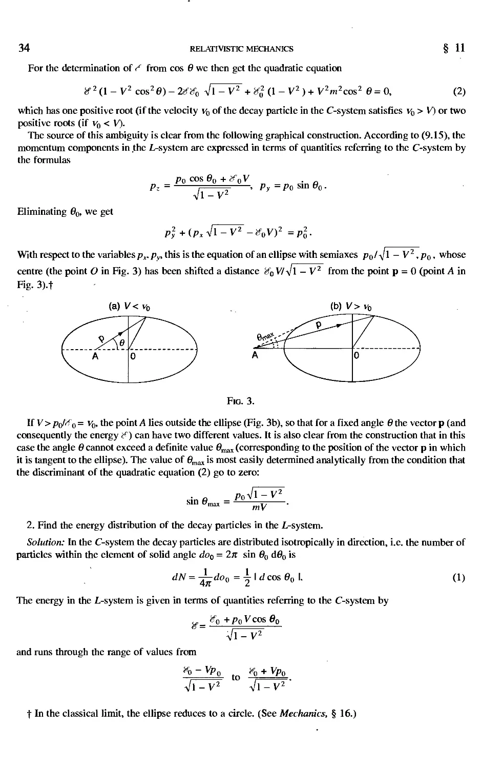
Text
The Classical
Theory of Fields
Fourth Kev.sed English Edition
Course of Theoretical Physics
Volume 2
THE CLASSICAL THEORY
OF
FIELDS
Fourth Revised English Edition
L. D. LANDAU AND E. M. LIFSHITZ
Institute for Physical Problems, Academy of Sciences of the U.S.S.R.
Translated from the Russian
by
MORTON HAMERMESH
University of Minnesota
SJU TTERWORTH
E I N E M A N N
AMSTERDAM BOSTON HEIDELBERG LONDON NEW YORK OXFORD
PARIS SAN DIEGO SAN FRANCISCO SINGAPORE SYDNEY TOKYO
CONTENTS
Excerpts from the Prefaces to the First and Second Editions ix
Preface to the Fourth English Edition x
Editor's Preface to the Seventh Russian Edition xi
Notation xiii
Chapter 1. The Principle of Relativity 1
1 Velocity of propagation of interaction 1
2 Intervals 3
3 Proper time 7
4 The Lorentz transformation 9
5 Transformation of velocities 12
6 Four-vectors 14
7 Four-dimensional velocity 23
Chapter 2. Relativistic Mechanics 25
8 The principle of least action 25
9 Energy and momentum 26
10 Transformation of distribution functions 30
11 Decay of particles 32
12 Invariant cross-section 36
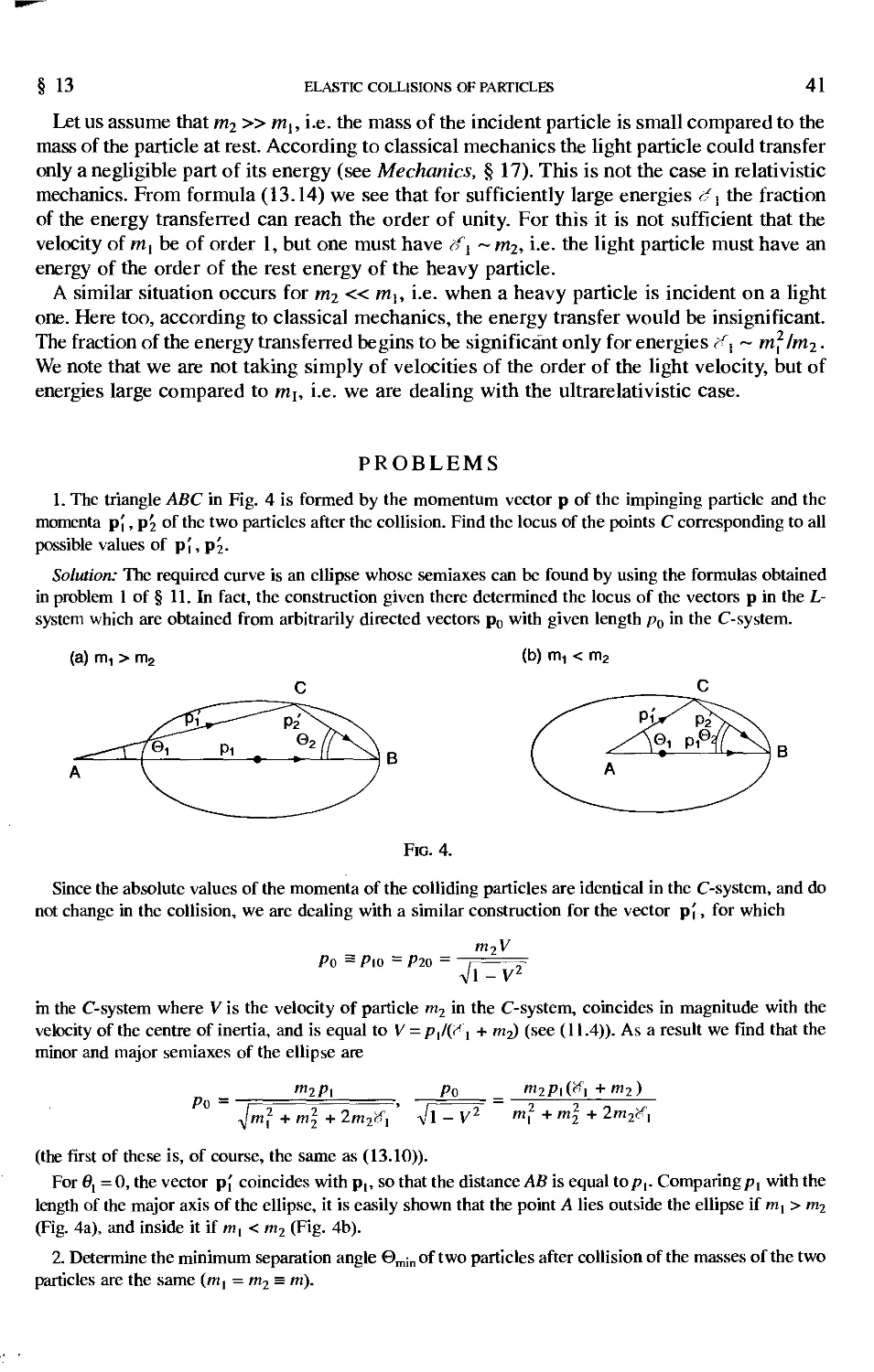
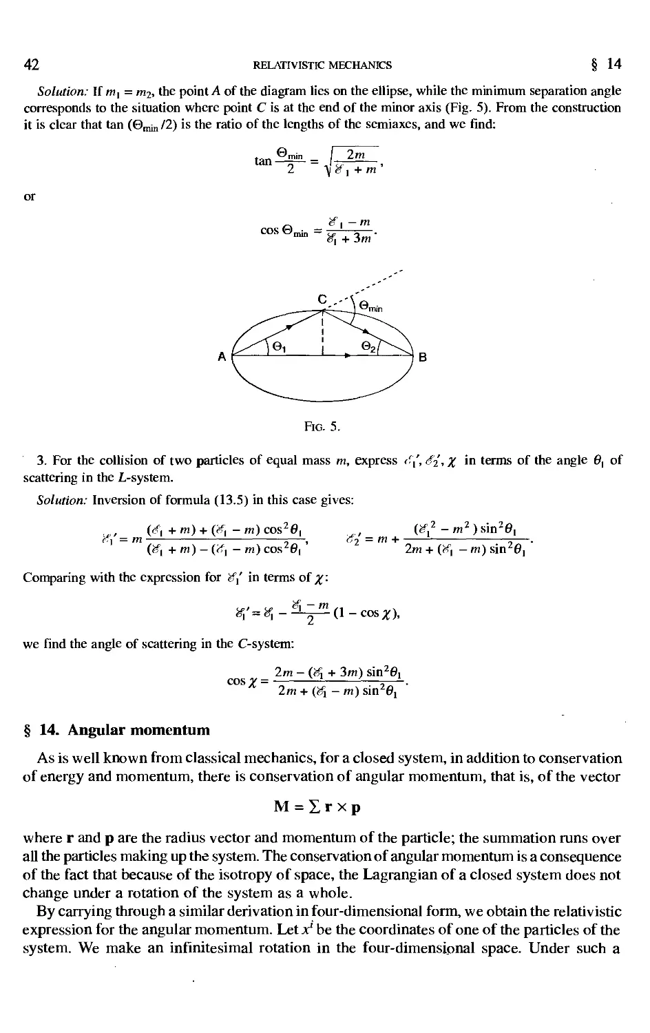
13 Elastic collisions of particles 38
14 Angular momentum 42
Chapter 3. Charges in Electromagnetic Fields 46
15 Elementary particles in the theory of relativity 46
16 Four-potential of a field 47
17 Equations of motion of a charge in a field 49
18 Gauge invariance 52
19 Constant electromagnetic field 53
20 Motion in a constant uniform electric field 55
21 Motion in a constant uniform magnetic field 56
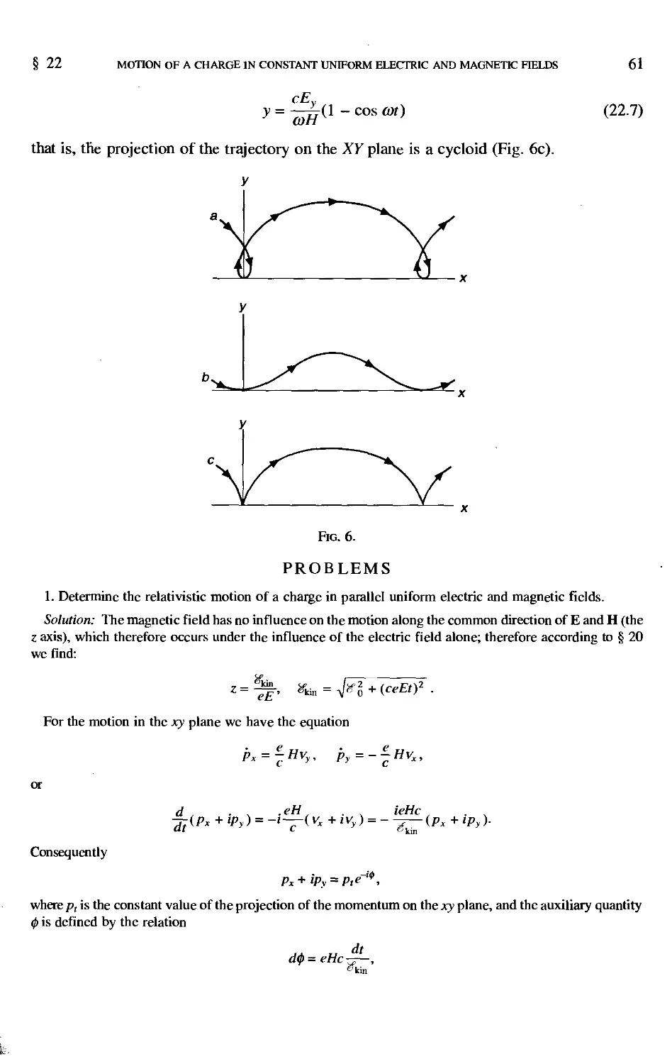
22 Motion of a charge in constant uniform electric and magnetic fields 59
23 The electromagnetic field tensor 64
24 Lorentz transformation of the field 66
25 Invariants of the field 67
VI
CONTENTS
Chapter 4. The Electromagnetic Field Equations
26 The first pair of Maxwell's equations
27 The action function of the electromagnetic field
28 The four-dimensional current vector
29 The equation of continuity
30 The second pair of Maxwell equations
31 Energy density and energy flux
32 The energy-momentum tensor
33 Energy-momentum tensor of the electromagnetic field
34 The virial theorem
35 The energy-momentum tensor for macroscopic bodies
Chapter 5. Constant Electromagnetic Fields
36 Coulomb's law
37 Electrostatic energy of charges
38 The field of a uniformly moving charge
39 Motion in the Coulomb field
40 The dipole moment
41 Multipole moments
42 System of charges in an external field
43 Constant magnetic field
44 Magnetic moments
45 Larmor's theorem
Chapter 6. Electromagnetic Waves
46 The wave equation
47 Plane waves
48 Monochromatic plane waves
49 Spectral resolution
50 Partially polarized light
51 The Fourier resolution of the electrostatic field
52 Characteristic vibrations of the field
Chapter 7. The Propagation of Light
53 Geometrical optics
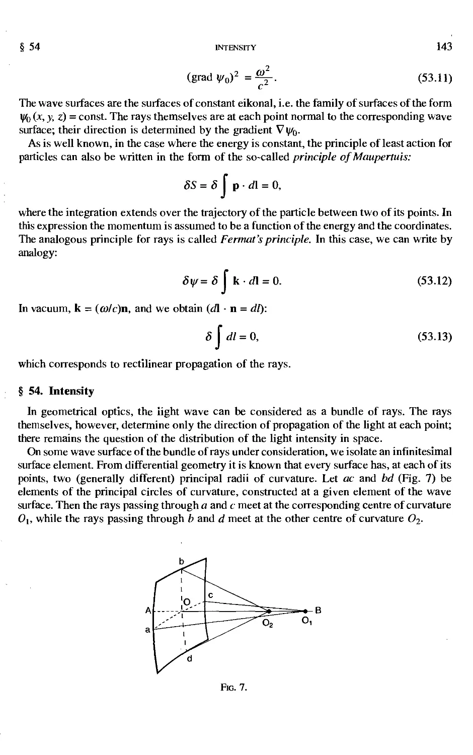
54 Intensity
55 The angular eikonal
56 Narrow bundles of rays
57 Image formation with broad bundles of rays
58 The limits of geometrical optics
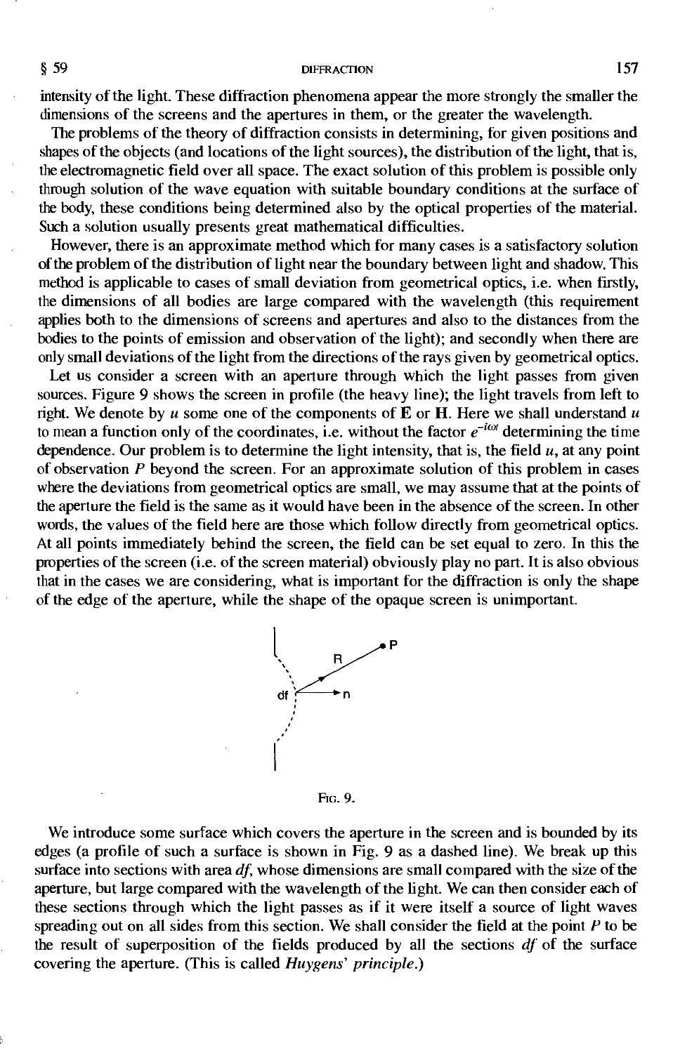
59 Diffraction
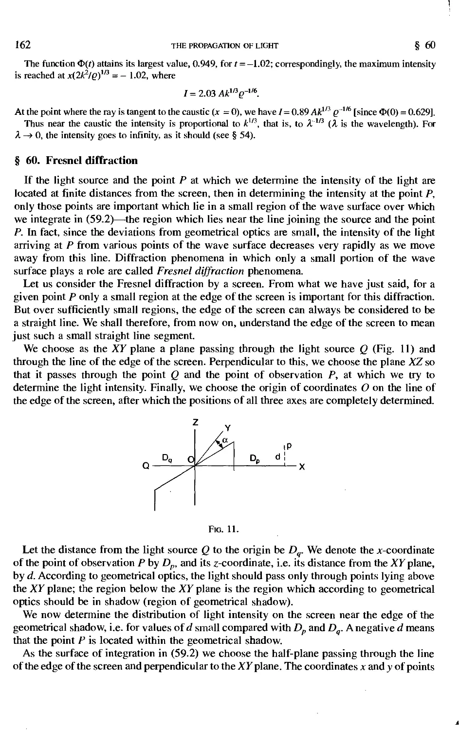
60 Fresnel diffraction
61 Fraunhofer diffraction
CONTENTS
Vll
Chapter 8. The Field of Moving Charges 171
62 The retarded potentials 171
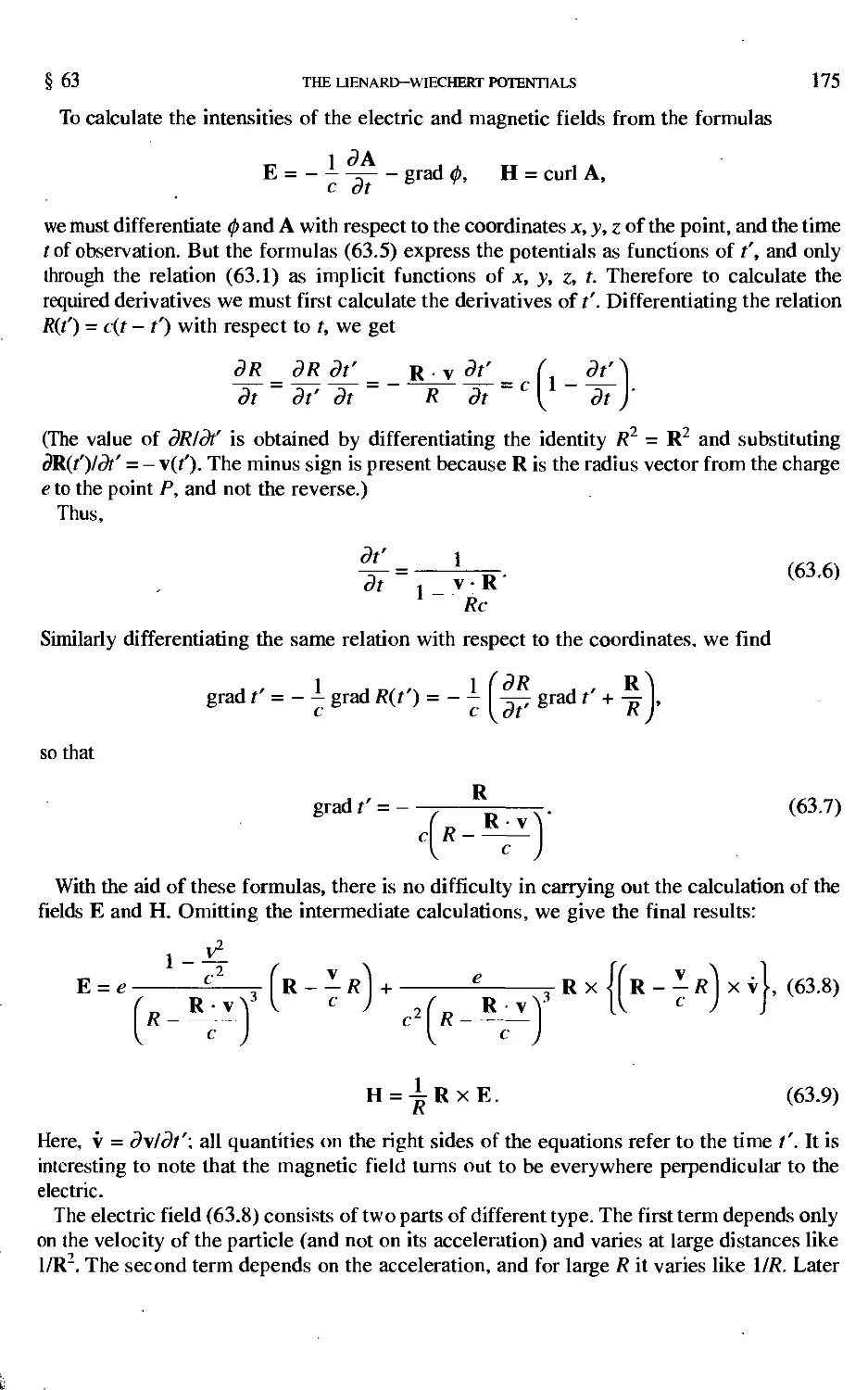
63 The Lienard—Wiechert potentials 173
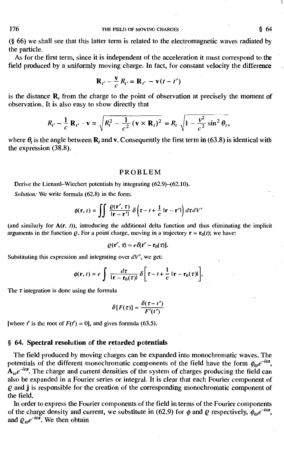
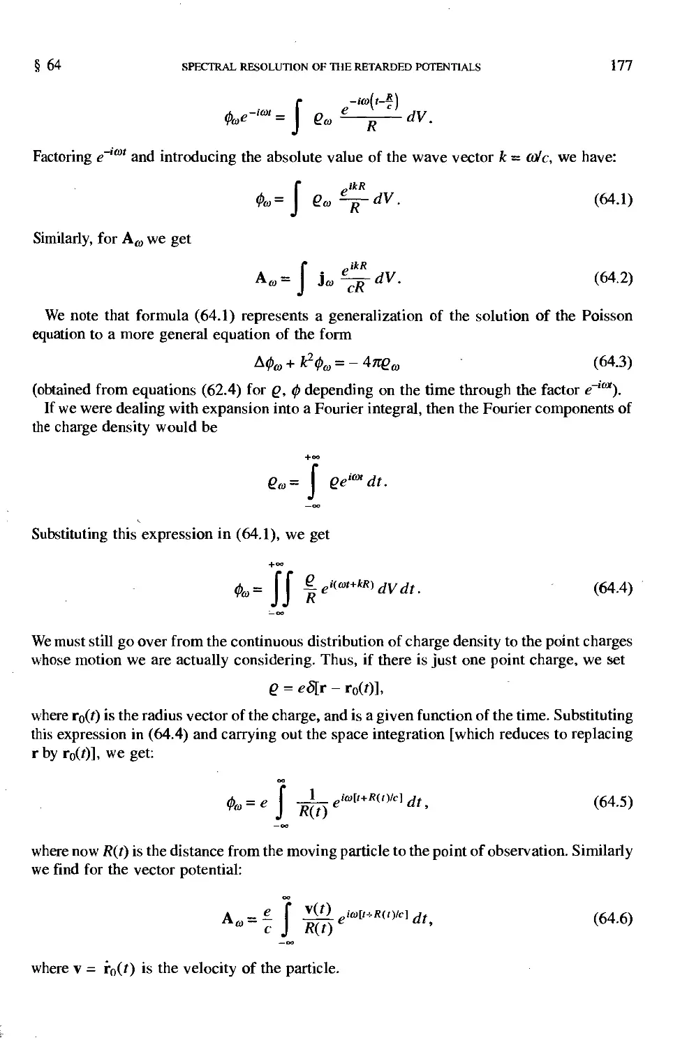
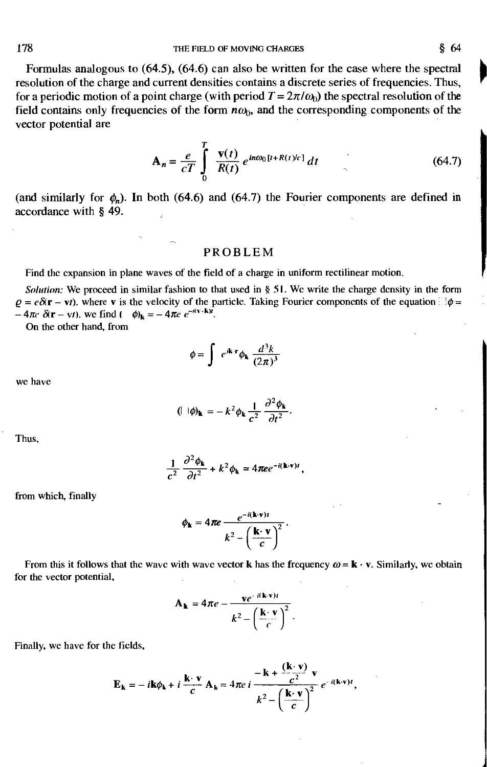
64 Spectral resolution of the retarded potentials 176
65 The Lagrangian to terms of second order 179
Chapter 9. Radiation of Electromagnetic Waves 184
66 The field of a system of charges at large distances 184
67 Dipole radiation 187
68 Dipole radiation during collisions 191
69 Radiation of low frequency in collisions 193
70 Radiation in the case of Coulomb interaction 195
71 Quadrupole and magnetic dipole radiation 203
72 The field of the radiation at near distances 206
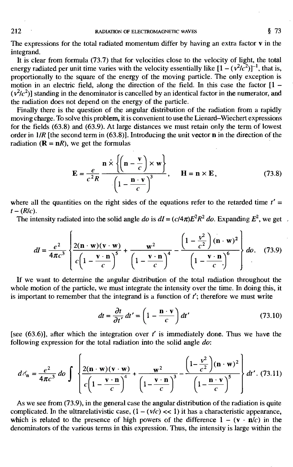
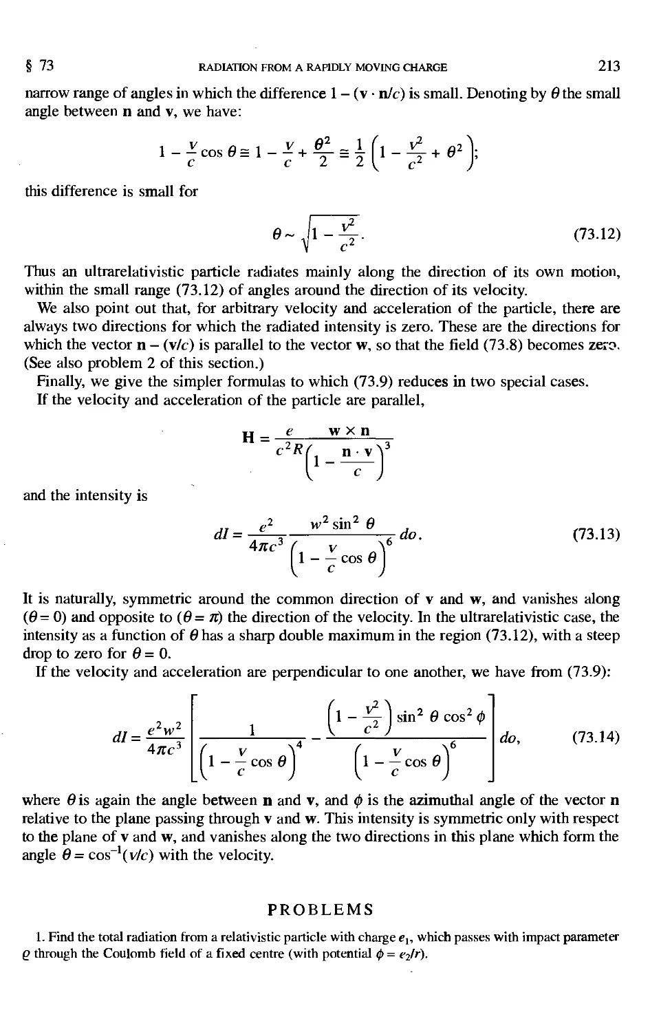
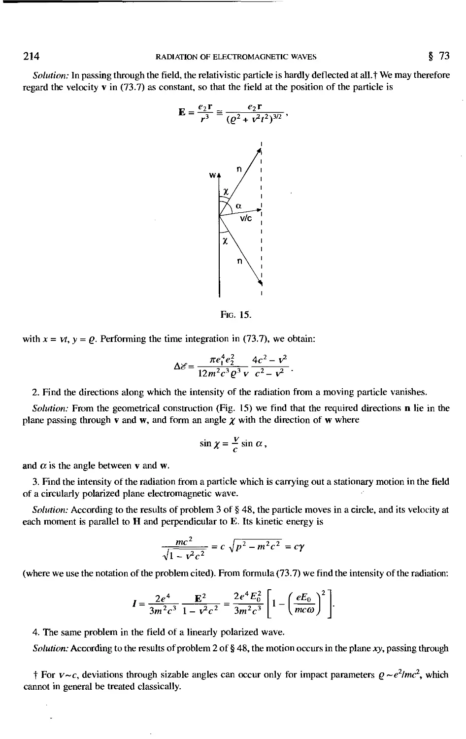
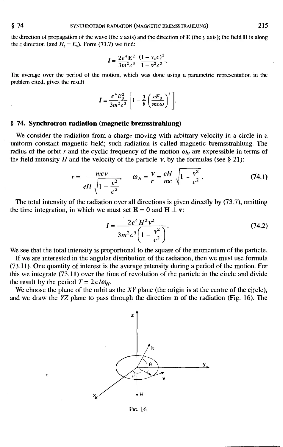
73 Radiation from a rapidly moving charge 210
74 Synchrotron radiation (magnetic bremsstrahlung) 215
75 Radiation damping 222
76 Radiation damping in the relativistic case 226
77 Spectral resolution of the radiation in the ultrarelativistic case 230
78 Scattering by free charges 233
79 Scattering of low-frequency waves 238
80 Scattering of high-frequency waves 240
Chapter 10. Particle in a Gravitational Field 243
81 Gravitational fields in nonrelativistic mechanics 243
82 The gravitational field in relativistic mechanics 244
83 Curvilinear coordinates 247
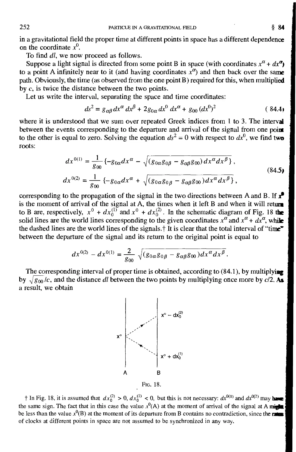
84 Distances and time intervals 251
85 Covariant differentiation 255
86 The relation of the Christoffel symbols to the metric tensor 260
87 Motion of a particle in a gravitational field 263
88 The constant gravitational field 266
89 Rotation 273
90 The equations of electrodynamics in the presence of a gravitational field 275
Chapter 11. The Gravitational Field Equations 278
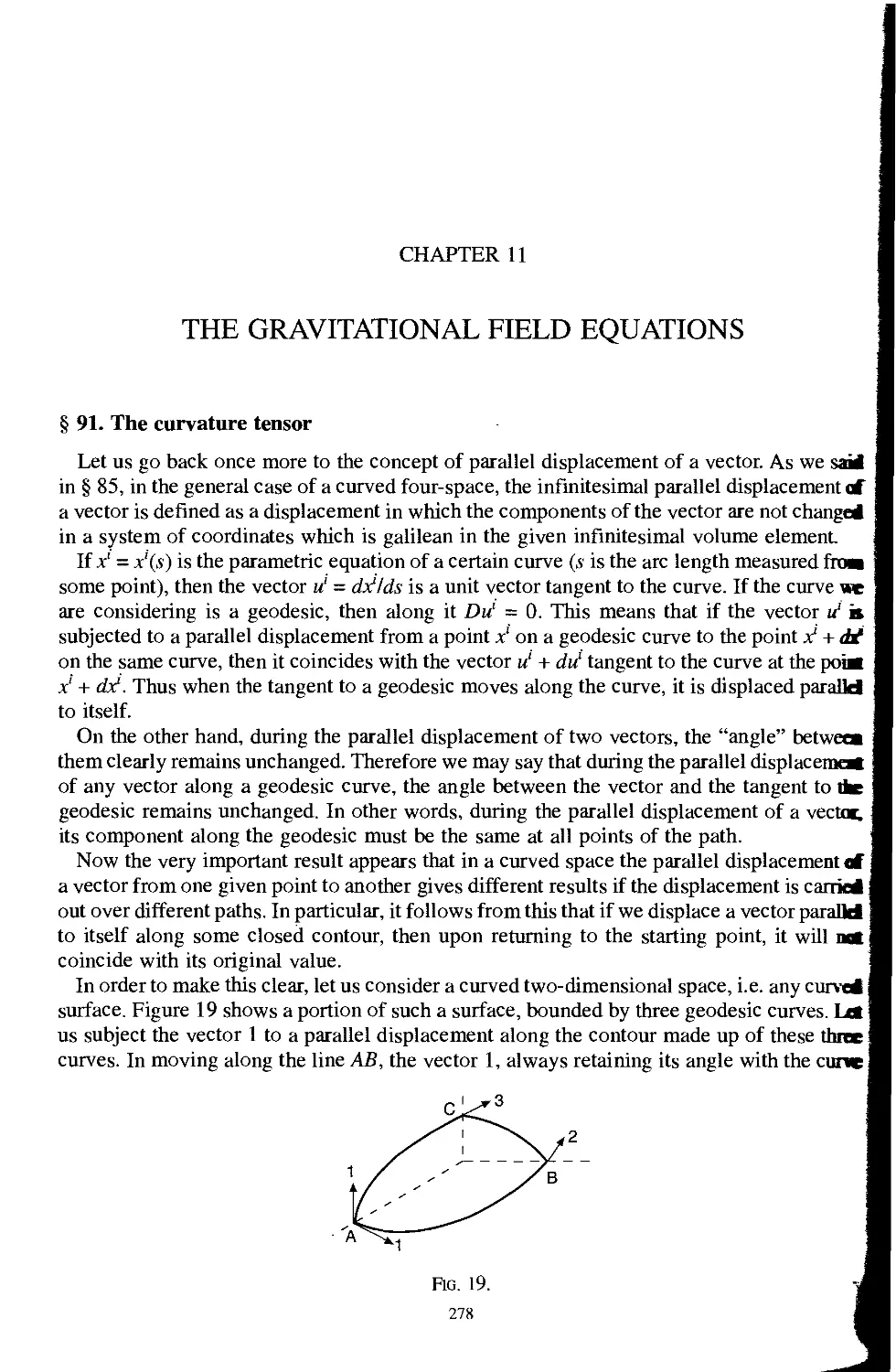
91 The curvature tensor 278
92 Properties of the curvature tensor 281
93 The action function for the gravitational field 287
94 The energy-momentum tensor 290
95 The Einstein equations 295
96 The energy-momentum pseudotensor of the gravitational field 301
97 The synchronous reference system 307
98 The tetrad representation of the Einstein equations 313
VlU
CONTENTS
Chapter 12. The Field of Gravitating Bodies 316
99 Newton's law 316
100 The centrally symmetric gravitational field 320
101 Motion in a centrally symmetric gravitational field 328
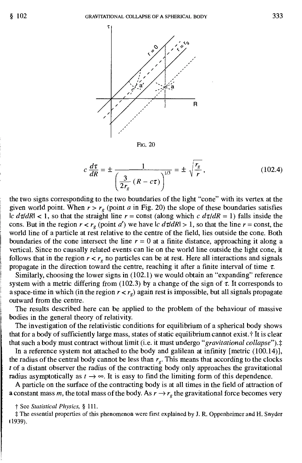
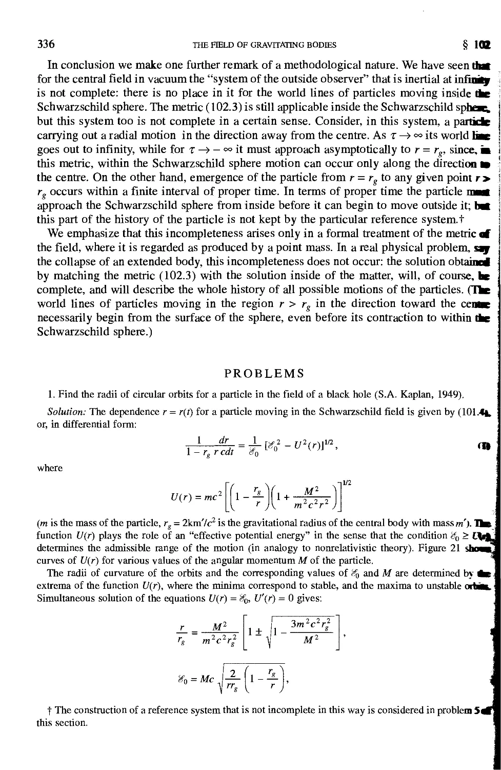
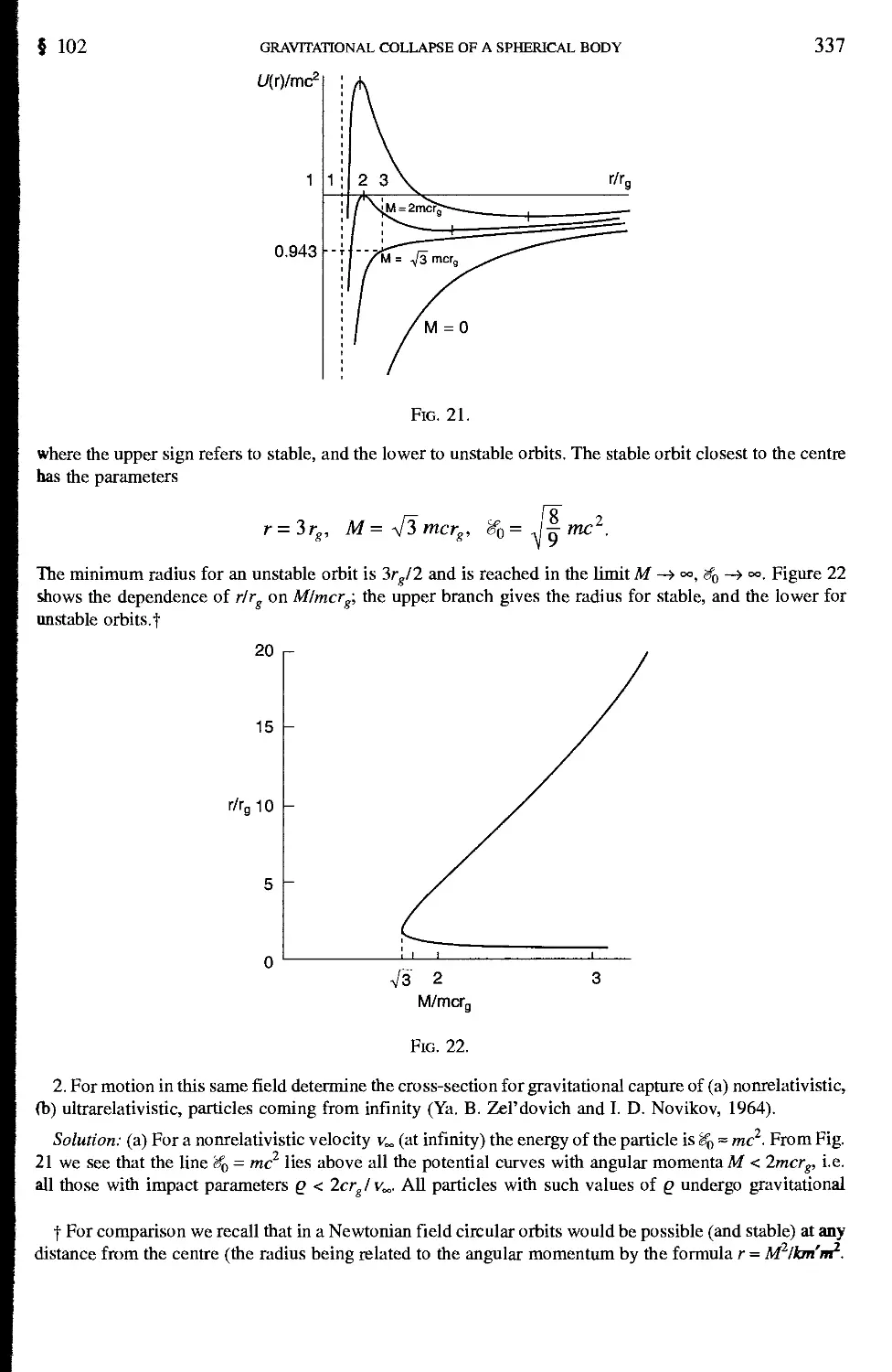
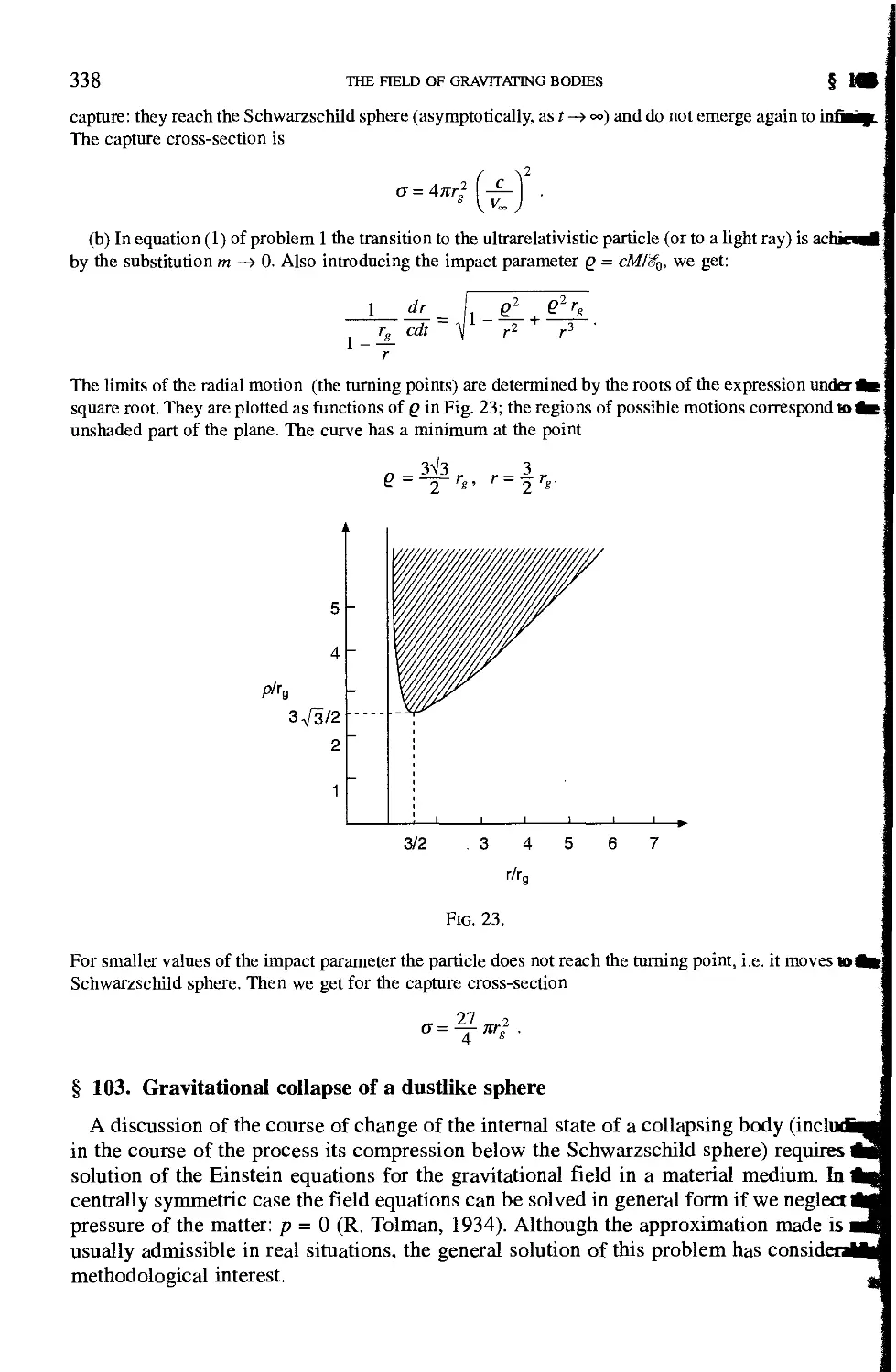
102 Gravitational collapse of a spherical body 331
103 Gravitational collapse of a dustlike sphere 338
104 Gravitational collapse of nonspherical and rotating bodies 344
105 Gravitational fields at large distances from bodies 353
106 The equations of motion of a system of bodies in the second approximation 360
Chapter 13. Gravitational Waves 368
107 Weak gravitational waves 368
108 Gravitational waves in curved space-time 370
109 Strong gravitational waves 373
110 Radiation of gravitational waves 376
Chapter 14. Relativistic Cosmology 382
111 Isotropic space 382
112 The closed isotropic model 386
113 The open isotropic model 390
114 The red shift 394
115 Gravitational stability of an isotropic universe 400
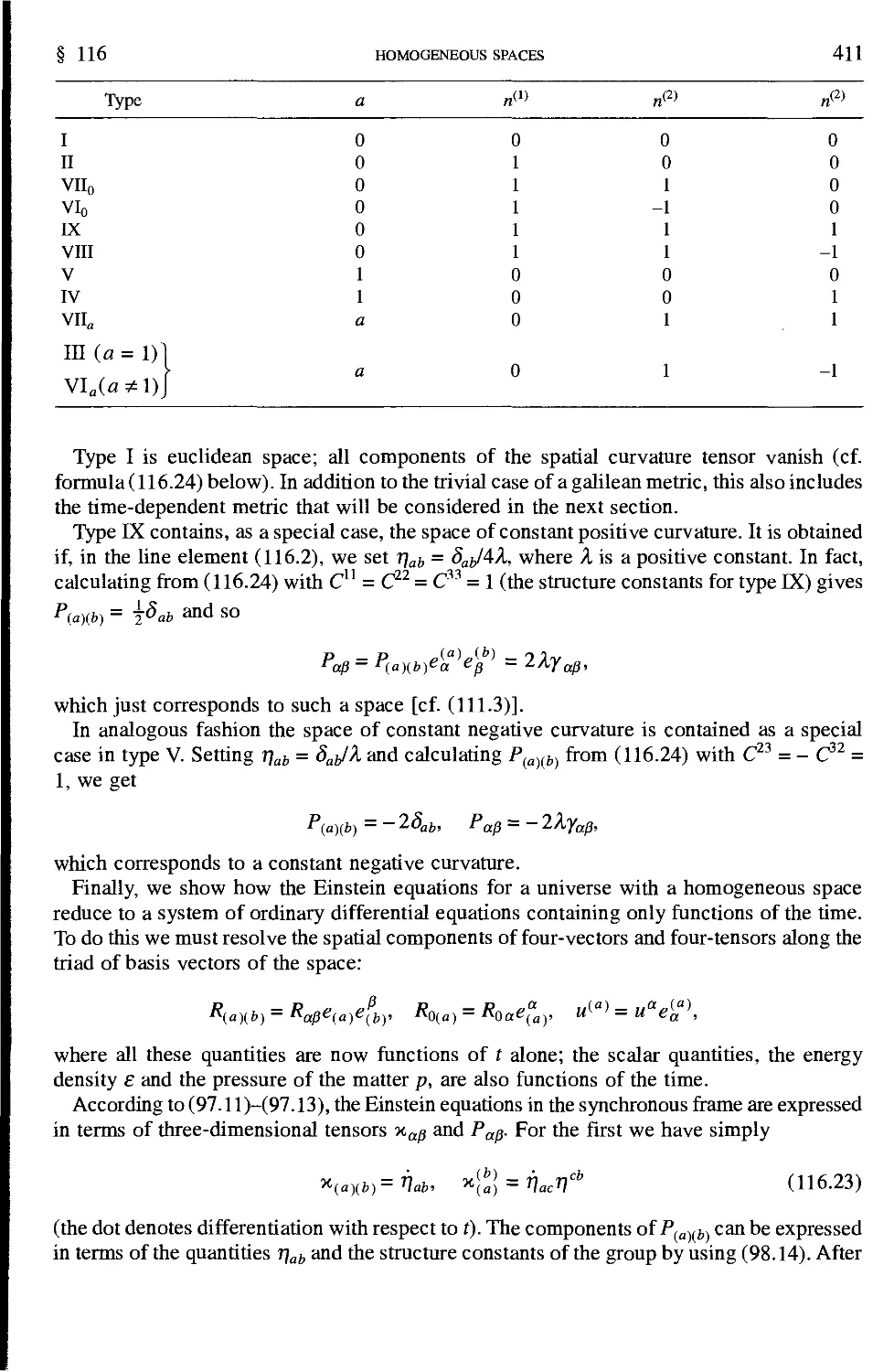
116 Homogeneous spaces 406
117 The flat anisotropic model 412
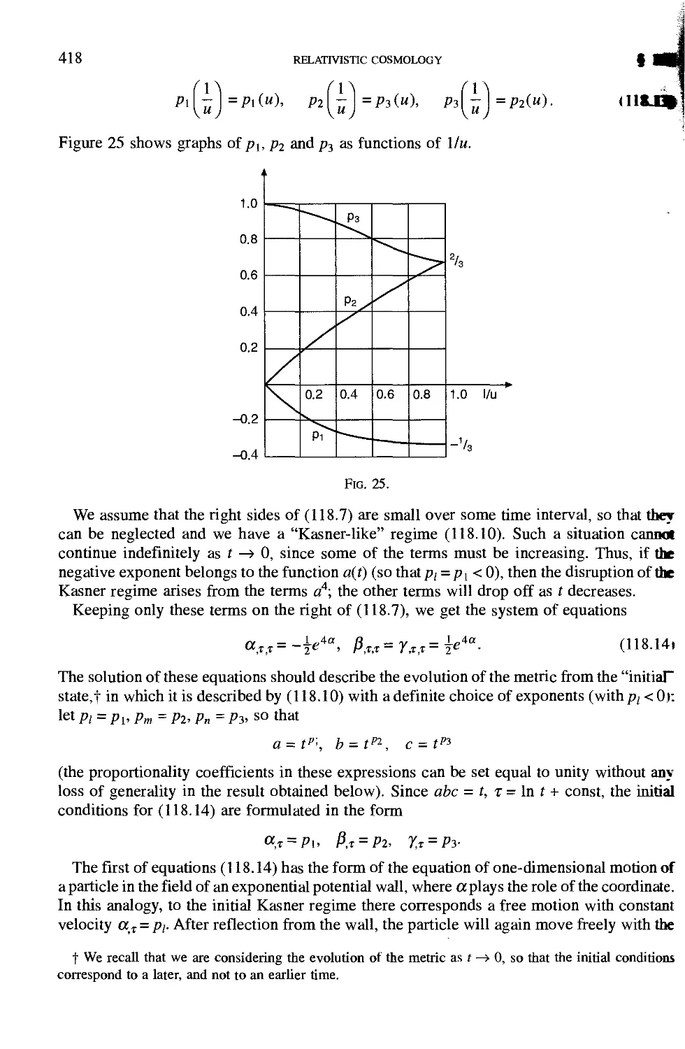
118 Oscillating regime of approach to a singular point 416
119 The time singularity in the general cosmo logical solution of the
Einstein equations 420
Index
EXCERPTS FROM THE PREFACES TO THE
FIRST AND SECOND EDITIONS
This book is devoted to the presentation of the theory of the electromagnetic and gravitational
fields, i.e. electrodynamics and general relativity. A complete, logically connected theory of
the electromagnetic field includes the special theory of relativity, so the latter has been taken
as the basis of the presentation. As the starting point of the derivation of the fundamental
relations we take the variational principles, which make possible the attainment of maximum
generality, unity and simplicity of presentation.
In accordance with the overall plan of our Course of Theoretical Physics (of which this
book is a part), we have not considered questions concerning the electrodynamics of continuous
media, but restricted the discussion to "microscopic electrodynamics"—the electrodynamics
of point charges in vacuo.
The reader is assumed to be familiar with electromagnetic phenomena as discussed in
general physics courses. A knowledge of vector analysis is also necessary. The reader is not
assumed to have any previous knowledge of tensor analysis, which is presented in parallel
with the development of the theory of gravitational fields.
Moscow, December 1939
Moscow, June 1947
L. Landau, E. Lifshitz
PREFACE TO THE FOURTH ENGLISH EDITION
The first edition of this book appeared more than thirty years ago. In the course of reissues
over these decades the book has been revised and expanded; its volume has almost doubled
since the first edition. But at no time has there been any need to change the method proposed
by Landau for developing the theory, or his style of presentation, whose main feature was
a striving for clarity and simplicity. I have made every effort to preserve this style in the
revisions that I have had to make on my own.
As compared with the preceding edition, the first nine chapters, devoted to electrodynamics,
have remained almost without changes. The chapters concerning the theory of the gravitational
field have been revised and expanded. The material in these chapters has increased from
edition to edition, and it was finally necessary to redistribute and rearrange it.
I should like to express here my deep gratitude to all of my helpers in this work—too
many to be enumerated—who, by their comments and advice, helped me to eliminate errors
and introduce improvements. Without their advice, without the willingness to help which
has met all my requests, the work to continue the editions of this course would have been
much more difficult. A special debt of gratitude is due to L. P. Pitaevskii, with whom I have
constantly discussed all the vexing questions.
The English translation of the book was done from the last Russian edition, which appeared
in 1973. No further changes in the book have been made. The 1994 corrected reprint
includes the changes made by E. M. Lifshitz in the Seventh Russian Edition published in
1987.
I should also like to use this occasion to sincerely thank Prof. Hamermesh, who has
translated this book in all its editions, starting with the first English edition in 1951. The
success of this book among English-speaking readers is to a large extent the result of his
labour and careful attention.
E. M. Lifshitz
PUBLISHER'S NOTE
As with the other volumes in the Course of Theoretical Physics, the authors do not, as a rule,
give references to original papers, but simply name their authors (with dates). Full bibliographic
references are only given to works which contain matters not fully expounded in the text.
EDITOR'S PREFACE TO THE
SEVENTH RUSSIAN EDITION
E. M. Lifshitz began to prepare a new edition of Teoria Polia in 1985 and continued his
work on it even in hospital during the period of his last illness. The changes that he proposed
are made in the present edition. Of these we should mention some revision of the proof of
the law of conservation of angular momentum in relativistic mechanics, and also a more
detailed discussion of the question of symmetry of the Christoffel symbols in the theory of
gravitation. The sign has been changed in the definition of the electromagnetic field stress
tensor. (In the present edition this tensor was defined differently than in the other volumes
of the Course.)
June 1987 L. P. Pitaevskii
XI
NOTATION
Three-dimensional quantities
Three-dimensional tensor indices are denoted by Greek letters
Element of volume, area and length: dV, di, d\
Momentum and energy of a particle: p and £
Hamiltonian function: X
Scalar and vector potentials of the electromagnetic field: 0 and A
Electric and magnetic field intensities: E and H
Charge and current density: p and j
Electric dipole moment: d
Magnetic dipole moment: m
Four-dimensional quantities
Four-dimensional tensor indices are denoted by Latin letters i, k,l,... and take on the values
0, 1, 2, 3
We use the metric with signature (+ )
Rule for raising and lowering indices—see p. 14
Components of four-vectors are enumerated in the form A' = (A0, A)
Antisymmetric unit tensor of rank four is e'klm, where e0123 = 1 (for the definition, see p. 17)
Element of four-volume dQ, = dx°dxldx2dxi
Element of hypersurface dS' (defined on pp. 20-21)
Radius four-vector: x' = (ct, r)
Velocity four-vector: u' = dx'/ds
Momentum four-vector: p = (&7c, p)
Current four-vector: j' = (cp, pv)
Four-potential of the electromagnetic field: A' = (¢, A)
r)A r)A
Electromagnetic field four-tensor F,t = —-: —-j- (for the relation of the components of
dxl dx
Fik to the components of E and H, see p. 65)
Energy-momentum four-tensor r'*(for the definition of its components, see p. 83)
Xlll
CHAPTER 1
THE PRINCIPLE OF RELATIVITY
§ 1. Velocity of propagation of interaction
For the description of processes taking place in nature, one must have a system of reference.
By a system of reference we understand a system of coordinates serving to indicate the
position of a particle in space, as well as clocks fixed in this system serving to indicate the
time.
There exist systems of reference in which a freely moving body, i.e. a moving body which
is not acted upon by external forces, proceeds with constant velocity. Such reference systems
are said to be inertial.
If two reference systems move uniformly relative to each other, and if one of them is an
inertial system, then clearly the other is also inertial (in this system too every free motion
will be linear and uniform). In this way one can obtain arbitrarily many inertial systems of
reference, moving uniformly relative to one another.
Experiment shows that the so-called principle of relativity is valid. According to this
principle all the laws of nature are identical in all inertial systems of reference. In other
words, the equations expressing the laws of nature are invariant with respect to transformations
of coordinates and time from one inertial system to another. This means that the equation
describing any law of nature, when written in terms of coordinates and time in different
inertial reference systems, has one and the same form.
The interaction of material particles is described in ordinary mechanics by means of a
potential energy of interaction, which appears as a function of the coordinates of the interacting
particles. It is easy to see that this manner of describing interactions contains the assumption
of instantaneous propagation of interactions. For the forces exerted on each of the particles
by the other particles at a particular instant of time depend, according to this description,
only on the positions of the particles at this one instant. A change in the position of any of
the interacting particles influences the other particles immediately.
However, experiment shows that instantaneous interactions do not exist in nature. Thus a
mechanics based on the assumption of instantaneous propagation of interactions contains
within itself a certain inaccuracy. In actuality, if any change takes place in one of the
interacting bodies, it will influence the other bodies only after the lapse of a certain interval
of time. It is only after this time interval that processes caused by the initial change begin
to take place in the second body. Dividing the distance between the two bodies by this time
interval, we obtain the velocity of propagation of the interaction.
We note that this velocity should, strictly speaking, be called the maximum velocity of
propagation of interaction. It determines only that interval of time after which a change
occurring in one body begins to manifest itself in another. It is clear that the existence of a
l
2
THE PRINCIPLE OF RELATIVITY
§ 1
maximum velocity of propagation of interactions implies, at the same time, that motions of
bodies with greater velocity than this are in general impossible in nature. For if such a
motion could occur, then by means of it one could realize an interaction with a velocity
exceeding the maximum possible velocity of propagation of interactions.
Interactions propagating from one particle to another are frequently called "signals", sent
out from the first particle and "informing" the second particle of changes which the first has
experienced. The velocity of propagation of interaction is then referred to as the signal
velocity.
From the principle of relativity it follows in particular that the velocity of propagation of
interactions is the same in all inertial systems of reference. Thus the velocity of propagation
of interactions is a universal constant. This constant velocity (as we shall show later) is also
the velocity of light in empty space. The velocity of light is usually designated by the letter
c, and its numerical value is
c = 2.998 x 1010 cm/sec. (1.1)
The large value of this velocity explains the fact that in practice classical mechanics
appears to be sufficiently accurate in most cases. The velocities with which we have occasion
to deal are usually so small compared with the velocity of light that the assumption that the
latter is infinite does not materially affect the accuracy of the results.
The combination of the principle of relativity with the finiteness of the velocity of propagation
of interactions is called the principle of relativity of Einstein (it was formulated by Einstein
in 1905) in contrast to the principle of relativity of Galileo, which was based on an infinite
velocity of propagation of interactions.
The mechanics based on the Einsteinian principle of relativity (we shall usually refer to it
simply as the principle of relativity) is called relativistic. In the limiting case when the
velocities of the moving bodies are small compared with the velocity of light we can neglect
the effect on the motion of the finiteness of the velocity of propagation. Then relativistic
mechanics goes over into the usual mechanics, based on the assumption of instantaneous
propagation of interactions; this mechanics is called Newtonian or classical. The limiting
transition from relativistic to classical mechanics can be produced formally by the transition
to the limit c —> °° in the formulas of relativistic mechanics.
In classical mechanics distance is already relative, i.e. the spatial relations between different
events depend on the system of reference in which they are described. The statement that
two nonsimultaneous events occur at one and the same point in space or, in general, at a
definite distance from each other, acquires a meaning only when we indicate the system of
reference which is used.
On the other hand, time is absolute in classical mechanics; in other words, the properties
of time are assumed to be independent of the system of reference; there is one time for all
reference frames. This means that if any two phenomena occur simultaneously for any one
observer, then they occur simultaneously also for all others. In general, the interval of time
between two given events must be identical for all systems of reference.
It is easy to show, however, that the idea of an absolute time is in complete contradiction
to the Einstein principle of relativity. For this it is sufficient to recall that in classical mechanics,
based on the concept of an absolute time, a general law of combination of velocities is valid,
according to which the velocity of a composite motion is simply equal to the (vector) sum
of the velocities which constitute this motion. This law, being universal, should also be
applicable to the propagation of interactions. From this it would follow that the velocity of
§ 2
INTERVALS
3
propagation must be different in different inertial systems of reference, in contradiction to
the principle of relativity. In this matter experiment completely confirms the principle of
relativity. Measurements first performed by Michelson (1881) showed complete lack of
dependence of the velocity of light on its direction of propagation; whereas according to
classical mechanics the velocity of light should be smaller in the direction of the earth's
motion than in the opposite direction.
Thus the principle of relativity leads to the result that time is not absolute. Time elapses
differently in different systems of reference. Consequently the statement that a definite time
interval has elapsed between two given events acquires meaning only when the reference
frame to which this statement applies is indicated. In particular, events which are simultaneous
in one reference frame will not be simultaneous in other frames.
To clarify this, it is instructive to consider the following simple example.
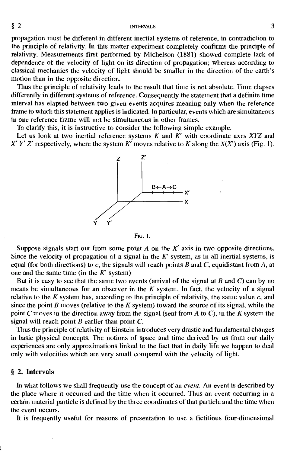
Let us look at two inertial reference systems K and K' with coordinate axes XYZ and
X' Y' Z' respectively, where the system K' moves relative to K along the X(X') axis (Fig. 1).
B<-A->C
H 1 1 X'
X
Y Y'
Fig. 1.
Suppose signals start out from some point A on the X' axis in two opposite directions.
Since the velocity of propagation of a signal in the K' system, as in all inertial systems, is
equal (for both directions) to c, the signals will reach points B and C, equidistant from A, at
one and the same time (in the K' system)
But it is easy to see that the same two events (arrival of the signal at B and C) can by no
means be simultaneous for an observer in the K system. In fact, the velocity of a signal
relative to the K system has, according to the principle of relativity, the same value c, and
since the point B moves (relative to the K system) toward the source of its signal, while the
point C moves in the direction away from the signal (sent from A to C), in the K system the
signal will reach point B earlier than point C.
Thus the principle of relativity of Einstein introduces very drastic and fundamental changes
in basic physical concepts. The notions of space and time derived by us from our daily
experiences are only approximations linked to the fact that in daily life we happen to deal
only with velocities which are very small compared with the velocity of light.
§ 2. Intervals
In what follows we shall frequently use the concept of an event. An event is described by
the place where it occurred and the time when it occurred. Thus an event occurring in a
certain material particle is defined by the three coordinates of that particle and the time when
the event occurs.
It is frequently useful for reasons of presentation to use a fictitious four-dimensional
4 THE PRINCIPLE OF RELATIVITY § 2
space, on the axes of which are marked three space coordinates and the time. In this space
events are represented by points, called world points. In this fictitious four-dimensional
space there corresponds to each particle a cetain line, called a world line. The points of this
line determine the coordinates of the particle at all moments of time. It is easy to show that
to a particle in uniform rectilinear motion there corresponds a straight world line.
We now express the principle of the invariance of the velocity of light in mathematical
form. For this purpose we consider two reference systems K and K' moving relative to each
other with constant velocity. We choose the coordinate axes so that the axes X and X'
coincide, while the Y and Z axes are parallel to Y and Z'; we designate the time in the
systems K and K' by t and f.
Let the first event consist of sending out a signal, propagating with light velocity, from a
point having coordinates xxyxZ\ in the K system, at time tx in this system. We observe the
propagation of this signal in the K system. Let the second event consist of the arrival of the
signal at point x2y2z2 at tne moment of time t2. The signal propagates with velocity c;
the distance covered by it is therefore c{t\ —t2). On the other hand, this same distance equals
[{x2 - xx)2 + (y2 - y\)2 + (¾ - l\ )2 ]2 • Thus we can write the following relation between the
coordinates of the two events in the K system:
(x2 - Xlf +(y2- yxf + (z2 - zxf - c\t2 - txf = 0. (2.1)
The same two events, i.e. the propagation of the signal, can be observed from the K'
system:
Let the coordinates of the first event in the K' system be x[y[z[t[, and of the second:
x'2y'2z2t2. Since the velocity of light is the same in the K and K' systems, we have, similarly
to (2.1):
(*£ - *02 + iy'i - yi)2 + Ui - z[)2 - c\t'2 -1[)2 = o. (2.2)
If x^y\Z\ h and x2y2z2t2 are the coordinates of any two events, then the quantity
*i2 = [c\h - hf - (x2 - x,)2 - (y2 - yd2 - (z2 - zx f P (2.3)
is called the interval between these two events.
Thus it follows from the principle of invariance of the velocity of light that if the interval
between two events is zero in one coordinate system, then it is equal to zero in all other
systems.
If two events are infinitely close to each other, then the interval ds between them is
ds2 = c2dt2 -dx2-dy2- dz2. (2.4)
The form of expressions (2.3) and (2.4) permits us to regard the interval, from the formal
point of view, as the distance between two points in a fictitious four-dimensional space
(whose axes are labelled by x, y, z, and the product ct). But there is a basic difference
between the rule for forming this quantity and the rule in ordinary geometry: in forming the
square of the interval, the squares of the coordinate differences along the different axes are
summed, not with the same sign, but rather with varying signs, f
As already shown, if ds — 0 in one inertial system, then ds' — 0 in any other system. On
t The four-dimensional geometry described by the quadratic form (2.4) was introduced by H. Minkowski,
in connection with the theory of relativity. This geometry is called pseudo-euclidean, in contrast to ordinary
euclidean geometry.
§2
INTERVALS
5
the other hand, ds and ds' are infinitesimals of the same order. From these two conditions
it follows that ds2 and ds'2 must be proportional to each other:
ds2 — ads'2
where the coefficient a can depend only on the absolute value of the relative velocity of the
two inertial systems. It cannot depend on the coordinates or the time, since then different
points in space and different moments in time would not be equivalent, which would be in
contradiction to the homogeneity of space and time. Similarly, it cannot depend on the
direction of the relative velocity, since that would contradict the isotropy of space.
Let us consider three reference systems K, K\, K2, and let Vj and V2 De tne velocities of
systems Kx and K2 relative to K. We then have:
ds2 = a(Vx)dsl, ds2 = a(V2)ds2.
Similarly we can write
ds2 = a(yn)ds\,
where V12 is the absolute value of the velocity of K2 relative to K\. Comparing these
relations with one another, we find that we must have
7^ = «0fc>- (2-5)
But V12 depends not only on the absolute values of the vectors Vt and V2, but also on the
angle between them. However, this angle does not appear on the left side of formula (2.5).
It is therefore clear that this formula can be correct only if the function a(V) reduces to a
constant, which is equal to unity according to this same formula.
Thus,
ds2^dsn, (2.6)
and from the equality of the infinitesimal intervals there follows the equality of finite
intervals: s - s'.
Thus we arrive at a very important result: the interval between two events is the same in
all inertial systems of reference, i.e. it is invariant under transformation from one inertial
system to any other. This invariance is the mathematical expression of the constancy of the
velocity of light.
Again let xxyxZ\t\ and x2y2z2t2 be the coordinates of two events in a certain reference
system K. Does there exist a coordinate system IC, in which these two events occur at one
and the same point in space?
We introduce the notation
h~h= 'i2> (*2 - *i)2 + 0¾ - yi? + (¾ - zxf = /¾.
Then the interval between events in the K system is:
s2 - r2,2 _ /2
Sl2 - C ln ln
and in the K' system
'2 _ 2,/2 _ 1/2
A12 — c '12 '12 '
whereupon, because of the invariance of intervals,
6 THE PRINCIPLE OF RELATIVITY § 2
r2,2 _ /2 _ 2,/2 _ ,/2
t J12 «12 — <- «12 »12 •
We want the two events to occur at the same point in the K' system, that is, we require
/[2 = 0. Then
12 = 12 ~~ 12 = 12
Consequently a system of reference with the required property exists if s22 > 0, that is, if the
interval between the two events is a real number. Real intervals are said to be timelike.
Thus, if the interval between two events is timelike, then there exists a system of reference
in which the two events occur at one and the same place. The time which elapses between
the two events in this system is
^2=^^2-^2=^. (2.7)
If two events occur in one and the same body, then the interval between them is always
timelike, for the distance which the body moves between the two events cannot be greater
than ctn, since the velocity of the body cannot exceed c. So we have always
/12 < ctn.
Let us now ask whether or not we can find a system of reference in which the two events
occur at one and the same time. As before, we have for the K and K' systems c2tf2 - /¾ = c2^
- l[2 ■ We want to have t'n = 0, so that
4 = -z,'22<o.
Consequently the required system can be found only for the case when the interval .¾
between the two events is an imaginary number. Imaginary intervals are said to be spacelike.
Thus if the interval between two events is spacelike, there exists a reference system in
which the two events occur simultaneously. The distance between the points where the
events occur in this system is
/12 = 4lh~c2th =w12. (2.8)
The division of intervals into space- and timelike intervals is, because of their invariance,
an absolute concept. This means that the timelike or spacelike character of an interval is
independent of the reference system.
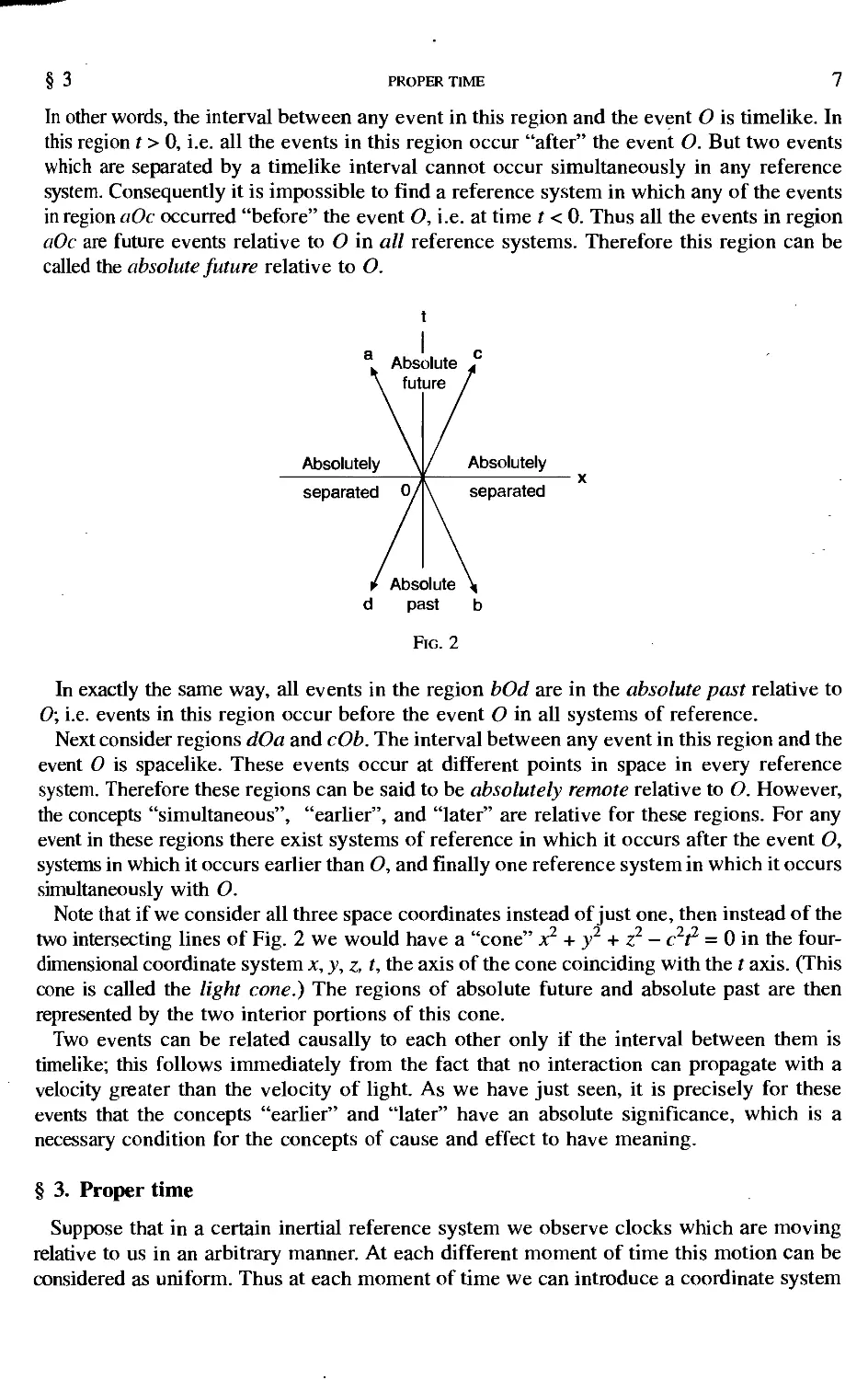
Let us take some event O as our origin of time and space coordinates. In other words, in
the four-dimensional system of coordinates, the axes of which are marked x, y, z, t, the world
point of the event O is the origin of coordinates. Let us now consider what relation other
events bear to the given event O. For visualization, we shall consider only one space
dimension and the time, marking them on two axes (Fig. 2). Uniform rectilinear motion of
a particle, passing through x = 0 at t = 0, is represented by a straight line going through O
and inclined to the t axis at an angle whose tangent is the velocity of the particle. Since the
maximum possible velocity is c, there is a maximum angle which this line can subtend with
the t axis. In Fig. 2 are shown the two lines representing the propagation of two signals (with
the velocity of light) in opposite directions passing through the event O (i.e. going through
x — 0 at t — 0). All lines representing the motion of particles can lie only in the regions aOc
and dOb. On the lines ab and cd, x - ± ct. First consider events whose world points lie
within the region aOc. It is easy to show that for all the points of this region c2/2 - x2 > 0.
§3
PROPER TIME
7
In other words, the interval between any event in this region and the event O is timelike. In
this region t > 0, i.e. all the events in this region occur "after" the event O. But two events
which are separated by a timelike interval cannot occur simultaneously in any reference
system. Consequently it is impossible to find a reference system in which any of the events
in region aOc occurred "before" the event O, i.e. at time t < 0. Thus all the events in region
aOc are future events relative to O in all reference systems. Therefore this region can be
called the absolute future relative to O.
t
c
Absolute .,
future I
Absolutely \
separated 0/
/ Absolutely
\ separated
i Absolute \
d past b
Fig. 2
In exactly the same way, all events in the region bOd are in the absolute past relative to
0; i.e. events in this region occur before the event O in all systems of reference.
Next consider regions dOa and cOb. The interval between any event in this region and the
event 0 is spacelike. These events occur at different points in space in every reference
system. Therefore these regions can be said to be absolutely remote relative to O. However,
the concepts "simultaneous", "earlier", and "later" are relative for these regions. For any
event in these regions there exist systems of reference in which it occurs after the event O,
systems in which it occurs earlier than O, and finally one reference system in which it occurs
simultaneously with O.
Note that if we consider all three space coordinates instead of just one, then instead of the
two intersecting lines of Fig. 2 we would have a "cone" x2 + y2 + z2 — c2/2 = 0 in the four-
dimensional coordinate system x, y, z, t, the axis of the cone coinciding with the t axis. (This
cone is called the light cone.) The regions of absolute future and absolute past are then
represented by the two interior portions of this cone.
Two events can be related causally to each other only if the interval between them is
timelike; this follows immediately from the fact that no interaction can propagate with a
velocity greater than the velocity of light. As we have just seen, it is precisely for these
events that the concepts "earlier" and "later" have an absolute significance, which is a
necessary condition for the concepts of cause and effect to have meaning.
§ 3. Proper time
Suppose that in a certain inertial reference system we observe clocks which are moving
relative to us in an arbitrary manner. At each different moment of time this motion can be
considered as uniform. Thus at each moment of time we can introduce a coordinate system
8
THE PRINCIPLE OF RELATIVITY
§ 3
rigidly linked to the moving clocks, which with the clocks constitutes an inertial reference
system.
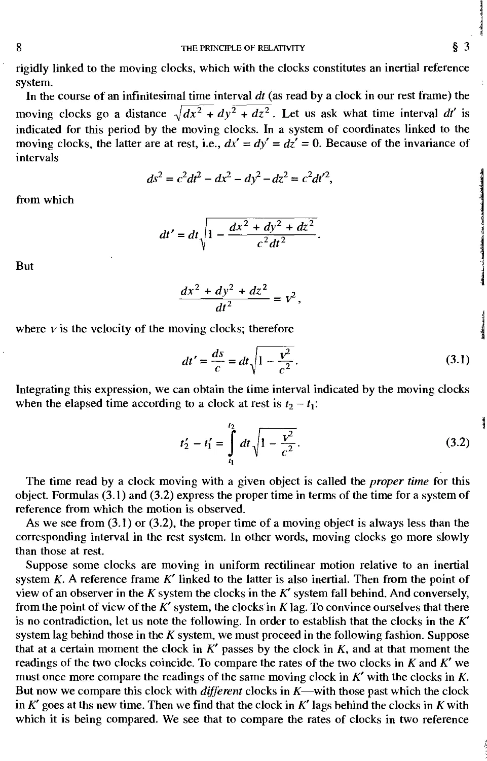
In the course of an infinitesimal time interval dt (as read by a clock in our rest frame) the
moving clocks go a distance sjdx2 + dy2 + dz2 . Let us ask what time interval dt' is
indicated for this period by the moving clocks. In a system of coordinates linked to the
moving clocks, the latter are at rest, i.e., dx' = dy' = dz' = 0. Because of the invariance of
intervals
ds2 = c2d? -dx2-dy2-dz2 = c2dt'2,
from which
,, ,,, dx2 + dy2 + dz2
dt' = dt\\--
cAdtz
But
dx2 + dy2 + dz2 _ ,
dT2 '
where v is the velocity of the moving clocks; therefore
^ = ^ = ^,/1-^-. (3.1)
C V ^2
Integrating this expression, we can obtain the time interval indicated by the moving clocks
when the elapsed time according to a clock at rest is t2 - t\-
t2-t; = jdt^j\-^-. (3.2)
'1
The time read by a clock moving with a given object is called the proper time for this
object. Formulas (3.1) and (3.2) express the proper time in terms of the time for a system of
reference from which the motion is observed.
As we see from (3.1) or (3.2), the proper time of a moving object is always less than the
corresponding interval in the rest system. In other words, moving clocks go more slowly
than those at rest.
Suppose some clocks are moving in uniform rectilinear motion relative to an inertial
system K. A reference frame K' linked to the latter is also inertial. Then from the point of
view of an observer in the K system the clocks in the K' system fall behind. And conversely,
from the point of view of the K' system, the clocks in K lag. To convince ourselves that there
is no contradiction, let us note the following. In order to establish that the clocks in the K'
system lag behind those in the K system, we must proceed in the following fashion. Suppose
that at a certain moment the clock in K' passes by the clock in K, and at that moment the
readings of the two clocks coincide. To compare the rates of the two clocks in K and K' we
must once more compare the readings of the same moving clock in K' with the clocks in K.
But now we compare this clock with different clocks in K—with those past which the clock
in K' goes at ths new time. Then we find that the clock in K' lags behind the clocks in K with
which it is being compared. We see that to compare the rates of clocks in two reference
§4
THE LORENTZ TRANSFORMATION
9
frames we require several clocks in one frame and one in the other, and that therefore this
process is not symmetric with respect to the two systems. The clock that appears to lag is
always the one which is being compared with different clocks in the other system.
If we have two clocks, one of which describes a closed path returning to the starting point
(the position of the clock which remained at rest), then clearly the moving clock appears to
lag relative to the one at rest. The converse reasoning, in which the moving clock would be
considered to be at rest (and vice versa) is now impossible, since the clock describing a
closed trajectory does not carry out a uniform rectilinear motion, so that a coordinate system
linked to it will not be inertial.
Since the laws of nature are the same only for inertial reference frames, the frames linked
to the clock at rest (inertial frame) and to the moving clock (non-inertial) have different
properties, and the argument which leads to the result that the clock at rest must lag is not valid.
The time interval read by a clock is equal to the integral
a
taken along the world line of the clock. If the clock is at rest then its world line is clearly a
line parallel to the t axis; if the clock carries out a nonuniform motion in a closed path and
returns to its starting point, then its world line will be a curve passing through the two points,
on the straight world line of a clock at rest, corresponding to the beginning and end of the
motion. On the other hand, we saw that the clock at rest always indicates a greater time
interval than the moving one. Thus we arrive at the result that the integral
b
jds.
a
taken between a given pair of world points, has its maximum value if it is taken along the
straight world line joining these two points, t
§ 4. The Lorentz transformation
Our purpose is now to obtain the formula of transformation from one inertial reference
system to another, that is, a formula by means of which, knowing the coordinates x, y, z, t,
of a certain event in the K system, we can find the coordinates x, y, z, t' of the same event
in another inertial system A".
In classical mechanics this question is resolved very simply. Because of the absolute
nature of time we there have t - t'\ if, furthermore, the coordinate axes are chosen as usual
(axes X, X' coincident, Y, Z axes parallel to Y', Z\ motion along X, X') then the coordinates
y, z clearly are equal to y, z', while the coordinates x and x' differ by the distance traversed
by one system relative to the other. If the time origin is chosen as the moment when the two
coordinate systems coincide, and if the velocity of the A" system relative to K is V, then this
distance is Vt. Thus
■j- It is assumed, of course, that the points a and b and the curves joining them are such that all elements
ds along the curves are timelike.
This property of the integral is connected with the pseudo-euclidean character of the four-dimensional
geometry. In euclidean space the integral would, of course, be a minimum along the straight line.
10
THE PRINCIPLE OF RELATIVITY
§4
x = x'+Vt, >• = /, z = z', t = t'. (4.1)
This formula is called the Galileo transformation. It is easy to verify that this transformation,
as was to be expected, does not satisfy the requirements of the theory of relativity; it does
not leave the interval between events invariant.
We shall obtain the relativistic transformation precisely as a consequence of the requirement
that it leaves the interval between events invariant.
As we saw in § 2, the interval between events can be looked on as the distance between
the corresponding pair of world points in a four-dimensional system of coordinates.
Consequently we may say that the required transformation must leave unchanged all distances
in the four-dimensional x, y, z, ct, space. But such transformations consist only of parallel
displacements, and rotations of the coordinate system. Of these the displacement of the
coordinate system parallel to itself is of no interest, since it leads only to a shift in the origin
of the space coordinates and a change in the time reference point. Thus the required
transformation must be expressible mathematically as a rotation of the four-dimensional x,
y, z, ct, coordinate system.
Every rotation in the four-dimensional space can be resolved into six rotations, in the
planes xy, zy, xz, tx, ty, tz (just as every rotation in ordinary space can be resolved into three
rotations in the planes xy, zy and xz)- The first three of these rotations transform only the
space coordinates; they correspond to the usual space rotations.
Let us consider a rotation in the tx plane; under this, the y and z coordinates do not change.
In particular, this transformation must leave unchanged the difference (ct)2 — x2, the square
of the "distance" of the point (ct, x) from the origin. The relation between the old and the
new coordinates is given in most general form by the formulas:
x = x' cosh y/ + ct' sinh y/, ct = x' sinh y/ + ct' cosh y/, (4.2)
where y/ is the "angle of rotation"; a simple check shows that in fact c2/2 - x2 = c2t'2 - x'2.
Formula (4.2) differs from the usual formulas for transformation under rotation of the
coordinate axes in having hyperbolic functions in place of trigonometric functions. This is
the difference between pseudo-euclidean and euclidean geometry.
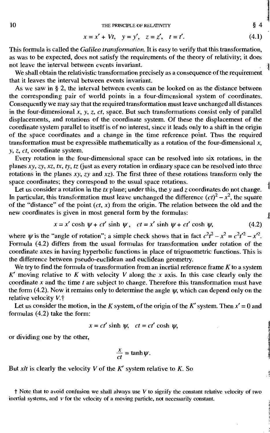
We try to find the formula of transformation from an inertial reference frame A" to a system
K' moving relative to K with velocity V along the x axis. In this case clearly only the
coordinate x and the time t are subject to change. Therefore this transformation must have
the form (4.2). Now it remains only to determine the angle y/, which can depend only on the
relative velocity V.f
Let us consider the motion, in the K system, of the origin of the K' system. Then x' = 0 and
formulas (4.2) take the form:
x = ct' sinh y/, ct — ct' cosh y/,
or dividing one by the other,
— = tanhi//\
ct Y
But xlt is clearly the velocity V of the K' system relative to K. So
t Note that to avoid confusion we shall always use V to signify the constant relative velocity of two
inertial systems, and v for the velocity of a moving particle, not necessarily constant.
§4
THE LORENTZ TRANSFORMATION
11
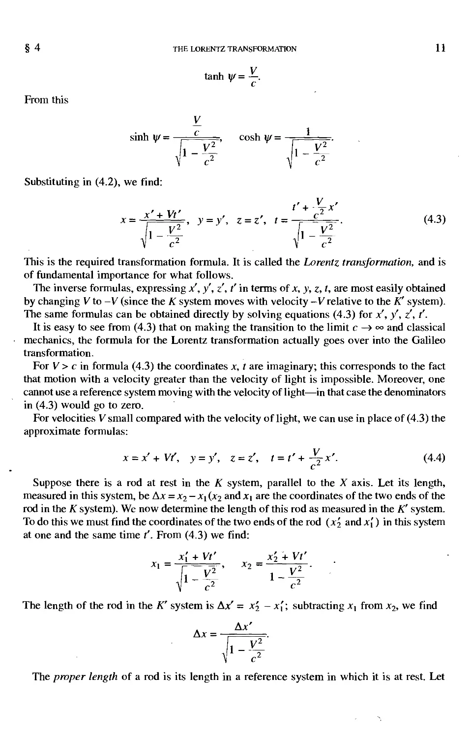
From this
V
tanh w= —.
c
V
r 1
sinh y= . cosh y/ =
Substituting in (4.2), we find:
i-^i i-^
c2 V c2
r + —*'
x = ^=±^, y = /, z = z', t = -T^Lr. (4.3)
^ . f^
This is the required transformation formula. It is called the Lorentz transformation, and is
of fundamental importance for what follows.
The inverse formulas, expressing x, y, z\ t' in terms of x, y, z, t, are most easily obtained
by changing V to -V (since the K system moves with velocity -V relative to the A" system).
The same formulas can be obtained directly by solving equations (4.3) for x', y\ z, t'.
It is easy to see from (4.3) that on making the transition to the limit c -» °° and classical
mechanics, the formula for the Lorentz transformation actually goes over into the Galileo
transformation.
For V > c in formula (4.3) the coordinates x, t are imaginary; this corresponds to the fact
that motion with a velocity greater than the velocity of light is impossible. Moreover, one
cannot use a reference system moving with the velocity of light—in that case the denominators
in (4.3) would go to zero.
For velocities V small compared with the velocity of light, we can use in place of (4.3) the
approximate formulas:
x = x'+Vt', y = y', z = z', t = t'+~x'. (4.4)
c
Suppose there is a rod at rest in the K system, parallel to the X axis. Let its length,
measured in this system, be Ax = x2- xx (x2 and X\ are the coordinates of the two ends of the
rod in the K system). We now determine the length of this rod as measured in the A" system.
To do this we must find the coordinates of the two ends of the rod (x'2 and x[) in this system
at one and the same time t'. From (4.3) we find:
x[ + Vt' x'2 + Vt'
C C
The length of the rod in the K' system is Ax' = x2 ~ x{; subtracting xx from x2, we find
Ax'
Ax =
1--^
c2
The proper length of a rod is its length in a reference system in which it is at rest. Let
12
THE PRINCIPLE OF RELATIVITY
§ 5
us denote it by /0 = Ax, and the length of the rod in any other reference frame K' by I.
Then
/ = /0^1--^. (4.5)
Thus a rod has its greatest length in the reference system in which it is at rest. Its length
in a system in which it moves with velocity Vis decreased by the factor ^jl — V2/c2 . This
result of the theory of relativity is called the Lorentz contraction.
Since the transverse dimensions do not change because of its motion, the volume f~ of a
body decreases according to the similar formula
^=^°-\r?"' (4-6)
where 7^ is the proper volume of the body.
From the Lorentz transformation we can obtain anew the results already known to us
concerning the proper time (§ 3). Suppose a clock to be at rest in the tC system. We take two
events occurring at one and the same point jc', y, z' in space in the A" system. The time
between these events in the A" system is At' = t'2 - t[. Now we find the time At which
elapses between these two events in the K system. From (4.3), we have
t\ + ~~t~X t2 "*" T~X
c c
V c2 r c2
or, subtracting one from the other,
t2-h=At= _,
in complete agreement with (3.1).
Finally we mention another general property of Lorentz transformations which distinguishes
them from Galilean transformations. The latter have the general property of commutativity,
i.e. the combined result of two successive Galilean transformations (with different velocities
Vi and V2) does not depend on the order in which the transformations are performed. On the
other hand, the result of two successive Lorentz transformations does depend, in general, on
their order. This is already apparent purely mathematically from our formal description of
these transformations as rotations of the four-dimensional coordinate system: we know that
the result of two rotations (about different axes) depends on the order in which they are
carried out. The sole exception is the case of transformations with parallel vectors Vi and V2
(which are equivalent to two rotations of the four-dimensional coordinate system about the
same axis).
§ 5. Transformation of velocities
In the preceding section we obtained formulas which enable us to find from the coordinates
of an event in one reference frame, the coordinates of the same event in a second reference
§ 5
TRANSFORMATION OF VELOCITIES
13
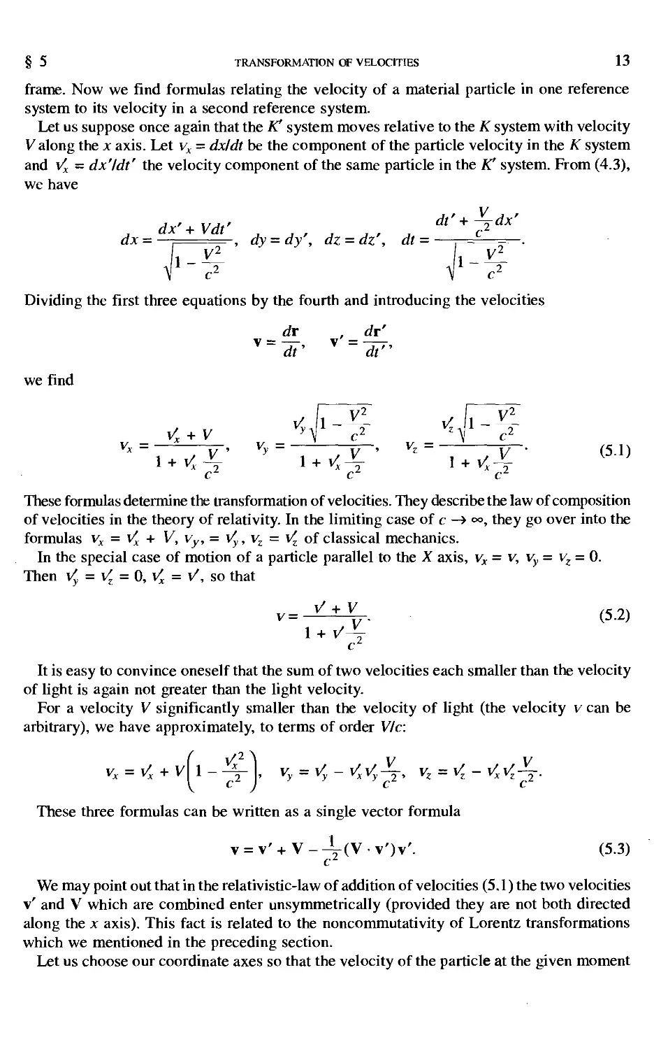
frame. Now we find formulas relating the velocity of a material particle in one reference
system to its velocity in a second reference system.
Let us suppose once again that the FC system moves relative to the K system with velocity
V along the x axis. Let vx = dxldt be the component of the particle velocity in the K system
and Vx = dx'ldt' the velocity component of the same particle in the fC system. From (4.3),
we have
dx'+Vdt' , ,, , , . . dt'+ ~c*dx'
dx = —. dy = dy', dz = dz', dt =
'-£ hvi
Dividing the first three equations by the fourth and introducing the velocities
dr , dx'
V = V =
dt' dt"
we find
vcji-4 vS-*1
vx + v _ 'yT c2 _ ZT c2
Vx = i + *-V Vy= i + ^4' Vz= i + ^-T (51)
c c cz
These formulas determine the transformation of velocities. They describe the law of composition
of velocities in the theory of relativity. In the limiting case of c —> °°, they go over into the
formulas vx = Vx + V, vy, = Vy, vz = Vz of classical mechanics.
In the special case of motion of a particle parallel to the X axis, vx = v, vy= vz = 0.
Then Vy = Vz = 0, Vx = V, so that
v=^r- (5.2)
c
It is easy to convince oneself that the sum of two velocities each smaller than the velocity
of light is again not greater than the light velocity.
For a velocity V significantly smaller than the velocity of light (the velocity v can be
arbitrary), we have approximately, to terms of order Vic:
( V2\ V V
vx = Vx + V\\--4r\, vy = Vy - VxVy-j, vz = Vz- VxVz--j.
These three formulas can be written as a single vector formula
v = v' + V-4-(V-v')v'. (53)
c
We may point out that in the relativistic-law of addition of velocities (5.1) the two velocities
v' and V which are combined enter unsymmetrically (provided they are not both directed
along the x axis). This fact is related to the noncommutativity of Lorentz transformations
which we mentioned in the preceding section.
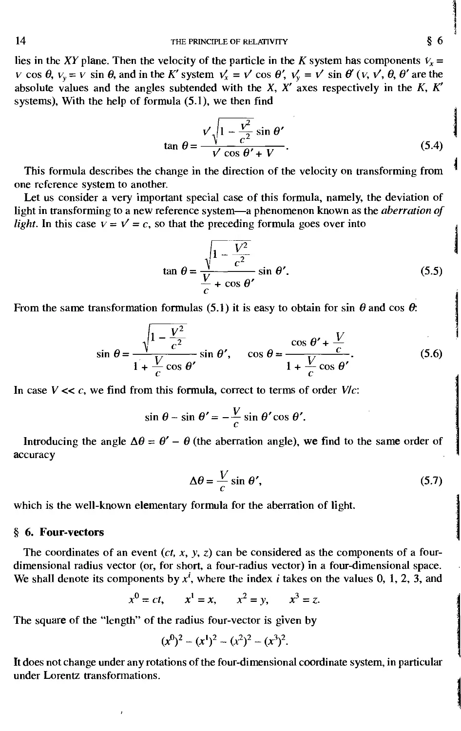
Let us choose our coordinate axes so that the velocity of the particle at the given moment
14
THE PRINCIPLE OF RELATIVITY
§ 6
lies in the XY plane. Then the velocity of the particle in the K system has components Vx =
v cos 6, vy - v sin 6, and in the K' system Vx = V cos 6\ Vy = V sin ff (v, V, 6, 6' are the
absolute values and the angles subtended with the X, X' axes respectively in the K, FC
systems), With the help of formula (5.1), we then find
V 1 - -4- sin 0'
tan ° = —7 CP' i/ ■ <5-4)
v cos 6 + V
This formula describes the change in the direction of the velocity on transforming from
one reference system to another.
Let us consider a very important special case of this formula, namely, the deviation of
light in transforming to a new reference system—a phenomenon known as the aberration of
light. In this case v = V = c, so that the preceding formula goes over into
1--^-
tan 6 = -rj sin 6'. (5.5)
— + cos 6'
c
From the same transformation formulas (5.1) it is easy to obtain for sin 6 and cos ft
1--^ V
1 c2 cos 6'+^-
sin0=—L-r? sin6', cos 6 = tj —. (5.6)
1+ -^-cos 0" l + ~ cos6'
c c
In case V « c, we find from this formula, correct to terms of order Vic:
sin 6 - sin 6' = - — sin 6' cos 6'.
c
Introducing the angle A6 = 6' - 6 (the aberration angle), we find to the same order of
accuracy
A0 = ~ sin 6', (5.7)
which is the well-known elementary formula for the aberration of light.
§ 6. Four-vectors
The coordinates of an event (ct, x, y, z) can be considered as the components of a four-
dimensional radius vector (or, for short, a four-radius vector) in a four-dimensional space.
We shall denote its components by x\ where the index i takes on the values 0, 1,2, 3, and
x -ct, x = x, x =y, x = z.
The square of the "length" of the radius four-vector is given by
(x°f - (x1)2 - (x2)2 - (jt3)2.
It does not change under any rotations of the four-dimensional coordinate system, in particular
under Lorentz transformations.
§ 6 FOUR-VECTORS 15
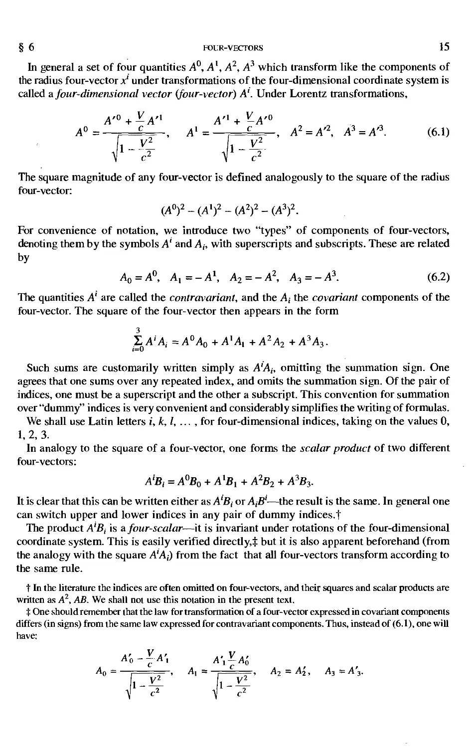
In general a set of four quantities A0, A1, A2, A3 which transform like the components of
the radius four-vector xl under transformations of the four-dimensional coordinate system is
called a four-dimensional vector (four-vector) A'. Under Lorentz transformations,
A'0 + ^A'1 A'1 + ^A'°
A°= , L_ , A'= . c— , A2 = A'2, A3 = A*. (6.1)
c2 V c2
The square magnitude of any four-vector is defined analogously to the square of the radius
four-vector:
(A0)2 - (A1)2 - (A2)2 - (A3)2.
For convenience of notation, we introduce two "types" of components of four-vectors,
denoting them by the symbols A' and A;, with superscripts and subscripts. These are related
by
A0 = A°, Ax=-Al, A2 = -A2, A^ = -A^. (6.2)
The quantities A' are called the contravariant, and the A,- the covariant components of the
four-vector. The square of the four-vector then appears in the form
3
ZA'Ai =A°A0+AlAi +A2A2 +A3A3.
Such sums are customarily written simply as A'Ah omitting the summation sign. One
agrees that one sums over any repeated index, and omits the summation sign. Of the pair of
indices, one must be a superscript and the other a subscript. This convention for summation
over "dummy" indices is very eonvenient and considerably simplifies the writing of formulas.
We shall use Latin letters i, k,l, ... , for four-dimensional indices, taking on the values 0,
1, 2, 3.
In analogy to the square of a four-vector, one forms the scalar product of two different
four-vectors:
A% = A°B0 + AlBi + A2B2 + A3B3.
It is clear that this can be written either as A'B, or AtB'—the result is the same. In general one
can switch upper and lower indices in any pair of dummy indices.!
The product A'Bt is a four-scalar—it is invariant under rotations of the four-dimensional
coordinate system. This is easily verified directly,^ but it is also apparent beforehand (from
the analogy with the square A'Aj) from the fact that all four-vectors transform according to
the same rule.
t In the literature the indices are often omitted on four-vectors, and their squares and scalar products are
written as A2, AB. We shall not use this notation in the present text.
t One should remember that the law for transformation of a four-vector expressed in covariant components
differs (in signs) from the same law expressed for contravariant components. Thus, instead of (6.1), one will
have:
A' ?-A' A' V A'
^o = i . A, = , A2=Ai, A3 = A'3.
16 THE PRINCIPLE OF RELATIVITY § 6
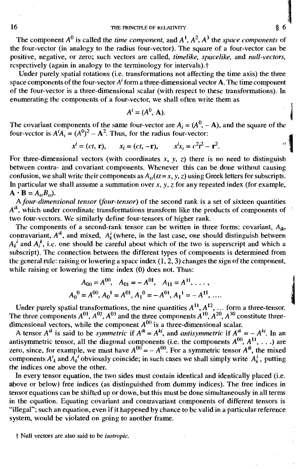
The component A0 is called the time component, and A1, A2, A the space components of
the four-vector (in analogy to the radius four-vector). The square of a four-vector can be
positive, negative, or zero; such vectors are called, timelike, spacelike, and null-vectors,
respectively (again in analogy to the terminology for intervals).!
Under purely spatial rotations (i.e. transformations not affecting the time axis) the three
space components of the four-vector A' form a three-dimensional vector A. The time component
of the four-vector is a three-dimensional scalar (with respect to these transformations). In
enumerating the components of a four-vector, we shall often write them as
A' = (A0, A).
The covariant components of the same four-vector are A, = (A , - A), and the square of the
four-vector is A'At = (A0)2 - A2. Thus, for the radius four-vector:
x' - (ct, r), xi = (ct, -r), xixi = c2/2 - r2. *T
For three-dimensional vectors (with coordinates x, y, z) there is no need to distinguish
between contra- and covariant components. Whenever this can be done without causing
confusion, we shall write their components as Aa(a=x, y, z) using Greek letters for subscripts.
In particular we shall assume a summation over x, y, z for any repeated index (for example,
A-B = AaBa).
A four-dimensional tensor (four-tensor) of the second rank is a set of sixteen quantities
A,k, which under coordinate transformations transform like the products of components of
two four-vectors. We similarly define four-tensors of higher rank.
The components of a second-rank tensor can be written in three forms: covariant, Aik,
contravariant, Alk, and mixed, A'k (where, in the last case, one should distinguish between
Ak' and Ak, i.e. one should be careful about which of the two is superscript and which a
subscript). The connection between the different types of components is determined from
the general rule: raising or lowering a space index (1,2, 3) changes the sign of the component,
while raising or lowering the time index (0) does not. Thus:
A00 = A00, A01=-A01, An=An,...,
A00 = A00,Ao1=A01,A1° = -A01,A11 = -A11, ....
Under purely spatial transformations, the nine quantities A11, A12, ... form a three-tensor.
The three components A01, A02, A03 and the three components A10, A20, A30 constitute three-
dimensional vectors, while the component A00 is a three-dimensional scalar.
A tensor A'k is said to be symmetric if A'k = Akl, and antisymmetric if A,k = - Akl. In an
antisymmetric tensor, all the diagonal components (i.e. the components A00, A11, . . .) are
zero, since, for example, we must have A00 = - A00. For a symmetric tensor A'k, the mixed
components A'k and Ak obviously coincide; in such cases we shall simply write A'k, putting
the indices one above the other.
In every tensor equation, the two sides must contain identical and identically placed (i.e.
above or below) free indices (as distinguished from dummy indices). The free indices in
tensor equations can be shifted up or down, but this must be done simultaneously in all terms
in the equation. Equating covariant and contravariant components of different tensors is
"illegal"; such an equation, even if it happened by chance to be valid in a particular reference
system, would be violated on going to another frame.
t Null vectors are also said to be isotropic.
§6
FOUR-VECTORS
17
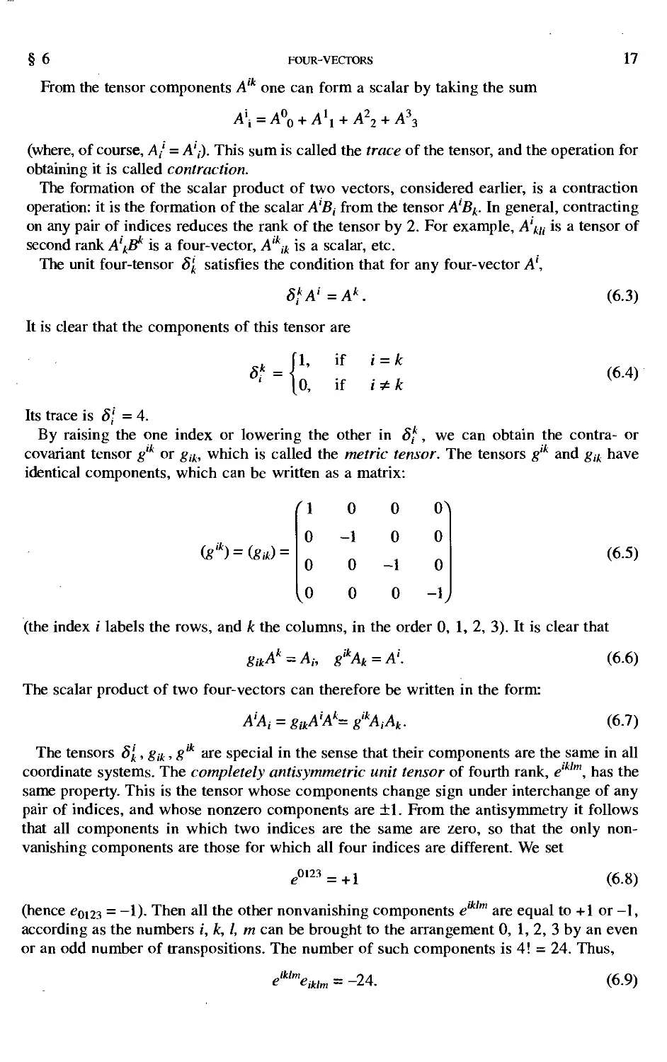
From the tensor components A'k one can form a scalar by taking the sum
A\ = A°0 + A\ + A22 + A\
(where, of course, A- = A',). This sum is called the trace of the tensor, and the operation for
obtaining it is called contraction.
The formation of the scalar product of two vectors, considered earlier, is a contraction
operation: it is the formation of the scalar AlBt from the tensor A'Bk. In general, contracting
on any pair of indices reduces the rank of the tensor by 2. For example, A'*/, is a tensor of
second rank A'^B* is a four-vector, Alkik is a scalar, etc.
The unit four-tensor 8'k satisfies the condition that for any four-vector A',
8kA! =Ak.
It is clear that the components of this tensor are
11, if i = k
8 =
0, if i * k
(6.3)
(6.4)
Its trace is 8\ = 4.
By raising the one index or lowering the other in 8k, we can obtain the contra- or
covariant tensor glk or gik, which is called the metric tensor. The tensors g,k and gik have
identical components, which can be written as a matrix:
or)=(#*) =
(\
o
o
0
-1
0
0
0
0
-1
0
0^
0
0
-1
(6.5)
(the index i labels the rows, and k the columns, in the order 0, 1, 2, 3). It is clear that
gikAk = Ah gikAk = A>. (6.6)
The scalar product of two four-vectors can therefore be written in the form:
«>»*_
A'Ai = glkA'A"= g"AtAk.
(6.7)
The tensors 8'k, gik, g'k are special in the sense that their components are the same in all
coordinate systems. The completely antisymmetric unit tensor of fourth rank, e' m, has the
same property. This is the tensor whose components change sign under interchange of any
pair of indices, and whose nonzero components are ±1. From the antisymmetry it follows
that all components in which two indices are the same are zero, so that the only non-
vanishing components are those for which all four indices are different. We set
e°123 = +l
(6.8)
Jklm
(hence e0123 = -1). Then all the other nonvanishing components e' m are equal to +1 or -1,
according as the numbers i, k, I, m can be brought to the arrangement 0, 1, 2, 3 by an even
or an odd number of transpositions. The number of such components is 4! - 24. Thus,
emmeiklm = -24.
(6.9)
18
THE PRINCIPLE OF RELATIVITY
§ 6
With respect to rotations of the coordinate system, the quantities e'klm behave like the
components of a tensor; but if we change the sign of one or three of the coordinates the
components elklm, being defined as the same in all coordinate systems, do not change,
whereas some of the components of a tensor should change sign. Thus e'klm is, strictly
speaking, not a tensor, but rather a pseudotensor. Pseudotensors of any rank, in particular
pseudoscalars, behave like tensors under all coordinate transformations except those that
cannot be reduced to rotations, i.e. reflections, which are changes in sign of the coordinates
that are not reducible to a rotation.
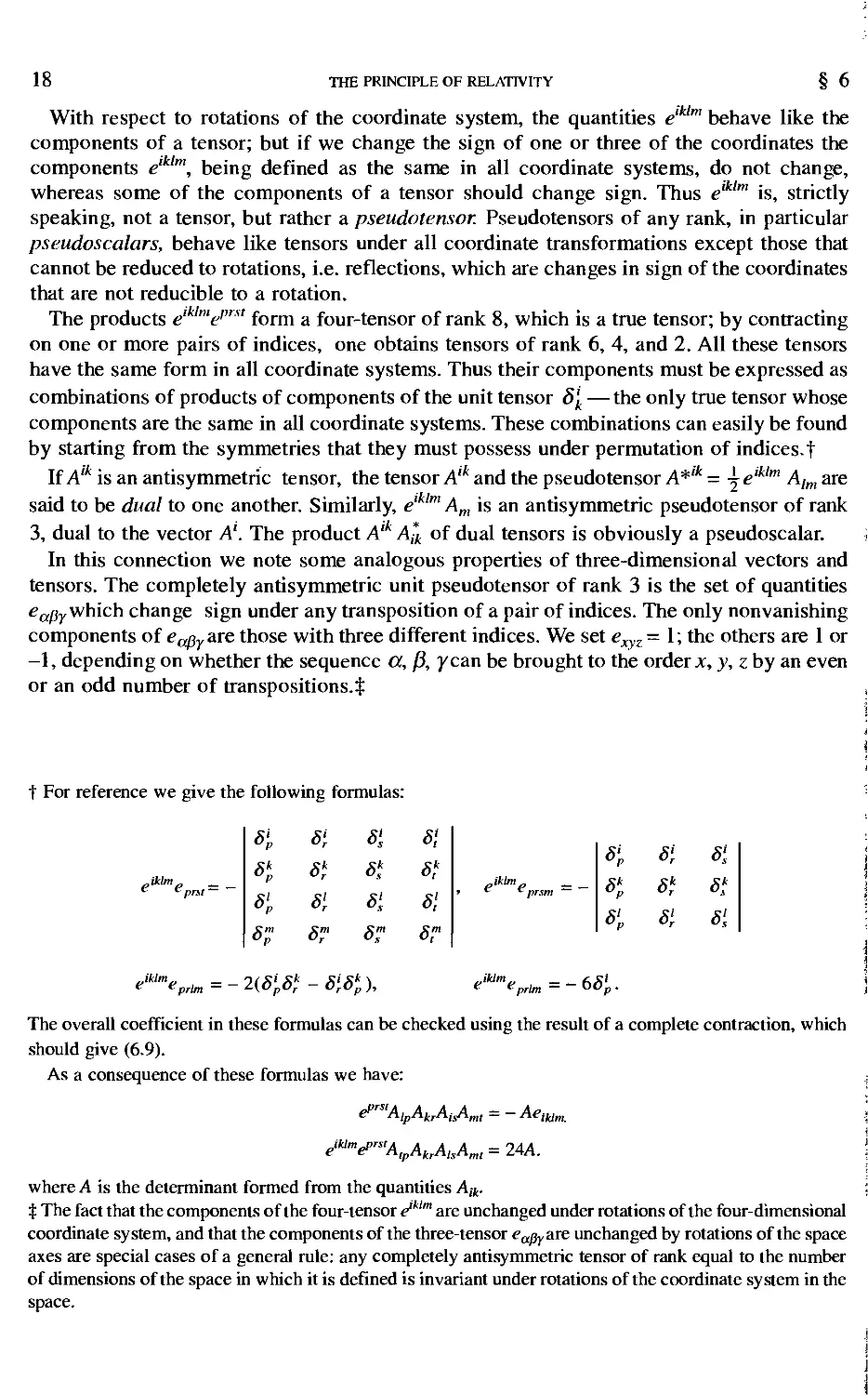
The products elk,mei'rst form a four-tensor of rank 8, which is a true tensor; by contracting
on one or more pairs of indices, one obtains tensors of rank 6, 4, and 2. All these tensors
have the same form in all coordinate systems. Thus their components must be expressed as
combinations of products of components of the unit tensor S'k — the only true tensor whose
components are the same in all coordinate systems. These combinations can easily be found
by starting from the symmetries that they must possess under permutation of indices, t
If A'* is an antisymmetric tensor, the tensor A'k and the pseudotensor A*'k = ^ e'klm Alm are
said to be dual to one another. Similarly, e'klm Am is an antisymmetric pseudotensor of rank
3, dual to the vector A'. The product A'k A*k of dual tensors is obviously a pseudoscalar.
In this connection we note some analogous properties of three-dimensional vectors and
tensors. The completely antisymmetric unit pseudotensor of rank 3 is the set of quantities
eaPr which change sign under any transposition of a pair of indices. The only nonvanishing
components of eapyare those with three different indices. We set exyz - 1; the others are 1 or
—1, depending on whether the sequence a, f5, yean be brought to the order x, y, z by an even
or an odd number of transpositions.$
t For reference we give the following formulas:
Mm _ _
c c prst
jklm _
c prim
s'p s-r si
8kp Skr 8k
SL Si Si
p r s
s™ s^ st
2(SPSH - S'rSkp),
S\
sk
si
ST
„iklm _
» c c prsm
„Mm _ _
c c prlm
-
s'„
P
K
SL
F
6<
%■
si
sk
si
si
sk
si
The overall coefficient in these formulas can be checked using the result of a complete contraction, which
should give (6.9).
As a consequence of these formulas we have:
e AipAicrAisAm, = — Aetklm
eMme>"s'AlpAkrAlsAml = 24A.
where A is the determinant formed from the quantities Aik.
% The fact that the components of the four-tensor e'*'"1 are unchanged under rotations of the four-dimensional
coordinate system, and that the components of the three-tensor eayjj,are unchanged by rotations of the space
axes are special cases of a general rule: any completely antisymmetric tensor of rank equal to the number
of dimensions of the space in which it is defined is invariant under rotations of the coordinate system in the
space.
§ 6
FOUR-VECTORS
19
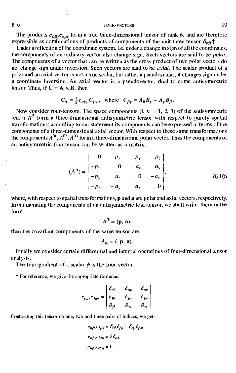
The products eapYexfiv form a true three-dimensional tensor of rank 6, and are therefore
expressible as combinations of products of components of the unit three-tensor 5a^.f
Under a reflection of the coordinate system, i.e. under a change in sign of all the coordinates,
the components of an ordinary vector also change sign. Such vectors are said to be polar.
The components of a vector that can be written as the cross product of two polar vectors do
not change sign under inversion. Such vectors are said to be axial. The scalar product of a
polar and an axial vector is not a true scalar, but rather a pseudoscalar; it changes sign under
a coordinate inversion. An axial vector is a pseudovector, dual to some antisymmetric
tensor. Thus, if C = A x B, then
^a — 2 eafiy ^Py >
where Cpy = ApBy -AyBp.
Now consider four-tensors. The space components (i, k, = 1, 2, 3) of the antisymmetric
tensor A,k form a three-dimensional antisymmetric tensor with respect to purely spatial
transformations; according to our statement its components can be expressed in terms of the
components of a three-dimensional axial vector. With respect to these same transformations
the components A01, A02, A03 form a three-dimensional polar vector. Thus the components of
an antisymmetric four-tensor can be written as a matrix:
(A*) =
0
-Px
-Py
~Pz
Px
0
az
-ay
Py
-az
0
ax
P
a
-a,
(
0
(6.10)
where, with respect to spatial transformations, p and a are polar and axial vectors, respectively.
In enumerating the components of an antisymmetric four-tensor, we shall write them in the
form
A* = (p, a);
then the covariant components of the same tensor are
A,-* = (-P, a).
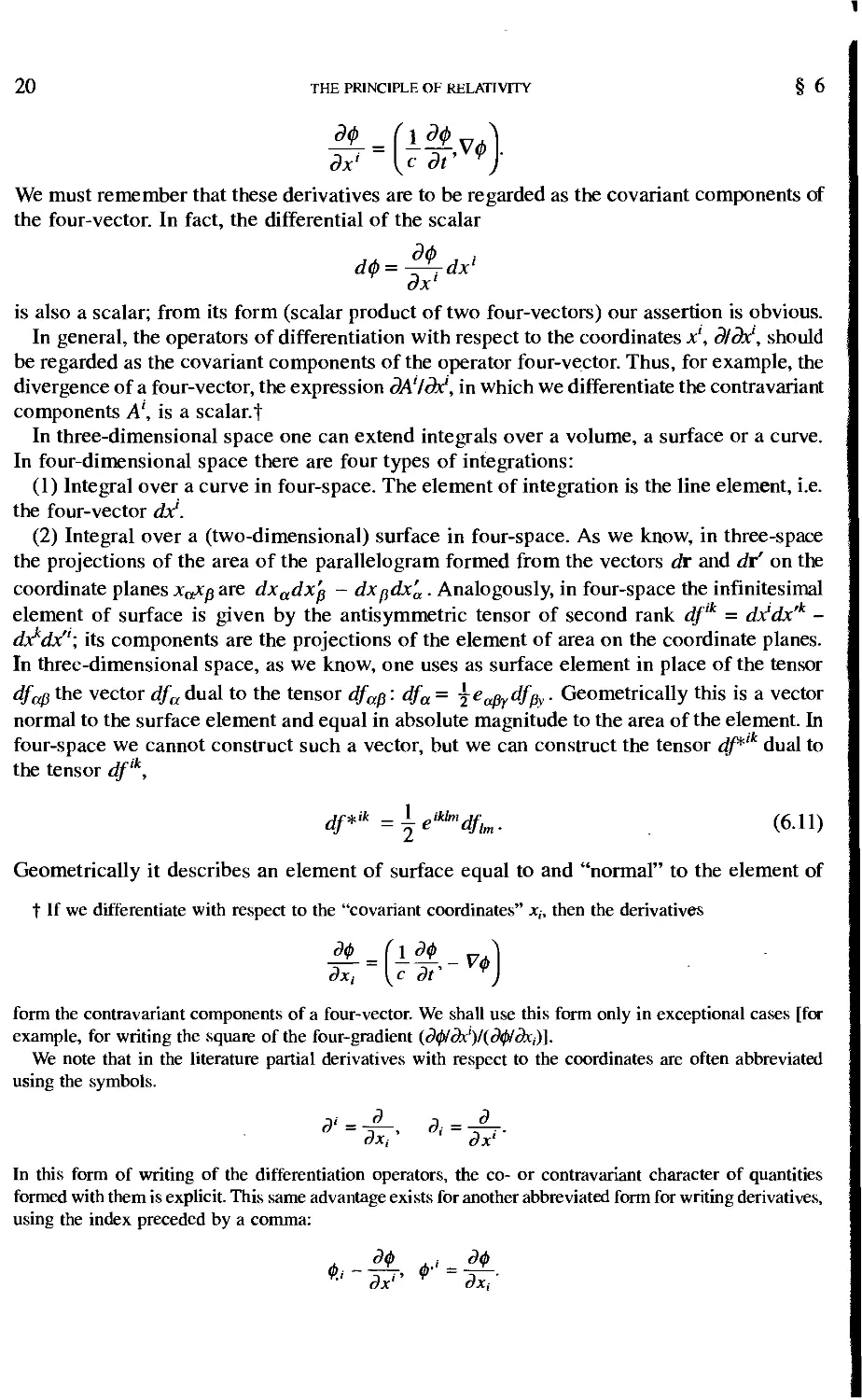
Finally we consider certain differential and integral operations of four-dimensional tensor
analysis.
The four-gradient of a scalar 0 is the four-vector
t For reference, we give the appropriate formulas:
"apYefytv
JaX
■>px
SyX
•'afi
Jpv
Jyv
Contracting this tensor on one, two and three pairs of indices, we get:
eapyeipy = 2¾¾.
eapyeapy = 6.
1
20 THE PRINCIPLE OF RELATIVITY § 6
dx' [c dt' v
We must remember that these derivatives are to be regarded as the covariant components of
the four-vector. In fact, the differential of the scalar
d<t>=—^dx'
ox'
is also a scalar; from its form (scalar product of two four-vectors) our assertion is obvious.
In general, the operators of differentiation with respect to the coordinates x', d/ax1, should
be regarded as the covariant components of the operator four-vector. Thus, for example, the
divergence of a four-vector, the expression dA'Idx1, in which we differentiate the contravariant
components A', is a sealant
In three-dimensional space one can extend integrals over a volume, a surface or a curve.
In four-dimensional space there are four types of integrations:
(1) Integral over a curve in four-space. The element of integration is the line element, i.e.
the four-vector dx1.
(2) Integral over a (two-dimensional) surface in four-space. As we know, in three-space
the projections of the area of the parallelogram formed from the vectors dr and dr' on the
coordinate planes x„xp are dxadx'g - dxpdx'a. Analogously, in four-space the infinitesimal
element of surface is given by the antisymmetric tensor of second rank df'k = dxidx'k -
dx^dx"; its components are the projections of the element of area on the coordinate planes.
In three-dimensional space, as we know, one uses as surface element in place of the tensor
dfap the vector dfa dual to the tensor dfap: dfa = 2ea6ydfpy ■ Geometrically this is a vector
normal to the surface element and equal in absolute magnitude to the area of the element. In
four-space we cannot construct such a vector, but we can construct the tensor dj*' dual to
the tensor df'k,
df*ik =±eik>mdflm. (6.11)
Geometrically it describes an element of surface equal to and "normal" to the element of
t If we differentiate with respect to the "covariant coordinates" xh then the derivatives
dx, {c
9S~V*
form the contravariant components of a four-vector. We shall use this form only in exceptional cases [for
example, for writing the square of the four-gradient (dQldx')l(dQldx,)].
We note that in the literature partial derivatives with respect to the coordinates are often abbreviated
using the symbols.
<?'=-^-, dt =^-.
<?x, dx'
In this form of writing of the differentiation operators, the co- or contravariant character of quantities
formed with them is explicit. This same advantage exists for another abbreviated form for writing derivatives,
using the index preceded by a comma:
A ^ A-' ^
§ 6 FOUR-VECTORS 21
surface df'k; all segments lying in it are orthogonal to all segments in the element df'k. It is
obvious that dfikdf*k = 0.
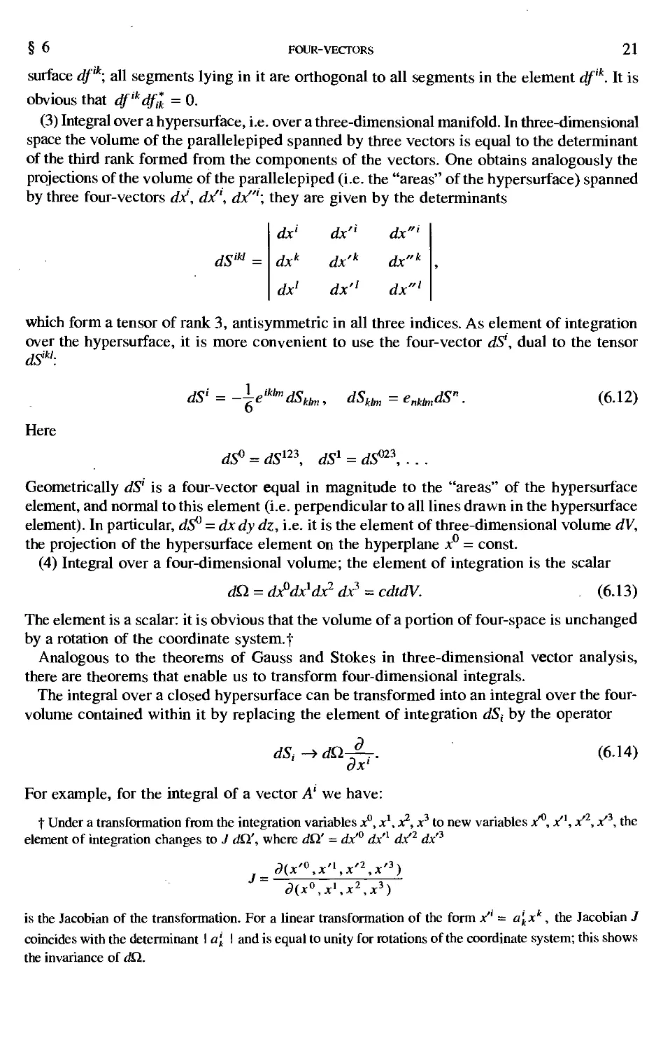
(3) Integral over a hypersurface, i.e. over a three-dimensional manifold. In three-dimensional
space the volume of the parallelepiped spanned by three vectors is equal to the determinant
of the third rank formed from the components of the vectors. One obtains analogously the
projections of the volume of the parallelepiped (i.e. the "areas" of the hypersurface) spanned
by three four-vectors dx', dx", dx'"; they are given by the determinants
dx'
dxk
dx1
dx"
dx'k
dx'1
dx"'
dx"k
dx"1
dSM =
which form a tensor of rank 3, antisymmetric in all three indices. As element of integration
over the hypersurface, it is more convenient to use the four-vector dS1, dual to the tensor
dSikl:
6
Here
dS< = -jreikh>dSklm, dSklm = enklmdS". (6.12)
dSP = dSn\ dS1 = dS023, . . .
Geometrically dS' is a four-vector equal in magnitude to the "areas" of the hypersurface
element, and normal to this element (i.e. perpendicular to all lines drawn in the hypersurface
element). In particular, dS° = dx dy dz, i.e. it is the element of three-dimensional volume dV,
the projection of the hypersurface element on the hyperplane x° = const.
(4) Integral over a four-dimensional volume; the element of integration is the scalar
dQ. = dx°dx1dx2 dx" = cdtdV. (6.13)
The element is a scalar: it is obvious that the volume of a portion of four-space is unchanged
by a rotation of the coordinate system, f
Analogous to the theorems of Gauss and Stokes in three-dimensional vector analysis,
there are theorems that enable us to transform four-dimensional integrals.
The integral over a closed hypersurface can be transformed into an integral over the four-
volume contained within it by replacing the element of integration dS( by the operator
dSi-^dQ^. (6.14)
dx'
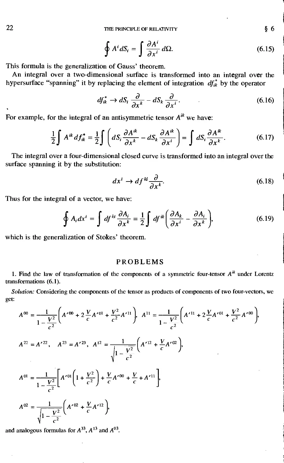
For example, for the integral of a vector A' we have:
t Under a transformation from the integration variables x°, x1, x2, x3 to new variables x'0, x'1, x'2, x'3, the
element of integration changes to J dQ', where dQ' = dx'° dx'1 dx'2 dx'3
d(x'°,xn,x'2,x'3)
d(x°,x\x2,x3)
is the Jacobian of the transformation. For a linear transformation of the form x" = a'kxk , the Jacobian J
coincides with the determinant I a'k I and is equal to unity for rotations of the coordinate system; this shows
the invariance of dQ.
22
THE PRINCIPLE OF RELATIVITY
§ 6
(6.15)
This formula is the generalization of Gauss' theorem.
An integral over a two-dimensional surface is transformed into an integral over the
hypersurface "spanning" it by replacing the element of integration df*k by the operator
df*k -» dSt —7- - dSk
dxk ~~K dx>
For example, for the integral of an antisymmetric tensor A'k we have:
dA*
dxk
^fA'df^lffdS^-dSt9**
dxk
dxl
jdS,
(6.16)
(6.17)
The integral over a four-dimensional closed curve is transformed into an integral over the
surface spanning it by the substitution:
dxl -> dfti^-r.
J dxk
Thus for the integral of a vector, we have:
i**-i*-£=ti*i&-£)
(6.18)
(6.19)
which is the generalization of Stokes' theorem.
PROBLEMS
1. Find the law of transformation of the components of a symmetric four-tensor A'k under Lorentz
transformations (6.1).
Solution: Considering the components of the tensor as products of components of two four-vectors, we
get:
A°° =
1
1--
A'«o + 2^A'm+^-A'n I An=- l
A.u+2VA.01 +V£A.oo
A22=A'22, A23=A'23, Al2=-
X^U'v + ila'A
A01 =•
'1+v1] + va«k, + v+a,„
-2 I c c
A02 = , 1 (a'01 + ^A'n\
and analogous formulas for A , A and A
33 /ll3„„j a03
§ 7 FOUR-DIMENSIONAL VELOCITY 23
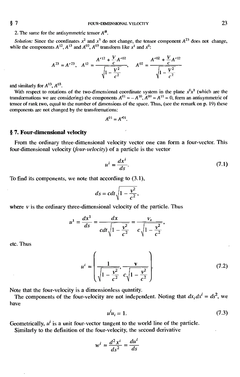
2. The same for the antisymmetric tensor A'k.
Solution: Since the coordinates x2 and x3 do not change, the tensor component A23 does not change,
while the components A12, A13 and A02, A03 transform like xl and jc°:
l 23 =4'23
112 =.
VM2+ VA,02
A,02+ VAM2
A02 =
1--
„2
and similarly for A13, A03.
With respect to rotations of the two-dimensional coordinate system in the plane x°xl (which are the
transformations we are considering) the components A01 = -A10, A00 =An = 0, form an antisymmetric of
tensor of rank two, equal to the number of dimensions of the space. Thus, (see the remark on p. 19) these
components are not changed by the transformations:
A01=A'01.
§ 7. Four-dimensional velocity
From the ordinary three-dimensional velocity vector one can form a four-vector. This
four-dimensional velocity (four-velocity) of a particle is the vector
u' =■
dx'1
ds
(7.1)
To find its components, we note that according to (3.1),
ds = cdtjl -~
where v is the ordinary three-dimensional velocity of the particle. Thus
dx1 dx vr
,i _
ds I J2-
cdtjl ^
c\\-
-*'
etc. Thus
u' =
1
c2 V c2 ;
(7.2)
Note that the four-velocity is a dimensionless quantity.
The components of the four-velocity are not independent. Noting that dXjdx1 = ds , we
have
u'Uj = 1.
Geometrically, u' is a unit four-vector tangent to the world line of the particle.
Similarly to the definition of the four-velocity, the second derivative
(7.3)
w' =
d2xl = du!
ds2 ds
24 THE PRINCIPLE OF RELATIVITY § 7
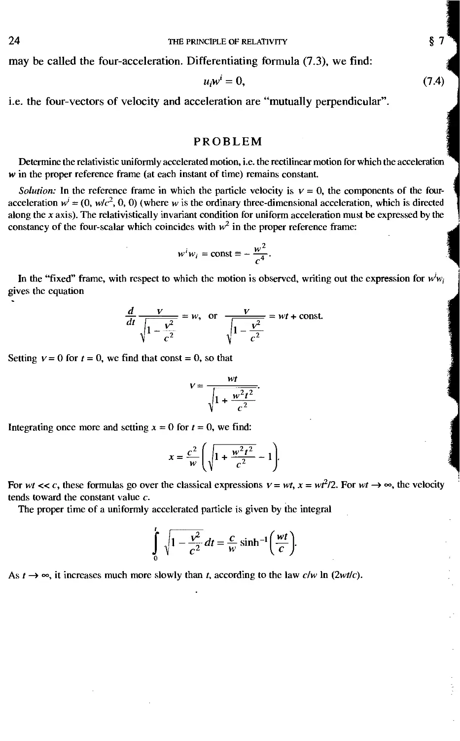
may be called the four-acceleration. Differentiating formula (7.3), we find:
u,W = 0, (7.4)
i.e. the four-vectors of velocity and acceleration are "mutually perpendicular".
PROBLEM
Determine the relativistic uniformly accelerated motion, i.e. the rectilinear motion for which the acceleration
w in the proper reference frame (at each instant of time) remains constant.
Solution: In the reference frame in which the particle velocity is v = 0, the components of the four-
acceleration W = (0, wlc~, 0, 0) (where w is the ordinary three-dimensional acceleration, which is directed
along the x axis). The relativistically invariant condition for uniform acceleration must be expressed by the
constancy of the four-scalar which coincides with w2 in the proper reference frame:
.,.2
w'Wi = const s -
c4
In the "fixed" frame, with respect to which the motion is observed, writing out the expression for Ww-t
gives the equation
d v v
—.—, = w, or , r = wt + const.
Setting v = 0 for t = 0, we find that const = 0, so that
wt
v =
l + *£
Integrating once more and setting x = 0 for t = 0, we find:
w
For wt « c, these formulas go over the classical expressions v = wt, x = wi2/!. For wt —» <*>, the velocity
tends toward the constant value c.
The proper time of a uniformly accelerated particle is given by the integral
o
As t —» <*>, it increases much more slowly than t, according to the law clw In (2wt/c).
CHAPTER 2
RELATIVISTIC MECHANICS
§ 8. The principle of least action
In studying the motion of material particles, we shall start from the Principle of Least
Action. The principle of least action is defined, as we know, by the statement that for each
mechanical system there exists a certain integral S, called the action, which has a minimum
value for the actual motion, so that its variation SS is zero.f
To determine the action integral for a free material particle (a particle not under the
influence of any external force), we note that this integral must not depend on our choice of
reference system, that is, it must be invariant under Lorentz transformations. Then it follows
that it must depend on a scalar. Furthermore, it is clear that the integrand must be a differential
of the first order. But the only scalar of this kind that one can construct for a free particle is
the interval ds, or a ds, where a is some constant. So for a free particle the action must have
the form
b
S = - a J ds,
a
where J is an integral along the world line of the particle between the two particular
events of the arrival of the particle at the initial position and at the final position at definite
times t\ and t2, i.e. between two given world points; and a is some constant characterizing
the particle. It is easy to see that a must be a positive quantity for all particles. In fact, as we
saw in § 3, a jbds has its maximum value along a straight world line; by integrating along
a curved world line we can make the integral arbitrarily small. Thus the integral a J ds with
the positive sign cannot have a minimum; with the opposite sign it clearly has a minimum,
along the straight world line.
The action integral can be represented as an integral with respect to the time
'2
S = \Ldt.
<1
The coefficient L of dt represents the Lagrange function of the mechanical system. With the
aid of (3.1), we find:
t Strictly speaking, the principle of least action asserts that the integral S must be a minimum only for
infinitesimal lengths of the path of integration. For paths of arbitrary length we can say only that S must be
an extremum, not necessarily a minimum. (See Mechanics, § 2.)
25
26
RELATIVISTIC MECHANICS
§ 9
'2
-J
5=-| ac.Jl--4 *.
where vis the velocity of the material particle. Consequently the Lagrangian for the particle
is
L = - ac^Jl - v2^2 .
The quantity a, as already mentioned, characterizes the particle. In classical mechanics
each particle is characterized by its mass m. Let us find the relation between a and m. It can
be determined from the fact that in the limit as c —> °°, our expression for L must go over into
the classical expression L = mv2/!. To carry out this transition we expand L in powers of
vie. Then, neglecting terms of higher order, we find
r /1 v2 (XV2
L = - acjl - -^y ~ - ac + -=—.
Constant terms in the Lagrangian do not affect the equation of motion and can be omitted.
Omitting the constant ac in L and comparing with the classical expression L = mv1!!, we
find that a = mc.
Thus the action for a free material point is
b
S=-melds (8.1)
a
and the Lagrangian is
L=-mc2Jl--4. (8.2)
§ 9. Energy and momentum
By the momentum of a particle we can mean the vector p = dL/dv (dL/dv is the symbolic
representation of the vector whose components are the derivatives of L with respect to the
corresponding components of v). Using (8.2), we find;
"- ^ (9.1)
For small velocities (v « c) or, in the limit as c —» °°, this expression goes over into the
classical p = mv. For v-c, the momentum becomes infinite.
The time derivative of the momentum is the force acting on the particle. Suppose the
velocity of the particle changes only in direction, that is, suppose the force is directed
perpendicular to the velocity. Then
§ 9
ENERGY AND MOMENTUM
27
If the velocity changes only in magnitude, that is, if the force is parallel to the velocity, then
dt , , >a dt' y '
1--^-
c2
We see that the ratio of force to acceleration is different in the two cases.
The energy cf of the particle is defined as the quantity f
<f= p • v - L.
Substituting the expressions (8.2) and (9.1) for L and p, we find
,2
mc
1-^
(9.4)
This very important formula shows, in particular, that in relativistic mechanics the energy
of a free particle does not go to zero for v = 0, but rather takes on a finite value
&= mc2. (9.5)
This quantity is called the rest energy of the particle.
For small velocities (v/c « 1), we have, expanding (9.4) in series in powers of v/c,
&~ mcz + —=—,
which, except for the rest energy, is the classical expression for the kinetic energy of a
particle.
We emphasize that, although we speak of a "particle", we have nowhere made use of the
fact that it is "elementary". Thus the formulas are equally applicable to any composite body
consisting of many particles, where by m we mean the total mass of the body and by v the
velocity of its motion as a whole. In particular, formula (9.5) is valid for any body which is
at rest as a whole. We call attention to the fact that in relativistic mechanics the energy of a
free body (i.e. the energy of any closed system) is a completely definite quantity which is
always positive and is directly related to the mass of the body. In this connection we recall
that in classical mechanics the energy of a body is defined only to within an arbitrary
constant, and can be either positive or negative.
The energy of a body at rest contains, in addition to the rest energies of its constituent
particles, the kinetic energy of the particles and the energy of their interactions with one
another. In other words, mc is not equal to JjriaC2 (where ma are the masses of the particles),
and so m is not equal to Xm„. Thus in relativistic mechanics the law of conservation of mass
does not hold: the mass of a composite body is not equal to the sum of the masses of its parts.
Instead only the law of conservation of energy, in which the rest energies of the particles are
included, is valid.
Squaring (9.1) and (9.4) and comparing the results, we get the following relation between
the energy and momentum of particle:
t See Mechanics, § 6.
28
RELATIVISTIC MECHANICS
§ 9
^-=p2+m2c2. (9.6)
c
The energy expressed in terms of the momentum is called the Hamiltonian function <%":
<%"= c-Jp2 +m2c2. (9.7)
For low velocities, p « mc, and we have approximately
%?~mc2 + 75—,
2m
i.e., except for the rest energy we get the familiar classical expression for the Hamiltonian.
From (9.1) and (9.4) we get the following relation between the energy, momentum, and
velocity of a free particle:
P = ^- (9.8)
For v = c, the momentum and energy of the particle become infinite. This means that a
particle with mass m different from zero cannot move with the velocity of light. Nevertheless,
in relativistic mechanics, particles of zero mass moving with the velocity of light can exist, f
From (9.8) we have for such particles:
P = —. (9.9)
c
The same formula also holds approximately for particles with nonzero mass in the so-called
ultrarelativistic case, when the particle energy ^is large compared to its rest energy mc1.
We now write all our formulas in four-dimensional form. According to the principle of
least action,
b
8S = — mod I ds = 0.
a
To set up the expression for 5S, we note that ds = ^dXjdx' and therefore
b b
SS = - mc I —'-; = - mc I U/ddx'.
a a
Integrating by parts, we obtain
b
SS=- mcUjSx1 \ba + mc f 8xl -j-ds. (9.10)
a
As we know, to get the equations of motion we compare different trajectories between the
same two points, i.e. at the limits (5x')a = (&C1)/, = 0. The actual trajectory is then determined
t For example, light quanta and neutrinos.
§ 9
ENERGY AND MOMENTUM
29
from the condition SS = 0. From (9.10) we thus obtain the equations dujds = 0; that is, a
constant velocity for the free particle in four-dimensional form.
To determine the variation of the action as a function of the coordinates, one must consider
the point a as fixed, so that (Sx')a = 0. The second point is to be considered as variable, but
only actual trajectories are admissible, i.e., those which satisfy the equations of motion.
Therefore the integral in expression (9.10) for 5S is zero. In place of (&% we may write
simply Sx', and thus obtain
6S = -mcuiSxi. (9.11)
The four-vector
dS
P,—j-r (9.12)
is called the momentum four-vector. As we know from mechanics, the derivatives dSldx,
dSldy, dSldz are the three components of the momentum vector p of the particle, while the
derivative -dSldt is the particle energy S. Thus the covariant components of the four-mementum-
are pt = {Sic, - p), while the contravariant components aref
p* = (87c,p). (9.13)
From (9.11) we see that the components of the four-momentum of a free particle are:
p[ = mcu\ (9.14)
Substituting the components of the four-velocity from (7.2), we see that we actually get
expressions (9.1) and (9.4) for p and K
Thus, in relativistic mechanics, momentum and energy are the components of a single
four-vector. From this we immediately get the formulas for transformation of momentum
and energy from one inertial system to another. Substituting (9.13) in the general formulas
(6.1) for transformation of four-vectors, we find:
Px + ~~2^ f + Vn'
"- ==-. Py=P'y, Pz=P'z, ^= \ ^-. (9-15)-
-£ F%
where px, py, pz are the components of the three-dimensional vector p.
From the definition (9.14) of the four-momentum, and the identity u'u; = 1, we have, for
the square of the four-momentum of a free particle:
pipi = m1c1. (9.16)
Substituting the expressions (9.13), we get back (9.6).
By analogy with the usual definition of the force, the force four-vector is defined as the
derivative:
,. dp' du' ,01-
g=^i = mc-dT- (9-17)
t We call attention to a mnemonic for remembering the definition of the physical four-vectors: the
contravariant components are related to the corresponding three-dimensional vectors (r for*', p forp') with
the "right", positive sign.
30
RELATIVISTIC MECHANICS
§ 10
Its components satisfy the identity g{ul = 0. The components of this four-vector are expressed
in terms of the usual three-dimensional force vector f = dp/dt:
8' =
f v
■-£<■'.
(9.18)
The time component is related to the work done by the force.
The relativistic Hamilton-Jacobi equation is obtained by substituting the derivatives
-dS/dx1 for Pi in (9.16):
dx; dx'
or, writing the sum explicitly:
v2 • ,„\2
dS dS llr dS dS 9 9
= g ——r _ ,, = m c
dx' dx
*{dt) (dx) (dy) (
dS}
dz
2 2
= m c .
(9.19)
(9.20)
The transition to the limiting case of classical mechanics in equation (9.19) is made as
follows. First of all we must notice that just as in the corresponding transition with (9.7), the
energy of a particle in relativistic mechanics contains the term mc2, which it does not in
classical mechanics. Inasmuch as the action S is related to the energy by W = - (dS/dt), in
making the transition to classical mechanics we must in place of S substitute a new action
S" according to the relation:
S = S' - mc2t.
Substituting this in (9.20), we find
2 / -,„,\2
1
2m
(jWX + fdsy + (MY _ 1 (dS"
(dx ) + (dy ) + ( dz J 2mc2 ( dt >
dS'
dt
In the limit as c —» °°, this equation goes over into the classical Hamilton—Jacobi equation.
§ 10. Transformation of distribution functions
In various physical problems we have to deal with distribution functions for the momenta
of particles: f(p)dpx dpy dpz is the number of particles having momenta with components in
given intervals dpx, dpy, dpz (or, as we say for brevity, the number of particles in a given
volume element (Pp = dpxdpydpz in "momentum space"). We are then faced with the
problem of finding the law of transformation of the distribution function f(p) when we
transform from one reference system to another.
To solve this problem, we first determine the properties of the "volume element" dpxdpydpz
with respect to Lorentz transformations. If we introduce a four-dimensional coordinate
system, on whose axes are marked the components of the four-momentum of a particle, then
dpxdpydpz can be considered as the zeroth component of an element of the hypersurface
defined by the equation p'p; = m c . The element of hypersurface is a four-vector directed
§ 10
TRANSFORMATION OF DISTRIBUTION FUNCTIONS
31
along the normal to the hypersurface; in our case the direction of the normal obviously
coincides with the direction of the four-vector pt. From this it follows that the ratio
dpxdpydpz
(10.1)
is an invariant quantity, since it is the ratio of corresponding Components of two parallel
four-vectors.f
The number of particles, fdpxdpydpz, is also obviously an invariant, since it does not
depend on the choice of reference frame. Writing it in the form
r/-^ dpxdpydpz
/(PJe -n,
and using the in variance of the ratio (10.1), we conclude that the product/(p)cf is invariant.
Thus the distribution function in the A" system is related to the distribution function in the
K system by the formula
/'(p')=/W£, (10.2)
where p and rf must be expressed in terms of p' and £" by using the transformation formulas
(9.15).
Let us now return to the invariant expression (10.1). If we introduce "spherical coordinates"
in momentum space, the volume element dpxdpydpz becomes p2dpdo, where do is the
element of solid angle around the direction of the vector p. Noting that pdp = ^/cf/c2
[from (9.6)], we have:
p2dpdo pdif do
~~% " c2 '
Thus we find that the expression
pdtfdo (10.3)
is also invariant.
The notion of a distribution function appears in a different aspect in the kinetic theory of
gases: the product/(r, p)dpxdpydpzdVis the number of particles lying in a given volume
element dV and having momenta in definite intervals dp^ dpy, dpz. The function /(r, p) is
t The integration with respect to the element (10.1) can be expressed in four-dimensional form by means
of the 5-function (cf. the footnote on p. 74) as an integration with respect to
- Sipip' - m2c2 )d4p, efp = dp^dpxdp2dpz'. (10.1a)
The four components p' are treated as independent variables (with p° taking on only positive values).
Formula (10.1a) is obvious from the following representation of the delta function appearing in it:
S(p'pt-m2c2) = S\(p0)2 -4-1=^
^0+7) + ^0-7}
(lO.lfc)
where &= c-^p2 + m2c2 . This formula in turn follows from formula (V) of the footnote on p. 74.
32
RELATIVISTIC MECHANICS
§ 11
called the distribution function in phase space (the space of the coordinates and momenta of
the particle), and the product of differentials dt = d3p dV is the element of volume of this
space. We shall find the law of transformation of this function.
In addition to the two reference systems A" and A", we also introduce the frame A"0 in which
the particles with the given momentum are at rest; the proper volume dV0 of the element
occupied by the particles is defined relative to this system. The velocities of the systems K
and A" relative to the system A"0 coincide, by definition, with the velocities v and V which
these particles have in the systems K and A". Thus, according to (4.6), we have
from which
dV_ = ^_
dV *f'
Multiplying this equation by the equation d^p/d^p' = &7cf', we find that
dt^dt', (10.4)
i.e. the element of phase volume is invariant. Since the number of particles f dt is also
invariant, by definition, we conclude that the distribution function in phase space is an
invariant:
/'(r\p')=/(r,p), (10.5)
where r', p' are related to r, p by the formulas for the Lorentz transformation.
§ 11. Decay of particles
Let us consider the spontaneous decay of a body of mass M into two parts with masses m1
and m2. The law of conservation of energy in the decay, applied in the system of reference
in which the body is at rest, givesf
A/= 8^+¾). (11.1)
where efw and #2o are the energies of the emerging particles. Since dl0 > m1 and (½ > ^¾. *e
equality (11.1) can be satisfied only if M> mt + m2, i.e. a body can disintegrate spontaneously
into parts the sum of whose masses is less than the mass of the body. On the other hand, if
M <rri\ + m2 the body is stable (with respect to the particular decay) and does not decay
spontaneously. To cause the decay in this case, we would have to supply to the body from
outside an amount of energy at least equal to its "binding energy" (mt + m2 - M).
Momentum as well as energy must be conserved in the decay process. Since the initial
momentum of the body was zero, the sum of the momenta of the emerging particles must be
zero: p10 + P20 = 0. Consequently pf0 = /?f0, or
t In §§ 11-13 we set c = 1. In other words the velocity of light is taken as the unit of velocity (so that
the dimensions of length and time become the same). This choice is a natural one in relativistic mechanics
and greatly simplifies the writing of formulas. However, in this book (which also contains a considerable
amount of nonrelativistic theory) we shall not usually use this system of units, and will explicitly indicate
when we do.
If c has been set equal to unity in formulas, it is easy to convert back to ordinary units: the velocity is
introduced to assure correct dimensions.
§ 11
DECAY OF PARTICLES
33
^1-mi =^-ml. (11.2)
The two equations (11.1) and (11.2) uniquely determine the energies of the emerging particles:
_ M2 + ml - ml M2 - ml + ml .
^10 " 2M ' ^20 " 2M • U j
In a certain sense the inverse of this problem is the calculation of the total energy M of two
colliding particles in the system of reference in which their total momentum is zero. (This
is abbreviated as the "system of the centre of inertia" or the "C-system".) The computation
of this quantity gives a criterion for the possible occurrence of various inelastic collision
processes, accompanied by a change in state of the colliding particles, or the "creation" of
new particles. A process of this type can occur only if the sum of the masses of the "reaction
products" does not exceed M.
Suppose that in the initial reference system (the "laboratory" system) a particle with mass
mx and energy cfx collides with a particle of mass m2 which is at rest. The total energy of the
two particles is
^=^, + &2 = &l + m2,
and their total momentum is p = Pi + p2 = Pi. Considering the two particles together as a
single composite system, we find the velocity of its motion as a whole from (9.8):
V = ^ = -^ (11.4)
This quantity is the velocity of the C-system with respect to the laboratory system (the L-
system).
However, in determining the mass M, there is no need to transform from one reference
frame to the other. Instead we can make direct use of formula (9.6), which is applicable to
the composite system just as it is to each particle individually. We thus have
M2 = if2 - p2 = (if, + m2)2 - (¾2 - ml),
from which
M2 = ml +ml + 2m2#1. (11.5)
PROBLEMS
1. A particle moving with velocity V dissociates "in flight" into two particles. Determine the relation
between the angles of emergence of these particles and their energies.
Solution: Let if0 be the energy of one of the decay particles in the C-system [i.e. & l0 or tf2o in (H-3)],
if the energy of this same particle in the L-system, and 6 its angle of emergence in the L-system (with
respect to the direction of V). By using the transformation formulas we find:
_ y- Vp cos e
so that
cose=y-y0yr-F (1)
VV^2 -m2
34 RELATIVISTIC MECHANICS
For the determination of ^ from cos 6 we then get the quadratic equation
?2(1- V2 cos2 0)-¾¾¾ Vl - V2 + %l (1 - V2 ) + V2m2cos2 0 = 0,
§ 11
(2)
which has one positive root (if the velocity v0 of the decay particle in the C-system satisfies v0 > V) or two
positive roots (if v0 < V).
The source of this ambiguity is clear from the following graphical construction. According to (9.15), the
momentum components in the L-system are expressed in terms of quantities referring to the C-system by
the formulas
Eliminating 0O, we get
p0 cos0o+<r0v .
Pz = 1 . Py = Po sm 60.
Vi-v2
p2 + (pxVi-v2 -if0vf =P2.
With respect to the variables px.py, this is the equation of an ellipse with semiaxes p0/^jl -V2,p0, whose
centre (the point O in Fig. 3) has been shifted a distance <f0 V/Vl - V2 from the point p = 0 (point A in
Fig. 3).t
(a) V< v0
(b) V>v0
Fig. 3.
If V > P{/^o = v0' ^e point A lies outside the ellipse (Fig. 3b), so that for a fixed angle 6 the vector p (and
consequently the energy <f) can have two different values. It is also clear from the construction that in this
case the angle 6 cannot exceed a definite value 0max (corresponding to the position of the vector p in which
it is tangent to the ellipse). The value of 6max is most easily determined analytically from the condition that
the discriminant of the quadratic equation (2) go to zero:
Po
vT^v2
mV
2. Find the energy distribution of the decay particles in the L-system.
Solution: In the C-system the decay particles are distributed isotropically in direction, i.e. the number of
particles within the element of solid angle do0 = 2n sin 60 A60 is
1
1
dN = -.—don = -=- I d cos On I.
An v 2 v
The energy in the L-system is given in terms of quantities referring to the C-system by
c^0 +p0 Vcos 60
(1)
vT^v2
and runs through the range of values from
*b- Vp0 to y0 + VPo
Vl-V2 Vi-v2
■j- In the classical limit, the ellipse reduces to a circle. (See Mechanics, § 16.)
§ 11 DECAY OF PARTICLES 35
Expressing d I cos ;0O I in terms of dt, we obtain the normalized energy distribution (for each of the two
types of decay particles):
dN=~±— .fi-VtdS.
2Vp0
3. Determine the range of values in the L-system for the angle between the two decay particles (their
separation angle) for the case of decay into two identical particles.
Solution: In the C-system, the particles fly off in opposite directions, so that 0,o = it— 02o = 0o- According
to (5.4), the connection between angles in the C- and L-systems is given by the formulas:
„„* a _ vocos eo + v cot e = _v°cos 6° + V
v0 sin 0oVl-V2' v0sine0Vl-V2
(since V|0 = v20 = v0 in the present case). The required separation angle is 0 = 0, + 02, and a simple
calculation gives:
cote=v2-^ + v^sin2e°
2Vv0 Vl-V2 sin 0O
An examination of the extreme for this expression gives the following ranges of possible values of 0:
forV< Vo.^tan-M-^-Vl-V2 J < 0 < n;
for v0 < V< . V° : 0 < 0 < sin"1 \X~Vl < 4;
forV> , V° :O<0<2tan-1 -^-,/T^V2" <^-.
4. Find the angular distribution in the L-system for decay particles of zero mass.
Solution: According to (5.6) the connection between the angles of emergence in the C- and L-systems for
particles with m = 0 is
a cos 6 - V
cos 60 = :;—7-, ^.
v 1 - V cos 6
Substituting this expression in formula (1) of Problem 2, we find:
dN= (1-V2)d° 2.
4tt(1 - Vcos0)2
5. Find the distribution of separation angles in the L-system for a decay into two particles of zero mass.
Solution: The relation between the angles of emergence, 0,, 02 in the L-system and the angles 0,o = 0o>
020 = it- 0o in the C-system is given by (5.6), so that we have for the separation angle 0 = 0, + 02:
_ 2 V2 - 1 - V2 cos2 0O
cos 0 = ^ z 2-
1 - V2 cos20o
and conversely,
cos ©o^l-^Kcot2^.
Substituting this expression in formula (1) of problem 2, we find:
36
RELATIVISTIC MECHANICS
§ 12
dN=l~V2 do
\6nV sin3 #,V2 -cos2 |*
The angle 0 takes on values from n to &^n = 2 cos ' V.
6. Determine the maximum energy which can be carried off by one of the decay particles, when a particle
of mass M at rest decays into three particles with masses mx, m2, and m3.
Solution: The particle ml has its maximum energy if the system of the other two particles m2 and m3 has
the least possible mass; the latter is equal to the sum m2 + m3 (and corresponds to the case where the two
particles move together with the same velocity). Having thus reduced the problem to the decay of a body
into two parts, we obtain from (11.3):
M2 + m2 - (m2 + nil )2
§ 12. Invariant cross-section
Collision processes are characterized by their invariant cross-sections, which determine the
number of collisions (of the particular type) occurring between beams of colliding particles.
Suppose that we have two colliding beams; we denote by nx and n2 the particle densities
in them (i.e. the numbers of particles per unit volume) and by Vj and v2 the velocities of the
particles. In the reference system in which particle 2 is at rest (or, as one says, in the rest
frame of particle 2), we are dealing with the collision of the beam of particles 1 with a
stationary target. Then according to the usual definition of the cross-section a, the number
of collisions occurring in volume dV in time dt is
dv = ovrei nxn2dVdt.
where vrel is the velocity of particle 1 in the rest system of particle 2 (which is just the
definition of the relative velocity of two particles in relativistic mechanics).
The number dv is by its very nature an invariant quantity. Let us try to express it in a form
which is applicable in any reference system:
dv = Anin2dVdt, (12.1)
where A is a number to be determined, for which we know that its value in the rest frame of
one of the particles is viei o. We shall always mean by cprecisely the cross-section in the rest
frame of one of the particles, i.e. by definition, an invariant quantity. From its definition, the
relative velocity vie\ is also invariant.
In the expression (12.1) the product dVdt is an invariant. Therefore the product Anxn2 must
also be an invariant.
The law of transformation of the particle density n is easily found by noting that the
number of particles in a given volume element dV, ndV, is invariant. Writing ndV = nodV0
(the index 0 refers to the rest frame of the particles) and using formula (4.6) for the
transformation of the volume, we find:
n = -^= (12.2)
or n = n0 '&lm, where / is the energy and m the mass of the particles.
Thus the statement that Anxn2 is invariant is equivalent to the invariance of the expression
A ^ tf2. This condition is more conveniently represented in the form
§ 12 INVARIANT CROSS-SECTION 37
1 °2 _ a 6 i o2
PliP2 ^ 1 ^2 - Pi • P2
where the denominator is an invariant—the product of the four-momenta of the two particles.
In the rest frame of particle 2, we have 'rt2 = m2, p2 = 0, so that the invariant quantity (12.3)
reduces to A. On the other hand, in this frame A = 0¾. Thus in an arbitrary reference
system,
A = cvrA^. (12.4)
To give this expression its final form, we express vieX in terms of the momenta or velocities
of the particles in an arbitrary reference frame. To do this we note that in the rest frame of
particle 2,
1 rni
PuPi = , m2.
v1 - *&
Then
\ iPuPi)
Expressing the quantity pup2 = %\ #2 - Pi • P2 in terms of the velocities V] and v2 by using
formulas (9.1) and (9.4):
1 1 - Vi • v2
PuPi = mxm2
V(l.-vf)(l-v^)
and substituting in (12.5), after some simple transformations we get the following expression
for the relative velocity:
V(vi - v2>2 -(vi xv2)2
vKl = 5 (12.6)
ei 1 - v, • v2
(we note that this expression is symmetric in Vj and v2, i.e. the magnitude of the relative
velocity is independent of the choice of particle used in defining it).
Substituting (12.5) or (12.6) in (12.4) and then in (12.1), we get the final formulas for
solving our problem:
or
dv = ay ' —- nxn2dVdt (12.7)
<SX e2
dv=a V(Vi -v2)2 -(v, xv2)2 nxn2dVdt (12.8)
(W. Pauli, 1933).
If the velocities \x and v2 are collinear, then \xx\2- 0, so that formula (12.8) takes the
form:
dv = 01 v, - v2 I nxn2dVdt. (12.9)
38 RELATIVISTIC MECHANICS § 13
PROBLEM
Find the "element of length" in relativistic "velocity space".
Solution: The required line element dlv is the relative velocity of two points with velocities v and v + dv.
We therefore find from (12.6)
where 6, 0 are the polar angle and azimuth of the direction of v. If in place of v we introduce the new
variable % through the equation v = tanh %, the line element is expressed as:
dll = dx2 + sinh2 x(d62 + sin2 6d(j>2).
From the geometrical point of view this is the line element in three-dimensional Lobachevskii space—
the space of constant negative curvature (see (111.12)).
§ 13. Elastic collisions of particles
Let us consider, from the point of view of relativistic mechanics, the elastic collision of
particles. We denote the momenta and energies of the two colliding particles (with masses
m{ and m2) by pt, ^ and p2, ^2; we use primes for the corresponding quantities after
collision. The laws of conservation of momentum and energy in the collision can be written
together as the equation for conservation of the four-momentum:
P'l*Pl2=P['+P2- (13.1)
From this four-vector equation we construct invariant relations which will be helpful in
further computations. To do this we rewrite (13.1) in the form:
P\ + P2 -Pi"' +Pz'>
and square both sides (i.e. we write the scalar product of each side with itself). Noting that
the squares of the four-momenta p\ and p[l are equal to m\, and the squares of p'2 and/?2'
are equal to m\, we get:
mf + P1/P2 - Pi/P,"' - PzePi' = 0. (13.2)
Similarly, squaring the equation p\ + p'2 - p'2l = p[', we get:
ml + PuPi - P2P2 - PuP'2 = 0- (13.3)
Let us consider the collision in a reference system (the L-system) in which one of the
particles (m2) was at rest before the collision. Then p2 = 0, ^2 = m2, and the scalar products
appearing in (13.2) are:
P1.P2 =^1 m2,
PuP'i' = m2<, (13.4)
PxiPx = *i */- Pi Pi = *i *,'- Pi Pi' cos 0,,
where 6t is the angle of scattering of the incident particle w^. Substituting these expressions
in (13.2) we get:
§ 13 ELASTIC COLLISIONS OF PARTICLES 39
a;'(8i + m2) - if, m2 - m,2
cos 0, = -^-^, —. (13.5)
Pi Pi
Similarly, we find from (13.3):
cose2^+m^rm>\ (13.6)
P\Pi
where 6¼ is the angle between the transferred momentum p2 and the momentum of the
incident particle p,.
The formulas (13.5)-(13.6) relate the angles of scattering of the two particles in the L-
system to the changes in their energy in the collision. Inverting these formulas, we can
express the energies ^i', £f2 in terms of the angles 8\ or 02. Thus, substituting in (13.6)
Pi = y&i2 - mi » Pi = -^(.^2)2 - m2 ^d squaring both sides, we find after a simple
computation:
„. (^+m2)2 +(^2-m,2)cos2e2
(ft + m2 )2 - (if \ - m2) cos2 62
Inversion of formula (13.5) leads in the general case to a very complicated formula for "€{
in terms of Qx.
We note that if m( > m2, i.e. if the incident particle is heavier than the target particle, the
scattering angle 6X cannot exceed a certain maximum value. It is easy to find by elementary
computations that this value is given by the equation
sin0,max=^r, (13-8)
which coincides with the familiar classical result.
Formulas (13.5)-(13.6) simplify in the case when the incident particle has zero mass: mi
= 0, and correspondingly px ~ /j, p[ = cf/. For this case let us write the formula for the
energy of the incident particle after the collision, expressed in terms of its angle of deflection:
gj' = ^2 . (13.9)
1 - cos 0, + ^-
»1
Let us now turn once again to the general case of collision of particles of arbitrary mass.
The collision is most simply treated in the C-system. Designating quantities in this system
by the additional subscript 0, we have p10 - - p20 = p0. From the conservation of momentum,
during the collision the momenta of the two particles merely rotate, remaining equal in
magnitude and opposite in direction. From the conservation of energy, the value of each of
the momenta remains unchanged.
Let x be the angle of scattering in the C-system—the angle through which the momenta
pl0 and p20 are rotated by the collision. This quantity completely determines the scattering
process in the C-system, and therefore also in any other reference system. It is also convenient
in describing the collision in the L-system and serves as the single parameter which remains
undetermined after the conservation of momentum and energy are applied.
We express the final energies of the two particles in the L-system in terms of this parameter.
To do this we return to (13.2), but this time write out the product pnp[' in the C-system:
40 RELATIVISTIC MECHANICS § 13
PtiPi* = «^10^16 - P10 • P10 = ^10 - Pi Cos X = Pi (1 - cos x) + ml
(in the C-system the energies of the particles do not change in the collision: K{'0 = ^f10). We
write out the other two products in the L-system, i.e we use (13.4). As a result we get:
<rfj'- /t = -(Po/m2 )(1 - cos^). We must still express /?(2 in terms of quantities referring
to the L-system. This is easily done by equating the values of the invariant pnp'2 in the L-
and C-systems:
^10¾) ~ Pio ' P20 = #iwi2,
or
4<<Pl +"»i2)(Po +mf) = yi m2 -pI-
Solving the equation for p$, we get:
2 mf {f} - m,2)
Po = 2 2 Ox" (1310)
Thus, we finally have:
m, + mj + 2m2^i
The energy of the second particle is obtained from the conservation law: .¾ + m2 = %{ + tf{.
Therefore
^ = m2+ 2 '2 '' (l-cosa). (13.12)
m, + m£ + 2m2^i
The second terms in these formulas represent the energy lost by the first particle and
transferred to the second particle. The maximum energy transfer occurs for % = n, and is
equal to
x" » -x k' 2m2(^i2-^!2) m ,,v
»2max - m2 -6\ - Slmin - 2 2 0 TT- UJ.10J
m] + rrij + lm2ex
The ratio of the minimum kinetic energy of the incident particle after collision to its initial
energy is:
y/min -mx _ (m, -m2)2 (13 14)
^ - m, m,2 + m| + 2m2^ '
In the limiting case of low velocities (when tf~m + mv^/2), this relation tends to a constant
limit, equal to
^2
m, - m2
m, + m2
In the opposite limit of large energies <fx, relation (13.14) tends to zero; the quantity r^'m
tends to a constant limit. This limit is
m\ + mj
1 ™a 2m2 '
§ 13
ELASTIC COLLISIONS OF PARTICLES
41
Let us assume that m2 » mx, i.e. the mass of the incident particle is small compared to the
mass of the particle at rest. According to classical mechanics the light particle could transfer
only a negligible part of its energy (see Mechanics, § 17). This is not the case in relativistic
mechanics. From formula (13.14) we see that for sufficiently large energies d\ the fraction
of the energy transferred can reach the order of unity. For this it is not sufficient that the
velocity of ml be of order 1, but one must have if\ ~ m2, i.e. the light particle must have an
energy of the order of the rest energy of the heavy particle.
A similar situation occurs for m2 « mx, i.e. when a heavy particle is incident on a light
one. Here too, according to classical mechanics, the energy transfer would be insignificant.
The fraction of the energy transferred begins to be significant only for energies ?x ~ mf/m2 ■
We note that we are not taking simply of velocities of the order of the light velocity, but of
energies large compared to mt, i.e. we are dealing with the ultrarelativistic case.
PROBLEMS
1. The triangle ABC in Fig. 4 is formed by the momentum vector p of the impinging particle and the
momenta p\, p2 of the two particles after the collision. Find the locus of the points C corresponding to all
possible values of p(, p2.
Solution: The required curve is an ellipse whose semiaxes can be found by using the formulas obtained
in problem 1 of § 11. In fact, the construction given there determined the locus of the vectors p in the L-
system which are obtained from arbitrarily directed vectors p0 with given length p0 in the C-system.
(a) m, > m2 (b) m, < m2
Fig. 4.
Since the absolute values of the momenta of the colliding particles are identical in the C-system, and do
not change in the collision, we are dealing with a similar construction for the vector pi, for which
m2V
Po = Pit) - P20 - r -
Vi-v2
in the C-system where V is the velocity of particle m2 in the C-system, coincides in magnitude with the
velocity of the centre of inertia, and is equal to V = pxl{/\ + tn^ (see (11.4)). As a result we find that the
minor and major semiaxes of the ellipse are
™iP\ Po _ m2pi(#i +m2)
j~m\ +m^+2m2H\ ' 4l-V2 mi + ml + 2m2^i
(the first of these is, of course, the same as (13.10)).
For 0, = 0, the vector p[ coincides with p,, so that the distance AB is equal top,. Comparingp, with the
length of the major axis of the ellipse, it is easily shown that the point A lies outside the ellipse if m, > m2
(Fig. 4a), and inside it if m, <m2 (Fig. 4b).
2. Determine the minimum separation angle 0minof two particles after collision of the masses of the two
particles are the same (m, = m2 = m).
42
RELATIVISTIC MECHANICS
§ 14
Solution: If ml = m2, the point A of the diagram lies on the ellipse, while the minimum separation angle
corresponds to the situation where point C is at the end of the minor axis (Fig. 5). From the construction
it is clear that tan (©,„„ 12) is the ratio of the lengths of the semiaxes, and we find:
tan ^-- I*"1
cos e,^ =
1
K + 3m'
Fig. 5.
3. For the collision of two particles of equal mass m, express <'\', S{, % in terms of the angle 6l of
scattering in the L-system.
Solution: Inversion of formula (13.5) in this case gives:
(df, + m) + (K, - m) cos20, .^., _ (#,2 - m2 ) sin2©.
^,'=m- —— =-^-, ^2' = m+ ,
(^,+m)-(Jf,-m)cos2e, 2m + (^, -m)sin2e.
Comparing with the expression for #/ in terms of %:
(1-COS £),
~, -~, 2
we find the angle of scattering in the C-system:
2m - (¾ + 3m) sin2©.
cos x-
2m + (¾ - m) sin2©.
§ 14. Angular momentum
As is well known from classical mechanics, for a closed system, in addition to conservation
of energy and momentum, there is conservation of angular momentum, that is, of the vector
M=Xrxp
where r and p are the radius vector and momentum of the particle; the summation runs over
all the particles making up the system. The conservation of angular momentum is a consequence
of the fact that because of the isotropy of space, the Lagrangian of a closed system does not
change under a rotation of the system as a whole.
By carrying through a similar derivation in four-dimensional form, we obtain the relativistic
expression for the angular momentum. Let x' be the coordinates of one of the particles of the
system. We make an infinitesimal rotation in the four-dimensional space. Under such a
§ 14 ANGULAR MOMENTUM 43
transformation, the coordinates x' take on new values x" such that the differences x" - x' are
linear functions
x'i-xi=xkSak (14.1)
with infinitesimal coefficients 8£l&. The components of the four-tensor 8£ltk are connected
to one another by the relations resulting from the requirement that, under a rotation, the
length of the radius vector must remain unchanged, that is, x[x" = X/x'. Substituting for x"
from (14.1) and dropping terms quadratic in SQ.ik, as infinitesimals of higher order, we find
jJdD.K = 0.
This equation must be fulfilled for arbitrary x1. Since jc"jc* is a symmetric tensor, SQ.ik must
be an antisymmetric tensor (the product of a symmetrical and an antisymmetrical tensor is
clearly identically zero). Thus we find that
«2« = -«2*. (14.2)
The change in the action for an infinitesimal change of coordinates of the initial point a
and the final point b of the trajectory has the form (see 9.11):
<a
(the summation extends over all the particles of the system). In the case of rotation which
we are now considering, &c, = Xly^, and so
6S = -8Clik'Lpixk\ba.
If we resolve the tensor £p'jt* into symmetric and antisymmetric parts, then the first of
these when multiplied by an antisymmetric tensor gives identically zero. Therefore, taking
the antisymmetric part of Yp'x*, we can write the preceding equality in the form
6S = - 6Q.ik \Y,(pixk-pkxi) I* . (14.3)
*a
For a closed system the action, being an invariant, is not changed by a rotation in 4-space.
This means that the coefficients of SQ.ik in (14.3) must vanish:
Kptf - Pkx% = W^ - pV)fl.
Consequently we see that for a closed system the tensor
Mik = XOc'p* - jtV) . (14.4)
This antisymmetric tensor is called the four-tensor of angular momentum. The space components
of this tensor are the components of the three-dimensional angular momentum vector M =
Xrxp:
M23 = MX, -Mn = My, Mn = Mz.
The components A/01, A/02, A/03 form a vector Y(tp - cfr/c2). Thus, we can write the
components of the tensor Af* in the form:
Mik =
I
\ c
M
(14.5)
44
RELATIV1STIC MECHANICS
§ 14
(Compare (6.10).)
Because of the conservation of M'k for a closed system, we have, in particular,
I
fp- —
V c J
= const.
Since, on the other hand, the total energy X ^is also conserved, this equality can be written
in the form
c2Ip
Iff I if
t = const.
(Quantities referring to different particles are taken at the same time i).
From this we see that the point with the radius vector
moves uniformly with the velocity
R=lF (14-6)
2ml a
which is none other than the velocity of motion of the system as a whole. [It relates the total
energy and momentum, according to formula (9.8).] Formula (14.6) gives the relativistic
definition of the coordinates of the centre of inertia of the system. If the velocities of all the
particles are small compared to c, we can approximately set if- mc so that (14.6) goes over
into the usual classical expression
We note that the components of the vector (14.6) do not constitute the space components
of any four-vector, and therefore under a transformation of reference frame they do not
transform like the coordinates of a point. Thus we get different points for the centre of
inertia of a given system with respect to different reference frames.
PROBLEM
Find the connection between the angular momentum M of a body (system of particles) in the reference
frame K in which the body moves with velocity V, and its angular momentum M<0) in the frame A"0 in which
the body is at rest as a whole; in both cases the angular momentum is defined with respect to the same
point—the centre of inertia of the body in the system K0.%
t We note that whereas the classical formula for the centre of inertia applies equally well to interacting
and non-interacting particles, formula (14.6) is valid only if we neglect interaction. In relativistic mechanics,
the definition of the centre of inertia of a system of interacting particles requires us to include explicitly the
momentum and energy of the field produced by the particles.
X We remind the reader that although in the system Kn (in which Xp = 0) the angular momentum is
independent of the choice of the point with respect to which it is defined, in the K system (in which Xp *■
0) the angular momentum does depend on this choice (see Mechanics, § 9).
§ 14
ANGULAR MOMENTUM
45
Solution: The A"0 system moves relative to the K system with velocity V; we choose its direction for the
x axis. The components of M'k that we want transform according to the formulas (see problem 2 in § 6):
^(0)i2 + V_ M{om M(0)i3 + V_ Miom
M12 = , c , Mn = ■ £— , M23 = M(0>23.
i_vi KZyK
T c2
Since the origin of coordinates was chosen at the centre of inertia of the body (in the A"0 system), in that
system X ? r = 0, and since in that system £p = 0, A/*0*02 = A/*0*03 = 0. Using the connection between the
components of M'k and the vector M, we find for the latter:
Mr = A/f, A/v = r y Afr = ■ '
y
CHAPTER 3
CHARGES IN ELECTROMAGNETIC FIELDS
§ 15. Elementary particles in the theory of relativity
The interaction of particles can be described with the help of the concept of a field of
force. Namely, instead of saying that one particle acts on another, we may say that the
particle creates a field around itself; a certain force then acts on every other particle located
in this field. In classical mechanics, the field is merely a mode of description of the physical
phenomenon—the interaction of particles. In the theory of relativity, because of the finite
velocity of propagation of interactions, the situation is changed fundamentally. The forces
acting on a particle at a given moment are not determined by the positions at that same
moment. A change in the position of one of the particles influences other particles only after
the lapse of a certain time interval. This means that the field itself acquires physical reality.
We cannot speak of a direct interaction of particles located at a distance from one another.
Interactions can occur at any one moment only between neighbouring points in space (contact
interaction). Therefore we must speak of the interaction of the one particle with the field,
and of the subsequent interaction of the field with the second particle.
We shall consider two types of fields, gravitational and electromagnetic. The study of
gravitational fields is left to Chapters 10 to 14 and in the other chapters we consider only
electromagnetic fields.
Before considering the interactions of particles with the electromagnetic field, we shall
make some remarks concerning the concept of a "particle" in relativistic mechanics.
In classical mechanics one can introduce the concept of a rigid body, i.e., a body which is
not deformable under any conditions. In the theory of relativity it should follow similarly
that we would consider as rigid those bodies whose dimensions all remain unchanged in the
reference system in which they are at rest. However, it is easy to see that the theory of
relativity makes the existence of rigid bodies impossible in general.
Consider, for example, a circular disk rotating around its axis, and let us assume that it is
rigid. A reference frame fixed in the disk is clearly not inertial. It is possible, however, to
introduce for each of the infinitesimal elements of the disk an inertial system in which this
element would be at rest at the moment; for different elements of the disk, having different
velocities, these systems will, of course, also be different. Let us consider a series of line
elements, lying along a particular radius vector. Because of the rigidity of the disk, the
length of each of these segments (in the corresponding inertial system of reference) will be
the same as it was when the disk was at rest. This same length would be measured by an
observer at rest, past whom this radius swings at the given moment, since each of its
segments is perpendicular to its velocity and consequently a Lorentz contraction does not
occur. Therefore the total length of the radius as measured by the observer at rest, being the
46
§ 16
FOUR-POTENTIAL OF A HELD
47
sum of its segments, will be the same as when the disk was at rest. On the other hand, the
length of each element of the circumference of the disk, passing by the observer at rest at a
given moment, undergoes a Lorentz contraction, so that the length of the whole circumference
(measured by the observer at rest as the sum of the lengths of its various segments) turns out
to be smaller than the length of the circumference of the disk at rest. Thus we arrive at the
result that due to the rotation of the disk, the ratio of circumference to radius (as measured
by an observer at rest) must change, and not remain equal to 2n. The absurdity of this result
shows that actually the disk cannot be rigid, and that in rotation it must necessarily undergo
some complex deformation depending on the elastic properties of the material of the disk.
The impossibility of the existence of rigid bodies can be demonstrated in another way.
Suppose some solid body is set in motion by an external force acting at one of its points. If
the body were rigid, all of its points would have to be set in motion at the same time as the
point to which the force is applied; if this were not so the body would be deformed.
However, the theory of relativity makes this impossible, since the force at the particular
point is transmitted to the others with a finite velocity, so that all the points cannot begin
moving simultaneously.
From this discussion we can draw certain conclusions concerning the treatment of
"elementary" particles, i.e. particles whose state we assume to be described completely by
giving its three coordinates and the three components of its velocity as a whole. It is obvious
that if an elementary particle had finite dimensions, i.e. if it were extended in space, it could
not be deformable, since the concept of deformability is related to the possibility of independent
motion of individual parts of the body. But, as we have seen, the theory of relativity shows
that it is impossible for absolutely rigid bodies to exist.
Thus we come to the conclusion that in classical (non-quantum) relativistic mechanics, we
cannot ascribe finite dimensions to particles which we regard as elementary. In other words,
within the framework of classical theory elementary particles must be treated as points.t
§ 16. Four-potential of a field
For a particle moving in a given electromagnetic field, the action is made up of two parts:
the action (8.1) for the free particle, and a term describing the interaction of the particle with
the field. The latter term must contain quantities characterizing the particle and quantities
characterizing the field.
It turns out$ that the properties of a particle with respect to interaction with the
electromagnetic field are determined by a single parameter—the charge e of the particle, which can
be either positive or negative (or equal to zero). The properties of the field are characterized
by a four-vector A;, the four-potential, whose components are functions of the coordinates
and time. These quantities appear in the action function in the term
t Quantum mechanics makes a fundamental change in this situation, but here again relativity theory
makes it extremely difficult to introduce anything other than point interactions.
t The assertions which follow should be regarded as being, to a certain extent, the consequence of
experimental data. The form of the action for a particle in an electromagnetic field cannot be fixed on the
basis of general considerations alone (such as, for example, the requirement of relativistic invariance). The
latter would permit the occurrence in formula (16.1) of terms of the form \Ads, where A is a scalar function.
To avoid any misunderstanding, we repeat that we are considering classical (and not quantum) theory,
and therefore do not include effects which are related to the spins of particles.
48 CHARGES IN ELECTROMAGNETIC FIELDS § 16
b
e C
— I Atdx',
where the functions A, are taken at points on the world line of the particle. The factor lie has
been introduced for convenience. It should be pointed out that, so long as we have no
formulas relating the charge or the potentials with already known quantities, the units for
measuring these new quantities can be chosen arbitrarily, t
Thus the action function for a charge in an electromagnetic field has the form
b
S=[(-mcds--Aidxt\ (16.1)
a
The three space components of the four-vector A' form a three-dimensional vector A
called the vector potential of the field. The time component is called the scalar potential; we
denote it by A0 = ¢. Thus
A' = (0, A). (16.2)
Therefore the action integral can be written in the form
5=1 -meds + — A • dr - e<pdt
a
Introducing dr/dt = v, and changing to an integration over t,
S= f \-mc2 /l --^- + jA-\-e(p dt. (16.3)
The integrand is just the Lagrangian for a charge in an electromagnetic field:
L = - mc2 1 - -4- + - A • v - e<j>. (16.4)
This function differs from the Lagrangian for a free particle (8.2) by the terms (e/c) A • v -
e<j), which describe the interaction of the charge with the field.
The derivative dL/dv is the generalized momentum of the particle; we denote it by P.
Carrying out the differentiation, we find
= , ^ + —A = p + —A. (16.5)
v^ c v c
' c2
Here we have denoted by p the ordinary momentum of the particle, which we shall refer to
simply as its momentum.
From the Lagrangian we can find the Hamiltonian function for a particle in a field from
the general formula
■j- Concerning the establishment of these units, see § 27.
§ 17
EQUATIONS OF MOTION OF A CHARGE IN A FIELD
49
Substituting (16.4), we get
dL
^ A. IMLC\
+ e0. (16.6)
v2
c2
!" 2
However, the Hamiltonian must be expressed not in terms of the velocity, but rather in terms
of the generalized momentum of the particle.
From (16.5) and (16.6) it is clear that the relation between 3P- e0 and P - (e/c)A is the
same as the relation between 'X and p in the absence of the field, i.e.
p^__mV + (p-fA)\ (,6,,
or else
v2
,2„4
Se = lm2c4 + c2(P--Aj + e<j>. (16.8)
For low velocities, i.e. for classical mechanics, the Lagrangian (16.4) goes over into
Z, = ^r- + -A-v-^. (16.9)
£ c
In this approximation
p = mv = P--A,
c
and we find the following expression for the Hamiltonian:
*^(p-7A)2+* (1610)
Finally we write the Hamilton-Jacobi equation for a particle in an electromagnetic field.
It is obtained by replacing, in the equation for the Hamiltonian, P by dSldr, and !%"
by -(dS/dt). Thus we get from (16.7)
(vS-fA) --Lf^L + ef) +m2c2=0. (16.11)
§ 17. Equations of motion of a charge in a field
A charge located in a field not only is subjected to a force exerted by the field, but also in
turn acts on the field, changing it. However, if the charge e is not large, the action of the
charge on the field can be neglected. In this case, when considering the motion of the charge
in a given field, we may assume that the field itself does not depend on the coordinates or
the velocity of the charge. The precise conditions which the charge must fulfil in order to be
50
CHARGES IN ELECTROMAGNETIC FIELDS
§ 17
considered as small in the present sense, will be clarified later on (see § 75). In what follows
we shall assume that this condition is fulfilled.
So we must find the equations of motion of a charge in a given electromagnetic field.
These equations are obtained by varying the action, i.e. they are given by the Lagrange
equations
d_(dL\ = dL
dt(dv) dr' K }
where L is given by formula (16.4).
The derivative dL/dv is the generalized momentum of the particle (16.5). Further, we
write
/9/
-=— = VL = — grad A • v - e grad ¢.
dr c
But from a formula of vector analysis.
grad (a • b) = (a - V)b + (b • V)a + b x curl a + a x curl b,
where a and b are two arbitrary vectors. Applying this formula to A • v, and remembering
that differentiation with respect to r is carried out for constant v, we find
/9/
-=— = —(v • V) A + — v x curl A - e grad ¢.
dr c c
So the Lagrange equation has the form:
■j\ P+ -A j =-(v- V)A + -vxcurlA-egrad0.
But the total differential (dA/dt) dt consists of two parts: the change (dA/dt) dt of the vector
potential with time at a fixed point in space, and the change due to motion from one point
in space to another at distance dr. This second part is equal to (dr ■ V)A. Thus
dA dA
— = —+ (y.V)A.
Substituting this in the previous equation, we find
-~ = - -^ e grad <b + - v x curl A. (17.2)
dt c dt c
This is the equation of motion of a particle in an electromagnetic field. On the left side
stands the derivative of the particle's momentum with respect to the time. Therefore the
expression on the right of (17.2) is the force exerted on the charge in an electromagnetic
field. We see that this force consists of two parts. The first part (first and second terms on
the right side of 17.2) does not depend on the velocity of the particle. The second part (third
term) depends on the velocity, being proportional to the velocity and perpendicular to it.
The force of the first type, per unit charge, is called the electric field intensity; we denote
it by E. So by definition,
§ 17 EQUATIONS OF MOTION OF A CHARGE IN A FIELD 51
E =
c dt
grad ¢.
(17.3)
The factor of v/c in the force of the second type, per unit charge, is called the magnetic
field intensity. We designate it by H. So by definition,
H = curl A.
(17.4)
If in an electromagnetic field, E * 0 but H - 0, then we speak of an electric field; if E =
0 but H # 0, then the field is said to be magnetic. In general, the electromagnetic field is a
superposition of electric and magnetic fields.
We note that E is a polar vector while H is an axial vector.
The equation of motion of a charge in an electromagnetic field can now be written as
dp
dt
= eE + -vxH.
(17.5)
The expression on the right is called the Lorentz force. The first term (the force which the
electric field exerts on the charge) does not depend on the velocity of the charge, and is
along the direction of E. The second part (the force exerted by the magnetic field on the
charge) is proportional to the velocity of the charge and is directed perpendicular to the
velocity and to the magnetic field H.
For velocities small compared with the velocity of light, the momentum p is approximately
equal to its classical expression mv, and the equation of motion (17.5) becomes
dt c
(17.6)
Next we derive the equation for the rate of change of the kinetic energy of the particlet
with time, i.e. the derivative
^kin _ d_
dt dt
mc
1 -
v1
It is easy to check that
d'(DV,
kin =y,dP
dt dt'
Substituting dp/dt from (17.5) and noting that v x H • v = 0, we have
■ = eE • v.
^kin
dt
(17.7)
The rate of change of the kinetic energy is the work done by the field on the particle per
unit time. From (17.7) we see that this work is equal to the product of the velocity by the
force which the electric field exerts on the charge. The work done by the field during a time
dt, i.e. during a displacement of the charge by dr, is clearly equal to eE ■ dr.
■j- By "kinetic" we mean the energy (9.4), which includes the rest energy.
52
CHARGES IN ELECTROMAGNETIC FIELDS
§ 18
We emphasize the fact that work is done on the charge only by the electric field; the
magnetic field does no work on a charge moving in it. This is connected with the fact that
the force which the magnetic field exerts on a charge is always perpendicular to the velocity
of the charge.
The equations of mechanics are invariant with respect to a change in sign of the time, that
is, with respect to interchange of future and past. In other words, in mechanics the two time
directions are equivalent. This means that if a certain motion is possible according to the
equations of mechanics, then the reverse motion is also possible, in which the system passes
through the same states in reverse order.
It is easy to see that this is also valid for the electromagnetic field in the theory of
relativity. In this case, however, in addition to changing t into - t, we must reverse the sign
of the magnetic field. In fact it is easy to see that the equations of motion (17.5) are not
altered if we make the changes
t-+-t, E->E, H->-H. (17.8)
According to (17.3) and (17.4), this does not change the scalar potential, while the vector
potential changes sign;
0->0, A ->- A. (17.9)
Thus, if a certain motion is possible in an electromagnetic field, then the reversed motion
is possible in a field in which the direction of H is reversed.
PROBLEM
Express the acceleration of a particle in terms of its velocity and the electric and magnetic field intensities.
Solution: Substitute in the equation of motion (17.5) p = v V^Jc1, and take the expression for d^^Jdt
from (17.7). As a result, we get
§ 18. Gauge invariance
Let us consider to what extent the potentials are uniquely determined. First of all we call
attention to the fact that the field is characterized by the effect which it produces on the
motion of a charge located in it. But in the equation of motion (17.5) there appear not the
potentials, but the field intensities E and H. Therefore two fields are physically identical if
they are characterized by the same vectors E and H.
If we are given potentials A and <j>, then these uniquely determine (according to (17.3) and
(17.4)) the fields E and H. However, to one and the same field there can correspond different
potentials. To show this, let us add to each component of the potential the quantity - dfld^,
where/is an arbitrary function of the coordinates and the time. Then the potential Ak goes
over into
Ak=Ak-jL. (18.1)
As a result of this change there appears in the action integral (16.1) the additional term
§ 19 CONSTANT ELECTROMAGNETIC HELD 53
<LJ*Ldxk=d{lf\ (18.2)
c dxk \c )
which is a total differential and has no effect on the equations of motion. (See Mechanics,
§2.)
If in place of the four-potential we introduce the scalar and vector potentials, and in place
of x1, the coordinates ct, x, y, z, then the four equations (18.1) can be written in the form
A' = A + grad/, 0' = 0-^-. (18.3)
It is easy to check that electric and magnetic fields determined from equations (17.3) and
(17.4) actually do not change upon replacement of A and 0 by A' and <j/, defined by (18.3).
Thus the transformation of potentials (18.1) does not change the fields. The potentials are
therefore not uniquely defined; the vector potential is determined to within the gradient of
an arbitrary function, and the scalar potential to within the time derivative of the same
function.
In particular, we see that we can add an arbitrary constant vector to the vector potential,
and an arbitrary constant to the scalar potential. This is also clear directly from the fact that
the definitions of E and H contain only derivatives of A and ¢, and therefore the addition of
constants to the latter does not affect the field intensities.
Only those quantities have physical meaning which are invariant with respect to the
transformation (18.3) of the potentials; in particular all equations must be invariant under
this transformation. This invariance is called gauge invariance (in German, eichinvarianz)A
This nonuniqueness of the potentials gives us the possibility of choosing them so that they
fulfil one auxiliary condition chosen by us. We emphasize that we can set one condition,
since we may choose the function/in (18.3) arbitrarily. In particular, it is always possible
to choose the potentials so that the scalar potential $ is zero. If the vector potential is not
zero, then it is not generally possible to make it zero, since the condition A = 0 represents
three auxiliary conditions (for the three components of A).
§ 19. Constant electromagnetic field
By a constant electromagnetic field we mean a field which does not depend on the time.
Clearly the potentials of a constant field can be chosen so that they are functions only of the
coordinates and not of the time. A constant magnetic field is equal, as before, to H - curl A.
A constant electric field is equal to
E = -grad0. (19.1)
Thus a constant electric field is determined only by the scalar potential and a constant
magnetic field only by the vector potential.
We saw in the preceding section that the potentials are not uniquely determined. However,
it is easy to convince oneself that if we describe the constant electromagnetic field in terms
of potentials which do not depend on the time, then we can add to the scalar potential,
without changing the fields, only an arbitrary constant (not depending on either the coordinates
t We emphasize that this is related to the assumed constancy of e in (18.2). Thus the gauge invariance
of the equations of electrodynamics (see below) and the conservation of charge are closely related to one
another.
54
CHARGES IN ELECTROMAGNETIC FIELDS
§ 19
or the time). Usually $ is subjected to the additional requirement that it has a definite value
at some particular point in space; most frequently 0 is chosen to be zero at infinity. Thus the
arbitrary constant previously mentioned is determined, and the scalar potential of the constant
field is thus determined uniquely.
On the other hand, just as before, the vector potential is not uniquely determined even for
the constant electromagnetic field; namely, we can add to it the gradient of an arbitrary
function of the coordinates.
We now determine the energy of a charge in a constant electromagnetic field. If the field
is constant, then the Lagrangian for the charge also does not depend explicitly on the time.
As we know, in this case the energy is conserved and coincides with the Hamiltonian.
According to (16.6), we have
% _ mc + ^ (19 2)
Thus the presence of the field adds to the energy of the particle the term e<j), the potential
energy of the charge in the field. We note the important fact that the energy depends only on
the scalar and not on the vector potential. This means that the magnetic field does not affect
the energy of the charge. Only the electric field can change the energy of the particle.
This is related to the fact that the magnetic field, unlike the electric field, does no work on
the charge.
If the field intensities are the same at all points in space, then the field is said to be
uniform. The scalar potential of a uniform electric field can be expressed in terms of the
field intensity as
0 = - E - r. (19.3)
In fact, since E = const, V(E • r) = (E ■ V) r = E.
The vector potential of a uniform magnetic field can be expressed in terms of its field
intensity as
A = JH x r. (19.4)
In fact, recalling that H = const, we obtain with the aid of well-known formulas of vector
analysis:
curl (H x r) = H div r - (H • V)r = 2H
(noting that div r = 3).
The vector potential of a uniform magnetic field can also be chosen in the form
Ax = - Hy, Ay = Az = 0 (19.5)
(the z axis is along the direction of H). It is easily verified that with this choice for A we have
H = curl A. In accordance with the transformation formulas (18.3), the potentials (19.4) and
(19.5) differ from one another by the gradient of some function: formula (19.5) is obtained
from (19.4) by adding V/, where /= -xyH/2.
PROBLEM
Give the variational principle for the trajectory of a particle (Maupertuis' principle) in a constant
electromagnetic field in relativistic mechanics.
§ 20
MOTION IN A CONSTANT UNIFORM ELECTRIC FIELD
55
Solution: Maupertuis' principle consists in the statement that if the energy of a particle is conserved
(motion in a constant field), then its trajectory can be determined from the variational equation
5 J P dr = 0,
where P is the generalized momentum of the particle, expressed in terms of the energy and the coordinate
differentials, and the integral is taken along the trajectory of the particle.■)• Substituting P = p + (e/c)A and
noting that the directions of p and dr coincide, we have
5 J (pdl + -^Adr]=0,
where dl = sjdr2 is the element of arc. Determining p from
2 2 2
p + m cL
we obtain finally
'ijlW7
m2c2dl + -h-dr\ = 0.
§ 20. Motion in a constant uniform electric field
Let us consider the motion of a charge e in a uniform constant electric field E. We take the
direction of the field as the X axis. The motion will obviously proceed in a plane, which we
choose as the XY plane. Then the equations of motion (17.5) become
px = eE, py =0
(where the dot denotes differentiation with respect to t), so that
px =eEt, py=p0. (20.1)
The time reference point has been chosen at the moment when px = 0; p0 is the momentum
of the particle at that moment.
The kinetic energy of the particle (the energy omitting the potential energy in the field) is
^kin = c^jm2c2 +p2 ■ Substituting (20.1), we find in our case
^kin = V'nV + c2p2 + (ceEt)2 = ^1+ (ceEt)2 , (20.2)
where (¾ is the energy at t = 0.
According to (9.8) the velocity of the particle is v = pc2/^kin. For the velocity vx = x we
have therefore
dx pxc2 c2eEt
dt ^kin ^/¾2 + {deEt)2 '
Integrating, we find
■j- See Mechanics, § 44.
56 CHARGES IN ELECTROMAGNETIC FIELDS § 21
X = 7E V^^+ (ceEt)2 ■ (20.3)
The constant of integration we set equal to zero.f
For determining y, we have
dy
dt
PyC2 PoC2
^kin ^,2 + (ceEt)2 '
v-p°c^h-4ceEt]
from which
>-eE~~ Uo J' (20'4)
We obtain the equation of the trajectory by expressing t in terms of y from (20.4) and
substituting in (20.3). This gives:
x = %cosh-^. (20.5)
eE p0c
Thus in a uniform electric field a charge moves along a catenary curve.
If the velocity of the particle is v « c, then we can set p0 = mv0, 'ff0 = mc2, and expand
(20.5) in series in powers of 1/c. Then we get, to within terms of higher order,
eE
x = =- y2 + const,
2mv£
that is, the charge moves along a parabola, a result well known from classical mechanics.
§ 21. Motion in a constant uniform magnetic field
We now consider the motion of a charge e in a uniform magnetic field H. We choose the
direction of the field as the Z axis. We rewrite the equation of motion
p=-vxH
c
in another form, by substituting for the momentum, from (9.8),
„ cfv
c
where ff is the energy of the particle, which is constant in the magnetic field. The equation
of motion then goes over into the form
^f = fvxH (2,,,
or, expressed in terms of components,
vx = (OVy, vy = -covx, vz = 0, (21.2)
t This result (for p0 = 0) coincides with the solution of the problem of relativistic motion with constant
"proper acceleration" w0 = eElm (see the problem in § 7). For the present case, the constancy of the
acceleration is related to the fact that the electric field does not change for Lorentz transformations having
velocities V along the direction of the field (see § 24).
§ 21 MOTION IN A CONSTANT UNIFORM MAGNETIC FIELD 57
where we have introduced the notation
ecH
(0=^-. (21.3)
We multiply the second equation of (21.2) by i, and add it to the first:
A
dt
-tM* + ivy) = ~ i(°(v* + *vy)>
so that
vx + ivy = ae ,m',
where a is a complex constant. This can be written in the form a = v^e '" where v0t and a
are real. Then
and, separating real and imaginary parts, we find
vx = vq, cos (ox + a), vy = - v0t sin (ox + a). (21.4)
The constants v0„ and a are determined by the initial conditions; a is the initial phase, and
as for v0„ from (21.4) it is clear that
t = ^ + ^,
v0
that is, %, is the velocity of the particle in the XY plane, and stays constant throughout the
motion.
From (21.4) we find, integrating once more,
x = x0 + r sin (ox + a), y = y0+ r cos (cot + a), (21.5)
where
CO ecH eH
(p, is the projection of the momentum on the XY plane). From the third equation of (21.2),
we find vz = v0z and
z = Zo+*V- (21-7)
From (21.5) and (21.7), it is clear that the charge moves in a uniform magnetic field along
a helix having its axis along the direction of the magnetic field and with a radius r given by
(21.6). The velocity of the particle is constant. In the special case where voz = 0, that is, the
charge has no velocity component along the field, it moves along a circle in the plane
perpendicular to the field.
The quantity CO, as we see from the formulas, is the angular frequency of rotation of the
particle in the plane perpendicular to the field.
If the velocity of the particle is low, then we can approximately set if = mc2. Then the
frequency CO is changed to
eH
CO=—. (21.8)
mc
58 CHARGES IN ELECTROMAGNETIC FIELDS § 21
We shall now assume that the magnetic field remains uniform but varies slowly in magnitude
and direction. Let us see how the motion of a charged particle changes in this case.
We know that when the conditions of the motion are changed slowly, certain quantities
called adiabatic invariants remain constant. Since the motion in the plane perpendicular to
the magnetic field is periodic, the adiabatic invariant is the integral
taken over a complete period of the motion, i.e. over the circumference of a circle in the
present case (P, is the projection of the generalized momentum on the plane perpendicular
to Hf). Substituting P, = p, + (e/c) A, we have:
In the first term we note that pt is constant in magnitude and directed along dr; we apply
Stokes' theorem to the second term and write curl A = H:*
'-'"-t"*1-^- <219>
From this we see that, for slow variation of H, the tangential momentumpt varies proportionally
to 4h.
This result can also be applied to another case, when the particle moves along a helical
path in a magnetic field that is not strictly homogeneous (so that the field varies little over
distances comparable with the radius and step of the helix). Such a motion can be considered
as a motion in a circular orbit that shifts in the course of time, while relative to the orbit the
field appears to change in time but remain uniform. One can then state that the component
of the momentum transverse to the direction of the field varies according to the law: pt = 4CH,
where C is a constant and H is a given function of the coordinates. On the other hand, just
as for the motion in any constant magnetic field, the energy of the particle (and consequently
the square of its momentum p2) remains constant. Therefore the longitudinal component of
the momentum varies according to the formula:
p! = P2 - P2 = P2 - CH(x, y, z). (21.10)
Since we should always have pf > 0, we see that penetration of the particle into regions
of sufficiently high field (CH > p2) is impossible. During motion in the direction of increasing
field, the radius of the helical trajectory decreases proportionally to p/H (i.e. proportionally
t See Mechanics, § 49. In general the integrals j p dq, taken over a period of the particular coordinate
q, are adiabatic invariants. In the present case the periods for the two coordinates in the plane perpendicular
to H coincide, and the integral I which we have written is the sum of the two corresponding adiabatic
invariants. However, each of these invariants individually has no special significance, since it depends on the
(non-unique) choice of the vector potential of the field. The nonuniqueness of the adiabatic invariants
which results from this is a reflection of the fact that, when we regard the magnetic field as uniform over
all of space, we cannot in principle determine the electric field which results from changes in H, since it will
actually depend on the specific conditions at infinity.
*By inspecting the direction of motion of a charge along the orbit for a given direction of H, we observe
that it is counterclockwise if we look along H. Hence the negative sign in the second term.
§ 22 MOTION OF A CHARGE IN CONSTANT UNIFORM ELECTRIC AND MAGNETIC FIELDS 59
to 1/V7/), and the step proportionally to p/. On reaching the boundary where pl vanishes,
the particle is reflected; while continuing to rotate in the same direction it begins to move
opposite to the gradient of the field.
Inhomogeneity of the field also leads to another phenomenon—a slow transverse shift
(drift) of the guiding centre of the helical trajectory of the particle (the name given to the
centre of the circular orbit); problem 3 of the next section deals with this question.
PROBLEM
Determine the frequency of vibration of a charged spatial oscillator, placed in a constant, uniform
magnetic field; the proper frequency of vibration of the oscillator (in the absence of the field) is (¾.
Solution: The equations of forced vibration of the oscillator in a magnetic field (directed along the z axis)
are:
, eH . .. , eH . .. 2
x+a>i.x = v, y+aiy = x, z + (Oiz = 0-
v me v mc v
Multiplying the second equation by i and combining with the first, we find
f+fl>g£=-i—£,
* °' mc '
where £=x + iy. From this we find that the frequency of vibration of the oscillator in a plane perpendicular
to the field is
-fs ♦*(£)**■
eH
fi>= Jfi>n +-H -=^ I ±~ -
Lmc
If the field H is weak, this formula goes over into
co = cOq ± eHITmc.
The vibration along the direction of the field remains unchanged.
§ 22. Motion of a charge in constant uniform electric and magnetic fields
Finally we consider the motion of a charge in the case where there are present both electric
and magnetic fields, constant and uniform. We limit ourselves to the case where the velocity
of the charge v « c, so that its momentum p = mv; as we shall see later, it is necessary for
this that the electric field be small compared to the magnetic.
We choose the direction of H as the Z axis, and the plane passing through H and E as the
YZ plane. Then the equation of motion
can be written in the form
mv = eE + —v x H
c
mx = — yH, my = eEy xH, mz = eEz. (22.1)
From the third equation we see that the charge moves with uniform acceleration in the Z
direction, that is,
60
CHARGES IN ELECTROMAGNETIC FIELDS
§ 22
Multiplying the second equation of (22.1) by i and combining with the first, we find
ii • • • • £?
—r(x + iy) + ia(x + iy) = i —
dt m
(a = eHlmc). The integral of this equation, where x + iy is considered as the unknown, is
equal to the sum of the integral of the same equation without the right-hand term and a
particular integral of the equation with the right-hand term. The first of these is ae~,cot, the
second is eEylmOi = cEy/H. Thus
x + iy = ae~
cEy
H
The constant a is in general complex. Writing it in the form a = be'x, with real b and a, we
see that since a is multiplied by e~ltat, we can, by a suitable choice of the time origin, give
the phase a any arbitrary value. We choose this so that a is real. Then breaking up x + iy
into real and imaginary parts, we find
cE
x = a cos at + —fj-, y = - a sin at. (22.3)
H
A\.t=Q the velocity is along the X axis.
We see that the components of the velocity of the particle are periodic functions of the
time. Their average values are:
- c£v
* = -JP ^ = 0-
This average velocity of motion of a charge in crossed electric and magnetic fields is often
called the electrical drift velocity. Its direction is perpendicular to both fields and independent
of the sign of the charge. It can be written in vector form as:
- _ cExH (22 4)
All the formulas of this section assume that the velocity of the particle is small compared
with the velocity of light; we see that for this to be so, it is necessary in particular that the
electric and magnetic fields satisfy the condition
E
~H
while the absolute magnitudes of Ey and H can be arbitrary.
Integrating equation (22.3) again, and choosing the constant of integration so that at t = 0,
x = y = 0, we obtain
cE
x = — sin at + —rrt; y = — (cos at - 1). (22.6)
a H J a v
Considered as parametric equations of a curve, these equations define a trochoid. Depending
on whether a is larger or smaller in absolute value than the quantity cEy/H, the projection
of the trajectory on the plane XY has the forms shown in Figs. 6a and 6b, respectively.
If a = - cEyIH, then (22.6) becomes
cEy
x = —^r(at - sin at),
an
-W«h (22.5)
§ 22
MOTION OF A CHARGE IN CONSTANT UNIFORM ELECTRIC AND MAGNETIC FIELDS
cEv
y = —rr(l - cos cot)
J CO//
that is, the projection of the trajectory on the XY plane is a cycloid (Fig. 6c).
y
61
(22.7)
Fig. 6.
PROBLEMS
1. Determine the relativistic motion of a charge in parallel uniform electric and magnetic fields.
Solution: The magnetic field has no influence on the motion along the common direction of E and H (the
z axis), which therefore occurs under the influence of the electric field alone; therefore according to § 20
we find:
2 = ¾.. ^,, = ^3 + (^)2
eE
For the motion in the xy plane we have the equation
or
px = ^Hvy, py=-^Hvx,
d , ■ . . eH, iefic , . N
777(Px + tpy) =-i—(vx +ivy) = --j—(Px+iPy)-
L ekin
dty
Consequently
px+ipx=pte v,
where p, is the constant value of the projection of the momentum on the xy plane, and the auxiliary quantity
0 is defined by the relation
dQ = eHc
dt
62
CHARGES IN ELECTROMAGNETIC FIELDS
§ 22
from which
c'=7isinh7K (1)
Furthermore we have:
-it ^kin,- ■•, eH d(x + iy)
Px + iPy=P,e "=-5-(jc + iy) = — y-~~,
so that
x = — sin ¢, y = ~tfi cos ^- (2)
Formulas (1), (2) together with the formula
z=Scoshf^ (3>
determine the motion of the particle in parametric form. The trajectory is a helix with radius cp,/eH and
monotonically increasing step, along which the particle moves with decreasing angular velocity Q =
eHcl&tjn and with a velocity along the z axis which tends toward the value c.
2. Determine the relativistic motion of a charge in electric and magnetic fields which are mutually
perpendicular and equal in magnitude.!
Solution: Choosing the z axis along H and the y axis along E and setting E = W, we write the equations
of motion:
4±=<LEvy, %L = eE{\-Z\ 4^ = 0
dt c y dt \ c y dt
and, as a consequence of them, formula (17.7),
From these equations we have:
pz = const, "g y,,- cpx = const = a.
Also using the equation
kin
c* — **r-r^ J. r*- n * —
2 -c2pl = (If^ + cpx)(^ -cpx) = c2p2 + e2
(where e = m c + c p\= const), we find:
a
and so
kin +cPx =—(c7Py +e2),
a c2p2 + e2
P* = ~ o7 +
2 2a '
a c2p2 + e2
2c 2ac
t The problem of motion in mutually perpendicular fields E and H which are not equal in magnitude can,
by a suitable transformation of the reference system, be reduced to the problem of motion in a pure electric
or a pure magnetic field (see § 25).
§ 22 MOTION OF A CHARGE IN CONSTANT UNIFORM ELECTRIC AND MAGNETIC FIELDS 63
Furthermore, we write
c kin
from which
^- = eE^xn ~ ^^-) = «£(*!- - «3Px ) = «£«.
=(1+#
2^=11+^-^+^3 (1)
To determine the trajectory, we make a transformation of variables in the equations
dx c2px
~dt = «^kin ""
to the variable py by using the relation dt = ^ndpyleEa, after which integration gives the formulas:
?(-'♦£)''
'=2fe[-'^j^*sfe^- «>
C2 2 _ P;C2
y_ 2aeEP^ Z~ eEaPy'
Formulas (1) and (2) completely determine the motion of the particle in parametric form (parameter py). We
call attention to the fact that the velocity increases most rapidly in the direction perpendicular to E and H
(the x axis).
3. Determine the velocity of drift of the guiding centre of the orbit of a nonrelativistic charged particle
in a quasihomogeneous magnetic field (H. Alfven, 1940).
Solution: We assume first that the particle is moving in a circular orbit, i.e. its velocity has no longitudinal
component (along the field). We write the equation of the trajectory in the form r = R(r) + £(r), where R(r)
is the radius vector of the guiding centre (a slowly varying function of the time), while £(r) is a rapidly
oscillating quantity describing the rotational motion about the guiding centre. We average the force
(elc) rxH(r) acting on the particle over a period of the oscillatory (circular) motion (compare Mechanics,
§ 30). We expand the function H(r) in this expression in powers of §:
H(r) = H(R) + (C-V)H(R).
On averaging, the terms of first order in £(r) vanish, while the second-degree terms give rise to an additional
force
f=££x(£V)H.
For a circular orbit
£=<»£xn, £=-^,
where n is a unit vector along H; the frequency co= eHlmc; v± is the velocity of the particle in its circular
motion. The average values of products of components of the vector £, rotating in a plane (the plane
perpendicular to n), are:
£«£/3 = 2¾ ^a/3>
where Sap is the unit tensor in this plane. As a result we find:
f=—2^(nxV)xH.
64 CHARGES IN ELECTROMAGNETIC FIELDS § 23
Because of the equations div H = 0 and curl H = 0 which the constant field H(R) satisfies, we have:
(n x V) x H = -n div H + (n • V)H + n x (V x H) = (n • V)H = H(n • V)n + n(n • VH).
We are interested in the force transverse to n, giving rise to a shift of the orbit; it is equal to
f=__i(n.V)„ = ^v,
where p is the radius of curvature of the force line of the field at the given point, and v is a unit vector
directed from the centre of curvature to this point.
The case where the particle also has a longitudinal velocity vj| (along n) reduces to the previous case if
we go over to a reference frame which is rotating about the instantaneous centre of curvature of the force
line (which is the trajectory of the guiding centre) with angular velocity vj/p. In this reference system the
particle has no longitudinal velocity, but there is an additional transverse force, the centrifugal force
mitf/p. Thus the total transverse force is
P
■*4'
This force is equivalent to a constant electric field of strength t±/e. According to (22.4) it causes a drift
of the guiding center of the orbit with a velocity
Vd = dp-
if + -y- I v x n.
The sign of this velocity depends on the sign of the charge.
§ 23. The electromagnetic field tensor
In § 17, we derived the equation of motion of a charge in a field, starting from the
Lagrangian (16.4) written in three-dimensional form. We now derive the same equation
directly from the action (16.1) written in four-dimensional notation.
The principle of least action states
b
8S = 6 I i-mc ds-£- Arfx' 1=0. (23.1)
Noting that ds = -JdXjdx', we find (the limits of integration a and b are omitted for
brevity):
6S = - J [mcdXi^' + ^Aiddx1 + ^SAtdx'} = 0.
We integrate the first two terms in the integrand by parts. Also, in the first term we set dxj
ds = U;, where m, are the components of the four-velocity. Then
J
medu: Sx' + — Sx' dA: 8A: dx' -
c c '
mcUj + —A; \6x'
= 0. (23.2)
The second term in this equation is zero, since the integral is varied with fixed coordinate
values at the limits. Furthermore:
§ 23 THE ELECTROMAGNETIC FIELD TENSOR 65
and therefore
1
mcduidx' + — „ ,' Sx'dxk - — '
c dxk
c dxk
dx'dx1* = 0
In the first term we write dut = (ditj/ds) ds, in the second and third, dx' = u'ds. In addition,
in the third term we interchange the indices i and k (this changes nothing since the indices
i and k are summed over). Then
f I dut
J[mCW
e\ dAk_
c\ dx'
dAi \uk
dx'ds = 0.
ds c\ dx' dxk
In view of the arbitrariness of 8x*, it follows that the integrand is zero, that is,
mc
ds
We now introduce the notion
duf _ e(dAk dAi
'{'dx7' " Jx1'
dAk dAj
Flt =
dx' dxk
(23.3)
The antisymmetric tensor Fik is called the electromagnetic field tensor. The equation of
motion then takes the form:
du e vik
mc—j— = — F iii,.
ds c
(23.4)
These are the equations of motion of a charge in four-dimensional form.
The meaning of the individual components of the tensor Fik is easily seen by substituting
the values A, = (0, - A) in the definition (23.3). The result can be written as a matrix in which
the index i = 0, 1, 2, 3 labels the rows, and the index k the columns:
Fu =
( 0
-Ex
-Ey
-E,
-H
Hr
Hy
-Hx
0
F =
( 0
Ex
Ey
yEz
-Er
- ^y
0 -H,
~EZ
0 -Hr
Hr
. (23.5)
More briefly, we can write (see § 6):
F;, = (E,H), F* = (-E,H).
Thus the components of the electric and magnetic field strengths are components of the
same electromagnetic field four-tensor.
Changing to three-dimensional notation, it is easy to verify that the three space components
(i = 1, 2, 3) of (23.4) are identical with the vector equation of motion (17.5), while the time
component (i = 0) gives the work equation (17.7). The latter is a consequence of the
equations of motion; the fact that only three of the four equations are independent can also
easily be found directly by multiplying both sides of (23.4) by it'. Then the left side of the
equation vanishes because of the orthogonality of the four-vectors u' and du(/ds, while the
right side vanishes because of the antisymmetry of Fik.
66
CHARGES IN ELECTROMAGNETIC FIELDS
§ 24
If we admit only possible trajectories when we vary S, the first term in (23.2) vanishes
identically. Then the second term, in which the upper limit is considered as variable, gives
the differential of the action as a function of the coordinates. Thus
6S = - [ mcui + ^ At \8x'. (23.6)
Then
-ttt = mcui + -Ai=pt + - At. (23.7)
dx' c r' c
The four-vector - dSldx1 is the four-vector Pt of the generalized momentum of the particle.
Substituting the values of the components pt and A„ we find that
pi = (>b*±*t p+^Aj (238)
As expected, the space components of the four-vector form the three-dimensional generalized
momentum vector (16.5), while the time component is eflc, where &ls the total energy of the
charge in the field.
§ 24. Lorentz transformation of the field
In this section we find the transformation formulas for fields, that is, formulas by means
of which we can determine the field in one inertial system of reference, knowing the same
field in another system.
The formulas for transformation of the potentials are obtained directly from the general
formulas for transformation of four-vectors (6.1). Remembering that A1 = (0, A), we get
easily
<P'+~K ' K + ~<?'
0=-7==, K= , ^=-, Ay=A'y, AZ=A'Z. (24.1)
•-£ f?
The transformation formulas for an antisymmetric second-rank tensor (like F'k) were
found in problem 2 of § 6: the components F23 and F01 do not change, while the components
F02, F03, and Fn, Fn transform like x° and xx, respectively. Expressing the components of
F* in terms of the components of the fields E and H, according to (23.5), we then find the
following formulas of transformation for the electric field:
E'y + ~H'Z E'z - ~H'y
and for the magnetic field:
§ 25
INVARIANTS OF THE FIELD
67
Thus the electric and magnetic fields, like the majority of physical quantities, are relative;
that is, their properties are different in different reference systems. In particular, the electric
or the magnetic field can be equal to zero in one reference system and at the same time be
present in another system.
The formulas (24.2), (24.3) simplify considerably for the case V « c. To terms of order
Vic, we have:
Ex = E'x> Ey = E'y + — Hz » Ez = E'z ~ ~H'y '■>
hx=h'x, Hy = h; - ^e: , hz = h: + ^e; .
These formulas can be written in vector form
E = E' + i H' x V, H = H' - - E' x V. (24.4)
c c
The formulas for the inverse transformation from K' to K are obtained directly from
(24.2)-(24.4) by changing the sign of V and shifting the prime.
If the magnetic field H' = 0 in the K' system, then, as we easily verify on the basis of (24.2)
and (24.3), the following relation exists between the electric and magnetic fields in the K
system:
H = - V x E. (24.5)
c
If in the K' system, E' = 0, then in the K system
E = - i-V x H. (24.6)
Consequently, in both cases, in the K system the magnetic and electric fields are mutually
perpendicular.
These formulas also have a significance when used in the reverse direction: if the fields
E and H are mutually perpendicular (but not equal in magnitude) in some reference system
K, then there exists a reference system K' in which the field is pure electric or pure magnetic.
The velocity V of this system (relative to K) is perpendicular to E and H and equal in
magnitude to cHIE in the first case (where we must have H <E) and to cEIH in the second
case (where E < H).
§ 25. Invariants of the field
From the electric and magnetic field intensities we can form invariant quantities, which
remain unchanged in the transition from one inertial reference system to another.
The form of these invariants is easily found starting from the four-dimensional representation
of the field using the antisymmetric four-tensor F,k. It is obvious that we can form the
following invariant quantities from the components of this tensor:
FlkF* = mv, (25.1)
eMmFikFlm = inv, (25.2)
where eMm is the completely antisymmetric unit tensor of the fourth rank (cf. § 6). The first
68 CHARGES IN ELECTROMAGNETIC FIELDS § 25
quantity is a scalar, while the second is a pseudoscalar (the product of the tensor Fk with its
dual tensor.f
Expressing Fk in terms of the components of E and H using (23.5), it is easily shown that,
in three-dimensional form, these invariants have the form:
H2-E2 = inv, (25.3)
E • H = inv. (25.4)
The pseudoscalar character of the second of these is here apparent from the fact that it is the
product of the polar vector E with the axial vector H (whereas its square (E • H)2 is a true
scalar).
From the invariance of the two expressions presented, we get the following theorems. If
the electric and magnetic fields are mutually perpendicular in any reference system, that is,
E • H = 0, then they are also perpendicular in every other inertial reference system. If the
absolute values of E and H are equal to each other in any reference system, then they are the
same in any other system.
The following inequalities are also clearly valid. If in any reference system E > H (or H
> E), then in every other system we will have E > H (or H > E). If in any system of reference
the vectors E and H make an acute (or obtuse) angle, then they will make an acute (or
obtuse) angle in every other reference system.
By means of a Lorentz transformation we can always give E and H any arbitrary values,
subject only to the condition that E2 - H2 and E • H have fixed values. In particular, we can
always find an inertial system in which the electric and magnetic fields are parallel to each
other at a given point. In this system E • H = EH, and from the two equations
E — H = Eq — Hq , EH = Eq • Hq •
we can find the values of E and H in this system of reference (Eq and Hq are the electric and
magnetic fields in the original system of reference).
The case where both invariants are zero is excluded. In this case, E and H are equal and
mutually perpendicular in all reference systems.
If E • H = 0, then we can always find a reference system in which E = 0 or H = 0
(according as E2 - H2 < or > 0), that is, the field is purely magnetic or purely electric.
Conversely, if in any reference system E = 0 or H = 0, then they are mutually perpendicular
in every other system, in accordance with the statement at the end of the preceding section.
We shall give still another approach to the problem of finding the invariants of an
antisymmetric four-tensor. From this method we shall, in particular, see that (25.3)-(25.4)
are actually the only two independent invariants and at the same time we will explain some
instructive mathematical properties of the Lorentz transformations when applied to such a
four-tensor.
Let us consider the complex vector
F = E + iH. (25.5)
t We also note that the pseudoscalar (25.2) can also be expressed as a four-divergence:
eMmFn,F- = 4
c * ik1 im — ^
(
-iklm a v a
dx'
„Mm a d
dx
iklm
as can be easily verified by using the antisymmetry of e1
§25
INVARIANTS OF THE FIELD
69
Using formulas (24.2)-(24.3), it is easy to see that a Lorentz transformation (along the x
axis) for this vector has the form
Fx = F/, Fy = Fy cosh <j) - iF/ sinh <j> = Fy cos i"0 - F/ sin i<j>.
Fz = F'cos ify + Fy sin ify, tanh ¢=-. (25.6)
We see that a rotation in the x, t plane in four-space (which is what this Lorentz transformation
is) for the vector F is equivalent to a rotation in the y, z plane through an imaginary angle
in three-dimensional space. The set of all possible rotations in four-space (including also the
simple rotations around the x, y, and z axes) is equivalent to the set of all possible rotations,
through complex angles in three-dimensional space (where the six angles of rotation in four-
space correspond to the three complex angles of rotation of the three-dimensional system).
The only invariant of a vector with respect to rotation is its square: F2 = E2 - H2 +
2i E - H; thus the real quantities E2 - H2 and E • H are the only two independent invariants
of the tensor Flk.
If F2 ^ 0, the vector F can be written as F = an, where n is a complex unit vector (n2 =
1). By a suitable complex rotation we can point n along one of the coordinate axes; it is clear
that then n becomes real and determines the directions of the two vectors E and H : F = (E
+ i/Y)n; in other words we get the result that E and H become parallel to one another.
PROBLEM
Determine the velocity of the system of reference in which the electric and magnetic fields are parallel.
Solution: Systems of reference A", satisfying the required condition, exist in infinite numbers. If we have
found one such, then the same property will be had by any other system moving relative to the first with
its velocity directed along the common direction of E and H. Therefore it is sufficient to find one of these
systems which has a velocity perpendicular to both fields. Choosing the direction of the velocity as the x
axis, and making use of the fact that in A": E'z = H', = 0, E'yH'z - E'zH'y = 0, we obtain with the aid of
formulas (24.2) and (24.3) for the velocity V of the A" system relative to the original system the following
equation:
ExH
E2 +H2
(we must choose that root of the quadratic equation for which V < c).
V
c
1 +
CHAPTER 4
THE ELECTROMAGNETIC FIELD EQUATIONS
§ 26. The first pair of Maxwell's equations
From the expressions
1 d\
H = curl A, E = 3 grad $
it is easy to obtain equations containing only E and H. To do this we find curl E:
curl E = 3- curl A - curl grad ¢.
But the curl of any gradient is zero. Consequently,
curlE =--^5. (26.1)
c dt '
Taking the divergence of both sides of the equation curl A = H, and recalling that div curl
= 0, we find
div H = 0. (26.2)
The equations (26.1) and (26.2) are called the first pair of Maxwell's equations.! We note
that these two equations still do not completely determine the properties of the fields. This
is clear from the fact that they determine the change of the magnetic field with time (the
derivative dH/dt), but do not determine the derivative dE/dt.
Equations (26.1) and (26.2) can be written in integral form. According to Gauss'theorem
f div HdV = (j> H dt,
where the integral on the right goes over the entire closed surface surrounding the volume
over which the integral on the left is extended. On the basis of (26.2), we have
§
H • dt = 0. (26.3)
t Maxwell's equations (the fundamental equations of electrodynamics) were first formulated by him in
the 1860's.
70
§ 27
THE ACTION FUNCTION OF THE ELECTROMAGNETIC FIELD
71
The integral of a vector over a surface is called the flux of the vector through the surface.
Thus the flux of the magnetic field through every closed surface is zero.
According to Stokes' theorem,
f curl E • di = (j> E • d\,
where the integral on the right is taken over the closed contour bounding the surface over
which the left side is integrated. From (26.1) we find, integrating both sides for any surface,
The integral of a vector over a closed contour is called the circulation of the vector around
the contour. The circulation of the electric field is also called the electromotive force in the
given contour. Thus the electromotive force in any contour is equal to minus the time
derivative of the magnetic flux through a surface bounded by this contour.
The Maxwell equations (26.1) and (26.2) can be expressed in four-dimensional notation.
Using the definition of the electromagnetic field tensor
F;k = ay a*' - dAtidJ,
it is easy to verify that
dFik dFkl dFu
dxl dx' dxk
= 0. (26.5)
The expression on the left is a tensor of third rank, which is antisymmetric in all three
indices. The only components which are not identically zero are those with i^k^l. Thus
there are altogether four different equations which we can easily show [by substituting from
(23.5)] coincide with equations (26.1) and (26.2).
We can construct the four-vector which is dual to this antisymmetric four-tensor of rank
three by multiplying the tensor by e'klm and contracting on three pairs of indices (see § 6).
Thus (26.5) can be written in the form
eikbn^im=0t (266)
dxk
which shows explicitly that there are only four independent equations.
§ 27. The action function of the electromagnetic field
The action function S for the whole system, consisting of an electromagnetic field as well
as the particles located in it, must consist of three parts:
S = Sf+Sm + Smf, (27.1)
where Sm is that part of the action which depends only on the properties of the particles, that
is, just the action for free particles. For a single free particle, it is given by (8.1). If there are
several particles, then their total action is the sum of the actions for each of the individual
particles. Thus,
Sm = - I mc I ds. (27.2)
I-
72
THE ELECTROMAGNETIC FIELD EQUATIONS
§ 27
The quantity Smf is that part of the action which depends on the interaction between the
particles and the field. According to § 16, we have for a system of particles:
Smf = -ItjJAkdxk. (27.3)
In each term of this sum, Ak is the potential of the field at that point of specetime at which
the corresponding particle is located. The sum Sm + Smf is already familiar to us as the action
(i 6.1) for charges in a field.
Finally Sf is that part of the action which depends only on the properties of the field itself,
that is, Sf is the action for a field in the absence of charges. Up to now, because we were
interested only in the motion of charges in a given electromagnetic field, the quantity Sf,
which does not depend on the particles, did not concern us, since this term cannot affect the
motion of the particles. Nevertheless this term is necessary when we want to find equations
determining the field itself. This corresponds to the fact that from the parts Sm + Smf of the
action we found only two equations for the field, (26.1) and (26.2), which are not yet
sufficient for complete determination of the field.
To establish the form of the action Sf for the field, we start from the following very
important property of electromagnetic fields. As experiment shows, the electromagnetic
field satisfies the so-called principle of superposition. This principle consists in the statement
that the field produced by a system of charges is the result of a simple composition of the
fields produced by each of the particles individually. This means that the resultant field
intensity at each point is equal to the vector sum of the individual field intensities at that
point.
Every solution of the field equations gives a field that can exist in nature. According to the
principle of superposition, the sum of any such fields must be a field that can exist in nature,
that is, must satisfy the field equations.
As is well known, linear differential equations have just this property, that the sum of any
solutions is also a solution. Consequently the field equations must be linear differential
equations.
From the discussion, it follows that under the integral sign for the action Sf there must
stand an expression quadratic in the field. Only in this case will the field equations be linear;
the field equations are obtained by varying the action, and in the variation the degree of the
expression under the integral sign decreases by unity.
The potentials cannot enter into the expression for the action Sf, since they are not uniquely
determined (in Smf this lack of uniqueness was not important). Therefore Sf must be the
integral of some function of the electromagnetic field tensor Fik. But the action must be a
scalar and must therefore be the integral of some scalar. The only such quantity is the
product FftF* t
t The function in the integrand of Sf must not include derivatives of Fik, since the Lagrangian can contain,
aside from the coordinates, only their first time derivatives. The role of "coordinates" (i.e., parameters to
be varied in the principle of least action) is in this case played by the field potential Ak; this is analogous
to the situation in mechanics where the Lagrangian of a mechanical system contains only the coordinates
of the particles and their first time derivatives.
As for the quantity e'k,mFikFlm (§ 25), as pointed out in the footnote on p. 68, it is a complete four-
divergence, so that adding it to the integrand in Sf would have no effect on the "equations of motion". It is
interesting that this quantity is already excluded from the action for a reason independent of the fact that it
is a pseudoscalar and not a true scalar.
§ 28
THE FOUR-DIMENSIONAL CURRENT VECTOR
73
Thus Sf must have the form:
Sf=a j f Fik Fik dVdt, dV=dxdydz,
where the integral extends over all of space and the time between two given moments; a is
some constant. Under the integral stands FikFik = 2(H2 - E2). The field E contains the
derivative dAJdt; but it is easy to see that (dAJdt)2 must appear in the action with the positive
sign (and therefore E2 must have a positive sign). For if (dA./dt)2 appeared in Sf with a minus
sign, then sufficiently rapid change of the potential with time (in the time interval under
consideration) could always make Sf a negative quantity with arbitrarily large absolute
value. Consequently Sf could not have a minimum, as is required by the principle of least
action. Thus, a must be negative.
The numerical value of a depends on the choice of units for measurement of the field. We
note that after the choice of a definite value for a and for the units of measurement of field,
the units for measurement of all other electromagnetic quantities are determined.
From now on we shall use the Gaussian system of units; in this system a is a dimensionless
quantity, equal to -(l/167r).t
Thus the action for the field has the form
Sf = - jj^r j Fik F* dQ., dQ. = cdt dx dy dz. (27.4)
In three-dimensional form:
Sf = ~h \(£2 _ Rl ^dVdu (27-5)
In other words, the Lagrangian for the field is
Lf = ± j (E2 -H2)dV. (27.6)
The action for field plus particles has the form
S = - I f mcds -if -Akdxk - j±- f /ftF*<«2. (27.7)
We emphasize that now the charges are not assumed to be small, as in the derivation of the
equation of motion of a charge in a given field. Therefore Ak and Fik refer to the actual field,
that is, the external field plus the field produced by the particles themselves; Ak and F;k now
depend on the positions and velocities of the charges.
§ 28. The four-dimensional current vector
Instead of treating charges as points, for mathematical convenience we frequently consider
them to be distributed continuously in space. Then we can introduce the "charge density" Q
t In addition to the Gaussian system, one also uses the Heaviside system, in which a = —j. In this
system of units the field equations have a more convenient form (47rdoes not appear) but on the other hand,
n appears in the Coulomb law. Conversely, in the Gaussian system the field equations contain 4n, but the
Coulomb law has a simple form.
74
THE ELECTROMAGNETIC FIELD EQUATIONS § 28
such that QdV is the charge contained in the volume dV. The density Q is in general a
function of the coordinates and the time. The integral of Q over a certain volume is the
charge contained in that volume.
Here we must remember that charges are actually pointlike, so that the density Q is zero
everywhere except at points where the point charges are located, and the integral J QdV must
be equal to the sum of the charges contained in the given volume. Therefore Q can be
expressed with the help of the ^-function in the following formf:
e = -Lea6(r-ra) (28.1)
a
where the sum goes over all the charges and ra is the radius vector of the charge ea.
The charge on a particle is, from its very definition, an invariant quantity, that is, it does
not depend on the choice of reference system. On the other hand, the density Q is not
generally an invariant—only the product QdV is invariant.
Multiplying the equality de = QdV on both sides with dx':
dx'
de dx' = QdVdx' = QdVdt —r-.
t The 5-function 8(x) is defined as follows: 8(x) = 0, for all nonzero values of jc; for x = 0, 8(0) = <*>, in
such a way that the integral
8(x)dx= 1. (I)
From this definition there result the following properties: if f(x) is any continuous function, then
j f(x)8(x-a)dx=f(a), (II)
and in particular,
+°
f(x)8(x) dx = f(0). (Ill)
J
(The limits of integration, it is understood, need not be ± <*>; the range of integration can be arbitrary,
provided it includes the point at which the 5-function does not vanish.)
The meaning of the following equalities is that the left and right sides give the same result when
introduced as factors under an integral sign:
S(-x) = 8(x), 8(ax) = ~S(x). (IV)
The last equality is a special case of the more general relation
S[*M]=^wk)\S(x-aiX (V)
where 0(jc) is a single-valued function (whose inverse need not be single-valued) and the a-, are the roots of
the equation 0(r) = 0.
Just as 8(x) was defined for one variable x, we can introduce a three-dimensional 8-function, 8(r), equal
to zero everywhere except at the origin of the three-dimensional coordinate system, and whose integral
overall space is unity. As such a function we can clearly use the product 8(x) 8(y) 8(z).
§ 28 THE FOUR-DIMENSIONAL CURRENT VECTOR 75
On the left stands a four-vector (since de is a scalar and dx' is a four-vector). This means that
the right side must be a four-vector. But dV dt is a scalar, and so Q(dx'/dt) is a four-vector.
This vector (we denote it by f) is called the current four-vector:
r = e^. (28.2)
The space components of this vector form the current density vector,
j = £v, (28.3)
where v is the velocity of the charge at the given point. The time component of the four-
vector (28.2) is cQ. Thus
7' = (ce,j). (28.4)
The total charge present in all of space is equal to the integral J QdVo\er all space. We can
write this integral in four-dimensional form:
J QdV = IJ fdV = i J ydS,, (28.5)
where the integral is taken over the entire four-dimensional hyperplane perpendicular to the
x° axis (clearly this integration means integration over the whole three-dimensional space).
Generally, the integral
ij*
dS,
over an arbitrary hypersurface is the sum of the charges whose world lines pass through this
surface.
Let us introduce the current four-vector into the expression (27.7) for the action and
transform the second term in that expression. Introducing in place of the point charges e a
continuous distribution of charge with density Q, we must write this term as
-~\ QA,dx'dV,
replacing the sum over the charges by an integral over the whole volume. Rewriting in the
form
-'{
dx . ,,,,
Q -^- AdVdt,
dt
we see that this term is equal to
Thus the action S takes the form
S = -if mc ds - \ f Aij'dCl - -r^— f FikFikdQ.. (28.6)
76 THE ELECTROMAGNETIC FIELD EQUATIONS § 29
§ 29. The equation of continuity
The change with time of the charge contained in a certain volume is determined by the
derivative
3 J w.
dt
On the other hand, the change in unit time, say, is determined by the quantity of charge
which in unit time leaves the volume and goes to the outside or, conversely, passes to its
interior. The quantity of charge which passes in unit time through the element df of the
surface bounding our volume is equal to Q\ ■ df, where v is the velocity of the charge at the
point in space where the element df is located. The vector df is directed, as always, along the
external normal to the surface, that is, along the normal toward the outside of the volume
under consideration. Therefore Qx ■ dfis positive if charge leaves the volume, and negative
if charge enters the volume. The total amount of charge leaving the given volume per unit
time is consequently j Qx • df, where the integral extends over the whole of the closed
surface bounding the volume.
From the equality of these two expressions, we get
j- f QdV- - (fc Qx ■ df. (29.1)
The minus sign appears on the right, since the left side is positive if the total charge in the
given volume increases. The equation (29.1) is the so-called equation of continuity, expressing
the conservation of charge in integral form. Noting that Qx is the current density, we can
rewrite (29.1) in the form
j-tJQdV=-j>jdf. (29.2)
We also write this equation in differential form. To do this we apply Gauss' theorem to
(29.2):
jdV.
and we find
f ( ?n^
dV=0.
0 j-rff = divj,
dQ^
J (divj
dt J
Since this must hold for integration over an arbitrary volume, the integrand must be zero:
divj+ -^ = 0. (29.3)
This is the equation of continuity in differential form.
It is easy to check that the expression (28.1) for Q in ^-function form automatically
satisfies the equation (29.3). For simplicity we assume that we have altogether only one
charge, so that
Q = e6(r - r0).
§ 29
THE EQUATION OF CONTINUITY
77
The current j is then
j = ex 5(r - r0),
where v is the velocity of the charge. We determine the derivative dQldt. During the motion
of the charge its coordinates change, that is, the vector r0 changes. Therefore
dQ _ dQ dr0
dt dr0 dt '
But dr0/dt is just the velocity v of the charge. Furthermore, since Q is a function of r - r0,
Consequently
de
dt
9q _ dg
dr0 dr'
- v • grad Q = -div(gv)
(the velocity v of the charge of course does not depend on r). Thus we arrive at the equation
(29.3).
It is easily verified that, in four-dimensional form, the continuity equation (29.3) is expressed
by the statement that the four-divergence of the current four-vector is zero:
^ = 0. (29.4)
In the preceding section we saw that the total charge present in all of space can be written
as
ldSu
SJ>
where the integration is extended over the hyperplane x° = const. At each moment of time,
the total charge is given by such an integral taken over a different hyperplane perpendicular
to the x° axis. It is easy to verify that the equation (29.4) actually leads to conservation of
charge, that is, to the result that the integral J j'dS{ is the same no matter what hyperplane x°
= const we integrate over. The difference between the integrals J j'dSj taken over two such
hyperplanes can be written in the form j j'dSj, where the integral is taken over the whole
closed hypersurface surrounding the four-volume between the two hyperplanes under
consideration (this integral differs from the required integral because of the presence of the
integral over the infinitely distant "sides" of the hypersurface which, however, drop out,
since there are no charges at infinity). Using Gauss' theorem (6.15) we can transform this to
an integral over the four-volume between the two hyperplanes and verify that
jj'dS, = j
~dQ = 0. (29.5)
ox'
The proof presented clearly remains valid also for any two integrals J j'dSt, in which the
integration is extended over any two infinite hypersurfaces (and not just the hyperplanes x°
= const) which each contain all of three-dimensional space. From this it follows that the
integral
78
THE ELECTROMAGNETIC FIELD EQUATIONS
§ 30
iJ
jus,
is actually identical in value (and equal to the total charge in space) no matter over what such
hypersurface the integration is taken.
We have already mentioned (see the footnote on p. 53) the close connection between the
gauge invariance of the equations of electrodynamics and the law of conservation of charge.
Let us show this once again using the expression for the action in the form (28.6). On
replacing A,- by A,- -(df/dx'), the integral
M'
dx'
is added to the second term in this expression. It is precisely the conservation of charge, as
expressed in the continuity equation (29.4), that enables us to write the integrand as a four-
divergence difj'ydx1, after which, using Gauss' theorem, the integral over the four-volume
is transformed into an integral over the bounding hypersurface; on varying the action, these
integrals drop out and thus have no effect on the equations on motion.
§ 30. The second pair of Maxwell equations
In finding the field equations with the aid of the principle of least action we must assume
the motion of the charges to be given and vary only the potentials (which serve as the
"coordinates" of the system); on the other hand, to find the equations of motion we assumed
the field to be given and varied the trajectory of the particle.
Therefore the variation of the first term in (28.6) is zero, and in the second we must not
vary the current f. Thus,
(where we have used the fact that FikdFik = Fik8Fik). Substituting Fik = dAkldxl - eA./efr* we
have
8S=-[ -l-j'SAi + ^-Fik^L8Ak - J-F*^T-6A,\dn.
J c\cJ ' 8tt dx' k 8n dxk "J
In the second term we interchange the indices i and k, over which the expressions are
summed, and in addition replace Fk by -Fk. Then we obtain
SS = - f -\-r8Ai - J-F^^r-SA, \d£l.
J c\cJ ' An dxk J
The second of these integrals we integrate by parts, that is, we apply Gauss' theorem:
5S--~C\ {^, + i|?}^Q- M FHAidSk\. (3ai)
In the second term we must insert the values at the limits of integration. The limits for the
coordinates are at infinity, where the field is zero. At the limits of the time integration, that
is, at the given initial and final time values, the variation of the potentials is zero, since in
§ 30 THE SECOND PAIR OF MAXWELL EQUATIONS 79
accord with the principle of least action the potentials are given at these times. Thus the
second term in (30.1) is zero, and we find
J
-J1 + T-^fr \SAidQ. = 0.
cJ An dxk '
Since according to the principle of least action, the variations 6At are arbitrary, the coefficients
of the SA; must be set equal to zero:
dFik _ _An .,-
dxk c
k =~^rf- (30-2)
Let us express these four (£ = 0, 1, 2, 3) equations in three-dimensional form. For £=1:
dFn dF12 dF13 i dF10 An .,
-^— + -^— + -^— + s— = ~ —J ■
dx dy dz c dt c
Substituting the values for the components of Fik, we find
dHz dHy t dEx = An
dy dz c dt c Jx'
This together with the two succeeding equations (£ = 2, 3) can be written as one vector
equation:
curlH = I^ + ^j. (30.3)
c dt c
Finally, the fourth equation (£ = 0) gives
div E = 4nQ. (30.4)
Equations (30.3) and (30.4) are the second pair of Maxwell equations.! Together with the
first pair of Maxwell equations they completely determine the electromagnetic field, and are
the fundamental equations of the theory of such fields, i.e. of electrodynamics.
Let us write these equations in integral form. Integrating (30.4) over a volume and applying
Gauss' theorem
I di\EdV=&Edf,
we get
I E • di = An f QdV. (30.5)
Thus the flux of the electric field through a closed surface is equal to An times the total
charge contained in the volume bounded by the surface.
Integrating (30.3) over an open surface and applying Stokes' theorem
■j- The Maxwell equations in a form applicable to point charges in the electromagnetic field in vacuum
were formulated by H. A. Lorentz.
80 THE ELECTROMAGNETIC FIELD EQUATIONS § 31
we find
The quantity
f curl H di = | H ■ d\,
1 (9E
Andt
is called the "displacement currenf. From (30.6) written in the form
(30.6)
(30.7)
f-*-^(i-££
di, (30.8)
we see that the circulation of the magnetic field around any contour is equal to Anlc times
the sum of the true current and displacement current passing through a surface bounded by
this contour.
From the Maxwell equations we can obtain the already familiar continuity equation (29.3).
Taking the divergence of both sides of (30.3), we find
div curl H = —r- div E + — div i.
c dt c J
But div curl H = 0 and div E = 4nQ, according to (30.4). Thus we arrive once more at
equation (29.3). In four-dimensional form, from (30.2), we have:
d2Fik 47T dj'
dx'dxk c dx'
But when the operator cP/dx'dx*, which is symmetric in the indices i and k, is applied to the
antisymmetric tensor Fk, it gives zero identically and we arrive at the continuity equation
(29.4) expressed in four-dimensional form.
§ 31. Energy density and energy flux
Let us multiply both sides of (30.3) by E and both sides of (26.1) by H and combine the
resultant equations. Then we get
IE-^ + ±H-^ = --jE-(HcurlE-EcurlH).
c dt c dt c
Using the well-known formula of vector analysis,
div (a x b) = b • curl a - a • curl b,
we rewrite this relation in the form
i|-(£2 + H2) = -^- j • E -div(E x H)
§-M
ENERGY DENSITY AND ENERGY FLUX
81
or
K^ar1)-'•■-*"R (3U)
The vector
S = f ExH (31.2)
An
is called the Poynting vector.
We integrate (31.1) over a volume and apply Gauss' theorem to the second term on the
right. Then we obtain
d_
dt
f £l + H2 dV = - f j • E dV - | S df. (31.3)
If the integral extends over all space, then the surface integral vanishes (the field is zero
at infinity). Furthermore, we can express the integral J j • EdV as a sum X e\ ■ E over all the
charges, and substitute from (17.7):
evE = 4r«id„.
A
dt
Then (31.3) becomes
^Tr^^H- <314>
Thus for the closed system consisting of the electromagnetic field and particles present in
it, the quantity in brackets in this equation is conserved. The second term in this expression
is the kinetic energy (including the rest energy of all the particles; see the footnote on p. 51),
the first term is consequently the energy of the field itself. We can therefore call the quantity
w=M~ir~ (3L5)
the energy density of the electromagnetic field; it is the energy per unit volume of the field.
If we integrate over any finite volume, then the surface integral in (31.3) generally does
not vanish, so that we can write the equation in the form
d_
dt
{J ElLH2 ^+ S*km| = - I S • rff, (31.6)
where now the second term in the brackets is summed only over the particles present in the
volume under consideration. On the left stands the change in the total energy of field and
particles per unit time. Therefore the integral j S ■ df must be interpreted as the flux of field
energy across the surface bounding the given volume, so that the Poynting vector S is this
flux density—the amount of field energy passing through unit area of the surface in unit
time.f
t We assume that at the given moment there are no charges on the surface itself. If this were not the case,
then on the right we would have to include the energy flux transported by particles passing through the
surface.
82
THE ELECTROMAGNETIC FIELD EQUATIONS
§ 32
§ 32. The energy-momentum tensor
In the preceding section we derived an expression for the energy of the electromagnetic
field. Now we derive this expression, together with one for the field momentum, in four-
dimensional form. In doing this we shall for simplicity consider for the present an
electromagnetic field without charges. Having in mind later applications (to the gravitational
field), and also to simplify the calculation, we present the derivation in a general form, not
specializing the nature of the system. So we consider any system whose action integral has
the form
5= f aL,—^-W*=if AdQ, (32.1)
where A is some function of the quantities q, describing the state of the system, and of their
first derivatives with respect to coordinates and time (for the electromagnetic field the
components of the four-potential are the quantities q); for brevity we write here only one of
the <?'s. We note that the space integral J A dV is the Lagrangian of the system, so that A can
be considered as the Lagrangian "density". The mathematical expression of the fact that the
system is closed is the absence of any explicit dependence of A on the x1, similarly to the
situation for a closed system in mechanics, where the Lagrangian does not depend explicitly
on the time.
The "equations of motion" (i.e. the field equations, if we are dealing with some field) are
obtained in accordance with the principle of least action by varying S. We have (for brevity
we write q,t = dq/dx1),
ss = ^j[^sq + -^-Sqtl\da
dA dA
dq dq,i
-'![
dASq + M^Sq)-5qd dA
dq dx1 \dq,i J dx' dq7i
dQ. = 0.
The second term in the integrand, after transformation by Gauss' theorem, vanishes upon
integration over all space, and we then find the following "equations of motion":
d dA dA=0 (32.2)
dx' dq,i dq
(it is, of course, understood that we sum over any repeated index).
The remainder of the derivation is similar to the procedure in mechanics for deriving the
conservation of energy. Namely, we write:
dA _ dA dq dA dq,k
dx' dq dx' dq,k dx
Substituting (32.2) and noting that qxi = qUk, we find
dA d ( dA
\
dA dqx $ ( dA
<7.<- +^T^TT = ^rr\ <7,i
dx' dxk{dq,kf'' dqik dxk dxk{H' dq,k )
\
On the other hand, we can write
§32
THE ENERGY-MOMENTUM TENSOR
83
— -8* dA
dx' "' dxk'
so that, introducing the notation
T,k =^~-5/A, (32.3)
U dq,k
we can express the relation in the form
dTk
a*-0- (32'4)
We note that if there is not one but several quantities <?(/), then in place of (32.3) we must
write
Tf =1,^-^-6? A. (32.5)
But in § 29 we saw that an equation of the form dAkldxk - 0, i.e. the vanishing of the four-
divergence of a vector, is equivalent to the statement that the integral J AkdSk of the vector
over a hypersurface which contains all of three-dimensional space is conserved. It is clear
that an analogous result holds for the divergence of a tensor; the equation (32.4) asserts that
the vector /-" = const J 7* dSk is conserved.
This vector must be identified with the four-vector of momentum of the system. We
choose the constant factor in front of the integral so that, in accord with our previous
definition, the time component P° is equal to the energy of the system multiplied by 1/c. To
do this we note that
P° = const I r0*^ = const I T°°dV
f r0*^ = const f
if the integration is extended over the hyperplane x° - const. On the other hand, according
to (32.3),
Comparing with the usual formulas relating the energy and the Lagrangian, we see that
this quantity must be considered as the energy density of the system, and therefore J T°°dV
is the total energy of the system. Thus we must set const = 1/c, and we get finally for the
four-momentum of the system the expression
3> = I J* T'k
dSk. (32.6)
The tensor T'k is called the energy-momentum tensor of the system.
It is necessary to point out that the definition of the tensor T'k is not unique. In fact, if T'k
is defined by (32.3), then any other tensor of the form
Tik + _d yiki^ m _ _ yiik (32.7)
dx
M
84 THE ELECTROMAGNETIC FIELD EQUATIONS § 32
will also satisfy equation (32.4), since we have identically d2y/ikl/dxkdx' - 0. The total four-
momentum of the system does not change, since according to (6.17) we can write
where the integration on the right side of the equation is extended over the (ordinary) surface
which "bounds" the hypersurface over which the integration on the left is taken. This
surface is clearly located at infinity in the three-dimensional space, and since neither field
nor particles are present at infinity this integral is zero. Thus the four-momentum of the
system is, as it must be, a uniquely determined quantity. To define the tensor 7* uniquely we
can use the requirement that the four-tensor of angular momentum (see § 14) of the system
be expressed in terms of the four-momentum by
* = f (x'dPk -xkdP') = if (x'T" -xkTi')dSl, (32.8)
that is its "density" is expressed in terms of the "density" of momentum by the usual
formula.
It is easy to determine what conditions the energy-momentum tensor must satisfy in order
that this be valid. We note that the law of conservation of angular momentum can be
expressed, as we already know, by setting equal to zero the divergence of the expression
under the integral sign in M'k. Thus
-~{xlTkl - xkTa) = 0. (32.9)
ax1
Noting that dx'ldx1 = b~\ and that dTkl/dx' = 0, we find from this
5\TU - b\Til = Tki - Tik = 0
or
Tlk = Tki, (32.10)
that is, the energy-momentum tensor must be symmetric.
We note that T'k, defined by formula (32.5), is generally speaking not symmetric, but can
be made so by transformation (32.7) with suitable y/kl. Later on (§ 94) we shall see that there
is a direct method for obtaining a symmetric tensor T'k.
As we mentioned above, if we carry out the integration in (32.6) over the hyperplane x°
= const., then P1 takes on the form
x'= I f J-iO
dV, (32.11)
where the integration extends over the whole (three-dimensional) space. The space components
of P form the three-dimensional momentum vector of the system and the time component
is its energy multiplied by 1/c. Thus the vector with components
J.yl0 ]_j20 !_ y30
c c c
may be called the "momentum density", and the quantity
§ 32
THE ENERGY-MOMENTUM TENSOR
W = T00
85
the "energy density".
To clarify the meaning of the remaining components of T'k, we separate the conservation
equation (32.4) into space and time parts:
c
00
dT
0a
dt
dxa
= 0,
ldTa0
c dt
dT"P
dxP
0.
(32.12)
We integrate these equations over a volume V in space. From the first equation
\i\TKdv+\
dT
0a
dxa
-dV=0
or, transforming the second integral by Gauss' theorem,
jLJT«>dV=-cJT0«dra,
(32.13)
where the integral on the right is taken over the surface surrounding the volume V (dfx, dfy,
df. are the components of the three-vector of the surface element df). The expression on the
left is the rate of change of the energy contained in the volume V; from this it is clear that
the expression on the right is the amount of energy transferred across the boundary of the
volume V, and the vector S with components
02
r03
cTUi, cTv\ cT
is its flux density—the amount of energy passing through unit surface in unit time. Thus we
arrive at the important conclusion that the requirements of relativistic invariance, as expressed
by the tensor character of the quantities T'k, automatically lead to a definite connection
between the energy flux and the momentum density: the energy flux density is equal to the
momentum density multiplied by c2.
From the second equation in (32.12) we find similarly:
jj- f -Ta0dV=-&Tafidfp.
(32.14)
On the left is the change of the momentum of the system in volume Vper unit time, therefore
j T^dfp is the momentum emerging from the volume Vper unit time. Thus the components
TaP of the energy-momentum tensor constitute the three-dimensional tensor of momentum
flux density; we denote it by -aap, where aap is the stress tensor. The energy flux density
is a vector; the density of flux of momentum, which is itself a vector, must obviously be a
tensor (the component Tap of this tensor is the amount of the a-component of the momentum
passing per unit time through unit surface perpendicular to the xr axis).
We give a table indicating the meanings of the individual components of the energy-
momentum tensor:
rrik
1d -
W
Sxlc
SylC
SJc
SJc
-a
SylC
yx
-a
yy
SJc
-<*xz
-a
yz
-a7
-a
zy
-a,
(32.15)
86 THE ELECTROMAGNETIC FIELD EQUATIONS § 33
§ 33. Energy-momentum tensor of the electromagnetic field
We now apply the general relations obtained in the previous section to the electromagnetic
field. For the electromagnetic field, the quantity standing under the integral sign in (32.1) is
equal, according to (27.4), to
A=--j-FHFw.
I6n u
The quantities q are the components of the four-potential of the field, Ak, so that the definition
(32.5) of the tensor Tk becomes
dxk
To calculate the derivatives of A which appear here, we find the variation dA. We have
dA = - ±Fkl6Fk, = - ^-Fkl(s^i- - 6^
8tt 8tt ^ dxk dx1
or, interchanging indices and making use of the fact that Fkl = - Flk,
1 rtdXdAl
SA=-^-Fkl6
From this we see that
d
An dxk '
dA, ^ 4n '
dxk
and therefore
k 1 dA, kl 1 sk /7 r?lm
T> -- 7^^7 F +M^°i F""F >
An dx' 167T
or, for the contravariant components:
T'k = ~ T- ^-F? + ihs"1 flmF'm.
An dx, ' I6n6 ""
But this tensor is not symmetric. To symmetrize it we add the quantity
1 dA1 .
Ff.
An dx, '
According to the field equation (30.2) in the absence of charges, dFkldx, = 0, and therefore
An dx, tl ~ An dx1 K b ''
so that the change made in 7* is of the form (32.7) and is admissible. Since dA'/dx, -
§ 33 ENERGY-MOMENTUM TENSOR OF THE ELECTROMAGNETIC FIELD 87
dA'/dxi = F'1, we get finally the following expression for the energy-momentum tensor of the
electromagnetic field:
Tik = -^{-F"Fik + }gikFimF""} (33.1)
This tensor is obviously symmetric. In addition it has the property that
T/ = 0, (33 2)
i.e. the sum of its diagonal terms is zero.
Let us express the components of the tensor T'k in terms of the electric and magnetic field
intensities. By using the values (23.5) for the components F'k, we easily verify that the
quantity T00 coincides with the energy density (31.5), while the components cT°a are the
same as the components of the Poynting vector (31.2). The space components T"P form a
three-dimensional tensor with components
-o„ = ^{E2 + E2Z - El + H2 + H2 - H2 ),
An
etc., or
a»p= ~k{+EaEp+ HaHp ~ \8«p^e2 + h2)\ (33-3)
This tensor is called the Maxwell strees tensor.
To bring the tensor Tik to diagonal form, we must transform to a reference system in which
the vectors E and H (at the given point in space and moment in time) are parallel to one
another or where one of them is equal to zero; as we know (§ 25), such a transformation is
always possible except when E and H are mutually perpendicular and equal in magnitude.
It is easy to see that after the transformation the only non-zero components of Vk will be
(the x axis has been taken along the direction of the field).
But if the vectors E and H are mutually perpendicular and equal in magnitude, the tensor
7* cannot be brought to diagonal form.t The non-zero components in this case are
r00 = r33 = r30 = w
(where the x axis is taken along the direction of E and the y axis along H).
Up to now we have considered fields in the absence of charges. When charged particles
are present, the energy-momentum tensor of the whole system is the sum of the energy-
momentum tensors for the electromagnetic field and for the particles, where in the latter the
particles are assumed not to interact with one another.
To determine the form of the energy-momentum tensor of the particles we must describe
their mass distribution in space by using a "mass density" in the same way as we describe
t The fact that the reduction of the symmetric tensor T'k to principal axes may be impossible is related
to the fact that the four-space is pseudo-euclidean. (See also the problem in § 94.)
88 THE ELECTROMAGNETIC FIELD EQUATIONS § 33
a distribution of point charges in terms of their density. Analogously to formula (28.1) for
the charge density, we can write the mass density in the form
Ai = £m0S(r-r0), (33.4)
a
where ra are the radius-vectors of the particles, and the summation extends over all the
particles of the system.
The "four-momentum density" of the particles is given by ficu;. We know that this density
is the component T°a/c of the energy-momentum tensor, i.e. T°x = ^c2ua(a - 1, 2, 3). But
the mass density is the time component of the four-vector fi/c(dxk/dt) (in analogy to the
charge density; see § 28). Therefore the energy-momentum tensor of the system of non-
interacting particles is
m,j. dxl dxk ; t ds ,„„ „
T =^-dT^r=^cu uV (33-5>
As expected, this tensor is symmetric.
We verify by a direct computation that the energy and momentum of the system, defined
as the sum of the energies and momenta of field and particles, are actually conserved. In
other words we shall verify the equation
d(T(f)<l + T(p)<1 ) = o, (33.6)
dxk
which expresses these conservation laws.
Differentiating (33.1), we write
dxk An{l dxl dxk dxk il
Substituting from the Maxwell equations (26.5) and (30.2),
dFkl An ., dFlm dFn; dFu
dxk c J ' dx' dxl dxm'
we have:
3Tlf)i _ 1 ( 1 <?^kF/m _ I^LF/m _ dIu_Fki _ ^LFuji I
dxk An[ 2 dx1 2 dxm dx
By permuting the indices, we easily show that the first three terms on the right cancel one
another, and we arrive at the result:
V-i^- (33'7>
Differentiating the expression (33.5) for the energy-momentum tensor of the particles gives
dT(p)\ d ( dxk\ dxk d^
= cui~^\Ll-n-\+Vc
dxk ' dxk\^ dt ^ dt dxk
§ 33
ENERGY-MOMENTUM TENSOR OF THE ELECTROMAGNETIC FIELD
89
The first term in this expression is zero because of the conservation of mass for non-
interacting particles. In fact, the quantities fl(djtldf) constitute the "mass current" four-
vector, analogous to the charge current four-vector (28.2); the conservation of mass is
expressed by equating to zero the divergence of this four-vector:
dxkV dt
fi-
dxk^
= 0, (33.8)
J
just as the conservation of charge is expressed by equation (29.4).
Thus we have:
dT^k _ dx^dui__ dUi_
dxk ~^C dt dxk '** df
Next we use the equation of motion of the charges in the field, expressed in the four-
dimensional form (23.4).
dui _ e c .,k
ds c
mc —— = — Flku
Changing to continuous distributions of charge and mass, we have, from the definitions of
the densities H and Q: film = Qle. We can therefore write the equation of motion in the form
dut Q k
or
du; 1 j. ds 1 „ ,
^^ = -Fikeuk^ = -FikJk.
Thus,
ik
-^T- = -F*Jk- (33-9)
dxK c
Combining this with (33.7), we find that we actually get zero, i.e. we arrive at equation (33.6).
PROBLEM
Find the law of transformation of the energy density, the energy flux density, and the components of the
stress tensor under a Lorentz transformation.
Solution: Suppose that the K' coordinate system moves relative to the K system along the x axis with
velocity V. Applying the formulas of problem 1, § 6 to the symmetric tensor T*, we find:
90 THE ELECTROMAGNETIC FIELD EQUATIONS § 34
Sy= r-J-^-(^-V^).
1 2-
C
:-£«■)
°yy = °rs' **" = °'a' °Vi ~ °« >
Ory =
and similar formulas for S. and a„
§ 34. The virial theorem
1-^-
c2
Since the sum of the diagonal terms of the energy-momentum tensor of the electromagnetic
field is equal to zero, the sum 7)' for any system of interacting particles reduces to the trace
of the energy-momentum tensor for the particles alone. Using (33.5), we therefore have:
Let us rewrite this result, shifting to a summation over the particles, i.e. writing [i as the sum
(33.4). We then get finally:
T{ = Z mac2j\ - ^- Sir - ra ). (34.1)
We note that, according to this formula, we have for every system:
Tf > 0, (34.2)
where the equality sign holds only for the electromagnetic field without charges.
Let us consider a closed system of charged particles carrying out a finite motion, in which
all the quantities (coordinates, momenta) characterizing the system vary over finite ranges.f
We average the equation
1 dTa0 dTaP
c dt + dxP
[see (32.11)] with respect to the time. The average of the derivative dTa0/dt, like the average
of the derivative of any bounded quantity, is zero-t Therefore we get
t Here we also assume that the electromagnetic field of the system goes to zero sufficiently rapidly at
infinity. In specific cases this condition may require the neglect of radiation of electromagnetic waves by
the system.
$ Let/(/) be such a quantity. Then the average value of the derivative dfldt over a certain time interval T is
df_i_\ didt = /m-/(0)
f/=lf
it T]
dt TJ dt T
o
Since/(/) varies only within finite limits, then as T increases without limit, the average value of dfldt clearly
goes to zero.
§ 34
THE VIRIAL THEOREM
91
-^-7^ = 0
dxP "
We multiply this equation by x" and integrate over all space. We transform the integral by
Gauss' theorem, keeping in mind that at infinity t£ = 0, and so the surface integral vanishes:
or finally,
[lfdV=0. (34.3)
On the basis of this equality we can write for the integral of 7]' = T£ + T§ :
f f/dV = f T$dV=V,
where ^is the total energy of the system.
Finally, substituting (34.1) we get:
& = 'Lmac2 Jl —|-. (34.4)
This relation is the relativistic generalization of the virial theorem of classical mechanics.
(See Mechanics, § 10.) For low velocities, it becomes
if-I.mac2 = -1,^,
a a L
that is, the total energy (minus the rest energy) is equal to the negative of the average value
of the kinetic energy—in agreement with the result given by the classical virial theorem for
a system of charged particles (interacting according to the Coulomb law).
We must point out that our formulas have a quite formal character and need to be made
more precise. The point is that the electromagnetic field energy contains terms that give an
infinite contribution to the electromagnetic self-energy of point charges (see § 37). To give
meaning to the corresponding expressions we should omit these terms, considering that the
intrinsic electromagnetic energy is already included in the kinetic energy of the particle
(9.4). This means that we should "renormalize" the energy making the replacement
<f -> t - Z I ~" ' ~ " dV
a) 87T
in (34.4), where E0 and Hfl are the fields produced by the a'th particle. Similarly in (34.3)
we should make the replacementf
r2 . u2
T„a dV -> | T„a dV + ^ Ea + H" dV.
a 8n
JTa-dV-*l
r f E2 +H2 m v2
t Note that without this change the expression - I T°dV= I —^ — dV+ X —<LJL^= is essentially
positive and cannot vanish.
92
THE ELECTROMAGNETIC FIELD EQUATIONS
§ 34
§ 35. The energy-momentum tensor for macroscopic bodies
In addition to the energy-momentum tensor for a system of point particles (33.5), we shall
also need the expression for this tensor for macroscopic bodies which are treated as being
continuous.
The flux of momentum through the element di of the surface of the body is just the force
acting on this surface element. Therefore -<?apdfpis the a-component of the force acting on
the element. Now we introduce a reference system in which a given element of volume of
the body is at rest. In such a reference system, Pascal's law is valid, that is, the pressure p
applied to a given portion of the body is transmitted equally in all directions and is
everywhere perpendicular to the surface on which it acts.t Therefore we can write oan dfn = —pdfa,
so that the stress tensor is cap = - p6ap. As for the components 7°°, which represent the
momentum density, they are equal to zero for the given volume element in the reference
system we are using. The component T°° is as always the energy density of the body, which
we denote by e; elc2 is then the mass density of the body, i.e. the mass per unit volume. We
emphasize that we are talking here about the unit "proper" volume, that is, the volume in the
reference system in which the given portion of the body is at rest.
Thus, in the reference system under consideration, the energy-momentum tensor (for the
given portion of the body) has the form:
rrik
( £ 0 0 0\
0 p 0 0
0 0 p 0
^0 0 0 p)
(35.1)
Now it is easy to find the expression for the energy-momentum tensor in an arbitrary
reference system. To do this we introduce the four-velocity u' for the macroscopic motion of
an element of volume of the body. In the rest frame of the particular element, u' = (1, 0). The
expression for T'kmust be chosen so that in this reference system it takes on the form (35.1).
It is easy to verify that this is
or, for the mixed components,
Tik = (p + £)iiuk - /?g'\ (35.2)
Ttk = (p + £)UjUk - p8k.
This expression gives the energy-momentum tensor for a macroscopic body. The expressions
for the energy density W, energy flow vector S and stress tensor aap are:
v1
£ + P^T / „\
w= c S=(f? + £)Y
c2 c2
t Strictly speaking, Pascal's law is valid for liquids and gases. However, for solid bodies the maximum
possible difference in the stress in different directions is negligible in comparison with the stresses which
can play a role in the theory of relativity, so that its consideration is of no interest.
§ 35
THE ENERGY-MOMENTUM TENSOR FOR MACROSCOPIC BODIES
93
(p + £)vaVp
aafi ~ 7 TT ~~ P°ap ■
c2
If the velocity vof the macroscopic motion is small compared with the velocity of light, then
we have approximately:
S = (p + e)\.
Since S/c2 is the momentum density, we see that in this case the sum (p + £)/c2 plays the role
of the mass density of the body.
The expression for T'k simplifies in the case where the velocities of all the particles
making up the body are small compared with the velocity of light (the velocity of the
macroscopic motion itself can be arbitrary). In this case we can neglect, in the energy
density £, all terms small compared with the rest energy, that is, we can write /ZoC2 in place
of £, where /Zq is the sum of the masses of the particles present in unit (proper) volume of
the body (we emphasize that in the general case, /Zq must differ from the actual mass density
f/c' of the body, which includes also the mass corresponding to the energy of microscopic
motion of the particles in the body and the energy of their interactions). As for the pressure
determined by the energy of microscopic motion of the molecules, in the case under
consideration it is also clearly small compared with the rest energy /ioc2. Thus we find
Tik = //ocVm*. (35.4)
From the expression (35.2), we get
T/=£-3p. (35.5)
The general property (34.2) of the energy-momentum tensor of an arbitrary system now
shows that the following inequality is always valid for the pressure and density of a macroscopic
body:
p < f. (35.6)
Let us compare the relation (35.5) with the general formula (34.1) which we saw was valid
for an arbitrary system. Since we are at present considering a macroscopic body, the expression
(34.1) must be averaged over all the values of r in unit volume. We obtain the result
e-3p = 'Lmac2Jl -% (35.7)
a \ Cl
(the summation extends over all particles in unit volume).
The right side of this equation tends to zero in the ultrarelativistic limit, so in this limit the
equation of state of matter is: f
P = \. (35.8)
t This limiting equation of state is obtained here assuming an electromagnetic interaction between the
particles. We shall assume (when this is needed in Chapter 14) that it remains valid for the other possible
interactions between particles, though there is at present no proof of this assumption.
94 THE ELECTROMAGNETIC HELD EQUATIONS § 35
We apply our formula to an ideal gas, which we assume to consist of identical particles.
Since the particles of an ideal gas do not interact with one another, we can use formula
(33.5) after averaging it. Thus for an ideal gas,
T'k = nine
dx' dxk
dt ds '
where n is the number of particles in unit volume and the dash means an average over all the
particles. If there is no macroscopic motion in the gas then we can use for T'k the expression
(35.1). Comparing the two formulas, we arrive at the equations:
£= nm
v1
P =
nm
v1
1 -
V1
(35.9)
These equations determine the density and pressure of a relativistic ideal gas in terms of the
velocity of its particles; the second of these replaces the well-known formula p = nmv1!?)
of the nonrelativistic kinetic theory of gases.
CHAPTER 5
CONSTANT ELECTROMAGNETIC FIELDS
§ 36. Coulomb's law
For a constant electric, or as it is usually called, electrostatic field, the Maxwell equations
have the form:
divE = 47rp, (36.1)
curl E = 0. (36.2)
The electric field E is expressed in terms of the scalar potential alone by the relation
E = - grad ¢. (36.3)
Substituting (36.3) in (36.1), we get the equation which is satisfied by the potential of a
constant electric field:
A0 = - 4np. (36.4)
This equation is called the Poisson equation. In particular, in vacuum, i.e., for Q = 0, the
potential satisfies the Laplace equation
A0 = 0. (36.5)
From the last equation it follows, in particular, that the potential of the electric field can
nowhere have a maximum or a minimum. For in order that 0have an extreme value, it would
be necessary that the first derivatives of 0 with respect to the coordinates be zero, and that
the second derivatives d20/dx2, d20/dy2, (Pftdz2 all have the same sign. The last is impossible,
since in that case (36.5) could not be satisfied.
We now determine the field produced by a point charge. From symmetry considerations,
it is clear that it is directed along the radius-vector from the point at which the charge e is
located. From the same consideration it is clear that the value E of the field depends only on
the distance R from the charge. To find this absolute value, we apply equation (36.1) in the
integral form (30.5). The flux of the electric field through a spherical surface of radius R
circumscribed around the charge e is equal to 4nR2E; this flux must equal 4ne. From this we
get
E = Ar.
R2
In vector notation:
E = ^-. (36.6)
95
96 CONSTANT ELECTROMAGNETIC FIELDS § 37
Thus the field produced by a point charge is inversely proportional to the square of the
distance from the charge. This is the Coulomb law. The potential of this field is, clearly,
¢ = %. (36.7)
If we have a system of charges, then the field produced by this system is equal, according
to the principle of superposition, to the sum of the fields produced by each of the particles
individually. In particular, the potential of such a field is
a Ka
where Ra is the distance from the charge ea to the point at which we are determining the
potential. If we introduce the charge density Q, this formula takes on the form
-J*
0=lj^V, (36.8)
where R is the distance from the volume element dV to the given point of the field.
We note a mathematical relation which is obtained from (36.4) by substituting the values
of Q and 0 for a point charge, i.e. Q = ed(R) and <j) = eIR. We then find
*)-
-4ttS(R). (36.9)
§ 37. Electrostatic energy of charges
We determine the energy of a system of charges. We start from the enegy of the field, that
is, from the expression (31.5) for the energy density. Namely, the energy of the system of
charges must be equal to
87T J
where E is the field produced by these charges, and the integral goes over all space. Substituting
E = - grad <j), U can be changed to the following form:
U= --^-\Egrad$dV = - -L fdiv(E0)dV + j-\ $di\EdV.
According to Gauss' theorem, the first integral is equal to the integral of E0 over the surface
bounding the volume of integration, but since the integral is taken over all space and since
the field is zero at infinity, this integral vanishes. Substituting in the second integral, div E
= 4nQ, we find the following expression for the energy of a system of charges:
U = ±[ QfdV. (37.1)
For a system of point charges, ea, we can write in place of the integral a sum over the charges
£/=jleo0o, (37.2)
L a
where <j>a is the potential of the field produced by all the charges, at the point where the
charge ea is located.
§ 37
ELECTROSTATIC ENERGY OF CHARGES
97
If we apply our formula to a single elementary charged particle (say, an electron), and the
field which the charge itself produces, we arrive at the result that the charge must have a
certain "self-potential energy equal to etyll, where 0 is the potential of the field produced
by the charge at the point where it is located. But we know that in the theory of relativity
every elementary particle must be considered as pointlike. The potential <j) = eIR of its field
becomes infinite at the point R = 0. Thus according to electrodynamics, the electron would
have to have an infinite "self-energy", and consequently also an infinite mass. The physical
absurdity of this result shows that the basic principles of electrodynamics itself lead to the
result that its application must be restricted to definite limits.
We note that in view of the infinity obtained from electrodynamics for the self-energy and
mass, it is impossible within the framework of classical electrodynamics itself to pose the
question whether the total mass of the electron is electrodynamic (that is, associated with the
electromagnetic self-energy of the particle).f
Since the occurrence of the physically meaningless infinite self-energy of the elementary
particle is related to the fact that such a particle must be considered as pointlike, we can
conclude that electrodynamics as a logically closed physical theory presents internal
contradictions when we go to sufficiently small distances. We can pose the question as to the
order of magnitude of such distances. We can answer this question by noting that for the
electromagnetic self-energy of the electron we should obtain a value of the order of the rest
energy mc2. If, on the other hand, we consider an electron as possessing a certain radius /?o,
then its self-potential energy would be of order e2/R0. From the requirement that these two
quantities be of the same order, e2//?o ~ mc2, we find
R0 ~-^j. (37.3)
mc
This dimension (the "radius" of the electron) determines the limit of applicability of
electrodynamics to the electron, and follows already from its fundamental principles. We
must, however, keep in mind that actually the limits of applicability of the classical
electrodynamics which is presented here lie must higher, because of the occurrence of
quantum phenomena. $
We now turn again to formula (37.2). The potentials <f>a which appear there are equal, from
Coulomb's law, to
&=£^K (37.4)
Kab
where Rab is the distance between the charges ea, eb. The expression for the energy (37.2)
consists of two parts. First, it contains an infinite constant, the self-energy of the charges, not
depending on their mutual separations. The second part is the energy of interaction of the
charges, depending on their separations. Only this part has physical interest. It is equal to
U'=±Xeati, (37.5)
t From the purely formal point of view, the finiteness of the electron mass can be handled by introducing
an infinite negative mass of nonelectromagnetic origin which compensates the infinity of the electromagnetic
mass (mass "renormalization"). However, we shall see later (§ 75) that this does not eliminate all the
internal contradictions of classical electrodynamics.
$ Quantum effects become important for distances of the order of h/mc, where h is Planck's constant. The
ratio of these distances to R0 is of order hc/e2 ~ 137.
98 CONSTANT ELECTROMAGNETIC FIELDS § 38
where
#=£-1*- (37.6)
b*a Kab
is the potential at the point of location of ea, produced by all the charges other than ea. In
other words, we can write
u'-&Tt- (37-7)
In particular, the energy of interaction of two charges is
U' = ^-. (37.8)
§ 38. The field of a uniformly moving charge
We determine the field produced by a charge e, moving uniformly with velocity V. We call
the laboratory frame the system K; the system of reference moving with the charge is the K'
system. Let the charge be located at the origin of coordinates of the K' system. The system
K' moves relative to K along the X axis; the axes Yand Z are parallel to V and Z'. At the time
t = 0 the origins of the two systems coincide. The coordinates of the charge in the K system
are consequently x = Vt, y = z = 0. In the K' system, we have a constant electric field with
vector potential A' = 0, and scalar potential equal to <j>' = e/R', where R'2 = x'2 + y'2 + z'2. In
the K system, according to (24.1) for A' = 0,
¢=,^ * (38.1)
We must now express R' in terms of the coordinates x, y, z, in the K system. According to
the formulas for the Lorentz transformation
x-Vt
^ = i y =y, z =z,
c
from which
(x-Vt)2 +11--^-1(^ + 22)
R'2 = V „2 J (38.2)
Substituting this in (38.1) we find
where we have introduced the notation
1-^-
2
C
e
¢ = -^ (38.3)
§ 38
THE FIELD OF A UNIFORMLY MOVING CHARGE
99
R*2 =(X- vt)2 + 1 -^r\y2 + z2). (38.4)
The vector potential in the K system is equal to
A = #T = ^- <38"5>
In the K' system the magnetic field H' is absent and the electric field is
eW
E' =
R
'3 ■
From formula (24.2), we find
F = F' - —-— F -
ex' E'y ey'
R- ' ^ *-f%
£,=- n
Substituting for R', x1, y', z', their expressions in terms of x, y, z, we obtain
E =(. -£}£. (38.6)
where R is the radius vector from the charge e to the field point with coordinates x, y, z (its
components are x — Vt, y, z).
This expression for E can be written in another form by introducing the angle 6 between
the direction of motion and the radius vector R. It is clear that y2 + z2 = R2 sin2 6, and
therefore R*2 can be written in the form:
R*2 =R2f \-~ sin2 fl). (38.7)
Then we have for E,
1-^-
eR c2
7T
R- I ./2
l--^rsin20
c
For a fixed distance R from the charge, the value of the field E increases as 6 increases
from 0 to 7Z/2 (or as 6 decreases from n to 7iI2). The field along the direction of motion
(8 = 0, n) has the smallest value; it is equal to
100
CONSTANT ELECTROMAGNETIC FIELDS
§ 39
The largest field is that perpendicular to the velocity (6 = Till), equal to
1
Ei =
R '- Yl
c7
!- 2
We note that as the velocity increases, the field En decreases, while E± increases. We can
describe this pictorially by saying that the electric field of a moving charge is "contracted"
in the direction of motion. For velocities V close to the velocity of light, the denominator in
formula (38.8) is close to zero in a narrow interval of values 6 around the value 6= 7tl2. The
"width" of this interval is, in order of magnitude,
Thus the electric field of a rapidly moving charge at a given distance from it is large only
in a narrow range of angles in the neighbourhood of the equatorial plane, and the width of
this interval decreases with increasing Vlike Ji~^(V2/c2).
The magnetic field in the K system is
H = -VxE (38.9)
c
[see (24.5)]. In particular, for V « c the electric field is given approximately by the usual
formula for the Coulomb law, E = eR/R3, and the magnetic field is
H= e VxR (38.10)
*- R
PROBLEM
Determine the force (in the K system) between two charges moving with the same velocity V.
Solution: We shall determine the force F by computing the force acting on one of the charges (e{) in the
field produced by the other (e2)- Using (38.9), we have
F = e|E2+^VxH2 =<Jl--|jiJE2 +^-V(V-E2).
Substituting for 1¼ from (38.8), we get for the components of the force in the direction of motion (Fx) and
perpendicular to it (Fy):
1 - ^- Icos 6 f 1 - -^- I sin 6
F - glg2 I g2 J F - ei-e2
R2 ( V2 V«' *' R2 ( y2 f*'
where R is the radius vector from e2 to e,, and 6 is the angle between R and V.
§ 39. Motion in the Coulomb field
We consider the motion of a particle with mass m and charge e in the field produced by
§ 39
MOTION IN THE COULOMB FIELD
101
a second charge e'\ we assume that the mass of this second charge is so large that it can be
considered as fixed. Then our problem becomes the study of the motion of a charge e in a
centrally symmetric electric field with potential 0 = e'lr.
The total energy ^of the particle is equal to
^ = c-Nfrr' ™2-2 --
I p + m c +
where a-ee . If we use polar coordinates in the plane of motion of the particle, then as we
know from mechanics,
p2 = (M2/r2)+p2,
wherepr is the radial component of the momentum, and M is the constant angular momentum
of the particle. Then
V = cJp2 + ^ + m2c2+^. (39.1)
r
2 r
We discuss the question whether the particle during its motion can approach arbitrarily close
to the centre. First of all, it is clear that this is never possible if the charges e and e repel each
other, that is, if e and e have the same sign. Furthermore, in the case of attraction (e and e
of opposite sign), arbitrarily close approach to the centre is not possible if Mc > I a I, for
in this case the first term in (39.1) is always large than the second, and for r -> 0 the right
side of the equation would approach infinity. On the other hand, if Mc < I a I, then as r ->
0, this expression can remain finite (here it is understood that pr approaches infinity).
Thus, if
cM < I a I, (39.2)
the particle during its motion "falls in" toward the charge attracting it, in contrast to non-
relativistic mechanics, where for the Coulomb field such a collapse is generally impossible
(with the exception of the one case M - 0, where the particle e moves on a line toward the
particle e).
A complete determination of the motion of a charge in a Coulomb field starts most
conveniently from the Hamilton-Jacobi equation. We choose polar coordinates r, ¢, in the
plane of the motion. The Hamilton-Jacobi equation (16.11) has the form
"*(■
v2 / i„\2
+ m2c2 = 0.
dt r) {drj r2^)
We seek an S of the form
S = - ift + M<p + f(r),
where & and M are the constant energy and angular momentum of the moving particle. The
result is
S = -Vt + M4>+\ UJ#-*L\ -Ml-m2c2dr (39.3)
The trajectory is determined by the equation dSldM - const. Integration of (39.3) leads to the
following results for the trajectory:
102
CONSTANT ELECTROMAGNETIC FIELDS
§ 39
( i 2-\
(a) If Mo I a I,
(c2M2 -a2)- = c-J(M>f)2 -m2c2(M2c2- a2) cos 0 /l - 2°^2 - ^a. (39.4)
(b) If Afc < I a I,
(a2 ~M2c2)j = ±c4(Mif)2 +m2c2(a2 - M2c2) coshLJ^^y- 1 1
(39.5)
(c) If Mc = I a I,
^=^-mv-^r^v
m c - *\7m) ■ <39-6>
The integration constant is contained in the arbitrary choice of the reference line for
measurement of the angle ¢.
In (39.4) the ambiguity of sign in front of the square root is unimportant, since it already
contains the arbitrary reference origin of the angle 0 under the cos. In the case of attraction
(a < 0) the trajectory corresponding to this equation lies entirely at finite values of r (finite
motion), if ef< mc2. If rf > mc2, then r can go to infinity (infinite motion). The finite motion
corresponds to motion in a closed orbit (ellipse) in nonrelativistic mechanics. From (39.4)
it is clear that in relativistic mechanics the trajectory can never be closed; when the angle 0
changes by In, the distance r from the centre does not return to its initial value. In place of
ellipses we here get orbits in the form of open "rosettes". Thus, whereas in nonrelativistic
mechanics the finite motion in a Coulomb field leads to a closed orbit, in relativistic mechanics
the Coulomb field loses this property.
In (39.5) we must choose the positive sign for the root in case a < 0, and the negative sign
if a > 0 [the opposite choice of sign would correspond to a reversal of the sign of the root
in (39.1)].
For a < 0 the trajectories (39.5) and (39.6) are spirals in which the distance r approaches
0 as $ -» ». The time required for the "falling in" of the charge to the coordinate origin is
finite. This can be verified by noting that the dependence of the coordinate r on the time is
determined by the equation dSldef= const; substituting (39.3), we see that the time is determined
by an integral which converges for r —> 0.
PROBLEMS
1. Determine the angle of deflection of a charge passing through a repulsive Coulomb field (a > 0).
Solution: The angle of deflection % equals x = it— 20o. where 2^ is the angle between the two asymptotes
of the trajectory (39.4). We find
2cM _, f v4c2M2 -a2
X = it = tan ■
4c2M2-a2
where v is the velocity of the charge at infinity.
§40
THE DIPOLE MOMENT
103
2. Determine the effective scattering cross section at small angles for the scattering of particles in a
Coulomb field.
Solution: The effective cross section do is the ratio of the number of particles scattered per second into
a given element do of solid angle to the flux density of impinging particles (i.e., to the number of particles
crossing one square centimetre, per second, of a surface perpendicular to the beam of particles).
Since the angle of deflection % of the particle during its passage through the field is determined by the
impact parameter Q (i.e. the distance from the centre to the line along which the particle would move in the
absence of the field),
* * dp . dp do
da= IngdQ = 2ng -r-d%= g-
dX dx sin/'
where do = In sin xdX-i The angle of deflection (for small angles) can be taken equal to the ratio of the
change in momentum to its initial value. The change in momentum is equal to the time integral of the force
acting on the charge, in the direction perpendicular to the direction of motion; it is approximately
(air1) ■ (Qlr). Thus we have
2a
*2)3/2 ~ pQV
_ 1_ f aQ dt
x~~p J[(e2 + vV
(vis the velocity of the particles). From this we find the effective cross section for small X'
da=J^Sfdo.
\PV) X4
In the nonrelativistic case, p = mv, and the expression coincides with the one obtained from the Rutherford
formula^ for small X-
§ 40. The dipole moment
We consider the field produced by a system of charges at large distances, that is, at
distances large compared with the dimensions of the system.
We introduce a coordinate system with origin anywhere within the system of charges. Let
the radius vectors of the various charges be ra. The potential of the field produced by all the
charges at the point having the radius vector R0 is
0=£,R C° r | (40.1)
a I K0 - ra I
(the summation goes over all charges); here Ro - ra are the radius vectors from the charges
ea to the point where we are finding the potential.
We must investigate this expansion for large R0 (Ro » ra). To do this, we expand it in
powers or ra/R0, using the formula
/(Ro-r)=/(Ro)-r-grad/(Ro)
(in the grad, the differentiation applies to the coordinates of the vector Ro). To terms of first
order,
0=^-£earo-grad^-. (40.2)
t See Mechanics, § 18.
$ See Mechanics, § 19.
104 CONSTANT ELECTROMAGNETIC FELDS § 40
The sum
d = I eara (40.3)
is called the dipole moment of the system of charges. It is important to note that if the sum
of all the charges, 5X,, is zero, then the dipole moment does not depend on the choice of the
origin of coordinates, for the radius vectors ra and r^ of one and the same charge in two
different coordinate systems are related by
< = ra + a,
where a is some constant vector. Therefore if 5X, = 0, the dipole moment is the same in both
systems:
d' = Z eax'a = Z eara + a I ea = d.
If we denote by e^, r* and e~, r~ the positive and negative charges of the system and
their radius vectors, then we can write the dipole moment in the form
d = Ie+art - Ie~r- = Ra I e+a - R" Z e~ (40.4)
where
R+ I_g0+ r; ^ R_ = Zeflrfl (4Q 5)
are the radius vectors of the "charge centres" for the positive and negative charges. If
Z e* = Z ea ~ e, then
d = eR+ _, (40.6)
where R,.„ = R+ - R" is the radius vector from the centre of negative to the centre of positive
charge. In particular, if we have altogether two charges, then R+ _ is the radius vector
between them.
If the total charge of the system is zero, then the potential of the field of this system at
large distances is
The field intensity is:
^T1 = " ^g™d(d • R0) - (d • R0) grad ^
or finally,
3(n d)n - d
M)
where n is a unit vector along R0. Another useful expression for the field is
E = ^ , (40.8)
E = (d V)V-J-, (40.9)
Thus the potential of the field at large distances produced by a system of charges with total
§41
MULTIPOLE MOMENTS
105
charge equal to zero is inversely proportional to the square of the distance, and the field
intensity is inversely proportional to the cube of the distance. This field has axial symmetry
around the direction of d. In a plane passing through this direction (which we choose as the
z axis), the components of the vector E are:
,3cos20- 1 E ^3 sin flcos 0
The radial and tangential components in this plane are
Ez=d~™; \ Ex=dJ*ul°™°. (40.10)
ER=d2 co3s 6 , Ee = -d^-. (40.11)
Ro Ro
§ 41. Multipole moments
In the expansion of the potential in powers of l/Ro,
0=0<O)+ 0(1)+ (jf2)+ ... , (41.1)
the term 0(n) is proportional to 1//?q+1 • We saw that the first term, <jf°\ is determined by the
sum of all the charges; the second term, 0(1), sometimes called the dipole potential of the
system, is determined by the dipole moment of the system.
The third term in the expansion is
^•^"-"'■s&ii-k) <41-2>
where the sum goes over all charges; we here drop the index numbering the charges; xa are
the components of the vector r, and Xa those of the vector R0. This part of the potential is
usually called the quadrupole potential. If the sum of the charges and the dipole moment of
the system are both equal to zero, the expansion begins with 0(2).
In the expression (41.2) there enter the six quantities J^exaxp. However, it is easy to see
that the field depends not on six independent quantities, but only on five. This follows from
the fact that the function l/R0 satisfies the Laplace equation, that is,
We can therefore write 0(2) in the form
*84J'h-H)j4({}
The tensor
Dap = X ei3xaXp - r^dap) (41.3)
is called the quadrupole moment of the system. From the definition of Dap it is clear that
the sum of its diagonal elements is zero:
£>««=0. (41.4)
Therefore the symmetric tensor Dap has altogether five independent components. With the
106
CONSTANT ELECTROMAGNETIC FIELDS
§ 41
aid of DaQ, we can write
/>(2) = -
6 dXadXo
d2 1 _ 3XaXp Sgp
dXadXp /?o " R% ~ Ri
and using the fact that 5ap Dap = Daa = 0,
♦«-^3v4ir(i) («.»)
or, performing the differentiation,
.m Dapnanp
0 =-2^-- (4L6)
Like every symmetric three-dimensional tensor, the tensor Dap can be brought to principal
axes. Because of (41.4), in general only two of the three principal values will be independent.
If it happens that the system of charges is symmetric around some axis (the z axis)f then this
axis must be one of the principal axes of the tensor Dap, the location of the other two axes
in the x, y plane is arbitrary, and the three principal values are related to one another:
D„=D„ = -±Da. (41.7)
Denoting the component DK by D (in this case it is simply called the quadrupole moment),
we get for the potential
<*<2) = TFT (3 cos2 e - !) = ^frp2(cos 0), (41.8)
4«o 1Ko
where 6 is the angle between R0 and the z axis, and P2 is a Legendre polynomial.
Just as we did for the dipole moment in the preceding section, we can easily show that the
quadrupole moment of a system does not depend on the choice of the coordinate origin, if
both the total charge and the dipole moment of the system are equal to zero.
In similar fashion we could also write the succeeding terms of the expansion (41.1). The
/'th term of the expansion defines a tensor (which is called the tensor of the 2'-pole moment)
of rank I, symmetric in all its indices and vanishing when contracted on any pair of indices;
it can be shown that such a tensor has 2/+1 independent components.:}:
We shall express the general term in the expansion of the potential in another form, by
using the well-known formula of the theory of spherical harmonics
1 l = £teT'A («**)• (41-9)
where % is the angle between R0 and r. We introduce the spherical angles 0, O and 6, <j),
formed by the vectors R0 and r, respectively, with the fixed coordinate axes, and use the
addition theorem for the spherical harmonics:
t We are assuming a symmetry axis of any order higher than the second.
X Such a tensor is said to be irreducible. The vanishing on contraction means that no tensor of lower rank
can be formed from the components.
§ 41 MULTIPOLE MOMENTS 107
/Kcos*) = it (^^^/""'(cose)^^ e)e-*»™, (41.10)
where the P[" are the associated Legendre polynomials.
We also introduce the spherical functions!
Ylm(6, 0) = (-1)-1 ^|^tKL_m)! P/m(cos QVmK m > 0f .-
1/,^1(0,0) = (-1)^1/^1- (41.11)
Then the expansion (41.9) takes the form:
1 °° l l Ayr
1 =1 I ^ .. ,^(0,0)^(0,0).
I R0 - r I /=o m=-/ ft'+i 2/ + 1
Carrying out this expansion in each term of (40.1), we finally get the following expression
for the /'th term of the expansion of the potential:
^')=^iJ^Ti^)Y^6^ <4Li2>
where
Q$ = I e^^TTT YbnWaA)- (41-13)
The set of 2/ + 1 quantities Q^ form the 2'-pole moment of the system of charges.
The quantities Q$ defined in this way are related to the components of the dipole
moment vector d by the formulas
Qp=idz, Q<» = + -^(dx±idy). (41.14)
The quantities Q$ are related to the tensor components Dap by the relations
Q® = - \DZZ, Q§ = ±-j=(Dxz± iDK),
(41.15)
Qfl = - l~J^ (*>« - D„ ± HD^).
PROBLEM
Determine the quadrupole moment of a uniformly charged ellipsoid with respect to its centre.
Solution: Replacing the summation in (41.3) by an integration over the volume of the ellipsoid, we have:
Dxx = p Ml (2jc2 -y2 -z2)dxdydz, etc.
t In accordance with the definition used to quantum mechanics.
108
CONSTANT ELECTROMAGNETIC FIELDS
§ 42
Let us choose the coordinate axes along the axes of the ellipsoid with the origin at its centre; from symmetry
considerations it is obvious that these axes are the principal axes of the tensor Dap. By means of the
transformation
x = x'a, y = y'b, z = z'c
the integration over the volume of the ellipsoid
4+4+4=1
a2 b2 c2
is reduced to integration over the volume of the unit sphere
^2+/2+^=1.
As a result we obtain:
Dxx = |(2a2 - b2 - c2 ), Dyy = |(2fc2 -a2 - c2),
Dzz=f(2c2-a2-b2),
where e = (4ji/3)abcQ is the total charge of the ellipsoid.
§ 42. System of charges in an external field
We now consider a system of charges located in an external electric field. We designate
the potential of this external field by 0(r). The potential energy of each of the charges is
ea0(ra), and the total potential energy of the system is
U=I«.«r.). (42.1)
a
We introduce another coordinate system with its origin anywhere within the system of
charges; ra is the radius vector of the charge ea in these coordinates.
Let us assume that the external field changes slowly over the region of the system of
charges, i.e. is quasiuniform with respect to the system. Then we can expand the energy U
in powers of ra:
£/=1/^+ lfl) + t/<2) + ...; (42.2)
in this expansion the first term is
t/<0) = 0o X ea, (42.3)
where <j>0 is the value of the potential at the origin. In this approximation, the energy of the
system is the same as it would be if all the charges were located at one point (the origin).
The second term in the expansion is
t/W = (grad 0)o • I eara
Introducing the field intensity Eq at the origin and the dipole moment d of the system, we
have
lAl) = - d • Eq. (42.4)
The total force acting on the system in the external quasiuniform field is, to the order we
are considering,
§ 42 SYSTEM OF CHARGES IN AN EXTERNAL FIELD 109
F = Eo I ea + [V(d • E)]0.
If the total charge is zero, the first term vanishes, and
F - (d • V)E, (42.5)
i.e. the force is determined by the derivatives of the field intensity (taken at the origin). The
total moment of the forces acting on the system is
K = I (rfl x eaE0) = d x Eq, (42.6)
i.e. to lowest order it is determined by the field intensity itself.
Let us assume that there are two systems, each having total charge zero, and with dipole
moments dx and d2, respectively. Their mutual distance is assumed to be large in comparison
with their internal dimensions. Let us determine their potential energy of interaction, U. To
do this we regard one of the systems as being in the field of the other. Then
U = - d2 • Ex.
where Ex is the field of the first system. Substituting (40.8) for Ex, we find:
U = (di-d2)/?2-3(dxR)(d2R)
where R is the vector separation between the two systems.
For the case where one of the systems has a total charge different from zero (and equal to
e), we obtain similarly
U = e -d-^R-, (42.8)
R3
where R is the vector directed from the dipole to the charge.
The next term in the expansion (42.1) is
l/®=Il«„* *2*
'o
2 ~ v*a*P dxadxp •
Here, as in § 41, we omit the index numbering the charge; the value of the second
derivative of the potential is taken at the origin; but the potential 0 satisfies Laplace's
equation,
dx2a ap dxadxp U-
Therefore we can write
or, finally,
l/O^fk^fc (42.9)
o ox„dXn
110 CONSTANT ELECTROMAGNETIC FIELDS § 43
The general term in the series (42.2) can be expressed in terms of the 2'-pole moments
D^ defined in the preceding section. To do this, we first expand the potential 0(r) in
spherical harmonics; the general form of this expansion is
' An
0(r) = Io r' Iu ^JfT1 almYlm (6, ¢), (42.10)
where r, 6, <j> are the spherical coordinates of a point and the alm are constants. Forming the
sum (42.1) and using the definition (41.13), we obtain:
£/<'>= ialmQ«K (42.11)
m=-l
§ 43. Constant magnetic field
Let us consider the magnetic field produced by charges which perform a finite motion, in
which the particles are always within a finite region of space and the momenta also always
remain finite. Such a motion has a "stationary" character, and it is of interest to consider the
time average magnetic field H, produced by the charges; this field will now be a function
only of the coordinates and not of the time, that is, it will be constant.
In order to find equations for the average magnetic field H, we take the time average of
the Maxwell equations
divH = 0,curlH = ±^ + ^j.
c dt c J
The first of these gives simply
div H =0. (43.1)
In the second equation the average value of the derivative d E/dt, like the derivative of any
quantity which varies over a finite range, is zero (cf. the footnote on p. 90). Therefore the
second Maxwell equation becomes
— An
curlH = —j. (43.2)
These two equations determine the constant field H.
We introduce the average vector potential A in accordance with
curl A = H.
We substitute this in equation (43.2). We find
— — An _
grad div A - AA - — j .
But we know that the vector potential of a field is not uniquely defined, and we can impose
an arbitrary auxiliary condition on it. On this basis, we choose the potential A so that
div A = 0. (43.3)
Then the equation defining the vector potential of the constant magnetic field becomes
— An _
AA = -—j. (43.4)
§ 44
MAGNETIC MOMENTS
111
It is easy to find the solution of this equation by noting that (43.4) is completely analogous
to the Poisson equation (36.4) for the scalar potential of a constant electric field, where in
place of the charge density Q we here have the current density j/c. By analogy with the
solution (36.8) of the Poisson equation, we can write
c ) h
R dV, (43.5)
where R is the distance from the field point to the volume element dV.
In formula (43.5) we can go over from the integral to a sum over the charges, by substituting
in place of j the product Q\, and recalling that all the charges are pointlike. In this we must
keep in mind that in the integral (43.5), R is simply an integration variable, and is therefore
not subject to the averaging process. If we write in place of the integral
J
±dV, the sum 1^^-,
then Ra here are the radius vectors of the various particles, which change during the motion
of the charges. Therefore we must write
A = 11 ^., (43.6)
where we average the whole expression under the summation sign.
Knowing A, we can also find the magnetic field,
in
c J R
H = curl A = curl - | -^ dV.
The curl operator refers to the coordinates of the field point. Therefore the curl can be
brought under the integral sign and j can be treated as constant in the differentiation.
Applying the well-known formula
curl/a =/curl a + grad/x a,
where/and a are an arbitrary scalar and vector, to the product j. \IR, we get
. I , 1 _ IxR
curl7?=grad7?XJ = ^'
and consequently,
B-H1-^" H3.7)
(the radius vector R is directed from dVto the field point). This is the law of Biot andSavart.
§ 44. Magnetic moments
Let us consider the average magnetic field produced by a system of charges in stationary
motion, at large distances from the system.
We introduce a coordinate system with its origin anywhere within the system of charges,
just as we did in § 40. Again we denote the radius vectors of the various charges by ra, and
112 CONSTANT ELECTROMAGNETIC FIELDS § 44
the radius vector of the point at which we calculate the field by R0. Then R0 - ra is the radius
vector from the charge ea to the field point. According to (43.6), we have for the vector
potential:
A = 11 g°Y°— (44 1)
c IR0-rflr ^1 >
As in § 40, we expand this expression in powers of ra. To terms of first order (we omit
the index a), we have
cR0 c { R0 J
In the first term we can write
dt
But the average value of the derivativejrf a quantity changing within a finite interval (like
X er) is zero. Thus there remains for A the expression
We transform this expression as follows. Noting that v = f, we can write (remembering
that R0 is a constant vector)
I e(R0 ■ r)v = |^ I er(r • R0) + 11 e[v(r • R0) - r(v • R0)] .
Upon substitution of this expression in A, the average of the first term (containing the time
derivative) again goes to zero, and we get
A = -^rIe[v(rR0)-r(vR0)].
ACKq
We introduce the vector
i»=y-Ierxv, (44.2)
which is called the magnetic moment of the system. Then we get for A:
A = ^ = vfx„- (44.3)
Knowing the vector potential, it is easy to find the magnetic field. With the aid of the
formula
curl (a x b) - (b • V)a - (a • V) b + a div b - b div a,
we find
f _
H = curl A - curl
XR° Wdiv^--(^-V)%
R0 ) ^0 Ro
§ 45 larmor's theorem 113
Furthermore,
-4- = R0 • grad —T + —~
0 K0 K0
and
div W = Ro • grad"^ + ^T div Ro = 0
c-.v> ° - * c- v>» j.» c- v> * - *"• 3R0(^ R0)
Thus,
H^"-;^", (44.4)
where n is again the unit vector along R0. We see that the magnetic field is expressed in
terms of the magnetic moment by the same formula by which the electric field was expressed
in terms of the dipole moment [see (40.8)].
If all the charges of the system have the same ratio of charge to mass, then we can write
* = 7--Io'XV= „g Z mX X V.
2c 2mc
If the velocities of all the charges v « c then mv is the momentum p of the charge and we
e v _ v. _ e
~-0 Irxp = /-M, (44.5)
2mc 2mc
where M = X r x p is the mechanical angular momentum of the system. Thus in this case,
the ratio of magnetic moment to the angular momentum is constant and equal to el2mc.
PROBLEM
Find the ratio of the magnetic moment to the angular momentum for a system of two charges (velocities
v«c).
Solution: Choosing the origin of coordinates as the centre of mass of the two particles we have mlrl +
m2 r2 = 0 and p: = - p2 = p, where p is the momentum of the relative motion. With the aid of these relations,
we find
_ 1 \ ei , e2
2c 1 m? m2 j
mx + m2
§ 45. Larmor's theorem
Let us consider a system of charges in an external constant uniform magnetic field. The
time average of the force acting on the system,
F = I^vxH=4£-rxH,
c at c
is zero, as is the time average of the time derivative of any quantity which varies over a finite
range. The average value of the moment of the forces is
114 CONSTANT ELECTROMAGNETIC FIELDS § 45
K = I-(rx(vxH))
and is different from zero. It can be expressed in terms of the magnetic moment of the
system, by expanding the vector triple product:
K = 11 {v(r • H) - H(v • r)} = 11 jv(r • H) - \ H j-f r2 J.
The second term gives zero after averaging, so that
K = I *- v(r • H) =^-1 e{v(r • H) - r(v • H)}
[the last transformation is analogous to the one used in deriving (44.3)], or finally
K=»xH. (45.1)
We call attention to the analogy with formula (42.6) for the electrical case.
The Lagrangian for a system of charges in an external constant uniform magnetic field
contains (compared with the Lagrangian for a closed system) the additional term
LH =I-A-v = I|-(Hxr)'V = I|(rx v) • H (45.2)
[where we have used the expression (19.4) for the vector potential of a uniform field].
Introducing the magnetic moment of the system, we have:
LH = m ■ H. (45.3)
We call attention to the analogy with the electric field; in a uniform electric field, the
Lagrangian of a system of charges with total charge zero contains the term
L£ = dE,
which in that case is the negative of the potential energy of the charge system (see § 42).
We now consider a system of charges performing a finite motion (with velocities v « c)
in the centrally symmetric electric field produced by a certain fixed charge. We transform
from the laboratory coordinate system to a system rotating uniformly around an axis passing
through the fixed particle. From the well-known formula, the velocity v of the particle in the
new coordinate system is related to its velocity v' in the old system by the relation
v' = v + Q. x r,
where r is the radius vector of the particle and Q. is the angular velocity of the rotating
coordinate system. In the fixed system the Lagrangian of the system of charges is
where U is the potential energy of the charges in the external field plus the energy of their
mutual interactions. The quantity U is a function of the distances of the charges from the
fixed particle and of their mutual separations; when transformed to the rotating system it
obviously remains unchanged. Therefore in the new system the Lagrangian is
L = I -|(v + ft x r)2 - U.
§ 45
larmor' s theorem
115
Let us assume that all the charges have the same charge-to-mass ratio elm, and set
ft = -£- H (45.4)
Then for sufficiently small H (when we can neglect terms in H2) the Lagrangian becomes:
I = I^ + |leHxr-v-(/.
2 2c
We see that it coincides with the Lagrangian which would have described the motion of the
charges in the laboratory system of coordinates in the presence of a constant magnetic field
(see (45.2)).
Thus we arrive at the result that, in the nonrelativistic case, the behaviour of a system of
charges all having the same elm, performing a finite motion in a centrally symmetric electric
field and in a weak uniform magnetic field H, is equivalent to the behaviour of the same
system of charges in the same electric field in a coordinate system rotating uniformly with
the angular velocity (45.4). This assertion is the content of the Larmor theorem, and the
angular velocity Q. = eHI2mc is called the Larmor frequency.
We can approach this same problem from a different point of view. If the magnetic field
H is sufficiently weak, the Larmor frequency will be small compared to the frequencies of
the finite motion of the system of charges. Then we may consider the averages, over times
small compared to the period 2;z/fi, of quantities describing the system. These new quantities
will vary slowly in time (with frequency Q).
Let us consider the change in the average angular momentum M of the system. According
to a well-known equation of mechanics, the derivative of M is equal to the moment K of the
forces acting on the system. We therefore have, using (45.1):
dM -K - -v w
—;— — IV — m X xl.
dt
If the elm ratio is the same for all particles of the system, the angular momentum and
magnetic moment are proportional to one another, and we find by using formulas (44.5) and
(45.4):
^=-flxM. (45.5)
dt
This equation states that the vector M (and with it the megnetic moment m) rotates with
angular velocity -Q around the direction of the field, while its absolute magnitude and the
angle which it makes with this direction remain fixed. (This motion is called the Larmor
precession.)
CHAPTER 6
ELECTROMAGNETIC WAVES
§ 46. The wave equation
The electromagnetic field in vacuum is determined by the Maxwell equations in which we
must set p - 0, j = 0. We write them once more:
i i9i-f
curlE = --^-, divH = 0, (46.1)
c dt
i <9E
curl H = - -=-, div E - 0. (46.2)
c dt
These equations possess nonzero solutions. This means that an electromagnetic field can
exist even in the absence of any charges.
Electromagnetic fields occurring in vacuum in the absence of charges are called
electromagnetic waves. We now take up the study of the properties of such waves.
First of all we note that such fields must necessarily be time-varying. In fact, in the
contrary case, dHJdt = dE/dt = 0 and the equations (46.1) and (46.2) go over into the
equations (36.1), (36.2) and (43.1), (43.2) of a constant field in which, however, we now
have p = 0, j = 0. But the solution of these equations which is given by formulas (36.8) and
(43.5) becomes zero for p = 0, j = 0.
We derive the equations determining the potentials of electromagnetic waves.
As we already know, because of the ambiguity in the potentials we can always subject
them to an auxiliary condition. For this reason, we choose the potentials of the electromagnetic
wave so that the scalar potential is zero:
0 = 0. (46.3)
Then
i <9A
E = -- -=-, H = curl A. (46.4)
c dt
Substituting these two expressions in the first of equations (46.2), we get
curl curl A = - AA + grad div A = - \ ~~. (46.5)
c
dt7
Despite the fact that we have already imposed one auxiliary condition on the potentials,
the potential A is still not completely unique. Namely, we can add to it the gradient of an
116
§ 46 THE WAVE EQUATION 117
arbitrary function which does not depend on the time (meantime leaving <j> unchanged). In
particular, we can choose the potentials of the electromagnetic wave so that
div A = 0. (46.6)
In fact, substituting for E from (46.4) in div E = 0, we have
div iA = d div A = 0
dt dt
that is, div A is a function only of the coordinates. This function can always be made zero
by adding to A the gradient of a suitable time-independent function.
The equation (46.5) now becomes
1 d*A
dt7
AA - -L ^f = 0. (46.7)
This is the equation which determines the potentials of electromagnetic waves. It is called
the d'Alembert equation, or the wave equation.^
Applying to (46.7) the operators curl and dldt, we can verify that the electric and magnetic
fields E and H satisfy the same wave equation.
We repeat the derivation of the wave equation in four-dimensional form. We write the
second pair of Maxwell equations for the field in the absence of charges in the form
(This is equation (30.2) with/ = 0.) Substituting F'k, expressed in terms of the potentials,
dxt dxk '
we get
d2Ak d2A!
dxtdxk dxkdxk
We impose on the potentials the auxiliary condition:
dAk
= 0. (46.8)
dxk
0. (46.9)
(This condition is called the Lorentz condition, and potentials that satisfy it are said to be in
the Lorentz gauge.) Then the first term in (46.8) drops out and there remains
irTT~s"in£T = 0- (4610)
dxkdx dx ox
t The wave equation is sometimes written in the form HA = 0, where
d2
dx,dx'
□ =-^^=A--L^r
is called the d'Alembertian operator.
118 ELECTROMAGNETIC WAVES § 47
This is the wave equation expressed in four-dimensional form.f
In three-dimensional form, the condition (46.9) is:
c dt
+ div A = 0.
(46.11)
It is more general than the conditions 0 = 0 and div A = 0 that were used earlier; potentials
that satisfy those conditions also satisfy (46.11). But unlike them the Lorentz condition has
a relativistically invariant character: potentials satisfying it in one frame satisfy it in any
other frame (whereas condition (46.6) is generally violated if the frame is changed).
§ 47. Plane waves
We consider the special case of electromagnetic waves in which the field depends only on
one coordinate, say x (and on the time). Such waves are said to be plane. In this case the
equation for the field becomes
d2f „2«92/
dt'<
- c
dx7
= 0,
where by /is understood any component of the vectors E or H.
To solve this equation, we rewrite it in the form
{— -c— If— + c —
ydt dxjydt dx
/=0,
and introduce new variables
(47.1)
f = .-f.
rj = t +
so that t = \ (j) + £), x = ^ {J] - £). Then
d_
2{dt dx/ dr\ 2{dt
dx
so that the equation for/becomes
d2f
dtdn
= o.
The solution obviously has the form/=/!(£) +/2(77), where/r and/2 are arbitrary functions.
Thus
/-.»('-£)♦/»(<♦£)■
(47.2)
■j- It should be mentioned that the condition (46.9) still does not determine the choice of the potentials
uniquely. We can add to A a term grad/ and subtract a term 1/c (dfldt) from ¢, where the function/is not
arbitrary but must satisfy the wave equation □/= 0.
§47
PLANE WAVES
119
Suppose, for example, /2 = 0, so that
/-/. (r-f).
Let us clarify the meaning of this solution. In each plane x = const, the field changes with
the time; at each given moment the field is different for different x. It is clear that the field
has the same values for coordinates x and times t which satisfy the relation t - (x/c) = const,
that is,
x = const + ct.
This means that if, at some time t = 0, the field at a certain point x in space had some definite
value, then after an interval of time t the field has that same value at a distance ct along the
X axis from the original place. We can say that all the values of the electromagnetic field are
propagated in space along the X axis with a velocity equal to the velocity of light, c.
Thus,
represents a plane wave moving in the positive direction along the X axis. It is easy to show
that
f:
H)
represents a wave moving in the opposite, negative, direction along the X axis.
In § 46 we showed that the potentials of the electromagnetic wave can be chosen so that
<j> = 0, and div A - 0. We choose the potentials of the plane wave which we are now
considering in this same way. The condition div A = 0 gives in this case
^- = 0,
dx
since all quantities are independent of y and z. According to (47.1) we then have also
cPAJdi1 = 0, that is, dAJdt = const. But the derivative dA/dt determines the electric field,
and we see that the nonzero component Ax represents in this case the presence of a constant
longitudinal electric field. Since such a field has no relation to the electromagnetic wave, we
can set Ax = 0.
Thus the vector potential of the plane wave can always be chosen perpendicular to the X
axis, i.e. to the direction of propagation of that wave.
We consider a plane wave moving in the positive direction of the X axis; in this wave, all
quantities, in particular also A, are functions only of t - (x/c). From the formulas
E =---^-, H = curlA
c dt
we therefore obtain
E = - ^ A', H = V x A = V (t - - ] x A' = - \ n x A', (47.3)
c \ c I c
120
ELECTROMAGNETIC WAVES
§ 47
where the prime denotes differentiation with respect to t - {xlc) and n is a unit vector along
the direction of propagation of the wave. Substituting the first equation in the second, we
obtain
H = nxE. ~ (47.4)
We see that the electric and magnetic fields E and H of a plane wave are directed perpendicular
to the direction of propagation of the wave. For this reason, electromagnetic waves are said
to be transverse. From (47.4) it is clear also that the electric and magnetic fields of the plane
wave are perpendicular to each other and equal to each other in absolute value.
The energy flux in the plane wave, i.e. its Poynting vector is
and since E • n - 0,
f ExH^f Ex(nxE),
An An v '
An An
Thus the energy flux is directed along the direction of propagation of the wave. Since
W= ~-(E2 + H2) = ^-
Sn 'An
is the energy density of the wave, we can write
S = cWn, (47.5)
in accordance with the fact that the field propagates with the velocity of light.
The momentum per unit volume of the electromagnetic field is Sic2. For a plane wave this
gives (W/c)n. We call attention to the fact that the relation between energy VKand momentum
WIc for the electromagnetic wave is the same as for a particle moving with the velocity of
light [see (9.9)].
The flux of momentum of the field is determined by the components Gaa of the Maxwell
stress tensor (33.3). Choosing the direction of propagation of the wave as the X axis, we find
that the only nonzero component of TaP is
T" = -oxx=W. (47.6)
As it must be, the flux of momentum is along the direction of propagation of the wave, and
is equal in magnitude to the energy density.
Let us find the law of transformation of the energy density of a plane electromagnetic
wave when we change from one inertial reference system to another. To do this we start from
the formula
W= L—(V+ lXrS'x +¥r<Jx
! _ Vi I c2 x c2 *
c2
(see the problem in § 33) and must substitute
S'x = cW cos a', o^ = - W'cos2a',
where a' is the angle (in the K' system) between the X' axis (along which the velocity V is
directed) and the direction of propagation of the wave. We find:
§47
PLANE WAVES
121
( V V
1 + — cos a' \
A c )
W=W - =—'—. (47.7)
Yl_
2
C
Since W = E2IAn = H2IAn, the absolute values of the field intensities in the wave transform
like -JW.
PROBLEMS
1. Determine the force exerted on a wall from which an incident plane electromagnetic wave is reflected
(with reflection coefficient R).
Solution: The force f acting on unit area of the wall is given by the flux of momentum through this area,
i.e., it is the vector with components
fa =-Gal)Np-<j'apNp,
where N is the vector normal to the surface of the wall, and a^ and a'ap are the components of the energy-
momentum tensors for the incident and reflected waves. Using (47.6), we obtain:
f = Wn(N • n) + Wn'(N • n').
From the definition of the reflection coefficient, we have: W = RW. Also introducing the angle of
incidence 6 (which is equal to the reflection angle) and writing out components, we find the normal force
("light pressure")
fN = W(l + R) cos2 e
and the tangential force
/ = W(l - R) sin 6 cos ft
2. Use the Hamilton-Jacobi method to find the motion of a charge in the field of a plane electromagnetic
wave with vector potential A[r - (x/c)].
Solution: We write the Hamilton-Jacobi equation in four-dimensional form:
,* f.2! ,£,) (Jl_ ^e,_ | _ 9 2
The fact that the field is a plane wave means that the A' are functions of one independent variable, which
can be written in the form | = kpf, where k! is a constant four-vector with its square equal to zero, k/t = 0
(see the following section). We subject the potentials to the Lorenjz condition
dA> dAl , .
for the variables field this is equivalent to the condition A'k; = 0.
We seek a solution of equation (I) in the form
S = -tf + F(|),
where/' = (/°, f) is a constant vector satisfying the condition//' = m2^ (5 = -/■*' is the solution of the
Hamilton-Jacobi equation for a free particle with four-momentum p' =/1). Substitution in (1) gives the
equation
122 ELECTROMAGNETIC WAVES § 47
c
d% c
where the constant y = k-J'. Having determined F from this equation, we get
S = -fix1 - -^ J f,A'dt + -^ J AtAld%. (2)
Changing to three-dimensional notation with a fixed reference frame, we choose the direction of propagation
of the wave as the x axis. Then | = ct -x, while the constant y=f°-fl. Denoting the two-dimensional
vector/, fz by k, we find from the condition/;/' = (/0)2 - (/1)2 - k2 = m2c2.
f°+fl =
2 2 2
m c + k
We choose the potentials in the gauge in which ¢ = 0, while A(<jj) lies in the yz plane. Then equation (2) takes
the form:
5 = K.r-l(rt + ,)-^i_±^| + ^ J K-A^-^J A2,!.
According to the general rules (Mechanics, § 47), to determine the motion we must equate the derivatives
dS/dic, dSldyto certain new constants, which can be made to vanish by a suitable choice of the coordinate
and time origins. We thus obtain the parametric equations in l~
The generalized momentum P = p + (e/c)A and the energy ^are found by differentiating the action with
respect to the coordinates and the time; this gives:
Py = Ky ——Ay, f j = K\ ~ ~ A;. ,
y m2c2 + k2 e A e2 .-,
Px =-~z + n ■ k ■ A + 7t- A L,
2 ly cy 2yc2
V=(y+Px)c.
If we average these over the time, the terms of first degree in the periodic function A(<jj) vanish. We assume
that the reference system has been chosen so that the particle is at rest in it on the average, i.e. so that its
averaged momentum is zero. Then
K = 0, y2 = m2c2 + -^- A2 .
c1
The final formulas for determining the motion have the form:
48 MONOCHROMATIC PLANE WAVES 123
(3)
c'=l+wJ(A2-A2)d|;
p2_
lyc1
^ = ^7T(a2-a2)' Py = -7Ay Pz = ~^Az,
P=cy+-|^-(A2-A2). (4)
§ 48. Monochromatic plane waves
A very important special case of electromagnetic waves is a wave in which the field is a
simply periodic function of the time. Such a wave is said to be monochromatic. All quantities
(potentials, field components) in a monochromatic wave depend on the time through a factor
of the form cos (ft* + a). The quantity co is called the cyclic frequency of the wave (we shall
simply call it the frequency).
In the wave equation, the second derivative of the field with respect to the time is now
d2f/dr = - ft)2/, so that the distribution of the field in space is determined for a monochromatic
wave by the equation
A/+ ^-/=0. (48.1)
c
In a plane wave (propagating along the x axis), the field is a function only of t - (x/c).
Therefore, if the plane wave is monochromatic, its field is a simply periodic function of
t-{xlc). The vector potential of such a wave is most conveniently written as the real part of
a complex expression:
A = Re {A0e~m' ^} (48.2)
Here A0 is a certain constant complex vector. Obviously, the fields E and H of such a wave
have analogous forms with the same frequency ft). The quantity
X = — (48.3)
ft) '
is called the wavelength; it is the period of variation of the field with the coordinate x at a
fixed time t.
The vector
k = Q- n (48.4)
(where n is a unit vector along the direction of propagation of the wave) is called the wave
vector. In terms of it we can write (48.2) in the form
A = Re {Aoe'(k"r-°*}, (48.5)
which is independent of the choice of coordinate axes. The quantity which appears multiplied
by i in the exponent is called the phase of the wave.
124 ELECTROMAGNETIC WAVES § 48
So long as we perform only linear operations, we can omit the sign Re for taking the real
part, and operate with complex quantities as such.f Thus, substituting
A = A0eKkr-°*)
in (47.3), we find the relation between the intensities and the vector potential of a plane
monochromatic wave in the form
E = ikA, H = ik x A. (48.6)
We now treat in more detail the direction of the field of a monochromatic wave. To be
specific, we shall talk of the electric field
E = Re {E0ei<kT-0X)}
(everything stated below applies equally well, of course, to the magnetic field). The quantity
E0 is a certain complex vector. Its square Eq is (in general) a complex number. If the
argument of this number is - la (i.e. Eq = I Eq I e_2,°), the vector b defined by
E0 = be-ia (48.7)
will have its square real, b2 = I Eq I2. With this definition, we write:
E = Re {be*''1*'*}. (48.8)
We write b in the form
b = bt + ib2,
where bj and b2 are real vectors. Since b2 = b2 - b2 + 2ibi ■ b2 must be a real quantity,
bj • b2 = 0, i.e. the vectors bt and b2 are mutually perpendicular. We choose the direction of
bj as the y axis (and the x axis along the direction of propagation of the wave). We then have
from (48.8):
Ey = bx cos (ox - k • r + a),
Ez = ± b2 sin (cot - k • r + a), (48.9)
where we use the plus (minus) sign if b2 is along the positive (negative) z axis. From (48.9)
it follows that
t If two quantities A(/) and B(0 are written in complex form
A(/) = Ao*-"''*", B(0 = Boe'O",
then in forming their product we must first, of course, separate out the real part. But if, as it frequently
happens, we are interested only in the time average of this product, it can be computed as
{Re{A-B*}.
In fact, we have:
Re A Re B = } (A0ei6" + A'0eio") ■ (B0eio" + B*0ei6U).
When we average, the terms containing factors e*2"0' vanish, so that we are left with
ReA-ReB = {(A0 -Bj +AJ ■ B0) = ^-Re (A • B*).
§ 48
MONOCHROMATIC PLANE WAVES
125
E2y El
b2
+ -§- = 1. (48.10)
Thus we see that, at each point in space, the electric field vector rotates in a plane
perpendicular to the direction of propagation of the wave, while its endpoint describes the
ellipse (48.10). Such a wave is said to be elliptically polarized. The rotation occurs in the
direction of (opposite to) a right-hand screw rotating along the x axis, if we have the plus
(minus) sign in (48.9).
If b\ - b2, the ellipse (48.10) reduces to a circle, i.e. the vector E rotates while remaining
constant in magnitude. In this case we say that the wave is circularly polarized. The choice
of the directions of the y and z axes is now obviously arbitrary. We note that in such a wave
the ratio of the y and z components of the complex amplitude Eq is
E0z
= ± i (48.11)
for rotation in the same (opposite) direction as that of a right-hand screw right and left
polarizations), f
Finally, if bx or b2 equals zero, the field of the wave is everywhere and always parallel (or
antiparallel) to one and the same direction. In this case the wave is said to be linearly
polarized, or plane polarized. An elliptically polarized wave can clearly be treated as the
superposition of two plane polarized waves.
Now let us turn to the definition of the wave vector and introduce the four-dimensional
wave vector with components
'-("■'
k . (48.12)
That these quantities actually form a four-vector is obvious from the fact that we get a scalar
the phase of the wave) when we nultiply by x1:
kix* = cot -k r. (48.13)
From the definitions (48.4) and (48.12) we see that the square of the wave four-vector is
zero:
*% = 0. (48.14)
This relation also follows directly from the fact that the expression
A = A0e-ikiX'
must be a solution of the wave equation (46.10).
As is the case for every plane wave, in a monochromatic wave propagating along the x
axis only the following components of the energy-momentum tensor are different from zero
(see § 47):
7^00 'T'Ol y^ll TI7
By means of the wave four-vector, these equations can be written in tensor form as
Wc2
Tik =—^-klkk. (48.15)
CO1
■j- We assume that the coordinate axes form a right-handed system.
126 ELECTROMAGNETIC WAVES § 48
Finally, by using the law of transformation of the wave four-vector we can easily treat the
so-called Doppler effect—the change in frequency 0) of the wave emitted by a source
moving with respect to the observer, as compared to the "true" frequency 0)0 of the same
source in the reference system (A"0) in which it is at rest.
Let V be the velocity of the source, i.e. the velocity of the A"0 system relative to K.
According to the general formula for transformation of four-vectors, we have:
£(0X> _ .
1--^-
2
C
(the velocity of the K system relative to A"0 is - V). Substituting k° = co/c, k1 = k cos a =
(olc cos a, where a is the angle (in the K system) between the direction of emission of the
wave and the direction of motion of the source, and expressing 0) in terms of COq, we obtain:
CO=co0 —y~^ (48.16)
1 cos a
c
This is the required formula. For V« c, and if the angle a is not too close to it 12, it gives:
(0= (o0\l + — cos a . (48.17)
For a = nil, we have:
co=co0 J1-^- = <°o(l -^-]; (48.18)
in this case the relative change in frequency is proportional to the square of the ratio Vic.
PROBLEMS
1. Determine the direction and magnitude of the axes of the polarization ellipse in terms of the complex
amplitude E0.
Solution: The problem consists in determining the vector b = bt + ib2, whose square is real. We have from
(48.7):
E0-Eo =b?+bl, EoxEj; =-2ib, xb2, (1)
or
tf -bl=A2 + B2, 6^2 = AB sin 8,
where we have introduced the notation
l£0yl=A. lE0zi=B, ^ = ^-e's
for the absolute values of £^ and £(¾. and for the phase difference S between them. Then
2bu2 = ^A2+B2 + 2ABsinS ± -sJA1+B2-2ABsinS, (2)
§48
MONOCHROMATIC PLANE WAVES
127
from which we get the magnitudes of the semiaxes of the polarization ellipse.
To determine their directions (relative to the arbitrary initial axes y and z) we start from the equality
Re{(E0-b,)(Eo-b2)} = 0,
which is easily verified by substituting E0 = (b, + ib2) e'la. Writing out this equality in the y, z coordinates,
we get for the angle 6 between the direction of b| and the y axis:
tan2e = 2ABcosS_ (3)
A2-B2
The direction of rotation of the field is determined by the sign of the x component of the vector b, x b2.
Taking its expression from (1)
2i(b, X b2)x = E0zE'0y - E*0zE0y = I E0y I2 f Jg-1 - f Jg-1 ,
we see that the direction of b, x b2 (whether it is along or opposite to the positive direction of the x axis),
and the sign of the rotation (whether in the same direction, or opposite to the direction of a right-hand screw
along the x axis) are given by the sign of the imaginary part of the ratio E0z/E0y (plus for the first case and
minus for the second). This is a generalization of the rule (48.11) for the case of circular polarization.
2. Determine the motion of a charge in the field of a plane monochromatic linearly polarized wave.
Solution: Choosing the direction of the Field E of the wave as the y axis, we write:
cE
Ey = E = E0 cos a%, Ay =A = — sin a%
(£ = t - xlc). From formulas (3) and (4) of problem 2, § 47, we find (in the reference system in which
the particle is at rest on the average) the following representation of the motion in terms of the parameter
7J =(05):
elE\c . eE0c
x=- 23 sin 277, y = Vcos?7' * = °>
p2F2 e2F'
/ = -2- 2-2¾-^2^ y2=m2c2 +
0 .
— 1-1 a RMS ^>f|i I — in «-■ T ^ .
e2El „ eE0 .
Px =-4^Tcos2?7' P>=-fiLsmT)' Pz=°-
The charge moves in the x, y plane in a symmetric figure-8 curve with its longitudinal axis along the y
axis. During a period of the motion, t] varies from 0 to 2n.
3. Determine the motion of a charge in the field of a circularly polarized wave.
Solution: For the field of the wave we have:
Ey = E0 cos (6^, Ez = E0 sin (6^,
Av = sin of, A, = —- cos a£.
The motion is given by the formulas:
ecE0 ecE0 .
x = 0, y = — cos at, z = r- sin at,
yaL ymL
_ eE0 . eE0
p, = 0, pv = —— sin at, p7 = — cos at,
128 ELECTROMAGNETIC WAVES § 49
i i i o
fir
Thus the charge moves in the y, z plane along a circle of radius ecE0/ya? with a momentum having the
constant magnitude p = eE^ca; at each instant the direction of the momentum p is opposite to the direction
of the magnetic field H of the wave.
§ 49. Spectral resolution
Every wave can be subjected to the process of spectral resolution, i.e. can be represented
as a superposition of monochromatic waves with various frequencies. The character of this
expansion varies according to the character of the time dependence of the field.
One category consists of those cases where the expansion contains frequencies forming a
discrete sequence of values. The simplest case of this type arises in the resolution of a purely
periodic (though not monochromatic) field. This is the usual expansion in Fourier series; it
contains the frequencies which are integral multiples of the "fundamental" frequency 6¾ =
2nlT, where T is the period of the field. We write it in the form
f= £ fne-^nt ' (49.1)
(where /is any of the quantities describing the field). The quantities/„ are defined in terms
of the function/by the integrals
772
fn=^ J f(t)e^'dt. (492)
-7/2
Because / (0 must be real,
/-„ =/„*• (49.3)
In more complicated cases, the expansion may contain integral multiples (and sums of
integral multiples) of several different incommensurable fundamental frequencies.
When the sum (49.1) is squared and averaged over the time, the products of terms with
different frequencies give zero because they contain oscillating factors. Only terms of the
form /„/_„ = 1/,12 remain. Thus the average of the square of the field, i.e. the average
intensity of the wave, is the sum of the intensities of its monochromatic components:
/*= £ l/„l2 =2£l/„l2. (49.4)
(where it is assumed that the average of the function/over a period is zero, i.e. f0= f — 0).
Another category consists of fields which are expandable in a Fourier integral containing
a continuous distribution of different frequencies. For this to be possible, the function J{t)
must satisfy certain definite conditions; usually we consider functions which vanish for t —>
± oo. Such an expansion has the form
/(0= J fae~iat 2^, (49 5)
§ 50 PARTIALLY POLARIZED LIGHT 129
where the Fourier components are given in terms of the function f[t) by the integrals
"J
Analogously to (49.3),
/« = f{t)e,0),dt.
J -10 ~JlO
(49.6)
(49.7)
Let us express the total intensity of the wave, i.e. the integral of/2 over all time, in terms
of the intensity of the Fourier components. Using (49.5) and (49.6), we have:
J f2dt =]\f] /..-«- §U = J L J Je-»d\ §-//./-.§.
— DO —DO —DO —DO —DO —DO
or, using (49.7),
]f2dt= J'/-'2|jf = 2jl/J2|jf- <49-8>
§ 50. Partially polarized light
Every monochromatic wave is, by definition, necessarily polarized. However we usually
have to deal with waves which are only approximately monochromatic, and which contain
frequencies in a small interval Aco. We consider such a wave, and let co be some average
frequency for it. Then its field (to be specific we shall consider the electric field E) at a fixed
point in space can be writen in the form
We4",
where the complex amplitude E0(j) is some slowly varying function of the time (for a strictly
monochromatic wave E0 would be constant). Since E0 determines the polarization of the
wave, this means that at each point of the wave, its polarization changes with time, such a
wave is said to be partially polarized.
The polarization properties of electromagnetic waves, and of light in particular, are observed
experimentally by passing the light to be investigated through various bodiesf and then
observing the intensity of the transmitted light. From the mathematical point of view this
means that we draw conclusions concerning the polarization properties of the light from the
values of certain quadratic functions of its field. Here of course we are considering the time
averages of such functions.
Quadratic functions of the field are made up of terms proportional to the products Ea Ep,
E^En or EaEp. Products of the form
-Hon
EaEp = E0aE0pe
Hat
EaEp = Endive
which contain the rapidly oscillating factors e±2,a" give zero when the time average is taken.
The products EaEn = E0aEop do not contain such factors, and so their averages are not
t For example, through a Nicol prism.
130 ELECTROMAGNETIC WAVES § 50
zero. Thus we see that the polarization properties of the light are completely characterized
by the tensor
Jap = EoaEop ■ (50.1)
Since the vector Eq always lies in a plane perpendicular to the direction of the wave, the
tensor Jap has altogether four components (in this section the indices a, (1 are understood to
take on only two values: a, P = 1, 2, corresponding to the y and z axes; the x axis is along
the direction of propagation of the wave).
The sum of the diagonal elements of the tensor Jan (we denote it by J) is a real quantity—
the average value of the square modulus of the vector E0 (or E):
J^Jmx = E0 -ES. (50.2)
This quantity determines the intensity of the wave, as measured by the energy flux density.
To eliminate this quantity which is not directly related to the polarization properties, we
introduce in place of Jap the tensor
Pap = "X". (50.3)
for which paa = 1; we call it the polarization tensor.
From the definition (50.1) we see that the components of the tensor Jap, and consequently
also pap, are related by
Pap = Ppa (50.4)
(i.e. the tensor is hermitian). Consequently the diagonal components plt and P22 are real
(with pu + P22 = 1) while p2t = pi*2. Thus the polarization is characterized by three real
parameters.
Let us study the conditions that the tensor pap must satisfy for completely polarized light.
In this case Eq = const, and so we have simply
Jap = J Pap = E0a Eop (50.5)
(without averaging), i.e. the components of the tensor can be written as products of components
of some constant vector. The necessary and sufficient condition for this is that the determinant
vanish:
I Pap I = P11P22 - P12P21 = 0. (50.6)
The opposite case is that of unpolarized or natural light. Complete absence of polarization
means that all directions (in the yz plane) are equivalent. In other words the polarization
tensor must have the form:
Pap=k5ap- (50.7)
The determinant is I pap I = \.
In the general case of arbitrary polarization the determinant has values between 0 and ^-. f
■j- The fact that the determinant is positive for any tensor of the form (50.1) is easily seen by considering
the averaging, for simplicity, as a summation over discrete values, and using the well-known algebraic
inequality
IZjc^I2 <Z\xaP Z\yb\\
a,b a b
§ 50
PARTIALLY POLARIZED LIGHT
131
By the degree of polarization we mean the positive quantity P, defined from
"Po0" = Id-^)- (50.8)
It runs from the value 0 for unpolarized to 1 for polarized light.
An arbitrary tensor pap can be split into two parts—a symmetric and an antisymmetric
part. Of these, the first
Sap = 2^Pap + Ppa)
is real because of the hermiticity of pan. The antisymmetric part is pure imaginary. Like any
antisymmetric tensor of rank equal to the number of dimensions, it reduces to a pseudo-
scalar (see the footnote on p. 18):
"2 (Pa/3 - Ppa ) = ~2 eap^,
where A is a real pseudoscalar, eap is the unit antisymmetric tensor (with components en
= - e2\ = 1). Thus the polarization tensor has the form:
Pap = $ap ~ 2 eapA, S^ = Spa, (50.9)
i.e. it reduces to one real symmetric tensor and one pseudoscalar.
For a circularly polarized wave, the vector Eq = const, where
E02 = ± iEm.
It is easy to see that then Sap = \8ap, while A = ± 1. On the other hand, for a linearly
polarized wave the constant vector E0 can be chosen to be real, so that A = 0. In the general
case the quantity A may be called the degree of circular polarization; it runs through values
from +1 to -1, where the limiting values correspond to right- and left-circularly polarized
waves, respectively.
The real symmetric tensor Sap, like any symmetric tensor, can be brought to principal
axes, with different principal values which we denote by Ay and /tj. The directions of the
principal axes are mutually perpendicular. Denoting the unit vectors along these directions
by n(1) and n(2), we can write Sap in the form:
Sap = ^n^nf + X2n^rip2\ A, + X2 = 1. (50.10)
The quantities Xx and A^ aTe positive and take on values from 0 to 1.
Suppose that A = 0, so that pap = Sap. Each of the two terms in (50.10) has the form of a
product of two components of a constant vector (^/X7n(1) or ^fj^n^). In other words,
each of the terms corresponds to linearly polarized light. Furthermore, we see that there is
no term in (50.10) containing products of components of the two waves. This means that the
two parts can be regarded as physically independent of one another, or, as one says, they are
incoherent. In fact, if two waves are independent, the average value of the product Ea E1?
is equal to the product of the averages of each of the factors, and since each of them is zero,
E$Ef = 0.
132 ELECTROMAGNETIC WAVES § 50
Thus we arrive at the result that in this case (A = 0) the partially polarized light can be
represented as a superposition of two incoherent waves (with intensities proportional to X\
and A2), linearly polarized along mutually perpendicular directions, f (In the general case of
a complex tensor pap one can show that the light can be represented as a superposition of
two incoherent elliptically polarized waves, whose polarization ellipses are similar and
mutually perpendicular (see problem 2).)
Let 0 be the angle between the axis 1 (the y axis) and the unit vector n(1); then
n(1) = (cos 0, sin 0), n(2) = (-sin 0, cos 0).
Introducing the quantity I = Xx ~ ^2 (assume Xx > ^2). we write the components of the tensor
(50.10) in the following form:
ifl + /cos20 /sin 20 ~\
S„« = 77 . . (50.11)
"P 2[ /sin20 l-/cos20j
Thus, for an arbitrary choice of the axes y and z, the polarization properties of the wave can
be characterized by the following three real parameters: A—the degree of circular polarization,
/—the degree of maximum linear polarization, and 0—the angle between the direction n(1)
of maximum polarization and the y axis.
In place of these parameters one can choose another set of three parameters:
£, = / sin 20, £2 = A, £,= /cos 20 (50.12)
(the Stokes parameters). The polarization tensor is expressed in terms of them as
if 1 + ¾ £1-1¾^ ,_ft1_.
p*=lU-'& 1-6 } <5°'13)
All three parameters run through values from -1 to +1. The parameter £3 characterizes the
linear polarization along the y and z axes: the value £3 = 1 corresponds to complete linear
polarization along the y axis, and £3 = -1 to complete polarization along the z axis. The
parameter £ characterizes the linear polarization along directions making an angle of 45°
with the v axis: the value <£ = 1 means complete polarization at an angle 0 = 7tl4, while
£1 = —1 means complete polarization at 0 = — itiA.%
The determinant of (50.13) is equal to
"A0" = i(l-£,2-&2-&2)- (50.14)
Comparing with (50.8), we see that
P=4W^W^W- (50.15)
t The determinant I Sap I = XxXi, suppose that Xx > hi, then the degree of polarization, as defined in (50.8),
is P = 1 - 2¾. In the present case (A = 0) one frequently characterizes the degree of polarization by using
the depolarization coefficient, defined as the ratio X2/X1.
$ For a completely elliptically polarized wave with axes of the ellipse b[ and b2 (see § 48), the Stokes
parameters are:
Here the y axis is along b1; while the two signs in £2 correspond to directions of b2 along and opposite to
the direction on the z axis.
§ 50
PARTIALLY POLARIZED LIGHT
133
Thus, for a given overall degree of polarization P, different types of polarization are possible,
characterized by the values of the three quantities £2, fe £3» me sum of whose squares is
fixed; they form a sort of vector of fixed length.
We note that the quantities £,2 = A and -^/£2 + £2 = I are invariant under Lorentz
transformations. This remark is already almost obvious from the very meaning of these
quantities as degrees of circular and linear polarization.f
PROBLEMS
1. Resolve an arbitrary partially polarized light wave into its "natural" and "polarized" parts.
Solution: This resolution means the representation of the tensor Jap in the form
JaP ~ 2J °ap + L0a £0j8 •
The first term corresponds to the natural, and the second to the polarized parts of the light. To determine the
intensities of the parts we note that the determinant
Writing Jap = J^p in the form (50.13) and solving the equation, we get
/"> = 7(1 -P).
The intensity of the polarized part is Jw = IE<,P)I2 = J - J(n) = JP.
The polarized part of the light is in general an elliptically polarized wave, where the directions of the axes
of the ellipse coincide with the principal axes of the tensor Sap. The lengths bx and b2 of the axes of the
ellipse and the angle <j> formed by the axis b: and the y axis are given by the equations:
bi + b\ = JP, 2bxb2 = JP%2, tan 20 = -j-.
S3
2. Represent an arbitrary partially polarized wave as a superposition of two incoherent elliptically
polarized waves.
Solution: For the hermitian tensor pap the "principal axes" are determined by two unit complex vectors
n(n • n* = 1), satisfying the equations
papnp = Ana. (1)
The principal values Xl and A2 are the roots of the equation
\pap-l8ap\ =0.
Multiplying (1) on both sides by na, we have:
^ = Papnanp = -j \E0ana\ ,
f For a direct proof, we note that since the field of the wave is transverse in any reference frame, it is clear
from the start that the tensor pap remains two-dimensional in any new frame. The transformation of pap into
Pap leaves unchanged the sum of absolute squares pappap (in fact, the form of the transformation does not
depend on the specific polarization properties of the light, while for a completely polarized wave this sum
is 1 in any reference system). Because this transformation is real, the real and imaginary parts of the tensor
Pap (50.9) transform independently, so that the sums of the squares of the components of each separately
remain constant, and are expressed in terms of I and A.
134 ELECTROMAGNETIC WAVES §51
from which we see that A1; A2 are real and positive. Multiplying the equations
n „<i) _ 5 „<i) n* „(2)* _ ; „(2)*
Papnp ~ A\na , Papnp ~ A2na
for the first by /jf* and for the second by n£*, taking the difference of the results and using the hermiticity
of Pop. we get:
ai-h)n£}n<?*=0.
It then follows that n(1) ■ n<2)* = 0, i.e. the unit vectors n(1) and n<2) are mutually orthogonal.
The expansion of the wave is provided by the formula
Pap - A\na np + A2na np ■
One can always choose the complex amplitude so that, of the two mutually perpendicular components, one
is real and the other imaginary (compare § 48). Setting
nf =V n?=ib2
(where now bx and b2 are understood to be normalized by the condition b\ + b\ = 1), we get from the
equation n(1) ■ n<2)* = 0:
/if = ib2, /if = by.
We then see that the ellipses of the two elliptically polarized vibrations are similar (have equal axis ratio),
and one of them is turned through 90° relative to the other.
3. Find the law of transformation of the Stokes parameters for a rotation of they y, z axes through and
angle 0.
Solution: The law is determined by the connection of the Stokes parameters to the components of the
two-dimensional tensor in the yz plane, and is given by the formulas
§,' = & cos 20 - £, sin 20, & = §, sin 20 + £, cos 20, %'2 = £2 .
§ 51. The Fourier resolution of the electrostatic field
The field produced by charges can also be formally expanded in plane waves (in a Fourier
integral). This expansion, however, is essentially different from the expansion of electromagnetic
waves in vacuum, for the field produced by charges does not satisfy the homogeneous wave
equation, and therefore each term of this expansion does not satisfy the equation. From this
it follows that for the plane waves into which the field of charges can be expanded, the
relation k? = ofi/c2, which holds for plane monochromatic electromagnetic waves, is not
fulfilled.
In particular, if we formally represent the electrostatic field as a superposition of plane
waves, then the "frequency" of these waves is clearly zero, since the field under consideration
does not depend on the time. The wave vectors themselves are, of course, different from
zero.
We consider the field produced by a point charge e, located at the origin of coordinates.
The potential <f> of this field is determined by the equation (see § 36)
A^» = -4^5(r). (51.1)
We expand 0 in a Fourier integral, i.e. we represent it in the form
§52
CHARACTERISTIC VIBRATIONS OF THE HELD
135
*= !;,tr^w (5L2)
where d*k denotes dkxdkydkz. In this formula 0k = J 0(r)e~,krrfV. Applying the Laplace
operator to both sides of (51.2), we obtain
V J ^k {In?
so that the Fourier component of the expression A0 is
(A0)k = -k2^.
On the other hand, we can find (A0)k by taking Fourier components of both sides of
equation (51.1),
(A0)k =- \ 4ne6(r)e-atTdV=-4ne.
Equating the two expressions obtained for (A0)k, we find
Ane
~k
This formula solves our problem.
Just as for the potential ¢, we can expand the field
0k = -rr- (51.3)
(2n)
With the aid of (51.2), we have
E= f Eke*r-^-. (51.4)
E
{2nf J ""T*" {2nf
Comparing with (51.4), we obtain
Ek=-fc0k =-1-^. (51.5)
Artek
T2
From this we see that the field of the waves, into which we have resolved the Coulomb field,
is directed along the wave vector. Therefore these waves can be said to be longitudinal.
§ 52. Characteristic vibrations of the field
We consider an electromagnetic field (in the absence of charges) in some finite volume of
space. To simplify further calculations we assume that this volume has the form of a rectangular
parallelepiped with sides A, P, C, respectively. Then we can expand all quantities characterizing
the field in this parallelepiped in a triple Fourier series (for the three coordinates). This
expansion can be written (e.g. for the vector potential) in the form:
136 ELECTROMAGNETIC WAVES § 52
*x ~ a , y ~ » ' z ~~ r ' (52.2)
A = ZA/" (52.1)
explicitly indicating that A is real. The summation extends here over all possible values of
the vector k whose components run through the values
2nnx _ 2nny _ 2nn
~A~' y ~ IT' Z~~C
where nx, nv, nz are positive or negative integers. Since A is real, the coefficients in the
expansion (52.1) are related by the equations A_k = Ak. From the equation div A = 0 it
follows that for each k,
k • Ak = 0, (52.3)
i.e., the complex vectors Ak are "perpendicular" to the corresponding wave vectors k. The
vectors Ak are, of course, functions of the time; from the wave equation (46.7), they satisfy
the equation
Ak +c2A:2Ak =0. (52.4)
If the dimensions A, B, C of the volume are sufficiently large, then neighbouring values
of kx, ky, kz (for which nx, ny„ n: differ by unity) are very close to one another. In this case we
may speak of the number of possible values of kx, ky, kz in the small intervals Akx, Akv, Ak^.
Since to neighbouring values of, say, kx, there correspond values of nx differing by unity,
the number Anx of possible values of kx in the interval Akx is equal simply to the number of
values of nx in the corresponding interval. Thus, we obtain
ABC
Anx = -~ — Akx, Any = -^- Aky, An, = -~— Akz.
The total number An of possible values of the vector k with components in the intervals AA*,
Aky, Akz is equal to the product Anx Any Anz, that is,
{2nY
where V = ABC is the volume of the field. It is easy to determine from this the number of
possible values of the wave vector having absolute values in the interval Ak, and directed
into the element of solid angle Ao. To get this we need only transform to polar coordinates
in the "k space" and write in place of Akx AkyAk, the element of volume in these coordinates.
Thus
An = —^-k2AkAo. (52.6)
(2?r)3
Replacing Ao by An, we find the number of possible values of k with absolute value in the
interval Ak and pointing in all directions: An = (Vftj^^Ak.
We calculate the total energy
An = 7^-T AkxAkyAkz, (52.5)
^/(E2+H2)rfV
of the field, expressing it in terms of the quantities Ak. For the electric and magnetic fields
we have
E = -iA=-iZAke,'k-r,
C C k k
§ 52
CHARACTERISTIC VIBRATIONS OF THE FIELD
137
H = curlA = i-£(kxAk)e* r. (52.7)
When calculating the squares of these sums, we must keep in mind that all products of terms
with wave vectors k and k' such that k ^ k' give zero on integration over the whole volume.
In fact, such terms contain factors of the form e'(k+k )r, and the integral, e.g. of
A- 2n
J
0
e A ax,
with integer nx different from zero, gives zero. In those terms with k' = -k, the exponentials
drop out and integration over dV gives just the volume V.
As a result, we obtain
8n k
Z j^-Ak -A; +(kxAk)(kxAk)
From (52.3), we have
(kxAk)(kxAk) = A:2Ak Ak,
so that
Snc2 ^
S{Ak -Ak +Pc2Ak-Ak}. (52.8)
Each term of this sum corresponds to one of the terms of the expansion (52.1).
Because of (52.4), the vectors Ak are harmonic functions of the time with frequencies ^¾
= ck, depending only on the absolute value of the wave vector. Depending on the choice of
these functions, the terms in the expansion (52.1) can represent standing or running plane
waves. We shall write the expansion so that its terms describe running waves. To do this we
write it in the form
A = £(ake* r + ake-* r) (52.9)
k
which explicitly exhibits that A is real, and each of the vectors ak depends on the time
according to the law
ak ~e"to*', ak =ck. (52.10)
Then each individual term in the sum (52.9) will be a function only of the difference
k • r - G^t, which corresponds to a wave propagating in the k direction.
Comparing the expansions (52.9) and (52.1), we find that their coefficients are related by
the formulas
Ak =ak +a!k,
and from (52.10) the time derivatives are related by
Ak =-ick(ak -a!k).
Substituting in (52.8), we express the field energy in terms of the coefficients of the expansion
(52.9). Terms with products of the form ak- a_k or ak • a*k cancel one another; also noting
138 ELECTROMAGNETIC WAVES § 52
that the sums Zak • a£ and Za_ka*k differ only in the labelling of the summation index,
and therefore coincide, we finally obtain:
^=1¾. ^k = ^ak -ak- (52.11)
Thus the total energy of the field is expressed as a sum of the energies &k, associated with
each of the plane waves individually.
In a completely analogous fashion, we can calculate the total momentum of the field,
p-JSrfV=4fcJExHtfV-
for which we obtain
flT" (52-12)
This result could have been anticipated in view of the relation between the energy and
momentum of a plane wave (see § 47).
The expansion (52.9) succeeds in expressing the field in terms of a series of discrete
parameters (the vectors ak), in place of the description in terms of a continuous series of
parameters, which is essentially what is done when we give the potential A(x, y, z, t) at all
points of space. We now make a transformation of the variables ak, which has the result that
the equations of the field take on a form similar to the canonical equations (Hamilton
equations) of mechanics.
We introduce the real "canonical variables" Qk and Pk according to the relations
Qk = J^r(ak+ai). (52.13)
Pk = -i(»k t^j (ak - ak) = Qk-
The Hamiltonian of the field is obtained by substituting these expressions in the energy
(52.11):
^=^4=^ (Pk2 +co2kQ2k). (52.14)
Then the Hamilton equation dcfr/dPk = Qk coincide with Pk = Qk, which is thus a
consequence of the equations of motion. (This was achieved by an appropriate choice of the
coefficient in (52.13).) The equations of motion, d£?/dQk = - Pk, become the equations
Qk + «2Qk = 0, (52.15)
that is, they are identical with the equations of the field.
Each of the vectors Qk and Pk is perpendicular to the wave vector k, i.e. has two independent
components. The direction of these vectors determines the direction of polarization of the
corresponding travelling wave. Denoting the two components of the vector Qk (in the plane
perpendicular to k) by Qkj,j = 1, 2, we have
§52 CHARACTERISTIC VIBRATIONS OF THE FIELD 139
and similarly for Pk. Then
<T= g <Tk;, ,¾ = } (/¾ + co2k Qlj). (52.16)
We see that the Hamiltonian splits into a sum of independent terms ^, each of which
contains only one pair of the quantities (2k/> Pkj- Each such term corresponds to a travelling
wave with a definite wave vector and polarization. The quantity ^kj has the form of the
Hamiltonian of a one-dimensional "oscillator", performing a simple harmonic vibration. For
this reason, one sometimes refers to this result as the expansion of the field in terms of
oscillators.
We give the formulas which express the field explicitly in terms of the variables Pk, Qk.
From (52.13), we have
ak = {jf (Pk - icokQk), ak = -fJf(Pk + '"©kGt )■ (52-17)
Substituting these expressions in (52.1), we obtain for the vector potential of the field:
A = 2 M S j(ckQk cos k ■ r - Pk sin k- r). (52.18)
For the electric and magnetic fields, we find
E = -2 Jy S(cA:Qk sin k • r + Pk cos k • r),
H = -2Mzj-{ck(kxQk) sink -r + (kxPk) cos k • r}. (52.19)
CHAPTER 7
THE PROPAGATION OF LIGHT
§ 53. Geometrical optics
A plane wave is characterized by the property that its direction of propagation and amplitude
are the same everywhere. Arbitrary electromagnetic waves, of course, do not have this
property. Nevertheless, a great many electromagnetic waves, which are not plane, have the
property that within each small region of space they can be considered to be plane. For this,
it is clearly necessary that the amplitude and direction of the wave remain practically
constant over distances of the order of the wavelength. If this condition is satisfied, we can
introduce the so-called wave surface, i.e. a surface at all of whose points the phase of the
wave is the same (at a given time). (The wave surfaces of a plane wave are obviously planes
perpendicular to the direction of propagation of the wave.) In each small region of space we
can speak of a direction of propagation of the wave, normal to the wave surface. In this way
we can introduce the concept of rays—curves whose tangents at each point coincide with
the direction of propagation of the wave.
The study of the laws of propagation of waves in this case constitutes the domain of
geometrical optics. Consequently, geometrical optics considers the propagation of waves, in
particular of light, as the propagation of rays, completely divorced from their wave properties.
In other words, geometrical optics corresponds to the limiting case of small wavelength,
X ->0.
We now take up the derivation of the fundamental equation of geometrical optics—the
equation determining the direction of the rays. Let/be any quantity describing the field of
the wave (any component of E or H). For a plane monochromatic wave,/has the form
t— aei(k-r-wt+a) = aei(-ktx'+a) (53.1)
(we omit the Re; it is understood that we take the real part of all expressions).
We write the expression for the field in the form
/= ae1*. (53.2)
In case the wave is not plane, but geometrical optics is applicable, the amplitude a is,
generally speaking, a function of the coordinates and time, and the phase y/, which is called
the eikonal, does not have a simple form, as in (53.1). It is essential, however, that y/be a
large quantity. This is clear immediately from the fact that it changes by 2n when we move
through one wavelength, and geometrical optics corresponds to the limit X —> 0.
Over small space regions and time intervals the eikonal y/ can be expanded in series; to
terms of first order, we have
140
§ 53
GEOMETRICAL OPTICS
141
dw dw
W=W0 + r.^ + t^-
(the origin for coordinates and time has been chosen within the space region and time
interval under consideration; the derivatives are evaluated at the origin). Comparing this
expression with (53.1), we can write
dw , dw
k = ~ = grad w, 0)=--^-, (53.3)
which corresponds to the fact that in each small region of space (and each small interval of
time) the wave can be considered as plane. In four-dimensional form, the relation (53.3) is
expressed as
*-i?- (53-4>
where k; is the wave four-vector.
We saw in § 48 that the components of the four-vector k1 are related by kjt = 0. Substituting
(53.4), we obtain the equation
This equation, the eikonal equation, is the fundamental equation of geometrical optics.
The eikonal equation can also be derived by direct transition to the limit A —> 0 in the wave
equation. The field/satisfies the wave equation
*l -0.
dx;dx'
Substituting/= ae'v, we obtain
-ff, e» + 2i*L f^<> + if-ffj -g-grf* 0. (53.6)
dxtdxl oxi dx' dxidx' dx; dx1
But the eikonal w, as we pointed out above, is a large quantity; therefore we can neglect the
first three terms compared with the fourth, and we arrive once more at equation (53.5).
We shall give certain relations which, in their application to the propagation of light in
vacuum, lead only to completely obvious results. Nevertheless, they are important because,
in their general form, these derivations apply also to the propagation of light in material
media.
From the form of the eikonal equation there results a remarkable analogy between geometrical
optics and the mechanics of material particles. The motion of a material particle is determined
by the Hamilton-Jacobi equation (16.11). This equation, like the eikonal equation, is an
equation in the first partial derivatives and is of second degree. As we know, the action S is
related to the momentum p and the Hamiltonian J( of the particle by the relations
142 THE PROPAGATION OF LIGHT § 53
Comparing these formulas with the formulas (53.3), we see that the wave vector plays the
same role in geometrical optics as the momentum of the particle in mechanics, while the
frequency plays the role of the Hamiltonian, i.e., the energy of the particle. The absolute
magnitude k of the wave vector is related to the frequency by the formula k = (olc. This
relation is analogous to the relation p = tf/c between the momentum and energy of a particle
with zero mass and velocity equal to the velocity of light.
For a particle, we have the Hamilton equations
d%r . dX
p = __ v-r = -^-.
In view of the analogy we have pointed out, we can immediately write the corresponding
equations for rays:
• dco . dco
k = -^T' r=5k (53J)
In vacuum, 0)= ck, so that k = 0, v = en (n is a unit vector along the direction of propagation);
in other words, as it must be, in vacuum the rays are straight lines, along which the light
travels with velocity c.
The analogy between the wave vector of a wave and the momentum of a particle is made
especially clear by the following consideration. Let us consider a wave which is a superposition
of monochromatic waves with frequencies in a certain small interval and occupying some
finite region in space (this is called a wave packet). We calculate the four-momentum of the
field of this wave, using formula (32.6) with the energy-momentum tensor (48.15) (for each
monochromatic component). Replacing k' in this formula by some average value, we obtain
an expression of the form
P1 = Ak\ (53.8)
where the coefficient of proportionality A between the two four-vectors P' and k" is some
scalar. In three-dimensional form this relation gives:
P = Ak, %=Aco. (53.9)
Thus we see that the momentum and energy of a wave packet transform, when we go from
one reference system to another, like the wave vector and the frequency.
Pursuing the analogy, we can establish for geometrical optics a principle analogous to the
principle of least action in mechanics. However, it cannot be written in Hamiltonian form as
since it turns out to be impossible to introduce, for rays, a function analogous
to the Lagrangian of a particle. Since the Lagrangian of a particle is related to the Hamiltonian
X by the equation L = p • dXld p - X, replacing the Hamiltonian <%"by the frequency CO and
the momentum by the wave vector k, we should have to write for the Lagrangian in optics
k • dco/dk - CO. But this expression is equal to zero, since CO = ck. The impossibility of
introducing a Lagrangian for rays is also clear directly from the consideration mentioned
earlier that the propagation of rays is analogous to the motion of particles with zero mass.
If the wave has a definite constant frequency CO, then the time dependence of its field is
given by a factor of the form e~'°*. Therefore for the eikonal of such a wave we can write
y/=-cot+ y/0(x, y, z), (53.10)
where y/0 is a function only of the coordinates. The eikonal equation (53.5) now takes the
form
§ 54
INTENSITY
143
(grad y/0)2 =
2 _ CO
(53.11)
The wave surfaces are the surfaces of constant eikonal, i.e. the family of surfaces of the form
% (x, y, z) = const. The rays themselves are at each point normal to the corresponding wave
surface; their direction is determined by the gradient Vy/0.
As is well known, in the case where the energy is constant, the principle of least action for
particles can also be written in the form of the so-called principle of Maupertuis:
6S
= «Jp
^1 = 0,
where the integration extends over the trajectory of the particle between two of its points. In
this expression the momentum is assumed to be a function of the energy and the coordinates.
The analogous principle for rays is called Fermat's principle. In this case, we can write by
analogy:
(53.12)
(53.13)
6y/=6 fk ^1 = 0.
In vacuum, k = (co/c)n, and we obtain (dl ■ n = dl):
d f dl = 0,
which corresponds to rectilinear propagation of the rays.
§ 54. Intensity
In geometrical optics, the light wave can be considered as a bundle of rays. The rays
themselves, however, determine only the direction of propagation of the light at each point;
there remains the question of the distribution of the light intensity in space.
On some wave surface of the bundle of rays under consideration, we isolate an infinitesimal
surface element. From differential geometry it is known that every surface has, at each of its
points, two (generally different) principal radii of curvature. Let ac and bd (Fig. 7) be
elements of the principal circles of curvature, constructed at a given element of the wave
surface. Then the rays passing through a and c meet at the corresponding centre of curvature
0i, while the rays passing through b and d meet at the other centre of curvature 02-
Fig. 7.
144 THE PROPAGATION OF LIGHT § 54
For fixed angular openings of the beams starting from Ox and 02, the lengths of the arcs
ac and bd are, clearly, proportional to the corresponding radii of curvature Rx and R2 (i.e. to
the lengths OxO and 020). The area of the surface element is proportional to the product of
the lengths ac and bd, i.e., proportional to R\R2. In other words, if we consider the element
of the wave surface bounded by a definite set of rays, then as we move along them the area
of the element will change proportionally to R\R2.
On the other hand, the intensity, i.e. the energy flux density, is inversely proportional to
the surface area through which a given amount of light energy passes. Thus we arrive at the
result that the intensity is
/=fir- (54.1)
This formula must be understood as follows. On each ray (AB in Fig. 7) there are definite
points Ox and 02, which are the centres of curvature of all the wave surfaces intersecting the
given ray. The distances 00 j and 002 from the point O where the wave surface intersects
the ray, to the points Ot and 02, are the radii of curvature R{ and R2 of the wave surface at
the point O. Thus formula (54.1) determines the change in intensity of the light along a given
ray as a function of the distances from definite points on this ray. We emphasize that this
formula cannot be used to compare intensities at different points on a single wave surface.
Since the intensity is determined by the square modulus of the field, we can write for the
change of the field itself along the ray
/=_const^;^ (542)
where in the phase factor elkR we can write either elkRx or elkRl. The quantities e'kRl and
elkRl. (for a given ray) differ from each other only by a constant factor, since the difference
/?! - R2, the distance between the two centres of curvature, is a constant.
If the two radii of curvature of the wave surface coincide, then (54.1) and (54.2) have the
form:
/=.coft_, /=cp|StglM (543)
This happens always when the light is emitted from a point source (the wave surfaces are
then concentric spheres and R is the distance from the light source).
From (54.1) we see that the intensity becomes infinite at the points Rx = 0, R2 = 0, i.e. at
the centres of curvature of the wave surface. Applying this to all the rays in a bundle, we find
that the intensity of the light in the given bundle becomes infinite, generally, on two surfaces—
the geometrical loci of all the centres of curvature of the wave surfaces. These surfaces are
called caustics. In the special case of a beam of rays with spherical wave surfaces, the two
caustics fuse into a single point (focus).
We note from well-known results of differential geometry concerning the properties of the
loci of centres of curvature of a family of surfaces, that the rays are tangent to the caustic.
It is necessary to keep in mind that (for convex wave surfaces) the centres of curvature of
the wave surfaces can turn out to lie not on the rays themselves, but on their extensions
beyond the optical system from which they emerge. In such cases we speak of imaginary
caustics (or foci). In this case the intensity of the light does not become infinite anywhere.
As for the increase of intensity to infinity, in actuality we must understand that the
intensity does become large at points on the caustic, but it remains finite (see the problem
§ 55
THE ANGULAR E1KONAL
145
in § 59). The formal increase to infinity means that the approximation of geometrical optics
is never applicable in the neighbourhood of the caustic. To this is related the fact that the
change in phase along the ray can be determined from formula (54.2) only over sections of
the ray which do not include its point of tangency to the caustic. Later (in § 59), we shall
show that actually in passing through the caustic the phase of the field decreases by 7t/2. This
means that if, on the section of the ray before its first intersection with the caustic, the field
is proportional to the factor e,kx (x is the coordinate along the ray), then after passage through
the caustic the field will be proportional to g'**-^2'*. The same thing occurs in the neighbourhood
of the point of tangency to the second caustic, and beyond that point the field is proportional
§ 55. The angular eikonal
Alight ray travelling in vacuum and impinging on a transparent body will, on its emergence
from this body, generally have a direction different from its initial direction. This change in
direction will, of course, depend on the specific properties of the body and on its form.
However, it turns out that one can derive general laws relating to the change in direction of
a light ray on passage through an arbitrary material body. In this it is assumed only that
geometrical optics is applicable to rays propagating in the interior of the body under
consideration. As is customary, we shall call such transparent bodies, through which rays of
light propagate, optical systems.
Because of the analogy mentioned in § 53, between the propagation of rays and the motion
of particles, the same general laws are valid for the change in direction of motion of a
particle, initially moving in a straight line in vacuum, then passing through some electromagnetic
field, and once more emerging into vacuum. For definiteness, we shall, however, always
speak later of the propagation of light rays.
We saw in a previous section that the eikonal equation, describing the propagation of the
rays, can be written in the form (53.11) (for light of a definite frequency). From now on we
shall, for convenience, designate by y/the eikonal y/() divided by the constant (o/c. Then the
basic equation of geometrical optics has the form:
(Vy)2=l. (55.1)
Each solution of this equation describes a definite beam of rays, in which the direction of
the rays passing through a given point in space is determined by the gradient of \j/ at that
point. However, for our purposes this description is insufficient, since we are seeking general
relations determining the passage through an optical system not of a single definite bundle
of rays, but of arbitrary rays. Therefore we must use an eikonal expressed in such a form that
it describes all the generally possible rays of light, i.e. rays passing through any pair of
points in space. In its usual form the eikonal y/(r) is the phase of the rays in a certain bundle
passing through the point r. Now we must introduce the eikonal as a function yAj, r') of the
coordinates of two points (r, r' are the radius vectors of the initial and end points of the ray).
A ray can pass through each pair of points r, r', and y/(r, r') is the phase difference (or, as
it is called, the optical path length) of this ray between the points r and r'. From now on we
shall always .understand by r and r' the radius vectors to points on the ray before and after
its passage through the optical system.
t Although formula (54.2) itself is not valid near the caustic, the change in phase of the field corresponds
formally to a change in sign (i.e. multiplication by e"1) of Ri or R2 in this formula.
146
THE PROPAGATION OF LIGHT
§ 55
If in y/(r, r') one of the radius vectors, say r', is fixed, then y/as a function of r describes
a definite bundle of rays, namely, the bundle of rays passing through the point r'. Then l/f
must satisfy equation (55.1), where the differentiations are applied to the components of r.
Similarly, if r is assumed fixed, we again obtain an equation for yAj, r'), so that
(Vry/)2=1, (Vr, y/)2=l. (55.2)
The direction of the ray is determined by the gradient of its phase. Since yAr, r') is the
difference in phase at the points r and r', the direction of the ray at the point r' is given by
the vector n' = dxj/ldr', and at the point r by the vector n = - dij/ldr. From (55.2) it is clear
that n and n' are unit vectors:
n2 = n'2=l. (55.3)
The four vectors r, r', n, n' are interrelated, since two of them (n, n') are derivatives of a
certain function \j/ with respect to the other two (r, r'). The function \\t itself satisfies the
auxiliary conditions (55.2).
To obtain the relation between n, n', r, r', it is convenient to introduce, in place of y/,
another quantity, on which no auxiliary condition is imposed (i.e., is not required to satisfy
any differential equations). This can be done as follows. In the function \j/ the independent
variables are r and r', so that for the differential dy/ we have
dw = -=— ■ dr + -=—r ■ dr' = - n • dr + n' • dr'.
dr dr
We now make a Legendre transformation from r, r' to the new independent variables n,
n', that is, we write
d\\t= - d(n ■ r) + r • dn + d(n' ■ r'( - r' • dn'.
from which, introducing the function
X = ri ■ r'-n • r- y/, (55.4)
we have
dx = - r • dn + r' • dn'. (55.5)
The function % is called the angular eikonal; as we see from (55.5), the independent
variables in it are n and n'. No auxiliary conditions are imposed on %. In fact, equation (55.3)
now states only a condition referring to the independent variables: of the three components
nx, ny, nz, of the vector n (and similarly for n'), only two are independent. As independent
variables we shall use ny, nz, n'y,n'z; then
nx = V* _ ny ~ "z' n* = -\r _ ny2 ~ n'z2 •
Substituting these expressions in
dx = -x dnx - y dny - z dnz + x'dn'x + y' dn'y + z' dn'z,
we obtain for the differential d%:
dx=- [y~'nfx)dny~ [z~7^x)dnz + [y,'^~xjdny + [z'-^TxJd<-
§ 56 NARROW BUNDLES OF RAYS 147
From this we obtain, finally, the following equations:
ny dx nz dx
y * = -3—> Z -x = -^-,
nx dny nx dn-
(55.6)
nx dny nx dnz
which is the relation sought between n, n', r, r'. The function x characterizes the special
properties of the body through which the rays pass (or the properties of the field, in the case
of the motion of a charged particle).
For fixed values of n, n\ each of the two pairs of equations (55.6) represent a straight line.
These lines are precisely the rays before and after passage through the optical system. Thus
the equation (55.6) directly determines the path of the ray on the two sides of the optical
system.
§ 56. Narrow bundles of rays
In studying the passage of beams of rays through optical systems, special interest attaches
to bundles whose rays all pass through one point (such bundles are said to be homocentric).
After passage through an optical system, homocentric bundles in general cease to be
homocentric, i.e. after passing through a body the rays no longer come together in any one
point. Only in exceptional cases will the rays starting from a luminous point come together
after passage through an optical system and all meet at one point (the image of the luminous
point), t
One can show (see § 57) that the only case for which all homocentric bundles remain
strictly homocentric after passage through the optical system is the case of identical imaging,
i.e. the case where the image differs from the object only in its position or orientation, or is
mirror inverted.
Thus no optical system can give a completely sharp image of an object (having finite
dimensions) except in the trivial case of identical imaging.^ Only approximate, but not
completely sharp images can be produced of an extended body, in any case other than for
identical imaging.
The most important case where there is approximate transition of homocentric bundles
into homocentric bundles is that of sufficiently narrow beams (i.e. beams with a small
opening angle) passing close to a particular line (for a given optical system). This line is
called the optic axis of the system.
Nevertheless, we must note that even infinitely narrow bundles of rays (in the three-
dimensional case) are in general not homocentric; we have seen (Fig. 7) that even in such
a bundle different rays intersect at different points (this phenomenon is called astigmatism).
Exceptions are those points of the wave surface at which the two principal radii of curvature
are equal—a small region of the surface in the neighbourhood of such points can be considered
as spherical, and the corresponding narrow bundle of rays is homocentric.
t The point of intersection can lie either on the rays themselves or on their continuations; depending on
this, the image is said to be real or virtual.
X Such imaging can be produced with a plane mirror.
148 THE PROPAGATION OF LIGHT § 56
We consider an optical system having axial symmetry, f The axis of symmetry of the
system is also its optical axis. The wave surface of a bundle of rays travelling along this axis
also has axial symmetry; as we know, surfaces of rotation have equal radii of curvature at
their points of intersection with the symmetry axis. Therefore a narrow bundle moving in
this direction remains homocentric.
To obtain general quantitative relations, determining image formation with the aid of
narrow bundles, passing through an axially-symmetric optical system, we use the general
equations (55.6) after determining first of all the form of the function % in the case under
consideration.
Since the bundles of rays are narrow and move in the neighbourhood of the optical axis,
the vectors n, n' for each bundle are directed almost along this axis. If we choose the optical
axis as the X axis, then the components, ny, nz, n'y, n'z will be small compared with unity. As
for the components nx, n'x; nx ~ 1 and n'x can be approximately equal to either +1 or -1. In
the first case the rays continue to travel almost in their original direction, emerging into the
space on the other side of the optical system, which in this case is called a lens. In the second
the rays change their direction to almost the reverse; such an optical system is called a
mirror.
Making use of the smallness of ny, nz, n'y,n'z, we expand the angular eikonal
X (n v ,nz,n'y,n'z) in series and stop at the first terms. Because of the axial symmetry of the
whole system, % must be invariant with respect to rotations of the coordinate system around
the optical axis. From this it is clear that in the expansion of % there can be no terms of first
order, proportional to the first powers of the y- and z-components of the vectors n and n';
such terms would not have the required invariance. The terms of second order which have
the required property are the squares n2 and n'2 and the scalar product n • n'. Thus, to terms
of second order, the angular eikonal of an axially-symmetric optical system has the form
X= const + -^Oy + nz) + f(nyn'y + nzn'z) + yOy2 + n'z2)> (56.1)
where f, g, h are constants.
For definiteness, we now consider a lens, so that we set n'x ~ 1; for a mirror, as we shall
show later, all the formulas have a similar appearance. Now substituting the expression
(56.1) in the general equations (55.6), we obtain:
ny{x- g) - fn'y = y, fny+n'y(x' + h)=y',
nz(x - g) - fnz = Z> fnz+n'z(x' + h) = z'. (56.2)
We consider a homocentric bundle emanating from the point x, y, z; let the point x\ y, z'
be the point in which all the rays of the bundle intersect after passing through the lens. If the
first and second pairs of equations (56.2) were independent, then these four equations, for
given x, y, z, x', y', z', would determine one definite set of values ny, nz, n'y,n'z, that is, there
would be just one ray starting from the point x, y, z, which would pass through the point x',
y', z'. In order that all rays starting from x, y, z shall pass through x', y, z', it is consequently
necessary that the equations (56.2) not be independent, that is, one pair of these equations
must be a consequence of the other. The necessary condition for this dependence is that the
t It can be shown that the problem of image formation with the aid of narrow bundles, moving in the
neighbourhood of the optical axis in a nonaxially-symmetric system, can be reduced to image formation in
an axially-symmetric system plus a subsequent rotation of the image thus obtained, relative to the object.
§ 56
NARROW BUNDLES OF RAYS
149
coefficients in the one pair of equations be proportional to the coefficients of the other pair.
Thus we must have
x-g f y z
(56.3)
/ x' + h y' z'~
In particular,
(x-g)(x' + h) = -f2. (56.4)
The equations we have obtained give the required connection between the coordinates of
the image and object for image formation using narrow bundles.
The points x = g and x' = — h on the optical axis are called the principal foci of the optical
system. Let us consider bundles of rays parallel to the optical axis. The source point of such
rays is, clearly, located at infinity on the optical axis, that is, x = °°. From (56.3) we see that
in this case, x' = — h. Thus a parallel bundle of rays, after passage through the optical system,
intersects at the principal focus. Conversely, a bundle of rays emerging from the principal
focus becomes parallel after passage through the system.
In the equation (56.3) the coordinates x and x' are measured from the same origin of
coordinates, lying on the optical axis. It is, however, more convenient to measure the
coordinates of object and image from different origins, choosing them at the corresponding
principal foci. As positive direction of the coordinates we choose the direction from the
corresponding focus toward the side to which the light travels. Designating the new
coordinates of object and image by capital letters, we have
X = x-g, X' = x' + h, Y = y, Y' = y, Z=z, Z' = z'.
The equations of image formation (56.3) and (56.4) in the new coordinates take the form
XX' = -f\ (56.5)
T = i=x = ~T (566)
The quantity/is called the principal focal length of the system.
The ratio Y'/Y is called the lateral magnification. As for the longitudinal magnification,
since the coordinates are not simply proportional to each other, it must be written in differential
form, comparing the length of an element of the object (along the direction of the axis) with
the length of the corresponding element in the image. From (56.5) we get for the "longitudinal
magnification"
dX'
dX
Z2
X
-(#•
2 - i v i ■ (56.7)
We see from this that even for an infinitely small object, it is impossible to obtain a
geometrically similar image. The longitudinal magnification is never equal to the transverse
(except in the trivial case of identical imaging).
A bundle passing through the point X = f on the optical axis intersects once more at the
point X' = -/on the axis; these two points are called principal points. From equation (56.2)
(riyX - fn'y = Y,nzX - fn'z = Z) it is clear that in this case (X = / Y = Z = 0), we have the
equations ny = n'y,nz= n'z. Thus every ray starting from a principal point crosses the
optical axis again at the other principal point in a direction parallel to its original direction.
150
THE PROPAGATION OF LIGHT
§ 56
If the coordinates of object and image are measured from the principal points (and not
from the principal foci), then for these coordinates <ij and £,', we have
Substituting in (56.5) it is easy to obtain the equations of image formation in the form
T~T~'=~~f' (56.8)
One can show that for an optical system with small thickness (for example, a mirror or a
thin lens), the two principal points almost coincide. In this case the equation (56.8) is
particularly convenient, since in it <ij and £' are then measured practically from one and the
same point.
If the focal distance is positive, then objects located in front of the focus (X > 0) are
imaged erect (Y'lY > 0); such optical systems are said to be converging. If/< 0, then for
X > 0 we have Y'lY < 0, that is, the object is imaged in inverted form; such systems are said
to be diverging.
There is one limiting case of image formation which is not contained in the formulas
(56.8); this is the case where all three coefficients/, g, h are infinite (i.e. the optical system
has an infinite focal distance and its principal foci are located at infinity). Going to the limit
of infinite /, g, h in (56.4) we obtain
, h f2~gh
x =—x + .
8 8
Since we are interested only in the case where the object and its image are located at finite
distances from the optical system, / g, h must approach infinity in such fashion that the
ratios hlg, (/2 - gh)lg are finite. Denoting them, respectively, by a2 and ft, we have
x' = ofx + p.
For the other two coordinates we now have from the general equation (56.7):
y z
Finally, again measuring the coordinates x and x' from different origins, namely from some
arbitrary point on the axis and from the image of this point, respectively, we finally obtain
the equations of image formation in the simple form
X' = cfX, r = ± aY, Z' = ±aZ. (56.9)
Thus the longitudinal and transverse magnifications are constants (but not equal to each
other). This case of image formation is called telescopic.
All the equations (56.5) through (56.9), derived by us for lenses, apply equally to mirrors,
and even to an optical system without axial symmetry, if only the image formation occurs
by means of narrow bundles of rays travelling near the optical axis. In this, the reference
points for the x coordinates of object and image must always be chosen along the optical
axis from corresponding points (principal foci or principal points) in the direction of propagation
of the ray. In doing this, we must keep in mind that for an optical system not possessing axial
symmetry, the directions of the optical axis in front of and beyond the system do not lie in
the same plane.
§56 NARROW BUNDLES OF RAYS 151
PROBLEMS
1. Find the focal distance for image formation with the aid of two axially-symmetric optical systems
whose optical axes, coincide.
Solution: Let/! and/2 be the focal lengths of the two systems. For each system separately, we have
X\XX = —fx , X2X2 = —/2 ■
Since the image produced by the first system acts as the object for the second, then denoting by / the
distance between the rear principal focus of the first system and the front focus of the second, we have
X2 = X( -I; expressing X2 in terms of Xu we obtain
Ml
Y, xJi
" /i2 + «i
[«-£)-
(^
from which it is clear that the principal foci of the composite system are located at the points Xx =
-f2ll,X2 =f22/l and the focal length is
/
(to choose the sign of this expression, we must write the corresponding equation for the transverse magnification).
3
1
x 0 x
Fig. 8.
In case 1 = 0, the focal length/= °°, that is, the composite system gives telescopic image formation. In
this case we have X2 = Xy(f2lf\ )2, that is, the parameter a in the general formula (56.9) is a =/2//1.
2. Find the focal length for charged particles of a "magnetic lens" in the form of a longitudinal homogeneous
field in the section of length / (Fig. 8).t
Solution: The kinetic energy of the particle is conserved during its motion in a magnetic field; therefore
the Hamilton-Jacobi equation for the reduced action 50(r) (where the total action is S = -6t + S0) is
(v50-fAl2=p2,
where
p2 = —=— m2c2 = const.
c
Using formula (19.4) for the vector potential of the homogeneous magnetic field, choosing the x axis along
the field direction and considering this axis as the optical axis of an axially-symmetric optical system, we
get the Hamilton-Jacobi equation in the form:
t This might be the field inside a long solenoid, when we neglect the disturbance of the homogeneity of
the field near the ends of the solenoid.
152
THE PROPAGATION OF LIGHT
§ 56
where r is the distance from the x axis, and 50 is a function of x and r.
For narrow beams of particles propagating close to the optical axis, the coordinate r is small, so that
accordingly we try to find 50 as a power series in r. The first two terms of this series are
S0=px + \a(x)r2, (2)
where o(x) satisfies the equation
r2 /.1,2
po'(x) + o1-fTH1=0. (3)
In region 1 in front of the lens, we have:
X — Xi
where x{ < 0 is a constant. This solution corresponds to a free beam of particles, emerging along straight
line rays from the point x = x{ on the optical axis in region 1. In fact, the action function for the free motion
of a particle with a momentum p in a direction out from the point x = xl is
50 = p-\r2 + (x-x1)2= p(x-xl) +
pr2
2(*-x,)"
Similarly, in region 2 behind the lens we write:
CT(2> = _^P_,
X — X<i
where the constant x2 is the coordinate of the image of the point jq.
In region 3 inside the lens, the solution of equation (3) is obtained by separation of variables, and gives:
,,, eH ( eH A
<7(3> = -=- cot -— x + C ,
2c {2cp J
where C is an arbitrary constant.
The constant C and x2 (for given jc,) are determined by the requirements of continuity of a(x) for x = 0
and x = I:
p eH
- — = -=— cot
p eH (eH , \
Xi 2c
Eliminating the constant C from these equations, we find:
(x, - g) (x2 + h) = -f2,
wheret
2cp eHl .
* = -7Fcot2cF h = 8 + l>
f= 2CP
„ . eHl'
eH sin -^—
Lcp
t The value of/is given with the correct sign. However, to show this requires additional investigation.
§ 57
IMAGE FORMATION WITH BROAD BUNDLES OF RAYS
153
§ 57. Image formation with broad bundles of rays
The formation of images with the aid of narrow bundles of rays, which was considered in
the previous section, is approximate; it is the more exact (i.e. the sharper) the narrower the
bundles. We now go over to the question of image formation with bundles of rays of
arbitrary breadth.
In contrast to the formation of an image of an object by narrow beams, which can be
achieved for any optical system having axial symmetry, image formation with broad beams
is possible only for specially constituted optical systems. Even with this limitation, as
already pointed out in § 56, image formation is not possible for all points in space.
The later derivations are based on the following essential remark. Suppose that all rays,
starting from a certain point O and travelling through the optical system, intersect again at
some other point O'. It is easy to see that the optical path length y/ is the same for all these
rays. In the neighbourhood of each of the points O, O', the wave surfaces for the rays
intersecting in them are spheres with centres at O and O', respectively, and, in the limit as
we approach O and O', degenerate to these points. But the wave surfaces are the surfaces of
constant phase, and therefore the change in phase along different rays, between their points
of intersection with two given wave surfaces, is the same. From what has been said, it
follows that the total change in phase between the points O and O' is the same (for the
different rays).
Let us consider the conditions which must be fulfilled in order to have formation of an
image of a small line segment using broad beams; the image is then also a small line
segment. We choose the directions of these segments as the directions of the £ and £,' axes,
with origins at any two corresponding points O and O' of the object and image. Let y/be the
optical path length for the rays starting from O and reaching O'. For the rays starting from
a point infinitely near to O with coordinate d£„ and arriving at a point of the image with
coordinate dE,', the optical path length is y/ + d\j/, where
dy/=-^d£ + -^7d£'.
We introduce the "magnification"
<£'
a*-dt
as the ratio of the length d% of the element of the image to the length d£ of the imaged
element. Because of the smallness of the line segment which is being imaged, the quantity
a can be considered constant along the line segment. Writing, as usual, dy/ld£, = —n^, dy/ldlj,'
- m (n%, n£ are the cosines of the angles between the directions of the ray and the corresponding
axes t, and £'), we obtain
dyt = (a^ - n^ )d£,.
As for every pair of corresponding points of object and image, the optical path length y/ +
dy/must be the same for all rays starting from the point d£ and arriving at the point d£'.
From this we obtain the condition:
Weti'^ — n^ = const. (57.1)
This is the condition we have been seeking, which the paths of the rays in the optical system
154
THE PROPAGATION OF LIGHT
§ 58
must satisfy in order to have image formation for a small line segment using broad beams.
The relation (57.1) must be fulfilled for all rays starting from the point O.
Let us apply this condition to image formation by means of an axially-symmetric optical
system. We start with the image of a line segment coinciding with the optical axis (x axis);
clearly the image also coincides with the axis. A ray moving along the optical axis (nx = 1),
because of the axial symmetry of the system, does not change its direction after passing
through it, that is, n'x is also 1. From this it follows that const in (57.1) is equal in this case
to ax - 1, and we can rewrite (57.1) in the form
\ — nx
— = ct
l-n'x a*-
Denoting by 0 and 0' the angles subtended by the rays with the optical axis at points of the
object and image, we have
0 i 0'
I - nx = I - cos 0=2 sin -y, 1 - n'x = 1 - cos 0' = 2 sin2 -=-.
Thus we obtain the condition for image formation in the form
• 0
sin -j
^7- = const = Jax . (57.2)
u
sinT
Next, let us consider the imaging of a small portion of a plane perpendicular to the optical
axis of an axially symmetric system; the image will obviously also be perpendicular to this
axis. Applying (57.1) to an arbitrary segment lying in the plane which is to be imaged, we
get:
ar sin 0' - sin 0 = const,
where 0 and 0' are again the angles made by the beam with the optical axis. For rays
emerging from the point of intersection of the object plane with the optical axis, and directed
along this axis (0 = 0), we must have 0' = 0, because of symmetry. Therefore const is zero,
and we obtain the condition for imaging in the form
4^ = const =ar. (57.3)
sin o
As for the formation of an image of a three-dimensional object using broad beams, it is
easy to see that this is impossible even for a small volume, since the conditions (57.2) and
(57.3) are incompatible.
§ 58. The limits of geometrical optics
From the definition of a monochromatic plane wave, its amplitude is the same everywhere
and at all times. Such a wave is infinite in extent in all directions in space, and exists over
the whole range of time from-°° to +°°. Any wave whose amplitude is not constant everywhere
at all times can only be more or less monochromatic. We now take up the question of the
"degree of non-monochromaticity" of a wave.
Let us consider an electromagnetic wave whose amplitude at each point is a function of
the time. Let coo be some average frequency of the wave. Then the field of the wave, for
§58
THE LIMITS OF GEOMETRICAL OPTICS
155
example the electric field, at a given point has the form E0 (t)e iw°'. This field, although it
is of course not monochromatic, can be expanded in monochromatic waves, that is, in a
Fourier integral. The amplitude of the component in the expansion, with frequency co, is
proportional to the integral
+«?
f E0(O*,'OB~ffl0>'<fr-
The factor g'C0-0*)' is a periodic function whose average value is zero. If E0 were exactly
constant, then the integral would be exactly zero, for co * coq. If, however, E0(t) is variable,
but hardly changes over a time interval of order 1/1(0- cOqI, then the integral is almost equal
to zero, the more exactly the slower the variation of E0. In order for the integral to be
significantly different from zero, it is necessary that E0(t) vary significantly over a time
interval of the order of 1/1(0 - (OqI
We denote by At the order of magnitude of the time interval during which the amplitude
of the wave at a given point in space changes significantly. From these considerations, it
now follows that the frequencies deviating most from coq, which appear with reasonable
intensity in the spectral resolution of this wave, are determined by the condition 1/1 co- fi\)'
~ At. If we denote by Aco the frequency interval (around the average frequency (¾) which
enters in the spectral resolution of the wave, then we have the relation
AcoAf-1. (58.1)
We see that a wave is the more monochromatic (i.e. the smaller Aco) the larger At, i.e. the
slower the variation of the amplitude at a given point in space.
Relations similar to (58.1) are easily derived for the wave vector. Let Ax, Ay, Az be the
orders of magnitude of distances along the X, Y, Z axes, in which the wave amplitude
changes significantly. At a given time, the field of the wave as a function of the coordinates
has the form
E0(r)^-r,
where k0 is some average value of the wave vector. By a completely analogous derivation
to that for (58.1) we can obtain the interval Ak of values contained in the expansion of the
wave into a Fourier integral:
Akx Ax ~ 1, AkyAy~ 1, Akz Az ~ 1. (58.2)
Let us consider, in particular, a wave which is radiated during a finite time interval. We
denote by At the order of magnitude of this interval. The amplitude at a given point in space
changes significantly during the time At in the course of which the wave travels completely
past the point. Because of the relations (58.1) we can now say that the "lack of
monochromaticity" of such a wave, Aco, cannot be smaller than l/At (it can of course be
larger):
Aco>i (58.3)
Similarly, if Ax, Ay, Az are the orders of magnitude of the extension of the wave in space,
then for the spread in the values of components of the wave vector, entering in the resolution
of the wave, we obtain
156
THE PROPAGATION OF LIGHT
§ 59
Akx>-x~, Aky>4~, Akz>-}-. (58.4)
*~ Ax' y ~ Ay' z Az
From these formulas it follows that if we have a beam of light of finite width, then the
direction of propagation of the light in such a beam cannot be strictly constant. Taking the
X axis along the (average) direction of light in the beam, we obtain
J A_
kAy Ay
6yZ txt: ~ -xz • (58-5>
where 6V is the order of magnitude of the deviation of the beam from its average direction
in the X Y plane and A is the wavelength.
On the other hand, the formula (58.5) answers the question of the limit of sharpness of
optical image formation. A beam of light whose rays, according to geometrical optics, would
all intersect in a point, actually gives an image not in the form of a point but in the form of
a spot. For the width A of this spot, we obtain, according to (58.5),
where 6 is the opening angle of the beam. This formula can be applied not only to the image
but also to the object. Namely, we can state that in observing a beam of light emerging from
a luminous point, this point cannot be distinguished from a body of dimensions A/6. In this
way formula (58.6) determines the limiting resolving power of a microscope. The minimum
value of A, which is reached for 6 ~ 1, is A, in complete agreement with the fact that the limit
of geometrical optics is determined by the wavelength of the light.
PROBLEM
Determine the order of magnitude of the smallest width of a light beam produced from a parallel beam
at a distance / from a diaphragm.
Solution: Denoting the size of the aperture in the diaphragm by d, we have from (58.5) for the angle of
deflection of the beam (the "diffraction angle"), 7dd, so that the width of the beam is of order d + {7Jd)l. The
smallest value of this quantity ~ VX/.
§ 59. Diffraction
The laws of geometrical optics are strictly correct only in the ideal case when the wavelength
can be considered to be infinitely small. The more poorly this condition is fulfilled, the
greater are the deviations from geometrical optics. Phenomenon which are the consequence
of such deviations are called diffraction phenomena.
Diffraction phenomena can be observed, for example, if along the path of propagation of
the light! there is an obstacle—an opaque body (we call it a screen) of arbitrary form or, for
example, if the light passes through holes in opaque screens. If the laws of geometrical
optics were strictly satisfied, there would be beyond the screen regions of "shadow" sharply
delineated from regions where light falls. The diffraction has the consequence that, instead
of a sharp boundary between light and shadow, there is a quite complex distribution of the
t In what follows, in discussing diffraction we shall talk of the diffraction of light; all these same
considerations also apply, of course, to any electromagnetic wave.
§59
DIFFRACTION
157
intensity of the light. These diffraction phenomena appear the more strongly the smaller the
dimensions of the screens and the apertures in them, or the greater the wavelength.
The problems of the theory of diffraction consists in determining, for given positions and
shapes of the objects (and locations of the light sources), the distribution of the light, that is,
the electromagnetic field over all space. The exact solution of this problem is possible only
through solution of the wave equation with suitable boundary conditions at the surface of
the body, these conditions being determined also by the optical properties of the material.
Such a solution usually presents great mathematical difficulties.
However, there is an approximate method which for many cases is a satisfactory solution
of the problem of the distribution of light near the boundary between light and shadow. This
method is applicable to cases of small deviation from geometrical optics, i.e. when firstly,
the dimensions of all bodies are large compared with the wavelength (this requirement
applies both to the dimensions of screens and apertures and also to the distances from the
bodies to the points of emission and observation of the light); and secondly when there are
only small deviations of the light from the directions of the rays given by geometrical optics.
Let us consider a screen with an aperture through which the light passes from given
sources. Figure 9 shows the screen in profile (the heavy line); the light travels from left to
right. We denote by u some one of the components of E or H. Here we shall understand u
to mean a function only of the coordinates, i.e. without the factor e~ia" determining the time
dependence. Our problem is to determine the light intensity, that is, the field u, at any point
of observation P beyond the screen. For an approximate solution of this problem in cases
where the deviations from geometrical optics are small, we may assume that at the points of
the aperture the field is the same as it would have been in the absence of the screen. In other
words, the values of the field here are those which follow directly from geometrical optics.
At all points immediately behind the screen, the field can be set equal to zero. In this the
properties of the screen (i.e. of the screen material) obviously play no part. It is also obvious
that in the cases we are considering, what is important for the diffraction is only the shape
of the edge of the aperture, while the shape of the opaque screen is unimportant.
I
df |
Fig. 9.
We introduce some surface which covers the aperture in the screen and is bounded by its
edges (a profile of such a surface is shown in Fig. 9 as a dashed line). We break up this
surface into sections with area df whose dimensions are small compared with the size of the
aperture, but large compared with the wavelength of the light. We can then consider each of
these sections through which the light passes as if it were itself a source of light waves
spreading out on all sides from this section. We shall consider the field at the point P to be
the result of superposition of the fields produced by all the sections df of the surface
covering the aperture. (This is called Huygens' principle.)
158
THE PROPAGATION OF UGHT
§ 59
The field produced at the point P by the section df is obviously proportional to the value
u of the field at the section 4f itself (we recall that the field at df is assumed to be the same
as it would have been in the absence of the screen). In addition, it is proportional to the
projection dfn of the area df on the plane perpendicular to the direction n of the ray coming
from the light source to df. This follows from the fact that no matter what shape the element
df has, the same rays will pass through it provided its projection df„ remain fixed, and
therefore its effect on the field at P will be the same.
Thus the field produced at the point P by the section df is proportional to u df„. Furthermore,
we must still take into account the change in the amplitude and phase of the wave during its
propagation from df to P. The law of this change is determined by formula (54.3). Therefore
u dfn must be multiplied by (\IR)elkR (where R is the distance from df to P, and k is the
absolute value of the wave vector of the light), and we find that the required field is
elkR
au —jfdfn,
where a is an as yet unknown constant. The field at the point P, being the result of the
addition of the fields produced by all the elements df, is consequently equal to
up = a I u
ikR
*-R-df«> (591)
where the integral extends over the surface bounded by the edge of the aperture. In the
approximation we are considering, this integral cannot, of course, depend on the form of this
surface. Formula (59.1) is, obviously, applicable not only to diffraction by an aperture in a
screen, but also to diffraction by a screen around which the light passes freely. In that case
the surface of integration in (59.1) extends on all sides from the edge of the screen.
To determine the constant a, we consider a plane wave propagating along the X axis; the
wave surfaces are parallel to the plane YZ. Let u be the value of the field in the YZ plane.
Then at the point P, which we choose on the X axis, the field is equal to up - uelkx. On the
other hand, the field at the point P can be determined starting from formula (59.1), choosing
as surface of integration, for example, the YZ plane. In doing this, because of the smallness
of the angle of diffraction, only those points of the YZ plane are important in the integral
which lie close to the origin, i.e. the points for which y, z « x (x is the coordinate of the
point P). Then
R=^x2+y2+z2^x+f_±ll
and (59.1) gives
+ oo 2 +oo 2
dz,
where u is a constant (the field in the YZ plane); in the factor MR, we can put R a x = const.
By the substitution y = £,^j2xlk these two integrals can be transformed to the integral
+ 00 +00 +DO
fe'*2</£= fcos£2</£+i fsin£2^ =
§59
DIFFRACTION
159
and we get
k '
ikx 2in
up = aue
On the other hand, up = ue , and consequently
2m
Substituting in (59.1), we obtain the solution to our problem in the form
ku
"p = J
2niR
eikRdf„. (59.2)
In deriving formula (59.2), the light source was assumed to be essentially a point, and the
light was assumed to be strictly monochromatic. The case of a real, extended source, which
emits non-monochromatic light, does not, however, require special treatment. Because of
the complete independence (incoherence) of the light emitted by different points of the
source, and the incoherence of the different spectral components of the emitted light, the
total diffraction pattern is simply the sum of the intensity distributions obtained from the
diffraction of the independent components of the light.
Let us apply formula (59.2) to the solution of the problem of the change in phase of a ray
on passing through its point of tangency to the caustic (see the end of § 54). We choose as
our surface of integration in (59.2) any wave surface, and determine the field up at a point
P, lying on some given ray at a distance x from its point of intersection with the wave surface
we have chosen (we choose this point as coordinate origin O, and as YZ plane the plane
tangent to the wave surface at the point O). In the integration of (59.2) only a small area of
the wave surface in the neighbourhood of O is important. If the XY and XZ planes are chosen
to coincide with the principal planes of curvature of the wave surface at the point O, then
near this point the equation of the surface is
y2 . z2
x=^- +
2Rl 2R2 '
where /?t and R2 are the radii of curvature. The distance R from the point on the wave surface
with coordinates X, y, z, to the point P with coordinates x, 0, 0, is
« - &=WT?T?.X + 4(1 - J-)«. 4(1. J-).
On the wave surface, the field u can be considered constant; the same applies to the factor
MR. Since we are interested only in changes in the place of the wave, we drop coefficients
and write simply
£. f ,,,/M"- i) U/M'-B-J. (59.3,
.,-^.-,1/..^4^-^
The centres of curvature of the wave surface lie on the ray we are considering, at the
points x = R\ and x = R2', these are the points where the ray is tangent to the caustic. Suppose
/?2 < Ri- For x < R2, the coefficients of i in the exponentials appearing in the two integrands
160
THE PROPAGATION OF LIGHT
§ 59
are positive, and each of these integrals is proportional to (1 + i). Therefore on the part of
the ray before its first tangency to the caustic, we have up ~ elkx. For R2 < x < Rt, that is, on
the segment of the ray between its two points of tangency, the integral over y is proportional
to 1 + i, but the integral over z is proportional to 1 - i, so that their product does not contain
i. Thus we have here up —ielkx = el(kx~(7C,2)), that is, as the ray passes in the neighbourhood
of the first caustic, its phase undergoes an additional change of—n/2. Finally, for x > Ru we
have up — e11" = e'^1"'7^, that is, on passing in the neighbourhood of the second caustic, the
phase once more changes by - n/2.
PROBLEM
Determine the distribution of the light intensity in the neighbourhood of the point where the ray is tangent
to the caustic.
Solution: To solve the problem, we use formula (59.2), taking the integral in it over any wave surface
which is sufficiently far from the point of tangency of the ray to the caustic. In Fig. 10, ab is a section of
this wave surface, and a'b' is a section of the caustic; a'b' is the evolute of the curve ab. We are interested
in the intensity distribution in the neighbourhood of the point O where the ray QO is tangent to the caustic;
we assume the length D of the segment QO of the ray to be large. We denote by x the distance from the point
O along the normal to the caustic, and assume positive values x for points on the normal in the direction of
the centre of curvature.
Fig. 10.
The integrand in (59.2) is a function of the distance R from the arbitrary point Q' on the wave surface to
the point P. From a well-known property of the evolute, the sum of the length of the segment Q'O" of the
tangent at the point O' and the length of the arc OO' is equal to the length QO of the tangent at the point
O. For points O and O' which are near to each other we have OO' = 0Q (Q is the radius of curvature of the
caustic at the point O). Therefore the length Q'Cf = D - 6Q. The distance QO (along a straight line) is
approximately (the angle 6 is assumed to be small)
A3
Q'O = Q'O' + Q sin 6= D- 0Q + Q sin 6= D- Q^-.
Finally, the distance R = Q'P is equal to R = Q'O - x sin 6 = Q'O - x6, that is,
R = D-x6-±Q03.
Substituting this expression in (59.2), we obtain
up ~ J*-**^3 de= 2 J cos(fcce+ fe^de
-~ 0
§59
DIFFRACTION
161
(the slowly varying factor MD in the integrand is unimportant compared with the exponential factor, so we
assume it constant). Introducing the new integration variable | = (kg/2)113 6, we get
up -O
A
where ¢(/) is the Airy function.t
For the intensity /~ I up I2, we write:
I=2A
2k
2 A
1/6 (
¢^
2k2
N.l/3^
(concerning the choice of the constant factor, cf, below).
For large positive values of x, we have from this the asymptotic formula
, A J 4x
/ = ,_ exp<-
3/2 l2k^_
Q
24x ' I 3
that is, the intensity drops exponentially (shadow region). For large negative values of x, we have
/ =
2A
sin'
2(-*)
3/2 |ot2
2*i »|
p 4|'
that is, the intensity oscillates rapidly; its average value over these oscillations is
7= A
From this meaning of the constant A is clear—it is the intensity far from the caustic which would be
obtained from geometrical optics neglecting diffraction effects.
t The Airy function ¢(/) is defined as
*(0=;Hcos(x+4^
(i)
(see Quantum Mechanics, Mathematical Appendices, § b). For large positive values of the argument, the
asymptotic expression for ¢(/) is
*W-^M«p (-f*»}
(2)
that is, ¢(/) goes exponentially to zero. For large negative values of /, the function ¢(/) oscillates with
decreasing amplitude according to the law:
= (^Si"(
^(O = T^TT sin I tH)3" + x |. (3)
The Airy function is related to the MacDonald function (modified Hankel function) of order 1/3:
<b(t)=4tfinKw(ltm). (4)
Formula (2) corresponds to the asymptotic expansion of KJit):
1
162 THE PROPAGATION OF LIGHT § 60
The function ¢(/) attains its largest value, 0.949, for t = —1.02; correspondingly, the maximum intensity
is reached at x(2l^lQ)w = - 1.02, where
I=2mAklBg-116.
At the point where the ray is tangent to the caustic (x = 0), we have /= 0.89 AA1'3 Q~m [since ¢(0) = 0.629].
Thus near the caustic the intensity is proportional to kln, that is, to X~113 (X is the wavelength). For
X —> 0, the intensity goes to infinity, as it should (see § 54).
§ 60. Fresnel diffraction
If the light source and the point P at which we determine the intensity of the light are
located at finite distances from the screen, then in determining the intensity at the point P,
only those points are important which lie in a small region of the wave surface over which
we integrate in (59.2)—the region which lies near the line joining the source and the point
P. In fact, since the deviations from geometrical optics are small, the intensity of the light
arriving at P from various points of the wave surface decreases very rapidly as we move
away from this line. Diffraction phenomena in which only a small portion of the wave
surface plays a role are called Fresnel diffraction phenomena.
Let us consider the Fresnel diffraction by a screen. From what we have just said, for a
given point P only a small region at the edge of the screen is important for this diffraction.
But over sufficiently small regions, the edge of the screen can always be considered to be
a straight line. We shall therefore, from now on, understand the edge of the screen to mean
just such a small straight line segment.
We choose as the XY plane a plane passing through the light source Q (Fig. 11) and
through the line of the edge of the screen. Perpendicular to this, we choose the plane XZ so
that it passes through the point Q and the point of observation P, at which we try to
determine the light intensity. Finally, we choose the origin of coordinates O on the line of
the edge of the screen, after which the positions of all three axes are completely determined.
Dq O
S
A\
ip
Dp d!
Fig. 11.
Let the distance from the light source Q to the origin be Dq. We denote the x-coordinate
of the point of observation P by Dp, and its z-coordinate, i.e. its distance from the XY plane,
by d. According to geometrical optics, the light should pass only through points lying above
the XY plane; the region below the XY plane is the region which according to geometrical
optics should be in shadow (region of geometrical shadow).
We now determine the distribution of light intensity on the screen near the edge of the
geometrical shadow, i.e. for values of d small compared with Dp and Dq. Anegative d means
that the point P is located within the geometrical shadow.
As the surface of integration in (59.2) we choose the half-plane passing through the line
of the edge of the screen and perpendicular to the XY plane. The coordinates x and _y of points
§60
FRESNEL DIFFRACTION
163
on this surface are related by the equation x = y tan a (a is the angle between the line of the
edge of the screen and the Y axis), and the z-coordinate is positive. The field of the wave
produced by the source Q, at the distance Rq from it, is proportional to the factor e *.
Therefore the field u on the surface of integration is proportional to
u ~ exp{ik^jy2 + z2 + (Dq + y tan a)2 }.
In the integral (59.2) we must now substitute for R,
R=y2 + (z-d)2 +(Dp -y tan a)2.
The slowly varying factors in the integrand are unimportant compared with the exponential.
Therefore we may consider l/R constant, and write dy dz in place of dfn. We then find that
the field at the point P is
up ~ exp {ik^(Dtj + y tan a)2 + y2 + z2
-oo o
+ ^{Dp -vtana)2 + (z - dy +yl)}dydz.
(60.1)
As we have already said, the light passing through the point P comes mainly from points
of the plane of integration which are in the neighbourhood of O. Therefore in the integral
(60.1) only values of y and z which are small (compared with Dq and Dp) are important. For
this reason we can write
2 2
r --- o ,—, y +z
^Dq + v tan ar + yz + z~ - Dq + —^— + >• tan a,
r~ t t r (z — d)2 + v2
^(Dp-ytana)2 +(z-d)2 + y2 = Dp + ^ —-yUma.
We substitute this in (60.1). Since we are interested only in the field as a function of the
distance d, the constant factor exp {ik{Dp + Dq)} can be omitted; the integral over y also
gives an expression not containing d, so we omit it also. We then find
Mp~JexP|^2^
z2 +
1
2D,
<z-d)2 \\dz
This expression can also be written in the form
up~exP|^2(D^DJ|JexP
ik-
1-^ + -^
d
Dn
-,2
J +J_
DP Dq
dz.
(60.2)
The light intensity is determined by the square of the field, that is, by the square modulus
ImJ2. Therefore, when calculating the intensity, the factor standing in front of the integral is
164
THE PROPAGATION OF LIGHT
§ 60
irrelevant, since when multiplied by the complex conjugate expression it gives unity. An
obvious substitution reduces the integral to
f e,T>2dr\,
(60.3)
where
w = d
Thus, the intensity I at the point P is :
2
1 =
kD„
2Dp{Dq+DpY
(60.4)
/o
a J.**, =M(C(„.*,+i)\(S(„.:, + i)2},
(60.5)
where
C(z)
\w J
0
Vz 4z
2 J„ <v.,\ _ / 2 f • „2.
cos ?7 ^77, S(z)
0
sin 77 d?7
are called the Fresnel integrals. Formula (60.5) solves our problem of determining the light
intensity as a function of d. The quantity /0 is the intensity in the illuminated region at points
not too near the edge of the shadow; more precisely, at those points with w » 1 (C(°°) =
5(oo) = -I in the limit w —» 00).
The region of geometrical shadow corresponds to negative w. It is easy to find the asymptotic
form of the function I(w) for large negative values of w. To do this we proceed as follows.
Integrating by parts, we have
J'
dr\ =
1 e<™2 +
2i\w\
1 f erf ^R
2i J r?2 •
Integrating by parts once more on the right side of the equation and repeating this process,
we obtain an expansion in powers of 1/lwl:
00
I
Iwl
«*" ^77 = eh
1
1
2i\w\ 4lwl3
(60.6)
Although an infinite series of this type does not converge, nevertheless, because the sucessive
terms decrease very rapidly for large values of \w\, the first term already gives a good
representation of the function on the left for sufficiently large Iwl (such a series is said to be
asymptotic). Thus, for the intensity I(w), (60.5), we obtain the following asymptotic formula,
valid for large negative values of w:
1 =
4nw
2 ■
(60.7)
§ 61 FRAUNHOFER DIFFRACTION 165
We see that in the region of geometric shadow, far from its edge, the intensity goes to zero
as the inverse square of the distance from the edge of the shadow.
We now consider positive values of w, that is, the region above the XY plane. We write
»0 +oo —w
[eir*2dri= le'^dTi- f
e'"2 dri = (1 + oJf - f e'"2 dr\.
For sufficiently large w, we can use an asymptotic representation for the integral standing on
the right side of the equation, and we have
1^^77 = (1 + 0^1 +
2« vi
(60.8)
Substituting this expression in (60.5), we obtain
(
/ =/o
1 +
r*(-»-fy
w
(60.9)
Thus in the illuminated region, far from the edge of the shadow, the intensity has an infinite
sequence of maxima and minima, so that the ratio I/I0 oscillates on both sides of unity. With
increasing w, the amplitude of these oscillations decreases inversely with the distance from
the edge of the geometric shadow, and the positions of the maxima and minima steadily
approach one another.
For small w, the function I(w) has qualitatively this same character (Fig. 12). In the region
of the geometric shadow, the intensity decreases monotonically as we move away from the
boundary of the shadow. (On the boundary itself, I/I0 = j.) For positive w, the intensity has
alternating maxima and minima. At the first (largest) maximum, I/I0 = 1.37.
Fig. 12.
§ 61. Fraunhofer diffraction
Of special interest for physical applications are those diffraction phenomena which occur
when a plane parallel bundle of rays is incident on a screen. As a result of the diffraction,
the beam ceases to be parallel, and there is light propagation along directions other than the
initial one. Let us consider the problem of determining the distribution over direction of the
intensity of the diffracted light at large distances beyond the screen (this formulation of the
problem corresponds to Fraunhofer diffraction). Here we shall again restrict ourselves to
166
THE PROPAGATION OF LIGHT
§ 61
the case of small deviations from geometrical optics, i.e. we shall assume that the angles of
deviation of the rays from the initial direction (the diffraction angles) are small.
This problem can be solved by starting from the general formula (59.2) and passing to the
limit where the light source and the point of observation are at infinite distances from the
screen. A characteristic feature of the case we are considering is that, in the integral which
determines the intensity of the diffracted light, the whole wave surface over which the
integral is taken is important (in contrast to the case of Fresnel diffraction, where only the
portions of the wave surface near the edge of the screens are important).!
However, it is simpler to treat this problem anew, without recourse to the general formula
(59.2).
Let us denote by «o the field which would exist beyond the screens if geometrical optics
were rigorously valid. This field is a plane wave, but its cross-section has certain regions
(corresponding to the "shadows" of opaque screens) in which the field is zero. We denote by
S the part of the plane cross-section on which the field m0 is different from zero; since each
such plane is a wave surface of the plane wave. m0 = const over the whole surface S.
Actually, however, a wave with a limited cross-sectional area cannot be strictly plane (see
§ 58). In its spatial Fourier expansion there appear components with wave vectors having
different directions, and this is precisely the origin of the diffraction.
Let us expand the field un into a two-dimensional Fourier integral with respect to the
coordinates y, z in the plane of the transverse cross-section of the wave. For the Fourier
components, we have:
"q = [[^0^^^^^, (61.1)
where the vectors q are constant vectors in the y, z plane; the integration actually extends
only over that portion S of the y, z plane on which u0 is different from zero. If k is the wave
vector of the incident wave, the field component uqe'qT gives the wave vector k' = k + q.
Thus the vector q = k' — k determines the change in the wave vector of the light in the
diffraction. Since the absolute values k = k' = co/c, the small diffraction angles 6Y, 67 in the
xy- and xz-planes are related to the components of the vector q by the equations
qy=fey, qz = fOt. (61.2)
For small deviations from geometrical optics, the components in the expansion of the field
u() can be assumed to be identical with the components of the actual field of the diffracted
light, so that formula (61.1) solves our problem.
t The criteria for Fresnel and Fraunhofer diffraction are easily found by returning to formula (60.2) and
applying it, for example, to a slit of width a (instead of to the edge of an isolated screen). The integration
over z in (60.2) should then he taken between the limits from 0 to a. Fresnel diffraction corresponds to the
case when the term containing r" in the exponent of the integrand is important, and the upper limit of the
integral can be replaced by «*>. For this to be the case, we must have
On the other hand, if this inequality is reversed, the term in z2 can be dropped; this corresponds to the case
of Fraunhofer diffraction.
§ 61
FRAUNHOFER DIFFRACTION
167
The intensity distribution of the diffracted light is given by the square lwql2 as a function
of the vector q. The quantitative connection with the intensity of the incident light is
established by the formula
\\u2^dz=\\^2W- (6L3)
[compare (49.8)]. From this we see that the relative intensity diffracted into the solid angle
do = tlOy d6z is given by
\u^dqydqz_( wf ^2^ (614)
(InY
-[it)
Let us consider the Fraunhofer diffraction from two screens which are "complementary":
the first screen has holes where the second is opaque and conversely. We denote by m(1) and
u'~' the field of the light diffracted by these screens (when the same light is incident in both
cases). Since wq(I) and wq(2) are expressed by integrals (61.1) taken over the surfaces of the
apertures in the screens, and since the apertures in the two screens complement one another
to give the whole plane, the sum wq(1) + wq(2) is the Fourier component of the field obtained
in the absence of the screens, i.e. it is simply the incident light. But the incident light is a
rigorously plane wave with definite direction of propagation, so that wq(1) + wq(2) = 0 for all
nonzero values of q. Thus we have wq(1) = - «q(2), or for the corresponding intensities,
S(1)l2 = S(2)l2 for q * 0. (61.5)
This means that complementary screens give the same distribution of intensity of the
diffracted light (this is called Babinet's principle).
We call attention here to one interesting consequence of the Babinet principle. Let us
consider a black body, i.e. one which absorbs completely all the light falling on it. According
to geometrical optics, when such a body is illuminated, there is produced behind it a region
of geometrical shadow, whose cross-sectional area is equal to the area of the body in the
direction perpendicular to the direction of incidence of the light. However, the presence of
diffraction causes the light passing by the body to be partially deflected from its initial
direction. As a result, at large distances behind the body there will not be complete shadow
but, in addition to the light propagating in the original direction, there will also be a certain
amount of light propagating at small angles to the original direction. It is easy to determine
the intensity of this scattered light. To do this, we point out that according to Babinet's
principle, the amount of light deviated because of diffraction by the body under consideration
is equal to the amount of light which would be deviated by diffraction from an aperture cut
in an opaque screen, the shape and size of the aperture being the same as that of the
transverse section of the body. But in Fraunhofer diffraction from an aperture all the light
passing through the aperture is deflected. From this it follows that the total amount of light
scattered by a black body is equal to the amount of light falling on its surface and absorbed
by it.
PROBLEMS
1. Calculate the Fraunhofer diffraction of a plane wave normally incident on an infinite slit (of width 2a)
with parallel sides cut in an opaque screen.
168
THE PROPAGATION OF LIGHT
§ 61
Solution: We choose the plane of the slit as the yz plane, with the z axis along the slit (Fig. 13 shows a
section of the screen). For normally incident light, the plane of the slit is one of the wave surfaces, and we
choose it as the surface of integration in (61.1). Since the slit is infinitely long, the light is deflected only
in the xy plane [since the integral (61.1)] becomes zero for qz *■ 0}.
e'
+ a
V
Therefore the field should be expanded only in the y coordinate:
«, = «o
a
I
-'«ydy = ^£- sin qa.
q
The intensity of the diffracted light in the angular range d6 is
udl =
la
«o
dq _ I0 sm2ka6
2n~Huic e"2~
d6,
where k = ale, and /0 is the total intensity of the light incident on the slit.
dlldO as a function of diffraction angle has the form shown in Fig. 14. As 6 increases toward either side
from 6=0, the intensity goes through a series of maxima with rapidly decreasing height. The successive
maxima are separated by minima at the points 6=nnlka (where n is an integer); at the minima, the intensity
falls to zero.
Fig. 14.
§ 61 FRAUNHOFER DIFFRACTION 169
2. Calculate the Fraunhofer diffraction by a diffraction grating—a plane screen in which are cut a series
of identical parallel slits (the width of the slits is 2a, the width of opaque screen between neighbouring slits
is 2b, and the number of slits is A/).
Solution: We choose the plane of the grating as the )¾ plane, with the z axis parallel to the slits.
Diffraction occurs only in the xy plane, and integration of (61.1) gives:
uq = u'Ni:e-2"^d = u'l-e~^,
q * «=o 1 - e ^
where d = a + b, and u'q is the result of the integration over a single slit. Using the results of problem 1,
we get:
I0afs\nNqd\ (sinqa\ _ /0 fsinNk6d\ sin2ka6
~Nn[ sin qd J {~~qa~) q ~ ~NnaI \ sin kOd J _e2
(70 is the total intensity of the light passing through all the slits).
For the case of a large number of slits (N —> ■»), this formula can be written in another form. For values
q = Ttn/d, where n is an integer, dlldq has a maximum; near such a maximum (i.e. for qd = nn+ e, with e
small)
,T , f sin qa^\ sin2Ne ,
dl = I0a\ — dq.
{ qa ) nNe2 H
But for N —> o=, we have the formula-)-
sin2JVx
lim =- = o(jc).
*->~ ttJVjc2
We therefore have, in the neighbourhood of each maximum:
i.e., in the limit the widths of the maxima are infinitely narrow and the total light intensity in the n'th
maximum is
w„) _ , d sm2(nnald)
l — io —9 2 •
nLa n*
3. Find the distribution of intensity over direction for the diffraction of light which is incident normal to
the plane of a circular aperture of radius a.
Solution: We introduce cylindrical coordinates z, r, <j> with the z axis passing through the centre of the
aperture and perpendicular to its plane. It is obvious that the diffraction is symmetric about the z axis, so
that the vector q has only a radial component qr = q = k6. Measuring the angle 0 from the direction q, and
integrating in (61.1) over the plane of the aperture, we find:
t For x ^ 0 the function on the left side of the equation is zero, while according to a well-known formula
of the theory of Fourier series,
lim Uf
sin2JVx
fW ., 2 dx
Nx
=/(0).
From this we see that the properties of this function actually coincide with those of the 5-function (see the
footnote on p. 74).
170 THE PROPAGATION OF LIGHT § 61
a 2/r a
««="o J \ e^'"** rd0dr = 2ltu0 J J0(qr)rdr,
0 0 0
where 70 is the zero'th order Bessel function. Using the well-known formula
a
J J0(qr)rdr = ^Jl{aq),
we then have
u0a
uq =2n J^aq),
and according to (61.4) we obtain for the intensity of the light diffracted into the element of solid angle do:
Jf (ak6)
He2
dI = Io _o2 do.
where /0 is the total intensity of the light incident on the aperture.
CHAPTER 8
THE FIELD OF MOVING CHARGES
§ 62. The retarded potentials
In Chapter 5 we studied the constant field, produced by charges at rest, and in Chapter 6,
the variable field in the absence of charges. Now we take up the study of varying fields in
the presence of arbitrarily moving charges.
We derive equations determining the potentials for arbitrarily moving charges. This derivation
is most conveniently done in four-dimensional form, repeating the derivation at the end of
§ 46, with the one change that we use the second pair of Maxwell equations in the form
(30.2)
dFik An
J-
dxk c
The same right-hand side also appears in (46.8), and after imposing the Lorentz condition
on the potentials, we get
^ = 0, i.e. I^ + divA = 0, (62.1)
dx' c dt
-PAL-=**y. ,62.2)
()xki)xk «'
This is the equation which determines the potentials of an arbitrary electromagnetic field.
In three-dimensional form it is written as two equations, for A and for ¢:
1 d2A _ An
dt2 c
AA--T^rr = -™J> <62-3>
^-\^T = -^nQ. (62.4)
c
dt
For constant fields, these reduce to the already familiar equations (36.4) and (43.4), and for
variable fields without charges, to the homogeneous wave equation.
As we know, the solution of the inhomogeneous linear equations (62.3) and (62.4) can be
represented as the sum of the solution of these equations without the right-hand side, and a
particular integral of these equations with the right-hand side. To find the particular solution,
we divide the whole space into infinitely small regions and determine the field produced by
171
p.-
172 THE FIELD OF MOVING CHARGES § 62
the charges located in one of these volume elements. Because of the linearity of the field
equations, the actual field will be the sum of the fields produced by all such elements.
The charge de in a given volume element is, generally speaking, a function of the time. If
we choose the origin of coordinates in the volume element under consideration, then the
charge density is Q = de{t) 5(R), where R is the distance from the origin. Thus we must
solve the equation
c2 dt2
A0 - -y —f = - 4nde(t) 5(R). (62.5)
Everywhere, except at the origin, 5(R) = 0, and we have the equation
A0 - \ -rt = ° • (626)
c
dt
It is clear that in the case we are considering <f> has central symmetry, i.e. 0 is a function only
of R. Therefore if we write the Laplace operator in spherical coordinates, (62.6) reduces to
R2 dR{
^l'5 = o.
dR) c2 dt2
To solve this equation, we make the substitution <j> = %(R, f)IR. Then, we find for %
d2X 1 d2x _n
dR2 c2 dt2
But this is the equation of plane waves, whose solution has the form (see § 47):
-/■KM-!}
Since we only want a particular solution of the equation, it is sufficient to choose only one
of the functions/t and/2. Usually it turns out to be convenient to take/2 = 0 (concerning this,
see below). Then, everywhere except at the origin, 0 has the form
*H)
¢= r '■ (62.7)
So far the function % is arbitrary; we now choose it so that we also obtain the correct value
for the potential at the origin. In other words, we must select % so that at the origin equation
(62.5) is satisfied. This is easily done noting that as R —> 0, the potential increases to infinity,
and therefore its derivatives with respect to the coordinates increase more rapidly than its
time derivative. Consequently as R —> 0, we can, in equation (62.5), neglect the term (1/c2)/
(d2<j)/dt2) compared with A<j>. Then (62.5) goes over into the familiar equation (36.9) leading
to the Coulomb law. Thus, near the origin, (62.7) must go over into the Coulomb law, from
which it follows that xtf) = de{t), that is,
A ( R
a *> c
R
§63
THE LIENARD-W1ECHERT POTENTIALS
173
From this it is easy to get to the solution of equation (62.4) for an arbitrary distribution of
charges Q(x, y, z, t). To do this, it is sufficient to write de = QdV {dV is the volume element)
and integrate over the whole space. To this solution of the inhomogeneous equation (62.4)
we can still add the solution <j>0 of the same equation without the right-hand side. Thus, the
general solution has the form:
ftT,t)=j ±e(r',t-£)dV' + fa, (62.8)
R = r - r', dV = dx dy dz
where
r = (x, y, z), r = (*', y', z')\
R is the distance from the volume element dV to the "field point" at which we determine the
potential. We shall write this expression briefly as
0=J^ip^+0o, (62.9)
where the subscript means that the quantity Q is to be taken at the time t - (R/c), and the
prime on dV has been omitted.
Similarly we have for the vector potential:
A=c J ^-^+ A0, (62.10)
where A0 is the solution of equation (62.3) without the right-hand term.
The potentials (62.9) and (62.10) (without 0O and A0) are called the retarded potentials.
In case the charges are at rest (i.e. density p independent of the time), formula (62.9) goes
over into the well-known formula (36.8) for the electrostatic field; for the case of stationary
motion of the charges, formula (62.10), after averaging, goes over into formula (43.5) for
the vector potential of a constant magnetic field.
The quantities A0 and ¢0 m (62.9) and (62.10) are to be determined so that the conditions
of the problem are fulfilled. To do this it is clearly sufficient to impose initial conditions, that
is, to fix the values of the field at the initial time. However we do not usually have to deal
with such initial conditions. Instead we are usually given conditions at large distances form
the system of charges throughout all of time. Thus, we may be told that radiation is incident
on the system from outside. Corresponding to this, the field which is developed as a result
of the interaction of this radiation with the system can differ from the external field only by
the radiation originating from the system. This radiation emitted by the system must, at large
distances, have the form of waves spreading out from the system, that is, in the direction of
increasing R. But precisely this condition is satisfied by the retarded potentials. Thus these
solutions represent the field produced by the system, while 0O and A0 must be set equal to
the external field acting on the system.
§ 63. The Lienard-Wiechert potentials
Let us determine the potentials for the field produced by a charge carrying out an assigned
motion along a trajectory r = r0(f).
174 THE FIELD OF MOVING CHARGES § 63
According to the formulas for the retarded potentials, the field at the point of observation
P(x, y, z) at time t is determined by the state of motion of the charge at the earlier time t',
for which the time of propagation of the light signal from the point r0(/), where the charge
was located, to the field point P just coincides with the difference t - t'. Let R(f) = r - r^f)
be the radius vector from the charge e to the point P; like r0(f) it is a given function of the
time. Then the time t' is determined by the equation
t' + ^>- = t. (63.1)
c
For each value of t this equation has just one root t'.i
In the system of reference in which the particle is at rest at time t', the potential at the
point of observation at time t is just the Coulomb potential,
¢=-^, A = 0. (63.2)
The expressions for the potentials in an arbitrary reference system can be found directly
by finding a four-vector which for v = 0 coincides with the expressions just given for 0and
A. Noting that, according to (63.1), 0 in (63.2) can also be written in the form
we find that the required four-vector is:
A' = eT^' (633)
where uk is the four-velocity of the charge, Rk = [c(t-1'), r - r'], where x\ y\ z\ t' are related
by the equation (63.1), which in four-dimensional form is
RkRk = 0. ' (63.4)
Now once more transforming to three-dimensional notation, we obtain, for the potentials of
the field produced by an arbitrarily moving point charge, the following expressions:
0=7 —■ST* A = ~7 gY „x. (63.5)
(-^y >--)'
where R is the radius vector, taken from the point where the charge is located to the point
of observation P, and all the quantities on the right sides of the equations must be evaluated
at the time t', determined from (63.1). The potentials of the field, in the form (63.5), are
called the Lienard-Wiechert potentials.
t This point is obvious but it can be verified directly. To do this we choose the field point P and the time
of observation t as the origin O of the four-dimensional coordinate system and construct the light cone
(§ 2) with its vertex at O. The lower half of the cone, containing the absolute past (with respect to the event
O), is the geometrical locus of world points such that signals sent from them reach O. The points in which
this hypersurface intersects the world line of the charge are precisely the roots of (63.1). But since the
velocity of a particle is always less than the velocity of light, the inclination of its world line relative to the
time axis is everywhere less than the slope of the light cone. It then follows that the world line of the particle
can intersect the lower half of the light cone in only one point.
§ 63 THE L1ENARD-WIECHERT POTENTIALS 175
To calculate the intensities of the electric and magnetic fields from the formulas
1 dA
E = = grad ¢, H = curl A,
c dt
we must differentiate 0 and A with respect to the coordinates x, y, z of the point, and the time
t of observation. But the formulas (63.5) express the potentials as functions of t', and only
through the relation (63.1) as implicit functions of x, y, z, t. Therefore to calculate the
required derivatives we must first calculate the derivatives of t'. Differentiating the relation
R{t') - c(f - t') with respect to t, we get
'-£1-
dt >
(The value of dRIdt' is obtained by differentiating the identity R2 - R2 and substituting
dR(t')/dt' = - \(t'). The minus sign is present because R is the radius vector from the charge
e to the point P, and not the reverse.)
Thus,
Re
Similarly differentiating the same relation with respect to the coordinates, we find
dR dR dt'
dt ~ dt' dt
R ■ v dt'
R dt
grad t' = - I grad R(t') = - I f j£ grad t' + ^
so that
grad t' = - — \ r • (637>
• v
{-1;
With the aid of these formulas, there is no difficulty in carrying out the calculation of the
fields E and H. Omitting the intermediate calculations, we give the final results:
1--^-
E = e c^—^r (R - - r] + ^ =- R x \{R - - r] x vl, (63.8)
H = |rxE. (63.9)
Here, v = d\/dt'; all quantities on the right sides of the equations refer to the time /'. It is
interesting to note that the magnetic field turns out to be everywhere perpendicular to the
electric.
The electric field (63.8) consists of two parts of different type. The first term depends only
on the velocity of the particle (and not on its acceleration) and varies at large distances like
1/R2. The second term depends on the acceleration, and for large R it varies like \IR. Later
176 THE FIELD OF MOVING CHARGES § 64
(§ 66) we shall see that this latter term is related to the electromagnetic waves radiated by
the particle.
As for the first term, since it is independent of the acceleration it must correspond to the
field produced by a uniformly moving charge. In fact, for constant velocity the difference
R,, - ^- Rt, = R,, -v(f-0
is the distance R, from the charge to the point of observation at precisely the moment of
observation. It is also easy to show directly that
Rt- -jRrv= JR,2-^(vxR,)2 = Rt jl - -^- sin2 6,,
where 6t is the angle between Rr and v. Consequently the first term in (63.8) is identical with
the expression (38.8).
PROBLEM
Derive the Lienard-Wiechert potentials by integrating (62.9)-(62.10).
Solution: We write formula (62.8) in the form:
0(r, 0 = j"j" %£FTS(T-t+ c lr ~ ■"'') dXdV'
(and similarly for A(r, /)), introducing the additional delta function and thus eliminating the implicit
arguments in the function Q. For a point charge, moving in a trajectory r = r0(/); we have:
ed-', T) = eft* - r0(T)].
Substituting this expression and integrating over dV', we get:
^•'>=eJi7^)[4T-'+^r-ro(T4
The T integration is done using the formula
[where f is the root of F(f) = 0], and gives formula (63.5).
§ 64. Spectral resolution of the retarded potentials
The field produced by moving charges can be expanded into monochromatic waves. The
potentials of the different monochromatic components of the field have the form ^ae~lox,
A^e"'0*. The charge and current densities of the system of charges producing the field can
also be expanded in a Fourier series or integral. It is clear that each Fourier component of
Q and j is responsible for the creation of the corresponding monochromatic component of
the field.
In order to express the Fourier components of the field in terms of the Fourier components
of the charge density and current, we substitute in (62.9) for 0 and Q respectively, ^e-10*,
and QfoC0". We then obtain
§ 64 SPECTRAL RESOLUTION OF THE RETARDED POTENTIALS 177
-iO|
-ICM
Factoring e and introducing the absolute value of the wave vector k = (ale, we have:
&,= J e* fis-dv. (64.1)
JkR
~~R~
Similarly, for Aa we get
,ikR
^R
Ara= J Ja.^rrfV. (64.2)
We note that formula (64.1) represents a generalization of the solution of the Poisson
equation to a more general equation of the form
A(p0)+k2(l)(a = -4ne0y (64.3)
(obtained from equations (62.4) for Q, <j> depending on the time through the factor e~,ox).
If we were dealing with expansion into a Fourier integral, then the Fourier components of
the charge density would be
+oo
e*= J eeimdt.
Substituting this expression in (64.1), we get
+ <>>>
&.= [[ £e*a+kR>dVdt. (64.4)
We must still go over from the continuous distribution of charge density to the point charges
whose motion we are actually considering. Thus, if there is just one point charge, we set
Q = eS[_r - r0(0L
where r0(t) is the radius vector of the charge, and is a given function of the time. Substituting
this expression in (64.4) and carrying out the space integration [which reduces to replacing
rby r0(f)L we get:
$o>=e J -J^ei0>['+R0)'c]dt, (64.5)
where now R(t) is the distance from the moving particle to the point of observation. Similarly
we find for the vector potential:
Aft)=f J ^eW+WWdt, (64.6)
where v - f0(0 is the velocity of the particle.
178 THE FIELD OF MOVING CHARGES § 64
Formulas analogous to (64.5), (64.6) can also be written for the case where the spectral
resolution of the charge and current densities contains a discrete series of frequencies. Thus,
for a periodic motion of a point charge (with period T = 2n/coo) the spectral resolution of the
field contains only frequencies of the form nco^, and the corresponding components of the
vector potential are
T
An=~k J W) ein(0°ll+R0Vc] dt (64'7)
o
(and similarly for 0„). In both (64.6) and (64.7) the Fourier components are defined in
accordance with § 49.
PROBLEM
Find the expansion in plane waves of the field of a charge in uniform rectilinear motion.
Solution: We proceed in similar fashion to that used in § 51. We write the charge density in the form
Q = eS(r - vt). where v is the velocity of the particle. Taking Fourier components of the equation ! J0 =
- 4w <5(r - vt). we find ( 0)k = - Ane <-"vk".
On the other hand, from
J
(27T)-1
we have
Thus,
from which, finally
<r 10)1 = -^-1-^-.
cz dt
^4^ + ^=47^-^,
cz dt~
01; = 47K-
k2
m
From this it follows that the wave with wave vector k has the frequency CO = k • v. Similarly, we obtain
for the vector potential,
-.„ i(kv)i
At = 4ne-
Cr)
Finally, we have for the fields,
t (k- v>
. -k + ---j— v
Ek = - ik0k + i — Ak = 4/K i tt£-T2- e"'<kv)',
-m
§65
THE LAGRANGIAN TO TERMS OF SECOND ORDER
179
Hk = ikxAk = ^i kXV
c
6
§ 65. The Lagrangian to terms of second order
In ordinary classical mechanics, we can describe a system of particles interacting with
each other with the aid of a Lagrangian which depends only on the coordinates and velocities
of these particles (at one and the same time). The possibility of doing this is, in the last
analysis, dependent on the fact that in mechanics the velocity of propagation of interactions
is assumed to be infinite.
We already know that because of the finite velocity of propagation, the field must be
considered as an independent system with its own "degrees of freedom". From this it
follows that if we have a system of interacting particles (charges), then to describe it we
must consider the system consisting of these particles and the field. Therefore, when we take
into account the finite velocity of propagation of interactions, it is impossible to describe the
system of interacting particles rigorously with the aid of a Lagrangian, depending only on
the coordinates and velocities of the particles and containing no quantities related to the
internal "degrees of freedom" of the field.
However, if the velocity v of all the particles is small compared with the velocity of light,
then the system can be described by a certain approximate Lagrangian. It turns out to be
possible to introduce a Lagrangian describing the system, not only when all powers of vie
are neglected (classical Lagrangian), but also to terms of second order, v^/c2. This last
remark is related to the fact that the radiation of electromagnetic waves by moving charges
(and consequently, the appearance of a "self-field) occurs only in the third approximation
in vie (see later, in § 67). f
As a preliminary, we note that in zero'th approximation, that is, when we completely
neglect the retardation of the potentials, the Lagrangian for a system of charges has the form
L<°>=li-mflv2- 1¾^ (65.1)
a z a>b Kab
(the summation extends over the charges which make up the system). The second term is the
potential energy of interaction as it would be for charges at rest.
To get the next approximation, we proceed in the following fashion. The Lagrangian for
a charge ea in an external field is
„2 i. V2 , e
La=-mac^l-^-ea0 + ^fA^a. (65.2)
Choosing any one of the charges of the system, we determine the potentials of the field
produced by all the other charges at the position of the first, and express them in terms of
the coordinates and velocities of the charges which produce this field (this can be done only
approximately—for 0, to terms of order v^/c2, and for A, to terms in vie). Substituting the
expressions for the potentials obtained in this way in (65.2), we get the Lagrangian for one
t For systems consisting of particles with the same charge-to-mass ratio, the appearance of radiation is
put off to the fifth approximation in vie; in such a case there is a Lagrangian to terms of fourth order in
vie. [See B.M. Baricer and R.F. O'Connel, Can. J. Phys. 58, 1659 (1980).]
180 THE FIELD OF MOVING CHARGES § 65
of the charges of the system (for a given motion of the other charges). From this, one can
then easily find the Lagrangian for the whole system.
We start from the expressions for the retarded potentials
, f Qt-R/c ... A 1 f 3t-Rlc ...
*=) ~lTdV' A=cJ -R-dV-
If the velocities of all the charges are small compared with the velocity of light, then the
charge distribution does not change significantly during the time RIc. Therefore we can
expand pt-R/c and j,^R/c in series of powers of R/c. For the scalar potential we thus find, to
terms of second order:
(Q without indices is the value of Q at time t; the time differentiations can clearly be taken
out from under the integral sign). But J QdV is the constant total charge of the system.
Therefore the second term in our expression is zero, so that
t-l^^wl**"- (65-3>
We can proceed similarly with A. But the expression for the vector potential in terms of
the current density already contains 1/c, and when substituted in the Lagrangian is multiplied
once more by 1/c. Since we are looking for a Lagrangian which is correct only to terms of
second order, we can limit ourselves to the first term in the expansion of A, that is,
■ij
^- dV (65.4)
(we have substituted j = Q\).
Let us first assume that there is only a single point charge e. Then we obtain from (65.3)
and (65.4),
. e , e d2R A e\
<l> = 'R + 2cT'dF' A = ^R' (65,5)
where R is the distance from the charge.
We choose in place of <j> and A other potentials <jf and A', making the transformation (see
§18):
c
in which we choose for/the function
0'= #--^. A' = A + grad/,
dR
f~ 2c dt '
Then we getf
t These potentials no longer satisfy the Lorentz condition (62.1), nor the equations (62.3)-(62.4).
§65
THE LAGRANGIAN TO TERMS OF SECOND ORDER
181
., e A, e\ e dR
¢=11- A=7r + 2-cV^-
To calculate A' we note first of all that V(dR/dt) = (d/dt)VR. The grad operator here means
differentiation with respect to the coordinates of the field point at which we seek the value
of A'. Therefore VR is the unit vector n directed from the charge e to the field point, so that
cR 2c
We also write:
dt{R R R2 '
But the derivative -R for a given field point is the velocity v of the charge, and the
derivative R is easily determined by differentiating R2 = R2, that is, by writing
RR = R R = -R v.
Thus,
- v + n(n • v)
n = ^ .
Substituting this in the expression for A', we get finally:
., e A, e[\ + (v ■ n)n]
¢=-^ A =—ic=—• (656)
If there are several charges then we must, clearly, sum these expressions over all the charges.
Substituting these expressions in (65.2), we obtain the Lagrangian La for the charge ea (for
a fixed motion of the other charges). In doing this we must also expand the first term in
(65.2) in powers of vjc, retaining terms up to the second order. Thus we find:
r ™a\% 1 ma\% T, eb ea T, eb
*■ o c b Kab 2C b Kab
(the summation goes over all the charges except ea; nab is the unit vector from eb to ea).
From this, it is no longer difficult to get the Lagrangian for the whole system. It is easy
to convince oneself that this function is not the sum of the La for all the charges, but has the
form
L= L, —^— + 2, -—2 2, -=— + 2, 2 [\a ■ vfc + (vfl ■ nab)(xb ■ nflfc)J.
a *■ a He a>b Kab a>b LC Rab
(65.7)
Actually, for each of the charges under a given motion of all the others, this function L goes
over into La as given above. The expression (65.7) determines the Lagrangian of a system
of charges correctly to terms of second order. (It was first obtained by C. G. Darwin, 1922.)
Finally we find the Hamiltonian of a system of charges in this same approximation. This
could be done by the general rule for calculating ^from L; however it is simpler to proceed
as follows. The second and fourth terms in (65.7) are small corrections to L(0)(65.1). On the
182 THE FIELD OF MOVING CHARGES § 65
other hand, we know from mechanics that for small changes of L and X, the additions to
them are equal in magnitude and opposite in sign (here the variations of L are considered for
constant coordinates and velocities, while the changes in X refer to constant coordinates and
momenta).t
Therefore we can at once write §£, subtracting from
^(0) = Z PL + Z ^£l
a *-ma a>b "ofc
the second and fourth terms of (65.7), replacing the velocities in them by the first approximation
v0 = pjma. Thus,
2 4
3f> — y P° _ y P° ■ V eaeb
2mo a %c2ml a>b Rab
- Z 2 gflgfc [pfl • pfc + (pfl • no6)(pfc ■ nofc)]. (65.8)
a>b 2c mambRab
PROBLEMS
1. Determine (correctly to terms of second order) the centre of inertia of a system of interacting particles.
Solution: The problem is solved most simply by using the formula
I,<fura+IWrdV
R =
a
[see (14.6)], where <^ is the kinetic energy of the particle (including its rest energy), and W is the energy
density of the field produced by the particles. Since the <^, contain the large quantities mj;2, it is sufficient,
in obtaining the next approximation, to consider only those terms in /u and W which do not contain c, i.e.
we need consider only the nonrelativistic kinetic energy of the particles and the energy of the electrostatic
field. We then have:
jwdV=±JE>TdV
(V<p)2rdV
8tt J
the integral over the infinitely distant surface vanishes; the second integral also is transformed into a surface
integral and vanishes, while we substitute A<p = - AitQ in the third integral and obtain:
f WrdV=\ f pq>TdV=±?.eaq>aTat
t See Mechanics, § 40.
65
THE LAGRANG1AN TO TERMS OF SECOND ORDER
183
where <pa is the potential produced at the point ra by all the charges other than ea.\
Finally, we get:
R = 3^
mac +
2 _,_ Pa _,_ £a_ •£' eb
2m„ 2
Rnl
(with a summation over all b except b = a), where
( 2
maC2 + -El!- +
eaeb
2ma a>b R,
ab
is the total energy of the system. Thus in this approximation the coordinates of the centre of inertia can
actually be expressed in terms of quantities referring only to the particles.
2. Write the Hamiltonian in second approximation for a system of two particles, omitting the motion of
the system as a whole.
Solution: We choose a system of reference in which the total momentum of the two particles is zero.
Expressing the momenta as derivatives of the action, we have
Pi + P2 = dSId rx + dS/d r2 = 0.
From this it is clear that in the reference system chosen the action is a function of r = r2 - rb the difference
of the radius vectors of the two particles. Therefore we have p2 = - Pi = P, where p = dS/dr is the
momentum of the relative motion of the particles. The Hamiltonian is
H™1 m2 ) 8c2
1 1
3 3
mi m2
4 e\ei
p4 + -i—- +
e,e2
2m1m2c r
[p2 + (p n)2].
t The elimination of the self-field of the particles corresponds to the mass "renormalization" mentioned
in the footnote on p. 97).
CHAPTER 9
RADIATION OF ELECTROMAGNETIC WAVES
§ 66. The field of a system of charges at large distances
We consider the field produced by a system of moving charges at distances large compared
with the dimensions of the system.
We choose the origin of coordinates O anywhere in the interior of the system of charges.
The radius vector from O to the point P, where we determine the field, we denote by Ro, and
the unit vector in this direction by n. Let the radius vector of the charge element de = Q dV
be r, and the radius vector from de to the point P be R. Obviously R = Ro - r.
At large distances from the system of charges, R0 » r, and we have approximately,
R = IRo - rl = R0 - r • n.
We substitute this in formulas (62.9), (62.10) for the retarded potentials. In the denominator
of the integrands we can neglect r • n compared with R0. In t - (R/c), however, this is
generally not possible; whether it is possible to neglect these terms is determined not by the
relative values of R0/c and r • (n/c), but by how much the quantities Q and j change during
the time r • (n/c). Since i?o is constant in the integration and can be taken out from under the
integral sign, we get for the potentials of the field at large distances from the system of
charges the expressions:
At sufficiently large distances from the system of charges, the field over small regions of
space can be considered to be a plane wave. For this it is necessary that the distance be large
compared not only with the dimensions of the system, but also with the wavelength of the
electromagnetic waves radiated by the system. We refer to this region of space as the wave
zone of the radiation.
In a plane wave, the fields E and H are related to each other by (47.4), E = H x n. Since
H = curl A, it is sufficient for a complete determination of the field in the wave zone to
calculate only the vector potential. In a plane wave we have H = (l/c)A x n [see (47.3)],
where the dot indicates differentiation with respect to time.t Thus, knowing A, we find H
t In the present case, this formula is easily verified also by direct computation of the curl of the
expression (66.2), and dropping terms in 1//¾ in comparison with terms ~ 1//¾.
184
§66
THE FIELD OF A SYSTEM OF CHARGES AT LARGE DISTANCES
185
and E from the formulas:!
H = -Axn, E = - (A x n) x n. (66.3)
We note that the field at large distances is inversely proportional to the first power of the
distance R0 from the radiating system. We also note that the time t enters into the expressions
(66.1) to (66.3) always in the combination t - {RqIc).
For the radiation produced by a single arbitrarily moving point charge, it turns out to be
convenient to use the Lienard-Wiechert potentials. At large distances, we can replace the
radius vector R in formula (63.5) by the constant vector R0, and in the condition (63.1)
determining t', we must set R = R0 - r0 • n(r0(0 is the radius vector of the charge). Thus,t
A= "(''>v (66.4)
«*(.-^J
where t' is determined from the equality
,'_B>^).n = ,_*CL. (66.5)
c c
The radiated electromagnetic waves carry off energy. The energy flux is given by the
Poynting vector which, for a plane wave, is
The intensity dl of radiation into the element of solid angle do is defined as the amount of
energy passing in unit time through the element df - Rfido of the spherical surface with
centre at the origin and radius R0. This quantity is clearly equal to the energy flux density
5 multiplied by df, i.e.
dI=c^-Rldo. (66.6)
Since the field H is inversely proportional to R0, we see that the amount of energy radiated
by the system in unit time into the element of solid angle do is the same for all distances (if
the values of t - (R0/c) are the same for them). This is, of course, as it should be, since the
energy radiated from the system spreads out with velocity c into the surrounding space, not
accumulating or disappearing anywhere.
We derive the formulas for the spectral resolution of the field of the waves radiated by the
system. These formulas can be obtained directly from those in § 64. Substituting in (64.2)
R = R0 - r • n (in which we can set R = R0 in the denominator of the integrand), we get for
the Fourier components of the vector potential:
A» = ^ J Ja>e-ikrdV (66.7)
t The formula E = - (l/c)A [see (47.3)] is here not applicable to the potentials ¢, A, since they do not
satisfy the same auxiliary condition as was imposed on them in § 47.
t In formula (63.8) for the electric field, the present approximation corresponds to dropping the first term
in comparison with the second.
186 RADIATION OF ELECTROMAGNETIC WAVES § 66
(where k = kn). The components H,,, and E,,, are determined using formula (66.3). Substituting
in it for H, E, A, respectively, H^e-'0*, Ewe~l0X, Awe~l0X, and then dividing by e~l0X, we find
Ha,= ikxAa,, EB=^(kxAffl)xk. (66.8)
When speaking of the spectral distribution of the intensity of radiation, we must distinguish
between expansions in Fourier series and Fourier integrals. We deal with the expansion into
a Fourier integral in the case of the radiation accompanying the collision of charged particles.
In this case the quantity of interest is the total amount of energy radiated during the time of
the collision (and correspondingly lost by the colliding particles). Suppose d ~s?nw is the
energy radiated into the element of solid angle do in the form of waves with frequencies in
the interval da. According to the general formula (49.8), the part of the total radiation lying
in the frequency interval dco/2n is obtained from the usual formula for the intensity by
replacing the square of the field by the square modulus of its Fourier component and
multiplying by 2. Therefore we have in place of (66.6):
d^nto = j^ IH J2 Rldo ll. (66.9)
If the charges carry out a periodic motion, then the radiation field must be expanded in a
Fourier series. According to the general formula (49.4) the intensities of the various components
of the Fourier resolution are obtained from the usual formula for the intensity by replacing
the field by the Fourier components and then multiplying by two. Thus the intensity of the
radiation into the element of solid angle do, with frequency co = rico^ equals
dI„ = ^m„\2R^do. (66.10)
Finally, we give the formulas for determining the Fourier components of the radiation
field directly from the given motion of the radiating charges. For the Fourier integral expansion,
we have:
= JjV
dt.
Substituting this in (66.7) and changing from the continuous distribution of currents to a
point charge moving along a trajectory r0 = r0(0 (see § 64), we obtain:
Aco=^R~o~ J eHt)e 'ro(01^' C66-11)
Since v = dr0/dt, \ dt = dr0 and this formula can also be written in the form of a line integral
taken along the trajectory of the charge:
Aco = e^RV] e'^''k^dr0. (66.12)
According to (66.8), the Fourier components of the magnetic field have the form:
§ 67 DIPOLE RADIATION 187
H„ = e^f e««»-N)nxjr0. (66.13)
If the charge carries out a periodic motion in a closed trajectory, then the field must be
expanded in a Fourier series. The components of the Fourier series expansion are obtained
by replacing the integration over all times in formulas (66.11) to (66.13) by an average over
the period T of the motion (see § 49). For the Fourier component of the magnetic field with
frequency a> = na^ = n(2nlT), we have
2nineikR°
H„=e —
c
" 0
T2R0 J
" \ e.(»»o<-k.r0)n x ^ (66M)
2ninem°
= e -
c
In the second integral, the integration goes over the closed orbit of the particle.
PROBLEM
Find the four-dimensional expression for the spectral resolution of the four-momentum radiated by a
charge moving along a given trajectory.
Solution: Substituting (66.8) in (66.9), and using the fact that, because of the condition (62.1), k0a =
k • A,,., we find:
^■(fc2IAJ2-lk.A„l2)i!gdo||
= # (IA J2 - l0ral2) *2 do f = - £ AM do f.
Representing the four-potential Aia in a form analogous to (66.12), we get:
d'l?Ba> = -]yIrXiXi*dodk,
An
where %' denotes the four-vector
' = I exp (- ik,x') dx'
"J
and the integration is performed along the world line of the trajectory of the particle. Finally, changing to
four-dimensional notation [including the four-dimensional "volume element" in fc-space, as in (10.1a)], we
find for the radiated four-momentum:
dP' = -TJl-XiXi'^kmk'")d4k.
§ 67. Dipole radiation
The time r • (n/c) in the integrands of the expressions (66.1) and (66.2) for the retarded
potentials can be neglected in cases where the distribution of charge changes little during
this time. It is easy to find the conditions for satisfying this requirement. Let T denote the
order of magnitude of the time during which the distribution of the charges in the system
188
RADIATION OF ELECTROMAGNETIC WAVES
§ 67
changes significantly. The radiation of the system will obviously contain periods of order T
(i.e. frequencies of order 1/7). We further denote by a the order of magnitude of the dimensions
of the system. Then the time r • (n/c) ~ ale. In order that the distribution of the charges in
the system shall not undergo a significant change during this time, it is necessary that ale « T.
But cT is just the wavelength A of the radiation. Thus the condition a « cT can be written
in the form
a«X, (67.1)
that is, the dimensions of the system must be small compared with the radiated wavelength.
We note that this same condition (67.1) can also be obtained from (66.7). In the integrand,
r goes through values in an interval of the order of the dimensions of the system, since
outside the system j is zero. Therefore the exponent ik • r is small, and can be neglected for
those waves in which ka « 1, which is equivalent to (67.1).
This condition can be written in still another form by noting that T ~a/v, so that A ~ calv,
if vis of the order of magnitude of the velocities of the charges. From a « A, we then find
v«c, (67.2)
that is, the velocities of the charges must be small compared with the velocity of light.
We shall assume that this condition is fulfilled, and take up the study of the radiation at
distances from the radiating system large compared with the wavelength (and consequently,
in any case, large compared with the dimensions of the system). As was pointed out in § 66,
at such distances the field can be considered as a plane wave, and therefore in determining
the field it is sufficient to calculate only the vector potential.
The vector potential (66.2) of the field now has the form
cRo J
i,dV, (67.3)
where the time t' = t- (Rq/c) now no longer depends on the variable of integration. Substituting
j = Q\, we rewrite (67.3) in the form
A = ^-(S,v)
(the summation goes over all the charges of the system; for brevity, we omit the index t'—
all quantities on the right side of the equation refer to time t'). But
£ev = -f £er = d,
dt
where d is the dipole moment of the system. Thus,
A = 4d- <67-4>
With the aid of formula (66.3) we find that the magnetic field is equal to
1
c2R
and the electric field to
H = -y— d x n, (67.5)
E = -^— (dxn)xn. (67.6)
c Ro
§ 67
DIPOLE RADIATION
189
We note that in the approximation considered here, the radiation is determined by the
second derivative of the dipole moment of the system. Radiation of this kind is called dipole
radiation.
Since d = X er, d - £ e\. Thus the charges can radiate only if they move with acceleration.
Charges in uniform motion do not radiate. This also follows directly from the principle of
relativity, since a charge in uniform motion can be considered in the inertial system in which
it is at rest, and a charge at rest does not radiate.
Substituting (67.5) in (66.6), we get the intensity of the dipole radiation:
dl = —i-j- (d x n)2 do = -^-5- sin2 6do, (67.7)
Anc5 4nc
where 6 is the angle between d and n. This is the amount of energy radiated by the system
in unit time into the element of solid angle do. We note that the angular distribution of the
radiation is given by the factor sin2 6.
Substituting do = In sin 8 d8 and integrating over 6 from 6 to n, we find for the total
radiation
I=TT*2- (67.8)
If we have just one charge moving in the external field, then d = er and d = ew, where
w is the acceleration of the charge. Thus the total radiation of the moving charge is
/=^, (67.9)
We note that a closed system of particles, for all of which the ratio of charge to mass is the
same, cannot radiate (by dipole radiation). In fact, for such a system, the dipole moment
d = £ er = £ — mr = const £ mr,
m
where const is the charge-to-mass ratio common to all the charges. But I mr = R I m,
where R is the radius vector of the centre of inertia of the system (remember that all of the
velocities are small, v « c, so that non-relativistic mechanics is applicable). Therefore d
is proportional to the acceleration of the centre of inertia, which is zero, since the centre of
inertia moves uniformly.
Finally, we give the formula for the spectral resolution of the intensity of dipole radiation.
For radiation accompanying a collision, we introduce the quantity d$m of energy radiated
throughout the time of the collision in the form of waves with frequencies in the interval
dco/2n(see § 66). It is obtained by replacing the vector d in (67.8) by its Fourier component
d,,, and multiplying by 2:
aw 4 f'i ,2 dCO
For determining the Fourier components, we have
dt
from which d^, = - G^d^. Thus, we get
190 ' RADIATION OF ELECTROMAGNETIC WAVES § 67
rf^^ldj2^. (67.10)
3c ln
For periodic motion of the particles, we obtain in similar fashion the intensity of radiation
with frequency a> = nco^ in the form
/„ = —Vld«'• (6711)
3c
PROBLEMS
1. Find the radiation from a dipole d, rotating in a plane with constant angular velocity Q.t
Solution: Choosing the plane of the rotation as the x, y plane, we have:
dx - d0 cos £lt, dy. - d0 sin Qt.
Since these functions are monochromatic, the radiation is also monochromatic, with frequency a— Q. From
formula (67.7) we find for the angular distribution of the radiation (averaged over the period of the
rotation):
- d*n4
dl=-^—-(1+cos2 6) do,
87TC3
where 6 is the angle between the direction n of the radiation and the z axis. The total radiation is
1=—^-=-.
3c3
The polarization of the radiation is along the vector d x n = aPti x d. Resolving it into components in
the n, z plane and perpendicular to it, we find that the radiation is elliptically polarized, and that the ratio
of the axes of the ellipse is equal to nz = cos 0; in particular, the radiation along the z axis is circularly
polarized.
2. Determine the angular distribution of the radiation from a system of charges, moving as a whole (with
velocity v), if the distribution of the radiation is known in the reference system in which the system is at
rest as a whole.
Solution: Let
dl' =/(cos 6', <;>') do', do' = d(cos 6') d$'
be the intensity of the radiation in the A" frame which is attached to the moving charge system (6', 0' are
the polar coordinates; the polar axis is along the direction of motion of the system). The energy d if radiated
during a time interval dt in the fixed (laboratory) reference frame K, is related to the energy d if' radiated
in the IC system by the transformation formula
dig' = —, = dig —,
(the momentum of radiation propagating in a given direction is related to its energy by the equation
t The radiation from a rotator or a symmetric top which has a dipole moment is of this type. In the first
case, d is the total dipole moment of the rotator; in the second case d is the projection of the dipole moment
of the top on a plane perpendicular to its axis of precession (i.e. the direction of the total angular momentum).
§ 68
D1POLE RADIATION DURING COLLISIONS
191
I dP I = d <flc). The polar angles, 6, 6' of the direction of the radiation in the K and K' frames are related
by formulas (5.6), and the azimuths 0 and 0' are equal. Finally, the time interval dt' in the fC system
corresponds to the time
dt'
dt -
1--^-
2
C
m the K system.
As a result, we find for the intensity dl = (d tfldt) do in the K system:
(-S)"
^cose-^ >
' y ^3
1 cos 6
c
1 - -^ cos e
do.
Thus, for a dipole moving along the direction of its own axis,/= const ■ sin2 6\ and by using the formula
just obtained, we find:
i-^ijWe
dl - const • — -j- do
(i --£ cose)
§ 68. Dipole radiation during collisions
In problems of radiation during collisions, one is seldom interested in the radiation
accompanying the collision of two particles moving along definite trajectories. Usually we
have to consider the scattering of a whole beam of particles moving parallel to each other,
and the problem consists in determining the total radiation per unit current density of
particles.
If the current density is unity, i.e. if one particle passes per unit time across unit area of
the cross-section of the beam, then the number of particles in the flux which have "impact
parameters" between Q and Q + dQ is 2nQ dQ (the area of the ring bounded by the circles
of radius Q and Q + dQ). Therefore the required total radiation is gotten by multiplying the
total radiation A/" from a single particle (with given impact parameter) by 2nQ dQ and
integrating over Q from 0 to °°. The quantity determined in this way has the dimensions of
energy times area. We call it the effective radiation (in analogy to the effective cross-section
for scattering) and denote it by x:f
"J
M-2nQdQ. (68.1)
o
We can determine in completely analogous manner the effective radiation in a given solid
angle element do, in a given frequency interval dco, eX.c.%
t The ratio of -x. to the energy of the radiating system is called the cross section for energy loss by
radiation.
X If the expression to be integrated depends on the angle of orientation of the projection of the dipole
moment of the particle on the plane transverse to the beam, then we must first average over all directions
in this plane and only then multiply by 2itQ dQ and integrate.
192 RADIATION OF ELECTROMAGNETIC WAVES § 68
We derive the general formula for the angular distribution of radiation emitted in the
scattering of a beam of particles by a centrally symmetric field, assuming dipole radiation.
The intensity of the radiation (at a given time) from each of the particles of the beam under
consideration is determined by formula (67.7), in which d is the dipole moment of the
particle relative to the scattering centre.f First of all we average this expression over all
directions of the vectors d in the plane perpendicular to the beam direction. Since ( d x n)2
- d2 - (n • d )2, the averaging affects only (n • d )2. Because the scattering field is centrally
symmetric and the incident beam is parallel, the scattering, and also the radiation, has axial
symmetry around an axis passing through the centre. We choose this axis as x axis. From
symmetry, it is obvious that the first powers dy, dz give zero on averaging, and since dx is
not subjected to the averaging process,
dxdy = dxdz — 0.
The average values of dy and d2 are equal to each other, so that
d2=d2=\[(d)2 -d2].
Keeping all this in mind, we find without difficulty:
(d xn)2=j (d2 + d2) + \ (d2- 3c?'2) cos2 0,
where 6 is the angle between the direction n of the radiation and the x axis.
Integrating the intensity over the time and over all impact parameters, we obtain the
following final expression giving the effective radiation as a function of the direction of
radiation:
d*a = 4^ [A + B 3C°S2g"1} (68"2)
where
DO +°° DO +°°
A = | f f A2dt2nQdQ, B = ^ f | (d2 - 3d2)dt2nQ dg. (68.3)
o -~ o —»
The second term in (68.2) is written in such a form that it gives zero when averaged over all
directions, so that the total effective radiation is x = A/c3. We call attention to the fact that
the angular distribution of the radiation is symmetric with respect to the plane passing
through the scattering centre and perpendicular to the beam, since the expression (68.2) is
unchanged if we replace 6 by n - 6. This property is specific to dipole radiation, and is no
longer true for higher approximations in vie.
The intensity of the radiation accompanying the scattering can be separated into two
parts—radiation polarized in the plane passing through the x axis and the direction n (we
choose this plane as the xy plane), and radiation polarized in the perpendicular plane xz.
The vector of the electric field has the direction of the vector
t Actually one usually deals with the dipole moment of two particles—the scatterer and the scattered
particle—relative to their common centre of inertia.
§ 69
RADIATION OF LOW FREQUENCY IN COLLISIONS
193
n x (d x n) = n(n • d) - d
[see (67.6)]. The component of this vector in the direction perpendicular to the xy plane is—
dz, and its projection on the xy plane is Isin 6dx - cos 6dy\. This latter quantity is most
conveniently determined from the z-component of the magnetic field which has the direction
d x n.
Squaring E and averaging over all directions of the vector d in the yz plane, we see first
of all that the product of the projections of the field on the xy plane and perpendicular to it,
vanishes. This means that the intensity can actually be represented as the sum of two
independent parts—the intensities of the radiation polarized in the two mutually perpendicular
planes.
The intensity of the radiation with its electric vector perpendicular to the xy plane is
determined by the mean square of d} = \(&I2 - dx). For the corresponding part of the
effective radiation, we obtain the expression
d*i = -^ \\\ti2- ^2)dt 2ne de- <68-4>
0 -~
We note that this part of the radiation is isotropic. It is unnecessary to give the expression
for the effective radiation with electric vector in the xy plane since it is clear that
dy}n + dx^ = dxn.
In a similar way we can get the expression for the angular distribution of the effective
radiation in a given frequency interval da:
3cos20-H do da (68 5)
d*nM = \A(a) + B(a) 3cos220-lj
2nc3 2tt
where
A(o) = ^p- J d2 IjzQ dq, B{a) = ^- J (d2 - 3d2xJ 2nQ dq (68.6)
§ 69. Radiation of low frequency in collisions
Let us consider the low-frequency "tail" of the spectral distribution of the bremsstrahlung:
the range of frequencies that is low compared to the frequency Oq around which the main
part of the radiation is concentrated:
a « Oq. (69.1)
We shall not assume that the velocities of the colliding particles are small compared to the
light velocity, as was done in the preceding paragraph; the following formulas are valid for
arbitrary velocities. In the nonrelativistic case, (¾ ~ 1/t, where ris the order of magnitude
of the duration of the collision; in the uhrarelativistic case, Oq is proportional to the square
of the energy of the radiating particle (cf. § 77).
In the integral
194
RADIATION OF ELECTROMAGNETIC WAVES
§ 69
H„ = J He
dt,
the field H of the radiation is significantly different from zero only during a time interval of
the order of 1/(¾. Therefore, in accord with condition (69.1), we can assume that cot« 1 in
the integral, so that we can replace e,(at by unity; then
H„=J
Hdt.
Substituting H = A x nlc and carrying out the time integration, we get:
HB=J(A2-A,)xn, (69.2)
where A2 - A, is the change in the vector poential produced by the colliding particles during
the time of the collision.
The total radiation (with frequency CO) during the time of the collision is found by substituting
(69.2) in (66.9):
R2
d%mo = —V t(A2 - A,) x n]2 do dco. (69.3)
AcitL
We can use the Lienard-Wiechert expression (66.4) for the vector potential, and obtain:
do dCO, (69.4)
d&tuo-
4n2c3
Y ( v2xn v,xn 1
e [I -(l/c)nv2 " 1 - (l/c)n • v, J
where vt and v2 are the velocities of the particle before and after the collision, and the sum
is taken over the two colliding particles. We note that the coefficient of dco is independent
of frequency. In other words, at low frequencies [condition (69.1)], the spectral distribution
is independent of frequency, i.e. d rfaJdco tends toward a constant limit asfi)-> O.f
If the velocities of the colliding particles are small compared with the velocity of light,
then (69.4) becomes
d^m) = —\-r [E e(v2 - v,) x n]2 do dco. (69.5)
An c
This expression corresponds to the case of dipole radiation, with the vector potential given
by formula (67.4).
An interesting application of these formulas is to the radiation produced in the emission
of a new charged particle (e.g. the emergence of a /J-particle from a nucleus). This process
is to be treated as an instantaneous change in the velocity of the particle from zero to its
t By integrating over the impact parameters, we can obtain an analogous result for the effective radiation
in the scattering of a beam of particles. However it must be remembered that this result is not valid for the
effective radiation when there is a Coulomb interaction of the colliding particles, because then the integral
over p is divergent (logarithmically) for large p. We shall see in the next section that in this case the
effective radiation at low frequencies depends logarithmically on frequency and does not remain constant.
§ 70
RADIATION IN THE CASE OF COULOMB INTERACTION
195
actual value. [Because of the symmetry of formula (69.5) with respect to interchange of vt
and v2, the radiation originating in this process is identical with the radiation which would
be produced in the inverse process—the instantaneous stopping of the particle.] The essential
point is that, since the "time" for the process is T —» 0, condition (69.1) is actually satisfied
for all frequencies.!
PROBLEM
Find the spectral distribution of the total radiation produced when a charged particle is emitted which
moves with velocity v .
Solution: According to formula (69.4) (in which we set v2 = v, vx - 0), we have:
K
e2^ f sin20
1
Evaluation of the integral givesii:
°a = da c ,y , ^-^ T2nsm6d6.
4n2c3 J ( v ^2
o |l cos 6
For v « c, this formula goes over into
cln£±Z-2\dco. (1)
nc \ v c - v '
d&a - * 3 da,
site
which can also be obtained directly from (69.5).
§ 70. Radiation in the case of Coulomb interaction
In this section we present, for reference purposes, a series of formulas relating to the
dipole radiation of a system of two charged particles; it is assumed that the velocities of the
particles are small compared with the velocity of light.
Uniform motion of the system as a whole, i.e. motion of its centre of mass, is not of
interest, since it does not lead to radiation, therefore we need only consider the relative
motion of the particles. We choose the origin of coordinates at the centre of mass. Then the
dipole moment of the system d = e\Tx + e2r2 has the form
V ml m2 )
where the indices 1 and 2 refer to the two particles, and r = rt - r2 is the radius vector
between them, and
t However, the applicability of these formulas is limited by the quantum condition that ha be small
compared with the total kinetic energy of the particle.
$ Even though, as we have already pointed out, condition (69.1) is satisfied for all frequencies, because
the process is "instantaneous" we cannot find the total radiated energy by integrating (1) over a—the
integral diverges at high frequencies. We mention that, aside from the violation of the conditions for
classical behaviour at high frequencies, in the present case the cause of the divergence lies in the incorrect
formulation of the classical problem, in which the particle has an infinite acceleration at the initial time.
196
RADIATION OF ELECTROMAGNETIC WAVES
§ 70
A* = —-^-
m\ + m2
is the reduced mass.
We start with the radiation accompanying the elliptical motion of two particles attracting
each other according to the Coulomb law. As we know from mechanicsf, this motion can be
expressed as the motion of a particle with mass ^u in the ellipse whose equation in polar
coordinates is
a(\ - e2)
1 + £cos 0 = — }-, (70.2)
where the semimajor axis a and the eccentricity £ are
a c L W\M2
a=im> £=f--^~- (703)
Here '<? is the total energy of the particles (omitting their rest energy!) and is negative for a
finite motion; M = jUr2 0 is the angular momentum, and a is the constant in the Coulomb
law:
a= \e\e£-
The time dependence of the coordinates can be expressed in terms of the parametric equations
r = a(l-£cos£), t= ^-(£- £ sin £). (70.4)
One full revolution in the ellipse corresponds to a change of the parameter £ from 0 to 2tt,
the period of the motion is
T=2n^
a
We calculate the Fourier components of the dipole moment. Since the motion is periodic
we are dealing with an expansion in Fourier series. Since the dipole moment is proportional
to the radius vector r, the problem reduces to the calculation of the Fourier components of
the coordinates x = r cos ¢, y = r sin ¢. The time dependence of x and y is given by the
parametric equations
x = a (cos ^ - £), y = «Vl - £2 sin £,
co0t= £- £sin<f|. (70.5)
Here we have introduced the frequency
3
co0 = 2n/T=4a^=m^.
an
t See Mechanics, § 15.
§70 RADIATION IN THE CASE OF COULOMB INTERACTION 197
Instead of the Fourier components of the coordinates, it is more convenient to calculate
the Fourier components of the velocities, using the fact that x„ =- icoonxn; y„ = - ia)tfiyn.
We have
A«
- ia>0n Oi0nT J
o
eico°"'xdt.
But x dt = dx = - a sin £ dE,; transforming from an integral over t to one over £, we have
In
f e'ntf-e-inflsin^.
2k
v - _ ia
2nn
o
Similarly, we find
, Ik , 2k
y«=2~n£l J e""^e ^ cos g rfg = " y^/2 J e'»«-«-»«)^
0 0
(in going from the first to the second integral, we write the integrand as cos £ = (cos £ -
Me) + lie, then the integral with cos £- l/£canbe done, and gives identically zero). Finally,
we use a formula of the theory of Bessel functions,
2k k
_L J e!(««-*sinS) j£ = 1 f CQS („£ _ , sin £) j£ = Jn(jc)5 (70 6)
0 0
where Jn(x) is the Bessel function of integral order n. As a final result, we obtain the
following expression for the required Fourier components:
xn = % J'n (n£), yn = "^ £l Jn(ne) (70.7)
(the prime on the Bessel function means differentiation with respect to its argument).
The expression for the intensity of the monochromatic components of the radiation is
obtained by substituting x„ and y„ into the formula
»4„4
3c3 \mi m2)
[see (67.11)]. Expressing a and (¾ in terms of the characteristics of the particles, we obtain
finally:
In particular, we shall give the asymptotic formula for the intensity of very high harmonics
(large n) for motion in an orbit which is close to a parabola (£ close to 1). For this purpose,
we use the formula
198
RADIATION OF ELECTROMAGNETIC WAVES
n » 1, 1 - e « 1,
§ 70
(70.9)
where O is the Airy function defined on p. 161.f
Substituting in (70.8) gives:
/„ =
64.2
2/3
3n
^(^tyf»-^[(C<
(1 - £3)
♦(!) •"[(*) <•-«'>
This result can also be expressed in terms of the MacDonald function Ky:
(70.10)
w-«v£
£2)3/2
(the necessary formulas are given in the footnote on p. 218).
Next, we consider the collision of two attracting charged particles. Their relative motion
is described as the motion of a particle with mass ^u in the hyperbola
1 + £ cos <j) ■
a{£2- 1)
where
« <- fi 2^fM2
(70.11)
(70.12)
(now & > 0). The time dependence of r is given by the parametric equations
t For n » 1, the main contributions to the integral
K
J„(ne) = j^ cos [«(£"-£sin £")]<*£"
o
come from small values of % (for larger values of §, the integrand oscillates rapidly). In accordance with
this, we expand the argument of the cosine in powers of g":
Jn(ne)
0 L v
.2 P
2 s 6
<*£
because of the rapid convergence of the integral, the upper limit has been replaced by °=; the term in % 3 must
be kept because the first order term contains the small coefficient 1 - e = (1 - ^)/2. The integral above is
reduced to the form (70.9) by an obvious substitution.
70 RADIATION IN THE CASE OF COULOMB INTERACTION 199
r = a(£Cosh<f;- 1), t= J^- (esinh £- £), (70.13)
where the parameter £ runs through values from -°° to +°°. For the coordinates x, y, we have
x = a(e - cosh £), >> = a^e2 - 1 sinh£. (70.14)
The calculation of the Fourier components (we are now dealing with expansion in a
Fourier integral) proceeds in complete analogy to the preceding case. We find the result:
na ,,v na-Je2 — 1 ...
xc, = — Hg> (ive), ya= ^ H^(ive). (70.15)
where H^ is the Hankel function of the first kind, of order iv, and we have introduced the
notation
— a WCC (70.16)
_«_ i»i
[la3
(v0 is the relative velocity of the particles at infinity; the energy &= juv^/2).f In the calculation
we have used the formula from the theory of Bessel functions:
epS-«s.-nh$ d^ = inHm (l-x)_ (70.17)
Substituting (70.15) in the formula
[see (67.10)], we get:
<% = *£$£- (^- - %f [lH^\ive)f + ^- [H^ive)]2} dco. (70.18)
A quantity of greater interest is the "effective radiation" during the scattering of a parallel
beam of particles (see § 68). To calculate it, we multiply d #a by 2ng dQ and integrate over
all Q from zero to infinity. We transform from an integral over Q to one over e (between the
limits 1 and oo) using the fact that 2nQ dQ = 2na2£de; this relation follows from the
definition (70.12), in which the angular momentum M and the energy ^are related to the
impact parameter q and the velocity v0 by
2
The resultant integral can be directly integrated with the aid of the formula
t Note that the function H\^(ive) is purely imaginary, while its derivative H\^ (ive) is real.
200
RADIATION OF ELECTROMAGNETIC WAVES
§ 70
Z>/ + \^-l\Z}
d
= f(^z;>,
where Zp(z) is an arbitrary solution of the Bessel equation of order p.f Keeping in mind that
for £ —> °°, the Hankel function H^\ive)goes to zero, we get as our result the following
formula:
**=1¾¾1 (* -1T'"™itvv®(,v) * • <7ai9>
Let us consider the limiting cases of low and high frequencies. In the integral
f eiv^-sirii^d^=inHJl\iv) (70.20)
defining the Hankel function, the only important range of the integration parameter £ is that
in which the exponent is of order unity. For low frequencies (v « 1), only the region of
large £ is important. But for large £ we have sinh £ » £. Thus, approximately,
Similarly, we find that
Using the approximate expression (for small x) from the theory of Bessel functions:
iW
2,. 2
iml)(ix) = - In -^-
0 v ' n yx
(7= ec, where C is the Euler constant; y= 1.781...), we get the following expression for the
effective radiation at low frequencies:
^=i^f^--^Yln
3v£c3 \m\ m2 )
dm for CO«
I ycoa
a
(70.21)
It depends logarithmically on the frequency.
For high frequencies (v » 1), on the other hand, the region of small £ is important in the
integral (70.20). In accordance with this, we expand the exponent of the integrand in powers
of £ and get, approximately,
t This formula is a direct consequence of the Bessel equation
( 2 ^
Z"+±Z'+ 1-^- Z = 0.
z { z2 )
§ 70 RADIATION IN THE CASE OF COULOMB INTERACTION 201
tf«>(iv) = -JL J e~s-^=-^Re J e-s-^
Vo
By the substitution iv£?/6 = r\, the integral goes over into the T-function, and we obtain the
result:
1/3
w»>*-M% <*)■
Similarly, we find
Next, using the formula of the theory of the T-function,
r(jc)r(l-jc) = ^—,
7 v ' sin jdc
we obtain for the effective radiation at high frequencies:
^=Jmf—-—Y^> for *»>#, (70.22)
that is, an expression which is independent of the frequency.
We now proceed to the radiation accompanying the collision of two particles repelling
each other according to the Coulomb law U = alr(a> 0). The motion occurs in a hyperbola,
-l + £cos0 = ^ tl, (70.23)
x = a(£ + cosh £), y = a^je2 - 1 sinh £,
a
' = J^-(£sinh£+£) (70.24)
[a and e as in (70.12)]. All the calculations for this case reduce immediately to those given
above, so it is not necessary to present them. Namely, the integral
+ DO
J£ f e'v(Esi„h^)sinh^^
for the Fourier component of the coordinate x reduces, by making the substitution £ —» in—
£, to the integral for the case of attraction, multiplied by -e~xv; the same holds for y„.
Thus the expressions for the Fourier components Xo, ya in the case of repulsion differ from
the corresponding expressions for the case of attraction by the factor e~m. So the only
change in the formulas for the radiation is an additional factor e~ m. In particular, for low
frequencies we get the previous formula (70.21) (since for v « 1, e~2KV = 1). For high
frequencies, the effective radiation has the form
•j
202 RADIATION OF ELECTROMAGNETIC WAVES § 70
I6na2 (ei e2 V ( 2naa\ .„ , „ ^ fn$ „n ~
^x<o= „w 9 ? exP T-\dGJ, for <w»—7". (70.25)
33/2v£c3 l«i «2j [ /jv§ J a
It drops exponentially with increasing frequency.
PROBLEMS
1. Calculate the average total intensity of the radiation for elliptical motion of two attracting charges.
Solution: From the expression (70.1) for the dipole moment, we have for the total intensity of the
radiation:
!_2n2 (ex e2 )2»2_2a2 f *x *i V 1
3C3 ymi m2 J 3c3 {mi m2 J r4
where we have used the equation of motion fir =- ar/r3. We express the coordinate r in terms of <j> from
the orbit equation (70.2) and, by using the equation dt = /J.r~ d<j>IM, we replace the time integration by an
integration over the angle <j> (from 0 to 2n). As a result, we find for the average intensity:
T J 3c3 {rri! m2) M5 I fia2
o '
2. Calculate the total radiation A^ffor the collision of two charged particles.
Solution: In the case of attraction the trajectory is the hyperbola (70.11) and in the case of repulsion,
(70.23). The angle between the asymptotes of the hyperbola and its axis is ¢¢, determined from + cos 0o =
l/e, and the angle of deflection of the particles (in the system of coordinates in which the centre of mass is
at rest) is % = \n - 20ol. The calculation proceeds the same as in Problem 1 (the integral over <j> is taken
between the limits -fo and + 0o). The result for the case of attraction is
and for the case of repulsion:
3c3a 2 [ A'{ 2) 2 J \mx m2
In both, x is understood to be a positive angle, determined from the relation
cot| = ^.
2 a
Thus for a head-on collision (Q —> 0, % —> it) of charges repelling each other:
8/^
45c
a Ui rn2 ) '
3. Calculate the total effective radiation in the scattering of a beam of particles in a repulsive Coulomb
field.
Solution: The required quantity is
0 -~ ■ 0 -00
§ 71
QUADRUPOLE AND MAGNETIC DIPOLE RADIATION
203
We replace the time integration by integration over r along the trajectory of the charge, writing dt = dr/vr,
where the radial velocity vr = r is expressed in terms of r by the formula
--\i
M2
2nr2
^-^7T-V(r)
-J^~ r2 ~ Hr
The integration over r goes between the limits from °= to the distance of closest approach r0 = r0(g) (the
point at which vr = 0), and then from r0 once again to infinity; this reduces to twice the integral from r0 to
o=. The calculation of the double integral is conveniently done by changing the order of integration—
integrating first over Q and then over r. The result of the calculation is:
9c3 ~f* uymi m2j
4. Calculate the angular distribution of the total radiation emitted when one charge passes by another, if
the velocity is so large (though still small compared with the velocity of light) that the deviation from
straight-line motion can be considered small.
Solution: The angle of deflection is small if the kinetic energy /1^/2 is large compared to the potential
energy, which is of order aJQdJ.cc1» CC/Q). We choose the plane of the motion as the x, y plane, with the
origin at the centre of inertia and the x axis along the direction of the velocity. In first approximation, the
trajectory is the straight line x = vr, y = Q. In the next approximation, the equations of motion give
ax ocvt .. ay ap
Y i |-J T T T
with
r= Tx^+J^S •N/g2+ v2/2 .
Using formula (67.7), we have:
where n is the unit vector in the direction of do. Expressing the integrand in terms of t and performing the
integration, we get:
_«!_^f IL. _ £2_}2 (4 - „2 _ 3 2) £,
!ic3eUmi m2) y
§ 71. Quadrupole and magnetic dipole radiation
We now consider the radiation associated with the succeeding terms in the expansion of
the vector potential in powers of the ratio alX of the dimensions of the system to the
wavelength. Since a/A is assumed to be small, these terms are generally small compared with the
first (dipole) term, but they are important in those cases where the dipole moment of the
system is zero, so that dipole radiation does not occur.
Expanding the integrand in (66.2),
cR0 J
jf,+ rj, dV,
in powers of r • n/c, we find, correct to terms of first order:
204 RADIATION OF ELECTROMAGNETIC WAVES § 71
Substituting j = Q\ and changing to point charges, we obtain:
A = ¾^ 7^1 ^-^ (7U)
(From now on, as in § 67, we drop the index t' in all quantities).
In the second term we write
v(r • n) = \ -^ r(n • r) + \ v(n • r) - | r(n • v)
= | ^- r(n • r) + | (r X v) x n.
We then find for A the expression
A = -£- + —J—-^I«r(n-r) + 4-(*xn), (71.2)
cR0 2c2Ro dt2 cR0K '
where d is the dipole moment of the system, and
1 v
2c
is its magnetic moment. For further transformation, we note that we can, without changing
the field, add to A any vector proportional to n, since according to formula (66.3), H and E
are unchanged by this. For this reason we can replace (71.2) by
A = -|- + —4— 4-T £ «[3r(n ■ r) - nr2] + -^- m x n.
cR0 6c2Ro dt2 cR0
But the expression under the summation sign is just the product rip Dap of the vector n and
the quadrupole moment tensor Dap = X e(3xaxp- dapr2) (see § 41). We introduce the vector
D with components Da = Dap rip, and get the final expression for the vector potential:
A = -^- + -4—D + -^-^ xn. (71.3)
cRo 6c2 R0 cRo
Knowing A, we can now determine the fields H and E of the radiation, using the general
formula (66.3):
H = -4— dxn + rDxn + (^xn)xn ,
c2Ro [ 6c J
E = -^- (dxn)xn + ^(Dxn)xn + nx» . (71.4)
c2R0 j/ 6c J
The intensity dl of the radiation in the solid angle do is given by the general formula
(66.6). We calculate here the total radiation, i.e., the energy radiated by the system in unit
time in all directions. To do this, we average dl over all directions of n; the total radiation
is equal to this average multiplied by 4n. In averaging the square of the magnetic field, all
§ 71
QUADRUPOLE AND MAGNETIC DIPOLE RADIATION
205
the cross-products of the three terms in H vanish, so that there remain only the mean squares
of the three. A simple calculation! gives the following result for J:
1=^-^ + -^-152 + -?=- Z2 (71.5)
3c3 180c5 <* 3c3
Thus the total radiation consists of three independent parts; they are called, respectively^
dipole, quadrupole, and magnetic dipole radiation.
We note that the magnetic dipole radiation is actually not present for many systems. Thus
it is not present for a system in which the charge-to-mass ratio is the same for all the moving
charges (in this case the dipole radiation also vanishes, as already shown in § 67). Namely,
for such a system the magnetic moment is proportional to the angular momentum (see § 44)
and therefore, since the latter is conserved, m. = 0. For the same reason, magnetic dipole
radiation does not occur for a system consisting of just two particles (cf. the problem in
§ 44. In this case we cannot draw any conclusion concerning the dipole radiation).
PROBLEMS
1. Calculate the total effective radiation in the scattering of a beam of charged particles by particles
identical with them.
Solution: In the collision of identical particles, dipole radiation (and also magnetic dipole radiation) does
not occur, so that we must calculate the quadrupole radiation. The quadrupole moment tensor of a system
of two identical particles (relative to their centre of mass) is
Dap = 2" OxaXp - r "ap)'
where xa are the components of the radius vector r between the particles. After threefold differentiation of
D^, we express the first, second, and third derivatives with respect to time of xa in terms of the relative
velocity of the particles va as:
r - 1/ ur -SLZ - e *» ™ -V - e2 V»r~3*»Vr
where.vr = v ■ r/r is the radial component of the velocity (the second equality is the equation of motion of
the charge, and the third is obtained by differentiating the second). The calculation leads to the following
expression for the intensity:
180(:3 15m c r
t We present a convenient method for averaging the products of components of a unit vector. Since the
tensor n,/ip is symmetric, it can be expressed in terms of the unit tensor 5^. Also noting that its trace is 1,
we have:
nanp = j"ap-
The average value of the product of four components is:
nanpnrns = ^(5^5,0 + 8^8 ps + 8^8^).
The right side is constructed from unit tensors to give a fourth-rank tensor that is symmetric in all its
indices; the overall coefficient is determined by contracting on two pairs of indices, which must give unity.
206 RADIATION OF ELECTROMAGNETIC WAVES § 72
(v2 = v?+ v^); v and v# are expressible in terms of r by using the equalities
4e2 ., _ ev0
"0
mr
We replace the time integration by an integration over r in the same way as was done in Problem 3 of § 70,
namely, we write
dt = ^ = - dr
-p r2 ~^F
In the double integral (over Q and r), we first carry out the integration over Q and then over r. The result
of the calculation is:
An e4i%
2. Find the force reacting on a radiating system of particles which is carrying out a stationary finite
motion.
Solution: The required force F is obtained by calculating the loss of momentum of the system per unit
time, i.e. it is the momentum flux carried off by the electromagnetic waves radiated by the system:
Fa = ~ Wap dfp = - i°l3anpRZ do;
the integration is over a large sphere of radius R0. The stress tensor is given by formula (33.3) and the fields
E and H by (71.4). In view of the transversality of these fields, the integral reduces to
F = -j£ \2H2nRl do.
The average over the direction of n is done using the formulas in the footnote on p. 205 (where the product
of an odd number of components of n gives zero). The result is:t
l f 1 ?: J . 2
Fa = ~ 4^ {BF D°Pde + 3 (d x *>«
§ 72. The field of the radiation at near distances
The formulas for the dipole radiation were derived by us for the field at distances large
compared with the wavelength (and, all the more, large compared with the dimensions of the
radiating system). In this section we shall assume, as before, that the wavelength is large
compared with the dimensions of the system, but shall consider the field at distances which
are not large compared with, but of the same order as, the wavelength.
The formula (67.4) for the vector potential
A = ^-d (72.1)
is still valid, since in deriving it we used only the fact that R0 was large compared with the
dimensions of the system. However, now the field cannot be considered to be a plane wave
t We note that this force is of higher order in \lc than the Lorentz frictional forces (§ 75). The latter give
no contribution to the total force of recoil: the sum of the forces (75.5) acting on the particles of an
electrically neutral system is zero.
§72
THE FIELD OF THE RADIATION AT NEAR DISTANCES
207
even over small regions. Therefore the formulas (67.5) and (67.6) for the electric and
magnetic fields are no longer applicable, so that to calculate them, we must first determine
both A and ¢.
The formula for the scalar potential can be derived directly from that for the vector
potential, using the general condition (62.1),
divA + I^ = 0,
c dt
imposed on the potentials. Substituting (72.1) in this, and integrating over the time, we get
cL
0=-div-|-. (72.2)
The integration constant (an arbitrary function of the coordinates) is omitted, since we are
interested only in the variable part of the potential. We recall that in the formula (72.2) as
well as in (72.1) the value of d must be taken at the time t' = t - (R0/c).t
Now it is no longer difficult to calculate the electric and magnetic field. From the usual
formulas, relating E and H to the potentials,
H = -curl-|-, (72.3)
c li0
E = graddiv-|- -4-1-- (72-4>
«0 C «0
The expression for E can be rewritten in another form, noting that d,'/i?0
just as any
function of coordinates and time of the form
Also using the formula
we find that
IK'"*)
c2dt2{Ro) l*b J"
curl curl a = grad div a - Aa,
satisfies the wave equation:
E = curl curl 4~ (72.5)
^o
The results obtained determine the field at distances of the order of the wavelength. It is
t Sometimes one introduces the so-called Hertz vector, defined by
Then
A = - - Z, 0 = div Z.
c
208 RADIATION OF ELECTROMAGNETIC WAVES § 72
understood that in all these formulas it is not permissible to take l/R0 out from under the
differentiation sign, since the ratio of terms containing 1//¾ to terms with l/R0 is just of the
same order as A/i?0.
Finally, we give the formulas for the Fourier components of the field. To determine H^, we
substitute in (72.3) for H and d their monochromatic components lA.ae~ia* and d^e""*
respectively. However, we must remember that the quantities on the right sides of equations
(72.1) to (72.5) refer to the time t' = t- (RqIc). Therefore we must substitute in place of d
the expression
Aae ^ c } = dae-m+,kR°.
Making the substitution and dividing by e~l°*, we get
Hra = - ikcurl I da ^- J = ikda x V^—.
or, performing the differentiation,
Hra = - i*d„ x n f -|- - J- J e**, (72.6)
where n is a unit vector along R0.
In similar fashion, we find from (72.4):
and differentiation gives
E-=a« (&+f - i) -*""+n(o ■ d»>(- £ - f+i) ""*■<72-7>
At distances large compared to the wavelength (kR0 » 1), we can neglect the terms in
1//¾ and 1//¾ in formulas (72.7) and (72.6), and we arrive at the field in the "wave zone",
Ea = £ n x (dffl x n) «**>, Ha = - ^- 6a x ne*** .
At distances which are small compared to the wavelength (kR0 « 1), we neglect the terms
in l/R0 and 1//¾ and set eikR° = 1; then
E« = -i- {3n(dffl • n) - dffl},
which corresponds to the static field of an electric dipole (§ 40); in this approximation, the
magnetic field vanishes.
PROBLEMS
1. Calculate the quadrupole and magnetic dipole radiation fields at near distances.
Solution: Assuming, for brevity, that dipole radiation is not present, we have (see the calculation carried
out in § 71)
§ 72
THE FIELD OF THE RADIATION AT NEAR DISTANCES
209
J, «o
^Kff-H*-*-^''"
where we have expanded in powers of r = Rq - R. In contrast to what was done in § 71, the factor 1//¾
cannot here be taken out from under the differentiation sign. We take the differential operator out of the
integral and rewrite the integral in tensor notation:
1 d f xfiJ"
C dXp) R0
{Xp are the components of the radius vector Rq). Transforming from the integral to a sum over the charges,
we find
1 d (Zevaxp),>
A„ '
c dXp R0
In the same way as in § 71, this expression breaks up into a quadrupole part and a magnetic dipole part. The
corresponding scalar potentials are calculated from the vector potentials in the same way as in the text. As
a result, we obtain for the quadrupole radiation:
A - l d
a ~ 6c dXp
and for the magnetic dipole radiation:
A =
Dap
Ro '
-- curl
¢--
m
1 d2
6 dXadXg
¢ = 0
Dap
Ro
[all quantities on the right sides of the equations refer as usual to the time t' = t— (/f0/c)].
The field intensities for magnetic dipole radiation are:
E = - ± curl-#-, H = curl curl-f-.
c R0 R0
Comparing with (72.3), (72.5), we see that in the magnetic dipole case, E and H are expressed in terms of
m. in the same way as—H and E are expressed in terms of d for the electric dipole case.
The spectral components of the potentials of the quadrupole radiation are:
(o) _ ik D(a» d e,kR° 0(«» = 1 £)(°0
Ai"' =
6 <*P dXK Ro ' * 6 <# dX„dX„ R0
Bacause of their complexity, we shall not give the expressions for the field.
2. Find the rate of loss of angular momentum of a system of charges through dipole radiation of
electromagnetic waves.
Solution: According to (32.9) the density of flux of angular momentum of the electromagnetic field is
given by the spatial components of the four-tensor ^Tkl-^T'1. Changing to three-dimensional notation, we
introduce the three-dimensional angular momentum vector with components j e^M^7; the flux density
is given by the three-dimensional tensor
2 eaPr^xP(TyS ~xr(TPs) = eapxp(TyS<
where Oap = T*^ is the three-dimensional Maxwell stress tensor (and we write all indices as subscripts in
accordance with the usual three-dimensional notation). The total angular momentum lost by the system per
unit time is equal to the flux of angular momentum of the radiation field through a spherical surface of
radius /?0:
210 RADIATION OF ELECTROMAGNETIC WAVES § 73
--^- = <P eaprxPaySnsdf<
where df= Rfido, and n is a unit vector in the direction of Rq. Using the tensor a^ from (33.3), we find:
^ = fe J {(n><E)(nE) + (nxH)(nH)}da (1)
In applying this formula to the radiation field at large distances from the system, we must not, however,
stop at terms ~1 R0; in this approximation n • E = n • H = 0, so that the integrand vanishes. These terms
[given by (67.5)-(67.6)] are sufficient only for calculating the factors n x E and n x H; the longitudinal
field components n • E and n • H arise from terms ~ 1//?q (as a result, the integrand in (1) becomes ~1 1//?q,
and the distance /f0 drops out of the answer, as it should). In the dipole approximation X » a, and we must
distinguish between terms containing additional factors [relative to (67.5)-(67.6)] ~X R0 or ~a R0; it is
sufficient to keep only the former. These terms can be obtained from (72.3) and (72.5); a calculation to
second order in 1 R0 gives:t
E n = -^5- n d, H n = 0. (2)
cRl
Substituting (2) and (67.6) in (1), we find:
^ = ^L.J(„.dX-d)*,.
Finally, writing the integrand in the form ea^npd^i&ds and averaging over the direction of n, we obtain:
-dF = ^dd> (3)
We note that for a linear oscillator (d + do cos cot with real amplitude do) the expression (3) vanishes;
there is no loss of angular momentum in the radiation.
§ 73. Radiation from a rapidly moving charge
Now we consider a charged particle moving with a velocity which is not small compared
with the velocity of light.
The formulas of § 67, derived under the assumption that v « c, are not immediately
applicable to this case. We can, however, consider the particle in that system of reference in
which the particle is at rest at a given moment; in this system of reference the formulas
referred to are of course valid (we call attention to the fact that this can be done only for the
case of a single moving particle; for a system of several particles there is generally no
system of reference in which all the particles are at rest simultaneously).
Thus in this particular system of reference the particle radiates, in time dt, the energy
d(f=^-w2dt (73.1)
3c
[in accordance with formula (67.9)], where w is the acceleration of the particle in this system
of reference. In this system of reference, the total radiated momentum is zero:
dP = 0. (73.2)
t A nonzero value of n • H would be obtained only if one included terms of higher order in alR0.
§ 73
RADIATION FROM A RAPIDLY MOVING CHARGE
211
In fact, the radiated momentum is given by the integral of the momentum flux density in the
radiation field over a closed surface surrounding the particle. But because of the symmetry
of the dipole radiation, the momenta carried off in opposite directions are equal in magnitude
and opposite in direction; therefore the integral is identically zero.
For the transformation to an arbitrary reference system, we rewrite formulas (73.1) and
(73.2) in four-dimensional form. It is easy to see that the "radiated four-momentum" dPt
must be written as
dpi=_2f^du^dxi = _2^d^du^ uids (133)
3c ds ds 3c ds ds
In fact, in the reference frame in which the particle is at rest, the space components of the
four-velocity u' are equal to zero, and
duk duk _ vv^
ds ds " c4'
therefore the space components of dP1 become zero and the time component gives equation
(73.1).
The total four-momentum radiated during the time of passage of the particle through a
given electromagnetic field is equal to the integral of (73.3), that is,
AP'=-^i f ^^ etc'. (73.4)
3c J ds ds
We rewrite this formula in another form, expressing the four-acceleration du'/ds in terms of
the electromagnetic field tensor, using the equation of motion (23.4):
ds c k
We then obtain
AP' = - -¾^ f (Fklu')(Fkmum) dx>. (73.5)
3m c J
The time component of (73.4) or (73.5) gives the total radiated energy Atf. Substituting for
all the four-dimensional quantities their expressions in terms of three-dimensional quantities,
we find
, (v x w)2
2e2 f W c"2"
Aff = 4^f J —; rn—* (73-6>
3cJ
(-sr
(w = v is the acceleration of the particle), or, in terms of the external electric and magnetic
fields:
{E + ivxH}2-i(E-v)2
2e* J" I" ■ C---J ci---'*2
3m2c3 J ! v^
,2
Aif=-^r^ J -i 1 '—^ dt. (73.7)
212 RADIATION OF ELECTROMAGNETIC WAVES § 73
The expressions for the total radiated momentum differ by having an extra factor v in the
integrand.
It is clear from formula (73.7) that for velocities close to the velocity of light, the total
energy radiated per unit time varies with the velocity essentially like [1 - (v^/c2)]-1, that is,
proportionally to the square of the energy of the moving particle. The only exception is
motion in an electric field, along the direction of the field. In this case the factor [1 -
(v^/c2)] standing in the denominator is cancelled by an identical factor in the numerator, and
the radiation does not depend on the energy of the particle.
Finally there is the question of the angular distribution of the radiation from a rapidly
moving charge. To solve this problem, it is convenient to use the Lienard-Wiechert expressions
for the fields (63.8) and (63.9). At large distances we must retain only the term of lowest
order in l/R [the second term in (63.8)]. Introducing the unit vector n in the direction of the
radiation (R = nR), we get the formulas
E =
nx{|n | x w
c2R
(-^)
H = nxE,
(73.8)
where all the quantities on the right sides of the equations refer to the retarded time t' =
t - (file).
The intensity radiated into the solid angle do is dl = (c/4n)E2R2 do. Expanding E2, we get
dl =
4nc3
2(n - w)(v - w)
w
('-£)«■
w)2
<'-^r (•-") (--^-)
• do. (73.9)
If we want to determine the angular distribution of the total radiation throughout the
whole motion of the particle, we must integrate the intensity over the time. In doing this, it
is important to remember that the integrand is a function of f; therefore we must write
dt
-w*={^-T-y
(73.10)
[see (63.6)], after which the integration over f is immediately done. Thus we have the
following expression for the total radiation into the solid angle do:
d#n =
4nc3
do
I
2(n • w)(v • w)
w
K>»
w)2
<'-^r ('-^i ('-^j
• dt'. (73.11)
As we see from (73.9), in the general case the angular distribution of the radiation is quite
complicated. In the ultrarelativistic case, (1 - {vie) « 1) it has a characteristic appearance,
which is related to the presence of high powers of the difference 1 - (v • n/c) in the
denominators of the various terms in this expression. Thus, the intensity is large within the
§ 73
RADIATION FROM A RAPIDLY MOVING CHARGE
213
narrow range of angles in which the difference 1 - (v • n/c) is small. Denoting by 6 the small
angle between n and v, we have:
,_*„,.,__v+£.i(,_£+..)
this difference is small for
0.
1 -
v2
(73.12)
Thus an ultrarelativistic particle radiates mainly along the direction of its own motion,
within the small range (73.12) of angles around the direction of its velocity.
We also point out that, for arbitrary velocity and acceleration of the particle, there are
always two directions for which the radiated intensity is zero. These are the directions for
which the vector n - (v/c) is parallel to the vector w, so that the field (73.8) becomes zero.
(See also problem 2 of this section.)
Finally, we give the simpler formulas to which (73.9) reduces in two special cases.
If the velocity and acceleration of the particle are parallel,
H =
w x n
c2R
and the intensity is
dl =
(>--)
w2 sin2 6
4nc
H
do.
cos 6
(73.13)
It is naturally, symmetric around the common direction of v and w, and vanishes along
(0 = 0) and opposite to (6= n) the direction of the velocity. In the ultrarelativistic case, the
intensity as a function of 6 has a sharp double maximum in the region (73.12), with a steep
drop to zero for 6=0.
If the velocity and acceleration are perpendicular to one another, we have from (73.9):
dl =
2 1
47fc3
(-£)-
sin2 6 cos2 0
[1--cos el (l--cos6M
do,
(73.14)
where 6 is again the angle between n and v, and 0 is the azimuthal angle of the vector n
relative to the plane passing through v and w. This intensity is symmetric only with respect
to the plane of v and w, and vanishes along the two directions in this plane which form the
angle 6= cos-1 (v/c) with the velocity.
PROBLEMS
1. Find the total radiation from a relativistic particle with charge e,, which passes with impact parameter
Q through the Coulomb field of a fixed centre (with potential ¢) = e2/r).
214
RADIATION OF ELECTROMAGNETIC WAVES
§ 73
Solution: In passing through the field, the relativistic particle is hardly deflected at all.t We may therefore
regard the velocity v in (73.7) as constant, so that the field at the position of the particle is
E =
e2r
e2r
(Q2+ v2*2)3
Fig. 15.
with x = vt, y = Q. Performing the time integration in (73.7), we obtain:
A*f=
4c2 -v2
I2m2c3e3v c2- v2
nefej
2. Find the directions along which the intensity of the radiation from a moving particle vanishes.
Solution: From the geometrical construction (Fig. 15) we find that the required directions n lie in the
plane passing through v and w, and form an angle % with the direction of w where
sin y = — sin a,
A c
and a is the angle between v and w.
3. Find the intensity of the radiation from a particle which is carrying out a stationary motion in the field
of a circularly polarized plane electromagnetic wave.
Solution: According to the results of problem 3 of § 48, the particle moves in a circle, and its velocity at
each moment is parallel to H and perpendicular to E. Its kinetic energy is
™„2
Vl-^c2
= cjp^
m c = cy
(where we use the notation of the problem cited). From formula (73.7) we find the intensity of the radiation:
1 =
2e4
3m2c3 1
2e4E2
3mV
1
\mcaj
4. The same problem in the field of a linearly polarized wave.
Solution: According to the results of problem 2 of § 48, the motion occurs in the plane xy, passing through
t For v~c, deviations through sizable angles can occur only for impact parameters Q~e2/mc2, which
cannot in general be treated classically.
§ 74
SYNCHROTRON RADIATION (MAGNETIC BREMSSTRAHLUNG)
215
the direction of propagation of the wave (the x axis) and the direction of E (the y axis); the field H is along
the z direction (and Hz = £v). Form (73.7) we find:
1 =
2e4E2 (1-v.c)2
3mV 1-v2*:2
The average over the period of the motion, which was done using a parametric representation in the
problem cited, gives the result
1 =
e*El
_3(eEo_)
8 \mca
mcco )
§ 74. Synchrotron radiation (magnetic bremsstrahlung)
We consider the radiation from a charge moving with arbitrary velocity in a circle in a
uniform constant magnetic field; such radiation is called magnetic bremsstrahlung. The
radius of the orbit r and the cyclic frequency of the motion wH are expressible in terms of
the field intensity H and the velocity of the particle v, by the formulas (see § 21):
r =
mcv
eHll-
v1
v eH I. v2
coH = — = — 1 -
(74.1)
The total intensity of the radiation over all directions is given directly by (73.7), omitting
the time integration, in which we must set E = 0 and H _L v:
/ =
2e4//V
3mV[l-^
(74.2)
We see that the total intensity is proportional to the square of the momentum of the particle.
If we are interested in the angular distribution of the radiation, then we must use formula
(73.11). One quantity of interest is the average intensity during a period of the motion. For
this we integrate (73.11) over the time of revolution of the particle in the circle and divide
the result by the period T = 2n/(0H.
We choose the plane of the orbit as the XY plane (the origin is at the centre of the circle),
and we draw the YZ plane to pass through the direction n of the radiation (Fig. 16). The
Fig. 16.
216
RADIATION OF ELECTROMAGNETIC WAVES
§ 74
magnetic field is along the negative Z axis (the direction of motion of the particle in Fig. 16
corresponds to a positive charge e). Further, let 6 be the angle between the direction k of the
radiation and the Y axis, and 0 = coHt be the angle between the radius vector of the particle
and the X axis. Then the cosine of the angle between k and the velocity v is cos 6 cos 0 (the
vector v lies in the XY plane, and at each moment is perpendicular to the radius vector of the
particle). We express the acceleration w of the particle in terms of the field H and the
velocity v by means of the equation of motion [see (21.1)]:
w = -^Jl-4-vxH.
mc \ c
After a simple calculation, we get:
. „ , 2? fl--4) sin20+f--cos0cos<M
S^-S^Lfl-4] fl ^ Lf !I# (74.3)
Sn2m2c5 \ c2 ) i ( v V
o 1 — COS 6 COS 0
(the time integration has been converted into integration over 0 = (0Ht). The integration is
elementary, though rather lengthy. As a result one finds the following formula:
dl = do
«<«v(i-£)
Snmlc
2„5
2 + £ cos2 0 (l - ~\[^ + £ cos2 e) cos26
5/2 f 9 \7/2
(l-^cosV| 4 (l -£ cos2 e]
(74.4)
The ratio of the intensity of radiation for 6 = n/2 (perpendicular to the plane of the orbit)
to the intensity for 6 = 0 (in the plane of the orbit) is
(
— ' 4 + 3 ^y
C-^a- (74.5)
do),
¢)- 8('^J
As v—> 0, this ratio approaches \, but for velocities close to the velocity of light, it becomes
very large.
Next we consider the spectral distribution of the radiation. Since the motion of the charge
is periodic, we are dealing with expansion in a Fourier series. The calculation starts conveniently
with the vector potential. For the Fourier components of the vector potential we have the
formula [see (66.12)]:
ikRo
A„=e
cR0T J e
where the integration is taken along the trajectory of the particle (the circle). For the coordinates
of the particle we have x = r cos coHt, y = r sin coHt. As integration variable we choose the
angle 0 = corf. Noting that
§ 74
SYNCHROTRON RADIATION (MAGNETIC BREMSSTRAHLUNG)
k • r = kr cos 6 sin 0 = (nvlc) cos 6 sin $
217
(k = n(0Hlc = nvlcr), we find for the Fourier components of the ^-component of the vector
potential:
In
2ncRo J
o
in 0 cos 0 sin 0
sin 0 ^0 .
We have already had to deal with such an integral in § 70. It can be expressed in terms of
the derivative of a Bessel function:
cR0 "{c
cos 6
Similarly, one calculates A •
Av„ — —
yn~ R0cos6
„ikR0 j
«(tcos0}
(74.6)
(74.7)
The component along the Z axis obviously vanishes.
From the formulas of § 66 we have for the intensity of radiation with frequency (0 = n(QH,
in the element of solid angle do:
dl„ = y~ IH„I2 Rldo = ^ Ik x A„I2 /?02 do.
Noting that
IAxkl2 = A2fc2 + A2fc2sin20,
and substituting (74.6) and (74.7), we get for the intensity of radiation the following formula
(G.A. Schott, 1912):
*=S5(^)hj-(7««)^'-("««)
do. (74.8)
To determine the total intensity over all directions of the radiation with frequency ft) = ncoH,
this expression must be integrated over all angles. However, the integration cannot be
carried out in finite form. By a series of transformations, making use of certain relations
from the theory of Bessel functions, the required integral can be written in the following
form:
2e
/„ =
'«'(>-£)
2 2
m c*v
^JL{^)-n\x-^)) J2A2^)d^
(74.9)
We consider in more detail the ultrarelativistic case where the velocity of motion of the
particle is close to the velocity of light.
Setting v = c in the numerator of (74.2), we find that in the ultrarelativistic case the
total intensity of the synchrotron radiation is proportional to the square of the particle
energy W:
218 RADIATION OF ELECTROMAGNETIC WAVES § 74
2e4H2 f y
3m2c3 \mc2
/ = ^£rh£rl- (74-10>
The angular distribution of the radiation is highly anisotropic. The radiation is concentrated
mainly in the plane of the orbit. The "width" A0 of the angular range within which most of
the radiation is included is easily evaluated from the condition 1 - (v^/c2) cos2 0 ~ 1 -
(v2^2), writing 6=n/2± A0, sin 0 = 1 - (A0)2/2. It is clear thatf
,2
We shall see below that in the ultrarelativistic case the main role in the radiation is played
by frequencies with large n (Arzimovich and Pomeranchuk, 1945). We can therefore use the
asymptotic formula (70.9), according to which:
J2n (2n£) = -jL= <&[n*(l - £2)] (74.12)
y7tn3
Substituting in (74.9), we get the following formula for the spectral distribution of the
radiation for large values of n:%
/„ =
4 u2 rtlC2 i
^jnm2c3
4>'(m) + y j ®(u)du L (74.13)
u — n''
For u —> 0 the function in the curly brackets approaches the constant limit <5'(0) - - 0.4587
... § Therefore for u « 1, we have
For u» 1, we can use the asymptotic expression for the Airy function (see the footnote
on p. 161, and obtain):
t This result is, of course, in agreement with the angular distribution of the instantaneous intensity which
we found in the preceding section [see (73.12)]; however, the reader should not confuse the angle 6 of this
.section with the angle 6 between n and v in § 73!
t In making the substitution, the limit rrn of the integral can be changed to infinity, to within the required
accuracy, we have also set v= c wherever possible. Even though values of £, close to 1 are important in the
integral (74.9), the use of formula (74.12) is still permissible, since the integral converges rapidly at the
lower limit.
§ From the definition of the Airy function, we have:
*'(0) = -^J Mr*--;/^ j*^-** = -
31/6r(f)
2Vtt
o
§ 74 SYNCHROTRON RADIATION (MAGNETIC BREMSSTRAHLUNG) 219
/- =
>H2(™f-Yn±
5
2
lAnm^c
2„3
expu„(^n, „>>(_&j (7,15)
that is, the intensity drops exponentially for large n.
Consequently the spectrum has a maximum for
n ~ ■
mc2
and the main part of the radiation is concentrated in the region of frequencies for which
rc-aJj^Y^fjU2. (74.16)
\mc2 ) mc\mc2 J
These values of co are very large, compared to the distance coH between neighbouring
frequencies. We may say that the spectrum has a "quasicontinuous" character, consisting of
a large number of closely spaced lines.
In place of the distribution function /„ we can therefore introduce a distribution over the
continuous series of frequencies (0 = ncoH, writing
dI=Indn = I„^- .
For numerical computations it is convenient to express this distribution in terms of the
MacDonald function Kv.t After some simple transformations of formula (74.13), it can be
written as
dl = dcoi^rF (£-), F(£) = £ f K5 (£) d& (74.17)
where we use the notation
mc=**L(jLy . (74.18)
Figure 17 shows a graph of the function F(£).
Finally, a few comments on the case when the particle moves, not in a plane orbit, but in
a helical trajectory, i.e. has a longitudinal velocity (along the field) vji = vcos % (where % is
the angle between H and v). The frequency of the rotational motion is given by the same
t The connection between the Airy function and the function Kl/3 is given by formula (4) of the footnote
on p. 161, In the further transformations one uses the recursion relations
*„_,(*) - Kv+,(x) =-^- Kv, 2K'v(x) = - *„_,(*) - Kv+l(x),
where K_v(x) = Kv(x). In particular, it is easy to show that
*'(') = vsrna
220
RADIATION OF ELECTROMAGNETIC WAVES
§ 74
0.92 ■->
0.29
Fig. 17.
formula (74.1), but now the vector v moves, not in a circle, but on the surface of a cone with
its axis along H and with vertex angle 2%. The total intensity of the radiation (defined as the
total energy loss per sec from the particle) will differ from (74.2) in having H replaced by
H± = H sin %
In the ultrarelativistic case the radiation is concentrated in directions near the generators
of the "velocity cone". The spectral distribution and the total intensity (in the same sense as
above) are obtained from (74.17) and (74.10) by the substitution H —> H±. If we are talking
about the intensity as seen in these directions by an observer at rest, then we must introduce
an additional factor which takes into account the approach or moving away of the radiator
(a particle moving in a circle). This factor is given by the ratio dt/dtobs, where dtobs is the time
interval between arrival at the observer of signals emitted by the source at an interval dt. It
is obvious that
dtdbs = dtl 1 --Mi cos j? j,
where r> is the angle between the directions of k and H (the latter being taken as the positive
direction of the velocity vji). In the ultrarelativistic case, when the direction of k is close to
the direction of v, we have r> = #, so that
dt
dt,
= 1
obs
Mi_
c
cos x \ =
1
sin2£
(74.19)
PROBLEMS
1. Find the law of variation of energy with time for a charge moving in a circular orbit in a constant
uniform magnetic field, and losing energy by radiation.
Solution: According to (74.2), we have for the energy loss per unit time:
dif _ 2e4H2 ry,2
dt ~ 3mV K '
(^is the energy of the particle). From this we find:
■m2c4)
fn^H1 \
§ 74
SYNCHROTRON RADIATION (MAGNETIC BREMSSTRAHLUNG)
221
As t increases, the energy decreases monotonically, approaching the value £— mc2 (for complete stopping
of the particle) asymptotically as t -» °°.
2. Find the asymptotic formula for the spectral distribution of the radiation at large values of n for a
particle moving in a circle with a velocity which is not close to the velocity of light.
Solution: We use the well-known asymptotic formula of the theory of Bessel functions
Jn(ne)
<2nn{\ - e2)1'4
1+ Vl-£2
which is valid for n(l - e2)2'3 » 1. Using this formula, we find from (74.9):
= g4tf2„l/2 f J V
" 2<nm2cA c2)
Wi-4
.4
This formula is applicable for n[l - (vVc2)]3'2 » 1; if in addition 1 - (vfyc2) is small, the formula goes over
into (74.15).
3. Find the polarization of the synchrotron radiation.
Solution: The electric field E„ is calculated from the vector potential A„ (74.6-74.7) according to the
formula
E„-|(kxA„)xk-|k(k- A„) + ik\„.
Let e,, e2 be unit vectors in the plane perpendicular to k, where e, is parallel to the x axis and e2 lies in the
yz plane (their components are ej = (1, 0, 0), e2 = (0, sin 6, - cos 6); the vectors ej, e2 and k form a right-
hand system). Then the electric field will be:
E„ = ikAx„ex + ik sin 6 Ame2,
or, dropping the unimportant common factors:
E„ ~ — J'nl — cos 6 e, + tan 6J„ — cos 6 ie2,
The wave is elliptically polarized (see § 48).
In the ultrarelativistic case, for large n and small angles 6, the functions /„ and J'„ are expressed in terms
of KU3 and /f2/3, where we set
1--4 cos2
c
e=i-£ + e2-(?f)\e2
in the arguments. As a result we get:
E^e^K^^yie.OK^fjW^, y,-^j^-J+02.
For 6=0 the elliptical polarization degenerates into linear polarization along ej. For large 6(1 61 » mc2/
if, nfi3 » 1), we have Km(x) ~ Km(x) ~ .^nJ2x e~x, and the polarization tends to become circular. E„ ~
e, + /e2; the intensity of the radiation, however, also becomes exponentially small. In the intermediate range
of angles the minor axis of the ellipse lies along e2 and the major axis along ej. The direction of rotation
depends on the sign of the angle 6(6 > 0 if the directions of H and k lie on opposite sides of the orbit plane,
as shown in Fig. 16).
222 RADIATION OF ELECTROMAGNETIC WAVES § 75
§ 75. Radiation damping
In § 65 we showed that the expansion of the potentials of the field of a system of charges
in a series of powers of vie leads in the second approximation to a Lagrangian completely
describing (in this approximation) the motion of the charges. We now continue the expansion
of the field to terms of higher order and discuss the effects to which these terms lead.
In the expansion of the scalar potential
0= j ^2t_RdV,
the term of third order in 1/c is
^=-6^^/^^- <751)
For the same reason as in the derivation following (65.3), in the expansion of the vector
potential we need only take the term of second order in 1/c, that is,
A(2)="^fj idV- (75-2)
We make a transformation of the potentials:
0' = 0-1 &., A' = A + grad/,
choosing the function / so that the scalar potential 0'(3) becomes zero:
Then the new vector potential is equal to
Making the transition from the integral to a sum over individual charges, we get for the
first term on the right the expression
1 v •
c
In the second term, we write R = Rq - r, where Rq and r have their usual meaning (see § 66);
then R = - f = - v and the second term takes the form
Thus,
1 v •
3c2
A'®=--^-Zev, (75.3)
3c2
§ 75 RADIATION DAMPING 223
The magnetic field corresponding to this potential is zero (H - curl A'(2) = 0), since A'(2)
does not contain the coordinates explicitly. The electric field E = - (l/c)A'(2) is
E = -Vd,- (75.4)
3c3
where d is the dipole moment of the system.
Thus the third order terms in the expansion of the field lead to certain additional forces
acting on the charges, not contained in the Lagrangian (65.7); these forces depend on the
time derivatives of the accelerations of the charges.
Let us consider a system of charges carrying out a stationary motionf and calculate the
average work done by the field (75.4) per unit time. The force acting on each charge e is
f = eE, that is,
f = ^- d. (75.5)
The work done by this force in unit time is f • v, so that the total work performed on all the
charges is equal to the sum, taken over all the charges:
If.T.^3.I„.^d.d.^^(d.d)-^(d)».
When we average over the time, the first term vanishes, so that the average work is equal to
If-v = -^d2. (75.6)
The expression standing on the right is (except for a sign reversal) just the average energy
radiated by the system in unit time [see (67.8)]- Thus, the forces (75.5) appearing in third
approximation, describe the reaction of the radiation on the charges. These forces are called
radiation damping or Lorentz frictional forces.
Simultaneously with the energy loss from a radiating system of charges, there also occurs
a certain loss of angular momentum. The decrease in angular momentum per unit time, dM/
dt, is easily calculated with the aid of the expression for the damping forces. Taking the time
derivative of the angular momentum M = X r x p, we have M =Srx p, since Ir xp =
X m{y x v) = 0. We replace the time derivative of the momentum of the particle by the
friction force (75.5) acting on it, and find
M = Irxf = ^-Zerxd = ^-dxd.
3c3 3c3
We are interested in the time average of the loss of angular momentum for a stationary
motion, just as before, we considered the time average of the energy loss. Writing
d x d = -^- (d x d) - d x d
and noting that the time derivative (first term) vanishes on averaging, we finally obtain the
following expression for the average loss of angular momentum of a radiating system:^
t More precisely, a motion which, although it would have been stationary if radiation were neglected,
proceeds with continual slowing down.
t In agreement with the result (3) obtained in problem 2 of § 72.
224
RADIATION OF ELECTROMAGNETIC WAVES
§ 75
£~£d^. (7,7)
Radiation damping occurs also for a single charge moving in an external field. It is equal
to
f = |^-v. (75.8)
For a single charge, we can always choose such a system of reference that the charge at
the given moment is at rest in it. If, in this reference frame, we calculate the higher terms in
the expansion of the field produced by the charge, it turns out that they have the following
property. As the radius vector R from the charge to the field point approaches zero, all these
terms become zero. Thus in the case of a single charge, formula (75.8) is an exact formula
for the reaction of the radiation, in the system of reference in which the charge is at rest.
Nevertheless, we must keep in mind that the description of the action of the charge "on
itself with the aid of the damping force is unsatisfactory in general, and contains contradictions.
The equation of motion of a charge, in the absence of an external field, on which only the
force (75.8) acts, has the form
• 2e2 -
mv = —5- v.
3c3
This equation has, in addition to the trivial solution v = const, another solution in which the
acceleration v is proportional to exp (3mcV2e2), that is, increases indefinitely with the
time. This means, for example, that a charge passing through any field, upon emergence
from the field, would have to be infinitely "self-accelerated". The absurdity of this result is
evidence for the limited applicability of formula (75.8).
One can raise the question of how electrodynamics, which satisfies the law of conservation
of energy, can lead to the absurd result that a free charge increases its energy without limit.
Actually the root of this difficulty lies in the earlier remarks (§ 37) concerning the infinite
electromagnetic "intrinsic mass" of elementary particles. When in the equation of motion
we write a finite mass for the charge, then in doing this we essentially assign to it formally
an infinite negative "intrinsic mass" of nonelectromagnetic origin, which together with the
electromagnetic mass should result in a finite mass for the particle. Since, however, the
subtraction of one infinity from another is not an entirely correct mathematical operation,
this leads to a series of further difficulties, among which is the one mentioned here.
In a system of coordinates in which the velocity of the particle is small, the equation of
motion when we include the radiation damping has the form
mv = eE + -vxH + ~v. (75.9)
c 5 c
From our discussion, this equation is applicable only to the extent that the damping force is
small compared with the force exerted on the charge by the external field.
To clarify the physical meaning of this condition, we proceed as follows. In the system of
reference in which the charge is at rest at a given moment, the second time derivative of the
velocity is equal, neglecting the damping force, to
v = -^E + -^vxH.
m mc
§ 75
RADIATION DAMPING
225
In the second term we substitute (to the same order of accuracy) v = (e/m)E, and obtain
v = -^E + -VExH.
m m2c
Corresponding to this, the damping force consists of two terms:
f = ^5-E + -^TExH. (75.10)
3mc 3m c
If ft) is the frequency of the motion, then E is proportional to ft)E and, consequently, the first
term is of order (e2G)/m(?)E; the second is of order (e4/m2c4)EH. Therefore the condition for
the damping force to be small compared with the force eE exerted by the external field on
the charge gives, first of all,
e ft)« 1,
A »-^-. (75.11)
mc3
or, introducing the wavelength X ~ c/ft),
,}
mc
Thus formula (75.8) for the radiation damping is applicable only if the wavelength of the
radiation incident on the charge is large compared with the "radius" of the charge e2/mc2.
We see that once more a distance of order e2lmc2' appears as the limit at which electrodynamics
leads to internal contradictions (see § 37).
Secondly, comparing the second term in the damping force to the force eE, we find the
condition
H« SL^-. (75.12)
e
Thus it is also necessary that the field itself be not too large. A field of order m2c4/e3 also
represents a limit at which classical electrodynamics leads to internal contradictions. Also
we must remember here that actually, because of quantum effects, electrodynamics is already
not applicable for considerably smaller fields.t
To avoid misunderstanding, we remind the reader that the wavelength in (75.11) and the
field value in (75.12) refer to the system of reference in which the particle is at rest at the
given moment.
PROBLEM
Calculate the time in which two attracting charges, performing an elliptic motion (with velocity small
compared with the velocity of light) and losing energy due to radiation, "fall in" toward each other.
Solution: Assuming that the relative energy loss in one revolution is small, we can equate the time
derivative of the energy to the average intensity of the radiation (which was determined in problem 1 of
§70):
t For fields of order m2<?lhe, i.e., when hwH ~ mc2. This limit is hcle 2 = 137 times smaller than the limit
set by the condition (75.12). The ratio of these distances to R0 is of order hcle2 ~ 137.
226 RADIATION OF ELECTROMAGNETIC WAVES § 76
d\ S. I (21 rT I)3
^(-^--^]2 (3-^^-1 (1)
45 \m! m2 J { pa2 )
dt 3c3M
where a = \eie2\. Together with the energy, the particles lose angular momentum. The loss of angular
momentum per unit time is given by formula (75.7); substituting the expression (70.1) for d, and noting that
/ir = - a r/r3 and M = /ir x v, we find:
M
dt 3c3 I ™i ™2 ) r3
We average this expression over a period of the motion. Because of the slowness of the changes in M, it is
sufficient to average on the right only over r 3; this average value is computed in precisely the same way
as the average of r-4 was found in problem 1 of § 70. As a result we find for the average loss of angular
momentum per unit time the following expression:
dM _ 2«(2/Jlrf|)3/2 (ex e2 \2
dt 3c3M2 [mi m2) ^)
[as in equation (1), we omit the average sign]. Dividing (1) by (2), we get the differential equation
d\ ?f I \ia2
dM 2M3
which, on integration, gives:
HtsB
2 i -^ i*u
2M2 ^ Ml j
^M- &
The constant of integration is chosen so that for M = M0, we have ^=^ where M0 and ^¾ are the initial
angular momentum and energy of the particles.
The "falling in" of the particles toward one another corresponds to M -» 0. From (3) we see that then
if—> -°°.
We note that the product I <*" \M2 tends toward /ia2/2, and from formula (70.3) it is clear that the
eccentricity e —> 0, i.e. as the particles approach one another, the orbit approaches a circle. Substituting (3)
in (2), we determine the derivative dt/dM expressed as a function of M, after which integration with respect
to M between the limits M0 and 0 gives the time of fall:
,M = p*L^ (%- - %-Y (w + fiMjwr2.
a^J2\<f0\fi3 \mi mi)
§ 76. Radiation damping in the relativistic case
We derive the relativistic expression for the radiation damping (for a single charge), which
is applicable also to motion with velocity comparable to that of light. This force is now a
four-vector g\ which must be included in the equation of motion of the charge, written in
four-dimensional form:
mc^ = ^Fikuk+gi. (76.1)
To determine g' we note that for v « c, its three space components must go over into the
components of the vector f/c (75.8). It is easy to see that the vector (2^/30)/(^7(¾2) has
this property. However, it does not satisfy the identity #'«, = 0, which is valid for any force
§ 76
RADIATION DAMPING IN THE RELAT1V1ST1C CASE
227
four-vector. In order to satisfy this condition, we must add to the expression given a certain
auxiliary four-vector, made up from the four-velocity u' and its derivatives. The three space
components of this vector must become zero in the limiting case v = 0, in order not to
change the correct values of f which are already given by (2<?2/3c)/(dV/ds2). The four-
vector u' has this property, and therefore the required auxiliary term has the form ecu1. The
scalar a must be chosen so that we satisfy the auxiliary relation g'w, = 0. As a result we find
,- 2e2 (d2ul i k d2uk \
8=^[-^-UU HP-)- (?6-2)
In accordance with the equations of motion, this expression can be written in another
form, by expressing d2u'lds2 directly in terms of the field tensor of the external field acting
on the particle:
du' _ e piku
ds mc2 k'
d2ul _ e dFik i e2 FikF i
ds mc ox m c
In making substitutions, we must keep in mind that the product of the tensor dF'k/ox', which
is antisymmetric in the indices i, k, and the symmetric tensor u,uk gives identically zero. So,
gi = _^_ d^_ ^, _ _2e^ FnFkiUk+ _J^ (Fuu'XF^UnW. (76.3)
imc ox 3m c 3m c
The integral of the four-force g' over the world line of the motion of a charge, passing
through a given field, must coincide (except for opposite sign) with the total four-momentum
AP' of the radiation from the charge [just as the average value of the work of the force f in
the nonrelativistic case coincides with the intensity of dipole radiation; see (75.6)]. It is easy
to check that this is actually so. The first term in (76.2) goes to zero on performing the
integration, since at infinity the particle has no acceleration, i.e. (du'/ds) = 0. We integrate
the second term by parts and get:
j gas 3c j u u ^ as 3c j ds ds ax
which coincides exactly with (73.4).
When the velocity of the particle approaches the velocity of light, those terms in the space
components of the four-vector (76.3) increase most rapidly which contain the components
of the four-velocity in the third degree. Therefore, keeping only these terms in (76.3) and
using the relation (9.18) between the space components of the four-vector g' and the three-
dimensional force f, we find for the latter:
{ = ^T(Fklu')(Fk'"um)n,
where n is a unit vector in the direction of v. Consequently, in this case the force f is opposite
to the velocity of the particle; choosing the latter as the X axis, and writing out the four-
dimensional expressions, we obtain:
228
RADIATION OF ELECTROMAGNETIC WAVES
§ 76
2e4 (Ey-Hzf+(EZ+Hyf
A = _3^V 7~V . (76-4)
c2
(where we have set v = c everywhere except in the denominator).
We see that for an ultrarelativistic particle, the radiation damping is proportional to the
square of its energy.
Let us call attention to the following interesting situation. Earlier we pointed out that the
expression obtained for the radiation damping is applicable only to fields which (in the
reference system K0, in which the particle is at rest) are small compared with m2c4/e3. Let
F be the order of magnitude of the external field in the reference system K, in which the
particle moves with velocity v. Then in the K0 frame, the field has the order of magnitude
fN\ - \P-lc2 (see the transformation formulas in § 24). Therefore F must satisfy the
condition
e .F « 1. (76.5)
At the same time, the ratio of the damping force (76.4) to the external force (~ eF) is of the
order of
e3F
2 4
m c
(•-£)'
and we see that, even though the condition (76.5) is satisfied, it may happen (for sufficiently
high energy of the particle) that the damping force is large compared with the ordinary Lorentz
force acting on the particle in the electromagnetic field, t Thus for an ultrarelativistic particle
we can have the case where the radiation damping is the main force acting on the particle.
In this case the loss of (kinetic) energy of the particle per unit length of path can be
equated to the damping forced alone; keeping in mind that the latter is proportional to the
square of the energy of the particle, we write
*t-«*)*&
where we denote by k(x) the coefficient, depending on the x coordinate and expressed in
terms of the transverse components of the field in accordance with (76.4). Integrating this
differential equation, we find
X
&kin %0 J
k(x) dx,
t We should emphasize that this result does not in any way contradict the derivation given earlier of the
relativistic expression for the four-force g', in which it was assumed to be "small" compared with the four-
force {elc)Fikuii. It is sufficient to satisfy the requirement that the components of one vector be small
compared to those of another in just one frame of reference; by virtue of relativistic invariance, the four-
dimensional formulas obtained on the basis of such an assumption will be valid in any other reference
frame.
§ 76 RADIATION DAMPING IN THE RELATIVISTIC CASE 229
where ^0 represents the initial energy of the particle (its energy for x —> - «>). In particular,
the final energy ^ of the particle (after passage of the particle through the field) is given by
the formula
+00
* = ~k + 1 k(x)dx-
We see that for ¾ —> «>, the final &j approaches a constant limit independent of WQ (I.
Pomeranchuk, 1939). In other words, after passing through the field, the energy of the
particle cannot exceed the energy £f crit, defined by the equation
-f-OO
©cnt J
k(x) dx,
or, substituting the expression for k(x),
,2 +~
3m c \mc J J
PROBLEMS
1. Calculate the limiting energy which a particle can have after passing through the field of a magnetic
dipole m\ the vector «* and the direction of motion lie in a plane.
Solution: We choose the plane passing through the vector m and the direction of motion as the XZ plane,
where the particle moves parallel to the X axis at a distance Q from it. For the transverse components of the
field of the magnetic dipole we have (see 44.4):
Hy = 0,
= 3(^-r) -^r2 = ^^_^ {3(e cos0 + jcsin ^ e _ {e2 + x2)cos(p)
rj. (gsx'r
(0 is the angle between m, and the Z axis). Substituting in (76.6) and performing the integration, we obtain
2c4£5 {mc2 )
4 5 , ,, (15 + 26cos20).
2. Write the three-dimensional expression for the damping force in the relativistic case.
Solution: Calculating the space components of the four-vector (76.3), we find
f= 2e3
3mc
K'-SnGr-'hHls"-')"
2f , |e x H + - H x (H x v) + - E(v ■ E)
3m c I c c
230
RADIATION OF ELECTROMAGNETIC WAVES
§ 77
§ 77. Spectral resolution of the radiation in the ultrarelativistic case
Earlier (in § 73) it was shown that the radiation from an ultrarelativistic particle is directed
mainly in the forward direction, along the velocity of the particle: it is contained almost
entirely within the small range of angles
around the direction of v.
In evaluating the spectral resolution of the radiation, the relation between the magnitude
of the angular range Af3 and the angle of deflection a of the particle in passing through the
external electromagnetic field is essential.
The angle a can be calculated as follows. The change in the transverse (to the direction of
motion) momentum of the particle is of the order of the product of the transverse force eFf
and the time of passage through the field, t ~ a/v= ale (where a is the distance within which
the field is significantly different from 0). The ratio of this quantity to the momentum
_ mv _ me
determines the order of magnitude of the small angle a:
Dividing by Aft, we find:
a „eFa_ !_if_
me1 V c2
a eFa (7?1)
A0 me2
We call attention to the fact that the ratio does not depend on the velocity of the particle, and
is completely determined by the properties of the external field itself.
We assume first that
eFa » me2, (77.2)
that is, the total deflection of the particle is large compared with Aft Then we can say that
radiation in a given direction occurs mainly from that portion of the trajectory in which the
velocity of the particle is almost parallel to that direction (subtending with it an angle in the
interval Aft) and the length of this segment is small compared with a. The field F can be
considered constant within this segment, and since a small segment of a curve can be
considered as an arc of a circle, we can apply the results obtained in § 74 for radiation during
uniform motion in a circle (replacing H by F). In particular, we may state that the main part
of the radiation is concentrated in the frequency range
co . eF „, (77.3)
me
('-$)
t If we choose the X axis along the direction of motion of the particle, then (eF)2 is the sum of the squares
of the y and z components of the Lorentz force, eE + e\/c x H, in which we can here set v= c:
F2 = (Ey-Hz)2+(Ez + Hy)2.
§77 SPECTRAL RESOLUTION OF THE RADIATION IN THE ULTRARELATIVISTIC CASE 231
[see (74.16)].
In the opposite limiting case,
eFa « mc2, (77.4)
the total angle of deflection of the particle is small compared with Aft In this case the
radiation is directed mainly into the narrow angular range A0 around the direction of motion,
while radiation arrives at a given point from the whole trajectory.
To compute the spectral distribution of the intensity, it is convenient to start in this case
from the Lienard-Wiechert expressions (73.8) for the field in the wave zone. Let us compute
the Fourier component
oo
,= 2^ J
Ea = ^ I Eei(0,dt.
The expression on the right of formula (73.8) is a function of the retarded time t', which is
determined by the condition t' = t - R(t')lc. At large distances from a particle which is
moving with an almost constant velocity v, we have:
,'s,_^ + In.r(,')H,_^ + In.v,'
c c c c
(r = r(t') = \t' is the radius vector of the particle), or
,(. n\\ R0
We replace the t integration by an integration over t', by setting
dt = dt'(\-^-\
and obtain:
e eikRo
■'CO ~ 2
«»(>--) J
f n x jfn - ^) x w(f')| e'°" ^" c > dt'.
We treat the velocity v as constant; only the acceleration w(r') is variable. Introducing the
notation
co''= co(\ -^^1, (77.5)
and the corresponding frequency component of the acceleration, we write Ew in the form
,2
V e e
-'CO ~ ?
C
■**b fay \( \\ 1
Finally from (66.9) we get for the energy radiated into solid angle do, with frequency in dco:
232
RADIATION OF ELECTROMAGNETIC WAVES
§ 77
e2
{%) |nx{(n-7)xw--}
2
do 4r-. (77.6)
2k
An estimate of the order of magnitude of the frequencies in which the radiation is mainly
concentrated in the case of (77.4) is easily made by noting that the Fourier component w^/
is significantly different from zero only if the time 1/ft/, or
1
("£)
ft)
is of the same order as the time a/v ~ ale during which the acceleration of the particle
changes significantly. Therefore we find:
(0 ~ , C ,, . (77.7)
*-£)■
The energy dependence of the frequency is the same as in (77.3), but the coefficient is
different.
In the treatment of both cases (77.2) and (77.4) it was assumed that the total loss of energy
by the particle during its passage through the field was relatively small. We shall now show
that the first of these cases also covers the problem of the radiation by an ultrarelativistic
particle, whose total loss of energy is comparable with its initial energy.
The total loss of energy by the particle in the field can be determined from the work of the
Lorentz frictional force. The work done by the force (76.4) over the path ~a is of order
af~
e4F2a
m2c4'
■("£)'
In order for this to be comparable with the total energy of the particle,
the field must exist at distances
m3c6 L v2
But then condition (77.2) is satisfied automatically:
j, m3c6 L v2 2
aeF r— , 1 — » mc ,
e3F V c2
since the field F must necessarily satisfy condition (76.5)
F m2c4
c2
A
§ 78 SCATTERING BY FREE CHARGES
since otherwise we could not even apply ordinary electrodynamics.
233
PROBLEMS
1. Determine the spectral distribution of the total (over all directions) radiation intensity for the condition
(77.2).
Solution: For each element of length of the trajectory, the radiation is determined by (74.13), where we
must replace H by the value of the transverse force F at the given point and, in addition, we must go over
from a discrete to a continuous frequency spectrum. This transformation is accomplished by formally
multiplying by dn and the replacement
Indn = In-^do = Inm.
" " dco " a0
Next, integrating over all time, we obtain the spectral distribution of the total radiation in the following
form:
dt,
where O(k) is the Airy function of the argument
mca
eF
(-SI
2/3
The integrand depends on the integration variable t implicitly through the quantity u (F and with it u, varies
along the trajectory of the particle; for a given motion this variation can be considered as a time dependence).
2. Determine the spectral distribution of the total (over all directions) radiated energy for the condition
(77.4).
Solution: Keeping in mind that the main role is played by the radiation at small angles to the direction
of motion, we write:
We replace the integration over angles do = sin 6d6d^>~6d6d$ in (77.6) by an integration over dQdaf/
a In writing out the square of the vector triple product in (77.6) it must be remembered that in the
ultrarelativistic case the longitudinal component of the acceleration is small compared with the transverse
component [in the ratio 1 - (vVc2)], and that in the present case we can, to sufficient accuracy, consider w
and v to be mutually perpendicular. As a result, we find for the spectral distribution of the total radiation
the following formula:
dV,,=
elada
2nc3
J
i'-i)
lwm-l2
a'2
«' I c2) + 2a'2 V c2 )
da'.
§ 78. Scattering by free charges
If an electromagnetic wave falls on a system of charges, then under its action the charges
are set in motion. This motion in turn produces radiation in all directions; there occurs, we
say, a scattering of the original wave.
1
234 RADIATION OF ELECTROMAGNETIC WAVES § 78
The scattering is most conveniently characterized by the ratio of the amount of energy
emitted by the scattering system in a given direction per unit time, to the energy flux density
of the incident radiation. This ratio clearly has dimensions of area, and is called the effective
scattering cross-section (or simply the cross-section).
Let dl be the energy radiated by the system into solid angle do per second for an incident
wave with Poynting vector S. Then the effective cross-section for scattering (into the solid
angle do) is
do=4L (78.1)
S
(the dash over a symbol means a time average). The integral a of do oyer all directions is
the total scattering cross-section.
Let us consider the scattering produced by a free charge at rest. Suppose there is incident
on this charge a plane monochromatic linearly polarized wave. Its electric field can be
written in the form
E = Eq cos (k • r - cot + a).
We shall assume that the velocity acquired by the charge under the influence of the
incident wave is small compared with the velocity of light (which is usually the case). Then
we can consider the force acting on the charge to be cE, while the force (e/c)\ X H due to
the magnetic field can be neglected. In this case we can also neglect the effect of the
displacement of the charge during its vibrations under the influence of the field. If the charge
carries out vibrations around the coordinate origin, then we can assume that the field which
acts on the charge at all times is the same as that at the origin, that is,
E = E0 cos (cot - a).
Since the equation of motion of the charge is
mr = eE
and its dipole moment d = er, then
" e1
d = — E. (78.2)
m
To calculate the scattered radiation, we use formula (67.7) for dipole radiation (this is
justified, since the velocity acquired by the charge is assumed to be small). We also note that
the frequency of the wave radiated by the charge (i.e., scattered by it) is clearly the same as
the frequency of the incident wave.
Substituting (78.2) in (67.7), we find
dl=—^(Exn')2 do,
4nm c
where n' is a unit vector in the scattering direction. On the other hand, the Poynting vector
of the incident wave is
S = -^E2. (78.3)
From this we find, for the cross-section for scattering into the solid angle do,
§ 78
SCATTERING BY FREE CHARGES
235
do=\-~\ sin2 6do, (78.4)
ymc* J
where 6 is the angle between the direction of scattering (the vector n), and the direction of
the electric field E of the incident wave. We see that the effective scattering cross-section of
a free charge is independent of frequency.
We determine the total cross-section o. To do this, we choose the polar axis along E. Then
do = sin 6 d6 d<p\ substituting this and integrating with respect to 6 from 0 to n, and over 0
from 0 to 2n, we find
\mc2 J
o = &- I ^- I (78.5)
(This is the Thomson formula.)
Finally, we calculate the differential cross-section do in the case where the incident wave
is unpolarized (ordinary light). To do this we must average (78.4) over all directions of the
vector E in a plane perpendicular to the direction of propagation of the incident wave
(direction of the wave vector k). Denoting by e the unit vector along the direction of E, we
write:
sin2 6 = 1 - (n ■ e) = 1 - nan.p eaep .
The averaging is done using the formulaf
1 (x kakp\
eneR = -z I OnR j-j— ,
and gives
-t-^tt, \{. (n-k)2>\
sin2 0 = ^1 + -^
(78.6)
= j- (1 + cos2 6)
where G is the angle between the directions of the incident and scattered waves (the scattering
angle). Thus the effective cross-section for scattering of an unpolarized wave by a free
charge is
2 Uc2J
2
2
do= ±\ -— (1 + cos2 G) do, (78.7)
1 \mc J
The occurrence of scattering leads, in particular, to the appearance of a certain force acting
on the scattering particle. One can verify this by the following considerations. On the
average, in unit time, the wave incident on the particle loses energy cWo, where W is the
average energy density, and ais the total effective scattering cross-section. Since the momentum
of the field is equal to its energy divided by the velocity of light, the incident wave loses
momentum equal in magnitude to Wo. On the other hand, in a system of reference in which
the charge carries out only small vibrations under the action of the force eE, and its velocity
t In fact, eaep is a symmetric tensor with trace equal to 1, which gives zero when multiplied by ka,
because e and k are perpendicular. The expression given here satisfies these conditions.
236
RADIATION OF ELECTROMAGNETIC WAVES
§ 78
vis small, the total flux of momentum in the scattered wave is zero, to terms of higher order
in vie (in § 73 it was shown that in a reference system in which v = 0, radiation of
momentum by the particle does not occur). Therefore all the momentum lost by the incident
wave is "absorbed" by the scattering particle. The average force f acting on the particle is
equal to the average momentum absorbed per unit time, i.e.
f = aW"n0 (78.8)
(no is a unit vector in the direction of propagation of the incident wave). We note that the
average force appears as a second order quantity in the field of the incident wave, while the
"instantaneous" force (the main part of which is eE) is of first order in the field.
Formula (78.8) can also be obtained directly by averaging the damping force (75.10). The
first term, proportional to E, goes to zero on averaging, as does the average of the main part
of the force, eE. The second term gives
which, using (78.5), coincides with (78.8).
PROBLEMS
1. Determine the effective cross-section for scattering of an elliptically polarized wave by a free charge.
Solution: The field of the wave has the form E = A cos (at + a) + B sin (at + a), where A and B are
mutually perpendicular vectors (see § 48). By a derivation similar to the one in the text, we find
Vmc2 J A2xB2
2. Determine the effective cross-section for scattering of a linearly polarized wave by a charge carrying
out small vibrations under the influence of an elastic force (oscillator).
Solution: The equation of motion of the charge in the incident field E = E0 cos (at + a) is
f + a2 r = — E0 cos (at + a),
where 0¾ is the frequency of its free vibrations. For the forced vibrations, we then have
eE0 cos (at + a)
r = T .
m(ft>o - a )
Calculating d from this, we find
da =(-^5-1 —, a4 , , sin2 6do
\mc2 ) (ft)2-ft)2)2
(6 is the angle between E and n').
3. Determine the total effective cross-section for scattering of light by an electric dipole which, mechanically,
is a rotator. The frequency a of the wave is assumed to be large compared with the frequency £20 of free
rotation of the rotator.
Solution: Because of the condition a» iio, we can neglect the free rotation of the rotator, and consider
only the forced rotation under the action of the moment of the forces d x E exerted on it by the scattered
§ 78
SCATTERING BY FREE CHARGES
237
wave. The equation for this motion is: JQ. = d x E, where J is the moment of inertia of the rotator and Q.
is the angular velocity of rotation. The change in the dipole moment vector, as it rotates without changing
its absolute value, is given by the formula d = 11 x d. From these two equations, we find (omitting the
quadratic term in the small quantity £2):
d = y(dxE)xd = j [Ed2 - (E • d) d].
Assuming that all orientations of the dipole in space are equally probable, and averaging d2 over them,
we find for the total effective cross-section,
c= 167KJ4
9c4J2 '
4. Determine the degree of depolarization in the scattering of ordinary light by a free charge.
Solution: From symmetry considerations, it is clear that the two incoherent polarized components of the
scattered light (see § 50) will be linearly polarized: one in the plane of scattering (the plane passing through
the incident and scattered waves) and the other perpendicular to this plane. The intensities of these components
are determined by the components of the field of the incident wave in the plane of scattering (E,,) and
perpendicular to it (Ex), and, according to (78.4), are proportional respectively to
(E|, x n)2 = Ej cos20 and (Ex x n')2 = E\
(where 0 is the angle of scattering). Since for the ordinary incident light, £,2 = E\ , the degree of depolarization
[see the definition in (50.9)] is:
Q = cos2 0.
5. Determine the frequency «' of the light scattered by a moving charge.
Solution: In a system of coordinates in which the charge is at rest, the frequency of the light does not
change on scattering (o = «'). This relation can be written in invariant form as
k'ju" = kjU1,
where u' is the four-velocity of the charge. From this we find without difficulty
G)'(l --cos 6' ] = G)(l --cos el
where 8 and 6' are the angles made by the incident and scattered waves with the direction of motion (vis
the velocity of the charge).
6. Determine the angular distribution of the scattering of a linearly polarized wave by a charge moving
with velocity v in the direction of propagation of the wave.
Solution: The velocity of the particle is perpendicular to the fields E and H of the incident wave, and is
therefore also perpendicular to the acceleration w given to the particle. The scattered intensity is given by
(73.14), where the acceleration w of the particle must be expressed in terms of the fields E and H of the
incident wave by the formulas obtained in the problem in § 17. Dividing the intensity dl by the Poynting
vector of the incident wave, we get the following expression for the scattering cross-section:
,2
V2 V, v
dc =
i-T^1
( * n6
1 sin 6 cos ¢)
[l--sin0cos0] -M--^]cos20
do,
where 6 and ¢) are the polar angle and azimuth of the direction n' relative to a system of coordinates with
Z axis along E, and X axis along v (cos (n', E) = cos 0; cos (n', v) = sin 6 cos ¢).
238 RADIATION OF ELECTROMAGNETIC WAVES § 79
7. Calculate the motion of a charge under the action of the average force exerted upon it by the wave
scattered by it.
Solution: The force (78.8), and therefore the velocity of the motion under consideration, is along the
direction of propagation of the incident wave (X axis). In the auxiliary reference system K0, in which the
particle is at rest (we recall that we are dealing with the motion averaged over the period of the small
vibrations), the force acting on it is oW0, and the acceleration acquired by it under the action of this force
is
(the index zero refers to the reference system K0). The transformation to the original reference system K (in
which the charge moves with velocity v) is given by the formulas obtained in the problem of § 7 and by
formula (47.7), and gives:
- 1-^
d v 1 dv Wo c
dt | j^~ f v2 V2 dt m 1 + ¥■'
Integrating this expression, we find
v
c c 2
Wo_t=l_
mc 3-ili__v'|__y 3'
K c c
which determines the velocity v = dxldt as an implicit function of the time (the integration constant has
been chosen so that v = 0 at t = 0).
8. Determine the effective cross-section for scattering of a linearly polarized wave by an oscillator, taking
into account the radiation damping.
Solution: We write the equation of motion of the charge in the incident field in the form
O 2
r+ft,0r--Eoe +i?r.
In the damping force, we can substitute approximately r = - co* r; then we find
f +yr + ft)^r = — E0e'ia",
u m
where y= (2e2/3mc3) co*. From this we obtain
e „->"»
r — Eo
m '° ™2 - ™2
g>5 - ft) - ioyy
The effective cross-section is
8w
a =
3 \mcz ) (ft)2, - ft)2)2 + w2y2
§ 79. Scattering of low-frequency waves
The scattering of a wave by a system of charges differs from the scattering by a single
charge (at rest), first of all in the fact that because of the presence of internal motion of the
§79
SCATTERING OF LOW-FREQUENCY WAVES
239
charges of the system, the frequency of the scattered radiation can be different from the
frequency of the incident wave. Namely, in the spectral resolution of the scattered wave
there appear, in addition to the frequency ft) of the incident wave, frequencies ft/ differing
from ft) by one of the internal frequencies of motion of the scattering system. The scattering
with changed frequency is called incoherent (or combinational), in contrast to the coherent
scattering without change in frequency.
Assuming that the field of the incident wave is weak, we can represent the current density
in the form j = j0 + j', where j0 is the current density in the absence of the external field, and
j' is the change in the current under the action of the incident wave. Correspondingly, the
vector potential (and other quantities) of the field of the system also has the form A = A0 +
A', where A0 and A' are determined by the currents j0 and j'. Clearly, A' describes the wave
scattered by the system.
Let us consider the scattering of a wave whose frequency ft) is small compared with all the
interna] frequencies of the system. The scattering will consist of an incoherent as well as a
coherent part, but we shall here consider only the coherent scattering.
In calculating the field of the scattered wave, for sufficiently low frequency ft), we can use
the expansion of the retarded potentials which was presented in §§ 67 and 71, even if the
velocities of the particles of the system are not small compared with the velocity of light.
Namely, for the validity of the expansion of the integral
u » c c
it is necessary only that the time r • vtlc ~ ale be small compared with the time \lax, for
sufficiently low frequencies (ft) « eld), this condition is fulfilled independently of the
velocities of the particles of the system.
The first terms in the expansion give
H' = —L- {d' x n' + (m x n') x n'},
c R0
where d', »' are the parts of the dipole and magnetic moments of the system which are
produced by the radiation falling on the system. The succeeding terms contain higher time
derivatives than the second, and we drop them.
The component H^ of the spectra] resolution of the field of the scattered wave, with
frequency equal to that of the incident wave, is given by this same formula, when we
substitute for all quantities their Fourier components: d^, = - ft^d'^, ^ =-0)2 m^. Then
we obtain
H;=-f^{n' + d;+n'xUxn')}. (79.1)
The later terms in the expansion of the field would give quantities proportional to higher
powers of the small frequency. If the velocities of all the particles of the system are small
(y« c), then in (79.1) we can neglect the second term in comparison to the first, since the
magnetic moment contains the ratio vie. Then
H^ =-TT- a2n'xd'ffl. (79.2)
If the total charge of the system is zero, then for ft) —> 0, d^ and m,^ approach constant
240
RADIATION OF ELECTROMAGNETIC WAVES
§ 80
limits (if the sum of the charges were different from zero, then for ft) = 0, i.e. for a constant
field, the system would begin to move as a whole). Therefore for low frequencies (ft)«
via) we can consider d^ and m^ as independent of frequency, so that the field of the
scattered wave is proportional to the square of the frequency. Its intensity is consequently
proportional to ft)4. Thus for the scattering of a low-frequency wave, the effective cross-
section for (coherent) scattering is proportional to the fourth power of the frequency of the
incident radiation, f
§ 80. Scattering of high-frequency waves
We consider the scattering of a wave by a system of charges in the opposite limit, when
the frequency ft) of the wave is large compared with the fundamental internal frequencies of
the system. The latter have the order of magnitude 6¾ ~ via, so that ft) must satisfy the
condition
ft)»ft)0~-. (80.1)
a
In addition, we assume that the velocities of the charges of the system are small (v « c).
According to condition (80.1), the periods of the motion of the charges of the system are
large compared with the period of the wave. Therefore during a time interval of the order of
the period of the wave, the motion of the charges of the system can be considered uniform.
This means that in considering the scattering of short waves, we need not take into account
the interaction of the charges of the system with each other, that is, we can consider them as
free.
Thus in calculating the velocity v', acquired by a charge in the field of the incident wave,
we can consider each of the charges in the system separately, and write for it an equation of
motion of the form
m^ = eE = eE0e-'(<ut-kr>,
where k = (ft)/c)n is the wave vector of the incident wave. The radius vector of the charge
is, of course, a function of the time. In the exponent on the right side of this equation the
time rate of change of the first term is large compared with that of the second (the first is a,
while the second is of order kv ~ v(ca/c) « ft)). Therefore in integrating the equation of
motion, we can consider the term r on the right side as constant. Then
v = - —
e
i com
Eoe-i(wt-k-r) (8a2)
For the vector potential of the scattered wave (at large distances from the system), we have
from (79.1):
A' = -^Z(ev') R0 r±,
where the sum goes over all the charges of the system. Substituting (80.2), we find
t This also applies to the scattering of light by ions as well as by neutral atoms. Because of the large mass
of the nucleus, the scattering resulting from the motion of the ion as a whole can be neglected.
§ 80
SCATTERING OF HIGH-FREQUENCY WAVES
241
A' = - ^~ e-"»[tJr) E0 I £- e~^\ (80.3)
where q = k' - k is the difference between the wave vector k = (<b/c n of the incident wave,
and the wave vector k' - (oo/c)n' of the scattered wave.f The value of the sum in (80.3) must
be taken at the time t' = t - (RqIc) (for brevity as usual, we omit the index t' on r); the
change of r in the time r • n'/c can be neglected in view of our assumption that the velocities
of the particles are small. The absolute value of the vector q is
q = 2 — sin §, (80.4)
c 2
where 0 is the scattering angle.
For scattering by an atom (or molecule), we can neglect the terms in the sum in (80.3)
which come from the nuclei, because their masses are large compared with the electron
mass. Later we shall be looking at just this case, so that we remove the factor e2/m from the
summation sign, and understand by e and m the charge and mass of the electron.
For the field H' of the scattered wave we find from (66.3):
c2R0 v ' m
The energy flux into an element of solid angle in the direction n' is
dH'12 -2,,,. £4
R2do = —Vt (n' X E0)2
-iqr
2
do.
Sn ° 87K-3m2
Dividing this by the energy flux clE0l2/87rof the incident wave, and introducing the angle 6
between the direction of the field E of the incident wave and the direction of scattering, we
finally obtain the effective scattering cross-section in the form
da
\mc2 J
I e-'qr
2
sin2 Bdo. (80.6)
The dash means a time average, i.e. an average over the motion of the charges of the system;
it appears because the scattering is observed over a time interval large compared with the
periods of motion of the charges of the system.
For the wavelength of the incident radiation, there follows from the condition (80.1) the
inequality A « adv. As for the relative values of A and a, both the limiting cases A » a and
A « a are possible. In both these cases the general formula (80.6) simplifies considerably.
In the case of A » a, in the expression (80.6) q • r « 1, since q ~ 1/A, and r is of order
of a. Replacing e~'q'T by unity in accordance with this, we have:
da= (-¾^ sin2 6 do. (80.7)
\mc J
that is, the scattering is proportional to the square of the atomic number Z.
t Strictly speaking, the wave vector k' = ft/n'/c, where the frequency of of the scattered wave may differ
from co. However, in the present case of high frequencies the difference of - to ~ 0¾ can be neglected.
,242
RADIATION OF ELECTROMAGNETIC WAVES
§ 80
We now go over to the case of A « a. In the square of the sum which appears in (80.6),
in addition to the square modulus of each term, there appear products of the form e~,q'(r| ~r2).
In averaging over the motion of the charges, i.e. over their mutual separations, r] - r2
takes on values in an interval of order a. Since q ~ 1/A, A « a, the exponential factor
e-'q(i-r2) js a rapid]y oscillating function in this interval, and its average value vanishes.
Thus for A « a, the effective scattering cross-section is
do=Z\-^T) sin2 6do, . (80.8)
\mc J
that is, the scattering is proportional to the first power of the atomic number. We note that
this formula is not applicable for small angles of scattering (G ~ A/a), since in this case q ~
G/A ~ XIa and the exponent q • r is not large compared to unity.
To determine the effective coherent scattering cross-section, we must separate out that
part of the field of the scattered wave which has the frequency ft). The expression (80.5)
depends on the time through the factor e~,ox, and also involves the time in the sum X e""1''.
This latter dependence leads to the result that in the field of the scattered wave there are
contained, along with the frequency ft), other (though close to ft)) frequencies. That part of
the field which has the frequency ft) (i.e. depends on the time only through the factor e~'°*),
is obtained if we average the sum X e~'q r over time. In accordance with this, the expression
for the effective coherent scattering cross-section dacoh, differs from the total cross-section
do in that it contains, in place of the average value of the square modulus of the sum, the
square modulus of the average value of the sum,
docnh =
2
coh ~ 2
1 mc
Zr",r
sin2 6do. (80.9)
It is useful to note that this average value of the sum is (except for a factor) just the space
Fourier component of the average distribution Q(r) of the electric charge density in the
atom:
e Ze-""= f Q(r)e-i(iIdV = Qq. (80.10)
In case A » a, we can again replace e'qr by unity, so that
dac6h=\Z-^-} sin2 6do. (80.11)
V mc J
Comparing this with the total effective cross-sction (80.7), we see that dacoh = da, that is,
all the scattering is coherent.
If X«a, then when we average in (80.9) all the terms of the sum (being rapidly oscillating
functions of the time) vanish, so that rfO"coh = 0. Thus in this case the scattering is completely
incoherent.
CHAPTER 10
PARTICLE IN A GRAVITATIONAL FIELD
I 81. Gravitational fields in nonrelativistic mechanics
Gravitational fields, or fields of gravity, have the basic property that all bodies move in
fcm in the same manner, independently of mass, provided the initial conditions are the
ome.
j For example, the laws of free fall in the gravity field of the earth are the same for all
| iodies; whatever their mass, all acquire one and the same acceleration.
[ This property of gravitational fields provides the possibility of establishing an analogy
fcctween the motion of a body in a gravitational field and the motion of a body not located
■i any external field, but which is considered from the point of view of a noninertial system
of reference. Namely, in an inertial reference system, the free motion of all bodies is uniform
aid rectilinear, and if, say, at the initial time their velocities are the same, they will be the
«ame for all times. Clearly, therefore, if we consider this motion in a given noninertial
system, then relative to this system all the bodies will move in the same way.
Thus the properties of the motion in a noninertial system are the same as those in an
■ertial system in the presence of a gravitational field. In other words, a noninertial reference
system is equivalent to a certain gravitational field. This is called the principle of equivalence.
Let us consider, for example, motion in a uniformly accelerated reference system. A body
of arbitrary mass, freely moving in such a system of reference, clearly has relative to this
system a constant acceleration, equal and opposite to the acceleration of the system itself.
The same applies to motion in a uniform constant gravitational field, e.g. the field of gravity
of the earth (over small regions, where the field can be considered uniform). Thus a uniformly
accelerated system of reference is equivalent to a constant, uniform external field. In the
same way, nonuniformity accelerated linear motion of the reference system is clearly equivalent
to a uniform but gravitational field.
However, the fields to which noninertial reference systems are equivalent are not completely
identical with "actual" gravitational fields which occur also in inertial frames. For there is
a very essential difference with respect to their behaviour at infinity. At infinite distances
from the bodies producing the field, "actual" gravitational fields always go to zero. Contrary
to this, the fields to which noninertial frames are equivalent increase without limit at infinity,
or, in any event, remain finite in value. Thus, for example, the centrifugal force which
appears in a rotating reference system increases without limit as we move away from the
axis of rotation; the field to which a reference system in accelerated linear motion is equivalent
is the same over all space and also at infinity.
The fields to which noninertial systems are equivalent vanish as soon as we transform to
r
243
244
PARTICLE IN A GRAVITATIONAL FIELD
§ 82
an inertial system. In contrast to this, "actual" gravitational fields (existing also in an inertial
reference frame) cannot be eliminated by any choice of reference system. This is already
clear from what has been said above concerning the difference in conditions at infinity
between "actual" gravitational fields and fields to which noninertial systems are equivalent
since the latter do not approach zero at infinity, it is clear that it is impossible, by any choice
of reference frame, to eliminate an "actual" field, since it vanishes at infinity.
All that can be done by a suitable choice of reference system is to eliminate the gravitational
field in a given region of space, sufficiently small so that the field can be considered uniform
over it. This can be done by choosing a system in accelerated motion, the acceleration of
which is equal to that which would be acquired by a particle placed in the region of the field
which we are considering.
The motion of a particle in a gravitational field is determined, in nonrelativistic mechanics,,
by a Lagrangian having (in an inertial reference frame) the form
L = ^--n4, (81.li
where 0 is a certain function of the coordinates and time which characterizes the field and
is called the gravitational potential.^ Correspondingly, the equation of motion of the particle
is
v = -grad ¢. (81.2)
It does not contain the mass or any other constant characterizing the properties of the
particle; this is the mathematical expression of the basic property of gravitational fields.
§ 82. The gravitational field in relativistic mechanics
The fundamental property of gravitational fields that all bodies move in them in the same
way, remains valid also in relativistic mechanics. Consequently there remains also the
analogy between gravitational fields and noninertial reference systems. Therefore in studying
the properties of gravitational fields in relativistic mechanics, we naturally also start front
this analogy.
In an inertial reference system, in cartesian coordinates, the interval ds is given by the
relation:
ds2 = cW- dx1 - dy2 - dz2.
Upon transforming to any other inertial reference system (i.e. under Lorentz transformation!,
the interval, as we know, retains the same form. However, if we transform to a noninertial
system of reference ds1 will no longer be a sum of squares of the four coordinate differentials.
So, for example, when we transform to a uniformly rotating system of coordinates,
x - x cos Q.t - / sin Q.t, y - x' sin Q.t + y' cos Q.t, z = z
(Q is the angular velocity of the rotation, directed along the Z axis), the interval takes on the
form
ds2 = [c2 - Q2(x'2 + /2)] dt2 - dx'2 - dy'2 - dz2 + 2Q/ dx' dt - 2Qjc' dy' dt.
t In what follows we shall seldom have to use the electromagnetic potential <j>, so that the designation <f
the gravitational potential by the same symbol cannot lead to misunderstanding.
f 82 THE GRAVITATIONAL FIELD IN RELATIVISTIC MECHANICS 245
jKo matter what the law of transformation of the time coordinate, this expression cannot be
■presented as a sum of squares of the coordinate differentials.
Thus in a noninertial system of reference the square of an interval appears as a quadratic
fcnn of general type in the coordinate differentials, that is, it has the form
ds2 = gikdxidxk, (82.1)
where the gik are certain functions of the space coordinates x1, x2, x3 and the time coordinate
x*. Thus, when we use a noninertial system, the four-dimensional coordinate system x°, xl,
x*. x3 is a curvilinear. The quantities gik, determining all the geometric properties in each
curvilinear system of coordinates, represent, we say, the space-time metric.
The quantities gik can clearly always be considered symmetric in the indices i and k (gki
= gik), since they are determined from the symmetric form (82.1), where gik and gki enter as
factors of one and the same product dx1 dx*. In the general case, there are ten different
quantities gik—four with equal, and 4.3/2 = 6 with different indices. In an inertial reference
System, when we use cartesian space coordinates x1'2'3 = x, y, z, and the time, x° = ct, the
quantities gik are
goo = 1. g\\ = #22 = &3 = - 1. gik = ° for i*k. (82.2)
We call a four-dimensional system of coordinates with these values of gik galilean.
In the previous section it was shown that a noninertial system of reference is equivalent
» a certain field of force. We now see that in relativistic mechanics, these fields are determined
by the quantities gik.
The same applies also to "actual" gravitational fields. Any gravitational field is just a
change in the metric of space-time, as determined by the quantities gik. This important fact
means that the geometrical properties of space-time (its metric) are determined by physical
phenomena, and are not fixed properties of space and time.
The theory of gravitational fields, constructed on the basis of the theory of relativity, is
called the general theory of relativity. It was established by Einstein (and finally formulated
by him in 1915), and represents probably the most beautiful of all existing physical theories.
It is remarkable that it was developed by Einstein in a purely deductive manner and only
later was substantiated by astronomical observations.
As in nonrelativistic mechanics, there is a fundamental difference between "actual"
gravitational fields and fields to which noninertial reference systems are equivalent.
Upon transforming to a noninertial reference system, the quadratic form (82.1), i.e. the
quantities gik, are obtained from their galilean values (82.2) by a simple transformation of
coordinates, and can be reduced over all space to their galilean values by the inverse
coordinate transformation. That such forms for gik are very special is clear from the fact that
it is impossible by a mere transformation of the four coordinates to bring the ten quantities
git to a preassigned form.
An "actual" gravitational field cannot be eliminated by any transformation of coordinates.
In other words, in the presence of a gravitational field space-time is such that the quantities
gik determining its metric cannot, by any coordinate transformation, be brought to their
galilean values over all space. Such a space-time is said to be curved, in contrast to flat
space-time, where such a reduction is possible.
By an appropriate choice of coordinates, we can, however, bring the quantities gik to
galilean form at any individual point of the non-galilean space-time: this amounts to
the reduction to diagonal form of a quadratic form with constant coefficients (the values
246
PARTICLE IN A GRAVITATIONAL FIELD
§ 82
of gik at the given point). Such a coordinate system is said to be galilean for the given
point, f
We note that, after reduction to diagonal form at a given point, the matrix of the quantities
gik has one positive and three negative principal values.^ From this it follows, in particular,
that the determinant g, formed from the quantities gik, is always negative for a real space-
time:
8 < 0 . (82.3)
A change in the metric of space-time also means a change in the purely spatial metric. To
a galilean gik in flat space-time, there corresponds a euclidean geometry of space. In a
gravitational field, the geometry of space becomes non-euclidean. This applies both to
"true" gravitational fields, in which space-time is "curved", as well as to fields resulting
from the fact that the reference system is non-inertial, which leave the space-time flat.
The problem of spatial geometry in a gravitational field will be considered in more detail
in § 84. It is useful to give here a simple argument which shows pictorially that space will
become non-euclidean when we change to a non-inertial system of reference. Let us consider
two reference frames, of which one (K) is inertial, while the other (K') rotates uniformly
with respect to K around their common z axis. A circle in the x, y plane of the K system (with
its centre at the origin) can also be regarded as a circle in the x', y' plane of the K' system.
Measuring the length of the circle and its diameter with a yardstick in the K system, we
obtain values whose ratio is equal to it, in accordance with the euclidean character of the
geometry in the inertial reference system. Now let the measurement be carried out with a
yardstick at rest relative to IC. Observing this process from the K system, we find that the
yardstick laid along the circumference suffers a Lorentz contraction, whereas the yardstick
placed radially is not changed. It is therefore clear that the ratio of the circumference to the
diameter, obtained from such a measurement, will be greater than it.
In the general case of an arbitrary, varying gravitational field, the metric of space is ml
only non-euclidean, but also varies with the time. This means that the relations betweea
different geometrical distances change with time. As a result, the relative position of "tea
bodies" introduced into the field cannot remain unchanged in any coordinate system. § That
if the particles are placed around the circumference of a circle and along a diameter, since
the ratio of the circumference to the diameter is not equal to it and changes with time, it s
clear that if the separations of the particles along the diameter remain unchanged the
separations around the circumference must change, and conversely. Thus in the genen<
theory of relativity it is impossible in general to have a system of bodies which are fixeJ
relative to one another.
This result essentially changes the very concept of a system of reference in the geneni
theory of relativity, as compared to its meaning in the special theory. In the latter we meaBI
t To avoid misunderstanding, we state immediately that the choice of such a coordinate system does ■
mean that the gravitational field has been eliminated over the corresponding infinitesimal volume of fca
space. Such an elimination is also always possible, by virtue of the principle of equivalence, and has
greater significance (see § 87).
% This set of signs is called the signature of the matrix.
§ Strictly speaking, the number of particles should be greater than four. Since we can construct
tetrahedron from any six line segments, we can always, by a suitable definition of the reference sy
make a system of four particles form an invariant tetrahedron. A fortiori, we can fix the particles re
to one another in system of three or two particles.
83 CURVILINEAR COORDINATES 247
a reference system a set of bodies at rest relative to one another in unchanging relative
itions. Such systems of bodies do not exist in the presence of a variable gravitational
eld, and for the exact determination of the position of a particle in space we must, strictly
peaking, have an infinite number of bodies which fill all the space like some sort of
Medium". Such a system of bodies with arbitrarily running clocks fixed on them constitutes
a reference system in the general theory of relativity.
In connection with the arbitrariness of the choice of a reference system, the laws of nature
mst be written in the general theory of relativity in a form which is appropriate to any four-
#mensional system of coordinates (or, as one says, in "covarianf form). This, of course,
#>es not imply the physical equivalence of all these reference systems (like the physical
equivalence of all inertial reference systems in the special theory). On the contrary, the
specific appearances of physical phenomena, including the properties of the motion of
kodies, become different in all systems of reference.
I 83. Curvilinear coordinates
Since, in studying gravitational fields we are confronted with the necessity of considering
phenomena in an arbitrary reference frame, it is necessary to develop four-dimensional
geometry in arbitrary curvilinear coordinates. Sections 83, 85 and 86 are devoted to this.
Let us consider the transformation from one coordinate system, x°, x1, x2, x3, to another
x* *\ x-2, **:
where the /' are certain functions. When we transform the coordinates, their differentials
transform according to the relation
dx1 = ——rdx'k.
dx k
(83.1)
Every aggregate of four quantities A' (i = 0, 1, 2, 3), which under a transformation of
coordinates transform like the coordinate differentials, is called a contravariant four-vector:
dx'
A1 =-^-A'k.
dx'k
(83.2)
Let 0 be some scalar. Under a coordinate transformation, the four quantities dfyldx1
transform according to the formula
dip
dx'
d(f) dx
'k
dx'k dx! '
(83.3)
which is different from formula (83.2). Every aggregate of four quantities A,- which, under
a coordinate transformation, transform like the derivatives of a scalar, is called a covariant
four-vector:
dx'k
A; = ^-A'k .
' dx' k
(83.4)
Because two types of vectors appear in curvilinear coordinates, there are three types of
tensors of the second rank. We call a contravariant tensor of the second rank, A'k, an
248
PARTICLE IN A GRAVITATIONAL FIELD
§ 83
aggregate of sixteen quantities which transform like the products of the components of two
contravariant vectors, i.e. according to the law
Aik =dx^d^_A,lm
dx'1 dx'm
A covariant tensor of rank two, transforms according to the formula
dx'1 dx""
*-irajr*" <83'6'
and a mixed tensor transforms as follows:
dx1 dx'm
The definitions given here are the natural generalization of the definitions of four-vectors
and four-tensors in galilean coordinates (§ 6), according to which the differentials dx1 constitute
a contravariant four-vector and the derivatives dtp/dx' form a covariant four-vector.f
The rules for forming four-tensor by multiplication or contraction of products of other
four-tensors remain the same in curvilinear coordinates as they were in galilean coordinates.
For example, it is easy to see that, by virtue of the transformation laws (83.2) and (83.4), the
scalar product of two four-vectors A'B; is invariant:
dr' dr'm d\'m
i ox ox n , _ ox n , _Ann>
'~ dx"dx' m~ dx'1 m~ '•
The unit four-tensor 8'k is defined the same as before in curvilinear coordinates: its
components are again 8'k = 0 for i jt k, and are equal to 1 for i = k. If A* is a four-vector, then
multiplying by 8'k we get:
Ak8'k =A!,
i.e. another four-vector; this proves that 8'k is a tensor.
The square of the line element in curvilinear coordinates is a quadratic form in the
differentials dx':
ds1 = gikdxidxk, (83.8»
where the g;k are functions of the coordinates; glk is symmetric in the indices i and k:
8ik = gki • (83.9)
Since the (contracted) product of gik and the contravariant tensor dx'dxk is a scalar, the gjk
form a covariant tensor; it is called the metric tensor.
Two tensors Aik and Blk are said to be reciprocal to each other if
AikBkl = 8\.
In particular the contravariant metric tensor is the tensor glk reciprocal to the tensor gik, that
is,
t Nevertheless, while in a galilean system the coordinates x1 themselves (and not just their differentiabi
also form a four-vector, this is, of course, not the case in curvilinear coordinates.
i 83 CURVILINEAR COORDINATES 249
= 81
(83.10)
The same physical quantity can be represented in contra- or co-variant components. It is
•bvious that the only quantities that can determine the connection between the different
forms are the components of the metric tensor. This connection is given by the formulas:
A' = gikAh A, = gikA\
In a galilean coordinate system the metric tensor has components:
(83.11)
gf = 8<m =
0
0
0
0
-1
0
0
0
0
-1
0
0^
0
0
-h
1,2,3
(83.12)
Then formula (83.11) gives the familiar relation A0 = A0, A1,23 = - A12i3, etc.f
These remarks also apply to tensors. The transition between the different forms of a given
physical tensor is accomplished by using the metric tensor according to the formulas:
A\ = g'lAih A'* =
ik _ nilnhnA
^lrrv>
etc.
In § 6 we defined (in galilean coordinates) the completely antisymmetric unit pseudo-
tensor e . Let us transform it to an arbitrary system of coordinates, and now denote it by
EMm. We keep the notation eMm for the quantities defined as before by e° 12 3 = 1 (or e0 12 3
= -!)•
Let the x" be galilean, and the x' be arbitrary curvilinear coordinates. According to the
general rules for transformation of tensors, we have:
ylklm _
dx'1 dxk dxl dx"
,prst
or
dx'p dx'r dx's dx"
piklm _ j iklm
where J is the determinant formed from the derivatives dx'/dx'p, i.e. it is just the Jacobian of
the transformation from the galilean to the curvilinear coordinates:
J =
d(x°,x\x2,x3)
d{x'\xn,x'2,x'*)'
This Jacobian can be expressed in terms of the determinant of the metric tensor gik (in the
system x1). To do this we write the formula for the transformation of the metric tensor:
dx1 dx1
Jm(0)
6 dx" dx""°
and equate the determinants of the two sides of this equation. The determinant of the
t Whenever, in giving analogies, we use galilean coordinate systems, one should realize that such a
system can be selected only in a flat space. In the case of a curved four-space, one should speak of a
coordinate system that is galilean over a given infinitesimal element of four-volume, which can always be
found. None of the derivations are affected by this change.
250 PARTICLE IN A GRAVITATIONAL FIELD § 83
reciprocal tensor Ig'^l - l/g. The determinant \glm{0)\ = -1. Thus we have l/g = -J1, and so
J =114=¾.
Thus, in curvilinear coordinates the antisymmetric unit tensor of rank four must be defined
as
EMm=_leiklmi (83.13)
The indices of this tensor are lowered by using the formula
** 5ipokr5ls5mt ~ ~ 5 "iklm »
so that its covariant components are
Eikim = -f-Semm- (83.14)
In a galilean coordinate system x" the integral of a scalar with respect to dQ.' = dx'° dx'1
dx'2 dx'3 is also a scalar, i.e. the element dQ.' behaves like a scalar in the integration (§ 6).
On transforming to curvilinear coordinates x', the element of integration dQ' goes over into
dQ' -> jdQ, = -f-8 dQ-
Thus, in curvilinear coordinates, when integrating over a four-volume the quantity V - gdQ.
behaves like an invariant.!
All the remarks at the end of § 6 concerning elements of integration over hypersurfaces.
surfaces and lines remain valid for curvilinear coordinates, with the one difference that the
definition of dual tensors changes. The element of "area" of the hypersurface spanned by
three infinitesimal displacements is the contravariant antisymmetric tensor dS'kl; the vector
dual to it is gotten by multiplying by the tensor 4~S eMm, so it is equal to
J^gdSi = -^eiklmdSklm^Pg~. (83.15)
" 6 ciklm
Similarly, if dfik is the element of (two-dimensional) surface spanned by two infinitesimal
displacements, the dual tensor is defined ast
4^8^= ^-ge,klmdflm. (83.16)
We keep the designations dSt and dfk) as before for -^elklmdSklm and \eiklmdflm (and not
t If $ is a scalar, the quantity -J-g<p, which gives an invariant when integrated over dQ., is called a scalar
density. Similarly, we speak of vector and tensor densities sJ^gA', 4~sA'k, etc. These quantities give a
vector or tensor on multiplication by the four-volume element dQ. (the integral J A1 4~8 dQ over a finite
region cannot, generally speaking, be a vector, since the laws of transformation of the vector A' are different
at different points).
t- It is understood that the elements dSklm and dfik are constructed on the infinitesimal displacements dr.
dx", dx" in the same way as in § 6, no matter what the geometrical significance of the coordinates x'. Thea
the formal significance of the elements dS-, and df*k is the same as before. In particular, as before iS,
= dx\ dx2 dx3 = dV. We keep the earlier definition of dV for the product of differentials of the three
space coordinates; we must, however, remember that the element of geometrical spatial volume is given la
curvilinear coordinates not by dV, but by -JydV, where y is the determinant of the spatial metric tensor
(which will be defined in the next section).
f 84 DISTANCES AND TIME INTERVALS 251
fceir products by ~J-~g); the rules (6.14)-(6.19) for transforming the various integrals into
«ne another remain the same, since their derivation was formal in character and not related
to the tensor properties of the different quantities. Of particular importance is the rule for
fcansforming the integral over a hypersurface into an integral over a four-volume (Gauss'
Aeorem), which is accomplished by the substitution:
dSi^dQ,—-. (83.17)
dx
I 84. Distances and time intervals
We have already said that in the general theory of relativity the choice of a coordinate
system is not limited in any way; the triplet of space coordinates x1, x2, x3, can be any
quantities defining the position of bodies in space, and the time coordinate x° can be defined
by an arbitrarily running clock. The question arises of how, in terms of the values of the
quantities x1, x2, x3, x°, we can determine actual distances and time intervals.
First we find the relation of the proper time, which from now on we shall denote by T, to
Ihe coordinate x°. To do this we consider two infinitesimally separated events, occurring at
one and the same point in space. Then the interval ds between the two events is, as we know,
just c dt, where dx is the (proper) time interval between the two events. Setting dx1 = dx2 =
dx3 = 0 in the general expression ds2 = gik dx1 dx*, we consequently find
ds2 =c2dr2 =g00(dx0)2,
from which
dr=±4g^dx°, (84.1)
or else, for the time between any two events occurring at the same point in space.
*=£ J 48^dx0. (84.2)
This relation determines the actual time interval (or as it is also called, the proper time for
the given point in space) for a change of the coordinate x°. We note in passing that the
quantity g^, as we see from these formulas, is positive:
800 > 0. (84.3)
It is necessary to emphasize the difference between the meaning of (84.3) and the meaning
of the signature [the signs of three principal values of the tensor gik (§ 82)]. A tensor gik
which does not satisfy the second of these conditions cannot correspond to any real gravitational
field, i.e. cannot be the metric of a real space-time. Nonfulfilment of the condition (84.3)
would mean only that the corresponding system of reference cannot be realized with real
bodies; if the condition on the principal values is fulfilled, then a suitable transformation of
the coordinates can make gm positive (an example of such a system is given by the rotating
system of coordinates, see § 89).
We now determine the element dl of spatial distance. In the special theory of relativity we
can define dl as the interval between two infinitesimally separated events occurring at one
and the same time. In the general theory of relativity, it is usually impossible to do this, i.e.
it is impossible to determine dl by simply setting dx° = 0 in ds. This is related to the fact that
252
PARTICLE IN A GRAVITATIONAL FIELD
§ 84
in a gravitational field the proper time at different points in space has a different dependence
on the coordinate x°.
To find dl, we now proceed as follows.
Suppose a light signal is directed from some point B in space (with coordinates xa + dxa)
to a point A infinitely near to it (and having coordinates xa) and then back over the same
path. Obviously, the time (as observed from the one point B) required for this, when multiplied
by c, is twice the distance between the two points.
Let us write the interval, separating the space and time coordinates:
ds2 = gap dxa dx? + 2g0a dx° dxa + goo (dx0)2 ( 84.4»
where it is understood that we sum over repeated Greek indices from 1 to 3. The interval
between the events corresponding to the departure and arrival of the signal from one point
to the other is equal to zero. Solving the equation ds2 - 0 with respect to dx°, we find two
roots:
dx0W = -—{-goadxa - ^(goagop ~ SapSoo) dxadxP} ,
goo
dxm) = J_ {-g0adxa + -^(goccgop -gapgoo)dxadxl}},
(84.5)
£oo
corresponding to the propagation of the signal in the two directions between A and B. If x*
is the moment of arrival of the signal at A, the times when it left B and when it will return
to B are, respectively, x° + dx^ and x° + dx{02). In the schematic diagram of Fig. 18 the
solid lines are the world lines corresponding to the given coordinates xa and xa + dxa, while
the dashed lines are the world lines of the signals, f It is clear that the total interval of "time"
between the departure of the signal and its return to the original point is equal to
dx°® - dx*™ = -1- ^(goagop-8ap8oo)dxadxP.
The corresponding interval of proper time is obtained, according to (84.1), by multiplyiag
by ->Jgoo/c, and the distance dl between the two points by multiplying once more by c/2. As
a result, we obtain
x° - dx(02)
x° + d>41)
B
Fig. 18.
t In Fig. 18, it is assumed that dx^ > 0, dx(0) < 0, but this is not necessary: <£t0(1) and dx®-2** may
the same sign. The fact that in this case the value x°(A) at the moment of arrival of the signal at A
be less than the value x°(B) at the moment of its departure from B contains no contradiction, since the
of clocks at different points in space are not assumed to be synchronized in any way.
§ 84
DISTANCES AND TIME INTERVALS
253
dl2 =
iap
goagop
goo
dxadxp.
This is the required expression, defining the distance in terms of the space coordinate
dements. We rewrite it in the form
dl2 - Jap dxadxp,
rhere
Yap =
iap
goagop
goo
(84.6)
(84.7)
is the three-dimensional metric tensor, determining the metric, i.e., the geometric properties
of the space. The relations (84.7) give the connection between the metric of real space and
Ihe metric of the four-dimensional space-time.f
However, we must remember that the gik generally depend on x°, so that the space metric
<84.6) also changes with time. For this reason, it is meaningless to integrate dl; such an
integral would depend on the world line chosen between the two given space points. Thus,
generally speaking, in the general theory of relativity the concept of a definite distance
between bodies loses its meaning, remaining valid only for infinitesimal distances. The only
case where the distance can be defined also over a finite domain is that in which the gik do
not depend on the time, so that the integral J dl along a space curve has a definite meaning.
It is worth noting that the tensor - yap1S me reciprocal of the contravariant three-dimensional
tensor g"P. In fact, from glkgu - 8\, we have, in particular,
gaSigpy + ga°goy = 8?, g^gpo + ga0§00 = 0, g°Pgpo + rtoo = 1. (84.8)
Determining g"0 from the second equation and substituting in the first, we obtain:
-8af,rpr = S?.
This result can be formulated differently, by the statement that the quantities -g"P form the
contravariant three-dimensional metric tensor corresponding to the metric (84.6):
fP = - gaP. (84.9)
t The quadratic form (84.6) must clearly be positive definite. For this, its coefficients must, as we know
from the theory of forms, satisfy the conditions
7n >0,
7n
721
712
722
>o,
7n
721
731
7l2
722
732
7l3
733
733
>0.
Expressing gik in terms of g^ it is easy to show that these conditions take the form
goo
«10
«01
«n
<0,
«00
«10
«20
«01
«11
«21
«02
«12
«22
>o, «<o.
These conditions, together with the condition (84.3), must be satisfied by the components of the
tensor in every system of reference which can be realized with the aid of real bodies.
254 PARTICLE IN A GRAVITATIONAL FIELD § 84
We also state that the determinants g and y, formed respectively from the quantities gik and
yap, are related to one another by
-g = gooY- (84.10)
In some of the later applications it will be convenient to introduce the three-dimensional
vector g, whose covariant components are defined as
8a = ~—. (84.11,
Considering g as a vector in the space with metric (84.6), we must define its contravariant
components as ga - ^gp. Using (84.9) and the second of equations (84.8), it is easy to see
that
= Yap8p = -8°a- (84.12)
We also note the formula
,oo _ 1
#00
,«
Sai
(84.13)
which follows from the third of equations (84.8).
We now turn to the definition of the concept of simultaneity in the general theory of
relativity. In other words, we discuss the question of the possibility of synchronizing clocks
located at different points in space, i.e. the setting up of a correspondence between the
readings of these clocks.
Such a synchronization must obviously be achieved by means of an exchange of ligM
signals between the two points. We again consider the process of propagation of signals
between two infinitely near points A and B, as shown in Fig. 18. We should regard as
simultaneous with the moment x° at the point A that reading of the clock at point B whicfc
is half-way between the moments of departure and return of the signal to that point, i.e. the
moment
x° +Ax°=x° + \(dx°^2) + dxom).
Substituting (84.5), we thus find that the difference in the values of the "time" x° for two
simultaneous events occurring at infinitely near points is given by
Axo = _8oadx^_ ^ o> (g4i4>
goo
This relation enables us to synchronize clocks in any infinitesimal region of space. Carryng
out a similar synchronization from the point A, we can synchronize clocks, i.e. we caa
define simultaneity of events, along any open curve.f
However, synchronization of clocks along a closed contour turns out to be impossible m
general. In fact, starting out along the contour and returning to the initial point, we wouH
obtain for Ax° a value different from zero. Thus it is, a fortiori, impossible to synchronise
t Multiplying (84.14) by goo and bringing both terms to one side, we can state the condition far
synchronization in the form dx0 = g0tdx' = 0: the "covariant differential" dx0 between two infinitely w.
simultaneous events must be equal to zero.
§ 85
COVARIANT DIFFERENTIATION
255
clocks over all space. The exceptional cases are those reference systems in which all the
components g0a are equal to zero.f
It should be emphasized that the impossibility of synchronization of all clocks is a property
of the arbitrary reference system, and not of the space-time itself. In any gravitational field,
it is always possible (in infinitely many ways) to choose the reference system so that the
three quantities g0a become identically equal to zero, and thus make possible a complete
synchronization of clocks (see § 97).
Even in the special theory of relativity, proper time elapses differently for clocks moving
relative to one another. In the general theory of relativity, proper time elapses differently
even at different points of space in the same reference system. This means that the interval
of proper time between two events occurring at some point in space, and the interval of time
between two events simultaneous with these at another point in space, are in general different
from one another.
§ 85. Covariant differentiation
In galilean coordinates^ the differentials dAt of a vector A, form a vector, and the derivatives
dAJdx* of the components of a vector with respect to the coordinates form a tensor. In
curvilinear coordinates this is not so; dAt is not a vector, and dAJdx* is not a tensor. This is
due to the fact that dAt is the difference of vectors located at different (infinitesimally
separated) points of space; at different points in space vectors transform differently, since
the coefficients in the transformation formulas (83.2), (83.4) are functions of the coordinates.
It is also easy to verify these statements directly. To do this we determine the transformation
formulas for the differentials dAt in curvilinear coordinates. A covariant vector is transformed
according to the formula
dxl
A-i - -, ,• A.k;
therefore
AK ^^ AA> A>Adx'k dX'k AA> A> d2X'k J I
dAi =^rdAk+Akd^- = ^- dAk + Af^dx'.
Thus dAt does not transform at all like a vector (the same also applies, of course, to the
differential of a contravariant vector). Only if the second derivatives cPx^ldxtdx1 - 0, i.e. if
the x'k are linear functions of the xk, do the transformation formulas have the form
dx'k
dAi = —- dA'k,
that is, dAt transforms like a vector.
We now undertake the definition of a tensor which in curvilinear coordinates plays the
same role as dAJdx* in galilean coordinates. In other words, we must transform dAJdx* from
galilean to curvilinear coordinates.
t We should also assign to this class those cases where the g0a can be made equal to zero by a simple
transformation of the time coordinate, which does not involve any choice of the system of objects serving
for the definition of the space coordinates.
$ In general, whenever the quantities gik are constant.
256
PARTICLE IN A GRAVITATIONAL FIELD
§ 85
In curvilinear coordinates, in order to obtain a differential of a vector which behaves like
a vector, it is necessary that the two vectors to be subtracted from each other be located at
the same point in space. In other words, we must somehow "translate" one of the vectors
(which are separated infinitesimally from each other) to the point where the second is
located, after which we determine the difference of two vectors which now refer to one and
the same point in space. The operation of translation itself must be defined so that in galilean
coordinates the difference shall coincide with the ordinary differential dAt. Since dAt is just
the difference of the components of two infinitesimally separated vectors, this means thai
when we use galilean coordinates the components of the vector should not change as aresuh
of the translation operation. But such a translation is precisely the translation of a vector
parallel to itself. Under ^parallel translation of a vector, its components in galilean coordinates
do not change. If, on the other hand, we use curvilinear coordinates, then in general the
components of the vector will change under such a translation. Therefore in curvilinear
coordinates, the difference in the components of the two vectors after translating one of
them to the point where the other is located will not coincide with their difference before the
translation (i.e. with the differential dAt),
Thus to compare two infinitesimally separated vectors we must subject one of them to a
parallel translation to the point where the second is located. Let us consider an arbitrary
contravariant vector; if its value at the point x' is A', then at the neighbouring point x' + dbi
it is equal to A' + dA'. We subject the vector A' to an infinitesimal parallel displacement to
the point oi + dx1; the change in the vector which results from this we denote by dA'. Then
the difference DA1 between the two vectors which are now located at the same point is
DA1 = dA1 - dA''. (85.1)
The change dA' in the components of a vector under an infinitesimal parallel displacement
depends on the values of the components themselves, where the dependence must clearly be
linear. This follows directly from the fact that the sum of two vectors must transform
according to the same law as each of the constituents. Thus 8Al has the form
5A' = -TiuAkdxl, (85.2)
where the Tlxi are certain functions of the coordinates. Their form depends, of course, on the
coordinate system; for a galilean coordinate system T'u = 0.
From this it is already clear that the quantities T'kl do not form a tensor, since a tensor
which is equal to zero in one coordinate system is equal to zero in every other one. In a
curvilinear space it is, of course, impossible to make all the T'kl vanish over all of space.
But the principle of equivalence requires that by a suitable choice of coordinate system we
can eliminate the gravitational field over a given infinitesimal region of space, i.e. we can
make the quantities Tlkl vanish in it. We shall see later in §87 that the Tlu play the role of
field strengths, f
The quantities Tlkl are called "connection coefficients" or "Christoffel symbols".
In addition to the quantities Tlkl we shall later also use quantities Yikl% defined as follows:
t This is precisely the coordinate system which we have in mind in arguments where we, for brevity's
sake, speak of a "galilean" system; still all the proofs remain applicable not only to flat, but also to curved
4-space.
kl
% In place of T'kl and Tikl, the symbols -j f and
kl
are sometimes used.
§ 85
Conversely,
COVARIANT DIFFERENTIATION
1 i,kl - Sim1 XI-
ri _ 0"T
1 kl ~ 8 l m,kl ■
257
(85.3)
(85.4)
It is also easy to relate the change in the components of a covariant vector under a parallel
displacement to the Christoffel symbols. To do this we note that under a parallel displacement,
a scalar is unchanged. In particular, the scalar product of two vectors does not change under
a parallel displacement.
Let A, and B' be any covariant and contravariant vectors. Then from d(AjB') - 0, we have
B'<5A,
AidB1 =TiklBkAidxl
or, changing the indices,
Bi8Ai ^rkAkBldxl.
From this, in view of the arbitrariness of the B',
8A{ =r^Akdxl,
which determines the change in a covariant vector under a parallel displacement.
Substituting (85.2) and dAl = (o'AVobc') dx1 in (85.1), we have
(85.5)
DA' =
dx1 kl
Similarly, we find for a covariant vector,
DAt =
dAi rti
dx' TilAk
dx1.
dx1.
(85.6)
(85.7)
The expressions in parentheses in (85.6) and (85.7) are tensors, since when multiplied by
the vector dx1 they give a vector. Clearly, these are the tensors which give the desired
generalization of the concept of a derivative to curvilinear coordinates. These tensors are
called the covariant derivatives of the vectors A' and A,- respectively. We shall denote them
by A'.k and Ai: k. Thus,
DA1 = A'., dx1; DAt = A,-.,dx1, (85.8)
while the covariant derivatives themselves are:
A i — V' A^
A'l"dxT + lklA '
a -^±-rkA
Aij-dxi raAk-
(85.9)
(85.10)
In galilean coordinates, T'kl = 0, and covariant differentiation reduces to ordinary
differentiation.
It is also easy to calculate the covariant derivative of a tensor. To do this we must
determine the change in the tensor under an infinitesimal parallel displacement. For example.
258 PARTICLE IN A GRAVITATIONAL FIELD § 85
let us consider any contravariant tensor, expressible as a product of two contravariant vectors
A'5*. Under parallel displacement,
8(AiBk)=Ai8Bk + Bk8Ai = -AT* Bldxm - BkTilmAldxm.
By virtue of the linearity of this transformation we must also have, for an arbitrary tensor
Aik,
8Aik = -(Aimr^+Amkrml)dx!. (85.11)
Substituting this in
DAik = dAik - 8Aik = Aik. z dx1,
we get the covariant derivative of the tensor A'k in the form
dAik
~~dx~l
Aik;l=^TT + TinlAmk + TmlAim- (85.12)
In completely similar fashion we obtain the covariant derivative of the mixed tensor A[
and the covariant tensor Aik in the form
(85.13)
A' -dK
Ak'l~ dx>
a _ dA*
Vm A> j. T' Am
1 klAm + l mlAk '
Tm A , Tm A
1 U nmk l kl nirn
(85.14)
OX'
One can similarly determine the covariant derivative of a tensor of arbitrary rank. In doing
this one finds the following rule of covariant differentiation. To obtain the covariant derivative
of the tensor A.'.', with respect to xl, we add to the ordinary derivative dA.'.'.ldx1 for each
covariant index i*(A-/ •) a term -T|A ^-, and for each contravariant index i(A ■' ) a term
+ r£A:*.-.
One can easily verify that the covariant derivative of a product is found by the same rule
as for ordinary differentiation of products. In doing this we must consider the covariant
derivative of a scalar (j) as an ordinary derivative, that is, as the covariant vector (j)k = ety>/<2**,
in accordance with the fact that for a scalar 5<p = 0, and therefore Dtp = d<$>. For example, the
covariant derivative of the product AtBk is
(AA);, = A,-;,Bt + AA;;.
If in a covariant derivative we raise the index signifying the differentiation, we obtain the
so-called contravariant derivative. Thus,
Ar * = £%.,, A** = /;a;;;.
We now derive formulas for the transformation of the Christoffel symbols from one
coordinate system to another.
These formulas can be got by comparing the two equations that determine the covariant
derivatives and requiring that these laws be the same for both. A simple calculation gives
■ _ dx{ dx'n dx'" d2x"» dx1
kl~ np dx'm dxk dx1 dxkdx1 dx'm ■ ^1^
185
COVARIANT DIFFERENTIATION
259
Rom this formula we see that the T'kl transforms like a tensor only for linear coordinate
transformations (when the second term in 85.15 drops out).
However we note that this term is symmetric in k and I, and therefore drops out for the
transformation of S'a = Tlkl - T'lk. It therefore transforms like a tensor:
. _ dx1 dx"1 dx'p
u "" dx'm dxk dxl '
and is called the "curvature tensor" of the space.
We now show that in this theory, based on the equivalence principle, the curvature tensor
must be zero. In fact, as already stated, by virtue of the equivalence principle there must be
a "galilean " coordinate system in which the T'kl, and consequently also the S'kl, vanish at
a given point. Since S'kl is a tensor, if it vanishes in one coordinate system it must vanish in
all frames. This means that the Christoffel symbols must be symmetric in their lower indices:
r<;=ri, (85.16)
Clearly, also
r,-,H = rj>tt. (85.17)
In general, there are altogether forty different quantities T'kl; for each of the four values of
the index i there are ten different pairs of values of the indices k and I (counting pairs
obtained by interchanging k and I as the time).
Formula (85.15) enables us to prove easily the assertion made above that it is always
possible under condition (85.16) to choose a coordinate system in which all the Tlkl become
zero at a previously assigned point (such a system is said to be locally-inertial or locally-
geodesic (see § 87)).f
In fact, let the given point be chosen as the origin of coordinates, and let the values of the
Ylu at it be initially (in the coordinates x1) equal to (Y'u )0. In the neighbourhood of this
point, we now make the transformation
x" = x' + \{Tikl)Qxkxl. (85.18)
Then
d2x'm dxl
dxkdxl dx"
= (X'u)o (85.19)
and according to (85.15), all the Y'n™ become equal to zero.
We emphasize that condition (85.16) is essential: the expression on the left side of (85.19)
is symmetric in k and I, and so too must be the right side of the equation.
We note that for the transformation (85.18)
fo"
dx
k
J
= S'k,
o
t It can also be shown that, by a suitable choice of the coordinate system, one can make all the T'u go
to zero not just at a point but all along a given world line. (The proof of this statement can be found in the
book by P. K. Rashevskii, Riemannian Geometry and Tensor Analysis, Nauka, 1964, § 91.)
260
PARTICLE IN A GRAVITATIONAL FIELD
§ 8i
so that it does not change the value of any tensor (including the tensor gik) at the given point,
so that we can make the Christoffel symbols vanish at the same time as we bring the gA ta
galilean form.
§ 86. The relation of the Christoffel symbols to the metric tensor
Let us show that the covariant derivative of the metric tensor g& is zero. To do this we nofc
that the relation
DAt = glkDAk
is valid for the vector DAt, as for any vector. On the other hand, A, = gikAk, so that
DA, = D(gikAk) = gikDAk + AkDgik.
Comparing with DA, = gik DAk, and remembering that the vector Ak is arbitrary;
Dgit = 0.
Therefore the covariant derivative
gik, , = 0. (86.11
Thus gik may be considered as a constant during covariant differentiation.
The equation gik;, = 0 can be used to express the Christoffel symbols 1^ in terms of the
metric tensor gik. To do this we write in accordance with the general definition (85.14):
d8ik dgik r r n
lik;l - ~5—J 8mkl « _ Sim1 kl ~ ~T1 l k,il ~ l i,kl~ u •
dx'
dxl
Thus the derivatives of gik are expressed in terms of the Christoffel symbols, f We w
the values of the derivatives of gik, permuting the indices i, k, I:
dgik
dx1
dgu
— ^k,il + r^a,
dx
k ~ ^1, kl + ^/, ik ,
dgu _ r
-r - -i- i ki
^k, li ■
dx1 ~ ''•" "*•'
Taking half the sum of these equations, we find (remembering that T, kl = T,- lk)
1dgik , dgu dgu
T -I
dx1 dxk
dx1
From this we have for the symbols F'kl = gimTm>H,
1_»
ru - 2'
dgmk_ dgm,
dgki^
dx1
dxk dx'
t Choosing a locally-geodesic system of coordinates therefore means that at the given point all the
derivatives of the components of the metric tensor vanish.
f 86
THE RELATION OF THE CHRISTOFFEL SYMBOLS TO THE METRIC TENSOR
261
These formulas give the required expressions for the Christoffel symbols in terms of the
■Ktric tensor.
We now derive an expression for the contracted Christoffel symbol T'kj which will be
important later on. To do this we calculate the differential dg of the determinant g made up
from the components of the tensor gik; dg can be obtained by taking the differential of each
component of the tensor gik and multiplying it by its coefficient in the determinant, i.e. by
me corresponding minor. On the other hand, the components of the tensor g'k reciprocal to
foare equal to the minors of the determinant of the gih divided by the determinant. Therefore
me minors of the determinant g are equal to gg'k. Thus,
dg = ggikdgik = - ggikdgik
(86.4)
{since gikgik = 6j =4,gikdgik = -g^dg*).
From (86.3), we have
dgmk dg_
dxi
dgu
dxk dxr
Changing the positions of the indices m and i in the third and first terms in parentheses, we
see that these two terms cancel each other, so that
or, according to (86.4),
r1 = —
1 hi - 2
, dgm
dxk
ki 2g dxk dxk '
It is useful to note also the expression for the quantity gkl T'kl; we have
' l kl - 2 « I
dgmk y dgun 9gkl ^
v dxl dxk dxm j
& l kl -
dxk
,kl „im
dg
mk
With the help of (86.4) this can be transformed to
1 dgkl ^
dxl 2dx'
(86.5)
(86.6)
For various calculations it is important to remember that the derivatives of the contravariant
tensor g'k are related to the derivatives of gik by the relations
dx'
,ik dgu
' dxm
(86.7)
(which are obtained by differentiating the equality guglk = 8k). Finally we point out that the
derivatives of g'k can also be expressed in terms of the quantities T'kl. Namely, from the
identity glk. l = 0 it follows directly that
dx1
— l ml& l mlS
(86.8)
262
PARTICLE DM A GRAVITATIONAL FIELD
§ 86
With the aid of the formulas which we have obtained we can put the expression for A1.,-,
the generalized divergence of a vector in curvilinear coordinates, in convenient form. Using
(86.5), we have
• dx' " dx' dxl
or, finally,
I d(4^gA')
dx1
(86.9)
We can derive an analogous expression for the divergence of an antisymmetric tensor Att.
From (85.12), we have
r)Aik
& , — _i_r' A™k , rk A""
k + l mkA + l mkA •
A';k =^^- +
OX
But, since Amk = -Akm,
■pi tmk _ r-i a km _ n
1 mkA l kmA ~ U-
Substituting the expression (86.5) for T^, we obtain
I d(^>Aik)
Atk-_k =
dx1
(86.10)
k
Now suppose Aik is a symmetric tensor; we calculate the expression Ai.k for its mixed
components. We have
'k ~ dxk
The last term here is equal to
* -dA* >rkAl r'\k- i ^Ai^) lk
+ l lkAi l ikAl - I -,k l kiAl •
Ak -
M~8 dxk
rdga dgki_ _ dgjk
dxk dx1 dx
Because of the symmetry of the tensor Akl, two of the terms in parentheses cancel each otha;
leaving
Ak i d(^g~Ak) idgk,Akl
dxh
2 dx1
(86.11>
In cartesian coordinates, <34,-/<&* - dAJdx1 is an antisymmetric tensor. In curvilino*
coordinates this tensor is Ai; k - Ak;,-. However, with the help of the expression for A,-. k aaA
since Tkl = T}k, we have
dAj dAk
Af,k -Ak-t =
dxk d)
(86.
§ 87 MOTION OF A PARTICLE IN A GRAVITATIONAL FIELD 263
Finally, we transform to curvilinear coordinates the sum d1§ldxidtf of the second derivatives
of a scalar tp. It is clear that in curvilinear coordinates this sum goes over into $; j. . But tj);i
= dfyldx1, since covariant differentiation of a scalar reduces to ordinary differentiation. Raising
the index i, we have
and using formula (86.9), we find
dxk
;,_ ■ Id
-gdx1
.it d$
' dxk
(86.13)
It is important to note that Gauss' theorem (83.17) for the transformation of the integral
of a vector over a hypersurface into an integral over a four-volume can, in view of (86.9),
be written as
&Al4^dSi = j A'j^dQ.
(86.14)
§ 87. Motion of a particle in a gravitational field
The motion of a free material particle is determined in the special theory of relativity from
the principle of least action,
8S = -mc8\ds = 0, (87.1)
according to which the particle moves so that its world line is an extremal between a given
pair of world points, in our case a straight line (in ordinary three-dimensional space this
corresponds to uniform rectilinear motion).
The motion of a particle in a gravitational field is determined by the principle of least
action in this same form (87.1), since the gravitational field is nothing but a change in the
metric of space-time, manifesting itself only in a change in the expression for ds in terms of
the dx1. Thus, in a gravitational field the particle moves so that its world point moves along
an extremal or, as it is called, a geodesic line in the four-space x°, x1, x2, x3; however, since
in the presence of the gravitational field space-time is not galilean, this line is not a "straight
line", and the real spatial motion of the particle is neither uniform nor rectilinear.
Instead of starting once again directly from the principle of least action (see the problem
at the end of this section), it is simpler to obtain the equations of motion of a particle in a
gravitational field by an appropriate generalization of the differential equations for the free
motion of a particle in the special theory of relativity, i.e. in a galilean four-dimensional
coordinate system. These equations are du'/ds = 0 or du' = 0, where u' = dx'/ds is the four-
velocity. Clearly, in curvilinear coordinates this equation is generalized to the equation
Du1 = 0. (87.2)
From the expression (85.6) for the covariant differential of a vector, we have
du' + r'ukdx! = 0.
264
Divid
PARTICLE IN A GRAVnATKM>
ing this equation by ds, we have
d2xl ri dxk dx1
ds2 kl ds ds
§ 87
= 0. (87.3)
This is the required equation of motion. We see that the motion of a particle in a gravitational
field is determined by the quantities Tlkl. The derivative Sx'lds1 is the four-acceleration of
the particle. Therefore we may call the quantity -mT'klukul the "four-force", acting on the
particle in the gravitational field. Here, the tensor gik plays the role of the "potential" of the
gravitational field—its derivatives determine the field "intensity" r^.f
In § 85 it was shown that by a suitable choice of the coordinate system one can always
make all the 1^ zero at an arbitrary point of space-time. We now see that the choice of sucfc
a locally-inertial system of reference means the elimination of the gravitational field in the
given infinitesimal element of space-time, and the possibility of making such a choice is aa
expression of the principle of equivalence in the relativistic theory of gravitation.:j:
As before, we define the four-momentum of a particle in a gravitational field as
p' = mcu\ (87.4)
Its square is
piPf = m2c2. (875)
Substituting -dSldx1 for pt, we find the Hamilton-Jacobi equation for a particle in
a
gravitational field:
?'*|~r-m2c2=0. (87.6»
The equation of a geodesic in the form (87.3) is not applicable to the propagation of a light
signal, since along the world line of the propagation of a light ray the interval ds, as we
know, is zero, so that all the terms in equation (87.3) become infinite. To get the equatioos
of motion in the form needed for this case, we use the fact that the direction of propagation
of a light ray in geometrical optics is determined by the wave vector tangent to the ray. We
can therefore write the four-dimensional wave vector in the form Id = dx'/dA,, where A n
some parameter varying along the ray. In the special theory of relativity, in the propagatiaa
of light in vacuum the wave vector does not vary along the path, that is, did = 0 (see § 53).
In a gravitational field this equation clearly goes over into Did = 0 or
t We also give the form of the equations of motion expressed in terms of covariant components of Ac
four-acceleration. From the condition Du; = 0, we find
duJ r „*„/_n
Substituting for I\ u from (86.2), two of the terms cancel and we are left with
as 2 dx'
$ In the footnote on p. 259 we also noted the possibility of choosing a reference system which is "inertitf
along a given world line." In particular, if this line is the time axis (along which xl, jc2, x3 = const), then ac
gravitational field will be eliminated for all times in the given spatial element.
f 87 MOTION OF A PARTICLE IN A GRAVITATIONAL FIELD 265
dk'
~ + T^k1 = 0 (87.7)
fthese equations also determine the parameter A).f
The absolute square of the wave four-vector (see § 48) is zero, that is,
ktf = 0. (87.8)
Substituting dyrfdx1 in place of kt (\j/ is the eikonal), we find the eikonal equation in a
gravitational field
In the limiting case of small velocities, the relativistic equations of motion of a particle in
a gravitational field must go over into the corresponding non-relativistic equations. In this
we must keep in mind that the assumption of small velocity implies the requirement that the
gravitational field itself be weak; if this were not so a particle located in it would acquire a
high velocity.
Let us examine how, in this limiting case, the metric tensor gik determining the field is
related to the nonrelativistic potential (j) of the gravitational field.
In nonrelativistic mechanics the motion of a particle in a gravitational field is determined
by the Lagrangian (81.1). We now write it in the form
2
L = -mc2 + -^j m§, (87.10)
adding the constant - mc2.$ This must be done so that the nonrelativistic Lagrangian in the
absence of the field, L = - mc2 + mv2/!, shall be the same exactly as that to which the
corresponding relativistic function L = -mc2 -i/l - v^/c2 reduces in the limit as vie —> 0.
Consequently, the nonrelativistic action function S for a particle in a gravitational field
has the form
'= \Ldt = -mc J ic-^- + -\dt.
Comparing this with the expression 5 = - mc J ds, we see that in the limiting case under
consideration
Squaring and dropping terms which vanish for c —> °°, we find
ds2 = (c2 + 20) dP- - dr2. (87.II)
where we have used the fact v dt = dr.
t Geodesies, along which ds = 0, are said to be null or isotropic.
$ The potential $ is, of course, defined only to within an arbitrary additive constant. We assume
throughout that one makes the natural choice of this constant so that the potential vanishes far from the bodies
producing the field.
266 PARTICLE IN A GRAVITATIONAL FIELD § 88
Thus in the limiting case the component goo of the metric tensor is
800 = 1 + % (87.12)
As for the other components, from (87.11) it would follow that gap = 8ap, g0a = 0.
Actually, however, the corrections to them are, generally speaking, of the same order of
magnitude as the corrections to g^ (for more detail, see § 106). The impossibility of detenriining
these corrections by the method given above is related to the fact that the corrections to the
gap, though of the same order of magnitude as the correction to goo, would give rise to terms
in the Lagrangian of a higher order of smallness (because in the expression for ds2 the
components gap are not multiplied by c2, while this is the case for goo).
PROBLEM
Derive the equation of motion (87.3) from the principle of least action (87.1).
Solution: We have:
Sds2 = Ids Sds = 5{gikdx'dxk) = dx'dxk^-5x' + 2gikdxiddxk.
dxl
Therefore
f I 1 dx' dxk dgik i dx' dSxk I
bS =-mc I i^r—j j t~t"x + 8ik —; ;—rds
J [2 ds ds dx' ds ds J
\
2 ds ds dx' ds{6* ds
(in integrating by parts, we use the fact that &c* = 0 at the limits). In the second term in the integral, we
replace the index k by the index I. We then find, by equating to zero the coefficient of the arbitrary variatioB
8xf:
2UU dx' -dsi8"U }-2"" dx' -8"^T-UU dxk _0-
Noting that the third term can be written as
-\u'uk\ -^- +
dgil dgki
2 {dxk dx'
and introducing the Christoffel symbols T/ ft in accordance with (86.2), we have
du' r- i- k n
gii-jf + Fi,iki*u =0.
Equation (87.3) is obtained form this by raising the index I.
§ 88. The constant gravitational field
A gravitational field is said to be constant if one can choose a system of reference ■
which all the components of the metric tensor are independent of the time coordinate x°; the
latter is then called the world time.
The choice of a world time is not completely unique. Thus, if we add to x° an arbitray
THE CONSTANT GRAVITATIONAL FIELD
267
ction of the space coordinates, the gik will still not contain x°; this transformation corresponds
> the arbitrariness in the choice of the time origin at each point in space.f In addition, of
[woorse, the world time can be multiplied by an arbitrary constant, i.e. the units for measuring
[ it are arbitrary.
Strictly speaking, only the field produced by a single body can be constant. In a system
I «f several bodies, their mutual gravitational attraction will give rise to motion, as a result of
, which the field produced by them cannot be constant.
If the body producing the field is fixed (in the reference system in which the gik do not
t depend on x°), then both directions of time are equivalent. For a suitable choice of the time
igin at all the points in space, the interval ds should in this case not be changed when we
change the sign of x°, and therefore all the components g0a of the metric tensor must be
identically equal to zero. Such constant gravitational fields are said to be static.
However, for the field produced by a body to be constant, it is not necessary for the body
Id be at rest. Thus the field of an axially symmetric body rotating uniformly about its axis
will also be constant. However in this case the two time directions are no longer equivalent
by any means—if the sign of the time is changed, the sign of the angular velocity is changed.
Therefore in such constant gravitational fields (we shall call them stationary fields) the
components g0a of the metric tensor are in general different from zero.
The meaning of the world time in a constant gravitational field is that an interval of world
time between events at a certain point in space coincides with the interval of world time
between any other two events at any other point in space, if these events are respectively
simultaneous (in the sense explained in § 84) with the first pair of events. But to the same
interval of world time x° there correspond, at different points of space, different intervals of
proper time T.
The relation between world time and proper time, formula (84.1), can now be written in
the form
t=-a/£oo*C
(88.1)
applicable to any finite time interval.
If the gravitational field is weak, then we may use the approximate expression (87.12),
and (88.1) gives
T =
1 +
0
(88.2)
Thus proper time elapses the more slowly the smaller the gravitational potential at a given
point in space, i.e., the larger its absolute value (later, in § 96, it will be shown that the
t It is easy to see that under such a transformation the spatial metric, as expected, does not change. In
fact, under the substitution
*»-^+^, J2,*3)
with an arbitrary function/(x1, jc2, jc3), the components gik change to
gap -» gafi + gO0f,af,fi + gOafj + go/j/.c*
gOa ~* gOa + gOof,a> goo ~* goo >
where/a = dfldxa. This obviously does not change the tensor (84.7).
268
PARTICLE IN A GRAVITATIONAL FIELD
§ 88
potential 0 is negative). If one of two idential clocks is placed in a gravitational field for
some time, the clock which has been in the field will thereafter appear to be slow.
As was already indicated above, in a static gravitational field the components g0a of the
metric tensor are zero. According to the results of § 84, this means that in such a field
synchronization of clocks is possible over all space. We note also that the element of spatial
distance in a static field is simply:
dl2 = -gapdxadxp. (88.3(
In a stationary field the g0a are different from zero and the synchronization of clocks over
all space is impossible. Since the gik do not depend on x°, formula (84.14) for the difference
between the values of world time for two simultaneous events occurring at different points
in space can be written in the form
n f gnadxa
Ax° = - — (88.4>
J #00
for any two points on the line along which the synchronization of clocks is carried out. In
the synchronization of clocks along a closed contour, the difference in the value of the world
time which would be recorded upon returning to the starting point is equal to the integral
,•--$
^»=-((,«52^1 (88.5,
#00
taken along the closed contour, f
Let us consider the propagation of a light ray in a constant gravitational field. We have
seen in § 53 that the frequency of the light is the time derivative of the eikonal y/ (with
opposite sign). The frequency expressed in terms of the world time x°/c is therefore 6¾ =
Since the eikonal equation (87.9) in a constant field does not contain x° explicitly,
the frequency coq remains constant during the propagation of the light ray. The frequency
measured in terms of the proper time is a> = - (dy//dt); this frequency is different at different
points of space.
From the relation
we have
dy _ dy dx° _ dy/
1h =~dxT!h~dxT
18oo
In a weak gravitational field we obtain from this, approximately,
a =-¥*=. (88.6,
(88.71
a>= a>0
V c J
We see that the light frequency increases with increasing absolute value of the potential of
t The integral (88.5) is identically zero if the sum goadx^Soo is an exact differential of some functioa
the space coordinates. However, such a case would simply mean that we are actually dealing with a si
field, and that all the g0a could be made equal to zero by a transformation of the form x° —» x° + flpfi.
§ 88 THE CONSTANT GRAVITATIONAL FIELD 269
Ibe gravitational field, i.e. as we approach the bodies producing the field; conversely, as the
light recedes from these bodies the frequency decreases. If a ray of light, emitted at a point
where the gravitational potential is 0j, has (at that point) the frequency co, then upon arriving
at a point where the potential is fa, it will have a frequency (measured in units of the proper
time at that point) equal to
CO
c2
0.
= CO
1 +
01 - 02 ^
A line spectrum emitted by some atoms located, for example, on the sun, looks the same
there as the spectrum emitted by the same atoms located on the earth would appear on it. If,
however, we observe on the earth the spectrum emitted by the atoms located on the sun,
then, as follows from what has been said above, its lines appear to be shifted with respect
to the lines of the same spectrum emitted on the earth. Namely, each line with frequency co
will be shifted through the interval Aco given by the formula
01 _ 02
Aco = , co, (88.8)
cz
where 0! and 02 aIe me potentials of the gravitational field at the points of emission and
observation of the spectrum respectively. If we observe on the earth a spectrum emitted on
the sun or the stars, then I0jl > \fo\, and from (88.8) it follows that Aco < 0, i.e. the shift occurs
in the direction of lower frequency. The phenomenon we have described is called the "red
shift".
The occurrence of this phenomenon can be explained directly on the basis of what has
been said above about world time. Because the field is constant, the interval of world time
during which a certain vibration in the light wave propagates from one given point of space
to another is independent of x°. Therefore it is clear that the number of vibrations occurring
in a unit interval of world time will be the same at all points along the ray. But to one and
the same interval of world time there corresponds a larger and larger interval of proper time,
the further away we are from the bodies producing the field. Consequently, the frequency,
i.e. the number of vibrations per unit proper time, will decrease as the light recedes from
these masses.
During the motion of a particle in a constant field, its energy, defined as
_ _^L
Cdx° '
the derivative of the action with respect to the world time, is conserved; this follows, for
example, from the fact that x° does not appear explicitly in the Hamilton-Jacobi equation.
The energy defined in this way is the time component of the covariant four-vector of
momentum pk = mcuk = mcgkiul. In a static field, ds1 = gm(dx°)2 - dl2, and we have for the
energy, which we here denote by ^0,
,, 9 CtX 9 dX
<f0 = mc'-goo-T- = mc'-goo
ds ^gooidx0)2 -dl2
We introduce the velocity
dl cdl
270 PARTICLE IN A GRAVITATIONAL FIELD § 88
of the particle, measured in terms of the proper time, that is, by an observer located at the
given point. Then we obtain for the energy
^0 =
mc
„2
(88.9)
This is the quantity which is conserved during the motion of the particle.
It is easy to show that the expression (88.9) remains valid also for a stationary field, if
only the velocity v is measured in terms of the proper time, as determined by clocks
synchronized along the trajectory of the particle. If the particle departs from point A at the
moment of world time x° and arrives at the infinitesimally distant point B at the moment j*
+ dx°, then to determine the velocity we must now take, not the time interval (x° + dx°) - j*
= dx°, but rather the difference between x° + dx° and the moment x° - (goo/goo)^" which is
simultaneous at the point B with the moment x° at the point A:
(x° + dx°)
80 a
800
x° -^-dxa \ = dx° +
80a
800
dxa.
Multiplying by -Jgoo/c, we obtain the corresponding interval of proper time, so that the
velocity is
v" =
cdxa
(88.10»
4h(dx° ~gadxa)"
where we have introduced the notation
h = goo, 8a = -^- (88.11)
goo
for the three-dimensional vector g (which was already mentioned in § 84) and for the three-
dimensional scalar g^. The covariant components of the velocity v form a three-dimensionj
vector in the space with metric yay3, and correspondingly the square of this vector is to be
taken asf
va=YapvP, v1=vaVx.
(88.1¾
We note that with such a definition, the interval ds is expressed in terms of the velocity 1
the usual fashion:
ds2 = gooidx0)2 + 2goa dx° dxa+ gap dxa dxp
= h(dx° - gadxa)2 - dl2
= h(dx° - gadxa)
C J
(88.14
t In our further work we shall repeatedly introduce, in addition to four-vectors and four-tensors,
dimensional vectors and tensors defined in the space with metric y^; in particular the vectors g and v, »*
we have already used, are of this type. Just as in four dimensions the tensor operations (in particular, 1
and lowering of indices) are done using the metric tensor gik, so, in three dimensions these are done -
the tensor yap. To avoid misunderstandings that may arise, we shall denote three-dimensional quantities
symbols other than those used for four-dimensional quantities.
energy is
^
" 4-$'
H°- 1
^
, g^
i 4-½
1 88 THE CONSTANT GRAVITATIONAL FIELD 271
The components of the four-velocity
M = —;—
as
(88.14)
^) = mc go;u' = mc h(u -gaiia) ,
and after substituting (88.14), takes the form (88.9).
In the limiting case of a weak gravitational field and low velocities, by substituting goo =
1 + (20/c2) in (88.9), we get approximately:
W0 = mc2 + ^- + mtj), (88.15)
where m§ is the potential energy of the particle in the gravitational field,which is in agreement
with the Lagrangian (87.10).
PROBLEMS
1. Determine the force acting on a particle in a constant gravitational field.
Solution: For the components of Tkl which we need, we find the following expressions:
pa _ }_u;a
1 00 _ o " '
2
KB=%(8?B-g;Ba)-\gph-\ (1)
In these expressions all the tensor operations (covariant differentiation, raising and lowering of indices) are
carried out in the three-dimensional space with metric yaB, on the three-dimensional vector ga and the
three-dimensional scalar h (88.11); AJL is the three-dimensional Christoffel symbol, constructed from the
components of the tensor ya^ in just the same way as T'u is constructed from the components of gik; in the
computations we use (84.9)-(84.12).
Substituting (1) in the equation of motion
^- = -r°(«°)2 - 21-«»«" - r^ur
and using the expression (88.14) for the components of the four-velocity, we find after some simple
transformations:
*.f% 4-^1 ,(, .£1 ,.f, >>
272
PARTICLE m A GRAVITATIONAL FIELD
§ »
The force f acting on the particle is the derivative of its momentum p with respect to the (synchronize*
proper time, as defined by the three-dimensional covariant differential:
fa cll ^^ ch^d
1 Cl<' c2 ds _CV c2ds
iV
v2
From (2) we therefore have (for convenience we lower the index a):
■+A"
Pr
J a —
v2 dxa
—]n4h + 4h
( dgp dga
dxa dx?
or, in the usual three-dimensional notation,t
f = -
mc
v2
•|-V In 4h + 4h - x (curl g)|.
<3»
We note that if the body is at rest, then the force acting on it [the first term in (3)] has a potential. For
low velocities of motion the second term in (3) has the form mc^fhv x (curl g) analogous to the Coriolii
force which would appear (in the absence of the field) in a coordinate system rotating with angular velocity
Q = |V^curlg.
t In three-dimensional curvilinear coordinates, the unit antisymmetric tensor is defined as
^y = Vr^ n"Pr=-^e^,
where exri = e123 = 1, and the sign changes under transposition of indices [compare (83.13)-(83.14)].
Accordingly the vector c = a x b, defined as the vector dual to the antisymmetric tensor c^=a^byayb^ has
components:
ca =\jjeapicfr = Jyema*V, c<* = -^e^c^ = -f= e^a^.
Conversely,
r fZp ry rap _ 1 raPrr
iY
In particular, curl a should be understood in this same sense as the vector dual to the tensor a^. a -
aa- b = (danldx") - (dajdxP), so that its contravariant components are
(curia)" =
Uj
PaPr
dav
da„
dx? dx^
In this same connection we repeat that for the three-dimensional divergence of a vector [see (86.9)]:
diva = 4= B
Vr dxa
Uyaa).
To avoid misunderstandings when comparing with formulas frequently used for the three-dimensional
vector operations in orthogonal curvilinear coordinates (see, for example, Electrodynamics of Continuous
Media, appendix), we point out that in these formulas the components of the vectors are understood to be
the quantities JgnA\= 4A\A^ ). Vszz"^2' Vsb"^3-
§ 89 ROTATION 273
2. Derive Fermat's principle for the propagation of a ray in a constant gravitational field.
Solution: Fermat's principle (§ 53) states:
5\kadxa = 0,
where the integral is taken along the ray, and the integral must be expressed in terms of the frequency 0¾
•which is constant along the ray) and the coordinate differentials. Noting that /¾ = - d\ffldx° = (fflb/c), we
write:
^°- = k0 = gak< = go*0 + g0ak<* = h(k° - gak<*).
Substituting this in the relation kjk! = gujik* = 0, written in the form
Kk°-gaka)2-yapkakP = 0,
we obtain:
1 0)0
yaPkakP =0.
h{ c
Noting that the vector ka must have the direction of the vector dxa, we then find:
C00 dxa
ka
c4h dl '
where dl (84.6) is the element of spatial distance along the ray. In order to obtain the expression for ka, we
write
ka = galki = g*Oko + gal,^ = -g" ^ - y"^ ,
so that
*«- rap[k + c g )- c{4h dl +8~
Finally, multiplying by dx", we obtain Fermat's principle in the form (dropping the constant factor (o^lc):
In a static field, we have simply:
= 0.
sj^ = o.
dl
4h
We call attention to the fact that in a gravitational field the ray does not propagate along the shortest line
in space, since the latter would be defined by the equation 8 j dl = 0.
§ 89. Rotation
As a special case of a stationary gravitational field, let us consider a uniformly rotating
reference system. To calculate the interval ds we carry out the transformation from a system
at rest (inertial system) to the uniformly rotating one. In the coordinates /, 0', z', t of the
system at rest (we use cylindrical coordinates /, 0', z), the interval has the form
ds2 = c2 dt2- d/2 - /2 dtp'2 - dz'2. (89.1)
Let the cylindrical coordinates in the rotating system be r, (j), z- If the axis of rotation
274
PARTICLE IN A GRAVITATIONAL FIELD
§
coincides with the axes Z and Z', then we have / = r, z - z, <t>' - <f) + £lt, where Q, is
angular velocity of rotation. Substituting in (89.1), we find the required expression for
in the rotating system of reference:
ds2 = (c2 - QV) dt2 - 2Q.T2 dip dt - dz2 - r2 df - dr2. (89
It is necessary to note that the rotating system of reference can be used only out to dist
equal to c/Q. In fact, from (89.2) we see that for r > c/Q, g^ becomes negative, which is i
admissible. The inapplicability of the rotating reference system at large distances is relate!
to the fact that there the velocity would become greater than the velocity of light,
therefore such a system cannot be made up from real bodies.
As in every stationary field, clocks on the rotating body cannot be uniquely synchronizoi
at all points. Proceeding with the synchronization along any closed curve, we find, upoa
returning to the starting point, a time differing from the initial value by an amount [s
(88.5)]
At
80a_
goo
dxa
1
Qr2
1 -
2,2
Q2r
or, assuming that Qrlc « 1 (i.e. that the velocity of the rotation is small compared with I
velocity of light),
At
„2
J^-±fj.
(8M»
where 5 is the projected area of the contour on a plane perpendicular to the axis of rotatw*
(the sign + or - holding according as we traverse the contour in, or opposite to, the directkai
of rotation).
Let us assume that a ray of light propagates along a certain closed contour. Let us calculi
to terms of order vie the time t that elapses between the starting out of the light ray and ■
return to the initial point. The velocity of light, by definition, is always equal to c, if
times are synchronized along the given closed curve and if at each point we use the p-
time. Since the difference between proper and world time is of order vVc2, then in calcula
the required time interval t to terms of order vie this difference can be neglected. Theref
we have
t =
2a
„2 *'
where L is the length of the contour. Corresponding to this, the velocity of light, meas
as the ratio Lit, appears equal to
c±2flf
(89.
This formula, like the first approximation for the Doppler effect, can also be easily de
in a purely classical manner.
PROBLEM
Calculate the element of spatial distance in a rotating coordinate system.
§ 90 THE EQUATIONS OF ELECTRODYNAMICS IN THE PRESENCE OF A GRAVITATIONAL FIELD 275
Solution: With the help of (84.6) and (84.7), we find
r2d$2
dl2 = dr2 + dz2 +
l-fi24
which determines the spatial geometry in the rotating reference system. We note that the ratio of the
circumference of a circle in the plane z = constant (with centre on the axis of rotation) to its radius r is
2nl-\\ -£>2r2/cT,
i.e. larger than In.
§ 90. The equations of electrodynamics in the presence of a gravitational field
The electromagnetic field equations of the special theory of relativity can be easily generalized
so that they are applicable in an arbitrary four-dimensional curvilinear system of coordinates,
i.e. in the presence of a gravitational field.
The electromagnetic field tensor in the special theory of relativity is defined as Fik =
(dAkldxl) - (dAj/dx*), Clearly it must now be defined correspondingly as Fik = Ak. ,• - A,-. k. But
because of (86.12),
dAk dAt
Ftk=Akii- At,k =^4-_L, (90.1)
and therefore the relation of Fik to the potential A,- does not change. Consequently the first
pair of Maxwell equations (26.5) also does not change its formf
In order to write the second pair of Maxwell equations, we must first determine the
current four-vector in curvilinear coordinates. We do this in a fashion completely analogous
to that which we followed in § 28. The spatial volume element, constructed on the space
coordinate elements dx1, dx2, and dx3, is -JydV, where /is the determinant of the spatial
metric tensor (84.7) and dV = dx1 dx2 dx3 (see the footnote on p. 249). We introduce the
charge density Q according to the definition de = Q-^fydV, where de is the charge located
within the volume element -JydV. Multiplying this equation on both sides by dx', we have:
dedx' = Q dx'Jydxldx2dx3 = jL^J^gdO.—K
Vgoo dxu
[where we have used the formula -g = /goo- (84.10)]. The product ^gdQ, is the invariant
element of four-volume, so that the current four-vector is defined by the expression
Vgoo dx"
t It is easily seen that the equation can also be written in the form
fik; I + Fli; k + Fkl; i = 0,
from which its covariance is obvious.
276 PARTICLE m A GRAVITATIONAL FIELD § 90
(the quantities dx'/dx0 are the rates of change of the coordinates with the "time" x°, and do
not constitute a four-vector). The component j° of the current four-vector, multiplied by
-Jgoo/c, is the spatial density of charge.
For point charges the density Q is expressed as a sum of (5-functions, as in formula (28.1).
We must, however, correct the definition of these functions for the case of curvilinear
coordinates. By Sir) we shall again mean the product Six1) Six2) Six3), regardless of the
geometrical meaning of the coordinates xl, x2, x3; then the integral over dV (and not over
■sfydV) is unity: J Sir) dV = 1. With this same definition of the (5-functions, the charge
density is
a Vr
and the current four-vector is
/ = £^=<5(r-rfl)^V (90.4>
a -yj-g dxV
Conservation of charge is expressed by the equation of continuity, which differs fro«
(29.4) only in replacement of the ordinary derivatives by covariant derivatives:
j'-.t = -f= -T7(aW ) = 0 (90-5)
J-e ax'
-8
[using formula (86.9)].
The second pair of Maxwell equations (30.2) is generalized similarly; replacing the ordinaiy
derivatives by covariant derivatives, we find:
1 d < r—,,*,_ 4^
F -k = -7=1TTUS?*) = -—J" (90.61
■yj-g OX C
[using formula (86.10)].
Finally the equations of motion of a charged particle in gravitational and electromagnetic
fields is obtained by replacing the four-acceleration du'/ds in (23.4) by Du'/ds:
Du>
mc —;— = mc
ds
1du' w k 1^
-3T + I>B,
PROBLEM
= JF*uk. (90.71
Write the Maxwell equations in a given gravitational field in three-dimensional form (in the threo-
dimensional space with metric ya/J), introducing the three-vectors E, D and the antisymmetric three-tenso«
Bap and Hap according to the definitions:
Ea = ^0<x> Bap = Fa/3 .
Da=-4i^F0a, Ha?=4^Fae. HI
Solution: The quantities introduced above are not independent. Writing out the equations
I 90 THE EQUATIONS OF ELECTRODYNAMICS IN THE PRESENCE OF A GRAVITATIONAL FIELD 277
md introducing the three-dimensional metric tensor ya/J = - ga/J + hgagp [with g and h from (88.11)], and
■sing formulas (84.9) and (84.12), we get:
D0=% + «"^, B<*=2?l + gl>E"-g"El>. ■ (2)
We introduce the vectors B and H, dual to the tensors Ba» and Haa, in accordance with the definition:
Ba =-T7yea/5riV' tia = -\^ea^y (3)
•see the footnote on p. 270; the minus sign is introduced so that in galilean coordinates the vector: H and
B coincide with the ordinary magnetic field intensity). Then (2) can be written in the forms
D = ^L + Hxg, B = -|+gxE. (4)
Introducing definition (1) in (90.2), we get the equations:
dBqp dBycc dBpr
dx? + dx? + dxa '
dBafi dEa dEp
dx° dx? dxa '
«r. changing to the dual quantities (3):
div B = 0, curl E = l-JL(JJB) (5)
c^jy at
bP=ct; the definitions of the operations div and curl are given in the footnote on p. 272). Similarly we find
from (90.6) the equations
or, in three-dimensional notation:
divD=47rg, curl H = -^=-^( JyD) + —s, (6)
c-\y c
where s is the vector with components sa = Q dxaldt.
We also write the continuity equation (90.5) in three-dimensional form:
-7=jj- (4re)+ div 8=0. (7)
The reader should note the analogy (purely formal, of course) of equations (5) and (6) to the Maxwell
equations for the electromagnetic field in material media. In particular, in a static gravitational field the
quantity -Jy drop out of the terms containing time derivatives, and relation (4) reduces to D = E/-Jh,
B = H/ 4h . We may say that with respect to its effect on the electromagnetic field a static gravitational field
plays the role of a medium with electric and magnetic permeabilities e = ji = \l4h.
CHAPTER 11
THE GRAVITATIONAL FIELD EQUATIONS
§ 91. The curvature tensor
Let us go back once more to the concept of parallel displacement of a vector. As we said
in § 85, in the general case of a curved four-space, the infinitesimal parallel displacement of
a vector is defined as a displacement in which the components of the vector are not change*
in a system of coordinates which is galilean in the given infinitesimal volume element
If x' = x'(s) is the parametric equation of a certain curve (s is the arc length measured frw
some point), then the vector u' = dxf/ds is a unit vector tangent to the curve. If the curve we
are considering is a geodesic, then along it Du' = 0. This means that if the vector i/ s
subjected to a parallel displacement from a point xl on a geodesic curve to the point xf + tU
on the same curve, then it coincides with the vector u' + du1 tangent to the curve at the pois
x' + dx1. Thus when the tangent to a geodesic moves along the curve, it is displaced parallel
to itself.
On the other hand, during the parallel displacement of two vectors, the "angle" betweca
them clearly remains unchanged. Therefore we may say that during the parallel displacement
of any vector along a geodesic curve, the angle between the vector and the tangent to the
geodesic remains unchanged. In other words, during the parallel displacement of a vecto.
its component along the geodesic must be the same at all points of the path.
Now the very important result appears that in a curved space the parallel displacement of
a vector from one given point to another gives different results if the displacement is carrici
out over different paths. In particular, it follows from this that if we displace a vector parallel
to itself along some closed contour, then upon returning to the starting point, it will not
coincide with its original value.
In order to make this clear, let us consider a curved two-dimensional space, i.e. any curve!
surface. Figure 19 shows a portion of such a surface, bounded by three geodesic curves. Let
us subject the vector 1 to a parallel displacement along the contour made up of these three
curves. In moving along the line AB, the vector 1, always retaining its angle with the cune
Fig. 19.
278
§ 91
THE CURVATURE TENSOR
279
unchanged, goes over into the vector 2. In the same way, on moving along BC it goes over
into 3. Finally, on moving from C to A along the curve CA, maintaining a constant angle
with this curve, the vector under consideration goes over into 1', not coinciding with the
vector 1.
We derive the general formula for the change in a vector after parallel displacement
around any infinitesimal closed contour. This change AAk can clearly be written in the form
j SAk, where the integral is taken over the given contour. Substituting in place of 8Ak the
expression (85.5), we have
AAk =
TiAdx1
(91.1)
(the vector A,- which appears in the integrand changes as we move along the contour).
For the further transformation of this integral, we must note the following. The values of
the vector A,- at points inside the contour are not unique; they depend on the path along
which we approach the particular point. However, as we shall see from the result obtained
below, this non-uniqueness is related to terms of second order. We may therefore, with the
first-order accuracy which is sufficient for the transformation, regard the components of the
vector A,- at points inside the infinitesimal contour as being uniquely determined by their
values on the contour itself by the formulas 8At = riJAndx!, i.e. by the derivatives
dAt
dx1
Tn A
1 ,7 *n ■
(91.2)
Now applying Stokes' theorem (6.19) to the integral (91.1) and considering that the area
enclosed by the contour has the infinitesimal value Aflm, we get:
AAk
o>(rLA;) c>(r<;A,.)'
dx1
dx"
A/
lm
dr,
km
At
dr,
Ai + l km a..;
-n
dA,
dx1 "* dx""* ' ' *" dx1 'kl dx»
Substituting the values of the derivatives (91.2), we get finally:
AAk =i^mA;Af"",
where R'k!m is a tensor of the fourth rank:
A/
lm
R'klm
dr.
km
drl
dx1 dx"
+ l nll km
1 nml kl-
(91.3)
(91.4)
That R'klm is a tensor is clear from the fact that in (91.3) the left side is a vector - the
difference AAk between the values of vectors at one and the same point. The tensor R'klm is
called the curvature tensor or the Riemann tensor.
It is easy to obtain a similar formula for a contravariant vector Ak. To do this we note, since
under parallel displacement a scalar does not change, that A(AkBk) = 0, where Bk is any
covariant vector. With the help of (91.3), we can then have
A(AkBk ) = AkABk + BkAAk = \AkBiRikimAflm + BkAAk =
= Bk(AAk + \AtRkUmAflm ) = 0,
280 THE GRAVITATIONAL FIELD EQUATIONS § 91
or, in view of the arbitrariness of the vector Bk,
AAk = -\RknmAiAflm . (91.5J
If we twice differentiate a vector A,- covariantly with respect to jc* and xf, then the result
generally depends on the order of differentiation, contrary to the situation for ordinary
differentiation. It turns out that the difference Ai; k.,- A,-.;. k is given by the same curvature
tensor which we introduced above. Namely, one finds the formula
Af,k;,-Ahl;k=AmRmik,, (91.6»
which is easily verified by direct calculation in the locally-geodesic coordinate system
Similarly, for a contravariant vector,f
Ai;k;,-Ai;,,k = -AmRimkl. (91.7)
Finally, it is easy to obtain similar formulas for the second derivatives of tensors [this is
done most easily by considering, for example, a tensor of the form Aflk, and using formulas
(91.6) and (91.7); because of the linearity, the formulas thus obtained must be valid for an
arbitrary tensor A!k\. Thus
Aik;l;m ~ ^it^n;l = AjnR k,m + AnkR „m . (91.8)
Clearly, in a flat space the curvature tensor is zero, for, in a flat space, we can chooa
coordinates such that over all the space all the 1^, = 0, and therefore also R'k,m = 0. Became
of the tensor character of R'k,m it is then equal to zero also in any other coordinate system^
This is related to the fact that in a flat space parallel displacement is a single-valued oper
so that in making a circuit of a closed contour a vector does not change.
The converse theorem is also valid: HR'kbn = 0, then the space is flat. Namely, in any <
we can choose a coordinate system which is galilean over a given infinitesimal region. I
R'kim = 0, then parallel displacement is a unique operation, and then by a parallel displace!
of the galilean system from the given infinitesimal region to all the rest of the space, we <
construct a galilean system over the whole space, which proves that the space is Euclid
Thus the vanishing or nonvanishing of the curvature tensor is a criterion which enable* i
to determine whether a space is flat or curved.
We note that although in a curved space we can also choose a coordinate system'
will be locally geodesic at a given point, at the same time the curvature tensor at this :
point does not go to zero (since the derivatives of the 1^, do not become zero along with I
Ih).
PROBLEMS
1. Determine the relative four-acceleration of two particles moving along infinitely close geodesic i
lines.
Solution: Consider a family of geodesies differing in the value of some parameter v; in other worths!
coordinates of the world point are expressed as functions xi=x'(s, v), so that for each v= const, thisi
equation of a geodesic (where s is the length of interval measured along the line from its point of inter
with some given hypersurface). We introduce the four-vector
t Formula (91.7) can also be obtained directly from (91.6) by raising the index i and using the syi
properties of the tensor Riklm (§ 92).
§ 92
PROPERTIES OF THE CURVATURE TENSOR
281
7]' = ^- 8v = v'Sv,
dv
joining points on infinitely close geodesies (corresponding to parameter values vand v+ dv) that have the
same value of s.
From the definition of a covariant derivative and the equality du'/dv = di/lds (where u' = dx'lds), it
follows that
«'':y = v'X- (1)
Now consider the second derivative:
DV
ds2
= {V-kUk).jUl =(«';ltV* ).,1^ = U';k;l V*u' + u'-.kv";
lUi-
We use (1) again in the second term, and change the order of covariant differentiation in the first term using
(91.7), and find:
DV
ds2
,.i .J
(u'ju1).^ + umR'lukvl.
The first term is zero, since u'. t u = 0 along geodesies. Introducing the constant factor dv, we get the final
equation:
^4-=#''Hm«V?7m, (2)
dsl
which is called the geodesic deviation.
2. Write the Maxwell equations in the absence of charges for the 4-potential in the Lorentz gauge.
Solution: The covariant generalization of the condition (46.9) has the form:
4,=0. (1)
Using formula (91.7) the Maxwell equations can be written as
Fik* = Ak.f - Ai;k* = Ak% + AmRim - A,/ = 0
with Rik from (92.6). Then from Eq. (1):
^ kk- RtkAk = 0. (2)
§ 92. Properties of the curvature tensor
The curvature tensor has symmetry properties which can be made completely apparent by
changing from mixed components R\im to covariant ones:
Riklm = Sin^klm-
By means of simple transformations it is easy to obtain the following expression:
Riklm
' d2gim d2gkl _ d2ga _ d2gkm y
Kdxkdxl dx[dxm dxkdxm dx'dx1 ,
+ MrK-r2„r£ ).(92.1)
From this expression one sees immediately the following symmetry properties:
Riklm = ~ Rkilm = ~ Ribnl (92.2)
Rtklm = Rlmik, (92.3)
282
THE GRAVITATIONAL FIELD EQUATIONS
§ »
i.e. the tensor is antisymmetric in each of the index pairs i, k and I, m, and is symmetric undo-
the interchange of the two pairs with one another. In particular, all components R;kim. ■
which i = k or I = m, are zero.
One also verifies that the cyclic sum of components of Rikim, formed by permutation of any
three indices, is equal to zero; e.g.,
Rikim + Rimkl + Rilmk = 0 . (92.4|
[The other relations of this type are obtained from (92.4) automatically, because of the
properties (92.2)-(92.3).]
Finally, we also prove the Bianchi identity:
R"ikl,m + R"imk;l + R"i!m;k = 0 . (92.5»
It is most conveniently verified by using a locally-geodesic coordinate system. Because of
its tensor character, the relation (92.5) will then be valid in any other system. Differentiating
(91.4) and then substituting in it Ty = 0, we find for the point under consideration
_„ dR"M d2rn d2vi
K ikl-/r ~ ~~
dxm dxmdxk dxmdxl '
With the aid of this expression it is easy to verify that (92.5) actually holds.
From the curvature tensor we can, by contraction, construct a tensor of the second rank.
This contraction can be carried out in only one way: contraction of the tensor Riklm on the
indices i and k or I and m gives zero because of the antisymmetry in these indices, while
contraction on any other pair always gives the same result, except for sign. We define the
tensor Rik (the Ricci tensor) asf
Rik=g""R,imk=Rllk- (92.6)
According to (91.4), we have:
c
This tensor is clearly symmetric:
R*=-^r~J^ + r<*r<" - TnrL■ (92.7»
Rik=Rki. (92.¾
Finally, contracting Rik, we obtain the invariant
R = 8ikRik=8il^nRikim, (92.9»
which is called the scalar curvature of the space.
The components of the tensor Rik satisfy a differential identity obtained by contracting the
Bianchi identity (92.5) on the pairs of indices ik and In:
p/ 1 dR
•l = 2~dx^- (92.10M
Because of the relations (92.2)-(92.4) not all the components of the curvature tensor are a
independent. Let us determine the number of independent components.
t In the literature one also finds another definition of the tensor Rih using contraction of RiUm on the fim
and last indices. This definition differs in sign from the one used here.
§ 92
PROPERTIES OF THE CURVATURE TENSOR
283
The definition of the curvature tensor as given by the formulas written above applies to a
space of an arbitrary number of dimensions. Let us first consider the case of two dimensions,
i.e. an ordinary surface; in this case (to distinguish them from four-dimensional quantities)
we denote the curvature tensor by Pabcd ar>d the metric tensor by yab, where the indices a, b,
... run through the values 1, 2. Since in each of the pairs ab and cd the two indices must have
different values, it is obvious that all the non-vanishing components of the curvature tensor
coincide or differ in sign. Thus in this case there is only one independent component, for
example P\2u- It is easily found that the scalar curvature is
IP
p = —~' 7=l7afcl = 7n722-(7i2)2- (92.11)
The quantity P/2 coincides with the Gaussian curvature K of the surface:
where the pu p2 are the principal radii of curvature of the surface at the particular point
(remember that px and p2 are assumed to have the same sign if the corresponding centres of
curvature are on one side of the surface, and opposite signs if the centres of curvature lie on
opposite sides of the surface; in the first case K > 0, while in the second K < O.f
Next we consider the curvature tensor in three-dimensional space; we denote it by Paprs
and the metric tensor by yap, where the indices a, /5 run through values 1, 2, 3. The index
pairs cqSand ySrun through three essentially different sets of values; 23, 31, and 12 (permutation
of indices in a pair merely changes the sign of the tensor component). Since the tensor Paprs
is symmetric under interchange of these pairs, there are all together 3 ■ 2/2 independent
components with different pairs of indices, and three components with identical pairs. The
identity (92.4) adds no new restrictions. Thus, in three-dimensional space the curvature
tensor has six independent components. The symmetric tensor Pap has the same number.
Thus, from the linear relations Pap = g75 Pyasp all the components of the tensor PapYs can
be expressed in terms of Pap and the metric tensor yap (see problem 1). If we choose a system
of coordinates that is cartesian at the particular point, then by a suitable rotation we can
bring the tensor Pap to principal axes.t Thus the curvature tensor of a three-dimensional
space at a given point is determined by three quantities.§
t Formula (92.12) is easy to get by writing the equation of the surface in the vicinity of the given point
(x = y = 0) in the form z = (x2I2q{) + (y2/2g2).
Then the square of the line element on it is
f 2
y2 1 j..2 .0 *y
1 + —5- \dy + 2 ——dxdy.
v <?? )y <?1<?2
Calculation of P1212 at the point x = y = 0 using formula (92.1) (in which only terms with second derivatives
of the yap are needed) leads to (92.12).
X For the actual determination of the principal values of the tensor Pap there is no need to transform to
a coordinate system that is cartesian at the given point. These values can be found by determining the roots
A of the equation I Pap - Xyap I = 0.
§ Knowledge of the tensor Papy$ enables us to determine the Gaussian curvature K of an arbitrary surface
in the space. Here we note only that if the xl, x2, x3 are an orthogonal coordinate system, then
p. .
K-.
711722 -(712)2
is the Gaussian curvature for the "plane" perpendicular (at the given point) to the x3 axis; by a "plane" we
mean a surface formed by geodesic lines.
284
THE GRAVITATIONAL FIELD EQUATIONS
§ 92
Finally we go to four-dimensional space. The pairs of indices ik and Im in this case na
through six different sets of values: 01, 02, 03, 23, 31, 12. Thus there are six components of
R!klm with identical, and 6 • 5/2 with different, pairs of indices. The latter, however, are still
not independent of one another; the three components for which all four indices are differem
are related, because of (92.4), by the identity:
^0123 + ^0312 + ^0231 = 0 . (92.13)
Thus, in four-space the curvature tensor has a total of twenty independent components.
By choosing a coordinate system that is galilean at the given point and considering the
transformations that rotate this system (so that the gik at the point are not changed), one caa
achieve the vanishing of six of the components of the curvature tensor (since there are six
independent rotations of a four-dimensional coordinate system). Thus, in the general case
the curvature of four-space is determined at each point by fourteen quantities.
If Rik = 0,f then the curvature tensor has a total of ten independent components in aa
arbitrary coordinate system. By a suitable transformation we can then bring the tensor i?^
(at the given point of four-space) to a "canonical" form, in which its components arc
expressed in general in terms of four independent quantities; in special cases this number
may be even smaller.
If, however, Rikj± 0, then the same classification can be used for the curvature tensor after
one has subtracted from it a particular part that is expressible in terms of the components R^.
Namely, we construct the tensor^
Clklm = Riklm ~ \Rilgkm + 2R'm8kl + 2Rklgim ~ 2RkmSil + ZR^SilSkm ~ gimgkl)- (92.14)
It is easy to see that this tensor has all the symmetry properties of the tensor Rjk!m, bgt
vanishes when contracted on a pair of indices (il or km).
Let us show how one classifies the possible types of canonical forms of the curvature
tensor when Rik = 0. (A. Z. Petrov, 1950).
We shall assume that the metric at the given point in four-dimensional space has bee»
brought to galilean form. We write the set of twenty independent components of the tensor
Rikim as a collection of three-dimensional tensors defined as follows:
Acfi = R0a0P' Cap = Jeay5eP^Ry<5^' ^aP = 2eocy5R0PyS (92.15)
(eapr is the unit antisymmetric tensor; since the three-dimensional metric is cartesian, there
is no need to deal with the difference between upper and lower indices in the summation).
The tensors Aap and Cap are symmetric by definition; the tensor Bap is asymmetric, while its
trace is zero because of (92.13). According to the definitions (92.15) we have, for example.
^11 = ^0123' ^21=^0131> ^31 = ^0112. C\\ = ^2323 > ■ • ■
t We shall see later (§ 95) that the curvature tensor for the gravitational field in vacuum has this property.
$ This complicated expression can be written more compactly in the form:
Ciklm = ^iklm -RlliSk^n + ^m[ig/t]i + jRgi[igk]m »
where the square brackets imply antisymmetrization over the indices contained in them:
A*i = t(A* — Aw) ■
The tensor (92.14) is called the Weyl tensor.
I 92 PROPERTIES OF THE CURVATURE TENSOR 285
It is easy to see that the conditions Rkm = g'1 Riklm = 0 are equivalent to the following
relations between the components of the tensors (92.15):
^«« = 0. Bap = Bpa, Aap=-Cap. (92.16)
We also introduce the symmetric complex tensor
Dap = 7 (4# + 2iBafi - Cap) = Aaf} + iBap. (92.17)
This combining of the two real three-dimensional tensors Aap and Bap into one complex
tensor corresponds precisely to the combination (in § 25) of the two vectors E and H into
the complex vector F, while the resulting relation between Dap and the four-tensor Riklm
corresponds to the relation between F and the four-tensor Fik. It then follows that four-
dimensional transformations of the tensor R!klm are equivalent to three-dimensional complex
rotations carried out on the tensor Dap.
With respect to these rotations one can define eigenvalues A = A' + /A" and eigenvectors
na (complex, in general) as solutions of the system of equations
Dapnp=Xna. (92.18)
The quantities A are the invariants of the curvature tensor. Since the trace Daa = 0, the sum
of the roots of equation (4) is zero:
A(1) + A<2) + A(3) = 0 .
Depending on the number of independent eigenvectors na, we arrive at the following
classification of possible cases of reduction of the curvature tensor to the canonical Petrov
types I-III.
(I) There are three independent eigenvectors. Then their squares nana are different from
zero and by a suitable rotation we can bring the tensor Dap, and with it Aap and Bap, to
diagonal form:
Aap
^A(1)' 0 0^
0 A(2)' 0
0 0 -A*1'' -A<2)'y
BaB
fA(1>"
0
I o
0
A<2)"
0
0
0
-A*1'" - A(2)
(92.19)
In this case the curvature tensor has four independent invariants.!
The complex invariants A(1), A(2) are expressed algebraically in terms of the complex
scalars
1 *
1 ~ 48 ^ iklm ~ iUm -*'
(92.20)
h =^(RiklmRlmprRprik + iRmmRlmprRPrik]
1 / p l?lmpr J? ik
g^KKikImK Kpr
where the asterisk over a symbol denotes the dual tensor:
Riklm = 2EjkprRPr Im.
t The degenerate case when A(1) = A(2)', = A(1)" = A(2) is called type D in the literature.
286 THE GRAVITATIONAL FIELD EQUATIONS
Calculating /t and /2 using (92.19), we obtain:
h = {(A*1'2 + A<2'2 + A<3'2), /2 = jA^A^A*1' + A<2»).
92
(92.21|
These formulas enable us to calculate A(1), A(2) starting from the values of Riklm in any
reference system.
(II) There are two independent eigenvectors. The square of one of them is then equal to
zero, so that it cannot be chosen as the direction of one of the coordinate axes. One cat
however, take it to he in the x1, x2 plane; then n2 = i«i, «3 = 0. The corresponding equation*
(92.18) give:
Dn + iDn = K D22 -iDl2 = A,
so that
D,
'11 = A - i/i, D22 = X + i/i, Dl2 = /i.
The complex quantity A = A' + iX" is a scalar and cannot be changed. But the quantity n am
be given any nonzero value by a suitable complex rotation; we can therefore, without lav
of generality, assume it to be real. As a result we get the following canonical type for the rol
tensors Aap and Bap:
r
a*
0
a*
A'
0
0
0
-2A'
B„
A"-a*
0
0
0
X" + li
0
0
0
-2A"
(92.2¾
In this case there are just two invariants A' and A". Then, in accordance with (92.22), I} s
A2,/2 = A3, so that /3 =/2.
(Ill) There is just one eigenvector, and its square is zero. All the eigenvalues A are dot
identical and consequently equal to zero. The solutions of equations (92.18) can be brougjta
to the form Dn = D22 = DX2 = 0, Du = fi, D2i = ifJ., so that
(92.2¾
In this case the curvature tensor has no invariants at all and we have a peculiar situation: t
four-space is curved, but there are no invariants which could be used as a measure of i
curvature, f
PROBLEMS
'0
0
,A*
0
0
0
n]
0
0;
' BaP ~
'0
0
,0
0
0
M
°1
M
oj
1. Express the curvature tensor Pap yS of three-dimensional space in terms of the second-rank tensor P^
Yg in the form
P apr8= AayYp8- Aa8Ypy+ A/3SYay- ApyyaS,
Solution: We look for Papys in the form
t The same situation occurs in the degenerate case (II) when A' = A" = 0; this case is called type N.
f 93 THE ACTION FUNCTION FOR THE GRAVITATIONAL FIELD 287
which satisfies the symmetry conditions; here Aa$ is some symmetric tensor whose relation to Pap is
determined by contracting the expression we have written on the indices a and y. We thus find:
Pap = AYap + Aap' Axp = Pap ~ JPYap >
and finally,
p
PapyS =PayYps -PasYpr + PpsYay ~ PprYaS + -^(YaSYpy ~ YayYps)-
2. Calculate the components of the tensors Riklm and Rik for a metric in which gik = 0 for ;' * k.
Solution: We represent the nonzero components of the metric tensor in the form
gu = ete2Fi , e0 = 1, ea = -1.
The calculation according to formula (92.4) gives the following expressions for the nonzero components
of the curvature tensor:
Rim = eie2F' [FltkFki + Ft kFu ,■ - Fu ,F(> k-FUk~\,i*k* i,
Rm = eie2F< (FlriFLt - Fl - Fuu) + eie2F< (FUFU, -F2t -FUJ)-
-e,e2F- S eteme**-*-->FlimFUmi*l
(no summation over repeated indices!). The subscripts preceded by a comma denote ordinary differentiation
with respect to the corresponding coordinate.
Contracting the curvature tensor on two indices, we obtain:
Rik = J-j. (Fi,kFkJ + FiykFij - FlAFuk - Fiik), i * k;
Ru = I [FUFU -F2, -FKU + e^e^'^'HF^Fj -F2t - FiJA - Fu ?/„,,)].
§ 93. The action function for the gravitational field
To arrive at the equations determining the gravitational field, it is necessary first to
determine the action Sg for this field. The required equations can then be obtained by
varying the sum of the actions of field plus material particles.
Just as for the electromagnetic field, the action Sg must be expressed in terms of a scalar
integral I G^j-g dQ., taken over all space and over the time coordinate x° between two
given values. To determine this scalar we shall start from the fact that the equations of the
gravitational field must contain derivatives of the "potentials" no higher than the second
(just as is the case for the electromagnetic field). Since the field equations are obtained by
varying the action, it is necessary that the integrand G contain derivatives of gik no higher
than first order; thus G must contain only the tensor gik and the quantities T'kl.
However, it is impossible to construct an invariant from the quantities gtk and Tkl alone.
This is immediately clear from the fact that by a suitable choice of coordinate system we can
always make all the quantities T'kl zero at a given point. There is, however, the scalar R (the
curvature of the four-space), which though it contains in addition to the g!k and its first
derivatives also the second derivatives of g!k, is linear in the second derivatives. Because or
this linearity, the invariant integral J R^gdQ, can be transformed by means of Gauss'
288
THE GRAVITATIONAL FIELD EQUATIONS
§ 93
theorem to the integral of an expression not containing the second derivatives. Namely.
J R^gdQ, can be presented in the form
R^dQ = G4ZgdQ+ ^ .—-dQ.,
where G contains only the tensor gik and its first derivatives, and the integrand of the second
integral has the form of a divergence of a certain quantity w' (the detailed calculation is
given at the end of this section). According to Gauss' theorem, this second integral can be
transformed into an integral over a hypersurface surrounding the four-volume over which
the integration is carried out in the other two integrals. When we vary the action, the
variation of the second term on the right vanishes, since in the principle of least action, the
variations of the field at the limits of the region of integration are zero. Consequently, we
may write
8 J R-^gdQ. = 6 \ G-f^dQ..
5S0 - c'
\61tk
The left side is a scalar; therefore the expression on the right is also a scalar (the quantity G
itself is, of course, not a scalar).
The quantity G satisfies the condition imposed above, since it contains only the gik and its
derivatives. Thus we may write
6JG^g'da = -T^dj R^g~da, (93.1)
where k is a new universal constant. Just as was done for the action of the electromagnetic
field in § 27, we can see that the constant k must be positive (see the end of this section).
The constant k is called the gravitational constant. The dimensions of k follow from
(93.1). The action has dimensions gm-cm2-sec_1; all the coordinates have the dimensions
cm, the gik are dimensionless, and so R has dimensions cm" . As a result, we find that k has
the dimensions cm3-gm_1-sec-2. Its numerical value is
k = 6.67 x 10~8 cnr'-gm^-sec-2. (93.2»
We note that we could have set k equal to unity (or any other dimensionless constant).
However, this would fix the unit of mass.f
Finally, let us calculate the quantity G of (93.1). From the expression (92.10) for Rih we
have
^rgR = 4^ggikRik = 4^g\ g«-^ - gik -f + §ikr<krz - g^TL .
dxl dx
In the first two terms on the right, we have
t If one sets k = c2, the mass is measured in cm, where 1 cm = 1.35 x 1028 gm. Sometimes one uses i
place of k the quantity
x = -^ = 1.86 x 10⁻²⁷ cm gm"1,
c
which is called the Einstein gravitational constant.
; § 93 THE ACTION FUNCTION FOR THE GRAVITATIONAL FIELD 289
! [—; Bik dTik _ d , r— jkri ) r/ d , r— ik,
- i W 8 8 l tk) v tk -j i W 88 h
dx! dxl ' dxl
' dxk dxk^ 88 ,l) "dxk
Dropping the total derivatives, we find
g = rz^ij^g*)-n^j{^rggik) - (r,?r<m - r<r^)g'k^
dxk^ °° ' "dxl
With the aid of formulas (86.5)-(86.8), we find that the first two terms on the right are equal
to «J^g multiplied by
or' ri nmk rmr> nki r'rmo* — o*/">r' rm rmri r!rm\
Zlikllm8 ~ l iml kl8 ~ l ikl lm8 ~8 \zl mkl li ~ l Iml ik ~ l ikl Im >
= 2gik(r™rlm-rjkr™).
Finally, we have
G = 8ik(r™r!km-nr™). (93.3)
The components of the metric tensor are the quantities which determine the gravitational
field. Therefore in the principle of least action for the gravitational field it is the quantities
gik which are subjected to variation. However, it is necessary here to make the following
fundamental reservation. Namely, we cannot claim now that in an actually realizable field
the action integral has a minimum (and not just an extremum) with respect to all possible
variations of the gik. This is related to the fact that not every change in the gik is associated
with a change in the space-time metric, i.e. with a real change in the gravitational field. The
components g;k also change under a simple transformation of coordinates connected merely
with the shift from one system to another in one and the same space-time. Each such
coordinate transformation is generally an aggregate of four independent transformations. In
order to exclude such changes in glk which are not associated with a change in the metric,
we can impose four auxiliary conditions and require the fulfilment of these conditions under
the variation. Thus, when the principle of least action is applied to a gravitational field, we
can assert only that we can impose auxiliary conditions on the gik, such that when they are
fulfilled the action has a minimum with respect to variations of the gik.-\
Keeping these remarks in mind, we now show that the gravitational constant must be
positive. As the four auxiliary conditions mentioned, we use the vanishing of the three
components go«> and the constancy of the determinant \ga$ made up from the components
of gap'
8oa = 0> I f«/31 = const;
from the last of these conditions we have
t We must emphasize, however, that everything we have said has no effect on the derivation of the field
equations from the principle of least action (§ 95). These equations are already obtained as a result of the
requirement that the action be an extremum (i.e., vanishing of the first derivative), and not necessarily a
minimum. Therefore in deriving them we can vary all of the gik independently.
290
THE GRAVITATIONAL FIELD EQUATIONS
§ 94
ap^ap_ _d_ , , Q
We are here interested in those terms in the integrand of the expression for the action which
contain derivatives of g!k with respect to x° (cf. p. 287). A simple calculation using (93.3»
shows that these terms in G are
A8 8 8 dx° dx0'
It is easy to see that this quantity is essentially negative. Namely, choosing a spatial system
of coordinates which is cartesian at a given point at a given moment of time (so that g^ —
gaP = - 8ap), we obtain:
1
,00
dgc
dx°
and, since g = l/g^ > 0, the sign of the quantity is obvious.
By a sufficiently rapid change of the components gap with the time x° (within the time
interval between the limits of integration of x°) the quantity G can consequently be made s
large as one likes. If the constant k were negative, the action would then decrease without
limit (taking on negative values of arbitrarily large absolute magnitude), that is, there could
be no minimum.
§ 94. The energy-momentum tensor
In § 32 the general rule was given for calculating the energy-momentum tensor of aay
physical system whose action is given in the form of an integral (32.1) over four-space, la
curvilinear coordinates this integral must be written in the form
iJ
-8 da
(94.1»
(in galilean coordinates g = -1, and 5 goes over into J A dVdt). The integration extends ovtr
all the three-dimensional space and over the time between two given moments, i.e., over the
infinite region of four-space contained between two hypersurfaces.
As already discussed in § 32, the energy-momentum tensor, calculated from the forma
(32.5), is generally not symmetric, as it should be. In order to symmetrize it, we had to ac
to (32.5) suitable terms of the form (d/d^)xi/!lcl, where y/ikl = - y/nh We shall now give another
method of calculating the energy-momentum tensor which has the advantage of leading;
once to the correct expression.
In (94.1) we carry out a transformation from the coordinates x' to the coordinates x" = jf
+ £,', where the %' are small quantities. Under this transformation the g'k are transformoi
according to the formulas:
■.'* (x-'i
(x") = glm(x>)
dx"dx
ik
dxldxr
-,1m
~ n'k
~g>k(x>) +
dx"
v
' dx1
dx1
dt
k \
dx'
§ 94
THE ENERGY-MOMENTUM TENSOR
291
Here the tensor g"k is a function of the x", while the tensor g'k is a function of the original
coordinates xl. In order to represent all terms as functions of one and the same variables, we
expand g"V + g) in powers of £'. Furthermore, if we neglect terms of higher order in £',
we can in all terms containing B,1, replace g"k by g'k. Thus we find
g'*(x') = gik(x')-?^ + gil^
' dxl
It is easy to verify by direct trial that the last three terms on the right can be written as a
sum £';k + £fc;' of contravariant derivatives of the £'. Thus we finally obtain the transformation
of the g'k in the form
g'ik = gik + 8gik, 8gik = ^k + ^1.
For the covariant components, we have:
g'ik = gik + 8gik> S8ik =-%i;k-£ku
(94.2)
(94.3)
(so that, to terms of first order we satisfy the condition gn g'kl = 8k). f
Since the action 5 is a scalar, it does not change under a transformation of coordinates. On
the other hand, the change 8S in the action under a transformation of coordinates can be
written in the following form. As in § 32, let q denote the quantities defining the physical
system to which the action S applies. Under coordinate transformation the quantities q
change by 5q. In calculating 8S we need not write terms containing the changes in q. All
such terms must cancel each other by virtue of the "equations of motion" of the physical
system, since these equations are obtained by equating to zero the variation of S with respect
to the quantities q. Therefore it is sufficient to write the terms associated with changes in the
gik. Using Gauss' theorem, and setting 8glk = 0 at the integration limits, we find 8S in the
formt
8S
I
dJ^gA
dgl
ik d^gA dg^
8 + Jgik dx<
dlxT
da
t We note that the equations
£"+£fci = 0
determine the infinitesimal coordinate transformations that do not change the metric. In the literature these
are often called the Killing equations.
$ It is necessary to emphasize that the notation of differentiation with respect to the components of the
symmetric tensor gik, which we introduce here, has in a certain sense a symbolic character. Namely, the
derivative dF/dgik (F is some function of the gik) actually has a meaning only as the expression of the fact
that dF = (dF/dgnJdgx- But in the sum (dF/dgjk)dgik, the terms with differentials dgik, of components with
/ ^ k, appear twice. Therefore in differentiating the actual expression for F with respect to any definite
component gik with i ^ k, we would obtain a value which is twice as large as that which we denote by
dFldgik. This remark must be kept in mind if we assign definite values to the indices ;', k, in formulas in
which the derivatives with respect to gik appear.
292
THE GRAVITATIONAL FIELD EQUATIONS
94
J
d-^gA d d-^gA
dxl gdgik
dgl
dxl
8gik dQ.
Here we introduce the notation
2^-gTik
dJ^gA _j_d4^gAi
dgik dxl d dgik
(94.4)
Then 8S takes the formf
8S = ± J Tik8g*4^da = -± J Tik8gik4^g-
dQ,
(94.5)
(note that gik8glk = - glk 8gik, and therefore Tik 8gik = - Tik8gik). Substituting for 8gik the
expression (94.2), we have, making use of the symmetry of the tensor Tih
8S
dQ.
(94.6»
Furthermore, we transform this expression in the following way:
8s = ^{Tk^),k^rgda-^Tkk^^rgda.
Using (86.9), the first integral can be written in the form
and transformed into an integral over a hypersurface. Since the £' vanish at the limits of
integration, this integral drops out.
Thus, equating 8 S to zero, we find
8S--
-c\T^^
gda = o.
Because of the arbitrariness of the £' it then follows that
0.
(94.7|
Comparing this with equation (32.4) dT^d^ = 0, valid in galilean coordinates, we see that
the tensor T!k, defined by formula (94.4), must be identical with the energy-momentim
tensor—at least to within a constant factor. It is easy to verify, carrying out, for example, the
calculation from formula (94.4) for the electromagnetic field
t In the case we are considering, the ten quantities 8gik are not independent, since they are the result of
a transformation of the coordinates, of which there are only four. Therefore from the vanishing of SS it does
not follow that Tik = 0!
§ 94
THE ENERGY-MOMENTUM TENSOR
293
A = — F, Fik = —F, F, J?'7?*"1
that this factor is equal to unity.
Thus, formula (94.4) enables us to calculate the energy-momentum tensor by differentiating
the function A with respect to the components of the metric tensor (and their derivatives).
The tensor Tik obtained in this way is symmetric. Formula (94.4) is convenient for calculating
the energy-momentum tensor not only in the case of the presence of a gravitational field, but
also in its absence, in which case the metric tensor has no independent significance and the
transition to curvilinear coordinates occurs formally as an intermediate step in the calculation
ofTik.
The expression (33.1) for the energy-momentum tensor of the electromagnetic field must
be written in curvilinear coordinates in the form
If TT TTl , 1 T? 17*«,
Tik = -^[-FaFi + jF^g* J ■ (94.8)
For a macroscopic body the energy-momentum tensor is
Tik = (P + e)upk - pgik . (94.9)
We note that the quantity Tqq is always positive:f
roo>0. (94.10)
(No general statement can be made about the mixed component T§ .)
PROBLEM
Consider the possible cases of reduction to canonical form of a symmetric tensor of second rank in a
pseudo-euclidean space.
Solution: The reduction of a symmetric tensor Aik to principal axes means that we find "eigenvectors" n'
for which
Aiknk = Xnl. (1)
The corresponding principal (or "proper") values A are obtained from the condition for consistency of
equation (1), i.e. as the roots of the fourth degree equation
IAjfc-Agftl = 0, (2)
and are invariants of the tensor. Both the quantities A and the eigenvectors corresponding to them may be
complex. (The components of the tensor Alk itself are of course assumed to be real.)
From equation (1) it is easily shown in the usual fashion that two vectors n((1) and nf* which correspond
to different principal values A(1> and A(2> are "mutually perpendicular":
t We have Tw = £u^ + p(u^ - gw). The first term is always positive. In the second term we write
"0 =g0O"° + g0a"~ =•
goo^-t0 + g0adxc
ds
and obtain after a simple transformation g^pidllds)2, where dl is the element of spatial distance (84.6); from
this it is clear that the second term of Tm is also positive. The same result can also be shown for the tensor
(94.8).
294
THE GRAVITATIONAL FIELD EQUATIONS
§ 94
nPn™ = 0.
(3(
In particular, if equation (2) has complex-conjugate roots A and A*, to which there correspond the complex-
conjugate vectors nt and n*, then we must have
«,«''* = 0.
(4i
The tensor Aik is expressed in terms of its principal values and the corresponding eigenvectors by the
formula
Att=EA
nin
(5)
(so long as none of the quantities ntnl is equal to zero—cf. below).
Depending on the character of the roots of equation (2), the following three situations may occur.
(a) All four eigenvalues A are real. Then the vectors n, are also real, and since they are mutually
perpendicular, three of them must have spacelike directions and one a timelike direction (and are normalized
by the conditions ntnl = -1 and nft = 1, respectively). Choosing the directions of the coordinates along
these vectors, we bring the tensor Alk to the form
Alt =
(0)
0
0
0
0
-A(1>
0
0
0
0
-A<2>
0
0
0
0
-A<3>
(6i
(b) Equation (2) has two real roots (A(2), A(3)) and two complex-conjugate roots (A' + iX"). We write the
complex-conjugate vectors nt, n*, corresponding to the last two roots in the form at ± ib{, since they ar
defined only to within an arbitrary complex factor, we can normalize them by the condition ntnl = n\nl* = 1.
Also using equation (4), we find
so that
aft + bf>' - 0, aft = 0, aft - bt b' = 1,
atal =\, btbl=-\,
i.e. one of these vectors must be spacelike and the other timelike.t Choosing the coordinate axes along the
vectors a', b', rt2^, n(3)l, we bring the tensor to the form:
A,k =
'X'
A"
0
. o
A"
-A'
0
0
0
0
-A(2>
0
0
0
0
-A<3>
<7i
(c) If the square of one of the vectors n' is equal to zero {ntnl = 0), then this vector cannot be chosen
the direction of a coordinate axis. We can however choose one of the planes x°, xa so that the vector ri E
in it. Suppose this is the x°, x1 plane; then it follows from ntnl = 0 that n° = n\ and from equation (1) i
have A00 + A01 = A, A10 + An = - A, so that Au = -A + fi, Am = A + fi, A0] = - /z, where (1 is a quantity w
is not invariant but changes under rotations in the jc°, xl plane; it can always be made real by a suii
rotation. Choosing the axes x2, x3 along the other two (spacelike) vectors n(2>r, n(3>r, we bring the tensor A»
to the form
t Since only one of the vectors can have a timelike direction, it then follows that equation (2) cannot 1
two pairs of complex-conjugate roots.
§ 95
THE EINSTEIN EQUATIONS
295
Att =
f A+/i
-/*
0
. o
-/*
-A + /i
0
0
0
0
-A(2)
0
0
0
0
-A<3>
(8)
This case corresponds to the situation when two of the roots (A<0), A(1)) of equation (2) are
equal.
We note that for the physical energy-momentum tensor Tlk of matter moving with velocities
less than the velocity of light only case (a) can occur; this is related to the fact that there must
always exist a reference system in which the flux of the energy of the matter, i.e. the
components Ta() are equal to zero. For the energy-momentum tensor of electromagnetic
waves we have case (c) with A(2) = A(3) = A = 0 (cf. p. 87); it can be shown that if this were
not the case there would exist a reference frame in which the energy flux would exceed the
value c times the energy density.
§ 95. The Einstein equations
We can now proceed to the derivation of the equations of the gravitational field. These
equations are obtained from the principle of least action 8(Sm + Sg) = 0, where Sg and Sm are
the actions of the gravitational field and matter respectively. We now subject the gravitational
field, that is, the quantities g-tk, to variation.
Calculating the variation 8S„, we have
5 J R^dQ = dj §ikRik4^dQ
= I {Rik
From formula (86.4), we have
J
l-g5g* + Rikglk84^> + gik4-g8Rik) da
S = -
1 g„ 1
77= °8 = ~2
ggikSg1'
substituting this, we find
8 J R^g~ da = J (Rik- \8ikR)8gik~f^ da + J gik
8Rik4^g~da. (95.1)
For the calculation of 8Rik we note that although the quantities Tlkl do not constitute a
tensor, their variations 8Tkl do form a tensor, for TklAkdxl is the change in a vector under
parallel displacement [see (85.5)] from some point P to an infinitesimally separated point P1.
Therefore 8TklAkdx! is the difference between the two vectors, obtained as the result of two
parallel displacements (one with the unvaried, the other with the varied T^) from the point
P to one and the same point f. The difference between two vectors at the same point is a
vector, and therefore 8Tkl is a tensor.
Let us use a locally geodesic system of coordinates. Then at that point all the T'kl = 0.
With the help of expression (92.10) for the Rik, we have (remembering that the first derivatives
of the g'k are now equal to zero)
296
THE GRAVITATIONAL FIELD EQUATIONS
§ 95
gik8Rik = gik{-£fSrL - J^-8Ti, \ = zik4r8rL -.
dxk
dx
1 UL ik
dx1 ik~ dx1 '
where
wl=g'k6r!k-gil8Tkk.
Since wl is a vector, we may write the relation we have obtained, in an arbitrary coordinate
system, in the form
[replacing doJldx1 by w1.; and using (86.9)]. Consequently the second integral on the right
side of (95.1) is equal to
d(4^g~w!)
j8>k8Rik^dn = j*±f^cin,
and by Gauss' theorem can be transformed into an integral of w! over the hypersurface
surrounding the whole four-volume. Since the variations of the field are zero at the integration
limits, this term drops out. Thus, the variation 6S„ is equal tof
8SV =
16nk
j [Rik - jgikRJSg'"-fl d£l.
(95.2)
We note that if we had started from the expression
for the action of the field, then we would have obtained
<5S„ = -
16ttk
\
d(G^g~)
dgik
d d(G^g~)
dx' . dgik
d^7
8gik da.
Comparing this with (95.2), we find the following relation:
Rik ~ ^8ikR - ,—'
d(Gy[^) d d(G^g~)
dx1
dg"
dx1
(95.3)
For the variation of the action of the matter we can write immediately from (94.5):
t We note here the following curious fact. If we calculate the variation 5 J R^j-gd£l [with /?tt from
(92.10)], considering the T^ as independent variables and the gik as constants, and then use expression
(86.3) for the T'kl we would obtain, as one easily verifies, identically zero. Conversely, one could determine the
relation between the r'k[ and the metric tensor by requiring that the variation we have mentioned should vanish.
§ 95 THE EINSTEIN EQUATIONS 297
5Sm = h J Tikd8>k V-« dQ' (95.4)
where Tik is the energy-momentum tensor of the matter (including the electromagnetic
field). Gravitational interaction plays a role only for bodies with sufficiently large mass
(because of the smallness of the gravitational constant), and therefore in studying the
gravitational field we usually have to deal with macroscopic bodies. Corresponding to this
we must usually write for Tik the expression (94.9).
Thus, from the principle of least action 8Sm + dS„ = 0 we find:
J U* - \gikR - ^-Tik jdgik 4^dQ = 0,
I6xk
from which, in view of the arbitrariness of the 8g'k :
or, in mixed components,
Rik-\gikR = ^Tik, (95.5)
8f-i«f* = ^. (95.6)
^ c
These are the required equations of the gravitational field—the basic equation of the general
theory of relativity. They are called the Einstein equations.
Contracting (95.6) on the indices i and k, we find
R = - —T; (95.7)
c
(T = Tj ). Therefore the equations of the field can also be written in the form
R* = ^(rik - |^r\ (95.8)
c
The Einstein equations are nonlinear. Therefore for gravitational fields the principle of
superposition is not valid. The principle is valid only approximately for weak fields which
permit a-linearization of the Einstein equations (in particular, the gravitational field in the
classical Newtonian limit, cf, § 99).
In empty space Tik = 0, and the equations of the gravitational field reduce to the equation
Rik = 0- (95.9)
We mention that this does not at all mean that in vacuum, spacetime is flat; for this we would
need the stronger conditions R'klm = 0.
The energy-momentum tensor of the electromagnetic field has the property that T/ = 0
[see (33.2)]. From (95.7), it follows that in the presence of an electromagnetic field without
any masses the scalar curvature of spacetime is zero.
As we know, the divergence of the energy-momentum tensor is zero:
7^=0; (95.10)
therefore the divergence of the left side of equation (95.6) must be zero. This is actually the
case because of the identity (92.13).
298
THE GRAVITATIONAL FIELD EQUATIONS
§ 95
Thus the equation (95.10) is essentially contained in the field equations (95.6). On the
other hand, the equation (95.10), expressing the law of conservation of energy and momentum
contains the equation of motion of the physical system to which the energy-momentum
tensor under consideration refers (i.e., the equations of motion of the material particles or
the second pair of Maxwell equations). Thus the equations of the gravitational field also
contain the equations for the matter which produces this field. Therefore the distribution and
motion of the matter producing the gravitational field cannot be assigned arbitrarily. On the
contrary, they must be determined (by solving the field equations under given initial conditions!
at the same time as we find the field produced by the matter.
We call attention to the difference in principle between the present situation and the one
we had in the case of the electromagnetic field. The equations of that field (the Maxwell
equations) contain only the equation of conservation of the total charge (the continuity
equation), but not the equations of motion of the charges themselves. Therefore the distributioB
and motion of the charges can be assigned arbitrarily, so long as the total charge is constant-
Assignment of this charge distribution then determines, through Maxwell's equations, the
electromagnetic field produced by the charges.
We must, however, make it clear that for a complete determination of the distribution and
motion of the matter in the case of the Einstein equations one must still add to them the
equation of state of the matter, i.e. an equation relating the pressure and density. This
equation must be given along with the field equations.!
The four coordinates jr1 can be subjected to an arbitrary transformation. By means of these
transformations we can arbitrarily assign four of the ten components of the tensor g^.
Therefore there are only six independent quantities #,¾. Furthermore, the four components of
the four-velocity u', which appear in the energy-momentum tensor of the matter, are related
to one another by u'ut = 1, so that only three of them are independent. Thus we have ten field
equations (95.5) for ten unknowns, namely, six components of gik, three components of if.
and the density e/c2 of the matter (or its pressure p).
For the gravitational field in vacuum there remain a total of six unknown quantities
(components of gik) and the number of independent field equations is reduced correspondingly:
the ten equations R,k- 0 are connected by the four identities (92.10).
We mention some peculiarities of the structure of the Einstein equations. They are a '<
system of second-order partial differential equations. But the equations do not contain the j
time derivatives of all ten components #,¾. In fact it is clear from (92.1) that second derivatives j
with respect to the time are contained only in the components Roaop °ftne curvature tensor,
where they enter in the form of the term -jgap (the dot denotes differentiation with respect
to jc°); the second derivatives of the components g0a and g0o do not appear at all. It is
therefore clear that the tensor Rik, which is obtained by contraction of the curvature tensot
and with it the equations (95.5), also contain the second derivatives with respect to the time
of only the six spatial components gap.
It is also easy to see that these derivatives enter only in the „-equation of (95.6), i.e. the
equation
t Actually the equation of state relates to one another not two but three thermodynamic quantities, far
example the pressure, density and temperature of the matter. In applications in the theory of gravitation, thu
point is however not important, since the approximate equations of state used here actually do not depeai
on the temperature (as, for example, the equation p = 0 for rarefied matter, the limiting extreme-relativisac
equation p = e/3 for highly compressed matter, etc.).
§95
THE EINSTEIN EQUATIONS
299
Ri-$5>R = ^T>. (95.11)
The § and „ equations, i.e. the equations
*o°-i* = ^r0°, R°a=^T°, (95.12)
c c
contain only first-order time derivatives. One can verify this by checking that in forming the
quantities R„ and R§ - jR = \(Rq - R%) fromi?,Hmby contraction, the components of the
form Roaop actually drop out. This can be seen even more simply from the identity (92.10),
by writing it in the form
(K° - i<5,0i?);0 =-(R? - H?K):„ (95-13)
<i = 0, 1,2, 3). The highest time derivatives appearing on the right side of this equation are
second derivatives (appearing in the quantities R", R). Since (95.13) is an identity, its left
side must consequently contain no time derivatives of higher than second order. But one
time differentiation already appears explicitly in it; therefore the expressions /?;° - j8® R
themselves cannot contain time derivatives of order higher than the first.
Furthermore, the left sides of equations (95.12) also do not contain the first derivatives
goa and£00 (but only the derivatives gap)- In fact, of all the T,- kl, only T^ qq and T0 qq
contain these quantities, but these latter in turn appear only in the components of the
curvature tensor of the form R0a 0p which, as we already know, drop out when we form the
left sides of equations (95.12).
If one is interested in the solution of the Einstein equations for given initial conditions (in
the time), we must consider the question of the number of quantities for which the initial
spatial distribution can be assigned arbitrarily.
The initial conditions for a set of equations of second order must include both the quantities
to be differentiated as well as their first time derivatives. But since in the present case the
equations contain second derivatives of only the six gap, not all the gik and gik can be
arbitrarily assigned. Thus, we may assign (in addition to the velocity and density of the
matter) the initial values of the functions gap and g^, after which the four equations (95.12)
determine the admissible initial values of g0aand g^; in (95.11) the initial values of g0astill
Kmain arbitrary.
Among the initial conditions thus assigned there are some functions whose arbitrariness
is related simply to the arbitrariness in choice of the four-dimensional coordinate system.
But the only thing that has real physical meaning is the number of "physically different"
arbitrary functions, which cannot be reduced by any choice of coordinate system. From
physical arguments it is easy to see that this number is eight: the initial conditions must
assign the distribution of the matter density and of its three velocity components, and also
of four other quantities characterising the free gravitational field in the absence of matter
("see later in § 107); for the free gravitational field in vacuum only the last four quantities
should be fixed by the initial conditions.
PROBLEM
Write the equations for a constant gravitational field, expressing all the operations of differentiation with
respect to the space coordinates as covariant derivatives in a space with the metric yap (84.7).
300 THE GRAVITATIONAL FIELD EQUATIONS § 95
Solution: We introduce the notation goo = h, goa = — hga (88.11) and the three-dimensional velocity \m
(88.10). In the following all operations of raising and lowering indices and of covariant differentiation are
carried out in the three-dimensional space with the metric yap on the three-dimensional vectors ga, v° and
the three-dimensional scalar h.
The desired equations must be invariant with respect to the transformation
x"->x"
J*-> J* + fo?),
(1»
which does not change the stationary character of the field. But under such a transformation, as is easily
shown (see the footnote on p. 267), ga —> ga- df/dx", while the scalar h and the tensor yap = - gap + hg&j
are unchanged. It is therefore clear that the required equations, when expressed in terms of y„», h and gm
can contain ga only in the form of combinations of derivatives that constitute a three-dimensional antisymmetric
tensor:
fa
dgfS dga
(Z»
,„;« *a;p dxa dxp ,
which is invariant under such transformations. Taking this fact into account, we can drastically simplify thr
computations by setting (after computing all the derivatives appearing in Rik) ga = 0 and g„. p + g^. « = 0.*
The Christoffel symbols are:
100 _
eah
6 "; a '
ra - — h<
ioo - 2
r«o =Thh.<* + i 813faB + •••
2h
1 op
r°
1 ap
-h.t
l
2
2 «
a-\gpKa,
fdga d8p) 1
[dxP dxa ) 2h
-j(gpfra+8rfp)<
(gah-p + gBh;a) + gyhL +
The terms omitted (indicated by the dots) are quadratic in the components of g„; these terms do drop <
when we set ga = 0 after performing the differentiations in Rik (92.10). In the calculations one usesfornMfca
(84.9), (84.12)-(84.13); the X'L are three-dimensional Christoffel symbols constructed from the metric %^.
The tensor Tik is calculated using formula (94.9) with the u' from (88.14) (where again we set ga =
As a result of the calculations, we obtain the following equations from (95.8):
£*oo^(VA ):2 + 4/0
ap _ ink
3J - T~
£+p £-p
4h '
-irK = -^fr"
4h_
2
;p-ifa?(4h).,p =
_±1 2
C2
Snk p+ £
1 -
if.
C
t To avoid any misunderstanding we emphasize that this simplified method for making the compui
which gives the correct field equations, would not be applicable to the calculation of arbitrary com]
of the Rik itself, since they are not invariant under the transformation (1). In equations (3)-(5) on the left
given those components of the Ricci tensor which are actually equal to the expressions given
components are invariant under (1).
§ 96 THE ENERGY-MOMENTUM PSEUDOTENSOR OF THE GRAVITATIONAL FIELD 301
2 Vh
%nk
c4
(P+£)v"vP £-p B
(5)
Here PaP is a three-dimensional tensor constructed from the yap in the same way as /?* is constructed from
the gtf-t
§ 96. The energy-momentum pseudotensor of the gravitational field
In the absence of a gravitational field, the law of conservation of energy and momentum
of the material (and electromagnetic field) is expressed by the equation dT^ldx* = 0. The
generalization of this equation to the case where a gravitational field is present is equation
(94.7):
Tk 1 d(.T,k^Pg) i dgkl Tkl _Q
-g dxk
2 dxl
(96.1)
In this form, however, this equation does not generally express any conservation law
whatever.4; This is related to the fact that in a gravitational field the four-momentum of the
matter alone must not be conserved, but rather the four-momentum of matter plus gravitational
field; the latter is not included in the expression for Tk.
To determine the conserved total four-momentum for a gravitational field plus the matter
located in it, we proceed as follows (L. D. Landau and E. M. Lifshitz, 1947). We choose a
system of coordinates of such form that at some particular point in spacetime all the first
derivatives of the gik vanish (the gik need not, for this, necessarily have their galilean
values).§ Then at this point the second term in equation (96.1) vanishes, and in the first term
we can take -f^g out from under the derivative sign, so that there remains
dxk
7? = 0,
t The Einstein equations can also be written in an analogous way for the general case of a time-dependent
metric. In addition to space derivatives they will also contain time derivatives of the quantities yaB, g^ and
h. See A. L. Zel'manov, Doklady Acad. Sci., U.S.S.R. 107, 815 (1956).
$ Because the integral J 7]* *J^g dSk is conserved only if the condition
d^Th
= 0
is fulfilled, and not (96.1). This is easily verified by carrying out in curvilinear coordinates all those
calculations which in § 29 were done in galilean coordinates. Besides it is sufficient simply to note that
these calculations have a purely formal character not connected with the tensor properties of the corresponding
quantities, like the proof of Gauss' theorem, which has the same form (83.17) in curvilinear as in cartesian
coordinates.
§ One might get the notion to apply to the gravitational field the formula (94.4), substituting A = - (c4/
16tt£:)G. We emphasize, however, that this formula applies only to physical systems described by quantities
q different from the gik; therefore it cannot be applied to the gravitational field which is determined by the
quantities gik themselves. Note, by the way, that upon substituting G in place of A in (94.4) we would obtain
simply zero, as is immediately clear from the relation (95.3) and the equations of the field in vacuum.
302 THE GRAVITATIONAL FIELD EQUATIONS § 9§
or, in contravariant components,
-^t- Tik = 0.
dxk
Quantities Tlk, identically satisfying this equation, can be written in the form
fik d „ ikl
dx1' '
Jkl
where the rf , are quantities antisymmetric in the indices k, /;
r(kl = - rflk.
Actually it is not difficult to bring T'k to this form. To do this we start from the fieli
equation
T* = lk{Rik ~ 1***}
and for R'k we have, according to (92.1)
»* _ 1-fa. to fef d28lP d2gmn _ d2gln _ d2gmp |
2s S S \dxmdxn dx1 dxp dxmdxP dx!dxn\
(we recall that at the point under consideration, all the T'^ = 0). After simple transformati
the tensor T'k can be put in the form
d J C4 1 d u „^(ik„lm „il„km-
dx1 \l6xk (-g) dx'
-[(-g)(glkglm-g"gm)]
The expression in the curly brackets is antisymmetric in k and /, and is the quantity whkfc
we designated above as rfkl. Since the first derivatives of gik are zero at the point under
consideration, the factor \l(-g) can be taken out from under the sign of differentiation d/chf.
We introduce the notation
hikl = _d_fcklm (% ^
dxm K ^
The quantities hlk! are antisymmetric in k and /:
hiki = _ hiik_ (%4|
Then we can write
F)hikl
dx1 K 8)
This relation, derived under the assumption dgnjdx1 = 0, is no longer valid when we goa»
an arbitrary system of coordinates. In the general case, the difference dhlklldx' - (-g)T* me
different from zero; we denote it by (-g)/*. Then we have, by definition,
§ 96 THE ENERGY-MOMENTUM PSEUDOTENSOR OF THE GRAVITATIONAL FIELD 303
(-g)(Tik + tik) = ^-. (96.5)
ox
The quantities fk are symmetric in i and k:
fk = P. (96.6)
This is clear immediately from their definition, since like the tensor Tk, the derivatives dtikll
dxf are symmetric quantities.! Expressing T'k in terms of R'k, according to the Einstein
equations, we get the identity
C f r>ft 1 „ik r>N _, .ik I C/tl
(-*>tM(**-** R) + t ) = i?-- (96-7)
from which, after a rather lengthy calculation, we find the following expression for tk:
4
tik = — U2T" TP -TTP -TnTp )( gil g*™ - gik glm ) +
I6nk ' np lp mn ' mp
+ gilgmn(TkTp +Tk Tp -Tk Tp -TkTp ) +
+ 5 5 K1 lp1 mn + l mn1 lp l np1 /m l /m1 np ) +
+ gklgmn(TkTp + T' Tp - T' Tp - T' Tp ) +
T 5 5 V1 lp1 mn T L mn1 lp *■ np1 /m *■ /m1 np ) +
+ 8""8np(^mp-rimTkp)}, (96.8)
or, in terms of derivatives of the components of the metric tensor,
(S)tik = ^iSik,i8lm,m - 8il,18^,m + \8ik8im8l\P8pm» -
-(8il8mn8kn,P8mp,i+ 8ugm,gbl.p8mp.1)-^- 8im8np8n,n8km,P +
+ \{2gilgkm-gikglm){2gnpgqr-gpqgnr)gnr,igp\m}, (96.9)
where g'k = sf-gg'k, while the index ,i denotes a simple differentiation with respect to xf.
An essential property of the tk is that they do not constitute a tensor; this is clear from the
fact that in dh^'/dx1 there appears the ordinary, and not the covariant derivative. However, fk
is expressed in terms of the quantities T^, and the latter behave like a tensor with respect
to linear transformations of the coordinates (see § 85), so the same applies to the r*.
From the definition (96.5) it follows that for the sum T'k + tik the equation
d (-g)(Tik +tik) = 0 (96.10)
dxk
is identically satisfied. This means that there is a conservation law for the quantities
Pl =\ J i-8)(Tik + tik)dSk. (96.11)
In the absence of a gravitational field, in galilean coordinates, r* = 0, and the integral we
t For just this purpose we took (-g) out from under the derivative sign in the expression for T'k. If this
has not been done, Mklld^ and therefore also f* would turn out not to be symmetric in ;' and k.
304 THE GRAVITATIONAL FIELD EQUATIONS § 96
have written goes over into (1/c) \TlkdSk, that is, into the four-momentum of the material.
Therefore the quantity (96.11) must be identified with the total four-momentum of matter
plus gravitational field. The set of quantities r* is called the energy-momentum pseudo-
tensor of the gravitational field.
The integration in (96.11) can be taken over any infinite hypersurface, including all of the
three-dimensional space. If we choose for this the hypersurface x° = const, then Pl can be
written in the form of a three-dimensional space integral:
Pl
H<-
■8)(T'
0 +ti0
)dV.
(96.12)
This fact, that the total four-momentum of matter plus field is expressible as an integral
of the quantity (-g) (T'k + t'k) which is symmetric in the indices i, k, is very important. It
means that there is a conservation law for the angular momentum, defined as (see § 32>i
Mik = f (x'dPk -xkdP') = i f {x'(Tkl + tkl)-xk(T" + i'7)}(-,g)dS;. (96.13»
Thus, also in the general theory of relativity, for a closed system of gravitating bodies the
total angular momentum is conserved, and, moreover, one can again define a centre of
inertia which carries out a uniform motion. This latter point is related to the conservation of
the components A/0" (see § 14) which is expressed by the equation
-J
-J
(rau +ta0)(-g)dV- xa(Tm +tw){-g)dV= const,
so that the coordinates of the centre of inertia are given by the formula
\ xa(T°° +t°°)(-g)dV
J
(96.14|
{T™ +tw){-g)dV
By choosing a coordinate system which is inertial in a given volume element, we
make all the r* vanish at any point in space-time (since then all the T'kl vanish). On the other
hand, we can get values of the t'k different from zero in flat space, i.e. in the absence of a
gravitational field, if we simply use curvilinear coordinates instead of cartesian. Thus, in aaj
case, it has no meaning to speak of a definite localization of the energy of the gravitational
field in space. If the tensor Tik is zero at some world point, then this is the case for aay
reference system, so that we may say that at this point there is no matter or electromagne
field. On the other hand, from the vanishing of a pseudo-tensor at some point in
reference system it does not at all follow that this is so for another reference system, so that
it is meaningless to talk of whether or not there is gravitational energy at a given place. Thai
f It is necessary to note that the expression obtained by us for the four-momentum of matter plus fkH '
is by no means the only possible one. On the contrary, one can, in an infinity of ways (see, for example,
problem in this section), form expressions which in the absence of a field reduce to T'k, and which i
integration over dSk, give conservation of some quantity. However, the choice made by us is the only <
for which the energy-momentum pseudotensor of the field contains only first (and not higher) ili li ilium]
of gik (a condition which is completely natural from the physical point of view), and is also symmetric i
that it is possible to formulate a conservation law for the angular momentum.
§ 96 THE ENERGY-MOMENTUM PSEUDOTENSOR OF THE GRAVITATIONAL FIELD 305
corresponds completely to the fact that by a suitable choice of coordinates, we can "annihilate"
the gravitational field in a given volume element, in which case, from what has been said,
the pseudotensor t'k also vanishes in this volume element.
The quantities Pl (the four-momentum of field plus matter) have a completely definite
meaning and are independent of the choice of reference system to just the extent that is
necessary on the basis of physical considerations.
Let us draw around the masses under consideration a region of space sufficiently large so
that outside of it we may say that there is no gravitational field. In the course of time, this
region cuts out a "channel" in four-dimensional space-time. Outside of this channel there is
no field, so that four-space is flat. Because of this we must, when calculating the energy and
momentum of the field, choose a four-dimensional reference system such that outside the
channel it goes over into a galilean system and all the fk vanish.
By this requirement the reference system is, of course, not at all uniquely determined—
it can still be chosen arbitrarily in the interior of the channel. However the Pl, in full accord
with their physical meaning, turn out to be completely independent of the choice of coordinate
system in the interior of the channel. Consider two coordinate systems, different in the
interior of the channel, but reducing outside of it to one and the same galilean system, and
compare the values of the four-momentum P1 and P" in these two systems at definite
moments of "time" x° and x'°. Let us introduce a third coordinate system, coinciding in the
interior of the channel at the moment x° with the first system, and at the moment x'° with the
second, while outside of the channel it is galilean. But by virtue of the law of conservation
of energy and momentum the quantities Pl are constant (dP'/dx° = 0). This is the case for the
third coordinate system as well as for the first two, and from this it follows that Pl = P".
Earlier it was mentioned that the quantities t*k behave like a tensor with respect to linear
transformations of the coordinates. Therefore the quantities Pl form a four-vector with
respect to such transformations, in particular with respect to Lorentz transformations which,
at infinity, take one galilean reference frame into another, f The four-momentum P* can also
be expressed as an integral over a distant three-dimensional surface surrounding "all space".
Substituting (96.5) in (96.11), we find
cj dxl k
This integral can be transformed into an integral over an ordinary surface by means of
(6.17):
Pi=^jhMdf*. (96.15)
If for the surface of integration in (96.11) we choose the hypersurface x° = const., then in
(96.15) the surface of integration turns out to be a surface in ordinary spaced
t Strictly speaking, in the definition (96.11) P' is a four-vector only with respect to linear transformations
with determinant equal to unity; among these are the Lorentz transformations, which alone are of physical
interest. If we also admit transformations with determinant not equal to unity, then we must introduce into
the definition of F the value of g at infinity by writing ~J-gJP' in place of P' on the left side of (96.11).
$ The quantity df^ is the "normal" to the surface element, related to the "tangential" element df'k by
(6.11): df*k = \eMmdflm . On the surface bounding the hypersurface which is perpendicular to the x° axis
the only nonzero components of df'm are those with l,m=\, 2, 3, and so df*k has only those components,
in which one of;' and k is 0. The components df^a are just the components of the three-dimensional element
of ordinary surface, which we denote by dfa.
306
THE GRAVITATIONAL FIELD EQUATIONS
1
P' = - d) hi0a
dfa-
§ 96
(96.16|
To derive the analogous formula for the angular momentum, we substitute (96.5) in
(96.13) and write h'kl in the form (96.2). Integrating by part, we obtain:
2 I klmn
d2X
dxmdxn
1 1 ilmn \
d2X
dxmdxn
2c J [_" dx" " dxn
= ±j(xihklm-Xkh"m)dfto-j;
dS,
, dXUmn
x — X
3 I ilmn
Im
*J(«
dX
klmn
dX
ilmn
dx"
dx"
dS,
-- [ -zr-(Xk!in -Xi!kn)dS,.
c ] dxn
From the definition of the quantities Xlklm it is easy to see that
1 ilkn 1 klin 1 ilnk 1 inlk 1 ilnk
A — A —A , A — — A
Thus the remaining integral over dSl is equal to
I ilnk
C
Finally, again choosing a purely spatial surface for the integration, we obtain:
ihkoa_xkhioa +Xioak)dfa_
irely spatial
Mik = i f (*'/
(96.111
PROBLEM
Find the expression for the total four-momentum of matter plus gravitational field, using formula (32Jfc.
Solution: In curvilinear coordinates one has, in place of (32.1),
S = J K^gdVdt,
and therefore to obtain a quantity which is conserved we must in (32.5) write J^4~S in place of A, so A
the four-momentum has the form
-ij
-aV=7# + z
dqW d(4^A)
dx'
,dq
(/)
dxk
dSk
In applying this formula to matter, for which the quantities q(l) are different from the gik, we can take ^ -f
out from under the sign of differentiation, and the integrand turns out to be equal to -yf^g Tf, where 7]-* m
the energy-momentum tensor of the matter. When applying this same formula to the gravitational field, ar
must set A = - (c*/16nk)G, while the quantities q® are the components gik of the metric tensor. The tactf
four-momentum of field plus matter is thus equal to
§ 97 THE SYNCHRONOUS REFERENCE SYSTEM 307
/>=ijVv^+I4J
Using the expression (93.3) for G, we can rewrite this expression in the form:
P- = I f J r* /=7 + -^
' c J 1 ' V g l&r
The second term in the curly brackets gives the four-momentum of the gravitational field in the absence of
matter. The integrand is not symmetric in the indices ;', k, so that one cannot formulate a law of conservation
of angular momentum.
§ 97. The synchronous reference system
As we know from § 84, the condition for it to be possible to synchronize clocks at
different points in space is that the components g0a of the metric tensor be equal to zero. If,
in addition, g^ = 1, the time coordinate x° = t is the proper time at each point in space.f A
reference system satisfying the conditions
So« = 0, Soo=l (97.1)
is said to be synchronous. The interval element in such a system is given by the expression
ds1 = df- Jap dxa dx?, (97.2)
where the components of the spatial metric tensor are the same (except for sign) as the gap.
Yap = -8ap- (97.3)
In the synchronous reference system the time lines are geodesies in the four-space. The
four-vector ul = dxl/ds, which is tangent to the world line xl, x2, x3 = const, has components
ua = 0, u° = 1, and automatically satisfies the geodesic equations:
~ + rkluku' = r£, =o,
since, from the conditions (99.1), the Christoffel symbols T^ and T^ vanish identically.
It is also easy to see that these lines are normal to the hypersurfaces t = const. In fact, the
four-vector normal to such a hypersurface, n; = dt/dx1, has covariant components n0 = 1, na
= 0. With the conditions (97.1), the corresponding contravariant components are also n° =
1, na = 0, i.e., they coincide with the components of the four-vector u' which is tangent to
the time lines.
Conversely, these properties can be used for the geometrical construction of a synchronous
reference system in any space-time. For this purpose we choose as our starting surface any
spacelike hypersurface, i.e. a hypersurface whose normals at each point have a time-like
direction (they lie inside the light cone with its vertex at this point); all elements of interval
on such a hypersurface are spacelike. Next we construct the family of geodesic lines normal
to this hypersurface. If we now choose these lines as the time coordinate lines and determine
GJ-gS! -
k dg,m d(G^g)
dx1
dSt
Gv
1—S* T^* d(s"" -Fg)
rl d(gmkj
« dx'
-g)
>dSk.
t In this section we set c = 1.
308
THE GRAVITATIONAL FIELD EQUATIONS
§ 97
the time coordinate t as the length s of the geodesic line measured from the initial hypersurface,
we obtain a synchronous reference system.
It is clear that such a construction, and the selection of a synchronous reference system,
is always possible in principle. Furthermore, this choice is still not unique. A metric of the
form (97.2) allows any transformation of the space coordinates which does not affect the
time, and also transformations corresponding to the arbitrariness in the choice of the initial
hypersurface for the geometrical construction.
The transformation to the synchronous reference system can, in principle, be done analytically
by using the Hamilton-Jacobi equation; the basis of this method is the fact that the trajectories
of a particle in a gravitational field are just the geodesic lines.
The Hamilton-Jacobi equation for a particle (whose mass we set equal to unity) in a
gravitational field is
(where we denote the action by T). Its complete integral has the form:
T=/(£°U) + A(<f), (97.5)
where f is a function of the four coordinates x' and the three parameters £,"; the fourth
constant A we treat as an arbitrary function of the three ^a. With such a representation for x.
the equations for the trajectory of the particle can be obtained by equating the derivatives
dT/dE," to zero, i.e.
df - 9A (97.6,
For each set of assigned values of the parameters £,", the right sides of equations (97.6) haw
definite constant values, and the world line determined by these equations is one of the
possible trajectories of the particle. Choosing the quantities %a, which are constant along the
trajectory, as new space coordinates, and the quantity T as the new time coordinate, we gel
the synchronous reference system; the transformation which takes us from the old coordinate*
to the new is given by equations (97.5)-(97.6). In fact, it is guaranteed that for such a
transformation the time lines will be geodesies and will be normal to the hypersurfaces r=
const. The latter point is obvious from the mechanical analogy: the four-vector -dtfdt
which is normal to the hypersurface coincides in mechanics with the four-momentum of the
particle, and therefore coincides in direction with its four-velocity u', i.e. with the fo
vector tangent to the trajectory. Finally the condition goo = 1 is obviously satisfied, since 1
derivative -dt/ds of the action along the trajectory is the mass of the particle, which we:
equal to 1; therefore \dr/ds\ = 1.
We write the Einstein equations in the synchronous reference system, separating t
operations of space and time differentiation in the equations.
We introduce the notation
for the time derivatives of the three-dimensional metric tensor; these quantities also fonm^
three-dimensional tensor. All operations of shifting indices and covariant differentiatioo <
the three-dimensional tensor xap will be done in three-dimensional space with the
[ f 97 THE SYNCHRONOUS REFERENCE SYSTEM 309
i
' TttjSt We note that the sum %" *s the logarithmic derivative of the determinant
i 7=^ = -8-
j < = YaP %^ = ft I" (7)- (97.8)
\ For the Christoffel symbols we find the expressions:
p0 _ pa _ pO _ q
^ap = l^ap' *op = 2Kp' *py = ^Py ' (97.9)
where A? are the three-dimensional Christoffel symbols formed from the tensor yap. A
calculation using formula (92.7) gives the following expressions for the components of the
tensor Rik
00 ~~ 1 rti 4 P '
*o«=^ (</>-*&«). (97-10)
^a/J = 2 dF"1^ + '4^%aPKy ~ ^%a %/?y) + ^a/?'
Here Pa »is the three-dimensional Ricci tensor which is expressed in terms of yap in the same
way as Rik is expressed in terms of gik. All operations of raising indices and of covariant
differentiation are carried out with the three-dimensional metric jap-
We write the Einstein equations in mixed components:
< = - \ft< ~ j*Z*ap = 8^(^0° - \T), (97.11)
£(*«;/>-*/U) = &*r«°. (97-12)
K
Ri = -Pi - -i=|- (4r4 ) = 8^(r/ - tfgT). (97.13)
2-^ jot
A characteristic feature of synchronous reference systems is that they are not stationary:
the gravitational field cannot be constant in such a system. In fact, in a constant field we
would have xap = 0. But in the presence of matter the vanishing of all the xap would
contradict (97.11) (which has a right side different from zero). In empty space we would find
from (97.13) that all the Pap, and with them all the components of the three-dimensional
curvature tensor Paprg, vanish, i.e. the field vanishes entirely (in a synchronous system with
a euclidean spatial metric the space-time is flat).
At the same time the matter filling the space cannot in general be at rest relative to the
synchronous reference frame. This is obvious from the fact that particles of matter within
t But this does not, of course, apply to operations of shifting indices in the space components of the four-
tensors Rik, Tik (see the footnote on p. 270). Thus tJ; must be understood as before to be g^T^ + g^°T0a,
which in the present case reduces to g^T7\« and differs in sign from y^yTya.
310
THE GRAVITATIONAL FIELD EQUATIONS
§ 91
which there are pressures generally move along lines that are not geodesies; the world liae
of a particle at rest is a time line, and thus is a geodesic in the synchronous reference system.
An exception is the case of "dust" (p = 0). Here the particles interacting with one another
will move along geodesic lines; consequently, in this case the condition for a synchrono«
reference system does not contradict the condition that it be comoving with the matter.t Ftw
other equations of state a similar situation can occur only in special cases when the press
gradient vanishes in all or in certain directions.
From (97.11) one can show that the determinant -g = /of the metric tensor in a synchronow
system must necessarily go to zero in a finite length of time.
To prove this we note that the expression on the right side of this equation is positive for
any distribution of the matter. In fact, in a synchronous reference system we have for i
energy-momentum tensor (94.9):
to
1o
\T= Ue+ 3p) +
(P+e)^
l-v1
[the components of the four-velocity are given by (88.14)]; this quantity is clearly posithe.
The same statement is also true for the energy-momentum tensor of the electromag
field (T= 0, r0° is the positive energy density of the field). Thus we have from (97.11c
K° ~ 2 dt
*H
<0
(97.1
(where the equality sign applies in empty space).
Using the algebraic inequality^
3 ("a )
we can rewrite (97.14) in the form
d_
dt
■£x2+i(*2)2 ^0
or
d_
dt
1
1
(97.
V~a J
Suppose, for example, that at a certain time x„ > 0. Then as t decreases the quantity
decreases, with a finite (nonzero) derivative, so that it must go to zero (from positive v~
in the course of a finite time. In other words, x% goes to +°°, but since x% = d In yldt,
means that the determinant /goes to zero [no faster than t6, according to the ine
t Even in this case, in order to be able to choose a "synchronously comoving" system of reference,
still necessary that the matter move "without rotation". In the comoving system the contra variant co
of the velocity are u° = 1, ua = 0. If the reference system is also synchronous, the covariant com
must satisfy u0 = 1, ua = 0, so that its four-dimensional curl must vanish:
W,-,£ — ^k'i =
^1
duk
~d7
= 0.
But this tensor equation must then also be valid in any other reference frame. Thus, in a synchronoos.
not comoving system we then get the condition curl v = 0 for the three-dimensional velocity v.
+ Its validity can easily be seen by bringing the tensor xg to diagonal form (at a given instant of
§ 97
THE SYNCHRONOUS REFERENCE SYSTEM
311
(97.15)]. If on the other hand x% < 0 at the initial time, we get the same result for increasing
times.
This result does not, however, by any means prove that there must be a real physical
singularity of the metric. A physical singularity is one that is characteristic of the space-time
itself, and is not related to the character of the reference frame chosen (such a singularity
should be characterized by the tending to infinity of various scalar quantities—the matter
density, or the invariants of the curvature tensor). The singularity in the synchronous reference
system, which we have proven to be inevitable, is in general actually fictitious, and disappears
when we change to another (nonsynchronous) reference frame. Its origin is evident from
simple geometrical arguments.
We saw earlier that setting up a synchronous system reduces to the construction of a
family of geodesic lines orthogonal to any space-like hypersurface. But the geodesic lines
of an arbitrary family will, in general, intersect one another on certain enveloping
hypersurfaces—the four-dimensional analogues of the caustic surfaces of geometrical optics.
We know that intersection of the coordinate lines gives rise to a singularity of the metric in
the particular coordinate system. Thus there is a geometrical reason for the appearance of a
singularity, associated with the specific properties of the synchronous system and therefore
not physical in character. In general an arbitrary metric of four-space also permits the
existence of nonintersecting families of geodesic lines. The unavoidable vanishing of the
determinant in the synchronous system means that the curvature properties of a real (non-
flat) space-time (which are expressed by the inequality Rq > 0) that are permitted by the
field equations exclude the possibility of existence of such families, so that the time lines in
a synchronous reference system necessarily intersect one another.!
We mentioned earlier that for dustlike matter the synchronous reference system can also
be comoving. In this case the density of the matter goes to infinity at the caustic—simply as
a result of the intersection of the world trajectories of the particles, which coincide with the
time lines. It is, however, clear that this singularity of the density can be eliminated by
introducing an arbitrarily small nonzero pressure of the matter, and in this sense is not
physical in character.
PROBLEMS
1. Find the form of the solution of the gravitational field equations in vacuum in the vicinity of a point
that is not singular, but regular in the time.
Solution: Having agreed on the convention that the time under consideration is the time origin, we look
for yap in the form;
Yap = aap + tbaP + ?cap +..., (1)
t For the analytic construction of the metric in the vicinity of a fictitious singularity in a synchronous
reference system, see E. M. Lifshitz, V. V. Sudakov and I. M. Khalatnikov, JETP 40, 1847, 1961, (Soviet
Phys. —JETP, 13,1298,1961). The general character of the metric is clear from geometrical considerations.
Since the caustic hypersurface always contains timelike intervals (the line elements of the geodesic time
lines at their points of tangency to the caustic), it is not spacelike. Furthermore, on the caustic one of the
principal values of the metric tensor yap vanishes, corresponding to the vanishing of the distance (8)
between two neighbouring geodesies that intersect one another at their point of tangency to the caustic. The
quantity 8 goes to zero as the first power of the distance (/) to the point of intersection. Thus the principal
value of the metric tensor, and with it the determinant y, goes to zero like I2.
312 THE GRAVITATIONAL FIELD EQUATIONS § 97
where aap, bap, cap are functions of the space coordinates. In this same approximation the reciprocal tensor
yaji =aaP-tbaP + t2(barbP -c"p),
ie tensor reciproca
We also have:
where aaP is the tensor reciprocal to aap, and the raising of indices of the other tensors is done by using a°*
Kap=bap + 2tca/3> *«=&! + K^a ~ V^ ).
The Einstein equations (97.11)-(97.13) lead to the following relations:
K00=-c+i*£*|=0, (2»
R% = T(ba;l3 - K) + t[-cv + f (¾^)„ + eh + |fca% - \(blb$ ),n] = 0, (3»
R£ = -Pi -jb^b + \blb* -4=0 (4|
(b = b„ ,c = c%). The operations of covariant differentiation are carried out in the three-dimensiooM
space with metric aap, the tensor Paa is also defined with respect to this metric.
From (4) the coefficients cap are completely determined in terms of the coefficients aap and bap. Then (2)
gives the relation
P+ib2-}bgb$=0. (5)
From the terms of zero order in (3) we have:
The terms ~ t in this equation vanish identically when we use (2) and (4)-(6) and the identity p£.p =jPa [see
(92.10)].
Thus the twelve quantities aap, bag are related to one another by the one relation (5) and the three
relations (6), so that there remain eight arbitrary functions of the three space coordinates. Of these, three ae
related to the possibility of arbitrary transformations of the three space coordinates, and one to the arbitrarino*
in choosing the initial hypersurface for setting up the synchronous reference system. Therefore we are left
with the correct number (see the end of § 95) of four "physically different" arbitrary functions.
2. Calculate the components of the curvature tensor Rmm m tne synchronous reference system
Solution: Using the Christoffel symbols (97.9) we find from (92.1):
Rafa5 = -PaPyS + j(KaSxfiy _xayx/3<5)>
Roafiy = 2"(Zayi/? _ xap;r)'
K0a0p ~ 2 dt aP ~ 4 y P'
where Pa$ys is the three-dimensional curvature tensor corresponding to the three-dimensional metric y^.
3. Find the general form of the infinitesimal transformation from one synchronous reference system m
another.
Solution: The transformation has the form
t -> t + (p(x\ x2, x3), xa->xa + %a(x\ x2, x3, t),
where (p and <fj" are small quantities. We are guaranteed that the condition goo = 1 is satisfied by keeping p
independent of t; to maintain the condition g0ct = 0, we must satisfy the equations
<%" _ d<p
7a& dt ~ dxa'
§ 98
THE TETRAD REPRESENTATION OF THE EINSTEIN EQUATIONS
313
from which
^ =f!j JYaPdt+fa(xl,x2,x3), (1)
where the/a are again small quantities (forming a three-dimensional vector f). The spatial metric tensor
yap is replaced by
Yap -> YaP ~ $a;P ~ l# a ~ <P*ap (2)
[as can be easily verified using (94.3)].
Thus the transformation contains four arbitrary functions ((p,fa) of the space coordinates.
§ 98. The tetrad representation of the Einstein equations
The determination of the components of the Ricci tensor (and the resulting formulation of
the Einstein equations) for a metric of some special form generally involves quite complicated
calculations. It is therefore important to consider various formulas that enable one to simplify
these calculations in some cases and to represent the result in a more easily understood form.
Among such formulas is the expression for the curvature tensor in tetrad form.
We introduce a set of four linearly independent coordinate four-vectors e\a) (labelled by
the index a) and subject only to the condition that
e{a)e(b)i = nab, (98.1)
where r\ab is a given constant symmetric matrix with signature + ; we denote the matrix
reciprocal to r\ab by rfb{rfcricb = db ).f Together with the tetrad of vectors el(a), we also
introduce a tetrad of reciprocal vectors e(a)' (labeled by superscript axial indices), and
defined by the conditions
e\a)e{b) = 8ab, (98.2)
i.e., each of the vectors e\a) is orthogonal to the three vectors el{b) with b * a. Multiplying
(98.2) by ek(a), we get {ek{a)e\a) )el(b) = e^b), from which we see that in addition to (98.2),
the equation
4a)<) = # (98.3)
is also automatically satisfied.
Multiplying the equation e'(a)e(c)i = r]ac on both sides by r\hc, we get:
eia)(ribce(c)i) = 8ba;
comparing with (98.2), we find that
e^rj^oi, e{b)l = r/ic^c). (98.4)
Thus the lowering and raising of tetrad indices is done with the matrices r/ic and rfc. The
importance of the tetrads thus introduced is that one can express the metric tensor in terms
t In this section we use early Latin letters a,b,c,... for indices labelling coordinate vectors; four-tensor
indices are again labelled by i, k,l... . In the literature the indices of axes are usually enclosed in brackets.
To avoid too cumbersome writing of formulas we shall use brackets only when indices for axes appear
along with tensor indices and omit them for quantifies which by their definition involve only coordinate
axis indices (for example, 77^ and later yabc< Xabc). A summation is understood throughout over repeated
indices of both types.
314 THE GRAVITATIONAL FIELD EQUATIONS §
of them. In fact, according to the definition of the relation between co- and contravari;
s(a)k
components of a four-vector, we have e\a) = g;;e(a)/: multiplying by e,a)k and using (98.3)
and (98.4), we find:
§ik=e(a)ieia) =riabe}a)e(kb). (985)
The square of the line element with the metric tensor (98.5) is
ds2 = Vab (e^dx1 ){e[b)dxk ). (98.6)
As for the arbitrarily assignable matrix r]ab, the most natural choice is the "galilean" form
(i.e. a diagonal matrix with elements 1,-1,- 1,- 1); then, according to (98.1) the coordinale
vectors will be orthogonal, with one of them timelike and the other three space like, t We
emphasize, however, that this choice is by no means necessary, and that situations are
possible where, for one or another reason (e.g., symmetry properties of the metric) the
choice of a nonorthogonal tetrad is advantageous.^
The tetrad components of a four-vector A' (and similarly for a four-tensor of any rank) are
defined as its "projections" on the coordinate four-vectors:
A(a)=e{a)Ait A^=e}a)A> = l)abA(b). (98.7)
Conversely,
Ai=e\a)A(a), A;=e'a)A'a\ (98.8)
In this same way we define the operation of "differentiation along the a direction":
We introduce quantities needed in the sequel:§
Yacb=e(a)i;ke{b)et)> (98.9»
and their linear combinations
^abc = Yabc ~ Yacb =
= («(„>■;* - e(a)kU )e[b)ek(c) = (e(a%k - e(a)kj )e{b)ek(c). (98.1¾
The last equation in (98.10) follows from (86.12); we note that the quantities Xabc are
calculated by a simple differentiation of the frame vectors. The converse expression for the
yabc in terms of the Xabc is:
t Having chosen the linear forms dx^ = e\a)dx' as the segments of the coordinate axes in the ghea
element of four-space (and taken "galilean" T]ab) we bring the metric in this element to galilean form, ^fc
emphasize once again that the forms dx(<i) are not in general exact differentials of any function of fe
coordinates.
% The advantageous choice of the tetrad may be dictated by a previous reduction of ds2 to the form (911%.
Thus the expression for ds2 in the form (88.13) corresponds to coordinate vectors
where the choice of the e(a) depends on the spatial form dl .
§ The quantifies yabc are called the Ricci rotation coefficients.
§ 98 THE TETRAD REPRESENTATION OF THE EINSTEIN EQUATIONS 315
Yabc = 2^abc + ^bca ~ Acab). (98.11)
These quantities have symmetry properties:
Yabc = -Ybac> Kbc = ~ Kcb- (98.12)
Our aim is to determine the tetrad components of the curvature tensor. To do this we must
start from the definition (91.6) as applied to the covariant derivatives of the frame vectors:
e(a)i;k;l ~ e(a)i;l;k = e'(a)^mikl»
or
R(aXb)(c)(d) = (e(a)i;k;l ~ e(a)i;l;k )e'(b)e(c)e(d) ■
This expression is easily written in terms of the quantities yahc. We write
e(a)i;k — I abc^i ck '
and after further covariant differentiation the derivatives of the frame vectors are again
expressed in this same way; here the covariant derivative of the scalar quantity yahc coincides
with its ordinary derivative.! As a result we get
R(a)(b)(c)(d) = Yabcd ~ Yabd,c + Yabf(Yfcd ~ Yfdc) + YafcYfbd ~ Yafdfbo (98.13)
where, in accordance with the general rule, yabc = rf^Yabo etc-
Contraction of this tensor on a pair of indices a, c gives the required tetrad components of
the Ricci tensor; we present them as expressed in terms of the quantities Xabc:
R(a)(b) = ~~2\h<xb »c + "'ba ,c + A ca.b + A cb.a +
+ AC b^cda + AC b^dca ~ 2 ^b Kcd + ^cdKb + ^°cd^ba )■ (98.14)
Finally, we call attention to the fact that our construction is essentially independent of the
four-dimensional nature of the metric. Thus the results obtained can also be used to calculate
the three-dimensional Riemann and Ricci tensors for a three-dimensional metric. Naturally,
then, in place of the tetrad of four-vectors we will deal with a triad of three-vectors, while
the matrix r\ah should have the signature + + + (we shall deal with such an application in
§ 116).
t We give for reference the transformation in similar fashion of arbitrary four-vectors and four-tensors:
Ai;ke'(a)e(b) =Aiay,b) -A(d)ydab,
Aik;le'(a) e(b)e'(c) =A(aXb)(c) ~ A^\b)J doc + A(a)^d) J dbc ,
etc.
CHAPTER 12
THE FIELD OF GRAVITATING BODIES
§ 99. Newton's law
In the Einstein field equations we now carry out the transition to the limit of nonrelativistic
mechanics. As was stated in § 87, the assumption of small velocities of all particles requires
also that the gravitational field be weak.
The expression for the component g^ of the metric tensor (the only one which we neaft
was found, for the limiting case which we are considering, in § 87:
20
Soo = 1 + — •
Further, we can use for the components of the energy-momentum tensor the expression
(35.4) Tk = fic2UiUk, where \i is the mass density of the body (the sum of the rest masses of
the particles in a unit volume; we drop the subscript 0 on \x). As for the four-velocity u', since
the macroscopic motion is also considered to be slow, we must neglect all its space component
and retain only the time component, that is, we must set ua = 0, u° = u0 = 1. Of all the
components Ttk, there thus remains only
T°=nc2. (99.11
The scalar T = T> will be equal to this same value fie2.
We write the field equations in the form (95.8):
f or i = k = 0
ro - Ank u
One easily verifies that in the approximation we are considering all the other equatioBi
vanish identically.
For the calculation of /?§ from the general formula (92.7), we note that terms containi^j
products of the quantities T'kl are in every case quantities of the second order. Ta»!
containing derivatives with respect to x° = ct are small (compared with terms with derivalimm
with respect to the coordinates xa) since they contain extra powers of lie. As a result,
remains Rqq = Rq = dT^/dx". Substituting
316
§ 99
newton's law
317
100 28 dxP c2 dxa
we find
?o _ J_ d <t> _ J_
0 c2 dxal c2
Thus the Einstein equations give
A0 = Ank\i. (99.2)
This is the equation of the gravitational field in nonrelativistic mechanics. It is completely
analogous to the Poisson equation (36.4) for the electric potential, where here in place of the
charge density we have the mass density multiplied by - k. Therefore we can immediately
write the general solution of equation (99.2) by analogy with (36.8) in the form
This formula determines the potential of the gravitational field of an arbitrary mass distribution
in the nonrelativistic approximation.
In particular, we have for the potential of the field of a single particle of mass m
¢=-^ (99.4)
K
and, consequently, the force F = -m'(e?0/<2/?), acting in this field on another particle (mass
m'), is equal to
F=_knwS (995)
this is the well-known law of attraction of Newton.
The potential energy of a particle in a gravitational field is equal to its mass multiplied by
the potential of the field, in analogy to the fact that the potential energy in an electric field
is equal to the product of the charge and the potential of the field. Therefore, we may write,
by analogy with (37.1), for the potential energy of an arbitrary mass distribution, the expression
iJ
U=± J /1(/)dV. (99.6)
For the Newtonian potential of a constant gravitational field at large distances from the
masses, producing it, we can give an expansion analogous to that obtained in §§ 40—41 for
the electrostatic field. We choose the coordinate origin at the inertial centre of the masses.
Then the integral J fir dV, which is analogous to the dipole moment of a system of charges,
vanishes identically. Thus, unlike the case of the electrostatic field, in the case of the
gravitational field we can always eliminate the "dipole terms". Consequently, the expansion
of the potential <f> has the form:
318 THE HELD OF GRAVITATING BODIES
where M = J jx dV is the total mass of the system, and the quantity
Dap = J fJllXaXp - ^1¾}) dV
99
(99.8»
may be called the mass quadrupole moment tensor, f It is related to the usual moment af
inertia tensor
Jap = J Vi^Sap - XaXp) dV
by the obvious relation
Dap = Jrr^ap ~ 2Jap ■ (99.91
The determination of the Newtonian potential from a given distribution of masses is the
subject of one of the branches of mathematical physics; the exposition of the various methods
for this is not the subject of the present book. Here we shall for reference purposes give only
the formulas for the potential of the gravitational field produced by a homogeneous ellipsoidM
body.
Let the surface of the ellipsoid be given by the equation
x2 y2 z2
a
2 b2 ,2
a > b > c.
(99.101
Then the potential of the field at an arbitrary point outside the body is given by the following
formula:
y
(p= -n\iabck \ I 1 - ,
J { aL + s b + s cz + s
I
ds
(99.111
Rs= 4ia2 + s)(b2 + s){c2 + s)..
where E, is the positive root of the equation
= 1.
a2+E, b2+E, c2+E,
The potential of the field in the interior of the ellipsoid is given by the formula
(p = - n/iabck 1 j—
b2 + s c2 + s
ds
R,
(99.1¾
(99.
which differs from (99.11) in having the lower limit replaced by zero; we note that tk
expression is a quadratic function of the coordinates x, y, z.
The gravitational energy of the body is obtained, according to (99.6), by integrating i
t We here write all indices a, /3 as subscripts, not distinguishing between co- and contravariant compooc^^
in accordance with the fact that all operations are carried out in ordinary Newtonian (Euclidean) space.
§ 99
NEWTON S LAW
319
expression (99.13) over the volume of the ellipsoid. This integral can be done by elementary
methods,! and gives:
U =
3km2
j r*
( a2 + b2
a2 + s b2 + s c + s
ds
3km2
1 [Hi
Ids
An \
m - -=- abc ix is the total mass of the body ; integrating the first term by parts, we obtain
finally:
U =
3km
I
ds
10 J R,
o
(99.14)
All the integrals appearing in formulas (99.11)-(99.14) can be expressed in terms of
elliptic integrals of the first and second kind. For ellipsoids of rotation, these integrals are
expressed in terms of elementary functions. In particular, the gravitational energy of an
oblate ellipsoid of rotation (a = b > c) is
U=-
3km2
54^-^2
cos
-1 c
and for a prolate ellipsoid of rotation (a> b = c)
3km2
U= -
5>4a
2 2
L -cL
cosh-1^.
c
(99.15)
(99.16)
For a sphere (a = c) both formulas give the value U = - 3km2/5a, which, of course, can also
be obtained by elementary methods. :j:
PROBLEM
Determine the equilibrium shape of a homogeneous gravitating mass of liquid which is rotating as a
whole.
Solution: The condition of equilibrium is the constancy on the surface of the body of the sum of the
gravitational potential and the potential of the centrifugal forces:
t The integration of the squares x2, y2, z2 is most simply done by making the substitution x = ax', y = by,
z = cz, which reduces the integral over the volume of the ellipsoid to an integral over the volume of the unit
sphere.
X The potential of the field inside a homogeneous sphere of radius a is
(p=-2nkn [a2- -^-
320
THE FIELD OF GRAVITATING BODIES
§ 100
CI2 -, -,
0- ==r- (x2 + y2) = const.
(£2 is the angular velocity; the axis of rotation is the z axis). The required shape is that of an oblate ellipsoid
of rotation. To determine its parameters we substitute (99.13) in the condition of equilibrium, and eliminaie
Z2 by using equation (99.10); this gives:
(x2 + y2)
f ds Q.2 c2 f __
J (a2 + s)2^c2+s 2niika2c a2 J (a2
ds
+ s)(c2 + s)3
const.,
from which it follows that the expression in the square brackets must vanish. Performing the integration, we
get the equation
(a2 + 2c2)c ^., c _ 3c2 _ J^_ _ 25 ( AjTf M2/i'« f c ^3
(a2-c2)312 a a2-c2 2nkfi
(M = jma2Q. is the angular momentum of the body around the z axis), which determines the ratio of the
semiaxes cla for given Q. or M. The dependence of the ratio cla on M is single-valued; cla increases
monotonically with increasing M.
However, it turns out that the symmetrical form which we have found is stable (with respect to smal
perturbations) only for not too large values of M.f The stability is lost for M = 2.89 fc1/2m5/3/i1/6 (when d
a = 0.58). With further increase of M, the equilibrium shape becomes a general ellipsoid with gradually
decreasing values of bla and cla (from 1 and from 0.58, respectively). This shape in turn becomes unstabfc
forM=3.84fc1/2-
§ 100. The centrally symmetric gravitational field
Let us consider a gravitational field possessing central symmetry. Such a field can be
produced by any centrally symmetric distribution of matter; for this, of course, not only the
distribution but also the motion of the matter must be centrally symmetric, i.e. the velocity
at each point must be directed along the radius.
The central symmetry of the field means that the space-time metric, that is, the expression
for the interval ds, must be the same for all points located at the same distance from the
centre. In euclidean space this distance is equal to the radius vector; in a non-euclidea*
space, such as we have in the presence of a gravitational field, there is no quantity which has
all the properties of the euclidean radius vector (for example to be equal both to the distance
from the centre and to the length of the circumference divided by In). Therefore the choice
of a "radius vector" is now arbitrary.
If we use "spherical" space coordinates r, 6, (j), then the most general centrally symmetric
expression for ds2 is
ds2 = h(r, t) dr2 + k(r, t) (sin2 6 d$2+ d&) + l(r, t) dt2 + a(r, f) dr dt, (100.1|
where ah,k,l are certain functions of the "radius vector" r and the "time" t. But because of
the arbitrariness in the choice of a reference system in the general theory of relativity, we caa
still subject the coordinates to any transformation which does not destroy the central symmetr*
of ds2; this means that we can transform the coordinates r and t according to the formulas
r=/1(r',0, t=f2(/,t'),
t References to the literature concerning this question can be found in the book by H. Lamb, Hydrodynamia.
chap. XII.
j
§100 THE CENTRALLY SYMMETRIC GRAVITATIONAL FIELD 321
where/l5/2 are any functions of the new coordinates r, t'.
Making use of this possibility, we choose the coordinate r and the time t in such a way
that, first of all, the coefficient a(r, t) of dr dt in the expression for ds1 vanishes and,
secondly, the coefficient k(r, t) becomes equal simply to -r2.! The latter condition implies
that the radius vector r is defined in such a way that the circumference of a circle with centre
at the origin of coordinates is equal to litr (the element of arc of a circle in the plane 6 =
tzI2 is equal to dl = r d<f>). It will be convenient to write the quantities h and I in exponential
form, as -ex and c2ev respectively, where X and v are some functions of r and t. Thus we
obtain the following expression for ds2:
ds2 = evc2 di2- ^(dd2 + sin2 6 d<?) - ex dr2. (100.2)
Denoting by x°, x1, x2, x3, respectively, the coordinates ct, r, 6, ¢, we have for the nonzero
components of the metric tensor the expressions
goo = ev, gu = - e\ g22 = -r2, g33 = - ^2 sin2 6 .
Clearly,
f>=e-\ gn=-e-\ g22 = -r-2, g33 = - r~2 sin'2 6.
With these values it is easy to calculate the T'kl from formula (86.3). The calculation leads
to the following expressions (the prime means differentiation with respect to r, while a dot
on a symbol means differentiation with respect to ct):
(100.3)
All other components (except for those which differ from the ones we have written by a
transposition of the indices k and /) are zero.
To get the equations of gravitation we must calculate the components of the tensor R'k
according to formula (92.7). A simple calculation leads to the following equations:
ri _ X'
Mi- 2 '
Mi- 2 e '
r2 - r3 - I
1 12 - x 13 _ r '
rl _ X
Mo - 2 '
ro V
Mo- 2 '
F1 - - re~X
1 22 ~ re '
r233 = cot e,
rjj = - r sml
9e
-X
r2 -
1 33 -
r1 -
1 oo -
1 oo -
- sin 0
2
V
2"
8«* _,2 _ 8«* _,3 _ 1 _x(% . v'2 v'-A' v'A'Y i
2 = ^, 3 = _ i e_A ,„ + _.
4 *2 - 4 '3 - 2«= " t 2 T r 2 Vl
+ rC
A+ 2 ~ 2
V
(100.5)
t These conditions do not determine the choice of the time coordinate uniquely. It can still be subjected
to an arbitrary transformation t =/(/), not containing r.
322
THE FIELD OF GRAVITATING BODIES
§ 100
™n=-e'^. (100.7,
The other components of (95.6) vanish identically. Using (94.9), the components of the
energy momentum tensor can be expressed in terms of the energy density e of the matter, its
pressure p, and the radial velocity v.
The equations (100.4)-(100.7) can be integrated exactly in the very important case of a
centrally symmetric field in vacuum, that is, outside of the masses producing the field
Setting the energy-momentum tensor equal to zero, we get the following equations:
r
-x
— --t) + -t = °< (100-9>
r r2 r2
X=0 (100.10)
[we do not write the fourth equation, that is, equation (100.5), since it follows from the other
three equations].
From (100.10) we see directly that X does not depend on the time. Further, adding equations
(100.8) and (100.9), we find X' + V = 0, that is,
A+v =/(0, (100.11»
where/(0 is a function only of the time. But when we chose the interval ds2 in the form
(100.2), there still remained the possibility of an arbitrary transformation of the time of the
form t =/(0- Such a transformation is equivalent to adding to v an arbitrary function of the
time, and with its aid we can always make/(0 in (100.11) vanish. And so, without any loss
in generality, we can set X + v = 0. Note that the centrally symmetric gravitational field in
vacuum is automatically static.
The equation (100.9) is easily integrated and gives:
e^ = ev=l + const. (100.12)
r
Thus, at infinity (r -> °°), e~x = ev = 1, that is, far from the gravitating bodies the metric
automatically becomes galilean. The constant is easily expressed in terms of the mass of the
body by requiring that at large distances, where the field is weak, Newton's law should
hold.f In other words, we should have goo = 1 + (20/c2), where the potential 0 has its
Newtonian value (99.4) ¢ = - (kmlr) (m is the total mass of the bodies producing the field).
From this it is clear that const = - (2km/c2). This quantity has the dimensions of length; it
is called the gravitational radius rg of the body:
/-. = -^. (100.13)
t For the field in the interior of a spherical cavity in a centrally symmetric distribution, we must have
const = 0, since otherwise the metric would have a singularity at r = 0. Thus the metric inside such a cavity
is automatically galilean, i.e. there is no gravitational field in the interior of the cavity (just as in Newtonian
theory).
§ 100
THE CENTRALLY SYMMETRIC GRAVITATIONAL FIELD
323
Thus we finally obtain the space-time metric in the form:
ds2 =
r° ^ ,2j,2_,2/,;„2 q ja2 ^ jq2^ dr2
1 - — c2dt2-r2(sm2 Qdip2 + d62) - —— . (100.14)
v -J Y_'j_
r
This solution of the Einstein equations was found by K. Schwarzschild (1916). It completely
determines the gravitational field in vacuum produced by any centrally-symmetric distributtion
of masses. We emphasize that this solution is valid not only for masses at rest, but also when
they are moving, so long as the motion has the required symmetry (for example, a centrally-
symmetric pulsation). We note that the metric (100.14) depends only on the total mass of the
gravitating body, just as in the analogous problem in Newtonian theory.
The spatial metric is determined by the expression for the element of spatial distance:
dl2 = —— + r2(sin2 Qd§2 + d62). (100.15)
1--^-
r
The geometrical meaning of the coordinate r is determined by the fact that in the metric
(100.15) the circumference of a circle with its centre at the centre of the field is 2itr. But the
distance between two points rx and r2 along the same radius is given by the integral
n
I
dr >r2-rx. (100.16)
1 -^-
r
Furthermore, we see that goo < 1. Combining with the formula (84.1) dt = ^ goo dt,
defining the proper time, it follows that
dx<dt. (100.17)
The equality sign holds only at infinity, where t coincides with the proper time. Thus at finite
distances from the masses there is a "slowing down" of the time compared with the time at
infinity.
Finally, we present an approximate expression for ds2 at large distances from the origin of
coordinates:
ds2 = dsl - ^r1 (dr2 + c2*2)- (100.18)
c r
The second term represents a small correction to the galilean metric dsl ■ At large distances
from the masses producing it, every field appears centrally symmetric. Therefore (100.18)
determines the metric at large distances from any system of bodies.
Certain general considerations can also be made concerning the behaviour of a centrally
symmetric gravitational field in the interior of the gravitating masses. From equation (100.6)
we see that for r —> 0, X must also vanish at least like r2; if this were not so the right side
of the equation would become infinite for r —> 0, that is, r0° would have a singular point at
r = 0, which is physically impossible. Formally integrating (100.6) with the limiting condition
/U^o = 0, we obtain
A =-In 1--¾^ J T$r2dr\. (100.19)
324 THE FIELD OF GRAVITATING BODIES § 100
Since, from (100.10), r0° = e'vTm > 0, it is clear that X > 0, that is,
ex>\. (100.20»
Subtracting equation (100.6) term by term from (100.4), we get;
v2
x s^t (e + p)l+ 2
^(v'+A') = ^(7?-7?) = ^-^>0,
c i ^
2
i.e. v' + X' > 0. But for r —> ©° (far from the masses) the metric becomes galilean, i.e. v-»
0, X -> 0. Therefore, from v' + A' > 0 it follows that over all space
v+A<0. (100211
Since X > 0, it then follows that v < 0, i.e.
ev<\. (1002¾
The inequalities obtained show that the above properties (100.16) and (100.17) of lie
spatial metric and the behaviour of clocks in a centrally symmetric field in vacuum apply
equally well to the field in the interior of the gravitating masses.
If the gravitational field is produced by a spherical body of "radius" a, then for r> a.wc
have r0° = 0. For points with r > a, formula (100.19) therefore gives
c*r J V
On the other hand, we can here apply the expression (100.14) referring to vacuum, accoi
to which
A=-lnfl-^
Equating the two expressions, we get the formula
^f J T°r2dr, (lOOJzd
m
expressing the total mass of a body in terms of its energy-momentum tensor.
In particular, for a static distribution of matter in the body we have r0° = £, so that
m
= ^j £r2dr_ (1(
We call attention to the fact that the integration is taken with respect to Anr^dr, whereas!
element of spatial volume for the metric (100.2) is dV = Aizr^e^2 dr, where, according |
(100.20), e^2 > 1. This difference indicates the gravitational mass defect of the body.
§ 100
THE CENTRALLY SYMMETRIC GRAVITATIONAL FIELD
325
PROBLEMS
1. Find the invariants of the curvature tensor for the Schwarzschild metric (100.14).
Solution: A calculation with (92.1) and the T'kl from (100.3) (or using the formulas found in problem 2
of § 92) leads to the following values for the nonzero components of the curvature tensor:
p _ rS r> «"o303 rg V ~ rg>
«0101 - —. «0202 - . 2 a ~ T~2 '
r* sin 6 2rz
^ = ^=¾¾ *"» = -"«-^-
For the invariants I{ and /2 of (92.20) we find:
,2 f \2
(products including the dual tensor Riklm are identically zero). The curvature tensor belongs to type D of the
Petrov classification (with real invariants A(1> = A(2> = -^/2^3). We note that the curvature invariants have
a singularity only at the point r = 0, and not at r = rg.
2. Determine the spatial curvature for this metric.
Solution: The components of the spatial curvature tensor Paars can be expressed in terms of the components
of the tensor Paa (and the tensor yaa) so that we need only calculate Pap (see problem 1 in § 92). The tensor
Papis expressed in terms of y„^just as Rik is expressed in terms of gik. Using the values of yap from (100.15),
we find from the calculations:
p6 _ p* _ rS or _ !j_
r 2r r
and Pi = 0 for a * /3. We note that P$, P* > 0, P/ < 0, while P = Pg = 0.
From the formula given in problem 1 of § 92, we find:
Prere = (Pr + Pi)YnYm = -P^YrrYee,
Priprip = ~P$ 7rrl¢¢,
Poipap = ~Pr Yml(p<p-
It then follows (see the footnote on p. 283) that for a "plane" perpendicular to the radius, the Gaussian
curvature is
* = -^ = -p;>o,
YeeYtpip
(which means that, in a small triangle drawn on the "plane" in the neighbourhood of its intersection with
the radius perpendicular to it, the sum of the angles of the triangle is greater than n). As to the "planes"
which pass through the centre, their Gaussian curvature K < 0; this means that the sum of the angles of a
small triangle in such a "plane" is less than n (however this does not refer to the triangles embracing the
centre—the sum of the angles in such a triangle is greater than n).
3. Determine the form of the surface of rotation on which the geometry would be the same as on a "plane"
passing through the origin in a centrally symmetric gravitational field in vacuo.
Solution: The geometry on the surface of rotation z = z(f) is determined (in cylindrical coordinates) by
the element of length:
326 THE FIELD OF GRAVITATING BODIES
dl2 = dr2 + dz2 + ^dcp2 = dr2^ + z'2) + ^dcp2.
Comparing with the element of length (100.15) in the "plane" 9 = nil
dr2
100
dl1 = rzd<pl +
1 - rjr
we find
from which
l+z-=|l-f
For r = r this function has a singularity—a branch point. The reason for this is that the spatial i
(100.15) in contrast to the space-time metric (100.14), actually has a singularity at r = rg.
The general properties of the geometry on "planes" passing through the centre, which were mentioaol
in the preceding problem, can also be found by considering the curvature in the pictorial model given hem.
4. Transform the interval (100.14) to such coordinates that its element of spatial distance has conformal—
euclidean form, i.e. dl2 is proportional to its euclidean expression.
Solution: Setting
7-=1 +
4p
we get from (100.14)
ds2
Ap
1 +
4p
dt2
1 +
4p
{dp2 + p2dG2 + p2sm26d<p2).
The coordinates p, 6, (p are called isotropic spherical coordinates; instead of them we can also introdHB
isotropic cartesian coordinates x, y, z- In particular, at large distances (p » rg) we have approximately:
ds1
1 + ^- \(dx2 + dy2 + dz2).
5. Find the equations for a centrally symmetric gravitational field in matter in the comoving refe
system.
Solution: We make use of the two possible transformations of the coordinates r, t in the elemea <
interval (100.1) in order to, first, make the coefficient a(r, t) of dr df vanish, and, second, to make the I
velocity of the matter vanish at each point (because of the central symmetry the other components arei
present). After this is done, r and t can still be subjected to an arbitrary transformation of the form r = i
and t = t(t').
We denote the radial coordinate and time selected in this way by R and T, and the coefficients h, k.H
—e\ -e*\ ev, respectively (where A, /I and v are functions of R and T). We then have for the line ele
ds2 = cVdi?- exdR2 - e^dO2 + sin2 9 dtf).
In the comoving reference system the components of the energy-momentum tensor are:
to
r/ = r22 = r33
-p-
§ 100 THE CENTRALLY SYMMETRIC GRAVITATIONAL FIELD 327
The calculation gives the following field equations:f
-^r/=^P = ie-^^ + jU'v'j-e-v(/i-i^+f/i2)-^, (2)
c4 c4
+ {e-y(Av+/iv-A/i-2A-A2-2/i-/i2), (3)
8£*To_85*„_ -x{,.„ 3..,2 M'A'l i _v|%\-, A2
4 i0 _
C C
^r0o=^£ = -e-(^ + V2-^f +ie-v iA+^| + e- (4)
-^-^=0 = ^(2^ + ^-^-^) (5)
(where the prime denotes differentiation with respect to R and the dot with respect to cX).
General relations for A, ji and v can be found easily if we start from the equations Tf: k = 0 which are
contained in the field equations. Using formula (86.11), we get the following two equations:
A+2£=--?£-, v'=--^-. (6)
If p is known as a function of £, equation (6) can be integrated in the form:
A+2"=-2 J jh +MR)> v=~2 J jt-£ +/2(T)> (7)
where the functions/^7?) and/2(t) can be chosen arbitrarily in view of the possibility mentioned above of
making arbitrary transformations of the form R = RiR"), x = x{x").
6. Find the equations determining the static gravitational field in vacuum around an axially symmetric
body at rest (H. Weyl, 1917).
Solution: The static line element in cylindrical space coordinates xl = ¢, x2 = Q, x3 - z is assumed to have
the form
ds2 = evc2d? - ea dtf - ^(dp2 + dz2),
where v, (0, /I are functions of p and r, such a representation fixes the choice of coordinates to within a
transformation of the form Q = Q(q', z'), z = z(£\ z), which multiplies the quadratic form dp2 + dz2 simply
by a common factor.
From the equations
R° =ie-"[2vp,p+ vp(v,p+fflp)+2v„+v,+ o)J] = 0,
R{ = !e-"[2fflp_p + ffl. p(v.p + <»p) + 2(0.« + coz(vtZ+ az)] = 0
(where the subscripts ,p and ,z denote differentiation with respect to Q and z), and taking their sum, we find:
e'.p.P + e'.« = o,
where
e'(e,z) = e—•
t The components Rik can be calculated directly as was done in the text or with formulas obtained in
problem 2 of § 92.
328
THE FIELD OF GRAVITATING BODIES
101
Thus g'(g, z) is a harmonic function of the variables Q, z- According to the well-known properties of suck
functions, this means that there exists a conjugate harmonic function z'(Q, z) such that g' + iz' =f(Q + a.
where/is an analytic function of the complex variable Q + iz. If now we choose g', z as new coordinate*,
because of the conformality of the transformation Q, z —> Q.'z we will have
e^(dQ2 + dz2) = e^(dQ'2+dz'2),
where //(£', z) is some new function. At the same time ea = Qae~v; writing (0 + v = y and dropping ifcr
primes, we write ds2 in the form
Forming the equations ^?q = 0, R
ds2 =
= 0,R1
dy
e^dt2
- Q2e-Vdtf
- Rl = 0, Rl = 0 f
1 d
dvdv
dq dz
[%Y
%■<
- e^\dq2 + dz1),
0 for this metric, we find:
ifv
dz2
0,
dvY _
dq
til
(¾
|J|
We note that (2) has the form of the Laplace equation in cylindrical coordinates (for a function independent ;
of (j>). If this equation is solved, then the function y (Q, z) is completely determined by eqs. (2)-(3). At Large
distances from the body producing the field, the functions v and y should tend to zero. \
§ 101. Motion in a centrally symmetric gravitational field
Let us consider the motion of a particle in a centrally symmetric gravitational field. As m
every centrally symmetric field, the motion occurs in a single "plane" passing through the
origin; we choose this plane as the plane 6= tt/2.
To determine the trajectory of the particle, we use the Hamilton-Jacobi equation:
., dS dS 2 2
* 3~T^~T_m c :
ox ox
0.
where m is the mass of the particle (and we denote the mass of the central body by m'). Usiag
the glk given in the expression (100.14), we find the following equation:
i-iV'm
cdt J
1
as
dr
ds_
dp
-mzc2 = 0,
(ioi.n
where rg = 2km!lc2 is the gravitational radius of the central body.
By the general procedure for solving the Hamilton-Jacobi equation, we look for an S i
the form
S = - (f0t + M0 + Sr(r),
(101.¾
with constant energy 1¾ and angular momentum M. Substituting (101.2) in (101.1), we
the derivative dSrldr, and thus:
W#
1
-2
2 2^ MZ
m c + —ir
r
1
-l
■dr.
(1013|*
The dependence r = r(f) is given (cf. Mechanics, § 47) by the equation dSld'^o = const, fraa
which
§ 101
MOTION IN A CENTRALLY SYMMETRIC GRAVITATIONAL FIELD
329
ct
mc2 J
dr
mc
1 +
M2
2 2 2
m c r
1 -
(101.4)
The trajectory itself is determined by the equation dSldM - const, so that
Mdr
0:
J
(101.5)
This integral reduces to an elliptic integral.
For the motion of a planet in the field of attraction of the Sun, the relativistic theory leads
to only an insignificant correction compared to Newton's theory, since the velocities of the
planets are very small compared to the velocity of light. In the integrand in the equation
(101.5) for the trajectory, this corresponds to a small value for the ratio rglr, where rg is the
gravitational radius of the Sun.f
To calculate the relativistic corrections to the trajectory, it is convenient to start from the
expression (101.3) for the radial part of the action, before differentiation with respect to M.
We make a transformation of the integration variable, writing
r(r - rg) = r
/2
i.e.
r
as a result of which the term with M2 under the square root takes the form M2lr'2. In the other
terms we make an expansion in powers of rglr, and obtain to the required accuracy:
-J
2(f'm +
'if
/2
+ - (2m2m'k + 4%"mrg) - -\
M2
3m2c2r2 \
1/2
dr,
(101.6)
where for brevity we have dropped the prime on r' and introduced the non-relativistic
energy ^ (without the rest energy).
The correction terms in the coefficients of the first two terms under the square root have
only the not particularly interesting effect of changing the relation between the energy and
momentum of the particle and changing the parameters of its Newtonian orbit (ellipse). But
the change in the coefficient of 1/r2 leads to a more fundamental effect—to a systematic
(secular) shift in the perihelion of the orbit.
Since the trajectory is defined by the equation <p + (dSr/dM) = const, the change of the
angle 0 after one revolution of the planet in its orbit is
A0 =
dM
ASr
where ASr is the corresponding change in Sr. Expanding Sr in powers of the small correction
to the coefficient of 1/r2, we get:
t For the Sun, r„ = 3 km; for Earth, r„ = 0.9 cm.
330 THE FIELD OF GRAVITATING BODIES § 101
A^-Ai, 4M dM ,
where A5*0) corresponds to the motion in the closed ellipse which is unshifted. Differentiating
this relation with respect to M, and using the fact that
dM
we find:
37tm2c2r2 „ 6xk2m2m'2
A$ = In + 5~^- = 2k +
2M2 czMz
The second term is the required angular displacement 8<p of the Newtonian ellipse during
one revolution, i.e. the shift in the perihelion of the orbit. Expressing it in terms of the length
a of the semimajor axis and the eccentricity e of the ellipse by means of the formula
Ml -a(l-e2),
km'm
we obtain:f
6nkm'
<%>=— 7T . (101.7»
v c'a{\ - e2)
Next we consider the path of a light ray in a centrally symmetric gravitational field. This
path is determined by the eikonal equation (87.9)
dx' dxk
which differs from the Hamilton-Jacobi equation only in having m set equal to zero. Therefore
the trajectory of the ray can be obtained immediately from (101.5) by setting m = 0; at the
same time, in place of the energy tf0 = - (dS/dt) of the particle we must write the frequency
of the light, (Do = - (dy/df). Also introducing in place of the constant M a constant Q defined
by Q = cM/cOq, we get:
(p=j , dr , — . (101.¾
*■*-$
r
1 --*■
r
If we neglect the relativistic corrections (rg —> 0), this equation gives r = Q/cos ¢, i.e. a
straight line passing at a distance Q from the origin. To study the relativistic corrections, we
proceed in the same way as in the previous case.
For the radial part of the eikonal we have [see (101.3)]:
WM c
• J iir-r.)1 r(r-rg)
t Numerical values of the shifts determined from formula (101.7) for Mercury and Earth are eqori.
respectively, to 43.0" and 3.8" per century.
§ 102
GRAVITATIONAL COLLAPSE OF A SPHERICAL BODY
331
Making the same transformations as were used to go from (101.3) to (101.6), we find:
Expanding the integrand in powers of rglr, we have:
where y^0) corresponds to the classical straight ray.
The total change in \i/r during the propagation of the light from some very large distance
R to the point r = Q nearest to the centre and then back to the distance R is equal to
A^ = A^°'+2^cosh-1|.
The corresponding change in the polar angle 0 along the ray is obtained by differentiation
with respect to M = Q0/(0c:
A dA¥r = dAy/^ : 2rgR
9 dM dM q^R^Y '
Finally, going to the limit i? —> °°, and noting that the straight ray corresponds to A0 = n, we
get:
This means that under the influence of the field of attraction the light ray is bent: its
trajectory is a curve which is concave toward the centre (the ray is "attracted" toward the
centre), so that the angle between its two asymptotes differs from n by
2rg _ 4km'
e c2q
s<p=^_ = f^rL. (1019)
in other words, the ray of light, passing at a distance Q from the centre of the field, is
deflected through an angle 50. f
§ 102. Gravitational collapse of a spherical body
In the Schwarzschild metric (101.14), g^ goes to zero and gn to infinity at r = rg (on the
"Schwarzschild sphere"). This could give the basis for concluding that there must be a
singularity of the space-time metric and that it is therefore impossible for bodies to exist that
have a "radius" (for a given mass) that is less than the gravitational radius. Actually, however,
this conclusion would be wrong. This is already evident from the fact that the determinant
g = -r4 sin2 0has no singularity at rg = r, so that the condition g < 0 (82.3) is not violated.
We shall see that in fact we are dealing simply with the impossibility of establishing a rigid
reference system for r < rg.
t For a ray just skirting the edge of the Sun, 8$ = 1.75".
332
THE FIELD OF GRAVITATING BODIES
§ 1«
To make clear the true character of the space-time metric in this domainf we make :
transformation of the coordinates of the form:
ct=± ct
±\x*. „.„♦/
Then
dr
1-f l/OO
(102.11
1 -
ds'
i-r
(c2dt2-f2dR2) - r2(d62 + sin2 6d<p2).
We eliminate the singularity at r ~ rg by choosing/(r) so that/(rg) = 1. If we set/(r) = ^jrg/r9
then the new coordinate system will also be synchronous (gn= 1). First choosing the upper
sign in (102.1), we have:
„_n_ffiL=£)* f JZ + .lr
3/2
T/2'
or
r=\j(R-cc)\ rt
2/3
.1/3
(102-¾
(we set the integration constant, which depends on the time origin, equal to zero). The
element of interval is:
ds2 = c2dT2
dR2
2^-^
2/3
2(*-ct)
4/3
rf{d62 + sin2 0d02). (102J|
In these coordinates the singularity on the Schwarzschild sphere [to which there correspodk
the equality ■§(/?- ct) = rg] is absent. The coordinate R is everywhere spacelike, while rii
timelike. The metric (102.3) is nonstationary. As in every synchronous reference system, te
time lines are geodesies. In other words, "test" particles at rest relative to the refer
system are particles moving freely in the given field.
To given values of r there correspond world lines R-cr= const (the sloping straight ]
in Fig. 20). The world lines of particles at rest relative to the reference system are shows«
this diagram as vertical lines; moving along these lines, after a finite interval of proper I
the particles "fall in" to the centre of the field (r = 0), which is the location of the
singularity of the metric.
Let us consider the propagation of radial light signals. The equation ds2 - 0 (for 6, f»
const) gives for the derivative dtldR along the ray: i
A
t The physical meaning of the Schwarzschild singularity was first explained by D. Finkelstein (
using a different transformation. The metric (102.3) was first found by Lemaitre (1938).
1
"1
§ 102
GRAVITATIONAL COLLAPSE OF A SPHERICAL BODY
1
333
Fig. 20
dR
= +
3
2ra
(R-ct)
1/3
= +
(102.4)
the two signs corresponding to the two boundaries of the light "cone" with its vertex at the
given world point. When r > rg (point a in Fig. 20) the slope of these boundaries satisfies
\c dildR\ < 1, so that the straight line r = const (along which c dr/dR = 1) falls inside the
cons. But in the region r < rg (point d) we have \c dr/dR\ > 1, so that the line r = const, the
world line of a particle at rest relative to the centre of the field, lies outside the cone. Both
boundaries of the cone intersect the line r = 0 at a finite distance, approaching it along a
vertical. Since no causally related events can lie on the world line outside the light cone, it
follows that in the region r < rg no particles can be at rest. Here all interactions and signals
propagate in the direction toward the centre, reaching it after a finite interval of time T.
Similarly, choosing the lower signs in (102.1) we would obtain an "expanding" reference
system with a metric differing from (102.3) by a change of the sign of t. It corresponds to
a space-time in which (in the region r < rg) again rest is impossible, but all signals propagate
outward from the centre.
The results described here can be applied to the problem of the behaviour of massive
bodies in the general theory of relativity.
The investigation of the relativistic conditions for equilibrium of a spherical body shows
that for a body of sufficiently large mass, states of static equilibrium cannot exist.f It is clear
that such a body must contract without limit (i.e. it must undergo "gravitational collapse").%
In a reference system not attached to the body and galilean at infinity [metric (100.14)],
the radius of the central body cannot be less than rg. This means that according to the clocks
t of a distant observer the radius of the contracting body only approaches the gravitational
radius asymptotically as t —> °°. It is easy to find the limiting form of this dependence.
A particle on the surface of the contracting body is at all times in the field of attraction of
a constant mass m, the total mass of the body. As r —> rg the gravitational force becomes very
t See Statistical Physics, § 111.
X The essential properties of this phenomenon were first explained by J. R. Oppenheimer and H. Snyder
(1939).
334
THE FIELD OF GRAVITATING BODIES
§ 102
large; but the density of the body (and with it, the pressure) remains finite. Neglecting the
pressure forces for this reason, we reduce the determination of the time dependence r - nt}
of the radius of the body to a consideration of the free fall of a test particle in the field of the
mass m.
The function r(t) for fall in a Schwarzschild field is given by the integral (101.4), where
for purely radial motion M = 0. Thus, if the fall starts at a "distance" r0 from the centre with
zero velocity at some time t0, the energy of the particle is #0 = mc2 Jl - rg/r0 , and for the
time t for it to reach the "distance" r we have:
c{t-h) = ^\\-rf \ *r (1025»
This integral diverges like rg In (r- rg) for r —» rg. Thus we find the asymptotic formula for
the approach of r to rg:
r-rg= const eAalr^. (102.6#
Thus the final stage of approach of the collapsing body to the gravitational radius occurs
according to an exponential law with a very small characteristic time ~ rglc.
Although the rate of contraction as observed from outside goes to zero asymptotically, the
velocity vof fall of the particles, as measured in their proper time, increases and approaches
the velocity of light. In fact, according to the definition (88.10):
v2_ _8u_ fdr
goo \dt
Taking gn and goo from (100.14) and drldt from (102.5), we find:
x_rJL
1 - 4 = T • (102.^1
c 1-i
The approach to the gravitational radius, which according to the clocks of the outside
observer takes an infinite time, occupies only a finite interval of proper time (i.e. time in Ac
reference system comoving with the body). This is already clear from the analysis givea
above, but one can also verify it directly by computing the proper time T as the invarial
integral
cr=j ds=j [c>8ooj^ + gn
dr
Taking drldt for the falling particle from (102.5), we get for the proper time for fall fRHB
r0 to r: \
4
ro
This integral converges for r —> r„.
-..-ijfi-ir*. <>o:
§ 102
GRAVITATIONAL COLLAPSE OF A SPHERICAL BODY
335
Having reached the gravitational radius (as measured by proper time), the body will
continue to contract, with all of its particles arriving at the centre within a finite time; the
moment of collapse of each portion of the matter into the centre is a true singularity of the
space-time metric. We do not, however, observe any of this process of collapse of the body
within the Schwarzschild sphere. The moment when the surface of the body crosses this
sphere corresponds to t = °=>; we may say that the whole process of collapse within the
Schwarzschild sphere occurs "after an infinite time" for the distant observer—an extreme
example of the relativity of time. There are, of course, on logical contradictions in this
picture. In complete accord with it is the statement above about the property of the contracting
coordinate system: in this system no signals emerge from the Schwarzschild sphere. Particles
or light rays may intersect this sphere (in the comoving reference system) only in one
direction—toward the inside, and once crossing there, can no longer emerge. Such a
"oneway valve" is called the event horizon.
With respect to an external observer the contraction to the gravitational radius is accompanied
by a "closing up" of the body. The time for propagation of signals sent from the body tends
to infinity: for a light signal c dt = dr/(l - rg/r), the time for propagation from r to some
r0 > r is given by the integral
m
cAt = f -^- = r0 - r + rg In ^=^-, (102.9)
J , 'g ' 'g
r 1
r
which [like the integral [102.5)] diverges for r —> rg. Intervals of proper time on the surface
of the body are shortened, as compared to intervals of time t for the distant observer, in the
ratio
goo = fi-rgir\
consequently, as r —> rg all processes on the body appear to be "frozen" with respect to the
external observer.
The frequency of a spectral line emitted by the body and received by a distant observer is
reduced, but this is not only an effect of the gravitational red shift, but also the effect of the
Doppler shift due to the motion of the source, which is falling toward the centre along with
the surface of the sphere. When the radius of the sphere is already close to rg (so that the
velocity of fall is already close to the light velocity) this effect reduces the frequency by a
factor
Under the influence of both effects, the observed frequency consequently goes to zero as
r —> rg according to the law
a = const
f r
V r
1--. (102.10)
Thus, from the point of view of a distant observer, the gravitational collapse leads to the
appearance of a "congealed" body which sends no signals into the surrounding space and
interacts with the external world only through its static gravitational field. Such a structure
is called a black hole or a collapsar.
336
THE HELD OF GRAVITATING BODIES
§ 1(D
In conclusion we make one further remark of a methodological nature. We have seen thai
for the central field in vacuum the "system of the outside observer" that is inertial at infinity
is not complete: there is no place in it for the world lines of particles moving inside the
Schwarzschild sphere. The metric (102.3) is still applicable inside the Schwarzschild spheat
but this system too is not complete in a certain sense. Consider, in this system, a particlt
carrying out a radial motion in the direction away from the centre. Ast^m its world hae
goes out to infinity, while for t —> - °° it must approach asymptotically to r = rg, since, m
this metric, within the Schwarzschild sphere motion can occur only along the direction to
the centre. On the other hand, emergence of the particle from r = rg to any given point r >
rg occurs within a finite interval of proper time. In terms of proper time the particle warn.
approach the Schwarzschild sphere from inside before it can begin to move outside it; bat
this part of the history of the particle is not kept by the particular reference system, t
We emphasize that this incompleteness arises only in a formal treatment of the metric of
the field, where it is regarded as produced by a point mass. In a real physical problem, say
the collapse of an extended body, this incompleteness does not occur: the solution obtainoj
by matching the metric (102.3) with the solution inside of the matter, will, of course, he
complete, and will describe the whole history of all possible motions of the particles. (The
world lines of particles moving in the region r > rg in the direction toward the cenuc
necessarily begin from the surface of the sphere, even before its contraction to within the
Schwarzschild sphere.)
PROBLEMS
1. Find the radii of circular orbits for a particle in the field of a black hole (S.A. Kaplan, 1949).
Solution: The dependence r = r(t) for a particle moving in the Schwarzschild field is given by (101.-¾
or, in differential form:
where
~^ = t^-UZ(r)V
m
U(r) = mc2
1 +
M2
(m is the mass of the particle, rg = 2km/c2 is the gravitational radius of the central body with mass m). _ _
function U(r) plays the role of an "effective potential energy" in the sense that the condition %0 > LV|L
determines the admissible range of the motion (in analogy to nonrelativistic theory). Figure 21 \um£
curves of U(r) for various values of the angular momentum M of the particle.
The radii of curvature of the orbits and the corresponding values of 8¾ and M are determined by
extrema of the function U(r), where the minima correspond to stable, and the maxima to unstable
Simultaneous solution of the equations U(r) = <f0, U\r) = 0 gives:
r
M2
l±.l
3m2c2r2
M2
"o = McJ^\l
t The construction of a reference system that is not incomplete in this way is considered in problem 5«
this section.
§ 102
GRAVITATIONAL COLLAPSE OF A SPHERICAL BODY
L/(r)/mc2
337
0.943 --
Fig. 21.
where the upper sign refers to stable, and the lower to unstable orbits. The stable orbit closest to the centre
has the parameters
r = 3 r„, M = V3 mcr„,
oniric
The minimum radius for an unstable orbit is 3rg/2 and is reached in the limit M —> °°, ^0 —> °°. Figure 22
shows the dependence of rlrg on M/mcrg; the upper branch gives the radius for stable, and the lower for
unstable orbits.f
20
15
r/r„10
/3 2
M/mcr0
Fig. 22.
2. For motion in this same field determine the cross-section for gravitational capture of (a) nonrelativistic,
(b) ultrarelativistic, particles coming from infinity (Ya. B. Zel'dovich and I. D. Novikov, 1964).
Solution: (a) For a nonrelativistic velocity v^ (at infinity) the energy of the particle is 1¾ = mc2. From Fig.
21 we see that the line ¾ = mc lies above all the potential curves with angular momenta M < 2mcrg, i.e.
all those with impact parameters Q < 2crg/v„. All particles with such values of Q undergo gravitational
■(■ For comparison we recall that in a Newtonian field circular orbits would be possible (and stable) at any
distance from the centre (the radius being related to the angular momentum by the formula r = M2lkm'ti^.
338 THE FIELD OF GRAVITATING BODIES § MB
capture: they reach the Schwarzschild sphere (asymptotically, as t —> <*>) and do not emerge again to infiaiy.
The capture cross-section is
0-=4717-2 (-£-
(b) In equation (1) of problem 1 the transition to the ultrarelativistic particle (or to a light ray) is actnewA
by the substitution m —> 0. Also introducing the impact parameter Q = cMIW0, we get:
_*I- i g2 , ^
re cdt V r2 r3
1--2-
r
The limits of the radial motion (the turning points) are determined by the roots of the expression under!
square root. They are plotted as functions of Q in Fig. 23; the regions of possible motions correspond mi
unshaded part of the plane. The curve has a minimum at the point
„ 3^3 3
r/r„
Fig. 23.
For smaller values of the impact parameter the particle does not reach the turning point, i.e. it moves tot
Schwarzschild sphere. Then we get for the capture cross-section
4 g
§ 103. Gravitational collapse of a dustlike sphere
A discussion of the course of change of the internal state of a collapsing body (inclu
in the course of the process its compression below the Schwarzschild sphere) requires 1
solution of the Einstein equations for the gravitational field in a material medium. In 1
centrally symmetric case the field equations can be solved in general form if we neglect I
pressure of the matter: p = 0 (R. Tolman, 1934). Although the approximation made is 1
usually admissible in real situations, the general solution of this problem has consid
methodological interest.
§ 103
GRAVITATIONAL COLLAPSE OF A DUSTLIKE SPHERE
339
As was shown in § 97, for a dustlike medium one can choose a reference system which is
both synchronous and comoving.f Denoting the time and the radial coordinate chosen in
this way by T and R, we write the spherically symmetric line element in the form|
ds2 = d%2 - e**** dR2 - ?{% R)(d62 + sin2 6 dp2). (103.1)
The function r(r, R) is the "radius", defined so that 2nr is the circumference of a circle
(with centre at the origin). The form (103.1) fixes the choice of T uniquely, but still permits
arbitrary transformations of the radial coordinate of the form R = R(R').
The calculation of the components of the Ricci tensor for this metric leads to the following
system of Einstein equations: §
-e"V2+2rr + r2+ 1 =0, (103.2)
_£^(2r"_r'A') + —+ A + 4^- + - = 0, (103.3)
r r 2 r
- -^- {2rr" + r'2 - rr'X') + \ (rri + r2 + 1) = %nke, (103.4)
rz rz
2r'-ir' = 0, (103.5)
where the prime denotes differentiation with respect to R, and the dot with respect to T.
Equation (103.5) is immediately integrated over the time, giving
e* = TTKR-y ^
where f(R) is an arbitrary function, subject only to the condition that 1 +f> 0. Substituting
this expression in (103.2), we get
2rr + r2-/=0
[substitution in (103.3) gives nothing new]. The first integral of this equation is
r2=f(R) + ^P-, (103.7)
where F(R) is another arbitrary function. Thus
dr
-I
r
The function r(r, R) obtained from the integration can be written in the parametric form:
t The matter must move "without rotation" (cf. the footnote on p. 310). In the present case this condition
is surely satisfied, since spherical symmetry implies purely radial motion of the material.
% In this section, we set c = 1.
§ Compare problem 5 of § 100. Equations (103.2)-(103.5) are obtained, respectively, from eqs. (2)-(5)
of the problem if we set v = 0, ^1 = r2, p = 0. We note that the second of eqs. (6) of this same problem gives
v'= 0, i.e., v= v(t), whenp = 0; the remaining arbitrariness in the metric (1) in the choice of Ttherefore
allows us to make v equal to zero, which again demonstrates the possibility of introducing a synchronous-
comoving reference frame.
340
THE HELD OF GRAVITATING BODIES
§ 103
r = y^(coshj7- 1), T0(R)- T =-^j (sinh 77 - rj)for/>0, (103.8)
1 IP
r = —-, (1 - cos r\), t0(R)-t=—£—r(r)- sinh rj)fbr/>0, (103.9)
1 2(-/)2
where T0(i?) is again an arbitrary function. If/= 0,
r= f^-)3 [^o(^) - ^]* for/= 0. (103.10)
In all cases, substituting (103.6) in (103.4) and eliminating/by using (103.7), we get the
following expression for the matter density:f
%nke =-^~. (103.11»
r rL
Formulas (103.6)-(103.11) determine the required general solution.^ We remark that ii
depends on only two "physically different" arbitrary functions: although three functions,/.
F and t0 appear in it, the coordinate R can still be subjected to an arbitrary transformation
R = R (/?'). This number corresponds exactly to the fact that the most general centrally
symmetric distribution of matter is given by two functions (the density distribution and the
radial velocity of the matter), while a free gravitational field with central symmetry does not
exist.
Since the reference frame is comoving with the matter, to each particle of matter there
corresponds a definite value of R; the function r(r, R) for this value of R determines the law
of motion of the particular particle, while the derivative r is its radial velocity. An important
property of the solution obtained here is that the assignment of the arbitrary functions
appearing in it over the interval from 0 to some R0 completely determines the behaviour of
the sphere of this radius; it does not depend on how the functions are assigned for R > Rq.
One automatically obtains the solution of the interior problem for any finite sphere. The
total mass of the sphere is given, according to (100.23), by the integral
r(r,R0) «0
m = An er2dr=4n er2r'dR.
0 r
Substituting (103.11) and noting that F(0) = 0 (when R = 0, we must have r = 0), we find
m = ^T' rg = F(Ro) (103.1¾
(rg is the gravitational radius of the sphere).
For F = const # 0, we find e = 0 from (103.11), so that the solution applies to empty space.
t The functions F,f, T0 have only to satisfy conditions assuring the positivity of e , r and e. In addition
to the condition 1 +/> 0 given above, it follows that F > 0. We shall also assume that F > 0, r > 0: this
excludes cases that lead to crossing of spherical layers of matter during their radial motion.
$ It does not, however, include the special case where r = lit), and does not depend on R, so that cq. %
(103.5) reduces to an identity; cf. V. A. Ruban, JETP, 56, 1914 (1969); SovietPhys. JETP, 29, 1027 (19691.
This case does not, however, correspond to the conditions of the problem of collapse of a finite body.
§103 GRAVITATIONAL COLLAPSE OF A DUSTLIKE SPHERE 341
Le. it describes the field of a point mass (located at the centre, the singular point of the
metric). So, setting F = rg,f= 0, T0 = R, we obtain the metric (102.3).f
Formulas (103.8)-(103.10) describe both contraction and expansion of the sphere (depending
on the range of values taken by the parameter ji); both are equally admissible for the field
equations. The important problem of behaviour of an unstable massive body corresponds to
contraction—gravitational collapse. The solutions (103.8)-(103.10) are written so that
contraction occurs when t, while increasing, tends to t0. To the moment T = T0(i?) there
corresponds the arrival at the centre of the matter with a given radial coordinate R (where
we must have To > 0).
The limiting character of the metric inside the sphere as t —> T0(R) is the same for all three
cases (103.8)-(103.10):
9F
4
i
3 2
(To-T)*,
,A/2 .
1F_
3
To
4^f
(To-T) 3-
(103.13)
This means that all radial distances (in the comoving reference frame used here) tend to
■finity, while tangential distances go to zero (like t - T0)4 Correspondingly the matter
density increases without limit: §
%nke~
IF'
3Ft'0(t0-t)-
(103.14)
Thus, in agreement with our remarks in § 102, there is a collapse of the whole matter
tribution in to the centre.'J
In the special case where the function T0(i?) = const (i.e. all the particles reach the centre
mltaneously), the metric inside the contracting sphere has a different character. In this
case
f )V.-o». ^-
(2\
v3y
F'
2F*«Jl +f
■(TO"*)1
%nke ~
(103.15)
3(T0-T)2"
as t —> T0, all distances, both tangential and radial, tend to zero according to the same law
+ The case of F = 0 (where (103.7) gives r = ~JJ(T- T0)) corresponds to the absence of a field; by a
ule transformation of variables, the metric can be brought to Galilean form.
fThe geometry on a "plane" passing through the centre is that which would exist on a conical surface
revolution which is stretching in the course of time along its generators and at the same time contracting
its bounding circles.
§ The fact that in this solution collapse occurs for any mass of the sphere is a natural consequence of
:ting the pressure. Clearly, as e —> °°, from the physical point of view the assumption that the matter
dastlike is never admissible, and we should use the ultrarelativistic equation of state p = £/3. It appears
iver, that the general character of the limiting laws of compression are to a large extent independent of
equation of state of the matter (cf. E. M. Lifshitz and I. M. Khalatnikov, JETP 39, 149, 1960; Soviet
. JETP, 12, 108, 1961).
^The case where t0 — const includes, in particular, the collapse of a completely homogeneous sphere—
ihe problem.
342
THE HELD OF GRAVITATING BODIES
108
~ (t0 - t)1 ; the matter density goes to infinity like (¾ - t)-2 and, in the limit, its distribu
becomes uniform.
We call attention to the fact that in all cases the moment of passage of the surface of the
collapsing sphere through the Schwarzschild sphere [r(t, R0) = rg] has no significance for iB
internal dynamics (described by the metric in the comoving reference frame). At eacfc
moment of time, however, a definite part of the sphere is already below its "event horizoa".
Just as F(R0). through (103.12), determines the gravitational radius of the sphere as a whole.
so F(R) for any given value of R is the gravitational radius of the part of the sphere withii
the spherical surface R = const; thus this part of the sphere is determined at each moment «f
time rby the condition r(T, R) < F(R).
Finally, we show how these formulas can be used to solve the problem posed at the ead
of § 102: to construct the most complete reference system for the field of a point mass.*
To achieve this goal we must start from a metric in vacuum that could contain boA
contracting and expanding space-time regions. Equation (103.8) is such a solution, in whki
we must set F = const = r„. Also choosing
/=-
(RlrR)2+V To-2rs(-/}
we get:
r
-2
f
+ 1
V rS J
(1 - cos rj),
(n - r\ + sin rj);
(103.1¾
where the parameter r\ runs through values from 0 to 2k, the time t (for a given R) de
monotonically, while r increases from zero, goes through a maximum, and then again i
to zero.
In Fig. 24, the lines ACB and A'C'B' correspond to the point r = 0 (parameter values qm
In and r\ = 0). The curves AOA' and BOB' correspond to the Schwarzschild sphere r = rr,
Between A'C'B' and A'OB' is the region of space-time in which only motion out from AM
centre is possible, while between ACB and AOB there is the region in which motion occmi
only toward the centre.
The world line of a particle that is at rest relative to this reference system is a vertical ]
(R = const). It starts from r = 0 (point a), cuts the Schwarzschild sphere at the poot I
reaches its farthest distance
R2 /
"T+ 1
r
at time t = 0, after which the particle;
begins to fall in toward the Schwarzschild sphere, passes through it at point c, and :
once more at r = 0 (point d) at the time
R2
3
\2
+ 1
J
t Such a system was first found by M. Kruskal using other variables (M. Kruskal, Phys. Rev. 115,
1960). The form of the solution given here, in which the reference system is synchronous, is due K>L|
Novikov, 1963.
§ 103 GRAVITATIONAL COLLAPSE OF A DUSTLIKE SPHERE 343
A T B
This reference system is complete: both ends of the world line of any particle moving in
Ihe field are either at the true singularity r = 0, or go off to infinity. The incomplete metric
{102.3) covers only the region to the right of the curve AOA' (or to the left of BOB'), while
the "expanding" reference system covers the region to the right of BOB' (or to the left of
AOA'). The Schwarzschild reference frame with the metric (100.14) covers only the region
to the right of BOA' (or to the left of AOB').
PROBLEM
Find the solution of the interior problem for the gravitational collapse of a dustlike homogeneous sphere
•hose material is at rest initially.
Solution: Setting
to = const, /= -sin2 R, F = 2a0sin3R,
we find
r = a0 sin R(l - cos rj), r - t0 = a0(rj - sin rf) (1)
(ihe radial coordinate R is dimensionless and runs through values from 0 to 2n). Then the density is
%nke= . , 6 T, (2)
a2(l-cosJ7)3
■id, for a given x, is independent of R, so the sphere is homogeneous. We can represent the metric (103.1)
with r from (1) in the form
ds2 = dx2 - a2(t)[dR2 + sin2 R(d62 + sin2 6 dtf], (3)
a = a0(l - cos 77).
We call attention to the fact that it coincides with the Friedmann solution for the metric of a universe
completely filled with uniform dustlike matter (§ 112)—a completely natural result, since a sphere cut out
af a uniform distribution of matter has central symmetry.t
t The metric (3) corresponds to a space of constant positive curvature. In analogous fashion, setting
/= sinh2 R, F = 2a0 sinh3 R, we obtain the solution corresponding to a space of constant negative curvattBie
(§ 113).
344
THE FIELD OF GRAVITATING BODIES
§ 1«
The condition originally posed can be satisfied by (1) for definite choices of the constants <%, Tq. Making
a change of parameter for convenience (77 —> n - 77), we write the solution in the form
r = fsS| (1 + C°S77)' r=2^C+Sin^ <*
where [according to (103.12)] the gravitational radius of the sphere is rg = r0 sin2 R0. At the initial timm
(T=0,77 = 0) the matter is at rest (r =0), and27Tr0 = 2Kr(0, R0) is the initial circumference of the sphac.
The collapse of this matter into the centre occurs at the time t= 7tr0/2 sin R0.
The time t in the reference frame of a distant observer (the Schwarzschild frame) is related to the ]
time T on the sphere by the equation
I r J X~htr
where by r we mean the value rix, R0) corresponding to the surface of the sphere. Integration of 1
equation leads to the following expression for t as a function of the same parameter 77:
cot R0 + tan
J- = In =- - cot R0
r§ cot,fl0-tan^
ri
1
2 sin R0
(77 - sin 77)
(3|
(where the time / = 0 corresponds to t= 0). The passage of the surface of the sphere through the Schwarzscfcai
sphere (r(T, Rq) = rg) corresponds to the value of the parameter 77 determined by the equation
cos2 -}- = -$- = sin2fl0.
2 n,
As we approach this value, the time t goes to infinity, in accordance with the remarks in § 102.f
§ 104. Gravitational collapse of nonspherical and rotating bodies
All the results of the preceding two sections were applicable strictly to bodies that ae
rigorously spherically symmetric. Simple arguments show, however, that the qualitative
picture of gravitational collapse remains the same for bodies with small deviations frcm
spherical symmetry (A. G. Doroshkevich, Ya. B. Zel'dovich and I. D. Novikov, 1965).
We shall consider, first, bodies whose deviation from central symmetry is related to the
matter distribution and not to a rotation of the body as a whole.
It is obvious that if a massive centrally symmetric body is gravitationally unstable, din
instability will remain for small disturbances of the symmetry, so that such a body
collapse. Treating the weak asymmetry as a small perturbation, we can follow its developn
(in the comoving frame) during the contraction of the body. Perturbations, generally speaki^
increase with increasing density of the body. But if the perturbations are sufficiently weak
at the start of the contraction, they will still be small at the time when the body reaches ife
gravitational radius; it was pointed out in § 103 that this moment is in no way special for the
internal dynamics of the contracting body, while its density is, of course, still finite.i
t The function r{%, R0) determined from formula (4) coincides, of course, with the function calcu
from the external metric and given by the integral (102.8). The same remark applies to the function!
defined by formulas (4) and (5); it coincides with that given by the integral (102.5).
i The development of perturbations in a nonstationary, unbounded homogeneous distribution of 1
is treated in § 115 (where the formulas obtained apply equally to the cases of expansion and contractmfc,
Nonuniformities of the unperturbed distribution or infinite extent of the body do not change the conclusiBrf
drawn there.
§ 104 GRAVITATIONAL COLLAPSE OF NONSPHERICAL AND ROTATING BODIES 34}
Because the internal perturbations in the body are small, the perturbations of the external
centrally symmetric gravitational field produced by it also remain small. This means that the
surface of the "event horizon," the Schwarzschild sphere, also remains almost unchanged,
and nothing prevents the collapsing body from crossing it (in the comoving reference frame).
No information reaches the external observer concerning the further growth of perturbations
inside the body since no signals emerge from beyond the event horizon; the whole process
remains "infinitely delayed" for the distant observer. From this it follows, in turn, that with
respect to the external reference frame the gravitational field of the collapsing body must
tend to become stationary as the body approaches the gravitational radius asymptotically.
The characteristic time for this approach is very small (~ rglc), and during it we may assume
that in the external space there are only those perturbations that developed earlier in the
centrally symmetric field. But all disturbances must in the course of time dissipate in space
as gravitational waves, going out to infinity (or passing beyond the horizon).
Time-independent static disturbances also cannot remain in the external gravitational field
of a developing black hole. This conclusion can be obtained from an analysis of constant
perturbations applied on the Schwarzschild sphere in vacuum. Such an analysis shows that
in the static case every perturbation (which drops off at infinity) increases without limit as
it approaches the Schwarzschild sphere of the unperturbed problem;f but, as already stated,
in the present case there is no reason for the appearance of large perturbations of the external
field.
The deviations from spherical symmetry in the density distribution of the body are described
by quadrupole and higher multipole moments of the distribution; each of them gives its
contribution to the external gravitational field. Our assertion means that all such perturbations
of the external field damp out in the final stages (from the point of view of the external
observer) of the collapse.^ The developing gravitational field of the black hole is again the
centrally symmetric Schwarzschild field, determined solely by the total mass of the body.
The question of the ultimate fate of the body in its collapse beyond the event horizon
(which is not observable from the external reference frame) is not completely clear. Apparently
one can assert that here, too, the collapse terminates in a true singularity of the space-time
metric, but a singularity of a completely different type than in the centrally symmetric case.
This question is, however, not settled completely at present.
Let us turn to the case where the weak disturbance of the spherical symmetry is associated
not with the density distribution but with rotation of the body as a whole; the assumption
that the perturbation is weak means that we must have a sufficiently slow rotation. All the
previous remarks remain valid with one exception. It is clear from the start that, because of
the conservation of the total angular momentum M of the body, the field of the black hole
cannot depend on just the mass of the body. To this there corresponds the fact that among
the stationary (but not static) time-independent perturbations of a centrally symmetric
gravitational field there is one which does not increase without limit as r —> rg. This perturbation
is just the one that is associated with rotation of the body, and is described by adding to the
t Cf. T. Regge and J. A. Wheeler, Phys. Rev. 108, 1063 (1957). We emphasize that we are speaking of
perturbations coming from the central body itself. The condition imposed at infinity excludes cases where
static perturbations arise from external sources: in such cases small perturbations only distort the Schwarzschild
sphere without changing its qualitative properties and without producing a true space-time singularity on
it.
% For this damping law, cf. R. H. Price, Phys. Rev. D, 5, 2419, 2439 (1972). During collapse, initially
static 2-pole perturbations of the external gravitational field damp like l/i1'*2.
346 THE FIELD OF GRAVITATING BODIES § 104
Schwarzschild metric tensor gik (in the coordinates x° = t, xl = r, x2 = 6, x3 = ¢) the small off-
diagonal component:!
2kM ■ 2 a „ai ,.
#03 = —jr~ sln e (104.1)
(cf. the problem in § 105). This expression remains valid (in the external space) as the body
approaches the gravitational radius, and thus the gravitational field of a slowly rotating
black hole will (to first approximation in the small angular momentum M) be a centrally
symmetric Schwarzschild field with the small correction (104.1). This field is no longer
static but only stationary.
If gravitational collapse is possible for small disturbances of spherical symmetry, then
collapse of the same character (with movement of the body beyond the event horizon) must
also be possible in some finite range of sizeable deviations from sphericity; the conditions
determining this region are not as yet established. Independent of these conditions, it appears
that one can assert that, from the point of view of an external observer, the properties of the
structure resulting from the collapse (a rotating collapsar) are independent of all characteristics
of the initial body except for its total mass m and angular momentum M.% If the body does
not rotate as a whole (M = 0), then the external gravitational field of the collapsar is the
centrally symmetric Schwarzschild field.§
The gravitational field of the rotating black hole is given by the following axially symmetric
stationary Kerr metric:%
ds2
l~JLT
P
dt2 -£-dr2- p2 d62
, . r„ra2
r2 + a2 + -^—r- sin2 0
V P J
2 Y Td
sin2 6dip2 + —*=- sin2 Odipdt, (104.2)
P
where we have introduced the notation
A = r2 - rgr + a2, p2 = r2 + a2 cos2 0, (104.3)
while rg is again rg = 2mk. This metric depends on two constant parameters, m and a, whose
meaning is clear from the limiting form of the metric at large distances r. To terms of order
~ 1/r, we have:
Soo = 1 - y. #03 = -j- sin2 0;
f In this section, we set c = 1.
$ To avoid misunderstandings we remind the reader that we are not considering bodies that carry am
uncompensated electric charge.
§ This assertion is strongly supported by the following theorem due to Israel: among all static solutiow
of the Einstein equations that are galilean at infinity and have closed single-sheeted spatial surfaces goo =
const, t = const, the Schwarzschild solution is the only one that has a horizon (gm = 0) without a singularity
of the space-time metric on it (for the proof cf. W. Israel, Phys. Rev. 164, 1776, 1967).
^ This solution of the Einstein equations was discovered by R. Kerr, 1963, in a different form, and
reduced to (104.2) by R. H. Boyer and R. W. Lindquist, 1967. There is no constructive analytic derivatkM
of the metric (104.2) in the literature that is adequate in its physical ideas, and even a direct check of ttan
solution of the Einstein equations involves cumbersome calculations. The claim that the Kerr metric is the
unique field for a rotating collapsar is supported by a theorem analogous to the theorem of Israel (cf. IL
Carter, Phys. Rev. Lett. 26, 331, 1971).
§ 104 GRAVITATIONAL COLLAPSE OF NONSPHERICAL AND ROTATING BODIES 347
comparison of the first expression with (100.18) and of the second with (104.1) shows that
m is the mass of the body, while the parameter a is related to the angular momentum M by
M = ma (104.4)
(M = mac in the usual units). For a = 0 the Kerr metric goes over into the Schwarzschild
metric in its standard form (100.14).f We also call attention to the fact that the form (104.2)
exhibits explicitly the symmetry under time reversal: this transformation (t —> - f) also
changes the rotation direction, i.e., the sign of the angular momentum (a —> - a), so that ds2
remains unchanged.
The determinant of the metric tensor (104.2) is
- g = p4 sin4 6. (104.5)
We also give the contravariant components g'k, by introducing them into the following
expression for the square of the four-gradient operator:
8 dx! dx* - A [r +U + p2 Sm 0){dt) ~ p2 [drj -
p2\de) Asin2el^ P A^J p^-kdfydt
When m = 0, in the absence of a gravitating mass, the metric (104.2) should become
galilean. In fact, the expression
D2
ds2 = dt1 - ,y , dr1 - p2d82 - (r2 + a2) sin2 8d$2 (104.7)
r + a
is the galilean metric
ds2 = df-dx1- dy2 - dz2
written in spatially oblate spheroidal coordinates; the transformation to cartesian coordinates
is accomplished with the formulas:
x = ~Jr2 + a2 sin 0cos ¢,
y = ~Jr2 + a2 sin 0cos ¢,
z = r cos 6;
the surfaces r = const are oblate ellipsoids of rotation:
*2 + y2 z2 ,
r + a r
The metric (104.2) has a fictitious singularity, just as the Schwarzschild metric (100.14)
t To terms of first order in a, the metric (104.2) for a « 1 differs from the Schwarzschild metric only
in the term (Ir^alr) sin2 Qd§ dt, in agreement with our remarks above about the case of weak deviations
from spherical symmetry.
348
THE FIELD OF GRAVITATING BODIES
§ 10«
has a fictitious singularity at r = rg. But, whereas in the Schwarzschild case g00 goes to 0 and
gn to infinity simultaneously on the surface r = rg, in the Kerr metric these two surfaces are
separated. The equality gm = 0 holds when p2 = rrg, the larger of the two roots of this
quadratic equation is
ro = Y+ Jm -«2cos20 («oo = 0). (104.8»
The quantity gn goes to infinity when A = 0; the larger of the two roots of this equation is
r -½
hor 2
2 i -a2 (£n = ~). (104.91
For brevity, we shall denote the surfaces r = r0 and r = rhor, whose physical meaning is
explained below, by S0 and Shor. The surface 5hor is a sphere, while S0 is an oblate figure
of rotation; Shor is contained inside S0, and the two surfaces touch at the poles (0=0 and
6= a).
As we see from (104.8)-(104.9), the surfaces S0 and Shor exist only whe»
a < Tgll. When a > rg/2 the character of the metric (104.2) changes radically and begins to
show physically inadmissible properties that violate the principle of causality.f
The fact that the Kerr metric is no longer meaningful for a > rjl implies that the value
r, mr„
«max = y, Mmsx = ^-, (104.10»
gives the upper limit of possible angular momenta of a collapsar. It must be regarded as a
limiting value that can be approached arbitrarily closely, while exact equality a = amax is
impossible. The corresponding limiting values of the radii of the surfaces 50 and Shor are
r0 = ^- (1 + sin 0), rh(X = ^j- (104.11»
We shall show that the surface Shor is the event horizon, which is passed by a moving
particle or light ray in only one direction, toward the interior.
As a preliminary, we show that, from the general point of view, the property of unidirectional
passage of world lines of moving particles holds for any null hypersurface (i.e. a hypersurface
whose normal at every point is a null vector). Suppose the hypersurface is defined by the
equation/(jc°, xl, x2, x3) = const. Its normal is directed along the four-gradient n' = df/dx1, so
that for a null hypersurface we have n,nr = 0. This means, in other words, that the directio*
of the normal lies in the surface itself: along the hypersurface df = ri/dx' = 0, and this
equation is satisfied when the directions of the four-vectors dx' and n' coincide. From this
same property npi' = 0, the element of length on the hypersurface in this same direction is
ds = 0. In other words, along this direction the hypersurface is tangent, at the given point.
t The violations manifest themselves in the appearance of closed timelike world lines: they would make
it possible to head into the past and then later develop into the future. We point out immediately that these
same violations would appear if we extended the Kerr metric inside of Sbor, even when a < rg/2, which
shows the physical inapplicability of this metric inside of Sb0T (we shall return to this point later). For this
same reason, there is no physical interest in the surfaces defined by the two smaller roots of the quadranc
equations goo = 0 and l/gu = 0, which lie inside Sbor; cf. B. Carter, Phys. Rev. 147, 1559 (1968).
§ 104 GRAVITATIONAL COLLAPSE OF NONSPHERICAL AND ROTATING BODIES 349
to the light cone constructed on the point. Thus, the light cones constructed at each point of
a null hypersurface (say, in the direction of the future) lie entirely on one side of it, and are
tangent to the hypersurface (at these points) along one of their generators. But this means
precisely that (directed into the future) the world lines of particles or light rays can cross the
hypersurface in only one direction.
This property of null hypersurfaces is usually physically trivial: unidirectional passage
through these surfaces simply expresses the impossibility of motion with a velocity greater
than the light velocity (the simplest example of this sort is the hypersurface x = t in a flat
space-time). A nontrivial new physical situation arises when the null hypersurface does not
extend out to spatial infinity, so that its sections t - const are closed spatial surfaces; these
surfaces are the event horizon in the same sense as the Schwarzschild sphere was in the
centrally symmetric gravitational field.
What is the surface Shor in the Kerr field? The condition n^n1 = 0 for the hypersurface of
the form/(r, 6) = const in the Kerr field has the form
,11
drj
98
r
A
dl)\(dl
drj
96
= 0 (104.12)
[with g'k from (104.6)]. This equation is not satisfied on S0, but is satisfied on Shor (where
dfldO = 0, A = 0).
Continuation of the Kerr metric inside the surface of the horizon (as was done in §§ 102,
103 for the Schwarzschild metric) has no physical meaning. Such a continuation would
depend on only the same two parameters (m and a) as the field outside of Shor, from which
it is already clear that it could have no connection with the physical question of the fate of
the collapsing body after its passing under the horizon. The effects of nonsphericity are not
at all damped out in the comoving reference frame, and, on the contrary, must increase with
further contraction of the body, so there is no reason to expect that the field beyond the
horizon should be determined solely by the mass and angular momentum of the body.f
Let us consider the properties of the surface S0 and the space between it and the horizon
(this region of the Kerr field is called the ergosphere).
The fundamental property of the ergosphere is that no particle in it can remain at rest
relative to the frame of a distant observer: when r, 6, (j) = const, we have ds2 < 0, i.e. the
interval is not timelike, as it should be for the world line of a particle; the variable t loses its
temporal character. Thus a rigid reference frame cannot be extended from infinity into the
ergosphere, and in this sense the surface S0 might be called the limit of stationarity.
The character of the motion of a particle in the ergosphere is essentially different from
what we had inside the horizon of the Schwarzschild field. In the latter case, also, particles
could not be at rest relative to an external reference system, and we could not have r = const;
all particles had to move radially toward the centre. In the ergosphere of the Kerr field it is
(p = const that is impossible for particles (the particles must necessarily rotate around the
axis of symmetry of the field), while r = const is possible for a particle. Furthermore,
particles (and light rays) can move both with increasing and decreasing r, and can emerge
from the ergosphere into the external space. Corresponding to this last point, it is possible
for particles coming from the external region to reach the ergosphere: the time for such a
particle (or light ray) to reach the surface S0, as measured with the clocks t of a distant
t Mathematically, this situation manifests itself in the violation of the causality principle (mentioned
above) when we extend the Kerr metric into the interior of iSh0r.
350
THE FIELD OF GRAVITATING BODIES
§ 104
observer, is finite for all of 50 except for the poles, at which 50 touches Shor; the time for
reaching these points, just as for all points of 5hor, is again, of course, infinite.f
Because of the inevitability of rotational motion of particles in the ergosphere, the natural
form for writing the metric in this region is:
ds2 =
The coefficient of dt1
y8o° ~ ^7
dt2 + gndr2 + §22d62 + g33\ dtp + |21 dt | (104.13)
#03
#00 _
#33 r2 + a2 + rgra sin2 dip
is positive everywhere outside of Shor (and does not vanish on S0); the interval ds is timelike
when r = const, 6 = const, d§ = - (g03/g33)dt- The quantity
-^- = -5-= =-5 5 =— (104.141
#33 p (r + a ) + rgra sin 6
plays the role of a "generalized angular velocity of rotation of the ergosphere" relative to the
external reference system (where this direction of rotation coincides with the direction of
rotation of the central body)4
The energy of a particle, defined as -dSldx, the derivative of the action with respect to the
proper time of the particle, synchronized along the trajectory, is always positive (cf. § 88).
But, as explained in § 88, during motion of the particle in a field independent of time t, the
energy ^¾ defined as -dS/dt, is conserved; this quantity coincides with the covariant component
of four-momentum p0 - mu0 = mgmd^ (where m is the mass of the particle). The fact that the
variable t (the time according to the clocks of the distant observer) does not have temporal
character inside the ergosphere results in a peculiar situation: in this region goo < 0, and thus
the quantity
^o = ™(goo"° + #03"3) = m I goo ^- + g03 -^-
can be negative. Since, in the external space, where t is the time, the energy ^0 cannot be
negative, a particle with ¾ < 0 cannot fall into the ergosphere from outside. A possible
source for the appearance of such a particle is the breakup of a body, entering the ergosphere,
into, say, two parts, one of which is captured in a "negative energy" orbit. This part can oo
longer emerge from the ergosphere, and is finally captured within the horizon. The secoai
t The time for reaching particular points of S0 may also turn out to be infinite in particular cases tf
special values of the energy and angular momentum of the particle, chosen so that the radial veloc%
vanishes at the particular point of S0.
i We call attention to the fact that intervals of proper time for particles moving along the boundary of te
ergosphere do not vanish along with g^. In this sense, S0 is not the surface of "infinite red sniff; te
frequencies of light signals sent out from it by a moving source (here sources cannot be at rest) art
observed by a distant observer, do not go to zero. We recall that in the centrally symmetric field there coril
be neither sources at rest nor moving sources on the Schwarzschild sphere (since a null surface caaaril
contain timelike world lines). The "infinite red shift" arose there because, as r-> r intervals of propera«
d?= Vgoo dt (for given dt), as measured with clocks at rest relative to the reference frame, went to zrm.
i
§104 GRAVITATIONAL COLLAPSE OF NONSPHERICAL AND ROTATING BODIES 351
part can return into the external space; since 1¾ is a conserved additive quantity, the energy
of this part is greater than the energy of the initial body, so we get an extraction of energy
from the rotating black hole (R. Penrose, 1969).
Finally, we note that although the surface S0 is not singular for the space-time metric, the
purely spatial metric [in the reference frame (104.2)] does have a singularity there. Outside
of S0, where the variable t has temporal character, the spatial metric tensor is calculated from
(84.7), and the element of spatial distance has the form
,2_Pl_ .,2 , „2-2 , Asin2e 2
dl2 = ^-dr2 + p2d62 + T d<b2. (104.15)
A 1 - rrglpL
Near S0 parallels (6=. const, r = const) go to infinity according to the law Ina sin2 6/^00 ■
The difference in readings of clocks [cf. (88.5)] also goes to infinity here when they are
synchronized along this closed contour.
PROBLEMS
1. Carry out the separation of variables in the Hamilton-Jacobi equation for a particle moving in the Kerr
field (B. Carter, 1968).
Solution: In the Hamilton-Jacobi equation
(m is the mass of the particle, not to be confused with the mass of the central body) with gk from (104.6)
the time t and the angle <p are cyclic variables; they therefore enter in the action S in the form -^0t + L<p,
where &0 is the conserved energy and L denotes the component of the angular momentum along the axis of
symmetry of the field. It turns out that the variables 6 and r can also be separated. Writing S in the form
S = - <f0* + 14 + Sfr) + Se(8), (1)
we reduce the Hamilton-Jacobi equation to two ordinary differential equations (cf. Mechanics, § 48):
^-1 +fa!if0 sine^rl + a2m2 cos2 6> = K,
d6 J \ sin 6)
lH --X^r2 + a2^o-aL]2 + m2r2 = -K, (2)
where K (the separation parameter) is a new arbitrary constant. The functions Se and Sr are then determined
by simple quadratures.
The four-momentum of the particle is
t dx' ik ik "S
p =«-£- = « ** = -«'* &;■
Calculating the right-hand side of this equation using (1) and (2), we get the following equations:
r2+a2+ -^1 sin2 e], (3)
mdL__ V1L+%L
mds~ £2A A
V
0."
d<t> L I. V\ 'it™ *■ ,A\
m , = ttt I t + -^— «o, (4)
ds Asin26 { q2 ) q2 A "'
352
THE FIELD OF GRAVITATING BODIES
§ KM
ml I it) =-TT l(r2 + az) >f0 - aL]'--^ (K + mlr% (5)
■''^l-^KrW)*-^-^..^
m2{t) =^r(^-«2'«2cos2e)-^r^0sme-^] (6|
These integrals are the first integrals of the equations of motion (the equations of the geodesies). The
equation of the trajectory and the time dependence of the coordinates along the trajectory can be found
either from (3) to (6) or directly from the equations
dSldW0 = const, dSldL = const, dSldK = const.
For the case of light rays, we must set m = 0 on the right sides of equations (3)-(6) and write 0¾ in place
of 1¾ (cf- § 101), while we must replace the derivatives mdlds on the left sides by the derivatives dldk with
respect to the parameter A, which varies along the ray (cf. the end of § 87).
Equations (4)-(6) permit purely radial motion only along the axis of rotation of the body, as is already
clear from symmetry arguments. From these same considerations it is clear that motion in a "plane" is
possible only if the plane is equatorial. In that case, setting 6= nil and expressing K in terms of 1¾ and I
from the condition dOlds = 0, we obtain the equations of motion in the form
dt r§a T eo
ds ra A
2 2
r + a +
2 A
V
<7i
d<S> _ M [ , rt
r„a
m-Z~f\l-r\ + 1Z*» ,8'
dr) _ 1 r,..2,„2w_„n2_Ar;„A_r\2i„2,2l
-£) =^Kr2 + al)^-aLY--^[{a^-LY + mlr% (9,
2. Determine the radius of the circle, closest to the centre, that is a stable orbit for a particle moving m
the equatorial plane of the limiting (a —> rg/2) Kerr field (R. Ruffini and J. A. Wheeler, 1969).
Solution: Proceeding as in problem 1 of § 102, we introduce the "effective potential energy" U{r%.
defined from
[(i2 + a2)U(r) - aLf - A[(aU(r) - L)2 + rV] = 0
[for 1¾ = U the right side of eq. (9) vanishes]. The radii of stable orbits are determined by the minima of Ac
function U(r), i.e. by simultaneous solution of the equations U(r) = ifo, U'(r) = 0 for U"(r) > 0. The orfaii
closest to the centre corresponds to {/'(/"min) = 0; for r < rXaw trle function U(r) has no minima. As a res*
we obtain the following values for the parameters of the motion:
(a) When L < 0 (motion opposite to the direction of rotation of the collapsar)
rmin g %0 5 L 11
rg 2 m 3a/3 mrg 3^/3
(b) For L > 0 (motion in the direction of rotation of the collapsar) as a —> rg /2 the radius rmiB tends tovmi
the radius of the horizon. Setting a = (rg/2) (1 + 8), we find, for 8 —> 0:
^=-=4(1+ V2«). — = ^[1 + (45)3]
Then
*L = ^ = -L [l+(45)*].
m mrg J%
We call attention to the fact that r^r^ remains greater than 1 throughout, i.e. the orbit does not go mini*
the horizon. This is as it should be: the horizon is a null hypersurface, and no timelike world lines of moviqg
particles can lie on it.
§105 GRAVITATIONAL FIELDS AT LARGE DISTANCES FROM BODIES 353
f 105. Gravitational fields at large distances from bodies
Let us consider a stationary gravitational field at large distances from the body producing
it and determine the first terms in its expansion in powers of 1/r.
Far from the body, the field is weak. This means that there the space-time metric is almost
galilean, i.e. we can choose a reference system in which the components of the metric tensor
are almost equal to their galilean values:
*S? = 1. ^ = 0. *g = -V (105.1)
We accordingly write the gik in the form
8ik = gf + *a. (105.2)
where the hik are small corrections determined by the gravitational field.
In operating with the tensor hik, we shall agree to raise and lower its indices using the
"unperturbed" metric: h\ = g{0)klhu, etc. Here we must distinguish the h'k from the corrections
to the contravariant components of the metric tensor g'k. The latter are determined by
solving the equations:
8ug,k = {gT+hil)glk=5t,
so that, to terms of second order, we find:
gik = gik^-hik+hjhlk. (105.3)
To this same accuracy, the determinant of the metric tensor is
g = g^\\ + h+\h2-\hikh^), (105.4)
where h= h\.
We emphasize immediately that the condition that the hik be small in no way fixes a unique
choice of reference frame. If this condition is satisfied in any one system, it will also be
satisfied after any transformation x" = x' + £', where the %' are small quantities. According
to (94.3), the tensor hlk then goes over into
dxh dx
hk = hik-^j--^-, (105.5)
where £,' = g^Ef [because of the constancy of the g$ the covariant derivatives in (94.3)
reduce to ordinary derivatives in the present case].f
In first approximation, to terms of order 1/r, the small corrections to the galilean values
are given by the corresponding terms in the expansion of the centrally symmetric Schwarzschild
metric. Because of the indeterminacy in the choice of reference frame (galilean at infinity)
mentioned above, the specific form of the hik depends on the way the radial coordinate r is
defined. Thus, if the Schwarzschild metric is written in the form (100.14) the first terms in
its expansion for large r are given by the expression (100.18). Changing from spherical
spatial coordinates to cartesian (for which we must write dr = nadxa, where n is the unit
vector in the direction of r), we obtain the following values:
t For a stationary field it is natural to admit only those transformations that preserve the time-independence
of the gih i.e. the ^' must be functions only of the space coordinates.
354
THE FIELD OF GRAVITATING BODIES
§ 105
/,(d_ _ Zk. /,(!)-_ !a-„ n„ /,(1)-n
"00 - ,' naB - , "or"/J> "0a~U'
(105.6)
where rg = 2km/c2.^
Among the terms of second order proportional to 1/r2, there are terms having two different
origins. Some of the terms result from the effect of nonlinearity of the Einstein equations on
the first-order terms. Since the latter depend only on the mass (and on no other characteristics
of the body), these second-order terms can depend only on the mass. It is therefore clear that
these terms can be obtained by expanding the Schwarzschild metric. In these coordinates,
we find
/,(2) _ Q ; (2) _
"00 - u' nap ~
r n2
ianp.
(105.7)
The remaining second-order terms arise as the corresponding solutions of the linearized
field equations. Having in mind later applications, we shall carry out the linearization of the
equations with the formulas written in more general form than is needed here; at the start we
shall not make use of the stationarity of the field.
For small hik the quantities T'kl, expressed in terms of derivatives of the hik, are also smalL
Neglecting powers higher than the first, we can keep in the curvature tensor (92.1) only the
terms in the first bracket:
Riklm — o"
d2hin
J
d2h
kl
d2h
km
d2hu
dxkdxl dxldxm dx'dx1 dxkdx'
(105.8»
For the Ricci tensor, we have to this same accuracy:
Rik ~ 8 Rlimk ~ 8 Rlimk>
or
Rik =
1
f
_ p'"<(0)
d2hik
21,/
d2h,
d2K
d2h
V
dxldxm dxkdxl dx'dx1 dxldxk
(105.91
The expression (105.9) can be simplified by making use of the remaining arbitrariness ia
the choice of reference frame. We can impose on the hik four (the number of arbitraiy
functions B,') supplementary conditions
M = 0, ¥k=hk-8kh.
Then the last three terms in (105.9) cancel one another, and we are left with
(105.10»
t If, however, we start from the Schwarzschild metric in isotropic spatial coordinates (cf. problem 41
§ 100), we would get:
"nn - - —, tlap - - — 0^, tl0a - U.
'00
(10S^#
The shift from (105.6) to (105.6a) is accomplished by the transformation (105.5) with
r„xa
£° = 0, £« = ■
2r
I 105 GRAVITATIONAL FIELDS AT LARGE DISTANCES FROM BODIES 355
*--±«-i?a^ <,05">
In the stationary case that we are considering here, when the hik do not depend on the time,
the expression (105.11) reduces to Rik = jAhik, where A is the Laplace operator in the three
spatial coordinates. The Einstein equations for the field in vacuum thus reduce to the Laplace
equation
Ahik = 0, (105.12)
with the supplementary conditions (105.10), which take the form
-£p(h%-±h8P) = 0, (105.13)
-£pKP = 0. (105.14)
We call attention to the fact that these conditions still do not completely fix a unique choice
of reference frame. It is easy to see that if the hik satisfy eqs. (105.13)-(105.14), then the
same conditions will be satisfied by the hik of (105.5) so long as the £' satisfy the equations
A£'' = 0. (105.15)
The component hm must be given by a scalar solution of the three-dimensional Laplace
equation. We know that such a solution, proportional to 1/r2, has the form a • V(l/r), where
a is a constant vector. But a term of this type in hm can always be eliminated by simply
shifting the coordinate origin in the term of first order in 1/r. Thus the presence of such a
term would indicate only a poor choice of the coordinate origin, and is therefore not of
interest.
The components h0a are given by a vector solution of the Laplace equation, i.e. they must
have the form
where Xap is a constant tensor. The condition (105.14) gives
1 d2 l -0
from which it follows that the Xap must have the form aap + X5ap, where aap is an antisymmetric
tensor. But a solution of the form X^—- — can be eliminated by the transformation (105.5)
n <& r
with q = Xlr, ga=0 [satisfying the condition (105.15)]. Thus the only solution that has real
meaning is
h -n d 1
Finally, by similar but more complicated arguments one can show that by a suitable
transformation of the spatial coordinates one can always eliminate the quantities hap given
by a tensor solution (symmetric in a and p) of the Laplace equation.
As for the tensor aap, it is related to the total angular momentum tensor Map, and the final
expression for h0a has the form
356
THE FIELD OF GRAVITATING BODIES
§ 105
h(Z) _ 2k M d 1 _ 2k M nP n ,
hoa = -JMccD ^-bZ = --3 Map~T (105.16)
dxPr c
We show this by calculating the integral (96.17).
The angular momentum Map is related only to the h0a, and so in calculating it we may
assume that all other components of hlk are absent. To terms of second order in the h0a, we
have from (96.2)-(96.3) (we note that ga0 = -ha0 = ha0, while -g differs from unity only by
a term of second order:
-£l <L (s"0spr _ „ro a/3) = _ _cl <L
Unkdx? KS S 8 8) l6nk dxy
n ~ u^^..y iS 8H ~ 8 8^)-- i^u^TVi^oOpr nro°a/3)-
Upon substituting from (105.16), the second term under the derivative sign vanishes, while
the first gives
Using this expression we find that, carrying out the integration in (96.16) over the surface
of a sphere of radius r (dfY = riyT^do):
if (xahl}0r-xl}ha0ndfr =
= ~Jk J (n<*nrM[>7 ~ npnrMay) do = -{(SayM^ - d^M^) = \M^.
An analogous calculation gives:
c J Xa°^dfr = - y|^ J (ha0dfp - hpodfa) = \Maj}.
Adding these two quantities we obtain the required value of Map.
We emphasize that in the general case, when the field near the body may not be weak, M^
is the total angular momentum of the body together with its gravitational field. Only if the
field is weak at all distances can its contribution to the angular momentum be neglected.*
Formulas (105.6)-(105.7) and (105.16) solve our problem to terms of order \lr2.t The
covariant components of the metric tensor are:
8ik = 8£]+h^ + h$\ (105.17»
According to (105.3), to this same accuracy the contravariant components are
gtk = gik(0) _ hm _ hik{2) + h>mhik(» (105.181
t If the rotating body is spherical in shape, the direction of M remains the only distinguished directiaB
for the field in all the space outside the body. If the field is weak everywhere (and not just at large distances
from the body) formula (105.16) is valid over all the space outside the body. This formula remains vaH
over all space also for the case when the centrally symmetric part of the field is not weak everywhere, ha
the spherical body rotates sufficiently slowly (cf. problem 1).
$ The transformations (105.5) with |° = 0, E,a = ^"(x^x1, x3) do not change the h0a. Thus the expressm
(105.16) does not depend on the choice of the coordinate r.
§ 105
GRAVITATIONAL FIELDS AT LARGE DISTANCES FROM BODIES
357
Formula (105.16) can be rewritten in vector form asf
g = -|^-nxM. (105.19)
c r
where M is the total angular momentum vector of the body. It was shown in problem 1 of
§ 88 that in a stationary gravitational field a "Coriolis force" acts on the body which is the
same as that which would act on the body in a reference frame rotating with angular velocity
fl = f 4soo curl g.
We may therefore say that in the field of a rotating body a coriolis force acts on a distant
particle with strength corresponding to an angular velocity:
Q = ^curlg = -^T[M-3n(M-n)]. (105.20)
Finally, we apply the expression (105.6) to calculate the total energy of a gravitating body
using the integral (96.16). Computing the necessary components of h'kl from formulas
(96.2)-(96.3), we find to the required accuracy (we keep terms to order 1/r2):
/ja0"=0,
hooa_ c4 d , oo gg., _ mc2 d ( da/3 jc"iM _ mc2 na
\6nk dxp %n foP \ r r* J ^
r
2
Now, integrating in (96.16) over a sphere of radius r, we get, finally,
^" = 0, P° = mc, (105.21)
a result which was naturally to be expected. It is an expression of the equality of "gravitational"
and "inertial" mass ("gravitational" mass is the mass that determines the gravitational field
produced by the body, the same mass that appears in the metric tensor in a gravitational
field, or, in particular, in Newton's law; "inertial" mass is the mas that determines the ratio
of energy and momentum of the body; in particular, the rest energy of the body is equal to
this mass multiplied by c2).
In the case of a constant gravitational field it is possible to derive a simple expression for
the total energy of matter plus filed in the form of an integral only over the space occupied
by the matter. We can do this, for example, by starting from the following expression, which
is valid when all quantities are independent of x°:t
t To the assumed accuracy, the vector ga = -gQjgsyo ~ ~ 8oa- F°r ^s same reason, in the definitions of
vector product and curl (cf. the footnote on p. 272) we must set y= 1, so that they may be understood in
their usual sense for cartesian vectors.
$ From (92.7) we have
pO _ „Ui p _ Ui iU -pi r« FT
X'
il x Om
and, using (86.5) and (86.8), we find that this expression can be written as
1 d r I 7 „0iW \ -Mri
"o _ I— Ti W 8 8 'iorS 1m/1ioi>
J-g ox
using the same relation (86.8) it is easy to show that the second term on the right is identically equal to
rio'm
~ 2^im -, o ' an(^' because all quantities are independent of jc°, is equal to zero. Finally, replacing the
ax
summation over I by one over a in the first term, for this same reason, we get (105.22).
358 THE FIELD OF GRAVITATING BODIES § 105
d
R0
o° = r1-/a (yFgg'^Si). (105.22)
Integrating R§ J^g over (three-dimensional) space and using the three-dimensional Gauss
formula, we obtain
I
R^-gdV=(k J-gg'OT&dfa.
Taking a sufficiently remote surface for the integration and using the expressions (105.6) for
the gki, we find, after simple calculations:
\
„n i— ,,, 4;rfc Ank „n
<r c
Noting also that, according to the field equations,
we get the required formula:
po = mc = ~ f (r0° - Tl - Tl - T33) -J^g dV. (105.23|
This formula expresses the total energy of the matter and the constant gravitational fieH
(i.e., the total mass of the body) in terms of the energy-momentum tensor of the matter aloae
(R. Tolman, 1930). We recall that in the case of central symmetry of the field we had sol
another expression for this quantity—formula (100.23).
PROBLEMS
1. Show that formula (105.16) remains valid for the field over all space outside of the rotating spheric*
body under conditions of slow rotation (M « cmrg) but without the requirement that the centrally symnMBC
part of the field be small (A. G. Doroshkevich, Ya. B. Zel'dovich and I. D. Novikov, 1965; V. Gurov
1965).
Solution: In spherical spatial coordinates (xl = r, jc2 = 6, x3 = ¢) formula (105.16) is written as
re
Considering this quantity to be a small correction to the Schwarzschild metric (100.14), we must verify
the equation R03 = 0, linearized in h0^, is satisfied (since in the other field equations the correction tc
drop out identically). Rq3 can be calculated using formula (4) of the problem in § 95, where the line;
means that the three-dimensional tensor operations should be carried out with the "unperturbed
(100.15). As a result we get the following equation
H.') d2/iQ3 2rs h sined ( 1 dhm
r dr2 r3 °3 r2 d6 { sin 6 dO
which expression (1) actually does satisfy.
2. Determine the systematic ("secular") shift of the orbit of a particle moving in the field of a
body, associated with the rotation of the latter (J. Lense, H. Thirring, 1918).
§105 GRAVITATIONAL FIELDS AT LARGE DISTANCES FROM BODIES 359
Solution: Because all the relativistic effects are small, they superpose linearly with one another, so in
calculating the effects resulting from the rotation of the central body we can neglect the influence of the
non-Newtonian centrally symmetric force field which we considered in § 101; in other words, we can make
ihe computations assuming that of al\ the hlk on\y the h0a are different from zero.
The orientation of the classical orbit of the particle is determined by two conserved quantities: the
angular momentum of the particle, M = r x p, and the vector
m r
whose conservation is peculiar to the Newtonian field (p = - km'lr (where m' is the mass of the central
body).f The vector M is perpendicular to the plane of the oribit, while the vector A is directed along the
major axis of the ellipse toward the perihelion (and is equal in magnitude to kmm'e, where e is the
eccentricity of the orbit). The required secular shift of the orbit can be described in terms of the change in
direction of these vectors.
The Lagrangian for a particle moving in the field (105.19) is
L = -mc ^- = L0 + 8L, SL = meg ■ v = -^- M'vxr, (1)
dt clr5
(where we denote the angular momentum of the central body by M' to distinguish it from the angular
momentum M of the particle). Then the Hamiltonian is [cf. Mechanics (40.7)]:
%?=%?0+5%f, 8%?= -^rr M' • r x p.
c r5
Computing the derivative M = rxp+rxp using the Hamilton equations r = <?<%7<?p, p = -(<?<%7<?r),
we get:
M = ^r-M'xM. (2)
c r3
Since we are interested in the secular variation of M, we should average this expression over the period of
rotation of the particle. The averaging is conveniently done using the parametric representation of the
dependence of r on the time for motion in an elliptical orbit, in the form
T
r = a(\-e cos !;), t = -=— (<jj - e sin !;)
ta and e are the semimajor axis and eccentricity of the ellipse; cf. Mechanics, § 15):
T 2k
dt 1
s=± f dt _ 1 f
T J r3 2xa3 J (1 -,
■ecos£)2 a3(\-e2)3
o o '
Thus the secular change of M is given by the formula
dM 2lM'xM
dt c2a\\ - e2)3
(3)
ix. the vector M rotates around the axis of rotation of the central body, remaining fixed in magnitude.
An analogous calculation for the vector A gives:
A = -Pr M' x A + .6k , (M • M')(r x M).
c r cmr
Tbe averaging of this expression is carried out in the same way as before; from symmetry considerations
its clear beforehand that the averaged vector r/r5 will be along the major axis of the ellipse, i.e. along the
t See Mechanics, § 15.
360
THE FIELD OF GRAVITATING BODIES
§ 1«
direction of the vector A. The computation leads to the following expression for the secular change of At
vector A:
f="^, ^=^3(^2)3/2 {-'-3DC •,.')} H»
(n and n' are unit vectors along the directions of M and M'), i.e. the vector A rotates with angular velocaj
£1, remaining fixed in magnitude; this last point shows that the eccentricity of the orbit does not undergo
any secular change.
Formula (3) can be written in the form
dt
with the same fi as in (4); in other words, fi is the angular velocity of rotation of the ellipse "as a whole".
This rotation includes both the additional (compared to that considered in § 101) shift of the perihelion rf
the orbit, and the secular rotation of its plane about the direction of the axis of the body (where the law
effect is absent if the plane of the orbit coincides with the equatorial plane of the body).
For comparison we note that to the effect considered in § 101 there corresponds
O - 6nkm'
c2a(\-e2)Tn-
§ 106. The equations of motion of a system of bodies in the second approximation
As we shall see later (§ 110), a system of moving bodies radiates gravitational waves and
thus loses energy. This loss appears only in the fifth approximation in 1/c. In the first fow
approximations, the energy of the system remains constant. From this it follows that a
system of gravitating bodies can be described by a Lagrangian correctly to terms of order
1/c4 in the absence of an electromagnetic field, for which a Lagrangian exists in general only
to terms of second order (§ 65). Here we shall give the derivation of the Lagrangian of a
system of bodies to terms of second order. We thus find the equations of motion of the
system in the next approximation after the Newtonian.
We shall neglect the dimensions and internal structure of the bodies, regarding the*
as "pointlike"; in other words, we shall restrict ourselves to the zero'th approximation at
the expansion in powers of the ratios of the dimensions a of the bodies to their mutoal
separations I.
To solve our problem we must start with the determination, in this same approximation,
of the weak gravitational field produced by the bodies at distances large compared to their
dimensions, but at the same time small compared to the wavelength X of the gravitational
waves radiated by the system (a « r « A ~ Iclv).
To terms of order 1/c2 the field far from the body is given by the expressions obtained m
the preceding section and denoted there by h-j^; here we use these expressions in the foam
(105.6a). In § 105 it was tacitly assumed that the field was produced by just one body,
located at the coordinate origin. But since the field hjj^ is a solution of the linearized
Einstein equations, the principle of superposition holds for it. Thus the field far from a
system of bodies is obtained by simply summing the fields of each of them; we write the
field in the form
hl = -\$dl (106.1J
fcoa=0, /¾0 =-^-0, (1062)
§ 106
THE EQUATIONS OF MOTION, SECOND APPROXIMATION
361
where
is the Newtonian gravitational potential of a system of point objects (ra is the radius vector
to the body with mass ma). The expression for the line element with the metric tensor
(106.1)-(106.2) is:
ds2 = [ 1 + — <j) J c2dt2 - [1 - — 0 j (dx2 + dy2 + dz2). (106.3)
We note that first order terms containing <f> appear not only in gm but also in gap; in § 87
it was already stated that, in the equations of motion of the particle, the correction terms in
gapgive quantities of higher order than the terms coming from gm; as a consequence, of this,
by a comparison with the Newtonian equations of motion we can determine only g^.
As will be seen from the sequel, to obtain the required equations of motion it is sufficient
to know the spatial components hap to the accuracy (~ lie2) with which they are given in
(106.1); the mixed components (which are absent in the 1/c2 approximation) are needed to
terms of order 1/c3, and the time component h^ to terms in 1/c4. To calculate them we turn
once again to the general equations of gravitation, and consider the terms of corresponding
order in these equations.
Disregarding the fact that the bodies are macroscopic, we must write the energy-momentum
tensor of the matter in the form (33.4), (33.5). In curvilinear coordinates, this expression is
rewritten as
-* v m"C dxt dxk 5(r-ra) (106.4)
/37 ds dt
[for the appearance of the factor 11 ~J^g, see the analogous transition in (90.4)]; the summation
extends over all the bodies in the system.
The component
r^Z^s&f *(r-ra)
in first approximation (for galilean gik) is equal to Emac25 (r-ra); in the next approximation,
we substitute for gik from (106.3) and find, after a simple computation:
7(,0 = ^Lmac2
<5(r-rJ, (106.5)
I + 5^ ■ *2
. 2 Or2
where v is the ordinary three-dimensional velocity (v® = dxaldf) and 0a is the potential of the
field at the point ra. (As yet we pay no attention to the fact that §a contains an infinite part—
the potential of the self-field of the particle ma; concerning this, see below.)
As regards the components Tap, T0a of the energy-momentum tensor, in this approximation
it is sufficient to keep for them only the first terms in the expansion of the expression
(106.4).
Tap = £ ma vaa vapd(r - ra),
362
THE FIELD OF GRAVITATING BODIES
T0a = - S macvaa8(r - ra).
§ 106
(106.6)
Next we proceed to compute the components of the tensor Rlk. The calculation is conveniently
done using the formula Rik = glmRumk with RUmk given by (92.1). Here we must remember
that the quantities hap and h00 contain no terms of order lower than l/c2, and h0a no terms
lower than l/c3; differentiation with respect to x° = ct raises the order of smallness of
quantities by unity.
The main terms in R00 are of order l/c2; in addition to them we must also keep terms of
the next non-vanishing order l/c4. A simple computation gives the result:
^oo-
c dt
dhg i dhg
dxa 2c dt
1A. A 1 haB ^2½) 1
dxa
1 dh,
00
4 dxP
dxa dx?
In this computation we have still not used any auxiliary condition for the quantities h^.
Making use of this freedom, we now impose the condition
Af l dhS
dxa 2c dt
= 0,
(106.71
as a result of which all the terms containing the components h0a drop out of R00. In the
remaining terms we substitute
and obtain, to the required accuracy,
i?oo = i Moo + 4 0A0 - 4 (V0)2, (106.81
l c c
where we have gone over to three-dimensional notation. In computing the components R^m
it is sufficient to keep only the terms of the first nonvanishing order—l/c3. In similar
fashion, we find:
Roa- -*rz
l d*h£ . i d*h§
+ 7T
1 Ml . 1
2c dtdxP 2 dxadx>} 2c dtdxa 2
and then, using the condition (106.7):
Ah,
0a
Ri
0a •
i AA0a +
1 d2(t>
2 * 2c3 dtdxa'
Using the expressions (106.5)-(106.9), we now write the Einstein equations
» 8Kk (t l T
*<tk- —— I J-ik- 2 Sik1
(106.91
(106.101
The time component of equation (106.10) gives:
f 106
THE EQUATIONS OF MOTION, SECOND APPROXIMATION
363
Moo + 4 0A0 - 4 (W = ^r 2 mac2
C C C a
/
50a 3v£
1 + 7T + 2r2 ,
V c Zc J
S(r - ra);
■aking use of the identity
4(V0)2 = 2A(02) - 40A0
aod the equation of the Newtonian potential
A0 = Ank £ ma8(r - ra),
a
we rewrite this equation in the form
a Uoo-^-r =
%nk
m„
€ . 3^
1 +^r +
2c2
S(r-ra).
(106.11)
(106.12)
After completing all the computations, we have replaced 0a on the right side of (106.12) by
& = -*£'
mb
b lr„ - rb\"
Le. by the potential at the point ra of the field produced by all the bodies except for the body
, the exclusion of the infinite self-potential of the bodies (in the method used by us, which
regards the bodies as pointlike) corresponds to a "renormalization" of their masses, as a
result of which they take on their true values, which take into account the field produced by
he bodies themselves.!
The solution of (106.12) can be given immediately, using the familiar relation (36.9)
We thus find:
A- = -4^5(r).
20 202 2k y ma<& 3k y ma\%
hot) = —.r + 3 T Li -. T T Li
'00- 2
c4 cA a lr-ral c4 «. Ir-rJ*
The mixed component of equation (106.10) gives
\6nk
Ah0a^-^^mavaaS(r-ra)-±^
(106.13)
(106.14)
The solution of this linear equation is|
+ Actually, if there is only one body at rest, the right side of the equation will have simply (%7ddc2)ma§(r
~ ra), and this equation will determine correctly (in second approximation) the field produced by the body.
+ In the stationary case, the second term on the right of equation (106.14) is absent. At large distances
Irom the system, its solution can be written immediately by analogy with the solution (44.3) of equation
♦43.4)
<rrz
fwhere M = J r x jsvdV = £ maxa x \a is the angular momentum of the system), in agreement with formula
«105.19).
364
THE FIELD OF GRAVITATING BODIES
§ 106
_ 4k y ma vaa i d2f
n0a- ~^r ^ '
c3 a |r-rj c3 dtdxa<
where/is the solution of the auxiliary equation
^, km„
Af=0 =
lr - rJ '
Using the relation Ar - 2/r, we find:
f= - -~ £mjr - rJ,
Z a
and then, after a simple computation, we finally obtain:
h0a = -^- E ,-^-r [7vaa x (va • na )„,„], (106.151
where na is a unit vector along the direction of the vector r - ra.
The expressions (106.1), (106.13) and (106.15) are sufficient for computing the required
Lagrangian to terms of second order.
The Lagrangian for a single body, in a gravitational field produced by other bodies aari
assumed to be given, is
t ds 7
1 + rt00 + 2,h0a — t + hm
a "a
c c2 ap c2
V J
Expanding the square root and dropping the irrelevant constant -mac2, we rewrite
expression, to the required accuracy, as
I^! + ^4_m,2
2 0Of c 2c2 a/J ~ ~8~ 4c2 ^
(106.1«
8c2
Here the values of all the hik are taken at the point ra; again we must drop terms wl
become infinite, which amounts to a "renonnalization" of the mass ma appearing as i
coefficient in La.
The further course of the calculations is the following. The total Lagrangian of the sys
is, of course, not equal to the sum of the Lagrangians La for the individual bodies, but \
be constructed so that it leads to the correct values of the forces ia acting on each of to
bodies for a given motion of the others. For this purpose we compute the forces f^ hg
differentiating the Lagrangian La:
f _ ■ '3L.
dr
the differentiation is carried out with respect to the running coordinate r of the "field
in the expressions for hik). It is then easy to form the total Lagrangian L, from which
the forces ia are obtained by taking the partial derivatives dLldra.
§ 106
THE EQUATIONS OF MOTION, SECOND APPROXIMATION
365
Omitting the simple intermediate computations, we give immediately the final result for
the Lagrangian: t
L=S
m
'v2
1 + 3E
/ kmb
m
v4
b c rab )
a b ^rab
8c
-EE
' km„m
a"lb
' L2
a b Ac2rab
[7va- \b + (va-na6)(v6-na6)] - SZ E
k mambmc
a b c 2c r^,rai
, (106.17)
where rab = \ra - rb\, nab is a unit vector along the direction ra - rb, and the prime on the
summation sign means that we should omit the term with b = a or c = a.
PROBLEMS
1. Find the action function for the gravitational field in the Newtonian approximation.
Solution: Using the gik from (106.3), we find from the general formula (93.3), G = (2/c4)(V<p)2, so that
the action for the field is
The total action, for the field plus the masses distributed in space with density /i, is:
m
■w-|5F<v«"2
dVdt.
(1)
One easily verifies that variation of S with respect to <p gives the Poisson equation (99.2), as it should.
The energy density is found from the Lagrangian density A [the integrand in (1)] by using the general
formula (32.5), which reduces in the present case (because of the absence of time derivatives of (p in A) to
changing the signs of the second and third terms. Integrating the energy density over all space, where we
substitute H<p= (l/4OTt)<pA^)in the second term and integrate by parts, we finally obtain the total energy of
field plus matter in the form
J
[ 2 %Kk
(V<p)2
dV.
Consequently the energy density of the gravitational field in the Newtonian theory is W- -{\l%nk)(y (p)2.%
2. Find the coordinates of the centre of inertia of a system of gravitating bodies in the second approximation.
Solution: In view of the complete formal analogy between Newton's law for gravitational interaction and
Coulomb's law for electrostatic interaction, the coordinates of the centre of inertia are given by the formula
mac +
A.
2m„
kma
T
T.' J!±-
b rab
2m„
in. X b
2 b Tab
t The equations of motion corresponding to this Lagrangian were first obtained by A. Einstein, L. Infeld
aid B. Hoffmann (1938) and by A. Eddington and G. Clark (1938).
% To avoid any misunderstanding, we state that this expression is not the same as the component (-g) /qo
of the energy-momentum pseudotensor (as calculated with the g^ from (106.3)); there is also a contribution
toW from (-g)Ttt.
366
THE FIELD OF GRAVITATING BODIES
§ 106
which is analogous to the formula found in Problem 1 of § 65.
3. Find the secular shift of the perihelion of the orbit of two gravitating bodies of comparable mass
(H. Robertson, 1938).
Solution: The Lagrangian of the system of two bodies is
L =
m,vf m2v2l kmxm
2 2
km1m2
v~2627
- + -V(fn,if +m2\4)
8c
[3v? + vf)-7vr v2-(vi-n)(v2-n)]-
k2mim2(mi + m2)
27v "
Going over to the Hamiltonian function and eliminating from it the motion of the centre of inertia (see
problem 2 in § 65), we get:
=r=
l l
— + —
mi m2
P
8c2
4 f \
4 ' 1 1
yjn\ m2 j
2c2r
^lt*i|*V.»V
k2mim2(mi + m2)
2c2r2 '
(11
where p is the momentum of the relative motion.
We determine the radial component of momentum pr as a function of the variable r and the parameters
M (the angular momentum) and Sf (the energy). This function is determined from the equation <%*= «f(ia
which, in the second-order terms, we must replace p2 by its expression from the zero'th approximation):
2 m, tn2
rz
2c2r
31^+-^1
+ 7
km1m2
ml + m2
1
8c2
' 1 1 A
vmf m52 j
2mim2
km1m2
hn\tn2
2c2
ml + m2
2 k2m1m2(m1 + m2)
~P' + 1-2..2
The further course of the computations is analogous to that used in § 98. Having determined pr from the
algebraic equation given above, we make a transformation of the variable r in the integral
'"J
prdr,
so that the term containing M2 is brought to the form M2/?2. Then expanding the expression under ike
square root in terms of the small relativistic corrections, we obtain:
J
r
M2
6k m[m2
2 A
1
dr
[see (101.6)], where A and B are constant coefficients whose explicit computation is not necessary.
As a result we find for the shift in the perihelion of the orbit of the relative motion:
6nk2m\m\ 6nk{m1 + m2)
8<p =
c2M2
c2a(l-e2)
Comparing with (101.7) we see that for given dimensions and shape of the orbit, the shift in the perihe&m ;
will be the same as it would be for the motion of one body in the field of a fixed centre of mass mx + ^.
4. Determine the frequency of precession of a spherical top, performing an orbital motion in the gravitatka^
field of a central body that is rotating about its axis. £
Solution: In the first approximation the effect is the sum of two independent parts, one of which is retatf i
§ 106
THE EQUATIONS OF MOTION, SECOND APPROXIMATION
367
to the non-Newtonian character of the centrally symmetric field (H. Weyl, 1923) and the other to the
rotation of the central body (L. Schiff, 1960).
The first part is described by an additional term in the Lagrangian of the top, corresponding to the second
term in (106.17). We write the velocities of individual elements of the top (with mass dm) in the form v =
V + wxr, where V is the velocity of the orbital motion, o> is the angular velocity, and r is the radius vector
of the element dm relative to the centre of the top (so that the integral over the volume of the top J r dm -
0). Dropping terms independent of w and also neglecting terms quadratic in o>, we have:
5<i)L= 3fe5l f 2WMnXrdm
2c
fJjL¥
where m' is the mass of the central body, R = IRq + rl is the distance from the centre of the field to the
element dm, Rq is the radius vector of the centre of inertia of the top. In the expansion MR ~ l/R0 - (n • r/
Rq ) (where n = Rq/Rq) the integral of the first term vanishes, while integration of the second term is done
using the formula
xaxp dm= \l8ap
where I is the moment of inertia of the top. As a result we get:
50)L = ^lM.vxn,
lc n0
where M = 7o> is the angular momentum of the top.
The additional term in the Lagrangian, due to the rotation of the central body, can also be found from
(106.17), but it is even simpler to calculate it using formula (1) of the problem in § 105:
g(2)L=2|J M'.(M»)xR^
where M' is the angular momentum of the ccentral body. Expanding,
R* Ri + /¾
and performing the integration, we get:
8<®L = ^-^ {M-M'-3(n-M)(n-M')}.
SL = -M-a, il= ^fl2 n x v0 x -f-^ {3n(n • M') - M'}.
Thus the total correction to the Lagrangian is
3km'
2c1 Rl c2R30
To this function there corresponds the equation of motion
^M = flxM
dt
[see equation (2) of the problem in § 105]. This means that the angular momentum M of the top precesses
with angular velocity £2, remaining constant in magnitude.
CHAPTER 13
GRAVITATIONAL WAVES
§ 107. Weak gravitational waves
Just as in electrodynamics, in the relativistic theory of gravitation the finite velocity of
propagation of interactions results in the possibility of the existence of free gravitational
fields that are not linked to bodies—gravitational waves.
We consider the weak gravitational field in vacuum. As in § 105, we introduce the tensor
hik, describing a weak perturbation of the galilean metric:
8ik = gT + hik. . (107.1)
Then, to terms of first order in the hik, the contravariant metric tensor is:
gik = gik<-^ ~ hik, (107.2)
and the determinant of the tensor gik:
g = £(0)(1 + h), (107.3)
where h = h\; all operations of raising and lowering tensor indices are done with the
unperturbed metric g(0).
As already pointed out in § 105, the condition that the hlk be small leaves the possibility
of arbitrary transformations of reference system of the form x' = x' + %', with small £'; then
hik=hik--^-w (107-4'
Using this arbitrariness of gauge for the tensor hik, we impose on it the supplementary
condition
^-=0, y,! = h?-±5?h, (107.5)
after which the Ricci tensor takes the simple form (105.11):
Rik = \ □ hik. (107.6)
where □ denotes the d'Alembertian operator:
□ = - glm^d2ldxldxm = A - \^
368
107 WEAK GRAVITATIONAL WAVES 369
conditions (107.5) still do not fix a unique choice of reference frame: if certain h-lk
these conditions, then so will the h'ik of (107.4), if only the £' are solutions of the
ons
n? = o.
(107.7)
Equating (107.6) to zero, we thus find the equations for the gravitational field in vacuum
the form
□ fc,*=0. (107.8)
s is the ordinary wave equation. Thus gravitational fields, like electromagnetic fields,
pagate in vacuum with the velocity of light.
Let us consider a plane gravitational wave. In such a wave the field changes only along
direction in space; for this direction we choose the axis xl = x. Equation (107.8) then
changes to
dx:
dt2
hk = o,
(107.9)
fce solution of which is any function of t ± xlc (§ 47).
Consider a wave propagating in the positive direction along the x axis. Then all the
ntities hk are functions of t - xlc. The auxiliary condition (107.5) in this case gives
fr/ - \j/9 = 0, where the dot denotes differentiation with respect to t. This equality can be
grated by simply dropping the sign of differentiation—the integration constants can be
equal to zero since we are here interested only (as in the case of electromagnetic waves)
the varying part of the field. Thus, among the components \\fk that are left, we have the
ations
wV-
v2°,
V3
wl
vh
vl
(107.10)
As we pointed out, the conditions (107.5) still do not determine the system of reference
'quely. We can still subject the coordinates to a transformation of the form x" = x! +
\t-xlc). These transformations can be employed to make the four quantities y/f, y/®,
V°, xp\, yt\ vanish; from the equalities(l07.10) it then follows that the components \p\t \j/\,
V3 > Wo a^so vanish. As for the remaining quantities y\, \y\, - \f/^, they cannot be made to
sh by any choice of reference system since, as we see from (107.4), these components
not change under a transformation § = 4 (t - xlc). We note that y/= y] also vanishes, and
"efore i//f = hf.
Thus a plane gravitational wave is determined by two quantities, /i23 and h22 = - ^33- In
sr words, gravitational waves are transverse waves whose polarization is determined by
symmetric tensor of the second rank in the yz plane, the sum of whose diagonal terms, /i22
A33, is zero.
For the two independent polarizations we may choose the cases in which one of the two
tities /i23 and \ (h22 - ^33) differs from zero. These two polarizations are distinguished
one another by a rotation through n/4 in the yz plane.
Let us calculate the energy-momentum pseudotensor in a plane gravitational wave. The
^ponents t*k are second-order quantities; we must calculate them neglecting terms of still
er order. Since, when h = 0, the determinant g differs from g(0) = -1 only by terms of
nd order, we can, in the general formula (96.9), set g j
the other nonzero terms in tlk are contained in the term
ik _ aik
g'ki ~ - h'kj. For a plane wave
370
GRAVITATIONAL WAVES
§ 1«
2 8 8 8np8qr8 J8 <m ~ 29 "
in curly brackets in (96.9) (as is easily shown by choosing one of the axes of a galikaa
system of reference along the direction of propagation of the wave). Thus,
"J L i.k
link q
h"/h
(107.111
The energy flux in the wave is given by the quantities - cgt0a ~ ct0a. In a plane want,
propagating along the xl axis, in which the nonzero quantities /i23 and h22 = - h33 depeai
only on the difference t - xlc, this flux is also along x1 and is equal to
c?01=ihk[h*+7(fc22~h*)2]-
(107.1¾
As initial conditions for the arbitrary field of a gravitational wave we must assign fam
arbitrary functions of the coordinates: because of the transversality of the field there are jmt
two independent components of h^, in addition to which we must also assign their first mm
derivatives. Although we have made this enumeration here by starting from the propediei
of a weak gravitational field, it is clear that the result, the number 4, cannot be related to tftii
assumption and applies for any free gravitational field, i.e. for any field which is not associaaai
with gravitating masses.
PROBLEMS
Determine the curvature tensor in a weak plane gravitational wave.
Solution: Calculating Rlk!mfTom (105.8), we find the following nonzero components:
_ ^0202 = ^0303 = ~ ^1212 = ^0212 = ^0331 = ^3131 = G >
^0203 = - ^1231 = - ^0312 = ^0231 = M>
where we use the notation
"2^33 - 2^225
-\h.
/1=- 2"23-
In terms of the three-dimensional tensors Aap and Bap in (92.15), we have:
(0 0 0^ (0 0 0^
0 -<T fl
Aafi ~
B,
ap-
0
10
a
*
By a suitable rotation of the jc2, xi axes, we can make one of the quantities a or ji vanish (at a giva
of four-space); if we make a vanish in this way, we reduce the curvature tensor to the degenerate
type II (type N).
§ 108. Gravitational waves in curved space-time
Just as we have treated the propagation of gravitational waves "on the background" t
flat space-time, we can consider weak perturbations relative to an arbitrary (nonga
"unperturbed" metric gfj*\ Also anticipating other possible applications, we shall write!
necessary formulas in a more general form.
i
§ 108
GRAVITATIONAL WAVES IN CURVED SPACE-TTME
371
Again taking the gik in the form (107.1), we find the first order correction to the Christoffel
symbols expressed in terms of the hik:
which can be verified by direct calculation (here, as in the sequel, all tensor operations of
raising and lowering of indices, and covariant differentiation, are done with the nongalilean
metric g%}). We find for the corrections to the curvature tensor:
R^an = \{hlM + h}mU - hki ., - hlto, - HMm + hkf ,m). (108.2)
The corrections to the Ricci tensor are then
Rahk = R'^iik = \(h\M + hlm - hj., - h,t,k). (108.3)
The corrections to the mixed components of the Ricci tensor are obtained from the relations
R*°\i + #*(1); = (R^u + /?(1),7)(sH(0) - hkl),
so that
Rk^i = gkmR^i, -hklR^\, (108.4)
The exact metric in vacuum must satisfy the exact Einstein equations R;k = 0. Since
the unperturbed metric g^ satisfies the equations /?(0)a = 0, we find for the perturbation,
K(\ = 0, i.e.,
KjrJ+K-JU- hk;l- *tt* =0. (108.5)
In the general case of arbitrary gravitational waves, simplification of this equation to a
form like (107.8) is not possible. This can, however, be done in the important case of waves
of high frequency: when the wavelength X and the oscillation period XIc are small compared
to the characteristic distances L and times Lie over which the "background field" changes.
Each differentiation of a component hik increases the order of the quantity by a factor L/X
relative to derivatives of the unperturbed metric g$. If we limit the accuracy to terms of the
two highest orders [(L/X)2 and (L/X)] we can interchange the orders of differentiation; in
fact, the difference
Hmi ~ Kit = hlmRm(Q)m - hrRm**i
is of order (L/X)°, whereas each of the expressions /i/^ and h-.^ contains terms of both
higher orders. Imposing on hlk the supplementary conditions
Vt* = 0 (108.6)
[analogous to (107.5)], we get the equation
hik-l.j = 0. (108.7)
which generalizes (107.8).
For the reasons given in § 107, the condition (108.6) does not fix a unique choice of
coordinates. They can still be subjected to a transformation x' = x' + £,', where the small
quantities %' satisfy the equation %''k.k = 0. These transformations can be used, in particular,
to impose on the hik the condition h= h\ = 0. Then y/f = /if, so that the /if are subjected
to conditions
372
GRAVITATIONAL WAVES
§ iot
fc£ =0, h = 0. (IO8.81
After this the set of admissible transformations is reduced to the requirement £'.,■ = 0.
The pseudotensor t'k contains, in addition to the unperturbed part fk(0\ terms of variom
orders in the hik. We arrive at an expression analogous to (107.11) if we consider the
quantities t*k averaged over regions of four-space with dimensions large compared to A b«
small compared to L. Such an averaging (which we denote by the angular brackets {...})
does not affect the g^ and annihilates all quantities that are linear in the rapidly oscillatiag
quantities hik. Of the quadratic terms, we preserve only the terms of higher (second) order
in 1/A; these are the terms quadratic in the derivatives hikj = dhik/dxl.
To this accuracy, all terms in tlk that are expressed as four-divergences can be dropped. ti
fact, the integrals of such quantities over a region of four-space (the region of averaging) ae
transformed by Gauss' theorem, as a result of which their order of magnitude in 1//. is
reduced by unity. In addition, those terms drop out which vanish because of (108.7) aai
(108.8) after integration by parts. Thus, integrating by parts and dropping integrals of fo*-
divergences, we find:
{hl\Phln) = -{hlnhfpn)=Q,
{hilXn) = - (h"h%) = 0 .
As a result the only second-order terms that remain are
<^(2)> = ^<fcffcf>. (108.*
We note that to this same accuracy, (?,'(2))° = 0.
Since it has a definite energy, the gravitational wave is iteself the source of some addition
gravitational field. Like the energy producing it, this field is a second-order effect in the k&.
But in the case of high-frequency gravitational waves the effect is significantly strengthened
the fact that the pseudotensor ik is quadratic in the derivatives of the hik introduces the lanje
factor A~2. In such a case we may say that the wave itself produces the background field ■■
which it propagates. This field is conveniently treated by carrying out the averaging describaf
above over regions of four-space with dimensions large compared to A. Such an averaging
smooths out the short-wave "ripple" and leves the slowly varying background metric (RJL
Isaacson, 1968).
To derive the equation determining this metric, we must, in expanding the Rik, keep aagj
only linear terms but also quadratic terms in hik: Rlk = R$ + R^ + RJ^'. As already poiaaaj"'
out, the averaging does not affect the zero-order terms. Thus, the averaged field i |ii nil— \]
(Rik) = 0 take the form 4
R^=-(R^), (108.1
where we should keep only terms of second-order in 1/A in R^. They are easily found
the identity (96.7). The terms quadratic in hik that arise on the right side of this identity,
have the form of a four-divergence, vanish (to the accuracy considered) when the av
is done, and there remains
((/?* _ Ig*J?)0)> = --^ (tik&),
C
§ 109 STRONG GRAVITATIONAL WAVES 373
or, since {tk{1)) = 0, to this same accuracy:
(42)) = - ™ <42)>-
c
Finally, using (108.9), we get eq. (108.10) in the final form
40) = i(^AV- (10811)
If the "background" is produced entirely by the waves themselves, (108.11) and (108.7)
must be solved simultaneously. An estimate of the expressions on both sides of (108.11)
shows that in this case the radius of curvature of the background metric, which is of order
L, is related to the wavelength A and the order of magnitude of its field h by L~2 ~ h2lX2, i.e.
XIL ~ h.
§ 109. Strong gravitational waves
In this section we shall consider the solution of the Einstein equations which is a generalization
of the weak, plane gravitational wave in a flat space-time (I. Robinson and H. Bondi, 1957).
We shall look for a solution in which, in a suitable reference frame, all the components of
the metric tensor are functions of a single variable, which we call x° (without, however,
prejudging its character). This condition still permits coordinate transformations of the form
xa ^ xa + $a(x°) , (109.1)
x° -> 0o(x°) , (109.2)
where 0°, 0" are arbitrary functions.
The character of the solution depends essentially on whether we can make all the g0a
vanish by using the three transformations (109.1). This can be done if the determinant I gap\
* 0. In fact, under the transformation (109.1), g0a —> g0a + gapd)!3 (where the dot denotes
differentiation with respect to x°); if I gap I * 0, the system of equations
#00+^0/30^=°
determines the </>^(x°) that accomplish the required transformation. Such a case will be
treated in § 117; here we shall be interested in the solution in which
I So/31 = 0. (109.3)
In this case there is no reference system in which all the g0a = 0. Instead, however, the four
transformations (109.1)-(109.2) can be used to make
Soi = l, g00 = g02 = 8oi = 0. (109.4)
Here the variable x° has "lightlike" character: for dxa = 0, dx° & 0, the interval ds = 0; we
shall denote the variable x° chosen in this way by x° = 7J. Under the conditions (109.4) the
line element can be written in the form
ds2 = 2dxl dr] + gabidx" + g'dx^idxf' + ghdxl). (109.5)
Throughout this section, the indices a, b, c, ... take on values 2, 3; gab(Tl) can be regarded
as a two-dimensional tensor. Calculation of the quantities Rab leads to the following field
equations:
Rab= -J8acgc8bdgd = 0.
374
GRAVITATIONAL WAVES
§ 109
It then follows that gac gc = 0, or gc = 0, i.e. gc = const. We can, therefore, by a transformation
xf + gaxl —> xf, bring the metric to the form
ds2 = 2dxl df] + gab{r])dxadxb. (109.6)
The determinant -g of this metric tensor coincides with the determinant \gab\, while the
only nonzero Christoffel symbols are the following:
Ta — Xva r^ — Xv
1 bO ~ 2s-*' l ab ~ 2^ab>
where we have introduced the two-dimensional tensor k^ = gab, Kba = gbcKac. Of all the
components of the Ricci tensor, the only one that does not vanish identically is /?oo, so that
we have the equation
Roo=-±Kab-}KbaKab = 0. (109.7)
Thus, the three functions g22(f]), g23(f?)> ^33(^) must satisfy just one equation. Therefore
two of them can be chosen arbitrarily. It is convenient to write (109.7) in another face
writing the gab in the form
8ab = -^7ab, lya*l = l. (109.8»
Then the determinant -g = \gab\ = y£, and substitution in (109.7) gives, after simple
transformations,
x + j(7acrbc)(fbdrad)x = 0 (mm
(yab is the two-dimensional tensor reciprocal to yab). If we assign arbitrary functions /<,*(■)
(related to one another through the relation \yab\ = 1) these equations determine the functw
x(n)-
We thus arrive at a solution containing two arbitrary functions. It is easy to see that ita
a generalization of the case considered in § 107 of a weak plane gravitational wave propaga
in one direction.! The latter is obtained if we make the transformation
_ t + x 1 t - x
V2 ' V2
and set yab = Sab + hab(ri) (where the hab are small quantities, subject to the condition hn+
/i33 = 0) and % = 1; a constant value of % satisfies (109.9) if we neglect small second-orinr
terms.
Suppose that a weak gravitational wave of finite extent (a "wave packet") is passing soans
point x. At the beginning of the passage we have hab = 0, % = 1; at the end of the passage vb
again have hab = 0, 0^/(¾2 = 0, but the inclusion of second order terms in (109.9) leads m
the appearance of a nonzero negative value of d%/dt:
%/a--||
^r*<»
(the integral is taken over the time of passage of the wave). Thus, after the wave has ]
X= 1 - const • t, and after a finite time interval, % changes its sign. But vanishing of % 1
t A solution of similar character in a larger number of variables is given in I. Robinson and A. Tn
Phys. Rev. Lett. 4, 431 (1960); Proc. Roy. Soc. A 265, 463 (1962).
§ 109
STRONG GRAVITATIONAL WAVES
375
vanishing of the metric determinant g, i.e. a singularity in the metric. This singularity,
however, is not physical in character; it is related only to the unsatisfactory nature of the
reference frame, "spoiled" by the passing gravitational wave, and can be eliminated by a
suitable transformation; after passage of the gravitational wave, the space-time does actually
become flat again.
This can be shown directly. If we measure the variable 7J from its value corresponding to
the singular point, % = H. so mat
ds2 = 2dT] dx1 - rflidx2)1 + (dx3)2].
After the transformation
2 2
2 3 l e y +Z
r\xl = y, 7jxJ = z, xl = £ j—,
we get
ds2 = 2dT] dE, - dy2 - dz2,
and the substitution 7J = (t + x)l V2 , £ = (t - x)l V2 finally brings the metric to galilean form.
This property of the gravitational wave—the creation of a fictitious singularity, is, of
course, not related to the fact that the wave is weak; it also applies to the general solution
of (109.7); just as in the example considered, near the singularity % ~ % i-e- S ~ if-f
PROBLEM
Find the condition for a metric of the form
ds2 = df- - dx2 - dy2 - dz2 + f(t - x, y, z)(dt - dx)2
to be an exact solution of the Einstein equations for a field in vacuum (A. Peres, 1960).
Solution: The Ricci tensor is calculated most simply in the coordinates u = (t- x)l^2 , v = (t + x)l V2 ,
y, z, in which
ds2 = -dy2-dz2 + Idu dv + 2/Tw, y, z) du2.
Aside from g22 = §33 = ~ 1, the only nonzero components of the metric tensor are guu = 2/, guv = 1; then
gvv = - 2/, guv = 1, while the determinant g = - LA direct calculation with (92.1) gives for the nonzero
components of the curvature tensor:
Kyuyu- ^ , "zuzu ~ ^2 , "yum fyfo-
The only nonzero component of the Ricci tensor is Ruu= A/, where A is the Laplacian in the coordinates y, z.
Thus the Einstein equation is A/= 0, i.e. the function/(/ - x, y, z) must be harmonic in the variables y, z.
If/is independent of y and z, or linear in them, there is no field—the space time is flat (the curvature
tensor vanishes). The function/(«, y, z) = yzf\(u) + -j(y2 - z2) f2(11), which is quadratic in y and z,
corresponds to a plane wave propagating in the positive x direction; the curvature tensor in such a field
depends only on t-x:
Ryuzu = -fi(u), ryuyu = - RZUZu = -fi(u)-
t This can be shown using (109.7) in precisely the same way as in § 97 for the analogous three-
dimensional equation in the synchronous reference frame. Just as there, the appearance of a fictitious
singularity is related to the crossing of coordinate curves.
376
GRAVITATIONAL WAVES
§ no
Corresponding to the two possible polarizations of the wave, the metric contains two arbitrary function
fi(u) and/2(u).
§ 110. Radiation of gravitational waves
Let us consider next a weak gravitational field, produced by arbitrary bodies, moving with
velocities small compared with the velocity of light.
Because of the presence of matter, the equations of the gravitational field will differ from
the simple wave equation of the form lJ /if = 0 (107.8) by having, on the right side of the
equality, terms coming from the energy-momentum tensor of the matter. We write these
equations in the form
1 — k %nk k ,.,„,
where we have introduced in place of the /if the more convenient quantities
and where rf denotes the auxiliary quantities which are obtained upon going over from the
exact equations of gravitation to the case of a weak field in the approximation we are
considering. It is easy to verify that the components Tq and t« are obtained directly from
the corresponding components T(k by taking out from them the terms of the order of
magnitude in which we are interested; as for the components t?, they contain along with
terms obtained from the To, also terms of second order from Rf - y<5f/?.f
The quantities yf satisfy the condition (107.5) dy/-/dxk = 0. From (110.1) it follows thai
this same equation holds for the if:
d.
,k
= 0. (110.21
This equation here replaces the general relation Tkk = 0.
Using the equations which we have obtained, let us consider the problem of the energy
radiated by moving bodies in the form of gravitational waves. The solution of this problem
requires the determination of the gravitational field in the "wave zone", i.e. at distances
large compared with the wavelength of the radiated waves.
In principle, all the calculations are completely analogous to those which we carried oat
for electromagnetic waves. Equation (110.1) for a weak gravitational field coincides in form
with the equation of the retarded potentials (§ 62). Therefore we can immediately write ia
general solution in the form
wi= Ak
TJVfUf • (1103»
t From eqs. (110.1) we can again obtain the formulas (106.1)-(106.2) that were used in § 106 forte
weak constant field far from bodies. In the first approximation we neglect terms with second time derh atrre§
(containing 1/c2), and of all the components of if, only Tq = lie1 remains. The solution of the equation
At/ff = 0, kyi" = 0, At/ffJ = 16^fc file1 that vanishes at infinity is y/£ = 0, y/" = 0, y/g - Atylc, where ok
the Newtonian gravitational potential; cf. (99.2). One then finds for the tensor h\ = y/f - \y/5* the valas
(106.1)-(106.2).
§ 110 RADIATION OF GRAVITATIONAL WAVES 377
Since the velocities of all the bodies in the system are small, we can write, for the field at
large distances from the system (see §§66 and 67),
v,* = --r§- f (^),1¾.^. a10-4)
C K0 J ' c
where R0 is the distance from the origin, chosen anywhere in the interior of the system. From
now on we shall, for brevity, omit the index t - (RqIc) in the integrand.
For the evaluation of these integrals we use equation (110.2). Dropping the index on the
if and separating space and time components, we write (110.2) in the form
dTay__dTaO__ dz^ _ dTm_ _
dx* dx° ' dxr dx° U }
Multiplying the first equation by x&, we integrate over all space,
?r J ~'"-J ^*'"-/*££"-J *•"•
Since at infinity -¾ = 0, the first integral on the right, after transformation by Gauss'
theorem, vanishes. Taking half the sum of the remaining equation and the same equation
with transposed indices, we find
J TapdV=-±-£p J (Ta0XP+TpaXa)dV_
Next, we multiply the second equation of (110.5) by xax^, and again integrate over all space.
An analogous transformation leads to
_d_
dxl
^ J T00Xax',dV = - J (TaoXP+ Tp0Xa)dV.
Comparing the two results, we find
J T^dV^2^r\ *mxaxp<tv. (110.6)
Thus the integrals of all the Tap appear as expressions in terms of integrals containing only
the component T00. But this component, as was shown earlier, is simply equal to the
corresponding component Tm of the energy-momentum tensor and can be written to sufficient
accuracy [see (99.1)] as:
Too = ^c2. (110.7)
Substituting this in (110.6) and introducing the time t = x°/c, we find for (110.4)
At large distances from the bodies, we can consider the waves as plane (over not too large
regions of space). Therefore we can calculate the flux of energy radiated by the system, say
along the direction of the xl axis, by using formula (107.12). In this formula there enter the
378
GRAVITATIONAL WAVES
§ no
components /i23 = V23 and ^22 - ^33 = ¥12 - ¥33- From (110.8), we find for them the
expressions!
^23 = - -Z%~ D23, h22 - fc33 = - -^- (D22 - £33) (110-9)
3c R0 3c*R0
(the dot denotes time differentiation), where we have introduced the mass quadrupole tensor
(99.8):
Dap = J fl(3xaxP - Sapr2) dV. (110.10)
As a result, we obtain the energy flux along the x1 axis in the form
ct10-.
367tc5R%
D22 ~ ^33
2
+ /¾
(110.11)
The flux of energy into an element of solid angle in the given direction is then obtained by
multiplying by R% do.
The two terms in this expression correspond to the radiation of waves of two independent
polarizations. To write them in invariant form (independent of the choice of the direction of
radiation) we introduce the three-dimensional unit polarization tensor eap of the plane
gravitational wave, which determines the nonzero components of hap (in the gauge for the
hjk in which h0a = /½ = h = 0). The polarization tensor is symmetric and satisfies the
conditions
eaa=0, eapnp=0, eapeap= I, (110.12)
where n is a unit vector in the direction of propagation of the wave.
Using this tensor we can write the intensity of radiation of a given polarization into solid
angle do in the form
dl = ^^(5^^)2 do. (110.13)
This expression depends implicitly on the direction of n through the transversality condition
eapnp = 0. The total angular distribution for all polarizations is gotten by summing (110.13)
over polarizations, or, what is equivalent, averaging over polarization and multiplying by 2
(the number of independent polarizations). The averaging is done using the formula
eapeYs = \{nanpnyns + (nan^5^ + nYns8afi) -
- (nany8pS + npnYSaS + nan$8py + npns8a^ -
- 8aS8rs + (8ay8pS + 8pr8aS) (110.14)
(the expression on the right is a tensor formed from the unit tensor and the components of
the vector n; it has the required symmetry in its indices, it gives unity on contraction on pairs
of indices a, /and /5, 8, and vanishes after scalar multiplication with n).
The result is
t The tensor (110.8) does not satisfy the conditions under which formula (107.12) was derived. Howewet
the transformation of reference frame that brings the /¾ to the required gauge does not affect the values of
the components of (110.9) that are used here.
§110 RADIATION OF GRAVITATIONAL WAVES 379
dl-
36^5
1 - , l -,
4 (D^nanpy + ^D^- D^DaytipHy
do. (110.15)
The total radiation in all directions, i.e., the energy loss of the system per unit time
{-dt /dt), can be found by averaging dl/do over all directions and multiplying the result
by 4n. The averaging is easily performed using the formulas given in the footnote on
p. 205, and gives
We note that the radiation of gravitational waves is a fifth order effect in 1/c. This fact,
together with the smallness of the gravitational constant k, makes the usual effects extremely
small.
PROBLEMS
1. Two bodies, attracting each other according to Newton's law, move in circular orbits (around) their
common centre of inertia). Determine the average (over a rotation period) of the intensity of radiation of
gravitational waves and its distribution in polarization and direction.
Solution: Choosing the coordinate origin at the centre of inertia, we have for the radius vectors of the two
bodies:
m2 m,
" r, r2 = - m , m r, r = r, - r2.
mx + m2 mx + m2
The components of the tensor D^ are (if the xy plane coincides with the plane of motion):
D„ = /^(3 cos2 y-1), ^ = /^(3^^-1),
D^ = 3/ir2 cos y/ sin y/, Da = - /it2,
where \x = mim2/(mi + m2), y/ is the polar angle of the vector r in the xy plane. For circular motion r = const,
_2 I
and y/= r 2 ^Jk(mi + m2) =(0.
We assign the direction of n by the polar angle 9 and azimuth ¢, with the polar axis z perpendicular to
the plane of the motion. Let us consider the two polarizations for which: (1) e0lj) = 1/V2; (2) eee = - e^ =
1/V2 . Projecting the tensor Dap on the directions of the spherical unit vectors ee and e^, calculating with
formula (110.13) and averaging over the time, we find the result for these two cases and for the sum/ =
h + h:
and after
integrating
dlx
do
do
— r—4 cos 9,
2kc5
kn20)6r* 2
— ; (1 + 6 COS
2nc5
over all directions:
dif
dt
32Jfc/l2ffl6r4
5c5
dl2
do
k/i2a)6r*
2kcs
0+cos4 9),
■ilk1
5c5 r5
(1 + cos2
m2)
h
ef,
5
7
[for calculating the total intensity I alone, we should, of course, have used (110.16)].
The loss of energy from the radiating system leads to a gradual (secular) approach of the two bodies.
Since % ■ = -kniim2/2r, the velocity of approach is
380 GRAVITATIONAL WAVES § 110
• _ 2r2 tM _ 64k3mlm2(ml + m2)
~ kniim2 dt ~ 5c5r3
2. Find the average (over a rotation period) of the energy radiated in the form of gravitational waves by
a system of two bodies moving in elliptical orbits (P. C. Peters and J. Mathews).t
Solution: In contrast to the case of circular motion, the distance r and the angular velocity vary along the
orbit according to the laws
= 1 + e cos W, —7- = -^-[k(m, + m2) a (1 - e2)]2,
r at r
where e is the eccentricity and a is the semimajor axis of the orbit (cf. Mechanics, § 15). A quite lengthy
calculation using (110.16) gives:
-^7= i« 5 s?i 2 "(1 + ecosy)4 [12(1 +gcosy)2+ e2 sin>],
"' 15(3^(1 - ezy
In averaging over the period of rotation, the integration over t is replaced by integration over y/, and gives
the result:
dlf _ 32fc4m2m2(mi + m2) 1 f 73 2_37 <
~ dt ~ 5cV (l-e2)± I 246 ~ 96 *
We note the rapid increase in intensity of radiation with increasing eccentricity of the orbit.
3. Determine the time-averaged rate of loss of angular momentum from a system of bodies in stationary
motion and emitting gravitational waves.
Solution: For convenience of writing formulas, we temporarily regard the body as consisting of discrete
particles. We represent the average rate of loss of energy of the system as the work of the "frictional forces'"
f acting on the particles:
dt
(we omit the index labelling the particles). Then the average rate of loss of angular momentum is given by
-^- = S (r x f)a = S eaf)r7Jjy <2J
(cf. the derivation of formula (75.7)). To determine f, we write
k
n n — * n n^v^
dt ~ ~ 45c5 <# <# " 45c5 "0 <# ■
(where we have used the fact that the average values of total time derivatives vanish). Substituting D^ =
Yjn(ixavp + ?>xpva - 2r ■ v5^) and comparing with (1), we find:
15c5
fa = -^jD^mxfi.
Substitution of this expression in (2) gives the result:
dMa _ 2k n(T)n 2k „ „
t For the angular, polarization, and spectral distributions of this radiation, cf. Phys. Rev. 131, 435 (19631.
§ 110 RADIATION OF GRAVITATIONAL WAVES 381
4. For a system of two bodies moving in elliptical orbits, find the average loss of angular momentum pa-
unit time.
Solution: A calculation with formula (3) of the preceding problem, analogous to that done in problem 2,
gives the result:
dMz _ 32k1mfm%^ml + m2 \ f 7 2
dt 5c* J (1^2)2
For circular motion (e = 0) the values of ^and M are, as they should be, related by if = Mm.
CHAPTER 14
RELATIVISTIC COSMOLOGY
§ 111. Isotropic space
The general theory of relativity opens new avenues of approach to the solution of problems
related to the properties of the universe on a cosmic scale. The new remarkable possibilities
which arise are related to the non-galilean nature of space-time (first noted by Einstein in
1917).
Before proceeding to a systematic construction of relativistic cosmological models, we
make the following comment concerning the basic field equations from which we start.
The requirements formulated in § 93 as conditions for determining the action for the
gravitational field will still be satisfied if we add a constant term to the scalar G, i.e. if we
set
where A is a new constant (with dimensions cm"2). Such a change leads to the appearance
in the Einstein equations of an auxiliary term Agik:
Sltrlr
Rik - 7% = —&-Tik + Agik.
c
If one ascribes a small value to the "cosmological constant" A, the presence of this term will
not significantly affect gravitational waves over not too large regions of space-time, but it
will lead to the appearance of new types of "cosmological solutions" which could describe
the universe as a whole.f At the present time, however, there are no cogent and convincing
reasons, observational or theoretical, for such a change in the form of the fundamental
equations of the theory. We emphasize that we are talking about changes that have a profound
physical significance: introducing into the Lagrange density a constant term which is generally
independent of the state of the field would mean that we ascribe to space-time a curvature
which cannot be eliminated in principle and is not associated with either matter or gravitational
waves. All of the remaining presentation in this section is therefore based on the Einstein
equations in their classical form without the "cosmological constant".
We know that the stars are distributed over space in a very nonuniform manner; they are
concentrated into separate star systems (galaxies). But in studying the universe on a "large
t In particular, one can now have stationary solutions which do not occur for A = 0. It was precisely for
this reason that the "cosmological term" was introduced by Einstein before the discovery by Friedmann of
nonstationary solutions of the field equations—cf. below.
382
§ 111
ISOTROPIC SPACE
383
scale" one should disregard "local" inhomogeneities produced by the condensation of matter
into stars and star systems. Thus, by the mass density we should understand the density
averaged over regions of space whose dimensions are large compared to the distances
between galaxies.
The solutions of the Einstein equations considered later (in §§ 111-114), the so-called
isotropic cosmological model (first discovered by A. A. Friedmann in 1922), are based on
the assumption of homogeneity and isotropy of the distribution of matter in space. Existing
astronomical data do not contradict such an assumption,! and at present there is every
reason to believe that in general terms the isotropic model gives an adequate description not
only of the present state of the universe but also of a significant part of its evolution in the
past. We shall see below that the main feature of this model is its nonstationarity. There is
no doubt that this property ("the expanding universe") gives a correct explanation of the
phenomenon of the red shift, which is fundamental for the cosmological problem (§ 114).
At the same time it is clear that, by its very nature, the assumption of homogeneity and
isotropy of the universe can have only an approximate character, since these properties
surely are not valid if we go to a smaller scale. We shall turn to the question of the possible
role of inhomogeneities of the universe in various aspects of the cosmological problem in
§§ 115-119.
The homogeneity and isotropy of space mean that we can choose a world time so that at
each moment the metric of the space is the same at all points and in all directions.
First we take up the study of the metric of the isotropic space as such, disregarding for the
moment any possible time dependence. As we did previously, we denote the three-dimensional
metric tensor by yap, i-e- we write the element of spatial distance in the form
dl2=yafidxadxfi. (111-1)
The curvature of the space is completely determined by its three-dimensional curvature
tensor, which we shall denote by PoS in distinction to the four-dimensional tensor Rk[m. In
the case of complete isotropy, the tensor PFg must clearly be expressible in terms of the
metric tensor yap alone. It is easy to see from the symmetry properties of PSL that it must
have the form:
Papyd = KjayYfiS ~ YvdYyp)- (11!-2)
where A is some constant. The Ricci tensor Pap - P^ is accordingly equal to
Pap=2XYap (111.3)
and the scalar curvature
P = 6L (111.4)
Thus the curvature properties of an isotropic space are determined by just one constant.
Corresponding to this there are altogether three different possible cases for the spatial
metric: (1) the so-called space of constant positive curvature (corresponding to a positive
value of A), (2) space of constant negative curvature (corresponding to values of A < 0), and
(3) space with zero curvature (A = 0). Of these, the last will be a flat, i.e. euclidean, space.
To investigate the metric it is convenient to start from geometrical analogy, by considering
the geometry of isotropic three-dimensional space as the geometry on a hypersurface known
t We have in mind data on the distribution of galaxies in space and on the isotropy of the so-called
background radio radiation.
384 RELATIVISTIC COSMOLOGY § 111
to be isotropic, in a fictitious four-dimensional space.f Such a space is a hypersphere; the
three-dimensional space corresponding to this has a positive constant curvature. The equation
of a hypersphere of radius a in the four-dimensional Sp«dCC Xj, X^f X^ Xfy has the form
7 7 7 7 7
X{ + x\ + Xj + xLA = w,
' and the element of length on it can be expressed as
dl2 - dx2 + dx\ + dx2 + dx2.
Considering xx, x2, x3 as the three space coordinates, and eliminating the fictitious
coordinate x4 with the aid of the first equation, we get the element of spatial distance in the
form
dl2 = dx2 + dx2 + dx2 + (^1+^2 + ^3)2 {m5)
CI — Ji-t X-y A-i
From this expression, it is easy to calculate the constant X in (111.2). Since we know
beforehand that Pap has the form (111.3) over all space, it is sufficient to calculate it only
for points located near the origin, where the Yap ^e equal to
0 xaxB
7aB = OaB + ~
a2 ■
Since the first derivatives of the yap, and consequently the quantities A? , vanish at the
origin, the calculation from the general formula (92.7) turns out to be very simple and gives
the result
A =-^. (111.6)
We may call the quantity a the "radius of curvature" of the space. We introduce in place
of the coordinates xx, x2, x^, the corresponding "spherical" coordinates r, 6, ¢. Then the line
element takes the form
dl2 = dr . + r2(sin20cty2 + d62). (111.7)
l-J—
a2
The coordinate origin can of course be chosen at any point in space. The circumference of
a circle in these coordinates is equal to 2nr, and the surface of a sphere to 4^2. The "radius"
of a circle (or sphere) is equal to
r
I
dr • -1/ / x
= asm (r/a),
0 ^Sla2
that is, is larger than r. Thus the ratio of circumference to radius in this space is less thaa
In.
Another convenient form for the dl2 in "four-dimensional spherical coordinates" is obtained
t This four-space is understood to have nothing to do with four-dimensional space-time.
§ 111
ISOTROPIC SPACE
385
by introducing in place of the coordinate r the "angle" x according to r = a sin % (% goes
between the limits 0 to n).^ Then
dl2 = a2[d%2 + sin2 ;tfsin2 6 d<? + dd1)]. (111.8)
The coordinate % determines the distance from the origin, given by a%. The surface of a
sphere in these coordinates equals Ana2 sin2 %. We see that as we move away from the origin,
the surface of a sphere increases, reaching its maximum value Atw2 at a distance of Ttall.
After that it begins to decrease, reducing to a point at the "opposite pole" of the space, at
distance na, the largest distance which can in general exist in such a space [all this is also
clear from (111.7) if we note that the coordinate r cannot take on values greater than a].
The volume of a space with positive curvature is equal to
V= I I I a3 sin2£sin ddxdddty.
0 00
so that
V=2ttV. (111.9)
Thus a space of positive curvature turns out to be "closed on itself. Its volume is finite
though of course it has no boundaries.
It is interesting to note that in a closed space the total electric charge must be zero.
Namely, every closed surface in a finite space encloses on each side of itself a finite region
of space. Therefore the flux of the electric field through this surface is equal, on the one
hand, to the total charge located in the interior of the surface, and on the other hand to the
total charge outside of it, with opposite sign. Consequently, the sum of the charges on the
two sides of the surface is zero.
Similarly, from the expression (96.16) for the four-momentum in the form of a surface
integral there follows the vanishing of the total four-momentum P1 over all space. Thus the
definition of the total four-momentum loses its meaning, since the corresponding conservation
law degenerates into the empty identity 0 = 0.
We now go on to consider geometry of a space having a constant negative curvature. From
(111.6) we see that the constant A is negative if a is imaginary. Therefore all the formulas for
a space with negative curvature can be immediately obtained from the preceding ones by
replacing a by ia. In other words, the geometry of a space with negative curvature is
obtained mathematically as the geometry on a four-dimensional pseudosphere with imaginary
radius.
Thus the constant A is now
l=-\, (111.10)
aL
and the element of length in a space of negative curvature has, in coordinates r, 6, ¢, the
form
t The "cartesian" coordinates X\, x2, x3, x4 are related to the four-dimensional spherical coordinates a, 6,
¢, x by the relations:
Xi = a sin % sin 6 cos ¢, ¾ = a sin % sin 6 sin ¢,
x3 = a sin % cos 6, x4 = a cos % ■
386
RELATIVISTIC COSMOLOGY
§ 112
dl2 = dr , + r2(sin2 0d<i>2 + dB2 ), (111.11)
1 + 4
where the coordinate r can go through all values from 0 to °°. The ratio of the circumference
of a circle to its radius is now greater than In. The expression for dl1 corresponding to
(111.8) is obtained if we introduce the coordinate % according to r = a sinh % {% here goes
from 0 to o=>). Then
dl1 = a2{df + sinh2 £( sin2 002 + d62)}. (111.12)
The surface of a sphere is now equal to 47m2 sinh2 % and as we move away from the origin
(increasing x\ it increases without limit. The volume of a space of negative curvature is.
clearly, infinite.
PROBLEM
Transform the element of length (111.7) to a form in which it is proportional to its euclidean expression
(conformal-euclidean coordinates).
Solution: The substitution
1 + ^
leads to the result:
dl2 = I 1 + -±
4a ,
-2
(dr2 + r2d82 + r2 sin2 6-dQ2).
§ 112. The closed isotropic model
Going on now to the study of the space-time metric of the isotropic model, we must first
of all make a choice of our reference system. The most convenient is a "co-moving" reference
system, moving, at each point in space, along with the matter located at that point. In other
words, the reference system is just the matter filling the space; the velocity of the matter in
this system is by definition zero everywhere. It is clear that this reference system is reasonable
for the isotropic model—for any other choice the direction of the velocity of the matter
would lead to an apparent nonequivalence of different directions in space. The time coordinate
must be chosen in the manner discussed in the preceding section, i.e. so that at each moment
of time the metric is the same over all of the space.
In view of the complete equivalence of all directions, the components g0a of the metric
tensor are equal to zero in the reference system we have chosen. Namely, the three components
g0a can be considered as the components of a three-dimensional vector which, if it weir
different from zero, would lead to a nonequivalence of different directions. Thus ds2 mast
have the form ds2 = g00(dx0)2 - dl2. The component goo is here a function only of x6.
Therefore we can always choose the time coordinate so that goo reduces to 1. Denoting it by
ct, we have
ds2 = c2 dt2 - dl2. (112.1»
§ 112 THE CLOSED ISOTROPIC MODEL 387
This time t is the synchronous proper time at each point in space.
Let us begin with the consideration of a space with positive curvature; from now on we
shall, for brevity, refer to the corresponding solution of the Einstein equations of gravitation
as the "closed model". For dl we use the expression (111.8) in which the "radius of curvature"
a is, in general, a function of the time. Thus we write ds2 in the form
ds2 = c2dt2- a\t) {dx2 + sin2 X(d62 + sin2 6 ■ d02)}. (112.2)
The function a(t) is determined by the equations of the gravitational field. For the solution
of these equations it is convenient to use, in place of the time, the quantity r\ defined by the
relation
cdt = adr\. (112.3)
Then ds2 can be written as
ds2 = a\r\) {drj2 - df - sin2 x(d62 + sin2 6 ■ d<j>2)}. (112.4)
To set up the field equations we must begin with the calculation of the components of the
tensor Rtk (the coordinates x°, xl, x2, x3 are r\, %, 6, ¢). Using the values of the components
of the metric tensor,
£oo = a2, gn = -a2, g22 = -a2 sin2 %, g33 =- a2 sin2 % sin2 6,
we calculate the quantities T^:
p0 _ 0_ p0 _ Q „ ra _ a sa t0 _ -pa _ n
1 00 - a ' l ap - 3 6af) ' 00 ~ a°P ' l aO ~ l 00 ~ u>
where the prime denotes differentiation with respect to r]. (There is no need to compute the
components T? explicitly.) Using these values, we find from the general formula (92.7):
*o° = Ma'2 - aa"y
a
From the same symmetry arguments as we used earlier for the g0a, it is clear from the start
that R0a = 0. For the calculation of the components i?£ we note that if we separate in them
' the terms containing only gap (i.e. only the r«L), these terms must constitute the components
of a three-dimensional tensor -Pa , whose values are already known from (111.3) and
(111.6):
Ka — ra + ■ ■ ■ — 2 °a + ■ ■ ■ '
where the dots represent terms containing goo in addition to the gap. From the computation
•f these latter terms we find:
R% = -\{2a2 + a'2 + aa")8t
that
R = Ro +Ra =-\{a + a").
Since the matter is at rest in the frame of reference we are using ua = 0, u° = \la, and we
388 RELATTVISTIC COSMOLOGY § 112
have from (94.9) r0° = e, where e is the energy density of the matter. Substituting these
expressions in the equation
we obtain:
0 " 2 ~ ° '
8^„_ 3.2, „/2
re=^-(a2 + fl'2). (112.5)
Here there enter two unknown functions £ and a; therefore we must obtain still another
equation. For this is convenient to choose (in place of the spatial components of the field
equations) the equation ro'.; = 0, which is one of the four equations (94.7) contained, as we
know, in the equations of gravitation. This equation can also be derived directly with the
help of thermodynamic relations, in the following fashion.
When in the field equations we use the expression (94.9) for the energy-momentum
tensor, we are neglecting all those processes which involve energy dissipation and lead to an
increase in entropy. This neglect is here completely justified, since the auxiliary terms which
should be added to Ttk in connection with such processes of energy dissipation are negligibly
small compared with the energy density e, which contains the rest energy of the material
bodies.
Thus in deriving the field equations we may consider the total entropy as constant. We
now use the well-known thermodynamic relation dg-T dS - p dV, where K S, V, are the
energy, entropy, and volume of the system, and p, T, its pressure and temperature. At
constant entropy, we have simply dg= - p dV. Introducing the energy density £= $IV we
easily find
de=-{e + p)— .
The volume V of the space is, according to (111.9), proportional to the cube of the radius of
curvature a. Therefore dVIV = 3da/a = 3d(ln a), and we can write
de
3d(lna),
e + p
or, integrating,
f de
31na=- + const (112.6)
J p + £
(the lower limit in the integral is constant).
If the relation between e and p (the "equation of state" of the matter) is known, then
equation (112.6) determines £as a function of a. Then from (112.5) we can determine r] in
the form
\
da =. (112.7,
Equations (112.6)-(112.7) solve, in general form, the problem of determining the metric in
the closed isotropic model.
§ 112
THE CLOSED ISOTROPIC MODEL
389
If the material is distributed in space in the form of discrete macroscopic bodies, then to
calculate the gravitational field produced by it, we may treat these bodies as material particles
having definite masses, and take no account at all of their internal structure. Considering the
velocities of the bodies as relatively small (compared with c), we can set £ = /uc1, where fx
is the sum of the masses, of the bodies contained in unit volume. For the same reason the
pressure of the "gas" made up of these bodies is extremely small compared with £, and can
be neglected (from what we have said, the pressure in the interior of the bodies has nothing
to do with the question under consideration). As for the radiation present in space, its
amount is relatively small, and its energy and pressure can also be neglected.
Thus, to describe the present state of the Universe in terms of this model, we should use
the equation of state for "dustlike" matter,
£ = fie2, p = 0.
The integration in (112.6) then gives |ia3 = const. This equation could have been written
immediately, since it merely expresses the constancy of the sum M of the masses of the
bodies in all of space, which should be so for the case of dustlike matter.f Since the volume
of space in the closed model is V = l^a3, const = MI2n2. Thus
/ia3 = const = ~j. (112.8)
Substituting (112.8) in equation (112.7) and performing the integration, we get:
a = a0 (1 - cos rj), (112.9)
where the constant
2kM
Finally, for the relation between t and r\ we find from (112.3):
t = —(ri - sin rj). (112.10)
The equations (112.9)-(112.10) determine the function a(t) inparametric form. The function
a(t) grows from zero at t = 0 (r] = 0) to a maximum value of a = 2a0, which is reached when
t = 7m0/c(ri = n), and then decreases once more to zero when t = 2na^c{r\ = 2k).
For r\ « 1 we have approximately a = a0rf/2, t = a0rf/6c, so that
a ~
f9a0c^
1/3
tm. (112.11)
The matter density is
J = 8 x 10s
6nkt2 t2
^ = 73-7 = ^7^- <112-12)
(where the numerical value is given for density in gm • cm and t in sec). We call attention
f To avoid misunderstandings (that might arise if one considers the remarks in § 111 that the total four-
momentum of a closed universe is zero), we emphasize that M is the sum of the masses of the bodies taken
one by one, without taking account of their gravitational interaction.
390
RELATTVISTIC COSMOLOGY
§ IB
to the fact that in this limit the function 11(f) has a universal character in the sense that it does
not depend on the parameter a0.
When a —> 0 the density \i goes to infinity. But as /I —> °° the pressure also becomes large,
so that in investigating the metric in this region we must consider the opposite case of
maximum possible pressure (for a given energy density £), i.e. we must describe the matter
by the equation of state
e
^=3
(see the footnote on p. 93). From formula (112.6) we then get:
3c4a2
ea4 = const =0,1 (112.13»
(where ax is a new constant), after which equations (112.7) and (112.3) give the relations
a = ax sin 77, t = — (1 - cos 77).
Since it makes sense to consider this solution only for very large values of £ (i.e. small a).
we assume 77 « 1. Then a ~ axr], t ~ axifllc, so that
a= 42axct. (112.14»
Then
£ 3 4.5 x 10⁵
:2 327tkt2 t2
(112.151
(which again contains no parameters).
Thus, here too a —> 0 for t —> 0, so that the value t = 0 is actually a singular point of the
space-time metric of the isotropic model (and the same remark applies in the closed model
also to the second point at which a = 0). We also see from (112.14) that if the sign of t is
changed, the quantity a(t) would become imaginary, and its square negative. All four components
gik in (112.2) would then be positive, and the determinant g would be positive. But such a
metric is physically meaningless. This means that it makes no sense physically to continue
the metric analytically beyond the singularity.
§ 113. The open isotropic model
The solution corresponding to an isotropic space of negative curvature ("open moder) is
obtained by a method completely analogous to the preceding. In place of (112.2), we now
have
ds2 = c2dt2- a2if){df + sinh2 xi.d62 + sin2 6 d<?)}. (113.1»
Again we introduce in place of t the variable 17, according to c dt = a dr\; then we get
ds2 = a2(ri) {dri2 - df - sinh2 ^02 + sin2 6 ■ d<fi)}. (113.2»
This expression can be obtained formally from (112.4) by changing 77, %, a respectively to
/77, ix, ia. Therefore the equations of the field can also be gotten directly by this same sub-
situation in equations (112.5) and (112.6). Equation (112.6) retains its previous form:
§ 113
THE OPEN ISOTROPIC MODEL
391
■P
while in place of (112.5), we have
3 In a = - I -^- + const, (113.3)
J e + r
c a
Corresponding to this we find, instead of (112.7)
-^-6= ^-(a'2-a2). (113.4)
U=±J
(113.5)
For material in the form of dust, we findrf
a =a0(c°shJ7 - 1), t = — (sinh 77 - rj), (113.6)
3c2
Mfl3 = 4^ao- (113.7)
The formulas (113.6) determine the function a(t) in parametric form. In contrast to the
closed model, here the radius of curvature changes monotonically, increasing from zero at
t = 0 (?7 = 0) to infinity for t —> °° (ri —> <»). Correspondingly, the matter density decreases
monotonically from an infinite value when t = 0 (when rj « 1, the monotonic decrease is
given by the same approximate formula (112.12) as in the closed model).
For large densities the solution (113.6)-(113.7) is not applicable, and we must again go to
the case p = £/3. We again get the relation
3c4a2
e a4 = const =-5-71-, (113.8)
t We note that, by the transformation
r = Aen sinh x, ex = Aen cosh x.
Ae" = Vc2T2 -r2, tanh X = ^ ■
the expression (113.2) is reduced to the "conformal-galilean" form
ds2 =f(r, T)[c2 df-di2- AdO2 + sirr 6d<jr)].
Specifically, in the case of (113.6), setting A equal to a0/2,
ds2 =
1 -
2Vc2r2-r2
[c2dr2 -dr2 -r2{d62 + sm2 6d$2)]
(V. A. Fock, 1955). For large values of Vc2T2 - r2 (which correspond to r\ » 1), this metric tends
toward a galilean form, as was to be expected since the radius of curvature tends toward infinity.
In the coordinates r, 6, ¢, T, the matter is not at rest and its distribution is not uniform; the distribution
and motion of the matter turns out to be centrally symmetric about any point of space chosen as the origin
of coordinates r, 6, ¢.
392
RELATTVISTIC COSMOLOGY
§ 113
and find for the function a(t):
a = ax sinh r\, t = — (cosh?7 - 1)
or, when rj « 1,
a = 4laxct (113.9)
[with the earlier formula (112.15) for £(?)]• Thus in the open model, also, the metric has a
singularity (but only one, in contrast to the closed model).
Finally, in the limiting case of the solutions under consideration, corresponding to aa
infinite radius of curvature of the space, we have a model with a flat (euclidean) space. The
interval ds2 in the corresponding space-time can be written in the form
ds2 = c2 dt2- b\t){d^ + dy2 + dz2) (113.10»
(for the space coordinates we have chosen the "cartesian" coordinates x, y, z). The time-
dependent factor in the element of spatial distance does not change the euclidean nature of
the space metric, since for a given t this factor is a constant, and can be made unity by a
simple coordinate transformation. A calculation similar to those in the previous paragraph
leads to the following equations:
ink 3 (db\2 „, , f de
—=- F- -2r- —_ I -X n h = -
, - £ = -^- -t- , 3 In Z? = — I + const.
2 b2\dt) J p + e
For the case of low pressures, we find
jUZ?3 = const, b = const t21*. (113.11»
For small t we must again consider the case p = £/3, for which we find
eb4 = const, b = const 4t~. (113.12|
Thus in this case also the metric has a singular point (t = 0)
We note that all the isotropic solutions found exist only when the matter density is differeal
from zero; for empty space the Einstein equations have no such solutions.! We also mention
that mathematically they are a special case of a more general class of solutions that contain
three physically different arbitrary functions of the space coordinates (see the problem).
PROBLEM
Find the general form near the singular point for the metric in which the expansion of the space proceeds
"quasihomogeneously", i.e. so that all components yap = - gap (in the synchronous reference system) tcari
t For e = 0 we would get from (113.5) a = ayen = ct [whereas the equations (112.7) are meaninglea
because the roots are imaginary]. But the metric
ds2 = c2 di1 - c¥ {dtf + sinh2 x(d62 + sin2 6 dtf)}
can be transformed by the substitution r=ct sinh ^, x = t cosh %, to the form
ds2 = cW -d?2- rVe2 + sin2 6 df),
i.e. to a galilean space-time.
§ 113 THE OPEN ISOTROPIC MODEL 353
to zero according to the same law. The space is filled with matter with the equation of state p = £73 (E. It.
Lifshitz and I. M. Khalatnikov, 1960).
Solution: We look for a solution near the singularity {t = 0) in the form:
Yap = taO0+ilbap+ .. ., <!>
where aap and bap are functions of the (space) coordinates!; below, we shall set c = 1. The reciprocal teaser
is
where the tensor aaB is reciprocal to aaS, while b°& = a^a^byg, all raising and lowering of indices and
covariant differentiation is done using the time-independent metric a^.
Calculating the left sides of equations (97.11) and (97.12) to the necessary order in \lt, we get
1 ,, ,« , 32^fc
2 (*;« -K;B) = 3- £"«"0
(where b = b%. Also using the identity
1 = Ujll' ~ Uq UaUaa°^ ,
we find:
8ffte = ^L.-±, Ua=-lL(b,a-blJ). (2)
The three-dimensional Christoffel symbols, and with them the tensor PaB, are independent of the time in
the first approximation in Mr, the Pap coincide with the expressions obtained when calculating simply with
the metric a^. Using this, we find that in equation (97.13) the terms of order r2 cancel, while the terms
~\lt give
Pi + jb> + ^8ib = Q,
from which
(where P = cftrPpj). In view of the identity
*«=-f^« +H*»P' (3)
[see (92.10)] the relation
PB - — P = 0
ra;B 2 •"
ba;B =!)b;<
is valid, so that the u„ can be written in the form:
««=-V*:«- (4)
9
t The Friedmann solution corresponds to a special choice of the functions aaB, corresponding to a space
of constant curvature.
394
RELATTVISTIC COSMOLOGY
§ 114
Thus, all six functions aap remain arbitrary, while the coefficients bap of the next term in the expansion
(1) are determined in terms of them. The choice of the time in the metric (1) is completely determined by
the condition t = 0 at the singularity; the space coordinates still permit arbitrary transformations that do noc
involve the time (which can be used, for example, to bring a^ to diagonal form). Thus the solution contains
all together three "physically different" arbitrary functions.
We note that in this solution the spatial metric is inhomogeneous and anisotropic, while the density of the
matter tends to become homogeneous as t —> 0. In the approximation (4) the three-dimensional velocity t
has zero curl, while its magnitude tends to zero according to the law
§ 114. The red shift
The main feature characteristic of the solutions we have considered is the nonstationary
metric; the radius of curvature of the space is a function of the time. A change in the radius
of curvature leads to a change in all distances between bodies in the space, as is already seen
from the fact that the element of spatial distance dl is proportional to a. Thus as a increases
the bodies in such a space "run away" from one another (in the open model, increasing a
corresponds to 77 > 0, and in the closed model, to 0 < r] < n).
From the point of view of an observer located on one of the bodies, it will appear as if all
the other bodies were moving in radial directions away from the observer. The speed of this
"running away" at a given time t is proportional to the separation of the bodies.
This prediction of the theory must be compared with a fundamental astronomical fact—
the red shift of lines in the spectra of galaxies. If we regard this as a Doppler shift, we arrive
at the conclusion that the galaxies are receding, i.e. at the present time the Universe is
expanding.f
Let us consider the propagation of a light ray in an isotropic space. For this purpose it is
simplest to use the fact that along the world line of the propagation of a light signal the
interval ds = 0. We choose the point from which the light emerges as the origin of coordinates
X, 0, ¢. From symmetry considerations it is clear that the light ray will propagate "radially",
i.e. along aline 6= const, ¢= const. In accordance with this, we set d6= d$=0in (112.4»
or (113.2) and obtain ds2 = a2(dif - dx2)- Setting this equal to zero we find dr\ = ±dx<X-
integrating,
X = ± r\ + const. (114.1»
The plus sign applies to a ray going out from the coordinate origin, and the minus sign to a
ray approaching the origin. In this form, equation (114.1) applies to the open as well as to
the closed model. With the help of the formulas of the preceding section, we can from this
express the distance traversed by the beam as a function of the time.
In the open model, a ray of light, starting from some point, in the course of its propagation
recedes farther and farther from it. In the closed model, a ray of light, starting out from the
initial point, can finally arrive at the "conjugate pole" of the space (this corresponds to a
change in x from 0 to n); during the subsequent propagation, the ray begins to approach the
t The conclusion that the bodies are running away with increasing a(f) can only be made if the energy
of interaction of the matter is small compared to the kinetic energy of its motion in the recession: ths
condition is always satified for sufficiently distant galaxies. In the opposite case the mutual separations af
the bodies is determined mainly by their interactions; therefore, for example, the effect considered hoe
should have practically no influence on the dimensions of the nebulae themselves, and even less so on ttr
dimensions of stars.
§ 114 THE RED SHIFT 395
initial point. A circuit of the ray "around the space", and return to the initial point, would
correspond to a change of % from 0 to 2k From (114.1) we see that then r] would also have
to change by 2k, which is, however, impossible (except for the one case when the light starts
at a moment corresponding to r] = 0). Thus a ray of light cannot return to the starting point
after a circuit "around the space".
To a ray of light approaching the point of observation (the origin of coordinates), there
corresponds the negative sign on r\ in equation (114.1). If the moment of arrival of the ray
at this point is t(r)a), then for 77 = i)0 we must have ^= 0, so that the equation of propagation
of such rays is
X=Vo~ri. (114.2)
From this it is clear that for an observer located at the point ^=0, only those rays of light
can reach him at the time t(??o)» which started from points located at "distances" not exceeding
X=Vo-
This result, which applies to the open as well as to the closed model, is very essential. We
see that at each given moment of time t{i)), at a given point in space, there is accessible to
physical observation not all of space, but only that part of it which corresponds to % — V-
Mathematically speaking, the "visible region" of the space is the section of the four-dimensional
space by the light cone. This section turns out to be finite for the open as well as the closed
model (the quantity which is infinite for the open model is its section by the hypersurface
t = const, corresponding to the space where all points are observed at one and the same
time 0- In this sense, the difference between the open and closed models turns out to be
much less drastic than one might have thought at first glance.
The farther the region observed by the observer at a given moment of time recedes from
him, the earlier the moment of time to which it corresponds. Let us look at the spherical
surface which is the geometrical locus of the points from which light started out at the time
f(*7 - X) and is observed at the origin at the time t(r\). The area of this surface is AKa2(r\ -
X) sin2 x (in the closed model), or AKa2{r\ - x) sinh2 % (in the open model). As it recedes
from the observer, the area of the "visible sphere" at first increases from zero (for x= 0) and
then reaches a maximum, after which it decreases once more, dropping back to zero for x
= r\ (where a{r\ - x) = a(0) = 0). This means that the section through the light cone is not
only finite but also closed. It is as if it closed at the point "conjugate" to the observer; it can
be seen by observing along any direction in space. At this point £ —> °°, so that matter in all
stages of its evolution is, in principle, accessible to observation.
The total amount of observed matter is equal in the open model to
n
Mobs = 4k J \ia? sinh2 x' <*X-
0
Substituting fia3 from (113.7), we get
3c2a
^obs = ~ji~-(sinh r] cosh r\ - r\). (114.3)
This quantity increases without limit as r] —> <». In the closed model, the increase of Mobs is
limited by the total mass M; in similar fashion, we find for this case:
M
Mobs = —(V - sm V cos rj). (114.4)
396
RELATIVISTIC COSMOLOGY
§ 114
As r] increases from 0 to n, this quantity increases from 0 to M; the further increase of M^
according to this formula is fictitious, and corresponds simply to the fact that in a "contracting"
universe distant bodies would be observed twice (by means of the Hght "circling the space"
in the two directions).
Let us now consider the change in the frequency of light during its propagation in an
isotropic space. For this we first point out the following fact. Let there occur at a certain
point in space two events, separated by a time interval dt = (1/c) a(ri) dr\. If at the moments
of these events light signals are sent out, which are observed at another point in space, then
between the moments of their observation there elapses a time interval corresponding to the
same change dr\ in the quantity r\ as for the starting point. This follows immediately from
equation (114.1), according to which the change in the quantity r\ during the time of propagation
of a Hght ray from one point to another depends only on the difference in the coordinates x
for these points. But since during the time of propagation the radius of curvature a changes,
the time interval t between the moments of sending out of the two signals and the moments
of their observation are different; the ratio of these intervals is equal to the ratio of the
corresponding values of a.
From this it follows, in particular, that the periods of light vibrations, measured in terms
of the world time t, also change along the ray, proportionally to a. Thus, during the propagation
of a Hght ray, along its path,
(Da = const. (114.5»
Let us suppose that at the time t(rf) we observe Hght emitted by a source located at a
distance corresponding to a definite value of the coordinate %■ According to (114.1), the
moment of emission of this Hght is t{r\ - %)■ If <x>o is the frequency of the Hght at the time
of emission, then from (114.5), the frequency a> observed by us is
Because of the monotonic increase of the function a{rj), we have (0 < C0q, that is. a
decrease in the light frequency occurs. This means that when we observe the spectrum of
Hght coming toward us, all of its Hnes must appear to be shifted toward the red compared
with the spectrum of the same matter observed under ordinary conditions. The "red shift"
phenomenon is essentially the Doppler effect of the galaxies "running away" from eack
other.
The magnitude of the red shift measured, for example, as the ratio w/cOq of the displaced
to the undisplaced frequency, depends (for a given time of observation) on the distance m.
which the observed source is located [in relation (114.6) there enters the coordinate % of the
Hght source]. For not too large distances, we can expand a{r\ - ^) in a power series in /.
Hmiting ourselves to the first two terms:
w0 x fl(rj)
(the prime denotes differentiation with respect to if). Further, we note that the product xoi ij»
is here just the distance I from the observed source. Namely, the "radial" line element »
equal to dl = a d%\ in integrating this relation the question arises of how the distance is id
be determined by physical observation. In determining this distance we must take the values
of a at different points along the path of integration at different moments of time (integrarjoa
for r\ = const would correspond to simultaneous observation of all the points along the park.
§ 114 THE RED SHIFT 397
which is physically not feasible). But for "small" distances we can neglect the change in a
along the path of integration and write simply I = ax, with the value of a taken for the
moment of observation.
As a result, we find for the percentage change z in the frequency the following formula:
z=<o_^=Kl
(0Q c
where we have introduced the notation
H=c^p- = ^ (114.8)
a2(ri) adt v
for the so-called "Hubble constant". For a given instant of observation, this quantity is
independent of I. Thus the relative shift in spectral lines must be proportional to the distance
to the observed light source.
Considering the red shift as a result of a Doppler effect, one can determine the corresponding
velocity vof recession of the galaxy from the observer. Writing z = vie, and comparing with
(114.7), we have
v=Hl (114.9)
(this formula can also be obtained directly by calculating the derivative v = d(ax)ldt.
Astronomical data confirm the law (114.7), but the determination of the value of the
Hubble constant is hampered by the uncertainty in the establishment of a scale of cosmic
distances suitable for distant galaxies. The latest determinations give the value
H= 0.8 x 10~10 yr~l = 0.25 x 10"17 sec"1, (114.10)
lffl=4x 10¹⁷ sec = 1.3 x 10¹⁰yr.
It corresponds to an increase in the "velocity of recession" by 75 km/sec for each megaparsec
distance.f
Substituting in equation (113.4), £ = lie1 and H = ca'la1, we get for the open model the
following relation:
4 = ^2 -^V. (114.11)
a j
Combining this equation with the equality
H= CSinh?7 ?=^cothg,
a0(cosh?7-1)2 a 2
we obtain
cosh? = ^1^-. (114.12)
2 A/ &ck[i
For the closed model we would get:
4 = ^V"2- (114.13)
a j
t There also exist estimates leading to a smaller value of H, corresponding to an increase of the velocity
of recession by 55 km/sec in each megaparsec; then \IH = 18 x 109 yr.
398
RELATIVISTIC COSMOLOGY
§ 114
coshH{m;- (114-14)
Comparing (114.11) and (114.13), we see that the curvature of the space is negative or
positive according as the difference (8^/3)/1 - h2 is negative or positive. This difference
goes to zero for /J, = /ih where
3//2
"'=&*• (1K15)
With the value (114.10), we get /½ = 1 x 10~29 g/cm3. In the present state of astronomical
knowledge, the value of the average density of matter in space can be estimated only with
very low accuracy. For an estimate, based on the number of galaxies and their average mass,
one now takes a value of about 3 x 10~31 g/cm3. This value is 30 times less than /¾ and thus
would speak in favour of the open model. But even if we forget about the doubtful reliability
of this number, we should keep in mind that it does not take into account the possible
existence of a metagalactic dark gas, which could greatly increase the average matter density.
Let us note here a certain inequality which one can obtain for a given value of the quantity
„ „ , . , i_ „ c sinh n
H. For the open model we have H = — ,
a0(cosh 77 - 1)
and therefore
a0 , . , . sinh n(sinh r\ - 77)
t = -f (sinh n - V) = „. '\ -rrr1
c //(cosh 77 - 1)
Since 0 < r\ < <», we must have
^j<t<jj- (114.16»
Similarly, for the closed model we obtain
_ sin 77(77 - sin 77)
/7(1 -cos 77)2
To the increase of 0(77) there corresponds the interval 0 < 77 < it, therefore we get
0<?<^. (114.171
Next we determine the intensity / of the light arriving at the observer from a source
located at a distance corresponding to a definite value of the coordinate %■ The ^ux density
of light energy at the point of observation is inversely proportional to the surface of the
sphere, drawn through the point under consideration with centre at the location of
the source; in a space of negative curvature the area of the surface of the sphere equak
47Kz2 sinh2 %. Light emitted by the source during the interval dt = (lie) a{r\ - x)dr] will reat*
the point of observation during a time interval
dt*jr>=ia(ri)dri,
a(ri-X) c
§ 114
THE RED SHIFT
399
Since the intensity is defined as the flux of hght energy per unit time, there appears in / a
factor a{r\ - #)/0(77). Finally, the energy of a wave packet is proportional to its frequency
[see (53.9)]; since the frequency changes during propagation of the light according to the
law (114.5), this results in the factor a(r] - ^)/a(??) appearing in I once more. As a result, we
finally obtain the intensity in the form
1= const 4fl.2(.nrg • (114.18)
a4(?7) sinhz x
For the closed model we would similarly obtain
/ = const a.^l~.V ■ (114.19)
a4 (rj) sin2 x
These formulas determine the dependence of the apparent brightness of an observed object
ortits distance (for a given absolute brightness). For small % we can set a(r\-x) -o(rf), and
then I ~ \la\r0x2 = l//2> that is, we have the usual law of decrease of intensity inversely as
the square of the distance.
Finally, let us consider the question of the so-called proper motions of bodies. In speaking
of the density and motion of matter, we have always understood this to be the average
density and average motion; in particular, in the system of reference which we have always
used, the velocity of the average motion is zero. The actual velocities of the bodies will
undergo a certain fluctuation around this average value. In the course of time, the velocities
of proper motion of the bodies change. To determine the law of this change, let us consider
a freely moving body and choose the origin of coordinates at any point along its trajectory.
Then the trajectory will be a radial line, 6 = const, tj) = const. The Hamilton-Jacobi equation
(87.6), after substitution of the values of g'k, takes the form
r<a)2 _ ff^2
+ mzcza2(rj) = 0. (114.20)
Since x does not enter into the coefficients in this equation (i.e., ^ is a cyclic coordinate), the
conservation law dSldx = const is valid. The momentum p of a moving body is equal, by
definition, to p = dSldl = dSIa <fy. Thus for a moving body the product pa is constant:
pa = const. (114.21)
Introducing the velocity v of proper motion of the body according to
mv
P =
1-*
2
C
we obtain
„2
const. (114.22)
The law of change of velocity with time is determined by these relations. With increasing a,
the velocity v decreases monotonically.
400 RELATIVISTIC COSMOLOGY § 115
PROBLEMS
1. Find the first two terms in the expansion of the apparent brightness of a galaxy as a function of its red
shift; the absolute brightness of a galaxy varies with time according to an exponential law, I abs = const ■ e^
(H. Robertson, 1955).
Solution: The dependence on distance % °f the apparent brightness of a galaxy at the "instant" 77, is given
(for the closed model) by the formula
fl2(n-y)
const- e"""'-"-"""
„a\t(n~xy-t(n)\
aA(r\)im2x
We define the red shift as the relative change in wavelength:
= A-A0 =CO0-CO = a{7]) - a{7] - X)
Z~ A0 co a(ri-x)
Expanding I and z in powers of x [using the functions a(rj) and t(T]) from (112.9) and (112.10)] and then
eliminating X from the resulting equations, we find the result:
7 = const —5-
z
l-|l-f + fk
where we have introduced the notation
2 P- „ ,
q = -; = < 1.
^ 1 + COS77 /J,k
For the open model, we get the same formula with
2 V , j
q l + cosh/7 fik
2. Find the leading terms in the expansion of the number of galaxies contained inside a "sphere" of gives
radius, as a function of the red shift at the boundary of the sphere (where the spatial distribution of galaxies
is assumed to be uniform).
Solution: The number N of galaxies at "distances" < ^ is (in the closed model)
x
^ It Av ~ rennet . V ->
N= const- I sin2 xfy- const X
0
Substituting the first two terms in the expansion of the function x (z), we obtain:
N = const ■ z3
In this form the formula also holds for the open model.
l-|(2 + «)z
§ 115. Gravitational stability of an isotropic universe
Let us consider the question of the behaviour of small perturbations in the isotropic modeL
i.e. the question of its gravitational stability (E. M. Lifshitz, 1946). We shall restrict oar
treatment to perturbations over relatively small regions of space—regions whose linear
dimensions are small compared to the radius a.f
t A more detailed presentation of this question, including the investigation of perturbations over regioBs
whose size is comparable to a, is given in Adv. in Physics 12, 208 (1963).
§ 115
GRAVITATIONAL STABILITY OF AN ISOTROPIC UNIVERSE
401
In every such region the spatial metric can be assumed to be euclidean in the first
approximation, i.e. the metric (111.8) or (111.12) is replaced by the metric
dl2 = a2(ri)(dx2 + dy2 + dz2), (115.1)
where x, y, z are cartesian coordinates, measured in units of the radius a. We again use the
parameter r] as time coordinate.
Without loss of generality we shall again describe the perturbed field in the synchronous
reference system, i.e. we impose on the variations 8gik of the metric tensor the conditions
%oo = %oa = 0. Varying the identity giku'uk = 1 under these conditions (and remembering
that the unperturbed values of the components of the four-velocity of the matter are u° =
1/a, ua = 0,f we get goo^du0 = 0, so that 8u° = 0. The perturbations Sua are in general
different from zero, so that the reference system is no longer co-moving.
We denote the perturbations of the spatial metric tensor by hap = 8yap = - 8gap- Then 5y°^
= - haP, where the raising of indices on hap is done by using the unperturbed metric yap-
In the linear approximation, the small perturbations of the gravitational field satisfy the
equations
8Rf -Wk8R = ^8Ttk. (115.2)
c
In the synchronous reference system the variations of the components of the energy-
momentum tensor (94.9) are:
8Tg = -8%8p, 8T0a = a(p + e)8ua, 8T° = 8e. (115.3)
Because of the smallness of 8e and 8p, we can write 8p = (dp/de)8e, and we obtain the
relations:
STS = -5^8TS. (115.4)
Formulas for 8RJ° can be gotten by varying the expression (97.10). Since the unperturbed
metric tensor Yap = a28ap, the unperturbed values are
_ 2d _ 2a' p _ 2a' <.p
%ap~ n Yap- 2 Yap> Ka - 2 °« '
where the dot denotes differentiation with respect to ct, and the prime with respect to 77. The
perturbations of xap and xf = ^ar7^ are:
SkoP = hap = \h'o-P^ foe = -h^Kay + Y^Ky = ^1= ^ ^',
where ha = Y^rhay F°r the euclidean metric (115.1) the unperturbed values of the three-
dimensional P^ are zero. The variations 8P£ are calculated from formulas (108.3)-(108.4):
it is obvious that 8p£ is expressed in terms of the 8yap just as the four-tensor 8Rik is
expressed in terms of the 8gik, all tensor operations being done in the three-dimensional
space with the metric (115.1); because this metric is euclidean, all the covariant differentiations
reduce to simple differentiations with respect to the coordinates xa (for the contravariant
+ In this section we denote unperturbed values of quantities by letters without the auxiliary superscript^.
402 RELATIVISTIC COSMOLOGY § 115
derivatives we must still divide by a2). Taking all this into account (and changing firm
derivatives with respect to t to derivatives with respect to rj), we get, after some simple
calculations:
SRP - - ~^-(hr' P + hp'r - hp* r - h'p) - -^-hr - —// - —h'dp
UIS-a — _ 2 *■ a> Y T> a a> Y <<* ' 9 2 a 3 « „3 " ua >
5R° = —^-A"--^-A',
0 la1 2a3
5RZ=^(h>a-ha/Y, (115 5)
(h = h^). Here both the upper and lower indices following the comma denote simple
differentiations with respect to the xa (we continue to write indices above and below only to
retain uniformity of the notation).
We obtain the final equations for the perturbations A« by substituting in (115.4) the
components 8Ttk, expressed in terms of the dTf according to (115.2). For these equations
it is convenient to choose the equations obtained from (115.4) for a * /3, and those obtained
by contracting on a, p. They are:
(hi] Py + ># I ~ Kl ~ ht \) + Af + ^Af = 0, a* 0,
hhf: I - h; rJ 1 + 3^+ h" + h' 4 2 + 3%) = 0 . (115.6,
2^r,8 ",y\1^" de) a\ de.
The perturbations of the density and matter velocity can be determined from the know*
h^ using formulas (115.2)-(115.3). Thus we have for the relative change of the density:
Among the solutions of equations (115.6) there are some that can be eliminated by a
simple transformation of the reference system (without destroying the condition of
synchronism), and so do not represent a real physical change of the metric. The form of such
solutions can be established by using formulas (1) and (2) in problem 3 of § 97. Substituting
the unperturbed values Yap = a28ap< we get from them the following expressions for fictitious
perturbations of the metric:
rf=foi f^ + 4/o*£+ (//+/*«). (115.8,
where the/0,/a are arbitrary (small) functions of the coordinates x, y, z-
Since the metric in the small regions of space we are considering is assumed to be
euclidean, an arbitrary perturbation in such a region can be expanded in plane waves. Using
x, y, z for cartesian coordinates measured in units of a, we can write the periodic space factor
for the plane waves in the form e'a'r, where n is a dimensionless vector, which represents
the wave vector measured in units of 1 la (the wave vector is k = n/a). If we have a
perturbation over a portion of space of dimensions ~ I, the expansion will involve waves of
length X = Inaln ~ /. If we restrict the perturbations to regions of size /« a, we automatically
§ 115 GRAVITATIONAL STABILITY OF AN ISOTROPIC UNIVERSE 403
assume the number n to be quite large (n »2n).
Gravitational perturbations can be divided into three types. This classification reduces to
a determination of the possible types of plane waves in terms of which the symmetric tensor
hap can be represented. We thus obtain the following classification:
1. Using the scalar function
Q = e!Dr, (115.9)
we can form the vector P = n<2 and the tensorsf
Op-^-8pO pP -{±8» -^-^
Q. (115.10)
These plane waves correspond to perturbations in which, in addition to the gravitational
field, there are changes in the velocity and density of the matter, i.e. we are dealing with
perturbations accompanied by condensations or rarefactions of the matter. The perturbation
of ha is expressed in terms of the tensors Q% and P£, the perturbation of the velocity is
expressed in terms of the vector P, and the perturbation of the density, in terms of the scalar
Q.
2. Using the transverse vector wave
S = se/n'r, s-ii = 0, (115.11)
we can form the tensor (n^Sa + ««5^); the scalar corresponding to this does not exist, since
n • S = 0. These waves correspond to perturbations-in which, in addition to the gravitational
field, we have a change in velocity but no change of the density of the matter; they may be
called rotational perturbations.
3. The transverse tensor wave
Gpa=gpaein\ g^p = 0. (115.12)
We can construct neither a vector nor a scalar by using it. These waves correspond to
perturbations of the gravitational field in which the matter remains at rest and uniformly
distributed throughout space. In other words, these are gravitational waves in an isotropic
universe.
The perturbations of the first type are of principal interest. We set
hpa=X{r])PS +n(TftQg, h = nQ. (115.13)
From (115.7) we find for the relative change of the density
8e c4
n2{X + n) + —n'
Q. (115.14)
e 2Ankea2
The equations for determining A and /J. are gotten by substituting (ll 5.13) in (115.6):
2a' n2
t We write upper and lower indices on the components of ordinary cartesian tensors only to preserve
uniformity of notation.
404
RELATTVISTIC COSMOLOGY
§ 115
These equations have the following two partial integrals, corresponding to those fictitious
changes of metric that can be eliminated by transforming the reference system:
X = - pl = const, (115.16)
[the first of these is gotten from (115.8) by choosing f0 = 0,fa = Pa; the second by choosing
/o = G,/« = 0].
In the early stages of expansion of the universe, when the matter is described by the
equation of state p = £/3, we have a ~ ax7), 7) « 1 (in both the open and closed models).
Equations (115.15) take the form:
A"+-A'--^-(A + /i) = 0, /i"+-/i' + -3-(A + /i) = 0. (115.18)
These equations are conveniently investigated separately for the two limiting cases depending
on the ratio of the large quantities n and I/77.
Let us assume first that n is not too large (or that 77 is sufficiently small), so thai
r\r\ « 1. To the order of accuracy for which the equations (115.18) are valid, we find
from them for this case:
where C1( C2 are constants; solutions of the form (115.16) and (115.17) are excluded (in the
present case these are the solution with X = -\i = const and the one with X + /j, ~ 1/r/2).
Calculating dele from (115.14) and (112.15), we get the following expressions for the
perturbations of the metric and the density:
^- = ^-(ClV+C2V2)Q for p = j, 77«^. (115.19)
The constants C\ and C2 must satisfy conditions expressing the smallness of the perturbation
at the time r\0 of its start: we must have /if « 1 (so that X « 1 and fx « 1) and SeJe «
1. As applied to (115.19) these conditions give the inequalities Cx « ri0, C2« 1.
In (115.19) there are various terms that increase in the expanding universe like differed
powers of the radius a = ^77. But this growth does not cause the perturbation to become
large: if we apply formula (115.19) for an order of magnitude to 77 ~ l/n, we see that
(because of the inequalities found above for C\ and C2) the perturbations remain small eve»
at the upper limit of application of these formulas.
Now suppose that n is so large that 7)7)» 1. Solving (115.18) for this condition, we find
that the leading terms in X and \i are:f
t The factor I/772 in front of the exponential is the first term in the expansion in powers of l/nty To fad
it we must consider the first two terms in the expansion simultaneously [which is justified within the linn
of accuracy of (115.18)].
§ 115
GRAVITATIONAL STABILITY OF AN ISOTROPIC UNIVERSE
405
1= -E = const- -\eM^.
2 r\l
We then find for the perturbations of the metric and the density:
nzri £ y
for p = f, -«rj«l, (115.20)
where C is a complex constant satisfying the condition \C I « 1. The presence of a periodic
factor in these expressions is entirely natural. For large n we are dealing with a perturbation
whose spatial periodicity is determined by the large wave vector k = nla. Such perturbations
must propagate like sound waves with velocity
dp
c
d(e/c2) V3
Correspondingly the time part of the phase is determined, as in geometrical acoustics, by the
large integral )ku dt = nr\l4l- As we see, the amplitude of the relative change of density
remains constant, while the amplitude of the perturbations of the metric itself decreases like
a~2 in the expanding universe, f
Now we consider later stages of the expansion, when the matter is already so rarefied that
we can neglect its pressure (p = 0). We shall limit ourselves to the case of small r], corresponding
to that stage of the expansion when the radius a was still small compared to its present value,
but the matter was already quite rarefied.
Forp = 0 and r\ « 1, we have a = a0ri2/2, and (115.15) takes the form:
r\ 3 ^'
The solution of these equations is
ClV2 2C2)
X + jx = 2CU X - jx = 2n
-1„2
15
jf
Also calculating delsby using (115.14) and (112.12), we find:
hi = Cl(PaP+Qi) + ^(Pi-Qi) for „«1
t It is easy to verify that (forp = £/3) nr\~LlX, where L ~ ul ^kelc2 . It is natural that the characteristic
length L, which determines the behaviour of perturbations with wavelength A « a, contains only hydrodynamic
quantities—the matter density elc2 and the sound velocity u (and the gravitational constant k). We note that
there is a growth of the perturbations when A» L [in (115.19)].
406
RELATTVISTIC COSMOLOGY
§ 116
hi = ^nWiPS - g£) + ^-(Pi - Qi) for I « V « 1, (115.21)
15 ^ n
d£
e
Cxn2r\2 C2n
2 ^
30 T n3
G-
We see that 8ele contains terms that increase proportionally with a.f But if nr\ « 1, then
c)£/£ does not become large even for r\ ~ \ln because of the condition Ct « 1. If, however,
r\n » 1, then for r\ ~ 1 the relative change of density becomes of order C^2, while the
smallness of the initial perturbation requires only that C\it2r\Q « 1. Thus, although the
growth of the perturbation occurs slowly, nevertheless its total growth may be considerable,
so that it becomes quite large.
One can similarly treat perturbations of the second and third types listed above. But the
laws for the damping of these perturbations can also be found without detailed calculations
by starting from the following simple arguments.
If over a small region of the matter (with linear dimensions Z) there is a rotational perturbation
with velocity 8v, the angular momentum of this region is ~ (s/c2)l3 ■ I ■ v. During the
expansion of the universe I increases proportionally with a, while £ decreases like a~3 (in the
case of p = 0) or like a"4 (for p = e/3). From the conservation of angular momentum, we
have
dv= const for p = e/3, 8v~ — forp = 0. (115.22)
Finally, the energy density of gravitational waves must decrease during the expansion of
the universe like a"4. On the other hand, this density is expressed in terms of the perturbation
of the metric by ~ k2 (¾ )2, where k = nla is the wave vector of the perturbation. It then
follows that the amplitude of perturbations of the type of gravitational waves decreases with
time like \la.
§ 116. Homogeneous spaces
The assumption of homogeneity and isotropy of space determines the metric completely
(leaving free only the sign of the curvature). Considerably more freedom is left if one
assumes only homogeneity of space, with no additional symmetry. Let us see what metric
properties a homogeneous space can have.
We shall be discussing the metric of a space at a given instant of time t. We assume that
the space-time reference system is chosen to be synchronous, so that t is the same synchronized
time for the whole space.
Homogeneity implies identical metric properties at all points of the space. An exact
definition of this concept involves considering sets of coordinate transformations that transform
the space into itself, i.e. leave its metric unchanged: if the line element before transformation is
dl2 = yaP(x\x1,x3)dxc'dxl},
then after transformation the same line element is
t A more detailed analysis taking into account the small pressure p(e) shows that the possibility of
neglecting the pressure requires that one satisfy the condition ur]nlc « 1 (where u = c^]dp/d£ is the small
sound velocity); it is easy to show that in this case also it coincides with the condition XlL » 1. Thus.
growth of the perturbation always occurs if XIL » 1.
§ 116 HOMOGENEOUS SPACES 407
dl2 = Yapix'1, x'\ x'3) dx'a dx'P,
with the same functional dependence of the yaygon the new coordinates. A space is homogeneous
if it admits a set of transformations (a group of motions) that enables us to bring any given
point to the position of any other point. Since space is three-dimensional the different
transformations of the group are labelled by three independent parameters.
Thus, in euclidean space the homogeneity of space is expressed by the invariance of the
metric under parallel displacements (translations) of the cartesian coordinate system. Each
translation is determined by three parameters—the components of the displacement vector
of the coordinate origin. All these transformations leave invariant the three independent
differentials (dx, dy, dz) from which the line element is constructed.
In the general case of a noneuclidean homogeneous space, the transformations of its group
of motions again leave invariant three independent linear differential forms, which do not,
however, reduce to total differentials of any coordinate functions. We write these forms as
e{aa)dxa, (116.1)
where the Latin index (a) labels three independent vectors (coordinate functions); we call
these vectors a frame.
Using the forms (116.1) we construct a spatial metric invariant under the given group of
motions:
dl2 = riab(e(aa)dxa)(e{pb)dxP), (116.2)
i.e. the metric tensor is
Yap = ri^aVfK (116.3)
where the coefficients r\ab, which are symmetric in the indices a and b, are functions of the
time.
Thus we arrive at a "triad" representation of the spatial metric using a triple of coordinate
vectors; all the formulas obtained in § 98 are applicable to this representation. The choice
of basis vectors is dictated by the symmetry properties of the space and, in general, these
basis vectors are not orthogonal (so that the matrix r]ab is not diagonal).
As in § 98, along with the triple of vectors e^a) we introduce the reciprocal triple of
vectors e"a}, for which
e?a/ab) = 8ba; e«a)ef = dar (116.4)
In the three-dimensional case, the relation between the two vector triples can be written
explicitly:
g(1) =ie<2>xe<3», e(2) = ie<3> x e*1', e(3) = ± e*1' x e<2», (116.5)
where
v=l4a)l = e^-eW xe(3),
and e(a) and e(a) should be regarded as cartesian vectors with components e"a) ande„al
respectively. The determinant of the metric tensor (116.3) is
Y=r]vl, (116.6)
where rj is the determinant of the matrix r\ab.
408 RELATTVISTIC COSMOLOGY § 116
The invariance of the differential forms (116.1) means that
e(a\x)dxa =e(aa)(x')dx'a, (116.7)
where the e^ on the two sides of the equation are the same functions of the old and new
coordinates, respectively. Multiplying this equation by efa)(x'), setting dx,/} = dxa,
1 ; ox
and comparing coefficients of the same differentials dxa, we find
^ = e{^{x')eiaHx).
(116.8)
These equations are a system of differential equations that determine the functions x'^(x) for
a given frame.f In order to be integrable, the equations (116.8) must satisfy identically the
conditions
d2x'L
d2x'l
dxadx? dxrdxa "
Calculating the derivatives, we find
deUx')
dx
deLix')
'8
e(b)(X') jx,S e(a)(X')
,(b)
e\D){x)e(aa\x)=ep(a){x')
de{ya\x) de{aa\x)
dxa
dx?
Multiplying both sides of the equations by e"d)(x)eJc)(x)eiJ)(x') and shifting the
differentiation from one factor to the other by using (116.4), we get for the left side:
e(I\x')
defd){x')
dx
t8
<)(*')-
deUx')
dx
'8 "-(d)
efAx')
<c)(*>(V*'>
de(I\x') de{/\x')
dx
'8
dx'P
and for the right, the same expression in the variable x. Since x and x' are arbitrary, these
expressions must reduce to constants:
dxp dxa
e(a)e(b) ~ C ab-
(116.9)
The constants Ccab are called the structure constants of the group. Multiplying by e.r we
can rewrite (116.9) in the form
t For a transformation of the form*''5 = xP+ %P, where the ^ are small quantities, we obtain from (116.8»
the equations
dxa
'-1 <°) -C)
' dxy a ■
(116.8a»
The three linearly independent solutions of these equations, <f;f (b = 1,2, 3), determine the infinitesimal
transformations of the group of motions of the space. The vectors |ffc) are called the Killing vectors. (Cf.
the footnote on p. 291).
f 116 HOMOGENEOUS SPACES 409
Xa = e^a)^-. (116.13)
g« ^1 -eP ^Ll-rcahey (116 10)
(a) dxa {b) dxP " a* (c)' U
These are the required conditions for homogeneity of the space. The expression on the left
side of (116.9) conicides with the definition of the quantities Xcab (98.10), which are therefore
constants.
As we see from their definition, the structure constants are antisymmetric in their lower
indices:
Ccab = -C\a. (116.11)
We can obtain still another condition on them by noting that (116.10) can be written in the
form of commutation relations
[Xa, Xb] = XJC, - X^ = CcabXc (116.12)
for the linear differential operators!
d_
*dxc
Then the condition mentioned above follows from the identity
[[Xa, Xb], Xc] + [[Xb, Xc], XJ + [[Xc, XJ, Xb] = 0
(the Jacobi identity), and has the form:
CeabCdec + CebcCdea + CecaCdeb = 0. (116.14)
It is a definite advantage to use, in place of the three-index constants C^, a set of two-
index quantities, obtained by the dual transformation
Ccab = eabdCdc, (116.15)
where eabc = eahc is the unit antisymmetric symbol (with e123 = +1). With these constants the
commutation relations (116.12) are written as
eahcX^Xc = C"%. (116.16)
The property (116.11) is already taken into account in the definition (116.15), while property
(116.14) takes the form
ebcdCcdCba = 0. (116.17)
We also mention that the definition (116.9) for the quantities Cah can be written in vector
form:
Cab = - - e{a)-V xe(t» (116.18)
v
t In the mathematical theory of continuous groups (Lie groups) the operators .¾ satisfying conditions
of the form (116.12) are called the generators of the group. We mention, however (to avoid confusion when
comparing with other presentations), that the systematic theory usually starts from operators defined using
Ihe Killing vectors:
Y - <?<* ^
410
RELATTVISTIC COSMOLOGY
§ 116
where the vector operations are again carried out as if the coordinates xa were cartesian.
The choice of the three frame vectors in the differential forms (116.1) (and with them the
operators Xa) is, of course, not unique. They can be subjected to any linear transformation
with constant coefficients:
e(a) = A*e(i). (116.19)
The quantities r\ah and Cab behave like tensors with respect to such transformations.
The conditions (116.17) are the only ones that the structure constants must satisfy. But
among the constants admissible by these conditions, there are equivalent sets, in the sense
that their difference is related to a transformation of the type (116.19). The question of the
classification of homogeneous spaces reduces to deterrnining all nonequivalent sets of structure
constants. This can be done, using the "tensor" properties of the quantities Cb, by the
following simple method (C. G. Behr, 1962).
The unsymmetric "tensor" Cb can be resolved into a symmetric and an antisymmetric
part. We denote the first by nab, and we express the second in terms of its "dual vector" ac\
Cb = nab + eabcac. (116.20)
Substitution of this expression in (116.17) leads to the condition
nabab = 0. (116.21)
By means of the transformations (116.19) the symmetric "tensor" nab can be brought to
diagonal form: let nh n2, n3 be its eigenvalues. Equation (116.21) shows that the "vector" ab
(if it exists) lies along one of the principal directions of the "tensor" nab, the one corresponding
to the eigenvalue zero. Without loss of generality we can therefore set ab = {a, 0, 0). Then
(116.21) reduces to an,\ = 0, i.e. one of the quantities a or n\ must be zero. The commutation
relations (116.12) take the form:
[Xi, X2] =-aX2 + n3X3,
[X2, X3] = nx Xu (116.22)
[X3, Xi) = n2X2 + aX3.
The only remaining freedom is a change of sign of the operators Xa and arbitrary scale
transformations of them (multiplication by constants). This permits us simultaneously to
change the sign of all the na and also to make the quantity a positive (if it is different from
zero). We can also make all the structure constants equal to ±1, if at least one of the
quantities a, n2, n3 vanishes. But if all three of these quantities differ from zero, the scale
transformations leave invariant the ratio a2/n2«3-f
Thus we arrive at the following list of possible types of homogeneous spaces; in the first
column of the table we give the roman numeral by which the type is labelled according to
the Bianchi classification (L. Bianchi, 1918):$
t Strictly speaking, to conform to the "tensor" properties of the Cab we should introduce a factor ^frj in
the definition (116.15) (cf. the remarks in § 83, which describe how the antisymmetric unit tensor must be
defined with respect to arbitrary transformations of coordinates). We shall not, however, enter on these
details here: for our purpose we can extract the law of transformation of the structure constants directly
fromeqs. (116.22).
$ The parameter a runs through all positive values. The corresponding types are actually one-parameter
families of different groups. Their assignment to types VI and VII is a matter of convention.
§ 116
HOMOGENEOUS SPACES
411
Type
„(D
„(2)
„(2>
I
II
VIIo
VIo
IX
VIII
V
IV
VIIa
III (a = 1)
VIa(a*l)
0
0
1
-1
1
1
0
0
1
0
0
0
0
1
-1
0
1
1
Type I is euclidean space; all components of the spatial curvature tensor vanish (cf.
formula (116.24) below). In addition to the trivial case of a galilean metric, this also includes
the time-dependent metric that will be considered in the next section.
Type IX contains, as a special case, the space of constant positive curvature. It is obtained
if, in the line element (116.2), we set r\ab = 8abIAX, where A is a positive constant. In fact,
calculating from (116.24) with C11 = C22 = C33 = 1 (the structure constants for type IX) gives
(a)(6) '
= \8ab and so
_ (<0 (b) _ o 1.,
rap~ r(a)(b)ea ep -z^Yap'
PnR — Pi,,
which just corresponds to such a space [cf. (111.3)].
In analogous fashion the space of constant negative curvature is contained as a special
case in type V. Setting r\ab = 8abIX and calculating P(a)(b) from (116.24) with C23 = - C32 =
1, we get
P(a)(b) = ~ 20ab> Pap = ~ Ityapi
which corresponds to a constant negative curvature.
Finally, we show how the Einstein equations for a universe with a homogeneous space
reduce to a system of ordinary differential equations containing only functions of the time.
To do this we must resolve the spatial components of four-vectors and four-tensors along the
triad of basis vectors of the space:
R(a)(b) = Rape(a)e(by R0(a) = R0ae"a), U(a) = Ua e(aa),
where all these quantities are now functions of t alone; the scalar quantities, the energy
density e and the pressure of the matter p, are also functions of the time.
According to(97.11)-(97.13), the Einstein equations in the synchronous frame are expressed
in terms of three-dimensional tensors %ap and Pap. For the first we have simply
l(a)(b)
— Vab'
C(a)
c*7
cb
(116.23)
(the dot denotes differentiation with respect to i). The components oiP{a){b) can be expressed
in terms of the quantities r\ab and the structure constants of the group by using (98.14). After
412 RELATTVISTIC COSMOLOGY § 117
replacing the three-index symbols A£. = Cgc by two-index symbols Cab and various
transformationsf we get:
+ 8*[(Cdd)2-2CdfCdfl}. (116.24)
Here, in accordance with the general rule,
Ca = Ti^Cr , Cab = riacribdCr .
We also note that the Bianchi identities for the three-dimensional tensor Pap in the homogeneous
space take the form
^/« + ^^ = 0. (116.25)
The final expressions for the triad components of the Ricci four-tensor are4
»0 _ _li(a) _ lv(*)v(<0
*S) ~ 2K(a) 4x(o)"(t)'
"(a) 2^((1)^ ca— Oa^ dc),
We emphasize that in setting up the Einstein equations there is thus no need to use explicit
expressions for the basis vectors as functions of the coordinates.
§ 117. The flat anisotropic model
The adequacy of the isotropic model for the description of the later stages of evolution of
the universe is in itself no reason for expecting that it will be equally suited for the description
of early stages of the evolution, near the time singularity. This question will be discussed in
detail in § 119, but in this and the following sections we shall, as a preliminary, consider
solutions of the Einstein equations that also have a time singularity, but of an essentially
different type from the Friedmann singularity.
We shall look for solutions in which, for a suitable choice of reference frame, all components
of the metric tensor are functions of a single variable, the time x° = f.§ Such a question
was already considered in § 109, where, however, we treated only the case when the determinant
Iga/jl = 0. As was shown in § 109, in such a case, we can, without loss of generality, set all
the g0a = 0.
By a transformation of the variable t according to -^jgoo dt -» dt, we can then make gm
equal to unity, so that we obtain a synchronous reference system, in which
«00=1, g0a=0> 8ap = -YapV)- (117.1)
t In which we use the formulas
riadmcVcfedv' =neabc, e^e'V = 5ca5i - 5daScb.
X The covariant derivatives x„.y which enter in R„, are transformed using the formulas derived in the
footnote on p. 315.
§ To simplify writing of formulas, we set c = 1 in §§ 117-118.
§ 117
THE FLAT ANISOTROPIC MODEL
413
We can now use the Einstein equations of gravitation in the form (97.11)-(97.13). Since
the quantities yap, and with them the components of the three-dimensional tensor Kap = y^,
do not depend on the coordinates xa, R0a = 0. For the same reason, Pap = 0, and as a result
the equations of the gravitational field in vacuum reduce to the following system:
x2+i*a*2=0, (117.2)
^=(Vr*«)"=0 (117.3)
V7
From equation (117.3) it follows that
4y^a=2Xl (117.4)
where the A„ are constants. Contracting on the indices a and j8, we then obtain
xa - ■£ = -2— Xa
Ka - — i— Aa,
from which we see that y= const • t2. Without loss of generality we may set the constant
equal to unity (simply by a scale change of the coordinates x"); then A„ = 1. Substitution
of (117.4) into equation (117.2) now gives the relation
A£ X% = 1 (117.5)
which relates the constants A„.
Next we lower the index j8 in equations (117.4) and rewrite them as a system of ordinary
differential equations:
faB = iKrYB. (117.6)
The set of coefficients A„ may be regarded as the matrix of some linear substitution. By a
suitable linear transformation of the coordinates xl, x2, x3 (or, what is equivalent, of g\p, g2p,
g3p), we can in general bring this matrix to diagonal form. We shall denote its principal
values (roots of the characteristic equation) by pi, p2, p3, and assume that they are all real
and distinct (concerning other cases, cf. below); the unit vectors along the corresponding
principal axes are n(1), n(2) and n(3). Then the solution of equations (117.6) can be written in
the form
7ap = t2*r$nf + t2^nfnf + t^n^nf (117.7)
(where the coefficients of the powers of t have been made equal to unity by a suitable scale
change of the coordinates). Finally, choosing the directions of the vectors n(1), n(2), n(3) as
the directions of our axes (we call them x, y, z), we bring the metric to the final form (E.
Kasner, 1922):
ds2 = dt2-t2pidx2-t2p2dy2-t2ndz2. (117.8)
Here ph p2 and p3 are any three numbers satisfying the two relations
Pi + P2+P3=h P\+Pl+Pl = l (117.9)
414 RELATTVTSTIC COSMOLOGY § 117
[the first of these follows form -g = t2, and the second—from (117.5)].
The three numbers ph p2 andp3 obviously cannot all have the same value. The case where
two of them are equal occurs for the triples 0, 0, 1 and -1/3, 2/3, 2/3. In all other cases the
numbers p\, p2 and p3 are all different, one of them being negative and the other two
positive. If we arrange them in the order pi <p2 < p3, their values will lie in the intervals
-±<Pl<0, 0<p2<-|, 4<p3<l. (117.10)
Thus the metric (117.8) corresponds to a flat homogeneous but anisotropic space whose
total volume increases (with increasing i) proportionally to t; the linear distances along two
of the axes (y and z) increase, while they decrease along the third axis (x). The moment t =
0 is a singular point of the solution; at this point the metric has a singularity which cannot
be eliminated by any transformation of the reference system where the invariants of the
four-dimensional curvature tensor vanish at infinity.f
The metric (117.8) is an exact solution of the Einstein equations for empty space. But near
the singular point, for small t, it remains an approximate solution (to terms of highest order
in 1/f) even for the case of matter uniformly distributed in space. How and how fast the
matter density changes is then determined simply by its equations of motion in the given
gravitational field, while the influence of the matter back on the field is negligible. As t -»
oo, the matter density tends to infinity—in accordance with the physical character of the
singularity (cf. problem 3).
PROBLEMS
1. Find the solution of equations (117.6) corresponding to the case where the characteristic equation of
the matrix A„ has one real (p3) and two complex (ply 2 = p' ± ip") roots.
Solution: In this case the parameter x°, on which all the quantities depend, must have spacelike character;
we denote it by x. Correspondingly, we must now have gm = -1 in (117.1). Equations (117.2)-(117.3) are
not changed.
The vectors n(1>, n(2> in (117.7) become complex: n(1,2> = (n' + in")/ -Jl, where n', n" are unit vectors.
Choosing the axes x1, x2, x3 along the directions n', n", n(3>, we obtain the solution in the form
-gii=g22 = *2"'cos^2p"ln^Y g12=-x2*'sinjVln^J,
g33 = -xip\ -g = -goo\gaSS\=x2,
t The only exception is the case where p1 =p2 = 0, p3 = 1. For these values we simply have a flat space-
time; by the transformation t sinh z = £ t cosh z = T we can bring the metric (117.8) to galilean form. We
also make reference to a paper that gives a variety of exact solutions of various types for the Einstein
equations in vacuum, depending on a larger number of variables. B. K. Harrison, Phys. Rev. 116, 1285
(1959).
A solution of the type of (117.8) also exists in the case where the parameter is spacelike; we need only
make the appropriate changes of sign, for example,
ds2 = x2^dt2-dx2 -x2p2dy2-x2^dz2.
However, in this case there also exist solutions of another type, which occur when the characteristic
equation of the matrix A„ in equations (117.6) has complex or coincident roots (cf. problems 1 and 2). For
the case of a timelike parameter t, these solutions are not possible, since the determinant g in them would
not satisfy the necessary condition g < 0.
§ 117 THE FLAT ANISOTROPIC MODEL 415
where a is a constant (which can no longer be eliminated by a scale change along the x axis, without
changing other coefficients in the expressions given). The numbers, pb p2, p3 again satisfy the relations
(117.9), where the real number p3 is either > -1/3 or > 1.
2. Do the same for the case where two of the roots coincide (p2 = P3)-
Solution: We know from the general theory of linear differential equations that in this case the system
(117.6) can be brought to the following canonical form:
2pi . 2p2 . 2p2 X ->
«11 = -^-«11. g2a = —— g2a> gia = ~~ «3« + ~ «2«. «=2,3,
where A is a constant. If A = 0, we return to (117.8). If A * 0, we can put A = 1; then
«n = -*2", g2a=aax2"\ g3a=bax2»i+aax2»ilnx.
From the condition g2i = g32, we find that a2 = 0, a3 = b2. By an appropriate choice of scale along the x2
and x3 axes, we finally bring the metric to the following form:
ds2 = -dx2 - x2"' (dx1)2 + 2x2"2 dx2 dx3 + jc2"2 In xla (dx3)2.
The numbers ph p2 can have the values 1, 0 or -1/3, 2/3.
3. In the neighbourhood of the singular point t = 0 find the law of variation with time of the density of
matter distributed uniformly in the space with metric (117.8).
Solution: Neglecting the back influence of the matter on the field, we start from the hydrodynamic
equations of motion
1 d
'-rU-gOW) = 0,
(p + £)Uk
dx1
dii,: 1 /¾)
"■" TT' (1)
' dut_ _ ± j dgu ^
dxk 2" dx'
dp k dp
contained in the equations T*k = 0 (cf. Fluid Mechanics, § 125). Here CTis the entropy density; near the
singularity we must use the ultrarelativistic equation of state, p = e/3, and then a ~ e3'4.
We denote the time factors in (117.8) by a = tp*, b = tpi ,c = tPi. Since all quantities depend only on
the time, and J-g - abc, eqs. (1) give
4 (abcu0£™) = 0, 4£^ + ua4f = 0.
dt u ' dt a dt
Then
abcu^14 = const, (2)
«a£1/4 = const. (3)
According to (3) all the covariant components ua are of the same order of magnitude. Of the contravariant
components, the largest (for t —> 0) is u3 - u^lc2. Keeping only the largest terms in the identity «,-«' = 1, we
therefore get u\ ~ u3u3 = («3)2/c2, and then, from (2) and (3):
£ j~r, ua ~ -fab ,
a bl
or
e„f-2(P.+«) = f-2(i-P3)j „a~fa-«y2. (4)
As it should, £ tends to infinity as t —> 0 for all values of p3 except p3 = 1, in accordance with the fact that
a singularity in the metric with exponents (0, 0, 1) is not physical.
416
RELATTVISTIC COSMOLOGY
§ 118
The validity of the approximations used is verified by estimating the components r/ that were dropped
on the right sides of Eqs. (117.2)-(117.3). Their main terms are:
r0° ~ eul - H1+«), 1-/-6- f-2(1-«>,
r22 - eu2u2 - r<l+2p2-^\ r33 - eu3u3 -1-<1+ra>.
They all actually increase more slowly as t —> 0 than the left sides of the equations, which grow like t~2.
§ 118. Oscillating regime of approach to a singular point
Using the model of a universe with a homogeneous space of type IX we shall study the
time singularity of the metric which has oscillatory character (V. A. Belinskii, E. M. Lifshitz,
I. M. Khalatnikov, 1968). We shall see in the next section that such a stituation has a very
general significance.
We shall be interested in the behaviour of the model near the singularity (which we choose
as the time origin t = 0). As in the Kasner solution treated in § 117, the presence of matter
does not affect the qualitative properties of this behaviour. For simplicity we shall therefore
assume at first that the space is empty.
We take the quantities riab(t) in (116.3) to be diagonal, denoting the diagonal elements by
a2, b2, c2; we here denote the three frame vectors e1, e2, e3 by 1, m, n. Then the spatial metric
is written as:
Yap = a\lp + fc2m^ + c2nanp. (118.1)
For a space of type IX the structure constants are:f
C11 = C22 = C33 = 1 (118.2)
(and C\3 = C\ = C\2 = 1).
From (116.26) it can be seen that for these constants and a diagonal matrix 77^, the components
/?(°a) of the Ricci tensor vanish identically in the synchronous reference system. According
to (116.26), the nondiagonal components P{a)(b) ^so vanish. The remaining components of
the Einstein equations give the following system of equations for the functions a, b, c:
^--iVtK*2-'2)2-*4!,
abc 2a2b2c2
t The frame vectors corresponding to these constants are:
I = (sin x?, - cos x3 sin xl, 0), m = (cos x3, sin x3 sin xl, 0), n = (0, cos xl, 1).
The coordinates run through values in the ranges 0 < xl < n, 0 < x2 < In, 0 < x3 < An. The space is closed,
and its volume
V=\ -Jf dx^x^dx3 = abc j sin xldxidx2dx3 = \67?abc.
When a — b = c it goes over into a space of constant positive curvature with radius of curvature 2a.
§ 118 OSCILLATING REGIME OF APPROACH TO A SINGULAR POINT 417
[(a2 - b2)2 - C4],
(abc)-_ i r/ 2 ,2 2
abc 2a2b2c2
- + -|+ - = 0. (118.4)
abc
[Equations (118.3) are the equation set RL = Rf2) = Rm =0; equation (118.4) is the equation
*o° = 0.
The time derivatives in the system (118.3)-(118.4) take on a simpler form if we introduce
in place of the functions a, b, c, their logarithms a, j8, y:
and in place of t, the variable t
Then:
a
T
= ea.
dt
2aT,T =
2Ar,r =
2Xt,t =
b =
e".
= abc dt.
(b2
(a2
(a2-
- c2)2 ■
-c2)2-
-b2)2-
c =
-a4,
-b\
-c4;
ey,
(118.5)
(118.6)
(118.7)
\(a+ P+ #,„= aTPiT+ atY,r+ P,tY,t, (118.8)
where the subscript, t denotes differentiation with respect to t. Adding equations (118.7)
and replacing the sum of second derivatives on the left by (118.8). we obtain:
«dS,T + a,xY,x + AtXt = j (a4 + b4 + c4 - 2a2b2 - 2a2c2 - 2b2c2). (118.9)
This relation contains only first derivatives, and is a first integral of the equations (118.7).
Equations (118.3)-(118.4) cannot be solved exactly in analytic form, but permit a detailed
qualitative study in the neighbourhood of the singular point.
We note first that if the right sides of equations (118.3) or (118.7) were absent, the system
would have an exact solution, in which
a~tp\ b~tPm, c~tp", (118.10)
where ph pm, and pn are numbers connected by the relations
Pl+Pm + Pn = pf + Pl +Pn = 1 (118.11)
[the analog of the Kasner solution (117.8) for a homogeneous flat space]. We have denoted
the exponents by ph pm, p„, without assuming any order of their size; we shall retain the
notation px, p2, p^ of § 117 for the triple of numbers arranged in the order p\<p2< ft and
taking on values in the intervals (117.10) respectively. These numbers can be written in
parametric form as
Pl(H)=, , ,. „2 , P2(«)=, , ,. ,2, P3(»)=, .%• (118.12)
-u . . 1 + u , . u(l + u)
, f Mm) = - j", P3(u) = - 2
1 + u + u 1 + u + u 1 + u + u
All the different values of the ph p2, p3 (preserving the assumed order) are obtained if the
parameter u runs through values in the range u > 1. The values u < 1 are reduced to this same
region as follows:
418
RELATTVISTIC COSMOLOGY
Pl|^)=Pl("), P2{^)=P3(U), pS\
= p2(u).
H
<11«J*|
Figure 25 shows graphs of px, p2 and p3 as functions of 1/w.
,
0.2
Pi
P3
PV
0.4
0.6
0.8
%
1.0 l/u
-V3
1.0
0.8
0.6
0.4
0.2
-0.2
-0.4
Fig. 25.
We assume that the right sides of (118.7) are small over some time interval, so that they
can be neglected and we have a "Kasner-like" regime (118.10). Such a situation cannot
continue indefinitely as t —> 0, since some of the terms must be increasing. Thus, if the
negative exponent belongs to the function a(t) (so thatp; = px < 0), then the disruption of the
Kasner regime arises from the terms a4; the other terms will drop off as t decreases.
Keeping only these terms on the right of (118.7), we get the system of equations
- l„4a
^,T,T 2^ ' P,t,T ~ Y,T,T~ 2
- ±e4a.
(118.14(
The solution of these equations should describe the evolution of the metric from the "initiaT
state,f in which it is described by (118.10) with a definite choice of exponents (with pt < 0»:
let pi=pl,pm= p2, pn = P3» so that
a = tp<, b = tpi, c = tn
(the proportionality coefficients in these expressions can be set equal to unity without any
loss of generality in the result obtained below). Since abc = t, r = In t + const, the initial
conditions for (118.14) are formulated in the form
«t = Pi, At = Pi, 7,t = P-i-
The first of equations (118.14) has the form of the equation of one-dimensional motion of
a particle in the field of an exponential potential wall, where a plays the role of the coordinate.
In this analogy, to the initial Kasner regime there corresponds a free motion with constant
velocity a T = pi. After reflection from the wall, the particle will again move freely with the
t We recall that we are considering the evolution of the metric as t —> 0, so that the initial conditions
correspond to a later, and not to an earlier time.
§ 118
OSCILLATING REGIME OF APPROACH TO A StflGULAR POINT
419
opposite sign of the velocity: aT- -pt. We also note that from equations (118.14), aT+ j8T
= const, and az + yx = const, hence we find that j8 T and yx take the values
P,z = Pi + 2pi, J,T = P3 = 2pi-
Now determining a, j8, y, and then t, using (118.6), we find
ea~e~PiT, eP ~ e(p2+2pi)T eY ~ e(n+2P\)z t ~ e(u2pi)Z
i.e.
where
a~tPt, b~tPm, c~tpn,
,__l£il_ , _Pi - 2lpJ p3-2l£i| ni8 1^
^"l-2lPll' p"-l-2lPll' P""l-2lAr (118-15)
Thus the action of the perturbation results in the replacement of one Kasner regime by
another, with the negative power of t shifting from one direction 1 to another m: if we had
pl < 0, then now p'm < 0. In the course of the shift the function a(t) goes through a maximum,
and the function b(t) through a minimum: the quantity b(t) which previously decreased,
begins to increase, the rising function a(t) starts to drop, while c(t) continues to fall off. The
perturbation itself [the terms a4 in (118.7)] which were rising, begin to drop and are damped
out. Further evolution of the perturbation leads in an analogous way to increase of the
perturbation due to the terms b4 in (118.7), another shift of Kasner regime, etc.
The rule for the shift of exponents (118.15) is conveniently represented by the parametrization
(118.12): if
Pi = Pi(u), pm = p2(u), pn = p3(u),
then
Pi=Pz(u-l), p'm=pi(u-l), p'n = p3(u - I). (118.16)
The larger of the two positive exponents remains positive.
This process of shifting of Kasner regimes is the key to understanding the character of the
evolution of the metric as we approach the singularity.
The successive shifts (118.16) with bouncing of the negative exponent between the directions
1 and m continues so long as the integral part of the initial value of u is not exhausted and
u becomes less than unity. The values u < 1 is transformed into u > 1, according to (118.13);
at that moment, either pl or pm is negative, while pn becomes the smaller of the two positive
numbers (pn = p2). The following series of shifts will now bounce the negative exponent
between the directions n and 1 or between n and m. For an arbitrary (irrational) initial value
of u, the process of shifting continues without end.
In an exact solution the exponents pu p2 and p3 will, of course, lose their literal meaning.
We note that the smearing that this produces in the definition of these numbers (and with
them, the parameter u) although small, makes it meaningless to consider any special (e.g.
rational) values of u. This is why it is only meaningful to consider those regularities that are
typical of the general case with irrational u.
Thus the process of evolution of the model toward the singular point is made up of
successive series of oscillations, during which the distances along two of the space axes
oscillate, while they fall off monotonically along the third; the volume drops off according
to a law that is close to ~ t. In going from one series to the next, the direction along which
there is a monotonic dropoff of distances shifts from one direction to another. Asymptotically
the order of these shifts takes on the character of a random process. The order of succession
420
RELATTVISTIC COSMOLOGY
§ 119
of lengths of successive series of oscillations (i.e. the number of Kasner epochs in each
series)f also takes on stochastic character.
The successive series of oscillations crowd together as we approach the singularity. An
infinite number of oscillations are contained between any finite world time t and the moment
t = 0. The natural variable for describing the time behaviour of this evolution is not the time
t, but its logarithm, In t, in terms of which the whole process of approach to the singular
point is spread out to - °°.
In the solution described here we simplified the problem from the very start, assuming that
the matrix 7]ab(t) in (116.3) is diagonal. The inclusion of nondiagonal components of 7]^
does not change the oscillatory character of the evolution of the metric or the law (118.16)
for the shift of the exponents ph pm, pn of successive Kasner epochs. It leads, however, to the
appearance of an additional property: the shifting of the exponents is also accompanied by
a change in the directions of the axes to which the exponents apply4
§ 119. The time singularity in the general cosmological
solution of the Einstein equations
It has already been pointed out that the adequacy of the Friedmann model for describing
the present state of the Universe is no basis for expecting that it is equally suitable for
describing its early stages of evolution. One may even ask to what extent the existence of a
time singularity is a necessary general property of cosmological models, or whether it is
really caused by the specific simplifying assumptions on which the models are based (in
particular, symmetry assumptions). We emphasize that when we speak of a singularity, we
have in mind a physical singularity, a place where the density of matter and the invariants
of the curvature tensor become infinite.
If the presence of the singularity were independent of these assumptions, it would mean
that it is inherent not only to special solutions, but also to the general solution of the Einstein
equations. The criterion of generality of the solution is the number of "physically arbitrary"
functions contained in it. In the general solution the number of such functions must be
sufficient for arbitrary assignment of initial conditions at any chosen time [4 for empty
space, 8 for space filled with matter (cf. § 95)].§
t If the "initial" value of the parameter u is u0 = k0 + x0 (where k0 is an integer and Xq < 1) the length of
the first series of oscillations will be Icq, while the initial value for the next series will be ux = l/x0 = kx +
xu etc. From this it is easy to conclude that the lengths of successive series will be given by the elements
Icq, ki, k2 ... of the expansion of u0 in an infinite (for irrational u0) continued fraction
, 1
u0 + k0 + : .
The succession of values of further elements in such an expansion is distributed according to statistical laws.
$ Concerning this and other details of the behaviour of homogeneous cosmological models of this type,
cf. V. A. Belinskii, E. M. Lifshitz and I. M. Khalatnikov, Adv. in Physics 19, 525 (1970); Adv. in Physics,
31, 639 (1982).
§ We emphasize that for a system of nonlinear equations, such as the Einstein equations, the notion of a
general solution is not unambiguous. In principle more than one general integral may exist, each of the
integrals covering not the entire manifold of conceivable initial conditions, but only some finite part of it.
The existence of a general solution possessing a singularity does not therefore preclude the existence of
other general solutions that do not have a singularity. For example, there is no reason to doubt the existence
of a general solution, without singularities, that describes a stable, isolated body with not too large mass.
§ 119 THE GENERAL COSMOLOGICAL SOLUTION 421
Finding such a solution in exact form, for all space and over all time, is clearly impossible.
But to solve our problem it is sufficient to study the form of the solution only near the
singularity.
The singularity of the Friedmann solution is characterized by the fact that the vanishing
of spatial distances occurs according to the same law in all directions. This type of singularity
is not sufficiently general: it is typical of a class of solutions that contain only three physically
arbitrary coordinate functions (cf. the problem in § 113). We also note that these solutions
exist only for a space filled with matter.
The singularity of oscillatory type, considered in the preceding section, is general in
character—there exists a solution of the Einstein equations with such a singularity and
containing the required set of arbitrary functions. We shall briefly describe the way to
construct such a solution, without going into the details of the calculation.!
As in the homogeneous model (§ 118) the regime of approach to the singularity consists
of successive series of Kasner epochs replacing one another. In the course of each epoch, the
main terms (in 1/f) in the spatial metric tensor (in the synchronous reference frame) have the
form (118.1) with functions of the time a, b, c, from (118.10), but the vectors 1, m, n are now
arbitrary functions of the space coordinates (and not definite functions, as in the homogeneous
model). Now the ph pm, p„ are also functions (and not simply numbers), again related by the
formulas (118.11). The metric constructed in this way satisfies the equations R® = 0 and /¾
= 0 for the vacuum field (at least, their leading terms) over a certain finite time interval. The
equations R„ = 0 give rise to three relations (not containing the time) that must be imposed
on the arbitrary functions of the space coordinates that are contained in the jap- These
relations connect ten different functions: three components of each of the three vectors 1, m,
n and one function of the time exponents (since the functions pu pm, p„ are connected by two
conditions (118.11). In determining the number of physically arbitrary functions we must
also consider that the synchronous reference frame still admits transformations of the three
spatial coordinates that do not affect the time. Thus the metric contains altogether 10 — 3 —
3 = 4 arbitrary functions—just the number one should have in the general solution for the
field in vacuum.
The replacement of one Kasner regime by another occurs (just as in the homogeneous
model) because of the presence in three of the six equations /¾ = 0 of terms which, with
decreasing t, increase more rapidly than the others, thus playing the role of a perturbation
destroying the Kasner regime. These equations, in the general case, have a form differing
from (118.14) only in a factor depending on the space coordinates (1 • curl 1/1 • m x n) on
their right sides (where it is understood that of the three exponents pb pm, p„, pl is negative).?
Since, however, eqs. (118.14) are a system of ordinary differential equations with respect to
the time, this difference in no way affects their solution or the law that follows from this
solution concerning the shift of Kasner exponents (118.16), or any of the further conclusions
presented in § 118.§
t They can be found in V.A. Belinskii, E. M. Lifshitz and I. M. Khalatnikov, Adv. in Physics. 31, 639
(1982).
X For the homogeneous model, this factor coincides with the square of the structure constant C11, and is
constant by definition.
§ If we impose on the arbitrary functions in the solution the supplementary condition I • curl I = 0, the
oscillations disappear, and the Kasner regime will continue right up to the point t = 0. Such a solution,
however, contains one function fewer than is required in the general case.
422
RELATTVISTIC COSMOLOGY
§ 119
The degree of generality of the solution is not reduced if matter is introduced: the matter
"inscribes" itself on the metric through all of the four new coordinate functions that are
needed for assigning the initial distribution of its density and its three velocity components.
The energy-momentum tensor Ttk of the matter introduces terms in the field equations that
are of higher order in 1/f than the leading terms (in precise analogy to what was shown in
problem 3 of § 117 for the plane homogeneous model).
Thus the existence of a singular point in the time is an extremely general property of
solutions of the Einstein equations, where the process of approach to the singular point in
the general case is oscillatory in character, f We emphasize that this character is not related
to the presence of matter (and therefore not related to its equation of state), and is already
typical of the empty space-time itself. The singularity of the monotonic, isotropic type,
typical of the Friedmann solution, and dependent on the presence of matter, has only special
significance. When we speak of singularities in the cosmological sense, we have in mind a
singular point that is reached over all the space and not just over some limited part, as in the
gravitational collapse of a finite body. But the generality of the oscillatory solution gives one
a basis for assuming that the singularity reached by a finite body in its collapse below the
event horizon in the comoving reference frame has this same character.
We have continually spoken of the direction of approach to the singular point as the
direction of decreasing time; but in view of the symmetry of the Einstein equations under
time reversal, we could with equal justification speak of approach to the singularity in the
direction of increasing time. Actually, however, in view of the physical nonequi vale nee of
future and past, there is an essential difference between these two cases in the very formulation
of the question. A singularity in the future can have physical meaning only if it is reachable
for arbitrary initial conditions assigned at some preceding moment of time. Clearly there is
no reason why the distribution of matter and field that was reached at some moment in the
process of evolution of the universe should have corresponded to the precise conditions
required for the appearance of some particular solution of the Einstein equations.
Concerning the question of the type of singularity in the past, an investigation based
solely on some equations of gravitation can hardly give a general answer. It is natural to
think that the choice of solution corresponding to the real world is related to some profound
physical requirements, whose establishment on the basis of the existing theory of gravitation
alone is impossible, and whose explanation will come only as the result of a further synthesis
of physical theories. In this sense it could in principle turn out that this choice corresponds
to some particular (e.g. isotropic) type of singularity.
Finally, it is necessary still to make the following remark. The domain of applicability of
the Einstein equations in themselves is in no way limited in the region of small distances or
large densities of matter in the sense that the equations in this limit do not lead to any-
internal contradictions (in contrast, for example, to the classical equations of electrodynamics».
In this sense, the investigation of the singularity of the space-time metric on the basis of the
Einstein equations is entirely correct. There is no doubt, however, that in this limit quantum
phenomena become important, and we can say nothing about them in the present state of the
theory. Only in a furture synthesis of the theory of gravitation and quantum theory will it
become clear which of the results of classical theory remain meaningful. At the same time
t The fact that a singular point exists in the general solution of the Einstein equations was first shown by
R. Penrose, 1965, by topological methods, which, however, do not enable one to establish the specific
analytic character of the singularity. A presentation of these methods and the theorems obtained using rbem
is given in R. Penrose, Structure of Space-Time, W. A. Benjamin, N.Y., 1968.
§ 119 THE GENERAL COSMOLOGICAL SOLUTION 423
there is no doubt that the very fact of the appearance of a singularity in the solutions of the
Einstein equations (both in their cosmological aspect and for the collapse of finite
bodies) has a profound physical meaning. One must not forget that the achievement during
gravitational collapse of densities so enormous and, yet, still undoubtedly correctly described
by the classical theory of gravitation, is enough for us to speak of a physically "singular"
phenomenon.
INDEX
Aberration of light 14
Absolute future 7
Absolute past 7
Action function 25, 71, 287, 365
Adiabatic invariant 58
Airy function 161, 198,218
Angular momentum 42, 84
Antisymmetric tensor 16, 21
Astigmatism 147
Asymptotic series 164
Axial vector 19, 51
Babinet's principle 167
Bessel functions 197
Bianchi classification 338
Bianchi identity 282
Binding energy 32
Biot-Savart law 111
Black hole 335
Bremsstrahlung 193
magnetic 215
Caustic 144, 159
Centrally symmetric gravitational field
Centre of inertia 44
Centre-of-mass system 33
Characteristic vibrations 135
Charge 47
density 73
Christoffel symbols 256
Circular polarization 125
Circulation 71
Classical mechanics 2
Closed model 386
Coherent scattering 239
Collapsar 335
Combinational scattering 239
Comoving reference system 310, 386
Conformal-galilean system 391
Contraction
of a field 100
of a tensor 17
Contravariant
derivative 258
tensor 16, 248
vector 14
Coriolis force 272
Coulomb field 95
Coulomb law 95
Covariant
derivative 257
tensor 248
vector 14
Cross section 36, 235
C-system 33
Current four-vector 73
Curvature tensor 278
canonical forms of 294
Curved space-time 245
Curvilinear coordinates 247
D'Alembert equation 117
D'Alembertian 117
Decay of particles 32
Degree of polarization 131
320,328 Delta function 31,74
Depolarization, coefficient 132
Diffraction 156
Dipole
moment 103
radiation 187
Displacement current 80
Distribution function 30
Doppler effect 126,274
Drift velocity 60, 63
Dual tensor 18
Dustlike matter 310, 338, 389
Effective radiation 191
Eikonal 140, 146
angular 145
equation 141
>
426
INDEX
Elastic collision 38
Electric dipole moment 103
Electric field intensity 50 •
Electromagnetic field tensor 64
Electromagnetic waves 116
Electromotive force 71
Electrostatic energy 96
Electrostatic field 95
Element of spatial distance 251
Elementary particles 27, 46
Elliptical polarization 125
Energy 27
density 80
flux 80
Energy-momentum pseudotensor 301
Energy-momentum tensor 82, 85, 290
for macroscopic bodies 105
Equation of continuity 76
Era 387
Euler constant 200
Event horizon 335
Events 3
Fermat's principle 143, 273
Field
constant 53
lorentz transformation of 66
quasiuniform 58
uniform electric 55
uniform magnetic 56
Flat space-time 245
Flux 71
Focus 144
Four-acceleration 24
Four-dimensional geometry 4
Four-force 29
Four-gradient 19
Four-momentum 29
Four-potential 47
Four-scalar 15
Four-vector 14
Four-velocity 22
Fourier resolution 128, 134, 135
Frame vector 379
Fraunhofer diffraction 165
Frequency 123
Fresnel diffraction 162, 166
integrals 164
Friedmann solution 383
Gamma function 221
Gauge invariance 52
Gauss' theorem 22
Gaussian curvature 283
Gaussian system of units 73
General cosmological solution 420
Generalized momentum 48
Geodesic line 263
Geometrical optics 140
Gravitational collapse 338, 344
Gravitational constant 288
Gravitational field 243, 297
centrally symmetric 320
Gravitational mass 357
Gravitational potential 244
Gravitational radius 322
Gravitational stability 400
Gravitational waves 368
Group of motions 407
Guiding centre 59, 63
Hamiltonian 28
Hamilton-Jacobi equation
330
Hankel function 161
Heaviside system 73
Homocentric bundle 147
Homogeneous space 406
Hubble constant 397
Huygens' principle 157
Hypersurface 21, 77
Impact parameter 103
Incoherent scattering 239
Incoherent waves 131
Inertial mass 357
Inertial system 1
Interval 3
Invariants of a field 67
Isotropic coordinates 326
Isotropic space 382
Jacobi identity 409
Kasner solution 413
Kerr metric 346
Killing equations 291
Killing vector 408
30,49, 101, 121, 141.
Galilean system 246
Galileo transformation 10
Laboratory system 33
INDEX
Lagrangian 26, 73
density 82
to fourth order 254
to second order 179
Laplace equation 95
Larmor precession 115
Larmor theorem 113
Legendre polynomials 106
Lens 148
Lie group 409
Lienard-Wiechert potentials 173, 185,
Light
aberration of 14
cone 7
pressure 121
Linearly polarized wave 125
Locally-geodesic system 259, 280
Locally-inertial system 259
Longitudinal waves 135
Lorentz condition 117
Lorentz contraction 12
Lorentz force 51
Lorentz frictional force 223
Lorentz gauge 117
Lorentz transformation 9, 66
L-system 33
MacDonald function 198
Macroscopic bodies 92
Magnetic bremsstrahlung 215
Magnetic dipole radiation 203
Magnetic field intensity 51
Magnetic lens 151
Magnetic moment 111
Magnification 153
Mass current vector 89
Mass density 87
Mass quadrupole moment tensor 318
Maupertuis' principle 54, 143
Maxwell equations 70, 78, 275
Maxwell stress tensor 87, 120
Metric
kerr 346
space-time 246
tensor 17, 248
Mirror 148
Mixed tensor 248
Moment-of-inertia tensor 318
Momentum 26
density 84
four-vector of 29
space 31
Monochromatic wave 123
Multiple moment 105
Natural light 130
Near zone 206
Newtonian mechanics 2
Newton's law 316
Nicol prism 129
Null vector 16
Observed matter 395
Open model 390
Optic axis 147
Optical path length 145
Optical system 145
Oscillator 59
Parallel translation 256
Partially polarized light 129
Pascal's law 92
Petrov classification 284
Phase 123
Plane wave 118
Poisson equation 95
Polarization
circular 125
elliptic 125
tensor 130
Polar vector 19, 51
Poynting vector 81
Principal focus 149
Principal points 149
Principle
of equivalence 243
of least action 25, 28
of relativity 1
superposition 72
Proper
acceleration 56
length 11
time 7
volume 12
Pseudo-euclidean geometry 4, 10
Pseudoscalar 18, 72
Pseudotensor 18
Quadrupole moment 105
Quadrupole potential 105
Quadrupole radiation 203
428
INDEX
Quantum mechanics 97
Quasicontinuous spectrum 219
Radiation
damping 223, 226
of gravitational waves 376
Radius of electron 97
Rays 140
Real image 147
Recession of nebulae 394
Red shift 269, 394
Reference system 1
Renormalization 97, 227, 364
Resolving power 156
Rest energy 27
Rest frame 36
Retarded potentials 171
Ricci tensor 282
Riemann tensor 279
Rotation 273
Rutherford formula 103
Scalar curvature 68
Scalar density 250
Scalar potential 48
Scalar product 15
Scattering 233
Schwarzschild sphere 331
Secular shift
of orbit 358
of perihelion 366
Self-energy 97
Signal velocity 2
Signature 246
Singular point 416
Space component 15
Spacelike interval 6
Spacelike vector 15
Spatial
curvature 325
distance 251
metric tensor 270
Spectral resolution 128, 176, 230
Spherical harmonics 106
Static gravitational field 268
Stationary gravitational field 268
Stoke s' parameters 13 2
Stokes' theorem 21
Stress tensor 85
Structure constants 408
Symmetric tensor 16,22
Synchronization 254
Synchronous reference system 307
Synchrotron radiation 215, 221
Telescopic imaging 150
Tensor 16
angular momentum 43
antisymmetric 16, 21
completely antisymmetric unit 17
contraction of 17, 247
contravariant 16, 247
covariant 16, 247
density 250
dual 18
electromagnetic field 64
hermitian 130
irreducible 106
mixed 248
moment-of-inertia 318
symmetric 16,22
Tetrad 313
Thomson formula 235
Time component 16
Timelike interval 6
Transverse vector 16
wave 120
Trochoidal motion 61
Ultrarelativisitc region 28, 212, 220
Unit four-tensor 17
Unpolarized light 130
Vector
axial 19,51
density 250
polar 19,51
potential 48
Poynting 81
Velocity space 38
Virial theorem 90
Virtual image 147
Wave
equation 116
length 123
packet 142
surface 140
vector 125
zone 184
World
line 4
point 4
time 268